Variability of freshwater reservoir effects : Implications for radiocarbon dating of prehistoric...

Variability of freshwater reservoir effects

Implications for radiocarbon dating of prehistoric pottery

and organisms from estuarine environments

Germany

Norway

Sweden

PolandUK

North Sea

Baltic Sea

0 0.5 1

kilometers

c

U

Bjørnsholm BayErtebølle

x

x

Skive

Skagenx

NissumBredning

North Sea

Kattegat

Skagerrak

AggerTange

Jutla

nd b

ank

Kilen

Venø Bay

The Limfjord

Aggersund

forest

water

contour lines(interval 5 m)

0-1 mKilen depth

1-2 m

5-6.5 m4-5 m3-4 m2-3 m

Kilen

The Limfjord

core

0 0.5 1

kilometers

ab

4000 3500 3000 2500 2000 1500 1000 500 0

10

15

20

25

30

35

40

45

50

55

60

65 uncooked... roach celery rocket roe deer chard cod

plaice

Tran

smis

sion

(%)

cm-1

PhD thesis

Bente PhilippsenAMS 14C Dating Centre

Department of Physics and AstronomyAarhus University

8 August 2012

This thesis has been submitted to the Faculty of Science and Technology at AarhusUniversity in order to fulfill the requirements for obtaining a PhD degree in physics.The work has been carried out under the supervision of Jan Heinemeier and JesperOlsen at the AMS 14C Dating Centre, Department of Physics and Astronomy.

Contents

1 Introduction 11.1 Motivation . . . . . . . . . . . . . . . . . . . . . . . . . . . . . . . . . . . . . . . . . . . . . . 11.2 Structure . . . . . . . . . . . . . . . . . . . . . . . . . . . . . . . . . . . . . . . . . . . . . . . 21.3 List of publications . . . . . . . . . . . . . . . . . . . . . . . . . . . . . . . . . . . . . . . . . . 3

1.3.1 Peer-reviewed publications . . . . . . . . . . . . . . . . . . . . . . . . . . . . . . . . . . 31.3.2 Other scientific publications . . . . . . . . . . . . . . . . . . . . . . . . . . . . . . . . . 31.3.3 Popular science publications . . . . . . . . . . . . . . . . . . . . . . . . . . . . . . . . . 3

1.4 Acknowledgments . . . . . . . . . . . . . . . . . . . . . . . . . . . . . . . . . . . . . . . . . . . 4

2 General Background and Methodology 52.1 Radiocarbon dating . . . . . . . . . . . . . . . . . . . . . . . . . . . . . . . . . . . . . . . . . 5

2.1.1 Historical development of radiocarbon dating . . . . . . . . . . . . . . . . . . . . . . . 62.1.2 AMS 14C dating in praxis . . . . . . . . . . . . . . . . . . . . . . . . . . . . . . . . . . 102.1.3 Bomb 14C . . . . . . . . . . . . . . . . . . . . . . . . . . . . . . . . . . . . . . . . . . . 162.1.4 Reservoir effects . . . . . . . . . . . . . . . . . . . . . . . . . . . . . . . . . . . . . . . 17

2.2 Stable isotope measurements . . . . . . . . . . . . . . . . . . . . . . . . . . . . . . . . . . . . 212.2.1 δ13C . . . . . . . . . . . . . . . . . . . . . . . . . . . . . . . . . . . . . . . . . . . . . . 212.2.2 δ15N . . . . . . . . . . . . . . . . . . . . . . . . . . . . . . . . . . . . . . . . . . . . . . 232.2.3 δ18O . . . . . . . . . . . . . . . . . . . . . . . . . . . . . . . . . . . . . . . . . . . . . . 23

2.3 14C and δ13C in freshwater . . . . . . . . . . . . . . . . . . . . . . . . . . . . . . . . . . . . . 242.4 Methods for pottery analysis . . . . . . . . . . . . . . . . . . . . . . . . . . . . . . . . . . . . 30

2.4.1 Dating of pottery . . . . . . . . . . . . . . . . . . . . . . . . . . . . . . . . . . . . . . . 302.4.2 Stable isotope analysis of food, human bone and pottery . . . . . . . . . . . . . . . . . 332.4.3 Infrared spectroscopy . . . . . . . . . . . . . . . . . . . . . . . . . . . . . . . . . . . . 342.4.4 Lipid analysis and other biochemical techniques . . . . . . . . . . . . . . . . . . . . . . 362.4.5 Petrographic microscopy . . . . . . . . . . . . . . . . . . . . . . . . . . . . . . . . . . . 37

2.5 Summary . . . . . . . . . . . . . . . . . . . . . . . . . . . . . . . . . . . . . . . . . . . . . . . 37

3 Methods 393.1 Sample collection and pre-treatment . . . . . . . . . . . . . . . . . . . . . . . . . . . . . . . . 39

3.1.1 Modern organic samples . . . . . . . . . . . . . . . . . . . . . . . . . . . . . . . . . . . 393.1.2 Charcoal, wood and food crusts . . . . . . . . . . . . . . . . . . . . . . . . . . . . . . . 393.1.3 Bone . . . . . . . . . . . . . . . . . . . . . . . . . . . . . . . . . . . . . . . . . . . . . . 393.1.4 Water DIC and shells . . . . . . . . . . . . . . . . . . . . . . . . . . . . . . . . . . . . 40

3.2 Radiocarbon Dating . . . . . . . . . . . . . . . . . . . . . . . . . . . . . . . . . . . . . . . . . 403.3 Stable isotopes (δ13C, δ15N, δ18O) . . . . . . . . . . . . . . . . . . . . . . . . . . . . . . . . . 41

4 Improvements of sample preparation techniques 434.1 CO2 collection . . . . . . . . . . . . . . . . . . . . . . . . . . . . . . . . . . . . . . . . . . . . 43

4.1.1 CO2 trap experiments in Aarhus . . . . . . . . . . . . . . . . . . . . . . . . . . . . . . 444.1.2 CO2 trap experiments in Belfast . . . . . . . . . . . . . . . . . . . . . . . . . . . . . . 48

4.2 Combustion in quartz tubes . . . . . . . . . . . . . . . . . . . . . . . . . . . . . . . . . . . . . 554.3 Graphitisation . . . . . . . . . . . . . . . . . . . . . . . . . . . . . . . . . . . . . . . . . . . . 59

iii

iv CONTENTS

4.3.1 Graphitisation rate and completeness . . . . . . . . . . . . . . . . . . . . . . . . . . . 604.3.2 Stable isotope measurements . . . . . . . . . . . . . . . . . . . . . . . . . . . . . . . . 664.3.3 Radiocarbon dating . . . . . . . . . . . . . . . . . . . . . . . . . . . . . . . . . . . . . 66

4.4 Conclusions . . . . . . . . . . . . . . . . . . . . . . . . . . . . . . . . . . . . . . . . . . . . . . 66

5 Nature and Culture 715.1 Terms, concepts and chronologies . . . . . . . . . . . . . . . . . . . . . . . . . . . . . . . . . . 715.2 The Northern European climate trajectory . . . . . . . . . . . . . . . . . . . . . . . . . . . . . 73

5.2.1 Sea level . . . . . . . . . . . . . . . . . . . . . . . . . . . . . . . . . . . . . . . . . . . . 745.2.2 Flora and Fauna . . . . . . . . . . . . . . . . . . . . . . . . . . . . . . . . . . . . . . . 80

5.3 The Hunter-Gatherer pottery trajectory . . . . . . . . . . . . . . . . . . . . . . . . . . . . . . 815.3.1 The origins of pottery . . . . . . . . . . . . . . . . . . . . . . . . . . . . . . . . . . . . 815.3.2 Early centres for the invention of pottery . . . . . . . . . . . . . . . . . . . . . . . . . 825.3.3 Hunter-gatherer pottery outside Eurasia . . . . . . . . . . . . . . . . . . . . . . . . . . 835.3.4 Spread of pottery among Eurasian hunter-gatherers . . . . . . . . . . . . . . . . . . . 835.3.5 Early farming communities . . . . . . . . . . . . . . . . . . . . . . . . . . . . . . . . . 915.3.6 The Ertebølle culture and the “neolithisation” of Northern Europe . . . . . . . . . . . 91

5.4 Summary . . . . . . . . . . . . . . . . . . . . . . . . . . . . . . . . . . . . . . . . . . . . . . . 94

6 Freshwater effect in Northern Germany 976.1 Locations . . . . . . . . . . . . . . . . . . . . . . . . . . . . . . . . . . . . . . . . . . . . . . . 996.2 Modern samples . . . . . . . . . . . . . . . . . . . . . . . . . . . . . . . . . . . . . . . . . . . 101

6.2.1 Water . . . . . . . . . . . . . . . . . . . . . . . . . . . . . . . . . . . . . . . . . . . . . 1016.2.2 Aquatic plants . . . . . . . . . . . . . . . . . . . . . . . . . . . . . . . . . . . . . . . . 1096.2.3 Aquatic animals . . . . . . . . . . . . . . . . . . . . . . . . . . . . . . . . . . . . . . . 111

6.3 Food crusts on pottery . . . . . . . . . . . . . . . . . . . . . . . . . . . . . . . . . . . . . . . . 1126.3.1 Experiments: production of pottery . . . . . . . . . . . . . . . . . . . . . . . . . . . . 1126.3.2 Experiments: cooking with Stone Age pottery . . . . . . . . . . . . . . . . . . . . . . . 1136.3.3 Stable isotope and 14C measurements . . . . . . . . . . . . . . . . . . . . . . . . . . . 116

6.4 Radiocarbon dating of archaeological samples . . . . . . . . . . . . . . . . . . . . . . . . . . . 1326.5 Additional methods for food crust analysis . . . . . . . . . . . . . . . . . . . . . . . . . . . . . 139

6.5.1 Lipid analysis . . . . . . . . . . . . . . . . . . . . . . . . . . . . . . . . . . . . . . . . . 1396.5.2 FTIR spectroscopy of food crusts on pottery . . . . . . . . . . . . . . . . . . . . . . . 1416.5.3 Petrographic microscopy . . . . . . . . . . . . . . . . . . . . . . . . . . . . . . . . . . . 144

6.6 Conclusion . . . . . . . . . . . . . . . . . . . . . . . . . . . . . . . . . . . . . . . . . . . . . . 157

7 The Limfjord 1597.1 Introduction . . . . . . . . . . . . . . . . . . . . . . . . . . . . . . . . . . . . . . . . . . . . . . 1597.2 Development of the Limfjord . . . . . . . . . . . . . . . . . . . . . . . . . . . . . . . . . . . . 1597.3 Location . . . . . . . . . . . . . . . . . . . . . . . . . . . . . . . . . . . . . . . . . . . . . . . . 1637.4 Methods . . . . . . . . . . . . . . . . . . . . . . . . . . . . . . . . . . . . . . . . . . . . . . . . 1637.5 Chronology . . . . . . . . . . . . . . . . . . . . . . . . . . . . . . . . . . . . . . . . . . . . . . 1647.6 Results . . . . . . . . . . . . . . . . . . . . . . . . . . . . . . . . . . . . . . . . . . . . . . . . . 167

7.6.1 Water samples . . . . . . . . . . . . . . . . . . . . . . . . . . . . . . . . . . . . . . . . 1687.6.2 Samples from the sediment core . . . . . . . . . . . . . . . . . . . . . . . . . . . . . . . 168

7.7 Discussion . . . . . . . . . . . . . . . . . . . . . . . . . . . . . . . . . . . . . . . . . . . . . . . 1757.7.1 δ13C, C/N, δ15N . . . . . . . . . . . . . . . . . . . . . . . . . . . . . . . . . . . . . . . 1757.7.2 ∆R and δ13C, δ18O of shells . . . . . . . . . . . . . . . . . . . . . . . . . . . . . . . . . 175

7.8 Additional methods . . . . . . . . . . . . . . . . . . . . . . . . . . . . . . . . . . . . . . . . . 1787.8.1 Results and Discussion . . . . . . . . . . . . . . . . . . . . . . . . . . . . . . . . . . . . 1787.8.2 Zone 1, 7300 cal BP to 7000 cal BP (5350-5050 BC) . . . . . . . . . . . . . . . . . . . 1817.8.3 Zone 2, 7000 cal BP to 5400 cal BP (5050-3450 BC) . . . . . . . . . . . . . . . . . . . 1827.8.4 Zone 3, 5400 cal BP to 2000 cal BP (3450-50 BC) . . . . . . . . . . . . . . . . . . . . 1827.8.5 Zone 4, 2000 cal BP to 1300 cal BP (50 BC-AD 650) . . . . . . . . . . . . . . . . . . . 183

CONTENTS v

7.9 Conclusion . . . . . . . . . . . . . . . . . . . . . . . . . . . . . . . . . . . . . . . . . . . . . . 184

8 Conclusions and Summary 1878.1 Method Development . . . . . . . . . . . . . . . . . . . . . . . . . . . . . . . . . . . . . . . . . 1878.2 Freshwater reservoir effect variability . . . . . . . . . . . . . . . . . . . . . . . . . . . . . . . . 1878.3 Radiocarbon dating of pottery . . . . . . . . . . . . . . . . . . . . . . . . . . . . . . . . . . . 1878.4 The Limfjord . . . . . . . . . . . . . . . . . . . . . . . . . . . . . . . . . . . . . . . . . . . . . 1888.5 Summary . . . . . . . . . . . . . . . . . . . . . . . . . . . . . . . . . . . . . . . . . . . . . . . 189

A Graphitisation test samples for 14C dating i

B FTIR spectra of food crusts iiiB.1 Raw ingredients . . . . . . . . . . . . . . . . . . . . . . . . . . . . . . . . . . . . . . . . . . . . iiiB.2 Cooked ingredients . . . . . . . . . . . . . . . . . . . . . . . . . . . . . . . . . . . . . . . . . . viiB.3 Experimental food crusts . . . . . . . . . . . . . . . . . . . . . . . . . . . . . . . . . . . . . . xvB.4 Archaeological food crusts . . . . . . . . . . . . . . . . . . . . . . . . . . . . . . . . . . . . . . xxiv

vi CONTENTS

List of Figures

2.1 Radiocarbon decay law . . . . . . . . . . . . . . . . . . . . . . . . . . . . . . . . . . . . . . . . 62.2 The terrestrial calibration curve IntCal09 . . . . . . . . . . . . . . . . . . . . . . . . . . . . . 82.3 The calibration curve in the Hallstatt period . . . . . . . . . . . . . . . . . . . . . . . . . . . 92.4 From chemically pretreated sample to δ13C, δ15N and 14C results . . . . . . . . . . . . . . . . 132.5 A tandem accelerator . . . . . . . . . . . . . . . . . . . . . . . . . . . . . . . . . . . . . . . . 142.6 Particle detector . . . . . . . . . . . . . . . . . . . . . . . . . . . . . . . . . . . . . . . . . . . 152.7 AMS measurement procedure . . . . . . . . . . . . . . . . . . . . . . . . . . . . . . . . . . . . 162.8 Measurements of atmospheric 14CO2 showing the bomb spike. . . . . . . . . . . . . . . . . . . 182.9 Bomb pulse in atmosphere and oceans . . . . . . . . . . . . . . . . . . . . . . . . . . . . . . . 192.10 Reservoir Effect . . . . . . . . . . . . . . . . . . . . . . . . . . . . . . . . . . . . . . . . . . . . 192.11 The thermohaline conveyor belt . . . . . . . . . . . . . . . . . . . . . . . . . . . . . . . . . . . 192.12 The marine calibration curve Marine09 . . . . . . . . . . . . . . . . . . . . . . . . . . . . . . . 202.13 Fractionation of 13C and 14C in natural processes . . . . . . . . . . . . . . . . . . . . . . . . . 262.14 Infrared spectrum of pure charcoal . . . . . . . . . . . . . . . . . . . . . . . . . . . . . . . . . 352.15 Powdering of a sample for FTIR measurement . . . . . . . . . . . . . . . . . . . . . . . . . . 352.16 Pressing of a sample for FTIR measurement . . . . . . . . . . . . . . . . . . . . . . . . . . . . 352.17 KBr-sample pellet for FTIR measurement . . . . . . . . . . . . . . . . . . . . . . . . . . . . . 35

3.1 Photograph of the elemental analyser for stable isotope analysis . . . . . . . . . . . . . . . . . 413.2 Photographs of the mass spectrometer for stable isotope analysis . . . . . . . . . . . . . . . . 41

4.1 From sample to δ13C, δ15N and 14C results with CO2 collection . . . . . . . . . . . . . . . . . 454.2 Sample transfer for δ13C and 18O dual inlet (DI) measurements . . . . . . . . . . . . . . . . . 454.3 Trapping CO2 from EA combustion for graphitisation . . . . . . . . . . . . . . . . . . . . . . 464.4 Water sample preparation . . . . . . . . . . . . . . . . . . . . . . . . . . . . . . . . . . . . . . 464.5 Cryogenic trap, made of glass, and connections. . . . . . . . . . . . . . . . . . . . . . . . . . . 494.6 Manual cryogenic trapping devices . . . . . . . . . . . . . . . . . . . . . . . . . . . . . . . . . 504.7 Cooling of the zeolite trap . . . . . . . . . . . . . . . . . . . . . . . . . . . . . . . . . . . . . . 534.8 CO2 trapping efficiency (Belfast) . . . . . . . . . . . . . . . . . . . . . . . . . . . . . . . . . . 544.9 Trapped yield of traps tested in Belfast . . . . . . . . . . . . . . . . . . . . . . . . . . . . . . 544.10 Trapped yield against trapping time for zeolite trap . . . . . . . . . . . . . . . . . . . . . . . 544.11 δ13C measurements on CO2 and graphite . . . . . . . . . . . . . . . . . . . . . . . . . . . . . 574.12 Effect of duration of combustion on δ13C values . . . . . . . . . . . . . . . . . . . . . . . . . . 584.13 δ13C values of Gel A samples as a function of carbon fraction . . . . . . . . . . . . . . . . . . 584.14 Corrected δ13C values of Gel A samples as a function of combusted sample size . . . . . . . . 594.15 Photographs of normal and small reactors . . . . . . . . . . . . . . . . . . . . . . . . . . . . . 614.16 Pressure curves for graphitisation of different amounts of CO2. . . . . . . . . . . . . . . . . . 634.17 Graphitisations with different amounts of cobalt or iron . . . . . . . . . . . . . . . . . . . . . 644.18 Assessment of fractionation during graphitisation: sampling for δ13C measurements. . . . . . 674.19 Graphitisation of different amounts of Ox-I . . . . . . . . . . . . . . . . . . . . . . . . . . . . 684.20 Graphitisation in big and small reactors, with cobalt and iron as catalysts. . . . . . . . . . . . 694.21 pmC of background samples, Ox-1 and Ox-2 . . . . . . . . . . . . . . . . . . . . . . . . . . . 69

vii

viii LIST OF FIGURES

4.22 pmC deviations for background samples and standards . . . . . . . . . . . . . . . . . . . . . . 70

5.1 The maximum expansion of the Stone Age sea. From Jessen (1920). . . . . . . . . . . . . . . 765.2 Late- and postglacial sea level changes in Denmark . . . . . . . . . . . . . . . . . . . . . . . . 775.3 Isobases for the maximum levels of the Littorina Sea . . . . . . . . . . . . . . . . . . . . . . . 785.4 Relative sea-level changes in the Limfjord region . . . . . . . . . . . . . . . . . . . . . . . . . 795.5 Baltic ceramics . . . . . . . . . . . . . . . . . . . . . . . . . . . . . . . . . . . . . . . . . . . . 865.6 Hunter-gatherer pottery in Eurasia . . . . . . . . . . . . . . . . . . . . . . . . . . . . . . . . . 875.7 Typical pointed-base vessel of the Ertebølle culture . . . . . . . . . . . . . . . . . . . . . . . . 925.8 Pointed bases of Ertebølle pottery – regional differences . . . . . . . . . . . . . . . . . . . . . 935.9 δ13C and δ15N values of Mesolithic and Neolithic humans and dogs from Denmark . . . . . . 95

6.1 Map of radiocarbon dated Stone Age pottery in Northern Germany . . . . . . . . . . . . . . . 986.2 Map of the examined rivers and sites in Northern Germany . . . . . . . . . . . . . . . . . . . 1006.3 14C, δ13C and δ18O in Northern German rivers . . . . . . . . . . . . . . . . . . . . . . . . . . 1046.4 14C, δ13C and δ18O in Northern German rivers: correlations . . . . . . . . . . . . . . . . . . . 1056.5 14C, δ13C and δ18O measurements in Northern German rivers: correlations . . . . . . . . . . 1066.6 δ13C and δ15N values of aquatic plants and animals from Northern Germany . . . . . . . . . 1096.7 14C ages of aquatic plants and animals from Northern Germany . . . . . . . . . . . . . . . . . 1106.8 δ13C values and C/N ratios of aquatic plants and animals Northern Germany . . . . . . . . . 1116.9 Rebuilding a pointed-base vessel . . . . . . . . . . . . . . . . . . . . . . . . . . . . . . . . . . 1146.10 Firing of the pointed-base vessels . . . . . . . . . . . . . . . . . . . . . . . . . . . . . . . . . . 1156.11 Cooking experiments . . . . . . . . . . . . . . . . . . . . . . . . . . . . . . . . . . . . . . . . . 1186.12 Sample types from archaeological pottery . . . . . . . . . . . . . . . . . . . . . . . . . . . . . 1196.13 δ13C and δ15N of ingredients for food crust experiments . . . . . . . . . . . . . . . . . . . . . 1196.14 Isotope values of ingredients and food crust, 1 . . . . . . . . . . . . . . . . . . . . . . . . . . . 1236.15 Isotope values of ingredients and food crust, 2 . . . . . . . . . . . . . . . . . . . . . . . . . . . 1236.16 Isotope values of ingredients and food crust, 3 . . . . . . . . . . . . . . . . . . . . . . . . . . . 1246.17 Isotope values of ingredients and food crust, 4 . . . . . . . . . . . . . . . . . . . . . . . . . . . 1246.18 Isotope values of ingredients and food crust, 5 . . . . . . . . . . . . . . . . . . . . . . . . . . . 1256.19 Isotope ratios of experimental and archaeological food crusts . . . . . . . . . . . . . . . . . . 1276.20 δ13C values and C/N ratios of archaeological and experimental food crusts . . . . . . . . . . . 1286.21 δ13C and δ15N values of food crusts, compared to Fischer and Heinemeier (2003) . . . . . . . 1296.22 δ13C and δ15N values of food crusts, compared to Craig et al. (2007) . . . . . . . . . . . . . . 1296.23 Radiocarbon ages and δ13C values from food crust experiments . . . . . . . . . . . . . . . . . 1296.24 Radiocarbon ages and δ15N values from food crust experiments . . . . . . . . . . . . . . . . . 1296.25 δ13C values and 14C ages of cod-and-vegetables food crust . . . . . . . . . . . . . . . . . . . . 1296.26 Change of isotope ratios during pre-treatment . . . . . . . . . . . . . . . . . . . . . . . . . . . 1306.27 Change of δ13C and C/N during pre-treatment . . . . . . . . . . . . . . . . . . . . . . . . . . 1306.28 Stable isotope values of a wild boar food crust that was pre-treated with different methods. . 1316.29 Stable isotope values of a roach food crust that was pre-treated with different methods. . . . 1316.30 δ13C values and 14C age of a roach food crust that was pre-treated with different methods. . 1316.31 δ13C values and 14C age of a porpoise blubber food crust, compared to the orginical fat. . . . 1316.32 Radiocarbon ages of archeaological samples from Kayhude/Alster. . . . . . . . . . . . . . . . 1336.33 Radiocarbon ages of archeaological samples from Schlamersdorf/Trave. . . . . . . . . . . . . . 1356.34 Radiocarbon ages of archeaological samples from the coastal site Neustadt . . . . . . . . . . . 1366.35 Calibrated ages of archeaological samples from Schlamersdorf/Trave. . . . . . . . . . . . . . . 1376.36 Calibrated ages of archeaological samples from Kayhude/Alster. . . . . . . . . . . . . . . . . . 1386.37 14C dates of archaeological food crusts . . . . . . . . . . . . . . . . . . . . . . . . . . . . . . . 1386.38 FTIR spectra of ingredients for food crust experiments . . . . . . . . . . . . . . . . . . . . . . 1426.39 FTIR spectrum of raw, cooked and charred roe deer meat . . . . . . . . . . . . . . . . . . . . 1426.40 FTIR spectrum of raw, cooked and charred roach . . . . . . . . . . . . . . . . . . . . . . . . . 1436.41 FTIR spectrum of raw, cooked and charred cod . . . . . . . . . . . . . . . . . . . . . . . . . . 1446.42 FTIR: pre-treatment of SID 12047 . . . . . . . . . . . . . . . . . . . . . . . . . . . . . . . . . 145

LIST OF FIGURES ix

6.43 FTIR: pre-treatment of SID 12048 . . . . . . . . . . . . . . . . . . . . . . . . . . . . . . . . . 1466.44 FTIR: arch. food crust (Neustadt) compared with different experimental food crusts . . . . . 1476.45 FTIR: wild boar food crust compared to pork fat . . . . . . . . . . . . . . . . . . . . . . . . . 1486.46 FTIR: wild boar food crust compared to lard and oils . . . . . . . . . . . . . . . . . . . . . . 1496.47 Polarisation microscopy of food crust sample SID 12048b . . . . . . . . . . . . . . . . . . . . 1526.48 Polarisation microscopy of food crust sample SID 12345a . . . . . . . . . . . . . . . . . . . . . 1536.49 Polarisation microscopy of food crust sample SID 12345b . . . . . . . . . . . . . . . . . . . . 1546.50 Polarisation microscopy of food crust sample SID 12350a . . . . . . . . . . . . . . . . . . . . . 1556.51 Scans of food crust sample SID 13882 . . . . . . . . . . . . . . . . . . . . . . . . . . . . . . . 1566.52 Scans of food crust sample SID 13894 . . . . . . . . . . . . . . . . . . . . . . . . . . . . . . . 156

7.1 Materials for radiocarbon dating and stable isotope analysis from Kilen . . . . . . . . . . . . 1637.2 Map of Kilen and the Limfjord . . . . . . . . . . . . . . . . . . . . . . . . . . . . . . . . . . . 1647.3 Historical maps of Kilen . . . . . . . . . . . . . . . . . . . . . . . . . . . . . . . . . . . . . . . 1657.4 Collection of surface water samples from the Limfjord . . . . . . . . . . . . . . . . . . . . . . 1667.5 Reservoir ages of surface water samples from the Limfjord . . . . . . . . . . . . . . . . . . . . 1667.6 Required weight and organic content . . . . . . . . . . . . . . . . . . . . . . . . . . . . . . . . 1677.7 Kilen 14C datings and age model . . . . . . . . . . . . . . . . . . . . . . . . . . . . . . . . . . 1687.8 Reservoir age calculation . . . . . . . . . . . . . . . . . . . . . . . . . . . . . . . . . . . . . . . 1717.9 Reservoir age calculation with age model . . . . . . . . . . . . . . . . . . . . . . . . . . . . . . 1727.10 Kilen bulk sediment δ13C, δ15N, C/N . . . . . . . . . . . . . . . . . . . . . . . . . . . . . . . 1737.11 Kilen shell 14C datings δ13C, δ18O . . . . . . . . . . . . . . . . . . . . . . . . . . . . . . . . . 1747.12 Kilen: scatter plots of sediment isotope values . . . . . . . . . . . . . . . . . . . . . . . . . . . 1767.13 TN and TOC of the Kilen sediment samples . . . . . . . . . . . . . . . . . . . . . . . . . . . . 1777.14 Kilen sedimentary parameters . . . . . . . . . . . . . . . . . . . . . . . . . . . . . . . . . . . . 1797.15 Kilen: diatom-inferred salinity and foraminifera . . . . . . . . . . . . . . . . . . . . . . . . . . 180

x LIST OF FIGURES

List of Tables

2.1 Aquatic plants: CO2 or HCO –3 photosynthesis . . . . . . . . . . . . . . . . . . . . . . . . . . 30

4.1 CO2 trapping tests . . . . . . . . . . . . . . . . . . . . . . . . . . . . . . . . . . . . . . . . . . 484.2 δ13C values measured during trapping and 14C of trapped CO2 . . . . . . . . . . . . . . . . . 494.3 CO2 trap tests in Belfast: manual trapping devices . . . . . . . . . . . . . . . . . . . . . . . . 514.3 CO2 trap tests in Belfast: manual trapping devices . . . . . . . . . . . . . . . . . . . . . . . . 524.4 Combustion and graphitisation of different sample sizes of Gel A . . . . . . . . . . . . . . . . 564.5 pmC and δ13C of standard materials . . . . . . . . . . . . . . . . . . . . . . . . . . . . . . . . 564.6 Combustion and 14C measurements of GelA . . . . . . . . . . . . . . . . . . . . . . . . . . . . 574.7 Effect of duration of combustion on δ13C values . . . . . . . . . . . . . . . . . . . . . . . . . . 584.8 Effect of combustion with different CuO amounts on δ13C values . . . . . . . . . . . . . . . . 594.9 Catalysts used for the experiments . . . . . . . . . . . . . . . . . . . . . . . . . . . . . . . . . 614.10 Mounting of graphite-catalyst mixture in cathodes . . . . . . . . . . . . . . . . . . . . . . . . 654.11 Graphitisation of different amounts of Ox-I . . . . . . . . . . . . . . . . . . . . . . . . . . . . 674.12 Cathodes that could not be measured . . . . . . . . . . . . . . . . . . . . . . . . . . . . . . . 68

5.1 The Blytt-Sernander stages and pollen zones for the European Holocene . . . . . . . . . . . . 735.2 Cultural phases in Denmark . . . . . . . . . . . . . . . . . . . . . . . . . . . . . . . . . . . . . 735.3 The spread of pottery through Eastern Europe and the Baltic region . . . . . . . . . . . . . . 855.4 Hunter-gatherer pottery in Northern Europe . . . . . . . . . . . . . . . . . . . . . . . . . . . 88

6.1 Measurements on water DIC from Alster and Trave . . . . . . . . . . . . . . . . . . . . . . . . 1026.2 Atmospheric 14C levels, 2007-2010 . . . . . . . . . . . . . . . . . . . . . . . . . . . . . . . . . 1026.3 Water hardness of Alster and Trave . . . . . . . . . . . . . . . . . . . . . . . . . . . . . . . . . 1086.4 Correlation coefficients of water DIC 14C age and δ13C with precipitation . . . . . . . . . . . 1096.5 Stable isotope measurements of aquatic plants from Alster and Trave . . . . . . . . . . . . . . 1106.6 14C determinations of aquatic plants from Alster and Trave . . . . . . . . . . . . . . . . . . . 1106.7 Radiocarbon dating and stable isotope measurements of animals from Alster and Trave. . . . 1126.8 Plants used in food crust experiments . . . . . . . . . . . . . . . . . . . . . . . . . . . . . . . 1166.9 Recipes for food crust experiments . . . . . . . . . . . . . . . . . . . . . . . . . . . . . . . . . 1176.10 Samples from the food crust experiments in September 2008 . . . . . . . . . . . . . . . . . . . 1206.11 Stable isotope measurements and radiocarbon dating of ingredients for food crust experiments 1216.12 Isotope ratios of raw and cooked celery and cod . . . . . . . . . . . . . . . . . . . . . . . . . . 1226.13 14C dating and stable isotopes of experimental food crusts . . . . . . . . . . . . . . . . . . . . 1266.14 Isotope ratios of outer crusts . . . . . . . . . . . . . . . . . . . . . . . . . . . . . . . . . . . . 1276.15 Protein extraction from experimental food crusts . . . . . . . . . . . . . . . . . . . . . . . . . 1326.16 Cathodes of archaeological samples that could not be measured . . . . . . . . . . . . . . . . . 1356.17 GC analysis of potsherds and food crusts . . . . . . . . . . . . . . . . . . . . . . . . . . . . . 1406.18 Petrographic microscopy of food crusts . . . . . . . . . . . . . . . . . . . . . . . . . . . . . . . 150

7.1 Shell samples from Kilen – Pretreatment . . . . . . . . . . . . . . . . . . . . . . . . . . . . . . 1677.2 Kilen radiocarbon dates . . . . . . . . . . . . . . . . . . . . . . . . . . . . . . . . . . . . . . . 1697.3 14C dating of water samples from the Limfjord . . . . . . . . . . . . . . . . . . . . . . . . . . 169

xi

xii LIST OF TABLES

7.4 Shell samples from Kilen . . . . . . . . . . . . . . . . . . . . . . . . . . . . . . . . . . . . . . . 177

Chapter 1

Introduction

This PhD project is located in the intersection of physics and archaeology, extending into palaeo-environmental research, and might be called an interdisciplinary project. Having received professional trainingboth in physics and archaeology, I am in the lucky position to be a specialist in both fields, and am thusable to carry out an interdisciplinary study on my own.

As Grahame Clark noted, in interdisciplinary research, the “co-operation between specialists must begenuine, that is to say that specialists must maintain their integrity” (Clark, 1981). I have done my best tokeep the thesis at a high scientific level for both disciplines. At the same time, I have tried to explain thephysical and archaeological concepts in a way that they might be understandable for specialists from therespective other discipline. I hope my readers, no matter what their scientific background may be, will find thelevel of this thesis appropriate and will forgive me for any over-simplified or over-complicated explanations.

Some of the research for this PhD project had already been initiated in my Diploma (master’s) project.Some preliminary results can be found there (Philippsen, 2008). As neither the principles of radiocarbondating nor the character of the sites and cultures analysed have changed, readers who are familiar with myprevious work might spot a few repetitions.

The general assumption in radiocarbon dating is that the dated sample had been in equilibrium withthe atmosphere so that its initial radiocarbon concentration is known. The lower the measured radiocarbonconcentration compared to the initial concentration, the older the sample. However, there are reservoirs withlower radiocarbon levels than the atmosphere. These include the oceans and freshwater systems like lakesand rivers. Samples originating from these reservoirs have low radiocarbon concentrations to begin with. Afreshly caught fish can thus be measured to be a thousand years old! This age deviation is called reservoirage, and the effect that causes it, marine reservoir effect or freshwater reservoir effect. The marine reservoireffect is a well-known and fairly well understood phenomenon. Radiocarbon ages of samples from the openseas around Denmark, for example, can be corrected by subtracting 400 years. The freshwater reservoireffect, in contrast, is elusive, complex and variable in time and space, as this study will illustrate.

1.1 Motivation

This study began with one research question, which evolved into a variety of investigations. The questionwas, is the earliest pottery found in Northern Germany really that old?

The age of pottery from inland sites was determined by radiocarbon dating of charred food remains onthe sherds, the so-called food crusts. The result was an archaeological sensation. This Stone Age potterywas not only found to be the oldest ever dated in this region, as old as 5400 BC, but also to be almost athousand years older than pottery from coastal settlements of the same culture. How could inland groups bea thousand years ahead of their fellows on the coast, less than 100 kilometres away?

Maybe a reservoir effect could explain the high ages – the inland sites with old pottery were at rivers, soa freshwater reservoir effect was suspected. But how large is the freshwater reservoir effect in these rivers?Could it really explain the sensationally high radiocarbon ages of the pottery? Radiocarbon dating of fishbones and contemporaneous “terrestrial” samples such as wood should give the answer – the reservoir age

1

2 CHAPTER 1. INTRODUCTION

would just be the difference of radiocarbon ages of these two sample types. However, it was difficult to findclearly associated aquatic and terrestrial samples at these sites.

Therefore, I tried to quantify the modern freshwater reservoir effect in that region, its order of magnitudeand degree of variability. Water, aquatic plants and animals were radiocarbon dated and found to be up toseveral thousand years old. A substantial reservoir effect in these rivers in the Stone Age is therefore likely.

However, the presence of “old fish” in a river does not automatically cause high ages in the pottery usednext to it. A high age would obviously only be transferred to the food crusts on pottery if fish had beencooked in these pots.

Consequently, the pottery itself was analysed to find the ingredients which had formed the food crusts.The potential of different methods such as stable isotope analysis, infrared spectroscopy and lipid analysiswas explored. For these methods, as well as for radiocarbon dating, reference samples were produced byreplicating the prehistoric production of pottery, as well as cooking and scorching of food.

The freshwater reservoir effect was found to be large and highly variable from one season to the next,and between different organisms from the same river. This lead to further questions: How large is reservoireffect variability over large time-scales, and to which degree does the freshwater reservoir effect influenceradiocarbon dating in an estuarine environment? Can we just assume a marine reservoir effect and subtract400 years from the radiocarbon dates of fish bones, shells and people who had lived on marine resourcesfrom the Limfjord, for example? Or does the freshwater reservoir effect disturb radiocarbon dating in thisenvironment, too?

In order to answer this question, terrestrial macrofossils and mollusk shells from a sediment core in theLimfjord were radiocarbon dated, and the reservoir age was calculated for the period 7300 to 1300 cal BP.Furthermore, stable isotopes of the sediment were measured in order to identify the origin of the organicmatter. These measurements contributed to a multi-proxy study in which the development of the Limfjordwas investigated.

Food crusts on pottery and samples from a sediment core can be very small compared to routine radiocar-bon samples. Therefore, some improvements for the preparation of small samples were suggested and tested,especially for combustion and graphitisation.

1.2 Structure

In chapter 2, I explain the natural sciences concepts that are required for understanding this study. Theseare of course the measurement techniques, mainly radiocarbon dating and stable isotope analysis, but alsoexcursions into other disciplines, e.g. freshwater botany or infrared spectroscopy. The freshwater reservoireffect is a complex phenomenon, and chapter 2 reflects this complexity. For understanding how the freshwaterreservoir effect works, for example, we have to understand how carbonates are dissolved in groundwater, orhow aquatic plants photosynthesize. I cannot go into depth for all aspects of neighbouring disciplines, butwill provide the information that I use for the analysis of my measurements in chapters 6 and 7 as well asreferences for the interested reader.

Chapter 3 presents the specific methods and parameters chosen. Some aspects of these methods areattempted to be improved in chapter 4, as small samples, such as food crusts on pottery, pose challengesespecially during combustion and graphitisation.

Radiocarbon dating and stable isotope measurements, in combination with other techniques, are appliedin two case studies of reservoir effects. One focuses on radiocarbon dating of the earliest Stone Age potteryin Northern Germany and short-term variability of freshwater reservoir effects in this region (chapter 6). Theother examines the long-term variability of reservoir effects in the Limfjord in Northern Denmark, which isinfluenced by both freshwater and marine reservoir effects (chapter 7). Chapter 5 provides the environmentaland cultural background for the two case studies.

A short conclusion, chapter 8, sums up the main results of chapter 4, 6 and 7. The appendix containsan overview over graphite cathodes prepared for chapter 4, and a reference library of FTIR spectra of foodcrusts on pottery which was prepared during the pottery studies in chapter 6.

Many of the results from chapter 6 and 7 have been (or will be) published in several articles. These areincluded in the list of publications.

1.3. LIST OF PUBLICATIONS 3

1.3 List of publications

1.3.1 Peer-reviewed publications

Bente Philippsen, Henrik Kjeldsen, Sonke Hartz, Harm Paulsen, Ingo Clausen, Jan Heinemeier (2010) “Thehardwater effect in AMS 14C dating of food crusts on pottery.” Nuclear Instruments and Methods in PhysicsResearch Section B: Beam Interactions with Materials and Atoms 268(7-8): 995-998.

Bente Philippsen and Jan Heinemeier (in press) “Ertebølle Cuisine: A freshwater radiocarbon reservoir effectin Mesolithic food crusts from Northern Germany.” Food and Drink in Archaeology

Bente Philippsen, Jesper Olsen, Jonathan P. Lewis, Peter Rasmussen, David B. Ryves, Karen Luise Knudsen(submitted) “Mid- to late-Holocene reservoir age variability and isotope-based palaeoenvironmental recon-struction in the Limfjord, Denmark” The Holocene

Bente Philippsen, Oliver Craig, Carl Heron, Sonke Hartz, Katerina Glykou, John Meadows, Jan Heinemeier(in preparation) “Radiocarbon dating prehistoric pottery from Northern Europe” Radiocarbon

Bente Philippsen and Jan Heinemeier (in preparation) “Freshwater reservoir effect variability in NorthernGermany” Radiocarbon

Jonathan P. Lewis, David B. Ryves, Peter Rasmussen, Karen L. Knudsen, Kaj S. Petersen, Jesper Olsen,Melanie J. Leng, Peter Kristensen, Suzanne McGowan, and Bente Philippsen (submitted) “Environmentalchange in the Limfjord, Denmark (ca. 5,500 BC-AD 500): a multiproxy study” QSR

1.3.2 Other scientific publications

Bente Philippsen, (2010). Die alteste Keramik. Archaologische Nachrichten aus Schleswig-Holstein 2009.Archaologisches Landesamt Schleswig-Holstein and Archaologische Gesellschaft Schleswig-Holstein, Wach-holz Verlag. 15: 52-55. In German.

Bente Philippsen (2010). Terminal Mesolithic Diet and Radiocarbon Dating at Inland Sites in Schleswig-Holstein. Landscapes and Human Development: The Contribution of European Archaeology. Proceedings ofthe International Workshop “Socio-Environmental Dynamics over the Last 12,000 Years: The Creation ofLandscapes (1st - 4th April 2009)”. Kiel Graduate School “Human Development in Landscapes”. Bonn, Dr.Rudolf Habelt GmbH. 191: 21-36.

Bente Philippsen, Katerina Glykou, Harm Paulsen (in press) Kochversuche mit spitzbodigen Gefaßen derErtebøllekultur und der Hartwassereffekt. EXAR (European Assiciation for the Advancement of Archaeologyby Experiment) Bilanz 2011. In German, with English summary.

1.3.3 Popular science publications

Philippsen, B. (2008). “Kulstof-14 datering af stenalderens keramik. Hvordan brændt mad, gamle fisk og enaccelerator hænger sammen.” Kvant 19(4): 13-16. In Danish.

Philippsen, B. (2009). “Madens alder.” Skalk(5): 8-12. In Danish.

4 CHAPTER 1. INTRODUCTION

1.4 Acknowledgments

This study would not have been possible without the major and minor contributions of numerous people,and I would like to express my sincere thanks to all of them.

My main supervisor Jan Heinemeier and my supervisor Jesper Olsen gave me the opportunity to workwith the interesting topics described in this thesis. The whole AMS 14C group, including former staff andstudents, helped me with remarkable patience whenever I needed assistance.

I was cordially received by Paula Reimer and her team at the 14CHRONO centre at Queen’s University,Belfast, where I could use their equipment to test some designs for CO2 collection devices.

My co-authors of the manuscripts listed above taught me a lot about their fields of expertise while wewere writing and discussing together.

Ingeborg Levin provided me with unpublished data on atmospheric 14CO2 measurements. Stefan Terzerfrom the IAEA helped me to obtain references and unpublished δ18O measurements from river water, in-cluding unpublished data from M. Elsner and W. Stichler (Helmholtz-Forschungszentrum Munchen) and theRUG Groningen, Centre for Isotope Research. Kathleen Giemsa from the Landesamt fur Landwirtschaft,Umwelt und landliche Raume des Landes Schleswig – Holstein, formerly Landesamt fur Natur und Umweltdes Landes Schleswig – Holstein (LANU), sent cation measurements from the Alster and Trave. Ricardo Fer-nandes from the Leibniz-Labor fur Altersbestimmung und Isotopenforschung, Christian-Albrechts-Universityof Kiel, shared his analyses of food webs in lakes with me.

Sonke Hartz from Schlewig and Ingo Clausen from Neumunster provided me with archaeological samples.Numerous archaeologists conducted the pottery experiments together with me: Sonke Hartz, Harm Paulsen,Katerina Glykou, Mara Weber, Henny Piezonka, Helge Erlenkeuser, John Meadows and Susan Harris wereall engaged in different parts of the experiments. Sonke Hartz was a great help in collecting samples fromrivers in Schleswig-Holstein, and established contact to people who could provide us with river fish: ManfredPfeiffer from Neustadt (Holstein), Winfried Dobbrunz from Bad Oldesloe, Rainer Brinkmann from Schlesen,Mattias Brunke from Flintbek, and Dennis Grawe and Markus Vainer from Institut BIOTA GmbH. Clausvon Carnap-Bornheim financed 30 of the radiocarbon datings, and the foundation “Prof. Werner Petersen-Stiftung” in Kiel, Germany, provided the funds.

Dorte Spangsmark and Linda B. Madsen from Aalborg University in Esbjerg measured the fatty acidcomposition of lipids absorbed in potsherds and food crusts. Oliver Craig from the University of York and ValSteele from the University of Bradford extracted lipids from pottery for radiocarbon dating. Karl Georgsenfrom the Department of Chemistry, Aarhus University, helped me with the preparation of these samples.Erik Thomsen and Hans Dieter Zimmermann from the Department of Geoscience, Aarhus University, taughtme how to use the petrographic microscope.

Kim Langtved Johansen and the crew of the Klitta collected water samples from the Limfjord – duringa regatta. Birte Kruse in Schleswig and Oline Laursen in Copenhagen provided a home for me whenever Ihad work to do in either of these cities.

Finally, I would like to thank my friends and family for their support during my PhD studies, and forgetting along without me on many days during the past couple of weeks.

Chapter 2

General Background and Methodology

This section describes the general background ofthe techniques used in this study. Specific informa-tion about my measurements can be found in chap-ter 3. The first part of this chapter is dedicated to14C dating. The method will be presented, and reser-voir effects will be explained. Then, stable isotope(13C, 15N, 18O) analyses will be introduced and illus-trated with several applications, especially from ar-chaeology. Finally, some additional methods for theanalysis of prehistoric pottery will be presented. Oneof them, lipid analysis, is widely used for ceramicsand yields interesting results. The other three addi-tional methods are widely used in archaeological sci-ence for several materials, but have not been estab-lished as methods for pottery analysis. The applica-bility of these methods will be discussed. The resultswill be presented in chapter 6.

The first two sections in this chapter deal with themeasurement of isotopic ratios, either of radioactiveor of stable isotopes. The name “isotope” consistsof the Greek words isos=equal and topos=place, be-cause isotopes of an element are situated at the sameposition of the periodic table of elements. All isotopesof an element have the same number of protons andelectrons. They have thus similar chemical properties.The isotopes of an element differ only in their numberof neutrons, i.e. their masses. The 13C atom is for ex-ample 8% heavier than 12C, whereas 14C is 17% heav-ier than 12C (Browman, 1981). The mass differencescan change diffusion rates, because heavier isotopesare not as mobile as lighter ones. The mass differ-ence between isotopes also leads to different reactionrates, because heavier isotopes have higher bindingenergies, so their bindings are more stable.

“Isotopic fractionation” is the enrichment of a cer-tain isotope of an element. The extent of fractionationcaused by isotopes of a certain element is the greaterthe smaller the molecules are that contain this iso-tope. Fractionation between the different carbon iso-topes, for example, is large when CO2 diffuses intoleaves, but is smaller for the transport of photosyn-

thesis products like sucrose C12H22O11, where the ex-change of one carbon atom with another isotope doesnot affect the relative molecular mass so strongly. Inthis study, the abundances of the stable and radioac-tive carbon isotopes 13C and 14C, and of the stablenitrogen and oxygen isotopes 15N and 18O are mea-sured and compared to the abundances of the lighter,most numerous isotope: 14C/12C, 13C/12C, 15N/14Nand 18O/16O.

2.1 Radiocarbon dating

Radiocarbon dating is an absolute dating method andhas been used for about 70 years.

Both in archaeology and geology, relative datingmethods have a long tradition. They are either basedon stratigraphy (the oldest artefacts/formations usu-ally lie deepest), or on type fossils, e.g. a certain pot-tery style or a certain life form that occurred duringa limited period of time. Gradual changes in artefactstyle can be used in archaeology to construct typo-logical sequences for relative dating. However, oftenabsolute dating is necessary, as relative dating cannotanswer all questions. One example is the calculationof the length of certain cultural phenomena. Also forcomparison of environmental proxies from differentsites in geology, absolute dating is needed. Finally, inarchaeology, the spread of innovations like pottery,agricultural techniques or monumental constructionscan only be unravelled when the phenomena are ab-solutely dated in the different areas.

Radiocarbon dating is based on the fact that thereis a nearly constant concentration of 14C in atmo-spheric CO2, due to the equilibrium between radioac-tive decay and production by cosmic rays. Plants in-corporate this CO2 through photosynthesis, animalsand humans by consumption of plants or animals. Atthe death of the organism, the uptake of 14C endsand the 14C in the dead plant or animal decreasesaccording to the exponential decay law (Figure 2.1,

5

6 CHAPTER 2. GENERAL BACKGROUND AND METHODOLOGY

0 10000 20000 30000 40000 50000 600000.0

0.1

0.2

0.3

0.4

0.5

0.6

0.7

0.8

0.9

1.0

1.1Fr

actio

n of

rem

aini

ng 14

C at

oms

Years5730

Figure 2.1: While alive, all organisms have a nearlyconstant 14C concentration. At the death of the or-ganism, uptake of 14C ends and the 14C concentra-tion decreases according to the exponential decay law,with a half-life of 5730 years.

equation 2.1). For calculating the age of a sample, its14C concentration A is measured and is compared tothe 14C concentration of the atmosphere at the timewhen the organism was alive, A0:

A = A0e−t/τ with τ = 8267a. (2.1)

As the atmospheric 14C concentration is not com-pletely constant, a so-called calibration curve is nee-ded for calculating a calendar age from the measuredradiocarbon age. In the calibration curve, the radio-carbon ages of tree rings are plotted against their den-drochronologically determined calendar ages. Thiscalibration curve is used for the conversion of 14C-ages to calender ages, or “calibrated ages”.

2.1.1 Historical development ofradiocarbon dating

I have chosen a historical perspective to explain theprinciples of radiocarbon dating. I will illustrate thedevelopment from the discovery of the radioactivecarbon isotope 14C to the routine measurements oftoday. Some of the basic assumptions of the earlydays have proven inaccurate. However, this has al-ways led to new knowledge and made the methodeven more reliable. The information presented in thissection has been extracted from the articles in Tayloret al. (1992), when not indicated otherwise.

Two key points lead to the state of knowledgewhich provided the basis for 14C dating. On the onehand, the unstable 14C carbon isotope was discoveredin 1937 (Ruben and Kamen, 1941). It was observedthat 14C was produced by cosmic rays which provide

free neutrons in the atmosphere:

10n +14

7 N →146 C +1

1 p (2.2)

and that 14C decays to nitrogen:

146C → e− +14

7 N + νe. (2.3)

14C was found to have a half-life “between 1,000 and25,000 years”, thus corresponding to archaeologicaltime scales (Korff and Danforth, 1939). Later, thehalf-life was determined more precisely to 5568 years,which was used for the first datings. Even though thehalf-life was not known exactly, the theoretical knowl-edge about the 14C atom and its decay was henceavailable in the 1940s. On the other hand, WillardLibby had invented the screen-wall counter. The prac-tical basis was consequently also given. This countermeasured radioactiviy and was thus capable of mea-suring the number of decaying 14C atoms, the activityof a sample.

The first list of radiocarbon ages for unknown sam-ples was published in 1951 (Arnold and Libby, 1951)after the idea had been proposed by Willard Libbyin 1946. The first radiocarbon laboratory in Europewas established in Copenhagen, Denmark, in 1951,after Hilde Levi had learnt about the method on astudy trip to the USA in 1947-48. In the summerof 1952, the first unknown samples were dated (An-derson et al., 1953). The introduction of radiocarbondating is often called the first radiocarbon revolutionand earned W. Libby the Nobel Prize in chemistry in1960. The first radiocarbon measurements were anal-ysed using a mean life of 8033 years or half life of5568 years, called Libby’s mean life and half life. It isstill used, for example when an age is stated as 14Cyears BP. In 1960, more precise measurements gavea half life of 5730 years and, correspondingly, a meanlife of τ = 8267 years. The conversion between halflife and mean life can be understood when regardingthe decay law (identical to equation 2.3) with the ac-tivity of the sample after time t, A, and its originalactivity, A0:

A = A0e−t/τ with τ = 8267a.

After the half life, by definition, the activity is halfed:

0.5 = 1e−t1/2/τ

→ ln12

= −t1/2

τ→ τ ln 2 = t1/2.

The NBS (National Bureau of Standards, USA) es-tablished oxalic acid as a standard to which archaeo-logical samples are compared (Browman, 1981).

2.1. RADIOCARBON DATING 7

The leader of the USGS (US Geological Survey)Radiocarbon Dating Laboratory, Hans E. Suess, be-came famous for the discovery of the “Suess effect”,the anthropogenic drop in 14C activity in air whichoccurred during the industrial revolution, when 14C-free CO2 from fossil-fuel combustion was added tothe atmosphere. This drop in atmospheric 14C con-centration is one of the reasons for the fact that theinitial 14C concentration of a sample in the past isnot the same as the “present” atmospheric 14C con-centration.

In 1959, de Vries demonstrated the variability ofatmospheric 14C over the past centuries. The varia-tions in 14C level are called “wiggles”. It took a longtime until the existence of those wiggles were widelyaccepted, and still they are not fully understood. Thelongterm variations in the 14C production rate arecaused by variations in the geomagnetic field inten-sity, the short term variations are caused by the helio-magnetic modulation of 14C production (Browman,1981). Also the Earth’s climate has an influence onthe atmospheric 14C concentration. When the globaltemperature decreases, the partial pressure of CO2

in the atmosphere decreases so that the specific 14Clevel increases as the production of 14C is not depen-dent on temperature. At the same time, though, thedecrease in global temperature leads to a more rapidtransport of 14C into deep ocean reservoirs. Thesefactors partly counteract each other, but result in ap-parently higher rate of 14C production during colderepochs (Browman, 1981).

Dendrochronology provides samples of a knownage for testing radiocarbon dating (e.g. Christensen,2007). When 14C-dating a tree ring of known age, onecan therefore calculate the atmospheric 14C activityof the time when the tree ring was formed. Whenthis is done for a long stretch of time reaching backin the past, one can give the initial 14C activity foreach year. The plot of this information is called thecalibration curve, as it can be used for calibrating ameasured 14C concentration to obtain a calendar age.A multitude of calibration curves was produced inthe following years. In August 1979, an InternationalCalibration Committee was formed to solve the prob-lems of different calibration curves. Still, in 1981 therewere more than 14 different curves. The free-handcurve drawing through the data points, which wascommon at that time, also lead to different calibra-tion curves even if the data were the same (Browman,1981). Regardless of all disagreements, the introduc-tion of calibration and the re-interpretation of datingswas perceived as the second radiocarbon revolution.Today, participants of the international Radiocarbonconferences agree on a new version of the terrestrial

and marine calibration curves every three years. Thecalibration curve used for most calibrations in thisstudy is IntCal09 (Figure 2.2 Reimer et al., 2009).The effect of calibration on the uncertainty of thecalibrated age is illustrated in figure 2.3. A plateauin the calibration curve leads to very broad proba-bility distributions of the calibrated age between 800and 400 cal BC, the period of the Hallstatt culture.The uncertainty of the calibrated age depends thusalso on the shape of the calibration curve, and notonly on the uncertainty of the 14C measurement.

During these first decades, radiocarbon dating wasperformed by decay counting. Only the 14C atoms de-caying during the measurement period could be de-tected. The sample masses required for this techniquewere about 1 g carbon (1 gC). Not all types of samplescould be dated: The carbon yield of different samplematerials differs a lot, so that in some cases far morethan only few grams of original sample were needed.Very small samples could thus not be dated. Othersamples are too valuable for allowing the removal offor example 100 g sample material to obtain the re-quired 1 gC. In a modern sample, the average fractionof 14C decaying per day equals only 2.4 · 10−7 of theamount present (the half-life of radiocarbon is 5730a,so when in 5730a 50% of the 14C atoms decay, in oneday, 0.5/5730/365=2.4·10−7 of the 14C atoms presentwill decay). If the number of 14C atoms present couldbe counted directly, the sample size could be reduceddrastically. The most important background in decaycounting, the cosmic radiation, would also be elimi-nated (Kirner et al., 1995).

The direct counting of 14C atoms is possible withaccelerator mass spectrometry (AMS). It is in princi-ple a very easy technique: The carbon atoms are ex-tracted as ions from the sample, they are accelerated,separated from each other, and counted. The sepa-ration and counting of isotopes of different massesis called mass spectrometry. Accelerator mass spec-trometry is a mass spectrometric measurement withthe help of an accelerator. All mass spectrometers ac-celerate ions to a few keV to dominate over the spreadin energy of the ions emitted from an ion source,but the accelerator is needed for 14C dating to ex-clude mass ambiguities by destroying molecular ions(Litherland et al., 1987).

In 1977, two independent approaches using par-ticle accelerators were taken, one with a cyclotronand one with a tandem Van de Graaff electrostaticaccelerator. In May 1977, 14C in an organic sample(barbecue charcoal) was measured via AMS for thefirst time. The team at the University of Rochester(USA) demonstrated that negative 14N ions are un-stable (Gove, 1992). Thus, the most important dis-


0 10000 20000 30000 40000 500000

10000

20000

30000

40000

5000014

C a

ge (Y

R BP

)

Calibrated age BP

IntCal09

Figure 2.2: The terrestrial calibration curve IntCal09, after Reimer et al. (2009). Black line = mean, areashaded green = 1σ.

turbing factor in 14C mass spectronomy, the 14N iso-tope with nearly the same mass, could be eliminated.NH− molecular ions are the only nitrogen species leftafter the negative ion source (Bennett et al., 1977;Beukens, 1992). Only three weeks later after this suc-cess, a group from the Canadian Simon Fraser Uni-versity detected 14C in a AD 1880-90 wood sample atMcMaster University’s accelerator, also in Canada.Purportedly, neither the Rochester nor Simon Frasergroup was aware of the other group’s efforts at thattime. It could be said that the time was just ripe forthe development of AMS: the first accelerator massspectrometric detections of 3He took place in 1939and the tandem accelerator employing negative ionshad been invented by Luis Alvarez in 1951 (Gove,1992). It was also shown in 1977 that if three ormore electrons are removed from a neutral mass 14molecule like 12CH2, the molecule dissociates in aCoulomb explosion and the resultant fragments areswept aside before reaching the final detector. Thus,another source of interferences with 14C could beeliminated.

For these first attempts of AMS radiocarbon dat-ing, existing accelerators were used. Later, small tan-dem accelerators were specifically designed for AMS,

because the high terminal voltages of the big acceler-ators were not necessary. All that was required wasa negative ion energy high enough to have a rea-sonable probability of producing charge 3+ ions inthe terminal stripper to ensure the elimination ofmass 14 molecules. At the end of the 1970s, 14C wasmeasured with completely acceptable sensitivity us-ing small tandem accelerators with terminal voltagesaround 2 MV.

As the sample size could be reduced to about1/1000, a whole new range of samples became dat-able. A reduction of sample mass in conventionalmeasurements, the use of small-counter facilities, hadthe disadvantage of long measurement times: severaldays for one sample. AMS with measurement timesabout half an hour to a few hours per sample isthus much more effective. The small required sam-ple mass makes it possible to date objects that weretoo small or too valuable to be dated with the con-ventional method. When e.g. a bone is reasonablywell preserved, 14C dating and stable isotope analysisis possible without destroying the object (Arneborget al., 1999). Therefore, the introduction of AMS isalso termed the third radiocarbon revolution (Tunizet al., 2003). Especially when dating the introduction


2000

2500

3000

3500

1500 BC 1340 BC 1180 BC 1020 BC 860 BC 700 BC 540 BC

Calendar Age

Age

(14C

yr B

P)

IntCal09

IIIII IV V VI

300 BC1700 BC

Figure 2.3: A section of the calibration curve “IntCal09” displaying the calibration of 50 fictional radiocarbonsamples. These are assumed to have calendar ages equally distributed between 1500 and 520 cal BC andare indicated by tick marks on the calendar age axis. Their 14C age is determined using the calibrationcurve. Each 14C age calibrated applying an uncertainty of 30 14C years. Note the plateau in the calibrationcurve which leads to broad probability distributions of calibrated/calendar ages during the Hallstatt period(800-475 cal BC). Figure by Jesper Olsen.


of agriculture in different areas, AMS is the only pos-sible dating method that can directly date the keymaterial, single cereal grains. Those plant remainsare too small to be dated conventionally and too mo-bile to be dated stratigraphically or via associatedfinds (Harris et al., 1987). AMS samples are not onlysmaller, but also more easily prepared than samplesfor decay counting. All three carbon isotopes can beaccelerated. In principle, both the date from 14C/12Cor 14C/13C as well as additional information from13C/12C is available.

It is possible to measure other radionuclides be-yond 14C with the accelerator. Long-lived cosmo-genic radioisotopes can be detected in the presence ofvastly larger quantities of their stable isotopes (Tu-niz et al., 2003). Many radionuclides which are pro-duced in measurable amounts in the atmosphere orenvironment have decay constants matching tempo-ral scales relevant to the history of hominidae (Tunizet al., 2003). While 14C can reach 50,000 years ago,when Homo sapiens sapiens started colonizing vastregions of our planet, 10Be and others can reach backto 5 million years when Australopithecus appeared.They all can be measured by AMS, although theonly cosmogenic radionuclide discussed in this the-sis will be 14C.The different detectable radioisotopescan not only be used for dating. A plenitude of ap-plications in hydrology, geoscience, materials science,biomedicine, sedimentology, environmental sciencesand many other fields emerged as soon as the AMSdetection capabilities of the appropriate isotopes weredemonstrated. One example is the measurement of36Cl: It was produced in nuclear weapon tests in the1950s by neutrons interacting with the chlorine in theseawater. It was injected into the biosphere at a levelwhich was two orders of magnitude above the pre-and postbomb test ambient levels and could be usedfor measuring water flow rates (Tuniz et al., 2003).

2.1.2 AMS 14C dating in praxis

A modern sample of 1 g carbon contains 5.8 · 1010

14C atoms. A mass spectrometer for detecting theradioisotope in a modern sample must have a detec-tion limit of the order of 10−12, whereas dating a60000 year old sample, which only contains 1/1000 ofthe initial 14C, necessitates a resolution of 10−15 to10−16 (Browman, 1981). Additionally, a mass spec-trometer for 14C dating must be able to discrimi-nate between particles of nearly equal mass such as14N, 14C, 13CH, 12CH2. The mass of 14N, for exam-ple, differs by only one part in 105 from the mass of14C (Browman, 1981). With AMS, it is possible todetect approximately 1% of all 14C present in a sam-

ple. The efficiency of AMS is thus 100 to 1000 timesas great the efficiency achieved by decay counting.

Before the measurement, the sample has to becleaned of contaminants and converted to a form thatis measurable with the AMS system. In the follow-ing, we will follow a sample from the chemical pre-treatment through target preparation and measure-ment until the calculation and reporting of a radio-carbon age.

Chemical pre-treatment of the sample

One of the basic assumptions for radiocarbon datingis that the sample, as measured, contains carbon thatcame only from a living organism or a similar sys-tem that ceases to be in chemical exchange with thebiosphere after a certain date, which is determinedby radiocarbon dating. However, in praxis, the sam-ple can contain contamination, i.e. substances thathave a radiocarbon age different from that of the sam-ple. Contamination can to a great extent be removedchemically. Chemical pretreatment isolates and puri-fies the chemical phase or phases that represent theevent or archaeological culture or geologic stratum tobe dated (Long, 1992). However, as each additionalstep in the chemical pre-treatment by itself bears therisk of introducing contamination e.g. from the chem-icals or containers used, the pre-treatment procedureshould be kept as simple as possible.

Two important classes of contaminants that enterarchaeological samples during burial are carbonatesand humic substances. Carbonates are transportedwith soil water and can be incorporated into themineral fraction of bones, but also into other sampletypes. They can be removed by acidifying the samplewith hydrochloric acid, HCl. Shells are composed ofcarbonate. Therefore, the amount of HCl for preteat-ment is chosen according to sample size so the outere.g. 10% are removed, while the rest of the sample isnot dissolved.

Humic substances are a fraction of the dissolvedorganic carbon in soils. The characterization of dif-ferent humic substances is largely based on separationmethods. Humic substances have the relatively highmolecular weight in common that can be up to sev-eral 100,000 mass units, or several 100kD. They arerefractory, heterogenous, alkali soluble and give thedark colour to soil and water (Clark and Fritz, 1997).Humic substances include humic acids, fulvic acidsand insoluble humic substances. Humic acids precip-itate from solution at pH < 2. Fulvic acid is solubleat all pH values. Both humic and fulvic acid derivefrom humification of vegetation, for example from cel-lulose and other carbohydrates, proteins, lignins and


tannins, by bacterial metabolism and oxidation. Hu-mic substances are removed with sodium hydroxide,NaOH, from the samples. This necessitates a finalHCl step to remove any atmospheric CO2 which thesamples might have absorbed while they were basic.

The general considerations about the removal ofcarbonates and humic substances described abovealso apply to bones. However, some additional stepsare often incorporated for making sure to isolate thechemical fraction that represents the true age of thebone. Bone and antler consist to approximately onethird of organical primary substance, i.e. ossein andfat (Dellbrugge, 2002). Two thirds of the bone con-sist of inorganical material, carbonate hydroxylap-atite (Piotrowska and Goslar, 2002), composed to85% of calcium phosphate, furthermore containingcalcium carbonate and calcium fluoride (Dellbrugge,2002). On the soil surface and in well-aerated soilssuch as sand or gravel, bones are not preserved: mi-crobiological processes degrade organical substancesand the silicid acid in the sand dissolves mineral sub-stances. In contrast to that, the preservation condi-tions for bone are excellent in humid sediments fromlakes and bogs or in submarine sites. Only in highmoors the high acidity (pH as low as 2) dissolves themineral substances (Dellbrugge, 2002).

Bones have a surface area of about 10m2g−1. Dueto the high porousity, they are very susceptible tocontamination. It is expected that the organical sub-stance of the bone changes least during deposition inthe soil. Therefore, the bone pretreatment method isprotein extraction, or “gelatinisation”. Most labora-tories today use a “modified Longin-method”, refer-ring to the paper by Longin (1971). In the originalLongin method, the crushed bone is treated with 8%HCl at 20◦C for about 20 minutes to remove carbon-ate and to break some of the hydrogen bonds of thecollagen. The collagen is extracted from the residuein an aqueous solution with a pH of 3.0 at 90◦C forabout 10 hours. Finally, the gelatin solution is dried inan oven. This method has been modified by loweringthe temperature to 58◦C and introducing ultrafiltra-tion (Brown et al., 1988).

The extracted substance is often referred to as col-lagen, although it is well known that the degradedbone material is different from the original collagen(Kanstrup, 2008). As bone substance consists in theaverage of bigger molecules than contaminants fromthe soil, the extracted dissolved “collagen” is some-times ultra-filtered to exclude small molecules. Usu-ally, the >30 kDa fraction is used for dating and iso-tope analysis. The most common type of collagen,Type I, has a molecular mass between 95 and 102kDa (Piotrowska and Goslar, 2002). Also in “modified

Longin-methods”, the first step of the bone prepara-tion is usually an acid treatment at low temperature,20◦C or less. This dissolves the mineral substancesof the bone as well as secondary carbonate that wastransported into the bone by water (Piotrowska andGoslar, 2002). Another important group of contam-inants, the humic substances (see above) can be re-moved by alkali treatment, but are also excluded dur-ing the gelatinisation of the collagen (Piotrowska andGoslar, 2002). The gelatinisation is the treatment ofthe remaining sample with a weak acid at high tem-peratures, about 60◦C. This dissolves the collagen.The solution is freeze-dried, after optional ultrafil-tration. The method used at the Aarhus AMS 14CDating Centre, and which I applied to my bone sam-ples, includes gelatinisation and ultra-filtration. De-tails can be found in section 3.1.3.

The preservation of bone samples can be classifiedaccording to the amount of original collagen remain-ing (Piotrowska and Goslar (2002), citing Hedges andvan Klinken (1992)):

• excellently preserved: >20% of the original col-lagen remains (>40mg/g)

• well preserved: 20-5% of collagen (10-40mg/g)• poorly preserved: <5% of collagen (<10mg/g)• non-collageneous: <0.5% of collagen (<1mg/g)

Collagen that was extracted with a low collagen yieldcan still be suitable for dating, but the smaller theyield, the bigger the sample needs to be – and thatincreases background contamination (Piotrowska andGoslar, 2002). The gelatin (“collagen”) yield can beused as a criterion of the sample’s quality. Bonsallet al. (2004) for example do not routinely date yieldsbelow 10 mg collagen per g sample, i.e. samples thatare not “well preserved” according to Piotrowska andGoslar (2002) and Hedges and van Klinken (1992).The demands on collagen yield were reduced in newerliterature when ultrafiltration was applied, so that ayield of 1 mg collagen per g sample is sufficient forsome groups (Kanstrup, 2008). For samples preparedwithout ultrafiltration, yields above 3.5% (35 mg col-lagen per g sample) are required. Another criterionfor the chemical integrity of the extracted gelatin isthe C/N ratio of the bone – if it is inside a certainrange, one can be fairly sure that the extracted sub-stance is collagen. Bonsall et al. (2004) define a rangeof acceptability between 2.9 and 3.6. This range canbe refined to between 3.1 and 3.5 for radiocarbon dat-ing (Kanstrup, 2008, and references therein). Also theweight percentages of carbon and nitrogen in the col-lagen can be used as quality indicators; well-preservedcollagen has around 35 wt% carbon and 11 to 16 wt%nitrogen (van Klinken, 1999).


Conversion to CO2

DIC from water and shell carbonate are acidifiedwith phosphoric acid to yield CO2. Organic sam-ples are combusted in evacuated quartz tubes con-taining CuO, which undergoes pyrolytic decomposi-tion at > 500◦C (Boutton, 1991) and thus providesoxygen for the combustion. The CuO is a significantcontribution to contamination. It has often lower car-bon concentration than the catalyst for graphitisation(see below), but usually, the amounts of CuO used forone sample preparation are some orders of magnitudelarger than the catalyst (Alderliesten et al., 1998).

The samples can also be combusted in an elemen-tal analyzer (EA) at a temperature of 1030◦C withsupply of gaseous oxygen (see figure 2.4). In this pro-cess, carbon and nitrogen from the sample are con-verted to CO2 and N2. The EA is coupled to a stableisotope ratio mass spectrometer (IRMS), where δ13Cand δ15N can be measured. In chapter 4, a combi-nation of the combustion for 14C dating and stableisotope measurements is proposed.

Target preparation

The CO2 from acidification or combustion has to beconverted to a form that is measurable with AMS.The method development (chapter 4) focuses on thispart of the sample preparation.

For the sputter ion sources used for AMS 14C mea-surement, compressed, filamentous graphite is a suit-able material (McNichol et al., 1992). The processthat reduces the CO2 is commonly called graphiti-sation, irrespective of the structure of the reducedcarbon. The sample CO2 is transferred to the graphi-tisation system by placing it in a tube cracker, whichis evacuated before the tube is broken manually. TheCO2 is transferred cryogenically into a calibrated vol-ume, where the CO2 pressure after defreezing can betranslated into an equivalent carbon mass, milligramcarbon (mgC). The desired quantity of gas, usually1mgC, is transferred cryogenically into the reactionvolume for graphitisation. About 0.2mgC of CO2 arekept in an ampoule for δ13C measurement with theIRMS, as a δ13C measurement is essential for a frac-tionation correction of the 14C measurement.

The Aarhus AMS 14C Dating Centre uses H2 asreductant, the most common method. The zinc re-duction method is also feasible, especially after re-cent improvements (Xu et al., 2007), but will not bediscussed here.

The graphitisation process has been studied usingvarious approaches (see e.g. McNichol et al. (1992);Nemec et al. (2010) and references therein), but dueto the complexity of the reaction and variety in de-

mands from the different AMS systems, an empiricalapproach finding the optimum graphitisation proce-dure for each lab is recommended (Turnbull et al.,2010). In some cases, it can thus be complicated tomeasure the graphite produced in one lab with an-other lab’s AMS machine. During this study, for ex-ample, a new high intensity ion source was installedat the Aarhus AMS system. This required an adap-tion of the graphite and cathodes, especially for smallsamples. A new focus of the investigation in chapter 4was therefore the preparation of cathodes optimizedfor the new ion source.

The overall reaction taking place during graphiti-sation is CO2 +2H2

−−⇀↽−− C+2H2O. The equilibriumis shifted towards the right side by cryogenic removalof the water. In reality, though, a multitude of re-actions takes place in the reactor, as McNichol et al.(1992) demonstrated by analysing the contents of thegraphitisation reactor with a residual gas analyzer:

• CO2 + H2−−⇀↽−− CO + H2O

• CO + H2−−⇀↽−− C(gr) + H2O

• 2 CO −−⇀↽−− CO2 + C(gr)• 2 CO + 2H2

−−⇀↽−− CO2 + CH4

• CO + 3 H2−−⇀↽−− H2O + CH4

• C + 2 H2−−⇀↽−− CH4

The following graphitisation parameters are usedin Aarhus:

• reductant: H2

• catalyst: cobalt or iron powder• temperature: 500 to 700◦C

Because of the high temperatures, quartz glass (melt-ing point 1600◦C) is used for the reaction tubes (“re-actors”), as pyrex glass (melting point 600◦C) couldmelt or deform. The quartz tubes are stored in ahumidified atmosphere prior to graphitisation to re-duce problems with static. World-wide, graphitisa-tion temperatures covering a wide range from 200to 650◦C are used. Some groups avoid low tempera-tures because of the production of methane insteadof graphite. Interestingly, other groups avoid the veryhigh temperatures for the same reason (Turnbullet al., 2010).

The graphitisation takes place in the presence ofa transition-metal catalyst, usually cobalt or iron. Aspecific type of catalyst from different manufactur-ers, batches, or even different bottles from the samebatch, can perform very differently during graphitisa-tion and AMS measurement (Santos et al., 2007). It isthus common practice to test every new bottle of cat-alyst and assess its graphitisation characteristics andradiocarbon background levels (Turnbull et al., 2010).The amount of catalyst, or the graphite-to-catalyst


pretreated sample

quartz tubewith CuO

tin capsule

CO2

CO2

N2

graphite

δ13C (DI)

δ13C (EA-CN)

δ15N (EA-CN)

cathode

14C

combustion

combustion(EA)

graphitisation

mounting

Figure 2.4: From chemically pretreated sample to δ13C, δ15N and 14C results - the method currently usedat the Aarhus AMS 14C Dating Centre. See text for detailed description. δ13C (DI) can be left out whenδ13C (EA-CN) is measured. For samples where a δ15N measurement would not give extra information, likecharcoal, the whole tin capsule-EA-CN process is left out.

ratio, also has an influence on sample performance.Large amounts of catalyst should be avoided as thecatalyst is a possible source of contamination (Santoset al., 2007).

The catalyst is preconditioned prior to the graphi-tisation by heating it in the presence of H2. Somegroups start the preconditioning with a O2-step. Huaet al. (2004), for example, could reduce the graphi-tisation time to one third after preconditioning thecatalyst with O2. However, this was not considerednecessary at the Aarhus AMS centre, also because ofthe risk that can arise when using H2 and O2 in thesame system.

The graphite-catalyst mixture is compressed intoa target. This process is called “mounting”. Fromthis target, negatively charged carbon ions are pro-duced by sputtering with caesium. This target is of-ten termed cathode. The usual method that has beenused in Aarhus is mounting in aluminium cathodes. Ahole is pressed into the cathode and filled with a thinlayer of silver. The catalyst-graphite mixture is placedon top of that and covered with a copper foil. Then,the mixture is compacted by pressing gently. The cop-per foil is removed, and the graphite-catalyst mixture

is pushed into the middle of the cathode again. Thiscan be repeated a couple of times before pressing withmaximum pressure. The silver powder can also be leftout; Alderliesten et al. (1998) for example only usedsilver powder for the smallest samples.

In chapter 4, different approaches on improving thesample preparation are investigated.

Measurement

All laboratories have their specific design of an AMSsetup. I will try to explain the principles as generalas possible, but when more details are needed, I willrefer to the setup that had been used at the 14CAMS dating laboratory at Aarhus University. In sum-mary, the carbon ions are extracted from the sam-ple, accelerated with 0.5-10 MV, separated accordingto their momentum, charge and energy and finallycounted by an ion detector after identification by nu-clear mass and charge. The following account is basedon Beukens (1992) and pers. comm. by Klaus Bahnerand Jan Heinemeier. It is summarized in figure 2.7(for the mass-14 beam).

The target is placed into the ion source and a beam


of caesium ions is focused onto its surface.This causesnegative carbon ions to leave the sample surface.They are accelerated towards a positive electrical po-tential. The most important mass-14 component thatdisturbs the 14C measurement is already removed:14N does not form negative ions and is therefore notpresent in the ion beam. The ion energy is the sumof the energy they obtained from the acceleration to-wards the positive potential, which is the same for allof them, plus the kinetic energy they obtained fromthe ionization. Therefore, the ions have different en-ergies. The ion beam is therefore electrostatically de-flected, so only ions with the desired energy E aremoving on the trajectory of radius r:

εr =Mv2

Q∝ E

Q(2.4)

with M = nuclear mass, Q = charge, v = velocityand E = kinetic energy (E = 1

2mv2) of the ion andε = electric field. We have thus obtained a beam ofions with equal energy. Ions with mass 12, 13 and14 are now selected for injection into the acceleratorby a magnetic field in which the ions are deflectedaccording to:

ME

Q2∝ (Br)2 (2.5)

with B = magnetic field. Only ions with a specificME/Q2 are deflected to the circular path with radiusr. As all ions have the same charge (-1 from the ionsource) and as the above-mentioned electrostatical fil-ter had selected ions with equal energy, one can alsosay that only ions with a specific mass are deflected tothe circular path with radius r. By varying the mag-netic field intensity B, one can again choose betweenthe ions with mass 12, 13, or 14. As this magnet isused for injecting beams of ions of different masses,it is called injection magnet. The mass-14 beam con-sists mainly of 12CH−

2 and 13CH−. 14C is present inthis mass-14 beam, but its percentage is negligible asthe other carbon isotopes are far more abundant. Thenext steps serve to isolate 14C in the mass-14 beam,beginning with the tandem accelerator (Fig. 2.5). Thenegative ion is attracted by a positive potential in themiddle of the accelerator. Typical acceleration volt-ages are between 2MV for Tandetrons and 6MV forVan de Graaff accelerators. In the middle of the accel-erator, a so-called stripper material is installed. Thiscan be a foil or a gas, such as Argon, which was usedin Aarhus. Collisions with the stripper material re-move several electrons, so that the resulting carbonions are positively charged. +3 is the most commoncase for 2MV acceleration and +4 for 6MV. When los-ing 3 or more electrons, molecules such as 12CH−

2 and13CH− from the mass-14 beam, are not longer stable.

Figure 2.5: A negative ion beam enters the tandemaccelerator, loses electrons in the stripper materialand leaves the accelerator with a charge of 3+.

The stripper removes thus the interfering molecules.As an example, when using an accelerator with 3MVand a charge state of +3, the ions gain an energy of(1+3)·3 MeV = 12MeV through acceleration with thetandem accelerator on top of the energy E (equation2.4) from ionization and acceleration out of the ionsource (first, the ions in a charge state of -1 are at-tracted by the positive potential of 3MV, then theyare in a charge state of -3 and repelled by the samepotential). After the accelerator, another magneticalanalysis (after equation 2.5) is necessary: Charge Qand energy E of the ions have changed due to theelectron stripping and acceleration. Also the mass Mof some constituents of the ion beam can be different,as molecules were destroyed.

Velocity selectors or Wien filters consist of mag-netic and electric fields at right angles to each otherand perpendicular to the direction of the incident ionsso that only ions with a specific velocity are not dis-placed:

v2 = 2EM

Q2∝ ε2B2 (2.6)

Afterwards, the ions have to be counted. More abun-dant isotopes can be counted in faraday cups. Theseare devices that measure the charge that accumulateson them. Less abundant ions are counted with par-ticle detectors. These have an additional advantage:They can measure the rate of the energy loss dE/dxwhich identifies the nuclear charge Z:

dE

dx∝ Z2

v2(2.7)

The identification of the nuclear charge is only pos-sible when the abundances of the different ions arelimited. When plotting the count ratio of a parti-cle detector, a picture similar to figure 2.6 emerges.The final energy is the total energy minus the energyloss. One would expect that, when having selectedthe mass-14 beam, only 14C enters the particle de-tector so that only a 14C peak could be observed.This is not the case because ambiguities can occur.


Figure 2.6: Count ratios of 14N, 12C, 13C and 14C ina particle detector as a function of total energy andfinal energy.

It is for example possible that particles that are re-moved from the ion beam again enter the beam aftersmall-angle scattering on residual gas particles (i.e. ongas particles that are not removed although the sys-tem is evacuated). In the particle spectrum obtainedby the gas ionization detector, there are three carbonpeaks (Fig. 2.6). All ions other than carbon have beenremoved from these spectra by means of the specific-energy-loss analysis. The difference between the car-bon isotopes is too small to allow effective removal ofthe 12C and 13C interferences (Beukens, 1992). In the“E-final” (total energy minus energy loss) spectrumthe lowest energy peak is mainly due to 14C, but caninclude 12C and 13C E/Q ambiguities. Two higherpeaks are due to 12C and 13C ambiguities. ME/Q2

ambiguities can also be found. To test that these am-biguities really exist, one can introduce a pure 12Cbeam into the accelerator while collecting the parti-cle spectrum (Beukens, 1992). The reasons for theseambiguities are the following: The E/Q ambiguitiy isgenerated from particles selected by the electrostaticanalysis (equation 2.4) and partially passed by themagnetic analysis through small angle scattering onthe residual gas in the vacuum of the magnetic ana-lyzers. The ME/Q2 ambiguity originates from parti-cles selected by magnetic analysis (equation 2.5) andpartially passed by the electric analysis through smallangle scattering on the residual gas of the vacuum.ME/Q2 ambiguities are not really a background, asthe ion detector is energy dispersive and 14C, 12C and13C ambiguity peaks are well seperated. The E/Q am-biguity is a real background as 13C and 12C counts areindistinguishable from 14C counts. The main sourcefor this is the sputter tail of the 12C peak (Beukens,1992).

Apart from the machine background, also the sam-ple itself can carry a background signal, originating

from the burial environment, the excavatation, stor-age, and preparation of the sample (see pages 10, 12).In total, high-quality AMS measurements can reacha precision in pmC determination of about 0.2 to0.3%. The accelerator background, i.e. the amountof 14C atoms that are registered although the sam-ple is 14C free, can go down to a 14C level accordingto 60-70,000 years. Dating is normally limited by thechemical preparation background to 50,000 years butcan be better with special techniques (Tuniz et al.,2003). In total, the different background sources indifferent steps of the sample preparation and mea-surement process are, after Kirner et al. (1995):

1. Machine background: 14C detected when thesample is 14C-free

(a) Detector anomaly: a 14C pulse is registeredwhen no 14C ion is present

(b) Ion identification anomaly: particle of samemass/energy ratio as 14C reaches the detec-tor

(c) Beam-line contamination

2. Combustion/acidification background

(a) Materials contamination from materials inthe combustion/acidification tube

(b) Tube contamination

3. Graphitisation background

(a) Materials contamination (e.g. catalyst)(b) Reaction tube contamination

4. Pseudo 14C-“dead” sample background

(a) Sample erroneously assumed to contain no14C

(b) 14C introduced into material that containsno 14C

Detector anomalies, or electronic noise, can bemeasured by collecting a spectrum for several dayswithout injecting any particles into the accelera-tor (Beukens, 1992). Charge recombination in the de-tector creates a tail from the 12C and 13C peaks whichunderlies the 14C peak. Nuclear physics techniques ofspectrum analysis can be used to cope with this prob-lem of a “tail”, but the reduced statistical precisionlimits the background level (Beukens, 1992).

The ion source can also introduce contamination,because only about 10% of the sample’s carbon atomsis turned into negative ions and the remaining 14Catoms are deposited somewhere in the ion-source re-gion (Beukens, 1992).

Kirner et al. (1995) also observed that the wayof sample storing has an effect on the backgroundvalue. A geologic graphite sample that was pow-dered and encapsulated under argon had a 14C age


Figure 2.7: Following the mass-14 beam through the AMS measurement procedure

of 69,000 BP while samples of the same material thatwere powdered and encapsulated in air had ages of58-60,000 BP.

The materials contamination from graphitisationcould for example been estimated by pressing purecatalyst into a target and then measuring it in theaccelerator. The disadvantage of this method is thatthe ion beam current in this case is too small andinstable for a general statement (Vandeputte et al.,1998).

In addition to 14C, also the rate of the stable car-bon isotopes 13C/12C is measured, in order to correctthe 14C measurement for fractionation (for details onthe 13C/12C measurement, see section 2.2).

Calculation and reporting of datings

In the case of samples less than 60 years old, thenuclear bomb effect would lead to negative 14C ages(see section 2.1.3). Instead of 14C ages, the radiocar-bon content is in these cases often given as percentmodern carbon (pmC) or as deviation from the ox-alic acid standard material (∆14C). In the following,I will present how these are calculated and follow therecommendations by Stuiver and Polach (1977).

1. measurement of 13C in h (see section 2.2) andthe activity or count rate of the sample, As, andof the standard material oxalic acid, Ox-I, Aox

2. normalize sample activity for fractionation:Asn = As(1− 2(25 +13 C)/1000)

3. normalize Ox-I activity for fractionation andcorrect to the natural reference level:Aon = 0.95Aox(1− 2(19 +13 C)/1000). In AMS,the 14C/13C ratio is measured, instead of14C/12C as in decay counting, and the factor 2is omitted.

4. calculate the absolute international standardactivity, corrected for decay between 1950 andyear y of actual measurement:Aabs = Aoneτ(y−1950) with τ = 1/8267a−1

Now, the conventional radiocarbon age t, pmC and∆14C can be calculated:

t = −8033 ln(Asn/Aon),

if sample and Ox-I are measured in the same year.

∆14C = (Asn/Aabs − 1) ∗ 1000h

pmC = 100Asn/Aon = 100e−t/8033

= 100(1 + ∆14C/1000)e−(1950−y)/8267

8033 years is the Libby mean life of radiocarbon (usedfor the conventional radiocarbon age in 14C years),8267 years is the actual mean life (see above).

2.1.3 Bomb 14C14C ages of materials in equilibrium with the atmo-sphere after ca. 1950 would be negative, because nu-clear bomb testing in the atmosphere mainly in thelate 1950s and early 1960s caused the global atmo-spheric 14C concentration to rise (Vries, 1958) toapproximately double the pre-bomb concentration.Since then, the concentration has fallen much fasterthan radioactive decay alone can account for. Thisis due to the uptake of atmospheric radiocarbon inthe biosphere and the oceans. Figure 2.8 shows anillustration of the so-called bomb spike. In surfacewater DIC from the oceans, the bomb spike is muchless pronounced than in the atmosphere (Figure 2.9).Today, the atmospheric 14C concentration is still de-creasing, but this is mostly due to the combustion


of fossil, 14C-free, fuel (Suess effect, see page 7). Arelease of bomb radiocarbon from the biosphere hasalready begun (Levin et al., 2008).

2.1.4 Reservoir effects

There are several possible error sources in radiocar-bon dating. This section will deal with reservoir ef-fects, but another source of too high ages should alsobe mentioned, the old wood effect. This occurs whene.g. a fireplace is dated by radiocarbon dating of char-coal. The true age of the wood may be much olderthan the age of its use in the fire. This can be thecase when the wood was stored a long time beforeits use, e.g. as timber in a building or driftwood. Butalso recently felled wood can show an old wood effect,when the inner year rings are dated. These year ringscan have formed centuries before the tree was felled.The preferred wood or charcoal for radiocarbon dat-ing thus comes from small branches, in the best casewith the bark preserved. Pieces of long-lived trunksare avoided when possible.

However, also short-lived samples can have toohigh radiocarbon ages. One of the basic assumptionsin radiocarbon dating is that a sample incorporatescarbon in equilibrium with the atmosphere. This canbe directly, e.g. in a plant via photosynthesis, or indi-rectly, e.g. when an animal feeds on plants. This typeof samples is also called terrestrial. When a sampleobtains its carbon from another reservoir with a lower14C level than the atmosphere, the basic assumptionis no longer valid, and too high apparent ages canbe obtained. The difference between the 14C age ofthe sample and the 14C age of a contemporaneousterrestrial sample is termed reservoir age. It is calcu-lated by subtracting the 14C age of a terrestrial sam-ple 14CT from the 14C age of the contemporaneousaquatic sample 14CA:

R =14 CA −14 CT (2.8)

As post-bomb terrestrial 14C ages are negative,the 14C age measured on an aquatic sample wouldunderestimate the reservoir effect. Therefore, boththe aquatic sample and a modern terrestrial sampleare dated. Measurements on atmospheric 14CO2 (e.g.Levin et al., 2010) provide a convenient record of ter-restrial references. The reservoir age R in 14C yearsis calculated from the difference in 14C ratios, whichare given as percent modern carbon, pmC (see sec-tion 2.1.2 and Stuiver and Polach (1977) for detailson notation and reporting of radiocarbon data):

R = 8033 · ln pmCT

pmCA

, (2.9)

where 8033 is the conventional “Libby” mean life of14C. Propagation of uncertainty gives

s(R) = 8033 ·

√(∆pmCA

pmCA

)2

+(

∆pmCT

pmCT

)2

.

(2.10)I assume that the pmC of atmospheric CO2 wasmeasured with greater precision than the pmC ofthe aquatic samples, so the uncertainty of the at-mospheric measurement pmCT is negligible and theabove equation simplifies to

s(R) = 8033 · ∆pmCA

pmCA

. (2.11)

As the slope of the bomb pulse is very steep (Fig-ure 2.8), small changes in the true age of source car-bon can lead to high changes in 14C ages. For the14C content of the contemporaneous atmosphere atthe time of sample formation, pmCT , measurementsfrom the Black Forest station Schauinsland are used(Levin et al., 2010 and pers. comm. 2012). In spiteof the high altitude, they are assumed to be a betterestimate than the available data from a low-altitudestation, Heidelberg, in the heavily polluted Rhein-Neckar area, which is affected both by additional 14Cfrom a nearby nuclear power plant and 14C-free CO2

from industry, heating and transport (Levin et al.,2008). As the reservoir effect is the difference in 14Cage between an aquatic sample and the 14C age of acontemporaneous terrestrial sample, water DIC 14C-concentrations measured in this study will be com-pared with those of the atmosphere in the month ofsampling, and aquatic plant 14C-concentrations withthe average atmospheric concentrations of the entiregrowing season during which the plant grew (April-September, or April-July/August in case of samplingin summer).

Figure 2.10 shows the radiocarbon content of a ter-restrial sample (solid line) and of a sample from areservoir with only 80% of the atmospheric 14C level,evolving over time according to the decay law (Fig-ure 2.1). The measurement of a certain 14C concen-tration (in this case, 0.5 of the atmospheric concen-tration) of the non-terrestrial sample leads to a toohigh age (a), if the initially lower 14C concentrationis not considered. If one had known the original 14Cconcentration of the reservoir, the right age (b) wouldhave been found. There are two important reservoireffects, both in aquatic systems: the marine and thefreshwater reservoir effect.

The marine reservoir effect

The atmosphere and the biosphere are regarded asforming the same radiocarbon reservoir, but they only


Figure 2.8: Measurements of atmospheric 14CO2 showing the bomb spike. From the Carbon Cycle Group,Institute of Environmental Physics, Heidelberg University, http://www.iup.uni-heidelberg.de/institut/

forschung/groups/kk/en/14CO2_html. For a definition of ∆14C, see section 2.1.2.

contain 7% of the global carbon, 5% in the biosphereand 2% in the atmosphere. The largest carbon reser-voir on Earth are the oceans, containing 93% of theglobal carbon. The ocean can be divided into twoparts, the surface water and the deep water. Bothare well mixed individually, and apart from regionsof upwelling or deep-water formation, there is littleexchange between them (cf. Figure 2.11). There is100 times as much deep water as surface water. Thecarbon in the deep water is isolated from exchangewith the atmosphere, before it wells up again and ismixed with surface water. During the long residencetime, the 14C in the deep water decays without beingreplaced by new 14C from the atmosphere. The ac-tivity of deep water is thus considerably lower thanthe activity of surface water (Olsson, 1976). In thesurface water, the mixed layer of the ocean, exchangewith atmospheric CO2 and old carbon from the deepocean combine to a reservoir effect of about 400 years(Stuiver et al., 1986). For the calibration of marinesamples, a calibration curve (Figure 2.12) is mod-elled from the terrestrial curve, e.g. IntCal09 (Figure

2.2), by applying a diffusive box model of the globalcarbon cycle (Stuiver and Braziunas, 1993; Hughenet al., 2004; Reimer et al., 2009). Often, it cannot beassumed that a marine sample was part of the uni-form surface ocean reservoir. Regional offsets, termed∆R(t), of the reservoir age can be caused by influx ofcarbonate-rich freshwater (see below and e.g. Heier-Nielsen et al., 1995) or by upwelling of deep water,and can result in offsets between a few hundred andup to thousand years (e.g. Ingram and Southon, 1996;Mangerud and Gulliksen, 1975). The Danish fjordsare an example of a mixing of two carbon reservoirs,marine and freshwater. Danish Baltic Sea areas likethe Skagerrak-Kattegat and the Belts show the samereservoir age as the North Sea and North Atlantic:about 400 years. In contrast to that, the Danish fjordshave higher and more scattered ages between 400 and900 years and are thus not part of the uniform marinereservoir. The variability in the reservoir ages of thefjords is explained with different concentrations of olddissolved carbonate (Heier-Nielsen et al., 1995).

Similar to the reservoir age (equation 2.8), the local


Figure 2.9: The bomb pulse in atmospheric CO2 and in the dissolved inorganic carbon in near-surfaceseawater. The annual total atmospheric testing of thermonuclear bombs is given in megatons (Clark andFritz, 1997).

Figure 2.10: Reservoir Effect

Figure 2.11: A simplified representation of the globalthermohaline circulation, the so-called thermohalineconveyor belt.

14C reservoir age deviation from the global ’model’ocean, ∆R(t), can be estimated as the differencebetween a measured marine 14C age, 14CM (t) andthe contemporaneous marine 14C age of the global’model’ ocean, 14CMAR(t) (when the calibrated aget of a sample is known, it can be converted into amarine 14C age, 14CMAR(t), by applying the globalmarine calibration curve Marine09 (Reimer et al.,2009)):

∆R =14 CM (t)−14 CMAR(t). (2.12)

Via photosynthesis, plants incorporate the carbonfrom the 14C-depleted DIC. From the phytoplanktonvia the zooplankton and fish, this “old” carbon finallyalso ends in food for animals living on land. One ex-ample are recent polar bears from Svalbard and EastGreenland which had 14C ages of 480±70 and 495±45years, respectively (Olsson, 1976). The same effectcan of course be found in humans (e.g. Olsson, 1976;Arneborg et al., 1999; Lanting and van der Plicht,1995/1996). In this case, δ13C measurements can beused for calculating the percentage of aquatic food inan individual’s diet (see section 2.2.1). The 14C age ofthe humans can then be corrected by the correspon-dant fraction of the marine reservoir age (Arneborget al., 1999).

The freshwater reservoir effect

Dissolved inorganic carbon (DIC) in the water is thebasis for photosynthesis. A common source of “old”,i.e. 14C-depleted, carbon is dissolved carbonate from14C-free carbonate minerals, but also from the de-


0 10000 20000 30000 40000 500000

10000

20000

30000

40000

5000014

C ag

e (Y

R BP

)

Calibrated age BP

Marine09

Figure 2.12: The marine calibration curve Marine09. Dark blue line = mean; area shaded blue = 1σ. AfterReimer et al. (2009).

composition of other rocks such as volcanic glasses(Sveinbjornsdottir et al., 1995). Other old carbonsources include CO2 from decaying organic matterin the catchment or organic matter that is washedinto the rivers and mineralized there. Organic ma-terial can both be contemporaneous terrestrial vege-tation, but also old material from a peat bog (Goh,1991). Also a long residence time of water in a lake oraquifer can lead to high 14C-ages (Hakansson, 1976;Culleton, 2006).

As carbonate-rich water is called hard water, thefreshwater reservoir effect caused by dissolved car-bonate minerals is often termed hardwater effect. De-tails on the mechanisms leading to a hardwater reser-voir effect can be found in Clark and Fritz (1997)and Fontes and Garnier (1979). The hardwater ef-fect is expected to be greater in running water likerivers than in stagnant water like lakes. If there is nota noticeable meltwater component, river water con-sists largely of groundwater which on its way throughthe underground can dissolve substantial amounts ofcarbonates, if present (Lanting and van der Plicht,1995/1996). In the following discussion, I will preferthe term freshwater reservoir effect over hardwater ef-

fect, as it often cannot be said with certainty whetherhigh apparent ages in a freshwater system solely arecaused by dissolved old carbonates, or whether othersources of old carbon should be considered as well. Al-though I studied the reservoir age in rivers (chapter6), lakes are often used as examples in the followingintroduction. This is mainly due to the fact that theprimary studies focused more on lakes than on rivers.However, most processes found in lakes are also im-portant in rivers. As one of the rivers I studied flowsthrough a lake, some of the information presented onlakes will be useful for the discussion of my results.

The hardwater effect was predicted by J. Iversen ina private communication to E. S. Deevey, October 5,1949 (Oana and Deevey, 1960). The effect was consid-ered by Godwin (1951) when discussing radiocarbondates from the British Isles, and measured for thefirst time in 1954 (Deevey et al., 1954). A freshwaterreservoir effect has also been found in human bonesdue to freshwater fish consumption (Lanting andvan der Plicht, 1995/1996; Cook et al., 2001; Smitsand van der Plicht, 2009; Olsen and Heinemeier, 2009;Olsen et al., 2010a; Shishlina et al., 2007) or in foodcrusts on pottery when freshwater resources had been

2.2. STABLE ISOTOPE MEASUREMENTS 21

prepared in the vessels (Boudin et al., 2009b; Fischerand Heinemeier, 2003; Philippsen, 2010; Philippsenet al., 2010).

Freshwater reservoir ages can be between zero andseveral thousand years, so a calibration or correc-tion is more complicated than with marine samplesfrom the well-mixed surface ocean (see above). Forcorrecting the radiocarbon dating of human bones,the full reservoir effect is calculated from associatedaquatic and terrestrial samples, e.g. seeds and fish-bones (Shishlina et al., 2007). The proportion ofaquatic diet in the humans is estimated by a δ15Nmeasurement (see section 2.2.2), and the dating iscorrected by the corresponding fraction of the fullreservoir effect (e.g. Cook et al., 2001; Shishlina et al.,2007; Bonsall et al., 2004). Freshwater reservoir ef-fects can show a lot of variation within a lake orriver (Srdoc et al., 1980; Olsson and Kaup, 2001;Philippsen et al., 2010), even when only regardingsumberged plants (Olsson and Kaup, 2001), or asingle species of fish from one lake (Keaveney andReimer, 2012). This will be discussed in detail in sec-tion 2.3, together with δ13C values in freshwater sys-tems.

2.2 Stable isotope measurements

In this study, the abundances of the stable carbon,nitrogen and oxygen isotopes 13C, 15N and 18O aremeasured. All these elements must be isolated andconverted to a gas that is stable and unreactive atroom temperature (Boutton, 1991). The gases usedhere are CO2 and N2. Organic samples are combustedin an elemental analyser yielding CO2 and N2. Asoxygen is added during the combustion, the CO2 doesnot retain the original 18O/16O signal of the sample.Inorganic samples (shell carbonate and water DIC)are acidified to yield CO2 on which 13C/12C and18O/16O can be measured.

The range of possible isotope ratios in nature isquite narrow. The most enriched materials of biologi-cal interest differ from the least enriched by only 10%(Boutton, 1991). They are therefore quoted as δ devi-ations in h from a reference material. With e.g. the13C/12C isotope ratios of the sample and standard,13Rsam and 13Rstd, the δ notation is

δ13C =13Rsam −13 Rstd

13Rstd· 1000h. (2.13)

The same notation is used for δ15N and δ18O.In the 1970s, the potential of stable isotope analysis

for diet reconstruction was discovered, after the dif-ferent fractionation between C4 (in this case maize)

and C3 plants had been observed (Tykot, 2003).There are also differences in the 13C or 15N valuesin bones of populations that lived mainly on terres-trial or marine food, respectively. Measurements ofstable isotopes make it thus possible to reconstructpast diets. The most commonly used stable isotopesfor this purpose are 13C and 15N, which I also used toanalyse food crusts on pottery and sediment samples.δ13C and 18O of shell carbonate or δ18O of water canbe used in studies of palaeoenvironment, -climate and-salinity.

2.2.1 δδδ13C

For 13C, δ13C values were calculated with respectto the standard material Pee Dee Belemnite, a Cre-taceous belemnite from the Pee Dee formation inthe south-eastern USA. It was formed during theCretaceous period from the fossils of the marinecephalopods Belemnoidea, in this case Belemnitellaamericana (Tuniz et al., 2003). Its absolute 13C/12Cratio is 0.0112372 (Craig, 1957). As the original stan-dard material is exhausted, newer measurements arereported with respect to the scale “Vienna Pee DeeBelemnite” (VPDB), which was calibrated againstthe standard material NBS 19, another carbonate.

For all 14C dated samples, δ13C measurements havebeen performed in order to correct for fractionation.Apart from that, δ13C measurements can give ad-ditional information about the samples. Fractiona-tion (see page 5) causes different materials or envi-ronments to have different δ13C ratios. The followingaccount focuses on fractionation

1. at the water-atmosphere boundary2. between the atmosphere and terrestrial plants

(during different types of photosynthesis) andduring uptake by animals and humans

3. after deposition in the soil, i.e. during diagenesis

δ13C values in freshwater systems will be discussed indetail, together with the freshwater reservoir effect, insection 2.3.

δδδ13C in atmosphere and ocean δ13C can be usedto differentiate between marine and terrestrial foodsources as the food chains in these environments be-gin with different 13C ratios in the CO2.

CO2 is exchanged between the atmosphere and theoceans by diffusion. The δ13C value of dissolved inor-ganic carbon (DIC) is salinity-dependent. The reasonis that fractionation occurs in the hydration stage,not when CO2 passes the air-water interface (Degens,1969). The equilibrium fractionation for the process

13CO2 + H12CO−3 ↔12 CO2 + H13CO−

3 (2.14)


is 9.2h at 0◦C and 6.8h at 30◦C (the CO2 is 13C-depleted).

In sea water with a pH of 8.5, more than 99% of theDIC occur in the form of HCO –

3 . Sea water DIC isthus isotopically heavier than atmospheric CO2 (De-gens, 1969; Craig, 1954). Air CO2 had δ13C = -6.4hprior to the combustion of fossil fuel. Now, the valueis lower (Tans et al., 1979). Marine DIC has δ13C ≈0h(the standard PDB is a marine carbonate).

During photosynthesis by water plants, the samefractionation takes place as in terrestrial plants (seebelow). The isotopic difference between land and seaat the basis of the food chain is thus transferred tohigher trophic levels and δ13C can be used to distin-guish materials of marine from those of terrestrialorigin. δ13C values for marine animals were foundto be in average 5.5h less negative than for terres-trial animals (Schoeninger and DeNiro, 1984). Hu-mans who live mainly on marine food, have δ13C val-ues in their bone collagen of -13±1h (Lanting andvan der Plicht, 1995/1996; Chisholm et al., 1982). Apurely terrestrial diet would lead to δ13C values of-20h (Chisholm et al., 1982).

δδδ13C and photosynthesis If not indicated other-wise, information about δ13C and photosynthesis wasextracted from Clark and Fritz (1997). Fractionationcan happen at different stages in photosynthesis:

1. CO2 diffusion into the leaf stomata2. dissolution in the cell sap3. carboxylation (carbon fixation) in the chloro-

plast of the leaf, where CO2 is converted to car-bohydrate (Cm(H2O)n).

Carboxylation is the addition of CO2 to an organicmolecule that acts as a CO2 acceptor (Craig, 1954).

The first stage in photosynthesis lead to fraction-ation because the velocity of gas molecules is mass-dependent:

v(12CO2)v(13CO2)

=

√4544

= 1.011 (2.15)

where v is the velocity of the gas molecule. In thisexample, the oxygen in the CO2 is the lightest iso-tope, 16O. Collisions of 12CO2 with a photosynthe-sizing leaf are according to this equation 1.1% morefrequent than those of 13CO2 (Degens, 1969; Craig,1954).

Three photosynthetic pathways occur in plants andresult in different isotope ratios. The evolutionar-ily oldest photosynthesis pathway, called Calvin orC3 cycle, is particularly suited to wet and meso-phytic, i.e. moderately humid, environments (Brow-man, 1981). It is called C3 cycle because the first

product of photosynthetic CO2 fixation is a 3-carbon-compound (Hibberd and Quick, 2002). It operates inabout 85% of plant species, including most trees andagricultural plants. Plants growing higher than 40 de-grees of latitude use exclusively the C3 cycle. TheC3 cycle developed when the earth’s atmosphere con-tained more CO2 than today. C3 plants fix CO2 withthe Rubisco enzyme, which also catalyses CO2 respi-ration through reaction with oxygen. In the presentday’s atmosphere, CO2 respiration is an inefficiency,only remaining as an artefact from development inan atmosphere with high CO2. Diffusion and dissolu-tion of CO2 lead to a net enrichment in 13C, whereascarbon fixation leads to a 29h depletion. The δ13Cvalues for C3 plants end up as -24 to -30h. C3 plantsare preferred by herbivores because they are moredigestible. Overgrazing causes therefore plants withother photosynthesis pathways to become dominant.

The C4 pathway, also called Hatch-Slack cycle af-ter its discoverers, evolved as atmospheric CO2 con-centrations began to decrease in the early Tertiary.Under low CO2:O2 conditions and at higher temper-atures, increased respiration in C3 plants interfereswith their ability to fix CO2. In this environment, theC4 cycle is thus more efficient. The name C4 comesfrom the 4-carbon-compound which is the first prod-uct of photosynthetic CO2 fixation. C4 is a partlyclosed system and not able to discriminate as com-pletely as C3 against the more energy-expensive heav-ier isotopes. C4 plants incorporate so a bigger ratioof 13C and 14C than C3 and appear too young whenthey are compared to contemporaneous wood sampleswithout δ13C correction. They have δ13C values of -12.5h in average, ranging from about -10h to about-16h. 5% of the known plant species are C4 plants.They dominate in hot open ecosystems such as trop-ical and temperate grasslands. Some important agri-cultural plants like sugar cane, corn and sorghum areC4 plants. Very few edible C4 plants, such as Purslane(Portulaca oleracea), are native to Northern Europe.The first agricultural C4 plant that came to North-ern Germany and Denmark was millet, introduced inthe Bronze Age. It never gained a large importance,but could have been used as a reserve in case of anoncoming failure of other cereal crops. Millet growsvery fast and needs much less time from sowing toharvesting than other cereals (Jensen, 2002).

Some C3 plants might have the potential to developC4 photosynthesis, as recently was found out for to-bacco. C4 photosynthesis has evolved independentlymany times (Hibberd and Quick, 2002).

Another photosynthesis pathway developed in aridregions: The Crassulacean acid metabolism (CAM)cycle which is used by about 10% of plants. This

2.2. STABLE ISOTOPE MEASUREMENTS 23

pathway sometimes operates as an open and some-times as a closed system, determined by environ-mental conditions. Therefore, it is well adapted towater-stressed environments. CAM plants have theability to switch from C3 photosynthesis during theday to the C4 pathway for fixing CO2 during thenight. Many CAM plants can shift to a C3-like modeof photosynthesis and grow faster when enough wa-ter is available (Browman, 1981). The δ13C valuesof CAM plants span the whole range of C3 and C4

plants, usually having intermediate values.Further fractionation takes place along the steps of

the food chain, from plant food to animal bone colla-gen about 5h, and generally only less than one permil for the subsequent steps, e.g. from herbivore bonecollagen to carnivore bone collagen (Schoeninger andDeNiro, 1984; Katzenberg et al., 2000; Lanting andvan der Plicht, 1998, see also section 2.4.2). Even indifferent materials from the same organism, differentδ13C values can be found. An African browsing un-gulate, for example, had a δ13C value of -21.2h forthe bone collagen, but -28.9h in the fat (Browman,1981).

Proteins in tissues of the consumer are mainly de-rived from proteins in the food. Carbonate in boneapatite is derived from blood CO2 and ultimatelyfrom all energy supplying components in the diet, in-cluding excess protein. The carbonate fraction there-fore reflects the mean isotopic composition of thewhole diet (Lanting and van der Plicht, 1995/1996).Experiments with rats show that δ13C values in bonecollagen not only depend on the δ13C values of theprotein in the food but also on the amount of pro-tein and on the difference in δ13C values of proteinand non-protein fractions. The δ13C values in bonecollagen could thus overestimate the amount of pro-tein in the food, especially when this contains limitedamounts of protein. The explanation is that proteinsare used in the first place to produce tissues like col-lagen, and are only used as energy suppliers in case ofexcess. Although δ13C values of bone collagen mightoverestimate the amount of protein in the diet, theygive valuable information by indicating the proteinsource of a population.

δδδ13C in soil Some diagenetic processes can enrichthe organic matter in soils in 13C, whereas diffusionof CO2 in soil leads to δ13C enrichment. The mainmechanisms in the early diagenetic fractionation ofcarbon isotopes are linked to the removal of 13C-rich compounds such as proteins or carbohydrates,or the decarboxylation of molecules, as the carboxylcarbon is 13C enriched. The remaining material in thesediment becomes thus isotopically lighter while 13C-

enriched CO2 is released (Degens, 1969). The decayof organic material in the soil does not lead to fur-ther fractionation. Aerobic bacteria convert much ofthe organic material back to CO2, and this CO2 hasmuch the same δ13C concentration as the vegetationitself. The CO2 concentration of soils is 10 to 100times as high as that of the atmosphere, and it isdiffusion of CO2 along this steep concentration gra-dient that results in a 13C enrichment of &4h of thesoils. δ13C in soils hosting C3 plants is about -23h,whereas it is -9h in a C4 landscape (Clark and Fritz,1997).

2.2.2 δδδ15N

The 15N/14N ratio is, just like 13C, expressed in thedelta notation. The standard material for 15N is at-mospheric air (AIR). In this case, we benefit from adifferent fractionation effect. There is an enrichmentof 15N with each step between trophic levels (Am-brose, 2001). This means that there is 15N enrich-ment from plants to herbivores to carnivores. Marineand freshwater zooplankton, for example, have δ15Nvalues that are on average 3h more positive thanassociated phytoplankton (Schoeninger and DeNiro,1984, and references therein). In aquatic systems,food chains are generally longer than in terrestrialsystems, so that more 15N enrichment steps can takeplace. The terrestrial system in most ecosystems hasonly three levels: plants, herbivores and carnivores.Enrichment between two steps in a food chain is nor-mally about 3h, but there are big differences be-tween species (Ambrose, 2001). Furthermore, trophiclevels can overlap to a large extent (Schoeninger andDeNiro, 1984). Humans who live on a 100% aquaticdiet have δ15N values of 16-18h in their bone collagen(Schoeninger et al., 1983; Cook et al., 2001). There isa large variation, though, depending on what aquaticfood was consumed (small fish, for example, result inlower, seals in higher δ15N values).

Fractionation might furthermore occur during den-itrification, nitrogen fixation and mineralisation of or-ganic nitrogen (Blackburn and Knowles, 1993). δ15Nvalues in the organic matter of aquatic systems maydepend on primary organic productivity or δ15N val-ues of dissolved nitrogen from the catchment (seechapter 7 for details).

2.2.3 δδδ18O

Two common materials for δ18O measurements arewater and shell carbonate. One standard for δ18O isthe same as for δ13C, VPDB. This is commonly usedwhen measuring shell carbonate. For water, another


standard is often used, VSMOW (Vienna standardmean ocean water), equivalent to SMOW (standardmean ocean water). The conversions are:

δ18OSMOW = 1.03086 · δ18OPDB + 30.86 (2.16)

and

δ18OPDB =δ18OSMOW − 30.86

1.03086(2.17)

δ18O values in precipitation are depleted relativeto the ocean because of fractionation processes dur-ing evaporation (Araguas-Araguas et al., 2000; Dans-gaard, 1964; Emeis et al., 2003). Precipitation col-lected in Cuxhaven, north-western Germany, in 1978-2005, for example, has values ranging from -15.61 to-1.26h VSMOW (IAEA/WMO, 2006). The averagefor the whole period from January 1978 to Decem-ber 2005 is δ18O=(-6.98±1.88)h VSMOW, whichis quite close to the “standard value” for meteoricwater of δ18O=-7.5h SMOW that was reported forthe British Isles (Andrews et al., 1993). During win-ter, when a mixture of snow and rain was collected,the range in the precipitation collected in Cuxhavenwas shifted towards more negative values (-15.61 to-2.23h VSMOW) than during the rest of the year,when only rain was collected (-11.41 to -1.26h VS-MOW). However, there is a great overlap of δ18Ovalues.

River water is a mixture of meteoric water andgroundwater, the latter of course being recharged bymeteoric water as well. The δ18O value of river waterrepresents thus an average of the precipitation thatfell within the watershed (Andrews et al., 1993), whilesingle storm events still are discernible (Criss, 1999).The GNIR database (Global Network of Isotopesin Rivers, http://www-naweb.iaea.org/napc/ih/IHSresources gnir.html) provides δ18O records of riverwater. Values in northern German rivers (Aller, Elbe,Ems, Fulda, Werra and Weser) in 2007-2008 varybetween ca. -8.5 and -6.5h VSMOW, occasionallyup to -4h (Koeniger et al., 2009, and unpublisheddata from M. Elsner and W. Stichler (Helmholtz-Forschungszentrum Munchen)). At the mouth of theSchelde, however, values greater than -4h VSMOWare quite common (data obtained from RUG Gronin-gen, CIO), probably due to evaporation (pers. comm.Stefan Terzer 2012).

Shells reflect the δ18O value of the water in whichthey grew. The fractionation between water and shellis temperature- and salinity-dependent. Shell δ18Ovalues reflect thus global climate, local water temper-ature and salinity. δ18O of marine shells can thus beused for palaeoclimate reconstruction - during glacia-tions, isotopically light water was frozen in ice caps,

and the sea water was correspondingly enriched in18O. However, low water temperatures lead to highδ18O values of shells (Mook, 1971).

Isotopic signals from shells and bulk sedimentshave been commonly used for quantitative salinityreconstruction (Punning et al., 1988; Winn et al.,1988, 1998), often in combination with δ13C. Winnet al. (1988) measured δ13C and δ18O of the benthicforaminifera Ammonia beccarii and 14C and δ13C ofthe organic fraction of the sediment. They found afast sea level rise in 8000-7000 BP where the salinityincreased with 13-15h and a short episode around6000 BP where salinity decreased by 9h. Burmanand Schmitz (2005) found from δ18O measurementson periwinkle shells from the Ertebølle kitchen mid-den that the salinity of the Limfjord was higher inthe EBK than today. (Mook, 1971) found a positivecorrelation between δ13C and δ18O values of shellsfrom estuarine waters in the Netherlands, and usedthis information for palaeosalinity reconstruction.

In this study, δ18O measurements will be per-formed on shells from a sediment core. Furthermore,δ18O will be measured on water DIC, not the wa-ter itself, as δ18O measurements on water DIC arereadily available during δ13C measurements. 18O inthe different dissolved carbonate phases (DIC) ex-changes rapidly with the water, so that DIC δ18Oreflects water δ18O (Clark and Fritz, 1997). The DICis extracted as CO2 gas, and the fractionation factorbetween CO2(g) and water is 103 lnα = 40.1 at 25◦C(Bottinga, 1968, for details on calculations of isotopicfractionation, see Clark and Fritz, 1997.). It should bekept in mind, however, that the δ18O measurementsof DIC and those on water are not completely equiv-alent, so the δ18O measurements on DIC cannot beused to draw accurate hydrological conclusions.

2.3 14C and δδδ13C in freshwater

The conditions for plants in freshwater systems aredifferent from those in atmospheric air. There aredifferent ways to cope with these challenges. Differ-ent plant species have found different adaptations. Iwill address two species in detail, the yellow and thewhite water lily, Nuphar lutea and Nymphaea alba,as they provide some interesting problems for radio-carbon dating. Aquatic plants assimilate carbon fromdissolved inorganic carbon, DIC. In the following, Iwill explain the properties, origins and possible radio-carbon ages and δ13C values of DIC, before I explainthe characteristics of aquatic plants and their radio-carbon ages.

2.3. 14C AND δ13C IN FRESHWATER 25

DIC An excellent introduction into, among otherisotopes, the stable and radioactive carbon isotopesin water systems can be found in Clark and Fritz(1997). Dissolved inorganic carbon, DIC, comprisesfour species:

• Carbon dioxide CO2

• Carbonic acid H2CO3

• Bicarbonate anion or hydrogen carbonate HCO−3

• Carbonate anion CO2−3

Carbonic acid is the predominant acid in natural wa-ters and most responsible for rock weathering (Lang-muir, 1997). The first two species, CO2 and carbonicacid, are often summed up as CO2 because the car-bonic acid only exists in aqueous solution and disso-ciates immediately. In the following discussion, I willtherefore exclude the carbonic acid, and only discussthe remaining three DIC species. The bicarbonate an-ion HCO−

3 is an amphoteric substance, it can bothdonate and accept protons. Bicarbonate is the conju-gate base of carbonic acid H2CO3 and the conjugateacid of the carbonate ion CO2−

3 :

CO2−3 + 2H2O ↔ HCO−

3 + H2O + OH−

↔ H2CO3 + 2OH−

H2CO3 ↔ HCO−3 + H+

↔ CO2−3 + 2H+

(2.18)The concentration of HCO−

3 and CO2−3 together is

called carbonate alkalinity.Alkalinity in general denotes the concentration of

dissolved species which act as proton acceptors andbuffer pH, i.e. consume acidity. The inorganic carbonis mainly controlled by acid-base reactions. The dis-tribution of the DIC species, CO2, HCO−

3 and CO23−,

is largely a function of pH (St-Jean, 2003). The threeDIC species are related in the following pH controlledchemical equilibrium:

CO2 + H2O ↔ H2CO3 ↔ H+ + HCO−3

↔ 2H+ + CO2−3

(2.19)

At pH values typical of natural waters, bicarbonateis the dominating DIC species (Broecker and Walton,1959).

The DIC enters the water system in the follow-ing way: Precipitation percolates through soil andbedrock. In the soil, root respiration and the decayof organic material release CO2. This CO2 can havea recent 14C activity, or be depleted in the case ofold organic matter, and δ13C≈ −25h. In contactwith rain water percolating through the soil, a smallamount of this CO2 is dissolved in the rain waterand forms carbonic acid (H2CO3). The amount of

CO2 that can dissolve depends on temperature, ini-tial water pH and the partial pressure of CO2. Thehigher the CO2 concentration in the soil atmosphere,the lower the initial pH. Although rainwater containssome CO2 from the atmosphere, the groundwater’sradiocarbon signal is dominated by the carbon fromthe soil zone, as the partial CO2 pressure in soil ismuch larger than in the atmosphere. In the deepersubsoil this dissolved CO2, i.e. carbonic acid, dis-solves carbonates, and the low pH of the water isbuffered by the mineral weathering, e.g.

CaCO3 + H2O −−→ Ca 2+ + HCO−3 + OH−

OH− + CO2 −−→ HCO−3 (2.20)

∴ CaCO3 + H2O + CO2 −−→ Ca 2+ + 2 HCO−3

The carbon of inorganic origin is thus a mixture ofactive carbon from soil gas CO2 and old carbon fromcarbonate in the subsurface. 1/2 mole of atmosphericCO2 is added to the system for each equivalent ofCa and Mg dissolved so that 1/2 of the total CO2 is14C-free while the other half has atmospheric concen-tration. Fossil carbonate from the subsoil has no 14Cactivity and δ13C≈+1h. When finally equilibrium isreached, CO2 in groundwater has only half the “re-cent” 14C activity and its δ13C is ca. -12h. Figure2.13 from Clark and Fritz (1997) summarizes the pro-cesses in the soil. The concentration of the alkalineearth metal ions, predominantly calcium (Ca) andmagnesium (Mg), is also termed “water hardness”.Carbonate dissolution is often automatically consid-ered as an index of 14C dilution and reported as the“hardwater effect” (see section 2.1.4). However, sin-gle examples show exceptions from this general rule(Fontes, 1992). A measurement of the water hardnessindicates therefore the possibility of a hardwater ef-fect, but is not sufficient to quantify the dilution of14C content in the water.

While carbonate dissolution (equation 2.20) leadsto “old” DIC in the water, the weathering of othertypes of rock only adds atmospheric/root zone CO2to the water. In the following example, the plagioclasefeldspar anorthite CaAl2Si2O8 (a silicate mineral) isdissolved:

CaAl2Si2O8 + H2O −−→ Ca 2+ + 2OH− + Al2O3 + 2SiO2

2OH− + 2CO2 −−→ 2HCO−3 (2.21)

CaAl2Si2O8 + H2O + 2CO2 −−→ Ca 2+ + 2HCO−3

+Al2O3 + 2SiO2

Each equivalent of Ca, Mg, Na, and K ions dis-solved from silicate minerals is accompanied by theaddition of 1 mole of atmospheric/root zone CO2. NoHCO−

3 from minerals is added in this case (Broecker


Figure 2.13: The pathway and associated fractionation of 14C and 13C in CO2 during photosynthesis, respi-ration in soils, and dissolution by groundwaters (Clark and Fritz, 1997).

and Walton, 1959). The only change to the carbon-ate system is the increase in pH that is associatedwith silicate dissolution. This increase in pH shiftsthe distribution of DIC species towards a dominanceof HCO−

3 . In an open system, i.e. if further exchangeis possible, additional CO2 will be dissolved from thesoil zone. In any case, the DIC from silicate weather-ing is derived solely from soil CO2.

The 14C age of surface water DIC approaches theatmospheric 14C level by CO2 exchange over thewater-air boundary. CO2 exchange rates for rivers canbe as high as 100 moles/m2, whereas CO2 exchangerates in inland lakes are about 5 moles/m2 (Broeckerand Walton, 1959).

When radiocarbon dating water samples, one cancorrect for the contribution of dissolved carbonatesto the radiocarbon age. To correct the measured 14Cconcentration, the δ13C value of the water is mea-sured. If assuming that fossil carbonate has a δ13Cvalue of about 0h and CO2 from the root zone has

-25h, the corrected 14C activity of the water is

Ad = Am−25

δ13Cm(2.22)

with the measured activity Am. The radiocarbonage is now calculated with the corrected activity, Ad

(Boaretto et al., 1998). The 14C age measurementcan also be corrected by estimating the initial 14Cactivity Ain that originates from the dilution of theatmospheric activity Aatm with fossil carbonate:

Ain = Aatmδ13Cm

−25(2.23)

However, this correction assumes that dissolvedcarbonate and recent CO2 from the root zone are theonly DIC sources. Atmospheric exchange and miner-alisation of old organic matter are not considered.

DOC In addition to the inorganic carbon, organiccarbon is also present in freshwater systems. The dif-


ferent organic carbon species are not defined chemi-cally, but just according to particle size: The parti-cle size of dissolved organic carbon, DOC, is smallerthan 0.45 µm. Organic carbon with particle sizes big-ger than 0.45 µm is called particulate organic car-bon. Organic carbon can enter the food chain via twopathways: direct uptake by filter feeders such as somemolluscs, or mineralisation to DIC. The DOC origi-nates from chemical and physical changes in soil or-ganic matter (SOM) that becomes soluble (St-Jean,2003) and is stored in the soil waters. The concentra-tion of DOC in soil moisture can reach a maximumof 10 to 100mgC/L in the root zone. This concen-tration drops off towards the water table. Groundwa-ters often have less than 1 to 2 mgC/L DOC (Clarkand Fritz, 1997). An example is a study of the lakeSchweriner See in north-eastern Germany. Two par-allel food chains could be identified by radiocarbondating of DIC, POC and several plants and animals.One food chain proceeds from DIC through phyto-plankton, zebra mussels, and fish, the other fromPOC through eels specializing on zooplankton (Ri-cardo Fernandes, under prep). Different methods canbe used for extracting the DOC. Gandhi et al. (2004)concentrated 150 to 200 mL stream water, contain-ing about 20 µmol C by rotary evaporation to about1 mL±0.5 mL and added 85% phosphoric acid untilpH 2 to remove DIC. 300 µL of the sample were step-wise transferred to silver capsules and dried at 70◦C.Alternatively, in an older method, 1-2 mL of concen-trated sample were acidified, transferred to a quartztube and freeze-dried, before CuO and Cu were addedand the tube sealed and combusted (Gandhi et al.,2004). As these methods only were used for 13C anal-yses, much larger sample sizes would be required ifwe used the same methods for DOC extraction forradiocarbon dating (about 5 times as much).

Seasonal variability and secular changes Whenmeasuring the reservoir age of a water system, it hasto be taken into account that the 14C content of thewater can be subject to seasonal or secular changes.The dating of one water sample only, taken at a spe-cial time, can therefore be not more than an estimateof the reservoir effect (Geyh et al., 1998). Lakes aresubject for the biggest changes because there is nocontinuous flow of water. However, it will be shownlater that rivers exhibit considerable reservoir agevariations as well (chapter 6).

Temporal changes in the hardwater effect are dueto water temperature and biological activity. Bicar-bonate for example is probably periodically concen-trated in lakes by evaporation (Culleton, 2006). Inlate summer, lakes are often thermally stratified with

warm water in the upper layers and colder water inthe bottom of the lake. Towards winter, the upperlayers cool down due to the sinking air temperaturesuntil their density exceeds that of the layers below,which are still a little bit warmer. Cool water from theupper layers sinks thus down and the lake water getsmixed by this process. When water with different bi-carbonate concentrations gets mixed, an excess CO2

concentration builds up which increases during winterdue to the decomposition of organic matter. In spring,the upper water layers warm up and biological activ-ity begins. Inorganic carbon precipitates due to thebiological removal of CO2 and to a lesser extend dueto degassing in the warm summer. This takes placein the upper layers of the lake where there is enoughlight for intensive biological activity. Carbonate thatwas precipitated through this process reaches the lakeground only when the water in the bottom layers issupersaturated with CO2. Sedimentation takes thusmainly place at the end of the warmer season. Totaldissolved inorganic carbon (TDIC) and precipitatedcarbonate should be in equilibrium, but as there canbe more exchange with atmospheric CO2 the morecarbon in the original DIC reservoir is biologicallyremoved, the 14C value increases with decreasing car-bonate sedimentation rate (Geyh et al., 1998).

Sedimentation can decrease the reservoir age of alake. The extent of the hardwater effect depends onthe surface-to-volume-ratio of a lake. It is thus basi-cally dependent on the water depth, as the surfaceof a lake with outflow only changes minimally whenthe water depth decreases because of sedimentation(Geyh et al., 1998). The reason for the dependenceon the surface-to-volume-ratio is that exchange withthe atmosphere only takes place at the water surfacewhile the dissolved inorganic carbon reservoir is pro-portional to the entire volume. When thus the waterdepth decreases because of a rising of the lake grounddue to sedimentation, the water volume gets smallerwhile the lake surface still is the same. There is thusthe same exchange with CO2 from the atmospherewhile the total amount of dissolved inorganic carbondecreases with the decreasing amount of water in thelake. Sedimentation in a lake is thus a reason for secu-lar changes in the reservoir age. Sedimentation couldalso cut off the supply of groundwater to the lakeso that the amount of dissolved inorganic carbon de-creases that is transported with the groundwater intothe lake.

Photosynthesis in freshwater

In this section, I will present the challenges aquaticplants meet in a freshwater system, and describe


some adaptation strategies in general. This will beexemplified by several plant species, especially wa-ter lilies, but also submerged and emergent plants.Consequences for radiocarbon dating and 14C ages ofrecent plants from the literature will end this section.

CO2 concentrations in air at sea level and in purewater are roughly the same. Aquatic plants have theadvantage that there is only 1/20 of the vol% O2 inwater than in air, but the larger disadvantage thatthe coefficient of molecular diffusion is much lower ina liquid than in a gaseous medium. This larger dif-fusion coefficient limits the rates of assimilation foraquatic plants. It is indicated by a lower coefficient ofdiscrimination against 13C in water plants (Hutchin-son, 1975; Keeley and Sandquist, 1992). The diffusiv-ity 13CO2 is only about 1% less than that of 12CO2,whereas a considerably greater difference of about 2-3% may be expected in the rates of chemical reactions(Hutchinson, 1975; Park and Epstein, 1961). Aquaticplants have three strategies for coping with the lowdiffusion coefficient:

• increase surface-to-volume ratio, e.g. the yellowwater lily Nuphar lutea has thinner leaves thanwould be possible for terrestrial plants

• use HCO –3 in addition to or instead of CO2, as

the HCO –3 concentration in most waters is sub-

stantially higher than the CO2 concentration• floating leaves utilise atmospheric CO2

The HCO –3 is, as well as the released hydroxide ions

OH-, balanced by calcium ions when taken up by theplant.

The utilisation of atmospheric CO2 by floatingleaves is plausible as floating leaves have stom-ata, pores for gaseous exchange, on the upper side(Hutchinson, 1975). Additionally, it was discoveredthat the wetting of the surface of floating leaves re-duced the rate of photosynthesis in Nuphar polysepa-lum (Brewer and Smith, 1995). The assimilation ofatmospheric CO2 must therefore play a substantialrole for this species. Aquatic plants are also ableto take up carbon through their roots and air-filledspaces in their stems and leaves (Olsson and Kaup,2001). This is an advantage as the concentration ofinterstitial CO2 in the sediment often is 100 times asgreat as in the lake water (Olsson and Kaup, 2001).The maximum photosynthetic yield in C4 plants isobtained at 30-40oC, so Hutchinson (1975) deemed itunlikely that C4 photosynthesis occurs in submersedmacrophytes. In contrast to Hutchinson (1975), an-other study found all kinds of photosynthesic path-ways in freshwater plants: C3, C4 and CAM (Keeleyand Sandquist, 1992).

The δ13C value of a plant depends on which DICspecies it utilises, but also on factors such as DICavailability and temperature. If bicarbonate availabil-ity is limited, the fractionation between bicarbonateand the plant cell will be less than the typical 18-19h(Olsson and Kaup, 2001), and results in more en-riched δ13C values. This effect is more severe at highertemperatures, because the growth rate is higher (Ols-son and Kaup, 2001), and in standing water, becausethe carbon pool is limited for the individual plant(Keeley and Sandquist, 1992). Higham et al. (2010),for example, found δ13C values of -19.7h and -19.8hfor water HCO –

3 and unidentified aquatic plant mat-ter. Water HCO –

3 and aquatic plant had thus al-most identical δ13C values, so fractionation did notoccur at all, and the carbon pool must have beenvery limited. CO2 in the water has, in equilibriumwith HCO –

3 at 10oC, ca. 9.5h lighter values than theHCO –

3 (Emrich et al., 1970; Romanek et al., 1992).This leads to lower δ13C values of the plants. Thesuitability of δ13C values of aquatic plants for iden-tifying CO2 or HCO –

3 assimilation is thus limited,as low δ13C-values can be caused by the assimila-tion of HCO –

3 including large fractionation, or bythe assimilation of CO2 without fractionation. En-riched δ13C values, however, always indicate HCO –

3

assimilation. As an example, two specimens of Myrio-phyllum from an Estonian lake had δ13C values of -17.8 and -12.2h. These δ13C values are high and areexpected to be the result of HCO –

3 photosynthesis.However, the plants must also be able to utilise CO2,because when Myriophyllum are grown commercially,they are often grown in soil and humid air. In fact,many aquatic plants can utilise both DIC species (Os-mond et al., 1981).

It is expected that emergent and floating leaveshave terrestrial radiocarbon ages, while submergedplants reflect the reservoir age of the DIC. One ofthe earliest studies of the freshwater reservoir effectconfirmed this expectation. The “materials formingentirely within fresh-water bodies” had the same 14Cconcentration as the dissolved bicarbonate (Broeckerand Walton, 1959), and aquatic moss was affected bya reservoir effect as well (MacDonald et al., 1987).Emergent plants were found to have 14C contentsin equilibrium with the atmosphere (Deevey et al.,1954). Also Nuphar lutea from two Estonian lakes,collected in 1990, showed the expected behavior, withfloating leaves having terrestrial radiocarbon ages(Olsson and Kaup, 2001). Already in 1953, however,Anderson et al. (1953) noted that “. . . the specific ac-tivity of water plants may depend on whether theyphotosynthesize CO2 from the air and CO2 dissolvedin the water, or they photosynthesize bicarbonate.”


A study by Olsson et al. (1969) revealed some dis-crepancies: 5 samples of aquatic plants were collectedin 1966, one sample of aquatic moss in 1968, andradiocarbon-dated. Comparison with 14C measure-ments of the contemporaneous atmosphere (Olssonand Klasson, 1970) yielded estimates of the reser-voir age. For representing the growing season bestpossible using the available atmospheric samples, foraquatic plants collected in 1966, the average of theatmospheric samples from September 1965 and Au-gust 1966 was used. The pmC of the aquatic moss wascompared to samples of atmospheric CO2 collected inApril 1968 and May 1968. The emergent sedge Carexelata has a reservoir age of 470 14C-years, a sample offloating plants 1180 14C-years and three samples ofsubmerged plants and Characeae had reservoir agesbetween 1060 and 2000 14C-years. Floating and sub-merged plants do thus not have different reservoirages, and the reservoir ages are high and variable(Olsson et al., 1969). An interesting case is the mosscollected in 1968, because it has a negative reservoirage of -430 14C years. This is apparently a conse-quence of bomb 14C in the lake (see section 2.1.3).The decrease of 14C concentration after the end ofatomic bomb tests is faster in the atmosphere thanin the lake.

In a study of freshwater sediments, another inter-esting discrepancy was discovered. The “true” ages ofall of these samples were so high that they had notbeen influenced by the bomb pulse or the Suess ef-fect. Remains of Potamogeton spp. and Nuphar luteashowed a full hardwater effect of about 500 years,while a sample of Nymphaea alba had a terrestrial ra-diocarbon age (Tornqvist et al., 1992). Consequently,Nymphaea alba has been used for constructing an agemodel, along with terrestrial samples (Hammarlundet al., 2003), without even mentioning the possibilityof a reservoir effect.

Both water lilies, N. lutea and N. alba, have float-ing leaves. They are thus expected to have the samereservoir age. Neither the floating and submergedleaves of N. lutea nor N. alba utilise HCO –

3 (Smitset al., 1988), and they are thus expected to be ableto utilise atmospheric CO2. Both water lilies are eu-ryionic species. N. lutea was found in 12% of acidiclakes (pH 4.4-6.9), 43% of variable or neutral lakesand 68% of alkaline (pH 7.0-9.0) lakes in Denmark.N. alba was found in 18% of acidic lakes, 29% of vari-able or neutral lakes, and in 63% of alkaline lakes(Hutchinson, 1975). Common for both species is alsothe fact that, in early spring, they develop waterleaves from the apices of the rhizome (the root stockin which they store nutrients from the previous grow-ing season, see below). Water leaves are very thin,

lack stomata and can even persist throughout winterwhen the water does not freeze. The floating leavesare formed in late spring and summer, are 4 to 4.5times as thick as the water leaves and have stomataon their upper side. However, both water and float-ing leaves develop their characteristics underwater insimilar environments (Hutchinson, 1975). The earlywater leaves of Nymphaea are less numerous and lesspersistent than those of Nuphar. Late in the season,Nymphaea may also form emerging leaves. The agedifference between the two water lily species has beenexplained by the fact that Nuphar has more sub-merged leaves than Nymphaea so the CO2 utilisedby Nuphar might to a larger extent be derived fromcarbonate instead of from the atmosphere (Adams,1985). However, as both species are fairly similar withregards to photosynthesis, I would suggest not totreat N. alba as a species that is totally unaffectedby reservoir effects. For N. lutea it had already beenshown that in some cases it shows a full freshwaterreservoir effect (Tornqvist et al., 1992), in other casesa terrestrial 14C age (Olsson and Kaup, 2001).

Also the stem of this recent Nuphar lutea leaf withthe terrestrial 14C age was dated. Surprisingly, it hadhigher 14C levels than the leaf (Olsson and Kaup,2001). This was interpreted as a memory effect, be-cause the plant grew during the decreasing part ofthe bomb pulse (section 2.1.3). The rhizomes of wa-ter lilies store nutrients from the previous growingseasons to provide them for growth in early spring.They have been widely used as human food (Hutchin-son, 1975, and references therein; see also section6.2.2). The primordia of all the leaves and flowersof Nuphar are formed the year before they appearas functional organs (Hutchinson, 1975). The stemsgrew thus utilising nutrients stored in the root stock,so these submerged parts of the early growth incorpo-rated carbon from the last several years, containingmore bomb-14C (Olsson and Kaup, 2001). In LakeLanga Getsjon, the floating leaves of Nymphaea albahad slightly lower 14C-activity than the water leaves(the leaves of the same plant that were under water)(Olsson and Kaup, 2001). This might indicate a mem-ory effect as well, because the water leaves depend toa higher degree on nutrients from the rhizome.

In an overview of several studies, Birks (2001) di-vided aquatic macrophytes into two groups, depend-ing on hardness of the water and carbon source forphotosynthesis (see table 2.1). However, this informa-tion cannot be used directly for assessing the possibil-ity of a hardwater effect: while all the plants from thefirst group are likely to show a hardwater effect, thesame is true for the submerged species of the secondgroup, including N. lutea.


Aquatic plant species that utilise HCO –3 and are

characteristic of hard, carbonate-rich waterAquatic plant species that utilise CO2 and arecharacteristic of soft, acidic water

Ceratophyllum demersum Hippuris vulgarisMyricophyllum alterniflorum Isoetes lacustrisM. spicatam Naias flexilismany Potamogeton spp. Nuphar luteaRanunculus aquatilis Potamogeton natansZannichellia palustris P. polygonifoliusCharaceae algae Subularia aquatica

Many mosses

Table 2.1: Aquatic plants sorted by carbon source for photosynthesis, CO2 or HCO –3 . Compiled by Birks

(2001), based on information from Smits et al. (1988); Adams (1985); Keeley and Sandquist (1992); Spenceand Maberly (1985).

An early study of δ13C values in freshwater plantsfound a simple relation, similar to Broecker and Wal-ton (1959). Floating leaves had 13C ratios similar toterrestrial plants, which was interpreted as the util-isation of atmospheric CO2, while the organic car-bon of submerged plants was enriched in proportionwith the hardness of the water (Oana and Deevey,1960). The greater the water hardness, the greaterthe DIC fraction that derives from dissolved lime-stone with δ13C≈0. However, greater water hardnesscan have the opposite effect and lower the δ13C val-ues of aquatic plants. In hard water, the bicarbonatereservoir is much larger. CO2 can be supplied at afaster rate, which leads to maximum fractionation,and thus maximum discrimination against 13C. Thiswas observed by Stuiver (1975). This is supported bythe study of organic lake sediments from two carbon-ate rich lakes. Hammarlund (1993) found that whenthe CaCO3 content was zero, the δ13C values werehigh (up to -23h). The water hardness has undoubt-edly an influence on δ13C values of water plants, butas it can both increase or decrease the δ13C values, itcannot be used to predict the δ13C of water plants.Also the great range of δ13C values in a freshwatersystem makes such predictions impossible. In a sin-gle lake’s water plants, variations of up to 10h canoccur (Stuiver, 1975). Productivity and climate, suchas the transition from Pleistocene to Holocene, areother factors that can control δ13C values. Hammar-lund (1993), for example, measured -23.2h for sedi-ment samples older than 10000 14C BP, and -28.2hfor Holocene samples.

2.4 Methods for pottery analysis

The analysis of pottery in the context of this studyis radiocarbon dating and reconstruction of potteryuse. The reconstruction of what was cooked in the

prehistoric pots indicates whether a reservoir effecthas to be expected when 14C dating a food crust.Modern food crusts which I had produced in copiesof prehistoric pottery could be used as a referencematerial for testing different methods.

2.4.1 Dating of pottery

Pottery is one of the most important materials inprehistoric archaeology. The reasons are summarizedby Clark (1976):

In early times it was primarily a local prod-uct, it was made in abundance, it survivedrelatively well and although representingonly a single craft, which may in some caseshave played a relatively unimportant role,the product was complex and involved anumber of variables, including composition,building, firing and shape as well as thetechnique, form and disposition of ornamen-tation.

This section focuses on the relevance of pottery, andthe problem of accurate dating, to present-day re-searchers. A summary of the importance of potteryfor prehistoric people is given in section 5.3. Here,the principles of pottery dating are summarized andfollowed by some examples for radiocarbon dating ofprehistoric pottery.

The oldest method of pottery dating uses pot-tery style and technique to build up chronologies.A precondition for this dating method is that dif-ferent pieces of pottery, looking the same and madeand decorated in the same way, are contemporane-ous. Another is that changes only occur gradually, sothat it is possible to build up a so-called “typologi-cal sequence”. Apparently, people in certain culturesand in certain times all used the same techniques and

2.4. METHODS FOR POTTERY ANALYSIS 31

shapes for producing pottery, although many differ-ent kinds of pottery would serve the same purpose.As Hayashida (2003) remarks, “There may be manyways to make a sturdy cooking pot given availablematerials but the particular clays chosen and thetechniques used to form, finish, and fire the vesselsare linked to such diverse factors as the organisationof the potters, their social identity, the perception ofdifferent raw materials and fuels, and the integrationof pottery-making with other activities”. The typo-logical method is the least expensive one and done byarchaeologists themselves so that the result is imme-diately available. However, this method only providesrelative datings and is subjective. For absolute dat-ings, other scientific methods have to be applied.

Thermoluminescence (TL) dating is one example.It dates the moment of the last heating of a sam-ple containing minerals, as the firing of pottery. Athermoluminescence signal builds up as a mineral isexposed to natural radioactivity. The TL signal iszeroed when the mineral is heated. When zeroing amineral in the laboratory, a measurement of the ther-moluminescence signal, the amount of light emittedby the mineral, is a measure for the time since thelast zeroing. The advantage of TL dating is that itavoids radiocarbon reservoir effects or the old woodeffect, and that it is not as expensive as AMS. Limi-tations are that a sherd “may have been accidentallyreheated after original firing”, that it “may not havebeen completely zeroed in ineffective firing” and that“some ceramics do not hold a TL signal” (Johnsonet al., 1986).

However, the following explanations only deal withradiocarbon dating for age determination of pottery,as this is the method I used.

The main restriction when trying to radiocarbon-date pottery is the limited extent to which carbon canbe found in pottery. Radiocarbon dating of potterywas first made possible with the introduction of AMS(see Feathers, 1993). Conventional 14C dating (withbeta-decay-counting) could only be applied to associ-ated samples of another material, for example char-coal, or implied the destruction of large quantities ofsherd material (Johnson et al., 1986). Other problemsoriginate from the variety of possible carbon sourcesand the different points in time they belong to: carbonoriginally present in the clay, carbon added as organictemper, carbon from soot deposits made during man-ufacture or use, carbon from food residues, and sec-ondary carbon contamination after deposition (DeAt-ley, 1980; Feathers, 1993). All these different carbonsources may have different ages (Hedges et al., 1992).Pottery normally consists of 50 to 70% clay. Carbonoriginally present in that clay has normally infinite

ages, although it can be younger (a few thousandyears) when it closely underlies surface vegetation.In each case, it tends to increase the apparent ageof the potsherd. Quarried clays may contain up to20% organic matter which can have geological ages(Hedges et al., 1992).

There are two datable moments when analysingpottery: The firing (i.e. production) and/or last heat-ing as well as the last use for processing food.

20 to 50% of a potsherd consist of temper whichis likely, but not exclusively, contemporaneous withthe production of the pottery. If consisting of organicmatter, temper is generally useful for dating. Thoughbeing useful for dating, it is not very probable thatenough temper survives the firing process. Gabasioet al. (1986) studied modern pottery with knowncomposition of clay (known carbon content), differ-ent temper and different amounts of organic admix-ture. Experiments with reconstructed neolithic kilnsshowed that the addition of up tp 10% organic mat-ter did not change the carbon content of the pot afterfiring. Often only imprints of burnt temper particlesremain. But even if present, organic temper is hardto separate from other organic material that was inthe clay long before it was formed and burned. In thecase of the pottery examined in this thesis, granitechippings were used as temper. The temper providesthus no carbon contemporary with the pot for radio-carbon dating.

Carbon from soot deposits made during manufac-ture or cooking is also regarded as useful for datingalthough the old wood effect has to be taken into ac-count. The more porous a pottery is, the more sootcan be deposited during firing. Also the use of prim-itive kilns enlarges the fraction of carbon depositsin the pottery, because pottery in primitive kilns isin direct contact with the fuel. Generally, the fire inprimitive kilns is fed by wood or dry grass so that a lotof soot develops. It is therefore expected that prehis-toric pottery contains enough carbon from the fire todate the firing process, whereas more advanced pot-tery from historical times, fired without direct con-tact with the fuel, is expected to be difficult to date(Gabasio et al., 1986). However, pottery from historicepochs can normally be dated more easily and preciseby style than by scientific methods.

Carbonaceous compounds such as humic acids canbe introduced from the burial context. Although thisis regarded as contamination, it possibly tends to re-flect the date of the burial stratum and often doesnot seriously alter the dating of the sherd. Bacte-rial activity has also to be taken into account if thesherd was buried in an organic-rich deposit (Hedges,1992). Bacteria, though, normally do not change the


isotopic composition of the carbon to a significant ex-tent because they use carbon from the sample insteadof introducing carbon from other sources.

The last use for processing food can be dated whena crust of charred material is found on the sherd. Asa pot with a thick, charred crust is not best suitedfor the preparation of well-tasting food and as it isimpossible to completely clean such a porous pot, onecan assume that the pot was not used much for cook-ing after the formation of the crust. Apart from itspotential for dating, the existence of food crusts pro-vides the knowledge that the examined type of pot-tery was used for the processing of food and not, forexample, only for carrying or storing water (Andersenand Malmros, 1984). Because the sherds appear thick,fragile and porous when excavated, it was doubted forsome time that the pots had been suitable for cook-ing. Klinge (1932) for example tried to boil water inrebuilt Ertebølle pots, but he did not succeed becausethe water was evaporating through the pores of thepot already at 70-90◦C. Therefore, he concluded thatthe pots were only used as salterns for sea water. Er-tebølle pots that were found in the inland, far awayfrom supplies of sea water, contradicted this inter-pretation (Mathiassen, 1935). Later experiments inwhich starch or fat had been added to the liquid inthe pot also disagree with Klinge’s conclusion: thepores of the pot were sealed with starch or fat sothat the content could be heated up to the boilingpoint (Andersen and Malmros, 1984). In contrast tothat, a charred crust on the inside of a pot can have acompletely different reason, as ethnographical obser-vations indicate: In Western Sudan, simple clay potshave been waterproofed by filling them with grass orstray before firing them upside down. The soot layerin the pots prevented water from soaking throughthe pores so that the pots were suitable for boilingwater (Haland, 1979). However, as our experimentsshowed, it is neither necessary to add starch or fatnor to waterproof with soot, when boiling water inErtebølle pottery (section 6.3).

On many pots of the Late Mesolithic Ertebølle cul-ture, crusts of charred organical material are pre-served, especially in coastal and bog areas (e.g. An-dersen and Malmros, 1984). In the material fromSchleswig-Holstein, food crusts from pots at coastalsettlements are always thicker than those from in-land sites, an observation that is not yet understood(pers. comm. S. Hartz 2007). A possible reason is thebetter preservation environment for organic samplesat coastal sites. The thickest crusts occur on the in-side of the pots, especially in the bottom half of thepots. Crusts on the upper outside of the pots are ex-plained to come from a liquid content boiling over, for

example a soup. The reason for the absence of suchcrusts on the outside of the bottom half of the potcould be that the food remains there were completelycharred away by the hearth fire (Andersen and Malm-ros, 1984). Crusts on the outside of the pots could alsocome from soot, as explained above.

One example for the dating of food crusts fromthe EBK is the submarine settlement Tybrind Vigon the western coast of the island Fyn in Denmark.The pottery at this site was embedded in the gyt-tja of the waste zone and is therefore well preserved.The site is radiocarbon dated to 4400-3200 BC (inuncalibrated 14C-years), whereas the pottery is from3700-3500 BC (in uncalibrated 14C-years) (Andersenand Malmros, 1984). The calibrated date for the siteis approximately 5400-4000 BC and for the potteryapproximately 4500-4350 BC.

A possible hardwater effect on pottery has beenshown by Fischer and Heinemeier (2003). Potterydating from Estonia has in one case given a date thatwas 1000 years older than expected (Kriiska et al.,2005). This dating may be correct and the archaeo-logical assumption may have to be corrected, but it isalso possible that the hardwater effect contributed tothe high age of the pottery which was found on a siteat a river bank (Kriiska et al., 2005). Nakamura et al.(2001) report ages as high as 15,710-16,540 cal BCfor the earliest Japanese pottery. It had been assumedbefore that the use of pottery started with the JomonCulture in the Holocene after a series of climatic fluc-tuations. The AMS dating of pottery, though, suggestthat the first pottery was already made during a coldclimate period “predating such climatic fluctuationsby about a millennium”. It would be interesting to ex-amine this pottery closer to find out if it also had beeninfluenced by the hardwater effect or if those surpris-ingly high radiocarbon ages also correspond to highhistorical ages. Up to now, the younger ages of char-coal samples have been explained with the assump-tion that these charcoal pieces really are younger andhave been anthropogenically or naturally mixed intothe layers in which the pottery was found (Nakamuraet al., 2001).

Segerberg et al. (1991) extracted protein for rad-ciorabon dating from food crusts from some Swedishsites. For obtaining one milligram carbon, 1 gramfood crust is needed from which proteins are ex-tracted with the “Lowry”-method. Amino acids aresplit using high performance thin layer chromatogra-phy (HPTLC). From the resulting 3 mg amino acids,1 mg carbon can be gained. The surprising result ofthe amino acid extraction was that the amino acidwhich normally is most abundant in all nutritives,glutamine, was totally absent on one sherd and only


detectable on another one. Alanine, though, a simplenon-essential amino acid, was found in large amountson another sherd. This can be explained by the factthat alanine is the simplest of all amino acids andlarge quantities of it are present in strongly deteri-orated products. The amino acid composition of thepotsherds is thus an indicator for the fact that theyare broken down by natural or man-made processes.

Another attempt is the extraction of lipids for ra-diocarbon dating from the entire sherd. Lipids ab-sorbed in the ceramic matrix are assumed to bewell protected from degradation and contamination(Heron et al., 1991). Hedges et al. (1992) tried this us-ing Soxhlet extraction in acetone. Many of the archae-ological sherds they examined contained extractablelipids at the level of 0.02 to 0.4% and seem to bea good dating material. Lipids are rather immobileand lipid concentrations in soils are low so that lit-tle exchange between sherd and burial context canbe expected. Nevertheless, only 3 out of 7 examinedsherd provided reasonable (not necessarily accurate)lipid ages.

Stott et al. (2001) also used lipid extraction for ra-diocarbon of potsherds but they extracted differentfatty acids from the sherd material. Stearic (C18:0)and palmitic (C16:0) acid and the C18:1 unsaturatedacid provided high enough concentrations for radio-carbon dating when examining potsherd samples ofabout 10 g. After extraction, the lipids were derivatedand purified. Gas chromatography (GC) was usedfor extracting the single fatty acids. This methodproved to be very time-demanding: To obtain suffi-cient material for precise dating repetitive, accumu-lating, GC separation was necessary. About 100 runswere needed for each sample. The radiocarbon agesobtained for the fatty acids were variable and, in thecase of C16:0, systematically too young by 100-150years. In a later study, C18:0 radiocarbon ages agreedwell with the archaeological context . However, C16:0

was still too young. This was explained by contami-nation from the burial environment; C16:0 is the mostdominant fatty acid in soil organic matter in thiscarbon number range (Stott et al., 2003). However,the method was developed further, and radiocarbondates of C16:0 and C18:0 agreed well with each otherand with the dendrochronologically dated context ofa Neolithic site (Berstan et al., 2008).

2.4.2 Stable isotope analysis of food,human bone and pottery

When reconstructing the ingredients from a foodcrust on pottery, as will be attempted in chapter 6,the isotopic ratios of the possible ingredients cannot

be compared directly to the food crust. Fractionationduring the processing, e.g. heating, of the food haveto be considered. Additionally, isotope values of bonecollagen cannot be used as a proxy for the flesh usedin cooking. The bones and food crusts from an ex-cavation are not directly comparable. For example,Katzenberg et al. (1995) found that fish flesh is 2-4h more negative than bone collagen. Lanting andvan der Plicht (1998) measured a difference of 1.5hbetween flesh and bone collagen of pike-perch. In ad-dition to this inherent differences, changes in habitatcan possibly lead to differences as well. Bones reflectthe diet of a longer period, and the flesh only recentdiet (Lanting and van der Plicht, 1998).

An isotopic shift has also be considered in diet re-construction by stable isotope measurements of hu-man bone: Katzenberg et al. (2000) measured δ13Cvalues of human bones from the mid-1800s and com-pared them to the historically recorded diet of thesepeople. δ13C values of ingredients used at that timewere measured. They discovered a difference of δ13Cbetween diet and bone of about 5.6h. Modern foodsare slightly more negative due to burning of isotopi-cally light fossil fuels. The difference between the orig-inal diet and bone is thus assumed to be slightly lessthan 5.6h. Lanting and van der Plicht (1998) suggestthe following mean values for the bone collagen thatcan be expected in 100% diets of the following cat-egories: δ13C=-21h and δ15N=+5h for a pure C-3vegetables-diet, δ13C=-18 and δ15N=+8 h for fleshof C3-herbivore-diet, δ13C=-13 and δ15N=+18h formarine diet, δ13C=-24 and δ15N=+16h for freshwa-ter (river) diet and δ13C=-20 and δ15N=+16h fora freshwater (lake) diet. In addition to differences inδ13C values between bones and flesh, it should betaken into account that fat is considerably lighterin δ13C than lean meat (Bonsall et al., 1997; Parkand Epstein, 1961; Parker, 1964; DeNiro and Epstein,1977).

Modern domesticated animals can have higherδ15N values than the typical 1-6h of their wild an-cestors as they can have more “omnivorous” feedingpatterns. Similar effects can already be expected forprehistoric domesticated animals as a result of feed-ing with e.g. pondweed or human food refuse (Bonsallet al., 1997; Schwarcz, 1991). The δ15N values of cropscan increase by up to 3.5h due to manuring (Fraseret al., 2011).

Several studies have examined changes in δ13C andδ15N during cooking and other preparation methodsof different foodstuffs. There is no significant differ-ence in isotope values of plants and heated plants(Hastorf and DeNiro, 1985). The δ13C variation is lessthan 1h when heating (boiling and roasting) maize


cobs, sunflower seeds, agave leages and Pachyrrhizustubers (Marino and DeNiro, 1987). Other authorsfound that heating has a small effect on δ13C val-ues. In some cases, mixing of ingredients has an ad-ditional effect. Differences are less than 1.5h andnot always in the same direction, e.g. carrots from-28.9h (raw) to -27.7h (cooked), beef: -24.3h (raw)to -24.4h (cooked) (Katzenberg et al., 2000; Abonyi,1993). δ15N values were analysed in another series offood preparation: Privat et al. (2005) measured δ15Nof milk, kefir, yoghurt and cheese (fresh, 2 months,and 14 months old) and did not find any significantisotopic alteration relative to the original milk fromwhich they were made. Baking at 200◦C and boilingin dem. water, each for half an hour, also had very lit-tle effect on various ingredients Bonsall et al. (1997).

Boudin et al. (2009a) tested a combination of ther-mal and microbial degradation by cooking food untilcharred and burying it in compost soil. The δ13C val-ues of hazelnut, wild boar and bream did not change,but the δ15N value increased by 1h thermal degra-dation. A deer sample had a larger spread of δ13Cvalues and a 1h lower δ15N value.

The few studies presented here did thus not findsignificant changes in isotopic ratios when processingfood.

2.4.3 Infrared spectroscopy

Infrared spectroscopy is based on the fact that in-frared radiation can excite vibrations of molecules.The excitation frequency is characteristic for func-tional groups. It is thus possible to identify the struc-ture and components of a sample by measuring aninfrared absorption spectrum. In an infrared spec-trometer, an infrared beam passes the sample, anda detector determines the intensity of the transmit-ted beam. Modern infrared spectrometers are usingthe principle of Fourier-Transform IR spectroscopy(FTIR). The source of IR radiation is polychromatic(a black body). The IR light passes an interferometerbefore entering the sample. One of the interferome-ter’s mirrors is movable. A He-Ne-laser acts as a refer-ence light source. It is also guided through the inter-ferometer to exactly determine the mirror’s position.The two IR beams in the interferometer interfere de-pending on their frequencies and on the mirror’s po-sition. The resulting interferogram contains one bigmaximum where both mirrors had the same distanceto the beam splitter and where all frequencies in-terferred additively. With a Fourier-transformation,an infrared spectrum is calculated from the interfer-ogram. FTIR is a comparatively cheap, easy and fasttechnique and it is possible to construct compact,

transportable FTIR spectrometers for on-site use. Itis used in archaeological science for a variety of appli-cations (see examples below). It would be well suitedfor screening food crust samples, for example to as-sess the presence of lipids or proteins, or the amountof clay present in the sample. Clay would not disturba 14C or δ13C, δ15N measurement, but necessitatesbigger sample sizes for pretreatment and combustion.

The presence of absorbtions at the following wavenumbers (in cm−1) indicates the following substancesin archaeological samples:

• 565 phosphate (Stiner et al., 1995)• 858, 1435 and 713: aragonite• 874 carbonate (Stiner et al., 1995)• 1035: major clay absorption, can be shifted to

1040-1050 cm−1 due to small amounts of thephosphare mineral dahllite (Yizhaq et al., 2005)

• 1033 (strong), 535 and 472:clay• 1032 is the Si-O-SI peak, typical of clay minerals• main absorption at 1035, rel. prominent at 535:

non-altered clay minerals• broad absorption at 1040: polysaccharides or hu-

mic acids (Weiner and Bar-Yosef, 1990)• 1085, doublet around 780, and 464: quartz• 1097, doublet around 790 and 473: opal, the min-

eral component of siliceous plant phytoliths• 1300 carbon, disordered material outside the

graphite layers• 1384 nitrate from the soil (Yizhaq et al., 2005)• 1456, 1417, 872 carbonate (Stiner et al., 1995)• 1600 graphite• 1650 water (Weiner and Bar-Yosef, 1990)• amino acids: 1653 amide I, 1539 amide II, 1456

proline of collagen (Stiner et al., 1995; Yizhaqet al., 2005) (with decreasing height, Weiner andBar-Yosef 1990)

• 1718 to 1595: charcoal• 2361, 2334: CO2 peaks• peaks just before 3000: organics like CH2, CH3

The exact wave number of an absorption band cangive information about the proportion of differentsubstances, e.g. saturated, mono- or polyunsaturatedacyl groups in edible oil and lard (Guillen and Cabo,1997).

As an example, figure 2.14 shows the infrared spec-trum of pure charcoal. The application of FTIR spec-troscopy in archaeological science will be discussedbelow.

Sample preparation

In all the works regarded here, the sample was pow-dered, mixed with KBr, which is transparent for in-frared radiation, and pressed into a pellet using a


Figure 2.14: Infrared spectrum of pure charcoal

Figure 2.15: Sample preparation for FTIR measure-ments: The sample is powdered and mixed with KBr

hand press or automated press (Figures 2.15, 2.16 and2.17). The amounts of sample and KBr used in thedifferent studies vary. The range of sample masses isbetween few 10 µg and 0.3 mg, while few mg to 80 mgof KBr were used.

Schiegl et al. (1996) mixed 0.1 mg or less ash sam-ple with 80 mg KBr. For the classification of calcites,Chu et al. (2008) used 0.3 mg powdered sample and40 mg KBr. For analysing sediments, 0.1 mg pow-dered sample were mixed with 80 mg KBr (Shahack-Gross et al., 2005). The same amounts, or even lesssample, were used by Berna et al. (2007). For my

Figure 2.16: Sample preparation for FTIR measure-ments: The KBr-sample mixture is pressed into a pel-let

Figure 2.17: Sample preparation for FTIR measure-ments: KBr-sample pellet for measurement

samples (section 6.5.2), the amount was chosen byvisual judgement, covering the tip of a spatula. Thespectra are typically collected between 4000 and 400cm−1 and have a resolution of 4 cm−1.

IR spectroscopy and archaeological science

In the following, I will describe the possibilities of IRspectroscopy to identify and characterise a sample’scontent. I will use examples from recent research to il-lustrate the archaeological questions IR spectroscopycan answer.

IR spectroscopy can give information about thetype of calcium carbonate polymorph and the extentof atomic order. That can be used to identify geologic,biogen or anthropogen calcite (Chu et al., 2008). Thereason is that the high temperatures used in the pro-duction of e.g. plaster (“anthropogenic calcite”) in-troduce disorder into the calcite crystal lattice. Thisinformation is also useful for 14C dating of plaster andmortar, as one needs to know the origin of the 14C forcorrectly interpreting the data (Chu et al., 2008). Ad-ditionally, the degree of weathering can be quantifiedwith IR spectroscopy of calcite. IR spectroscopy canalso be useful for much older periods. At palaeolithicsites, it is desired to be able to identify ash, as this isan indicator of human activity. Fresh wood ash con-sists mainly of calcite. It is formed by the decomposi-tion of calcium oxalate crystals followed by rehydra-tion and carbonation to CaCO3 (Schiegl et al., 1996).There are five stages in ash diagenesis which canbe identified with IR spectroscopy. First, the ash ismainly composed of calcite, then of dahllite, and thenof montgomerite. In the fourth stage, the ash containsleucophosphate, and finally, only siliceous aggregatesare present (Schiegl et al., 1996). In a totally differ-ent context, in a Phoenician monumental building, IRspectroscopy helped to show that the white “floors”found in the sediments actually were phytolith lay-ers which indicate that the building, amongst other


purposes, was used for livestock stabling (Shahack-Gross et al., 2005). Other materials that could beidentified with IR spectroscopy were calcite, quartz,clay and the phosphate mineral dahllite which maybe derived from fragmented bones or authigenic phos-phate nodules (Shahack-Gross et al., 2005). It couldalso be concluded that the clay minerals in most lay-ers were not altered due to exposure to high temper-atures (Shahack-Gross et al., 2005). IR spectra canbe used to distinguish heating temperatures of claywithin a range of about 200oC (Berna et al., 2007).

The course of diagenetic processes in bones wasexamined by Weiner and Bar-Yosef (1990). Diage-netic processes involve the growth of larger crystalsat the expense of smaller ones, so that archaeologicalbones have greater crystallinity indices than modernones. The crystals analysed here are the carbonateapatite crystals. Their “crystallinity” is a combina-tion of the relative sizes of the crystals as well asthe extent to which the atoms in the lattice are or-dered. The crystallinity of the carbonate apatite crys-tals is reflected in the extent of splitting between twoof its IR-absorptions (Weiner and Bar-Yosef, 1990).Stiner et al. (1995) also used the dahllite (carbonatedapatite) splitting factor to estimate the crystallinity.In their study of burned bones, they estimated fur-thermore the relative carbonate content of the min-eral phase from the ratio of the carbonate absorp-tion band to the phosphate absorption band (Stineret al., 1995). They found out that the signatures ofcrystallinity of bones altered by weathering, burning,and fossilation partly overlap. IR techniques did thusnot reliably diagnose burning on prehistoric bones. IRspectroscopy and other techniques serve as a qualitycontrol for 14C dating in the study of Yizhaq et al.(2005). They used the IR splitting factor for a qual-ity control of bone, while the purity of the charcoalsamples was assessed via IR-measurements of the clayand carbon contents.

In chapter 6, I will introduce another archaeologicalmaterial to this collection: food crusts on pottery.

2.4.4 Lipid analysis and otherbiochemical techniques

Fatty acids are a class of lipids. They are the principalconstituents of food fats and oils (Heron et al., 2007).Fatty acid analysis of prehistoric pottery has a longtradition (e.g. Condamin et al., 1976; Condamin andFormenti, 1978; Mathiassen, 1935). The first analysison Ertebølle pottery from Denmark was performedin 1935 by Einar Biilmann and K. A. Jensen, Copen-hagen. They could show, amongst others, the pres-ence of fatty acids with 16 to 18 carbon atoms in shal-

low ceramic bowls. These analyses agreed with the ar-chaeological interpretation that the bowls had beenused as blubber lamps (Mathiassen, 1935; Van Diest,1981).

GC-MS (gas chromatography - mass spectrome-try) can be used to identify lipid biomarkers. Themolecules are separated and their masses are measu-red. GC-C-IRMS (gas chromatography - combustion- isotope ratio mass spectrometry) furthermore mea-sures the δ13C values of individual fatty acids (e.g.Craig et al., 2007, 2011). Certain fatty acids are char-acteristic for certain resources. Stable isotope valuesof individual fatty acids can further distinguish thefood sources.

Pottery is often dominated by C16:0 and C18:0fatty acids (e.g. Dudd and Evershed, 1998; Heronet al., 2007). However, many fatty acids occur in dif-ferent foodstuffs and are thus not alone characteris-tic for a certain product. Brown and Heron (2005)gives some examples: While terrestrial animal fatsand marine fats can easily be distinguished, there aresimilarities between fish oil and (terrestrial) seed oil,which both are depleted in saturated fatty acids incomparison with the unsaturated fatty acids. Threebiomolecules have been proposed for the identifica-tion of fish oils in archaeological ceramics, C16:1, C20:1

and C22:1. All these, however, can also be present inother sources, albeit in smaller amounts. C22:1, forexample, is also found in oat germ oil.

Certain fatty acids are indicators of heated fishoil, thus a direct demonstration for the processingof aquatic products (Hansel et al., 2004).

It should be kept in mind that not all fish processedin prehistoric pottery will leave a lipid signal. Thesoaking and cooking of salted and wind-dried coalfish,for example, resulted in a residue with amino acidsand sugars, but little evidence for fatty acids (Brownand Heron, 2005).

In this study, the extraction of lipids from foodcrusts, instead of from the ceramic matrix, was tested.Furthermore, lipids that had been extracted frompotsherds were radiocarbon dated. The results ofthese preliminary tests are presented in chapter 6.

In addition to lipids, proteins can sometimes be ex-tracted from prehistoric pottery. Together with highlevels of iron found in some food crusts, protein andlipid composition suggested that the prehistoric pot-tery from e.g. Tybrind Vig (cf. Andersen and Malm-ros, 1984) had been used for the production of afermented porridge (Arrhenius, 1985; Arrhenius andLiden, 1989).

2.5. SUMMARY 37

2.4.5 Petrographic microscopy

The archaeological food crusts were homogeneous tothe naked eye. No structures that could indicate theircomposition were visible. I investigated thus the pos-sibility of using a petrographic microscope for in-specting the samples. With this method, details likespicules (e.g. from sponges), foraminifera, diatoms,oxalate or phytoliths can be discerned. Furthermore,clay, charcoal, calcium carbonate and quartz may bedistinguished. An idea of the relative proportions ofclay, calcium carbonate and organic material wouldbe an advantage when pretreating the sample, e.g. forchoosing the appropriate sample size. The identifica-tion of phytoliths in food crusts on Ertebølle potterywas e.g. performed by Arrhenius and Liden (1989).

As the results have proven inconclusive (see sec-tion 6.5.3), I will not go into details with a literaturereview or with describing the method. In short, a pet-rographic or polarized light microscope has a polar-izer filter in the light path beneath the sample. Whena second polarizer filter is added above the sample,perpendicular to the first one, all light is blocked un-less the sample contains anisotropies (i.e. birefringentcomponents). When turning the stage with the sam-ple, an anisotropic sample lights therefore up in thecrossed filters. Furthermore, interference colours canbe observed.

2.5 Summary

This chapter has provided the methodological back-ground for the studies presented in this dissertation.Radiocarbon dating in theory and praxis as well asreservoir effects have been explained. Special empha-sis was put on the freshwater reservoir effect, partlybecause it is highly complex, but also because it is inthe focus of this paper.

Stable isotope measurements will supplement ra-diocarbon dating of various materials. δ13C will bemeasured in all materials that are radiocarbon dated,on the one hand for fractionation correction, and onthe other hand to give additional information aboutthe origin of a sample, e.g. terrestrial vs. marine. δ15Nvalues will be measured in food to reconstruct thetrophic level of the ingredient and distinguish plantsfrom terrestrial herbivores and fish. δ15N values onorganic matter in a fjord sediment will indicate pro-cesses like changes in land-use in the catchment. δ18Ovalues in water DIC reflect precipitation dynamics,while δ18O values in mollusk shells and foraminiferafrom an estuarine environment are influenced by wa-ter temperature and salinity.

Additional methods from archaeological science

were presented as they will experimentally be appliedfor food crust analysis.

Chapter 3

Methods

This chapter describes the specific methods used inthis study. For general information on the radiocar-bon dating and stable isotope analysis, see chapter2.

3.1 Sample collection andpre-treatment

Water samples were collected in 0.5L dark brown bot-tles which were filled underwater up to the top, avoid-ing whirls, thus avoiding too much contact with at-mospheric air. 3-4 drops of a solution of HgCl2 (7 gper 100 ml) were used for preserving the samples, e.g.avoiding growth of algae which would consume DIC(dissolved inorganic carbon) and build up organiccarbon. The samples were kept dark and cool untilanalysis. Modern aquatic macrophytes and animalswere sampled alive. As many riverine mollusc speciesare protected by environmental legislation, it waschosen to collect shells of recently-dead individualsfrom the rivers. Material for AMS dating, shells andterrestrial plant remains, from the sediment core inthe Limfjord (section 7) was retrieved by wet sieving.Archaeological samples were, in co-operation with ar-chaeologists, chosen from the archives of the respec-tive archaeological institutions.

3.1.1 Modern organic samples

Modern ingredients for food crust experiments, aqua-tic plants and animals were freeze-dried prior to ana-lysis. There were no visible carbonate encrustationson the aquatic plants. HCl-pretreatment was there-fore not considered necessary. From some recent fishbones, collagen was extracted, as this is the materialused for analyses of archaeological bones (see below).

3.1.2 Charcoal, wood and food crusts

Archaeological samples were inspected with a stereomicroscope. Visible contamination, such as sand orrootlets, was removed from the samples using ascalpel or tweezers. Archaeological charcoal and woodsamples as well as plant macrofossils from the sed-iment core were pre-treated by the acid-alkali-acidmethod, with 1M HCl at 80◦C for one hour, 1MNaOH at 80◦C for at least three hours and lastly1M HCl at 20◦C overnight. Archaeological and ex-perimental food crusts were under a stereo micro-scope carefully scraped off from the sherds with ascalpel. Pretreated like charcoal, but at 20◦C insteadof 80◦C, and with 0.5 or 0.2 1M NaOH in case offrail archaeological food crusts. If a large proportionof the sample dissolved during the NaOH step, thisso-called base soluble fraction was separated from thesample, precipitated with an excess of 1M HCl, boiledin demineralised water, and dried. The chemical pre-treatment of the experimental food crusts is not nec-essary for removing contaminant, as these sampleshave not been buried in the soil, but for extractingchemical fractions comparable to archaeological foodcrusts after pre-treatment.

3.1.3 Bone

General considerations about the chemical pretreat-ment of archaeological bone samples are presentedin chapter 2. The following method is used at theAMS 14C Dating Centre and was also applied to mysamples:

1. clean the bone’s surface with a special drill (al-ternative: clean in demineralised water and ul-trasound)

2. drill out 200 to 300 mg bone powder (alternative:smash and pestle a piece / pieces of bone)

3. decalcification

(a) cool the bone powder to 5◦C(b) add 1M HCl, also at 5◦C

39

40 CHAPTER 3. METHODS

(c) stir regularly and keep at 5◦C until the bub-bling stops (usually 15-20 minutes)

(d) control pH: if pH >0.5, more acid is added;when the bubbling has stopped again, thepH is controlled again; repeat if necessary

4. centrifuge: 3-5 minutes at 2000 rounds per mi-nute (rpm), pour off the solution

5. rinse with demineralised water6. removal of humic substances:

(a) add 0.2M NaOH at room temperature(b) after 15 minutes, control the colour of the

sample(c) if it is very dark, new NaOH is applied to

the sample(d) repeat until the solution is almost colourless(e) pour off the NaOH solution and rinse with

demineralised water (centrifuge in between)

7. collagen extraction

(a) add 10−2M HCl to the samples(b) control pH: has to be between 2.0 and 2.5(c) control pH again after 30 minutes, add HCl

or demineralised water if needed, until thepH is stable at 2.0 - 2.5

(d) leave this “gelatin solution” at 58◦C overnight

(e) clean ultrafilters (Amicon Ultra 4mL, >30kDa): fill with dem. water and centrifugetwice with fresh water, clean them in dem.water in the ultrasonic bath, centrifugethree times with fresh dem. water

(f) pour the gelatin solution into the ultrafil-ters; insoluble residues on the bottom ofthe reaction tubes are kept down using cen-trifugation and 5-8 µm Ezee mesh filters(Elkay Laboratory Products) which havebeen cleaned with ultrasound and deminer-alized water

(g) ultrafiltrate the gelatin solution (7 minutesat 3500 rpm) to remove small molecules

(h) after ultrafiltration, pour the >30 kDa ge-latin solution into new, weighed glasses

(i) cool down the samples, freeze with lN2 andlyophilise (takes one to two days)

(j) weigh the glasses containing the “collagen”to calculate the collagen mass and estimatethe collagen yield

The insoluble residues after collagen extraction havebeen radiocarbon dated for two fishbone samples. Theresults emphasize the necessity of this elaborate col-lagen extraction procedure (6.4).

3.1.4 Water DIC and shells

Water DIC was extracted by acidifying the waterwith 100% H3PO4 (85%?), thus converting all car-bonate and bicarbonate to CO2. The CO2 was ex-tracted from the water by bubbling N2 through itand was cryogenically trapped.

Mollusc shells are pretreated for radiocarbon dat-ing and δ13C and δ18O measurement by removingpossible organic remains and the outer layer of shellcarbonate. The shells are then acidified to yield CO2.The procedure is summarized below.

1. ultrasonic bath, demineralized water, 2 minutes(less for brittle samples)

2. the outer parts of the sample are removed with1M HCl: the sample is covered with deminer-alized water, then a specific amount of HCl isadded, depending on the sample size, and is leftuntil the reaction is finished (no more bubbles)

• sample size ≥ 14 mg: the outer 20-25% areremoved (40 µl HCl for every 10 mg of shell)

• sample size ≥ 8 mg: the outer 10% are re-moved (20 µl HCl for every 10 mg of shell)

• sample size < 8 mg: no HCl

3. 25 ml demineralized water with 7-8 drops of0.25M KMnO4, 16-20 hours at 80◦C

4. 13-14 mg of pretreated shell are weighed out intoa flask

5. 100% H3PO4 is added to the flask, but separatedfrom the sample

6. after evacuation, H3PO4 is poured upon the sam-ple and left overnight to react at 25◦C, convert-ing the shell’s CaCO3 into CO2

3.2 Radiocarbon Dating

Organic samples were converted to CO2 by combus-tion in sealed evacuated quartz tubes containing 200mg CuO. The CO2 from acidification (water DIC andshells) and from combustion is converted to graphitewith the H2 reduction method (e.g. Vogel et al., 1984,see also section 4.3).

Most measurements were performed at the AMS14C Dating Centre at Aarhus University (AAR-numbers). Some shells from the Limfjord sedimentcore were dated at the 14CHRONO Centre, Queen’sUniversity Belfast (UBA-numbers). As the accelera-tor in Aarhus was out of action for extended peri-ods, some 14C measurements had to be performed atother laboratories. However, chemical pre-treatment,data analysis, quality control and δ13C measurementswere still performed in Aarhus, so these dates arealso marked with AAR-numbers, irrespective of what

3.3. STABLE ISOTOPES (δ13C, δ15N, δ18O) 41

Figure 3.1: Elemental analyser for stable isotope ana-lysis.

laboratory provided the accelerator where the actualmeasurements were performed. Dating results are re-ported as conventional 14C dates in 14C yr BP (Stu-iver and Polach, 1977). Calibrated dates have beenobtained using OxCal version 4 (Ramsey, 2008) withIntCal09 (Reimer et al., 2009) and are quoted as calyr BP.

3.3 Stable isotopes (δδδ13C, δδδ15N,δδδ18O)

Bulk sediment samples for the determination of totalorganic carbon (TOC), total nitrogen (TN), 13C/12Cand 15N/14N ratios were pre-treated with 1M HClat 60◦C to remove carbonate, washed with deionisedwater and freeze dried.

Organic samples for δ13C and δ15N measurementswere weighed out into tin capsules. The required sam-ple size of 35 µg nitrogen and 100 µg carbon corre-sponds to sample sizes between 200 and 250 µg col-lagen. For food crusts, plants and sediment samples,larger sample sizes of up to 10 mg are required, de-pending on carbon and nitrogen content. These sam-ple types have much larger C/N ratios than bone col-lagen. The samples’ CO2 had thus to be diluted asthe CO2 peak otherwise would be too large for a mea-surement (overrange). The analyses were performedby combustion in a EuroVector elemental analysercoupled to an IsoPrime stable isotope ratio mass spec-trometer at the AMS 14C Dating Centre at AarhusUniversity. Most samples yielded enough material fordoublet measurements. δ13C values are reported ash VPDB, δ15N values as h AIR. C/N ratios werederived from TOC and TN measurements and arepresented in atomic units.

Figure 3.2: Mass spectrometer for stable isotope ana-lysis.

δ13C and δ18O of water DIC and shells were mea-sured on a CO2 aliquot from the radiocarbon prepa-ration using a Dual Inlet IsoPrime stable isotope massspectrometer (Figures 3.1, 3.2) at the AMS 14C Dat-ing Centre at Aarhus University. Measurements wereperformed relative to the internal standard materialCarrare CaCO3. δ13C and δ18O values are reported ash VPDB (Coplen, 1994) and were determined witha standard deviation of 0.05h. δ13C values of manyorganic samples were also measured with the Dual In-let setup, especially when a δ15N measurement wouldnot have given additional information about the sam-ple. These δ13C values will be denoted (DI) in thisstudy. 15N is reported as h deviance from atmo-spheric air, AIR.

42 CHAPTER 3. METHODS

Chapter 4

Investigations of possible improvementsof sample preparation techniques

The methods described in chapter 2 and 3 will beapplied to, among other sample types, food crustson pottery and samples from a sediment core. Bothapplications pose the same challenge: small samples.Therefore, two approaches have been tested to im-prove the handling of small samples. When a sampleis so small that it yields less than about 0.5 mg car-bon (mgC), stable isotope measurements are oftenomitted as all of the sample’s carbon is needed tosecure optimal 14C dating. Valuable information isthus lost: As the 14C concentration can change dueto fractionation, a δ13C measurement is needed forcorrection. Furthermore, the stable isotopes 13C and15N can provide valuable information about a sam-ple’s origin (see section 2.2), and for example indi-cate the risk of a reservoir effect. In this chapter, Iwill thus describe my attempts to combine the ex-traction of carbon for 14C dating with stable isotopemeasurements. I will present some suggestions for im-provements of the methods presented in chapter 2 and3. I will especially focus on the combustion and thegraphitisation of samples for radiocarbon dating andsuggest some improvements for the graphitisation ofsmall samples.

This study was meant to be published as a peer-reviewed article in an international journal. However,as our accelerator was put out of action, many ques-tions were prevented from being answered completely,and some sections of this report might thus appearhalf-finished. The improvement of sample preparationfor radiocarbon dating, especially the production oftargets for the accelerator, was aimed at our uniquecombination of ion source and accelerator, Therefore,I could not compensate for our missing accelerator bysending targets to other laboratories (which I fortu-nately could do for many of the archaeological andgeological samples). Regardless of the aforementionedshortcomings, this study still provides some results

and considerations that should not be forgotten, asthey might be a good basis for optimising the samplepreparation for the new accelerator. The first pre-liminary results of this study can also be found inPhilippsen (2008).

Many of the procedures in this study have beentested using two kinds of material. Standards aresample materials with known radiocarbon ages andδ13C values. Backgrounds are 14C free samples forassessing the amount of modern contamination. In-ternally, samples are identified by sample IDs (SID),whereas AAR-numbers are used for reporting ages(see chapter 3). Different fractions of a sample areidentified by sub-sample IDs (SSID). Every manipu-lation of a sub-sample (e.g. weighing, chemical treat-ment, combustion, graphitisation) results in a newSSID. The values belonging to the sub-samples aswell as their precursors and successors are saved ina database (Kjeldsen et al., 2010).

4.1 CO2 collection

The usual procedure for combustion and graphitisa-tion of samples is presented in figure 2.4 in chapter 2.The proposed improvement of this method includesCO2 collection for graphitisation after combustion inthe elemental analyzer (Figure 4.1). This would savetime and sample material (only weigh out one sam-ple) as well as money (no need for quartz tubes andCuO), although potential extra costs for the trap-ping have to be taken into account. At the AarhusAMS 14C Dating Centre, there are plans for automa-tisation of the graphitisation, and in this context,a CO2-collection system would be especially useful:the whole process from combustion to graphitisationcould be automated. In contrast, the samples wouldstill have to be transferred manually into the auto-mated graphitisation system when samples are com-

43

44 CHAPTER 4. IMPROVEMENTS OF SAMPLE PREPARATION TECHNIQUES

busted in quartz tubes.It is therefore suggested to split the gas from com-

bustion at the EA, let part of it enter the mass spec-trometer for isotope ratio measurements, and collectCO2 for radiocarbon dating from the rest of the gas.

An automatic gas handling system for collectingCO2 from the elemental analyzer has already beendeveloped by Jesper Olsen (Olsen et al., 2007). It isa cryogenic trapping device added in such a way thatit is possible to shift between dual inlet isotope ratiomeasurement applications and the collection of CO2

for AMS. Olsen et al. (2007) report a trapping ef-ficiency of 38% to 84% when the system is runningautomatically, but 97% when dewar and needle aremoved by hand. δ13C and δ15N values are measuredfrom part of the gas, while CO2 is collected from themajority of the gas. The δ13C and δ15N values mea-sured during CO2 collection agree with those fromnormal measurements. The δ13C values of the col-lected CO2 agree as well, indicating that the splittingof the gas does not introduce fractionation (Olsenet al., 2007).

In routine operation, CO2 gas from samples thathave been combusted or acidified elsewhere is trans-ported in manifold vials to the mass spectrometer for13C and 18O measurements. A Gilson 220XL sam-pling robot transfers the CO2 from the vials to themass spectrometer. This system is shown in figure 4.2.In the case of CO2 collection, the same Gilson robotis used the other way round for collecting the sam-ples that were combusted in the EA and transferringthe CO2 into manifold vials to transport it to thegraphitisation system.

However, this system had a disadvantage. It wasnot possible to know how much CO2 had been col-lected. It would therefore be difficult to prepare thegraphitisation of these samples (the catalyst has tobe preconditioned, see section 2.1.2). It would not bepossible to know in advance how many succesfullytrapped samples had to be graphitised, and whetherbig or small reactors would be required. When thesample size was known in advance, it would further-more not be necessary to measure the amount of CO2

in a calibrated volume on the graphitisation system,so one step of freezing–unfreezing could be left out.

Therefore, an extra device had to be developed fortrapping the CO2 and measuring its amount beforecollecting the CO2 in the vials in which it is trans-ferred to the graphitisation system. The known sam-ple size will be an advantage for graphitising the sam-ple, as the required reactor size and amount of H2 areknown before the sample is transferred to the graphi-tisation system.

4.1.1 CO2 trap experiments in Aarhus

Pneumatic valves, controlled by a computer that alsocontrols the mass spectrometer, are used for realisingthis trapping system (figure 4.3). The four-port valvecan switch between two positions. In the first one, thegas from the EA passes through the trap. In the sec-ond position, the trap is isolated so that gas comingfrom the EA is directly led to vent. For the trap weuse a small copper tank that can be filled with liquidnitrogen using a pressure air pump. The actual trapis a stainless steel tube that is wrapped around thistank. For heating the trap after trapping, a heatingwire is also wrapped around the copper tank. Thetrapped CO2 is cryogenically transferred to samplevials.

The trapping is carried out as follows: The trap iscooled by filling the copper tank with liquid nitro-gen. 99% of the CO2 from the combustion are ledthrough the trap by a constant flow of helium. TheCO2 freezes on the walls of the stainless steel tube.Then, helium and other gases that may be presentin the trap are pumped away, the trap is sealed andwarmed up again. The CO2 is now again gaseous andonce this closed volume is calibrated, the pressuremeasured here indicates the sample size.

When the pressure has been measured, the CO2 iscryogenically transferred to one of the sample vials inthe manifold bed (see figure 4.3). All the vials that weneed for one batch of trapped samples are standingin a container filled with liquid nitrogen, and a robotarm moves the tube and needle through which thesample will be transferred to the respective vial (cf.Figure 4.2).

It is much easier to freeze pure CO2 from a closedvolume than trapping CO2 cryogenically when itpasses by in a stream of other gases. Therefore, someefforts have been put into developing and testing dif-ferent trap designs. A similar situation is the prepa-ration of water samples. There, the CO2 from thewater is transported in a stream of nitrogen gas (seechapter 3). One of the cryogenic traps from the wa-ter system is displayed in figure 4.4. Three cryogenictraps after one another are necessary for trapping allthe CO2. Therefore, three dewars with liquid nitro-gen have to be put under the cryogenic traps. Thisis feasible for a few water samples, but would be toolaborious for routine preparation of all sample types,and very complicated to automate. Therefore, somealternative trap designs have been tested during an-other series of experiments (see section 4.1.2).

As the objective is to trap samples for 14C dat-ing, the fractionation and contamination introducedduring the trapping procedure have to be estimated.

4.1. CO2 COLLECTION 45

pretreated sample

tin capsule

CO2

CO2

N2

graphite

δ13C (EA-CN)

δ15N (EA-CN)

cathode

14C

graphitisation

combustion(EA)

CO 2 tra

ppingmounting

Figure 4.1: From chemically pretreated sample to δ13C, δ15N and 14C results - the proposed method withcollection of CO2 for graphitisation after combustion in the elemental analyzer. This method is suggestedfor samples where both radiocarbon dating, δ13C and δ15N measurement are requested, e.g. human bonesor food crusts on pottery.

Figure 4.2: Sample transfer for δ13C and 18O dual inlet (DI) measurements. Left: The manifold bed andthe Gilson 220 XL sampling robot. Right: Sample transfer from a manifold through a needle to the massspectrometer.


Figure 4.3: Trapping CO2 from EA combustion for graphitisation.

Figure 4.4: The preparation of water samples (DIC extraction) as an example for CO2 trapping from acontinuous flow of gases.


The fractionation can be examined by combustionand trapping of isotopic standards. In this case, theinternal laboratory standards gelatine Gel A or An-thracite are used. The difference in δ13C between theobtained graphite and the original material indicatesthe extent of fractionation. This fractionation has tobe compared with the fractionation that is introducedduring the “traditional” sample combustion in quartztubes.

Contamination is divided into two categories: mod-ern, i.e. 14C containing, and old, i.e. 14C free. Theextent of modern contamination is assessed by thepreparation of 14C-free samples. If those backgroundsamples have a 14C age comparable to that of otherbackground samples prepared with other methods,then the trapping procedure is suitable for routinepreparation of old samples.

The samples were filled into tin capsules and com-busted at the EA. The sample size in mgC is calcu-lated from the sample size and the carbon content ofthe respective sample type: 90% for the backgroundmaterial Anthracite charcoal and 46% for the stableisotope working standard Gel A. The trapped amountof CO2 was determined by cryogenically transferringthe trapped CO2 from the samples vials to a cali-brated volume where the pressure of the CO2 wasmeasured.

The results of the trap tests are presented in table4.1. The trapping efficiency is quite low. The installa-tion of the new valves with lower leak rates resultedin better trapping efficiency. Still, 63% on average istoo low, and the inconsistency of the yield is problem-atic. As shown in figure 4.3, 99% of the CO2 from asample should pass through the trap. One reason forthe low trapping efficiency could be that some CO2

passes the trap without being frozen. It is also possi-ble that frozen CO2 blocks the trap, not allowing therest of the sample’s CO2 to enter the trap. However,the trapping efficiency between 31% and 97% is com-parable to the CO2 collection efficiency reported byOlsen et al. (2007), 38% to 84% in automatic mode.The low efficiency in automatic mode was a resultof problems with the CO2 collection device; a nee-dle was frequently blocked by rubber from the vialrubber septum. The result is thus not satisfactory,but promising, considering that I had added an extrastep to the automatic CO2 collection. However, in mycase, the reason for the variability of the yield is notknown.

To test how large a fractionation the low trappingefficiency results in, we graphitised the Gel A sam-ples that were trapped with the new design. Thenwe measured the δ13C values of the graphite-catalystmixture. Table 4.1 shows the results of these measure-

ments. It can be seen that the fractionation is accept-able for sample preparation and not larger than forthe usual combustion in quartz tubes (cf. figure 4.20).

The three last samples in table 4.1, background An-thracite, were graphitised and mounted in cathodes,as the contamination with modern carbon should bedetermined. However, these backgrounds were storedfor a long time while I waited for the accelerator to beready again, so I decided to discard them. Because ofthe long storage time, these samples would probablyhave accumulated modern contamination that wouldhave masked any contribution from the trapping pro-cedure. Fortunately, some samples from a later seriesof trapping experiments could be dated (Table 4.2).

One can preliminarily conclude that the trappedCO2 is a good representation of the sample’s car-bon, although the trapping efficiency might be low.As the trapping takes place while another fractionof gas from the same combustion is measured in themass spectrometer, we also have to check these mea-surements. Table 4.2 shows the results of these mea-surements. Oxalic acid (C2H2O4) and anthracite coalhave no δ15N values as they do not contain nitrogen.Isotope ratios of the standards are given in table 4.5.

The samples were combusted and trapped in theorder they appear in the table. The stable isotopevalues for the trapped gas and for the gas that wasmeasured directly during the trapping process agreewith the standard values (see table 4.5). Six of thetrapped samples were 14C dated. The results (14Cages) of the three oxalic acid II samples and the threebackground anthracite samples are given in table 4.2.

The 14C ages determined during routine measure-ments are ca. -2300 14C years BP for oxalic acid II andca. 46,000 14C years BP for background anthracite,so the trapped samples agree with the expected val-ues. Apparently, the background values are better forthe samples that were combusted after another back-ground, which indicates a memory effect. Possible ar-rangements to eliminate this memory effect are, forexample, warming the trap to higher temperaturesbetween each sample, or flushing the system with Hefor a longer time between samples.

Although the results of stable isotope and 14C mea-surements of the trapped samples are promising, theinconsistent trapping efficiency is a serious problem,especially for very small samples. Experiments withdifferent trap designs (see below) are needed to maketrapping more efficient. A longer steel tube and longertrapping time could prevent CO2 leaving the trap“untrapped”. A larger diameter of the tube couldprevent blocking by frozen CO2. The first attempt ismore promising, because if there is a risk of block-ing, it would be greater for larger samples. In ta-


Sample Sample Sample Trapped Trapping reactor δ13Cmaterial size (mg) size (mgC) (mgC) efficiency type (h VPDB)Anthracite 0.23 0.21 0.20 95%Anthracite 0.39 0.35 0.30 86%Anthracite 0.80 0.72 0.50 69%Anthracite 1.34 1.21 0.63 52%Gel A 2.40 1.10 0.36 35%Gel A 2.70 1.24 0.28 23%Gel A 1.41 0.65 0.16 25%Gel A 2.07 0.95 0.15 16%Gel A 0.86 0.40 0.09 23%Average — — — 47%Replacement of valvesAnthracite 0.49 0.44 0.28 64%Anthracite 1.04 0.94 0.29 31%Gel A 1.12 0.52 0.45 87% big -23.11±0.10Anthracite 0.49 0.44 0.28 64%Anthracite 1.04 0.94 0.29 31%Gel A 1.12 0.52 0.45 87% big -23.18±0.10Gel A 1.02 0.47 0.23 49% big -22.82±0.10Gel A 0.75 0.35 0.19 54% small -21.62±0.10Gel A 0.41 0.19 0.08 42% small -22.91±0.10Gel A 1.02 0.47 0.27 57%Gel A 0.86 0.40 0.27 68%Gel A 2.26 1.04 0.68 65%Gel A 1.93 0.89 0.41 46%Gel A 2.06 0.95 0.59 62%Anthracite 2.06 0.38 0.59 94%Anthracite 2.06 0.90 0.59 97%Anthracite 2.06 0.17 0.59 75%Average — — — 63%

Table 4.1: CO2 trapping tests. The first nine tests were done with valves that had a higher leak rate thanacceptable for the required vacuum range. New valves were installed and the volume of the tubes and fittingswas reduced before the remaining trap tests. The trapped CO2 from five of these samples was graphitisedin big or small reactors (see below), and the δ13C values of the graphite were measured. The standard valuefor Gel A is δ13C=-21.81h.

ble 4.1, the trapping efficiency would thus be lower forlarger samples, but such a tendency is not observed.The combustion in the EA might furthermore be in-complete – the samples for trapping are much largerthan the samples we usually combust for stable iso-tope measurements. We use already larger amountsof oxygen for the combustion of samples for trapping,but more adjustments might be necessary. In addi-tion, the amount of contamination with dead carbonshould be measured by combusting and trapping ox-alic acid samples of different sizes.

4.1.2 CO2 trap experiments in Belfast

I had the opportunity to test some manual trap-ping devices with the EA at the 14CHRONO Cen-tre, Queen’s University Belfast, to experiment withdifferent designs. The reliability of δ13C values and14C ages of the trapped CO2 had been demonstratedbefore (see above). Therefore, stable isotope measure-ments and 14C datings were left out during these ex-periments.

The tested designs included different cryogenictraps (Figure 4.6) and a trap made of zeolite, a mi-croporous aluminosilicate mineral. The first cryogenictrap made of glass was only used for very few experi-ments. Soon it became clear that the connections be-


Material SSID Sample δ13C ∆δ13C δ15N ∆δ15N 14C agesize [mg] (h VPDB) (h) (h AIR) (h) (uncal BP)

Gel A 34236 1.1 -21.85 -0.04 5.14 -0.26 —Gel A 34237 1.589 -21.76 0.05 5.74 0.34 —Gel A 34238 3.33 -21.82 -0.01 5.32 -0.08 —OX II 34241 4.62 -17.09 0.71 — — -2282±26OX II 34242 4.787 -17.08 0.72 — — -2278±27OX II 34243 2.078 -17.48 0.32 — — -2260±130

Bgd Anthracite 34244 0.88 -22.36 0.48 — — 40900±1200Bgd Anthracite 34245 0.641 -22.55 0.29 — — 43000±2300Bgd Anthracite 34246 1.165 -22.42 0.42 — — 44800±1500Bgd Anthracite 34247 0.501 -22.72 0.12 — — —Bgd Anthracite 34248 1.561 -22.45 0.39 — — —

bgd db sp 34249 8.799 -1.13 2.71 — — —

Table 4.2: Stable isotope measurements of samples whose CO2 was trapped at the same time. In six cases,the trapped CO2 was radiocarbon dated.

Figure 4.5: Cryogenic trap, made of glass, and con-nections.

tween glass and steel parts were not stable enough tocarry the weight of the trap, and two samples werelost because the trap disconnected from the tubes.Subsequent designs with steel and glass traps did for-tunately not show this problem.

During trapping, there is a continuous gas flowthrough the traps. The flow consists of Helium, thecarrier gas from the EA, carrying the CO2 and N2

from sample combustion. The continuous He flow pre-vents air from entering the trap.

Table 4.3 gives the results of the trapping experi-ments in Belfast. Figure 4.8 is a graphical represen-tation of the trapping efficiency from table 4.3.

The cryogenic traps were filled with copper orquartz chippings in order to offer a large cold sur-face on which the CO2 could freeze. For improvingthe trapping yield, the trap could be filled up withmore quartz, which would increase the effective coldsurface, but would slow down the gas flow. A possibleproblem with a too slow gas flow is that air might takethe opposite direction and come into the trap fromthe atmosphere, but this can be tested with a blank:combusting and trapping a sample that does not con-tain carbon, e.g. an empty tin capsule, indicates howmuch atmospheric CO2 enters the system. The com-

bustion, trapping and dating of a radiocarbon-freesample indicates how much modern contaminationenters the trap. One combustion blank, an empty tincapsule, was combusted. As no CO2 was trapped, wecan be confident that no significant air leaks werepresent in the system, and that the gas flow was suf-ficient to keep atmospheric CO2 out of the trap.

As the trap was filled with copper during the firstexperiments, it was suspected that the following re-action could take place: CO2 + 2 Cu −−⇀↽−− 2 CuO + C.The trap was therefore rebuilt using quartz chippingsinstead of copper. A11 is the first sample that wascollected after the rebuilding under optimum condi-tions. While trapping A10, the liquid nitrogen supplywas not sufficient. As the CO2 collection had beenunsatisfactory for the first many samples, it was sus-pected that there was a problem with the test mate-rial anthracite - e.g. incomplete combustion. For fur-ther tests, another material was used: Nicotinamide,which was known to combust well in the EA. Themetal trap was later replaced by a new design of aglass trap (see table 4.3) which had been designedin cooperation with George Burton, glassblower atQueen’s University. There, the transition from big di-ameter in the trap to small diameter, as for the tubesfrom the EA, was mainly built in glass, so fewer po-tentially leaking connectors were needed.

The trapping efficiency of the cryogenic traps, i.e.the percentage of carbon from the sample that couldbe trapped, is plotted against the trapping time infigure 4.9. The trapping time is defined as the timefrom the end of sample combustion until the trappingprocedure is ended by closing the trap valves. Fur-thermore, figure 4.9 displays the trapping percentagefor all trap designs as a function of sample size.


Figure 4.6: Manual cryogenic trapping devices. While trapping, the glass tube (left) / the U-shaped steeltube (right) is immersed in liquid nitrogen.


Tab

le4.

3:C

O2

trap

test

sin

Bel

fast

:m

anua

ltr

appi

ngde

vice

s

Mat

eria

lID

trap

tim

eW

eigh

tTra

pped

Exp.

Mea

s.C

omm

ents

(Min

)[µ

g][µ

gC]

Cyie

ldC

yie

ldA

nthr

acit

eA

161

4≈

200

95%

≈30

%m

etal

trap

Ant

hrac

ite

A2

234

lost

95%

glas

str

apA

nthr

acit

eA

326

09

95%

3.5%

glas

str

apA

nthr

acit

eA

411

9lo

st95

%gl

ass

trap

glas

str

apre

plac

edw

ith

met

altr

apA

nthr

acit

eA

519

546

95%

24%

25%

ofex

pect

edyi

eld

new

ferr

ule

used

for

conn

ecti

onto

EA

Ant

hrac

ite

A6

810

319

95%

18%

19%

ofex

pect

edyi

eld;

123/

144

not

froz

enti

ghte

nal

lco

nnec

tion

sA

nthr

acit

eA

79

754

240

95%

32%

33%

ofex

pect

edyi

eld;

130/

156

not

froz

enA

nthr

acit

eA

817

9030

95%

34%

36%

ofex

pect

edyi

eld;

135/

157

not

froz

enA

nthr

acit

eA

910

8829

95%

32%

34%

ofex

pect

edyi

eld;

101/

118

not

froz

enC

uin

trap

repl

aced

wit

hqu

artz

Ant

hrac

ite

A10

1020

255

95%

27%

29%

ofex

pect

edyi

eld;

114/

132

not

froz

enA

nthr

acit

eA

1113

132

4395

%32

%34

%of

expe

cted

yiel

d;12

0/13

9no

tfr

ozen

Ant

hrac

ite

A12

1515

557

95%

37%

39%

ofex

pect

edyi

eld;

104/

123

not

froz

enA

nthr

acit

eB

116

209

100

95%

48%

50%

ofex

pect

edyi

eld;

79/9

4no

tfr

ozen

Ant

hrac

ite

B2

1610

724

95%

22%

23%

ofex

pect

edyi

eld;

165/

193

not

froz

enA

nthr

acit

eB

316

8719

95%

22%

23%

ofex

pect

edyi

eld;

132/

155

not

froz

enA

nthr

acit

eB

416

9329

95%

31%

32%

ofex

pect

edyi

eld;

128/

151

not

froz

enO

-rin

gco

nnec

tion

sre

plac

edby

stai

nles

s-st

eelco

nnec

tion

sA

nthr

acit

eB

515

735

350

95%

48%

50%

ofex

pect

edyi

eld;

121/

147

not

froz

enox

ygen

flow

from

250

to30

0,in

ject

ion

tim

efr

om10

sto

13s

Ant

hrac

ite

B6

1539

345

95%

12%

12%

ofex

pect

edyi

eld;

171/

176

not

froz

enN

icot

inam

ide

C1

1710

0518

359

%18

%31

%of

expe

cted

yiel

d;13

9/16

4no

tfr

ozen

oxyg

enflo

wan

din

ject

ion

tim

eba

ckto

norm

alA

nthr

acit

eB

715

1485

595

95%

28%

30%

ofex

pect

edyi

eld;

140/

162

not

froz

enA

nthr

acit

eB

920

470

105

95%

22%

23%

ofex

pect

edyi

eld;

173/

203

not

froz

enN

icot

inam

ide

C3+

425

1210

229

59%

19%

32%

ofex

pect

edyi

eld;

146/

172

not

froz

enA

nthr

acit

eB

815

1387

683

95%

49%

52%

ofex

pect

edyi

eld;

89/1

11no

tfr

ozen

Nic

otin

amid

eC

215

1485

595

59%

40%

68%

ofex

pect

edyi

eld;

90/1

13no

tfr

ozen

blan

kB

1213

00

00

77/8

8no

tfr

ozen

Nic

otin

amid

eC

515

561

160

59%

28%

48%

ofex

pect

edyi

eld;

76/8

9no

tfr

ozen

Nic

otin

amid

eC

615

554

226

59%

41%

69%

ofex

pect

edyi

eld;

77/9

1no

tfr

ozen


Tab

le4.

3:C

O2

trap

test

sin

Bel

fast

:m

anua

ltr

appi

ngde

vice

s

Mat

eria

lID

trap

tim

eW

eigh

tTra

pped

Exp.

Mea

s.C

omm

ents

(Min

)[µ

g][µ

gC]

Cyie

ldC

yie

ldN

icot

inam

ide

C7

1655

320

259

%37

%62

%of

expe

cted

yiel

d;66

/79

not

froz

enN

icot

inam

ide

C8

1752

423

859

%45

%77

%of

expe

cted

yiel

d;59

/70

not

froz

enN

icot

inam

ide

C9

1653

516

459

%31

%52

%of

expe

cted

yiel

d;66

/78

not

froz

enN

icot

inam

ide

C10

1748

811

459

%23

%40

%of

expe

cted

yiel

d;69

/80

not

froz

enne

wgl

ass

trap

Nic

otin

amid

eC

1116

490

3359

%7%

12%

ofex

pect

edyi

eld;

187/

188

not

froz

enN

icot

inam

ide

C12

773

010

559

%14

%24

%of

expe

cted

yiel

d;19

1/21

9no

tfr

ozen

Nic

otin

amid

eD

115

524

9859

%19

%32

%of

expe

cted

yiel

d;18

4/21

1no

tfr

ozen

Nic

otin

amid

eD

26

450

5559

%12

%21

%of

expe

cted

yiel

d;16

8/19

0no

tfr

ozen

Nic

otin

amid

eD

315

460

8359

%18

%31

%of

expe

cted

yiel

d;16

4/18

5no

tfr

ozen

Nic

otin

amid

eD

43

462

6259

%13

%23

%of

expe

cted

yiel

dN

icot

inam

ide

D5

142

240

59%

10%

16%

ofex

pect

edyi

eld

Nic

otin

amid

eD

67

263

5059

%19

%32

%of

expe

cted

yiel

dN

icot

inam

ide

D7

512

2414

359

%12

%20

%of

expe

cted

yiel

dze

olit

etr

apN

icot

inam

ide

D8

644

630

759

%69

%11

7%of

expe

cted

yiel

dN

icot

inam

ide

D9

541

421

259

%51

%87

%of

expe

cted

yiel

dN

icot

inam

ide

D10

862

769

59%

11%

19%

ofex

pect

edyi

eld

Nic

otin

amid

eD

114

524

198

59%

38%

64%

ofex

pect

edyi

eld

Nic

otin

amid

eD

124.

547

286

59%

18%

31%

ofex

pect

edyi

eld

Nic

otin

amid

eE

13.

550

122

159

%44

%75

%of

expe

cted

yiel

dN

icot

inam

ide

E2

344

10

59%

0%0%

ofex

pect

edyi

eld

Nic

otin

amid

eE

34

579

155

59%

27%

45%

ofex

pect

edyi

eld

Nic

otin

amid

eE

43.

7544

818

359

%41

%69

%of

expe

cted

yiel

dN

icot

inam

ide

E5

3.5

453

114

59%

25%

43%

ofex

pect

edyi

eld

Nic

otin

amid

eE

115

491

3359

%7%

12%

ofex

pect

edyi

eld;

clea

ned

prio

rto

trap

ping

Nic

otin

amid

eE

124.

546

757

59%

12%

21%

ofex

pect

edyi

eld;

clea

ned

prio

rto

trap

ping

Nic

otin

amid

eF1

459

631

459

%53

%89

%of

expe

cted

yiel

d;cl

eane

dpr

iorto

trap

ping

Nic

otin

amid

eF2

3.5

545

7459

%14

%23

%of

expe

cted

yiel

d;cl

eane

dpr

iorto

trap

ping

Nic

otin

amid

eF3

4.25

567

129

59%

23%

38%

ofex

pect

edyi

eld;

clea

ned

prio

rto

trap

ping

Nic

otin

amid

eF4

3.75

471

105

59%

22%

38%

ofex

pect

edyi

eld;

clea

ned

prio

rto

trap

ping


0

50

100

150

200

250

300

350

400

450

500

0 10 20 30 40 50 60

Time (Minutes from switching off)

Tem

pera

ture

(o C)

Figure 4.7: Cooling of the zeolite trap. Blue dia-monds: passive cooling. Pink squares: active cooling.

For cryogenic trapping, a trap time of 10 minuteswas assumed to be sufficient. Usually, after 10 min-utes, all sample and reference gas peaks have passedthrough the system (the delay is a result of the GCcolumn which is needed for separating CO2 and N2).To test the influence of the trapping time, two sam-ples of almost equal size were combusted under thesame circumstances and trapped for 17 minutes (A8)and 10 minutes (A9). There is no significant differencein measured trapped carbon yield (table 4.3). In con-clusion, the cryogenic traps are not reliable enough.Experiments with different combination of valves andtubes indicated that some CO2 might already freezebefore it enters the actual trap. Especially the transi-tion from thin to thick tubes seems to be problematic.

The zeolite trap absorbs CO2 at room tempera-ture and releases it at ca. 500◦C. The zeolite trap isequipped with two pairs of inlet and outlet, for thegas flow and for pressurized air for cooling the trap,respectively. Furthermore, a heating wire is connectedwith the trap. The pressurized air may cool the traprapidly, but trapping also works without cooling. It isfeasible just to wait until the trap has cooled down.Alternatively, blowing cool air into the pressurized-airinlet with a hair dryer (set on cool, obviously) can ac-celerate the cooling substantially. Figure 4.7 displaysthe cooling of the zeolite trap after it had been heatedto 500◦C. It takes almost an hour for the trap to cooldown to the suggested trapping temperature of ca.30◦C. Active cooling can reduce this time to about15 minutes.

Figure 4.10 plots the yields from the zeolite trapagainst trapping time. The yields were very variable.However, this changed when a cleaning procedure,5 minutes at 500◦C while being flushed with He-lium immediately prior to trapping, was implemented(Figure 4.10). Apparently, the yield depends stronglyon the trapping time. For these experiments with the

zeolite trap, the trapping time was measured as thetime from the beginning of the sample combustion tothe closing of the trap valves. It was easier to deter-mine the start time for combustion, as this was in-dicated by EA valves opening/closing, than the endtime for combustion, as the end of the combustionwas identified visually.

The trap valves had to be operated manually.Therefore, it was difficult to obtain highly precisetrapping times. For future studies, the trap valvesshould be operated electronically by the same com-puter that operates the EA, so combustion and trap-ping can be adapted to each other If the high yieldof the zeolite trap at a certain trapping time can beconfirmed, measurements of the trapped CO2 will in-dicate the reliability of this trap. Especially the riskof memory effects should be examined by alternatelytrapping background and modern samples, and ra-diocarbon dating them.

If both cryogenic and zeolite trap gave the sameresults, zeolite traps would be preferable for routineoperation as they do not require liquid nitrogen, onlyconnections for heating wire and pressurized air. Ze-olite traps would thus be easier to integrate into lab-oratory routine.

The aim of the experiments in Belfast had been totest different possibilities for trapping CO2. It wasdemonstrated that cryogenic traps do not work ifthere are large volumes into which the H2-flow (trans-porting the CO2) can spread. A final cryogenic trapdesign should thus work as much as possible with the1/16” tubes, in which the H2-CO2-mixture is trans-ferred from the EA. The transition to tubes withlarger diameter should be avoided. A possible designcould include two needles in a sealed glass tube.


Trapped % of sample's carbon, in chronological order

0

20

40

60

80

100

1 4 7 10 13 16 19 22 25 28 31 34 37 40 43 46 49 52 55 58 61 64 67

Figure 4.8: Percentage of the carbon present in a sample that could be trapped with the respective trappingdevice during the experiments in Belfast. See table 4.3.

10

20

30

40

50

60

70

80

90

1 3 5 7 9 11 13 15 17 19 21 23 25

Trap time (min)

trap

ped

(%) o

f sam

ple'

s C

0

10

20

30

40

50

60

70

80

90

100

0 200 400 600 800 1000 1200 1400 1600

Sample size (ug)

trap

ped

% o

f car

bon

Figure 4.9: Trapped yield of traps tested in Belfast. Right: Yield against trapping time for cryogenic traps.Left: Yield against sample size for cryogenic and zeolite traps.

Zeolite trap

0102030405060708090

100

3 4 5 6 7 8

trapping time (minutes after end of sample combustion)

trapp

ed %

of s

ampl

e's

carb

on

Zeolite trap (after 5 Min cleaning)

0

10

20

30

40

50

60

70

80

90

100

3 3.5 4 4.5 5 5.5

Trapping time (minutes after start of sample combustion)

trap

ped

% o

f sam

ple'

s ca

rbon

Figure 4.10: Trapped yield against trapping time for the zeolite trap. Right: without pre-cleaning. Left: afterpre-cleaning (5 minutes at 500◦C with He flow)

.

4.2. COMBUSTION IN QUARTZ TUBES 55

4.2 Combustion in quartz tubes

The aim of this study is to improve the preparationof small samples. The question is thus, do we have toadjust the combustion method for small samples, orcan they be combusted in the same way as normal-sized samples without being affected by more frac-tionation?

Two blanks were combusted, i.e. quartz tubes with200 mg CuO, but without sample. They yielded 0.01and 0.02 mgC, respectively. These are small amountscompared with the usual sample size of 1 mgC, butcompared to some small samples, 0.01 and 0.02 mgCare quite large amounts. Further tests with smallbackground samples and standards are needed forquantifying the radiocarbon age of this contamina-tion. The effects of a constant contamination canbe corrected when combusting standards and back-grounds of the same size for the small samples.

Furthermore, Gel A was weighed out into threequartz tubes. The sizes were chosen in a way thatone combustion yielded carbon for four graphitisa-tions (quadruplet), one for two (doublet), and one forone graphitisation. Between 0.23 and 0.25mgC weregraphitised in small reactors (big/small reactors willbe presented below). The results are given in table4.4. Standard δ13C and pmC values for Gel A can befound in table 4.5.

The weighted mean of the four (quadruplet) or two(doublet) EA-CN δ13C-measurements is calculatedby weighting the δ13C-values with the deviation ofthe measured CO2 peak height p.h. from the idealCO2 peak height of 10:

Øδ13C =

∑n

δ13cn

(10−p.h.n)2∑n

1(10−p.h.n)2

(4.1)

When the peak height is significantly lower or higher(“overrange”) than 10, the measurement becomes un-reliable. In the case of SSID30749-51, all peak heightswere high/low enough so no measurement had tobe discarded. However, with weighting the measure-ments with how well they approach the ideal peakheight, one makes sure that the most reliable mea-surements count most. The weighted means of theEA δ13C measurements are displayed in table 4.4. Infact, a calibration curve should have been produced,for finding the relation between sample size (and thuspeak height) and δ13C values in order to correct theδ13C values for effects of small sample size. However,this would have been too great an effort for the fewsamples I analysed here. Especially the incorporationof such corrections into our database would have costtoo much time.

All δ13C-measurements, both DI, EA and theweighted means, are given in figure 4.11. The com-bustion does not result in significant fractionation,only about 0.2h, and not systematically. An effectof sample size on the δ13C value after combustioncan thus not be found in these samples.

The effect of the combustion of different amounts ofsample on the radiocarbon age were planned to be in-vestigated. Slightly different amounts of the internalstandard material Gel A were combusted in quartztubes for graphitisation and 14C measurement (ta-ble 4.6). The sample sizes of the graphite are moreor less the same, so the effect of the different sizesin combustion will not be masked by a size effect ofthe graphitisation. Unfortunately, our accelerator wasput out of action before some of these samples couldbe measured.

The combustion usually only lasts for one hour (themaximum temperature is maintained for one hour).I have tested if a longer combustion leads to a bettercombustion yield by combusting samples of differentsizes for one or three hours and comparing the CO2

yield for samples of equal size. The standard yield forGel A is 45.58%. As can be seen from table 4.7, the av-erage yield does not change significantly with longercombustion time. It is even lower for the longer com-bustion time. Therefore, the normal combustion timeof one hour can be applied to all following samples.A higher measured yield is the result of measurementuncertainties.

Furthermore, the CO2 from these combustions wasgraphitised and the resulting graphite-catalyst mix-ture divided into sub-samples containing about 100µgC each. These were placed in tin cups and mea-sured with the elemental analyser (EA) coupled tothe mass spectrometer (see chapter 3 for a descrip-tion of the measurement procedure, table 4.7 for theresults). The δ13C values which were measured ondifferent sub-samples from the same graphitisationagree fairly well. This indicates that the reducedgraphite is quite homogeneous, and that graphitisa-tion and EA measurement do not introduce randomfractionation.

In figure 4.12, the δ13C values, averages of all δ13Cvalues measured for one combustion and graphitisa-tion, are plotted as a function of combusted samplesize (µg Gel A). Blue diamonds indicate one hourcombustion, pink squares three hours. As the stan-dard value for Gel A is -21.81h, all measured valuesare too low. This fractionation is larger for smallersamples, in contrast to the results in table 4.4. Fur-thermore, three-hour combustion introduces largerfractionation than one-hour combustion.

However, size effects in the mass spectrometer


size and CO2 yield measurement on CO2 measurement onmaterial after combustion or further procedures graphite2.83mg Gel A 1.16mgC (41%) -21.58±0.05h(DI)

graphitisation SSID 48886 C-243150.25mgC pmC 107.39±0.55graphitisation SSID 48887 C-243160.24mgC pmC 107.31±0.52graphitisation SSID 48888 tin cup SSID 490680.24mgC CO2 peak height 10.50

-21.53±0.1h(EA-CN)tin cup SSID 49069CO2 peak height 5.86-20.87±0.1h(EA-CN)

graphitisation SSID 48889 tin cup SSID 490700.23mgC CO2 peak height 7.04

-21.31±0.1h(EA-CN)tin cup SSID 49071CO2 peak height 7.80-22.27±0.1h(EA-CN)

Øδ13C (EA) -21.55h

1.92mg Gel A 0.70mgC (36%) -22.01±0.05h(DI)graphitisation SSID 31036 tin cup SSID 310530.24mgC CO2 peak height 9.59

-23.64±0.1h(EA-CN)graphitisation SSID 31037 tin cup SSID 310540.25mgC CO2 peak height 13.86

-24.07±0.1h(EA-CN)Øδ13C (EA) -23.64h

1.02mg Gel A 0.41mgC (40%) -21.65±0.05h(DI)graphitisation SSID 30817 tin cup SSID 309300.24mgC CO2 peak height 14.73

-21.87±0.1h(EA-CN)Øδ13C (EA) -21.87h

Table 4.4: Combustion and graphitisation of different sample sizes of Gel A. The standard values for Gel Aare 107.6 pmC and δ13C = -21.81h. See figure 4.11 for a graphical representation of these measurements.

Abbreviation Material pmC δ13C δ15Nbgd db sp Iceland spar (calcite) 0 -3.84 —Ox-I Oxalic acid 103.979 -19.0 —Ox-II Oxalic acid 134.06 -17.8 —bgd graphite graphite 0 ca. -25.7 —bgd anthracite anthracite coal 0 -22.84 —bgd gw Background groundwater (dissolved Iceland spar) 0 ca. -3.84 —Gel A gelatine 107.6 -21.81 5.4bgd wood wood 0 — —

Table 4.5: Radiocarbon concentrations in percent modern carbon (pmC) and δ13C values, if known, of thestandard materials used in this study.

4.2. COMBUSTION IN QUARTZ TUBES 57

quadruplet

quadruplet

quadruplet

doublet

quadruplet singlet

doublet weighted mean

singlet

quadrupletquadruplet weighted

mean

doublet

doublet

-24.50

-24.00

-23.50

-23.00

-22.50

-22.00

-21.50

-21.00

-20.50δ13

C (‰

VPD

B)

d13C (EA-CN) d13C (DI)

standard value: -21.81

Figure 4.11: δ13C measurements (DI on CO2, EA on graphite) as well as the weighted means of the graphiteδ13C measurements for Gel A subsamples no. 30749, 30750 and 30751 (Table 4.4).

SSID Size SSID C-no. pmC(combustion) (mgC) (graphitisation) (h VPDB)

50135 1.89 50136 24476 110.41±0.4650135 1.89 50137 24477 109.07±0.4724587 2.30 24588 20129 —24030 2.35 24031 20085 —50138 2.62 50139 24478 —50138 2.62 50140 24479 —24017 2.77 24025 20088 —

Table 4.6: Combustion and 14C measurements of GelA. An aliquot of the CO2 from the combustion, cor-responding to about 0.9-1.0 mgC, was used for graphitisation and 14C dating. The standard pmC value ofGelA is 107.6 (Table 4.5). The samples marked with — could not be measured because our accelerator wasput out of action.

could have changed δ13C values. In case the peakheight in the mass spectrometer deviates stronglyfrom the optimum, wrong δ13C values can be mea-sured. To test this, the δ13C values which were aver-aged in figure 4.12, are displayed depending on thecarbon fraction of the graphite-catalyst mixture infigure 4.13. It can be seen that the carbon fractionhas a large effect on the δ13C values.

When correcting for the effect of carbon fraction(concentration of carbon in the sample for the massspectrometer), the values from figure 4.12 display aless clear behaviour (Figure 4.14). Still, the fraction-ation effect is larger for samples that had been com-busted for three hours, and slightly larger for the

smallest sample sizes. Previous measurements hadnot resulted in a size dependency of the fractionationintroduced by combustion (Table 4.4).

In conclusion, the fractionation, defined as the de-viation of the measured values from the standard val-ues of -21.81h for Gel A, is larger for the longer com-bustion time. It is therefore again recommended notto extend the combustion time. Furthermore, the av-erage fractionation may be larger for smaller com-busted sample sizes, although my results are am-biguous. This emphasizes the necessity of combustingsmall standards and backgrounds along with smallsamples.

The usual amount of 200–210 mg CuO, which is


1 hour combustion 3 hours combustionSSID Mass (mg) Yield (%) δ13C (EA) SSID Mass (mg) Yield (%) δ13C (EA)20655 0.33 47.7 -28.28 20690 0.30 46.9 -30.80

20722 0.390 43.2 -26.8620718 0.606 39.2 -30.75

20659 0.68 43.7 -24.70 20695 0.62 35.1 -26.82-25.39 -26.82

20684 0.790 50.1 -30.73-26.71-26.80

20664 0.87 43.4 -24.33 20700 0.92 40.8 -26.69-24.80 -26.93

-26.7820669 1.16 43.6 -24.25 20706 1.16 44.4 -25.56

-24.34 -25.57-25.52

20674 1.49 38.0 -23.69 20712 1.54 37.3 -24.01-23.71 -25.63-23.40 -23.93-23.63

Average 43.3±1.7 -24.64 Average 40.9±2.2 -26.26

Table 4.7: Combustion of Gel A, 1 hour compared to 3 hours. The averages were calculated without SSID-20684, 20718 and 20722, as these had been combusted with 100 mg CuO instead of the usual 200 mg.

-33.00

-32.00

-31.00

-30.00

-29.00

-28.00

-27.00

-26.00

-25.00

-24.00

-23.00

0 500 1000 1500 2000combusted sample size (μg)

δ13C

(‰ V

PD

B)

Figure 4.12: δ13C values of Gel A samples that werecombusted in quartz tubes and graphitised, as a func-tion of combusted sample size. Blue diamonds: onehour combustion. Pink squares: three hours combus-tion.

used for combustion, corresponds to 2.51–2.64 mmol(CuO has 79.545 g/mol). One mole of carbon canbe combusted with two moles of CuO (2CuO +C −−→ 2 Cu + CO2). 200–210 mg CuO can thus beused for the combustion of 1.26–1.32 mmol pure car-bon, which corresponds to 15–16 mgC. Real samplescontain of course other elements than carbon whichalso have to be oxidised, but this estimate indicatesalready that the CuO amount is plenty for big sam-ples. For small samples, the CuO amount could pos-

y = 2.9775Ln(x) - 21.241R2 = 0.8321

-33

-32

-31

-30

-29

-28

-27

-26

-25

-24

-23

0 0.1 0.2 0.3 0.4carbon fraction

d13C

(‰ V

PD

B)

Figure 4.13: δ13C values of Gel A samples as a func-tion of carbon fraction.

sibly be reduced.A few tests have been performed where standards

between ca. 200 and 700 µg were combusted with100 mg CuO. The results are displayed in table 4.8.In all cases, the deviations from the standard valuesare huge. It is thus strongly recommended to use 200mg CuO for combustion, even when the samples aresmall. The strange combustion yields for the graphitesamples, 166 and 52%, can not be explained yet. Thetheoretical value is 100%.

4.3. GRAPHITISATION 59

Combustion with 100 mg CuOSSID Mass (mg) Yield (%) δ13C (EA) deviation

and material (h VPDB) from std.21902 0.20 graphite 166 -16.16 +9.57

-31.06 -5.3320803 0.48 Gel A 44.3 -26.77 -4.9620807 0.33 Gel A 52.4 -29.51 -7.7021583 0.63 Ox-I 19.0 -26.92 -7.9221587 0.23 graphite 52.0 -16.62 +9.1121591 0.50 Gel A 34.6 -26.39 -4.5821595 0.29 Gel A 41.3 -24.37 -2.5621599 0.68 Ox-I 17.6 -16.10 +2.9020718 0.606 Gel A 39.2 -30.75 +8.9420722 0.390 Gel A 43.2 -26.86 +5.05

Table 4.8: Combustion of different amounts of standards with 100 mg CuO instead of 200 mg. The δ13Cvalues of the standard materials are given in table 4.5.

-30

-29

-28

-27

-26

-25

-24

-23

-22

0 500 1000 1500 2000combusted sample size (μg)

corr

ecte

d δ13

C (‰

VP

DB

)

Figure 4.14: δ13C values of Gel A samples that werecombusted in quartz tubes and graphitised, as a func-tion of combusted sample size. Corrected for massspectrometer sample size effects as explained in thetext. Blue diamonds: one hour combustion. Pinksquares: three hours combustion.

4.3 Graphitisation

The principles of graphitisation are described in sec-tion 2.1.2. Here, I will present some attempts to im-prove the graphitisation, especially for small (<0.4mgC) samples. A good graphitisation method is char-acterized by its rate (the reaction finishes after a rea-sonable amount of time) and reliability (no failed,delayed or incomplete reactions). The optimum pro-cedure must be best in three categories, graphitisa-tion characteristics, fractionation and cathode per-formance. If a constant fractionation occurs duringsample preparation and measurement, this will notinfluence the radiocarbon dating, as samples, stan-dards and backgrounds are processed with the samemethods. However, fractionation always indicates an

incomplete reaction, and is thus a measure of thequality of the method used, together with the con-sistency of the fractionation.

As mentioned in section 2.1.2, I will follow anempirical approach for optimising the graphitisationprocedure. The effect of changes in e.g. reactor vol-ume or catalyst material on reaction rate, isotopicfractionation and graphite characteristics is exam-ined. The three catalyst types tested in this studyare listed in table 4.9. With the manual graphitisa-tion systems currently used in Aarhus, the reactionrate is less important as the graphitisation is preparedduring the day and left to react overnight. However,a shorter reaction time minimizes the risk of contam-ination through air leaks (Smith et al., 2007), andcould be an advantage with an automated graphiti-sation system.

The graphite produced must be easy to handle andcompress to a target, and it must produce a highbeam current during a sufficiently long lifetime in theAMS system. While these graphitisation experimentswere performed, a new ion source was installed at ourAMS system. It had been noted that the life time ofcathodes in the new ion source was very low. Typi-cally, the samples would only last for one-two runs (8cycles per run). The total output was high enough,though, to produce higher precision dates than withthe old ion source. The short life time made radio-carbon dating quite risky; there was for example notenough time to optimise settings for small samplesbefore they were burnt out. Different strategies havebeen chosen for attempting to improve the life timeof the cathodes:

• mix powder of metals or metal oxides with thegraphite-catalyst while graphitising or mounting


it in the cathode• use iron instead of cobalt as catalyst for graphi-

tisation• use different amounts of catalyst for graphitisa-

tion• mount the cathodes in a different way, e.g. ham-

mering in drilled cathodes

It had been planned to develop the graphitisationfor small samples so far that it could be applied tomy archaeological and geological samples in the othersub-projects, but different factors delayed the instru-mental developments. The worst delay, the construc-tion works in the basement, turned out to prevent theconclusion of the methodological study completely bydestroying our accelerator. However, some of the im-provements suggested here were applied to some ofthe small archaeological samples. Several were graphi-tised with iron instead of cobalt, and for the smallestarchaeological samples, the small reactors tested herewere used.

4.3.1 Graphitisation rate andcompleteness

Here, all graphitisation experiments are listed andpressure curves following the reactions are shown.The different catalysts used in these experimentsare presented in table 4.9. Other parameters ex-amined here are the amount of catalyst, or thegraphite/catalyst ratio, and the graphitisation vol-ume. The samples were graphitised either in the usual“normal-sized” reactors (in this context also called“big”, 4.5 cm3) or in new small reactors (0.8 cm3,only for samples up to 0.25 mgC, see figure 4.15),with iron or one of the cobalt types (Table 4.9). Whenthe reactor size is reduced, the pressure increases andwith it the collision rate of the gas molecules in thereactor. The effect of reduced reactor size for smallersamples has been used by other groups, e.g. Hua et al.(2001). The reaction volumes are denoted R followedby a number, the first digit indicating the graphiti-sation system (1 or 2), the other the reaction volumeon that system (0–7 for system 2, where only big re-actors are installed, and 0–11 for system 1, where inaddition to eight normal-sized reactors, 4 new smallreactors were installed). R10–R17 and R20–R27 arethus big, R18–R111 small reactors.

Figure 4.16 summarizes the graphitisation of dif-ferent amounts of CO2 in big or small reactors, withone of the three catalyst types. For all graphitisationpressure curves, only the first 5 hours are plotted. Notall graphitisations were finished at that time; manyof them continued over night. Further information

about the samples from the pressure curves can befound in the appendix, section A.

Effect of choice of catalyst

Figure 4.16 summarizes graphitisations with largeand small reactors, Fe and Co catalysts and differ-ent sample sizes. Only the first 300 minutes of thereactions are plotted. This shows differences in thereaction rate, but not the effectivity of the reaction.Only graphitisations with iron are completed before300 minutes.

It can be observed that graphitisation with iron isboth faster and “more complete”, reaching a lowerend pressure, than graphitisation with cobalt. Fur-thermore, for a given catalyst, the graphitisation ofsmall samples in small reactors is faster than inbig reactors (Figure 4.16). For two graphitisations,chromium was added to the catalyst (GoodfellowChromium (Cr) Powder, LS270407 L O, CR006 020/1, max. particle size 200 micron, purity 99.0%). Thechromium has not changed the graphitisation charac-teristics (see figure 4.16, graphitisation of 0.900-0.999mgC and 1.000-1.099 mgC). In addition to that, thefollowing observations have been made, ordered aftersample size:

For samples between 1.000 and 1.099 mgC, lowerleft in figure 4.16, the new Co starts the reaction asfast as Fe, but then the reaction slows down and thepressure curves for the new Co “meet” the pressurecurves for the old Co and the pressure curves of thetwo Co types are from now on indistinguishable. Thereactions with Fe are finished after less than threehours; the reactions with Co (old and new) take morethan the plotted five hours.

0.900 to 0.999 mgC, lower right in figure 4.16: Mostof the graphitisations with the new Co start fasterthan those with old Co, but become eventually slower.The reaction with iron proceeds as for the sampleswith 1.000–1.099 mgC.

0.500 to 0.699 mgC and 0.300 to 0.499 mgC, in themiddle of figure 4.16: The graphitisations with Fe arealready finished after 90 minutes. The reactions withold and new cobalt are as described for the biggersamples.

0.200 to 0.299 mgC, upper right in figure 4.16: Twographitisations with Fe in big reactors are finishedafter 90 minutes. The one that is very slow is a wa-ter sample, and it has been observed before that thegraphitisation of water samples is slower/harder tostart. The graphitisations with old/new Co are al-most indistinguishable. Graphitisations with Co insmall reactors are (almost all) faster than those inbig reactors.


Name Type, manufacturer etc.Old Cobalt spherical Co powder, -325mesh (<45 microns), from Johnson Matthey GmbH Alfa

Products, article no. 00739, manufacturing ceasedNew Cobalt obalt powder, 2-4 micron 99+%, 009093, Ch. 150799 MaTeck GmbHIron iron reduced, grain size 10 micron, from Merck KGaA (article no. 3819)

Table 4.9: Catalysts used for the experiments

Figure 4.15: Normal-sized and small graphitisation reaction volumnes (“reactors”). The peltier coolers areplaced at the glass tube in which water is frozen. On top, a pressure transducer is installed. To the left, thegreen valve connects the reaction volume with the rest of the system.


0.100 to 0.199 mgC, upper left in figure 4.16: Thefastest reaction is obtained with Fe in small reac-tors. The second-fastest is with Fe in big reactors, theCo in small and, the slowest, Co in big reactors. Allgraphitisations in small reactors reach a better “levelof completeness” than those in big reactors. Graphi-tisations with Co in small reactors are in this regardsuperior to graphitisations with Fe in big reactors.

In conclusion, Fe is always recommended as cat-alyst for obtaining optimal graphitisation rates. Forsamples below 0.25 mgC, small reactors should beused for obtaining a satisfactory graphitisation. How-ever, for making a final decision, graphite character-istics, fractionation and background levels must alsobe considered (see below).

Effect of amount of catalyst

Figure 4.17 displays the effect of different amountsof iron or cobalt, or of different catalyst ratios. Theamounts of CO2 for graphitisation (mgC) as wellas the weight of catalysts (mg) and the graphite-to-catalyst ratios are noted on the figure. The amount ofcatalyst or graphite-to-catalyst ratio has no system-atic influence on the reaction rate (e.g. how much thepressure decreases after the start of the reaction), oreffectivity (i.e. how low the end pressure is). There-fore, the amount or ratio which proves to result inthe best performance of the graphite-catalyst mixtureduring mounting and measurement should be chosen.

Table 4.10 summarizes the characteristics of thegraphite-catalyst mixture under mounting into cath-odes. Samples that were graphitised with iron tend tostick to the copper sheet which covers the graphite-catalyst mixture during pressing, instead of stickingto the aluminum cathode. Samples around 1 mgCwere graphitised in big, samples with 0.2 mgC insmall reactors. C-24466 is the only exception, a smallsample graphitised in a big reactor. Unfortunately,most of these samples could not be measured. Onlyfour samples that had been graphitised with cobaltwere dated (see table 4.10). The amount of cobaltdoes not seem to influence the measurement, al-though four samples are not enough to show a cleartendency. Apparently, the added chromium had noeffect, either.

A different method of mounting has also beentried (cf. the table in section A). This included pre-drilled holes in the cathodes, into which the graphite-catalyst mixture was filled. The sample was com-pressed by hammering, using a pin that could easilybe cleaned between samples. This had an advantageover the method of pressing with copper sheets as thesample stuck to the cathode, and not to the copper

sheet as happened often when mounting graphite-ironmixtures (see above). However, as a new pneumaticpress is being developed for target preparation, anda different cathode design might be needed for thenew ion source and accelerator, I will not dwell ondifferent mounting methods.


0 60 120 180 240 300

0.1

0.2

0.3

0.4

0.5

0.6

0.7

0.8

0.9

1.0

Co, small reactor Co, big reactor Fe, big reactor Fe, small reactor New Co, big reactor New Co, small reactor

Pres

sure

(fra

ctio

n of

sta

rt p

ress

ure)

0 60 120 180 240 300

0.1

0.2

0.3

0.4

0.5

0.6

0.7

0.8

0.9

1.0

1.1

Fe, big reactor Co, big reactor Co, small reactor New Co, big reactor New Co, small reactor

0 60 120 180 240 300

0.2

0.3

0.4

0.5

0.6

0.7

0.8

0.9

1.0 Co Fe New Co

Pres

sure

(fra

ctio

n of

sta

rt p

ress

ure)

0 60 120 180 240 300

0.2

0.3

0.4

0.5

0.6

0.7

0.8

0.9

1.0

Co Fe New Co

0.100-0.199mgC 0.200-0.299mgC

0.300-0.499mgC

0.500-0.699mgC

0.900-0.999mgC

0 60 120 180 240 300

0.1

0.2

0.3

0.4

0.5

0.6

0.7

0.8

0.9

1.0

old Co new Co Fe Fe + Cr

Pres

sure

(fra

ctio

n of

sta

rt p

ress

ure)

Time (Minutes)

0 60 120 180 240 300

0.1

0.2

0.3

0.4

0.5

0.6

0.7

0.8

0.9

1.0

old Co Fe new Co

+ Cr new Co

Time (Minutes)

1.000-1.099mgC

Figure 4.16: Pressure curves for graphitisation of different amounts of CO2.


0.07

0.17

0.27

0.37

0.47

0.57

0.67

0.77

0.87

0.97

0 50 100 150 200 250Time (Minutes)

Pres

sure

(fra

ctio

n of

sta

rt p

ress

ure)

2.53mgFe 0.97mgC R10: 0.38

0.55mgFe 1.01mgC R11: 1.84

0.67mgFe+1.58mgCr 0.97mgC R12: 1.45

0.84mgFe 1.06mgC R13: 1.26

0.83mgFe 0.95mgC R14: 1.14

2.0mgFe 0.93mgC R15: 0.47

0.52mgFe 0.98mgC R16: 1.88

0.19mgFe 0.99mgC R17: 5.21

<2mgFe 0.19mgC R18: >0.10

0.34mgFe 0.19mgC R19: 0.56

0.1

0.2

0.3

0.4

0.5

0.6

0.7

0.8

0.9

1

1.1

Time (Minutes)

Pres

sure

(fra

ctio

n of

sta

rt p

ress

ure)

1mgC 0.21mg Co R10: 4.761mgC 0.49mg Co R11: 2.040.2mgC 0.8mg Co R13: 0.251mgC 2.64mg Co R15: 0.381mgC 1.43mg Co R16: 0.701mgC 0.66mg Co+0.90mg Cr R17: 1.520.2mgC 0.39mg Co R18: 0.510.2mgC 1.38mg Co R19: 0.14

0 200 400 600 1000800 1200

Figure 4.17: Graphitisations with different amounts of cobalt or iron. Bold numbers denote the graphite/ca-talyst ratio.


C-no. amount (mg) & mgC sample appearance, mountingtype of catalyst material characteristics, pmC

24464 0.21 Co 1.04 bgd dbsp fell out, mounted againsilver visible in surfacepmC 0.83±0.03

24465 0.49 Co 0.97 bgd dbsp24466 0.8 Co 0.20 bgd dbsp big reactor

filamentous; easy to mount24467 2.64 Co 1.00 bgd dbsp

pmC 0.58±0.0224468 1.43 Co 1.00 bgd dbsp

pmC 0.54±0.0224469 0.66 Co 1.00 bgd dbsp Cu cut, but could

+0.90 Cr be removed from the cathodepmC 0.55±0.02

24470 0.39 Co 0.20 bgd dbsp fine powder; easy to mount24471 1.38 Co 0.20 bgd dbsp one compact piece, some powder

easy to crush and to mount24472 2.53 Fe 0.97 bgd wood easy to crush and to mount24473 0.55 Fe 1.01 bgd wood like 24472, but fell out

mounted again with more silverhalf of it fell out (stuck to Cu)

24474 0.67 Fe 0.97 bgd wood powder with some chunks+1.58 Cr easy to crush

some fell outlight spots visible on surface

24475 0.84 Fe 1.06 bgd wood graphite like 24474some fell out, some stuck to Cu

24476 0.83 Fe 0.95 Gel A graphite like 24474fell out (stuck to Cu)mounted again with more silvermost of the graphite fell outmounted again without more silver

24477 2.0 Fe 0.93 Gel A fell out (stuck to Cu)and mounted again without more silver

24478 0.52 Fe 0.98 Gel A and with lower pressure24479 0.19 Fe 0.99 Gel A powder with some chunks

some fell out, some stuck to Cu24480 <2 Fe 0.19 bgd wood some iron couldn’t be taken out

one compact piece, hard to crushhard to mount, but finally ok

24481 0.34 Fe 0.19 bgd wood not all could be taken outhalf of the graphite fell outmounted again; silver visible

Table 4.10: Mounting of graphite-catalyst mixture in cathodes


4.3.2 Stable isotope measurements

To quantify the fractionation resulting from graphi-tisation, samples for δ13C measurements were takenfrom different steps in the combustion-graphitisationprocedure (cf. Figure 2.4). Stable carbon isotope ra-tios, δ13C, can be measured either on solids (EA-CN)or on CO2 (DI). It is thus possible to measure thefractionation during graphitisation with first mea-suring δ13C (DI) on the CO2 and then δ13C (EA-CN) on the graphite (figure 4.18). For this purpose,the graphite-catalyst mixture was homogenized andweighed out into tin capsules.

To measure the effect of graphitisation only, withexcluding effects from combustion, a large amount(20.52 mg) of the standard material Ox-I was com-busted in an evacuated quartz tube with 200 mg CuO,and yielded CO2 corresponding to 4.06 mgC (19.8%).This CO2 was divided into 9 subsamples for graphi-tisation and one for DI-δ13C measurement. All sub-samples were graphitised with Co at 700◦C. Sevensubsamples were graphitised in big reactors, two insmall reactors (one of these two was lost when thegraphitisation tube broke). The δ13C value of the gas,measured with the DI method (cf. chapter 3), was -19.18h, very close to the standard value of -19h(Table 4.5). The δ13C values of the graphite, mea-sured with the EA method, are given in table 4.11.Four of the δ13C values were extremely low, and thesewere those with the lowest carbon fractions and thelowest peak heights in the mass spectrometer. Theyare therefore excluded from further analysis.

In figure 4.19, the δ13C value measured on CO2 isindicated by a read line. It is close to the standardvalue of -19h. Blue diamonds denote δ13C measure-ments on graphite plotted against the amount of CO2

graphitised. This figure shows that the fractionationis larger for smaller graphitised amounts. The excep-tion is the smallest sample, with 0.15 mgC, which liesclosest to the CO2 δ13C-value. This was in fact theonly sample that had been graphitised in a small reac-tor; all the other samples were graphitised in normal-sized reactors. The smaller reactor volume thus pre-vents the increase of fractionation for small samples.

Figure 4.20 displays the fractionation (i.e. the de-viation of the δ13C of the graphite from the standardvalues) for different graphitisations in big and smallreactors with cobalt and iron catalysts and empha-sizes the importance of small reactors to minimizefractionation in small samples. From this figure, it isdifficult to tell whether iron or cobalt is the best cat-alyst, as both can introduce large fractionation forsmall samples.

4.3.3 Radiocarbon dating14C dating was performed to assess the amount ofcontamination. Modern contamination can be de-tected by dating background (14C-free) samples, oldcontamination by dating modern samples, e.g. Oxalicacid. Unfortunately, some samples could not be mea-sured. Cathodes had been prepared, so the graphitecould not be sent to another laboratory for radio-carbon dating. Table 4.12 gives an overview of thesesamples.

Radiocarbon datings of samples graphitised withthe different settings are shown in figure 4.21. Thedata are given in percent modern carbon, pmC. Thebackground values (figure 4.21a) for small samplesin small reactors are slightly better (i.e., lower) thanthose for a normal-sized sample in a big reactor. Usu-ally, background values are expected to be worse forsmaller samples, assuming a constant amount of mod-ern contamination that is added to the sample duringpreparation. It can also be seen that iron gives betterbackground levels than cobalt.

Figure 4.21b shows pmC determinations of oxalicacid (both Ox-1 and Ox-2), given as deviation fromthe respective standard values. From the few mea-surements displayed here, I cannot decide whetheriron or cobalt gives the better oxalic acid values: sixof the samples graphitised on cobalt have better, twoof them inferior values to the samples graphitised oniron.

4.4 Conclusions

Although many measurements could not be finished,some recommendations can nevertheless be made.

The CO2 collected with an additional step of trap-ping and pressure measurement is a good representa-tion of the sample’s carbon, both regarding δ13C mea-surement and 14C dating. However, possible memoryeffects have to be examined further, and the yield istoo low and variable.

For CO2 trapping, tube diameters should be keptas small as possible when constructing a cryogenictrap. If a zeolite trap is used, a pre-cleaning procedureimmediately prior to trapping should be performed.Furthermore, opening and closing of the trap valvesshould be controlled electronically and take place af-ter a fixed period past sample combustion, as thetrapping time seems to be vital for the zeolite trap.

The fractionation during quartz tube combustioncould not be quantified, and it is not clear whetherthe fractionation is larger for smaller samples, asthe results from different tests are ambiguous. TheCuO used in quartz tube combustion is a signifi-

4.4. CONCLUSIONS 67

pretreated sample

quartz tubewith CuO

CO2

graphite

δ13C (DI)

δ13C (EA-CN)combustion graphitis

ation tin capsule

Figure 4.18: Assessment of fractionation during graphitisation: sampling for δ13C measurements.

graphitisation transferred to tin cup sample δ13CSSID reactor (mgC) SSID weight (mg) (h VPDB48674 0.99 48736 0.196 -21.16±0.1

48737 0.229 -20.37±0.148738 0.201 -20.26±0.1748739 0.179 -20.31±0.148740 0.195 -20.89±0.17

48675 0.79 48741 0.346 -17.32±0.148742 0.112 -20.17±0.148743 0.227 -20.38±0.148744 0.267 -21.28±0.1748745 0.174 -21.65±0.17

48676 0.59 49066 0.497 -40.26±0.149067 0.248 -39.89±0.1

48677 0.4 48748 0.247 -21.15±0.148749 0.326 -21.3±0.1748750 0.365 -21.5±0.1

48678 0.35 48751 0.537 -23.03±0.148752 0.436 -23.87±0.1

48679 0.2 48753 0.48 -25.44±0.148754 0.211 -25.81±0.1

48680 0.15 48755 0.576 -36.53±0.148682 0.15 48733 0.78 -18.67±0.1

Table 4.11: Combustion of a large Ox-I sample and graphitisation of different amounts of the resulting CO2.

cant potential source of contamination because largeamounts (200 mg) are used (Alderliesten et al., 1998).However, a reduction of the CuO amount to adaptthe combustion for small samples is problematic andleads to large deviations from the standard values. Apossible solution is combustion at the EA with CO2

collection as presented in section 4.1.

For the graphitisation of samples below 0.25 mgC,small reaction volumes should be used. This enhancesgraphitisation characteristics and reduces fractiona-tion. However, radiocarbon dating of graphite fromsmall reactors must still be tested, and e.g. back-ground levels must be determined, before the small

reactors are recommended for routine sample prepa-ration (cf. table 4.12). The few background sam-ples from small reaction volumes have unsatisfactorybackground levels (see figure 4.21 and chapter A inthe appendix).


Sample SSID C-nr. sample size, graphitisationparametres

Ox-I 22075 19792 550◦C, Febgd bone 23079 19924 should have been measured

together with C-20496, C-20497,C-19754

bgd bone 23082 19931 little reactor, 0.087mgCstd humic acid 23157 19963 1.13mgC

Gel A 23189 19970 1.05 mgCbgd anthracite 23251 19987 small reactor, small cathode,

0.202mgCbgd anthracite 23252 19988 small reactor, small cathode,

0.087mgCbgd wood 23972 20079 small reactor, 0.120mgC

Gel A 24087 20096 1.17 mgC, combusted withsilver, Fe 550◦C

bgd gw 24126 20048 0.042 mgC, small reactor, smallcathode

bgd gw 24127 20049 0.042 mgC, small reactor, smallcathode, Fe 530◦C

Gel A 24588 20129 1.11 mgCGel A 24589 20130 0.2024 mgCGel A 24590 20133 0.64005 mgCGel A 24591 20134 0.12684 mgC

bgd bone 24800 20168 0.04032 mgC BP; Smallcathode, hammered; not muchgraphite visible (P end veryhigh, although reaction wasfinished).

bgd bone 24801 20169 0.05628 mgC BP; Smallcathode, hammered.

Gel A 50136 0.85 mg FeGel A 50137 2.0 mg FeGel A 50139 0.52 mg FeGel A 50140 0.19 mg Fe

Table 4.12: Cathodes that could not be measured because they had waited too long for the accelerator towork again.

-26

-25

-24

-23

-22

-21

-20

-19

-18

-17

0 0.2 0.4 0.6 0.8 1 1.2

mgC graphitised

δ13C

(‰ V

PD

B)

Figure 4.19: Combustion of a large Ox-I sample andgraphitisation of different amounts of the resultingCO2.

4.4. CONCLUSIONS 69

Figure 4.20: Graphitisation in big and small reactors, with cobalt and iron as catalysts.

Figure 4.21: pmC and pmC deviations for background samples and the oxalic acid standards Ox-1 andOx-2. Black symbols indicate graphitisation on cobalt, red symbols graphitisation on iron. 1: big reactor, 2:small reactor. Note that the background level of the large sample, graphitised with cobalt, is unusually high.Normally, the same levels as for iron are achieved.


-1

-0.5

0

0.5

1

1.5

2

0 0.2 0.4 0.6 0.8 1 1.2Sample mass (mgC)

Dev

iatio

n fr

om s

tand

ard

pmC

Co, small reactorCo, big reactorFe, big reactor

Figure 4.22: pmC deviations for background samples (bgd gw, bgd db sp, bgd anthracite) and standards(Ox-I and Gel A).

Chapter 5

Nature and Culture in Eurasia during theHolocene

The aim of this chapter is to create a frameworkfor the studies presented in chapter 6 and 7, whichare about radiocarbon dating of the earliest potteryin Northern Germany, the development of the Lim-fjord in Northern Denmark and about variability ofreservoir effects in freshwater and estuarine systems.

The information about palaeoclimate, the develop-ment of environment and human cultures since theend of the last glacial period fills libraries and an all-embracing presentation would go beyond the scopeof this chapter – even when concentrating only onEurasia. I will thus only follow two space-time tra-jectories when describing the mutual interaction be-tween people and their environment, between natureand culture. The first trajectory proceeds in time, atconstant space co-ordinate, and follows the develop-ment of climate and environment in Northern Eu-rope, concentrating on Denmark and Northern Ger-many with the surrounding seas (North Sea, Skager-rak, Kattegat, Baltic) from the end of the last glacialperiod until today. The second trajectory advancesboth in time and space and follows the oldest pot-tery among hunter-gatherer groups from the East-ern fringe of Eurasia (Japan, China and Russia’s fareast), where it originated after 20,000 cal BP (18,000BC), until it encounters the first trajectory with theintroduction of pottery in Schleswig-Holstein in theErtebølle culture, 5400-4000 BC (7400-6000 cal BP).The pottery trajectory begins thus in time before thestart of the Holocene, i.e. around the last glacial max-imum.

Although the first trajectory focuses on the nat-ural environment and the second on a cultural phe-nomenon, both aspects are intrinsically tied to eachother, as humans adapt to their natural environment,while all human activities also influence the environ-ment.

5.1 Terms, concepts andchronologies

If not noted otherwise, the definitions presented hereare based on Roberts (1998). I will describe phasesand nomenclature as they are common in NorthernEurope. Ages will mainly be given as calibrated agesBP, cal BP, according to the tradition in climate re-search, for climatological and environmental develop-ments as well as for the oldest pottery. BP denoteshere “before present” and means “before AD 1950”.Cultural developments will mostly be dated as cali-brated ages BC/AD. However, in most cases I try togive the alternative format as well. For better read-ability, numbers equal to and higher than 10,000 willbe given with a comma separator, numbers equal toand below 9999 without.

The most recent geological period, from about 2.6million years BP until today, is called the Quater-nary. It spans the era of anatomically modern humansand is divided into the Pleistocene and Holocene.The Pleistocene is characterized by repeated glacia-tions. The Saalian stage, 300,000-130,000 BP, in-cluded 2-3 glaciations. Denmark and the entire NorthGerman Plain were covered by glaciers (Henningsenand Katzung, 1992). After the Eemian warm period,the Weichselian glaciation began in ca. 115,000 BP.During this glaciation, western Jutland and west-ern Schleswig-Holstein were ice-free. The Last GlacialMaximum with minimum sea levels was in ca. 25,000-13,000 cal BP.

The end of the Weichselian glaciation was charac-terised by some temperature fluctuations between rel-atively warm periods (interstadials) and cold periods(stadials). Each of these stages only lasted betweenseveral hundred and up to thousand years. Beginningwith the oldest, these are the Bølling interstadial, theOlder Dryas stadial, the Allerød interstadial and, fi-

71

72 CHAPTER 5. NATURE AND CULTURE

nally, the Younger Dryas stadial which marks the endof the Weichselian period and thus the end of thePleistocene.

The Holocene begins after the end of the last glacia-tion, ca. 12,000 - 10,000 cal BP, and lasts until today.The dating of the onset of the Holocene depends onwhich region is examined and what climatic proxy isused for finding the timing of the end of the glacialperiod. It has also been suggested to define the begin-ning of the Holocene as 10,000 14C years BP. How-ever, as the calibration curve has a plateau at 10,00014C years BP, this 14C level does not define a mo-ment in time, but a period of about 400 years (Fig-ure 2.2). A consensus value is the dating found inice core records of δ18O values, 11,703±99 b2k (“be-fore AD 2000”, Rasmussen et al., 2006, see figure5.6). The Holocene is a period of relatively stable cli-mate in Europe, compared to the glacials and inter-glacials of the preceding Pleistocene. The Holoceneis divided into climatic stages, the so-called Blytt-Sernander stages, and pollen zones (see table 5.1).As deficiencies were found in the original scheme,and vegetational changes can be time-transgressive,the Blytt-Sernander stages are falling into disuse, al-though they still are used colloquially.

The oldest form of human economy is hunting,fishing, and gathering (hfg). In many regions of theworld, it was practiced throughout the major part ofthe Holocene. However, the Holocene also witnessedone of the most important changes in human subsis-tence, the introduction of agriculture and domesti-cation. In some regions, it was followed by the firstcities and civilisations.

Human cultural development has been divided intothree big phases, according to the primary raw mate-rial for the production of tools. These are the StoneAge, Bronze Age, and Iron Age. When these tran-sitions occurred varies by locality, and also the sub-division between the phases differs in different regionsof the world.

Worsaae (1859) analysed Danish finds and discov-ered that the Stone Age can be divided into twoparts. The older Stone Age, with coarsely knappedflint tools and kitchen middens, could also be found incaves in England and France associated with remainsof extinct animal species. The younger Stone Agewas characterised by polished axes and megalithicgraves. In the beginning, this idea was criticised,as the tools could have been manufactured contem-poraneously, but for different purposes Steenstrup(1859). However, today there is general agreementthat the Stone Age can be divided into an older andyounger part. They are termed Palaeolithic and Ne-olithic after the Greek παλαıoς, “old”, νεoς, “new”;

and λıθoς, “stone”. In many regions, a transitionphase between the Palaeolithic to the Neolithic is rec-ognized and termed, depending on local tradition,Epipalaeolithic or Mesolithic. Although “Epipalae-olithic” and “Mesolithic” can be used synonymously,the first term usually describes cultures in regionsunaffected by glaciation. The latter is used exten-sively in Northern Europe to describe post-Glacialhunter-fisher-gatherer (hfg) groups after the Euro-pean megafauna extinction who utilise tools made ofsmall flint flakes, the so-called microliths.

The beginning of the Neolithic is the incorporationof one or more elements of the “Neolithic package”into the region, e.g. agriculture, animal husbandry,pottery, polished (in contrast to chipped) stone tools,sedentariness and/or urbanization. In Eastern Eu-rope, for example, the onset of the Neolithic is definedas the first occurrence of pottery, while in North-western Europe, the focus is on subsistence strategy(Jordan and Zvelebil, 2009). Taken to extremes, ahfg group producing pottery would thus belong tothe Mesolithic if it was found west of the modernGerman-Polish border, but Neolithic, if it was foundeast of that border. As the above-mentioned cul-tural phenomena can occur in different combinations,phases like a pre-pottery Neolithic, pre-agriculturalNeolithic or a ceramic Mesolithic can be defined.

The cultural phases which are distinguished in thestudy area, Denmark and northernmost Germany, arepresented in table 5.2. Due to the global eustaticsea level rise after the end of the last glacial period(see section 5.2), many Mesolithic sites are now sub-merged. As the oldest coastal sites lie deepest underthe sea, they are hardest to find. Large coastal settle-ments from the beginning of the Kongemose culturehave been found, e.g. on the bottom of the Storebælt(Fischer, 1997b), and coastal sites from the Magle-mose culture may have existed, but lie now severalmeters below present sea level. Earlier cultures in-clude the Hamburg culture at the end of the We-ichselian glaciation, the subsequent Bromme cultureduring the Allerød interstadial and the Ahrensburgculture, during the Younger Dryas. These were spe-cialized reindeer or elk hunters and are mainly knownfrom stray finds and occasional small settlement sitesin Denmark and Northern Germany.

5.2. THE NORTHERN EUROPEAN CLIMATE TRAJECTORY 73

Period Pollen zone Inferred climate Approx. age cal. BPPre-Boreal IV cool/dry 11,500-10,500Boreal V/VI warm/dry 10,500-7800Atlantic VIIa warm/wet 7800-5700Sub-Boreal VIIb warm/dry 5700-2600Sub-Atlantic VIII cool/wet 2600-present

Table 5.1: The Blytt-Sernander stages and pollen zones for the European Holocene

Age cal. BP Age BC/AD Culture10950/10550-8450/8350 9000/8600-6500/6400 Maglemose culture; settlements mainly at rivers

and lakes8450/8350-7350/7150 6500/6400-5400/5200 Kongemose culture; the earliest coastal sites7350/7150-5950/5900 5400/5200-4000/3950 Ertebølle culture (EBK)5950/5900-3750/3650 4000/3950-1800/1700 Neolithic; introduction of agriculture; same

settlement sites as in the Ertebølle culture, huntingand fishing stations still in use, but also new siteson light soils where cereals were grown

5950/5900-4750 4000/3950-2800 Funnel Beaker culture (TRB)5150-4250 3200-2300 Pitted Ware culture (PWC), a

hunter-fisher-gatherer culture in southernScandinavia

4750-4350 2800-2400 Single Grave culture (EGK)4350-3750/3650 2400-1800/1700 Late Neolithic Dagger Culture; trade connections

with the rest of Europe are intensified and metalobjects are imported

3750/3650-2450 1800/1700-500 Bronze Age; animal husbandry and agriculture arethe main subsistence strategies

3750-2950 1800-1000 Older Bronze Age2950-2450 1000-500 Younger Bronze Age2450-1200 500 BC - AD 750 Iron Age2450-1950 500-0 Preroman Iron Age1950-1550 AD 0-400 Roman Iron Age1550-1200 AD 400-750 Germanic Iron Age

Table 5.2: Cultural phases in Denmark. This division also applies to Northern Germany, though partly withslightly different dates. After Andersen (1986, 1990); Fischer (2002a).

5.2 The Northern Europeanclimate trajectory

The information in this section, if not indicated oth-erwise, is from (Roberts, 1998) and Lowe and Walker(1997). After the end of the glaciation, Eurasia wit-nessed a series of environmental changes that di-rectly affected human populations. These includemegafauna (e.g. mammoth) extinction, global eu-static sea-level rise, reforestation, and soil formation.

Lateglacial climatic oscillations include the end ofthe Glacial about 15,000 cal BP, the warm Bølling/ Allerød Interstadial until 13,000 cal BP, the coldYounger Dryas Stadial after that, and finally, fromabout 11,500 cal BP, the early Holocene. Although

the Holocene is a period of relatively stable cli-mate, some minor changes have been identified. TheHolocene thermal optimum, ca. 9000-5500 cal BP,was followed by a stepwise cooling. One step of cli-mate deterioration was the transition from the Sub-Boreal to the Sub-Atlantic (table 5.1) which hap-pened in Europe in about 2600 cal BP. The RomanWarm Period from ca. 250 BC to AD 400 facilitatedthe Roman expansion, as it became easier to crossthe Alps, or to grow wine in England. The warm pe-riod was followed by a minor cooling until ca. AD 750where the climate in Europe was wetter and the win-ters cooler. During the Medieval Warm Period, AD950-1250, Iceland and Greenland were settled. TheLittle Ice Age is known for e.g. ice fairs on the river


Thames in London. It lasted from AD 1590-1850 andbrought a drop in temperature of ca. 1◦C – not verymuch, compared to the 10◦C drop of the Pleistocene.

5.2.1 Sea level

During the Last Glacial Maximum, the global sealevel was up to 120 m lower than at present (Fair-banks, 1989). During the first ca. 1000 years of theHolocene, temperatures rose to approximately mod-ern values. Glaciers and ice-sheets melted correspond-ingly. The smallest ice-masses disappeared first, whilethe Laurentide ice sheet in northern America re-mained extensive until ca. 9000 cal BP. The periodfrom the end of the last glacial period until ca. 9000cal BP/7000 BC is also called the “Continental Pe-riod”, fastlandstiden, in Denmark, as the westernBaltic Sea and much of the Kattegat and North Seaformed a continuous forest-covered land mass (Chris-tensen et al., 1997; Noe-Nygard et al., 2006).

With the end of the glaciation, meltwater causedthe global sea level to rise (“eustatic sea-level rise”),until modern levels were reached ca. 7000–6000 yearsago. A lot of forest was covered by the sea, oftenafter the trees had died because of rising groundwa-ter levels. Trunks that soon after were covered byoxygen-depleted sea water or mud are preserved un-til today. In the Storebælt, for example, a pine for-est from around 10,000 cal BP was found at a waterdepth of 30 m, while a submerged forest at 8 m depthcontained lime tree and alder, which had died in thecenturies around 8300 cal BP (Fischer, 1997a). TheNorth Sea developed in 10,000 to 8000 cal BP, andthe coast line moved on average 100 m per year, sothat settlements had to be relocated frequently (Luthet al., 2004). The sea level rise resulted since 9000 calBP in the transition of the freshwater-filled AncylusLake to a marine environment on the location of theBaltic Sea (Bjorck, 1995, 2008). The new sea is alsocalled Littorina Sea after the salt water snail Litto-rina littorea. Several “Littorina transgressions” canbe identified (Christensen, 1995; Noe-Nygard et al.,2006). At Vedbæk, for example, four Littorina trans-gressions were dated to 7200, 6700, 6200 and 5700 calBP (Blankholm, 2008). They are termed the EarlyAtlantic, High Atlantic, Late Atlantic and SubborealTransgressions (Noe-Nygard et al., 2006).

Figure 5.1 shows an early account of the maximumexpansion of the sea in Northern Jutland in the StoneAge.

The maximum sea level in the Littorina Sea oc-curred around 7500 cal BP when salinity was 6-8 hhigher, and the water volume in the Baltic proper al-most 50% larger than today (Lougheed et al., 2012,

and references therein). The Danish fjords of the Lit-torina Sea were more saline and nutrient-rich thantoday, possibly a consequence of a higher tidal am-plitude (Noe-Nygard et al., 2006; Iversen, 1967a).

Details about the development of the Baltic Seacan be found in Bjorck (1995, 2008). The formationof the Baltic Sea resulted in a wide variety of habitats,with estuarine systems being the most stable and di-versified ones (Mahler, 1981). Around 9-8000 cal BP,the Danish sounds like the Storebælt were formed(Christensen et al., 1997). From then on, the sea levelwas relatively stable on large parts of the Earth andcoastlines took on their modern form (Roberts, 1998).Today’s marshlands on the western coast of northernGermany and south-western Denmark were part ofthe North Sea in 5000 BC (7000 cal BP). A spit coastdeveloped, and some of the spits were used as settle-ment sites by e.g. the Ertebølle culture (see belowArnold, 1991). Large shell middens are basically un-known before ca. 7000-6000 cal BP as a stable coastline is a precondition for the anthropogenic accumu-lation of shells over centuries (Bailey, 2007).

At the same time, land masses that had beenweighed down by ice sheets began to rise, a processthat is called “isostatic rebound”. In areas like north-ern Scandinavia, the isostatic land rise could be muchlarger than the eustatic sea level rise. The resultingmodern sea levels are thus actually lower than at thebeginning of the Holocene. ∆R in the Littorina Seadecreased accordingly from about 400 years in 7000cal BP to -200 years in 1000 cal BP, as freshwater withlow reservoir ages dominated increasingly (Lougheedet al., 2012). Around the areas that had been pusheddown by the weight of the ice, in contrast, there werezones that had been pushed up during the Glacial.These zones now started to “rebound downwards”,as the isostatic uplift took place in areas freed fromtheir ice cover (Roberts, 1998). After the end of globaleustatic sea level rise around 6000 cal BP, isostaticadjustments became dominant in governing local sealevels. In the north of Denmark, isostatic reboundfinally dominated, while the south of Denmark andNorthern Germany have experienced rising sea levelsuntil today. The border between these two phenom-ena is called the “vippelinie”, the tilt line, in Danish,and is indicated by the zero-isobase on the map byMertz (1924), figure 5.2. On this line, there had beenno land rise or sea level rise since the last glacialperiod, only small changes in sea level due to fluc-tuations in world climate (Christensen et al., 1997).Figure 5.3 summarizes the information about the Lit-torina Sea.

North of the tilt line, sea level has thus decreasedsince the Stone Age, as the land rose. The Limfjord,


a sound through Northern Jutland, illustrates thisdevelopment: What today is a continuous land massnorth of the Limfjord had been an archipelago 6000years ago. Stone Age settlements north of the tilt lineare today accessible on land and can lie several me-tres above present sea-level. Stone Age settlements insouthern Denmark and Northern Germany, however,south of the tilt line, are today submerged and can beseveral metres under water. This makes the sites moredifficult to find and excavate, but results in excel-lent preservation of organic materials. One exampleof such a submerged settlement is the site Neustadtin Northern Germany (see chapter 6).

As an example north of the vippelinie, the effectof the isostatic rebound on the Limfjord region is il-lustrated in figure 5.4. In these figures, a uniform sealevel development was assumed for the whole Lim-fjord region. The actual sea level had been even higherin the Northern Limfjord region, than in the south.

Some other effects are not represented in figure 5.4.The Western part of the Limfjord, for example, hadbeen closed off from the North Sea by the “JutlandBank”. The region north of the Limfjord, in contrast,had been even more open before aeolian and fluvialtransport deposited substantial amounts of sand.


Figure 5.1: The maximum expansion of the Stone Age sea. From Jessen (1920).


Figure 5.2: Map of late- and postglacial sea level changes in Denmark. Mertz (1924). For a drawing of themaximum sea levels of the Littorina Sea only, see figure 5.3.


Acts Univ. Ups. Ips. Ann. Quing. Cel.: 1. 1979

A m dine: fibs. Symp. Univ. Ups. Ann. Quing. Cei.: I , 1979

.ailantic period

Denmark 213

nnaea Sea

ve reveals that some of too old, partly because sediments and partly :igraphy can be inter In particular, the olde d on such datings an( ~ t , at -10 m, extremely ased on Bp. 12, Prasto dikkelsen to the begin- '11 a. This level in ly, however, be cor- rder AT 1/AT 2 in a eback, western Skine, trfeldt to be dated to c. i which further marks ,ittorha transgression 975). This dating will Prasto curve closer to a slight change of the itic part of the Store two curves so close ; during the Atlantic

obtain a composite o areas covering the the Preboreal to the

Fig. 3. Mertz' isobases for the maximum levels of the Littorina Sea.

present. The change of origin and the corrected + 1 m indicated by the "Littorina isobases" of course of the P r b t o curve are indicated in Fig. 4 Fig. 3. by an arrow and by a dashed line. On the basis of diatom analyses, Mikkelsen

The maximum level of nearly + 1 m recorded correlated the first part of the transgression at by the Prasto curve correponds well to that of Prasto, his local pollen zones VII a and VII b',

Figure 5.3: Isobases for the maximum levels of the Littorina Sea, redrawn by Krog (1979) after Mertz (1924).


Figure 5.4: Relative sea-level changes in the Limfjord region. By Jesper Olsen.


5.2.2 Flora and Fauna

During the glacial, the ice-free regions of Europe werecovered by tundra-steppe and boreal forest. Around15,000 cal BP, Northern Jutland, for example, was atundra landscape characterised by dwarf birch, po-lar willow, juniper, dryas, crowberry, sea-buckthorn,herbs and grasses. It supported reindeer, horse, bison,elk, bear, wolverine, beaver, snow hare and polar bear(Andersen, 1986; Noe-Nygard et al., 2006).

This changed after 11,500 cal BP when deciduoustrees returned to Europe. From ca. 10,500 cal BP,trees also returned to Northern Jutland, first pioneerspecies like birch and pine, later hazel, elm, fraxinus,oak and lime (Andersen, 1986). By 9000 cal BP, thedominant vegetation type in Europe had become de-ciduous forest, but also wetlands had increased. Thespecies composition of these forests, however, was stillsubject to changes. Many plant species had survivedthe glaciation in refugia south of the Alps. Therefore,some plants returned to Denmark a long time afterthe climatic conditions had become suitable for them(Noe-Nygard et al., 2006). During the first 5000 yearsafter the last glaciation, the soil, the climate and thecompetition and spread of trees governed the com-position of the forest (Aaby, 1993a). Together withthe megafauna extinction during the late Glacial, thischange in vegetation required a change in subsistencestrategy from the prehistoric Europeans. Instead offollowing large herds of horse or reindeer on the opensteppe plains, people hunted for example red deerwith bow and arrow in the deciduous woodland. Thewoodland animals were more dispersed and less visi-ble. Edible plant species, however, became much morenumerous and could be collected with less effort thantheir hunted meat equivalent (Roberts, 1998). Siteswere often located close to freshwater environmentswhere edible plant species such as cress and water lily(Clarke, 1978) could be exploited alongside fish andshellfish.

In 9500-7000 BP, δ13C values of human bones fromsouthern Scandinavia indicate that human diet hadbeen mainly terrestrial. However, at this time, theBaltic basin transformed from the Ancylus lake tothe Littorina sea, and a marine signature cannot beexpected for people who lived on resources from theBaltic during the Ancylus stage (Ahlstrom, 2003). Af-ter 7000 BP, however, all human bone δ13C values canbe considered marine (Ahlstrom, 2003).

The first indications of deliberate anthropogenicvegetation transformations are from the late Meso-lithic. They include forest clearances, probably byfire (Roberts, 1998) or ringing, where the bark andphloem are cut, resulting in the death of the tree

(Iversen, 1967b). Also the management of hazel cop-picewood could be reconstructed (Christensen, 1997).Forest regrowth after clearances enhances browsingand grazing potential and attracts animals like deer.Hazel provides hazelnuts and straight branches forthe construction of e.g. permanent fishing construc-tions. Coppiced lime-tree was used as well for stakesand withes for fish weirs (Christensen, 1997). Forestclearance had thus multiple benefit for the Mesolithicpopulation, and the primary reason for clearances isdifficult to identify. The felling of large trees for fire-wood, however, can be excluded. Analysis of StoneAge fireplaces showed that mainly small brancheswere used (Malmros, 1997).

At the transition between Atlantic and Subboreal,pollen diagrams all over Northern Europe show a dis-tinct decline in elm pollen. This has been explainedas a result of decreasing temperature, elm disease,anthropogenic forest clearances or the use of elmas leaf fodder (Noe-Nygard et al., 2006; Odgaard,2006; Iversen, 1949, 1967a). The uniformity of theelm decline all over Northern Europe is an argumentagainst anthropogenic causes. However, climatic rea-sons seam unlikely as the elm decline also occurredin regions that still were warm enough to supportelm (Iversen, 1967a). The most likely explanation isa combination of the above-mentioned factors that allinteracted to weaken the elm.

The introduction of agriculture around 6000 calBP (4000 BC) is recorded in pollen diagrams as thedecline of trees and increasing amounts of pollenfrom herbs and grasses, especially sorrel and plan-tain. Early cereals were self-pollinators and are there-fore difficult to observe in pollen diagrams (Iversen,1949).

Middle and Late Holocene vegetation changes areto a larger extent anthropogenic and can mask e.g.the climate cooling around 2600 cal BP; anthro-pogenic and climate causes are difficult to discern.Agriculture can lead to vegetation degradation, as aresult of soil erosion and deforestation. However, earlyagriculture also created new habitats and a morevaried landscape, providing ecological niches for newplant species.

In the Bronze Age (see table 5.2), Denmark wasstill covered with primeval forest, although clearancesand pasture for cattle had become more common (An-dersen, 1986). With the beginning of the Iron Agein about 500 BC, 2450 cal BP, the climate in Den-mark became cooler and more humid. Together withanthropogenic deforestation, this facilitated the in-vasion of a new tree species, the beech (Andersen,1986).

Since the Iron Age, or perhaps already since the

5.3. THE HUNTER-GATHERER POTTERY TRAJECTORY 81

Late Bronze Age, permanent field systems were usedin Denmark. The square Early Iron Age fields disap-pear in AD 100-200. In AD 1200, the so-called ridge-and-furrow fields appear (Aaby, 1993b). This system,before the introduction of artificial fertiliser, couldsupport 50-300 people per km2 (Aaby, 1993b).

During the last 500 years, anthropogenic environ-mental change has accelerated because of mechaniza-tion in agriculture, accelerated urbanisation and in-creasingly exploitative economies. European colonial-ism had not only a substantial impact on the lives ofpeople throughout the world, but also on vegetationon numerous continents, mainly by spread of species,but also by the introduction of new modes oof pro-duction, forest clearances and extinction of species.Two of the present-day main crops in Denmark andNorthern Germany, maize and potatoes, were intro-duced after their “discovery” in the New World.

5.3 The Hunter-Gatherer potterytrajectory

First, I will give a review of theories that try to ex-plain how and why pottery was invented, and con-sider its possible benefits for nutrition. I will focuson pottery in the sense of ceramic containers for foodpreparation or storage, as other ceramic artefacts, e.g.baked clay figurines, seem to be an unrelated phe-nomenon. I will then follow the spread of pottery fromthe presumed origins in East Asia to central Europe,where it accompanied hunter-fisher-gatherer groups.I will also mention pottery in early farming cultures,as it is speculated that Ertebølle pottery was influ-enced by these as well (e.g. Andersen, 1973).

5.3.1 The origins of pottery

The phenomenon of baked clay must have been well-known for humankind since the first fireplaces werebuilt and clay-rich soils next to them were uninten-tionally fired (Hoopes and Barnett, 1995). The con-trol of fire might already be 1.8 million years old(Wrangham, 2009), so in theory, already Homo erec-tus might have observed the accidental formation of“ceramics”.

In Central Europe, the first clay figurines weremade in 28,000-22,000 cal BP (Jordan and Zvelebil,2009). However, the usage of clay for the productionof containers is a relatively late phenomenon and ap-pears after 20,000 cal BP.

V. Gordon Childe described pottery as the firstdeliberate use of a chemical transformation by hu-mankind (Childe, 1951). Three different scenarios

for the idea that started the invention of potteryhave been proposed. It could have been analogousto bread-making or the processing of nuts (Amiran,1965), to clay-lined storage pits that were fired be-cause of proximity to a hearth Bar-Yosef and Valla(1991), or to clay linings of baskets Mills and Crown(1995). The shape and surface decoration of veryearly pottery is in fact often decorated in a way thatresembles baskets (Jordan and Zvelebil, 2009).

Pottery makes it possible to prepare food over di-rect heat. An older cooking method like boiling incooking pits which are warmed by hot stones makesit more difficult to consume the nutrients that leachinto the water. During roasting, meat juice and lipidswould be lost to the fire (Jordan and Zvelebil, 2009).Cooking in pottery is thus a very efficient cookingmethod and the nutrients that leach out of the cookedfood are preserved in the liquid that can be con-sumed as well. Pottery can be especially useful inthe preparation of plant foods. The hunted animalspecies in temperate and warmer climate zones do notcontain enough fat to protect the human consumersfrom protein poisoning, the famous “rabbit starva-tion” (Bilsborough and Mann, 2006). Therefore, fatand starch/carbohydrates from other sources, i.e. fishor plants, must complement the diet. Many plants areindigestible or even toxic when eaten raw, and alsothe uptake of proteins from food is improved whenthe food is cooked. Furthermore, lipids could easily berendered from fish when cooking in pottery (Jordanand Zvelebil, 2009). With pottery, palm oil extractionand the production of weaning foods is facilitated,and the food values of plants such as maize, man-ioc and beans are improved. Furthermore, surplusfruits can be fermented into beverages (Hoopes, 1995;Hoopes and Barnett, 1995). Pottery thus provides theopportunity of collection, storage and preparation offood and drink for feasts, and offered in this waya social advantage besides the nutritional advantage(Hoopes, 1995).

In western Europe, it had been assumed that all as-pects of the Neolithisation came in a tightly bundled“Neolithic package”. It was soon realized that phe-nomena like farming and pottery not necessarily wereconnected. Farming could antedate the introductionof pottery, and vice versa (Clark, 1953). However, itwas still assumed that different groups just adapteddifferent techniques from the Neolithic package at dif-ferent times. This notion has changed in the recentdecades when radiocarbon dating showed that pot-tery had been invented millennia before agriculture.

In conclusion, pottery is beneficial for nutrition,and independent of other cultural phenomena likefarming. Why was it invented at the Pleistocene-


Holocene transition, and not already much earlier?One precondition for the invention of pottery is

that the climate, as well as the mobility pattern of thepeople, have to be suitable for drying and firing theceramics. This implies the presence of large enoughquantities of firewood, but also predictable periods ofdry weather and reduced mobility so the pots coulddry several days to a few weeks before firing. Firingis the most difficult and energy-demanding stage inpottery production, but it becomes cheaper the morepots are fired at the same time. In a technique likebasketry, in contrast, the effort increases linearly withthe number of containers. Pottery is thus favoured ingroups with a high demand for containers, i.e. largergroups, or populations that depend on the collectionof small food items instead of e.g. hunting large ani-mals (Jordan and Zvelebil, 2009).

With the beginning of the Holocene, several largemammal species became extinct in Eurasia, whilerising sea levels resulted in a variety of estuar-ine and coastal environments. These provided pre-dictable and varied resources, which in many caseshad different seasonal availability. This favoured anew settlement pattern with semi-permanent settle-ments in the most productive places and smaller spe-cialized hunting sites. The opportunity for potteryproduction was thus given (Clark, 1983). But alsothe demand for pottery increased due to e.g. shellfishcollection or the hunting of marine mammals whosefat could be processed and stored in the ceramic con-tainers. Pottery production has also been reportedfrom other hunter-fisher-gatherer sites in similar en-vironments. In southern Pacific Mesoamerica, for ex-ample, settlements in estuaries and mangroves werecharacterised by pottery, settling of permanent vil-lages, shell middens and initial adoption of agricul-ture (Arroyo, 1995).

The earliest pottery is from the Late Pleistocene,but its numbers are limited. Only with the onset ofthe Holocene, ceramic technology increased in im-portance in the early centres, and spread rapidlythroughout Eurasia (Jordan and Zvelebil, 2009). Be-sides its usefulness for food preparation and stor-age, it also “. . . provided a medium peculiarly welladapted to a variety of modelling and ornamenta-tion” (Clark, 1979). In prehistoric societies, potterywas thus used to express group identity. As a vari-ety of pottery designs may fulfil the same purpose,pottery is more sensitive to change than other arte-facts (Becker, 1948). To present-day archaeologists,it is therefore a means to distinguish cultural groupsand follow communication routes as well as develop-ments in time. Furthermore, pottery is abundant onarchaeological sites: “Its brittleness guarantees fre-

quent breakage and disposal; its crystalline structurevirtually guarantees preservation” (Braun, 1983).

5.3.2 Early centres for the invention ofpottery

Three independent centres for the invention of pot-tery have been identified: Southern China, Japanand the Russian Far East. However, a single cen-ter in China has also been proposed (Jordan andZvelebil, 2009). The earliest pottery was producedby Pleistocene hunter-gatherers, before the onset ofthe Holocene.

China

The oldes pottery in China was recently dated to19-20,000 BP by radiocarbon dates on the context(Wu et al., 2012). This early date makes it the oldestknown pottery in the world. It was possibly inventedin order to extract more nutrients/calories from thefood (Shelach, 2012). Before that, the earliest potteryfrom southern China had been dated to 17,000-14,700cal BP. It was stroke- and cord-marked, round-basedand quartz-tempered (Jordan and Zvelebil, 2009).

In northern China, in contrast, flat-based potteryappears later than the earliest pottery of southernChina, Japan and the Russian Far East.

The end of the Chinese Palaeolithic is charac-terised by population growth, increasing sedentari-ness, greater reliance on fishing and intensive shell-fish collection. The first aspects of Neolithic economyappear in 7500 BC (9500 cal BP) with the domesti-cation of wild rice.

Japan

In Japan, the “Jomon period” began at the end of thelast glacial period. Innovations at the beginning ofthe Jomon period were archery and domestication ofthe dog. The Jomon economy included a wide rangeof terrestrial, marine and littoral species, for examplebirds, sea mammals and shellfish. Also Jomon kitchenmiddens are present. As the present sea level is 3–6 mlower as in 8000-7000 cal BP (6000-5000 BC), manyshell middens across the former shoreline are now lo-cated up to 60 km inland. The Jomon period endedaround 3000-2400 cal BP (1000-400 BC) with the ar-rival of rice agriculture (Roberts, 1998; Kobayashi,2004).

Jomon pottery iss decorated with cord-marks. TheIncipient Jomon pottery occurs in two forms, bullet-shaped deep pots with round bases and square potswith flat bases (Kobayashi, 2004). The pottery was


apparently used for cooking food, as carbonised re-mains and signs of secondary firing were found onsherds from the site Kakoinohara. Kobayashi (2004)assumes that the pottery was important for cookingplant food that could not be eaten raw, thus facilita-ting the development of the Jomon culture’s increas-ingly sedentary lifestyle. Cooking in pots facilitatedthe consumption of two of the basic Jomon aliments:shellfish, that can be opened easily after cooking, andacorns, that have to be boiled for an extended periodto be edible (Kobayashi, 2004).

Jomon pottery was en early example of the factthat pottery and agriculture are completely unre-lated: “Although the high radiocarbon dates fromthe early ceramic levels of Japanese middens were atfirst recieved with incredulity, their consistency withthe internal development of Jomon pottery has sincebrought widespread acceptance and with this the re-jection of the doctrine, prevalent since the time ofLubbock, that the making of pottery appeared at thesame ’stage’ as farming economy.” (Clark, 1980)

Until the middle of the 1990s, Jomon pottery wasassumed to be the oldest in the world, dated to 12,700uncal BP (Aikens, 1995), which is around 13,000 calBC when calibrated with OxCal 4.0 and IntCal04(Bronk Ramsey, 2009; Reimer et al., 2004). More re-cently, it was dated to 16,000-10,000 cal BP (14,000-8000 BC Kaner, 2009).

Russian far east

At the lower reaches of the Amur river in theRussian Far East, artefacts and subsistence changeat the Late Pleistocene–Early Holocene transition.Ground stone tools were introduced, and fishing be-gin to play an important role. In the most favourablezones, salmon fishing facilitated sedentariness, orsemi-sedentariness. The pottery can be decoratedwith comb marks, zigzag lines, and cord impressions.Flat bases as well as pointed bases occur (Kuzmin,2002, 2006). The earliest pottery is dated by ther-moluminescence and radiocarbon dating of temperand associated charcoal to 16,000-14,300 cal BP(14,000-12,300 BC Zhushchikhovskaya, 2009; Dere-vianko et al., 2004).

5.3.3 Hunter-gatherer pottery outsideEurasia

In a global perspective, pottery among hunter-ga-therer cultures is a wide-spread and diversified phe-nomenon. Here, I will give two other examples forearly pottery in different regions. They are signifi-cantly younger than the pottery from the three in-

novation centres described above, but most probableindependent inventions.

The oldest pottery on the Western Hemisphere wasfound at a shell-midden site in Amazonia. It is datedto 8-7000 cal BP (6-5000 BC) and belonged to a semi-sedentary culture whose economy was largely basedon fishing and shellfish collection (Roosevelt et al.,1991; Roosevelt, 1995).

Another center for the independent invention ofpottery is the southern Sahara and the Sahel region.It was invented in the mid-tenth to early ninth mil-lennium uncal BP and produced by groups “. . . whoranged from (at most) semi-sedentary to highly mo-bile and whose subsistence was based almost entirelyupon wild species” (Close, 1995). Not surprisingly,the quantities of pottery use increased with decreas-ing mobility of the groups.

In Northern Africa, pottery was invented in 10,000cal BP (8000 BC); this may have been a local inno-vation as well (Jordan and Zvelebil, 2009).

5.3.4 Spread of pottery among Eurasianhunter-gatherers

The spread of pottery throughout Eurasia is summa-rized by Jordan and Zvelebil (2009):

After ca. 7,500 BC (9,500 BP), in the con-text of early post-glacial environmental con-ditions, pottery is dispersed further to thenorthwest, via the northerly route throughcentral Russia, the Upper Volga, into Kare-lia and beyond, forming various local tradi-tions of pointed-based pitted and combedwares, such as the Sperrings pottery ofFinland, and entering the East Baltic andnorthern Scandinavia by about 5,000 BC. . .

Additionally, a more southern route of dispersal ispossible. It might have been responsible for the in-troduction of pottery into the farming communitiesof the Near East (Jordan and Zvelebil, 2009).

In the following, I will present the earliest potterydates of Eurasia.

In Siberia, pottery occurred between 13,800 and12,500 cal BP (11,800-10,500 BC McKenzie, 2009;Kuzmin, 2002).

Ground stone tools and pottery mark the begin-ning of the local “Neolithic” in Korea in 8000 uncalBC, possibly even earlier (Cho and Ko, 2009).

In the Ural mountains and the Western SiberianPlain, different pottery forms occur around 8000 calBP (6000 BC), these are vessels with decorations onthe whole outer surface, round or slightly pointed bot-toms or flat bottoms. Boat-shaped vessels have also


been found. Some of the potsherds had food crusts(Chairkina and Lubov’, 2009).

The oldest pottery from Western Asia differs fromother early hunter-gatherer ceramics in the way it wasused: Deep jars served as storage containers, whileshallow dishes were used for serving. This pottery isdated to about 8000 BP (6000 BC Moore, 1995).

Pottery occurred as early as 8300 BC in the stepperegions of Russia and the Ukraine (Bailey, 2008). Thetechnique of ceramic production spread from this re-gion in the second half of the sixth millennium BCto the west and north, leading to the developmentof the pottery types Narva, Ka I:1/Sperrings andSaraisniemi 1 in Karelia (Piezonka, 2008; German,2009). In Finland, seal hunting replaced terrestrialhunting at approximately the same time when pot-tery was introduced, probably because pottery waswell-suited for rendering seal fat.

The Narva culture pottery forms were large potswith pointed or round bases and smaller oval bowls,possibly lamps. Most of this pottery is decorated.The conclusion after 16 14C datings of Narva, KaI:1/Sperrings and Saraisniemi 1 pottery is presentedin table 5.3. Figure 5.5 from Hallgren (2004) illus-trates many of these pottery styles.

Pottery occurs around 5500 BC (7500 cal BP) inthe Baltic (Bailey, 2008; Piezonka, 2008). We havethus been able to follow the spread of pottery fromthree innovation centres in China, Japan and theRussian Far east towards the west, covering a times-pan of more than 10,000 years. Figure 5.6 illustratesthis development. Between 5000 and 4000 BC (7000-6000 cal BP), pottery is a wide-spread phenomenonalso among northeastern to northwestern Europeanhunter-gatherers. The radiocarbon dates for this pot-tery are very similar, and many age ranges over-lap. Furthermore, I am not aware of corrections forfreshwater- or marine reservoir effects. I am there-fore not able to resolve the development of potteryin Northern Europe and cannot explain in detail howthis innovation spread through the region. This em-phasizes the need for studies like the one presentedin chapter 6, where the oldest pottery in a region isattempted to be dated accurately by identifying reser-voir effects. With accurate, i.e. reservoir-corrected,and precise datings of Northern European pottery,the spread of this innovation could be recorded andcommunication networks could be mapped.

However, as this is not possible yet, I have col-lected dates and references as well as description ofthe ceramics in table 5.4, without trying to sort themchronologically. Interestingly, the vessel shapes seemto be very similar throughout Northern Europe. Es-

pecially the pointed base is a recurrent trait, so it canbe assumed to have functional advantages.


Millennium Culture and/or sitecal. BC where pottery was found

8. at the lower reaches of the rivers Wolga and Don7. in the Bug-Dnestr Culture further to the west

end of 7. in the forest zone in central Russia at the upperWolga (Upper Wolga Culture) and further to thewest in the basin of the western Dvina(Serteja-group)

during 6. pottery spreads to most regions of the foreststeppes and forests of eastern Europe

mid 6. Neman culture, southeast Baltic, pottery similar toEBK

mid 6. Narva culture, eastern Baltic6. (2. half) northern forests of Karelia and Fennoscandia

Table 5.3: The spread of pottery through Eastern Europe and the Baltic region


Figure 5.5: Baltic ceramics. From Hallgren (2004), page 125. M – Malardalen, A – Aland archipelago, 1 –Early Older Comb Ware pottery, 2 – Saraisniemi pottery, 3 – Narva pottery, 4 – Neman pottery, 5 – Ertebøllepottery, 6 – Linear Band pottery.


time(kyr BP)

spaceDenmark / NorthernGermany

Japan SouthernChina

0

5

10

15

20

−44−42−40−38−36−34

δ18O (VSMOW)

Holocene

Pleistocene

RussianFar East

EasternSiberia

KoreaUral/Steppeof Russia andthe Ukraine

NGRIP ice core

EasternEurope

Figure 5.6: The spread of hunter-gatherer pottery through Eurasia. The gray arrow indicates the approximatetime and space of the appearance of pottery. On the time axis, a climate proxy, δ18O values from the NGRIPice core, is given (Rasmussen et al., 2006). High δ18O indicate warmer, low δ18O values colder climate. Theend of the Glacial Period, and the beginning, can easily be seen as a significant increase in δ18O values.Dates of pottery are from the references mentioned in the text. Sources for illustrations of pottery: Wu et al.(2012); Kuzmin (2002); Cho and Ko (2009); the photograph of the Jomon vessel is in the public domain, theBug-Dniester Culture vessel is from The National Museum of Archaeology and History of Moldova, http://www.nationalmuseum.md/en/timetape/5000_dc_a_doua_jumatate_a_mil_vi/neolithic_age, and the pointed-based vessel is by E. Koch, from https://sites.google.com/site/earlypotteryresearch/KochEBK.jpg.


Table 5.4: Examples for hunter-gatherer pottery in Northern Europe. Some authors define the beginningof the Neolithic as the beginning of pottery production, not as the beginning of agriculture. The culturescharacterised as “Neolithic” in this table were also hunter-gatherer cultures. Where only 14C ages BP weregiven, I calibrated them with OxCal 4.1, using the calibration curve IntCal09, and put the 95.4% age rangesin brackets.

Site(s)/ Culture/ Age/ Description ReferencesRegion Group PeriodHude I amDummer(NWGermany)

Rossen/TRB

4200-3700bc(uncalibrated)

“large vessels with pointed bases,very similar to those of theErtebølle/Ellerbek culture of theBaltic area”

Bogucki,1988

Osa(Latvia)

“EarlyNeolithic”

5730±50 BP, 5580±80BP and 5780±70 BP(4692-4460 BC,4608-4262 BC and4788-4464 BC)

“. . . large, thick-walled pots withpointed bottoms and [. . . ] small,ovoid “lamps”. The pottery isornamented with comb stamps,lines and small pits, forminghorizontal or diagonal rows orzig-zag patterns.”

Dolukhanovand Liiva,1979

Sarnate(Latvia)

4045-2496 BC (mycalibration; extremes of94.5% ranges from 5datings)

“conical vessels with straight orS-shaped rims and small ’lamps”’

Dolukhanovand Liiva,1979

Aland EarlyOlderCombWareCulture

around 5000 BC;pottery from the sameculture in Finland andKarelia, Russia:5400-4200 BC

“un-profiled pots with a round orpointed bottom”, tempered withcrushed rock, sometimes withsand, surface often decorated(cords, stamps)

Hallgren,2004

EasternBaltic

NarvaCulture

“. . . it should be safe toconclude that potteryappears around5500-5200 cal BC inthe Narva Culture.”

“large pots with pointed baseand low plates, very reminiscentof the Ertebolle clay lamps. . . ”.“The richly decorated Ertebollevessels display clear similaritiesto Narva pottery. . . ”

Hallgren,2004

Continued on next page


Site(s)/ Culture/ Age/ Description ReferencesRegion Group PeriodNEPoland, SLithuania,SWByelorus-sia

NemanCulture

Neman datings fromPoland: 5900±100 BP,5700±120 BP(5030-4529 BC,4827-4335 BC); fromLithuania: 6550, 6020,5980, 5950, 5360, all±70 BP (the oldest:5623-5374 BC)

vessels have slightly profiledshape and pointed bottoms

Hallgren,2004

Melsele-Hof tenDamme(NWBelgium)

Rhine-Meuse-Schelde-Culture

Mesolithic, althoughremains fromdomesticated cattleand pigs were found

“The potsherds are temperedwith schamotte, bone and quartzand show pointed base vesselsand sparse decoration”

Heinen, 2006

WEurope,Baltic

Mesolithic pointed-based pottery is acharacteristic trait of a range ofsubneolithic and mesolithiccultures along the whole of theAtlantic fringe and further to theeast in the Baltic

Klassen,2002

Dabki,Balticcoast ofPommera-nia

6300-5300 BP (cal.95.4% age range of5800±500 BP:6909-4621 BC)

“. . .Mesolithic flints, rich potterycollection of Ertebølle type withan admixture of Linear Ceramicpottery, [. . . ] and especially agrowing number of bones fromcattle and pigs.” the pottery alsoindicates contacts to the EastBaltic Area, e.g. Narva culture

Kobusiewicz,2006;Ilkiewicz,1991, 1997

Swifter-bant,Nether-lands

EarlyNeolithic

around 3300 BC “. . . pottery in a Nordic(Ertebølle) style and (trade)relationships with late Rossencommunities. . . ”

Louwe-Kooijmans,1980

Polder-weg,Nether-lands

4700 BC “Op de site Polderweg werdalleen in het hoogste niveau(4700 v. Chr.) een beperktaantal aardewerkschervengevonden, waaronder eenkarakteristiek dikwandigkommetje met puntbodem.”

Louwe-Kooijmans,1998

Swifter-bant S2and S3,Nether-lands

EarlyNeolithic

3400-3200 BC, “TheC14 dates correspondto the initial phases ofthe Michelsberg culture(Germany, Belgium)and the end of theErtebølle culture(Denmark, NorthernGermany)”

“. . . pots with a flowing S-shapedprofile and round or pointedbases”

de Roever,1979



Site(s)/ Culture/ Age/ Description ReferencesRegion Group PeriodDoel“Deur-ganck-dok”,Belgium

Final(Swifter-bant)Mesolithic

food crusts 4900-4700BC, carbonisedplant/bone: 4500-4000BC

“. . . dominated by slightlyS-shaped vessels, provided with arounded or pointed base”

Sergantet al., 2006

Finland 5300 BC pottery with pointed bases;according to lipid analysis, it wasused for fermentation or cooking

Pesonen andLeskinen,2009

Estoniancoast

Mesolithic between 4700 and 3500BC

pottery with conical bases;seal-hunter culture

Jaanits,1995

Sweden Ertebølle 4500 BC (in NorthernSweden: Early CombWare, slightly earlier)

Stilborg andHolm, 2009


Czerniak and Kabacinski (1997) propose that theterm “Ertebølle” should be used for all those groupsthat are now called Ertebølle, Ellerbek, Lietzow,Swifterbant, Tanowo, and Dabki because of

• similar Neolithisation history, on the northernborder of the Danubian colonisation, later trans-formation to TRB

• located (relatively) close to each other

• the pottery is technologically and stylisticallyquite uniform (cf. Table 5.4), even if flint tech-nology may differ

5.3.5 Early farming communities

The Near East is probably the oldest center for agri-culture (Roberts, 1998); here, a pre-pottery Neolithichas been identified from 12,000 to 9300 cal BP whereagriculture developed from a start with experimen-tal agriculture inside a broad-spectrum economy to-wards a full farming society (Roberts, 1998). Potterywas adapted in the Near East about 1000 years af-ter the invention of farming. From then on, the “Ne-olithic package” was completed and spread across Eu-rope, primarily northwestwards along the Danube-Rhine axis (Roberts, 1998). It was highly success-ful, partly because of its composition of domesticatedspecies: Cattle, sheep, goats and pigs feed on differ-ent plants, and the latter can also live on humanfood refuse and woodland resources. The domesti-cated plant species in the “Neolithic package” werea good combination as well. Cereals provided energy,while pulse species could fix nitrogen and providedprotein (Jarman et al., 1982).

During the last 6000 years, there has been inten-sive agriculture on the loess areas plains of centralEurope (Bogucki, 1988). These areas had been thinlyinhabited by hunter-gatherers as the natural produc-tivity of loess habitats is low. This region provided ahabitat for the first agricultural and ceramic culturein central Europe, the Linear Pottery Culture (LBK),which had originated from Danubian cultures. Con-tacts of the LBK with hunter-gatherer groups aredocumented in e.g. Belgium, where contacts with theSwifterbant culture were demonstrated, and at thesite Dabki in Poland (Hauzeur, 2006; Crombe et al.,2000; Ilkiewicz, 1997). The LBK was also contempo-raneous with large periods of the Ertebølle culture. Inaddition, two other central European cultures, LateLengyel and Rossen culture, have been proposed aspossible Neolithic trade partners of the Ertebølle cul-ture (Fischer, 1982; Czerniak and Kabacinski, 1997).

However, the Swifterbant economy may also beclassified as Neolithic. In the Rhine-Maas delta, incip-ient agriculture is found in the Swifterbant culture.Beyond agriculture, the material culture is very sim-ilar to the Ertebølle culture or the hunter-gatherersettlements on the lake Dummer (see below), espe-cially the pointed-based pottery (de Roever, 1979;Crombe et al., 2008; de Roever, 2004; Verhart, 2003;Bogucki, 1988; Louwe Kooijmans, 1993, 2003; Louwe-Kooijmans, 1980).

Hude I at the lake Dummer in north-western Ger-many might be another indicator of contact betweenMesolithic and Neolithic cultures. It is a Neolithic siteand contains remains from Rossen culture and Fun-nel Beaker culture (TRB), both of which are farmingcultures. However, over 95% of the bones belongingto the TRB culture on this site are from wild ani-mals, so Hude is classified as a Neolithic hunting sta-tion (Steffens, 2005). Pottery from this site, datedto 4200-3700 uncal BC, is described as “large vesselswith pointed bases, very similar to those of the Er-tebølle/Ellerbek culture of the Baltic area” (Bogucki,1988). The calibrated age is between 5100 and 4500BC (7050-6450 cal BP), after calibration with OxCal4.1 and IntCal09.

In the western Mediterranean, pottery exchangemight have played a role in accumulation strategiesthat led to the transition to agriculture (Barnett,1995). This is thus another one of the regions wherepottery pre-dates agriculture.

In conclusion, there are two big lines of innovationsthat cross in central Europe, the pottery from EasternAsia, and the agriculture from the Near East. Theseform together the “Neolithic package” that spreadalong the Danube into Central Europe. Northern Eu-ropean cultures, in contrast, adopted several of theseinnovation at different times, from different culturesand to a varying degree. New techniques like pot-tery and agriculture were incorporated into the localeconomy when they fit in; a complete cultural trans-formation can not be observed. In some cases, it tookmillennia from the first use of pottery or the first ex-periments with agriculture to a “fully-neolithisized”society. The favourable economic conditions in thehigh-productivity coastal regions of Northern Europewere certainly a reason why agriculture was intro-duced so hesitatingly.

5.3.6 The Ertebølle culture and the“neolithisation” of NorthernEurope

The first half of this section focuses on the lastMesolithic culture in Northern Germany and Den-


mark, the Ertebølle culture (EBK). In this region,the neolithisation was, as described above, not atall a “Neolithic revolution”. The transition frommobile hunter-fisher-gatherers to sedentary, pottery-producing farmers was gradual and step-wise, andtook place within the local population (Andersen,1973; Hartz and Schmolcke, 2006; Glykou, 2011). Thetransition from the mesolithic Ertebølle culture to theneolithic Funnel Beaker culture, or the neolithisationof this region, will form the second half of this section.

The Ertebølle culture is characterised by large cen-tral settlements and smaller hunting stations (Ander-sen, 1989). Some of the settlements had already beenin use during the Kongemose culture (table 5.2 An-dersen, 1990). Over 400 shell middens are recordedfrom the Ertebølle culture in Denmark (Bailey, 2008).The largest are several 100 m long and several mthick. However, shell middens tend to exaggerate theimportance of shells in the economy because they arebetter preserved than e.g. animal bones. It was esti-mated that only 25 to 50% of the animal food wasmarine (Jarman et al., 1982). However, marine re-sources had the advantage of being easily accessible,as a result of fish or marine mammal migration pat-terns, or at peak nutritional value in winter and earlyspring (Jarman et al., 1982). The coast provided thusimportant resources during seasons when terrestrialresources were poor.

A number of Ertebølle burials are known, e.g. acemetery at Vedbæk (Petersen and Meiklejohn, 2003;Petersen, 2006).

Typical artefacts in the Ertebølle culture are T-shaped antler axes and transverse arrowheads. Per-manent fishing constructions are known from numer-ous sites and can be very large - weirs with lengths ofseveral 100 m have been found. The construction ofthese structures requires substantial efforts, includingforestry to obtain suitable raw material (see above).Once completed, however, these structures providecontinuous supplies of fish, while the only effort is theemptying of the fish traps. Permanent fishing struc-tures stimulate conceptions of ownership of a certainplace and increase tendencies towards sedentariness.

The submerged site Tybrind Vig (today 250 m offthe coast, at a water depth of 3 m) provided excellentpreservation conditions and yielded numerous organicfinds. These include dugout canoes, decorated pad-dles, textiles (made in “needle-binding”) and ropesmade of willow and lime fibres (Andersen, 1997).

In the Danish Mesolithic, some changes happenaround 5700 uncal. BP (Andersen, 1973), which isaround 4500 cal BC after calibration with OxCal 4.1and IntCal09 (Bronk Ramsey, 2009; Reimer et al.,2009). The formation of kitchen middens begins, and

Figure 5.7: A typical pointed-base vessel of the Erte-bølle culture. From https://sites.google.com/site/

earlypotteryresearch/KochEBK.jpg, by E. Koch.

also the increase in size and duration of settlementsindicates an increasing degree of sedentariness (An-dersen, 1973). This coincides with the introduction ofpottery which is dated to 5610-5660 uncal. BP in Jut-land (Andersen, 1973; Hartz, 1996), approximately4400-4600 cal BC after calibration with OxCal 4.1and IntCal09 (Bronk Ramsey, 2009; Reimer et al.,2009). Later studies date the introduction of potteryto about 4700 cal BC (Andersen, 1989). A typicalErtebølle vessel is shown in figure 5.7, another exam-ple in figure 5.5. This early pottery is thick-walledwith dot ornamentation (cf. Figure 5.5), which re-lates it to pottery from the central and northern Ger-man Stroke Ornament Pottery Culture – e.g. pointed-base pottery from Dummer and Boberg, which wouldbe earlier than the previously assumed influencesof the Rossen culture (Andersen, 1973, and refer-ences therein). Pointed bases are characteristic forErtebølle pottery, but regional differences in the formof the bases can be distinguished (Figure 5.8 Hulthen,1977).

The Ertebølle pottery at Rosenhof, Northern Ger-many, is about 400 years older than its Danishequivalent (Hartz, 1993a). The oldest pottery fromcoastal sites in Northern Germany is from about4750 BC Hartz and Lubke (2006). One possible ex-planation for the age difference between German andDanish pottery – if it should not be the marine reser-voireffect – is the close contact between southernSchleswig-Holstein and the Neolithic regions south ofthe river Elbe that occurred in the later parts of theErtebølle culture (Blankholm, 2008).


BALTIC SEA

OSTHOLSTEIN

IIIIIIIIIIII IIIIIIIIIIIIIlillll 'C I I I I I I I MeilgArd

1 I Dyrholmen .

Djurslund Ostholstein

I I

becker Bucht I

I RINGKLOSTER I

Oldenburger Graben

Fig. 19 Map of Scania, Bornholm, Oldenburg and Ringkloster areas.

Figure 5.8: Pointed bases of Ertebølle pottery – regional differences. From Hulthen (1977), Fig. 19, page 139.

One of the aspects facilitating the introductionof agriculture in the region of the Ertebølle cul-ture was the decreased mobility with relatively stablelarge settlements. Reduced mobility makes storageof resources possible, which is a first step towards adelayed-return economy. Other examples of delayed-return practices in the Ertebølle culture are per-manent fishing structures and coppiced hazelwoods.Decreased mobility necessitates trade to obtain re-sources or prestige goods that are not present in theterritory of the group. Trade has even been describedas the spatial analogue of storage: the “transfer offood in the dimension of space rather than time” (Jar-man et al., 1982). Trade in the Ertebølle culture isexemplified by finds of Danubian shafthole axes (Fis-cher, 1982).

Different models for the adoption of domesticationhave been proposed. One is the population pressuremodel, where an increase in population pressure ne-cessitates increased food production. This is mostlikely to happen in stressed, marginal environments.

The other model is the competitive feasting model. Inthis scenario, domesticated foods are used for feast-ing, but not needed as staples to prevent starva-tion. This is likely to happen among complex hunter-gatherers with dense populations, semi-sedentarismand status display items such as imported artefacts(Hayden, 1995). The latter is a good description ofthe Ertebølle culture, and the “food for feasting” hy-pothesis may prove correct for the neolithisation ofDenmark and Northern Germany (see also Fischer,2002b).

There were about 700-500 years of contact betweenEBK and farming groups (Blankholm, 2008), beforefarming was introduced in Northern Germany andDenmark. Two reasons have been suggested for thistime lag, summarized by Armit and Finlayson (1995):The economic investment of many hunter-gatherergroups in specialized subsistence practices might havebeen too high to give them up easily, or there hadbeen an ideological opposition to agriculture. How-ever, such a time lag is an aspect of the socioeconomic


competition model for the introduction of agriculture(see above and Hayden, 1995), where domesticatesonly were used for special occasions.

The culture following the Ertebølle culture was theFunnel Beaker culture, TRB. In early research, it hasbeen argued that late EBK and the entire TRB hadbeen contemporaneous (Becker, 1955). It was sug-gested that the TRB culture represented the immi-gration of a farming culture. Today, it is clear thatTRB followed EBK and was a mainly independentdevelopment. At the rivers Trave, Alster, Bille andStecknitz, settlement regions from the Ertebølle cul-ture correspond with those of the Funnel Beaker cul-ture – the regions probably did not lose their eco-nomic importance as fishing and hunting sites untilthe beginning of the Bronze Age (Schirren, 1997).The same can be observed on sites at the BalticCoast of Schleswig-Holstein. In the early stages ofthe Funnel Beaker culture, the food-producing econ-omy only contributed about 20% of the subsistence(Hoika, 1997).

The EBK and TRB pottery also indicates an au-tochthonous development. During the Ertebølle pe-riod, the production of pottery was constantly im-proved until the technological basis for the transitionto funnel beaker pottery was established (Glykou,2011).

The nutrition at the Mesolithic-Neolithic transi-tion is apparently complicated to reconstruct. δ13Cvalues of a limited number of skeletons had shownheavy dependence on marine resources during theMesolithic, and a sharp shift of diet towards exclu-sively terrestrial resources during the Neolithic (e.g.Tauber, 1981; Noe-Nygaard, 1988; Richards et al.,2003b,a). Later evidence showed that the process hadbeen more complex, including evidence for fishing inthe Neolithic (e.g. Milner et al., 2004; Liden et al.,2004) and was debated extensively (e.g. Richards andSchulting, 2006; Milner et al., 2006). Newer researchincludes δ15N values of human bones as well and il-lustrates the full dietary complexity (Figure 5.9, Fis-cher et al., 2007). Marine food became less impor-tant with the transition to the Mesolithic. However,aquatic food, as indicated by elevated δ15N values,was still consumed regularly in the Neolithic.

Another aspect of the Mesolithic-Neolithic tran-sition can also be observed in human skeletons.Mesolithic skeletons have pronounced muscular at-tachments as result of life-long physical exertion(Bennike and Alexandersen, 2002). After the neolithi-sation, bones and skulls generally became less sturdyand the teeth smaller (Bennike, 1993). Heavy attri-tion on Mesolithic teeth was replaced by more dentaldecay and tooth loss in the Neolithic (Bennike and

Alexandersen, 2002).

5.4 Summary

The first pottery was produced during the LastGlacial Maximum in China, while large parts of Den-mark still were covered by ice. The pottery made itpossible for the lateglacial hunter-gatherers to opti-mize the amount of nutrients they could obtain fromtheir food resources. At the end of the Pleistocene,three centres for pottery invention can be identifiedin southern China, Japan, and the Russian Far East.However, pottery is only used in small quantities anddoes not spread from these centres until the begin-ning of the Holocene.

After the end of the glacial period, changing cli-mate and sea levels resulted in the formation of newhabitats, offering a variety of plant food and aquaticresources and supporting semi-sedentary complexhunter-fisher-gatherer cultures. These cultures hadthe opportunity to produce pottery, as a result oftheir restricted mobility. Furthermore, many of thenew resources that became available in the Holocene,such as plant food or shellfish, necessitated containersfor collecting, processing and storing.

The next two chapters will shed light on two smallaspects of the developments presented here. The en-vironmental history of the Limfjord in the mid- andlate Holocene will be reconstructed in chapter 7. Theearliest pottery of the Ertebølle culture will be exam-ined in chapter 6 to date it precisely and to find outwhat it was used for. The neolithisation of NorthernGermany will be dated by dating the latest EBK pot-tery and the earliest funnel beakers from a site on theBaltic coast.

5.4. SUMMARY 95

Maglemose Kongemose Ertebølle Neolithic

δ13C

‰ V

PDB

δ15N

‰ A

IR

age 14C yr BP

Inland dog, uncertain epochInland human, uncertain epochInland human

Inland dogCoastal human, uncertain epochCoastal human

Coastal dog Unknown 14C reservoir age

400050006000700080009000

-24

-22

-20

-18

-16

-14

-12

-10

4000500060007000800090006

7

8

9

10

11

12

13

14

15

16

Figure 5.9: δ13C and δ15N values for bone collagen of Mesolithic and Neolithic humans and dogs fromDenmark plotted versus time. The one-sided “error bars” represent reservoir corrections. Individuals markedby open symbols belong to the Mesolithic–Neolithic transition (5300-5050 14C years BP). Open signaturessupplemented with an arrow represent samples where the reservoir effect is inadequately accounted for. Thehorizontal dashed line at δ13C ≈ -20h indicates a limit above which there is solid indication of a non-negligible marine dietary component. Individuals somewhat below the line may also have consumed somesmall quantities of marine food. Based on the presently available data the individuals (adults) above thehorizontal dashed line at δ15N ≈ 9.5h must have consumed aquatic food regularly, and the same may applyto individuals below the line if substantial parts of this dietary component derived from low trophic levelorganisms such as shellfish. Figure, description and interpretation from Fischer et al. (2007).

Chapter 6

Freshwater reservoir effect in NorthernGermany and radiocarbon dating ofpottery

In this project, the freshwater reservoir effect inNorthern Germany is examined in order to date theearliest pottery of that region more accurately. Pot-tery is one of the most important materials for pre-historic archaeology and often used to define culturesand to study cultural contacts and developments, aschapter 5 dealt with in detail. Apart from that, it wasalso a remarkable innovation for Terminal Mesolithicsociety: Boiling in vessels over direct heat made foodresources available that otherwise were indigestive,while preserving all nutrients in the liquid. Thesenutrients would be lost with other food preparationtechniques such as roasting.

Reliable dating is an important precondition forrelating the archaeological sequences to a calendartime scale and for identifying the origin of pottery.Here, the presumably oldest Ertebølle pottery fromSchleswig-Holstein will be dated, i.e. the transitionfrom the aceramic Ertebølle culture to the ceramicErtebølle culture. Also the transition from the Er-tebølle culture to the Funnel Beaker culture will bedated. This study thus attempts to date both the old-est and the youngest pottery of the Ertebølle culture.

The inducement for this study was the radiocar-bon dating of food crusts from Stone Age potteryin Northern Germany. The pottery belonged to theErtebølle culture, a hunter-fisher-gatherer (hfg) cul-ture which existed in Southern Scandinavia, North-ern Germany and Poland in the fifth millennium BC.This culture was the first in the region to producepottery. For finding out where this innovation camefrom, we need to know which other cultural groupswere contemporaneous with the first pottery of theErtebølle culture. Due to the unclear stratigraphyof many of the interesting sites, a direct dating ofthe pottery is necessary, as there often are no as-

sociated terrestrial materials available. Fortunately,many sherds have food crusts – charred food remainson the inner side of cooking vessels which most prob-ably formed when food scorched during preparation.These can be used for radiocarbon dating. The pot-tery from two inland sites, Kayhude and Schlamers-dorf, in Northern Germany was dated to 5400 cal BCand 5200 cal BC, respectively – up to thousand yearsolder than pottery from coastal sites of the same cul-ture, less than 100 km away (Figure 6.1). Were peoplefrom inland sites so much more innovative than theirfellows at the coast? Terminal Mesolithic Ertebølleinland sites in Schleswig-Holstein are often situatednext to rivers. Fish bones are frequently found in theexcavations, so freshwater resources must have playedan important role in the Ertebølle subsistence pat-tern. Food crusts on pottery from these sites likelycontain remains of freshwater fish, and may thus beaffected by a freshwater reservoir effect. The two in-land sites, Kayhude and Schlamersdorf, were close torivers with hard water, the Alster and the Trave (Fig-ure 6.2). Hard water contains considerable amountsof dissolved carbonate minerals which have infinitelyhigh radiocarbon ages. A freshwater reservoir effectwas therefore suspected as an alternative explanationfor the high ages. The freshwater reservoir effect is awell-known phenomenon in e.g. aquatic plants (seesection 2.1.4), and was also found in food crusts onprehistoric pottery (Fischer and Heinemeier, 2003).However, some skeptics still had to be convinced thata freshwater reservoir effect is a real, and not onlytheoretical, problem when dating food crusts on pot-tery (Hart and Lovis, 2007). Apparently, the numberof dated samples in the study by Fischer and Heine-meier (2003) was small enough to explain the agedifference between terrestrial and freshwater samples

97

98 CHAPTER 6. FRESHWATER EFFECT IN NORTHERN GERMANY

Figure 6.1: Map of radiocarbon dated Stone Age pottery in Northern Germany.

with statistical methods so that the hardwater effectwas not necessary as an explanation. Instead of a realradiocarbon age difference, Hart and Lovis (2007) ex-plain the measured values with a single outlier andstatistical variations. The methodological weakness ofthat study, however, was the fact that calibrated ageswere compared, thus introducing a larger uncertaintyfrom the calibration.

The food crusts found at inland sites in Schleswig-Holstein are quite thin and homogeneous. It is thusnot possible to deduce the type of food that formedthe crust by just looking at it: Terrestrial (plants,meat) and aqueous food (fish, molluscs) can not bedistinguished. For assessing the possibility of a fresh-water reservoir effect, other methods for food crustanalysis must be used. In this study, the main focusis on stable isotope (C, N) analysis, but other meth-ods have also been tried, including petrographic mi-croscopy, FTIR spectroscopy and lipid analysis. Asan additional benefit, past dietary habits (or, more

precisely, culinary practices) can be inferred whenanalysing the food crusts.

The problem of a possible freshwater reservoir leadto a broadly conceived study of, on the one hand,the freshwater reservoir effect in the rivers Alster andTrave, and on the other hand, of radiocarbon dat-ing and stable isotope analysis of prehistoric pottery.For characterising the freshwater reservoir effect, itsmagnitude and variability, in the two rivers, watersamples as well as modern plants and animals havebeen radiocarbon dated. For proving that ingredientswith a certain reservoir age cause food crusts on pot-tery to have the same reservoir age, experiments withcopies of Stone Age pottery were conducted. Further-more, stable isotope measurements on experimentalfood crusts are used as a basis for interpreting stableisotope measurements on archaeological food crusts.

In the case of the coastal site Neustadt, not the old-est, but the youngest Ertebølle pottery will be dated.Additionally, some radiocarbon dates on pottery of

6.1. LOCATIONS 99

the subsequent Funnel Beaker culture will be pre-sented.

In the following, the results of my measurementswill be presented, discussed and compared to otherstudies. First, the measurements on modern sampleswill be described, assorted by sample type followingthe food chain (water, aquatic plants, aquatic an-imals, ingredients for cooking experiments and ex-perimental food crusts on pottery). Second, the re-sults on the archaeological samples from the inlandsites Schlamersdorf and Kayhude will be presentedand compared to radiocarbon dates from the well-examined submerged coastal site Neustadt (markedwith N on the map, figure 6.2).

6.1 Locations

The archaeological sites Schlamersdorf, Neustadt andKayhude as well as the rivers Alster and Trave arelocated in Germany’s northernmost federal state,Schleswig-Holstein. The Trave is the biggest riverof Schleswig-Holstein that flows into the Baltic sea(Schleswig-Holstein’s ministry of environment andagriculture 2003, Ostholstein und Lubeck). The Al-ster drains into the Elbe in Hamburg. The rivers runthrough a morainal landscape from the last two IceAges. The Trave only passes upper moraines (fromthe Weichselian glaciation), whereas the Alster runsbetween upper and lower moraines (the latter fromthe Saale glaciation). The pedogenic bedrock in theupper moraines is glacial till, Geschiebemergel, withabout 20% calcium carbonate. The glacial sand inthe lower moraines, Geschiebesand, only contains 0–5% calcium carbonate (Stewig, 1982, and referencestherein).

The two inland sites regarded here were shortlyoccupied hunting sites from the Ertebølle culture. Ashort occupation time of a settlement site can be de-rived from different findings, including the presenceof flint artefacts while there is no indication for flintknapping or the absence of pollen of settlement indi-cators like ribwort plantain or sorrel.

The site at Schlamersdorf lies about 7 km northwest of Bad Oldesloe in the valley of the river Trave,in a valley section which is 2 km long and 700 mwide and narrows to the North and South to 200 m.The site regarded here is officially called Schlamers-dorf LA 5, as another site, Schlamersdorf LA 15, isnearby. In the following, Schlamersdorf LA 5 will onlybe called Schlamersdorf. The site is situated on a lowspit of land that reached into the former lake or riversystem. During the Atlantic period, there was a largebody of water in the Trave valley with a slow cur-

rent. Probably the Trave already ran through thislake system during the Boreal (Cimiotti, 1983). Inthe Atlantic, a strong aggradation of the lake basinstarted that lead to a lowland with fens throughwhich the river Trave was flowing, surrounded by wet-lands. Through the dry phase of the Sub-Boreal, thelevel of water sank and forests spread along the river,resulting in the formation of peat (“Bruchwaldtorf”)but are drowned again during the cool and humidSub-Atlantic, leading to fens and the formation offen peat. Today, the Trave valley would still be dom-inated by fens if there had not been anthropogenicchanges such as straightening of the river, drainageand pasturing (Cimiotti, 1983).

Already in the 1930s, stone age artefacts werefound 3 km northwest of Schlamersdorf when theTrave was straightened on a stretch of 350 m. Thefinds (different antler and flint artefacts and pot-sherds) belonged to the Ertebølle culture. In 1985,K. Bokelman and S. Hartz tried to find the settle-ment site where these finds came from, and in 1986-1989, a total area of 400 m2 was excavated, not onlyfor reconstructing the situation at the settlement,but also for reconstructing the development of thelake/river which now is the Trave (Hartz, 1997). AtSchlamersdorf, there are two sites called LA5 andLA15 (LA as abbreviation of “Landesaufnahme”)which were excavated in 1986-1990 in the courseof the project “Neolithisation in Schleswig-Holstein”of the DFG (Deutsche Forschungsgemeinschaft, Ger-man Research Association). About 3500 flint arte-facts were excavated, furthermore 800 potsherds, 400unworked bones and antler fragments, three antlertools, one sandstone axe, numerous pot boilers andpieces of burnt flint and some wooden stakes thathad been rammed into the lake/river ground (Hartz,1996). In spite of the large number of flint tools, thereis no evidence for the production of them (Heinrich,1993). This supports the interpretation of Schlamers-dorf as being a specialized hunting or fishing station.

A detailed zoological analysis is available for thebones found at Schlamersdorf (Heinrich, 1993). Insummery, the fish bone assemblage is dominatedby Northern pike (Esox lucius). Other importantfish are cyprinids (Cyprinidae) and European perch(Perca fluviatilis) The comparatively high number ofcyprinids is consistent with their availability in theriver. Also the Northern pike has been important forprehistoric fishing in middle and northern Europe, al-though it can be expected that it is overrepresentedin the archaeological record because of the high re-sistance of its bones (Heinrich, 1993). The same ef-fect can be expected for perch bones, because theyare also more resistant than some other bones. Es-


Alster Trave

x

xS

Hamburg-Fuhlsbüttel

SchleswigFehmarn

K

N

Figure 6.2: Map of the rivers Alster and Trave, the archaeological sites Kayhude/Alster (red cross,marked K) and Schlamersdorf/Trave (S), locations for cation measurements (black crosses) and three lo-cations for precipitation measurements (Schleswig, Fehmarn and Hamburg-Fuhlsbuttel). Main watershedsare indicated by yellow lines (after http://www.erneuerbare-energien.de/files/bilder/allgemein/image/gif/flussgebietseinheiten.gif,Umweltbundesamt,2004). Map of Schleswig-Holstein by wikimedia user NordNord-West, relief by wikimedia user Lencer, globe by wikimedia user TheEmirr.

pecially the very small ones could be taphocoenotic.There were bones from at least 11 individuals ofwaterfowl and 1 wild boar, 2 red deer and one au-rochs that probably had been hunted for meat. Somesmaller mammals like wildcat, European otter, Euro-pean beaver and red squirrel may have been huntedfor their fur. A large number of different mice canbest be explained with the ideal life conditions forthese species in the surroundings of the site Hein-rich (1993). Schlamersdorf has been dated by differ-ent methods. Pollen analysis dates the site to the At-lantic before the elm decline. Radiocarbon calibrationof the pollen profile assigns an age of 5400±27 to theEBK find layer (Hartz, 1993b).

Kayhude is situated 15 km north of Hamburg nextto the river Alster. The site is situated in a nar-row flood plain (about 50 m wide) with geest ridgeson both sides of the Alster. North of the site thereis the fen “Wakendorfer Moor”, to the south the“Niendorfer Moor”. Both fens are likely to be for-

mer lakes. During river regulation works, numerousorganic finds were dug up from the fluvial sediments.The site was characterized by a lot of mesolithicsurface finds (Clausen, 2007). It was excavated in2005/2006 by Schleswig-Holstein’s state office for ar-chaeology (“Archaologisches Landesamt”) on an areaof 80 m2. 1500 finds could be excavated, among themabout 70 were potsherds. All find material came fromthe waste zone in open water. Pollen analysis showedthat the site was in a shallow water region whichslowly sedimented. The Alster at that time was about50 m wide and often changed its riverbed (pers. com-ment Ingo Clausen 2007). A 8 m long row of woodenpoles with a length of up to 70 cm can be inter-preted as a fish weir. According to 14C datings, itwas constructed around 5000 BC. Other finds wereantler axes (among them several T-axes), typical Er-tebølle pottery, wooden tools, a stone mace head, potboilers and several bone and antler remains from wildanimals (Clausen, 2007). One date of a foodcrust on

6.2. MODERN SAMPLES 101

a potsherd gave the age 5400 BC, which is 400 yearsolder than the fish weir and almost 800 years olderthan pottery from coastal sites (Clausen, 2007).

Layers of sand and detritus were washed ashore andhad influence on the finds of the upper layers. Some ofthe finds are positioned diagonally or upright in thesand because they had been moved by the water. Itis therefore difficult to draw a stratigraphy and iden-tify associated artefacts. Therefore, only finds froma stone layer at the bottom of all the layers werechosen for this study. The stone layer seemed to beundisturbed and contained two T-axes, a mace headand many ceramic and flint artefacts (pers. commentIngo Clausen 2007).

6.2 Modern samples

All modern samples were collected close to the ar-chaeological sites of Kayhude/Alster and Schlamers-dorf/Trave. Water samples from different seasons anddifferent years illustrate the temporal variability ofthe reservoir effect in Alster and Trave. Samples ofplants and animals from both rivers show how theeffect propagates in the food web. Finally, experi-mental food crusts on copies of Stone Age potterydemonstrate how the reservoir age of the ingredientsis reflected in the food crusts. Figure 6.2 shows a mapwith both rivers examined in this study. The Alsterdischarges into the Elbe in Hamburg, the Trave intothe Baltic Sea at Lubeck/Travemunde. Although theshortest distance between both rivers is only c. 20 km,they are separated by a watershed and have differ-ent catchment areas. The locations of the archaeolog-ical sites Kayhude/Alster and Schlamersdorf/Traveare given as well as locations for cation measure-ments, Wulksfelde/Alster and Warderbruck/Trave.The drainage basin limits and names of the catch-ments are given, as well as three locations for pre-cipitation measurements (Schleswig, Fehmarn andHamburg-Fuhlsbuttel).

6.2.1 Water14C, δ13C and δ18O were measured on DIC fromwater samples collected from each river on August21st, 2007; September 25th, 2008; February 18th,2009 and July 6th, 2010. The water sample collec-tion sites (Figure 6.2) were directly at the archae-ological site (Kayhude, Alster) or few km down-river (Schlamersdorf, Trave). For comparison, mea-surements of the concentrations of Ca+

2 , Mgr+, Na+

and K+ were obtained from “Landesamt fur Land-wirtschaft, Umwelt und landliche Raume des Lan-des Schleswig-Holstein”, formerly “Landesamt fur

Natur und Umwelt”. These were measured at Wulks-felde/Alster and Warderbruck/Trave, downriver ofthe lake Wardersee. Both survey stations are markedwith black crosses on Figure 6.2. Furthermore, 14Cand stable isotope results were related to precipita-tion measurements (Deutscher Wetterdienst, 2007-2010) at three stations, Schleswig, Fehmarn andHamburg-Fuhlsbuttel, which are also shown on themap (Figure 6.2).

14C, δδδ13C, δδδ18O

The results of 14C, δ13C and δ18O on water DIC arepresented in table 6.1 and Figure 6.3. All water sam-ples have 14C ages greater than 1000 14C years (1170to 2620 14C-years), while δ13C values range between -15 and -9h and δ18O values between c. +3 and +6h.

At pH values between 7 and 9, which are typicalfor most aquifers, the dominant DIC species is bicar-bonate, HCO –

3 (Emrich et al., 1970; Romanek et al.,1992). This range of pH values is certainly a goodrepresentation of the Alster and Trave, as the pHvalue measured in the Wardersee, through which theTrave flows, is 8.4 to 8.9 (Nixdorf et al., 2003). Duringthe DIC extraction, all bicarbonate is converted intoCO2. During this step, no fractionation takes place,as

• the reaction is complete, and all HCO –3 is con-

verted into CO2 and• no exchange with atmospheric CO2 is possible

during extraction.

The DIC δ13C values should thus basically representHCO –

3 δ13C values. The δ13C values of Alster andTrave water DIC are inside the distribution that Kee-ley and Sandquist (1992) found for a collection ofpublished water DIC values: -21.2 to +1h. δ13C val-ues in the Alster are, with the exception of Septem-ber 2008, between 1.37 and 5.91h lower than in theTrave. Values of almost -15h are close to the mini-mum HCO –

3 δ13C values that are expected in riverwater: CO2 in the soil has δ13C values around -25h.When this CO2 is dissolved in water, e.g. rainwateror shallow groundwater, it forms carbonic acid whichdissociates almost completely. At equilibrium and10◦C, the δ13C value of bicarbonate is about 9.5hhigher than that of the CO2 (Emrich et al., 1970; Ro-manek et al., 1992). The dominant DIC species in theriver water, bicarbonate, has thus δ13C values of atleast -15h. More negative values indicate the pres-ence of CO2 in the DIC. Other DIC sources wouldlead to higher δ13C values, such as dissolved carbon-ate with -3 to +3h or atmospheric CO2 with -7h


River, SID DIC DIC DIC δ13C DIC δ18O water δ18O Res. ageDate pmC 14C age (hVPDB) (hVPDB) (hVSMOW) estimateA, Aug 07 12503 78.30±0.30 1967±33 -14.96±0.05 4.41±0.07 -4.69±0.07 2418±44A, Sep 08 13618 72.18±0.43 2619±48 -10.92±0.05 6.00±0.06 -3.05±0.06 3044±57A, Feb 09 14624 82.75±0.36 1521±35 -14.85±0.05 2.98±0.05 -6.17±0.05 1873±47A, Jul 10 15871 75.49±0.24 2259±26 -14.27±0.05 6.04±0.06 -3.01±0.06 2638±40T, Aug 07 12504 86.45±0.57 1170±55 -13.59±0.05 6.09±0.05 -2.96±0.05 1622±62T, Sep 08 13619 78.04±0.42 1992±44 -11.3±0.05 5.86±0.06 -3.20±0.06 2417±53T, Feb 09 14623 86.38±0.35 1176±33 -8.94±0.05 4.95±0.05 -4.14±0.05 1528±45T, Jul 10 15875 75.52±0.25 2255±27 -11.86±0.05 5.87±0.05 -3.19±0.05 2634±41

Table 6.1: Measurements on water DIC from Alster (A) and Trave (T), collected on August 21st, 2007;September 25th, 2008; February 18th, 2009 and July 6th, 2010. The reservoir age was estimated by comparingthe pmC of the DIC with the pmC of the contemporaneous atmosphere (table 6.2 and equation 2.9). Waterδ18O in VSMOW is calculated from DIC δ18O by assuming isotopic equilibrium at 25◦C (see text fordiscussion and calculation of water δ18O values at 0◦C).

Timespan ∆14C pmC 14C ageAugust 2007 50.7 105.80 -453

September 2008 47 105.44 -425February 2009 37.3 104.47 -352

July 2010 40.7 104.83 -379growing season up to August 2007 49.1 105.64 -440

growing season up to September 2008 46.5 105.39 -421growing season before February 2009 46.5 105.39 -421

growing season up to July 2010 37.6 104.52 -355Table 6.2: Atmospheric 14C levels, expressed as ∆14C, pmC and 14C age. Monthly means are given for themonths in which water samples had been collected, and averages of the growing seasons before the samplingof aquatic plants and animals (Data from Levin et al., 2010, and pers. comm. I. Levin 2012).

Andrews et al. (1993). The lowest δ13C value I mea-sured for water DIC is -14.96h, which thus agreeswith the assumption that the dominant species in therivers I analyse is bicarbonate.

14C ages of water DIC are between 1170 and 262014C years. The 14C age of Alster DIC is for everysampling date higher than that of Trave DIC (Ta-ble 6.1), although the δ13C values are lower. If theonly source for high ages were dissolved carbonateminerals, and the only source for low ages soil CO2,then the low δ13C values of the Alster are inconsis-tent with the high 14C ages. A possible explanationis that the dissolved CO2 in the water entering theAlster derives from the dissolution of old organic mat-ter, like peat. Another possible explanation is the factthat the Trave flows through a lake, Wardersee, whichhas an average depth of 3.7 m and consists of twoparts that are only connected via a 5 m wide, shallowditch (Nixdorf et al., 2003). This leads to a compar-atively long residence time of the water and facili-tates exchange with atmospheric CO2. δ13C and 14Cage (Figure 6.4) are strongly correlated in the Alster(r=0.82, R2 = 0.67), but not in the Trave (r=0.11, R2

= 0.01). Without the samples from February 2009,though, the correlation coefficients are r=0.95, R2

= 0.91 for the Alster and r=0.89, R2 = 0.79 forthe Trave (Figure 6.5. Higher δ13C values indicatea higher proportion of fossil carbonates (which haveδ13C≈0h), and this causes higher 14C ages, as thefossil carbonates are 14C-free. In some cases of sim-ple systems, the δ13C values can be used to correctthe 14C age of water DIC (Boaretto et al., 1998).Their equation assumes only two sources of carbon inthe water, CO2 from the root zone with modern 14Cconcentrations, and old dissolved carbonate minerals.Apparently, the Alster and Trave are not such simpletwo-component systems, as 14C ages corrected by thisequation would be between -2160 and -7085 14C yearsBP. As mentioned above, other sources of old carbonhave to be taken into account, such as mineralisa-tion of old organic matter, e.g. peat. The values fromFebruary 2009 are different from the values of theother samples, which were collected in summer andautumn. A possible reason is the winter weather inthe weeks before sample collection. As the ground wasfrozen, rain- and meltwater could not penetrate thesoil and dissolve soil CO2. With a lower concentrationof dissolved CO2, the water is less acidic and can dis-solve less carbonate. The frozen ground can thus leadto lower 14C ages, because less old carbonate is dis-


solved, but also to higher δ13C values, because lessCO2 from respiration in the soil enters the water. Asat least some of the variability of the 14C ages andδ13C values is explained by short-term fluctuationsin precipitation, it is probable that other short-termphenomena like frost in winter have a similar effect.

δ18O measurements on water DIC were readilyavailable during the δ13C measurements. They willbriefly be discussed here, although for a thoroughdiscussion, δ18O should have been measured directlyon the water. However, 18O in the different dissolvedcarbonate phases (=DIC) exchanges rapidly with thewater, so that DIC δ18O reflects water δ18O (Clarkand Fritz, 1997). Expressed as h VSMOW, the wa-ter DIC has δ18O values between 33.9 and 37.1hVSMOW. The DIC is extracted as CO2 gas, andthe fractionation factor between CO2(g) and wateris 103 lnα = 40.1 at 25◦C (Bottinga, 1968). For 0◦C,the fractionation factor would be 45.67h. The wa-ter in equilibrium with this CO2 would thus haveδ18O values between -6.2 and -3.0h VSMOW at 25◦Cand between -11.77 and -8.57h VSMOW at 0◦C (fordetails on calculations of isotopic fractionation, seeClark and Fritz, 1997). These are typical values formeteoric water, see section 2.2.3. At both rivers, thelowest δ18O values occurred in February 2009, whilethere was still lying snow. The same tendency wasobserved for precipitation collected in Cuxhaven (sec-tion 2.2.3).

The δ18O values of the DIC in Alster and Trave areinside the range of δ18O values from precipitation inCuxhaven, but heavier than the Cuxhaven average.Evaporation, for example in lakes through which ariver flows (e.g. the Wardersee in case of the Trave) orin lakes which recharge the groundwater that entersAlster and Trave, is a possible explanation.

δ18O values were compared to isotope data fromrivers from the GNIR database (Global Network ofIsotopes in Rivers, http://www-naweb.iaea.org/napc/ih/IHS_resources_gnir.html). δ18O values from Al-ster and Trave in the range of typical values fromNorthern German rivers. The δ18O values in Alsterand Trave, measured during summer and correctedwith the fractionation factor for 25◦C, are greaterthan -4h. This is seldom in the Northern Germanrivers. At the mouth of the Schelde, however, valuesgreater than -4h VSMOW are quite common (dataobtained from RUG Groningen, CIO), probably dueto evaporation (pers. comm. Stefan Terzer 2012). Itshould be kept in mind that the δ18O measurementsof DIC and those on water are not completely equiv-alent, so the δ18O measurements presented here can-not be used for accurate hydrological conclusions. Forthat purpose, the oxygen of the water itself, and not

of the DIC, should be measured. Also the assumptionthat summer water temperatures in the rivers are ashigh as 25◦C is debatable, considering my experienceof summer weather in Schleswig-Holstein. In futurestudies, δ18O should be measured both directly onthe water and on DIC, and be compared allowing forthe actual water temperature.


-16 -15 -14 -13 -12 -11 -10 -9 -8 -71000

1200

1400

1600

1800

2000

2200

2400

2600

2800

Aug 2007

Sep 2008

Feb 2009

Aug 2007

Sep 2008

Feb 2009

Jul 2010 Jul 2010

14C

age

BP

δ13C (‰ VPDB)

Trave Alster

2.5 3.0 3.5 4.0 4.5 5.0 5.5 6.0 6.5-16

-15

-14

-13

-12

-11

-10

-9

-8

Aug 2007

Sep 2008

Feb 2009

Aug 2007

Sep 2008

Feb 2009

Jul 2010

Jul 2010

δ13C

(‰ V

PDB)

δ18O (‰ VPDB)

Trave Alster

2.5 3.0 3.5 4.0 4.5 5.0 5.5 6.0 6.51000

1200

1400

1600

1800

2000

2200

2400

2600

2800

Aug 2007

Sep 2008

Feb 2009

Aug 2007

Sep 2008

Feb 2009

Jul 2010Jul 2010

14C

age

BP

δ18O (‰ VPDB)

Trave Alster

Figure 6.3: Measurements on water DIC from Alster (A) and Trave (T), collected on August 21st, 2007;September 25th, 2008; February 18th, 2009 and July 6th, 2010. Scatter plots of 14C age-δ13C, 14C age-δ18Oand δ13C-δ18O are shown.


y = 199.38x + 4833R2 = 0.6727

y = -32.447x + 1277.6R2 = 0.0124

0

500

1000

1500

2000

2500

3000

3500

-16 -15 -14 -13 -12 -11 -10 -9 -8d13C (‰ VPDB)

14C

age

(14C

yea

rs B

P)

AlsterTraveLinear (Alster)Linear (Trave)

y = 299.83x + 635.08R2 = 0.8929

y = 423.76x - 764R2 = 0.1472

0

500

1000

1500

2000

2500

3000

3500

2 3 4 5 6 7d18O (‰ VPDB)

14C

age

(14C

yea

rs B

P)AlsterTraveLinear (Alster)Linear (Trave)

y = 0.477x + 11.417R2 = 0.3877

y = -0.2496x + 2.8419R2 = 0.8965

2

3

4

5

6

7

-16 -15 -14 -13 -12 -11 -10 -9 -8d13C (‰ VPDB)

d18O

(‰ V

PDB

)


Figure 6.4: Measurements on water DIC from Alster (A) and Trave (T), collected on August 21st, 2007;September 25th, 2008; February 18th, 2009 and July 6th, 2010. Correlations of 14C age-δ13C, 14C age-δ18Oand δ13C-δ18O are shown. 14C, δ13C and δ18O values are listed in table 6.1.


y = 144.24x + 4212R2 = 0.9109

y = 422.44x + 6980.6R2 = 0.7939

0

500

1000

1500

2000

2500

3000

3500

-16 -15 -14 -13 -12 -11 -10 -9 -8δ13C (‰ VPDB)

14C

age

(14C

yea

rs B

P)


y = 288.87x + 697.71R2 = 0.6763

y = -4192.6x + 26710R2 = 0.9273

0

500

1000

1500

2000

2500

3000

3500

2 3 4 5 6 7δ18O (‰ VPDB)

14C

age

(14C

yea

rs B

P)


y = 0.2646x + 9.0246R2 = 0.3783

y = -0.1068x + 4.6321R2 = 0.9612

3

4

5

6

7

-16 -15 -14 -13 -12 -11 -10 -9 -8δ13C (‰ VPDB)

δ18 O

(‰ V

PDB

)


Figure 6.5: Measurements on water DIC from Alster (A) and Trave (T), collected on August 21st, 2007;September 25th, 2008; and July 6th, 2010. Correlations of 14C age-δ13C, 14C age-δ18O and δ13C-δ18O areshown (the same correlations as in figure 6.4, but without the sample from February 2009). 14C, δ13C andδ18O values are listed in table 6.1.


Cation concentrations

In 2007, 2008 and 2010, the carbonate hardness wasmeasured immediately after sampling with test strips(Merckoquant Carbonate Hardness Test 1. 10648.0001, table 6.3). Carbonate hardness is the portionof alkaline earth ions present in the water for whichthere exists an equivalent amount of hydrogen car-bonate ions and carbonate ions. Carbonate hardnessis thus the concentration of HCO –

3 and CO 2 –3 , in

contrast to the general term water hardness which in-dicates the total concentration of alkaline earth ions.

pH measurements for the rivers were not available,but in the Wardersee, a pH of 8.4 was measured. Themeasurement was performed in April 1996, but thepH is reported to vary only slightly (Nixdorf et al.,2003), for example was the maximum value only 8.9(in April 1997). At this pH, most of the DIC occursin the form of bicarbonate (Olsson and Kaup, 2001).The carbonate hardness should thus be a good indi-cator of DIC concentration, as we can assume thatalmost no DIC existed in the form of CO2. The car-bonate hardness measured with the test strips is givenin units of German hardness, odH. This unit is com-monly used for the general water hardness, the totalconcentration of alkaline earth ions.

For comparison, the Ca and Mg measurements forthe Trave (measured downriver of the Wardersee atWarderbruck) and Alster (measured at the gaugeWulksfelde, black crosses on Figure 6.2) are given(Table 6.3). At the Alster, Ca+Mg was only mea-sured from 1997 to 2006 and in 2011. In the follow-ing table, the average of the period 1997-2006 (pers.comm. Landesamt fur Natur und Umwelt des LandesSchleswig-Holstein, 2007) is given for the years 2007and 2008. For water samples from 2009 and 2010,the average value of 2011 is given for comparison(pers. comm. Landesamt fur Landwirtschaft, Umweltund landliche Raume des Landes Schleswig-Holstein,2012). No measurement uncertainties were given forthe Ca and Mg measurements, so I estimate it to bequite large, about 10 mg/L, which certainly overesti-mates the actual measurement uncertainty, but is atypical increase or decrease from one month to an-other. This large assumed measurement uncertaintytakes the fact into account that water sample collec-tion and Ca+Mg measurement often were not doneon the same day of the month.

In the Trave, values between 66 and 122 mg Ca/Lwere measured during the years 2007-2011. In the Al-ster, 41 to 72 mg Ca/L during January-September2011 (table 6.3). Especially in the Trave, higher val-ues tend to occur during the winter months, lowervalues during the summer months (pers. comm. Lan-

desamt fur Natur und Umwelt des Landes Schleswig-Holstein, 2007).

For comparison, the carbonate alkalinity (in mgCaCO3/L) of three British rivers was measured to150, 200 and 245 mg/L (Keaveney and Reimer, 2012)which corresponds to Calcium ion concentrations of60, 80 and 98 mg/L, respectively, quite similar to thevalues from Schleswig-Holstein. The Ca concentra-tion should be a good indicator for the amount of bi-carbonate that derives from fossil calcium carbonatedissolution. However, the Alster has lower Ca concen-trations than the Trave, although it has higher DIC14C ages.

In British and Irish rivers and lakes, there was aweak correlation between water alkalinity and reser-voir age of fish bones: R2=0.47. For lakes only, thecorrelation coefficient was R2=0.68. Regarding onlythe two rivers where water samples were dated, how-ever, the one with the lower carbonate alkalinity(river Ouse at York, 150 mg CaCO3/L) has a higherwater 14C age (1067±47 14C years BP) than the onewith the higher carbonate alkalinity (river Trent atFlixborough, 200 mg CaCO3/L), where the water was>modern (Keaveney and Reimer, 2012). This corre-sponds to the situation in Northern Germany. Thecorrelation between Ca content or carbonate alkalin-ity and 14C age is apparently only visible over largeranges of alkalinities.

As bicarbonate in the river can derive both fromsilicate mineral solution and carbonate solution (sec-tion 2.3, equations 2.20 and 2.21), the concentrationsof cations in the water (Ca 2+, Mg 2+, Na+, K+) canbe used for estimating the ratio of 14C-free bicarbon-ate to total bicarbonate (Broecker and Walton, 1959):

14C-free HCO−3total HCO−3

= (6.1)

([Ca2+] + [Mg2+]− 2

([Na+] + [K+]

))/2

3([Na+] + [K+]

)+

([Ca2+] + [Mg2+]− 2

([Na+] + [K+]

))where [Ca 2+] etc. are the concentrations of the

cations in equivalent per litre. According to this esti-mation and the data from Alster and Trave in 2006(averages over the whole year), the Trave should con-tain 30% 14C-free HCO –

3 and the Alster 22%. TheAlster DIC should thus be “younger”, although theopposite is the case. So, neither the Calcium concen-tration nor the cation ratios can predict which riverhas the higher DIC radiocarbon age. As mentionedabove, the high ages could also be caused by the min-eralisation of old organic matter.


River, Carbonate Ca + Mg (odH) Precipitation PrecipitationDate hardness (odH) (mg/l) Ca + Mg (mm, week) (mm, month)

A, Aug 07 10.5 (5) 66.71±9.58 9.3±1.3 10 (HH) 134.9 (HH)T, Aug 07 13 (7.5) 90.64±10 12.7±1.4 19.3 (SL) 116.8 (SL)

10.1 (F) 103.8 (F)A, Sep 08 10 (4.5) 66.71±9.58 9.3±1.3 1.3 (HH) 14 (HH)T, Sep 08 12 (7.5) 76.94±10 10.8±1.4 2.4 (SL) 33.9 (SL)

0.6 (F) 19.2 (F)A, Feb 09 (5) 63.09±9.18 8.8±1.3 6.7 (HH) 27.1 (HH)T, Feb 09 (8) 130.46±10 18.3±1.4 11.1 (SL) 34.4 (SL)

5.8 (F) 24.1 (F)A, Jul 10 11 63.09±9.18 8.8±1.3 7.10 (HH) 26.80 (HH)T, Jul 10 10 81.87±10 11.5±1.4 0.20 (SL) 36.10 (SL)

0.60 (F) 28.70 (F)

Table 6.3: Water hardness of Alster and Trave, measured with different techniques (see text). The waterhardness of the first three samples was measured again in February 2010, after the samples had been storedcooled, dark and in sealed bottle. The result of this measurement are given in brackets. Precipitation datafor the three stations Hamburg-Fuhlsbuttel (HH), Schleswig (SL) and Fehmarn (F) are given as accumulatedamount in mm of the week or the month prior to sampling (see Figure 6.2 for a map of the stations forprecipitation measurements).

Precipitation records

Daily sums (in mm) of precipitation were obtainedfrom the German Weather Service (Deutscher Wet-terdienst) for the three stations Schleswig, Fehmarnand Hamburg-Fuhlsbuttel (Deutscher Wetterdienst,2007-2010). The total amount of precipitation in theweek and in the month before sample collection wascalculated. For every river, it was checked whetherthe amount of precipitation correlated with the 14Cage or the δ13C values. The correlations between themeasured parameters and the precipitation are shownin table 6.4. In all cases, the correlations of 14C orδ13C with precipitation data are negative. The morerain in the period before sampling,

1. the lower the 14C age (more “modern” carbon,relatively less CaCO3)

2. the lower the δ13C values (more terrestrial ma-terial)

In almost all cases, the correlation of the precipita-tion of the week before sample collection and the14C age is stronger than the correlation betweenmonthly precipitation and 14C age. The only excep-tion is the Trave and the precipitation data fromHH-Fuhlsbuttel (week: r = -0.52, month: r = -0.59).This means that short-term precipitation fluctuationshave a considerable influence on the 14C age of waterDIC. This could explain the large variability of waterDIC 14C ages from year to year / in different seasons.In the Alster, the correlation of δ13C with the accu-mulated precipitation of the week before sampling is

larger than the correlation with the accumulated pre-cipitation of the whole month. In the Trave, however,δ13C values are more strongly correlated with precipi-tation in the month before sampling, and δ18O valuesare totally uncorrelated with the weekly precipitation(table 6.4). This is probably due to the longer resi-dence time of water in the Trave before it reaches thesampling station, which is located downriver of theWardersee. The correlation of Trave water DIC 14Cage and precipitation/week is also especially good forSchleswig and Fehmarn, so the precipitation in thenorth-eastern part of Schleswig-Holstein has an in-fluence both on water level and water DIC 14C agein the Trave.

In conclusion, the 14C ages of water DIC are gov-erned by the origin of the water, as is shown bythe correlation of 14C ages and δ13C values. Thelarge fluctuations of 14C age, δ13C and δ18O val-ues are to a large extent determined by variationsin local precipitation. For being certain about this,the rivers should have been sampled at shorter timeintervals, e.g. weekly or monthly. Furthermore, thepH of the water samples should be measured directlyand the carbonate hardness/alkalinity should be mea-sured with more sophisticated methods than with teststrips. Water samples collected in autumn, early win-ter and spring would complete the scheme.


month HH month SL month F week HH week SL week FAlster 14C -0.26 -0.18 -0.21 -0.63 -0.61 -0.65

δ13C -0.52 -0.43 -0.49 -0.94 -0.58 -0.65δ18O -0.26 -0.20 -0.20 -0.45 -0.69 -0.69

Trave 14C -0.59 -0.56 -0.55 -0.52 -0.92 -0.91δ13C -0.72 -0.76 -0.76 -0.38 -0.28 -0.29δ18O 0.47 0.53 0.52 0.09 -0.01 -0.01

Table 6.4: Correlation coefficients, Pearson’s r, of 14C age and δ13C with the accumulated precipitation ofthe week and the month before sampling. HH: Hamburg-Fuhlsbuttel, SL: Schleswig, F: Fehmarn.

6.2.2 Aquatic plants

Aquatic plants assimilate water DIC through photo-synthesis and are expected to smooth out short-termfluctuations of water DIC 14C and δ13C values be-cause they assimilate over the whole growing season.Basically, aquatic plants represent the second levelin the aquatic food chain and are suggested/reportedto have been used for human nutrition/as food sourcefor Stone Age populations. For example, the rhizomesof both Nuphar and Nymphaea (see section 2.3) havebeen widely used as human food (Hutchinson, 1975,and references therein). Nuphar lutea is also able tometabolize anaerobically and produce alcohol, henveits common English name “brandy bottle” (Hutchin-son, 1975). However, I am not aware of any evidencefor the exploitation of this product of Nuphar luteain the Stone Age.

Ten samples of aquatic plants were collected inSeptember 2008 and July 2010 for 14C, δ13C, δ15Nand C/N measurements. Three of these are from theAlster, the other seven from the Trave.

Stable isotope measurements The carbon contentof aquatic plants was reported to be around 40%(Spencer et al., 1997). 3.5 to 4.5 mg fractions ofthe freeze-dried, but otherwise un-pretreated, waterplants were thus combusted in order to yield enoughCO2 for 14C dating and δ13C measurement (about1.2 mgC). The samples have carbon fractions between22% and 42% (see table). It could thus be suggestedto preferably combust larger samples of ≈4.5 mg,but larger samples could yield such a large amountof gasses during combustion that the quartz tubecould explode; this happened for three samples withsample sizes of 5.41, 5.62 and 6.23 mg, respectively.Floating leaves tend to have higher carbon fractionsthan submerged plants or parts of plants. On average,floating leaves have a carbon fraction of 0.410±0.022,submerged plants and parts of plants 0.295±0.057.No other measured parameter distinguishes betweensubm. and floating plants.

-34 -32 -30 -28 -26 -24 -22 -20 -18 -16 -14-4

-2

0

2

4

68

10

12

14

16

Fisch, Alster

15N

(‰ A

IR)

13C(‰ VPDB)

xxxxxxxxxxxx

xxxx

xxxx xx xxxxxxxxxxxx xxxxx

xxxx

x River Travex River Alster

xxxx

Figure 6.6: δ13C and δ15N values of aquatic plantsand animals. See figure 6.7 for a description of thesymbols (drawings and photographs).

C/N ratios of aquatic plants from Alster and Travespan a large range from 7.5 to 20.5 (Figure 6.8), thusranging from typical values of algae to those of ter-restrial matter (Meyers and Teranes, 2001). The ma-jority (6 out of 10) of the aquatic plants analysedhere, however, has C/N ratios between 10 and 11.5.Also the range of δ13C values is large for the plantsanalysed here and spans from -34.2 to -17.5h. Thisreduces to -31.6 to -25.4h when excluding the twoextreme values. The δ13C values of bicarbonate inthe rivers are approximately -11h for both rivers inSeptember 2008, and -14h (Alster) and -12h (Trave)in July 2010. The normal δ13C shift from bicarbonateto plant cell is 18-19h (Olsson and Kaup, 2001). Thewater plants would thus be expected to have δ13Cvalues between -29 and -33h. However, when pro-ductivity is high or the DIC pool is limited, highervalues can occur and even zero fractionation is pos-sible (see section 2.3 and e.g. Higham et al., 2010).The CO2 in the water can be almost 10h lighter thanthe HCO –

3 . However, the dominating DIC species inthe rivers analysed here is bicarbonate. Plants utilis-ing CO2 experience thus a limited carbon pool and


River, AAR Species Carbon C/N δ13C δ15NDate fraction ratio

A, Sep 08 12873 subm. plant 0.221±0.132 7.54±0.56 -31.62±0.23 12.63±0.58

A, Jul 10 14334 Nuphar leaf 0.419±0.209 10.02±1.74 -31.5±0.05 10.4±0.27

A, Jul 10 14335 Nuphar petiole 0.364±0.038 17.58±3.20 -31.24±0.05 10.39±0.49

T, Sep 08 12870 subm. plant 0.263±0.022 10.36±0.68 -25.42±0.46 9.89±0.52

T, Sep 08 12871 floating plant 0.377±0.021 10.94±0.83 -28.09±0.73 12.05±0.55

T, Sep 08 12872 subm. plant 0.255±0.001 11.54±0.46 -17.45±1.88 6.81±2.51

T, Jul 10 14336 subm. plant 0.319±0.004 11.58±0.86 -34.22±0.05 12.82±0.15

T, Jul 10 14337 subm./float. 0.427±0.006 7.51±0.79 -26.95±0.05 -3.35±0.40

T, Jul 10 14338 Nuphar leaf 0.415±0.017 10.18±1.40 -27.52±0.05 7.86±0.23

T, Jul 10 14339 Nuphar petiole 0.350±0.007 20.51±0.49 -26.67±0.10 5.35±0.12

Table 6.5: Stable isotope measurements of aquatic plants from Alster (A) and Trave (T). Subm. plant =submerged plant, Subm./float. = Submerged plant with floating leaves. Nuphar = Nuphar lutea, yellow waterlily, sampled both at the tip of the leaf and at the end of the petiole (stem).

River, AAR Species pmC 14C Res. ageDate age (14C yrs)

A, Sep 08 12873 subm. plant 75.36±0.38 2273±41 2694±41

A, Jul 10 14334 Nuphar leaf 76.83±0.24 2117±25 2472±25

A, Jul 10 14335 Nuphar petiole 78.51+0.23 1944±24 2299±24

T, Sep 08 12870 subm. plant 100.93±0.44 -74±35 347±35

T, Sep 08 12871 floating plant 89.64±0.41 879±37 1300±37

T, Sep 08 12872 subm. plant 80.93±0.55 1700±55 2120±54

T, Jul 10 14336 subm. plant 78.80±0.24 1914±24 2269±23

T, Jul 10 14337 subm./float. 85.45±0.24 1263±23 1618±23

T, Jul 10 14338 Nuphar leaf 96.48±0.24 288±20 643±20

T, Jul 10 14339 Nuphar petiole 97.04±0.30 241±25 596±25

Table 6.6: 14C determinations of aquatic plants from Alster and Trave. Subm. plant = submerged plant,Subm./float. = Submerged plant with floating leaves. Nuphar = Nuphar lutea, yellow water lily, sampledboth at the tip of the leaf and at the end of the petiole (stem). The reservoir age is estimated by comparingthe pmC of the plant with the average pmC of the atmosphere during the preceding growing season (table6.2 and equation 2.9).

-600 -400 -200 0 200 400 600 800 1000 1200 1400 1600 1800 2000 2200 2400measured 14C age (uncal. yr BP)

x River Trave x River Alster

x

xx xx

xxxx

xxxx

xx

xx

xxxx

xxxx

xxxx

xx xxxx

xxxxxxxx

xxxxxxxx

0

rela

tive

wat

er d

epth

WaterPlantsOnly14C-illustrated.p1 1WaterPlantsOnly14C-illustrated.p1 1 20-07-2012 09:05:5420-07-2012 09:05:54

Figure 6.7: 14C ages and relative sampling depth (surface to bottom, c. 1m deep) of aquatic plants andanimals. Photos/drawings not to scale. Feather: mallard (Anas platyrhynchos), larger fish: roach (Rutilusrutilus), smaller fish: spined loach (Cobitis taenia), floating leaves: yellow water lily (Nuphar lutea), bivalveshell: probably Unio sp.


-35 -30 -25 -20 -15

2

4

6

8

10

12

14

16

18

20

22

C/N

ratio

xxxxx xx

xx

xxxxxxxxxxxx

xxxx

xxxxxx

x xxxxxxxxxxxx

x Travex Alster

xxxx

δ13C(‰ VPDB)

Figure 6.8: δ13C values and C/N ratios of plants andanimals from Alster and Trave.

discriminate less against 13C than plants utilising bi-carbonate. This can compensate for the lower δ13Cvalues of their carbon source. As explained earlier,δ13C values of aquatic plant cannot be used to dis-tinguish HCO –

3 photosynthesis from CO2 photosyn-thesis (section 2.3).

14C dating General remarks and a literature reviewabout radiocarbon dating of aquatic plants can befound in section 2.1.4. The aquatic plants from Al-ster and Trave have 14C ages between -74 and 2273BP. Comparison with the average 14C level of the at-mosphere during the preceding growth season (Levinet al., 2010, and pers. comm. I. Levin 2012) yieldedestimated reservoir ages between 347 and 2700 years.Just like the δ13C values, 14C ages do not differ sys-tematically between submerged and floating leaves.The 14C age range of the plants overlaps with that ofthe water (14C age between 1170 and 2620 BP), butis shifted towards lower values.

Two leaves of Nuphar lutea, one from the Alsterand one from the Trave, have been subsampled twice,at the bottom of the petiole (stem) and at the tip ofthe leaf. In both cases, the tip of the leaf is slightlyolder than the end of the petiole, and both sub-samples show a substantial reservoir effect. The es-timated reservoir age of the Nuphar lutea from theTrave is 600-640 14C years, from the Alster, 2300-2500 14C years, although the leaf is floating. Nupharlutea assimilates CO2 (Birks, 2001) and can even haveterrestrial forms (Hutchinson, 1975, and referencestherein), so it is certainly able to assimilate CO2 fromthe air. One would thus expect the leaf to have a 14Cage closer to atmospheric values, and not the highreservoir age measured. Nuphar lutea roots stronglyin the bottom of the rivers and stores nutrients from

previous growing seasons in the rhizome, which areused for growth in early spring. During the preceed-ing years, the atmospheric 14C level had been higherbecause of bomb 14C (section 2.1.3). Photosyntheticproducts stored in the rhizome and used for growth ofthe petioles are thus likely to have higher 14C levelsthan parts of the plants that grew later, using nutri-ents from photosynthesis during the current growingseason. Although the whole plant has a high reservoireffect, the 14C age of the petiole is lowered as a re-sult of bomb carbon assimilated during the previousyears.

6.2.3 Aquatic animals

Radiocarbon dates and stable isotope measurementsof aquatic animals are presented in table 6.7 amdfigure 6.6.

From an uncooked roach fish bone, collagen wasextracted for radiocarbon dating. Another bone fromthe same fish was cooked during the preparation of afood crust. Afterwards, collagen was extracted withthe same method as for the uncooked bone (describedin chapter 3), including ultrafiltration. The collagenyield of the cooked bone was expected to be smallerthan that of the uncooked bone, as collagen begins todegrade at 60◦C (Richter, 1986). However, the colla-gen yields of both samples were high: 102 mg col-lagen per g sample for the uncooked and even 130mg collagen per g sample for the cooked bone. Colla-gen degradation during cooking did thus not happen.However, the fish was only cooked until it was doneand ready for consumption. This was the case at a wa-ter temperature of 77◦C, and the temperature of thefish bones might have been even lower. In any case,collagen degradation of fish bones cannot be used asan indicator of cooking of the fish, as proposed by(Richter, 1986).

δ13C values of the shells are comparable to thosefound in shells in rivers and streams (Keith et al.,1964). In North American rivers and streams, themean values of shell isotope ratios were δ13C=-11.80h and δ18O=-8.45h. δ13C could be as low as-15.16h and as high as -8.32h. The range of δ18Ovalues was from -4.29h to -10.24h. δ13C and δ18Oof the bivalve shell from the Alster are comparableto pelecypods from Meramec River, Missouri. δ18Oof the snail shell is comparable to several samples inKeith et al. (1964), whereas δ13C values as low as theone from the Alster only are found at one site (Keithet al., 1964). In good agreement with the tendencyfound in δ13C values, the 14C ages of the snail andbivalve from the Alster are also lower than the ages ofthree fluvial shells which were collected alive and had


River, AAR Species pmC 14C age Res. age estimateDate (14C yrs BP)

A, Sep 07 11460 Mussel shell(probably Unio sp.)

85.98±0.37 1214±34 1654±35

A, Sep 07 11461 Snail shell 94.75±0.37 433±32 869±34

A, Sep 07 11462 Roach, bone collagen 97.27±0.35 223±29 660±33

T, Sep 07 11394 Roach, bone collagen 96.51±0.38 285±32 727±33

T, Sep 07 11396 Roach, bone collagen(from cooked bone)

97.01±0.34 244±28 685±25

T, Sep 08 12874 mallard feather 104.77±0.41 -374±32 47±31

T, Sep 08 12875 spined loach 81.29±0.39 1664±39 2085±39

T, Sep 08 12876 crayfish 84.37±0.42 1365±40 1787±40

T, Sep 08 12878 Roach, flesh 99.17±0.40 67±32 488±32

River, AAR Species δ13C δ15N δ18ODate (hVPDB) (hAIR) (hVPDB)

A, Sep 07 11460 Mussel shell(probably Unio sp.)

-13.22 ±0.05 (DI) 7.21±0.06

A, Sep 07 11461 Snail shell -15.36 ±0.05 (DI) 8.01±0.05

A, Sep 07 11462 Roach, bone collagen -25.46 ±0.05 (DI) 12.24±0.33

T, Sep 07 11394 Roach, bone collagen -25.91 ±0.05 (DI) 14.85±0.44

T, Sep 07 11396 Roach, bone collagen(from cooked bone)

-24.24 ±0.05 (DI) 15.27±1.03

T, Sep 08 12874 mallard feather -23.99 ±0.11 4.81±0.24

T, Sep 08 12875 spined loach -27.24 ±0.09 15.55±0.34

T, Sep 08 12876 crayfish -27.89 ±0.46 11.89±2.04

T, Sep 08 12878 Roach, flesh -22.30 ±0.10 14.86±0.19

Table 6.7: Radiocarbon dating and stable isotope measurements of animals from Alster and Trave.

14C ages between 1010 and 2300 years (Keith et al.,1964).

6.3 Food crusts on pottery

In this section, I will investigate whether the reser-voir age of the ingredients is reflected in the foodcrust and whether stable isotope measurements canbe used to identify the ingredients. Experimental foodcrusts were produced from known ingredients to havereference material available for comparison with ar-chaeological food crusts.

Three series of food crust experiments were con-ducted, one in August 2007, one in September 2008and one in June 2012. Samples from the last seriesof experiments haven’t been analysed yet, but obser-vations from these will be included into the follow-ing discussion. In 2007, the objective was to provethe possibility of a freshwater reservoir effect in foodcrusts on pottery and to show that the age of ingre-dients and food crust is the same, irrespective of the14C age of the cooking water. Therefore, two foodcrusts were produced; one from freshwater fish andone from wild boar meat. In 2008, mixed ingredientswith different isotope values and 14C ages plants were

used. Their effect on the isotope values and 14C ageof the food crusts was examined. Plants and sea fishwere included, but also freshwater fish and meat ofa terrestrial animal were used. Mixtures of differentingredients were prepared. In 2012, the range of in-gredients was again broadened and included meat,freshwater and marine fish, wild plants, cereals (bothC3 and C4), and milk. Additionally, multiple cookingof different ingredients with different isotope valuesand 14C was done. One objective at the last series ofexperiments was also the analysis and dating of lipidsabsorbed in the clay.

6.3.1 Experiments: production ofpottery

To copy the prehistorical situation best possible,copies of Stone Age pottery were produced. In 2007and 2008, pointed base vessels (the typical pot-tery of the Ertebølle culture) were formed by HarmPaulsen, experimental archaeologist in Schleswig. In2012, copies of Ertebølle pottery were formed by Dr.Katerina Glykou, archaeologist in Schleswig, whilecopies of e.g. Narva pottery were formed by Dr.Henny Piezonka, Berlin. The pots were temperedwith crushed red granite (see picture 6.9). It is rela-

6.3. FOOD CRUSTS ON POTTERY 113

tively easy to crush the granite stones when they havepreviously been heated, as is the case for pot boilersor stones that formed a fire place. Different types ofclays were used for the experiments. The clays werenot analysed in detail, as the forming and firing ofthe pottery and the properties of the different claytypes were not the focus of this study.

The finished pots (figure 6.9) were then dried for 15days to one month at room temperature. The firingalso was done copying the prehistorical conditions.First, a spot of soil was cleaned of grass and lev-elled. This place was dried and warmed by a fire,because firing the pots directly on the cool soil couldcause them to break, due to the temperature differ-ences between soil and fire (pers. comm. H. Paulsen2007). The firing of the pottery is illustrated in fig-ure 6.10. When this first fire was almost completelyburnt down, it was pulled apart and the pots wereplaced in the middle, with the top facing down . Now,the ring of embers surrounding the pots was fed withmore firewood and slowly brought closer to the pots,so they heated up slowly. Small portions of glowingembers were also placed between the pots. The slowheating process is necessary because the thick wallscrack easily when there are too high temperature dif-ferences between within the pot. Especially the thickpointed bases are very fragile, as they might not becompletely dry in the middle.

When the fire finally covered the pots, ca. 30 min-utes after the pots had been placed onto the firingsite, it was steadily enlarged. A large fire was main-tained for c. 20 minutes. After that, the fire was leftto burn down to ashes, which took about two hours,and the pots were carefully rolled away from the firingsite to cool down (figure 6.10).

These conditions are comparable to the assumedprehistorical open firing, described by Tite (2003):The bonfire reaches the maximum temperature in20-30 minutes, while the maximum temperature ismaintained only for a few minutes. A temperatureof about 710◦C was measured in the outer parts ofthe fire. With our instruments, we were not able tomeasure the temperature in the central parts, but itcan be assumed that the temperature there was atleast that high. This is again comparable to the ar-chaeological experiences: in an open firing, maximumtemperatures reach from 500 to 900◦C, in most casesbetween 600 and 800◦C. The firing atmosphere in anopen fire can change rapidly from reducing to oxidis-ing, and fully oxidising conditions are reached veryseldom, because the pottery is in intimate contactwith smoky and sooty fuel (Tite, 2003). The latterdescription also fits to our pots: They have an irreg-ular colour, partly reddish and partly dark, reflecting

the mixed firing atmosphere with oxidising and re-ducing conditions (figure 6.10).

Despite our efforts with drying and slowly heatingthe pottery, we experienced some losses during the fir-ing. In 2007, two of the pots lost their pointed bases.In 2008, all the pots remained undamaged. In 2012,one large Narva-pot burst. A large pointed-base ves-sel cracked, but could still be used for cooking (thecracks filled with food which charred and sealed thepot).

6.3.2 Experiments: cooking with StoneAge pottery

The main purpose of the cooking experiments wasthe production of food crusts on the pottery as areference material for the analysis of prehistoric foodcrusts. In addition to that, we were able to assess theusability of the vessels and e.g. the effect of differentkinds of fireplaces on the cooking process.

Table 6.8 displays the plant species used in theexperiments together with their wild forms possiblyused in the Stone Age. The fish and animal specieschosen for the experiments had also been used in theErtebølle culture and are assumed to have changedvery little during the last 7000 years. All vegetableplants are C3 plants. There are only very few edibleC4 plants native to Europe, such as purslane (Por-tulaca oleracea). We can therefore consider that C4

plants were insignificant in Stone Age nutrition. How-ever, for the third series of experiments, some C4 ce-reals were included for providing, together with theother ingredients, a large range of initial δ13C values.In 2008, plants from organic Irrespective of how wellchosen the individual plants and animals are, theyare all potentially affected by modern agriculture oranthropogenic environmental changes.

Table 6.9 shows the “recipes” for the mixtures thatwere cooked in copies of Ertebølle pointed-base ves-sels. The following mixtures were chosen because theypromised interesting isotope results:

• plant food only• marine fish and plant• freshwater fish and plant• terrestrial herbivore and plant• terrestrial herbivore and marine fish• marine fish and C3 cereal• terrestrial herbivore and plant in the first cook-

ing procedure, marine fish and plant in the sec-ond

• marine fish and plant in the first cooking proce-dure, terrestrial herbivore and plant in the sec-ond


Figure 6.9: Rebuilding a pointed-base vessel in the so-called U-technique. Clay and temper (crushed redgranite) are mixed and the pointed base is formed. Coils are added to build up the vessel.

• hazelnut and freshwater fish• marine fish, terrestrial herbivore and plant• C4 cereals and bovine milk

The pointed-base vessels are well suited for cook-ing a variety of ingredients. Different kinds of fire-place can be used; the pots can be placed onto threestones over a small fire, or they can be placed di-rectly into a mixture of glowing embers, ashes, andpieces of firewood. In both cases, the heavy pointedbase gives stability and prevents the pot from tip-ping. Experiments with Ertebølle pottery had beenperformed quite early (see also section 2.4.1). In the1930s, it was attempted to boil water in Ertebøllepots. As this did not work, and the water evaporated

through the pores before boiling, it was concludedthat the Ertebølle pottery was used for making saltfrom sea water by evaporation at 70-90◦C (Klinge,1932, 1934). However, this explanation was soon dis-carded, as the same type of pottery was found atinland sites (Mathiassen, 1935). Later experimentsshowed that the presence of fat or starch in the foodwould seal the pores and made it possible to boil theingredients (Andersen and Malmros, 1984). However,our experiments with authentic copies of Ertebøllepottery showed that it is possible to boil pure waterin the pots and disprove thus the conclusions fromthe earlier experiments. It was suggested that it ismore probable that the pots were placed in hot em-


Figure 6.10: Firing of the pointed-base vessels. The firing site is prepared, and the pots are placed on thepre-heated ground. The fire is brought closer to the pots and enlarged. The fire is left to burn down. Afterfiring, the pots show signs of oxidising and reducing firing. Photographs by Katerina Glykou

bers and ashes than on an open fire, as this wouldhave been safer for the fragile pots (Andersen andMalmros, 1984). However, our experiments showedthat both is possible without breaking the vessels.

The temperature in the pots during the cookingand charring experiments in September 2008 wererecorded (Figure 6.11). The temperature profiles weresimilar in all the pots. It was therefore not consid-ered necessary to monitor the temperatures duringthe cooking experiments in 2012. In all cases, the

temperature increases to 100◦C during the first 10-20minutes. The formation of food crusts begins after 30to 90 minutes. When the entire water is evaporated,the temperature increases further. Temperatures ashigh as 300◦C can be reached. At different moments,samples were taken from the pots. These moments aremarked with numbers in figure 6.11. Table 6.10 sum-marizes all the samples that were collected from theexperiments in 2008. During all three series of exper-iments, in 2007, 2008 and 2012, it was observed that


Species possibly used Species chosenin the Stone Age for experiments

Seakale Brussels sproutsCrambe maritima Brassica olaracea var. gemmifera

Wild celery Celery stalksApium graveolens Apium graveolens var. dulce

Wild carrot CarrotDaucus carota Daucus carota ssp. sativus

Common scurvy-grass RocketCochlearia officinalis Diplotaxis tenuifolia / Eruca sativaSpecies collected for the experimentthat most likely were used in the Stone AgeGreater Plantain Plantago majorDandelion Taraxacum officinaleStinging nettle Urtica dioicaHazelnut Corylus avellanaSpecies used in the experiment that most likely not wereused in the Stone Age, but give interesting isotopic resultsSpelt Triticum aestivum ssp. speltaAmaranth AmaranthusMillet different species are sold as millet

Table 6.8: Ingredients for food crusts experiments: which samples were used, and what is the prehistoricplant they are expected to be similar with?

food crusts do not necessarily form during cooking.Crust formation takes so much time and energy thatit is unlikely to have happened very often in the StoneAge. Food crusts that covered the entire lower half ofthe inner surface of the pot either contained substan-tial amounts of fat (like the wild boar meat) or ofhomogeneous starchy ingredients (e.g. milk, groundcereals or hazelnuts). In the case of vegetables, leanmeat and fish, single pieces of the food stuff charred,often without adhering to the pottery. It is possiblethat the thick homogeneous food crusts found on ar-chaeological potsherds form after repeated cooking,not a single “accident”. In two pots, we cooked twomixtures, terrestrial herbivore and plant in the firstcooking procedure, marine fish and plant in the sec-ond; vice versa in the other pot. However, even with-out cleaning the pot in between, no signs of crustformation were observed.

The different materials that can be dated or anal-ysed from prehistoric potsherds are shown in figure6.12.

6.3.3 Stable isotope and 14Cmeasurements

This section shows the range of stable isotpe valuesand radiocarbon ages for different modern ingredi-ents and how they change during cooking, mixing

and charring. Stable isotope measurements on someof the archaeological food crusts (section 6.4) will beincluded in the discussion.

Stable isotope values of ingredients

In the second series of food crust experiments, inSeptember 2008, the isotope values of the raw ingre-dients were measured. The same is planned for theingredients from the experiments in 2012. The ingre-dients themselves are not comparable to Mesolithicfood resources, as modern agriculture can have a largeinfluence on the isotope values (e.g. fertilizer for cul-tivated plants or modern feeding patterns for domes-ticated animals). However, their isotope values areneeded for comparison with the isotope values of theresulting food crusts. The isotope values of the ingre-dients are displayed in table 6.11 and figure 6.13.

The δ13C values of the vegetables span from -30.27to -26.89h, their δ15N values are in the range from2.05 to 10.45h. This is a large variation comparedto the standard values that are assumed for plants,δ13C=-25h and δ15N=3h, but in the range of iso-topic values for other modern cultivated plants. Bon-sall et al. (1997) measured δ13C values between -26and -23h and δ15N values from 4.5 to 8.5h, whilevan der Merwe (1982) found δ13C values between -30.1 and -23.7 for four modern crops. The δ13C val-


Pot Ingredient Mass [g] Percentage of solids

2008-1 celery stalks 128 38carrots 90 27brussels sprouts 120 36water 119 —

2008-2 cod 157 50celery 159 50water 405 —

2008-3 rocket 65 30chard 60 28fish (roach) 90 42water 575 —

2008-4 roe deer meat 180 50rocket 90 25chard 90 25water 930 —

2008-5 plaice 111 50roe deer meat 111 50water 850 —

2012-1 herring 90 47spelt 100 53

2012-2a roe deer meat 200 87plantain 30 13

2012-2b cod 130 90dandelion 15 10

2012-3a cod 130 90dandelion 15 10

2012-3b roe deer meat 200 87plantain 30 13

2012-4 ground hazelnut 100 19carp 440 81

2012-5 cod 170 36roe deer meat 260 55nettle 40 9

2012-6 amaranth 100 31millet 100 31milk, 1L 125 (solids) 38

Table 6.9: “Recipes” for the food crust experiments in September 2008 and June 2012.

ues of different vegetables measured by Abonyi (1993)span from -28.9±0.5 to -25.6±0.46h, and are thus inthe same range as my measurements. The δ13C val-ues for modern vegetables are probably lower thanfor prehistoric plants due to the combustion of iso-topically light fossil fuel (Katzenberg et al., 2000).Also plants grown in greenhouses can have very lowδ13C values as a result of combustion of fossil fuels forheating and providing high CO2 levels in the green-house. This could be checked by 14C dating of thevegetables. This has not been done for the vegetablesin this study, though. Interestingly, in the analysesof my samples and in the study by (van der Merwe,1982), the most negative values belong to plants fromeither the family Brassicaceae (Raphanus sp., rocket,Brussels sprouts) or the species Beta vulgaris (includ-

ing chard).

δδδ13C of flesh and bones Bone collagen of a roachwas analysed, and meat from the same fish was usedto produce a crust. The difference between the bonesand the crust is 1.5 to 3 h for the fresh and 3 to 4.5hfor the cooked bone, which is the same order of mag-nitude as that between flesh and bones of fish. Fishflesh was found to be 1.5 to 4h more negative in δ13Cthan bone, whereas differences around 5h have beenreported for terrestrial animals (van der Merwe, 1982;Lanting and van der Plicht, 1998; Katzenberg et al.,2000, 1995, section 2.4.2). Stone Age pike bones fromDenmark had δ13C values as high as -21.2h. None ofthe modern fish flesh samples from the same regionhad δ13C values over -26h (Fischer and Heinemeier,


Figure 6.11: Cooking experiments: temperature in the pots.

2003). This indicates that the shift of 5h betweenflesh and bone collagen, which is typical in herbivores,also can occur in fish, although it is complicated tocompare modern with Stone Age values.

The roe deer had isotope values of δ13C = -26.24 hand δ15N = 8.69, and is thus in the range of domes-ticated animals (Bonsall et al., 1997). Its δ15N valueis higher than that of wild herbivores, which had arange of 1-6h and an average of 3.1h (Schwarcz,1991). The roe deer meat was bought at a butcher’s

shop, so the animal was probably not wild, but fedwith a similar diet as domesticated animals.

The δ13C value of the roach flesh used in the ex-periments in 2008 (Table 6.11) is with -22h surpris-ingly high and almost marine. For comparison, theroach food crust, made one year earlier from a roachfrom the same river, had δ13C=-29h. The fishbonesof roach from the rivers Alster and Trave had δ13Cbetween -24 and -26h. δ13C values of flesh of thesefish would have been even more negative. The roach


outer crust:soot; food fromboiling over

food crust:charred food remains

lipids absorbedin the ceramic matrix

lipids in thefood crust

organic materialin the ceramic matrix,including temper

δ13C: distinguishes freshwater,terrestrial and marineδ15N: indicates trophic level

molecular and isotopic characteristicts of lipids:distinguish marine, freshwater, porcine,ruminant adipose and ruminant dairy contributions

Figure 6.12: Different materials from archaeological pottery for radiocarbon dating (left) and biomolecularanalyses (lipids and stable isotopes, right).

flesh from 2008 is thus an outlier, also when com-pared with literature values for freshwater fish. Lant-ing and van der Plicht (1998), for example, analysedflesh of freshwater fish from the Netherlands. It re-sulted in δ13C values between -37.2 and -27.5h. Ina totally different environment, however, heavily en-riched freshwater fish has been found. Shishlina et al.(2007) report δ13C=-16.5h for prehistoric bones ofpike from the north-western Caspian steppe.

Fat has generally lower δ13C values than meat. Beeffat and lamb fat, for example, have δ13C=-30h and-33h, respectively (Bonsall et al., 1997; Browman,1981). Fatty fish is accordingly expected to have lowerδ13C values than lean fish. Therefore, both herringand cod were used in the experiments in 2012.

Ingredients for food crusts of mixtures(uncooked; animals: measured on flesh, not bone)

024681012141618

-33 -31 -29 -27 -25 -23 -21 -19 -17 -15

δ13C (‰ VPDB)

δ15N

(‰ A

IR)

chard

rocket

roach

roe deer

plaice

cod

carrot

Brusselssprouts

celery

Figure 6.13: δ13C and δ15N values of the ingredientsfor the food crust experiments in September 2008.See table 6.11 for the values.


Pot Sample ID Material Extracted...

1

13575 raw celery13573 raw Brussels sprout13572 raw carrot13814 cooked vegetables figure 6.11b: 413868 cooked vegetables13869 cooked vegetables

2

13575 raw celery13579 raw cod13815 cooked fish and vegetables figure 6.11c: 413877 cooked vegetables13878 cooked fish13880 crust13881 crust13882 crust13883 crust13884 crust from boiling over13885 outer crust, probably soot

3

13574 raw rocket13571 raw chard13578 raw roach13816 cooked fish and vegetables figure 6.11d: 213886 cooked fish and vegetables13887 fish and fishbones, slightly charred13888 uncharred crust from upper rim13889 crust, just below rim

4

13574 raw rocket13571 raw chard13576 raw roe deer13817 cooked meat and vegetables figure 6.11e: 113818 cooked meat and vegetables figure 6.11e: 213890 crust13891 crust13892 soot (outside)

5

13577 raw plaice13576 raw roe deer13819 cooked meat figure 6.11f: 313820 cooked fish figure 6.11f: 313821 froth from upper rim figure 6.11f: 313822 fish and meat with charred crust figure 6.11f: 413893 crust 1 upper rim13894 crust 213895 crust 313896 crust 4

Table 6.10: Samples from the food crust experiments in September 2008


.

SID AAR Material δ13C δ15N C/N Carbon Nitrogen 14C age[h PDB] [h AIR] fraction fraction yr BP

13571 14005 chard -30.17±0.35 2.05±0.22 9.26±0.83 0.301±0.041 0.044±0.006

13572 14006 carrot -26.89±0.17 3.63±0.24 38.96±44.55 0.412±0.037 0.011±0.001

13573 14007 brusselssprout

-29.04±0.81 8.07±0.30 20.23±2.56 0.391±0.012 0.019±0.002

13574 14008 rocket -30.27±1.05 9.02±3.88 6.90±0.18 0.339±0.015 0.060±0.008

13575 14009 celery -28.82±0.31 10.45±0.66 38.37±10.08 0.334±0.016 0.011±0.002

13576 14010 roe deer -26.24±0.22 8.69±0.23 4.18±0.14 0.473±0.019 0.132±0.013

13577 12877 plaice -18.53±0.25 14.03±0.52 3.97±0.28 0.474±0.020 0.138±0.010 -588±32

13578 12878 roach -22.30±0.10 14.86±0.32 3.92±0.28 0.486±0.022 0.144±0.008 67±32

13579 12879 cod -18.73±0.36 15.15±0.53 3.65±0.24 0.468±0.020 0.150±0.007 -667±34

Table 6.11: Stable isotope measurements of the ingredients for the food crust experiments in September 2008.Measurements on cooked ingredients, cooked mixtures and food crusts are presented in table 6.13.


Change of isotopic ratios during cooking andcharring

The cooked ingredients have only been measured forthe 5 mixture-stews. The expected isotope ratios ofthe mixtures were calculated from the isotope ratios,carbon and nitrogen fractions of the ingredients andfrom their percentages in the mixture (see recipes intable 6.9). The uncertainties of the expected valuesare not drawn in the diagrams for the sake of clarity.They are relatively large because they combine theuncertainties of the measured isotope ratio, C or Nfraction, and the weighed amount of ingredients.

Figures 6.14 to 6.18 show how stable isotope valueschange with cooking. In all cases, the isotopic valuesof the mixture are close to one of the ingredients, orclose to a mixing line, or both. There are only twoexceptions. First, the vegetable mixture, where theisotopic values of the cooked mixture are more thanone standard deviation away from the carrot-celerymixing line (see figure 6.14). Still, this can be just astatistical outlier. Second, the δ15N value of the veg-etables that were cooked together with roe deer meatis negative, and much lower than the raw vegetables’δ15N values. This sample had a low nitrogen content(nitrogen fraction=0.063), but the δ15N value couldbe measured by taking a large sample and dilutingthe CO2. Three subsamples were measured indepen-dently (in different sample lists/MS runs on differ-ent days), producing values of δ15N=-2.14±0.35h,-0.68±0.70h and -1.97±0.38h, so that the measure-ment is reliable, although the variation is quite large.

For vegetables and cod, the δ15N values increasethrough cooking. This increase is especially large forvegetables that have been cooked together with fish.For vegetables and roe deer, the δ15N values of thevegetables decrease, while the δ13C values increase(become less negative).

The largest change in δ13C values is observed forBrussels sprouts which are cooked with carrot andcelery. It is +1.16h. The δ13C value of the car-rot from the same stew changes by -0.70h. Thelargest δ15N change occurs for celery which cookedtogether with cod and increases with 5.39h. Theδ15N value of roach with is cooked together withvegetables decreases by 1.24h. On average, δ13Cvalues change with +0.22±0.60h, δ15N values with+0.69±2.05h. The average changes for meat and fishare 0.14±0.39 in δ13C values and 0.56±2.41 in δ15N.For vegetables, the changes are ∆δ13C=0.36±0.96and ∆δ13N=2.51±2.49.

The cooking of mixtures thus confirms the resultsof the authors cited in chapter 2, that cooking onlyslightly changes the isotopic values of different food-

Material δ13C δ15N[h PDB] [h AIR]

celery -28.82 10.45cookedcelery -28.20 15.84cod -18.73 15.15cookedcod -18.99 15.29

Table 6.12: Isotope ratios of raw and cooked celeryand cod.

stuffs. It should also be noted that the difference be-tween the cooked vegetable mixture and its expectedvalue only is about 1h, which is in the range ofchanges that other authors found when cooking in-gredients, which was 1 to 1.5h (Katzenberg et al.,2000; Abonyi, 1993; Marino and DeNiro, 1987; Bon-sall et al., 1997). As neither me nor the cited authorsfind a certain trend of isotopic change when cook-ing food, I suggest to add an extra uncertainty ofabout 1h when comparing fresh and cooked ingredi-ents, e.g. when trying to reconstruct ingredients fromisotopic values of cooked food.

Celery and cod were cooked together. I comparethe carbon and nitrogen fractions of the raw celeryand cod (Table 6.11) with those of the cooked celery(Table 6.13) to estimate the amount of fish organicmatter that was absorbed by the celery through cook-ing. The carbon and nitrogen fraction of the raw codare higher than of the raw celery. The carbon frac-tion of the celery increases slightly during cooking(from 0.334 to 0.346) while its nitrogen fraction in-creases substantially (from 0.011 to 0.033). The car-bon fraction indicates that the cooked celery containsc. 9% cod organic matter, while the nitrogen frac-tion indicates 16%. Corresponginly, the δ13C value ofthe celery increases slightly while the δ15N value in-creases substantially (Table 6.12). However, as men-tioned above, δ15N values increase for both celery andcod, maybe as a result of leaching of substances con-taining lighter δ15N values.

For the vegetable crust, the cooked mixture andthe crust values are in the range that was expected.From the finished crust, two pieces of vegetable thatstill were recognizable were extracted, one piece ofBrussels sprouts and one piece of carrot. Both of themwere charred on one side and had their original colouron the other side. The change of isotope ratios for thecooked and the charred vegetable from the raw is inthe same direction. In all cases, δ15N values increase.δ13C values decrease by about 0.7h for the carrotand increase by 1.1h from raw to cooked and 1.8h


Cooking of vegetables(38% celery, 27% carrot, 36% Brussels sprouts)

0.00

2.00

4.00

6.00

8.00

10.00

12.00

14.00

16.00

18.00

-33.00 -31.00 -29.00 -27.00 -25.00 -23.00 -21.00 -19.00 -17.00 -15.00δ13C (‰ VPDB)

δ15 N

(‰ A

IR)

Brusselssprouts

celery

carrot

cooked mixture

expected value

Cooking of vegetables(38% celery, 27% carrot, 36% Brussels sprouts)

3.00

4.00

5.00

6.00

7.00

8.00

9.00

10.00

11.00

12.00

-30.00 -29.50 -29.00 -28.50 -28.00 -27.50 -27.00 -26.50 -26.00δ13C (‰ VPDB)

δ15 N

(‰ A

IR)

Brusselssprouts

celery

carrot

cooked mixture

expected value

Figure 6.14: Isotope ratios of ingredients and experi-mental food crusts. The expected value of the crust iscalculated with the relative proportion of the ingredi-ents, their carbon and nitrogen contents and isotoperatios.

from raw to charred Brussels sprouts.When cooking roe deer and plaice, δ15N values de-

crease.

Stable isotope measurements of experimental foodcrusts Very high C/N values occur for δ13C = -26 to -28h which indicates terrestrial plants. Veryhigh C/N values only occur for rather low δ15N val-ues which is caused by the fact that plants have lowδ15N and high C/N, in contrast to fish and terrestrialanimals.

In total, the experimental food crusts have δ13Cvalues between c. -31 and -19h (not including the“marine wild boar”) and δ15N values between c. 4 and19h. The δ13C range of the experimental food crustscan be as high as 7h for the food crusts from onepot, the δ15N range about 6h. In contrast to that,the isotope ratios of the food crusts from the two ar-chaeological inland sites span much smaller intervals.We can conclude that no marine products were usedat the inland sites and that only terrestrial plantsand animals as well as freshwater fish were consumedthere.

The broad ranges of isotope ratios of modern food

Cooking of cod and vegetables(50% cod and 50% celery stalks)

0.00

2.00

4.00

6.00

8.00

10.00

12.00

14.00

16.00

18.00

-33.00 -31.00 -29.00 -27.00 -25.00 -23.00 -21.00 -19.00 -17.00 -15.00

δ13C (‰ VPDB)

δ15 N

(‰ A

IR)

celery

cod

cooked mixture

expected value

Cooking of cod and vegetables(50% cod and 50% celery stalks)

9.00

10.00

11.00

12.00

13.00

14.00

15.00

16.00

-29.50 -27.50 -25.50 -23.50 -21.50 -19.50 -17.50δ13C (‰ VPDB)

δ15 N

(‰ A

IR)

celery

codcooked mixture

expected value


crusts are reflected in the ranges of food crust mea-surements from Neustadt. Marine fish and terrestrialplants and animals were certainly consumed there,but the consumption of freshwater fish can not beexcluded.

A marine wild boar The food crust made on wildboar meat (black squares in figure 6.19) has δ13C val-ues around -18h, which are typical of marine fish andmammals, but relatively low δ15N values around 8h.If the wild boar had been fed with marine fish, itwould have had higher δ15N values. A possible expla-nation is the consumption of C4 plants (see section2.2.1). As there are virtually no wild C4 plants inNorthern Germany, the wild boar had probably notbeen “wild”, but was raised in a game enclosure, orit lived wild in the forest, but had been fed regularlywith maize, a C4 plant. This is a common practice byhunters who want the animals to get used to a certainspot in the forest for easier hunting.

In figure 6.19, I include data by Craig et al. (2011)on experimental food crusts and on archaeologicalfood crusts from Neustadt. Experimental food crusts


Cooking of freshwater fish and vegetables(42% roach, 28% chard, 30% rocket)

0.00

2.00

4.00

6.00

8.00

10.00

12.00

14.00

16.00

18.00

-33.00 -31.00 -29.00 -27.00 -25.00 -23.00 -21.00 -19.00 -17.00 -15.00δ13C (‰ VPDB)

δ15 N

(‰ A

IR)

expected valuecooked mixture

rocket

chard

roach

Cooking of freshwater fish and vegetables(42% roach, 28% chard, 30% rocket)

1.00

3.00

5.00

7.00

9.00

11.00

13.00

15.00

-32.00 -31.00 -30.00 -29.00 -28.00 -27.00 -26.00 -25.00 -24.00 -23.00 -22.00δ13C (‰ VPDB)

δ15 N

(‰ A

IR)

expected value

rocket

chard

cooked mixture

roach


with δ13C>-24.5h include at least some marine fish.This is in contrast to Andersen and Malmros (1984)who interpreted δ13C values of -22.1h in a food crustas terrestrial, although remains of cod had been foundin the crust. Fischer and Heinemeier (2003) inter-preted food crust δ13C values >-26h as indicatinga contribution of marine food. However, some of theexperimental food crusts have δ13C>-26h althoughthey are free of marine food. These are roe deer meatwith vegetables, freshwater fish with vegetables andEinkorn (see figures 6.19 and 6.21). Furthermore, Fis-cher and Heinemeier (2003) interpreted food crustδ13C values <-28h as indicating a contribution offreshwater food. In total, five out of the 21 samplesshown in figure 6.21 would have been identified in-correctly when applying the criteria from Fischer andHeinemeier (2003) (e.g. finding a “marine” value ina food crust that does not contain any marine in-gredients). Andersen and Malmros (1984) use δ13Cvalues <-20h as criterion for terrestrial ingredientsin a food crust. In fact, all of the experimental foodcrusts that would be labelled “terrestrial” after theirdistinction, do contain at least some terrestrial in-gredient. All of the food crusts that would be la-

Cooking of roe deer and vegetables(50% roe deer meat, 25% rocket, 25% chard)

-2

0

2

4

6

8

10

12

14

16

18

-33 -31 -29 -27 -25 -23 -21 -19 -17 -15δ13C (‰ VPDB)

δ15 N

(‰ A

IR)rocket

chard

roe deerexpected value

cooked mixture

cooked meat

cooked vegetables

Cooking of roe deer and vegetables(50% roe deer meat, 25% rocket, 25% chard)

-2.5

-0.5

1.5

3.5

5.5

7.5

9.5

-30.5 -30 -29.5 -29 -28.5 -28 -27.5 -27 -26.5 -26δ13C (‰ VPDB)

δ15 N

(‰ A

IR)rocket

chard

roe deer

expected value

cooked mixture

cooked meat

cooked vegetables


belled “non-terrestrial” do contain at least some non-terrestrial ingredient. However, there are many foodcrusts with a marine contribution that have δ13C val-ues <-20h and a substantial reservoir age (see be-low), which would not have been distinguished by the20h-criterion.

Craig et al. (2007) analysed stable isotopes as wellas lipid biomarkers. They could identify some isotopicranges that are characterised by specific biomark-ers. Their classification is drawn as boxes upon anoverview of my measurements on experimental andarchaeological food crusts. With the isotopic rangesof Craig et al. (2007), most of my experimental sam-ples would have been classified correctly. However,many of my experimental and archaeological foodcrusts have higher δ15N values than the samples ofCraig et al. (2007).

Radiocarbon dating of experimental food crustsAll aquatic ingredients as well as food crusts contain-ing aquatic resources were radiocarbon dated. Theresults are presented in table 6.13. Additionally, scat-ter plots of δ13C and radiocarbon age as well as δ15Nand radiocarbon age are shown in figures 6.23 and


Cooking of roe deer (50%) and plaice (50%)

0.00

2.00

4.00

6.00

8.00

10.00

12.00

14.00

16.00

18.00

-33.00 -31.00 -29.00 -27.00 -25.00 -23.00 -21.00 -19.00 -17.00 -15.00δ13C (‰ VPDB)

δ15 N

(‰ A

IR)

expected value

Cooking of roe deer (50%) and plaice (50%)

7.50

8.50

9.50

10.50

11.50

12.50

13.50

14.50

-26.50 -25.50 -24.50 -23.50 -22.50 -21.50 -20.50 -19.50 -18.50

δ13C (‰ VPDB)

δ15 N

(‰ A

IR)

cooked plaice

expected value

roe deer

cooked roe deer

cooked mixture

plaice


6.24. The measured radiocarbon ages are between-1250 and +67 years. Terrestrial plants harvestedaround September 2008 are expected to have radio-carbon ages around -420 14 years. The radiocarbonage of -427±23 years of the vegetables that had beencooked together with cod (AAR-14021) meets theseexpectations. Meat of terrestrial animals is expectedto be correspondingly slightly “younger” as a resultof turnover time in the muscles. AAR-12878, 14013,14029, 14031 and 14033 are samples of freshwater fishand of the mixture of freshwater fish with vegetables.They reflect a combination of a freshwater reservoireffect (positive radiocarbon ages) with partial admix-ture of vegetables (-235 14C years). The other sam-ples are expected to show a marine reservoir effect.However, they are all significantly “younger” than theatmosphere, i.e. have even more negative radiocarbonages.

Isotope ratios of soot Soot consists of carbonin the form of graphite. Soot from e.g. hearth firesfurthermore contains substantial amounts of organiccompounds. Outer crusts on pottery are a mixture ofsoot from the fire and food that had boiled over. The

isotope ratios of five outer crusts have been measured(Table 6.14). Two of theses were experimental foodcrusts, the other three archaeological. The large rangeof isotope ratios and C/N values indicates that sootfrom the combustion of firewood cannot be the onlysource of the outer crusts. Food that boiled over isone possible explanation. However, the C/N ratios ofthe experimental food crusts are higher than those ofthe inner crusts from the same pots (cf. Figure 6.20)which indicates a soot contribution.

A reverse old wood effect Different materialsfrom the cooking and charring of cod with vegetableswere 14C-dated. The reservoir ages were estimatedfor these samples by comparison with atmosphericCO2 (see section 2.1.4). The cooked vegetables havea reservoir age of ≈0 14C years, as expected. The codis a marine fish, and thus a reservoir age in the or-der of magnitude of 400 years was expected. However,the cod samples all have negative reservoir ages. Thiscould be a result of bomb carbon in the food chainof the cod (section 2.1.3). The outer crust is evenyounger. This could be a reverse old wood effect. Thewood for our hearth fires was partly collected in theforest surrounding the cooking site, but part of it wasused timber. It is thus possible that some of the fire-wood grew some decades ago, when atmospheric 14Clevels were substantially higher due to the bomb ef-fect (section 2.1.3). As the old wood lead to younger(more negative) 14C ages, the bomb spike had re-versed the old wood effect. The calendar age rangesof the outer crust are AD 1958-1959 (24.6%) and AD1987-1990 (70.8% Bronk Ramsey, 2009) which agreeswith the interpretation of old timber.


AAR Name δ13C δ15N C/N ratio C frac. N frac, 14C age

12877 plaice, uncooked -18.53±0.25 14.03±0.52 3.97±0.28 0.474±0.020 0.138±0.010 -588±32

12878 roach (freshwaterfish)

-22.30±0.10 14.86±0.32 3.92±0.28 0.486±0.022 0.144±0.008 67±32

12879 cod, uncooked -18.73±0.36 15.15±0.53 3.65±0.24 0.468±0.020 0.150±0.007 -667±34

14012 cod andvegetables, cooked

-19.61±0.23 14.97±0.19 3.98±0.25 0.481±0.019 0.141±0.007 -604±27

14013 roach andvegetables, cooked

-23.12±0.15 14.02±0.24 4.29±0.31 0.504±0.021 0.137±0.008 6±27

14016 plaice and roedeer, cooked meat

-26.03±0.19 8.24±0.25 4.00±0.24 0.515±0.024 0.150±0.008 -503±23

12880 plaice and roedeer, cooked fish

-18.61±0.21 13.96±0.36 3.94±0.26 0.494±0.020 0.146±0.008 -635±23

14017 plaice and roedeer, froth

-19.76±0.11 13.40±0.59 4.12±0.26 0.500±0.019 0.142±0.007 -623±23

14018 plaice and roedeer, cookedmixture with crust

-25.90±0.13 8.04±0.19 4.09±0.29 0.524±0.022 0.149±0.008 -403±23

14021 cod andvegetables, cookedvegetable

-28.20±0.15 15.84±0.29 13.78±1.23 0.346±0.007 0.033±0.002 -427±23

14022 cod andvegetables, cookedfish

-18.99±0.10 15.29±0.46 3.78±0.26 0.501±0.022 0.155±0.008 -660±24

14023 cod andvegetables, crust

-21.63±0.49 16.21±0.39 10.17±1.37 0.445±0.004 0.048±0.006 -578±34


-19.08±0.19 16.53±0.15 5.44±0.61 0.535±0.011 0.115±0.007 -569±32


-20.34±0.46 12.45±0.38 5.56±0.30 0.520±0.039 0.050±0.040 -538±22


-18.57±0.36 17.44±0.31 5.18±0.12 0.613±0.017 0.139±0.007 -557±38

14027 cod andvegetables, crust(boiled over)

-25.14±0.44 12.87±0.23 6.58±0.39 0.453±0.008 0.081±0.004 -617±30

14028 cod andvegetables, outercrust

-23.38±0.49 12.36±1.71 13.77±4.57 0.636±0.046 0.035±0.009 -1247±27

14029 roach andvegetables, cooked

-21.55±0.38 13.62±1.16 3.76±0.16 0.477±0.076 0.147±0.025 4±25

14031 roach andvegetables, crust,upper rim

-26.18±0.80 12.73±0.31 7.99±1.95 0.458±0.073 0.068±0.004 7±24

14032 roach andvegetables, crust

-24.81±0.15 13.08±0.63 7.03±0.29 0.468±0.019 0.081±0.003 -236±34

14035 plaice and roedeer, crust, upperrim

-20.14±1.06 13.43±0.76 3.89±0.17 0.500±0.010 0.150±0.004 -1162±26

14036 plaice and roedeer, crust

-19.48±1.05 13.94±0.73 4.66±0.71 0.580±0.029 0.013±0.072 -481±25


-19.42±1.05 13.94±0.32 5.19±0.17 0.627±0.011 0.008±0.075 -521±26


-21.14±0.10 11.89±0.65 5.82±0.23 0.613±0.012 0.009±0.060 -538±23

Table 6.13: 14C dating and stable isotopes of experimental food crusts. Only 14C dated samples are listedhere. The majority of the purely terrestrial samples has not been 14C dated.


Freshwater fish

Marine fish

-32 -30 -28 -26 -24 -22 -20 -18 -160

2

4

6

8

10

12

14

16

18

20

δ15N‰AIR

δ13C ‰VPDB

NN N

S

S S

S

RoachCod and vegetables

Roach and vegetables

Plaice and roe deer

Roe deer and vegetables

Vegetables K Kayhude N Neustadt S Schlamersdorf

h Humic substances

h

h

not pretreated

pretreated

K

K

K KK

K

Recent food crusts (Craig et al. 2011)

river fish

mussel

mussel-15.2

porpoise

EinkornEinkorn and milk

acorn

N N

NN

N

NNN

NN

N NN

N

NN

NN

N

N

N

NN

NN

N NN

N

hh

wild boar

Figure 6.19: Isotope ratios of experimental and archaeological food crusts. Experimental food crusts areshown in different colours, archaeological food crusts are labelled with a letter indicating the site.

Material δ13C δ15N C/N[h PDB] [h AIR] ratio

exp. (cod and -23.38 12.36 13.77vegetables)exp. (roe deer -25.16 9.56 26.81and vegetables)archaeological -28.01 3.39 16.29(SLA5-1713)archaeological -24.53 12.46 12.75(Neustadt) -24.44 (base-soluble)archaeological -27.24 10.54 10.56(Neustadt) -25.74 (base-soluble)

Table 6.14: Isotope ratios of experimental and archae-ological “outer crusts” from pottery.


-32 -30 -28 -26 -24 -22 -20 -18

2

4

6

8

10

12

14

16

18

20

22

24

26

28

C/N

rat

io

δ13C ‰VPDB

(outer crust)

Roe deer and vegetables K Kayhude N Neustadt S Schlamersdorf

Roach Vegetables h Humic substancesRoach and vegetables

h

SSSSSSSSSS

KKKKKKS S

(outer crust)SSSSSSSSS

(outer crust)SSSSS

S

N

N

hKKKKKKKKKKKKKKKKKKKKKKKKKK

K

Cod and vegetables Plaice and roe deerwild boarMarine mammal

N h

Figure 6.20: δ13C values and C/N ratios of archaeological and experimental food crusts. There are threepairs of values from Kayhude, each containing one pre-treated (AAA) and one not pre-treated subsamplefrom the same sherd. As the values are so close to each other, and the changes in δ13C values or C/N ratiosare not systematic, I do not indicate on this figure which sample was pre-treated and which not. For anexplanation of the “marine” wild boar, see page 123.


Figure 6.21: δ13C and δ15N values of some experi-mental and archaeological food crusts. With an in-terpretation from Fischer and Heinemeier (2003).

Figure 6.22: δ13C and δ15N values of some experi-mental and archaeological food crusts. With an in-terpretation from Craig et al. (2007).

-1500

-1300

-1100

-900

-700

-500

-300

-100

100

-30.00 -28.00 -26.00 -24.00 -22.00 -20.00 -18.00 -16.00

δ13C (‰ VPDB)

14C

age

Figure 6.23: Radiocarbon ages and δ13C values ofmodern ingredients, mixtures of food stuffs and foodcrusts.

-1500

-1300

-1100

-900

-700

-500

-300

-100

100

7.00 9.00 11.00 13.00 15.00 17.00

δ15N (‰ AIR)

14C

age

Figure 6.24: Radiocarbon ages and δ15N values ofmodern ingredients, mixtures of food stuffs and foodcrusts.

Figure 6.25: δ13C values and 14C ages of experimentalfood crusts. The values obtained for the food crustsmade of cod and vegetables are marked.


Effect of pre-treatment

Figure 6.26: Change of δ13C and δ15N ratios of threearchaeological food crust samples during chemicalpre-treatment.

Figure 6.27: Change of δ13C values and C/N ratiosof archaeological food crusts during chemical pre-treatment.

Some of the archeaological food crust sampleswere very small. Under pre-treatment, some samplematerial is always lost. It was therefore examinedwhether reliable stable isotope measurements on ar-chaeological food crusts can be made without pre-vious pre-treatment. Some food crust samples weretherefore analysed twice, before and after chemicalpre-treatment (AAA, see chapter 3). The results arepresented in figures 6.26 and 6.27.

It can be seen that the shifts in isotope ratios aresmall and not systematic. In the C/N ratio, however,larger shifts are possible and in six cases out of seven,the C/N ratio decreases after the pre-treatment. In

conclusion, the chemical pre-treatment of archaeolog-ical food crusts can be omitted if the samples other-wise would be too small for isotope measurements.The uncertainty of the δ13C and δ15N values may in-crease. C/N ratios of unpretreated food crusts shouldbe disregarded and never be compared to C/N ratiosof pre-treated food crusts.

I have extracted proteins from three experimen-tal food crusts with the modified Longin-method forthe extraction of collagen from bones. 535 mg of wildboar crust, 282 mg of roach crust and 573 mg of por-poise crust were weighed out for protein extraction.I could extract 1-6 mg protein per 1 g of food crust,but not all could be taken out of the pretreatmentvials. The pretreatment yields are: 0.49% for the wildboar food crust, 0.60% for the roach food crust and0.12% for the porpoise food crust. This is compara-ble to the yield reported in another study. Segerberget al. (1991) could extract 3mg amino acids from 1gof food crust, so their pretreatment yield was 0.3%.The pre-treatment yields I measured correspond tothe observed fat contents, the more fat, the less pro-tein. In the case of the porpoise, 0 mg of the extractedprotein could be taken out of the glass. Also the roachprotein samples were too small for reliable measure-ments. With a carbon fraction of about 0.5 in theprotein, and the experience that about 1.5 mg of thesample can stick to the pretreatment vial and be im-possible to extract, I would suggest to use 1 g of foodcrust to be sure to have a carbon yield of 1 mgC. Ayield of 1 mgC in protein extracted from 1 g of foodcrust has previously been reported (Segerberg et al.,1991). The results from the different pre-treatmentprocedures are summarized in table 6.15 and figures6.28, 6.29, 6.30 and 6.31. Note the different scaleson the figures. The wild boar has more positive δ13Cvalues than the porpoise because it was probably fedwith maize, a C4 plant (see section 2.2.1).

The average δ13C value of the roach food crust,which was prepared in 2007, is 2.30±1.23h more neg-ative than the bone δ13C value. This is in agreementwith the reported differences between flesh and bones(see section 2.4.2). The δ15N value of the food crustis 3.33±0.77h higher than the bone value. Unfortu-nately, I have not been able to find a reference thatcompared δ15N values of fish bones and flesh. Theroach cooked in 2008 has δ15N values similar to theroach fish bones from 2007. Unfortunately, the fishbones from the experiments in 2008 have not beensecured and analysed.

Porpoise blubber was cooked in a copy of a pointed-based EBK vessel to produce oil for a lamp. The crustthat was formed in the pointed-based vessel duringthis process has a radiocarbon age which is 655 years


Wild boar food crust, different pretreatment methods

7.20

7.40

7.60

7.80

8.00

8.20

8.40

8.60

-18.10 -18.00 -17.90 -17.80 -17.70 -17.60 -17.50 -17.40 -17.30 -17.20 -17.10

δ13C (‰ VPDB)

δ15N

(‰ A

IR)"collagen" extraction

NaOH soluble

Figure 6.28: Stable isotope values of a wild boar foodcrust that was pre-treated with different methods.

Roach from the Trave: comparison food crust - bone

14.00

14.50

15.00

15.50

16.00

16.50

17.00

17.50

18.00

18.50

19.00

-32.00 -31.00 -30.00 -29.00 -28.00 -27.00 -26.00 -25.00 -24.00

δ13C (‰ VPDB)

δ15N

(‰ A

IR)

"humic fraction"of the food crust

food crust

food crust

bone

cooked bone

Figure 6.29: Stable isotope values of a roach foodcrust that was pre-treated with different methods.

“younger” than the uncooked fat. Its δ13C value is3.17h higher than that of the fat. During cooking inthe pot, the oil from the fat cells liquefied and couldbe poured off. The crust was probably formed of theresidue, i.e. empty fat cells. This explains the differ-ence in δ13C values. Similar differences had been re-ported for fat and lean meat of other animals (see sec-tion 2.4.2). The fat cells had probably formed whenthe animal was young and the 14C level in the oceanswas higher than today (see section 2.1.3). These cellswere then filled with fat from recent metabolism when14C levels had decreased, hence the age difference.

The small amount of protein that could be ex-tracted from the wild boar food crust made the stableisotope measurement difficult. The N2 and CO2 peakheights were too low for relliable measurements. Thecollagen δ13C is different from the normal δ13C, andthis is probably due to the too low peak height ofthe CO2 peak, which only was 1/10 of the required.For roach, there is no difference in isotope values, sothe normal pretreatment gives the same results asthe more complex collagen extraction. This methodshould be tested for archaeological food crusts as well,as one might assume that the proteins are more likely

Roach from the Trave: comparison food crust - bone

150.00

200.00

250.00

300.00

350.00

400.00

450.00

500.00

-32.00 -31.00 -30.00 -29.00 -28.00 -27.00 -26.00 -25.00 -24.00

δ13C (‰ VPDB)

14C

age

(14C

yea

rs B

P)"humic fraction"of the food crust

food crust

bone

cooked bone

Figure 6.30: δ13C values and 14C age of a roach foodcrust that was pre-treated with different methods.

Porpoise: comparison fat-crust-1400

-1200

-1000

-800

-600

-400

-200

0-23.00 -22.50 -22.00 -21.50 -21.00 -20.50 -20.00 -19.50 -19.00

δ13C (‰ VPDB)

14C

age

(14C

yr B

P)

crust from potteryin which the fatwas cooked

fat (piece of blubber)

Figure 6.31: δ13C values and 14C age of a porpoiseblubber food crust, compared to the orginical fat.

to represent the original sample than the bulk organicmatter from the food crust that otherwise is used.Furthermore, a better method for taking the sam-ples out of the pretreatment vials has to be found.The samples could for example be transferred to thequartz tubes for combustion (see chapter 3) while stillin solution. Alternatively, quartz chippings could beplaced in the glasses in which the gelatin solution isdried. When the gelatin solutions dries, a substan-tial proportion of it would adhere to the quartz chip-pings instead of the vial. Gelatin and quartz chippingscould the be transferred together to a quartz tube forcombustion.


Mat. / pretr. δ13C δ15N C/N Carbon Nitrogen[h PDB] [h AIR] ratio fraction fraction

Wild boar, humic -17.96±0.06 8.04±0.09 6.90±0.04 0.659±0.001 0.111±0.001Wild boar, collagen -17.54±0.36 7.94±0.52 5.25±0.03 0.503±0.015 0.111±0.03

Roach, normal -29.11±0.002 18.62±0.09 5.47±0.20 0.598±0.029 0.127±0.000Roach, humic -31.12±0.0020 18.30±0.06 6.76±1.08 0.575±0.056 0.100±0.000Roach, coll. -26.9±0.1 — — — —

Table 6.15: Experimental food crusts of freshwater fish and wild boar meat: comparison of two differentpretreatment methods. “Normal” = residue after standard AAA treatment as for charcoal and archaeologicalfood crusts, “humic” = the base-soluble fraction that was extracted during the AAA treatment, “collagen”= protein extraction as for collagen extraction of bones (see chapter 3).

6.4 Radiocarbon dating ofarchaeological samples

For radiocarbon dating, 4-6 mg of extracted lipid areused, whereas 30-40 mg of food crust or 10 mg ogsoot (weighed prior to pre-treatment) are required.For pre-treatment of charcoal and wood, 15-30 mgwere taken. When available, 200-300 mg of drilled orcrushed bone powder were pre-treated, but in manycases, the samples were smaller. Pre-treatment pro-cedures are described in chapter 3.

Figures 6.32 and 6.33 show radiocarbon ages of thesamples from Kayhude and Schlamersdorf which Iprocessed myself. The lowermost two boxes in eachfigure include dates for the aquatic and terrestrialcontext. The other boxes above contain each the ra-diocarbon dates belonging to the same potsherd.

Likewise, I show the radiocarbon dates from thecoastal site Neustadt. There, I only made the sevenlipid dates myself, the rest is from the literature(Craig et al., 2011). Neustadt comprised two cultures,the Mesolithic Ertebølle culture (EBK) and the Ne-olithic Funnel Beaker culture (TRB). 2-σ intervalsare given for the dates. The upper boundary of theyoungest terrestrial date from the Ertebølle culture,and the lower boundary of the oldest terrestrial datefrom the Funnel Beaker culture are indicated by verti-cal lines. The overlap between the two phases, definedin this way, is only about 100 years.

Kayhude In Kayhude, the samples were collectedfrom a relatively undisturbed stone paving (pers.comm. I. Clausen, 2007). The age difference of over3000 years between the fish and the charcoal fromKayhude is much larger than the reservoir ages thatwe find for modern fish, but of the same order ofmagnitude as the reservoir age for modern water andplants. One terrestrial sample has a radiocarbon ageof more than 9000 BP. This bone must be an admix-ture from earlier layers, as it is not only older than

the other terrestrial sample from Kayhude, but alsoolder than the oldest finds of the entire Ertebølle cul-ture. This exemplifies that the stone paving wherewe found our samples cannot be regarded as totallyundisturbed. Direct radiocarbon dating of the pot-tery is thus necessary, as we cannot be sure which ter-restrial samples are clearly associated with the pot-tery.

None of the food crusts are as old as the fish bones,though. The humic fraction of three food crusts hasalso been dated. The humic fraction is likely to consistof humic acids from the soil, and is thus removedfrom the samples. Here it is older than the food crusts(Figure 6.32), indicating contamination with an oldersoil substance.

Schlamersdorf The terrestrial age range of Schla-mersdorf complies with earlier charcoal datings fromthis site (Hartz, 1993b). The age range of terrestrialsamples is very broad (Figure 6.33). This does notmean that this site has been inhabited for 1000 14Cyears. It was probably occupied repeatedly for shorterperiods, as archaeological analysis indicated that thesite was a hunting or fishing station. The broad terres-trial age range reveals the necessity of direct potterydating.

Two sub-samples of the food crust AAR-11484have been dated. One of them was very small, 0.15mgC, while the other one had half of the optimum size(0.47 mgC). “Normal” samples have about 1 mgC.Within uncertainties, the radiocarbon dates agree.However, the smaller sample is slightly younger. Thismight be the effect of a constant amount of moderncontamination that enters the samples during prepa-ration or measurement. The wildcat bone AAR-11398and the food crusts AAR-11482 and AAR-11484 hadbeen found quite close to each other. It is thereforeprobable that they are contemporaneous. Their ra-diocarbon ages are in fact very similar. If the mea-surement of the larger sample indicates the correct

6.4. RADIOCARBON DATING OF ARCHAEOLOGICAL SAMPLES 133

AAR-11403Food crustFood crust base-soluble



AAR-14212Food crust

Terrestrial dates of the contextAAR-11477 BoneAAR-11480 Charcoal

Aquatic date of the contextAAR-11695 Fish bone

5000600070008000900014C age BP

OxCal v4.1.4 Bronk Ramsey (2010); r:5 diagonal (diagonal.c14)

food crust

food crust: base sol.

terrestrial sample

�shbone

Uncalibrated radiocarbon dates:

Figure 6.32: Uncalibrated radiocarbon ages of archeaological samples from Kayhude/Alster. The plot wasmade with OxCal 4.1 (Bronk Ramsey, 2009), using a straight line y=x as a “calibration curve”. 2σ-intervalsare indicated below the probability distributions of the radiocarbon ages.

age for AAR-11484, this sample shows a small reser-voir effect.

The fishbone sample AAR-11475 was found asso-ciated with the tooth of an aurochs (Bos primige-nius). Unfortunately, only very small amounts of col-lagen could be extracted from the tooth. The cath-ode prepared from this sample did not yield anycurrent in the ion source. Another pair of riverine-terrestrial samples was dated successfully. Two fishbone samples, AAR-11842 and AAR-11844, were as-sociated with the red deer sample AAR-11476. Theradiocarbon ages of the fish bones agree with eachother, whereas they are significantly older than thered deer sample. The residue after collagen extractionfrom AAR-11842 and AAR-11844 was dated as wellto explore the effects of the pre-treatment method.The residue contained the substance of the bone thatwas insoluble in 1M HCl at 5◦C, but also insolublein 0.2M NaOH at room temperature as well as ata pH of 2.0 - 2.5 and a temperature of 58◦C (cf.chapter 3). The collagen ages of the two samples are7640±65 and 7620±110 BP and agree perfectly. How-ever, the residue ages are 8711±38 BP for AAR-11842and 7375±35 BP for AAR-11844, i.e. significantlytoo old in the first, and significantly too young in

the second case. These results emphasise the need ofchemical pre-treatment of bones that goes beyond re-moval of carbonates and humic substances by AAA-pretreatment.

However, as a result of the unclear stratigraphy(see above), “associations” should be treated withcaution. Samples might have been deposited close toeach other due to movements of the river, althoughthey have different ages.

Three food crusts had earlier been dated to around5300 cal BC (Hartz, 1996); their δ13C values be-tween -28.6 and -31.9h indicate freshwater ingre-dients. Two of the four food crusts we radiocarbondated from that site are from 4000-5000 BC, and twofrom 5600-6000 BC (Figure 6.35).

An interesting case is the potsherd AAR-11481where both inner and outer crust have been dated.If one assumes that the outer crust is soot from thecooking fire, then it should give the date of cooking,or an older date in case old wood had been used. Thereservoir effect would, in this case, be approximately2000 years. As this outer crust is younger than allthe other terrestrial samples, it was suspected to beinfluenced by modern contamination. However, if ithad been modern contamination from the burial en-


vironment, from the handling during the excavationor later during storage in the archives, this contami-nation would be expected to have affected both sidesof the sherd equally.

In one of the sherds, AAR-11483, we were lucky tofind some plant remains that presumably had been in-corporated in the clay during the forming of the pot-tery. Unfortunately, the food crust sample of AAR-11483 was lost during dating.

The hardwater effect at Schlamersdorf and Kay-hude seems to be larger than the effect reported byFischer and Heinemeier (2003), at least for the fishbones. In their study area, the Amose on Zealand,Denmark, the fish was 100 to 500 14C years olderthan the archaeological context, while the food crustswere up to 300 14C years older.

Neustadt The two outer crust samples from EBKpottery gave very dark solutions under treatmentwith NaOH. Therefore, the base-soluble fraction wasprecipitated and dated as well (the method is de-scribed in chapter 3). The base-soluble fraction isin this case unlikely to consist of humic substances,as the inner crust samples from the same sherdshad much lower concentration of base-soluble sub-stances. Humic substances are a contamination fromthe burial environment which obviously was the samefor two sides of the same sherd.

When compared with the context and with associ-ated food crust samples, lipids from Ertebølle potteryare too old, even though they have indication of dairy,or at least terrestrial animal, fat. Lipids from FunnelBeaker pottery, however, are slightly younger thanexpected.

In figures 6.36 and 6.35, the calibrated ages of thesamples from Kayhude and Schlamersdorf are given,assuming that the terrestrial calibration curve Int-Cal09 (Reimer et al., 2009) can be used for the cali-bration of all samples.

Radiocarbon dates and stable isotope ratios Infigure 6.37, the isotope ratios of experimental foodcrusts are plotted together with isotope ratios and14C ages of the radiocarbon dated food crusts fromNeustadt, Kayhude and Schlamersdorf.

The samples from Neustadt clearly have a marinecomponent. For comparison, the experimental por-poise crust has δ13C = -19.58h (average of DI andEA measurements). A reservoir age of 200-400 yearsfor the Neustadt crusts is suggested.

For the Kayhude samples, the 14C age is higherfor lower δ13C values (as low as -28.9h), and higherδ15N. The age of the oldest crust, 6090 uncal BP, isthus assumed to be too high. The youngest crust from

Kayhude, with 5350 uncal BP, δ15N=6.4h, δ13C=-26.5h, possibly consists of terrestrial material. Thecalibrated age range for the youngest Kayhude crustis 4440–3960 BC (95.4%, calibrated with with Ox-Cal 4.1 and IntCal09). The second youngest is sig-nificantly older, 4690–4370 BC (95.4%). Due to thehigh probability of a freshwater reservoir effect in theoldest food crusts from Kayhude, I conclude that thepottery from this site most likely is younger than 5000cal. BC. It may be even younger than coastal pottery,which has ages around 4600 cal BC.

The oldest food crust from Schlamersdorf hasδ13C=-27.2h and δ15N≈4h. This δ15N value is thehighest for all Schlamersdorf food crusts. Comparedto the other food crusts in figure 6.37 however, it isrelatively low. The crust probably consists of terres-trial material, and the extremely high age of 5500cal. BC could be correct. However, δ15 values of foodcrusts from Schlamersdorf are generally quite low.

In conclusion, both the comparison with datesof the context and with stable isotope ratios indi-cates the possibility of a freshwater reservoir effect inthe food crusts from the inland sites Kayhude andSchlamersdorf, and a marine reservoir effect in thefood crusts from the coastal site Neustadt.

Omitted samples Some very small samples couldnot be measured due to problems with the acceler-ator (table 6.16). These include a plant rest fromwithin a sherd, SID 12347, SLA5-1713, of which twoother cathodes had been prepared: C-19979, foodcrust (14C age 6850±120), and C-19974, outer crust(5190±110). The other two lost samples are a terres-trial bone and a fish bone from Kayhude. Cathodeshad been prepared for all three of these samples. Asthey were all very small, it was decided to wait withthe measurement until the ion source and accelera-tor settings were optimised for very small samples.However, the accelerator was put out of action beforethis could take place. As a long storage period of thecathodes makes the dating results unreliable becauseof possible accumulation of modern contamination,it was decided after some time to discard these cath-odes.


AAR-11481outer crustinner crust

AAR-11482food crust

AAR-11483plant rests from sherd

AAR-11484food crust (0.15 mgC)food crust (0.47 mgC)

AAR-14211food crust

Terrestrial dates of the contextAAR-11402 woodAAR-11408 woodAAR-11398 wildcatAAR-11407 woodAAR-11405 woodAAR-11406 woodAAR-11483 plant rests from sherdAAR-11400 wild boarAAR-11476 red deer (a)AAR-11476 red deer (b)AAR-11399 beaver

Aquatic date of the contextAAR-11844 fishboneAAR-11842 fishboneAAR-11475 fishbone

500060007000800014C age BP

OxCal v4.1.4 Bronk Ramsey (2010); r:5 diagonal.14c

food crust

terrestrial sample

�shbone

other


Figure 6.33: Uncalibrated radiocarbon ages of archeaological samples from Schlamersdorf/Trave. The plotwas made with OxCal 4.1 (Bronk Ramsey, 2009), using a straight line y=x as a “calibration curve”. 2σ-intervals are indicated below the probability distributions of the radiocarbon ages.

Sample ID Sample SSID C-nr. sample size, graphitisation parameters12343 Kay8-815.0 24580 20126 0.018 mgC, small reactor, almost no carbon visible in

cathode12347 SLA5-1713 26827 20502 0.0273 mgC BP; Fe (550)12393 Hecht, Kayhude 26829 20503 0.02814 mgC BP; Fe (550)

Table 6.16: Cathodes of archaeological samples that could not be measured because they had waited toolong for the accelerator to work again.


Ertebølle Culture (EBK)

N626AAR-16172 lipid (dairy)AAR-16173 food crust

N2756AAR-16174 lipid (dairy)AAR-16175 food crust

N173AAR-16176 lipid (dairy)AAR-16177 exterior depositAAR-16177 base sol. fraction

N2648AAR-16178 lipid (marine)AAR-16179 food crustAAR-16180 crust on rimAAR-16180 base sol. fraction

N1178KIA-39762 food crustKIA-39762a food crustKIA-39762b associated charcoal

N3251KIA-39763 food crustKIA-39763a food crust

N629AAR-11409 food crustAAR-11409 bas sol. fractionAAR-11410 food crust

N1025KIA-30378 food crust

Charcoal associated with EBK vesselsKIA-37841 ass. with N-868KIA-37842 ass. with N-2751KIA-37843 ass. with N-957

Funnel Beaker Culture (TRB)N1494AAR-15064 lipid (marine)KIA-30592 food crust

N2162AAR-15066 lipid (marine)

N2451AAR-15067 lipid (dairy)

N441-442KIA-30377 food crust

N1457KIA-30379 food crust

N1495KIA-30593 food crustKIA-39760 associated charcoal

N2636KIA-39761 food crustKIA-39761a food crust

Charcoal associated with TRB vesselsKIA-37845 ass. with N-2131KIA-37846 ass. with N-1496KIA-39768 ass. with GE 142

Dates of the contextKIA-29091 sheep/goatKIA-29091 cattleKIA-30590 cattleKIA-30591 goatKIA-39767 cattle

40005000600070008000900014C age BP

OxCal v4.1.4 Bronk Ramsey (2010); r:5 diagonal.14c

lipid residue

food crust

food crust: base soluble fraction

terrestrial sample

other

other: base soluble fraction


Figure 6.34: Uncalibrated radiocarbon ages of archeaological samples from the coastal site Neusadt. Theplot was made with OxCal 4.1 (Bronk Ramsey, 2009), using a straight line y=x as a “calibration curve”.2σ-intervals are indicated below the probability distributions of the radiocarbon ages. Radiocarbon datesfrom Craig et al. (2011).


AAR-11398 wildcat

AAR-11399 beaver

AAR-11400 wild boar

AAR-11402 wood

AAR-11405 wood

AAR-11406 wood

AAR-11407 wood

AAR-11408 wood

AAR-11476 red deer (a)

AAR-11476 red deer (b)

AAR-11481 outer crust

AAR-11481 inner crust

AAR-11482 food crust

AAR-11483 plant rests from sherd

AAR-11484 food crust (0.15 mgC)

AAR-11484 food crust (0.47 mgC)

AAR-14211 food crust

AAR-11842 fishbone

AAR-11844 fishbone

AAR-11475 fishbone

7000 6500 6000 5500 5000 4500 4000 3500Calibrated date (calBC)

OxCal v4.1.4 Bronk Ramsey (2010); r:5 Atmospheric data from Reimer et al (2009);

aquatic terrestrial

terrestrial sample

food crust

�shbone

associated samples

Figure 6.35: Calibrated ages of archaeological samples from Schlamersdorf/Trave. The plot was made withOxCal 4.1 (Bronk Ramsey, 2009), using the terrestrial calibration curve IntCal09 (Reimer et al., 2009).2σ-intervals are indicated below the probability distributions of the calibrated ages. Age ranges of fishbonesand of terrestrial samples are shaded blue and green, respectively.


AAR 11480 Charcoal

AAR 11403 Food crust

AAR 11403 Food crust (bs)






AAR 11695 Fish bone

AAR 11477 Bone

8000 7000 6000 5000 4000Calibrated date (calBC)

OxCal v4.1.4 Bronk Ramsey (2010); r:5 Atmospheric data from Reimer et al (2009);

aquatic terrestrial

terrestrial samplefood crust

�shbonefood crust: base soluble

associated samples

Figure 6.36: Calibrated ages of archaeological samples from Kayhude/Alster. The plot was made with OxCal4.1 (Bronk Ramsey, 2009), using the terrestrial calibration curve IntCal09 (Reimer et al., 2009). 2σ-intervalsare indicated below the probability distributions of the calibrated ages. Age ranges of fish bones and ofterrestrial samples are shaded blue and green, respectively.

-32 -30 -28 -26 -24 -22 -20 -18 -160

2

4

6

8

10

12

14

16

18

20

δ15N‰AIR

δ13C ‰VPDB

NN N

S

S S

S

RoachCod and vegetables Roach and vegetables

Plaice and roe deer Roe deer and vegetablesVegetables K Kayhude N Neustadt S Schlamersdorf

h Humic substances

h

h

not pretreated

pretreated

K

K

K KK

K5355±50

5460±90 5350±75

6850±1205985±505590±1105830±180

6090±55

5695±55 5350±110

Figure 6.37: Radiocarbon dates of some of the archaeological food crusts from Kayhude, Neustadt andSchlamersdorf on the background of isotope values of food crusts (cf. figure 6.19).

6.5. ADDITIONAL METHODS FOR FOOD CRUST ANALYSIS 139

6.5 Additional methods for foodcrust analysis

This section presents preliminary studies of the suit-ability of three additional techniques for the analysisof food crusts. All techniques could be tested by mea-surements on the food crusts produced in the experi-ments described above. Some archaeological sampleswere examined as well. Lipid analysis is already an

established technique for the analysis of fatty acidsfrom the ceramic sherd. As this implies the destruc-tion of the sherd, I tested lipid analysis on food crusts,which can be removed from the sherd without de-stroying the pottery. FTIR spectra of numerous ref-erence food crusts were recorded and will form thebasis of a reference library for food crust analysis. Afew spectra are discussed to exemplify the wealth ofinformation that can be obtained from FTIR spectra.Finally, the observations made with a petrographicmicroscope on some food crust samples are noted andillustrated with photographs.

6.5.1 Lipid analysis

Dorte Spangsmark and Linda B. Madsen from Aal-borg University in Esbjerg measured the fatty acidcomposition of lipids absorbed in prehistoric pot-tery (Spangsmark and Madsen, 2005). For this tech-nique, 1-2 g of potsherd are crushed. Chloroforme andmethanol were used for extracting the fat. After cen-trifuging, the residue is discarded. The fluid is evap-orated and then derivatised: The lipid substances aremade into esters so they can be analysed by the GC.

As the potsherds have to be destroyed for thesemeasurements, the most valuable or archaeologicallyinteresting samples would never by analysed. There-fore, we tried to extract lipids from food crusts,as these could be scraped off the ceramics withoutdestroying the sherd. 100-200 mg food crust weretreated just like the crushed potsherds. Archaeologi-cal food crusts were examined, but also modern foodcrusts, to test the reliability of the method.

In the beginning, it was not clear whether themethod would work with modern food crusts, becausefor the measurement, the fats must be degraded tofatty acids. The results of the measurements on threearcheaological food crusts, one archaeological sherd,and six food crusts from the experiments are given intable 6.17.

The results from the four archaeological samplesare inconclusive. This could be a result of advanceddegradation of the samples. Four of the six modernsamples are identified correctly. Regarding the factthat the GC in Esbjerg had not been optimised forthe processing of these sample types, the results arepromising. Further research should clearly focus onlipid analysis of food crusts.

Lipid analysis on samples from Neustadt was per-formed by Craig et al. (2011). They also extractedlipids for me for radiocarbon dating. The results oftheir lipid analyses will not be discussed here. How-ever, their results will be used to classify the datedlipids. The fatty acids C18:0 and C16:0 are present


SID Description What was used? What was found? Conclusion12047 arch. (Kay) food crust C16/C18 ≤ 1, minimum

amounts of FA (C15, C17or C19), no FA ≥ 20

not fish orruminant

12048 arch. (Kay) food crust C16/C18 ≤ 1, minimumamounts of FA (C15, C17or C19), no FA ≥ 20

not fish orruminant

12345 arch. (Kay) food crust C16/C18 ≤ 1, minimumamounts of FA (C15, C17or C19), no FA ≥ 20

not fish orruminant

SLA5-2721 arch. (Sla) potsherd C16/C18 ≤ 1, minimumamounts of FA (C15, C17or C19), no FA ≥ 20

not fish orruminant

13816 exp cooked roach andvegetables

contains cholesterol andC15, C17 and C19

ruminant, butC16/C18indicates fish

13869 exp food crustvegetables

no animal fats

13882 exp food crust cod andvegetables

plants and fish

13887 exp food crust roachand vegetables

fish

13891 exp food crust roe deerand vegetables

ruminant andplants

13894 exp food crust plaiceand roe deer

very smallamounts of fat,maybe pig orwild boar

Table 6.17: GC analysis of potsherds and food crusts, made in Esbjerg by Dorte Spangsmark and Linda B.Madsen (for abbreviations and methods, see e.g. Ackman and Hooper, 1968; Craig et al., 2007; Spangsmarkand Madsen, 2005)

in almost all degraded fats and often occur in prehis-toric pottery. Several EBK samples are dominated bycholesterol and its degradation products, but containalmost no other fatty acids. The identification is thusdifficult. Wax, which could be beeswax or plant wax,was found in a few EBK sherds. Two EBK lampscontained the whole range of aquatic biomolecules,which is consistent with blubber and thus supportsthe interpretation of these shallow bowls as blubberlamps (e.g. Mathiassen, 1935). The gas chromato-graphic separation of lipids can be combined withcombustion and isotope ratio mass spectrometry ofindividual fatty acids (GC-C-IRMS) and further dis-tinguish between fat sources. The measured isotoperatios are compared to reference fats. Using this tech-nique, some EBK samples were interpreted to con-tain dairy fats – which is unrealistic considering thatthe EBK economy was based on hunting, fishing andgathering. It is possible that the “dairy” fats in re-ality were roe deer adipose fat. However, it is very

difficult to obtain truly “pristine” reference fats.

Contacts of EBK groups with Neolihic cultures arereflected in numerous artefacts that were exchanged.One could therefore also imagine that dairy productsor cattle had been exchanged. However, this is purespeculation until more analyses on reference fat havebeen performed. Roe deer fat from Europe’s last pris-tine forest in Poland possibly has the same fatty acidisotope ratios as the roe deer in the Ertebølle period,and will be analysed in the future.

Lipid analyses from Neustadt also show that pot-tery was used for other purposes than preparationand storage of food. This is exemplified by the waxremains from some EBK sherds, but also remains ofwood tar in a few TRB samples.

Radiocarbon datings of the lipids extracted frompottery from Neustadt are discussed on page 134.


6.5.2 FTIR spectroscopy of food crustson pottery

The main purpose of this part of the study was tobuild up a reference library for food crust analyses.Furthermore, the potential of FTIR spectroscopy forthe analysis of prehistoric pottery with food crustswas examined. Spectra of modern experimental foodcrusts were recorded and compared. The aim was tofind peaks or peak height ratios that are characteris-tic for certain ingredients. As a result of differencesin sample sizes, peak heights or transmission percent-ages cannot be compared directly. Only the relativeshape and peak heights can be compared. Transmit-tance is given in percent and the absorbed frequenciesare measured as wave numbers in cm−1. Details onmeasurement technique, sample preparation and ex-amples for the application of FTIR spectroscopy inarchaeological science are given in chapter 2.

The collection of reference spectra, which will formthe basis of a reference library, is given in the ap-pendix. In the future, these spectra will be analysedin greater detail and they will be compared to pub-lished reference spectra of e.g. food. In the following,some examples for possible analyses of the spectra aregiven. I will start by comparing some of the spectrawith each other, then show some comparisons of myspectra with spectra from the literature.

It has been tried whether similar ingredients givesimilar spectra. Figure 6.38 displays the FTIR spec-tra of the raw ingredients. The spectra are very sim-ilar, but some differences can be observed in the re-gion between 1000 and 1800 cm−1. All three vegetablesamples have high transmittance around 1200 cm−1,whereas the transmittance of the fish and meat sam-ples is decreasing in this region. The absorption be-tween 1350 and 1500 cm−1 is broad for the vegeta-bles but has the form of a double minimum for themeat and fish samples. The large absorption at 3300-3500 cm−1 is deeper for the plants than for the meatand fish, when compared to the rest of the respectivespectrum, and has a slightly different shape. In theregion 700-1000 cm−1, the spectra of meat and fishare very similar and can easily be distinguished fromthe plant spectra. The spectra of celery and rocketare here very similar to each other, too. However, thespectrum of chard has a sharp absorption peak at780 cm−1 which cannot be found in the spectra ofthe other ingredients.

It has been reported that a high 3012 cm−1/2923cm−1 peak ratio indicates higher concentrations ofpolyunsaturated fatty acids such as EPA (Eicosapen-taenoic acid) and DHA (Docosahexaenoic acid) whichare omega-3 fatty acids and characteristic of oily fish

(Zhang, 2009). In the spectra of the ingredients, nosuch pair of peaks has been identified (Figure 6.38).However, there are pairs of peaks at 2957 cm−1/2922cm−1. The absorption at 3012 cm−1 (Zhang, 2009)might be shifted to lower wave numbers when entireflesh samples are analysed instead of pure oils. Theratio of the absorptions at 2957 cm−1/2922 cm−1 islargest for cod and plaice (about 1) and significantlylower for the other ingredients, including roach, roedeer meat and the vegetables. The absorption at 2957cm−1 can not be found in the celery spectrum.

In conclusion, FTIR spectra can distinguish rawplant food from raw meat and fish. Furthermore, ma-rine fish can be identified. However, the spectra offreshwater fish and terrestrial meat are too similar toallow a distinction.

Figures 6.39, 6.40 and 6.41 exemplify how FTIRspectra of ingredients can change when they arecooked together with other ingredients and charred.

The 2957 cm−1/2922 cm−1 ratio of the cod be-comes smaller when it is cooked and charred withvegetables. However, in one crust, the original ratio ispreserved, presumably because a piece of cod charredat this spot of the vessel surface. This is thus a signa-ture that potentially is preserved after charring. Rawand cooked cod are very similar. Only the peak be-tween 1500 and 1250 cm−1 becomes smaller.

An absorption around 750 cm−1 can not be foundin vegetables and some mixtures, but occurs in exper-imental wild boar food crust and roach food crust. Anabsorption around 778 cm−1, in contrast, can only befound in vegetables or in mixtures that contain veg-etables (and one fish that had been cooked togetherwith vegetables). These absorptions might thus becharacteristic for fish/meat and for vegetables, re-spectively.

There is one absorption in the region between 551and 562 cm−1 which only occurs in cooked or charredsamples (and in two archaeological samples), but notin raw ingredients. Most of the samples with an ab-sorption in this region contain fish, although also avegetable crust and roe deer meat (that had beencooked together with plaice) belong to this group.This absorption probably reflects molecular changesduring heating.

As an example for comparison of pre-treated andnot pre-treated food crusts, I show the spectra of SID12047 and SID 12048, two food crusts from the ar-chaeological site Kayhude. The pre-treatment proce-dure, acid-base-acid, is described in chapter 3. ForSID 12047, the pre-treated and not pre-treated sam-ples have similar spectra, but differences at lowerwave numbers. The unpretreated food crust has peaksat 1374 and 1025, the pretreated only one broad peak


4000 3500 3000 2500 2000 1500 1000 500 0

10

15

20

25

30

35

40

45

50

55

60

65 uncooked... roach celery rocket roe deer chard cod

plaice

Tran

smis

sion

(%)

cm-1

Figure 6.38: FTIR spectra of ingredients for food crust experiments

Figure 6.39: FTIR spectrum of raw, cooked and charred roe deer meat. In one experiment, the roe deer meatwas cooked together with vegetables, in the other together with plaice. Note that the x-axis is in reverseorder, compared to the other spectra.


Figure 6.40: FTIR spectrum of raw, cooked and charred roach (freshwater fish). The roach was cookedtogether with vegetables.

at 1213, Furthermore, the unpretreated food crusthas two pronounced peaks at 602 and 551 cm−1,whereas the pre-treated does not have any peaks inthat region.

The position and height of some peaks only changeslightly under pre-treatment. For 12048, 465 cm−1

changes from being a peak to being a shoulder;778cm−1 to 763 cm−1; 1032 cm−1 from peak toshoulder; a large peak at 1374 cm−1 to a smallpeak at 1370 cm−1, 1588 cm−1 to 1586 cm−1. Infood crust SID 12047, the peaks at 750 cm−1 and1600 cm−1 remain unchanged. Some peaks occuronly in the unpretreated samples, like 551/552 cm−1

and 602/600 cm−1. Some peaks occur only in thepretreated samples, like 1213/1219 cm−1. For SID12047, the pretreatment removes the peaks at 602and 551 cm−1 without replacing them and removesthe doublet 1025/1075 cm−1 and the peak 1374 cm−1

and replaces them with a peak at 1213 cm−1. ForSID 12048, pretreatment removes the peaks at 552and 600 cm−1 without replacing them. The doublet1032/1089 cm−1 and the peak 1374 cm−1 are replacedby a peak at 1219 cm−1 with shoulders at 1034 cm−1

and 1370 cm−1.Certain peaks seem thus to be characteristic for

some of the substances that are removed from thesamples during pre-treatment. Future studies couldanalyse samples between different steps of the pre-treatment procedure. The FTIR spectrum of a foodcrust might in the future also be used for assessingthe degree of preservation of the food crust, or forplanning a pre-treatment procedure adapted to thatspecific sample.

An archaeological food crust from the coastal siteNeustadt is compared to different experimental foodcrusts in figure 6.44. Stable isotope measurement ofthis food crust indicates that it contains marine fish.It is difficult to decide which of the spectra are mostsimilar. Around 3000 cm−1 and 1500 cm−1, the mostsimilar spectrum is that of the cod and vegetablescrust. However, at lower wave numbers, similaritieswith other spectra are greater. An identification ofthe Neustadt food crust from its FTIR spectrum isthus not possible yet.

The food crust made from wild boar meat is com-pared to two spectra from the literature. As the wildboar food crust dissolved completely in NaOH, thebase-soluble fraction was used. It is termed “humic”,as NaOH treatment often dissolves humic substancesduring the pre-treatment of archaeological samples.


Figure 6.41: FTIR spectrum of raw, cooked and charred cod (marine fish). The cod was cooked togetherwith vegetables.

The wild boar food crust has never been buried insoil, and thus does not contain any humic substances.Instead, the base soluble fraction is believed to con-tain significant amounts of fat. In figure 6.45, it iscompared to a spectrum of pork fat (Flatten et al.,2005). The spectra agree nicely, apart from the regionbetween 1700 and 1600 cm−1. However, figure 6.46 il-lustrates that spectra of fat and oil in general are verysimilar (spectrum from Guillen and Cabo, 1997). Amore thorough analysis should thus take the precisewave numbers of the absorbtions and their relativeheights into account.

In conclusion, an extensive reference library of foodcrusts on pottery has been built up. The complexityof FTIR analysis was demonstrated. Further analyseswill include focus on specific absorptions, instead ofcomparing whole spectra, as well as computer-aidedanalysis.

6.5.3 Petrographic microscopy

Petrographic microscopy may identify numerous in-teresting substances in food crusts on pottery, assummarized shortly in section 2.4.5. It was for exam-ple used to identify phytoliths in food remains on Er-

tebølle ceramics (Arrhenius and Liden, 1989). I havetherefore tried to apply this technique to food crustson pottery. The observations I made on some experi-mental and archaeological samples are given in table6.18. I would not have been able to do these interpre-tations on my own and could fortunately benefit fromthe expertise of Elisabetta Boaretto, Erik Thomsenand Hans Dieter Zimmermann.

Sample preparation

SID 12048a, 12345a, 12350a+b (see table 6.18 for in-formation about the samples) were put directly ontothe microscope slide, and there, they were pulverisedwith a spatula in a drop of water. 12350a is coarseand probably contains a lot of clay, 12350b is finerand darker. SID 12048b and 12345b were pulverisedin water in test tubes. It has been tried for SID 12048whether it is possible to pulverise the sample in anultrasonic bath, but that is not the case. Crushingthe samples in test tubes instead of crushing themon the slides does not make better samples, but somematerial can be lost. Thus, all the other samples werejust pulverised directly on the slides in a drop of wa-ter. They were then dried under the desk lamp. After


Figure 6.42: Food crust pre-treatment: FTIR spectrum of SID 12047.

drying, evt. remaining large particles were removedby scraping or tapping. A drop of silicone oil was putonto the sample which was then covered by the coverslip. Colourless nail polish was used to seal the edgesof the cover slip while avoiding the trapping of airbubbles. Scans of the slides and photographs of themicroscope image will be presented in chapter 6.

Observations

Unfortunately, no organic material could be dis-cerned. Apart from some occasional clay or charcoalparticles, no indications for the origin of a food crustcould be identified. Neither could information aboutthe presence of contaminants or the preservation ofthe food crusts be obtained.

Figures 6.47, 6.48, 6.49 and 6.50 show examples forpetrographic microscopy of food crusts. Each sam-ple was also scanned twice, one of the scans includ-ing crossed polarisation filters. Figures 6.51 and 6.52show examples of such scans.


4000 3500 3000 2500 2000 1500 1000 500

5

10

15

20

25

30

35

40

465697

103413701586

763

1219

1089

552

600

778

10321374

SID 12048PretreatedUnpretreated

Tran

smis

sion

(%)

cm -1

1588

Figure 6.43: Food crust pre-treatment: FTIR spectrum of SID 12048.


15

20

25

30

35

40

45

50

55

60

65

SID 12053 Neustadt

4000 3500 3000 2500 2000 1500 1000 500

35

40

45

50

Tran

smis

sion

(%)

cm -1

SID 13891 roe deer + vegetables

15

20

25

30

35

40

45

50

55

60

65

SID 12053 Neustadt

4 0 0 0 3 5 0 0 3 0 0 0 2 5 0 0 2 0 0 0 1 5 0 0 1 0 0 0 5 0 05

1 0

1 5

2 0

2 5

3 0

3 5

4 0

c m-1

S ID 1 3 8 8 1 c o d + v e g e ta b le s , c ru s t

5004000 3500 3000 2500 2000 1500 100026

28

30

32

34

36

38

Tran

smis

sion

(%)

15

20

25

30

35

40

45

50

55

60

65

SID 12053 Neustadt SID 13894 roe deer + plaice, crust

cm -1

4000 3500 3000 2500 2000 1500 1000 500

69

70

71

72

73

74

Tran

smis

sion

(%)

-1

15

20

25

30

35

40

45

50

55

60

65

SID 12053 Neustadt

SID 13889 roach + vegetables, crust

cm

Tran

smis

sion

(%)

Figure 6.44: Comparison of FTIR spectra of an archaeological food crust from the coastal site Neustadt anddifferent experimental food crusts.


4000 3500 3000 2500 2000 1500 1000 500

15

20

25

30

35

40

45

50

55

60

2960

3060

624

699

750

830

1245

1375

1456

16531700

28512922

exp. wild boar food crust SID 12055 humic SID 12056 humic

Tran

smis

sion

(%)

cm -1

3199

Figure 6.45: Comparison of FTIR spectra of experimental wild boar food crust (two samples, base solublefraction) and pork fat (Flatten et al., 2005).


4000 3500 3000 2500 2000 1500 1000 500

15

20

25

30

35

40

45

50

55

60

2960

3060

624

699

750

830

1245

1375

1456

16531700

28512922


Tran

smis

sion

(%)

cm -1

3199

Figure 6.46: Comparison of FTIR spectra of experimental wild boar food crust (two samples, base solublefraction) and lard and different edible oils (Guillen and Cabo, 1997)


Table 6.18: Petrographic microscopy of food crusts. The observations noted in italics were made with thehelp of Elisabetta Boaretto during the Tell es-Safi/Gath Archaeological Science Field School (organisedby Bar Ilan University and Weizmann Institute). The other observations were made at the Department ofGeoscience, Aarhus University, with the helpf of Erik Thomsen and Hans Dieter Zimmermann. For someobservations, the magnification is given (indicated by x and the number).

AAR-number,sample ID(SID),sample nameandadditionalinformation

Observations during petrographic microscopy

AAR-11409,SID 12053,N-629.Neustadt,coastal site.

No phytoliths. With crossed polarisation filters: some brown, clear and colouredspots, no forams, an elongated object, about 1/4mm long, 25-40um wide; theothers a bit smaller. With crossed and non-crossed filters: red elongated object10-20um wide and 1.5mm long. Brown particles: clay.

AAR-11403,SID 12047

Only black and clear spots; a lot of charcoal in different sizes, very smallparticles. With crossed filters, there are only structureless bright parts, no forams,no phytoliths, but an elongated object.Mainly black particles, few are brown with crossed filters, the sample iscompletely dark with crossed filters apart from few tiny pieces which probablyare quartz. Almost exclusively black particles, also some brown particles, whichalso become dark when the polarisation filter is turned. What looked like big,sharp-edged quartz particles with the modern samples (see below) could inreality be pieces of cellulose (with a few of them, we could see the structure).This also seems to occur in the archaeological sample, but fewer and smaller.

AAR-11484,SID 12350,SLA5-1802a

Sponge spicula, one foraminifer (oval with cross), several diatoms. Oxalate(slightly elongated hexagonal form) from firewood?, one huge phytolith and asmaller one. Some big charcoal pieces.

AAR-11484b Charcoal, quartz, clay; some clear material that disappears with crossed filters, aphytolith, some spicula.

SID 12350b 256x: Many brown essentially structureless particles, might be clay. There is oneparticle which is black, but lights up strongly, this must be a mineral, but it ishard to see, which mineral, maybe it is chalk.

SID 12350a 1.6x16x10: Several particles are colourless to brownish in parallel polarised light.Some of the show blue-green interference colours when the upper filter isinserted, but not crossed. In crossed filters, these particles light up strongly.However, they could not be identified. There are some totally black particleswhich might be pyrite from the clay or granite.

SID 12350a general impression in 10x magnification: lighter than SID 12345b, fewer blackand more brown particles. There are a few elongate pieces like the one shown in6.50f. xpl and lambda in 40x magnification: when turning the sample, only theparticles shine that are colourless in ppl. They change their colour from blue toyellow and vice versa, see e.g. 6.50l, where the yellow part becomes blue and theblue part becomes yellow when turning the sample.

Cod andvegetables

red, with inner structure, which shines red with crossed filters: plant.



AAR-no.,SID, name

Observations during petrographic microscopy

SID 12048 small totally black particles, several small quartz pieces, several small particleswhich light up red/brown with crossed filters, brownish organic particles. 256x:several brown particles do not light up, some particles have no inner structure,some others have an inner structure which is not ordered and those particles onlylight up slightly (also they are brown). 400x: a fibrous brownish particle lights upbut changes intensity when rotating.

SID 12048a grain 1 can well be an aggregate of two grains; I took a fotograph of the lowerone (this is the first picture of 12048a); in the lower magnifications, nothing elsecould be seen. Grain 2: cell structure. Grain 4: very little double refraction andvery little anisotropy.

SID 12345a one long reddish fibre that lights up: probably modern contamination (clothes,dust, hair). The black particles are a bit larger than for the last sample (SID12048), there is no quartz, but it seems as if there are more of the brownparticles, some with an inner structure that partly lights up when rotating(6x1.6x10). 400x: there are brown particles without inner structure that do notlight up and some with an inner structure that lights up partly when rotating, itmust be something organic with inorganic inclusions.

SID 12345b mainly structureless black particles, in between a few brown and colourlessparticles. The brown particles have a granular, not ordered structure in 40xmagnification. Single particles are red-brown and more homogeneous.

SID 13894b one crystal in extinction position when the parallel stripes are in north-southdirection; the brown particles are not crystalls. In all three grains, the parallellines are parallel with the length direction. The brown spots are maybe ironoxide. Iron can oxidise at 800oC, Iron(II) from plant material could probablyoxidise with lower temperatures; it might be hematite that was formed from theiron of the clay. The lighter brown particles could be very thin haematite sheetswhich still are a slightly translucent.

152 CHAPTER 6. FRESHWATER EFFECT IN NORTHERN GERMANY146 CHAPTER 5. FRESHWATER EFFECT IN NORTHERN GERMANY

(a) SID12048b, scan ppl (same imagesection as b)

(b) SID12048b, scan xpl (same imagesection as a)

(c) SID12048b, 2x ppl (same imagesection as d)

(d) SID12048b, 2x xpl (same imagesection as c)

(e) SID12048b, 10x ppl (same imagesection as f)

(f) SID12048b, 10x xpl (same imagesection as e)

(g) SID12048b, 10x xpl (same imagesection as h)

(h) SID12048b, 10x with λ plate(same image section as g)

(i) SID12048b, 40x ppl (no xpl of thisimage section)

(j) SID12048b, 40x ppl (same imagesection as k and l)

(k) SID12048b, 40x xpl (same imagesection as j and l)

(l) SID12048b, 40x with λ plate (sameimage section as j and k)

Figure 5.47: Polarisation microscopy of food crust sample SID 12048b. ppl: parallel polarized light; xpl:crossed polarisation filters; the λ plate shifts the light with 550 nm.Figure 6.47: Polarisation microscopy of food crust sample SID 12048b. ppl: parallel polarized light; xpl:crossed polarisation filters; the λ plate shifts the light with 550 nm.

6.5. ADDITIONAL METHODS FOR FOOD CRUST ANALYSIS 1535.4. RADIOCARBON DATING OF ARCHAEOLOGICAL SAMPLES 147

(a) SID12345a, scan ppl (same imagesection as b)

(b) SID12345a, scan xpl (same imagesection as a)

(c) SID12345a, 2x ppl (same imagesection as d)

(d) SID12345a, 2x xpl (same imagesection as c)

(e) SID12345a, 10x ppl (same imagesection as f,h)

(f) SID12345a, 10x xpl (same imagesection as e,h)

(g) SID12345a, 10x ppl (h) SID12345a, 10x with λ plate(same image section as f,e)

(i) SID12345a, 40x ppl (same imagesection as j and k)

(j) SID12345a, 40x xpl (same imagesection as i and k)

(k) SID12345a, 40x with λ plate (sa-me image section as i and j)

(l) SID12345a, 40x ppl

Figure 5.48: Polarisation microscopy of food crust sample SID 12345a, ppl: parallel polarized light; xpl:crossed polarisation filters; the λ plate shifts the light with 550 nm.Figure 6.48: Polarisation microscopy of food crust sample SID 12345a, ppl: parallel polarized light; xpl:crossed polarisation filters; the λ plate shifts the light with 550 nm.


(a) SID12345b, scan ppl (same imagesection as b)

(b) SID12345b, scan xpl (same imagesection as a)

(c) SID12345b, 10x ppl (same imagesection as d and e)

(d) SID12345b, 10x xpl (same imagesection as c and e)

(e) SID12345b, 10x with λ plate (sa-me image section as c and d)

(f) SID12345b, 40x ppl (same imagesection as g and h)

(g) SID12345b, 40x xpl (same imagesection as f and h)

(h) SID12345b, 40x with λ plate (sa-me image section as f and g)

(i) SID12345b, 40x ppl (same imagesection as j and k)

(j) SID12345b, 40x xpl (same imagesection as i and k)

(k) SID12345b, 40x with λ plate (sa-me image section as i and j)

Figure 5.49: Polarisation microscopy of food crust sample SID 12345b. ppl: parallel polarized light; xpl:crossed polarisation filters; the λ plate shifts the light with 550 nm.Figure 6.49: Polarisation microscopy of food crust sample SID 12345b. ppl: parallel polarized light; xpl:crossed polarisation filters; the λ plate shifts the light with 550 nm.

6.5. ADDITIONAL METHODS FOR FOOD CRUST ANALYSIS 1555.4. RADIOCARBON DATING OF ARCHAEOLOGICAL SAMPLES 149

(a) SID12350a, scan ppl (same imagesection as b)

(b) SID12350a, scan xpl (same imagesection as a)

(c) SID12350a, 10x ppl (same imagesection as d and e)

(d) SID12350a, 10x xpl (same imagesection as c and e)

(e) SID12350a, 10x with λ plate (sameimage section as c and d)

(f) SID12350a, 40x ppl

(g) SID12350a, 40x ppl (same imagesection as j and k)

(h) SID12350a, 40x ppl (i) SID12350a, 40x ppl (same imagesection as l)

(j) SID12350a, 40x xpl (same imagesection as g and k)

(k) SID12350a, 40x with λ plate (sa-me image section as g and j)

(l) SID12350a, 40x with λ plate (sameimage section as i)

Figure 5.50: Polarisation microscopy of food crust sample SID 12350a. ppl: parallel polarized light; xpl:crossed polarisation filters; the λ plate shifts the light with 550 nm.Figure 6.50: Polarisation microscopy of food crust sample SID 12350a. ppl: parallel polarized light; xpl:crossed polarisation filters; the λ plate shifts the light with 550 nm.


(a) SID13882a, scan ppl (b) SID13882a, scan xpl (c) SID13882b, scan ppl

(d) SID13882b, scan xpl (e) SID13882b, scan xpl

Figure 5.51: Scans of food crust sample SID 13882 (two slides: 13882a and 13882b). ppl: parallel polarizedlight; xpl: crossed polarisation filters.


(d) SID13882b, scan xpl





(d) SID13882b, scan xpl (e) SID13882b, scan xpl



(d) SID13882b, scan xpl

Figure 5.52: Scans of food crust sample SID 13894 (two slides: 13894a and 13894b). ppl: parallel polarizedlight; xpl: crossed polarisation filters.Figure 6.52: Scans of food crust sample SID 13894 (two slides: 13894a and 13894b). ppl: parallel polarizedlight; xpl: crossed polarisation filters.

6.6. CONCLUSION 157

6.6 Conclusion

The freshwater reservoir effect in the rivers Alster andTrave is large and very variable. In both rivers, 14Cage and δ13C values of water DIC are correlated. Theorigin of the water thus explains its age. The moredissolved old carbonate in the water, the higher theδ13C values, as the ancient marine carbonates haveδ13C≈0, and the higher the 14C ages, as the ancientlimestones do not longer contain any 14C. Further-more, δ13C and 14C of water DIC are correlated withthe amount of precipitation during the week beforesampling. The high variability of the 14C ages canthus be explained with short-term fluctuations in pre-cipitation. In periods with high precipitation, terres-trial run-off with CO2 from the root zone (δ13C≈-25h, recent 14C levels) becomes relatively more im-portant in the rivers, in contrast to the more or lessconstant supply of groundwater with dissolved oldcarbonate.

The high ages and great variability can also befound in aquatic plants. Short-term fluctuations inprecipitation are unlikely the reason, as the plantsaverage 14C levels over the entire growth season.Aquatic plants can utilise a multitude of carbonspecies for photosynthesis: HCO –

3 or CO2 in the wa-ter (DIC), atmospheric CO2 in the case of emergentor floating species, and CO2 from decaying organicmaterial at the bottom of the river in case of rootedspecies. Some aquatic plants can store nutrients fromthe previous growth seasons for the growth in earlyspring. The DIC species can have high apparent ages,but also the other carbon sources have different 14Cages. The “true” age of the organic material stored ina plant’s rhizome or at the bottom of the rivers canbe several years, and this would lead to much higherdifferences in radiocarbon age, due to the bomb pulse(see section 2.1.3). The high reservoir age of floatingleaves clearly shows that the assimilation of atmo-spheric CO2 is not the dominant carbon source forthese specimens, despite the expectations. This resultis clearly interesting for freshwater botanists. Radio-carbon dating might in the future be used for iden-tifying carbon sources in photosynthesis of aquaticplants in their natural environment, as long as this isan aquatic system with high water DIC ages.

It is striking that, in spite of the influence of bombcarbon, almost all modern river samples have high14C ages. This indicates a substantial reservoir effectwhich would be even greater without the bomb effect.

Cooking experiments and analyses of the experi-mental food crusts have proven that a high reservoireffect of the ingredients is transferred to the foodcrust. Stable isotope analysis of food crusts from a

small potsherd cannot identify the precise recipe, if amixture of ingredients had been cooked. This is dueto the fact that different lumps of food char at dif-ferent places in the pot. Stable isotope analysis offood residues of single sherds can thus not be usedto reconstruct palaeodiet or palaeocuisine. However,they can indicate the possibility of freshwater or ma-rine food, and thus a reservoir effect in the food crustanalysed.

Lipids can be extracted from both potsherds andfrom food crusts. The analysis of fatty acids extractedfrom food crusts, however, needs to be optimized.Lipids can also be extracted in sufficient quantitiesfor radiocarbon dating. Some lipid dates are certainlytoo old, although the residues were purely terrestrial.Reservoir effects were therefore not indicated. How-ever, the contamination with old carbon from the clayor from chemicals used during sample extraction isunlikely, as the trend to higher ages is not system-atic, and some lipids were actually younger than ex-pected from their archaeological context. Further re-search will focus on radiocarbon dating of single fattyacids and improve the extraction methods to elimi-nate possible sources of contamination. The mysteri-ous presence of dairy fat in a hunter-fisher-gathererculture will be examined more closely and hopefullysolve the riddle of milk products in the Mesolithic.

The archaeological material as well indicates a sub-stantial freshwater reservoir effect, although we canbe less certain, as we do not know the true age ofthe archaeological food crusts or aquatic samples. Wecan assume the youngest food crusts to show the trueage of the pottery, while the older crusts are affectedby a reservoir effect. The large spread of terrestrialages shows the unclear stratigraphic situation andemphasizes the importance of direct pottery dating.The reservoir effect in the two rivers could have beenhigher during the Stone Age, as one could assumethat a lot of the carbonate present in the undergroundof the rivers has leached out since then. The con-centration of old carbonate in the rivers could thushave been higher during the Stone Age. However, asthe rivers were broader, more shallow, more meander-ing and slower running, more atmospheric exchangecould have taken place. The age difference betweenarchaeological fish bones and terrestrial samples in-dicates the reservoir effect in the Stone Age, if weassume that these samples were contemporaneous. Inthe Trave, the reservoir age is more than 1000 years,in the Alster, almost 3000 years.

Both for modern and archaeological samples, thereservoir age in the Alster is higher than in the Trave.Water hardness and cation ratios in the rivers wouldlead to the opposite expectation. This indicates that


dissolved carbonate minerals are not the only sourcefor the high reservoir ages. Mineralized organic mat-ter or groundwater with high “real” ages could haveincreased the reservoir age of Alster water, while ex-change with the atmosphere could have decreased thereservoir age in the Trave while it passed the shallowWardersee.

In general, this study shows that the characteri-zation of the reservoir effect in a freshwater systemrequires more than a few water-, plant or animal sam-ples. It is shown that freshwater reservoir effects inrivers can be very high and strongly variable. Archae-ologists should be made aware of this source of spuri-ous ages when sending pottery or bones of omnivoreslike humans from inland sites for 14C dating.

The surprisingly high ages of Northern Germanpottery are in all likelihood caused by the freshwaterreservoir effect. There is no longer reason to believethat inland potters were hundreds of years ahead oftheir colleagues at the coast.

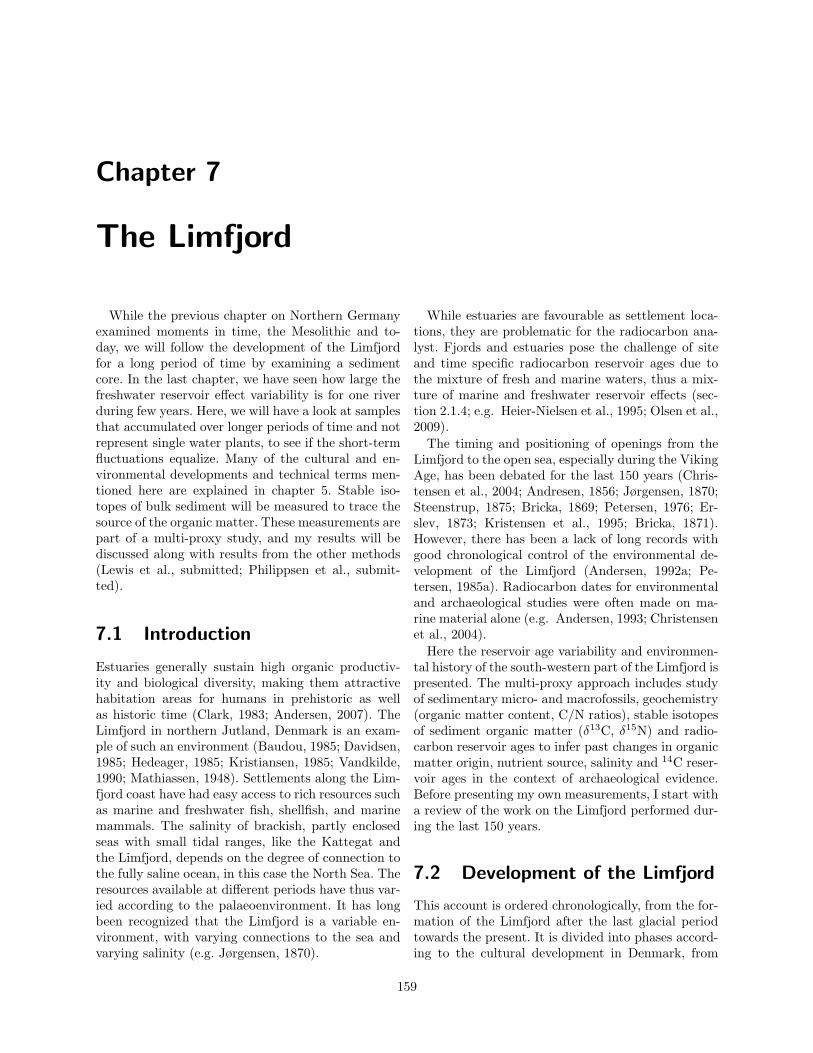
Chapter 7

The Limfjord

While the previous chapter on Northern Germanyexamined moments in time, the Mesolithic and to-day, we will follow the development of the Limfjordfor a long period of time by examining a sedimentcore. In the last chapter, we have seen how large thefreshwater reservoir effect variability is for one riverduring few years. Here, we will have a look at samplesthat accumulated over longer periods of time and notrepresent single water plants, to see if the short-termfluctuations equalize. Many of the cultural and en-vironmental developments and technical terms men-tioned here are explained in chapter 5. Stable iso-topes of bulk sediment will be measured to trace thesource of the organic matter. These measurements arepart of a multi-proxy study, and my results will bediscussed along with results from the other methods(Lewis et al., submitted; Philippsen et al., submit-ted).

7.1 Introduction

Estuaries generally sustain high organic productiv-ity and biological diversity, making them attractivehabitation areas for humans in prehistoric as wellas historic time (Clark, 1983; Andersen, 2007). TheLimfjord in northern Jutland, Denmark is an exam-ple of such an environment (Baudou, 1985; Davidsen,1985; Hedeager, 1985; Kristiansen, 1985; Vandkilde,1990; Mathiassen, 1948). Settlements along the Lim-fjord coast have had easy access to rich resources suchas marine and freshwater fish, shellfish, and marinemammals. The salinity of brackish, partly enclosedseas with small tidal ranges, like the Kattegat andthe Limfjord, depends on the degree of connection tothe fully saline ocean, in this case the North Sea. Theresources available at different periods have thus var-ied according to the palaeoenvironment. It has longbeen recognized that the Limfjord is a variable en-vironment, with varying connections to the sea andvarying salinity (e.g. Jørgensen, 1870).

While estuaries are favourable as settlement loca-tions, they are problematic for the radiocarbon ana-lyst. Fjords and estuaries pose the challenge of siteand time specific radiocarbon reservoir ages due tothe mixture of fresh and marine waters, thus a mix-ture of marine and freshwater reservoir effects (sec-tion 2.1.4; e.g. Heier-Nielsen et al., 1995; Olsen et al.,2009).

The timing and positioning of openings from theLimfjord to the open sea, especially during the VikingAge, has been debated for the last 150 years (Chris-tensen et al., 2004; Andresen, 1856; Jørgensen, 1870;Steenstrup, 1875; Bricka, 1869; Petersen, 1976; Er-slev, 1873; Kristensen et al., 1995; Bricka, 1871).However, there has been a lack of long records withgood chronological control of the environmental de-velopment of the Limfjord (Andersen, 1992a; Pe-tersen, 1985a). Radiocarbon dates for environmentaland archaeological studies were often made on ma-rine material alone (e.g. Andersen, 1993; Christensenet al., 2004).

Here the reservoir age variability and environmen-tal history of the south-western part of the Limfjord ispresented. The multi-proxy approach includes studyof sedimentary micro- and macrofossils, geochemistry(organic matter content, C/N ratios), stable isotopesof sediment organic matter (δ13C, δ15N) and radio-carbon reservoir ages to infer past changes in organicmatter origin, nutrient source, salinity and 14C reser-voir ages in the context of archaeological evidence.Before presenting my own measurements, I start witha review of the work on the Limfjord performed dur-ing the last 150 years.

7.2 Development of the Limfjord

This account is ordered chronologically, from the for-mation of the Limfjord after the last glacial periodtowards the present. It is divided into phases accord-ing to the cultural development in Denmark, from

159

160 CHAPTER 7. THE LIMFJORD

the Stone Age until historical times (see chapter 5for definitions and datings of these phases).

After the glacial period, there were lakes and riversin the area of the Limfjord. Then, seawater enteredthis area, and a marine environment with many is-lands was formed (Andersen, 1990).

In 13050 BC (15000 cal BP), marine waters reachedthe Skagen area (Knudsen, 1994). From 11550 to11050 BC (13500-13000 cal BP), the Kattegat wasinundated (Petersen, 1985b). The modern circulationsystem in the Kattegat and Skagerrak was establishedaround 6550 BC (8500 cal BP) (Gyllencreutz, 2005).The presence of human groups in the Limfjord regionis indicated by artefacts made of reindeer antler andthe so-called Lyngby arrowheads, belonging to theBromme culture (cf. chapter 5 Mathiassen, 1948).

It is debated when exactly the Limfjord was for-med, and different models have been presented. Theformation of the Limfjord was linked to the initialLittorina transgression between 6550 and 6150 BC(8500-8100 cal BP), when the Limfjord was connectedto the Skagerrak (Petersen, 1981). This transgres-sion began between 6700 and 6400 BC (8650-8350cal BP) and marks the transition from Maglemoseto Kongemose culture (Christensen, 1995). Differentdatings were also proposed, between 6000 and 5500BC ((7950-7450 cal BP) Andersen, 1990) or around7000-6700 BC ((8950-8650 cal BP) Andersen, 1992b).

For a precise dating of the formation of the Lim-fjord, one would need a well-dated sedimental recordspanning both the freshwater period and the earlymarine period. Unfortunately, no such records are yetavailable. Marine material like mollusc shells in sed-iment cores or the archaeological record as well asclearly discernible inundations such as drowned sed-iments give a terminus ante quem for the formationof the Limfjord. A terminus ante quem is the lat-est time at which an event must have happened. Thetermini ante quos for the starting of marine influ-ence in different parts of the Limfjord are the follow-ing: Heier-Nielsen (1992) 14C-dated marine molluscsfrom Løgstør Bredning. The two oldest samples havecalibrated ages between ca. 8700 and 7100 cal BC,ca. 10700-9100 cal BP (95.4%), after my calibrationwith OxCal 4.1 and the marine calibration curve Ma-rine09 (Reimer et al., 2009; Bronk Ramsey, 2009).An oyster bank at Gjøttrup have, Ullerup Gaard,northern-central Limfjord, was dated to 6060-5670BC (8010-7620 cal BP) . On the southern coast ofLivø in the central Limfjord, the oldest marine gyttjeis from 5620-5210 BC (7570-7160 cal BP, Petersen,1976). The drowning of the earliest settlement at theLimfjord in 5600 BC (7550 cal BP) (Andersen, 1990)gives a terminus ante quem for the beginning of ma-

rine influence in the area – in 5600 BC at the latestthe sea must have entered the area in order to floodthe settlement. The oldest samples analysed in thisstudy are from ca. 7300 cal BP (5350 BC), thus froma period where all authors agree on the existence ofthe Limfjord as a marine environment.

It is also debated how fast the sea level rise was thatformed the Limfjord. Petersen (1981) suggests 3-4 mper 100 a, according to a drilling at Vust north of theLimfjord, while Christensen (2001) found 1m/100afor the Danish seas. The fast sea level rise at Vustmight only be a local phenomenon.

From ca. 5500 BC, 7500 cal BP, the global eu-static sea level rise slowed down, so that regres-sions or standstills occasionally occurred due to theisostatic uplift of Northern Denmark (Christensenet al., 2004). The resulting fluctuations in relativesea level caused the Limfjord to vary between a ma-rine archipelago and a brackish estuary. The earliestmarine maximum was around 5300 BC (7250 cal BP)in the north-northeast and around 4600 BC (6550 calBP) in the southwestern parts of the Limfjord (An-dersen, 1990). The maximum extent of the Sea isshown in figure 5.1 in chapter 5. In the Stone Age,the eastern Limfjord consisted of very large shallowbroads, through which the narrow and deep under-water valley “Langerak” went. The eastern Limfjordwas only open towards the Kattegatt and at the sametime more protected against the open sea by the hillsof Himmerland and Vendsyssel, resulting in brackishsalinities. The western Limfjord was under strongermarine influence and consisted of large and deeperwaters, with openings toward the north to the Skager-rak. Only at the narrow Aggersund, the two parts ofthe Limfjord had been connected (Andersen, 1992b,see also figure 7.2).

Mesolithic There is some uncertainty about theDanish marine environment, including the Limfjord,in the Mesolithic. Iversen (1967a) claims it was war-mer, saltier and more nutritious than now and thetidal range was larger. Sea level rise is after his opin-ion not the only reason for the sudden rise in salin-ity of the Baltic in the beginning of “Litorina time”.The higher tides were also responsible for the highersalinity. Also Noe-Nygard and Hede (2006) report astrong tidal amplitude of the order of 4 m for theNorth Sea and Kattegatt during the Atlantic. Theyare objected by Christensen (1995) who asserts thatthere is no significant difference in tidal range; his in-vestigations showed that “tides in the Atlantic periodwere not significantly greater than today”.

However, there is general agreement that the sealevel in the Stone Age Limfjord was higher than

7.2. DEVELOPMENT OF THE LIMFJORD 161

today, at least 3 m above the present-day DanishVertical Reference, DVR90 (Petersen, 1976). In con-trast, the proportion of shallow areas in the Limfjordwas larger than today, as large areas which now aredry land were shallow bays. Hence, sunlight reachedlarger areas of the sea floor than today (Andersen,1992b, 1995). This provided excellent possibilities forphotosynthesis and resulted in a much richer floraand fauna. The preconditions for human subsistencewere thus particularly advantageous, in an environ-ment that already was favourable due to its estuarinecharacter.

A high salinity in the Stone Age is exemplified byfinds from the Ertebølle locus classicus on the cen-tral Limfjord. Fishbones of Pollachius indicate highsalinity (Enghoff, 1986), as well as the foraminiferElphidium margaritaceum, which needs a salinity of>30 PSU (Burman and Schmitz, 2005). From isotopemeasurements (δ13C, δ18O) on periwinkles, the mid-Holocene winter salinity at Ertebølle was calculatedto be 31±1 PSU, comparable to the salinity of thepresent-day North Sea (Burman and Schmitz, 2005).

The productivity of the marine environment wasgreater in the Stone Age than today. Petersen (1922)calculated that the accumulation of the kitchen mid-den of Meilgard (northern Djursland, east coast ofJutland) must have taken 1200 years. His calculationwas based on modern oyster production. 14C datings,however, showed that the accumulation of Meilgardonly took 400-500 years. The biological productivityof the sea decreased thus significantly from the StoneAge to recent times (Andersen, 2001). Also in theLimfjord, high salinity and temperature as well asthe shallowness of the water were the basis for highmarine productivity (see above and e.g. Andersen,1995).

These rich resources were exploited by the StoneAge population at the Limfjord. This is proven by nu-merous remains of Mesolithic coastal sites. In fact, in-land sites from this period have not been found in theLimfjord region. All sites are coastal settlemets alongthe former coast. They are relatively easily found inthe Limfjord region: the isostatic land rise was largerthan the eustatic sea level rise after the end of theglacial period, so that the settlements are not in-undated (as is the case for the “southern half” ofDenmark and for Northern Germany, see chapter 5).The oldest known settlement on the Limfjord, belong-ing to the Kongemose Culture, was inundated around5600 BC (7550 cal BP, Andersen, 1990). Also the old-est kitchen middens are found in the Limfjord areaand dated to around 5400 cal BC (7350 cal BP, An-dersen, 1995), with my own calibration using OxCal4.0 and IntCal04. The kitchen midden site Ertebølle

was frequented for almost 1000 years, indicating ahigh degree of resource stability (Andersen, 1992b).

δ13C analyses of human bones as well as arte-facts and faunal remains such as fishbones, fishtrapsand fish food crusts on pottery indicate that ma-rine resources were the main economic basis of theMesolithic society (Andersen, 1995, 1993; Andersenand Malmros, 1984). An argument for the importanceof hunting marine mammals are specialized tools likethe harpoon and the EBK-blubber lamp (Andersen,1992b). Fishing was mainly performed using perma-nent structures like weirs and traps. Remains fromcoastal sites give “a non-selective sample of whateverfish was present in the local coastal waters duringthe summer half of the year” (Enghoff, 1995). How-ever, coastal settlements where subsistence dependedexclusively on the sea have not been found yet (An-dersen, 1993). In fact, two kitchen-midden sites fromthe Limfjord are famous for freshwater fishing: In Er-tebølle and Bjørnsholm, fishing concentrated on eel(Andersen, 1993). People staying at Ertebølle fishedin a nearby freshwater lake, mainly in late summerand autumn (Enghoff, 1995).

Neolithic Although the Stone Age Sea around 3000BC with its highest sea level opened the fjord to thesea between Hanstholm and Svinkløv, Nissum Bred-ning was closed to the west (Meesenburg, 1981). Thepassage between the Skagerrak and the Limfjord wasdeepest in the Middle Atlantic, though. The marineinfluence originating from the connection to the Sk-agerrak was largest in the Atlantic and decreased dur-ing the the Subboreal, when beach walls formed inthis area (Petersen, 1992).

With the beginning of the Neolithic, kitchen mid-dens and coastal sites became fewer and smaller. Oys-ters became smaller and were replaced by cockles inthe kitchen middens. This has been connected to low-ered tidal ranges and lower salinity. Marine mammalswere still hunted in the Limfjord area in the Neolithic.In the middle Neolithic, shell middens are again dom-inated by oysters, but the shell layers are still verythin (Andersen, 1992b).

In spite of the apparent decline in marine resources,there were still natural oyster banks in the Limfjord.There is also evidence for collection of marine shells,and hunting of marine mammals on the coast of theLimfjord (Andersen, 1990, 1992b; Marseen, 1962).

Bronze Age and Iron Age In the Bronze Age, thereis a general lack of shell middens in Denmark, whilethey are numerous before and after, i.e. in the Ne-olithic and in the Iron Age (Milner et al., 2007). How-ever, the collection of marine mollusks had not ceased


totally, and also fishing in the Limfjord was stillimportant, as the exemplified by the sites Torslev,Vadgard and Fragtrup (Johansen, 1985; Lomborg,1973; Draiby, 1985).

During the Iron Age, the salinity in the Baltic wassignificantly higher than today, which is indicatedby large oysters growing in relatively enclosed areaslike the Flensburg Fjord or the Bay of Eckernforde(Anger, 1974). During the Stone Age, however, con-ditions for oysters had been even more favourable.

From the early Roman Iron Age on (AD 0-200),the Limfjord began to look like it is today, althoughthere still was a passage from the Skagerrak intothe Limfjord. In the late Iron Age, the Limfjord wasan important starting point for voyages towards thewest (Andersen, 1990). The filling of a pit house onFur contained marine shells from ca. AD 900, whichindicates marine conditions in the Limfjord.

From AD 1000 In AD 1027, an open connection atAgger Tange is known to have existed as the DanishViking King Knud the Great returned from his ex-pedition to England via this sound (e.g. Petersen,1976; Kristensen et al., 1995). During the reign ofCanute IV of Denmark, AD 1042-1086, there a wasfree passage from the Limfjord to the North Sea, ac-cording to the 11th book of Saxo’s Gesta danorum,but this passage was already closed during the timethis book of Gesta danorum was written (aroundAD 1200, Bricka, 1869, 1871). However, the stateof the Limfjord in the 11th century AD was de-bated passionately around AD 1870 in the Danishjournal Aarbøger for Nordisk Oldkyndighed og His-torie. A saga accredited to the Icelandic polititian,historian and poet Snorre Sturluson (The Sagas ofOlaf Tryggvason and of Harald The Tyrant (HaraldHaardraade)) tells how the Norwegian King HaraldHaardraade fled from a superior Danish fleet lead byKing Svend Estridsson in AD 1061 from the Limfjordto the North Sea by emptying his boats, draggingthem over a barrier and re-loading them, all duringone single night. The debate focused on the questionwhere this barrier had been located. It was suggestedthat it was a barrier at Agger Tange (Andresen, 1856;Jørgensen, 1870), while others argued that the Lim-fjord had been widely open at Agger, and Haraldtransported the ships over the shallows at Løgstør,“Løgstør grunde” (Steenstrup, 1875; Bricka, 1869) orover a small strip of land at Vust (Erslev, 1873) be-tween the Limfjord and the Skagerrak. The questionabout the intepretation of the saga thus led to a re-search question which is similar to the question ex-amined in this study: to what extent did the Limfjordhave connections with the open sea?

Later research continued to examine this ques-tion. It was suggested that Nissum Bredning neverhad a direct connection to the sea in prehistory, ac-cording to the analysis of prehistoric shells and thelack of beach walls of North Sea type in that area(Jessen, 1920). Petersen (1976) suggests that HaraldHaardraade fled towards north through a connectionfrom Løgstør Bredning to the Skagerrak. Throughthe Han Herrederne region, there are two possibili-ties for passages to the north: west of Fjerritslev andat Bulbjerg, where there are valleys in the old lime-stone surface which are now covered by later sedi-ments. On old maps, you can for example follow atrough from the dunes in the north through KlimOdde and Gøttrup Rimme and from here, furthertowards south-east through the coastal meadows tothe Limfjord at Ullerup, close to Aggersborg (Møller,1986). This view is also supported by drillings in thearea were the former connection was expected (Pe-tersen, 1976).

A chronicle from AD 1186/87 mentions that Hum-le, most probably Humlum close to Oddesund, was asea harbour (Aagesen, 1186/1187).

During the following centuries, historical recordsbecome more reliable.

In AD 1624, “the great breakthrough” happenedin the western Limfjord, resulting in a connection tothe North Sea for a longer period 7. This connec-tion was near Harboøre and silted up later (Hylle-berg, 1992; Andresen, 1856). Until AD 1671, AggerTange was covered with fields and meadows. Afterthis date, they were ruined by sand entrainment andfloods from the North Sea (Andresen, 1856). In thelate 18th century, the Limfjord contained “brackish orhalf salty” water, although it often was more salinewhen the North Sea under a storm broke throughat Agger, or when the inlet at Hals in the east wasflooded (Pontoppidan, 1769). In the Middle Ages andup to 1825, the salinity of the Limfjord was 8h, liketoday the Baltic Sea around Bornholm (Hylleberg,1992). The Limfjord was an important fresh- andbrackish water fishery (Petersen, 1992) in this period.

On the third february 1825, a flood opened a pas-sage at Agger Tange, turning the Limfjord into asound (Andresen, 1856). Ships could pass this chan-nel from 1834, so the marine transport was improved,while the road over Agger Tange was damaged. Thehigher salinity, stronger currents and resulting de-creasing plant cover on the fjord ground destroyedthe opportunities of catching herring and freshwaterfish (Andresen, 1856). Next to this channel, anotherflood opened the Thyborøn Channel in 1862. The newopening also silted up, but it was artificially openedagain, so that the Limfjord today is a sound, connect-

7.3. LOCATION 163

13C, 15N, C/N

14C age: aquaticand terrestrial

d bl dfd bl df

Figure 7.1: Materials from the sediment core whichare analysed in this study.

ing the North Sea and the Kattegatt. Connectionsfrom the Limfjord to the North Sea have a tendencyof moving southwards, as there is a northward floodtide stream and a southward ebb tide stream on Jut-land’s west coast (Andresen, 1856). The opening atThyborøn would silt up and close if it was not heldopen by regular dredging.

7.3 Location

The Limfjord is a branched sound through northernJutland, Denmark, connecting the North Sea with theKattegat (Figure 7.2). The western and central Lim-fjord is characterised by large expanses of water withopen bays, while the eastern part resembles a broadriver (Andersen, 1990). The Limfjord today contains7.4 km3 water, has a surface area of 1500 km2 and anaverage depth of 4.9 m. Sunlight reaches large parts ofthe Limfjord’s sea floor due to its shallowness (Ander-sen, 1995). From a drainage area of 7528 km2, 2.7 km3

fresh water enter the Limfjord per year. On average,there is a flow of 6.8 km3 from the North Sea via Thy-borøn Channel through the Limfjord to the Kattegat.Close to the eastward main current, the salinity varieswith 2-4h from week to week (Grooss et al., 1996).It is about 30h, which compared to the North Sea’s33h indicates a 10% dilution of the marine waterwith freshwater (Heier-Nielsen et al., 1995).

Kilen is a former fjord arm of the Limfjord (56◦

30.005’N, 08◦34.089’E, Figure 7.2), located in a tun-nel valley (Smed, 1981). It is surrounded by 25-35m high slopes, has a mean water depth of 2.9 mand a surface area of 3.34 km2 (Jensen et al., 2006).The catchment area of 35.3 km2 includes two brooks,Bredkær bæk and Vasens bæk (Jensen et al., 2006).Today, Kilen is a brackish embayment with salin-ity around 6h, as sandspit formation and the con-struction of a dam in AD 1856 isolated Kilen fromthe main Limfjord (Ringkjøbing Amtskommune andTeknik- og Miljøforvaltningen, 1991). Beginnings ofsandspit formation can be seen on historical maps,figure 7.3. Kilen is believed to have been naturallyprotected from strong currents, storms and wave ac-tion in the past, and hence a continuous sedimentsequence has been preserved.

7.4 Methods

In 2010, five surface water samples were collectedfrom different parts of the Limfjord (Figures 7.4, 7.5)for DIC water dating. Details on collection of watersamples and CO2-extraction can be found in chapter3. In 2007, a ca. 1560 cm long sediment sequencewas obtained from Kilen. The coring was made witha Russian peat sampler with a chamber length of 100cm (Jowsey, 1966) in two parallel boreholes at a waterdepth of 390 cm below present sea level (bpsl). Thesediments consist of homogenous grey-brown marineclay gyttja. Our analyses focus on the part between467 and 1935 cm bpsl which was subsampled at 1-2cm depth intervals. During the approximately 6100years of our core, 1470 cm of sediments accumulated,so that the average sedimentation rate is 0.24 cm peryear. The 1-2 cm depth intervals thus contain therecord of ca. 4-8 years (depending on the actual sed-imentation rate). Terrestrial plant macrofossils wereradiocarbon dated and used to construct an age-to-depth model. Shells were dated to calculate reservoirages. Stable isotope measurements (C,N) were per-formed on bulk organic matter samples from the sed-iment core. δ13C, δ15N, C/N ratio, carbon fractionand nitrogen fraction have been measured. Figure 7.1illustrates the different samples for radiocarbon dat-ing and stable isotope measurements.

Firstly, only 26 of the 60 samples were measured.The 26 largest samples were chosen, as it was notclear in the beginning how much material there hadto be weighed out. After each measurement, the CO2

and N2 peak height indicated how much there had tobe weighed out for the next measurement. Figure 7.6shows the required weight for ideal 13C and 15N mea-


c

Germany

Norway

Sweden

PolandUK

North Sea

Baltic Sea

U

Bjørnsholm BayErtebølle

x

x

Skive

Skagenx

NissumBredning

North Sea

Kattegat

Skagerrak

AggerTange

Jutla

nd B

ank

Kilen

Venø Bay

The Limfjord

Aggersund

forest

water

contour lines(interval 5 m)

0-1 mKilen depth

1-2 m

5-6.5 m4-5 m3-4 m2-3 m

Kilen

The Limfjord

core

0 0.5 1

kilometers

ab

Figure 7.2: Location of the Limfjord in Denmark, and Kilen in the Limfjord. Own work, made with MapInfoProfessional 7.8 using bathymetry data by Thorkild Høy, published in Ringkjøbing Amtskommune andTeknik- og Miljøforvaltningen (1991).

surements, depending on the samples’ organic contentas determined by LOI (see section 7.8). The func-tions fitted to the data points were used to estimatethe sample size for the later weighing of the other 34samples.

Chapter 3 gives details on sample collection, pre-treatment, and radiocarbon and stable isotope mea-surements. δ13C and δ15N denote stable isotope mea-surements on bulk sediment organic matter. δ13C andδ18O measurements on foraminifera (see below) andshell carbonate are marked as δ13Cforams, δ18Oforams,δ13Cshell and δ18Oshell, respectively.

Table 7.1 gives details on the pretreatment of the

thirteen shell samples which I prepared in Aarhus.Four additional shell samples were later dated at the14CHRONO Centre, Queen’s University Belfast, UK.

7.5 Chronology

The reservoir age R of a shell sample can easily becalculated when a terrestrial sample from the samedepth is availabe (see section 2.1.4 and Figure 7.8).Likewise, ∆R can be calculated as shown in Figure7.8. However, when no terrestrial sample from the

7.5. CHRONOLOGY 165

18001767 (Jutland)1767 (Viborg)

1820 1844 1855

1860 1864 1871

Figure 7.3: Historical maps of Kilen (de Reventlov, 1767; Abildgaard, 1767; Det Kongelige VidenskabernesSelskab, 1800; Bugge, 1820; Mansa, 1844; Anonymous, 1855; Both, 1860; Petermann, 1864; Both, 1871). Notethe varying degree of openness of the connection between Kilen and the Limfjord, caused by the formationof sand spits.

same depth is available, the calibrated age t of theshell is obtained from an age-to-depth model, where-after ∆R can be calculated (Figure 7.9).

An age-to-depth model assigns an age to each cmof the core. Therefore, we also know the calendar agesof all the bulk sediment samples on which stable iso-topes were measured.

The age-depth model is based on 13 14C datedmacrofossil samples of unequivocal terrestrial origin(Table 7.2). Six of these samples, the uppermost threeand the lowermost three, were very small. All thecarbon they yielded had to be used for 14C dating,and a δ13C measurement was not possible. For nor-malisation of the 14C dating, assumed δ13C values

had thus to be used. An error of 1h in the δ13Cmeasurement would in our case lead to an error of8 ≈14C years, as we measured the 14C/13C ratio. Ifthe 14C/13C ratio had been measured, e.g. in conven-tional dating, the error would have been 16 14C years(see section 2.1.2 for detailed explanations and equa-tions). At first, only two of the terrestrial macrofossilshad been dated, AAR-11463 and AAR-11464. Oneof them, AAR-11463, contained enough carbon for aδ13C determination and resulted in δ13C=-28.36h.AAR-11464 was so small that a δ13C value had to beestimated. As only one extra sample from the samecore was available for comparison, a standard valuefor terrestrial plants of -25h was assumed and used


Figure 7.4: Collection of surface water samples from the Limfjord

86-76

-114-20

42

Reservoir age estimates (14C years BP)

Visby BredningRisgårde Bredning

LangerrakAggersund

Aalborg

Figure 7.5: Reservoir ages of surface water samples from the Limfjord. The uncertainty of the reservoir ageestimates is 20-22 years (all values can be found in table 7.3).

7.6. RESULTS 167

Table 7.1: Shell samples from Kilen – Pretreatment

Sample Weighed Amount of Weight afterSID AAR weight out for 1M HCl [µl] pretreatment

[mg] pretreatment (yield [%])14253 13213 207.1 51.8 207 39.3 (75.9)14254 13214 20.9 20.9 76 14.9 (71.2)14255 13215 91.6 41.1 164 28.7 (69.8)14256 13216 14.0 14.0 27 12.0 (85.7)14257 13217 9.5 9.5 18 8.1 (85.3)14258 13218 19.2 19.2 76 13.9 (72.4)14259 13219 32.8 32.8 131 24.8 (75.6)14260 13220 34.9 34.9 139 25.4 (72.8)14261 13221 20.2 20.2 80 15.5 (76.7)14262 13222 44.6 44.6 178 34.1 (76.5)14263 13223 4.9 4.9 0 4.6 (93.9)14264 13224 31.7 31.7 127 21.9 (69.1)14265 13225 5.0 5.0 0 4.7 (94.0)

Figure 7.6: Required weight for isotope measure-ments, plotted versus organic content of sedimentsamples. Top, for δ13C measurements, bottom, forδ15N measurements.

for normalisation. The second sample submission con-tained the other 11 terrestrial macrofossil samplesfrom the core. For five of these, estimated δ13C valueshad to be used. However, the assumed value was inthis case -27h, as the six other samples from this sub-mission consistently had more negative values than -25h (the average was -27.8h). For estimating thepossible additional error, we assume that the trueδ13C value of the sample with the estimated δ13C=-25h is -28.5h. This δ13C deviation of 3.5h wouldresult in a 14C error of 28 14C years. This is insidethe error range of 60 to 90 14C years for the smallterrestrial macrofossils (table 7.2). The fact that wehad to use estimated δ13C values does thus not havea large influence on the 14C dating.

The age model was constructed using depositionalmodels in OxCal 4.1 (Ramsey, 2008). To account forchanges in accumulation rate, boundaries are insertedat 447, 552, 1055 and 1748 cm, based on large changesin the CaCO3 content (Figures 7.7 and 7.14). The de-positional model yielded an agreement index of 73.3%with a k value of 150. Following the tradition in geo-logical and palaeoenvironmental research, calibratedages will be given in calibrated years BP (cal BP, i.e.,calender years prior to AD 1950). Calibrated calenderages BC can be obtained by substracting 1950 yearsfrom the ages in cal BP.

7.6 Results

The results from shell 14C dating and δ13C, δ18Omeasurements are presented in table 7.2 and figure


1000200030004000500060007000

600

800

1000

1200

1400

1600

1800

14C age (BP)

Dep

th (c

m)

200030004000500060007000

400

600

800

1000

1200

1400

1600

1800

Age (cal yr BP)D

epth

(cm

)

terrestrial macrofossil

age-model boundary

terrestrial sample

mollusc shell

a b

Figure 7.7: a) 14C datings of terrestrial macrofossils and of shells. b) The age model, based on the 14C-datedterrestrial macrofossils, constructed with OxCal 4.1 (Ramsey, 2008).

7.11. Stable isotope measurements of bulk sedimentare shown in figure 7.10. However, I begin with thewater samples that were collected in the Limfjord in2010.

7.6.1 Water samples

Surface water DIC collected in 2010 had 14C ages of -500 to -300 14C years. For the calculation of reservoirage estimations, the pmC of the samples was com-pared to that of the contemporaneous atmosphere(Levin et al., 2010, and pers. comm. Ingeborg Levin2012). This resulted in reservoir ages between -114and +86 14C years (Table 7.3 and Figure 7.5). Mod-ern water samples collected in the Limfjord in 1996yielded DIC reservoir ages between 110 and 450 14Cyears, uncorrelated to sampling depth (pers. comm.Jan Heinemeier 2012). ∆R values of the modern wa-ter samples from 1996 and 2010 are thus in the rangeof -500 to +50 years. It is possible that bomb car-bon, maybe some decades old and thus containing>modern levels of 14C, entered the Limfjord andthus substantially reduced some of the reservoir ef-fect measured today (cf. section 2.1.3). Modern sur-face water samples can thus only give very rough es-timates of past reservoir ages and should not be usedfor correcting archaeological 14C datings.

7.6.2 Samples from the sediment core

Based on the temporal variability of accumulationrate, CaCO3 and minerogenic flux (section 7.8), δ13Cvalues and C/N ratios, the core has been visually di-vided into four time intervals, denoted zones 1-4.

Zone 1, 7300 cal BP-7000 cal BP

The shells from this zone yield ∆R values around55 years. δ13C values are around -22h and decreaseto -24.6h at ca. 7100 cal BP, the lowest value of theprofile. This δ13C minimum is accompanied by a C/Nratio maximum of up to 18. δ15N values are between3 and 3.5h and increase to about 4h at the top ofthe zone.


This zone exhibits the largest variations in ∆R. Theshell with the highest ∆R of 300 years occurs in thiszone at ca. 6200 cal BP. Two shells next to this onehave ∆R values of -105 and -106 years, respectively.Two δ13C minima, approximately -23 and -24h, co-incide with the two highest C/N values of the core,C/N>18. In general, δ13C values are slightly increas-ing, and C/N ratios decreasing, especially at the topof this zone. In the lower half of the zone, δ15N val-ues are relatively stable around 3h, but vary with

7.6. RESULTS 169

Sample ID Depth Species/ 14C age Model age ∆R (14C δ13C δ18O(cm bpsl) Material (uncal. BP) (cal yr BP) years) (hVPDB) (hVPDB)

AAR-12150 459-460 1 lf, 1 Betula sp. fruit, 2 bss,1 Cyperaceae seed

1315±65 -27

AAR-13213 463-464 Tapes sp. [28-33] 1733±34 1247±64 61±112 1.59 -1.77AAR-12151 472-473 1 flower Quercus sp. 1440±65 -27AAR-13214 473-474 Corbula gibba [15-20] 1684±34 1357±53 -142±69 1.78 -1.51UBA-16568 503-504 Corbula gibba [15-20] 2161±35 1689±68 57±66 14* —AAR-13215 522-523 Cerastoderma edule [6] 2193±33 1899±72 -102±75 2.85 -3.31AAR-12152 523-524 1 Scirpus seed 1880±60 -27AAR-13216 601-603 Abra alba [20] 2754±46 2572±116 -55±87 0.89 -1.34AAR-12142 603-605 1 lf 2464±40 -26.87AAR-12143 745-747 1 tf + bark 3215±35 -28.38AAR-13217 751-753 Cardium sp. 3556±39 3439±48 -1±62 1.44 -1.47AAR-12144 975-977 1 tf + bark; cf Salix sp. 4132±45 -27.27AAR-13218 975-977 Abra alba [20] 4500±48 4628±79 41±71 0.58 -1.38AAR-12145 1149-1151 1 lf 4635±75 -28.19AAR-13219 1149-1151 Corbula gibba [15-20] 5028±50 5301±66 59±108 1.89 -1.55AAR-13220 1169-1171 Corbula gibba [15-20] 5096±34 5353±62 70±85 0.70 -1.33AAR-11463 1171-1175 206 lfs, 3 Betula sp. fruits, 1

bud, 1 bs4635±40 -28.36

AAR-12146 1279-1281 1 Alnus sp. t + bark 4848±42 -28.61AAR-13221 1279-1281 Abra alba [20] 5199±46 5638±47 -91±66 1.09 -0.72AAR-12147 1399-1401 97 lfs 5225±40 -27.52AAR-13222 1403-1405 Abra alba [20] 5621±39 5974±45 28±66 0.47 -1.25UBA-16569 1427-1429 Abra alba [20] 5545±58 6047±49 -106±61 5.6* —AAR-12148 1483-1487 11 lfs 5260±90 -27AAR-13223 1487-1489 Bittium reticulatum [25] 6090±65 6214±59 298±108 2.54 -1.48UBA-16570 1527-1529 Corbula gibba [15-20] 5825±29 6329±66 -105±98 1.8* —AAR-13224 1711-1713 Corbula gibba [15-20] 6241±34 6857±95 -140±89 1.12 -0.92AAR-12149 1715-1717 43 lfs 6120±65 -27UBA-16571 1819-1821 Corbula gibba [15-20] 6616±30 7100±89 58±103 4.3* —AAR-11464 1923-1927 25 lfs 6405±60 -25AAR-13225 1927-1929 Tellimya ferruginosa [30] 6850±150 7314±71 55±172 0.96 -0.72

Table 7.2: Radiocarbon dates of shells and terrestrial macrofossils. lf: leaf-fragment, lfs: leaf-fragments, bs:bud-scale, bss: bud-scales, t: twig, tf: twig-fragment. Scirpus seed: Scirpus maritimus/ lacustris. Numbersin squared brackets denote minimum salinity tolerances according to Sorgenfrei (1958). δ13C marked by anasterisk were measured by the accelerator and can only be used for normalisation of the 14C dating, not fordrawing palaeoenvironmental conclusions. δ13C values in italics denote estimations for samples that were sosmall that all carbon had to be used for the 14C dating. See section 7.5 for discussion.

Location DIC pmC 14C age Res. age δ13C δ18Oand weather (mgC/L) (yr BP) (14C yrs) (hVPDB ±0.05h)Aggersund 23 106.41±0.26 -499±20 -114±20 -1.09 11.46Sunshine, partly cloudy. Wind: 5m/s, west.Visby Bredning 21 103.79±0.27 -299±21 86±21 -1.22 11.11Showers. Wind: 8-10m/s, south-westRisgarde Bredning 22 105.91±0.29 -461±22 -76±22 -0.8 11.77Wind: 6m/s, west-northwest.Aalborg 22 105.17±0.27 -405±21 -20±21 -0.76 11.29Wind: 8-10 m/s, west-northwest.Langerrak 22 104.36±0.29 -343±22 42±22 -0.9 12.06Light wind from southeast. Inwards current 1/2 knot.

Table 7.3: 14C dating of water samples from the Limfjord, collected by the crew of the Klitta (Figure 7.4. Seefigure 7.5 for a map of the sampling locations. For calculating the uncertainty of the reservoir age estimate, itwas assumed that the measurement uncertainty of atmospheric pmC is neglectible compared to measurementuncertainty of water DIC pmC.


ca. 1h in the upper half.


∆R decreases gradually from 70 to -55 yrs through-out this zone. The general trend towards less nega-tive δ13C values continues to -20h. At the end ofthe zone, variation increases and δ13C and C/N ratiospan ranges from -21.7 to -19.1h and from 11 to 15,respectively. δ15N values vary between 2.5 and 3.5huntil they begin to increase after 4000 cal BP.


∆R ranges between -142 and 61 years. The highestδ13Cshell and lowest δ18Oshell of the profile occur atthe bottom of this zone. δ13C values are around -21hand increase slightly. δ15N is highly variable in thisinterval. The maximum value for δ15N, 5.3h, occursat 1700 cal BP. Following a C/N ratio peak of 16,the values remain quite stable around 13 and onlyincrease to 14 at the top of the zone.

7.6. RESULTS 171

14C age of terrestrialmacrofossil, 14CT

14C age of shell, 14CM

0 10000 20000 30000 40000 500000

10000

20000

30000

40000

50000

14C

age

(YR

BP)

Calibrated age BP

IntCal09

14CT

t

0 10000 20000 30000 40000 500000

10000

20000

30000

40000

50000

14C

age

(YR

BP)

Calibrated age BP

Marine09

t

14CMAR calibratedage, t

marinemodel age,

14CMAR

ΔR = 14CM - 14CMAR

R = 14CM - 14CT R = 14CM - 14CT

Figure 7.8: Calculation of the reservoir age R(t) and the local reservoir age offset ∆R after radiocarbondating of shell and terrestrial macrofossil from the same depth.


depth in thesedimentcore (cm)14C age of shell, 14CM

cm

t

0 10000 20000 30000 40000 500000

10000

20000

30000

40000

50000

14C

age

(YR

BP)

Calibrated age BP

Marine09

t

14CMAR calibratedage, t

marinemodel age,

14CMAR

ΔR = 14CM - 14CMAR

200030004000500060007000

400

600

800

1000

1200

1400

1600

1800

Age (cal yr BP)

Dep

th (c

m)

age model

Figure 7.9: Calculation of the reservoir age R(t) and the local reservoir age offset ∆R using the age-to-depthmodel when no terrestrial macrofossil from the same depth as the shell is available.

7.6. RESULTS 173

2000

3000

4000

5000

6000

7000

Calib

rate

d ag

e (c

al y

r BP)

12 14 16 18C/N ratio

−24 −22 −20δ13C (‰ VPDB)

3 4 5δ15N (‰ AIR)

1

2

3

4

Zone

Figure 7.10: Measurements on bulk sediment organic matter: δ13C, C/N ratio and δ15N.


2000

3000

4000

5000

6000

7000

Calib

rate

d ag

e (c

al y

r BP)

−200 0 200∆R (14C years)

1

2

3

4

Zone

−2 0 2δ13C (‰ VPDB)

carbonateδ18O (‰ VPDB)

carbonate

−202

Figure 7.11: 14C datings and stable isotope values (δ13C, δ18O), of shell carbonate.

7.7. DISCUSSION 175

7.7 Discussion

7.7.1 δδδ13C, C/N, δδδ15N

Variations in δ13C and C/N values are commonlycaused by changes in organic matter origin or pri-mary organic productivity. In isolation basins, δ13Cand C/N ratios have been used to distinguish marineand terrestrial organic matter (Mackie et al., 2007;Olsen et al., 2011). C/N ratios below 10 primarily re-flect algae and C/N ratios above 20 terrestrial organicmatter (Meyers and Teranes, 2001). Kilen C/N ratiosrange between 12 and 19 and span almost the entirerange from algae to terrestrial organic matter (Figure7.10). Marine organic matter has typically δ13C val-ues between -16 and -22h (e.g. Mackie et al., 2007),freshwater organic matter between -35 and −25hand terrestrial organic matter between -30 and -25h(Meyers and Teranes, 2001). The δ13C values fromKilen range from -24.6 to -19.1h, i.e. between ter-restrial and marine δ13C values. The low δ13C values(around -22h) and high C/N ratios (around 14) fromthe core base to ca. 5700 cal BP indicate that theorganic matter content is dominated by a mixture ofautochthonous and allochthonous sources. After 5700cal BP, δ13C≈-22h and C/N<15 signify that au-tochthonous organic matter became increasingly im-portant (Figure 7.10).

A strong correlation of the C/N ratios and δ13Cvalues (ρ=-0.83, Figure 7.12) indicates a linear mix-ing between terrestrial and marine organic matter.Hence, both δ13C and C/N measurements distin-guish marine from terrestrial organic matter. Thecorrelation is strongest in zones 1 (ρ=-0.99) and 2(ρ= -0.89). Productivity plays a minor role in deter-mining the δ13C values in the Kilen sediments, al-though correlations between δ13C and TOC (indicat-ing that productivity controls the δ13C values) canbe observed for some periods, particularly in zone 4(ρ=0.74, Figure 7.12). In conclusion, in periods withthe strongest δ13C-C/N correlations, the δ13C-TOCcorrelation is very weak, and vice versa.

Major and rapid increases in C/N ratios associatedwith significant decreases in δ13C values around 7100and 6000 cal BP (Figure 7.10) are probably causedby a large transfer of terrestrial organic matter intothe sediments. These values may indicate transgres-sion events, local increases of the relative sea level,in which large areas are inundated and terrestrial or-ganic material is transported into the water. Duringthe first centuries after each transgression event, δ13Cvalues increase to values higher than before the trans-gressions. The higher sea level had possibly causedan increased distance from the shore to the coring

location, thus limiting the input of terrestrial mate-rial, and increasing the relative importance of marineorganic matter. Furthermore, nutrients released dur-ing the transgression can have enhanced marine pro-ductivity. Increasing autochthonous production alsoincreases the relative importance of marine organicmatter.

Total nitrogen and total organic carbon content,TN and TOC, are linearly correlated with an inter-cept of zero (Figure 7.13). Hence, only nitrogen oforganic origin is present in our samples and we donot have to consider inorganic nitrogen, e.g. in theform of nitrates.

Organic matter nitrogen stable isotope values canbe challenging to interpret because δ15N may de-pend on source organic matter, primary organic pro-ductivity and anaerobic processes of ammonificationand denitrification (Talbot, 2001). Land plants havetypical δ15N values of 2 to 10h, lake sediment -2to 20h, and marine phytoplankton 3-12h (Talbot,2001; Owens, 1987). The Kilen δ15N values between2.5 and 5.3h fall within the normal range of ma-rine and terrestrial δ15N values. The δ15N values areuncorrelated with δ13C and C/N (ρ =0.17 and -0.01respectively) suggesting, contrary to δ13C, that δ15Ncannot resolve the origin of the source organic matter.Ammonification and denitrification are also deemedunlikely to be able to explain the increasing δ15Nvalues, due to the lack of supporting evidence fromdiatom, foraminifera and pigment analysis (Lewis,2011; Lewis et al., submitted). The weak correla-tion between δ15N and TOC (ρ=0.51, Figure 7.12)suggests that the δ15N values are partly controlledby primary organic productivity (Figure 7.12). How-ever, for zone 3, δ15N is stronger correlated with TOC(ρ=0.68). Combined with the generally low C/N val-ues (average =13), i.e. autochthonous organic mat-ter, this suggests a strong coupling with organic pro-ductivity. In most environments, nitrogen is a lim-iting nutrient for the production of organic matter.Therefore, an alternative explanation for the Kilenδ15N values is complete utilisation of dissolved inor-ganic nitrogen (DIN) during nitrogen assimilation byplankton and higher plants, leading to limited iso-topic fractionation between organic matter and DIN(i.e. the organic matter δ15N will reflect δ15NDIN).Due to the close proximity of the core location toland, δ15N values likely reflect terrestrial δ15NDIN.

7.7.2 ∆R and δδδ13C, δδδ18O of shells

∆R values range from -140 to 300 years (Figure 7.10,table 7.2). They are of the same order of magnitude asthe values measured on 19th and 20th century (pre-


3 4 50

0.1

0.2

0.3

0.4

0.5

δ15N (‰ AIR)

TOC

MA

R m

g/yr

/cm

2

−26 −24 −22 −20 −180

0.1

0.2

0.3

0.4

0.5

δ13C (‰ VPDB)

TOC

MA

R m

g/yr

/cm

2

−26 −24 −22 −20 −18

15

20

25

30

35

δ13C (‰ VPDB)

DI s

alin

ity

−26 −24 −22 −20 −188

10

12

14

16

18

20

22

δ13C (‰ VPDB)

C/N

ratio

marine

←terrestrial

←freshwater

Z1, 7330-7000 cal BPZ2, 7000-5400 cal BPZ3, 5400-2000 cal BPZ4, 2000-1285 cal BP

a

b d

c

Figure 7.12: Scatter plots of measurements on bulk sediment organic matter. a) C/N ratio vs δ13C, b) TOCmass accumulation rate vs δ15N, c) DI salinity vs δ13C, d) TOC mass accumulation rate vs δ13C.

bomb) shells from the Limfjord (Heier-Nielsen et al.,1995). These measurements are in contrast to the ra-diocarbon dates of modern water samples which have∆R values between -500 and +50 (see above).

In three cases, Rdirect can be calculated directly bycomparing the 14C ages of a shell sample and a ter-restrial sample from the same depth. The differencesbetween Rdirect and R(t), calculated with the terres-trial age model, are 8±89, -80±191 and 57±107 14C-years. Thus within the large uncertainties the valuesagree.

There is no correlation between shell species andreservoir age, suggesting that species effects due to

feeding habits or burrowing depths do not influencethe reservoir age (cf. table 7.4). A similar conclusionwas reached by studies of three other Danish fjordsand the North Icelandic shelf (Olsen et al., 2009;Eirıksson et al., 2004).

Assuming a constant marine reservoir age of ca.400 years (∆R=0), it can be expected that the Kilen∆R values are around 0 years during inferred marineconditions and more variable during brackish condi-tions.

The inferred relatively high-salinity bottom-waterconditions, coinciding with brackish sea-surface con-ditions, during zone 1 display ∆R values around 55

7.7. DISCUSSION 177

y = 0.0878x - 7E-05R2 = 0.9804

0

0.002

0.004

0.006

0.008

0.01

0.012

0.014

0.016

0 0.02 0.04 0.06 0.08 0.1 0.12 0.14 0.16 0.18

TOC

TN

Figure 7.13: Total nitrogen and total organic carbon content of the Kilen sediment samples.

AAR Name Species Depth Cal. Age BP ∆R13213 R3C1 Tapes sp. 463-464 1212±27 101±34

benthic, filterer [28-33]13214 R3C1 Corbula gibba 473-474 1345±21 -131±34

benthic, filterer marine, survives in brackish water [15-20]13215 R3C3 Cerastoderma edule 525-526 1932±32 -129±33

filterer tolerant of brackish conditions [6]13216 R4C2 Abra alba 598-600 2448±29 10±46

benthic, deposit and suspension feeder marine, occurs down to 10h (Baltic) [20]13217 R4C3 Cardium sp. 748-750 3433±12 7±39

suspension feeder marine13218 R4C6 Abra alba 972-974 4643±26 32±4813219 R4C7 Corbula gibba 1146-1148 5318±16 90±4313220 R4C8 Corbula gibba 1166-1168 5367±15 2±5013221 R4C9 Abra alba 1276-1278 5623±11 -77±4613222 R4C10 Abra alba 1400-1402 5965±11 35±3913223 R4C11 Bittium reticulatum 1484-1486 6196±17 320±65

deposit feeder, grazer marine, found at 22-32h, tolerates lo-wer salinity, but not brackish water [25]

13224 R4C13 Corbula gibba 1708-1710 6871±31 -149±3413225 R4C15 Tellimya ferruginosa 1924-1926 7336±24 34±150

benthic, demersal marine [30]

Table 7.4: Shell samples from Kilen – Age of the layer in which the shell was found and ∆R. For each shell,some information abouts its habitat and/or feeding habits is given (from Rosenberg and Moller, 1979; Holmesand Miller, 2006; Fretter and Graham, 1981; Evagelopoulos et al., 2009; Bozilova and Beug, 1994; Barnes,1994; sealifebase.org, 2009; marlin.ac.uk, 2009; conchsoc.org, 2009; marinespecies.org, 2009c,b,a; Petersenand Rasmussen, 1995). Numbers in squared brackets indicate salinity tolerances after Sorgenfrei (1958).


years. This may be a combined influence of normalmarine water masses at the sea floor and an influenceof 14C-free dissolved carbonates, i.e. hard water. Dur-ing the inferred brackish conditions in zones 2 and4, ∆R values are generally around -100, indicatinga strong atmospheric/terrestrial influence. In zone 3,∆R≈0 signifies marine conditions.

δ18Oshell ranges from -3.3 to -0.7h, δ13Cshell from0.4 to 2.9h, corresponding to marine shell values ofmodern and historical samples (Keith et al., 1964;Burman and Schmitz, 2005; Heier-Nielsen et al.,1995). Low δ13C and δ18O values of shell carbonateindicate a high terrestrial contribution/freshwater in-fluence (see section 2.2 and e.g. Olsen et al., 2009):Decaying terrestrial plants release CO2 with low δ13Cvalues, and δ18O values in precipitation are depletedrelative to the ocean (Araguas-Araguas et al., 2000).When δ13Cshell and δ18Oshell are positively corre-lated, shell isotope values could thus be used to es-timate the relative freshwater contribution (Mook,1971). However, freshwater DIC can have high δ13Cand δ18O values due to dissolved fossil carbonatesbeing closer to ocean isotope values, because thecarbonates originate from Cretaceous calcite (sec-tion 2.2.1). In the Kilen data, the correlation ofδ13C and δ18O is negative (ρ=-0.69), and there-fore shell carbonate isotope values cannot be usedfor palaeosalinity reconstruction. R(t) is not corre-lated with δ13Cshell or δ18Oshell, but one interestingevent can be observed: The unusually high ∆R valuearound 6200 cal BP (zone 2) is supported by a rela-tively high δ13Cshell and probably influenced by 14C-free dissolved carbonates in hard freshwater. The high∆R value is followed by a series of negative ∆R, whenδ13Cshell values are also depleted (Figure 7.11), in-dicating terrestrial derived DIC, which has youngerradiocarbon ages and lower δ13C values than oceanDIC.

Variability of δ18Oshell values can also be influ-enced by water temperature amounting to a change inδ18O of -0.24h/◦C (Craig, 1965). Higher δ18O valuesmay correspond to lower temperatures and vice versa.However, due to the minor temperature variationsduring the Holocene (Brown et al., 2011), variationsin salinity and oxygen source are expected to domi-nate the δ18Oshell isotope values. Intershell variabil-ity in δ18O can be over 4h, as Burman and Schmitz(2005) demonstrated on periwinkle shells from theErtebølle locus classicus. These shells had negativesummer δ18O values and positive winter values. Allmy shell samples have negative δ18O values, whichwould indicate that the majority of the shell car-bonate was built up during summer. Burman andSchmitz (2005) also observed a seasonality of δ13C

values for Holocene shells, but not for recent gas-tropods.

7.8 Additional methods for theKilen sediment core

Loss on ignition at 550◦C and 925◦C allowed esti-mation of organic matter (LOI) and CaCO3, respec-tively (Bengtsson and Enell, 1986; Dean, 1974), andwas determined by Peter Rasmussen (GEUS). Thetotal organic carbon content (TOC) was determinedby the elemental analyser used for stable isotope mea-surements. TOC and LOI are equivalent measuredfor the proportion of organic matter in the sediment.As the sediment samples for stable isotope measure-ments were pre-treated with acid to remove carbon-ate, the carbon determined by the elemental analyser(chapter 3) originates exclusively from organic mat-ter.

Mass accumulation rates (MAR, g/cm2/yr) ofLOI, TOC and CaCO3 were calculated using thesediment dry density (g/cm3) and the accumula-tion rate (cm/yr) derived from the constructed agemodel. Other analyses on the same sediment sequenceinclude diatoms, foraminifera, molluscs, terrestrialmacrofossils and sedimentary pigments, and are de-scribed in detail in Lewis (2011); Lewis et al. (sub-mitted).

A correlation of TOC and δ13C especially in zone4, the zone with the largest TOC content (Figures7.12 and 7.14), indicates that δ13C values are at leastpartly determined by productivity.

7.8.1 Results and Discussion

Selected results from the additional methods men-tioned above will be presented here and put into con-text of the radiocarbon datings and stable isotopemeasurements. After a section about salinity in thephotic zone and bulk sediment isotopes, the discus-sion is divided into the time intervals that were iden-tified in the data, zones 1-4. The results of the geo-chemical analyses are presented in figure 7.14.

7.8. ADDITIONAL METHODS 179

00.

2

2000

3000

4000

5000

6000

7000

CaC

O3,

min

ero-

geni

c [m

g/(y

r cm

2 )]

0.02

0.04

0.06

LOI [

mg/

(yr c

m2 )

]

24

x 10

−4TO

C [m

g/(y

r cm

2 )]

−200

020

0∆R

(14C

yea

rs)

1214

1618

C/N

ratio

−24

−22

−20

δ13 C

(‰ V

PD

B)

34

5δ1

5 N (‰

AIR

)

Calibrated age (cal yr BP)

1234

Zone

Fig

ure

7.14

:Se

dim

enta

rypa

ram

eter

s:m

ass

accu

mul

atio

nra

tes

ofC

aCO

3,m

iner

ogen

ican

dor

gani

cm

atte

r,m

easu

red

aslo

sson

igni

tion

(LO

I),an

dto

talor

gani

cca

rbon

(TO

C)

mea

sure

dw

ith

the

EA

.δ1

3C

,C

/Nra

tio,

δ15N

and

∆R

are

give

nfo

rco

mpa

riso

n.


∑ m

arineforam

inifera [%]

2040

2000

3000

4000

5000

6000

7000

DI−salinity[g L

-1]

−20

2δ

13C (‰

VP

DB

)carbonate

δ18O

(‰ V

PD

B)

carbonate

−2000

200

∆R ( 14C

years)

Calibrated age (cal yr BP)

−24−22

−20δ

13C (‰

VP

DB

)organic m

atter

foraminifera

foraminifera

mollusc

shells

1 2 3 4

Zone

020

40−2

02

mollusc

shells

Figure

7.15:D

iatom-inferred

(DI)

salinity;added

percentagesof

them

arine(>

25psu)foram

iniferaElphidium

incertum,Elphidium

magellanicum

,Elphidium

margaritaceum

,H

aynesinadepressula,

Bulim

inam

arginataand

Stainforthiasp.

(Alve

andM

urray,1999;

Conradsen

etal.,

1994;H

aake,1962;

Lutze,

1965,1974;

Murray,

1991);δ13C

andδ18O

valuesof

shellcarbonate

andforam

iniferaElphidium

excavatumf.

selseyensis;and,

forcom

parison,sedim

entorganic

matter

δ13C

andlocal

reservoirage

∆R

.


δδδ13C and salinity in the photic zone

The photic zone is the uppermost layer of a body ofwater which is reached by enough light so that photo-synthesis can take place. This is thus the zone of phy-toplankton productivity. One important type of phy-toplankton are diatoms, unicellular algae which havea cell wall, called frustule, of silica SiO2. Diatoms alsoinclude benthic/littoral forms, but common for all isthat they require light for photosynthesis.

The salinity of the photic zone has been quantita-tively reconstructed from diatom assemblages (Lewiset al., submitted; Lewis, 2011) and is shown in Fig-ure 7.15. Interestingly, there is a strong correlationbetween the δ13C values and the diatom-inferred(DI)-salinity (ρ=0.69 excluding zone 4). High DI-salinities concur with high δ13C values, reflecting au-tochthonous marine organic matter. Low DI-salinitiesconcur with low δ13C values and high C/N ratios,i.e. a higher proportion of terrestrial organic mat-ter. This suggests that marine conditions enhance au-tochthonous organic productivity in contrast to fresh-water/brackish conditions, during which the fractionof allochthonous organic matter is high.

Emeis et al. (2003) meaured δ13C values of sur-face sediment and compared with modern salinitymeasurements. They found a linear correlation be-tween the two variables, δ13C = -27.8 + 0.54·salinity,R2=0.85, for a salinity range of 1 to 12h and a δ13Crange from -28.5 to -22.5h. If this equation was usedfor the Kilen sediment δ13C values, the reconstructedsalinity (salinity = (δ13C + 27.8)/0.54) would be be-tween 5 and 16 h. This is in contrast to the salinityreconstructed from diatom assemblages which indi-cates a minimum salinity of 19h for the Kilen record.As almost all Kilen sediment δ13C values are outsidethe δ13C interval measured by Emeis et al. (2003),their model cannot be applied to our measurements.It would be interesting to expand the study of modernsalinity and surface sediment δ13C values to highersalinities. If the linear relation continues to highersalinities, it will apparently not be applicable to sed-iment cores. However, it is also possible that the re-lationship is non-linear over larger ranges of salinityand δ13C values.

7.8.2 Zone 1, 7300 cal BP to 7000 calBP (5350-5050 BC)

From the base of the core, δ13C, C/N, diatoms andforaminifera indicate a highly productive environ-ment with stratified, relatively deep water, brackish-marine salinity in the surface water and high salinityat the bottom (Figure 7.15 and Lewis et al., submit-

ted). As we were able to retrieve about 15 m of sedi-ment from a water depth of 4 m, we estimate that thewater depth in Kilen was over 20 m during this zone(corrected for ca. 3 m of isostatic land rise). Stratifi-cation is a likely scenario because salinity differencesof up to 6h between surface and deep water still oc-curs in the Limfjord today (Grooss et al., 1996). Thepresence of a Tellimya ferruginosa suggests a bottomsalinity of at least 30h (Sorgenfrei, 1958), agreeingwith a salinity of 31h reconstructed from δ13C andδ18O values of periwinkles from the Ertebølle shellmidden (eponymous site of the Ertebølle culture) inthe central Limfjord (Burman and Schmitz, 2005).

Other studies agree with our environmental recon-structions (see also section 7.2 for other studies ofthe Limfjord). The highest level of the Littorina Seain the south-western part of the Limfjord was about2-3 m higher than today, and in the northern Lim-fjord, 5-6 m higher than today (chapter 5 and Mertz,1924). The high sea level concurs with temperaturesslightly higher than today, that resulted in an abun-dance of fish and the first occurrence of shell middens,consisting predominantly of oysters, in Denmark, themajority of which is from 6550-6350 cal BP (Brownet al., 2011; Enghoff et al., 2007; Andersen, 2007).Many settlements of the Ertebølle culture (ca. 7400-5900 cal BP) in the Limfjord region were inhabitedfor 1000-1500 years, and they were larger and closerto each other than in the rest of Denmark, most likelythe consequence of a highly productive environment(Andersen, 1998). The dominance of oysters (80-90%)in shell middens and natural shell banks between7600 and 5700 cal BP indicates salinities of at least23-25h (Andersen, 2007; Jensen and Sparck, 1934;Yonge, 1960). Low δ13C values and high C/N ratiosindicate a transgression around 7100 cal BP (Figure7.10) which coincides with a minimum in sea surfaceDI-salinity and a maximum in bottom-water salin-ity as reflected in the foraminiferal record (Figure7.15). Mineralisation of the terrestrial organic matterlikely resulted in an increased nutrient supply whichmay be reflected in the increased δ15N values justafter the transgression event and probably reflect in-creased productivity. Furthermore, the relatively high∆R values may reflect a terrestrial influence on DIC(Figure 7.11).

Transgression maxima or rising sea levels around7100 cal BP were also demonstrated in the south-ern North Sea, on Sjælland, eastern Denmark and inthe southern Baltic (Behre, 2007; Christensen, 1982;Hede, 2003; Christensen et al., 1997; Harff et al.,2005). However, when comparing sea-level curves, itmust be kept in mind that transgression maxima gen-erally occur later in south-western than in north-


eastern Denmark (Christensen, 1998; Hede, 2003).


In zone 2, δ13C and C/N signify a brackish marine en-vironment (Figures 7.10, 7.12). From ca. 6900 to 5400cal BP, foraminifera and diatoms suggest periodicstratification of the water column. The concentra-tion of high-salinity (>25h) demanding foraminiferaat the bottom is high, but variable, while diatomsindicate brackish-marine surface waters with salini-ties occasionally down to 20h (Figure 7.15). δ18Oand δ13C values of foraminifera (Elphidium excava-tum f. selseyensis) are available from about 6600cal BP (4650 BC) and are proxies for bottom wa-ter salinity. High δ18Oforams values in 6600-4650 calBP, and thus high bottom salinity, agree with theinferred stratification of the water column. The bot-tom water is freshening gradually until 4650 cal BP.δ13Cforams are negative which indicates greater utili-sation of terrestrial derived CO2 under stratified con-ditions (Lewis et al., submitted). Another transgres-sion event at ca. 6000 cal BP (δ13C minimum, C/Nmaximum) is associated with decreased ∆R, δ13Cshell

and DI-salinity as well as increasing plant macrofos-sil concentration (Lewis et al., submitted) supportingincreased terrestrial influence on DIC (Figures 7.10,7.15). In other regions of Denmark and the Baltic,transgression maxima or rising sea levels can be foundat this time, though less pronounced than at 7100 calBP (Christensen, 1982; Harff et al., 2005; Christensenet al., 1997). We can thus identify two transgressionsduring the Atlantic period (ca. 7800-5700 cal BP, seesection 5.1). Other studies have found three or fourepisodes of high sea level in Denmark during the At-lantic (cf. Christensen, 1995). However, at HalsskovFjord on the west coast of Sjælland, sea level curvesagree with our data and only show two Atlantic trans-gressions (Christensen et al., 1997).

After ca. 6000 cal BP, foraminifera and diatoms in-dicate some salinity fluctuations (Figure 7.15). Fur-thermore, numerous Bittium reticulatum and occa-sional T. ferruginosa suggest frequently relativelyhigh salinity (Lewis, 2011).

At the time of the mid-Holocene elm decline,around 5900 cal BP, plant macrofossil and sedimen-tary pigment analyses indicate a reduction in for-est density and increased inputs of terrestrial organicmatter, which most likely is associated with anthro-pogenic catchment disturbances (Lewis, 2011). An in-creased number of Betula fruits in the plant macro-fossil record after 5800 cal BP likely reflects the earlyNeolithic Betula expansion which can be identified

in pollen diagrams (Iversen, 1941). Betula is a light-demaning tree and profits from anthropogenic for-est clearances. At Kilen, the first evidence of agricul-ture is witnessed by the appearance of ribwort plan-tain pollen (Plantago lanceolata, Iversen, 1941). Thefirst P. lanceolata pollen are from 5850 cal BP and acontinuous curve begins around 5600 cal BP (Lewis,2011; Lewis et al., submitted). In the western Lim-fjord region, P. lanceolata pollen occur at 5750 calBP (Andersen, 1992-93). However, the minerogenicflux - a proxy for catchment soil erosion - does notincrease substantially until after 5400 cal BP.

Elevated δ13C and decreasing C/N show increasedmarine influence after 5600 cal BP. This may be as-sociated with a strengthening of the Jutland currentand increased inflow of North Sea water into the Kat-tegat (Gyllencreutz and Kissel, 2006; Conradsen andHeier-Nielsen, 1995). The Jutland current erodes andre-deposits sediments along the western and northerncoast of Jutland, and may therefore have impactedthe opening or closing of connections between theLimfjord and the North Sea or Skagerrak.


From 5400 cal BP, the minerogenic content increasesstrongly until 4600 cal BP suggesting increased catch-ment erosion (Figure 7.10) which concurs with the“landnam” phase (Iversen, 1941), a period of for-est clearances and the first traces of major agricul-tural activities starting around 5500 cal BP (Ander-sen, 1992-93). This is supported by pollen analysesfrom Thy, north-west of the Limfjord, where a suddenand large-scale clearance period is indicated in 4750-3750 cal BP (2800-1800 BC) by pollen of herbs, butalso cereals (Andersen, 1992c). After 4600 cal BP, theminerogenic content is roughly constant and remainshigh (Figure 7.10) suggesting a more constant hu-man influence. Foraminifera and diatoms indicate ap-proximately similar salinity conditions in surface andbottom waters, suggesting a well-mixed water col-umn (Lewis et al., submitted). Bottom water salinityas derived from δ18Oforams apparently increases after4650 cal BP. This is interpreted as a decreasing degreeof water column stratification, and δ18Oforams beginsto reflect overall water column salinity (Lewis et al.,submitted). Isostatic uplift, in combination with thelower rate of the eustatic sea level rise reduced thedepth of Kilen. It may have contributed to the tran-sition from strong water column stratification to awell mixed water column. The increased δ13C and lowC/N ratios of the sediment, and relatively high DI-salinities, show an increased marine influence, prob-


ably caused by greater exposure to the North Seain the western Limfjord. A δ13Cforams increase of0.5-1h supports the interpretation of greater mixingwith open marine water (Lewis et al., submitted).This is coincident with a transgression in the Lim-fjord from around 4800-4240 cal BP (Petersen, 1976)and a sea-level highstand around 4700 cal BP at Sk-agen, northern Jutland (Clemmensen et al., 2001b).The foraminiferal assemblages indicate unstable en-vironmental conditions from 3650 cal BP, and thestronger wave action and shallower water are likelyto have contributed to a weakening of the water col-umn stratification. Between 4000 and 3500 cal BP,high δ13C values and very low C/N ratios indicate ahigh fraction of marine organic matter and thus highautochthonous productivity. Archaeological finds andδ13C values of human bones from the Limfjord regionstill indicate the importance of fishing and shell col-lection (Andersen, 2007). This agrees well with thealmost fully marine conditions inferred from the δ13Cvalues and C/N ratios. In zone 3, δ15N and TOC arecorrelated (ρ=0.68), suggesting that the δ15N valuesare governed by primary organic productivity or δ15Nenriched DIN from the catchment. The δ15N valuesof crops can increase by up to 3.5h due to manuring(Fraser et al., 2011). Interestingly, increasing δ15Nvalues from ca. 3500 cal BP concur with a shift offocus in agricultural practice from farming to cat-tle husbandry in the western Limfjord region (pers.comm. S. H. Andersen). An increase in the numberof cattle around Kilen would have had a manuring ef-fect on the pasture and increased the δ15N values ofthe DIN in the Kilen catchment. The change in agri-culture may have been provoked by climate: Severalstudies show a climate deterioration with lower tem-peratures in southern Scandinavia after ca. 4500 calBP (Brown et al., 2011), increased storminess at ca.4200 cal BP both in north- and south-western Jut-land (Clemmensen et al., 2006, 2001a) and increasedprecipitation in Denmark during the last 3700-4300years (Olsen et al., 2010b). Cereal yields may have de-creased due to this climate deterioration. Hence wespeculate that the change in cultural practice couldbe induced by climate change making cattle the bet-ter option, particularly on the relatively poor soilsaround Kilen. This is supported by pollen diagramsfrom the western Limfjord area which indicate an ex-pansion of pasture at the same time (Andersen, 1992-93).

Between 2800 and ca. 2000 cal BP, the δ13C valuesand C/N ratios suggest marine but unstable condi-tions with variable input of terrestrial organic mat-ter, perhaps due to variable amounts of freshwaterinflow (Figure 7.10). A possible freshwater event is

also recorded in the δ18Oforams values (Figure 7.15Lewis et al., submitted). A strong marine influenceis supported by the increasing DI-salinity (Figure7.15) which is consistent with micro- and macrofaunarecords from Bjørnsholm Bay (Christensen et al.,2004; Kristensen et al., 1995) and continuous marinesedimentation until ca. 2200 cal BP at Agger Tange(Petersen, 1985a). Around 2400 cal BP, a high rela-tive sea level persisted in the Skagen region (Clem-mensen et al., 2001b) and a marine transgressionphase began in the southern North Sea (Behre, 2007).In the Pre-Roman Iron Age (2450-1950 cal BP), thearchaeological record in the Limfjord area includesfishbones and molluscs (mussels, cockles and oys-ters) indicating that marine resources were impor-tant (Andersen, 1998), in concord with the inferredmarine conditions (Figures 7.10, 7.15). ∆R valuesaround zero also reflect marine conditions. Only atthe boundary between zones 2 and 3, the ∆R valuesare slightly higher, around 100 years (Figure 7.10).

7.8.5 Zone 4, 2000 cal BP to 1300 calBP (50 BC-AD 650)

Around 2000 cal BP (50 BC), a dramatic environmen-tal change is recorded in the Kilen sediments. LowDI-salinity and the disappearance of marine forami-nifera indicate brackish conditions, whereas maximain organic matter and minerogenic MAR are recordedat ca. 2000 cal BP (Figures 7.10, 7.15). The increasedaccumulation of minerogenic material might have iso-lated Kilen from the Limfjord, and/or the isolationhindered the removal of minerogenic material fromKilen, which lead to an increased MAR. Negative∆R values at 1900 and 1700 cal BP can be causedby a reduced connection of Kilen with the Limfjord,resulting in a larger extent in equilibrium of its wa-ter with the atmosphere, which is in agreement withthe low salinity and the general decrease in waterdepth. The indication of a shift from open marineto brackish conditions by the δ13C and C/N valuesis supported by evidence at Bjørnsholm Bay (Chris-tensen et al., 2004; Kristensen et al., 1995). There-fore, this shift in the marine environment appears toinclude the whole Limfjord which most likely was cutoff from the North Sea and Skagerrak at that time.The organic productivity in Kilen increases substan-tially after 2000 cal BP, as indicated by increasingorganic matter MAR and supported by a maximumin CaCO3 MAR (Figure 7.10), probably caused bycarbonate precipitation due to increased photosyn-thetic activity removing CO2 from the water. Thearchaeological record in the Limfjord region and δ13Cmeasurements on human bones from ca. 1550 to 900


cal BP show a reduced utilisation of marine resources(Andersen, 1998). It is unclear whether this change iscaused by the less marine conditions observed for theLimfjord, or whether the change in human diet pref-erences has a cultural background. The period around1500 cal BP, with high δ15N values, concurs with lowC/N ratios indicating autochthonous organic matter.Between 1360 and 1200 cal BP, there is a short-termre-appearance of marine (>25h) foraminifera (Fig-ure 7.15). At 1250 cal BP, ∆R indicates a marinereservoir age (Figure 7.10). Hence, both foraminiferaand ∆R suggest that the isolation of Kilen was onlyof short duration.

7.9 Conclusion

In the sediment record from Kilen in the Limfjord,northern Denmark, δ13C values and C/N ratios ofsediment organic matter are strongly correlated andreflect source organic matter. A linear mixing of ma-rine and terrestrial matter can be observed. δ13C val-ues also correlate with a diatom-inferred (DI) quanti-tative reconstruction of salinity and can thus be usedas a proxy for salinity estimation in the photic zone.During freshwater/brackish conditions, the sedimentorganic matter is dominated by terrestrial input,whereas marine conditions enhance autochthonousproduction.

In the interval 7300-7000 cal BP (zone 1), the wateris relatively deep and salinity-stratified with brack-ish sea-surface conditions and high-salinity bottomwaters. A transgression event occurred around 7100cal BP with minima in δ13C and DI-salinity and amaximum in bottom water salinity. A subsequentδ15N maximum reflects increased organic productiv-ity caused by mineralisation of terrestrial organicmatter that had entered Kilen during the transgres-sion. ∆R values around +55 years may be influencedby mixing of high-salinity bottom waters and 14C-depleted freshwater with a hardwater effect, furthersupporting the interpretation of relatively brackishsurface waters. The high bottom water salinity in-dicates an unimpeded connection between the Lim-fjord and the open ocean. However, as many proxiesindicate a low-energy environment, the connection(s)to the ocean must have been at some distance fromKilen, and we suggest that the northern Limfjord wassubstantially exposed to the Skagerrak during thistime interval.

In the interval 7000-5400 cal BP (zone 2), δ13C,C/N and DI-salinity indicate another transgressionat around 6000 cal BP. This zone is characterized bynegative ∆R values that presumably are caused by a

freshwater influence with terrestrial derived DIC. A∆R value around 300 years at ca. 6300 cal BP canonly be a result of the hardwater effect, implying alarge contribution of carbonate-rich freshwater. TOCand TN increase through zone 2 and reach stable val-ues in the interval 5400-2000 cal BP (zone 3). Zone 3is furthermore characterised by increasingly more ma-rine conditions, as shown by increasing δ13C and DI-salinity, decreasing C/N and ∆R around zero. Surfacesalinity increases, while bottom salinity decreases, in-dicating that the previously stratified water columnnow became mixed.

The interval 2000-1300 cal BP (zone 4) representsa highly productive brackish environment with rel-atively low water depth and varying ∆R, which al-ternately shows an increased exchange with the at-mosphere (negative ∆R) and a small influence fromthe hardwater effect (positive ∆R). The DI-salinityreaches a minimum of about 15h, but is no longercorrelated with δ13C. The δ13C values and C/N ra-tios only show a limited terrestrial influence and aredominated by autochthonous production, which is inagreement with indications of high productivity suchas high CaCO3 MAR, TN, TOC and δ15N. We sug-gest that the salinity changes observed in zones 3and 4 show increased marine influence in the westernpart of the Limfjord (through the western opening ofthe fjord towards the North Sea), whereas the north-ern openings diminished as a result of isostatic uplift,aeolian sand transport and redeposition of sedimentby ocean currents, mainly the Jutland current. Addi-tionally, reduced connection of Kilen to the Limfjordshould be considered.

Generally, δ15N values do not follow the develop-ment in the brackish/marine environment. The valuesappear to reflect changes in the catchment of Kilenand vary only slightly until a major increase after ca.3500 cal BP, which may reflect a change in agricultureas a response to a cooler climate. In general, the Kilenrecord shows a gradual increase in anthropogenic in-fluence, from the first catchment disturbances begin-ning around the time of the elm decline (ca. 5900 calBP) over the first substantial traces of agriculture(ca. 5600 cal BP) and intensification of agriculture(5400-4600 cal BP) to possibly heavier dependenceon cattle after 3500 cal BP.

As the reservoir ages are variable in zones 1, 2, and4, no single value for a reservoir correction can beobtained. The absolute values and degree of variabil-ity, however, is much smaller than in freshwater rivers(cf. chapter 6). From 5000 to 2000 cal BP, however,a marine reservoir age of ∆R=0 can be applied tosamples from the Limfjord.

In conclusion, the good agreement of the different

7.9. CONCLUSION 185

proxies with each other and with previous studiesshows the strength of the different methods. Vari-ous aspects of the palaeoenvironment have been as-certained and indicate the development of Kilen andthe Limfjord. As a result of the shore-near locationof the core, some processes on land have furthermorebeen reflected in the sediment record. A multi-proxyapproach like the present study is thus a powerful toolfor the reconstruction of the aquatic and terrestrialenvironment and for the detection of anthropogenicchanges.

Chapter 8

Conclusions and Summary

In this chapter, I will shortly summarize the mainresults from chapter 4, 6 and 7.

8.1 Method Development

Food crusts on pottery, but also shells and terres-trial macrofossils from a sediment core, are often verysmall samples. I have therefore investigated some pos-sibilities for improving the preparation of these smallsample for radiocarbon dating.

It is possible to combine CO2 collection during sta-ble isotope measurements with trapping of the CO2

to measure its amount without changing the isotoperatios or radiocarbon ages of the trapped gas. How-ever, the trapped yield is too low and too variable.A carefully designed trap could increase the yield,and especially a zeolite trap should be considered.CO2 collection from the elemental analyser wouldavoid fractionation and contamination introduced byquartz tube combustion of small samples.

For the graphitisation of small samples, the reactorvolume should be reduced in order to secure effectivegraphitisation and minimize fractionation. Further-more, the use of iron instead of cobalt as catalyst isrecommended.

When a new accelerator is installed at the AMS14C Dating Centre in Aarhus, the method develop-ment will be continued to optimize the performanceof small samples in the new ion source and accelera-tor.

8.2 Freshwater reservoir effectvariability

The freshwater reservoir effect was measured on dif-ferent materials from Northern German rivers. Theaim was to understand the mechanisms behind it,and to quantify its order of magnitude and degreeof variability in order to predict the possible error in

radiocarbon dating of Stone Age samples originatingfrom these rivers.

As a result, freshwater reservoir effects in rivers arelarge and highly variable. The DIC 14C age, for exam-ple, depends on the amounts of precipitation in theweek before sampling. Radiocarbon ages of over 2000years could be measured on water DIC and aquaticplants, in spite of the effect of bomb carbon. Appar-ently, the reservoir age of aquatic plants or animalsdoes not depend on the species. Floating leaves, forexample, can have higher radiocarbon ages than sub-merged plants. Age differences as high as 1500 14Cyears are possible for plants collected on the sameday in the same part of the river. It is therefore notpossible to assign a precise reservoir age to a river.

Radiocarbon might in future studies be used toidentify the carbon source of aquatic plants, and tomap food webs in freshwater systems.

8.3 Radiocarbon dating ofpottery

Radiocarbon dating of pottery from inland sites inNorthern Germany had resulted in sensationally highages. Therefore, the possibility of a freshwater reser-voir effect was examined. As mentioned above, reser-voir effects in the regions are potentially very high.

Experiments, during which food crusts were pro-duced from different aquatic and terrestrial ingredi-ents, proved that the reservoir age of the ingredientsis reflected in the reservoir age of the food crust onpottery. The freshwater reservoir effect must there-fore be considered when dating pottery from inlandsites, and the sensationally old pottery is in all like-lihood not older as similar pottery from coastal set-tlements.

δ13C and δ15N values cannot be used to preciselyreconstruct palaeocuisine, i.e. the complete recipewhich was cooked in the pot. However, they can indi-cate the risk of a freshwater or marine reservoir effect,

187

188 CHAPTER 8. CONCLUSIONS AND SUMMARY

and identify the ingredients that scorched on the partof the sherd which is analysed.

For δ13C and δ15N measurements, food crusts onpottery do not need to be chemically pre-treated. Forradiocarbon dating, food crusts can be pre-treatedby the AAA method, which is also used for charcoal.Furthermore, protein extraction by a simple modifiedLongin method can be applied to food crusts on pot-tery. However, this requires large samples, >500 mg,and an optimised method for taking the food crustprotein out of the pre-treatment vials.

Lipid analysis of food crusts is feasible and manyof the modern food crusts were identified correctly.However, lipids in archaeological pottery seem to beless well preserved than lipids in the ceramic matrix.Radiocarbon dating of lipids extracted from ceramicsherds or food crusts is possible, although some of theages appear too young or too old. Some of the oldestlipid dates were made on remains that were classifiedas “dairy”. As dairying at such early times is im-probable, the radiocarbon date or the lipid analysismay be inaccurate. The only material that with ab-solute certainty is associated with the lipids are foodcrusts on the same sherds. As these can be affected bya reservoir effect, the true age of the pottery can bedifficult to determine. Future studies will focus on un-derstanding the mechanisms that lead to inaccuratelipid dates. Sample extraction and collection shouldbe systematized, and the radiocarbon dating of singlefatty acids will be attempted. With this strategy, ma-rine and terrestrial lipids from the same sherd couldbe dated individually, and precise reservoir ages aswell as accurate pottery dates would be obtained.

Ideally, pottery from different cultures from all overNorthern Europe will be dated with the same methodto obtain comparable results. Reservoir effects shouldbe identified and corrected. Then it would be possibleto follow the spread of the earliest pottery throughoutNorthern Europe in detail.

FTIR spectroscopy has some potential for charac-terizing food crusts, but is very complicated. Morework needs to be done before FTIR spectroscopy canbe used as a routine screening method for radiocar-bon dating or other analyses of food crusts on pottery.However, the basis for a reference library is providedwith the spectra recorded during this study. Petro-graphic microscopy, in contrast, cannot add new in-formation to the analysis of food crust samples.

8.4 The Limfjord

Since its formation after the end of the last glaciation,the Limfjord has been an attractive environment for

human habitation. People have adapted to the var-ious resources the Limfjord provided, but have in-creasingly shaped the environment, from the first for-est clearances in the beginning of the Neolithic to theartificially maintained opening of the Limfjord to theNorth Sea today. For understanding the mutual in-teraction between people and their environment, ac-curate datings of cultural phenomena and environ-mental records are essential. In an estuarine systemlike the Limfjord, radiocarbon dating is complicatedbecause of the combination of marine and freshwaterreservoir effects. The chapter on the Limfjord focusedtherefore on the long-term variability of the reservoirage, in combination with the reconstruction of natu-ral and anthropogenic environmental changes duringthe mid- to late Holocene.

Radiocarbon reservoir ages and stable isotope ra-tios of bulk sediment organic matter agree well withenvironmental reconstructions from other proxies.The reservoir age in this part of the Limfjord is muchlower and less variable than in the Northern Germanrivers. Reservoir ages were measured on shells whichhad developed throughout the life time of the mol-lusks. Therefore, shells represent the mean radiocar-bon age of several years and average over short-termfluctuations.

δ13C values and C/N ratios of bulk sediment or-ganic matter are strongly correlated with each otherand with the salinity in the photic zone, as recon-structed from diatom assemblages. This indicatesthat autochthonous productivity is high in the marineenvironment, while sediments from brackish phasesare dominated by allochthonous terrestrial organicmatter. δ15N values of sediment organic matter re-flect changes in the catchment and depend to a lesserdegree on processes in the aquatic environment.

Kilen, the fjord arm analysed in this study, is rel-atively deep and salinity-stratified around 7000 calBP (5000 BC). The high bottom salinity indicates astrong connection of the Limfjord to the North Sea orSkagerrak. At the same time, low wave energies areindicated for Kilen. The connection of the Limfjordto the ocean was thus probably in the north, and notin the west as the present-day connection. The depthof Kilen decreases during the subsequent millenniaas a result of sedimentation and isostatic land rise.Bottom water salinity decreases while surface watersalinity increases. Two transgression events in 7100and 6000 cal BP were identified. In 2000 cal BP, achange towards a brackish, high-productivity envi-ronment can be observed.

In the interval 5000–2000 cal BP (3040–50 BC),the mollusks from Kilen have marine reservoir ages.In 7300–5000 cal BP and after 2000 cal BP, reser-

8.5. SUMMARY 189

voir ages are more variable. Values between R = 700and 250 14C years indicate alternating hardwater in-fluence and terrestrial organic carbon or enhancedatmospheric exchange. In this part of the Limfjord,radiocarbon dates on organisms originating from thefjord, including bones of humans that depended onmarine resources, can be corrected with a reservoirage of 400 years for the period 5000–2000 cal BP(3040–50 BC). However, samples older than 5000 calBP or younger than 2000 cal BP can be affected by areservoir effect which is much more difficult to quan-tify, and reservoir ages of up to 700 years must beconsidered.

8.5 Summary

Further improvement of the preparation of small sam-ples for radiocarbon dating will greatly improve fu-ture studies on cultural or environmental develop-ments. It will be possible to date small samples frompottery, such as plant inclusions or food crusts, butalso small samples from sediment cores, so that ter-restrial age models can be constructed for environ-ments with small amounts of terrestrial macrofossils.

Large and highly variable freshwater reservoir agesare a source of considerable errors in radiocarbon dat-ing of different samples from inland contexts. Theyalso influence the reservoir effect of estuarine envi-ronments, albeit variations in these contexts tend tobe reduced.

Freshwater systems cannot be characterized by aconstant reservoir offset, and the correction of radio-carbon dates is thus complicated. However, the reser-voir reservoir effect can also be a source of informa-tion. The origin of water masses in an estuarine sys-tem, i.e. the relative proportions of marine and fresh-water, can be estimated. Furthermore, the freshwaterreservoir effect may help to identify carbon pathwaysin aquatic systems.

When pottery from inland sites is dated by radio-carbon dating of food crusts, a freshwater reservoireffect must be considered. It can introduce large agedeviations and may not always be reflected in thestable isotope ratios of the food crusts. However, ac-curate and precise radiocarbon dating is essential forunderstanding the complex history of the introduc-tion of pottery in Northern Europe. Therefore, reser-voir effects must be attempted to be quantified, or atleast identified.

Appendix A

Graphitisation test samples forradiocarbon dating

The following table summarises the graphitised samples from chapter 4, for which pressure curves had beenrecorded. Samples above 1mgC are only listed in this table if their graphitisation and mounting differed fromthe standard method. The pmC of standard materials is given in table 4.5 in chapter 4. Some samples weremounted in pre-drilled cathodes by hammering, in contrast to the usual pressing (cf. section 2.1.2). Sampleswhich could not be measured are marked with —.

Material C-no. mgC reactor, statuscatalyst

bgd gw 20048 0.013 r, Co —

bgd gw 20049 0.013 r, Fe —

SID 12347 arch.sample

20502 0.027 r, Fe —


20503 0.028 r, Fe —

bgd wood 20078 0.093 r, Co —


20495 0.093 R, Fe terminated; no output in ion source

bgd wood 20079 0.120 r, Co —

bgd db sp 20236 0.120 r, Co pmC 1.07±0.06

anthracite 20513 0.130 r, Fe —

anthracite 20512 0.133 r, Fe —

Ox-I 20206 0.133 r, Co small cathode, hammered, pmC 103.48±1.49

bgd db sp 20230 0.133 r, Co small cathode, hammered, pmC 0.67±0.05

bgd dp sp 20235 0.133 r, Co small cathode, hammered, pmC 1.04±0.07

bgd db sp 20229 0.150 r, Co small cathode, hammered, pmC 0.90±0.05

Ox-I 20207 0.173 r, Co pmC 103.91±1.06

bgd wood 0.19 24480 r, < 2 mg Fe —

bgd wood 0.19 24481 r, 0.34 mg Fe —

Ox-I 21199 0.200 r, Co —

bgd db sp 0.20 24470 r, 0.39 mgCo

—

bgd db sp 0.20 24471 r, 1.38 mgCo

—

bgd db sp 0.21 24466 R, 0.80 mgCo

—

Ox-I 21198 0.210 r, Co pmC 103.95±0.39

bgd gw 20046 0.235 R, Fe pmC 1.24±0.44

Gel A 0.24 24316 r, Co pmC 107.31±0.52

Gel A 0.25 24315 r, Co pmC 107.39±0.55

i

ii APPENDIX A. GRAPHITISATION TEST SAMPLES FOR 14C DATING

Material C-no. mgC reactor, statuscatalyst

Gel A 20498 0.280 R, Fe —

bgd db sp 20236 0.280 R, Fe pmC 1.07±0.06

arch. sample fromanother user

20224 0.320 R, Co pmC 76.4±0.21

bone collagen SID12608

20497 0.370 R, Fe pmC 38.73±0.50 (residue after collagen extraction:normal size cathode, extern graphitisation, pmC39.93±0.16)

bgd anthracite 20510 0.460 R, Fe pmC 0.58±0.05


20494 0.470 R, Fe pmC 45.24±0.36 (a sample from the same bone:C-20125, 0.89mgC, pmC 45.79±0.37)



20496 0.65 R, Fe pmC 38.64±0.32 (residue after collagen extraction:extern graphitisation, 0.574mgC, pmC 33.81±0.16)

Gel A 24477 0.93 R, 2.0 mg Fe —

Gel A 24476 0.95 R, 0.83 mgFe

—

bgd db sp 24465 0.97 R, 0.49 mgCo

pmC 0.83±0.03

bgd wood 24472 0.97 R, 2.53 mgFe

—

bgd wood 24474 0.97 R, 0.67 mgFe + 1.58mg Cr

—

Ox-I 21197 0.980 R, Co pmC 105.75±0.18

Gel A 24478 0.98 R, 0.52 mgFe

—

Gel A 24479 0.99 R, 0.19 mgFe

—

Ox-I 21090 0.998 R, Co cathode hammered Ø 1mm, depth 2mm, no pressurecurve, pmC 103.46±0.95

bgd db sp 24467 1.00 R, 2.64 mgCo

pmC 0.58±0.02

bgd db sp 24468 1.00 R, 1.43 mgCo

pmC 0.54±0.02

bgd db sp 24469 1.00 R, 0.66 mgCo + 0.90mg Cr

pmC 0.55±0.02

Ox-I 20509 1.01 R, Fe pmC 103.02±0.40

bgd wood 24473 1.01 R, 0.55 mgFe

—

Ox-I 21092 1.013 R, Fe —

Ox-I 21093 1.019 R, Fe —

bgd db sp 24464 1.04 R, 0.21 mgCo

pmC 0.70±0.03

Ox-I 21086 1.054 R, Co hammered Ø 1mm, pmC 103.02±0.40

bgd wood 24475 1.06 R, 0.84 mgFe

—



Ox-I 20508 1.09 R, Fe pmC 105.22±0.30

Gel A 20096 1.11 R, Fe —

Appendix B

A reference library for FTIR analysis offood crusts on pottery

FTIR spectra of different foodstuffs, raw and cooked, as well as their mixtures have been recorded. Bothexperimental and archaeological food crusts have been examined, before and after chemical pre-treatment.These spectra are collected here and will form the basis of a reference library, a collection of spectra of foodcrusts with known ingredients. Some of these spectra have been discussed in section 6.5.2.

The peaks in several spectra are marked with vertical lines to facilitate comparison. These are in somespectra additionally labelled with the respective wave numbers.

B.1 Raw ingredients

4000 3500 3000 2500 2000 1500 1000 500

10

15

20

25

30

35

40

45

50

55

517

616

668

780

898

1064

1111

11501244

1317

1373

3421

1436

1456

15541641

1734

2850

2925

2955

3066

Tran

smis

sion

(%)

cm-1

SID 13571 uncooked chard

3421

iii

iv APPENDIX B. FTIR SPECTRA OF FOOD CRUSTS

4000 3500 3000 2500 2000 1500 1000 50025

30

35

40

45

50

55

60

65

538

599

667

780

825

870

106710991144

12381419

1541

1652

2845

2919

2955

3076

Tran

smis

sion

(%)

cm-1

SID 13574uncooked rocket

3395

4000 3500 3000 2500 2000 1500 1000 500

30

35

40

45

50

55

60

65

628

668

778

832

882

928

1019

1080

1200

11391260

1283

1399

16161739

2935

3287

Tran

smis

sion

(%)

cm-1

SID 13575uncooked celery

3405

B.1. RAW INGREDIENTS v

4000 3500 3000 2500 2000 1500 1000 50030

35

40

45

50

55

60

521

609

659696

747

829

852

929

9791078

1118

1173

12401304

1344

1393

1455

1465

15371653

2849

2872

2918

2961

3071

Tran

smis

sion

(%)

cm-1

SID 13576uncooked roe deer meat

3375

4000 3500 3000 2500 2000 1500 1000 500

10

15

20

25

30

35

40

45

2117

528

607668

697

742

832

932981

1041

1076

1115

1170

1236

1305

1340

1394

14511539

1653

2875

29282964

3069

Tran

smis

sion

(%)

cm-1

SID 13577 uncooked plaice

3355

vi APPENDIX B. FTIR SPECTRA OF FOOD CRUSTS

4000 3500 3000 2500 2000 1500 1000 50040

45

50

55

60

65

532

608

668

698

1081

1111

1170

1238

1305

13871459

1534

1653

2849

2875

2921

2959

3069

Tran

smis

sion

(%)

cm-1

SID 13578uncooked roach

3390

4000 3500 3000 2500 2000 1500 1000 50020

25

30

35

40

45

50

55

933

Tran

smis

sion

(%)

cm-1

SID 13579uncooked cod

527

602

653

698

734

830

B.2. COOKED INGREDIENTS vii

B.2 Cooked ingredients

4000 3500 3000 2500 2000 1500 1000 500

20

25

30

35

40

45

50

Tran

smis

sion

(%)

cm-1

SID 13868 vegetables: 1. sample, a) Brussels sprouts

Cooked vegetables

viii APPENDIX B. FTIR SPECTRA OF FOOD CRUSTS

4000 3500 3000 2500 2000 1500 1000 50015

20

25

30

35

40

45

Tran

smis

sion

(%)

cm-1

SID 13868 vegetables: 1. sample,b) Brussels sprouts

Cooked vegetables

4000 3500 3000 2500 2000 1500 1000 500

10

15

20

25

30

35

40

45

50

55

Tran

smis

sion

(%)

cm-1

SID 13878 cod + vegetables:cooked cod

B.2. COOKED INGREDIENTS ix

4000 3500 3000 2500 2000 1500 1000 5005

10

15

20

25

30

35

40

45

50

55

60

526609

664

699

736

840

929

979

1075

1173

1232

1310

1387

1454

1533

1656

2872

2927

2960

3071

3286

Tran

smis

sion

(%)

cm-1

uncooked cod cooked cod * 2.1

3377

4000 3500 3000 2500 2000 1500 1000 500

58

60

62

64

66

SID 13815 cookedcod and vegetables

Tran

smis

sion

(%)

cm-1

x APPENDIX B. FTIR SPECTRA OF FOOD CRUSTS

4000 3500 3000 2500 2000 1500 1000 500 010

15

20

25

30

35

40

45

50

55

60

65

70

75

30782958 2852

1745

16541542

1419

1381

1317

1240

1162

1094

874

787719

667

550

2924

3404

1314

1160

778897

929

2853

28722961

3273

2926

606701

16951652

15411456

13871234

667768

697

1076

Roach (freshwater fish), cooked with vegetables crust

cooked and mixedwith vegetables

uncooked

crust, upper rim

cooked

cooked

Tran

smis

sion

(%)

cm-1

827

4000 3500 3000 2500 2000 1500 1000 500

35

40

45

50

55

60

Tran

smis

sion

(%)

cm-1

SID 13817cooked roe deer meatand vegetables

B.2. COOKED INGREDIENTS xi

4000 3500 3000 2500 2000 1500 1000 500

54

56

58

60

62

Tran

smis

sion

(%)

cm-1

SID 13819 roe deer + plaice,cooked meat

4000 3500 3000 2500 2000 1500 1000 500

66

68

70

72

Tran

smis

sion

(%)

cm-1

SID 13820 roe deer + plaice,cooked fish

xii APPENDIX B. FTIR SPECTRA OF FOOD CRUSTS

4000 3500 3000 2500 2000 1500 1000 500

56

58

60

62

Tran

smis

sion

(%)

cm-1

SID 13821 roe deerand plaice, froth

4000 3000 2000 1000 0 -10000

10

20

30

40

50

60 crust (with plaice) meat (cooked with plaice) crust (with plaice) uncooked meat cooked meat and vegetables crust (with plaice) crust (with vegetables) crust (with plaice) crust (with vegetables)

Tran

smis

sion

(%)

cm-1

Cooking and charring of roe deer meat and plaice.

B.2. COOKED INGREDIENTS xiii

4000 3500 3000 2500 2000 1500 1000 50012

14

16

18

20

22

24

26

28

30

32

34

36

Tran

smis

sion

(%)

cm-1

SID 13886roach and vegetablescooked fish

4000 3500 3000 2500 2000 1500 1000 5008

10

12

14

16

18

20

22

24

26

28

30

32

34

36

Tran

smis

sion

(%)

cm-1

SID 13886roach and vegetablescooked vegetables

xiv APPENDIX B. FTIR SPECTRA OF FOOD CRUSTS

4000 3500 3000 2500 2000 1500 1000 50020

22

24

26

28

30

32

34

36

38

40

42

Tran

smis

sion

(%)

cm-1

SID 13887roach and vegetablescooked fish

B.3. EXPERIMENTAL FOOD CRUSTS xv

B.3 Experimental food crusts

4000 3500 3000 2500 2000 1500 1000 500

15

20

25

30

35

40

45

50

55

60

2960

3060

624699

750

830

1245

1375

1456

16531700

28512922


Tran

smis

sion

(%)

cm-1

3199

Base-soluble fraction (“humic”) of two wild boar food crust samples.

xvi APPENDIX B. FTIR SPECTRA OF FOOD CRUSTS

4000 3000 2000 1000

35

40

45

50

55

60

65

70

3065

830

1710

1034

624699

750

1219

1383

1436

1538

1652

2853

2921

Tran

smis

sion

(%)

cm-1

SID 12058 humic fraction SID 12058 * 1.425 SID 12057 * 1.7

3290

Roach food crust. Comparison of different pre-treatment fractions: Base-soluble (“humic”) vs.base-insoluble. Furthermore, comparison of two sub-samples from the same food crust, pre-treated

individually (base-insolube fraction from both, indicated by black and green lines).

4000 3500 3000 2500 2000 1500 1000 500

24

26

28

30

32

34

36

38

40

42

44

Tran

smis

sion

(%)

cm-1

SID 13869 vegetables, crust

B.3. EXPERIMENTAL FOOD CRUSTS xvii

4000 3500 3000 2500 2000 1500 1000 5005

10

15

20

25

30

35

40

Tran

smis

sion

(%)

cm-1

SID 13881 cod + vegetables, crust

4000 3000 2000 1000

10

15

20

25

30

35

40

45

50

55

60

7481117

1239

2867

29553061

561

617

699

923

11681398

1456

1539

1662

2930

Tran

smis

sion

(%)

cm-1

SID 13882 SID 13880 SID 13883 * 0.794 SID 13881 * 1.5

3295

Cod and vegetables: different food crust samples

xviii APPENDIX B. FTIR SPECTRA OF FOOD CRUSTS

4000 3500 3000 2500 2000 1500 1000 500

50

55

60

Tran

smis

sion

(%)

cm-1

SID 13884cod + vegetablescrust (boiled over)

4000 3500 3000 2500 2000 1500 1000 50044

46

48

50

52

54

56

Tran

smis

sion

(%)

cm-1

SID 13885cod + vegetablesouter crust

B.3. EXPERIMENTAL FOOD CRUSTS xix

4000 3500 3000 2500 2000 1500 1000 500

32

34

36

38

40

42

44

46

48

50

52

Tran

smis

sion

(%)

cm-1

SID 13888 roach andvegetables: 3. sample,upper rim

4000 3500 3000 2500 2000 1500 1000 5002468

101214161820222426283032343638

Tran

smis

sion

(%)

cm-1

SID 13890roe deer + vegetablescrust

xx APPENDIX B. FTIR SPECTRA OF FOOD CRUSTS

4000 3500 3000 2500 2000 1500 1000 500

35

40

45

50

Tran

smis

sion

(%)

cm-1

SID 13891roe deer + vegetables

20 scans 4 scans

Roe deer and vegetables food crust. Comparison: four scans vs. 20 scans on the same tablet.

4000 3500 3000 2500 2000 1500 1000 50025

30

35

40

45

50

55

60

Tran

smis

sion

(%)

cm-1

SID 13894 roe deer + plaice, crustThe same sample measured ondifferent days, on different tablets.

B.3. EXPERIMENTAL FOOD CRUSTS xxi

4000 3500 3000 2500 2000 1500 1000 50047

48

49

50

51

52

53

54

55

Tran

smis

sion

(%)

cm-1

The same tablet measured twice.

Roe deer and plaice food crust.

4000 3500 3000 2500 2000 1500 1000 500

69

70

71

72

73

74

Tran

smis

sion

(%)

cm-1

SID 13889roach + vegetables,crust

xxii APPENDIX B. FTIR SPECTRA OF FOOD CRUSTS

4000 3500 3000 2500 2000 1500 1000 500

44

46

48

50

Tran

smis

sion

(%)

cm-1

SID 13822 roe deerand plaice with crust

4000 3500 3000 2500 2000 1500 1000 50026

28

30

32

34

36

38

Tran

smis

sion

(%)

cm-1

SID 13894roe deer + plaice, crust

B.3. EXPERIMENTAL FOOD CRUSTS xxiii

4000 3500 3000 2500 2000 1500 1000 500

20

22

24

26

28

30

32

34

36

38

40

Tran

smis

sion

(%)

cm-1

SID 13893 roe deer + plaicesample from upper rim

4000 3500 3000 2500 2000 1500 1000 500

28

30

32

34

36

38

40

42

44

46

48

50

52

54

Tran

smis

sion

(%)

cm-1

SID 13895 roe deer + plaice, crust

xxiv APPENDIX B. FTIR SPECTRA OF FOOD CRUSTS

B.4 Archaeological food crusts

4000 3000 2000 100015

20

25

30

35

40

45

50

55

60

65

465

515

648

694

777795

10351087

1164

1387

1448

15141647

2346

2867

2928

2966

3060

SID 12053 Neustadt SID 12054 Neustadt

Tran

smis

sion

(%)

cm-1

3331

B.4. ARCHAEOLOGICAL FOOD CRUSTS xxv

xxvi APPENDIX B. FTIR SPECTRA OF FOOD CRUSTS

4000 3500 3000 2500 2000 1500 1000 500

5

10

15

20

25

30

35

40

465697

103413701586

763

1219

1089

552

600

778

10321374

SID 12048PretreatedUnpretreated

Tran

smis

sion

(%)

cm -1

1588

4000 3500 3000 2500 2000 1500 1000 50020

25

30

35

40

479

526

693

777

796

1034

1078

1169

1263

13741585

2851

2919

3210

Tran

smis

sion

(%)

cm-1

SID 12345 Kayhudenot pretreated

3378

xxviii

Bibliography

Aaby, B. “Flora.” In Digging into the Past. 25 Years ofArchaeology in Denmark, edited by S. Hvass, andB. Storgaard, Arhus: Aarhus Universitetsforlag,1993a, 24–27.

. “Man and the environment.” In Digging intothe Past. 25 Years of Archaeology in Denmark, editedby S. Hvass, and B. Storgaard, Arhus: AarhusUniversitetsforlag, 1993b, 16–19.

Aagesen, S. Brevis Historia Regum Dacie. København:Universitetsboghandler C. A. Reitzel Bianco LunosBogtrykkeri, 1186/1187.

Abildgaard, N. “Tabula Generalis Iutiæ Septentrionalis,Augustissimo & Potentissimo Monarchæ ChristianoSeptimo, Regi Daniæ, Norvegiæ, Vandal: Goth: DuciSlesv:Hols: Storm: Ditm: Comiti in Oldenb: &Delmenh: Patri Patriæ Clementissimo.”, 1767.

Abonyi, S. The Effects of Processing on Stable IsotopeLevels and Mineral Concentration in Foods:Implications for Palaeodietary Reconstruction. Ph.D.thesis, University of Calgary, 1993.

Ackman, R. G., and S. N. Hooper. “Examination ofisoprenoid fatty acids as distinguishing characteristicsof specific marine oils with particular reference towhale oils.” Comparative Biochemistry and Physiology24, 2: (1968) 549–565.

Adams, M. S. “Inorganic carbon reserves of naturalwater and the ecophysiological consequences of theirphotosynthetic depletion: II macrophytes.” InInorganic Carbon Uptake by Aquatic PhotosyntheticOrganisms, edited by W. J. Lucas, and J. A. Berry,American Society of Plant Physiologists, 1985,421–435.

Ahlstrom, T. “Mesolithic Human Skeletal Remains fromTagerup, Scania, Sweden.” In Mesolithic on theMove. Papers presented at the Sixth InternationalConference on the Mesolithic in Europe, edited byL. Larsson, H. Kindgren, K. Knuttson, D. Loefler, andA. Akerlund, Oxford: Oxbow Books, 2003, 478–484.

Aikens, C. M. “First in the World. The Jomon Potteryof Early Japan.” In The Emergence of Pottery.Technology and Innovation in Ancient Societies,edited by W. K. Barnett, and J. W. Hoopes,Washington and London: Smithsonian InstitutionPress, 1995, 11–21.

Alderliesten, C., K. van der Borg, and A. F. M. de Jong.“Contamination and fractioniation effects inAMS-measured 14C/12C and 13C/12C ratios of smallsamples.” Radiocarbon 40, 1: (1998) 215–221.

Alve, E., and J. W. Murray. “Marginal marineenvironments of the Skagerrak and Kattegat: abaseline study of living (stained) benthic foraminiferalecology.” palaeogeography, Palaeoclimatology,Palaeoecology 146: (1999) 171–193.

Ambrose, S. H. “Controlled Diet and ClimateExperiments on Nitrogen Isotope Ratios of Rats.” InBiogeochemical Approaches in Paleodietary Analysis,edited by S. Ambrose, New York: Kluwer AcademicPublishers, 2001, 243–259.

Amiran, R. “The beginnings of pottery making in theNear East.” In Ceramics and Man, edited by F. R.Matson, New York: Wenner Gren Foundation forAnthropological Research Inc., 1965, volume 41 ofViking Fund Publications in Anthropology, 240–247.

Andersen, B. “En undersøgelse af holocæneforaminiferfaunaer fra Vilsund i det vestligeLimfjordsomraade.” Dansk Geologisk Forening,Arsskrift for 1990-1991: (1992a) 47–52.

Andersen, S. H. “The Transition from the Early to theLate Stone Age in Southern Scandinavia, seen from aMesolithic Point of View.” In The Neolithisation ofDenmark. 150 years of debate, edited by A. Fischer,and K. Kristiansen, Sheffield: J.R. Collins, 1973,221–230.

. “De forhistoriske tider pa Aggersborgegnen.” InAggersborg gennem 1000 ar. Fra vikingeborg tilslægtsgard, edited by F. Nørgaard, E. Roesdahl, andR. Skovmand, Herning: Poul Kristensens Forlag, 1986,chapter II, 29–52.

. “Fra jæger til bonde. Den ældste bondekultur iDanmark.” In Bondefrigørelse. Dansk landbrug ifortid, nutid og fremtid, edited by J. Andersen,T. Bekker-Nielsen, and O. Fenger, Arhus: AarhusUniversitetsforlag, 1989, volume 65:3 of ActaJutlandica.

. “Limfjordens forhistorie - en oversigt.” InLimfjordsprojektet: Rapport nr. 1, 1990, 29–65.

xxix

. “Marin udnyttelse af Limfjorden i stenalderen.”In Limfjordsprojektet. Rapport nr. 4: Limfjordsfiskeri ifortid og nutid. Rapport fra seminar afholdt 1.-2.november 1990 pa Krabbesholm ved Skive, Arhus:Sekretariat for Limfjordsprojektet, Afdelingen forForhistorisk Arkæologi, Moesgard, 1992b, volume 4 ofLimfjordsprojektet, 65–96.

. “Mesolithic coastal settlement.” In Digging intothe Past. 25 Years of Archaeology in Denmark, editedby S. Hvass, and B. Storgaard, Arhus: AarhusUniversitetsforlag, 1993, 65–68.

. “Coastal adaptation and marine exploitation inLate Mesolithic Denmark - with special emphasis onthe Limfjord region.” In Man and Sea in theMesolithic. Coastal settlement above and below presentsea level, edited by A. Fischer, Oxford: Oxbow Books,1995, volume 53 of Oxbow Monograph.

. “Tybrind Vig a Submerged Ertebølle Site andAspects of the Late Mesolithic Coastal Exploitation.”In The Built Environment of Coast Areas during theStone Age, edited by D. Krol, Gdansk: RegionalCentre for Studies and Preservation of BuiltEnvironment, 1997, volume Session 1 of The BalticSea-Coast Landscapes Seminar, 80–82.

. “Erhvervsspecialisering og ressourceudnyttelse iLimfjordsomradet i forhistorisk tid.” InLimfjordsprojektet. Rapport nr. 8: Variation og enhedomkring Limfjorden. Rapport fra seminar afholdt 2.-3.november 1995 pa Vitskøl Kloster, edited by J. Lund,and J. Ringtved, 1998, volume I, 97–139.

. “Danske køkkenmøddinger anno 2000.” InDanmarks jægerstenalder - status og perspektiver,edited by O. L. Jensen, S. A. Sørensen, and K. M.Hansen, Hørsholm: Hørsholms Egns Museum, 2001,21–41.

. “Shell middens “Køkkenmøddinger” in Danishprehistory as a reflection of the marine environment.”In Shell Middens in Atlantic Europe, edited byN. Milner, O. Craig, and G. N. Bailey, Norwich:Oxbow Books, 2007, 31–45.

Andersen, S. H., and C. Malmros. “Madskorpe paErtebøllekar fra Tybrind Vig.” Aarbøger for NordiskOldkyndighed og Historie 1984: (1984) 78–95.

Andersen, S. T. “Miljøhistorie og Kulturhistorie i detvestlige Limfjordsomrade.” In Limfjordsprojektet.Rapport nr. 5: Kommunikation ved Limfjorden frafortid til nutid. Rapport fra seminar afholdt 2.-3. maj1991 i Egense., Arhus: Sekretariat forLimfjordsprojektet, Afdelingen for ForhistoriskArkæologi, Moesgard, 1992c, volume 5, 87–91.

. “History of vegetation and agriculture atHassing Huse Mose, Thy, Northwest Denmark, since

the Ice Age.” Journal of Danish Archaeology 11:(1992-93) 57–79.

Anderson, E. C., H. Levi, and H. Tauber. “CopenhagenNatural Radiocarbon Measurements, I.” Science 118,3053: (1953) 6–9.

Andresen, C. C. “Om Landtungen mellem Vesterhavetog Liimfjorden fra Agger til Pælediget (RingkjøbingAmt), dens Fortid og Nutid.” Tidsskrift for populæreFremstillinger af Naturvidenskaben 3: (1856) 313–337.

Andrews, J. E., R. Riding, and P. F. Dennis. “Stableisotopic compositions of Recent freshwatercyanobacterial carbonates from the British Isles: localand regional environmental controls.” Sedimentology40, 2: (1993) 303–314.

Anger, K. “Untersuchungen an eisenzeitlichenMuschelhaufen an der Flensburger Forde.” Offa 30:(1974) 55–59.

Anonymous. “Jutland.”, 1855.

Araguas-Araguas, L., K. Frohlich, and K. Rozanski.“Deuterium and oxygen-18 isotope composition ofprecipitation and atmospheric moisture.” Hydrologicalprocesses 14, 8: (2000) 1341–1355.

Armit, I., and B. Finlayson. “Social Strategies andEconomic Change. Pottery in Context.” In TheEmergence of Pottery. Technology and Innovation inAncient Societies, edited by W. K. Barnett, and J. W.Hoopes, Washington and London: SmithsonianInstitution Press, 1995, 267–275.

Arneborg, J., J. Heinemeier, N. Lynnerup, H. L. Nielsen,N. Rud, and A. E. Sveinbjornsdottir. “Change of Dietof the Greenland Vikings Determined from StableCarbon Isotope Analysis and 14C Dating of TheirBones.” Radiocarbon 41, 2: (1999) 157–168.

Arnold, J. R., and W. Libby. “Radiocarbon Dates.”Science 113: (1951) 111–120.

Arnold, V. “Die vorchristliche Westkuste. Besiedlungund Nutzung.” In Fruhe Siedler an der Kuste.Kustenarchaologie in Dithmarschen und Steinburg,Heide: Westholsteinische Verlags-Anstalt Boyens,1991, 47–70.

Arrhenius, B. “Chemical analysis of organic remains inarchaeological context.” ISKOS 5: (1985) 339–344.

Arrhenius, B., and K. Liden. “Fisksoppa ellervegetablisik grot? Diskussion kring matresterna franTybrind Vig.” Laborativ Arkeologi 3: (1989) 7–15.

Arroyo, B. “Early Ceramics from El Salvador. The ElCarmen Site.” In The Emergence of Pottery.Technology and Innovation in Ancient Societies,edited by W. K. Barnett, and J. W. Hoopes,Washington and London: Smithsonian InstitutionPress, 1995, 199–208.

xxx

Bailey, G. “The Palaeogeography of the North SeaBasin.” In Mesolithic Studies in the North Sea Basinand Beyond. Proceedings of a Conference held inNewcastle in 2003, edited by C. Waddington, andK. Pedersen, Oxford: Oxbow Books, 2007, 3–11.

. “Mesolithic Europe: Overview and NewProblems.” In Mesolithic Europe, edited by G. Bailey,and P. Spikins, Cambridge: Cambridge UniversityPress, 2008, 357–371.

Bar-Yosef, O., and F. R. Valla, editors. The NatufianCulture in the Levant. Ann Arbor, 1991.

Barnes, R. S. K. The brackish-water fauna ofnorthwestern Europe: a guide to brackish-waterhabitats, ecology, and macrofauna for field workers,naturalists, and students. Cambridge: CambridgeUniversity Press, 1994.

Barnett, W. K. “Putting the Pot before the Horse.Earliest Ceramics and the Neolithic Transition in theWestern Mediterranean.” In The Emergence ofPottery. Technology and Innovation in AncientSocieties., edited by W. K. Barnett, and J. W.Hoopes, Washington and London: SmithsonianInstitution Press, 1995, 79–88.

Baudou, E. “Archaeological Source Criticism and theHistory of Modern Cultivation in Denmark.” InArchaeological Formation Processes, edited byK. Kristiansen, København: Nationalmuseet, 1985,63–80.

Becker, C. J. “Early Neolithic Pottery from Bogs – aStudy of the Funnel Beaker Culture in Denmark.” InThe Neolithisation of Denmark. 150 years of debate,edited by A. Fischer, and K. Kristiansen, Sheffield:J.R. Collins, 1948, 91–101.

. “The Early Neolithic Settlement at Store Valby,West Zealand.” In The Neolithisation of Denmark:150 years of debate, edited by A. Fischer, andK. Kristiansen, Sheffield: J.R. Collins, 1955, 145–164.

Behre, K.-E. “A new Holocene sea-level curve for thesouthern North Sea.” Boreas 36, 1: (2007) 82–102.

Bengtsson, L., and M. Enell. “Chemical Analysis.” InHandbook of Holocene palaeoecology andpalaeohydrology, edited by B. E. Berglund, Chichester,New York: John Wiley & Sons, 1986, 423–451.

Bennett, C. L., R. P. Beukens, M. R. Clover, H. E.Gove, R. B. Liebert, A. E. Litherland, K. H. Purser,and W. E. Sondheim. “Radiocarbon Dating UsingElectrostatic Accelerators: Negative Ions Provide theKey.” Science 198: (1977) 508–510.

Bennike, P. “The people.” In Digging into the Past. 25Years of Archaeology in Denmark, edited by S. Hvass,and B. Storgaard, Arhus: Aarhus Universitetsforlag,1993, 34–39.

Bennike, P., and V. Alexandersen. “PopulationPlasticity in the Stone Age.” In The Neolithisation ofDenmark. 150 years of debate, edited by A. Fischer,and K. Kristiansen, Sheffield: J.R. Collins, 2002,291–301.

Berna, F., A. Behar, R. Shahack-Gross, J. Berg,E. Boaretto, A. Gilboa, I. Sharon, S. Shalev,S. Shilstein, N. Yahalom-Mack, J. R. Zorn, andS. Weiner. “Sediments exposed to high temperatures:reconstructing pyrotechnological processes in LateBronze and Iron Age Strata at Tel Dor (Israel).”Journal of Archaeological Science 34: (2007) 358–373.

Berstan, R., A. W. Stott, S. Minnitt, C. Bronk Ramsey,R. E. M. Hedges, and R. P. Evershed. “Direct datingof pottery from its organic residues: new precisionusing compound-specific carbon isotopes.” Antiquity82: (2008) 702–713.

Beukens, R. P. “Radiocarbon accelerator massspectrometry: Background, precision and accuracy.”In Radiocarbon After Four Decades, edited by R. E.Taylor, A. Long, and R. S. Kra, New York: SpringerVerlag, 1992.

Bilsborough, S., and N. Mann. “A review of issues ofdietary protein intake in humans.” Internationaljournal of sport nutrition and exercise metabolism 16,2: (2006) 129–152.

Birks, H. H. “Plant Macrofossils.” In TrackingEnvironmental Change Using Lake Sediments, editedby J. P. Smol, H. J. B. Birks, and W. M. Last,Dordrecht: Kluwer Academic Publishers, 2001,volume 3: Terrestrial, Algal and Siliceous Indicators ofDevelopments in Paleoenvironmental Research,chapter 4, 49–74.

Bjorck, S. “Late Weichselian to early Holocenedevelopment of the Baltic Sea – with implications forcoastal settlements in the southern Baltic region.” InMan and Sea in the Mesolithic. Coastal settlementabove and below present sea level, edited byA. Fischer, Oxford: Oxbow Books, 1995, volume 53 ofOxbow Monograph, 23–34.

. “The late Quaternary development of the BalticSea.” In Assessment of Climate Change for the BalticSea Basin, edited by T. B. A. Team, BerlinHeidelberg: Springer-Verlag, 2008, Regional ClimateStudies, 398–407.

Blackburn, T. H., and R. Knowles. “Introduction.” InNitrogen Isotope Techniques, edited by R. Knowles,and T. H. Blackburn, San Diego: Academic Press,1993, Isotope Techniques in Plant, Soil, and AquaticBiology, 1–10.

Blankholm, H. P. “Southern Scandinavia.” In MesolithicEurope, edited by G. Bailey, and P. Spikins,

xxxi

Cambridge: Cambridge University Press, 2008,107–131.

Boaretto, E., L. Thorling, A. E. Sveinbjornsdottir,Y. Yechieli, and J. Heinemeier. “Study of the effect offossil organic carbon on 14C in groundwater fromHvinningdal, Denmark.” Radiocarbon 40, 2: (1998)915–920.

Bogucki, P. Forest farmers and stockherders. Newstudies in archaeology. Cambridge: CambridgeUniversity Press, 1988.

Bonsall, C., G. T. Cook, R. E. M. Hedges, T. F. G.Higham, C. Pickard, and I. Radovanovic.“Radiocarbon and stable isotope evidenve of dietarychange from the Mesolithic to the middle ages in theiron gates: New results from Lepenski Vir.”Radiocarbon 46, 1: (2004) 293–300.

Bonsall, C., R. Lennon, K. McSweeney, C. Stewart,D. Harkness, V. Boroneant, L. Bartosiewicz,R. Payton, and J. Chapman. “Mesolithic and EarlyNeolithic in the Iron Gates: a palaeodietaryperspective.” Journal of European Archaeology 5, 1:(1997) 50–92.

Both, L. “Oversigtskaart over Liimfjorden og Veiene idens Omegn.”, 1860.

. “Kaart over Thisted Amt.”, 1871.

Bottinga, Y. “Calculation of fractionation factors forcarbon and oxygen isotopic exchange in the systemcalcite-carbon dioxide-water.” The Journal ofPhysical Chemistry 72, 3: (1968) 800–808.

Boudin, M., W. Fremout, M. V. Strydonck, M. V. Bos,P. Cromb´ e, and J. Sergant. “Application of differentanalystical techniques on charred residues as a samplequality control for 14C dating.”, 2009a.

Boudin, M., M. V. Strydonck, and P. Crombe.“Radiocarbon Dating of Pottery Food Crusts:Reservoir Effect or Not? The Case of SwifterbantPottery from Doel “Deurganckdok” (Belgium).” InChronology and Evolution in the Mesolithic ofNorth-West Europe. Proceedings of an internationalmeeting, Brussels, May 30-June 1st 2007, edited byP. Crombe, M. V. Strydonck, J. Sergant, M. Boudin,and M. Bats, Newcastle upon Tyne: CambridgeScholars Publishing, 2009b, chapter 37, 753–772.

Boutton, T. W. “Stable Carbon Isotope Ratios ofNatural Materials: I. Sample Preparation and MassSpectrometric Analysis.” In Carbon IsotopeTechniques, edited by D. C. Coleman, and B. Fry, SanDiego: Academic Press, 1991, Isotopic Techniques inPlant, Soil, and Aquatic Biology, chapter 10, 155–171.

Bozilova, E., and H.-J. Beug. “Studies on the vegetationhistory of Lake Varna region, northern Black Sea

coastal area of Bulgaria.” Vegetation History andArchaeobotany 3: (1994) 143–154.

Braun, D. “Pots as Tools.” In Archaeological Hammersand Theories, edited by J. A. Moore, and A. S.Keene, New York: Academic Press, 1983, Studies inArchaeology, 107–134.

Brewer, C. A., and W. K. Smith. “Leaf Surface Wetnessand Gas Exchange in the Pond Lily Nupharpolysepalum (Nymphaeaceae).” American Journal ofBotany 82, 10: (1995) 1271–1277.

Bricka, C. F. “Om Limfjordens Forbindelse medVesterhavet i det 11te Aarhundrede.” Aarbøger fornordisk Oldkyndighed og Historie 1868: (1869)313–333.

. “Endnu nogle Ord om Limfjordens Forbindelsemed Vesterhavet i det 11te Aarhundrede.” Aarbøgerfor nordisk Oldkyndighed og Historie 1871: (1871)402–409.

Broecker, W. S., and A. Walton. “The geochemistry ofC14 in fresh-water systems.” Geochimica etCosmochimica Acta 16: (1959) 15–38.

Bronk Ramsey, C. “Bayesian analysis of radiocarbondates.” Radiocarbon 51, 1: (2009) 337–360.

Browman, D. L. “Isotopic discrimination and correctionfactors in radiocarbon dating.” Advances inArchaeological Method and Theory 4: (1981) 241–295.

Brown, K. J., H. Seppa, G. Schoups, R. S. Fausto,P. Rasmussen, and H. J. B. Birks. “A spatio-temporalreconstruction of Holocene temperature change insouthern Scandinavia.” The Holocene 22, 2: (2011)165–177.

Brown, L. D., and C. Heron. “Presence or absence: apreliminary study into the detection of fish oils inceramics.” In The Zooarchaeology of Fats, Oils, Milkand Dairying. Proceedings of the 9th ICAZConference, Durham 2002, edited by J. Mulville, andA. K. Outram, Oxford: Oxbow Books, 2005, 67–76.Borrowed from statsbiblioteket; excerpt written.

Brown, T. A., D. E. Nelson, J. C. Vogel, and J. R.Southon. “Improved collagen extraction by improvedLongin method.” Radiocarbon 30: (1988) 171–177.

Bugge, T. “Kort over Jylland.”, 1820.

Burman, J., and B. Schmitz. “Periwinkle (Littorinalittorea) intrashell δ18O and δ13C records from themid-holocene Limfjord region, Denmark: a newhigh-resolution palaeoenvironmental proxy approach.”The Holocene 15, 4: (2005) 567–575.

Chairkina, N. M., and L. K. Lubov’. “EarlyHunter-Gatherer Ceramics in the Urals and WesternSiberia.” In Ceramics Before Farming. The Dispersal

xxxii

of Pottery among Prehistoric EurasianHunter-Gatherers, edited by P. Jordan, andM. Zvelebil, Walnut Creek, CA, USA: Left CoastPress, 2009, Publications of the Institute ofArchaeology, University College London, chapter 6,209–235.

Childe, V. G. Man Makes Himself. London: NewAmerican Library of World Literature, 1951.

Chisholm, B. S., D. E. Nelson, and H. P. Schwarcz.“Stable-carbon isotope ratios as a measure of marineversus terrestrial protein in ancient diets.” Science216: (1982) 1131–1132.

Cho, D., and I. Ko. “Hunter-Gatherer Ceramics ofNeolithic Korea.” In Ceramics Before Farming. TheDispersal of Pottery among Prehistoric EurasianHunter-Gatherers, edited by P. Jordan, andM. Zvelebil, Walnut Creek, CA, USA: Left CoastPress, 2009, Publications of the Institute ofArchaeology, University College London, chapter 4,149–166.

Christensen, C. “Havniveauændringer 5500-2500 f.Kr. iVedbækomradet, NØ-Sjælland.” Dansk geologiskForening, Arsskrift 1981: (1982) 91–107.

. “The littorina transgressions in Denmark.” InMan and Sea in the Mesolithic. Coastal settlementabove and below present sea level, edited byA. Fischer, Oxford: Oxbow Books, 1995, volume 53 ofOxbow Monograph, 15–22.

. “Miljøet omkring Spodsbjergbopladsen - samtet bidrag til fastlæggelse af submarine kystlinier i detsydlige Danmark.” In Spodsbjerg - en yngrestenalderboplads pa Langeland, edited by H. H.Sørensen, Rudkøbing, 1998, 7–28.

. “Kystbosættelser og havniveauændringer istenalderen.” In Danmarks Jægerstenalder – Statusog Perspektiver, edited by A. Jensen, S. Sørensen, andK. Hansen, Hørsholm: Hørsholm Egns Museum, 2001,183–193.

Christensen, C., A. Fischer, and D. R. Mathiassen. “Thegreat sea rise in the Storebælt.” In The DanishStorebælt since the Ice Age – man, sea and forest,edited by L. Pedersen, A. Fischer, and B. Aaby,Copenhagen: A/S Storebælt Fixed Link, 1997,chapter 1.6, 45–54.

Christensen, J. T., T. Cedhagen, and J. Hylleberg.“Late-Holocene salinity changes in Limfjorden,Denmark.” Sarsia 89: (2004) 379–387.

Christensen, K. “Wood from fish weirs – forestry in theStone Age.” In The Danish Storebælt since the IceAge – man, sea and forest, edited by L. Pedersen,A. Fischer, and B. Aaby, Copenhagen: A/S StorebæltFixed Link, 1997, chapter 3.6, 147–156.

. “Forhistorisk dendrokronologi i Danmark.”Kuml 2007: (2007) 217–236.

Chu, V., L. Regev, S. Weiner, and E. Boaretto.“Differentiating between anthropogenic calcite inplaster, ash and natural calcite using infraredspectroscopy: implications in archaeology.” Journal ofArchaeological Science 35: (2008) 905–911.

Cimiotti, U. Zur Landschaftsentwicklung des mittlerenTrave-Tales zwischen Bad Oldesloe und Schwissel,Schleswig-Holstein, volume 13 of BerlinerGeographische Studien. Berlin (West): TechnischeUniversitat Berlin, 1983.

Clark, G. “The economic approach to prehistory: AlbertReckitt Archaeological Lecture.” Proceedings of theBritish Academy 39: (1953) 215–238.

. “Prehistory since Childe.” Bulletin of theInstitute of Archaeology 13: (1976) 1–21.

. “Archaeology and human diversity.” AnnualReview of Anthropology 8: (1979) 1–20.

. “World prehistory and natural science. J. C.Jacobsen memorial lecture.” Historisk-filosofiskeMeddelelser 50: (1980) 1–40.

. “Some remarks about the interrelations betweenarchaeology and natural sciences.” In Proceedings ofthe third international symposium on flint 24-27 May1979, Maastricht, edited by E. F. G. Engelen, 1981,Staringia, 8–10.

. “Coastal settlement in European prehistorywith special reference to Fennoscandia.” InPrehistoric settlement patterns: essays in honour ofGordon R. Willey, edited by E. von Z. Vogt, andR. M. Leventhal, Albuquerque, N. M.: University ofNew Mexico and Harvard: Peabody Museum ofArchaeology and Ethnology, 1983.

Clark, I. D., and P. Fritz. Environmental Isotopes inHydrogeology. New York, Boca Raton: LewisPublishers, CRC Press LLC, 1997.

Clarke, D. Mesolithic Europe: the economic basis.London: Duckworth, 1978.

Clausen, I. “Steinzeitliches Alstervergnugen.”Archaologie in Deutschland 2: (2007) 54.

Clemmensen, L. B., K. Pedersen, A. Murray, andJ. Heinemeier. “A 7000-year record of coastalevolution, Vejers, SW Jutland, Denmark.” Bulletin ofthe Geological Society of Denmark 53: (2006) 1–22.

Clemmensen, L. B., K. Pye, A. Murray, andJ. Heinemeier. “Sedimentology, stratigraphy andlandscape evolution of a Holocene coastal dunesystem, Lodbjerg, NW Jutland, Denmark.”Sedimentology 48, 1: (2001a) 3–27.

xxxiii

Clemmensen, L. B., N. Richardt, and C. Andersen.“Holocene sea-level variation and spit development:data from Skagen Odde, Denmark.” The Holocene 11,3: (2001b) 323–331.

Close, A. E. “Few and Far Between. Early Ceramics inNorth Africa.” In The Emergence of Pottery.Technology and Innovation in Ancient Societies,edited by W. K. Barnett, and J. W. Hoopes,Washington and London: Smithsonian InstitutionPress, 1995, 23–37.

conchsoc.org. “Tellimya.”, 2009. http://www.conchsoc.org/encyclopedia/speciesInfo.

php?taxon\_version\_key=NBNSYS0000178296.

Condamin, J., and F. Formenti. “Detection du contenud’amphores antiques (huiles, vins). Etudemethodologique.” Revue d’archeometrie 2: (1978)43–58.

Condamin, J., F. Formenti, M. O. Metais, M. Michel,and P. Blond. “The Application of GasChromatography to the Tracing of Oil in AncientAmphorae.” Archaeometry 18, 2: (1976) 195–201.

Conradsen, K., H. Bergsten, K. L. Knudsen,K. Nordberg, and M.-S. Seidenkrantz. “Recentforaminiferal distribution in the Kattegat and theSkagerrak, Scandinavia.” Cushman Foundation forForaminiferal Research, Special Publication 32: (1994)53–68.

Conradsen, K., and S. Heier-Nielsen. “Holocenepalaeoceanography and palaeoenvironment of theSkagerrak-Kattegat, Scandinavia.” Palaeoceanography10, 4: (1995) 801–813.

Cook, G. T., C. Bonsall, R. E. M. Hedges,K. McSweeney, V. Boroneant, and P. B. Pettitt. “AFreshwater Diet-Derived 14C Reservoir Effect at theStone Age Sites in the Iron Gates Gorge.”Radiocarbon 43, 2A: (2001) 453–460.

Coplen, T. B. “Reporting of stable hydrogen, carbonand oxygen isotopic abundances.” Pure and AppliedChemistry 66, 2: (1994) 273–276.

Craig, H. “Carbon 13 in plants and the relationshipsbetween carbon 13 and carbon 14 variations innature.” The Journal of Geology 62, 2: (1954)115–149. Excerpt written (see below).

. “Isotopic standards for carbon and oxygen andcorrection factors for mass-spectrometric analyses ofcarbon dioxide.” Geochimica et Cosmochimica Acta12, 1-2: (1957) 133–149.

. “The measurement of oxygen isotopepalaeotemperatures.” In Stable isotopes inoceanographic studies and palaeotemperatures, editedby E. Tongiorgi, Pisa: Consiglio Nazionale delleRicerche, 1965, 161–182.

Craig, O. E., M. Forster, S. H. Andersen, E. Koch,P. Crombe, N. J. Milner, B. Stern, G. N. Bailey, andC. P. Heron. “Molecular and Isotopic Demonstrationof the Processing of Aquatic Products in NorthernEuropean Prehistoric Pottery.” Archaeometry 49, 1:(2007) 135–152.

Craig, O. E., V. J. Steele, A. Fischer, S. Hartz, S. H.Andersen, P. Donohoe, A. Glykou, H. Saul, D. M.Jones, E. Koch, and C. P. Heron. “Ancient lipidsreveal continuity in culinary practices across thetransition to agriculture in Northern Europe.” PNAS– Proceedings of the National Academy of Sciences ofthe United States of America 108, 44: (2011)17,910–17,915.

Criss, R. E. Principles of Stable Isotope Distribution.Oxford, New York: Oxford University Press, 1999.

Crombe, P., M. Boudin, and M. Van Strydonck.“Swifterbant pottery in the Scheldt Basin and theemergence of the earliest indigenous pottery in thesandy lowlands of Belgium.” In Early Pottery in theBaltic - Dating, Origin and Social Context, edited byS. Hartz, F. Luth, and T. Terberger,Darmstadt/Mainz: Philipp von Zabern, 2008,volume 89 of Bericht der Romisch-GermanischenKommission, 465–483.

Crombe, P., J.-P. Van Roeyen, J. Sergant, Y. Perdaen,K. Cordemans, and M. Van Strydonck. “Doel“Deurganckdok” (Flanders, Belgium): settlementtraces from the Final Palaeolithic and the Early toMiddle Neolithic.” Notae Praehistoricae 20: (2000)111–119.

Culleton, B. J. “Implications of a freshwaterradiocarbon reservoir correction for the timing of lateHolocene settlement of the Elk Hills, Kern County,California.” Journal of Archaeological Science 33:(2006) 1331–1339.

Czerniak, L., and J. Kabacinski. “The Ertebølle Culturein the Southern Baltic Coast.” In The BuiltEnvironment of Coast Areas during the Stone Age,edited by D. Krol, Gdansk: Regional Centre forStudies and Preservation of Built Environment, 1997,volume Session 1 of The Baltic Sea-Coast LandscapesSeminar, 70–79.

Dansgaard, W. “Stable isotopes in precipitation.” Tellus16, 4: (1964) 436–468.

Davidsen, K. “Neolithic Settlements of the TRBCulture.” In Archaeological Formation Processes,edited by K. Kristiansen, Nationalmuseet, 1985,110–115.

Dean, W. E. “Determination of carbonate andorganic-matter in calcareous sediments andsedimentary-rocks by loss on ignition - comparison

xxxiv

with other methods.” Journal of SedimentaryPetrology 44: (1974) 242–248.

DeAtley, S. P. “Radiocarbon dating of ceramicmaterials: progress and prospects.” In 10thInternational 14C Conference, edited by M. Stuiver,and R. S. Kra. Radiocarbon, 1980, volume 22,987–996.

Deevey, E. S., M. S. Gross, G. E. Hutchinson, and H. L.Kraybill. “The Natural C14 Contents of Materialsfrom Hard-Water Lakes.” PNAS - Proceedings of theNational Academy of Sciences of the United States ofAmerica 40: (1954) 285–288.

Degens, E. T. “Biogeochemistry of stable carbonisotopes.” In Organic geochemistry: Methods andresults, edited by G. Eglinton, and M. T. J. Murphy,Berlin, Heidelberg, New York: Springer, 1969,304–329.

Dellbrugge, S. B. Steinzeitliche Knochen- undGeweihfunde im nordlichen Schleswig-Holstein,volume 83 of Universitatsforschungen zurprahistorischen Archaologie. Aus dem Institut fur Ur-und Fruhgeschichte der Universitat Kiel. Bonn: Dr.Rudolf Habelt GmbH, 2002.

DeNiro, M. J., and S. Epstein. “Mechanism of carbonisotope fractionation associated with lipid synthesis.”Science 197: (1977) 261–263.

Derevianko, A. P., Y. V. Kuzmin, G. S. Burr, A. J. T.Jull, and J. C. Kim. “AMS 14C age of the earliestpottery from the Russian Far East: 1996-2002results.” Nuclear Instruments and Methods in PhysicsResearch B 223-224: (2004) 735–739.

Det Kongelige Videnskabernes Selskab. “Kort overSkivehuus, Bøvling og Lundenæs Amter samt Stykkeraf de tilstodende Amter. under det KongeligeViidenskabernes Societets Direction ved rigtigLandmaaling optaget og ved trigonometriske samtastronomiske Operationer proved.”, 1800.

Dolukhanov, P. M., and A. A. Liiva. “PrehistoricCivilisations in the Baltic Basin.” In The QuaternaryHistory of the Baltic, edited by V. Gudelis, and L.-K.Konigsson, Uppsala, 1979, volume 1 of ActaUniversitatis Upsaliensis. Symposia UniversitatisUpsaliensis Annum Quintegentesimum Celebrantis,243–249.

Draiby, B. “Fragtrup - en boplads fra yngre bronzealderi Vesthimmerland.” Aarbøger for NordiskOldkyndighed og Historie 1984: (1985) 127–216.

Dudd, S. N., and R. P. Evershed. “DirectDemonstration of Milk as Element of ArchaeologicalEconomies.” Science 282: (1998) 1478–1481.

Eirıksson, J., G. Larsen, K. L. Knudsen, J. Heinemeier,and L. A. Sımonarson. “Marine reservoir agevariability and water mass distribution in the IcelandSea.” Quaternary Science Reviews 23: (2004)2247–2268.

Emeis, K.-C., U. Struck, T. Blanz, A. Kohly, andM. Voß. “Salinity changes in the central Baltic Sea(NW Europe) over the last 10000 years.” TheHolocene 13, 3: (2003) 411–421.

Emrich, K., D. H. Ehhalt, and J. C. Vogel. “Carbonisotope fractionation during the precipitation ofcalcium carbonate.” Earth Planet. Sci. Lett. 8: (1970)363–371.

Enghoff, I. B. “Freshwater Fishing from a Sea-CoastSettlement - the Ertebølle locus classicus Revisited.”Journal of Danish Archaeology 5: (1986) 62–76.

. “Fishing in Denmark during the MesolithicPeriod.” In Man and Sea in the Mesolithic. Coastalsettlement above and below present sea level, edited byA. Fischer, Oxford: Oxbow Books, 1995, volume 53 ofOxbow Monograph.

Enghoff, I. B., B. R. MacKenzie, and E. E. Nielsen. “TheDanish fish fauna during the warm Atlantic period(ca. 7000-3900 BC): Forerunner of future changes?”Fisheries Research 87, 2-3: (2007) 167–180.

Erslev, K. “Harald Hardrade i Limfjorden.” Aarbøgerfor Nordisk Oldkyndighed og Historie 57–72.

Evagelopoulos, A., E. Spyrakos, and D. Koutsoubas.“Phytoplankton and macrofauna in the low salinityponds of a productive solar saltworks: spatialvariability of community structure and its majorabiotic determinants.” Global NEST 11, 2: (2009)64–72.

Fairbanks, R. G. “A 17,000-year glacio-eustatic sea levelrecord: influence of glacial melting rates on theYounger Dryas event and deep-ocean circulation.”Nature 342: (1989) 637–642.

Feathers, J. K. “Thermoluminescence dating of potteryfrom Southeastern Missouri and the problem ofradioactive disequilibrium.” Archaeomaterials 7, 1:(1993) 3–20.

Fischer, A. “Trade in Danubian Shaft-Hole Axes.”Journal of Danish Archaeology 1: (1982) 7–12.

. “Drowned forests from the Stone Age.” In TheDanish Storebælt since the Ice Age – man, sea andforest, edited by L. Pedersen, A. Fischer, andB. Aaby, Copenhagen: A/S Storebælt Fixed Link,1997a, chapter 1.4, 29–36.

. “People and the sea – settlement and fishingalong the mesolithic coasts.” In The Danish Storebælt

xxxv

since the Ice Age – man, sea and forest, edited byL. Pedersen, A. Fischer, and B. Aaby, Copenhagen:A/S Storebælt Fixed Link, 1997b, chapter 2.2, 63–77.

. “Editorial Introduction to the Papers.” In TheNeolithisation of Denmark. 150 years of debate, editedby A. Fischer, and K. Kristiansen, Sheffield: J.R.Collis Publications, 2002a.

. “Food for Feasting? An evaluation ofexplanations of the neolithisation of Denmark andsouthern Sweden.” In The Neolithisation of Denmark.150 years of debate, edited by A. Fischer, andK. Kristiansen, Sheffield: J.R. Collis Publications,2002b.

Fischer, A., and J. Heinemeier. “Freshwater ReservoirEffect in 14C Dates of Food Residue on Pottery.”Radiocarbon 45, 3: (2003) 449–466.

Fischer, A., J. Olsen, M. Richards, J. Heinemeier, A. E.Sveinbjornsdottir, and P. Bennike. “Coast-inlandmobility and diet in the Danish Mesolithic andNeolithic: evidence from stable isotope values ofhumans and dogs.” Journal of Archaeological Science34: (2007) 2125–2150.

Flatten, A., E. A. Bryhni, A. Kohler, B. Egelandsdal,and T. Isaksson. “Determination of C22:5 and C22:6marine fatty acids in pork fat with Fourier transformmid-infrared spectroscopy.” Meat Science 69, 3:(2005) 433–440.

Fontes, J.-C. “Chemical and isotopic constraints on 14Cdating of groundwaters.” In Radiocarbon After FourDecades, edited by R. E. Taylor, A. Long, and R. S.Kra, New York: Springer Verlag, 1992.

Fontes, J.-C., and J.-M. Garnier. “Determination of theinitial 14C activity of total dissolved carbon: A reviewof existing models and a new approach.” WaterResources Research: A journal of the sciences of water15, 2: (1979) 399–413.

Fraser, R. A., A. Bogaard, T. Heaton, M. Charles,G. Jones, B. T. Christensen, P. Halstead, I. Merbach,P. R. Poulton, D. Sparkes, and A. K. Styring.“Manuring and stable nitrogen isotope ratios incereals and pulses: towards a new archaeobotanicalapproach to the inference of land use and dietarypractices.” Journal of Archaeological Science 38, 10:(2011) 2790–2804.

Fretter, V., and A. Graham. “The prosobranch molluscsof Britain and Denmark. Part 6 – Cerithiacea,Strombacea, Hipponicacea, Calyptraeacea,Lamellariacea, Cypraeacea, Naticacea, Tonnacea,Heteropoda.” J. Mollus. Stud. 47, supp9: (1981)285–362.

Gabasio, M., J. Evin, G. B. Arnal, and P. Andrieux.“Origins of Carbon in Potsherds.” Radiocarbon 28,2A: (1986) 711–718.

Gandhi, H., T. N. Wiegner, P. H. Ostrom, L. A. Kaplan,and N. E. Ostrom. “Isotopic (13C) analysis ofdissolved organic carbon in stream water using anelemental analyzer coupled to a stable isotope ratiomass spectrometer.” Rapid Communications in MassSpectrometry 18: (2004) 903–906.

German, K. “Early Hunter-Gatherer Ceramics inKarelia.” In Ceramics Before Farming. The Dispersalof Pottery among Prehistoric EurasianHunter-Gatherers, edited by P. Jordan, andM. Zvelebil, Walnut Creek, CA, USA: Left CoastPress, 2009, Publications of the Institute ofArchaeology, University College London, chapter 8,255–280.

Geyh, M. A., U. Schotterer, and M. Grosjean.“Temporal Changes of the 14C Reservoir Effect inLakes.” Radiocarbon 40, 2: (1998) 921–931.

Glykou, K. Neustadt – ein submariner Fundplatz desspaten Mesolithikums und fruhesten Neolithikums inSchleswig-Holstein. Untersuchungen zurSubsistenzstrategie der letzten Jager, Sammler undFischer an der norddeutschen Ostseekuste.Dissertation, 2011.

Godwin, H. “Comments on radiocarbon dating samplesfrom the British Isles.” American Journal of Science249: (1951) 301–307.

Goh, K. M. “Carbon Dating.” In Carbon IsotopeTechniques, edited by D. C. Coleman, and B. Fry, SanDiego: Academic Press, 1991, Isotopic Techniques inPlant, Soil, and Aquatic Biology, chapter 8, 125–145.

Gove, H. E. “The history of AMS; its advantages overdecay counting: Applications and prospects.” InRadiocarbon After Four Decades: An InterdisciplinaryPerspective, edited by R. E. Taylor, A. Long, andR. S. Kra, New York: Springer Verlag, 1992.

Grooss, J., M. Laursen, J. Deding, B. Jensen, F. Larsen,E.-M. Platz, S. A. Bendtsen, and G. Rasmussen.“Vandmiljø i Limfjorden 1995.” Technical report,Limfjordsovervagningen (Ringkøbing amtskommune,Viborg amt og Nordjyllands amt), 1996.

Guillen, M., and N. Cabo. “Characterization of edibleoils and lard by fourier transform infraredspectroscopy. Relationships between composition andfrequency of concrete bands in the fingerprint region.”Journal of the American Oil Chemists’ Society 74,10: (1997) 1281–1286.

Gyllencreutz, R. “Late glacial and Holocenepaleoceanography in the Skagerrak fromhigh-resolution grain size records.” Palaeogeography,Palaeoclimatology, Palaeoecology 222, 3-4: (2005)344–369.

xxxvi

Gyllencreutz, R., and C. Kissel. “Lateglacial andHolocene sediment sources and transport patterns inthe Skagerrak interpreted from high-resolutionmagnetic properties and grain size data.” QuaternaryScience Reviews 25, 11-12: (2006) 1247–1263.

Hakansson, S. “Radiocarbon activity in submergedplants from various South Swedish lakes.” InRadiocarbon dating - ninth international conference,edited by R. Berger, and H. E. Suess. Los Angeles andLa Jolla: University of California Press, 1976,433–443.

Haake, F. W. “Untersuchungen an derForaminiferen-Fauna im Wattgebiet zwischenLangeoog und dem Festland.” Meyniana 12: (1962)25–64.

Haland, R. “Ethnographical observations ofpottery-making in Darfur, Western Sudan, with somereflections on archaeological interpretations.” In Newdirections in Scandanavian archaeology, studies inScandanavian prehistory and early history, edited byK. Kristiansen, and C. Paludan-Muller, Copenhagen,1979, volume 1, 48–61.

Hallgren, F. “The introduction of ceramic technologyaround the Baltic Sea in the 6th millennium.” InCoast to coast - arrival. Proceedings of the FinalCoast to Coast Conference 1-5 Oct. 2002 inFalkoping, Sweden, edited by H. Knuttson, Uppsala:Coast to Coast Project, 2004, 123–142.

Hammarlund, D. “A distinct δ13C decline in organiclake sediments at the Pleistocene-Holocene transitionin southern Sweden.” Boreas 22, 3: (1993) 236–243.

Hammarlund, D., S. Bjorck, B. Buchardt, C. Israelson,and C. T. Thomsen. “Rapid hydrological changesduring the Holocene revealed by stable isotope recordsof lacustrine carbonates from Lake Igelsjon, southernSweden.” Quaternary Science Reviews 22, 2-4: (2003)353–370.

Hansel, F. A., M. S. Copley, L. A. S. Madureiraa, andR. P. Evershed. “Thermally producedomega(o-alkylphenyl)alkanoic acids provide evidencefor the processing of marine products inarchaeological pottery vessels.” Tetrahedron Letters45: (2004) 2999–3002.

Harff, J., R. Lampe, W. Lemke, H. Ludke, F. Luth,M. Meyer, and F. Tauber. “The Baltic Sea: A ModelOcean to Study Interrelations of Geosphere,Ecosphere, and Anthroposphere in the Coastal Zone.”Journal of Coastal Research 21, 3: (2005) 441–446.

Harris, D. R., H. E. Grove, and P. Damon. “The Impacton Archaeology of Radiocarbon Dating by AcceleratorMass Spectrometry [and Discussion].” PhilosophicalTransactions of the Royal Society of London. SeriesA, Mathematical and Physical Sciences 323, 1569

(Ultra-High-Sensitivity Mass Spectrometry withAccelerators): (1987) 22–43.

Hart, J. P., and W. A. Lovis. “The Freshwater Reservoirand Radiocarbon Dates on Cooking Residues: OldApparent Ages or a Single Outlier? Comments onFischer and Heinemeier (2003).” Radiocarbon 49, 3:(2007) 1403–1410.

Hartz, S. “Der Kustenfundplatz Rosenhof inOstholstein.” In Archaologie in Schleswig 2/1992(Symposium St. Jyndevad), edited by P. Ethelberg,Haderslev: Haderslev Museum, 1993a, 69–75.

. “Inland-Ertebølle in Schleswig-Holstein. DieFundstelle Schlamersdorf LA5, Kr. Stormarn.”Archaologie in Schleswig 1/1991 [Symposium Wohlde]33–38.

. “Zehnter Arbeitsbericht des ArchaologischenLandesamtes Schleswig-Holstein. Grabungsberichteder Jahre 1988-1993: Travenbruck (AltgemeindeSchlamersdorf), Kr. Stormarn, SteinzeitlicheWohnplatze Travenbruck, LA5 und LA15.” Offa 53:(1996) 374–378.

. “Ertebøllekultur im Travetal. Ausgrabungen aufdem Fundplatz Travenbruck LA 5 (GemarkungSchlamersdorf), Kreis Stormarn. Ein Vorbericht. In:Denkmalpflege im Kreis Stormarn III.” StormarnerHefte 20: (1997) 171–186.

Hartz, S., and H. Lubke. “New Evidence for aChronostratigraphic Division of the Ertebølle Cultureand the Earliest Funnel Beaker Culture on theSouthern Mecklenburg Bay.” In After the Ice Age.Settlements, subsistence and social development on theMesolithic of Central Europe, edited by C.-J. Kind,Stuttgart: Konrad Theiss Verlag, 2006, volume 78 ofMaterialhefte zur Archaologie in Baden-Wurttemberg.

Hartz, S., and U. Schmolcke. “Spurensuche an derOstseekuste.” Archaologie in Deutschland 3: (2006)36–37.

Hastorf, C. A., and M. J. DeNiro. “Reconstruction ofprehistoric plant production and cooking practices bya new isotopic method.” Nature 315: (1985) 489–491.

Hauzeur, A. “Belgium among the Neolithisation Flow ofWestern Europe.” In La Neolithisation / TheNeolithisation Process. Actes du XIVeme CongresUISPP, Universite de Liege, Belgique, 2-8 Septembre2001, edited by Guilane, and v. Berg, Oxford:Archaeopress, 2006, volume 1520 of BARInternational Series, 27–31.

Hayashida, F. “Bridging the Gap between Archaeologyand the Physical Sciences.” Hyperfine Interactions150: (2003) 7–11.

xxxvii

Hayden, B. “A new overview of domestication.” In LastHunters – First Farmers. New Perspectives on thePrehistoric Transition to Agriculture, edited by T. D.Price, and A. B. Gebauer, Santa Fe, New Mexico:School of American Research Press, 1995, School ofAmerican Research Advanced Seminar Series,273–299. 1 edition.

Hede, S. U. “Prehistoric settlements and Holocenerelative sea-level changes in north-west Sjælland,Denmark.” Bulletin of the Geological Society ofDenmark 50, 2: (2003) 141–149.

Hedeager, L. “Grave Finds from the Roman Iron Age.”In Archaeological Formation Processes, edited byK. Kristiansen, København: Nationalmuseet, 1985,152–174.

Hedges, R. E. M. “Sample Treatment Strategies inRadiocarbon Dating.” In Radiocarbon After FourDecades. An Interdisciplinary Perspective, edited byR. E. Taylor, A. Long, and R. S. Kra, New York:Springer-Verlag, 1992.

Hedges, R. E. M., and G. J. van Klinken. “A Review ofCurrent Approaches in the Pretreatment of Bone forRadiocarbon Dating by AMS.” Radiocarbon 34, 3:(1992) 279–291.

Hedges, R. E. M., C. Tiemei, and R. A. Housley.“Results and methods in the radiocarbon dating ofpottery.” Radiocarbon 34, 3: (1992) 906–915.

Heier-Nielsen, S. “Foraminferanalyse, 14C-dateringer ogstabil isotop analyse i kerne 95, Limfjorden.” DanskGeologisk Forening Arsskrift, 1990-1991: (1992)39–45.

Heier-Nielsen, S., J. Heinemeier, H. L. Nielsen, andN. Rud. “Recent Reservoir Ages for Danish Fjordsand Marine Waters.” Radiocarbon 37, 3: (1995)875–882.

Heinen, M. “The Rhine-Meuse-Schelde Culture inWestern Europe. Distribution, Chronology andDevelopment.” In After the Ice Age. Settlements,subsistence and social development on the Mesolithicof Central Europe, edited by C.-J. Kind, Stuttgart:Konrad Theiss Verlag, 2006, volume 78 ofMaterialhefte zur Archaologie in Baden-Wurttemberg,75–86.

Heinrich, D. “Die Wirbeltierreste vom ellerbekzeitlichenSiedlungsplatz Schlamersdorf LA5, Kreis Stormarn.”ZfA Z. Archaol. 27: (1993) 67–89.

Henningsen, D., and G. Katzung. Einf˘hrung in dieGeologie Deutschlands. Stuttgart: Ferdinand EnkeVerlag, 1992.

Heron, C., O. E. Craig, M. Forster, B. Stern, and S. H.Andersen. “Residue analysis of ceramics from

prehistoric shell middens in Denmark: Initialinvestigations at Norsminde and Bjørnsholm.” InShell Middens in Atlantic Europe, edited byN. Milner, O. E. Craig, and G. N. Bailey, Norwich:Oxbow Books, 2007, chapter 7, 78–85.

Heron, C., R. R. Evershed, and L. J. Goad. “Effects ofmigration of soil lipids on organic residues associatedwith buried potsherds.” Journal of ArchaeologicalScience 18, 6: (1991) 641–659.

Hibberd, J. M., and W. P. Quick. “Characteristics of C4photosynthesis in stems and petioles of C3 floweringplants.” Nature 415, 6870: (2002) 451–454.

Higham, T., R. Warren, A. Belinskij, H. Harke, andR. Wood. “Radiocarbon dating, stable isotopeanalysis, and diet-derived offsetes in 14C ages fromthe Klin-Yar site, Russian North Caucasus.”Radiocarbon 52, 2-3: (2010) 653–670.

Hoika, J. “Neolithic Settlements on the Baltic Coast ofSchleswig-Holstein, Germany.” In The BuiltEnvironment of Coast Areas during the Stone Age,edited by D. Krol, Gdansk: Regional Centre forStudies and Preservation of Built Environment, 1997,volume Session 1 of The Baltic Sea-Coast LandscapesSeminar, 98–107.

Holmes, S. P., and N. Miller. “Aspects of the ecologyand population genetics of the bivalve Corbula gibba.”Marine Ecology Progress Series 315: (2006) 129–140.

Hoopes, J. W. “Interaction in Hunting and GatheringSocieties as a Context for the Emergence of Pottery inthe Central American Isthmus.” In The Emergence ofPottery. Technology and Innovation in AncientSocieties, edited by W. K. Barnett, and J. W.Hoopes, Washington and London: SmithsonianInstitution Press, 1995, 185–198.

Hoopes, J. W., and W. K. Barnett. “The Shape of EarlyPottery Studies.” In The Emergence of Pottery.Technology and Innovation in Ancient Societies,edited by W. K. Barnett, and J. W. Hoopes,Washington and London: Smithsonian InstitutionPress, 1995, 1–7.

Hua, Q., G. E. Jacobsen, U. Zoppi, E. M. Lawson, A. A.Williams, A. M. Smith, and M. J. McGann. “Progressin radiocarbon target preparation at the ANTARESAMS centre.” Radiocarbon 43, 2A: (2001) 275–282.

Hua, Q., U. Zoppi, A. A. Williams, and A. M. Smith.“Small-mass AMS radiocarbon analysis atANTARES.” Nuclear Instruments & Methods inPhysics Research Section B-Beam Interactions withMaterials and Atoms 223-224: (2004) 284–292.

Hughen, K. A., M. G. L. Baillie, E. Bard, J. W. Beck,C. J. H. Bertrand, P. G. Blackwell, C. E. Buck, G. S.Burr, K. B. Cutler, P. E. Damon, R. L. Edwards,

xxxviii

R. G. Fairbanks, M. Friedrich, T. P. Guilderson,B. Kromer, G. McCormac, S. Manning, C. B.Ramsey, P. J. Reimer, R. W. Reimer, S. Remmele,J. R. Southon, M. Stuiver, S. Talamo, F. W. Taylor,J. van der Plicht, and C. E. Weyhenmeyer. “Marine04marine radiocarbon age calibration, 0-26 cal kyr BP.”Radiocarbon 46, 3: (2004) 1059–1086.

Hulthen, B. On ceramic technology during theScandinavian Neolithic, volume 6 of Theses andPapers in North European Archaeology. Stockholm:Akademilitteratur, 1977.

Hutchinson, G. E. Limnological botany, volume 3 of Atreatise on limnology. New York: John Wiley, 1975.

Hylleberg, J. “Ændringer i Limfjordens dyreliv ihistorisk tid.” In Limfjordsprojektet. Rapport nr. 4:Limfjordsfiskeri i fortid og nutid. Rapport fra seminarafholdt 1.-2. november 1990 pa Krabbesholm vedSkive, Arhus: Sekretariat for Limfjordsprojektet,Afdelingen for Forhistorisk Arkæologi, Moesgard,1992, volume 4 of Limfjordsprojektet, 37–61.

Ilkiewicz, J. “Specialistic elaboration of the materialsfrom the postmesolithic settlement in Dabki (site 9).Introduction.” Przeglad Archeologiczny 38: (1991)17–18.

. “From Studies on Ertebølle Type Cultures inthe Koszalinian Coastal Area (Dabki 9,Koszalin-Dzierzecino 7).” In The Built Environmentof Coast Areas during the Stone Age, edited byD. Krol, Gdansk: Regional Centre for Studies andPreservation of Built Environment, 1997, volumeSession 1 of The Baltic Sea-Coast LandscapesSeminar, 50–65.

Ingram, B. L., and J. R. Southon. “Reservoir Ages inEastern Pacific Coastal and Estuarine Waters.”Radiocarbon 38, 3: (1996) 573–582.

Iversen, J. “Landnam i Danmarks Stenalder. Enpollenanalytisk Undersøgelse over det førsteLandbrugs Indvirkning paa Vegetationsudviklingen.”Danmarks Geologiske Undersøgelse Ser. 2, 66: (1941)1–68.

. “The Influence of Prehistoric Man onVegetation.” Danmarks Geologiske UndersøgelseSeries 4, 3/6.

. “Naturens udvikling siden sidste istid.” InDanmarks Natur, edited by A. Nørrevang, and T. J.Meyer, København, 1967a, volume 1.

. “Stone Age Man’s Transformation andExploitation of the Primeval Forest.” In Theneolithisation of Denmark. 150 years of debate, editedby A. Fischer, and K. Kristiansen, Sheffield: J. R.Collins, 1967b, 197–209.

Jaanits, K. “Two Late Mesolithic / Early Neolithiccoastal sites of seal hunters in Estonia.” In Man andSea in the Mesolithic. Coastal settlement above andbelow present sea level, edited by A. Fischer, Oxford:Oxbow Books, 1995, volume 53, 247–249.

Jarman, M. R., G. N. Bailey, and H. N. Jarman. EarlyEuropean agriculture: its foundations anddevelopment, volume 3 of Papers in economicprehistory. Cambridge: Cambridge University Press,1982.

Jensen, J. Danmarks Oldtid. Bronzealder 2000-5000 f.Kr., volume 2 of Danmarks Oldtid. København:Gyldendalske Boghandel, Nordisk Forlag A/S,København, 2002.

Jensen, J. P., A. R. Pedersen, E. Jeppesen, andM. Søndergaard. “An empirical model describing theseasonal dynamics of phosphorus in 16 shalloweutrophic lakes after external loading reduction.”Limnology and Oceanography 51, 1.2: (2006) 791–800.

Jensen, S., and R. Sparck. “Bløddyr II.Saltvandsmuslinger.” Danmarks Fauna 40: (1934)208.

Jessen, A. Stenalderhavets Udbredelse i det nordligeJylland, volume II. række, nr. 35 of DanmarksGeologiske Undersøgelse. 1920.

Johansen, E. “A Burial Mound with Culture Layersfrom the Early Bronze Age near Torslev, NorthernJutland.” Journal of Danish Archaeology 4: (1985)115–120.

Johnson, R. A., J. J. Stipp, M. A. Tamers, G. Bonani,M. Suter, and W. Wolfli. “Archaeologic sherd dating:Comparison of thermoluminescence dates withradiocarbon dates by beta counting and acceleratortechniques.” Radiocarbon 28, 2A: (1986) 719–725.

Jordan, P., and M. Zvelebil. “Ex Oriente Lux : ThePrehistory of Hunter-Gatherer Ceramic Dispersals.”In Ceramics Before Farming. The Dispersal of Potteryamong Prehistoric Eurasian Hunter-Gatherers, editedby P. Jordan, and M. Zvelebil, Walnut Creek, CA,USA: Left Coast Press, 2009, Publications of theInstitute of Archaeology, University College London,chapter 1, 33–89.

Jørgensen, A. D. “Harald Hardrade i Limfjorden.”Aarbøger for nordisk oldkyndighed og historie 1870:(1870) 111–119.

Jowsey, P. C. “An Improved Peat Sampler.” NewPhytologist 65, 2: (1966) 245–248.

Kaner, S. “Long-Term Innovation: Appearance andSpread of Pottery in the Japanese Archipelago.” InCeramics Before Farming. The Dispersal of Potteryamong Prehistoric Eurasian Hunter-Gatherers, edited

xxxix

by P. Jordan, and M. Zvelebil, Walnut Creek, CA,USA: Left Coast Press, 2009, Publications of theInstitute of Archaeology, University College London,chapter 2, 93–119.

Kanstrup, M. Madkultur - vane og variation. Koststudierbaseret pa isotopanalyser af skeletmateriale fravikingetidsgravpladsen Galgedil pa Nordfyn.Konferensspeciale, Aarhus Universitet, 2008.

Katzenberg, M. A., S. R. Saunders, and S. Abonyi.“Bone Chemistry, Food and History: A Case Studyfrom 19th Century Upper Canada.” In BiogeochemicalApproaches to Paleodietary Analysis, edited by S. H.Ambrose, and M. A. Katzenberg, New York: KluwerAcademic/Plenum Publishers, 2000, chapter 1, 1–22.

Katzenberg, M. A., H. P. Schwarcz, M. Knyf, and F. J.Melbye. “Stable Isotope Evidence for MaizeHorticulture and Paleodiet in Southern Ontario,Canada.” American Antiquity 60, 2: (1995) 335–350.

Keaveney, E. M., and P. J. Reimer. “Understanding thevariability in freshwater radiocarbon reservoir offsets:a cautionary tale.” Journal of Archaeological Science39, 5: (2012) 1306–1316.

Keeley, J. E., and D. R. Sandquist. “Carbon: freshwaterplants.” Plant, Cell & Environment 15, 9: (1992)1021–1035.

Keith, M. L., G. M. Anderson, and R. Eichler. “Carbonand oxygen isotopic composition of mollusk shellsfrom marine and fresh-water environments.”Geochimica et Cosmochimica Acta 28: (1964)1757–1786.

Kirner, D. L., R. E. Taylor, and J. R. Southon.“Reduction in backgrounds of microsamples for AMS14C dating.” Radiocarbon 37, 2: (1995) 697–704.

Kjeldsen, H., J. Olsen, and J. Heinemeier. “Anintegrated data-analysis and database system forAMS 14C.” Nuclear Instruments and Methods inPhysics Research Section B: Beam Interactions withMaterials and Atoms 268, 7-8: (2010) 980–984.

Klassen, L. “The Ertebølle Culture and NeolithicContinental Europe: traces of contact andinteraction.” In The Neolithisation of Denmark. 150years of debate, edited by A. Fischer, andK. Kristiansen, Sheffield: J.R. Collins, 2002, 305–317.

Klinge, M. “De store Lerkar i StenalderensAffaldsdynger.” Naturens verden 16, 1: (1932) 1–18.

. “Stenalderens Affaldsdynger. Hvilke Forholdtyper paa, at de store Lerkar er blevet anvendt tilSaltkogning?” Naturens verden 18, 2: (1934) 60–70.

van Klinken, G. J. “Bone Collagen Quality Indicatorsfor Palaeodietary and Radiocarbon Measurements.”Journal of Archaeological Science 26, 6: (1999)687–695.

Knudsen, K. L. “The marine Quaternary in Denmark: areview of new evidence from glacial-interglacialstudies.” Bulletin of the Geological Society ofDenmark 41: (1994) 203–218.

Kobayashi, T. Jomon Reflections. Forager life andculture in the prehistoric Japanese archipelago.Oxford: Oxbow Books, 2004.

Kobusiewicz, M. “Paraneolithic – ObstinateHunter-Gatherers of the Polish Plain.” In After theIce Age. Settlements, subsistence and socialdevelopment on the Mesolithic of Central Europe,edited by C.-J. Kind, Stuttgart: Konrad TheissVerlag, 2006, volume 78 of Materialhefte zurArchaologie in Baden-Wurttemberg, 181–188.

Koeniger, P., C. Leibundgut, and W. Stichler. “Spatialand temporal characterisation of stable isotopes inriver water as indicators of groundwater contributionand confirmation of modelling results; a study of theWeser river, Germany.” Isotopes in Environmentaland Health Studies 45, 4: (2009) 289–302.

Korff, S. A., and W. E. Danforth. “NeutronMeasurements with Boron-Trifluoride Counters.”Physical Review 55, 10: (1939) 980.

Kriiska, A., M. Lavento, and J. Peets. “New AMS datesof the Neolithic and Bronze Age ceramics in Estonia:Preliminary results and interpretations.” EstonianJournal of Archaeology 9, 1: (2005) 3–31.

Kristensen, P., S. Heier-Nielsen, and J. Hylleberg.“Late-Holocene salinity fluctuations in BjørnsholmBay, Limfjorden, Denmark, as deduced from micro-and macrofossil analysis.” The Holocene 5, 3: (1995)313–322.

Kristiansen, K. “Early Bronze Age Burial Finds.” InArchaeological Formation Processes, edited byK. Kristiansen, København: Nationalmuseet, 1985,116–128.

Krog, H. “Denmark.” In The Quaternary History of theBaltic, edited by V. Gudelis, and L.-K. Konigsson,Uppsala, 1979, volume 1 of Acta UniversitatisUpsaliensis. Symposia Universitatis UpsaliensisAnnum Quintegentesimum Celebrantis, 207–217.

Kuzmin, Y. V. “The earliest centres of pottery origin inthe Russian Far East and Siberia: review ofchronology for the oldest Neolithic cultures.”Documenta Praehistorica XXIX: (2002) 37–46.

. “Chronology of the earliest pottery in EastAsia: progress and pitfalls.” Antiquity 80, 308: (2006)362–371.

Langmuir, D. Aqueous environmental geochemistry.Upper Saddle River: Prentice-Hall, 1997.

xl

Lanting, J. N., and J. van der Plicht. “Wat hebbenFloris V, skelet swifterbant S2 en visotters gemeen?”Palaeohistoria 37/38: (1995/1996) 491–519.

. “Reservoir effects and apparent ages.” TheJournal of Irish Archaeology 9: (1998) 151–165.

Levin, I., S. Hammer, B. Kromer, and F. Meinhardt.“Radiocarbon observations in atmospheric CO2:Determining fossil fuel CO2 over Europe usingJungfraujoch observations as background.” Science ofThe Total Environment 391, 2-3: (2008) 211–216.

Levin, I., T. Naegler, B. Kromer, M. Diehl, R. J.Francey, A. J. Gomez-Pelaez, L. P. Steele,D. Wagenbach, R. Weller, and D. E. Worthy.“Observations and modelling of the globaldistribution and long-term trend of atmospheric14CO2.” Tellus 62 B, 1: (2010) 26–46. Tellus B.

Lewis, J. Holocene environmental change in coastalDenmark: interactions between land, sea and society.Ph.D. thesis, 2011.

Lewis, J. P., D. B. Ryves, P. Rasmussen, K. S. Petersen,J. Olsen, M. J. Leng, P. Kristensen, S. McGowan, andB. Philippsen. “Environmental change in the westernLimfjord (≈ 5,500 BC-AD 500): a multiproxy study.”QSR .

Liden, K., G. Eriksson, B. Nordqvist, A. Gotherstrom,and E. Bendixen. “”The wet and the wild followed bythe dry and the tame” - or did they occur at the sametime? Diet in Mesolithic-Neolithic southern Sweden.”Antiquity 78, 299: (2004) 23–33.

Litherland, A. E., M. Paul, K. W. Allen, and H. E. Gove.“Fundamentals of Accelerator Mass Spectrometry[and Discussion].” Philosophical Transactions of theRoyal Society of London. Series A, Mathematical andPhysical Sciences 323, 1569 (Ultra-High-SensitivityMass Spectrometry with Accelerators): (1987) 23–43.

Lomborg, E. “En landsby med huse og kultsted fra ældrebronzealder.” Nationalmuseets Arbejdsmark 5–14.

Long, A. “Instrumentation and sample preparation -Preface.” In Radiocarbon After Four Decades: AnInterdisciplinary Perspective, edited by R. E. Taylor,A. Long, and R. S. Kra, New York: Springer Verlag,1992.

Longin, R. “New method of collagen extraction forradiocarbon dating.” Nature 230: (1971) 241–242.

Lougheed, B. C., I. Snowball, M. Moros, K. Kabel,R. Muscheler, J. J. Virtasalo, and L. Wacker. “Usingan independent geochronology based onpalaeomagnetic secular variation (PSV) andatmospheric Pb deposition to date Baltic Seasediments and infer 14C reservoir age.” QuaternaryScience Reviews 42: (2012) 43–58.

Louwe-Kooijmans, L. “Archaeology and Coastal Changein the Netherlands.” In Archaeology and coastalchange: being the papers presented at meetings inLondon and Manchester on 27th October and 5thNovember, 1977, edited by F. Thompson, Society ofAntiquaries of London, 1980, Occasional Paper (NewSeries), 106–133.

Louwe Kooijmans, L. “Wetland exploitation and uplandrelations of prehistoric communities in theNetherlands.” In Flatlands and wetlands: currentthemes in East Anglian Archaeology, edited byJ. Gardiner, Norwich: Scole ArchaeologicalCommittee, 1993, volume 50 of East AnglianArchaeology, 71–116.

Louwe-Kooijmans, L. “Trijntje van de Betuweroute,jachtkampen uit de Steentijd teHardinxveld-Giessendam.” Spiegel Historiael 33:(1998) 423–428.

Louwe Kooijmans, L. P. “TheHardinxveld sites in theRhine/Meuse Delta, the Netherlands, 5500-4500 calBC.” In Mesolithic on the Move. Papers presented atthe Sixth International Conference on the Mesolithicin Europe, edited by L. Larsson, H. Kindgren,K. Knuttson, D. Loefler, and A. Akerlund, Oxford:Oxbow Books, 2003, 608–624.

Lowe, J. J., and M. J. C. Walker. ReconstructingQuaternary Environments. Harlow: Pearson, 1997.

Luth, F., T. J. Maarleveld, and F. Rieck. “Spuren deraltesten Besiedlung.” In Tauchgang in dieVergangenheit. Unterwasserarchaologie in Nord- undOstsee, edited by F. Luth, T. J. Maarleveld, andF. Rieck, Stuttgart: Konrad Theiss Verlag, 2004,Archaologie in Deutschland, 22–26.

Lutze, G. F. “Zur Foraminiferenfauna der Ostsee.”Meyniana 15: (1965) 75–142.

. “Foraminiferenfauna der Kieler Bucht(Westliche Ostsee): 1. ’Hausgartengebiet’ desSonderforschungsbereiches 95 der Universitat Kiel.”Meyniana 26: (1974) 9–22.

MacDonald, G. M., R. P. Beukens, W. E. Kieser, andD. H. Vitt. “Comparative radiocarbon dating ofterrestrial plant macrofossils and aquatic moss fromthe “ice-free corridor” of western Canada.” Geology15, 9: (1987) 837–840.

Mackie, E. A. V., J. M. Lloyd, M. J. Leng, M. J.Bentley, and C. Arrowsmith. “Assessment of δ13C andC/N ratios in bulk organic matter as palaeosalinityindicators in Holocene and Lateglacial isolation basinsediments, northwest Scotland.” Journal ofQuaternary Science 22, 6: (2007) 579–591.

Mahler, D. “Hunter’s storage - farmer’s birth.”Kontaktstencil 19, 19: (1981) 51–61.

xli

Malmros, C. “Charcoal from the Stone-age fireplaces.”In The Danish Storebælt since the Ice Age – man, seaand forest, edited by L. Pedersen, A. Fischer, andB. Aaby, Copenhagen: A/S Storebælt Fixed Link,1997, chapter 3.9, 170–174.

Mangerud, J., and S. Gulliksen. “Apparent RadiocarbonAges of Recent Marine Shells from Norway,Spitsbergen, and Arctic Canada.” QuaternaryResearch 5: (1975) 263–273.

Mansa, J. H. “Norrejylland.”, 1844.

marinespecies.org. “Abra alba.”, 2009a.http://www.marinespecies.org/aphia.php?p=

taxdetails\&id=141433.

. “Bittium reticulatum.”, 2009b.http://www.marinespecies.org/aphia.php?p=


. “Cardium.”, 2009c.http://www.marinespecies.org/aphia.php?p=


Marino, B. D., and M. J. DeNiro. “Isotopic analysis ofarchaeobotanicals to reconstruct past climates: Effectsof activities associated with food preparation oncarbon, hydrogen and oxygen isotope ratios of plantcellulose.” Journal of Archaeological Science 14:(1987) 537–548.

marlin.ac.uk. “Tellimya.”, 2009.http://www.marlin.ac.uk/specieshabitats.php?

speciesID=3228(salinity).

Marseen, O. “Smedegarde og Livø. Grubekeramiskebopladser ved Limfjorden.” Kuml 123–143.

Mathiassen, T. “Blubber lamps in the Ertebølleculture?” Acta Archaeologica 6: (1935) 139–152.

. Studier over Vestjyllands oldtidsbebyggelse,volume II of Nationalmuseets Skrifter.Arkæologisk-Historisk Række. København:Gyldendalske Boghandel, Nordisk Forlag, 1948.

McKenzie, H. G. “Review of Early Hunter-GathererPottery in Eastern Siberia.” In Ceramics BeforeFarming. The Dispersal of Pottery among PrehistoricEurasian Hunter-Gatherers, edited by P. Jordan, andM. Zvelebil, Walnut Creek, CA, USA: Left CoastPress, 2009, Publications of the Institute ofArchaeology, University College London, chapter 5,167–208.

McNichol, A. P., A. R. Gagnon, G. A. Jones, and E. A.Osborne. “Illumination of a black box: analysis of gascomposition during graphite target preparation.”Radiocarbon 34, 3: (1992) 321–329.

Meesenburg, H. Limfjorden i flyfotos og kort. Esbjerg:BYGD, 1981.

Mertz, E. L. “Oversigt over de sen- og postglacialeniveauforandringer i Danmark.” Danmarks GeologiskeUndersøgelse 2, 41: (1924) 1–49.

van der Merwe, N. J. “Carbon isotopes, photosynthesisand archaeology.” American Scientist 70: (1982)596–606.

Meyers, P. A., and J. L. Teranes. “Sediment OrganicMatter.” In Tracking Environmental Change UsingLake Sediments, edited by W. M. Last, and J. P.Smol, Dordrecht: Kluwer Academic Publishers, 2001,volume 2 of Physical and Geochemical Methods,chapter 9, 239–269.

Mills, B. J., and P. L. Crown, editors. Ceramicproduction in the American Southwest. Tuscon:University of Arizona Press, 1995.

Milner, N., O. E. Craig, and G. N. Bailey. “Shellmiddens in Atlantic Europe.” In Shell middens inAtlantic Europe, edited by N. Milner, O. E. Craig,and G. N. Bailey, Oxford: Oxbow, 2007, 1–4.

Milner, N. J., O. E. Craig, G. N. Bailey, and S. H.Andersen. “Touch not the fish: theMesolithic-Neolithic change of diet and its significance- A response to Richards and Schulting.” Antiquity80, 308: (2006) 456–458.

Milner, N. J., O. E. Craig, G. N. Bailey, K. Pedersen,and S. H. Andersen. “Something fishy in theNeolithic? A re-evaluation of stable isotope analysis ofMesolithic and Neolithic coastal populations.”Antiquity 78: (2004) 9–22.

Møller, J. T. “Han Herrederne - et gammelt ørige.” InAggersborg gennem 1000 ar. Fra vikingeborg tilslægtsgard, edited by F. Nørgaard, E. Roesdahl, andR. Skovmand, Herning: Poul Kristensens Forlag, 1986,chapter I, 13–28.

Mook, W. G. “Paleotemperatures and chlorinates fromstable carbon and oxygen isotopes in shell carbonate.”Palaeogeography, Palaeoclimatology, Palaeoecology 9,4: (1971) 245–263.

Moore, A. M. T. “The Inception of Potting in WesternAsia and Its Impact on Economy and Society.” InThe Emergence of Pottery. Technology and Innovationin Ancient Societies, edited by W. K. Barnett, andJ. W. Hoopes, Washington and London: SmithsonianInstitution Press, 1995, 39–53.

Murray, J. W. Ecology and Palaeoecology of BenthicForaminifera. Longman Scientific and Technical.Harlow, Essex, 1991.

Nakamura, T., Y. Taniguchi, S. Tsuji, and H. Oda.“Radiocarbon dating of charred residues on theearliest pottery in Japan.” Radiocarbon 43, 2B:(2001) 1129–1138.

xlii

Nixdorf, B., M. Hemm, A. Hoffmann, and P. Richter.“Dokumentation von Zustand und Entwicklung derwichtigsten Seen Deutschlands.” Technical report,Brandenburg University of Technology Cottbus, 2003.

Noe-Nygaard, N. “δ13C-values of dog bones reveal thenature of changes in man’s food resources.” ChemicalGeology 73: (1988) 87–96.

Noe-Nygard, N., and M. U. Hede. “The first appearanceof cattle in Denmark occurred 6000 years ago: aneffect of cultural or climate and environmentalchanges.” Geogr. Ann. 88 A, 2: (2006) 87–95.

Noe-Nygard, N., K. L. Knudsen, andM. Houmark-Nielsen. “Fra istid til og medjægerstenalder.” In Geologien, edited by G. Larsen,København: Gyldendal, 2006, volume 2 of Naturen iDanmark, 303–332.

Nemec, M., L. Wacker, and H. Gaggeler. “Optimizationof the graphitization process AT AGE-1.”Radiocarbon 52, 3: (2010) 1380–1393.

Oana, S., and E. S. Deevey. “Carbon 13 in Lake Watersand its Possible Bearing on Paleolimnology.”American Journal of Science 258, A: (1960) 253–272.

Odgaard, B. “Fra bondestenalder til nutid.” InGeologien, edited by G. Larsen, København:Gyldendal, 2006, volume 2 of Naturen i Danmark,333–360.

Olsen, J., and J. Heinemeier. “AMS dating of humanbone from the Ostorf cemetery in the light of newinformation on dietary habits and freshwater reservoireffects.” In Innovation and Continuity.Non-Megalithic Mortuary Practices in the Baltic.Workshop Schwerin 24.-25. April 2006, edited byL. Larsson, F. Luth, and T. Terberger, 2009, Berichteder Romisch-Germanischen Kommission.

Olsen, J., J. Heinemeier, K. Bahner, B. Graney, andA. Phillips. “Integrating continuous-flow massspectrometry and automatic CO2 collection forAMS.” Radiocarbon 49, 2: (2007) 233–244.

Olsen, J., J. Heinemeier, H. Lubke, F. Luth, andT. Terberger. “Dietary habits and freshwater reservoireffects in bones from a Neolithic Northern Germancemetery.” Radiocarbon 52, 2-3: (2010a) 635–644.

Olsen, J., K. H. Kjær, S. Funder, N. K. Larsen, andA. Ludikova. “High-Arctic climate conditions for thelast 7000 years inferred from multi-proxy analysis ofthe Bliss Lake record, North Greenland.” Journal ofQuaternary Science .

Olsen, J., N. Noe-Nygaard, and B. B. Wolfe. “Mid- tolate-Holocene climate variability and anthropogenicimpacts: multi-proxy evidence from Lake Bliden,Denmark.” Journal of Paleolimnology 43, 2: (2010b)323–343.

Olsen, J., P. Rasmussen, and J. Heinemeier. “Holocenetemporal and spatial variation in the radiocarbonreservoir age of three Danish fjords.” Boreas 38, 3:(2009) 458–470.

Olsson, I. U. “The radiocarbon content of variousreservoirs.” In Radiocarbon dating - ninthinternational conference, edited by R. Berger, andH. E. Suess. Los Angeles and La Jolla: University ofCalifornia Press, 1976, 613–618.

Olsson, I. U., G. S. El, and Y. Goeksu. “Uppsala naturalradiocarbon measurements IX.” Radiocarbon 11, 2:(1969) 515–544.

Olsson, I. U., and E. Kaup. “The varying radiocarbonactivity of some recent submerged Estonian plantsgrown in the early 1990s.” Radiocarbon 43, 2B:(2001) 809–820.

Olsson, I. U., and M. Klasson. “Uppsala RadiocarbonMeasurements X.” Radiocarbon 12, 1: (1970)281–284.

Osmond, C. B., N. Valaane, S. M. Haslam, P. Uotila,and Z. Roksandic. “Comparisons of δ13C values inleaves of aquatic macrophytes from different habitatsin Britain and Finland; some implications forphotosynthetic processes in aquatic plants.” Oecologia50, 1: (1981) 117–124.

Owens, N. J. P. “Natural variations in 15N in the marineenvironment.” Adv. Mar. BioI. 24: (1987) 389–451.

Park, R., and S. Epstein. “Metabolic fractionation of13C and 12C in plants.” Plant Physiology 36: (1961)133–138.

Parker, P. L. “The biochemistry of the stable isotopes ofcarbon in a marine bay.” Geochimica etCosmochimica Acta 28: (1964) 1155–1164.

Pesonen, P., and S. Leskinen. “Pottery of the Stone AgeHunter-Gatherers in Finland.” In Ceramics BeforeFarming. The Dispersal of Pottery among PrehistoricEurasian Hunter-Gatherers, edited by P. Jordan, andM. Zvelebil, Walnut Creek, CA, USA: Left CoastPress, 2009, Publications of the Institute ofArchaeology, University College London, chapter 10,299–318.

Petermann, A. “Special-Karte von Jutland.”, 1864.

Petersen, C. G. J. “Means of Calculating the Time ofAccumulation of Kitchen Middens. Food Sources inDenmark during the Early Stone Age: a biologicalstudy.” In The Neolithisation of Denmark. 150 yearsof debate, edited by A. Fischer, and K. Kristiansen,Sheffield: J.R. Collins, 1922, 83–88.

Petersen, E. B. “Cultural and Social Landscapes ofMesolithic Vedbæk, Denmark.” In After the Ice Age.

xliii

Settlements, subsistence and social development in theMesolithic of Central Europe. Proceedings of theInternational Conference 9th to 12th of September2003 in Rottenburg/Neckar, Baden-Wurttemberg,Germany, edited by C.-J. Kind, Stuttgart: KonradTheiss Verlag, 2006, Materialhefte zur Archaologie inBaden-Wurttemberg, 15–31.

Petersen, E. B., and C. Meiklejohn. “Three Cremationsand a Funeral: Aspects of Burial Practice inMesolithic Vedbæk.” In Mesolithic on the Move.Papers presented at the Sixth InternationalConference on the Mesolithic in Europe, edited byL. Larsson, H. Kindgren, K. Knuttson, D. Loefler, andA. Akerlund, Oxford: Oxbow Books, 2003, 485–493.

Petersen, K. S. “Om Limfjordens postglaciale marineudvikling og niveauforhold, belyst ved molluskfaunaenog C-14 dateringer.” Danmarks GeologiskeUndersøgelse Arbog 1975: (1976) 75–103.

. “The Holocene marine transgression and itsmolluscan fauna in the Skagerrak-Limfjord region,Denmark.” Special Publication of the InternationalAssociation of Sedimentologists 5: (1981) 497–503.

. “Late Weichselian and Holocene MarineTransgressions in Northern Jutland, Denmark.”Eiszeitalter und Gegenwart 35: (1985a) 71–78.

. “The Weichselian Icesheets and Land/SeaConfiguration in the Late Pleistocene and Holocene.”Journal of Danish Archaeology 4: (1985b) 7–22.

. “Om større geologiske / miljøhistoriskeændringer i Limfjorden i Holocæn.” InLimfjordsprojektet. Rapport nr. 4: Limfjordsfiskeri ifortid og nutid. Rapport fra seminar afholdt 1.-2.november 1990 pa Krabbesholm ved Skive, Arhus:Sekretariat for Limfjordsprojektet, Afdelingen forForhistorisk Arkæologi, Moesgard, 1992, volume 4 ofLimfjordsprojektet, 17–28.

Petersen, K. S., and K. L. Rasmussen. “LateWeichselian and Holocene changes in the marineenvironment - with examples from North WestDenmark.” In Man and Sea in the Mesolithic. Coastalsettlement above and below present sea level, edited byA. Fischer, Oxford: Oxbow Books, 1995, volume 53 ofOxbow Monograph, 35–38.

Philippsen, B. “Hard Water or High Ages? 14C foodcrust analysis on Mesolithic pottery from NorthernGermany.” Diploma thesis. Universitat Heidelberg,Aarhus Universitet 2008.

. “Terminal Mesolithic Diet and RadiocarbonDating at Inland Sites in Schleswig-Holstein.” InLandscapes and Human Development: TheContribution of European Archaeology. Proceedings ofthe International Workshop “Socio-EnvironmentalDynamics over the Last 12,000 Years: The Creation

of Landscapes (1st - 4th April 2009)”, edited by K. G.S. H. D. in Landscapes”, Bonn: Dr. Rudolf HabeltGmbH, 2010, volume 191 of Universitatsforschungenzur prahistorischen Archaologie. Aus derGraduiertenschule “Human Development inLandscapes” der Universitat Kiel, 21–36.

Philippsen, B., H. Kjeldsen, S. Hartz, H. Paulsen,I. Clausen, and J. Heinemeier. “The hardwater effectin AMS 14C dating of food crusts on pottery.”Nuclear Instruments and Methods in Physics ResearchSection B: Beam Interactions with Materials andAtoms 268, 7-8: (2010) 995–998.

Philippsen, B., J. Olsen, J. P. Lewis, P. Rasmussen,D. B. Ryves, and K. L. Knudsen. “Mid- tolate-Holocene reservoir age variability andisotope-based palaeoenvironmental reconstruction inthe Limfjord, Denmark.” The Holocene .

Piezonka, H. “Neue AMS-Daten zur fruhneolithischenKeramikentwicklung in der NordosteuropaischenWaldzone.” Estonian Journal of Archaeology 12, 2:(2008) 67–113.

Piotrowska, N., and T. Goslar. “Preparation of BoneSamples in the Gliwice Radiocarbon Laboratory forAMS Radiocarbon Dating.” Isotopes inEnvironmental and Health Studies 38, 4: (2002)267–275.

Pontoppidan, E. Den Danske Atlas Eller Konge=RigetDannemark, : med dets naturlige Egenskaber,Elementer, Indbyggere, Væxter, Dyr og andreAffødninger... : forestillet ved en udførligLandsbeskrivelse... Tomus 5, 2. Bind : Ribe Stift /fortsat af Hans de Hofman, 1769. Kiobenhavn:Godiche, 1769.

Privat, K., T. O’Connell, K. Neal, and R. Hedges.“Fermented dairy product analysis and palaeodietaryrepercussions: is stable isotope analysis not cheesyenough?” In The Zooarchaeology of Fats, Oils, Milkand Dairying. Proceedings of the 9th ICAZConference, Durham 2002, edited by J. Mulville, andA. K. Outram, Oxford: Oxbow Books, 2005, 60–66.

Punning, J.-M., T. Martma, H. Kessel, and R. Vaikme.“The isotopic composition of oxygen and carbon inthe subfossil mollusc shells of the Baltic Sea as anindicator of palaeosalinity.” Boreas 17: (1988) 27–31.

Ramsey, C. B. “Deposition models for chronologicalrecords.” Quaternary Science Reviews 27, 1-2: (2008)42–60.

Rasmussen, S. O., K. K. Andersen, A. M. Svensson,J. P. Steffensen, B. M. Vinther, H. B. Clausen, M.-L.Siggaard-Andersen, S. J. Johnsen, L. B. Larsen,D. Dahl-Jensen, M. Bigler, R. Rothlisberger,H. Fischer, K. Goto-Azuma, M. E. Hansson, andU. Ruth. “A new Greenland ice core chronology for

xliv

the last glacial termination.” Journal of GeophysicalResearch 111, D06102: (2006) 1–16.

Reimer, P. J., M. G. L. Baillie, E. Bard, A. Bayliss,J. W. Beck, C. J. H. Bertrand, P. G. Blackwell, C. E.Buck, G. S. Burr, K. B. Cutler, P. E. Damon, R. L.Edwards, R. G. Fairbanks, M. Friedrich, T. P.Guilderson, A. G. Hogg, K. A. Hughen, B. Kromer,G. McCormac, S. Manning, C. Bronk Ramsey, R. W.Reimer, S. Remmele, J. R. Southon, M. Stuiver,S. Talamo, F. W. Taylor, J. van der Plicht, and C. E.Weyhenmeyer. “IntCal04 terrestrial radiocarbon agecalibration, 0-26 cal kyr BP.” Radiocarbon 46, 3:(2004) 1029–1058.

Reimer, P. J., M. G. L. Baillie, E. Bard, A. Bayliss,J. W. Beck, P. G. Blackwell, C. Bronk Ramsey, C. E.Buck, G. S. Burr, R. L. Edwards, M. Friedrich, P. M.Grootes, T. P. Guilderson, I. Hajdas, T. J. Heaton,A. G. Hogg, K. A. Hughen, K. F. Kaiser, B. Kromer,F. G. McCormac, S. W. Manning, R. W. Reimer,D. A. Richards, J. R. Southon, S. Talamo, C. S. M.Turney, J. van der Plicht, and C. E. Weyhenmeyer.“IntCal09 and Marine09 Radiocarbon Age CalibrationCurves, 0–50,000 Years cal BP.” Radiocarbon 51, 4:(2009) 1111–1150.

de Reventlov, D. “Præfecturæ Viburgensis. TabulamGeographicam Heroi Illustrissimo & Excellentiss.”,1767.

Richards, M. P., T. D. Price, and E. Koch. “TheMesolithic/Neolithic transition in Denmark: newstable isotope data.” Current Anthropology 44:(2003a) 288–294.

Richards, M. P., and R. J. Schulting. “Against thegrain? A response to Milner et al. (2004).” Antiquity80: (2006) 444–456.

Richards, M. P., R. J. Schulting, and R. E. M. Hedges.“Archaeology: Sharp shift in diet at onset ofNeolithic.” Nature 425, 6956: (2003b) 366–366.

Richter, J. “Evidence for a Natural Deposition of Fish inthe Middle Neolithic Site, Kainsbakke, East Jutland.”Journal of Danish Archaeology 5: (1986) 116–124.

Ringkjøbing Amtskommune, and Teknik- ogMiljøforvaltningen. Kilen. Miljøovervagning 1989.Vandmiljøovervagning. 1991.

Roberts, N. The Holocene. An Environmental History.Blackwell Publishing, 1998, second edition edition.

de Roever, J. P. “The pottery from Swifterbant – DutchErtebølle?” Helinium 19: (1979) 13–36.

. Swifterbant-aardewerk: een analyse van deneolithische nederzettingen bij Swifterbant, 5emillennium voor Christus. Doctoral thesis, Faculteitder Letteren, 2004. Available through the bookshop

Barkhuis Publishing, http://www.barkhuis.nl; cannotbe printed.

Romanek, C. S., E. L. Grossman, and J. W. Morse.“Carbon isotope fractionation in synthetic aragoniteand calcite: effects of temperature and precipitationrate.” Geochimica et Cosmochimica Acta 56: (1992)419–430.

Roosevelt, A. C. “Early Pottery in the Amazon. TwentyYears of Scholarly Obscurity.” In The Emergence ofPottery. Technology and Innovation in AncientSocieties, edited by W. K. Barnett, and J. W.Hoopes, Washington and London: SmithsonianInstitution Press, 1995, 115–131.

Roosevelt, A. C., R. A. Housley, M. I. Da Silveira,S. Maranca, and R. Johnson. “Eighth MillenniumPottery from a Prehistoric Shell Midden in theBrazilian Amazon.” Science 254, 5038: (1991)1621–1624.

Rosenberg, R., and P. Moller. “Salinity stratifiedbenthic macrofaunal communities and long-termmonitoring along the west coast of Sweden.” Journalof Experimental Marine Biology and Ecology 37, 2:(1979) 175–203.

Ruben, S., and M. D. Kamen. “Long-Lived RadioactiveCarbon: C14.” Physical Review 59, 4: (1941) 349.

Santos, G. M., M. Mazon, J. R. Southon, S. Rifai, andR. Moore. “Evaluation of iron and cobalt powders ascatalysts for 14C-AMS target preparation.” NuclearInstruments and Methods in Physics Research SectionB-Beam Interactions with Materials and Atoms 259,1: (2007) 308–315.

Schiegl, S., P. Goldberg, O. Bar-Yosef, and S. Weiner.“Ash Deposits in Hayonim and Kebara Caves, Israel:Macroscopic, Microscopic and MineralogicalObservations, and their Archaeological Implications.”Journal of Archaeological Science 23: (1996) 763–781.

Schirren, C. M. Studien zur Trichterbecherkultur inSudostholstein, volume 42 of Universitatsforschungenzur prahistorischen Archaologie. Aus dem Institut furUr- und Fruhgeschichte der Universitat Kiel. Bonn:Habelt, 1997.

Schoeninger, M., M. J. DeNiro, and H. Tauber. “Stablenitrogen isotope ratios of bone collagen reflect marineand terrestrial components of prehistoric humandiet.” Science 220: (1983) 1381–1383.

Schoeninger, M. J., and M. J. DeNiro. “Nitrogen andcarbon isotopic composition of bone collagen frommarine and terrestrial animals.” Geochimica etCosmochimica Acta 48: (1984) 625–639.

Schwarcz, H. P. “Some theoretical aspects of paleodietstudies.” Journal of Archaeological Science 18: (1991)261–275.

xlv

sealifebase.org. “Tellimya ferruginosa.”, 2009.http://www.sealifebase.org/Ecology/

FishEcologySummary.php?StockCode=39045\

&GenusName=Tellimya\&SpeciesName=ferruginosa.

Segerberg, A., G. Possnert, B. Arrhenius, and K. Liden.“Ceramic chronology in view of 14C datings.”Laborativ Arkeologi 5: (1991) 83–91.

Sergant, J., P. Crombe, and Y. Perdaen. “The Sites ofDoel “Deurganckdok” and the Mesolithic/NeolithicTransition in the Sandy Lowlands of Belgium.” In LaNeolithisation / The Neolithisation Process. Actes duXIVeme Congres UISPP, Universite de Liege,Belgique, 2-8 Septembre 2001, edited by Guilane, andvan Berg, Oxford: Archaeopress, 2006, volume 1520 ofBAR International Series, 53–60.

Shahack-Gross, R., R.-M. Albert, A. Gilboa,O. Nagar-Hilman, I. Sharon, and S. Weiner.“Geoarchaeology in an urban context: the uses ofspace in a Phoenician monumental building at TelDor (Israel).” Journal of Archaeological Science 32:(2005) 1417–1431.

Shelach, G. “On the Invention of Pottery.” Science 336,6089: (2012) 1644–1645.

Shishlina, N. I., J. Van der Plicht, R. E. M. Hedges, E. P.Zazovskaya, V. S. Sevastyanov, and O. A. Chichagova.“The catacomb cultures of the north-west Caspiansteppe: 14C chronology, reservoir effect, andpaleodiet.” Radiocarbon 49, 2: (2007) 713–726.

Smed, P. “Landskabskort over Danmark. Blad 1,Nordjylland.”, 1981.

Smith, A. M., V. V. Petrenko, Q. Hua, J. R. Southon,and G. Brailsford. “The effect of N2O, catalyst, andmeans of water vapor removal on the graphitization ofsmall CO2 samples.” Radiocarbon 49, 2: (2007)245–254.

Smits, A. J. M., M. J. H. De Lyon, G. Van Der Velde,P. L. M. Steentjes, and J. G. M. Roelofs.“Distribution of three nymphaeid macrophytes(Nymphaea alba L., Nuphar lutea (L.) Sm. andNymphoides peltata (Gmel.) O. Kuntze) in relation toalkalinity and uptake of inorganic carbon.” AquaticBotany 32, 1-2: (1988) 45–62.

Smits, L., and H. van der Plicht. “Mesolithic andNeolithic human remains in the Netherlands: physicalanthropological and stable isotope investigations.”Journal of Archaeology in the Low Countries 1, 1:(2009) 55–85.

Sorgenfrei, T. Molluscan Assemblages from the MarineMiddle Miocene of South Jutland and theirEnvironments, volume række 2, 79 of Danmarksgeologiske Undersøgelse. DGU, 1958.

Spangsmark, D., and L. B. Madsen. Karakterisering aflipider i arkæologiske potteskar ved hjælp af GC-MS.Afgangsprojekt for diplomuddannelsen i bioteknologi,procesteknologi og kemi,. Ph.D. thesis, 2005.

Spence, D. H. N., and S. C. Maberly. “Occurrence andecological importance of HCO−3 use among aquatichigher plants.” In Inorganic Carbon Uptake byAquatic Photosynthetic Organisms, edited by W. J.Lucas, and J. A. Berry, Rockville, MD Baltimore, MDMaryland: American Society of Plant PhysiologistsWaverly Press, 1985, 125–143.

Spencer, D. F., F. J. Ryan, and G. G. Ksander.“Construction costs for some aquatic plants.” AquaticBotany 56, 3-4: (1997) 203–214.

Srdoc, D., B. Obelic, N. Horvatincic, and A. Sliepcevic.“Radiocarbon dating of calcareous tufa: how reliabledata can we expect?” Radiocarbon 22, 3: (1980)858–862.

St-Jean, G. “Automated quantitative and isotopic (13C)analysis of dissolved inorganic carbon and dissolvedorganic carbon in continuous-flow using a totalorganic carbon analyser.” Rapid Communications inMass Spectrometry 17: (2003) 419–428.

Steenstrup, J. J. S. “On Professor Worsaae’s Division ofthe Stone Age.” In The Neolithisation of Denmark.150 years of debate, edited by A. Fischer, andK. Kristiansen, Sheffield: J.R. Collins, 1859, 59–68.

. Harald Haardraades Tog til Limfjorden ogLimfjordens Tilstand i XIte Aarhundrede.Kjøbenhavn: G. E. C. Gad Thieles Bogtrykkeri, 1875.

Steffens, J. “Die Bedeutung der Jagd in derTrichterbecherkultur.”, 2005.

Stewig, R. Landeskunde von Schleswig-Holstein,volume 5 of Geocolleg. Berlin, Stuttgart: GebruderBorntraeger, 1982.

Stilborg, O., and L. Holm. “Ceramics as a Novelty inNorthern and Southern Sweden.” In Ceramics BeforeFarming. The Dispersal of Pottery among PrehistoricEurasian Hunter-Gatherers, edited by P. Jordan, andM. Zvelebil, Walnut Creek, CA, USA: Left CoastPress, 2009, Publications of the Institute ofArchaeology, University College London, chapter 11,319–345.

Stiner, M. C., S. L. Kuhn, S. Weiner, and O. Bar-Yosef.“Differential Burning, Recrystallization, andFragmentation of Archaeological Bone.” Journal ofArchaeological Science 22: (1995) 223–237.

Stott, A. W., R. Berstan, P. Evershed, R. E. M. Hedges,C. Bronk Ramsey, and M. J. Humm. “Radiocarbondating of single compounds isolated from potterycooking vessel residues.” Radiocarbon 43, 2A: (2001)191–197.

xlvi

Stott, A. W., R. Berstan, R. P. Evershed,C. Bronk-Ramsey, R. E. M. Hedges, and M. J.Humm. “Direct dating of archaeological pottery bycompund-specific 14C analysis of preserved lipids.”Anal. Chem. 75: (2003) 5037–5045.

Stuiver, M. “Climate versus changes in 13C content ofthe organic component of lake sediments during theLate Quaternary.” Quaternary Research 5: (1975)251–262.

Stuiver, M., and T. F. Braziunas. “Modelingatmospheric 14C ages of marine samples to 10,000BC.” Radiocarbon 35, 1: (1993) 137–189.

Stuiver, M., G. W. Pearson, and T. Braziunas.“Radiocarbon Age Calibration of Marine SamplesBack to 9000 Cal Yr BP.” Radiocarbon 28, 2B:(1986) 980–1021.

Stuiver, M., and H. A. Polach. “Discussion. Reporting of14C Data.” Radiocarbon 19, 3: (1977) 355–363.

Sveinbjornsdottir, A. E., J. Heinemeier, andS. Arnorsson. “Origin of 14C in Icelandicgroundwater.” Radiocarbon 37, 2: (1995) 551–565.

Talbot, M. R. “Nitrogen isotopes in palaeolimnology.”In Tracking Environmental Change Using LakeSediments, edited by W. M. Last, and J. P. Smol,Dordrecht: Kluwer Academic Publishers, 2001,volume 2 of Physical and Geochemical Methods,401–439.

Tans, P. P., A. F. M. De Jong, and W. G. Mook.“Natural atmospheric 14C variation and the Suesseffect.” Nature 280, 5725: (1979) 826–828.

Tauber, H. “Kostvaner i forhistorisk tid - belyst vedC-13 malinger.” In Det skabende Menneske, edited byR. Egevang, Nationalmuseet, 1981, 112–126.

Taylor, R. E., A. Long, and R. S. Kra. RadiocarbonAfter Four Decades. An Interdisciplinary Perspective.New York: Springer Verlag, 1992.

Tite, M. S. “Production technology of ancient pottery.”In International School of Physics “Enrico Fermi”,Course CLIV “Physics Methods in Archaeometry”,edited by M. Martini, M. Milazzo, and M. Piacentini.Varenna on Lake Como, Villa Monastero: IOS Press,2003, volume 154, 357–367.

Tornqvist, T. E., A. F. M. de Jong, W. A. Oosterbaan,and K. Van der Borg. “Accurate dating of organicdeposits by AMS 14C measurement of macrofossils.”Radiocarbon 34, 3: (1992) 566–577.

Tuniz, C., U. Zoppi, and M. Barbetti. “Radionuclidedating in archaeology by accelerator massspectrometry.” In International School of Physics“Enrico Fermi”, Course CLIV “Physics Methods in

Archaeometry”, edited by M. Martini, M. Milazzo,and M. Piacentini. Varenna on Lake Como, VillaMonastero: IOS Press, 2003, volume 154, 385–405.

Turnbull, J., C. Prior, and G. W. Participants. “Reporton the 20th international radiocarbon conferencegraphitization workshop.” Radiocarbon 52, 3: (2010)1230–1235.

Tykot, R. H. “Stable isotopes and diet: You are whatyou eat.” In International School of Physics “EnricoFermi”, Course CLIV “Physics Methods inArchaeometry”, edited by M. Martini, M. Milazzo,and M. Piacentini. Varenna on Lake Como, VillaMonastero: IOS Press, 2003, volume 154, 433–444.

Van Diest, H. “Zur Frage der “Lampen” nach denAusgrabungsfunden von Rosenhof (Ostholstein).”Archaologisches Korrespondenzblatt 11: (1981)301–314.

Vandeputte, K., L. Moens, R. Dams, and J. van derPlicht. “Study of the 14C-contamination potential ofC-impurities in CuO and Fe.” Radiocarbon 40, 1:(1998) 103–110.

Vandkilde, H. “Senneolitikum ved Limfjorden: Fradominans til anonymitet.” In Limfjordsprojektet.Rapport nr. 1: Limfjordsegnens kultur- ognaturhistorie. Rapport fra seminar afholdt 4.-5.november 1989 i Nykøbing Mors, Sekretariat forLimfjordsprojektet, Afdelingen for ForhistoriskArkæologi, Moesgard, 1990, 109–122.

Verhart, L. “Mesolithic Economic and Social Changes inthe Southern Netherlands.” In Mesolithic on theMove. Papers presented at the Sixth InternationalConference on the Mesolithic in Europe, edited byL. Larsson, H. Kindgren, K. Knuttson, D. Loefler, andA. Akerlund, Oxford: Oxbow Books, 2003, 442–450.

Vogel, J. S., J. R. Southon, D. E. Nelson, and T. A.Brown. “Performance of catalytically condensedcarbon for use in accelerator mass spectrometry.”Nuclear Instruments and Methods in Physics ResearchSection B: Beam Interactions with Materials andAtoms 5, 2: (1984) 289–293.

Vries, H. d. “Atomic Bomb Effect: Variation ofRadiocarbon in Plants, Shells, and Snails in the Past4 Years.” Science 128, 3318: (1958) 250–251.

Weiner, S., and O. Bar-Yosef. “States of Preservation ofBones from Prehistoric Sites in the Near East: ASurvey.” Journal of Archaeological Science 17: (1990)187–196.

Winn, K., F.-R. Averdieck, H. Erlenkeuser, andF. Werner. “Hydrography of the Kiel Bay, WesternBaltic, during the Littorina transgression.” Meyniana40: (1988) 61–80.

xlvii

Winn, K., H. Erlenkeuser, K. Nordberg, andM. Gustafsson. “Paleohydrography of the Great Belt,Denmark, during the Littorina transgression: theisotope signal.” Meyniana 50: (1998) 237–251.

Worsaae, J. J. A. “Concerning a New Division of theStone and Bronze Ages, and a strange find atEngestofte on Lolland from the Early Stone Age.” InThe Neolithisation of Denmark. 150 years of debate,edited by A. Fischer, and K. Kristiansen, Sheffield:J.R. Collins, 1859.

Wrangham, R. Catching Fire. How Cooking Made UsHuman. London: Profile Books, 2009.

Wu, X., C. Zhang, P. Goldberg, D. Cohen, Y. Pan,T. Arpin, and O. Bar-Yosef. “Early Pottery at 20,000Years Ago in Xianrendong Cave, China.” Science 336,6089: (2012) 1696–1700.

Xu, X., S. E. Trumbore, S. Zheng, J. R. Southon, K. E.McDuffee, M. Luttgen, and J. C. Liu. “Modifying asealed tube zinc reduction method for preparation ofAMS graphite targets: Reducing background andattaining high precision.” Nuclear Instruments andMethods in Physics Research Section B: BeamInteractions with Materials and Atoms 259, 1: (2007)320–329.

Yizhaq, M., G. Mintz, I. Cohen, H. Khalaily, S. Weiner,and E. Boaretto. “Quality controlled radiocarbondating of bones and charcoal from the EarlyPre-Pottery Neolithic B (PPNB) of Motza (Israel).”Radiocarbon 47, 2: (2005) 193–206.

Yonge, C. M. Oysters. The New Naturalist. London:Collins, 1960.

Zhang, J. Analysis and characterization of consumberproducts by FTIR, Raman, chemometrics, and twodimensional ATR-FTIR correlation spectroscopy.Ph.D. thesis, 2009.

Zhushchikhovskaya, I. S. “Pottery Making in PrehistoricCultures of the Russian Far East.” In CeramicsBefore Farming. The Dispersal of Pottery amongPrehistoric Eurasian Hunter-Gatherers, edited byP. Jordan, and M. Zvelebil, Walnut Creek, CA, USA:Left Coast Press, 2009, Publications of the Instituteof Archaeology, University College London, chapter 3,121–147.

xlviii

Variability of freshwater reservoir effects : Implications for radiocarbon dating of prehistoric...

Documents

Transcript of Variability of freshwater reservoir effects : Implications for radiocarbon dating of prehistoric...