1

Construction and Building Materials, 14, 325-339 (2000)

Reprinted with permission from Elsevier Science

www.elsevier.com/locate/conbuildmat

VALIDATING THE GENERALITY AND PREDICTIVE ABILITY OF UNIFIED RHEOLOGICAL CURVES FOR UNMODIFIED PAVING ASPHALTS

AROON SHENOY

Senior Research Fellow

Turner-Fairbank Highway Research Center

6300 Georgetown Pike

McLean, VA 22101

Tel: (202) 493 3105

Fax: (202) 493 3161

E-mail: aroon.shenoy@fhwa.dot.gov

2

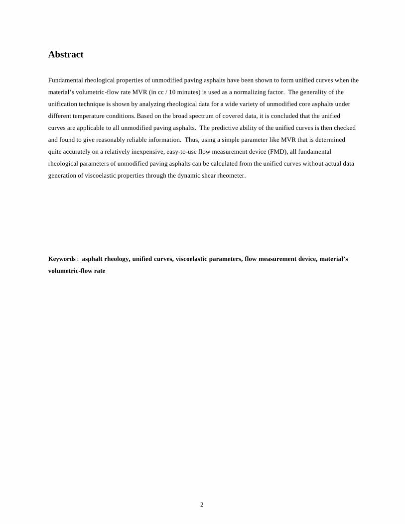
Abstract

Fundamental rheological properties of unmodified paving asphalts have been shown to form unified curves when the

material’s volumetric-flow rate MVR (in cc / 10 minutes) is used as a normalizing factor. The generality of the

unification technique is shown by analyzing rheological data for a wide variety of unmodified core asphalts under

different temperature conditions. Based on the broad spectrum of covered data, it is concluded that the unified

curves are applicable to all unmodified paving asphalts. The predictive ability of the unified curves is then checked

and found to give reasonably reliable information. Thus, using a simple parameter like MVR that is determined

quite accurately on a relatively inexpensive, easy-to-use flow measurement device (FMD), all fundamental

rheological parameters of unmodified paving asphalts can be calculated from the unified curves without actual data

generation of viscoelastic properties through the dynamic shear rheometer.

Keywords : asphalt rheology, unified curves, viscoelastic parameters, flow measurement device, material’s

volumetric-flow rate

3

Introduction

Asphalts on paved roads witness a wide range of static and dynamic stresses at varying temperatures and under

different environmental conditions. Hence it is essential to develop a good insight into the rheological properties of

the asphalts covering a wide range of shear rates over an equally broad range of temperatures and under simulated

environmental conditions.

Paving asphalts exhibit varying degrees of viscoelasticity under different conditions of temperature and loading.

Understanding the rheology of paving asphalts is important from different viewpoints. It is useful as a control tool to

distinguish between various asphalts from different crude sources and which are refined using different processes.

Understanding asphalt rheology aids in determining the appropriate temperature for mixing aggregates with asphalt

and also to compact the composite material in place so that the final pavement can be prepared well and with ease. It

is also important to find out how the rheological properties of asphalts relate to the distresses in the pavements after

the lay down process and after years of service. It is, therefore, not surprising that the subject of asphalt rheology

has been the focus of a great deal of research as can be seen from even a partial list of references1- 13

on various

aspects of this topic.

The findings of Strategic Highway Research Program (SHRP) have shown9 that fundamental viscoelastic behavior

of asphalts under different levels of stresses and temperatures need to be understood for performance-related

specifications to address major pavement distresses. Equipments that provide the fundamental rheological

information have a constraint in that they cannot easily be taken to the field or on-site, normally require highly

trained operators and are also relatively much more expensive. On the other hand, rapid methods of rheological

measurements normally give information on the consistency of the asphalts but do not provide all the fundamental

rheological knowledge about the material.

An attempt to relate fundamental rheological data with a very simple, yet reasonably accurate and rapidly

determinable rheological parameter was done through the development of unified curves for polymer-modified

asphalts14

as well as unmodified asphalts15

. Six asphalts were chosen from among the SHRP Materials Reference

Library asphalts to serve as representatives during initial verification of the developed theory for unification15

.

These were AAK-1, AAA-1, AAB-1, AAD-1, AAF-1 and AAM-1. Their select properties are shown in Table 1.

Though these asphalts cover a wide range of asphaltene content, a broad span of molecular weight, and a good

spread of viscosity values, it is essential to validate the generality of the unified curves through a different set of

asphalts under different temperature conditions.

The purpose of the present paper is to reinforce the unified curves through data analyses of a new set of asphalts. It

is confirmed through the extra data analyses that the unified curves are universal for all unmodified asphalts at least

within the studied temperature range of 46°C - 70°C. Since the validation has been done only in the temperature

4

range of 46°C - 70°C, the use of this work will be limited to high temperature applications. Assessment of the

predictive ability of the unified curves is also done. The results show that the simple material’s volumetric -flow rate

(MVR) is able to give good predictions of the viscoelastic parameters by mere calculations from the unified curves

for all unmodified asphalts. It is thus possible to now get all fundamental rheological information on the unmodified

paving asphalts in the temperature ranges of 46°C - 70°C by determining the MVR using a simple flow-measuring

device (FMD) rather than the dynamic shear rheometer (DSR).

There have been earlier efforts4, 6 to generate viscosity data using a capillary rheometer. Initially4, experiments were

conducted at a constant rate of strain but later6 a constant stress mode was employed for more rapid testing. The

approach did not become popular because of the large shear stresses and strains that were produced during

measurement. These could lead to spurious results under certain conditions of high stresses due to the elasticity of

the material and in other cases, where experimentally correct data could be produced, the results could be outside the

range of practical use because of the unreasonably high strain values. Moreover, their attemp t4, 6 was to generate the

entire shear stress versus shear rate data through the capillary rheometer.

In the present case, though a capillary die is used for flow rate measurement, the data is limited to one single value

of MVR that is carefully controlled to lie within restricted bounds, thereby keeping the shear rates within acceptable

limits. Moreover, the MVR data is collected only under a limited range of dead load conditions, thereby putting an

upper bound on the stress level. If at all there are any deficiencies in the measuring technique, these are

automatically annulled because the MVR is only used as a normalizing parameter.

Background

Most of the details of the unification concepts are covered elsewhere15, 16.

However, a brief account is provided

here in order to facilitate the understanding of the present work. In fact, all the salient features of the concepts are

covered here so that the present work becomes self-sufficient and it becomes easier to digest the subject matter.

Simple Rheological Parameter

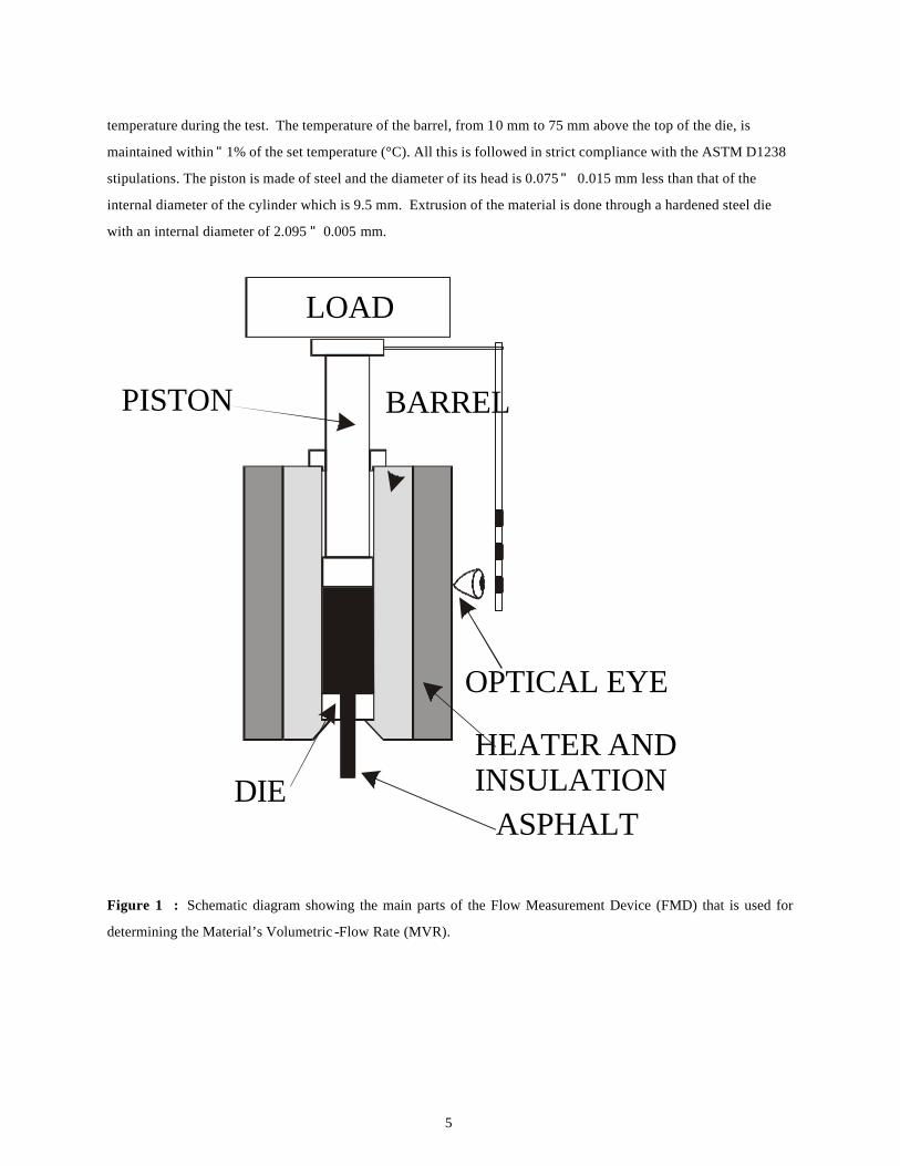
The simple parameter that is chosen to give a good measure of the rheological characteristics of the asphalt is the

material’s volumetric-flow rate (MVR) that is determined through a closely defined flow measurement device

(FMD), whose main parts are shown in Figure 1. This equipment is borrowed from the polymer industry where it is

routinely used to measure the melt flow index of polymers. The cylinder of the flow measurement device is made

of hardened steel and is fitted with heaters, insulated, and controlled for operation at the required temperature. The

thermocouple is buried inside the instrument’s barrel. The thermocouple and the associated temperature control

electronics are calibrated against NIST traceable temperature probes by the equipment manufacturer. The heating

device is capable of maintaining the temperature at 10 mm above the die to within "0.2°C of the desired

5

temperature during the test. The temperature of the barrel, from 10 mm to 75 mm above the top of the die, is

maintained within "1% of the set temperature (°C). All this is followed in strict compliance with the ASTM D1238

stipulations. The piston is made of steel and the diameter of its head is 0.075 " 0.015 mm less than that of the

internal diameter of the cylinder which is 9.5 mm. Extrusion of the material is done through a hardened steel die

with an internal diameter of 2.095 " 0.005 mm.

LOAD

PISTON BARREL

HEATER ANDINSULATIONDIE

OPTICAL EYE

ASPHALT

Figure 1 : Schematic diagram showing the main parts of the Flow Measurement Device (FMD) that is used for

determining the Material’s Volumetric -Flow Rate (MVR).

6

MVR

The MVR is defined as the volume of the material (in milliliters or cubic centimeters) that is extruded in 10 minutes

through the die of specific diameter and length as described above by applying pressure through dead weight under

prescribed temperature conditions. This definition is rather an arbitrary one. It has been chosen to be consistent with

the well-known rheological parameter used in polymer melt rheology, namely, the melt flow index MFI 16

, except

that MFI is the weight extruded in 10 minutes while MVR is the volume extruded in 10 minutes. The volume-flow

rate is more convenient to measure than the mass flow rate and does not require the knowledge of the density of the

material in the calculations. Possible sources of errors in MVR data could be due to a) kinetic energy effect, b)

hydrostatic head of the fluid material above the die exit, c) time-dependency of the flow, d) entrance and end

corrections, and e) effective wall slip. Correction terms to account for these errors are not included in the

unification and the reasons for that are given elsewhere 15

.

Unification Theory

The equipment used for measurement of MVR as defined above falls in the category of a circular orifice rheometer 16

. Hence the expressions for shear stress J and shear rate u in this equipment can be written in the following well-

known conventional forms:

RN F

J = ------------- (1)

2B RP 2 lN

4 Q

u = ----------- (2)

B RN 3

where nozzle radius RN = 0.105 cm, piston radius RP = 0.4737 cm, nozzle length lN = 0.8 cm, force F = load L (kg)

X 9.807 X 105 dynes and the flow rate Q (cc/s) is related to MVR (cc/10min) as follows by definition.

MVR

Q = -------- (3)

600

7

Since the geometry of the measuring equipment is fixed as given above, Equations (1) and (2) can be reduced to

give the following:

J/L = 9.13 x 104 = constant (4)

and

u/MVR = 1.83 = constant (5)

Note that the constant has only geometric values and no material properties.

When the MVR value is generated under a specific load condition for a particular grade of asphalt at a given

temperature, the shear stress and shear rate values corresponding to those test conditions can be obtained from Eqs.

(4) and (5). At that very temperature, by changing the applied load, a different value of MVR can be generated

which corresponds to a new set of shear stress and shear rate values. In this way, it is possible to generate the shear

stress versus shear rate curve for the asphalt at that temperature. This curve, which may be generated through the

flow measurement device (FMD), should correspond to the shear stress versus shear rate curve generated from any

rheometer because the response of the material to stress should be independent of the type of measuring equipment.

Generating the full flow curve from the FMD is meaningless, when more sophisticated equipments are available.

However, any curve generated from a sophisticated equipment would have a point on it which corresponds to the

shear stress and shear rate values from the FMD as given by equations (4) and (5). Thus, if the shear stress J versus

shear rate u data from any rheometer were replotted as J/L versus u/MVR, then for all samples, the curves should

pass through the co-ordinates of J/L = 9.13 x 104 and u/MVR = 1.83. This in effect, allows a vertical shift of the

curves though division by L and a horizontal shift through division by MVR, thereby resulting in a superposition of

the curves.

SHRP asphalt binder research findings have indicated that dynamic shear rheometer data are the preferred

fundamental rheological properties of neat asphalts to relate to pavement performance for rutting at high

temperatures. Hence, if a unification of rheological data is to be sought, then it is essential to develop a method to

coalesce dynamic data in terms of the complex modulus |G*|, loss modulus G@, and parameter |G*|/Sin * .

Earlier investigations of rheological properties (at least for polymer melts) have shown that the data under dynamic

conditions can be related to that obtained under steady shear within certain ranges of shear rates and frequencies17-

22. The empirical method suggested by Cox and Mertz

18 for relating steady shear viscosity with the absolute value

8

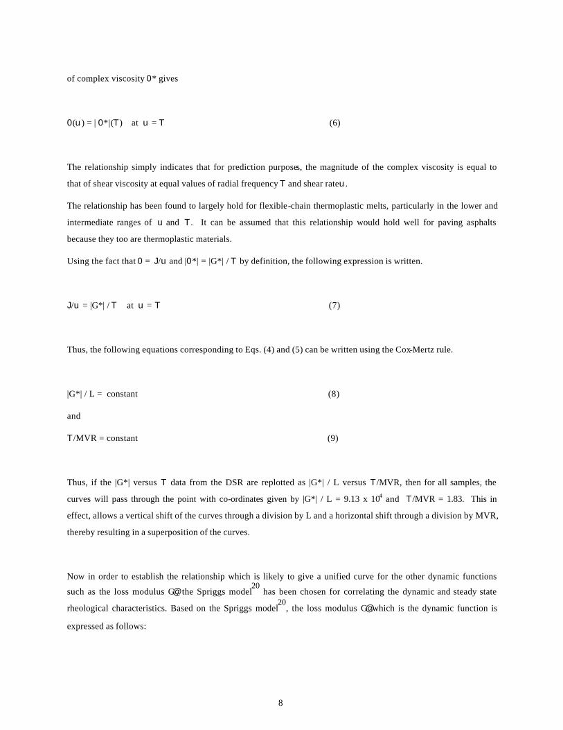
of complex viscosity 0* gives

0(u) = | 0*|(T) at u = T (6)

The relationship simply indicates that for prediction purposes, the magnitude of the complex viscosity is equal to

that of shear viscosity at equal values of radial frequency T and shear rateu.

The relationship has been found to largely hold for flexible-chain thermoplastic melts, particularly in the lower and

intermediate ranges of u and T. It can be assumed that this relationship would hold well for paving asphalts

because they too are thermoplastic materials.

Using the fact that 0 = J/u and |0*| = |G*| / T by definition, the following expression is written.

J/u = |G*| / T at u = T (7)

Thus, the following equations corresponding to Eqs. (4) and (5) can be written using the Cox-Mertz rule.

|G*| / L = constant (8)

and

T/MVR = constant (9)

Thus, if the |G*| versus T data from the DSR are replotted as |G*| / L versus T/MVR, then for all samples, the

curves will pass through the point with co-ordinates given by |G*| / L = 9.13 x 104 and T/MVR = 1.83. This in

effect, allows a vertical shift of the curves through a division by L and a horizontal shift through a division by MVR,

thereby resulting in a superposition of the curves.

Now in order to establish the relationship which is likely to give a unified curve for the other dynamic functions

such as the loss modulus G@, the Spriggs model20

has been chosen for correlating the dynamic and steady state

rheological characteristics. Based on the Spriggs model20

, the loss modulus G@ which is the dynamic function is

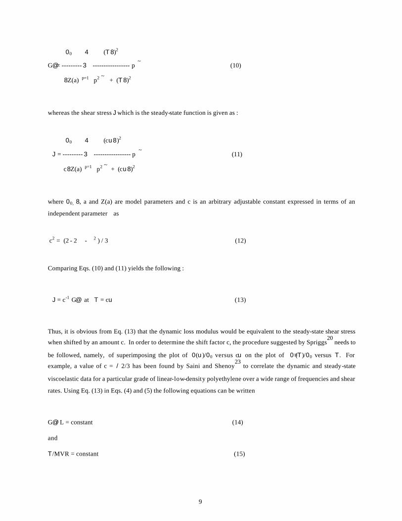
expressed as follows:

9

00 4 (T8)2

G@ = --------- 3 ----------------- p ~ (10)

8Z(a) p=1 p2 ~ + (T8)2

whereas the shear stress J which is the steady-state function is given as :

00 4 (cu8)2

J = --------- 3 ----------------- p ~ (11)

c8Z(a) p=1 p2 ~ + (cu8)2

where 00, 8, a and Z(a) are model parameters and c is an arbitrary adjustable constant expressed in terms of an

independent parameter ë as

c2 = (2 - 2 ë - ë2 ) / 3 (12)

Comparing Eqs. (10) and (11) yields the following :

J = c-1 G@ at T = cu (13)

Thus, it is obvious from Eq. (13) that the dynamic loss modulus would be equivalent to the steady-state shear stress

when shifted by an amount c. In order to determine the shift factor c, the procedure suggested by Spriggs20

needs to

be followed, namely, of superimposing the plot of 0(u)/00 versus cu on the plot of 0=(T)/00 versus T. For

example, a value of c = /2/3 has been found by Saini and Shenoy23

to correlate the dynamic and steady-state

viscoelastic data for a particular grade of linear-low-density polyethylene over a wide range of frequencies and shear

rates. Using Eq. (13) in Eqs. (4) and (5) the following equations can be written

G@ / L = constant (14)

and

T/MVR = constant (15)

10

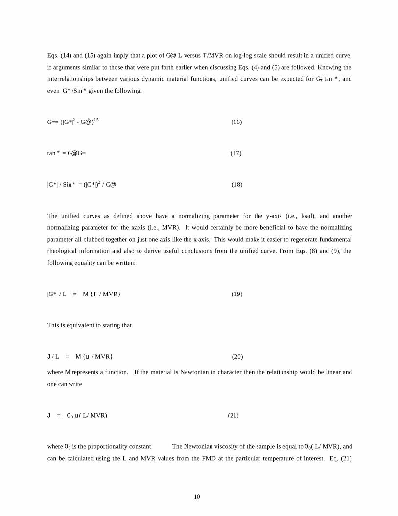
Eqs. (14) and (15) again imply that a plot of G@ / L versus T/MVR on log-log scale should result in a unified curve,

if arguments similar to those that were put forth earlier when discussing Eqs. (4) and (5) are followed. Knowing the

interrelationships between various dynamic material functions, unified curves can be expected for G=, tan *, and

even |G*|/Sin * given the following.

G= = (|G*|2 - G@2 )0.5 (16)

tan * = G@/ G= (17)

|G*| / Sin * = (|G*|)2 / G@ (18)

The unified curves as defined above have a normalizing parameter for the y-axis (i.e., load), and another

normalizing parameter for the x-axis (i.e., MVR). It would certainly be more beneficial to have the normalizing

parameter all clubbed together on just one axis like the x-axis. This would make it easier to regenerate fundamental

rheological information and also to derive useful conclusions from the unified curve. From Eqs. (8) and (9), the

following equality can be written:

|G*| / L = M {T / MVR} (19)

This is equivalent to stating that

J / L = M {u / MVR} (20)

where M represents a function. If the material is Newtonian in character then the relationship would be linear and

one can write

J = 00 u( L/ MVR) (21)

where 00 is the proportionality constant. The Newtonian viscosity of the sample is equal to 00( L/ MVR), and

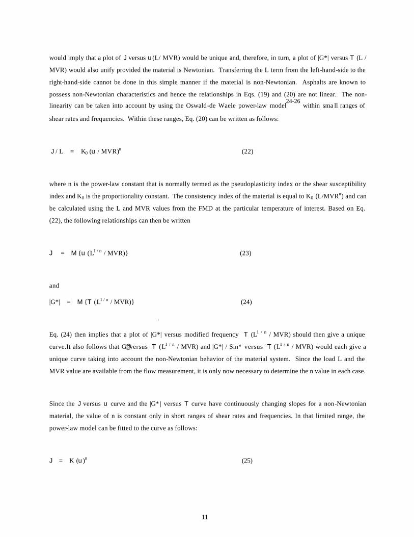
can be calculated using the L and MVR values from the FMD at the particular temperature of interest. Eq. (21)

11

would imply that a plot of J versus u(L/ MVR) would be unique and, therefore, in turn, a plot of |G*| versus T (L /

MVR) would also unify provided the material is Newtonian. Transferring the L term from the left-hand-side to the

right-hand-side cannot be done in this simple manner if the material is non-Newtonian. Asphalts are known to

possess non-Newtonian characteristics and hence the relationships in Eqs. (19) and (20) are not linear. The non-

linearity can be taken into account by using the Oswald-de Waele power-law model24-26

within sma ll ranges of

shear rates and frequencies. Within these ranges, Eq. (20) can be written as follows:

J / L = K0 (u / MVR)n (22)

where n is the power-law constant that is normally termed as the pseudoplasticity index or the shear susceptibility

index and K0 is the proportionality constant. The consistency index of the material is equal to K0 (L/MVRn) and can

be calculated using the L and MVR values from the FMD at the particular temperature of interest. Based on Eq.

(22), the following relationships can then be written

J = M {u (L1 / n / MVR)} (23)

and

|G*| = M {T (L1 / n / MVR)} (24)

.

Eq. (24) then implies that a plot of |G*| versus modified frequency T (L1 / n / MVR) should then give a unique

curve.It also follows that G@ versus T (L1 / n / MVR) and |G*| / Sin* versus T (L1 / n / MVR) would each give a

unique curve taking into account the non-Newtonian behavior of the material system. Since the load L and the

MVR value are available from the flow measurement, it is only now necessary to determine the n value in each case.

Since the J versus u curve and the |G* | versus T curve have continuously changing slopes for a non-Newtonian

material, the value of n is constant only in short ranges of shear rates and frequencies. In that limited range, the

power-law model can be fitted to the curve as follows:

J = K (u)n (25)

12

Note that this is not the unified curve that is being considered but the curve that could be generated by simply

changing the load conditions in the FMD as discussed earlier during the development of Eqs. (4) and (5). In the

present context, the value of n has to be chosen in the range of shear stress and shear rate which corresponds closely

to those applicable to the MVR value that is used for the normalizing process. Hence, in case the MVR value has

been determined at a load L for a particular asphalt sample at a specific temperature, then two more MVR values

are to be determined at two other load conditions to estimate the value of n. The two load conditions are chosen in

such a way that one is higher than L (i.e., say L1) while the other is lower than L (i.e., L2). In order to get the value

of n, Eq. (25) is rewritten using Eqs. (4) and (5) as follows:

L1 = K (MVR1)n (26)

and

L2 = K (MVR2)n (27)

Solving Eqs. (26) and (27), the following equation can be written for the estimation of the value of n.

n = log (L1/L2) / log (MVR1/MVR2) (28)

Experiments

The theoretical development in the previous section has shown the possibility of unifying fundamental rheological

data through the use of the material’s volumetric -flow rate (MVR). In order to verify this, systematic experiments

are needed on a number of different asphalts that have widely different rheological characteristics. These asphalts

have to be characterized on two different rheometers, one which gives the fundamental rheological properties in

terms of the dynamic material functions and the other which gives the material’s volumetric flow rate.

13

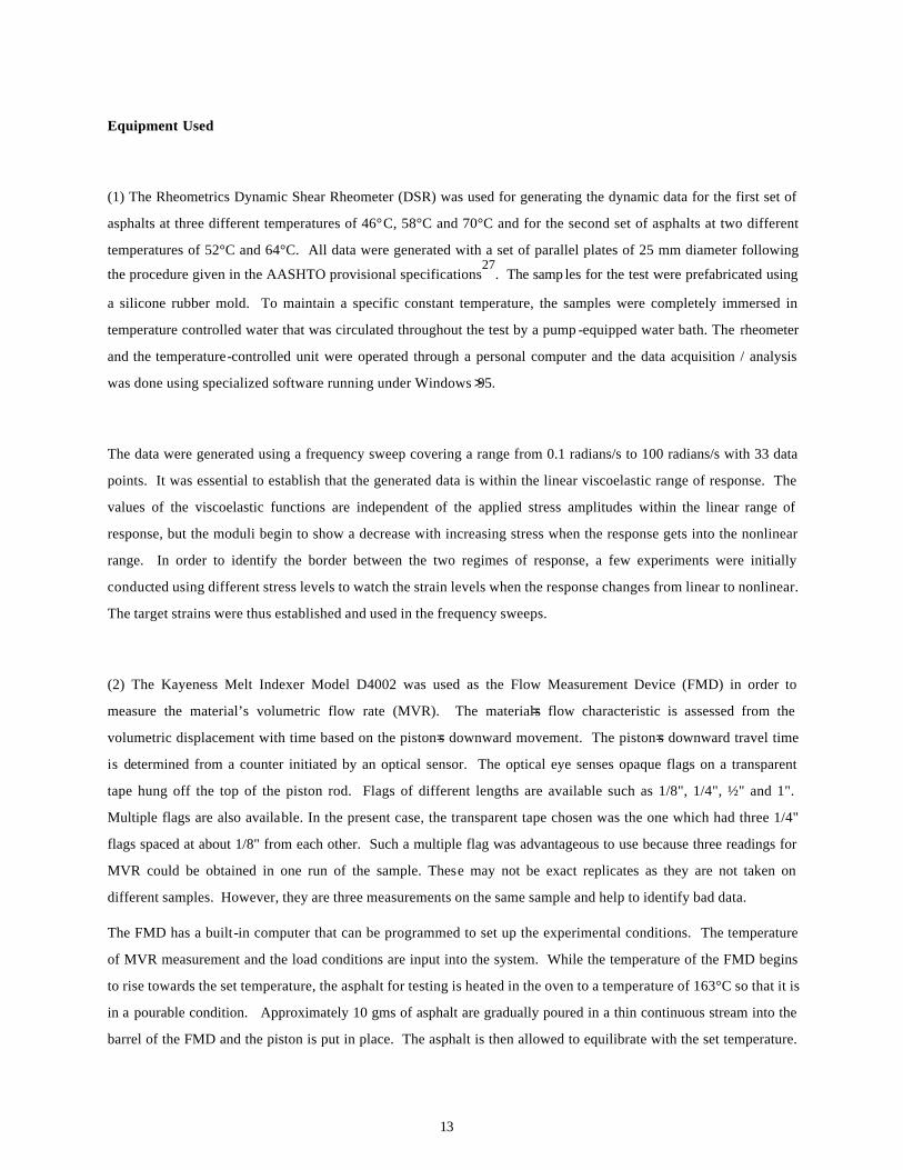
Equipment Used

(1) The Rheometrics Dynamic Shear Rheometer (DSR) was used for generating the dynamic data for the first set of

asphalts at three different temperatures of 46°C, 58°C and 70°C and for the second set of asphalts at two different

temperatures of 52°C and 64°C. All data were generated with a set of parallel plates of 25 mm diameter following

the procedure given in the AASHTO provisional specifications27

. The samp les for the test were prefabricated using

a silicone rubber mold. To maintain a specific constant temperature, the samples were completely immersed in

temperature controlled water that was circulated throughout the test by a pump -equipped water bath. The rheometer

and the temperature-controlled unit were operated through a personal computer and the data acquisition / analysis

was done using specialized software running under Windows >95.

The data were generated using a frequency sweep covering a range from 0.1 radians/s to 100 radians/s with 33 data

points. It was essential to establish that the generated data is within the linear viscoelastic range of response. The

values of the viscoelastic functions are independent of the applied stress amplitudes within the linear range of

response, but the moduli begin to show a decrease with increasing stress when the response gets into the nonlinear

range. In order to identify the border between the two regimes of response, a few experiments were initially

conducted using different stress levels to watch the strain levels when the response changes from linear to nonlinear.

The target strains were thus established and used in the frequency sweeps.

(2) The Kayeness Melt Indexer Model D4002 was used as the Flow Measurement Device (FMD) in order to

measure the material’s volumetric flow rate (MVR). The material=s flow characteristic is assessed from the

volumetric displacement with time based on the piston=s downward movement. The piston=s downward travel time

is determined from a counter initiated by an optical sensor. The optical eye senses opaque flags on a transparent

tape hung off the top of the piston rod. Flags of different lengths are available such as 1/8", 1/4", ½" and 1".

Multiple flags are also available. In the present case, the transparent tape chosen was the one which had three 1/4"

flags spaced at about 1/8" from each other. Such a multiple flag was advantageous to use because three readings for

MVR could be obtained in one run of the sample. These may not be exact replicates as they are not taken on

different samples. However, they are three measurements on the same sample and help to identify bad data.

The FMD has a built-in computer that can be programmed to set up the experimental conditions. The temperature

of MVR measurement and the load conditions are input into the system. While the temperature of the FMD begins

to rise towards the set temperature, the asphalt for testing is heated in the oven to a temperature of 163°C so that it is

in a pourable condition. Approximately 10 gms of asphalt are gradually poured in a thin continuous stream into the

barrel of the FMD and the piston is put in place. The asphalt is then allowed to equilibrate with the set temperature.

14

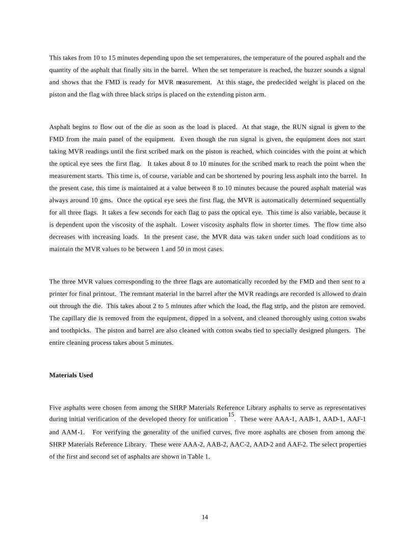
This takes from 10 to 15 minutes depending upon the set temperatures, the temperature of the poured asphalt and the

quantity of the asphalt that finally sits in the barrel. When the set temperature is reached, the buzzer sounds a signal

and shows that the FMD is ready for MVR measurement. At this stage, the predecided weight is placed on the

piston and the flag with three black strips is placed on the extending piston arm.

Asphalt begins to flow out of the die as soon as the load is placed. At that stage, the RUN signal is given to the

FMD from the main panel of the equipment. Even though the run signal is given, the equipment does not start

taking MVR readings until the first scribed mark on the piston is reached, which coincides with the point at which

the optical eye sees the first flag. It takes about 8 to 10 minutes for the scribed mark to reach the point when the

measurement starts. This time is, of course, variable and can be shortened by pouring less asphalt into the barrel. In

the present case, this time is maintained at a value between 8 to 10 minutes because the poured asphalt material was

always around 10 gms. Once the optical eye sees the first flag, the MVR is automatically determined sequentially

for all three flags. It takes a few seconds for each flag to pass the optical eye. This time is also variable, because it

is dependent upon the viscosity of the asphalt. Lower viscosity asphalts flow in shorter times. The flow time also

decreases with increasing loads. In the present case, the MVR data was taken under such load conditions as to

maintain the MVR values to be between 1 and 50 in most cases.

The three MVR values corresponding to the three flags are automatically recorded by the FMD and then sent to a

printer for final printout. The remnant material in the barrel after the MVR readings are recorded is allowed to drain

out through the die. This takes about 2 to 5 minutes after which the load, the flag strip, and the piston are removed.

The capillary die is removed from the equipment, dipped in a solvent, and cleaned thoroughly using cotton swabs

and toothpicks. The piston and barrel are also cleaned with cotton swabs tied to specially designed plungers. The

entire cleaning process takes about 5 minutes.

Materials Used

Five asphalts were chosen from among the SHRP Materials Reference Library asphalts to serve as representatives

during initial verification of the developed theory for unification15

. These were AAA-1, AAB-1, AAD-1, AAF-1

and AAM-1. For verifying the generality of the unified curves, five more asphalts are chosen from among the

SHRP Materials Reference Library. These were AAA-2, AAB-2, AAC-2, AAD-2 and AAF-2. The select properties

of the first and second set of asphalts are shown in Table 1.

15

The asphalts from the dash1 series and the dash2 series together cover a wide range of asphaltene content, a broad

span of molecular weight, and a good spread of viscosity values. The samples were each tested in their original

unaged form and then again after aging using the rolling thin film oven test (RTFOT) at 163°C for 85 minutes and in

the pressure aging vessel (PAV) at 100°C for 20 hours in accordance with the AASHTO provisional standard

procedure28

.

TABLE 1 : Selected Details about the Asphalts Used

---------------------------------------------------------------------------------------------------------------------

Asphalt ID Source Viscosity@140F, poise Asphaltenes, % W.Av.Mol.Wt., daltons

---------------------------------------------------------------------------------------------------------------------

Set 1

AAA-1 Lloydminster 864 16.2 790

AAB-1 WY Sour 1029 17.3 840

AAD-1 California 1055 20.5 870

AAF-1 W Tx Sour 1872 13.3 840

AAM-1 W Tx Inter 1992 4.0 1300

Set 2

AAA-2 Lloydminster 363 16.2 ---

AAB-2 WY Sour 403 16.7 ---

AAC-2 Redwater 304 9.8 870

AAD-2 Coastal 600 21.3 ---

AAF-2 W Tx Sour 867 13.0 ---

----------------------------------------------------------------------------------------------------------------------

16

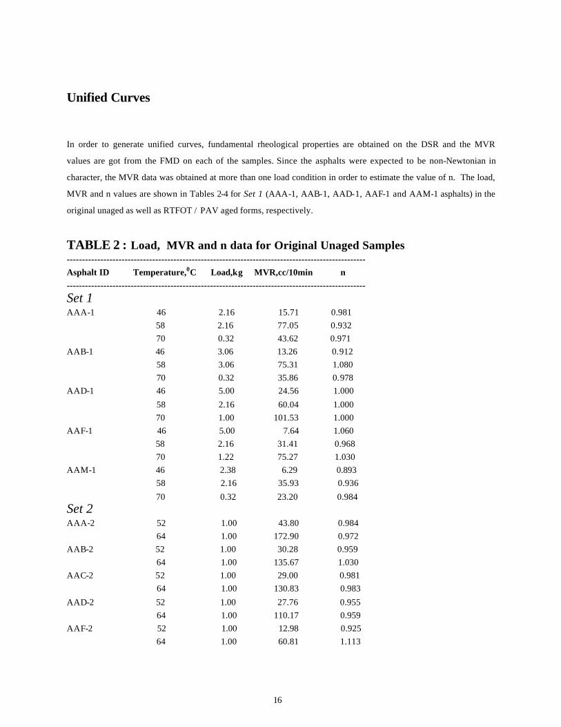
Unified Curves

In order to generate unified curves, fundamental rheological properties are obtained on the DSR and the MVR

values are got from the FMD on each of the samples. Since the asphalts were expected to be non-Newtonian in

character, the MVR data was obtained at more than one load condition in order to estimate the value of n. The load,

MVR and n values are shown in Tables 2-4 for Set 1 (AAA-1, AAB-1, AAD-1, AAF-1 and AAM-1 asphalts) in the

original unaged as well as RTFOT / PAV aged forms, respectively.

TABLE 2 : Load, MVR and n data for Original Unaged Samples -------------------------------------------------------------------------------------------------- Asphalt ID Temperature,0C Load,kg MVR,cc/10min n --------------------------------------------------------------------------------------------------

Set 1 AAA-1 46 2.16 15.71 0.981 58 2.16 77.05 0.932 70 0.32 43.62 0.971 AAB-1 46 3.06 13.26 0.912 58 3.06 75.31 1.080 70 0.32 35.86 0.978 AAD-1 46 5.00 24.56 1.000

58 2.16 60.04 1.000 70 1.00 101.53 1.000 AAF-1 46 5.00 7.64 1.060 58 2.16 31.41 0.968 70 1.22 75.27 1.030 AAM-1 46 2.38 6.29 0.893 58 2.16 35.93 0.936

70 0.32 23.20 0.984 Set 2 AAA-2 52 1.00 43.80 0.984 64 1.00 172.90 0.972 AAB-2 52 1.00 30.28 0.959 64 1.00 135.67 1.030 AAC-2 52 1.00 29.00 0.981 64 1.00 130.83 0.983

AAD-2 52 1.00 27.76 0.955 64 1.00 110.17 0.959 AAF-2 52 1.00 12.98 0.925 64 1.00 60.81 1.113

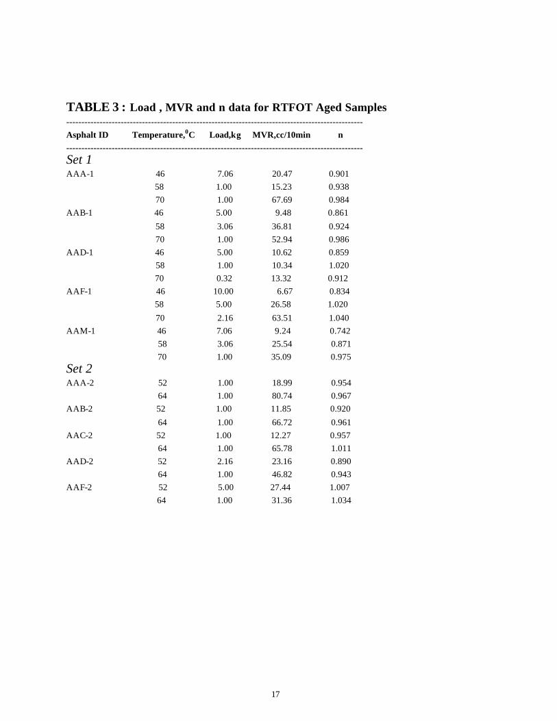
17

TABLE 3 : Load , MVR and n data for RTFOT Aged Samples -------------------------------------------------------------------------------------------------- Asphalt ID Temperature,0C Load,kg MVR,cc/10min n -------------------------------------------------------------------------------------------------- Set 1 AAA-1 46 7.06 20.47 0.901 58 1.00 15.23 0.938 70 1.00 67.69 0.984 AAB-1 46 5.00 9.48 0.861

58 3.06 36.81 0.924 70 1.00 52.94 0.986 AAD-1 46 5.00 10.62 0.859 58 1.00 10.34 1.020 70 0.32 13.32 0.912 AAF-1 46 10.00 6.67 0.834 58 5.00 26.58 1.020

70 2.16 63.51 1.040 AAM-1 46 7.06 9.24 0.742 58 3.06 25.54 0.871 70 1.00 35.09 0.975 Set 2 AAA-2 52 1.00 18.99 0.954 64 1.00 80.74 0.967 AAB-2 52 1.00 11.85 0.920

64 1.00 66.72 0.961 AAC-2 52 1.00 12.27 0.957 64 1.00 65.78 1.011 AAD-2 52 2.16 23.16 0.890 64 1.00 46.82 0.943 AAF-2 52 5.00 27.44 1.007 64 1.00 31.36 1.034

18

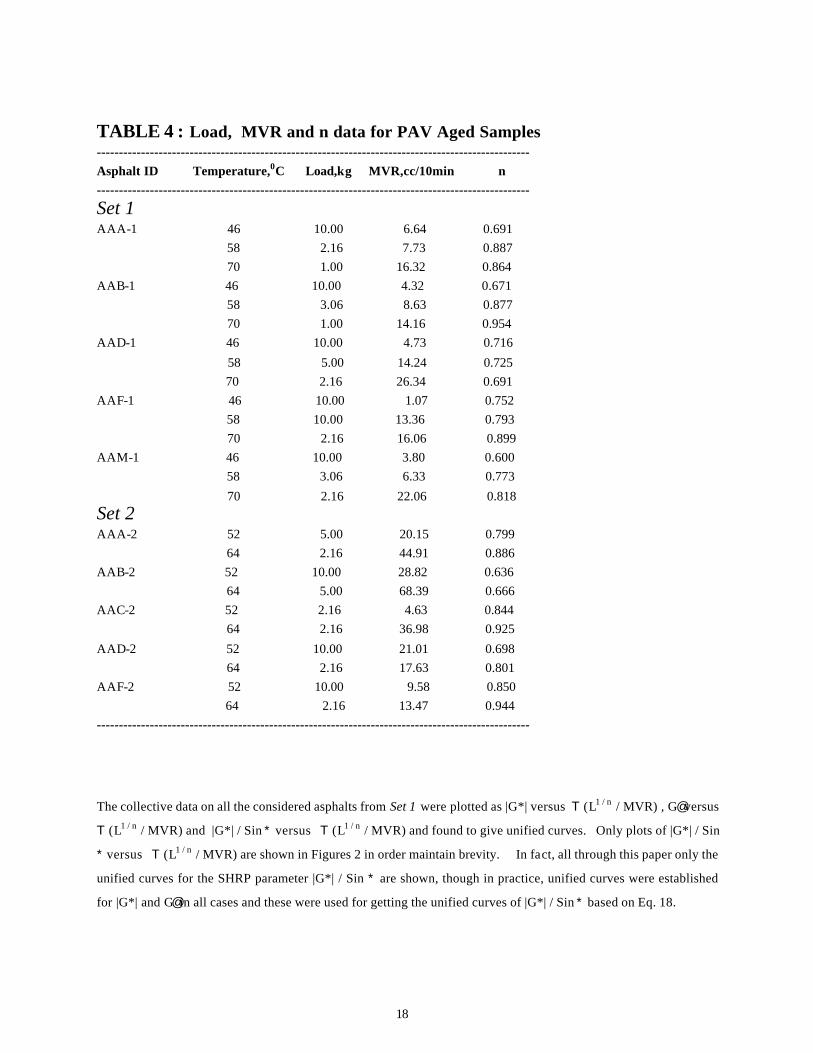
TABLE 4 : Load, MVR and n data for PAV Aged Samples -------------------------------------------------------------------------------------------------- Asphalt ID Temperature,0C Load,kg MVR,cc/10min n --------------------------------------------------------------------------------------------------

Set 1 AAA-1 46 10.00 6.64 0.691 58 2.16 7.73 0.887 70 1.00 16.32 0.864 AAB-1 46 10.00 4.32 0.671 58 3.06 8.63 0.877 70 1.00 14.16 0.954 AAD-1 46 10.00 4.73 0.716

58 5.00 14.24 0.725 70 2.16 26.34 0.691 AAF-1 46 10.00 1.07 0.752 58 10.00 13.36 0.793 70 2.16 16.06 0.899 AAM-1 46 10.00 3.80 0.600 58 3.06 6.33 0.773

70 2.16 22.06 0.818 Set 2 AAA-2 52 5.00 20.15 0.799 64 2.16 44.91 0.886 AAB-2 52 10.00 28.82 0.636 64 5.00 68.39 0.666 AAC-2 52 2.16 4.63 0.844 64 2.16 36.98 0.925

AAD-2 52 10.00 21.01 0.698 64 2.16 17.63 0.801 AAF-2 52 10.00 9.58 0.850 64 2.16 13.47 0.944 --------------------------------------------------------------------------------------------------

The collective data on all the considered asphalts from Set 1 were plotted as |G*| versus T (L1 / n / MVR) , G@ versus

T (L1 / n / MVR) and |G*| / Sin * versus T (L1 / n / MVR) and found to give unified curves. Only plots of |G*| / Sin

* versus T (L1 / n / MVR) are shown in Figures 2 in order maintain brevity. In fact, all through this paper only the

unified curves for the SHRP parameter |G*| / Sin * are shown, though in practice, unified curves were established

for |G*| and G@ in all cases and these were used for getting the unified curves of |G*| / Sin * based on Eq. 18.

19

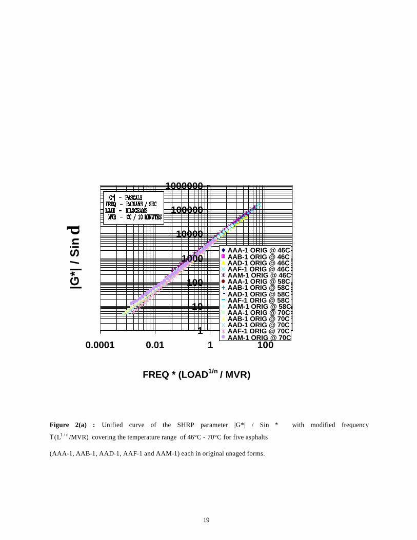
Figure 2(a) : Unified curve of the SHRP parameter |G*| / Sin * with modified frequency

T(L1 / n /MVR) covering the temperature range of 46°C - 70°C for five asphalts

(AAA-1, AAB-1, AAD-1, AAF-1 and AAM-1) each in original unaged forms.

1

10

100

1000

10000

100000

1000000

0.0001 0.01 1 100

FREQ * (LOAD1/n / MVR)

|G*|

/ S

in δ

AAA-1 ORIG @ 46CAAB-1 ORIG @ 46CAAD-1 ORIG @ 46CAAF-1 ORIG @ 46CAAM-1 ORIG @ 46CAAA-1 ORIG @ 58CAAB-1 ORIG @ 58CAAD-1 ORIG @ 58CAAF-1 ORIG @ 58CAAM-1 ORIG @ 58CAAA-1 ORIG @ 70CAAB-1 ORIG @ 70CAAD-1 ORIG @ 70CAAF-1 ORIG @ 70CAAM-1 ORIG @ 70C

20

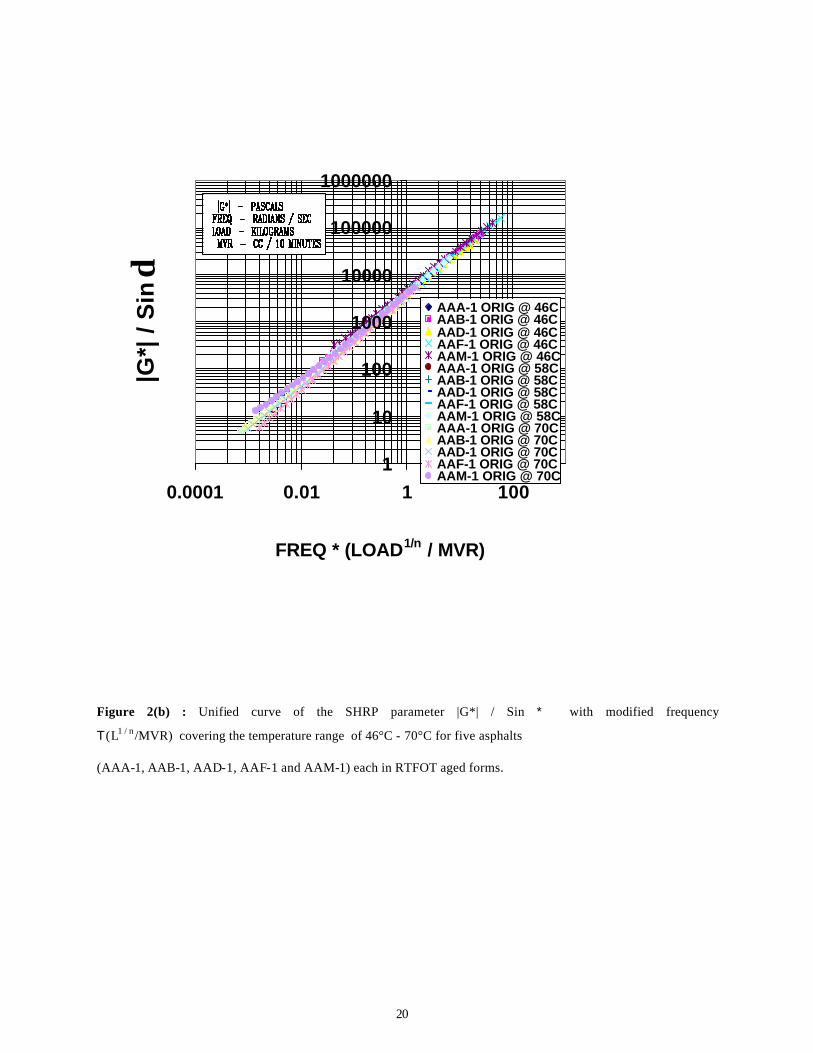
Figure 2(b) : Unified curve of the SHRP parameter |G*| / Sin * with modified frequency

T(L1 / n /MVR) covering the temperature range of 46°C - 70°C for five asphalts

(AAA-1, AAB-1, AAD-1, AAF-1 and AAM-1) each in RTFOT aged forms.

1

10

100

1000

10000

100000

1000000

0.0001 0.01 1 100

FREQ * (LOAD1/n / MVR)

|G*|

/ S

in δ

AAA-1 ORIG @ 46CAAB-1 ORIG @ 46CAAD-1 ORIG @ 46CAAF-1 ORIG @ 46CAAM-1 ORIG @ 46CAAA-1 ORIG @ 58CAAB-1 ORIG @ 58CAAD-1 ORIG @ 58CAAF-1 ORIG @ 58CAAM-1 ORIG @ 58CAAA-1 ORIG @ 70CAAB-1 ORIG @ 70CAAD-1 ORIG @ 70CAAF-1 ORIG @ 70CAAM-1 ORIG @ 70C

21

Figure 2(c) : Unified curve of the SHRP parameter |G*| / Sin * with modified frequency

T(L1 / n /MVR) covering the temperature range of 46°C - 70°C for five asphalts

(AAA-1, AAB-1, AAD-1, AAF-1 and AAM-1) each in PAV aged forms.

1

10

100

1000

10000

100000

1000000

0.0001 0.01 1 100 10000

FREQ * (LOAD1/n / MVR)

|G*|

/ S

in δ AAA-1 PAV @ 46C

AAB-1 PAV @ 46CAAD-1 PAV @ 46CAAF-1 PAV @ 46CAAM-1 PAV @ 46CAAA-1 PAV @ 58CAAB-1 PAV @ 58CAAD-1 PAV @ 58CAAF-1 PAV @ 58CAAM-1 PAV @ 58CAAA-1 PAV @ 70CAAB-1 PAV @ 70CAAD-1 PAV @ 70CAAF-1 PAV @ 70CAAM-1 PAV @ 70C

22

It can be seen that the curves in Figures 2 (a)- (c) are unique and independent of the type of asphalt as well as the

temperature of measurement. Each unified curve has a total of 495 data points (i.e., 99 data points for each of the

five asphalts: AAA-1, AAB-1, AAD-1, AAF-1 and AAM-1). Different unified curves have been shown at different

levels of aging, i.e. (a) original unaged, (b) RTFOT aged and (c) PAV aged. This was done on account of two

reasons. Firstly, to avoid clogging too much data on one curve and secondly because there was a slight but

noticeable difference in PAV aged unified curve which would be otherwise lost if all data were plotted on one curve.

It is not clear whether this is an experimental artifact or whether truly the unified curve is different for PAV aged

samples.

In Figures 2 (a) - (c), only the dash1 grades of various asphalts were considered. It was important to check whether

the rheological data of dash2 grades fall on a unified curve as well and whether there was truly a single curve for the

dash1 and dash2 grades. To confirm this, DSR data were generated for asphalts AAA-2, AAB-2, AAC-2, AAD-2

and AAF-2. For each of these asphalts, MVR data were also obtained and the values of n were estimated as well.

These are shown in Tables 2-4 under Set 2. Data were generated at two temperatures 52°C and 64°C. It is

important to note that thes e two temperatures (52°C, 64°C) were chosen to be different from the ones (46°C, 58°C,

70°C) that were used for dash1 grades under Set 1 in Tables 2-4.

The primary check was to confirm that all the dash2 grades of asphalt formed a unified curve.

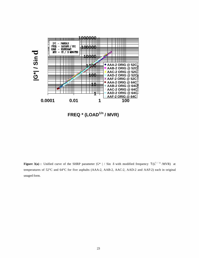
The collective data on all the considered asphalts from Set 2 were plotted as |G* | versus T (L1 / n / MVR), G” versus

T (L1 / n / MVR) and |G* | / Sin * versus T (L1 / n / MVR) and found to give unified curves. The plot of |G* | / Sin *

versus T (L1 / n / MVR) is shown in Figures 3 (a) - (c).

23

Figure 3(a) : Unified curve of the SHRP parameter |G* | / Sin δ with modified frequency T(L1 / n /MVR) at

temperatures of 52°C and 64°C for five asphalts (AAA-2, AAB-2, AAC-2, AAD-2 and AAF-2) each in original

unaged form.

1

10

100

1000

10000

100000

1000000

0.0001 0.01 1 100

FREQ * (LOAD1/n / MVR)

|G*|

/ S

in δ

AAA-2 ORIG @ 52CAAB-2 ORIG @ 52CAAC-2 ORIG @ 52CAAD-2 ORIG @ 52CAAF-2 ORIG @ 52CAAA-2 ORIG @ 64CAAB-2 ORIG @ 64CAAC-2 ORIG @ 64CAAD-2 ORIG @ 64CAAF-2 ORIG @ 64C

24

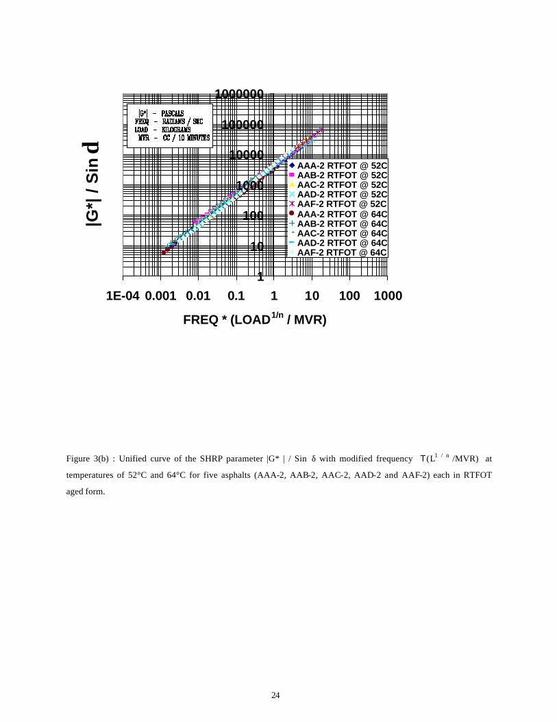
Figure 3(b) : Unified curve of the SHRP parameter |G* | / Sin δ with modified frequency T(L1 / n /MVR) at

temperatures of 52°C and 64°C for five asphalts (AAA-2, AAB-2, AAC-2, AAD-2 and AAF-2) each in RTFOT

aged form.

1

10

100

1000

10000

100000

1000000

1E-04 0.001 0.01 0.1 1 10 100 1000

FREQ * (LOAD1/n / MVR)

|G*|

/ S

in δ

AAA-2 RTFOT @ 52CAAB-2 RTFOT @ 52CAAC-2 RTFOT @ 52CAAD-2 RTFOT @ 52CAAF-2 RTFOT @ 52CAAA-2 RTFOT @ 64CAAB-2 RTFOT @ 64CAAC-2 RTFOT @ 64CAAD-2 RTFOT @ 64CAAF-2 RTFOT @ 64C

25

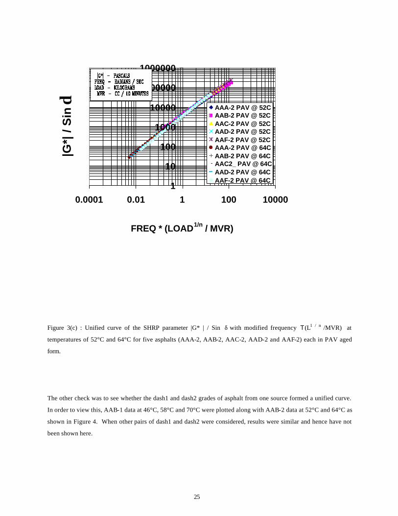
Figure 3(c) : Unified curve of the SHRP parameter |G* | / Sin δ with modified frequency T(L1 / n /MVR) at

temperatures of 52°C and 64°C for five asphalts (AAA-2, AAB-2, AAC-2, AAD-2 and AAF-2) each in PAV aged

form.

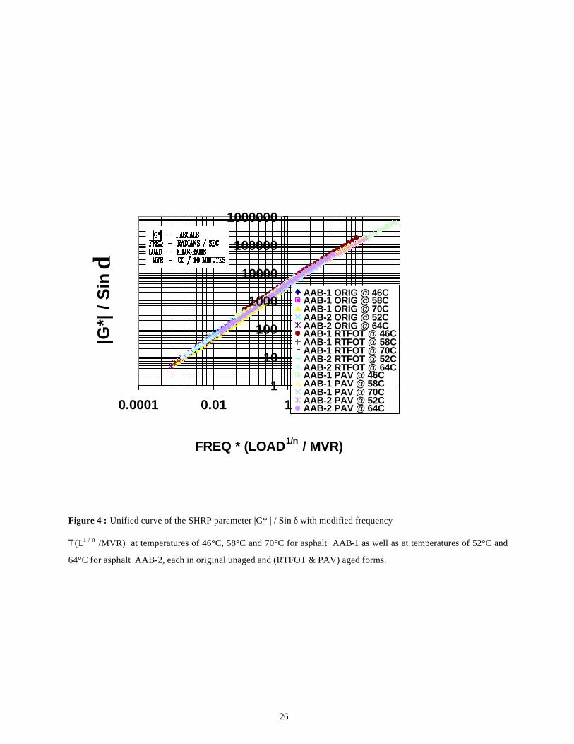
The other check was to see whether the dash1 and dash2 grades of asphalt from one source formed a unified curve.

In order to view this, AAB-1 data at 46°C, 58°C and 70°C were plotted along with AAB-2 data at 52°C and 64°C as

shown in Figure 4. When other pairs of dash1 and dash2 were considered, results were similar and hence have not

been shown here.

1

10

100

1000

10000

100000

1000000

0.0001 0.01 1 100 10000

FREQ * (LOAD1/n / MVR)

|G*|

/ S

in δ AAA-2 PAV @ 52C

AAB-2 PAV @ 52CAAC-2 PAV @ 52CAAD-2 PAV @ 52CAAF-2 PAV @ 52CAAA-2 PAV @ 64CAAB-2 PAV @ 64CAAC2_ PAV @ 64CAAD-2 PAV @ 64CAAF-2 PAV @ 64C

26

Figure 4 : Unified curve of the SHRP parameter |G* | / Sin δ with modified frequency

T(L1 / n /MVR) at temperatures of 46°C, 58°C and 70°C for asphalt AAB-1 as well as at temperatures of 52°C and

64°C for asphalt AAB-2, each in original unaged and (RTFOT & PAV) aged forms.

1

10

100

1000

10000

100000

1000000

0.0001 0.01 1 100

FREQ * (LOAD1/n / MVR)

|G*|

/ S

in δ

AAB-1 ORIG @ 46CAAB-1 ORIG @ 58CAAB-1 ORIG @ 70CAAB-2 ORIG @ 52CAAB-2 ORIG @ 64CAAB-1 RTFOT @ 46CAAB-1 RTFOT @ 58CAAB-1 RTFOT @ 70CAAB-2 RTFOT @ 52CAAB-2 RTFOT @ 64CAAB-1 PAV @ 46CAAB-1 PAV @ 58CAAB-1 PAV @ 70CAAB-2 PAV @ 52CAAB-2 PAV @ 64C

27

Figures 2-4 confirm that the unification technique works for at least ten different asphalts. A closer look at the

selection of the ten asphalts indicates that they span a wide range of viscosity levels, have varied asphaltene content,

varied wax content as well as high to low molecular weights. When such a wide spectrum of differences can be

unified by the suggested approach, it may not be too unrealistic to expect that all unmodified asphalts would fall on

the same curve.

The unified curves show a band within which all the data points coalesce. An estimate15

of the bandwidth gave an

error bound range of 3-16%, most of which was a reflection of the errors in the original DSR data . Reinforcement

of the curves with more data and further refinement of the curves to reduce the error bounds can be accomplished to

finally establish the decisive shapes of the unified curves. The main accent of the present work was essentially to

establish the unification technique and suggest the methodology that needs to be followed in order to achieve proper

unification based on good theoretical foundations, and this could be achieved through the analysis of rheological

data on the ten chosen asphalts. The unified curves of fundamental rheological data for all unmodified asphalts have

many advantages. The beneficial implications of this unification have been discussed elsewhere15

.

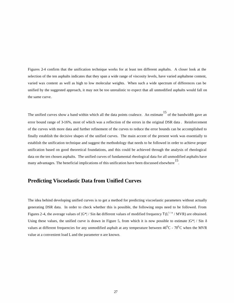
Predicting Viscoelastic Data from Unified Curves

The idea behind developing unified curves is to get a method for predicting viscoelastic parameters without actually

generating DSR data. In order to check whether this is possible, the following steps need to be followed. From

Figures 2-4, the average values of |G*| / Sin δat different values of modified frequency T(L1 / n / MVR) are obtained.

Using these values, the unified curve is drawn in Figure 5, from which it is now possible to estimate |G*| / Sin δ

values at different frequencies for any unmodified asphalt at any temperature between 460C - 700 C when the MVR

value at a convenient load L and the parameter n are known.

28

Figure 5 : Unified curve of the SHRP parameter |G* | / Sin δ with modified frequency

T(L1 / n /MVR) at temperatures of 46°C - 70°C for unmodified original unaged asphalts.

In order to check the predictability, unmodified asphalt AAF-2 is chosen. It should be noted that this asphalt was

not used when the unified curve was formed in the first place in Figure 5. Asphalt AAF-2 is a West Texas Sour with

a viscosity of 867 poise @ 1400F and has about 13% asphaltenes.

1

10

100

1000

10000

100000

0.001 0.01 0.1 1 10 100

FREQ * (LOAD1/n / MVR)

|G*|

/ S

in δ

UNIFIED CURVE

29

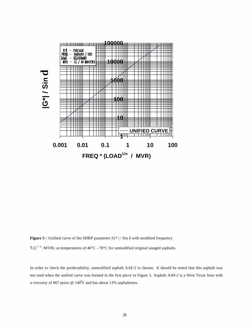
Figure 6 : Comparison of the predicted curve and experimental data for the SHRP parameter |G* | / Sin δ with

frequency T at temperature of 520C for unmodified original unaged asphalt AAF2.

The test temperature is chosen as 52°C. At this temperature, for original unaged AAF-2, the MVR is determined to

be 12.97 cm3/10min at load L=1 kg and the value of n is determined from two other MVR measurements as equal to

0.925. The value of (L 1/n / MVR) is calculated as 0.077. Using this value in Figure 5, the variation of SHRP

parameter is calculated and shown by the solid lines in Figure 6. Actual DSR data are plotted on the same figures

and the match between predicted curve and experimental data is seen to be good.

1

10

100

1000

10000

100000

0.01 0.1 1 10 100 1000

FREQ

|G*|

/ S

in δ

PREDICTEDCURVEEXPERIMENTALDATA

30

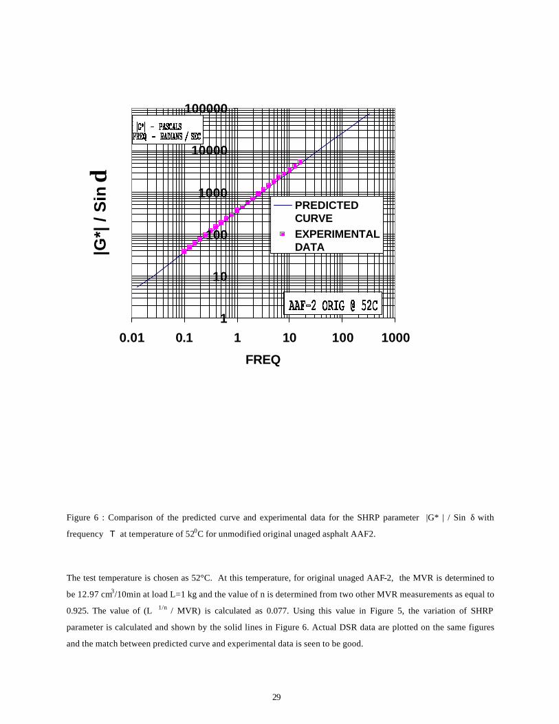
Figure 7 : Comparison of the predicted curve and experimental data for the SHRP parameter

|G* | / Sin δ with frequency T at temperature of 52°C for unmodified PAV aged asphalt AAF2.

A similar exercise is carried out for PAV-aged asphalt AAF-2 at 52°C. The MVR is determined to be 9.58

cm3/10min at load L=10 kg and the value of n is determined as equal to 0.85. The value of (L1/n / MVR) is

calculated as 1.566. Following the same procedure, again it can be seen that the match between predicted curve and

experimental data is excellent in Figure 7.

1

10

100

1000

10000

100000

0.0001 0.01 1 100

FREQ

|G*|

/ S

in δ

PREDICTEDCURVEEXPERIMENTALDATA

31

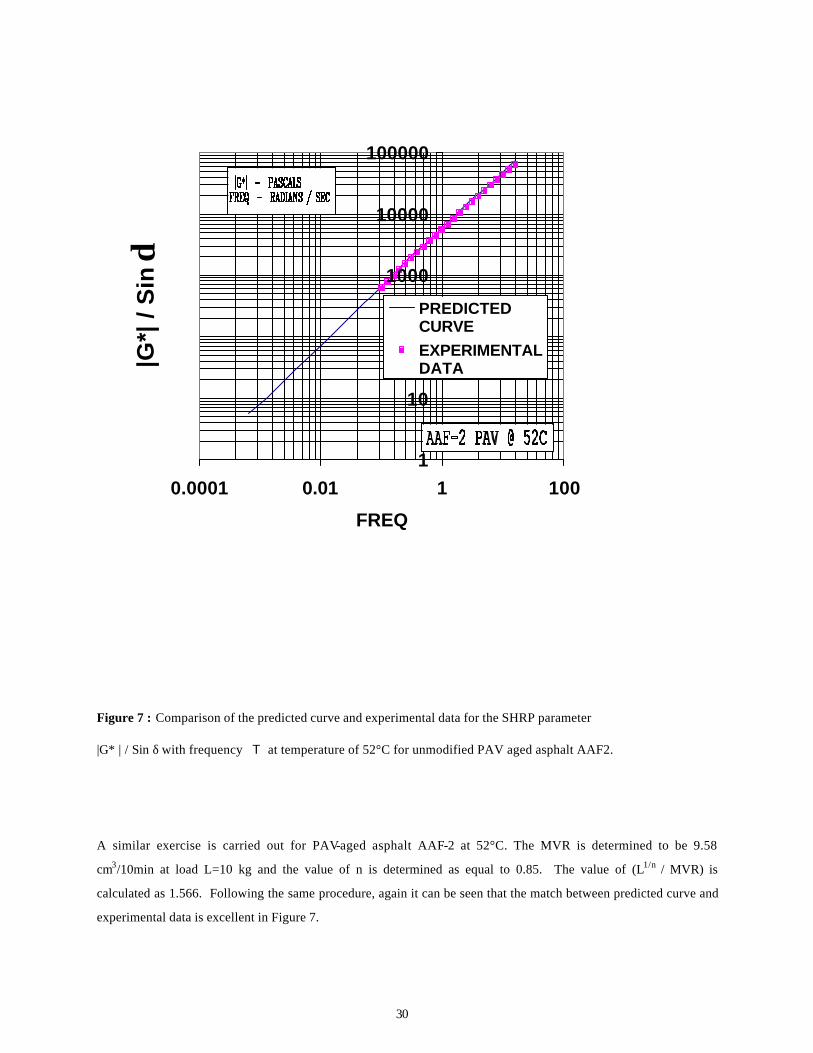
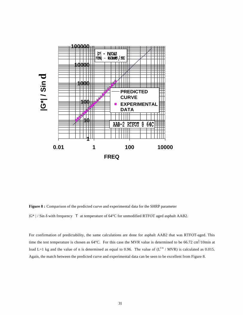
Figure 8 : Comparison of the predicted curve and experimental data for the SHRP parameter

|G* | / Sin δ with frequency T at temperature of 64°C for unmodified RTFOT aged asphalt AAB2.

For confirmation of predictability, the same calculations are done for asphalt AAB2 that was RTFOT-aged. This

time the test temperature is chosen as 64°C. For this case the MVR value is determined to be 66.72 cm3/10min at

load L=1 kg and the value of n is determined as equal to 0.96. The value of (L1/n / MVR) is calculated as 0.015.

Again, the match between the predicted curve and experimental data can be seen to be excellent from Figure 8.

1

10

100

1000

10000

100000

0.01 1 100 10000

FREQ

|G*|

/ S

in δ

PREDICTEDCURVEEXPERIMENTALDATA

32

Concluding Remarks

The unification of fundamental rheological data for unmodified asphalts provides a rather powerful tool to reduce

subsequent experimentation and to ease the generation of rheological information in the future. The FMD that is

used for the generation of MVR data is a relatively simple and inexpensive piece of equipment and can be carried

from place to place because of its relative light weight. It neither needs any arrangements for air pressure nor

requires a circulating water-bath to maintain a constant temperature environment. Since this equipment was

originally built for taking polymer melt data at high temperatures (125°C - 300°C), it has an excellent temperature

control system with variations of about 0.1°C, especially in the temperature range applicable to paving asphalts.

When generating MVR data from the FMD, a few important points should be borne in mind in order to assure

accuracy.

1) The barrel, piston and die of the FMD should be meticulously cleaned before every measurement. Cotton

swabs dipped in mineral spirits can be used for the barrel and the piston for scrubbing out the residual

asphalt. The die can be dropped into a bowl of mineral spirits for about two minutes and then cleaned with

a toothpick dipped in mineral spirits. The cleaning process takes no more than five minutes.

2) When pouring hot asphalt into the barrel, care should be taken to pour in a thin uniform stream so that no

air pockets are formed due to jerky filling. When air gets trapped in asphalt due to faulty pouring, the

asphalt will not flow uniformly out of the die. In fact, an audible sound of a burst bubble will be heard

when there is a discontinuity in the flow. Any reading taken during the time when such a sound is heard

must be discarded, as it is erroneous. Based on the present experimental experience during generation of

MVR data for asphalts considered herein, it can be said that the air entrapment may happen no more than

2% of the time. However, it is worth being aware of this in order to distinguish spurious readings from

good ones.

3) The total time for experiment is quite small. Care should be taken to maintain the MVR value between

proper limits by a judicious choice of the load condition. Note that the testing time for 1.3 < MVR < 50 lies

between 0.08 and 3.3 minutes, which is quite reasonable. It was found that for MVR . 0.2, the testing time

was about 20 minutes and for MVR . 100, it was about 0.045 minutes using a Flag of 6.35 mm. In the

former case, the flow is too slow while in the latter case the flow is too fast. Hence, it is recommended that

the load condition should be chosen in such a way as to get MVR value between 1 and 50 when the Flag of

6.35 mm is used. By opting for a different Flag, these limits can be relaxed to a certain extent (for

example, for MVR . 22 the flow time of about 0.2 minutes with Flag of length 6.35 mm can be increased

to 0.8 minutes by using a Flag of length 25.4 mm).

33

If the above points are borne in mind, it will be found that MVR data generated from the FMD is very highly

reproducible15

. In fact, in terms of repeatability of data, the FMD was found15

to perform better than DSR. There

are a number of other benefits in using the FMD. The evaluation of the benefits of the FMD is to be based on a

number of factors such as initial equipment cost, operational cost, maintenance cost, operator training requirements,

experimental ease, testing time, specimen size, variability of output, data reduction method, information obtained,

and mobility or portability. The FMD beats out DSR on all counts except specimen size and the information

obtained as can be seen from Table 5. While from the DSR, all fundamental rheological parameters can be

obtained, the FMD can only give a single value measurement of MVR at a fixed load condition. However, in the

foregone text, it has been shown how this single value can be correlated with each of the fundamental rheological

parameters from the DSR. This new unification technique thus upgrades the simple flow rate parameter to a level of

high utility. The fact that the FMD is a relatively inexpensive equipment, operational costs are low, MVR data

generation requires minimal training and the output has low level of variability, and the equipment is portable could

merit its use at the paving sites or at the refineries. The actual time for data generation is also very low and this

makes the measurement particularly attractive.

34

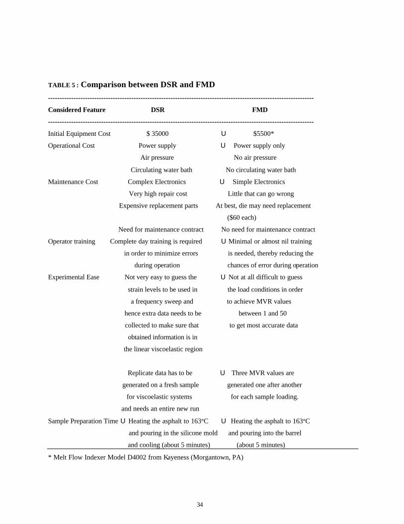
TABLE 5 : Comparison between DSR and FMD

-------------------------------------------------------------------------------------------------------------------

Considered Feature DSR FMD

-------------------------------------------------------------------------------------------------------------------

Initial Equipment Cost $ 35000 U $5500*

Operational Cost Power supply U Power supply only

Air pressure No air pressure

Circulating water bath No circulating water bath

Maintenance Cost Complex Electronics U Simple Electronics

Very high repair cost Little that can go wrong

Expensive replacement parts At best, die may need replacement

($60 each)

Need for maintenance contract No need for maintenance contract

Operator training Complete day training is required U Minimal or almost nil training

in order to minimize errors is needed, thereby reducing the

during operation chances of error during operation

Experimental Ease Not very easy to guess the U Not at all difficult to guess

strain levels to be used in the load conditions in order

a frequency sweep and to achieve MVR values

hence extra data needs to be between 1 and 50

collected to make sure that to get most accurate data

obtained information is in

the linear viscoelastic region

Replicate data has to be U Three MVR values are

generated on a fresh sample generated one after another

for viscoelastic systems for each sample loading.

and needs an entire new run

Sample Preparation Time U Heating the asphalt to 163°C U Heating the asphalt to 163°C

and pouring in the silicone mold and pouring into the barrel

and cooling (about 5 minutes) (about 5 minutes)

* Melt Flow Indexer Model D4002 from Kayeness (Morgantown, PA)

35

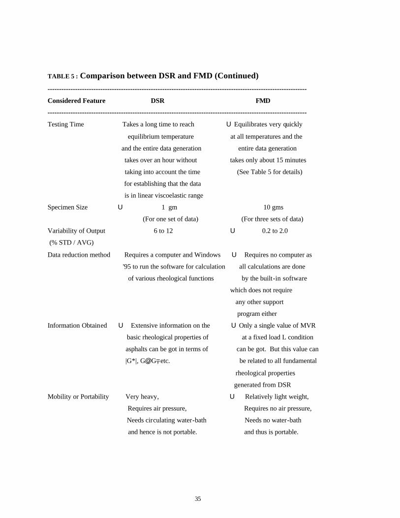
TABLE 5 : Comparison between DSR and FMD (Continued)

-----------------------------------------------------------------------------------------------------------------

Considered Feature DSR FMD

-----------------------------------------------------------------------------------------------------------------

Testing Time Takes a long time to reach U Equilibrates very quickly

equilibrium temperature at all temperatures and the

and the entire data generation entire data generation

takes over an hour without takes only about 15 minutes

taking into account the time (See Table 5 for details)

for establishing that the data

is in linear viscoelastic range

Specimen Size U 1 gm 10 gms

(For one set of data) (For three sets of data)

Variability of Output 6 to 12 U 0.2 to 2.0

(% STD / AVG)

Data reduction method Requires a computer and Windows U Requires no computer as

'95 to run the software for calculation all calculations are done

of various rheological functions by the built-in software

which does not require

any other support

program either

Information Obtained U Extensive information on the U Only a single value of MVR

basic rheological properties of at a fixed load L condition

asphalts can be got in terms of can be got. But this value can

|G*|, G@, G=, etc. be related to all fundamental

rheological properties

generated from DSR

Mobility or Portability Very heavy, U Relatively light weight,

Requires air pressure, Requires no air pressure,

Needs circulating water-bath Needs no water-bath

and hence is not portable. and thus is portable.

36

Acknowlegements

The author is extremely grateful to Ms Susan Needham for diligently generating all the rheological data. The author

would also like to acknowledge the financial support given by the Federal Highway Administration and National

Research Council for this work.

References

1 Van der Poel, C., A general system of describing the viscoelastic properties of bitumens and its relation

to routine test data. J. Appl. Chem. ,1954, 4, 221-236.

2 Griffin, R. L., Miles, T. K., Penther, C. J. and Simpson, W. C., Sliding plate microviscometer for rapid

measurement of asphalt viscosity in absolute units. ASTM Special Tech. Publ. , 1956, 212, 36-50.

3 Wood, P. R. and Miller, H. C., Rheology of bitumens and the parallel plate microviscometer. Highway

Res. Brd. Bull. , 1960, 270, 38-46.

4 Schweyer, H. E. and Buscot, J. C., Experimental studies on the viscosity of asphalt cements at 77 F.

Highway Res. Rec., 1971, 361: 58-70.

5 Heukelom, W., An improved method of characterizing asphaltic bitumens with aid of their mechanical

properties. Proc. AAPT, 1973, 42, 67-98.

6 Schweyer, H. E., Smith, L. L. and Fish, G. W., A constant stress rheometer for asphalt cements. Proc.

AAPT , 1976, 45, 53-72.

7 Nadkarni, V. M., Shenoy, A. V. and Mathew, J., Thermomechanical behavior of modified asphalts.

Ind. Eng. Chem. Prod. Res. Dev. , 1985, 24, 478-484.

8 Goodrich, J. L., Asphalt and polymer modified asphalt properties related to the performance of asphalt

concrete mixes. Proc. AAPT , 1988, 57, 116-175.

37

9 Anderson, D. A., Christensen, D. W., Bahia, H. U., DongrJ, R., Sharma, M. G., Antle, C. E. and

Button, J., Binder characterization and evaluation, Vol. 3 : Physical Characterization. Strategic Highway

Research Program, National Research Council, Washington D. C.(SHRP-A-369 Report),1994.

10 Hanson, D. I., Mallick, R. B. and Foo, K., Strategic Highway Research Program : Properties of

asphalt cement. Trans. Res. Record , 1995, 1488, 40-51.

11 Shashidhar, N., Needham, S. P. and Chollar, B. H., Rheological properties of chemically modified

asphalts. Trans. Res. Record , 1995, 1488, 89-95.

12 Stroup-Gardiner, M. and Newcomb, D., Evaluation of rheological measurements for unmodified and

modified asphalt cements. Trans. Res. Record , 1995, 1488, 72-81.

13 Dongré, R., Youtcheff, J. and Anderson, D., Better roads through rheology. Applied Rheology(Trade

Magazine, Verlag, Hannover, Germany),1996.

14 Shenoy, A., Developing unified rheological curves for polymer-modified asphalts - I. Theoretical

analysis and II. Experimental verification. Materials and Structures, 2000, 33 (231), 425-437.

15 Shenoy, A., Unifying asphalt rheological data using the material’s volumetric -flow rate, J. Materials

in Civil Engg., 2001, 13 (4), 260-273.

16 Shenoy, A. V. and Saini, D. R., Thermoplastic Melt Rheology and Processing. Marcel Dekker Inc.,

New York, 1996.

17 Pao, Y.-H., Hydrodynamic theory for the flow of a viscoelastic fluid. J. Appl. Phys., 1957, 28, 591-

598.

18 Cox, W. P. and Mertz, E. H., Correlation of dynamic and steady flow viscosities. J. Polym. Sci.,1958,

28, 619-621.

38

19 Pao, Y.-H., Theories for the flow of dilute solutions of polymer and of non-diluted liquid polymers. J.

Polymer Sci.,1962, 61, 413-448.

20 Spriggs, T. W., A four constant model for viscoelastic fluids. Chem. Engg. Sci., 1965, 20, 931-946.

21 Bogue, D. C., An explicit constitutive equation based on integrated strain history. Ind. Eng. Chem.

Fundamentals,1966, 5, 253-259.

22 Meister, B. J., An integral constitutive equation based on molecular network theory. Trans. Soc.

Rheol, 1971, 15, 63-89.

23 Saini, D. R. and Shenoy, A. V., Dynamic and steady-state rheological properties of linear-low-

density polyethylene melt. Polym. Engg. Sci., 1984, 24, 1215-1218.

24 De Waele, A., Viscometry and plastometry. J. Oil Color Chem. Assoc., 1923, 6, 33-69.

25 Ostwald, W., Ueber die geschwindigkeitsfunktion der viskositat disperser systeme I. Kolloid-Z, 1925,

36, 99-117.

26 Ostwald, W., Ueber die viskositat kolloider hosungen in struktur-laminar und turbulezgebeit.

Kolloid-Z., 1926, 38, 261-280.

27 AASHTO, Standard test method for determining the rheological properties of asphalt binder using a

Dynamic Shear Rheometer (DSR). AASHTO Provisonal Standard TP5(Edition 1A): Washington D. C.,

1993.

28 AASHTO, Standard practice for accelerated aging of asphalt binder using a pressurized aging vessel

(PAV). AASHTO Provisional Standard PPI(Edition 1A): Washington D. C., 1993.