Quantum State Purification

by

Honghao Fu

A thesispresented to the University of Waterloo

in fulfillment of thethesis requirement for the degree of

Master of Mathematicsin

Computer Science, Quantum Information Option

Waterloo, Ontario, Canada, 2016

c© Honghao Fu 2016

CORE Metadata, citation and similar papers at core.ac.uk

Provided by University of Waterloo's Institutional Repository

I hereby declare that I am the sole author of this thesis. This is a true copy of the thesis,including any required final revisions, as accepted by my examiners.

I understand that my thesis may be made electronically available to the public.

ii

Statement of Contributions

This project started in the summer of 2014 when Andrew Childs and his intern VedangVyas became interested in Simon’s problem with a faulty oracle. During their research,they developed the idea of using the swap-test in purification procedures and proved thatthe sample complexity of such procedure is of oder O(poly(1

ε)). This is the foundation

for the new analysis of the swap-test procedure by me and my advisors and it provides atighter upper bound on its sample complexity.

Later, when we moved on to study the optimal purification procedure, Aram Harrowprovided us with the idea to formulate the purification problem as an optimization problemusing the symmetries of the Choi matrices. Based on his idea, Maris Ozols derived andproved the constraints in this optimization problem. Section 4.2 is based on Aram’s ideaand Maris’ work. I solved the purification problem for qubit and qutrit and analyzed theoptimal fidelity in these two cases with help from my advisors.

Beyond the specific technical contributions, my advisors Andrew Childs and DebbieLeung provided countless new ideas and insight that made this thesis possible.

iii

Abstract

Quantum state purification is a process in which decoherence is partially reversed byusing multiple copies of the input states that have been subject to the same decoherenceeffect. This thesis focuses on purifying the decoherence caused by the depolarizing channel.In the first half of the thesis, the purification problem is formally introduced and oneefficient purification procedure featuring the swap-test is presented and analyzed. The restof the thesis formulates the optimal purification problem as an optimization problem andapplies it to qubit and qutrit purification.

The first half (Chapter 1 and 2) is devoted to the study of a practical quantum purifica-tion procedure based on the swap-test. Before the procedure is introduced, the purificationproblem is formulated and parameterized in Chapter 1. The procedure and the analysisof its sample complexity are presented in Chapter 2. Chapter 2 ends by applying thisprocedure to the Simon’s problem with a faulty oracle.

The second half of this thesis (Chapter 3 to 5) is built on the Schur-Weyl dualitywhich is the decomposition of space (Cd)⊗N into carrier spaces of symmetric group Snand unitary group U(d) irreducible representations. Necessary background informationon it and Schur-Weyl duality itself are introduced in Chapter 3. Chapter 4 focuses oneach irreducible representation of U(d) and formulates the purification of the state onthis subspace as an optimization problem over all the covariant quantum channels. Theconstraints implied by the covariance condition and quantum channel properties are derivedto make the optimization complete and solvable. In Chapter 5, the method to solve thisoptimization problem for qubit and qutrit is presented and the implications of the resultare also discussed.

iv

Acknowledgements

I first want to thank Andrew Childs and Debbie Leung for their help and guidancethroughout my master’s program. Without them, little of the work I have done in the lasttwo years would have been possible.

I am also indebted to Maris Ozols who joined this project despite his busy work scheduleand made consistent contributions to it which included formal derivation of the constraintsof the optimization problem and exploration of the general d-dimensional case. Thanks toAram Harrow who met with Maris and told us the way to formulate the optimal purificationproblem as an optimization problem when we lost our research direction. I am grateful toVedang Vyas whose initial work on this project in summer 2014 laid the foundation of allthe future work.

I also want to thank Zhengfeng Ji, Nengkun Yu and Mo Zhou for inspiring and fruitfuldiscussions about this project.

v

Dedication

This thesis is dedicated to my parents and my teachers.

vi

Table of Contents

List of Figures ix

1 Introduction 1

1.1 Motivation and previous work . . . . . . . . . . . . . . . . . . . . . . . . . 1

1.2 Problem setup . . . . . . . . . . . . . . . . . . . . . . . . . . . . . . . . . . 2

1.3 Summary of results . . . . . . . . . . . . . . . . . . . . . . . . . . . . . . . 3

2 Purification based on the swap-test 4

2.1 The swap-test . . . . . . . . . . . . . . . . . . . . . . . . . . . . . . . . . . 4

2.2 Steps of the procedure . . . . . . . . . . . . . . . . . . . . . . . . . . . . . 6

2.3 Expected cost . . . . . . . . . . . . . . . . . . . . . . . . . . . . . . . . . . 7

2.4 Application: Simon’s problem with a faulty oracle . . . . . . . . . . . . . . 12

3 Representation theory and Schur-Weyl duality 14

3.1 Related concepts of representation theory . . . . . . . . . . . . . . . . . . . 15

3.2 Schur-Weyl duality . . . . . . . . . . . . . . . . . . . . . . . . . . . . . . . 16

3.3 Young diagram and Schur basis . . . . . . . . . . . . . . . . . . . . . . . . 18

4 Optimal purification procedure 22

4.1 Optimal qubit procedure . . . . . . . . . . . . . . . . . . . . . . . . . . . . 22

4.1.1 Optimality proof . . . . . . . . . . . . . . . . . . . . . . . . . . . . 24

vii

4.1.2 Analysis of average fidelity F(2)N . . . . . . . . . . . . . . . . . . . . 30

4.1.3 Lower bound on sample complexity of purifying higher-dimensionalstates . . . . . . . . . . . . . . . . . . . . . . . . . . . . . . . . . . 35

4.2 Generalization to qudit . . . . . . . . . . . . . . . . . . . . . . . . . . . . . 37

4.2.1 Dual representation and covariance condition . . . . . . . . . . . . 38

4.2.2 Clebsch-Gordan transform and the first constraint on J(Ψ) . . . . . 39

4.2.3 The trace-preserving condition . . . . . . . . . . . . . . . . . . . . . 40

4.2.4 Gel’fand-Tsetlin basis and the objective value . . . . . . . . . . . . 41

4.2.5 Putting together the optimization problem . . . . . . . . . . . . . . 46

5 Optimal purification of qubit and qutrit 48

5.1 Qubit case revisited . . . . . . . . . . . . . . . . . . . . . . . . . . . . . . . 48

5.2 Qutrit case . . . . . . . . . . . . . . . . . . . . . . . . . . . . . . . . . . . 51

5.2.1 Optimal fidelity achievable on unitary group irrep Q3λ . . . . . . . . 52

5.2.2 Formula of average fidelity F(3)N . . . . . . . . . . . . . . . . . . . . 57

5.2.3 Preliminaries of the analysis of F(3)N . . . . . . . . . . . . . . . . . . 58

5.2.4 Analysis of the dominant part of F(3)N . . . . . . . . . . . . . . . . . 62

5.2.5 Analysis of the minor part of F(3)N . . . . . . . . . . . . . . . . . . . 67

References 69

viii

List of Figures

2.1 The swap-test used in our procedure . . . . . . . . . . . . . . . . . . . . . 4

3.1 Young tableau corresponding to L(1)(3,1) . . . . . . . . . . . . . . . . . . . . . 18

3.2 standard Young tableau of shape (4, 2, 1) . . . . . . . . . . . . . . . . . . . 19

3.3 semi-standard Young tableau of shape (4, 2, 1) . . . . . . . . . . . . . . . . 19

ix

Chapter 1

Introduction

1.1 Motivation and previous work

Since the discovery of Shor’s Factoring algorithm[20], we have seen increasingly many newquantum algorithms. In theory, we could assume the implementations of the algorithmsare perfect. However, in reality, decoherence from thermal noise or interaction with furtherdegrees of freedom could make each step of the quantum algorithms prone to errors. There-fore, one important task is to make sure quantum algorithm implementations still workideally under the influence of decoherence. One approach is to make the implementationsrobust and resistant to decoherence. Another approach is to reverse the effect of decoher-ence on the quantum states produced by such implementations. This thesis is devoted tostudying the second approach.

Decoherence has the effect to produce mixed states out of pure states. Thus one of ourgoals is to partially reverse the effect of decoherence and produce purer states out of mixedones. It is impossible to achieve such goal with a single copy of the noisy state as boththe original state and the type of decoherence are unknown. However, with the presenceof multiple copies of the same noisy state, which are produced from the same pure stateand subject to the same decoherence process, it is possible to reconstruct a state that isclose to the original state by analyzing the properties of the combined states. As we willsee in this thesis, the quality of the state we reconstructed gets higher if we are providedwith more copies of the noisy state. In the extreme case of analyzing infinite copies of thenoise state, we will be able to reconstruct the original state perfectly.

This question was first studied by Cirac, Ekert and Macchiavello [9]. They were inspiredby the studies of entanglement purification [5] and studied the problem of purifying depo-

1

larized qubit and proved the purification procedure proposed in their publication achieveshighest output fidelity. They also noticed the connection between the purification proce-dure and the quantum cloner for a certain type of cloning problem. Later, Keyl and Wernersummarized the work by Cirac et al. and studied the purification problem for qubit underdifferent criteria [15]. The criteria range from requiring one output state or multiple out-put states to measuring the fidelity by picking one output state or selecting all the outputstates. They also found out that the optimal purification procedure is the same as thecloning procedure proposed in [13]. However, the questions that whether such procedureis generalizable to the higher-dimensional case and whether the generalized procedure isoptimal remain open. Later in this thesis, we will see that such procedure is not likely tobe optimal for higher-dimensional quantum states and we will propose a way to study theoptimal purification procedure for higher-dimensional states.

One drawback of [9] is that the calculations and proofs were only outlined. Since theirprocedure is the starting point of our study, we will give detailed calculation and proofin Chapter 4. In the next section, we will formally state the problem and give necessaryparameterization.

1.2 Problem setup

In the general purification problem, we are given multiple copies of the initial d-dimensionalnoisy state which is of the following form:

ρ0 = (1− e0) |ψ〉 〈ψ|+ e0

dI, e0 ∈ (0, 1). (1.1)

We add the subscript 0 to stress the fact that no purification has been performed. Thesymbol e0 represents the probability that the state is disturbed and it is called the errorparameter. Since it also represents a level of error in the state, we use letter e to save letterp for other purpose. The constraint on e0 is that it cannot be too close to 1.

When we study the optimal purification procedure, we will make use of the eigenvaluesof ρ0. We will label the target state |ψ〉 by |d〉 and the other eigenstates will be denotedby |1〉 , . . . , |d− 1〉. The corresponding eigenvalues are

αd = 1− d− 1

de0 and

α1 = · · · = αd−1 =e0

d.

2

Let P denote a purification procedure which consists of a set of operations and measure-ments on the N qudits and perhaps on additional ancillas. After performing purificationprocedure P , we calculate the fidelity by the following formula:

f = 〈ψ| P(ρ⊗N0 ) |ψ〉 . (1.2)

We are interested in the number of initial states required when the final fidelity is at least1− ε for a given ε.

As the purification problem is introduced, we will outline the structure of this thesis inthe next section.

1.3 Summary of results

This thesis is divided into two halves: Chapter 2 discusses a practical purification procedurebased on the swap-test and Chapter 3 to 5 present a formulation of optimal purificationprocedure for general d-dimensional quantum states (or qudits).

Chapter 2 introduces a practical quantum state purification procedure for qudits. More-over, an upper bound on the number of initial noisy states is derived to show thatthe procedure is efficient.

Chapter 3 introduces the necessary background of representation theory of unitary groupand symmetric group that leads to the Schur-Weyl duality. The Schur-Weyl dualitywill help us understand the properties of combining identical quantum states.

Chapter 4 reduces the problem of finding the optimal fidelity to an optimization problemover quantum channels. We will review the known optimal qubit procedure first andprovide a detailed optimality proof. Then we will re-frame the purification problemfor general qudits. The complete set of constraints will be derived. It turns out thatthe problem is a linear programming problem. As we derive the constraints, we willintroduce Gel’fand-Tsetlin patterns and Clebsch-Gordan coefficients.

Chapter 5 applies the new formulation to the qubit and qutrit case. The known optimalfidelity of qubit procedure will be reproduced as the solution to the optimizationproblem developed in Chapter 4. Then we will give the expression for the optimalfidelity for qutrit purification. Based on this fidelity, we will derive a lower bound onthe number of input states needed for purification.

3

Chapter 2

Purification based on the swap-test

This chapter will focus on a purification procedure based on the swap-test [8]. We willintroduce basic properties of the pairwise swap-test [6] in the first section. In the followingsections, we will list and explain the steps of the procedure and give an upper bound onthe number of input states. In the last section, we will discuss one application of thisprocedure which is Simon’s problem [21] with a faulty oracle. Based on this procedure,we can solve the noisy version of Simon’s problem with quadratic query complexity andpolynomial time complexity.

2.1 The swap-test

The swap-test we used is depicted in the following figure where the input states are twocopies of the noisy state ρ0 = (1− e0) |ψ〉 〈ψ|+ e0

dI and an ancilla state |0〉.

|0〉 H H

ρ0

ρ0

Post-selection of |0〉

Figure 2.1: The swap-test used in our procedure

In the end, we will measure the first register. If we measure 0, we will only keep the

4

second register as the output state. Otherwise, we will declare failure and discard both thesecond and third registers.

This circuit will work as follows:

1. After the first Hadamard gate, the state becomes

1

2(|0〉+ |1〉)(〈0|+ 〈1|)⊗ ρ0 ⊗ ρ0. (2.1)

Note that for a state ρ0 = (1−e0) |ψ〉 〈ψ|+ e0dI, we can extend |ψ〉 to an orthonormal

basis |v1〉 , . . . , |vd〉 of the d-dimensional space such that |v1〉 = |ψ〉. Hence ρ0 canbe written as

ρ0 = (1− d− 1

de0) |v1〉 〈v1|+

d∑i=2

e0

d|vi〉 〈vi| . (2.2)

Let λ1 = (1− d−1de), λ2 = e

dand |Ψ+〉 = 1√

2(|0〉+ |1〉). We could view the input as a

probability distribution:

• with probability λ21, we have input state |Ψ+〉 |v1〉 |v1〉;

• with probability λ1λ2, we have input state of the form |Ψ+〉 |v1〉 |vi〉 or |Ψ+〉 |vi〉 |v1〉for some i ∈ 2, 3, . . . , d;• with probability λ2

2, we have input state of the form |Ψ+〉 |vi〉 |vj〉 for somei, j ∈ 2, 3, . . . , d.

2. After the controlled-swap gate denoted by Uc−swap we have the following states:

Uc−swap |Ψ+〉 |vi〉 |vi〉 = |Ψ+〉 |vi〉 |vi〉 and ,

Uc−swap |Ψ+〉 |vi〉 |vj〉 =1√2

(|Ψ+〉

|vi〉 |vj〉+ |vj〉 |vi〉√2

+ |Ψ−〉|vi〉 |vj〉 − |vj〉 |vi〉√

2

)for i 6= j

3. After the last Hadamard gate, we have the following states:

(H ⊗ I ⊗ I) |Ψ+〉 |vi〉 |vi〉 = |0〉 |vi〉 |vi〉 ,

(H ⊗ I ⊗ I)1√2

(|Ψ+〉

|vi〉 |vj〉+ |vj〉 |vi〉√2

+ |Ψ−〉|vi〉 |vj〉 − |vj〉 |vi〉√

2

),

=1√2

(|0〉 |vi〉 |vj〉+ |vj〉 |vi〉√

2+ |1〉 |vi〉 |vj〉 − |vj〉 |vi〉√

2

)for i 6= j.

5

For each possible input state, we could calculate the probability to measure state |0〉 inthe first register and the state after the selection. Combining the results, we have that theprobability to measure |0〉 or the success probability ps is

ps = 1− d− 1

de0 +

d− 1

2de2

0. (2.3)

The output state will be of the form

ρ1 = (1− e1) |ψ〉 〈ψ|+ e1

dI (2.4)

with new error parameter

e1ps =e0

2+e2

0

2d. (2.5)

2.2 Steps of the procedure

Our procedure involves recursively applying the prescribed swap-test, hence, we will denoteit by Pswap.

The procedure starts with preparing many copies of initial states, ρ0, and applying thepre-described swap-test to them pairwise. When the swap-test succeeds, we collect all thecopies of the output stateρ1 for the next step of the procedure. The failed swap-test willbe rejected until we have more than two copies of ρ1.

After we have collected two copies of ρ1, we will apply the swap-test to get state ρ2.From Equation (2.5), the fidelity of ρ2 can be determined. If it is above 1 − ε, then it isthe output state of the procedure, otherwise, we proceed.

We could view the procedure as a binary tree where initial states ρ0’s are the leavesand other output states are the internal nodes. At the i-th level starting at the botttom,we will have state ρi. The subscript i is denoting the steps of the procedure. Here ρi is ofthe form:

ρi = (1− ei) |v1〉 〈v1|+ eiI

d, (2.6)

where ei is defined recursively by

eipi =ei−1

2+e2i−1

2d, (2.7)

6

and pi is the success probability of step i which also depends on the error parameter ei−1

by the formula:

pi = 1− d− 1

dei−1 +

d− 1

2de2i−1. (2.8)

The choice of proceeding or stop is still depended on the fidelity of ρi.

It is always possible that at some step the swap-test will fail and in that case, theprocedure will restart and consume more of ρ0. This procedure will always produce onefinal state ρn which can meet the fidelity criterion. We could see that this procedure is oneof the Las Vegas algorithms which could be converted to one of the Monte Carlo algorithmsby running the procedure multiple times and each time supplying the procedure with theexpected number of copies.

In the next section, we will analyze how many copies of the initial state are expectedto produce the final state ρn.

2.3 Expected cost

Let C(P ) denote the cost of procedure P . Our result is the following theorem.

Theorem 2.3.1 For Pswap, if the final fidelity is at least 1− ε, then the expected cost is oforder O(1

ε).

First of all, we need to get an expression of the expected cost which will be presentedin the following lemma.

Lemma 2.3.2 Assuming the whole process takes l steps, the expected cost of Pswap is

E(C(Pswap)) =2l∏li=1 pi

(2.9)

Proof To prove the lemma, we will use induction starting at the end of the procedure.

If we look at the expected cost of the last step of the procedure, the last step cansucceed with probability pl, then in expectation, we need to run it 1/pl times to succeed.Since each time we run the test, the cost is two states, the expected cost is 2/pl.

7

Assume in expectation, the last i steps cost 2i∏lj=l−i+1 pj

states. For each of state served

as input state to the last i steps, the expected cost is 2pl−i

. Hence, the expected cost of the

last i+ 1 steps is

2i∏lj=l−i+1 pj

× 2

pl−i=

2i+1∏lj=l−i pj

Hence, by the principle of inductive proof, the expected cost of all the l steps is as inEquation (2.9).

Since the whole process can be described by two sequences e0, e1, . . . , el andp1, p2, . . . , pl, we will state some properties of Pswap derived from these two sequences.The first property is the following lemma.

Lemma 2.3.3 For Pswap, purification of larger-dimensional dimensional quantum statescosts more initial states.

Proof We could rewrite pi as

pi = 1− ei−1 +e2i−1

2+

1

dei−1(1− ei−1

2).

For fixed ei−1, pi decreases as d increases which means that each step will be less likely tosucceed for higher dimension.

For ei, we view it as a function with variables ei−1 and d. Even though ei only takes ondiscrete values of d but we will see it is monotonic by taking partial derivative against d,

∂ei∂d

=∂

∂d

(ei−1

2+

e2i−1

2d

1− d−1dei−1 + d−1

2de2i−1

)

=e3i−1(1− ei−1)

2d2(1− d−1dei−1 + d−1

2de2i−1)2

> 0.

The interpretation is that for a given step, output error parameter will grow as d increasesbut we want the state after each step to have error parameter as small as possible.

Larger error parameter implies that the next step will be harder to succeed and thewhole process will possibly be longer. Hence, this two observation combined show thatstate in larger dimension is harder to purify.

8

Based on Lemma (2.3.3), we can prove the following lemma

Lemma 2.3.4 For Pswap, if the final output state has fidelity 1 − ε, then the number ofsteps of the procedure in expectation is of order O(log(1

ε)).

Proof By Lemma (2.3.3), we only need to consider the case that d is infinite to derive theupper bound of the number of steps, n.

If we take d to be inifinite, the parameters are

e′i = limd→+∞

ei =e′i−1

2− 2e′i−1 + e′2i−1

, (2.10)

p′i = limd→+∞

pi = 1− e′i−1 +e′2i−1

2. (2.11)

However, the sequence e′i is not easy to analyze directly, so we upper bound it by anew sequence e′′i which is defined by

e′′0 = e′0 = e0 and (2.12)

e′′i+1 =e′′i

2− 2e′′i. (2.13)

The first property of e′′i to show is that e′′i > ei for all i > 0.

In the base case,

e′′1 =e′′0

2− e′′0>

e′′02− 2e′′0 + e′′20

= e′1 > e1.

Assuming it is true for all i up to n. Then we can think of e′′i as a function of e′′i−1 andnotice that

de′′n+1

de′′n=

1

2(1− e′′n)2> 0.

Therefore, we could replace e′′n in the expression of e′′n+1 by e′n which is known to be smallerand get a lower bound of e′′n+1

e′′n+1 =e′′n

2− 2e′′n>

e′n2− 2e′n

> e′n+1 > en+1.

9

By the principle of induction, we know e′′n > en for all n > 0.

The reason to choose sequence e′′i is that we can give closed form expression for thissequence. Since

1

e′′n+1

=2

e′′n− 2,

the closed form expression is

1

e′′n= 2n(

1

e0

− 2) + 2.

Now we can use e′′n to derive a upper bound on the number of steps. If we set e′′m = ε,then em < ε. This m would be an upper bound on the number of steps. The conditione′′m = ε implies that

m = log(e0

ε− 2e0)− log(1− 2e0),

which will be an upper bound of the real number of steps, n. Hence, the number of stepsis of order O(log(1

ε)).

Remark The proof above only holds for e0 <12.

To have a complete proof of Theorem (2.3.1), we need to show another property of thesequence e′i.

Proposition 2.3.5

e′n ≤e0

(2− 2e0 + e20)n

. (2.14)

Proof This proof will be inductive as well.

The base case is that e′1 = e0(2−2e0+e20)

.

Assume the proposition is true for all the i up to n, then consider i = n+ 1,

e′n+1 =e′n

(2− 2e′n + e′2n )

≤ e0

(2− 2e0 + e20)n

1

2− 2e′n + e′2n

≤ e0

(2− 2e0 + e20)n+1

.

10

In the first inequality, we applied the induction hypothesis on e′n.

Note that function f(x) = 2− 2x+ x2 decreases on the interval (0, 1), so in the secondinequality we used the fact e′n < e0 and the monotonicity of f(x) on interval (0, 1) to get

12−2e′n+e′2n

≤ 1(2−2e0+e20)

.

By the principle of induction proof, we have completed the proof.

Remark Proposition (2.3.5) can also be used to prove the number of steps is of orderO(log(1

ε)).

Now we can prove the main theorem of this section

Proof of Theorem (2.3.1) By Lemma (2.3.2) we know that the expected cost can bebounded by analyze its numerator and denominator separately.

By Lemma (2.3.4), we can bound the numerator part by

2l ≤ 2log(e0ε−2e0)−log(1−2e0) =

1

ε

e0 − 2e0ε

1− 2e0

. (2.15)

Then we need a lower bound of the denominator. Following Proposition (2.3.5), we canderive a lower bound on p′i+1 first

p′i+1 =1− e′i +e′2i2

>1− e′i≥1− e0

(2− 2e0 + e20)i.

Hence, the denominator can be rewritten as

n∏i=1

p′i >n−1∏i=0

(1− e0

(2− 2e0 + e20)i

)

>

∞∏i=0

(1− e0

(2− 2e0 + e20)i

)

=(e0; e0

(2−2e0+e20))∞

1− e0

.

11

where (a; q)∞ is the q-Pochhammer symbol which is defined as

(a; q)∞ =∞∏j=0

(1− aqj). (2.16)

When 11−e0 ∈ O(1), the q-Pochhammer symbol (e0; e0

(2−2e0+e20))∞ is also of order O(1).

Combining all the results we have derived so far, we have

E(C) ≤ 1

ε

1− e0

(e0; 1/(2− 2e0 + e20))∞

e0 − 2e0ε

1− 2e0

∈ O(1

ε). (2.17)

Since this upper bound is derived for the infinite dimension case which is the hardest, theupper bound applies to all possible dimensions.

2.4 Application: Simon’s problem with a faulty oracle

Quantum purification procedures and especially Pswap can be applied to improve accuracyof quantum algorithms querying faulty oracles, for example, Simon’s problem [21]. In thissection, we will introduce Simon’s problem with a faulty oracle and show how Pswap solvesit.

In Simon’s problem [21], we are given a function f : 0, 1n → 0, 1n implemented asa black-box oracle Uf such that for a given input state |x〉 and ancilla state |y〉, Uf |x〉 |y〉 =|x〉 |y ⊕ f(x)〉. It has a special property that there exists a hidden string s ∈ 0, 1n suchthat f(x) = f(y) if and only if x = y or x⊕ y = s. The goal is to find s.

In the ideal case, we will solve this problem by preparing initial state∑2n−1

x=0 |x〉 |0〉, andthen querying the oracle with the initial state followed by the Hadamard transform. In theend, when we measure the first register, we will get some y ∈ 0, 1n such that y · s = 0.By repeating such steps O(n) times, we could determine the special string s.

What if the oracle only works with a certain probability and depolarize the input stateotherwise? That is, we have a quantum channel

Dp(ρ) = (1− p)UfρU †f + pI

22n(2.18)

where p ∈ (0, 1) represents the probability that oracle will depolarize the input state. Inthis case, If we follow the algorithm above, we will get a state of the form:

ρ = (1− p) |Ψ〉 〈Ψ|+ pI

22n(2.19)

12

where

|Ψ〉 =1√

2n(n− 1)

2n∑x=0

∑y·s=0

|y〉 |f(x)〉 . (2.20)

If we measure the first register of ρ, with probability (1 − p) we could get y satisfyingy · s = 0 but with probability p, we will get a random string z. Then determining thequantum query complexity is a difficult ”learning with error” problem [18]. It could besolved with O(n) equations, hence O(n) queries, by the maximum likelihood algorithm butthe drawback is that the time complexity will be exponentially large [19] which made usthink whether it is possible to achieve polynomial gate complexity as well.

The other strategy would be to perform quantum state purification to the outputstate before measuring the first register so that the error probability can be as smallas possible. We will see this strategy will achieve both polynomial query complexity andgate complexity.

If we collect M copies of ρ and apply Pswap on them, the procedure Pswap will produceone output state ρ′ = (1 − ε) |Ψ〉 〈Ψ| + ε I

22n. At this point, we could measure the first

register and with probability at least (1− ε) we will have a string y satisfying the conditiony · s = 0. Then we could repeat such process, to get more strings perpendicular to strings.

To make sure the error is within a certain threshold c, we will choose ε = cn. By the

subadditivity of error, which is discussed in Chapter 4 of [16], it suffices to pick such ε.By Theorem (2.3.1), we know that M ∈ O(1

ε) = O(n). Since we will need O(n) unique

strings perpendicular to s, we need to repeat such process O(n) times. Overall, the gatecomplexity and query complexity will be O(n2).

This is just one application of Pswap. It can also be applied to quantum algorithmsinvolving parallel queries or sequential queries of length O(1) to some faulty oracle. How-ever, applying Pswap to algorithm with longer sequential queries to the oracle will result invery large query and sample complexity. Hence, more sophisticated procedure should bedesigned to control the noise in the sequential algorithms, if possible.

13

Chapter 3

Representation theory andSchur-Weyl duality

This chapter will introduce necessary representation theory background which will leadto Schur-Wely duality and Schur-Weyl duality is the foundation of studying the optimalpurification procedure.

Generally speaking, representation theory is the study of mapping group members tomatrices so that the group properties are preserved. Representation theory consists ofmany topics and the topic we are interested in is Schur-Weyl duality. It is about how todecompose vector space (Cd)⊗n into irreducible representation of symmetric group Sn andunitary group U(d). The corresponding transformation is called Schur transform.

Schur-Weyl duality is widely used in quantum information research and I noticed manyapplications of Schur-Weyl duality during my research. It can be applied to the studyof symmetric properties of tensor product of multiple identical quantum states by Alicki,Rudnicki and Sadowski [2]. In that publication [2], Alicki and his colleagues calculatedthe probability distribution over subspaces in the Schur decomposition of (Cd)⊗n and gavemathematical description of the shape of this distribution. Later, this technique was ap-plied to the study of optimal qubit purification ([9] and [15]), optimal cloning [13] andestimation of the spectrum of a density operator [14]. In recent years, Haah, Harrow,Ji, Wu and Yu applied it to quantum tomography [12]. Besides application in quantuminformation research, it can also be applied to quantum computation research. In 2005,an efficient quantum circuit for implementing Quantum Schur transform was invented [4].The Schur transform is also known as Schur sampling which was applied to the study ofthe Hidden subgroup problem (HSP) [3] to get better understanding of the general HSP

14

[7].

This chapter is organized as follows. We will first review many important concepts ofrepresentation theory which will lead to the introduction of Schur-Weyl duality. Then inthe last section, we will examine the concept and properties of Schur transform. Moredetailed explanation and proof can be found in [10].

3.1 Related concepts of representation theory

In this section we will give formal definitions of several representation theory conceptswhich will be used in the rest of the thesis.

Representation: A representation RRR of a group G on a vector space V associates witheach element g ∈ G a linear map:

RRR(g) : V → V : v → RRR(g)v

such that

RRR(gh) = RRR(g)RRR(h) ∀g, h ∈ G ,

RRR(e) = I

where e is the identity element of the group G and I is the identity map on V . V is calledthe carrier space of the representation RRR. The set of all the linear maps from V to itself isdefined as End(V ) and such linear maps are called endomorphisms. Thus a representationis a map from G to End(V ) satisfying aforementioned properties. If RRR(g) is unitary forall group members g, then RRR is a unitary representation. Moreover, if the vector space Vassociated with representation RRR is finite-dimensional, then we say the representation RRR isfinite-dimensional. In this thesis, we will focus on finite-dimensional unitary representationover complex numbers. The reason is that a d-dimensional quantum system correspondsto a unit vector in a d-dimensional carrier space.

The convention that we will follow is that bold letter is used for the representation, forexample,RRR. Normal capital letter is for the carrier space of the representation, for example,V . To refer to a particular representation, it is necessary to give both the mapping andthe carrier space so the notion will be (RRR, V ). When the carrier space is clear from thecontext, we may omit the carrier space and only keep the mapping for convenience.

Irreducible Representation: For every representation (RRR, V ), there exist a subspace Wof its carrier space V such that for all w ∈ W and all g ∈ G, RRR(g)w ∈ W . This subspace

15

is called an invariant subspace. A representation rrr is an irreducible representation, or anirrep, if the only invariant subspaces of it are its carrier space and 0. The convention wefollow is that bold lower-case letter denotes the mapping of an irrep.

In this thesis, we are particularly interested in the irreps of the symmetric group andunitary group. Symmetric group Sn is the group of all the permutations of n distinctobjects. Unitary group U(d) is the group of all d× d unitary matrices.

A finite-dimensional unitary representation over complex number can be decomposedinto a direct sum of irreps. Thus, for any g ∈ G, we could find a change of basis such thatRRR(g) is block-diagonal and each block on the diagonal corresponds to an operator over anirrep. This will lead to the next concept.

Isotypic decomposition: Let G denote the set of irreps of G. Then for a reduciblefinite-dimensional representation RRR, there exist a change of basis such that

RRR(g) ∼=⊕rrr∈G

rrr(v)⊗ Inrrr (3.1)

where rrr is an irrep of RRR; nrrr is the multiplicity of the irrep rrr in the decomposition and∼= is denoting the matrix similarity. Following this decomposition, we can decompose thecarrier space V of RRR in the similar way:

V ∼=⊕rrr∈G

Vrrr ⊗ Cnrrr . (3.2)

Such decomposition is called the isotypic decomposition.

3.2 Schur-Weyl duality

The two groups with particular interest for us are the symmetric group, Sn and unitarygroup, U(d). The two groups can both have representation on the space (Cd)⊗n denotedby PPP n for Sn and QQQd

n for U(d). Here we include a superscript d to stress the fact that Uacts on d-dimensional vector-space.

The representation (PPP n, (Cd)⊗n) is defined by

PPP n(s) |i1〉 ⊗ |i2〉 ⊗ · · · ⊗ |in〉 =∣∣is−1(1)

⟩⊗∣∣is−1(2)

⟩⊗ · · · ⊗

∣∣is−1(n)

⟩(3.3)

where s ∈ Sn denotes some permutation, s(i) describe how it permute item i. Vector|ij〉 with j ∈ 1, 2, . . . , n denotes some basis vector in Cd. This is a natural way to

16

represent a permutation as it only permutes the vectors and leaves the content of thevector unchanged. To illustrate it by an example, let s be the transposition (1, 2) ofgroup S3 which exchanges the first and second item and leaves the third item still. ThenPPP 3(s) |i1〉 ⊗ |i2〉 ⊗ |i3〉 = |i2〉 ⊗ |i1〉 ⊗ |i3〉.

The representation (QQQdn, (Cd)⊗n) is defined by

QQQdn(U) |i1〉 ⊗ |i2〉 ⊗ · · · ⊗ |in〉 = U |i1〉 ⊗ U |i2〉 ⊗ · · · ⊗ U |in〉 (3.4)

for any U ∈ U(d). In this representation, U is applied to each vector |ij〉 but the order ofthe vectors is not changed. In this representation, U is represented by U⊗n.

In general, PPP n and QQQdn are reducible representations, so we can use Equation (3.1) to

decompose them as

PPP n(s) ∼=⊕α

pppα(s)⊗ Inα and

QQQdn(U) ∼=

⊕β

qqqβ(U)⊗ Imβ

where α, β are labels of the irreps pppα, qqqβ and nα,mβ denote the multiplicities. Then thequestion whether we can decompose the product of the two representations arises. Indeed,beyond this decomposition, there are further structures. From the description above, wecan see that PPP n(s)QQQd

n(U) = QQQdn(U)PPP n(s). By Schur’s Lemma, if we expand the product of

two representations, each pppα(s) can only act on Imβ , otherwise the commutation relationwill not hold. Similarly for each qqqdβ(U), it only acts on Inα . Hence we can decompose

QQQdn(U)PPP n(s) =

⊕α,β

Imα,β ⊗ qqqdβ(U)⊗ pppα(s). (3.5)

Now consider the algebra generated by PPP n which is A = PPP n(C[Sn]) = spanPPP n(s).The set of all the operators commute with every element of A can be proved to be B =QQQdn(C[U(d)]) = spanQQQd

n(U) which is the algebra generated by QQQdn. Similarly, for B, the

set of all the commuting operators is A. This means the multiplicity factors in Equation(3.5), mα,β, are either 0 or 1 and it leads to the actual decomposition

QQQdn(U)PPP n(s) ∼=

⊕λ

qqqdλ(U)⊗ pppλ(s). (3.6)

For details of the proof, one can find it in the book [10].

17

The set of all the irrep labels is also specified by Schur-Weyl duality. It turns out λshould be a partition of integer n into d parts. More specifically, it should be in the setId,n = λ = (λ1, λ2, . . . , λd)|λ1 ≥ λ2 ≥ . . . ≥ λd ≥ 0 ,

∑di=1 λi = n. For labels of Sn

irreps, the number of parts can vary, so the set of labels is In,n = In. One thing to note isthat two partitions which only differ by trailing 0’s are considered the same. One can seethis point in the following visualization of the label. For labels of U(d) irrep, d is fixed butn can vary, so there are infinitely many such labels and irreps. Since the same λ belongingto different partition set Id,n corresponds to different irrep, we add the superscript d to qqqdλand QQQd

n. In the decomposition in Equation (3.6), both n and d are fixed, so we are onlylooking at a subset of all the possible irreps. The decomposition in Equation (3.6) alsomeans that there is a basis that can simultaneously decompose Pn(s) and Qd

n(U), hencewe can decompose the carrier space (Cd)⊗n as follows

(Cd)⊗n ∼=⊕λ

Qdλ ⊗ Pλ (3.7)

where Qdλ and Pλ are the corresponding carrier space of qqqdλ and pppλ respectively. The basis

is called Schur basis. This transform is called Schur transform. The term Qdλ ⊗ Pλ could

be interpreted as a direct sum with dimPλ number of terms where each term is a unitarilyequivalent but orthogonal unitary group irrep.

3.3 Young diagram and Schur basis

In this section, we will introduce the structure of Pλ and Qdλ. Before that, we will introduce

a way to visualize a partition λ which is called Young diagram.

For λ ∈ Id,n, the corresponding Young diagram is a diagram with d rows and the i-throw has λi boxes. For example, the Young diagram associates with (4, 2, 1) is

Figure 3.1: Young tableau corresponding to L(1)(3,1)

If we fill the boxes with numbers 1, 2, . . . , n. such that the numbers in each row areincreasing and similarly for numbers in each column , then such diagram is defined to bestandard Young tableaux. For example, one standard Young tableaux of shape (4, 2, 1) is

18

1 2 4 6

3 7

5

Figure 3.2: standard Young tableau of shape (4, 2, 1)

It could be proven that the dimension of Pλ is the number of such standard Youngtableau of shape λ. For example, the trivial representation of dimension 1 has label (n).The sign representation has label (1, 1, . . . , 1). When we use Schur-Weyl duality to studyoptimal quantum purification procedure, we do not need the basis states of such irrep.We only need to use the expression of the dimension which is known as the Hook Lengthformula.

To introduce the Hook length formula, we need to assign each box in the Young diagramλ a coordinate (i, j) meaning the box is on the i-th row and j-th column. For example,the top left box has coordinate (1, 1). Then we define hλ(i, j) to be the number of boxesto the right of the box (i, j) plus the number of boxes below it plus 1. If λ = (4, 2, 1), thenh(4,2,1)(1, 1) = 6. The Hook length formula says

dimPλ =n!∏hλ(i, j)

(3.8)

where the product is over all the possible coordinate of boxes in the Young diagram labelledby λ. For Young diagram with only two or three rows, the expression of the dimension canbe simplified and we will use the simplified expression in the following chapters.

There is another way to fill the boxes of a Young diagram. For shape λ ∈ Id,n, if theboxes are filled with numbers 1, 2, . . . , d so that the integers are increasing from top tobottom in each column and non-decreasing from left to right in each row, such Youngtableaux is called semi-standard Young tableaux. For example, a semi-standard Youngtableaux of shape (4, 2, 1) ∈ I3,7 is depicted in the following figure.

1 1 1 2

2 2

3

Figure 3.3: semi-standard Young tableau of shape (4, 2, 1)

19

It turns out that for a given λ, each semi-standard Young tableaux has an associatedbasis vector. The association is by the so called Young symmetrizer. For a standard Youngtableaux T , define Row(T ) to be the set of permutations of integers in each row of T ;similarly define Col(T ) to be the set of permutations of integers in each column. Now theYoung symmetrizer Πλ:T is defined as

Πλ:T =( ∑c∈Col(T )

sgn(c)PPP n(c))( ∑

r∈Row(T )

PPP n(r))

(3.9)

where sgn(c) is the sign of the permutation c.

Young symmetrizer is the projector onto a subspace isomorphic to Qdλ. Hence, the way

to find the basis of Qdλ is to choose one standard Young tableaux T first and then apply

Πλ:T to all the computational basis states. The remaining non-zero states will be the basisstates. We will demonstrate this technique in an example. This example can be generalizedto help us understand how the optimal qubit purification procedure is designed.

Since we will be working with qubits, d is set to be 2. To give a simple example, weset n = 4 and λ = (3, 1). The standard Young tableaux is chosen to be T = 1 3 4

2.

To denote the permutations, we will use the cycle structure. For example (1) means nopermutation and (12) means switching the first and second item. Here the correspondingYoung symmetrizer is

Π(3,1):T = (PPP 4((1))−PPP 4((12)))

× (PPP 4((1)) +PPP 4((13)) +PPP 4((14)) +PPP 4((34)) +PPP 4((134)) +PPP 4((143))).

Then the basis states are?

Π(3,1):T |1211〉 ∝ 1√2

(|12〉 − |21〉)⊗ |11〉 ,

Π(3,1):T |1212〉 ∝ 1√2

(|12〉 − |21〉)⊗ 1√2

(|12〉+ |21〉) ,

Π(3,1):T |1222〉 ∝ 1√2

(|12〉 − |21〉)⊗ |22〉 .

For all the other computational basis states, one can easily check that the projector willdestroy those states. Upon closer examining of the form of the non-zero basis states, onecan see a pattern. All the basis states have the first two quantum systems in the singlet

20

state, 1√2(|12〉− |21〉), and the last two systems in a symmetric state. In general, one could

show that for qubit and λ = (λ1, λ2), one particular basis consists of states with λ2 singletstates and last λ1 − λ2 states in symmetric state. This structure leads to the discovery ofoptimal quantum purification procedure of qubits.

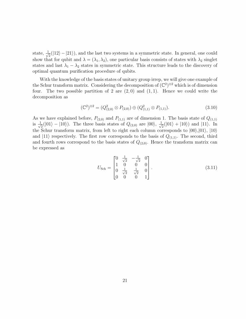
With the knowledge of the basis states of unitary group irrep, we will give one example ofthe Schur transform matrix. Considering the decomposition of (C2)⊗2 which is of dimensionfour. The two possible partition of 2 are (2, 0) and (1, 1). Hence we could write thedecomposition as

(C2)⊗2 = (Q2(2,0) ⊗ P(2,0))⊕ (Q2

(1,1) ⊗ P(1,1)). (3.10)

As we have explained before, P(2,0) and P(1,1) are of dimension 1. The basis state of Q(1,1)

is 1√2(|01〉 − |10〉). The three basis states of Q(2,0) are |00〉, 1√

2(|01〉 + |10〉) and |11〉. In

the Schur transform matrix, from left to right each column corresponds to |00〉,|01〉, |10〉and |11〉 respectively. The first row corresponds to the basis of Q(1,1). The second, thirdand fourth rows correspond to the basis states of Q(2,0). Hence the transform matrix canbe expressed as

USch =

0 1√

2− 1√

20

1 0 0 00 1√

21√2

0

0 0 0 1

. (3.11)

21

Chapter 4

Optimal purification procedure

In this chapter, we will introduce the optimal qubit purification procedure first. In thepaper by Ekert et al. [9], the optimal purification procedure was presented for the first time.This procedure has some very important properties which should be preserved by higher-dimensional quantum states purification procedures. Following these properties we willformulate the optimal purification problem for higher-dimensional case as an optimizationproblem and derive all the constraints for this optimization problem.

4.1 Optimal qubit procedure

Before introducing the procedure, we will introduce some parameterization of the irreplabels and irrep basis states first. Assume we are working with N = 2J noisy qubits, thenall the partitions can be written as (J + j, J − j) for j ∈ 0, 1, . . . , J. (The case whenN = 2J + 1 is very similar, we only need to change the range of j to 1/2, 3/2, . . . , N/2.)Following Equation 3.7. we have

(C2)⊗N =J⊕j=0

Q2(J+j,J−j) ⊗ P(J+j,J−j). (4.1)

In this decomposition, we will abbreviate Q2(J+j,J−j) as Q2

j and P(J+j,J−j) as Pj. As we have

discussed before, Q2j ⊗Pj can be written as

⊕dimPjα=1 Q2

j:α where α represents an order of allthe standard Young tableau of shape (J + j, J − j). Here the order can be implicit exceptwhen α = 1. The standard Young tableaux with α = 1 has the integers 1 though N filled

22

in the diagram column by column, for example, 1 32

. This way of filling will make sure

that the first J − j pair of qubits will be in the singlet state.

For a given irrep Q2j:αj

, the basis state are labelled as |j,m, αj〉 with m = −j,−j +1, . . . , j − 1, j. It is easy to check that the dimension or the number of the semi-standardYoung tableau is 2j+ 1 for λ = (J + j, J − j). When αj = 1, the basis state is of the form:

|j,m, 1〉 = |Ψ−〉⊗J−j ⊗ |j,m〉 (4.2)

where |Ψ−〉 = 1√2(|12〉 − |21〉) is the singlet state and |j,m〉 is the symmetric state with

j −m states in |1〉 and j +m states in |2〉. When αj > 1,

|j,m, αj〉 = Uj:αj |j,m, 1〉 (4.3)

where Uj,αj is a linear combination of permutation operators PPP n(π) with π ∈ Sn that willalso map the Young symmetrizer Π(J+j,J−j):1 to Π(J+j,J−j):αj .

Then we can introduce one important property shared by all the purification procedures.Here we use ρ to represent the input state and assume the procedure P will output Mquantum states.

Definition Let P be a procedure on N d-dimensional quantum states and possibly onadditional ancillas and output M quantum systems. We say procedure P is symmetric if

1. the reduced density operator on each output register is the same;

2. the map P is convariant, meaning

P [(UρU †)⊗N ] = U⊗MP (ρ⊗N)(U †)⊗M (4.4)

for all U ∈ U(d).

The symmetric condition implies that qubit purification procedure P is invariant underthe group actions of Sn and U(2) and the procedure should work for any qubits.

Here the criteria of optimality is that after applying P , it is impossible to increasefidelity even at the cost of fewer output states.

Given the setup, we can introduce the steps of the optimal procedure Popt.

1. Perform quantum measurement defined by the set of projectors (Young symmetriz-ers): Πj:α|j ∈ 0, 1, . . . , J , αj ∈ 1, 2, . . . , dimPj.

23

2. Given the measurement result j and αj, perform U †j,αj on the post-measurement state

ρj,αj to get state ρj,1 in the space Q2j,1.

3. Discard the first J − j singlet states and get state ρj.

4. Trace out all but one states on ρj.

We will first show that Popt satisfies the symmetric condition. After the last step, wewill have state ρj which is in the symmetric subspace and can be expressed as

ρj =α2 − α1

α2j+12 − α2j+1

1

j∑m=−j

αj−m1 αj+m2 |j,m〉 〈j,m| (4.5)

where |j,m〉 is as introduced before.

The reduced density operator is the same for all output states, so the procedure satisfiesthe first property of the symmetric condition.The covariance property is built on the factthat U⊗N and Πj:α commute.

Πj,αU⊗Nρ⊗N(U †)⊗NΠ†j,α

=U⊗NΠj,αρ⊗NΠ†j,α(U †)⊗N

=U⊗Nρj,α(U †)⊗N .

If we discard the first few singlet states, it becomes U⊗2jρj(U†)⊗2j. In the next subsection,

we will give the optimality proof of this procedure.

4.1.1 Optimality proof

The major result of [9] is the following theorem. In the paper, the authors only gave outlineof the optimality proof. We will fill in the details below. Later in Chapter 5, we will givea different proof using Clebsch-Gordan transform.

Theorem 4.1.1 The procedure Popt is the optimal purification procedure for N = 2j de-polarized qubits.

Before that we will state a lemma which is used in the proof.

24

Lemma 4.1.2 The state ρj is of the form

ρj =α2 − α1

α2j+12 − α2j+1

1

(2j + 1)

∫dΩ

4πn(θ)2j(|Ψ(θ, φ)〉 〈Ψ(θ, φ)|)⊗2j (4.6)

where

n(θ) = α2 cos(θ/2)2 + α1 sin(θ/2)2,

|Ψ(θ, φ)〉 =√α2

cos(θ/2)√n(θ)

|1〉+√α1

sin(θ/2)√n(θ)eiφ

|0〉

.

Proof of Lemma 4.1.2 We will omit the common factor α2−α1

α2j+12 −α2j+1

1

throughout the proof,

so it is equivalent to show

(2j + 1)

∫dΩ

4πn(θ)2j(|Ψ(θ, φ)〉 〈Ψ(θ, φ)|)⊗2j =

j∑m=−j

αj−m1 αj+m2 |j,m〉 〈j,m| . (4.7)

First of all

n(θ) |Ψ(θ, φ)〉 〈Ψ(θ, φ)|=C11 |1〉 〈1|+ C00 |0〉 〈0|+ C10 |1〉 〈0|+ C01 |0〉 〈1| ,

with

C00 = α1 sin2 θ

2C11 = α2 cos2 θ

2,

C01 =√α1α2 cos

θ

2sin

θ

2e−iφ C10 =

√α1α2 cos

θ

2sin

θ

2eiφ.

Since

(|Ψ(θ, φ)〉 〈Ψ(θ, φ)|)⊗2j =∑a,b,c,d

a+b+c+d=2j

Ca11C

b00C

c10C

d01ρa,b,c,d (4.8)

where ρa,b,c,d contains all the ordering of a copies of |1〉 〈1|, b copies of |0〉 〈0|, c copies of|1〉 〈0| and d copies of |0〉 〈1|. For example, if j = 1, a = c = 1 and b = d = 0, thenρ1,0,1,0 = |11〉 〈10|+ |11〉 〈01|.

25

Hence we could rewrite the integration as

(2j + 1)∑a,b,c,d

a+b+c+d=2j

∫dΩ

4πn(θ)2jCa

11Cb00C

c10C

d01ρa,b,c,d. (4.9)

To prove Equation (4.7), we only need to show the coefficient of one state in ρk,l,m,n matchesthe corresponding state in |j,m〉 〈j,m|.

The integration on the coefficient (the order of |0〉 and |1〉 will not affect the coefficient)is

2j + 1

4π

∫ π

0

dθ sin θαa+ c+d

22 α

b+ c+d2

1 cos2a+c+d θ

2sin2b+c+d θ

2

∫ 2π

0

ei(d−c)φdφ.

If c 6= d,∫ 2π

0ei(c−d)φ = 0, so the integration can be reduced to

2j + 1

4π

∫ 2π

0

dφ

∫ π

0

dθαa+c2 αb+c1 sin θ cos2a+2c θ

2sin2b+2c θ

2

=(2j + 1)αa+c2 αb+c1

∫ π2

0

sin 2θ cos2a+2c θ sin2b+2c θdθ

=2(2j + 1)αa+c2 αb+c1

∫ π2

0

cos2a+2c+1 θ sin2b+2c+1 θdθ

with a + b + 2c = 2j. Let a + c = j + m then b + c = j −m.The last integration can bewritten as

(4j + 2)αj+m2 αj−m1

∫ π2

0

cos2j+2m+1 θ sin2j−2m+1 θdθ = αj+m2 αj−m1

(j +m)!(j −m)!

(2j)!. (4.10)

The last part is derived from the Beta function for −j < m < j [1]. We could also see that

ρa,b,c,d =

(2j

j +m

)|j,m〉 〈j,m| (4.11)

where(

2jj+m

)is the normalization factor of |j,m〉 〈j,m|.

When n = j or n = −j, the integration can be evaluated as∫ π

2

0cos4j+1 θ sin θdθ =∫ π

2

0cos θ sin4j+1 θdθ = 1

4j+2.

26

Therefore, the coefficient of |j,m〉 〈j,m| derived from the left-hand side of Equation(4.7) would be (

2j

j +m

)αj+m2 αj−m1

(j +m)!(j −m)!

(2j)!= αj+m2 αj−m1

which matches what is given in Eqaution 4.5.

This lemma is showing how to express a state in the symmetric subspace as an integral.More information about symmetric subspace is presented in [23]. With this lemma proved,we could move on to the proof of Theorem (4.1.1). The calculation of the optimal fidelityachievable on each Q2

j is included in the proof.

Proof of Theorem 4.1.1 Assume input states are of the form

ρ = α1 |1〉 〈1|+ α2 |2〉 〈2| (4.12)

where |2〉 is the target state that we want to purify. Define pj,αj to be the probability tomeasure states in Qj,αj , that is

pj,αj = Tr(Πj,αjρ⊗N). (4.13)

By [2], it has been shown that

pj,αj = pj = (α2α1)J−jα2j+1

2 − α2j+11

α2 − α1

. (4.14)

Now we define

ρj,αj =1

pjΠj,αjρ

⊗NΠ†j,αj . (4.15)

After transferring ρj,αj to ρj,1 and discarding the singlet states, we are left with ρj thenthe fidelity for each j is measured by fj = 〈2|Tr2j−1(ρj) |2〉 where Tr2j−1 means tracingout the last (2j − 1) states. We can calculate that

fj =1

2j

[ (2j + 1)α2j+12

α2j+12 − α2j+1

1

− α2

α2 − α1

]. (4.16)

Note that the equation above only works for j > 0, when j = 0, Popt will produce nooutput state, hence f0 = 0.

27

Since ρ⊗N can be expressed as

ρ⊗N =J∑j=0

pj

dimPj∑αj=1

ρj,αj (4.17)

to prove Popt is indeed optimal, we only need to show that fj is the highest fidelity one canachieve on each irrep labelled by (J + j, J − j).

Now, consider all the procedures that can be applied to ρj,αj . Since ρj,αj can be con-structed from ρj, it is equivalent to consider all the procedures applied to ρj with onlyone output state. We denote such a covariant procedure by P1 where the subscript 1 is tostress the fact that only one output state will be produced.

Since P1 is covariant, for any unitary U ∈ U(2), the application of P1 on any inputstate (UρU †)⊗2j is

P1((UρU †)⊗2j) = UP1(ρ⊗2j)U †.

Let UΨ represent a rotation in the bloch sphere around |Ψ〉 〈Ψ|, then UΨ |Ψ〉 〈Ψ|U †Ψ =|Ψ〉 〈Ψ| and UΨ

∣∣Ψ⊥⟩ ⟨Ψ⊥∣∣UΨ =∣∣Ψ⊥⟩ ⟨Ψ⊥∣∣ where 〈Ψ|Ψ⊥〉 = 0. We have

UΨP1((|Ψ〉 〈Ψ|)⊗2j)U †Ψ

=P1((UΨ |Ψ〉 〈Ψ|U †Ψ)⊗2j)

=P1((|Ψ〉 〈Ψ|)⊗2j).

This means the state produced by the mapping P1 applied to 2j copies of |Ψ〉 〈Ψ| commuteswith UΨ, so the output state in the bloch sphere is on the line joining |Ψ〉 〈Ψ| and

∣∣Ψ⊥⟩ ⟨Ψ⊥∣∣,therefore, we have

P1((|Ψ〉 〈Ψ|)⊗2j) = x |Ψ〉 〈Ψ|+ y∣∣Ψ⊥⟩ ⟨Ψ⊥∣∣ , x, y ≥ 0, x+ y ≤ 1. (4.18)

By Lemma 4.1.2 we have

P1(ρj) =α2 − α1

α2j+12 − α2j+1

1

(2j + 1)

∫dΩ

4πn(θ)2jP1(|Ψ(θ, φ)〉 〈Ψ(θ, φ)|⊗2j)

=α2 − α1

α2j+12 − α2j+1

1

(2j + 1)

∫dΩ

4πn(θ)2j

(x |Ψ(θ, φ)〉 〈Ψ(θ, φ)|+ y

∣∣Ψ(θ, φ)⊥⟩ ⟨

Ψ(θ, φ)⊥∣∣ )

where ∣∣Ψ(θ, φ)⊥⟩

=√α1

sin θ2√

n(θ)|2〉 −

√α2

cos θ2eiφ√

n(θ)|1〉 .

28

Because∫ 2π

0eiφdφ = 0, we can drop the terms with eiφ or e−iφ which are the terms associ-

ated with |1〉 〈2| and |2〉 〈1|. Hence, we have

P1(ρj) =α2 − α1

α2j+12 − α2j+1

1

(2j + 1) and

×∫ π

0

sin θ

2dθn(θ)2j−1(xα2 cos2 θ

2+ yα1 sin2 θ

2) |2〉 〈2|+ (xα1 sin2 θ

2+ yα2 cos2 θ

2) |1〉 〈1| .

Consider the coefficient of |2〉 〈2| as the fidelity is calculated as f = 〈2|P1(ρj) |2〉. Thecoefficient is

f =

∫ π

0

sin θ

2dθn(θ)2j−1(xα2 cos2 θ

2+ yα1 sin2 θ

2)dθ

=

∫ π

0

(xα2 cos3 θ

2sin

θ

2+ yα1 cos

θ

2sin3 θ

2)(α2 cos2 θ

2+ α1 sin2 θ

2)2j−1dθ.

Since (α2 cos2 θ2

+ α1 sin2 θ2)2j−1 =

∑2j−1i=0

(2j−1i

)αi2 cos2i θ

2α2j−1−i

1 sin4j−2i−2 θ2, we have

f =

2j−1∑i=0

(2j − 1

i

)αi2α

2j−1−i1

∫ π

0

xα2 cos2i+3 θ

2sin4j−2i−1 θ

2+ yα1 cos2i+1 θ

2sin4j−2i+1 θ

2dθ.

(4.19)

By properties of the Beta function, we can get∫ π

0

cos2i+3 θ

2sin4j−2i−1 θ

2dθ =

(i+ 1)!(2j − i− 1)!

(2j + 1)!, (4.20)∫ π

0

cos2i+1 θ

2sin4j−2i+1 θ

2dθ =

i!(2j − i)!(2j + 1)!

(4.21)

Plugging Equations (4.20 and 4.21) into Equation (4.19), we will get

f =

∫ π

0

sin θ

2dθn(θ)2j−1(xα2 cos2 θ

2+ yα1 sin2 θ

2)dθ

=1

2j(2j + 1)

(x

2j−1∑i=0

(i+ 1)αi+12 α2j−i−1

1 + y

2j−1∑i=0

αi2α2j−i1 (2j − i)

)=

1

2j(2j + 1)

(x

2j∑i=1

iαi2α2j−i1 + y

2j−1∑i=0

αi2α2j−i1 (2j − i)

)=

α2j1

2j(2j + 1)

(x

2j∑i=1

i(α2

α1

)i + y

2j−1∑i=0

(α2

α1

)i(2j − i)).

29

Maximizing f is a simple linear programming problem. Let A =∑2j

i=1 i(α2

α1)i and B =∑2j−1

i=0 (2j − i)(α2

α1)i, then

A > 0 B > 0 and

A−B =

2j∑i=0

(2i− 2j)(α2

α1

)i

=

j−1∑i=0

2i(

(α2

α1

)2j−i − (α2

α1

)i)> 0

as α2 > α1 and i < j, the maximum of Ax+By is attained at x = 1, y = 0.

Then the optimal fidelity is

fopt =α2j+1

2

α2j+12 − α2j+1

1

− 1

2j

α2α1(α2j2 − α

2j1 )

(α2 − α1)(α2j+12 − α2j+1

1 )= fj. (4.22)

This is matches the expression given in [9].

4.1.2 Analysis of average fidelity F(2)N

In the previous section, we have shown the optimal fidelity achieved on a particular U(2)-irrep labelled by λ = (J + j, J − j). Then the next question to ask is that how good is thisprocedure over all the irreps. That is, we would like to know the fidelity averaged over allthe U(2) irrep in the Schur decomposition of (C2)⊗N . We will denote the average fidelity

by F(2)N .

F(2)N =

J∑j=1

djpjfj (4.23)

where dj is the multiplicity factor of the irrep Q2J . The formula for dj is

dj =(2J)!(2j + 1)

(J − j)!(J + j + 1)!=

2j + 1

2J + 1

(2J + 1

J + j + 1

). (4.24)

Then the average fidelity can be specified as we substitute Equation (4.22) and Equation(4.24) into Equation (4.23)

F(2)N =

1

2J + 1

J∑j=1

(2j + 1)

(2J + 1

J + j + 1

)(αJ−j1 αJ+j+12

α2 − α1

− αJ−j+11 αJ+j+1

2 − αJ+j+11 αJ−j+1

2

(2j)(α2 − α1)2

).

(4.25)

30

Before we start the analysis, we need to state the Chernoff-Hoeffding Theorem whichwill be used to bound the minor parts of F

(2)N .

Theorem 4.1.3 (Chernoff-Hoeffding) Suppose X1, . . . , Xn are i.i.d random variables,taking values in 0, 1, let p = E[Xi] and ε > 0, then

Pr(1

n

∑Xi > p+ ε) ≤ e−D(p+ε‖p)n (4.26)

where D(x‖y) = x ln(xy) + (1− x) ln(1−x

1−y ).

For n independent and identical Bernoulli trial Xi’s, the sum X =∑n

i=1Xi is also arandom variable which satisfies the binomial distribution, so the theorem is equivalent to

Pr(X > n(p+ ε)) ≤ e−D(p+ε‖p)n for X ∼ B(n, p).

For approximation, the first step is to break F(2)N into three parts. Then we can extend

the sum to include every term in the corresponding binomial expansion. The three partsare:

F(2)N,1 =

J∑j=1

2j + 1

(α2 − α1)(2J + 1)

(2J + 1

J + j + 1

)αJ−j1 αJ+j+1

2 ,

F(2)N,2 = −

J∑j=1

α1

(α2 − α1)2

2j + 1

(2j)(2J + 1)

(2J + 1

J + j + 1

)αJ−j1 αJ+j+1

2 ,

F(2)N,3 =

J∑j=1

α2

(α2 − α1)2

2j + 1

(2j)(2J + 1)

(2J + 1

J + j + 1

)αJ+j+1

1 αJ−j2

so that F(2)N = F

(2)N,1 + F

(2)N,2 + F

(2)N,3.

For F(2)N,1, we could set k = J − j and it can be approximated by

F(2)N,1 =

1

(2J + 1)(α2 − α1)

2J+1∑k=0

(2J + 1

k

)αk1α

2J+1−k2 (2J + 1− 2k)−∆F

(2)N,1

=1−∆F(2)N,1

31

where

∆F(2)N,1 =

1

(2J + 1)(α2 − α1)

2J+1∑k=J

(2J + 1

k

)αk1α

2J+1−k2 (2J + 1− 2k).

Using the fact 2J + 1− 2k ≤ 2J + 1, we can see that

∆F(2)N,1 ≤

2J + 1

(2J + 1)(α2 − α1)

2J+1∑k=J

(2J + 1

k

)αk1α

2J+1−k2

=1

α2 − α1

2J+1∑k=J

(2J + 1

k

)αk1α

2J+1−k2

=1

(α2 − α1)Pr(X ≥ J)

≤ 1

α2 − α1

e−D(α1+δ‖α1)(2J+1) ∈ O(e−N)

where the last inequality is based on Theorem 4.1.3. Here δ = (α2−α1)J−α1−12J+1

and X ∼B(2J + 1, α1).

Hence, we can see that F(2)N,1 is very close to 1 as

F(2)N,1 = 1−O(e−N). (4.27)

For F(2)N,2 we have

F(2)N,2 =−

J∑j=1

α1

(α2 − α1)2

2j + 1

(2j)(2J + 1)

(2J + 1

J + j + 1

)αJ−j1 αJ+j+1

2

=− 1

2J + 1

α1

(α2 − α1)2

J∑j=1

(2J + 1

J + j + 1

)αJ−j1 αJ+j+1

2 (1 +1

2j)

=− S2,1 − S2,2

32

where

S2,1 =1

2J + 1

α1

(α2 − α1)2

J∑j=1

(2J + 1

J + j + 1

)αJ−j1 αJ+j+1

2 ,

S2,2 =1

2J + 1

α1

(α2 − α1)2

J∑j=1

(2J + 1

J + j + 1

)αJ−j1 αJ+j+1

2 (1

2j).

Here we still follow the convention k = J − j, then we estimate S2,1 and S2,2 separately,

S2,1 =1

2J + 1

α1

(α2 − α1)2

2J+1∑k=0

αk1α2J+1−k2

(2J + 1

k

)−∆S2,1

=1

2J + 1

α1

(α2 − α1)2−∆S2,1.

Here the sum of the extended terms is

∆S2,1 =1

2J + 1

α1

(α2 − α1)2

2J+1∑k=J

αk1α2J+1−k2

(2J + 1

k

)=

1

2J + 1

α1

(α2 − α1)2Pr(X ≥ J)

≤ 1

2J + 1

α1

(α2 − α1)2e−D(α1+δ‖α1)(2J+1) ∈ O(

1

Ne−N)

with X ∼ B(2J + 1, α1).

Since 1j≥ 1

N,

S2,2 =1

2J + 1

α1

(α2 − α1)2

J∑j=1

αJ−j1 αJ+j+12

(2J + 1

J + j + 1

)1

2j(4.28)

≥ 1

N(N + 1)

α1

2(α2 − α1)2

J∑j=1

(2J + 1

J − j

)αJ−j1 αJ+j+1

2 (4.29)

=1

N(N + 1)

α1

2(α2 − α1)2

2J+1∑k=0

(2J + 1

k

)αk1α

2J+1−k2 −∆S2,2 (4.30)

=1

N(N + 1)

α1

2(α2 − α1)2−∆S2,2 (4.31)

33

with

∆S2,2 =1

N(N + 1)

α1

2(α2 − α1)2

2J+1∑k=J

(2J + 1

k

)αk1α

2J+1−k2 (4.32)

=1

N(N + 1)

α1

2(α2 − α1)2Pr(X ≥ J) (4.33)

≤ 1

N(N + 1)

α1

2(α2 − α1)2e−D(α1+δ‖α1)(N+1). (4.34)

Putting them together, we will have the following equations:

F(2)N,2 =

1

N + 1

α1

(α2 − α1)2+O(

1

N2), (4.35)

F(2)N,2 ≤

1

N + 1

α1

(α2 − α1)2− 1

N(N + 1)

α1

2(α2 − α1)2. (4.36)

Since 2j+12j≤ 2, setting k = J + j + 1, F

(2)N,3 can be evaluated as

F(2)N,3 =

J∑j=1

α2

(α2 − α1)2

2j + 1

(2j)(2J + 1)

(2J + 1

J + j + 1

)αJ+j+1

1 αJ−j2 (4.37)

≤ α2

(α2 − α1)2

2

2J + 1

J∑j=1

(2J + 1

J + j + 1

)αJ+j+1

1 αJ−j2 (4.38)

=α2

(α2 − α1)2

2

2J + 1

2J+1∑k=J+2

(2J + 1

k

)αk1α

2J+1−k2 . (4.39)

At this point, we could apply Theorem (4.1.3) to conclude that

F(2)N,3 ∈ O(

1

Ne−N). (4.40)

Overall, summing F(2)N,1, F

(2)N,2 and F

(2)N,3, we have

F(2)N = 1− 1

N + 1

α1

(α2 − α1)2+O(

1

N2). (4.41)

which matches Cirac, Ekert and Macchiavello’s result [9].

By setting F(2)N = 1 − ε, we can get N ≥ α1

(α2−α1)21ε. The interpretation is that Ω(1

ε) is

the sample complexity for this purification problem and this lower bound on the samplecomplexity is what we are interested in.

34

4.1.3 Lower bound on sample complexity of purifying higher-dimensional states

As we know that the complexity of purifying qubit is Ω(1/ε), we are thinking about theimplication of this bound on the d-dimensional case and we reach the following lemma.

Lemma 4.1.4 Given the final output fidelity is 1 − ε, the sample complexity of purifyingd-dimensional state ρ

(d)0 is of order Ω( 1

dε)

Proof The idea of this proof is that when we purify N copies of ρ(2)0 = (1−e(2)

0 /2) |1〉 〈1|+e(2)0

2|2〉 〈2|, there are two procedures we can consider:

1. applying the optimal qubit procedure denoted by P(2)opt on the N copies;

2. embedding each of ρ(2)0 in the d-dimensional space and then applying optimal qudit

purification procedure denoted by P(d)opt.

The second procedure will be denoted by P(2)embed and it cannot outperform the optimal

procedure P(2)opt.

The embedded d-dimensional state is

ρ(d)0 = (1− q)ρ(2)

0 +q

d− 2M (4.42)

where

M =d∑i=3

|i〉 〈i| . (4.43)

We want ρ(d)0 to be of the form

ρ(d)0 = (1− d− 1

de

(d)0 |1〉 〈1|+

e(d)0

d

d∑i=2

|i〉 〈i| . (4.44)

Note that for the simplicity of the proof, we choose |1〉 as the target state which is differentfrom the other choices in this thesis.

35

By equating coefficient of |1〉 〈1| in Equation (4.42) and Equation (4.44), we will get

(1− q)(1− e(2)0

2) = 1− d− 1

de

(d)0 .

Then if we equate coefficient of |2〉 〈2| in Equation (4.42) and Equation (4.44), we will get

(1− q)e(2)0

2=e

(d)0

d.

For coefficient of |i〉 〈i|, for i = 3, . . . , d, in Equation (4.42) and Equation (4.44), we willget

q

d− 2=e

(d)0

d.

We will choose e(d)0 as constant, then we can express q and e

(2)0 in terms of e

(d)0 and d as

q =d− 2

de

(d)0 ,

e(2)0 =

2e(d)0

d− (d− 2)e(d)0

.

Let the final output fidelity be Fembed and Fopt for P(2)embed and P

(2)opt respectively. Since

P(2)embed cannot outperform P

(2)opt, we know that

Fembed ≤ Fopt. (4.45)

From the proof of Theorem (4.1.1), we get the final fidelity Fopt ≤ 1 − e(2)0

2(1−e(2)0 )21N

, so if

Fembed = 1− ε, we will have

1− ε ≤ 1− e(2)0

2(1− e(2)0 )2

1

N,

N ≥ e(d)0 (d− (d− 2)e

(d)0 )

d2(1− e(d)0 )2

1

ε=

e(d)0

(1− e(d)0 )dε

+ Θ(1

d2ε).

This shows that N ∈ Ω( 1dε

).

36

This lemma indicates that the lower bound is dependent on d and for larger d we mayneed fewer copies of the initial states. It also implies that for constant d, the lower boundis Ω(1

ε) which matches the upper bound of Pswap sample complexity and Pswap is optimal

in this case. However, for exponentially large d, Pswap might be suboptimal and we needto find better procedures or the optimal procedure.

4.2 Generalization to qudit

In the last section, we have proved a lower bound on the sample complexity of the quditpurification problem. It is unknown whether such lower bound is achievable. However,we know that the only way to reach the lower bound is to study the optimal purificationprocedure.

The first question we asked was that if it is possible to generalize the optimal qubitprocedure to qudits. The qubit procedure is built on the fact that Q2

λ is isomorphic tosome symmetric subspace. However, this is not true for general unitary group U(d). Wewill give an example here. Let T be the standard Young tableaux of shape λ = (2, 1) andT = 1 3

2. Then

Πλ:T |012〉 ∝ (|12〉 − |21〉) |3〉 − (|23〉 − |32〉) |1〉

This example made us start to think about a new formulation of the problem.

By Equation (3.7), we could assume the procedure start by measuring λ. Hence, wecould focus on studying the optimal fidelity achievable by purifying post-measurement statein space Qd

λ. We want to optimize the final fidelity over all covariant quantum channelsthat will produce one output state. Then we can construct the optimal procedure. Theoptimal purification procedure will apply the channel corresponding to the measurementresult λ with the highest fidelity.

Specifically, we want to apply a quantum channel to a state in Qdλ to produce a state

in Qd(1) which is the carrier space of the U(d) defining irrep. Thus we are optimizing over

all the quantum channels Ψ : Qdλ → Qd

(1). Moreover, we want such quantum channel to be

covariant and commute with action of U(d) defined by the λ-irrep and defining irrep.

For simplicity, we need to introduce a few notions first. The input state is ρ0 as definedin Section 1.2. The projected state from ρ⊗N0 onto Qd

λ is denoted as ρλ. We also defineUλ = QQQd

λ(U).

37

Tp better present this optimization problem, we divide the content into several subsec-tions. In the first subsection, we will see what the implication of the covariance property isfor this optimization problem. To study the covariance condition, some background knowl-edge will also be introduced in the second subsection Then in the following subsections,we will derive explicit constraints and simplify this optimization problem.

4.2.1 Dual representation and covariance condition

Dual representation: Recall that the dual vector space of V is the set of linear mapsfrom V to C. Vectors in the dual space are usually denoted by bras as contrary to ketnotation for vectors in the original space. Moreover, if the vector space has basis vectors|v1〉 , |v2〉 , . . . , |vn〉, then the basis for the dual space is 〈v1| , 〈v2| , . . . , 〈vn|. Now for arepresentationRRR with carrier space V , the dual representation is denoted byRRR∗ with carrierspace V ∗. Moreover, we want to have 〈v| |v〉 = (RRR∗(g) 〈v|)(RRR(g) |v〉) for all g ∈ G, thenRRR∗(g) = RRR(g−1)T . When RRR is a unitary representation, RRR∗ is the conjugate representationwhere RRR∗(g) = RRR(g)∗ and RRR(g)∗ is the entrywise complex conjugate of RRR(g).

After introducing dual representation, we can examine the covariance condition of quan-tum channel Ψ, which can be stated as

Ψ(ρλ) = U †Ψ(UλρλU†λ)U ∀U ∈ U(d). (4.46)

Now expressing Ψ(ρλ) in terms of the Choi representation as Ψ(ρλ) = TrQdλ(J(Ψ)(I(1)⊗ρTλ ))

[23],

Ψ(ρλ) = U †TrQdλ(J(Ψ)(I(1) ⊗ (UλρλU†λ)T ))U

= TrQdλ [(U † ⊗ Iλ)J(Ψ)(I(1) ⊗ (UλρλU†λ)T )(U ⊗ Iλ)]

= TrQdλ [(U † ⊗ UTλ )J(Ψ)(U ⊗ U∗λ)(I(1) ⊗ ρTλ )].

Hence the covariance condition can be reduced to this condition on J(Ψ)

J(Ψ) = (U † ⊗ UTλ )J(Ψ)(U ⊗ U∗λ) ∀U ∈ U(d). (4.47)

For simplicity, we can replace U by UT and get

J(Ψ) = (U∗ ⊗ Uλ)J(Ψ)(U∗ ⊗ Uλ)† ∀U ∈ U(d). (4.48)

38

This will be the first constraint on J(Ψ). Since Ψ is a quantum channel, it must be completepositive and trace-preserving, so the other two conditions for J(Ψ) are:

J(Ψ) 0, (4.49)

TrQ∗(1)

(J(Ψ)) = Iλ, (4.50)

The covariance condition depends on the decomposition of tensor product of dual irrepQd

(1) and Qdλ which we will explore after introducing Clebsch-Gorden transform. The trace-

preserving condition will be explored after that.

4.2.2 Clebsch-Gordan transform and the first constraint on J(Ψ)

What we conclude in this subsection can be summarized in the following proposition.

Proposition 4.2.1 Let Ψ : Qdλ → (Qd

(1))∗ be a quantum channel satisfying the covariance

condition, then its Choi representation must be of the form:

J(Ψ) = W †

⊕µ∈λ−

cµIµ

W (4.51)

for some cµ ≥ 0 and W is the corresponding Clebsch-Gordan transform matrix.

Before proving this proposition, we need to introduce the Clebsch-Gordan transform.

Let RRR1 and RRR2 be two representations of group G and let V1,V2 be their carrier spacesrespectively, then RRR1⊗RRR2 is also a representation of group G. Usually, this representationis reducible even if both RRR1 and RRR2 are irreducible. This means we can decompose itscarrier space V1 ⊗ V2 as

V1 ⊗ V2

G∼=⊕λ∈G

mλ1,2Vλ (4.52)

where mλ1,2 is the multiplicity factor of the carrier space Vλ of irrep rrrλ. This factor could

be zero sometimes. Such decomposition is called Clebsch-Gordan decomposition.

In our case, we are particularly interested in the decomposition of (Qd(1))∗⊗Qd

λ. It turnsout

(Qd(1))∗ ⊗Qd

λ

U(d)∼=⊕

µ∈λ−

Qdµ (4.53)

39

where λ− denotes the set of valid Young diagrams obtained from λ by removing onebox from the end of each possible row. For example, if λ = , then the set is , .

Further notice that, the decomposition we encountered is a special case as the multiplicityfactor is 1.

This unitary change of basis is called Clebsch-Gordan transform and we will denote itby W : Q∗(1) ⊗Qd

λ →⊕

µ∈λ−Qdµ. By Equation 4.53 we know that

W (U∗ ⊗ Uλ)W † =⊕

µ∈λ−

Uµ (4.54)

where Uµ = QQQdµ(U).

Proof of Proposition (4.2.1) Since J(Ψ) commutes with (U∗ ⊗ Uλ), then under thesame Clebsch-Gordan transform, it must be block diagonal with each block being a multipleof identity matrix in the corresponding subspace.

Hence, covariant quantum channel Ψ : Qdλ → (Qd

(1))∗ must satisfy the following condi-

tion:

WJ(Ψ)W † =⊕

µ∈λ−

cµIµ. (4.55)

Since we require J(Ψ) 0, we get the first condition on cµ which is cµ ≥ 0.

This is the first constraint we have on cµ, the next constraint will be derived from thetrace-preserving condition.

4.2.3 The trace-preserving condition

Now we would like to know the implication of the trace-preserving condition on the coef-ficient cµ’s. The condition is summarized in the following proposition.

Proposition 4.2.2 Let Ψ : Qdλ → (Qd

(1))∗ be a quantum channel with Choi representation

of the form J(Ψ) = W †[⊕

µ∈λ− cµIµ

]W , then the trace-preserving condition implies

that the coefficients cµ’s must satisfy the following condition∑µ∈λ−

cµdimQd

µ

dimQdλ

= 1. (4.56)

40

To see it we will introduce a lemma

Lemma 4.2.3 ([17]) For a given µ ∈ λ−, let Eµ ∈ End((Qd(1))∗⊗Qd

λ) be an operator

act as Iµ on Qdµ and acts as 0 on all the other irrep carrier spaces, then

Tr(Qd(1)

)∗(W†EµW ) =

dimQdµ

dimQdλ

Iλ. (4.57)

Proof of Lemma (4.2.3) Consider any U ∈ U(d), we have

Uλ Tr(Qd(1)

)∗(W†EµW )U †λ = Tr(Qd

(1))∗ [(U

∗ ⊗ Uλ)W †EµW (U∗ ⊗ Uλ)†]

= Tr(Qd(1)

)∗ [W†( ⊕µ′∈λ−

Uµ′)Eµ

( ⊕µ′′∈λ−

U †µ′′)W ]

= Tr(Qd(1)

)∗(W†EµW ).

By Schur’s Lemma, we can conclude that Tr(Qd(1)

)∗(W†EµW ) ∝ Iλ.

Let the coefficient be x, then Tr(W †EµW ) = xTr(Iλ). Further note that Tr(WEµW†) =

dimQdµ and Tr(Iλ) = dimQd

λ, we can conclude that x =dimQdµdimQdλ

.

Proof of Proposition (4.2.2) Since⊕

µ∈λ− cµIµ =∑

µ∈λ− cµEµ, we can have thefollowing equation:

Iλ = Tr(Qd(1)

)∗(W†∑

µ∈λ−

cµEµW )

=∑

µ∈λ−

cµdimQd

µ

dimQdλ

Iλ.

Cancelling Iλ from both sides will give us Proposition (4.2.2).

4.2.4 Gel’fand-Tsetlin basis and the objective value

With all the constraints on cµ’s have been derived, the next step is to give an expressionof the objective value of this optimization problem. The objective value or the fidelityachieved on Qd

λ is of the form

fλ = 〈d|TrVλ(J(Φλ)(I ⊗ ρTλ )) |d〉 (4.58)

41

where |d〉 is the target state and ρλ is the state projected onto Qdλ. When we calculate

the fidelity, we need to know the entries of W . To learn about the transform, we need tointroduce the Gel’fand-Tsetlin basis.

In general, suppose (rrr, V ) is an irrep of group G and H is a proper subgroup of G.Restricting the representation rrr to H will give us an representation of H denoted by(rrr ↓H , V ↓H). In most of the cases, rrr ↓H will be reducible and V ↓H can be decomposed as

V ↓HH∼=⊕α∈H

Vα ⊗ Cnα .

where H is the set of all the irreps of H and nα is the branching multiplicity factor of theirrep labelled by α. The case that all the branching multiplicities are either 0 or 1 is calledmultiplicity-free branching.

Such restriction and decomposition can be recursively applied until we reach the trivialsubgroup that only contains the identity element and we will have a tower of groups:G = G1 ⊃ G2 ⊃ · · · ⊃ Gk−1 ⊃ Gk = e. The recursion starts by decomposing V1,the carrier space of G1, under restriction to G2. Then for each V 2

α appearing in thedecomposition of G1, we further decompose it under restriction to G3. The process goeson until we reach the trivial group. If we choose orthonormal basis for each multiplicityspace, then we will have a complete orthonormal basis for V1. We label such basis by|α2,m2, α3,m3, . . . , αk,mk〉 where αi is the label of an irrep of Gi and mi is denoting abasis of the corresponding multiplicity space.

If the branching for each Gi in the tower is multiplicity-free , then we say the tower ofsubgroup is canonical. In this case we don’t need to worry about the multiplicity spaceCnα and the basis can be simply labelled by |α2, α3, . . . , αk〉. Often we will include theirrep label of G1 as well to get a complete label of the basis state.

It turns out that the chain of subgroup, U(d) ⊃ U(d−1) ⊃ · · · ⊃ U(2) ⊃ U(1) ⊃ 1, iscanonical. The embedding is by the fact that U(i)⊕ 1 = U ⊕ 1 : U ∈ U(i) is a subgroupof U(i+1). For a irrep carrier space Qd

λ of U(d), the restriction to U(d−1) is reducible andit decomposes as the direct sum of all irreps of U(d− 1) with the irrep label satisfying thebetweenness condition. Let λ = (λ1,d, λ2,d, . . . , λd,d) and λ′ = (λ1,d−1, λ2,d−1, . . . , λd−1,d−1),if

λj,d ≥ λj,d−1 ≥ λj+1,d, ∀ 1 ≤ j ≤ d− 1, (4.59)

then λ′ satisfy the betweenness condition and irrep labelled by λ′ will appear in the de-composition of Qd

λ.

42

The basis we get from the branching is called Gel’fand-Tsetlin basis. Since it is labelledby partitions, we will introduce one visualization of such basis:

M =

m1,d m2,d . . . md−1,d md,d

m1,d−1 . . . . . . . . . m22...

m1,2 m2,2

m1,1

(4.60)

where each mi,j is between mi,j−1 and mi+1,j−1. We shall denote such pattern by M =(mmmd,mmmd−1, . . . ,mmm2,mmm1) with each mmmi being a valid partition and bold to stress the fact itis an array of integers. Such pattern is called Gel’fand-Tsetlin pattern. One thing to noteis that for a given Qd

λ, the first row of all the Gel’fand-Tsetlin pattern will be the same asλ. When we denote a particular basis state of Qd

m, we will use the notation |mmm,M〉 whereM is the corresponding Gel’fand-Tsetlin pattern and we repeat mmm to stress the label of theirrep, Qd

m.

There is an one-to-one correspondence between Gel’fand-Tsetlin pattern and semi-standard Young tableaux. Here we will give steps to convert a Gel’fand-Tsetlin pattern toa semistand Young tableaux for a given pattern M :

1. create an empty Young tableaux;

2. extend the first row to length m1,1 and fill the newly added boxes with number 1;

3. extend the first row to length m1,2 and fill the newly added boxes with number 2;

4. repeat this process by extend i-th row to length mi,j and fill the newly boxes withnumber j;

The process is finished when all the numbers in the pattern are used. Following thesame idea, we can read out the corresponding Gel’fand-Tsetlin pattern from a given semi-standard Young tableaux.

The entries of W matrix are called Clebsch-Gordan coefficients which are denoted by〈mmm′,M ′,mmm′′,M ′′|mmm,M〉 and defined by

|mmm,M〉 =∑M ′,M ′′

〈mmm′,M ′,mmm′′,M ′′|mmm,M〉 |mmm′,M ′〉 ⊗ |mmm′′,M ′′〉 (4.61)

43

when the decomposition is Qdmmm′ ⊗ Qd

mmm′′ and Qdmmm is one of the resulting subspace. The

general formula for calculating such coefficients is very complicated, but our case is special.Moreover, the covariance property gives us the freedom to choose a simpler formula in thisspecial case.

Before giving formulas, we need to mention one important property since we are workingwith dual representation.

Proposition 4.2.4

〈mmm′,M ′,mmm,M |mmm′′,M ′′〉 =dimQd

mmm′′

dimQdmmm

〈mmm′,M ′,mmm′′,M ′′|mmm,M〉 (4.62)

where Qdmmm′

= (Qdmmm′)∗, mmm′ = (−md,d,−md−1,d, . . . ,−m2,d,−m1,d) and M ′ = (mmmd,mmmd−1, . . .mmm1).

The overline above the coefficient is denoting the complex conjugate.

The proof can be found in Chapter 18 of [22].

For most of combinations of M ′,M ′′ and M , the coefficient 〈mmm′,M ′,mmm′′,M ′′|mmm,M〉 willbe zero. This coefficient will not vanish only if

j∑i=1

(m′i,j +m′′i,j) =

j∑i=1

mi,j (4.63)

holds for j = 1, 2, . . . , d.

Expanding the partial trace of Equation (4.58), we can get

fλ =

dimQdλ∑i=1

〈d| 〈i|W †(⊕µ

cµIµ)W (Id ⊗ ρTλ ) |d〉 |i〉

=

dimQdλ∑i=1

ρλ,i 〈d| 〈i|W †(⊕µ

cµIµ)W |d〉 |i〉

where |i〉 is a basis state of Qdλ and ρλ,i is the (i, i)-th entry of ρλ. From the form of Qd

λ basisstates we know that ρλ,i is the i-th entry of the Schur function sλ(α1, α2, . . . , αd) dividedby the Schur function. Hence, we need to introduce Schur function and one importanttheorem.

44

Definition Given a partition λ = (λ1, λ2, . . . , λn) where λ1 ≥ λ2 ≥ · · · ≥ λn and eachλi ≥ 0, let

a(λ1+n−1,λ2+n−2,...,λn)(x1, x2, . . . , xn) = det

xλ1+n−1

1 xλ1+n−12 . . . xλ1+n−1

n

xλ2+n−21 xλ2+n−2

2 . . . xλ2+n−2n

......

. . ....

xλn1 xλn2 . . . xλnn

and

a(n−1,n−2,...,0)(x1, x2, . . . , xn) =∏

1≤j<k≤n

(xj − xk)

then we can define the Schur function labelled by λ as

sλ(x1, x2, . . . xn) =a(λ1+n−1,λ2+n−2,...,λn)(x1, x2, . . . , xn)

a(n−1,n−2,...,0)(x1, x2, . . . , xn)

The expression we used sλ(α1, α2, . . . , αd) is the Schur function evaluated when xi = αi.This factor represents the probability to measure the state projected onto Qd

λ by the fol-lowing theorem by Alicki et al. [2].

Theorem 4.2.5 For a d-dimensional quantum state ρ with eigenvalues α1, α2, . . . , αd, theprobability to be projected onto subspace Qd

λ is

Tr(Πλ,αρ⊗n) = sλ(α1, α2, . . . , αd) for α = 1, 2, . . . , dimPλ (4.64)

where λ is a valid partition of n.

Now we can further simplify the expression of fλ. We can write⊕

µ cµIµ as (∑

µ

√cµΠµ)

where Πµ’s are orthonormal projectors onto irrep subspace Qdµ. Then

fλ =

dimQdλ∑i=1

ρλ,i∑

µ∈λ−

‖√cµΠµW |d〉 |i〉 ‖2 (4.65)

=

dimQdλ∑i=1

ρλ,i∑

µ∈λ−

cµ

dimQdµ∑j=1

‖ 〈j|W |d〉 |i〉 ‖2 (4.66)

where |i〉 and |j〉 are basis state of Qdλ and Qd

µ respectively.

45

4.2.5 Putting together the optimization problem

To make the trace-preserving condition convex, we introduce cµ =dimQdµdimQdλ

cµ. Combining

Proposition (4.2.1) and (4.2.2) and Equation (4.66), the optimization problem is

Maxcµ

∑µ∈λ−

cµ

dimQdλ∑i=1

ρλ,idimQd

λ

dimQdµ

dimQdµ∑j=1

‖ 〈j|W |d〉 |i〉 ‖2l

subject to cµ ≥ 0∑

µ∈λ−

cµ = 1

.

Here cµ’s are the variables of this linear programming problem and the expression(∑dimQdλ

i=1 ρλ,idimQdλdimQdµ

∑dimQdµj=1 ‖ 〈j|W |d〉 |i〉 ‖2l

)is the coefficient for each cµ which is determined by λ and µ. The norm ‖ 〈j|W |d〉 |i〉 ‖2 isthe Clesch-Gordan coefficient.

Since this is a convex linear programming problem, the objective value can be replacedby

Maxµ∈λ−

dimQdλ

dimQdµ

dimQdµ∑j=1

dimQdλ∑i=1

ρλ,i‖ 〈j|W |d〉 |i〉 ‖2. (4.67)

Here we used the fact that the maximum can only be achieved when one of the cµ’s is 1and all the others are 0.

To start evaluate such optimization problem, we need to know the expression of ‖ 〈j|W |d〉 |i〉 ‖2.By our introduction of Gel’fand-Tsetlin pattern and Clebsch-Gordan coefficients, we knowthat the non-vanishing terms ‖ 〈j|W |d〉 |i〉 ‖2 must have this corresponding Gel’fand-Tsetlinpattern

(000,−1) mmmd mmmd − i000 mmmd−1 mmmd−1

...0 m11 0

.

Here we used the fact that the Gel’fand-Tsetlin pattern of |d〉 has all entries being 0 exceptfor the last entry in the first row being −1. The term mmmd − i means the i-th entry of mmmd

was deducted by 1. This means that for each |i〉 ∈ Qdλ, there is only one corresponding

46

state |j〉 that will produce non-zero Clebsch-Gordan coefficient. Hence, the summationover j can be dropped in the calculation. The summation over i can be further specifiedby summing over entries in its Gel’fand-Tsetlin pattern. We will see how to do it in thenext chapter.

The formula for this coefficient is known. To simplify the expression, we define lj,k =mj,k − j, then

(000,−1) mmmd mmmd − i000 mmmd−1 mmmd−1

...0 m11 0

=∣∣∣∏d−1

j=1(lj,d−1 − li,d)∏j 6=i(lj,d − li,d)

∣∣∣1/2. (4.68)

With this formula we can solve this problem computationally for any given d and N .However, the universal solution for all d and N is unknown. Hence we will start by solvingthe case when d = 2 and d = 3 first in the next chapter.

47

Chapter 5

Optimal purification of qubit andqutrit

In this chapter, we will follow the optimization problem formulation in Equation (4.67) towork out the optimal fidelity achieved by purification of qubits and qutrits on each unitarygroup irrep. In the qubit case, we will see that the optimal fidelity achievable on each irrepis the same as shown in Equation (4.22). For the qutrit case, we will not only calculatethe optimal fidelity achievable on each unitary irrep, we will also consider all such irrepsto calculate the average fidelity.

5.1 Qubit case revisited

For unitary group U(2), a particular semi-standard Young tableaux can be represented bythe Gel’fand-Tsetlin pattern: (

m1,2 m2,2

m1,1

)(5.1)

where the shape of the Young diagram is λ = (λ1, λ2) and m1,2 = λ1,m2,2 = λ2.

The set of all possible µ’s contains only two elements: µ1 and µ2 with µi defined to bethe Young diagram obtained from λ by removing one box from the i-th row. Hence, for ageneral µi the objective value can be expressed as

fλ(µi) =dimQ2

λ

dimQ2µi

dimQ2λ∑

i=1

dimQ2µi∑

j=1

ρλ,i| 〈j|W |2〉 |i〉 |2 (5.2)

48

and we need to compare fλ(µ1) and fλ(µ2).

In the dual space of defining representation, state |2〉 has the following Gel’fand-Tsetlinpattern (

0 −10

).

If |i〉 ∈ Q2λ has Gel’fand-Tsetlin pattern of the form (5.1), then the only |j〉 ∈ Q2

µ1which

will give non-trivial Clebsch-Gordan coefficient must be of the form(m1,2 − 1 m2,2

m1,1

).

For µ2, the first row of the non-vanish state |j〉 will be (m1,2,m2,2 − 1) and its second rowwill be unchanged.

To evaluate fλ(µi), we first need to find the expression of ρλ,i which is the eigenvalueof ρλ on state |i〉 ∈ Q2

λ. Recall that α2 = 1 − e02

is the eigenvalue of |2〉 of ρ and α1 = e02

is the eigenvalue of |1〉. Assume the Gel’fand-Tsetlin pattern of |i〉 ∈ Q2λ is as shown in

Equation (5.1), then we have

ρλ,i =αm1,1

1 αm1,2−m1,1+m2,2

2

sλ(α1, α2). (5.3)

In general, the Schur function s(λ1,λ2)(x1, x2) is defined as

s(λ1,λ2)(x1, x2) =xλ21 x

λ22 (xλ1−λ2+1

1 − xλ1−λ2+12 )

x1 − x2

and the denominator of Equation (5.3) is the corresponding Schur function evaluated whenx1 = α1 and x2 = α2. However, in the comparison, we will omit this denominator as it isalways positive and will not affect the relation between fλ(µ1) and fλ(µ2).

To get closed-form expressions of fλ(µ1) and fλ(µ2), we further assume thatN = λ1+λ2.Note that when λ is fixed, each Gel’fand-Tsetlin pattern can be uniquely described by itsvalue of m1,1. Rewriting Equation (5.2), we can simplify the sum to be over possible values

49

of m1,1.

fλ(µ1) =λ1 − λ2 + 1

λ1 − λ2

λ1−1∑m11=λ2

αm111 αN−m11

2

λ1 −m11

λ1 − λ2 + 1

=λ1 − λ2 + 1

λ1 − λ2

αN2

λ1−1∑m11=λ2

qm11λ1 −m11

λ1 − λ2 + 1

=αN2

λ1 − λ2

λ1−1∑m11=λ2

qm11(λ1 −m11)

=αN2

λ1 − λ2

(λ1 − λ2)(1− q)qλ2 − q(qλ2 − qλ1)(1− q)2

where q = α1

α2.

Similarly, the other fidelity is

fλ(µ2) =λ1 − λ2 + 1

λ1 − λ2 + 2αN2

λ1∑m11=λ2

qm11m11 + 1− λ2

λ1 − λ2 + 1

=αN2

λ1 − λ2 + 2

λ1∑m11=λ2

qm11(m11 + 1− λ2)

=αN2

λ1 − λ2 + 2

qλ2 − (λ1 + 2− λ2)qλ1+1 + (λ1 + 1− λ2)qλ1+2

(1− q)2.

The comparison reveals that

Proposition 5.1.1 fλ(µ1) > fλ(µ2) ∀ λ ` N, e0 ∈ (0, 1).

Proof We will do the comparison directly by calculating the difference and then show thisdifference is always positive. The difference is

f(2)λ (µ1)− f (2)

λ (µ2)

=(λ1 + 1− λ2)qλ2

(λ1 + 2− λ2)(λ1 − λ2)(1− q)2(−2q(1− qλ1−λ2) + (λ1 − λ2)(1− q)(1 + qλ1−λ2+1)).

We are interested in the behaviour of −2q(1− qλ1−λ2) + (λ1−λ2)(1− q)(1 + qλ1−λ2+1) sincethe factor in front of it is always positive.

50

Let l = λ1 − λ2 and define an auxillary function:

g(q, l) = −2q(1− ql) + l(1− q)(1 + ql+1). (5.4)

Taking partial derivative of q on its domain (0, 1), we have

∂g2

∂2q= l(l + 1)(l + 2)(ql−1 − ql) > 0,

so the maximum of ∂g∂q

is achieved at q = 1. However, the maximal value of ∂g∂q

is

∂g

∂q

∣∣∣q=1

=(−2− l + (l + 1)(l + 2)ql − l(l + 2)ql+1

)∣∣∣q=1

= 0

which means ∂g∂q< 0 and the minimum of g(q, l) for any given l is achieved at q = 1.

For any give l > 0, g(1, l) = 0 so we have proved f(2)λ (µ1) > f

(2)λ (µ2).

There are other ways to prove it. The reason we choose this method is that this methodis similar to the method used for the qutrit case.

Let 2j = λ1 − λ2 and adding back the Schur function factor we omitted, the optimalfidelity is

fλ(µ1)

s(λ1,λ2)(α1, α2)

=α2(2jα2j+1

2 − (2j + 1)α1α2j2 + α2j+1

1 )

2j(α2 − α1)(α2j+12 − α2j+1

1 )

which matches the optimal fidelity given in [9]. The average fidelity in [9] can also bere-derived using method presented in Section 4.1.2.

5.2 Qutrit case

In this section, we will first calculate the fidelity achieved on each irrep Q3λ in the first

subsection. The second subsection will combine the result from previous subsection tocalculate the average fidelity. With average fidelity, we can derive a lower bound on thenumber of states required to purify a state until it is ε−close to original state.

51

5.2.1 Optimal fidelity achievable on unitary group irrep Q3λ

Before we start the calculation, we need to state one fact, which is true for all λ ∈ Id,N and

∑µ∈λ−

dimQdµ

dimQdλ

fλ(µ) =

dimQdλ∑i=1

ρλ,i∑

µ∈λ−

‖ΠµW |d〉 |i〉 ‖2 =

dimQdλ∑i=1

ρλ,i = sλ(ααα) (5.5)

where Πµ is the projector onto Qdµ and ααα represents the vector of all the eigenvalues of ρ0.

With this fact, we will be able to calculate the closed-form expressions for fλ(µ1),fλ(µ2)and fλ(µ3), then we can compare them to figure out which one is the largest.

For qutrit, a particular semi-standard Young tableaux can be represented by the Gel’fand-Tsetlin pattern: m1,3 m2,3 m3,3

m1,2 m2,2

m1,1

. (5.6)

The first row is persisted over all such patterns for a given λ = (λ1, λ2, λ3) with m1,3 =λ1,m2,3 = λ2 and m3,3 = λ3.

As in the qubit case, we define

fλ(µk) =dimQ3

λ

dimQ3µk

dimQ3λ∑

i=1

dimQ3µk∑

j=1

ρλ,i| 〈j|W |2〉 |i〉 |2 for k = 1, 2, 3 (5.7)

and we need to compare fλ(µ1),fλ(µ2) and fλ(µ3).

The pattern for state |3〉 of the dual defining representation is of the form 0 0 −10 0

0

.

Hence for a basis state of Q3λ with Gel’fand-Tsetlin pattern in Equation (5.6), the only

state in Q3µ1

that will give non-zero Clebsch-Gordan coefficient must be of the form: m1,3 − 1 m2,3 m3,3

m1,2 m2,2

m1,1

.

52

To get the Gel’fand-Tsetlin pattern of such states in Q3µ2

and Q3µ3

, we just need to move−1 to m2,3 and m3,3 respectively. Then the corresponding Clebsch-Gordan Coefficients is

⟨ (02,−1) m3m3m3 m3m3m3 − i(0, 0) m2m2m2 m2m2m2

0 m11 m11

⟩2

=dimQ3

µi

dimQ3λ

⟨ (1, 02) m3m3m3 − i m3m3m3

(1, 0) m2m2m2 m2m2m2

1 m11 m11

⟩2

=dimQ3

µi

dimQ3λ

((1, 02) m3m3m3 − i m3m3m3

(0, 0) m2m2m2 m2m2m2

)2

=dimQ3

µi

dimQ3λ

∣∣∣∣∣∏2

j=1(lj,2 − li,3 − 1)∏j 6=i(lj,3 − li,3)

∣∣∣∣∣ .Hence when we do summation over such coefficients, we could sum over m1,2,m2,2 and m1,1

because the three numbers could uniquely identify the Cledsch-Gordan coefficient.

Similarly, ρλ,i can be expressed in terms of α1 and α3. For a given semi-standard Youngtableaux, every box filled with 1 or 2 will contribute one copy of α1 to ρλ,i and each boxfilled with 3 will contribute one copy of α3. Expressing it in terms of the Gel’fand-Tsetlinpattern and adding the Schur function factor we get

ρλ,i =αm1,2+m2,2

1 αN−m1,2−m2,2

3

sλ(α1, α1, α3)(5.8)

where

sλ(α1, α1, α3)

=αN3

(1− q)2

((λ2 − λ3 + 1)qλ2+λ3 − (λ1 − λ3 + 2)qλ1+λ3+1 + (λ1 − λ2 + 1)qλ1+λ2+2

).

Here, quotient q is defined as q = α1

α3∈ (0, 1). This Schur function factor will be dropped

in the following calculation with the same reason as for the qubit case.

With the expressions above we can derive the formula of the fidelity without the Schur

53

function factor.

fλ(µ1)

=

λ1−1∑m12=λ2

λ2∑m22=λ3

m12∑m11=m22

αm12+m221 αN−m12−m22

3

(λ1 −m12)(λ1 + 1−m22)

(λ1 − λ2)(λ1 + 1− λ3)

=αN3

(λ1 − λ2)(λ1 + 1− λ3)

λ1−1∑m12=λ2

λ2∑m22=λ3

qm12+m22(m12 −m22 + 1)(λ1 −m12)(λ1 + 1−m22)

=αN3

(1− q)3

((λ2 − λ3 + 1)qλ2+λ3 − (λ1 − λ2 + 1)(λ1 − λ3 + 2)(λ2 − λ3 + 1)

(λ1 − λ2)(λ1 − λ3 + 1)qλ2+λ3+1

+λ1 − λ3 + 2

λ1 − λ2

qλ1+λ3+1 − λ1 − λ2 + 1

λ1 − λ3 + 1qλ1+λ2+2

).

For µ3, fλ(µ3) can be evaluated directly as

fλ(µ3)

=αN3

(λ1 + 3− λ3)(λ2 + 2− λ3)

λ1∑m12=λ2

λ2∑m22=λ3

qm12+m22(m12 −m22 + 1)(m12 + 2− λ3)(m22 + 1− λ3)

=αN3

(1− q)3

(λ2 − λ3 + 1

λ1 − λ3 + 3qλ2+λ3 − λ1 − λ3 + 2

λ2 − λ3 + 2qλ3+λ1+1 + (λ1 − λ2 + 1)qλ1+λ2+2

− (λ2 − λ3 + 1)(λ1 − λ2 + 1)(λ1 − λ3 + 2)

(λ1 − λ3 + 3)(λ2 − λ3 + 2)qλ1+λ2+3

).

Similarly, we can write fλ(µ2) as a sum over m1,2 and m2,2 as

fλ(µ2)

=αN3

(λ1 + 2− λ2)(λ2 − λ3)

λ1∑m12=λ2

λ2−1∑m22=λ3

qm12+m22(m12 −m22 + 1)(m12 + 1− λ2)(λ2 −m22).

54

However, this value is hard to evaluate directly, so we need to use Equation (5.5) and get

fλ(µ2)

=dimQ3

λ

dimQ3µ2

(sλ(α1, α1, α2)−

dimQ3µ1

dimQ3λ

fλ(µ1)−dimQ3

µ3

dimQλ

fλ(µ3))

=αN3 q

λ2+λ3

(1− q)3

(λ2 − λ3 + 1

λ1 − λ2 + 2− (λ1 − λ3 + 2)qλ1−λ2+1

+(λ1 − λ3 + 2)(λ2 − λ3 + 1)(λ1 − λ2 + 1)

(λ2 − λ3)(λ1 − λ2 + 2)qλ1−λ2+2 − λ1 − λ2 + 1

λ2 − λ3

qλ1−λ3+2).

Before comparing the three fidelities, we could omit the common factor C(λ, q) =αN3 q

λ2+λ3

(1−q)3 and define λ1 − λ2 = c, λ2 − λ3 = b to simplify the expressions:

fλ(µ1) = C(λ, q)(b+ 1− (c+ 1)(b+ c+ 2)(b+ 1)

c(b+ c+ 1)q +

b+ c+ 2

cqc+1 − c+ 1

b+ c+ 1qb+c+2

),

(5.9)

fλ(µ2) = C(λ, q)(b+ 1

c+ 2− (b+ c+ 2)qc+1 +

(b+ c+ 2)(b+ 1)(c+ 1)

b(c+ 2)qc+2 − c+ 1

bqb+c+2

),

(5.10)

fλ(µ3) = C(λ, q)( b+ 1

b+ c+ 3− b+ c+ 2

b+ 2qc+1 + (c+ 1)qb+c+2 − (b+ 1)(c+ 1)(b+ c+ 2)

(b+ c+ 3)(b+ 2)qb+c+3

).

(5.11)

Proposition 5.2.1

fλ(µ1) > fλ(µ2) > fλ(µ3) ∀ λ ` N & p ∈ (0, 1). (5.12)

Proof To compare fλ(µ1) and fλ(µ2), we define an auxiliary function:

g(b, c, q) =fλ(µ1)− fλ(µ2)

C(λ, q)(c+ 1)

=b+ 1

c+ 2− (b+ c+ 2)(b+ 1)

c(b+ c+ 1)q +

b+ c+ 2

cqc+1

− (b+ c+ 2)(b+ 1)

b(c+ 2)qc+2 +

c+ 1

b(b+ c+ 1)qb+c+2.

55

Note that

g(b, c, 0) =b+ 1

c+ 2> 0,

g(b, c, 1) = 0.

At this step, we just need to show g(b, c, q) is decreasing on q ∈ (0, 1) by

1

b+ c+ 2

∂g

∂q= − b+ 1

c(b+ c+ 1)+c+ 1

cqc − b+ 1

bqc+1 +

c+ 1

b(b+ c+ 1)qb+c+1.

Note that

∂g

∂q

∣∣∣q=0

= −(b+ c+ 2)(b+ 1)

c(b+ c+ 1)< 0,

∂g

∂q

∣∣∣q=1

= 0.

Then we take the second derivative and get

1

b+ c+ 2

∂2g

∂q2= (c+ 1)qc−1(1− b+ 1

bq +

1

bqb+1).

The minimum of (1− b+1bq + 1

bqb+1) is achieved when q = 1 and the minimum is 0, hence,

∂g∂q

is increasing on q ∈ (0, 1). The maximal value of ∂g∂q

is at q = 1 and the maximal value

is 0, so ∂g∂q< 0 and the minimum of g(b, c, q) is achieved when q = 1 and we can see that

g(b, c, q) > 0.

At this point we can conclude that fλ(µ1) > fλ(µ2).

Similarly, to compare fλ(µ2) and fλ(µ3), we define an auxiliary function:

h(b, c, q) =fλ(µ2)− fλ(µ3)

C(λ, q)(b+ 1)

=b+ 1

(c+ 1)(b+ c+ 3)− b+ c+ 2

b+ 2qc+1 +

(b+ c+ 2)(c+ 1)

b(c+ 2)qc+2

− c+ 1

bqb+c+2 +

(c+ 1)(b+ c+ 2)

(b+ 2)(b+ c+ 3)qb+c+3.

Note that

h(b, c, 0) =b+ 1

(c+ 1)(b+ c+ 3)> 0,

h(b, c, 1) = 0.

56

At this step, we just need to show h(b, c, q) is decreasing on q ∈ (0, 1) as

1

(b+ c+ 2)(c+ 1)

∂h

∂q= qc

(− 1

b+ 2+

1

bq − 1

bqb+1 +

1

b+ 2qb+2

).

Note that (− 1

b+ 2+

1

bq − 1

bqb+1 +

1

b+ 2qb+2

)∣∣∣q=0

= − 1

b+ 2< 0,(

− 1

b+ 2+

1

bq − 1

bqb+1 +

1

b+ 2qb+2

)∣∣∣q=1

= 0.

By taking derivatives we could show k(b, q) =(− 1

b+2+ 1

bq− 1

bqb+1 + 1

b+2qb+2

)is increasing

on q ∈ (0, 1). Hence ∂h∂q< 0 on q ∈ (0, 1) and the minimum of fλ(µ2)− fλ(µ3) is 0.

Combining the two results we have fλ(µ1) > fλ(µ2) > fλ(µ3).

Hence, we have shown that in the qutrit case, the optimal fidelity achievable on Q3λ is

f(3)λ

sλ(α1, α1, α3)=

αN3 qλ2+λ3

(1− q)3sλ(α1, α1, α3)

×(b+ 1− (c+ 1)(b+ c+ 2)(b+ 1)

c(b+ c+ 1)q +

b+ c+ 2

cqc+1 − c+ 1

b+ c+ 1qb+c+2

). (5.13)

5.2.2 Formula of average fidelity F(3)N

Similar to the qubit case, the qutrit case average fidelity is still calculated by the formula:

F(3)N =

∑λ`N,λ1≥λ2≥λ3

f(3)λ d

(3)λ (5.14)

where f(3)λ can be substituted from Equation (5.13). d

(3)λ is the dimension of symmetric

group irrep Pλ and defined by

d(3)λ =

(λ1 − λ2 + 1)(λ2 − λ3 + 1)(λ1 − λ3 + 2)

(N + 1)(N + 2)(N + 3)

(N + 3

λ3, λ2 + 1, λ1 + 2

). (5.15)

57

Let b = λ2 − λ3,c = λ1 − λ2 and q = α1

α3, then

F(3)N =

∑λ`N

d(3)λ

αN3 qλ2+λ3

(1− q)3

×(b+ 1− (c+ 1)(b+ c+ 2)(b+ 1)

c(b+ c+ 1)q +

b+ c+ 2

cqc+1 − c+ 1

b+ c+ 1qb+c+2

).

We will first break the sum into three parts: F(3)N,1, F

(3)N,2 and F

(3)N,3 such that

F(3)N,1 =

∑λ`N

dλαN2 q

λ2+λ3

(1− q)3[b+ 1− (c+ 1)(b+ c+ 2)(b+ 1)

c(b+ c+ 1)q], (5.16)

F(3)N,2 =

∑λ`N

dλαN2 q

λ2+λ3

(1− q)3

b+ c+ 2

cqc+1, (5.17)

F(3)N,3 =−

∑λ`N

dλαN2 q

λ2+λ3

(1− q)3

c+ 1

b+ c+ 1qb+c+2 (5.18)

with F(3)N = F

(3)N,1 + F

(3)N,2 + F

(3)N,3. In the following analysis, we will see that F

(3)N,1 is the

dominant part and F(3)N,2 and F

(3)N,3 are the minor parts.

5.2.3 Preliminaries of the analysis of F(3)N

Before we go onto analyze the average fidelity, we need to state the Multinomial theoremand propositions derived from the Multinomial theorem and one corollary derived fromChernoff-HoeffdingTheorem (4.1.3).

Theorem 5.2.2 (Multinomial Theorem) Let n be a nonnegative integer and m be apositive integer, then

(x1 + x2 + · · ·+ xm)n =∑

k1+k2+···+km=n

(n

k1, k2, . . . , km

)xk11 x

k22 . . . xkmm (5.19)

where(

nk1,k2,...,km

)= n!

k1!k2!...km!.

In the calculation, we also need to use some propositions derived from Theorem (5.2.2).

58

Proposition 5.2.3 Let n be a nonnegative integer, then the following equations hold:∑k1+k2+k3=n+4

(n+ 4

k1, k2, k3

)xk11 x

k22 x

k33 k

21k2x3 =

(n+ 4)(n+ 3)(n+ 2)[(n+ 1)(x1 + x2 + x3)nx2

1x2x3 + (x1 + x2 + x3)n+1x1x2x3

], (5.20)

∑k1+k2+k3=n+4

(n+ 4

k1, k2, k3

)xk11 x

k22 x

k33 k

21k

22 = (n+ 4)(n+ 3)

[(n+ 2)(n+ 1)

× (x1 + x2 + x3)nx21x

22 + (n+ 2)(x1 + x2 + x3)n+1(x2

1x2 + x1x22) + (x1 + x2 + x3)n+2x1x2

],

(5.21)

∑k1+k2+k3=n+4

(n+ 4

k1, k2, k3

)xk11 x

k22 x

k33 k

31k2 = (n+ 4)(n+ 3)

×[(n+2)(n+1)(x1+x2+x3)nx3

1x2+3(n+2)(x1+x2+x3)n+1x21x2+(x1+x2+x3)n+2x1x2

].

(5.22)

Proof we will only give the proof of Equation (5.20) as the techniques required to provethe other equations are the same.

Applying the Multinomial Theorem (5.2.2) to the case that m = 3, we have that

(x1 + x2 + x3)n+4 =∑

k1+k2+k3=n+4

(n+ 4

k1, k2, k3

)xk11 x

k22 x

k33 . (5.23)

Taking partial derivative against x1 on both sides, we have

∂

∂x1

(x1 + x2 + x3)n+4 = (n+ 4)(x1 + x2 + x3)n+3 (5.24)

∂

∂x1

∑k1+k2+k3=n+4

(n+ 4

k1, k2, k3

)xk11 x

k22 x

k33 =

∑k1+k2+k3=n+4

(n+ 4

k1, k2, k3

)xk1−1

1 xk22 xk33 k1. (5.25)

Equating the two equations above and multiplying both sides by x1, we have

(n+ 4)(x1 + x2 + x3)n+3x1 =∑

k1+k2+k3=n+4

(n+ 4

k1, k2, k3

)xk11 x

k22 x

k33 k1. (5.26)

59

Taking partial derivative on both sides against x1 again, we will have

∂

∂x1

(n+ 4)(x1 + x2 + x3)n+3x1 = (n+ 4)[(n+ 3)(x1 + x2 + x3)n+2x1 + (x1 + x2 + x3)n+3

](5.27)

∂

∂x1

∑k1+k2+k3=n+4

(n+ 4

k1, k2, k3

)xk11 x

k22 x

k33 k1 =

∑k1+k2+k3=n+4

(n+ 4

k1, k2, k3

)xk1−1

1 xk22 xk33 k

21. (5.28)

Equating the two equations above and multiplying both sides by x1 we get

(n+ 4)[(n+ 3)(x1 + x2 + x3)n+2x2

1 + (x1 + x2 + x3)n+3x1

]=

∑k1+k2+k3=n+4

(n+ 4

k1, k2, k3

)xk11 x

k22 x

k33 k

21. (5.29)

Taking partial derivative on both sides against x2 and x3 we will have

∂

∂x2

∂

∂x3

(n+ 4)[(n+ 3)(x1 + x2 + x3)n+2x2

1 + (x1 + x2 + x3)n+3x1

]=

= (n+ 4)(n+ 3)(n+ 2)[(n+ 1)(x1 + x2 + x3)nx2

1 + (x1 + x2 + x3)n+1x1

], (5.30)

∂

∂x2

∂

∂x3

∑k1+k2+k3=n+4

(n+ 4

k1, k2, k3

)xk11 x

k22 x

k33 k

21

=∑

k1+k2+k3=n+4

(n+ 4

k1, k2, k3

)xk11 x

k2−12 xk3−1

3 k21k2k3. (5.31)

Equating the two equations above and multiplying both sides by x2 and x3, we will get theformula∑

k1+k2+k3=n+4

(n+ 4

k1, k2, k3

)xk11 x

k22 x

k33 k

21k2k3 =

(n+ 4)(n+ 3)(n+ 2)[(n+ 1)(x1 + x2 + x3)nx2

1x2x3 + (x1 + x2 + x3)n+1x1x2x3

](5.32)

as we expected.

60

Proposition 5.2.4 Let N be a positive integer,and x1, x2 be some real number, then

∑k,l,m≥0

k+l+m=N

(N

k, l,m

)xk1x

l+m2 = (2

∑k>l>m

k+l+m=N

+2∑

l≥k,l>mk+l+m=N

+∑

k≥0,l=mk+l+m=N

)

(N

k, l,m

)xk1x

l+m2 . (5.33)

Proof By the Multinomial theorem (5.2.2), we have

(x1 + x2 + x2)N =∑

k,l,m≥0k+l+m=N

(N

k, l,m

)xk1x

l+m2 . (5.34)

Since(

Nk,l,m

)=(

Nk,m,l

), when l 6= m, the partitions (k, l,m) and (k,m, l) will contribute

same value to the sum. Hence we could rewrite the sum as∑k,l,m≥0

k+l+m=N

(N

k, l,m

)xk1x

l+m2 (5.35)

=(2N∑k=0

∑l>m

l+m=N−k

+N∑k=0

∑l=m

l+m=N−k

)

(N

k, l,m

)xk1x

l+m2 (5.36)

=(2∑k>l>m

k+l+m=N

+2∑

l≥k,l>mk+l+m=N

+∑

k≥0,l=mk+l+m=N

)

(N

k, l,m

)xk1x

l+m2 (5.37)

.

We introduced Proposition (5.2.4) because our strategy will be built on extending the sum∑k>l>m

k+l+m=N+3to the full trinomial expansion.

To further simplify the calculation, we need one corollary of Theorem (4.1.3).

Corollary 5.2.5 For d ≥ 2, let probabilities α1, α2, . . . αd ∈ (0, 1), α1 + α2 + · · ·+ αd = 1,αd <

1d

and indices i1 + I2 + · · ·+ id = N with special condition id > ij for all j < d, then

∑id>ij

i1+i2+···+id=N

(N

i1, i2, . . . , id

) d∏k=1

αikk ∈ O(e−N) for large N (5.38)

.

61

Proof The first observation is that if id > ij for all j < d, then id >Nd

,

The second observation is that∑

id>iji1+i2+···+id=N

can be relaxed to∑N

id=Nd

+1

∑i1,i2,...,id−1≥0

i1+i2+···+id−1=N−id,

then we will have∑id>ij

i1+i2+···+id=N

(N

i1, i2, . . . , id

) d∏k=1

αikk

≤∑id>

Nd

(N

id

)αidd (1− αd)N−id

∑i1+i2+···+id−1=N−id

(N − id

i1, i2, . . . , id−1

)αi11 . . . α

id−1

d−1

(1− αd)N−id

=∑id>

Nd

(N

id

)αidd (1− αd)N−id .

From the second step to the third step, we have used the Theorem (5.2.2) and reach apoint where we can apply Theorem (4.1.3) as∑

id>Nd

(N

id

)αidd (1− αd)N−id ≤ e−D( 1

d‖αd)N ∈ O(e−N).

Hence, ∑id>ij

i1+i2+···+id=N

(N

i1, i2, . . . , id

) d∏k=1

αikk ∈ O(e−N) (5.39)

as we expected.

5.2.4 Analysis of the dominant part of F(3)N

We will analyze F(3)N,1 first by further splitting F

(3)N,1. In order to do that, we need to split

(c+1)(b+c+2)(b+1)c(b+c+1)

in Equation (5.16) first by

(c+ 1)(b+ c+ 2)(b+ 1)

c(b+ c+ 1)

=(1 +1

c)(1 +

1

b+ c+ 1)(b+ 1)

=(b+ 1) +(b+ 1

c+

b+ 1

b+ c+ 1+

b+ 1

c(b+ c+ 1)

).

62

Hence we could further split F(3)N,1 into two parts S1,1 and S1,2 where

S1,1 =∑λ`N

d(3)λ

αN2 qλ2+λ3

(1− q)3[(b+ 1)− (b+ 1)q]

=∑λ`N

d(3)λ

αN2 qλ2+λ3

(1− q)2(b+ 1),

S1,2 =−∑λ`N

d(3)λ

αN2 qλ2+λ3

(1− q)3

[b+ 1

c+

b+ 1

b+ c+ 1+

b+ 1

c(b+ c+ 1)

].

Substituting the expression of d(3)λ into S1,1 and rewriting b+ 1 as λ2 − λ3 + 1, we get

S1,1 =∑λ`N

αλ1+23 αλ2+λ3

1

(α3 − α1)2

(λ1 − λ2 + 1)(λ2 − λ3 + 1)2(λ1 − λ3 + 2)

(N + 1)(N + 2)(N + 3)

(N + 3

λ1 + 2, λ2 + 1, λ3

).

(5.40)

To further simplify S1,1 and all the following expressions, we will set k = λ1 + 2, l = λ2 + 1and m = λ3 and then

S1,1 =

∑k+l+m=N+3k>l>m

(N+3k,l,m

)αk3α

l+m1 (k − l)(l −m)2(k −m)

(N + 3)(N + 2)(N + 1)α1(α3 − α1)2. (5.41)

Now our strategy is to extend the sum in the expression of S1,1 to include every term ofthe corresponding multinomial expansion and then bound the additional terms. We willuse this strategy repeatedly in the following analysis.

Hence, by Proposition (5.2.4) we have

S1,1 =

[12

∑k,l,m−

12

∑l=m−

∑l≥k,l>m

](N+3k,l,m

)αk3α

l+m1 (k − l)(l −m)2(k −m)

(N + 3)(N + 2)(N + 1)α1(α3 − α1)2. (5.42)

The terns in summations with indices k = l or l = m are cancelled because of the factor(k − l)(l −m), so S1,1 can be further simplified as

S1,1 =

12

∑k,l,m

(N+3k,l,m

)αk3α

l+m1 (k − l)(l −m)2(k −m)

(N + 3)(N + 2)(N + 1)α1(α3 − α1)2(5.43)

−∑

l>k,l>m

(N+3k,l,m

)αk3α

l+m1 (k − l)(l −m)2(k −m)

(N + 3)(N + 2)(N + 1)α1(α3 − α1)2(5.44)

=1−∆S1,1 (5.45)

63

where

∆S1,1 =

∑l>k,l>m

(N+3k,l,m

)αk3α

l+m1 (k − l)(l −m)2(k −m)

(N + 3)(N + 2)(N + 1)α1(α3 − α1)2(5.46)

and we used the fact that the dominant part of S1,1 which is

S ′1,1 =

∑k,l,m

(N+3k,l,m

)αk3α

l+m1 (k − l)(l −m)2(k −m)

2(N + 3)(N + 2)(N + 1)α1(α3 − α1)2= 1 (5.47)

.

The calculation of S ′1,1 is as follows. First of all, we need to expand (k−l)(l−m)2(k−m)to get

(k − l)(l −m)2(k −m)

=k2l2 − 2k2lm+ k2m2 − kl3 + kl2m+ klm2 − km3 + l3m− 2l2m2 + lm3.

Then we calculate the numerator of S ′1,1 by applying Proposition (5.2.3) and get the fol-lowing:∑

k,l,m

(N + 3

k, l,m

)αk3α

l+m1 (k2l2 + k2m2 − 2m2l2)

= 2(N + 3)(N + 2)(α3 − α1)((N + 1)N(α3 + α1)α21 + (N + 2)α1), (5.48)

∑k,l,m

(N + 3

k, l,m

)αk3α

l+m1 (−kl3 − km3 + l3m+ lm3)

= −2(N + 3)(N + 2)(α3 − α1)((N + 1)Nα31 + 3(N + 1)α2

1 + α1), (5.49)

∑k,l,m

(N + 3

k, l,m

)αk3α

l+m1 (−2k2lm+ kl2m+ klm2)

= −2(N + 3)(N + 2)(N + 1)N(α3 − α1)α3α21. (5.50)

Summing the three equations above, we can get S ′1,1 = N+1−p(N+1)(N+1)(α3−α1)

= 1.

Then we will bound the value of ∆S1,1. A closer examine of the summation in thenumerator of ∆S1,1 tells us that we could apply Corollary (5.2.5). Using the fact that(k − l)(l −m)2(k −m) < N4 and Corollary (5.2.5), we could conclude that

∆S1,1 <N4e−D( 1

3‖ p3

)(N+3)

(N + 3)(N + 2)(N + 1)α1(α3 − α1)2∈ O(Ne−N). (5.51)

64

Summing S ′1,1 and ∆S1,1, we see that

S1,1 = 1−O(Ne−N). (5.52)

To complete the analysis of F(3)N,1, the last part is S1,2 which contains the terms that

should be subtracted from F(3)N,1. The expression for S1,2 is

S1,2 = −∑λ`N

d(3)λ (b+ 1)(

1

c+

1

b+ c+ 1+

1

c(b+ c+ 1))αλ1−1

3 αλ2+λ3+11

(1− q)3. (5.53)

We will multiply d(3)λ with the fractional expressions and separate out the integral parts by

d(3)λ

c=[(b+ 1)(b+ c+ 2) +

1

c(b+ 1)(b+ c+ 2)

] (N+3

λ1+2,λ2+1,λ3

)(N + 3)(N + 2)(N + 1)

,

d(3)λ

b+ c+ 1=[(b+ 1)(c+ 1) +

(b+ 1)(c+ 1)

b+ c+ 1

] (N+3

λ1+2,λ2+1,λ3

)(N + 3)(N + 2)(N + 1)

,

d(3)λ

c(b+ c+ 1)=[b+ 1 +

b+ 1

c+

b+ 1

b+ c+ 1+

b+ 1

c(b+ c+ 1)

] (N+3

λ1+2,λ2+1,λ3

)(N + 3)(N + 2)(N + 1)

.

Hence, we could simplify |S1,2| by

|S1,2| =∑λ`N

(b+ 1)2(b+ c+ 2 + c+ 1 + 1)

(N+3

λ1+2,λ2+1,λ3

)αλ1−1

3 αλ2+λ3+11

(1− q)3(N + 3)(N + 2)(N + 1)

+∑λ`N

(b+ 1)2(b+ c+ 3

c+

c+ 2

b+ c+ 1+

1

c(b+ c+ 1))

(N+3

λ1+2,λ2+1,λ3

)αλ1−1

3 αλ2+λ3+11

(N + 3)(N + 2)(N + 1)(1− q)3.

Expressing it with k = λ1 + 2,l = λ2 + 1 and m = λ3, we get

|S1,2| =

∑k>l>m≥0

k+l+m=n+3

(N+3k,l,m

)αk3α

N+3−k1 (l −m)2(2k + 1− l −m)

(N + 3)(N + 2)(N + 1)(α3 − α1)3

+

∑k>l>m≥0

k+l+m=n+3

(N+3k,l,m

)αk3α

N+3−k1 (l −m)2(k−m+1

k−l−1+ k−l+1

k−m−1+ 1

(k−l−1)(k−m−1))

(N + 3)(N + 2)(N + 1)(α3 − α1)3

=S ′1,2 + ∆S1,2

where S ′1,2 is the dominant term of |S1,2| and ∆S1,2 is the minor term.

65

We will evaluate S ′1,2 by applying Proposition (5.2.4) in the following way:

S ′1,2 =

∑k>l>m≥0

k+l+m=n+3

(N+3k,l,m

)αk3α

N+3−k1 (l −m)2(2k + 1− l −m)

(N + 3)(N + 2)(N + 1)(α3 − α1)3(5.54)

=(1

2

∑k,l,m≥0

k+l+m=n+3

−1

2

∑k≥0 ,l=m

−∑

l≥k ,l>m

)(N+3k,l,m

)αk3α

N+3−k1 (l −m)2(2k + 1− l −m)

(N + 3)(N + 2)(N + 1)(α3 − α1)3

(5.55)

=(1

2

∑k,l,m≥0

k+l+m=n+3

−∑

l>k ,l>m

)(N+3k,l,m

)αk3α

N+3−k1 (l −m)2(2k + 1− l −m)

(N + 3)(N + 2)(N + 1)(α3 − α1)3(5.56)

=α1

(N + 1)(α3 − α1)2−

∑l>k ,l>m

(N+3k,l,m

)αk3α

N+3−k1 (l −m)2(2k + 1− l −m)

(N + 3)(N + 2)(N + 1)(α3 − α1)3(5.57)

=α1

(N + 1)(α3 − α1)2−O(e−N). (5.58)

Bounding∑

l>k ,l>m

(N+3k,l,m)αk3α

N+3−k1 (l−m)2(2k+1−l−m)

(N+3)(N+2)(N+1)(α3−α1)3is similar to bounding ∆S1,1, as it is also

an application of Corollary (5.2.5). The result, which is

1

2

∑k,l,m≥0

k+l+m=n+3

(N+3k,l,m

)αk3α

N+3−k1 (l −m)2(2k + 1− l −m)

(N + 3)(N + 2)(N + 1)(α3 − α1)3=

α1

(N + 1)(α3 − α1)2, (5.59)

is also derived from Proposition (5.2.3) and the calculation is similar to that of S ′1,1.

To finish the analysis of F(3)N,1, we need to bound ∆S1,2 where

∆S1,2 =

∑k>l>m≥0

k+l+m=n+3

(N+3k,l,m

)αk3α

N+3−k1 (l −m)2(k−m+1

k−l−1+ k−l+1

k−m−1+ 1

(k−l−1)(k−m−1))

(N + 3)(N + 2)(N + 1)(α3 − α1)3. (5.60)

Since k −m+ 1 > k − l − 1, we have k−m+1k−l−1

+ k−l+1k−m−1

+ 1(k−l−1)(k−m−1)

> 1, Hence, we willhave

∆S1,2 >

∑k>l>m≥0

k+l+m=n+3

(N+3k,l,m

)αk3α

N+3−k1 (l −m)2

(N + 3)(N + 2)(N + 1)(α3 − α1)3(5.61)

=α1

(N + 2)(N + 1)(α3 − α1)3−O(

1

Ne−N). (5.62)

66

The calculation is similar to that of S1,1.

Now F(3)N,1 is fully analyzed and we could conclude that

F(3)N,1 =S1,1 + S1,2 = 1−∆S1,1 − S ′1,2 −∆S1,2 (5.63)

=1− α1

(N + 1)(α3 − α1)2+O(

1

N2). (5.64)

5.2.5 Analysis of the minor part of F(3)N

The methods to bound F(3)N,2 and F

(3)N,3 are very similar as we only need to show they are

exponentially small. We can simplify F(3)N,2 as

F(3)N,2 =

∑λ`N

d(3)λ

αN2 qλ2+λ3

(1− q)3

b+ c+ 2

cqc+1

=∑

k>l>m≥0k+l+m=n+3

d(3)λ

k −ml −m− 1

αl+13 αk+m−1

1

(α3 − α1)3

=

∑k>l>m

(N+3k,l,m

)αl+1

3 αk+m−11 (k −m)2(k − l)(l −m)

(l −m− 1)(N + 3)(N + 2)(N + 1)(α3 − α1)3.

Using the fact (k−m)2(k−l)(l−m)l−m−1

< N3 and Corollary (5.2.5), we will see that

F(3)N,2 ∈ O(e−N). (5.65)

Similarly for F(3)N,3, we have that

F(3)N,3 = −

∑λ`N

d(3)λ

αN2 qλ2+λ3

(1− q)3

c+ 1

b+ c+ 1qb+c+2

= −∑

k>l>m≥0k+l+m=n+3

d(3)λ

k − lk −m− 1

αm+13 αk+l−1

1

(α3 − α1)3

= −∑

k>l>m

(N+3k,l,m

)αm+1

3 αk+l−11 (k −m)(k − l)2(l −m)

(k −m− 1)(N + 3)(N + 2)(N + 1)(α3 − α1)3.

67

Using the fact (k−m)(k−l)2(l−m)k−m−1

< N3 and Corollary (5.2.5), we will see that

|F (3)N,3| ∈ O(e−N). (5.66)

Hence, as we expect, F(3)N,2 and F

(3)N,3 are exponentially small. The average fidelity can be

expressed as

F(3)N = 1− α1

(N + 1)(α3 − α1)2+O(

1

N2) (5.67)

and we can conclude that if we want to purify qutrit to ε-close to the original state, weneed at least α1

ε(α3−α1)2copies of the initial state. However, for the d-dimensional case, any

achievable lower bound of the sample complexity of the purification problem is unknown.

To fully understand the optimal purification procedure, the first step is to solve theoptimization problem formulated in Chapter 4. Maybe we could avoid explicit analysis ofthe average fidelity but upper bound the average fidelity achieved by the optimal procedureand then derive the achievable lower bound of the d-dimensional quantum state purificationsample complexity.

68

References

[1] Milton Abramowitz and Irene A Stegun. Handbook of mathematical functions. Appliedmathematics series, 55:62, 1966.

[2] Robert Alicki, Sl/awomir Rudnicki, and Sl/awomir Sadowski. Symmetry propertiesof product states for the system of N n-level atoms. Journal of mathematical physics,29(5):1158–1162, 1988.

[3] Dave Bacon, Andrew M Childs, and Wim van Dam. From optimal measurement toefficient quantum algorithms for the hidden subgroup problem over semidirect prod-uct groups. In 46th Annual IEEE Symposium on Foundations of Computer Science(FOCS’05), pages 469–478. IEEE, 2005.

[4] Dave Bacon, Isaac L Chuang, and Aram W Harrow. The quantum Schur transform:I. efficient qudit circuits. arXiv preprint quant-ph/0601001, 2005.

[5] Charles H Bennett, Gilles Brassard, Sandu Popescu, Benjamin Schumacher, John ASmolin, and William K Wootters. Purification of noisy entanglement and faithfulteleportation via noisy channels. Physical review letters, 76(5):722, 1996.

[6] Harry Buhrman, Richard Cleve, John Watrous, and Ronald De Wolf. Quantum fin-gerprinting. Physical Review Letters, 87(16):167902, 2001.

[7] Andrew M Childs, Aram W Harrow, and Pawe l Wocjan. Weak Fourier-Schur sam-pling, the hidden subgroup problem, and the quantum collision problem. In AnnualSymposium on Theoretical Aspects of Computer Science, pages 598–609. Springer,2007.

[8] Andrew M Childs and Vedang Vyas. Note for spring 2014. Personal notes, 2014.

[9] JI Cirac, AK Ekert, and C Macchiavello. Optimal purification of single qubits. PhysicalReview Letters, 82(21):4344, 1999.

69

[10] Roe Goodman and Nolan R Wallach. Representations and invariants of the classicalgroups, volume 68. Cambridge University Press, 2000.

[11] Lov K Grover. A fast quantum mechanical algorithm for database search. In Pro-ceedings of the twenty-eighth annual ACM symposium on Theory of computing, pages212–219. ACM, 1996.

[12] Jeongwan Haah, Aram W Harrow, Zhengfeng Ji, Xiaodi Wu, and Nengkun Yu.Sample-optimal tomography of quantum states. In Proceedings of the 48th AnnualACM SIGACT Symposium on Theory of Computing, pages 913–925. ACM, 2016.

[13] Michael Keyl and Reinhard F Werner. Optimal cloning of pure states, testing singleclones. Journal of Mathematical Physics, 40(7):3283–3299, 1999.

[14] Michael Keyl and Reinhard F Werner. Estimating the spectrum of a density operator.Physical Review A, 64(5):052311, 2001.

[15] Michael Keyl and Reinhard F Werner. The rate of optimal purification procedures.In Annales Henri Poincare, volume 2, pages 1–26. Springer, 2001.

[16] Michael A Nielsen and Isaac L Chuang. Quantum computation and quantum infor-mation. Cambridge university press, 2010.

[17] Maris Ozols. Purification. Personal notes, 2015.

[18] Oded Regev. On lattices, learning with errors, random linear codes, and cryptography.Journal of the ACM (JACM), 56(6):34, 2009.

[19] Oded Regev. The learning with errors problem. Invited survey in CCC, 2010.

[20] Peter W Shor. Polynomial-time algorithms for prime factorization and discrete log-arithms on a quantum computer. SIAM Journal on Computing, 26(5):1484 – 1509,1997.

[21] Daniel R Simon. On the power of quantum computation. SIAM journal on computing,26(5):1474–1483, 1997.

[22] N.Ya. Vilenkin and A.U. Klimyk. Representation of Lie Groups and Special Functions:Volume 3: Classical and Quantum Groups and Special Functions, volume 75. SpringerScience & Business Media, 2013.

[23] John Watrous. Theory of quantum information. 2011.

70