AFIT/GOR/ENS/99M-10

Using Simulation to Model The Army Recruiting Station With Multi-Quality Prospects

THESIS

Edward L. McLarney Captain, U.S.A.

AFIT/GOR/ENS/99M-10

Approved for public release; distribution unlimited

ARC QUAUTY INSPECTED 8 19990412 072

The views expressed in this thesis are those of the author and do not reflect the official policy of position of

the Department of Defense or the U.S. Government.

AF1T/GOR/ENS/99M-10

Using Simulation to Model The Army Recruiting Station With Multi-Quality Prospects

THESIS

Presented to the Faculty of the School of Engineering of the Air Force Institute of Technology, Air

University, In Partial Fulfillment of the

Requirements for the Degree of

Master of Science

Edward L. McLarney, B.S.

Captain, U.S.A.

Air Force Institute of Technology

Wright-Patterson AFB, Ohio

March 1999

U.S. Army Recruiting Command (USAREC)

Approved for public release; distribution unlimited

AFTT/GOR/ENS/99M-10

THESIS APPROVAL

Student: Edward L. McLarney, Captain, U.S. Army Class: GOR-99M

Title: Using Simulation to Model The Army Recruiting Station With Multi-Quality Prospects

Defense Date: 3 March 1999

Committee: Name/Title/Department Signature

Advisor J. O. Miller, Lt. Colonel, USAF Assistant Professor Department of Operational Sciences

Reader Kenneth Bauer, Ph. D. Professor Department of Operational Sciences

Reader Jack Kloeber, LTC, USA Assistant Professor Department of Operational Sciences

DEPARTMENT OF THE AIR FORCE AIR UNIVERSITY

ATR FORCE INSTITUTE OF TECHNOLOGY

Wright-Patterson Air Force Base, Ohio

Acknowledgements

My sincere thanks to my wife, Saundra, and my son, Kenny, for their

encouragement and understanding during preparation of this work. Thanks also to my

thesis committee for their guidance, assistance, and patience: Advisor LT COL J.O.

Miller, and readers Dr. Kenneth Bauer, and LTC Jack Kloeber. The Dayton Recruiting

Company (CPT DeZienny) and United States Army Recruiting Command (MAJ Robert

Fancher) provided invaluable data and recruiting advice. Thanks to everyone for your

help.

Table of Contents

Acknowledgments ü

Table of Contents iii

List of Figures v

List of Tables vi

Abstract vii

I. Introduction LI

Statement of the Problem LI Background L2 Current Army Policies L2 Approach L3 Scope L3 Organization L4

II. Literature Review 2.1

General 2.1 Recruiting Station Workings 2.1 Leader - Recruiter Interactions 2.3

Past Recruiting Studies 2.3 Leadership Theory 2.4 Motivation Theory 2.7 Established Military Models 2.8

Summary 2.8

HI. Methodology 3.1

General 3.1 Review of Survey Development Techniques 3.1

Information Need Determination 3.1 Data Gathering Process Decisions 3.2 Instrument Drafting 3.2 Instrument Testing 3.2 Specification of Procedures 3.2

Application of Survey Development Techniques 3.3 Application of Information Need Determination 3.3 Application of Data Gathering Process Decisions 3.5 Application of Instrument Drafting 3.5 Application of Instrument Testing 3.10 Application of Specification of Procedures 3.11

Data Analysis Methodology 3.11 Simulation Methodology 3.12

Examining the Previous Model 3.14 Intended Modifications 3.15 Conceptual Implementation of Modifications 3.16 Coding the Modifications 3.19

Verification and Validation 3.23 Output Collection 3.24

in

Summary 3.24

IV. Results and Analysis 4.1 General 4.1 Input Analysis 4.1

Analysis of 1999 Survey Data 4.2 Analysis of Supporting Data 4.6 Synthesis of 1998 and 1999 Survey Data 4.10

Experimental Design 4.12 Simulation Output 4.14

General 4.14 Steady State Analysis 4.15 Analysis of Output from Experimental Design 4.17

Conclusion 4.20

V. Conclusion 5.1 Summary 5.1 Recommendations 5.4 Final Remarks 5.5

Appendix A: 1998 Model A.l Appendix B: Summary of Model Changes B.l Appendix C: Instructions for Model Use C.l Appendix D: Survey D.l Appendix E: Input Data E. 1 Appendix F: Output Data F.l Appendix G: Electronic Enclosures G.l Bibliography BIB.l Vita V.l

IV

List of Figures

Figure Page

2.1. Recruiting Process 2.1

3.1. Top-Level SIMPROCESS Model 3.14

4.1. Using a Random Draw and Proportions to Assign Prospect Type 4.10

4.2. Contract Times by Sequence Number 4.15

4.3. Average Intercontract Time by Sequence Number 4.16

4.4. Contract Occurrences by RFG (Setting 1) 4.18

4.5. Total Contracts (Setting 1) 4.19

4.6. Average Contracts by Month 4.21

List of Tables

Table Page

3.1. Goal Setting Markers 3.6

3.2. Demographic Markers 3.9

3.3. Sorted Survey Results 3.13

3.4. Categorization of Prospect Types 3.17

3.5. Proportions of Prospect Types 3.22

4.1. Ideal Data Set (by Prospect Type) 4.1

4.2. Real World Data Set 4.2

4.3. Results of Station Commander Leadership / Recruiter Personality Survey 4.3

4.4. Interviews and Contracts Regressed by Leadership and Personality 4.4

4.5. Mean Parameter Values from 1998 Survey Database 4.7

4.6. Adjusted Conversion Rates for Model 4.8

4.7. Average Contracted Proportions 4.9

4.8. Process Duration Modification Example (Average Prospect) 4.12

4.9. Experimental Design Settings 4.13

4.10. Translating Simulation Time to Month of the Year 4.20

vi

Abstract

This thesis explores the application of simulation to the Army Recruiting Station. Included are the effects of

leadership styles and policies, the effects of recruiters with different personality types, and differences in processing

for varying types of recruits. Research included heavy emphasis into determining the effects of leadership on

recruiter productivity. In addition, major changes were made to a previous simulation model. The changes allowed

current research to be implemented into the simulation. This research is intended to help the United States Army

Recruiting Command better understand how changes in the recruiting process and in leadership policies affect

productivity.

Vll

I - Introduction

Statement of the Problem

Army recruiters work extremely long hours, suffer morale problems, and face many more failed

recruitment efforts than successful ones (Roberts, 210). The recruiter is involved at nearly every step in the

recruitment process for a potential recruit. In addition, recruiters are required to prospect for potential

recruits (by phone or in face-to-face presentations), and to conduct other auxiliary duties. All these duties

add up to extremely long work hours. Morale problems stem from overwork, micro-management, and

continual prospecting rejection. In prospecting, recruiters call or visit potential recruits, and ask them if

they would consider joining the Army. Recruiters become frustrated because they get such a high ratio of

negative responses. Also, sometimes the amount of recruiting contracts attained is more dependent on

demographic and seasonal factors than on the efforts of recruiters. This could lead to a perception of no

control on the part of the recruiter: no matter how hard the recruiter works, he might not make his monthly

quota.

The goal of this thesis was to explore possible methods of improving recruiter quality of life and

efficiency. The study was accomplished through information gathering (surveys, interviews, etc.),

simulation, and output analysis. Specifically studied were:

1. The effect of Station Commander leadership methods. We theorize that Station Commanders

should have the ability to influence recruiter productivity through policies and leadership techniques.

These factors were examined using a goal-setting frame of reference, one of several established leadership

quantification methods used by behavioral scientists.

2. Incorporating personalities, policies, motivation, and potential recruit attributes into a

previously developed recruiting station model.

3. System throughput for various types of potential recruits, categorized by gender, ASVAB

score, and whether or not they have graduated high school.

1.1

Background

In 1997-98, Lieutenants Mark A. Friend and James D. Cordeiro conducted research and completed

a thesis for United States Army Recruiting Command (USAREC) which included a model of the army

recruiting station. This thesis is a follow-on effort to the study conducted by Friend and Cordeiro. While

the previous study explored actions at the individual recruiter level, the current effort seeks to provide

insight into station activities, to include leadership and varying prospects, with little loss of resolution.

Cordeiro and Friend aptly summarized some of the problems facing the recruiter in their

background section (Cordiero & Friend, 2-3). Some obstacles noted were: negative press exposure in

sexual harassment cases; a loss of macho image; societal changes; and a more lucrative civilian job market.

All the afore-mentioned factors tend to make potential recruits less willing to join the army. During

briefings to senior Recruiting Leadership, BG Smith noted that recruiters probably reported inflated

telephone prospecting hours. BG Smith indicated that recruiters strongly dislike telephone prospecting. He

suspects they inflate reported prospecting hours to make established quotas.

Current Army Policies

Much of a recruiter's daily schedule is tightly controlled. Each morning, recruiters meet with their

station commander to discuss and plan their schedule for the day. Recruiters are rewarded for making

individual quotas. Despite past attempts to foster teamwork and implement Total Quality Management

(TQM) practices, individuals are the focus of current management practices. If the individual succeeds, he

receives praise and awards. If the individual fails (possibly despite trying) he is held accountable.

1.2

Approach

In Simulation Modeling and Analysis (Law & Kelton, 107), the authors outline a ten-step process

for conducting a simulation study as follows:

1. Formulate the problem and plan the study.

2. Collect data and define a model

3. Check for model and data validity.

4. Construct a computer program and verify it.

5. Make pilot runs.

6. Check pilot runs for validity.

7. Design experiments.

8. Make production runs.

9. Analyze output data.

10. Document, present, and implement results.

Law & Kelton point out that verification and validation should occur during all steps of the

process, and that several iterations of parts 1- 6 may be necessary. We used the ten-step process as a

framework for this thesis. As we progressed through this study, we realized that step 2, collecting data and

defining the model would be a very large task. We spent a large amount of effort in gathering data, and as

a result, the end product should provide a more accurate and robust representation of the system.

Since recruiter performance data must come from the field, data gathering and model/problem

formulation required major efforts. We designed a survey for recruiters and station commanders. Once

surveys and other data collection began, we focused on programming the simulation.

Scope

This study focuses on three major areas: First, the Station Commander leadership effects are

assessed in combination with recruiter personalities. Second, the leader/recruiter interactions are

incorporated into a much more detailed station model. Third, the ability to handle recruits with different

attributes are incorporated into the model. These attributes are: whether or not the candidate is a high

school graduate; ASVAB (Armed Services Vocational Aptitude Battery) score; and gender.

1.3

Organization

This thesis is organized as follows. Chapter 1 gives a general background and introduction.

Chapter 2 is the literature review, and contains more specific background information. Chapter 3 explains

general problem analysis, survey design, and simulation. Chapter 4 covers input analysis, experimental

design, and simulation output analysis. Finally, conclusions are presented in Chapter 5.

1.4

II. Literature Review

General

In order to simulate an Army Recruiting Station, we had to gain a detailed understanding of how a

recruiting station works, how different leader-recruiter combinations affect productivity, and how different

prospective recruit types vary in processing. The first part, understanding how a recruiting station works,

was relatively easy. We were able to consult the previous thesis by Cordeiro and Friend, as well as

recruiting manuals and actual recruiters. The second two topics required extensive research, as discussed

below.

Recruiting Station Workings

The previous thesis by Cordeiro and Friend provided a good starting point for generating our

understanding of the recruiting process. We coupled previous research with Army manuals (USAREC,

1997) and recruiting experts (MAJ Robert Fancher at USAREC and CPT John DeZienny from the Dayton

Recruiting Company) to gain a well-rounded understanding of the process. Our understanding of the

recruiting process at station level is shown below in flow-chart form.

Prospects:

By Appointment

Walk- In

Sales Pre- Qual.

Sales L-J Sal*'s j_J Get Documents _j Select 1'liMlll lllull r.i|.n»Mik l\imit I lill-i-lll I'lliir»MII!! ■

I I ! I I Method I * * I"""'

Test

1 60%

Pep Talk

> Paper« ork 5 hours

H Go to

Moral I * I Waiver

MEPS Medical Waiver

-*\ ULI* Jlnteriicw

1

DEP Sustain

»15%

^ : Fail / Drop out

—fc. : Continue next line

Figure 2.1. Recruiting Process

2.1

The process flow chart shows the actions which must take place to get a prospective recruit

(prospect) into the Army. Along the top line are the main tasks recruiters do, shaded in dark grey. The rest

of the chart shows the process from the view of the individual prospect. A recruiter guides and assists the

prospect through each step in the process. Prospects arrive by appointment, or by just walking-in off the

street. Then two processing priorities are established. First, there are some prospects who receive

"immediate" processing. They are enthusiastic about the military, and require less time to convince and

process. Second, there is "normal" processing. Those who are "normally" processed require additional

sales effort and additional time at certain steps. The steps which "immediate" and "normal" processing

share are shown in light grey shading. Note that although both methods may share a particular step, the

step may require different durations for normal and immediate processing. At the bottom of each step is a

small circle attached by a line. These circles signify that the prospect may fail or drop out of the system at

any point along the way. Also note that only selected candidates require moral or medical waivers.

There are many different groups of prospective recruits (also known as applicants or prospects).

We wanted to be able to model different processing times and drop out rates for eight different types of

recruits. For example, if high school graduates are more likely to pass the ASVAB (Armed Services

Vocational Aptitude Battery) than non-graduates, we would like to be able to model the difference. The

sponsor chose three attributes to define our prospect types: gender, high school graduation status, and

ASVAB score (high/low). This meant we needed to be able to model eight (23) types of prospects. For

each process parameter where there was a potential difference in service time of drop out rate, we wanted

to be able to vary the parameter based on prospect type. Modeling these different service times and

probabilities does not present a theoretical or philosophical problem. It requires a fairly straightforward

modeling construct to assign model parameters based on prospect type. In turn, measuring process times

for various types of prospects simply requires data collection on the recruiters' part for a long period of

time. The measurement tools and modeling methods to satisfy this modeling requirement do not require

extensive theory and research. On the other hand, the effects of leadership and recruiter personality are

very hard to measure; researching them comprises the bulk of this chapter.

2.2

Leader - Recruiter Interactions

This area posed a particular challenge. The goal was to be able to simulate the effects of

leadership at the recruiting station level, so the results could eventually be used in higher level recruiting

models (company-level and higher). To create an effective aggregated model, we thought it would be

necessary to include the leader/follower interactions; otherwise an aggregated model would consist of

simply summing several lower level models. We researched several aspects of leadership, followership,

and motivation to establish a framework for our work. Past recruiting studies, leadership theory,

established military models, and motivation theory were all areas of keen interest. None of the research

areas provided definitive answers to the recruiting problem, so we determined that we are actually breaking

new ground with this study. Our findings in each area are given below.

Past Recruiting Studies. We found numerous previous studies on military recruitment.

However, none directly addressed the issue of leader / recruiter leadership interactions.

In Encouraging Recruiter Achievement (Oken & Asch, 1997), the authors examine recruiter

incentive plans, and how they have changed over time for all the different services. This document

provided excellent background into incentive policies (promotions, awards, and quotas). In addition, Oken

& Asch describe an Army plan called "Success 2000" which came into being in 1995, and was supposed to

encourage more teamwork at the station level. The idea was to have "recruiters works as a team to find the

recruits necessary to meet the station mission," and to expand " the recruiting station commander's

authority, autonomy, and flexibiliity" (Oken & Asch, 12-13). We were not able to find evidence of

Success 2000 being practiced in the field. In their conclusions, Oken and Asch acknowledge that relatively

little is yet known about 1) whether productivity is improved with changes in incentive plans, 2) which plan

is better, 3) what the ideal plan would be, and 4) whether monetary incentives would be feasible (Oken &

Asch, 62). In short, they were able to summarize recruiter incentive plans across different services, but

were not able to determine (or find research that indicated) which methods would work the best.

In Navy Recruiter Productivity and the Freeman Plan, (Asch, 1990), the author found some

interesting results for Navy recruiters under the Freeman Plan, a recruiting program which employed quotas

as well as rewards. Of particular interest were (52):

2.3

1. The relative number of low quality recruits rises when recruiters have been more successful.

2. Productivity rises over the production cycle.

3. Productivity generally rises with experience, but drops after a recruiter wins an award.

4. Recruiters who have been more successful in terms of the Freeman plan produce fewer net

contracts and their productivity rises less over the production cycle.

5. Recruiters reduce productivity at the end of their tour, but reduce it less if they are close to

getting a reward.

The above findings seem consistent with human behavior, but do not really get us any closer to

answering the question of how leaders and recruiters interact.

We researched several other past military recruiting studies, all of which provided additional

background, but none of which addressed the leader / recruiter interactions at the recruiting station level.

References included (Orvis, 1996), (Greene, 1996), (Orvis, 1996), and (Thomas, 1990).

Leadership Theory. We researched several areas of leadership theory, to include Total Quality

Management (TQM) and other leadership ideas not given explicit names.

Total Quality Management (TQM). TQM was a management process in vogue with

the military in the mid-1990's, which seemed to slip out of favor, possibly due to over-use. Never the less,

during our research, some of TQM's key points seemed pertinent to the recruiting problem. Putting Total

Quality Management to Work, by Marshall Sashkin and Kenneth J. Kiser was a relatively concise source of

information. According to Sashkin and Kiser, TQM includes: the tools and techniques to identify and solve

problems; a definite focus on the customer; and modifying organizational culture. The authors describe

eight TQM culture elements as follows (Sashkin & Kiser, 39, 77):

1. Quality information must be used for improvement, not to judge or control people.

2. Authority must equal responsibility.

3. There must be rewards for results.

4. Cooperation, not competition, must be the basis for working together.

5. Employees must have secure jobs.

6. There must be a climate of fairness.

2.4

7. Compensation should be equitable.

8. Employees should have an ownership stake.

Most of the above areas seem to have some applicability to recruiting. If we collect quality

information (surveys, job evaluations) and only use it to punish, we will soon get only the answers

recruiters think we want to hear. So, in keeping with element 1, this information should be used to improve

the process, not punish the individual. Such practice would presumably lead to more candid responses, and

might even breed the feeling that recruiter ideas are actually listened to. Element 2 says authority must

equal responsibility. This means that if we make recruiters responsible for achieving certain goals, we

must give them the appropriate level of authority (recruiting tools, autonomy) to get the job done. If we set

difficult goals, and then severely restrict recruiters, we cannot expect the goals to be easily met. Element 3,

rewards for results, means there must be tangible rewards (money, time off, recognition) for achievement.

Element 4, cooperation, not competition, appears to be seriously lacking in the recruiting arena. Recruiters

are generally given individual performance quotas and do not work as part of a team. This area of concern

reflects one of the goals of "Success 2000". Elements 5, 7, and 8 seem to be less applicable to military

recruiters since military jobs are relatively secure (as long as promotion is achieved in a timely manner); all

recruiters of equal rank and time in service are paid equally; and no monetary ownership stake is allowed in

the military. The final element, a climate of fairness, is also applicable to recruiters. Ideally, each would

feel they had just as good a chance as the next person to achieve their quotas, get rewarded, and get

promoted. However, in the course of background and field research, we learned some recruiters are

assigned more lucrative communities simply based on demographics. Not all communities are created

equal, and there is little the recruiters can do about it. In summary of TQM, it seemed to have many

elements applicable to the recruiting problem. However, TQM only gave advice on how to better manage

an organization. There were no concrete tools (example surveys, etc.) given which could help assess the

climate of an organization with regard to TQM. Eventually, we decided to examine a combination of

similar leadership philosophies: "goal setting theory," and "The Big Five," a personality structure model.

Both of these are described in later paragraphs.

Other perspectives on leadership. In this area, we were interested in gaining further

insight into leadership techniques which have worked for various people. We discovered that many

2.5

different philosophies seem to overlap quite a bit. In A General's Insights Into Leadership and

Management, retired Major General Charles R. Henry reflects on his 32 years of leadership in the Army

(Henry, 1996). MG Henry's book provided more excellent background, and echoed much of what we had

heard before: involve employees, demand fairness and integrity, foster teamwork, do not shoot the

messenger, maintain a focus on the customer, and so on (Henry, 181). What made this book particularly

interesting was that it was full of anecdotes, which vividly displayed the applicability of the principle at

hand. MG Henry gives tips on how many Army officers have succeeded through the use of competent,

firm, yet understanding leadership methods.

In The West Point Way of Leadership, by COL. (Retired) Larry R. Donnithorne (1993), the author

describes a more aggressive and morally-driven leader. However, it is interesting to note that he absolutely

embraces the idea of teamwork (Donnithorne, 73) as part of the foundation for success. He also warns

against bullying subordinates and creating the "every man for himself environment (Donnithorne, 75-78).

He speaks of empowerment, which reflects our previous research on TQM. In addition to reflecting some

of the common leadership attitudes, COL Donnithorne peppers his book with examples of doing the right

thing and avoiding personal compromise. He states, "At age seventy-five, when I am on the porch in my

rocking chair, I don't want to have to admit to myself, 1 compromised myself to get ahead or grow rich'"

(Donnithorne, 115).

Dr. Gary A. Yukl, a noted author and professor at the State University of New York at Albany,

has published many articles and books which explore leadership from a more scientific perspective. He has

done extensive work on the behavioral theories of leadership, while most of the above leadership literature

has been in the form of advice. The key piece of information we were looking for was the link between

leader / follower interactions and performance. In "Influence Tactics Used for Different Objectives With

Subordinates, Peers, and Superiors," (Yukl, Guinan, and Sottolano, 1995), the authors examine influence

tactics used between the three groups described in the title. The article clearly explained each influence

tactic, and explored in detail the frequency with which each tactic was used by each group on the others.

However, the key ingredient for our study was not to be found - the tactic which worked best (producing

the desired outcome) was never identified. So we were able to tell which technique was used most, but not

2.6

what was best. We examined several other texts and articles by Yukl, but were unable to find the link

between tactic frequency and outcomes in his work.

We found numerous other sources on leadership in general, which echoed many of the same

principles already covered. References included (Hitt, 1988), (Sashkin, and Kiser, 1993), and (Eitelberg

and Mehay, 1994). We did not find it prudent to further explore leadership anecdotes and advice. The goal

was to find a link between leadership action, recruiter personality, and outcomes. We realized we would

have to establish this link ourselves, and set out to research some basic personality and motivation theory.

Motivation Theory. We theorized that two factors had strong possibilities of influencing

recruiting outcomes: leader / recruiter interactions, and recruiter personality traits. We decided on goal

setting theory (an established motivation theory) to help us identify the link between leadership and

outcomes. In addition, we chose to use the "Five Factor Model," developed by Robert R. McCrae, and Paul

T. Costa, Jr. (Digman, 1998), which is essentially the same as the "Big Five Model," attributed to Lewis R.

Goldberg (Goldberg, 1998). The two theories argue that personalities can be described by a series of traits.

We briefly explain goal setting theory and the Five Factor Model in the paragraphs that follow.

Goal Setting Theory. In (Locke and Latham, 1990) the authors describe goal setting

theory. The basic idea is that if leaders set clear, achievable, understandable goals, their subordinates will

perform in an efficient manner. This seems reasonable at face value, and ties-in with much of the

leadership background research we had done previously. The authors included a goal setting questionnaire

(Appendix E) which encompasses most of goal setting theory at a level where individual respondents can

be queried about the methods used by their supervisors. We used Locke and Latham's goal setting

questionnaire as a framework for part of our survey; however, we adapted some questions so they would be

more applicable to the military mindset. The authors indicate that their questionnaire is designed to relate

goal setting methods to performance, but that they have found a stronger relationship with satisfaction than

with performance. Even so, we hope to explore the relationship between goal setting and performance

using this questionnaire, since it seems the most applicable of any tools we have found thus far. We will

further explore these ideas in "Survey Development," in Chapter 3.

2.7

Personality Assessment. Personality assessment appears to be a large, complex, and

heavily-argued field. The "Big Five" / "Five Factor Model" appears to have support from many noted

authorities in the field. There are some critics, but the model should be more than sufficient for the

purposes of this research. The five factors are: extraversion, agreeableness, conscientiousness, neuroticism,

and openness (Digman, 1998). Extraversion deals with how outgoing and sociable a person is.

Agreeableness addresses friendliness and hostility. Conscientiousness measures how concerned a person is

with doing a good job, being orderly, and following a schedule. Neuroticism concerns anxiety levels and

emotional stability. Openness reflects intellect, imagination, and ability to understand abstract concepts.

Dr. Lewis R. Goldberg provides extensive information on the "Big Five" personality markers on his web

site (Goldberg, 1998), to include extensive questions for measuring each of the five factors. We use

excerpts from his questionnaire in our survey development presented in Chapter 3. We theorize that the

combination of goal setting measurement and personality assessment may be able to provide some insight

into recruiter productivity. With a large database of responses from our survey, we hoped to confirm these

factors were applicable to our problem using factor analysis.

Established Military Models. A final area which we thought might include clues to the

leadership / productivity relationship was pre-existing military models. Upon investigation, however, we

discovered that many military models do not even include a leadership factor. The models we discovered

which did include leadership factors usually had a single parameter, which the analyst was expected to

subjectively evaluate. For example, in the Oak Ridge Battle Spreadsheet Model (ORBSM), by Dean S.

Hartley (Hartley, 1991), leadership for each country's forces is described by a number which the analyst

enters (-2 to 2). In the popular air combat model, Thunder, leadership is not explicitly represented. While

a fully-exhaustive search of military models was not performed, several instructors knowledgeable in the

field were queried; none knew of military models which dealt with leadership in the detail we desired.

Summary

Our literature review covered many broad areas, which all needed to be brought together for this

study. Although we found abundant previous studies on recruiting, leadership, motivation, and

2.8

personalities, we found no particular study which brought all the ingredients together. In the following

chapter, we present our methodology for synthesizing these ingredients. In addition, we explore the

methodology used to account for different prospect types.

2.9

HI - Methodology

General

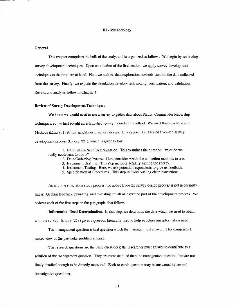
This chapter comprises the bulk of the study, and is organized as follows. We begin by reviewing

survey development techniques. Upon completion of the first section, we apply survey development

techniques to the problem at hand. Next we address data exploration methods used on the data collected

from the survey. Finally, we explain the simulation development, coding, verification, and validation.

Results and analysis follow in Chapter 4.

Review of Survey Development Techniques

We knew we would need to use a survey to gather data about Station Commander leadership

techniques, so we first sought an established survey formulation method. We used Business Research

Methods (Emory, 1980) for guidelines in survey design. Emory gave a suggested five-step survey

development process (Emory, 221), which is given below.

1. Information-Need Determination. This examines the question, "what do we really need/want to know?"

2. Data-Gathering Process. Here, consider which the collection methods to use. 3. Instrument Drafting. This step includes actually writing the survey. 4. Instrument Testing. Here, we ask potential respondents to give us feedback. 5. Specification of Procedures. This step includes writing clear instructions.

As with the simulation study process, the above five-step survey design process is not necessarily

linear. Getting feedback, rewriting, and re-testing are all an expected part of the development process. We

address each of the five steps in the paragraphs that follow.

Information Need Determination. In this step, we determine the data which we need to obtain

with the survey. Emory (218) gives a question hierarchy used to help structure our information need:

The management question is that question which the manager must answer. This comprises a

macro view of the particular problem at hand.

The research questions are the basic question(s) the researcher must answer to contribute to a

solution of the management question. They are more detailed than the management question, but are not

finely detailed enough to be directly measured. Each research question may be answered by several

investigative questions.

3.1

Investigative questions are specific questions the researcher must answer to answer the research

questions. These questions should be directly measurable, but they may be posed in analytical language

rather than language a survey respondent would understand.

Measurement questions include sought data (the information at the core of our questioning),

respondent characteristics (gender, age, education), and administrative information (respondent ID, date,

place of survey, etc.) (Emory, 223). These are the questions the respondent sees, and should be in language

he will understand. The measurement questions directly answer the investigative questions, which the

analyst must synthesize to answer the higher level questions.

Data Gathering Process Decisions. Which methods will be used to gather the data? The

communications procedure (face to face, mail, e-mail, internet), structure level (from free response to

Yes/No answers) and degree of disguise should all be considered. With degree of disguise, we consider

whether the object of our questions will be apparent, or whether we will ask evasive questions and then

"read between the lines."

Instrument Drafting. This step includes actually crafting the measurement questions and

structuring the survey. Items to consider are: logical question sequence, psychological order of questions,

and difficulty-level of questions. The questions should be in some kind of logical order - question order

must not be distracting from actually thinking about answers to the questions at hand. When we consider

the psychological order of questions, we must see if having one question before another affects the answer

to either one. Ideally, each question would be independent of all others. However, if we set one frame of

mind with the first question, we may influence the answer to the second question. When we consider

degree of difficulty of questions, we must work to develop a rapport with the respondent. Some easy, non-

threatening questions should be asked at first, to get the respondent "warmed-up."

Instrument Testing. Once a draft survey is written, the author must get feedback, rewrite, and go

back for more evaluation until satisfied with the results.

Specification of Procedures. Each set of respondents must get a uniform set of instructions so

they are answering the questions with the same reference point. The survey author must draft a set of

instructions, and put it through a similar revision procedure as described before. The instructions should

include, a brief explanation of the goals of the study, instructions for filling out the survey, point of contact

3.2

information, and assurance that individual answers would be completely confidential. This concludes

discussion of general survey development. We now turn to our application of the general survey

development procedures as applied to our problem.

Application of Survey Development Techniques

Having reviewed generic survey development methods, we set out to apply the appropriate

techniques to our problem. Understanding the effect of measured leadership traits on recruiters is a

relatively barren area of research. Exploring leadership factors was a two-part process: first we had to

decide what the factors were and how to measure them; second, we had to devise a method to incorporate

them in the model. In this section, we address evaluation and measurement methods. Incorporation into

the model is explained later in the chapter. As noted in Chapter two, there was little previous work which

measured leadership influences on recruiting. Of particularly notable absence is the answer to the question,

"Which leadership techniques achieve the best results?" We sought answers to this question for Army

Recruiters. This section's organization mirrors that of the previous one; it includes application of the

guidelines for information need determination, data gathering process decisions, instrument drafting,

instrument testing, and specification of procedures.

Application of Information Need Determination. For this step, we needed to determine what

our management, research, investigative, and measurement questions would be.

USAREC comprised the management for the recruiting problem. They wanted to know how we

could increase recruiter efficiency and recruit quality. By increasing efficiency, we believe that we can get

more quality prospects converted to recruits.

For management questions, we wanted to explore what recruiters and first-line leaders can do to

increase recruiter efficiency and recruit quality. We also evaluated which relevant recruiter and leader

attributes we could actually measure and model. In addition to the leadership and personality factors we

wanted to measure, we needed process-duration information about the eight different types of prospects.

By-prospect information falls at the research question level; however it was beyond the scope of the survey

at hand. We depended on USAREC for generation of as much by-prospect data as possible.

3.3

Our investigative questions came next. We needed to know how productive different recruiters

would be under various types of leadership. We measured these effects by adapting two established

behavioral science theories: goal setting theory (measures leadership methods) and the "Big Five"

personality markers. These theories are referenced and explained further in the paragraphs which follow.

We also had to find out how much latitude leaders and recruiters have, within regulations, to change their

work methods and policies; what current policies actually are; and how current policies are implemented at

local levels. For these latest items, some information came from the survey, while some came from

regulations. Here again, we depended on USAREC to supply data which differentiated between the

prospects with different attributes.

We next identified our measurement questions. For leadership aspects, we wanted to know how

recruiters responded to various leader attributes, such as goal setting techniques and policies. As measures

of effectiveness, we measured the number of initial interviews per week and the number of contracts a

recruiter gets in six months. To measure leadership techniques, we used a goal setting framework, which

we modified slightly to incorporate the recruiting atmosphere. Goal setting (Locke and Latham, 1990) is

one of several leading worker motivation theories, and it fit this problem well. We also chose to measure

several recruiting policies, which are sometimes points of contention. USAREC, the sponsor, supported

additional measures: different methods of telephone prospecting, and frequency of training.

We also theorized that there are some recruiters who would excel no matter what their supervisor

or environment is like. The same should be true for those who will always fail at recruiting. To try to

identify these recruiters, we used part of a modern personality theory called "The Big Five (Goldberg,

1998)." The Big Five factors are an aggregation of many personality categorization techniques which have

come and gone over the years. Big Five developers hypothesize that most personalities can be described by

five measures: Extraversion, Agreeableness, Conscientiousness, Emotional Stability, and

Intellect/Imagination. Extraversion deals with how outgoing a person is. Agreeableness deals with how

well a person gets along with others. Conscientiousness involves paying attention, being exacting in work,

and getting things done in a timely manner. Emotional stability deals with mood swings and how much

work stresses a person. Intellect and Imagination measure exactly what a lay person would think they

would. For this study, we chose to use Extraversion, Agreeableness, and Conscientiousness as our

3.4

measures. We theorized that these measures would tell us the most about differences between recruiters.

The completed questions are included at Appendix D. By measuring recruiter personalities, we hoped to

identify recruiters who we could actually influence with varying leadership techniques. Also, we sought to

identify personality types who are naturally more suited to recruiting.

Application of Data Gathering Process Decisions. There were several methods to find which

leadership techniques work best on recruiters. We could have observed recruiters and their leaders, made

observations, and taken notes. However, this would have required much more time than allotted for this

thesis. Therefore, we chose to survey recruiters about their current job performance and leadership. For

this study, we conducted a paper survey, although we had considered conducting a web-based survey. We

did not put the survey on the world wide web since the recruiters do not have internet access. To start with,

we administered the paper survey to the local recruiting company. In addition, we mailed surveys to

recruiting stations in the 3rd, 5th, and 6* Brigades. The question structure is mostly a five-tiered rating

system, meaning that the questions are answered on a scale of 1 to 5.

Application of Instrument Drafting. We organized the survey in the following categories and

began writing questions:

1. Goal Setting Markers

2. Personality Markers

3. Outcomes

4. Demographic Markers

We believed the goal setting markers and personality markers would partially explain the

outcomes (number of interviews conducted and number of successful contracts). The demographic

markers were to be used to create statistical blocking effects. Each of the above categories is described in

detail below, with example questions given for each.

Goal Setting Markers. There were 41 questions in the survey which measured the goal-

setting atmosphere in the recruiting station. The questions were broken down into several categories;

category scores were attained by summing scores for individual questions in a particular category. The

categories were as follows:

3.5

Table 3.1. Goal Setting Markers

KSD: I Know what I'm Supposed to Do

CSG: I have Challenging and Specific Goals

RFG: I have the Resources For my Goals

FBK: I get FeedBacK about my goals

RWV: I am Rewarded With things I Value

Secondary categories

SUP: My boss is SUPportive

ACC: I ACCept that my goals are important.

We theorized the primary categories would show us the most profound effects on outcomes, but

that we might also be able to learn interesting trends from the secondary categories. Each category is

further explained below.

KSD (I know what I'm supposed to do) measures how well a recruiter's tasks are explained and

understood. Example KSD questions are: "I know which recruiting goals take priority," and "My

commander clearly explains my recruiting goals." The theory is that a person is more likely to successfully

complete a task if they have a clear understanding of what they are expected to do. This makes intuitive

sense, and reflects much of the leadership advice discovered in background research.

CSG (Challenging and Specific Goals) measures whether the difficulty level of a recruiter's tasks

is appropriate, and whether specific, tangible, goals are given. Example CSG questions are: "I have

specific, clear goals as a recruiter," and "I am given conflicting recruiting goals by my supervisor(s)." The

theory is that a person will be more likely to succeed if they are challenged at an appropriate level (not too

hard, not too easy), and if they are able to accomplish tangible results. Note that the second example

question is an example of a negatively-scaled question. Being given conflicting goals by the same, or

different, supervisors would detract from the clarity of a person's goals.

RFG (I have the resources for my goals) measures whether the recruiter has the appropriate

amount of training and other resources (supplies, computers, etc.) to accomplish his mission. Example

3.6

RFG questions are: "My station has sufficient resources to accomplish our recruiting goals," and "We have

the right amount of Recruiter Trainer visits to help achieve our goals." The theory is that each recruiter

must have the proper intellectual resources (training) and mission-support resources (office equipment) in

order to complete the mission confidently and efficiently.

FBK (I get feedback about my goals) measures whether the recruiter knows how he is doing in

regard to accomplishing his goals. Example FBK questions are: "My supervisor praises me when I

accomplish my recruiting goals," and "I get regular counseling on how I am doing with respect to recruiting

goals." We theorize that a recruiter will modify their recruiting methods if they receive negative feedback,

in the form of constructive counseling. On the other hand, positive feedback may encourage a recruiter to

do even better, or at least maintain their current production level. The key is that if a recruiter never gets

any feedback, they are operating in a vacuum, and may have poor production simply because they don't

know any better. They will have no idea how they are doing. Feedback can come from many sources, to

include supervisors, peers, self, and statistics. Most of our questions focused on supervisor-related

feedback, since we are interested in the leader / recruiter interaction.

RWV (I am rewarded with things I value) measures not only whether the recruiter is rewarded, but

also if the reward means anything to the recruiter. Example RWV questions are "If I reach my recruiting

goals, I will receive a good NCOER (rating)," and "If I reach my recruiting goals, I will be awarded a

pass." The theory is that if rewards mean nothing to a person, then they do not provide an incentive to

perform well. Rewards must have some tangible benefit to be effective in persuading subordinates.

SUP (My boss is supportive) measures the way supervisors react to problems and encourage their

subordinates. Example SUP questions are: "In counseling, my supervisor stresses problem-solving," and

"My supervisor is not supportive." The idea is that subordinates will probably do better if their boss attacks

the problem instead of the person. Subordinates need to feel that their boss will back them up and support

them as long as they are trying hard at their job. In addition, being supportive may simply include lending

a sympathetic ear.

ACC (I accept that my goals are important) measures the degree of goal-internalization a recruiter

has achieved. Example ACC questions are: "I am encouraged to make suggestions on how we can better

achieve our recruiting goals," and "My supervisor lets me have a say in how I go about accomplishing my

3.7

goals." We theorize that participation may foster better acceptance of goals, and of the methods used to

accomplish goals. Personal experience has shown that subordinates will be willing to work harder if they

believe in the validity of the goal, and that their opinion has been registered with the supervisor.

Personality Markers. We used the "Big Five" personality markers as described by

Goldberg as a starting point for our personality assessment. Recall that the "Big Five" were extraversion,

agreeableness, conscientiousness, emotional stability, and intellect / imagination. We chose to only

measure three of the five markers: extraversion, agreeableness, and conscientiousness. We theorized a

basic level of emotional stability was a prerequisite to military service. In addition, we thought the

emotional stability questions would be more sensitive items for most people. This sensitivity could cause

discomfort in answering the survey. In addition, we did not want to have a repository of sensitive personal

information when we really did not need it for our research. We decided to not include intellect and

imagination in the survey since the recruiting process is very structured, and creativity/imagination

(departing from guidelines) is not encouraged. In addition, we knew that to get promoted to Non-

Commissioned-Officer, recruiters had to meet certain intellectual standards. While recruiters do not have

to be brain-surgeons, they have completed several promotion screening processes. This is not to say that

there are no sub-standard recruiters; there are sub-standard performers who slip through in every

profession. However, we believe most recruiters are reasonable intelligent and competent. Having

eliminated emotional stability and intellect/imagination, we were able to focus on the remaining three

personality markers.

Extraversion measures how outgoing a person is. Example extraversion questions are: "I feel

comfortable around people," and "I keep in the background." (Note the second statement would be scored

on a negative scale.) We theorized good recruiters would be outgoing and gregarious. They would like

talking to prospects, telling them enthusiastic stories about the Army, and convincing them to join. The

recruiter's job requires constant interpersonal contact; anyone who is withdrawn and shy would probably

have a harder time at recruiting than would an outgoing person.

Agreeableness measures how well a person gets along with others. Examples of agreeableness

questions are: "I insult people," (negatively scored) and "I make people feel at ease." An agreeable

disposition would enable recruiters to create a welcoming atmosphere for prospective recruits. In contrast,

3.8

a bitter continence would likely turn-off prospective recruits. While recruiters should not have to be

extremely "touchy-feely," (they are in the Army, after all) they should at least present a non-hostile

atmosphere to prospects.

Conscientiousnsess measures how dedicated to work a person is. Example conscientiousness

questions are: "I am always prepared," and "I waste my time" (negatively scored). Although a recruiter's

schedule is heavily dictated, the degree to which they follow their schedule is largely up to the individual.

In addition, the efficiency of each hour worked could vary greatly depending on how many breaks were

taken, how many solitaire games were played, etc. We thought the conscientiousness markers would do a

good job of measuring these qualities.

Outcomes and Demographic Markers. We chose the number of initial interviews per

week and the number of contracts per six months as the primary survey outcomes. According to the

Dayton Company Commander, CPT DeZienny, the recruiters would be familiar with the number of initial

interviews conducted per week, and the number of contracts achieved in the last six months. Because they

must report them on a regular basis, these statistics are on the tip of a recruiter's tongue, and do not require

extensive estimation. The demographic markers used are given below:

Table 3.2. Demographic Markers

Recruiting station name Does the station regularly make mission? Number of months as a recruiter Are they a career recruiter (79R) or not? Are they a station commander? Number of hours worked per week Number of times a month the work week exceeds five days Pay grade Gender

The above demographic markers made intuitive sense, and should not require extensive

explanation. Prior to finalizing the survey, we formulated a detailed plan for how we would use the data

gathered. This helped the data collection process, because we mapped where each piece of data would fit.

We also examined how we would get from raw data to data usable in the model. This process helped

3.9

eliminate unneeded questions, and also identified the need for several additional questions, which were

used to help tie data elements together.

Upon completion of writing the measurement questions, we had to decide how to employ them.

Items we considered were: logical question sequence, psychological order of questions, and difficulty-level

of questions. We wanted the questions to be in some kind of logical order since question order should not

be distracting from actually thinking about answers to the questions at hand. We considered the

psychological order of questions, and tried to ensure that earlier questions did not bias later ones. We

considered degree of difficulty of questions, and put easily-answered questions up front to help develop a

rapport with the respondent.

We eventually broke the measurement questions into three parts, General Information, Leadership

and Recruiting Goals, and About Yourself. General information covered some training issues, as well as

general items which did not fit elsewhere. Leadership and Recruiting Goals included questions designed

after the goal setting questionnaire described earlier. About Yourself covered personality traits using the

"Big Five" personality markers as a framework. In addition, About Yourself 'measured several demographic

and performance markers. We wrote and re-wrote the survey until representatives from USAREC and

AFIT were happy with it. The complete survey is given in Appendix D.

Application of Instrument Testing. We wrote several drafts of the survey, received feedback,

rewrote, and went back for more evaluation. The thesis committee served as the first line of survey-

reviewers. In addition, we enlisted the help of MAJ Paul Thurston, a survey expert, from the AFIT

Logistics School and MAJ Robert Fancher (USAREC) to critique the drafts. Next, we visited the Dayton,

Ohio Recruiting Company Commander and asked him for advice on survey content, design, and clarity. At

each step, we re-wrote until satisfied with the result. Finally, we administered the survey to a group of 30

recruiters and station commanders from the Dayton, Ohio Recruiting Company. We used the data gathered

from the Dayton Company as an initial data set. In addition, we asked the recruiters for recommendations

on the survey, and implemented several minor changes which improved survey clarity. Upon finalizing the

survey, we mailed it to all recruiting stations from three randomly selected battalions, one battalion from

each of the Third, Fifth, and Sixth Brigades. We hoped that by spreading out our sample among the

brigades, we would get a wide variety of leadership to draw from.

3.10

Application of Specification of Procedures. We wanted to ensure each set of respondents

received a uniform set of instructions. We drafted a set of instructions, and put it through a similar revision

procedure as described before. The instructions included a privacy act statement (required by the military),

a brief explanation of the goals of the study, instructions for filling out the survey, point of contact

information, and assurance that individual answers would be completely confidential. This concludes

discussion of survey development. We now turn to data analysis methodology and simulation

implementation.

Data Analysis Methodology

Data for this simulation fell into several categories. First, there was data which had been gathered

in the prior simulation study and by USAREC. Second was data gathered using the survey in this study.

Finally, there was the data which described different processing times and probabilities depending on

prospect type. We first address the most difficult problem: examining the survey data. Analysis of the

remaining data is described in the second half of this section. Detailed data analysis is reserved for Chapter

4.

We gathered data using the survey in two sets. First, we administered it to approximately 30

recruiters from the Dayton, Ohio Recruiting Company. This initial administration did two things for us.

First, it gave us data to begin examining. Second, it was an opportunity to test the survey, and make minor

modifications based on recruiter input. After we made the final modifications, we mailed the survey to all

the companies in three battalions, selected at random from the Third, Fifth, and Sixth Recruiting Brigades.

In total, we sent out over 500 surveys. We desired at least 200 responses. USAREC indicated that they

were historically able to get an approximate 55% return rate on surveys with a one-month turn-around. We

only had about a month to meet the study timeline, so we sent out a little over twice as many surveys as we

thought we needed. We chose to send the surveys to battalions from different brigades to attempt to

capture more of the variation in leadership and station policies. In the end, several administrative problems

prevented us from mailing, collecting, and analyzing the second set of surveys in time for inclusion in this

study.

3.11

Upon gathering the data, we entered each respondent's replies (coded from -2 to 2) into a row in a

Microsoft Excel spreadsheet. We coded the responses with their marker type (KSD, RWV, etc.), added a

response number (1-30) and then sorted the responses by marker type. Then, we summed scores for each

marker type, making sure to take into account the negatively-scored questions. These summed marker

scores were exported to another sheet in the Excel workbook, and were used for most of the analysis. The

marker, outcome, and demographic scores for the first 30 surveys are shown on the following page as an

Excel spreadsheet. Note the major headings, with marker sub-headings, across the top of the spreadsheet.

Each row consists of scores for a particular respondent.

With an extensive database about leadership, policies, and personality, we regressed numbers of

initial interviews and contracts achieved against all other factors in the database. We used SAS JMP (a

windows-based statistical analysis package) and MS Excel to conduct our data analysis. JMP helped with

regression analysis and descriptive statistics, while Excel was good for data manipulation. The goal of our

regressions was to determine which factors affected our outcome variables (interviews and contracts). If

we knew the degree to which certain factors improved the number of contracts achieved, we could attempt

to implement leadership methods in accordance with the factors identified. In addition, it seemed intuitive

that if a recruiter had more initial interviews, he should get more contracts (we assumed some correlation

between success in interviewing and success in contracting). Therefore, if we could discover which factors

increased the number of initial interviews, we could increase the interview rate in the model and observe

how the output (contracts) changed.

Simulation Methodology

There were several objectives in the simulation part of this study. First, we wanted to incorporate

data from the leadership and personality research we had conducted. Second, we wanted to be able to

include different data for different types of prospects, based on gender, ASVAB score, and high school

graduation status. Third, we sought to incorporate the above items into the current model in the most

efficient manner possible. Finally, we desired to make the model as user-friendly as possible, so the

sponsor could actually use it for further studies. This section is organized as follows. First, we examine

the previous model. Next, we examine the form of the data we needed to incorporate. We then

3.12

CO CO

japuaö "

2 2 2 2 2 2 2 S5S55225S5521L555555SS5 9PBJQ ÄEd

lD(0(0<OlI)MO<DNMI)lD(DT3IOS(D(010(ONMO(D(OMn(Oin(D LIJWWWWWUWWWWWWWWWWWWWUJIIJLULLJLUWLJJUJLLILJJ

<J3 jp^ gjq OOOOOI-OOOT-OOOOOT-OOOOOOOOOOOOOT-

CB 5 O 11„,OOOOOI-OOOI-OOOOOI-T-I-00000000000'>- 2 doi Q. CO o nau QP Qiiiiinmi u)cNio-jrocpNC\ioowcoir>coi^cvioo,-oNcowcocoi£5wcoi^c\ico

0) o Q ■= hai|IOB'-'-'-N*'-OOi-rNi-0*Nr«|i-i-NrT-T-N<tBti- CO UuJJ i i i ■ ■ ■ ■

"O O

CO baj-l CDI^'D'*<OWCNlCOCOOCO'*C\l-*ir)C\10JCOCOCOT-tO-i-T-COin'*'*'*CO

D) c h- Q. AOBOIU^ ■t**'-*wo(otir)(DO)*cscowT-mnn(onnwcMiDco^(0(D

Q. iirMciajonv^ U)NncOi-l»(I)»0100n04Nn010SNOSrNc900nT-lD

CO UUlOJOACjjA^ It I T- T- T- T- t— T- 'T- 'T- T~ T~ T~ '

o 1_ CO 2 snouueiOSUOO »»""nmo^MocDwincoowNr-^nfflOMnoNmcoNOO)

CO 2 § sseU9|qp99jßv coNr-^ffl^ifl^o^cD^coiocor-coosionN^oinmco

0 Q- CC ._„ cMwionoT-tt-itm^ocM^CMO^w^coco^i-i-T-NT-too^n >, dflS ■ i ■ i ■ iii ■ CD | zi AMU ■ ■ ■ i— ■ i— -w— ■ > ■ -I-1 J2 CO CO •c

CO rMuW<tOT-OCOWtMO(DUS(DCM^mCDi-r-COmT-n*COCDN>-(DT- «■' f-}-4H i i I I I I I I II I I I I I i II OdH

<B no\j uiwtT-N^i-oioMnu)T-oiDN'->-'ifnnncoooinu)coiint (Jb/l I I I I I II T—

IMCC) C0OO<0U)C0't(D*NNOr-'!f^OO4r-S1-U)U)*^C\INt0mr-

2 MO ,T-WT-COC\1C\1COC>10100T-COOJC\ICNIOLOCO-I-COT-OC\IO-I-C\IC\ICOOJ CD >lSd i i . i it

cB

C3) QSO ■ ■ i ■ ■ . i . i i c t: CD

— OOV ■ i i i i • i . i i co V o ' (3

UOjSSjlfl VTT-,-TT0,-T0VCVCVC>ICVCVC>IC>,C>I'7CVCVCV0000T7VV

SDUX99AA WCOCOCOtinCOCOCOCOCOit'*CO'a--*'<t'*-*COCOCO'*'*-*CO'*COCO-*

einni lOOLOOOWOOOOOOOOOOOOOOOOOOOOOOOin

S10BJ1U0O Oi-ONonNiocooiDcoinniflocotnT-cDcoNWO^cocoMn

CO CD

S *'ojc\ico cococoriirico

o a|QLUBS ,_ pj ,_ pj i- CM i-T-i-^CM *- CM CM Od CM i-OJ T- CM CO

conceptualize implementation methods, followed by actually coding the implementations. We next address

verification and validation, although this occurred throughout the entire process. In Chapter 4, we design

the experimental settings, run appropriate replications of the model, and collect the output in preparation

for output analysis.

Examining the Previous Model. The previous model was written in SIMPROCESS, an icon-

based process modeling tool. Benefits of this tool are built-in statistics and graphics, as well as relative

ease of use. As we will see later, the price we pay for ease of use is some loss of flexibility.

SIMPROCESS is a hierarchical simulation package. This means a process may be broken down into

several macro-level processes, each with multiple levels of sub-processes. The top level of the previous

simulation is shown below.

R3 applicants RBSaies R3Processing R3Depsustäinment'

Figure 3.1. Top-Level SIMPROCESS Model

In looking at the top level network, we are able to get an idea of the general processing method.

Prospects can enter the system in one of two methods: they can either walk-in off the street or they can

3.14

come in for an appointment, as a result of recruiters conducting prospecting. Upon arrival to the station,

each prospect is assigned a recruiter, and goes through initial sales, processing, and DEP sustainment. This

simplified view agrees with the recruiting station workings outlined in Chapter 2. There are three parallel

processes, with each denoting a different "type" of recruiter (depending on experience or other factors).

Note the square folders shown in the macro-level view above. Each folder, or process, contains a sub-

network, each sub-level containing more detail than the next. The rest of the previous model is included at

appendix A, Model, for reference.

In considering implementation methods, we must understand some of the syntax and

implementations of the previous model. Entities (prospects) are created and travel through a network of

nodes (servers and queues) based on the framework the programmer establishes. Basic entity routing

through the network is accomplished with conditional branches (the three-branched symbol in the chart

above). Recruiters are designated as resources for this model, and prospects compete for the limited

recruiter resources based on a priority system. Variables are generally modified through the use of

expressions. Expressions are user-written code, implemented at various points in the process, but mostly

either when an entity enters or leaves a node. The syntax for expressions is based on a subset of MODSDVI.

One of the inherent weaknesses of SIMPROCESS is that the MODSIM subset used does not support

arrays, which would have simplified the programming effort greatly for this study. A strength of

SIMPROCESS is that it allows the programmer to simply drag and drop the network onto the workspace.

In addition, graphics are built-in so the analyst can watch and troubleshoot as entities process.

Intended Modifications. We set out to modify the existing model to incorporate the additional

data from the study to this point. Specifically, we needed to incorporate leadership factors for station

commanders, personality factors for the recruiters, and attributes for the eight types of prospects. We

wanted to be able to enter a few personality traits for the station commander, as well as personality traits

for the recruiters, to see how these factors would affect model throughput (number of contracts achieved).

For the eight prospect types, we wanted to be able to have different processing times for each type at each

stage of processing. In addition, we wanted each type to have different probabilities of dropping-out at

each stage. Finally, we wanted to see how many of each type of prospect actually made it all the way

through the process, tracked on a monthly basis.

3.15

Conceptual Implementation of Modifications. In this section, we explore conceptual methods

for implementing our intended modifications, from the above paragraph. First we consider the leadership

and personality factors, followed by the eight prospect types.

For the leadership and personality factors, we analyzed the data to determine if the factors had an

effect on various parameters in the model (such as number of initial interviews.) If the leadership and

personality factors had an effect, we added an appropriate multiplier to the affected parameter. For the

previous model, the durations of most processes were determined by a random draw from a triangular

distribution. Triangular distributions require three parameters: mode, minimum, and maximum. If a

station commander had the effect of making recruiters more efficient at a particular process, we could

implement it in the model by decreasing the triangular distribution's parameters by appropriate amounts.

The same type of modification applied for recruiter personality traits. Basically, we applied a series of

multipliers (based on leadership and personality regression equations, explained in chapter 4) to the values

of the triangular distribution's parameters. This allowed the leadership and personality traits to influence

the random draws which determined processing times and drop-out probabilities. In the end, we calculated

the effects of leadership and personality in a Microsoft Excel pre-processor interface, which automatically

supplied a text input parameter file to SIMPROCESS. Excel calculated the adjusted parameter values, and

fed them to the simulation. Basic development of the pre-processor is given in this chapter, while analysis

of the data for this front end is given in Chapter 4. The spreadsheet is shown in Appendix B, Summary of

Model Changes.

Methods for implementation of the eight prospect types required considerably more thought and

deliberation. In the beginning we believed we could elegantly implement the different attribute values by

using an array to store the parameters for each type of prospect. This would have entailed assigning each

entity a prospect type, from one to eight. As the entity made its way through each process, the process

would query the entity for its type. The simulation would then conduct appropriate random draws based on

the parameters associated with that prospect type.

Since USAREC had purchased SIMPROCESS for the previous study at considerable expense,

they were interested in using SIMPROCESS for this study as well. There had been a memory limitation

problem when running a large number of replications of the prior simulation in SIMPROCESS. However,

3.16

when we installed the latest update of SIMPROCESS, it ran multiple replications of the prior simulation

without any problems. When compared with gathering the data, coding the simulation appeared relatively

easy. There were several minor limitations, which we worked around. The largest limitation was that

SIMPROCESS does not allow the user to define arrays. Arrays would have been a very elegant way to

differentiate between processing times and drop-out probabilities for the eight different types of prospect.

For any given process, the time could have been specified in a manner such as:

ThisProcessingTime = InterviewProcessingTime (p),

Where p would be an integer from 1 to 8, which identified which type of prospect was being

handled. Without the use of arrays, we were forced to use less elegant (and less efficient) nested if-then

loops.

We now turn to our method of differentiating between prospective recruit (prospect) types. To be

able to differentiate between grad/seniors, high/low ASVAB scores, and male/female genders, it is apparent

that there are eight (2A3) categories of prospect:

Table 3.4. Categorization of Prospect Types

Prospect Category

Grad (G) / Senior (SR)

ASVAB (High/Low)

Gender (M/F)

1 G H M 2 S H M 3 G L M 4 S L M 5 G H F 6 S H F 7 G L F 8 S L F

Cordiero & Friend (1997) collected data for various performance characteristics (time to conduct

an interview, time needed for paperwork, etc.) for the average prospect. They used average prospect data

to define most service delays and dropout rates in their computer simulation model. Ideally, we would be

able to collect similar data for each of the eight prospect categories shown above.

We used several data collection methods to determine the differences in parameters for the

different recruit types. We requested all data needed from USAREC headquarters. USAREC was able to

provide probabilities of going from one step to the next, broken down by ASVAB score and graduation

status. We also thought we might get some by-prospect data from the Dayton Recruiting Company,

3.17

however, there was no existing record which included task durations. MAJ Robert Fancher, our point of

contact at USAREC, has indicated that all recruiting stations will be equipped with laptop computers within

the next year. Software included with the computers will allow electronic tracking of each step of the

recruiting process for future recruits. Future analysts will be able to generate a database with the

electronically-gathered information, and query it for data such as the distribution of initial interview times

for male seniors with high ASVAB scores.

While collecting the data, we searched for trends. For example, if the initial interview always

seemed to take about the same amount of time for all prospect types, we could to model this with a single

number instead of eight. In addition, if a certain prospect type seemed to take longer at every step in the

recruiting process, we could use an average duration, combined with prospect-type-multipliers to vary

modeled times. Anything we were able to do to reduce the dimensionality of the problem was very helpful.

Given three recruiter types, eight prospect types, 17 delay or dropout types (from the previous model), and

three values (low, mean, high) to describe each parameter, we needed to handle over 1200 variables.

(3*8*17*3 = 1224).

We considered several methods to get around the no-array limitation of SIMPROCESS. Methods

considered included brute force (explicitly declaring a different variable for every possible parameter), and

several methods of modeling the variations through simple formulas. One example of modeling the

variations would be if a certain prospect type seemed to take longer at everything. We could just assign

that prospect type a multiplier, which would be applied to every process as it went through the model.

Another method we considered was to conduct data analysis on by-prospect processing data and then

implement variations only for the parts of the data which actually varied. However, the availability of by-

prospect data was very limited. Recruiters do not currently maintain a record of task duration for the

recruiting process. USAREC is in the process of deploying personal laptop computers to each recruiter,

which will include software to gather task duration and other data for each prospect. With the advent of

computers for every recruiter, there should be plentiful data available for analysis in the future. Since by-

prospect data was currently largely unavailable, we chose to implement the coding method which allowed

the most flexibility: the brute force method. We explicitly declared a separate variable for each possible

parameter for each of the eight different prospect types. This method was not elegant, but it worked!

3.18

Coding the Modifications. The leadership and personality calculations were performed in

Microsoft Excel while the by-prospect implementations were coded within SIMPROCESS.

Excel leadership and personality calculations. The coding requirement here was to

modify the input parameters which station commander leadership traits and recruiter personality traits

affected. We knew that the variation in service times was affected by two general groups of influences -

those which we had measured, and those which we had not. The influences we were not able to measure

are accounted for in the model by using random draws to accomplish variation. For the measured

influences (station commander leadership and individual recruiter personality traits), we sought to

determine the effect on model output, as well as individual process service times and dropout rates. We

designed the survey to measure two main output variables: number of interviews per week and number of

contracts in the last six months. We theorized leadership and personality should have some measurable

effect on these two outputs. Later in the study, we realized it would have been ideal to measure all process

times (1998 survey) concurrently with leadership and personality influences (1999 survey). After an

exhaustive but futile search, we were unable to obtain 1998 survey data for the Dayton Recruiting

Company. Therefore, we chose to use real data from another Brigade for the 1998 data - this meant there

was only a notional correlation between the two data sets. While this situation is not ideal, it did enable us

to come up with a methodology for correlating the two surveys and subsequently using the results.

We began by investigating the correlation between our measured outcomes (interviews and

contracts) with the measured influences (leadership and personality). We used SAS JMP to conduct the

analysis. The details of this process are presented in Chapter 4. With the data entered into JMP, we

conducted stepwise regressions to identify those parameters which influenced an outcome variable. We

began with linear models and achieved lower explanatory power than generally seen in statistics courses.

The adjusted R-Square value from the regression gave us a good idea how much of the variation was

explained by our linear regression model, and how much was still unexplained (random for our purposes).

Our R-Square values of .3 meant we were explaining about 30% of the variation of the outcome variables

with leadership and personality factors. We then explored interaction models - we wanted to see if we

could explain more by examining the interaction between various leadership and personality factors. While

it seems intuitive that leadership and personalities would indeed interact, with the limited data set (we had

3.19

26 respondents), the additional explanatory power of interactions was overshadowed by loss of degrees of

freedom, and thus a lower adjusted R-Square value. Therefore, we chose to use a linear, no interaction

model for interviews per week and contracts per six months.

We next performed a similar regression analysis on the 1998 process time survey data, which was

notionally correlated with the 1999 leadership and personality survey data. We did stepwise regression to

establish linear models for this data as well. Here again, we examined a few interaction models but the loss

of degrees of freedom negated any additional explanatory power. Therefore we used linear models to

explain the process-time outcomes. Identifying the need to collect both sets of data concurrently is an

exciting concept. Many of the outcomes of the process-time survey can be directly fed to the model.

Therefore, if we are able to see how they are influenced by leadership and personality, we can easily make

the appropriate parameter modifications in Excel. It is important to remember that our notional correlation

only allows us to explore data analysis methods for connecting the 1998 and 1999 surveys. We cannot

make any powerful inferences from the results since any relation between the two surveys and their values

is incidental.

With the regressions complete, we made an Excel pre-processor interface. This spreadsheet

consisted of several parts - a base data set for all model parameters, a matrix of regression information, and

an output section. The base data set was based on analysis of a large database generated by USAREC with

the 1998 survey, as well as other data provided by USAREC (see Chapter 4). The matrix of regression

information was generated using the regression information described above. The output section was

generated by modifying the base data with the regression information. A simple example is given below,

and additional details are presented in Chapter 4. These parameters are for the average prospect; they are

not yet broken-down by prospect type.

Given: Base mean amount of initial interviews per week = 2.5 hours

Influences: KSD -.095

Conscientiousness .16

Extraversion .08

R-Square .315

Output: Mean interviews = 2.5 + (-.095*AKSD + .16*ACONSC. + .08*AEXTRA)

3.20

In the example above, A<parameter name> denotes the deviation of the given parameter from its

mean. Note that we want to break the variation, which was previously all modeled as random, into two

parts. Now, we vary the parameters so that part of the variation is due to leadership and personality, while

part is still due to randomness. Given a set of hypothetical leadership and personality attributes, it is easy

to see how we can modify model parameters with such a process. This concludes the methodology of the

Excel front-end. The spreadsheet itself is given in Appendix B, while detailed development is shown in

Chapter 4.

By-Prospect Coding. Coding the brute force method for prospect type differentiation

required several steps which were repeated tediously many times. For each parameter we chose to modify,

we had to declare it as a variable, read it into SIMPROCESS, assign it to the correct entity variable, and

modify the code to use the entity variable. To declare each parameter, we used the <define> tab in

SIMPROCESS. For each parameter, we had to define eight global variables (one for each prospect type)

and eight entity variables. We defined each as a real number, assigned any appropriate default values, and

lettered the seven duplicates from B to H. The <copy> command was very useful in making seven copies

of each variable. For each global variable, we appended a letter from B to H on the end of the variable

name.

To read the data into SIMPROCESS, we used a <read from file> command within the "start

simulation" expression in the walk-in creation node. The general format was already defined in the

previous simulation. The code defined the input file and then read the data sequentially, line by line, into

the correct variables. We made seven additional copies of the data-reading code, and went through the

code, appending each variable name with the appropriate letter (B through H, as discussed in the paragraph

above). This might have been a simple search-and-replace routine, however we did each variable one at a

time as we made modifications for Recruiter 1. This allowed a short run of the simulation with each

modified variable to ensure the changes were error-free. For the second two recruiters, we did many

variables at a time, since we were confident the coding method was good. We deleted a few data lines

which did not depend on prospect type. We then modified the input file (varvals.txt) to include seven

3.21

additional copies of the base case values, with the appropriate lines deleted to match the data-reading code.

Each variable read in this manner was a global variable.

To assign the by-prospect data to each entity, we used a large if-else statement within the

transform node expression for each recruiter type. The if-else statement generated a random draw to

determine prospect type, and then assigned each entity variable the appropriate value from the global

variables which had been read-in previously. To conduct the random draw, we used a random uniform

distribution, and assigned prospect type based on the proportion of prospects in each category. We used the

following proportions based on data given by USAREC:

Table 3.5. Proportions of Prospect Types

Proportion Probability Values Gender High School ASVAB .09 0.00 < X < 0.09 M Senior Low .03 0.09 <X< 0.12 F Senior Low .21 0.12<X<0.33 M Grad Low .03 0.33 <X< 0.36 F Grad Low .15 0.36<X<0.51 M Senior High .04 0.51 <X< 0.55 F Senior High .34 0.55 < X < 0.89 M Grad High .11 0.89 <X< 1.00 F Grad High

Note that assigning all parameters to each entity means there are numerous copies of the same

parameters being stored simultaneously in the model. This increases model overhead and reduces

efficiency. When we ran the model, runtimes were drastically higher with all the logic and overhead of

differentiating between the different prospect types.

With the parameters read-in, variables declared, and parameters assigned to entity variables, we

needed to modify the code to use the appropriate entity variable instead of the global variable. In declaring

entity variables, we maintained consistency with the names of the global variables. Therefore, in most

places, we were able to simply replace Model.<parametername> with Entitv.<parametername>. We

had to be careful to find every place in the model that each parameter was used, but otherwise, this was

fairly repetitious. This completed modification of the model to incorporate by-prospect data.

3.22

Verification and Validation. Verification is the process of making sure the model is coded

correctly, while validation ensures the model algorithm matches the real world. We conducted both

processes during all stages of this study. We verified the code was correctly implemented as we wrote it,

and we re-verified the algorithm of the previous model by re-checking it against Army recruiting manuals

and recruiting experts.

We first address verification. As we modified each piece of code, we used an output statement to

verify the code was doing what we thought it would. We changed a single set of parameters, included

output statements, ran the model, and watched the output. The output statement caused a small text

window to pop up as the simulation ran, and the requested output was displayed. If any output looked

suspicious, we corrected the code or looked for a reason the output was doing what it was.

The automatic animation feature of SIMPROCESS was particularly helpful in troubleshooting and

verification efforts. Not only does the animation show the entities making their way through the system, it

also shows a count of the number of entities at every node. Therefore the programmer is able to check the

model for bottlenecks by observing the node populations. If too many entities are in a particular node or

system, the analyst has the opportunity to check the model logic and input parameters to see what is

causing the bottleneck. Since each entity carried with it a large amount of data, we wanted to generate only

as many prospects as it took to keep the recruiters busy. In the 1998 model, there had been a huge pool of

prospects waiting for the recruiters to prospect them (as there assumably is in the real world.) For the

current model, we reduced the size of this pool drastically, which had the effect of cutting model run time

by over half. To make this change, we disposed of entities which had been in the pool for over 20 days.

This did not affect model realism, or processing of the prospects who entered the system, it simply reduced

the program's overhead.

We also used the previous version of the simulation as a sanity check. We used the previous

model's parameter values as default values for the updated model. We set all eight copies of each

parameter to the default value. Thus, the previous model and the current model had the same values for

each parameter. Then we ran both simulations and compared the output. The results were similar, and are

analyzed in Chapter 4. This confirmed that our modifications had not corrupted the model logic.

3.23

We conducted validation efforts as well. The previous model was well-validated, however, we

sought confirmation for the purposes of this study. We made a more streamlined process-flow diagram

(shown in Chapter 2) and compared it against current Army doctrine (AR 601-98). In addition, we

consulted our POC at USAREC, MAJ Robert Fancher. MAJ Fancher confirmed that the basic flow and

assumptions of the algorithm were correct. Finally, we compared model output with actual recruiter

contracting data from the real world. The results were favorable. Again, detailed results are shown in

Chapter 4.

Output collection. We used a simple WRITE statement to write the statistics of interest directly

to a text file. SIMPROCESS has automatic statistics collection, which we also used. However, using the

text file allowed direct access to the numbers. We were then able to import the numbers into Excel and

JMP for analysis. The main statistic we were interested in was the monthly number of contracts achieved,

broken down by type of prospect and recruiter type. In addition, we collected selected data on where

dropouts occurred, utilization rates, and times in system of recruits.

Summary

In this chapter, we covered the methodology behind the study. We began by reviewing survey

development techniques. We then applied survey development techniques to the problem at hand. Next

we addressed data exploration methods used on the data collected from the survey. Finally, we covered

simulation development, coding, verification, and validation. With the methodology exposed, we turn to

Chapter 4 for input analysis, survey analysis, initial simulation output analysis, experimental design, final

simulation output analysis, and interpretation.

3.24

Results and Analysis

General

This chapter is divided into three main parts. First, we explore analysis methods for implementing

the survey data and ancillary data into the model (input analysis). Second, we formulate an experimental

design and run the model. Finally, we present and analyze the simulation output.

Input Analysis

This section is broken-down into two parts: analysis of the surveys, and analysis of additional

supporting data. As background, we first describe the ideal data set, and then review the data available.

The ideal data set would include (for each prospect type):

Table 4.1. Ideal Data Set (by prospect type)

1. Probabilities of dropping out at each stage of the recruiting process

2. Duration parameters for each stage of the recruiting process

3. Station Commander leadership influences on each step of the process (durations and probabilities)

4. Recruiter personality influences on each step of the process

5. Proportion of each prospect type entering the system

6. Recruiter priorities for each step

** Each with enough sample points for statistical significance

In the 1999 survey, we gathered data on numbers 3 and 4, above. We gathered as much of the rest

of the data as possible from existing databases. The data set we were able to assemble was robust in some

areas, and relatively sparse in others. A summary of the real world data we assembled is given below.

4.1

Table 4.2. Real World Data Set

1. Probabilities of dropping out at selected stages of the recruiting process broken down by graduation and ASVAB status (not gender) from the 1998 survey

2. Duration parameters for each stage of the recruiting process on average (not broken down by prospect type) from the 1998 survey

3. Station Commander leadership influences on interviews and contracts: 26 sample points* from the 1999 survey

4. Recruiter personality influences on interviews and contracts: 26 sample points* from the 1999 survey

5. Proportion of each prospect type contracted (not entering) the system from USAREC

6. Recruiter priorities for each step from the 1998 survey

* We address the effect of leadership and personality on the other parameters later this section.

The 1999 surveys gave us an idea how station commander leadership attributes affected various

parameters. Supporting data gathered included recruiting conversion data, prospect demographic data, and

average processing times. Conversion data showed how many prospects made it past several checkpoints

in the recruiting process (and how many dropped out). Prospect demographic data defined the proportions

of the eight prospect types entering the model. Average processing times (for an average prospect) for

various steps in the model came from the 1998 survey.

Analysis of 1999 Survey Data. We analyzed the survey data using SAS JMP. We calculated

basic descriptive statistics and conducted stepwise linear regressions. We calculated descriptive statistics

so we could find the average, variation, and range of our responses. Descriptive statistics also allowed us

to look for outlying data points and decide what to do with them. The intent of doing linear regressions

was to establish a linear relationship between the outcome variables and the markers. We knew that any

factors we could come up with would only account for part of the variation in recruiting production.

Through regression analysis, we hoped to find some linear combination of our markers which would

4.2

explain as much of the variation as possible. We imported the data into Excel for initial processing, and

then transferred it to JMP for statistical analysis.

For initial processing, we identified the questions which related to like parameters (recall the

survey was designed with multiple questions contributing to each trait.) We then summed the scores for

each group (such as ACC, CSG, or CONSC) and placed the resultant values on a separate worksheet. We

would use these summed scores for the rest of our analysis. For future analysis, the user should only need

to enter the raw data and then drag the summation formulas as appropriate in the summed score worksheet.

We next examined basic descriptive statistics for our parameters. The descriptive statistics were

calculated using SAS JMP's <Analyze> <Distribution> tab. A table of applicable results is shown below.

Table 4.3. Results of Station Commander Leadership / Recruiter Personality Survey

Response Mean Standard Dev. Minimum Maximum Interviews / Week

3.59 1.42 0 7

Contracts / 6 Months

4.96 3.87 0 13

ACC 0.86 2.48 -5 6 CSG .58 1.65 -2 4 FBK 1.12 1.84 -3 5 GSM 2.5 2.96 -4 7 KSD 1.92 3.39 -5 10 RFG -.88 3.84 -8 6 RWV 2.88 6.13 -11 16 SUP 1.5 2.93 -4 7 AGREE 7.69 5.73 -6 18 CONSC 7.08 4.0 0 17 EXTRA 5.08 6.42 -13 14 EFFIC 3.0 4.76 -9 11

Looking at the table of results shown above, we see that there was a lot of variation in the

responses since the standard deviation was high. This indicates that we covered a wide variety of

leadership and personalities, which is just what we wanted. With a wide variety of responses, we are able

to explore many different leadership and personality settings without extrapolating outside our data set.

The minimum and maximum values bound the region we used later in the simulation settings. We also

used the descriptive statistics to look for outlying points. What we found was that the four station

4.3

commanders (who had also taken the recruiter survey) were all outliers, most likely since they must

perform many other duties beyond just recruiting. We chose to eliminate the station commander

production data from the data we analyzed. Therefore, our statistical analysis is based on the responses of

26 recruiters, none of whom are station commanders. This completes descriptive statistics and leads to

regression analysis.

Next, we wanted to identify the factors which affected our outcome variables. We wanted to see

which of the measured leadership and personality factors affected interviews and contracts. Stepwise

regression allowed us to only enter significant factors into the model. It acted as a screening process to

eliminate factors which did not affect the outcome variable of interest. First we standardized the regressors

by subtracting the mean and dividing by the standard deviation. Standardization puts the regressors on the

same (unitless) scale to allow more meaningful comparisons. Then we regressed the number of interviews

per week against leadership markers and recruiter personalities. Next we did the same for number of

contracts in the last six months. What we found were weak linear relationships, however, this was to be

expected. From the outset, we thought the leadership and personality factors could only explain a small

part of the variability in production. A table of applicable results is shown below. Some results are non-

intuitive; we theorize reasons in the following paragraphs.

Table 4.4. Interviews and Contracts Regressed by Leadership and Personality

Leadership Markers Personality Markers

Response R-Sq Int ACC CSG KSD RFG SUP CONSC EXTRA EFFIC

Interviews,

SSquares

.31 3.64 -.34

2.36

.64

8.52

.50

5.88

Contracts,

SSquares

.36 5.39 1.09

15.6

1.19

23.1

-1.40

27.3

-2.86

105.7

1.97

50.4

4.4

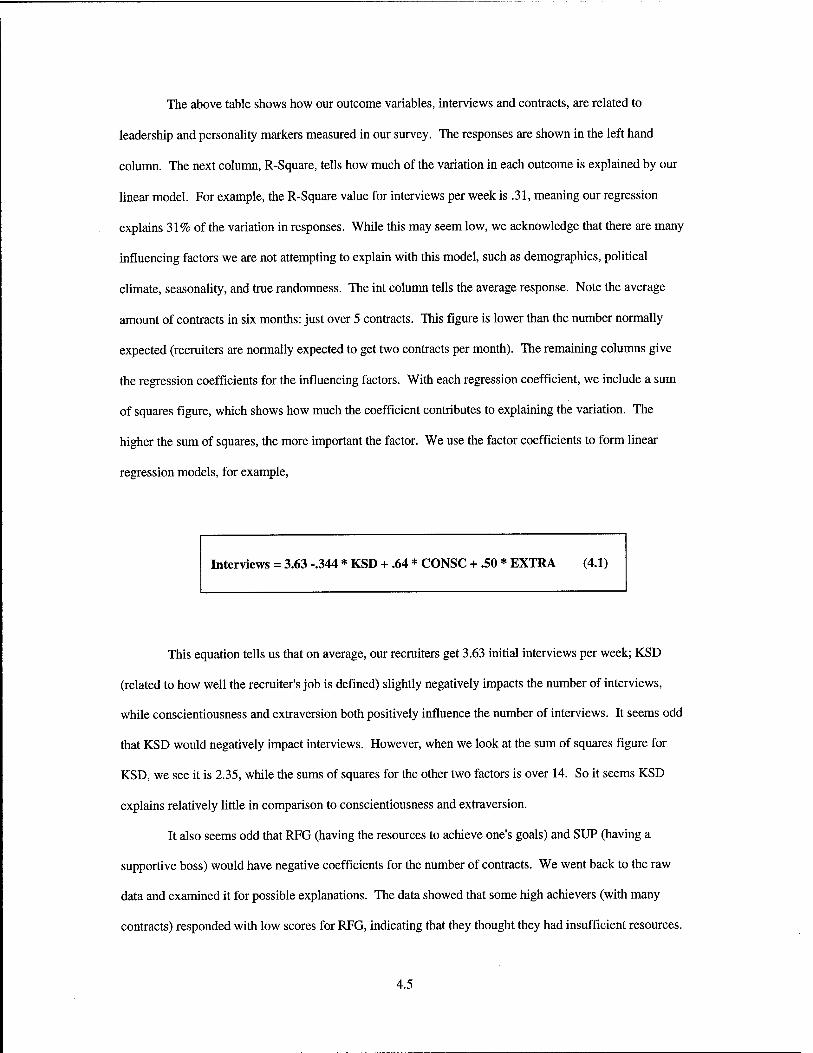
The above table shows how our outcome variables, interviews and contracts, are related to

leadership and personality markers measured in our survey. The responses are shown in the left hand

column. The next column, R-Square, tells how much of the variation in each outcome is explained by our

linear model. For example, the R-Square value for interviews per week is .31, meaning our regression

explains 31% of the variation in responses. While this may seem low, we acknowledge that there are many

influencing factors we are not attempting to explain with this model, such as demographics, political

climate, seasonality, and true randomness. The int column tells the average response. Note the average

amount of contracts in six months: just over 5 contracts. This figure is lower than the number normally

expected (recruiters are normally expected to get two contracts per month). The remaining columns give

the regression coefficients for the influencing factors. With each regression coefficient, we include a sum

of squares figure, which shows how much the coefficient contributes to explaining the variation. The

higher the sum of squares, the more important the factor. We use the factor coefficients to form linear

regression models, for example,

Interviews = 3.63 -.344 * KSD + .64 * CONSC + .50 * EXTRA (4.1)

This equation tells us that on average, our recruiters get 3.63 initial interviews per week; KSD

(related to how well the recruiter's job is defined) slightly negatively impacts the number of interviews,

while conscientiousness and extraversion both positively influence the number of interviews. It seems odd

that KSD would negatively impact interviews. However, when we look at the sum of squares figure for

KSD, we see it is 2.35, while the sums of squares for the other two factors is over 14. So it seems KSD

explains relatively little in comparison to conscientiousness and extraversion.

It also seems odd that RFG (having the resources to achieve one's goals) and SUP (having a

supportive boss) would have negative coefficients for the number of contracts. We went back to the raw

data and examined it for possible explanations. The data showed that some high achievers (with many

contracts) responded with low scores for RFG, indicating that they thought they had insufficient resources.

4.5

Perhaps these high achievers can envision how they would do even better with more resources. SUP had

the highest sum of squares of any influences on the number of contracts, and had a large negative

coefficient. We thought having a supportive boss would have a positive impact on contracts, so this result

was curious as well. After looking back at the raw data, it seems that some low achievers rated their bosses

as supportive. What this may mean is that some supportive bosses are more understanding about failure.

Therefore we get a negative coefficient. One would expect being supportive and understanding to foster a

good work environment. However, in the small sample of this survey, it appears that being supportive

constituted accepting failure.

We thought interaction terms might help explain more of the variation in our responses. We ran

two-way interaction models in SAS JMP with a slightly increased R-Squared value. However, due to the

additional factors in the model, the adjusted R-Squared value fell below what it had been in the linear

model. In other words, the reduced degrees of freedom in the interaction model negated any additional

explanatory power. In addition, we had hoped an interaction model would get rid of some of the negative

coefficients. However, there were just as many (or more) negative coefficients in the interaction models.

With a larger database, exploration of interaction terms could provide fruitful since the loss of degrees of

freedom would not matter as much when compared with sample size. However, since we had a relatively

small database, we limited this study to exploring the linear effects.

We administered the leadership / personality survey to 30 recruiters from the Dayton, Ohio

Recruiting Company. We had hoped to gather additional information by doing a mass-mailing to over 500

recruiters from three brigades. Due to several administrative problems, we were unable to distribute and

collect the additional surveys in time to be included in this study. However, as they arrive, we will collect

them and provide them to USAREC, the sponsor, for further use in the model. As we progress through the

analysis, we will provide and explain all the necessary tools to analyze the data on hand, as well as the data

yet to be gathered.

Analysis of Supporting Data. Supporting data consisted of several areas. First, USAREC had

used the 1998 survey to compile a large database of average processing times which we were able to

incorporate into this upgraded model. Second, USAREC was able to provide conversion data which

4.6

showed how many prospects made it to various stages of the recruiting process. The conversion data was

broken down by ASVAB score and high school status, but not by gender. Finally we explored data on the

number of prospects entering and contracted in the real world, broken down by all eight prospect types.

Many of the items measured in the 1998 survey directly translated to parameters in the model.

Since USAREC had used the 1998 survey to generate a large database, we wanted to update the model with

average values from the new, more robust, database. For each parameter, this entailed finding the mean

and standard deviation. A table of applicable parameters and their updated mean is shown below.

Table 4.5. Mean Parameter Values from 1998 Survey Database

Variable Name Explanation Low Mean High CollateralTime Hours spent per day on duties not accounted for in the rest

of the recruiting process 1.30 2.25 3.50

Dinterview Hours the initial DEP interview will last 0.95 1.5 2.15 FdmeetD Hours spend on a face-to-face DEP meeting 1.06 2.25 4.80 GetPpapers Hours spent waiting for prospects to bring in paperwork

needed for processing 8.90 19.2 43.50

Medwp Hours spent completing a medical waiver package 2.89 5.43 10.35 Morwp Hours spent completing a moral waiver package 5.93 9.31 17.40 Process Hours spent on a prospect's enlistment package 1.86 3.20 7.05 ProsF (Grad) Hours spent face prospecting to get one grad prospect 4.17 8.07 13.72 ProsF (Senior) Hours spent face prospecting to get one senior prospect 1.56 2.76 4.39 ProsT Hours spent telephone prospecting to get one prospect 1.03 2.53 4.81 Psale Hours spent on pre-sales interview for walk-in applicants 0.49 0.77 1.15 Sale Hours spent for sales interview 0.99 1.51 2.26 SaleP Hours spent on paperwork from a sales interview 0.58 0.86 1.56 TdmeetD Hours spent on a telephonic DEP meeting 0.47 1.08 2.86

The above table shows average values for many of the parameters in the model, based on a survey

of 138 recruiters from the 3rd Brigade, conducted by MAJ Robert Fancher of USAREC. We used these

figures as base values for the current model. Note that this data is for the average prospect, and is not

broken down by each prospect type. More on their incorporation is explained at the end of this section.

Conversion data provided us insight into how many of each prospect type made it through each

stage of our model, and how many dropped out. USAREC's conversion data showed how many of each

type prospect made it from their initial appointment to testing (taking the ASVAB); from testing to passing

the ASVAB; from passing the ASVAB to making it to the MEPS station for additional processing (called

4.7

"Floor" by recruiters); and from the MEPS station to actually being contracted. Analysis of this data and

incorporation into the model was fairly straightforward; however, there are two highlights to note.

First, if going from one step in the conversion data to the next embodied more than one step in the

model, we spread the probabilities evenly in the model. For example, going from the MEPS station (floor)

to contracting included passing the QNE (Qualified, Not Enlist), medical waiver, and moral waiver stages

in the model. Thus, we evenly distributed the probability of going from floor to contracting between the

three model stages. When multiplied together, the three stage probabilities resulted in the overall

probability of going from floor to contracting.

Second, the conversion data had some values over 1.0, which was puzzling at first. They seemed

to indicate that there was a greater than 100% chance of passing the ASVAB. Upon further analysis, we

discovered that some prospects take the ASVAB in high school prior to seeing a recruiter. Thus, even

though all prospects do not pass the ASVAB, we see the effect of more passing than the recruiter tests,

because they are tested elsewhere. In the cases where we had this problem, we evenly distributed the

probabilities of passing the ASVAB and getting to floor. For example out of 100 applicants, we know six

will pass the recruiter-administered ASVAB as low grads. However, because some are tested prior, eight

low grads actually make it to floor. This would mean the conversion rate would be 8/6 = 1.33. We are

unable to model probabilities over 1.0 in simulation, so we raise the amount who pass appropriately so the

proper amount get to floor. Continuing the example, we set the probabilities so that more low grads pass

the ASVAB, but not all who pass make it to floor. From the conversion data, approximately 28% of low

grads pass the recruiter-administered ASVAB, but 133% of that number make it to floor. For modeling

purposes, we let 40% of low grads pass the ASVAB, and let 92.5% of those make it to floor. Thus, .28 *

1.33 = .3724 = .40 * .925 and we are able use simulation probabilities from 0 to 1.0. A table of adjusted

(when necessary) conversion data is given below.

Table 4.6. Adjusted Conversion Rates for Model

Prospect Type Appointment to Testing

Pass Test From Testing to MEPS

From MEPS to Contract

Grad High ASVAB .29 .81 .92 .98 Grad Low ASVAB .29 .35 .95 .95 Senior High ASVAB .20 .75 .91 .95- Senior Low ASVAB .20 .40 .92 .87

4.8

To accurately model the different prospect types, we had to know how many of each type of

prospect we should make. In other words, we needed the proportion of total applicants that each prospect

type comprised. We used data provided from USAREC which showed the number of each type that was

contracted by month in fiscal year 1998. We divided the number of a particular type by the total number

contracted, and got the proportion that type made up. Ideally, we would have known the numbers of

applicants instead of the number of contracts, however, contract data should provide a good starting

estimate. A table of proportions is shown below. It is important to note that this is only average data from

one time period. We acknowledge that these figures may vary over time, location, station, and many other

factors. We leave further work into demographic effects for future work.

Table 4.7. Average Contracted Proportions (Gender, SrVGrad. ASVAB)

Male Female MSL .09 FSL .03 MGL .21 FGL .03 MSH .15 FSH .04 MGH .34 FGH .11

As we can see from the table, males made up 79% of the contracted recruits, and females 21%.

We used these proportions to establish the proper probabilities for a random number draw in the simulation

which decided which type each prospect would be. We used the above proportions to come up with a

running probability table, conducted a random uniform draw, and assigned prospect type by comparing the

result with the probability table. This concept is shown graphically below.

4.9

Form a running probability by adding each proportion to the last probability:

MSL FSL MGL FGL MSH FSH MGH FGH

0.0 .09.12 .33 .36 t .41

.51 .55 .89 1.0

Conduct a random draw, for example, .41, and assign prospect type (MSH)

Figure 4.1. Using a Random Draw and Proportions to Assign Prospect Type

In the above example, we conduct a random, uniform draw and assign prospect type based on a

number line consisting of a running sum of the prospect type proportions. While we model these

probabilities as constant, we acknowledge that in the real world, there is control and feedback. For

example, if a particular station is getting too many low grads, the leadership will probably put more

emphasis on finding high grads.

Synthesis of 1998 and 1999 Survey Data. We used the 1999 survey to see how station

commander leadership and recruiter personality affected the number of contracts (and interviews) a

recruiter achieved. This information gave us the big picture of what we should expect to see as leadership

and personality traits varied. However, the 1999 survey by itself did not tell us how we should change the

individual parameters of the model (besides interviews). We discovered an exciting concept during data

analysis - why not combine information from the two surveys and see how leadership and personality

affected the durations measured in the 1998 survey! This could be done at the aggregated station level, or

(ideally) surveys of individual recruiters could be linked-up. We attempted to relate the raw data from the

1998 and 1999 surveys for the Dayton Recruiting Company. However, after an exhaustive search at AFTT,

USAREC, and with the authors of the prior study, the raw data from the 1998 survey was unattainable.

4.10

The 1998 survey raw data was lost by the previous researchers in a computer crash a week after their

research was completed. We thought the concept of combining the two surveys was important, so we

decided to use two independent pieces of data, assume a notional correlation between them, and provide a

methodology to analyze the results. This certainly was not ideal, because the correlations and influences

we would discover would not be meaningful in the real world. However, we hope the benefit of providing

the methodology will outweigh the problems with inducing a notional correlation.

To accomplish the notional correlation, we appended the 1999 survey data results with selected

data (durations) from the 1998 survey results of the 5th Brigade. Again, ideally we would have simply

administered both surveys as one. Now we had a data matrix 26 rows deep, with columns for both 1999

and 1998 measurements. Columns in the matrix included leadership and personality factors, interview and

contract outputs, and durations for key points in the process. We next conducted stepwise regression of the

durations against leadership and personality factors, much like we had done previously. With real

correlation, this regression would tell us which leadership/personality factors affected process durations,

and would give an equation to describe their influence.

With regression equations in hand, we needed to modify the average process durations by the

leadership and personality influences. If a leadership aspect differed from the average station, we wanted

our Excel data interface to modify the appropriate durations in the model. To accomplish this modification,

we added columns for each leadership/personality factor to our interface. For each duration, we entered the

appropriate regression coefficients for the influencing columns. We then calculated a modified value for

each duration using our regression equations. Since our average data was based on average

leadership/personality scores, we multiplied the regression coefficient by the deviation from the mean for

each factor. A simple example is shown below, and the full spreadsheet is given in Appendix E, Input

Data, as well as Appendix G, Electronic Enclosures.

4.11

Table 4.8. Process Duration Modification Example (Average Prospect)

CSG FBK EXTRA Average L/P Scores

8 6 7

This Station

9 7 8

Deviation +1 +1 +1 Variable Base Value CSG FBK EXTRA Initial Interview Duration

1.5 hours -0.5 -0.35 +.25 This row contains regression coefficients.

Modified Initial Interview Duration = 1.5 + (-0.5) * 1 + (-0.35) * 1 + (0.25) * (1) = 0.9 hours

Using the above example, we enter leadership / personality scores for an individual station to be

studied on the second line. The front end calculates the deviation between average (first line) and our

studied station, and calculates an adjusted initial interview duration based on the coefficients and the

deviations.

Conclusion of Input Analysis. In this section, we have explained analysis methods for the

leadership and personality study, incorporation of supporting data, and correlation of the 1998 and 1999

surveys. We have provided electronic methodologies for future analysts to easily incorporate their own

data with a minimum of programming in Appendix G, Electronic Enclosures. In addition, we have

explained the methodologies in detail in this section. With input analysis complete, we turn to designing

our experiment and analyzing model output.

Experimental Design

When fully coded, the simulation took approximately 30 minutes of real time per year of

simulation time when run on a 266 MHz Pentium II class system. Therefore, it was in our best interest to

conduct a careful experimental design so we could minimize run time. In our initial regressions, the

4.12

number of contracts had been most influenced by the factors CSG, RFG, SUP, and EFFIC. Therefore, we

wanted to be able to vary these parameters from their mean values and see what happened to the simulation

output. In Response Surface Methodology (Myers and Montgomery, 157), the authors describe fractional

factorial designs. With four factors to examine, if we held all constant while varying one at a time from

low to high, we would have 2M = 16 runs to make. Each run took over 15 hours (discussed more later), so

we needed to reduce the amount of runs if possible. By using a half fraction design with eight runs, we are

able to discern the main effects clearly and gain some insight into the two-way interactions. We assume

three-way and higher interactions are negligible for our experiment. For our chosen factors, we chose to let

the high and low design points be one standard deviation from the mean. Thus, a table of design values is

given below.

Table 4.9. Experimental Design Settings

Run CSG = A RFG = B SUP = C EFFIC = ABC 1 +

2.23 +

2.96 +

4.43 +

7.76 2

-1.08 +

2.96 +

4.43 -1.76 3 +

2.23 -4.72 +

4.43 -1.76 4

-1.08 -4.72 +

4.43 +

7.76 5 +

2.23 +

2.96 -1.43 -1.76 6

-1.08 +

2.96 -1.43 +

7.76 7 +

2.23 -4.72 -1.43 +

7.76 8

-1.08 -4.72 -1.43 -1.76

The above table shows whether each setting represents the high (+) or low (-) setting, as well as

giving the numerical (in terms of natural variables) setting to be used in the Excel front end.

Since each year of simulation time took over 30 minutes to run, it was also in our best interest to

choose the simulation run method which minimized the amount of data thrown away. In order to achieve

statistical significance, we wanted to have sample sizes of thirty. There were two main methods we could

use to achieve this. Since the warmup time before steady state was approximately a year (shown in output

4.13

analysis), we could run thirty replications of two years apiece, discarding the first year (warmup) of each

replication. This would entail 30*2*.5 = 30 hours per design setting. Alternatively, we could run one long

run of 31 years, and discard only the first year. This is the method of batch means, and would mean 31*.5

= 15.5 hours per design setting, a time savings of nearly half. We chose to use the method of batch means

in our output analysis, which is explained in the next section.

Simulation Output

General. The main objective of our simulation was to be able to vary station commander

attributes (leadership) and recruiter personalities and see what would happen to the number of prospects

who were successfully contracted. In addition, the sponsor desired to be able to track contracts by prospect

type on a monthly basis. This section is divided into an introduction, a discussion on how we found steady

state conditions, analysis of output from different settings, and variance reduction through control

variables. For our simulation, we used three recruiters, one of each type available in the model, so the

station modeled is slightly smaller than average.

We gathered simulation output with a <WRITE> statement in the final contracting node of the

simulation network. The simulation recorded type of prospect, type of recruiter, and time of contract for

each successful contract made. With all the prospect types in the model, the simulation ran very slowly.

On a 266 MHz Pentium II class computer, each year of simulation time took over 30 minutes of real time.

As we observed the simulation with the animation running (to see numbers of entities at each node), we

realized that the simulation was creating a large number of unused entities. These entities formed the pool

of potential prospects which the recruiters attempted to prospect. As the simulation went on, there could be

as many as 500 entities in this pool, doing nothing but waiting in a queue. Each of these entities carried its

own copy of the pertinent parameters with it, so the simulation overhead was very high. We slowed

creation of entities for the pool by a factor of ten, and included a release mechanism, which disposed of

prospects who had not been contacted by a recruiter within 20 days of their creation. Still, this left an

average pool of 30 potential prospects for each recruiter to draw from, which was plenty to keep the

recruiters busy. With fewer unused entities, the model ran a little faster, and had way less disk-access

activity with no loss of input distribution accuracy.

4.14

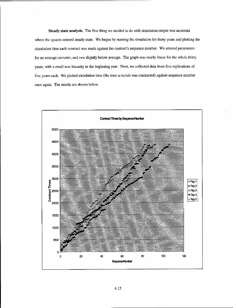
Steady state analysis. The first thing we needed to do with simulation output was ascertain

where the system entered steady-state. We began by running the simulation for thirty years and plotting the

simulation time each contract was made against the contract's sequence number. We entered parameters

for an average recruiter, and two slightly below average. The graph was nearly linear for the whole thirty

years, with a small non-linearity in the beginning year. Next, we collected data from five replications of

five years each. We plotted simulation time (the time a recruit was contracted) against sequence number

once again. The results are shown below.

4.15

The above chart shows simulation time (in hours) versus sequence number (the order in which the

recruits were contracted.) If contracts were exactly evenly spaced, we would expect the points to form a

perfectly straight line. It is easy to see that the graph for each replication is approximately linear, indicating

that the times between contracts are approximately evenly spaced. We also note the number of contracts

produced in this five year span ranged from approximately 80 (Rep 1) to just over 100 (Rep 2.) To gain a

little more insight into the output, we plot time between contracts in the chart below.

Times Between Contracts

i e i5oo

Rep 1 Rep 2 Rep 3 Rep 4 Rep 5

-Average -Moving Average

Sequence Number

Figure 4.3. Average Intercontract Time by Sequence Number

This chart is read as follows. The individual dots represent individual observations of inter-

contract times versus sequence number. For example, the first sequence number shown here is the

difference in simulation time between the first two contracts. The relatively ragged line connecting the

round dots represents the average inter-contract time by sequence number across the five runs, which we

call a sequence number average. The line labeled "moving average" represents the average of 21 sequence

number averages (a definition is included at the end of this paragraph.) Using a moving average has the

effect of smoothing the data, so we can tell where steady state conditions appear. If we examine the above

4.16

rth graph, it appears inter-contract times are slightly high at first, and then settle into steady state by the 15

contract. When we cross-reference the 15th contract with simulation times, we see that the 15th contract

occurs between the 10* and 12th month of the first year. Therefore, we can safely use a warm-up period of

one year for our simulation. As a side note, the n* moving average of size 21 for the bulk of the points is

calculated by summing the 21 values centered on the n* point and dividing by 21. Therefore, each moving

average point is simply the average of the nearest 21 points. At the start, we must use smaller sizes to

average. For example, the first moving average is simply the first data point. The second moving average

is the average of the first three data points, and so on, until we reach our chosen interval size of 21.

From the above graph, it is also interesting to note the maximum inter-contract times. Most fall

below 1000 hours, but one is over 3000 hours, which translates to over four months for a team of three

recruiters to get one contract. On the other hand, the steady-state time between contracts is very near 450

hours, or 18.75 days. This would mean the three-person team would average approximately 20 contracts

per year. The average number of contracts per six months for our surveyed recruiters was 4.96, so we

would expect 4.96 * 3 recruiters * 2 six month periods = approximately 30 contracts per year. Therefore,

we can see that our simulated recruiters are producing a little less than we would expect to see in the real

world. This makes sense because of our choice of recruiter parameters in the model - one average, and two

slightly less capable. In addition, although the numbers may never exactly predict our real-world average

production, we are in the same range as the real world, and we can see how simulation output varies as we

change our experimental settings. We can observe deviation from the average simulated production.

Analysis of Output from Experimental Design. We ran the simulation for eight long runs of 31

years, one run for each experimental setting. The output of the most significance was the number of

contracts produced in an average year. RFG was the only significant influencing factor in our experimental

design. (Recall our parameters were from a notional correlation). The following figure contrasts results

between RFG high and RFG low.

4.17

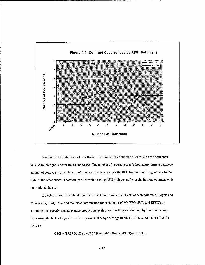
Figure 4.4. Contract Occurrences by RFG (Setting 1)

# —■ ■ RFG Hi t |«HnHW^MWMtppQ |_OW

iiSllill^ (0 <D U 25 - —„ __ —~ .

c 0) *llllip^ fc. ^ 3 u 20 - IIIM Ü O „H**^ A it . o 15 -

u £1 E 3 Z

10 -

5 - ^^^^^■■■i^^fei^^M^^fc^^fc .^^^^■^^iÄ^I^^BiÄI

0 1 ̂ ^ Mjg—*w --"v- •-, l l ( •....• ^ ♦'"''♦ ♦ ♦' " ' ^ *

./ * % # .$> <£> $■ <£> * <b6 t»° ^ t?>

0*

Number of Contracts

We interpret the above chart as follows. The number of contracts achieved is on the horizontal

axis, so to the right is better (more contracts). The number of occurrences tells how many times a particular

amount of contracts was achieved. We can see that the curve for the RFG high setting lies generally to the

right of the other curve. Therefore, we determine having RFG high generally results in more contracts with

our notional data set.

By using an experimental design, we are able to examine the effects of each parameter (Myers and

Montgomery, 141). We find the linear combination for each factor (CSG, RFG, SUP, and EFFIC) by

summing the properly-signed average production levels at each setting and dividing by four. We assign

signs using the table of signs from the experimental design settings (table 4.9). Thus the factor effect for

CSG is:

CSG = (19.33-30.23+16.07-15.93+40.4-18.9+8.53-18.33)74 = .25833

4.18

Similarly, the effects for the other factors are: RFG: 12.525; SUP: -1.175; and EFFIC: -.7333.

This means that CSG and RFG positively influence the number of contracts, while SUP and EFFIC slightly

negatively impact contracts. From the magnitudes of these factor effects, we conclude that RFG is the only

really significant effect, and the others are small enough to be considered zero. Also, remember that these

numbers only represent the results of a notional correlation. We would expect different results with more

complete data. We have only provided the methodology for analysis here.

By-prospect type results were collected as well. An example chart of contracts by prospect for the

first experimental design setting is given below.

F Grad High 11%

F SR High 3%

F Grad Low 3%

F SR Low 3%

M Grad High 35%

M SR Low

M Grad Low 21%

SR High 15%

Figure 4.5. Total Contracts (Setting 1)

For each category, the first letter is for gender (Male/Female), the second letter group for high

school graduation status (Graduate / Senior), and the third letter group for ASVAB score (High / Low).

From the above chart, we can see the different proportions of contracts by prospect type. For example, we

4.19

can see that 76% of all recruits were male, and 24% were female. Additional results are self-explanatory

from the chart.

USAREC was interested in being able to track the number of contracts per month. This is easily

achieved since the time for each contract is collected in the output file. Simulation times are given in

hours, so we must transform hours into months. A table of hours versus months is given below (assuming

non-leap years.)

Table 4.10. Translating Simulation Time to Month of the Year

Hour Range Month 0-744 January

745 -1416 February 1417 - 2160 March 2161 - 2880 April 2881 - 3624 May 3621 - 4344 June 4345 - 5088 July 5089 - 5832 August 5833 - 6522 September 6523 - 7296 October 7297 - 8016 November 8017 - 8760 December

Since no seasonality is built into this model, we have the same expected number of contracts in

any given month. When we gathered the output data, we put each contract into the appropriate bin to

determine how many had been contracted in any given month. A chart of results by month is shown below

for setting one.

4.20

Fibure 4.6. Average Contracts By Month

2.5-

2- Hlp m Ü 2

Con

en

o

.a E z

Ave

rage

0.5- M

M

1

Note that the variation goes from approximately 1.3 to 2.2. Any variation we see here is due to

random effects, since we expect approximately the same number from month to month.

Conclusion

In this chapter, we have discussed the analysis portion of this study. First, we explored analysis

methods for implementing the survey data and supporting data into the model (input analysis). Second, we

formulated an experimental design and ran the model. Finally, we presented and analyzed the simulation

output. We first analyzed the output to determine when we reached steady state conditions. We then

varied input settings according to our experimental design and observed the simulation output. Results

from the simulation were similar to reported real-world performance, so we ascertained that the model is an

accurate representation of the recruiting system. In the final chapter, we give our conclusions and

recommendations.

4.21

Conclusion

Army Recruiting is a complex process which military leaders have been struggling to control for

many years. As Army leaders, we are brought-up to believe we can accomplish any mission with hard

work, professional leadership, and dedication. The problem with recruiting is that it includes many factors

which are beyond the control of the recruiter, the station commander, or even the Commander-in-Chief.

Recruiting productivity may sway with the times as military popularity waxes and wanes; as the civilian

job market improves or worsens; as the seasons change; or as military conflicts come and go. However, we

believe there is some hope for recruiting leadership. In the middle of this storm of uncontrollable factors,

there are some we can influence. We have the ability to provide our recruiters the most effective leadership

possible. We have the ability to select recruiters who are best suited to the job. We have the ability to

provide recruiters a framework for success through implementing fair policies, allocating an appropriate

budget, and providing recruiters with ample resources. However, the question remains for each of the

above, "What constitutes 'the best?'" We hope to have addressed part of the answer through this thesis.

The remainder of this chapter contains a summary of our research, simulation methods, and

results. Finally, we include a discussion of recommendations for future studies and research.

Summary

With this study, we sought to explore the first two elements within our control - the effects of the

station commander's leadership on productivity, and the effects of recruiter personality on the same. We

explored several aspects of Army recruiting previously not modeled. We have provided initial research

into the ways station commander leadership attributes affect productivity and process times. We also

explored the ways productivity and process times are affected by recruiter personality. Finally, we wrestled

with several methods of modeling eight different types of prospective recruits, to include creating,

processing, and tracking methods.

To begin, we searched for previous work on the effects of leadership in military models. We

found little more than blanket variables which described leadership on a scale from excellent to poor. We

5.1

found nothing which modeled specific leadership qualities and scientifically linked them to success or

failure. Therefore we turned to behavioral science experts who had studied leadership a great deal.

However, behavioral scientists had not been interested in modeling; they had been interesting in

establishing trends through surveys. Therefore, behavioral science provided us some established

measurement tools for leadership; the one we chose to use was called "goal setting theory," and seemed to

apply to recruiting quite well. We also borrowed research on personalities from the behavioral science

side. We wanted to see if there were some people who were more suited to being recruiters than others.

Again, there were several personality measurement scales in existence; we chose to use the one called the

"Big Five," developed by Goldberg. The great advantage to beginning with existing measurement tools

was that they provided a scientifically accepted framework from which to work. We modified the

questions slightly to apply more to the military mind-set, but the essence of the questions remained intact.

This added validity to our research. In the end, we generated a survey which covered station commander

leadership traits, as well as recruiter personality.

With a survey in hand, we administered it to a test population - the Dayton, Ohio Recruiting

Company. This generated 30 responses: 26 from straight recruiters and 4 from station commanders. After

initial analysis of the data, we could see that the station commander points were generally outliers. We

theorized that this was due to them spending more time on leadership and less time on recruiting. We

chose to conduct our analysis on the remaining 26 data points, which had no serious outliers. In addition to

the data from our survey, we incorporated data from several USAREC databases and from the previous

year's survey. In the end, we were able to provide a good estimate for all model parameters, some of which

were influenced by leadership and personality, and some of which were differentiated by prospect type.

Due to one piece of unavailable data, we chose to make a notional correlation between samples from the

1998 and 1999 surveys. We made the notional correlation because we wanted to provide USAREC

analysts the tools to analyze similar data with a real correlation. USAREC will have the ability to gather

this data in the future through the addition of laptop computers for all recruiters. Since we used a notional

correlation, our resulting influences may not make intuitive sense. Therefore, we do not make any

judgements based on the outcomes; we simply provide a framework for data analysis.

5.2

With the data in hand, we set out to modify the previous simulation model. The previous

researchers, Cordeiro and Friend, had produced a working, well-documented model in a language called

SIMPROCESS. SIMPROCESS is an icon-based simulation tool based on MODSIM, and was developed

by the CACI company. After a thorough review of the previous model, we modified it to create eight

different types of prospect, process them based on their type, and collect productivity statistics for each

type. We accomplished this by explicitly declaring separate variables for each model parameter and each

prospect-type combination. In effect, we multiplied the number of variables in the model by eight. We

then passed the model an enlarged input file which carried the by-prospect parameter information.

In addition, we provided the ability to modify most model parameters based on station commander

leadership and recruiter personality. We regressed various model parameters against the leadership and

personality influences, to see which influences affected model processing times. Since we were already

passing the model separate parameters for each prospect type, we chose to modify the parameters affected

by leadership and personality in a pre-processor interface. We used MS Excel for our interface since it was

user-friendly, and most future analysts will be familiar with it. We entered the results of our leadership and

personality regressions into the interface and watched how they affected the model parameters. When we

were satisfied our preprocessor was working well, we chose an experimental design and began making

model runs.

We first ran the model for an extended period of time to determine when we achieved steady state.

Next, we set out to vary some parameters and observe the output. The four factors which most affected

productivity in our leadership and personality survey were CSG (Clear and Specific Goals), RFG (Reward

For Goals), SUP (Supportive Leader) and EFFIC (Efficacy). Efficacy denotes the degree to which the

recruiter thinks he has the personal capability of recruiting success. Since each simulation run took

approximately 18 hours, we knew we needed to make the most of our simulation runs. We created a half-

fraction design which allowed us to examine the effects of the four factors listed above in a total of eight

runs, or about six days worth of simulation time.

We provided a method of analyzing the simulation output and analyzed the results based on our

notional correlation of 1998 and 1999 surveys. We must stress that this analysis only provides the

framework for future analysis. We saw that having better resources for achieving goals provided

5.3

significantly higher production with our notional data correlation. We were able to show the percentages of

each type of prospect who was contracted. In addition, we were able to track the number of contracts per

month.

Finally, we provided several tools for future analysts to use and build on. The 1999 survey

provides scientifically-backed methods of measuring evasive leadership and personality factors. When

correlated with the 1998 survey, we can see how leadership and personality directly affect model process

times. Additionally, we improved the model so eight different types of prospective recruits can be

processed, and so leadership and personality influences can affect the appropriate parameters.

Recommendations

The recruiting process can take up to a year from start to finish for any particular prospect. The

long duration of the process makes data gathering difficult for a researcher on a tight timeline. A great deal

of data was provided by USAREC, but some critical data was simply not in existence. Through the course

of this study, we identified key data needed and included it in our survey. However, time did not allow

extensive survey distribution, collection, and compilation. We recommend the leadership and personality

survey be used in conjunction with the 1998 process-time survey in future data collection efforts. In

addition, a suggested modification to the 1998 survey is recommended. The 1998 survey requests

recruiters to estimate the minimum, maximum, and average lengths of various recruiting processes. This

estimation has error built-in. If recruiters could actually record the task durations as they are being

performed, future analysts could get much more accurate estimates. The recording process would take a

long time (six months to a year), however the results should be more accurate than the recruiters' estimates.

As a simulation language, SIMPROCESS is stretched to its limits with this model. Each run of 30

years takes approximately 18 hours on a 266 MHz Pentium-class machine. In addition, SIMPROCESS

does not allow the user to define arrays, which would have greatly simplified the process of programming

the eight different types of prospects. Finally the user expressions (text code) which accompany many

simulation nodes are pushing the size limitations of SIMPROCESS. There is nearly too much code in

some of the expressions for SIMPROCESS to handle. We recommend using a different simulation

5.4

language for recruiting models of any more complexity. SIMPROCESS has nice features, such as drag-and

drop process flow, and automatic automation; however these user-friendly attributes also limit user

flexibility.

We had wanted to aggregate the model to Company level or higher; however, researching the

leadership and personality aspects of recruiting required much more attention than initially estimated. We

knew aggregation would depend on a solid framework for measuring leadership and personality, so we

developed that framework with this research. It would be very interesting to explore the effects of higher-

level leadership and their interactions with station commander leadership and recruiter personality in an

aggregated model.

Final Remarks

The recruiter's job is not easy, and there is no simple way to make it so. There are many things

beyond the control of recruiters and their leaders. However, we hope to have provided insight into certain

factors within their span of control. We have had success in providing insight into station commander

leadership and recruiter personality influences on the recruiting process. In addition, we have improved a

simulation model, which accurately depicts the flow of the recruiting process and now incorporates eight

prospect types, as well as leadership and personality influences. We sincerely hope this research will serve

to assist future recruiters and their leadership in maximizing the use of their time and getting quality

recruits into the Army of the 21st Century.

5.5

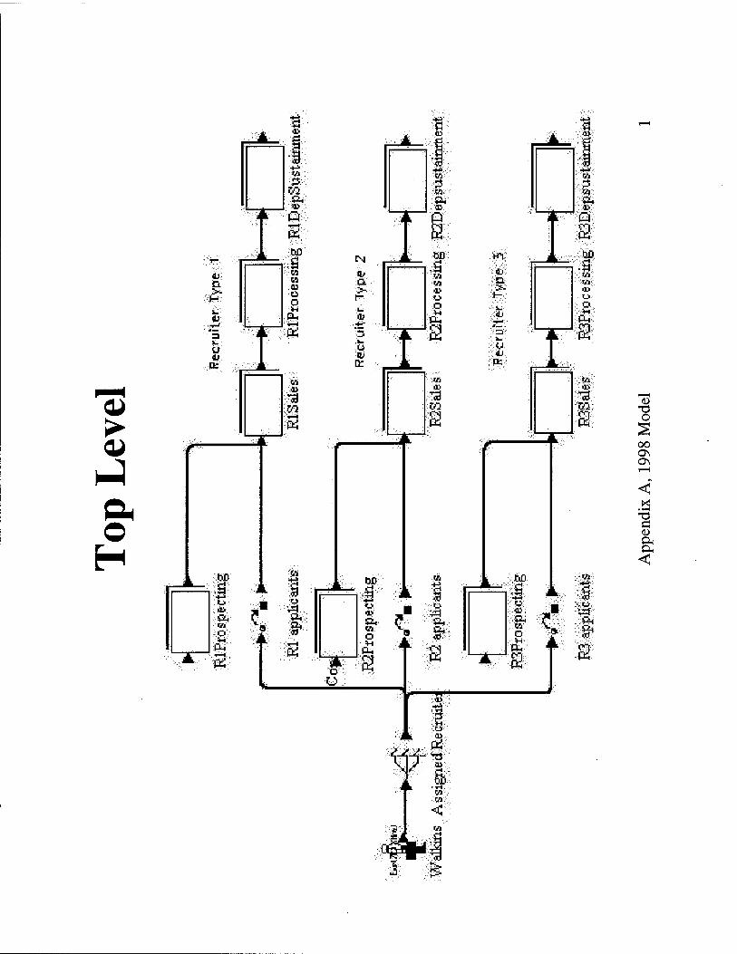
tt O

OO ON OS

• I—I

Ö

2

wo

w ft

o

9

!

w o « Q

1

<1 I

Ha so: 0 O

■:«>;■

< i

f

<N

Ö

T3 O

00 ON ON

X!

C D &

m

<J1

—

*3 g.- 4-1

a»

•a

■a

1

i [

3 o

a>

a*

en

O

cn

r H ■<

ay

&3

t B

+ '%

I 4>

"50 ay

1

"'©'■

... vi ay

'S o O

oo

X • 1—I

C

4

'»;'■«■■

.'.-■ja*

ÖiD

'S «a

o ©

OH

■<.

SOD

■.«■

■■tiv o 0H-

O

OO ON ON

X ■l-H

C a. OH

^

■;.0;-'

o

©

o

w- '-VOV

'■ • *+

«ft;

b H4

PH

I <1

05

- E-

w> w od

OH

I, * PH

t I

m—i

■■B

-3

^!

<1 & M

o

^

4.

■c PH

o S *ö Ö

t

I JPQ?

SPHC:

f

4-1

■6

4H O

vn

O

oo ON ON

X!

Ö U

1 r §

S PH *H

WD

"35 1/5

©

4>

a

Q

CO W

J3 i

OH

■73 1 +* 4

0>

'S Q

^

i

05

o O

o

15

.a w w

o O

PL,

i<i5v;

■sä

■•S05:

W "■6

I» 4 Q

1

<? L -3 41 05

■ ■6

'13

■a

'S: o

41

05

VO

O

OO ON ON

X ■ I—I

Ö <D OH

4

*ö':

M

O

00 ON ON

&' Ö (D

•^

Q:

m

Q

oo

0)

O

OO

■ 1—1

-d Ö <D OH OH

•a

ja <p

a)

o

&

OH

Q

Q\

o

oo ON ON

C

Appendix B: Summary of Model Changes

We updated the model to be able to incorporate eight different prospect types and station

commander leadership / recruiter personality influences. Handling the eight prospect types required

addition to the SIMPROCESS model, while the leader / follower influences were implemented in a

preprocessor interface (MS Excel).

To implement the eight prospect types, we needed to be able to give each prospect type a different

set of model parameters (process durations and probabilities of dropping out). This meant we needed to

expand the variable set by a factor of eight, since there were eight prospect types. Implementation meant

we needed to declare the appropriate variables, import the values into the simulation, assign prospect type

to each entity, attach by-prospect-type parameters to each entity, change each process to reference the

entity's parameters, and collect data on production by prospect type.

We needed to declare global and entity variables. We would read all the values from an external

file into the global variables. Then we would use the global variables as a database to reference when

assigning entity variables to each copy of each entity. To declare global variables, we used

SIMPROCESS's <Define><AttributesxModel> tabs. For most global variables in the original model,

we made seven additional copies, and appended their names with B through H. Thus, if we had a type 2

(B) prospect, we assigned that entity the appropriate <parameternameB>'s. We used the same type

procedure to define entity variables, with the <Entity> tab substituted for <Model>. For every parameter

we intended to vary, we declared a new entity variable. This did not entail eight copies, since each entity

only needed to be able to carry one set (it's own) set of the parameters.

Partial code for reading the parameters into the model is given below. We omit the full code since

it is repetitious, and the reader should be able to see the pattern immediately. This code can be found in the

"start simulation" expression in the walk-in entity creation node (far left node of the top level). The first

lines define the user input and output files. Then "ReadFromFile" statements begin. The first several read

the running proportions of each type of prospect. Then we begin reading in each parameter from the

Appendix B, Summary of Model Changes, Page 1

original model, to be used with type 1 prospects (type A). When all the original variables have been filled,

we begin reading into the second copy of them (appended with B). It is important to note that for the B-H

copies, we did not re-read time for recruiter lunch or collateral time, since this should not be prospect-

dependent. Therefore each of the B-H copies reads two less values than the original. The code follows.

SIMPROCESS Data Input Code

Model.MyOutStream := OpenFile("Output", "myoutput.dat"); Model.my:=OpenFile("Input","varvals.txt"); {prospect running proportions} ReadFromFile(Model.my,Model.MSL,Model.FSL,Model.MGL); ReadFromFile(Model.my,Model.FGL,Model.MSH,Model.FSH); ReadFromFile(Model.my,Model.MGH);

{A: M, SR, Low}

ReadFromFile(Model.my,Model. ReadFromFile(Model.my,Model. ReadFromFile(Model.my,Model. ReadFromFile(Model.my .Model. ReadFromFile(Model.my,Model. ReadFromFile(Model.my,Model. ReadFromFile(Model.my .Model. ReadFromFile(Model.my .Model. ReadFromFile(Model.my .Model. ReadFromFile(Model.my .Model. ReadFromFile(Model.my,Model. ReadFromFile(Model.my,Model, ReadFromFile(Model.my,Model, ReadFromFile(Model.my,Model, ReadFromFile(Model.my,Model. ReadFromFile(Model.my,Model. ReadFromFile(Model.my,Model. ReadFromFile(Model.my .Model. ReadFromFile(Model.my .Model. ReadFromFile(Model.my .Model. ReadFromFile(Model.my .Model ReadFromFile(Model.my .Model ReadFromFile(Model.my .Model ReadFromFile(Model.my .Model ReadFromFile(Model.my .Model ReadFromFile(Model.my .Model ReadFromFile(Model.my .Model ReadFromFile(Model.my .Model, ReadFromFile(Model.my .Model ReadFromFile(Model.my .Model ReadFromFile(Model.my .Model ReadFromFile(Model.my .Model ReadFromFile(Model.my .Model ReadFromFile(Model.my .Model. ReadFromFile(Model.my .Model ReadFromFile(Model.my .Model

Rlmpros,Model.Rlapros,Model.Rlmaxpros); RlTLoss,Model.R2TLoss,Model.R3TLoss); RlFLoss,Model.R2FLoss,Model.R3FLoss); .RlSaleloss,Model.R2Saleloss,Model.R3Saleloss); RlImdPLoss,Model.R2ImdPLoss,Model.R3ImdPLoss); RlNorPLoss,Model.R2NorPLoss,Model.R3NorPLoss); ,mgetPpapers,Model.agetPpapers,Model.hgetPpapers); mRlmorwp.Model.aRlmorwp.Model.maxRlmorwp); mR2morwp,Model.aR2morwp,Model.maxR2morwp); .mR3morwp,Model.aR3morwp,Model.maxR3morwp); mRlmedwp,Model.aRlmedwp,Model.maxRlmedwp) mR2medwp,Model.aR2medwp,Model.maxR2medwp) mR3medwp,Model.aR3medwp,Model.maxR3medwp) .mMoralD,Model.aMoralD,Model.maxMoralD); mMedD.Model.aMedD.Model.maxMedD); mImdMepsD,Model.aImdMepsD,Model.maxImdMepsD); inNorMepsD.Model.aNorMepsD.Model.maxNorMepsD); mNtotestD .Model. aNtotestD.Model.maxNtotestD); mDeptime,Model.aDeptime,Model.maxDeptime); .mDinterview,Model.aDinterview,Model.maxDinterview); mRlTdmeetD,Model.aRlTdmeetD,Model.maxRlTdmeetD) ,mR2TdmeetD,Model.aR2TdmeetD,Model.maxR2TdmeetD) .mR3TdmeetD,Model.aR3TdmeetD,Model.maxR3TdmeetD) mRlFdmeetD.Model.aRlFdmeetD.Model.maxRlFdmeetD) ,mR2FdmeetD,Model.aR2FdmeetD,Model.maxR2FdmeetD) ,rnR3FdmeetD,Model.aR3FdmeetD,Model.maxR3FdmeetD) mtoDep.Model.atoDep.Model.maxtoDep); BaseDprob); .Moralprob); .Medicalprob); .Ptestprob); .CollateralTime); .Lunch); walkinloss); .mprosTRl,Model.aprosTRl,Model.maxprosTRl); .mprosTR2,Model.aprosTR2,Model.maxprosTR2);

Appendix B, Summary of Model Changes, Page 2

ReadFromFile(Model.my .Model ReadFromFile(Model.my,Model ReadFromFile(Model.my,Model ReadFromFile(Model.my,Model ReadFromFile(Model.my .Model ReadFromFile(Model.my .Model ReadFromFile(Model.my .Model ReadFromFile(Model.my .Model ReadFromFile(Model.my .Model ReadFromFile(Model.my .Model ReadFromFile(Model.my,Model ReadFromFile(Model.my,Model ReadFromFile(Model.my,Model ReadFromFile(Model.my .Model ReadFromFile(Model.my .Model ReadFromFile(Model.my .Model ReadFromFile(Model.my .Model ReadFromFile(Model.my .Model. ReadFromFile(Model.my .Model.

{B: F.SR.Low}

ReadFromFile(Model.my .Model, ReadFromFile(Model.my .Model, ReadFromFile(Model.my .Model, ReadFromFile(Model.my,Model, ReadFromFile(Model.my,Model, ReadFromFile(Model.my .Model, ReadFromFile(Model.my .Model

mprosTR3,Model.aprosTR3,Model.maxprosTR3); .mprosFRl,Model.aprosFRl,Model.maxprosFRl); mprosFR2,Model.aprosFR2,Model.maxprosFR2); mprosFR3,Model.aprosFR3,Model.maxprosFR3); .mPsaleRl,Model.aPsaleRl,Model.maxPsaleRl); .mPsaleR2,Model.aPsaleR2,Model.maxPsaleR2); .mPsaleR3,Model.aPsaleR3,Model.maxPsaleR3); .msaleRl,Model.asaleRl,Model.maxsaleRl); msaleR2,Model.asaleR2,Model.maxsaleR2); .msaleR3,Model.asaleR3,Model.maxsaleR3); .msalePRl,Model.asalePRl,Model.maxsalePRl); msalePR2,Model.asalePR2,Model.maxsalePR2); .msalePR3,Model.asalePR3,Model.maxsalePR3); .mProcessRl.Model.aProcessRl.Model.maxProcessRl); .mProcessR2,Model.aProcessR2,Model.maxProcessR2); .mProcessR3,Model.aProcessR3,Model.maxProcessR3); .RlQNEprob); R2QNEprob) R3QNEprob)

Rlmpros.Model.Rlapros.Model.Rlmaxpros); RlTLossB,Model.R2TLossB,Model.R3TLoss); RlFLossB,Model.R2FLossB,Model.R3FLossB); RlSalelossB,Model.R2SalelossB,Model.R3SalelossB); RlImdPLossB,Model.R2ImdPLossB,Model.R3ImdPLossB); RlNorPLoss,Model.R2NorPLoss,Model.R3NorPLoss); mgefPpapersB.Model.agefPpapersB.Model.hgetPpapersB);

CloseFile(Model .my);

Note that we have omitted seven additional copies of these global variables. When we are done

reading the variables into SEVIPROCESS, we use the <CloseFile> command to close the file.

With the global variable database successfully read-in, we now need to assign each entity its type

(1-8) and give it an appropriate copy of the parameters. This code appears in two places; one for walkins,

and one for those who are prospected. For walk-ins, we placed it in the "Release Entity" expressions of the

three transform nodes in the top level of the simulation model. For the prospected entities, we inserted the

code in the "Release Entity" expression in the first entity node ("R(X) Applicants") in the "Processing "

sub-level. If we look at the code, we see that we draw a sample from a uniform distribution and use if-then

statements to determine which type the prospect will be. Each if-then statement is quite long, as each

contains assignments of all parameter values for that type of prospect. The variable <Model.MSL> is the

Appendix B, Summary of Model Changes, Page 3

upper bound of the section of the running probability line which defines the relative proportions of the

prospect types. For example, if 10% of prospects are MSL (male, senior, low ASVAB), then

<Model.MSL> carries a value of .10. These proportions are entered by the user in the Excel preprocessor.

Note that for each type 1 prospect, we simply assign its entity variables the values held in the original

global model variables (now these only apply to type 1 prospects). If we have a type two prospect, we

assign its entity variables values from the global variables appended with "B."

Code to Assign each Entity a Copy of its Parameters

Model.Rlcount:= Model.Rlcount + 1; Entity.applicantNumber:=Model.Rlcount; Temp : REAL; Entity .Psource:=3; Temp:=DrawRealSample("Uni(0.0,1.0)"); IF (Temp < Model.MSL) Entity.TypeP:=l; Entity.TLoss:=Model.RlTLoss; Entity.FLoss:=Model.RlFLoss; Entity.SaleLos:=Model.RlSaleLoss; Entity .ImdPLoss:=Model.RlImdPLoss; Entity .mgetPpapers:=Model.mgetPpapers; Entity.agetPpapers:=Model.agetPpapers; Entity .hgefPpapers:=Model.hgetPpapers; Entity .mmorwp:=Model.mR 1 morwp; Entity.amorwp:=Model.aRlmorwp; Entity.maxmorwp:=Model.maxRlmorwp; Entity .mmedwp:=Model.mRlmedwp; Entity.amedwp:=Model.aRlmedwp; Entity .maxmedwp:=Model.maxRlmedwp; Entity .mMoralD:=Model.mMoralD; Entity.aMoralD:=Model.aMoralD; Entity .maxMoralD:=Model.maxMoralD; Entity.mMedD:=Model.mMedD; Entity.aMedD:=Model.aMedD; Entity .maxMedD:=Model.maxMedD; Entity .mImdMepsD:=Model.mImdMepsD; Entity.aImdMepsD:=Model.aImdMepsD; Entity .maxImdMepsD:=Model.maxImdMepsD; Entity .mNorMepsD:=Model.mNorMepsD; Entity.aNorMepsD:=Model.aNorMepsD; Entity .maxNorMepsD:=Model.maxNorMepsD; Entity.mNtotestD:=Model.mNtotestD; Entity.aNtotestD:=Model.aNtotestD; Entity .maxNtotestD:=Model.maxNtotestD; Entity .mDeptime:=Model.mDeptime; Entity.aDeptime:=Model.aDeptime; Entity .maxDeptime:=Model.maxDeptime; Entity .mDinterview:=Model.mDinterview; Entity.aDinterview:=Model.aDinterview; Entity .maxDinterview:=Model.maxDinterview;

Appendix B, Summary of Model Changes, Page 4

Entity.mRlTdmeetD:=Model.mRlTdmeetD; Entity.aRlTdmeetD:=Model.aRlTdmeetD; Entity.maxRlTdmeetD:=Model.maxRlTdmeetD; Entity .mRlFdmeetD:=Model.mRlFdmeetD; Entity.aRlFdmeetD:=Model.aRlFdmeetD; Entity .maxRlFdmeetD:=Model.maxRlFdmeetD; Entity.mtoDep:=Model.mtoDep; Entity.atoDep:=Model.atoDep; Entity.maxtoDep:=Model.maxtoDep; Entity.Moralprob:=Model.Moralprob; Entity.Medicalprob:=Model.Medicalprob; Entity .Ptestprob:=Model.Ptestprob; Entity .walkinloss:=Model.walkinloss; Entity .mprosTRl :=Model.mprosTRl; Entity.aprosTRl :=Model.aprosTRl; Entity .maxprosTRl :=Model.maxprosTRl; Entity .mprosFRl :=Model.mprosFRl; Entity .aprosFRl :=Model.aprosFRl; Entity .maxprosFRl :=Model.maxprosFRl; Entity .mPsaleRl :=Model.mPsaleRl; Entity .aPsaleRl :=Model.aPsaleRl; Entity.maxPsaleRl :=Model.maxPsaleRl; Entity .msaleRl :=Model.msaleRl; Entity .as aleRl :=Model.asaleRl; Entity.maxsaleRl :=Model.maxsaleRl; Entity.msalePRl :=Model.msalePRl; Entity.asalePRl :=Model.asalePRl; Entity .maxsalePRl :=Model.maxsalePRl; Entity .mProcessRl :=Model.mProcessRl; Entity.aProcessRl :=Model.aProcessRl; Entity .maxProcessRl :=Model.maxProcessRl; Entity .RlQNEprob:=Model.RlQNEprob; {OUTPUT ("1 Male SR Low");}

ELSE IF (Temp < Model.FSL) Entity.TypeP:=2; Entity .TLoss:=Model.RlTLossB; Entity .FLoss:=Model.RlFLossB; Entity.SaleLos:=Model.RlSaleLossB; Entity.ImdPLoss:=Model.RlImdPLossB; Entity .mgetPpapers:=Model.mgetPpapersB; Entity .agetPpapers:=Model.agetPpapersB; Entity .hgetPpapers:=Model.hgetPpapersB; Entity .mmorwp:=Model.mRlmorwpB; Entity.amorwp:=Model.aRlmorwpB; Entity.maxmorwp:=Model.maxRlmorwpB; Entity .mmedwp:=Model.mRlmedwpB;

END IF; END IF; END IF; END IF; END IF; END IF; END IF;

Appendix B, Summary of Model Changes, Page 5

Once we had the appropriate parameters assigned to each entity, we had to change the code in the

rest of the simulation to use the entity parameters instead of the global parameters. We maintained

consistency with original variable names in most cases, so this usually entailed simply replacing

<Model.parametername> with <Entity.parametername>. An example expression is given below; for

the curious, you can find the rest in the electronic copy of the simulation model. This expression comes

from the telephone time delay node in the Rl processing sub-level. We have bolded the places where

entity variables have replaced global model variables.

SIMPROCESS Expression Code Using Entity Variables

temp : REAL; IF (Entity.ProspectLoss = 0) Entity .ProspectT:=DrawRealSample("Tri("+REALTOSTR(Entity.mprosTRl)+","+REALTOSTR(Entity. aprosTRl)+","+REALTOSTR(Entity.maxprosTRl)+")");

{assigns the applicant the amount of time it will need to be prospected based on the recruiters} {unique telephone prospecting abilities}

END IF;

Self.TelephoneWait:=(Entity.ProspectT / 8.0); {breaks up the telephone prospecting time into 4 equal parts} Entity.ProspectLoss := Entity.ProspectLoss + 1; {just counts how many times the applicant has passed through the loop}

{OUTPUT("RlApplicants ",Entity.applicantNumber," prospect count is ".Entity.ProspectLoss," Time ",SimTime); OUTPUT("RlApplicants ".Entity.applicantNumber," wait 1/8 is ",Self.TelephoneWait," at time ",SimTime);}

{If an entity in the pool has had to wait too long for a phone call, dispose it.} IF ((Model.SimTime - Entity.CreationTime) >= 480.0)

Entity.ProspectLoss := 26; END IF;

W (Entity.ProspectLoss = 8) {applicant has been prospected}

{OUTPUT("This was the telephone delay for applicant ".Entity.applicantNumber," ",Entity.ProspectT," attime",SimTime);}

temp:=DrawRealSample("Uni(0.0,1.0)"); IF (temp <= Entity.TLoss) Entity.ProspectLoss:= 20; { OUTPUTfApplicant ".Entity.applicantNumber," lost at T prospecting");} ELSE Entity .ProspectLoss: =25; { OUTPUTfApplicant ",Entity.applicantNumber," Not lost at T prospecting");} END IF;

END IF; {Note The program will say the applicant not lost before completing last delay}

Appendix B, Summary of Model Changes, Page 6

Note also the italicized code, above, which we added to the model. Since there was so much

overhead in with assigning different prospect types (so many parameters for the model to track) we could

not afford to be making excess prospect entites if we were not going to use them. The italicized code forms

a way to dispose of entities which wait for a long period of time to be called for the first time by a recruiter.

This is equivalent to a potential prospect (who has not yet been identified as a prospect) finding other

things to do in life before even joining the recruiting process.

This summarizes the main changes to the SEVIPROCESS code. Further modifications are

implemented through the Excel pre-processor. The following three pages show the spreadsheet used for

the Excel pre-processor. More detailed instructions for use are given in the next appendix. Note that in the

Excel sheet, we provide eight groups of parameters, one for each prospect type. Each parameter group

includes base values for that prospect type's parameters. On the third page, we see columns for leadership

and personality attributes. The matrix of values is filled-in by doing linear regressions of each parameter

against the leadership and personality attributes, and entering the coefficients which are deemed significant.

Model variable names for each group of affected rows are given in the far right column. Also note that we

enter the proportions of each prospect type on the last row. These proportions must add up to one.

Appendix B, Summary of Model Changes, Page 7

Front End

The analyst should use this form to enter most parameter values into the model. This form calculates the appropriate parameters and enters them in the sheet

This Form Contains Base Values for Parameters by Prospect Type Multiplier Male Senior Low Lowest Average Highest

Female Senior Low Lowest Average Highest

Entity Generation

Percentage of applicants lost between telephone prospecting to Sales Percentage of applicants lost between face to face prospecting to Sales Percentage of applicants lost between sales interview to processing Percentage of applicants lost between immediate processing and DEP Percentage of applicants lost between normal processing and DEP

Time spent waiting for applicants to bring in paperwork need for processing Recruiter 1 time spent in any way completing a moral package Recruiter 2 time spent in any way completing a moral package Recruiter 3 time spent in any way completing a moral package Recruiter 1 time spent in any way completing a medical package Recruiter 2 time spent in any way completing a medical package Recruiter 3 time spent in any way completing a medical package Wait for command to make a determination on a moral waiver package Wait for command to make a determination on a medical waiver package Immediate processing delay to schedule an acceptable Meps appointment Normal processing delay to schedule an acceptable Meps appointment Delay in Normal processing to schedule an acceptable time to test Time an applicant will spend in the Delayed Entry Program How long the initial DEP interview will last. Time Recruiter 1 spends on one telephone DEP contact Time Recruiter 2 spends on one telephone DEP contact Time Recruiter 3 spends on one telephone DEP contact Time Recruiter 1 spends on one face to face DEP contact Time Recruiter 2 spends on one face to face DEP contact Time Recruiter 3 spends on one face to face DEP contact Delay between an applicant being contracted to the first DEP interview Probability an applicant in DEP will break contract in any given month Probability an applicant will need a moral waiver Probability an applicant will need a medical waiver Probability an applicant will pass the ASVAB Time spent daily on collateral duties Lunch Percentage of walk-in applicants who do not pass the intial pre-qualification questions Time needed telephone prospecting by Recruiter 1 to generate 1 interview Time needed telephone prospecting by Recruiter 2 to generate 1 interview Time needed telephone prospecting by Recruiter 3 to generate 1 interview Time needed face to face prospecting by Rec 1 to generate 1 interview (w/driving time) Time needed face to face prospecting by Rec 2 to generate 1 interview (w/driving time) Time needed face to face prospecting by Rec 3 to generate 1 interview (w/driving time) Length of pre sales interview for walk-in applicants for Recruiter 1 Length of pre sales interview for walk-in applicants for Recruiter 2 Length of pre sales interview for walk-in applicants for Recruiter 3 Length of Recruiter 1 sales interview Length of Recruiter 2 sales interview Length of Recruiter 3 sales interview Time spent by recruiter 1 on paperwork related to sales interview Time spent by recruiter 2 on paperwork related to sales interview Time spent by recruiter 3 on paperwork related to sales interview Total time spent for any reason by recruiter 1 on an applicants enlistment package Total time spent for any reason by recruiter 2 on an applicants enlistment package Total time spent for any reason by recruiter 3 on an applicants enlistment package Probability that an applicant for recruiter 1 will QNE Probability that an applicant for recruiter 2 will QNE Probability that an applicant for recruiter 3 will QNE Proportions of Each Type of Prospect

10 15 20 10 15 20 Red Rec 2 Rec 3 Red Rec 2 Rec 3

0.39 0.35 0.31 0.39 0.35 0.31

0.39 0.35 0.31 0.39 0.35 0.31

0.87 0.8 0.83 0.87 0.8 0.73

0.05 0.07 0.09 0.05 0.07 0.09

0.07 0.08 0.09 0.07 0.08 0.09

Lowest Average Highest

9 19 44 6 9 17 7 10 18 8 10 18 7 14 36 8 15 38 9 16 40

120 240 720 528 720 1440 24 96 144 48 168 240 48 96 168

1440 2880 4320

0.9 1.5 2.15

0.5 1.1 2.9 0.6 1.2 3 0.7 1.3 3.2

1 2.25 4.8 1.25 2.5 5 1.5 3 5.5 72 1.5 240

0.035 0.05 0.07 0.4

1 1

0.6 1 2.5 4.8

1.2 3 5 1.5 3.3 5.5

1 2.75 4.4 1.1 3 4.6

1.25 3.3 5 0.5 0.75 1.1

0.55 0.8 1.2 0.6 0.85 1.25

1 1.5 2.25

1.1 1.6 2.4 1.2 1.75 2.5 0.6 0.85 1.5 0.6 0.9 1.75

0.6 1.1 2 1.8 3.2 7 1.9 3.3 7.2 2 3.5 7.5

0.045 0.04

0.035 0.09

Lowest Average Highest

9 19 44 6 9 17 7 10 18 8 10 18 7 14 36 8 15 38 9 16 40

120 240 720 528 720 1440

24 96 144 48 168 240 48 96 168

1440 2880 4320

0.9 1.5 2.15

0.5 1.1 2.9 0.6 1.2 3 0.7 1.3 3.2

1 2.25 4.8 1.25 2.5 5 1.5 3 5.5 72 168 240

0.035 0.05 0.07

0.4 1 1

0.6 1 2.5 4.8

1.2 3 5 1.5 3.3 5.5

1 2.75 4.4 1.1 3 4.6

1.25 3.3 5 0.5 0.75 1.1

0.55 0.8 1.2 0.6 0.85 1.25

1 1.5 2.25

1.1 1.6 2.4 1.2 1.75 2.5 0.6 0.85 1.5 0.6 0.9 1.75

0.6 1.1 2 1.8 3.2 7 1.9 3.3 7.2 2 3.5 7.5

0.045 0.04

0.035 0.03

Key Green entries are those related to conversion data from 5th BDE (1998). Blue entries are affected by leadership and personality factors.

Appendix B, Summary of Model Changes, Page 8

Front End

t, "Export this to varvals.'

Male Grad Low Lowest Average Highest

10 15 20 Rec 1 Rec 2 Rec 3

0.39 0.35 0.31 0.39 0.35 0.31

0.8 0.72 0.66 0.05 0.04 0.03 0.07 0.05 0.03

Lowest Average Highest 9 19 44 6 9 17 7 10 18 8 10 18 7 14 36 8 15 38 9 16 40

120 240 720 528 720 1440

24 96 144 48 168 240 48 96 168

1440 2880 4320 0.9 1.5 2.15 0.5 1.1 2.9 0.6 1.2 3 0.7 1.3 3.2

1 2.25 4.8 1.25 2.5 5

1.5 3 5.5 72 168 240

0.035 0.02 0.01 0.35

1 1

0.6 1 2.5 4.8

1.2 3 5 1.5 3.3 5.5

4 8 14 5 9 15 6 10 16

0.5 0.75 1.1 0.55 0.8 1.2

0.6 0.85 1.25 1 1.5 2.25

1.1 1.6 2.4 1.2 1.75 2.5 0.6 0.85 1.5 0.6 0.9 1.75 0.6 1.1 2 1.8 3.2 7 1.9 3.3 7.2

2 3.5 7.5 0.015

0.01 0.005

0.21

Female Grad Low Lowest Average Highest

10 15 ~2Ö1 Rec 1 Rec 2 Rec 3

0.39 0.35 0.31 0.39 0.35 0.31

0.8 0.72 0.66 0.05 0.04 0.03 0.07 0.05 0.03

Lowest Average Highest 9 19 44 6 9 17 7 10 18 8 10 18 7 14 36 8 15 38 9 16 40

120 240 720 528 720 1440

24 96 144 48 168 240 48 96 168

1440 2880 4320 0.9 1.5 2.15 0.5 1.1 2.9 0.6 1.2 3 0.7 1.3 3.2

1 2.25 4.8 1.25 2.5 5

1.5 3 5.5 72 168 240

0.035 0.02 0.01 0.35

1 1

0.6 1 2.5 4.8

1.2 3 5 1.5 3.3 5.5

4 8 14 5 9 15 6 10 16

0.5 0.75 1.1 0.55 0.8 1.2

0.6 0.85 1.25 1 1.5 2.25

1.1 1.6 2.4 1.2 1.75 2.5 0.6 0.85 1.5 0.6 0.9 1.75 0.6 1.1 2 1.8 3.2 7 1.9 3.3 7.2

2 3.5 7.5 0.015

0.01 0.005

0.03

Male Senior High Lowest Average Highest

10 15 20 Rec 1 Rec 2 Rec 3

0.39 0.35 0.31 0.39 0.35 0.31 0.87 0.8 0.73 0.07 0.09 0.11 0.07 0.1 0.12

Lowest Average Highest 9 19 44 6 9 17 7 10 18 8 10 18 7 14 36 8 15 38 9 16 40

120 240 720 528 720 1440

24 96 144 48 168 240 48 96 168

1440 2880 4320 0.9 1.5 2.15 0.5 1.1 2.9 0.6 1.2 3 0.7 1.3 3.2

1 2.25 4.8 1.25 2.5 5

1.5 3 5.5 72 168 240

0.035 0.01 0.02 0.75

1 1

0.6 1 2.5 4.8

1.2 3 5 1.5 3.3 5.5

1 2.75 4.4 1.1 3 4.6

1.25 3.3 5 0.5 0.75 1.1

0.55 0.8 1.2 0.6 0.85 1.25

1 1.5 2.25 1.1 1.6 2.4 1.2 1.75 2.5 0.6 0.85 1.5 0.6 0.9 1.75 0.6 1.1 2 1.8 3.2 7 1.9 3.3 7.2

2 3.5 7.5 0.015

0.01 0.005

0.15

Female Senior High Lowest Average Highest

10 15 20 Rec 1 Rec 2 Rec 3

0.39 0.35 0.31 0.39 0.35 0.31 0.87 0.8 0.73 0.07 0.09 0.11 0.07 0.1 0.12

Lowest Average Highest 9 19 44 6 9 17 7 10 18 8 10 18 7 14 36 8 15 38 9 16 40

120 240 720 528 720 1440

24 96 144 48 168 240 48 96 168

1440 2880 4320 0.9 1.5 2.15 0.5 1.1 2.9 0.6 1.2 3 0.7 1.3 3.2

1 2.25 4.8 1.25 2.5 5

1.5 3 5.5 72 168 240

0.035 0.01 0.02 0.75

1 1

0.6 1 2.5 4.8

1.2 3 5 1.5 3.3 5.5

1 2.75 4.4 1.1 3 4.6

1.25 3.3 5 0.5 0.75 1.1

0.55 0.8 1.2 0.6 0.85 1.25

1 1.5 2.25 1.1 1.6 2.4 1.2 1.75 2.5 0.6 0.85 1.5 0.6 0.9 1.75 0.6 1.1 2 1.8 3.2 7 1.9 3.3 7.2

2 3.5 7.5 0.015

0.01 0.005

0.04

Male Grad High Lowest Average Highest

10 15 20 Rec 1 Rec 2 Rec 3

0.39 0.35 0.31 0.39 0.35 0.31

0.8 0.72 0.66 0.06 0.08 0.1 0.08 0.1 0.12

Lowest Average Highest 9 19 44 6 9 17 7 10 18 8 10 18 7 14 36 8 15 38 9 16 40

120 240 720 528 720 1440

24 96 144 48 168 240 48 96 168

1440 2880 4320 0.9 1.5 2.15 0.5 1.1 2.9 0.6 1.2 3 0.7 1.3 3.2

1 2.25 4.8 1.25 2.5 5

1.5 3 5.5 72 168 240

0.035 0.01 0.01 0.81

1 1

0.6 1 2.5 4.8

1.2 3 5 1.5 3.3 5.5

4 8 14 5 9 15 6 10 16

0.5 0.75 1.1 0.55 0.8 1.2

0.6 0.85 1.25 1 1.5 2.25

1.1 1.6 2.4 1.2 1.75 2.5 0.6 0.85 1.5 0.6 0.9 1.75 0.6 1.1 2 1.8 3.2 7 1.9 3.3 7.2

2 3.5 7.5 0.015

0.01 0.005

0.34

Female Lowest

I—1Ö1 Red

0.39 0.39

0.8 0.06 0.08

Lowest

120 528

24 48 48

1440 0.9 0.5 0.6 0.7

1.25 1.5 72

0.035 0.01 0.01 0.81

0.6

1.2 1.5

0.5 0.55

0.6

1.1 1.2 0.6 0.6 0.6 1.8 1.9

0.015 0.01

0.005 0.11

Appendix B, Summary of Model Changes, Page 9

Front End

! Grad High Average Highest

15 20 Rec2 Rec3

0.35 0.31 0.35 0.31 0.72 0.66 0.08 0.1

0.1 0.12 Average Highest

19 44 9 17

10 18 10 18 14 36 15 38 16 40

240 720 720 1440

96 144 168 240 96 168

2880 4320 1.5 2.15 1.1 2.9 1.2 3 1.3 3.2

2.25 4.8 2.5 5

3 5.5 168 240

2.5 4.8 3 5

3.3 5.5 8 14 9 15

10 16 0.75 1.1 0.8 1.2

0.85 1.25 1.5 2.25 1.6 2.4

1.75 2.5 0.85 1.5

0.9 1.75 1.1 2 3.2 7 3.3 7.2 3.5 7.5

Leadership Attributes Personality Attributes ACC CSG FBK GSM KSD RFG RWV SUP Agree Consc Extra Efficacy Variable Affected Leadership Scores (-5 to 5) Personality Scores (-10 to 10)

1 0.5 0.87 2.5 1.75 2 3 1.25 8 7 6 3.5 Average Station 0.2 -1.58 0.13 -0.5 0.25 -6.72 -0.5 -2.68 -1 0 1 -5.26 Deviation 1.2 -1.08 1 2 2 -4.72 2.5 -1.43 7 7 7 -1.76 This Station

ACC CSG FBK GSM KSD RFG RWV SUP Agree Consc Extra Efficacy

0 0 -0.24 0 -0.24 0 -0.24

0 0 0 -0.34 0 -0.34 0 -0.34

0 0 0

0 1.14 0 0 0 0 0 0 0 0.085 0 0.085 0 0.085

0 0.17 0.17 0.17

0.1 0.1 0.1 -0.16 -0.15

0 0.3 0.3 0.3

-0.16 -0.15 -0.16 -0.15

0 -0.59 0 0 0 0.24

0 0.24 0 0.24 0 0.112 0 0.112 0 0.112

Saleloss ImdPloss NorPloss

getPpapers morwp

medwp

0 0 -0.16 0 0 0 0 0 0 0 0 0 Dinterview 0 0 0 0 -0.03 0.036 0 0 0 0 0 0 TdmeetD 0 0 0 0 -0.03 0.036 0 0 0 0 0 0 0 0 0 0 -0.03 0.036 0 0 0 0 0 0 0 0 0 0.17 0 -0.76 -0.05 -0.09 0 0 0 0 FdmeetD 0 0 0 0.17 0 -0.76 -0.05 -0.09 0 0 0 0 0 0 0 0.17 0 -0.76 -0.05 -0.09 0 0 0 0

Moral Prob Medical Prob Ptestprob

0 0.75 -0.23 0 0 0 0 -0.27 0 0 0 0 Collateral

0 -0.33 0 0 0.196 -0.22 0 0 0 -0.11 0 0.137 prosT 0 -0.33 0 0 0.196 -0.22 0 0 0 -0.11 0 0.137 0 -0.33 0 0 0.196 -0.22 0 0 0 -0.11 0 0.137 0 0.6 -1.14 0 0 0 0.16 0 0 0 0 0 prosF 0 0.6 -1.14 0 0 0 0.16 0 0 0 0 0 0 0.6 -1.14 0 0 0 0.16 0 0 0 0 0 0 0 0.119 0 -0.1 -0.07 0 0 0 0 0 0.109 Psale 0 0 0.119 0 -0.1 -0.07 0 0 0 0 0 0.109 0 0 0.119 0 -0.1 -0.07 0 0 0 0 0 0.109 0 0 0.078 0 0 -0.09 0 0 0.035 -0.08 0 0.046 sale 0 0 0.078 0 0 -0.09 0 0 0.035 -0.08 0 0.046 0 0 0.078 0 0 -0.09 0 0 0.035 -0.08 0 0.046 0 0 0 0 -0.11 0.155 0 0 0 0.115 -0.07 0 saleP 0 0 0 0 -0.11 0.155 0 0 0 0.115 -0.07 0 0 0 0 0 -0.11 0.155 0 0 0 0.115 -0.07 0 0 -0.28 0 0.057 -0.13 0.19 0 0.132 0 0.13 -0.04 0 Process 0 -0.28 0 0.057 -0.13 0.19 0 0.132 0 0.13 -0.04 0 0 -0.28 0 0.057 -0.13 0.19 0 0.132 0 0.13 -0.04 0

QNEprob

Sum: 1 This row must add up to one!

Appendix B, Summary of Model Changes, Page 10

Appendix C: Instructions for Model Use

General. This appendix includes basic instructions to get the analyst started using the recruiting

model and SIMPROCESS. The instructions are organized as follows. First, we cover getting

SIMPROCESS started and loading the simulation files. Next, we show how to use the Excel preprocessor

to create the variable input file. Finally, we explain the output file.

Starting SIMPROCESS. Installing and starting SIMPROCESS can take several days due to

security measures taken by the CACI Company. Assuming you do not have a hardware key (dongle), you

will have to install the software and attempt to run the program. At this point, you will be issued a key

code, which you must email to the CACI Company. They will email you back a password, after a delay of

several hours to a couple days. Once you enter the password, your copy of SIMPROCESS will be

functional until your contract runs out (generally one year).

With SIMPROCESS installed, load the recruiting simulation, <LetsGo.SPM>. Now, save the

model as whatever filename you choose. SIMPROCESS will generate a project folder for various model

files under your new filename. The <varvals.txt> file for your particular instance of the model needs to go

into the project folder SIMPROCESS creates. For now, simply use the default <varvals.txt> file supplied

with the model. You need to place the <varvals.txt> file into your project folder by dragging and dropping

it within Windows Explorer, or whatever file management system you are comfortable with. Later, we will

modify the <varvals> file based on the situation.

To run the simulation, hit the <Simulate> <Run> menu entries, and follow the instructions. When

asked if you want to save model changes, click <yes>. To toggle the animation mode, which runs a little

slower, use the <F8> key, or choose <SimulatexAnimation On/Off> from the menu. Animation lets you

see the entities as they progress through the system. In addition, animation shows entity counts at various

nodes in the model, which can be a valuable troubleshooting tool. To stop the simulation early, hit the

toolbar button which looks like a hand, or choose <SimulatexStop>.

Appendix C, Instructions for Model Use, Page 1

Using the Excel Preprocessor. The Excel preprocessor is used to input base values for each

model parameter, broken-down by prospect type. In the absence of by-prospect-type data, it should be

acceptable to use average data (repeated eight times) in the columns of the Excel preprocessor. The

prospect type parameter columns are clearly marked in the preprocessor; many correspond directly to

questions from the 1998 survey.

The second use of the preprocessor is to modify the model parameters based on leadership and

personality scores from the combined 1999 and 1998 surveys. The analyst should collect data using both

the 1998 duration survey and the 1999 leadership/personality survey concurrently. This will allow the

most explanatory power. Next, the analyst should regress each applicable parameter from the 1998 survey

against the leadership / personality markers from the 1999 survey. The coefficients from these regressions

are entered in rows on the right hand side of the preprocessor spreadsheet. In addition, enter the average

leadership / personality scores in the proper line near the top right of the spreadsheet. Finally, enter the

hypothetical leadership / personality scores for the station you wish to simulate. The preprocessor takes the

average parameter values you entered, and scales them based on the regression parameters and leadership /

personality scores. The analyst should take time to study the text of this thesis, as well as the Excel

preprocessor, to ensure they understand the proper application of the regression equations. These equations

are the heart of the leadership / personality factors.

Finally, the preprocessor creates the file <varvals.txt>. To update the file automatically, type

<ctrlxu>. A macro will start which selects the data set and writes it to the file <varvals.txt>. If Excel

messages come up, click <yes> to overwrite the old <varvals.txt> and <no> when asked if you want the file

updated to Excel 97 (we want it to only be a .txt file).

Examining the Output File. SIMPROCESS writes the times (in hours) and types of each

successful contract to the file, <myoutput.dat>. This file is written to the project folder you are working on.

<myoutput.dat> can be imported to Excel, and manipulated as needed. In addition, SIMPROCESS collects

Appendix C, Instructions for Model Use, Page 2

many statistics automatically. See the SIMPROCESS user's manual for an explanation of automatic

statistics.

Appendix C, Instructions for Model Use, Page 3

Appendix D: Survey

Air Force Institute of Technology 1998 Army Recruiting Simulation Survey

Leadership & Personalities in Army Recruiting Stations

A survey of leadership techniques recruiter characteristics, and their combined effect on recruiter effectiveness

Privacy Notice

Authority: 10 U.S.C. 8012

Purpose: To obtain information regarding recruiter characteristics, leadership techniques, and their combined effect on recruiter effectiveness.

Routine Use: A final report will be provided to Commander, USAREC, FT Knox, KY. No analysis of individual responses will be conducted, and only members of the research team will be permitted access to the raw data. Reports summarizing trends in large groups of people may be published.

Participation: Participation is VOLUNTARY. No adverse action will be taken against any member who does not participate in this survey or who does not complete any part of the survey.

Conducted by the Air Force Institute of Technology For

Commander, United States Recruiting Command, Fort Knox, Kentucky

Army Recruiting Survey Winter 1998/99 All Results will be kept confidential and are for research only.

Background and Purpose

It is believed that Army Recruiters are some of the most overworked soldiers in the Army. USAREC has commissioned this study in a continuing effort to find out what makes some recruiters and recruiting stations more effective than others. The goal of this survey is to determine leader, recruiter, and demographic parameters that can be used in computer simulation of recruiting stations. The underlying assumption of this particular study is recruiting stations will be more effective when leadership techniques, and recruiters are used in the right combination.

There are three sections to this survey: 1) General Information, 2) Leadership & Recruiting Goals, and 3) About Yourself. General information is designed to answer mostly administrative questions. Leadership and Recruiting Goals is designed to examine the leadership methods implemented at your recruiting station. About Yourself is designed to tell us a little about you, so we can see if there is some relationship between your individual characteristics and the type of leadership used on you.

You may be assured of complete confidentiality in this survey. Data collected will be used for research purposes only. Your supervisor will never know how you answered. There are no right or wrong answers to this survey. We are simply in search of trends which may occur. Read each question carefully though... all your answers will probably not fall in a vertical line. All questions are straightforward and can be taken at face value.

Should you have questions or comments about this survey, you may contact me at (937)-294- 9146, or through electronic mail at emclarne@afit.af.mil. Thank you very much for your participation.

EDWARD L. MCLARNEY CPT.EN U.S. Army

Appendix D, Survey, Page 2

Army Recruiting Survey All Results will be kept confidential and are for research only.

Winter 1998/99

Section 1. General Information

Which recruiting station do you work for?

How often do you have recruiter-trainer visits?

How often do you have off-site training (Battalion level or higher)?

How often do you have company collective training?

How often do you have station level training?

How often do you have formal unit functions?

How often do you get together with your fellow recruiters after work hours?

How often do you have functions for DEPS and potential recruits?

My station regularly makes mission.

Almost Never

Yearly Every 6 Months

Every 3 Months

Monthly

Almost Never

Yearly Every 6 Months

Every 3 Months

Monthly

Almost Never

Yearly Every 6 Months

Every 3 Months

Monthly

Almost Never

Yearly Every 6 Months

Monthly Weekly

Almost Never

Yearly Every 6 Months

Every 3 Months

Monthly

Almost Never

Yearly Every 6 Months

Every 3 Months

Monthly

Almost Never

Yearly Every 6 Months

Every 3 Months

Monthly

Strongly Disagree

Disagree Neutral Agree Strongly Agree

Appendix D, Survey, Page 3

Army Recruiting Survey All Results will be kept confidential and are for research only.

Winter 1998/99

Section 2. Leadership and Recruiting Goals

Ouestion Strongly Disagree

Disagree Neutral Agree Strongly Agree

RF G

Army policies hurt, rather than help, achieve recruiting goals.

SD D N A SA

AC C

I am encouraged to make suggestions on how we can better achieve our recruiting goals.

SD D N A SA

GS M

My supervisor directs me to spend a certain amount of time telephone prospecting.

SD D N A SA

GS M

My supervisor directs me to telephone prospect for a certain number of phone calls.

SD D N A SA

GS M

My supervisor directs me to telephone prospect until I have enough appointments scheduled.

SD D N A SA

GS M

I control my daily schedule SD D N A SA

GS M

My supervisor controls my daily schedule SD D N A SA

GS M

The daily schedule my supervisor directs conflicts with my recruiting goals

SD D N A SA

KS D

I am given conflicting recruiting goals by my supervisor (s).

SD D N A SA

RF G

I feel my recruiter training was good enough that I can attain my goals.

SD D N A SA

RW V

I feel proud when I get feedback indicating I have attained my goals.

SD D N A SA

cs G

I find recruiting to be very stressful. SD D N A SA

FB K

I get regular counseling on how I am doing w/ respect to recruiting goals.

SD D N A SA

RW V

I get the credit when I accomplish my recruiting goals.

SD D N A SA

RF G

I have a good plan to reach my recruiting goals.

SD D N A SA

CS G

I have recruiting deadlines. SD D N A SA

Appendix D, Survey, Page 4

Army Recruiting Survey Winter 1998/99 All Results will be kept confidential and are for research only.

KS I have specific clear goals as a recruiter. SD D N A SA D

KS I know which recruiting goals take priority. SD D N A SA D

KS I understand exactly what I am supposed to do SD D N A SA D as a recruiter.

FB I understand the way I am rated. SD D N A SA K

SU If I need to do something personal, but SD D N A SA P necessary, my supervisor allows me the time to

take care of it.

RW If I reach my recruiting goals, I will be SD D N A SA V awarded a pass.

RW If I reach my recruiting goals, I will receive a SD D N A SA V good NCOER.

RW If I reach my recruiting goals, I will receive SD D N A SA V appropriate awards.

RW If I reach my recruiting goals, it increases my SD D N A S A V chances for promotion.

RW If I reach my recruiting goals, my supervisor SD D N A SA V will be pleased.

SU In counseling, my supervisor stresses criticism. SD D N A SA P

SU In counseling, my supervisor stresses problem- SD D N A SA P solving.

KS My commander clearly explains my recruiting SD D N A SA D goals.

RF My company has the right amount of collective SD D N A S A G training to help achieve our goals.

CS My recruiting goals are challenging. SD D N A SA G

CS My recruiting goals are much too difficult. SD D N A SA G

RF My station has sufficient resources to SD D N A SA G accomplish our recruiting goals.

SU My supervisor is not supportive. SD D N A SA

Appendix D, Survey, Page 5

Army Recruiting Survey Winter 1998/99 All Results will be kept confidential and are for research only.

AC My supervisor lets me have a say in how I go SD D N A SA C about accomplishing my goals.

AC My supervisor lets me participate in setting my SD D N A SA C goals.

RW My supervisor praises me when I accomplish SD D N A SA V my recruiting goals.

FB Recruiting goals are used to punish rather than SD D N A SA K reward.

RW There is a strong sense of military pride in my SD D N A S A V station.

RF We have the right amount of Recruiter Trainer SD D N A SA G visits to help achieve our goals.

RF We have the wrong amount of off-site training SD D N A SA G to help attain our goals.

Appendix D, Survey, Page 6

Army Recruiting Survey All Results will be kept confidential and are for research only.

Section 3. About Yourself

Question

Winter 1998/99

AP I am interested in people.

CP I am exacting in my work.

AP I am on good terms with nearly everyone.

CP I get tasks done right away.

CN I leave my belongings around.

XP I start conversations.

AP I take time out for others.

XN I wait for others to lead the way.

AN I am hard to get to know.

CN I do things in a halfway manner.

XP I don't mind being the center of attention.

CP I am always prepared.

AN I am not interested in other people's

problems.

XP I feel comfortable around people.

CN I find it difficult to get down to work.

AN I insult people.

XN I keep in the background.

AP I make people feel at ease.

XP I take charge.

XP I talk to a lot of different people easily.

AN I am indifferent to other people's feelings.

XN I am quiet around strangers.

XN I don't like to draw attention to myself.

XN I don't talk a lot.

AN I feel little concern for others.

CP I follow a schedule.

AP I like to help others.

CP I pay attention to detail.

CN I waste my time.

CN I make a mess of things.

Strongly Disagree

Disagree Neutral Agree Strongly Agree

SD D N A SA

SD D N A SA

SD D N A SA

SD D N A ' SA

SD D N A SA

SD D N A SA

SD D N A SA

SD D N A SA

SD D N A SA

SD D N A SA

SD D N A SA

SD D N A SA

SD D N A SA

SD D N A SA

SD D N A SA

SD D N A SA

SD D N A SA

SD D N A SA

SD D N A SA

SD D N A SA

SD D N A SA

SD D N A SA

SD D N A SA

SD D N A SA

SD D N A SA

SD D N A SA

SD D N A SA

SD D N A SA

SD D N A SA

SD D N A SA

Appendix D, Survey, Page 7

Army Recruiting Survey Winter 1998/99 All Results will be kept confidential and are for research only.

How many initial interviews do you have in an average week?

How many contracts have you gotten in the last six months combined?

How many months have you been a recruiter?

Are you a 79R?

If you are not a 79R, would you consider becoming one?

Are you a station commander?

On average, how many hours a week do you work?

On average, how many times a month do you work more than a 5 day week?

40 or less 50

Almost 1 Never

60

Yes No

Yes No

Yes No

70 80 or more

3 4 or more

For the following questions, tell how much the statement applies to you.

I have received adequate telephone prospecting training.

I have received adequate face to face prospecting training.

I have received adequate salesmanship training.

I am good at phone prospecting.

I am good at face to face prospecting.

I am good at recruiting salesmanship.

Strongly Disagree Neutral Agree Disagree

SD

SD

SD

D

D

D

N

N

N A

Strongly Agree

SA

SA

SA

SD D N A SA

SD D N A SA

SD D N A SA

Thank you very much for your participation in this survey.

Appendix D, Survey, Page 8

euiLljBJeieiloo g £ Si r o'c

aieempj S 2 S '

do o ooooooo

MOIAJeiUin u>'~cvlc,ICvloou?in. '-'-PJLO t P) CM 10 NUlt-rOUlT-UNi-NOO

dMJOUJ °

dMDeui ««cMr-innooooot-T-oooONnoNiOi-i-rtinouioo

d CMMWM |i»NNninNOinnifliiiVi-N«o*^inBfflU)<MNniiinNii)0 sseoojd ^ N ^ Nr^ <N ,_• d^:

deles u

^nnnmcuMiiMNNOO^Nin

CM -j CM CM CM CO _J CM CM Ifl l- fl N *- CM Q 1- CM '

J n n m n t g pBJQ jsoJd ° E D

ji-NNuiMCMnui(Mr-ciiM<-rMNmu)n<-c<iN<l)nc>i( jsaid T

■D TJ IJ ;o

c ^_wdwzwOT(/jwc/j«55555m__Miä&f»,&,_ S QQoaiiinsnianiiiaaaffliiieniii .?.?.? o. a. a a m Wc^o.t-c^-mmQQQQQQQQQQQQQOQQaQ.CLCoa)a)«)X

$2222222 2 2 2 2 2 2 E S 2 S 2 2 u_ 2 2 2 2 2 2 2 2 2

5

QU1(O(DI£U)S<O(0NNtn<0C0'DinN(D(Din(DNN<D<0(DNU)<0U1(0 cLlUUJIJJUJIilLlJliJLUlllUJUJLULllllJUJLUWIlJlilÜJLlJUJUJLULUUJ iOOOOO'-OOO'-OOOOOT-OOOOOOOOOOOOO'-C

■§_ —OOOOO'-OOO'-OOOOOT-i-T-OOOOOOOOOOO'-tvl E 5» °

» d

bey iBpos »"7'T«'T = °'VfO'»"™-';"1"-,'«"'v2

bej-i ßui<Dr^tDV(oncJ,t*,c?oto,1"cv^''nNCVICTO'n'-in,-'-<Din,r*,t{*'t m

itnieiQADiivTi WNOOi-OOOlOinonOtM'lOinSNONt-NOlOOO^IOlO

to IWIDOWNr'M'nfflOSBOMnojSOOlN

I sseueiqBeejßv ™f-rro,:ul,f »""P^^^'S^S™^^^"" <D 0.

Q. ■ ' ■ ' ' ' ^

co rlOtSN'-i-N'-i-Mn'-Si-IDM'VNMlT-i-IIlOllOr'MniflOS

OI*0--Otl)NNOIOmN<ONtUl(p>-'-0!ini-W<t!D(DN'-IO»N C3,T ... . ■■ .T . .^. U_ v a Q .... / rf CO ■ *: ^

nooiDinmvw^cviwO'-ttoas'ji-S'itiriint^NNwmi-ffl 2 ' ' ' c\i (/] (3

(2 T-exiT-MWCMicocMioinOi-eocMCJNOincoi-coT^OwO'-evicvicowh- m .... . g

I EL ° _ «N^r-OON«>-i-r^^^O»'0-N'-OOrNi-i-ON^CMl(l 01 a-* ..... ... 0

1 Ü ™ oinwooti)o»Nin»-o»,Ki'-^M'*'-rn>-r(Oi-o*NnM ? 8 ' . . . . ^ .

? spujjeeM pj ■«;

sjnoH sssssssesssssgsgssssssssssssoss tp

eiiBimnn Oi-O(MOBNffl<0OI0WIOnWO8^C0''(0ONNO*nnMOS SpBJ(UOJ ,_ _ ,- ,_ ,_ ^ ,_

to in

§ MBiiii wi'i'-nuiomuioontiniii'eoi 8 ,uotU| CM CM « (

§ QIHIIIDO cKOOinninsaivömo^NNNOKDONaT-T-foi C7|UUJG^ v» CM *~ CM ^ CM ^ ^ ^ ^ CM T— CM CM CM CM ^ C

Appendix F, Output Data

Variance 15.88506 26.11609 15.02989 14.47816 21.15517 23.54138 8.533333 17.74713

HighCI 20.53035 31.76816 17.23102 17.07611 41.88138 20.35721 9.410667 19.59856

Mean 19.33333 30.23333 16.06667 15.93333 40.5 18.9 8.533333 18.33333

LowCI 18.13632 28.69851 14.90232 14.79056 39.11862 17.44279 7.656 17.0681

++++ ■++- f-+- -++ +•+-- ■+-+ f~+ —

Year Setting 1 Setting 2 Setting 3 Setting 4 Setting 5 Setting 6 Setting 7 Setting 8

1 23 29 17 10 36 11 14 27

2 25 24 13 16 32 27 8 15

3 13 25 17 9 39 17 4 18

4 18 25 17 12 33 19 9 24

5 24 28 11 15 50 13 5 24

6 25 36 22 17 37 18 12 12

7 17 24 15 15 44 19 11 18

8 22 32 18 13 43 15 4 19

9 14 36 20 25 40 17 6 26

10 20 33 22 19 44 27 9 17

11 19 41 13 21 39 23 7 19

12 18 40 19 19 37 13 9 14

13 21 22 20 14 40 15 9 21

14 23 25 14 19 38 23 6 22

15 19 38 11 16 49 12 . 7 16

16 23 29 17 15 43 24 11 18

17 14 27 12 24 42 19 3 14

18 24 27 16 16 41 21 11 17

19 16 28 12 13 41 25 12 16

20 15 28 17 14 39 27 5 15

21 15 26 19 17 42 17 11 22

22 20 29 11 8 45 14 8 14

23 18 31 24 13 38 21 4 26

24 18 32 18 16 47 13 13 20

25 12 38 8 18 35 20 10 21

26 13 31 16 18 34 23 8 14

27 22 37 12 16 41 13 11 14

28 24 27 15 19 38 16 9 18

29 23 30 21 15 49 20 10 12

30 22 29 15 16 39 25 10 17

Appendix F, Output Data Page 1

Rectr Type Rec Ltr Type Time Year Month Comment Year Count by Year Count by Category R3 7G 620.0666 0 1 Warmup 1 23 Type Category Total Contracts

R1 7G 1118.751 0 2 2 25 1 MSL 23

R2 7G 1210.611 0 2 3 13 2 FSL 9

R3 7G 1284.409 0 2 4 18 3MGL 54

R2 7G 1333.596 0 2 5 24 4FGL 7

R3 3C 2217 0 4 6 25 5 MSH 110

R1 1 A 3111.994 0 5 7 17 6 FSH 29

R3 2 B 3208.789 0 5 8 22 7 MGH 274

R1 7G 3853.364 0 6 9 14 8 FGH 93

R1 5 E 3876.409 0 6 10 20 R3 3C 3998.776 0 6 11 19 Average Count by Month

R1 7G 4358.956 0 6 12 18 1 JAN 1.566667

R3 7G 4476.409 0 7 13 21 2 FEB 1.733333

R2 8H 4480.813 0 7 14 23 3 MAR 1.966667

R3 7G 5241.879 0 8 15 19 4 APR 1.533333

R3 8 H 5364.409 0 8 16 23 5 MAY 1.333333

R2 5 E 5394.061 0 8 17 14 6 JUN 1.966667

R2 5 E 5900.192 0 9 18 24 7 JUL 1.933333

R3 3C 6708.409 0 10 19 16 8 AUG 1.266667

R3 7G 7502.717 0 11 20 15 9 SEP 1.5

R1 5 E 8435.802 0 12 21 15 10OCT 2.1

R1 3 C 8487.724 0 12 End Warmui 22 20 11 NOV 1.466667

R3 7G 9060.409 1 23 18 12 DEC 1.566667

R3 7G 9373.572 1 24 18 R1 7G 9593.589 2 25 12 R2 5 E 9756.409 2 26 13 R3 7G 9876.409 2 27 22 R3 5 E 9930.158 2 28 24 R3 7G 10070.87 2 29 23 R3 7G 10214.74 2 30 22 R2 6 F 10434.53 3 R1 6 F 12259.65 5 R2 8 H 12281.31 5 R3 7G 12283.55 5 R1 7G 12349.58 5 R2 7G 12879.93 6 R2 7G 12901.27 6 R1 7G 13436.93 7 R2 7G 14268.41 8

...Continues for 30 years.,

Appendix F, Output Data Page 2

Appendix G, Electronic Enclosures

Included with the paper copy of this thesis is a CD-Recordable disk, which includes the following

set of files. I have described the most important files here.

Directory File Description Root LetsGo Final SMPROCESS Model EXCEL ANALYSIS 3 Survey 1998 Survey results provided by USAREC (MAJ Fancher)

5/6 Survey 1998 Survey results provided by USAREC Convrate USAREC data for conversion rates Eom dep losses USAREC data for DEP losses Front End Preprocessor designed in this research IPARAM Input parameters for last year's model SORTED SURVEY

Results from 1999 leadership/personality survey

Survey results Raw data from surveys

JMP ANALYSIS Sorted Survey JMP version of survey results Standardized 1999

Standardized version of survey results

PRESENTATIONS Almost Defense briefing slides Model levels Screen shots of all levels of the SIMPROCESS model Recruiting Process

Shows recruiting process as simulated

SIMOUTPUT AllResults Results from runs of eight different experimental designs Rone-Reight Simulation results for each experimental design setting Setone-Seteight Raw data results for each experimental design setting

WRITING Contains the thesis written product

Appendix G, Electronic Enclosures, Page 1

BIBLIOGRAPHY

Asch, Beth J. Navy recruiter productivity and the Freeman Plan. Santa Monica, CA: Rand Corp., 1990.

Cordeiro, James D., Jr., and Mark A. Friend. Using Simulation to Model Time Utilization of Army Recruiters. Master's thesis. Air Force Institute of Technology, 1998.

Digman, J.M. "Personality Structure: Emergence of the Five-Factor Model." Excerpt from unpublished article, n. pag. WWWeb, lpcwww.grc.nia.nih.gov/www-psc-ptc.html. December 1998.

Donnithorne, Larry R. The West Point Way of Leadership. New York: Doubleday, 1993.

Eitelberg, Mark J., and Mehay, Stephen L. Marching Toward the 21st Century: Military Manpower and Recruiting. Contributions in military studies, no 154. Westport, Conn.: Greenwood Press, 1994.

Emory, C. William. Business Research Methods. Washington University, St. Louis: Richard D. Irwin Inc., 1980.

Goldberg, Lewis R. "International Personality Item Pool." Excerpt from unpublished article, n. pag. WWWeb, (http://) ipip.ori.org. December 1998.

Greene, Bert F. and Mayor, Anne S., editors. Modeling Cost and Performance for Military Enlistment: Report of a Workshop; Committee on Military Enlistment Standards, Commission on Behavioral Sciences and Education, National Research Council. Washington, DC: National Academy Press, 1994

Hartley, Dean S. Oak Ridge Battle Simulation Model. Electronic Simulation Model, Oak Ridge, TN, 1991.

Hartman, James K. Lecture Notes in Aggregated Combat Modeling. AFIT-ENS, Wright-Patterson AFB, OH, 1985.

Henry, Charles R. A General's Insights into Leadership and Management. Columbus: Doubleday, 1996.

Hitt, William D. The Leader-Manager, Guidelines for Action. Columbus, Battelle Press: 1988.

Locke, E. A., and G. P. Latham. A Theory of Goal Setting and Task Performance. Englewood Cliffs, N.J.: Prentice-Hall, 1990.

Oken, Carole and Asch, Beth J. Encouraging Recruiter Achievement: a Recent History of Military Recruiter Incentive Programs, Santa Monica, CA: Rand, 1997.

Orvis, Bruce R. Military Recruiting Outlook: Recent Trends in Enlistment Propensity and Conversion of Potential Enlisted Supply. Santa Monica, CA: Rand, 1996.

Sashkin, Marshall, and Kenneth J. Riser. Putting Total Quality Management to Work. San Francisco: Berrett-Koehler Publishers Inc., 1993.

Saylor, James H. TOM Field Manual. New York: McGraw-Hill, 1992.

BIB.l

Thomas, David Alan. Data Envelopment Analysis Methods in the Management of Personnel Recruitment under Competition in the Context of U.S. Army Recruiting. Ph.D. dissertation. The University of Texas at Austin, 1990.

United States Army Recruiting Command (USAREC). USAREC Regulation 140-4; Recruiting Station Administration.. Fort Knox, Kentucky, 1997.

United States Army Recruiting Command (USAREC). USAREC Regulation 350-6; Recruiter Management. Fort Knox, Kentucky, 1997.

United States Army Recruiting Command (USAREC). USAREC Regulation 601-98; Recruiting Station Operations. Fort Knox, Kentucky, July 1997.

Van Fleet, David D., and Gary A. Yukl. Military Leadership: An Organizational Perspective. Greenwich, Connecticut, Jai Press: 1986.

Yukl, Gary A., Helen Kim, and Cecilia M. Falbe. "Antecedents of Influence Outcomes," Journal of Applied Psychology. 81. No. 3. 309-317(1996).

Yukl, Gary A. Leadership in Organizations. Englewood Cliffs, New Jersey, Prentice-Hall, Inc.: 1981.

BIB.2

Vita

CPT Edward L. McLarney was born in Vancouver, Washington in June 1967. He graduated from

Stevenson High School in 1985 and entered the United States Military Academy (USMA) at West Point.

He graduated USMA with a Bachelor of Science in Electrical Engineering in May 1989, and was

commissioned as an Engineer Lieutenant.

His first assignment was at Fort Lewis, Washington, where he acted as a Combat Engineer Platoon

Leader, Float Ribbon Bridge Support Platoon Leader, and Combat Heavy Executive Officer. He met and

married his wife, Saundra while they were both stationed at Fort Lewis. Next, he attended the Engineer

Officer Advanced Course at Fort Leonard Wood, Missouri and headed to Alaska for four years. During the

first year in Alaska, CPT McLarney was assigned to Eareckson Air Station (formerly Shemya AFB) as a

U.S. Army Corps of Engineers Construction Project Engineer and Quality Assurance Representative. Next,

CPT McLarney returned to Fort Richardson, Alaska, where he acted as Battalion Supply Officer. After

several months as Battalion S-4, he assumed command of the 23rd Engineer Company (Combat, Heavy) for

20 months. CPT and Mrs. McLarney's son, Kenny, was born midway through the Alaskan tour. In the fall

of 1997, CPT McLarney relinquished his command and entered the Air Force Institute of Technology in

pursuit of a Master's Degree in Operations Research.

Permanent Address: P.O. Box 539 Stevenson, WA 98648

V.l

REPORT DOCUMENTATION PAGE Form Approved OMB No. 0704-0188

Public reporting burden lor this collection of information is estimated to average 1 hour per response, including the time for reviewing instructions, searching existing data sources, gathering and maintaining the data needed and completing and reviewing Ine collection of information. Send comments regarding this burden estimate or any other aspect of this collection of information, including suggestions for reducing this burden, to Washington Headguarters Service's Directorate for Information Operations and Reports, 1215 Jefferson Davis Highway, Suite 1204, Arlington, VA 222024302, and to the Office of Management and Budget, Paperwork Reduction Project (0704-0188), Washington, DC 20503.

1. AGENCY USE ONLY (Leaveblank) 2. REPORT DATE

March 1999 3. REPORT TYPE AND DATES COVERED

4. TITLE AND SUBTITLE

USING SIMULATION TO MODEL THE ARMY RECRUITING STATION WITH MULTI-QUALITY PROSPECTS

Master's Thesis

6. AUTHOR(S)

McLARNEY, EDWARD L., CAPTAIN, U.S. ARMY

7. PERFORMING ORGANIZATION NAME(S) AND ADDRESS(ES)

Air Force Institute of Technology 2950 P. Street WPAFB, OH 45433-7765

5. FUNDING NUMBERS

8. PERFORMING ORGANIZATION REPORT NUMBER

AFIT/GOR/ENS/99M-10

9. SPONSORING/MONITORING AGENCY NAME(S) AND ADDRESS(ES)

MAJ Robert Fancher Headquarters, USAREC, ATTN: RCPAE-RP 1307 Third Avenue Fort Knox, Ky 40121-2726

10. SPONSORING/MONITORING AGENCY REPORT NUMBER

11. SUPPLEMENTARY NOTES

LT COL J.O. Miller, AFIT/ENS

12a. DISTRIBUTION AVAILABILITY STATEMENT

Approved for public release, distribution unlimited

12b. DISTRIBUTION CODE

13. ABSTRACT (Maximum 200 words}

This thesis explores the application of simulation to the Army Recruiting Station. Included are the effects of leadership styles and policies, the effects of recruiters with different personality types, and differences in processing for varying types of recruits. Research included heavy emphasis into determining the effects of leadership on recruiter productivity. In addition, major changes were made to a previous simulation model. The changes allowed current research to be implemented into the simulation. This research is intended to help the United States Army Recruiting Command better understand how changes in the recruiting process and in leadership policies affect productivity.

14. SUBJECT TERMS

Army Recruiting, Simulation, Leadership, Recruiter Personality, Motivation 15. NUMBER OF PAGES

111 16. PRICE CODE

17. SECURITY CLASSIFICATION OF REPORT

UNCLASSIFIED

18. SECURITY CLASSIFICATION OF THIS PAGE

UNCLASSIFIED

19. SECURITY CLASSIFICATION OF ABSTRACT

UNCLASSIFIED

20. LIMITATION OF ABSTRACT

UNC Standard Form 298 (Rev. 2-89) (EG) Prescribed by ANSI Std. 239.18 Designed using Perform Pro, WHSID10R, Oct 94