using motad model to determine efficient production plans in al ...

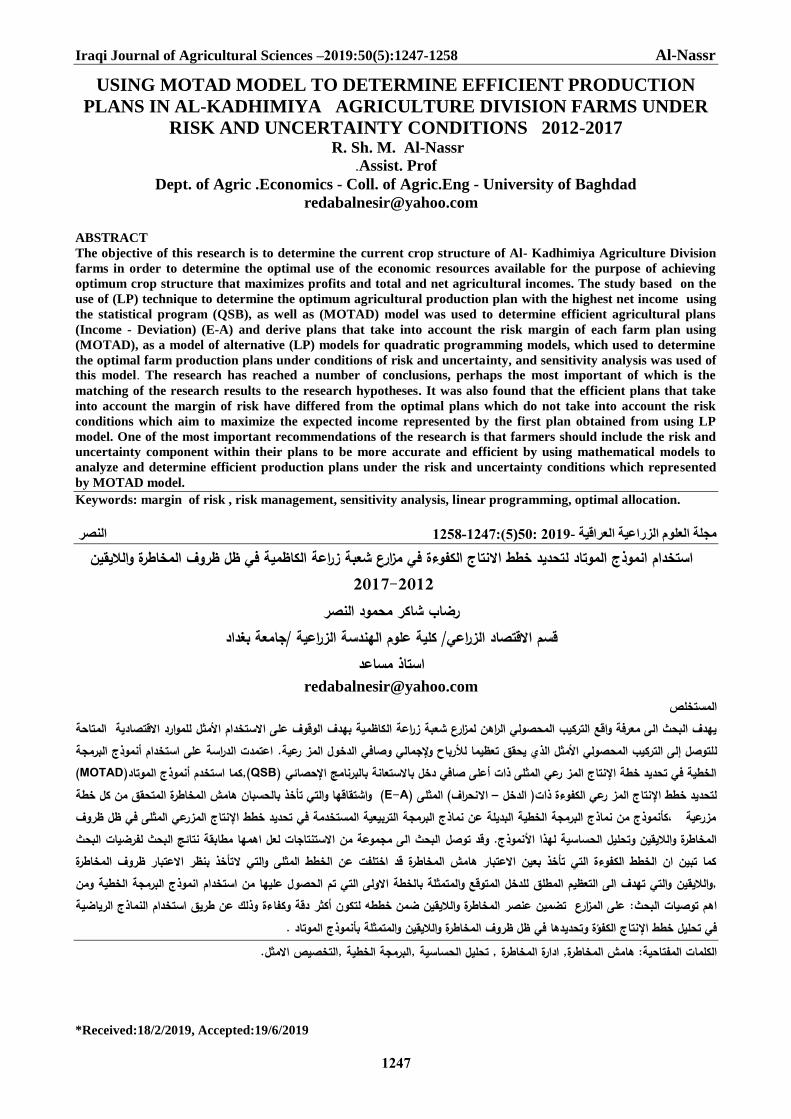
Iraqi Journal of Agricultural Sciences –2019:50(5):1247-1258 Al-Nassr

1247

USING MOTAD MODEL TO DETERMINE EFFICIENT PRODUCTION

PLANS IN AL-KADHIMIYA AGRICULTURE DIVISION FARMS UNDER

RISK AND UNCERTAINTY CONDITIONS 2012-2017 R. Sh. M. Al-Nassr

ProfAssist. .

Dept. of Agric .Economics - Coll. of Agric.Eng - University of Baghdad

[email protected]

ABSTRACT

The objective of this research is to determine the current crop structure of Al- Kadhimiya Agriculture Division

farms in order to determine the optimal use of the economic resources available for the purpose of achieving

optimum crop structure that maximizes profits and total and net agricultural incomes. The study based on the

use of (LP) technique to determine the optimum agricultural production plan with the highest net income using

the statistical program (QSB), as well as (MOTAD) model was used to determine efficient agricultural plans

(Income - Deviation) (E-A) and derive plans that take into account the risk margin of each farm plan using

(MOTAD), as a model of alternative (LP) models for quadratic programming models, which used to determine

the optimal farm production plans under conditions of risk and uncertainty, and sensitivity analysis was used of

this model. The research has reached a number of conclusions, perhaps the most important of which is the

matching of the research results to the research hypotheses. It was also found that the efficient plans that take

into account the margin of risk have differed from the optimal plans which do not take into account the risk

conditions which aim to maximize the expected income represented by the first plan obtained from using LP

model. One of the most important recommendations of the research is that farmers should include the risk and

uncertainty component within their plans to be more accurate and efficient by using mathematical models to

analyze and determine efficient production plans under the risk and uncertainty conditions which represented

by MOTAD model.

Keywords: margin of risk , risk management, sensitivity analysis, linear programming, optimal allocation.

النصر 1258-1247:(5(50: 2019-مجلة العلوم الزراعية العراقية

تحديد خطط االنتاج الكفوءة في مزارع شعبة زراعة الكاظمية في ظل ظروف المخاطرة والاليقين استخدام انموذج الموتاد ل2012-2017

رضاب شاكر محمود النصر / كلية علوم الهندسة الزراعية /جامعة بغداداالقتصاد الزراعي قسم

استاذ مساعد[email protected]

المستخلصللموارد االقتصادية المتاحة األمثل كاظمية بهدف الوقوف على االستخداميهدف البحث الى معرفة واقع التركيب المحصولي الراهن لمزارع شعبة زراعة ال

اعتمدت الدراسة على استخدام أنموذج البرمجة ز رعية. صافي الدخول الملتوصل إلى التركيب المحصولي األمثل الذي يحقق تعظيما لألرباح وإلجمالي و ل (MOTAD)(,كما استخدم أنموذج الموتادQSBالخطية في تحديد خطة اإلنتاج المز رعي المثلى ذات أعلى صافي دخل باالستعانة بالبرنامج اإلحصائي )

واشتقاقها والتي تأخذ بالحسبان هامش المخاطرة المتحقق من كل خطة (E-Aاالنحراف( المثلى ) –لتحديد خطط اإلنتاج المز رعي الكفوءة ذات) الدخل ظل ظروف مزرعية ،كأنموذج من نماذج البرمجة الخطية البديلة عن نماذج البرمجة التربيعية المستخدمة في تحديد خطط اإلنتاج المزرعي المثلى في

البحث الى مجموعة من االستنتاجات لعل اهمها مطابقة نتائج البحث لفرضيات البحث المخاطرة والاليقين وتحليل الحساسية لهذا األنموذج. وقد توصل خاطرة كما تبين ان الخطط الكفوءة التي تأخذ بعين االعتبار هامش المخاطرة قد اختلفت عن الخطط المثلى والتي التأخذ بنظر االعتبار ظروف الم

انموذج البرمجة الخطية ومن التي تم الحصول عليها من استخدام توقع والمتمثلة بالخطة االولىوالتي تهدف الى التعظيم المطلق للدخل الم والاليقين,النماذج الرياضية دقة وكفاءة وذلك عن طريق استخدام على المزارع تضمين عنصر المخاطرة والاليقين ضمن خططه لتكون أكثر :اهم توصيات البحث

ظل ظروف المخاطرة والاليقين والمتمثلة بأنموذج الموتاد . في تحليل خطط اإلنتاج الكفؤة وتحديدها في , تحليل الحساسية ,البرمجة الخطية ,التخصيص االمثل.امش المخاطرة, ادارة المخاطرة الكلمات المفتاحية: ه

*Received:18/2/2019, Accepted:19/6/2019


1248

INTRODUCTION As the conditions of agricultural production

are characterized by volatility and instability

as a result of a variety of factors such as

environmental conditions, general economic

policies, market forces, inventions, technology

and other factors that interact with each other

to be a state of lack of knowledge and

uncertainty of economic variables that lead to

the emergence of risk conditions which faces

the agricultural producer (decision-maker) in

the decision-making process, so risk

management and methods of dealing with it

have attracted the interest of agricultural

economic researchers and government

institutions and have taken multiple directions

to deal with them ,and reduce their negative

effects in the decision-making process (1( .As

Iraq is under the circumstances passed by and

the apparent deterioration in the agricultural

sector in all its aspects, this study is trying to

identify the reality of the crop structure in an

important agricultural area which suffer from

multiple problems surrounding the city of

Baghdad represented by the Sinaa farm as a

large farm contribute to the nutrition and the

provision of agricultural crops to surrounding

areas in Baghdad province which has been

selected as a model farm in the cultivation of

summer and winter crops in addition to

cultivated covered vegetables . This study is a

new qualitative attempt to deal with the risk

and management conditions that are often

associated with agricultural decision-making

which missing by most of the previous

agricultural economic research and studies and

since the agricultural sector and agricultural

production are characterized by the great risk

and uncertainties, especially in the recent

period, because of the exposure of the Iraqi

market to global markets, which increased the

elements of risk, the need seems necessary to

determine the optimal and efficient

agricultural plans in these farms through the

use of mathematical models that take into

account the circumstances of risk and

uncertainty ,The importance of the study is

shown by the fact that it is considering a very

important subject that concerns the food and

national security of Iraq and that it is possible

to adopt a scientific method in how to mix the

elements of production in a manner that

achieves the greatest return at the lowest

cost(3) and by defining mathematical models

that deal with risk conditions in agricultural

decision-making processes in general and

linearity in particular , in which optimum and

efficient agricultural production plans that take

into account risk and uncertain conditions in

farm production can be identified, which

situation will be more match with the

agricultural productive reality(20). Thus

saving the extra efforts and costs and the need

for special and complex software such as what

needed nonlinear and quadratic programming

, in particular to obtain optimum and efficient

production plans under the conditions of risk,

And the possibility of adoption of the

mathematical methods in any project or

facility, regardless of the quality of its activity

because of the simple method and treatments

without the complexities in dealing with data

and access to information required.The

problem of the study is the deterioration in

agricultural production in return for the high

cost of production due to the cessation of state

support as well as the problems of pollution

and market exposure and dumping policy and

others, which increased the degree of risk that

was neglected by the planner or farms in Sinaa

farm in determining their production plans

which resulted in a negative impact on the

efficiency of the use of resources.

Consequently, optimal agricultural production

plans, assuming the case of certainty, were

impractical and unrealistic. This requires

determining optimal agricultural production

plans that take into account the risk and

uncertainty conditions that accompany the

decision making process. Since Sinaa Farm as

a productive unit suffers from weakness in the

planning processes, it is possible to determine

the nature of the study problem in how to

ensure optimal allocation of agricultural

resources to arable areas based on the basis of

economic efficiency which means obtaining

more production with the same resources

available or obtaining the same amount of

production but with fewer resources (4, 17).

This study is aim to identify and derive

efficient production plans with optimal(

income-deviation) (E-A) farm production for

Sinaa farm using MOTAD model as a linear

programming model alternative to quadratic


1249

programming models that requires the

identification of mathematical models used to

determine optimal farm production plans and

compare them with the optimal farm

production plans obtained using LP

Technique, as well as to determine the

sensitivity of the model and explain it to some

or different dispersion measures as an

indicator of the risk margin on the farm

mentioned above. The study is based on the

following hypotheses: 1- The optimum crop

structure according to the linear programming

model, which does not take into account the

risk and uncertainty conditions in the

agricultural production, differs from those of

the expected income ) E (and the risk expressed

by average absolute total deviations (A) within

the MDATO model, which takes into account

the risk and uncertainty conditions that have

always accompanied the decision-making

process. 2-Plans which derived from

DDATOmodel are sensitive to the data used

in the measurement of average total absolute

deviations (A) if the average of the gross net

income for the years of study or any other

weighted average is used.

MATERIALS AND METHODS

Conceptual Framework:

Risk and Uncertainty Programming Models Mathematical models for risk analysis and

uncertainty in economic activities in general

and agricultural production activities in

particular are important analytical models. The

use of these programs and models enables

edired efficient production plans under the

conditions of risk and uncertainties that

decision makers often face and are expressed

in Risk Programming Models These efficient

production plans derived from the use of these

models are called Efficient Production Plans.

It means that these plans give a specific

income (return) with the lowest possible risk

or higher return from a specific risk margin.

Risk is expressed in these models by amount

of Variance (V), Standard Deviation (Sd) or

Mean Absolute Deviations (A) in each plan.

Non-linear programming models (especially

quadratic programming models), and MOTAD

model is one of the most common of these

programs. Table 1 represents the primary table

of the MOTD model that can be solved in

regular linear programming technique (10). It

is worth mentioning that there are other

models for dealing with Risk and uncertainty

in determining optimal and efficient

production plans other than quadrilateral

programming models and models, including

the Target MOTAD model and simulation

model, which represent an analytical technique

that includes the formulation of a realistic

model and then its choice (13). Because of the

difficulty of obtaining programs for other

models to deal with risk and the lack of full

detailed data needed by these models,

MOTAD model was used to derive efficient

production plans that achieve the objectives of

the study

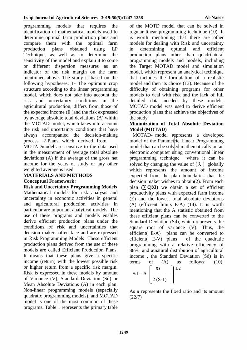
Minimization of Total Absolute Deviation

Model (MOTAD) MOTAD model represents a developed

model of the Parametric Linear Programming

model that can be solved mathematically on an

electronic computer using conventional linear

programming edqinrced where it can be

solved by changing the value of ( ) globally

which represents the amount of income

expected from the plan boundaries that the

decision maker wishes to obtain(2). From each

plan (∑𝐂𝐣𝐗𝐢) we obtain a set of efficient

productivity plans with expected farm income

(E) and the lowest total absolute deviations

(A) (efficient limits E-A) (14). It is worth

mentioning that the A statistic obtained from

these efficient snanp can be converted to the

Standard Deviation (Sd), which represents the

square root of variance (V). Thus, the

efficient) E-A ( plans can be converted to

efficient) E-V( snanp o f the quadratic

programming with a relative efficiency of

88% ane ae natural distribution of agricultural

income , the Standard Deviation (Sd) is in

terms of (A) as follows: (10):

s 1/2

Sd = A ---------------

2 (S-1)

As represents the fixed ratio and its amount

(22/7(


1250

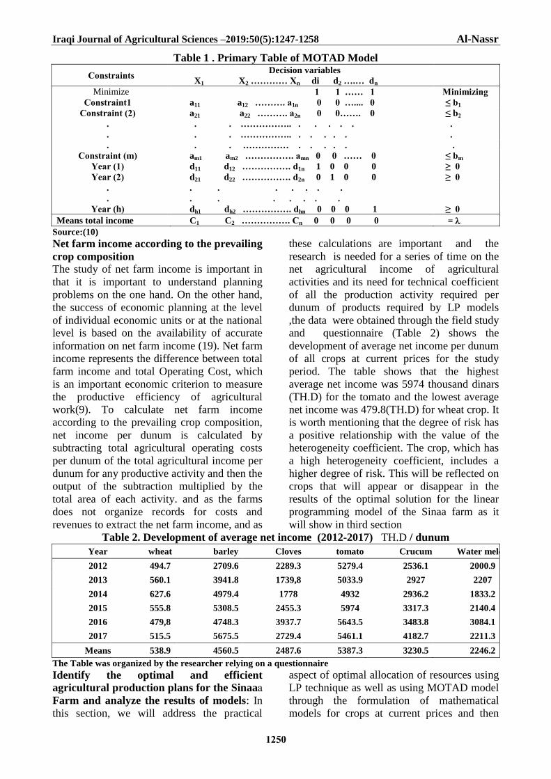
Table 1 . Primary Table of MOTAD Model

stnCortsnoC Decision variables

X1 X2 ………… Xn di d2 ….… dn

Minimize 1 1 …… 1 gsnsisisnM

1stnCortsno a11 a12 ………. a1n 0 0 ….... 0 ≤ b1

(2 )stnCortsno a21 a22 ………. a2n 0 0……. 0 ≤ b2

. . . …………….. . . . . . .

. . . …………….. . . . . . .

. . . …………… . . . . . .

(m )stnCortsno am1 am2 ……………. amn 0 0 …… 0 ≤ bm

(1 )ratr d11 d12 ……………. d1n 1 0 0 0 ≥ 0

(2 )ratr d21 d22 ……………. d2n 0 1 0 0 ≥ 0

. . . . . . . .

. . . . . . . .

(h )ratr dh1 dh2 ……………. dhn 0 0 0 1 ≥ 0

Means total income C1 C2 ……………. Cn 0 0 0 0 =

Source:(10)

Net farm income according to the prevailing

crop composition The study of net farm income is important in

that it is important to understand planning

problems on the one hand. On the other hand,

the success of economic planning at the level

of individual economic units or at the national

level is based on the availability of accurate

information on net farm income (19). Net farm

income represents the difference between total

farm income and total Operating Cost, which

is an important economic criterion to measure

the productive efficiency of agricultural

work(9). To calculate net farm income

according to the prevailing crop composition,

net income per dunum is calculated by

subtracting total agricultural operating costs

per dunum of the total agricultural income per

dunum for any productive activity and then the

output of the subtraction multiplied by the

total area of each activity. and as the farms

does not organize records for costs and

revenues to extract the net farm income, and as

these calculations are important and the

research is needed for a series of time on the

net agricultural income of agricultural

activities and its need for technical coefficient

of all the production activity required per

dunum of products required by LP models

,the data were obtained through the field study

and questionnaire (Table 2) shows the

development of average net income per dunum

of all crops at current prices for the study

period. The table shows that the highest

average net income was 5974 thousand dinars

(TH.D) for the tomato and the lowest average

net income was 479.8(TH.D) for wheat crop. It

is worth mentioning that the degree of risk has

a positive relationship with the value of the

heterogeneity coefficient. The crop, which has

a high heterogeneity coefficient, includes a

higher degree of risk. This will be reflected on

crops that will appear or disappear in the

results of the optimal solution for the linear

programming model of the Sinaa farm as it

will show in third section

Table 2. Development of average net income (2012-2017) TH.D / dunum

Year wheat barley Cloves tomato Crucum Water melon

2012 494.7 2709.6 2289.3 5279.4 2536.1 2000.9

2013 560.1 3941.8 1739,8 5033.9 2927 2207

2014 627.6 4979.4 1778 4932 2936.2 1833.2

2015 555.8 5308.5 2455.3 5974 3317.3 2140.4

2016 479,8 4748.3 3937.7 5643.5 3483.8 3084.1

2017 515.5 5675.5 2729.4 5461.1 4182.7 2211.3

Means 538.9 4560.5 2487.6 5387.3 3230.5 2246.2

The Table was organized by the researcher relying on a questionnaire

Identify the optimal and efficient

agricultural production plans for the Sinaaa

Farm and analyze the results of models: In

this section, we will address the practical

aspect of optimal allocation of resources using

LP technique as well as using MOTAD model

through the formulation of mathematical

models for crops at current prices and then


1251

analysis of results. The most important stage

of LP model is model formulation stage,

which is based on the fact that the farm aims to

maximize net farm income through cultivate of

several crops subject to specific

constraints(1,12). After LP model was

formulated, we used QSB (Quantitative

System for Business), which maximizes profit

by using Simplex Method (5), which is used to

solve LP problems in order to achieve the

optimal production plan for the agricultural

season (2016-2017) which represent last year

of study. Producers prefer to adopt the last

year, and the changes it has experienced as a

benchmark in conceptualizing their future

activities.

Methods of analysis

Efficient agricultural production plans

according to gedom itTaM To achieve the objectives of the study, we

formulated LP model for the Sinaa Farm for

the agricultural season (2016-2017) to obtain

the optimal allocation of resources, which

maximizes the total net farm income per

dunam, as the target model is a mathematical

model restricted to calculate the best income

for the best plan and for the best combination

of production maximizes net income, in

addition ,drafting the constraints of MOTAD

model needs to formulate the constraints of

linear programming model because the

optimal income obtained from the optimal plan

in the linear programming model represents

the value of (6) in the first plan of the

MOTAD model and represents the greatest

expected income In this plan which represents

the plan realized without taking into

consideration the risk (Risk- Free Plan) (15).

gtriaMtosnM gedom Models of the Sinaa

Farm ( (gsrCo cSantrst : To identify and derive efficient agricultural

production plans which has (income -

deviation) (E-A), (Win QSB) Windows

Quantitative System for Business, has been

used it is ready application with windows

operating systems (7). The program was

specifically designed to solve administrative

problems, decision-making problems,

operations research and production systems

(8). QSB program was used, which operates

on the Simplex Method as well as using

MOTAD program in two scenarios as shown

below:

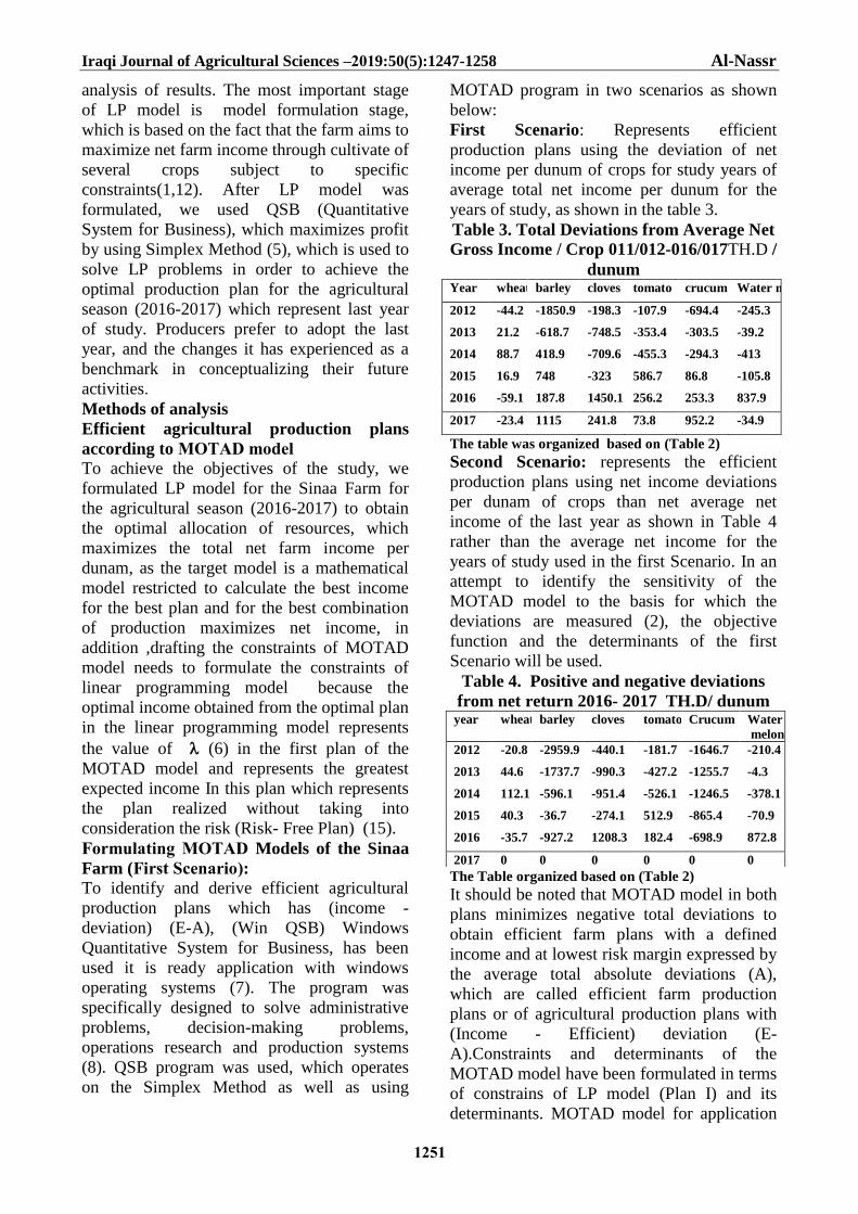
First Scenario: Represents efficient

production plans using the deviation of net

income per dunum of crops for study years of

average total net income per dunum for the

years of study, as shown in the table 3.

Table 3. Total Deviations from Average Net

Gross Income / Crop 011/012-016/017TH.D /

dunum Year wheat barley cloves tomato crucum Water melon

2012 -44.2 -1850.9 -198.3 -107.9 -694.4 -245.3

2013 21.2 -618.7 -748.5 -353.4 -303.5 -39.2

2014 88.7 418.9 -709.6 -455.3 -294.3 -413

2015 16.9 748 -323 586.7 86.8 -105.8

2016 -59.1 187.8 1450.1 256.2 253.3 837.9

2017 -23.4 1115 241.8 73.8 952.2 -34.9

The table was organized based on (Table 2)

Second Scenario: represents the efficient

production plans using net income deviations

per dunam of crops than net average net

income of the last year as shown in Table 4

rather than the average net income for the

years of study used in the first Scenario. In an

attempt to identify the sensitivity of the

MOTAD model to the basis for which the

deviations are measured (2), the objective

function and the determinants of the first

Scenario will be used.

Table 4. Positive and negative deviations

from net return 2016- 2017 TH.D/ dunum

The Table organized based on (Table 2)

It should be noted that MOTAD model in both

plans minimizes negative total deviations to

obtain efficient farm plans with a defined

income and at lowest risk margin expressed by

the average total absolute deviations (A),

which are called efficient farm production

plans or of agricultural production plans with

(Income - Efficient) deviation (E-

A).Constraints and determinants of the

MOTAD model have been formulated in terms

of constrains of LP model (Plan I) and its

determinants. MOTAD model for application

year wheat barley cloves tomato Crucum Water

melon

2012 -20.8 -2959.9 -440.1 -181.7 -1646.7 -210.4

2013 44.6 -1737.7 -990.3 -427.2 -1255.7 -4.3

2014 112.1 -596.1 -951.4 -526.1 -1246.5 -378.1

2015 40.3 -36.7 -274.1 512.9 -865.4 -70.9

2016 -35.7 -927.2 1208.3 182.4 -698.9 872.8

2017 0 0 0 0 0 0


1252

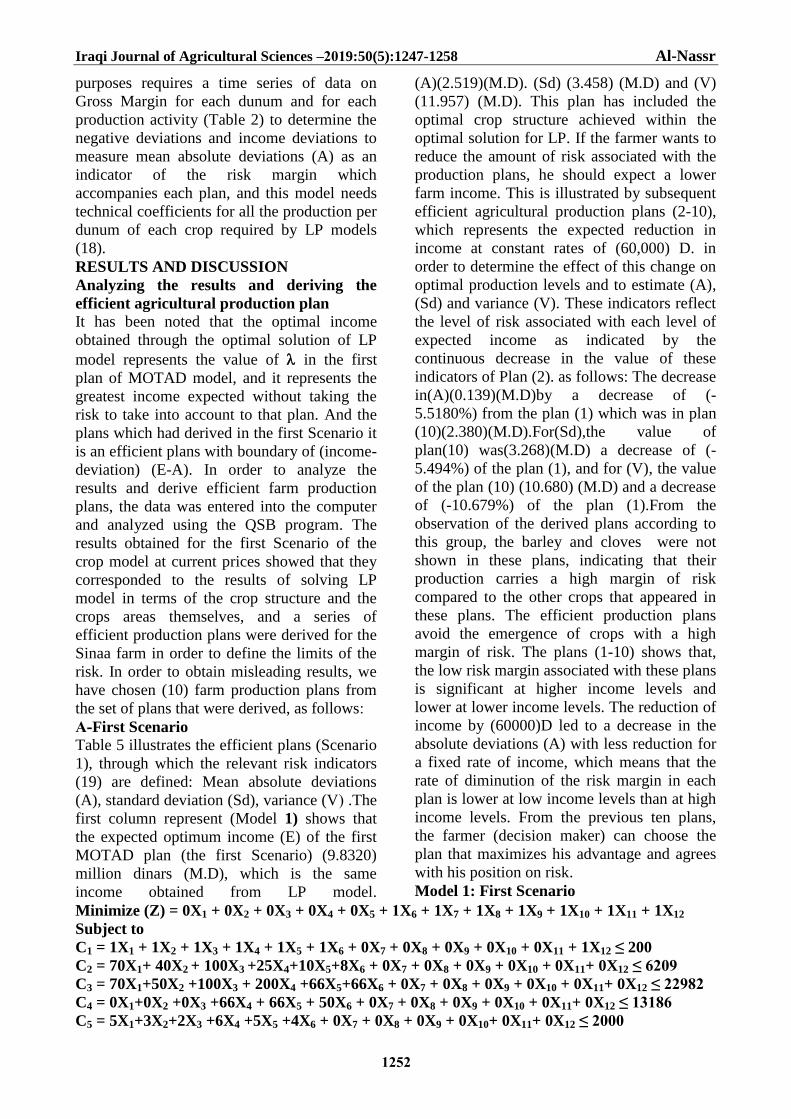
purposes requires a time series of data on

Gross Margin for each dunum and for each

production activity (Table 2) to determine the

negative deviations and income deviations to

measure mean absolute deviations (A) as an

indicator of the risk margin which

accompanies each plan, and this model needs

technical coefficients for all the production per

dunum of each crop required by LP models

(18).

RESULTS AND DISCUSSION

Analyzing the results and deriving the

efficient agricultural production plan

It has been noted that the optimal income

obtained through the optimal solution of LP

model represents the value of in the first

plan of MOTAD model, and it represents the

greatest income expected without taking the

risk to take into account to that plan. And the

plans which had derived in the first Scenario it

is an efficient plans with boundary of (income-

deviation) (E-A). In order to analyze the

results and derive efficient farm production

plans, the data was entered into the computer

and analyzed using the QSB program. The

results obtained for the first Scenario of the

crop model at current prices showed that they

corresponded to the results of solving LP

model in terms of the crop structure and the

crops areas themselves, and a series of

efficient production plans were derived for the

Sinaa farm in order to define the limits of the

risk. In order to obtain misleading results, we

have chosen (10) farm production plans from

the set of plans that were derived, as follows:

-o First Scenario

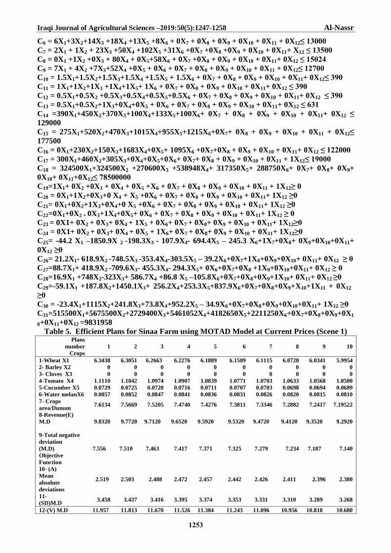
Table 5 illustrates the efficient plans (Scenario

1), through which the relevant risk indicators

(19) are defined: Mean absolute deviations

(A), standard deviation (Sd), variance (V ( .The

first column represent (Model 1) shows that

the expected optimum income (E) of the first

MOTAD plan (the first Scenario) (9.8320)

million dinars (M.D), which is the same

income obtained from LP model.

(A)(2.519)(M.D). (Sd) (3.458) (M.D) and (V)

(11.957) (M.D). This plan has included the

optimal crop structure achieved within the

optimal solution for LP. If the farmer wants to

reduce the amount of risk associated with the

production plans, he should expect a lower

farm income. This is illustrated by subsequent

efficient agricultural production plans (2-10),

which represents the expected reduction in

income at constant rates of (60,000) D. in

order to determine the effect of this change on

optimal production levels and to estimate (A),

(Sd) and variance (V). These indicators reflect

the level of risk associated with each level of

expected income as indicated by the

continuous decrease in the value of these

indicators of Plan (2). as follows: The decrease

in(A)(0.139)(M.D)by a decrease of (-

5.5180%) from the plan (1) which was in plan

(10)(2.380)(M.D).For(Sd),the value of

plan(10) was(3.268)(M.D) a decrease of (-

5.494%) of the plan (1), and for (V), the value

of the plan (10) (10.680) (M.D) and a decrease

of (-10.679%) of the plan (1).From the

observation of the derived plans according to

this group, the barley and cloves were not

shown in these plans, indicating that their

production carries a high margin of risk

compared to the other crops that appeared in

these plans. The efficient production plans

avoid the emergence of crops with a high

margin of risk. The plans (1-10) shows that,

the low risk margin associated with these plans

is significant at higher income levels and

lower at lower income levels. The reduction of

income by (60000)D led to a decrease in the

absolute deviations (A) with less reduction for

a fixed rate of income, which means that the

rate of diminution of the risk margin in each

plan is lower at low income levels than at high

income levels. From the previous ten plans,

the farmer (decision maker) can choose the

plan that maximizes his advantage and agrees

with his position on risk.

Model 1: First Scenario

Minimize (Z) = 0X1 + 0X2 + 0X3 + 0X4 + 0X5 + 1X6 + 1X7 + 1X8 + 1X9 + 1X10 + 1X11 + 1X12

Subject to

C1 = 1X1 + 1X2 + 1X3 + 1X4 + 1X5 + 1X6 + 0X7 + 0X8 + 0X9 + 0X10 + 0X11 + 1X12 ≤ 200

C2 = 70X1+ 40X2 + 100X3 +25X4+10X5+8X6 + 0X7 + 0X8 + 0X9 + 0X10 + 0X11+ 0X12 ≤ 6209

C3 = 70X1+50X2 +100X3 + 200X4 +66X5+66X6 + 0X7 + 0X8 + 0X9 + 0X10 + 0X11+ 0X12 ≤ 22982

C4 = 0X1+0X2 +0X3 +66X4 + 66X5 + 50X6 + 0X7 + 0X8 + 0X9 + 0X10 + 0X11+ 0X12 ≤ 13186

C5 = 5X1+3X2+2X3 +6X4 +5X5 +4X6 + 0X7 + 0X8 + 0X9 + 0X10+ 0X11+ 0X12 ≤ 2000


1253

C6 = 6X1+3X2+14X3 +18X4 +13X5 +8X6 + 0X7 + 0X8 + 0X9 + 0X10 + 0X11 + 0X12≤ 13000

C7 = 2X1 + 1X2 + 23X3 +50X4 +102X5 +31X6 +0X7 +0X8 +0X9 + 0X10 + 0X11+ X12 ≤ 13500

C8 = 0X1 +1X2 +0X3 + 80X4 + 0X5+58X6 + 0X7 +0X8 + 0X9 + 0X10 + 0X11+ 0X12 ≤ 15024

C9 = 7X1 + 4X2 +7X3+52X4 +0X5 + 0X6 + 0X7 + 0X8 + 0X9 + 0X10 + 0X11 + 0X12≤ 12700

C10 = 1.5X1+1.5X2+1.5X3+1.5X4 +1.5X5 + 1.5X6 + 0X7 + 0X8 + 0X9 + 0X10 + 0X11+ 0X12≤ 390

C11 = 1X1+1X2+1X3 +1X4+1X5+ 1X6 + 0X7 + 0X8 + 0X9 + 0X10 + 0X11+ 0X12 ≤ 390

C12 = 0.5X1+0.5X2 +0.5X3+0.5X4+0.5X5+0.5X6 + 0X7 + 0X8 + 0X9 + 0X10 + 0X11+ 0X12 ≤ 390

C13 = 0.5X1+0.5X2+1X3+0X4+0X5 + 0X6 + 0X7 + 0X8 + 0X9 + 0X10 + 0X11+ 0X12 ≤ 631

C14 =390X1+450X2+370X3+100X4+133X5+100X6+ 0X7 + 0X8 + 0X9 + 0X10 + 0X11+ 0X12 ≤

129000

C15 = 275X1+520X2+470X3+1015X4+955X5+1215X6+0X7+ 0X8 + 0X9 + 0X10 + 0X11 + 0X12≤

177500

C16 = 0X1+230X2+150X3+1683X4+0X5+ 1095X6 +0X7+0X8 + 0X9 + 0X10 + 0X11+ 0X12 ≤ 122000

C17 = 300X1+460X2+305X3+0X4+0X5+0X6+ 0X7+ 0X8 + 0X9 + 0X10 + 0X11 + 1X12≤ 19000

C18 = 324500X1+324500X2 +270600X3 +538948X4+ 317350X5+ 288750X6+ 0X7+ 0X8+ 0X9+

0X10+ 0X11+0X12≤ 78500000

C19=1X1+ 0X2 +0X3 + 0X4 + 0X5 +X6 + 0X7 + 0X8 + 0X9 + 0X10 + 0X11 + 1X12≥ 0

C20 = 0X1+1X2+0X3+0 X4 + X5 +0X6 + 0X7 + 0X8 + 0X9 + 0X10 + 0X11+ 1X12 ≥0

C21= 0X1+0X2+1X3+0X4+0 X5 +0X6 + 0X7 + 0X8 + 0X9 + 0X10 + 0X11+ 1X12 ≥0

C22=0X1+0X2 + 0X3+1X4+0X5+ 0X6 + 0X7 + 0X8 + 0X9 + 0X10 + 0X11+ 1X12 ≥ 0

C23 = 0X1+ 0X2 + 0X3+ 0X4 + 1X5 + 0X6+ 0X7 + 0X8+ 0X9 + 0X10 + 0X11+ 1X12≥0

C24 = 0X1+ 0X2 + 0X3+ 0X4 + 0X5 + 1X6+ 0X7 + 0X8+ 0X9 + 0X10 + 0X11+ 1X12≥0

C25= -44.2 X1 –1850.9X 2 -198.3X3 - 107.9X4- 694.4X5 – 245.3 X6+1X7+0X8+ 0X9+0X10+0X11+

0X12 ≥0

C26= 21.2X1- 618.9X2 -748.5X3 -353.4X4-303.5X5 – 39.2X6+0X7+1X8+0X9+0X10+ 0X11+ 0X12 ≥ 0

C27=88.7X1+ 418.9X2 -709.6X3- 455.3X4- 294.3X5+ 0X6+0X7+0X8 +1X9+0X10+0X11+ 0X12 ≥ 0

C28=16.9X1 +748X2-323X3+ 586.7X4 +86.8 X5 –105.8X6+0X7+0X8+0X9+1X10+ 0X11+ 0X12 ≥0

C29=-59.1X1 +187.8X2+1450.1X3+ 256.2X4+253.3X5+837.9X6+0X7+0X8+0X9+X10+1X11 + 0X12

≥0

C30 = -23.4X1+1115X2+241.8X3+73.8X4+952.2X5 – 34.9X6+0X7+0X8+0X9+0X10+0X11+ 1X12 ≥0

C31=515500X1+5675500X2+2729400X3+5461052X4+4182650X5+2211250X6+0X7+0X8+0X9+0X1

0+0X11+0X12 =9831958

Table 5. Efficient Plans for Sinaa Farm using MOTAD Model at Current Prices (Scene 1)

10 9 8 7 6 5 4 3 2 1

Plans

number

Crops

5.9954 6.0341 6.0728 6.1115 6.1509 6.1889 6.2276 6.2663 6.3051 6.3438 1-Wheat X1

0 0 0 0 0 0 0 0 0 0 2- Barley X2

0 0 0 0 0 0 0 0 0 0 3- Cloves X3

1.0500 1.0568 1.0633 1.0703 1.0771 1.0839 1.0907 1.0974 1.1042 1.1110 4-Tomato X4

0.0689 0.0694 0.0698 0.0703 0.0707 0.0711 0.0716 0.0720 0.0725 0.0729 5-Cucumber X5

0.0810 0.0815 0.0820 0.0826 0.0831 0.0836 0.0841 0.0847 0.0852 0.0857 6-Water melanX6

7.19522 7.2417 7.2882 7.3346 7.3811 7.4276 7.4740 7.5205 7.5669 7.6134 7- Crops

area/Dunum

9.2920 9.3520 9.4120 9.4720 9.5320 9.5920 9.6520 9.7120 9.7720 9.8320

8-Revenue(E)

M.D

7.140 7.187 7.234 7.279 7.325 7.371 7.417 7.463 7.510 7.556

9-Total negative

deviation

(M.D)

Objective

Function

2.380 2.396 2.411 2.426 2.442 2.457 2.472 2.488 2.503 2.519

10- (A)

Mean

absolute

deviations

3.268 3.289 3.310 3.331 3.353 3.374 3.395 3.416 3.437 3.458 11-

(SD)M.D

10.680 10.818 10.956 11.096 11.243 11.384 11.526 11.670 11.813 11.957 12-(V) M.D


1254

Source: The table was organized by the

researcher as follows data grades (1-6, 8 and

9) based on the results of the above plans, the

data of the other rows were calculated by the

researcher. The first scenario shows that

efficient farm production plans that take into

consideration the margin of risk have differed

from optimal farm production plans that do not

take into account the risk conditions and which

aim to maximize the expected income

represented by the first plan obtained from

using the model Linear programming. It is also

different from the actual farm plan, and the

difference is to allocate fewer resources to

crops with higher risk margins than we have

observed in the direction of their areas of

decline compared with low levels of income,

as opposed to crops with a lower margin of

risk.

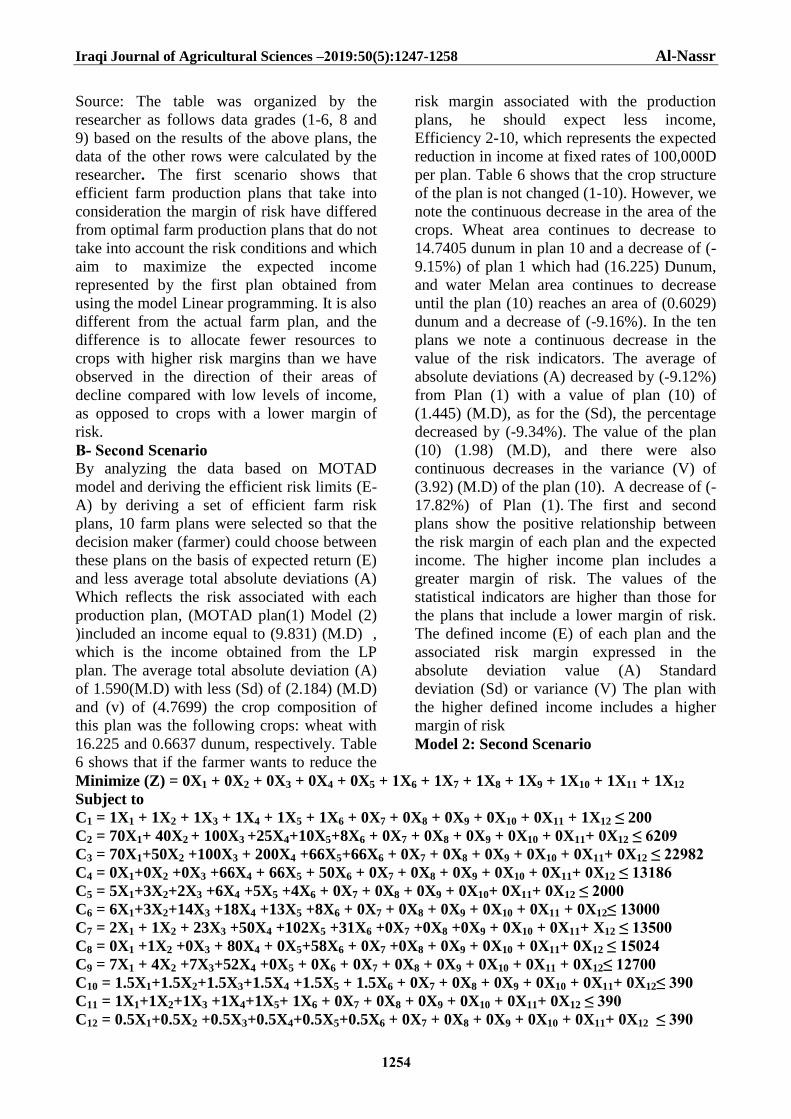
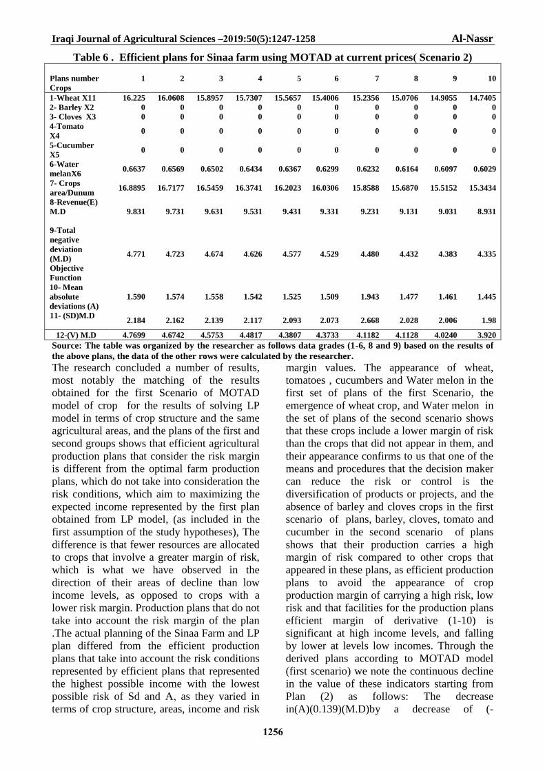
-B caStnT Scenario By analyzing the data based on MOTAD

model and deriving the efficient risk limits (E-

A) by deriving a set of efficient farm risk

plans, 10 farm plans were selected so that the

decision maker (farmer) could choose between

these plans on the basis of expected return (E)

and less average total absolute deviations (A)

Which reflects the risk associated with each

production plan, (MOTAD plan(1) Model (2)

)included an income equal to (9.831) (M.D) ,

which is the income obtained from the LP

plan. The average total absolute deviation (A)

of 1.590(M.D) with less (Sd) of (2.184) (M.D)

and (v) of (4.7699) the crop composition of

this plan was the following crops: wheat with

16.225 and 0.6637 dunum, respectively. Table

6 shows that if the farmer wants to reduce the

risk margin associated with the production

plans, he should expect less income,

Efficiency 2-10, which represents the expected

reduction in income at fixed rates of 100,000D

per plan. Table 6 shows that the crop structure

of the plan is not changed (1-10). However, we

note the continuous decrease in the area of the

crops. Wheat area continues to decrease to

14.7405 dunum in plan 10 and a decrease of (-

9.15%) of plan 1 which had (16.225) Dunum,

and water Melan area continues to decrease

until the plan (10) reaches an area of (0.6029)

dunum and a decrease of (-9.16%). In the ten

plans we note a continuous decrease in the

value of the risk indicators. The average of

absolute deviations (A) decreased by (-9.12%)

from Plan (1) with a value of plan (10) of

(1.445) (M.D), as for the (Sd), the percentage

decreased by (-9.34%). The value of the plan

(10) (1.98) (M.D), and there were also

continuous decreases in the variance (V) of

(3.92) (M.D) of the plan (10). A decrease of (-

17.82%) of Plan (1). The first and second

plans show the positive relationship between

the risk margin of each plan and the expected

income. The higher income plan includes a

greater margin of risk. The values of the

statistical indicators are higher than those for

the plans that include a lower margin of risk.

The defined income (E) of each plan and the

associated risk margin expressed in the

absolute deviation value (A) Standard

deviation (Sd) or variance (V) The plan with

the higher defined income includes a higher

margin of risk

Model 2: Second Scenario

Minimize (Z) = 0X1 + 0X2 + 0X3 + 0X4 + 0X5 + 1X6 + 1X7 + 1X8 + 1X9 + 1X10 + 1X11 + 1X12

Subject to

C1 = 1X1 + 1X2 + 1X3 + 1X4 + 1X5 + 1X6 + 0X7 + 0X8 + 0X9 + 0X10 + 0X11 + 1X12 ≤ 200

C2 = 70X1+ 40X2 + 100X3 +25X4+10X5+8X6 + 0X7 + 0X8 + 0X9 + 0X10 + 0X11+ 0X12 ≤ 6209

C3 = 70X1+50X2 +100X3 + 200X4 +66X5+66X6 + 0X7 + 0X8 + 0X9 + 0X10 + 0X11+ 0X12 ≤ 22982

C4 = 0X1+0X2 +0X3 +66X4 + 66X5 + 50X6 + 0X7 + 0X8 + 0X9 + 0X10 + 0X11+ 0X12 ≤ 13186

C5 = 5X1+3X2+2X3 +6X4 +5X5 +4X6 + 0X7 + 0X8 + 0X9 + 0X10+ 0X11+ 0X12 ≤ 2000

C6 = 6X1+3X2+14X3 +18X4 +13X5 +8X6 + 0X7 + 0X8 + 0X9 + 0X10 + 0X11 + 0X12≤ 13000

C7 = 2X1 + 1X2 + 23X3 +50X4 +102X5 +31X6 +0X7 +0X8 +0X9 + 0X10 + 0X11+ X12 ≤ 13500

C8 = 0X1 +1X2 +0X3 + 80X4 + 0X5+58X6 + 0X7 +0X8 + 0X9 + 0X10 + 0X11+ 0X12 ≤ 15024

C9 = 7X1 + 4X2 +7X3+52X4 +0X5 + 0X6 + 0X7 + 0X8 + 0X9 + 0X10 + 0X11 + 0X12≤ 12700

C10 = 1.5X1+1.5X2+1.5X3+1.5X4 +1.5X5 + 1.5X6 + 0X7 + 0X8 + 0X9 + 0X10 + 0X11+ 0X12≤ 390

C11 = 1X1+1X2+1X3 +1X4+1X5+ 1X6 + 0X7 + 0X8 + 0X9 + 0X10 + 0X11+ 0X12 ≤ 390

C12 = 0.5X1+0.5X2 +0.5X3+0.5X4+0.5X5+0.5X6 + 0X7 + 0X8 + 0X9 + 0X10 + 0X11+ 0X12 ≤ 390


1255

C13 = 0.5X1+0.5X2+1X3+0X4+0X5 + 0X6 + 0X7 + 0X8 + 0X9 + 0X10 + 0X11+ 0X12 ≤ 631

C14 =390X1+450X2+370X3+100X4+133X5+100X6+ 0X7 + 0X8 + 0X9 + 0X10 + 0X11+ 0X12 ≤

129000

C15 = 275X1+520X2+470X3+1015X4+955X5+1215X6+0X7+ 0X8 + 0X9 + 0X10 + 0X11 + 0X12≤

177500

C16 = 0X1+230X2+150X3+1683X4+0X5+ 1095X6 +0X7+0X8 + 0X9 + 0X10 + 0X11+ 0X12 ≤ 122000

C17 = 300X1+460X2+305X3+0X4+0X5+0X6+ 0X7+ 0X8 + 0X9 + 0X10 + 0X11 + 1X12≤ 19000

C18 = 324500X1+324500X2 +270600X3 +538948X4+ 317350X5+ 288750X6+ 0X7+ 0X8+ 0X9+

0X10+ 0X11+ 0X12≤ 78500000

C19=1X1+ 0X2 +0X3 + 0X4 + 0X5 +X6 + 0X7 + 0X8 + 0X9 + 0X10 + 0X11 + 1X12≥ 0

C20 = 0X1+1X2+0X3+0 X4 + X5 +0X6 + 0X7 + 0X8 + 0X9 + 0X10 + 0X11+ 1X12 ≥0

C21= 0X1+0X2+1X3+0X4+0 X5 +0X6 + 0X7 + 0X8 + 0X9 + 0X10 + 0X11+ 1X12 ≥0

C22=0X1+0X2 + 0X3+1X4+0X5+ 0X6 + 0X7 + 0X8 + 0X9 + 0X10 + 0X11+ 1X12 ≥ 0

C23 = 0X1+ 0X2 + 0X3+ 0X4 + 1X5 + 0X6+ 0X7 + 0X8+ 0X9 + 0X10 + 0X11+ 1X12≥0

C24 = 0X1+ 0X2 + 0X3+ 0X4 + 0X5 + 1X6+ 0X7 + 0X8+ 0X9 + 0X10 + 0X11+ 1X12≥0

C25= -20.8X1 – 2959.9X 2 -440.1X3 – 181.7X4- 1646.7X5 – 210.4X6+1X7+0X8+ 0X9+0X10+0X11+

0X12 ≥0

C26= 44.6X1- 1737.7X2 -990.3X3 -427.2X4-1255.7X5 – 4.3X6+0X7+1X8+0X9+0X10+ 0X11+ 0X12 ≥

0

C27=112.1X1 – 596.1X2 -951.4X3- 529.1X4- 1246.5X5- 378.1 X6+0X7+0X8 +1X9+0X10+0X11+ 0X12

≥ 0

C28=40.3X1 -36.7X2 -274.1X3+ 512.9X4 -865.4X5 –70.9X6+0X7+0X8+0X9+1X10+ 0X11+ 0X12 ≥0

C29=-35.7X1 -927.2X2+1208.3X3+ 182.4X4 -698.9X5+872.8X6+0X7+0X8+0X9+X10+1X11 + 0X12

≥0

C30 = 0X1+0X2+0X3+0X4+0X5 +0X6+0X7+0X8+0X9+0X10+0X11+ 1X12 ≥0

C31=515500X1+5675500X2+2729400X3+5461052X4+4182650X5+2211250X6+0X7+0X8+0X9+0X1

0+0X11+ 0X12 =9831958

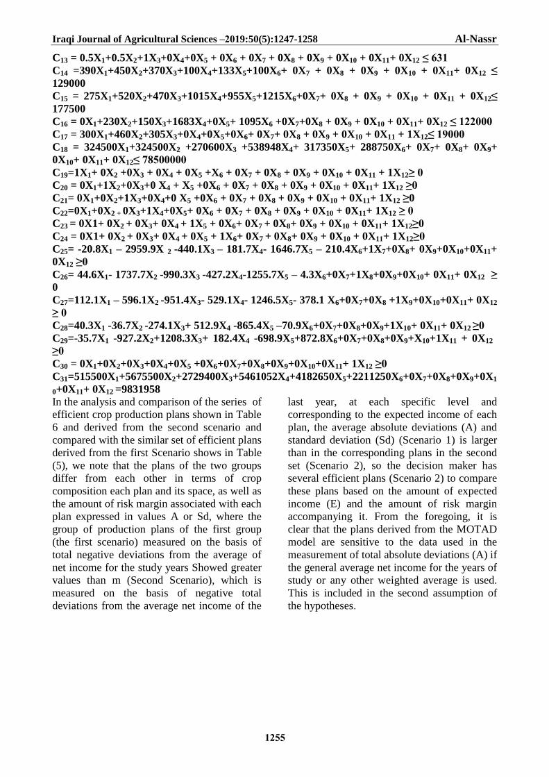
In the analysis and comparison of the series of

efficient crop production plans shown in Table

6 and derived from the second scenario and

compared with the similar set of efficient plans

derived from the first Scenario shows in Table

(5), we note that the plans of the two groups

differ from each other in terms of crop

composition each plan and its space, as well as

the amount of risk margin associated with each

plan expressed in values A or Sd, where the

group of production plans of the first group

(the first scenario) measured on the basis of

total negative deviations from the average of

net income for the study years Showed greater

values than m (Second Scenario), which is

measured on the basis of negative total

deviations from the average net income of the

last year, at each specific level and

corresponding to the expected income of each

plan, the average absolute deviations (A) and

standard deviation (Sd) (Scenario 1) is larger

than in the corresponding plans in the second

set (Scenario 2), so the decision maker has

several efficient plans (Scenario 2) to compare

these plans based on the amount of expected

income (E) and the amount of risk margin

accompanying it. From the foregoing, it is

clear that the plans derived from the MOTAD

model are sensitive to the data used in the

measurement of total absolute deviations (A) if

the general average net income for the years of

study or any other weighted average is used.

This is included in the second assumption of

the hypotheses.


1256

Table 6 . Efficient plans for Sinaa farm using MOTAD at current prices) Scenario 2)

10 9 8 7 6 5 4 3 2 1

Plans number

Crops

14.7405 14.9055 15.0706 15.2356 15.4006 15.5657 15.7307 15.8957 16.0608 16.225 1-Wheat X11

0 0 0 0 0 0 0 0 0 0 2- Barley X2

0 0 0 0 0 0 0 0 0 0 3- Cloves X3

0 0 0 0 0 0 0 0 0 0 4-Tomato

X4

0 0 0 0 0 0 0 0 0 0 5-Cucumber

X5

0.6029 0.6097 0.6164 0.6232 0.6299 0.6367 0.6434 0.6502 0.6569 0.6637 6-Water

melanX6

15.3434 15.5152 15.6870 15.8588 16.0306 16.2023 16.3741 16.5459 16.7177 16.8895 7- Crops

area/Dunum

8.931 9.031 9.131 9.231 9.331 9.431 9.531 9.631 9.731 9.831

8-Revenue(E)

M.D

4.335 4.383 4.432 4.480 4.529 4.577 4.626 4.674 4.723 4.771

9-Total

negative

deviation

(M.D)

Objective

Function

1.445 1.461 1.477 1.943 1.509 1.525 1.542 1.558 1.574 1.590

10- Mean

absolute

deviations (A)

1.98 2.006 2.028 2.668 2.073 2.093 2.117 2.139 2.162 2.184 11- (SD)M.D

3.920 4.0240 4.1128 4.1182 4.3733 4.3807 4.4817 4.5753 4.6742 4.7699 12-(V) M.D

Source: The table was organized by the researcher as follows data grades (1-6, 8 and 9) based on the results of

the above plans, the data of the other rows were calculated by the researcher.

The research concluded a number of results,

most notably the matching of the results

obtained for the first Scenario of MOTAD

model of crop for the results of solving LP

model in terms of crop structure and the same

agricultural areas, and the plans of the first and

second groups shows that efficient agricultural

production plans that consider the risk margin

is different from the optimal farm production

plans, which do not take into consideration the

risk conditions, which aim to maximizing the

expected income represented by the first plan

obtained from LP model, (as included in the

first assumption of the study hypotheses), The

difference is that fewer resources are allocated

to crops that involve a greater margin of risk,

which is what we have observed in the

direction of their areas of decline than low

income levels, as opposed to crops with a

lower risk margin. Production plans that do not

take into account the risk margin of the plan

.The actual planning of the Sinaa Farm and LP

plan differed from the efficient production

plans that take into account the risk conditions

represented by efficient plans that represented

the highest possible income with the lowest

possible risk of Sd and A, as they varied in

terms of crop structure, areas, income and risk

margin values. The appearance of wheat,

tomatoes , cucumbers and Water melon in the

first set of plans of the first Scenario, the

emergence of wheat crop, and Water melon in

the set of plans of the second scenario shows

that these crops include a lower margin of risk

than the crops that did not appear in them, and

their appearance confirms to us that one of the

means and procedures that the decision maker

can reduce the risk or control is the

diversification of products or projects, and the

absence of barley and cloves crops in the first

scenario of plans, barley, cloves, tomato and

cucumber in the second scenario of plans

shows that their production carries a high

margin of risk compared to other crops that

appeared in these plans, as efficient production

plans to avoid the appearance of crop

production margin of carrying a high risk, low

risk and that facilities for the production plans

efficient margin of derivative (1-10) is

significant at high income levels, and falling

by lower at levels low incomes. Through the

derived plans according to MOTAD model

(first scenario) we note the continuous decline

in the value of these indicators starting from

Plan (2) as follows: The decrease

in(A)(0.139)(M.D)by a decrease of (-


1257

5.5180%) from the plan (1) which was in plan

(10)of(2.380)(M.D).And for(Sd),the value of

plan(10) was(3.268)(M.D) a decrease of (-

5.494%) of the plan (1), and for (V), the value

of the plan (10) (10.680) (M.D) and a decrease

of (-10.679%) of the plan (1) in (Scenario 2)

we can see a continuous decrease in the value

of the risk indicators . Plan (1) shows the

average total absolute deviation (A) of

1.590(M.D) with (Sd) of (2.184) (M.D) and

(v) of (4.7699) ,the crop composition of this

plan was the following : wheat with 16.225

and 0.6637 dunum, respectively. The average

of absolute deviations (A) decreased by (-

9.12%) from plan (1) with a value of plan (10)

of (1.445)(M.D), as for the (Sd), the

percentage decreased by (-9.34%). The value

of the plan (10) (1.98)(M.D) and there were

also continuous decreases in the variance (V)

of (3.92)(M.D) of the plan (10) A decrease of

(-17.82%) of plan (1).We also note through the

two sets of plans that there is a type of trade-

off or barter between the expected income (E)

for each plan and the amount of risk margin.

The high-income plans are highly risky and

the values of the statistical indicators are larger

than for the plans that include a lower risk

margin. There is a positive relationship

between the margin for each plan and the

expected income from it, and there is a

difference between efficient production plans

with a fixed income and less (V) or less (A)

and measured on the basis of total deviations

from the value of the average of farm net

income for the entire period of time expressed

in the first plan of those efficient farm plans

and measured on the basis of total negative

deviations from the average net farm income

for the last year of the period expressed in the

second scenario Which is included in the

second assumption of the hypotheses of the

study).Which reflects the sensitivity of

MOTAD model to the scale of total deviations

used. These agricultural plans differed in terms

of the crop structure and the areas exploited

for each crop as well as the margin of risk

associated with each plan. From the previous

conclusions, we can make a number of

recommendations, the most important of

which is the use of the linear programming

method to determine the extent to which the

available resources are invested efficiently,

which helps to increase production, and the

need to generalize this method and apply it in

farms with similar conditions to determine the

optimal use of the available productive

resources. Crop yield as indicated by linear

programming results with the aim of achieving

economic efficiency for farmers and excluding

agricultural crops that are not economically

important, while establishing agricultural

training and extension courses for farmers to

use the best productive methods. Modern

sponsor. In addition, the farmer must include

the risk and uncertainties within their plans to

be more accurate and efficient by using

mathematical models in the analysis of the

efficient production plans and identifying them

under the risk and uncertainty conditions of

the model of death or other mathematical

models as the target model of the target as the

decision maker has several efficient plans To

choose from them what maximizes their

benefit or preference and agrees with their

position on risk. As well as increasing

resources whose shadow prices are positive,

including land and capital for the purpose of

benefiting from other surplus resources whose

prices are zero, such as compost, urea, manure,

pesticides, manual labor, mechanical work and

irrigation water to increase production, Crops

in order to reduce the impact of risk and

uncertainties such as crop cultivation included

in the plan after reducing the impact of risk. If

the management of the association wants to

increase the degree of risk, it should limit its

cultivation to less crops as in the first or

second plan of the mopeds in order to obtain a

higher net income.

REFERENCES

1. Al-Nassr , R .2013. The optimum

commodities combination in factory of

medical cotton production in Baghdad by

using the linear programming technique. The

Iraqi Journal of Agricultural Sciences.

44(1):114-129

2. Al-Nassr, R .2014.Efficient production

plans in the association of Hamorabi farms

under conditions of risk and uncertainty using

MOTAD. The Iraqi Journal of Agricultural

Sciences. 45(1):77-91

3. Al-Nassr,R.2019 .The optimal crop rotation

of Al-Rashed district farms using linear

programming technique. The Iraqi Journal of


1258

Agricultural Sciences. : 50(Special Issue):113-

127

4. Al-Samarai, H. A. 1974. Economics and

Methods of Farm Management. 1st

ed. Coll. of

Agric., Univ. of Baghdad. pp: 103.

5. Al-Taei, Kh. D. 2009. Applications and

Analysis of Quantitative Business System

WinQSB. Al-Thakira Library. pp:150

6.Barry, R and M. Ralph, 2003. Quantitative

Analysis for Management, 8th

ed .Prentice

Hall, New Jersey, pp:234-235

7.Frederick, H. and L, Gerald.1995.

Introduction to Operations Research, Stand

Ford University, McGraw-Hill, International

Editions, Industrial Engineering Series, and

pp:203

8.Gibson, J. and M, Ivancevic2003.

Organization Behavior Structure Process

.McGraw-Hill Company, Inc, New

York.pp:265-268

9.Hamdy, A.1997.The Introduction of

Operation Research, 6th

ed, Prentice-Hall

International, Inc, pp:67-68

10.Hazell, P.B.R.1971. A linear alternative to

quadratice and semi variance programming for

farm planning under uncertainty", Amer.J.Agr,

Econ, (53)1971. pp: 53-62

11.Holder,A.G and S . Zhang, 1997.

Sensitivity Analysis and Parametric Linear

Programming, pp: 20

12.James,E.S and,G.t Stevens.1974 Operations

Research, a Fundamental Approach, McGraw-

Hill. New York. pp: 243-303

13.Krajewiski L.J and L, Ritzman.1996

.OperationsManagement,3rd

edition. Addison

Wesley Publishing Company, New York,

pp:628

14. Kwak .N.K, 1987. Mathematical

Programming with Business Application,

McGraw-Hill Book Company, New

York.pp:15

15.Prem Kumer Gupta ,2008.Operation

Research.S.Chand&Compay LTD.Ram

Nagar,New Delhi.pp:110-115

16.Saltelli, A and K.S. Chan, 2001,Sensitivity

Analysis, Wiley Series in Probability and

Statistics, England. pp: 13-15

17.T.H.F and I.H.Ali.2017.An analysis of

economic efficiency and optimal allocation of

economic resources in abu Ghraib dairy

factory using linear programming in 2015. The

Iraqi Journal of Agricultural Sciences

48(1):382-396

18.Thomas,S.and S.A Bateman.2002.

Management"5th

ed,MeGraw-Hill Irwin, New

York,pp:4

19.Yildirim, E.A and M.Todd,

2001.Sensitivity analysis in linear

programming and semi definite programming

using interior-point methods, Journal

mathematical programming, 90( 2), pp:229-

261

20. Zilberman, D, 2002 . Agriculture and

Environment Policies, U.S.A. pp: 94-100.

using motad model to determine efficient production plans in al ...

Documents

Transcript of using motad model to determine efficient production plans in al ...