Using marine biome maps to expand Marine Reserve network

Dinusha Rasanjalee Menike Jayathilake Mudiyanselage

A thesis submitted in fulfilment of the requirement for the degree of Doctor of Philosophy in Marine Science,

University of Auckland January 2020

i

Abstract

Compared to their marine counterparts, terrestrial biomes have long been known to the

world (grasslands, coniferous forests, and tropical rainforests). Terrestrial biome mapping has

been used frequently as a conservation tool. However, a global map of marine biomes

(seagrass, kelp, zooxanthelate corals, and mangroves) is still lacking. Therefore this thesis

aims to develop a complete global marine biome map with 30 arcsec (1 km x 1 km at the

equator) resolution, and analyse its potential applications as a conservation tool.

This study first modelled the global distribution of the seagrass biome and the kelp

biome. The primary occurrence records and environmental variables were modelled using

MaxEnt software, Version 3.3.1. The global extents of seagrass and kelp biomes were 1.6 x

106 km2 and 1.5 x 106 km2 respectively. These modelled biome layers and the existing

mangrove and coral biome layers were overlaid to make a complete marine biome map using

Arc GIS software.

Because of marine biomes’ ecological and biological significance and increasing

depletion due to anthropogonic activities, the conservation intiatives called for assessing the

conservation status of biome species. Nearly 80% out of the 824 biome-forming species

studied here had their conservation status assigned by the IUCN Red List, with the rest yet to

be evaluated. Approximately 22% of species had been categorised as threatened, whereas

almost none of the kelp species had yet been evaluated for their IUCN conservation status.

Australia had the largest distribution of the seagrass, kelp and zooxanthellate coral

biomes, while Indonesia had the largest mangrove distribution. A weighted sum analysis was

carried out to identify the overlapping biome areas within a cell grid of 1 km x 1 km. Australia

had the largest distribution of areas with a single biome and two biomes whereas Indonesia

had the largest three-biome-inhabited area. The largest areas covered by multiple overlapping

biomes were found in East and Southeast Asia, and Oceania regions. Only 1% of marine

biomes were conserved in marine reserves globally. Delineating new reserves and expanding

the exsisting reserves, especially in the countries and regions with multiple overlapping

biomes will conserve marine habitat diversity, thereby conserving marine biodiversity.

ii

Acknowledgement

Undertaking this PhD has been a truly life-changing challenge for me, and I would like to take

this opportunity to express my sincere gratitude to everybody to who I am indebted for their

generosity and support throughout my PhD.

I would firstly like to thank my PhD supervisors: Professor Mark J. Costello and

Associate Professor Luitgard Schwendenmann for the understanding, guidance, and advice

they provided during my PhD.

To Mark Costello, I would like to express my heartfelt gratitude to you for the continuous

support of my PhD study and related research. This journey started with an email asking for a

PhD opportunity from you. Since then, you have believed in me and given me endless support

to succeed in achieving this PhD. I must thank you for your patience, motivation, and

immense knowledge. Your guidance helped me throughout all the time I spent in the research

and writing of this thesis. I could not have imagined a better supervisor and mentor for my

PhD study.

To Luitgard Schwendenmann, thank you for your enthusiasm, inspiration, and the ideas that

have helped to shape this thesis. This research benefitted significantly from your profound

knowledge, experience, and understanding of the distribution of mangrove biome and the

global blue carbon budget.

I gratefully acknowledge the funding received towards my PhD from the UN

Environmental Programme – World Conservation Monitoring Centre (UNEP – WCMC)

Marine conservation project 8198.00.R Healthy Ocean Phase 2 for their financial support and

the opportunity to learn about marine conservation programs. I would like to thank Dr.

Corinne S. Martin, former Head of Programme (ad interim) – Marine, Dr Naomi Kingston

Head of Programme - Marine, Juliette Martin, Dr. Osgur McDermott Long, and Dr Chris

Mcowen for their support during my visit to UNEP – WCMC. Special thanks go to Dr.

Corinne S. Martin, Dr. Osgur McDermott Long, and Juliette Martin for their help during the

uploading of the global distribution of seagrass biome polygon layer to the Ocean Data

Viewer online database. Furthermore, I would like to extend my gratitude to Dr. Brian

MacSharry for sharing his immense knowledge on the Protected Planet (WDPA) online tool. I

thank all of you at the UNEP – WCMC for giving me the opportunity to learn about the

current ongoing projects as well as the advanced technologies used in marine conservation and

monitoring Marine Protected Areas (MPAs).

I would like to extend my appreciation to Adrianne Holland from the University of

British Columbia, Canada, for helping me to clean kelp occurrence records downloaded from

iii

the Global Biodiversity Information Facility (GBIF) and the Ocean Biogeographic

Information System (OBIS).

I am indebted to all my senior PhD colleagues, including Dr. Qianshuo Zhao, Dr.

Chhaya Chaudhary, Dr. Irawan Asaad, Dr. Hanieh Saeedi, Dr Zeenatul Basher, Dr Iresha

Rathnayake, and Dr. Sampath Fernando for their advice and for sharing their research

knowledge and skills with me. A very special thank you to Dr. Irawan Asaad for helping me

to use Arc GIS software and the Arc GIS online tool during image processing and biome

mapping. I must thank him for his invaluable advice and feedback on my research and for

always being so supportive of my work. Dr. Iresha Rathnayake and Dr Sampath Fernando

helped me to understand the theory behind the MaxEnt modeling and probability analysis. I

must thank Chhaya Chaudary and Qianshuo Zhao for always being there and taking care of

me, especially during my pregnancy. I thank my current fellow lab mates and friends for being

supportive throughout. My special thanks to Han Yang, Tri, Joko, Danny, Thomas, Lena and

Tamlin for all the discussions, encouragement, and help they gave me to improve my writing.

I am also thankful to Amanda Kennedy for proofreading my thesis. Amanda, thank

you for all your hard work and motivation in picking up my writing errors and your valuable

advice. It has been really helpful.

My special thanks to Katherine Costello for all the love, support and advice you have

given to me. I am also very grateful to Rakhshan Roohi who helped me in numerous ways

during my PhD.

Many wonderful people have supported me throughout these four years. Special

thanks to Sepalika Siriwardhana, Jana Ravichandran, Gayani Thennakoon, Helene

Illangarathna Vipula Dissanayake and Anuradha Kulathilake, and all my other Sri Lankan

friends in Auckland whom I cannot mention one by one. Your help and support will never be

forgotten.

I would like to thank my family back home in Sri Lanka. I would like to express my

love and respect to them for always believing in me and encouraging me to follow my dreams.

My appreciation goes to my sister for helping in whatever way she could during this

challenging period.

Finally, I would like to thank my husband Rohana, without whose endless patience,

emotional support, love, and understanding I would not have had the courage to do a PhD. A

big thank you to my Senali for being such a good little baby over the past twelve months,

making it possible for me to accomplish what I started. You are the best reason there could

possibly be for not giving up on completing my PhD.

iv

v

TABLE OF CONTENTS

ABSTRACT ................................................................................................................................ I

ACKNOWLEDGEMENT .......................................................................................................... II

TABLE OF CONTENTS ...........................................................................................................V

LIST OF FIGURES ................................................................................................................. VII

LIST OF TABLES .................................................................................................................VIII

LIST OF APPENDICES ............................................................................................................X

1 THESIS OVERVIEW .................................................................................................... 1

1.1 General Introduction.............................................................................................................. 1

1.2 Terrestrial biome maps.......................................................................................................... 1

1.2.1 Terrestrial biome map as a conservation tool ....................................................... 2

1.3 Marine maps ........................................................................................................................... 3

1.3.1 Seagrass biome ..................................................................................................... 4

1.3.2 Kelp biome ........................................................................................................... 5

1.3.3 Mangrove biome ................................................................................................... 6

1.3.4 Zooxanthellate coral biome .................................................................................. 8 1.4 Ecologically and biologically significance features, threats and conservation of

biomes. .................................................................................................................................... 8

1.5 Important knowledge gap ................................................................................................... 11

1.6 Thesis objectives and structure .......................................................................................... 14

2 A MODELLED GLOBAL DISTRIBUTION OF THE SEAGRASS BIOME ............ 17

2.1 Introduction .......................................................................................................................... 17

2.2 Methods ................................................................................................................................. 18

2.2.1 Species occurrence data ...................................................................................... 18

2.2.2 Environmental data ............................................................................................. 19

2.2.3 Modelling ........................................................................................................... 22

2.3 Results ................................................................................................................................... 23

2.3.1 Distribution ......................................................................................................... 23 2.3.2 Latitudinal distribution ....................................................................................... 24

2.3.3 Environmental variables ..................................................................................... 24

2.4 Discussion ............................................................................................................................. 25

3 A MODELLED GLOBAL DISTRIBUTION OF THE KELP BIOME ...................... 29

3.1 Introduction .......................................................................................................................... 29

3.2 Methods ................................................................................................................................. 30

vi

3.2.1 Species occurrence data ...................................................................................... 30

3.2.2 Environmental data ............................................................................................. 31 3.2.3 Modelling ........................................................................................................... 33

3.2.4 Model evaluation ................................................................................................ 33

3.3 Results .................................................................................................................................... 35

3.4 Discussion ............................................................................................................................. 39

4 DELINEATION OF PRIORITY AREAS OF STRICT MARINE RESERVES TO

CONSERVE MARINE BIOMES ................................................................................ 45

4.1 Introduction ........................................................................................................................... 45

4.2 Methods ................................................................................................................................. 48

4.2.1 Data ..................................................................................................................... 48 4.2.2 Current extinction risk of biome forming species .............................................. 50

4.2.3 Mapping .............................................................................................................. 50

4.2.4 The area of overlapping biomes ......................................................................... 51

4.3 Results .................................................................................................................................... 51

4.3.1 Species conservation status assessment .............................................................. 51

4.3.2 Area of biome distribution .................................................................................. 52

4.3.2.1 EEZ ..................................................................................................... 52

4.3.2.2 IUCN regions ...................................................................................... 53 4.3.3 Area of multiple biomes occur with 30 arcsec cell grid ..................................... 54

4.3.3.1 EEZ ..................................................................................................... 54

4.3.3.2 IUCN regions ...................................................................................... 54

4.3.4 Area of multiple biomes within marine reserves ................................................ 56

4.4 Discussion ............................................................................................................................. 67

5 GENERAL DISCUSSION ........................................................................................... 81

5.1 Introduction ........................................................................................................................... 81

5.2 Applications .......................................................................................................................... 82

5.2.1 Delineating new strict marine reserve areas to conserve marine biomes. .......... 82

5.2.2 Predicting the future of the world’s marine biomes in response to the rising temperature. .................................................................................................................. 83 5.2.3 Using new area values to recalculate blue carbon budget .................................. 84

5.2.4 Species’ environmental niche ............................................................................. 87

5.3 Conclusion ............................................................................................................................. 88

6 APPENDICES .............................................................................................................. 91

7 BIBLIOGRAPHY ...................................................................................................... 224

vii

List of figures

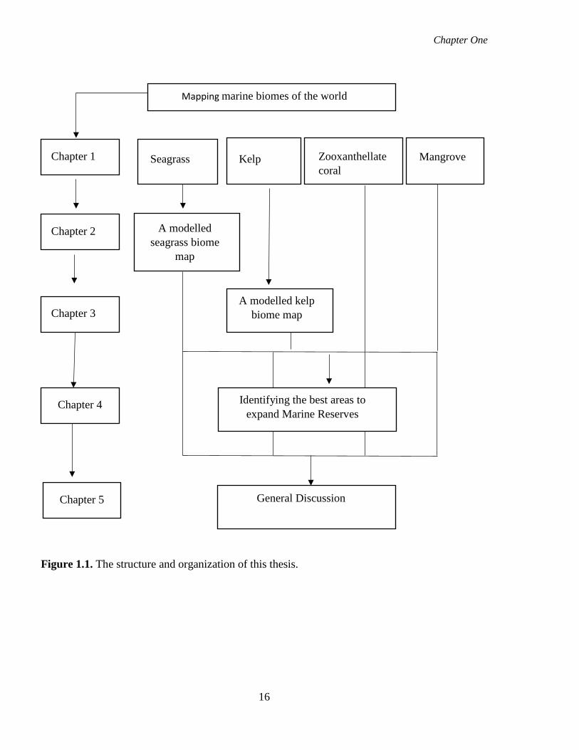
Figure 1.1. The structure and organization of this thesis. ........................................................ 16

Figure 2.1. The MaxEnt model predicted environmental range for seagrasses. ..................... 27

Figure 2.2. The area mapped for seagrasses in 5o latitudinal bands by UNEP-WCMC and

Short (2016) (hollow bars) and in the present study (solid bars). ......................... 28

Figure 3.1. The distribution of laminarian kelp observations used in this study.. ................... 42

Figure 3.2. The predicted environmental range for kelp species of the order Laminariales.. . 43

Figure 3.3. Response of kelp to depth, distance from land, wave height, average sea surface

temperature, maximum sea surface temperature, and salinity .............................. 44

Figure 4.1. The number of marine biome species and their conservation status as identified by

the IUCN Red List. ............................................................................................... 53

Figure 4.2. The regional distribution of marine biomes. ......................................................... 55

Figure 4.3. The overlap of biome areas in the IUCN regions. ................................................ 56

Figure 4.4. The global distribution of the seagrass biome. ...................................................... 58

Figure 4.5. The global distribution of the kelp biome. ............................................................ 59

Figure 4.6. The global distribution of the zooxanthellate coral biome. ................................... 60

Figure 4.7. The global distribution of the mangrove biome. ................................................... 61

Figure 4.8. The areas where one marine biome occurs. .......................................................... 62

Figure 4.9. The areas where two marine biomes occur. .......................................................... 63

Figure 4.10. The areas where three marine biomes occur. ...................................................... 64

Figure 4.11. The existing reserves (black) and top priority areas for the future declaration of

reserves (three biome occupied areas) (red). ........................................................ 65

Figure 4.12. Present biome protection within reserves.This map is available on the Arc GIS

online service via link https://arcg.is/1HCfK ........................................................ 66

Figure 5.1. The present primary occurrence records of each marine biome (grey dots) shown

against the maximum, mean, and minimum projected sea surface temperature for

2100 in 5-degree latitudinal bands. ....................................................................... 85

viii

List of tables

Table 1.1. Examples of literature on the eological and biological significance of marine

biomes. ...................................................................................................................... 9

Table 1.2. Examples of studies on the socio-economic uses of marine biomes. ..................... 10

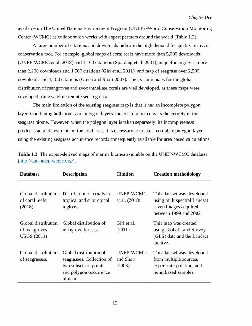
Table 1.3. The expert-derived maps of marine biomes available on the UNEP-WCMC

database (http://data.unep-wcmc.org/). .................................................................. 12

Table 2.1. The seagrass species studied during this research. ................................................. 20

Table 2.2. A summary of occurrence records which were extracted from each database. ...... 21

Table 2.3. List of environmental variables used in this study from GMED (Basher et al.

2014b).. ................................................................................................................... 23

Table 2.4. The estimation of relative contributions of the environmental variables to the

Maxent model. ........................................................................................................ 26

Table 3.1. List of kelp species used in this study to model the global distribution of the kelp

biome.. .................................................................................................................... 32

Table 3.2. The environmental variables used in the Maxent models to predict the geographic

distribution of kelp species of the order Laminariales. ......................................... 36

Table 3.3. Estimates of relative contributions of the environmental variables to the MaxEnt

model of the laminarian kelp species. .................................................................... 37

Table 3.4. Estimates of relative contributions of the environmental variables to the MaxEnt

model of the laminarian kelp genera. ..................................................................... 38

Table 3.5. Estimates of the relative contributions of the environmental variables to the

MaxEnt model of the laminarian kelp families. .................................................... 39

Table 4.1. Summary of data sources used in this study. .......................................................... 49

Table 4.2. The conservation status of the marine biome species based on the IUCN Red List.

................................................................................................................................ 69

Table 4.3. The distribution of seagrass, kelp, mangroves, zooxanthellate coral biomes, the

area of overlapping biomes for each EEZ, percentage of biomes covered with strict

marine reserves. ..................................................................................................... 70

Table 4.4. The summary of the top four EEZ and IUCN region with most area of biome

distribution. The area values are given in x 102 km2. ............................................. 78

Table 4.5. The regional distribution of biomes covered in marine reserves (IUCN category

Ia).Area values are given in 102 x km2.. ................................................................. 80

Table 5.1. Summary of the marine biome distribution. ........................................................... 83

ix

Table 5.2. The present and the projected future distribution of marine biomes with the

expanding and declining locations. ........................................................................ 86

x

List of Appendices Appendix S.2. 1. The comparison between the GBIF and OBIS seagrass occurrence

records. ................................................................................................. 91

Appendix S.2. 2. The global distribution of seagrass based on existing points and

polygon records. ................................................................................... 93

Appendix S.2. 3. The regional level comparison of the distribution of seagrass. ............ 95

Appendix S.2. 4. The MaxEnt model maps (in red) for individual (a) species, (b) genera

and (c) families of seagrass.. ................................................................ 98

Appendix S.2. 5. The comparison between the sum of the MaxEnt model maps for

individual species, genera and families. ............................................. 125

Appendix S.2. 6. MaxEnt model results: Jack-knife of regularized training gain the

resulting MaxEnt model. .................................................................... 126

Appendix S.2. 7. Response curves of each abiotic variable used in the model.. ........... 127

Appendix S.2. 8. Area calculation for UNEP-WCMC (2014, 2016) and the MaxEnt

derived biome for latitudinal band. .................................................... 128

Appendix S.2. 9. Citations of datasets used in this study as provided in the GBIF

metadata. ............................................................................................. 129

Appendix S.3. 1. The distribution of kelp occurrence records from the (a) OBIS and (b)

GBIF (lower) databases. ..................................................................... 147

Appendix S.3.2. The receiver operating curve for both training (red) and test data (blue)

to evaluate model’s predicting power.. ............................................... 148

Appendix S.3. 3. The results of the jackknife tests of variable importance.. ................. 149

Appendix S.3. 4. The list of citations for the data downloaded from the GBIF database.

............................................................................................................ 150

Appendix S.3. 5. The list of citations for the datasets containing laminarian kelp in OBIS

on 2017-10-24 as provided in the datasets metadata. ......................... 159

Appendix S.3. 6. The species (a), genus (b) and family (c) level maps of the Oder

Laminariales.. ..................................................................................... 164

Appendix S.4. 1. List of species’ conservation status in the zooxanthellate coral biome

based on the IUCN Red List. .............................................................. 189

Appendix S.4. 2. List of species’ conservation status in the kelp biome based on the

IUCN Red List. ................................................................................... 197

xi

Appendix S.4. 3. List of species’ conservation status in the mangrove biome based on the

IUCN Red List. ................................................................................... 198

Appendix S.4. 4. List of species’ conservation status in the mangrove biome based on the

IUCN Red List. ................................................................................... 199

Appendix S.5. 1. Projected change of the global distribution of (a) seagrass, (b) kelp, (c)

zooxanthellate coral, and (d) mangrove biomes by 2100.. ................. 200

Appendix S.5. 2. Seagrass species environmental niche. .............................................. 204

Chapter 1

Thesis Overview

Chapter One

1

1 Thesis Overview

1.1 General Introduction Biomes are geographic regions dominated by the same plant growth form (Woodward et al.

2004). Typical terrestrial biomes are grasslands, coniferous forests, and tropical rainforests.

Mangroves and salt marshes form biomes along the coast and seagrasses, kelps (laminarian

kelps and other canopy-forming brown algae), and zooxanthellate corals form biomes in

shallow water. This vertical and horizontal distribution of marine biomes depends on

environmental factors such as temperature, salinity, wave action, seabed substrata, and the

amount of light that penetrates through the water (Mann 1973; Short et al. 2001). The three-

dimensional structure of marine biomes provides feeding, breeding, and nesting habitats, and

helps protect the coast from storms, floods, and sea-level rise (Hemminga and Duarte 2000;

Duarte 2002; Duke et al. 2007; Teagle et al. 2017). Marine biomes contribute significantly to

global “blue” (marine) carbon sequestration (the carbon stored vegetation such as mangrove,

seagrass, and saltmarsh) (Nellemann et al. 2009). Coastal human communities have exploited

marine biomes for food, fertiliser, medication, firewood, fabric, and housing materials, but

consequently these have been depleted (Duarte 2002; Short et al. 2011; Burke et al. 2011;

Bridge et al. 2013; Richards and Friess 2016; Krumhansl et al. 2016; Wear 2016). Current

rates of marine biome change may affect blue carbon sequestration, fisheries productivity, and

habitat loss. Increasing temperatures due to global warming may also change biome

distributions (Hyndes et al. 2016; Assis et al. 2016; Wernberg et al. 2013, Filbee-Dexter et al.

2016; Saintilan et al. 2014). Because the primary measure of biome change is the area it

occupies, it is essential to map their distribution in order to judge their significance in terms of

providing ecological habitat and trends in associated biodiversity.

1.2 Terrestrial biome maps From the late 18th century, classification systems for terrestrial mapping began to be

developed to demarcate boundaries for different biomes (Woodward 2003). These maps were

derived using factors such as the associations between vegetation and animal communities

(Clements and Shelford 1939), predominant vegetation and their adaptations to a particular

environment (Campbell 1996), physiognomy and climate (climate envelopes) (Holdridge

1967), and vegetation recognised by satellites images (Woodward et al. 2004). In present

times, museums, herbaria, and several organizations and funding bodies such as the World

Chapter One

2

Resources Institute, and the World Wildlife Fund are using the map created by Olson et al.

(2001)’s map to identify the distribution of terrestrial biomes. It was developed using existing

expert-derived maps and the knowledge and assistance of over a thousand regional

taxonomists, conservation biologists and ecologists from around the world. Where existing

maps were unavailable, they used landform and dominant vegetation to demarcate boundaries.

This map was gridded to a five arc-minute resolution and is in a polygon vector format

projected in geographic coordinate system WGS 1984. Having one unique classification

system for biomes facilitates much collaborative research on a global scale (Hassan et al.

2005)

1.2.1 Terrestrial biome map as a conservation tool

Terrestrial biome maps have been used for the delineation of terrestrial protected areas,

estimation of net primary production, and assessment of the rate of land transformation

(Nemani et al. 2003; Hoekstra et al. 2005; Jenkins and Joppa 2009; Juffe-Bignoli et al. 2014;

Li et al. 2017). Land cover heterogeneity within a biome can be created by many

anthropogenic activities, such as clearing land for agriculture, building settlements, and

cutting trees for timber (Schulze et al. 2018). In response to the increasing human impact on

the natural environment, many governments started to declare protected areas to conserve the

environment. The protected areas conserve floral and faunal communities (Dinerstein et al.

2017). The total area of all 14 terrestrial biomes shows a moderate decrease (Jenkins and

Joppa 2009). However, the area under protection is not proportionate to the total area of

biomes (Hassan et al. 2005). The flooded grasslands and savannas (31%), mangroves (28%),

and montane grasslands and shrublands (27%) had more than 25% of their area protected. In

contrast, tropical and subtropical dry broadleaf forests (10%) and temperate grasslands,

savannas and shrublands (5%) had less than 10% of their area protected (Juffe-Bignoli et al.

2014).

Nearly half of all terrestrial species are found in tropical biomes (Olson and Dinerstein

2002). Furthermore, tropical biomes hold the highest number of endemic species, and the

highest number of families (Hassan et al. 2005). For this reason, tropical forests receive more

conservation attention than other 13 biomes.

Chapter One

3

1.3 Marine maps

Existing marine ecological maps have subdivided the marine environment using

different variables such as environmental attributes, phytoplankton communities, and other

biotic communities; fish, shellfish, molluscs, echinoderms and corals. The existing marine

ecological maps are as follows: Large Marine Ecosystems (LMEs) (1988) (Sherman 1988),

Ecological Biomes (Longhurst 1995; 2007), Ecoregions of ocean (Bailey 1998), Coastal

marine ecoregions of the world (MEOW) (Spalding et al. 2007), Global Open Oceans and

Deep Sea-habitats (GOODS) Bioregional classification (UNESCO 2009), Ecological Coastal

Units (ECU) (Sayre et al. 2019), Ecological Marine Units (EMU) (Sayre et al. 2015; 2017;

2017b), Marine Biogeographic Realms (Costello et al. 2017), Mesopelagic BioGeoChemical

Provinces (Reygondeau et al. 2013; 2018), and near surface global marine ecosystems (Zhao

et al. 2019). A few studies have mentioned the term “marine biomes,” but applied it

differently in each study. For example, Longhurst (1995; 2007) defined biome as “the largest

community unit that it is convenient to recognise. In a given biome the life form of the

climatic climax of the vegetation is uniform ”. Spalding et al. (2012) defined it a “groupings

of provinces with common oceanographic processes.” According to Hayden et al. (1984), a

biome is “an ecological formation in bio-physiognomic terms and having a particular 'stamp'

which on land is usually vegetational.” However, none of those above mentioned studies

defined marine plant life forms other than phytoplankton. Yet marine plant analogues to

terrestrial biomes exist and have been well studied. Phytoplankton communities do not

provide the 3D habitat for other species and they are spatially and temporally not permanent,

thus they do not strictly qualify as a biome. Phytoplankton communities can have high growth

rates and species turnover, show rapid responses to environmental conditions and are more

geographically widespread than benthic taxa (Costello and Chaudhary 2017; Alvain et al.

2008). In contrast, benthic marine plants are long-lived and provide ecologically important

three-dimensional habitats for a wide variety of faunal communities. The strict marine biomes

thus comprise of seagrasses, kelp forests, and zooxanthellate corals. Mangroves and

saltmarshes are rooted in the marine but grow in terrestrial environments. However,

mangroves and saltmarshes provide feeding, breeding, and nesting habitats for marine and

coastal fauna, and are also important in blue carbon sequestration. Saltmarsh species are

basically terrestrial species and are not restricted only to the coastal or marine environments.

Therefore, in this thesis seagrasses, kelps, mangroves and zooxanthellate corals will be used in

analysis. The following paragraphs will describe morphological and biological characteristics,

basic taxonomy, ecological importance, and the threats to each of the marine biomes.

Chapter One

4

1.3.1 Seagrass biome Seagrasses are marine submerged angiosperm monocots which form complex, widely spread

patches known as "meadows" along the shallow water coastlines in tropical, sub-tropical and

temperate regions (Green and Short 2003). These angiosperm monocots have a well-

developed root system to anchor to the seabed. Not only roots but rhizomes also anchor

seagrasses to the seabed and form underground biomass (Short et al. 2007). They have well-

built mechanisms to survive in saline conditions in estuaries, lagoons, and open seawater on

the continental shelf and nowhere else. Seagrasses live their life in a submerged environment

and have specialised pollens for underwater pollination (Green and Short 2003; den Hartog

and Kuo 2006; Short et al. 2007).

Phylogenetically, the seagrass biome is a functional group of four not necessarily

closely related aquatic monocot families, namely the Zosteraceae, Cymodoceaceae,

Posidoniaceae, and Hydrocharitaceae. They have 11 genera and 60 to 70 species (Green and

Short 2003; den Hartog and Kuo 2006; Horton et al. 2018). The family Zosteraceae has two

genera; Phyllospadix and Zostera. The family Cymodoceaceae has five genera, Amphibolis,

Cymodocea, Halodule, Syringodium, and Thalassodendron and the family Hydrocharitaceae

has three genera; Enhalus, Halophila, and Thalassia and family Posidoniaceae has one genus,

genus Posidonia. All species in the families Zosteraceae, Cymodoceaceae, and Posidoniaceae

are true seagrasses. The family Hydrocharitaceae has only 3 out of 17 genera that are

exclusively marine (den Hartog and Kuo 2006).

A few monocot species in the family Ruppiaceae and the family Zannichelliaceae,

which are primarily freshwater taxa, can live in brackish and marine conditions. They may

occur in seagrass meadows among true seagrasses. Thus, the seagrass biome does not

exclusively consist of certain plant families. Ruppia tuberosa from the family Ruppiaceae and

Lepilaena marina from the family Zannichelliaceae are exclusively marine whereas Ruppia

maritima forms meadows in both marine and freshwaters (den Hartog and Kuo 2006).

Molecular studies revealed how seagrass evolved from marine algae to terrestrial plants and

transitioned back to sea and clarified uncertainties of taxonomic relationships of seagrass

species (Les et al. 1997). The genome of Zostera marina has been fully sequenced to identify

the genomic losses and gains involved in adapting to the marine environment (Olsen et al.

2016).

Physical variables that control the distribution of seagrasses include depth, wave

height, water clarity (a measure of light attenuation), temperature, salinity and

photosynthetically active radiation, chemical parameters such as pH, and nutrients such as

Chapter One

5

phosphate, nitrate, and dissolved oxygen concentration, control the distribution of seagrasses

(Short et al. 2001). Depth is a proxy for light penetration through the water column and

controls the vertical distribution of seagrasses (Duarte 1991; Short et al. 2001; Duarte et al.

2007). The lower depth limit of seagrass distribution is known as the compensation depth

(Gallegos and Kenworthy 1996; Hemminga and Duarte 2000). At this level of depth, is the

depth at which photosynthesis meets losses (e.g. respiration, grazing and reproductive losses).

The distribution of seagrasses may vary from 1 m to 90 m (Duarte 1991). The amount of light

required for photosynthesis differs from seagrass species to species. The minimum light

requirement for seagrass photosynthesis is identified as 10-20% of sea surface light (Duarte

1991). Many studies have been focused on only one or a few species and how a few abiotic

factors contribute to the distribution of seagrasses. A full study on how comprehensive the

response is of all seagrass species to all possible abiotic variables is yet to be done.

1.3.2 Kelp biome In this study, I focus on the distribution of laminarian kelp species from the order

Laminariales (brown algae). They attach to rocky seabeds in the lower intertidal and shallow

subtidal zones in temperate and subpolar regions (Steneck et al. 2002; Santelices 2007;

Graham et al. 2007; Krumhansl et al. 2016; Teagle et al. 2017; Smale and Moore 2017;

Wernberg and Filbee-Dexter 2019). Similar to terrestrial biomes and other marine biomes

(seagrass, mangrove, and zooxanthellate corals), the kelp biome has a three-dimensional (3D)

structure with macroalgae attached to the rocky seafloor with a holdfast (Smith 2000). These

macroalgal underwater primary producers exhibit high diversity in growth forms, with some

of them growing above 30 m in length (Wernberg et al. 2019).

As kelp species are brown algae, the plant is known as a thallus and in plural thalli.

The thallus has a holdfast, stipe and blades or frond (Dayton 1985). Similar to the angiosperm

roots, the holdfast attaches the thallus to the rocky substratum. The stipe is analogous to the

stem of plants and fronds function as leaves. The arrangement of stipe and fronds are the

primary morphological characters to identify different species of kelp (Druehl et al. 1997).

These algae have the ability to change their morphology according to environmental

conditions, such as high wave action and turbulence, and population density (Arenas and

Fernandez 2000; Fowler-Walker et al. 2006).

Through molecular studies, the families and generic relationships in the order

Laminariales have been clarified to some extent (Bolton 2010). Currently, kelp comprises 9

accepted families, 59 genera and 147 species (Guiry and Guiry 2018). Most of the identified

Chapter One

6

species are in the three most common families: Alariaceae, Laminariaceae, and Lessoniaceae.

The most species-rich genera are Alaria, Laminaria, Saccharina, Ecklonia, and Lessonia

(Druehl et al. 1997). The genus Laminaria has 29 species and genus Alaria has 15 species

(Guiry and Guiry 2018). There are two to three times more kelp species present in the

northern hemisphere than in the southern hemisphere (Wernberg et al. 2019). In general, kelp

species are cold-water adapted species. However, there are deep water kelp forests in the

tropics and subtropics in both hemispheres, comprising of Eisenia galapagensis, Laminaria

brasiliensis, and L. abyssalis (Graham et al 2007; Santelices 2007).

The distribution of kelp forests is controlled by many environmental variables such as

substratum, wave action, sea temperature, light penetration through the water, and nutrients

(Mann 1973). Kelp typically anchors its holdfast to rocks, boulders or cobbles (Wernberg et

al. 2019). The lowest maximum temperature kelp occurs in is 5 oC in the Arctic. In the tropics,

although the sea surface temperature is 23 oC to 24 oC, they live at depths where the

temperature is 20 °C (Žuljević et al 2016; Wernberg et al. 2019). High sea surface temperature

can cause physiological stress to kelp (Gerard 1997), and consequently can cause range

contractions and reduction of kelp cover (Voerman et al. 2013; Wernberg et al. 2016; Smale

and Moor 2017). Like all marine plants, kelps restrict their distribution to the photic zone.

Their depth distribution is limited by light (Wernberg et al. 2019). Some deep water kelps

such as Eisenia galapagensis, Laminaria abyssalis, L. brasiliensis, L. rodriguezii, L.

philippinensis and Ecklonia radiata can grow down to average depths of 100 m in the Indian

Ocean, New Zealand, East and West coasts of Australia and in the Mediterranean Sea where

the water column is clear enough for light penetration (Graham et al. 2007; Marzinelli et al.

2015; Žuljević et al. 2016; Nelson et al. 2018). Kelp grows well in turbulent water. Wave

action or water currents are important to supply nutrients, disperse propagules, and remove

mucus and fouling organisms from the frond (Hurd et al. 2000; Gaylord et al. 2002).

1.3.3 Mangrove biome Mangroves are halophytic plants that grow along the sea-land margin in the tropical and

subtropical coastal areas (Kathiresan and Bingham 2001; Spalding et al. 2010). This

vegetation covers less than 0.4 % of the world’s forests (Spalding et al. 2010). Mangroves are

trees, shrubs, palms (Nypa fruticans) or ferns (Acrostichum sp.) adapted to withstand high

salinity, strong waves, muddy and anaerobic soil, and high temperature (Kathiresan and

Bingham 2001; Spalding et al. 2010).

Chapter One

7

The true mangroves exhibit many morphological and physiological adaptations to

survive in high salinity. They actively deposit excess salt into their internal lignified tissues

and excrete it through the leaves and aerial roots. However, some species such as Bruguiera

sexangula, Nypa fruticans, and Sonneratia caseolaris prefer lower salinity (Spalding et al.

2010). To withstand the oxygen-less anaerobic environment these mangrove species have stilt

(aerial) roots, pneumatophores, and knee roots (Kathiresan and Bingham 2001). Another

prominent feature of the true mangrove species is producing viviparous propagules. These

viviparous propagules are growing plantlets similar to the seeds or fruits of other plants

(Spalding et al. 2010). Some viviparous species such as Aegiceras corniculatum show high

salt tolerance during the germination (Wijayasinghe et al. 2019).

Families Rhizophoraceae, Avicenniaceae, and Sonneratiaceae consist of the majority

of mangrove species. Avicennia and Rhizophora are the most common genera among nearly

70 species of true mangroves (Spalding et al. 2010). Avicennia marina is the most widespread

species which extends from South Africa to the Red Sea, and towards the eastern Pacific

Islands and New Zealand (Spalding et al. 2010). Mangrove species distribution is controlled

by their coastal range, intertidal preference, and their location within an estuary (Duke et al.

1992). Some mangrove species are restricted at the regional level. Aegiceras floridum,

Avicennia rumphiana, Camptostemon philippinense, Heritiera globosa, and Sonneratia ovate

are unique to Southeast Asia, and Aegialitis annulata, Avicennia integra, Bruguiera

exaristata, Camptostemon schultzii, and Ceriops australis are all restricted to north and west

of Australia and New Guinea (Spalding et al. 2010).

On the global scale, mangrove biome distribution was documented as it is confined to

the 20 oC isotherm for winter sea surface temperature, with exceptions in New Zealand,

Australia, and Brazil, where winter sea surface temperature is lower as 15 oC (Ellison 1994;

Duke et al. 1992; Quisthoudt et al. 2012). Mangroves grow in the average atmospheric

temperature of 24 oC (Kathiresan and Bingham 2001). At the regional level, their distribution

is controlled by the sea surface temperature, air temperature, and precipitation (Osland et al.

2017). The total global area of mangroves was estimated to be 1,368 x 102 km2 (Giri et al.

2011). Southeast Asia has the highest mangrove distribution (51,049 km) followed by South

America, North and Central America, and West and Central Africa (Spalding et al. 2010).

Most of the broader mangrove forests are confined to the deltoid coasts (e.g., Sundarbans in

India and Bangladesh covers 6,516 km2 and extends up to 85 km on the land (Spalding et al.

2010).

Chapter One

8

1.3.4 Zooxanthellate coral biome Coral reefs are the largest marine biological structures created by living organisms (Karako et

al. 2002). The photosymbiotic relationship between zooxanthellae unicellular microalgae and

corals has been contributing to reef coral formation since their evolution in the Triassic period

(Karako et al. 2002). The coral host relies on zooxanthellae for photosynthetic products and

zooxanthellae depends on the coral for accommodation. Zooxanthellate reef-building corals

are distributed in the shallow tropical and sub-tropical oceans (Spalding et al. 2001). Based on

the topographic features and the formation of the reef, they are classified as fringe reefs,

barrier reefs, and atolls (Veron 2000; Spalding et al. 2001; Veron et al. 2019).

Almost all the zooxanthellate corals show morphological variation, even among the

corallites within the same colony (e.g., Acropora) (Veron 1995; 2000; Veron et al. 2019). In

some cases, the same species from two different locations such as a reef flat and a shallow

slope can have two different morphological features (Veron 1995). Coral taxonomists have

identified nearly 800 zooxanthellate coral species around the world (Veron 2000; Veron 2002;

Cairns et al. 1999; Veron 2013; Veron et al. 2015). The coral diversity is far higher in the

Indo- Pacific than in the Atlantic (Spalding et al. 2001). The Coral Triangle has the highest

number of zooxanthellate corals. It covers 6 x 106 km2 area of the ocean including Indonesia,

the Philippines, Brunei Darussalam, Malaysia, East Timor, Papua New Guinea and the

Solomon Islands (Veron et al. 2019). Raja Ampat, Papua, Celebes Sea, the Banda Sea and

Moluccas, Halmahera, and the south-west coast of Papua all have high species richness, from

400 – 475 scleractinia stony coral species found (DeVantier and Turak, 2017).

1.4 Ecologically and biologically significance features, threats and

conservation of biomes. The marine biomes have very impaortant ecological and biological significances (Table 1.1).

These biomes have endemic and rare species both in biome forming species and associated

faunal communities. For example, the seagrass biome has 19 endemic species, including

Phyllospadix scouleri, Phyllospadix serrulatus, Posidonia oceanica, Posidonia australis and

Amphibolis antarctica (Green and Short 2003). These biomes provide feeding breeding

habitats for the associated fauna (Orth et al. 2006; Lilley and Unsworth 2014; Teagle et al.

2017). Nearly 830,000 (550,000–1,330,000) number of associated species were estimated just

in coral reefs world wide (Fisher et al. 2015).

Chapter One

9

Table 1.1. Examples of literature on the eological and biological significance of marine biomes.

Significance Seagrass Kelp Mangrove Zooxanthellate coral

Have unique, rare or endemic species, populations or communities

Short et al. (2011); Green and Short (2003)

Roleda (2016); Lane and Mayes (2006)

Polidoro et al. (2010); Ellison et al. (2004); Saenger (1998)

Veron et al. 2011

Are essential for associated faunal population to survive and grow

Beck et al. (2001); Orth et al. (2006); Lilley and Unsworth (2014)

Teagle et al. (2017) Walters et al. (2008); Sheaves et al. (2016)

Moberg and Folke (1999)

Contain species, populations or communities with high natural biological productivity

Cullen-Unsworth and Unsworth (2013)

Alongi (2018); Krumhansl and Scheibling (2012)

Komiyama et al. (2008); Alongi (2009)

McWilliam et al. (2018)

Blue carbon storage Fourqurean et al. (2012) Krause-Jensen et al. (2018)

Alongi (2012) Not applicable

Contain high biodiversity

Green and Short (2003) Steneck et al. (2002) Duke (2017) Duffy et al. (2016); Hoeksema (2017)

Foundation species and ecosystem engineers

Bouma et al. (2009) Jones et al. (1994) Osland et al. (2014)

Shoreline protection Christianen et al. (2013) Pinsky et al. (2013) Kathiresan and Rajendran 2005; Sandilyan and Kathiresan 2012

Elliff and Silva (2017)

Chapter One

10

These biome-forming species are known as foundation species or ecosystem engineers. These

species can atler and provide favourable environmental conditions to the associated fauna (Jones

et al. 1994; Bouma et al. 2009). In addition to ecological and biological significances marine

biomes have socio-economic importance (Table 1.2). These biomes have long been exploited by

the coastal communities for food, housing materials, medicines, and other commercial products

(Montaño et al. 1999; Cornara et al. 2018; Walters et al. 2008). Commercial fishing, aquaculture

and tourism are a main source of income for many coastal communities (Correa et al. 2014;

Carrasquilla‐Henao and Juanes 2017; Spalding 2017).

Table 1.2. Examples of studies on the socio-economic uses of marine biomes.

Socio-economic uses

Seagrass Kelp Mangrove Zooxanthellate coral

Fisheries (commercial and recreational)

Nordlund et al. (2018); Unsworth et al. (2019)

Bertocci et al. (2015)

Carrasquilla‐Henao and Juanes (2017)

Newton et al. (2007); Birkeland (2017)

Tourism Cullen-Unsworth et al. (2014)

Vásquez et al. (2014)

Spalding and Parrett (2019)

Spalding (2017)

Aquaculture Dumbauld and McCoy (2015)

Correa et al. (2014)

Barbier et al. (2008)

Pomeroy et al. (2006)

Human food Montaño et al. (1999)

Stévant et al. (2018)

Bandaranayake (1998)

Not applicable

Medicine Cornara et al. (2018)

McGuffin and Dentali (2007)

Bandaranayake (1998); Kovacs (1999)

Bruckner (2002); Cooper et al. (2014)

Commercial products

Cornara et al. (2018)

Bixler & Porse (2011); Wargacki et al. (2012)

Bandaranayake (1998); Kovacs (1999)

Someya (1995)

Housing materials

Allègue et al. (2014)

Walters et al. (2008)

Howdyshell (1974)

Chapter One

11

Marine biomes have been lost due to the anthropogenic and climatic impacts. Seagrass

cover has been declining globally at a rate of 0.9% per year before 1940 and 7% per year after

1990 (Waycott et al. 2009). Over the last 125 years, more than 51,000 km2 of seagrass meadows

has lost due to natural and anthropogenic disturbances (Orth et al. 2006; Waycott et al. 2009). At

least 35% of mangroves were destroyed between 1980 and 2000 (Valiela et al. 2001). In some

Asian regions, the disappearance rate is 8% per year (Miththapala 2008). Marine biomes are

vulnerable to natural disasters on both a regional scale (storms, cyclones, floods, hurricanes,

tsunami, earthquakes, disease, grazing by herbivores, oil spill) and on a global scale (in terms of

warming) (Short and Wyllie-Echeverria 1996; Short and Neckles 1999; Marba and Duarte 2010;

Sandilyan and Kathiresan 2012; Wear 2016). Human-induced disturbance, such as dredging,

sedimentation, eutrophication, habitat fragmentation, boat anchoring, and propeller scars

accelerate these biome losses (Montefalcone et al. 2010; Gilman et al. 2008; Wernberg et al.

2019). The deforestation of the kelp biome occurs when sea urchin populations increase after

their predators, such as lobsters, crayfish, fish and otters, are removed by fishing (Smale et al.

2013; Costello 2014). The natural ‘trophic cascade’, and thus kelp cover, is naturally restored in

marine reserves when predator populations recover (Leleu et al. 2012). One of the major causes

of the decline of coral is coral bleaching. With the exponential growth of the human population,

most of the global mangrove areas have been converted into residential areas, agriculture fields,

and shrimp ponds (Upadhyay et al. 2002; Richards and Friess 2016)

In contrast to the present rate of loss, some localities have expanding biomes due to active

restoration. For example, fishermen in Japan created a Marine Protected Area where they banned

dredging and replanted seagrass to help restore fisheries (Tsurita et al. 2017). Similar active

seagrass restoration has been used to help coastal ecosystems recover from eutrophication,

pollution, and dredging in the Wadden Sea in the Netherland (Van Katwijk et al. 2016). In New

Zealand, mangrove cover (Avicennia marina var. resinifera) cover has been increasing (Yang et

al. 2013) and Avicennia germinans has extended its distribution along the USA Atlantic coast

(Saintilan et al. 2014). Important knowledge gap.

1.5 Important knowledge gap

The ever-increasing marine biome loss, as noted in the above section, highlights the strong need

to conserve them, and the need for global distribution maps. The following existing maps are

Chapter One

12

available on The United Nations Environment Program (UNEP) -World Conservation Monitoring

Center (WCMC) as collaboration works with expert partners around the world (Table 1.3).

A large number of citations and downloads indicate the high demand for quality maps as a

conservation tool. For example, global maps of coral reefs have more than 5,000 downloads

(UNEP-WCMC et al. 2018) and 1,100 citations (Spalding et al. 2001), map of mangroves more

than 2,200 downloads and 1,500 citations (Giri et al. 2011), and map of seagrass over 2,500

downloads and 1,100 citations (Green and Short 2003). The existing maps for the global

distribution of mangroves and zooxanthellate corals are well developed, as these maps were

developed using satellite remote sensing data.

The main limitation of the existing seagrass map is that it has an incomplete polygon

layer. Combining both point and polygon layers, the existing map covers the entirety of the

seagrass biome. However, when the polygon layer is taken separately, its incompleteness

produces an underestimate of the total area. It is necessary to create a complete polygon layer

using the existing seagrass occurrence records consequently available for area based calculations.

Table 1.3. The expert-derived maps of marine biomes available on the UNEP-WCMC database (http://data.unep-wcmc.org/). Database Description Citation Creation methodology

Global distribution of coral reefs (2018)

Distribution of corals in tropical and subtropical regions.

UNEP-WCMC et al. (2018)

This dataset was developed using multispectral Landsat seven images acquired between 1999 and 2002.

Global distribution of mangroves USGS (2011)

Global distribution of mangrove forests.

Giri et.al. (2011)

This map was created using Global Land Survey (GLS) data and the Landsat archive.

Global distribution of seagrasses.

Global distribution of seagrasses. Collection of two subsets of points and polygon occurrence of data

UNEP-WCMC and Short (2003).

This dataset was developed from multiple sources, expert interpolation, and point based samples.

Chapter One

13

The kelp biome has many ecological and biological significance and socio-economic

values (Tables 1.1 and 1.2). One of the most important conservation measures to minimise the

destruction of kelp biome is to map the extent of these forests. To date, there is no map to

calculate the area of the kelp biome. The maps available in the literature were designed to

represent the range of one or a few species. Mapping kelp at a global scale using manual

cartographic techniques is not practical, as it is costly and time-consuming. However, modelling

the distribution of kelp could fill this research gap.

Anthropogenic and climatic stresses increase the extinction risk of marine species (Short

et al. 2011; Sandilyan and Kathiresan 2012; Gilman et al. 2008; Wernberg et al. 2019). Aichi

Target 12 (UNEP/CBD/COP/10/9) called for the decline of threatened species to be stopped and

their conservation statuses needed to be improved by 2020. It is still not known how many marine

biome forming species had been assessed and their conservation status based on the IUCN Red

List. A summary of the conservation status of marine biome forming species based on the IUCN

Red List will be helpful to improve their conservation status.

The timeline for fulfilling the Aichi Biodiversity Target 11 is coming to an end in 2020.

The Convention on Biological Diversity (CBD)’s Aichi Biodiversity Target 11

(UNEP/CBD/COP/10/9) called for at least 10% of coastal and marine areas, specifically areas of

importance for biodiversity and ecosystem services, to be fully protected, with an increased focus

on comprehensive, ecologically representative, efficiently managed protected areas. It aimed to

protect both habitats and populations of species. Marine biomes have many features of ecological

and biological significance, such as providing feeding and breeding habitats for the associated

faunal communities, their high natural productivity and blue carbon sequestration (Table 1.1). So

far, very little attention has been paid to the conservation of marine biomes within fully protected

areas (marine reserves, IUCN Ia Category). Furthermore, some countries have coastlines covered

with multiple biomes. For example, Indonesea has mangrove, seagrass, and coral in a continuum

within very closer proximities to one another (Unsworth et al. 2009). These neighbouring biomes

enhance the ecological connectivity and niche differentiation among faunal communities as well

as the different stages of complex life cycles (Berkström et al. 2013). A systematic understanding

of how much area of multiple overlapping biomes has been protected within reserves is still

lacking. A quantitative analysis of present conservation status of biomes within reserves will

therefore help to identify the areas that will need more qualitative conservation measures to

maintain their vital ecological role in the coastal zones.

Chapter One

14

Conservation initiatives now recall recommendations of urgent conservation of an

ecologically representative and well-connected marine protected area network (IUCN 2016). The

World Conservation Congress (2016) encouraged the implementation of at least 30% of each

marine habitat in a network of marine reserves (IUCN 2016) by 2030. To date, only a few

countries use the calculated areas of biomes within their Exclusive Economic Zones (EEZ) in

policy making and strategic planning of conservation. Knowing the extent of marine biomes

belonging to each country will be helpful to improve marine conservation as well as delineate

new marine reserves. Further, the resulting awareness of the regional level distribution would also

be useful to conservation initiatives in expanding their conservation projects.

1.6 Thesis objectives and structure

Based on the terrestrial biome definition “the larger areas with same plant life form”, the aim of

this research is to map marine biomes with a sufficient geospatial resolution and be readily

available for analysis in the Geographycal Information System (GIS) and thereby identify the

potential locations to expand Marine Reserve network. This thesis has three objectives, and

chapters are structured to respond to the research objectives (Fig.1.1).

• Objective 1: A modelled global distribution of the seagrass biome.

To achieve this, areas with the highest probability of seagrass distribution were mapped

using existing primary occurrence records and environmental variables (Chapter 2).

Chapter 2 has been published in the journal Biological Conservation with the title: A

modelled global distribution of the seagrass biome (DOI:

https://doi.org/10.1016/j.biocon.2018.07.009). I was the lead author of this manuscript and

it was produced in collaboration with my supervisor (Co-authorship form attached)

• Objective 2: A modelled global distribution of the kelp biome.

To accomplish this, areas with the highest probability of the laminarian kelp distribution

were mapped using existing primary occurrence records and environmental variables.

(Chapter 3). Chapter 3 is under review in the journal Biological Conservation with the

title: A modelled global distribution of the kelp biome. I was the lead author of this

Chapter One

15

manuscript and it was produced in collaboration with my supervisor (Co-authorship form

attached).

• Objective 3: Global gap analysis: delineation of priority areas of strict marine reserves to

conserve marine biomes.

To accomplish this: The IUCN conservation status of each biome-forming species was

reviewed, and the areas calculated that were covered by each biome within each Exclusive

Economic Zones (EEZs) and within each IUCN operational regions. This led to

identification of which species were still to have their conservation status assessed, and

which countries could were able to and had protected one or more biomes.

• Section 1.4.1 and 1.4.2 in the Thesis overview chapter have been published as two book

chapters in the Encyclopedia of the world’s biomes. Seagrass biome

https://doi.org/10.1016/B978-0-12-409548-9.11748-8. Kelp biome

https://doi.org/10.1016/B978-0-12-409548-9.11768-3. I was the lead author of these

manuscripts and it was produced in collaboration with my supervisor (Co-authorship form

attached)

The resulting global marine biome map will provide a baseline for several other marine biological

and ecological studies. This will be useful to carry out studies such as re-calculation of the blue

carbon budget with new area values from the seagrass and kelp biomes, predicting the future

distribution of biomes with increasing sea surface temperatures, the influences of environmental

variables on biome species, the latitudinal habitat availability, and marine species richness. This

resulting map will be a planning tool for conducting strategic environmental impact assessments

and making polices for biodiversity-friendly practices.

Chapter One

16

Figure 1.1. The structure and organization of this thesis.

Chapter 1 Seagrass Kelp Zooxanthellate coral

Mangrove

Chapter 2 A modelled seagrass biome

map

Chapter 3 A modelled kelp

biome map

Chapter 4 Identifying the best areas to expand Marine Reserves

Chapter 5 General Discussion

Mapping marine biomes of the world

Chapter 2

A modelled global distribution of the seagrass biome

Chapter Two

17

2 A modelled global distribution of the seagrass biome

2.1 Introduction

The seagrass biome is an assemblage of submerged marine angiosperms belonging to nearly 60

species, 11 genera, and 4 families (Green and Short 2003; den Hartog and Kuo 2006; Horton et al.

2017). Seagrasses form ‘meadows’ in saline conditions in estuaries, lagoons, and in the open sea

throughout tropical and temperate regions, and have high biomass compared to marine plankton

communities (Short et al. 2007). The seagrass biome plays a key role in the ecology of coastal

ecosystems. It provides feeding, breeding, nesting and nursery habitat to many faunal communities

including a number of threatened species such as dugong (Dugong dugon), green sea turtle (Chelonia

mydas), fan mussels (Pinna nobilis), and dwarf seahorse ( Hippocampus zosterae) (Preen and Marsh

1995; Hughes et al. 2009). Consequently seagrass beds are a protected habitat in many countries,

notably under the European Union Habitats Directive (Evans 2006).

Recognising the conservation importance of seagrass, several global maps have been produced.

For example, Green and Short (2003) published the first global map of seagrass distribution, showing

observed (in situ) occurrence. This map has been used to study the probability of extinction of seagrass

species (Short et al. 2011), regional level seagrass habitat mapping (Wabnitz et al. 2008), assessing the

global marine protection targets (Wood et al. 2008), identifying the errors and gaps in spatial data sets

on marine conservation (Visconti et al. 2013), and blue carbon sinks (Nellemann et al. 2009). Whilst

the Green and Short (2003) map documented some locations as a narrative, it did not necessarily

include them in the map because the sources did not provide precise locations. Thus, considerable

uncertainty remains in terms of estimating the global extent (i.e. surface area) of the seagrass biome

globally (Green and Short 2003). Since 2005, UNEP-WCMC has been curating the Green and Short

map, and released a fourth update in 2016 (UNEP-WCMC and Short 2016) that included a significant

update to seagrass knowledge for the Mediterranean (Telesca et al. 2015), other European seas, and the

Philippines. The geographic layer is still global in scope, and composed of polygon (i.e. with surface

area) and point occurrence data. As mentioned in the dataset’s metadata, there are a number of

overlapping polygons in places, meaning that non-expert users can overestimate the total seagrass

surface area. Furthermore, the dataset still suffers from known spatial gaps in knowledge. For instance

the north east Pacific, the coastal area of Scandinavia and the Northern African coast, are known to

Chapter Two

18

have extensive seagrass meadows but only indicated by point records. Directly using point occurrence

data is likely to significantly underestimate the spatial extent of seagrass beds.

Mapping the seagrass biome has been compromised by the absence of georeferenced records in

many regions, and for a range of rare species (Short et al. 2007). Even where geographic records are

available, point samples are unlikely to reflect the full geographic area occupied by a species. In the

absence of in situ mapping of seagrass at a global scale, existing occurrence data can be used in species

distribution models to map the biome in unsurveyed areas, and indeed some regional attempts have

been made (e.g. Scardi et al. 2013). Moreover, species distribution modeling has been widely and

successfully used to predict marine species distributions and the their relationships with environmental

vabiables (Vaz et al. 2008; Martin et al. 2012, 2014; Yesson et al. 2012; Basher et al. 2014a; Saeedi et

al. 2016).

This study models the global distribution of seagrass using point records, and compares model

outputs to existing records and polygons, and literature reports. Consequently, the resulting map is a

complete polygon layer of the potential distribution of seagrass meadows globally. However, it does

not account for factors such as seabed substratum, or pollution and dredging that can reduce seagrass

cover. In preparing the models, I also compared results from mapping species, genera and families to

all species data. This test of methodology will inform how to best run future models when more field

data become available for more species. In addition, I identified which environmental variables best

predicted seagrass distributions. Thus future models can be improved with higher spatial resolution

environmental data. Knowing the global extent of seagrass is important,for seagrass conservation such

as environmental sensitivity mapping, (e.g., oil-spill emergency planning) and monitoring of change in

biome cover and calculating carbon budgets (Duarte et al. 2010; Lavery et al. 2013).

2.2 Methods

2.2.1 Species occurrence data

All true seagrasses have adapted to live in a saline medium, grow fully submerged, and have a root

system for anchoring (Green and Short 2003; den Hartog and Kuo 2006). Three families, Zosteraceae,

Cymodoceaceae, and Posidoniaceae, have exclusively seagrass species, and the Hydrocharitaceae have

three genera (den Hartog and Kuo 2006). Hence, our study focused on the species belonging to these

families (Table 2.1).

Chapter Two

19

Seagrass distribution data were extracted from the Global Biodiversity Information Facility

(GBIF 2016; 2017), Ocean Biogeographic Information System (OBIS 2016; 2017), and UNEP-

WCMC and Short (2016) (Table 2.2). GBIF and OBIS data were cross-referenced to check what

additional records and species were available in each database (Appendix S.2.1). GBIF had a total of

95,525 records in 397 datasets (Appendix S.2.9). Taxonomic names were reconciled with the World

Register of Marine Species (Horton et al. 2017) and the Atlas of Seagrass (Green and Short 2003). Out

of those occurrences, 82,039 were georeferenced records from the years 1792 to 2016. I limited

analysis to time periods when geo-referencing was likely to be more accurate. We thus excluded

12,480 records which were collected before the year 1900, 4 fossil specimens, 514 with ambiguous

locations according to occurrence remarks, 28,542 records with coordinate uncertainty > 10 km,

15,717 records falling on land, and duplicate records. Nearly 75% of records were excluded during this

data preparation. Consequently, 25,082 occurrence data points from GBIF 17,955 from UNEP-WCMC

and Short (2016) and 3806 from OBIS were plotted on a latitude longitude grid to visualise their global

coverage (Appendix S.2.2).

Comparison of point and polygon records in UNEP-WCMC and Short (2016) and data from

GBIF showed geographic gaps in the availability of records (Appendix S.2.2).The UNEP-WCMC and

Short (2016) polygon layer did not cover all areas with point records. Locations which only had

occurrence records from GBIF and UNEP-WCMC and short (2016) included western Canada and the

United States including the Gulf of Alaska and the Gulf of California, Brazil coast from the state of

Ceará to the state of Rio de Janeiro, Norway and the Indo-Pacific region (Appendix S.2.3).

2.2.2 Environmental data

The selection of environmental layers is a very important step in species distribution modelling

because the combined effect of too many abiotic layers could lead to over or under prediction

(Peterson et al. 2007). I used 13 abiotic variables which have been related to the distribution of

seagrasses (Table 2.3).

Chapter Two

20

Table 2.1. The seagrass species studied during this research.

Cymodoceaceae Hydrocharitaceae Zosteraceae

Amphibolis antarctica Enhalus acoroides Heterozostera tasmanica

Amphibolis griffithii Halophila australis Phyllospadix iwatensis

Cymodocea angustata Halophila baillonii Phyllospadix japonicus

Cymodocea nodosa Halophila beccarii Phyllospadix scouleri

Cymodocea rotundata Halophila capricorni Phyllospadix serrulatus

Cymodocea serrulata Halophila decipiens Phyllospadix torreyi

Halodule beaudettei Halophila engelmanni Zostera angustifolia

Halodule bermudensis Halophila hawaiiana Zostera asiatica

Halodule emarginata Halophila johnsonii Zostera caespitosa

Halodule pinifolia Halophila minor Zostera capensis

Halodule uninervis Halophila ovalis Zostera capricorni

Halodule wrightii Halophila ovata Zostera caulescens

Syringodium filiforme Halophila spinulosa Zostera japonica

Syringodium isoetifolium Halophila stipulacea Zostera marina

Thalassodendron ciliatum Halophila tricostata Zostera mucronata

Thalassodendron pachyrhizum Thalassia hemprichii Zostera muelleri

Thalassia testudinum Zostera noltii

Posidoniaceae Zostera novazelandica

Posidonia oceanica Zostera tasmanica

Posidonia australis

Posidonia sinuosa

Posidonia angustifolia

Posidonia ostenfeldii

Posidonia robertsoniae

Posidonia coriacea

Posidonia denhartogii

Posidonia kirkmanii

Chapter Two

21

As seagrass meadows are distributed in coastal areas, depth, distance from land, slope, salinity,

diffuse attenuation coefficient, sea surface temperature, pH, photosynthetically active radiation, wave

height, dissolved oxygen, and nitrate could directly or indirectly affect the distribution of seagrass

(Fonseca and Kenworthy 1987; Murray and Wetzel 1987; Duarte 1991; Erftemeijer and Middliburg

1995; Dawson and Denisson 1996; Pedersen et al. 1998; Short and Neckles 1999; Dixon 2000; Short et

al. 2001; Green and Short 2003; Ralph 2007).

In this study I obtained the environmental data from the Global Marine Environment Datasets (GMED)

(Basher et al. 2014b) data layers which represent annual averages calculated over decades, and thus

indicate long-term enduring characteristics of the environment (Basher et al. 2014b). These have a 5

arc-minute (0.083o grid cell) resolution which is approximately 9.2 km at the equator. For this study I

needed a finer spatial resolution so I interpolated the GMED data to 30 arc second resolution (0.0083o

grid cell) which is approximately 1 km at the equator. All the interpolated layers were cropped to a 0 to

1000 m depth layer in order to map only the near coast region and reduce computational time.

Table 2.2. A summary of occurrence records which were extracted from each database. Data source Geometry

type

Number of

records

Primary data source Number

of species

GBIF point 82,200 Fossil specimens, human

observations, preserved

specimens, literature

74

OBIS point 6235 Fossil specimens, human

observations, preserved

specimens, literature

40

UNEP-WCMC

and Short (2016)

point 17,955 Point-based occurrences 25 +

unspecified

UNEP-WCMC

and Short (2016)

polygon 220,157 Regional maps, expert

interpolated maps

Not given

Chapter Two

22

2.2.3 Modelling

I used Maximum Entropy (MaxEnt) version 3.3.3k software (Phillips et al. 2006; Phillips and Dudik

2008) to generate the seagrass species distribution model. This is widely used for species distribution

modelling with presence-only data, and works well in the marine environment (e.g., Tittensor et al.

2009; Verbruggen et al. 2009; Yesson et al. 2012; Basher et al. 2014a; 2014c; Saeedi et al. 2016). In

the current study, MaxEnt models were generated using 10 cross-validated replicate runs with

parameters: convergence threshold = 10-5, regularization multiplier = 1, maximum number of

background points = 10,000 and maximum iterations = 1000. The cross-validation replication divides

the sample into replicate folds; with each fold in turn used as test data (Phillips and Dudik, 2008). Thus

all the occurrence records at once become a test point. I excluded duplicate records that fell within the

same grid cell. MaxEnt models for individual species, individual genera, individual families, all

occurrence record from individual databases (GBIF, OBIS and UNEP-WCMC and Short (2016)) and

combined databases (GBIF+OBIS and GBIF+UNEP-WCMC and Short (2016)) generated separately

to identify what taxonomic level best defined the biomes. The post image processing for the map was

carried out using Arc Map version 10.5.1. The areas with a MaxEnt probability value greater than 0.5

were taken as the potential global distribution of seagrass. The overlap of MaxEnt predicted areas and

the available point and polygon records from GBIF and UNEP-WCMC and Short (2016) were visually

inspected to determine the spatial accuracy of predictions.

The performance of the model was assessed using the Receiver Operating Characteristic (ROC)

(Phillips et al. 2006). The Area Under the Curve (AUC) of ROC values between 0 and 0.5 indicate

predictions are no better than random and the highest value of 1 gives the best prediction (Phillips et al.

2006, Elith et al. 2011). I used a jack-knife test and the percent variable contribution to identify the

relative importance of each environmental variable. In Maxent, the jack-knife test systematically drops

variables one at a time and compares the predictions using all variables except the dropped one and a

model which is based on that variable only (Phillips et al. 2006). I used MaxEnt’s maximum training

sensitivity plus specificity threshold as the cut-off for the presence of seagrasses.

I compared our map with UNEP-WCMC and Short (2016) by dividing both into 5o latitudinal

bands using Arc Map tools. This also served to check the accuracy of the global area of seagrass with

the sum of each latitudinal band because errors in area calculation are possible with different spatial

scales and projections.

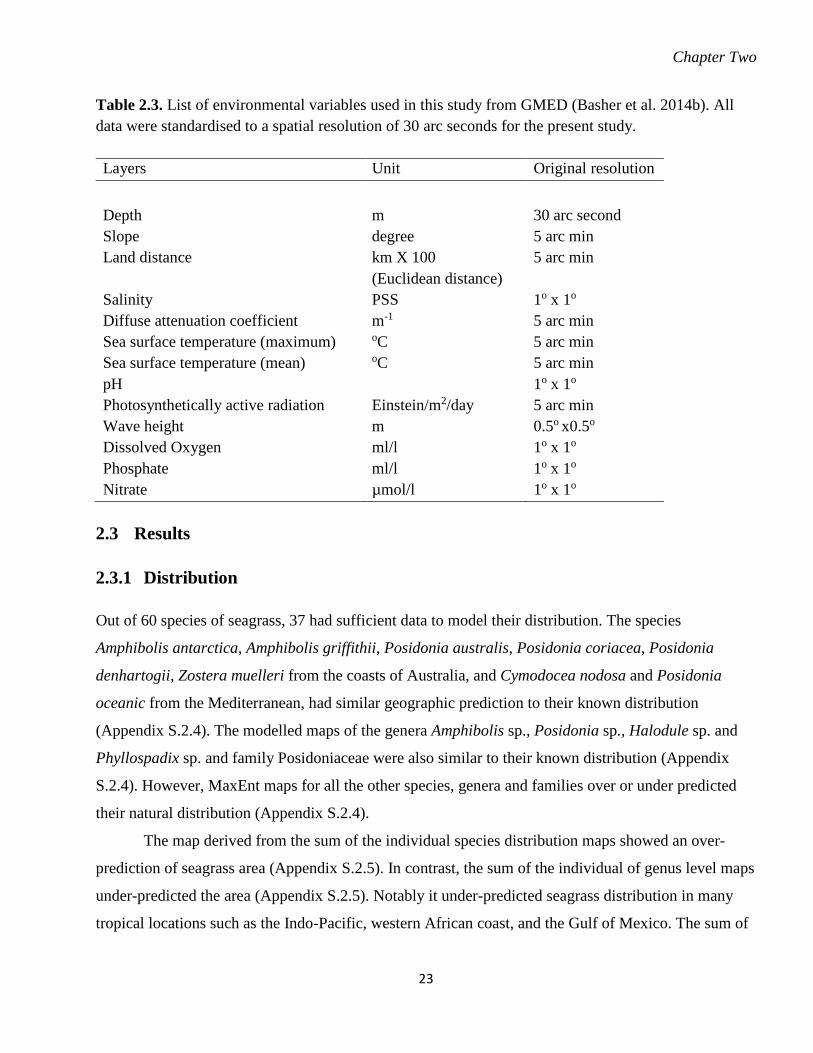
Chapter Two

23

Table 2.3. List of environmental variables used in this study from GMED (Basher et al. 2014b). All data were standardised to a spatial resolution of 30 arc seconds for the present study. Layers Unit Original resolution Depth m 30 arc second Slope degree 5 arc min Land distance km X 100

(Euclidean distance) 5 arc min

Salinity PSS 1o x 1o Diffuse attenuation coefficient m-1 5 arc min Sea surface temperature (maximum) oC 5 arc min Sea surface temperature (mean) oC 5 arc min pH 1o x 1o Photosynthetically active radiation Einstein/m2/day 5 arc min Wave height m 0.5o x0.5o Dissolved Oxygen ml/l 1o x 1o Phosphate ml/l 1o x 1o Nitrate µmol/l 1o x 1o

2.3 Results

2.3.1 Distribution Out of 60 species of seagrass, 37 had sufficient data to model their distribution. The species

Amphibolis antarctica, Amphibolis griffithii, Posidonia australis, Posidonia coriacea, Posidonia

denhartogii, Zostera muelleri from the coasts of Australia, and Cymodocea nodosa and Posidonia

oceanic from the Mediterranean, had similar geographic prediction to their known distribution

(Appendix S.2.4). The modelled maps of the genera Amphibolis sp., Posidonia sp., Halodule sp. and

Phyllospadix sp. and family Posidoniaceae were also similar to their known distribution (Appendix

S.2.4). However, MaxEnt maps for all the other species, genera and families over or under predicted

their natural distribution (Appendix S.2.4).

The map derived from the sum of the individual species distribution maps showed an over-

prediction of seagrass area (Appendix S.2.5). In contrast, the sum of the individual of genus level maps

under-predicted the area (Appendix S.2.5). Notably it under-predicted seagrass distribution in many

tropical locations such as the Indo-Pacific, western African coast, and the Gulf of Mexico. The sum of

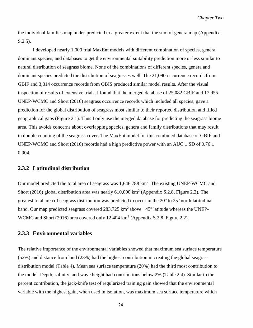
Chapter Two

24

the individual families map under-predicted to a greater extent that the sum of genera map (Appendix

S.2.5).

I developed nearly 1,000 trial MaxEnt models with different combination of species, genera,

dominant species, and databases to get the environmental suitability prediction more or less similar to

natural distribution of seagrass biome. None of the combinations of different species, genera and

dominant species predicted the distribution of seagrasses well. The 21,090 occurrence records from

GBIF and 3,814 occurrence records from OBIS produced similar model results. After the visual

inspection of results of extensive trials, I found that the merged database of 25,082 GBIF and 17,955

UNEP-WCMC and Short (2016) seagrass occurrence records which included all species, gave a

prediction for the global distribution of seagrass most similar to their reported distribution and filled

geographical gaps (Figure 2.1). Thus I only use the merged database for predicting the seagrass biome

area. This avoids concerns about overlapping species, genera and family distributions that may result

in double counting of the seagrass cover. The MaxEnt model for this combined database of GBIF and

UNEP-WCMC and Short (2016) records had a high predictive power with an AUC ± SD of 0.76 ±

0.004.

2.3.2 Latitudinal distribution

Our model predicted the total area of seagrass was 1,646,788 km2. The existing UNEP-WCMC and

Short (2016) global distribution area was nearly 610,000 km2 (Appendix S.2.8, Figure 2.2). The

greatest total area of seagrass distribution was predicted to occur in the 20o to 25o north latitudinal

band. Our map predicted seagrass covered 283,725 km2 above +45o latitude whereas the UNEP-

WCMC and Short (2016) area covered only 12,404 km2 (Appendix S.2.8, Figure 2.2).

2.3.3 Environmental variables The relative importance of the environmental variables showed that maximum sea surface temperature

(52%) and distance from land (23%) had the highest contribution in creating the global seagrass

distribution model (Table 4). Mean sea surface temperature (20%) had the third most contribution to

the model. Depth, salinity, and wave height had contributions below 2% (Table 2.4). Similar to the

percent contribution, the jack-knife test of regularized training gain showed that the environmental

variable with the highest gain, when used in isolation, was maximum sea surface temperature which

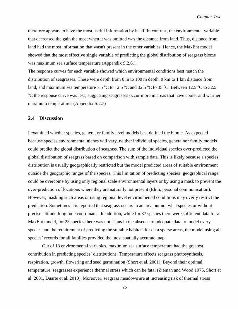
Chapter Two

25

therefore appears to have the most useful information by itself. In contrast, the environmental variable

that decreased the gain the most when it was omitted was the distance from land. Thus, distance from

land had the most information that wasn't present in the other variables. Hence, the MaxEnt model

showed that the most effective single variable of predicting the global distribution of seagrass biome

was maximum sea surface temperature (Appendix S.2.6.).

The response curves for each variable showed which environmental conditions best match the

distribution of seagrasses. These were depth from 0 m to 100 m depth, 0 km to 1 km distance from

land, and maximum sea temperature 7.5 oC to 12.5 oC and 32.5 oC to 35 oC. Between 12.5 oC to 32.5 oC the response curve was less, suggesting seagrasses occur more in areas that have cooler and warmer

maximum temperatures (Appendix S.2.7)

2.4 Discussion

I examined whether species, genera, or family level models best defined the biome. As expected

because species environmental niches will vary, neither individual species, genera nor family models

could predict the global distribution of seagrass. The sum of the individual species over-predicted the

global distribution of seagrass based on comparison with sample data. This is likely because a species’

distribution is usually geographically restricted but the model predicted areas of suitable environment

outside the geographic ranges of the species. This limitation of predicting species’ geographical range

could be overcome by using only regional scale environmental layers or by using a mask to prevent the

over-prediction of locations where they are naturally not present (Elith, personal communication).

However, masking such areas or using regional level environmental conditions may overly restrict the

prediction. Sometimes it is reported that seagrass occurs in an area but not what species or without

precise latitude-longitude coordinates. In addition, while for 37 species there were sufficient data for a

MaxEnt model, for 23 species there was not. Thus in the absence of adequate data to model every

species and the requirement of predicting the suitable habitats for data sparse areas, the model using all

species’ records for all families provided the most spatially accurate map.

Out of 13 environmental variables, maximum sea surface temperature had the greatest

contribution in predicting species’ distributions. Temperature effects seagrass photosynthesis,

respiration, growth, flowering and seed germination (Short et al. 2001). Beyond their optimal

temperature, seagrasses experience thermal stress which can be fatal (Zieman and Wood 1975, Short et

al. 2001, Duarte et al. 2010). Moreover, seagrass meadows are at increasing risk of thermal stress

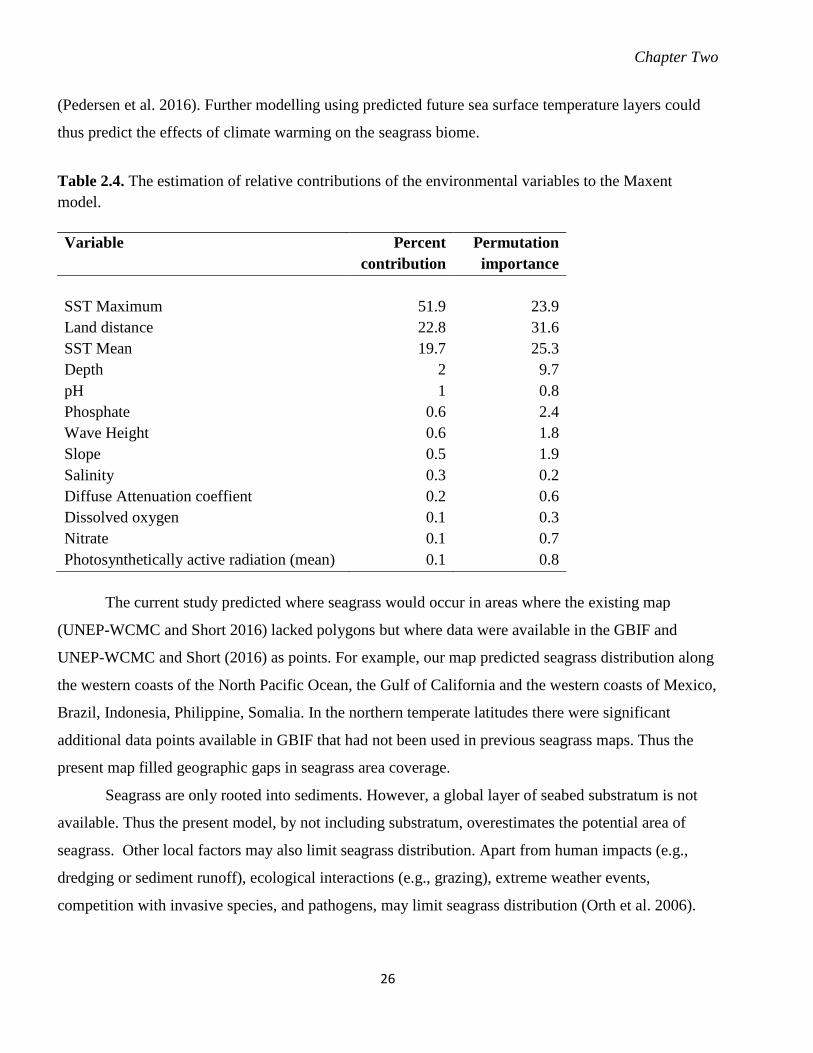
Chapter Two

26

(Pedersen et al. 2016). Further modelling using predicted future sea surface temperature layers could

thus predict the effects of climate warming on the seagrass biome.

Table 2.4. The estimation of relative contributions of the environmental variables to the Maxent model. Variable Percent

contribution Permutation importance

SST Maximum 51.9 23.9 Land distance 22.8 31.6 SST Mean 19.7 25.3 Depth 2 9.7 pH 1 0.8 Phosphate 0.6 2.4 Wave Height 0.6 1.8 Slope 0.5 1.9 Salinity 0.3 0.2 Diffuse Attenuation coeffient 0.2 0.6 Dissolved oxygen 0.1 0.3 Nitrate 0.1 0.7 Photosynthetically active radiation (mean) 0.1 0.8

The current study predicted where seagrass would occur in areas where the existing map

(UNEP-WCMC and Short 2016) lacked polygons but where data were available in the GBIF and

UNEP-WCMC and Short (2016) as points. For example, our map predicted seagrass distribution along

the western coasts of the North Pacific Ocean, the Gulf of California and the western coasts of Mexico,

Brazil, Indonesia, Philippine, Somalia. In the northern temperate latitudes there were significant

additional data points available in GBIF that had not been used in previous seagrass maps. Thus the

present map filled geographic gaps in seagrass area coverage.

Seagrass are only rooted into sediments. However, a global layer of seabed substratum is not

available. Thus the present model, by not including substratum, overestimates the potential area of

seagrass. Other local factors may also limit seagrass distribution. Apart from human impacts (e.g.,

dredging or sediment runoff), ecological interactions (e.g., grazing), extreme weather events,

competition with invasive species, and pathogens, may limit seagrass distribution (Orth et al. 2006).

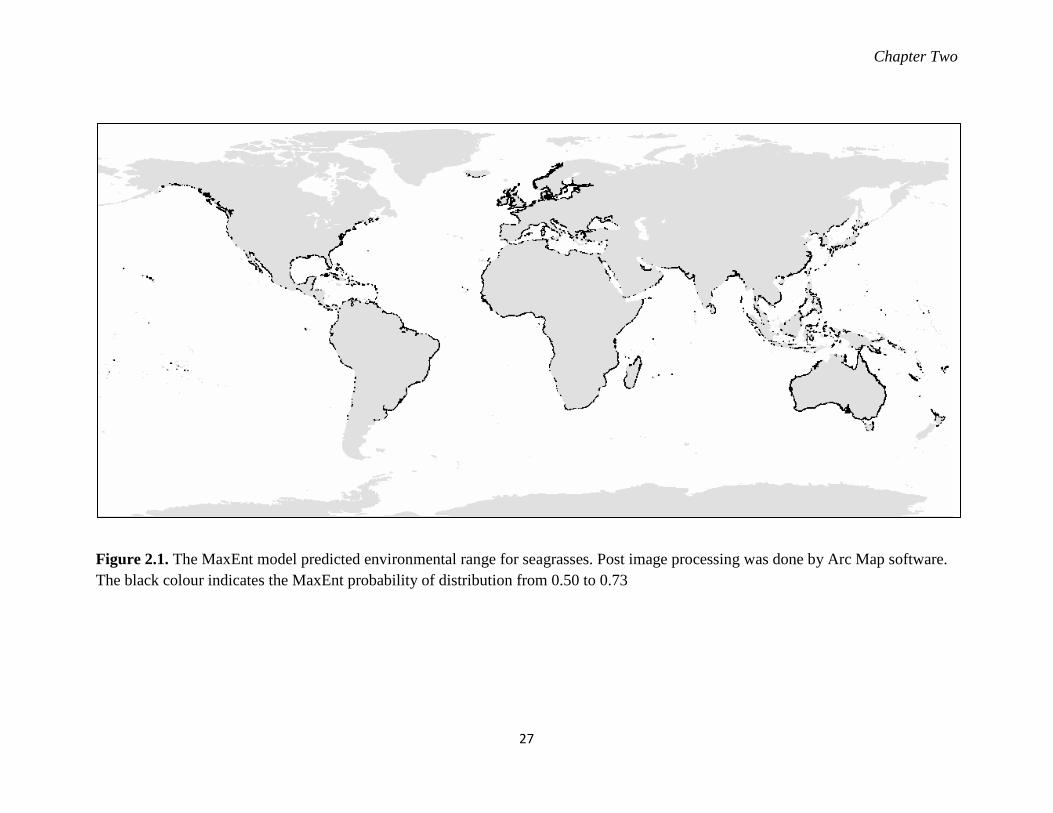
Chapter Two

27

Figure 2.1. The MaxEnt model predicted environmental range for seagrasses. Post image processing was done by Arc Map software. The black colour indicates the MaxEnt probability of distribution from 0.50 to 0.73

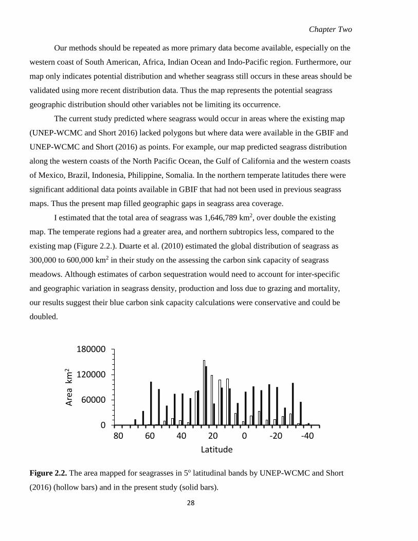
Chapter Two

28

Our methods should be repeated as more primary data become available, especially on the

western coast of South American, Africa, Indian Ocean and Indo-Pacific region. Furthermore, our

map only indicates potential distribution and whether seagrass still occurs in these areas should be

validated using more recent distribution data. Thus the map represents the potential seagrass

geographic distribution should other variables not be limiting its occurrence.

The current study predicted where seagrass would occur in areas where the existing map

(UNEP-WCMC and Short 2016) lacked polygons but where data were available in the GBIF and

UNEP-WCMC and Short (2016) as points. For example, our map predicted seagrass distribution

along the western coasts of the North Pacific Ocean, the Gulf of California and the western coasts

of Mexico, Brazil, Indonesia, Philippine, Somalia. In the northern temperate latitudes there were

significant additional data points available in GBIF that had not been used in previous seagrass

maps. Thus the present map filled geographic gaps in seagrass area coverage.

I estimated that the total area of seagrass was 1,646,789 km2, over double the existing

map. The temperate regions had a greater area, and northern subtropics less, compared to the

existing map (Figure 2.2.). Duarte et al. (2010) estimated the global distribution of seagrass as

300,000 to 600,000 km2 in their study on the assessing the carbon sink capacity of seagrass

meadows. Although estimates of carbon sequestration would need to account for inter-specific

and geographic variation in seagrass density, production and loss due to grazing and mortality,

our results suggest their blue carbon sink capacity calculations were conservative and could be

doubled.

Figure 2.2. The area mapped for seagrasses in 5o latitudinal bands by UNEP-WCMC and Short

(2016) (hollow bars) and in the present study (solid bars).

0

60000

120000

180000

80 60 40 20 0 -20 -40

Area

km

2

Latitude

Chapter 3

A modelled global distribution of the kelp biome

Chapter Three

29

3 A modelled global distribution of the kelp biome 3.1 Introduction The kelp biome is comprised of over one hundred species of habitat-forming seaweeds of the

order Laminariales that form forests on shallow rocky seabeds in temperate and subpolar seas,

and a few deep cold tropical locations (Steneck et al. 2002; Santelices 2007; Graham et al. 2007;

Krumhansl et al. 2016; Teagle et al. 2017; Smale and Moore 2017; Wernberg and Filbee-Dexter

2019). The complexity of the three-dimensional structure of the kelp biome provides habitat for a

diversity of species, including commercial fish (Vásquez et al. 2014) and mammals of

conservation importance (e.g., Markel and Shurin 2015). Kelp forests are the dominant primary

producers in cold-temperate rocky reef ecosystems (Krumhansl and Scheibling 2012; Krumhansl

et al. 2016) and amongst the most productive vegetation types in the world (Mann 1973). Not

only does kelp have indirect benefits to society by virtue of its ecological importance, but it is

food for people (Stévant et al. 2018; Peteiro and Freire 2012). Kelp forests, and thus their

associated fauna and flora, are threatened by harvesting, diseases, herbivory, competition from

non-native species, storms, climate change, pollution, and the combined effects of these factors

(Steneck et al. 2002; Wernberg et al. 2011; Wernberg et al. 2016). Maps are thus useful to

indicate the potential area that could be occupied by kelp species from local to global scales and

facilitate conservation of kelp and its associate faunal and floral communities.

Even though kelp does not have a root system to store carbon in sediment like in the

seagrass and mangrove biomes, or calcareous skeleton as in the zooanthellate coral biome, the

“blue” (ocean) carbon in kelp can be transformed to other food webs through herbivory and

detrital pathways (Krumhansl and Scheibling 2012; Alongi 2018). Algal carbon sequestration

occurs primarily through burial of consumer biomass and this detritus in sediments, and 82% of

kelp productivity is estimated to become detritus (Krause-Jensen and Duarte 2016, Krumhansl

and Scheibling 2012) although the amount of carbon that is being stored by kelp alone and

contributing to the carbon cycle of the ocean has not yet been quantified (Krause-Jensen and

Duarte 2016; Duarte 2017). The global area of kelp occurrence is an important factor in this

calculation.

To date there is no existing map that can be used to calculate the global distribution of

kelp biome. A few hand-drawn maps have shown the distribution of the kelp genera Macrocystis,

Chapter Three

30

Nereocystis, Laminaria, Lessonia and Ecklonia (Raffaelli and Hawkins 1999); and Laminaria,

Saccharina, Macrocystis, Nereocystis, Lessonia, Ecklonia and Eularia (Wernberg et al. 2019).

While useful to get an idea of the distribution of kelp, they cannot be used to calculate the biome

area. Local scale species distribution models have mapped the present distribution of kelp species

(Bekkby et al. 2009), long term changes of kelp cover (Raybaud et al. 2013), and locations of

deep water tropical kelp refugia (Graham et al 2007). However, none of the studies has developed

a polygon layer of the global distribution of kelp biome can be used in geographical information

systems (GIS).

This study attempt to fill this research gap by modelling the global distribution of kelp

biome using field records and environmental variables to provide a world map of this ecologically

important biome. The combination of observed locations of species and knowledge of their

environmental preferences enables the use of species distribution models to more

comprehensively map this biome. The availability of such a global map will illustrate the

importance of the kelp biome in global biodiversity, and enable improved estimates of global

primary production, blue carbon budget, and deforestation rates. Further, this map could be useful

for mapping the distribution ranges of kelp associated fauna.

3.2 Methods 3.2.1 Species occurrence data The common term kelp typically refers to the order Laminariales. However, sometimes some

large brown algae in the order Fucales, such as species of the genus Durvillaea, are included

(Dayton 1985; Fraser et al.2009; Wernberg and Filbee-Dexter 2019). The present study was

limited to the order Laminariales, which has 59 genera and 147 species (Guiry and Guiry 2018).

Kelp distribution data were extracted from the Global Biodiversity Information Facility (GBIF

2017) and the Ocean Biogeographic Information System (OBIS 2017). Initially, I downloaded

109,824 occurrence records for the order Laminariales in 145 datasets from GBIF (Appendix

S3.1, S3.4), and 47,695 records in 99 datasets from OBIS (Appendix S.3.1, S.3.5). Prior to

analysis, taxonomic names were reconciled with AlgaeBase (Guiry and Guiry 2018). Data were

available for 66 species belonging to 5 families (Table 3.1). I limited the analysis to data collected

from 1900 to 2017 because species identification and geo-referencing were likely to be more

accurate since then. Of the data used, 86% were sampled between 1970 and 2017. Records of

Chapter Three

31

fossil specimens, ambiguous locations according to comments in the dataset (e.g., drift material),

and records with coordinate uncertainty > 10 km and falling on land, were removed. Multiple

records for a species in the same geographic location, including duplicates from both databases,

were reduced to one record per location (Fig. 3.1). The dataset used can be downloaded from

Figshare DOI https://doi.org/10.17608/k6.auckland.8787026.

3.2.2 Environmental data I obtained the environmental data from the Global Marine Environment Datasets (GMED)

(Basher et al. 2014b; Basher et al. 2018). These data layers represent annual averages calculated

over decades and thus indicate long-term characteristics of the environment (Basher et al. 2014b).

GMED environmental layers have a 5 arc-minute resolution which is approximately 9.2 km at the

equator. For this study, a finer spatial resolution was needed to get more accurate distributions.

Therefore, I re-interpolated the GMED data to 30 arcsecond resolution which is approximately 1

km at the equator. All the interpolated raster layers were cropped to a 0 to 1000 m depth layer to

reduce the computational time. The deepest at which any species of kelp has been found to be

living is 90 m for Laminaria rodriguezii in the Adriatic Sea (Žuljević et al. 2016). Deeper records

may be due to sinking of kelp from shallow depths following detachment due to storms. Graham

et al. (2007) predicted that the maximum depth for any kelp species would be 236 m in tropical

deep waters. Thus the present study extended well beyond the deepest likely range of kelp.

Previous studies focused on the influence of single abiotic variables such as temperature,

wave exposure, water motion, salinity, light availability, dissolved oxygen, pH, nitrate and

phosphate on the natural distribution of one or a few kelp species (Dayton 1985; Graham et al.

1997; Gerard 1997; Hurd 2000; Gaylord et al. 2002; Steneck et al. 2002; Wernberg and Thomsen

2005; Smale et al. 2013; Žuljević et al. 2016; Wernberg et al. 2019). Here I selected almost all the

abiotic variables from previous studies to understand which variables most influenced the

distribution of kelp. A preliminary model was run with 19 environmental variables (mean sea

bottom temperature, calcite concentration, depth, diffuse attenuation coefficient, dissolved

oxygen concentration, distance from the land, nitrate concentration, pH, phosphate concentration,

photosynthetically active radiation, average sea surface temperature, maximum sea surface

temperature, minimum sea surface temperature, range of sea surface temperature, salinity, silicate

concentration, slope, surface current, and wave height) for each species, genus, family and all

kelp (Table 3.2).

Chapter Three

32

Table 3.1. List of kelp species used in this study to model the global distribution of the kelp biome. For species authorities see Algaebase (Guiry and Guiry 2018).

Agaraceae Laminariaceae Lessoniaceae

Agarum clathratum

Agarum turneri

Costaria costata

Dictyoneuropsis reticulata

Thalassiophyllum clathrum

Alariaceae

Alaria angusta

Alaria crassifolia

Alaria crispa

Alaria esculenta

Alaria marginata

Alaria praelonga

Alaria pylaii

Eualaria fistulosa

Lessoniopsis littoralis

Pleurophycus gardneri

Pterygophora californica

Undaria pinnatifida

Chordaceae

Chorda filum

Laminaria abyssalis

Laminaria brasiliensis

Laminaria digitata

Laminaria ephemera

Laminaria farlowii

Laminaria hyperborea

Laminaria ochroleuca

Laminaria pallida

Laminaria rodriguezii

Laminaria setchellii

Laminaria sinclairii

Laminaria solidungula

Laminaria yezoensis

Macrocystis pyrifera

Nereocystis luetkeana

Pelagophycus porra

Postelsia palmaeformis

Saccharina angustata

Saccharina bongardiana

Saccharina cichorioides

Saccharina complanata

Saccharina dentigera

Saccharina japonica

Saccharina latissima

Saccharina longicruris

Saccharina sculpera

Saccharina sessilis

Streptophyllopsis kuroshioense

Ecklonia biruncinata

Ecklonia brevipes

Ecklonia cava

Ecklonia fastigiata

Ecklonia kurome

Ecklonia maxima

Ecklonia muratii

Ecklonia radiate

Ecklonia richardiana

Ecklonia stolonifera

Egregia menziesii

Eisenia cokeri

Lessonia adamsiae

Lessonia brevifolia

Lessonia corrugate

Lessonia flavicans

Lessonia nigrescens

Lessonia tholiformis

Lessonia trabeculata

Lessonia variegate

Chapter Three

33

3.2.3 Modelling However, the variables calcite, minimum and range of sea surface temperature, mean sea bottom

temperature, surface current, and silicate had < 0.5 % contribution to the models and were thus

excluded from the kelp biome model.

The Maximum Entropy (MaxEnt) modelling software has been widely applied for marine

species distribution modelling with presence-only data (e.g., Tittensor et al. 2009; Verbruggen et

al. 2009; Yesson et al. 2012; Basher et al. 2014a; Saeedi et al. 2016; Jayathilake and Costello

2018; Martinez et al. 2018). I used MaxEnt version 3.3.3k (Phillips et al. 2006; Phillips and

Dudik 2008) to generate the kelp distribution model. In the current study, the model had 10

replicate runs with cross-validation, a maximum number of background points 10,000, and

maximum iterations 1,000. The ‘remove duplicate presence records’ option was activated to keep

one observation point per 30 arc sec grid cell. Separate MaxEnt models for species, genera,

families and the order were created, and the environmental variables contributing most to the

models tabulated. However, 25 species had insufficient occurrence records to develop individual

MaxEnt models to predict their distributions.

By applying the model to all species together I was able to include records of even rare

species. I previously found that this approach provides a more accurate model of a marine biome

distribution (Chapter 2; Jayathilake and Costello 2018). While this model used 13 potentially

related variables, I also generated results (see model evaluation below) to determine the

contribution of each variable individually.

3.2.4 Model evaluation The accuracy of the MaxEnt model was evaluated using the receiver operating characteristic

(ROC) curve and AUC (area under the ROC) (Peterson et al. 2008; Peterson et al. 2011). The

ROC curve and AUC evaluate how well a species distribution model fits true presence and

absence data (Elith et al. 2006; Elith et al. 2011). It is a graphical interpretation of the omission

and commission rates. The omission rate is defined as the proportion of known occurrence

records which are not predicted as presence. The proportion of known presence occurrence

records predicted as present in the model is known as its sensitivity (1 - omission rate) (Phillips et

al. 2004). Theoretically, the commission rate is the proportion of absences predicted as presence.

The commission rate is defined as 1 – specificity, where specificity is the proportion of absences

Chapter Three

34

correctly predicted (Phillips et al. 2004). In a study where only presence data are available (i.e.,

no true absence data), MaxEnt selects random background points as pseudo-absences instead of

true absence records (Phillips and Dudik 2008). Here it assumes that, all the grid cells without

occurrence localities could be pseudo absences even if they have the suitable environmental

conditions (Phillips et al. 2004; Phillips et al. 2006). The current study area was ten times deeper

than the average depth of kelp. This greatly increased the likelihood that the location that would

be selected as a pseudo absence would be in a true absence.

MaxEnt has a high predictive performance with presence-only data (Elith et al. 2006).

AUC is an indicator of the predictive power of a probabilistic model, and ranges from 0 to 1,

where the highest ranking is 1 (Phillips et al. 2004; Phillips and Dudik 2008; Peterson et al.

2008). In the present study, the AUC was high at 0.771, indicating the model had a probability of

0.771 to discriminate predicted presence records over the pseudo-absence records (Appendix 3.2).

The MaxEnt model indicates which variables most influence the distribution of the

species using analyses of percent contribution, response curves, and a jackknife test. While the

MaxEnt model is being run the percentage contribution of each variable to the model is

calculated. This gives a heuristic estimate of the relative contribution of the environmental

variable to the MaxEnt model (Phillips 2017). The jackknife test creates three plots to show how

each variable has contributed to model training, model testing and to the AUC. Which of the

variables mattered the most in determining an environmental or geographic distribution can be

identified by evaluating the overall results of each jackknife plot.

The post image processing of the MaxEnt modelled map used ArcGIS version 10.5.1. The

MaxEnt probability values above 0.45 gave the most similar geographic coverage to the field

observation records. Those areas were considered to define the global distribution of the kelp

biome. The accuracy of the classified map was cross-checked with the existing occurrence

records, available literature, and the satellite imagery on Google Earth (Google Earth 2018). The

original abiotic layers were on the WGS84 geographical coordinate system. Thus, the initial

MaxEnt modelled map used WGS84 geographical coordinate system which has larger grid cells

at lower latitudes. I converted the MaxEnt modelled map to cylindrical equal-area projection (all

grid cells have the same area) using the ArcGIS projection tool to calculate the true area of

distribution and the coastline length covered by the kelp biome.

Chapter Three

35

3.3 Results At the order level, the laminarian kelp biome data contained 44,265 occurrence records

distributed mainly in temperate and sub-Polar Regions. There were no occurrence records from

the tropics and Antarctica (Fig. 3.1). The modelled kelp biome map closely matched the

distribution of reported occurrence records (Fig. 3.1 and 3.2). The biome covered 1,469,900 km2

and 22 % of the world’s coastline. The model predicted locations suitable for kelp which lacked

georeferenced records in GBIF and OBIS, namely: the Atlantic coast of Argentina; Hokkaido

Island, Japan; Shandong Peninsula, China; and Svalbard Island in the Arctic Ocean. However, the

map did not predict laminarian kelp forests in the tropics and Antarctica.

The annual average and maximum sea surface temperatures (SST), distance from land,

and wave height, were the topmost variables contributing to the MaxEnt model (Table 3.2). The

results from the training gain, test gain, and AUC jackknife test plots showed that including only

slope, salinity or pH achieved almost no gain (Table 3.2, Appendix S.3.3). Thus, these three

variables were not meaningful for predicting the global distribution of kelp. In the jackknife plots,

average and maximum SST gave better prediction than other variables. The environmental

variable with the highest gain when used in isolation was the annual average SST. Thus, average

SST had the most useful information by itself. Distance from land was the third, wave height was

the fourth, and dissolved oxygen the fifth most important variable for predicting the distribution

of kelp (Table 3.2).

The probability of occurrence of kelp decreased with depth from 0 to 100 m, and no kelp

occurred deeper than 250 m (Fig. 3.3). Most kelp occurred within 1 km of land. Kelp largely

occurred with a maximum SST from 7 oC to 27 oC, and average from 5 oC to 25 oC. Kelp never

occurred above an annual maximum of 30 oC and an annual average of 27 oC. The probability of

kelp occurrence increased with wave height up to 7 m. Although no kelp was predicted above a

salinity of 37.5, there were peaks of occurrence at 5 and 35 PSS (Fig. 3.3). The low salinity peak

was due to the presence of Chorda filum in the Baltic Sea, parts of which have low salinity.

Of the 66 species used in this study for which geographic coordinates were available, 41

species had sufficient locations to be successfully modelled. Wave height was the topmost for 23,

and one of the top three most important environmental variable for 35 of these species in the

MaxEnt models (Table 3.3, Appendix S.3.6) distance from the land was the next most important

variable, being amongst the top three variables for 21 species, followed by minimum SST (14

Chapter Three

36

species). Wave height and land distance, followed by minimum and average SST, were also the

most important variables at the genus level (Table 3.4). Wave height, average SST and minimum

SST were the most important variables at the family level (Table 3.5).

Table 3.2. The environmental variables used in the Maxent models to predict the geographic

distribution of kelp species of the order Laminariales. Columns indicate the range of the each

variable in the data used, the range kelp occurred most frequently in, and statistics (see main text

for details) on the relative importance of each variable to predicted the distribution of kelp. SST =

sea surface temperature. PSS = practical salinity scale units. AUC = area under the curve.

Abiotic variable Unit Variable

range

Most

suitable

range

% contrib-

ution

AUC Test

gain

Traini

ng

gain

Average SST oC 0-35 5-25 47.7 0.755 0.595 0.575

Land Distance km 0-20 0-1 23.7 0.715 0.380 0.375

Maximum SST oC 0-35 7-27 15.9 0.750 0.575 0.555

Wave height m 0-8 1-8 9.5 0.740 0.450 0.445

Dissolved Oxygen ml l−1 1-10 5-7 1.2 0.730 0.425 0.425

Depth m 0-1000 0-100 0.7 0.680 0.270 0.260

Nitrate μmol -l 0-30 5-14 0.3 0.710 0.300 0.280

pH 6.6-8.6 7.9-8.3 0.3 0.670 0.175 0.150

Photosynthetically

Active Radiation

Einstein/m2

/day

0-55 25-40 0.3 0.680 0.275 0.250

Phosphate μmol -l 0-2.5 0.1-1.0 0.1 0.690 0.255 0.225

Salinity PSS 0-45 0-5, 30-37 0.1 0.660 0.175 0.150

Slope degree 0-14 0-3 0.1 0.640 0.150 0.150

Diffuse Attenuation

Coefficient

m−1 0-65 0-25 0 0.690 0.280 0.275

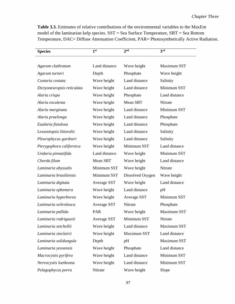
Chapter Three

37

Table 3.3. Estimates of relative contributions of the environmental variables to the MaxEnt model of the laminarian kelp species. SST = Sea Surface Temperature, SBT = Sea Bottom Temperature, DAC= Diffuse Attenuation Coefficient, PAR= Photosynthetically Active Radiation. Species 1st 2nd 3rd

Agarum clathratum Land distance Wave height Maximum SST

Agarum turneri Depth Phosphate Wave height

Costaria costata Wave height Land distance Salinity

Dictyoneuropsis reticulata Wave height Land distance Minimum SST

Alaria crispa Wave height Phosphate Land distance

Alaria esculenta Wave height Mean SBT Nitrate

Alaria marginata Wave height Land distance Minimum SST

Alaria praelonga Wave height Land distance Phosphate

Eualaria fistulosa Wave height Land distance Phosphate

Lessoniopsis littoralis Wave height Land distance Salinity

Pleurophycus gardneri Wave height Land distance Salinity

Pterygophora californica Wave height Minimum SST Land distance

Undaria pinnatifida Land distance Wave height Minimum SST

Chorda filum Mean SBT Wave height Land distance

Laminaria abyssalis Minimum SST Wave height Nitrate

Laminaria brasiliensis Minimum SST Dissolved Oxygen Wave height

Laminaria digitata Average SST Wave height Land distance

Laminaria ephemera Wave height Land distance pH

Laminaria hyperborea Wave height Average SST Minimum SST

Laminaria ochroleuca Average SST Nitrate Phosphate

Laminaria pallida PAR Wave height Maximum SST

Laminaria rodriguezii Average SST Minimum SST Nitrate

Laminaria setchellii Wave height Land distance Maximum SST

Laminaria sinclairii Wave height Maximum SST Land distance

Laminaria solidungula Depth pH Maximum SST

Laminaria yezoensis Wave height Phosphate Land distance

Macrocystis pyrifera Wave height Land distance Minimum SST

Nereocystis luetkeana Wave height Land distance Minimum SST

Pelagophycus porra Nitrate Wave height Slope

Chapter Three

38

Species 1st 2nd 3rd

Postelsia palmaeformis DAC Wave height Minimum SST

Saccharina dentigera Wave height Land distance Nitrate

Saccharina latissima Wave height Average SST Land distance

Saccharina sessilis Wave height Land distance DAC

Ecklonia cava Maximum SST Phosphate Wave height

Ecklonia kurome Maximum SST Depth PAR

Ecklonia maxima Wave height PAR Phosphate

Ecklonia radiate Salinity Wave height Land distance

Egregia menziesii Wave height Land distance Minimum SST

Lessonia corrugate Wave height Minimum SST Land distance

Lessonia flavicans Land distance Phosphate Dissolved Oxygen

Lessonia variegate Minimum SST Land distance Nitrate

Table 3.4. Estimates of relative contributions of the environmental variables to the MaxEnt

model of the laminarian kelp genera. SST = Sea Surface Temperature.

Genus 1st most contribution 2nd most contribution 3rd most contribution Agarum Wave height Land distance Salinity Alaria Average SST Wave height Land distance Chorda Average SST Wave height Land distance Costaria Wave height Land distance Salinity Dictyoneuropsis Wave height Land distance Minimum SST Ecklonia Minimum SST Land distance pH Egregia Wave height Land distance Diffuse Attenuation

Coefficient Laminaria Average SST Wave height Land distance Lessonia Land distance Minimum SST Wave height Macrocystis Wave height Land distance Minimum SST Nereocystis Wave height Land distance Nitrate Postelsia Diffuse Attenuation

Coefficient Wave height Minimum SST

Pterygophora Wave height Minimum SST Diffuse Attenuation Coefficient

Saccharina Wave height Average SST Land distance Thalassiophyllum Average SST Phosphate Minimum SST Undaria Land distance Wave height Average SST

Chapter Three

39

Table 3.5. Estimates of the relative contributions of the environmental variables to the MaxEnt

model of the laminarian kelp families. SST = Sea Surface Temperature

Family 1st most contribution 2nd most contribution 3rd most contribution

Agaraceae Wave height Land distance Average SST

Alariaceae Wave height Average SST Land distance

Chordaceae Average SST Land distance Wave height

Laminariaceae Average SST Wave height Land distance

Lessoniaceae Minimum SST Land distance Wave height

3.4 Discussion In this study, I provide the first global distribution map of laminarian kelp as a polygon layer that

can be used in geographical information systems (GIS). This polygon layer has a more complete

geographical distribution of the kelp biome than the published range maps of kelp species.

However, the map had a very similar distribution to the observed field records (Fig. 3.1), and as

reported in the literature (Steneck et al. 2002; Wernberg et al. 2019; Wernberg and Filbee-Dexter

2019). I found kelp was limited to latitudes 25o to 70o in the northern, and 25o to 55o in the

southern, hemispheres.

Kelp occupied 1,469,900 km2 and 22 % of the world’s coastline. Previous studies

estimated that 25% of the world’s coastline was covered by kelp forests (Filbee-Dexter and

Wernberg 2018; Blamey and Bolton 2018; Wernberg et al. 2019). Thus, the kelp biome is the

second most widely distributed marine biome, following seagrass with 1,646,788 km2

(Jayathilake and Costello 2018). The other marine biomes have ten times less area, namely

zooxanthellate coral with 151,390 km2 (UNEP-WCMC et al. 2018), and mangroves with 136,850

km2 (Giri et al. 2011).

Some of the locations predicted to contain kelp in our map, but without occurrence

records in GBIF and OBIS, were reported to have kelp forests in the literature. Macrocystis

pyrifera and Undaria pinnatifida have been recorded in the Gulf of Nuevo, along the coast of

Argentina from Puerto Deseado (Santa Cruz province) to Mar del Plata (Buenos Aires province)

Chapter Three

40

(Raffo et al. 2009; Pereyra et al. 2017; Paula et al. 2018). Laminaria japonica and Saccharina

japonica occur along the coast of Shandong Peninsula, China (Wu et al. 2016; Shao et al. 2019).

Laminaria japonica, L. religiosa and U. pinnatifida occur around Hokkaido Island, Japan

(Matsunaga et al. 1999). Alaria esculenta, Laminaria digitata, and Saccharina latissimi occur in

Hornsund, and L. digitata in Kongsfjorden, Svalbard (Włodarska-Kowalczuk et al. 2009; Bartsch

et al. 2016). The current map did not predict any suitable locations in Antarctica and no

laminarian kelp have been reported there (Moe and Silva 1977; Quartino and Boraso de Zaixso

2008; Wernberg et al. 2019). This suggests that the absence of laminarian kelp in these regions is

primarily due to environmental unsuitability. Thus, our map appears to be an accurate

representation of the kelp biome at a global scale.

As a photosynthetic plant, kelp is limited to the photic zone. In this study, the probability

of presence of kelp was high between 0 to 100 m depth, and it was limited to 1 km from the land.

However, it is likely that there may be offshore rocky reefs, such as the tops of seamounts, where

kelp may occur but were not detected due to the spatial resolution of our data (Parker and

Tunnicliffe 1994; Bo et al. 2011). Kelp forests always occur on hard substrata such as rocky

seabeds (Teagle et al. 2017, Wernberg et al. 2019). The present study could not include seabed

substrata because a global layer is not available. Nevertheless, the accuracy of the map suggests

that sufficient rocky substrata exist for all regions where temperature and light are suitable.

However, more detailed regional maps of kelp distribution would benefit from including seabed

substratum within the present biome map.

Kelp had an increased probability of presence with increasing wave height from 1 m to 7

m, with low probability of occurrence in areas without wave action. In general, kelp species

prefer turbulent water (Hurd 2000, Wernberg et al. 2019). For the individual species, genera and

families, wave height was generally the most important factor in influencing their distribution.

Species such as Laminaria hyperborea and Alaria esculenta are more common on wave exposed

coasts (Frid and Kitching 1988; Norton 1992; Kraan et al. 2000; Pedersen et al. 2012).

I confirmed that the annual average sea surface temperature is the most significant factor

limiting the distribution of the kelp biome, as suggested by others (e.g., Lüning 1990; Tegner et

al. 1996; Muller et al. 2009; Smale and Moore 2017). Kelp occurred in average sea surface

temperatures from 5 oC to 25 oC, and was rare above 27 oC (Table 2). Thus, if sea surface

temperature increases beyond these temperatures, such as due to global warming, it will alter the

kelp distribution (Tegner et al. 1996; Assis et al. 2016). Indeed, the range of Australian temperate

Chapter Three

41

kelp forests has contracted after ocean warming and extreme heat waves (Wernberg et al. 2013;

Wernberg et al. 2016). Macrocystis pyrifera forests in Australia have been predicted to become

extinct if the predicted high sea surface temperatures in 2100 eventuate (Wernberg et al. 2011;

Martínez et al. 2018). In contrast, Arctic kelp forests of Laminaria digitata have extended with

ocean warming into areas that were previously too-cold (Bartsch et al. 2016). Modelling of future

kelp biome distribution is necessary to predict its responses to climate change.

The kelp biome map indicates where kelp forests should occur. If kelp is absent, and such

absences are not predicted due to ocean warming, other causes could be examined. For example,

the absence of kelp may be due to the loss of natural ‘trophic cascades’ due to hunting and fishing

of animals that predate sea urchins, and consequent over-grazing of kelp by the sea urchins (e.g.,

Leleu et al. 2012). Future studies may model the potential distribution of kelp species at local and

regional scales, so as to provide finer spatial resolution for local scale conservation and fishery

management. The availability of additional data for the species with insufficient data may allow

their range to be mapped. The present map may also be a useful data layer for predicting the

occurrence of kelp-associated species and estimating ‘blue carbon’ budgets. Moreover, knowing

the global extent of the kelp biome is important for the conservation of not only kelp but

associated species, including species threatened with extinction or important to fisheries.

Chapter Three

42

Figure 3.1. The distribution of laminarian kelp observations used in this study.

Chapter Three

43

Figure 3.2. The predicted environmental range for kelp species of the order Laminariales. The dark blue colour indicates the MaxEnt probability of distribution. (a) west coast of North America, (b) north-west Atlantic including Greenland and Iceland, (c) Europe, (d) north-west Pacific including parts of Japan, China, Russia, and Korea, (e) New Zealand and southern Australia, (f) southern Africa, (g) southern South America.

Chapter Three

44

Figure 3.3. Response of kelp to depth, distance from land, wave height, average sea surface temperature, maximum sea surface temperature, and salinity

Chapter 4

Global gap analysis: delineation of priority areas of strict marine reserves to conserve marine biomes

Chapter Four

45

4 Delineation of priority areas of strict marine reserves to conserve marine biomes

4.1 Introduction

Analogous to the conservation of terrestrial forests in order to preserve feeding and breeding

habitats of terrestrial animals, it is essential to conserve marine biomes to safeguard marine

faunal and floral communities. Marine biomes of mangroves, seagrasses, zooxanthellate corals,

and kelps cover almost all the shallow coastal areas of the world. Marine protected areas are one

of the tools used in marine biodiversity conservation (IUCN 2019). At present, there are ongoing

discussions about the extent to which biodiversity goals have been achieved by marine protected

areas.

As noted in Chapter 1, seagrass, kelp, mangrove, and zooxanthellate coral biomes play an

important role in environmental, economic and social services, and are being negatively

impacted by anthropogenic and climatic stresses. Marine fauna living in these biomes are

consequently threatened by loss of habitat (Powles et al. 2000; Lotze et al. 2006; McCauley et al.

2015). Since the 1980s, the seagrass biome has been lost at a rate of 110 km2 yr-1 (Waycott et al.

2009). Short et al. (2011) showed that 22 seagrass species have declining populations. Coastal

urbanisation, degraded water quality, and mechanical damage are contributing most to the

decline of seagrass populations (Short et al. 2011).

At least 35% of mangroves have declined globally over the last decades (Valiela et al.

2001; Duke et al. 2007; Polidora et al. 2010). Among the Southeast Asian countries where the

most mangrove distribution as well as the deforestation occur (Blasco et al. 2001; Primavera et

al. 2019), Myanmar has the highest rate of mangrove deforestation (Hamilton and Casey 2016).

From 2000 to 2012, 88% of the Myanmar mangrove forests were transformed into rice fields.

Over the last 75 years, 83% of the mangroves in the Ayeyarwaddy Delta (Irrawaddy River) were

lost (Htay 2016; Richards and Friess 2016). In Indonesia, Cambodia, and the Philippines, 30% of

mangrove forests have been replaced by ponds for aquaculture (Richards and Friess 2016).

Between 50% and 80% of coral reefs have been impacted locally by human activities

(Hoegh-Guldberg 1999; Bellwood et al. 2004; Bridge et al. 2013). Globally, more than 60% of

coral reefs are under pressure from destructive fishing, fertiliser runoff from agriculture, sewage

Chapter Four

46

discharge, solid waste disposal, and toxins from oil, gas, coastal developments and landfill sites

(Cesar et al. 2003; Wear and Thurber 2015; Burke et al. 2017). Nearly 95% of Southeast Asian

coral reefs are threatened by overfishing, coastal construction and pollutants (Burke et al. 2011;

Wear 2016).

The kelp biome has declined due to kelp harvesting, eutrophication, sedimentation, oil

spills, and climatic impacts (Steneck et al. 2002). Central Chile, the Aleutian Islands, the South

Australian Gulfs, and the North Sea have a > 95% probability of declining kelp abundance in

locations where water temperatures are warming, increased sea urchin abundance due to

overfishing of their predators, pollution and invasive species (Krumhansl et al. 2016).

The Convention on Biological Diversity (CBD) (UNEP/CBD/COP/DEC/IX/20) defined

scientific criteria for identifying ecologically or biologically significant marine areas, namely: (1)

have unique, rare or endemic species, populations or communities; (2) are essential for a

population to survive and grow (e.g., breeding grounds, spawning areas, nursery areas); (3)

contain habitat for the survival and recovery of declining, threatened, and endangered species or

contain an area with significant assemblages of such species; (4) cover a relatively high

percentage of sensitive, functionally fragile species (that is, highly susceptible to degradation or

decline by anthropogenic activities or by natural events) or species that recover slowly; (5)

contain species, populations or communities with comparatively higher natural biological

productivity; and (6) contain comparatively higher biodiversity. All four marine biomes meet all

of the above conditions required to be prioritised for conservation (Chapter 1).

The CBD’s Aichi Biodiversity Target 11 (UNEP/CBD/COP/10/9) calls for at least 10%

of coastal and marine areas, specifically areas of importance for biodiversity and ecosystem

services to be fully protected with an increased focus on comprehensive, ecologically

representative, effectively managed protected areas. It aims to protect both habitats and

populations of species. Aichi Target 11 further asserts that future protected areas should be

focused on the importance of complementarity and spatial configuration to maintain ecological

connectivity and the concept of an ecological network. Therefore Aichi Target 11 concerns both

quantitative and qualitative conservation outcomes through increasing new protected areas (Rees

et al. 2018).

Aichi Biodiversity Target 12 (UNEP/CBD/COP/10/9) calls for the decline of threatened

species to be stopped and their conservation status improved by 2020. The International Union

Chapter Four

47

for Conservation of Nature’s (IUCN) Red List of Threatened Species (commonly referred to as

IUCN Red List) is the most comprehensive inventory of the species conservation status at a

global scale. The IUCN Red List has nine conservation status categories: Not Evaluated, Data

Deficient, Least Concern, Near Threatened, Vulnerable, Endangered, Critically Endangered,

Extinct in the Wild, and Extinct. The Data Deficient (DD) category applies to taxa with a lack of

occurrence and abundance data to evaluate their risk of extinction and the Least Concern (LC)

category includes any taxa that are not categorised as threatened. The Near Threatened (NT) taxa

are likely to qualify for threatened status in the near future. The Vulnerable (VU), Endangered

(EN), and Critically Endangered (CR) taxa have high, very high, and extremely high risks of

extinction in the wild respectively. A taxon is Extinct in the Wild (EW) when it no longer

survives in the wild, and it is considered as Extinct (EX) when no living specimens exist either in

the wild and or in captivity (IUCN 2012). Considering 2020 is the deadline to review progress

against the Aichi Targets, it is timely to review the conservation assessment and status of the

species forming the marine biomes, and to review how well the biomes are protected within

reserves.

Marine Protected Areas (MPAs) play an important role in the conservation of marine

biodiversity. The total area of MPAs is 27,841,368 km2, and comprises 8% of the total ocean

area (UNEP-WCMC and IUCN 2019). Although MPAs account for about 8% of the entire

ocean, only about 0.7% of the ocean area is fully protected from deliberate human impacts in

marine reserves (UNEP-WCMC and IUCN 2019). Costello and Ballantine (2015) found that

94% of MPAs permit fishing and consequently do not aim to conserve biodiversity in a natural

state. Strict marine reserves are essential to conserve biodiversity, not MPAs (Costello and

Ballantine 2015). IUCN guidelines for defining strict marine reserves (category Ia) have their

primary objective of protecting biodiversity by strictly limiting human impacts.

In this chapter, I summarised the current conservation status of each marine biome

forming species in the IUCN Red List. Then I calculated the area of each biome and the areas

with overlapping biomes within each country’s Exclusive Economic Zone (EEZ), and in the

High Seas (areas outside EEZs), were calculated. Since biodiversity conservation projects are

currently proceeding in the IUCN operational region, the area of marine biome within the IUCN

regions was also calculated. The area of each biome protected within fully-protected areas

(IUCN category Ia), hereafter called marine reserves, was calculated. Because biodiversity per

Chapter Four

48

unit area will be higher when several biomes occur together, the analysis mapped geographic

cells where more than one biome occurred. The analysis thus determined the extent to which

marine biomes are (in theory) protected in the marine reserves and which countries can do most

to better protect them.

4.2 Methods 4.2.1 Data

This study used EEZs and marine protected area polygon layers as well as maps of the four

biomes of seagrass, kelp, mangroves and zooxanthellate corals (Table 4.1).

The seagrass distribution was modelled using MaxEnt software (Chapter 2, Jayathilake

and Costello 2018), using 43,037 occurrence records belonging to 60 species from the GBIF

database, the UNEP-WCMC seagrass point layer and 13 abiotic variables available on the Global

Marine Environment Datasets (GMED) (Chapter 2). The map predicted that the seagrass biome

may occupy 1,646,788 km2 which was approximately double the previous seagrass polygon layer

from UNEP-WCMC and Short (2016).

In this study 67 kelp species were used in the summary of the conservation status based

on IUCN Red List. The kelp biome distribution was modelled using MaxEnt (Chapter 3;

Jayathilake and Costello 2019). It was created with 44,265 occurrence records from GBIF and

OBIS and 13 abiotic variables from GMED. The modelled kelp biome map has a distribution

area of 1,469,907.81 km2 distribution in area and is present on 22% of the coastline.

Mangrove biome species were identified according to the World Atlas of Mangroves

(Spalding 2010). Here I used 64 mangrove species for summarizing the conservation status based

on the IUCN Red List. The mangrove polygon layer was downloaded from the UNEP-WCMC

Ocean Data Viewer website (Giri et al. 2011). It was developed using satellite images classified

by a supervised and an unsupervised image classification process (Giri et al. 2011). The map had

a 30 m resolution.

Chapter Four

49

Table 4.1. Summary of data sources used in this study. Data layer Data

format(s) Creation method Spatial

resolution Reference

Seagrass biome Polygon layer

Modelled with MaxEnt

30 arc seconds

Jayathilake and Costello (2018)

Kelp biome Polygon layer

Modelled with MaxEnt

30 arc seconds

Jayathilake and Costello (2019)

Zooxanthellate coral biome

Polygon layer

Multispectral Landsat 7 images acquired between 1999 and 2002

30 m UNEP-WCMC et al. (2018)

Mangrove biome Polygon layer

Multispectral Landsat images processing

30 m Giri et al. (2011)

Exclusive Economic Zones

Polygon layer

Flanders Marine Institute (2014)

Marine Protected Area (MPA)

Polygon layer

Designated under international agreements and conventions

Varied IUCN and UNEP-WCMC (2019)

The zooxanthellate coral species names were extracted from the available literature

(Cairns et al. 1999; Veron 2013; Veron et al. 2015) for the IUCN conservation status summary.

Here I used the IUCN conservation status for 633 zooxanthellate coral species. The

zooxanthellate coral biome vector was downloaded from the UNEP-WCMC Ocean Data Viewer

website (UNEP-WCMC et al. 2018). This dataset contains the global distribution of tropical and

subtropical warm-water coral reefs. It has a point and a polygon shapefile enabled to work in

GIS software. These vectors were compiled from multiple sources including the Millennium

Coral Reef Mapping Project, UNEP World Conservation Monitoring Centre (UNEP-WCMC),

the WorldFish Centre, World Resources Institute, The Nature Conservancy, and the World Atlas

of Coral Reefs. The significant contribution of data is from the Millennium Coral Reef Mapping

Chapter Four

50

Project (85%) which used multispectral Landsat 7 images acquired between 1999 and 2002 with

30 m resolution (UNEP-WCMC et al. 2018).

4.2.2 Current extinction risk of biome forming species

In this study, the global conservation status of 60 seagrass, 67 kelp, 633 zooxanthellate coral, and

64 mangrove species’ (including true mangroves, palm species (Nypa fruticans) and fern species

(Acrostichum sp. ) wide spread within mangrove biome) were summarised based on the

International Union for Conservation of Nature (IUCN) Red List of Threatened Species

(commonly known as IUCN Red List). The conservation statuses were recorded with the same

abbreviations as those used in the IUCN Red List and the abbreviation. The ‘NOT’ status was

given for accepted species yet to be evaluated and which have not been listed in the Red List

(Appendix S.4.1).

4.2.3 Mapping

All four biome polygon layers were converted to the cylindrical equal-area projection coordinate

system and overlaid on the same map using Arc Map 10.5.1. To get an understanding of how

each marine biome covers the EEZ and High Seas, the four biome layers were split into the EEZs

using the Arc Map tool. The biome areas belonging to each country’s EEZ and High Seas were

then calculated separately (Table 4. 3).

The regional conservation of each biome was calculated for each of the IUCN regions. I selected

IUCN operational regions because those regions have ongoing conservation projects in nearly

160 countries. However, the IUCN did not include all countries into their operational regions.

The countries that were not already not categorised in any IUCN operational regions were

therefore included in a region according to their continent. In the current study I included the

Mediterranean countries together same as per the IUCN operational region without divide them

into the three different continents to which they belong. Further I subdivided large continents

such as Asia and Africa to get attain clearer observations of conservation progress.

Chapter Four

51

4.2.4 The area of overlapping biomes

The biome vector layers were converted to raster layers through a tessellation grid of 1 km x 1

km to maintain a standard pixel size for all four biome layers throughout the analysis. The biome

area was classified as 1 when present and 0 when absent using the reclassify tool in the ArcMap

3 D analyst toolbox. Then the presence of multiple biomes was identified using the weighted

sum (spatial analyst) tool. The weighted sum (spatial analyst) tool overlays several raster layers

and sums them up together. In the current study, weights were set as 1 for each biome raster

layer. Thus, cells could be scored from 0 (on biome) to 4 (4 biomes). However, there were no

cells found with all four biomes. The area covered with the existing IUCN Category Ia marine

reserves was extracted using the IUCN and UNEP-WCMC (2018) vector layer to map reserves

to the biomes. The following areas were then calculated.

1) Area of seagrass, kelp, zooxanthellate coral, and mangrove biome distribution.

I. In each EEZ

II. In each IUCN operational region

2) Area of multiple biomes occuring within a 1 km x 1 km cell grid

I. In each EEZ

II. In each IUCN operational region

3) Area of multiple biomes within marine reserves

I. In each EEZ

II. In each IUCN operational region

4.3 Results

4.3.1 Species conservation status assessment

561 zooxanthellate coral species, 58 seagrass species, 1 kelp species, and 60 mangrove species

had already been assessed by the IUCN Red List meaning 72, 2, 66, and 4 species respectively

have not been assessed (Table 4.2, Fig. 4.1).

Of the assessed zooxanthellate coral species, 160 (25%) were categorised as threatened;

i.e. Critically Endangered, Endangered, or Vulnerable. Another 131 species (22%) were listed as

Chapter Four

52

not assessed (NOT) and data deficient (DD). Almost all of the species of kelp biome were not

evaluated (Table 4.2, Fig. 4.1). Among the conservation statuses of 78 laminarian kelp species

and 25 other kelp species, only one species (Eisenia galapagensis) was listed as vulnerable and

the rest were yet to be evaluated.

Of the 60 seagrass species, 7 (12%) were listed in one of the three Red List categories of threat:

Critically Endangered, Endangered, or Vulnerable (Fig. 4.1). Phyllospadix japonicas and Zostera

chilensis were listed as endangered species. The majority of the seagrass species belonged to the

Least Concern category. Halophila baillonis, Halophila engelmannii were not evaluated, and

two, Halodule beaudettei and Halodule emarginata were categorised as Data Deficient. Out of

the studied mangrove species, a 10% have been categorised as Threatened with the Risk of

Extinction in the IUCN Red List. The majority of mangroves have been listed under the Least

Concern category in the IUCN Red List (Fig 4.1).

4.3.2 Area of biome distribution 4.3.2.1 EEZ Australia had the largest area of seagrass of any country (Tables 4.3, 4.4, Fig. 4.4, 4.5, 4.6, 4.7),

and 16% of the total global seagrass distribution. The USA and Indonesian EEZs had the next

largest areas of seagrass with 6% and 5% of the global seagrass distribution respectively. The

largest area of kelp for any country was also found in Australia, with 21% of the global kelp

cover. The USA (9%), The UK (7%), and Japan (7%) had the next largest kelp cover. Australia,

Indonesia, the Philippines, and Papua New Guinea had 21%, 13%, 7% and 5% of the highest

global coral distribution respectively. These four countries covered nearly half of the global coral

biome. Indonesia had 1/5 of the global mangrove cover, followed by Brazil (8%), Australia

(7%), and Mexico (5%) (Table 4. 3, 4.4). Thus, Australia is therefore known to have more

seagrass, kelp and zooxanthellate coral reef biomes than any other country.

When countries were considered along with their overseas territories, the largest seagrass

and kelp distributions were in Australia and the USA (Table 4.3). Australia and its overseas

territories had the largest mangrove distribution followed by Indonesia and the Philippines.

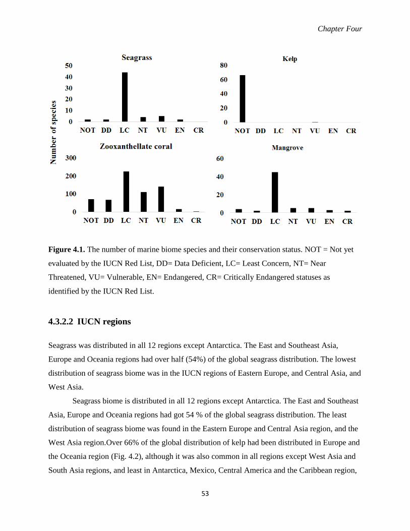
Chapter Four

53

Figure 4.1. The number of marine biome species and their conservation status. NOT = Not yet

evaluated by the IUCN Red List, DD= Data Deficient, LC= Least Concern, NT= Near

Threatened, VU= Vulnerable, EN= Endangered, CR= Critically Endangered statuses as

identified by the IUCN Red List.

4.3.2.2 IUCN regions Seagrass was distributed in all 12 regions except Antarctica. The East and Southeast Asia,

Europe and Oceania regions had over half (54%) of the global seagrass distribution. The lowest

distribution of seagrass biome was in the IUCN regions of Eastern Europe, and Central Asia, and

West Asia.

Seagrass biome is distributed in all 12 regions except Antarctica. The East and Southeast

Asia, Europe and Oceania regions had got 54 % of the global seagrass distribution. The least

distribution of seagrass biome was found in the Eastern Europe and Central Asia region, and the

West Asia region.Over 66% of the global distribution of kelp had been distributed in Europe and

the Oceania region (Fig. 4.2), although it was also common in all regions except West Asia and

South Asia regions, and least in Antarctica, Mexico, Central America and the Caribbean region,

Chapter Four

54

and the West and Central Africa region. The mangrove biome had mostly distributed along the

tropical coastlines. Half of the global distribution of mangrove biome and two-thirds of the

zooxanthellate biome were found in the East and Southeast Asian region and Oceania regions.

4.3.3 Area of multiple biomes occur with 30 arcsec cell grid 4.3.3.1 EEZ The coastal area wih 1 km x 1 km cells covered by at least one biome was 86,146 x 102 km2. Of

this a 56,807 x 102 km2 area was covered by one biome, 25,190 x 102 km2 by two and 4,148 x

102 km2 by three biomes. There were no 30 arcsec cells (1 km x km) within all four studied

biomes. The largest area, covered by two biomes, was found in Australia, followed by Indonesia

and then the USA. The largest area, with three overlapping biomes, was in Indonesia and

comprised of seagrass, coral, and mangroves. The next largest were followed by the Philippines,

Australia, and Papua New Guinea (Table 4.3, 4.4, Fig 4.8, 4.9, 4.10).

4.3.3.2 IUCN regions Most of the areas covered by one biome were found in Oceania and the East and Southeast Asian

region and the region with the fewest was Antarctica (Fig. 4.3). The largest areas covered by two

biomes were found in East and Southeast Asia, Europe and Oceania regions. The largest area

with three overlapping biomes, was found in the East and Southeast Asian region, followed by

the Eastern and Southern Africa, Oceania and Mexico and the Central America and the

Caribbean regions.

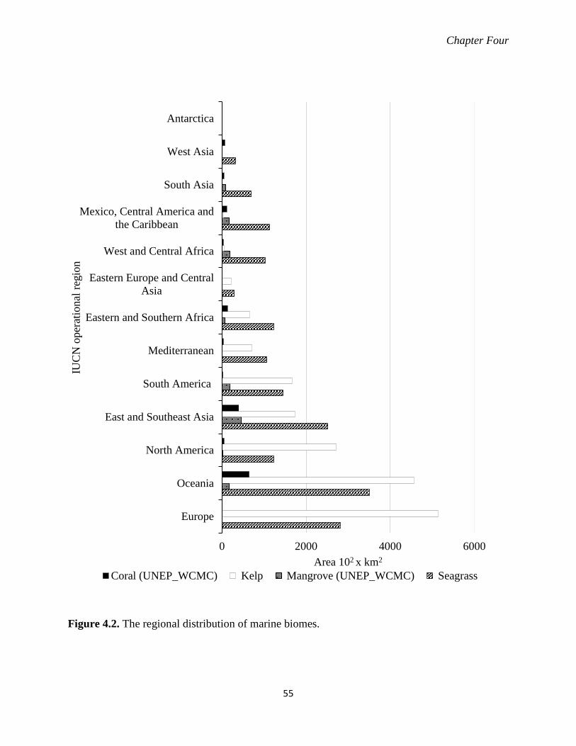
Chapter Four

55

Figure 4.2. The regional distribution of marine biomes.

0 2000 4000 6000

Europe

Oceania

North America

East and Southeast Asia

South America

Mediterranean

Eastern and Southern Africa

Eastern Europe and CentralAsia

West and Central Africa

Mexico, Central America andthe Caribbean

South Asia

West Asia

Antarctica

Area 102 x km2

IUC

N o

pera

tiona

l reg

ion

Coral (UNEP_WCMC) Kelp Mangrove (UNEP_WCMC) Seagrass

Chapter Four

56

Figure 4.3. The overlap of biome areas in the IUCN regions.

4.3.4 Area of multiple biomes within marine reserves Globally only 1% of marine biomes were conserved in marine reserves (Table 4.5). Of these,

586.5 x102 km2 of reserves contained one biome, 192.3 x102 km2 had two, and 27 x102 km2 had

three biomes. As a percentage, reserves covered only 0.7% of areas with one biome, 0.2% of

0 2000 4000 6000 8000 10000 12000 14000

East and Southeast Asia

Oceania

South America

Europe

North America

Mexico, Central America and theCaribbean

Mediterranean

Eastern and Southern Africa

West and Central Africa

South Asia

West Asia

Eastern Europe and Central Asia

Antarctica

Area 102x km2

IUC

N o

pera

tiona

l reg

ion

3 biomes 2 biomes 1 biome

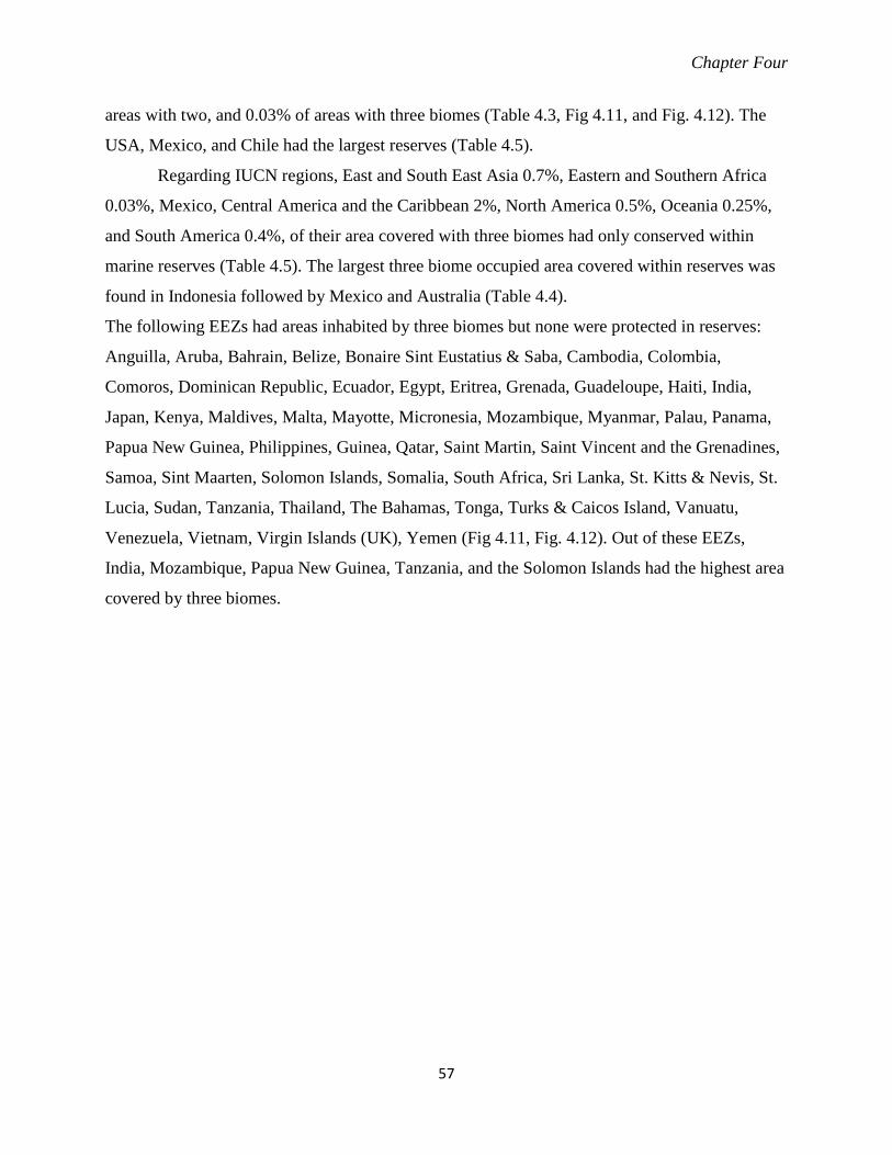
Chapter Four

57

areas with two, and 0.03% of areas with three biomes (Table 4.3, Fig 4.11, and Fig. 4.12). The

USA, Mexico, and Chile had the largest reserves (Table 4.5).

Regarding IUCN regions, East and South East Asia 0.7%, Eastern and Southern Africa

0.03%, Mexico, Central America and the Caribbean 2%, North America 0.5%, Oceania 0.25%,

and South America 0.4%, of their area covered with three biomes had only conserved within

marine reserves (Table 4.5). The largest three biome occupied area covered within reserves was

found in Indonesia followed by Mexico and Australia (Table 4.4).

The following EEZs had areas inhabited by three biomes but none were protected in reserves:

Anguilla, Aruba, Bahrain, Belize, Bonaire Sint Eustatius & Saba, Cambodia, Colombia,

Comoros, Dominican Republic, Ecuador, Egypt, Eritrea, Grenada, Guadeloupe, Haiti, India,

Japan, Kenya, Maldives, Malta, Mayotte, Micronesia, Mozambique, Myanmar, Palau, Panama,

Papua New Guinea, Philippines, Guinea, Qatar, Saint Martin, Saint Vincent and the Grenadines,

Samoa, Sint Maarten, Solomon Islands, Somalia, South Africa, Sri Lanka, St. Kitts & Nevis, St.

Lucia, Sudan, Tanzania, Thailand, The Bahamas, Tonga, Turks & Caicos Island, Vanuatu,

Venezuela, Vietnam, Virgin Islands (UK), Yemen (Fig 4.11, Fig. 4.12). Out of these EEZs,

India, Mozambique, Papua New Guinea, Tanzania, and the Solomon Islands had the highest area

covered by three biomes.

Chapter Four

58

Figure 4.4. The global distribution of the seagrass biome.

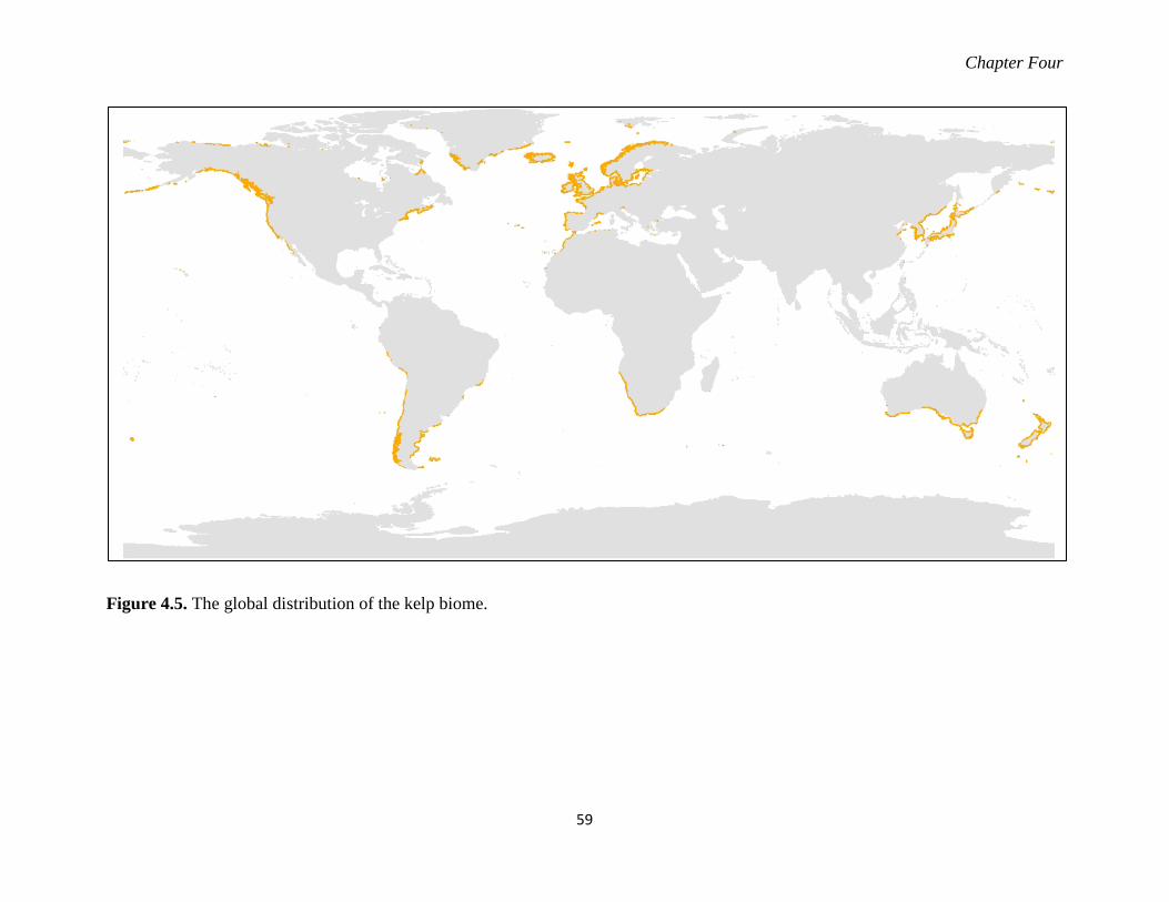
Chapter Four

59

Figure 4.5. The global distribution of the kelp biome.

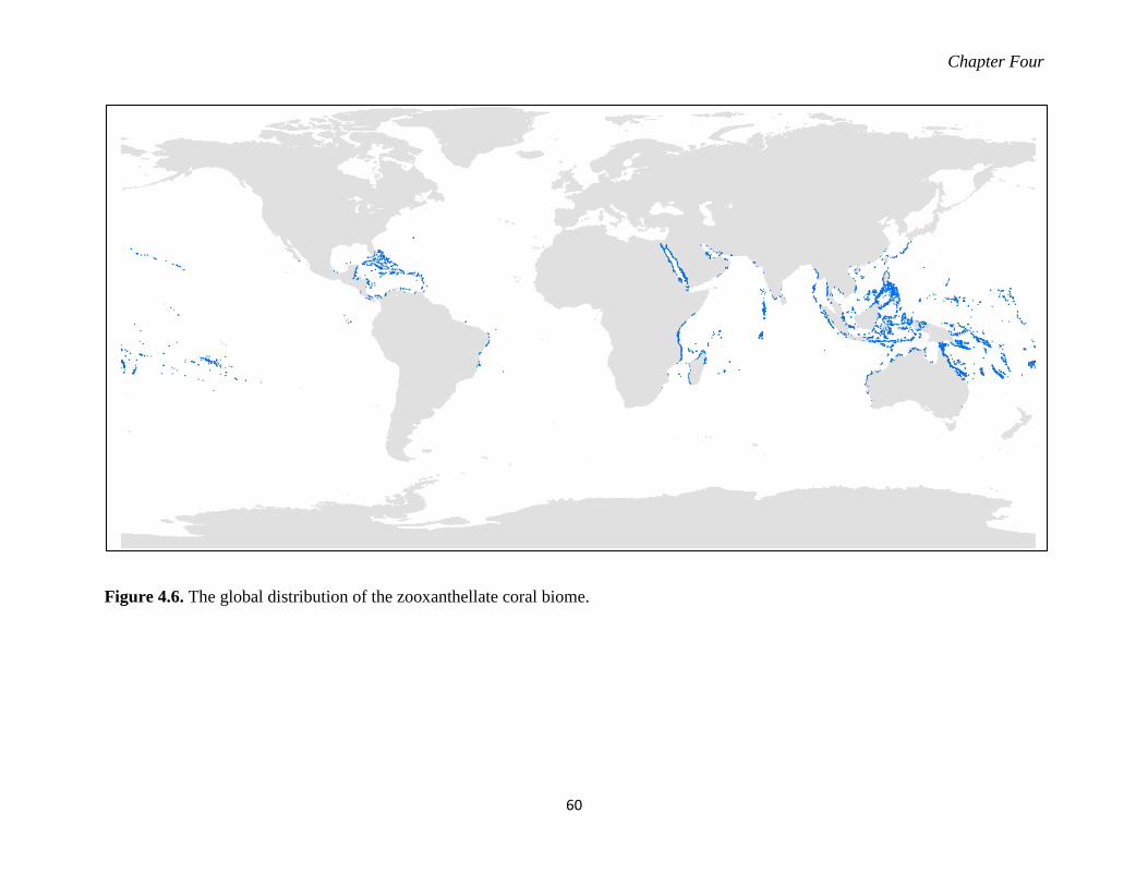
Chapter Four

60

Figure 4.6. The global distribution of the zooxanthellate coral biome.

Chapter Four

61

Figure 4.7. The global distribution of the mangrove biome.

Chapter Four

62

Figure 4.8. The areas where one marine biome occurs.

Chapter Four

63

Figure 4.9. The areas where two marine biomes occur.

Chapter Four

64

Figure 4.10. The areas where three marine biomes occur.

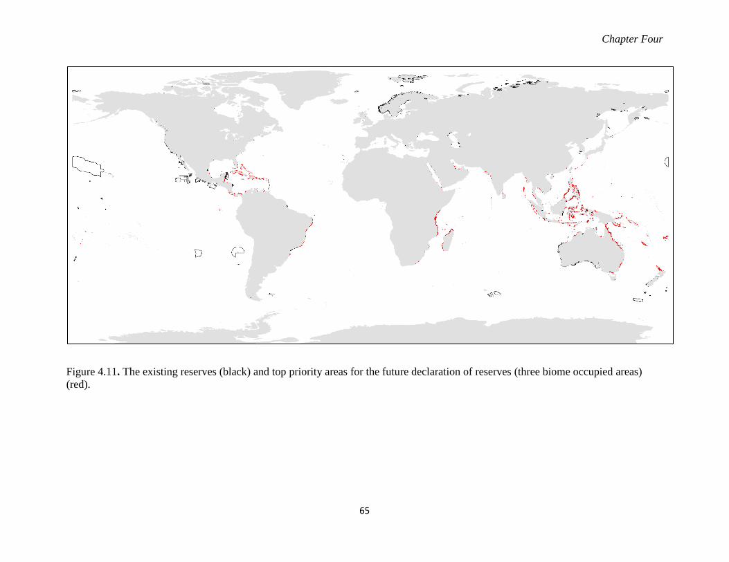
Chapter Four

65

Figure 4.11. The existing reserves (black) and top priority areas for the future declaration of reserves (three biome occupied areas) (red).

Chapter Four

66

Figure 4.12. Present biome protection within reserves.This map is available on the Arc GIS online service via link https://arcg.is/1HCfK

Chapter Four

67

4.4 Discussion

This chapter identified the current conservation status of biome species based on the IUCN Red

List and locations where marine reserves would be optimally designated to conserve marine biomes.

Nearly 80% out of 824 biome-forming species studied here had their conservation status assigned by

the IUCN Red List. The remaining 20% had not been assessed. Approximately 5% of species were

categorised into the DD conservation status based on the IUCN Red List due to the lack of appropriate

data on abundance and/or distribution. Listing of a species in the NOT evaluated and DD categories

acknowledges the potential for further research to show that Threatened classification is appropriate

(IUCN 2012). Assessment of the conservation statuses of the kelp biome species had been largely

neglected, despite the vital role they play in the coastal ecology in sub-tropical, temperate and sub-

polar Regions. In addition, of all the species studied, 20% had been assigned as an IUCN conservation

status of threatened. The major finding on the biome-forming species’ conservation concerns based on

IUCN Red List was that nearly one quarter of biome-forming species were yet to be assessed.

Current research is based on the equally weighted summation of presence of seagrass, kelp,

mangroves and zooxanthellate corals within 1 km x 1 km cell grid-calculated areas of each biome, and

overlapping biomes belonging to each country, as well as in each IUCN operational region. The biome

distribution area and the composition of multiple overlapping biomes vary in EEZs and in the IUCN

operational regions. Here I found that Australia had the world’s largest distribution of seagrass, kelp,

and zooxanthellate coral biomes, whereas Indonesia had the largest mangrove cover. These two

countries had the largest area of overlapping biomes as well. Australia occupied the largest area

covered with one biome, as well as two overlapping biomes within one 30 arcsec cell, while Indonesia

had the largest area covered with three overlapping biomes; mangrove, seagrass, and zooxanthellate

corals. As Australia contributed to such a large extent, the Oceania region had the largest distribution

of seagrass and zooxanthellate coral biomes. The Europe region had the largest laminarian kelp

distribution. I found not only the world’s largest mangrove cover but also the largest distribution of

one biome, two overlapping biomes, and three overlapping biome areas in the East and Southeast

Asian regions, followed by the Oceania region. Although the US declared larger reserves, totalling

15,109 x 102 km, only 0.9% of it protects biome-distributed areas. In contrast, Indonesia had an 88.3 x

102 km reserve area, and 85% of it had covered the coastal areas and thereby the biomes. However, out

Chapter Four

68

of 1,101 x 102 km of three biomes-occupied areas of Indonesia, only 12 x 102 km had been protected

within reserves.

This study shows the importance of the expansion of reserves to protect multiple biome areas.

Multiple biomes occurring within close proximity (e.g. a mangrove-seagrass-zooxanthellate coral

continuum) provides ecological connectivity and niche differentiation among the associated faunal

communities (Unsworth et al. 2009; Berkström et al. 2013). The declining of biomes due to climatic

and anthropogenic activities impacts diminish the linkages between adjacent biomes (Heck et al.

2008). During this study, I therefore aimed to identify the multiple biome areas which had not been

covered within reserves. The most obvious finding of this study was that the countries belonging to

East and South East Asian, Oceania, East and South Africa, South America and Mexico, Central

America, and the Caribbean regions had the largest distribution of multiple biome areas, but were left

out of the marine reserve network thereby conservation efforts. Countries such as India, Philippines,

Papua New Guinea, Mozambique, Tanzania and Solomon Islands had largely been covered with

multiple biomes. These countries can make a big impact in conservation by declaring marine reserves

to cover the multiple biome areas belonging to them. Instead of declaring new marine reserves,

countries such as Indonesia, Australia, Madagascar, Fiji, Brazil, and Cuba can expand their existing

reserves to protect their larger distribution of marine biomes.

A further study could assess the conservation status of the kelp biome species based on the

IUCN Red List. Considerably more work will need to be done to identify the regions with the highest

number of species belonging to the NOT and the DD categories. Similarly, it is important to identify

hotspots of threatened species in order to get prompt conservation measures, as suggested by the Aichi

Biodiversity Target 12 (UNEP/CBD/COP/10/9).

There is a predicted anthropogenic stress on the biomes due to the increasing population in

low-lying coastal areas in China, India, Bangladesh, Indonesia, Vietnam, Egypt, Nigeria, the United

States, Thailand, and Philippines in 2030 and 2060 (Neumann et al. 2015). Human-induced

disturbances, such as dredging, sedimentation, eutrophication, habitat fragmentation, boat anchoring,

and propeller scars accelerate these biome losses (Short and Wyllie-Echeverria 1996; Montefalcone et

al. 2010; Gilman et al. 2008; Wernberg et al. 2019). The current research shows the above-mentioned

countries with high coastal populations had been covered with multiple marine biomes. Marine reserve

networks should moreover be focused on extension in order to effectively control the negative impacts

of the increasing disturbances caused by human populations.

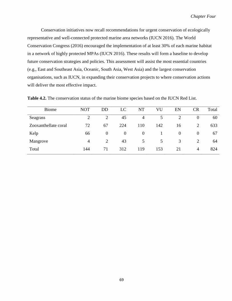
Chapter Four

69

Conservation initiatives now recall recommendations for urgent conservation of ecologically

representative and well-connected protected marine area networks (IUCN 2016). The World

Conservation Congress (2016) encouraged the implementation of at least 30% of each marine habitat

in a network of highly protected MPAs (IUCN 2016). These results will form a baseline to develop

future conservation strategies and policies. This assessment will assist the most essential countries

(e.g., East and Southeast Asia, Oceanic, South Asia, West Asia) and the largest conservation

organisations, such as IUCN, in expanding their conservation projects to where conservation actions

will deliver the most effective impact.

Table 4.2. The conservation status of the marine biome species based on the IUCN Red List.

Biome NOT DD LC NT VU EN CR Total

Seagrass 2 2 45 4 5 2 0 60

Zooxanthellate coral 72 67 224 110 142 16 2 633

Kelp 66 0 0 0 1 0 0 67

Mangrove 4 2 43 5 5 3 2 64

Total 144 71 312 119 153 21 4 824

Chapter Four

70

Table 4.3. The distribution of seagrass, kelp, mangroves, zooxanthellate coral biomes, the area of overlapping biomes for each EEZ, percentage of biomes covered with strict marine reserves. IUCN operational regions were abbreviated as Antarctica = (ANT), East and South East Asia = (ESEA), East and South Africa = (ESA), Eastern Europe and Central Asia = (EEUA), Europe = (EUP), Mediterranean, Mexico, Central America and the Caribbean = (MCC), North America = (NAM), Oceania = (OCN), South America = (SMA) , South Asia = (SAS), West and Central Africa = (WCA), West Asia = (WAS). The countries belonging to the Mediterranean region were marked with an *. All areas are x 102 km2.

Country

Region Biome distribution The area of overlapping biomes Total area of biomes within Ia

% cover in Ia

Present area of Ia Seagrass Kelp Coral Mangr

ove 1

biome 2

biomes 3

biomes Total

Albania* EUP 2.0 5.5

18.6 0.0 0.0 18.6

Algeria* WCA 28.8 0.0

68.1 35.6 0.0 103.7

American Samoa OCN 0.0 0.0 0.5

15.9 0.0 0.0 15.9 1.1 7 1.6 Angola ESA 112.6 0.0 0.0 3.0 281.4 23.0 0.0 304.4 Anguilla (UK) MCC 2.6 0.0 0.2

4.5 3.9 1.0 9.3

Antigua & Barbuda MCC 12.4 0.0 0.5 0.1 17.6 5.9 11.8 35.3 0.2 1 0.2 Argentina SAM 68.5 457.0 0.0

906.3 18.6 0.0 924.9

Aruba (Netherland) MCC 0.0 0.0 0.7

4.0 5.0 1.0 10.0 Australia OCN 2617.3 3476.1 316.4 94.6 5172.1 3068.4 433.8 8674.3 118.1 1 742.6 Bahrain WAS 8.8 0.0 2.7 0.0 27.4 20.6 3.5 51.5 Bangladesh SAS 148.4 0.0 0.0 45.7 316.5 116.2 0.0 432.7 Barbados MCC 0.0 0.0 0.3 0.0 9.0 2.0 0.0 11.0 Belgium EUP 6.6 11.1 0.0 0.0 3.2 15.7 0.0 19.0 Belize MCC 38.6 0.0 11.1 5.7 74.1 65.9 33.4 173.4 Benin WCA 16.5 0.0 0.0 0.4 26.5 6.8 0.0 33.3 Bermuda (UK) NAM 1.8 0.0 5.3 0.0 10.4 3.5 3.5 17.4 0.003 0 0.003 Bonaire Sint Eustatius & Saba (Netherland)

MCC 0.0 0.0 0.3 0.0 13.7 8.0 1.0 22.7

Bosnia & Herzegovina

EUP 0.0 0.0 0.0 0.0 0.6 0.0 0.0 0.6

Brazil SAM 808.8 66.9 7.0 105.2 1591.1 778.5 102.3 2471.9 32.1 1 64.4 British Indian Ocean Territory (UK)

WAS 0.0 0.0 18.1 0.0 210.6 0.0 0.0 210.6

Chapter Four

71

Country

Region Biome distribution The area of overlapping biomes Total area of biomes within Ia

% cover in Ia

Present area of Ia Seagrass Kelp Coral Mangr

ove 1

biome 2

biomes 3

biomes Total

Brunei ESEA 0.0 0.0 0.6 1.2 41.7 0.7 0.0 42.3 0.04 0.1 0.1 Bulgaria EUP 13.8 0.0 0.0 0.0 36.0 0.0 0.0 36.0 0.1 0.4 0.1 Cambodia ESEA 17.0 0.0 0.5 4.7 69.4 36.0 7.0 112.4 Cameroon WCA 19.2 0.0 0.0 21.5 62.6 31.9 0.0 94.5 Canada NAM 242.3 880.9 0.0 0.0 1297.2 800.1 0.0 2097.2 2.1 0.1 34.3 Cape Verde WCA 6.5 0.0 0.0 0.0 40.4 0.0 0.0 40.4 Cayman Island (UK) MCC 0.0 0.0 1.8 0.8 2.9 13.6 0.0 16.5 Chile SAM 26.6 1003.9 0.0 0.0 1961.2 85.8 0.0 2047.1 1.5 0.07 4502.0 China ESEA 412.7 51.5 4.7 1.8 1005.2 278.4 4.8 1288.4 1.1 0.08 4.4 Christmas Island (Australia)

OCN 0.0 0.0 0.1 0.0 5.0 2.0 0.0 7.1

Clipperton Island (France)

MCC 0.0 0.0 0.0 0.0 4.0 0.0 0.0 4.0

Cocos Island (Australia)

OCN 0.0 0.0 1.2 0.0 8.0 0.0 0.0 8.0

Colombia SAM 66.5 0.0 9.3 21.2 367.7 110.6 12.1 490.4 Comoros ESA 1.0 0.0 2.2 0.0 32.0 13.0 3.0 47.9 Conflict zone China/Japan/Taiwan

ESEA 0.0 0.0 0.1 0.0 6.5 0.0 0.0 6.5

Conflict zone Japan/Russia

ESEA 6.7 89.9 0.0 0.0 154.2 20.1 0.0 174.3

Congo WCA 6.0 0.0 0.0 0.0 23.7 0.0 0.0 23.7 Congo, DRC WCA 7.5 0.0 0.0 2.2 15.6 7.6 0.0 23.2 Cook Islands (New Zealand)

OCN 0.0 0.0 2.5 0.0 61.5 0.0 0.0 61.5

Costa Rica MCC 25.2 0.0 0.8 3.9 68.0 61.3 13.2 142.4 0.0004 0.0003 0.8 Cote d'Ivoire WCA 68.0 0.0 0.0 0.4 114.8 34.8 0.0 149.6 Croatia* EUP 109.3 0.0 0.0 0.0 210.9 0.3 0.0 211.2 Cuba MCC 216.4 0.0 26.9 42.6 427.1 511.8 96.7 1035.6 0.1 0.01 0.1 Curaçao (Netherland) MCC 0.0 0.0 0.5 0.0 9.0 5.0 1.0 15.1 Cyprus* EUP 4.3 0.0 0.0 0.0 18.4 0.0 0.0 18.4

Chapter Four

72

Country

Region Biome distribution The area of overlapping biomes Total area of biomes within Ia

% cover in Ia

Present area of Ia Seagrass Kelp Coral Mangr

ove 1

biome 2

biomes 3

biomes Total

Denmark EUP 232.3 312.9 0.0 0.0 74.6 423.6 0.0 498.2 Disputed Kenya/Somalia

ESA 0.3 0.0 0.0 0.0 0.7 0.5 0.0 1.3

Disputed Western Sahara/Mauritania

WCA 0.0 0.0 0.0 0.0 1.3 0.0 0.0 1.3

Djibouti ESA 0.0 0.0 2.5 0.1 31.2 7.4 0.0 38.6 Dominica MCC 0.0 0.0 0.2 0.0 13.8 0.0 0.0 13.8 Dominican Republic MCC 66.5 0.0 3.4 1.8 101.8 67.8 49.6 219.1 Ecuador SAM 86.5 0.2 1.3 13.8 246.3 112.0 3.1 361.4 Egypt* WCA 121.2 0.0 33.8 0.0 277.9 170.6 0.9 449.5 El Salvador MCC 0.2 0.0 0.0 3.2 36.7 2.8 0.0 39.5 Equatorial Guinea WCA 17.2 0.0 0.0 1.7 50.7 11.3 0.0 62.0 Eritrea ESA 3.7 0.0 15.8 0.5 138.7 71.3 9.0 219.0 Estonia EUP 119.4 31.0 0.0 0.0 170.4 49.6 0.0 220.0 0.1 0.04 0.1 Falkland Islands (UK) SAM 0.0 63.5 0.0 0.0 167.5 0.0 0.0 167.5 0.1 0.07 0.5 Faroe Islands (Denmark)

EUP 0.0 97.5 0.0 0.0 111.1 0.0 0.0 111.1

Fiji OCN 78.8 0.0 33.9 11.0 419.3 145.9 114.5 679.7 0.7 0.1 0.5 Finland EUP 161.5 128.9 0.0 0.0 113.6 201.4 0.0 315.0 France* EUP 0.8 338.5 0.0 0.0 280.9 371.9 0.0 652.8 French Guiana SAM 2.2 0.0 0.0 8.7 60.2 17.5 0.0 77.7 French Polynesia OCN 11.7 0.0 30.0 0.0 484.9 57.5 0.0 542.4 French Southern & Antarctic Lands

ANT 0.0 4.3 4.2 0.0 44.2 0.0 0.0 44.2

Gabon WCA 57.1 0.0 0.0 16.2 155.5 53.9 0.0 209.4 Gaza Strip* WCA 0.0 0.0 0.0 0.0 0.0 0.0 0.0 0.0 Georgia EEUA 0.2 0.0 0.0 0.0 10.3 0.0 0.0 10.3 Germany EUP 101.3 136.5 0.0 0.0 51.2 211.8 0.0 263.0 Ghana WCA 63.6 0.0 0.0 1.1 111.5 35.6 0.0 147.2 Greece* EUP 141.8 6.8 0.0 0.0 455.5 17.8 0.0 473.3 0.01 0.002 1.6 Greenland NAM 0.0 285.2 0.0 0.0 753.8 0.0 0.0 753.8

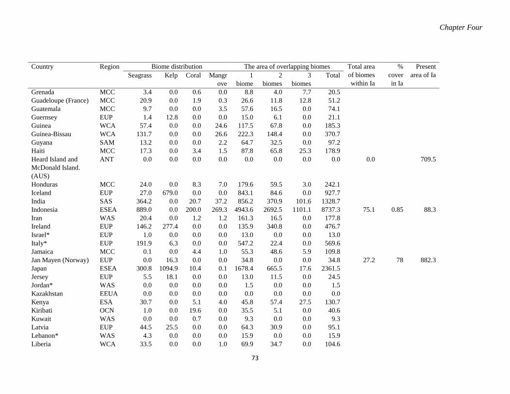
Chapter Four

73

Country

Region Biome distribution The area of overlapping biomes Total area of biomes within Ia

% cover in Ia

Present area of Ia Seagrass Kelp Coral Mangr

ove 1

biome 2

biomes 3

biomes Total

Grenada MCC 3.4 0.0 0.6 0.0 8.8 4.0 7.7 20.5 Guadeloupe (France) MCC 20.9 0.0 1.9 0.3 26.6 11.8 12.8 51.2 Guatemala MCC 9.7 0.0 0.0 3.5 57.6 16.5 0.0 74.1 Guernsey EUP 1.4 12.8 0.0 0.0 15.0 6.1 0.0 21.1 Guinea WCA 57.4 0.0 0.0 24.6 117.5 67.8 0.0 185.3 Guinea-Bissau WCA 131.7 0.0 0.0 26.6 222.3 148.4 0.0 370.7 Guyana SAM 13.2 0.0 0.0 2.2 64.7 32.5 0.0 97.2 Haiti MCC 17.3 0.0 3.4 1.5 87.8 65.8 25.3 178.9 Heard Island and McDonald Island. (AUS)

ANT 0.0 0.0 0.0 0.0 0.0 0.0 0.0 0.0 0.0 709.5

Honduras MCC 24.0 0.0 8.3 7.0 179.6 59.5 3.0 242.1 Iceland EUP 27.0 679.0 0.0 0.0 843.1 84.6 0.0 927.7 India SAS 364.2 0.0 20.7 37.2 856.2 370.9 101.6 1328.7 Indonesia ESEA 889.0 0.0 200.0 269.3 4943.6 2692.5 1101.1 8737.3 75.1 0.85 88.3 Iran WAS 20.4 0.0 1.2 1.2 161.3 16.5 0.0 177.8 Ireland EUP 146.2 277.4 0.0 0.0 135.9 340.8 0.0 476.7 Israel* EUP 1.0 0.0 0.0 0.0 13.0 0.0 0.0 13.0 Italy* EUP 191.9 6.3 0.0 0.0 547.2 22.4 0.0 569.6 Jamaica MCC 0.1 0.0 4.4 1.0 55.3 48.6 5.9 109.8 Jan Mayen (Norway) EUP 0.0 16.3 0.0 0.0 34.8 0.0 0.0 34.8 27.2 78 882.3 Japan ESEA 300.8 1094.9 10.4 0.1 1678.4 665.5 17.6 2361.5 Jersey EUP 5.5 18.1 0.0 0.0 13.0 11.5 0.0 24.5 Jordan* WAS 0.0 0.0 0.0 0.0 1.5 0.0 0.0 1.5 Kazakhstan EEUA 0.0 0.0 0.0 0.0 0.0 0.0 0.0 0.0 Kenya ESA 30.7 0.0 5.1 4.0 45.8 57.4 27.5 130.7 Kiribati OCN 1.0 0.0 19.6 0.0 35.5 5.1 0.0 40.6 Kuwait WAS 0.0 0.0 0.7 0.0 9.3 0.0 0.0 9.3 Latvia EUP 44.5 25.5 0.0 0.0 64.3 30.9 0.0 95.1 Lebanon* WAS 4.3 0.0 0.0 0.0 15.9 0.0 0.0 15.9 Liberia WCA 33.5 0.0 0.0 1.0 69.9 34.7 0.0 104.6

Chapter Four

74

Country

Region Biome distribution The area of overlapping biomes Total area of biomes within Ia

% cover in Ia

Present area of Ia Seagrass Kelp Coral Mangr

ove 1

biome 2

biomes 3

biomes Total

Libya* WCA 47.1 0.0 0.0 0.0 214.0 0.0 0.0 214.0 Lithuania EUP 11.3 0.1 0.0 0.0 17.9 0.9 0.0 18.8 Madagascar ESA 359.1 0.6 31.1 23.6 637.8 335.0 164.1 1136.9 0.2 0.01 0.2 Malaysia ESEA 78.8 0.0 23.8 55.0 673.3 204.5 75.5 953.4 1.3 0.13 1.3 Maldives SAS 4.9 0.0 27.0 0.0 369.7 25.5 4.1 399.3 Malta EUP 1.2 0.2 0.0 0.0 11.5 0.0 0.0 11.5 Marshall Islands OCN 4.4 0.0 19.9 0.0 340.5 26.4 0.0 366.8 Martinique (France) MCC 0.0 0.0 0.0 0.1 9.9 8.0 6.0 23.8 Mauritania WCA 4.6 0.0 0.0 0.0 152.9 0.5 0.0 153.4 Mauritius ESA 7.9 0.0 7.5 0.0 49.9 22.2 0.0 72.2 Mayotte (France) ESA 4.7 0.0 3.0 0.1 13.1 8.0 10.0 31.1 Mexico MCC 486.5 41.0 7.0 72.6 1436.1 632.0 36.5 2104.6 142.6 7 4544.6 Micronesia OCN 4.4 0.0 31.7 1.0 435.2 31.4 11.2 477.8 Montenegro* EEUA 2.1 0.0 0.0 0.0 8.9 0.0 0.0 8.9 Montserrat (UK) MCC 0.0 0.0 0.0 0.0 6.0 0.0 0.0 6.0 Morocco* WCA 19.4 41.0 0.0 0.1 225.1 75.6 0.0 300.7 Mozambique ESA 290.1 0.0 20.7 29.4 385.8 285.3 99.8 770.9 Myanmar SAS 57.2 0.0 6.1 50.4 523.8 256.4 14.7 794.9 Namibia ESA 21.2 255.0 0.0 0.0 347.4 83.9 0.0 431.3 Nauru OCN 0.0 0.0 0.1 0.0 347.4 83.9 0.0 431.3 Netherlands EUP 56.9 84.8 0.0 0.0 31.9 133.1 0.0 165.0 Netherlands Antilles MCC 0.0 0.0 1.7 0.0 5.5 0.0 0.0 5.5 New Caledonia (France)

OCN 145.6 0.1 45.7 2.5 426.6 183.7 79.3 689.6 1.7 0.24 1.7

New Zealand OCN 132.5 1081.7 0.0 2.7 1444.2 349.2 72.9 1866.2 55.8 3 175.5 Nicaragua MCC 4.0 0.0 4.6 7.1 202.1 25.7 0.0 227.8 67.5 30 88.4 Nigeria WCA 51.0 0.0 0.0 62.3 275.5 80.0 0.0 355.5 Niue OCN 0.0 0.0 0.2 0.0 8.5 0.0 0.0 8.5 Norfolk Island (Australia)

OCN 1.1 16.8 0.0 0.0 22.5 7.2 0.0 29.7

North Korea ESEA 41.7 167.4 0.0 0.0 202.8 92.9 0.0 295.7

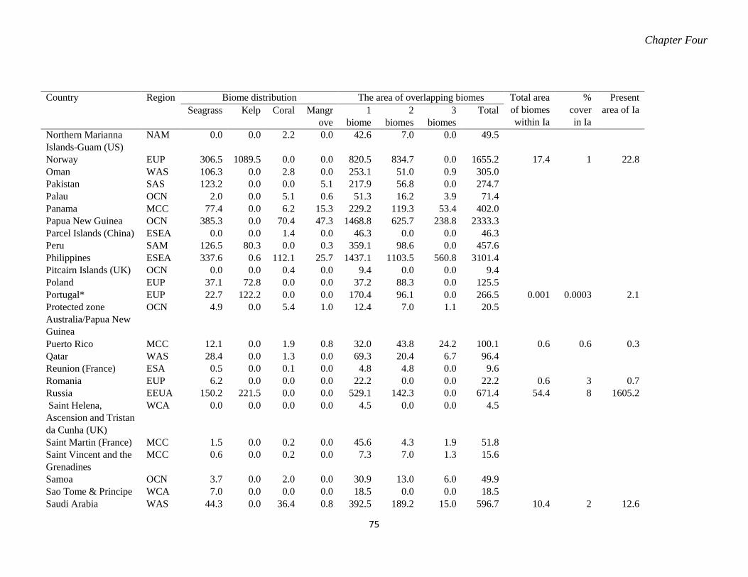
Chapter Four

75

Country

Region Biome distribution The area of overlapping biomes Total area of biomes within Ia

% cover in Ia

Present area of Ia Seagrass Kelp Coral Mangr

ove 1

biome 2

biomes 3

biomes Total

Northern Marianna Islands-Guam (US)

NAM 0.0 0.0 2.2 0.0 42.6 7.0 0.0 49.5

Norway EUP 306.5 1089.5 0.0 0.0 820.5 834.7 0.0 1655.2 17.4 1 22.8 Oman WAS 106.3 0.0 2.8 0.0 253.1 51.0 0.9 305.0 Pakistan SAS 123.2 0.0 0.0 5.1 217.9 56.8 0.0 274.7 Palau OCN 2.0 0.0 5.1 0.6 51.3 16.2 3.9 71.4 Panama MCC 77.4 0.0 6.2 15.3 229.2 119.3 53.4 402.0 Papua New Guinea OCN 385.3 0.0 70.4 47.3 1468.8 625.7 238.8 2333.3 Parcel Islands (China) ESEA 0.0 0.0 1.4 0.0 46.3 0.0 0.0 46.3 Peru SAM 126.5 80.3 0.0 0.3 359.1 98.6 0.0 457.6 Philippines ESEA 337.6 0.6 112.1 25.7 1437.1 1103.5 560.8 3101.4 Pitcairn Islands (UK) OCN 0.0 0.0 0.4 0.0 9.4 0.0 0.0 9.4 Poland EUP 37.1 72.8 0.0 0.0 37.2 88.3 0.0 125.5 Portugal* EUP 22.7 122.2 0.0 0.0 170.4 96.1 0.0 266.5 0.001 0.0003 2.1 Protected zone Australia/Papua New Guinea

OCN 4.9 0.0 5.4 1.0 12.4 7.0 1.1 20.5

Puerto Rico MCC 12.1 0.0 1.9 0.8 32.0 43.8 24.2 100.1 0.6 0.6 0.3 Qatar WAS 28.4 0.0 1.3 0.0 69.3 20.4 6.7 96.4 Reunion (France) ESA 0.5 0.0 0.1 0.0 4.8 4.8 0.0 9.6 Romania EUP 6.2 0.0 0.0 0.0 22.2 0.0 0.0 22.2 0.6 3 0.7 Russia EEUA 150.2 221.5 0.0 0.0 529.1 142.3 0.0 671.4 54.4 8 1605.2 Saint Helena, Ascension and Tristan da Cunha (UK)

WCA 0.0 0.0 0.0 0.0 4.5 0.0 0.0 4.5

Saint Martin (France) MCC 1.5 0.0 0.2 0.0 45.6 4.3 1.9 51.8 Saint Vincent and the Grenadines

MCC 0.6 0.0 0.2 0.0 7.3 7.0 1.3 15.6

Samoa OCN 3.7 0.0 2.0 0.0 30.9 13.0 6.0 49.9 Sao Tome & Principe WCA 7.0 0.0 0.0 0.0 18.5 0.0 0.0 18.5 Saudi Arabia WAS 44.3 0.0 36.4 0.8 392.5 189.2 15.0 596.7 10.4 2 12.6

Chapter Four

76

Country

Region Biome distribution The area of overlapping biomes Total area of biomes within Ia

% cover in Ia

Present area of Ia Seagrass Kelp Coral Mangr

ove 1

biome 2

biomes 3

biomes Total

Senegal WCA 54.1 0.0 0.0 12.1 206.5 34.5 0.0 241.1 Seychelles ESA 12.2 0.0 15.1 0.1 133.1 20.4 1.0 154.5 3.5 2 3.5 Sierra Leone WCA 56.7 0.0 0.0 13.8 107.4 62.7 0.0 170.1 Singapore ESEA 0.0 0.0 0.0 0.1 5.7 2.6 0.0 8.3 Sint Maarten (Netherland)

MCC 0.2 0.0 0.0 0.0 0.8 1.5 0.1 2.4

Slovenia* EUP 1.9 1.0 0.0 0.0 0.1 3.6 0.0 3.7 Solomon Islands. OCN 75.6 0.0 28.0 4.6 437.6 276.5 80.7 794.8 Somalia ESA 115.3 0.0 4.1 0.2 313.8 60.2 14.3 388.3 South Africa ESA 138.5 405.5 0.0 0.2 471.1 293.1 6.1 770.2 South Georgia & the South Sandwich Is. (UK)

ANT 0.0 0.0 0.0 0.0 0.0 0.0 0.0 0.0

South Korea ESEA 83.4 326.8 0.0 0.0 444.8 187.1 0.0 631.9 18.1 3 20.1 South Sudan ESA 0.0 0.0 0.0 0.0 0.0 0.0 0.0 0.0 Spain* EUP 176.3 176.3 0.0 0.0 461.1 254.0 0.0 715.1 Spratly Islands ESEA 0.0 0.0 27.3 0.0 309.3 0.0 0.0 309.3 Sri Lanka SAS 54.9 0.0 0.8 2.1 142.7 100.2 19.1 262.0 St. Kitts & Nevis MCC 0.0 0.0 0.4 0.0 10.2 2.8 1.0 14.0 St. Lucia MCC 0.0 0.0 0.3 0.0 8.0 4.0 2.0 14.0 St. Pierre & Miquelon NAM 0.0 0.0 0.0 0.0 0.0 0.0 0.0 0.0 Sudan ESA 7.4 0.0 4.8 0.0 90.8 31.4 1.9 124.1 Suriname SAM 7.7 0.0 0.0 7.4 50.2 37.4 0.0 87.5 Svalbard (Norway) EUP 0.0 21.4 0.0 0.0 48.7 0.0 0.0 48.7 14.7 30 0.0 Sweden EUP 221.1 337.1 0.0 0.0 168.2 424.9 0.0 593.1 1.3 0.2 3.0 Syria* WAS 3.4 0.0 0.0 0.0 15.2 0.0 0.0 15.2 Taiwan ESEA 17.3 0.1 3.8 0.0 88.4 41.2 0.0 129.6 0.1 0.1 0.2 Tanzania ESA 123.3 0.0 20.9 9.7 108.8 124.2 124.3 357.3 Thailand ESEA 133.1 0.0 1.8 24.4 376.3 218.0 25.1 619.4 The Bahamas MCC 86.7 0.0 22.3 8.1 721.8 277.6 68.7 1068.1 WCA 16.4 0.0 0.0 6.8 49.6 29.7 0.0 79.3

Chapter Four

77

Country

Region Biome distribution The area of overlapping biomes Total area of biomes within Ia

% cover in Ia

Present area of Ia Seagrass Kelp Coral Mangr

ove 1

biome 2

biomes 3

biomes Total

Timor-Leste ESEA 0.0 0.0 0.3 0.1 42.9 17.0 0.0 59.9 Togo WCA 8.6 0.0 0.0 0.1 16.7 2.4 0.0 19.1 Tokelau (New Zealand)

OCN 0.0 0.0 1.0 0.0 11.1 0.0 0.0 11.1

Tonga OCN 1.0 0.1 9.9 0.1 128.6 8.7 6.8 144.0 Trinidad & Tobago MCC 4.6 0.0 0.3 0.6 51.9 10.1 0.0 62.0 Tunisia* WCA 66.3 0.0 0.0 0.0 184.4 0.0 0.0 184.4 Turkey* EUP 127.1 6.4 0.0 0.0 366.5 17.9 0.0 384.4 Turks & Caicos Island (UK)

MCC 1.0 0.0 1.9 1.7 40.1 17.2 4.8 62.1

Tuvalu OCN 0.0 0.0 11.8 0.0 96.0 1.9 0.0 97.9 Ukraine EEUA 140.2 0.0 0.0 0.0 312.0 0.0 0.0 312.0 United Arab Emirates WAS 86.6 0.0 1.4 1.1 150.0 70.6 9.3 229.9 0.1 0.02 0.0 United Kingdom EUP 532.9 1127.0 0.0 0.0 653.7 1166.9 0.0 1820.6 0.03 0.002 0.03 United States NAM 987.1 1550.8 40.9 23.5 3557.5 1292.7 31.5 4881.6 136.1 3 15109.3 United States Minor Outlying Islands

NAM 0.1 0.0 1.7 0.0 165.1 2.0 0.0 167.2 18.0 11 117.3

United States Virgin Islands

MCC 10.4 0.0 0.0 0.0 14.6 10.7 4.3 29.6 1.4 5 0.8

Uruguay SAM 68.6 3.4 0.0 0.0 137.3 9.3 0.0 146.6

Vanuatu OCN 32.0 0.0 7.1 0.1 212.0 89.4 7.9 309.3

Venezuela SAM 174.7 0.0 3.5 33.3 413.2 249.6 26.2 689.1

Vietnam ESEA 140.6 0.0 4.2 21.4 434.5 168.5 12.8 615.8

Virgin Islands, (UK) MCC 13.2 0.0 1.4 0.0 14.9 12.7 3.5 31.1

Wallis & Futuna (France)

OCN 0.0 0.0 1.1 0.0 52.9 3.0 0.0 55.9

Western Sahara WCA 60.8 10.0 0.0 0.0 147.6 32.8 0.0 180.4

Yemen WAS 23.0 0.0 3.9 0.1 213.3 24.5 1.0 238.8

Total 16215 14700 1514 1368 56807 25191 4149 86147 805 28742

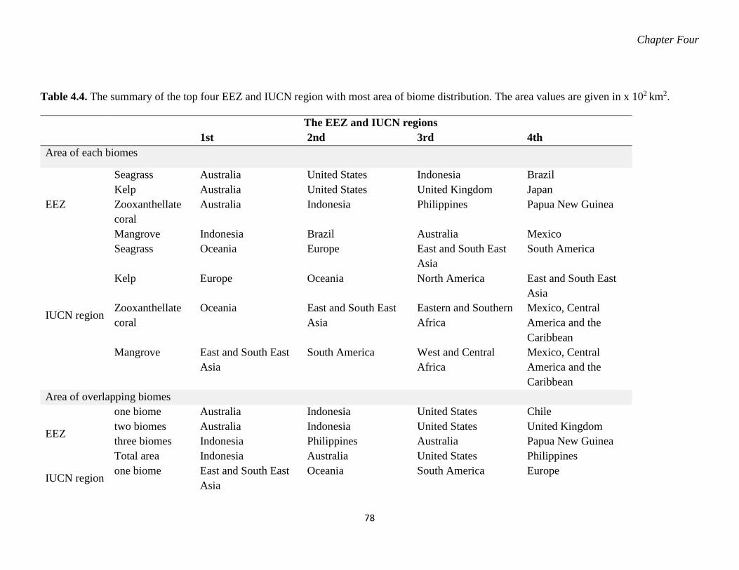
Chapter Four

78

Table 4.4. The summary of the top four EEZ and IUCN region with most area of biome distribution. The area values are given in x 102 km2.

The EEZ and IUCN regions 1st 2nd 3rd 4th

Area of each biomes

EEZ

Seagrass Australia United States Indonesia Brazil Kelp Australia United States United Kingdom Japan Zooxanthellate coral

Australia Indonesia Philippines Papua New Guinea

Mangrove Indonesia Brazil Australia Mexico

IUCN region

Seagrass Oceania Europe East and South East Asia

South America

Kelp Europe Oceania North America East and South East Asia

Zooxanthellate coral

Oceania East and South East Asia

Eastern and Southern Africa

Mexico, Central America and the Caribbean

Mangrove East and South East Asia

South America West and Central Africa

Mexico, Central America and the Caribbean

Area of overlapping biomes

EEZ

one biome Australia Indonesia United States Chile two biomes Australia Indonesia United States United Kingdom three biomes Indonesia Philippines Australia Papua New Guinea Total area Indonesia Australia United States Philippines

IUCN region one biome East and South East Asia

Oceania South America Europe

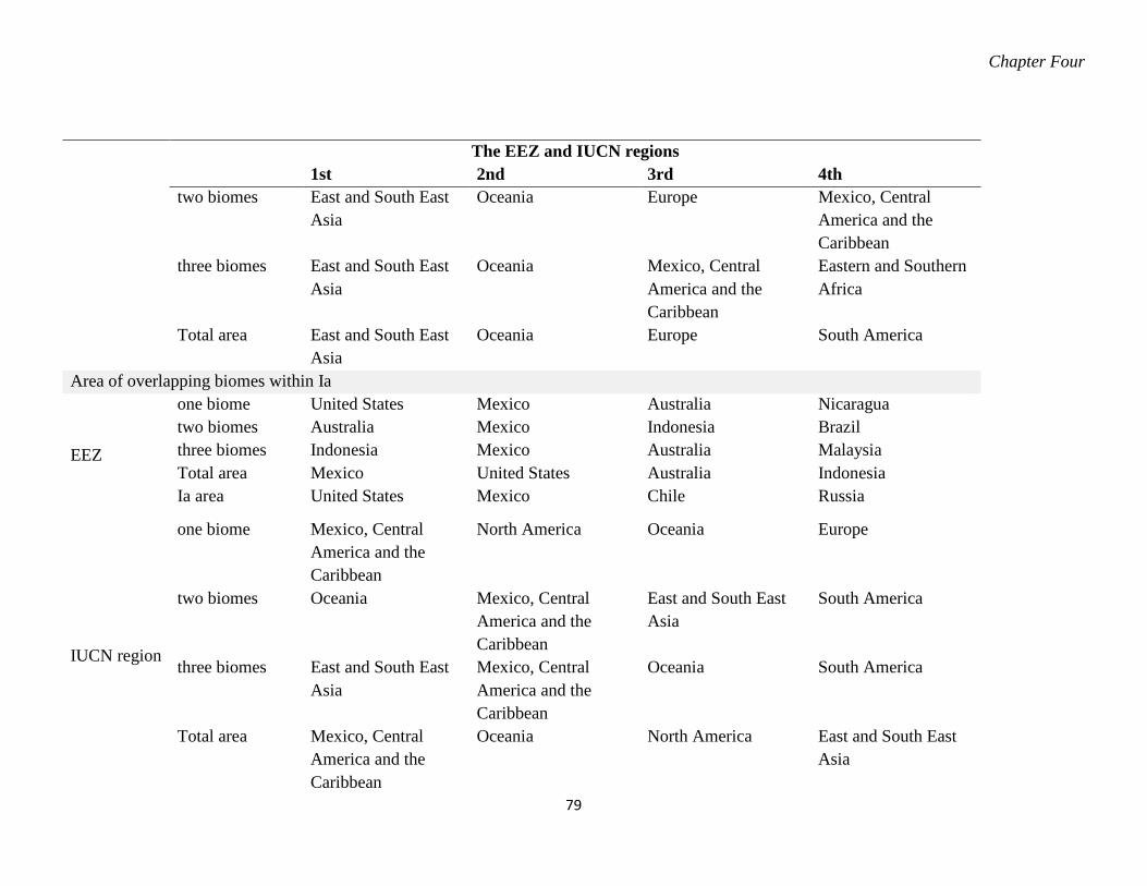
Chapter Four

79

The EEZ and IUCN regions

1st 2nd 3rd 4th two biomes East and South East

Asia Oceania Europe Mexico, Central

America and the Caribbean

three biomes East and South East Asia

Oceania Mexico, Central America and the Caribbean

Eastern and Southern Africa

Total area East and South East Asia

Oceania Europe South America

Area of overlapping biomes within Ia

EEZ

one biome United States Mexico Australia Nicaragua two biomes Australia Mexico Indonesia Brazil three biomes Indonesia Mexico Australia Malaysia Total area Mexico United States Australia Indonesia Ia area United States Mexico Chile Russia

IUCN region

one biome Mexico, Central America and the Caribbean

North America Oceania Europe

two biomes Oceania Mexico, Central America and the Caribbean

East and South East Asia

South America

three biomes East and South East Asia

Mexico, Central America and the Caribbean

Oceania South America

Total area Mexico, Central America and the Caribbean

Oceania North America East and South East Asia

Chapter Four

80

Table 4.5. The regional distribution of biomes covered in marine reserves (IUCN category Ia).Area values are given in 102 x km2. The background colour gradient: higher (white), lower (blue) and in-between values (blue to white gradient) in each column. IUCN operational regions Area of

1 biome in Ia

Area of 2 biome in Ia

Area of 3 biomes in Ia

Total Ia area

Total area of all biomes

Total area of biomes in Ia

East and Southeast Asia 39 44 13 114 20289 96

Oceania 120 54 3 922 17797 177

Europe 51 10 0 913 10830 62

South America 19 14 1 4567 8019 34

North America 149 7 0 15261 7967 156

Mexico, Central America

and the Caribbean 150 52 10 4635

6645 212

Eastern and Southern

Africa 0 3 0 4

4988 4

Mediterranean 0 0 0 4 4620 0

West and Central Africa 0 0 0 0 3919 0

South Asia 0 0 0 0 2697 0

West Asia 8 2 0 13 1948 10

Eastern Europe and

Central Asia 51 4 0 1605

1003 54

Antarctica 0 0 0 710 44 0

Chapter 5

General Discussion

Chapter Five

81

5 General Discussion

5.1 Introduction

The world's natural environment is being destroyed by anthropogenic impacts and

climatic impacts at an increasing rate (Short and Wyllie-Echeverria 1996; Short and Neckles

1999; Marba and Duarte 2010; Sandilyan and Kathiresan 2012; Wear 2016; Halpern et al 2008;

Neumann et al. 2015). The concept of biomes, defined as large areas with similar plant life forms,

plays a central role in conservation and macroecology in the terrestrial environment. For example,

biome maps have long been used in forest conservation (Ellis et al. 2010; Finch and Meadows

2019) to calculate net primary productivity (Churkina and Running 1998; Kicklighter et al. 1999),

study of the diversity of species (Murphy and Romanuk 2016), to understand the primary and

secondary plant successions (Prach and Walker 2019), and for indigenous land protection

(Garnett et al. 2018). In the present day, many organisations such as the World Bank, the US

Agency for International Development, and the World Wildlife Fund are using the map created

by Olson et al. (2001) to identify the distribution of terrestrial biomes. The map subdivided the

global terrestrial domain into 14 biomes, including tropical and subtropical coniferous forests,

savannahs and shrublands, and tundra (Arctic, humid).

In the marine environment the equivalent biomes are seagrass, kelp, mangrove, and

zooxanthellate coral biomes (Jayathilake and Costello 2019a; 2019b).They also have

characteristic features such as a three-dimensional vertical and horizontal distribution, stable

long-term spatial and temporal distribution, and providing feeding and breeding habitats for

associated fauna. However, until the present study, maps with complete global coverage only

existed for corals and mangroves.

The main limitation of the previous seagrass map was that it had an incomplete polygon layer

(UNEP-WCMC and Short 2016). Combining both point and polygon layers, the existing map

covers the entirety of the seagrass biome. However, when the polygon layer was taken separately,

it presented incomplete coverage. The current study advanced the previous existing polygon map

by filling gaps through MaxEnt modelling. As this model was assembled for all seagrass species,

the map may predict the locations for possible seagrass distribution that are rare, not currently

found, or previously undocumented.

Chapter Five

82

Previously, area-based calculations of the kelp biome were not possible at a global scale

because no spatially resolved map could be used in GIS. In this thesis, this gap was filled with a

world-first map of the kelp biome. It was found that laminarian kelp may occupy 22% of the

world’s coastlines, particularly in sub-tropical, temperate and sub-polar regions excepting

Antarctica. The current study excluded large fucoid seaweeds which are sometimes called kelp

(e.g. in Antarctica). Thus, in the future, a more complete global estimate of seaweed biomes could

include fucoid algae.

Together with mangrove and zooxanthellate corals, we have summarised the latitudinal

distribution, environmental limits, and area of each of the four main marine biomes (Table 5.1).

The distribution of these biomes is likely to influence the distribution of many associated species,

hence maintaining the health of these biomes is important for many other marine species, and

their loss due to seabed trawling, dredging, fishing-induced trophic cascades, pollution, and

climate change is likely to impact many species as well as overall biodiversity, including fisheries

(Leleu et al. 2012; Unsworth et al. 2014; McCloskey et al. 2015).

5.2 Applications

The marine biome maps can be used in marine conservation, climate change projections, carbon

cycle budgets, and for understanding the environmental niche of species. While full chapters on

these applications were beyond the scope of this thesis, examples of these applications are

provided here.

5.2.1 Delineating new strict marine reserve areas to conserve marine biomes.

In this thesis, I looked at which countries could do most to protect the biomes. As the CBD Aichi

Targets are being reviewed in 2020, this work is timely to show how poor the coverage is of strict

marine reserves containing these major ocean biomes and habitats, and which countries can do

most to protect them. Countries in the Indian Ocean and Indo-Pacific region have large areas with

multiple marine biome distribution within 1 km x 1 km cells, yet are some of the areas least

covered by strict marine reserves. In addition, I hope it will inform planning for the CBD 2030

targets of 30% of ocean habitats fully protected.

Chapter Five

83

Table 5.1. Summary of the marine biome distribution. Seagrass Kelp Zooxanthellate coral Mangrove Latitudinal distribution

70o N to 43o S

25o N to 75o

N and 25o S to 55o S

32o N to 35o S 32o N to 38o S

Total area km2 1,646,788 1,469,900 151,390 136,850

Mean sea surface temperature

0 oC to 30 oC 0 oC to 25 oC 18 oC to 30 oC

15 oC to 30 oC mean sea surface temperature

Depth (-1) to (-90) m coastal 1m to 90 m (Duarte 1991)

0 to (-90 m) Mostly shallow coastal. Some deep water kelp can grow as deep as 90 m (Žuljević et al 2016)

(-1) to (-125) m Shallow to upper mesophotic zone from 30 m to 125 m (Englebert et al. 2017)

(-10) to 10 m elevation. Shallow coastal sea- land interface at the mean sea level

5.2.2 Predicting the future of the world’s marine biomes in response to the

rising temperature.

Species distribution models could be used to predict changes in biome distributions under climate

change. For example, I here provide preliminary models of the future distribution of marine

biomes with projected mean sea surface temperature in 2100. Primary occurrence records were

downloaded from the Global Biodiversity Information Facility (GBIF 2016; 2017; 2018), UNEP-

WCMC and Short (2016), and the Ocean Biogeographic Information System (OBIS 2017; 2018).

The values of the present mean sea surface temperature, future minimum sea surface temperature,

mean sea surface temperature, and the maximum sea surface temperature the Global Marine

Environment Datasets (GMED; Basher et al. 2014a) were plotted verses the latitude value of the

Chapter Five

84

present occurrence records. The occurrence records were modelled and projected to 2100 using

MaxEnt software, Version 3.3, with present mean sea surface temperature, future mean surface

temperature, depth, and distance from land. Depth and distance from land variables were used to

proximate the prediction to more coastal.

The results of this study show the current mean temperature values of all four biomes’

occurrence records are equal to or lower than future mean sea surface temperatures (Fig. 5. 1).

With future sea warming, biome distribution can be predicted in two ways. One is the expansion

of the biome towards the poles. The most important and novel finding of this study is that

temperature changes in some places in the tropics and sub-tropics adversely affect biome survival

(Table 5.2, Appendix S 5.1. a, b, c, and d).

5.2.3 Using new area values to recalculate blue carbon budget

The recognition of marine biomes as a significant source of ‘blue’ carbon sequestration and

storage has attracted global attention (Duarte et al. 2005). Studies on blue carbon storage in the

seagrass biome had used available seagrass area values from 0.12 x 106 km2 (Green and Short

2003) and 0.6 x 106 km2 (Duarte and Chiscano 1999). The global blue carbon budget could be

updated by recalculating the blue carbon sequestration of seagrass with a new distribution area,

i.e., 1.6 x 106 km2.

Most of the studies have so far assessed the Carbon depositions of mangroves, seagrass

beds and saltmarshes, and largely neglected the amount of carbon sequestration by macroalgae

(Krause-Jensen et al. 2018). Currently, the amount of total global macroalgal carbon assimilation

and storage had been estimated (Chung et al. 2011; Barrón Duarte 2015; Krause-Jensen and

Duarte 2016) but the contribution from the laminarian kelp species was yet to be calculated. A

new estimate of global blue carbon sequestration by kelp species could be done using local and

experimental data on sequestration rates and the newly calculated global area of kelp biome; i.e.,

1.5 x 1012 m2 (Jayathilake and Costello 2019).

Chapter Five

85

Figure 5.1. The present primary occurrence records of each marine biome (grey dots) shown against the maximum, mean, and minimum projected sea surface temperature for 2100 in 5-degree latitudinal bands.

Chapter Five

86

Table 5.2. The present and the projected future distribution of marine biomes with the expanding and declining locations. Biome Present

distribution Future distribution

Expanding locations Declining locations

Seagrass 70o N to 43o

S 80o N to 55o S

High latitudes of Alaska, the USA, Canada, Iceland, Norway, Russia, North Korea, China, and Japan

Some tropical locations in Indonesia, Philippines, Papua New Guinea, Solomon Islands, Sri Lanka, Madagascar, Somalia, Kenya, Tanzania, Mozambique, Haiti, Dominican Republican, and the Bahamas

Kelp 25o N to 75o

N and 25o S to 55o S

30o N to 80o N and 31.5o S to 55o S

Russia, Norway, the United States, Canada, Sweden, and Finland

Peru, and Brazil and some areas of Namibia, South Africa, Australia, Chile, and Morocco

Zooxanthellate coral

32o N to 35o S

40o N to 40o S

Peru and Chile, Namibia, South West and South Australia and North Island of New Zealand and the western coastline of Africa

Around the Great Barrier Reef, Australia, many Pacific Islands, The Coral triangle and many Indian Ocean islands including the Maldives

Mangrove 32o N to 38o S

42o N to 44o S

The coasts of Morocco, the Mediterranean Sea, Japan, China, the southern coasts of Australia, middle of the North Island of New Zealand, South Africa, Chile, and Peru

Cuba, Haiti, Dominican Republic, Guinea Bissau

Chapter Five

87

5.2.4 Species’ environmental niche

I analysed the ranges, geographical distribution, and environmental variables of each seagrass

species, including the seagrass-associated freshwater monocot species (Appendix S5 2.) as the

first step of analysing the biome (seagrass, kelp, zooxanthellate coral and mangrove) species’

environmental niche. The occurrence records of each species were downloaded from the GBIF

(GBIF 2016) and UNEP-WCMC and Short (2016). The values of each environmental variable at

the place of each occurrence records were extracted from the Global Marine Environment

Datasets (GMED; Basher et al. 2014a) using the Arc GIS tool multi values to points. The resulting

point attribute table was exported to develop each environmental variable box plot using R Studio,

Version 1.0.44.

The findings of this study fill the knowledge gap on the environmental niche of the

seagrass species (Appendix S5. 2). Seagrasses were found to have been distributed in different

ranges of geographical (latitude, longitude), physical (depth, distance from the land, sea surface

temperature, wave height) chemical (pH), and nutrient (nitrate and phosphate concentrations)

variables.

Seagrass species were also found to occur in different geographical regions. There were

three major groups of seagrasses that could be identified according to their latitudinal

distribution. They were southern temperate, tropical-subtropical, and northern temperate groups.

The tropical-subtropical group had 23 species and had been distributed in a wider range of

latitudes than the other two temperate groups. Of the species studied, 2/3 of seagrass species (41

species) had occurred between 60o E and 160o E. Eight species were distributed along the 0

longitudes and eleven species were found exclusively in western oceans.

I found that the seagrass species had adapted to live within widely different physical

variables. Most of the species occur within the 0 to 20 m depth range. Species such as Halophila

decipiens, Halodule beaudettei, Halophila ovalis, Halophila spinulosa had been on average

distributed as deep as 35 to 40 m. The majority of species had been distributed within 0.1 km of

the land. Only a few Halophila sp had occurred from 0 to 0.5 km of the land, including H.

capricorni, H. decipiens, H.minor, H. ovalis, H.spinulosa, Thalassia hemprichii, Thalassia

testidinum and Zostera marina. Seagrass distribution had found from 10 oC to 34 oC. Zostera

marina had a broad range and can live in 10 oC to 33 oC of the maximum sea surface

temperature. Seagrasses living in the higher temperature of > 35 oC had narrow ranges. For

example, the tropical species Cymodocea rotundata, C. serrulata, Thalassia testudinum,

Chapter Five

88

Syringodium filiforme, Enhalus acoroides, and Halophila pinifolia, Halophila major, Halophila

engelmannii had adapted to live in high conditions, and their distribution was limited to a

narrow temperature range. The majority of species had occurred in 35 pps salinity. Cymodocea

nodosa, Halophila stipulacea and Posidonia oceanica had adapted to live in high salinity (>38

pss). Zostera marina and Zostera noltii had a wider (10 to 40 pss) salinity range. Seagrass

species had commonly been distributed at the moderate wave height, range from 3.5 m to 4 m.

This study showed that the majority of seagrass species had occurred in 8.2 pH

conditions, whereas only Halophila capricorni, Halophila decipiens, Halophila minor,

Halophila ovalis, Halophila spinulosa, Halophila tricostata, and Zostera capricorni had

adapted to live in more usual conditions, as 8.4 pH.

Almost all of the seagrass species had been distributed in similar nutrient conditions. The

majority of species had occurred in low nitrate and phosphate concentrations. All the members

of family Cymodoceaceae, family Hydrocharitaceae, and family Posidoniaceae had been

distributed in nitrate concentrations as slight as 0 to 1 μmol/l. In contrast, the members of the

family Zosteraceae had been distributed in a wide range of nitrate concentrations, varying from

0 to 33 μmol/l. Similarly, families Cymodoceaceae, Hydrocharitaceae, and Posidoniaceae had

been distributed in a narrow range of phosphate concentration. Phyllospadix scouleri and

Phyllospadix serrulatus had adapted to live in the highest phosphate concentration.

The seagrass-associated monocot (Ruppia cirrhosa and R. maritima) species’

environmental niche were mostly similar to the members of family Zosteraceae, where as

Lepilaena marina and Ruppia tuberosa species’ environmental niche was mostly similar to the

other three families.

5.3 Conclusion

Similar to terrestrial biome has been frequently used as an environmental conservation tool,

marine biome maps can also be used in marine conservation. Up to date, there is a huge

knowledge as well as a technical gap in marine conservation due to the lack of a base map that

can readily be used in conservation. This thesis presents four biome maps (seagrass, kelp,

mangrove, and zooxanthellate coral) with sufficient resolution and enables use in Geographical

Information System (GIS) and make high-quality products for planning, decision making on

marine conservation. Here I would like to recommend, countries and conservation initiatives

should delineate and expand marine reserves in tropical and subtropical regions especially in

Chapter Five

89

East and Southeast Asia. These countries have high individual biome distribution as well as

multiple biome distribution. Further research should be taken to update the conservation statuses

of biome forming species based on the IUCN Red List. Future studies can use the biome maps, I

present here for calculating the blue carbon budget, environmental niche analysis, and for future

distribution predictions

Chapter 6

Appendices

90

91

6 Appendices

Appendix S.2. 1. The comparison between the GBIF and OBIS seagrass occurrence records.

Species OBIS GBIF

Before data

cleaning

After data cleaning

Before data cleaning

After data cleaning

Amphibolis antarctica 64 24 988 360 Amphibolis griffithii 42 20 260 119 Cymodocea angustata 0 0 31 18 Cymodocea nodosa 47 10 906 170 Cymodocea rotundata 35 18 237 62 Cymodocea serrulata 56 40 267 84 Enhalus acoroides 15 8 301 94 Halodule beaudettei 0 61 16 Halodule bermundensis 0 0 6 0 Halodule emarginata 0 0 14 3 Halodule pinifolia 0 0 84 22 Halodule uninervis 87 48 508 188 Halodule wrightii 331 215 11420 3385 Halophila australis 0 0 246 145 Halophila baillonii 0 0 2 2 Halophila beccarii 1 1 36 3 Halophila capricorni 4 3 46 34 Halophila decipiens 578 557 751 471 Halophila engelmannii 24 24 219 82 Halophila hawaiiana 0 0 75 7 Halophila johnstonii 1 1 9 5 Halophila minor 2 2 116 45 Halophila ovalis 237 191 1315 557 Halophila ovata 1 1 15 4 Halophila spinulosa 268 244 712 492 Halophila tricostata 32 32 61 57 Phyllospadix iwatensis 25 12 79 12 Phyllospadix japonicus 245 15 Phyllospadix scouleri 76 75 896 347 Phyllospadix serrulatus 55 55 78 29 Phyllospadix torreyi 4 4 576 191 Posidonia angustifolia 0 0 198 94 Posidonia australis 5 4 603 267 Posidonia coriacea 0 0 89 51 Posidonia denhartogii 0 0 70 45

92

Posidonia kirkmanii 0 0 38 25 Posidonia oceanica 459 72 3138 228 Posidonia ostenfeldii 0 0 35 26 Posidonia robertsoniae 0 0 84 62 Posidonia sinuosa 18 8 386 192 Syringodium filiforme 0 0 6888 1646 Syringodium isoetifolium 88 48 306 90 Thalassia hemprichii 91 24 428 138 Thalassia testudinum 964 776 27279 5903 Thalassodendron ciliatum 86 19 317 48 Thalassodendron pachyrizum 7 4 25 15 Zostera asiatica 0 0 28 0 Zostera capensis 17 7 274 40 Zostera capricorni 0 0 391 25 Zostera caulescens 0 0 7 0 Zostera japonica 97 24 176 32 Zostera marina 2232 1168 18490 3879 Zostera mucronata 0 0 36 9 Zostera muelleri 3 3 317 168 Zostera noltii 8 0 3193 959 Zostera novazelandica 0 0 30 2 Zostera tasmanica 17 10 210 95 Ruppia cirrhosa 77 44 4083 1107 Ruppia maritima 80 64 9080 2931 Total 6235 3806 96525 25082

93

Appendix S.2. 2. The global distribution of seagrass based on existing points and polygon records.

25 082 GBIF points

17 955 UNEP-WCMC points

94

3 806 OBIS points

220 157 UNEP-WCMC polygons

95

Appendix S.2. 3. The regional level comparison of the distribution of seagrass in the (a) UNEP-WCMC and Short (2016) polygon (red) layer, (b) UNEP-WCMC and Short (2016) point (blue) layer, and (c) GBIF occurrence records (black). Note layers and points can overlap

Western North Pacific Ocean

Gulf of California, Gulf of Mexico and Caribbean

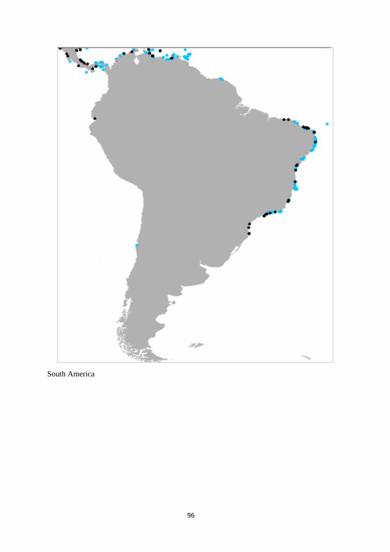
96

South America

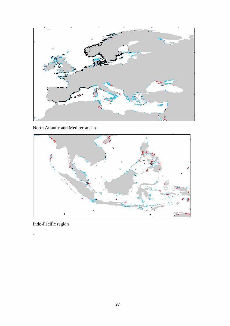
97

North Atlantic and Mediterranean

Indo-Pacific region

.

98

Appendix S.2. 4. The MaxEnt model maps (in red) for individual (a) species, (b) genera and (c) families of seagrass.All taxa were mapped at a global scale. Where the model predicted an environmental range in a restricted region the image is enlarged there for display purposes. Reported occurrence records are shown as black dots.

(a)

Amphibolis antarctica

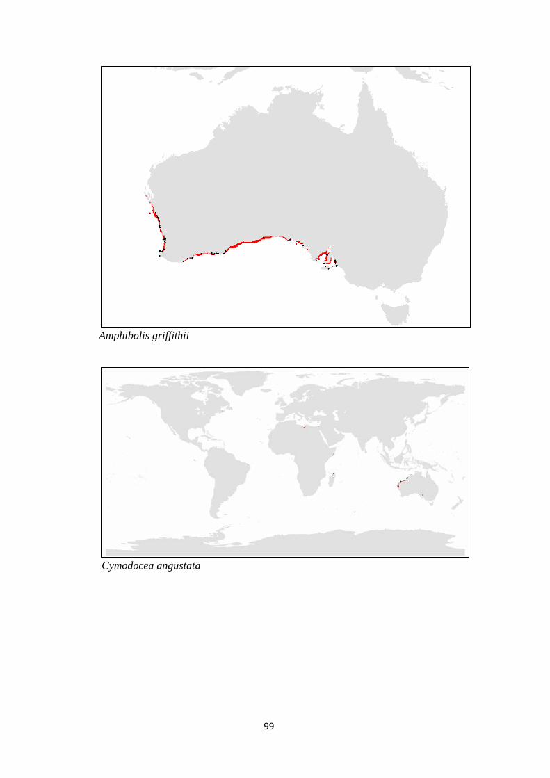
99

Amphibolis griffithii

Cymodocea angustata

100

Cymodocea nodosa

Cymodocea rotundata

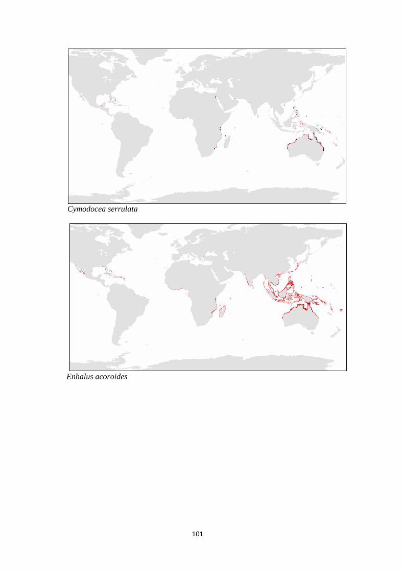
101

Cymodocea serrulata

Enhalus acoroides

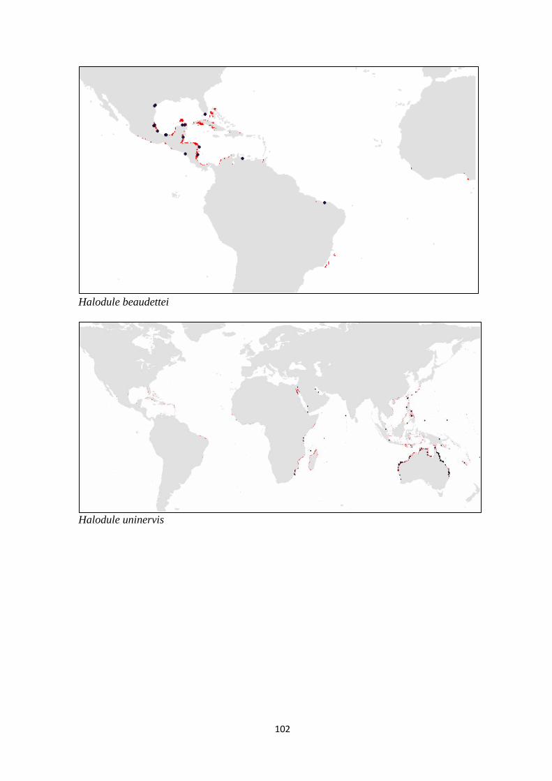
102

Halodule beaudettei

Halodule uninervis

103

Halodule pinifolia

Halodule wrightii

104

Halophila capricorni

Halophila decipiens

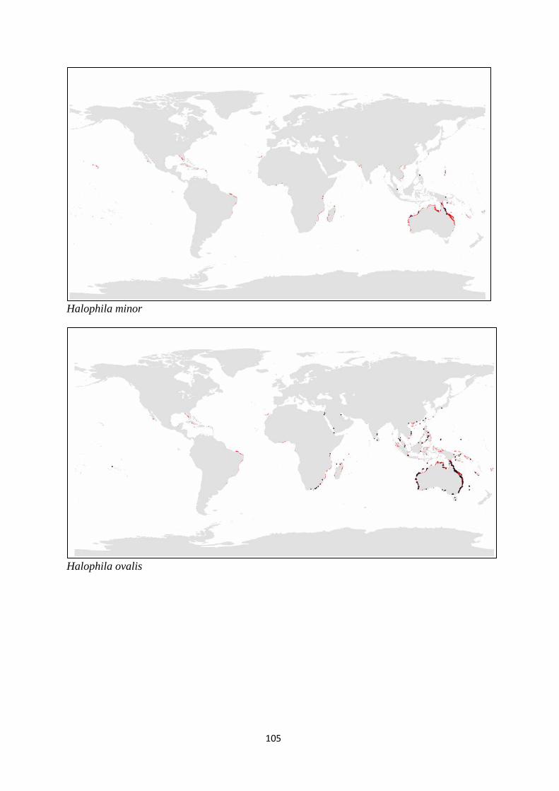
105

Halophila minor

Halophila ovalis

106

Halophila spinulosa

Halophila tricostata

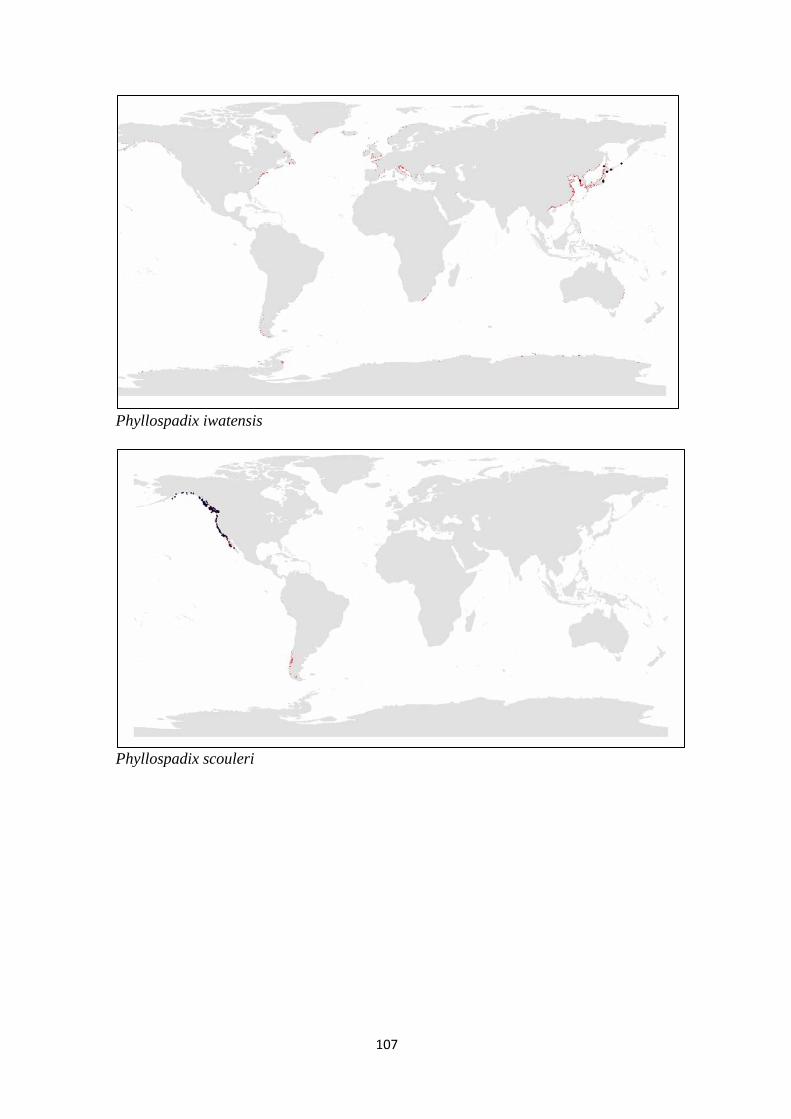
107

Phyllospadix iwatensis

Phyllospadix scouleri

108

Phyllospadix serrulatus

Phyllospadix torreyi

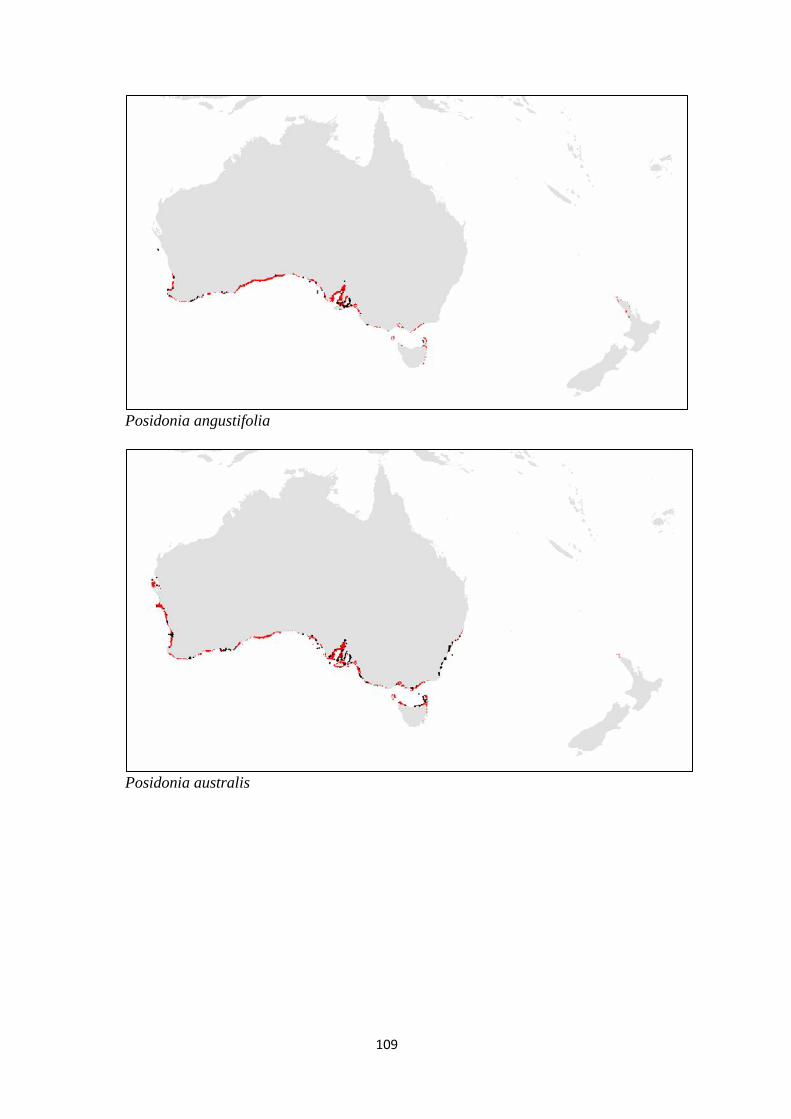
109

Posidonia angustifolia

Posidonia australis

110

Posidonia coriacea

Posidonia denhartogii

111

Posidonia kirkmanii

Posidonia oceanica

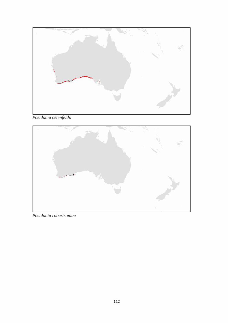
112

Posidonia ostenfeldii

Posidonia robertsoniae

113

Posidonia sinuosa

Syringodium filiforme

114

Syringodium isoetifolium

Thalassia hemprichii

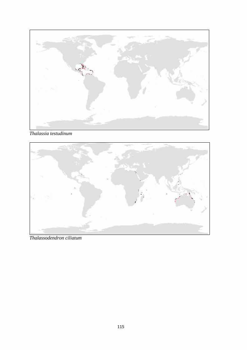
115

Thalassia testudinum

Thalassodendron ciliatum

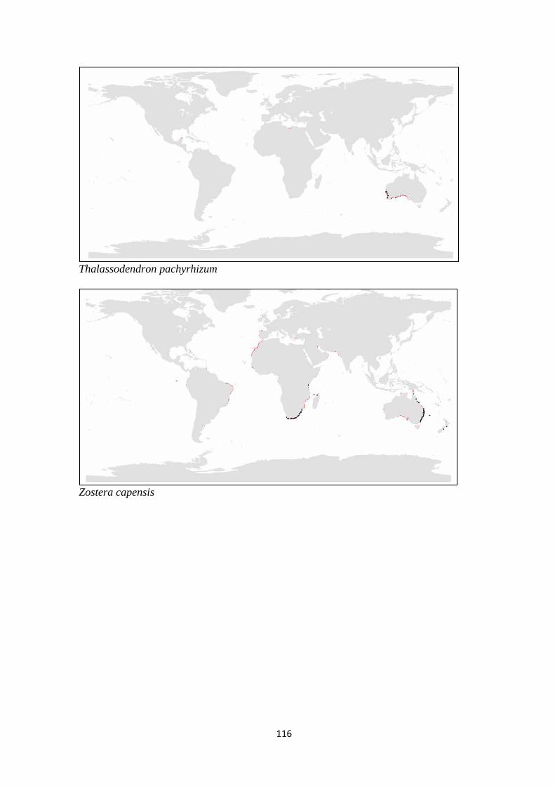
116

Thalassodendron pachyrhizum

Zostera capensis

117

Zostera marina

Zostera muelleri

118

Zostera noltii

(b)

Amphibolis sp.

119

Cymodocea sp.

Enhalus sp.

Halodule sp.

120

Halophila sp.

Phyllospadix sp.

Posidonia sp.

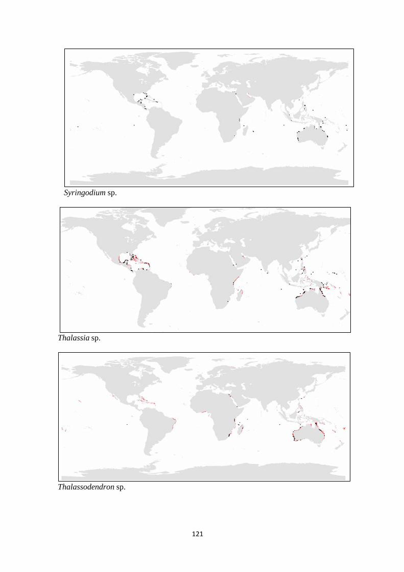
121

Syringodium sp.

Thalassia sp.

Thalassodendron sp.

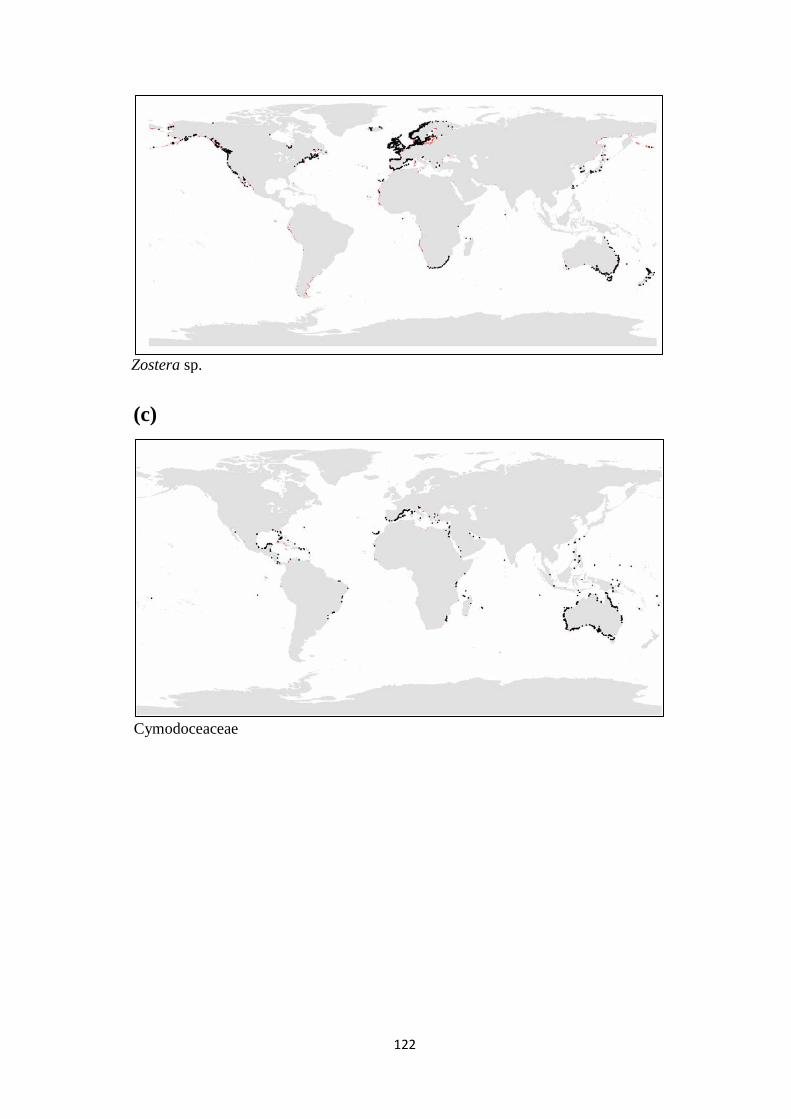
122

Zostera sp.

(c)

Cymodoceaceae

123

Hydrocharitaceae

Posidoniaceae

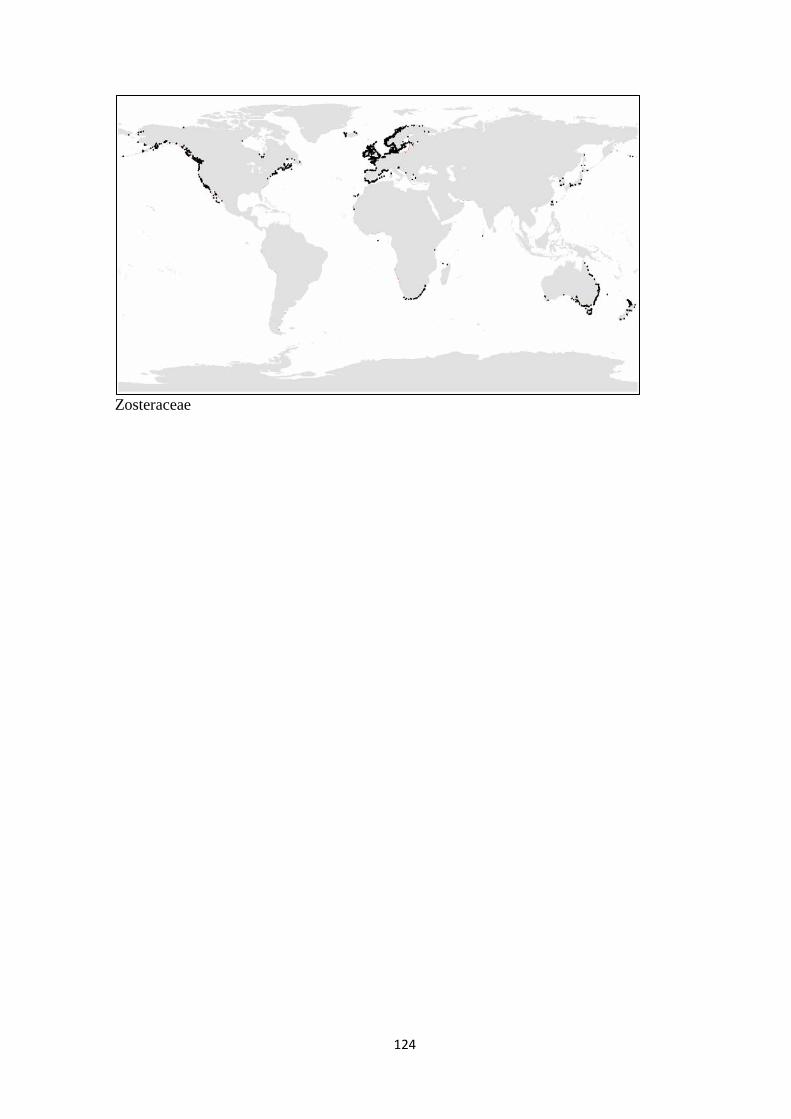
124

Zosteraceae

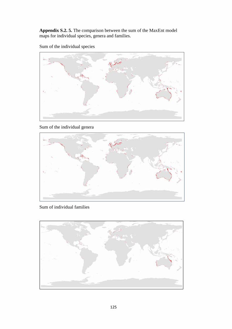
125

Appendix S.2. 5. The comparison between the sum of the MaxEnt model maps for individual species, genera and families.

Sum of the individual species

Sum of the individual genera

Sum of individual families

126

Appendix S.2. 6. MaxEnt model results: Jack-knife of regularized training gain the resulting MaxEnt model.

127

Appendix S.2. 7. Response curves of each abiotic variable used in the model. Each of the above curves represents a Maxent model created using only the corresponding variable. These plots reflect the dependence of predicted suitability both on the selected variable and on dependencies induced by correlations between the selected variable and other variables.

128

Appendix S.2. 8. Area calculation for UNEP-WCMC (2014, 2016) and the MaxEnt derived biome for latitudinal band.

Latitudinal band UNEP-WCMC (2016) Shape area (km2)

MaxEnt model Shape area (km2)

80-75 north 0 0 75-70 north 0 0 70-65 north 3 14092 65-60 north 11 33988 60-55 north 1489 103256 55-50 north 1513 85773 50-45 north 8702 46616 45-40 north 10085 74598 40-35 north 10027 75251 35-30 north 6351 64322 30-25 north 72828 82727 25-20 north 129666 139916 20-15 north 97177 51515 15-10 north 81076 89199 10_5 north 51561 87413 5_0 north 19913 52722 0_5 south 9272 79532 5_10 south 16156 92225 10_15 south 29369 82996 15-20 south 12295 97254 20-25 south 7681 90676 25-30 south 13954 41961 30-35 south 23397 100376 35-40 south 2649 55482 40-45 south 1877 4899 45-50 south 0 0 Total 607052 1646789

129

Appendix S.2. 9. Citations of datasets used in this study as provided in the GBIF metadata.

Alexander, J., Gross, J. (2017). Consortium of California Herbaria. Version 66.7. Consortium of California Herbaria. Occurrence Dataset https://doi.org/10.15468/i5cqdk accessed via GBIF.org.

Alves de Siqueira Filho J. (2017). HVASF - Herbário Vale do São Francisco. Version 1.33. Universidade Federal do Vale do São Francisco. Occurrence Dataset https://doi.org/10.15468/ebf7xz accessed via GBIF.org.

Aragón Axomulco L., Ramos Rivera, P. (2017). Etapa final de la captura y catalogación del Herbario del Instituto de Ecología, AC, Centro Regional del Bajío. Version 1.3. Comisión nacional para el conocimiento y uso de la biodiversidad. Occurrence Dataset https://doi.org/10.15468/dk7ca2 accessed via GBIF.org.

Arizona State University, Global Institute for Sustainability. Arizona State University Vascular Plant Herbarium. Occurrence Dataset https://doi.org/10.15468/nwcpx3 accessed via GBIF.org.

Asase, A, data administrator N (2015). University of Ghana - Ghana Herbarium. Version 8.2. Ghana Biodiversity Information Facility (GhaBIF). Occurrence Dataset https://doi.org/10.15468/l7b2zt accessed via GBIF.org.

Åsen, P. (2017). Vascular Plants, Field notes, Agder naturmuseum (KMN). Version 1.80. Natural History Museum, University of Oslo. Occurrence Dataset https://doi.org/10.15468/gja4jo accessed via GBIF.org.

Australia's Virtual Herbarium (2017). Australia's Virtual Herbarium. Occurrence Dataset https://doi.org/10.15468/rhzrxw accessed via GBIF.org.

B. Torres, R. (2017). IAC - Herbário do Instituto Agronômico de Campinas. Version 1.32. Instituto Agronômico (IAC). Occurrence Dataset https://doi.org/10.15468/w48pii accessed via GBIF.org.

Babcock, R. (2016). CSIRO, SRFME, Algal Biomass, Perth region, Southwest Australia, 2003-2005. CSIRO Oceans and Atmosphere. Occurrence Dataset https://doi.org/10.15468/84pbh9 accessed via GBIF.org.

Bain, J. (2016). University of Lethbridge Herbarium (LEA). Version 6.2. University of Lethbridge. Occurrence Dataset https://doi.org/10.5886/wrt547hq accessed via GBIF.org.

Besson, L. (2016). Collection botanique Le Grand A. (BOUM). Version 13.4. Muséum d'Histoire Naturelle de Bourges. Occurrence Dataset https://doi.org/10.15468/ihclii accessed via GBIF.org.

Besson, L. (2017). Herbier E. P. Larchevêque (BOUM). Version 1.2. Muséum d'Histoire Naturelle de Bourges. Occurrence Dataset https://doi.org/10.15468/b2llge accessed via GBIF.org.

Bioversity International. EURISCO, The European Genetic Resources Search Catalogue. Occurrence Dataset https://doi.org/10.15468/a3lnmd accessed via GBIF.org.

Birk, S. (2017). BioFresh Pond Data. Version 2.2. BioFresh. Occurrence Dataset https://doi.org/10.13148/bf76 accessed via GBIF.org.

BIS for Powys & Brecon Beacons National Park (2017). Natural Resources Wales Regional Data: Mid-Wales. Occurrence Dataset https://doi.org/10.15468/whj6d7 accessed via GBIF.org.

Blindheim, T. (2017). BioFokus. Version 1.638. Natural History Museum, University of Oslo. Occurrence Dataset https://doi.org/10.15468/jxbhqx accessed via GBIF.org.

Bodensee-Naturmuseum Konstanz. Leiner-Herbar Konstanz. Occurrence Dataset https://doi.org/10.15468/zprnhi accessed via GBIF.org.

Bolton, J., Ranwashe, F. (2016). UCT: South Africa Seaweeds (1905-2008). Version 1.2. South African National Biodiversity Institute. Occurrence Dataset https://doi.org/10.15468/zp9rxk accessed via GBIF.org.

Bonilla Barbosa J. R., Ramos Rivera P. (2017). Flora acuática vascular del área focal Felipe Carrillo Puerto, Corredor Biológico Sian Ka'an-Calakmul, Quintana Roo, México. Comisión nacional para el conocimiento y uso de la biodiversidad. Occurrence Dataset https://doi.org/10.15468/kryidi accessed via GBIF.org.

Bonilla Barbosa J R, Ramos Rivera P (2017). Flora acuática vascular del estado de Morelos, México. Version 1.3. Comisión nacional para el conocimiento y uso de la biodiversidad. Occurrence Dataset https://doi.org/10.15468/ronjyq accessed via GBIF.org.

130

Bonilla Barbosa J R, Ramos Rivera P (2017). Flora acuática vascular y de zonas inundables del área de protección de flora y fauna Laguna de Términos, Campeche, México. Comisión nacional para el conocimiento y uso de la biodiversidad. Occurrence Dataset https://doi.org/10.15468/zp7jgv accessed via GBIF.org.

Botanic Garden and Botanical Museum Berlin-Dahlem. Asociación Jardín Botánico La Laguna - Herbarium LAGU. Occurrence Dataset https://doi.org/10.15468/gfwydn accessed via GBIF.org.

Botanic Garden and Botanical Museum Berlin-Dahlem. Herbarium Berolinense. Occurrence Dataset https://doi.org/10.15468/dlwwhz accessed via GBIF.org.

Botanic Garden and Botanical Museum Berlin-Dahlem. Sammlung Dinter Herbarium Hamburg HBG. Occurrence Dataset https://doi.org/10.15468/aavwqt accessed via GBIF.org.

Botanic Garden and Botanical Museum Berlin-Dahlem. Sammmlung Ule Brasilien Herbarium Hamburgense HBG. Occurrence Dataset https://doi.org/10.15468/xbutk4 accessed via GBIF.org.

Botanical Garden of Córdoba. Jardín Botánico de Córdoba: Herbarium COA. Occurrence Dataset https://doi.org/10.15468/vjuvw1 accessed via GBIF.org.

Botanical Garden, University of Valencia (2015). Colección de plantas vasculares del herbario de la Universitat de València (VAL). Occurrence Dataset https://doi.org/10.15468/xmki52 accessed via GBIF.org.

Botanical Institute of Barcelona (IBB-CSIC-ICUB) (2015). Institut Botanic de Barcelona, BC. Occurrence Dataset https://doi.org/10.15468/pff0t6 accessed via GBIF.org.

Botanical Institute of Barcelona (IBB-CSIC-ICUB) (2015). Institut Botanic de Barcelona, BC-Histórico. Occurrence Dataset https://doi.org/10.15468/ubf7pu accessed via GBIF.org.

Botanical Society of Britain & Ireland (2017). Other BSBI Scottish data up to 2012. Occurrence Dataset https://doi.org/10.15468/2dohar accessed via GBIF.org.

Botanical Society of Britain & Ireland (2017). Scottish SNH-funded BSBI records. Occurrence Dataset https://doi.org/10.15468/llasrt accessed via GBIF.org.

Botanical Society of Britain & Ireland (2017). Welsh BSBI data (ex-VPDB dataset) at hectad resolution. Occurrence Dataset https://doi.org/10.15468/rsvnif accessed via GBIF.org.

Bristol Regional Environmental Records Centre (2017). BRERC species records recorded over 15 years ago. Occurrence Dataset https://doi.org/10.15468/h1ln5p accessed via GBIF.org.

Brouillet, L., Shorthouse, D. (2017). Marie-Victorin Herbarium (MT) - Plantes vasculaires. Version 14.4. Université de Montréal Biodiversity Centre. Occurrence Dataset https://doi.org/10.5886/rzav8bu2 accessed via GBIF.org.

Bruno, D., Solène, R. (2016). INPN - Données flore des CBN agrégées par la FCBN. Version 1.2. SPN - Service du Patrimoine naturel, Muséum national d'Histoire naturelle, Paris. Occurrence Dataset https://doi.org/10.15468/omae84 accessed via GBIF.org.

Bruun Asmussen Lange C., Hermann, J. (2016). Atlas Flora Danica. Version 1.1. Botanical Society of Denmark. Occurrence Dataset https://doi.org/10.15468/jzwfql accessed via GBIF.org.

Bundesamt für Naturschutz / Netzwerk Phytodiversität Deutschland. Flora von Deutschland (Phanerogamen). Occurrence Dataset https://doi.org/10.15468/0fxsox accessed via GBIF.org.

Cabezudo Artero, B., García Sánchez, J. (2016). MGC Herbarium of University of Malaga (Spain): MGC-Cormof dataset. University of Malaga. Occurrence Dataset https://doi.org/10.15468/2gfyxk accessed via GBIF.org.

Calabuig, I. (2014). Botanical Museum, Copenhagen, the Phycology Herbarium. Botanical Garden & Museum, Natural History Museum of Denmark. Occurrence Dataset https://doi.org/10.15468/8oxxmx accessed via GBIF.org.

Calabuig, I. (2014). Botanical Museum, Copenhagen. Database of type specimens. Botanical Garden & Museum, Natural History Museum of Denmark. Occurrence Dataset https://doi.org/10.15468/y8oyym accessed via GBIF.org.

Calabuig, I. (2014). Botany registration database by Danish botanists. Botanical Garden & Museum, Natural History Museum of Denmark. Occurrence Dataset https://doi.org/10.15468/hszvmx accessed via GBIF.org.

Calabuig, I. (2016). Nivå Bay species list, Zealand, Denmark. Department of Biology, University of Copenhagen. Occurrence Dataset https://doi.org/10.15468/97nj93 accessed via GBIF.org.

131

Cameron, E., Moriarty A (2017). Auckland Museum Botany Collection. Version 1.18. Auckland War Memorial Museum. Occurrence Dataset https://doi.org/10.15468/mnjkvv accessed via GBIF.org.

Canadian Museum of Nature. Canadian Museum of Nature Herbarium. Occurrence Dataset https://doi.org/10.15468/88qq3e accessed via GBIF.org.

Canadian node of the Ocean Biogeographic Information System (OBIS Canada). Gwaii Haanas Marine Plants (OBIS Canada). Occurrence Dataset https://doi.org/10.15468/liabjc accessed via GBIF.org.

Capers, R. (2014). CONN. University of Connecticut. Occurrence Dataset https://doi.org/10.15468/w35jmd accessed via GBIF.org.

Carapeto, A., Porto, M. (2016). Flora-On: occurrence data of the flora of mainland Portugal. Version 4.1. Sociedade Portuguesa de Botânica. Occurrence Dataset https://doi.org/10.15468/gi6aum accessed via GBIF.org.

Carl, Faust. Foundation (2017). Fundación Carl Faust: Herbario del Jardí Botànic Marimurtra: HMIM. Occurrence Dataset https://doi.org/10.15468/blmvxk accessed via GBIF.org.

Carnevali Fernández Concha, G., Ramos Rivera, P. (2017). Depuración de la colección y base de datos del Herbario CICY. Fase IV. Version 1.4. Comisión nacional para el conocimiento y uso de la biodiversidad. Occurrence Dataset https://doi.org/10.15468/9pmytr accessed via GBIF.org.

Carriquiry Beltrán, J. D., Ramos Rivera, P. (2017). Monitoreo del bentos, nutrientes e isótopos en relación a la salud arrecifal de áreas naturales protegidas del norte de Quintana Roo con mayor vulnerabilidad al cambio de fase arrecifal: Primera Etapa. Version 1.3. Comisión nacional para el conocimiento y uso de la biodiversidad. Occurrence Dataset https://doi.org/10.15468/ocpubm accessed via GBIF.org.

Carvalho de Alencar Barbosa, M. (2017). UFP - Herbário UFP - Geraldo Mariz. Version 1.32. Universidade Federal de Pernambuco. Occurrence Dataset https://doi.org/10.15468/k0gqg4 accessed via GBIF.org.

Casas Valdez, M., Ramos Rivera, P. (2017). Sistematización de la Colección de Algas Marinas del Centro Interdisciplinario de Ciencias Marinas CICIMAR-IPN. Version 1.4. Comisión nacional para el conocimiento y uso de la biodiversidad. Occurrence Dataset https://doi.org/10.15468/9kmlfs accessed via GBIF.org.

Casassovici, A., Brosens, D. (2017). Diveboard - Scuba diving citizen science observations. Version 54.5. Diveboard. Occurrence Dataset https://doi.org/10.15468/tnjrgy accessed via GBIF.org.

Castro Souza, V. (2017). ESA - Herbário da Escola Superior de Agricultura Luiz de Queiroz. Version 1.33. Escola Superior de Agricultura Luiz de Queiroz. Occurrence Dataset https://doi.org/10.15468/6e9ry8 accessed via GBIF.org.

Chungnam University Natural History Museum (2017). Marine Plants (NHMC-SA). Occurrence Dataset https://doi.org/10.15468/sburuu accessed via GBIF.org.

CIBIO (Institute of Biodiversity), Univ. Alicante. CIBIO, Alicante:ABH-GBIF. Occurrence Dataset https://doi.org/10.15468/hs9hmr accessed via GBIF.org.

Cofnod – North Wales Environmental Information Service (2017). Miscellaneous records held on the Cofnod database. Occurrence Dataset https://doi.org/10.15468/hcgqsi accessed via GBIF.org.

Cofnod – North Wales Environmental Information Service (2017). NRW Regional Data: North Wales. Occurrence Dataset https://doi.org/10.15468/krljpu accessed via GBIF.org.

Colorado State University Herbarium (CSU). Colorado State University Herbarium. Occurrence Dataset https://doi.org/10.15468/zciacm accessed via GBIF.org.

Conservatoire et Jardin botaniques de la Ville de Genève - G. Geneva Herbarium – General Collection (G). Occurrence Dataset https://doi.org/10.15468/rvjdu1 accessed via GBIF.org.

Contreras Jiménez, J. L., Ramos Rivera, P. (2017). Actualización e incremento de la base de datos del Herbario de la Benemérita Universidad Autónoma de Puebla. Version 1.4. Comisión nacional para el conocimiento y uso de la biodiversidad. Occurrence Dataset https://doi.org/10.15468/c8fj2j accessed via GBIF.org.

Creuwels, J. (2016). Naturalis Biodiversity Center (NL) - Micropaleontology. Version 295. Naturalis Biodiversity Center. Occurrence Dataset https://doi.org/10.15468/utqe8q accessed via GBIF.org.

132

Creuwels, J. (2017). Naturalis Biodiversity Center (NL) - Botany. Naturalis Biodiversity Center. Occurrence Dataset https://doi.org/10.15468/ib5ypt accessed via GBIF.org.

CSIC-Real Jardín Botánico (2017). CSIC-Real Jardín Botánico-Colección de Algas (MA-Algae). Occurrence Dataset https://doi.org/10.15468/9yqfic accessed via GBIF.org.

CSIC-Real Jardín Botánico (2017). CSIC-Real Jardín Botánico-Colección de Plantas Vasculares (MA). Occurrence Dataset https://doi.org/10.15468/mug7kr accessed via GBIF.org.

Cumbria Biodiversity Data Centre (2017). Tullie House Museum Natural History Collections. Occurrence Dataset https://doi.org/10.15468/epewfs accessed via GBIF.org.

Damboise, K. (2016). Herbier Louis-Marie (QFA) - Collection de plantes vasculaires. Version 10.2. Université Laval. Occurrence Dataset https://doi.org/10.5886/3p8ltbg7 accessed via GBIF.org.

Danis, B., Coupremanne, M. (2017). Echinoderms occurence in a strongly contaminated Bay (Portman, Spain), using ROV and Scuba-diving surveys. Version 1.4. Université Libre de Bruxelles (ULB). Sampling_event Dataset https://doi.org/10.15468/wew7hf accessed via GBIF.org.

Danish Nature Agency (2016). Vascular plants in Denmark recorded under the The Nationwide Monitoring and Assessment Programme for the Aquatic and Terrestrial Environments (NOVANA). Version 9.1. Occurrence Dataset https://doi.org/10.15468/m40vfk accessed via GBIF.org.

de Cássia Araújo Pereira, R. (2017). IPA - Herbário - IPA Dárdano de Andrade Lima. Version 1.34. Instituto Agronômico de Pernambuco. Occurrence Dataset https://doi.org/10.15468/hxrell accessed via GBIF.org.

Dean, E. A., Starbuck, T. (2016). DAV UC Davis Center for Plant Diversity. University of California, Davis. Occurrence Dataset https://doi.org/10.15468/z77ps7 accessed via GBIF.org.

Dep. of Plant Biology (Botany), Faculty of Pharmacy, Univ. Salamanca (2015). Herbario de Plantas Vasculares de la Universidad de Salamanca: SALA. Occurrence Dataset https://doi.org/10.15468/ul946t accessed via GBIF.org.

Dep. of Plant Biology and Ecology, Univ. Seville (2016). Herbario de la Universidad de Sevilla. Occurrence Dataset https://doi.org/10.15468/zhmy7q accessed via GBIF.org.

Dep. of Plant Biology, Ecology and Earth Sciences, Botany Area, Univ. Extremadura (2015). Herbarium of Vascular Plants Collection of the University of Extremadura (Spain). Occurrence Dataset https://doi.org/10.15468/l8vpay accessed via GBIF.org.

Department of Botany, Faculty of Biological Sciences, University of Valencia. Universitat de València, Colecciones de Criptógamas: VAL_Algae. Occurrence Dataset https://doi.org/10.15468/odw9qj accessed via GBIF.org.

Department of Organisms and Systems Biology. University of Oviedo (2015). Universidad de Oviedo. Departamento de Biología de Organismos y Sistemas: FCO. Occurrence Dataset https://doi.org/10.15468/xtvrk2 accessed via GBIF.org.

Department of Organisms and Systems Biology. University of Oviedo. Universidad de Oviedo. Departamento de Biología de Organismos y Sistemas: FCO-Briof. Occurrence Dataset https://doi.org/10.15468/ciuxge accessed via GBIF.org.

Dept. of Botany, Ecology and Plant physiology, University of Cordoba (2016). Dpto de Botánica, Ecología y Fisiología Vegetal (Herbario COFC). Facultad de Ciencias. Universidad de Córdoba. Occurrence Dataset https://doi.org/10.15468/fdzzal accessed via GBIF.org.

Dept. of Vegetal Biology and Ecology, Faculty of Experimental Science, University of Almeria. Herbario de la Universidad de Almeria. Occurrence Dataset https://doi.org/10.15468/d5is9n accessed via GBIF.org.

Dias Thomaz, L. (2017). VIES - Herbário Central da Universidade Federal do Espírito Santo. Version 1.35. Universidade Federal do Espírito Santo. Occurrence Dataset https://doi.org/10.15468/rt7ybs accessed via GBIF.org.

Dickinson, T. (2013). Green Plant Herbarium (TRT). Royal Ontario Museum. Occurrence Dataset https://doi.org/10.5886/g7j6gct1 accessed via GBIF.org.

Dorset Environmental Records Centre (2017). Dorset SSSI Species Records 1952 - 2004 (Natural England). Occurrence Dataset https://doi.org/10.15468/vcjzts accessed via GBIF.org.

133

Droege, G., Ludovic, O. (2016). DNA and Tissue Bank of the Natural History Museum of Denmark. Version 1.16. Botanical Garden & Museum, Natural History Museum of Denmark. Occurrence Dataset https://doi.org/10.15468/pbbvmk accessed via GBIF.org.

Elizabeth Bandeira-Pedrosa, M. (2017). PEUFR - Herbário Professor Vasconcelos Sobrinho. Version 1.32. Universidade Federal Rural de Pernambuco. Occurrence Dataset https://doi.org/10.15468/o6lt9x accessed via GBIF.org.

Environmental Information Network of Andalusia (REDIAM), Regional Ministry for the Environment, Regional Government of Andalusia. Cartografía de vegetación a escala de detalle 1:10.000 de la masa forestal de Andalucía. Occurrence Dataset https://doi.org/10.15468/a7isx1 accessed via GBIF.org.

Ernst-Moritz-Arndt-Universitaet. Floristic Databases of Mecklenburg-Pomerania - Higher Plants. Occurrence Dataset https://doi.org/10.15468/jvupsl accessed via GBIF.org.

Espejel Carbajal, M. I., Ramos Rivera, P. (2017). Flora de las playas y dunas costeras de México. Version 1.3. Comisión nacional para el conocimiento y uso de la biodiversidad. Occurrence Dataset https://doi.org/10.15468/txdsw3 accessed via GBIF.org.

Espejo Serna, M. A., Ramos Rivera, P. (2017). Las monocotiledóneas mexicanas, una sinopsis florística. Parte II. Version 1.3. Comisión nacional para el conocimiento y uso de la biodiversidad. Occurrence Dataset https://doi.org/10.15468/jckyos accessed via GBIF.org.

Espejo Serna, M. A., Ramos Rivera, P. (2017). Las monocotiledóneas mexicanas, una sinopsis florística. Version 1.3. Comisión nacional para el conocimiento y uso de la biodiversidad. Occurrence Dataset https://doi.org/10.15468/telzcw accessed via GBIF.org.

Essex Wildlife Trust Biological Records Centre (2017). National Rivers Authority Essex Coastal Surveys. Occurrence Dataset https://doi.org/10.15468/mnwmzs accessed via GBIF.org.

European Molecular Biology Laboratory (EMBL) (2014). Geographically tagged INSDC sequences. Occurrence Dataset https://doi.org/10.15468/cndomv accessed via GBIF.org.

Evju, M., Vang, R. (2015). ARKO strandeng. Norwegian Institute for Nature Research. Occurrence Dataset https://doi.org/10.15468/bgloh8 accessed via GBIF.org.

Ezaki, Y. (2016). Herbarium Specimens of Museum of Nature and Human Activities, Hyogo Pref., Japan. National Institute of Genetics, ROIS. Occurrence Dataset https://doi.org/10.15468/acd0rn accessed via GBIF.org.

Fairchild Tropical Botanic Garden. Fairchild Tropical Botanic Garden Virtual Herbarium Darwin Core format. Occurrence Dataset https://doi.org/10.15468/hdpruf accessed via GBIF.org.

Fernández Nava, R., Ramos Rivera, P. (2017). Computarización del Herbario ENCB. Fase I (Base de datos de los ejemplares del Valle de México). Version 1.4. Comisión nacional para el conocimiento y uso de la biodiversidad. Occurrence Dataset https://doi.org/10.15468/uxmws5 accessed via GBIF.org.

Floraine (2014). Atlas des plantes vasculaires de Lorraine. Occurrence Dataset https://doi.org/10.15468/jntmiw accessed via GBIF.org.

Flores Guido, J. S., Ramos Rivera, P. (2017). Incremento de los bancos florístico y etnobotánico de la Península de Yucatán. Version 1.3. Comisión nacional para el conocimiento y uso de la biodiversidad. Occurrence Dataset https://doi.org/10.15468/u7txgt accessed via GBIF.org.

Flores Palacios, A., Ramos Rivera, P. (2017). Computarización de las colectas del estado de Morelos depositadas en el Herbario HUMO de la Universidad Autónoma del Estado de Morelos. Version 1.3. Comisión nacional para el conocimiento y uso de la biodiversidad. Occurrence Dataset https://doi.org/10.15468/b1oury accessed via GBIF.org.

Folklore and Natural History Museum (2017). Plant (JNHM-PL). Occurrence Dataset https://doi.org/10.15468/mqio1q accessed via GBIF.org.

Font Castell, X. (2016). FloraCAT: Banco de datos de los cormófitos de Cataluña. Banc de dades de biodiversitat de Catalunya. Occurrence Dataset https://doi.org/10.15470/fzwiiu accessed via GBIF.org.

Franck, A. R., Bornhorst, K. (2017). University of South Florida Herbarium (USF). Version 7.107. USF Water Institute. Occurrence Dataset https://doi.org/10.15468/mdnmzb accessed via GBIF.org.

Friedrich-Alexander University of Erlangen-Nürnberg. Herbarium Erlangense. Occurrence Dataset https://doi.org/10.15468/i7some accessed via GBIF.org.

134

Fryday, A. (2016). Michigan State University Herbarium Vascular Plants. Version 6.1. Michigan State University Herbarium. Occurrence Dataset https://doi.org/10.15468/iv6y8m accessed via GBIF.org.

Gall, L. (2017). Botany Division, Yale Peabody Museum. Yale University Peabody Museum. Occurrence Dataset https://doi.org/10.15468/hrztgn accessed via GBIF.org.

Gall, L. (2017). Paleobotany Division, Yale Peabody Museum. Yale University Peabody Museum. Occurrence Dataset https://doi.org/10.15468/hpasyo accessed via GBIF.org.

García, N. (2016). Herbario Pontificia Universidad Javeriana. Version 4.0. Pontificia Universidad Javeriana. Occurrence Dataset https://doi.org/10.15472/oyj27o accessed via GBIF.org.

García Rubio, O. R., Ramos Rivera, P. (2017). Inventario florístico de los cerros San Martí y El Patol en el semidesierto queretano. Version 1.3. Comisión nacional para el conocimiento y uso de la biodiversidad. Occurrence Dataset https://doi.org/10.15468/hbtpi4 accessed via GBIF.org.

García San León, D. (2017). SANT Herbarium vascular plants collection. Herbario SANT, Universidade de Santiago de Compostela. Occurrence Dataset https://doi.org/10.15468/dgbpla accessed via GBIF.org.

GBIF-Spain (2009). Sistema de Información de la vegetación Ibérica y Macaronésica. Occurrence Dataset https://doi.org/10.15468/qyzfdt accessed via GBIF.org.

GEO-Tag der Artenvielfalt. Artenvielfalt der Nordsee - Sylt. Occurrence Dataset https://doi.org/10.15468/nvhjkx accessed via GBIF.org.

GEO-Tag der Artenvielfalt. GEO-Hauptveranstaltung (Insel Vilm). Occurrence Dataset https://doi.org/10.15468/zgyujv accessed via GBIF.org.

GEO-Tag der Artenvielfalt. GEO-Hauptveranstaltung Bodden (Vilm). Occurrence Dataset https://doi.org/10.15468/ismecy accessed via GBIF.org.

GEO-Tag der Artenvielfalt. Gesamtartenliste Bremerhaven, Helgoland und Sylt. Occurrence Dataset https://doi.org/10.15468/85zmqv accessed via GBIF.org.

GEO-Tag der Artenvielfalt. Küste Wismar-Wendorf bis Hoben. Occurrence Dataset https://doi.org/10.15468/yptgzr accessed via GBIF.org.

GEO-Tag der Artenvielfalt. Wismar Bucht coast-watching. Occurrence Dataset https://doi.org/10.15468/h776is accessed via GBIF.org.

GEO-Tag der Artenvielfalt. Zukünftiges NSG Höftland/Bockholmwik. Occurrence Dataset https://doi.org/10.15468/licmym accessed via GBIF.org.

Gonzatti, F. (2017). HUCS - Herbário da Universidade de Caxias do Sul. Version 1.33. Universidade de Caxias do Sul. Occurrence Dataset https://doi.org/10.15468/nfw0hr accessed via GBIF.org.

Grant, S., Niezgoda, C. (2017). Field Museum of Natural History (Botany) Seed Plant Collection. Version 11.3. Field Museum. Occurrence Dataset https://doi.org/10.15468/nxnqzf accessed via GBIF.org.

Griffiths, H. (2017). The First Comprehensive Description of the Biodiversity and Biogeography of Antarctic and Sub-Antarctic Intertidal Communities. Version 2.1. Antarctic Biodiversity Information Facility (ANTABIF). Occurrence Dataset https://doi.org/10.15468/doyfzk accessed via GBIF.org.

Groom, Q. (2017). All observations extracted from the Flora of Northumberland and Durham 1831. Version 6.1. Belgian Biodiversity Platform. Occurrence Dataset https://doi.org/10.15468/flrn3w accessed via GBIF.org.

Gross, J. (2017). University of California Museum of Paleontology. Version 125.23. Berkeley Natural History Museums. Occurrence Dataset https://doi.org/10.15468/bxpyo3 accessed via GBIF.org.

Guadarrama Olivera, M. D. L. A., Ramos Rivera, P. (2017). Actualización de las bases de datos de las colecciones de plantas vasculares y macromicetos del herbario de la UJAT. Version 1.3. Comisión nacional para el conocimiento y uso de la biodiversidad. Occurrence Dataset https://doi.org/10.15468/owpskf accessed via GBIF.org.

Gutierrez, D., Rodríguez, D. (2017). Museo Argentino de Ciencias Naturales "Bernardino Rivadavia" (MACN). Vascular Plants National Collection (BAv). Version 1.9. Museo Argentino de Ciencias Naturales. Occurrence Dataset https://doi.org/10.15468/cbpzmf accessed via GBIF.org.

135

Gutierrez, D., Rodríguez, D. (2017). Museo Argentino de Ciencias Naturales "Bernardino Rivadavia" (MACN). Vascular Plants National Collection (BAv). Version 1.9. Museo Argentino de Ciencias Naturales. Occurrence Dataset https://doi.org/10.15468/cbpzmf accessed via GBIF.org.

Gutiérrez Garduño, M. V., Ramos Rivera, P. (2017). Sistematización del Herbario Nacional Forestal Biól Luciano Vela Gálvez. Version 1.5. Comisión nacional para el conocimiento y uso de la biodiversidad. Occurrence Dataset https://doi.org/10.15468/uw3owi accessed via GBIF.org.

Harvard University Herbaria (2016). Harvard University Herbaria. Occurrence Dataset https://doi.org/10.15468/o3pvnh accessed via GBIF.org.

Hennekens, S. (2016). Dutch Vegetation Database (LVD). Version 1.6. Alterra, Wageningen UR. Sampling_event Dataset https://doi.org/10.15468/ksqxep accessed via GBIF.org.

Herbaria of the University and ETH Zürich (Z+ZT). Herbaria of the University and ETH Zürich. Occurrence Dataset https://doi.org/10.15468/dg1xxz accessed via GBIF.org.

Herbarium of the University of Aarhus. The AAU Herbarium Database. Occurrence Dataset https://doi.org/10.15468/7uigwo accessed via GBIF.org.

Herbarium of Université de Montpellier 2, Institut de Botanique (2017). Herbarium specimens of Université de Montpellier 2, Institut de Botanique (MPU)). Version 71.39. Occurrence Dataset https://doi.org/10.15468/gyvkrn accessed via GBIF.org.

Herbier de l'université de Limoges (2017). Herbarium specimens of Limoges university (LIMO). Version 72.40. Occurrence Dataset https://doi.org/10.15468/urcyur accessed via GBIF.org.

Herbiers Universitaires de Clermont-Ferrand (CLF) (2017). Herbarium specimens of Herbiers Universitaires de Clermont-Ferrand (CLF). Version 1.40. Occurrence Dataset https://doi.org/10.15468/9axq0b accessed via GBIF.org.

Herrera Silveira, J. A., Ramos Rivera, P. (2017). Biodiversidad de productores primarios de las lagunas costeras del norte de Yucatán. Comisión nacional para el conocimiento y uso de la biodiversidad. Occurrence Dataset https://doi.org/10.15468/gj6bvt accessed via GBIF.org.

Highland Biological Recording Group (2017). HBRG Highland Seashore Project Dataset. Occurrence Dataset https://doi.org/10.15468/sau7qh accessed via GBIF.org.

Hoem, S. A. (2017). Norwegian Biodiversity Information Centre - Other datasets. Version 31.119. Natural History Museum, University of Oslo. Occurrence Dataset https://doi.org/10.15468/tm56sc accessed via GBIF.org.

Hoem, S. A. (2017). Norwegian Species Observation Service. Version 3.5. The Norwegian Biodiversity Information Centre (NBIC). Occurrence Dataset https://doi.org/10.15468/zjbzel accessed via GBIF.org.

Honey, L., Kutner, L. (2016). NatureServe Network Species Occurrence Data. NatureServe. Occurrence Dataset https://doi.org/10.15468/lysaex accessed via GBIF.org.

Hopkins, M., Campos de Oliveira, D. (2015). Herbarium - Instituto Nacional de Pesquisas da Amazônia (INPA). Instituto Nacional de Pesquisas da Amazônia - INPA. Occurrence Dataset https://doi.org/10.15468/5ictpz accessed via GBIF.org.

Horvitz, N. (2015). BioGIS - Vascular plants - SPNI. Israel Nature and Parks Authority. Occurrence Dataset https://doi.org/10.15468/hk5k5o accessed via GBIF.org.

Horvitz, N., Danin, A. (2015). BioGIS - Vascular plants - A. Danin's grid database. Israel Nature and Parks Authority. Occurrence Dataset https://doi.org/10.15468/vrj8ay accessed via GBIF.org.

Hsieh, C., Lai, K. (2017). The digitization of plant specimens of NTU. Version 5.1. TELDAP. Occurrence Dataset https://doi.org/10.15468/sdyzw5 accessed via GBIF.org.

Icelandic Institute of Natural History. Herbarium (AMNH). Occurrence Dataset https://doi.org/10.15468/hkydl2 accessed via GBIF.org.

Icelandic Institute of Natural History. Herbarium (ICEL). Occurrence Dataset https://doi.org/10.15468/6n0bhi accessed via GBIF.org.

Icelandic Institute of Natural History. Observational database of Icelandic plants. Occurrence Dataset https://doi.org/10.15468/u85y6t accessed via GBIF.org.

Ickert-Bond, S. (2017). UAM Herbarium (ALA), Algae Collection (Arctos). Version 8.8. University of Alaska Museum of the North. Occurrence Dataset https://doi.org/10.15468/gwjvwf accessed via GBIF.org.

136

Ickert-Bond, S. (2017). UAM Herbarium (ALA), Vascular Plant Collection (Arctos). Version 38.8. University of Alaska Museum of the North. Occurrence Dataset https://doi.org/10.15468/iawody accessed via GBIF.org.

inatura - Erlebnis Naturschau Dornbirn. inatura - Erlebnis Naturschau Dornbirn. Occurrence Dataset https://doi.org/10.15468/gitoa1 accessed via GBIF.org.

iNaturalist.org (2017). iNaturalist Research-grade Observations. Occurrence Dataset https://doi.org/10.15468/ab3s5x accessed via GBIF.org.

Infante Sánchez, M., Heras Pérez, P. (2016). VIT Herbarium - Vascular Plants (The Natural History Museum of Alava). Version 1.3. Natural History Museum of Alava (Museo de Ciencias Naturales de Álava). Occurrence Dataset https://doi.org/10.15468/tqcbr0 accessed via GBIF.org.

Institute of Nature Conservation, Polish Academy of Sciences. National System of Protected Areas in Poland - Plants. Occurrence Dataset https://doi.org/10.15468/raiu5i accessed via GBIF.org.

Instituto de Botánica Darwinion - CONICET. Instituto de Botánica Darwinion. Occurrence Dataset https://doi.org/10.15468/vtfbe3 accessed via GBIF.org.

Iracema Bezerra Loiola, M. (2017). EAC - Herbário Prisco Bezerra. Version 1.36. Universidade Federal do Ceará. Occurrence Dataset https://doi.org/10.15468/mgeah1 accessed via GBIF.org.

Islam M., Levy R. (2017). DBG Kathryn Kalmbach Herbarium. Version 6.4. Kathryn Kalmbach Herbarium (Denver Botanic Gardens). Occurrence Dataset https://doi.org/10.15468/euw5ge accessed via GBIF.org.

Isle of Wight Local Records Centre (2017). Isle of Wight Notable Species. Occurrence Dataset https://doi.org/10.15468/sm4ety accessed via GBIF.org.

Israel Nature and Parks Authority. Israel Nature and Parks Authority. Occurrence Dataset https://doi.org/10.15468/cmnjt1 accessed via GBIF.org.

Ito, Y. (2014). An updated checklist of aquatic plants of Myanmar and Thailand. Biodiversity Data Journal. Checklist Dataset https://doi.org/10.15468/jzjzee accessed via GBIF.org.

Jennings, L. (2017). University of British Columbia Herbarium (UBC) - Vascular Plant Collection. Version 16.2. University of British Columbia. Occurrence Dataset https://doi.org/10.5886/rtt57cc9 accessed via GBIF.org.

Joint Nature Conservation Committee (2017). Marine Nature Conservation Review (MNCR) and associated benthic marine data held and managed by JNCC. Occurrence Dataset https://doi.org/10.15468/kcx3ca accessed via GBIF.org.

Joint Nature Conservation Committee (2017). River Macrophytes Database. Occurrence Dataset https://doi.org/10.15468/mebiar accessed via GBIF.org.

Jordal, J. B. (2017). Jordal. Version 1.83. Natural History Museum, University of Oslo. Occurrence Dataset https://doi.org/10.15468/wqsad9 accessed via GBIF.org.

José Válka Alves, R., Ferreira Costa, A. (2017). R - Herbário do Museu Nacional. Version 1.33. Museu Nacional / UFRJ. Occurrence Dataset https://doi.org/10.15468/3qpd4g accessed via GBIF.org.

Kerbs, B., Schulenberg, J. (2016). H.A. Stephens Herbarium. Version 29.1. Emporia State University. Occurrence Dataset https://doi.org/10.15468/k3m1qc accessed via GBIF.org.

Kluse, J. (2017). LSU Shirley C. Tucker Herbarium at Louisiana State University - Vascular Plants. Louisiana State University Herbarium. Occurrence Dataset https://doi.org/10.15468/xxoo68 accessed via GBIF.org.

Knoben, R., van der Wal B (2015). Dutch Foundation for Applied Water Research (STOWA) - Limnodata Neerlandica. Dutch Foundation for Applied Water Research. Occurrence Dataset https://doi.org/10.15468/ennulm accessed via GBIF.org.

Korea Institute of Science and Technology Information (2017). Plant Living in Water (KIDR-PL). Occurrence Dataset https://doi.org/10.15468/rs80dh accessed via GBIF.org.

Korea Institute of Science and Technology Information. Korean Aquatic Vascular Plants. Occurrence Dataset https://doi.org/10.15468/pctzlx accessed via GBIF.org.

Korea National Arboretum (Korea Forest Service). Plant. Occurrence Dataset https://doi.org/10.15468/e2luor accessed via GBIF.org.

Korean Aquatic Plant Resources and Information Bank. Plant Systematics Laboratory, Ajou University, Korea. Occurrence Dataset https://doi.org/10.15468/fudzr5 accessed via GBIF.org.

137

Kuntsi, S., Koskela T (2013). Herbarium of Jyväskylä University Museum. Jyväskylä University Museum - The Section of Natural Sciences. Occurrence Dataset https://doi.org/10.15468/hziovr accessed via GBIF.org.

Labiak, P. (2017). UPCB - Herbário do Departamento de Botânica. Version 1.32. Universidade Federal do Paraná. Occurrence Dataset https://doi.org/10.15468/udpvi1 accessed via GBIF.org.

Lancashire Environment Record Network (2017). LERN Records. Occurrence Dataset https://doi.org/10.15468/esxc9a accessed via GBIF.org.

León de la Luz J L, Ramos Rivera, P. (2017). Inventario florístico en Baja California Sur: Región del Cabo e Islas adyacentes. Version 1.3. Comisión nacional para el conocimiento y uso de la biodiversidad. Occurrence Dataset https://doi.org/10.15468/l8ahkz accessed via GBIF.org.

León de la Luz J L, Ramos Rivera, P. (2017). Inventario florístico en la zona de Bahía Magdalena e islas adyacentes, Baja California Sur. Version 1.3. Comisión nacional para el conocimiento y uso de la biodiversidad. Occurrence Dataset https://doi.org/10.15468/eidraf accessed via GBIF.org.

León de la Luz J, L., Ramos Rivera, P. (2017). Inventarios florísticos en Baja California Sur (II): Vegetación costera. Version 1.3. Comisión nacional para el conocimiento y uso de la biodiversidad. Occurrence Dataset https://doi.org/10.15468/ltxyd4 accessed via GBIF.org.

Liu, Q., xu, Z. (2014). Plant Specimen from Herbarium (NAS) in China, Institute of Botany, Jiangsu Province and Chinese Academy of Sciences. Chinese Academy of Sciences (CAS). Occurrence Dataset https://doi.org/10.15468/r2la8h accessed via GBIF.org.

Liu, Y., xu, Z. (2014). Plant Specimen from Herbarium (IBK) in China, Guangxi Institute of Botany, Chinese Academy of Sciences. Chinese Academy of Sciences (CAS). Occurrence Dataset https://doi.org/10.15468/dk5gko accessed via GBIF.org.

Lorea Hernández, F., Ramos Rivera, P. (2017). Actualización de las bases de datos del Herbario XAL. Fase III. Version 1.3. Comisión nacional para el conocimiento y uso de la biodiversidad. Occurrence Dataset https://doi.org/10.15468/fgt1nt accessed via GBIF.org.

Lorn Natural History Group (2017). LNHG Biological Records Dataset. Occurrence Dataset https://doi.org/10.15468/ejve6c accessed via GBIF.org.

Mackay, K. (2017). Marine biological observation data from coastal and offshore surveys around New Zealand. The National Institute of Water and Atmospheric Research (NIWA). Occurrence Dataset https://doi.org/10.15468/pzpgop accessed via GBIF.org.

Mackay, K. (2017). Records from the NIWA AllSeaBio marine biology database. The National Institute of Water and Atmospheric Research (NIWA). Occurrence Dataset https://doi.org/10.15468/7y1efw accessed via GBIF.org.

Magill, B., Solomon J, Stimmel H (2016). Tropicos Specimen Data. Missouri Botanical Garden. Occurrence Dataset https://doi.org/10.15468/hja69f accessed via GBIF.org.

Manx Biological Recording Partnership (2017). Isle of Man wildlife records from 01/01/2000 to 13/02/2017. Occurrence Dataset https://doi.org/10.15468/mopwow accessed via GBIF.org.

Marcondes-Ferreira, W. (2017). UEC - Herbário da Universidade Estadual de Campinas. Version 1.33. Universidade Estadual de Campinas - Instituto de Biologia. Occurrence Dataset https://doi.org/10.15468/4hnsz8 accessed via GBIF.org.

Maria Zanin, E. (2017). HPBR - Herbário Padre Balduino Rambo. Version 1.32. Universidade Regional Integrada do Alto Uruguai e das Missões. Occurrence Dataset https://doi.org/10.15468/6cvp75 accessed via GBIF.org.

Marine Biological Association (2017). DASSH Data Archive Centre Academic Surveys. Occurrence Dataset https://doi.org/10.15468/cwqszy accessed via GBIF.org.

Marine Biological Association (2017). DASSH Data Archive Centre volunteer sightings records. Occurrence Dataset https://doi.org/10.15468/xwiw3h accessed via GBIF.org.

Marine Biological Association (2017). DASSH Data Archive Centre volunteer survey data. Occurrence Dataset https://doi.org/10.15468/pjowth accessed via GBIF.org.

Martin, P., Heughebaert, A. (2017). Herbarium of Namur. Université de Namur Département de Biologie. Occurrence Dataset https://doi.org/10.15468/xy0eoi accessed via GBIF.org.

Martínez Hernández, E., Ramos Rivera, P. (2017). Propuesta para sistematizar la colección palinológica de polen reciente y fósil del IGLUNAM. Version 1.3. Comisión nacional para el conocimiento y uso de la biodiversidad. Occurrence Dataset https://doi.org/10.15468/qhexci accessed via GBIF.org.

138

Mayfield, T. (2017). UTEP Plants (Arctos). Version 5.8. University of Texas at El Paso Biodiversity Collections. Occurrence Dataset https://doi.org/10.15468/yhb6ky accessed via GBIF.org.

Medina Domingo, L., Aedo Pérez, C. (2017). CSIC-Real Jardín Botánico-Anthos. Sistema de Información de las Plantas de España. CSIC-Real Jardín Botánico. Occurrence Dataset https://doi.org/10.15468/4wnutv accessed via GBIF.org.

Merediz Alonso, G., Ramos Rivera, P. (2017). Caracterización y monitoreo de la condición arrecifal en cinco áreas naturales protegidas y un área de influencia de Quintana Roo, México: Primera etapa. Version 1.3. Comisión nacional para el conocimiento y uso de la biodiversidad. Occurrence Dataset https://doi.org/10.15468/yx7eck accessed via GBIF.org.

Merseyside BioBank (2017). Merseyside BioBank (verified). Occurrence Dataset https://doi.org/10.15468/ar0p6s accessed via GBIF.org.

MNHN - Museum national d'Histoire naturelle (2017). Herbarium specimens, Harmas J.H. Fabre (FABR - Sérignan-du-Comtat) of the Muséum national d'Histoire naturelle (MNHN - Paris). Version 71.40. Occurrence Dataset https://doi.org/10.15468/n46mqt accessed via GBIF.org.

MNHN - Museum national d'Histoire naturelle (2017). The cryptogamy collection (PC) at the Herbarium of the Muséum national d'Histoire Naturelle (MNHN - Paris). Version 70.40. Occurrence Dataset https://doi.org/10.15468/mywiem accessed via GBIF.org.

MNHN - Museum national d'Histoire naturelle (2017). The fossil collection (F) of the Muséum national d'Histoire naturelle (MNHN - Paris). Version 68.40. Occurrence Dataset https://doi.org/10.15468/fjjmkb accessed via GBIF.org.

MNHN - Museum national d'Histoire naturelle (2017). The vascular plants collection (P) at the Herbarium of the Muséum national d'Histoire Naturelle (MNHN - Paris). Version 69.41. Occurrence Dataset https://doi.org/10.15468/nc6rxy accessed via GBIF.org.

Moeslund, J. E., (2016). Vegetation data from protected areas in Denmark (§ 3 in the Danish Nature Protection Act). Version 8.1. Department of Bioscience, Aarhus University. Occurrence Dataset https://doi.org/10.15468/ar7pbr accessed via GBIF.org.

Mohamed Vall, A., Heughebaert, A. (2014). Herbier National de Mauritanie (HNM). Ecole Normale Supérieure de Nouakchott. Occurrence Dataset https://doi.org/10.15468/mz2hp2 accessed via GBIF.org.

Mora Olivo, A., Ramos Rivera, P. (2017). Flora vascular acuática de la cuenca del Río Tamesí. Comisión nacional para el conocimiento y uso de la biodiversidad. Occurrence Dataset https://doi.org/10.15468/rxgcq7 accessed via GBIF.org.

Morse, C. (2017). R. L. McGregor Herbarium Vascular Plants Collection. University of Kansas Biodiversity Institute. Occurrence Dataset https://doi.org/10.15468/htptzr accessed via GBIF.org.

Murakami, M. (2016). Herbarium Specimens of Bonin and Ryukyu Islands. National Institute of Genetics, ROIS. Occurrence Dataset https://doi.org/10.15468/yemvyg accessed via GBIF.org.

Museo Nacional de Costa Rica. herbario. Occurrence Dataset https://doi.org/10.15468/yhvbj8 accessed via GBIF.org.

Muséum d'Histoire Naturelle d'Autun, Herbarium (2017). Herbarium specimens of the Muséum d'Histoire Naturelle d'Autun (AUT). Version 73.41. Occurrence Dataset https://doi.org/10.15468/adpp0x accessed via GBIF.org.

Museum d'Histoire Naturelle of Aix-en-Provence, Herbarium (2017). Herbarium specimens of the Muséum d'Histoire Naturelle of Aix-en-Provence (AIX). Version 70.40. Occurrence Dataset https://doi.org/10.15468/fqykeb accessed via GBIF.org.

Museum für Naturkunde Berlin. MfN - Fossil plants (Cenophytic). Occurrence Dataset https://doi.org/10.15468/nu14br accessed via GBIF.org.

N/A N, Ramos Rivera, P. (2017). Base de datos de los pastos marinos mexicanos. Version 1.4. Comisión nacional para el conocimiento y uso de la biodiversidad. Occurrence Dataset https://doi.org/10.15468/cimce6 accessed via GBIF.org.

NA N (2012). Institut Menorquí d'Estudis. Herbarium Generale Minoricae: HGM. GBIF-Spain. Occurrence Dataset https://doi.org/10.15468/gww8x8 accessed via GBIF.org.

NA N (2012). Universidad de Navarra, Herbarium: PAMP-Vascular Plants. GBIF-Spain. Occurrence Dataset https://doi.org/10.15468/cerrll accessed via GBIF.org.

139

NA N (2013). Base de datos de plantas vasculares del País Vasco: ARAN-EH. Aranzadi Science Society. Occurrence Dataset https://doi.org/10.15468/m86bzk accessed via GBIF.org on 2017-12-08

NA N (2013). Herbario del Jardín Botánico-Histórico La Concepción: HBC. GBIF-Spain. Occurrence Dataset https://doi.org/10.15468/vfvnmu accessed via GBIF.org.

NA N (2013). Institut Menorquí d'Estudis. Colección Histórica de Rodríguez Femenías, Herbarium Generale Minoricae: HGM-Femenias. GBIF-Spain. Occurrence Dataset https://doi.org/10.15468/e3qpdo accessed via GBIF.org.

National Biodiversity Data Centre (2017). Coastal and marine species. Occurrence Dataset https://doi.org/10.15468/oynwkx accessed via GBIF.org.

National Biodiversity Data Centre (2017). Ireland's BioBlitz. Occurrence Dataset https://doi.org/10.15468/aiiz3z accessed via GBIF.org.

National Biodiversity Data Centre (2017). Marine sites, habitats and species data collected during the BioMar survey of Ireland.. Occurrence Dataset https://doi.org/10.15468/cr7gvs accessed via GBIF.org.

National Biodiversity Data Centre (2017). Online Atlas of vascular plants 2012-2020. Occurrence Dataset https://doi.org/10.15468/qaevz2 accessed via GBIF.org.

National Chemical Laboratory. IndOBIS, Indian Ocean Node of OBIS. Occurrence Dataset https://doi.org/10.15468/tbedgi accessed via GBIF.org.

National Herbarium of New South Wales. Plants of Papua New Guinea. Occurrence Dataset https://doi.org/10.15468/adw1tp accessed via GBIF.org.

National Museum of Nature and Science, Japan. FKSE-Herbarium specimens of Faculty of Symbiotic Systems Science, Fukushima University, Japan. Occurrence Dataset https://doi.org/10.15468/n1fv2k accessed via GBIF.org.

National Museum of Nature and Science, Japan. Herbarium of Kitakyushu Museum of Natural History and Human History. Occurrence Dataset https://doi.org/10.15468/upoyz1 accessed via GBIF.org.

National Museum of Nature and Science, Japan. Herbarium Specimens of Museum of Nature and Human Activities, Hyogo Prefecture, Japan. Occurrence Dataset https://doi.org/10.15468/sqctqh accessed via GBIF.org.

National Museum of Nature and Science, Japan. Herbarium Specimens of Tokushima Prefectural Museum, Japan. Occurrence Dataset https://doi.org/10.15468/f2r5wy accessed via GBIF.org.

National Museum of Nature and Science, Japan. Ibaraki Nature Museum, Algae collection. Occurrence Dataset https://doi.org/10.15468/tdqeow accessed via GBIF.org.

National Museum of Nature and Science, Japan. Ibaraki Nature Museum, Vascular Plants collection. Occurrence Dataset https://doi.org/10.15468/klkpr3 accessed via GBIF.org.

National Museum of Nature and Science, Japan. Kochi Prefectural Makino Botanical Garden. Occurrence Dataset https://doi.org/10.15468/myfnxe accessed via GBIF.org.

National Museum of Nature and Science, Japan. Plant Specimens collections of the Kyushu UNniversity Museum. Occurrence Dataset https://doi.org/10.15468/f31qvn accessed via GBIF.org.

National Museum of Nature and Science, Japan. Plant specimens depodited in Osaka Museum of Natural History, Japan.. Occurrence Dataset https://doi.org/10.15468/sythrh accessed via GBIF.org.

National Museum of Nature and Science, Japan. Plant Specimens of Kurashiki Museum of Natural History. Occurrence Dataset https://doi.org/10.15468/cgm3js accessed via GBIF.org.

National Museum of Nature and Science, Japan. Plant Specimens of The Shimane Nature Museum of Mt. Sanbe. Occurrence Dataset https://doi.org/10.15468/prftiy accessed via GBIF.org.

National Museum of Nature and Science, Japan. Tracheophyta collection of Biodiversity Center of Japan, Ministry of Environment. Occurrence Dataset https://doi.org/10.15468/iss3vf accessed via GBIF.org.

National Museum of Nature and Science, Japan. Vascular Plant Specimen Database of Kanagawa Prefectural Museum of Natural History. Occurrence Dataset https://doi.org/10.15468/c7c9qa accessed via GBIF.org.

140

National Museum of Nature and Science, Japan. Vascular plant specimens of Akita Prefectural Museum. Occurrence Dataset https://doi.org/10.15468/gelr6b accessed via GBIF.org.

National Museum of Nature and Science, Japan. Vascular Plants Collection of Sagamihara City Museum. Occurrence Dataset https://doi.org/10.15468/0npzcg accessed via GBIF.org.

National Science Museum of Korea (2017). Plant (NSMK-PL). Occurrence Dataset https://doi.org/10.15468/yjyp4c accessed via GBIF.org.

National Trust (2017). National Trust Species Records. Occurrence Dataset https://doi.org/10.15468/opc6g1 accessed via GBIF.org.

National Trust for Scotland (2017). National Trust for Scotland Species Records. Occurrence Dataset https://doi.org/10.15468/a5y1cz accessed via GBIF.org.

Natural England (2017). Marine Nature Conservation Review (MNCR) and associated benthic marine data held and managed by English Nature. Occurrence Dataset https://doi.org/10.15468/2vttzr accessed via GBIF.org.

Natural England (2017). Natural England Marine Monitoring surveys. Occurrence Dataset https://doi.org/10.15468/ysikg5 accessed via GBIF.org.

Natural History Museum (2017). Natural History Museum (London) Collection Specimens. Occurrence Dataset https://doi.org/10.5519/0002965 accessed via GBIF.org.

Natural History Museum, University of Oslo (2017). Rådgivende Biologer. Version 33.78. Occurrence Dataset https://doi.org/10.15468/tqxvcg accessed via GBIF.org.

Natural History Museum, University of Oslo (2017). Red list project inventory, vascular plants. Version 1.101. Occurrence Dataset https://doi.org/10.15468/nema2n accessed via GBIF.org.

Natural History Museum, University of Oslo (2017). Vascular plant herbarium, Agder naturmuseum og botaniske hage. Version 1.401. Occurrence Dataset https://doi.org/10.15468/2g6i0v accessed via GBIF.org.

Natural History Museum, University of Oslo (2017). Vascular Plant Herbarium, Oslo (O). Version 1.392. Occurrence Dataset https://doi.org/10.15468/wtlymk accessed via GBIF.org.

Natural History Museum, University of Oslo (2017). Vascular Plants, Field notes, Oslo (O). Version 1.101. Occurrence Dataset https://doi.org/10.15468/w8gru5 accessed via GBIF.org.

Natural History Museum, University of Oslo (2017). Vascular Plants, Observations, Oslo (O). Version 1.102. Occurrence Dataset https://doi.org/10.15468/tvnjk7 accessed via GBIF.org.

Natural History Museum, Vienna - Herbarium W. Natural History Museum, Vienna - Herbarium W. Occurrence Dataset https://doi.org/10.15468/5sl7sh accessed via GBIF.org.

Natural Resources Wales (2017). Marine data from Natural Resources Wales (NRW) Technical Support (Research & Monitoring) Contracts, Wales. Occurrence Dataset https://doi.org/10.15468/az7nw3 accessed via GBIF.org.

Natural Resources Wales (2017). Marine Intertidal Phase 1 Species Dataset from the Countryside Council for Wales 1996-2005. Occurrence Dataset https://doi.org/10.15468/kflo7m accessed via GBIF.org.

Natural Resources Wales (2017). Marine Records from Pembrokeshire Marine Species Atlas. Occurrence Dataset https://doi.org/10.15468/42yudm accessed via GBIF.org.

Neil, K., Mackay, K. (2017). Rhodolith Beds in Northern New Zealand: Characterisation of Associated Biodiversity. Version 1.6. The National Institute of Water and Atmospheric Research (NIWA). Sampling_event Dataset https://doi.org/10.15468/3zyorf accessed via GBIF.org.

Newell, R., Pufahl, C., Richard, J. (2014). E. C. Smith Herbarium (ACAD). Acadia University. Occurrence Dataset https://doi.org/10.15468/zc4csq accessed via GBIF.org.

Norfolk Biodiversity Information Service (2017). NBIS Records to December 2016. Occurrence Dataset https://doi.org/10.15468/jca5lo accessed via GBIF.org.

Northern Territory Department of Land Resource Management (2017). Flora Atlas N.T.. Occurrence Dataset https://doi.org/10.15468/d5o7bf accessed via GBIF.org.

Norwegian University of Life Sciences (NMBU), Faculty of Environmental Sciences and Natural Resource Management (2017). Vascular Herbarium, NMBU. Version 1.100. Occurrence Dataset https://doi.org/10.15468/mbhmmt accessed via GBIF.org.

Novelo Retana A, Ramos Rivera P (2017). Computarización de la colección de plantas acuáticas mexicanas del Herbario Nacional (MEXU), 2da Etapa. Comisión nacional para el conocimiento y

141

uso de la biodiversidad. Occurrence Dataset https://doi.org/10.15468/9uut5l accessed via GBIF.org.

Novelo Retana A, Ramos Rivera P (2017). Computarización de la Colección de plantas acuáticas mexicanas del Herbario Nacional (MEXU), 3a Etapa. Version 1.3. Comisión nacional para el conocimiento y uso de la biodiversidad. Occurrence Dataset https://doi.org/10.15468/ebnhtg accessed via GBIF.org on 2017-12-08

Novelo Retana A, Ramos Rivera P (2017). Computarización de la colección de plantas acuáticas mexicanas del Herbario Nacional (MEXU). Version 1.3. Comisión nacional para el conocimiento y uso de la biodiversidad. Occurrence Dataset https://doi.org/10.15468/9ock6w accessed via GBIF.org.

Novelo Retana A, Ramos Rivera P (2017). Inventario de la vegetación acuática vascular de cuatro regiones hidrológicas prioritarias del centro de México. Version 1.3. Comisión nacional para el conocimiento y uso de la biodiversidad. Occurrence Dataset https://doi.org/10.15468/8sb6ho accessed via GBIF.org.

NTNU University Museum (2017). Vascular plant field notes, NTNU University Museum. Version 1.92. Occurrence Dataset https://doi.org/10.15468/kkb2x0 accessed via GBIF.org.

NTNU University Museum (2017). Vascular plant herbarium, NTNU University Museum. Version 30.372. Occurrence Dataset https://doi.org/10.15468/zrlqok accessed via GBIF.org.

Nualart N (2017). Dataset of herbarium specimens of threatened vascular plants in Catalonia. Version 2.2. Herbarium specimens of threatened vascular plants in Catalonia. Occurrence Dataset https://doi.org/10.15470/sqanal accessed via GBIF.org.

Ocean Biogeographic Information System. A Biological Survey of the Waters of Woods Hole and Vacinity. Occurrence Dataset https://doi.org/10.15468/bxmxx0 accessed via GBIF.org.

Ocean Biogeographic Information System. BioMar (EurOBIS). Occurrence Dataset https://doi.org/10.15468/tx3yvy accessed via GBIF.org.

Ocean Biogeographic Information System. MarBEF Publication Series data (EurOBIS). Occurrence Dataset https://doi.org/10.15468/ag5prb accessed via GBIF.org.

Ocean Biogeographic Information System. Natural Geography In Shore Areas (NaGISA) Dataset. Occurrence Dataset https://doi.org/10.15468/5uprth accessed via GBIF.org.

Ocean Biogeographic Information System. South Western Pacific Regional OBIS Data All Sea Bio Subset (South Western P acific OBIS). Occurrence Dataset https://doi.org/10.15468/rqxetf accessed via GBIF.org.

Office of Environment & Heritage (2017). OEH Atlas of NSW Wildlife. Occurrence Dataset https://doi.org/10.15468/14jd9g accessed via GBIF.org.

Oklahoma Vascular Plants Database Provider. Oklahoma Vascular Plants Database Provider. Occurrence Dataset https://doi.org/10.15468/i9cerk accessed via GBIF.org.

Oregon State University. Vascular Plant Collection. Occurrence Dataset https://doi.org/10.15468/2bmt3a accessed via GBIF.org.

Orrell, T., Hollowell, T. (2017). NMNH Extant Specimen Records. Version 1.11. National Museum of Natural History, Smithsonian Institution. Occurrence Dataset https://doi.org/10.15468/hnhrg3 accessed via GBIF.org.

Paganucci Queiroz, L. (2017). HUEFS - Herbario da Universidade Estadual de Feira de Santana. Version 1.31. Universidade Estadual de Feira de Santana. Occurrence Dataset https://doi.org/10.15468/6ymx97 accessed via GBIF.org.

Panero, J. L., Ramos Rivera, P. (2017). Catálogo electrónico de especímenes depositados en el Herbario de la Universidad de Texas en Austin, Fase IV. Version 1.3. Comisión nacional para el conocimiento y uso de la biodiversidad. Occurrence Dataset https://doi.org/10.15468/rr9u8o accessed via GBIF.org.

Panero, J. L., Ramos Rivera, P. (2017). Catálogo electrónico de especímenes depositados en el Herbario de la Universidad de Texas en Austin, Fase IV. Version 1.3. Comisión nacional para el conocimiento y uso de la biodiversidad. Occurrence Dataset https://doi.org/10.15468/rr9u8o accessed via GBIF.org.

PANGAEA - Publishing Network for Geoscientific and Environmental Data. Abundance of macrobenthos organisms in the northern Wadden Sea in 2007. Occurrence Dataset https://doi.org/10.1594/pangaea.755036 accessed via GBIF.org.

142

PANGAEA - Publishing Network for Geoscientific and Environmental Data. Abundance of macrobenthos organisms in the northern Wadden Sea in 2008. Occurrence Dataset https://doi.org/10.1594/pangaea.755037 accessed via GBIF.org.

PANGAEA - Publishing Network for Geoscientific and Environmental Data. Abundance of macrobenthos organisms in the northern Wadden Sea in 2009. Occurrence Dataset https://doi.org/10.1594/pangaea.755038 accessed via GBIF.org.

PANGAEA - Publishing Network for Geoscientific and Environmental Data. Abundance of macrobenthos organisms in the northern Wadden Sea in 2010. Occurrence Dataset https://doi.org/10.1594/pangaea.755039 accessed via GBIF.org.

Paulay, G., Brown, W. (2017). UF Invertebrate Zoology. Florida Museum of Natural History. Occurrence Dataset https://doi.org/10.15468/sm6qo6 accessed via GBIF.org.

Pavis, C., Nuissier, F. (2012). Guadeloupe_Herbier. INRA Antilles-Guyane. Occurrence Dataset https://doi.org/10.15468/0lfcom accessed via GBIF.org.

Peng, C. (2014). Database of Native Plants in Taiwan. TELDAP. Occurrence Dataset https://doi.org/10.15468/h1txwb accessed via GBIF.org.

Pereira e Lyra Lemos, R. (2017). MAC - Herbário do Instituto do Meio Ambiente do Estado de Alagoas. Version 1.34. Instituto do Meio Ambiente do Estado de Alagoas. Occurrence Dataset https://doi.org/10.15468/kpsugm accessed via GBIF.org.

Pérez Navarro, J. J, Ramos Rivera, P. (2017). El banco de datos del Herbario HCIB en línea (Fase I): Implementación del Sistema Biótica. Version 1.3. Comisión nacional para el conocimiento y uso de la biodiversidad. Occurrence Dataset https://doi.org/10.15468/doghxc accessed via GBIF.org.

Perkins, K. D. (2017). University of Florida Herbarium (FLAS). Version 11.168. Florida Museum of Natural History. Occurrence Dataset https://doi.org/10.15468/v5wjn7 accessed via GBIF.org.

Pino Pérez, R. (2015). Herbario de Plantas Vasculares de la Asociación BIGA para el estudio del patrimonio natural de Galicia: FBIGA. Colecciones naturales de la Asociación BIGA para el estudio del patrimonio natural de Galicia: FBIGA y ABIGA.. Occurrence Dataset https://doi.org/10.15468/3a8kec accessed via GBIF.org.

Pitcher, R. (2016). CSIRO, Benthic Plant Invertebrate and Fish Biodiversity, Great Barrier Reef, Northeast Australia, 2003-2006. CSIRO Oceans and Atmosphere. Occurrence Dataset https://doi.org/10.15468/25cbe3 accessed via GBIF.org.

PlutoF (2017). Estonian Museum of Natural History. Version 1.13. Occurrence Dataset https://doi.org/10.15156/bio/587442 accessed via GBIF.org.

PlutoF (2017). Estonian University of Life Sciences. Version 1.13. Occurrence Dataset https://doi.org/10.15156/bio/587441 accessed via GBIF.org.

PlutoF (2017). Natural History Museum, University of Tartu. Version 1.18. Occurrence Dataset https://doi.org/10.15156/bio/587444 accessed via GBIF.org.

PlutoF (2017). PlutoF platform reference-based occurrences. Version 1.11. Occurrence Dataset https://doi.org/10.15468/e15jve accessed via GBIF.org.

Porcupine Marine Natural History Society (2017). Marine flora and fauna records from the North-east Atlantic. Occurrence Dataset https://doi.org/10.15468/pcmg9q accessed via GBIF.org.

Pyle, R. (2016). Bernice P. Bishop Museum. Version 8.1. Bernice Pauahi Bishop Museum. Occurrence Dataset https://doi.org/10.15468/s6ctus accessed via GBIF.org.

Queensland Museum (2017). Queensland Museum provider for OZCAM. Occurrence Dataset https://doi.org/10.15468/lotsye accessed via GBIF.org.

Ragupathy, S. (2016). OAC-BIO Herbarium. Version 2.1. University of Guelph. Occurrence Dataset https://doi.org/10.5886/66f3rsta accessed via GBIF.org.

Ramirez, J., Tulig, M. (2015). The New York Botanical Garden Herbarium (NY) - Vascular Plant Collection. Version 2.1. The New York Botanical Garden. Occurrence Dataset https://doi.org/10.15468/6e8nje accessed via GBIF.org.

Ranz, J. (2017). Banco de Datos de la Biodiversidad de la Comunitat Valenciana. Biodiversity data bank of Generalitat Valenciana. Occurrence Dataset https://doi.org/10.15468/b4yqdy accessed via GBIF.org.

Record (2017). RECORD Vascular Plant Data. Occurrence Dataset https://doi.org/10.15468/nmdcir accessed via GBIF.org.

143

Renata Scalon, V. (2017). OUPR - Herbário "Professor José Badini". Version 1.32. Universidade Federal de Ouro Preto. Occurrence Dataset https://doi.org/10.15468/gg0o1b accessed via GBIF.org.

Riemann González, H., Ramos Rivera, P. (2017). Riqueza y distribución de especies vegetales en la Península de Baja California. Comisión nacional para el conocimiento y uso de la biodiversidad. Occurrence Dataset https://doi.org/10.15468/swgqdk accessed via GBIF.org.

Robblee, M., Benson, A. (2016). USGS South Florida Fish and Invertebrate Assessment Network Braun Blanquet. United States Geological Survey. Occurrence Dataset https://doi.org/10.15468/o1z5ha accessed via GBIF.org.

Roque, N. (2017). ALCB - Herbário Alexandre Leal Costa. Version 1.41. Universidade Federal da Bahia. Occurrence Dataset https://doi.org/10.15468/wogetb accessed via GBIF.org.

Royal Botanic Garden Edinburgh (2017). Royal Botanic Garden Edinburgh Herbarium (E). Occurrence Dataset https://doi.org/10.15468/ypoair accessed via GBIF.org.

Royal Botanic Gardens, Kew (2016). Royal Botanic Gardens, Kew - Herbarium Specimens. Occurrence Dataset https://doi.org/10.15468/ly60bx accessed via GBIF.org.

Condack, S. J. P. (2017). FCAB - Herbário Friburguense. Version 1.34. Pontifícia Universidade Católica do Rio de Janeiro. Occurrence Dataset https://doi.org/10.15468/vd8xjc accessed via GBIF.org.

Saelao, T., Tuntiprapas, P. (2017). PSU-Seagrass Collection. Version 1.3. Princess Maha Chakri Sirindhorn Natural History Museum (PSU Museum, Prince of Songkla University, Thailand). Occurrence Dataset https://doi.org/10.15468/pkerjl accessed via GBIF.org.

Salete Marchioretto M (2017). PACA-AGP - Herbarium Anchieta. Version 1.32. Instituto Anchietano de Pesquisas/UNISINOS. Occurrence Dataset https://doi.org/10.15468/qchxtg accessed via GBIF.org.

School of Forestry Engineering. Technical University of Madrid (2015). Herbario EMMA. Herbario de la Escuela Técnica Superior de Ingenieros de Montes. UPM. Occurrence Dataset https://doi.org/10.15468/oasg9o accessed via GBIF.org.

Scientific Research Centre of the Slovenian Academy of Sciences and Arts, Institute of Biology. FloVegSI - Floristical and fitocenological database of ZRC SAZU. Occurrence Dataset https://doi.org/10.15468/v3vxya accessed via GBIF.org.

Scottish Natural Heritage (2017). Species data for Scottish waters held and managed by Scottish Natural Heritage, derived from benthic surveys 1993 to 2014. Occurrence Dataset https://doi.org/10.15468/faxvgd accessed via GBIF.org.

Scottish Natural Heritage (2017). Standing Waters Database - Scotland. Occurrence Dataset https://doi.org/10.15468/iwllx8 accessed via GBIF.org.

Scottish Wildlife Trust (2017). Commissioned surveys and staff surveys and reports for Scottish Wildlife Trust reserves - Verified data. Occurrence Dataset https://doi.org/10.15468/a6snhl accessed via GBIF.org.

Seasearch (2017). Seasearch Marine Surveys in England. Occurrence Dataset https://doi.org/10.15468/kywx6m accessed via GBIF.org.

Seasearch (2017). Seasearch Marine Surveys in Ireland. Occurrence Dataset https://doi.org/10.15468/pyugge accessed via GBIF.org.

Seasearch (2017). Seasearch Marine Surveys in Scotland. Occurrence Dataset https://doi.org/10.15468/0hyjxi accessed via GBIF.org.

Seasearch (2017). Seasearch Marine Surveys in the Channel Islands. Occurrence Dataset https://doi.org/10.15468/0ppp4p accessed via GBIF.org.

Seasearch (2017). Seasearch Marine Surveys in the Isle of Man. Occurrence Dataset https://doi.org/10.15468/mxkbcg accessed via GBIF.org.

Seasearch (2017). Seasearch Marine Surveys in Wales. Occurrence Dataset https://doi.org/10.15468/4us2hk accessed via GBIF.org.

Senckenberg. Herbarium Senckenbergianum (FR) - Fungi. Occurrence Dataset https://doi.org/10.15468/0oaq5v accessed via GBIF.org.

Shah, M., Coulson, S. (2017). Artportalen (Swedish Species Observation System). Version 92.89. ArtDatabanken. Occurrence Dataset https://doi.org/10.15468/kllkyl accessed via GBIF.org.

144

Shah, M., Wikström, N. (2016). The Bergius Herbarium. Version 1.1. GBIF-Sweden. Occurrence Dataset https://doi.org/10.15468/mqwnmj accessed via GBIF.org.

Slieker, F. J., Beuk, P. (2014). Natural History Museum Maastricht (NL) - Herbarium. Natural History Museum Maastricht. Occurrence Dataset https://doi.org/10.15468/npk1o5 accessed via GBIF.org.

Sóller Botanical Garden Foundation. Hortus Botanicus Sollerensis Herbarium (FBonafè). Occurrence Dataset https://doi.org/10.15468/ghnxdi accessed via GBIF.org.

South African National Biodiversity Institute. PRECIS (KwaZulu-Natal Herbarium). Occurrence Dataset https://doi.org/10.15468/wbw5v0 accessed via GBIF.org.

South African National Biodiversity Institute. Precis Plant Data. Occurrence Dataset https://doi.org/10.15468/qfcykq accessed via GBIF.org.

South African National Biodiversity Institute. PRECIS. Occurrence Dataset https://doi.org/10.15468/rckmn2 accessed via GBIF.org.

South Australia, Department of Environment, Water and Natural Resources (2017). SA Flora (BDBSA). Occurrence Dataset https://doi.org/10.15468/af24d8 accessed via GBIF.org.

South East Wales Biodiversity Records Centre (2017). SEWBReC Vascular Plants (South East Wales). Occurrence Dataset https://doi.org/10.15468/7qjujd accessed via GBIF.org.

Sparrius L, van der Hoorn B (2016). FLORIVON. Version 11.5. Dutch Foundation for Botanical Research (FLORON). Occurrence Dataset https://doi.org/10.15468/ke2ody accessed via GBIF.org.

SPN - Service du Patrimoine naturel, Muséum national d'Histoire naturelle, Paris (2012). Inventaire National du Patrimoine Naturel : Espèces Végétales Menacées de France métropolitaine. Occurrence Dataset https://doi.org/10.15468/uhrhsz accessed via GBIF.org.

SPN - Service du Patrimoine naturel, Muséum national d'Histoire naturelle, Paris (2012). Inventaire National du Patrimoine Naturel : Flore d'Ille-et-Vilaine. Occurrence Dataset https://doi.org/10.15468/bphv73 accessed via GBIF.org.

SPN - Service du Patrimoine naturel, Muséum national d'Histoire naturelle, Paris (2012). Inventaire National du Patrimoine Naturel : Flore du Massif Armoricain. Occurrence Dataset https://doi.org/10.15468/xywlgm accessed via GBIF.org.

SPN - Service du Patrimoine naturel, Muséum national d'Histoire naturelle, Paris (2012). Inventaire National du Patrimoine Naturel : Flore Franco-Belge. Occurrence Dataset https://doi.org/10.15468/vhpkbn accessed via GBIF.org.

SPN - Service du Patrimoine naturel, Muséum national d'Histoire naturelle, Paris (2013). Inventaire National du Patrimoine Naturel : Programme CARTHAM: Inventaire biologique dans le cadre de Natura 2000 en Mer. Occurrence Dataset https://doi.org/10.15468/ehnrif accessed via GBIF.org.

Staatliche Naturwissenschaftliche Sammlungen Bayerns. Fungus Collections at Staatliches Museum für Naturkunde Karlsruhe (Herbarium KR). Occurrence Dataset https://doi.org/10.15468/0bhhip accessed via GBIF.org.

Staatliche Naturwissenschaftliche Sammlungen Bayerns. The Vascular Plant Collection at the Botanische Staatssammlung München. Occurrence Dataset https://doi.org/10.15468/vgr4kl accessed via GBIF.org.

Steeman, R., Vanreusel, W., Barendse, R., Verloove, F., Wysmantel, N., Van den Bussche, W., Gyselinck, T., Hendrickx, P., Zwaenepoel, A., Van Vooren, P., Desmet, P., Gielen, K., Herremans, M., Swinnen, K. (2017). Waarnemingen.be - Plant occurrences in Flanders and the Brussels Capital Region, Belgium. Version 1.4. Natuurpunt. Occurrence Dataset https://doi.org/10.15468/fyuklz accessed via GBIF.org.

Suffolk Biodiversity Information Service (2017). Suffolk Biodiversity Information Service (SBIS) Dataset. Occurrence Dataset https://doi.org/10.15468/ab4vwo accessed via GBIF.org.

SysTax. SysTax - Herbaria. Occurrence Dataset https://doi.org/10.15468/nkrrd6 accessed via GBIF.org.

Tadeu Weidlich Motta, J., dos Santos Ribas, O. (2017). MBM - Herbário do Museu Botânico Municipal. Version 1.33. Museu Botânico Municipal. Occurrence Dataset https://doi.org/10.15468/g6ppmt accessed via GBIF.org.

145

Teixeira de Souza Chies, T., Fernando Prado, J. (2017). ICN - Herbário do Instituto de Ciências Naturais. Version 1.33. Universidade Federal do Rio Grande do Sul. Occurrence Dataset https://doi.org/10.15468/gwuezt accessed via GBIF.org.

Tela Botanica. Carnet en Ligne. Occurrence Dataset https://doi.org/10.15468/rydcn2 accessed via GBIF.org.

Tela Botanica. Phytochorologie des départements français. Occurrence Dataset https://doi.org/10.15468/x3te8g accessed via GBIF.org.

TELDAP. Plantae, TAIF (Taiwan e-Learning and Digital Archives Program, TELDAP). Occurrence Dataset https://doi.org/10.15468/1bq0x1 accessed via GBIF.org.

Telenius, A. (2016). Gothenburg Herbarium - General (GBIF:IH:GB:Herbarium). GBIF-Sweden. Occurrence Dataset https://doi.org/10.15468/afkfpi accessed via GBIF.org.

Telenius, A., Rühling, Å. (2017). Oskarshamn herbarium (OHN). GBIF-Sweden. Occurrence Dataset https://doi.org/10.15468/u5wjib accessed via GBIF.org.

Telenius, A., Shah M (2016). Botany (UPS). GBIF-Sweden. Occurrence Dataset https://doi.org/10.15468/ufmslw accessed via GBIF.org.

Telenius, A., Shah M (2016). Phanerogamic Botanical Collections (S). GBIF-Sweden. Occurrence Dataset https://doi.org/10.15468/yo3mmu accessed via GBIF.org.

Torre Cosío, J., Ramos Rivera, P. (2017). Inventario y monitoreo del Canal de Infiernillo para el comanejo de los recursos marinos en el territorio Seri, Golfo de California. Comisión nacional para el conocimiento y uso de la biodiversidad. Occurrence Dataset https://doi.org/10.15468/upfpik accessed via GBIF.org.

Trock, D., Fong, J. (2017). CAS Botany (BOT). Version 157.103. California Academy of Sciences. Occurrence Dataset https://doi.org/10.15468/7gudyo accessed via GBIF.org.

Tyrrell, C. (2017). MPM Milwaukee Public Museum Herbarium. Version 1.5. Milwaukee Public Museum. Occurrence Dataset https://doi.org/10.15468/sclgzd accessed via GBIF.org.

Uehbe de Oliveira, M. I. (2017). ASE - Herbário da Universidade Federal de Sergipe. Version 1.39. Universidade Federal de Sergipe. Occurrence Dataset https://doi.org/10.15468/urlzfj accessed via GBIF.org.

UiT The Arctic University of Norway (2017). Vascular plant herbarium, Tromsø Museum. Version 1.377. Occurrence Dataset https://doi.org/10.15468/14epds accessed via GBIF.org.

UNIBIO, IBUNAM. MEXU/Colección de Plantas Acuáticas. Occurrence Dataset https://doi.org/10.15468/hze2o4 accessed via GBIF.org.

UNIBIO, IBUNAM. MEXU/Flora de Oaxaca. Occurrence Dataset https://doi.org/10.15468/gkujpl accessed via GBIF.org.

Universität Salzburg. Universität Salzburg. Occurrence Dataset https://doi.org/10.15468/ufqq8d accessed via GBIF.org.

University of Alabama Biodiversity and Systematics. Herbarium (UNA). Occurrence Dataset https://doi.org/10.15468/qy6hkl accessed via GBIF.org.

University of Alberta Museums (2017). University of Alberta Vascular Plant Herbarium (ALTA-VP). Version 10.15. Occurrence Dataset https://doi.org/10.18165/qssyvr accessed via GBIF.org.

University of Bergen (2017). Vascular Plant Herbarium, UiB. Version 4.100. Occurrence Dataset https://doi.org/10.15468/ofn0lf accessed via GBIF.org.

University of Navarre Herbarium Service, Dept. of Natural Environment Sciences, University of Navarre (2017). Herbario de la Universidad Pública de Navarra, Pamplona: UPNA-H. Occurrence Dataset https://doi.org/10.15468/vuqjrw accessed via GBIF.org.

University of Tennessee, Knoxville. EKY_Darwincore. Occurrence Dataset https://doi.org/10.15468/ie14cg accessed via GBIF.org.

University of Tennessee, Knoxville. MISS_DC_01MAR2006. Occurrence Dataset https://doi.org/10.15468/deubpy accessed via GBIF.org.

University of Vienna, Institute for Botany - Herbarium WU. University of Vienna, Institute for Botany - Herbarium WU. Occurrence Dataset https://doi.org/10.15468/tnj8wm accessed via GBIF.org.

University of Warsaw, Botanic Garden. Botanical Garden Collection. Occurrence Dataset https://doi.org/10.15468/sly4je accessed via GBIF.org.

146

University of Washington Burke Museum. Vascular Plant Collection - University of Washington Herbarium (WTU). Occurrence Dataset https://doi.org/10.15468/plngb6 accessed via GBIF.org.

Utah State University. USU-UTC Specimen Database. Occurrence Dataset https://doi.org/10.15468/3ii4qz accessed via GBIF.org.

van der Es H. (2017). Natural History Museum Rotterdam (NL) - Plantae collection. Version 8.6. Natural History Museum Rotterdam. Occurrence Dataset https://doi.org/10.15468/n583ie accessed via GBIF.org.

Van Landuyt, W., Brosens, D. (2017). Florabank1 - A grid-based database on vascular plant distribution in the northern part of Belgium (Flanders and the Brussels Capital region). Version 45.7. Research Institute for Nature and Forest (INBO). Occurrence Dataset https://doi.org/10.3897/phytokeys.12.2849 accessed via GBIF.org.

Van Landuyt, W., Noe, N. (2015). Belgian IFBL Flora Checklists (1939-1971). Belgian Biodiversity Platform. Occurrence Dataset https://doi.org/10.15468/xnlbke accessed via GBIF.org.

Vargas, M. (2016). Plantae of Costa Rica (INBio). Version 1.14. Instituto Nacional de Biodiversidad (INBio), Costa Rica. Occurrence Dataset https://doi.org/10.15468/tgno8a accessed via GBIF.org.

Vega Aviña, R., Ramos Rivera, P. (2017). Catálogo y base de datos preliminar de la flora de Sinaloa. Comisión nacional para el conocimiento y uso de la biodiversidad. Occurrence Dataset https://doi.org/10.15468/rdm1oa accessed via GBIF.org.

Vega Aviña, R., Ramos Rivera, P. (2017). Flora del municipio de Culiacán, Sinaloa. Version 1.3. Comisión nacional para el conocimiento y uso de la biodiversidad. Occurrence Dataset https://doi.org/10.15468/5rt4fv accessed via GBIF.org.

Viana, P. (2016). Museu Paraense Emilio Goeldi Herbarium. Museu Paraense Emílio Goeldi. Occurrence Dataset https://doi.org/10.15468/igjr8k accessed via GBIF.org.

Waterway, M., Martins, K., Larocque, G. (2017). McGill University Herbarium Database. McGill University. Occurrence Dataset https://doi.org/10.5886/srzbj7 accessed via GBIF.org.

West Wales Biodiversity Information Centre (2017). NRW Regional Data: all taxa (excluding sensitive species), West Wales. Occurrence Dataset https://doi.org/10.15468/q3d1hl accessed via GBIF.org.

Williams, J. (2011). Colección de Herbario. Facultad de Ciencias Naturales y Museo - U.N.L.P.. Occurrence Dataset https://doi.org/10.15468/i9bj5r accessed via GBIF.org.

Wilton, A. (2017). Allan Herbarium (CHR). Landcare Research. Occurrence Dataset https://doi.org/10.15468/x5ucvh accessed via GBIF.org.

Wittzell, H., Shah M (2017). Lund Botanical Museum (LD). Lund Botanical Museum (LD). Occurrence Dataset https://doi.org/10.15468/c4w4co accessed via GBIF.org.

Yang, Z., Xu, Z. (2016). Some Plant Specimens from KUN, IBSC, NAS Herbarium in China from 1900 to 1950. Chinese Academy of Sciences (CAS). Occurrence Dataset https://doi.org/10.15468/irnwew accessed via GBIF.org.

Yorkshire Naturalists' Union (2012). Yorkshire Naturalists Union Marine and Coastal Section Records. Occurrence Dataset https://doi.org/10.15468/ajwexx accessed via GBIF.org.

Zamora Crescencio, P., Ramos Rivera, P. (2017). Formación del banco de datos del herbario (UCAM). Comisión nacional para el conocimiento y uso de la biodiversidad. Occurrence Dataset https://doi.org/10.15468/kmt5vo accessed via GBIF.org.

Zannin, (plantas vasculares) A., Alice Neves, (fungos) M., Bonomi Barufi, (algas) J. (2017). FLOR - Herbário do Departamento de Botânica da Universidade Federal de Santa Catarina. Version 1.36. Universidade Federal de Santa Catarina. Occurrence Dataset https://doi.org/10.15468/yaie53 accessed via GBIF.org.

Zhang, X. (2016). Some Plant Specimens from PE Herbarium in China from 1900 to 1950. Chinese Academy of Sciences (CAS). Occurrence Dataset https://doi.org/10.15468/liiipc accessed via GBIF.org.

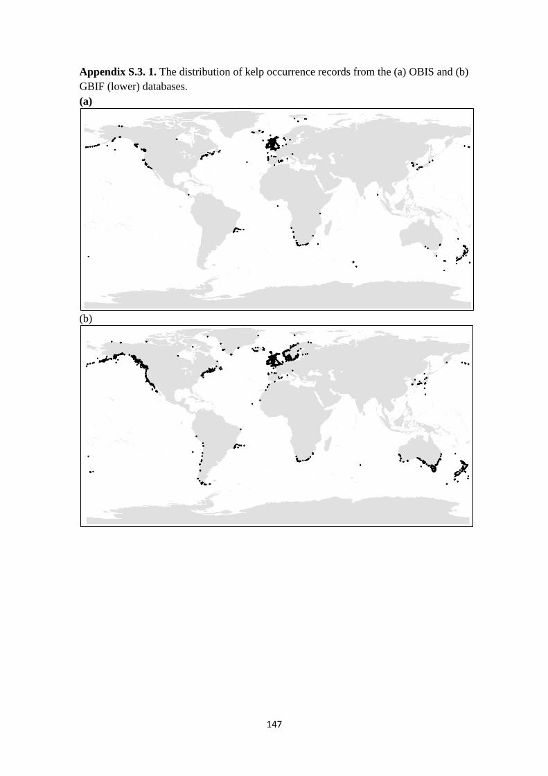
147

Appendix S.3. 1. The distribution of kelp occurrence records from the (a) OBIS and (b) GBIF (lower) databases. (a)

(b)

148

Appendix S.3.2. The receiver operating curve for both training (red) and test data (blue) to evaluate model’s predicting power. The red line indicates the “fit” of the model to the training data. The blue line shows the fit of the model to the testing data, and that is the real test of the model’s predictive power (Phillips 2017).

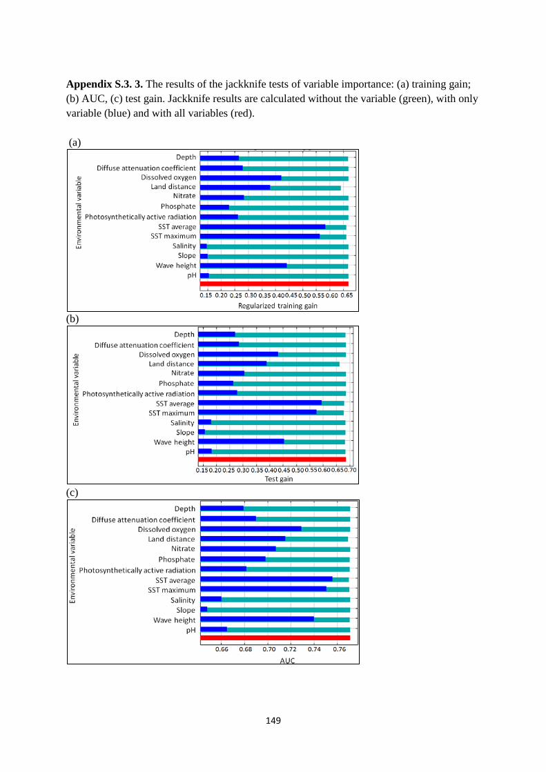
149

Appendix S.3. 3. The results of the jackknife tests of variable importance: (a) training gain; (b) AUC, (c) test gain. Jackknife results are calculated without the variable (green), with only variable (blue) and with all variables (red). (a)

(b)

(c)

150

Appendix S.3. 4. The list of citations for the data downloaded from the GBIF database.

Abitia C.L.A., Ramos R.P. (2017). Evaluación estacional de la fauna ictiológica, malacológica y flora ficológica de la Reserva de la Biósfera El Vizcaino, BCS, Fase I: Laguna Ojo de Liebre. Version 1.3. Comisión nacional para el conocimiento y uso de la biodiversidad. Occurrence Dataset https://doi.org/10.15468/ytv8m1 accessed via GBIF.org on 2017-10-24. doi:10.15468/ytv8m1.

Aguilar R.L.E., Ramos R.P. (2017). Estado actual de las especies de macroalgas introducidas e invasoras en la costa Pacífico de México. Version 1.3. Comisión nacional para el conocimiento y uso de la biodiversidad. Occurrence Dataset https://doi.org/10.15468/r3v6b9 accessed via GBIF.org on 2017-10-24. doi:10.15468/r3v6b9.

Aguilar R.R, Ramos R.P. (2017). Macroalgas marinas de la costa noroccidental de Baja California, México. Version 1.3. Comisión nacional para el conocimiento y uso de la biodiversidad. Occurrence Dataset https://doi.org/10.15468/kuipmz accessed via GBIF.org on 2017-10-24. doi:10.15468/kuipmz.

Atlas of Life in the Coastal Wilderness (2017). Atlas of Life in the Coastal Wilderness - Sightings. Occurrence Dataset https://doi.org/10.15468/rtxjkt accessed via GBIF.org on 2017-10-24. doi:10.15468/rtxjkt.

Atlas of Living Australia (2017). Climatewatch. Occurrence Dataset https://doi.org/10.15468/xlx9o4 accessed via GBIF.org on 2017-10-24. doi:10.15468/xlx9o4.

Atlas of Living Australia (2017). New Zealand Virtual Herbarium. Occurrence Dataset https://doi.org/10.15468/bxxmis accessed via GBIF.org on 2017-10-24. doi:10.15468/bxxmis.

Atlas of Living Australia (2017). WildNet- Queensland Wildlife Data. Occurrence Dataset https://doi.org/10.15468/lxgoyb accessed via GBIF.org on 2017-10-24. doi:10.15468/lxgoyb.

Australia's Virtual Herbarium (2017). Australia's Virtual Herbarium. Occurrence Dataset https://doi.org/10.15468/rhzrxw accessed via GBIF.org on 2017-10-24. doi:10.15468/rhzrxw.

Biological Institute Helgoland (BAH) in the Alfred Wegener Institute, Helmholtz Centre for Polar and Marine Research. AWI-Herbarium Marine Macroalgae. Occurrence Dataset https://doi.org/10.15468/uyo5za accessed via GBIF.org on 2017-10-24. doi:10.15468/uyo5za.

Blindheim T (2017). BioFokus. Version 1.592. Natural History Museum, University of Oslo. Occurrence Dataset https://doi.org/10.15468/jxbhqx accessed via GBIF.org on 2017-10-24. doi:10.15468/jxbhqx.

Bolton, J., Ranwashe, F. (2016). UCT: South Africa Seaweeds (1905-2008). Version 1.2. South African National Biodiversity Institute. Occurrence Dataset https://doi.org/10.15468/zp9rxk accessed via GBIF.org on 2017-10-24. doi:10.15468/zp9rxk.

Botanic Garden and Botanical Museum Berlin-Dahlem (2017). AlgaTerra. Occurrence Dataset https://doi.org/10.15468/nz7lld accessed via GBIF.org on 2017-10-24. doi:10.15468/nz7lld.

Botanic Garden and Botanical Museum Berlin-Dahlem (2017). Herbarium Berolinense. Occurrence Dataset https://doi.org/10.15468/dlwwhz accessed via GBIF.org on 2017-10-24. doi:10.15468/dlwwhz.

Cabezudo,A.B., García S.J. (2015). MGC Herbarium of University of Malaga (Spain): MGC-Algae dataset. University of Malaga. Occurrence Dataset https://doi.org/10.15468/q8hzlc accessed via GBIF.org on 2017-10-24. doi:10.15468/q8hzlc.

Calabuig, I. (2014). Botanical Museum, Copenhagen, the Phycology Herbarium. Botanical Garden & Museum, Natural History Museum of Denmark. Occurrence Dataset

151

https://doi.org/10.15468/8oxxmx accessed via GBIF.org on 2017-10-24. doi:10.15468/8oxxmx.

Cameron, E., Moriarty, A. (2017). Auckland Museum Botany Collection. Version 1.18. Auckland War Memorial Museum. Occurrence Dataset https://doi.org/10.15468/mnjkvv accessed via GBIF.org on 2017-10-24. doi:10.15468/mnjkvv.

Capers, R. (2014). CONN. University of Connecticut. Occurrence Dataset https://doi.org/10.15468/w35jmd accessed via GBIF.org on 2017-10-24., http://bgbaseserver.eeb.uconn.edu/ doi:10.15468/w35jmd.

Casas, V. M, Ramos, R. P., (2017). Sistematización de la Colección de Algas Marinas del Centro Interdisciplinario de Ciencias Marinas CICIMAR-IPN. Version 1.4. Comisión nacional para el conocimiento y uso de la biodiversidad. Occurrence Dataset https://doi.org/10.15468/9kmlfs accessed via GBIF.org on 2017-10-24. doi:10.15468/9kmlfs.

Cassano, V. (2017). SPF-Algae - Herbário da Universidade de São Paulo - Coleção de Algas. Version 1.30. Universidade de São Paulo. Occurrence Dataset https://doi.org/10.15468/xhpmge accessed via GBIF.org on 2017-10-24., http://splink.cria.org.br/manager/detail?resource=SPF-Algae doi:10.15468/xhpmge.

CeDoc of Plant Biodiversity (CeDocBIV), Univ. Barcelona (2017). CeDoc de Biodiversitat Vegetal: BCN-Phycophyta. Occurrence Dataset https://doi.org/10.15468/lgu4v6 accessed via GBIF.org on 2017-10-24. doi:10.15468/lgu4v6.

Citizen Science - ALA Website (2017). Individual Sightings. Occurrence Dataset https://doi.org/10.15468/jayxmn accessed via GBIF.org on 2017-10-24. doi:10.15468/jayxmn.

Cofnod North Wales Environmental Information Service (2017). Miscellaneous records held on the Cofnod database. Occurrence Dataset https://doi.org/10.15468/hcgqsi accessed via GBIF.org on 2017-10-24. doi:10.15468/hcgqsi.

Cofnod North Wales Environmental Information Service (2017). NRW Regional Data: North Wales. Occurrence Dataset https://doi.org/10.15468/krljpu accessed via GBIF.org on 2017-10-24. doi:10.15468/krljpu.

Creuwels, J. (2017). Naturalis Biodiversity Center (NL) - Botany. Naturalis Biodiversity Center. Occurrence Dataset https://doi.org/10.15468/ib5ypt accessed via GBIF.org on 2017-10-24. doi:10.15468/ib5ypt.

Cumbria Biodiversity Data Centre (2017). Cumbria Biodiversity Data Centre fungi and lower plant species observations for Cumbria for the period 1845 to 2014. Occurrence Dataset https://doi.org/10.15468/qup5rk accessed via GBIF.org on 2017-10-24. doi:10.15468/qup5rk.

Department of Botany, Faculty of Biological Sciences, University of Valencia (2017). Universitat de València, Colecciones de Criptógamas: VAL_Algae. Occurrence Dataset https://doi.org/10.15468/odw9qj accessed via GBIF.org on 2017-10-24. doi:10.15468/odw9qj.

Department of Organisms and Systems Biology. University of Oviedo (2017). Universidad de Oviedo. Departamento de Biología de Organismos y Sistemas: FCO-Algae. Occurrence Dataset https://doi.org/10.15468/qfwigq accessed via GBIF.org on 2017-10-24. doi:10.15468/qfwigq.

Department of Science, Information Technology and Innovation (2017). Queensland Herbarium Records. Occurrence Dataset https://doi.org/10.15468/jsffsa accessed via GBIF.org on 2017-10-24. doi:10.15468/jsffsa.

Dorset Environmental Records Centre (2017). Ross Coral Mapping Project - NBN South West Pilot Project Case Studies. Occurrence Dataset https://doi.org/10.15468/mnlzxc accessed via GBIF.org on 2017-10-24. doi:10.15468/mnlzxc.

152

European Molecular Biology Laboratory (EMBL) (2014). Geographically tagged INSDC sequences. Occurrence Dataset https://doi.org/10.15468/cndomv accessed via GBIF.org on 2017-10-24. doi:10.15468/cndomv.

European Molecular Biology Laboratory Australia (2017). European Molecular Biology Laboratory Australian Mirror. Occurrence Dataset https://doi.org/10.15468/ypsvix accessed via GBIF.org on 2017-10-24. doi:10.15468/ypsvix.

Fife Nature Records Centre (2017). St Andrews BioBlitz 2014. Occurrence Dataset https://doi.org/10.15468/erweal accessed via GBIF.org on 2017-10-24. doi:10.15468/erweal.

Fife Nature Records Centre (2017). St Andrews BioBlitz 2015. Occurrence Dataset https://doi.org/10.15468/xtrbvy accessed via GBIF.org on 2017-10-24. doi:10.15468/xtrbvy.

Fife Nature Records Centre (2017). St Andrews BioBlitz 2016. Occurrence Dataset https://doi.org/10.15468/146yiz accessed via GBIF.org on 2017-10-24. doi:10.15468/146yiz.

Forzza, R., Dalcin, E. (2017). RB - Rio de Janeiro Botanical Garden Herbarium Collection. Version 84.123. Instituto de Pesquisas Jardim Botanico do Rio de Janeiro. Occurrence Dataset https://doi.org/10.15468/7ep9i2 accessed via GBIF.org on 2017-10-24., http://www.jbrj.gov.br/jabot/formularios/comocitar_jabot.php doi:10.15468/7ep9i2.

GEO-Tag der Artenvielfalt (2017). Artenvielfalt der Nordsee - Helgoland. Occurrence Dataset https://doi.org/10.15468/omx28y accessed via GBIF.org on 2017-10-24. doi:10.15468/omx28y.

GEO-Tag der Artenvielfalt (2017) Gesamtartenliste Bremerhaven, Helgoland und Sylt. Occurrence Dataset https://doi.org/10.15468/85zmqv accessed via GBIF.org on 2017-10-24. doi:10.15468/85zmqv.

Griffiths, H. (2017). The First Comprehensive Description of the Biodiversity and Biogeography of Antarctic and Sub-Antarctic Intertidal Communities. Version 2.1. Antarctic Biodiversity Information Facility (ANTABIF). Occurrence Dataset https://doi.org/10.15468/doyfzk accessed via GBIF.org on 2017-10-24., Griffiths & Waller (In Press) doi:10.15468/doyfzk.

Highland Biological Recording Group (2017). HBRG Highland Seashore Project Dataset. Occurrence Dataset https://doi.org/10.15468/sau7qh accessed via GBIF.org on 2017-10-24. doi:10.15468/sau7qh.

Hoem, S.A. (2017). Norwegian Biodiversity Information Centre - Other datasets. Version 31.111. Natural History Museum, University of Oslo. Occurrence Dataset https://doi.org/10.15468/tm56sc accessed via GBIF.org on 2017-10-24. doi:10.15468/tm56sc.

Hoem, S.A. (2017). Norwegian Species Observation Service. Version 3.5. The Norwegian Biodiversity Information Centre (NBIC). Occurrence Dataset https://doi.org/10.15468/zjbzel accessed via GBIF.org on 2017-10-24. doi:10.15468/zjbzel.

Icelandic Institute of Natural History. Herbarium (AMNH).(2017) Occurrence Dataset https://doi.org/10.15468/hkydl2 accessed via GBIF.org on 2017-10-24. doi:10.15468/hkydl2.

Ickert-Bond, S. (2017). UAM Herbarium (ALA), Algae Collection (Arctos). Version 8.6. University of Alaska Museum of the North. Occurrence Dataset https://doi.org/10.15468/gwjvwf accessed via GBIF.org on 2017-10-24. doi:10.15468/gwjvwf.

iNaturalist.org (2017). iNaturalist Research-grade Observations. Occurrence Dataset https://doi.org/10.15468/ab3s5x accessed via GBIF.org on 2017-10-24. doi:10.15468/ab3s5x.

Institute of Biodiversity, Animal Health and Comparative Medicine, College of Medical, Veterinary and Life Sciences, University of Glasgow (2016). International Barcode of Life project (iBOL). Occurrence Dataset https://doi.org/10.15468/inygc6 accessed via GBIF.org on 2017-10-24. doi:10.15468/inygc6.

153

Isle of Wight Local Records Centre (2017). Isle of Wight Notable Species. Occurrence Dataset https://doi.org/10.15468/sm4ety accessed via GBIF.org on 2017-10-24. doi:10.15468/sm4ety.

Jennings, L. (2017). University of British Columbia Herbarium (UBC) - Algae Collection. Version 14.3. University of British Columbia. Occurrence Dataset https://doi.org/10.5886/ujwtvvs2 accessed via GBIF.org on 2017-10-24., doi:10.5886/ujwtvvs2 doi:10.5886/ujwtvvs2.

Joint Nature Conservation Committee (2017). Marine Offshore Seabed Survey data held by JNCC. Occurrence Dataset https://doi.org/10.15468/skvdld accessed via GBIF.org on 2017-10-24. doi:10.15468/skvdld.

Jordal, J.B. (2017). Jordal. Version 1.75. Natural History Museum, University of Oslo. Occurrence Dataset https://doi.org/10.15468/wqsad9 accessed via GBIF.org on 2017-10-24. doi:10.15468/wqsad9.

Kluse, J. (2017). LSU Shirley C. Tucker Herbarium at Louisiana State University - Algae. Version 1.8. Louisiana State University Herbarium. Occurrence Dataset https://doi.org/10.15468/3jp2zb accessed via GBIF.org on 2017-10-24. doi:10.15468/3jp2zb.

Lahti, T. (2017). Hatikka Observation Database. Version 1.1. Finnish Biodiversity Information Facility. Occurrence Dataset https://doi.org/10.15468/te1t6l accessed via GBIF.org on 2017-10-24. doi:10.15468/te1t6l

Lampinen, R., Lahti T (2017). Finnish Floristic Database (Finnish Museum of Natural History Collections). Version 1.1. Finnish Biodiversity Information Facility. Occurrence Dataset https://doi.org/10.15468/kasmwk accessed via GBIF.org on 2017-10-24. doi:10.15468/kasmwk.

Mackay, K. (2017). Marine biological observation data from coastal and offshore surveys around New Zealand. Version 1.5. The National Institute of Water and Atmospheric Research (NIWA). Occurrence Dataset https://doi.org/10.15468/pzpgop accessed via GBIF.org on 2017-10-24. doi:10.15468/pzpgop.

Mackay, K. (2017). Records from the NIWA AllSeaBio marine biology database. The National Institute of Water and Atmospheric Research (NIWA). Occurrence Dataset https://doi.org/10.15468/7y1efw accessed via GBIF.org on 2017-10-24. doi:10.15468/7y1efw.

MACOI - Portuguese Seaweeds.(2017) Portuguese Seaweeds. Occurrence Dataset https://doi.org/10.15468/evxsae accessed via GBIF.org on 2017-10-24. doi:10.15468/evxsae

Magill, B., Solomon, J., Stimmel, H. (2016). Tropicos Specimen Data. Missouri Botanical Garden. Occurrence Dataset https://doi.org/10.15468/hja69f accessed via GBIF.org on 2017-10-24. doi:10.15468/hja69f.

Manx Biological Recording Partnership (2017). Isle of Man wildlife records from 01/01/2000 to 13/02/2017. Occurrence Dataset https://doi.org/10.15468/mopwow accessed via GBIF.org on 2017-10-24. doi:10.15468/mopwow.

Marine Biological Association (2017). 2004-2012 Bishop et al. Occurrence of non-native sessile invertebrates on the English coast. Occurrence Dataset https://doi.org/10.15468/t9edux accessed via GBIF.org on 2017-10-24. doi:10.15468/t9edux.

Marine Biological Association (2017). 2005 - Ongoing United Kingdom MarLIN Shore Thing timed search results. Occurrence Dataset https://doi.org/10.15468/ikwlzr accessed via GBIF.org on 2017-10-24. doi:10.15468/ikwlzr.

Marine Biological Association (2017). DASSH Data Archive Centre Academic Surveys. Occurrence Dataset https://doi.org/10.15468/cwqszy accessed via GBIF.org on 2017-10-24. doi:10.15468/cwqszy.

154

Marine Biological Association (2017). DASSH Data Archive Centre expert sightings records. Occurrence Dataset https://doi.org/10.15468/tggq3w accessed via GBIF.org on 2017-10-24. doi:10.15468/tggq3w.

Marine Biological Association (2017). DASSH Data Archive Centre volunteer sightings records. Occurrence Dataset https://doi.org/10.15468/xwiw3h accessed via GBIF.org on 2017-10-24. doi:10.15468/xwiw3h.

Marine Biological Association (2017). DASSH Data Archive Centre volunteer survey data. Occurrence Dataset https://doi.org/10.15468/pjowth accessed via GBIF.org on 2017-10-24. doi:10.15468/pjowth

Marine Biological Association (2017). RISC and ALERT Marine Non-Native Species (Chinese Mitten Crab, Wakame and Carpet Sea Squirt) Records. Occurrence Dataset https://doi.org/10.15468/ls37zx accessed via GBIF.org on 2017-10-24. doi:10.15468/ls37zx

Marine Biological Association (2017). Verified Marine records from Indicia-based surveys. Occurrence Dataset https://doi.org/10.15468/yfyeyg accessed via GBIF.org on 2017-10-24. doi:10.15468/yfyeyg

Marine Science Institute, UCSB. Paleobiology Database. Occurrence Dataset https://doi.org/10.15468/2durgn accessed via GBIF.org on 2017-10-24. doi:10.15468/2durgn.

Merseyside BioBank (2017). Merseyside BioBank (unverified). Occurrence Dataset https://doi.org/10.15468/iou2ld accessed via GBIF.org on 2017-10-24. doi:10.15468/iou2ld.

MNHN - Museum national d'Histoire naturelle (2017). The cryptogamy collection (PC) at the Herbarium of the Muséum national d'Histoire Naturelle (MNHN - Paris). Version 70.33. Occurrence Dataset https://doi.org/10.15468/mywiem accessed via GBIF.org on 2017-10-24. doi:10.15468/mywiem.

Muséum national d'histoire naturelle Luxembourg. Palaeontological collections National Museum of Natural History Luxembourg. Occurrence Dataset https://doi.org/10.15468/vbuvyu accessed via GBIF.org on 2017-10-24. doi:10.15468/vbuvyu.

National Biodiversity Data Centre (2016). National Invasive Species Database. Occurrence Dataset https://doi.org/10.15468/pkjqbk accessed via GBIF.org on 2017-10-24. doi:10.15468/pkjqbk.

National Biodiversity Data Centre (2016). Rocky Shore Macroalgae. Occurrence Dataset https://doi.org/10.15468/evhuy3 accessed via GBIF.org on 2017-10-24. doi:10.15468/evhuy3.

National Biodiversity Data Centre (2017). Coastal and marine species. Occurrence Dataset https://doi.org/10.15468/oynwkx accessed via GBIF.org on 2017-10-24. doi:10.15468/oynwkx.

National Biodiversity Data Centre (2017). Ireland's BioBlitz. Occurrence Dataset https://doi.org/10.15468/aiiz3z accessed via GBIF.org on 2017-10-24. doi:10.15468/aiiz3z.

National Chemical Laboratory. IndOBIS, Indian Ocean Node of OBIS. Occurrence Dataset https://doi.org/10.15468/tbedgi accessed via GBIF.org on 2017-10-24. doi:10.15468/tbedgi.

National Museum of Nature and Science, Japan. (2017). Ibaraki Nature Museum, Algae collection. Occurrence Dataset https://doi.org/10.15468/tdqeow accessed via GBIF.org on 2017-10-24. doi:10.15468/tdqeow.

National Trust (2017). National Trust Species Records. Occurrence Dataset https://doi.org/10.15468/opc6g1 accessed via GBIF.org on 2017-10-24. doi:10.15468/opc6g1

Natural England (2017). Natural England Marine Monitoring surveys. Occurrence Dataset https://doi.org/10.15468/ysikg5 accessed via GBIF.org on 2017-10-24. doi:10.15468/ysikg5

155

Natural History Museum (2017). Natural History Museum (London) Collection Specimens. Occurrence Dataset https://doi.org/10.5519/0002965 accessed via GBIF.org on 2017-10-24., http://dx.doi.org/10.5519/0002965 doi: 10.5519/0002965.

Natural History Museum, University of Oslo (2017). Algae, Norwegian College of Fishery Science. Version 1.366. Occurrence Dataset https://doi.org/10.15468/a2ewca accessed via GBIF.org on 2017-10-24. doi:10.15468/a2ewca.

Natural History Museum, University of Oslo (2017). Algae, Specimens, Agder naturmuseum (KMN). Version 1.321. Occurrence Dataset https://doi.org/10.15468/jldjxh accessed via GBIF.org on 2017-10-24. doi:10.15468/jldjxh.

Natural History Museum, University of Oslo (2017). Rådgivende Biologer. Version 33.76. Occurrence Dataset https://doi.org/10.15468/tqxvcg accessed via GBIF.org on 2017-10-24. doi:10.15468/tqxvcg

Natural Resources Wales (2017). Marine data from Natural Resources Wales (NRW) Technical Support (Research & Monitoring) Contracts, Wales. Occurrence Dataset https://doi.org/10.15468/az7nw3 accessed via GBIF.org on 2017-10-24. doi:10.15468/az7nw3.

Natural Resources Wales (2017). Marine Intertidal Phase 1 species dataset from the Countryside Council for Wales 1996-2005. Occurrence Dataset https://doi.org/10.15468/kflo7m accessed via GBIF.org on 2017-10-24. doi:10.15468/kflo7m.

Natural Resources Wales (2017). Marine Non Native Species records from Natural Resources Wales (NRW) monitoring research and ad-hoc sightings. Occurrence Dataset https://doi.org/10.15468/jc9uj9 accessed via GBIF.org on 2017-10-24. doi:10.15468/jc9uj9.

Natural Resources Wales (2017). Marine species records from Skomer Marine Conservation Zone (MCZ) Marine Monitoring Programme. Occurrence Dataset https://doi.org/10.15468/207iog accessed via GBIF.org on 2017-10-24. doi:10.15468/207iog.

Nature Locator (2017). Sealife Tracker. Occurrence Dataset https://doi.org/10.15468/qgk3pg accessed via GBIF.org on 2017-10-24. doi:10.15468/qgk3pg.

naturgucker.de. naturgucker. Occurrence Dataset https://doi.org/10.15468/uc1apo accessed via GBIF.org on 2017-10-24. doi:10.15468/uc1apo.

Neil, K., Mackay, K. (2017). Rhodolith Beds in Northern New Zealand: Characterisation of Associated Biodiversity. Version 1.6. The National Institute of Water and Atmospheric Research (NIWA). Sampling_event Dataset https://doi.org/10.15468/3zyorf accessed via GBIF.org on 2017-10-24. doi:10.15468/3zyorf.

Newell, R., Pufahl, C., Richard, J. (2014). E. C. Smith Herbarium (ACAD). Acadia University. Occurrence Dataset https://doi.org/10.15468/zc4csq accessed via GBIF.org on 2017-10-24. doi:10.15468/zc4csq.

NTNU University Museum (2017). Algae herbarium, NTNU University Museum. Version 11.642. Occurrence Dataset https://doi.org/10.15468/elzhsu accessed via GBIF.org on 2017-10-24. doi:10.15468/elzhsu.

Ocean Biogeographic Information System. A Biological Survey of the Waters of Woods Hole and Vacinity. Occurrence Dataset https://doi.org/10.15468/bxmxx0 accessed via GBIF.org on 2017-10-24. doi:10.15468/bxmxx0.

Ocean Biogeographic Information System. Benthic biodiversity along the central coast in the Brazilian EEZ (OBIS South America, BRAZIL) (OBIS South America, BRAZIL). Occurrence Dataset https://doi.org/10.15468/uofqoh accessed via GBIF.org on 2017-10-24. doi:10.15468/uofqoh

156

Ocean Biogeographic Information System. BioMar (EurOBIS). Occurrence Dataset https://doi.org/10.15468/tx3yvy accessed via GBIF.org on 2017-10-24. doi:10.15468/tx3yvy.

Ocean Biogeographic Information System. Gwaii Haanas Marine Plants (OBIS Canada). Occurrence Dataset https://doi.org/10.15468/liabjc accessed via GBIF.org on 2017-10-24. doi:10.15468/liabjc.

Ocean Biogeographic Information System. Natural Geography In Shore Areas (NaGISA) Dataset. Occurrence Dataset https://doi.org/10.15468/5uprth accessed via GBIF.org on 2017-10-24. doi:10.15468/5uprth.

Ocean Biogeographic Information System. South Western Pacific Regional OBIS Data All Sea Bio Subset (South Western Pacific OBIS). Occurrence Dataset https://doi.org/10.15468/rqxetf accessed via GBIF.org on 2017-10-24. doi:10.15468/rqxetf.

Ocean Biogeographic Information System. Taxonomic Information Sytem for the Belgian coastal area (EurOBIS). Occurrence Dataset https://doi.org/10.15468/mstheo accessed via GBIF.org on 2017-10-24. doi:10.15468/mstheo.

Orrell, T., Hollowell, T. (2017). NMNH Extant Specimen Records. Version 1.8. National Museum of Natural History, Smithsonian Institution. Occurrence Dataset https://doi.org/10.15468/hnhrg3 accessed via GBIF.org on 2017-10-24. doi:10.15468/hnhrg3.

Outer Hebrides Biological Recording (2017). Non-vascular Plants, Outer Hebrides. Occurrence Dataset https://doi.org/10.15468/goidos accessed via GBIF.org on 2017-10-24. doi:10.15468/goidos.

Piriz, M. L., Marin, M. R. (2017). Seaweeds records from Argentina and Uruguay. Version 1.4. ArOBIS Centro Nacional Patagónico. Occurrence Dataset https://doi.org/10.15468/e0ick5 accessed via GBIF.org on 2017-10-24. doi:10.15468/e0ick5.

Pyle, R. (2016). Bernice P. Bishop Museum. Version 8.1. Bernice Pauahi Bishop Museum. Occurrence Dataset https://doi.org/10.15468/s6ctus accessed via GBIF.org on 2017-10-24. doi:10.15468/s6ctus.

Queensland Museum (2017). Queensland Museum provider for OZCAM. Occurrence Dataset https://doi.org/10.15468/lotsye accessed via GBIF.org on 2017-10-24. doi:10.15468/lotsye

Questagame (2017). Questagame weekly feed. Occurrence Dataset https://doi.org/10.15468/slqqt8 accessed via GBIF.org on 2017-10-24. doi:10.15468/slqqt8

Ranz, J. (2017). Banco de Datos de la Biodiversidad de la Comunitat Valenciana. Biodiversity data bank of Generalitat Valenciana. Occurrence Dataset https://doi.org/10.15468/b4yqdy accessed via GBIF.org on 2017-10-24. doi:10.15468/b4yqdy

Riosmena, R. R., Ramos R.P. (2017). Computarización del Herbario Ficológico de la Universidad Autónoma de Baja California Sur. Version 1.3. Comisión nacional para el conocimiento y uso de la biodiversidad. Occurrence Dataset https://doi.org/10.15468/rey7bx accessed via GBIF.org on 2017-10-24. doi:10.15468/rey7bx

SantAnna, C., Tucci, A. (2017). SP-Algae - SP-Algae - Herbário do Estado "Maria Eneyda P. Kaufmann Fidalgo - Coleção de Algas. Version 1.30. Instituto de Botânica, São Paulo. Occurrence Dataset https://doi.org/10.15468/md6zcx accessed via GBIF.org on 2017-10-24.,http://splink.cria.org.br/manager/detail?resource=SP-Algae doi:10.15468/md6zcx.

Scottish Natural Heritage (2017). Species data for Scottish waters held and managed by Scottish Natural Heritage, derived from benthic surveys 1993 to 2014. Occurrence Dataset https://doi.org/10.15468/faxvgd accessed via GBIF.org on 2017-10-24. doi:10.15468/faxvgd.

157

Scottish Wildlife Trust (2017). Survey and monitoring records for Scottish Wildlife Trust reserves from reserve convenors and Trust volunteers - Unassessed data. Occurrence Dataset https://doi.org/10.15468/jxrydj accessed via GBIF.org on 2017-10-24. doi:10.15468/jxrydj.

Seasearch (2017). Seasearch Marine Surveys in England. Occurrence Dataset https://doi.org/10.15468/kywx6m accessed via GBIF.org on 2017-10-24. doi:10.15468/kywx6m.

Seasearch (2017). Seasearch Marine Surveys in Ireland. Occurrence Dataset https://doi.org/10.15468/pyugge accessed via GBIF.org on 2017-10-24. doi:10.15468/pyugge.

Seasearch (2017). Seasearch Marine Surveys in Scotland. Occurrence Dataset https://doi.org/10.15468/0hyjxi accessed via GBIF.org on 2017-10-24. doi:10.15468/0hyjxi..

Seasearch (2017). Seasearch Marine Surveys in the Isle of Man. Occurrence Dataset https://doi.org/10.15468/mxkbcg accessed via GBIF.org on 2017-10-24. doi:10.15468/mxkbcg.

Seasearch (2017). Seasearch Marine Surveys in Wales. Occurrence Dataset https://doi.org/10.15468/4us2hk accessed via GBIF.org on 2017-10-24. doi:10.15468/4us2hk.

Shah M, Coulson S (2017). Artportalen (Swedish Species Observation System). Version 92.82. ArtDatabanken. Occurrence Dataset https://doi.org/10.15468/kllkyl accessed via GBIF.org on 2017-10-24. doi:10.15468/kllkyl

South East Wales Biodiversity Records Centre (2017). SEWBReC Algae and allied species (South East Wales). Occurrence Dataset https://doi.org/10.15468/55albd accessed via GBIF.org on 2017-10-24. doi:10.15468/55albd

SPN - Service du Patrimoine naturel, Muséum national d'Histoire naturelle, Paris (2013). Inventaire National du Patrimoine Naturel : Programme CARTHAM: Inventaire biologique dans le cadre de Natura 2000 en Mer. Occurrence Dataset https://doi.org/10.15468/ehnrif accessed via GBIF.org on 2017-10-24. doi:10.15468/ehnrif

Suffolk Biodiversity Information Service (2017). Suffolk Biodiversity Information Service (SBIS) Dataset. Occurrence Dataset https://doi.org/10.15468/ab4vwo accessed via GBIF.org on 2017-10-24. doi:10.15468/ab4vwo.

Tasmanian Department of Primary Industries, Parks, Water and Environment (2017). Tasmanian Natural Values Atlas. Occurrence Dataset https://doi.org/10.15468/rtnb4m accessed via GBIF.org on 2017-10-24. doi:10.15468/rtnb4m.

Telenius, A. (2016). Algae (S). GBIF-Sweden. Occurrence Dataset https://doi.org/10.15468/pqxsbz accessed via GBIF.org on 2017-10-24. doi:10.15468/pqxsbz.

Telenius, A., Ericson, N. (2016). Herbarium of Umeå University (UME). GBIF-Sweden. Occurrence Dataset https://doi.org/10.15468/gatdg4 accessed via GBIF.org on 2017-10-24. doi:10.15468/gatdg4.

Telenius, A., Rühling, Å. (2017). Oskarshamn herbarium (OHN). GBIF-Sweden. Occurrence Dataset https://doi.org/10.15468/u5wjib accessed via GBIF.org on 2017-10-24. doi:10.15468/u5wjib.

Telenius, A., Shah, M. (2016). Botany (UPS). GBIF-Sweden. Occurrence Dataset https://doi.org/10.15468/ufmslw accessed via GBIF.org on 2017-10-24. doi:10.15468/ufmslw.

The Wildlife Information Centre (2017). TWIC Biodiversity Field Trip Data (1995-2014). Occurrence Dataset https://doi.org/10.15468/ljc0ke accessed via GBIF.org on 2017-10-24. doi:10.15468/ljc0ke.

158

The Wildlife Trusts (2017). Marine data from The Wildlife Trusts (TWT) Dive Team; Somerset, Cornwall and Sussex; 2014-2015. Occurrence Dataset https://doi.org/10.15468/aqr7zv accessed via GBIF.org on 2017-10-24. doi:10.15468/aqr7zv.

Vanreusel, W., Barendse, R., Steeman, R., Gielen, K., Swinnen, K., Desmet, P., Herremans, M. (2017). Waarnemingen.be - Non-native plant occurrences in Flanders and the Brussels Capital Region, Belgium. Version 1.1. Natuurpunt. Occurrence Dataset https://doi.org/10.15468/smdvdo accessed via GBIF.org on 2017-10-24., https://doi.org/10.15468/smdvdo doi:10.15468/smdvdo.

Victorian Department of Environment, Land, Water and Planning (2017). Victorian Biodiversity Atlas. Occurrence Dataset https://doi.org/10.15468/khlfs3 accessed via GBIF.org on 2017-10-24. doi:10.15468/khlfs3.

Wilton, A. (2017). Allan Herbarium (CHR). Landcare Research. Occurrence Dataset https://doi.org/10.15468/x5ucvh accessed via GBIF.org on 2017-10-24. doi:10.15468/x5ucvh

Wittzell, H., Shah, M. (2017). Lund Botanical Museum (LD). Lund Botanical Museum (LD). Occurrence Dataset https://doi.org/10.15468/c4w4co accessed via GBIF.org on 2017-10-24. doi:10.15468/c4w4co

Yabur, P. R., Ramos, R. P. (2017). Inventario de macroalgas de Isla Guadalupe, México . Version 1.4. Comisión nacional para el conocimiento y uso de la biodiversidad. Occurrence Dataset https://doi.org/10.15468/m821to accessed via GBIF.org on 2017-10-24. doi:10.15468/m821to.

Yorkshire Wildlife Trust (2017). Yorkshire Wildlife Trust Shoresearch. Occurrence Dataset https://doi.org/10.15468/1nw3ch accessed via GBIF.org on 2017-10-24. doi:10.15468/1nw3ch.

159

Appendix S.3. 5. The list of citations for the datasets containing laminarian kelp in OBIS on 2017-10-24 as provided in the datasets metadata.

AIMS - Bioresources Library, accessed via OBIS.org on 2017-10-24. Allen, D., Beckett B., Brophy J., Costello, M.J., Emblow, C., Maciejewska, B., McCrea, M., Nash,

R., Penk, M. & Tierney, A. Marine species recorded in Ireland during field suveys by EcoServe, Ecological Consultancy Services Ltd. Available online at http://www.marbef.org/data/eurobis.php. Consulted on 2017-10-24.

Aráujo, R., Bárbara, I., Tibaldo, M., Berecibar, E., Díaz, Tapia P., Pereira, R., Santos, R. & Sousa-Pinto, I. Checklist of benthic marine algae and cyanobacteria of northern Portugal. Centre of Marine and Environmental Research; Interdisciplinary Centre for Marine and Environmental Research (Porto) (Ciimar). accessed via OBIS.org on 2017-10-24.

Arenas Parra, F.; Sousa Pinto, I.; Interdisciplinary Centre for Marine and Environmental Research (Porto) (CIIMAR) - University of Porto, Portugal; (2012). Monitoring Porto 2006-2008. http://dx.doi.org/10.14284/65, accessed via OBIS.org on 2017-10-24.

Benguela Current Large Marine Ecosystem (BCLME) – Namibia, accessed via OBIS.org on 2017-10-24.

Biodiversity Center of Japan, Ministry of the Environment. Data file of algal beds survey on Monitoring sites 1000 project at http://www.biodic.go.jp/moni1000/findings/data/index_file_algalbeds.html. Accessed on 2017-10-24.

Boisset, F. et al. (2009). VAL Cryptogamic collections online databases. Bolus Herbarium Algal Specimen Database, accessed via OBIS.org on 2017-10-24.

Branch (2002). West Coast biodiversity survey. University of Cape Town. Published by AfrOBIS; consulted via iOBIS.

Cape Breton University. (2015). ACZISC-AEI: CBU republication of species distribution records from the Bras d'Or Lakes, Cape Breton, Nova Scotia. 1. Large epibenthic invertebrates. Version 1 in OBIS Canada Digital Collections. Bedford Institute of Oceanography, Dartmouth, NS, Canada. Published by OBIS, Digital http://www.iobis.org/. Accessed on 2017-10-24

Cape Breton University. (2015). ACZISC-AEI: NRC-McLachlan collections: Marine Algae of Nova Scotia. IX. Flora of Bras d'Or Lakes, Cape Breton Island. Version 1 in OBIS Canada Digital Collections. Bedford Institute of Oceanography, Dartmouth, NS, Canada. Published by OBIS, Digital http://www.iobis.org/. Accessed on 2017-10-24

Chavan, V., and Achuthankutty, C.T., (editors), IndOBIS Catalogue of Life, Available at http://www.indobis.org/, Retrived 2017-10-24

Coalition-SGSL (2015). ACZISC-AEI: Republication of species distribution records from Atlantic Canada - A Survey of Marine Algae of the Maritime Provinces conducted between 1924 - 1931. Version 1 in OBIS Canada Digital Collections. Bedford Institute of Oceanography, Dartmouth, NS, Canada. Published by OBIS, Digital http://www.iobis.org/. Accessed on 2017-10-24.

Contributors to the Coastal Habitat Invasives Monitoring Program Database (2007). Coastal Habitat Invasives Monitoring Program Dataset; generated by using Ocean Biogeographic Information System (OBIS) [online application]. Salem, MA: Salem Sound Coastwatch [producer], Cambridge, MA: MIT Sea Grant College Program, Massachusetts Institute of Technology [distributor], New Brunswick, NJ: OBIS, Rutgers University Institute of Marine and Coastal Science [distributor]. http://www.iobis.org/mapper; accessed on 2017-10-24.

160

Contributors to the Rapid Assessment Surveys Database (2007). Rapid Assessment Survey Dataset; generated by using Ocean Biogeographic Information System (OBIS) [online application]. Cambridge, MA: MIT Sea Grant College Program, Massachusetts Institute of Technology [producer and distributor], New Brunswick, NJ: OBIS, Rutgers University Institute of Marine and Coastal Science [distributor]. http://www.iobis.org/mapper; accessed on 2017-10-24.

Countryside Council for Wales. Marine Nature Conservation Review (MNCR) and associated benthic marine data held and managed by CCW. Countryside Council for Wales, Gwynedd, UK.

Dale Rostron. Marine records from Pembrokeshire Marine Species Atlas. Countryside Council for Wales, Gwynedd, UK. https://doi.org/10.15468/42yudm.

Department of Invertebrate Zoology, Research and Collections Information System, NMNH, Smithsonian Institution. http://www.mnh.si.edu/rc/db/collection_db_policy1.html

DFO (2013). DFO Pacific Shorekeepers Intertidal Survey a community based project. Version 1 in OBIS Canada Collections. Bedford Institute of Oceanography, Dartmouth, NS, Canada. Published by OBIS. http://www.iobis.org/. (Consulted on 2017-10-24)

Diveboard - Scuba diving citizen science observations. Online at http://www.diveboard.com and http://ipt.diveboard.com/resource.do?r=diveboard-occurrences. http://dx.doi.org/10.15468/tnjrgy.

English Nature. Marine Nature Conservation Review (MNCR) and associated benthic marine data held and managed by English Nature. English Nature, Peterborough, UK.

Flanders Marine Institute (VLIZ). Taxonomic Information System for the Belgian coastal area. 10 Aug 2004, Oostende, Belgium, Accessed on 2017-10-24.

GEO-Tag der Artenvielfalt, Artenvielfalt der Nordsee - Helgoland (accessed through GBIF data portal, http://data.gbif.org/datasets/resource/2688, 2017-10-24)

Griffin, N. (2012). Selmar Schonland Hermarium Marine Algae Collection; Dataset published by AfrOBIS; consulted via iOBIS , on 2017-10-24.

Guardia, R. et al. (2007). Bases de dades de l'Herbari BCN http://www.ub.es/cedocbiv/bancdade.htm, accessed via OBIS.org on 2017-10-24.

Herbario Universidad de Malaga (MGC). Herbarium collections online databases. accessed via OBIS.org on 2017-10-24.

Indian Ocean Biogeographic Information System (IndOBIS)- Distribution records of marine organisms from the Indian Ocean, accessed via OBIS.org on 2017-10-24.

Institute of Marine Research (IMAR - Azores), Portugal; Department of Oceanography and Fisheries (DOP) - UAC, Portugal (2015): COLETA - IMAR/DOP-Uac reference collection from 1977 to 2012. http://dx.doi.org/10.14284/23, accessed via OBIS.org on 2017-10-24.

Jintsu-Uchifune, Y., Yamamoto, H. (2016). Marine organism occurrence data of the Asia-Pacific region extracted from literature. Available at http://www.godac.jamstec.go.jp/bismal/e/S9-5_Asia-Pacific. Accessed on 2017-10-24.

Lavrado, H.P. e Ignacio, B.L. (eds.) (2006). Biodiversidade bentonica da costa central da Zona Economica Exclusiva brasileira. Rio de Janeiro : Museu Nacional, 2006.(Série Livros; 18) 389 p. ISBN 85-7427-014-8. accessed via OBIS.org on 2017-10-24.

Living marine legacy of Gwaii Haanas. I: Marine plant baseline to 1999 and plant-related management issues, accessed via OBIS.org on 2017-10-24.

Marine Biological Association of the UK (MBA) (2016). DASSH: The UK Archive for Marine Species and Habitats Data, accessed via OBIS.org on 2017-10-24.

161

Marine Conservation Society. Seasearch Marine Surveys. Marine Conservation Society, Ross-on-Wye, UK, accessed via OBIS.org on 2017-10-24.

Marine flora and fauna records from the North-east Atlantic. Porcupine Marine Natural History Society, UK - UK National Biodiversity Network, accessed via OBIS.org on 2017-10-24.

Marine records from Skomer Marine Reserve (MNR) Marine Monitoring Programme. Countryside Council for Wales, UK - UK National Biodiversity Network, accessed via OBIS.org on 2017-10-24.

Ministry for Primary Industries (2014). Soviet Fishery Data (New Zealand Waters) 1964-1987. Southwestern Pacific OBIS, National Institute of Water and Atmospheric Research (NIWA), Wellington, New Zealand, 111883 records, Online http://nzobisipt.niwa.co.nz/resource.do?r=mbis_soviettrawl released on November 5, 2014, accessed via OBIS.org on 2017-10-24.

Munda, I. (1965). Benthic algal vegetation of Mjóifjürdur. Scientific Research Centre of the Slovenian Academy of Sciences and Arts, Ljubliana, Slovenia, accessed via OBIS.org on 2017-10-24.

Munda, I. (1967). Characteristic features of the benthic algal vegetation along the Snaefellsnes peninsula. Scientific Research Centre of the Slovenian Academy of Sciences and Arts, Ljubljana, Slovenia, accessed via OBIS.org on 2017-10-24.

Munda, I. (1968). Survey of the benthic algal vegetation of the Berufjördur, southeastern Iceland. Scientific Research Centre of the Slovenian Academy of Sciences and Arts, Ljubljana, Slovenia, accessed via OBIS.org on 2017-10-24.

Munda, I. (1969). Benthic algal vegetation of Borgafjördur. Scientific Research Centre of the Slovenian Academy of Sciences and Arts, Ljubljana, Slovenia, accessed via OBIS.org on 2017-10-24.

Munda, I. (1980). Macroalgae of the Tjornes Peninsula in the North of Iceland. Scientific Research Centre of the Slovenian Academy of Sciences and Arts, Ljubljana, Slovenia, accessed via OBIS.org on 2017-10-24.

National Biodiversity Data Centre: Marine species distributions in Irish coastal waters, 2013-11-20. Accessed via http://www.gbif.org/dataset/0d83ea43-5afb-4c50-af9c-fd22674338bb on 2017-10-24.

NatureWatch NZ (2013). Marine species citizen-science observations from NatureWatch NZ. Southwestern Pacific OBIS, National Institute of Water and Atmospheric Research (NIWA), Wellington, New Zealand, 939 records, Online http://nzobisipt.niwa.co.nz/resource.do?r=naturewatchnz released on August 22, 2016, accessed via OBIS.org on 2017-10-24.

Nelson, W.A., Neill, K., Barr, N., D'Archino, R., Miller, S., Stewart, R. (2012). Data from: Rhodolith Beds in Northern New Zealand: Characterisation of Associated Biodiversity. Southwestern Pacific OBIS, National Institute of Water and Atmospheric Research (NIWA), Wellington, New Zealand, 684 records, Online http://nzobisipt.niwa.co.nz/resource.do?r=rhodolithhabitats released on June 20, 2015, accessed via OBIS.org on 2017-10-24.

Norman and Florence Hammond records. Seawatch and coastal survey records. Cumbria Biodiversity Data Centre, UK - UK National Biodiversity Network, accessed via OBIS.org on 2017-10-24.

162

Ostler, R. Marine Nature Conservation Review (MNCR) and associated benthic marine data held and managed by JNCC. Joint Nature Conservation Committee, Centre for Ecology and hydrology, Aberdeenshire, UK, accessed via OBIS.org on 2017-10-24.

Parr, J. Marine Life Information Network (MarLIN) marine survey data (Professional). Marlin, Collated Marine Life Survey Datasets, Marine Biological Association of the UK, Plymouth, UK, accessed via OBIS.org on 2017-10-24.

Parr, J. Marine Life Survey Data (collected by volunteers) collated by MarLIN. MarLIN, collated Marine Life Survey Datasets, Marine Biological Association of the UK, Plymouth, UK, accessed via OBIS.org on 2017-10-24.

Picton, B.E., Emblow, C.S., Morrow, C.C., Sides, E.M., Tierney, P., McGrath, D., McGeough, G., McCrea, M., Dinneen, P., Falvey, J., Dempsey, S., Dowse, J., and Costello, M.J. (1999) Marine sites, habitats and species data collected during the BioMar survey of Ireland. Environmental Sciences Unit, Trinity College, Dublin, Ireland. accessed via OBIS.org on 2017-10-24.

Piriz, M. L. (2015): Seaweeds records from Argentina and Uruguay. v1.3. ArOBIS Centro Nacional Patagónico. Dataset/Occurrence. http://arobis.cenpat-conicet.gob.ar:8081/resource?r=arobis-seaweeds&v=1.3, accessed via OBIS.org on 2017-10-24.

Pohle, G., Van Guelpen, L., Martin, A., Welshman, D., and McGuire, A., (2004). Bay of Fundy Species,accessed via OBIS.org on 2017-10-24.

Pulfrich, A. (2013). Namdeb Diamond Corporation Limited Marine Moni toring Programme: Offshore licences. Dataset published by AfrOBIS; consulted via iOBIS on 2017-10-24.

Ramirez-Llodra, E., Blanco, (2005). ChEssBase: an online information system on biodiversity and biogeography of deep-sea fauna from chemosynthetic ecosystems. Version 2. World Wide Web electronic publications, http://www.noc.soton.ac.uk/chess/database/db_home.php, accessed via OBIS.org on 2017-10-24.

Robinson, C.B. (2016) Marine Biological Station - Canso: Detailed list of seaweeds observed during the month of August 1902. Version 1 in OBIS Canada Digital Collections. Bedford Institute of Oceanography, Dartmouth, NS, Canada. Published by OBIS, Digital http://www.iobis.org/. Accessed on 2017-10-24

Scottish Natural Heritage. Marine species data for Scottish waters held and managed by Scottish Natural Heritage, derived from benthic surveys 1993 to 2012. Scottish Natural Heritage, Edinburgh, UK.

Sousa Pinto, I., Viera, R., (2012). Monitoring of the intertidal biodiversity of rocky beaches with schools in Portugal 2005-2010. CIIMAR - Interdisciplinary Centre for Marine and Environmental Research, Porto. http://dx.doi.org/10.14284/38, accessed via OBIS.org on 2017-10-24.

Sousa-Pinto I. & Araújo, R. (2003). Intertidal rocky shore assemblages in Portugal. Centro Interdisciplinar de Investigaçao Marinha e Ambiental (CIMAR), Portugal, accessed via OBIS.org on 2017-10-24.

Sousa-Pinto I. & Araújo, R. (2003). Macroalgal communities of intertidal rock pools in Portugal. Centro Interdisciplinar de Investigaçao Marinha e Ambiental (CIMAR), Portugal, accessed via OBIS.org on 2017-10-24.

Stout, N.J., Kuhnz, L., Lundsten, L., Schlining, K., Thun, S.V. (2002). Video Annotation and Reference System (VARS) database, Year 2000, Monterey Bay Aquarium Research Institute, Moss Landing, California USA, Database, www.mbari.org/vars, accessed via OBIS.org on 2017-10-24.

163

Sumner, F. B., Osborn, R. C., Cole, L. J., and Davis B. M. A biological survey of the waters of Woods Hole and vicinity. Bulletin of the U.S. Bureau of Fisheries. 1911. 31: 1-860, accessed via OBIS.org on 2017-10-24.

SWPRON (2014). Marine biological observation data from coastal and offshore surveys around New Zealand. Southwestern Pacific OBIS, National Institute of Water and Atmospheric Research (NIWA), Wellington, New Zealand, 5707 records, Online http://nzobisipt.niwa.co.nz/resource.do?r=mbis_nz released on April 17, 2015. accessed via OBIS.org on 2017-10-24.

SWPRON (2017). Records from the NIWA AllSeaBio database. Southwestern Pacific OBIS, National Institute of Water and Atmospheric Research (NIWA), Wellington, New Zealand, 57376 records, Online http://nzobisipt.niwa.co.nz/resource.do?r=obisallseabio released on January 25, 2017. accessed via OBIS.org on 2017-10-24.

TANAKA, Y. (2014). Marine Algae Herbarium at Chijiri-hama, Tsugaru Strait, Citizen Monitoring Program 2012 (in Japanese). accessed via OBIS.org on 2017-10-24.

UK National Biodiversity Network, British Phycological Society - Seaweed data for Great Britain and Ireland accessed via OBIS.org on 2017-10-24.

UK National Biodiversity Network, Centre for Environmental Data and Recording - Marine Data from Northern Ireland, accessed via OBIS.org on 2017-10-24.

UK National Biodiversity Network, Countryside Council for Wales - Marine data from Countryside Council for Wales (CCW) Technical Support (Research & Monitoring) Contracts, Wales, accessed via OBIS.org on 2017-10-24.

UK National Biodiversity Network, Countryside Council for Wales - Marine Intertidal Phase 1 species dataset from the Countryside Council for Wales 1996-2005, accessed via OBIS.org on 2017-10-24.

UK National Biodiversity Network, Countryside Council for Wales - Survey of North Wales and Pembrokeshire Tide Influenced Communities, accessed via OBIS.org on 2017-10-24.

UK National Biodiversity Network, Dorset Environmental Records Centre - Ross Coral Mapping Project - NBN South West Pilot Project Case Studies, accessed via OBIS.org on 2017-10-24.

UK National Biodiversity Network, Marine Biological Association - RISC and ALERT Marine Non-Native Species (Chinese Mitten Crab, Wakame and Carpet Sea Squirt) Records, accessed via OBIS.org on 2017-10-24.

Van Guelpen, L., (2016). Atlantic Reference Centre Museum of Canadian Atlantic Organisms - Invertebrates and Fishes Data. Version 4 in OBIS Canada Digital Collections. Bedford Institute of Oceanography, Dartmouth, NS, Canada. Published by OBIS, Digital http://www.iobis.org/. Accessed on 2017-10-24

Watt, C.A., and Scrosati, R.A., (2016). Abundance of intertidal algae and invertebrates on the Atlantic coast of Nova Scotia. Version 1 in OBIS Canada Digital Collections. Bedford Institute of Oceanography, Dartmouth, NS, Canada. Published by OBIS, Digital http://www.iobis.org/. Accessed on 2017-10-24.

Węslawski J. M. (1997). Svalbard tidal zone data. Polish Academy of Sciences; Institute of Oceanology (IOPAS), Poland, accessed via OBIS.org on 2017-10-24.

Yorkshire Naturalists Union Marine and Coastal Section Records. Yorkshire Naturalists Union Marine and Coastal Section, York, Yorkshire, UK - UK National Biodiversity Network, accessed via OBIS.org on 2017-10-24.

164

Appendix S.3. 6. The species (a), genus (b) and family (c) level maps of the Oder Laminariales were created using primary occurrence records from the GBIF and OBIS online databases. The environmental variables were extracted from the GMED. Left hand side maps show the available occurrence records and the right hand side maps show the MaxEnt species distribution model map. The black colour areas show the highest probability of occurrence of the species. a)

Occurrence records Maxent model map Agaraceae

Agarum clathratum

Agarum turneri

165

Occurrence records Maxent model map

Costaria costata

Dictyoneuropsis reticulate Alariaceae

Alaria crispa

166

Occurrence records Maxent model map

Alaria esculenta

Alaria marginata

Alaria praelonga

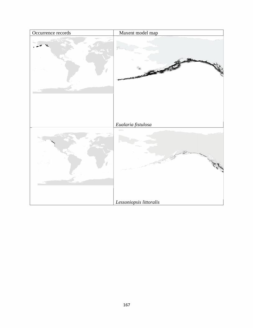
167

Occurrence records Maxent model map

Eualaria fistulosa

Lessoniopsis littoralis

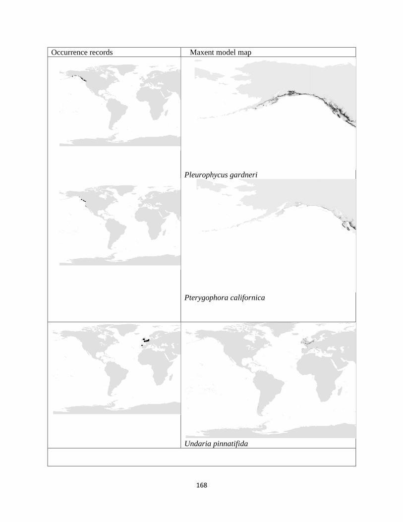
168

Occurrence records Maxent model map

Pleurophycus gardneri

Pterygophora californica

Undaria pinnatifida

169

Occurrence records Maxent model map Chordaceae

Chorda filum Laminariaceae

Laminaria abyssalis

170

Occurrence records Maxent model map

Laminaria brasiliensis

Laminaria digitata

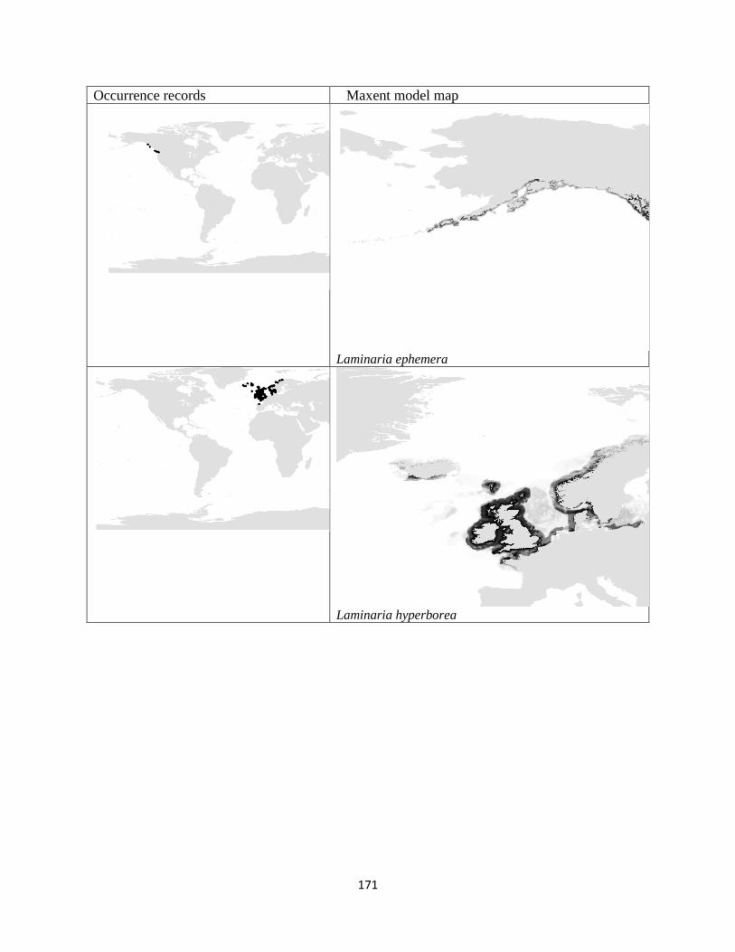
171

Occurrence records Maxent model map

Laminaria ephemera

Laminaria hyperborea

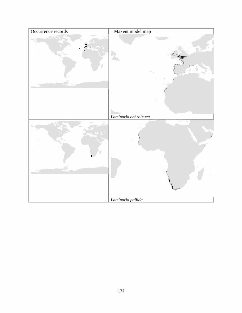
172

Occurrence records Maxent model map

Laminaria ochroleuca

Laminaria pallida

173

Occurrence records Maxent model map

Laminaria rodriguezii

Laminaria setchellii

174

Occurrence records Maxent model map

Laminaria sinclairii

Laminaria solidungula

Laminaria yezoensis

175

Occurrence records Maxent model map

Macrocystis pyrifera

Nereocystis luetkeana

Postelsia palmaeformis

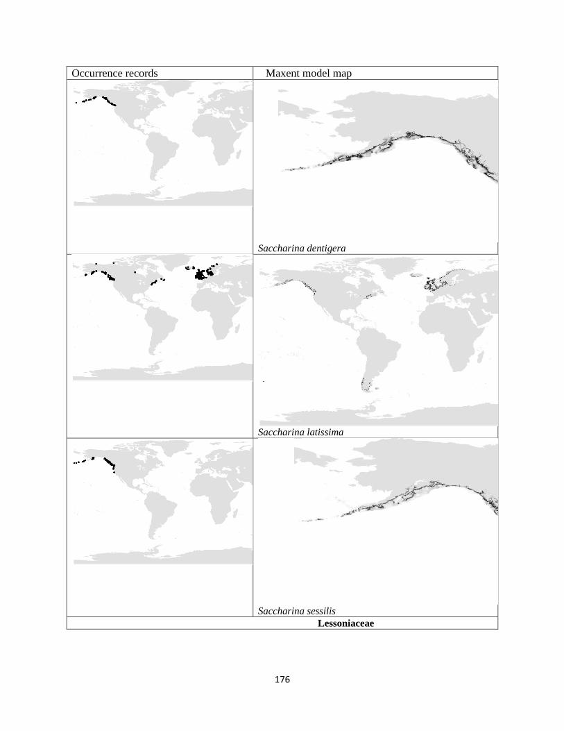
176

Occurrence records Maxent model map

Saccharina dentigera

Saccharina latissima

Saccharina sessilis

Lessoniaceae

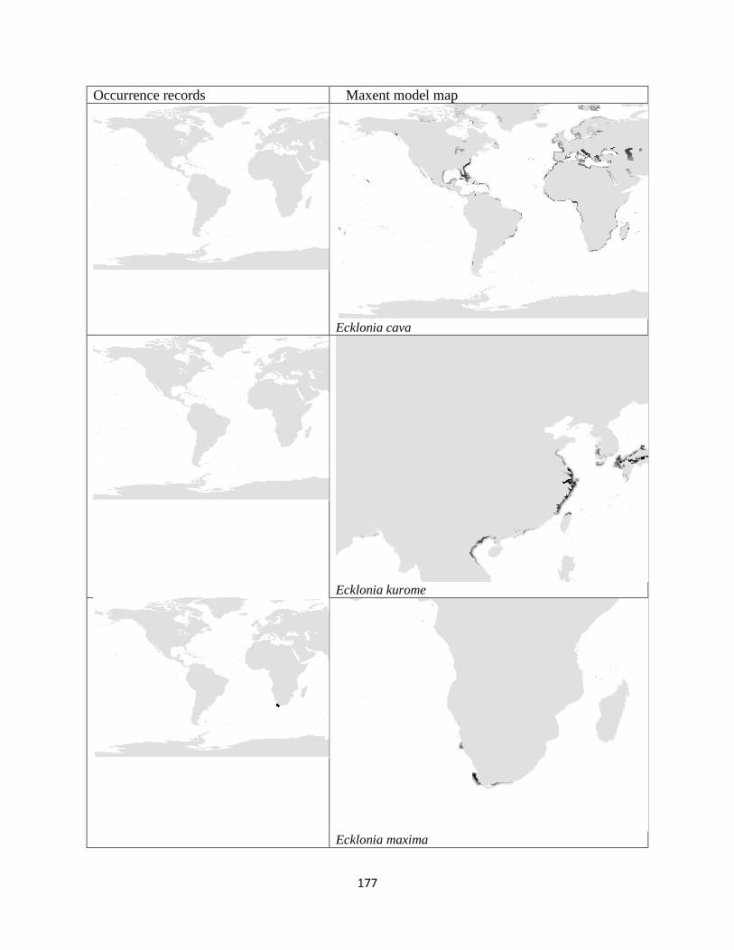
177

Occurrence records Maxent model map

Ecklonia cava

Ecklonia kurome

Ecklonia maxima

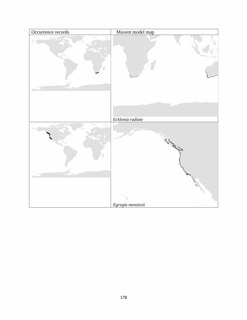
178

Occurrence records Maxent model map

Ecklonia radiate

Egregia menziesii

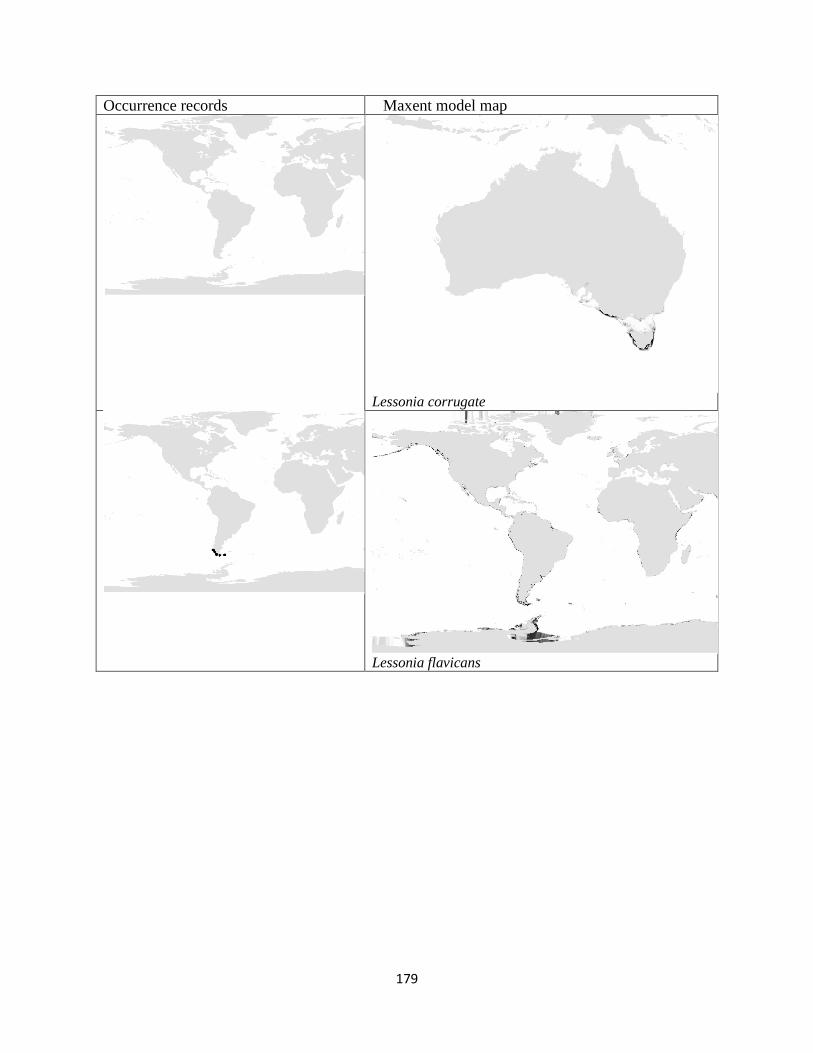
179

Occurrence records Maxent model map

Lessonia corrugate

Lessonia flavicans

180

Occurrence records Maxent model map

Lessonia variegate

b)

Occurrence localities MaxEnt Model map Genus

Agarum

181

Occurrence localities MaxEnt Model map

Costaria

Dictyoneuropsis

Alaria

182

Occurrence localities MaxEnt Model map

Eualaria

Lessoniopsis

Pleurophycus

183

Occurrence localities MaxEnt Model map

Pterygophora

Undaria

Chorda

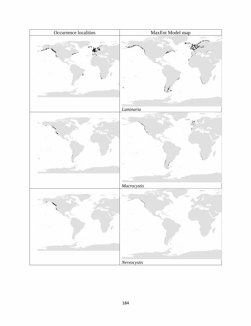
184

Occurrence localities MaxEnt Model map

Laminaria

Macrocystis

Nereocystis

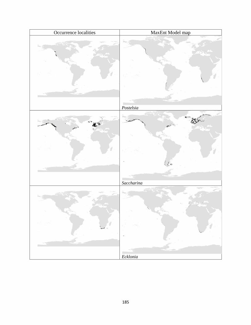
185

Occurrence localities MaxEnt Model map

Postelsia

Saccharina

Ecklonia

186

Occurrence localities MaxEnt Model map

Egregia

Lessonia

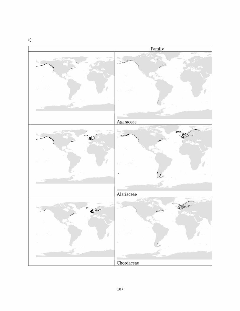
187

c)

Family

Agaraceae

Alariaceae

Chordaceae

188

Laminariaceae

Lessoniaceae

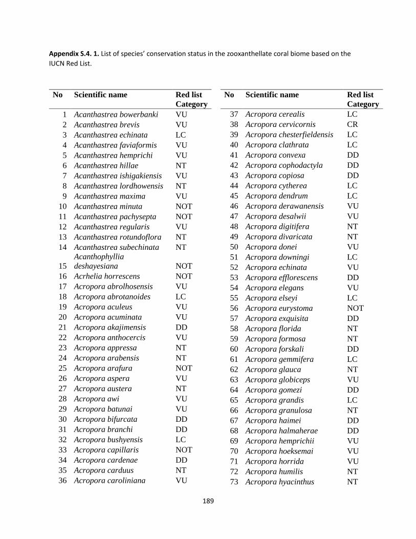
189

Appendix S.4. 1. List of species’ conservation status in the zooxanthellate coral biome based on the IUCN Red List.

No Scientific name Red list Category

1 Acanthastrea bowerbanki VU 2 Acanthastrea brevis VU 3 Acanthastrea echinata LC 4 Acanthastrea faviaformis VU 5 Acanthastrea hemprichi VU 6 Acanthastrea hillae NT 7 Acanthastrea ishigakiensis VU 8 Acanthastrea lordhowensis NT 9 Acanthastrea maxima VU

10 Acanthastrea minuta NOT 11 Acanthastrea pachysepta NOT 12 Acanthastrea regularis VU 13 Acanthastrea rotundoflora NT 14 Acanthastrea subechinata NT

15 Acanthophyllia deshayesiana NOT

16 Acrhelia horrescens NOT 17 Acropora abrolhosensis VU 18 Acropora abrotanoides LC 19 Acropora aculeus VU 20 Acropora acuminata VU 21 Acropora akajimensis DD 22 Acropora anthocercis VU 23 Acropora appressa NT 24 Acropora arabensis NT 25 Acropora arafura NOT 26 Acropora aspera VU 27 Acropora austera NT 28 Acropora awi VU 29 Acropora batunai VU 30 Acropora bifurcata DD 31 Acropora branchi DD 32 Acropora bushyensis LC 33 Acropora capillaris NOT 34 Acropora cardenae DD 35 Acropora carduus NT 36 Acropora caroliniana VU

No Scientific name Red list Category

37 Acropora cerealis LC 38 Acropora cervicornis CR 39 Acropora chesterfieldensis LC 40 Acropora clathrata LC 41 Acropora convexa DD 42 Acropora cophodactyla DD 43 Acropora copiosa DD 44 Acropora cytherea LC 45 Acropora dendrum LC 46 Acropora derawanensis VU 47 Acropora desalwii VU 48 Acropora digitifera NT 49 Acropora divaricata NT 50 Acropora donei VU 51 Acropora downingi LC 52 Acropora echinata VU 53 Acropora efflorescens DD 54 Acropora elegans VU 55 Acropora elseyi LC 56 Acropora eurystoma NOT 57 Acropora exquisita DD 58 Acropora florida NT 59 Acropora formosa NT 60 Acropora forskali DD 61 Acropora gemmifera LC 62 Acropora glauca NT 63 Acropora globiceps VU 64 Acropora gomezi DD 65 Acropora grandis LC 66 Acropora granulosa NT 67 Acropora haimei DD 68 Acropora halmaherae DD 69 Acropora hemprichii VU 70 Acropora hoeksemai VU 71 Acropora horrida VU 72 Acropora humilis NT 73 Acropora hyacinthus NT

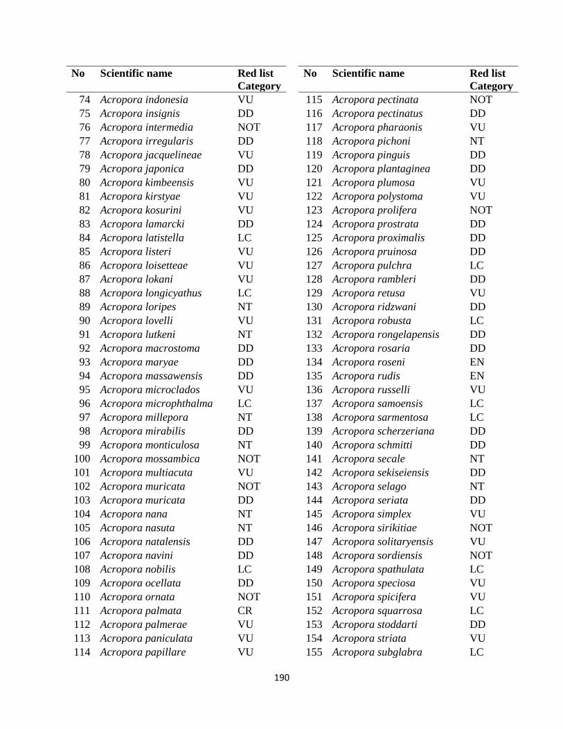
190

No Scientific name Red list Category

74 Acropora indonesia VU 75 Acropora insignis DD 76 Acropora intermedia NOT 77 Acropora irregularis DD 78 Acropora jacquelineae VU 79 Acropora japonica DD 80 Acropora kimbeensis VU 81 Acropora kirstyae VU 82 Acropora kosurini VU 83 Acropora lamarcki DD 84 Acropora latistella LC 85 Acropora listeri VU 86 Acropora loisetteae VU 87 Acropora lokani VU 88 Acropora longicyathus LC 89 Acropora loripes NT 90 Acropora lovelli VU 91 Acropora lutkeni NT 92 Acropora macrostoma DD 93 Acropora maryae DD 94 Acropora massawensis DD 95 Acropora microclados VU 96 Acropora microphthalma LC 97 Acropora millepora NT 98 Acropora mirabilis DD 99 Acropora monticulosa NT

100 Acropora mossambica NOT 101 Acropora multiacuta VU 102 Acropora muricata NOT 103 Acropora muricata DD 104 Acropora nana NT 105 Acropora nasuta NT 106 Acropora natalensis DD 107 Acropora navini DD 108 Acropora nobilis LC 109 Acropora ocellata DD 110 Acropora ornata NOT 111 Acropora palmata CR 112 Acropora palmerae VU 113 Acropora paniculata VU 114 Acropora papillare VU

No Scientific name Red list Category

115 Acropora pectinata NOT 116 Acropora pectinatus DD 117 Acropora pharaonis VU 118 Acropora pichoni NT 119 Acropora pinguis DD 120 Acropora plantaginea DD 121 Acropora plumosa VU 122 Acropora polystoma VU 123 Acropora prolifera NOT 124 Acropora prostrata DD 125 Acropora proximalis DD 126 Acropora pruinosa DD 127 Acropora pulchra LC 128 Acropora rambleri DD 129 Acropora retusa VU 130 Acropora ridzwani DD 131 Acropora robusta LC 132 Acropora rongelapensis DD 133 Acropora rosaria DD 134 Acropora roseni EN 135 Acropora rudis EN 136 Acropora russelli VU 137 Acropora samoensis LC 138 Acropora sarmentosa LC 139 Acropora scherzeriana DD 140 Acropora schmitti DD 141 Acropora secale NT 142 Acropora sekiseiensis DD 143 Acropora selago NT 144 Acropora seriata DD 145 Acropora simplex VU 146 Acropora sirikitiae NOT 147 Acropora solitaryensis VU 148 Acropora sordiensis NOT 149 Acropora spathulata LC 150 Acropora speciosa VU 151 Acropora spicifera VU 152 Acropora squarrosa LC 153 Acropora stoddarti DD 154 Acropora striata VU 155 Acropora subglabra LC

191

No Scientific name Red list Category

156 Acropora subulata LC 157 Acropora suharsonoi EN 158 Acropora sukarnoi DD 159 Acropora tenella VU 160 Acropora tenuis NT 161 Acropora teres DD 162 Acropora tizardi DD 163 Acropora torihalimeda DD 164 Acropora torresiana DD 165 Acropora tortuosa LC 166 Acropora tumida DD 167 Acropora turaki VU 168 Acropora valenciennesi LC 169 Acropora valida LC 170 Acropora valida LC 171 Acropora variabilis DD 172 Acropora variolosa LC 173 Acropora vaughani VU 174 Acropora verweyi VU 175 Acropora walindii VU 176 Acropora willisae VU 177 Acropora yongei LC 178 Agaricia agaricites LC 179 Agaricia fragilis DD 180 Agaricia grahamae LC 181 Agaricia humilis LC 182 Agaricia lamarcki VU 183 Agaricia tenuifolia NT 184 Agaricia undata DD 185 Alveopora allingi VU 186 Alveopora catalai NT 187 Alveopora daedalea VU 188 Alveopora excelsa EN 189 Alveopora fenestrata VU 190 Alveopora gigas VU 191 Alveopora japonica VU 192 Alveopora marionensis VU 193 Alveopora minuta EN 194 Alveopora ocellata DD 195 Alveopora spongiosa NT 196 Alveopora superficialis NOT

No Scientific name Red list Category

197 Alveopora tizardi LC 198 Alveopora verrilliana VU 199 Alveopora viridis NT 200 Anomastraea irregularis NOT 201 Anomastraea tayamai NOT 202 Anomastrea irregularis NOT 203 Astreopora acroporina NOT 204 Astreopora cenderawasih NOT 205 Astreopora cucullata VU 206 Astreopora eliptica DD 207 Astreopora expansa NT 208 Astreopora explanata NOT 209 Astreopora gracilis LC 210 Astreopora incrustans VU 211 Astreopora lambertsi NOT 212 Astreopora listeri VU 213 Astreopora listeri LC 214 Astreopora macrostoma NT 215 Astreopora monteporina NOT 216 Astreopora moretonensis VU 217 Astreopora myriophthalma LC 218 Astreopora ocellata LC 219 Astreopora randalli LC 220 Astreopora suggesta LC 221 Astreopora tabulata NOT 222 Australomussa rowleyensis NT 223 Blastomussa loyae NOT 224 Blastomussa merleti LC 225 Blastomussa simplicitexta NOT 226 Blastomussa vivida NOT 227 Blastomussa wellsi NT 228 Boninastrea boninensis DD 229 Cantharellus doederleini LC 230 Cantharellus jebbi LC 231 Cantharellus noumeae EN 232 Cladocora arbuscula LC 233 Cladocora caespitosa EN 234 Cladocora debilis DD 235 Cladocora pacifica NOT 236 Coeloseris mayeri LC 237 Coscinaraea columna LC

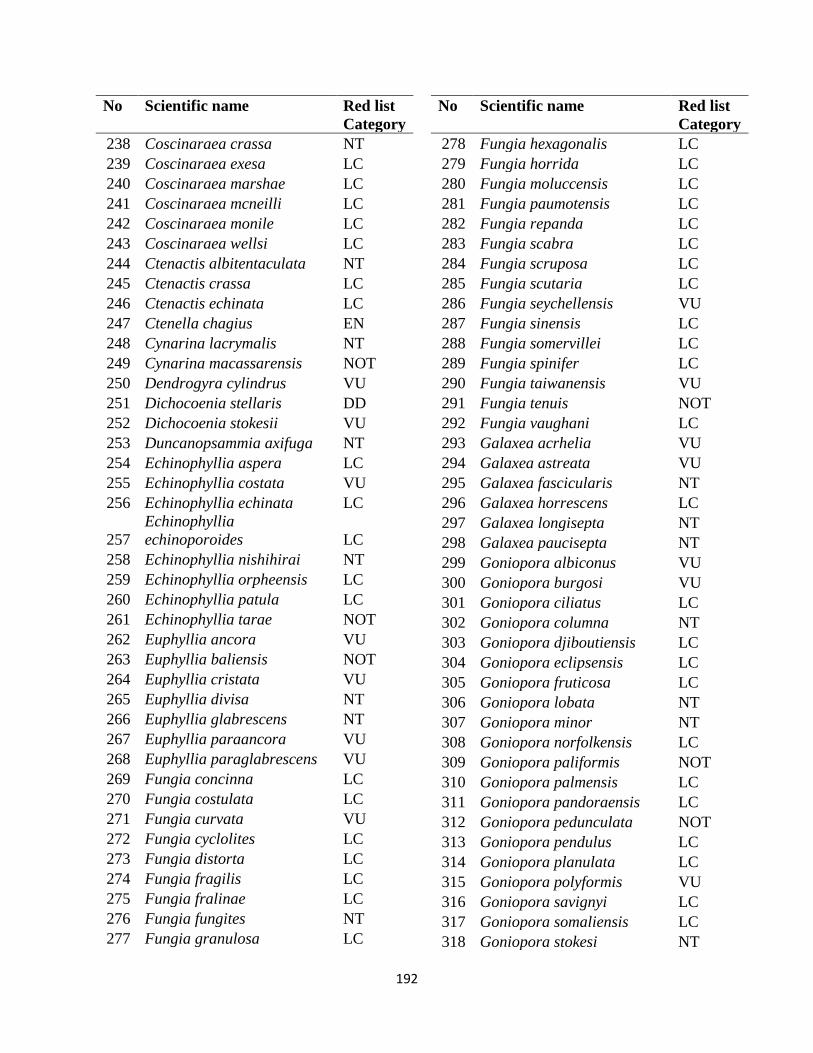
192

No Scientific name Red list Category

238 Coscinaraea crassa NT 239 Coscinaraea exesa LC 240 Coscinaraea marshae LC 241 Coscinaraea mcneilli LC 242 Coscinaraea monile LC 243 Coscinaraea wellsi LC 244 Ctenactis albitentaculata NT 245 Ctenactis crassa LC 246 Ctenactis echinata LC 247 Ctenella chagius EN 248 Cynarina lacrymalis NT 249 Cynarina macassarensis NOT 250 Dendrogyra cylindrus VU 251 Dichocoenia stellaris DD 252 Dichocoenia stokesii VU 253 Duncanopsammia axifuga NT 254 Echinophyllia aspera LC 255 Echinophyllia costata VU 256 Echinophyllia echinata LC

257 Echinophyllia echinoporoides LC

258 Echinophyllia nishihirai NT 259 Echinophyllia orpheensis LC 260 Echinophyllia patula LC 261 Echinophyllia tarae NOT 262 Euphyllia ancora VU 263 Euphyllia baliensis NOT 264 Euphyllia cristata VU 265 Euphyllia divisa NT 266 Euphyllia glabrescens NT 267 Euphyllia paraancora VU 268 Euphyllia paraglabrescens VU 269 Fungia concinna LC 270 Fungia costulata LC 271 Fungia curvata VU 272 Fungia cyclolites LC 273 Fungia distorta LC 274 Fungia fragilis LC 275 Fungia fralinae LC 276 Fungia fungites NT 277 Fungia granulosa LC

No Scientific name Red list Category

278 Fungia hexagonalis LC 279 Fungia horrida LC 280 Fungia moluccensis LC 281 Fungia paumotensis LC 282 Fungia repanda LC 283 Fungia scabra LC 284 Fungia scruposa LC 285 Fungia scutaria LC 286 Fungia seychellensis VU 287 Fungia sinensis LC 288 Fungia somervillei LC 289 Fungia spinifer LC 290 Fungia taiwanensis VU 291 Fungia tenuis NOT 292 Fungia vaughani LC 293 Galaxea acrhelia VU 294 Galaxea astreata VU 295 Galaxea fascicularis NT 296 Galaxea horrescens LC 297 Galaxea longisepta NT 298 Galaxea paucisepta NT 299 Goniopora albiconus VU 300 Goniopora burgosi VU 301 Goniopora ciliatus LC 302 Goniopora columna NT 303 Goniopora djiboutiensis LC 304 Goniopora eclipsensis LC 305 Goniopora fruticosa LC 306 Goniopora lobata NT 307 Goniopora minor NT 308 Goniopora norfolkensis LC 309 Goniopora paliformis NOT 310 Goniopora palmensis LC 311 Goniopora pandoraensis LC 312 Goniopora pedunculata NOT 313 Goniopora pendulus LC 314 Goniopora planulata LC 315 Goniopora polyformis VU 316 Goniopora savignyi LC 317 Goniopora somaliensis LC 318 Goniopora stokesi NT

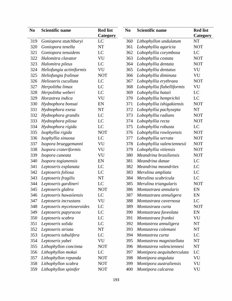
193

No Scientific name Red list Category

319 Goniopora stutchburyi LC 320 Goniopora tenella NT 321 Goniopora tenuidens LC 322 Halomitra clavator VU 323 Halomitra pileus LC 324 Heliofungia actiniformis VU 325 Heliofungia fralinae NOT 326 Helioseris cucullata LC 327 Herpolitha limax LC 328 Herpolitha weberi LC 329 Horastrea indica VU 330 Hydnophora bonsai EN 331 Hydnophora exesa NT 332 Hydnophora grandis LC 333 Hydnophora pilosa LC 334 Hydnophora rigida LC 335 Isophyllia rigida NOT 336 Isophyllia sinuosa LC 337 Isopora brueggemanni VU 338 Isopora crateriformis VU 339 Isopora cuneata VU 340 Isopora togianensis EN 341 Leptoseris explanata LC 342 Leptoseris foliosa LC 343 Leptoseris fragilis NT 344 Leptoseris gardineri LC 345 Leptoseris glabra NOT 346 Leptoseris hawaiiensis LC 347 Leptoseris incrustans VU 348 Leptoseris mycetoseroides LC 349 Leptoseris papyracea LC 350 Leptoseris scabra LC 351 Leptoseris solida LC 352 Leptoseris striata NT 353 Leptoseris tubulifera LC 354 Leptoseris yabei VU 355 Lithophyllon concinna NOT 356 Lithophyllon mokai LC 357 Lithophyllon repanda NOT 358 Lithophyllon scabra NOT 359 Lithophyllon spinifer NOT

No Scientific name Red list Category

360 Lithophyllon undulatum NT 361 Lobophyllia agaricia NOT 362 Lobophyllia corymbosa LC 363 Lobophyllia costata NOT 364 Lobophyllia dentata NOT 365 Lobophyllia dentatus VU 366 Lobophyllia diminuta VU 367 Lobophyllia erythraea NOT 368 Lobophyllia flabelliformis VU 369 Lobophyllia hataii LC 370 Lobophyllia hemprichii LC 371 Lobophyllia ishigakiensis NOT 372 Lobophyllia pachysepta NT 373 Lobophyllia radians NOT 374 Lobophyllia recta NOT 375 Lobophyllia robusta LC 376 Lobophyllia rowleyensis NOT 377 Lobophyllia serrata NOT 378 Lobophyllia valenciennesii NOT 379 Lobophyllia vitiensis NOT 380 Meandrina brasiliensis NOT 381 Meandrina danae LC 382 Meandrina meandrites LC 383 Merulina ampliata LC 384 Merulina scabricula LC 385 Merulina triangularis NOT 386 Montastraea annularis EN 387 Montastraea annuligera EN 388 Montastraea cavernosa LC 389 Montastraea curta NOT 390 Montastraea faveolata EN 391 Montastraea franksi VU 392 Montastrea annuligera NT 393 Montastrea colemani NT 394 Montastrea curta LC 395 Montastrea magnistellata NT 396 Montastrea valenciennesi NT 397 Montipora aequituberculata LC 398 Montipora angulata VU 399 Montipora australiensis VU 400 Montipora calcarea VU

194

No Scientific name Red list Category

401 Montipora caliculata VU 402 Montipora capitata NT 403 Montipora capricornis VU 404 Montipora cebuensis VU 405 Montipora circumvallata LC 406 Montipora cocosensis VU 407 Montipora corbettensis NOT

408 Montipora crassituberculata VU

409 Montipora cryptus NT 410 Montipora danae LC 411 Montipora delicatula VU 412 Montipora digitata LC 413 Montipora efflorescens NT 414 Montipora effusa NT 415 Montipora flabellata VU 416 Montipora florida VU 417 Montipora floweri LC 418 Montipora foliosa NT 419 Montipora foveolata NT 420 Montipora friabilis VU 421 Montipora gaimardi VU 422 Montipora grisea LC 423 Montipora hirsuta NT 424 Montipora hispida LC 425 Montipora hoffmeisteri LC 426 Montipora incrassata NT 427 Montipora informis LC 428 Montipora lobulata VU 429 Montipora mactanensis VU 430 Montipora meandrina VU 431 Montipora millepora LC 432 Montipora mollis LC 433 Montipora monasteriata LC 434 Montipora nodosa NT 435 Montipora patula VU 436 Montipora peltiformis NT 437 Montipora porites NT 438 Montipora samarensis VU 439 Montipora saudii NT 440 Montipora spongiosa LC

No Scientific name Red list Category

441 Montipora spongodes LC 442 Montipora spumosa LC 443 Montipora stellata LC 444 Montipora stilosa VU 445 Montipora tuberculosa LC 446 Montipora turgescens LC 447 Montipora turtlensis VU 448 Montipora undata NT 449 Montipora venosa NT 450 Montipora verrilli DD 451 Montipora verrucosa LC 452 Montipora vietnamensis VU 453 Moseleya latistellata VU 454 Mussa angulosa LC 455 Mussismilia braziliensis DD 456 Mussismilia harttii DD 457 Mussismilia hispida DD 458 Mycedium elephantotus LC 459 Mycedium mancaoi LC 460 Mycedium robokaki LC 461 Mycedium steeni VU 462 Mycedium umbra LC 463 Mycetophyllia aliciae LC 464 Mycetophyllia danaana LC 465 Mycetophyllia ferox VU 466 Mycetophyllia lamarckiana LC 467 Mycetophyllia reesi DD 468 Oulastrea crispata LC 469 Oxypora crassispinosa LC 470 Oxypora glabra LC 471 Oxypora lacera NOT 472 Pachyseris foliosa LC 473 Pachyseris gemmae NT 474 Pachyseris rugosa VU 475 Pachyseris speciosa LC 476 Palauastrea ramosa NT 477 Paraclavarina triangularis NT 478 Pavona bipartita VU 479 Pavona cactus VU 480 Pavona chiriquiensis LC 481 Pavona clavus LC

195

No Scientific name Red list Category

482 Pavona danai VU 483 Pavona decussata VU 484 Pavona diffluens VU 485 Pavona divaricata NOT 486 Pavona duerdeni LC 487 Pavona explanulata LC 488 Pavona frondifera LC 489 Pavona gigantea LC 490 Pavona maldivensis LC 491 Pavona minuta NT 492 Pavona varians LC 493 Pavona venosa VU 494 Pectinia africanus VU 495 Pectinia alcicornis VU 496 Pectinia lactuca VU 497 Pectinia paeonia NT 498 Pectinia teres NOT 499 Physogyra lichtensteini VU 500 Physophyllia ayleni NOT 501 Platygyra acuta NT 502 Platygyra carnosa NOT 503 Platygyra contorta LC 504 Platygyra crosslandi NT 505 Platygyra daedalea LC 506 Platygyra lamellina NT 507 Platygyra pini LC 508 Platygyra ryukyuensis NT 509 Platygyra sinensis LC 510 Platygyra verweyi NT 511 Plesiastrea versipora LC 512 Pocillopora acuta NOT 513 Pocillopora aliciae NOT 514 Pocillopora ankeli VU 515 Pocillopora brevicornis NOT 516 Pocillopora capitata LC 517 Pocillopora damicornis LC 518 Pocillopora danae VU 519 Pocillopora effusa NOT 520 Pocillopora elegans VU 521 Pocillopora eydouxi NT 522 Pocillopora grandis EN

No Scientific name Red list Category

523 Pocillopora indiania VU 524 Pocillopora inflata VU 525 Pocillopora ligulata LC 526 Pocillopora meandrina LC 527 Pocillopora molokensis DD 528 Pocillopora verrucosa LC 529 Pocillopora woodjonesi LC 530 Pocillopora zelli LC 531 Podabacia crustacea LC 532 Podabacia motuporensis NT 533 Polyphyllia novaehiberniae NT 534 Polyphyllia talpina LC 535 Porites annae NT 536 Porites aranetai VU 537 Porites astreoides LC 538 Porites attenuata VU 539 Porites australiensis LC 540 Porites baueri DD 541 Porites bernardi LC 542 Porites branneri NT 543 Porites brighami LC 544 Porites colonensis DD 545 Porites columnaris LC 546 Porites compressa LC 547 Porites cumulatus VU 548 Porites cylindrica NT 549 Porites deformis NT 550 Porites densa NT 551 Porites divaricata LC 552 Porites duerdeni LC 553 Porites echinulata NT 554 Porites eridani EN 555 Porites evermanni DD 556 Porites flavus DD 557 Porites furcata LC 558 Porites harrisoni NT 559 Porites hawaiiensis NOT 560 Porites heronensis NOT 561 Porites horizontalata VU 562 Porites latistellata LC 563 Porites lichen LC

196

No Scientific name Red list Category

564 Porites lobata NT 565 Porites lutea LC 566 Porites mayeri LC 567 Porites monticulosa LC 568 Porites murrayensis NT 569 Porites negrosensis NT 570 Porites nigrescens VU 571 Porites nodifera LC 572 Porites panamensis LC 573 Porites porites LC 574 Porites profundus LC 575 Porites pukoensis LC 576 Porites rus LC 577 Porites solida LC 578 Porites somaliensis NT 579 Porites stephensoni NT 580 Porites superfusa LC 581 Porites sverdrupi VU 582 Porites vaughani LC 583 Psammocora albopicta DD 584 Psammocora contigua NT 585 Psammocora digitata NT 586 Psammocora haimeana LC 587 Psammocora haimiana LC 588 Psammocora nierstraszi LC 589 Psammocora obtusangula NT 590 Psammocora profundacella LC 591 Psammocora stellata VU 592 Psammocora superficialis LC 593 Psammocora vaughani NT 594 Pseudosiderastrea tayamai NOT 595 Pseudosiderastrea tayami NT 596 Sandalolitha dentata LC 597 Sandalolitha robusta LC 598 Scapophyllia cylindrica LC 599 Scolymia australis LC 600 Scolymia cubensis LC 601 Scolymia lacera LC 602 Scolymia vitiensis NT 603 Scolymia wellsii NOT 604 Seriatopora aculeata VU

No Scientific name Red list Category

605 Seriatopora angulata VU 606 Seriatopora caliendrum NT 607 Seriatopora dentritica NOT 608 Seriatopora guttatus NOT 609 Seriatopora hystrix LC 610 Seriatopora stellata NT 611 Siderastrea radians LC 612 Siderastrea savignyana LC 613 Siderastrea siderea LC 614 Siderastrea stellata DD 615 Solenastrea bournoni LC 616 Solenastrea hyades LC 617 Stylaraea punctata DD 618 Stylocoeniella armata LC 619 Stylocoeniella guentheri LC 620 Stylophora danae LC

621 Stylophora madagascarensis EN

622 Stylophora mamillata LC 623 Stylophora pistillata NT 624 Stylophora prostrata NT 625 Stylophora subseriata LC 626 Stylophora wellsi NT 627 Symphyllia agaricia LC 628 Symphyllia radians LC 629 Symphyllia recta LC 630 Symphyllia valenciennesii LC 631 Symphyllia wilsoni LC 632 Trachyphyllia geoffroyi NT 633 Zoopilus echinatus LC

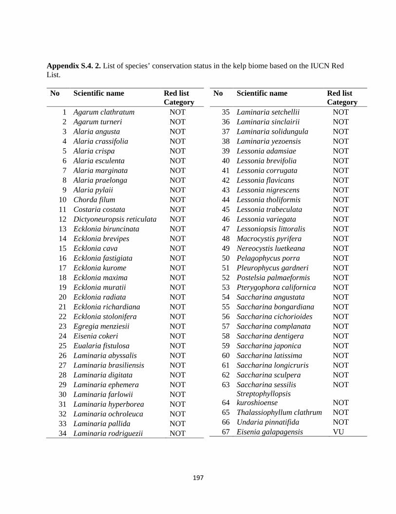
197

Appendix S.4. 2. List of species’ conservation status in the kelp biome based on the IUCN Red List. No Scientific name Red list

Category 1 Agarum clathratum NOT 2 Agarum turneri NOT 3 Alaria angusta NOT 4 Alaria crassifolia NOT 5 Alaria crispa NOT 6 Alaria esculenta NOT 7 Alaria marginata NOT 8 Alaria praelonga NOT 9 Alaria pylaii NOT

10 Chorda filum NOT 11 Costaria costata NOT 12 Dictyoneuropsis reticulata NOT 13 Ecklonia biruncinata NOT 14 Ecklonia brevipes NOT 15 Ecklonia cava NOT 16 Ecklonia fastigiata NOT 17 Ecklonia kurome NOT 18 Ecklonia maxima NOT 19 Ecklonia muratii NOT 20 Ecklonia radiata NOT 21 Ecklonia richardiana NOT 22 Ecklonia stolonifera NOT 23 Egregia menziesii NOT 24 Eisenia cokeri NOT 25 Eualaria fistulosa NOT 26 Laminaria abyssalis NOT 27 Laminaria brasiliensis NOT 28 Laminaria digitata NOT 29 Laminaria ephemera NOT 30 Laminaria farlowii NOT 31 Laminaria hyperborea NOT 32 Laminaria ochroleuca NOT 33 Laminaria pallida NOT 34 Laminaria rodriguezii NOT

No Scientific name Red list Category

35 Laminaria setchellii NOT 36 Laminaria sinclairii NOT 37 Laminaria solidungula NOT 38 Laminaria yezoensis NOT 39 Lessonia adamsiae NOT 40 Lessonia brevifolia NOT 41 Lessonia corrugata NOT 42 Lessonia flavicans NOT 43 Lessonia nigrescens NOT 44 Lessonia tholiformis NOT 45 Lessonia trabeculata NOT 46 Lessonia variegata NOT 47 Lessoniopsis littoralis NOT 48 Macrocystis pyrifera NOT 49 Nereocystis luetkeana NOT 50 Pelagophycus porra NOT 51 Pleurophycus gardneri NOT 52 Postelsia palmaeformis NOT 53 Pterygophora californica NOT 54 Saccharina angustata NOT 55 Saccharina bongardiana NOT 56 Saccharina cichorioides NOT 57 Saccharina complanata NOT 58 Saccharina dentigera NOT 59 Saccharina japonica NOT 60 Saccharina latissima NOT 61 Saccharina longicruris NOT 62 Saccharina sculpera NOT 63 Saccharina sessilis NOT

64 Streptophyllopsis kuroshioense NOT

65 Thalassiophyllum clathrum NOT 66 Undaria pinnatifida NOT 67 Eisenia galapagensis VU

198

Appendix S.4. 3. List of species’ conservation status in the mangrove biome based on the IUCN Red List. No Scientific name Red list

Category 1 Acanthus ebracteatus LC 2 Acanthus ilicifolius LC 3 Acrostichum aureum LC 4 Acrostichum danaeifolium LC 5 Acrostichum speciosum LC 6 Aegialitis annulata LC 7 Aegialitis rotundifolia NT 8 Aegiceras corniculatum LC 9 Aegiceras floridum NT

10 Aglaia cucullata DD 11 Avicennia alba LC 12 Avicennia bicolor VU 13 Avicennia germinans LC 14 Avicennia integra VU 15 Avicennia marina LC 16 Avicennia officinalis LC 17 Avicennia schaueriana LC 18 Bruguiera cylindrica LC 19 Bruguiera exaristata LC 20 Bruguiera gymnorhiza LC 21 Bruguiera hainesii CR 22 Bruguiera parviflora LC 23 Bruguiera rhynchopetala NOT 24 Bruguiera sexangula LC

25 Camptostemon philippinensis EN

26 Camptostemon schultzii LC 27 Ceriops australis LC 28 Ceriops decandra NT 29 Ceriops tagal LC 30 Cynometra iripa LC 31 Dolichandrone spathacea LC 32 Excoecaria agallocha LC

No Scientific name Red list Category

33 Excoecaria indica DD 34 Heritiera fomes EN 35 Heritiera globosa EN 36 Heritiera littoralis LC 37 Kandelia candel LC 38 Kandelia obovata LC 39 Laguncularia racemosa LC 40 Lumnitzera littorea LC 41 Lumnitzera racemosa LC 42 Mora oleifera VU 43 Nypa fruticans LC 44 Osbornia octodonta LC 45 Pelliciera rhizophorae VU 46 Pemphis acidula Forst. LC 47 Rhizophora harrisonii NOT 48 Rhizophora lamarckii NOT 49 Rhizophora mangle LC 50 Rhizophora mucronata LC 51 Rhizophora racemosa LC 52 Rhizophora samoensis NT 53 Rhizophora stylosa LC 54 Scyphiphora hydrophylacea LC 55 Sonneratia alba LC 56 Sonneratia apetala LC 57 Sonneratia caseolaris LC 58 Sonneratia griffithii CR 59 Sonneratia gulngai NOT 60 Sonneratia lanceolata LC 61 Sonneratia ovata NT 62 Tabebuia palustris VU 63 Xylocarpus granatum LC 64 Xylocarpus moluccensis LC

199

Appendix S.4. 4. List of species’ conservation status in the mangrove biome based on the IUCN Red List.

No Scientific name Red list Category

1 Amphibolis antarctica LC 2 Amphibolis griffithii LC 3 Cymodocea angustata LC 4 Cymodocea nodosa LC 5 Cymodocea rotundata LC 6 Cymodocea serrulata LC 7 Enhalus acoroides LC 8 Halodule beaudettei DD 9 Halodule emarginata DD

10 Halodule pinifolia LC 11 Halodule uninervis LC 12 Halodule wrightii LC 13 Halophila australis LC 14 Halophila baillonis NOT 15 Halophila beccarii VU 16 Halophila capricorni LC 17 Halophila decipiens LC 18 Halophila engelmannii NOT 19 Halophila hawaiiana VU 20 Halophila johnsonii LC 21 Halophila minor LC 22 Halophila nipponica NT 23 Halophila ovalis LC 24 Halophila ovata LC 25 Halophila spinulosa LC 26 Halophila stipulacea LC 27 Halophila tricostata LC 28 Phyllospadix iwatensis VU 29 Phyllospadix japonicus EN 30 Phyllospadix scouleri LC 31 Phyllospadix serrulatus LC 32 Phyllospadix torreyi LC 33 Posidonia angustifolia LC 34 Posidonia australis NT 35 Posidonia coriacea LC 36 Posidonia denhartogii LC 37 Posidonia kirkmanii LC

No Scientific name Red list Category

38 Posidonia oceanica LC 39 Posidonia ostenfeldii LC 40 Posidonia robertsoniae LC 41 Posidonia sinuosa LC 42 Syringodium filiforme LC 43 Syringodium isoetifolium LC 44 Thalassia hemprichii LC 45 Thalassia testudinum LC 46 Thalassodendron ciliatum LC

47 Thalassodendron pachyrhizum LC

48 Zostera asiatica NT 49 Zostera caespitosa VU 50 Zostera capensis VU 51 Zostera capricorni LC 52 Zostera caulescens NT 53 Zostera chilensis EN 54 Zostera japonica LC 55 Zostera marina LC 56 Zostera muelleri LC 57 Zostera nigricaulis LC 58 Zostera noltii LC 59 Zostera polychlamys LC 60 Zostera tasmanica LC

200

Appendix S.5. 1. Projected change of the global distribution of (a) seagrass, (b) kelp, (c) zooxanthellate coral, and (d) mangrove biomes by 2100. Red areas are where the biome is predicted to increase its area covered, black where no change is projected, and blue where the biome is projected to decline.

(a)

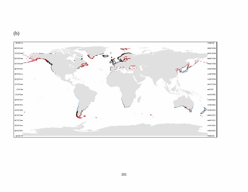
201

(b)

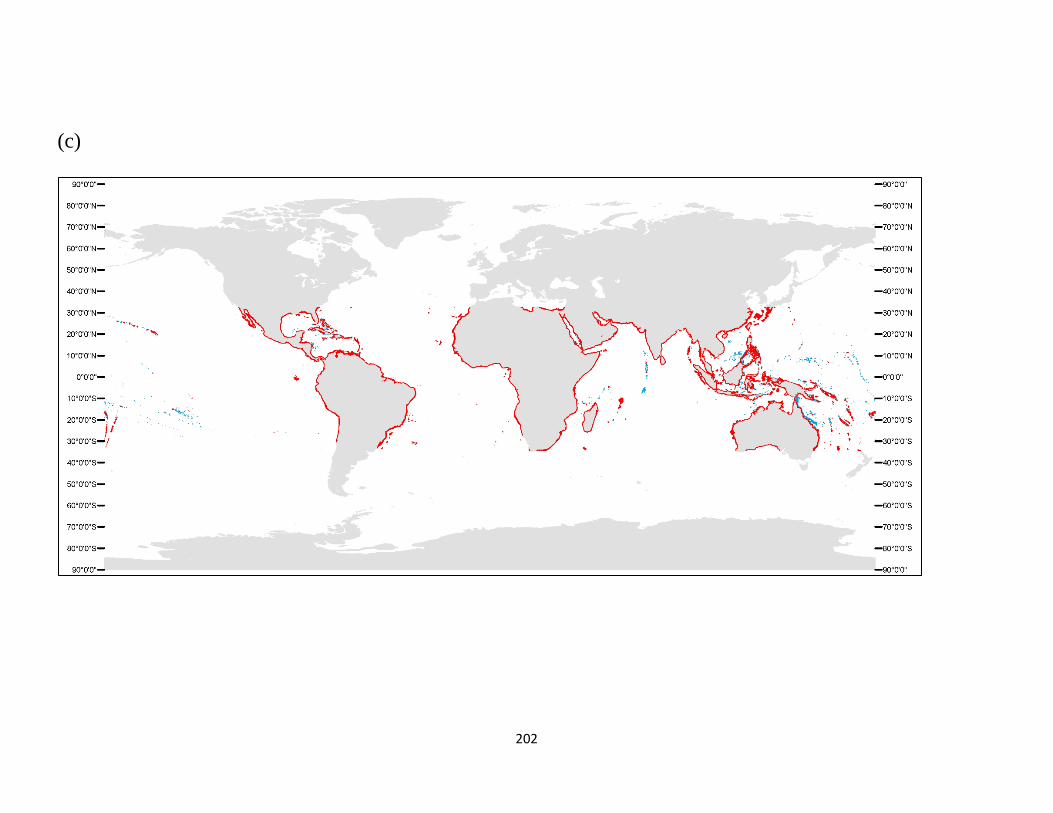
202

(c)

203

(d)

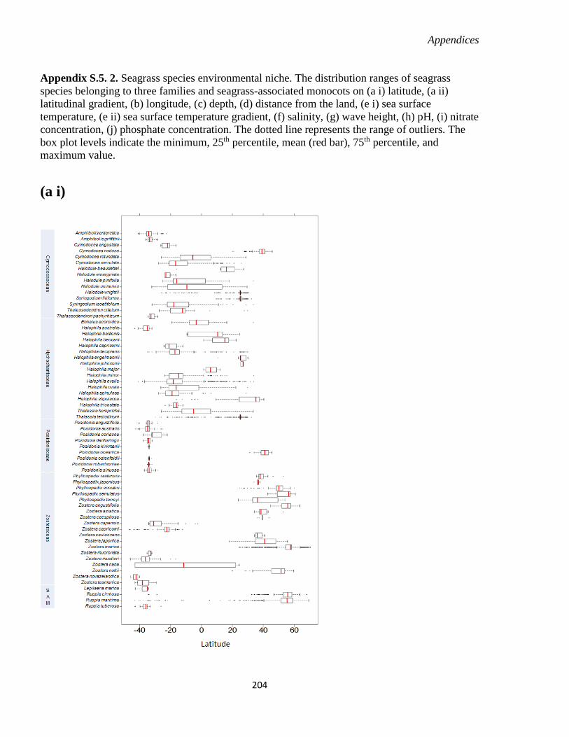
Appendices

204

Appendix S.5. 2. Seagrass species environmental niche. The distribution ranges of seagrass species belonging to three families and seagrass-associated monocots on (a i) latitude, (a ii) latitudinal gradient, (b) longitude, (c) depth, (d) distance from the land, (e i) sea surface temperature, (e ii) sea surface temperature gradient, (f) salinity, (g) wave height, (h) pH, (i) nitrate concentration, (j) phosphate concentration. The dotted line represents the range of outliers. The box plot levels indicate the minimum, 25th percentile, mean (red bar), 75th percentile, and maximum value.

(a i)

Appendices

205

(a ii)

Appendices

206

(b)

Appendices

207

(c)

Appendices

208

(d)

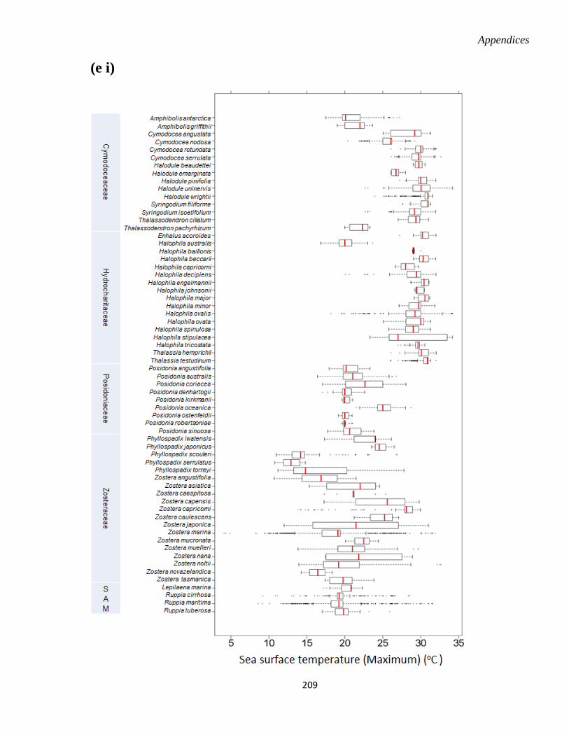
Appendices

209

(e i)

Appendices

210

(e ii)

Appendices

211

(f)

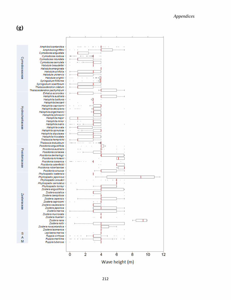
Appendices

212

(g)

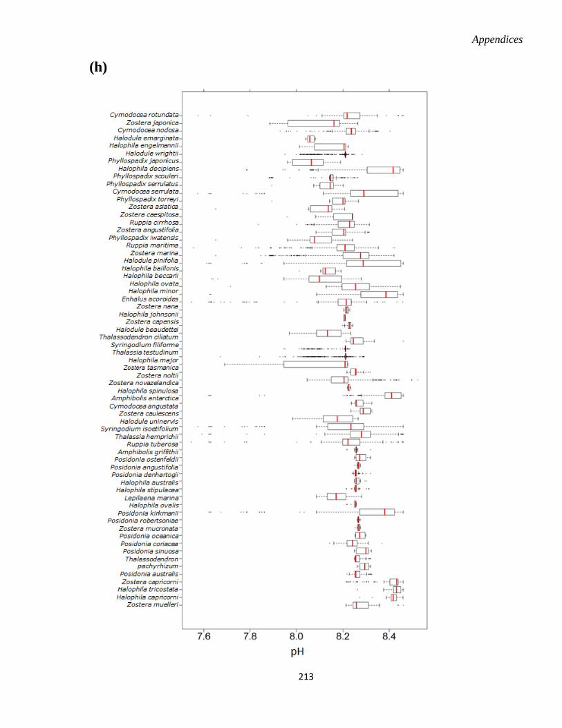
Appendices

213

(h)

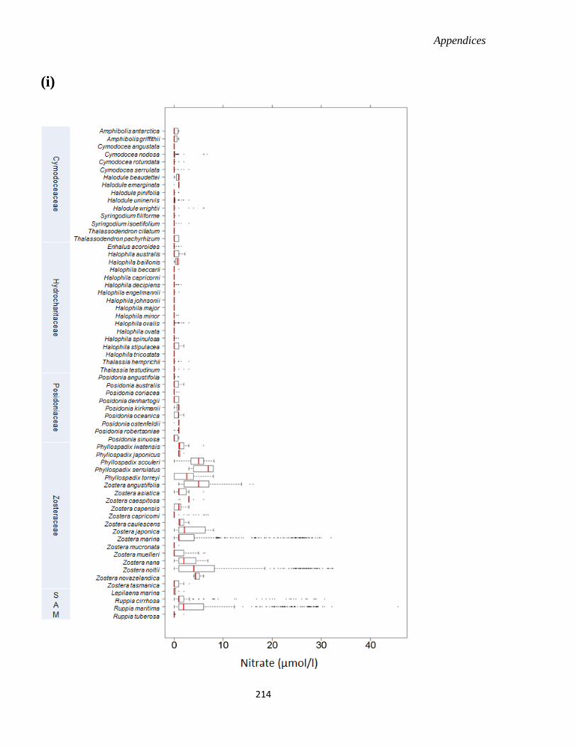
Appendices

214

(i)

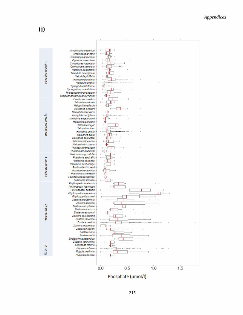
Appendices

215

(j)

Chapter 7

Bibliography

Bibliography

224

7 Bibliography

Allègue, L., Zidi, M., Sghaier, S. (2014). Mechanical properties of Posidonia oceanica fibers reinforced cement. Journal of Composite Materials, 49(5), 509-517.

Allen, J.R.L. (1992). Saltmarshes. Morphodynamics, in: Allen J.R.L. Pye, K. (Eds) Conservation and Engineering Significance, Cambridge University Press, Cambridge, UK.

Alongi D.M. (2018). Kelp Forests. In: Blue Carbon. Springer Briefs in Climate Studies. Springer, Cham.

Alongi, D. (2009). The Energetics of Mangrove Forests, Springer. Alongi, D.M. (2012). Carbon sequestration in mangrove forests. Carbon Management, 3(3), 313-

322. Alongi, D.M. (2018b). Impact of global change on nutrient dynamics in mangrove forests.

Forests, 9(10), 596. Alvain, S., Moulin, C., Dandonneau, Y., et al. (2008). Seasonal distribution and succession of

dominant phytoplankton groups in the global ocean: A satellite view. Global Biogeochemical Cycles, 22(3), n/a. doi:10.1029/2007GB003154

Arenas, F., Fernandez, C. (2000). Size structure and dynamics in a population of Sargassum muticum (Phaeophyceae). Journal of. Phycology, 36, 1012-1020. doi: 10.1046/j.1529-8817.2000.99235.x

Asaad, I., Lundquist, C.J., Erdmann, M.V., et al. (2018). Ecological criteria to identify areas for biodiversity conservation. Biological Conservation, 213, Part B, 309-316. https://doi.org/10.1016/j.biocon.2016.10.007.

Assis, J., Lucas, A.V., Barbara, I., Serrãoa E.A. (2016). Future climate change is predicted to shift long-term persistence zones in the cold-temperate kelp Laminaria hyperborea. Marine Environmental Research, 113, 174-182. https://doi.org/10.1016/j.marenvres.2015.11.005.

Bailey, R. G. (1998). Ecoregions: The Ecosystem Geography of the Oceans and Continents (2nd Ed). Springer, New York, USA.

Bandaranayake, W.M. (1998). Traditional and medicinal uses of mangroves. Mangroves and Salt Marshes, 2(3), 133–148.

Barbier, E. B., Koch, E. W., Silliman, B. R., et al. (2008). Coastal ecosystem-based management with nonlinear ecological functions and values. Science, 319(5861), 321-323. doi:10.1126/science.1150349

Bartsch, I., Paar, M., Fredriksen, S., et al. (2016). Changes in kelp forest biomass and depth distribution in Kongsfjorden, Svalbard, between 1996–1998 and 2012–2014 reflect Arctic warming. Polar Biology, 39, 2021-2036.

Basher, Z, Bowden, D.A., Costello, M.J., 2014c. GMED: Global Marine Environment Datasets for environment visualization and species distribution modeling. Earth Syst. Sci. Data (ESSD-2018-64) (In-Review)

Basher, Z., Bowden, D. A., Costello, M. J. (2014a). Diversity and distribution of deep-sea shrimps in the Ross Sea region of Antarctica. PLoS ONE, 9, e103195, doi:10.1371/journal.pone.0103195

Basher, Z., Bowden, D.A., Costello, M.J. (2014b). Global Marine Environment Datasets (GMED). WorldWide Web electronic publication. Version 1.0 (Rev.01.2014), accessed at. http://gmed.auckland.ac.nz.

Bibliography

225

Basher, Z., Bowden, D.A., Costello, M.J., (2018). GMED: Global Marine Environment Datasets for environment visualization and species distribution modelling. Earth Syst. Sci. Data (ESSD-2018-64). https://doi.org/10.5194/essd-2018-64

Beck, M. W., Heck, K. L., Able, K.W., et al. (2001). The identification, conservation and management of estuarine and marine nurseries for fish and invertebrates. BioScience, 51, 633-641.

Bekkby, T., Rinde, E., Erikstad, L., Bakkestuen, V. (2009). Spatial predictive distribution modelling of the kelp species Laminaria hyperborea. ICES Journal of Marine Science, 66, 2106-2115.

Bellwood, D.R., Hughes, T.P., Folke, C., et al. (2004). Confronting the coral reef crisis. Nature, 429, 827-833.

Bennett, S., Wernberg, T., Connell, S. D., et al. (2015). The ‘Great Southern Reef’: socio-ecological and economic value of Australia’s neglected kelp forests. Marine and Freshwater Research, 67, 47-56.

Berkström, C., Jörgensen, T. L., Hellström, M. (2013). Ecological connectivity and niche differentiation between two closely related fish species in the mangrove-seagrass-coral reef continuum. Marine Ecology Progress Series, 477, 201-215

Bertocci, I., Araújo, R., Oliveira, P., et al. (2015). REVIEW: Potential effects of kelp species on local fisheries. Journal of Applied Ecology, 52(5), 1216-1226. doi:10.1111/1365-2664.12483

Birkeland, C. (2017). Working with, not against, coral-reef fisheries. Coral Reefs, 36, 1-11. Bixler, H. J., Porse, H. (2011). A decade of change in the seaweed hydrocolloids industry.

Journal of Applied Phycology, 23, 321–335 Blamey, L.K., Bolton, J.J. (2018). The economic value of South African kelp forests and

temperate reefs: Past, present and future. Journal of Marine Systems, 188, 172-181. Blasco, F., Aizpuru, M., Gers, C. (2001). Depletion of the mangroves of Continental Asia.

Wetlands Ecology and Management, 9(3), 255-266. Bo, M., Bertolino, M., Borghini, M., et al. (2011). Characteristics of the mesophotic megabenthic

assemblages of the Vercelli Seamount (North Tyrrhenian Sea). Plos One, 6, 1-11. Bolton, J. J. (2010). The biogeography of kelps (Laminariales, Phaeophyceae): a global analysis

with new insights from recent advances in molecular phylogenetics. Helgoland Marine Research, 64, 263–279. doi 10.1007/s10152-010-0211-6

Bos, A. R., Bouma, T. J., de Kort, G. L. J., et al. (2007). Ecosystem engineering by annual intertidal seagrass beds: sediment accretion and modification. Estuarine, Coastal and Shelf Science, 74, 344-348.

Bouma, T.J., Olenin, S., Reise, K. et al. (2009). Ecosystem engineering and biodiversity in coastal sediments: posing hypotheses. Helgoland Marine Research, 63, 95–106 (2009) doi:10.1007/s10152-009-0146-y

Bridge, T.C.L., Hughes, T.P., Guinotte, J.M., et al. (2013). Call to protect all coral reefs. Nature Climate Change, 3, 528–530.

Briggs, J.C. (1995). Global Biogeography. Elsevier Science B.V. Amsterdam Bruckner, A. W. (2002). Life-Saving products from coral reefs. Issues in Science & Technology,

18(3), 39. Burke, L. M., Reytar, K., Spalding, M., Perry, A. (2017). Reefs at risk revisited: World Resources

Institute. Burke, L., Reytar, K., Spalding, M., et al. (2011) Reefs at risk revisited. World Resources

Institute, Washington, DC.

Bibliography

226

Cairns, S.D., Hoeksema, B.W., van der Land, J. (1999). List of extant stony corals. Atoll Research Bulletin, 459, 13-46.

Campbell, N. (1996). Biology (4th Ed). Benjamin-Cummings, San Francisco, CA. Carpenter, K.E., Abrar, M, Aeby, G., et al. (2008). One-third of reef-building corals face elevated

extinction risk from climate change and local impacts. Science, 321, 560-563. Carrasquilla‐Henao, M., Juanes, F. (2017). Mangroves enhance local fisheries catches: A global

meta‐analysis. Fish and Fisheries, 18(1), 79-93. doi:10.1111/faf.12168 CBD/POST2020/PREP/1/1 (2019). Post-2020 global biodiversity framework: discussion paper,

Preparations for the post-2020 biodiversity framework. Convention on Biological Diversity.

Cesar, H., Burke, L., Pet-Soede, L. (2003). The economics of worldwide coral reef degradation. Cesar environmental economics consulting (CEEC)

Christianen, M.J.A., Belzen, J.V., Herman, P.M.J., et al. (2013). Low-canopy seagrass beds still provide important coastal protection services. PLOS ONE, 8(5), e62413

Churkina, G., Running, S. W. (1998). Contrasting climatic controls on the estimated productivity of global terrestrial biomes. Ecosystems, 1(2), 206-215.

Clements, F. E., Shelford, V.E. (1939). Bio-ecology. J. Wiley & Sons, inc. New York. Cleveland, C.C., Houlton, B.Z., Smith, W.K., et al. (2013). Patterns of new versus recycled

primary production in the terrestrial biosphere. Proceedings of the National Academy of Sciences of the United States of America, 110(31), 12733-12737. doi:10.1073/pnas.1302768110.

Cooper, E. L., Hirabayashi, K., Strychar, K. B., Sammarco, P. W. (2014). Corals and their potential applications to integrative medicine. Evidence-Based Complementary and Alternative Medicine, 2014.

Cornara, L., Pastorino, G., Borghesi, B., et al. (2018). Posidonia oceanica (L.) Delile Ethanolic Extract Modulates Cell Activities with Skin Health Applications, Marine Drugs, 16(1), 21, https://doi.org/10.3390/md16010021.

Correa, T., Gutiérrez, A., Flores, R., et al. (2014). Production and economic assessment of giant kelp Macrocystis pyrifera cultivation for abalone feed in the south of Chile. Aquaculture Research, 47, 698-707. doi: 10.1111/are.12529

Costello, M. J. (2014). Long live Marine Reserves: A review of experiences and benefits. Biological Conservation,176, 289–296. http://dx.doi.org/10.1016/j.biocon.2014.04.023

Costello, M.J., Ballantine, B. (2015). Biodiversity conservation should focus on no-take Marine Reserves: 94% of Marine Protected Areas allow fishing. Trends in Ecology and Evolution, 30 (9), 507-509.

Costello, M. J., Tsai, P., Wong, P. S., et al. (2017). Marine biogeographic realms and species endemicity. Nature communications, 8(1), 1057.

Costello, M. J., Chaudhary, C. (2017). Marine biodiversity, biogeography, deep-sea gradients, and conservation. Current Biology, 27(11), R511-R527

Cullen-Unsworth, L., Unsworth, R. (2013). Seagrass meadows, ecosystem services, and sustainability, environment. Science and Policy for Sustainable Development, 55(3), 14-28. doi: 10.1080/00139157.2013.78586

Cullen-Unsworth, L.C., Nordlund, L.M., Paddock, J., et al. (2014). Seagrass meadows globally as a coupled social–ecological system: Implications for human wellbeing. Marine Pollution Bulletin, 83, 387- 397

Dawson, S. P., Dennison, W. C. (1996). Effects of ultraviolet and photosynthetically active radiation on five seagrass species. Marine Biology, 125, 629–638.

Bibliography

227

Dayton, P. K. (1985). Ecology of kelp communities. Annual Review of Ecology and Systematics, 16, 215-245. https://doi.org/10.1146/annurev.es.16.110185.001243

den Hartog, C., Kuo, J., (2006). Taxonomy and biogeography of seagrasses. Larkum, A. D. W., Orth, R. J., Duarte C. M., (Eds.), Seagrasses: Biology, Ecology and Conservation, Springer, Dordrecht, the Netherlands. 1-23.

DeVantier, L., Turak, E. (2017). Species richness and relative abundance of reef-building corals in the Indo-West Pacific. Diversity, 9(3), 25, https://doi.org/10.3390/d9030025

Dinerstein, E., Olson, D., Joshi, A. et al. (2017). An ecoregion-based approach to protecting half the terrestrial realm. BioScience, 67(6), 534–545.

Dixon, L. K. (2000). Light requirement of Tampa bay seagrasses: nutrient related issues still pending. Tampa Bay Estuary Program, technical publication. 20-28.

Druehl, L.D., Mayes, C., Tan, I.H., Saunders, G.W. (1997). Molecular and morphological phylogenies of kelp and associated brown algae. In Origins of Algae and their Plastids. Springer, Vienna.

Duarte, C. M., Chiscano, C. L. (1999). Seagrass biomass and production: a reassessment. Aquatic botany, 65(1-4), 159-174.

Duarte, C. M. (1991). Seagrass depth limits. Aquatic Botany, 40, 363-377. https://doi.org/10.1016/0304-3770 (91)90081-F.

Duarte, C. M., Marbà, N., Gacia, E., et al., (2010). Seagrass community metabolism: Assessing the carbon sink capacity of seagrass meadows. Global Biochemical Cycle, 24, 1-8. doi: 10.1029/2010GB003793

Duarte, C. M., Marba, N., Krause-Jensen, D., et al. (2007). Testing the predictive power of seagrass depth limit models. Estuaries and Coasts, 30, 652-656 doi- 10.1007/BF02841962

Duarte, C. M., Middelburg, J. J., Caraco, N. (2005). Major role of marine vegetation on the oceanic carbon cycle. Biogeosciences Discuss. 1, 659–679.

Duarte, C.M. (2002). The future of seagrass meadows. Environmental Conservation, 29(2), 192-206. doi: 10.1017/S0376892902000127

Duarte, C.M. (2017). Reviews and syntheses: Hidden forests, the role of vegetated coastal habitats in the ocean carbon budget. Biogeosciences, 14, 301-310. https://doi.org/10.5194/bg-14-301-2017

Duffy, J.E., Lefcheck, S.J., Stuart-Smith, R.D., et al. (2016). Biodiversity enhances reef fish biomass and resistance to climate change. Proceedings of the National Academy of Sciences of the United States of America, 113(22), 6230-6235. doi:10.1073/pnas.1524465113

Duke N.C. (2017). Mangrove floristic and biogeography revisited: further deductions from biodiversity hot spots, ancestral discontinuities, and common evolutionary processes. In: Rivera-Monroy V., Lee S., Kristensen E., Twilley R. (eds) Mangrove Ecosystems: A Global Biogeographic Perspective. Springer, Cham.

Duke, N.C. (1992). Mangrove floristic and biogeography in: Robertson, A.I., Alongi, D.M. (eds) Tropical Mangrove ecosystem, Costal and Estuaries Study Series, American Geophysical Union, Washington.

Duke, N.C., Meynecke, J.O., Dittmann, S., et al. (2007). A world without mangroves? Science, 317(5834), 41-43, DOI: 10.1126/science.317.5834.41b.

Dumbauld, B. R., McCoy, L. M. (2015). Effect of oyster aquaculture on seagrass Zostera marina at the estuarine landscape scale in Willapa Bay, Washington (USA). Aquaculture Environment Interactions, 7(1), 29-47.

Elith J., Phillips, S.J., Hastie, T., et al. (2011). A statistical explanation of MaxEnt for ecologists. Diversity and Distribution, 17, 43-57.

Bibliography

228

Elith, J. Graham, C.H., Anderson,R.P., Dudik, M., et al. (2006). Novel methods improve prediction of species' distributions from occurrence data. Ecography, 29, 129-151.

Elliff, C. I., Silva, I. R. (2017). Coral reefs as the first line of defense: Shoreline protection in face of climate change. Marine Environmental Research, 127, 148-154. doi:10.1016/j.marenvres.2017.03.007

Ellis, E. C., Klein Goldewijk, K., Siebert, S., et al. (2010). Anthropogenic transformation of the biomes, 1700 to 2000. Global ecology and biogeography, 19(5), 589-606.

Ellison, A.M., Farnsworth, E.J., Merkt, R.E. (2004). Origins of mangrove ecosystems and the mangrove biodiversity anomaly. Global Ecology and Biogeography, 8(2), 95-155.

Ellison, J.C. (1994). Climate change and sea level rise impacts on mangrove ecosystems in: Pernetta, J., Leemans, R., Elder, D., et al. (eds) Impacts of climate change on ecosystem and species: Marine and coastal ecosystems, IUCN, Gland, Switzerland.

Englebert, N., Bongaerts, P., Muir, P. R., et al. (2017). Lower mesophotic coral communities (60-125 m depth) of the northern Great Barrier Reef and Coral Sea. PLoS One, 12(2), e0170336.

Erftemeijer, P. L. A., Middelburg, J. J. (1995). Mass balance constraints on nutrient cycling in tropical seagrass beds. Aquatic Botany, 50, 21-36. https://doi.org/10.1016/0304-3770 (94)00440-W.

Filbee-Dexter, K., Wernberg, T. (2018). Rise of turfs: A new battlefront for globally declining kelp forests. BioScience, 68, 64-76.

Filbee-Dexter, K., Feehan, C., Scheibling, R. (2016). Large-scale degradation of a kelp ecosystem in an ocean warming hotspot. Marine Ecology Progress Series, 543, 141-152. doi:10.3354/meps11554

Finch, J. M., Meadows, M. E. (2019). South African biomes and their changes over time. In The Geography of South Africa, 57-69. Springer, Cham

Fisher, R., O’Leary, R. A., Low-Choy, S., et al. (2015). Species richness on coral reefs and the pursuit of convergent global estimates. Current Biology, 25(4), 500-505.

Fonseca, M.S., Kenworthy, W.J. (1987). Effects of current on photosynthesis and distribution of seagrasses. Aquatic Botany, 27, 59-78. https://doi.org/10.1016/0304-3770(87)90086-6.

Fowler-Walker, M. J., Wernberg, T., Connell, S. D. (2006). Differences in kelp morphology between wave sheltered and exposed localities: morphologically plastic or fixed traits. Marine Biology, 148, 755-767. https://doi.org/10.1007/s00227-005-0125-z.

Fraser, C.I., Spencer, H.G., Waters J.M. (2009). Glacial oceanographic contrasts explain phylogeography of Australian kelp. Molecular Ecology, 18, 2287–96.

Frid, C. L. J., and Kitching, J. A. (1988). The Laminaria forest of Barloge Creek, Lough Hyne, Ireland, with special reference to the importance of wave action. The Irish Naturalists’ Journal, 22, 463–469.

Gallegos, C. L., Kenworthy, W.J., (1996). Seagrass depth limits in the Indian River lagoon (Florida, U.S.A): application of an optical water quality model. Estuarine, Coastal and Shelf Science, 42, 267-288.

Garnett, S. T., Burgess, N. D., Fa, J. E., et al. (2018). A spatial overview of the global importance of Indigenous lands for conservation. Nature Sustainability, 1(7), 369.

Gaylord, B., Reed, D.C., Raimondi, P.T. (2002). A physically based model of macroalgal spore dispersal in the wave and current-dominated nearshore. Ecology, 83, 1239-1251. doi: 10.1890/00129658

GBIF (2016). Global Biodiversity Information Facility Occurrence Download of seagrass species, accessed in 2016 .

Bibliography

229

GBIF (2017). Global Biodiversity Information Facility Occurrence Download of seagrass species, accessed in 2017

GBIF (2017). Global Biodiversity Information Facility Occurrence Download of Laminariales. https://doi.org/10.15468/dl.oanp7d, accessed on 24-10-2017.

GBIF (2018). Global Biodiversity Information Facility Occurrence Download of Mangrove species, accessed on 23-2-2018 and 19-3-2018

GBIF (2018). Global Biodiversity Information Facility Occurrence Download of Scleractinia. DOI: 10.15468/dl.u1qkk8, accessed on 19-3-2018

Gerard, V. A. (1997). The role of nitrogen nutrition in high-temperature tolerance of kelp, Laminaria saccharina (Chromophyta). Journal of Phycology, 33, 800–810.doi: /10.1111/j.0022-3646.1997.00800.x

Gilman, E., Ellison, J., Duke, N. and Field, C. (2008). Threats to mangroves from climate change and adaptation options: a review. Aquatic Botany, 89(2), 237–250.

Giri, C., Ochieng, E., Tieszen, L.L., et al. (2011). Status and distribution of mangrove forests of the world using earth observation satellite data (version 1.3, updated by UNEP-WCMC). Global Ecology and Biogeography 20: 154-159. doi: 10.1111/j.1466-8238.2010.00584.x. Data URL: http://data.unep-wcmc.org/datasets/4

Google Earth (2018). Google earth version 7.1.2., accessed on 12-11-2018. Graham, M.H., Harrold, C., Lisin, S., et al. (1997). Population dynamics of giant kelp

Macrocystis pyrifera along a wave exposure gradient. Marine Ecology Progress Series, 148, 269 – 279. doi: 10.3354/meps148269

Graham, M.H., Kinlan, B.P., Druehl, L.D., et al. (2007). Deep-water kelp refugia as potential hotspots of tropical marine diversity and productivity. Proceedings of the National Academy of Sciences of the United State of America, 104, 16576-16580. https://doi.org/10.1073/pnas.0704778104

Green E. P., Short F. T. (2003). World Atlas of Seagrasses. Prepared by UNEP World Conservation Monitoring Centre. Berkeley (California, USA): University of California. 332. URL: https://archive.org/details/worldatlasofseag03gree.

Guiry, M. D., Guiry, G. M. (2018). AlgaeBase. World-wide electronic publication, National University of Ireland, Galway. http://www.algaebase.org; searched on 11 October 2018

Halpern, B. S., Walbridge, S., Selkoe, K. A., et al. (2008). A global map of human impact on marine ecosystems. Science, 319(5865), 948-952.

Hamilton, S.E., Casey, D. (2016). Creation of a high spatio-temporal resolution global database of continuous mangrove forest cover for the 21st century (CGMFC-21). Global Ecology and Biogeography, 25, 729-738.

Hassan. R, Scholes. R, Ash. N. (2005). Millennium Ecosystem Assessment. Ecosystems and human well-being: current state and trends: findings of the Condition and Trends Working Group, 1, 85-89.

Hassler, M., Schmitt, B (2019). Checklist of Ferns and Lycophytes of the World, Version 7.71 - accessed in March 2019.

Hayden, B.P., Dolan, R., Dolan R. (1984). Classification of coastal and marine environments. Environmental Conservation, 11, 199-207.

Heck, K. L., Carruthers, T. J., Duarte, C. M., et al. (2008). Trophic transfers from seagrass meadows subsidize diverse marine and terrestrial consumers. Ecosystems, 11(7), 1198-1210.

Hemminga, M.A., Duarte, C.M. (2000). Seagrass Ecology, Cambridge University Press, UK.

Bibliography

230

Heron, S. F., Maynard, J. A., van Hooidonk, R., et al. (2016). Warming trends and bleaching stress of the world’s coral reefs 1985–2012. Scientific Reports, 6(1). doi:10.1038/srep38402

Hoegh-Guldberg, O. (1999). Climate change, coral bleaching and the future of the world’s coral reefs. Marine and Freshwater Research, 50(8) 839-866.

Hoegh-Guldberg, O., Mumby, P. J., Hooten, A. J., et al. (2007). Coral reefs under rapid climate change and ocean acidification. Science, 318(5857), 1737-1742. doi:10.1126/science.1152509

Hoeksema, B.W. (2017). The hidden biodiversity of tropical coral reefs. Biodiversity, 18(1), 8-12, doi: 10.1080/14888386.2017.1307787

Hoekstra, J. M., Boucher, T. M., Ricketts, T. H., et al. (2005). Confronting a biome crisis: Global disparities of habitat loss and protection. Ecology Letters, 8, 23-29.

Hogarth, P.J. (2015). The biology of mangrove and seagrasses. Oxford University Press, USA. Holdridge, L. R. (1967) Life zone ecology. San Jose ́, Costa Rica: Tropical Science Center. Holmer, M. (2019). Productivity and biogeochemical cycling in seagrass ecosystems.In: Coastal

Wetlands (Second Edition) An Integrated Ecosystem Approach, https://doi.org/10.1016/B978-0-444-63893-9.00013-7

Horton, T, Kroh, A., Ahyong, S., et al. (2017). World Register of Marine Species. Available from http://www.marinespecies.org at VLIZ. Accessed 2017.

Horton, T, Kroh, A., Ahyong, S., et al. (2018). World Register of Marine Species. Available from http://www.marinespecies.org at VLIZ. Accessed 2018-09-19.doi:10.14284/170

Howdyshell, P. A. (1974). The use of coral as an aggregate for portland cement concrete structures (No. CERL-TR-M-88). Construction Engineering Research Lab (Army) Champaign IL

Htay, K. M. (2016). Mangroves in Myanmar: conflicts and impacts. In Politics of Autonomy and Sustainability in Myanmar, Springer, Singapore, 73-90.

Hughes, A. R., Williams, S. L., Duarte, C. M., et al., (2009) Associations of concern: Declining seagrasses and threatened dependent species. Frontiers in Ecology and the Environment, 7, 242–246.doi: 10.1890/080041.

Hurd, C. L. (2000). Water motion, marine macroalgal physiology, and production. Journal of Phycology, 36, 453-472. doi:10.1046/j.1529-8817.2000.99139.x

Hyndes, G. A., Heck, J., Kenneth L, et al. (2016). Accelerating tropicalization and the transformation of temperate seagrass meadows. Bioscience, 66(11), 938-948. doi:10.1093/biosci/biw111

IPCC, (2013): Summary for Policymakers. Stocker, T.F., D. Qin, G.-K. Plattner, et al. (eds.) Climate Change 2013: The Physical Science Basis. Contribution of Working Group I to the Fifth Assessment Report of the Intergovernmental Panel on Climate Change. Cambridge University Press, Cambridge, United Kingdom and New York, NY, USA

IUCN (2019). Protected Area Categories available on https://www.iucn.org/theme/protected-areas/about/protected-area-categories, accessed in August 2019.

IUCN, WCPA (2018). Applying IUCN’s Global Conservation Standards to Marine Protected Areas (MPA). Delivering effective conservation action through MPAs, to secure ocean health & sustainable development. Version 1.0. Gland, Switzerland.

IUCN, UNEP-WCMC (2018). The World Database on Protected Areas (WDPA). (March) release. Cambridge (UK): UNEP World Conservation Monitoring Centre. URL: www.protectedplanet.net

IUCN (2016). Increasing marine protected area coverage for effective marine biodiversity conservation Motion 53.

Bibliography

231

IUCN (2016). IUCN Resolutions, Recommendations and other Decisions. Gland, Switzerland: IUCN. 106.

IUCN. (2012). IUCN Red List Categories and Criteria: Version 3.1. Second edition. Gland, Switzerland and Cambridge, UK: IUCN. Iv

Jayathilake D.R.M., Costello M.J. (2018). A modelled global distribution of the seagrass biome. Biological Conservation, 226. 120-126. https://doi.org/10.1016/j.biocon.2018.07.009.

Jayathilake, D.R.M., Costello, M.J. (2019). A modelled global distribution of the kelp biome. Biological Conservation,

Jayathilake, D.R.M., Costello M.J. (2019a). The seagrass biome. Encyclopedia of the World’s Biome, https://doi.org/10.1016/B978-0-12-409548-9.11748-8

Jayathilake, D.R.M., Costello, M.J. (2019b). The kelp biome. Encyclopedia of the World’s Biome, https://doi.org/10.1016/B978-0-12-409548-9.11768-3

Jenkins, C. N., Joppa, L. (2009). Expansion of the global terrestrial protected area system. Biological Conservation, 142(10), 2166-2174. doi:10.1016/j.biocon.2009.04.016

Jones, C. G., Lawton, J. H., Shachak, M. (1994).Organisms as ecosystem engineers in Samson, F. B., Knopf, F. L., (Eds). Ecosystem Management Springer-Verlag New York, Inc, 69, doi: 10.1007/978-1-4612-4018-1_14

Jones, G.P., McCormick, M.I., Srinivasan, M., et al. (2004). Coral decline threatens fish biodiversity in marine reserves. Proceedings of the National Academy of Sciences of the United States of America, 101(21), 8251-8253. doi:10.1073/pnas.0401277101

Juffe-Bignoli, D., Burgess, N.D., Bingham, H., et al. (2014).Protected Planet Report 2014. UNEP-WCMC: Cambridge, UK.

Karako,S., Stambler, N., Dubinsky, Z., (2002). Cellular origin and life in extreme habitat symbiosis: The taxonomy and evolution of the zooxanthellae -coral symbiosis. Kluwer academic publications, USA. 541-555

Kathiresan, K., Bingham, B.L. (2001). Biology of mangroves and mangrove ecosystems. Advances in Marine Biology, 40, 84-193

Kathiresan, K., Rajendran, N. (2005). Coastal mangrove forests mitigated tsunami. Estuarine, Coastal and Shelf Science, 65(3), 601-606.

Kicklighter, D. W., Bondeau, A., Schloss, A. L., et al. (1999). Comparing global models of terrestrial net primary productivity (NPP): global pattern and differentiation by major biomes. Global Change Biology, 5(S1), 16-24.

Kingsford, R.T., Watson, J.M.E., Lundquist, C.J., et al. (2009). Major conservation policy issues for biodiversity in Oceania. Conservation Biology, 23(4), 834-840.

Kleypas, J.A., McManus, J.W., Menez, L.A.B. (1999). Environmental limits to coral reef development: where do we draw the line? American Zoologist, 39, 146-159. DOI:10.1093/icb/39.1.146.

Komiyama, A., Ong, J.E., Poungparn, S. (2008). Allometry, biomass, and productivity of mangrove forests: A review. Aquatic Botany, 89,128-137.

Kovacs, J. M. (1999). Assessing mangrove use at the local scale. Landscape and Urban Planning, 43(4), 201-208. doi:10.1016/S0169-2046(98)00106-6

Kraan, S., Tramullas, A.V., Guiry, M.D. (2000). The edible brown seaweed Alaria esculenta (Phaeophyceae, Laminariales): hybridization, growth and genetic comparisons of six Irish populations. Journal of Applied Phycology, 12, 577-583.

Krause-Jensen, D., Duarte, C. M. (2016). Substantial role of macroalgae in marine carbon sequestration. Nature Geoscience, 9(10), 737-742.

Krause-Jensen, D., Lavery, P., Duarte, C. M. et al. (2018). Sequestration of macroalgal carbon: the elephant in the Blue Carbon room. Biology Letters, 14(6), 20180236.

Bibliography

232

Krumhansl, K.A., Okamoto, D.K., Rassweiler, A. et al. (2016). Global patterns of kelp forest change over the past half-century. Proceedings of the National Academy of Sciences, 113 (48) 13785-13790; doi: 10.1073/pnas.1606102113.

Krumhansl, K.A., Scheibling, R.E. (2012). Production and fate of kelp detritus. Marine Ecology Progress Series, 467, 281-302.

Lane, C.E., Mayes, C. (2006). A multi-gene molecular investigation of the kelp (laminariales, phaeophyceae) supports substantial taxonomic re-organization. Journal of Phycology, 42, 493-512.

Lavery, P. S., Mateo, M. Á, Serrano, O., Rozaimi M. (2013). Variability in the carbon storage of seagrass habitats and its implications for global estimates of blue carbon ecosystem service. PLoS ONE, 8. e73748 https://doi.org.ezproxy.auckland.ac.nz/10.1371/journal.pone.0073748

Lee, W.H., Abdullah, S.A. (2019). Framework to develop a consolidated index model to evaluate the conservation effectiveness of protected areas. Ecological Indicators, 102, 131-144. https://doi.org/10.1016/j.ecolind.2019.02.034

Leleu, K, Remy-Zephir B., Grace R., Costello M.J. (2012). Mapping habitat change after 30 years in a marine reserve shows how fishing can alter ecosystem structure. Biological Conservation, 155, 193–201.

Les, D.H., Cleland, M.A., Waycott, M. (1997). Phylogenetic studies in Alismatidae, II: evolution of marine angiosperms (seagrasses) and hydrophily. Systematic Botany, 22, 443-463. doi:10.2307/2419820

Li, W., Li, P., Peng, C., et al. (2017). Quantification of the response of global terrestrial net primary production to multifactor global change. Ecological Indicators, 76, 245-255. doi:10.1016/j.ecolind.2017.01.021

Lilley, R. J., Unsworth, R. K. F., (2014). Atlantic Cod (Gadus morhua) benefits from the availability of seagrass (Zostera marina) nursery habitat. Global Ecology and Conservation, 2, 367-377. https://doi.org/10.1016/j.gecco.2014.10.002

Longhurst A., (2007). Ecological Geography of the Sea. 2nd Ed. San Diego, Elsevier Inc. Moberg, F., Folke, C. (1999). Ecological goods and services of coral reef ecosystems. Ecological Economics, 29(2), 215-233, https://doi.org/10.1016/S0921-8009(99)00009-9.

Longhurst, A., (1995). Seasonal cycles of pelagic production and consumption. Progress in Oceanography, 36, 77-167.

Lotze, H.K., Lenihan, H.S., Bourque, B.J., et al. (2006). Depletion, degradation, and recovery potential of estuaries and coastal seas. Science, 312, (5781), 1806-1809. doi: 10.1126/science.1128035.

Lüning K. (1990). Seaweeds.Their environment, biogeography and ecophysiology. John Wiley & Sons, Inc. New York.

Mann, K.H. (1973). Seaweeds: their productivity and strategy for growth. Science, 182, 975-981. Marbà, N., Duarte, C. M. (2010). Mediterranean warming triggers seagrass (Posidonia oceanica)

shoot mortality. Global. Change Biology. 16, 2366–2375 doi-/10.1111/j.1365-2486.2009.02130.x.

Markager, S., Sand-Jensen, K. (1992). Light requirements and depth zonation of marine macroalgae. Marine Ecology Progress Series, 88, 83-92.

Markel, R.W., Shurin, J.B. (2015). Indirect effects of sea otters on rockfish (Sebastes spp.) in giant kelp forests. Ecology, 96, 2877-90.

Martin C. S, Giannoulaki M, De Leo F, et al., (2014). Coralligenous and maerl habitats: predictive modelling to identify their spatial distributions across the Mediterranean Sea. Scientific Reports, 4, 5073

Bibliography

233

Martin, C. S., Vaz, S., Ellis, J. R., et al., (2012). Modelled distributions of ten demersal elasmobranchs of the eastern English Channel in relation to the environment. Journal of Experimental Marine Biology and Ecology, 418-419, 91-103

Martínez, B., Wernberg, T., Radford, B., Thomsen, M.S., et al. (2018). Distribution models predict large contractions of habitat-forming seaweeds in response to ocean warming. Diversity and Distribution, 24, 1350-1366.

Matsunaga, K., Kawaguchi, T., Suzuki, Y., Nigi, G. (1999). The role of terrestrial humic substances on the shift of kelp community to crustose coralline algae community of the southern Hokkaido Island in the Japan Sea. Journal of Experimental Marine Biology and Ecology, 241, 193-205.

McCauley, D.J., Pinsky, M.L, Palumbi, S.R., et al. (2015). Marine defaunation: Animal loss in the global ocean. Science, 347(6219).

McCloskey, R. M., Unsworth, R. K. (2015). Decreasing seagrass density negatively influences associated fauna. PeerJ, 3, e1053.

McGlathery, K. J., Reynolds, L. K., Cole, L. W., et al. (2012). Recovery trajectories during state change from bare sediment to eelgrass dominance. Marine Ecology Progress Series, 448, 209–221. doi:10.3354/meps09574.

McGuffin, M., Dentali, S. (2007). Safe use of herbal kelp supplements. Environmental Health Perspectives, 15(12), A576.

McWilliam, M., Chase, T.J., Hoogenboom, M.O (2018). Neighbor diversity regulates the productivity of coral assemblages. Current Biology, 28(22), 3634-3639.e3

Miththapala, S. (2008). Mangroves. Coastal Ecosystems Series Volume 2. Colombo Sri Lanka: Ecosystems and Livelihoods Group Asia IUCN 28.

Moe, R.L, Silva, P.C. (1977). Antarctic marine flora: uniquely devoid of kelps. Science, 196, 1206-1208.

Montaño, M.N.E., Bonifacio, R.S., Rumbaoa, R.G.O. (1999). Proximate analysis of the flour and starch from Enhalus acoroides (L.f.) Royle seeds, Aquatic Botany, 65, 321–325.

Montefalcone, M., Parravicini, V., Vacchi, M., et al. (2010). Human influence on seagrass habitat fragmentation in NW Mediterranean Sea. Estuarine, Coastal and Shelf Science. 86, 292-298. https://doi.org/10.1016/j.ecss.2009.11.018

Montero-Serra, I., Linares, C., Doak, D.F., et al. (2018). Strong linkages between depth, longevity and demographic stability across marine sessile species. Proceedings Of The Royal Society B, Biological Sciences, 285, DOI: 10.1098/rspb.2017.2688.

Muller, R., Laepple, T., Bartsch, I., Wiencke, C. (2009). Impact of oceanic warming on the distribution of seaweeds in polar and cold-temperate waters. Botanica Marina, 52, 617–638. doi: 10.1515/BOT.2009.080.

Murphy, G. E., Romanuk, T. N. (2016). Data gaps in anthropogenically driven local‐scale species richness change studies across the Earth's terrestrial biomes. Ecology and evolution, 6(9), 2938-2947.

Murray, L., Wetzel, R. L. (1987). Oxygen production and consumption associated with the major autotrophic components in two temperate seagrass communities. Marine Ecology Progress Series, 38, 231–239.

Nagelkerken, I. (2009). Evaluation of nursery function of mangroves and seagrass beds for tropical decapods and reef fishes: patterns and underlying mechanisms. In I. Nagelkerken, editor. Ecological connectivity among tropical coastal ecosystems. Springer, Heidelberg, 357-361

Nellemann, C., Corcoran, E., Duarte, C. M., et al. (Eds). (2009). Blue Carbon. A Rapid Response Assessment. United Nations Environment Programme, GRID Arendal.

Bibliography

234

Nelson, W., Duffy, C., Trnski, T.,et al. (2018). Mesophotic Ecklonia radiata (Laminariales) at Rangitāhua, Kermadec Islands, New Zealand. Phycologia, 57(5), 534-538

Nemani, R., C. Keeling, H. Hashimoto, W., et al. (2003), Climate-driven increases in global terrestrial net primary production from 1982 to 1999, Science, 300, 1560–1563.

Neumann, B., Vafeidis, A. T., Zimmermann, J., Nicholls, R. J. (2015). Future coastal population growth and exposure to sea-level rise and coastal flooding-a global assessment. PloS one, 10(3), e0118571.

Newton, K., Cote, I. M., Pilling, G. M., et al. (2007). Current and future sustainability of island coral reef fisheries. Current Biology, 17(7), 655-658.

Nordlund, L. M., Unsworth, R. K. F., Gullström, M., et al. (2018). Global significance of seagrass fishery activity. Fish and Fisheries, 19(3), 399-412. doi:10.1111/faf.12259

Norton, T.A. (1992). Dispersal by macroalgae. British Phycological Journal, 27(3), 293-301, doi: 10.1080/00071619200650271

OBIS. (2016). Ocean Biogeographic Information System. Occurrence download of seagrass species. Retrieved from: http://www.iobis.org, accessed on 2016, 2017

OBIS. (2017). Ocean Biogeographic Information System. Occurrence download of order Laminariales. Retrieved from: http://www.iobis.org, accessed on 24-10-2017.

OBIS. (2018). Ocean Biogeographic Information System. Occurrence download of. Scleractinia. Retrieved from: http://www.iobis.org, accessed on 24-10-2017

Olds, A.D., Connolly, R.M., Pitt, K.A., et al. (2011). Habitat connectivity improves reserve performance. Conservation Letters, 5, 56-63. DOI: 10.1111/j.1755-263X.2011.00204.x

O'Leary, B.C., Winther-Janson, M., Bainbridge, J.M., et al. (2016). Effective coverage targets for ocean protection. Conservation Letters, 9, 398-404.

Olsen, J. L. Rouzé, P., Verhelst, B., et al. (2016). The genome of the seagrass Zostera marina reveals angiosperm adaptation to the sea. Nature, 530, 331-335 doi:10.1038/nature16548pmid:26814964

Olson, A., Hessing-Lewis, M., Juanes, F. (2018). Seagrass nursery function enhanced by habitat connectivity. Salish Sea Ecosystem Conference.

Olson, D. M., Dinerstein, E., Wikramanayake, E. D., et al. (2001) Terrestrial ecoregions of the world: A new map of life on earth, BioScience, 51(11), 933-938.

Olson, D.M., Dinerstein, E. (2002). The global 200: Priority ecoregions for global. Annals of the Missouri Botanical Garden, 89, 199–224.

Orth, R. J., Carruthers, T. J. B., Dennison W. C., et. al., (2006). A global crisis for seagrass ecosystems. Bioscience, 56 (12), 987-996.

Osland M.J., Enwright, N., Stagg, C.L. (2014). Freshwater availability and coastal wetland foundation species: ecological transitions along a rainfall gradient. Ecological Society of America, 95(10), 2789-2802.

Osland, M.J., Feher, L.C., Griffith, K.T. et al. (2017). Climatic controls on the global distribution, abundance, and species richness of mangrove forests. Ecological Monographs, 87, 341-359

Parker, T., Tunnicliffe, V. (1994). Dispersal strategies of the biota on an oceanic seamount: implications for ecology and biogeography. The Biological Bulletin, 187,336-345.

Paula, B.M., Marcomini, S.C., Casas, G.N. (2018). Environmental Impacts of an Alien Kelp Species (Undaria pinnatifida, Laminariales) Along the Patagonian Coasts In: Makowski C., Finkl C. (eds) Impacts of invasive species on coastal environments. Coastal Research Library, vol 29. Springer, Cham.doi: 10.1007/978-3-319-91382-7_10.

Bibliography

235

Pedersen, M.F., Nejrup, L.B., Fredriksen, S., et al. (2012). Effects of wave exposure on population structure, demography, biomass and productivity of the kelp Laminaria hyperborea. Marine Ecology Progress Series, 451, 45-60.

Pedersen, O., Borum, J., Duarte, C.M. Fortes, M.D. (1998). Oxygen dynamics in the rhizosphere of Cymodocea rotundata. Marine Ecology Progress Series, 169, 283–288.

Pedersen, O., Colmer, T. D., Borum, J., et. al., (2016). Heat stress of two tropical seagrass species during low tides–impact on underwater net photosynthesis, dark respiration and diel in situ internal aeration. New Phytologist, 210, 1207–1218.doi: 10.1111/nph.13900

Pereyra, P.J., de la Barra, P., Gastaldi, M., et al. (2017). When the tiny help the mighty: facilitation between two introduced species, a solitary ascidian and a macroalga in northern Patagonia, Argentina. Marine Biology, 164-185. doi: 10.1007/s00227-017-3202-1.

Perry, D., Staveley, T. A., Gullström, M. (2018). Habitat connectivity of fish in temperate shallow-water seascapes. Frontiers in Marine Science, 4, 440.

Peteiro, C., Freire, Ó. (2012). Outplanting time and methodologies related to mariculture of the edible kelp Undaria pinnatifida in the Atlantic coast of Spain. Journal of Applied Phycology, 24 (6), 1361–1372.

Peterson, A. T., Papes¸M, Eaton, M. (2007). Transferability and model evaluation in ecological niche modeling: a comparison of GARP and Maxent. Ecography, 30, 550-560. DOI: 10.1111/j.2007.0906-7590.0510.

Peterson, A.T., Papes, M., Soberon, J. (2008). Rethinking receiver operating characteristic analysis application in ecological niche modelling. Ecological Modelling, 213, 63-72.

Peterson, A.T., Soberón, J., Pearson, R.G., et al. (2011). Ecological niches and geographic distributions. Princeton University Press, United States of America.

Pfister, C.A., Altabet, M.A., Weigel, B.L. (2019). Kelp beds and their local effects on seawater chemistry, productivity, and microbial communities. Ecology, 100(10), e02798. https://doi-org. /10.1002/ecy.2798

Phillips, S. J. (2017). A Brief Tutorial on Maxent. AT&T Labs-Research, Available from url: http://biodiversityinformatics.amnh.org/open_source/maxent, accessed on 10/1/2019.

Phillips, S. J., Anderson, R. P., Schapire, R. E. (2006). Maximum entropy modeling of species geographic distributions. Ecological Modelling, 190,231–259. https://doi.org/10.1016/j.ecolmodel.2005.03.026.

Phillips, S.J., Dudík, M., (2008). Modeling of species distributions with Maxent: new extensions and a comprehensive evaluation. Ecography, 31, 161–175. https://doi.org/10.1111/j.0906-7590.2008.5203.x

Phillips, S.J., Dudík, M., Schapire R.E. (2004). A maximum entropy approach to species distribution modeling. Proceedings of the 21st International Conference on Machine Learning, ACM Press, New York, 655-662.

Pinsky, M.L., Guannel, G., Arkema, K.K. (2013). Quantifying wave attenuation to inform coastal habitat conservation. Ecosphere, 4(8), 1-16.

Polidoro, B.A., Carpenter, K.E., Collins, L., et al. (2010). The loss of species: mangrove extinction risk and geographic areas of global concern. Plos One, 1-10, doi: 10.1371/journal.pone.0010095

Pomeroy, R. S., Parks, J. E., Balboa, C. M. (2006). Farming the reef: is aquaculture a solution for reducing fishing pressure on coral reefs? Marine Policy, 30(2), 111-130.

Powles, H., Bradford, M.J., Bradford, R.G., et al. (2000). Assessing and protecting endangered marine species. ICES Journal of Marine Science, 57(3), 669-676, doi: 10.1006/jmsc.2000.0711.

Bibliography

236

Prach, K., Walker, L. R. (2019). Differences between primary and secondary plant succession among biomes of the world. Journal of Ecology, 107(2), 510-516.

Preen, A., Marsh. H., (1995). Responses of Dugongs to large- scale loss of seagrass from Hervey Bay, Queensland, Australia. Wildlife Research, 22(4), 507-519. doi: 10.1071/WR9950507

Prentice, I. C., Cramer, W., Harrison, S. P., Leemans, R., Monserud, R.A., Solomon A.M. (1992). A global biome model based on plant physiology and dominance, soil properties and climate. Journal of Biogeography, 19, 117-134. DOI: 10.2307/2845499

Primavera, J. H., Friess, D. A., Van Lavieren, H., et al. (2019). The Mangrove Ecosystem. In World Seas: an Environmental Evaluation, Academic Press, 1-34.

Quartino, M. L., Boraso de Zaixso A.L. (2008). Summer macroalgal biomass in Potter Cove, South Shetland Islands, Antarctica: its production and flux to the ecosystem. Polar Biology, 31, 281-294.

Quisthoudt, K., Schmitz, N., Randin, C. F., et al. (2012). Temperature variation among mangrove latitudinal range limits worldwide. Trees, 26(6), 1919-1931

Raffaelli, D., Hawkins, S. (1999). Intertidal Ecology, Kluwer Academic Publishers, The Netherlands.

Raffo, M.P., Eyras, M.C., Iribarne O.O. (2009). The invasion of Undaria pinnatifida to a Macrocystis pyrifera kelp in Patagonia (Argentina, south-west Atlantic). Journal of the Marine Biological Association of the United Kingdom, 89, 1571-1580. doi: 10.1017/S002531540900071X.

Ralph, P. J., Durako, M. J., Enríquez, S., et al. (2007). Impact of light limitation on seagrasses. Journal of Experimental Marine Biology and Ecology, 350,176-193. https://doi.org/10.1016/j.jembe.2007.06.017

Raybaud, V., Beaugrand, G., Goberville, E., et al. (2013). Decline in Kelp in West Europe and Climate. PLOS ONE, 8 (6), e66044.

Rees, S.E., Foster, N.L., Langmead, O., et al. (2018). Defining the qualitative elements of Aichi Biodiversity Target 11 with regard to the marine and coastal environment in order to strengthen global efforts for marine biodiversity conservation outlined in the United Nations Sustainable Development Goal 14. Marine Policy, 93, 241-250, DOI: https://doi.org/10.1016/j.marpol.2017.05.016

Reygondeau, G., Longhurst, A., Martinez, E., et al. (2013). Dynamic biogeochemical provinces in the global ocean. Global Biogeochemical Cycles, 27, 1046–1058.

Reygondeau, G., Guidi, L., Beaugrand, G., et al. (2018). Global biogeochemical provinces of the mesopelagic zone. Journal of biogeography, 45(2), 500-514.

Richards, D. R., Friess, D. A. (2016). Rates and drivers of mangrove deforestation in Southeast Asia, 2000–2012. Proceedings of the National Academy of Sciences, 113(2), 344-349.

Robinson N. M., Nelson, W. A., Costello, M. J., et al., (2017) A systematic review of marine based species distribution models (SDMs) with recommendation for best practice. Frontiers in Marine Science, 4 (421), 1-11

Rodgers, K.L., Shears, N.T. (2016). Modelling kelp forest primary production using in situ photosynthesis, biomass and light measurements. Marine Ecology Progress Series, 553, 67-79. DOI: 10.3354/meps11801.

Roleda, M.Y. (2016). Stress physiology and reproductive phenology of Arctic endemic kelp Laminaria solidungula J. Agardh. Polar Biology, 39(11), 1967-1977.

Saeedi, H., Dennis, T.E., Costello, M.J. (2016). Bimodal latitudinal species richness and high endemicity of razor clams (Mollusca). Journal of Biogeography, 44, 592604. https://doi . org/10.1111/jbi.12903

Bibliography

237

Saenger, P. (1998). Mangrove vegetation: an evolutionary perspective. Marine and Freshwater Research 49(4) 277-286.

Saenger, P. (2013). Mangrove Ecology, Silviculture and Conservation. Kluwer Academic Publishers.

Saintilan, N., Wilson, N.C., Rogers, K., et al. (2014). Mangrove expansion and salt marsh decline at mangrove poleward limits. Global Change Biology, 20, 147-157.

Sandilyan, S., Kathiresan, K. (2012). Mangrove conservation: a global perspective. Biodiversity and Conservation, 21(14), 3523–3542.

Santelices, B. (2007). The discovery of kelp forests in deep-water habitats of tropical regions. Proceedings of the National Academy of Sciences of the United State of America, 104, 19163-19164. doi: 10.1073/pnas.0708963104

Sayre, R., Noble, S., Hamann, S., et al. (2019). A new 30 meter resolution global shoreline vector and associated global islands database for the development of standardized ecological coastal units. Journal of Operational Oceanography, 12, S47-S56.

Sayre, R., Wright, D., Aniello, P., et al. (2015). Mapping EMUs (Ecological Marine Units)-the creation of a global GIS of distinct marine environments to support marine spatial planning, management and conservation. 2, 21.

Sayre, R., Dangermond, J., Wright, D., et al. (2017). A new map of global ecological marine units- An environmental stratification approach (p. 36). Washington, DC: Association of American Geographers.

Sayre, R. G., Wright, D. J., Costello, M. J. et al. (2017). A three-dimensional mapping of the ocean based on environmental data. Oceanography, 30(1), 90-103.

Scardi, M., Martin, C.S., Valavanis, V., et al., (2013). Task 1.3. Modelling of protected habitats using predictor variables. In: Mediterranean Sensitive Habitats (MEDISEH), final project report. Eds. Giannoulaki, M., Belluscio, A., et al., DG - MARE, specific contract SI2.600741. Heraklion (Greece): Hellenic Centre for Marine Research. 557. URL: mareaproject.net/download/71/

Shao, Z., Wang, W., Zhang, P., Yao, J., Wang, F., et al. (2019). Genome-wide identification of genes involved in carbon fixation in Saccharina japonica and responses of putative C4-related genes to bicarbonate concentration and light intensity. Plant Physiology and Biochemistry, 137, 75-83.

Saintilan, N., Wilson, N.C., Rogers, K., et al. (2014). Mangrove expansion and salt marsh decline at mangrove poleward limits. Global Change Biology, 20, 147-157.

Sheaves, M., Dingle, L., Mattone, C. (2016). Biotic hotspots in mangrove-dominated estuaries: macro-invertebrate aggregation in unvegetated lower intertidal flats. Marine Ecology Press Series, 556, 31-43.

Sherman K. (1988). Large marine ecosystems as global units for recruitment experiments. In: Rothschild B.J. (eds) Toward a Theory on Biological-Physical Interactions in the World Ocean. NATO ASI Series (Series C: Mathematical and Physical Sciences), 239. Springer, Dordrecht

Short F. T., Neckles, H. A. (1999). The effects of global climate change on seagrasses. Aquatic Botany, 63, 169-196. https://doi.org/10.1016/S0304-3770 (98)00117-X

Short F.T., Carruthers, T., Dennison, W., Waycott, M. (2007). Global seagrass distribution and diversity: A bioregional model. Journal of Experimental Marine Biology and Ecology, 350, 3-20.

Short F.T., Coles, R.G., Pergent-Martini, C. (2001). Global Seagrass Research Methods, Global seagrass distribution. Elsevier Science B.V, Amsterdam, the Netherland. 5-46.

Bibliography

238

Short F.T., Neckles, H.A. (1999). The effects of global climate change on seagrasses. Aquatic Botany, 63, 169-196. https://doi.org/10.1016/S0304-3770 (98)00117-X.

Short, F. T., Polidoro, B., Livingstone, et al. (2011). Extinction risk assessment of the world’s seagrass species, Biological Conservation, 144(7), 1961- 1971. doi: https://doi-org.ezproxy.auckland.ac.nz/10.1016/j.biocon.2011.04.010.

Short, F. T., Wyllie-Echeverria, S. (1996). Natural and human-induced disturbance of seagrasses. Environmental Conservation. 23 17–27. doi- 10.1017/S0376892900038212

Short, F.T., Coles, R.G., Pergent-Martini, C. (2001). Chapter 1 - Global seagrass distribution. In: Short, F.T., Short, C.A., Coles, R.G. (Eds.), Global Seagrass Research Methods. Elsevier Science, Amsterdam.

Short, F.T., Short, C.A., Novak, A.B. (2018). Seagrasses. In: Finlayson C., Milton G., Prentice R., Davidson N. (eds) The Wetland Book. Springer, Dordrecht.73-90. https://doi.org/10.1007/978-94-007-4001-3_262

Smale, D.A., Burrows, M.T., Moore, P., O’Connor, N., Hawkins, S.J. (2013). Threats and knowledge gaps for ecosystem services provided by kelp forests: a northeast Atlantic perspective. Ecology and Evolution, 3, 4016-4038. doi: 10.1002/ece3.774

Smale, D.A., Moore, P.J. (2017). Variability in kelp forest structure along a latitudinal gradient in ocean temperature. Journal of Experimental Marine Biology and Ecology, 486, 255-264. https://doi.org/10.1016/j.jembe.2016.10.023

Smith, S. D. A. (2000). Evaluating stress in rocky shore and shallow reef habitats using the macrofauna of kelp holdfasts. Journal of Aquatic Ecosystem Stress and Recovery, 7, 259. doi: 10.1023/A:1009993611262

Someya, N. (1995). Physiological activating material extracted from coral sand U.S. Patent No. 5,445,824. Washington, DC: U.S. Patent and Trademark Office.

Spalding, M. D., Ravilious, C.Green, E. P. (2001). World Atlas of Coral Reefs .University of California Press, Berkeley

Spalding, M., Burke, L., Wood, S. A., et al. (2017). Mapping the global value and distribution of coral reef tourism. Marine Policy, 82, 104-113. doi:10.1016/j.marpol.2017.05.014

Spalding, M., Kainuma, M., Collins, L. (2010). World Atlas of Mangroves. A collaborative project of ITTO, ISME, FAO, UNEP-WCMC, UNESCO-MAB, UNU-INWEH and TNC. London (UK): Earthscan, London.

Spalding, M., Parrett, C. L. (2019). Global patterns in mangrove recreation and tourism. Marine Policy, 103540. doi:10.1016/j.marpol.2019.103540

Spalding, M.D., Agostini, V.N., Rice, J., et al. (2012). Pelagic provinces of the world: a biogeographic classification of the world’s surface pelagic waters. Ocean and Coastal Management, 60, 19-30.

Spalding, M.D., Fox, H.E., Allen, G.R., et al. (2007). Marine ecoregions of the world: a bioregionalization of coast and shelf areas. BioScience, 57, 573–83.

Steneck R. S., Graham, M. H., Bourque, B. J., et al., (2002). Kelp forest ecosystems: biodiversity, stability, resilience and future. Environmental Conservation, 29, 436-459 doi:10.1017/S0376892902000322.

Stephens, D., Sayre, R. G., Wright, D. J., et al. (2018). Local Ecological Marine Units for 3D Ocean Mapping and Analysis, EGU General Assembly Conference Abstracts, 20, 6938.

Stévant, P., Marfaing, H., Duinker, A. et al. (2018). Biomass soaking treatments to reduce potentially undesirable compounds in the edible seaweeds sugar kelp (Saccharina latissima) and winged kelp (Alaria esculenta) and health risk estimation for human consumption. Journal of Applied Phycology, 30(3), 2047–2060.

Bibliography

239

Stewart, F.E.C., Darlington, S., Volpe, J.P., et al. (2019). Corridors best facilitate functional connectivity across a protected area network. Scientific Reports, 9, 10852.

Teagle, H., Hawkins, S.J., Moore, P.J., et al. (2017). The role of kelp species as biogenic habitat formers in coastal marine ecosystems. Journal of Experimental Marine Biology and Ecology, 492, 81-98. https://doi.org/10.1016/j.jembe.2017.01.017

Tegner, M.J., Dayton, P.K., Edwards, P.B., Riser, K.L. (1996). Is there evidence for long-term climatic change in southern California kelp forests? California Cooperative Oceanic Fisheries Investigations Reports, 37,111-126.

Telesca, L., Belluscio, A., Criscoli, A., et al., (2015). Seagrass meadows (Posidonia oceanica) distribution and trajectories of change. Scientific Reports, 5: 12505

Tittensor, D. P., Baco, A. R., Brewin, P. E.,et al. (2009). Predicting global habitat suitability for stony corals on seamounts. Journal of Biogeography, 36, 1111–1128. DOI: 10.1111/j.1365-2699.2008.02062.x

Tsurita, I., Hori, M., Makino, M. (2017). Fishers and conservation: sharing the case study of Hinase, Japan. Westlund, L., Charles, A., Garcia, S. Sanders, J. (eds). Marine protected areas: Interactions with fishery livelihoods and food security. FAO Fisheries and Aquaculture Technical Paper No. 603. Rome, FAO

UNEP/CBD/COP/10/9 (2010). Revised and updated strategic plan: technical rationale and suggested milestones and indicators. Convention on Biological Diversity.

UNEP/CBD/COP/DEC/IX/20 (2008), Decision adopted by the conference of the parties to the convention on biological diversity at its ninth meeting, IX/20. Marine and coastal biodiversity, Convention on Biological Diversity

UNEP-WCMC and IUCN (2019) Marine Protected Planet, Cambridge, UK: UNEP-WCMC and IUCN Available at: www.protectedplanet.net accessed in August 2019.

UNEP-WCMC, Short F. T., (2016). Global distribution of seagrasses (version 4.0). Fourth update to the data layer used in Green and Short (2003). Cambridge (UK): UNEP World Conservation Monitoring Centre. URL: http://data.unep-wcmc.org/datasets/7

UNEP-WCMC, WorldFish Centre, WRI, TNC (2018). Global distribution of warm-water coral reefs, compiled from multiple sources including the Millennium Coral Reef Mapping Project. Version 4.0. Includes contributions from IMaRS-USF and IRD (2005), IMaRS-USF (2005) and Spalding et al. (2001). Cambridge (UK): UN Environment World Conservation Monitoring Centre. URL: http://data.unep-wcmc.org/datasets/1 accessed on 24-04-2019.

UNESCO. (2009). Global Open Oceans and Deep Seabed (GOODS) – Biogeographic Classification. Paris, UNESCO-IOC. (IOC Technical Series, 84.

Unsworth, R. K. F., Nordlund, L. M., Cullen‐Unsworth, L. C. (2019). Seagrass meadows support global fisheries production. Conservation Letters, 12(1), e1256-n/a. doi:10.1111/conl.12566

Unsworth, R. K., Garrard, S. L., De León, et al. (2009). Structuring of Indo-Pacific fish assemblages along the mangrove–seagrass continuum. Aquatic Biology, 5(1), 85-95.

Unsworth, R. K., van Keulen, M., Coles, R. G. (2014). Seagrass meadows in a globally changing environment. Marine Pollution Bulletin, 83(2), 383-386.

Unsworth, R.K.F., McKenzie, L.J., Collier, C.J., et al. (2019). Global challenges for seagrass conservation. Ambio, 48(8), 801- 815.

Unsworth, R.K.F., Nordlund, L.M., Cullen-Unsworth, L.C. (2018b). Seagrass meadows support global fisheries production. Conservation Letters. DOI: 10.1111/conl.12566.

Upadhyay, V.P., Ranjan, R., Singh, J.S. (2002). Human- Mangrove conflicts: The way out. Current Science, 83(11). 1328- 1339

Bibliography

240

Valiela I, Bowen, J.L., York, J.K. (2001). Mangrove Forests: One of the World's Threatened Major Tropical Environments: At least 35% of the area of mangrove forests has been lost in the past two decades, losses that exceed those for tropical rain forests and coral reefs, two other well-known threatened environments. BioScience, 51(10), 807–815,doi: 10.1641/0006-3568(2001)051[0807:MFOOTW]2.0.CO;2.

van Katwijk, M. M., Thorhaug, A., Marbà, N., et al. (2016). Global analysis of seagrass restoration: The importance of large-scale planting. Journal of Applied Ecology, 53, 567-578. doi:10.1111/1365-2664.12562

Vásquez, J.A., Zuñiga, S., Tala, F., et al. (2014). Economic valuation of kelp forests in northern Chile: values of goods and services of the ecosystem. Journal of Applied Phycology, 26, 1081-1088. /10.1007/s10811-013-0173-6.

Vaz S, Martin C. S., Eastwood P.D., et al., (2008). Modelling species distributions using regression quantiles. Journal of Applied Ecology, 45 204-217.

Verbruggen, H., Tyberghein, L., Pauly, K., et al. (2009). Macroecology meets macroevolution: Evolutionary niche dynamics in the seaweed Halimeda. Global Ecology and Biogeography, 18, 393-405. https://doi.org/10.1111/j.1466-8238.2009.00463.x

Veron, J.E.N. (2002). New species described in Corals of the World (Vol. 11). Townsville: Australian Institute of Marine Science.

Veron J.E.N., Stafford-Smith M.G., Turak E., DeVantier L.M. (2019). Corals of the World. Accessed [2019], http://coralsoftheworld.org/ [v0.01(Beta)]. (version access: http://coralsoftheworld.org)

Veron, J. (2013). Overview of the taxonomy of zooxanthellate Scleractinia. Zoological Journal of the Linnean Society, 169(3), 485-508.

Veron, J.E.N. (1995). Corals in space and time: The biogeography and evolution of the Scleractinia, UNSW PRESS, Sydney, NSW, Australia.

Veron, J.E.N. (2000). Corals of the World. Townsville: Australian Institute of Marine Science. Veron, J.E.N. (2015). The potential of type species to destabilise the taxonomy of zooxanthellate

Scleractinia, Zootaxa, 4048(3), 433-435 Veron, J.E.N., et al. (2011). The Coral Triangle. In: Dubinsky Z., Stambler N. (eds) Coral Reefs:

An Ecosystem in Transition. Springer, Dordrecht. Veron, J.E.N., Stafford-Smith, M., DeVantier, L., et al. (2015). Overview of distribution patterns

of zooxanthellate Scleractinia. Frontiers in Marine Science, 1(81), 1-19, doi:10.3389/fmars.2014.00081

Voerman, S. E., Llera, E., Rico, J. M. (2013). Climate driven changes in subtidal kelp forest communities in NW Spain. Marine Environmental Research, 90, 119-127. https://doi.org/10.1016/j.marenvres.2013.06.006.

Wabnitz, C.C., Andréfouët, S., Torres-Pulliza, D., Müller-Karger, F.E., Kramer, P. A. (2008). Regional-scale seagrass habitat mapping in the Wider Caribbean region using Landsat sensors: Applications to conservation and ecology. Remote Sensing of Environment, 112, 3455–3467. https://doi.org/10.1016/j.rse.2008.01.020

Walters, B.B., Rönnbäck, P., Kovacs, J.M., et al. (2008). Ethnobiology, socio-economics and management of mangrove forests: a review. Aquatic Botany, 89, 220-236.

Wargacki, A. J., Leonard, E., Nyan Win, M. N., et al. (2012). An engineered microbial platform for direct biofuel production from brown macroalgae. Science, 335, 308–313. DOI: 10.1126/science.1214547

Waycott, M, Duarte C. M., Carruthers T. J. B., et al., (2009). Accelerating loss of seagrasses across the globe threatens coastal ecosystems. Proceeding of the Natural Academy of Science of the United States of America, 106, 12377–81. doi- 10.1073/pnas.0905620106

Bibliography

241

WCSP (2019). 'World Checklist of Selected Plant Families. Facilitated by the Royal Botanic Gardens, Kew. Published on the Internet; http://wcsp.science.kew.org/ accessed in March 2019.

Wear, S. L., Thurber, R. V. (2015). Sewage pollution: mitigation is key for coral reef stewardship. Annals of the New York Academy of Sciences, 1355(1), 15-30.

Wear, S.L. (2016). Missing the boat: Critical threats to coral reefs are neglected at global scale. Marine Policy, 74, 153-157.

Wernberg T., Thomsen M.S. (2005). The effect of wave exposure on the morphology of Ecklonia radiata. Aquatic Botany. 83, 61-70

Wernberg, T., Bennett, S., Babcock, R.C., et al. (2016). Climate-driven regime shift of a temperate marine ecosystem. Science, 353, 169-172. doi: 10.1126/science.aad8745.

Wernberg, T., Filbee-Dexter, K. (2019). Missing the marine forest for the trees. Marine Ecology Progress Series, 612, 209-215. https://doi.org/10.3354/meps12867.

Wernberg, T., Krumhansl, K.A., Filbee-Dexter, K., Pedersen, M.F. (2019). Status and trends for the world’s kelp forests. Sheppard, C. (Ed.), World Seas: An Environmental Evaluation (Second edition), Vol. III, Elsevier. https://doi.org/10.1016/B978-0-12-805052-1.00003-6.

Wernberg, T., Russell, B.D., Moore, P. J., et al. (2011). Impacts of climate change in a global hotspot for temperate marine biodiversity and ocean warming. Journal of Experimental Marine Biology and Ecology, 400, 7-16. doi: 10.1016/j.jembe.2011.02.021.

Wernberg, T., Smale, D. A., Tuya, F., et al. (2013). An extreme climatic event alters marine ecosystem structure in a global biodiversity hotspot. Nature Climate Change, 3(1), 78-82. doi:10.1038/nclimate1627

Wijayasinghe, M.M, Jayasuriya K.M.G, Gunatilleke C.V.S, et al. (2019). Effect of salinity on seed germination of five mangroves from Sri Lanka: use of hydrotime modelling for mangrove germination seed, Science Research, 29, 55–63. https://doi.org/10.1017/S0960258518000405

Włodarska-Kowalczuk, M., Kukliński, P., Ronowicz, M. et al. (2009). Assessing species richness of macrofauna associated with macroalgae in Arctic kelp forests (Hornsund, Svalbard). Polar Biology. 32, 897-905.doi: 10.1007/s00300-009-0590-9.

Wood, L. J., Fish, L., Laughren, J. & Pauly, D. (2008). Assessing progress towards global marine protection targets: shortfalls in information and action. Oryx, 42, 1–2.

Woodley, S., Bertzky, B., Crawhall, N., et al. (2012). Meeting Aichi target 11: what does success look like for protected area systems? Park, 18, 24.

Woodward, F.I., Lomas, M.R., Kelly, C.K. (2004). Global climate and the distribution of plant biomes. Philosophical Transaction of the Royal Society B, Biological Sciences, 359, 1465–1476.

Woodward, S. (2003) Biomes of Earth: terrestrial, aquatic, and human-dominated. Greenwood Press, London.

Wu, Z., Zhang, X., Lozano-Montes, H.M., Loneragan, N.R. (2016). Trophic flows, kelp culture and fisheries in the marine ecosystem of an artificial reef zone in the Yellow Sea. Estuarine, Coastal and Shelf Science, 182, 86-97.

Yang, J., Gao, J., Cheung, A., Liu, B., et al. (2013). Vegetation and sediment characteristics in an expanding mangrove forest in New Zealand. Estuarine, Coastal and Shelf Science. 134, 11-38

Yesson, C., Taylor, M.L., Tittensor, D.P., et al. (2012). Global habitat suitability of cold-water octocorals. Journal of Biogeography, 39, 1278-1292. doi: 10.1111/j.1365-2699.2011.02681.x

Bibliography

242

Zakaria, M., Rajpar, M.N. (2015). Assessing the fauna diversity of Marudu Bay mangrove forest, Sabah, Malaysia, for future conservation. Diversity, 7(2), 137-148.

Zeiman, J.C., (1982). The ecology of the seagrasses of the South Florida: a community profile. U.S. Fish and wildlife services, Office of Biological services, Washington, D.C. FWS/OBS-82/25.158.

Zhao, Q., Basher, Z., Costello, M. J. (2019). Mapping near surface global marine ecosystems through cluster analysis of environmental data. Ecological Research.

Zieman, J. C., Wood E. J. F (1975). Effects of thermal pollution on a tropical-type estuary.in R.E. Johannes, E.J.F. Wood (Eds.), Tropical Marine Pollution, Elsevier Oceanography Series, Elsevier, Amsterdam, Vol. 12, 75-98.

Zuercher, R., Galloway, A. W. (2019). Coastal marine ecosystem connectivity: pelagic ocean to kelp forest subsidies. Ecosphere, 10(2), e02602

Žuljević, A., Peters, A.F., Nikolić, V., et al. (2016). The Mediterranean deep-water kelp Laminaria rodriguezii is an endangered species in the Adriatic Sea. Marine Biology, 163, 69. doi: 10.1007/s00227-016-2821-2

Bibliography

243