
Using GAMMs to model trial-by-trial fluctuations in ... - OSF
35
Using GAMMs to model trial-by-trial fluctuations in experimental data: More risks but hardly any benefit Rüdiger Thul University of Nottingham Kathy Conklin University of Nottingham Dale J. Barr University of Glasgow Abstract Data from each subject in a repeated-measures experiment forms a time se- ries, which may include trial-by-trial fluctuations arising from human factors such as practice or fatigue. Concerns about the statistical implications of such effects have increased the popularity of Generalized Additive Mixed Models (GAMMs), a powerful technique for modeling wiggly patterns. We question these statistical concerns and investigate the costs and benefits of using GAMMs relative to linear mixed-effects models (LMEMs). In two sets of Monte Carlo simulations, LMEMs that ignored time-varying effects were no more prone to false positives than GAMMs. Although GAMMs generally boosted power for within-subject effects, they reduced power for between-subject effects, sometimes to a severe degree. Our results signal the importance of proper subject-level randomization as the main defense against statistical artifacts due to by-trial fluctuations. Studies including repeated measurements on individual subjects are extremely common in the social sciences. Because all the data for a single subject cannot be collected simul- taneously, the set of observations for that subject will form a time series, and the full dataset a collection of such. By itself, this observation may seem trivial, but its statistical implication—non-independence over time—is not. Human subjects often fluctuate in their performance over the course of an experimental session, reflecting changing environmental, physiological, or psychological factors as a subject completes a task. The psychological Corresponding author: Dale J. Barr, Institute of Neuroscience and Psychology, 62 Hillhead Street, Uni- versity of Glasgow, United Kingdom, G12 8QB. Data, code, and instructions for reproducing the simulations are available through the project archive at https://osf.io/cp9z8. Thanks to Jonathon Holland for as- sisting with pilot simulations and a literature review, and to Mante Nieuwland and Christoph Scheepers for feedback on a draft of this manuscript.
-
Upload
khangminh22 -
Category
Documents
-
view
1 -
download
0
Transcript of Using GAMMs to model trial-by-trial fluctuations in ... - OSF

Using GAMMs to model trial-by-trial fluctuations inexperimental data: More risks but hardly any benefit
Rüdiger ThulUniversity of Nottingham
Kathy ConklinUniversity of Nottingham
Dale J. BarrUniversity of Glasgow
Abstract
Data from each subject in a repeated-measures experiment forms a time se-ries, which may include trial-by-trial fluctuations arising from human factorssuch as practice or fatigue. Concerns about the statistical implications ofsuch effects have increased the popularity of Generalized Additive MixedModels (GAMMs), a powerful technique for modeling wiggly patterns. Wequestion these statistical concerns and investigate the costs and benefits ofusing GAMMs relative to linear mixed-effects models (LMEMs). In twosets of Monte Carlo simulations, LMEMs that ignored time-varying effectswere no more prone to false positives than GAMMs. Although GAMMsgenerally boosted power for within-subject effects, they reduced power forbetween-subject effects, sometimes to a severe degree. Our results signalthe importance of proper subject-level randomization as the main defenseagainst statistical artifacts due to by-trial fluctuations.
Studies including repeated measurements on individual subjects are extremely common inthe social sciences. Because all the data for a single subject cannot be collected simul-taneously, the set of observations for that subject will form a time series, and the fulldataset a collection of such. By itself, this observation may seem trivial, but its statisticalimplication—non-independence over time—is not. Human subjects often fluctuate in theirperformance over the course of an experimental session, reflecting changing environmental,physiological, or psychological factors as a subject completes a task. The psychological
Corresponding author: Dale J. Barr, Institute of Neuroscience and Psychology, 62 Hillhead Street, Uni-versity of Glasgow, United Kingdom, G12 8QB. Data, code, and instructions for reproducing the simulationsare available through the project archive at https://osf.io/cp9z8. Thanks to Jonathon Holland for as-sisting with pilot simulations and a literature review, and to Mante Nieuwland and Christoph Scheepers forfeedback on a draft of this manuscript.

MODELING BY-TRIAL FLUCTUATIONS WITH GAMMS 2
literature has identified a broad range of factors that can give rise to time-varying effects,such as repetition of stimuli (Forbach, Stanners, & Hochhaus, 1974), task switching (Mon-sell, 2003), mental fatigue (Ackerman & Kanfer, 2009), mind wandering (McVay & Kane,2009), and statistical learning (Jones, Curran, Mozer, & Wilder, 2013). Occasionally, thesetime-varying effects are phenomena of interest in their own right, but more often they arejust treated as irrelevant and ignored.
By-trial fluctuations are seen as a problem because it is believed that datasets with sucheffects violate the assumption of independently and identically distributed errors under-lying parametric statistical analyses. When such effects are ignored in the analysis, theresiduals for each subject may show temporal autocorrelation: pairs of observations withina series are correlated (usually positively), with the correlation strength depending on thetime lag (Baayen, Vasishth, Kliegl, & Bates, 2017). In traditional analyses using t-testand ANOVA, trials for each subject in each condition are usually aggregated into a set ofmeans, and the analysis is performed on these means rather than on the trial-level obser-vations. Although aggregation reduces the degrees of freedom, it is not immediately clearthat it eliminates all concerns about non-independence, since the means themselves or theirvariances may be biased. In more modern analysis approaches, the need to simultaneouslymodel crossed random factors such as subjects and stimuli (Baayen, Davidson, & Bates,2008) precludes aggregation, thus exposing the analyst to the potential consequences ofthis non-independence. Later we will question the relevance of temporal autocorrelation formeeting statistical assumptions in most experimental contexts; but to fully understand thenature of these concerns, let us provisionally accept the premise.
To illustrate the potential problem, consider the contrived example in Figure 1, whichshows simple response-time data from a single participant, fluctuating around a mean of600 milliseconds (left panel). A sinusoidal effect such as this might arise through changingpsychological factors during the experimental session. As the participant becomes familiarwith the task, reaction time speeds up (trials 1 through 12), but then boredom and fatigueset in, gradually slowing responses (trials 12 through 36). As the end of the session comesinto view, the subject speeds up in order to finish earlier (trials 36 through 48). A tradi-tional linear mixed-model analysis fit to a collection of such data would be likely to includeby-subject random intercepts, which would account for the mean height of the curve foreach subject (the dashed line in the left panel), but would remain static over time. We couldalso envision an alternative analysis that captures the sinusoidal pattern in the data by in-corporating a kind of time-varying random intercept (solid line). The latter model providesa better fit to the data, and also would remove the temporal autocorrelation. Temporalautocorrelation is usually diagnosed through an autocorrelelogram of the residuals (rightpanels), which plots the correlation coefficient between any two arbitrary time points in theseries as a function of the lag between them.1 (A lag of zero always has a perfect correla-
1The validity of autocorrelelograms for psychological data is questionable. Calculating correlations as afunction of the time lag between observations is only valid when the underlying process has the mathematicalproperty of stationarity; roughly, when the process is not itself changing over time. There is every reasonto think that psychological data would not exhibit stationarity, since human subjects in an experiment arehighly reactive to changing conditions (e.g., the learning, practice, task switching, and mind wanderingeffects cited above). Moreover, such plots are not fully diagnostic: it is possible to devise a non-stationaryautocorrelated process that would yield a ‘false negative’ autocorrelation plot, i.e., one that suggests no

MODELING BY-TRIAL FLUCTUATIONS WITH GAMMS 3
tion of one, because it is the observation’s correlation with itself.) As can be seen in theautocorrelelogram for the static intercept model, failure to model the time-varying patternhas induced initial positive autocorrelation that decreases as a function of lag. In contrast,the model with the time-varying intercept has removed all temporal autocorrelation.
560
600
640
0 10 20 30 40 50trial number
resp
onse
tim
e (m
s)
raw data (points) with model fits (lines)
static intercept model time−varying intercept model
0 5 10 15 0 5 10 15−0.25
0.00
0.25
0.50
0.75
1.00
lag
corr
elat
ion
autocorrelation plots
Figure 1 . Hypothetical observations showing a sinusoidal pattern along with model fits(lines) and autocorrelation plots.
Models that ignore by-trial fluctuations may violate statistical assumptions, but with whatconsequences? There is a large statistical literature on temporal autocorrelation and po-tential remedies in time series analysis, with the typical message that failing to account forautocorrelation results in underestimation of standard errors, thereby inflating false posi-tive rates for hypothesis tests, or equivalently, producing confidence intervals that are toonarrow (e.g., Bence, 1995; Cochrane & Orcutt, 1949; Griffiths & Beesley, 1984). However,the statistical literature largely involves the analysis of just one or perhaps several timeseries—a common situation in economic forecasting or political polling—but very muchunlike the situation in experimental studies with human subjects. In contrast, the litera-ture on temporal autocorrelation in functional magnetic resonance imaging (fMRI) suppliesexamples with study designs and statistical considerations that are much closer to studieswith human subjects. In experiments using fMRI, time-varying effects in the BOLD signalare generally seen as nuisance variation that will tend to inflate false positive rates if nottaken into account (Purdon & Weisskoff, 1998). Proposed remedies include estimating andremoving the autocorrelation parameter (‘pre-whitening,’ Bullmore et al., 1996; Woolrich,Ripley, Brady, & Smith, 2001) or ‘coloring’ the signal with known autocorrelation usingtemporal filtering (Worsley & Friston, 1995).
An alternative to these spectral approaches that is attractive for univariate situations is tosimply estimate fluctuations as part of the model by including time-based predictors. Forinstance, one could include the polynomial effects of time (Mirman, 2016). To the extentthe fluctuations are accurately modeled, this would remove the temporal autocorrelationfrom the residuals. However, determining the appropriate degree of the polynomial can bechallenging, and fitting such models with the appropriate random effects structure can leadto convergence problems (Winter & Wieling, 2016). Also, polynomials perform poorly onpatterns with discontinuities or asymptotes.
autocorrelation.
MODELING BY-TRIAL FLUCTUATIONS WITH GAMMS 4
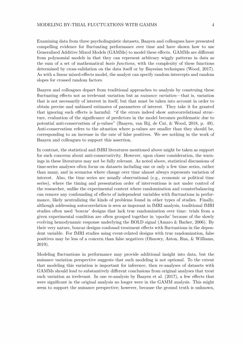
Examining data from three psycholinguistic datasets, Baayen and colleagues have presentedcompelling evidence for fluctuating performance over time and have shown how to useGeneralized Additive Mixed Models (GAMMs) to model these effects. GAMMs are differentfrom polynomial models in that they can represent arbitrary wiggly patterns in data asthe sum of a set of mathematical basis functions, with the complexity of these functionsdetermined by cross-validation on the data itself or by Bayesian techniques (Wood, 2017).As with a linear mixed-effects model, the analyst can specify random intercepts and randomslopes for crossed random factors.
Baayen and colleagues depart from traditional approaches to analysis by construing thesefluctuating effects not as irrelevant variation but as nuisance variation—that is, variationthat is not necessarily of interest in itself, but that must be taken into account in order toobtain precise and unbiased estimates of parameters of interest. They take it for grantedthat ignoring such effects is harmful: “if the errors indeed show autocorrelational struc-ture, evaluation of the significance of predictors in the model becomes problematic due topotential anti-conservatism of p-values” (Baayen, van Rij, de Cat, & Wood, 2018, p. 49).Anti-conservatism refers to the situation where p-values are smaller than they should be,corresponding to an increase in the rate of false positives. We see nothing in the work ofBaayen and colleagues to support this assertion.
In contrast, the statistical and fMRI literatures mentioned above might be taken as supportfor such concerns about anti-conservativity. However, upon closer consideration, the warn-ings in these literatures may not be fully relevant. As noted above, statistical discussions oftime-series analyses often focus on datasets including one or only a few time series, ratherthan many, and in scenarios where change over time almost always represents variation ofinterest. Also, the time series are usually observational (e.g., economic or political timeseries), where the timing and presentation order of interventions is not under control ofthe researcher, unlike the experimental context where randomization and counterbalancingcan remove any confounding of effects of independent variables with fluctuations in perfor-mance, likely neutralizing the kinds of problems found in other types of studies. Finally,although addressing autocorrelation is seen as imporant in fMRI analysis, traditional fMRIstudies often used ‘boxcar’ designs that lack true randomization over time: trials from agiven experimental condition are often grouped together in ‘epochs’ because of the slowlyevolving hemodynamic response underlying the BOLD signal (Amaro & Barker, 2006). Bytheir very nature, boxcar designs confound treatment effects with fluctuations in the depen-dent variable. For fMRI studies using event-related designs with true randomization, falsepositives may be less of a concern than false negatives (Olszowy, Aston, Rua, & Williams,2019).
Modeling fluctuations in performance may provide additional insight into data, but thenuisance variation perspective suggests that such modeling is not optional. To the extentthat modeling this variation is important for inference, then re-analyses of datasets withGAMMs should lead to substantively different conclusions from original analyses that treatsuch variation as irrelevant. In one re-analysis by Baayen et al. (2017), a few effects thatwere significant in the original analysis no longer were in the GAMM analysis. This mightseem to support the nuisance perspective; however, because the ground truth is unknown,

MODELING BY-TRIAL FLUCTUATIONS WITH GAMMS 5
such differences in outcome could either reflect false positives from LMEMs or false negativesfrom GAMMs.
In this paper, we contend that the use of GAMMs to model by-trial fluctuations in ex-periments with randomized presentation is generally unnecessary and potentially harmful.Traditional LMEMs show reasonable Type I error rates in the face of temporal autocorre-lation, so long as the presentation order has been appropriately randomized. And GAMMsare not only harder to implement and interpret compared to LMEMs, but they may alsoimpair power for between-subject effects.
We begin by explaining the use of GAMMs in multi-level data, focusing on the use of factorsmooths to account for time-varying patterns in individual subjects’ data. Then, a briefthought experiment questions the necessity of accounting for these patterns to satisfy sta-tistical assumptions. Next, Monte Carlo simulations examine the performance of GAMMsand LMEMs across a range of theoretical patterns, including sinusoidal and random-walkGaussian patterns. The simulations support the thought experiment: outcomes for modelsignoring temporal autocorrelation are statistically indistinguishable from outcomes of mod-els fit to data with comparable residual variation but no temporal autocorrelation, with falsepositive rates close to nominal, so long as the presentation of within-subject levels is trulyrandomized over time. It is only in designs with blocked presentation order of within-subjectlevels that LMEM models perform poorly relative to GAMMs, due to their inability to de-confound treatment variation from time-varying effects. In designs with fully randomizedpresentation order, GAMMs sometimes offer a modest boost to power for within-subjecteffects, but usually at the cost of increased Type II errors for between-subject effects.
Next, due to concerns about the external validity of our theoretical simulations, we under-took a second set of simulations modeled upon real data, namely the Stroop task from theMany Labs 3 mega-study (Ebersole et al., 2016). Here, we simulated data based on estimatesof fixed and random effects from the main study, ‘grafting’ on real residuals from randomlychosen subjects. Results were similar to the theoretical simulations: LMEMs show no evi-dence of inflated false positives, GAMMs modestly boost power for within-subject effects,but impair power for between-subject effects under some circumstances.
The bottom line from these simulations is that concerns about inflated Type I error rates forLMEMs applied to experimental data that include trial-by-trial fluctuations are completelyunwarranted, so long as the presentation order of stimuli and experimental conditions havebeen properly randomized. If model residuals show signs of autocorrelation, this shouldnot be cause for alarm, since proper randomization and counterbalancing is already a suf-ficient remedy. GAMMs may modestly increase power for within-subject effects in thesesituations, but given their complexity, and the potential costs to power for between-subjecteffects, their use should be seen as optional rather than mandatory. It is only where truerandomization and counterbalancing of presentation order is absent or imperfect that trial-by-trial fluctations become a dangerous nuisance. In these circumstances, GAMMs (orother time-series modeling) are likely to be useful to deconfound variation of interest fromtime-varying noise.
While we question the need to model by-trial fluctuations in fully randomized experiments,

MODELING BY-TRIAL FLUCTUATIONS WITH GAMMS 6
we do not doubt the utility of GAMMs in data exploration, or in situations when thevariable of time is of theoretical interest. Thus, longitudinal studies, such as in cognitivedevelopment or language evolution, are exempt from our recommendations. We focus onstudies where each subject’s data is a series of trials with just one observation per trial.Our recommendations therefore may not generalize to studies where multiple observationsare sampled during each trial or stimulus, as is the case in mouse-tracking, visual-worldeyetracking, MEG, EEG, and pupillometry studies, except when the data from each trialhas been reduced to a single summary statistic. We do not question the applicability ofGAMMs for investigating the time-course of effects at the trial level, such as demonstratedby van Rij, Hendriks, van Rijn, Baayen, and Wood (2019). In short, there is still a widerange of situations in which the use GAMMs may be advantageous. Even so, users shouldbe cautious about the potential dangers we document here.
How to model time-varying nuisance effects with GAMMs
In this section, we illustrate and explain those features of Generalized Additive Mixed Mod-els that are most relevant to modeling fluctuations over time. For a more in-depth tutorialfor psychological or linguistic data, see Baayen et al. (2017), Baayen et al. (2018), Sóskuthy(2017), and Winter and Wieling (2016). The textbook by Wood (2017) provides a morecomprehensive, technical treatment. Our investigation centers on four main considerationsin dealing with data containing by-trial fluctuations: (1) the form the pattern takes overtime, and whether individual patterns share common structure or are completely idiosyn-cratic; (2) the consequences of the temporal structure with respect to model assumptions;namely, whether the pattern only violates independence assumptions or whether it addition-ally violates the assumption of normally distributed residuals; (3) whether the presentationof the levels of any within-subject factors are randomized over time or blocked; and (4)whether the independent variables under investigation are administered as between-subjector within-subject factors.
Let us start by considering a contrived dataset in which we assume that subjects’ responsesexhibit a sinusoidal pattern such as that shown in Figure 1. Using the autocorr packagefor R that accompanies this manuscript (https://github.com/dalejbarr/autocorr), wecan simulate a dataset with by-trial fluctuations using the sim_2x2() function. This func-tion simulates data from a 2x2 mixed design with one within-subject factor (‘A’) and onebetween-subject factor (‘B’), and allows the user to explore different time-varying patterns.The resulting dataset has variables representing either a randomized or blocked design. Wewill start with the randomized design.
1 ## devtools::install_github("dalejbarr/autocorr")2 library("autocorr")3 library("mgcv")4 library("tidyverse")56 set.seed(62) # for reproducibility7 dat <- sim_2x2(int = 3, # set the intercept to an arbitrary non-zero value8 version = 2L) # form of the time varying effect; see ?errsim

MODELING BY-TRIAL FLUCTUATIONS WITH GAMMS 7
This gives us a dataset with simulated data from 48 subjects, with 48 trials per subject,and where individual subjects show a sinusoidal pattern, much like in the original exampleabove. The mgcv package (Wood, 2017) provides functions for fitting GAMMs. Althoughthe functions are designed for fitting data with ‘smooth’ terms to capture wiggly patternsin the data, they can also be used to fit a generic linear mixed-effects model (LMEM) ifstandard random effects and no smooth terms are specified. For comparability with GAMMmodels, we will fit standard LMEMs using mgcv functions instead of using lme4 . Wecan use either the gam() or bam() functions, which are similar, except the latter has beenoptimized for large datasets.
Given the design includes one within-subject factor with multiple observations per levelper subject, an appropriate LMEM model for these data would include by-subject randomintercepts and slopes for the within (‘A’) factor.
1 mod_lmem <- gam(Y_r ~ A_c * B_c +2 s(subj_id, bs = "re") + # by-subject random intercept3 s(subj_id, A_c, bs = "re"), # by-subject random slope for A_c4 data = dat)
The above syntax models the dependent variable Y_r in terms of an (implicit) interceptplus main effects of the within-subject factor (A_c) and the between-subject factor (B_c).The by-subject random intercepts and slopes are included using the s() function with theoption bs="re".2
How can an analyst detect the presence of by-trial fluctuations in data? Although it isuseful and convenient to simply look at each subject’s raw data, for the purpose of checkingassumptions it is essential to look at model residuals. Autocorrelations that appear in theraw data may be absent from the residuals of an appropriately specified model, and maylead the analyst to pursue unnecessary remedies that may cloud interpretation or otherwiseharm inference (Huitema & McKean, 1998). Let us plot the residuals as a function of trialnumber (tnum_r) for the first four subjects.
It is apparent from Figure 2 that we have time-varying effects that have not been accountedfor. Also, the residuals do not appear to be normally distributed; in fact, we prove inthe Appendix that in a hypothetical scenario where all subjects show variations on a basicsinusoidal pattern, the residuals from a LMEM will always depart from normality.
The GAMM approach for resolving these problems of non-independence and non-normalitywould be to add certain ‘smooth’ terms to the model. We can start by changing the staticintercept to a time-varying intercept, by estimating a smooth function for time (in thiscase, indexed by trial number). However, if we stopped there, this would assume that thesinusoidal pattern is identical for all subjects. So we can add factor smooths to the model,which captures any leftover wigglyness for each subject after accounting for the time-varyingfixed intercept. The wigglyness of these smooth terms is determined by a cross-validationprocedure or by Bayesian techniques to prevent overfitting (Wood, 2017). Although the
2Unlike a standard LMEM fit using lme4, random intercepts and slopes in a GAMM are specifiedindividually and treated as independent.

MODELING BY-TRIAL FLUCTUATIONS WITH GAMMS 8
1 2 3 4
0 10 20 30 40 50 0 10 20 30 40 50 0 10 20 30 40 50 0 10 20 30 40 50−2
−1
0
1
2
trial number
resi
dual
0
50
100
150
−2 −1 0 1 2 3residual
coun
t
−2
−1
0
1
2
3
sam
ple
−2 0 2theoretical
Figure 2 . Residuals from a linear-mixed effects model. Top row: residuals plotted by time.Bottom row: histogram and Q-Q plot.
user can control many aspects of the estimation process (see the mgcv vignettes anddocumentation), we will just use the defaults.
1 mod_gamm <- gam(Y_r ~ A_c * B_c +2 s(tnum_r) + # time-varying fixed intercept3 s(subj_id, tnum_r, m = 1, bs = "fs") + # time-varying random intercepts4 s(subj_id, A_c, bs = "re"), # by-subject random slope for A_c5 data = dat)
1 2 3 4
0 10 20 30 40 50 0 10 20 30 40 50 0 10 20 30 40 50 0 10 20 30 40 50−2
−1
0
1
2
trial number
resi
dual
0
50
100
150
200
−3 −2 −1 0 1 2residual
coun
t
−3
−2
−1
0
1
2
sam
ple
−2 0 2theoretical
Figure 3 . Residuals from a generalized additive mixed model. Top row: residuals plottedby time. Bottom row: histogram and Q-Q plot.
The s(tnum_r) term adds a fixed time-varying intercept for the time predictor tnum_r,estimated with the default “thin plate” basis functions. The s(subj_id, tnum_r, m = 1,

MODELING BY-TRIAL FLUCTUATIONS WITH GAMMS 9
bs = "fs") term specifies factor smooths, which allows additional subject-specific wiggly-ness over time. The m = 1 argument specifies a penalty to the first basis function, whichis completely smooth. This ensures the factor smooths will behave like proper randomsmooths; that is, like a typical random effect rather than a fixed effect (Baayen et al., 2017).We kept random slopes for the within-subject factor (A_c) in the model, because the factorsmooths function as a time-varying intercept only, and do not capture random slope vari-ation. Checking the residuals from this model, (Figure 3), we see that the smooth termshave removed the temporal autocorrelation, and made the residuals look more normallydistributed.
A limitation of the above model is that it treats the within-subject effect as static over time.It is possible that the effect varies over time, and that different subjects show distinct time-varying patterns. The model could be further enriched to capture such effects. However,the simpler model turns out to be adequate for our simulated data, and may also generallybe so for real data; indeed, the models fit by Baayen et al. (2017) only included time-varyingintercepts with conventional random slopes, and nonetheless proved effective in removingtemporal autocorrelation.3
In the current scenario, the fluctuations for each subject come from a simple variation ona common sinusoidal pattern. When a model ignores these patterns, the residuals end upautocorrelated and non-normally distributed. In our simulations, we considered additionalscenarios where the time-varying patterns were unique to each subject, as well as patternsthat yielded autocorrelated residuals that were normally distributed.
Design considerations
The impact of autocorrelation on model performance is likely to depend not only on thepattern of autocorrelation (e.g., degree of common versus idiosyncratic structure) but also onhow it relates to the experimental design. Ideally, in experimental studies, the presentationorder of within-subject factors is randomized independently for each subject. This subject-level randomization ensures the temporal fluctuations will not be systematically confoundedwith any variation of interest, possibly making it safe to ignore them. It seems likely thatmodeling these effects with GAMMs could boost power, but it is unclear whether there areany hidden costs to this approach.
Occasionally, researchers use a counterbalanced blocked presentation instead of randomizedpresentation; for instance, half of the participants may receive the first half of trials incondition A1 and the second half in condition A2, while the other half gets them in thecontrary order. In blocked designs, it may be problematic to ignore temporal fluctuations.Although counterbalancing across subjects should keep the false positive rate in check,power could be reduced if the variation of interest gets swamped by the nuisance variation.GAMMs or other types of time-series models might prove especially valuable for separatingsignal from noise.
As already discussed, GAMMs may increase power for within subject effects, but it is3For further discussion of specifying random effects with GAMMs, see van Rij et al. (2019).
MODELING BY-TRIAL FLUCTUATIONS WITH GAMMS 10
unclear how they will perform relative to LMEMs for between-subject effects. In a linearmixed-effects model, variation associated with between-subject treatment effects is likely tobe masked by random intercept variation; for GAMMs, it is masked by variation capturedby the factor smooths. It is important to verify whether GAMMs with factor smoothsperform as well as LMEMs at distinguishing signal from noise.
Irrelevant or nuisance variation?
We have seen how temporal fluctuations can be accounted for by GAMMs but up to nowwe have deferred answering a more basic question: Is it even necessary to account for thesefluctuations? In other words, should such effects be considered as nuisance variation, asBaayen and colleagues evidently view them when emphasizing the importance of ‘cleaningup’ autocorrelation, or are they irrelevant? We contend that the latter view is appropriatefor randomized experimental data. Our Monte Carlo simulations confirm this contention,but let us first argue the case analytically.
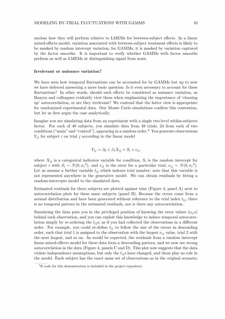
Imagine you are simulating data from an experiment with a single two-level within-subjectsfactor. For each of 48 subjects, you simulate data from 48 trials, 24 from each of twoconditions (“main” and “control”), appearing in a random order.4 You generate observationsYij for subject i on trial j according to the linear model
Yij = β0 + β1Xij + Si + eij
where Xij is a categorical indicator variable for condition, Si is the random intercept forsubject i with Si ∼ N(0, σs2), and eij is the error for a particular trial, eij ∼ N(0, σe2).Let us assume a further variable tij which indexes trial number; note that this variable isnot represented anywhere in the generative model. We can obtain residuals by fitting arandom-intercepts model to the simulated data.
Estimated residuals for three subjects are plotted against time (Figure 4, panel A) next toautocorrelation plots for these same subjects (panel B). Because the errors come from anormal distribution and have been generated without reference to the trial index tij , thereis no temporal pattern in the estimated residuals, nor is there any autocorrelation.
Simulating the data puts you in the privileged position of knowing the error values (eijs)behind each observation, and you can exploit this knowledge to induce temporal autocorre-lation simply by re-ordering the tijs, as if you had collected the observations in a differentorder. For example, you could re-define tij to follow the size of the errors in descendingorder, such that trial 1 is assigned to the observation with the largest eij value, trial 2 withthe next largest, and so on. As would be expected, the residuals from a random interceptlinear mixed-effects model for these data form a descending pattern, and we now see strongautocorrelation in the data (Figure 4, panels C and D). This plot now suggests that the dataviolate independence assumptions, but only the tijs have changed, and these play no role inthe model. Each subject has the exact same set of observations as in the original scenario;
4R code for this demonstration is included in the project repository.
MODELING BY-TRIAL FLUCTUATIONS WITH GAMMS 11
subject: 1 subject: 2 subject: 3
0 10 20 30 40 50 0 10 20 30 40 50 0 10 20 30 40 50
−2
−1
0
1
2
trial number
resi
dual
Asubject: 1 subject: 2 subject: 3
0 5 10 15 0 5 10 15 0 5 10 150.00
0.25
0.50
0.75
1.00
lag
corr
elat
ion
B
subject: 1 subject: 2 subject: 3
0 10 20 30 40 50 0 10 20 30 40 50 0 10 20 30 40 50
−2
−1
0
1
2
trial number
resi
dual
Csubject: 1 subject: 2 subject: 3
0 5 10 15 0 5 10 15 0 5 10 150.00
0.25
0.50
0.75
1.00
lag
corr
elat
ion
D
subject: 1 subject: 2 subject: 3
0 10 20 30 40 50 0 10 20 30 40 50 0 10 20 30 40 50
−2
−1
0
1
2
trial number
resi
dual
Esubject: 1 subject: 2 subject: 3
0 5 10 15 0 5 10 15 0 5 10 15
0.00
0.25
0.50
0.75
1.00
lag
corr
elat
ion
F
condition main control
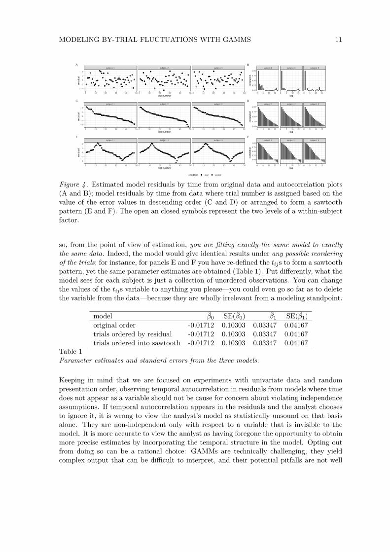
Figure 4 . Estimated model residuals by time from original data and autocorrelation plots(A and B); model residuals by time from data where trial number is assigned based on thevalue of the error values in descending order (C and D) or arranged to form a sawtoothpattern (E and F). The open an closed symbols represent the two levels of a within-subjectfactor.
so, from the point of view of estimation, you are fitting exactly the same model to exactlythe same data. Indeed, the model would give identical results under any possible reorderingof the trials; for instance, for panels E and F you have re-defined the tijs to form a sawtoothpattern, yet the same parameter estimates are obtained (Table 1). Put differently, what themodel sees for each subject is just a collection of unordered observations. You can changethe values of the tijs variable to anything you please—you could even go so far as to deletethe variable from the data—because they are wholly irrelevant from a modeling standpoint.
model β0 SE(β0) β1 SE(β1)original order -0.01712 0.10303 0.03347 0.04167trials ordered by residual -0.01712 0.10303 0.03347 0.04167trials ordered into sawtooth -0.01712 0.10303 0.03347 0.04167
Table 1Parameter estimates and standard errors from the three models.
Keeping in mind that we are focused on experiments with univariate data and randompresentation order, observing temporal autocorrelation in residuals from models where timedoes not appear as a variable should not be cause for concern about violating independenceassumptions. If temporal autocorrelation appears in the residuals and the analyst choosesto ignore it, it is wrong to view the analyst’s model as statistically unsound on that basisalone. They are non-independent only with respect to a variable that is invisible to themodel. It is more accurate to view the analyst as having foregone the opportunity to obtainmore precise estimates by incorporating the temporal structure in the model. Opting outfrom doing so can be a rational choice: GAMMs are technically challenging, they yieldcomplex output that can be difficult to interpret, and their potential pitfalls are not well

MODELING BY-TRIAL FLUCTUATIONS WITH GAMMS 12
known. Consequently, using them does not guarantee better insight into data.
Lest it still seem ‘wrong’ or ‘inappropriate’ for an analyst to ignore residual autocorrelationwhen analyzing data from a randomized experiment, let us attempt to further dislodge thisnotion by considering yet another way in which experimental data form a time series. Just asthe individual measurements taken from a given subject are influenced by the characteristicsof the particular moment at which the measurement is taken, so is the overall performance ofa subject influenced by the time of day at which testing occurs, with subjects often showingmore efficient performance on tasks during afternoons compared to mornings (Blake, 1967;Kleitman, 1963). Time of day fluctuations are very likely to induce residual autocorrelation,at least for tasks that are minimally cognitively demanding. In a study where you attemptto predict participants’ mean performance by experimental group, this autocorrelation couldbe seen by plotting the residual for each subject against the time of day at which the sessiontook place. Yet despite this variable being a likely source of non-independence, and despiteit being a variable that is recorded in every experiment (if only by computer timestamps)it is almost always ignored during analysis. Why does no one question this?
We do not worry about time-of-day effects for the same reason we need not worry abouttime-of-trial effects: because we randomized. Randomization prospectively guards againstthe contamination of variance we care about by variance that we don’t. Even beyondtime of trial or time of day effects, in any study there is a potentially infinite number ofpossible variables for which residuals, when plotted against the variable values, would shownon-independence—day of the week, season of the year, temperature of the room, degreeof ambient visual or acoustic noise, subject conscienciousness, visual angle subtended bystimuli relative to each subject’s visual acuity, and so on. So long as we have randomized,we don’t need to worry about non-independence relative to these variables. Trial-by-trialfluctuations in performance are no different.
We have argued that modeling trial-by-trial fluctuations is not necessary, but we haven’tanswered the question of whether doing so is worthwhile. The rest of this article describestwo sets of Monte Carlo simulations aimed at illuminating the potential costs and benefitsof GAMM modeling so that analysts can be more informed in their decisions. The firstset of simulations is meant to illuminate properties of GAMMs and LMEMs on data withtime-varying effects by challenging them with a variety of patterns, including sinusoidaland Gaussian random walk patterns. The second set of simulations examines more realisticpatterns, where the residuals from the simulated data contain real practice effects from amodel fit to Stroop task data from the Many Labs 3 project (Ebersole et al., 2016).
Simulation Set 1: Sinusoidal and Random Walk Patterns
Method
Different approaches for dealing with autocorrelation might impact within-subject factorsin a different way from between-subject factors. Thus, for our hypothetical experiment ofinterest we chose a mixed 2x2 design, including one within-subject factor, one between-subject factor, and their interaction. For simplicity, the design included no stimulus effects.

MODELING BY-TRIAL FLUCTUATIONS WITH GAMMS 13
Each hypothetical experiment comprised 48 time-series, each representing data from a singlehypothetical participant. The sim_2x2() function in the accompanying autocorr gen-erated the datasets used in the Monte Carlo study, according to the following procedure.
The Yij observations for participant i on trial j were generated according to the multi-levellinear model
Yij = β0 + S0i + (β1 + S1i)Aj + β2Bi + β3AjBi + eij
where Aj is a deviation-coded (-.5, .5) predictor representing the level of the within-subjectfactor for trial j, Bi is a deviation-coded predictor representing the level of the between-subject factor for subject i, and the eijs comprise a 48-length vector of residuals. Theby-subject random intercept and random slope for participant i, 〈S0i, S1i〉, were drawnfrom the bivariate normal distribution
〈S0i, S1i〉 ∼ N(〈0, 0〉 ,Σ
)where
Σ =(
τ02 ρτ0τ1
ρτ0τ1 τ12
).
The sim_2x2() function generated sample datasets based on the above equations, with spe-cific fixed-effects parameter values β0, β1, β2, β3, random-effects parameter values τ0, τ1, ρ,and residuals (as defined in the next section). The intercept β0 remained fixed at zerofor simplicity. We considered six unique values for the main-effect of the within-subjectfactor, β1 ∈ 0, .05, .10, .15, .20, .25: . We also considered six unique values for the effectof the between-subject factor, β2 ∈ 0, .10, .20, .30, .40, .50, as well as for the interaction,β3 ∈ 0, .10, .20, .30, .40, .50: . These values were determined through trial and error toyield a good range of power for effects in the “no autocorrelation” (baseline) scenario, giventhe ranges for the parameters defining the variance components. The values for β1, β2, andβ3 were not varied independently: whenever β1 was set to the nth value in the series (e.g.,if n = 4, β1 = .15), then β2 and β3 were also set to their nth values (e.g., β2 = β3 = .30).This seemed like a reasonable way to reduce the number of simulations required, since alleffects are independent and the design was always balanced.
Parameters for the variance components that define the random effects should ideally bechosen to approximate the ratio of subject-level to trial-level noise found in real data. Sincedata on this ratio are lacking, we derived values from the convenience sample of data from13 psycholinguistic experiments provided by Barr, Levy, Scheepers, and Tily (2013) in theironline appendix. The estimated variance components from these studies, expressed as aproportion of residual variance, are shown in Table 2 and are also available as the objectblst_studies in autocorr. Each simulated dataset had parameters τ0 and τ1 drawn froma uniform distribution spanning from the 20th to the 80th percentiles of the correspondingempirical distribution, specifically τ0 ∼ U (0.105, 0.420) and τ1 ∼ U (0.001, 0.261). The

MODELING BY-TRIAL FLUCTUATIONS WITH GAMMS 14
ID σ τ0/σ τ1/σ
1 3572 0.216 0.0002 8439 0.140 0.0013 24388 0.105 0.0004 29934 0.321 0.0005 0.494 1.877 0.3856 275363 0.449 0.0027 230191 0.106 0.0598 231824 0.172 0.0039 51372 0.412 0.021
10 7536625 0.036 0.06611 406043 0.229 0.22212 0.128 0.104 0.36613 242830 0.426 0.287
Table 2Estimated variance components from the sample of 13 psycholinguistic studies in Barr etal. (2013).
random correlation ρ was also from a uniform distribution, reflecting a range of realisticvalues: ρ ∼ U(−.8, .8).
For each sample dataset generated by sim_2x2(), the residuals for all 48 participants ei-ther had no autocorrelation (baseline scenario), or had the same autocorrelation structurerepresenting one of the eight scenarios described below. All samples were homogeneouswith respect to the autocorrelation structure. That is, the residuals for all subjects withina sample were generated according to the same selected scenario; we did not mix scenarioswithin a sample.
The scenarios of autocorrelated residuals were chosen to represent a variety of theoreticallyinteresting scenarios, from highly consistent and structured sinusoidal patterns to highlyidiosyncratic and unstructured ‘random walk’ patterns. Because real data is likely to havemultiple sources of autocorrelation operating at distinct time scales, we also consideredscenarios that were a mixture of the sinusoidal and random walk patterns. Figure 5 showsexample sequences from each scenario. The residuals were generated using the errsimfunction of autocorr. In all scenarios, we normalized each residual time series so thatthe mean was 0 and the standard deviation was 1. We also compare the autocorrelationscenario to a baseline scenario without autocorrelation (also with SD = 1). Thus, the totalvariation is identical across the scenarios; all that varies is how this variation is distributedover time.
Scenario 1 and 2: Sinusoidal. The first two scenarios represent relatively slow processesunfolding over the course of an experimental session, such as fatigue or practice effects. Forsimplicity, we represent such processes as a single bandwidth of a sinusoidal function. Areal-world example might be a reaction time experiment where a participant speeds upresponse times at the beginning of a session as they gain experience with the task, followedby a gradual slowing due to fatigue, and ending with a final speed up as the participant

MODELING BY-TRIAL FLUCTUATIONS WITH GAMMS 15
5. Scenario 1 + Scenario 3 6. Scenario 1 + Scenario 4 7. Scenario 2 + Scenario 3 8. Scenario 2 + Scenario 4
1. Sinusoidal, Varying phase 2. Sinusoidal, Varying amp 3. Random walk, High frequency 4. Random walk, Mid frequency
1 12 24 36 48 1 12 24 36 48 1 12 24 36 48 1 12 24 36 48
−2
0
2
−2
0
2
observation number (1−48)
resi
dual
Figure 5 . Randomly generated sequences exemplifying the eight autocorrelation scenarios.Each line represents the residuals for a single hypothetical participant.
rallies toward the end. Another participant might show an opposite (anti-phased) pattern,gradually slowing at the start as they learn how to maximize accuracy, followed by a gradualspeed with practice, and slowing towards the end as fatigue sets in.
Reflecting this type of scenario, the first scenario we consider is one in which participantsexhibit a common sinusoidal form offset by random phase angles, which we call the varyingphase scenario. In these simulations, the phase angle gi for the ith participant was drawnfrom a uniform distribution, gi ∼ U(−π, π). Each simulated participant having a differentrandom phase angle implies no time-varying structure at the population level, since theexpected value of the sum of a set of sine waves with fixed amplitude and frequency butwith phase offsets randomly drawn from a uniform distribution is a flat line (i.e., the wavestend to cancel one another out).
Of course, we also assume the presence of noise (without any temporal autocorrelation)superimposed upon this overall pattern. Specifically, for this first scenario, we assume 90%of the total variance is driven by the sinusoidal pattern and the remaining 10% is trial-levelnoise.
It may be too extreme to assume no structure to the autocorrelation pattern at the popu-lation level. Thus, our second varying amplitude scenario considers the opposite extreme:What if everyone showed the exact same pattern, but with varying strength? For Scenario 2,the residuals for each participant were represented as a sinusoidal pattern with frequencyand phase fixed, but with amplitude determined by Ai for the ith participant drawn froma uniform distribution, Ai2 ∼ U(.2, .8) (Figure 5, second panel of the first row). Between20% to 80% of the residual variance is driven by the sine wave signal, and the remainingvariance is Gaussian noise (σ2 = 1 − Ai2). Here, rather than canceling, the phase-locked

MODELING BY-TRIAL FLUCTUATIONS WITH GAMMS 16
patterns combine to yield a population-level effect.
Scenarios 3 and 4: Random walk. The two above scenarios assume that the time-varying patterns on the dependent variable have a common sinusoidal form across partici-pants. But it is also of interest to consider scenarios where the functional forms are idiosyn-cratic. To this end, we randomly generated time series from an autocorrelated Gaussianprocess, following the numerical method developed in Shinozuka and Deodatis (1991), whichwe implemented in the stat_gp() function in the autocorr package. Technical details areprovided in the Appendix. The function takes two arguments, σ and γ, determining thestandard deviation and the correlation length, respectively. For Scenarios 3 and 4, σ wasfixed at 1, while γ was 1 for Scenario 3, and 2 for Scenario 4, such that the oscillatory pat-terns in Scenario 3 were higher frequency than in Scenario 4 (see the third and fourth panelsin the top row of Figure 5). Because we are interested in patterns occurring on multipletime scales, these two values of γ were selected so that the resulting oscillation frequencieswould be higher than the sine wave oscillations considered in Scenarios 1 and 2. We refer toScenario 3 as “high frequency” and Scenario 4 as “mid frequency” random walks, in contrastwith the lower-frequency sine waves.
Note that the idiosyncratic nature of these time series implies that, like the varying phasescenario described above, the series will tend to cancel across subjects such that the depen-dent variable would show no population-level effect.
Scenarios 5–8: Mixed timescales. The four remaining scenarios (Scenarios 5–8) reflecttime series with autocorrelation occurring on the slow, sinusoidal time scale as well as onthe faster, random walk time scales. Each scenario is simply the sum of one of the two sinewave scenarios and one of the two random walk scenarios, as described below.
Scenario 5 and Scenario 6 had a the varying-phase sine wave (Scenario 1) mixed with thehigh- and mid- frequency random walk patterns, respectively. Each vector of residualsreflected a mix of 90% of a randomly generated sine wave pattern with 10% of the corre-sponding random walk, with results exemplified in the first two panels of the second row inFigure 5.
Scenario 7 and Scenario 8 had the varying-amplitude sine wave (Scenario 2) mixed withthe high- and mid- frequency random walk patterns, respectively. As described above forScenario 2, the amplitude Ai for the ith participant was determined by A2
i ∼ U(.2, .8), withthe remaining random walk variance scaled to comprise 1−Ai2 of the total variance.
Analysis. In contrast to the uncertain position of the analyst, a researcher working withsimulated data is in the privileged position of having complete knowledge of the processgiving rise to the data. This makes it possible to analyze data either from the uncertain per-spective of the analyst or from the omniscient perspective of the designer of the simulation.Because we were interested in the performance of GAMMs under ideal circumstances, weperformed our analyses from the latter perspective: the GAMM models that we fit exactlymatched the generative process.
We created the autocorr function fit_2x2 to fit models to the data generated by sim_2x2.The function fits a GAMM as well as an LMEM style model using the bam function fromthe mgcv package, version 1.8.31 (Wood, 2011).

MODELING BY-TRIAL FLUCTUATIONS WITH GAMMS 17
The model formula for fitting LMEM-style models in bam was
Y ~ W * B + s(id, bs = "re") + s(id, W, bs = "re")
which is formally equivalent to the lme4 formula
Y ~ W * B + (1 + W || id)
where the ‘double bar’ || syntax in (1 + W || id) fixes the covariance between randomintercepts and slopes to zero. The fixed part W * B specifies main effects for the within-factor W and between-factor B and the interaction between them. The ‘smooth’ termss(.., bs="re") specify standard random effects where id is the subject identifier, withs(id, bs="re") specifying the random intercept and s(id, W, bs="re") specifying therandom slope (i.e, allowing the effect of W to vary over subjects).5
For the three scenarios with the underlying phase-locked but varying amplitude sine pattern(scenarios 2, 7, and 8) the full GAMM model formula was
Y ~ W * B + s(t, bs="tp") + s(t, id, bs="fs") + s(id, W, bs="re").
In this formula, the s(id, W, bs="re") term, which also appears in the LMEM formula,specifies a random slope for the within-subject factor. The s(t, bs="tp") term specifiesthe (default) ‘thin plate’ smooth intended to capture the part of the sinusoidal patternthat varies over time t and is common to all subjects. The bs="fs" argument in s(t,id, bs="fs") term specifies a factor smooth, allowing the time-varying pattern for eachsubject to diverge from the overall pattern. Note that the factor smooth plays the role ofthe random intercept in the LMEM formula, with the difference of allowing the interceptto vary over time. The default behavior for factor smooths is to behave like a fixed effect,and so some authors have advised specifying a penalty to the linear basis function for factorsmooths (m = 1) so that they behave more like random effects (Baayen et al., 2017, p.211). For simplicity, we refer to this as a GAMM with a “penalized” factor smooth, andthe previous version as “unpenalized.”
Y ~ W * B + s(t, bs="tp") + s(t, id, m=1, bs="fs") + s(id, W, bs="re").
We included results for both the unpenalized and penalized factor smooth versions becausewe assume that many users will be unaware of the advice and just rely on function defaults.
The GAMM formula for the baseline “no autocorrelation” scenario as well as for the fiveremaining scenarios was
Y ~ W * B + s(t, id, bs = "fs") + s(id, W, bs = "re")
for the unpenalized version, and
Y ~ W * B + s(t, id, m = 1, bs = "fs") + s(id, W, bs = "re")
5Variable names in the text have been simplified for expository purposes and do not match the namesin the datasets resulting from sim_2x2. The exact formulas used to fit models can be obtained by runningfit_2x2(NULL, cs = TRUE, dontfit = TRUE) for scenarios 2, 7, and 8 and fit_2x2(NULL, cs = FALSE,dontfit = TRUE) for the remaining scenarios.

MODELING BY-TRIAL FLUCTUATIONS WITH GAMMS 18
for the penalized version. Both forms are the same as above except the fixed smoothterm, s(t, bs="tp"), has been omitted, since these patterns have no common time-varyingstructure across participants. We used theWald z statistic to derive p-values for fixed effects,defined as the ratio of the parameter estimate to its estimated standard error.
An important aspect of GAMM modeling involves setting the type and number of basisfunctions. We opted to stick with the defaults provided by the mgcv package, reasoningthat this is what a typical user would do. This implies that the smooth terms introduced bys(t) will use about 10 basis functions (see ?choose.k and ?tprs for details). This seemssufficiently large given there are only 48 observations in each time series.
Software. We ran the simulations and analyzed the results using R version 3.6.2 (RCore Team, 2019). Simulations were run using the function mcsim() in the R autocorrpackage (https://github.com/dalejbarr/autocorr). We bundled all necessary softwareinfrastructure in a Singularity 3.5 software container (https://sylabs.io/singularity).The simulations can be reproduced by the command
singularity run library://dalejbarr/talklab/autocorr
which activates the shell script acsim inside the container. The script’s default action is toinvoke mcsim() to run 1,000 Monte Carlo simulations at each of the 54 unique combina-tions of Monte Carlo parameters (six effect size settings times nine scenarios, including thebaseline scenario).
Results and Discussion
We completed 25,000 simulation runs at each of the 54 unique parameter settings (six effectsize settings times the nine scenarios including baseline). Results from the simulations areavailable in the project repository at https://osf.io/cp9z8, which also includes sourcecode files for reproducing analyses and for compiling this manuscript. The raw results areavailable in the data_derived subfolder of the repository. The repository also containsresults from supplementary simulations looking at other time-varying patterns as well asadditional AR(1) modeling for some scenarios, and provides instructions on how to runfurther simulations based on user-defined functions.
False positive rate. We calculated false positive rates for GAMM and LMEM modelsapplied to data with time-varying effects across the 48 different combinations obtained byfactorially combining the three effect types (within, between, interaction) with the twopresentation orders (random and blocked) and the eight autocorrelation scenarios. Thep values were computed based on Wald z statistics. It is well-known that this methodtends to be slightly anti-conservative—that is, yielding false positive rates above the α level(Baayen et al., 2008; Luke, 2017). A key question of the current investigation was whetherthe naïve application of LMEMs to data with known autocorrelation would yield additionalanti-conservativity beyond this baseline. As Figure 6 illustrates, with some exceptions, mostfalse positive rates were acceptably close to the nominal α level.
We compared the false positive rates to the 99% Agresti-Coull confidence interval for LMEMmodels applied to baseline data with temporally unstructured variation (Gaussian white

MODELING BY-TRIAL FLUCTUATIONS WITH GAMMS 19
random blocked
between
within
interaction
0 .01 .02 .03 .04 .05 .06 0 .01 .02 .03 .04 .05 .06
1. sine, varying phase
2. sine, varying amp
3. random walk HF
4. random walk MF
5. multiscale (1 + 3)
6. multiscale (1 + 4)
7. multiscale (2 + 3)
8. multiscale (2 + 4)
1. sine, varying phase
2. sine, varying amp
3. random walk HF
4. random walk MF
5. multiscale (1 + 3)
6. multiscale (1 + 4)
7. multiscale (2 + 3)
8. multiscale (2 + 4)
1. sine, varying phase
2. sine, varying amp
3. random walk HF
4. random walk MF
5. multiscale (1 + 3)
6. multiscale (1 + 4)
7. multiscale (2 + 3)
8. multiscale (2 + 4)
proportion significant
model
GAMM−penalized−fs
LMEM
GAMM−unpenalized−fs
status
conservative
nominal
anticonservative
Figure 6 . False positive rates. The shaded region represents the 99% Agresti-Coull con-fidence interval of the false positive rate obtained for LMEMs applied to data withouttemporal autocorrelation.
noise). Overall, false positive rates for eight of the 48 LMEM cases exceeded the confidenceinterval, with a maximum false positive rate of .059. This was no worse than for GAMMs,where the false positive rate exceeded the upper bound in nine cases for the unpenalizedversion, with a maximum false positive rate of .060. For the penalized version, the falsepositive rate exceeded the confidence interval in ten cases, with a maximum false positiverate of .059 In sum, for multi-level data from designs with appropriate counterbalancingof presentation order, there is no reason to think that application of LMEMs to data withtrial-by-trial fluctuations increases the rate of false positives.
For designs with blocked presentation, there were three scenarios where LMEMs were ex-tremely conservative; specifically, in Scenarios 2, 7, and 8, no false positive ever occurred forthe test of the within-subject effect. GAMMs with unpenalized factor smooths exhibitedmoderate conservativity for tests of the between-subject factor in Scenario 1, with a falsepositive rate of about .044 across both presentation orders. In short, applying LMEMs todata with trial-by-trial fluctuations may lead to extreme conservativity in blocked designs,but general concerns about increased false positive rates for LMEMs find no support in

MODELING BY-TRIAL FLUCTUATIONS WITH GAMMS 20
our data, despite the fact that these models had residuals that were not independent withrespect to time, and violated normality assumptions in all scenarios except 3 and 4.
1. sine, varying phase 2. sine, varying amp 3. random walk HF 4. random walk MF 5. multiscale (1 + 3) 6. multiscale (1 + 4) 7. multiscale (2 + 3) 8. multiscale (2 + 4)
between
0 .1 .2 .3 .4 .5 0 .1 .2 .3 .4 .5 0 .1 .2 .3 .4 .5 0 .1 .2 .3 .4 .5 0 .1 .2 .3 .4 .5 0 .1 .2 .3 .4 .5 0 .1 .2 .3 .4 .5 0 .1 .2 .3 .4 .50
.2
.4
.6
.8
1
effect size
prop
ortio
n si
gnifi
cant
GAMM−penalized−fs GAMM−unpenalized−fs LMEM
1. sine, varying phase 2. sine, varying amp 3. random walk HF 4. random walk MF 5. multiscale (1 + 3) 6. multiscale (1 + 4) 7. multiscale (2 + 3) 8. multiscale (2 + 4)
within
0 .05 .1 .15 .2 .25 0 .05 .1 .15 .2 .25 0 .05 .1 .15 .2 .25 0 .05 .1 .15 .2 .25 0 .05 .1 .15 .2 .25 0 .05 .1 .15 .2 .25 0 .05 .1 .15 .2 .25 0 .05 .1 .15 .2 .250
.2
.4
.6
.8
1
effect size
prop
ortio
n si
gnifi
cant
1. sine, varying phase 2. sine, varying amp 3. random walk HF 4. random walk MF 5. multiscale (1 + 3) 6. multiscale (1 + 4) 7. multiscale (2 + 3) 8. multiscale (2 + 4)
interaction
0 .1 .2 .3 .4 .5 0 .1 .2 .3 .4 .5 0 .1 .2 .3 .4 .5 0 .1 .2 .3 .4 .5 0 .1 .2 .3 .4 .5 0 .1 .2 .3 .4 .5 0 .1 .2 .3 .4 .5 0 .1 .2 .3 .4 .50
.2
.4
.6
.8
1
effect size
prop
ortio
n si
gnifi
cant
Figure 7 . Power curves for the between effect (top row), within effect (middle row) andinteraction (bottom row) in the randomized design. Note that the range of effect sizes con-sidered for the within-subject effect is half that used for the between-subject and interactioneffects. The dashed line in the background reflects average performance for LMEMs on datawith a comparable level of Gaussian white noise.
Power for randomized designs. The power functions for GAMMs and LMEMs dependin a complex way on the type of effect (between or within), whether presentation order wasrandom or blocked, and scenario. Figure 7 shows results for the randomized design. Forcomparison, in each plot the curves for the GAMM and LMEM approaches are plottedagainst the averaged performance of GAMMs and LMEMs in the baseline scenario wherethe errors contained a corresponding amount of white noise. The curves for the interactioneffect patterned nearly identically to the corresponding curves for the within-subject effect,albeit with the former exhibiting exactly half of the power of the latter (note the differencein range of the x-axis scale).
Across all effects and scenarios within the random presentation order, power for LMEMsthat ignored time-varying effects was identical to power for LMEMs on datasets with un-correlated Gaussian noise. The power curves for the two sets are indistinguishable. Viewedin one way, this result is not surprising: as we noted in the Introduction, the temporalordering of each subject’s residuals is unimportant in a model where time plays no role inthe model. Still, it is somewhat surprising that LMEMs performed so well even in caseswhere underlying sinusoidal patterns introduced non-normality into the residuals. Thisconfirms our contention at the outset: that from the point of view of a garden varietymixed-effects model, when each participant receives a different random presentation order,

MODELING BY-TRIAL FLUCTUATIONS WITH GAMMS 21
any temporal structure in the residuals is essentially irrelevant; each subjects’ residuals arefully exchangeable over time.
However, when there is temporal ordering in the residuals, this can be exploited to improvepower over the baseline for within-subject effects. In all scenarios with random presentation,GAMMs yielded modest improvements in power over LMEMs for within-subject factors aswell as for any interactions involving these factors. We calculated the average percentagegain for GAMMs over LMEMs in each of the 8 scenarios, combining data from the within-subject and interaction effects given their near identical patterning. For GAMMs withunpenalized factor smooths, power gains as compared to LMEMs ranged from 2% (scenario3) to 37% (scenario 6) with a median of 27%. For GAMMs with penalized factor smooths,power gains as compared to LMEMs ranged from 7% (scenario 3) to 37% (scenario 6) witha median of 25%.
However, the power gains with GAMMs for within-subject effects in randomized designstypically came at the price of impaired power for between-subject effects. Power for GAMMson between-subject effects never exceeded power for LMEMs, and was very poor in five of theeight scenarios (1, 4, 5, 6, and 8). At best, GAMMs were equivalent to LMEMs (scenario 2)or only slightly worse (scenarios 3 and 7, where average power for GAMMs with unpenalizedfactor smooths was 85% and 90% of LMEM power, respectively; for GAMMs with penalizedfactors smooths, it was 69% and 80% of LMEM power, respectively). At worst, across therange of effect sizes examined, power for GAMMs with unpenalized factor smooths remainedstuck at the α-level (.05) while LMEMs approached 100% power (scenarios 4 and 8). In thesescenarios, the variance associated with the between-subject manipulation was fully absorbedby the factor smooths, rendering even extremely large effects completely undetectable.
When comparing penalized and unpenalized GAMMs for randomized designs, both versionsyield identical performance for within-subject effects across scenarios, but show varyingpatterns for between-subject effects. Apart from Scenario 2, where between-subject powerwas equivalent, the unpenalized version outperformed the penalized version in Scenarios 1,3, and 7, with gains of about 23%, 19%, and 8%, respectively. The penalized versionoutperformed the penalized version in Scenarios 4, 5, 6, and 8, with gains of about 335%,43%, 102%, and 419%, respectively.
Power for blocked designs. Turning now to power for designs with blocked presentationorder (Figure 8), where variation of the within-subject effect is confounded with time-varyingeffects, GAMMs show drastically improved detection of within-subject effects relative toLMEMs for all but the pure random walk cases (Scenarios 3 and 4). In Scenarios 2, 7,and 8, which included a common underlying sinusoidal pattern, power for detecting thewithin-subject effect or interaction effect with LMEMs remained at floor over the full range,while both GAMM versions performed vastly better, matching (or nearly matching) baselinepower in Scenarios 1, 2, 5, and 6. In Scenarios 7 and 8, power for GAMMs was impairedrelative to baseline, but still vastly superior to LMEM power. Unexpectedly, the relationshipwas reversed in random walk Scenarios 3 and 4, where LMEMs outperformed both GAMMversions. Relative to unpenalized GAMMs, LMEMs improved power by 33% and 43%respectively; relative to penalized GAMMs, LMEMs improved power by 85% and 59%. Insum, power for within-subject effects in designs with blocked presentation tended to be far

MODELING BY-TRIAL FLUCTUATIONS WITH GAMMS 22
1. sine, varying phase 2. sine, varying amp 3. random walk HF 4. random walk MF 5. multiscale (1 + 3) 6. multiscale (1 + 4) 7. multiscale (2 + 3) 8. multiscale (2 + 4)
between
0 .1 .2 .3 .4 .5 0 .1 .2 .3 .4 .5 0 .1 .2 .3 .4 .5 0 .1 .2 .3 .4 .5 0 .1 .2 .3 .4 .5 0 .1 .2 .3 .4 .5 0 .1 .2 .3 .4 .5 0 .1 .2 .3 .4 .50
.2
.4
.6
.8
1
effect size
prop
ortio
n si
gnifi
cant
GAMM−penalized−fs GAMM−unpenalized−fs LMEM
1. sine, varying phase 2. sine, varying amp 3. random walk HF 4. random walk MF 5. multiscale (1 + 3) 6. multiscale (1 + 4) 7. multiscale (2 + 3) 8. multiscale (2 + 4)
within
0 .05 .1 .15 .2 .25 0 .05 .1 .15 .2 .25 0 .05 .1 .15 .2 .25 0 .05 .1 .15 .2 .25 0 .05 .1 .15 .2 .25 0 .05 .1 .15 .2 .25 0 .05 .1 .15 .2 .25 0 .05 .1 .15 .2 .250
.2
.4
.6
.8
1
effect size
prop
ortio
n si
gnifi
cant
1. sine, varying phase 2. sine, varying amp 3. random walk HF 4. random walk MF 5. multiscale (1 + 3) 6. multiscale (1 + 4) 7. multiscale (2 + 3) 8. multiscale (2 + 4)
interaction
0 .1 .2 .3 .4 .5 0 .1 .2 .3 .4 .5 0 .1 .2 .3 .4 .5 0 .1 .2 .3 .4 .5 0 .1 .2 .3 .4 .5 0 .1 .2 .3 .4 .5 0 .1 .2 .3 .4 .5 0 .1 .2 .3 .4 .50
.2
.4
.6
.8
1
effect size
prop
ortio
n si
gnifi
cant
Figure 8 . Power curves for the between effect (top row), within effect (middle row) andinteraction (bottom row) in the blocked design. Note that the range of effect sizes consideredfor the within-subject effect is half that used for the between-subject and interaction effects.The dashed line in the background reflects average performance for LMEMs on data witha comparable level of Gaussian white noise.
superior for GAMMs except in purely random walk scenarios, where LMEMs were superior.
For the between-subject factor under the blocked presentation, LMEMs matched baselineperformance, while GAMMs showed an unacceptable degree of conservatism. Indeed, thecurves were equivalent to those from the random presentation condition.
Comparing the performance of penalized and unpenalized GAMMs on power for the within-subject effect in blocked designs showed variation across scenarios. Apart from Scenario 2,where performance was equivalent, unpenalized GAMMs always outperformed the penalizedversions. Average gains in power ranged from 5% (Scenario 5) to 43% (Scenario 3).
The relative performance of penalized and unpenalized GAMMs on power for the between-subject effect showed exactly the same patterns as for the randomized designs.
Bias and precision. To assess the bias and precision of the parameter estimates, wecalculated the difference between each parameter estimate and the true population value,and then formed distributions (Figure 9). All of the distributions are centered at zero, whichindicates no bias across any effects under either presentation order and across all scenarios.The precision data closely mirrors the main findings from the power curves: (1) estimatesfor between-subject effects were imprecise under GAMMs relative to LMEMs, especiallyfor the unpenalized versions; (2) GAMMs improved precision for within-subject effects andinteractions under the random presentation order; and (3) under the blocked presentationorder, LMEM estimates for within-subject effects and interactions tended to be imprecise

MODELING BY-TRIAL FLUCTUATIONS WITH GAMMS 23
random blocked
between
−5 −2.5 0 2.5 5 −5 −2.5 0 2.5 5
1. sine, varying phase
2. sine, varying amp
3. random walk HF
4. random walk MF
5. multiscale (1 + 3)
6. multiscale (1 + 4)
7. multiscale (2 + 3)
8. multiscale (2 + 4)
estimate
GAMM−penalized−fs GAMM−unpenalized−fs LMEM
random blocked
within
−.10 0 .10 −.5 −.25 0 .25 .5
1. sine, varying phase
2. sine, varying amp
3. random walk HF
4. random walk MF
5. multiscale (1 + 3)
6. multiscale (1 + 4)
7. multiscale (2 + 3)
8. multiscale (2 + 4)
estimate
random blocked
interaction
−.20 0 .20 −1 −.5 0 .5 1
1. sine, varying phase
2. sine, varying amp
3. random walk HF
4. random walk MF
5. multiscale (1 + 3)
6. multiscale (1 + 4)
7. multiscale (2 + 3)
8. multiscale (2 + 4)
estimate
Figure 9 . Bias and precision of parameter estimates.

MODELING BY-TRIAL FLUCTUATIONS WITH GAMMS 24
compared to the two GAMM versions, except in the two random walk scenarios (Scenarios 3and 4).
Simulation Set 2: Many Labs 3 Stroop Dataset
The previous simulations illuminated properties of LMEMs and GAMMs by challengingthem with a variety of artificial time-varying patterns in the residuals. The patterns werebased on theoretical criteria and were not intended to form a representative sample ofreal-world patterns. The findings lend overwhelming support to our claim that ignoringtrial-by-trial fluctuations in studies with randomized presentation order does not increasefalse positive rates. They also suggest scenarios where the use of GAMMs will enhancepower for within-subject effects or impair power for between-subject effects. To show thesefindings have external validity, it would be advantageous to reproduce them with real ratherthan artificial data.
For this second set of simulations, residuals were drawn directly from a real dataset con-taining practice effects. The American Psychological Association’s online dictionary definespractice effects as “any change or improvement that results from practice or repetition oftask items or activities” (https://dictionary.apa.org/practice-effect). In the caseof repeated measures designs, participants are likely to respond more quickly and accuratelyon later trials than on earlier trials as they master task demands and become familiar withstimuli. While we know of no overview study estimating their prevalence, the sheer volumeof literature on this topic suggests they are a common feature in datasets with repeated mea-surements, appearing across a variety of measurement types and time scales (e.g., Keuleers,Diependaele, & Brysbaert, 2010).
As source data, we used the Stroop Task dataset from the Many Labs 3 mega-study (Eber-sole et al., 2016). This is a very large dataset containing response latencies from 3,337distinct participants performing 63 trials of a version of the Stroop task (Stroop, 1935), fora total of 210,231 observations. In the basic Stroop task, participants must identify thefont color of a word. Although the actual identity of a word is irrelevant for reporting itscolor, the basic finding is that people are slower and less accurate in reporting the colorof words whose semantics are incongruent with the color (responding “green” to the wordRED presented in a green font) relative to when the semantics of the word are congruent(responding “green” to the word GREEN presented in a green font).
In the Many Labs 3 version of the task, participants saw the color words RED, GREEN,and BLUE presented in red, green, or blue font, with each color word appearing 21 times,seven times in each font color. They identified the font color by pressing one of threeassigned response keys, and the response and its latency (in milliseconds) were recorded.Details about randomization are not provided, but to all appearances, each participantreceived the stimuli in a different random ordering. Further details about the procedure areavailable in the Many Labs 3 repository at https://osf.io/csj7r/.
We downloaded the data from the Many Labs 3 repository at https://osf.io/n8xa7/, pre-processed it and bundled it as part of the accompanying autocorr R package, availableas the object stroop_ML3. Consistent with the Many Labs 3 procedures, we removed any

MODELING BY-TRIAL FLUCTUATIONS WITH GAMMS 25
session_id: 7539290 session_id: 7570750 session_id: 7573086 session_id: 7574202 session_id: 7616908
session_id: 7474886 session_id: 7502085 session_id: 7502275 session_id: 7507129 session_id: 7518481
session_id: 7423117 session_id: 7459790 session_id: 7459845 session_id: 7460062 session_id: 7474770
session_id: 675988 session_id: 680016 session_id: 680507 session_id: 681163 session_id: 7419584
0 20 40 60 0 20 40 60 0 20 40 60 0 20 40 60 0 20 40 60
0
500
−200
0
200
0
500
0
1000
2000
3000
−400
−200
0
200
400
600
−200
0
200
400
600
0
500
1000
−500
0
500
1000
0
400
800
1200
−500
0
500
1000
1500
0
300
600
−200
0
200
400
−250
0
250
500
0
500
1000
−500
0
500
1000
1500
−200
0
200
400
−250
0
250
500
750
1000
0
500
1000
−250
0
250
500
−250
0
250
500
trial number
resi
dual
block
1
2
3
Figure 10 . Trial-by-trial patterns in residuals for 20 participants in the Many Labs 3 Stroopdataset, chosen to illustrate the variety of patterns.
incorrect responses as well as response latencies greater than 10 seconds (replacing themwith NA values). To estimate parameters for data generation and extract residuals, we fit alinear mixed effects model containing a single fixed predictor for congruency (the congruencyof the color word with the font color) and by-subject random intercepts and a random slopefor congruency. The parameter estimates and residuals are stored in the object stroop_modin the autocorr package.
0
200
400
1 8 15 22 29 36 43 50 57 63trial
mea
n re
sidu
al block
1
2
3
Figure 11 . Mean patterns in the residuals of the Many Labs 3 Stroop dataset.
Figure 10 presents a sample of residuals from 20 participants, chosen to illustrate the varietyof patterns observed in the data, while Figure 11 shows the overall pattern averaged acrossall 3,337 participants. Although this was not reported in the Many Labs 3 documention,discontinuities in the residuals suggest that the 63 trials were divided into three blocks of 21trials, with a practice effect at the start of each. Inclusion of data with such discontinuities

MODELING BY-TRIAL FLUCTUATIONS WITH GAMMS 26
could cause problems for GAMMs. To keep our models simple, we opted to use only thoseresiduals from the first block.
Method
The data generating process and the parameter value distributions were identical to thefirst set of simulations except for the following differences. Given the identical patterning ofthe interaction and within-subject effects in the previous simulation, we set the interactioneffect to zero and excluded it from our models. All simulated datasets had 48 participantsand 20 trials, 10 of which were in the congruent condition, and 10 of which were in theincongruent condition.
The errors for each participant in each simulated dataset were created by sampling fromthe set of residuals from a linear mixed-effects model fit to the Stroop dataset. The modelsyntax was
lmer(latency ~ cong + (cong || session_id), stroop_ML3)
where latency is the response latency and cong is a deviation-coded predictor for congru-ency. We used the estimates of variance components from the model (by-subject randomintercept and random slope for cong) as generative parameters. The random intercept stan-dard deviation, τ0, was estimated as 165 and the random slope standard deviation, τ1, as18. The random correlation was fixed to zero.
After randomly generating the individual subject random effects for each dataset, thesewere combined with the fixed effects to calculate the fitted values, and we then ’grafted’a randomly sampled set of 48 real residual vectors onto these fitted values to calculateresponse latencies. Each set of 48 vectors were sampled from the 3,337 vectors of residualswithout replacement, so that the same residual vectors would not appear twice in the samedataset. The logic is implemented by simulate_stroop() in autocorr. We only usedthe first 20 residual values from each vector to avoid including the discontinuities notedabove, and because the design required an even number of trials.
After generating each dataset, we fit the same three models to the data as in the first setof simulations: two GAMM models, one with penalized and one with unpenalized factorsmooths, and one linear mixed effects model. Both GAMMs included a ’common smooth’to account for shared variance in practice effects across participants. The code is availablein fit_stroop() in autocorr.
To estimate power and Type I error, we ran 10,000 Monte Carlo simulations at eachof six parameter settings for the fixed effects: at β1 ∈ 0, 14, 28, 42, 56, 70 and β2 ∈0, 44, 88, 132, 176, 220 where β1 and β2 are the within-subject and between-subject fixedeffects, respectively.

MODELING BY-TRIAL FLUCTUATIONS WITH GAMMS 27
model within between1 GAMM-penalized-fs 0.038 0.0552 GAMM-unpenalized-fs 0.038 0.0553 LMEM 0.040 0.053
Table 3Type I error rates for within-subject and between-subject effects by model, Stroop simulations.
within between
0 14 28 42 56 70 0 44 88 132 176 2200.00
0.25
0.50
0.75
1.00
effect size
prop
ortio
n si
gnifi
cant
model
GAMM−penalized−fs
GAMM−unpenalized−fs
LMEM
Figure 12 . Power curves for LMEMs and GAMMs with and without penalized factorsmooths, for within-subject and between-subject effects.
Results and Discussion
As with the previous simulations, there was no evidence that LMEMs applied to data withtrial-by-trial fluctuations inflated false positive rates beyond the specified α level (Table 3).All error rates were close to α. Also consistent with the previous simulations, GAMMsboosted within-subject power while impairing between-subject power (Figure 12). Theenhancement to within-subject power did not depend upon whether factor smooths werepenalized or unpenalized; on average, GAMMs boosted power by 10%, with a maximum of18%. LMEMs showed superior power for between-subject effects relative to GAMMs with
between within
−100 0 100 −60 −30 0 30 60
LMEM
GAMM−unpenalized−fs
GAMM−penalized−fs
estimate
Figure 13 . Bias and precision for within-subject and between-subject effects by model.

MODELING BY-TRIAL FLUCTUATIONS WITH GAMMS 28
the recommended penalized factor smooths, with an average gain of 6% and a maximum of10%. Between-subject power for GAMMs with unpenalized factor smooths showed no suchimpairment. These main patterns are echoed in the plot of bias and precision of parameterestimates (Figure 13).
General Discussion
Experts have suggested that fitting standard linear mixed-effects models to data with resid-ual autocorrelation inflates false positive rates. We argued that this would not be the casefor experiments with randomized presentation order, and our simulations uniquivocallyconfirm this. For randomized experiments, it is perfectly safe to ignore residual autocor-relation. Finding structure when plotting residuals against the irrelevant variable of timemerely implies the possibility of increasing power and precision; it does not imply that amodel that ignores time is inadequate, nor that it violates statistical assumptions. Thatpower could be improved by using GAMMs does not entail that one should use them, sinceusing complex, advanced techniques that are not fully understood itself has costs: costs ofacquiring the relevant technical skills; costs of having to estimate a more complex modeland the increased computing time and potential convergence issues this entails; costs toreproducibility due to greater analytic flexibility; and the potential hidden costs of usinghighly complex techniques whose proper use and potential side-effects are not yet fullyunderstood.
We investigated the costs and benefits of modeling by-trial fluctuations using Monte Carlosimulations, comparing the performance of GAMMs versus conventional LMEMs in theanalysis of multi-level data with a variety of types of by-trial fluctuations. According toour findings, using GAMMs to remove time-varying effects in residuals is unnecessary andsometimes even counterproductive. Although GAMMs with factor smooths offer minorimprovements to power for within-subject effects, this benefit was often accompanied byunacceptably low power for between-subject effects.
For experiments with random presentation where time is not a variable of interest, it isunnecessary and potentially misleading for researchers to look for temporal structure in theresiduals during the model checking stage. By-subject autocorrelelograms may be especiallymisleading, because they assume that the underlying process is stationary over time; in otherwords, for any given lag k, they assume the same correlation between residuals for trials iand i + k as between those for trials m and m + k. For instance, in an experiment withn trials this assumes that the correlation of residuals for trials 1 and 2 be the same asfor any other two trials separated by a lag of 1. Stationarity seems extremely unlikely inhuman data due to learning, fatigue, and mind-wandering effects. Autocorrelation plots aretherefore likely to be deceptive. If one is looking for temporal structure, the best place tolook is in a simple plot of the residuals by trial (or time).
When deciding whether or not to account for by-trial fluctuations in data with GAMMs,considerations of experimental design are crucial. Our analysis suggests that designs whereall factors are administered within sampling units (typically, subjects or stimuli), GAMMscould moderately increase power. However, if any factors have been administered between

MODELING BY-TRIAL FLUCTUATIONS WITH GAMMS 29
sampling units, results from GAMMs for these factors may be misleading, due to the poten-tial for increased false negatives. Applying GAMMs to a 2x2 experiment where both factorsare between-subjects could be potentially catastrophic for power. For designs with mixedbetween and within factors, it would seem prudent to analyze between subjects factorsand within subject factors in separate models, one using factor smooths to improve powerfor within-subject effects, and one without them to test between-subject effects withoutcompromising to power.
With blocked presentation order, the nuisance perspective on by-trial fluctuation is forcedupon us, because such designs naturally confound treatment variation with by-trial varia-tion. Although LMEM performance was extremely poor for within-subject effects with sinu-soidal patterns, we must note that the simulations presented a worst-case situation whereinthe frequency of the sine wave was identical to the frequency of the condition indicatorvariable (considered as a square wave). For the fixed phase/varying amplitude scenarios,by-subject random slope variation becomes nearly completely confounded with the time-varying effects. In real situations, such near-perfect confounding is extremely unlikely, andso our results dramatically overestimate the impairment to within-subject power. A fur-ther observation that is of interest is that GAMMs actually performed worse than LMEMson blocked designs with the random walk patterns even for within-subject effects. Thus,GAMMs are not guaranteed to do better than LMEMs on data from experiments withblocked presentation.
All our simulated experiments conformed to an ideal experimental design, with full coun-terbalancing, a presentation order that was randomized independently for each subject (orblocked but perfectly counterbalanced), and no missing data. Real datasets often—perhapsusually—fall short of this ideal. Researchers sometimes do not randomize independentlyfor each subject, but instead re-use a small number of random orders, or randomize onlyat the level of the presentation list. Missing data—a factor less under the researcher’scontrol—may also give rise to imbalances in the design. Our investigation suggests that iftrial-by-trial fluctuations in performance are present, partial randomization and unbalanceddata may be problematic, at least to the extent that they confound trial-by-trial fluctua-tions with variability from independent variables. However, from the current results it is notentirely clear how much this should be cause for concern, nor how well using GAMMs wouldameliorate these problems. To gain better insight, more simulations are needed that varya greater range of factors. For now, we recommend that researchers randomize trial orderindependently at the subject level to minimize the potential impact of by-trial fluctuations.
We did not intend for the autocorrelation scenarios we explored to comprise a representativesample of the set of time-varying nuisance patterns found in real datasets. Although wesought to make the ratio of residual variance to random effect variance realistic, our choiceof autocorrelation patterns in the first set of simulations was intended to map out the spaceof possibilities and highlight properties of GAMMs. We confirmed the general patternwith real data in the second set of simulations, but it would be worthwhile examiningadditional natural datasets. Also, we have not considered the effects of subject sample sizenor number of trials. We would expect the problems we uncovered to be exacerbated withsmaller samples, where estimation is more difficult.
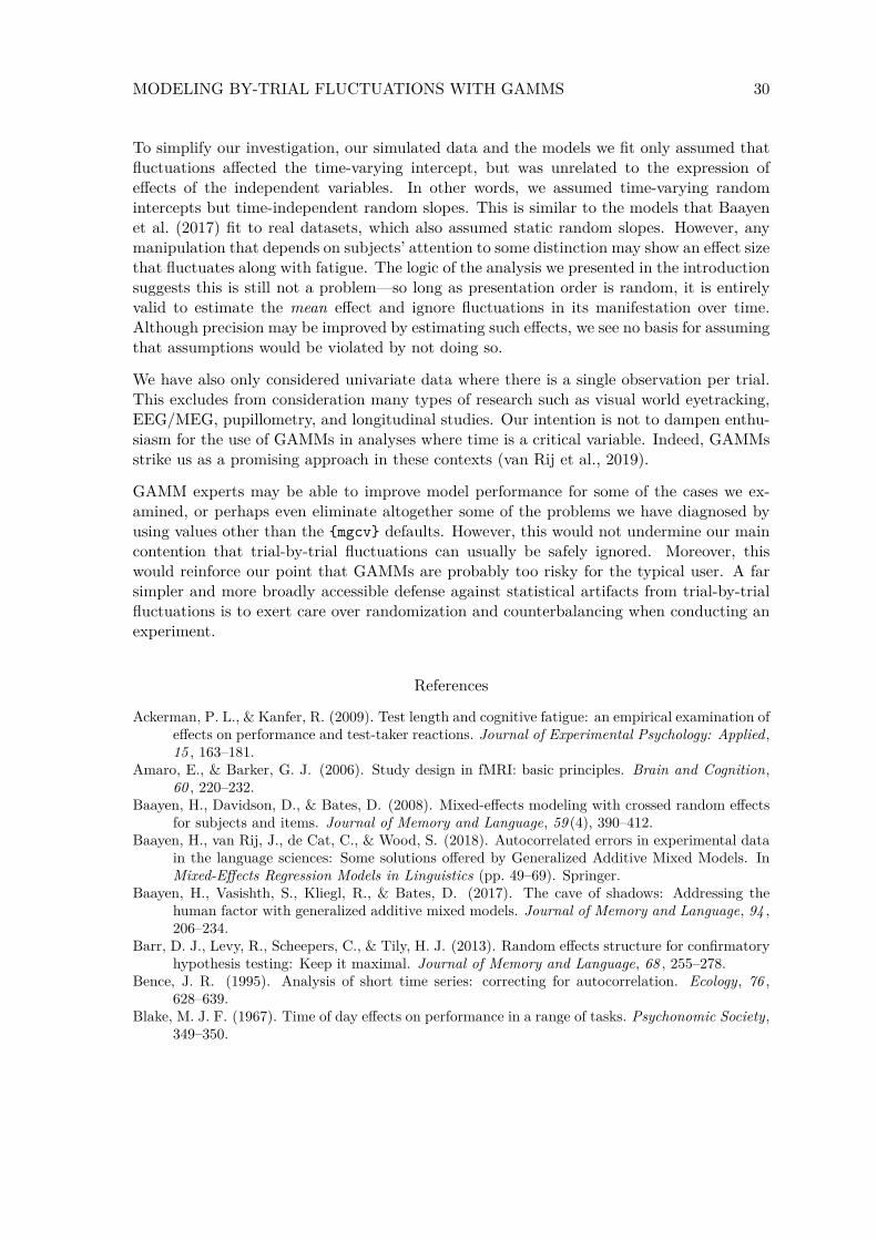
MODELING BY-TRIAL FLUCTUATIONS WITH GAMMS 30
To simplify our investigation, our simulated data and the models we fit only assumed thatfluctuations affected the time-varying intercept, but was unrelated to the expression ofeffects of the independent variables. In other words, we assumed time-varying randomintercepts but time-independent random slopes. This is similar to the models that Baayenet al. (2017) fit to real datasets, which also assumed static random slopes. However, anymanipulation that depends on subjects’ attention to some distinction may show an effect sizethat fluctuates along with fatigue. The logic of the analysis we presented in the introductionsuggests this is still not a problem—so long as presentation order is random, it is entirelyvalid to estimate the mean effect and ignore fluctuations in its manifestation over time.Although precision may be improved by estimating such effects, we see no basis for assumingthat assumptions would be violated by not doing so.
We have also only considered univariate data where there is a single observation per trial.This excludes from consideration many types of research such as visual world eyetracking,EEG/MEG, pupillometry, and longitudinal studies. Our intention is not to dampen enthu-siasm for the use of GAMMs in analyses where time is a critical variable. Indeed, GAMMsstrike us as a promising approach in these contexts (van Rij et al., 2019).
GAMM experts may be able to improve model performance for some of the cases we ex-amined, or perhaps even eliminate altogether some of the problems we have diagnosed byusing values other than the mgcv defaults. However, this would not undermine our maincontention that trial-by-trial fluctuations can usually be safely ignored. Moreover, thiswould reinforce our point that GAMMs are probably too risky for the typical user. A farsimpler and more broadly accessible defense against statistical artifacts from trial-by-trialfluctuations is to exert care over randomization and counterbalancing when conducting anexperiment.
References
Ackerman, P. L., & Kanfer, R. (2009). Test length and cognitive fatigue: an empirical examination ofeffects on performance and test-taker reactions. Journal of Experimental Psychology: Applied,15 , 163–181.
Amaro, E., & Barker, G. J. (2006). Study design in fMRI: basic principles. Brain and Cognition,60 , 220–232.
Baayen, H., Davidson, D., & Bates, D. (2008). Mixed-effects modeling with crossed random effectsfor subjects and items. Journal of Memory and Language, 59 (4), 390–412.
Baayen, H., van Rij, J., de Cat, C., & Wood, S. (2018). Autocorrelated errors in experimental datain the language sciences: Some solutions offered by Generalized Additive Mixed Models. InMixed-Effects Regression Models in Linguistics (pp. 49–69). Springer.
Baayen, H., Vasishth, S., Kliegl, R., & Bates, D. (2017). The cave of shadows: Addressing thehuman factor with generalized additive mixed models. Journal of Memory and Language, 94 ,206–234.
Barr, D. J., Levy, R., Scheepers, C., & Tily, H. J. (2013). Random effects structure for confirmatoryhypothesis testing: Keep it maximal. Journal of Memory and Language, 68 , 255–278.
Bence, J. R. (1995). Analysis of short time series: correcting for autocorrelation. Ecology, 76 ,628–639.
Blake, M. J. F. (1967). Time of day effects on performance in a range of tasks. Psychonomic Society,349–350.
MODELING BY-TRIAL FLUCTUATIONS WITH GAMMS 31
Briggs, W. L., & Henson, V. E. (1995). The DFT: An Owner’s Manual for the Disrete FourierTransform. SIAM.
Bullmore, E., Brammer, M., Williams, S. C., Rabe-Hesketh, S., Janot, N., David, A., . . . Sham,P. (1996). Statistical methods of estimation and inference for functional MR image analysis.Magnetic Resonance in Medicine, 35 , 261–277.
Cochrane, D., & Orcutt, G. H. (1949). Application of least squares regression to relationshipscontaining auto-correlated error terms. Journal of the American Statistical Association, 44 ,32–61.
Ebersole, C. R., Atherton, O. E., Belanger, A. L., Skulborstad, H. M., Allen, J. M., Banks, J. B., . . .Nosek, B. A. (2016). Many Labs 3: Evaluating participant pool quality across the academicsemester via replication. Journal of Experimental Social Psychology, 67 , 68-82.
Forbach, G. B., Stanners, R. F., & Hochhaus, L. (1974). Repetition and practice effects in a lexicaldecision task. Memory & Cognition, 2 , 337–339.
Griffiths, W., & Beesley, P. (1984). The small-sample properties of some preliminary test estimatorsin a linear model with autocorrelated errors. Journal of Econometrics, 25 , 49–61.
Huitema, B. E., & McKean, J. W. (1998). Irrelevant autocorrelation in least-squares interventionmodels. Psychological Methods, 3 (1), 104.
Jones, M., Curran, T., Mozer, M. C., & Wilder, M. H. (2013). Sequential effects in response timereveal learning mechanisms and event representations. Psychological Review, 120 (3), 628.
Keuleers, E., Diependaele, K., & Brysbaert, M. (2010). Practice Effects in Large-Scale Visual WordRecognition Studies: A Lexical Decision Study on 14,000 Dutch Mono- and Disyllabic Wordsand Nonwords. Frontiers in Psychology, 1 , 174.
Kleitman, N. (1963). Sleep and wakefulness.Luke, S. G. (2017). Evaluating significance in linear mixed-effects models in R. Behavior Research
Methods, 49 , 1494–1502.McVay, J. C., & Kane, M. J. (2009). Conducting the train of thought: working memory capacity,
goal neglect, and mind wandering in an executive-control task. Journal of ExperimentalPsychology: Learning, Memory, and Cognition, 35 , 196.
Mirman, D. (2016). Growth curve analysis and visualization using R. CRC press.Monsell, S. (2003). Task switching. Trends in Cognitive Sciences, 7 , 134–140.Olszowy, W., Aston, J., Rua, C., & Williams, G. B. (2019). Accurate autocorrelation modeling
substantially improves fMRI reliability. Nature Communications, 10 , 1–11.Papoulis, A., & Pillai, S. U. (2002). Probability, Random Variables and Stochastic Processses (Fourth
ed.). Boston: McGraw Hill.Purdon, P. L., & Weisskoff, R. M. (1998). Effect of temporal autocorrelation due to physiolog-
ical noise and stimulus paradigm on voxel-level false-positive rates in fMRI. Human BrainMapping, 6 (4), 239–249.
R Core Team. (2019). R: A language and environment for statistical computing [Computer softwaremanual]. Vienna, Austria. Retrieved from https://www.R-project.org/
Shinozuka, M., & Deodatis, G. (1991). Simulation of stochastic processes by spectral representation.Applied Mechanics Reviews, 44 (4), 191–204.
Sóskuthy, M. (2017). Generalised additive mixed models for dynamic analysis in linguistics: Apractical introduction. arXiv preprint arXiv:1703.05339 .
Stroop, J. R. (1935). Studies of interference in serial verbal reactions. Journal of ExperimentalPsychology, 18 , 643–662.
van Rij, J., Hendriks, P., van Rijn, H., Baayen, R. H., & Wood, S. (2019). Analyzing the timecourse of pupillometric data. Trends in Hearing, 23 , 1–22.
Winter, B., & Wieling, M. (2016). How to analyze linguistic change using mixed models, GrowthCurve Analysis and Generalized Additive Modeling. Journal of Language Evolution, 1 , 7-18.
Wood, S. (2011). Fast stable restricted maximum likelihood and marginal likelihood estimation ofsemiparametric generalized linear models. Journal of the Royal Statistical Society (B), 73 ,

MODELING BY-TRIAL FLUCTUATIONS WITH GAMMS 32
3-36.Wood, S. (2017). Generalized Additive Models: An Introduction with R (2nd ed.). Chapman and
Hall/CRC.Woolrich, M. W., Ripley, B. D., Brady, M., & Smith, S. M. (2001). Temporal autocorrelation in
univariate linear modeling of FMRI data. Neuroimage, 14 , 1370–1386.Worsley, K. J., & Friston, K. J. (1995). Analysis of fMRI time-series revisited—again. Neuroimage,
2 , 173–181.
Appendix
Generating correlated residuals
We use the numerical method developed in Shinozuka and Deodatis (1991) to generatecorrelated residuals. Residuals are modeled as a zero-mean stationary stochastic processX(t), which we express in its temporally discretized spectral form as (Papoulis & Pillai,2002)
X (p∆t) = ReM−1∑n=0
Bn exp [i(n∆ω)(p∆t)], (1)
for p = 0, . . . ,M − 1 and Bn =√
2An exp(iαn) for n = 0, . . . ,M − 1. The coefficients Anare given by An =
√2S(n∆ω)∆ω with αn uniformly distributed on [0, 2π] and A(0) = 0
for S(0) 6= 0. S(ω) denotes the spectrum (see below). We discretize time and frequency insteps of ∆t and ∆ω, respectively.
The spectrum S(ω) is the Fourier transform of the autocorrelation function (ACF) R(t)and is given by
S(ω) = 12π
∫ ∞−∞
R(t)e−iωtdt . (2)
In the present study, we empployed the squared-exponential function
R(t) = σ2 exp(− t2
2γ2
). (3)
For practical reasons, we cannot evaluate the integral in (2) for limits at infinity, but requiresome finite limit Tmax. Since realistic ACFs decay towards zero for large times, we chooseTmax such that |γ(t)| < δ for t > Tmax and some δ with 0 ≤ δ 1. In other words, theACF is very small for times larger than Tmax, so that we make a vanishingly small errorby excluding these values in the evaluation of the integral. ACFs for stationary stochasticprocesses are symmetric around t = 0, so that the entire time domain for the integral in (2)is [−Tmax, Tmax].
As Eq. (1) shows, there is a maximal frequency (M − 1)∆ω — which results from settingn = M−1 in the sum — for which we need to compute the spectrum. In other words, thereis a critical cut-off frequency ωc for the spectrum, which we determine by demanding that∫ ωc
0S(ω)dω = (1− ε)
∫ ∞0
S(ω)dω , (4)

MODELING BY-TRIAL FLUCTUATIONS WITH GAMMS 33
for 0 < ε 1. Equation (4) states that we choose ωc in such a way that we only lose a smallfraction ε of the total power, i.e. the integral over the spectrum. The practical steps fordetermining ωc are as follows. We first divide the time domain [Tmax, Tmax] into 2Nt gridpoints and then use the fast Fourier transform (FFT) to evaluate the integral in Eq. (2).The FFT yields 2Nt values of the spectrum evaluated at [−Nt∆ωS, (Nt − 1)∆ωS], where∆ωS = (2π)/(2Tmax) denotes the fundamental frequency (Briggs & Henson, 1995). Notethat we work with the angular frequency ω, and not the frequency f , hence a factor of 2π.The cut-off frequency ωc follows by numerically evaluating the integrals in Eq. (4) based onthe computed spectrum on the frequency domain [−Nt∆ωS, (Nt − 1)∆ωS].
With the critical frequency ωc determined, we introduce the spectral discretisation ∆ω =ωc/N and the corresponding spectral grid [−N∆w, (N−1)∆w] for the the stochastic processin Eq. (1). We can choose N to be different from Nt and hence ∆w may differ from ∆ωS.Because X(t) in Eq. (1) has a period of T0, i.e. X(t+T0) = X(t), we arrive at the constraint
M∆t = T0 = 2π∆ω . (5)
In other words, we can either fix M , and obtain ∆t, or we fix ∆t, and hence obtain M .Because we can choose ∆t, the time discretisation of X(t) can be different from the timediscretisation that we used for determining the cut-off frequency for the spectrum, ∆tS =Tmax/Nt.
A key issue in spectral reconstruction is known as aliasing. Essentially, components withcertain frequencies, i.e. certain values of n in Eq. (1), cannot be distinguished (hence thename alias). To avoid this, the critical frequency in the spectral decomposition (fc) needsto be smaller than the so-called Nyquist frequency, which is half the sampling frequency fs,i.e.
fc <fs2 ⇐⇒ ωc <
2πfs2 = 2π
2∆t . (6)
Here, we used the fact that the sampling frequency is the inverse of the time discretization∆t of X(t): fs = 1/∆t. Equation (6) entails that given a cut-off frequency ωc, the timediscretization of X(t) needs to satisfy
∆t < 2π2ωc
. (7)
In other words, there is a maximal time step for the numerical construction of X(t). UsingEq. (5) and the definition of ∆ω from above, this relates M and N via
∆t = 2πM∆ω = 2πN
Mωc<
2π2ωc
⇐⇒ 2N < M . (8)
This constraint needs to be observed when implementing Eq. (1). A final consideration isworth noting. As mentioned above, the spectral discretization for computing the cut-offfrequency, ∆ωS , may differ from the one for constructing X(t), ∆ω. If this is the case, weneed to recompute the spectrum since the computation of X(t) in Eq. (1) relies on S(n∆ω)via the coefficients An, while the integration in Eq. (2) is based on S(n∆ωS). In order torecompute the spectrum for the frequency domain [−N∆w, (N − 1)∆w] using FFT and

MODELING BY-TRIAL FLUCTUATIONS WITH GAMMS 34
Eq. (2), we require a new time discretization. Neither ∆t, which enters the computation ofX(t), nor ∆tS from above are appropriate. The new time discretisation follows from thefrequency discretization ∆ω and the fact that there are 2N grid points as
∆t∆f = 12N ⇐⇒ ∆t = 2π
2N∆ω = 2π2ωc
. (9)
As a consequence, the length of the time domain for the integral in Eq. (2) is
2N∆t = 2πNωc
= 2π∆ω = T0 , (10)
where we used Eq. (5). Hence, the total time over which we integrate the ACF to obtain thespectrum and the total time of X(t) are identical. What differs is the time discretization.
Probability densities for sine waves
We here derive the probability density for the residuals when they are described by a sumof Gaussian white noise with either a sine function with fixed amplitude/random phase ora sine function with fixed phase/random amplitude. These two cases are labelled 1 and 2 inFigure 5. Let X denote the random variable involving the sine function and Y ∼ N (0, σ2)the Gaussian white noise. When we set Z = X + Y , the probability density for Z is givenby (Papoulis & Pillai, 2002)
pZ(z) =∫
ΩpX(x)pY (z − x)dx, (11)
where the possible values of X are collected in the set Ω. For the first case when we fixthe amplitude and randomize the phase, we use X = sin(ωt + Φ) where ω = 2π/T isthe frequency of the sine function and Φ ∼ U [−π, π] is a uniformly distributed randomphase. Note that we use ∆ = 48 and t ∈ [0,∆] throughout, see e.g. Figure 1. Because tis a deterministic variable on [0,∆], we can also interpret it as a random variable drawnuniformly from the same interval, i.e. T ∼ U [0,∆]. With that, it is evident that (2πT+Φ) isa uniformly distributed random variable, which we can replace with Ψ ∼ U [−π, π] because ofthe periodicity of the sine function. Hence, we require the probability density for X = sin Ψ.Since the range of X is [−1, 1], we can restrict Ψ to the interval [−π/2, π/2]. Due to theconservation of probability, we obtain (Papoulis & Pillai, 2002)
pX(x) = pΨ(ψ)∣∣∣∣dψdx
∣∣∣∣ = 1π
1√1− x2
, (12)
where we used that dx = cosψdψ and
cos2(ψ) = cos2(arcsin x) = 1− x2 , (13)
since cos2(x) = 1− sin2(x). Note that the restriction of Ψ to [−π/2, π/2] also insures thatwe can invert the sine function, since it is strictly monotonically increasing in this interval.From Eq. (11), we therefore find that
pZ(z) = 1π
∫ 1
−1
F (z − x, σ)√1− x2
dx , (14)

MODELING BY-TRIAL FLUCTUATIONS WITH GAMMS 35
whereF (x, σ) = 1√
2πσ2exp
(− x2
2σ2
)(15)
is the Gaussian probability distribution. In the second case, when the phase is constant,but the amplitude is randomized, we generate the residuals with X = A sin(ωt), whereA ∼ U [0, α]. Based on the considerations above, we can replace X with X = A sin(Ψ) whereΨ ∼ U [−π/2, π/2]. Hence, X is the product of two random variables A and B = sin(Ψ)with the probability density (Papoulis & Pillai, 2002)
pX(x) =∫ 1
−1pB(b)pA
(x
b
) 1|b|
db . (16)
Because of the absolute value in Eq. (16), it is instructive to consider the two cases b ∈ [−1, 0]and b ∈ [0, 1] separately. Starting with the latter, we need to evaluate
pX(x) =∫ 1
0pB(b)pA
(x
b
) 1b
db . (17)
Since b > 0 and a > 0, x > 0. Moreover, as maxA = α, we require x/b ≤ α in Eq. (17),which leads to
pX(x) =∫ 1
x/αpB(b)pA
(x
b
) 1b
db . (18)
When b ≤ 0, x ≤ 0. Because x/b ≤ α still holds, we now have the restriction, b ≤ x/a, sothat
pX(x) =∫ x/α
−1pB(b)pA
(x
b
) 1b
db , (19)
which can be rewritten (transforming b 7→ −b) as
pX(x) =∫ 1
|x|/αpB(−b)pA
(−xb
) 1|b|
db , (20)
As pB(b) = pB(−b) (see Eq. (12)) and pA = 1/α, we can combine Eqs. (18) and (20) into
pX(x) = 1πα
∫ 1
|x|/α
1z√
1− b2db ,
= 1πα
ln
√1− x2
α2 + 1
− ln( |x|α
) . (21)
Using Eq. (11), we finally obtain the probability density for the case of a randomizedamplitude as
pZ(z) =∫ α
−αpX(x)F (z − x)dy . (22)