Using Economically Designed Shewhart and Adaptive X - Charts for

Monitoring the Quality of Tiles

Yiannis Nikolaidis

George Rigas

George Tagaras (tagaras@auth.gr)

Department of Mechanical Engineering

Aristotle University of Thessaloniki

54124 Thessaloniki

Greece

tel: +30-2310-996017

fax: +30-2310-996018

March 2005

1

Using Economically Designed Shewhart and Adaptive X - Charts for

Monitoring the Quality of Tiles

Summary

This paper presents the economic design of X control charts for monitoring a

critical stage of the main production process at a tile manufacturer in Greece. Two

types of X -charts are developed: a chart of the Shewhart type with fixed parameters

and adaptive charts with variable sampling intervals and/or sample size. Our prime

motivation was to improve the statistical control scheme employed for monitoring an

important quality characteristic of the process with the objective of minimizing the

relevant costs. At the same time we test and confirm the applicability of the theoretical

models supporting the economic design of control charts with fixed and variable

parameters in a practical situation. We also evaluate the economic benefits of moving

from the broadly used static charts to the application of the more flexible and effective

adaptive control charts. The main result of our study is that by redesigning the currently

employed Shewhart chart using economic criteria, the quality-related cost is expected

to decrease by approximately 50% without increasing the implementation complexity.

Monitoring the process by means of an adaptive X -chart with variable sampling

intervals will increase the expected cost savings by about 10% compared to the

economically designed Shewhart chart at the expense of some implementation

difficulty.

Key words: Statistical Process Control, Process Monitoring, Control Charts

2

Using Economically Designed Shewhart and Adaptive X - Charts for

Monitoring the Quality of Tiles

1. Introduction

This paper presents a detailed study leading to the industrial application of

relatively new concepts in control chart design for more effective statistical monitoring

of a critical stage of tile manufacturing. The motivation for the study came on one hand

from the endeavor of the management of Philkeram - Johnson s.a. (PJ for brevity), a

major Greek manufacturer of ceramic tiles, to continuously improve their on-line quality

assurance methods and on the other hand from the authors’ observation that such an

improvement could be based on the utilization of economically designed control charts.

Philkeram - Johnson was founded in 1963 with initial production capacity of

around 78,000 m2 of tiles per year. Its immediate financial success attracted the

interest of foreign investors and very soon the company tripled its production and

started emphasizing its exporting activities. In 1966 PJ produced embossed tiles for the

first time. As the new product was widely accepted by the market, both in Greece and

abroad, the company expanded even more reaching a workforce level of around 350

employees. In 1982 PJ introduces for the first time an innovative technology for the

production of tiles, based on a “single-firing” production process, instead of the well

known and used until then “double-firing” technology. The new technology resulted in

cost reduction, higher productivity and better tile quality. In 1987 the company enters

the American market and in 1989 it is awarded the Sign of Quality from the Greek

Organization of Standardization, thanks to the conformance of all of the company’s

products to the relevant European norms and standards. Today, PJ’s capitalization

exceeds 41,500,000 €. The company has a workforce of 415 employees, its

manufacturing facilities cover an area of approximately 40,000 m2 and its production

3

capacity is around 4,300,000 m2 of tiles per year.

The profile of a tile’s final quality is composed by a multitude of characteristics

and properties, including resistance to scratching, breaking and every kind of wear,

water absorption, resistance to acids and other chemical agents, color, design and

dimensions. Tiles’ dimensions, and in particular orthogonality, are very important

determinants of quality of the final product. The dimensions are primarily determined

during the tile formation stage in the press. It is therefore important to monitor on line at

that stage the values of a critical quality characteristic, which is directly related to the

dimensions and shape of the final product. It turns out that such a characteristic is a

suitably chosen measure of the penetrability of tiles as will be further explained in the

next section.

The main practical objective of the research presented in this paper was to

determine the optimal monitoring of the aforementioned critical quality characteristic so

as to minimize the relevant costs. Economic optimization of control charts is viewed

with skepticism by many researchers in the SPC field, mostly because it often leads to

monitoring schemes with high false alarm rates [1]. For this reason, Montgomery [2],

among others, recommends an economic statistical design approach like the one

proposed by Saniga [3], where the cost function is optimized subject to constraints on

statistical properties, such as type I and type II errors. Taking these concerns and

recommendations into account, we have proceeded by adopting cost minimization as

the primary objective, but giving due consideration to statistical performance as well.

A secondary objective is to contribute to the enrichment of the research in

practical applications of economically designed control charts, placing emphasis on the

relatively new class of adaptive charts. Although more than forty years have elapsed

since the pioneering work of Duncan [4] on the economic selection of control chart

parameters, there are only few reported applications of economically designed control

charts in the academic literature. An example is the work of Krishnamoorthi [5] that

4

presents an early application of economic X -charts of the Shewhart type for

monitoring the process of punching holes in a plastic strip, where the distance between

centers of successive holes is the quality characteristic being controlled. He concludes

that the economically designed X -chart leads to a very sizeable reduction in average

hourly cost.

If there is a scarcity of published applications of economically designed simple

X -charts with fixed parameters (sampling interval, sample size, control limit

coefficient), there is a complete void in the literature as far as applications of

economically designed adaptive charts are concerned. Adaptive control charts were

introduced by Reynolds et al. [6] in 1988 and they have been studied quite thoroughly

since; for a comprehensive review of the first decade of developments see Tagaras [7].

The distinctive feature of the adaptive charts is that the values of the control chart

parameters change in real time, in response to information gathered from the process

in the form of sample measurements. This flexibility results in better statistical

properties and/or lower expected quality costs compared to static charts with fixed

parameters. Despite these advantages, practitioners are still reluctant to exploit this

group of charts, mostly due to perceived implementation difficulties. A notable and

unique exception, at least to our knowledge, is presented by Baxley [8] and it concerns

the application of a variable sampling interval, exponentially weighted moving average

control chart at a nylon fiber plant. In that application the chart parameter values were

chosen on the basis of statistical considerations, without explicit consideration of all the

relevant quality costs. Thus, we claim that there is no published account of using an

economically designed adaptive control chart for monitoring an actual production

process.

The following section describes briefly the production process of tiles and

section 3 presents the currently used quality monitoring procedure in the tile formation

5

stage. Section 4 introduces alternative monitoring schemes and the methodology,

which will be used for their comparison. Section 5 contains and discusses the

evaluation of the alternative process control schemes. The paper concludes with a

summary of the main findings.

2. The product and the production process

The type of tiles that was selected for this study is KERASTAR 30x30 cm,

unglazed tiles. Three reasons dictated this choice:

a) KERASTAR tiles are considered a flagship product of PJ due to their very good

properties and large volume of annual sales.

b) As this product is the only type of PJ tiles that is offered with a 50-year guarantee,

the company is especially sensitive to matters related to its quality assurance.

c) KERASTAR tiles are representative of a wide array of products with similar

properties.

KERASTAR tiles consist of a number of refined raw materials, such as kaolin,

quartz, etc. These materials are first mixed according to the specific recipe and then

the mixture is transferred to the milling department, where it is homogenized through

grinding. The grinding lasts for almost 8 hours and results in a slip that must have

specific properties concerning its viscosity, specific gravity and particle size. The

conformance of the slip to the desired values is checked systematically by means of

specific quality control procedures. Subsequently, the slip is transferred to tanks for

storage. Then, a pump leads the necessary quantities to the spray-drier tower. The

conditions of drying, namely the remaining dust moisture, air temperature and pump

pressure, are all monitored on line on a PC. The moisture is eventually reduced to 3.5 -

5.5%. Having achieved this level of drying, the “dry” dust is stored in the silos and from

there it proceeds to the production line, when that is necessary.

At the beginning of the production line, tiles are formed by a press, using the

6

appropriate dies according to the tiles’ variety. A special device connected to quality

control data computer network, records the number of hits per minute, the thickness of

each tile and the pressing power. The proper operation of the press is necessary to

ensure that the final product will have the right strength, dimensions and shape.

Due to the need for further reduction of moisture tiles are then forwarded to the

drier. Warm air blowing in the drier helps to achieve the desirable value of moisture,

which is less than 1%. As a general rule, remaining moisture in tiles is unwanted,

because it can cause explosions during the entrance of the tiles in the kiln. Therefore,

two kinds of moisture control are exercised after the drier: an indirect one by measuring

tiles’ temperature on line and a direct one by measuring the tiles’ remaining moisture at

regular intervals in the lab.

After ensuring an acceptably low moisture level, the tiles are driven into the kiln.

This process consists of three stages: the first is a warm-up stage, the second is the

“fire-zone” stage (tiles are heated at approximately 1200οC) and the third is the freezing

stage. Temperatures in all three stages are monitored on line, and so are the exhaust

temperature and the pressure in the kiln, as well as the pressure of the air both in the

“fire-zone” and in the freezing stages.

Finally, tiles are submitted to acceptance quality control. A laser device checks

for dimensional and curvature problems, while specialized personnel range the tiles

according to their appearance quality. Figure 1 presents a summary flow chart of the

entire production process.

Figure 1 about here

Our study concentrates on the tile formation stage. The press, depending on

the size of tiles produced, stamps 2 or 3 or 6 tiles in each cycle (strike). In the case of

the 30x30 cm KERASTAR tiles under examination, the press stamps 3 tiles per cycle

(there are essentially three streams of tiles and respective pressing positions). The

press operation is controlled mainly by measuring the penetrability of tiles at fixed time

7

intervals. The measurements are done by means of an instrument, which records the

penetrability of a pin in which a certain force is exercised. The level of penetrability is

indicative of the homogeneity of tiles’ material and of pressing quality, which in turn is

connected with the dimensions and shape of tiles coming out from the kiln at a

subsequent stage of the production line.

The penetrability of a tile is measured at three points on each side of the tile for

a total of 8 measurements, as shown in Figure 2. The sum of the 3 measurements of

each side is calculated and then the difference between the largest and the smallest of

these four sums is computed and recorded as the value of the controlled variable

(quality characteristic) X for that tile. This random variable expresses the dissimilarity of

press conditions, according to PJ’s know-how and practice.

Figure 2 about here

The target value for the quality characteristic X is obviously 0, as that value

typically implies the greatest possible uniformity of compression by the press. If the

value of X does not exceed 0.05 mm, then the tile is considered A class; if the value is

between 0.05 mm, and 0.1 mm the tile is classified as B class; finally, if the value of X

exceeds 0.1 mm, then such a tile is characterized as scrap, due to the faulty press

conditions that eventually result in unacceptable departure from the required

orthogonal shape.

3. Current quality monitoring practice in tile formation

The currently used quality monitoring procedure in the tile formation stage is the

following. At the beginning of each shift (i.e., every 8 hours) three tiles are collected,

one from each stream/pressing position (corresponding to a die of the punching set),

and their penetrability is measured at an adjacent working bench. If all three X values

are lower than the critical value of 0.05 mm, then the production process continues its

operation without intervention. If, however, there is at least one measurement larger

8

than 0.05 mm, then this is considered as an indication of possible disturbance

(occurrence of an assignable cause) at that position. The assignable cause, which

results in asymmetric pressure and irregular tile formation, is related to a malfunction of

the upper part of the press in one of the three pressing dies. Since it is not technically

feasible to stop only one or two of the streams, the entire press operation is

immediately interrupted and the maintenance technician is called. If the indication is

indeed correct, the technician proceeds with the necessary adjustment of the pressing

mechanism and turns on the press, having ensured that the assignable cause has

been removed. If the alarm is false, the maintenance technician can easily and quickly

identify it as such and he turns on the press immediately.

It is important to note that when the press operation is stopped, the downstream

stages (and especially the kiln, which is the bottleneck operation) continue their

operation unaffected due to the existing inventory buffers. Furthermore, the press

production rate is higher in comparison to the kiln so that it can provide the kiln with the

necessary input of tiles, even if it operates for only 20 hours in a day. Consequently, an

unnecessary interruption of the press operation generally does not result in a profit loss

due to decreased productivity.

Using conventional control chart terminology and notation, the above quality

monitoring procedure may be described as follows.

The quality characteristic X behaves as a normally distributed random variable with

mean μ = 0.0308 mm and standard deviation σ = 0.0092 mm when the process is

in control. The normality assumption was verified by means of a standard Chi-

Square goodness-of- fit test. The values of the parameters μ and σ were estimated

using a large number of data from the company’s database.

The tiles under study are produced in batches of 10,000 m2 or 15,000 m2. Taking

into account PJ’s average production rate, it follows that the duration of a

9

production run is typically either Η = 72 hours (9 shifts) or Η = 112 hours (14 shifts).

At the beginning of every production run the press is operating well and the mean

value of X is equal to the nominal value μ0 = 0.0308 mm.

The press operation is subject to the occurrence of a single assignable cause,

which increases the mean value of X without significantly affecting σ, which is

therefore considered constant (σ = 0.0092 mm). According to the analysis of

measurements in the out-of-control state the mean of X increases from μ0 = 0.0308

mm to μ1 = μ0 + δσ 0.0446 mm, which implies that the approximate magnitude of

the shift in the mean is δ = 1.5 standard deviations.

The mean time between successive occurrences of the assignable cause at any

one of the three pressing positions is approximately 20 days, which translates to a

mean rate of occurrence equal to 0.0021 per hour. As no one of the three positions

is more prone to malfunction than the others, the mean rate of occurrence of the

assignable cause at each position is v = 0.0007 per hour. The probability

distribution of that time is not sufficiently documented. For the purposes of this

study it was assumed that the occurrence time follows an exponential distribution,

adopting the usual assumption of the academic literature but also relying on the

finding of Surtihadi and Raghavachari [9] that optimality of the X -chart design is

insensitive to the distributional assumption of the occurrence time, especially for

small values of the sampling interval.

Since the interruption of the press operation due to a signal at a particular pressing

position has practically no economic effect on the operation of the other positions,

the press operation is essentially monitored by means of three independent X-

charts ( X -charts with n = 1), one per position, with sampling interval h = 8 hours

and sample size n = 1. The currently used control limit of 0.05 mm corresponds to a

control limit coefficient k = 2.09 (μ0+kσ = 0.05 with μ0 = 0.0308 and σ = 0.0092) and

10

implies that each chart operates with a false alarm probability (type I error)

0.01850.0308μ0.05Prα 00 X ,

while the power of the chart is

0.27860.04461μ0.05Pr1α X .

4. Quality costs and alternative process monitoring schemes

The current monitoring procedure of the process operation has been

determined without direct consideration of either statistical or economic criteria. In

order to evaluate the effectiveness of the current monitoring scheme from an economic

point of view and to propose improved monitoring schemes, the first step is to identify

and estimate the relevant costs. These costs include those of sampling, false alarms,

out-of-control operation and restoration, which have been estimated as follows.

The sampling cost is proportional to the sample size. The sampling cost per

unit, c, consists of two parts: the cost of sampling and measurement (labor and

materials) and the cost of the sample tiles, since the measurement is destructive. The

estimate for the total sampling cost per unit is c = 0.56 €.

Every time the monitoring scheme erroneously suggests the occurrence of an

assignable cause, the time required for the maintenance technician to assert that the

signal was indeed a false one is approximately 10 min. Taking into account the relevant

labor costs leads to the estimate of the cost of a false alarm L0 = 2.87 €.

When the control chart correctly indicates the occurrence of an assignable

cause, the adjustment of the pressing mechanism takes on average 45 min. Taking

into account the relevant labor costs and the cost of measurements required to ensure

that the adjustment was successful, the estimate of the restoration cost is L1 = 16.84 €.

Operation of the process in the out-of-control state incurs a cost due to the

production of an increased percentage of B class tiles; the percentage of

11

nonconforming tiles is negligible even when the process is out of control. Taking into

consideration the profit from the production and sale of A class tiles and that of B class

tiles (15% lower profit than for A class tiles), the average cost of out-of-control

operation (profit reduction) is estimated at Μ = 52.80 € per hour.

The next step is to decide which alternative process monitoring schemes will be

considered, optimized and compared. Recall that the duration of each production run

in the case under consideration is fixed. Thus, taking into account the need to evaluate

economic and statistical measures of performance in finite (short) runs, the choice of

monitoring schemes is limited because models suitable for short runs are available only

for a few types of charts. One possibility is to consider a Shewhart chart; Ladany [10]

first developed a model for economic optimization of a p-chart in a short run and later

Tagaras [11] adapted this model to the case of a Shewhart-type X chart. Other

obvious alternatives include the CUSUM and EWMA charts and several types of

adaptive charts, but the available economic design models for those charts assume

that the production process operates indefinitely; see, for example, the general model

of Lorenzen and Vance [12] and the model of Park and Reynolds [13] for the economic

design of adaptive charts with variable sample size and sampling interval. In contrast,

Bayesian adaptive control charts are typically designed and analyzed for production

runs of limited duration [14]. Furthermore, it is known that the Bayesian updating of the

knowledge about the state of the process (in or out of control) after every sample leads

to the optimal adaptive process control rules by taking into account all the available

relevant information [15]. Therefore, we set out to determine the economically optimal

parameters of the standard Shewhart X chart (sampling interval h, sample size n and

control limit coefficient k) and of the following four types of Bayesian adaptive X -charts

for which appropriate economic models are available [16]:

- X -chart with fixed sample size and sampling interval (Bayes chart),

12

- X -chart with fixed sample size and adaptive sampling interval (Bayes-h chart),

- X -chart with adaptive sample size and fixed sampling interval (Bayes-n chart),

- X -chart with adaptive sample size and adaptive sampling interval (Bayes-h-n chart).

The total expected cost related to monitoring a process by means of a

Shewhart X control chart over the duration H of a finite production run is determined

through the following cost function [11]:

i-vh1 1-vh

si 0 i 0 1

1 1i-vh -vh

0 0 1 1i 0 i 0

1 α 1 1 αvh 1 eC b cn Μ P i Mh 1 e P i

v α

L α e P i L 1 e P i 1 1 α

(1)

where

b: fixed cost per sample (0 in this case),

c: variable cost per sample unit,

Μ: cost of out-of-control operation per time unit,

L0: cost of a false alarm,

L1: cost of restoring the process after a true alarm,

α1: probability of detecting the shift in case of occurrence of the assignable cause,

α0: probability of a false alarm,

ν: average rate of occurrence of the assignable cause,

: number of samples taken during the production run; = (H/h) – 1,

P(i): probability that the sampling interval after the ith sample will start with the

production process in the in control state; i = 0, 1, …, , where i = 0 denotes the

beginning of the production run.

The expected cost Cs is a function of the control chart parameters h, n and k,

the latter entering Cs indirectly through α0 and α1. Minimization of Cs with respect to

these parameters yields their optimal combination for monitoring the process with a

control chart of the Shewhart type.

13

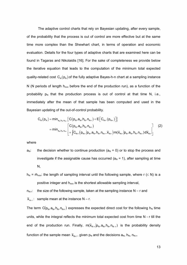
The adaptive control charts that rely on Bayesian updating, after every sample,

of the probability that the process is out of control are more effective but at the same

time more complex than the Shewhart chart, in terms of operation and economic

evaluation. Details for the four types of adaptive charts that are examined here can be

found in Tagaras and Nikolaidis [16]. For the sake of completeness we provide below

the iterative equation that leads to the computation of the minimum total expected

quality-related cost Ν ΝC p of the fully adaptive Bayes-h-n chart at a sampling instance

N (Ν periods of length hmin before the end of the production run), as a function of the

probability pN that the production process is out of control at that time N, i.e.,

immediately after the mean of that sample has been computed and used in the

Bayesian updating of the out-of-control probability.

Ν Ν Ν-r

Ν Ν Ν-r

Ν Ν a ,h ,n Ν Ν Ν Ν-r Ν-r Ν-r

Ν Ν Ν Ν-r

a ,h ,nΝ-r Ν-r Ν Ν Ν Ν-r Ν-r Ν-r Ν Ν Ν Ν-r Ν-r

C p min C p ,a ,h ,n E C p

C p ,a ,h ,nmin

C p p ,a ,h ,n ,x m(x p ,a ,h ,n )dx

(2)

where

aΝ: the decision whether to continue production (aΝ = 0) or to stop the process and

investigate if the assignable cause has occurred (aΝ = 1), after sampling at time

N,

hΝ = rhmin: the length of sampling interval until the following sample, where r ( N) is a

positive integer and hmin is the shortest allowable sampling interval,

nΝ-r: the size of the following sample, taken at the sampling instance Ν – r and

rΝx : sample mean at the instance Ν – r.

The term r-ΝΝΝΝ n,h,a,pC expresses the expected direct cost for the following hN time

units, while the integral reflects the minimum total expected cost from time N - r till the

end of the production run. Finally, )n,h,a,px(m rΝΝΝΝrΝ is the probability density

function of the sample mean r-Νx , given pΝ and the decisions aΝ, hΝ, nΝ-r.

14

The numerical evaluation of the cost function Ν ΝC p yields the optimal

monitoring policy, namely the optimal values of the decision variables aN, hN and nN-r for

every possible sampling instance N and for every possible (discretized) value of the

probability pN. The iterative function (2) is simplified in the cases where the production

process is monitored with the aid of a Bayes-h chart (with decision variables aΝ, hΝ), a

Bayes-n chart (with decision variables aN, nN-1) or a Bayes control chart (with decision

variables aN only). In all cases, though, the optimal policy is a set of values of the

decision variables for all N and pN.

In addition to the economic performance of the above charts, it is important to

consider their statistical performance, especially with respect to the false alarm rate

that is often high when the chart parameters are obtained through a cost minimization

model. To this end we use the expected total number of false alarms, F, during a run

that stays in control for its entire duration, as a suitable indicator of statistical

performance in a short run.

In the case of the Shewhart chart with false alarm probability α0, the expected

total number of false alarms in the samples of the run, assuming that the process

stays in control, is F = α0. For a given monitoring policy with any Bayesian adaptive

chart, the expected total number of false alarms during a run that remains in control for

its entire duration is computed iteratively from

*N r

*N r

x

Ν Ν N r N r N r N r N r N r N r N rx

F F p F (p )f(x )dx [1 F (p 0)]f(x )dx (3)

where N rf(x ) is the probability density function of the sample mean r-Νx given that the

process is in control at the instance N – r (normal with mean μ0 and variance σ2/nN-r) and

*N rx is the critical value of r-Νx above which pN-r is such that aN-r = 1 (false alarm).

15

5. Evaluation of the competing process control schemes

As it has already been explained in section 3, the current monitoring scheme at

each stream/pressing position is essentially a standard Shewhart X chart with h = 8

hours, n = 1 and k = 2,09, resulting in F = α0 = (H/8 -1)(0.0185) expected false alarms

per production run of H hours in the in-control state. Its economic performance is

evaluated through the calculation of the expected quality-related cost using (1). It turns

out that the expected cost of this scheme is Cs = 49.76 € for a production run of H = 72

hours and Cs = 88.25 € for a production run of H = 112 hours. The total expected cost,

Ct, for all three pressing positions is simply three times the expected cost of one

position, i.e., Ct = 3Cs = 149.28 € for H = 72 hours and Ct = 264.75 € for H = 112 hours

(Table 1).

Around 90% of the expected cost of the current scheme is attributed to

operation in the out-of-control state, implying that the power of the charts in use is

insufficient. Indeed, a search for the optimal values of the chart parameters h, n, k of

the Shewhart chart shows that while the optimal sample size remains at n = 1 and the

optimal sampling interval h is not dramatically different from the current h = 8 hours, the

optimal value of the control chart coefficient is only k = 0.82 (H = 72) or k = 0.85 (H =

112) to achieve a much higher power of detecting the assignable cause. The optimal

Shewhart chart results in a cost reduction of 48% (H = 72) to 53% (H = 112) with

respect to the current monitoring scheme. The results are summarized in Table 1. The

improvement in the detection power and the resulting cost reduction are achieved at

the expense of more frequent false alarms as the F values in Table 1 indicate.

However, recall that false alarms are relatively inexpensive in this case. Moreover, the

process interruptions due to false alarm signals do not have any negative impact on the

productivity of the production line due to the slack capacity of the press operation

compared to the bottleneck kiln operation. A simple calculation shows that, on average,

16

the downtime due to false alarms when the optimal Shewhart chart is used amounts to

no more than 7% of the available slack. Thus, the higher than usual false alarm rate is

tolerable in this particular application.

Table 1 about here

The next issue that we investigated was whether the use of adaptive Bayesian

control charts could lead to substantial further cost reduction with respect to the optimal

Shewhart chart. The optimal process control policies for the four types of Bayesian

charts were obtained using the appropriate version of (2) according to the type of the

chart and searching for the optimal values of the fixed parameters. The results for

production runs of length H = 72 hours and H = 112 hours are shown in Tables 2 and 3

respectively, where ΔC denotes the percentage cost reduction with respect to the

current scheme and ΔC’ denotes the further cost reduction with respect to the optimal

Shewhart chart. The allowable values of the variable parameter n for the Bayes-n and

Bayes-h-n charts were {1, 2, 3, 4}, while the allowable values of the variable parameter

h for the Bayes-h and Bayes-h-n charts were {0.1hs, 0.2hs, 0.4hs, 0.6hs, 0.8hs, hs}, i.e.

hmin = 0.1hs, where hs is the sampling interval of the respective optimal Shewhart chart:

hs = 6.55 hours when H = 72 hours and hs = 6.22 hours when H = 112 hours.

Tables 2 and 3 about here

Tables 2 and 3 show that there is practically no difference between the Bayes

and Bayes-n charts, nor between the Bayes-h and Bayes-h-n charts, because it is

almost always optimal to use n = 1, even when the sample size n is allowed to vary

and the probability pN that the process operates in the out-of-control state is high. In

fact, only for a few pN values at the final stages of the production run it was preferable

to use n = 2 (with insignificant effect on the total cost), while it was never optimal to use

a larger sample size. Thus, since for practical purposes it suffices to use a fixed sample

size n = 1, we limit our attention to the Bayes and Bayes-h charts with n = 1 and

variable sampling interval h. Then, the most important conclusion from Tables 2 and 3

17

is that the Bayes chart is not considerably more effective than the much simpler optimal

Shewhart chart, but the Bayes-h chart with n = 1 offers a substantial additional cost

reduction over the optimal Shewhart chart that approaches 10%. Furthermore, the

Bayes-h chart with n = 1 has a much lower false alarm rate than the optimal Shewhart

chart and consequently it is more acceptable in terms of statistical performance.

Another conclusion that is in agreement with the general findings in [16] is that

the main determinant of the performance of the Bayes-h chart is the shortest allowable

value hmin of the variable sampling interval. In addition to the set of h values that was

used to obtain the optimal policy reported in Tables 2 and 3 (six h values in the range

from 0.1hs to hs), we tried numerous other sets of h values. Due to space limitations we

will only provide below a brief indication of the effect of the allowable h values on the

total expected cost of the Bayes-h chart with n = 1 for the case H = 72 hours:

With h {0.25hs, 0.5hs, 0.75hs, hs, 1.5hs, 2hs, 2.5hs, 3hs} the cost is 72.57 (ΔC' =

6,46%).

With h {0.1hs, 0.2hs, 0.4hs, 0.6hs, 0.8hs, hs} the cost is 71.43 (ΔC' = 7.9%).

With h {0.025hs, 0.05hs, 0.1hs, 0.2hs, 0.45hs, 0.8hs, hs} the cost is 70.50 (ΔC' =

9,13%).

We have also tried variations of the Bayes-h chart with only two values of the sampling

interval (hmin and hmax), as has been suggested in the literature based on the

satisfactory statistical properties of such charts [17], but their economic performance

was not nearly as good as that of the Bayes-h chart with multiple (six in this case)

choices for the variable sample size.

While the above comparison of different control chart types and the

investigation of the effect of the allowable h values are theoretically meaningful, for an

industrial application like the one presented in this paper it is important to take into

consideration some practical issues and constraints to arrive at a final

18

recommendation. Specifically, the sampling interval must be convenient and the control

limit has to be a simple value that is easy to remember. Recall, for example that the

optimal sampling intervals for the Shewhart chart were found to be hs = 6.55 hours for

production runs of H = 72 hours ( = 10 samples per run) and hs = 6.22 hours when H =

112 hours ( = 17 samples per run) and that hmin = 0.1hs for the Bayes-h chart. Such

sampling intervals are definitely impractical. Moreover, it is highly desirable to use the

same scheme irrespective of the duration of the production run H if the economic

consequence is not too large. Therefore, the optimal parameters have to be slightly

modified in the direction of simplification, ease of use and improved statistical

performance, especially knowing that moderate departures from optimality have a

minor effect on the expected cost, as the cost function is rather flat around the

optimum.

The final outcome of these considerations and the need to compromise

between theoretical optimality and practicality was the following recommendation to PJ:

If the press operation is to be monitored by a Shewhart type chart for the sake of

simplicity, then the sampling interval should be h = 6 hours, the sample size will still

be n = 1 per position and the control limit must be changed to 0.04 mm,

corresponding to a control limit coefficient k = 1 and expected number of false

alarms F = 1.75 for H = 72 hours and F = 2.86 for H = 112 hours, down from F =

2.06 and F = 3.36 respectively of the optimal Shewhart chart. The total expected

quality-related cost of this monitoring scheme, computed from (1), will be Ct = 78.00

€ for H = 72 hours and Ct = 124.70 € for H = 112 hours. The cost reduction with

respect to the currently used monitoring scheme is estimated at 47.7% and 52.9%

respectively.

From an economic and a statistical viewpoint it is advisable to monitor the press

operation by means of a Bayes-h chart with n = 1 per position and allowing the

19

sampling interval to vary taking values (in hours) from the set {0.5, 1, 2, 4, 6, 8}

according to the updated probability pN after each sample. Table 4 shows the

optimal decision aN to continue (aN=0) or stop the process and restore it if an

assignable cause has indeed occurred (aN=1) and the optimal next sampling

interval hN as functions of the pN value for stage N = 72, namely in the middle of the

production run H = 72 (N=72 “periods” of length hmin = 0.5 hours before the end of

the run). The total expected quality-related cost of this Bayes-h chart, computed

from (2) with fixed nN-r = 1, will be 71.25 € for production runs of length H = 72

hours and 113.05 € for runs of H = 112 hours. The cost reduction with respect to

the currently used monitoring scheme will be 52.3% and 57.3% respectively. The

expected number of false alarms, computed from (3) for this monitoring scheme, is

F = 0.76 for H = 72 hours and F = 1.23 for H = 112 hours.

Table 4 about here

6. Conclusion

We have presented a complete analysis for the redesign of the on-line

monitoring procedure of a critical stage in the manufacturing of ceramic tiles aiming at

reducing the expected quality-related costs subject to practical constraints and

considerations. Our main conclusions are summarized in the following:

The economic design of the Shewhart-type chart used for monitoring the press

operation in the tile formation stage results in a procedure that is as simple as the

one currently used but at the same time reduces the total expected quality costs by

about 50%. On the negative side the false alarm rate of this procedure is rather

high, but this is not a major concern in this application due to its particular

characteristics.

Monitoring the process by means of an adaptive Bayesian control chart with fixed

20

sample size and variable sampling interval is not much more complicated and may

further increase the cost savings by almost 10% compared to the optimal Shewhart

chart, improving at the same time the statistical performance of the monitoring

scheme by substantially reducing the expected number of false alarms.

The company has already expressed its intention to modify the inspection

process in the press department taking into account the above conclusions.

Acknowledgement

The authors are grateful to Nikolaos Metaxas, Control Manager of Philkeram-Johnson,

for his valuable assistance throughout this project.

References

1. Woodall WH. Weaknesses of Economic Design of Control Charts. Technometrics

1986 28: 408-409.

2. Montgomery DC. Introduction to Statistical Quality Control; Wiley: New York, NY,

2001.

3. Saniga EM. Economic Statistical Control Chart Designs With an Application to X

and R Charts. Technometrics 1989 31: 313-320.

4. Duncan AJ. The Economic Design of X -Charts Used to Maintain Current Control of

a Process. Journal of the American Statistical Association 1956 51: 228-242.

5. Krishnamoorthi KS. Economic Control Charts - An Application. ASQC Quality

Congress Transaction 1985: 385-391.

6. Reynolds MR Jr, Amin RW, Arnold JC, Nachlas JA. X Charts with Variable Sampling

Intervals. Technometrics 1988 30: 181-192.

7. Tagaras G. A Survey of Recent Developments in the Design of Adaptive Control

21

Charts. Journal of Quality Technology 1998 30: 212-231.

8. Baxley RV Jr. An Application of Variable Sampling Interval Control Charts. Journal

of Quality Technology 1995 27: 275-282.

9. Surtihadi J, Raghavachari, M. Exact economic design of X charts for general time

in-control distributions. International Journal of Production Research 1994 32: 2287-

2302.

10. Ladany SP. Optimal Use of Control Charts for Controlling Current Production.

Management Science 1973 19: 763-772.

11. Tagaras G. Dynamic Control Charts for Finite Production Runs. European Journal of

Operational Research 1996 91: 38-55.

12. Lorenzen, TJ, Vance, LC. The Economic Design of Control Charts: A Unified

Approach. Technometrics 1986 28: 3-10.

13. Park C, Reynolds MR Jr. Economic Design of a Variable Sampling Rate X Chart.

Journal of Quality Technology 1999 31: 427-443.

14. Calabrese JM. Bayesian Process Control for Attributes. Management Science 1995

41: 637-645.

15. Porteus EL, Angelus A. Opportunities for Improved Statistical Process Control.

Management Science 1997 43: 1214-1228.

16. Tagaras G, Nikolaidis Y. Comparing the Effectiveness of Various Bayesian X Control

Charts. Operations Research 2002 50: 878-888.

17. Reynolds MR Jr, Arnold JC. Optimal One-Sided Shewhart Control Charts with

Variable Sampling Intervals. Sequential Analysis 1989 8: 51-77.

Authors’ biographies

Yiannis Nikolaidis is Teaching Associate at the Department of Energy Management

22

Engineering of the University of Western Macedonia and the Department of Technology

Management of the University of Macedonia in Greece. He is also a Research Associate

at the Department of Mechanical Engineering of the Aristotle University of Thessaloniki,

where he completed his PhD. His research interests include statistical quality control,

business economics and reverse logistics.

George Rigas obtained a Diploma in Mechanical Engineering from the Aristotle

University of Thessaloniki and a Master’s degree in Logistics and Supply Chain

Management from the Cranfield School of Management. His interests include statistical

quality control, forecasting and inventory management.

George Tagaras is Professor and Head of the Industrial Management Division at the

Mechanical Engineering Department of the Aristotle University of Thessaloniki. He

obtained his PhD in Industrial Engineering from Stanford University. Prior to joining the

Aristotle University, Professor Tagaras held faculty positions at the Wharton School of

the University of Pennsylvania and at INSEAD. His research focuses on stochastic

models in production and operations management with emphasis on quality control,

inventory management and maintenance management. He has published many

technical papers in a variety of journals, including Management Science, Operations

Research, and Journal of Quality Technology. He is currently Associate Editor of

Management Science, Associate Editor of Operations Research, and Senior Editor of

Production Operations Management.

23

Table 1: Chart parameters, expected false alarms and expected cost of current and

optimal Shewhart charts

Currently used chart Optimal Shewhart chart

H 72 hours 112 hours 72 hours 112 hours

h 8 8 6.55 6.22

n 1 1 1 1

k 2.09 2.09 0.82 0.85

F 0.15 0.24 2.06 3.36

Cs 49.76 88.25 25.86 41.29

Ct 149.28 264.75 77.58 123.87

24

Table 2: Costs, parameters and expected false alarms of the optimal Bayesian charts

for H = 72 hours and percentage cost reduction with respect to the current

and optimal Shewhart chart

Cost h n F ΔC ΔC'

Currently used chart 149.28 8 1 0.15

Optimal Shewhart chart 77.58 6.55 1 2.06 48.0%

Bayes with optimal h and n 76.95 6 1 1.90 48.5% 0.8%

Bayes-n with optimal h 76.95 6 variable 1.87 48.5% 0.8%

Bayes-h with optimal n 71.43 variable 1 0.83 52.2% 7.9%

Bayes-h-n 71.43 variable variable 0.83 52.2% 7.9%

25

Table 3: Costs, parameters and expected false alarms of the optimal Bayesian charts

for H = 112 hours and percentage cost reduction with respect to the current

and optimal Shewhart chart

Cost h n F ΔC ΔC'

Currently used chart 264.75 8 1 0.24

Optimal Shewhart chart 123.87 6.22 1 3.36 53.2%

Bayes with optimal h and n 122.79 5.89 1 3.12 53.6% 0.9%

Bayes-n with optimal h 122.79 5.89 variable 3.05 53.6% 0.9%

Bayes-h with optimal n 113.52 variable 1 1.33 57.1% 8.4%

Bayes-h-n 113.52 variable variable 1.32 57.1% 8.4%

26

Table 4: Optimal decisions aN (continue or stop and investigate/restore) and hN (next

sampling interval) of the Bayes-h chart as functions of the out-of-control

probability pN at N = 72 for a production run of duration H = 72 hours

pN aN hN

0.0 – 0.0003 0 (continue) 8 hours

0.0003 – 0.0017 0 6

0.0017 – 0.0031 0 4

0.0031 – 0.0042 0 2

0.0042 – 0.007 0 1

0.007 – 0.024 0 0.5

0.024 – 1.0 1 (stop and investigate/restore) 8