User's Manual for the Program Package ECOWEIGHT (C ...
230
-
Upload
khangminh22 -
Category
Documents
-
view
0 -
download
0
Transcript of User's Manual for the Program Package ECOWEIGHT (C ...
User's Manual for the ProgramPackage ECOWEIGHT (C
Programs for Calculating EconomicWeights in Livestock), Version 5.1.1.
Part 3A: Program EWSH2 forSheep, Version 1.0.2
by J. Wolf, M. Wolfová, Z. Krupová and E. Krupa
25th August 2011

1
Authors' addresses:Jochen Wolf and Marie Wolfová, Institute of Animal Science, P.O.Box 1, CZ 10401Praha Uh°ín¥ves, Czech Republic, E-mail addresses: [email protected], [email protected];Zuzana Krupová and Emil Krupa, Animal Production Research Centre Nitra, Hlo-hovecká 2, SK 951 41 Luºianky, Slovak Republic, E-mail addresses: [email protected],[email protected].

Preface
The program EWSH2 together with the program GFSH [21] form the third partof the program package ECOWEIGHT. The program EWSH2 was written withinthe framework of the research project MZE0002701404 of the Ministry of Agri-culture of the Czech Republic starting in the year 2009. In the Slovak Republic,�nancial support was given by the Ministry of Agriculture within the frameworkof the research project 2006 UO27/0910502/0910517. Travelling was funded bythe Ministries of Education of the Czech Republic and Slovak Republic (ProgramKONTAKT, project number MEB 080802 or SK-CZ-0007-07).
Though only four people were engaged directly in writing the program, severalcolleagues have helped in di�erent ways in preparing the algorithm for the program.M. Margetín, M. Oravcová (both Nitra) and M. Milerski (Prague-Uh°ín¥ves) havegiven advises concerning the management systems and made available informationon the breeding value estimation and on selection programs in sheep. Jan Kica andJozef Daño from the Animal Production Research Centre Nitra cooperated in the�elds of nutrient requirement and economics, respectively. The technical assistanceof Renata Pro²ková (Prague-Uh°ín¥ves) is acknowledged.
2
License conditions
This program is distributed under the conditions of the GNU GENERAL PUBLICLICENSE. You will �nd the details of the license in the enclosed �le license. Pleaseread this �le carefully. Especially notice the following part of the license:
NO WARRANTY11. BECAUSE THE PROGRAM IS LICENSED FREE OF CHARGE, THERE
IS NO WARRANTY FOR THE PROGRAM, TO THE EXTENT PERMITTEDBY APPLICABLE LAW. EXCEPT WHEN OTHERWISE STATED IN WRIT-ING THE COPYRIGHT HOLDERS AND/OR OTHER PARTIES PROVIDE THEPROGRAM "AS IS" WITHOUT WARRANTY OF ANY KIND, EITHER EX-PRESSED OR IMPLIED, INCLUDING, BUT NOT LIMITED TO, THE IM-PLIED WARRANTIES OF MERCHANTABILITY AND FITNESS FOR A PAR-TICULAR PURPOSE. THE ENTIRE RISK AS TO THE QUALITY AND PER-FORMANCE OF THE PROGRAM IS WITH YOU. SHOULD THE PROGRAMPROVE DEFECTIVE, YOU ASSUME THE COST OF ALL NECESSARY SER-VICING, REPAIR OR CORRECTION.
12. IN NO EVENT UNLESS REQUIRED BY APPLICABLE LAWORAGREEDTO INWRITINGWILL ANY COPYRIGHT HOLDER, OR ANYOTHER PARTYWHO MAY MODIFY AND/OR REDISTRIBUTE THE PROGRAM AS PER-MITTED ABOVE, BE LIABLE TO YOU FOR DAMAGES, INCLUDING ANYGENERAL, SPECIAL, INCIDENTAL OR CONSEQUENTIAL DAMAGES ARIS-ING OUT OF THE USE OR INABILITY TO USE THE PROGRAM (INCLUD-ING BUT NOT LIMITED TO LOSS OF DATA OR DATA BEING RENDEREDINACCURATE OR LOSSES SUSTAINED BY YOU OR THIRD PARTIES ORA FAILURE OF THE PROGRAM TO OPERATE WITH ANY OTHER PRO-GRAMS), EVEN IF SUCH HOLDER OR OTHER PARTY HAS BEEN ADVISEDOF THE POSSIBILITY OF SUCH DAMAGES.
3
Contents
Preface 2
License conditions 3
List of Tables 9
1 Introduction 10
2 Modelled production systems 122.1 Production system 1: Pure-bred system with one production level . 122.2 Production system 2: System with terminal crossing and one pro-
duction level only . . . . . . . . . . . . . . . . . . . . . . . . . . . . . 13
3 Structure of the �ock 143.1 Structure of the ewe �ock . . . . . . . . . . . . . . . . . . . . . . . . 14
3.1.1 De�nition of reproductive cycles . . . . . . . . . . . . . . . . 143.1.2 De�nition of categories of animals . . . . . . . . . . . . . . . 15
3.1.2.1 Developmental stages of ewes within reproductivecycle r (r = 1, ..., LL− 1) . . . . . . . . . . . . . . . 15
3.1.2.2 Developmental stages of ewes within reproductivecycle LL . . . . . . . . . . . . . . . . . . . . . . . . 15
3.1.3 Calculation of transition matrix TE and of the stationarystate of the ewe �ock . . . . . . . . . . . . . . . . . . . . . . . 153.1.3.1 Calculation of several variables needed for transition
matrix TE . . . . . . . . . . . . . . . . . . . . . . . 153.1.3.2 Calculation of the elements of the transition matrix 163.1.3.3 Calculation of the stationary state . . . . . . . . . . 17
3.1.4 Calculation of some further quantities describing the structureof the ewe �ock . . . . . . . . . . . . . . . . . . . . . . . . . . 17
3.2 Structure of the ram population . . . . . . . . . . . . . . . . . . . . . 193.2.1 De�nition of breeding cycles . . . . . . . . . . . . . . . . . . . 193.2.2 De�nition of categories of rams . . . . . . . . . . . . . . . . . 20
3.2.2.1 Developmental stages of rams within breeding cycler (r = 1, ..., RR− 1) . . . . . . . . . . . . . . . . . . 20
3.2.2.2 Developmental stages of rams within breeding cycleRR . . . . . . . . . . . . . . . . . . . . . . . . . . . 20
3.2.3 Calculation of transition matrix TR and of the stationarystate of the ram population . . . . . . . . . . . . . . . . . . . 203.2.3.1 Calculation of the elements of the transition matrix 203.2.3.2 Calculation of the stationary state for the ram pop-
ulation . . . . . . . . . . . . . . . . . . . . . . . . . 213.2.4 Calculation of some further quantities describing the structure
of the ram population . . . . . . . . . . . . . . . . . . . . . . 21
4
CONTENTS 5
4 Structure of progeny 224.1 General remarks to progeny management . . . . . . . . . . . . . . . 224.2 De�nition of categories of progeny . . . . . . . . . . . . . . . . . . . 234.3 Structure of progeny from birth to weaning . . . . . . . . . . . . . . 25
4.3.1 Calculation of the array l1L (frequency of progeny in all com-binations of individual categories, types of breeding and littersizes) . . . . . . . . . . . . . . . . . . . . . . . . . . . . . . . 27
4.3.2 Calculation of the array l1skL (frequency of progeny in allcombinations of individual categories and types of breedingsummarised over litter sizes) - �rst part . . . . . . . . . . . . 27
4.4 Structure of progeny after weaning . . . . . . . . . . . . . . . . . . . 284.4.1 Calculation of the number of pure-bred weaned female lambs
needed for own �ock replacement . . . . . . . . . . . . . . . . 284.4.2 Calculation of the number of surplus weaned female lambs
and of the number of purchased females . . . . . . . . . . . . 304.4.3 Calculation of the number of pure-bred weaned male lambs
needed for own �ock replacement . . . . . . . . . . . . . . . . 324.4.4 Calculation of the number of pure-bred and cross-bred surplus
weaned male lambs (including castrates) used for di�erentpurposes . . . . . . . . . . . . . . . . . . . . . . . . . . . . . . 34
4.4.5 Calculation of the matrix l1skL (frequency of progeny in allcombinations of individual categories and types of breeding)- second part . . . . . . . . . . . . . . . . . . . . . . . . . . . 36
5 Growth of progeny 395.1 General assumptions . . . . . . . . . . . . . . . . . . . . . . . . . . . 395.2 Calculation of several coe�cients relating several growth character-
istics to each other . . . . . . . . . . . . . . . . . . . . . . . . . . . . 405.3 Recalculation of growth parameters . . . . . . . . . . . . . . . . . . . 425.4 Growth until weaning . . . . . . . . . . . . . . . . . . . . . . . . . . 435.5 Growth of breeding female progeny after weaning . . . . . . . . . . . 445.6 Growth of breeding male progeny after weaning . . . . . . . . . . . . 465.7 Growth in fattening . . . . . . . . . . . . . . . . . . . . . . . . . . . 485.8 Growth of ewes . . . . . . . . . . . . . . . . . . . . . . . . . . . . . . 495.9 Growth of rams . . . . . . . . . . . . . . . . . . . . . . . . . . . . . . 50
6 Milk production 516.1 Lactation curve . . . . . . . . . . . . . . . . . . . . . . . . . . . . . . 51
6.1.1 Lactation curve is known . . . . . . . . . . . . . . . . . . . . 516.1.2 Lactation curve is unknown . . . . . . . . . . . . . . . . . . . 51
6.2 Calculation of the milk yield per ewe in di�erent segments of thelactation . . . . . . . . . . . . . . . . . . . . . . . . . . . . . . . . . . 526.2.1 Calculation of milk yield until weaning . . . . . . . . . . . . . 526.2.2 Calculation of milk yield from weaning till the end of the
milking period . . . . . . . . . . . . . . . . . . . . . . . . . . 536.3 Cheese production . . . . . . . . . . . . . . . . . . . . . . . . . . . . 54
7 Wool production 557.1 Calculation of the wool production of ewes and rams . . . . . . . . . 557.2 Calculation of several ratios relating �eece weight of several categories
of animals to �eece weight of rams . . . . . . . . . . . . . . . . . . . 557.3 Recalculation of parameters for �eece weight . . . . . . . . . . . . . 56
CONTENTS 6
8 Discounting 578.1 Length of the time period for each category . . . . . . . . . . . . . . 578.2 Discounting coe�cients for ewes . . . . . . . . . . . . . . . . . . . . . 608.3 Discounting coe�cients for rams . . . . . . . . . . . . . . . . . . . . 608.4 Discounting coe�cients for lambs . . . . . . . . . . . . . . . . . . . . 61
9 Nutrition costs 639.1 De�nition of feeding rations and nutrition groups for animals . . . . 63
9.1.1 Ewes . . . . . . . . . . . . . . . . . . . . . . . . . . . . . . . . 649.1.2 Rams . . . . . . . . . . . . . . . . . . . . . . . . . . . . . . . 659.1.3 Lambs . . . . . . . . . . . . . . . . . . . . . . . . . . . . . . . 65
9.2 Nutrition costs for ewes . . . . . . . . . . . . . . . . . . . . . . . . . 659.2.1 Some parameters needed for the calculation of energy and
protein requirement . . . . . . . . . . . . . . . . . . . . . . . 669.2.2 Net energy and protein requirement for maintenance, growth
of body weight and wool . . . . . . . . . . . . . . . . . . . . . 669.2.3 Net energy and protein requirement for pregnant ewes . . . . 699.2.4 Net energy and protein requirement during �ushing . . . . . 709.2.5 Net energy and protein requirement for lactating ewes . . . . 719.2.6 Total net energy and protein requirement for individual cat-
egories of ewes . . . . . . . . . . . . . . . . . . . . . . . . . . 729.2.7 Total feed costs for individual categories of ewes . . . . . . . 73
9.3 Nutrition costs for rams . . . . . . . . . . . . . . . . . . . . . . . . . 749.3.1 Net energy and protein requirement for rams . . . . . . . . . 749.3.2 Feeding costs per ram of the individual categories . . . . . . 76
9.4 Nutrition costs for lambs . . . . . . . . . . . . . . . . . . . . . . . . . 779.4.1 Lambs till weaning (categories 5, 30 and 2) . . . . . . . . . . 799.4.2 Lambs from early weaning till the end of arti�cial rearing
(categories 6, 31 and 2) . . . . . . . . . . . . . . . . . . . . . 829.4.3 Lambs sold for slaughter after weaning or arti�cial rearing
(categories 7 and 32) . . . . . . . . . . . . . . . . . . . . . . . 849.4.4 Breeding lambs in the rearing period (categories 4, 13 to 26,
29 and 38 to 42) . . . . . . . . . . . . . . . . . . . . . . . . . 849.4.4.1 Net energy and protein requirement for maintenance,
growth and wool . . . . . . . . . . . . . . . . . . . . 849.4.4.2 Net energy and protein requirement for pregnancy . 889.4.4.3 Net energy and protein requirement for �ushing . . 899.4.4.4 Total net energy and protein requirement . . . . . . 909.4.4.5 Fresh feed requirement and feeding costs . . . . . . 91
9.4.5 Fattened lambs (categories 3, 8 to 12, 28, 33 to 37, 43 to 47and 48) . . . . . . . . . . . . . . . . . . . . . . . . . . . . . . 91
9.4.6 Discounted total feed costs . . . . . . . . . . . . . . . . . . . 939.5 Costs for water . . . . . . . . . . . . . . . . . . . . . . . . . . . . . . 93
9.5.1 Ewes . . . . . . . . . . . . . . . . . . . . . . . . . . . . . . . . 939.5.2 Rams . . . . . . . . . . . . . . . . . . . . . . . . . . . . . . . 949.5.3 Lambs . . . . . . . . . . . . . . . . . . . . . . . . . . . . . . . 95
10 Non-feed and total costs 9710.1 Non-feed costs for ewes . . . . . . . . . . . . . . . . . . . . . . . . . . 9810.2 Non-feed costs for rams . . . . . . . . . . . . . . . . . . . . . . . . . 9910.3 Non-feed costs for lambs . . . . . . . . . . . . . . . . . . . . . . . . . 100
10.3.1 Veterinary costs . . . . . . . . . . . . . . . . . . . . . . . . . 10110.3.2 Labour costs . . . . . . . . . . . . . . . . . . . . . . . . . . . 10510.3.3 Shearing costs . . . . . . . . . . . . . . . . . . . . . . . . . . 105
CONTENTS 7
10.3.4 Fixed costs . . . . . . . . . . . . . . . . . . . . . . . . . . . . 10610.3.5 Cost for bedding material . . . . . . . . . . . . . . . . . . . . 10710.3.6 Breeding costs . . . . . . . . . . . . . . . . . . . . . . . . . . 10810.3.7 Cost to tan skin . . . . . . . . . . . . . . . . . . . . . . . . . 10810.3.8 Marketing costs . . . . . . . . . . . . . . . . . . . . . . . . . . 10910.3.9 Cost for removing and rendering dead animals . . . . . . . . 10910.3.10Total non-feed costs for lambs . . . . . . . . . . . . . . . . . . 109
10.4 Total costs . . . . . . . . . . . . . . . . . . . . . . . . . . . . . . . . 110
11 Revenues 11111.1 Calculation of the milk price . . . . . . . . . . . . . . . . . . . . . . 111
11.1.1 Option 1 for milkprice . . . . . . . . . . . . . . . . . . . . . . 11111.1.2 Option 2 for milkprice . . . . . . . . . . . . . . . . . . . . . 11111.1.3 Option 3 for milkprice . . . . . . . . . . . . . . . . . . . . . 11211.1.4 Option 4 for milkprice . . . . . . . . . . . . . . . . . . . . . . 11211.1.5 Option 5 for milkprice . . . . . . . . . . . . . . . . . . . . . . 112
11.2 Revenues from ewes . . . . . . . . . . . . . . . . . . . . . . . . . . . 11311.3 Revenues from rams . . . . . . . . . . . . . . . . . . . . . . . . . . . 11511.4 Revenues from lambs . . . . . . . . . . . . . . . . . . . . . . . . . . . 116
11.4.1 Revenues from wool . . . . . . . . . . . . . . . . . . . . . . . 11611.4.2 Revenues from slaughter animals . . . . . . . . . . . . . . . . 118
11.4.2.1 Undiscounted revenues from culled breeding lambs . 11811.4.2.2 Undiscounted revenues from lambs slaughtered after
weaning or after arti�cial rearing . . . . . . . . . . . 11811.4.2.3 Undiscounted revenues from fattened lambs . . . . . 12011.4.2.4 Discounted revenues from slaughtered animals . . . 121
11.4.3 Revenues from raw and tanned skin . . . . . . . . . . . . . . 12111.4.4 Revenues from manure . . . . . . . . . . . . . . . . . . . . . . 12111.4.5 Revenues from sold breeding animals . . . . . . . . . . . . . . 12211.4.6 Total revenues per lamb . . . . . . . . . . . . . . . . . . . . . 122
12 Pro�t and economic values 12312.1 Pro�t per ewe and year . . . . . . . . . . . . . . . . . . . . . . . . . 12312.2 De�nition of traits . . . . . . . . . . . . . . . . . . . . . . . . . . . . 124
12.2.1 Growth traits . . . . . . . . . . . . . . . . . . . . . . . . . . . 12412.2.2 Carcass traits . . . . . . . . . . . . . . . . . . . . . . . . . . . 12612.2.3 Functional traits . . . . . . . . . . . . . . . . . . . . . . . . . 12812.2.4 Milk production traits . . . . . . . . . . . . . . . . . . . . . . 13012.2.5 Wool production traits . . . . . . . . . . . . . . . . . . . . . . 132
12.3 Calculation of economic values of traits . . . . . . . . . . . . . . . . 13212.3.1 Economic values for traits with continuous variation . . . . . 13212.3.2 Economic values for categorical traits . . . . . . . . . . . . . 13312.3.3 Calculation of economic values if there is cross-breeding . . . 136
13 Installing and running the program 13713.1 List of �les in the installation package . . . . . . . . . . . . . . . . . 137
13.1.1 Directory PROG . . . . . . . . . . . . . . . . . . . . . . . . . 13713.1.2 Directory PS1 . . . . . . . . . . . . . . . . . . . . . . . . . . . 13813.1.3 Directory PS2 . . . . . . . . . . . . . . . . . . . . . . . . . . . 13813.1.4 Directory DOC . . . . . . . . . . . . . . . . . . . . . . . . . . 13813.1.5 Directory SRC . . . . . . . . . . . . . . . . . . . . . . . . . . 139
13.2 Installation . . . . . . . . . . . . . . . . . . . . . . . . . . . . . . . . 13913.2.1 Under LINUX . . . . . . . . . . . . . . . . . . . . . . . . . . 13913.2.2 Under Microsoft Windows . . . . . . . . . . . . . . . . . . . . 139
CONTENTS 8
13.3 Running the program . . . . . . . . . . . . . . . . . . . . . . . . . . 14013.3.1 Running the program for production system 1 . . . . . . . . 14013.3.2 Running the program for production system 2 . . . . . . . . 141
13.4 General remarks . . . . . . . . . . . . . . . . . . . . . . . . . . . . . 143
14 Input �les 14414.1 Parameter �les . . . . . . . . . . . . . . . . . . . . . . . . . . . . . . 144
14.1.1 Parameter �le P00.TXT . . . . . . . . . . . . . . . . . . . . . 14414.1.2 Parameter �le PARAS*.TXT . . . . . . . . . . . . . . . . . . 145
14.2 Data input �les . . . . . . . . . . . . . . . . . . . . . . . . . . . . . . 14614.2.1 Input �le INPUTS01*.TXT . . . . . . . . . . . . . . . . . . . 14614.2.2 Input �le INPUTS02*.TXT . . . . . . . . . . . . . . . . . . . 14714.2.3 Input �le INPUTS03*.TXT . . . . . . . . . . . . . . . . . . . 14714.2.4 Input �le INPUTS05*.TXT . . . . . . . . . . . . . . . . . . . 14814.2.5 Input �le INPUTS04*.TXT . . . . . . . . . . . . . . . . . . . 15014.2.6 Input �le INPUTS06*.TXT . . . . . . . . . . . . . . . . . . . 15214.2.7 Input �le INPUTS07*.TXT . . . . . . . . . . . . . . . . . . . 15314.2.8 Input �le INPUTS08*.TXT . . . . . . . . . . . . . . . . . . . 15314.2.9 Input �le INPUTS09*.TXT . . . . . . . . . . . . . . . . . . . 15814.2.10 Input �le INPUTS10*.TXT . . . . . . . . . . . . . . . . . . . 16214.2.11 Input �le INPUTS11*.TXT . . . . . . . . . . . . . . . . . . . 164
14.2.11.1 Example for Part A . . . . . . . . . . . . . . . . . . 16614.2.11.2 Example 1 for Part B . . . . . . . . . . . . . . . . . 16714.2.11.3 Example 2 for Part B . . . . . . . . . . . . . . . . . 16714.2.11.4 Example 3 for Part B . . . . . . . . . . . . . . . . . 16814.2.11.5 Example for part C . . . . . . . . . . . . . . . . . . 16914.2.11.6 Example for part D . . . . . . . . . . . . . . . . . . 17014.2.11.7 Example for part E . . . . . . . . . . . . . . . . . . 170
14.2.12 Input �le INPUTS12*.TXT . . . . . . . . . . . . . . . . . . . 17014.2.13 Input �le INPUTS13*.TXT . . . . . . . . . . . . . . . . . . . 17114.2.14 Input �le INPUTS14*.TXT . . . . . . . . . . . . . . . . . . . 17314.2.15 Input �le INPUTGFS03.TXT . . . . . . . . . . . . . . . . . . 174
14.3 TEXTS2_OUT.TXT . . . . . . . . . . . . . . . . . . . . . . . . . . 174
15 Files for data transfer 17515.1 TRANSFER01.TXT . . . . . . . . . . . . . . . . . . . . . . . . . . . 17515.2 TRANSFER02.TXT . . . . . . . . . . . . . . . . . . . . . . . . . . . 17515.3 TRANSFER03.TXT . . . . . . . . . . . . . . . . . . . . . . . . . . . 17515.4 ERROR.TXT . . . . . . . . . . . . . . . . . . . . . . . . . . . . . . . 176
16 Program output 17716.1 The results �le . . . . . . . . . . . . . . . . . . . . . . . . . . . . . . 17716.2 Files CHECKS*# and CHECKS*#a . . . . . . . . . . . . . . . . . . 17916.3 File INPUTGFS01A for program GFSH . . . . . . . . . . . . . . . . 17916.4 File INPUTGFS01B for program GFSH . . . . . . . . . . . . . . . . 180
Bibliography 181
A Numbering of traits in the program 183
B List of variables and constants 185
List of Tables
1.1 Survey on the program package ECOWEIGHT, version 5.1.1 . . . . 10
4.1 Time periods for which the individual categories of progeny are de�ned 24
9.1 Example for modelling the seasonal feeding rations . . . . . . . . . . 649.2 Start and end dates for feeding periods for ewes of categories 3,
nstgE + 3, 2 × nstgE + 3, . . . , (LL − 1) × nstgE + 3 (nstgE = 5in the given version of the program) . . . . . . . . . . . . . . . . . . 67
9.3 Start and end dates for feeding periods for ewes of categories 4,nstgE + 4, 2 × nstgE + 4, . . . , (LL − 2) × nstgE + 4 (nstgE = 5in the given version of the program) . . . . . . . . . . . . . . . . . . 67
9.4 Start and end dates for feeding periods for ewes of categories 5,nstgE + 5, 2 × nstgE + 5, . . . , (LL − 2) × nstgE + 5 (nstgE = 5in the given version of the program) . . . . . . . . . . . . . . . . . . 67
9.5 Start and end dates for feeding periods for pregnant ewes (categories5, nstgE + 5, 2 × nstgE + 5, . . . , (LL − 2) × nstgE + 5, nstgE = 5for the given version of the program) . . . . . . . . . . . . . . . . . . 69
9.6 Start and end dates for feeding rations 1 and 2 for rams of category i 759.7 Values of constants c1 to c6 for female and male progeny; these con-
stants are used in the equations for net energy and protein require-ment of progeny . . . . . . . . . . . . . . . . . . . . . . . . . . . . . 78
9.8 Start and end dates for individual feeding rations for categories offemale and male breeding lambs. Part I: Categories 13 to 19 . . . . . 85
9.9 Start and end dates for individual feeding rations for categories offemale and male breeding lambs. Part II: Categories 20 to 25 and 38to 41 . . . . . . . . . . . . . . . . . . . . . . . . . . . . . . . . . . . . 86
9.10 Values for k1 and k2 for the categories of breeding lambs . . . . . . 879.11 Start weight and daily gain used in the equations for net energy and
protein requirements for categories of pure-bred (j = 1) and cross-bred (j = 2) female and male breeding progeny . . . . . . . . . . . . 88
12.1 Variables changed in the calculation of economic weights for traitswith continuous variation . . . . . . . . . . . . . . . . . . . . . . . . 134
12.2 Frequencies changed in the calculation of economic weights for cate-gorical traits . . . . . . . . . . . . . . . . . . . . . . . . . . . . . . . 135
14.1 Value of the parameters crossing and ewopt as function of the pro-duction system and breed . . . . . . . . . . . . . . . . . . . . . . . . 145
9
Chapter 1
Introduction
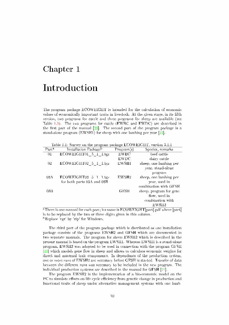
The program package ECOWEIGHT is intended for the calculation of economicvalues of economically important traits in livestock. At the given stage, in its �fthversion, two programs for cattle and three programs for sheep are available (seeTable 1.1). The two programs for cattle (EWBC and EWDC) are described inthe �rst part of the manual [23]. The second part of the program package is astand-alone program (EWSH1) for sheep with one lambing per year [22].
Table 1.1: Survey on the program package ECOWEIGHT, version 5.1.1Parta Installation Packageb Program(s) Species, remarks01 ECOWEIGHT01_5_1_1.tgz EWBC beef cattle
EWDC dairy cattle02 ECOWEIGHT02_5_1_1.tgz EWSH1 sheep, one lambing per
year, stand-aloneprogram
03A ECOWEIGHT03_5_1_1.tgzfor both parts 03A and 03B
EWSH2 sheep, one lambing peryear, used in
combination with GFSH03B GFSH sheep, program for gene
�ow, used incombination with
EWSH2aThere is one manual for each part; its name is ECOWEIGHT[part].pdf where [part]is to be replaced by the two or three digits given in this column.bReplace 'tgz' by 'zip' for Windows.
The third part of the program package which is distributed as one installationpackage consists of the programs EWSH2 and GFSH which are documented intwo separate manuals. The program for sheep EWSH2 which is described in thepresent manual is based on the program EWSH1. Whereas EWSH1 is a stand-aloneprogram, EWSH2 was adopted to be used in connection with the program GFSH[21] which models gene �ow in sheep and allows to calculate economic weights fordirect and maternal trait components. In dependence of the production system,one or more runs of EWSH2 are necessary before GFSH is started. Transfer of databetween the di�erent runs was necessary to be included in the new program. Theindividual production systems are described in the manual for GFSH [21].
The program EWSH2 is the implementation of a bio-economic model on thePC to simulate e�ects on life-cycle e�ciency from genetic change in production andfunctional traits of sheep under alternative management systems with one lamb-
10
CHAPTER 1. INTRODUCTION 11
ing per year. The �ock structure is described in terms of animal categories andprobabilities of transitions among them. The Markov chain approach is used tocalculate the stationary state of the ewe �ock (see Chapter 3). Up to 47 categoriesof progeny may be de�ned whereby pure-bred and cross-bred animals may occurin most categories if cross-breeding is used in the system. The calculation of thestructure of progeny is described in Chapter 4.
The algorithm includes both deterministic and stochastic components. Perfor-mance for most traits is simulated as the population mean, but variation in severaltraits is taken into account. Several performance characteristics for all animal cat-egories (mainly growth and milk production) are calculated in Chapters 5 and 6.Management options include the mating system and culling strategy for ewes, wean-ing and marketing strategy of progeny, and feeding system. The recent version ofthe program is for systems with one lambing per year, accelerated lambing cannotbe handled at present.
Pro�t estimated as the di�erence between the total revenues and total costs perewe1 per reproductive cycle is used as criterion of the economic e�ciency of theproduction system in the stationary state. The pro�t includes also governmentalsubsidies. Details on the calculation of nutrition costs, non-feed costs and revenuesare given in Chapters 9, 10 and 11. The economic importance (economic values)of up to 35 traits (milk production traits, growth traits, carcass traits, functionaltraits and wool traits) may be estimated. These economic values are intended fordeveloping a breeding objective for sheep. A list of the traits is given in AppendixA and the calculation of the economic weights is described in Chapter 12.
A large number of input parameters (see Chapter 14) can be given by the userallowing a detailed description of the production system and the economic, manage-ment and biological conditions. The program will be also useful for some economicanalyses in di�erent production systems. The impact of production, managementand economic circumstances on the economic e�ciency of a given production systemcan be studied.
The users of the program EWSH2 are recommended to read the papers of Wol-fová et al. published 2009 in the Journal of Dairy Science [25, 26] which describethe basic theory underlying the program and show applications.
Version 5.1.1 of the program package ECOWEIGHT contains version 1.0.2 of theEWSH2 program. For installing and running the program read Chapter 13. Theprogram was tested to run under LINUX and Microsoft Windows, but probably itshould run also on other platforms if there is a C compiler available.
1present in the �ock at lambing time
Chapter 2
Modelled production systems
Within each production system, the population of any breed is assumed to beself-replacing producing both males and females for own replacement. Selling andpurchasing of breeding animals between farms within each breed is not taken intoaccount in the pro�t function for the calculation of economic values. The costs forpurchasing animals in some farms within a population of the same breed are equalto the revenues from selling animals in other farms. This part of costs and revenuesis nulli�ed in the pro�t function for calculation of economic values1.
Nevertheless purchasing a part of female and male pure-bred replacement fromoutside the modelled population is allowed to account for import of superior breed-ing animals. But the proportions of bought female and male replacements should bealways kept low. Female replacement are expected to be purchased as young lambswhich are (to simplify the calculation) included into the category of own replace-ment female lambs at the time of lamb weaning. Therefore, the price of a purchasedfemale lamb is not an input parameter but is set to the costs for rearing a femalelamb till weaning increased by a quanti�able factor which re�ects the di�erence be-tween the rearing costs and the true value of imported animals. Male replacementare expected to be purchased at an age and weight suitable for breeding beforestarting the breeding (mating) season in the �ock. To simplify the calculation, theybecome part of the corresponding ram categories. The price, live weight and age ofthe purchased male replacement are input parameters.
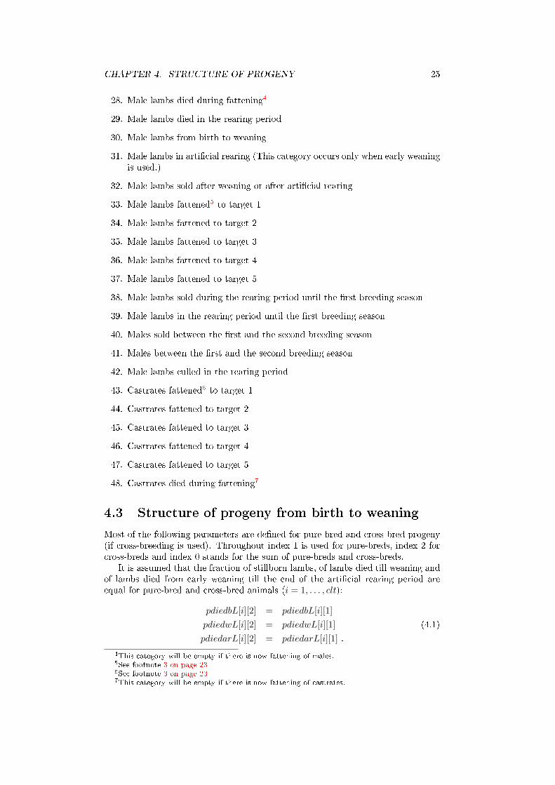
2.1 Production system 1: Pure-bred system withone production level
In this system, the population of sheep is not distinguished in nucleus and commer-cial herds. The system is similar as in cattle, where the dams of sires are selectedfrom the whole population (see Fig. 2.1). Only one breed is considered in thisproduction system and, without loss of generality, the capital letter �A� is used todesignate this breed; this letter is used at the end of several variables to make clearthat these variables refer to breed A.
1However, using the program for estimation of economic e�ciency of a farm selling and pur-chasing of breeding animals can be included.
12

CHAPTER 2. MODELLED PRODUCTION SYSTEMS 13
population fem
alePure−bred
Slaughter animals
rep
lace
men
t
mal
ere
pla
cem
ent
Figure 2.1: Pure-bred system with one production level
2.2 Production system 2: System with terminal cross-ing and one production level only
In this production system, a specialized sire breed (designated as breed A) and dambreed (designated as breed B) are assumed. Sire breed �ocks produce also sires forterminal crossing in the dam breed �ocks (see Figure 2.2). The costs for purchasing
fem
ale
rep
lace
men
t
mal
ere
pla
cem
ent
slaughter animals A
Sire breedA
sires A
malereplacement B
slaughter animals AxB
rep
lace
men
t B
fem
ale
cross
ing
Par
tly t
erm
inal
B
Dam breed
slaughter animals B
Figure 2.2: System with terminal crossing on one production level
rams of breed A for crossing are included into the pro�t function of the productionsystem for breed B. Notice that the proportion of crossing in the self-reproducingproduction system of breed B can never be 100%. Calculating economic values forbreed A, the whole production system, i.e. both populations A and B, are takeninto account. However, the economic values for breed B can be also calculatedindependently on the structure, management and input parameters for breed Aexcept for the age, weight and price of sires A bought for crossing.
Chapter 3
Structure of the ewe �ock and
the ram population
3.1 Structure of the ewe �ock1
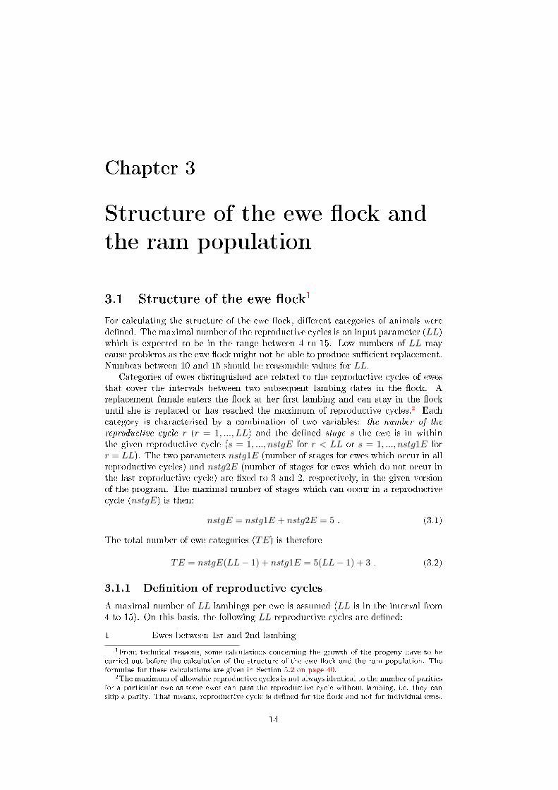
For calculating the structure of the ewe �ock, di�erent categories of animals werede�ned. The maximal number of the reproductive cycles is an input parameter (LL)which is expected to be in the range between 4 to 15. Low numbers of LL maycause problems as the ewe �ock might not be able to produce su�cient replacement.Numbers between 10 and 15 should be reasonable values for LL.
Categories of ewes distinguished are related to the reproductive cycles of ewesthat cover the intervals between two subsequent lambing dates in the �ock. Areplacement female enters the �ock at her �rst lambing and can stay in the �ockuntil she is replaced or has reached the maximum of reproductive cycles.2 Eachcategory is characterised by a combination of two variables: the number of thereproductive cycle r (r = 1, ..., LL) and the de�ned stage s the ewe is in withinthe given reproductive cycle (s = 1, ..., nstgE for r < LL or s = 1, ..., nstg1E forr = LL). The two parameters nstg1E (number of stages for ewes which occur in allreproductive cycles) and nstg2E (number of stages for ewes which do not occur inthe last reproductive cycle) are �xed to 3 and 2, respectively, in the given versionof the program. The maximal number of stages which can occur in a reproductivecycle (nstgE) is then:
nstgE = nstg1E + nstg2E = 5 . (3.1)
The total number of ewe categories (TE) is therefore
TE = nstgE(LL− 1) + nstg1E = 5(LL− 1) + 3 . (3.2)
3.1.1 De�nition of reproductive cycles
A maximal number of LL lambings per ewe is assumed (LL is in the interval from4 to 15). On this basis, the following LL reproductive cycles are de�ned:
1 Ewes between 1st and 2nd lambing
1From technical reasons, some calculations concerning the growth of the progeny have to becarried out before the calculation of the structure of the ewe �ock and the ram population. Theformulae for these calculations are given in Section 5.2 on page 40.
2The maximum of allowable reproductive cycles is not always identical to the number of paritiesfor a particular ewe as some ewes can pass the reproductive cycle without lambing, i.e. they canskip a parity. That means, reproductive cycle is de�ned for the �ock and not for individual ewes.
14
CHAPTER 3. STRUCTURE OF THE FLOCK 15
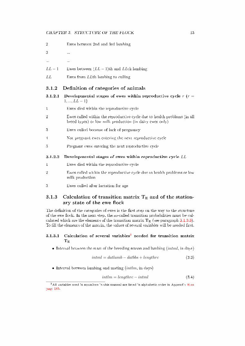
2 Ewes between 2nd and 3rd lambing
3 ...
... ...
LL− 1 Ewes between (LL− 1)th and LLth lambing
LL Ewes from LLth lambing to culling
3.1.2 De�nition of categories of animals
3.1.2.1 Developmental stages of ewes within reproductive cycle r (r =1, ..., LL− 1)
1 Ewes died within the reproductive cycle
2 Ewes culled within the reproductive cycle due to health problems (in allbreed types) or low milk production (in dairy ewes only)
3 Ewes culled because of lack of pregnancy
4 Not pregnant ewes entering the next reproductive cycle
5 Pregnant ewes entering the next reproductive cycle
3.1.2.2 Developmental stages of ewes within reproductive cycle LL
1 Ewes died within the reproductive cycle
2 Ewes culled within the reproductive cycle due to health problems or lowmilk production
3 Ewes culled after lactation for age
3.1.3 Calculation of transition matrix TE and of the station-ary state of the ewe �ock
The de�nition of the categories of ewes is the �rst step on the way to the structureof the ewe �ock. In the next step, the so-called transition probabilities must be cal-culated which are the elements of the transition matrix TE (see paragraph 3.1.3.3).To �ll the elements of the matrix, the values of several variables will be needed �rst.
3.1.3.1 Calculation of several variables3 needed for transition matrixTE
• Interval between the start of the breeding season and lambing (intml, in days)
intml = datlamb− datbbs+ lengthrc (3.3)
• Interval between lambing and mating (intlm, in days)
intlm = lengthrc− intml (3.4)
3All variables used in equations in this manual are listed in alphabetic order in Appendix B onpage 185.

CHAPTER 3. STRUCTURE OF THE FLOCK 16
• Fraction of ewes entering reproductive cycle i (i = 1, . . . , LL) that were invol-untarily culled for reasons other than infertility (pcullE[i])
pcullE[i] =
{pcullhE[i] + pcullmE[i] for dairy ewespcullhE[i] for non-dairy ewes
(3.5)
• Fraction of ewes entering reproductive cycle i (i = 1, . . . , LL− 1) that will bemated in this cycle (pmatE[i])4
pmatE[i] = 1− intlm
lengthrc(pcullE[i] + pdiedE[i]) (3.6)
• Fraction of ewes entering reproductive cycle i (i = 1, . . . , LL − 1) that willbecome pregnant in this cycle (pconE[i])
pconE[i] = pmatE[i]× conrateE[i] (3.7)
• Fraction of ewes entering reproductive cycle i (i = 1, . . . , LL−1) that will notbecome pregnant in this cycle (pnconE[i])
pnconE[i] = pmatE[i](1− conrateE[i]) (3.8)
• Probability that a ewe entering reproductive cycle i (i = 1, . . . , LL − 1) willnot become pregnant in this cycle and will be culled (pnconculE[i])
pnconculE[i] = pnconE[i](1− pbarrE[i]) (3.9)
• Probability that a ewe entering reproductive cycle LL will be culled for agein this cycle (pnconculE[LL])
pnconculE[LL] = 1− pcullE[LL]− pdiedE[LL] (3.10)
• Probability that a ewe entering reproductive cycle i (i = 1, . . . , LL−1) will notbecome pregnant in this cycle and will stay to the next cycle (pnconstayE[i])
pnconstayE[i] = pnconE[i]×pbarrE[i]
(1− intml
lengthrc(pcullE[i] + pdiedE[i])
)(3.11)
• Probability that a ewe entering reproductive cycle i (i = 1, . . . , LL − 1) willbecome pregnant in the cycle and stay to the next cycle (pconstayE[i])
pconstayE[i] = 1− pnconstayE[i]− pnconculE[i]− pcullE[i]− pdiedE[i](3.12)
3.1.3.2 Calculation of the elements of the transition matrix
We write te[i][j] for the elements of the transition matrix TE, i being the index forthe row and j being the index for the column. For the �rst �ve (= nstgE) columns,the non-zero elements are:
te[i][1] = pdiedE[1]
te[i][2] = pcullE[1]
te[i][3] = pnconculE[1] (3.13)
te[i][4] = pnconstayE[1]
te[i][5] = pconstayE[1]
4It is assumed that culling and dying of ewes are uniformly distributed over the whole repro-ductive cycle.
CHAPTER 3. STRUCTURE OF THE FLOCK 17
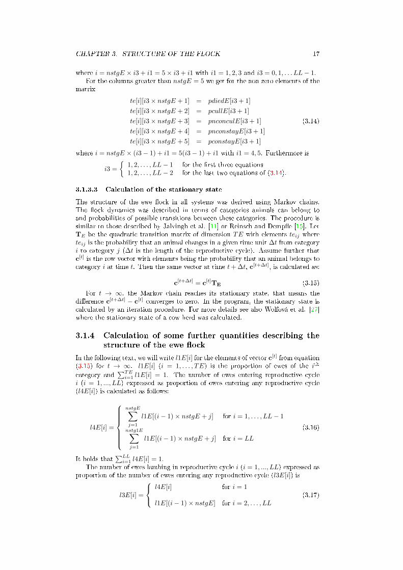
where i = nstgE × i3 + i1 = 5× i3 + i1 with i1 = 1, 2, 3 and i3 = 0, 1, . . . LL− 1.For the columns greater than nstgE = 5 we get for the non-zero elements of the
matrix
te[i][i3× nstgE + 1] = pdiedE[i3 + 1]
te[i][i3× nstgE + 2] = pcullE[i3 + 1]
te[i][i3× nstgE + 3] = pnconculE[i3 + 1] (3.14)
te[i][i3× nstgE + 4] = pnconstayE[i3 + 1]
te[i][i3× nstgE + 5] = pconstayE[i3 + 1]
where i = nstgE × (i3− 1) + i1 = 5(i3− 1) + i1 with i1 = 4, 5. Furthermore is
i3 =
{1, 2, . . . , LL− 1 for the �rst three equations1, 2, . . . , LL− 2 for the last two equations of (3.14).
3.1.3.3 Calculation of the stationary state
The structure of the ewe �ock in all systems was derived using Markov chains.The �ock dynamics was described in terms of categories animals can belong toand probabilities of possible transitions between these categories. The procedure issimilar to those described by Jalvingh et al. [11] or Reinsch and Demp�e [15]. LetTE be the quadratic transition matrix of dimension TE with elements teij whereteij is the probability that an animal changes in a given time unit ∆t from categoryi to category j (∆t is the length of the reproductive cycle). Assume further thatc[t] is the row vector with elements being the probability that an animal belongs tocategory i at time t. Then the same vector at time t+ ∆t, c[t+∆t], is calculated as:
c[t+∆t] = c[t]TE (3.15)
For t → ∞, the Markov chain reaches its stationary state, that means thedi�erence c[t+∆t] − c[t] converges to zero. In the program, the stationary state iscalculated by an iteration procedure. For more details see also Wolfová et al. [27]where the stationary state of a cow herd was calculated.
3.1.4 Calculation of some further quantities describing thestructure of the ewe �ock
In the following text, we will write l1E[i] for the elements of vector c[t] from equation(3.15) for t → ∞. l1E[i] (i = 1, . . . , TE) is the proportion of ewes of the ith
category and∑TE
i=1 l1E[i] = 1. The number of ewes entering reproductive cyclei (i = 1, ..., LL) expressed as proportion of ewes entering any reproductive cycle(l4E[i]) is calculated as follows:
l4E[i] =
nstgE∑j=1
l1E[(i− 1)× nstgE + j] for i = 1, . . . , LL− 1
nstg1E∑j=1
l1E[(i− 1)× nstgE + j] for i = LL
(3.16)
It holds that∑LL
i=1 l4E[i] = 1.The number of ewes lambing in reproductive cycle i (i = 1, ..., LL) expressed as
proportion of the number of ewes entering any reproductive cycle (l3E[i]) is
l3E[i] =
l4E[i] for i = 1
l1E[(i− 1)× nstgE] for i = 2, . . . , LL(3.17)
CHAPTER 3. STRUCTURE OF THE FLOCK 18
The number of lambings in the �ock per ewe and reproductive cycle (Nlamb) iscalculated as the sum of the elements of the vector l3E:
Nlamb =
LL∑i=1
l3E[i] . (3.18)
This sum is smaller than one if barren ewes are kept to the next breeding season.Ewes mated with rams of a di�erent breed as proportion of all mated ewes (pcrosst)are calculated as
pcrosst =1
1− l4E[LL]
LL−1∑i=1
pcrossE[i]× l4E[i] (3.19)
The fraction of ewes used for pure-breeding (pctE[1]), i.e. ewes mated with rams(only natural mating) of the same breed, is
pctE[1] = (1− pinsE[1]× coninsE)
LL−1∑i=1
(l4E[i]× (1− pcrossE[i])) (3.20)
and the fraction of ewes used for cross-breeding (pctE[2]), i.e. for mating to a ramof a di�erent breed, is
pctE[2] = (1− pinsE[2]× coninsE)
LL−1∑i=1
(l4E[i]× pcrossE[i]) . (3.21)
In the following text, some quantities will be calculated which are connectedwith ewe replacement. The dead rate of ewes averaged over all reproductive cycles(pdiedE0) is calculated as
pdiedE0 =
LL∑i=1
l4E[i]× pdiedE[i] (3.22)
and the number of ewes died expressed as percentage of ewes replaced per repro-ductive cycle (pdiedEp) are:
pdiedEp = 100× pdiedE0
l4E[1]. (3.23)
The relative frequencies of ewes involuntarily culled for health problems otherthan failure to conceive (pcullhE0), of ewes involuntarily culled for failure to con-ceive (pcullfcE0) and of ewes voluntarily culled for low milk production (pcullmE0),all averaged over all reproductive cycles, are
pcullhE0 =
LL∑i=1
l4E[i]× pcullhE[i]
pcullfcE0 =
LL−1∑i=1
l1E[(i− 1)× nstgE + nstg1E] (3.24)
pcullmE0 =
LL∑i=1
l4E[i]× pcullmE[i] .
Ewes involuntarily culled for health problems other than failure to conceive (pcullhEp),ewes involuntarily culled for failure to conceive (pcullfcEp) and ewes voluntarily
CHAPTER 3. STRUCTURE OF THE FLOCK 19
culled for low milk production (pcullmEp), each expressed as percentage of ewesreplaced per reproductive cycle, are calculated as:
pcullhEp = 100× pcullhE0
l4E[1]
pcullfcEp = 100× pcullfcE0
l4E[1](3.25)
pcullmEp = 100× pcullmE0
l4E[1].
3.2 Structure of the ram population
For calculating the age structure of the ram population, di�erent categories of an-imals were de�ned. The number of the breeding cycles a ram is used is an inputparameter (RR) which is expected to be in the range between 1 to 5. A breed-ing cycle covers the interval between two subsequent breeding seasons of rams5.Categories distinguished are related to the breeding cycles. A replacement maleenters the �ock at his �rst breeding cycle and can stay in the �ock until he is re-placed or has reached the maximum of allowable breeding cycles. Each category ischaracterised as a combination of two variables: the number of the breeding cycle r(r = 1, ..., RR) and the de�ned stage s the ram is in within the given breeding cycle(s = 1, ..., nstgR for r < RR and s = 1, ...nstg1R for r = RR). The two parametersnstg1R (number of stages for rams which occur in all breeding cycles) and nstg2R(number of stages for rams which do not occur in the last breeding cycle) are �xedto 3 and 1, respectively, in the given version of the program. The maximal numberof stages which can occur in a breeding cycle (nstgR) is then:
nstgR = nstg1R+ nstg2R = 4 . (3.26)
The total number of ram categories (TR) is therefore
TR = nstgR(RR− 1) + nstg1R = 4(RR− 1) + 3 . (3.27)
3.2.1 De�nition of breeding cycles
A maximal number of RR breeding cycles per ram is assumed (RR is in the intervalfrom 1 to 7). On this basis, the following RR breeding cycles are de�ned:
1 Rams between 1st and 2nd breeding season
2 Rams between 2nd and 3rd breeding season
3 ...
... ...
RR− 1 Rams between (RR− 1)th and RRth breeding season
RR Rams from RRth breeding season to culling or selling
5The length of the breeding cycle is equal to the length of the corresponding reproductive cycleof ewes.
CHAPTER 3. STRUCTURE OF THE FLOCK 20
3.2.2 De�nition of categories of rams
3.2.2.1 Developmental stages of rams within breeding cycle r (r = 1, ..., RR−1)
1 Rams died within the breeding cycle
2 Rams sold as breeding animals within the breeding cycle
3 Rams culled within the breeding cycle due to health problems
4 Rams entering the next breeding cycle
3.2.2.2 Developmental stages of rams within breeding cycle RR
1 Rams died within the breeding cycle
2 Rams sold as breeding animals within the breeding cycle
3 Rams culled within the breeding cycle
3.2.3 Calculation of transition matrix TR and of the station-ary state of the ram population
3.2.3.1 Calculation of the elements of the transition matrix
The variables pdiedR[i], psoldR[i] and pcullR[i] are read from the input �le IN-PUTS02*.TXT for i = 1, . . . , RR where '*' must be replaced by 'A' or 'B'. Fori = RR, it must hold
pdiedR[RR] + psoldR[RR] + pcullR[RR] = 1 . (3.28)
The probability that a ram entering breeding cycle i (i = 1, . . . , RR − 1) will stayto the next cycle is calculated as
pstayR[i] = 1− pdiedR[i]− psoldR[i]− pcullR[i] . (3.29)
This value must be always positive. Please note that for the special case of RR = 1this variable does not give sense and is not de�ned.
We write tr[i][j] for the elements of the transition matrix TR, i being the indexfor the row and j being the index for the column. First consider the special casethat RR = 1. Then matrix TR is a nstg1R × nstg1R matrix (nstg1R = 3 in thegiven version of the program) with all rows equal. The elements of the matrix are(i = 1, . . . , nstg1R):
tr[i][1] = pdiedR[1]
tr[i][2] = psoldR[1] (3.30)
tr[i][3] = pcullR[1]
For RR > 1, the non-zero elements in the �rst four (= nstgR) columns of matrixTR are:
tr[i][1] = pdiedR[1]
tr[i][2] = psoldR[1]
tr[i][3] = pcullR[1] (3.31)
tr[i][4] = pstayR[1]
where i = nstgR× i3 + i1 = 4× i3 + i1 with i1 = 1, 2, 3 and i3 = 0, 1, . . . RR− 1.
CHAPTER 3. STRUCTURE OF THE FLOCK 21
For the columns greater than nstgR = 4 we get for the non-zero elements of thematrix
tr[i][i3× nstgR+ 1] = pdiedR[i3 + 1]
tr[i][i3× nstgR+ 2] = psoldR[i3 + 1]
tr[i][i3× nstgR+ 3] = pcullR[i3 + 1] (3.32)
tr[i][i3× nstgR+ 4] = pstayR[i3 + 1]
where i = nstgR× (i3− 1) + i1 = 4(i3− 1) + i1 with i1 = 4. Furthermore is
i3 =
{1, 2, . . . , RR− 1 for the �rst three equations1, 2, . . . , RR− 2 for the last equation of (3.32).
3.2.3.2 Calculation of the stationary state for the ram population
The structure of the ram population in all systems was derived using Markov chainswhere the stationary state was calculated on the same principles as described inSection 3.1.3.3 on page 17.
3.2.4 Calculation of some further quantities describing thestructure of the ram population
In the following text, we will write l1R[i] for the elements of vector c[t] from equation(3.15) for t→∞ where matrix TR (transmission matrix for the ram population) isused instead of matrix TE. l1R[i] (i = 1, . . . , TR) is the proportion of rams of the
ith category and∑TR
i=1 l1R[i] = 1.The number of rams entering breeding cycle i (i = 1, ..., RR) expressed as pro-
portion of the number of rams entering any breeding cycle (l4R[i]) is calculated asfollows:
l4R[i] =
nstgR∑j=1
l1R[(i− 1)× nstgR+ j] for i = 1, . . . , RR− 1
nstg1R∑j=1
l1R[(i− 1)× nstgR+ j] for i = RR
(3.33)
It holds that∑RR
i=1 l4R[i] = 1. The rams may be from the same breed as the ewesin the �ock or from another breed which is used for crossing.
Chapter 4
Structure of progeny
4.1 General remarks to progeny management
Besides of customary weaning, early weaning of lambs is allowed which is alwaysfollowed by an arti�cial rearing period using milk replacer. After customary weaningor arti�cial rearing, all progeny can be divided into three groups whereby not allgroups are necessarily represented in each production system. The �rst group isformed by lambs sold for slaughter immediately after weaning or arti�cial rearing.The second group is made up by lambs fattened to target slaughter weight or age(the number of di�erent target weights or ages is limited to 5 each for female progeny,male progeny and castrates). The third group are lambs reared as breeding animalsintended for own �ock replacement or for selling.
Female breeding lambs (i.e. lambs from the third group) may be sold during therearing period either without being mated or as pregnant animals. For each femalelamb determined for mating, three options are allowed:
• Female lambs are mated in the �rst mating period after their weaning (usuallyat an age of 7 to 9 months). Only female lambs reaching the given minimalproportion of mature weight at this breeding season can be used for thismating.
• Barren female lambs from the �rst breeding season which were not culled andall remaining female lambs alive at the second breeding season are mated inthis breeding season.
• Barren female lambs from the second breeding season alive at the third breed-ing season are mated in this breeding season. After the third breeding season,all barren female lambs are culled.1
Male breeding lambs reared in the �ock may be already sold as young animals beforereaching the minimal weight to be used in breeding, i.e. at an age of about 7 to 9months before the �rst breeding season following their weaning, or as older animals.Male lambs for own replacement can enter the �ock at the �rst or second breedingseason after their weaning. The number of ewes per ram is di�erent for young andold rams.
Furthermore, the structure of the progeny depends on the survival rates. Lossesof lambs are de�ned for di�erent periods: (i) losses at birth including stillborn lambsand lambs died until 24 hours, (ii) losses from 24 hours after birth to weaning and
1The proportion of mated but barren females kept to the next breeding season can be set to avalue between 0 and 1. The number of breeding seasons can be restricted to two by setting theproportion of barren female lambs kept to the third breeding season (pbarrFP [2][i]) to zero.
22
CHAPTER 4. STRUCTURE OF PROGENY 23
(iii) if there is an arti�cial rearing period after early weaning, losses for this periodare de�ned separately. All losses of lambs are given as average losses jointly formale and female lambs across parities, but separately for each litter size. Litter sizecan take values from 1 up to 4 in the present program version (level 4 for litter sizeincludes litters with four or more lambs). Within each litter size, the same lossesare assumed for pure-bred and cross-bred lambs.
To include the e�ect of the number of suckled lambs on ewe's milk production,the distribution of the losses over the ewes has to be taken into account. Consider,for example, three ewes with three lambs each and assume that the total lossesamount to three lambs. This �nal number of three lambs may result from a lossof one lamb for each of the ewes or from a loss of three lambs for one of the ewes.This will be of di�erent impact on the milk production of the ewes. The detailedanalyses of losses allow to calculate the proportion of ewes at each parity that arewithout lambs after lambing or are suckled by di�erent numbers of lambs (singles,twins, etc.). Later losses of lambs are of minor importance on ewe's milk productionand are therefore not taken into account when calculating the milk production.
The number of suckled lambs has a great impact on the growth of lambs and the�nal slaughter weight. For the birth weight, the number of lambs born per litter isassumed to be crucial whereas for the subsequent growth rate, the number of lambsalive at 24 hours after lambing is probably more decisive.
The survival rates of progeny after weaning or after arti�cial rearing are sep-arately de�ned according to sex, category of progeny and genotype (pure-bred orcross-bred).
4.2 De�nition of categories of progeny
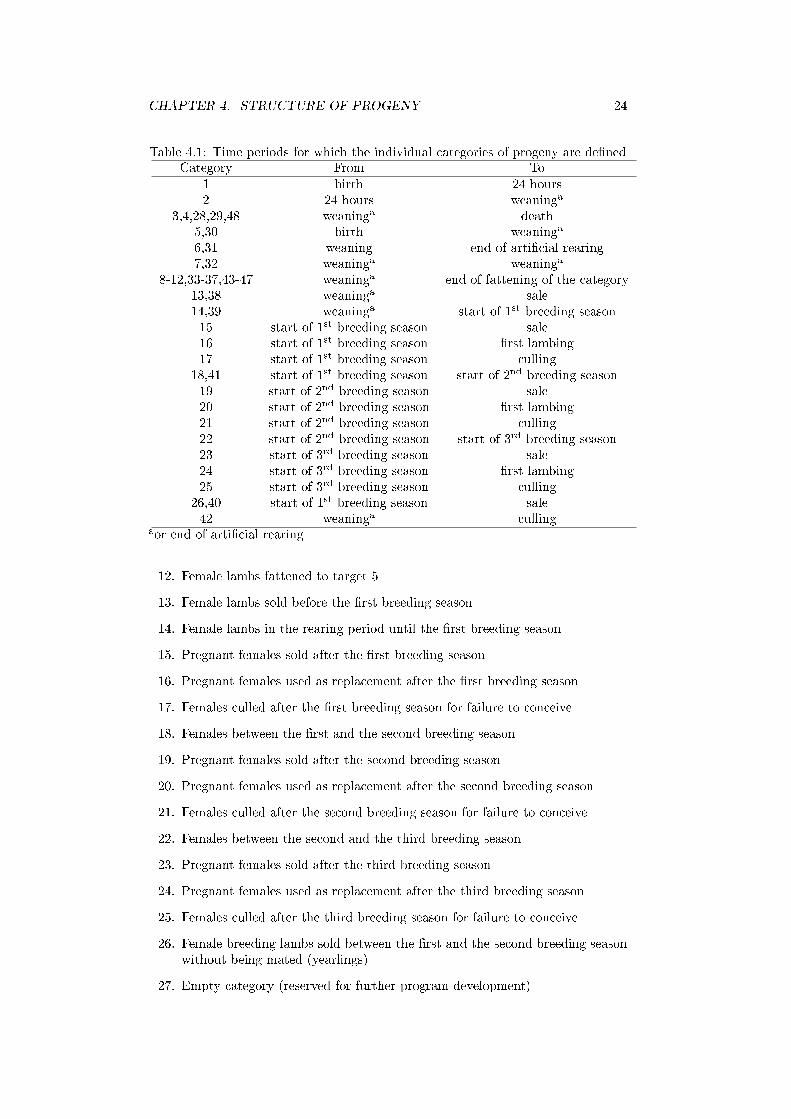
Categories of progeny are formed according to revenues and costs. The followingcategories of progeny are di�erentiated. The time periods the categories are de�nedfor are summarized in Table 4.1. Several categories may be empty.
1. Stillborn lambs and lambs died until 24 hours (both sexes)
2. Lambs died from 24 hours until weaning or until the end of arti�cial rearing(both sexes)
3. Female lambs died during fattening2
4. Female lambs died in the rearing period
5. Female lambs from birth to weaning
6. Female lambs in arti�cial rearing (This category occurs only when early wean-ing is used.)
7. Female lambs sold after weaning or after arti�cial rearing
8. Female lambs fattened3 to target 1
9. Female lambs fattened to target 2
10. Female lambs fattened to target 3
11. Female lambs fattened to target 4
2This category will be empty if there is no fattening of females.3Fattening may be to a constant weight or a constant age. The concrete meaning of targets 1
to 5 will be de�ned by input parameters in input �le INPUTS05*.TXT (see Subsection 14.2.4 onpage 148). Some or all of the categories related to fattening may be empty.
CHAPTER 4. STRUCTURE OF PROGENY 24
Table 4.1: Time periods for which the individual categories of progeny are de�nedCategory From To
1 birth 24 hours2 24 hours weaninga
3,4,28,29,48 weaninga death5,30 birth weaninga
6,31 weaning end of arti�cial rearing7,32 weaninga weaninga
8-12,33-37,43-47 weaninga end of fattening of the category13,38 weaninga sale14,39 weaninga start of 1st breeding season15 start of 1st breeding season sale16 start of 1st breeding season �rst lambing17 start of 1st breeding season culling
18,41 start of 1st breeding season start of 2nd breeding season19 start of 2nd breeding season sale20 start of 2nd breeding season �rst lambing21 start of 2nd breeding season culling22 start of 2nd breeding season start of 3rd breeding season23 start of 3rd breeding season sale24 start of 3rd breeding season �rst lambing25 start of 3rd breeding season culling
26,40 start of 1st breeding season sale42 weaninga culling
aor end of arti�cial rearing
12. Female lambs fattened to target 5
13. Female lambs sold before the �rst breeding season
14. Female lambs in the rearing period until the �rst breeding season
15. Pregnant females sold after the �rst breeding season
16. Pregnant females used as replacement after the �rst breeding season
17. Females culled after the �rst breeding season for failure to conceive
18. Females between the �rst and the second breeding season
19. Pregnant females sold after the second breeding season
20. Pregnant females used as replacement after the second breeding season
21. Females culled after the second breeding season for failure to conceive
22. Females between the second and the third breeding season
23. Pregnant females sold after the third breeding season
24. Pregnant females used as replacement after the third breeding season
25. Females culled after the third breeding season for failure to conceive
26. Female breeding lambs sold between the �rst and the second breeding seasonwithout being mated (yearlings)
27. Empty category (reserved for further program development)
CHAPTER 4. STRUCTURE OF PROGENY 25
28. Male lambs died during fattening4
29. Male lambs died in the rearing period
30. Male lambs from birth to weaning
31. Male lambs in arti�cial rearing (This category occurs only when early weaningis used.)
32. Male lambs sold after weaning or after arti�cial rearing
33. Male lambs fattened5 to target 1
34. Male lambs fattened to target 2
35. Male lambs fattened to target 3
36. Male lambs fattened to target 4
37. Male lambs fattened to target 5
38. Male lambs sold during the rearing period until the �rst breeding season
39. Male lambs in the rearing period until the �rst breeding season
40. Males sold between the �rst and the second breeding season
41. Males between the �rst and the second breeding season
42. Male lambs culled in the rearing period
43. Castrates fattened6 to target 1
44. Castrates fattened to target 2
45. Castrates fattened to target 3
46. Castrates fattened to target 4
47. Castrates fattened to target 5
48. Castrates died during fattening7
4.3 Structure of progeny from birth to weaning
Most of the following parameters are de�ned for pure-bred and cross-bred progeny(if cross-breeding is used). Throughout index 1 is used for pure-breds, index 2 forcross-breds and index 0 stands for the sum of pure-breds and cross-breds.
It is assumed that the fraction of stillborn lambs, of lambs died till weaning andof lambs died from early weaning till the end of the arti�cial rearing period areequal for pure-bred and cross-bred animals (i = 1, . . . , clt):
pdiedbL[i][2] = pdiedbL[i][1]
pdiedwL[i][2] = pdiedwL[i][1] (4.1)
pdiedarL[i][2] = pdiedarL[i][1] .
4This category will be empty if there is now fattening of males.5See footnote 3 on page 236See footnote 3 on page 237This category will be empty if there is now fattening of castrates.
CHAPTER 4. STRUCTURE OF PROGENY 26
The number of lambs born per ewe per reproductive cycle (nbtL[i][j]) for typei of breeding (i = 1 : pure-bred lambs, i = 2 : cross-bred lambs, i = 0 : sum ofpure-bred and cross-bred lambs) and for litter size j (j = 1, . . . , clt; j = 1 : singles,j = 2 : twins, j = 3 : triplets, j = 4 : quadruplets) is calculated as
nbtL[1][j] = j ×LL∑k=1
Pltype[j][k]× l3E[k]× (1− pcrossE[k − 1])
nbtL[2][j] = j ×LL∑k=1
Pltype[j][k]× l3E[k]× pcrossE[k − 1]
nbtL[0][j] = nbtL[1][j] + nbtL[2][j] (4.2)
The number of lambs born per ewe per reproductive cycle (NbtL[i]) summed overlitter sizes for the type of breeding (i = 0, 1, 2) is then calculated as
NbtL[i] =
clt∑j=1
nbtL[i][j] . (4.3)
The number of lambs alive at 24 hours after birth per ewe per reproductive cycle(na24hL[i][j]) for type i of breeding (i = 1 : pure-bred lambs, i = 2 : cross-bredlambs, i = 0 : sum of pure-bred and cross-bred lambs) and for each litter size j(j = 1, . . . , clt) is calculated as
na24hL[1][j] = (1− pdiedbL[j][1])× nbtL[1][j]
na24hL[2][j] = (1− pdiedbL[j][2])× nbtL[2][j] (4.4)
na24hL[0][j] = na24hL[1][j] + na24hL[2][j]
The number of lambs alive at 24 hours after birth per ewe per reproductive cycle(Na24hL[i]) summed over litter sizes for the type of breeding i (i = 0, 1, 2) is then
Na24hL[i] =
clt∑j=1
na24hL[i][j] . (4.5)
The number of lambs weaned per ewe per reproductive cycle (nwL[i][j]) for thetype of breeding i (i = 1 : pure-bred lambs, i = 2: cross-bred lambs, i = 0: sum ofpure-bred and cross-bred lambs) and for each litter size j (j = 1, . . . , clt) is
nwL[i][j] =
{(1− pdiedwL[j][i])× na24hL[i][j] for i = 1, 2nwL[1][j] + nwL[2][j] for i = 0
. (4.6)
The number of lambs weaned per ewe per reproductive cycle (NwL[i]) summed overlitter sizes for type i of breeding (i = 0, 1, 2) is given by
NwL[i] =
clt∑j=1
nwL[i][j] . (4.7)
In the presence of early weaning and arti�cial rearing of lambs with milk replacer,the number of lambs per ewe and reproductive cycle at the end of arti�cial rearing(narL[i][j]) for type i of breeding (i = 1 : pure-bred lambs, i = 2 : cross-bredlambs, i = 0 : sum of pure-bred and cross-bred lambs) and for each litter size j(j = 1, . . . , clt) is calculated as
narL[i][j] =
{(1− pdiedarL[j][i])× nwL[i][j] for i = 1, 2narL[1][j] + narL[2][j] for i = 0
. (4.8)
CHAPTER 4. STRUCTURE OF PROGENY 27
The total number of lambs at the end of arti�cial rearing summed over the littersizes is
NarL[i] =
clt∑j=1
narL[i][j] . (4.9)
4.3.1 Calculation of the array l1L (frequency of progeny in allcombinations of individual categories, types of breed-ing and litter sizes)
The �rst index of the matrix refers to category i (i = 1, . . . , PP ) of progeny as givenin Section 4.2 on page 23, the second index refers to type j of breeding (j = 1 : pure-bred animals, j = 2: cross-bred animals, j = 0: sum of pure-bred and cross-bredanimals) and the third index refers to litter size k (k = 1, . . . , clt) where k = 1 aresingles, k = 2 are twins, k = 3 are triplets etc. The following numbers of animalsare given per ewe and reproductive cycle.
The number of stillborn lambs (category 1 of progeny) of both sexes or lambsdied until 24 hours (l1L[1][j][k]) is :
l1L[1][j][k] = nbtL[j][k]− na24hL[j][k] for j = 0, 1, 2 and k = 1, . . . , clt. (4.10)
The number of lambs died from 24 hours until weaning (l1L[2][j][k], both sexes,category 2) is:
l1L[2][j][k] = na24hL[j][k]− nwL[j][k] for j = 0, 1, 2 and k = 1, . . . , clt. (4.11)
If there is arti�cial rearing, the equation changes to
l1L[2][j][k] = na24hL[j][k]− narL[j][k] for j = 0, 1, 2 and k = 1, . . . , clt. (4.12)
The number of female lambs at weaning (category 5) and of male lambs atweaning (category 30) is
l1L[5][j][k] = sexrbf × nwL[j][k]
l1L[30][j][k] = sexrbm× nwL[j][k] (4.13)
The number of female and male lambs at the end of the arti�cial rearing period(l1L[6][j][k], category 6 and l1L[31][j][k], category 31) are calculated as follows:
l1L[6][j][k] = sexrbf × narL[j][k]
l1L[31][j][k] = sexrbm× narL[j][k] (4.14)
4.3.2 Calculation of the array l1skL (frequency of progeny inall combinations of individual categories and types ofbreeding summarised over litter sizes) - �rst part
The �rst index of the matrix refers to the category of progeny as given in Section 4.2on page 23, the second index refers to type j of breeding (j = 1 : pure-bred animals,j = 2: cross-bred animals, j = 0: sum of pure-bred and cross-bred animals). Theelements of the matrix for the categories 1, 2, 5, 6, 30 and 31 are calculated as
l1skL[i][j] =
clt∑k=1
l1L[i][j][k] (4.15)
CHAPTER 4. STRUCTURE OF PROGENY 28
4.4 Structure of progeny after weaning8
Variables speci�c for female progeny only contain �FP� in their name, variablesspeci�c for male progeny only are indicated by �MP�. In variables which are de�nedboth for female and male progeny and, in some cases, also for castrates, the �rstindex indicates the sex: 1 stands for female progeny, 2 stands for male progeny and0 is used for castrates.
4.4.1 Calculation of the number of pure-bred weaned femalelambs needed for own �ock replacement
The fraction of pure-bred (second index) weaned female lambs conceived in the �rstbreeding season after their weaning (�rst index) (prconFP [1][1]) is calculated as
prconFP [1][1] = surbs[1][1][1]× pmat[1][1][1]× conrateFP [1][1] . (4.16)
The fraction of weaned female lambs conceived in the �rst breeding season aftertheir weaning and entered the �ock (pherd[1][1]) is then
pherd[1][1] = prconFP [1][1]× surmlFP [1] . (4.17)
The fraction of weaned pure-bred female lambs mated in the second breedingseason after their weaning (pmat[1][2][1]) is
pmat[1][2][1] = {surbs[1][1][1]− prconFP [1][1]
−surbs[1][1][1]× pmat[1][1][1]× (1− conrateFP [1][1])
×(1− pbarrFP [1][1])} × surbs[1][2][1] . (4.18)
The fraction of pure-bred weaned female lambs conceived in the second breedingseason after their weaning (prconFP [2][1]) is
prconFP [2][1] = pmat[1][2][1]× conrateFP [2][1] . (4.19)
The fraction of pure-bred weaned female lambs conceived in the second breedingseason after their weaning and entered the �ock (pherd[1][2]) is then
pherd[1][2] = prconFP [2][1]× surmlFP [1] . (4.20)
The fraction of pure-bred weaned female lambs mated in the third breedingseason after weaning (pmat[1][3][1]) is
pmat[1][3][1] = (pmat[1][2][1]− prconFP [2][1])
×pbarrFP [2][1]× surbs[1][3][1] , (4.21)
the fraction of pure-bred weaned female lambs conceived in the third breeding seasonafter their weaning (prconFP [3][1]) is calculated as
prconFP [3][1] = pmat[1][3][1]× conrateFP [3][1] (4.22)
and the fraction of pure-bred weaned female lambs conceived in the third breedingseason after their weaning and entered the �ock (pherd[1][3]) is then
pherd[1][3] = prconFP [3][1]× surmlFP [1] . (4.23)
8Before calculating the structure of the progeny after weaning, several variables connected withthe growth of the progeny must be calculated. The appropriate equations are given in Sections5.3 to 5.7.
CHAPTER 4. STRUCTURE OF PROGENY 29
The total fraction of pure-bred weaned female lambs that entered the �ock as re-placement (Pherd[1]) is
Pherd[1] =
bs[1]∑1=1
pherd[1][i] . (4.24)
The number9 of pure-bred weaned female lambs that must be reared for own�ock replacement (nherd[1]) is
nherd[1] = l4E[1]/Pherd[1] . (4.25)
The number of pure-bred female lambs for replacement died from weaning to the�rst breeding season (nrdied[1][1][1]) is
nrdied[1][1][1] = nherd[1]× (1− surbs[1][1][1]) . (4.26)
The number of pure-bred female lambs for replacement culled after the �rst breedingseason for failure to conceive (nrcull[1][1][1]) is
nrcull[1][1][1] = nherd[1]× (surbs[1][1][1]× pmat[1][1][1]
−prconFP [1][1])× (1− pbarrFP [1][1]) . (4.27)
The number of pure-bred female lambs for replacement mated in the secondbreeding season after weaning (nrmatFP [2]) is
nrmatFP [2] = nherd[1]× pmat[1][2][1] . (4.28)
The number of pure-bred female lambs for replacement which died from the �rst tothe second breeding season (nrdied[1][2][1]) is
nrdied[1][2][1] = {nherd[1]× (1− prconFP [1][1])− nrdied[1][1][1]
−nrcull[1][1][1]} × (1− surbs[1][2][1]) (4.29)
The number of pure-bred female lambs for replacement culled after the secondbreeding season for failure to conceive (nrcull[1][2][1]) is
nrcull[1][2][1] = nherd[1]× (pmat[1][2][1]− prconFP [2][1])
×(1− pbarrFP [2][1]) (4.30)
The number of pure-bred female lambs for replacement mated in the third breed-ing season after weaning (nrmatFP [3]) is
nrmatFP [3] = nherd[1]× pmat[1][3][1] . (4.31)
The number of pure-bred female lambs died from the second to the third breedingseason (nrdied[1][3][1]) is
nrdied[1][3][1] = (nrmatFP [2]− nherd[1]× prconFP [2][1]
−nrcull[1][2][1])× (1− surbs[1][3][1]) (4.32)
The number of pure-bred female lambs culled after the third breeding season forfailure to conceive (nrcull[1][3][1]) is
nrcull[1][3][1] = nherd[1]× (pmat[1][3][1]− prconFP [3][1]) . (4.33)
The number of pure-bred female lambs for replacement died from mating (con-ceiving) till lambing (nrdiedmlFP [1]) summed over all breeding seasons i is
nrdiedmlFP [1] = nherd[1]× (1− surmlFP [1])
bs[1]∑i=1
prconFP [i][1] . (4.34)
In the present version of the program bs[1] is set to 3.
9All numbers of animals in this section are per ewe per reproductive cycle.
CHAPTER 4. STRUCTURE OF PROGENY 30
4.4.2 Calculation of the number of surplus weaned femalelambs and of the number of purchased females
First assume that all own replacement females are reared. Then, in the case ofcustomary weaning, the number10 of surplus female progeny for type i of breeding(nwsp[1][i], i = 1: pure-bred lambs, i = 2: cross-bred lambs) is
nwsp[1][1] = l1skL[5][1]− nherd[1]
nwsp[1][2] = l1skL[5][2] (4.35)
If there is arti�cial rearing of early weaned lambs nwsp[1][i] is calculated as
nwsp[1][1] = l1skL[6][1]− nherd[1]
nwsp[1][2] = l1skL[6][2] (4.36)
A negative value of nwsp[1][1] means that there are not enough own replace-ment females and females must be purchased. The number of purchased females(npurchFP ) per ewe and reproductive cycle is then simply
npurchFP = −nwsp[1][1] (4.37)
and nwsp[1][1] is set to zero for the following calculations.Now consider the case that a part of replacement females (ppurchFP ) will be
purchased. Then the number of surplus weaned pure-bred females is
nwsp[1][1] =
{l1skL[5][1]− nherd[1]× (1− ppurchFP ) for customary weaningl1skL[6][1]− nherd[1]× (1− ppurchFP ) for arti�cial rearing
(4.38)The number of purchased female replacement is therefore:
npurchFP = nherd[1]× ppurchFP . (4.39)
The number of surplus weaned cross-bred females (nwsp[1][2]) will not be touchedby purchasing female replacement and will be the same as given in equations (4.35)and (4.36) in dependence if there is customary weaning or arti�cial rearing.
The number of pure-bred (j = 1) or cross-bred (j = 2) weaned surplus femaleprogeny (nsp[1][i][j]) sold in di�erent categories i (i = 1, . . . , csp[1], i = 1: soldat weaning for slaughter, i = 2: sold as breeding animals, i = 3, . . . 7: fattened totargets 1 to 5, respectively) is calculated as follows:
nsp[1][i][j] = nwsp[1][j]× psp[1][i][j] . (4.40)
If there is fattening of female progeny, the number of pure-bred (j = 1) orcross-bred (j = 2) female progeny died in fattening to target i (ndiedfat[1][i][j],i = 1, . . . , lf [1]) is
ndiedfat[1][i][j] = nsp[1][i+ 2][j]× (1− surfat[1][i][j]) . (4.41)
The number of pure-bred (j = 1) or cross-bred (j = 2) female progeny reaching theappropriate target i (nfattar[1][i][j], i = 1, . . . , lf [1]) in fattening is
nfattar[1][i][j] = nsp[1][i+ 2][j]× surfat[1][i][j] . (4.42)
The number of surplus female progeny for type of breeding i (i = 1: pure-bred lambs, i = 2: cross-bred lambs) sold as breeding females before mating(nsold[1][0][i]) is
nsold[1][0][i] = nsp[1][2][i]× psold[1][0][i] . (4.43)
10All numbers of animals in this section are per ewe per reproductive cycle.
CHAPTER 4. STRUCTURE OF PROGENY 31
The number of pure-bred (i = 1) or cross-bred (i = 2) surplus female progenydetermined for selling as breeding animals that died from weaning till the �rstbreeding season (nspdied[1][1][i]) is
nspdied[1][1][i] = (nsp[1][2][i]−nsold[1][0][i]×ps13[i])×(1−surbs[1][1][i]) . (4.44)
The following quantities (nmatFP [1][i] till nspcull[1][3][i]) will be calculatedonly if not all surplus female progeny will be sold before mating, i.e. psold[1][0][i]must be less than 1. The number of pure-bred (i = 1) or cross-bred (i = 2) surplusfemale progeny determined for selling as breeding animals that were mated in the�rst breeding season (nmatFP [1][i]) is
nmatFP [1][i] = (nsp[1][2][i]−nsold[1][0][i])× surbs[1][1][i]× pmat[1][1][i] . (4.45)
The number of pure-bred (i = 1) or cross-bred (i = 2) surplus female progenydetermined for selling as breeding animals that were culled after the �rst breedingseason because of failure to conceive (nspcull[1][1][i]) is
nspcull[1][1][i] = nmatFP [1][i]×(1−conrateFP [1][i])×(1−pbarrFP [1][i]) . (4.46)
The number of surplus female progeny (for type of breeding i, i = 1: pure-bredfemale lambs, i = 2: cross-bred female lambs) sold pregnant after the �rst breedingseason (nsold[1][1][i]) is
nsold[1][1][i] = nmatFP [1][i]× conrateFP [1][i] . (4.47)
The number of pure-bred (i = 1) or cross-bred (i = 2) surplus female progenydetermined for selling as breeding animals that were mated in the second breedingseason (nmatFP [2][i]) is
nmatFP [2][i] = (nsp[1][2][i]− nsold[1][0][i]− nsold[1][1][i]− nspdied[1][1][i]
−nspcull[1][1][i])× surbs[1][2][i] . (4.48)
The number of surplus female progeny (for type of breeding i, i = 1: pure-bredlambs, i = 2: cross-bred lambs) sold pregnant after the second breeding season(nsold[1][2][i]) is
nsold[1][2][i] = nmatFP [2][i]× conrateFP [2][i] . (4.49)
The number of pure-bred (i = 1) or cross-bred (i = 2) surplus female progeny (notpregnant) determined for selling as breeding animals that died from the �rst to thesecond breeding season (nspdied[1][2][i]) is
nspdied[1][2][i] = (nsp[1][2][i]− nsold[1][0][i]− nsold[1][1][i]− nspdied[1][1][i]
−nspcull[1][1][i])× (1− surbs[1][2][i]) . (4.50)
The number of pure-bred (i = 1) or cross-bred (i = 2) surplus female progenydetermined for selling as breeding animals that were culled after the second breedingseason because of failure to conceive (nspcull[1][2][i]) is
nspcull[1][2][i] = (nmatFP [2][i]− nsold[1][2][i])× (1− pbarrFP [2][i]) . (4.51)
The number of pure-bred (i = 1) or cross-bred (i = 2) surplus female progenydetermined for selling as breeding animals that were mated in the third breedingseason (nmatFP [3][i]) is
nmatFP [3][i] = (nmatFP [2][i]− nsold[1][2][i]− nspcull[1][2][i])
×surbs[1][3][i] (4.52)
CHAPTER 4. STRUCTURE OF PROGENY 32
The number of surplus female progeny (for type of breeding i, i = 1: pure-bredlambs, i = 2: cross-bred lambs) sold pregnant after the third breeding season(nsold[1][3][i]) is
nsold[1][3][i] = nmatFP [3][i]× conrateFP [3][i] . (4.53)
The number of pure-bred (i = 1) or cross-bred (i = 2) surplus female progeny (notpregnant) determined for selling as breeding animals that died from the second tothe third breeding season (nspdied[1][3][i]) is
nspdied[1][3][i] = (nmatFP [2][i]− nsold[1][2][i]− nspcull[1][2][i])
×(1− surbs[1][3][i]) . (4.54)
The number of pure-bred (i = 1) or cross-bred (i = 2) female progeny originallydetermined for selling as breeding animals that were culled after the third breedingseason because of failure to conceive (nspcull[1][3][i]) is
nspcull[1][3][i] = nmatFP [3][i]− nsold[1][3][i] . (4.55)
4.4.3 Calculation of the number of pure-bred weaned malelambs needed for own �ock replacement
If there is crossing in the �ock the rams in the �ock are either from the same breedas the ewes or from another breed which is used for crossing. Therefore it is usefulto subdivide the vectors l1R[i] and l4R[i] calculated in the subsection 3.2.4 intoparts which relate to rams from the breed of the �ock (l1aR[i][1] and l5R[i][1]) andparts which relate to rams used for crossing in the �ock (l1aR[i][2] and l5R[i][2]).The values of l1aR[i][j] are calculated as:
l1aR[i][1] = l1R[i]× pctE[1] + a2× (1− pcrosst)pctE[1] + pctE[2] + a2
l1aR[i][2] = l1R[i]− l1aR[i][1] (4.56)
where i = 1, . . . , TR and
a2 = nherd[1]
bs[1]∑i=1
pmat[1][i][1] . (4.57)
The values of l5R[i][j] are calculated in a similar way:
l5R[i][1] = l4R[i]× pctE[1] + a2× (1− pcrosst)pctE[1] + pctE[2] + a2
l5R[i][2] = l4R[i]− l5R[i][1] (4.58)
where i = 1, . . . , RR and a2 has the same meaning as above.The fraction of pure-bred weaned male lambs that entered the �ock in the �rst
(pherd[2][1]) or the second (pherd[2][2]) breeding season after weaning is
pherd[2][1] = surbs[2][1][1]× (1− cullbsMP [1][1])× pmat[2][1][1]
pherd[2][2] = surbs[2][1][1]× (1− cullbsMP [1][1])× (1− pmat[2][1][1])
× surbs[2][2][1]× (1− cullbsMP [2][1]) . (4.59)
By summing up these two values we get the total fraction of pure-bred weaned malelambs that entered the �ock (Pherd[2]):
Pherd[2] =
bs[2]∑i=1
pherd[2][i] . (4.60)
CHAPTER 4. STRUCTURE OF PROGENY 33
Pure-bred young rams (rams used in the �rst breeding season after their wean-ing) that entered the �ock as proportion of the total number of pure-bred rams thatentered the �ock (pherdyMP ) are given by the following relation
pherdyMP = pherd[2][1]/Pherd[2] (4.61)
and the fraction of pure-bred rams in the �ock that are pure-bred young rams(pyoungMP [1]) is
pyoungMP [1] = pherdyMP × l5R[1][1] . (4.62)
The average ewes-to-ram ratio in the breeding season (ratioR) is
ratioR = pyoungMP [1]× ratioyoungR+(1−pyoungMP [1])× ratiooldR . (4.63)
The number11 of pure-bred rams which are of the same breed as the ewes neededper ewe per reproductive cycle (neweR[1]) is
neweR[1] =1
ratioR
pctE[1] + nherd[1]× (1− pcrossE[0])
bs[1]∑i=1
pmat[1][i][1]
.
(4.64)The number of rams of the same breed as the breed of the ewes purchased fromoutside the �ock (npurchMP [1]) is
npurchMP [1] = ppurchMP [1]× neweR[1] . (4.65)
The number of pure-bred weaned male lambs that must enter the �ock per eweper reproductive cycle (nramMP [1]) is
nramMP [1] = (neweR[1]− npurchMP [1])× l5R[1][1] (4.66)
and the number of pure-bred weaned male lambs per ewe per reproductive cycle thatmust be reared for own replacement (nherd[2]) is given by the following equation:
nherd[2] = nramMP [1]/Pherd[2] . (4.67)
The number of pure-bred male lambs intended for replacement that died from wean-ing to the �rst breeding season (nrdied[2][1][1]) is
nrdied[2][1][1] = nherd[2]× (1− surbs[2][1][1]) . (4.68)
The number of pure-bred male lambs that were culled from weaning to the �rstbreeding season (nrcull[2][1][1]) is given as
nrcull[2][1][1] = nherd[2]× cullbsMP [1][1] . (4.69)
The number of pure-bred male lambs for replacement that died from the �rst tothe second breeding season (nrdied[2][2][1]) is
nrdied[2][2][1] = (nherd[2]− nrdied[2][1][1]− nrcull[2][1][1]
−nherd[2]× pherd[2][1])
×(1− surbs[2][2][1]) (4.70)
and the number of pure-bred male lambs for replacement that were culled from the�rst to the second breeding season (nrcull[2][2][1]) is
nrcull[2][2][1] =(nherd[2]× (1− pherd[2][1])− nrdied[2][1][1]
−nrcull[2][1][1])× cullbsMP [2][1] . (4.71)
11All numbers of animals in this section are per ewe per reproductive cycle.
CHAPTER 4. STRUCTURE OF PROGENY 34
The number of rams for cross-breeding needed per ewe per reproductive cycle(neweR[2], assumed to be purchased outside the �ock) is
neweR[2] =1
ratioR
pctE[2] + nherd[1]× pcrossE[0]
bs[1]∑i=1
pmat[1][i][1]
. (4.72)
The number of rams of the breed used for crossing which must enter the �ock perewe and reproductive cycle (nramMP [2]) is
nramMP [2] = neweR[2]× l5R[1][2] . (4.73)
The number of rams of the breed used for crossing in the �ock which must bepurchased (npurchMP [2]) is then
npurchMP [2] = nramMP [2] . (4.74)
4.4.4 Calculation of the number of pure-bred and cross-bredsurplus weaned male lambs (including castrates) usedfor di�erent purposes
In the case of customary weaning, the number12 of surplus male progeny for type jof breeding (nwsp[2][j], j = 1: pure-bred lambs, j = 2: cross-bred lambs) is
nwsp[2][1] = l1skL[30][1]− nherd[2]
nwsp[2][2] = l1skL[30][2] (4.75)
If there is arti�cial rearing of early weaned lambs nwsp[2][j] is calculated as
nwsp[2][1] = l1skL[31][1]− nherd[2]
nwsp[2][2] = l1skL[31][2] (4.76)
The number of pure-bred (j = 1) or cross-bred (j = 2) weaned surplus maleprogeny (nsp[2][i][j]) sold in di�erent categories i (i = 1, . . . , csp[2], i = 1: sold atweaning for slaughter, i = 2: sold as breeding animals, i = 3 : castrated, i = 4, . . . 8:fattened to targets 1 to 5, respectively) is calculated as follows:
nsp[2][i][j] = nwsp[2][j]× psp[2][i][j] . (4.77)
If there is fattening of male progeny, the number of pure-bred (j = 1) or cross-bred (j = 2) male progeny died in fattening to target i (ndiedfat[2][i][j], i =1, . . . , lf [2]) is
ndiedfat[2][i][j] = nsp[2][i+ 3][j]× (1− surfat[2][i][j]) . (4.78)
The number of pure-bred (j = 1) or cross-bred (j = 2) male progeny reaching theappropriate target i (nfattar[2][i][j], i = 1, . . . , lf [2]) in fattening is
nfattar[2][i][j] = nsp[2][i+ 3][j]× surfat[2][i][j] . (4.79)
The number of surplus male progeny for type of breeding j (j = 1: pure-bredlambs, j = 2: cross-bred lambs) sold as breeding males between weaning and the�rst breeding season (nsold[2][1][j]) is
nsold[2][1][j] = nsp[2][2][j]× surbs[2][1][j]× (1− cullbsMP [1][j])
×psold[2][1][j] . (4.80)
12All numbers of animals in this section are per ewe per reproductive cycle.
CHAPTER 4. STRUCTURE OF PROGENY 35
The number of pure-bred (j = 1) or cross-bred (j = 2) surplus male progenydetermined for selling as breeding animals that died from weaning till the �rstbreeding season (nspdied[2][1][j]) is
nspdied[2][1][j] = nsp[2][2][j]× (1− surbs[2][1][j]) . (4.81)
The number of pure-bred (j = 1) or cross-bred (j = 2) surplus male progenydetermined for selling as breeding animals that were culled from weaning till the�rst breeding season (nspcull[2][1][j]) is
nspcull[2][1][j] = nsp[2][2][j]× cullbsMP [1][j] . (4.82)
The number of surplus male progeny for type of breeding j (j = 1: pure-bredlambs, j = 2: cross-bred lambs) sold as breeding males between the �rst and thesecond breeding season after weaning (nsold[2][2][j]) is
nsold[2][2][j] = (nsp[2][2][j]− nsold[2][1][j]− nspdied[2][1][j]
−nspcull[2][1][j])× surbs[2][2][j]× (1− cullbsMP [2][j]) .
(4.83)
The number of pure-bred (j = 1) or cross-bred (j = 2) surplus male progenydetermined for selling as breeding animals that died from the �rst to the secondbreeding season (nspdied[2][2][j]) is
nspdied[2][2][j] = (nsp[2][2][j]− nsold[2][1][j]− nspdied[2][1][j]
−nspcull[2][1][j])× (1− surbs[2][2][j]) . (4.84)
The number of pure-bred (j = 1) or cross-bred (j = 2) surplus male progenydetermined for selling as breeding animals that were culled between the �rst andthe second breeding season (nspcull[2][2][j]) is
nspcull[2][2][j] = (nsp[2][2][j]− nsold[2][1][j]− nspdied[2][1][j]
−nspcull[2][1][j])× cullbsMP [2][j] . (4.85)
If there is fattening of castrates, the number of pure-bred (j = 1) or cross-bred(j = 2) weaned surplus male progeny fattened as castrates to target i (nsp[0][i][j], i =1, . . . , lf [0]) is calculated as follows13:
nsp[0][i][j] = nwsp[2][j]× psp[0][i][j] . (4.86)
The number of pure-bred (j = 1) or cross-bred (j = 2) castrates died in fatteningto target i (ndiedfat[0][i][j], i = 1, . . . , lf [0]) is
ndiedfat[0][i][j] = nsp[0][i][j]× (1− surfat[0][i][j]) . (4.87)
The number of pure-bred (j = 1) or cross-bred (j = 2) castrates reaching theappropriate target i (nfattar[0][i][j], i = 1, . . . , lf [0]) in fattening is
nfattar[0][i][j] = nsp[0][i][j]× surfat[0][i][j] . (4.88)
13Comment: For the input values psp[0][i][j] holds that∑csp[0]
i=1 psp[0][i][j] = 1 for all j. However,immediately after reading the data, the values psp[0][i][j] are converted so that they are expressed
as fraction of the weaned surplus male progeny. Therefore is∑csp[0]
i=1 psp[0][i][j] = psp[2][3][j] forj = 1, 2. These values are used in all calculations.
CHAPTER 4. STRUCTURE OF PROGENY 36
4.4.5 Calculation of the matrix l1skL (frequency of progenyin all combinations of individual categories and typesof breeding) - second part
The �rst index of the matrix refers to the category of progeny as given in Section 4.2on page 23, the second index refers to the type of breeding (j = 1 : pure-bred ani-mals, j = 2: cross-bred animals, j = 0: sum of pure-bred and cross-bred animals).All numbers of animals are given per ewe per reproductive cycle. The numbersof cross-bred animals are calculated only for the case that there is cross-breeding(parameter crossing = 2 in the parameter �le PARAS*.TXT - see Section 14.1.2on page 145). The equations for categories 1, 2, 5, 6, 30 and 31 were already givenin Section 4.3.2 on page 27. Here the equations for the remaining categories will bepresented. In all equations, j takes the values 1 or 2.
• Category 3. This category is calculated only if there is fattening of femaleprogeny.
l1skL[3][j] =
lf [1]∑i=1
ndiedfat[1][i][j] (4.89)
• Category 4
l1skL[4][1] = nrdiedmlFP [1] +
bs[1]∑i=1
(nrdied[1][i][1] + nspdied[1][i][1])
l1skL[4][2] =
bs[1]∑i=1
nspdied[1][i][2] (4.90)
• Category 7l1skL[7][j] = nsp[1][1][j] (4.91)
• Categories 8 to 12. These categories are calculated only if there is fatteningof female progeny.
l1skL[i][j] = nfattar[1][i− 7][j] for i = 8, . . . , 12 (4.92)
• Category 13l1skL[13][j] = nsold[1][0][j]× ps13[j] (4.93)
• Category 14
l1skL[14][1] = (nherd[1] + nsp[1][2][1]− nsold[1][0][1]× ps13[1])
×surbs[1][1][1]
l1skL[14][2] = (nsp[1][2][2]− nsold[1][0][2]× ps13[2])
×surbs[1][1][2] (4.94)
• Category 18
l1skL[18][1] = nrmatFP [2] + nmatFP [2][1]
l1skL[18][2] = nmatFP [2][2] (4.95)
• Category 22
l1skL[22][1] = nrmatFP [3] + nmatFP [3][1]
l1skL[22][2] = nmatFP [3][2] (4.96)
CHAPTER 4. STRUCTURE OF PROGENY 37
• Categories 15, 19 and 23
lsk1L[i][j] = nsold[1][(i− 11)/4][j] for i = 15, 19, 23 (4.97)
• Categories 16, 20 and 24
l1skL[i][1] = nherd[1]× pherd[1][(i− 12)/4]
l1skL[i][2] = 0 (4.98)
where i = 16, 20 or 24.
• Categories 17, 21 and 25
l1skL[i][1] = nrcull[1][(i− 13)/4][1] + nspcull[1][(i− 13)/4][1]
l1skL[i][2] = nspcull[1][(i− 13)/4][2] (4.99)
where i = 17, 21 or 25.
• Category 26
l1skL[26][j] = nsold[1][0][j]× (1− ps13[j])× surbs[1][1]][j] (4.100)
• Category 28. This category is calculated only if there is fattening of maleprogeny.
l1skL[28][j] =
lf [1]∑i=1
ndiedfat[2][i][j] (4.101)
• Category 29
l1skL[29][1] =
bs[2]∑i=1
(nrdied[2][i][1] + nspdied[2][i][1])
l1skL[29][2] =
bs[2]∑i=1
nspdied[2][i][2] (4.102)
• Category 32l1skL[32][i] = nsp[2][1][i] (4.103)
• Categories 33 to 37. These categories are calculated only if there is fatteningof male progeny.
l1skL[i][j] = nfattar[2][i− 32][j] for i = 33, . . . , 37 (4.104)
• Category 38l1skL[38][j] = nsold[2][1][j] (4.105)
• Category 39
l1skL[39][1] = nherd[2] + nsp[2][2][1]− nrdied[2][1][1]
−nrcull[2][1][1]− nsold[2][1][1]
l1skL[39][2] = nsp[2][2][2]− nsold[2][1][2]− nspdied[2][1][2]
−nspcull[2][1][2] (4.106)
• Category 40l1skL[40][j] = nsold[2][2][j] (4.107)
CHAPTER 4. STRUCTURE OF PROGENY 38
• Category 41
l1skL[41][1] = nherd[2]× pherd[2][2]
l1skL[41][2] = 0 (4.108)
• Category 42
l1skL[42][1] =
bs[2]∑i=1
(nrcull[2][i][1] + nspcull[2][i][1])
l1skL[42][2] =
bs[2]∑i=1
nspcull[2][i][2] (4.109)
• Categories 43 to 47. These categories are calculated only if there is fatteningof castrates.
l1skL[i][j] = nfattar[0][i− 42][j] for i = 43, . . . , 47 (4.110)
• Category 48. This category is calculated only if there is fattening of castrates.
l1skL[48][j] =
lf [0]∑i=1
ndiedfat[0][i][j] (4.111)
For all categories, the sum of frequencies of pure-bred and cross-bred animals(l1skL[i][0]) is
l1skL[i][0] = l1skL[i][1] + l1skL[i][2] . (4.112)
Chapter 5
Growth of progeny
5.1 General assumptions
Growth of progeny is described by average daily gain in di�erent growing periods.As growth rate of animals of the same breed can be very di�erent in di�erent con-ditions (lowland, highland, intensive, semi-intensive or extensive feeding), a generalgrowth curve is not used in the program. The growth curve is approximated by amulti-phase growth curve assuming linear functions for the individual phases. Thefollowing phases of growth are distinguished:
• from birth till weaning
• from weaning to the end of arti�cial rearing (if early weaning is applied)
• from weaning (or from the end of arti�cial rearing) to a given target in fat-tening
• from weaning to the �rst breeding season for breeding female and male lambs
• from the �rst to the second breeding season for breeding female and malelambs
• from the second to the third breeding season for breeding female lambs
• from the second breeding season to mature weight for males if the weight atthe second breeding season is smaller than mature weight of rams
• from the �rst lambing to mature weight if the weight at �rst lambing is smallerthan mature weight of ewes
Di�erences in growth rates between animals according to litter size (singles, twins,triplets, quadruplets) are taken into account till weaning or till the end of arti�cialrearing. At weaning or at the and of the arti�cial rearing period, the average weightsof male and female lambs are calculated which are used for describing growth inthe following periods. That means, after weaning (or after arti�cial rearing), a sex-speci�c average growth rate is applied for all litter sizes. Variation in the live weightsat �rst breeding of male and female breeding lambs are described by the phenotypicstandard deviations. In fattening, up to 15 targets (animal groups for fattening)can be de�ned in total (�ve targets each for female progeny, for male progeny andfor castrates). These targets are given as live weight or age at slaughter.
39
CHAPTER 5. GROWTH OF PROGENY 40
5.2 Calculation of several coe�cients relating sev-eral growth characteristics to each other1
First, average daily gain till weaning (adgbwL[s][i][j]) for female (s = 1) and male(s = 2) pure-bred (j = 1) and cross-bred (j = 2) lambs born in litter size i (i =1, . . . , clt) is calculated using the input parameters for birth and weaning weight oflambs2:
adgbwL[s][i][j] = (wwL[s][i][j]− bwL[s][i][j])/agewL . (5.1)
If there is early weaning followed by arti�cial rearing of lambs, the average dailygains from weaning until the end of arti�cial rearing for lambs of di�erent sexes,breeding types and from di�erent litter sizes (adgwarL[s][i][j]) are calculated in asimilar way:
adgwarL[s][i][j] =warL[s][i][j]− wwL[s][i][j]
agearL− agewL. (5.2)
Birth weight and average daily gain of female and male progeny born in di�er-ent litter sizes are related to the birth weight or average daily gain, respectively,of the female progeny born as singles. The coe�cients expressing these relationsare speci�c for sex, breeding type and litter size. For birth weight, the followingcoe�cients (kbw[s][i][j]) for female (s = 1) and male (s = 2) progeny are calculatedas:
kbw[s][i][j] = bwL[s][i][j]/bwL[1][1][j] (5.3)
where i is litter size (i = 1, . . . , clt), j is the breeding type (j = 1 : pure-breds,j = 2 : cross-breds), bwL[s][i][j] is the birth weight of lambs of sex s of breedingtype j born in a litter with size i.
The coe�cients for average daily gain (kadgbw[s][i][j]) of female and male progenyare calculated in the same way:
kadgbw[s][i][j] = adgbwL[s][i][j]/adgbwL[1][1][j] (5.4)
where the meaning of the indices is the same as in equation (5.3) and adgbwL[s][i][j]is the average daily gain from birth to weaning for litter size i and breeding type jfor female (s = 1) or male (s = 2) progeny.
If there is arti�cial rearing, coe�cients for the average daily gain of progeny(kadgwar[s][i][j]) from weaning until the end of arti�cial rearing are calculatedfollowing the same procedure as for birth weight and average daily gain from birthto weaning:
kadgwar[s][i][j] = adgwarL[s][i][j]/adgwarL[1][1][j] (5.5)
where the meaning of the indices is again the same as in equation (5.3) and thevariable adgwarL[s][i][j] is average daily gain from weaning until the end of thearti�cial rearing period for litter size i, breeding type j and sex of progeny s.
Things become more complicated when calculating the appropriate coe�cientsfor average daily gain in fattening. Up to �ve targets are allowed for fattening.Two reference growth traits have to be de�ned when both pure-bred and cross-bredprogeny are fattened. If available, average daily gain of pure-bred or cross-bredfemale progeny of animals fattened to the �rst target will be used as referencetrait for pure-bred or cross-bred animals, respectively. If, for example, only pure-bred female progeny is fattened to targets 1 and 2 and cross-bred female progeny
1These coe�cients must be calculated at the very beginning of the program before the structureof the ewe �ock. They are needed during the calculation of the economic values for growth traits.
2A list of all variables and constants used in the program is given in Appendix B on page 185.See this list for all symbols not explained in the text.
CHAPTER 5. GROWTH OF PROGENY 41
is fattened to target 3, average daily gain of cross-bred female progeny fattenedto target 3 will be used as reference trait for cross-bred animals. The coe�cientscalculated for female progeny (kadgfat[1][i][j]) are:
kadgfat[1][i][j] = adgP [7 + i][j]/adgP [7 + lj ][j] , (5.6)
where i is the number of the target for fattening (i = 1, . . . , lf [1]), j is the breedingtype (j = 1 : pure-breds, j = 2 : cross-breds), adgP [7 + i][j] is average daily gainof female progeny of breeding type j in fattening to target i and index lj (j = 1 :pure-breds, j = 2 : cross-breds) in adgP [7 + lj ][j] refers to the number of the targetits average daily gain is used as reference trait.
If male progeny and/or castrates are fattened in addition to female progeny, theappropriate coe�cients kadgfat[2][i][j]) and (kadgfat[0][i][j]) are calculated in theappropriate way:
kadgfat[2][i][j] = adgP [32 + i][j]/adgP [7 + lj ][j]
kadgfat[0][i][j] = adgP [42 + i][j]/adgP [7 + lj ][j] , (5.7)
where i is the number of the target for fattening (i = 1, . . . , lf [2] for male progeny,i = 1, . . . , lf [0] for castrates), j is the same as above and adgP [32 + i][j] oradgP [42 + i][j] are average daily gain of male progeny or castrates of breedingtype j in fattening to target i.
If there is no fattening of female progeny, the reference traits are de�ned similarlyas above for male progeny or for castrates. If male progeny is available, the followingcoe�cients are calculated:
kadgfat[2][i][j] = adgP [32 + i][j]/adgP [32 + lj ][j]
kadgfat[0][i][j] = adgP [42 + i][j]/adgP [32 + lj ][j] , (5.8)
where adgP [32 + lj ][j] (j = 1, 2) are the reference traits. If only castrates arefattened, coe�cients are calculated only for castrates:
kadgfat[0][i][j] = adgP [42 + i][j]/adgP [42 + lj ][j] , (5.9)
where adgP [42 + lj ][j] (j = 1, 2) are the reference traits.Average daily gain of female or male progeny from weaning to the �rst breeding
season or from breeding season i−1 to breeding season i (i = 2, . . . , bs[1] for femaleprogeny, i = 2, . . . , bs[2] for male progeny) is related to average daily gain of femaleprogeny from weaning to the �rst breeding season as reference trait resulting in thecoe�cients kadgr[s][i][j] for female (s = 1) and male (s = 2) progeny (j = 1 or 2for pure-bred or cross-bred progeny, respectively):
kadgr[s][i][j] = adgr[s][i][j]/adgr[1][1][j] . (5.10)
In cross-bred animals it can happen that there are only male animals but nofemales. Then equation (5.10) cannot be applied for cross-bred animals and mustbe modi�ed to
kadgr[2][i][2] = adgr[2][i][2]/adgr[2][1][2] . (5.11)
That means average daily gain of cross-bred male progeny from weaning to the �rstbreeding season is used as reference trait for cross-bred animals.
Mature weight of rams of the breed of the �ock is related to mature weight ofewes of the same breed:
kmwRE[1] = mwR[1]/mwE[1] . (5.12)
CHAPTER 5. GROWTH OF PROGENY 42
Similarly, mature weight of rams of the breed used for crossing in the �ock is relatedto mature weight of ewes of the same breed:
kmwRE[2] = mwR[2]/mwE2 . (5.13)
Age of lambs at weaning is calculated from the date of weaning and the date oflambing:
agewL = datwL− datlamb (5.14)
5.3 Recalculation of growth parameters
In Section 5.2, coe�cients were calculated to relate the value of a growth traitto the value of a reference growth trait. These coe�cients are calculated oncebefore starting the calculation of economic weights. In the course of the calculationof economic weights, the reference growth traits are changed. Therefore, all theremaining growth traits must be recalculated from the reference growth traits. Theappropriate equations for the recalculation are given in this subsection.
Birth weight, average daily gain from birth to weaning and average daily gainfrom weaning until the end of the arti�cial rearing period of lambs for female (s = 1)and male (s = 2) progeny born in litter size i (i = 1, . . . , clt) and of breeding typej (j = 1, 2) will be expressed as functions of birth weight, average daily gain frombirth to weaning and average daily gain from weaning until the end of arti�cialrearing, respectively, for female lambs born as singles (compare equations 5.3 to5.5):
bwL[s][i][j] = bwL[1][1][j]× kbw[s][i][j]
adgbwL[s][i][j] = adgbwL[1][1][j]× kadgbw[s][i][j] (5.15)
adgwarL[s][i][j] = adgwarL[1][1][j]× kadgwar[s][i][j] .
The recalculation of average daily gain in fattening is carried out on the basisof equations (5.6) to (5.9). See also Section 5.2 for further explanations. If femaleprogeny is fattened, average daily gain for female (s = 1) and male (s = 2) progenyand castrates (s = 0) for fattening to target i (i = 1, . . . , lf [s]) for breeding type j(j = 1 : pure-breds, j = 2 : cross-breds) is calculated as follows:
adgP [ks + i][j] = adgP [7 + lj ][j]× kadgfat[s][i][j] (5.16)
where index lj in adgP [7 + lj ][j] refers to the number of the target its average dailygain is used as reference trait and
ks =
7 for s = 132 for s = 242 for s = 0
. (5.17)
If there is fattening of male progeny, but no fattening of female progeny, equation(5.16) changes to
adgP [ks + i][j] = adgP [32 + lj ][j]× kadgfat[s][i][j] (5.18)
where s = 0 (castrates) or s = 2 (male progeny) and ks is given by equation (5.17).If only castrates are fattened, equation (5.16) reduces to
adgP [42 + i][j] = adgP [42 + lj ][j]× kadgfat[0][i][j] . (5.19)
Average daily gain of female (s = 1) or male (s = 2) progeny (j = 1 or 2: pure-bred or cross-bred progeny, respectively) from weaning to the �rst breeding season
CHAPTER 5. GROWTH OF PROGENY 43
or from breeding season i− 1 to breeding season i (i = 2, . . . , bs[s]) is calculated as(see equation 5.10):
adgr[s][i][j] = kadgr[s][i][j]× adgr[1][1][j] . (5.20)
If equation (5.11) was used instead of equation (5.10) then equation (5.20)changes for cross-bred male animals to:
adgr[2][i][2] = kadgr[2][i][2]× adgr[2][1][2] . (5.21)
Mature weight of rams from the breed of the �ock is calculated as
mwR[1] = mwE[1]× kmwRE[1] (5.22)
and mature weight of rams from the breed used for crossing in the �ock is
mwR[2] = mwE2× kmwRE[2] . (5.23)
In the cross-breds, a heterotic e�ect for mature weight hetmw (input parameter) istaken into account. Mature weight for cross-bred ewes (mwE[2]) and for cross-bredrams (mwMP [2]) is then calculated as:
mwE[2] = (1 + hetmw/100)× (mwE[1] +mwE2)/2
mwMP [2] = (1 + hetmw/100)× (mwR[1] +mwR[2])/2 . (5.24)
5.4 Growth until weaning
Weaning weight (ww[s][i][j]) for female (s = 1) and male (s = 2) lambs born inlitter size i (i = 1, . . . , clt) within breeding type j (j = 1 : pure-bred progeny, j = 2 :cross-bred progeny) is given by
ww[s][i][j] = bwL[s][i][j] + adgbwL[s][i][j]× agewL . (5.25)
In the presence of early weaning and arti�cial rearing of lambs, the weight at theend of arti�cial rearing (warL[s][i][j]) for female (s = 1) and male lambs (s = 2)born in litter size i within breeding type j is calculated as
warL[s][i][j] = ww[s][i][j] + adgwarL[s][i][j]× (agearL− agewL) . (5.26)
According to analyses of Krupová (2006, personal communication) and Miler-ski (2007, personal communication), the proportions of singles, twins, triplets andquadruplets are approximately the same in weaned and reared lambs. These pro-portions are assumed to be equal for male and female lambs because only overalllosses summed over male and female lambs at birth and till weaning or till the endof arti�cial rearing are available. To calculate the average weights and daily gainsof breeding lambs in the rearing period (till selling or till entering the �ock) and infattening, the average weight of female and male lambs at the start of the rearingperiod or at the beginning of fattening was taken as start weight for further periods.It was calculated as weighted average of lamb weights over litter sizes.
The proportion of weaned lambs in litter size i (i = 1, . . . , clt) and breeding typej (pwL[i][j]) or the proportion of lambs at the end of arti�cial rearing in litter size iand breeding type j (parL[i][j]) are used as weights. They are calculated as follows:
pwL[i][j] = nwL[j][i]/NwL[j]
parL[i][j] = narL[j][i]/NarL[j] . (5.27)
CHAPTER 5. GROWTH OF PROGENY 44
The average weaning weight (avww[s][j]) for female (s = 1) and male (s = 2)progeny is then for breeding type j (j = 1, 2):
avww[s][j] =
clt∑i=1
(wwL[s][i][j]× pwL[i][j]) . (5.28)
If there is arti�cial rearing, the average weight at the end of arti�cial rearing iscalculated for breeding type j by the following equation:
avwar[s][j] =
clt∑i=1
(warL[s][i][j]× parL[i][j]) . (5.29)
The �nal weights of categories 7 and 32 (female or male lambs slaughtered afterweaning) are therefore:
wP [7][j] =
{avww[1][j] if typew = 1avwar[1][j] if typew = 2
wP [32][j] =
{avww[2][j] if typew = 1avwar[2][j] if typew = 2
. (5.30)
5.5 Growth of breeding female progeny after wean-ing3
Age of female lambs at the beginning of breeding season i (i = 1, . . . , bs[1]) afterweaning ager[1][i] is assumed not to depend on breeding type j:
ager[1][i] = datbbs+ (i− 1)× lengthrc− datlamb+ 1 (5.31)
Average weight of pure-bred (j = 1) or cross-bred (j = 2) female lambs at the�rst breeding season after weaning (wrL[1][1][j]) is calculated as:
wrL[1][1][j] = avww[1][j] + adgr[1][1][j]× (ager[1][1]− agewL) . (5.32)
If there is arti�cial rearing of lambs, equation (5.32) takes the form
wrL[1][1][j] = avwar[1][j] + adgr[1][1][j]× (ager[1][1]− agearL) . (5.33)
The weight at the �rst breeding season must be lower than mature weight. If thiscondition is not ful�lled, an error message occurs when running the program.
The minimal weight of pure-bred (j = 1) or cross-bred (j = 2) female lambs formating (minw[1][j]) is calculated as proportion of the mature weight:
minw[1][j] = mwE[j]× pwrepFP [j] . (5.34)
For the further calculations, it is assumed that the weight at the �rst breedingseason both for pure-bred (j = 1) or cross-bred (j = 2) female lambs is normallydistributed with the mean wrL[1][1][j] calculated in equations (5.32) or (5.33) andstandard deviation sigmawr[1][j]. The standard deviation is calculated from thecoe�cient of variation and the mean weight:
sigmawr[1][j] = vcwr[1][j]× wrL[1][1][j]/100 . (5.35)
3Note please that variables speci�c for female progeny only contain �FP� in their name. Invariables which are de�ned both for female and male progeny and, in some cases, also for castrates,an index indicates the sex where 1 stands for female progeny. In most variables, the index referringto the sex of progeny is the �rst index.
CHAPTER 5. GROWTH OF PROGENY 45
On the basis of the normal distribution, the proportion of females that reached theminimal weight for mating (pmat[1][1][j]) is calculated. For the two groups of lambs(pure-breds and cross-breds) selected for mating, the mean weight is calculated(wmat[1][j]) as median from the part of the normal distribution which belongs tothe selected animals. Similarly, the mean weight of lambs not intended for mating(wnmat[1][j]) is calculated as median from the part of the normal distributionbelonging to the not selected animals. As the animals selected for mating will enterthe ewe �ock, the mean weight of the animals not selected for mating is the basisfor calculating the growth to the next two breeding seasons.
The average weight of pure-bred (j = 1) or cross-bred (j = 2) female lambs atthe second breeding season after weaning (wrL[1][2][j]) is given by the followingequation:
wrL[1][2][j] = wnmat[1][j] + adgr[1][2][j]× (ager[1][2]− ager[1][1]) . (5.36)
The weight at the second breeding season cannot be higher than mature weight.The weight at the third breeding season is expected to be the mature weight:
wrL[1][3][j] = mwE[j] . (5.37)
Average daily gain of female lambs between the second and the third breeding seasonor between the second breeding season and lambing is no input parameter but iscalculated as follows:
adgr[1][3][j] = (wrL[1][3][j]− wrL[1][2][j])/(ager[1][3]− ager[1][2]) . (5.38)
The weight after lambing (wlFP [i]) of females conceived in breeding season i(i = 1, . . . , bs[1]) is
wlFP [1] = wmat[1][1] + adgr[1][2][1]× (datlamb+ lengthrc− datbbs)wlFP [2] = wrL[1][2][1] + adgr[1][3][1]× (datlamb+ lengthrc− datbbs)wlFP [3] = mwE[1] (5.39)
and the age at lambing of females conceived in breeding season i is calculated as
agelFP [i] = i× lengthrc . (5.40)
For the following calculations the date of conception is needed which is
datconFP [i] = datlamb+ i× lengthrc− lpreg (5.41)
where
i =
1 for categories 15 and 162 for categories 19 and 203 for categories 23 and 24
. (5.42)
For the de�nition of categories see Section 4.2 on page 23. Next the weight (wP [i][j])of di�erent categories of pure-bred (j = 1) or cross-bred (j = 2) female progeny iscalculated. Index i is the number of category of progeny as given in Section 4.2 onpage 23. The weight of breeding female lambs sold before mating (category 13) iscalculated in the case of customary weaning as
wP [13][j] = avww[1][j] + adgr[1][1][j]× (agetP [13][j]− agewL) (5.43)
and in the case of arti�cial weaning as
wP [13][j] = avwar[1][j] + adgr[1][1][j]× (agetP [13][j]− agearL) . (5.44)
CHAPTER 5. GROWTH OF PROGENY 46
The weight of seven further categories of sold or culled females is:
wP [15][j] = wmat[1][j] + adgr[1][2][j]× (datconFP [1] + dpregsFP − datbbs)wP [17][j] = wmat[1][j] + adgr[1][2][j]× (datebs+ dnpregcFP − datbbs)wP [19][j] = wrL[1][2][j] + adgr[1][3][j]× (datconFP [2] + dpregsFP − datbbs)wP [21][j] = wrL[1][2][j] + adgr[1][3][j]× (datebs+ dnpregcFP − datbbs)wP [23][j] = mwE[j] (5.45)
wP [25][j] = mwE[j]
wP [26][j] = wnmat[1][j] + adgr[1][2][j]× (agetP [26][j]− ager[1][1])
Average live weight of females died in the rearing period (category 4) is calculatedas the weighted average of the weights of the females in the di�erent parts of therearing period (from weaning to 1st breeding, from 1st to 2nd and from 2nd to3rd breeding) and from conception to lambing. It is assumed that animals died onaverage in the middle of the appropriate period. For pure-bred females in a systemwith customary weaning we get:
wP [4][1] =1
2× l1skL[4][1]
((wrL[1][1][1] + avww[1][1])× (nrdied[1][1][1]
+nspdied[1][1][1]) + (wrL[1][2][1] + wnmat[1][1])
×(nrdied[1][2][1] + nspdied[1][2][1]) + (wrL[1][3][1]
+wrL[1][2][1])× (nrdied[1][3][1] + nspdied[1][3][1]) (5.46)
+nrdiedmlFP [1]×(pherd[1][1]× (wnmat[1][1] + wlFP [1])
+pherd[1][2]× (wrL[1][2][1] + wlFP [2])
+pherd[1][3]× (wrL[1][3][1] + wlFP [3]))/Pherd[1]
).
For cross-bred females in a system with customary weaning this equation changesto:
wP [4][2] =1
2× l1skL[4][2]
((wrL[1][1][2] + avww[1][2])× (nrdied[1][1][2]
+nspdied[1][1][2]) + (wrL[1][2][2] + wnmat[1][2])
×(nrdied[1][2][2] + nspdied[1][2][2]) + (wrL[1][3][2] (5.47)
+wrL[1][2][2])× (nrdied[1][3][2] + nspdied[1][3][2])).
If arti�cial rearing is used instead of customary weaning, replace avww[1][j] withavwar[1][j] (j = 1, 2) in equations (5.46) and (5.47).
5.6 Growth of breeding male progeny after wean-ing4
The procedure of calculating growth parameters for male lambs is similar as forfemale lambs in the preceding subsection. Index j refers generally to the breedingtype (j = 1 : pure-bred, j = 2 : cross-bred animals). Age of male lambs (ager[2][i])at the beginning of breeding season i (i = 1, . . . , bs[2]) is assumed not to depend onbreeding type j and is calculated as:
ager[2][i] = datbbs+ (i− 1)× lengthrc− datlamb+ 1 (5.48)
4Note please that variables speci�c only for male progeny contain �MP� in their name. Invariables which are de�ned both for female and male progeny and, in some cases, also for castrates,the �rst index indicates the sex where 2 stands for male progeny. In most variables, the indexreferring to the sex of progeny is the �rst index.
CHAPTER 5. GROWTH OF PROGENY 47
Average weight of male lambs at the �rst breeding season after their weaning in theabsence of arti�cial rearing (wrL[2][1][j]) is calculated as:
wrL[2][1][j] = avww[2][j] + adgr[2][1][j]× (ager[2][1]− agewL) . (5.49)
If there is arti�cial rearing of lambs, equation (5.49) takes the form
wrL[2][1][j] = avwar[2][j] + adgr[2][1][j]× (ager[2][1]− agearL) . (5.50)
The weight in the �rst breeding season must be lower than mature weight. If thiscondition is not ful�lled, an error message occurs when running the program.
The minimal weight of male lambs for mating (minw[2][j]) is:
minw[2][j] = mwMP [j]× pwrepMP . (5.51)
The proportion of males that reached the minimal weight for mating (pmat[2][1][j])is calculated on the basis of assuming the weights to be normally distributed. Thestandard deviation of this distribution is calculated from the coe�cient of variationand the mean weight:
sigmawr[2][j] = vcwr[2][j]× wrL[2][1][j]/100 . (5.52)
From this normal distribution, the mean weight of animals selected for breedingin the �rst breeding season (wmat[2][j]) and the mean weight of animals not se-lected for breeding (wnmat[2][j]) is calculated. The mean weight of the animalsnot selected for mating is the basis for calculating the growth to the next breedingseason.
The average weight of male lambs at the beginning of the second breeding seasonafter weaning (wrL[2][2][j]) is given by the following equation:
wrL[2][2][j] = wnmat[2][j] + adgr[2][2][j]× (ager[2][2]− ager[2][1]) . (5.53)
The weight at the second breeding season cannot be higher than mature weight.Finally, the weight (wP [i][j]) of di�erent categories of male progeny is calculated.
Index i is the number of category of progeny as given in Section 4.2 on page 23.The weight of breeding male lambs sold before mating (category 38) is calculatedin the case of customary weaning as
wP [38][j] = avww[2][j] + adgr[2][1][j] ∗ (agetP [38][j]− agewL) (5.54)
and in the case of arti�cial weaning as
wP [38][j] = avwar[2][j] + adgr[2][1][j] ∗ (agetP [38][j]− agearL) . (5.55)
The weight of a further category of sold males is:
wP [40][j] = wrL[2][1][j] + adgr[2][2][j]× (agetP [40][j]− ager[2][1]) . (5.56)
Average live weight of males died in the rearing period (category 29) is calculatedas the weighted average of the weights of the males in the di�erent parts of therearing period (from weaning to 1st breeding, from 1st to 2nd breeding). It isassumed that animals died on average in the middle of the appropriate period. Forpure-bred (j = 1) or cross-bred (j = 2) males in a system with customary weaningwe get:
wP [29][j] =1
2× l1skL[29][j]
((wrL[2][1][j] + avww[2][j])× (nrdied[2][1][j]
+nspdied[2][1][j]) + (wrL[2][2][j] + wnmat[2][j]) (5.57)
×(nrdied[2][2][j] + nspdied[2][2][j])).
CHAPTER 5. GROWTH OF PROGENY 48
If arti�cial rearing is used instead of customary weaning, replace avww[2][j] withavwar[2][j] in this equation.
The �nal weights of pure-bred (j = 1) or cross-bred (j = 2) male lambs in therearing period until the �rst breeding season (category 39) and of males betweenthe �rst and second breeding season (category 41) are:
wP [39][j] = wrL[2][1][j] (5.58)
wP [41][j] = wrL[2][2][j] .
Average live weight of males culled in the rearing period (category 42) is calculatedin a similar way as average live weight of males died in the rearing period:
wP [42][j] =1
2× l1skL[42][j]
((wrL[2][1][j] + avww[2][j])× (nrcull[2][1][j]
+nspcull[2][1][j]) + (wrL[2][2][j] + wnmat[2][j]) (5.59)
×(nrcull[2][2][j] + nspcull[2][2][j])).
If arti�cial rearing is used instead of customary weaning, replace again avww[2][j]with avwar[2][j] in this equation.
5.7 Growth in fattening
As already mentioned in Section 5.2, up to 15 targets for fattening to target slaugh-ter weight or slaughter age may be de�ned in total whereby each 5 targets arereserved for female progeny, male progeny and castrates. Most input parametersfor fattening are concentrated in input �le INPUTS05*.TXT (see subsection 14.2.4on page 148, where some more explanations of the input parameters are given).The main principles are the same for female and male progeny and castrates. Theparameter ulf [s][i] indicates if fattening to target i is to �xed slaughter weight(ulf [s][i] = 1) or to �xed slaughter age (ulf [s][i] = 2). Index s refers to thesex of progeny (s = 1 : female progeny, s = 2 : male progeny and s = 0 : cas-trates). The parameter clf [s][i] informs if fattening to target i is only for pure-breds (clf [s][i] = 1), only for cross-breds (clf [s][i] = 2) or both for pure-breds andcross-breds (clf [s][i] = 0).
If there is customary weaning and fattening is to �xed slaughter weight, slaughterage of pure-bred (j = 1) or cross-bred (j = 2) progeny at target i is calculated as
agetP [ks + i][j] = agewL+ (vlf [s][i]− avww[s][j])/adgP [ks + i][j] (5.60)
where ks is given by equation (5.17). Equation (5.60) changes to
agetP [ks + i][j] = agearL+ (vlf [s][i]− avwar[s][j])/adgP [ks + i][j] (5.61)
in the case of arti�cial rearing. If there is fattening to �xed slaughter age, slaughterweight is calculated in the presence of customary weaning as
wP [ks + i][j] = avww[s][j] + (vlf [s][i]− agewL)× adgP [ks + i][j] (5.62)
and in the presence of arti�cial weaning as
wP [ks + i][j] = avwar[s][j] + (vlf [s][i]− agearL)× adgP [ks + i][j] . (5.63)
Average live weight of females died in fattening (category 3) is calculated as theweighted average of the weights of the females fattened to targets 1 to lf [1]. It isassumed that animals died on average in the middle of the appropriate period. For
CHAPTER 5. GROWTH OF PROGENY 49
pure-bred (j = 1) or cross-bred (j = 2) females in a system with customary weaningwe get:
wP [3][j] =1
2× l1skL[3][j]
×lf [1]∑i=1
(wP [7 + i][j] + avww[1][j])× ndiedfat[1][i][j]. (5.64)
The same approach is used to calculate the average live weight for males died infattening (category 28)
wP [28][j] =1
2× l1skL[28][j]
×lf [2]∑i=1
(wP [32 + i][j] + avww[2][j])× ndiedfat[2][i][j]. (5.65)
and for castrates died in fattening (category 48)
wP [48][j] =1
2× l1skL[48][j]
×lf [0]∑i=1
(wP [42 + i][j] + avww[2][j])× ndiedfat[0][i][j]. (5.66)
If arti�cial rearing is used instead of customary weaning, replace avww[s][j] withavwar[s][j] in equations (5.64) to (5.66) with the corresponding indices.
5.8 Growth of ewes
The average age ageE[1] or weight wlE[1] of females at �rst lambing are calculatedas weighted average of the ages or weights, respectively, of females lambing afterthe individual breeding seasons i (i = 1, . . . , bs[1]):
ageE[1] =
bs[1]∑i=1
(agelFP [i]× pherd[1][i])/Pherd[1]
wlE[1] =
bsFM∑i=1
(wlFP [i]× pherd[1][i])/Pherd[1] . (5.67)
The age of ewes at lambing i (i = 2, . . . , LL) is then
ageE[i] = ageE[1] + (i− 1)× lengthrc . (5.68)
It is assumed that the weight of ewes at the second and subsequent lambings isequal to mature weight:
wlE[i] = mwE[1] for i = 2, . . . , LL . (5.69)
Average daily gain between �rst and second lambing is then
adgE = (wlE[2]− wlE[1])/lengthrc . (5.70)
In case that the ewes reach mature weight at �rst lambing already, daily gainbetween �rst and second lambing will be zero.
CHAPTER 5. GROWTH OF PROGENY 50
5.9 Growth of rams
The average age of rams of the breed of the �ock when entering the �ock (ageR[1][1])is given by the following equation:
ageR[1][1] = (1− ppurchMP )×
bs[2]∑i=1
(ager[2][i]× pherd[2][i])/Pherd[2]
+agepurMP [1]× ppurchMP . (5.71)
The age of rams of the breed of the �ock at the beginning of breeding cycle i(i = 2, . . . , RR) is
ageR[i][1] = ageR[1][1] + (i− 1)× lengthrc . (5.72)
If rams of another breed are used for crossing in the �ock, their age at enteringthe �ock (ageR[1][2]) or at the beginning of breeding cycle i (ageR[i][2] with i =2, . . . , RR) is:
ageR[1][2] = agepurMP [2]
ageR[i][2] = ageR[1][2] + (i− 1)× lengthrc . (5.73)
The average weight of rams of the breed of the �ock when entering the �ock(wbR[1][1]) is calculated as:
wbR[1][1] = (1− ppurchMP )×
bs[2]∑i=1
(wrL[2][i][1]× pherd[2][i])/Pherd[2]
+wpurMP [1]× ppurchMP . (5.74)
The weight at the beginning of the subsequent breeding cycles i (wbR[i][1] withi = 2, . . . , RR) is assumed to be equal to mature weight:
wbR[i][1] = mwR[1] . (5.75)
The average daily gain for rams of the breed of the �ock between the time of enteringthe �ock and the beginning of the second breeding cycle is
adgR[1] = (wbR[2][1]− wbR[1][1])/lengthrc . (5.76)
If rams of another breed are used for crossing in the �ock, their weight when enteringthe �ock (wbR[1][2]) or at the beginning of breeding cycle i (wbR[i][2] with i =2, . . . , RR) and their average daily gain between the time of entering the �ock andthe beginning of the second breeding cycle are:
wbR[1][2] = wpurMP [2]
wbR[i][2] = mwR[2] (5.77)
adgR[2] = (wbR[2][2]− wbR[1][2])/lengthrc .
Chapter 6
Milk production
6.1 Lactation curve
6.1.1 Lactation curve is known
The time course of milk production is modelled using the Wood function [28] asdefault. The simplest form of the Wood function can be written as
y(t) = atbe−ct (6.1)
where y(t) is the milk yield at day t of lactation and a, b and c are parametersof the lactation curve. Parameter a in�uences the overall height of the lactationcurve, parameter b speci�es the increase of milk production and is of importancein the �rst part of the curve and parameter c is responsible for the decrease ofthe curve in the second part. In input �le INPUTS06*.TXT (see subsection 14.2.6on page 152), the parameters of the lactation function are given for a standardsituation (for example for sheep with single lambs in the �rst lactation). The milkyield in di�erent parities is calculated by multiplying the milk yield in the standardsituation with a constant. These constants are input parameters. Similarly the milkyield for ewes with a di�erent number of lambs (including no lambs) is calculatedby multiplying the milk yield in the standard situation with appropriate constantswhich are also input parameters.
6.1.2 Lactation curve is unknown
In non-dairy sheep the lactation curve may be unknown. Then it is assumed (be-cause of lack of information) that the daily milk yield is equal for the whole lactation.As it will be convenient to use the same program code for all situations, the Woodfunction (6.1) will be adapted to this special case by setting the parameters b andc (bwo and awo in the program) to zero. Parameter a (awo in the program) iscalculated as average daily milk yield:
a =basemilkw
agewL. (6.2)
The variable basemilkw is an input parameter if the lactation curve is unknown.
51
CHAPTER 6. MILK PRODUCTION 52
6.2 Calculation of the milk yield per ewe in di�erentsegments of the lactation
First, the probability pbtba[i][j] that the number of suckled lambs is j for a ewe whohas born i (i ≥ j) lambs will be calculated:
pbtba[i][j] =
pdiedbtL[i][i− j]/(i− j) for j < i
1−i∑
k=1
pdiedbtL[i][k]/k for j = i.(6.3)
The number of ewes (PsuckE[i][j]) with i suckled lambs (i = 0, . . . , clt) in lactationj (j = 1, . . . , LL) expressed as proportion of all ewes in the �ock is then:
PsuckE[i][j] = l3E[j]
clt∑k=i2
Pltype[k][j]× pbtba[k][i] (6.4)
where i2 = 1 for i = 0 or i = 1 and i2 = i for i ≥ 2. For checking the correctness ofthe results, note that the following two relations must be ful�lled:
clt∑i=0
PsuckE[i][j] = l3E[j] for each j and
clt∑i=0
LL∑i=1
PsuckE[i][j] = Nlamb . (6.5)
In dairy breeds, it is assumed that ewes without lambs alive at 24 hours afterlambing are milked and their milk is collected till weaning lambs and is used for lambfeeding or is sold. The proportion of milk for sale produced by ewes from lambingtill weaning is given by the input parameter pmilkwm in �le INPUTS06*.TXT. Innon-dairy breeds, ewes without lambs alive at 24 hours after lambing are dried o�and this parameter is therefore zero.
6.2.1 Calculation of milk yield until weaning
Milk yield until weaning per ewe lambing (basemilkw) calculated for the standardsituation of the lactation curve (6.1) is calculated as
basemilkw = awo
agewL−1∑i=1
ibwoe−cwo×i (6.6)
where i is the number of days in lactation, awo, bwo and cwo are the coe�cientsof the lactation curve. The lactation curve is assumed to be known for dairy ewes.Estimates for the lactation curve are also published for meat sheep breeds [7, 16].If data are available for di�erent functions than the Wood curve we recommend torecalculate the parameters to allow using the Wood curve. Alternatively, di�erentlactation curves may be implemented in the program in future. If you intend to usesuch a lactation curve contact please the authors of the program.
If no lactation curve is known (probably in most cases of non-dairy sheep breeds),the milk yield until weaning (basemilkw) must be given by the user as input param-eter in input �le INPUTS07*.TXT (see subsection 14.2.7 on page 153). If there areno data available a rough estimate of the milk yield until weaning may be achievedassuming values from 0.6 to 1.0 kg milk per day according to the growth rate of thelambs [17].
CHAPTER 6. MILK PRODUCTION 53
Milk yield until weaning (milkwrel[i][j]) per ewe lambing with i (i = 0, . . . , clt)suckled lambs in lactation j (j = 1, . . . , LL) is calculated by multiplying the milkyield for the standard situation (basemilkw) with the appropriate adjustment fac-tors correcting for the number of suckled lambs (ktlsl[i]) and for parity (ktlp[j]):
milkwrel[i][j] = basemilkw × ktlsl[i]× ktlp[j] . (6.7)
In non-dairy breeds there is no milk available from ewes with no suckling lambs.Therefore, you should put ktlsl[0] = 0 in input �le INPUTS06*.TXT. If you acci-dentally give a di�erent number, the program will automatically set the value tozero.
The total milk yield until weaning per ewe in the �ock per reproductive cycle(tmilkw) is:
tmilkw =
clt∑i=0
LL∑j=1
milkwrel[i][j]× PsuckE[i][j] . (6.8)
The amount of milk (milksw[j]) milked for sale until weaning in lactation j is1:
milksw[j] =1
l3E[j]
(milkwrel[0][j]× PsuckE[0][j] (6.9)
+pmilkwm
clt∑i=1
milkwrel[i][j]× PsuckE[i][j])
For non-dairy sheep (typeb > 1 in the parameter �le), the date of weaning isidentical to the date of drying o� of ewes:
datdry = datwL . (6.10)
6.2.2 Calculation of milk yield from weaning till the end ofthe milking period
The calculations presented in this subsection are relevant only for dairy sheep. Thevariables calculated and the calculations themselves are formally very similar to thevariables and calculations in the preceding subsection 6.2.1.
The length of the milking period after weaning (lengthmp) is
lengthmp = datdry − datwL . (6.11)
Milk yield from weaning to the end of the milking period per lambing ewe (basemilkm)calculated for the standard situation of the lactation curve (6.1) is
basemilkm = awo
lengthmp+agewL∑i=agewL
ibwoe−cwo×i . (6.12)
Milk yield from weaning to the end of the milking period (milkmrel[i][j]) per lamb-ing ewe with i (i = 0, . . . , clt) suckled lambs in lactation j (j = 1, . . . , LL) is givenby the equation:
milkmrel[i][j] = basemilkm× ktlsl[i]× ktlp[j] . (6.13)
The total milk yield from weaning to the end of the milking period per ewe inthe �ock per reproductive cycle (tmilkm) is:
tmilkm =
clt∑i=0
LL∑j=1
milkmrel[i][j]× PsuckE[i][j] . (6.14)
1The variable milksw[j] is calculated only for dairy sheep and if pmilkwm > 0.
CHAPTER 6. MILK PRODUCTION 54
Milk yield per ewe lambing in parity j (milkmpar[j], j = 1, . . . , LL) averaged overall possible numbers of suckled lambs is calculated as
milkmpar[j] =1
l3E[j]
clt∑i=0
milkmrel[i][j]× PsuckE[i][j] . (6.15)
6.3 Cheese production
There are two options for the calculation of the amount of milk needed per kg ofcheese. In the �rst option (parameter cy = 1), the amount of milk needed per kgof cheese (milkch) is expressed as a linear function of milk fat (fat, in %) and milkprotein content (prot, in %) as follows:
milkch = ach+ bch× fat+ cch× protein . (6.16)
where ach is a constant and bch and cch are the regression coe�cients for fatand protein content of milk. These three parameters are input parameters in IN-PUTS06*.TXT (see page 152). If the parameters for the regression equation arenot known and you did not decide for the second option, insert an average value forthe milk needed per kg cheese for the constant ach and zeros for both regressioncoe�cients.
The second option is based on Van Slyke's formula [20]. We used the followingmodi�ed form of this formula given by Jaeggi et al. [10]:
cheesey =(rfat× fat+ rcas× casprot× prot)× rs
100−moich(6.17)
where cheesey is the cheese yield in kg from 1 kg milk, rfat is the fat recoveredin cheese (given as fraction), fat is the fat content in milk in %, rcas is the caseinrecovered in cheese (given as fraction), casprot is the amount of casein given asproportion of milk proteins, prot is the protein content in milk given in %, rs is acoe�cient representing other milk solids and added salt recovered in cheese (thiscoe�cient is calculated below) and moich is the moisture of cheese (in %).
The coe�cient rs is calculated as follows:
rs =rfat× fat× 100
(rfat× fat+ rcas× casprot× prot)× fdm(6.18)
where fdm is fat in dry matter (in %):
fdm =fatch
100−moich× 100 (6.19)
where fatch is the fat content in cheese given in %. During the calculation of theeconomic values, rs is held constant.
A by-product of cheese production is cheese whey. The amount of cheese whey(in kg) produced per kg cheese (cheesewhey) is given by
cheesewhey = milkch− 1 (6.20)
assuming that no liquids were lost when processing milk to cheese.
Chapter 7
Wool production
7.1 Calculation of the wool production of ewes andrams
The wool production per ewe and reproductive cycle (woolptE) and the wool pro-duction per ram of the breed of the �ock (j = 1) or of the breed used for crossingin the �ock (j = 2) and per breeding cycle (woolptR[j]) are calculated from theamount of wool gained per shearing and from the number of shearings per animalin the corresponding time periods:
woolptE = wsheE × nsheEwoolptR[j] = wsheR[j]× nsheR[j] . (7.1)
7.2 Calculation of several ratios relating �eece weightof several categories of animals to �eece weightof rams1
In this section, the �eece weight of the individual categories of animals are relatedto the �eece weight of adult rams. When calculating economic values it is assumedthat the following calculated ratios stay constant when changing the �eece weightof rams. That means, �eece weight of all categories of animals is considered to beone trait. The following ratios are calculated:
kwE =wsheE
wsheR[1]
kwarL[i][j] =wshearL[i][j]
wsheR[j]if typew = 2
kwfL[i][j] =wshefL[i][j]
wsheR[j]if there is fattening (7.2)
kwrL[i][j] =wsherL[i][j]
wsheR[j]
kwwL[i][j] =wshewL[i][j]
wsheR[j]if typew = 1
1These ratios must be calculated at the very beginning of the program before the structure ofthe ewe �ock. They are needed during the calculation of the economic value for �eece weight.
55
CHAPTER 7. WOOL PRODUCTION 56
7.3 Recalculation of parameters for �eece weight
In Section 7.2, ratios were calculated to relate the value of the �eece weight of acategory of animals to the value of �eece weight of rams. These ratios are calcu-lated once before starting the calculation of economic weights. In the course of thecalculation of economic weights, the �eece weight of rams is changed. Therefore, allthe remaining �eece weights must be recalculated from the �eece weight of rams.The appropriate equations for the recalculation are given here:
wsheE = kwE × wsheR[1]
wshearL[i][j] = kwarL[i][j]× wsheR[j] if typew = 2
wshefL[i][j] = kwfL[i][j]× wsheR[j] if there is fattening (7.3)
wsherL[i][j] = kwrL[i][j]× wsheR[j]
wshewL[i][j] = kwwL[i][j]× wsheR[j] if typew = 1

Chapter 8
Discounting
Genetic improvement in di�erent traits is expressed in di�erent animal categories ata di�erent age. Consequently, the traits in�uence revenues and costs in an animalcategory at a di�erent time. Costs for feeding, e.g., occur daily in the whole periodof the animal's life, costs for shearing may be spend at any time and costs formarketing or revenues from slaughtered animals occur only once and that at theend of a particular animal category.
The time at which a trait in�uences revenues and costs can be accounted forwhen calculating economic values by discounting all revenues and costs for eachprogeny category to the birth date of the animal. The revenues and costs forewes are discounted to the date of lambing and the revenues and costs for ramsare discounted to the date of the beginning of the breeding cycle. Discounting ofrevenues and costs to the birth date of ewes and rams is then carried out in theprocedure for gene �ow using the program GFSH [21].
Discounting coe�cients for all revenue and cost items are calculated for eachcategory of ewes, rams and lambs. The discounting coe�cient in its general form(q) is de�ned as
q = (1 + u)−t (8.1)
where u is the annual discount rate and t is the time (in years) when the revenuesand costs occur in a particular category of animals. The time t is concretely
• the age of the animal in all progeny categories
• the time interval between the occurence of revenues or costs and the date oflambing in ewes
• the time interval between the occurence of revenues or costs and the date ofbeginning of the breeding cycle in rams.
If the discount rate u is set to zero in the input parameter �le INPUTS01*.TXTeconomic values will be calculated without discounting, i.e. not taking into accountthe time factor.
8.1 Length of the time period for each category
The length of the time period for the occurence of each category is needed forthe calculation of the discounting coe�cients and for further calculations in thefollowing chapters.
For ewes, we write dcE[i] for the length of the time period for category i fromthe start of the reproductive cycle to the end of the category. The length of the
57
CHAPTER 8. DISCOUNTING 58
time period is calculated for stages 1 to 3 (see Section 3.1) for all lactations (j =1, . . . , LL) :
dcE[(j − 1)× nstgE + 1] = lengthrc/2
dcE[(j − 1)× nstgE + 2] = datdry − datlamb+ 1 (8.2)
dcE[(j − 1)× nstgE + 3] = datebs+ dnpregcE − datlamb+ 1 .
For stages k = 4 or 5, the following equation holds only for lactations j = 1, . . . , LL−1 :
dcE[(j − 1)× nstgE + k] = lengthrc . (8.3)
For rams, we write dcR[i] for the length of the time period for category i. Thelength of the time period is calculated for stages 1 to 2 (see Section 3.2.2) for allbreeding cycles (j = 1, . . . , RR) in the same way:
dcR[(j − 1)× nstgR+ 1] = lengthrc/2 (8.4)
dcR[(j − 1)× nstgR+ 2] = datebs+ dselR− datbbs+ flushbbR+ 1 .
In stage 3, the calculation is di�erent for the last breeding cycle:
dcR[(j − 1)× nstgR+ 3] =
{lengthrc/2 for j < RRdatebs− datbbs+ flushbbR+ 1 for j = RR
.
(8.5)Stage 4 does not occur in the last breeding cycle so that the following equationholds only for j = 1, . . . , RR− 1 :
dcR[(j − 1)× nstgR+ 4] = lengthrc . (8.6)
For lambs, we write dcL[i][j] for the length of the time period for category i(i = 1, . . . PP ) and breeding type j (j = 1 : pure-bred animals, j = 2 : cross-bredanimals). For female and male lambs till weaning the following equation holds:
dcL[5][j] = dcL[30][j] = agewL . (8.7)
The time period for arti�cial rearing of lambs is
dcL[6][j] = dcL[31][j] = agearL− agewL . (8.8)
The lambs died till weaning or till the end of the arti�cial rearing (category 2) areassumed to stay in the �ock on average half of the period of the lambs alive:
dcL[2][j] =
{agewL/2 for typew = 1agearL/2 for typew = 2
. (8.9)
In fattening of pure-bred (j = 1) or cross-bred (j = 2) progeny of category i,the time period is
dcL[i][j] = agetP [i][j]− a (8.10)
where
a =
{agewL for typew = 1agearL for typew = 2
. (8.11)
The time periods for female (category i = 3) and male (category i = 28) lambs andcastrates (category i = 48) that died in fattening are calculated as one half of theweighted averages of the time periods for the appropriate categories k in fattening(k = 8, . . . , 12 for category 3, k = 33, . . . , 37 for category 28 and k = 43, . . . , 47 forcategory 48):
dcL[i][j] =1
2× l1skL[i][j]
∑k
(dcL[k][j]× ndiedfat[s][k − l][j]) (8.12)
CHAPTER 8. DISCOUNTING 59
wheres = 1 and l = 7 for category i = 3s = 2 and l = 32 for category i = 28s = 0 and l = 42 for category i = 48
. (8.13)
For breeding female lambs (categories 13 to 26), the following periods are cal-culated:
dcL[13][j] = agetP [13][j]− adcL[14][j] = ager[1][1]− adcL[15][j] = dpregsFP + datconFP [1]− datbbsdcL[16][j] = lengthrc− ager[1][1]
dcL[17][j] = datebs+ dnpregcFP − datlamb− ager[1][1]
dcL[18][j] = ager[1][2]− ager[1][1] (8.14)
dcL[19][j] = dpregsFP + datconFP [2]− datbbs− 365
dcL[20][j] = 2× lengthrc− ager[1][2]
dcL[21][j] = datebs+ dnpregcFP + lengthrc− datlamb− ager[1][2]
dcL[22][j] = ager[1][3]− ager[1][2]
dcL[23][j] = dpregsFP + datconFP [3]− datbbs− 2× 365
dcL[24][j] = 3× lengthrc− ager[1][3]
dcL[25][j] = datebs+ dnpregcFP + 2× lengthrc− datlamb− ager[1][3]
dcL[26][j] = agetP [26][j]− ager[1][1]
where a is given by equation (8.11). The time period for female lambs died in therearing period (category 4) is calculated as one half of the weighted average of thetime periods for categories 14, 18, 20 and 22:
dcL[4][j] =(dcL[14][j]× (nrdied[1][1][j] + nspdied[1][1][j])
+dcL[18][[j]× (nrdied[1][2][j] + nspdied[1][2][j])
+dcL[22]× (nrdied[1][3][j] + nspdied[1][3][j]) (8.15)
+dcL[20][j]× nrdiedmlFP [j])/
(2× l1skL[4][j]).
For breeding male lambs (categories 38 to 41), the periods of time are:
dcL[38][j] = agetP [38][j]− adcL[39][j] = ager[2][1]− adcL[40][j] = agetP [40][j]− ager[2][1] (8.16)
dcL[41][j] = ager[2][2]− ager[2][1] .
where a is again given by equation (8.11).The time period for male lambs died inthe rearing period (category 29) is calculated as one half of the weighted average ofthe time periods for categories 39 and 41:
dcL[29][j] =(dcL[39][j]× (nrdied[2][1][j] + nspdied[2][1][j]
+dcL[41][j]× (nrdied[2][2][j] + nspdied[2][2][j]))
/(2× l1skL[29][j]) . (8.17)
Similarly, the time period for male lambs of category 42 (culled during the rearingperiod) is also calculated as one half of the weighted average of the time periods for
CHAPTER 8. DISCOUNTING 60
categories 39 and 41:
dcL[42][j] =(dcL[39][j]× (nrcull[2][1][j] + nspcull[2][1][j]
+dcL[41][j]× (nrcull[2][2][j] + nspcull[2][2][j]))
/(2× l1skL[42][j]). (8.18)
8.2 Discounting coe�cients for ewes
Discounting coe�cients for revenues or costs that occur continuously over the wholetime period the ewes of category i (i = 1, ..., TE) are kept (qaveE[i]) are calculatedas
qaveE[i] = (1 + u)−(dcE[i]/2)/365 . (8.19)
It is assumed that costs and revenues are distributed evenly over the whole timeperiod so that the middle of the time period is taken as representative value for thecalculation of the discounting coe�cient. As all time intervals are primarily givenin days and the annual discount rate is applied, the values for these intervals mustbe divided by 365.
Discounting coe�cients for revenues or costs that occur at the end of the keepingperiod of ewes of category i (qendE[i]) are calculated as
qendE[i] = (1 + u)−dcE[i]/365 . (8.20)
Discounting coe�cients for breeding costs for ewes of category i (qbreedE[i]) aregiven by the equation
qbreedE[i] = (1 + u)−(datbbs−datlamb)/365 (8.21)
and discounting coe�cients for revenues from milk and/or cheese and for costsconnected with milking sheep are
qmilkE[i] = (1 + u)−(agew+lengthmp/2)/365 . (8.22)
8.3 Discounting coe�cients for rams
For pure-bred (j = 1) or cross-bred (j = 2) rams of category i (i = 1, ..., TR),discounting coe�cients for revenues or costs that occur continuously over the wholetime period the rams are kept (qaveR[i][j]) are calculated as
qaveR[i][j] = (1 + u)−(dcR[i][j]/2)/365 . (8.23)
Discounting coe�cients for revenues or costs that occur at the end of the keepingperiod of rams of category i (qendR[i][j]) are calculated as
qendR[i][j] = (1 + u)−dcR[i][j]/365 . (8.24)
The discounting coe�cient for costs for purchasing breeding rams (qpurchR) isgiven by
qpurchR = (1 + u)−(datbbs−datlamb)/365 . (8.25)
CHAPTER 8. DISCOUNTING 61
8.4 Discounting coe�cients for lambs
First, the age in the middle of the time period (taveL[i][j]) and at the end of thetime period (tendL[i][j]) is calculated for pure-bred (j = 1) and cross-bred (j = 2)lambs of all categories i (i = 1, . . . , PP ). Both values are zero for catergory 1. Thecorresponding values for category 2 are:
taveL[2][j] = dcL[2][j]/2
tendL[2][j] = dcL[2][j] . (8.26)
For categories i = 3, 4, 8 to 14, 28, 29, 33 to 39 and 42 to 48 we get:
taveL[i][j] = a+ dcL[i][j]/2
tendL[i][j] = a+ dcL[i][j] (8.27)
where a = agewL for customary weaning and a = agearL for arti�cial rearing. Forcatetories i = 5 and 30 the corresponding ages are:
taveL[i][j] = agewL/2
tendL[i][j] = agewL (8.28)
and in the case of arti�cial rearing we get for categories i = 6 and 31:
taveL[i][j] = agewL+ dcL[i][j]/2
tendL[i][j] = agearL . (8.29)
Female or male lambs sold after arti�cial rearing (categories i = 7 and 31) have thefollowing ages in the middle and at the end of their existence:
taveL[i][j] = a
tendL[i][j] = a (8.30)
where a has the same meaning as in equation (8.27). For female breeding lambsbetween the �rst and the second breeding season (categories i = 15 to 18 and 26)we get:
taveL[i][j] = ager[1][1] + dcL[i][j]/2
tendL[i][j] = ager[1][1] + dcL[i][j] . (8.31)
Furthermore, the equations for female breeding lambs between the second and thethird breeding season (categories i = 19 to 22) are:
taveL[i][j] = ager[1][2] + dcL[i][j]/2
tendL[i][j] = ager[1][2] + dcL[i][j] (8.32)
For female breeding lambs after the third breeding season (categories i = 23 to 25),the equations look as follows:
taveL[i][j] = ager[1][3] + dcL[i][j]/2
tendL[i][j] = ager[1][3] + dcL[i][j] . (8.33)
Finally, the equations for male breeding lambs (categories 40 and 41) are
taveL[i][j] = ager[2][1] + dcL[i][j]/2
tendL[i][j] = ager[2][1] + dcL[i][j] . (8.34)
CHAPTER 8. DISCOUNTING 62
The discounting coe�cients for revenues or costs that occur continuously duringthe whole time of keeping the given category of lambs (qaveL[i][j]) are then:
qaveL[i][j] = (1 + u)−taveL[i][j]/365 (8.35)
and the discounting coe�cients for revenues and costs that accrue at the end of thetime period of the given category (qendL[i][j]) are:
qendL[i][j] = (1 + u)−tendL[i][j]/365 . (8.36)
The discounting coe�cient for breeding costs (qbreedL[i]) is relevant only for cate-gories i = 14, 18 and 22 and is calculated as follows:
qbreedL[i] = (1 + u)−ager[1][k]/365 (8.37)
where k = (i− 10)/4.
Chapter 9
Nutrition costs
Feed requirements of animals of di�erent categories (ewes, rams, lambs) in di�er-ent periods of their life are calculated on the base of their daily net energy andprotein (PDI, protéines digestibles dans l'intestin) requirements for maintenance,growth of body weight, milk production, wool production, pregnancy and changein body weight during �ushing and pregnancy. The daily net energy and proteinrequirements are summed within periods with the same feeding rations.
Feeding rations should be built from the feed components that are available ina de�ned production system and for the given seasons during the year. Buildingthe feeding rations, the dry matter intake of the given category of animals in thegiven production stage (e.g. lactation, pregnancy) and the expected productionlevel (growth rate, body weight, milk production) should be taken into account [5].
For all feeding rations, the average dry matter, net energy, protein (PDI) contentand the average price per kg fresh matter of the ration must be known. These valuesare input parameters for the program. If PDI values for feed components are notavailable, it is possible to calculate the nutrition costs only on the basis of netenergy content in feed. The net energy and protein requirements of animals in allfeeding periods within each feeding season are transformed to the amount of freshfeed of the given feeding rations. The calculated feed amount is increased by a givenpercentage to take into account feed wasting for the given feeding technology (e.g.indoor feeding, di�erent technologies of pasture). Feeding costs are calculated peranimal of the given category and per the time period the category exists which isgiven by the variables dcE[i], dcR[i][j] and dcL[i][j] (see Section 8.1).
9.1 De�nition of feeding rations and nutrition groupsfor animals
Feeding rations for the same group of animals can di�er between the seasons of theyear (e.g. between summer and winter, between wet and dry seasons in the tropics).The number of di�erent feeding seasons during the year is an input parameter (nfs)the maximal value of which is set to 4. In case that summer and winter feeding arethe only two feeding rations during the year, nfs is 2. For the individual feedingseasons, the codes 1, 2, . . . , nfs must be used in input �le INPUTS08*.TXT (seeSection 14.2.8 on page 153).
The code of the feeding season on January 1st is read to the variable valfs[0].To describe the changes during the year, the date(s) must be given when the feedingration changes and the new value or code of the feeding ration which is valid fromthe date of change. It is assumed that the dates of changes and the appropriatecodes of the feeding rations remain the same also in the following years.
63
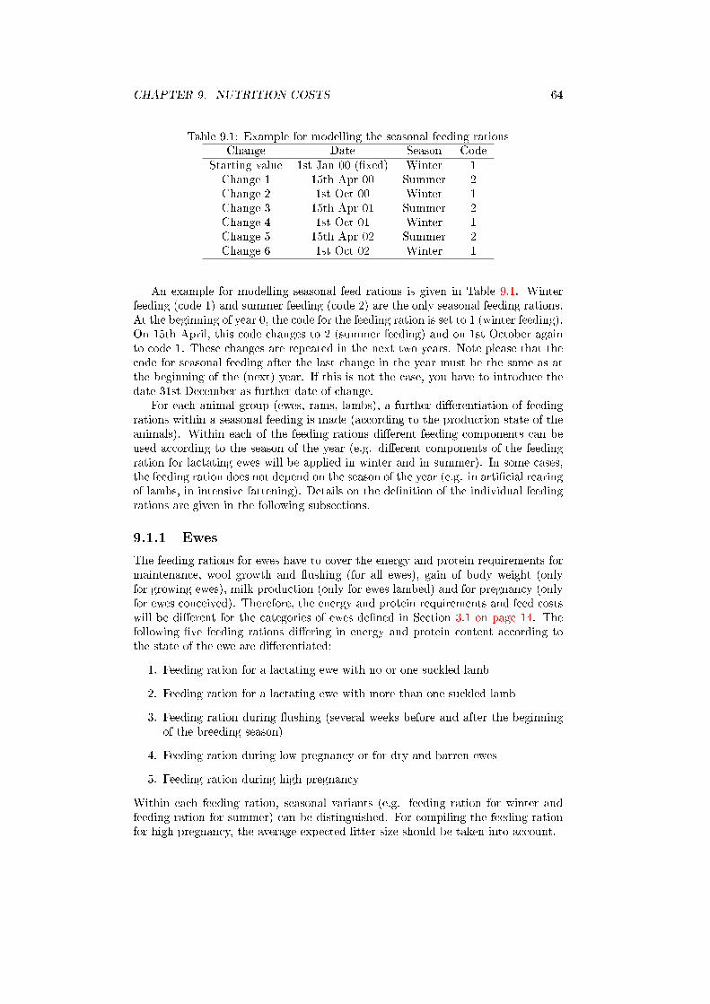
CHAPTER 9. NUTRITION COSTS 64
Table 9.1: Example for modelling the seasonal feeding rationsChange Date Season Code
Starting value 1st Jan 00 (�xed) Winter 1Change 1 15th Apr 00 Summer 2Change 2 1st Oct 00 Winter 1Change 3 15th Apr 01 Summer 2Change 4 1st Oct 01 Winter 1Change 5 15th Apr 02 Summer 2Change 6 1st Oct 02 Winter 1
An example for modelling seasonal feed rations is given in Table 9.1. Winterfeeding (code 1) and summer feeding (code 2) are the only seasonal feeding rations.At the beginning of year 0, the code for the feeding ration is set to 1 (winter feeding).On 15th April, this code changes to 2 (summer feeding) and on 1st October againto code 1. These changes are repeated in the next two years. Note please that thecode for seasonal feeding after the last change in the year must be the same as atthe beginning of the (next) year. If this is not the case, you have to introduce thedate 31st December as further date of change.
For each animal group (ewes, rams, lambs), a further di�erentiation of feedingrations within a seasonal feeding is made (according to the production state of theanimals). Within each of the feeding rations di�erent feeding components can beused according to the season of the year (e.g. di�erent components of the feedingration for lactating ewes will be applied in winter and in summer). In some cases,the feeding ration does not depend on the season of the year (e.g. in arti�cial rearingof lambs, in intensive fattening). Details on the de�nition of the individual feedingrations are given in the following subsections.
9.1.1 Ewes
The feeding rations for ewes have to cover the energy and protein requirements formaintenance, wool growth and �ushing (for all ewes), gain of body weight (onlyfor growing ewes), milk production (only for ewes lambed) and for pregnancy (onlyfor ewes conceived). Therefore, the energy and protein requirements and feed costswill be di�erent for the categories of ewes de�ned in Section 3.1 on page 14. Thefollowing �ve feeding rations di�ering in energy and protein content according tothe state of the ewe are di�erentiated:
1. Feeding ration for a lactating ewe with no or one suckled lamb
2. Feeding ration for a lactating ewe with more than one suckled lamb
3. Feeding ration during �ushing (several weeks before and after the beginningof the breeding season)
4. Feeding ration during low pregnancy or for dry and barren ewes
5. Feeding ration during high pregnancy
Within each feeding ration, seasonal variants (e.g. feeding ration for winter andfeeding ration for summer) can be distinguished. For compiling the feeding rationfor high pregnancy, the average expected litter size should be taken into account.
CHAPTER 9. NUTRITION COSTS 65
9.1.2 Rams
The feeding rations for rams have to cover the energy and protein requirements formaintenance, wool growth and �ushing (for all rams) and gain of body weight (onlyfor growing rams). Two feeding rations are di�erentiated:
1. Feeding ration outside the breeding season
2. Feeding ration during �ushing (which starts several weeks before the breedingseason) and during the breeding season
Normally, both feeding rations depend on the season of the year and seasonal vari-ants of the feeding rations are de�ned.
9.1.3 Lambs
The feeding rations of lambs cover the periods from birth to death, culling, sellingor entering the �ock as replacement and to slaughter. During these periods, feedinghas to cover the energy and protein requirements for maintenance, body weightgain, wool growth (for all lambs), for �ushing (only for female lambs intended to beused for breeding) and for pregnancy (only for pregnant female lambs). Altogether,the following 20 feeding rations are de�ned:
1. Feeding ration from birth to weaning (includes only supplementary feed, with-out milk suckled from ewes)
2. Feeding ration in arti�cial rearing (only if there is arti�cial rearing)
3. Feeding ration during �ushing of female lambs intended for breeding (somedays before and after the start of the breeding season)
4. Feeding ration in rearing of breeding female and male lambs (till selling or tillentering the �ock)
5. Feeding ration during the period of high pregnancy of female progeny
6. to 20. Feeding rations in fattening of female lambs (feeding rations 6 to 10),male lambs (feeding rations 11 to 15) and castrates (feeding rations 16 to 20)to targets 1 to 5 (see Subsection 14.2.4 on page 148 for more information onthe targets for fattening)
For each feeding ration, seasonal variants are possible. If only one feeding rationis used over the year (e.g. as expected for lambs in arti�cial rearing), enter thesame values for all seasons in input �le INPUTS08*.TXT (see Subsection 14.2.8on page 153). Male lambs intended for �ock replacement and rams bought forreplacement are expected to enter the �ock at the time of starting �ushing (somedays before starting the breeding season). Therefore, no feeding ration during�ushing for male lambs in the rearing period is de�ned. This ration is includedin the rations for rams (see Subsection 9.1.2).
9.2 Nutrition costs for ewes
All ewes enter their �rst reproductive cycle with lambing. After the �rst lambing,however, it is allowed to keep barren ewes to the next reproductive cycles. Therefore,both lambing and barren ewes will enter reproductive cycle 2. As the culling rate,death rate and conception rate in any reproductive cycle is assumed to be thesame for ewes with and without lambs, the proportion of lambed and barren ewes
CHAPTER 9. NUTRITION COSTS 66
within each category i (plambE[i] and pnlambE[i] for i = 1, . . . , TE) is given bythe proportion of ewes at stages 4 and 5, respectively (see Paragraph 3.1.2.1 onpage 15), in the previous reproductive cycle. We express the number of the categoryi as function of the number of the reproductive cycle l and the stage k withinthe reproductive cycle. The following equations hold for l = 2, . . . , LL and k =1, . . . , nstgE for l < LL or k = 1, . . . , nstg1E for l = LL :
plambE[(l − 1)× nstgE + k] = l1E[(l − 2)× nstgE + 5]/
(l1E[(l − 2)× nstgE + 5]
+l1E[(l − 2)× nstgE + 4]) (9.1)
pnlambE[(l − 1)× nstgE + k] = l1E[(l − 2)× nstgE + 4]/
(l1E[(l − 2)× nstgE + 5]
+l1E[(l − 2)× nstgE + 4])
For the �rst lactation, i.e. for the �rst nstgE categories, plambE[i] is set to oneand pnlambE[i] is set to zero. Both groups of ewes within each ewe category willdi�er in the dates when they are fed certain feeding rations.
9.2.1 Some parameters needed for the calculation of energyand protein requirement
To calculate energy and protein requirements, some further parameters are neededwhich are calculated �rst. Daily wool production of ewes is given by the equation
dwoolptE = woolptE/lengthrc . (9.2)
Extra daily live weight gain per day during �ushing (adgfE) is calculated fromthe total live weight gain during �ushing (wgfE) and the length of the �ushingperiod (flushbbE + flushabE)
adgfE = wgfE/(flushbbE + flushabE) . (9.3)
Net energy and protein requirement for pregnancy depends on litter birth weight.Litter weight at birth (twL[i][l]) for ewes in reproductive cycle l (l = 1, . . . , LL) withlitter size i (i = 1, . . . , clt) is calculated as
twL[i][l] = i× ((1− pcrossE[l − 1])× (bwL[1][i][1]× sexrbf+bwL[2][i][1]× sexrbm) + pcrossE[l − 1] (9.4)
×(bwL[1][i][2]× sexrbf + bwL[2][i][2]× sexrbm)) .
9.2.2 Net energy and protein requirement for maintenance,growth of body weight and wool
Net energy and protein requirements for maintenance and growth depend on bodyweight and growth rate. All calculated values for net energy requirement in thissubsection are in MJ per ewe of the given category and per the particular timeinterval and the calculated values for protein requirement are in grammes per eweand per appropriate time interval.
The start date and the end date for the individual feeding rations de�ned inSubsection 9.1.1 are given in Table 9.2 for the ewe categories 3, nstgE + 3, 2 ×nstgE+3, . . . , (LL−1)×nstgE+3, in Table 9.3 for the ewe categories 4, nstgE+4,2× nstgE + 4, . . . , (LL− 2)× nstgE + 4 and in Table 9.4 for the ewe categories 5,nstgE+5, 2×nstgE+5, . . . , (LL−2)×nstgE+5, where nstgE = 5 in the present
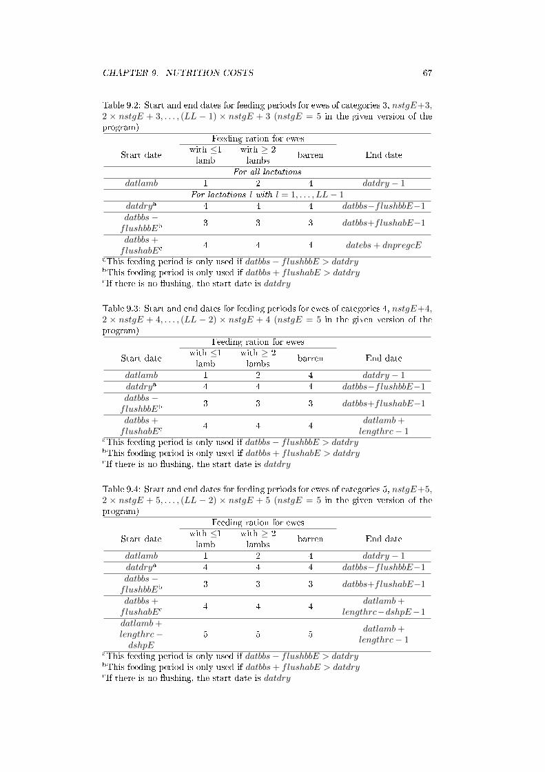
CHAPTER 9. NUTRITION COSTS 67
Table 9.2: Start and end dates for feeding periods for ewes of categories 3, nstgE+3,2 × nstgE + 3, . . . , (LL − 1) × nstgE + 3 (nstgE = 5 in the given version of theprogram)
Feeding ration for ewes
Start datewith ≤1lamb
with ≥ 2lambs
barren End date
For all lactationsdatlamb 1 2 4 datdry − 1
For lactations l with l = 1, . . . , LL− 1datdrya 4 4 4 datbbs−flushbbE−1
datbbs−flushbbEb 3 3 3 datbbs+flushabE−1
datbbs+flushabEc 4 4 4 datebs+ dnpregcE
aThis feeding period is only used if datbbs− flushbbE > datdrybThis feeding period is only used if datbbs+ flushabE > datdrycIf there is no �ushing, the start date is datdry
Table 9.3: Start and end dates for feeding periods for ewes of categories 4, nstgE+4,2 × nstgE + 4, . . . , (LL − 2) × nstgE + 4 (nstgE = 5 in the given version of theprogram)
Feeding ration for ewes
Start datewith ≤1lamb
with ≥ 2lambs
barren End date
datlamb 1 2 4 datdry − 1
datdrya 4 4 4 datbbs−flushbbE−1
datbbs−flushbbEb 3 3 3 datbbs+flushabE−1
datbbs+flushabEc 4 4 4
datlamb+lengthrc− 1
aThis feeding period is only used if datbbs− flushbbE > datdrybThis feeding period is only used if datbbs+ flushabE > datdrycIf there is no �ushing, the start date is datdry
Table 9.4: Start and end dates for feeding periods for ewes of categories 5, nstgE+5,2 × nstgE + 5, . . . , (LL − 2) × nstgE + 5 (nstgE = 5 in the given version of theprogram)
Feeding ration for ewes
Start datewith ≤1lamb
with ≥ 2lambs
barren End date
datlamb 1 2 4 datdry − 1
datdrya 4 4 4 datbbs−flushbbE−1
datbbs−flushbbEb 3 3 3 datbbs+flushabE−1
datbbs+flushabEc 4 4 4
datlamb+lengthrc−dshpE−1
datlamb+lengthrc−dshpE
5 5 5datlamb+lengthrc− 1
aThis feeding period is only used if datbbs− flushbbE > datdrybThis feeding period is only used if datbbs+ flushabE > datdrycIf there is no �ushing, the start date is datdry
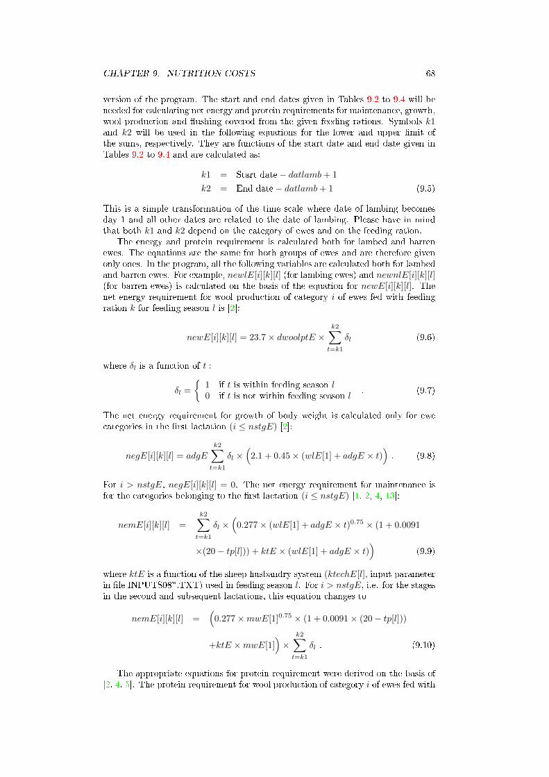
CHAPTER 9. NUTRITION COSTS 68
version of the program. The start and end dates given in Tables 9.2 to 9.4 will beneeded for calculating net energy and protein requirements for maintenance, growth,wool production and �ushing covered from the given feeding rations. Symbols k1and k2 will be used in the following equations for the lower and upper limit ofthe sums, respectively. They are functions of the start date and end date given inTables 9.2 to 9.4 and are calculated as:
k1 = Start date− datlamb+ 1
k2 = End date− datlamb+ 1 (9.5)
This is a simple transformation of the time scale where date of lambing becomesday 1 and all other dates are related to the date of lambing. Please have in mindthat both k1 and k2 depend on the category of ewes and on the feeding ration.
The energy and protein requirement is calculated both for lambed and barrenewes. The equations are the same for both groups of ewes and are therefore givenonly ones. In the program, all the following variables are calculated both for lambedand barren ewes. For example, newlE[i][k][l] (for lambing ewes) and newnlE[i][k][l](for barren ewes) is calculated on the basis of the equation for newE[i][k][l]. Thenet energy requirement for wool production of category i of ewes fed with feedingration k for feeding season l is [2]:
newE[i][k][l] = 23.7× dwoolptE ×k2∑
t=k1
δl (9.6)
where δl is a function of t :
δl =
{1 if t is within feeding season l0 if t is not within feeding season l
. (9.7)
The net energy requirement for growth of body weight is calculated only for ewecategories in the �rst lactation (i ≤ nstgE) [2]:
negE[i][k][l] = adgE
k2∑t=k1
δl ×(
2.1 + 0.45× (wlE[1] + adgE × t)). (9.8)
For i > nstgE, negE[i][k][l] = 0. The net energy requirement for maintenance isfor the categories belonging to the �rst lactation (i ≤ nstgE) [1, 2, 4, 13]:
nemE[i][k][l] =
k2∑t=k1
δl ×(
0.277× (wlE[1] + adgE × t)0.75 × (1 + 0.0091
×(20− tp[l])) + ktE × (wlE[1] + adgE × t))
(9.9)
where ktE is a function of the sheep husbandry system (ktechE[l], input parameterin �le INPUTS08*.TXT) used in feeding season l. For i > nstgE, i.e. for the stagesin the second and subsequent lactations, this equation changes to
nemE[i][k][l] =(
0.277×mwE[1]0.75 × (1 + 0.0091× (20− tp[l]))
+ktE ×mwE[1])×
k2∑t=k1
δl . (9.10)
The appropriate equations for protein requirement were derived on the basis of[2, 4, 5]. The protein requirement for wool production of category i of ewes fed with
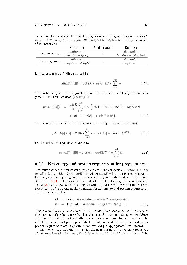
CHAPTER 9. NUTRITION COSTS 69
Table 9.5: Start and end dates for feeding periods for pregnant ewes (categories 5,nstgE+5, 2×nstgE+5, . . . , (LL−2)×nstgE+5, nstgE = 5 for the given versionof the program)
Start date Feeding ration End date
Low pregnancydatlamb+
lengthrc− lpreg 4datlamb+
lengthrc−dshpE−1
High pregnancydatlamb+
lengthrc− dshpE 5datlamb+lengthrc− 1
feeding ration k for feeding season l is:
pdiwE[i][k][l] = 3088.6× dwoolptE ×k2∑
t=k1
δl . (9.11)
The protein requirement for growth of body weight is calculated only for ewe cate-gories in the �rst lactation (i ≤ nstgE) :
pdigE[i][k][l] =adgE
0.59
k2∑t=k1
δl ×(
156.1− 1.94× (wlE[1] + adgE × t)
+0.0173× (wlE[1] + adgE × t)2). (9.12)
The protein requirement for maintenance is for categories i with i ≤ nstgE :
pdimE[i][k][l] = 2.1875
k2∑t=k1
δl × (wlE[1] + adgE × t)0.75 . (9.13)
For i > nstgE this equation changes to
pdimE[i][k][l] = 2.1875×mwE[1]0.75 ×k2∑
t=k1
δl . (9.14)
9.2.3 Net energy and protein requirement for pregnant ewes
The only categories representing pregnant ewes are categories 5, nstgE + 5, 2 ×nstgE + 5, . . . , (LL − 2) × nstgE + 5, where nstgE = 5 in the present version ofthe program. During pregnancy, the ewes are only fed feeding rations 4 and 5 (seeSubsection 9.1.1). The start and end dates for the two feeding rations are given inTable 9.5. As before, symbols k1 and k2 will be used for the lower and upper limit,respectively, of the sums in the equations for net energy and protein requirement.They are calculated as:
k1 = Start date− datlamb− lengthrc+ lpreg + 1
k2 = End date− datlamb− lengthrc+ lpreg + 1 . (9.15)
This is a simple transformation of the time scale where date of conceiving becomesday 1 and all other dates are related to this date. Both k1 and k2 depend via �Startdate� and �End date� on the feeding ration. Net energy requirement will have theunit MJ per ewe and per appropriate time interval and the calculated values forprotein requirement are in grammes per ewe and per appropriate time interval.
The net energy and the protein requirement during low pregnancy for a eweof category i = (j − 1) × nstgE + 5 (j = 1, . . . , LL − 1, j is the number of the
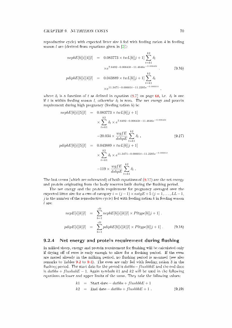
CHAPTER 9. NUTRITION COSTS 70
reproductive cycle) with expected litter size b fed with feeding ration 4 in feedingseason l are (derived from equations given in [2]):
nepbE[b][i][4][l] = 0.083773× twL[b][j + 1]
k2∑t=k1
δl
×e7.6492−0.00643t−11.4646e−0.00643t
, (9.16)
pdipbE[b][i][4][l] = 0.043889× twL[b][j + 1]
k2∑t=k1
δl
×e11.3471−0.00601t−11.2205e−0.00601t
.
where δl is a function of t as de�ned in equation (9.7) on page 68, i.e. δl is oneif t is within feeding season l, otherwise δl is zero. The net energy and proteinrequirement during high pregnancy (feeding ration 5) is:
nepbE[b][i][5][l] = 0.083773× twL[b][j + 1]
×k2∑
t=k1
δl × e7.6492−0.00643t−11.4646e−0.00643t
−20.034× wgfE
dshpE
k2∑t=k1
δl , (9.17)
pdipbE[b][i][5][l] = 0.043889× twL[b][j + 1]
×k2∑
t=k1
δl × e11.3471−0.00601t−11.2205e−0.00601t
−119× wgfE
dshpE
k2∑t=k1
δl .
The last terms (which are subtracted) of both equations of (9.17) are the net energyand protein originating from the body reserves built during the �ushing period.
The net energy and the protein requirement for pregnancy averaged over theexpected litter size for a ewe of category i = (j− 1)×nstgE+ 5 (j = 1, . . . , LL− 1,j is the number of the reproductive cycle) fed with feeding ration k in feeding seasonl are:
nepE[i][k][l] =
clt∑b=1
nepbE[b][i][k][l]× Pltype[b][j + 1] ,
pdipE[i][k][l] =
clt∑b=1
pdipbE[b][i][k][l]× Pltype[b][j + 1] . (9.18)
9.2.4 Net energy and protein requirement during �ushing
In milked sheep, energy and protein requirement for �ushing will be calculated onlyif drying o� of ewes is early enough to allow for a �ushing period. If the ewesare mated already in the milking period, no �ushing period is assumed (see alsoremarks to Tables 9.2 to 9.4). The ewes are only fed with feeding ration 3 in the�ushing period. The start date for the period is datbbs−flushbbE and the end dateis datbbs + flushabE − 1. Again symbols k1 and k2 will be used in the followingequations as lower and upper limits of the sums. They take the following values:
k1 = Start date− datbbs+ flushbbE + 1
k2 = End date− datbbs+ flushbbE + 1 . (9.19)
CHAPTER 9. NUTRITION COSTS 71
The net energy and protein requirement for �ushing per ewe of category i (i =(j−1)×nstgE+k where j is the reproductive cycle with j = 1, . . . , LL−1 and k isthe stage within the lactation cycle with k = 3, . . . , nstgE, nstgE = 5 for the givenversion of the program) fed with feeding ration 3 in feeding season l (l = 1, . . . , nfs)are [1, 4]:
nefE[i][3][l] = 23.85× adgfE ×k2∑
t=k1
δl
pdifE[i][3][l] = 140× adgfE ×k2∑
t=k1
δl (9.20)
where δl is one if t is within feeding season l, otherwise δl is zero.
9.2.5 Net energy and protein requirement for lactating ewes
Lactating ewes are fed with feeding rations 1 or 2 in dependence on the number ofsuckled lambs (see Tables 9.2 to 9.4). The start date for the period is datlamb andthe end date is datdry − 1. Again symbols k1 and k2 will be used in the followingequations as lower and upper limits of the sums. They take the following values:
k1 = Start date− datlamb+ 1
k2 = End date− datlamb+ 1 . (9.21)
The net energy and protein requirement for lactation per ewe of category i(i = (j − 1)× nstgE + i1 where i1 = 3, . . . , nstgE for j = 1, . . . , LL− 1 and i1 = 3for j = LL, j is the number of the reproductive cycle and i1 the stage within thereproductive cycle, nstgE = 5 for the given version of the program) with b suckledlambs (b = 0, . . . , clt) fed with feeding ration k (k = 1 or 2) in feeding season l(l = 1, . . . , nfs) are1 [5, ?]:
nelbE[b][i][k][l] = (0.948 + 0.376fat+ 0.209prot)× ktlsl[b]× ktlp[j]
×k2∑
t=k1
δl × awo× tbwo × e−cwo×t (9.22)
pdilbE[b][i][k][l] = 17.2414prot× ktlsl[b]× ktlsl[j]
×k2∑
t=k1
δl × awo× tbwo × e−cwo×t
where δl is one if t is within feeding season l, otherwise δl is zero.The net energy and protein requirement during lactation per ewe of category
i with 0 or 1 suckled lambs fed with feeding ration 1 in feeding season l (l =
1For non-dairy sheep, energy and protein requirement is zero for b = 0. This is solved in theprogram by setting ktlsl[0] = 0.
CHAPTER 9. NUTRITION COSTS 72
1, . . . , nfs) are
nelE[i][1][l] =
1∑b=0
nelbE[b][i][1][l]× PsuckE[b][j]
1∑b=0
PsuckE[b][j]
(9.23)
pdilE[i][1][l] =
1∑b=0
pdilbE[b][i][1][l]× PsuckE[b][j]
1∑b=0
PsuckE[b][j]
and net energy and protein requirement during lactation per ewe of category i with2 or more suckled lambs fed with feeding ration 2 in feeding season l (l = 1, . . . , nfs)are
nelE[i][2][l] =
clt∑b=2
nelbE[b][i][2][l]× PsuckE[b][j]
clt∑b=2
PsuckE[b][j]
(9.24)
pdilE[i][2][l] =
clt∑b=2
pdilbE[b][i][2][l]× PsuckE[b][j]
clt∑b=2
PsuckE[b][j]
.
9.2.6 Total net energy and protein requirement for individ-ual categories of ewes
In this subsection, the equations for the total net energy and protein requirementare given. The net energy and protein requirement are speci�c for the categoriesof ewes, the feeding ration the ewes are fed with and the seasonal variant of thefeeding ration.
The equations for the calculation of the total net energy and protein requirementfor a ewe of category i (i = (j − 1) × nstgE + i1 where i1 = 3, . . . , nstgE forj = 1, . . . , LL− 1 and i1 = 3 for j = LL, j is the number of the reproductive cycleand i1 the stage within the reproductive cycle, nstgE = 5 for the given versionof the program) di�er between feeding rations. The total net energy and proteinrequirement for a ewe fed with feeding ration 1 in feeding season l (l = 1, . . . , nfs)are:
neE[i][1][l] = (neglE[i][1][l] + nemlE[i][1][l] + newlE[i][1][l] + nelE[i][1][l])
×plambE[i]× 1
l3E[j]
1∑b=0
PsuckE[b][j] (9.25)
pdiE[i][1][l] = (pdiglE[i][1][l] + pdimlE[i][1][l] + pdiwlE[i][1][l] + pdilE[i][1][l])
×plambE[i]× 1
l3E[j]
1∑b=0
PsuckE[b][j] .

CHAPTER 9. NUTRITION COSTS 73
The appropriate equations for ewes fed with feeding ration 2 are:
neE[i][2][l] = (neglE[i][2][l] + nemlE[i][2][l] + newlE[i][2][l] + nelE[i][2][l])
×plambE[i]× 1
l3E[j]
clt∑b=2
PsuckE[b][j] (9.26)
pdiE[i][2][l] = (pdiglE[i][2][l] + pdimlE[i][2][l] + pdiwlE[i][2][l] + pdilE[i][2][l])
×plambE[i]× 1
l3E[j]
clt∑b=2
PsuckE[b][j] .
The total net energy and protein requirement for a ewe fed with feeding ration 3are calculated as:
neE[i][3][l] = (neglE[i][3][l] + nemlE[i][3][l] + newlE[i][3][l])
×plambE[i] + (negnlE[i][3][l] + nemnlE[i][3][l]
+newnlE[i][3][l])× (1− plambE[i]) + nefE[i][3][l] (9.27)
pdiE[i][3][l] = (pdiglE[i][3][l] + pdimlE[i][3][l] + pdiwlE[i][3][l])
×plambE[i] + (pdignlE[i][3][l] + pdimnlE[i][3][l]
+pdiwnlE[i][3][l])× (1− plambE[i]) + pdifE[i][3][l] .
The equations for feeding ration 4 are:
neE[i][4][l] = (neglE[i][4][l] + nemlE[i][4][l] + newlE[i][4][l])
×plambE[i] + (negnlE[i][4][l] + nemnlE[i][4][l]
+newnlE[i][4][l])× (1− plambE[i]) (9.28)
pdiE[i][4][l] = (pdiglE[i][4][l] + pdimlE[i][4][l] + pdiwlE[i][4][l])
×plambE[i] + (pdignlE[i][4][l] + pdimnlE[i][4][l]
+pdiwnlE[i][4][l])× (1− plambE[i]) .
Finally, the total net energy and protein requirement for ewes fed with feedingration 5 are:
neE[i][5][l] = (neglE[i][5][l] + nemlE[i][5][l] + newlE[i][5][l])
×plambE[i] + (negnlE[i][5][l] + nemnlE[i][5][l]
+newnlE[i][5][l])× (1− plambE[i]) + nepE[i][5][l] (9.29)
pdiE[i][5][l] = (pdiglE[i][5][l] + pdimlE[i][5][l] + pdiwlE[i][5][l])
×plambE[i] + (pdignlE[i][5][l] + pdimnlE[i][5][l]
+pdiwnlE[i][5][l])× (1− plambE[i]) + pdipE[i][5][l] .
9.2.7 Total feed costs for individual categories of ewes
Fresh feed requirement is always given in kg per ewe and appropriate time intervalin this subsection. Fresh feed requirement (feE[i][k][l]) calculated from the netenergy content in feed per ewe of category i (i = (j − 1) × nstgE + i1 wherei1 = 3, . . . , nstgE for j = 1, . . . , LL − 1 and i1 = 3 for j = LL, j is the number ofthe reproductive cycle and i1 the stage within the reproductive cycle, nstgE = 5 forthe given version of the program) fed with the seasonal variant l of feeding rationk is:
feE[i][k][l] =neE[i][k][l]
nedE[k][l]× drymE[k][l]. (9.30)
CHAPTER 9. NUTRITION COSTS 74
The appropriate fresh feed requirement calculated from the protein content in thefeed (fpdiE[i][k][l]) is:
fpdiE[i][k][l] =pdiE[i][k][l]
pdidE[k][l]× drymE[k][l]. (9.31)
If the �nal value of the fresh feed requirement (ffE[i][k][l]) is calculated both fromthe net energy content and the protein content of the feed (option feedcost = 1 inparameter �le PARAS*.TXT, see Section 14.1.2 on page 145) the maximum of thevalues calculated in equations (9.30) and (9.31) is taken corrected by the losses offeed caused by wasting:
ffE[i][k][l] =max(feE[i][k][l], fpdiE[i][k][l])
1− lossfE[k][l]/100(9.32)
If the �nal feed requirement is calculated only from the net energy content in thefeed (option feedcost = 2 in parameter �le PARAS*.TXT), equation (9.32) changesto:
ffE[i][k][l] =feE[i][k][l]
1− lossfE[k][l]/100(9.33)
The total undiscounted feeding costs (costfudE[i]) per ewe of category i (i =(j − 1) × nstgE + i1 where i1 = 3, . . . , nstgE for j = 1, . . . , LL − 1 and i1 = 3for j = LL, j is the number of the reproductive cycle and i1 the stage within thereproductive cycle, nstgE = 5 for the given version of the program) are then:
costfudE[i] =
fE∑k=1
nfs∑l=1
ffE[i][k][l]× prfE[k][l] . (9.34)
For the remaining categories (i = (j − 1) × nstgE + i1 where i1 = 1, 2 for j =1, . . . , LL) it is assumed that the ewes died or were culled on average in the middleof the appropriate time interval. Therefore, the costs for them are half the costs forthe corresponding categories the costs were already calculated. For reproductivecycles j = 1, . . . , LL− 1 is
costfudE[(j−1)×nstgE+1] = costfudE[(j−1)×nstgE+2] = costfudE[j×nstgE]/2(9.35)
and for j = LL
costfudE[(j−1)×nstgE+1] = costfudE[(j−1)×nstgE+2] = costfudE[TE]/2 .(9.36)
The total feeding costs discounted to the date of lambing (costfE[i]) are for allcategories i of ewes (i = 1, . . . , TE) :
costfE[i] = qaveE[i]× costfudE[i] . (9.37)
9.3 Nutrition costs for rams
9.3.1 Net energy and protein requirement for rams
As already mentioned in Subsection 9.1.2, feeding of rams has to cover the energyand protein requirement for maintenance, wool growth, �ushing and growth of bodyweight. Net energy and protein requirements for maintenance and growth dependon body weight and growth rate. All calculated values for net energy requirementin this subsection are in MJ per ram and per appropriate time interval and the cal-culated values for protein requirement are in grammes per ram and per appropriate
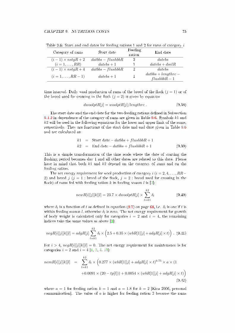
CHAPTER 9. NUTRITION COSTS 75
Table 9.6: Start and end dates for feeding rations 1 and 2 for rams of category i
Category of rams Start dateFeedingration
End date
(i− 1)× nstgR+ 2 datbbs− flushbbR 2 datebs(i = 1, . . . , RR) datebs+ 1 1 datebs+ dselR
(i− 1)× nstgR+ 4 datbbs− flushbbR 2 datebs
(i = 1, . . . , RR− 1) datebs+ 1 1datbbs+ lengthrc−
flushbbR− 1
time interval. Daily wool production of rams of the breed of the �ock (j = 1) or ofthe breed used for crossing in the �ock (j = 2) is given by equation
dwoolptR[j] = woolptR[j]/lengthrc . (9.38)
The start date and the end date for the two feeding rations de�ned in Subsection9.1.2 in dependence of the category of rams are given in Table 9.6. Symbols k1 andk2 will be used in the following equations for the lower and upper limit of the sums,respectively. They are functions of the start date and end date given in Table 9.6and are calculated as:
k1 = Start date− datbbs+ flushbbR+ 1
k2 = End date− datbbs+ flushbbR+ 1 (9.39)
This is a simple transformation of the time scale where the date of starting the�ushing period becomes day 1 and all other dates are related to this date. Pleasehave in mind that both k1 and k2 depend on the category of rams and on thefeeding ration.
The net energy requirement for wool production of category i (i = 2, 4, . . . , RR−2) and breed j (j = 1 : breed of the �ock, j = 2 : breed used for crossing in the�ock) of rams fed with feeding ration k in feeding season l is [2]:
newR[i][j][k][l] = 23.7× dwoolptR[j]×k2∑
t=k1
δl (9.40)
where δl is a function of t as de�ned in equation (9.7) on page 68, i.e. δl is one if t iswithin feeding season l, otherwise δl is zero. The net energy requirement for growthof body weight is calculated only for categories i = 2 and i = 4, the remainingindices take the same values as above [2]:
negR[i][j][k][l] = adgR[j]
k2∑t=k1
δl×(
2.5 + 0.35× (wbR[1][j] +adgR[j]× t)). (9.41)
For i > 4, negR[i][j][k][l] = 0. The net energy requirement for maintenance is forcategories i = 2 and i = 4 [1, 2, 4, 13]:
nemR[i][j][k][l] =
k2∑t=k1
δl ×(
0.277× (wbR[1][j] + adgR[j]× t)0.75 × a× (1
+0.0091× (20− tp[l])) + 0.0054× (wbR[1][j] + adgR[j]× t))
(9.42)
where a = 1 for feeding ration k = 1 and a = 1.8 for k = 2 [Kica 2006, personalcommunication]. The value of a is higher for feeding ration 2 because the rams
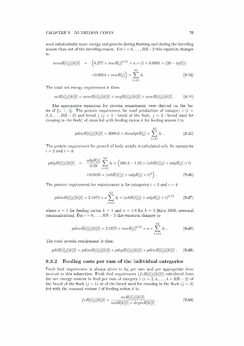
CHAPTER 9. NUTRITION COSTS 76
need substantially more energy and protein during �ushing and during the breedingseason than out of the breeding season. For i = 6, . . . , RR−2 this equation changesto
nemR[i][j][k][l] =(
0.277×mwR[j]0.75 × a× (1 + 0.0091× (20− tp[l]))
+0.0054×mwR[j])×
k2∑t=k1
δl . (9.43)
The total net energy requirement is then:
neR[i][j][k][l] = nemR[i][j][k][l] + negR[i][j][k][l] + newR[i][j][k][l] . (9.44)
The appropriate equations for protein requirement were derived on the ba-sis of [2, 4, 5]. The protein requirement for wool production of category i (i =2, 4, . . . , RR − 2) and breed j (j = 1 : breed of the �ock, j = 2 : breed used forcrossing in the �ock) of rams fed with feeding ration k for feeding season l is:
pdiwR[i][j][k][l] = 3088.6× dwoolptR[j]×k2∑
t=k1
δl . (9.45)
The protein requirement for growth of body weight is calculated only for categoriesi = 2 and i = 4:
pdigR[i][j][k][l] =adgR[j]
0.59
k2∑t=k1
δl ×(
160.4− 1.22× (wbR[1][j] + adgR[j]× t)
+0.0105× (wbR[1][j] + adgR[j]× t)2). (9.46)
The protein requirement for maintenance is for categories i = 2 and i = 4:
pdimR[i][j][k][l] = 2.1875× ak2∑
t=k1
δl × (wbR[1][j] + adgR[j]× t)0.75 (9.47)
where a = 1 for feeding ration k = 1 and a = 1.8 for k = 2 [Kica 2006, personalcommunication]. For i = 6, . . . , RR− 2 this equation changes to
pdimR[i][j][k][l] = 2.1875×mwR[j]0.75 × a×k2∑
t=k1
δl . (9.48)
The total protein requirement is then:
pdiR[i][j][k][l] = pdimR[i][j][k][l] + pdigR[i][j][k][l] + pdiwR[i][j][k][l] . (9.49)
9.3.2 Feeding costs per ram of the individual categories
Fresh feed requirement is always given in kg per ram and per appropriate timeinterval in this subsection. Fresh feed requirement (feR[i][j][k][l]) calculated fromthe net energy content in feed per ram of category i (i = 2, 4, . . . , 4 × RR − 2) ofthe breed of the �ock (j = 1) or of the breed used for crossing in the �ock (j = 2)fed with the seasonal variant l of feeding ration k is:
feR[i][j][k][l] =neR[i][j][k][l]
nedR[k][l]× drymR[k][l]. (9.50)
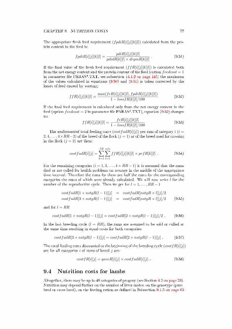
CHAPTER 9. NUTRITION COSTS 77
The appropriate fresh feed requirement (fpdiR[i][j][k][l]) calculated from the pro-tein content in the feed is:
fpdiR[i][j][k][l] =pdiR[i][j][k][l]
pdidR[k][l]× drymR[k][l]. (9.51)
If the �nal value of the fresh feed requirement (ffR[i][j][k][l]) is calculated bothfrom the net energy content and the protein content of the feed (option feedcost = 1in parameter �le PARAS*.TXT, see subsection 14.1.2 on page 145) the maximumof the values calculated in equations (9.50) and (9.51) is taken corrected by thelosses of feed caused by wasting:
ffR[i][j][k][l] =max(feR[i][j][k][l], fpdiR[i][j][k][l])
1− lossfR[k][l]/100(9.52)
If the �nal feed requirement is calculated only from the net energy content in thefeed (option feedcost = 2 in parameter �le PARAS*.TXT), equation (9.52) changesto:
ffR[i][j][k][l] =feR[i][j][k][l]
1− lossfR[k][l]/100(9.53)
The undiscounted total feeding costs (costfudR[i][j]) per ram of category i (i =2, 4, . . . , 4×RR−2) of the breed of the �ock (j = 1) or of the breed used for crossingin the �ock (j = 2) are then:
costfudR[i][j] =
fR∑k=1
nfs∑l=1
ffR[i][j][k][l]× prfR[k][l] . (9.54)
For the remaining categories (i = 1, 3, . . . , 4×RR− 1) it is assumed that the ramsdied or are culled for health problems on average in the middle of the appropriatetime interval. Therefore the costs for them are half the costs for the correspondingcategories the costs of which were already calculated. We will now write l for thenumber of the reproductive cycle. Then we get for l = 1, . . . , RR− 1
costfudR[1 + nstgR(l − 1)][j] = costfudR[nstgR× l][j]/2costfudR[3 + nstgR(l − 1)][j] = costfudR[nstgR× l][j]/2 (9.55)
and for l = RR
costfudR[1 + nstgR(l − 1)][j] = costfudR[2 + nstgR(l − 1)][j]/2 . (9.56)
In the last breeding cycle (l = RR), the rams are assumed to be sold or culled atthe same time resulting in equal costs for both categories:
costfudR[3 + nstgR(l − 1)][j] = costfudR[2 + nstgR(l − 1)][j] . (9.57)
The total feeding costs discounted to the beginning of the breeding cycle (costfR[i][j])are for all categories i of rams of breed j are:
costfR[i][j] = qaveR[i][j]× costfudR[i][j] . (9.58)
9.4 Nutrition costs for lambs
Altogether, there may be up to 48 categories of progeny (see Section 4.2 on page 23).Nutrition may depend further on the number of litter mates, on the genotype (pure-bred or cross-bred), on the feeding ration as de�ned in Subsection 9.1.3 on page 65
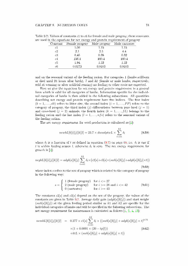
CHAPTER 9. NUTRITION COSTS 78
Table 9.7: Values of constants c1 to c6 for female and male progeny; these constantsare used in the equations for net energy and protein requirement of progeny
Constant Female progeny Male progeny Male castratesc1 1.00 1.15 1.15c2 2.1 2.5 4.4c3 0.45 0.35 0.32c4 156.1 160.4 160.4c5 1.94 1.22 1.22c6 0.0173 0.0105 0.0105
and on the seasonal variant of the feeding ration. For categories 1 (lambs stillbornor died until 24 hours after birth), 7 and 32 (female or male lambs, respectively,sold at weaning or after arti�cial rearing) no feeding or other costs are expected.
Here we give the equations for net energy and protein requirement in a generalform which is valid for all categories of lambs. Information speci�c for the individ-ual categories of lambs is then added in the following subsections. All quantitiesdescribing net energy and protein requirement have �ve indices. The �rst index(b = 1, . . . , clt) refers to litter size, the second index (i = 1, . . . , PP ) refers to thecategory of progeny, the third index (j) di�erentiates between pure-bred (j = 1)and cross-bred (j = 2) animals, the fourth index (k = 1, . . . , fL) belongs to thefeeding ration and the last index (l = 1, . . . , nfs) refers to the seasonal variant ofthe feeding ration.
The net energy requirement for wool production is calculated as [2]:
newbL[b][i][j][k][l] = 23.7× dwoolptwL×k2∑
t=k1
δl (9.59)
where δl is a function of t as de�ned in equation (9.7) on page 68, i.e. δl is one ift is within feeding season l, otherwise δl is zero. The net energy requirement forgrowth is [2]:
negbL[b][i][j][k][l] = adgb[s][b][j]
k2∑t=k1
δl×(c2[s]+c3[s]×(swb[s][b][j]+adgb[s][b][j]×t)
)(9.60)
where index s refers to the sex of progeny which is related to the category of progenyin the following way:
s =
1 (female progeny) for i <= 272 (male progeny) for i >= 28 and i <= 420 (castrates) for i >= 43
(9.61)
The constants c2[s] and c3[s] depend on the sex of the progeny, the values of theconstants are given in Table 9.7. Average daily gain (adgb[s][b][j]) and start weight(swb[s][b][j]) at the given feeding period similar as k1 and k2 are speci�c for theindividual categories of lambs and will be speci�ed in the following subsections. Thenet energy requirement for maintenance is calculated as follows [1, 2, 4, 13]:
nembL[b][i][j][k][l] = 0.277× c1[s]
k2∑t=k1
δl ×((swb[s][b][j] + adgb[s][b][j]× t)0.75
×(1 + 0.0091× (20− tp[l])) (9.62)
+ktL× (swb[s][b][j] + adgb[s][b][j]× t))
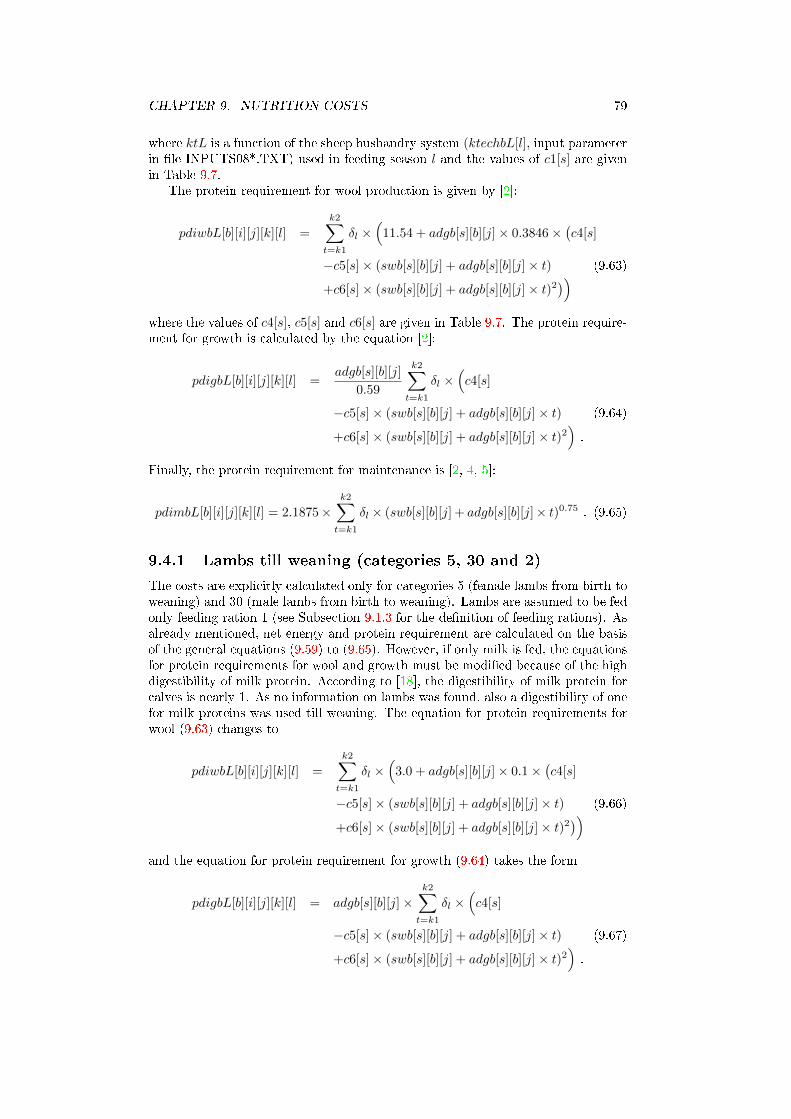
CHAPTER 9. NUTRITION COSTS 79
where ktL is a function of the sheep husbandry system (ktechbL[l], input parameterin �le INPUTS08*.TXT) used in feeding season l and the values of c1[s] are givenin Table 9.7.
The protein requirement for wool production is given by [2]:
pdiwbL[b][i][j][k][l] =
k2∑t=k1
δl ×(
11.54 + adgb[s][b][j]× 0.3846×(c4[s]
−c5[s]× (swb[s][b][j] + adgb[s][b][j]× t) (9.63)
+c6[s]× (swb[s][b][j] + adgb[s][b][j]× t)2))
where the values of c4[s], c5[s] and c6[s] are given in Table 9.7. The protein require-ment for growth is calculated by the equation [2]:
pdigbL[b][i][j][k][l] =adgb[s][b][j]
0.59
k2∑t=k1
δl ×(c4[s]
−c5[s]× (swb[s][b][j] + adgb[s][b][j]× t) (9.64)
+c6[s]× (swb[s][b][j] + adgb[s][b][j]× t)2).
Finally, the protein requirement for maintenance is [2, 4, 5]:
pdimbL[b][i][j][k][l] = 2.1875×k2∑
t=k1
δl × (swb[s][b][j] + adgb[s][b][j]× t)0.75 . (9.65)
9.4.1 Lambs till weaning (categories 5, 30 and 2)
The costs are explicitly calculated only for categories 5 (female lambs from birth toweaning) and 30 (male lambs from birth to weaning). Lambs are assumed to be fedonly feeding ration 1 (see Subsection 9.1.3 for the de�nition of feeding rations). Asalready mentioned, net energy and protein requirement are calculated on the basisof the general equations (9.59) to (9.65). However, if only milk is fed, the equationsfor protein requirements for wool and growth must be modi�ed because of the highdigestibility of milk protein. According to [18], the digestibility of milk protein forcalves is nearly 1. As no information on lambs was found, also a digestibility of onefor milk proteins was used till weaning. The equation for protein requirements forwool (9.63) changes to
pdiwbL[b][i][j][k][l] =
k2∑t=k1
δl ×(
3.0 + adgb[s][b][j]× 0.1×(c4[s]
−c5[s]× (swb[s][b][j] + adgb[s][b][j]× t) (9.66)
+c6[s]× (swb[s][b][j] + adgb[s][b][j]× t)2))
and the equation for protein requirement for growth (9.64) takes the form
pdigbL[b][i][j][k][l] = adgb[s][b][j]×k2∑
t=k1
δl ×(c4[s]
−c5[s]× (swb[s][b][j] + adgb[s][b][j]× t) (9.67)
+c6[s]× (swb[s][b][j] + adgb[s][b][j]× t)2).
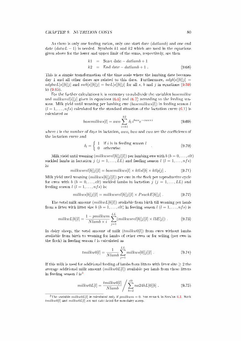
CHAPTER 9. NUTRITION COSTS 80
As there is only one feeding ration, only one start date (datlamb) and one enddate (datwL − 1) is needed. Symbols k1 and k2 which are used in the equationsgiven above for the lower and upper limit of the sums, respectively, are then
k1 = Start date− datlamb+ 1
k2 = End date− datlamb+ 1 . (9.68)
This is a simple transformation of the time scale where the lambing date becomesday 1 and all other dates are related to this date. Furthermore, adgb[s][b][j] =adgbwL[s][b][j] and swb[s][b][j] = bwL[s][b][j] for all s, b and j in equations (9.59)to (9.65).
For the further calculations it is necessary to subdivide the variables basemilkwand milkwrel[i][j] given in equations (6.6) and (6.7) according to the feeding sea-sons. Milk yield until weaning per lambing ewe (basemilkws[l]) in feeding season l(l = 1, . . . , nfs) calculated for the standard situation of the lactation curve (6.1) iscalculated as
basemilkws[l] = awo
k2∑i=k1
δl ibwoe−cwo×i (9.69)
where i is the number of days in lactation, awo, bwo and cwo are the coe�cients ofthe lactation curve and
δl =
{1 if i is in feeding season l0 otherwise
. (9.70)
Milk yield until weaning (milkwsrel[b][j][l]) per lambing ewe with b (b = 0, . . . , clt)suckled lambs in lactation j (j = 1, . . . , LL) and feeding season l (l = 1, . . . , nfs)is:
milkwsrel[b][j][l] = basemilkws[l]× ktlsl[b]× ktlp[j] . (9.71)
Milk yield until weaning (milkws[b][j][l]) per ewe in the �ock per reproductive cyclefor ewes with b (b = 0, . . . , clt) suckled lambs in lactation j (j = 1, . . . , LL) andfeeding season l (l = 1, . . . , nfs) is:
milkws[b][j][l] = milkwsrel[b][j][l]× PsuckE[b][j] . (9.72)
The total milk amount (milkwL[b][l]) available from birth till weaning per lambfrom a litter with litter size b (b = 1, . . . , clt) in feeding season l (l = 1, . . . , nfs) is
milkwL[b][l] =1− pmilkwmNlamb× i
LL∑j=1
(milkwsrel[b][j][l]× l3E[j]) . (9.73)
In dairy sheep, the total amount of milk (tmilkw0[l]) from ewes without lambsavailable from birth to weaning for lambs of other ewes or for selling (per ewe inthe �ock) in feeding season l is calculated as
tmilkw0[l] =1
Nlamb
LL∑j=1
milkws[0][j][l] . (9.74)
If this milk is used for additional feeding of lambs from litters with litter size ≥ 2 theaverage additional milk amount (milkw0L[l]) available per lamb from these littersin feeding season l is2
milkw0L[l] =tmilkw0[l]
Nlamb
/clt∑b=2
na24hL[0][b] . (9.75)
2The variable milkw0L[l] is calculated only if pmilkwm = 0. See remark in Section 6.2. Bothtmilkw0[l] and milkw0L[l] are not calculated for non-dairy sheep.
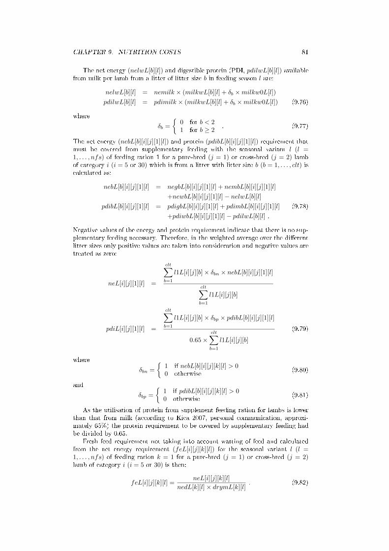
CHAPTER 9. NUTRITION COSTS 81
The net energy (nelwL[b][l]) and digestible protein (PDI, pdilwL[b][l]) availablefrom milk per lamb from a litter of litter size b in feeding season l are:
nelwL[b][l] = nemilk × (milkwL[b][l] + δb ×milkw0L[l])
pdilwL[b][l] = pdimilk × (milkwL[b][l] + δb ×milkw0L[l]) (9.76)
where
δb =
{0 for b < 21 for b ≥ 2
. (9.77)
The net energy (nebL[b][i][j][1][l]) and protein (pdibL[b][i][j][1][l]) requirement thatmust be covered from supplementary feeding with the seasonal variant l (l =1, . . . , nfs) of feeding ration 1 for a pure-bred (j = 1) or cross-bred (j = 2) lambof category i (i = 5 or 30) which is from a litter with litter size b (b = 1, . . . , clt) iscalculated as:
nebL[b][i][j][1][l] = negbL[b][i][j][1][l] + nembL[b][i][j][1][l]
+newbL[b][i][j][1][l]− nelwL[b][l]
pdibL[b][i][j][1][l] = pdigbL[b][i][j][1][l] + pdimbL[b][i][j][1][l] (9.78)
+pdiwbL[b][i][j][1][l]− pdilwL[b][l] .
Negative values of the energy and protein requirement indicate that there is no sup-plementary feeding necessary. Therefore, in the weighted average over the di�erentlitter sizes only positive values are taken into consideration and negative values aretreated as zero:
neL[i][j][1][l] =
clt∑b=1
l1L[i][j][b]× δbn × nebL[b][i][j][1][l]
clt∑b=1
l1L[i][j][b]
pdiL[i][j][1][l] =
clt∑b=1
l1L[i][j][b]× δbp × pdibL[b][i][j][1][l]
0.65×clt∑b=1
l1L[i][j][b]
(9.79)
where
δbn =
{1 if nebL[b][i][j][k][l] > 00 otherwise
(9.80)
and
δbp =
{1 if pdibL[b][i][j][k][l] > 00 otherwise
(9.81)
As the utilisation of protein from supplement feeding ration for lambs is lowerthan that from milk (according to Kica 2007, personal communication, approxi-mately 65%) the protein requirement to be covered by supplementary feeding hadbe divided by 0.65.
Fresh feed requirement not taking into account wasting of feed and calculatedfrom the net energy requirement (feL[i][j][k][l]) for the seasonal variant l (l =1, . . . , nfs) of feeding ration k = 1 for a pure-bred (j = 1) or cross-bred (j = 2)lamb of category i (i = 5 or 30) is then:
feL[i][j][k][l] =neL[i][j][k][l]
nedL[k][l]× drymL[k][l]. (9.82)
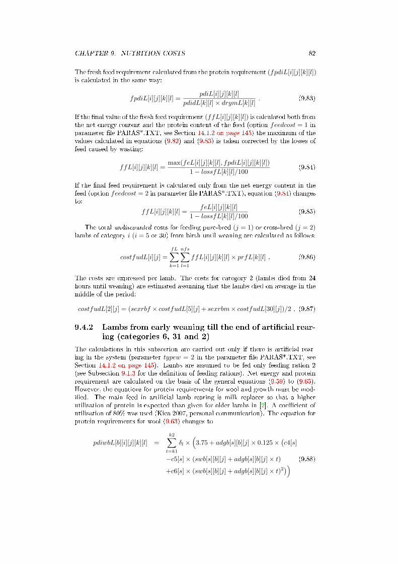
CHAPTER 9. NUTRITION COSTS 82
The fresh feed requirement calculated from the protein requirement (fpdiL[i][j][k][l])is calculated in the same way:
fpdiL[i][j][k][l] =pdiL[i][j][k][l]
pdidL[k][l]× drymL[k][l]. (9.83)
If the �nal value of the fresh feed requirement (ffL[i][j][k][l]) is calculated both fromthe net energy content and the protein content of the feed (option feedcost = 1 inparameter �le PARAS*.TXT, see Section 14.1.2 on page 145) the maximum of thevalues calculated in equations (9.82) and (9.83) is taken corrected by the losses offeed caused by wasting:
ffL[i][j][k][l] =max(feL[i][j][k][l], fpdiL[i][j][k][l])
1− lossfL[k][l]/100(9.84)
If the �nal feed requirement is calculated only from the net energy content in thefeed (option feedcost = 2 in parameter �le PARAS*.TXT), equation (9.84) changesto:
ffL[i][j][k][l] =feL[i][j][k][l]
1− lossfL[k][l]/100(9.85)
The total undiscounted costs for feeding pure-bred (j = 1) or cross-bred (j = 2)lambs of category i (i = 5 or 30) from birth until weaning are calculated as follows:
costfudL[i][j] =
fL∑k=1
nfs∑l=1
ffL[i][j][k][l]× prfL[k][l] . (9.86)
The costs are expressed per lamb. The costs for category 2 (lambs died from 24hours until weaning) are estimated assuming that the lambs died on average in themiddle of the period:
costfudL[2][j] = (sexrbf × costfudL[5][j] + sexrbm× costfudL[30][j])/2 . (9.87)
9.4.2 Lambs from early weaning till the end of arti�cial rear-ing (categories 6, 31 and 2)
The calculations in this subsection are carried out only if there is arti�cial rear-ing in the system (parameter typew = 2 in the parameter �le PARAS*.TXT, seeSection 14.1.2 on page 145). Lambs are assumed to be fed only feeding ration 2(see Subsection 9.1.3 for the de�nition of feeding rations). Net energy and proteinrequirement are calculated on the basis of the general equations (9.59) to (9.65).However, the equations for protein requirements for wool and growth must be mod-i�ed. The main feed in arti�cial lamb rearing is milk replacer so that a higherutilisation of protein is expected than given for older lambs in [2]. A coe�cient ofutilisation of 80% was used (Kica 2007, personal communication). The equation forprotein requirements for wool (9.63) changes to
pdiwbL[b][i][j][k][l] =
k2∑t=k1
δl ×(
3.75 + adgb[s][b][j]× 0.125×(c4[s]
−c5[s]× (swb[s][b][j] + adgb[s][b][j]× t) (9.88)
+c6[s]× (swb[s][b][j] + adgb[s][b][j]× t)2))
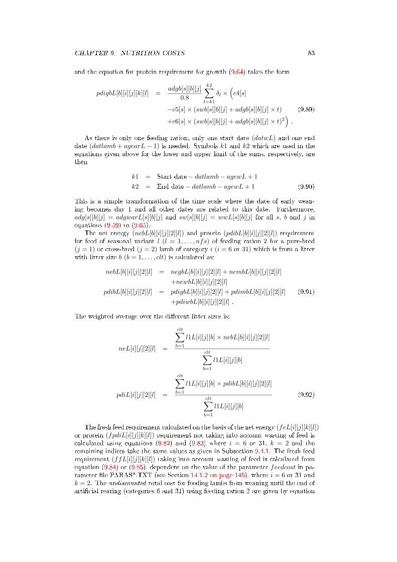
CHAPTER 9. NUTRITION COSTS 83
and the equation for protein requirement for growth (9.64) takes the form
pdigbL[b][i][j][k][l] =adgb[s][b][j]
0.8
k2∑t=k1
δl ×(c4[s]
−c5[s]× (swb[s][b][j] + adgb[s][b][j]× t) (9.89)
+c6[s]× (swb[s][b][j] + adgb[s][b][j]× t)2).
As there is only one feeding ration, only one start date (datwL) and one enddate (datlamb + agearL − 1) is needed. Symbols k1 and k2 which are used in theequations given above for the lower and upper limit of the sums, respectively, arethen
k1 = Start date− datlamb− agewL+ 1
k2 = End date− datlamb− agewL+ 1 (9.90)
This is a simple transformation of the time scale where the date of early wean-ing becomes day 1 and all other dates are related to this date. Furthermore,adg[s][b][j] = adgwarL[s][b][j] and sw[s][b][j] = wwL[s][b][j] for all s, b and j inequations (9.59) to (9.65).
The net energy (nebL[b][i][j][2][l]) and protein (pdibL[b][i][j][2][l]) requirementfor feed of seasonal variant l (l = 1, . . . , nfs) of feeding ration 2 for a pure-bred(j = 1) or cross-bred (j = 2) lamb of category i (i = 6 or 31) which is from a litterwith litter size b (b = 1, . . . , clt) is calculated as:
nebL[b][i][j][2][l] = negbL[b][i][j][2][l] + nembL[b][i][j][2][l]
+newbL[b][i][j][2][l]
pdibL[b][i][j][2][l] = pdigbL[b][i][j][2][l] + pdimbL[b][i][j][2][l] (9.91)
+pdiwbL[b][i][j][2][l] .
The weighted average over the di�erent litter sizes is:
neL[i][j][2][l] =
clt∑b=1
l1L[i][j][b]× nebL[b][i][j][2][l]
clt∑b=1
l1L[i][j][b]
pdiL[i][j][2][l] =
clt∑b=1
l1L[i][j][b]× pdibL[b][i][j][2][l]
clt∑b=1
l1L[i][j][b]
(9.92)
The fresh feed requirement calculated on the basis of the net energy (feL[i][j][k][l])or protein (fpdiL[i][j][k][l]) requirement not taking into account wasting of feed iscalculated using equations (9.82) and (9.83) where i = 6 or 31, k = 2 and theremaining indices take the same values as given in Subsection 9.4.1. The fresh feedrequirement (ffL[i][j][k][l]) taking into account wasting of feed is calculated fromequation (9.84) or (9.85), dependent on the value of the parameter feedcost in pa-rameter �le PARAS*.TXT (see Section 14.1.2 on page 145), where i = 6 or 31 andk = 2. The undiscounted total cost for feeding lambs from weaning until the end ofarti�cial rearing (categories 6 and 31) using feeding ration 2 are given by equation
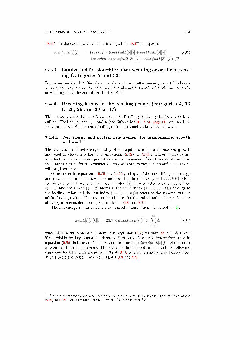
CHAPTER 9. NUTRITION COSTS 84
(9.86). In the case of arti�cial rearing equation (9.87) changes to
costfudL[2][j] =(sexrbf × (costfudL[5][j] + costfudL[6][j]) (9.93)
+sexrbm× (costfudL[30][j] + costfudL[31][j]))/
2 .
9.4.3 Lambs sold for slaughter after weaning or arti�cial rear-ing (categories 7 and 32)
For categories 7 and 32 (female and male lambs sold after weaning or arti�cial rear-ing) no feeding costs are expected as the lambs are assumed to be sold immediatelyat weaning or at the end of arti�cial rearing.
9.4.4 Breeding lambs in the rearing period (categories 4, 13to 26, 29 and 38 to 42)
This period covers the time from weaning till selling, entering the �ock, death orculling. Feeding rations 3, 4 and 5 (see Subsection 9.1.3 on page 65) are used forbreeding lambs. Within each feeding ration, seasonal variants are allowed.
9.4.4.1 Net energy and protein requirement for maintenance, growthand wool
The calculation of net energy and protein requirement for maintenance, growthand wool production is based on equations (9.59) to (9.65). These equations aremodi�ed as the calculated quantities are not dependent from the size of the litterthe lamb is born in for the considered categories of progeny. The modi�ed equationswill be given here.
Other than in equations (9.59) to (9.65), all quantities describing net energyand protein requirement have four indices. The �rst index (i = 1, . . . , PP ) refersto the category of progeny, the second index (j) di�erentiates between pure-bred(j = 1) and cross-bred (j = 2) animals, the third index (k = 1, . . . , fL) belongs tothe feeding ration and the last index (l = 1, . . . , nfs) refers to the seasonal variantof the feeding ration. The start and end dates for the individual feeding rations forall categories considered are given in Tables 9.8 and 9.93.
The net energy requirement for wool production is then calculated as [2]:
newL[i][j][k][l] = 23.7× dwoolptrL[s][j]×k2∑
t=k1
δl (9.94)
where δl is a function of t as de�ned in equation (9.7) on page 68, i.e. δl is oneif t is within feeding season l, otherwise δl is zero. A value di�erent from that inequation (9.59) is inserted for daily wool production (dwoolptrL[s][j]) where indexs refers to the sex of progeny. The values to be inserted in this and the followingequations for k1 and k2 are given in Table 9.10 where the start and end dates citedin this table are to be taken from Tables 9.8 and 9.9.
3In several categories, the same feeding ration occurs twice. In these cases the sums in equations(9.94) to (9.99) are calculated over all days the feeding ration is fed.
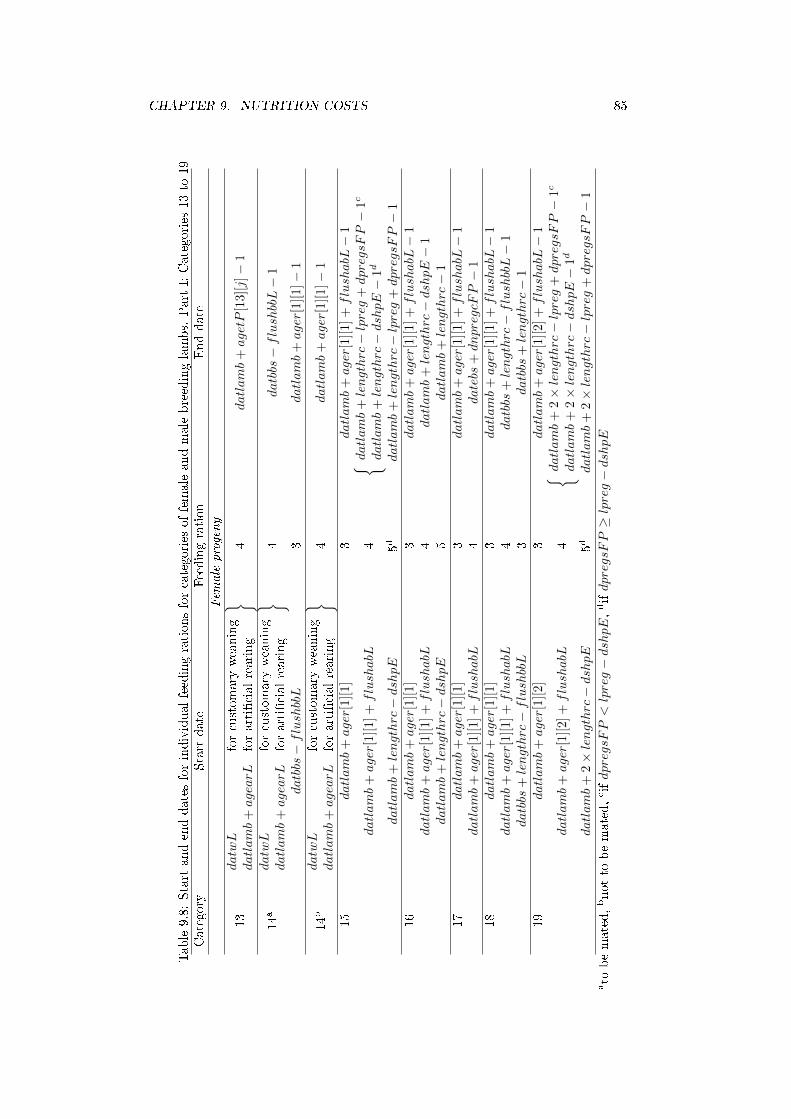
CHAPTER 9. NUTRITION COSTS 85
Table9.8:Start
andenddatesforindividualfeedingrationsforcategories
offemaleandmalebreedinglambs.
Part
I:Categories
13to
19
Category
Start
date
Feedingration
Enddate
Fem
aleprogeny
13
datwL
forcustomary
weaning
datlamb
+agearL
forarti�cialrearing
}4
datlamb
+agetP
[13][j]−
1
14a
datwL
forcustomary
weaning
datlamb
+agearL
forarti�cialrearing
}4
datbbs−flushbbL−
1
datbbs−flushbbL
3datlamb
+ager
[1][
1]−
1
14b
datwL
forcustomary
weaning
datlamb
+agearL
forarti�cialrearing
}4
datlamb
+ager
[1][
1]−
1
15
datlamb
+ager
[1][
1]3
datlamb
+ager
[1][
1]+
flushabL−
1
datlamb
+ager
[1][
1]+flushabL
4
{ datlamb
+lengthrc−lpreg
+dpregsFP−
1c
datlamb
+lengthrc−dshpE−
1d
datlamb
+lengthrc−dshpE
5d
datlamb
+lengthrc−lpreg
+dpregsFP−
116
datlamb
+ager
[1][
1]3
datlamb
+ager
[1][
1]+
flushabL−
1datlamb
+ager
[1][
1]+flushabL
4datlamb
+lengthrc−dshpE−
1datlamb
+lengthrc−dshpE
5datlamb
+lengthrc−
117
datlamb
+ager
[1][
1]3
datlamb
+ager
[1][
1]+
flushabL−
1datlamb
+ager
[1][
1]+flushabL
4datebs
+dnpregcFP−
118
datlamb
+ager
[1][
1]3
datlamb
+ager
[1][
1]+
flushabL−
1datlamb
+ager
[1][
1]+flushabL
4datbbs
+lengthrc−flushbbL−
1datbbs
+lengthrc−flushbbL
3datbbs
+lengthrc−
119
datlamb
+ager
[1][
2]3
datlamb
+ager
[1][
2]+
flushabL−
1
datlamb
+ager
[1][
2]+flushabL
4
{ datlamb
+2×lengthrc−lpreg
+dpregsFP−
1c
datlamb
+2×lengthrc−dshpE−
1d
datlamb
+2×lengthrc−dshpE
5d
datlamb
+2×lengthrc−lpreg
+dpregsFP−
1ato
bemated,bnotto
bemated,cifdpregsFP<lpreg−dshpE,difdpregsFP≥lpreg−dshpE
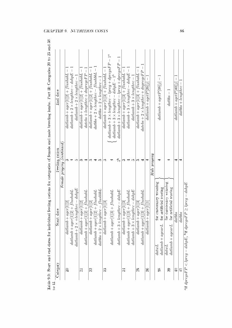
CHAPTER 9. NUTRITION COSTS 86
Table9.9:Start
andenddatesforindividualfeedingrationsforcategories
offemaleandmalebreedinglambs.
Part
II:Categories
20to
25and38
to41
Category
Start
date
Feedingration
Enddate
Fem
aleprogeny(continued)
20
datlamb
+ager
[1][
2]3
datlamb
+ager
[1][
2]+
flushabL−
1datlamb
+ager
[1][
2]+flushabL
4datlamb
+2×lengthrc−dshpE−
1datlamb
+2×
+lengthrc−dshpE
5datlamb
+2×lengthrc−
121
datlamb
+ager
[1][
2]3
datlamb
+ager
[1][
2]+
flushabL−
1datlamb
+ager
[1][
2]+flushabL
4datebs
+lengthrc
+dnpregcFP−
122
datlamb
+ager
[1][
2]3
datlamb
+ager
[1][
2]+
flushabL−
1datlamb
+ager
[1][
2]+flushabL
4datbbs
+2×lengthrc−flushbbL−
1datbbs
+2×lengthrc−flushbbL
3datbbs
+2×lengthrc−
123
datlamb
+ager
[1][
3]3
datlamb
+ager
[1][
3]+
flushabL−
1
datlamb
+ager
[1][
3]+flushabL
4
{ datlamb
+3×lengthrc−lpreg
+dpregsFP−
1a
datlamb
+3×lengthrc−dshpE−
1b
datlamb
+3×lengthrc−dshpE
5b
datlamb
+3×lengthrc−lpreg
+dpregsFP−
124
datlamb
+ager
[1][
3]3
datlamb
+ager
[1][
3]+
flushabL−
1datlamb
+ager
[1][
3]+flushabL
4datlamb
+3×lengthrc−dshpE−
1datlamb
+3×lengthrc−dshpE
5datlamb
+3×lengthrc−
125
datlamb
+ager
[1][
3]3
datlamb
+ager
[1][
3]+
flushabL−
1datlamb
+ager
[1][
3]+flushabL
4datebs
+2×lengthrc
+dnpregcFP−
126
datlamb
+ager
[1][
1]4
datlamb
+agetP
[26][j]−
1Maleprogeny
38
datwL
forcustomary
weaning
datlamb
+agearL
forarti�cialrearing
}4
datlamb
+agetP
[38][j]−
1
39
datwL
forcustomary
weaning
datlamb
+agearL
forarti�cialrearing
}4
datbbs−
1
40
datbbs
4datlamb
+agetP
[40][j]−
141
datbbs
4datbbs
+lengthrc−
1aifdpregsFP<lpreg−dshpE,bifdpregsFP≥lpreg−dshpE
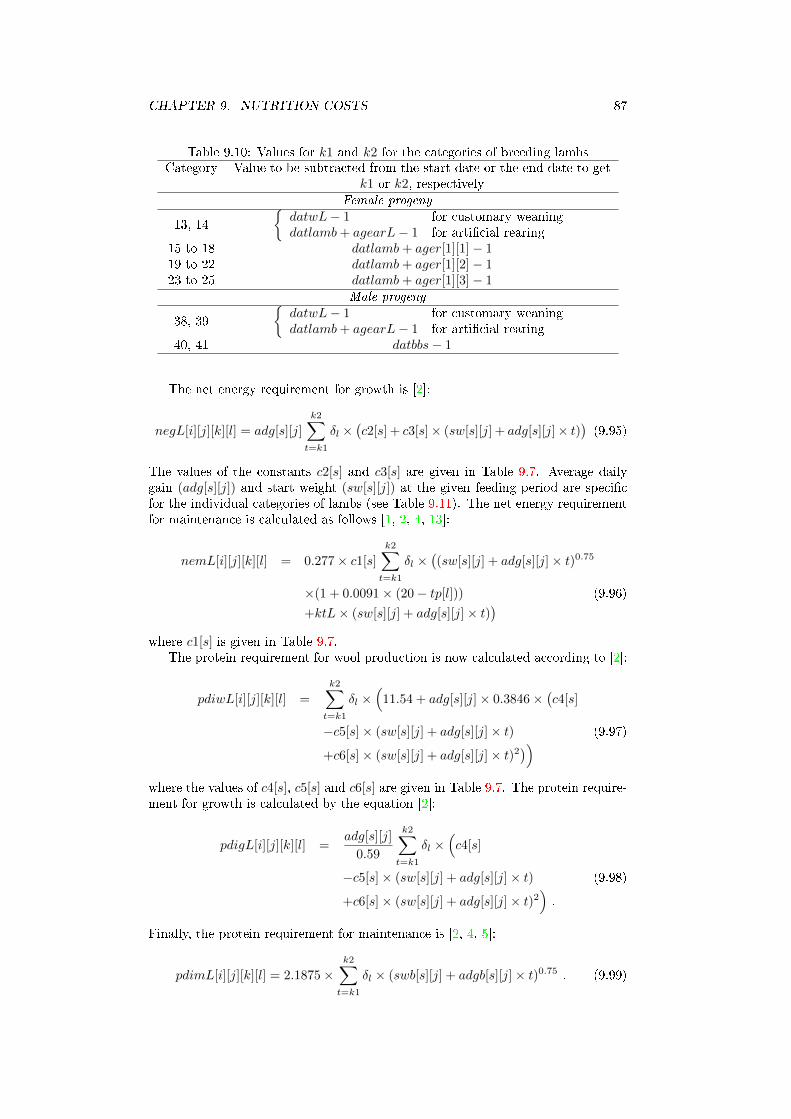
CHAPTER 9. NUTRITION COSTS 87
Table 9.10: Values for k1 and k2 for the categories of breeding lambsCategory Value to be subtracted from the start date or the end date to get
k1 or k2, respectivelyFemale progeny
13, 14
{datwL− 1 for customary weaningdatlamb+ agearL− 1 for arti�cial rearing
15 to 18 datlamb+ ager[1][1]− 119 to 22 datlamb+ ager[1][2]− 123 to 25 datlamb+ ager[1][3]− 1
Male progeny
38, 39
{datwL− 1 for customary weaningdatlamb+ agearL− 1 for arti�cial rearing
40, 41 datbbs− 1
The net energy requirement for growth is [2]:
negL[i][j][k][l] = adg[s][j]
k2∑t=k1
δl ×(c2[s] + c3[s]× (sw[s][j] + adg[s][j]× t)
)(9.95)
The values of the constants c2[s] and c3[s] are given in Table 9.7. Average dailygain (adg[s][j]) and start weight (sw[s][j]) at the given feeding period are speci�cfor the individual categories of lambs (see Table 9.11). The net energy requirementfor maintenance is calculated as follows [1, 2, 4, 13]:
nemL[i][j][k][l] = 0.277× c1[s]
k2∑t=k1
δl ×((sw[s][j] + adg[s][j]× t)0.75
×(1 + 0.0091× (20− tp[l])) (9.96)
+ktL× (sw[s][j] + adg[s][j]× t))
where c1[s] is given in Table 9.7.The protein requirement for wool production is now calculated according to [2]:
pdiwL[i][j][k][l] =
k2∑t=k1
δl ×(
11.54 + adg[s][j]× 0.3846×(c4[s]
−c5[s]× (sw[s][j] + adg[s][j]× t) (9.97)
+c6[s]× (sw[s][j] + adg[s][j]× t)2))
where the values of c4[s], c5[s] and c6[s] are given in Table 9.7. The protein require-ment for growth is calculated by the equation [2]:
pdigL[i][j][k][l] =adg[s][j]
0.59
k2∑t=k1
δl ×(c4[s]
−c5[s]× (sw[s][j] + adg[s][j]× t) (9.98)
+c6[s]× (sw[s][j] + adg[s][j]× t)2).
Finally, the protein requirement for maintenance is [2, 4, 5]:
pdimL[i][j][k][l] = 2.1875×k2∑
t=k1
δl × (swb[s][j] + adgb[s][j]× t)0.75 . (9.99)
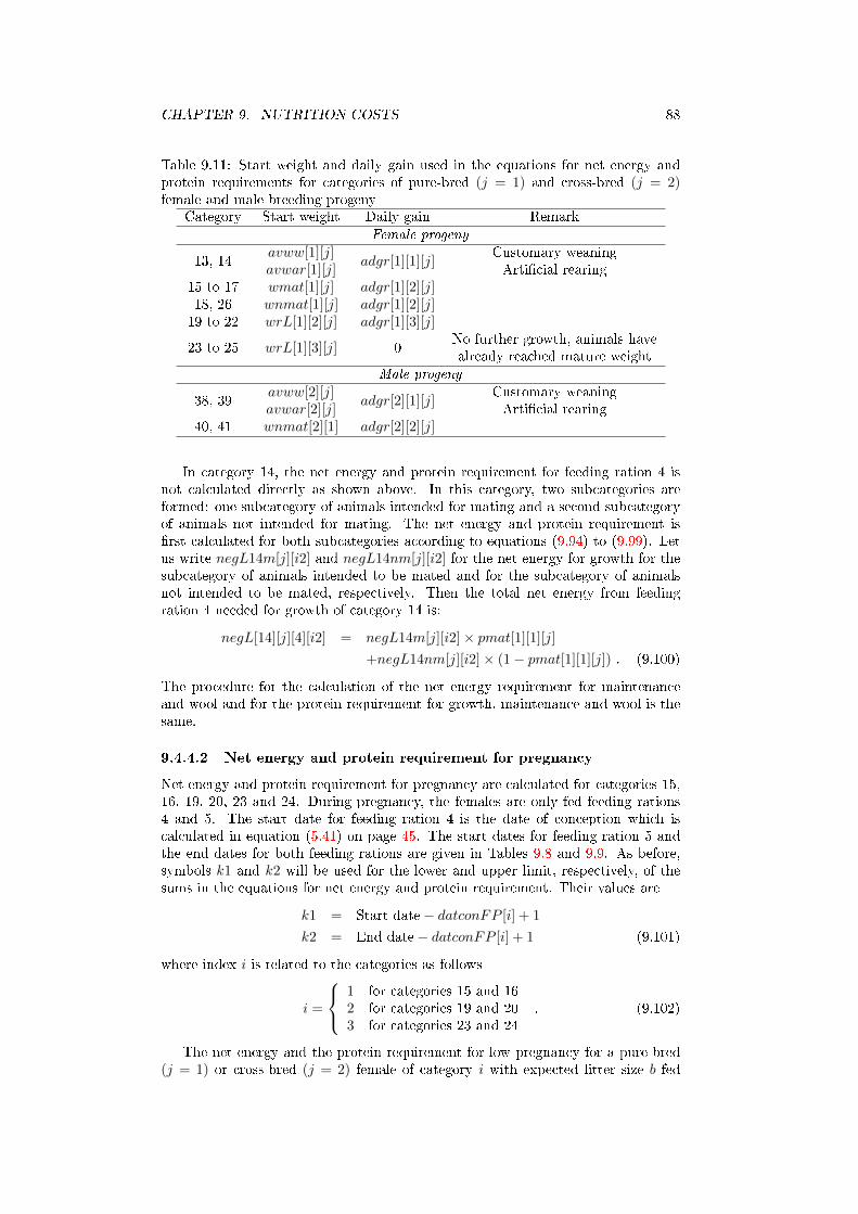
CHAPTER 9. NUTRITION COSTS 88
Table 9.11: Start weight and daily gain used in the equations for net energy andprotein requirements for categories of pure-bred (j = 1) and cross-bred (j = 2)female and male breeding progeny
Category Start weight Daily gain Remark
Female progeny
13, 14avww[1][j]avwar[1][j]
adgr[1][1][j]Customary weaningArti�cial rearing
15 to 17 wmat[1][j] adgr[1][2][j]18, 26 wnmat[1][j] adgr[1][2][j]19 to 22 wrL[1][2][j] adgr[1][3][j]
23 to 25 wrL[1][3][j] 0No further growth, animals havealready reached mature weight
Male progeny
38, 39avww[2][j]avwar[2][j]
adgr[2][1][j]Customary weaningArti�cial rearing
40, 41 wnmat[2][1] adgr[2][2][j]
In category 14, the net energy and protein requirement for feeding ration 4 isnot calculated directly as shown above. In this category, two subcategories areformed: one subcategory of animals intended for mating and a second subcategoryof animals not intended for mating. The net energy and protein requirement is�rst calculated for both subcategories according to equations (9.94) to (9.99). Letus write negL14m[j][i2] and negL14nm[j][i2] for the net energy for growth for thesubcategory of animals intended to be mated and for the subcategory of animalsnot intended to be mated, respectively. Then the total net energy from feedingration 4 needed for growth of category 14 is:
negL[14][j][4][i2] = negL14m[j][i2]× pmat[1][1][j]
+negL14nm[j][i2]× (1− pmat[1][1][j]) . (9.100)
The procedure for the calculation of the net energy requirement for maintenanceand wool and for the protein requirement for growth, maintenance and wool is thesame.
9.4.4.2 Net energy and protein requirement for pregnancy
Net energy and protein requirement for pregnancy are calculated for categories 15,16, 19, 20, 23 and 24. During pregnancy, the females are only fed feeding rations4 and 5. The start date for feeding ration 4 is the date of conception which iscalculated in equation (5.41) on page 45. The start dates for feeding ration 5 andthe end dates for both feeding rations are given in Tables 9.8 and 9.9. As before,symbols k1 and k2 will be used for the lower and upper limit, respectively, of thesums in the equations for net energy and protein requirement. Their values are
k1 = Start date− datconFP [i] + 1
k2 = End date− datconFP [i] + 1 (9.101)
where index i is related to the categories as follows
i =
1 for categories 15 and 162 for categories 19 and 203 for categories 23 and 24
. (9.102)
The net energy and the protein requirement for low pregnancy for a pure-bred(j = 1) or cross-bred (j = 2) female of category i with expected litter size b fed
CHAPTER 9. NUTRITION COSTS 89
with feeding ration 4 in feeding season l are calculated essentially in the same wayas in equations (9.16):
nepbL[b][i][j][4][l] = 0.083773× twL[b][1]
k2∑t=k1
δl
×e7.6492−0.00643t−11.4646e−0.00643t
, (9.103)
pdipbL[b][i][j][4][l] = 0.043889× twL[b][1]
k2∑t=k1
δl
×e11.3471−0.00601t−11.2205e−0.00601t
.
where δl is a function of t as de�ned in equation (9.7) on page 68, i.e. δl is oneif t is within feeding season l, otherwise δl is zero. The net energy and proteinrequirement for high pregnancy (feeding ration 5) is:
nepbL[b][i][j][5][l] = 0.083773× twL[b][1]
×k2∑
t=k1
δl × e7.6492−0.00643t−11.4646e−0.00643t
−20.034× wgfL
dshpE
k2∑t=k1
δl , (9.104)
pdipbL[b][i][j][5][l] = 0.043889× twL[b][1]
×k2∑
t=k1
δl × e11.3471−0.00601t−11.2205e−0.00601t
−119× wgfL
dshpE
k2∑t=k1
δl .
The last terms (which are subtracted) of both equations of (9.104) are the net energyand protein originating from the body reserves built during the �ushing period.
The net energy and the protein requirement for pregnancy averaged over theexpected litter size for a pure-bred (j = 1) or cross-bred (j = 2) female of categoryi fed with feeding ration k in feeding season l are:
nepL[i][j][k][l] =
clt∑b=1
nepbL[b][i][j][k][l]× Pltype[b][1] ,
pdipL[i][j][k][l] =
clt∑b=1
pdipbL[b][i][j][k][l]× Pltype[b][1] . (9.105)
9.4.4.3 Net energy and protein requirement for �ushing
Extra daily live weight gain per day during �ushing (adgfL) is calculated from thetotal live weight gain during �ushing (wgfL) and the length of the �ushing period(flushbbL+ flushabL)
adgfL = wgfL/(flushbbL+ flushabL) . (9.106)
Net energy and protein requirement for �ushing will be calculated for categories14 to 25. Lambs of these categories are fed with feeding ration 3 in the �ushingperiod. The start dates and end dates are the start and end dates for feeding ration3 for the corresponding categories as given in Table 9.8 to 9.9. Again symbols k1
CHAPTER 9. NUTRITION COSTS 90
and k2 will be used in the following equations as lower and upper limits of the sums.They take the following values:
k1 = Start date− datlamb− ager[i][1] + 1
k2 = End date− datlamb− ager[i][1] + 1 (9.107)
where
i =
1 for categories 15 to 182 for categories 19 to 223 for categories 23 to 25
. (9.108)
For category 14 we get
k1 = Start date− datbbs+ flushbbL+ 1
k2 = End date− datbbs+ flushbbL+ 1 . (9.109)
The net energy and protein requirement for �ushing per pure-bred (j = 1) orcross-bred (j = 2) female of category 14 fed with feeding ration 3 in feeding seasonl (l = 1, . . . , nfs) are [1, 4]:
nefL[14][j][3][l] = 23.85× adgfL× pmat[1][1][j]×k2∑
t=k1
δl
pdifL[14][j][3][l] = 140× adgfL× pmat[1][1][j]×k2∑
t=k1
δl (9.110)
where δl is one if t is within feeding season l, otherwise δl is zero. The multiplicationby pmat[1][1][j] is necessary because only a part of the females in this category areintended for mating. The equations for the remaining categories (i = 15 to 25) iswithout this term as all females of these categories are prepared for mating4:
nefL[i][j][3][l] = 23.85× adgfL×k2∑
t=k1
δl
pdifL[i][j][3][l] = 140× adgfL×k2∑
t=k1
δl . (9.111)
9.4.4.4 Total net energy and protein requirement
The total net energy requirement (neL[i][j][k][l]) for pure-bred (j = 1) or cross-bred (j = 2) animals of categories i =13 to 26 and 38 to 41 fed with feeding rationk in feeding season l is calculated as the sum of the net energy requirement formaintenance, growth, wool production, pregnancy and �ushing whereby the valuesof net energy for pregnancy and �ushing are di�erent from zero only in severalcategories of female progeny:
neL[i][j][k][l] = nemL[i][j][k][l] + negL[i][j][k][l] + newL[i][j][k][l]
+nepL[i][j][k][l] + nefL[i][j][k][l] . (9.112)
The total protein requirement (pdiL[i][j][k][l]) is calculated in the same way:
pdiL[i][j][k][l] = pdimL[i][j][k][l] + pdigL[i][j][k][l] + pdiwL[i][j][k][l]
+pdipL[i][j][k][l] + pdifL[i][j][k][l] . (9.113)
4If two �ushing periods occur for a category (categories 18 and 22) the summation is over bothperiods.
CHAPTER 9. NUTRITION COSTS 91
9.4.4.5 Fresh feed requirement and feeding costs
For breeding lambs of categories 13 to 26 and 38 to 41, the fresh feed requirementcalculated on the basis of the net energy (feL[i][j][k][l]) or protein (fpdiL[i][j][k][l])requirement not taking into account wasting of feed and the fresh feed requirement(ffL[i][j][k][l]) taking into account wasting of feed are calculated from equations(9.82) to (9.85). The undiscounted total cost for feeding breeding lambs are givenby equation (9.86).
The feeding costs per female lamb died in the rearing period (category 4) iscalculated as one half of the weighted sum of the feeding costs for categories 14, 18,22 and 16, 20 and 24:
costfudL[4][j] =1
2× l1skL[4][j]
(3∑
i=1
costfudL[14 + 4(i− 1)][j]×
(nrdied[1][i][j] + nspdied[1][i][j]) (9.114)
+nrdiedmlFP [j]
Pherd[1]
3∑i=1
costfudL[16 + 4(i− 1)][j]× pherd[1][i]
)
The feeding costs per male breeding lamb of category 29 (died during rearing) arecalculated as one half of the weighted average of the feeding costs for categories 39and 41:
costfudL[29][j] =
2∑i=1
costfudL[39 + 2(i− 1)][j]× nrdied[2][i][j]× nspdied[2][i][j]
2× l1skL[29][j](9.115)
The feeding costs per male breeding lamb of category 42 (culled during rearing)are also calculated as one half of the corresponding weighted average of the feedingcosts for categories 39 and 41:
costfudL[42][j] =
2∑i=1
costfudL[39 + 2(i− 1)][j]× nrcull[2][i][j]× nspcull[2][i][j]
2× l1skL[42][j](9.116)
9.4.5 Fattened lambs (categories 3, 8 to 12, 28, 33 to 37, 43to 47 and 48)
If there is fattening of all categories, the net energy requirement for wool, growthand maintenance for fattened female (categories 8 to 12) and male (categories 33 to37) progeny and castrates (categories 43 to 47) is calculated using equations (9.94)to (9.96). In most cases, probably only some of the categories will be calculated.More exactly, categories 8 to 7 + lf [1] will be calculated if there is fattening offemale progeny, categories 33 to 32 + lf [2] will be calculated if there is fattening ofmale progeny and categories 43 to 42 + lf [0] will be calculated if there is fatteningof castrates.
For fattened lambs the same daily wool production as for breeding lambs isassumed (dwoolptrL[s][j]) whereas the value for male lambs is inserted also forcastrates. The protein requirement for wool, growth and maintenance for fattenedprogeny is given by equations (9.97) to (9.99). Each category is fed only with one
CHAPTER 9. NUTRITION COSTS 92
feeding ration. Writing i for the category, the number of the feeding ration k is:
k =
i− 2 for categories 8 to 12i− 22 for categories 33 to 37i− 27 for categories 43 to 47
. (9.117)
The start date for all categories is datwL if there is customary weaning ordatlamb + agearL if there is arti�cial rearing. The end date for all categories isdatlamb + agetP [ks + i][j] where ks is given in equation (5.17). In the case ofcustomary weaning, k1 and k2 used in the equations given above for the lower andupper limit of the sums, respectively, are
k1 = Start date− datlamb− agewL+ 1
k2 = End date− datlamb− agewL+ 1 (9.118)
This equation changes to
k1 = Start date− datlamb− agearL+ 1
k2 = End date− datlamb− agearL+ 1 (9.119)
for arti�cial rearing.For average daily gain of pure-bred (j = 1) or cross-bred (j = 2) progeny of
category i the following values are inserted into equations (9.94) to (9.99):
adg[s][j] = adgP [ks + i][j] (9.120)
where ks is given by equation (5.17). The start weight for female progeny (categories8 to 12) is
sw[1][j] =
{avww[1][j] if there is customary weaningavwar[1][j] if there is arti�cial weaning
(9.121)
and the start weight for male progeny (categories 33 to 37) and castrates (categories43 to 47) is:
sw[s][j] =
{avww[2][j] if there is customary weaningavwar[2][j] if there is arti�cial weaning
(9.122)
where s = 2 (male progeny) or s = 0 (castrates).The fresh feed requirement calculated on the basis of the net energy (feL[i][j][k][l])
or protein (fpdiL[i][j][k][l]) requirement not taking into account wasting of feed iscalculated using equations (9.82) and (9.83). The fresh feed requirement (ffL[i][j][k][l])taking into account wasting of feed is calculated from equation (9.84) or (9.85), de-pendent on the value of the parameter feedcost in parameter �le PARAS*.TXT(see Section 14.1.2 on page 145). The undiscounted total cost for fattening lambsof categories 8 to 12, 33 to 37 and 42 to 47 is given by equation (9.86).
If there is fattening of female progeny, total feeding costs per pure-bred (j = 1)or cross-bred (j = 2) female lamb of category 3 (died in fattening) are calculatedas one half of the weighted average of feeding costs for categories 8 to 7 + lf [1]:
costfudL[3][j] =1
2× l1skL[3][j]
lf [1]∑i=1
costfudL[i+ 7][j]× ndiedfat[1][i][j]. (9.123)
If there is fattening of male progeny, the total feeding costs per male lamb of category28 (died in fattening) are
costfudL[28][j] =1
2× l1skL[28][j]
lf [2]∑i=1
costfudL[i+ 32][j]× ndiedfat[2][i][j].
(9.124)
CHAPTER 9. NUTRITION COSTS 93
Finally, if there is fattening of castrates, the total feeding costs per castrate ofcategory 48 (died in fattening) are
costfudL[48][j] =1
2× l1skL[48][j]
lf [0]∑i=1
costfudL[i+ 42][j]× ndiedfat[0][i][j].
(9.125)
9.4.6 Discounted total feed costs
Total feeding costs for pure-bred (j = 1) or cross-bred (j = 2) lambs of categoryi (i = 1, . . . , PP ) discounted to the birth date of the animals (costfL[i][j]) is cal-culated by multiplying the undiscounted total feeding costs with the correspondingdiscounting coe�cient:
costfL[i][j] = qaveL[i][j]× costfudL[i][j] . (9.126)
9.5 Costs for water
Water requirement is assumed to be dependent on the feeding ration. Therefore,input parameters are demanded for daily water requirement for each seasonal variantof all feeding rations (in input �le INPUTS08*.TXT - see Subsection 14.2.8 onpage 153). Daily water requirement can be calculated on the base of dry matterintake as proposed by [8].
9.5.1 Ewes
Lactating and non-lactating ewes must be di�erentiated as done in the calculationof energy and protein requirement. The water requirement (watlE[i][k][l]) per lac-tating ewe of category i fed with seasonal variant l of feeding ration k is simply thedaily water requirement dwatE[k][l] connected with seasonal variant l of feedingration k multiplied with the number of days this variant of the feeding ration is fed.Formally we can write:
watlE[i][k][l] = dwatE[k][l]×k2∑
t=k1
δl (9.127)
where k1 and k2 are taken from equation (9.5) which uses the start and end datesfor the individual feeding rations given in Tables 9.2 to 9.4 and δl is 1 if day t iswithin feeding season l or δl is 0 if day t is not within feeding season l. The waterrequirement per non-lactating ewe (watnlE[i][k][l]) is calculated in the same wayon the basis of the feeding rations given for barren ewes in Tables 9.2 to 9.4.
The equations for the calculation of the total water requirement (watE[i][k][l])for a ewe of category i (i = (j − 1) × nstgE + i1 where i1 = 3, . . . , nstgE forj = 1, . . . , LL− 1 and i1 = 3 for j = LL, j is the number of the reproductive cycleand i1 the stage within the reproductive cycle, nstgE = 5 for the given version ofthe program) di�er between feeding rations. The total water requirement for a ewefed with feeding ration 1 in feeding season l (l = 1, . . . , nfs) is:
watE[i][1][l] = watlE[i][1][l]× plambE[i]× 1
l3E[j]
1∑b=0
PsuckE[b][j] (9.128)
The appropriate equation for ewes fed with feeding ration 2 are:
watE[i][2][l] = watlE[i][2][l]× plambE[i]× 1
l3E[j]
clt∑b=2
PsuckE[b][j] (9.129)
CHAPTER 9. NUTRITION COSTS 94
The total water requirement for a ewe fed with feeding rations k = 3, 4 or 5 arecalculated as:
watE[i][k][l] = watlE[i][k][l]× plambE[i] + watnlE[i][k][l]× (1− plambE[i]) .(9.130)
The undiscounted total costs for water (costwatudE[i]) per ewe of category i(i = (j − 1)× nstgE + i1 where i1 = 3, . . . , nstgE for j = 1, . . . , LL− 1 and i1 = 3for j = LL, j is the number of the reproductive cycle and i1 the stage within thereproductive cycle, nstgE = 5 for the given version of the program) are:
costwatudE[i] = prwat×fE∑k=1
nfs∑l=1
watE[i][k][l] . (9.131)
For the remaining categories (i = (j − 1) × nstgE + i1 where i1 = 1, 2 for j =1, . . . , LL) it is assumed that the ewes died or were culled on average in the middleof the appropriate time interval. Therefore, the costs for them are half the costs forthe corresponding categories the costs were already calculated. For reproductivecycles j = 1, . . . , LL− 1 is
costwatudE[(j − 1)× nstgE + 1] = costwatudE[(j − 1)× nstgE + 2]
= costwatudE[j × nstgE]/2 (9.132)
and the costs for j = LL are
costwatudE[(j − 1)× nstgE + 1] = costwatudE[(j − 1)× nstgE + 2]
= costwatudE[TE]/2 . (9.133)
The total costs for water discounted to the date of lambing (costwatE[i]) are for allcategories i of ewes (i = 1, . . . , TE) :
costwatE[i] = qaveE[i]× costwatudE[i] . (9.134)
9.5.2 Rams
The water requirement (watR[i][j][k][l]) per ram of the breed of the �ock (j = 1)or of the breed used for crossing in the �ock (j = 2) of category i fed with seasonalvariant l of feeding ration k is the daily water requirement dwatR[k][l] connectedwith seasonal variant l of feeding ration k multiplied with the number of days thisvariant of the feeding ration is fed:
watR[i][j][k][l] = dwatR[k][l]×k2∑
t=k1
δl (9.135)
where k1 and k2 are taken from equation (9.39) which uses the start and end datesfor the individual feeding rations given in Table 9.6 and δl is 1 if day t is withinfeeding season l or δl is 0 if day t is not within feeding season l.
The undiscounted total costs for water (costwatudR[i][j]) per ram of category i(i = 2, 4, . . . , 4× RR − 2) of the breed of the �ock (j = 1) or of the breed used forcrossing in the �ock (j = 2) are:
costwatudR[i][j] = prwat×fR∑k=1
nfs∑l=1
watR[i][j][k][l] . (9.136)
For the remaining categories (i = 1, 3, . . . , 4×RR− 1) it is assumed that the ramsdied or are culled for health problems on average in the middle of the appropriate
CHAPTER 9. NUTRITION COSTS 95
time interval. Therefore the costs for them are half the costs for the correspondingcategories the costs of which were already calculated. We will now write l for thenumber of the breeding cycle. Then we get for l = 1, . . . , RR− 1
costwatudR[1 + nstgR(l − 1)][j] = costwatudR[3 + nstgR(l − 1)][j]
= costwatudR[nstgR× l][j]/2 (9.137)
and for l = RR
costwatudR[1 + nstgR(l − 1)][j] = costwatudR[2 + nstgR(l − 1)][j]/2 . (9.138)
In the last breeding cycle (l = RR), the rams are assumed to be sold or culled atthe same time resulting in equal costs for both categories:
costwatudR[3 + nstgR(l − 1)][j] = costwatudR[2 + nstgR(l − 1)][j] . (9.139)
The total costs for water discounted to the beginning of the breeding cycle (costwatR[i][j])are for all categories i of rams of breed j are:
costwatR[i][j] = qaveR[i][j]× costwatudR[i][j] . (9.140)
9.5.3 Lambs
The water requirement (watL[i][j][k][l]) per pure-bred (j = 1) or cross-bred (j =2) lamb of category i fed with seasonal variant l of feeding ration k is the dailywater requirement dwatL[k][l] connected with seasonal variant l of feeding ration kmultiplied with the number of days this variant of the feeding ration is fed:
watL[i][j][k][l] = dwatL[k][l]×k2∑
t=k1
δl (9.141)
where k1 and k2 depend on the category of animals and the feeding ration in thesame way as in Section 9.4. Their values are therefore given in equations (9.68),(9.90), (9.101), (9.107), (9.118) and (9.119) or in Table 9.10. δl is 1 if day t is withinfeeding season l or δl is 0 if day t is not within feeding season l.
In category 14, the water requirement is separately calculated for mated andnon-mated female lambs (watL14m[j][l] and watL14nm[j][l], respectively) using thesame procedure as in equation (9.141). The total water requirement for category14 fed with feeding ration 4 is then:
watL[14][j][4][l] = watL14m[j][l]× pmat[1][1][j]
= +watL14nm[j][l]× (1− pmat[1][1][j]) . (9.142)
The undiscounted total costs for water (costwatudL[i][j]) per pure-bred (j = 1)or cross-bred (j = 2) lamb of category i (i = 5, 6, 8 to 26, 30, 31, 33 to 41, 43 to 47)are:
costwatudL[i][j] = prwat×fL∑k=1
nfs∑l=1
watL[i][j][k][l] . (9.143)
No costs are assumed for categories 1, 7 and 32 (and also for the empty category 27).For the remaining categories (2, 3, 4, 28, 29, 42 and 48) it is assumed that the lambsdied or were culled for health problems on average in the middle of the appropriatetime interval. Therefore the costs for them are the weighted averages of half thecosts for the corresponding categories the costs of which were already calculated.The costs for water for these categories are calculated in the same way as the costsfor feeding, just replace in the following equations costfudL by costwatudL:
CHAPTER 9. NUTRITION COSTS 96
• Category 2: equation (9.87) if there is customary weaning or equation (9.93)if there is arti�cial rearing
• Category 3: equation (9.123)
• Category 4: equation (9.114)
• Category 28: equation (9.124)
• Category 29: equation (9.115)
• Category 42: equation (9.116)
• Category 48: equation (9.125)
Total costs for water for pure-bred (j = 1) or cross-bred (j = 2) lambs of categoryi (i = 1, . . . , PP ) discounted to the birth date of the animals (costwatL[i][j]) arecalculated by multiplying the undiscounted total water costs with the correspondingdiscounting coe�cient:
costwatL[i][j] = qaveL[i][j]× costwatudL[i][j] . (9.144)
Chapter 10
Non-feed and total costs
Non-feed costs include veterinary costs, breeding costs, general labour costs, costsfor bedding, costs for shearing, �xed costs, costs for removing and rendering deadanimals, costs for buying animals, marketing costs, costs for tanning skins, milkingcosts and costs for cheese production. The latter two cost components accrue onlyfor dairy ewes. Not each single item of the non-feed costs occurs in all categoriesof animals. The costs for ewes are discounted to the date of lambing, the costs forrams are discounted to the beginning of the breeding cycle and the costs for lambsare discounted to the birth date of the animals.
Veterinary costs enclose costs for drenching against endo- and ecto-parasites andcosts for further drugs and veterinary service. Breeding costs involve only costs forinsemination and oestrus synchronisation (e.g. when mating ewes outside of the'natural' period for seasonal breeds). General labour costs are the costs for labourof the shepherd(s) and seasonal workers without shearing and milking labour costs.
Fixed costs are miscellaneous costs dependent on the �ock size, husbandry sys-tem and intensity of the sheep production system but independent of animal perfor-mance. They include depreciation costs for stables excluding facilities for milkingdairy sheep, cost for energy, fuel, repairs, insurance of animals and building, over-head costs, hires, etc.
It is assumed that �xed costs for ewes and rams do not depend on the timethe individual categories stay in the �ock. It is assumed, for example, that the�xed costs for a ewe died during a reproductive cycle are the same as for a ewethat stays in the �ock for the whole reproductive cycle. It is expected that thereleased stable place cannot be used for other purposes and can be occupied by newreplacement only at the start of the next reproductive cycle (seasonality of matingand lambing). However, �xed costs for lambs depend on the time they stay in the�ock. For example, less stable places are needed when mating female lambs at anage of 7-8 months than when mating them at 20 months.
Milking costs occur only in dairy sheep and include all costs connected withmilking: labour costs for milking, equipment and energy for milking and milk cool-ing, depreciation costs for milking parlour, etc. Cost for cheese production includedepreciation costs for the cheese production facility and labour and equipment costsconnected with cheese production. They do not include costs for milk used for cheeseprocessing.
97
CHAPTER 10. NON-FEED AND TOTAL COSTS 98
10.1 Non-feed costs for ewes
The veterinary costs per ewe of category i (costvetE[i]) are calculated as:
costvetE[i] = (nendopE ×mwE[1]× prendop+ nectopE × prectop+ vetE)
×dcE[i]× qaveE[i]/lengthrc . (10.1)
In the �rst reproductive cycle, mwE[1] is replaced by (wlE[1] +mwE[1])/2 whichis the average weight of the ewe during the �rst reproductive cycle (see Section 5.8).General labour costs per ewe of category i including lambs till weaning (costlabE[i])are given by
costlabE[i] = qaveE[i]× costAkh×AkhE × dcE[i]/365 . (10.2)
The cost for shearing per ewe of category i (costsheE[i]) are calculated as
costsheE[i] = qaveE[i]× nsheE × costshe0E × dcE[i]/lengthrc . (10.3)
Fixed costs per ewe of category i including lambs till weaning (costfixE[i]) are
costfixE[i] = qaveE[i]× costfix0E × lengthrc . (10.4)
Cost for bedding per ewe of category i including lambs till weaning (costbedE[i])are calculated as
costbedE[i] = qaveE[i]× prstraw × strawE ×k2∑
l=k1
δl (10.5)
where k1 = datlamb is equal for all categories, but k2 depends on the ewe's categorythrough dcE[i]:
k2 = datlamb+ dcE[i]− 1 (10.6)
The quantity δl is 1 if day l is within a season where the ewes are housed (techE[l] =1), otherwise δl takes the value zero. Cost for breeding (costbreedE[i]) per ewe ofcategory i (i = 1, . . . , TE − nstg1E) are calculated as
costbreedE[i] =(pinsE[1]× (1− pcrossE[j])× (costins[1] + nreins
×costreins[1]) + costoeinE + pinsE[2]× pcrossE[j](10.7)
×(costins[2] + nreins× costreins[2]))× qbreedE[i]
where index j in pcrossE[j] refers to the number of the reproductive cycle. Thevalue of j can be calculated from i in the following way:
j = int
(i
nstgE− 0.01
)+ 1 . (10.8)
The second part of equation (10.7)
pinsE[2]× pcrossE[j]× (costins[2] + nreins× costreins[2])
is zero in production systems without crossing. Costs for tanned skin (costskE[i])are calculated only for the categories i = (j − 1)× nstgE + k where k = 2 or 3 andthe number of the reproductive cycle j ranges from 1 to LL:
costskE[i] = qendE[i]× costtan× pskE × ptskE . (10.9)
Marketing costs (costmarkE[i]) are calculated for the same ewe categories as thecosts for tanned skin:
costmarkE[i] = qendE[i]× costmarkcul . (10.10)
CHAPTER 10. NON-FEED AND TOTAL COSTS 99
Cost for removing and rendering dead animals (costdiedE[i]) are calculated onlyfor the ewe categories i = (j − 1)× nstgE + 1 where j = 1, . . . , LL:
costdiedE[i] = qendE[i]× costdead× wlE[j] . (10.11)
Costs for milking (costmilkE[i]) and for cheese production costcheeseE[i] areonly calculated for dairy sheep (parameter typeb = 1 in �le PARAS*.TXT). Thesecosts for a ewe of category i with i = (j−1)×nstgE+k where k = 1, . . . , nstgE forj = 1, . . . LL− 1 and k = 1, . . . , 3 for j = LL are given by the following equations
costmilkE[i] = b× costmilk0E × (milkmpar[j] + a)× plambE[i]
×qmilkE[i] (10.12)
costcheeseE[i] = b× costcheese0E × (milkmpar[j] + a)× plambE[i]
×pmilkch× qmilkE[i]
where
b =
{kmilkcE if k = 1, 21 if k = 3, . . . , nstgE
(10.13)
and
a =
{0 if pmilkwm = 0milksw[j] if pmilkwm > 0
. (10.14)
The total non-feed costs (costnfE[i]) per ewe of category i (i = 1, . . . , TE),discounted to the date of lambing, are the sum of all calculated cost items:
costnfE[i] = costvetE[i] + costlabE[i] + costfixE[i] + costsheE[i]
+costbedE[i] + costbreedE[i] + costskE[i] (10.15)
+costmarkE[i] + costdiedE[i] + costmilkE[i] + costcheeseE[i] .
10.2 Non-feed costs for rams
The veterinary costs (costvetR[i][j]) per ram of category i (i = 1, . . . , TR) andbreed j (j = 1 : breed of the �ock, j = 2 : breed used for crossing in the �ock) arecalculated as:
costvetR[i][j] = (nendopR×mwR[j]× prendop+ nectopR× prectop+ vetR)
×dcR[i]× qaveR[i][j]/lengthrc . (10.16)
In the �rst breeding cycle, mwR[j] is replaced by (wbR[1][j] +mwR[j])/2 which isthe average weight of a ram of breed j during the �rst breeding cycle (see Section5.9). General labour costs (costlabR[i][j]) per ram of category i and breed j aregiven by
costlabR[i][j] = qaveR[i][j]× costAkh×AkhR× dcR[i]/365 . (10.17)
The shearing cost (costsheR[i][j]) per ram of category i and breed j are calculatedas
costsheR[i][j] = qaveR[i][j]× nsheR[j]× costshe0R× dcR[i]/lengthrc . (10.18)
The �xed costs (costfixR[i][j]) per ram of category i and breed j are assumed tobe equal for all categories and for both breeds:
costfixR[i][j] = qaveR[i][j]× costfix0R× lengthrc . (10.19)
CHAPTER 10. NON-FEED AND TOTAL COSTS 100
The costs for bedding (costbedR[i][j]) per ram of category i and breed j are calcu-lated as
costbedR[i][j] = qaveR[i][j]× prstraw × strawR× dcR[i] (10.20)
whereby all-season housing is assumed. Costs for tanned skin (costskR[i][j]) arecalculated only for the categories i = (k − 1)× nstgR+ 3 where the number of thebreeding cycle k ranges from 1 to RR:
costskR[i][j] = qendR[i][j]× costtan× pskR× ptskR . (10.21)
The costs for marketing (costmarkR[i][j]) for a ram of breed j are calculated forthe categories
i = (k − 1)× nstgR+ l (10.22)
referring to stages l = 2 and 3 (see Subsection 3.2.2.1 on page 20):
costmarkR[i][j] =
{qendR[i][j]× costmarkbR for l = 2qendR[i][j]× costmarkcul for l = 3
(10.23)
where k = 1, . . . , RR. Cost for removing and rendering dead animals (costdiedR[i][j])are calculated only for the ram categories belonging to stage 1 (i = (k−1)×nstgR+1) where k = 1, . . . , RR:
costdiedR[i][j] = qendR[i][j]× costdead× wbR[k][j] . (10.24)
It is assumed that all rams for crossing in the �ock are purchased whereas rams ofthe breed of the �ock may or may not be purchased. The costs for purchasing rams(costpurchR[i][j]) of the breed of the �ock (j = 1) or rams for crossing (j = 2) ofcategory i (i = 1, . . . , nstgR) are then:
costpurchR[i][j] =
{qpurchR× prbR[j]× ppurchMP for j = 1qpurchR× prbR[j] for j = 2
. (10.25)
The total non-feed costs (costnfR[i][j]) per ram of category i (i = 1, . . . , TR)and per breeding cycle, discounted to the start date of the breeding cycle, are thesum of all calculated cost items:
costnfR[i][j] = costvetR[i][j] + costlabR[i][j] + costfixR[i][j]
+costsheR[i][j] + costbedR[i][j] + costskR[i][j] (10.26)
+costmarkR[i][j] + costdiedR[i][j] + costpurchR[i][j] .
10.3 Non-feed costs for lambs
Comment. From technical reasons, equations for undiscounted costs are given�rst for several categories of the costs. The variable name for all kinds ofundiscounted costs for lambs is of the form cost . . . udL where the dots arereplaced by a string which speci�es the costs (vet for veterinary costs, lab forlabor costs etc.) The variable name of the corresponding discounted costs isthen cost . . . L. In the program, the variable names for discounted costs arealso used for undiscounted costs. Therefore, the variables cost . . . udL are notgiven in Appendix B.
CHAPTER 10. NON-FEED AND TOTAL COSTS 101
10.3.1 Veterinary costs
No veterinary costs are expected for stillborn lambs (category 1) and lambs soldimmediately after weaning (categories 7 and 32). First the undiscounted veterinarycosts (costvetudL[i][j]) are calculated for all categories. These costs for female(s = 1) and male (s = 2) lambs till weaning (categories i = 5 and i = 30) are:
costvetudL[i][j] = nendopwL× avww[s][j]× prendop+nectopwL× prectop+ vetwL (10.27)
where
s =
{1 for category 52 for category 30
. (10.28)
If there is arti�cial rearing of lambs the veterinary costs for female and malecategories i = 6 and i = 31 are calculated as:
costvetudL[i][j] = nendoparL× avwar[s][j]× prendop+nectoparL× prectop+ vetarL (10.29)
where
s =
{1 for category 62 for category 31
. (10.30)
The veterinary costs for lambs died from 24 hours until weaning (category 2)are
costvetudL[2][j] =((costvetudL[5][j] + costvetudL[6][j])× sexrbf
+(costvetudL[30][j] + costvetudL[31][j]) (10.31)
×sexrbm)/2
wherecostvetudL[6][j] = costvetudL[31][j] = 0
for customary weaning (no arti�cial rearing).The veterinary costs for breeding female (category 14) and male (category 39)
lambs from weaning (or the end of arti�cial rearing) until the �rst breding seasonare calculated as:
costvetudL[i][j] = nendoprL[1]× prendop× (a+ wrL[s][1][j])/2
+nectoprL[1]× prectop+ vetrL[1] (10.32)
where
a =
{avww[s][j] for typew = 1avwar[s][j] for typew = 2
(10.33)
and
s =
{1 for category i = 142 for category i = 39
. (10.34)
The veterinary costs for breeding female (category i = 13) and male (categoryi = 38) lambs sold before their �rst breding season are:
costvetudL[i][j] = dcL[i][j]×(nendoprL[1]× prendop× (a+ wrL[s][1][j])/2
+nectoprL[1]× prectop+ vetrL[1])/(ager[s][1]− b) (10.35)
where
a = avww[s][j] and b = agewL for typew = 1a = avwar[s][j] and b = agearL[1] for typew = 2
(10.36)
CHAPTER 10. NON-FEED AND TOTAL COSTS 102
and
s =
{1 for category i = 132 for category i = 38
. (10.37)
For breeding female (category 18) and male (category 41) lambs between the�rst and the second breeding season, the veterinary costs are calculated as:
costvetudL[i][j] = nendoprL[2]× prendop× (wnmat[s][j] + wrL[s][2][j])/2
+nectoprL[2]× prectop+ vetrL[2] (10.38)
where
s =
{1 for category i = 182 for category i = 41
. (10.39)
For breeding female lambs between the second and the third breding season (cate-gory i = 22), the veterinary costs are calculated as:
costvetudL[22][j] = nendoprL[2]× prendop× (wrL[1][3][j] + wrL[1][2][j])/2
+nectoprL[2]× prectop+ vetrL[2] (10.40)
The veterinary costs for breeding female lambs sold without being mated betweenthe �rst and the second breeding season (category i = 26) are:
costvetudL[26][j] =dcL[26][j]
ager[1][2]− ager[1][1]×(nendoprL[2]× prendop
×(wnmat[1][j] + wP [26][j])/2
+nectoprL[2]× prectop+ vetrL[2])
(10.41)
The veterinary costs for breeding female lambs culled (category i = 17) andbreeding male lambs sold (category i = 40), both after the �rst breeding season,are:
costvetudL[i][j] =dcL[i][j]
ager[s][2]− ager[s][1]×(nendoprL[2]× prendop
×(wnmat[s][j] + wrL[s][2][j])/2 (10.42)
+nectoprL[2]× prectop+ vetrL[2])
where
s =
{1 for category i = 172 for category i = 40
. (10.43)
The veterinary costs for breeding female lambs culled after the second breedingseason (category i = 21) are:
costvetudL[21][j] =dcL[21][j]
ager[1][3]− ager[1][2]×(nendoprL[2]× prendop
×(wrL[1][3][j] + wrL[1][2][j])/2
+nectoprL[2]× prectop+ vetrL[2])
(10.44)
For pregnant female lambs sold after the �rst (category i = 15) and after the
CHAPTER 10. NON-FEED AND TOTAL COSTS 103
second (category i = 19) breding season, the veterinary costs are calculated as:
costvetudL[15][j] =dcL[15][j]
ager[1][2]− ager[1][1]×(nendoprL[2]× prendop
×(wmat[1][j] + wrL[1][2][j])/2
+nectoprL[2]× prectop+ vetrL[2])
(10.45)
costvetudL[19][j] =dcL[19][j]
ager[1][3]− ager[1][2]×(nendoprL[2]× prendop
×(wrL[1][3][j] + wrL[1][2][j])/2
+nectoprL[2]× prectop+ vetrL[2]).
For pregnant female lambs sold (category i = 23) and culled (category i = 25) afterthe third breeding season, the veterinary costs are
costvetudL[23][j] =dcL[23][j]
ager[1][3]− ager[1][2]×(nendoprL[2]× prendop
×(wP [23][j] + wrL[1][2][j])/2
+nectoprL[2]× prectop+ vetrL[2])
(10.46)
costvetudL[25][j] =dcL[25][j]
ager[1][3]− ager[1][2]×(nendoprL[2]× prendop
×(wrL[1][3][j] + wrL[1][2][j])/2
+nectoprL[2]× prectop+ vetrL[2]).
Veterinary costs for pregnant female lambs used for replacement after the �rst(category i = 16), the second (category (i = 20) and the third (category i = 24)breeding period are calculated as:
costvetudL[i][j] = nendopclFP × (wrL[1][k][j] + wlFP [k])/2× prendop+nectopclFP × prectop+ vetclFP (10.47)
where
k =
1 for category i = 162 for category i = 203 for category i = 24
. (10.48)
In fattening of pure-bred (j = 1) or cross-bred (j = 2) progeny of sex s (s = 1 :female, s = 2 : male, s = 0 : castrates) of category i fattened to target k (k =1, . . . , lf [s]), the veterinary costs are
costvetudL[i][j] = nendopf [s][k]× prendop× (a+ wP [i][j])/2
+nectopf [s][k]× prectop+ vetf [s][k] (10.49)
wheres = 1 and k = i− 7 for i = 8, . . . , 12s = 2 and k = i− 32 for i = 33, . . . , 37s = 0 and k = i− 42 for i = 43, . . . , 47
(10.50)
and
a =
{avww[s][j] for typew = 1avwar[s][j] for typew = 2
. (10.51)
Finally, the equations for the calculation of veterinary costs for lamb categoriesdied or culled in di�erent periods will be given. The way of calculation of the
CHAPTER 10. NON-FEED AND TOTAL COSTS 104
veterinary costs for these categories is equal to the manner of the calculation of othernon-feed cost items. Therefore, explicit formulae will be given only for veterinarycosts.
Veterinary costs per female (category i = 3) and male (category i = 28) lamband castrate (category i = 48) that died in fattening are calculated as one half of theweighted averages of the veterinary costs for the appropriate categories k in fattening(k = 8, . . . , 12 for category 3, k = 33, . . . , 37 for category 28 and k = 43, . . . , 47 forcategory 48):
costvetudL[i][j] =1
2× l1skL[i][j]
∑k
(costvetudL[k][j]× ndiedfat[s][k − l][j])
(10.52)where
s = 1 and l = 7 for category i = 3s = 2 and l = 32 for category i = 28s = 0 and l = 42 for category i = 48
. (10.53)
The veterinary costs per female lamb died in the rearing period (category 4) iscalculated as one half of the weighted average of the veterinary costs for categories14, 18, 20 and 22:
costvetudL[4][j] =(costvetudL[14][j]× (nrdied[1][1][j] + nspdied[1][1][j])
+costvetudL[18][[j]× (nrdied[1][2][j] + nspdied[1][2][j])
+costvetudL[22][j]× (nrdied[1][3][j] + nspdied[1][3][j])
+costvetudL[20][j]× nrdiedmlFP [j])/
(2× l1skL[4][j]).
(10.54)
The veterinary costs per male lamb died in the rearing period (category 29) arecalculated as one half of the weighted average of the veterinary costs for categories39 and 41:
costvetudL[29][j] =(costvetudL[39][j]× (nrdied[2][1][j] + nspdied[2][1][j])
+costvetudL[41][j]× (nrdied[2][2][j] + nspdied[2][2][j]))
/(2× l1skL[29][j]) . (10.55)
Similarly, the veterinary costs per male lamb of category 42 (culled during the rear-ing period) are also calculated as one half of the weighted average of the veterinarycosts for categories 39 and 41:
costvetudL[42][j] =(costvetudL[39][j]× (nrcull[2][1][j] + nspcull[2][1][j])
+costvetudL[41][j]× (nrcull[2][2][j] + nspcull[2][2][j]))
/(2× l1skL[42][j]). (10.56)
The discounted veterinary costs (costvetL[i][j]) for pure-bred (j = 1) or cross-bred (j = 2) lambs of category i (i = 1, . . . , PP ) are:
costvetL[i][j] = qaveL[i][j]× costvetudL[i][j] . (10.57)
CHAPTER 10. NON-FEED AND TOTAL COSTS 105
10.3.2 Labour costs
The labour costs for lambs till weaning and lambs sold immediately after wean-ing (categories 1, 2, 5, 7, 30 and 32) are included into the labour costs for ewes.Therefore the labour costs for these lamb categories are zero.
If there is arti�cial rearing of lambs (option typew = 2) the undiscounted labourcosts for female and male lambs till the end of arti�cial rearing (categories i = 6and i = 31) are
costlabudL[i][j] = costAkh×AkharL . (10.58)
For female and male breeding lambs (categories i = 13, . . . , 26 and i = 38, . . . , 41)the undiscounted labour costs are
costlabudL[i][j] = costAkh×AkhrL× dcL[i][j]/365) . (10.59)
For lambs in fattening (categories i = 8, . . . , 12, i = 33, . . . , 37 and i = 43, . . . 47 forfemale and male calves and castrates, respectively) the undiscounted labour costsare calculated as
costlabudL[i][j] = costAkh×AkhfL× dcL[i][j]/365) . (10.60)
The undiscounted labour costs for the categories 3, 28, 48, 4, 29 and 42 are cal-culated in the same way as undiscounted veterinary costs. Replace costvetudL[i][j]by costlabudL[i][j] using the corresponding indices in equations (10.52) to (10.56).
The discounted labour costs (costlabL[i][j]) for pure-bred (j = 1) or cross-bred(j = 2) lambs of category i (i = 1, . . . , PP ) are:
costlabL[i][j] = qaveL[i][j]× costlabudL[i][j] . (10.61)
10.3.3 Shearing costs
There are no shearing costs for stillborn lambs, lambs died until weaning or untilthe end of arti�cial rearing and lambs sold immediately after weaning or arti�cialrearing (categories i = 1, 2, 7 and 32). Again the undiscounted shearing costs(costsheudL[i][j]) will be calculated �rst. They are for lambs until weaning (cate-gories i = 5 and 30):
costsheudL[i][j] = nshewL× costshe0L (10.62)
and shearing costs for lambs until the end of arti�cial rearing (categories i = 6 and31) are calculated as follows:
costsheudL[i][j] = nshearL× costshe0L . (10.63)
For these four categories, costs are assumed to be independent of the breeding typeof the progeny (index j).
In fattening of pure-bred (j = 1) or cross-bred (j = 2) progeny of sex s (s = 1 :female, s = 2 : male, s = 0 : castrates) of category i fattened to target k (k =1, . . . , lf [s]), the shearing costs are
costsheudL[i][j] = nshefL[s][k]× costshe0L (10.64)
where s and k are given by equation (10.50).For breeding female and male lambs of categories 14, 18, 22, 39 and 41 the
shearing costs are calculated as
costsheudL[i][j] = nsherL[k]× costshe0L (10.65)
CHAPTER 10. NON-FEED AND TOTAL COSTS 106
where
k =
1 for categories i = 14 and 392 for categories i = 18 and 413 for category i = 22
. (10.66)
For pregnant female lambs used for replacement (categories 16, 20 and 24), theshearing costs are
costsheudL[i][j] = nsheFP × costshe0L . (10.67)
The shearing costs for categories 13 of female and 38 and 40 of male breeding lambsare calculated as follows:
costsheudL[13][j] =dcL[13][j]
ager[1][1]− a× nsherL[1]× costshe0L
costsheudL[38][j] =dcL[38][j]
ager[2][1]− a× nsherL[1]× costshe0L (10.68)
costsheudL[40][j] =dcL[40][j]
ager[2][2]− ager[2][1]× nsherL[2]× costshe0L
where a is given by equation (8.11). For categories i = 15, 17 and 26 these costsare
costsheudL[i][j] =dcL[i][j]
ager[1][2]− ager[1][1]× nsherL[2]× costshe0L (10.69)
and for categories 19 and 21 the equation for shearing costs looks like
costsheudL[i][j] =dcL[i][j]
ager[1][3]− ager[1][2]× nsherL[3]× costshe0L . (10.70)
The shearing costs for categories 23 and 25 are calculated as follows:
costsheudL[i][j] =dcL[i][j]
3× lengthrc− ager[1][3]× nsheFP × costshe0L . (10.71)
The undiscounted shearing costs for the categories 3, 28, 48, 4, 29 and 42are calculated in the same way as veterinary costs. Replace costvetudL[i][j] bycostsheudL[i][j] using the corresponding indices in equations (10.52) to (10.56).
The discounted shearing costs (costsheL[i][j]) for pure-bred (j = 1) or cross-bred(j = 2) lambs of category i (i = 1, . . . , PP ) are:
costsheL[i][j] = qaveL[i][j]× costsheudL[i][j] . (10.72)
10.3.4 Fixed costs
Fixed costs for a lamb till weaning and for lambs sold immediately after weaning(categories i = 1, 2, 5, 7, 30 and 32) are included in the �xed costs for ewes and areset to zero therefore.
The same procedure as above is used, i.e. the undiscounted �xed costs (costfixudL[i][j])will be calculated �rst. If there is arti�cial rearing of lambs, these costs per female(category i = 6) and male (category i = 31) lamb in arti�cial rearing are
costfixudL[i][j] = costfixarL× dcL[i][j] . (10.73)
For breeding female and male lambs of categories i = 14, 18, 22, 26, 39 and 41,the �xed costs are calculated as
costfixudL[i][j] = costfixrL× dcL[i][j] . (10.74)
CHAPTER 10. NON-FEED AND TOTAL COSTS 107
For the categories of fattened lambs (i = 8, . . . , 12 for females, i = 33, . . . , 37 formales and i = 43, . . . , 47 for castrates), the equation for �xed costs is
costfixudL[i][j] = costfixfL× dcL[i][j] . (10.75)
For the categories of female and male breeding lambs (i = 13, 38 or 40) the �xedcosts are
costfixudL[13][j] = costfixrL× (ager[1][1]− a)
costfixudL[38][j] = costfixrL× (ager[2][1]− a) (10.76)
costfixudL[40][j] = costfixrL× (ager[2][2]− ager[2][1])
where a is given by equation (8.11).For pregnant female lambs used for replacement (categories 16, 20 and 24), the
�xed costs are
costfixudL[16][j] = costfixrL× (lengthrc− ager[1][1])
costfixudL[20][j] = costfixrL× (2× lengthrc− ager[1][2]) (10.77)
costfixudL[24][j] = costfixrL× (3× lengthrc− ager[1][3]) .
The �xed costs for categories i = 15 and 17 are
costfixudL[i][j] = costfixrL× (ager[1][2]− ager[1][1]) . (10.78)
For categories i = 19 and 21, the �xed costs are calculated as
costfixudL[i][j] = costfixrL× (ager[1][3]− ager[1][2]) (10.79)
and for categories i = 23 and 25 the equation for �xed costs is
costfixudL[i][j] = costfixrL× (3× lengthrc− ager[1][3]) . (10.80)
The undiscounted �xed costs for the categories 3, 28, 48, 4, 29 and 42 arecalculated similarly as veterinary costs. Replace costvetudL[i][j] by costfixudL[i][j]and write l1skL[i][j] instead of 2 × l1skL[i][j] using the corresponding indices inequations (10.52) to (10.56).
The discounted �xed costs (costfixL[i][j]) for pure-bred (j = 1) or cross-bred(j = 2) lambs of category i (i = 1, . . . , PP ) are:
costfixL[i][j] = qaveL[i][j]× costfixudL[i][j] . (10.81)
10.3.5 Cost for bedding material
Costs for bedding material for lambs till weaning and for lambs sold immediatelyafter weaning (categories i = 1, 2, 5, 7, 30 and 32) are included in the costs forbedding material for ewes and are set to zero therefore.
As above the undiscounted costs for bedding material (costbedudL[i][j]) will becalculated �rst. If there is arti�cial rearing of lambs the bedding costs for female(category i = 6) and male (category i = 31) lambs in arti�cial rearing are
costbedudL[i][j] = prstraw × strawarL× dcL[i][j] . (10.82)
For breeding female (categories i = 13, . . . , 26) and male lambs (categories i =38, . . . , 41), the costs for bedding material are calculated only for the period whenanimals are housed:
costbedudL[i][j] = prstraw × strawrL×k2∑
l=k1
δl (10.83)
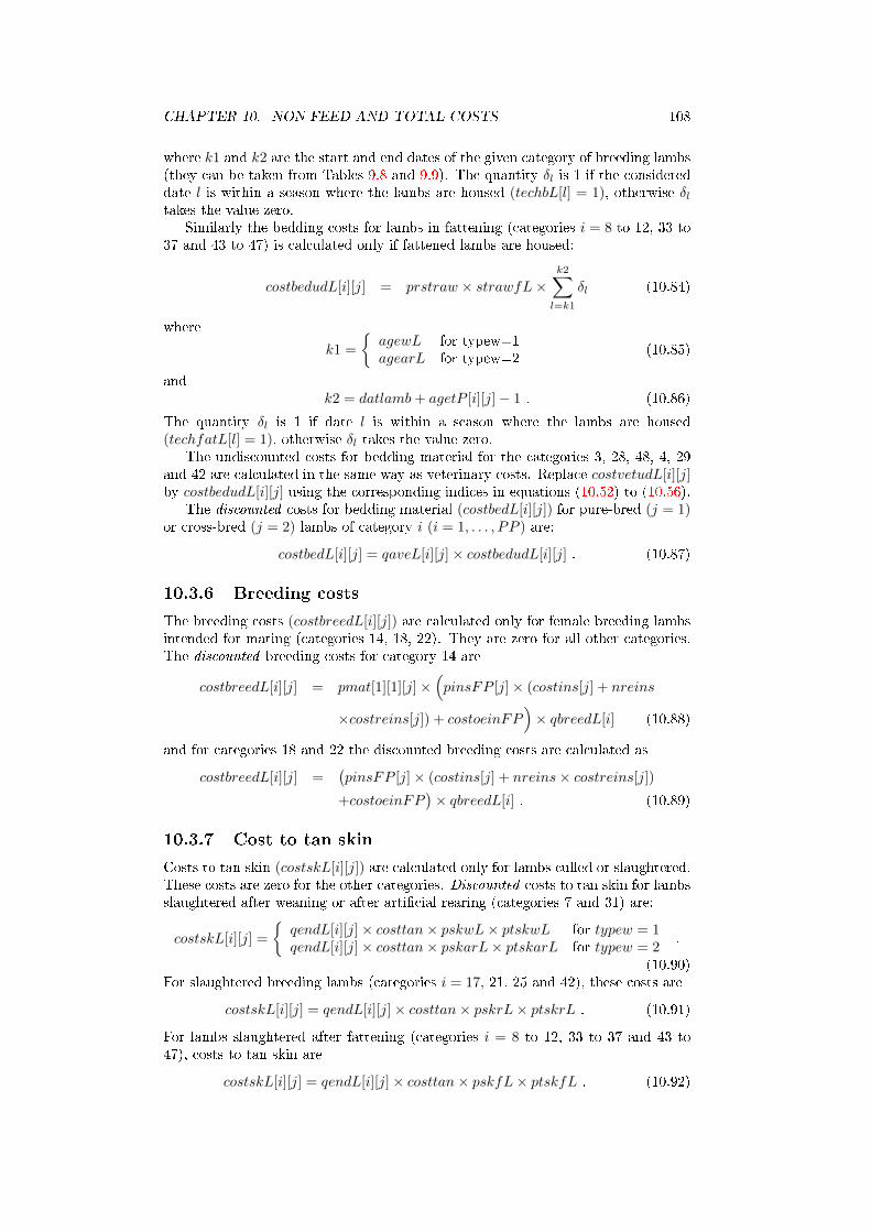
CHAPTER 10. NON-FEED AND TOTAL COSTS 108
where k1 and k2 are the start and end dates of the given category of breeding lambs(they can be taken from Tables 9.8 and 9.9). The quantity δl is 1 if the considereddate l is within a season where the lambs are housed (techbL[l] = 1), otherwise δltakes the value zero.
Similarly the bedding costs for lambs in fattening (categories i = 8 to 12, 33 to37 and 43 to 47) is calculated only if fattened lambs are housed:
costbedudL[i][j] = prstraw × strawfL×k2∑
l=k1
δl (10.84)
where
k1 =
{agewL for typew=1agearL for typew=2
(10.85)
andk2 = datlamb+ agetP [i][j]− 1 . (10.86)
The quantity δl is 1 if date l is within a season where the lambs are housed(techfatL[l] = 1), otherwise δl takes the value zero.
The undiscounted costs for bedding material for the categories 3, 28, 48, 4, 29and 42 are calculated in the same way as veterinary costs. Replace costvetudL[i][j]by costbedudL[i][j] using the corresponding indices in equations (10.52) to (10.56).
The discounted costs for bedding material (costbedL[i][j]) for pure-bred (j = 1)or cross-bred (j = 2) lambs of category i (i = 1, . . . , PP ) are:
costbedL[i][j] = qaveL[i][j]× costbedudL[i][j] . (10.87)
10.3.6 Breeding costs
The breeding costs (costbreedL[i][j]) are calculated only for female breeding lambsintended for mating (categories 14, 18, 22). They are zero for all other categories.The discounted breeding costs for category 14 are
costbreedL[i][j] = pmat[1][1][j]×(pinsFP [j]× (costins[j] + nreins
×costreins[j]) + costoeinFP)× qbreedL[i] (10.88)
and for categories 18 and 22 the discounted breeding costs are calculated as
costbreedL[i][j] =(pinsFP [j]× (costins[j] + nreins× costreins[j])
+costoeinFP)× qbreedL[i] . (10.89)
10.3.7 Cost to tan skin
Costs to tan skin (costskL[i][j]) are calculated only for lambs culled or slaughtered.These costs are zero for the other categories. Discounted costs to tan skin for lambsslaughtered after weaning or after arti�cial rearing (categories 7 and 31) are:
costskL[i][j] =
{qendL[i][j]× costtan× pskwL× ptskwL for typew = 1qendL[i][j]× costtan× pskarL× ptskarL for typew = 2
.
(10.90)For slaughtered breeding lambs (categories i = 17, 21, 25 and 42), these costs are
costskL[i][j] = qendL[i][j]× costtan× pskrL× ptskrL . (10.91)
For lambs slaughtered after fattening (categories i = 8 to 12, 33 to 37 and 43 to47), costs to tan skin are
costskL[i][j] = qendL[i][j]× costtan× pskfL× ptskfL . (10.92)

CHAPTER 10. NON-FEED AND TOTAL COSTS 109
10.3.8 Marketing costs
Marketing costs for a lamb of category i and of breeding type j (costmarkL[i][j])are calculated for lambs sold for slaughter or sold as breeding animals. For female(i = 7) and male (i = 32) lambs sold at weaning or at the end of arti�cial rearing,the discounted marketing costs are:
costmarkL[i][j] = qendL[i][j]× costmarkwL× a (10.93)
where
a =
{avww[s][j] for typew = 1avwar[s][j] for typew = 2
(10.94)
and
s =
{1 for category i = 72 for category i = 32
. (10.95)
For lambs slaughtered after fattening, the marketing costs are:
costmarkL[i][j] = qendL[i][j]× costmarkfL× wP [i][j] . (10.96)
For categories of female and male lambs sold for breeding purposes (categoriesi = 13, 15, 19, 23, 26, 38 and 40), the marketing costs are
costmarkL[i][j] = qendL[i][j]× costmarkrL[s] (10.97)
where
s =
{1 for categories 13, 15, 19, 23 and 262 for categories 38 and 40
. (10.98)
For categories of male and female lambs culled in rearing for di�erent reasons (cat-egories i = 17, 21, 25 and 42), the marketing costs are
costmarkL[i][j] = qendL[i][j]× costmarkcul . (10.99)
The marketing costs are zero for the remaining categories not given here.
10.3.9 Cost for removing and rendering dead animals
The cost for removing and rendering a dead animal (costdiedL[i][j]) are calculatedonly for categories of lambs that died (categories i = 2, 3, 4, 28, 29 and 48). Thesecosts discounted to the birth date of the animals are:
costdiedL[i][j] = qendL[i][j]× costdead× wP [i][j] . (10.100)
For the remaining categories these costs are assumed to be zero.
10.3.10 Total non-feed costs for lambs
The total non-feed costs (costnfL[i][j]) per lamb of category i (i = 1, . . . , PP ) andbreeding type j (j = 1, 2) discounted to the animal's birth date are the sum of theabove calculated discounted cost components:
costnfL[i][j] = costvetL[i][j] + costlabL[i][j] + costsheL[i][j]
+costfixL[i][j] + costbedL[i][j] + costbreedL[i][j](10.101)
+costskL[i][j] + costmarkL[i][j] + costdiedL[i][j] .
Some of the cost components may be zero for several categories or/and for a breedingtype.
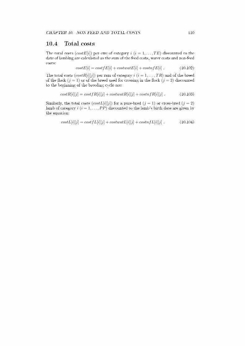
CHAPTER 10. NON-FEED AND TOTAL COSTS 110
10.4 Total costs
The total costs (costE[i]) per ewe of category i (i = 1, . . . , TE) discounted to thedate of lambing are calculated as the sum of the feed costs, water costs and non-feedcosts:
costE[i] = costfE[i] + costwatE[i] + costnfE[i] . (10.102)
The total costs (costR[i][j]) per ram of category i (i = 1, . . . , TR) and of the breedof the �ock (j = 1) or of the breed used for crossing in the �ock (j = 2) discountedto the beginning of the breeding cycle are:
costR[i][j] = costfR[i][j] + costwatR[i][j] + costnfR[i][j] . (10.103)
Similarly, the total costs (costL[i][j]) for a pure-bred (j = 1) or cross-bred (j = 2)lamb of category i (i = 1, . . . , PP ) discounted to the lamb's birth date are given bythe equation:
costL[i][j] = costfL[i][j] + costwatL[i][j] + costnfL[i][j] . (10.104)
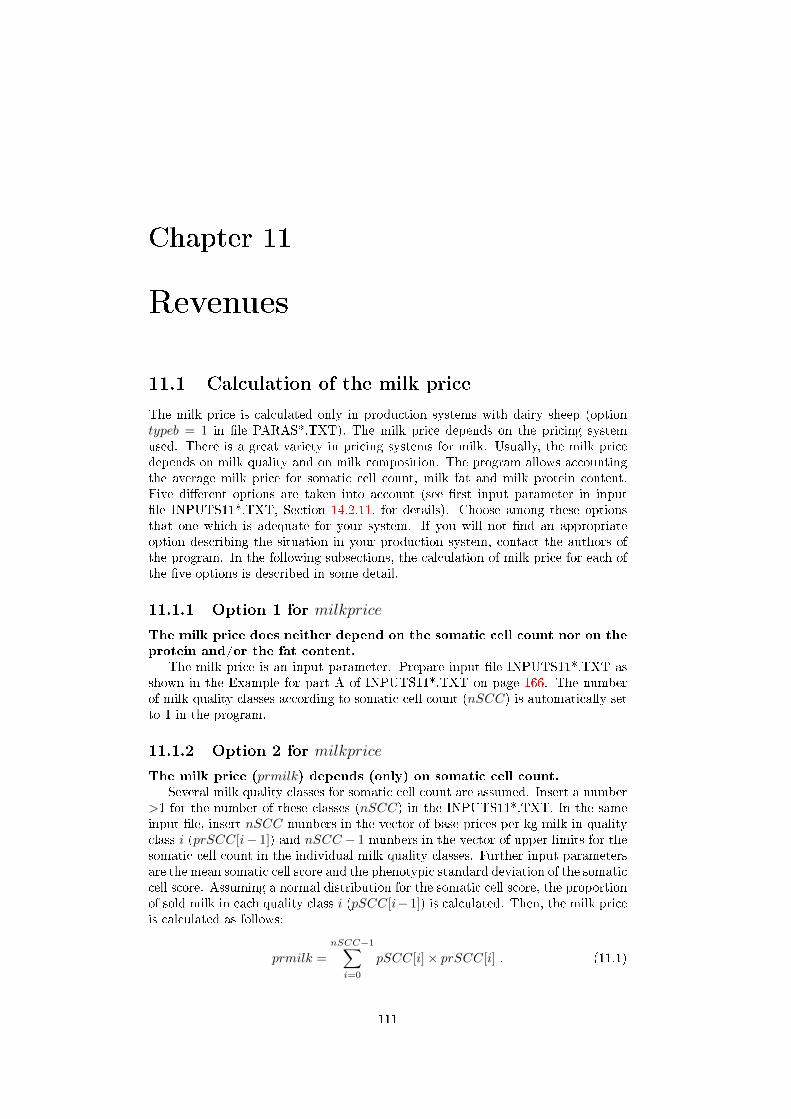
Chapter 11
Revenues
11.1 Calculation of the milk price
The milk price is calculated only in production systems with dairy sheep (optiontypeb = 1 in �le PARAS*.TXT). The milk price depends on the pricing systemused. There is a great variety in pricing systems for milk. Usually, the milk pricedepends on milk quality and on milk composition. The program allows accountingthe average milk price for somatic cell count, milk fat and milk protein content.Five di�erent options are taken into account (see �rst input parameter in input�le INPUTS11*.TXT, Section 14.2.11, for details). Choose among these optionsthat one which is adequate for your system. If you will not �nd an appropriateoption describing the situation in your production system, contact the authors ofthe program. In the following subsections, the calculation of milk price for each ofthe �ve options is described in some detail.
11.1.1 Option 1 for milkprice
The milk price does neither depend on the somatic cell count nor on theprotein and/or the fat content.
The milk price is an input parameter. Prepare input �le INPUTS11*.TXT asshown in the Example for part A of INPUTS11*.TXT on page 166. The numberof milk quality classes according to somatic cell count (nSCC) is automatically setto 1 in the program.
11.1.2 Option 2 for milkprice
The milk price (prmilk) depends (only) on somatic cell count.Several milk quality classes for somatic cell count are assumed. Insert a number
>1 for the number of these classes (nSCC) in the INPUTS11*.TXT. In the sameinput �le, insert nSCC numbers in the vector of base prices per kg milk in qualityclass i (prSCC[i− 1]) and nSCC − 1 numbers in the vector of upper limits for thesomatic cell count in the individual milk quality classes. Further input parametersare the mean somatic cell score and the phenotypic standard deviation of the somaticcell score. Assuming a normal distribution for the somatic cell score, the proportionof sold milk in each quality class i (pSCC[i−1]) is calculated. Then, the milk priceis calculated as follows:
prmilk =
nSCC−1∑i=0
pSCC[i]× prSCC[i] . (11.1)
111
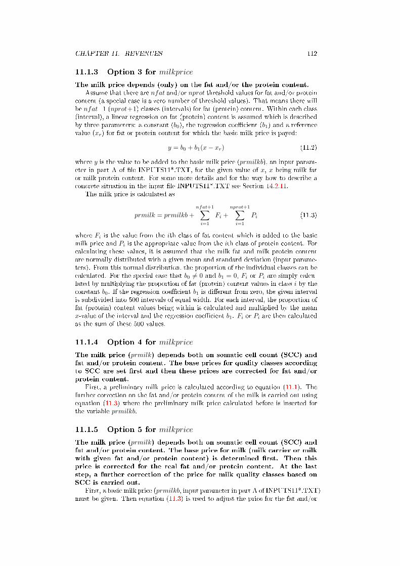
CHAPTER 11. REVENUES 112
11.1.3 Option 3 for milkprice
The milk price depends (only) on the fat and/or the protein content.Assume that there are nfat and/or nprot threshold values for fat and/or protein
content (a special case is a zero number of threshold values). That means there willbe nfat+1 (nprot+1) classes (intervals) for fat (protein) content. Within each class(interval), a linear regression on fat (protein) content is assumed which is describedby three parameters: a constant (b0), the regression coe�cient (b1) and a referencevalue (xr) for fat or protein content for which the basic milk price is payed:
y = b0 + b1(x− xr) (11.2)
where y is the value to be added to the basic milk price (prmilkb), an input param-eter in part A of �le INPUTS11*.TXT, for the given value of x, x being milk fator milk protein content. For some more details and for the way how to describe aconcrete situation in the input �le INPUTS11*.TXT see Section 14.2.11.
The milk price is calculated as
prmilk = prmilkb+
nfat+1∑i=1
Fi +
nprot+1∑i=1
Pi (11.3)
where Fi is the value from the ith class of fat content which is added to the basicmilk price and Pi is the appropriate value from the ith class of protein content. Forcalculating these values, it is assumed that the milk fat and milk protein contentare normally distributed with a given mean and standard deviation (input parame-ters). From this normal distribution, the proportion of the individual classes can becalculated. For the special case that b0 6= 0 and b1 = 0, Fi or Pi are simply calcu-lated by multiplying the proportion of fat (protein) content values in class i by theconstant b0. If the regression coe�cient b1 is di�erent from zero, the given intervalis subdivided into 500 intervals of equal width. For each interval, the proportion offat (protein) content values being within is calculated and multiplied by the meanx-value of the interval and the regression coe�cient b1. Fi or Pi are then calculatedas the sum of these 500 values.
11.1.4 Option 4 for milkprice
The milk price (prmilk) depends both on somatic cell count (SCC) andfat and/or protein content. The base prices for quality classes accordingto SCC are set �rst and then these prices are corrected for fat and/orprotein content.
First, a preliminary milk price is calculated according to equation (11.1). Thefurther correction on the fat and/or protein content of the milk is carried out usingequation (11.3) where the preliminary milk price calculated before is inserted forthe variable prmilkb.
11.1.5 Option 5 for milkprice
The milk price (prmilk) depends both on somatic cell count (SCC) andfat and/or protein content. The base price for milk (milk carrier or milkwith given fat and/or protein content) is determined �rst. Then thisprice is corrected for the real fat and/or protein content. At the laststep, a further correction of the price for milk quality classes based onSCC is carried out.
First, a basic milk price (prmilkb, input parameter in part A of INPUTS11*.TXT)must be given. Then equation (11.3) is used to adjust the price for the fat and/or
CHAPTER 11. REVENUES 113
protein content of the milk. Let us write prmilkfp for the resulting (preliminary)milk price. For each quality class i of milk according to somatic cell count, a multi-plicative (facSCC[i]) and an additive (prSCC[i]) price adjustment factor are readfrom INPUTS11*.TXT. Then the �nal milk price is:
prmilk =
nSCC−1∑i=0
pSCC[i] (prmilkfp× facSCC[i] + prSCC[i]) (11.4)
where pSCC[i] has the same meaning as in (11.1). Several of the multiplicative(facSCC[i]) and additive (prSCC[i]) price adjustment factors may take a value ofzero. No change of the milk price means that the multiplicative adjustment factoris 1 and the additive factor zero. If you want add or subtract a constant to or fromthe milk price in the given milk quality class, the multiplicative adjustment factoris 1 and the additive factor is a positive or a negative constant, respectively. If youwant the �nal milk price to be 30% of the preliminary price, set the multiplicativeconstant to 0.3 and the additive constant to 0. If you desire to set the milk priceto a constant independent o� the preliminary price, set the multiplicative factorto zero and the additive factor to the constant. See also examples for input �leINPUTS11*.TXT in Section 14.2.11 on page 164.
11.2 Revenues from ewes
The total revenues from an ewe of category i (i = 1, . . . , TE) per reproductive cycleconsist of revenues from wool, culled animals, raw skin, tanned skin and manure.In milk sheep, also revenues from sold milk, cheese and cheese whey are included.All revenues are discounted to the date of lambing.
Revenues from wool from an ewe of category i (i = 1, . . . , TE) per reproductivecycle (revwE[i]) are calculated as
revwE[i] = qaveE[i]× nsheE × wsheE × prwoolE × dcE[i]/lengthrc . (11.5)
Di�erent pricing systems for slaughter animals may be used. The variable priceSis used to indicate the variant of the pricing system for adult sheep (ewes and rams)and negatively selected breeding lambs. The variants are (see also description of�le INPUTS12*.TXT on page 170):
1 According to live weight without taking into account conformation
2 According to live weight taking into account conformation
3 According to carcass weight not accounting for carcass quality
4 According to EU evaluation system (quality classes for �eshiness andquality classes for fat covering)
If necessary, further variants may be included in the program later on.Revenues from culled ewes (revcE[i]) are available only for categories i with
i = (j − 1)× nstgE + k where j = 1, . . . , LL and k = 2, 3. If the culled animals arepaid per live weight, the revenues are calculated as:
revcE[i] = qendE[i]× (wlE[j] + δ × adgE × dcE[i])× prlwS[1] (11.6)
where δ = 1 for j = 1 and δ = 0 for j ≥ 2. The price prlwS[1] is an input parameterfor pricing system 1 (priceS = 1) and is calculated as average price over the quality
CHAPTER 11. REVENUES 114
classes of adult sheep (l = 1 : pure-bred animals, l = 2 : cross-bred animals or ramsof the breed used for crossing in the �ock)
prlwS[l] =
nclS∑i=1
pclS[l][i]× prclS[i] (11.7)
for pricing system 2 (priceS = 2). In pricing systems 3 and 4, animals are paid percarcass weight and the revenues are calculated as
revcE[i] = qendE[i]× (wlE[j]+δ×adgE×dcE[i])×prcwS[1]×dresE/100 (11.8)
where again δ = 1 for j = 1 and δ = 0 for j ≥ 2. The price prcwS[1] is an inputparameter for pricing system 3 (priceS = 3) and is calculated as average price overthe classes for �eshiness and fat covering of adult sheep (l = 1 : pure-bred animals,l = 2 : cross-bred animals or rams of the breed used for crossing in the �ock)
prcwS[l] = prrefS
nclflS∑i=1
nclfcS∑j=1
pclfcS[l][i][j]× prclfcS[i][j] (11.9)
for pricing system 4 (priceS = 4).Revenues from raw skin (revskrE[i]) and from tanned skin (revsktE[i]) are
calculated for the same categories as revenues from culled ewes, i.e. for categoriesi with i = (j − 1) x nstgE + k where j = 1, . . . , LL and k = 2, 3. They are:
revskrE[i] = qendE[i]× prskrE × pskE × (1− ptskE)
revsktE[i] = qendE[i]× prsktE × pskE × ptskE (11.10)
Revenues from manure per ewe of category i (i = 1, . . . , TE) including lambstill weaning (revmanE[i]) are calculated as
revmanE[i] = qaveE[i]× prman×manE ×k2∑
l=k1
δl (11.11)
where k1 = datlamb is equal for all categories, but k2 depends on the ewe's categorythrough dcE[i]:
k2 = datlamb+ dcE[i]− 1 (11.12)
The quantity δl is 1 if day l is within a season where the ewes are housed (techE[l] =1), otherwise δl takes the value zero.
Revenues from milk (revmilkE[i]) and cheese including cheese whey (revcheeseE[i])are only calculated for dairy sheep (parameter typeb = 1 in �le PARAS*.TXT).These revenues from a ewe of category i with i = (j − 1) × nstgE + k wherek = 1, . . . , nstgE for j = 1, . . . LL− 1 and k = 1, . . . , 3 for j = LL are given by thefollowing equations
revmilkE[i] = b× prmilk × (milkmpar[j] + a)× plambE[i]
×(1− pmilkch)× qmilkE[i] (11.13)
revcheeseE[i] = b× (prcheese+ prwhey × cheesewhey)× (milkmpar[j] + a)
×plambE[i]× pmilkch
milkch× qmilkE[i]
where
b =
{kmilkcE if k = 1, 21 if k = 3, . . . , nstgE
(11.14)
CHAPTER 11. REVENUES 115
and
a =
{0 if pmilkwm = 0milksw[j] if pmilkwm > 0
. (11.15)
The total discounted revenues (revE[i]) from an ewe of category i (i = 1, . . . , TE)per reproductive cycle are
revE[i] = revwE[i] + revcE[i] + revskrE[i] + revsktE[i] + revmanE[i]
+revmilkE[i] + revcheeseE[i]) . (11.16)
11.3 Revenues from rams
The total revenues from rams are formed by revenues from wool, culled animals,raw and tanned skin, sold animals and manure. Some components of the totalrevenues may be zero for certain ram categories. All revenues are discounted to thebeginning of the breeding cycle.
Revenues from wool (revwR[i][j]) per breeding cycle from a ram of category i(i = 1, . . . , TR) and of the breed of the �ock (j = 1) or of the breed used for crossingin the �ock (j = 2) are calculated as
revwR[i][j] = qaveR[i][j]× nsheR[j]× wsheR[j]× prwoolR[j]× dcR[i]/lengthrc .(11.17)
Di�erent pricing systems for slaughter animals may be used. A survey of thepricing systems is given in Section 11.2. Revenues from culled rams (revcR[i][j])are available only for categories i with i = (r−1)×nstgR+ 3 where r = 1, . . . , RR.If the culled animals are paid per live weight, the revenues are calculated as:
revcR[i][j] = qendR[i][j]× (wbR[r][j] + δ × adgR[j]× dcR[i])× prlwS[j] (11.18)
where δ = 1 for r = 1 and δ = 0 for r ≥ 2.The price prlwS[j] (j = 1, 2) is an inputparameter for pricing system 1 (priceS = 1) and is calculated as average price overthe quality classes according to equation (11.7) for pricing system 2 (priceS = 2).In pricing systems 3 and 4, animals are paid per carcass weight and the revenuesare calculated as
revcR[i][j] = qendR[i][j]×(wbR[r][j]+δ×adgR[j]×dcR[i])×prcwS[j]×dresR[j]/100(11.19)
where again δ = 1 for r = 1 and δ = 0 for r ≥ 2. The price prcwS[j] (j = 1, 2) isan input parameter for pricing system 3 (priceS = 3) and is calculated as averageprice over the classes for �eshiness and fat covering according to equation (11.9) forpricing system 4 (priceS = 4).
Revenues from raw skin (revskrR[i][j]) and from tanned skin (revsktR[i][j]) arecalculated for the same categories as revenues from culled rams, i.e. for categoriesi with i = (r − 1)× nstgR+ 3 where r = 1, . . . , RR. They are:
revskrR[i][j] = qendR[i][j]× prskrR[j]× pskR× (1− ptskR)
revsktR[i][j] = qendR[i][j]× prsktR[j]× pskR× ptskR . (11.20)
Revenues from manure (revmanR[i][j]) for all categories of rams (i = 1, . . . , TR)and breeds (j = 1, 2) are
revmanR[i][j] = qaveR[i][j]× prman×manR× dcR[i] . (11.21)
Revenues from sold rams of breed j (revsoldR[i][j]) are calculated only for categoriesi with i = (r − 1)× nstgR+ 2 and r = 1, . . . , RR:
revsoldR[i][j] = qendR[i][j]× prsbR[j] . (11.22)
CHAPTER 11. REVENUES 116
The total revenues (revR[i][j]) from a ram of category i (i = 1, . . . , TR) and breedj (j = 1, 2) per breeding cycle are
revR[i][j] = revwR[i][j] + revcR[i][j] + revskrR[i][j] + revsktR[i][j]
+revmanR[i][j] + revsoldR[i][j] . (11.23)
11.4 Revenues from lambs
Comment. From technical reasons, equations for undiscounted revenues are given�rst for several categories of revenues. The variable name for all kinds ofundiscounted revenues from lambs is of the form rev . . . udL where the dotsare replaced by a string which speci�es the costs (w for wool, c for culledanimals etc.). The variable name of the corresponding discounted revenuesis then rev . . . L. In the program, the variable names for discounted revenuesare also used for undiscounted revenues. Therefore, the variables rev . . . udLare not given in Appendix B.
Revenues from lambs come from wool, slaughter animals, raw and tanned skin, soldbreeding lambs and manure. Some components of the total revenues may be zerofor certain lamb categories.
11.4.1 Revenues from wool
Undiscounted revenues from wool (revwudL[i][j]) from pure-bred (j = 1) or cross-bred (j = 2) lambs of sex s (s = 1 : female, s = 2 : male) until weaning (categoriesi = 5 and 30) are:
revwudL[i][j] = nshewL× wshewL[s][j]× prwoolL[j] (11.24)
where s = 1 for i = 5 and s = 2 for i = 30. The corresponding revenues from lambsduring arti�cial rearing are calculated as follows:
revwudL[i][j] = nshearL× wshearL[s][j]× prwoolL[j] (11.25)
with s = 1 for i = 6 and s = 2 for i = 31.In fattening of pure-bred (j = 1) or cross-bred (j = 2) progeny of sex s (s = 1 :
female, s = 2 : male, s = 0 : castrates) of category i fattened to target k (k =1, . . . , lf [s]), the revenues from wool are
revwudL[i][j] = nshefL[s][k]× wshefL[s][j]× prwoolL[j] (11.26)
where s and k are given by the following equation:
s = 1 and k = i− 7 for i = 8, . . . , 12s = 2 and k = i− 32 for i = 33, . . . , 37s = 0 and k = i− 42 for i = 43, . . . , 47
. (11.27)
For categories i = 14, 18 and 22 of female lambs (s = 1) and for categories i = 39and 41 of male lambs (s = 2) the revenues from wool are calculated as
revwudL[i][j] = nsherL[k]× wsherL[s][j]× prwoolL[j] (11.28)
where
k =
1 for i = 14, 392 for i = 18, 413 for i = 22
. (11.29)
CHAPTER 11. REVENUES 117
For categories i = 16, 20 and 24 of female lambs the revenues from wool are
revwudL[i][j] = nsheFP × wsherL[1][j]× prwoolL[j] . (11.30)
For categories i = 13, 15, 17, 19, 21, 23 and 25 of female lambs (s = 1) and forcategory i = 40 of male lambs (s = 2), the revenues from wool are calculated as
revwudL[i][j] =dcL[i][j]
A× (nsherL[k]× wsherL[s][j]× prwoolL[j]) (11.31)
where
A =
ager[1][1]− agewL for i = 13 and typew = 1ager[1][1]− agearL for i = 13 and typew = 2ager[1][2]− ager[1][1] for i = 15, 17, 26ager[1][3]− ager[1][2] for i = 19, 21, 23, 25ager[2][2]− ager[2][1] for i = 40
(11.32)
and
k =
1 for i = 132 for i = 15, 17, 26, 403 for i = 19, 21, 23, 25
. (11.33)
Revenues from wool per female (category i = 3) or male (category i = 28)lamb or castrate (category i = 48) that died in fattening are calculated as one halfof the weighted averages of the revenues from wool for the appropriate categoriesk in fattening (k = 8, . . . , 12 for category 3, k = 33, . . . , 37 for category 28 andk = 43, . . . , 47 for category 48:
revwudL[i][j] =1
2× l1skL[i][j]
∑k
(revwudL[k][j]× ndiedfat[s][k − l][j]) (11.34)
wheres = 1 and l = 7 for category i = 3s = 2 and l = 32 for category i = 28s = 0 and l = 42 for category i = 48
. (11.35)
Revenues from wool per female lamb died in the rearing period (category 4) are cal-culated as one half of the weighted average of the revenues from wool for categories14, 18, 20 and 22:
revwudL[4][j] =(revwudL[14][j]× (nrdied[1][1][j] + nspdied[1][1][j])
+revwudL[18][[j]× (nrdied[1][2][j] + nspdied[1][2][j])
+revwudL[22][j]× (nrdied[1][3][j] + nspdied[1][3][j])
+revwudL[20][j]× nrdiedmlFP [j])/
(2× l1skL[4][j]).
(11.36)
Revenues from wool per male lamb died in the rearing period (category 29) are cal-culated as one half of the weighted average of the revenues from wool for categories39 and 41:
revwudL[29][j] =(revwudL[39][j]× (nrdied[2][1][j] + nspdied[2][1][j])
+revwudL[41][j]× (nrdied[2][2][j] + nspdied[2][2][j]))
/(2× l1skL[29][j]) . (11.37)
CHAPTER 11. REVENUES 118
Similarly, the revenues from wool per male lamb of category 42 (culled during therearing period) are also calculated as one half of the weighted average of the revenuesfrom wool for categories 39 and 41:
revwudL[42][j] =(revwudL[39][j]× (nrcull[2][1][j] + nspcull[2][1][j])
+revwudL[41][j]× (nrcull[2][2][j] + nspcull[2][2][j]))
/(2× l1skL[42][j]). (11.38)
The discounted revenues from wool (revwL[i][j]) for pure-bred (j = 1) or cross-bred (j = 2) lambs of category i (i = 1, . . . , PP ) are:
revwL[i][j] = qaveL[i][j]× revwudL[i][j] . (11.39)
11.4.2 Revenues from slaughter animals
Revenues from slaughter animals (revcL[i][j]) are calculated only for categoriesi = 7 to 12, 17, 21, 25, 32 to 37 and 42 to 47. Di�erent pricing systems forslaughter animals may be used. First the undiscounted revenues (revcudL[i][j]) arecalculated.
11.4.2.1 Undiscounted revenues from culled breeding lambs
For female lambs culled after the �rst (category i = 17), the second (i = 21) or thethird (i = 25) breeding season and for males culled in the rearing period (i = 42),the same pricing systems as given for ewes (see Section 11.2 on page 113) may beused.
If the culled animals are paid per live weight, the revenues from pure-bred (j = 1)or cross-bred (j = 2) animals of these categories are calculated as:
revcudL[i][j] = wP [i][j]× prlwS[j] . (11.40)
The price prlwS[j] is an input parameter for pricing system 1 (priceS = 1) and iscalculated as average price over the quality classes according to equation (11.7) forpricing system 2 (priceS = 2).
In pricing systems 3 and 4, animals are paid per carcass weight and the revenuesare calculated as
revcudL[i][j] = wP [i][j]× prcwS[j]× dresrL[j]/100 . (11.41)
The price prcwS[j] is an input parameter for pricing system 3 (priceS = 3) and iscalculated as average price over the classes for �eshiness and fat covering accordingto equation (11.9) for pricing system 4 (priceS = 4).
11.4.2.2 Undiscounted revenues from lambs slaughtered after weaningor after arti�cial rearing
Four di�erent pricing systems for lambs slaughtered after weaning (categories 7 and32) may be used. The variable pricewL is used to indicate the variant of the pricingsystem. The variants are:
1 According to live weight without taking into account conformation
2 According to live weight taking into account conformation
3 According to carcass weight not accounting for carcass quality

CHAPTER 11. REVENUES 119
4 According to EU evaluation system with classes for carcass weight (A:≤7 kg, B: > 7 kg and ≤ 10 kg, C: > 10 kg and ≤ 13 kg) and meatquality classes 1 (best class) and 2 within each weight class. Lambs witha carcass weight > 13 kg are evaluated in the same way as adult sheepor fattened lambs according to EU evaluation system (quality classes for�eshiness and fat covering). In the following text, lambs weighing ≤ 13kg are called light lambs and lambs weighing > 13 kg are called heavylambs.
If the culled animals are paid per live weight, the revenues per pure-bred (j = 1) orcross-bred (j = 2) lamb of categories i = 7 or 32 are calculated as:
revcudL[i][j] = wP [i][j]× prlwwL[j] . (11.42)
The price prlwwL[j] is an input parameter for pricing system 1 (pricewL = 1) andis calculated as average price over the quality classes
prlwwL[j] =
nclwL∑i=1
pclwL[j][i]× prclwL[i] (11.43)
for pricing system 2 (pricewL = 2).In pricing systems 3 and 4, animals are paid per carcass weight. The revenues
from slaughter animals of categories i = 7 or 32 are calculated for pricing system 3as
revcudL[i][j] = wP [i][j]× prcwwL[j]× dreswL[j]/100 (11.44)
where the price prcwwL[j] is an input parameter. For calculating the revenues forpricing system 4, �rst the mean carcass weight (mcwwL[i][j]) and the standarddeviation for the distribution of the carcass weight (sigmacwwL[i][j]) for pure-bred(j = 1) or cross-bred (j = 2) female (i = 1) and male (i = 2) lambs must becalculated:
mcwwL[i][j] = wP [k][j]× dreswL[j]/100
sigmacwwL[i][j] = vcwwL×mcwwL[i][j]/100 (11.45)
where
k =
{7 for i = 132 for i = 2
. (11.46)
Assuming for each sex and type of breeding (pure-breeding and cross-breeding) anormal distribution of the carcass weight with the mean mcwwL[i][j] and stan-dard deviation sigmacwwL[i][j], the relative frequencies (pclcwwL[i][r][j]) in car-cass weight classes A to C (r = 1, . . . , 3) and for the class of heavy lambs (carcassweight > 13 kg, r = 4) are calculated. It is
4∑r=1
pclcwwL[i][r][j] = 1 for all i and j . (11.47)
In the next step, the relative frequencies (pclcwL[i][r][s][j]) for the combinationsof weight classes A to C (r = 1, . . . , 3) and quality classes 1 and 2 (s = 1, 2) arecalculated:
pclcwL[i][r][s][j] =pclcqwL[r][s][j]× pclcwwL[i][r][j]
1− pclcwwL[i][4][j]. (11.48)
It holds that3∑
r=1
2∑s=1
pclcwL[i][r][s][j] = 1 for all i and j . (11.49)
CHAPTER 11. REVENUES 120
The average price (prcwawL[i][j]) per kg carcass weight speci�c for sex i and breed-ing type j is then
prcwawL[i][j] =
3∑r=1
3∑s=1
pclcwL[i][r][s][j]× prclcwwL[r][s] . (11.50)
Furthermore, the average price (prcwbwL[j]) for pure-bred (j = 1) and cross-bred (j = 2) heavy lambs must be calculated:
prcwbwL[j] = prrefwL
nclflwL∑r=1
ncfcwL∑s=1
pclfcwL[j][r][s]× prclfcwL[r][s] . (11.51)
The average price per kg carcass weight (prcwcwL[i][j]) for categories 7 (sex i = 1)and 32 (sex i = 2) is then:
prcwcwL[i][j] = (1−pclcwwL[i][4][j])×prcwawL[i][j]+pclcwwL[i][4][j]×prcwbwL[j] .(11.52)
Finally, the revenues per lamb of categories 7 and 32 are:
revcudL[7][j] = wP [7][j]× prcwcwL[1][j]× dreswL[j]/100
revcudL[32][j] = wP [32][j]× prcwcwL[2][j]× dreswL[j]/100 . (11.53)
11.4.2.3 Undiscounted revenues from fattened lambs
In fattened lambs (categories 8 to 12, 33 to 37 and 43 to 47), the same pricingsystems as in adult sheep may be used (see Section 11.2 on page 113). Instead ofthe variable priceS the variable pricefL will be used to indicate the variant of thepricing system. By using di�erent variables distinct pricing systems for adult sheepand fattened lambs will be possible. The carcass weight of the fattened lambs isassumed to take values above 13 kg.
If the culled animals are paid per live weight, the revenues are calculated as:
revcudL[i][j] = wP [i][j]× prlwfL[j] . (11.54)
The price prlwfL[j] (j = 1, 2) is an input parameter for pricing system 1 (pricefL =1) and is calculated as average price over the quality classes
prlwfL[j] =
nclfL∑i=1
pclfL[j][i]× prclfL[i] (11.55)
for pricing system 2 (pricefL = 2).In pricing systems 3 and 4, animals are paid per carcass weight and the revenues
are calculated as
revcudL[i][j] = wP [i][j]× prcwfL[j]× dresfL[k][l][j]/100 (11.56)
wherek = 1 and l = i− 7 for i = 8, . . . , 12k = 2 and l = i− 32 for i = 33, . . . , 37k = 0 and l = i− 42 for i = 43, . . . , 47
. (11.57)
The price prcwfL[j] is an input parameter for all categories for pricing system 3(pricefL = 3) and is calculated as average price over the classes for �eshiness andfat covering
prcwfL[j] = prreffL
nclflS∑s=1
nclfcS∑t=1
pclfcfL[j][s][t]× prclfcfL[s][t] (11.58)
for pricing system 4 (pricefL = 4).
CHAPTER 11. REVENUES 121
11.4.2.4 Discounted revenues from slaughtered animals
The discounted revenues from slaughtered animals (revcL[i][j]) for a pure-bred (j =1) or cross-bred (j = 2) lamb of category i (i = 1, . . . , PP ) are:
revcL[i][j] = qendL[i][j]× revcudL[i][j] . (11.59)
11.4.3 Revenues from raw and tanned skin
Discounted revenues from raw and tanned skin (revskrL and revsktL) are calcu-lated for pure-bred (j = 1) and cross-bred (j = 2) lambs of categories i = 7 to 12,17, 21, 25, 32, 33 to 37 and 42 to 47. The revenues are given by the equations:
revskrL[i][j] = qendL[i][j]× prskrL[j]× a× (1− b)revsktL[i][j] = qendL[i][j]× prsktL[j]× a× b (11.60)
where
a = pskfL and b = ptskfL for i = 8− 12, 33− 37 and 43− 47a = pskrL and b = ptskrL for i = 17, 21, 25 and 42a = pskwL and b = ptskwL for i = 7, 32 and typew = 1a = pskarL and b = ptskarL for i = 7, 32 and typew = 2
. (11.61)
11.4.4 Revenues from manure
Revenues from manure occur in categories of progeny which are housed at least fora certain time period. First undiscounted revenues are calculated. These revenuesfrom a lamb in fattening (categories i = 8 to 12, 33 to 37 and 43 to 47) are calculatedas:
revmanudL[i][j] = prman×manfL×k2∑
l=k1
δl (11.62)
where
k1 =
{agewL for typew=1agearL for typew=2
(11.63)
andk2 = datlamb+ agetP [i][j]− 1 . (11.64)
The quantity δl is 1 if date l is within a season where the lambs are housed(techfatL[l] = 1), otherwise δl takes the value zero.
For breeding female (categories i = 13, . . . , 25) and male lambs (categories i =38, . . . , 42), the revenues from manure are:
revmanudL[i][j] = prman×manbL×k2∑
l=k1
δl (11.65)
where k1 and k2 are the start and end dates of the given category of breedinglambs (they can be taken from Tables 9.8 and 9.9). The quantity δl is again 1 ifthe considered date l is within a season where the lambs are housed (techbL[l] = 1),otherwise δl takes the value zero.
If there is arti�cial rearing of lambs revenues from manure of a female (categoryi = 6) or male (category i = 31) lamb in arti�cial rearing are
revmanudL[i][j] = prman×manarL× dcL[i][j] . (11.66)
CHAPTER 11. REVENUES 122
Revenues from manure per animal of categories 3, 28 and 48 are calculated ac-cording to equation (11.34) where revwudL[i][j] must be replaced by revmanudL[i][j].Similarly, revenues per animal of categories 4, 29 and 42 are calculated accordingto equations (11.36), (11.37) and (11.38), respectively, where again revwudL[i][j]must be replaced by revmanudL[i][j].
The discounted revenues from manure (revmanL[i][j]) per pure-bred (j = 1) orcross-bred (j = 2) lamb of category i (i = 1, . . . , PP ) are:
revmanL[i][j] = qaveL[i][j]× revmanudL[i][j] . (11.67)
11.4.5 Revenues from sold breeding animals
Revenues from sold breeding animals occur for breeding females of categories 13,15, 19, 23 and 26 and for breeding males of categories 38 and 40. If the breedinglambs are paid per animal, the undiscounted revenues are input parameters in �leINPUTS10*.TXT. If the breeding lambs are paid for live weight, the prices perkg live weight (prsbL[i][j]) are read from the same input �le and the revenues(revsbL[i][j]) from sold pure-bred (j = 1) or cross-bred (j = 1) breeding lambs ofcategory i are then calculated as
revsbL[i][j] = prsbL[i][j]× wP [i][j] . (11.68)
To get the discounted revenues, the undiscounted revenues are multiplied by qendL[i][j].
11.4.6 Total revenues per lamb
The total revenues (revL[i][j]) from a pure-bred (j = 1) or cross-bred (j = 2) lambof category i (i = 1, . . . , PP ) discounted to the birth date of the animal are:
revL[i][j] = revwL[i][j] + revcL[i][j] + revskrL[i][j] + revsktL[i][j]
+revmanL[i][j] + revsbL[i][j] . (11.69)

Chapter 12
Pro�t and economic values
12.1 Pro�t per ewe and year
For calculating the pro�t per ewe and year, the total revenues and costs and thesubsidies per ewe and year are needed. The total subsidies per ewe and year arecalculated as:
Tsub = subR× 365
lengthrc
crossing∑j=1
(l1skL[38][j] + l1skL[40][j]) + subE . (12.1)
The total costs per ewe and per reproductive cycle for ewes (TcostsE), rams(TcostsR) and lambs (TcostsL) are calculated by multiplying the costs per animalof each category that occurs in the �ock with the number of animals of each categoryper ewe and reproductive cycle for the stationary state of the ewe �ock:
TcostsE =
TE∑i=1
costE[i]× l1E[i]
TcostsR =
crossing∑j=1
neweR[j]( TR∑
i=1
costR[i][j]× l1R[i])
(12.2)
TcostsL =
PP∑i=1
crossing∑j=1
costL[i][j]× l1skL[i][j] .
Similarly, the total revenues per ewe and per reproductive cycle from ewes (TrevE),rams (TrevR) and lambs (TrevL) are calculated:
TrevE =
TE∑i=1
revE[i]× l1E[i]
TrevR =
crossing∑j=1
neweR[j]( TR∑
i=1
revR[i][j]× l1R[i])
(12.3)
TrevL =
PP∑i=1
crossing∑j=1
revL[i][j]× l1skL[i][j] .
The total costs (Tcosts) and revenues (Trev) per ewe per year for the whole
123
CHAPTER 12. PROFIT AND ECONOMIC VALUES 124
production system are:
Tcosts =365
lengthrc(TcostsE + TcostsR+ TcostsL+ costpurchFP )
Trev =365
lengthrc(TrevE + TrevR+ TrevL) (12.4)
where
costpurchFP = npurchFP × kdif × (costL[i][1] + costlamb− revL[i][1]) (12.5)
with i = 5 for customary weaning and i = 6 for arti�cial rearing. The variablecostlamb (costs for ewes and rams which should be allotted to one weaned lamb) iscalculated as follows:
costlamb = (TcostsE − TrevE + TcostsR− TrevR)/a (12.6)
where a = NwL[0] for customary weaning and a = NarL[0] for arti�cial rearing. Ifa negative value of costlamb is calculated this value is set to zero.
Total pro�t (Tprof) per ewe and year is calculated as the di�erence of totalrevenues and total costs increased by governmental subsidies:
Tprof = Trev − Tcosts+ Tsub . (12.7)
The pro�tability (in per cent) of the production system including (profsub) orexcluding subsidies (profnsub) is calculated as:
profsub = 100× Tprof/Tcostsprofnsub = 100× (Trev − Tcosts)/Tcosts . (12.8)
12.2 De�nition of traits
Generally, four groups of traits are of interest in sheep: growth traits, carcass traits,wool production traits and functional traits (reproduction and health). For dairysheep, milk production traits are to be attached. If there is crossing in the �ock,the economic value for a trait is calculated separately for pure-bred and cross-bredanimals.
12.2.1 Growth traits
Growth is assumed to be the same trait in all categories of animals. Intra-breeddi�erences between sexes and litter sizes the animals are from are assumed to beexpressed by constant factors. Therefore, for the calculation of economic valuesfor growth, a reference growth trait can be de�ned. Live weights or growth ratesof females born as singles, which are speci�c for the breeding type (pure-bred orcross-bred), are mostly used as reference growth traits.
When calculating the economic weights for growth traits, the average values ofthe appropriate reference traits are changed. The related growth traits will thenchange automatically when running the program (see Sections 5.2 and 5.3). Thoughthe economic values are expressed per unit of the reference trait (mostly de�ned forfemales) and per ewe and year, they also include the economic e�ect of the changesin all related growth traits in other sexes.
To allow for changing the growth curve of sheep by selection using di�erentweightings for the individual parts of the growth curve, each part of the growthcurve was evaluated separately keeping the remaining part of the growth curveunchanged. The following growth traits were de�ned:
CHAPTER 12. PROFIT AND ECONOMIC VALUES 125
Birth weight. The e�ects of birth weight on lambing performance (dystocia oc-currence) or lambs survival are not included when calculating the economicweight of birth weight as data on lambing performance were not available andlamb survival is evaluated separately.
Average daily gain from birth till weaning
Average daily gain in arti�cial rearing (only for option typew = 2)
For these three traits, the weight or gain of a female born as single is the referencetrait. As alternative traits for average daily gain from birth to weaning or in arti�cialrearing, weaning weight and weight at the end of arti�cial rearing may be de�ned.Their economic values are easily obtained by a simple conversion of the economicvalues of the appropriate daily gain.
Changes in the growth traits till weaning or till the end of arti�cial rearing havean impact on the feeding costs and veterinary costs for treatment again parasites.Furthermore, the weights of animals in the subsequent rearing or fattening period at�xed age will change causing modi�cations in costs and revenues of further animalcategories.
If weaned lambs (or lambs at the end of arti�cial rearing) are paid according totheir slaughter weight (e.g. weight classes are built) the e�ect of changed proportionsof animals in each slaughter weight class is included in the economic value of thesetraits.
A further trait is
Daily gain in rearing of breeding animals. The reference trait is daily gain offemales from weaning or from the end of arti�cial rearing to �rst breeding.
The economic value of the trait takes into account e�ects of proportional changesin growth rates of all categories of breeding females and males in the whole rearingperiod.
Changes in the values of the above mentioned growth trait in�uence mainlynutrition costs, costs for drenching against ecto- and endo-parasites and revenuesfrom animals sold at a given age. Furthermore, changes in the proportions of femaleand male lambs that can be mated in the �rst breeding season after their weaningare assumed to be caused by changes in the mean live weight.
If there is fattening, the following trait is considered:
Daily gain in fattening. The reference trait is daily gain of females fattened totarget 1; if there is no fattening of females, the reference trait is daily gain ofmales fattened to target 1; if there is no fattening of females and males dailygain of castrates fattened to target 1 is the reference trait.
The economic value of the trait takes into consideration e�ects of proportionalchanges in growth rates of all categories of fattened animals.
A change in the growth rate during fattening in�uences nutrition costs for fat-tened animals and revenues from slaughtered animals (if fattening is to �xed slaugh-ter age) or �xed costs (if fattening is to �xed weight). Furthermore, drenching costsmay increase if there is drenching again ecto- and endo-parasites in fattening.
The last growth trait is
Mature weight. The reference trait is mature weight of ewes.
A proportional change in mature weight of rams is assumed. Changing matureweight will a�ect the minimal weight of breeding females and males when used forreproduction for the �rst time which is taken into consideration in the calculationof the economic value. Possible correlated changes occurring in the birth weight,
CHAPTER 12. PROFIT AND ECONOMIC VALUES 126
carcass value or milk yield are not included in the economic value of mature weightas the mentioned traits are evaluated separately. Therefore, changes in matureweight in�uence mainly nutrition costs and revenues from culled mature animals.In some extent, the structure of female progeny is in�uenced.
12.2.2 Carcass traits
Carcass quality traits can be evaluated only if the pricing system for slaughteranimals takes into account carcass quality be it on the base of live or slaugh-tered animals (options 2 or 4 for pricing system in �les INPUTS13*.TXT and IN-PUTS14*.TXT). Dressing percentage is evaluated only if animals are payed accord-ing to carcass weight (options 3 or 4 for pricing systems in �les INPUTS13*.TXTand INPUTS14*.TXT). The following carcass traits were de�ned:
Dressing percentage of lambs sold at weaning or at the end of arti�cial rear-ing for slaughter (only considered if pricewL = 3 or 4).
No di�erences are made between sexes.
Dressing percentage of lambs in fattening (only considered if pricefL = 3or 4). The reference trait is dressing percentage of females fattened to target1; if there is no fattening of females dressing percentage of males fattened totarget 1 is the reference trait; if there is no fattening of female and male lambsdressing percentage of castrates fattened to �rst target 1 is the reference trait.
Proportional changes are assumed in dressing percentage of all other categoriesof fattened animals. For this purpose the initial relations between the values ofdresfL[k][i][j] are expressed as coe�cients kdresfL[k][i][j]. The procedure is thesame as for adgP [ks + i][j] and kadgfat[k][i][j] described in detail in Sections 5.2and 5.3.
Dressing percentage of adult sheep (only considered if priceS = 3 or 4). Thereference trait is dressing percentage of pure-bred ewes and for rams fromthe breed of the ewe �ock; dressing percentage of rams of the breed used forcrossing in the ewe �ock is the reference trait for cross-bred animals.
Proportional changes are assumed in dressing percentage of all other categories ofadult sheep. The procedure for realizing these changes in the program is similar asfor adgP [ks + i][j] and kadgfat[k][i][j] described in detail in Sections 5.2 and 5.3.
Average quality class for lambs at weaning or at the end of arti�cial rearingwhen paid for live weight (only considered if pricewL = 2).
No di�erences are made between sexes. The average quality class (avclwL[j]) forpure-bred (j = 1) or cross-bred (j = 2) lambs is calculated as
avclwL[j] =
nclwL∑i=1
i× pclwL[j][i] . (12.9)
Average quality class for fattened lambs when paid for live weight (only con-sidered if pricefL = 2).
As in lambs at weaning, no di�erences are made between sexes and the average qual-ity class (avclfL[j]) for pure-bred (j = 1) or cross-bred (j = 2) lambs is calculatedin the same way:
avclfL[j] =
nclfL∑i=1
i× pclfL[j][i] . (12.10)
CHAPTER 12. PROFIT AND ECONOMIC VALUES 127
Average quality class for adult sheep when paid for live weight (only consid-ered if priceS = 2).
As in lambs at weaning, no di�erences are made between sexes and the averagequality class (avclS[j]) for pure-bred (j = 1) or cross-bred (j = 2) animals iscalculated in the same way:
avclS[j] =
nclS∑i=1
i× pclS[j][i] . (12.11)
Average class for �eshiness for adult sheep (only considered if priceS = 4).
The average class for �eshiness (avfleshS[j]) for pure-bred (j = 1) or cross-bred(j = 2) adult sheep is given by the equation
avfleshS[j] =
nclflS∑i=1
i×nclfcS∑k=1
pclfcS[j][i][k] . (12.12)
Average class for fat covering for adult sheep (only considered if priceS =4).
The average class for fat covering (avfcS[j]) for pure-bred (j = 1) or cross-bred(j = 2) adult sheep is calculated in the similar way as the average class for �eshiness:
avfcS[j] =
nclfcS∑k=1
k ×nclflS∑i=1
pclfcS[j][i][k] . (12.13)
Average class for �eshiness for fattened lambs and/or for heavy lambs (car-cass weight > 13 kg) slaughtered after weaning or after arti�cial rearing (onlyconsidered if pricefL = 4 or pricewL = 4 and typeb > 2).
Average class for fat covering for fattened lambs and/or for heavy lambs (car-cass weight > 13 kg) slaughtered after weaning or after arti�cial rearing (onlyconsidered if pricefL = 4 or pricewL = 4 and typeb > 2).
The average classes for �eshiness and fat covering only for fattened lambs (avfleshfL[j]and avfcfL[j]) or only for heavy lambs slaughtered after weaning or arti�cial rear-ing (avfleshwL[j] and avfcwL[j]) are calculated in the same way as for adult sheep.For obtaining the corresponding equations, just replace ′S′ in all variables by ′fL′
or ′wL′, respectively, in equations (12.12) and (12.13). The index j stands for pure-bred (j = 1) or cross-bred (j = 2) animals. The average classes for �eshiness andfat covering (avfleshL[j] and avfcL[j]) jointly calculated for fattened lambs andheavy lambs after weaning or arti�cial rearing are:
avfleshL[j] = favfL[j]× avfleshfL[j] + favwL[j]× avfleshwL[j]
avfcL[j] = favfL[j]× avfcfL[j] + favwL[j]× avfcwL[j] (12.14)
where
favfL[j] =favfL0[j]
favfL0[j] + favwL0[j]
favwL[j] =favwL0[j]
favfL0[j] + favwL0[j](12.15)
withfavfL0[j] =
∑i
l1skL[i][j] (12.16)
CHAPTER 12. PROFIT AND ECONOMIC VALUES 128
where the sum is over all categories i of fattened animals and
favwL0[j] = l1skL[7][j]× pclcwwL[1][4][j] + l1skL[32][j]× pclcwwL[2][4][j] .(12.17)
Average class for carcass quality for lambs slaughtered after weaning or ar-ti�cial rearing (only considered if pricewL = 4).
The average class for carcass quality (avcqwL[j]) for pure-bred (j = 1) or cross-bred (j = 2) light lambs (carcass weight ≤ 13 kg) slaughtered at weaning or afterarti�cial rearing is calculated as follows:
avcqwL[j] =
nclcqwL∑i=1
i×( nclcwwL∑
k=1
pclcqwL[k][i][j]×(pclcwwL[1][k][j]
×l1skL[7][j] + pclcwwL[2][k][j]× l1skL[32][j]))
(12.18)/(l1skL[7][j]× (1− pclcwwL[1][nclcwwL+ 1][j])
+l1skL[32][j]× (1− pclcwwL[2][nclcwwL+ 1][j])).
It is assumed that dressing percentage and the traits describing carcass quality haveimpact only on the revenues from culled animals. No changes in costs are takeninto account when calculating the economic values for carcass traits.
12.2.3 Functional traits
Among the functional traits, reproduction and health traits are most important forsheep. The following traits were de�ned and evaluated:
Conception rate of female lambs.
The reference trait is the conception rate of pure-bred (j = 1) or cross-bred (j = 2)female lambs in their �rst breeding season after weaning conrateFP [1][j]. Propor-tional changes in the conception rate of female lambs in their second and third breed-ing season are assumed when calculating the economic value of the trait. Changesin the conception rate of female lambs in�uence the structure of progeny and theaverage age and weight of ewes at �rst lambing, but the structure of ewe �ock staysthe same. Therefore, the trait has an impact on the total revenues and costs perewe and year through changing the number of animals in several progeny categoriesand on nutrition and drenching costs of ewes as well as on revenues from culledewes.
Average conception rate of ewes.
Average conception rate of ewes (avconrateE) is calculated as
avconrateE =1
1− l4E[LL]
LL−1∑i=1
l4E[i]× conrateE[i] . (12.19)
Proportional changes in the conception rate of ewes on each parity are assumed whencalculating the economic value of the trait. Changes in this traits in�uence the agestructure of the ewe �ock (a new stationary state is calculated) with consequenceson the number of lambs born and weaned, milk yield and number of culled ewes,resulting in changes of all revenues and costs for ewes and progeny.
Average litter size per lambed ewe.
CHAPTER 12. PROFIT AND ECONOMIC VALUES 129
The average litter size per ewe lambing (avlitpE[j], i.e. number of lambs born perewe lambing) in reproductive cycle j (j = 1, . . . , LL) is given by the equation
avlitpE[j] =
clt∑i=1
(i× Pltype[i][j]) (12.20)
and the litter size per ewe lambing in the �ock calculated as weighted average overparities (avlitE) is
avlitE =1
Nlamb
LL∑j=1
l3E[j]× avlitpE[j] . (12.21)
A proportional change in litter size on each parity is assumed when calculatingthe economic weight for litter size. Litter size is handled as categorical trait whenits economic value is calculated, i.e. an underlying normal distribution is assumed.The survival rate of lambs within each litter size does not change when changingthe average litter size. However, litter size will have an impact on the total lossesof lambs at lambing and till weaning or till the end of arti�cial rearing. Litter sizewill also in�uence the number and average weight in progeny categories resultingin changes in revenues and costs of these categories. Furthermore, the nutritioncosts for lactation and revenues and cost associated with changes in milk yield willbe a�ected. If lambs are paid according to their slaughter weight (e.g. weanedlambs are graded according to slaughter weight) the e�ect of changing frequenciesin the individual slaughter weight classes on the average price for slaughter weightis included into the economic value of litter size.
Average survival rate of lambs at lambing (till 24 hours after lambing) forthe given average litter size.
This trait (avsur24hL[j]) expressed in per cent is de�ned as quotient of the num-ber of lambs alive at 24 hours after birth and the number of lambs born in total(including aborts and stillbirth):
avsur24hL[j] = 100×Na24hL[j]/NbtL[j] . (12.22)
Average survival rate of lambs at lambing is calculated for both breeding types j(j = 1 : pure-bred lambs, j = 2 : cross-bred lambs). The economic weight of thetrait is calculated via changing the variable pdiedbL[i][j] in equal proportions forall litter sizes i. Changes in the trait have a similar impact on revenues and costsas changes in average litter size.
Average survival rate of lambs till weaning (from 24 hours after birth, onlyconsidered if there is customary weaning, i.e. typew = 1.)
This trait (avsurwL[j]) is de�ned as quotient of the number of lambs alive atweaning and the number of lambs alive at 24 hours after birth:
avsurwL[j] = 100×NwL[j]/Na24hL[j] . (12.23)
It is expressed in per cent and calculated for both pure-bred (j = 1) and cross-bred(j = 2) lambs.
Average survival rate of lambs till the end of arti�cial rearing (from 24 hoursafter birth, only considered if there is arti�cial rearing, i.e. typew = 2.)
CHAPTER 12. PROFIT AND ECONOMIC VALUES 130
This trait (avsurarL[j]) is de�ned as quotient of the number of lambs alive at theend of arti�cial rearing and the number of lambs alive at 24 hours after birth:
avsurarL[j] = 100×NarL[j]/Na24hL[j] . (12.24)
As the preceding trait, also this trait is expressed in per cent and calculated forboth pure-bred (j = 1) and cross-bred (j = 2) lambs.
Proportional change of survival rates within each litter size is assumed whenchanging the average survival rate of lambs till weaning. In case of arti�cial rearingof lambs, proportional changes of survival rates within each litter size are assumedfor both periods, from 24 hours after birth till early weaning and from early weaningtill the end of arti�cial rearing. Changes in both traits (average survival rate tillweaning or till the end of arti�cial rearing) have a similar impact on revenues andcosts as average litter size, but an impact on milk yield of ewes is not expected.
Productive lifetime of ewes measured as average number of reproductive cyclesper ewe.
This trait (avlifelE) is calculated as the reciprocal value of the relative frequencyof ewes in �rst reproductive cycle:
avlifelE = 1/l4E[1] . (12.25)
Productive lifetime of ewes measured in years from the date of �rst lambing.
This trait (avlifeyE) is calculated as
avlifeyE =1
365× l4E[1]
LL∑i=1
nstg1E∑j=1
l1E[k]× (dcE[k] + (i− 1)× lengthrc) (12.26)
where k = (i− 1)× nstgE + j.When calculating the economic value of productive lifetime, the proportions of
ewes died and culled for health problems (input variables pdiedE[i] and pcullhE[i]in input �le INPUTS01*.TXT) are changed by the same proportion each. In dairysheep, the proportions of ewes culled for low milk production do not change. So, theproductive lifetime as de�ned here is the functional lifetime of ewes and expressesthe health status of animals. The consequence of changing productive lifetime isan altered structure of the ewe �ock (a new stationary state is calculated) causingchanges in all revenues and costs connected with ewes. The frequencies of cate-gories of reared breeding females as well as the revenues and costs associated withthese categories will also be modi�ed as the number of female lambs needed forreplacement will be changed.
Average productive lifetime of ewes in number of reproductive cycles does nottake into account that some ewes do not stay in the �ock the whole reproductivecycle. Alternatively, the average productive lifetime in years takes into account thereal time a ewe stays in the �ock.
12.2.4 Milk production traits
Milk production traits are evaluated only for dairy sheep. Somatic cell score isassigned to milk production traits from practical reasons. Though somatic cellscore is a functional trait expressing udder health, it is recorded only in milkedsheep.
The reference trait for the calculation of the economic value of milk yield canbe de�ned in di�erent ways. In this program version, two variants are allowed:
CHAPTER 12. PROFIT AND ECONOMIC VALUES 131
Milk yield in the standardized milking period according to the recommen-dations of the ICAR [9].
The total milk yield in the standardized milking period per ewe per reproductivecycle (tmilkmst) is calculated from the lactation curve as follows:
tmilkmst =
clt∑i=0
LL∑j=1
(ktlsl[i]× ktlp[j]× PsuckE[i][j]×
(awo
agewL+dmilkst∑t=agewL
tbwoe−cwo×t). (12.27)
The length of the standardized milking period (dmilkst) depends on the breed andthe production system. Therefore, this parameter is in input parameter (in input�le INPUTS06*.TXT) which has to be de�ned by the user.
Daily milk production averaged over the whole lactation.
Average daily milk production (avmilkd) is calculated as follows:
avmilkd =tmilkw + tmilkm
datdry − datlamb. (12.28)
The e�ect of changing milk production of an ewe in the whole lactation is in-cluded in the economic values of both milk yield traits. When calculating theeconomic values, the parameter a (awo in the program) of the lactation curve (6.1)is modi�ed to cause changes both in the total and in the daily milk yield. Theselection of the appropriate milk yield trait is on the responsibility of the user. Theprogram will always calculate both traits for dairy ewes.
Fat content (in percent).
Fat yield (in kg).
Fat yield in the standardized milking period (fatymst) is calculated as
fatymst = tmilkmst× fat
100. (12.29)
A change in the average fat content has always an impact on feeding costs. Changesin the revenues from milk are included only if milk is sold at least partly as rawmilk and if the pricing system of milk takes into account the fat content. The traitis alternatively expressed as fat yield during the standardized milking period, butthe change in fat yield is assumed to be always caused by a change in fat contentand not in milk yield.
Protein content (in percent).
Protein yield (in kg).
Milk protein yield in the standardized milking period (protymst) is calculated as
protymst = tmilkmst× prot
100. (12.30)
As in fat yield, the change in protein yield is assumed to be always caused by achange in protein content and not in milk yield.
Somatic cell score.
CHAPTER 12. PROFIT AND ECONOMIC VALUES 132
The somatic cell score (SCS) is calculated from the somatic cell count (SCC,de�ned as the average number of somatic cells per ml milk) as follows [3, 6, 12]:
SCS = log2
(SCC
100000
)+ 3 (12.31)
where log2 is 'logarithmus dualis', the logarithm to the basis 2. For simplicity, thenatural logarithm (ln) may be used instead:
SCS = ln
(SCC
100000
)/0.69314718 + 3 . (12.32)
In the opposite way, the somatic cell count can be calculated from the somatic cellscore:
SCC = 100000× 2SCS−3 . (12.33)
The economic value of somatic cell score is expressed per change in average SCS.
12.2.5 Wool production traits
In the present version of the program the only wool trait evaluated is
Fleece weight (in kg) de�ned as amount of greasy wool per shearing. Fleeceweight in di�erent animal categories (ewes, rams, lambs) is assumed to be thesame trait.
Intra-breed di�erences in �eece weight between sexes and age categories are assumedto show constant ratios. Therefore, for the calculation of the economic value, the�eece weight of the individual categories is related to the �eece weight of adult rams.
Alteration in feed requirement is considered when changing �eece weight. Thecost of shearing are generally paid per animal and are not expected to change foradditionaly �eece weight. Only the bene�t in additional revenues from extra weightof �eece sold is therefore included in the economic value of �eece weight.
12.3 Calculation of economic values of traits
The marginal economic value is generally de�ned as the partial derivative of thepro�t function with respect to the trait considered [14]. It is expressed per givenunit of the trait and per time interval (here per ewe entering a reproductive cycleand per year). When using complex bio-economic models instead of simple pro�tfunctions (as in the present program) the exact partial derivative must be replacedby an approximate method, by a numeric derivative (di�erence quotient). Thepro�t the estimation of economic weights is based on is calculated for a commercialpopulation of sheep of the given breed or breed combination. The methodologyused for the calculation of economic values is di�erent for traits with continuousvariation and for categorical traits.
12.3.1 Economic values for traits with continuous variation
The numeric derivative of the pro�t with respect to the considered trait is calculatedby increasing and decreasing the average value of the trait TVav by 0.5%. Let TVh bethe higher value of the trait considered which was derived as TVh = 1.005TVav. Sim-ilarly, TVl is calculated by decreasing the average trait value by the same amount:TVl = 0.995TVav. Furthermore, let TPh and TPl be the total pro�t belonging to
CHAPTER 12. PROFIT AND ECONOMIC VALUES 133
the �rst or the second of these values, respectively. The partial derivative is thenapproximated by the following di�erence quotient:
ev =TPh − TPl
TVh − TVl. (12.34)
The marginal economic value is expressed in monetary units (MU) per unit of thetrait per ewe and year.
Table 12.1 gives a survey of the traits with continuous variation and of thevariables which are changed to calculate the economic value of these traits. Thatmeans, not in all cases the average value of the trait is changed directly. Sometraits are complex quantities which are calculated from a series of parameters. Forexample, average conception rate of ewes is calculated from the conception rates inthe individual lactations. For that reason, the conception rate in all lactations ischanged in the way described above for calculating the economic value of the averageconception rate. Total milk is calculated from the sum of daily milk yield of ewes ondi�erent lactations. In this trait a change in parameter a (awo in the program) ofthe lactation curve (6.1) proved to be useful for the calculation of economic weights.
12.3.2 Economic values for categorical traits
The economic values for categorical traits (e.g. �eshiness and fat covering) arecalculated according to [24]. The calculation is based on a threshold model. Theunderlying normal distribution is shifted to the left and to the right, each time by0.05 standard deviations. The resulting changes in the distribution are convertedto changes in the average class. For the numerical expression of the average class,the numbers 1 to N are assigned to the individual classes. Let pi be the frequencyof animals in class i. Then the average class AC is calculated simply as
AC =
N∑i=1
i× pi . (12.35)
Let ACh be the average class for shifting the distribution to higher values of thetrait and let ACl be the average class for shifting the distribution to lower valuesof the trait. Furthermore, let TPh and TPl be the total pro�t belonging to the �rstor the second of these values, respectively. Then the marginal economic value ev iscalculated as change of total pro�t related to a change in the average class:
ev =TPh − TPl
ACh −ACl. (12.36)
For the evaluation of the trait �average class�, at least two classes must beoccupied with numbers. If all data are in one class only, there is no variation in thegiven trait, a selection is not possible and the estimation of an economic value forthis trait is senseless.
The economic value of several traits has to be calculated from a two-dimensionaldistribution. For example, there is given one joint table of frequencies for �eshi-ness and fat covering. In such situations, the distribution of the investigated traitwas shifted within all levels of the second trait whereby the marginal frequenciesof the second trait stayed unchanged. This procedure ensured the calculation ofindependent economic weights for both traits of the frequency table. A survey ofcategorical traits the economic values are calculated for is given in Table 12.2. Thefrequencies the changes of which the calculation of the economic values is based onare also given in this table.
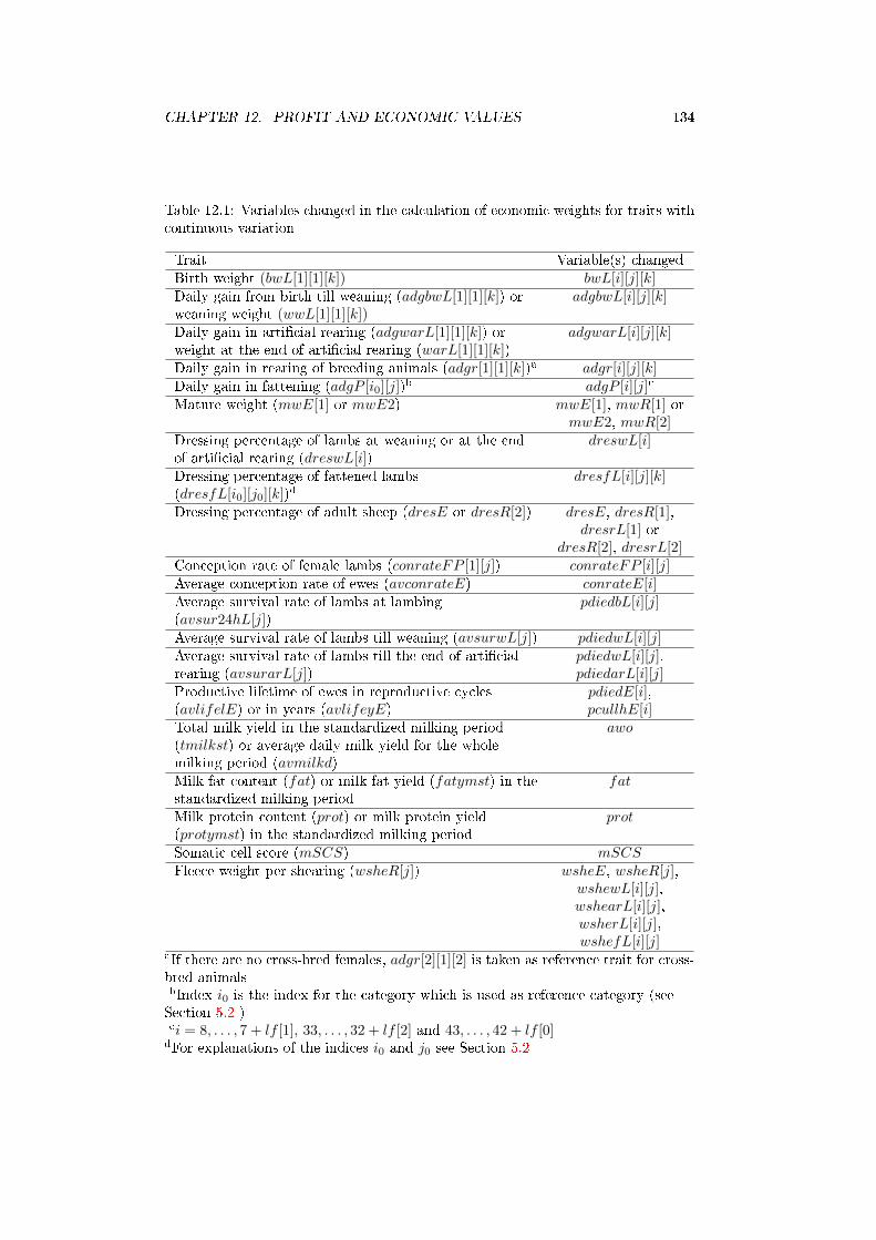
CHAPTER 12. PROFIT AND ECONOMIC VALUES 134
Table 12.1: Variables changed in the calculation of economic weights for traits withcontinuous variation
Trait Variable(s) changedBirth weight (bwL[1][1][k]) bwL[i][j][k]Daily gain from birth till weaning (adgbwL[1][1][k]) orweaning weight (wwL[1][1][k])
adgbwL[i][j][k]
Daily gain in arti�cial rearing (adgwarL[1][1][k]) orweight at the end of arti�cial rearing (warL[1][1][k])
adgwarL[i][j][k]
Daily gain in rearing of breeding animals (adgr[1][1][k])a adgr[i][j][k]Daily gain in fattening (adgP [i0][j])b adgP [i][j]c
Mature weight (mwE[1] or mwE2) mwE[1], mwR[1] ormwE2, mwR[2]
Dressing percentage of lambs at weaning or at the endof arti�cial rearing (dreswL[i])
dreswL[i]
Dressing percentage of fattened lambs(dresfL[i0][j0][k])d
dresfL[i][j][k]
Dressing percentage of adult sheep (dresE or dresR[2]) dresE, dresR[1],dresrL[1] or
dresR[2], dresrL[2]Conception rate of female lambs (conrateFP [1][j]) conrateFP [i][j]Average conception rate of ewes (avconrateE) conrateE[i]Average survival rate of lambs at lambing(avsur24hL[j])
pdiedbL[i][j]
Average survival rate of lambs till weaning (avsurwL[j]) pdiedwL[i][j]Average survival rate of lambs till the end of arti�cialrearing (avsurarL[j])
pdiedwL[i][j],pdiedarL[i][j]
Productive lifetime of ewes in reproductive cycles(avlifelE) or in years (avlifeyE)
pdiedE[i],pcullhE[i]
Total milk yield in the standardized milking period(tmilkst) or average daily milk yield for the wholemilking period (avmilkd)
awo
Milk fat content (fat) or milk fat yield (fatymst) in thestandardized milking period
fat
Milk protein content (prot) or milk protein yield(protymst) in the standardized milking period
prot
Somatic cell score (mSCS) mSCSFleece weight per shearing (wsheR[j]) wsheE, wsheR[j],
wshewL[i][j],wshearL[i][j],wsherL[i][j],wshefL[i][j]
aIf there are no cross-bred females, adgr[2][1][2] is taken as reference trait for cross-bred animalsbIndex i0 is the index for the category which is used as reference category (seeSection 5.2 )ci = 8, . . . , 7 + lf [1], 33, . . . , 32 + lf [2] and 43, . . . , 42 + lf [0]dFor explanations of the indices i0 and j0 see Section 5.2
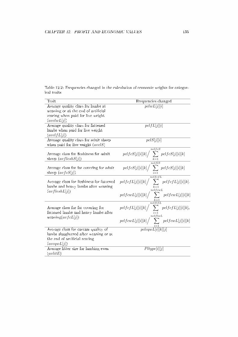
CHAPTER 12. PROFIT AND ECONOMIC VALUES 135
Table 12.2: Frequencies changed in the calculation of economic weights for categor-ical traits
Trait Frequencies changedAverage quality class for lambs atweaning or at the end of arti�cialrearing when paid for live weight(avclwL[j])
pclwL[j][i]
Average quality class for fattenedlambs when paid for live weight(avclfL[j])
pclfL[j][i]
Average quality class for adult sheepwhen paid for live weight (avclS)
pclS[j][i]
Average class for �eshiness for adultsheep (avfleshS[j])
pclfcS[j][i][k]/ nclfcS∑
k=1
pclfcS[j][i][k]
Average class for fat covering for adultsheep (avfcS[j])
pclfcS[j][i][k]/ nclflS∑
i=1
pclfcS[j][i][k]
Average class for �eshiness for fattenedlambs and heavy lambs after weaning(avfleshL[j])
pclfcfL[j][i][k]/ nclfcfL∑
k=1
pclfcfL[j][i][k],
pclfcwL[j][i][k]/ nclfcwL∑
k=1
pclfcwL[j][i][k]
Average class for fat covering forfattened lambs and heavy lambs afterweaning(avfcL[j])
pclfcfL[j][i][k]/ nclflfL∑
i=1
pclfcfL[j][i][k],
pclfcwL[j][i][k]/ nclflwL∑
i=1
pclfcwL[j][i][k]
Average class for carcass quality oflambs slaughtered after weaning or atthe end of arti�cial rearing(avcqwL[j])
pclcqwL[i][k][j]
Average litter size for lambing ewes(avlitE)
Pltype[i][j]
CHAPTER 12. PROFIT AND ECONOMIC VALUES 136
12.3.3 Calculation of economic values if there is cross-breeding
In the case of two progeny types in the evaluated population (i.e. pure-bred andcross-bred progeny), the trait level is increased (decreased) separately for bothprogeny types and two economic values are calculated for each trait: an economicvalue for trait i expressed in the pure-bred progeny of the breed of the �ock (ev[i][1])and an economic value for trait i expressed in the cross-bred progeny (ev[i][2]). Botheconomic values are given per unit of the trait and per ewe in the modelled produc-tion system per year. If no crossing is used in the ewe �ock, the economic valuesare calculated only for traits expressed in pure-bred progeny.
Chapter 13
Installing and running the
program
13.1 List of �les in the installation package
The program EWSH2 is distributed together with the program GFSH [21]. There-fore, �les for both programs are in the installation package. The �les are in �vedirectories.
13.1.1 Directory PROG
This directory contains executable program �les and text �les which are not to beedited.
ewsh2.exe Executable �le for program EWSH2.
gfsh.exe Executable �le for program GFSH [21].
TEXTS2_OUT.TXT This �le contains text for writing the results for the pro-gram EWSH2. See also Section 14.3.
TEXTGFS_OUT.TXT This �le contains text for writing the results for theprogram GFSH. For further details see the manual for the program GFSH [21].
P01_00.TXT This �le contains the initial parameters for the production system(prods = 1), the breed (breed = 1) and the number of the run of EWSH2 (calc = 1)for production system 1.
P02_00.TXT This �le contains the initial parameters for the production system(prods = 2), the breed (breed = 2) and the number of the run of EWSH2 (calc = 1)for production system 2.
ERROR.TXT A text �le forwarding error messages between succesive runs ofthe program EWSH2 and the program GFSH. The �le in this directory containsthe starting value 0 which means no error message.
cygwin1.dll This is a �le from Cygwin which is necessary for running the pro-grams under Windows. It is contained only in the distribution for Windows.
137
CHAPTER 13. INSTALLING AND RUNNING THE PROGRAM 138
13.1.2 Directory PS1
This directory contains �les necessary for running production system 1. Productionsystem 1 is only for one breed. Without loss of generality, we will call this breed A.
PARASA.TXT Parameter �le which contains the most important parametersfor running the program EWSH2 (see Section 14.1.2).
PARAGFS.TXT Parameter �le which contains the most important parametersfor running the program GFSH. For further details see the manual for the programGFSH [21].
INPUTS#A.TXT with # = 01, 02, ..., 14 Data input �les for programEWSH2. Not all data input �les are needed for all calculations (see Section 14.2).
INPUTGFS#.TXT with # = 01A, 02, 04 Data input �les for programGFSH. For further details see the manual for the program GFSH [21].
ps1A.sh under LINUX or ps1A.bat under Windows This is the shell script(LINUX) or batch �le (Windows) which starts the calculations for production sys-tem 1.
13.1.3 Directory PS2
This directory contains �les necessary for running production system 2. This is asystem with terminal crossing. There are two breeds. Breed A is the sire breed andbreed B is the dam breed.
PARASA.TXT, PARASB.TXT Parameter �les for breeds A and B, respec-tively, which contain the most important parameters for running the programEWSH2 (see Section 14.1.2).
PARAGFS.TXT Parameter �le which contains the most important parametersfor running the program GFSH. For further details see the manual for the programGFSH [21].
INPUTS#A.TXT and INPUTS#B.TXT with # = 01, 02, ..., 14 Datainput �les for breeds A and B, respectively, for program EWSH2. Not all data input�les are needed for all calculations (see Section 14.2).
INPUTGFS#.TXT with # = 01A, 01B, 03, 04 Data input �les for programGFSH. For further details see the manual for the program GFSH [21].
ps2AB.sh under LINUX or ps2AB.bat under Windows This is the shellscript (LINUX) or batch �le (Windows) which starts the calculations for productionsystem 2.
13.1.4 Directory DOC
license This �le contains the license conditions. Read them carefully and donot use the program package ECOWEIGHT if you do not agree with the licenseconditions.
CHAPTER 13. INSTALLING AND RUNNING THE PROGRAM 139
ECOWEIGHT03A.pdf Part 3A of the documentation of the program packageECOWEIGHT, manual for the program EWSH2.
ECOWEIGHT03B.pdf Part 3B of the documentation of the program packageECOWEIGHT, manual for the program GFSH.
13.1.5 Directory SRC
This directory contains the source �les in C language.
ewsh2.c Source code of the program EWSH2.
gfsh.c Source code of the program GFSH.
13.2 Installation
13.2.1 Under LINUX
The program EWSH2 together with the program GFSH come to you as a com-pressed tar-�le with the name ECOWEIGHT03_{# of version}.tgz, for exampleECOWEIGHT03_5_1_1.tgz contains the programs from version 5.1.1 of the pro-gram package. Copy this �le to a directory of your choice and enter the command
tar xvf ECOWEIGHT03_{# of version}.tgzfor uncompressing and unarchiving the �le. You will get the �le structure as de-scribed in Section 13.1.
Only for experts in programming. If you want to do changes in the program(source code) by yourself, then you must use the option -lm for compiling the sourcecode when using the compiler gcc because otherwise the mathematical functionswould not work; e.g.
gcc -lm -o ewsh2.exe ewsh2.cwill compile the source �le ewsh2.c to the executable �le ewsh2.exe.
13.2.2 Under Microsoft Windows
The Windows version of the program is distributed as zip �le with the nameECOWEIGHT03_{# of version}.zip. It contains the compiled programs ewsh2.exeand gfsh.exe. The programs were compiled under Cygwin (http:// www.cygwin.com)and run only in the presence of the �le cygwin1.dll which is part of the Windowsdistribution.
Only for experts in programming. If you intend to change the source codeand to compile the program you are recommended to install Cygwin which is freelyavailable. When compiling the source code, the following statement works for theprogram EWSH2:
gcc -Wl,�stack=55000000 -o ewsh2.exe ewsh2.cThe program GFSH can be simply compiled by the statement
gcc -o gfsh.exe gfsh1.cAlternatively it should be possible to use commercial C compilers (we did not testcommercial compilers).
CHAPTER 13. INSTALLING AND RUNNING THE PROGRAM 140
13.3 Running the program
You are recommended to create one directory for each calculation where you willcopy and edit all �les you will need. The program may be also in this directory ormay be copied to a directory for executable �les, e.g. to the directory /usr/local/binin LINUX.
13.3.1 Running the program for production system 1
All �les needed for running production system 1 are in the directory PS1. Further-more, the directory PROG is needed where the program �les and further �les arelocated which should not be edited. The directories PS2, DOC and SRC are notneeded for the calculation.
Edit the parameter �les PARASA.TXT and PARAGFS.TXT and the input �lesINPUTS#A.TXT with # = 01, 02, ..., 14 and INPUTGFS#.TXT with # = 01A,02, 04 in directory PS1. Under LINUX, type ./ps1A.sh and press ENTER to startthe shell script which runs the programs EWSH2 and GFSH. Under Windows, typeps1A.bat and press ENTER to start the batch �le which runs the programs EWSH2and GFSH.
For redirecting the text written to the screen to a text �le, say a.txt, type./ps1A.sh > a.txt under LINUX or ps1A.bat > a.txt under Windows and pressENTER.
The shell script ps1A.sh for running production system 1 looks like that:
#!/bin/sh
echo '*********************************'
echo I am copying P01_00.TXT to P00.TXT
echo '*********************************'
cp ../PROG/P01_00.TXT P00.TXT
echo ' '
echo '***************************************************'
echo 'I am copying TEXT*_OUT.TXT to the working directory'
echo '***************************************************'
cp ../PROG/TEXTS2_OUT.TXT .
cp ../PROG/TEXTGFS_OUT.TXT .
echo ' '
echo '***********************************************'
echo 'I am copying ERROR.TXT to the working directory'
echo '***********************************************'
cp ../PROG/ERROR.TXT .
echo ' '
echo '***************************'
echo I am starting program EWSH2
echo '***************************'
./../PROG/ewsh2.exe
echo ' '
echo '**************************'
echo I am starting program GFSH
echo '**************************'
./../PROG/gfsh.exe
echo ' '
echo '**********'
echo I am ready
echo '**********'
CHAPTER 13. INSTALLING AND RUNNING THE PROGRAM 141
The following two results �les will be printed:
• resA01 : This is the results �le from program EWSH2 which is described inthis manual.
• resgfps01 : This is the results �le from program GFSH [21].
Furthermore, the values of all variables are printed for both programs in the follow-ing �les:
• CHECKSA01 : Complete list of the values of all variables of breed A fromprogram EWSH2 at the end of the calculation. The description of the variablesis given in Appendix B.
• CHECKSA01a: Complete list of the values of all variables of breed A fromprogram EWSH2 before the program starts the calculation of economic values.This �le is printed mainly as help for further programming and as a check forcorrect computing. With one exception (variable zr, number of the loop),the values of all variables contained in both �les must be equal. The �leCHECKSA01a does not contain the economic values which are printed onlyin CHECKSA01.
• CHECKGFS : Complete list of the values of all variables from program GFSH.The description of the variables is given in Appendix B of the manual forGFSH [21].
13.3.2 Running the program for production system 2
All �les needed for running production system 2 are in the directory PS2. Further-more, the directory PROG is needed where the program �les and further �les arelocated which should not be edited. The directories PS1, DOC and SRC are notneeded for the calculation.
Edit the parameter �les PARASA.TXT, PARASB.TXT and PARAGFS.TXTand the input �les INPUTS#A.TXT with # = 01, 02, ..., 14, INPUTS#B.TXTwith # = 01, 02, ..., 14 and INPUTGFS#.TXT with # = 01A, 01B, 03, 04 indirectory PS2. Under LINUX, type ./ps2AB.sh and press ENTER to start theshell script which runs several times the program EWSH2 and then the programGFSH. Under Windows, type ps2AB.bat and press ENTER to start the batch �lewhich runs the programs EWSH2 and GFSH.
For redirecting the text written to the screen to a text �le, say a.txt, type./ps2AB.sh > a.txt under LINUX or ps2AB.bat > a.txt under Windows and pressENTER.
The shell script ps2AB.sh for running production system 2 has the followingstructure:
#!/bin/sh
echo '**********************************'
echo I am copying P02_00.TXT to P00.TXT
echo '**********************************'
cp ../PROG/P02_00.TXT P00.TXT
echo ' '
echo '***************************************************'
echo 'I am copying TEXT*_OUT.TXT to the working directory'
echo '***************************************************'
cp ../PROG/TEXTS2_OUT.TXT .
cp ../PROG/TEXTGFS_OUT.TXT .

CHAPTER 13. INSTALLING AND RUNNING THE PROGRAM 142
echo ' '
echo '***********************************************'
echo 'I am copying ERROR.TXT to the working directory'
echo '***********************************************'
cp ../PROG/ERROR.TXT .
echo ' '
echo '************************************'
echo I am starting program EWSH2, breed B
echo '************************************'
./../PROG/ewsh2.exe
echo ' '
echo '************************************'
echo I am starting program EWSH2, breed A
echo '************************************'
./../PROG/ewsh2.exe
echo ' '
echo '************************************'
echo I am starting program EWSH2, breed A
echo '************************************'
./../PROG/ewsh2.exe
echo ' '
echo '************************************'
echo I am starting program EWSH2, breed B
echo '************************************'
./../PROG/ewsh2.exe
echo ' '
echo '**************************'
echo I am starting program GFSH
echo '**************************'
./../PROG/gfsh.exe
echo ' '
echo '**********'
echo I am ready
echo '**********'
The following results �les will printed:
• resB01 : This is the results �le from the �rst run of program EWSH2 whichis for breed B.
• resA02 : This is the results �le from the second run of program EWSH2 whichis for breed A.
• resA03 1: This is the results �le from the third run of program EWSH2 whichis for breed A.
• resB042: This is the results �le from the forth run of program EWSH2 whichis for breed B.
• resgfps02 : This is the results �le from program GFSH.
Furthermore, the values of all variables are printed for both programs in the follow-ing �les:
1This �le contains the �nal results for breed A from the program EWSH as the third run ofEWSH is the last run for breed A.
2This �le contains the �nal results for breed B from the program EWSH as the forth run ofEWSH is the last run for breed B.
CHAPTER 13. INSTALLING AND RUNNING THE PROGRAM 143
• CHECKSB01 : Complete list of the values of all variables of breed B from the�rst run of program EWSH2 at the end of the calculation. The description ofthe variables is given in Appendix B.
• CHECKSB01a: Complete list of the values of all variables of breed B fromthe �rst run of program EWSH2 before the program starts the calculation ofeconomic values. This �le is printed mainly as help for further programmingand as a check for correct computing. With one exception (variable zr, numberof the loop), the values of all variables contained in both �les must be equal.The �le CHECKSB01a does not contain the economic values which are printedonly in CHECKSB01.
• CHECKSA02 : Complete list of the values of all variables of breed A from thesecond run of program EWSH2 at the end of the calculation.
• CHECKSA02a: Complete list of the values of all variables of breed A fromthe second run of program EWSH2 before the program starts the calculationof economic values.
• CHECKSA033: Complete list of the values of all variables of breed A fromthe third run of program EWSH2 at the end of the calculation.
• CHECKSA03a: Complete list of the values of all variables of breed A fromthe third run of program EWSH2 before the program starts the calculationof economic values.
• CHECKSB04 4: Complete list of the values of all variables of breed B fromthe forth run of program EWSH2 at the end of the calculation.
• CHECKSB04a: Complete list of the values of all variables of breed B fromthe forth run of program EWSH2 before the program starts the calculationof economic values.
• CHECKGFS : Complete list of the values of all variables from program GFSH.The description of the variables is given in Appendix B of the manual forGFSH [21].
13.4 General remarks
Several checks of input parameters are included in the programs. For example,certain input parameters have to sum to one. A warning will appear if these inputparameters are invalid and the program will stop. You will be told which inputparameters to correct before restarting the program. In general, it is your respon-sibility to use input parameters which are realistic and �t together, because it isimpossible to predict any possible erroneous combinations of input parameters. Donot forget to have always a critical look on your results before using them for furtherpurposes.
3See footnote 1 on the preceding page.4See footnote 2 on the previous page.
Chapter 14
Input �les
Important remark: When editing the input �les, keep attention not to changequotation marks. All �les are read as sequential �les and the program rec-ognizes the beginning and the end of texts on the basis of quotation marks.Adding or deleting a quotation mark will cause the program to break downor to calculate wrong results.
Monetary unit: In all input �les the abbreviation MU is used for monetary unit.All values in the distributed version of the program refer to Euros. You canglobally replace the abbreviation MU by the abbreviation of your monetaryunit in all data input �les (INPUTS#*.TXT, where '#' = 01, 02, 03 etc. and'*' = A or B) and in the input �le TEXTS2_OUT.TXT using any text editor;the results �le will then contain the monetary unit speci�ed by you.
Language of the program: The program will need just the numbers for calcu-lations. The texts are read in and printed out to the result �le as they are.Therefore, you can freely change the text in all input �les as long as you donot modify the quotation marks. For example, you can translate all textsin the input �les to another language what will cause the appropriate partof the result �le to be printed in the same language as the input �les (maybe there are some exceptions where the English text will be remained). Thelength of the texts can be changed, but each text must start and �nish withquotation marks. A great part of the text for the results �le is read from the�le TEXTS2_OUT.TXT. You can translate all the text in this �le. But bevery careful not to change quotation marks.
14.1 Parameter �les
14.1.1 Parameter �le P00.TXT
This �le is automatically generated. Do not edit this �le. It contains three param-eters (without text) in the following order:
• Production system (prods). This code is
� 1 for a pure-bred system of breed A with one production level
� 2 for a production system with breeds A and B, each on one productionlevel; partially terminal crossing is applied
• Breed for which the calculation is carried out (breed). This code is
144
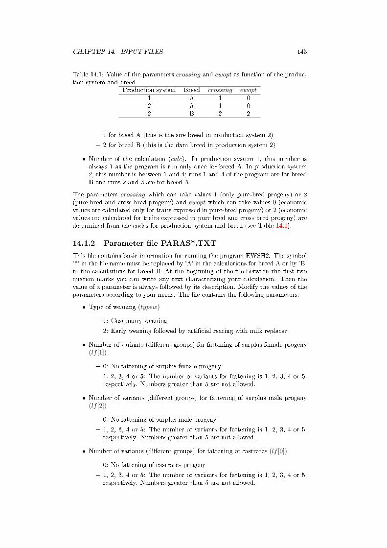
CHAPTER 14. INPUT FILES 145
Table 14.1: Value of the parameters crossing and ewopt as function of the produc-tion system and breed
Production system Breed crossing ewopt1 A 1 02 A 1 02 B 2 2
� 1 for breed A (this is the sire breed in production system 2)
� 2 for breed B (this is the dam breed in production system 2)
• Number of the calculation (calc). In production system 1, this number isalways 1 as the program is run only once for breed A. In production system2, this number is between 1 and 4; runs 1 and 4 of the program are for breedB and runs 2 and 3 are for breed A.
The parameters crossing which can take values 1 (only pure-bred progeny) or 2(pure-bred and cross-bred progeny) and ewopt which can take values 0 (economicvalues are calculated only for traits expressed in pure-bred progeny) or 2 (economicvalues are calculated for traits expressed in pure-bred and cross-bred progeny) aredetermined from the codes for production system and breed (see Table 14.1).
14.1.2 Parameter �le PARAS*.TXT
This �le contains basic information for running the program EWSH2. The symbol'*' in the �le name must be replaced by 'A' in the calculations for breed A or by 'B'in the calculations for breed B. At the beginning of the �le between the �rst twoquation marks you can write any text characterizing your calculation. Then thevalue of a parameter is always followed by its description. Modify the values of theparameters according to your needs. The �le contains the following parameters:
• Type of weaning (typew)
� 1: Customary weaning
� 2: Early weaning followed by arti�cial rearing with milk replacer
• Number of variants (di�erent groups) for fattening of surplus female progeny(lf [1])
� 0: No fattening of surplus female progeny
� 1, 2, 3, 4 or 5: The number of variants for fattening is 1, 2, 3, 4 or 5,respectively. Numbers greater than 5 are not allowed.
• Number of variants (di�erent groups) for fattening of surplus male progeny(lf [2])
� 0: No fattening of surplus male progeny
� 1, 2, 3, 4 or 5: The number of variants for fattening is 1, 2, 3, 4 or 5,respectively. Numbers greater than 5 are not allowed.
• Number of variants (di�erent groups) for fattening of castrates (lf [0])
� 0: No fattening of castrates progeny
� 1, 2, 3, 4 or 5: The number of variants for fattening is 1, 2, 3, 4 or 5,respectively. Numbers greater than 5 are not allowed.
CHAPTER 14. INPUT FILES 146
• Type of breed (typeb)
� 1: Dairy sheep
� 2: Meat sheep or other non-dairy sheep with known lactation curve
� 3: Meat sheep or other non-dairy sheep with unknown lactation curve
• Method for calculating the feed costs (feedcost)
� 1: Feed costs are calculated from the net energy and protein requirements
� 2: Feed costs are calculated only from the net energy requirements
• Female replacement (femrep)
� 1: Own replacement females are reared
� 2: A part of replacement females are purchased
14.2 Data input �les
The data input �les must be prepared only for breed A in production system 1 orboth for breed A (sire breed) and breed B (dam breed) in production system 2. Thenames of the input �les have the structure INPUTS#*.TXT where '#' = 01, 02,03 etc. and '*' = A or B. The input �les for both breeds have the same structure.
14.2.1 Input �le INPUTS01*.TXT
This �le contains input parameters for calculating the ewe �ock structure. Theyare:
• Number of reproductive cycles (LL, must be between 4 and 15)
• Fraction of ewes entering reproductive cycle i that will die in this cycle(pdiedE[i], i = 1, . . . , LL). All values pdiedE[i] must be in the range from 0to 1.
• Fraction of ewes entering reproductive cycle i (i = 1, . . . , LL) that were volun-tarily culled for low milk production (pcullmE[i], i = 1, . . . , LL). All valuespcullmE[i] must be in the range from 0 to 1. These values are read only fordairy ewes.
• Fraction of ewes entering reproductive cycle i (i = 1, . . . , LL) that were invol-untarily culled for health problems other than failure to conceive (pcullhE[i],i = 1, . . . , LL). All values pcullhE[i] must be in the range from 0 to 1.
• Conception rate of ewes in reproductive cycle i (conrateE[i], i = 1, . . . , LL−1). All values conrateE[i] must be in the range from 0 to 1.
• Fraction of barren ewes in reproductive cycle i that will be kept to the nextreproductive cycle (pbarrE[i], i = 1, . . . , LL − 1). All values pbarrE[i] mustbe in the range from 0 to 1.
• Fraction of female lambs crossed with other breeds (pcrossE[0])
• Fraction of ewes crossed with other breeds in reproductive cycle i (pcrossE[i],i = 1, . . . , LL− 1). All values pcrossE[i] must be in the range from 0 to 1.
CHAPTER 14. INPUT FILES 147
The following �ve inputs contain dates. All dates are given in the format 'yearmonth day'. The number of the year must be relative, the earliest dates mustalways be in year 0, the next year is year 1 etc.:
• Date of lambing (datlamb)
• Date of weaning (datwL)
• Date of the beginning of the breeding season (datbbs)
• Date of the end of the breeding season (datebs)
• Date of drying o� of ewes (datdry). This date is read only for dairy sheep(option 1 of the type of the sheep breed in PARAS*.TXT).
The last input is the annual discount rate (u).
14.2.2 Input �le INPUTS02*.TXT
This �le contains the following input parameters for calculating the structure of theram population:
• Number of breeding cycles (RR, must be between 1 and 5)
• Fraction of rams that died in breeding cycle i (pdiedR[i], i = 1, . . . , RR)
• Fraction of rams sold as breeding animals in breeding cycle i (psoldR[i], i =1, . . . , RR)
• Fraction of rams entering breeding cycle i that were culled for health or forage (pcullR[i], i = 1, . . . , RR)
The following equation must be ful�lled for the last breeding cycle RR:
pdiedR[RR] + psoldR[RR] + pcullR[RR] = 1 . (14.1)
14.2.3 Input �le INPUTS03*.TXT
This �le contains the following input parameters for calculating the structure of theprogeny of the ewe �ock.
• Number of classes for litter size, e.g. singles, twins, triplets (clt). clt is aninteger in the range from 1 to CLT −1 where CLT is set to 5 in the program.
• Fraction of lambings in individual classes for litter size for all reproductivecycles (Pltype[i][j], i = 1, . . . , clt, j = 1, . . . , LL). Row: litter size (thenumber of rows must be equal to the number of classes for litter size), column:reproductive cycle (the number of columns equals the number of reproductive
cycles). It holds that 0 ≤ Pltype[i][j]≤ 1 and∑clt
i=1 Pltype[i][j] = 1 for all j(j = 1, . . . , LL).
• Fraction of lambs stillborn or died until 24 hours for the individual classesfor number of dead lambs j within each litter size i (pdiedbtL[i][j], i =1, . . . , clt; j = 1, . . . , i). Rows are the litter sizes (i = 1, . . . , clt), columnsare number of dead lambs within each litter size (j = 1, . . . , i). The fractionof purebred lambs (of both sexes) stillborn or died until 24 hours for the indi-vidual classes for litter size (pdiedbL[i][1], i = 1, . . . , clt) is assumed to be thesame as the fraction of crossbred lambs (of both sexes) stillborn or died until
CHAPTER 14. INPUT FILES 148
24 hours for the individual classes for litter size (pdiedbL[i][2], i = 1, . . . , clt)and is calculated as:
pdiedbL[i][1] =
i∑j=1
pdiedbtL[i][j] (14.2)
• Lambs died till weaning as proportion of lambs born alive (lambs alive at 24hours after birth) for all classes of litter size (pdiedwL[i][1], i = 1, . . . , clt)
• Lambs died from early weaning till the end of arti�cial rearing with milkreplacer as proportion of lambs alive at early weaning for all classes of littersize (pdiedarL[i][1], i = 1, . . . , clt). This parameter is needed only for option2 of the type of weaning (see parameter �le PARAS*.TXT on page 145).
The following parameters are given as separate input rows for pure-bred (j = 1)and cross-bred (j = 2) female and male progeny1:
• Birth weights of female (s = 1) and male (s = 2) progeny born in litter size iwithin each breeding type j (bwL[s][i][j], i = 1, . . . , clt, j = 1, 2).
• Weaning weight of female (s = 1) and male (s = 2) progeny born in litter sizei within each breeding type j (wwL[s][i][j], i = 1, . . . , clt, j = 1, 2).
• Weight of female (s = 1) and male (s = 2) progeny born in litter size i withineach breeding type j at the end of arti�cial rearing (warL[s][i][j], i = 1, . . . , clt,j = 1, 2). This parameter is needed only for option 2 of the type of weaning(see parameter �le PARAS*.TXT on page 145).
• Age of lambs at the end of arti�cial rearing (agearL). This parameter is readonly for option 2 of the type of weaning (see �le PARAS*.TXT on page 145).
14.2.4 Input �le INPUTS05*.TXT
This �le contains input parameters for surplus progeny. These parameters areneeded for calculating the structure of the progeny and for the description of growth.The �le includes values for pure-bred and cross-bred progeny.2 The two items (fourinputs) are read always:
• Fraction of pure-bred (j = 1) or cross-bred (j = 2) weaned surplus femaleprogeny (psp[1][i][j]) sold in di�erent categories i (i = 1, . . . , csp[1]). i = 1:sold at weaning for slaughter, i = 2: sold as breeding animals, i = 3, . . . 7:
fattened to target 1 to 5, respectively. It must be∑csp[1]
i=1 psp[1][i][j] = 1 forj = 1, 2.
• Fraction of pure-bred (j = 1) or cross-bred (j = 2) weaned surplus maleprogeny (psp[2][i][j]) sold in di�erent categories i (i = 1, . . . , csp[2]). i =1: sold at weaning for slaughter, i = 2: sold as breeding animals, i = 3 :castrated, i = 4, . . . 8: fattened to target 1 to 5, respectively. It must be∑csp[2]
i=1 psp[2][i][j] = 1 for j = 1, 2. Important remark: In production system2, these input parameters are in the third run of EWSH2 overwritten for breedA by data from the �le TRANSFER02.TXT.
1The values for the cross-bred progeny are ignored in all input �les if the parameter crossingin the parameter �le PARAS*.TXT is set to 1, that means if there is only pure-bred progeny.
2See footnote 1.
CHAPTER 14. INPUT FILES 149
• Not mated pure-bred (j = 1) or cross-bred (j = 2) female progeny sold beforethe �rst breeding season as proportion of surplus female progeny intended forselling without mating (ps13[j])
The following inputs are read only if there is fattening of female progeny (The fourinputs in the description are seven inputs in the input �le as some inputs weresummarized in the manual).
• In the �rst two inputs, up to 5 targets for fattening of female progeny have tobe de�ned. The number of targets for fattening (lf [1]) must be given in theparameter �le PARAS*.TXT on page 145. In the �rst input (ulf [1][i]), theunits for targets 1 to lf [1] for fattening must be de�ned. Write 1 for kg or 2for days. In the next input (vlf [1][i]), write the values for targets 1 to lf [1]for fattening. Each value is either in kg (code 1 in the input above) or in days(code 2 in the input above).
• In the next input, the code for target i (i =1 to lf [1]) is given (clf [1][i]) thatdetermines if the given target i is for pure-bred (code 1) or for cross-bredfemale progeny (code 2) or for both groups (code 0).
• Average daily gain of pure-bred (j = 1) or cross-bred (j = 2) female progeny(adgP [7 + i][j]) in fattening to target i (i =1 to lf [1]). In the input forpure-bred progeny, type 0 for average daily gain if the code clf [1][i] = 2. Inthe input for cross-bred progeny, type 0 for average daily gain if the codeclf [1][i] = 1. That means, if the given breeding type is not fattened to thegiven target, zeros indicate missing values.
• Survival rate of pure-bred (i = 1) or cross-bred (i = 2) female progeny infattening to target i (surfat[1][i][j], i = 1, . . . , lf [1])
The following inputs are read only if there is fattening of male progeny.
• In the following two inputs, up to 5 targets for fattening of male progeny haveto be de�ned in the same way as for female progeny through the variablesulf [2][i] and vlf [2][i]. The number of targets for fattening (lf [2]) must begiven in the parameter �le PARAS*.TXT on page 145.
• In the next input, the code for target i (i =1 to lf [2]) is given (clf [2][i]) thatdetermines if the given target i is for pure-bred (code 1) or for cross-bred maleprogeny (code 2) or for both groups (code 0).
• Average daily gain of pure-bred (j = 1) or cross-bred (j = 2) male progeny(adgP [32 + i][j]) in fattening to target i (i =1 to lf [2]). In the input forpure-bred progeny, type 0 for average daily gain if the code clf [2][i] = 2. Inthe input for cross-bred progeny, type 0 for average daily gain if the codeclf [2][i] = 1. That means, if the given breeding type is not fattened to thegiven target, zeros indicate missing values.
• Survival rate of pure-bred (j = 1) or cross-bred (j = 2) male progeny infattening to target i (surfat[2][i][j], i = 1, . . . , lf [2])
The following inputs are read only if there is fattening of castrates.
• In the following two inputs, up to 5 targets for fattening of castrates haveto be de�ned in the same way as for female progeny through the variablesulf [0][i] and vlf [0][i].. The number of targets for fattening (lf [0]) must begiven in the parameter �le PARAS*.TXT on page 145.
CHAPTER 14. INPUT FILES 150
• In the next input, the code for target i (i =1 to lf [0]) is given (clf [0][i]) thatdetermines if the given target i is for pure-bred (code 1) or for cross-bredcastrates (code 2) or for both groups (code 0).
• Fraction of pure-bred (j = 1) or cross-bred (j = 2) castrates (psp[0][i][j])fattened to to target i (i = 1, . . . , lf [0]). The input values must sum to 1. Inthe program they are recalculated so that they are expressed as fraction of the
weaned surplus male progeny so that holds∑lf [0]
i=1 psp[0][i][j] = psp[2][3][j] forj = 1, 2.
• Average daily gain of pure-bred (j = 1) or cross-bred (j = 2) castrates(adgP [42 + i][j]) in fattening to target i (i =1 to lf [0]). In the input forpure-bred progeny, type 0 for average daily gain if the code clf [0][i] = 2. Inthe input for cross-bred progeny, type 0 for average daily gain if the codeclf [0][i] = 1. That means, if the given breeding type is not fattened to thegiven target, zeros indicate missing values.
• Survival rate of pure-bred (j = 1) or cross-bred (j = 2) castrates in fatteningto target i (surfat[0][i][j], i = 1, . . . , lf [0])
14.2.5 Input �le INPUTS04*.TXT
This �le contains input parameters for the progeny of the ewe �ock reared for breed-ing for the interval from weaning to mature weight or to selling. These parametersare needed for calculating the structure of the progeny and for the description ofgrowth. The �le includes values for pure-bred and cross-bred progeny. The individ-ual parameters are read only if they are relevant for the given production system.
• Mature weight of ewes. If crossing is applied, two values are given, for thepure-bred ewe in the �ock (mwE[1]) and for the breed the rams of which areused for crossing in the �ock (mwE2).
• Proportion of mature weight at which pure-bred (i = 1) or cross-bred (i = 2)female progeny can be mated for the �rst time (pwrepFP [i])3
• Average daily gain of pure-bred (j = 1) or cross-bred (j = 2) female breedingprogeny from weaning (for i = 1) or from breeding season i− 1 (for i > 1) tobreeding season i (adgr[1][i][j], i = 1, . . . , bs[1]− 1).
• Coe�cient of variation of the weight of pure-bred (j = 1) or cross-bred (j = 2)female breeding progeny in the �rst breeding season (sigmawr[1][j])
• Reared pure-bred (j = 1) or cross-bred (j = 2) female progeny intended forselling as breeding animals before mating as proportion of surplus weanedfemale progeny intended for selling (psold[1][0][j])
• Conception rate of pure-bred (j = 1) or cross-bred (j = 2) female progeny inthe individual breeding seasons (conrateFP [i][j], i = 1, . . . , bs[1])
• Fraction of barren pure-bred (j = 1) or cross-bred (j = 2) female progenyafter breeding season i kept to the next breeding season (pbarrFP [i][j], i =1, . . . , bs[1]− 1)
3Note please that variables speci�c for female progeny only contain �FP� in their name. Invariables which are de�ned both for female and male progeny and, in some cases, also for castrates,the �rst index indicates the sex where 1 stands for female progeny. In most variables, the indexreferring to the sex of progeny is the �rst index.

CHAPTER 14. INPUT FILES 151
• Survival rate of pure-bred (j = 1) or cross-bred (j = 2) female progeny fromweaning (for i = 1) or from breeding season i−1 (for i > 1) to breeding seasoni (surbs[1][i][j], i = 1, . . . , bs[1])
• Survival rate of pure-bred (i = 1) or cross-bred (i = 2) female progeny frommating to lambing (surmlFP [i])
• Length of pregnancy (lpreg)
• Live weight gain during �ushing of ewes (wgfE)
• Live weight gain during �ushing of female breeding lambs (wgfL)
• Age of pure-bred (i = 1) or cross-bred (i = 2) breeding female lambs soldbefore the �rst breeding season (agetP [13][i]). The age must be between theage of lambs at weaning or at the end of arti�cial rearing and the age at thebeginning of the 1st breeding season.
• Age of pure-bred (i = 1) or cross-bred (i = 2) breeding female lambs soldbetween the �rst and the second breeding season (agetP [26][i]).
• Days in pregnancy when pregnant female lambs are sold (dpregsFP )
• Interval between the end of the appropriate breeding season and time of cullingfemale lambs for failure to conceive (dnpregcFP )
• Fraction of pure-bred females needed for own replacement purchased fromoutside the �ock (ppurchFP ). This value must be less than 1.
• Fraction of pure-bred males needed for own replacement purchased from out-side the �ock (ppurchMP )4
• Mature weight of rams (mwR[i]). If crossing is applied, two values are given,for the pure-bred rams in the �ock (i = 1) and for the breed rams of whichare used for crossing in the �ock (i = 2). Important remark: The value ofmwR[2] is overwritten in the fourth run of EWSH2 for production system 2which is for breed B.
• Proportion of mature weight at which rams can be used for breeding (pwrepMP )
• Average daily gains of pure-bred (j = 1) or cross-bred (j = 2) male breedingprogeny from weaning (for i = 1) or from breeding season i− 1 (for i > 1) tobreeding season i (adgr[2][i][j], i = 1, . . . , bs[2])
• Coe�cient of variation of the weight of pure-bred (j = 1) or cross-bred (j = 2)male breeding progeny at the �rst breeding season (sigmawr[2][j])
• Reared pure-bred (j = 1) or cross-bred (j = 2) male progeny intended forselling as breeding animals before the �rst breeding season as proportion ofsurplus weaned male progeny intended for selling (psold[2][1][j])
• Survival rate of pure-bred (j = 1) or cross-bred (j = 2) male progeny fromweaning (for i = 1) or from breeding season i−1 (for i > 1) to breeding seasoni (surbs[2][i][j], i = 1, . . . , bs[2])
4Note please that variables speci�c for male progeny only contain �MP� in their name. Invariables which are de�ned both for female and male progeny and, in some cases, also for castrates,the �rst index indicates the sex where 2 stands for male progeny. In most variables, the indexreferring to the sex of progeny is the �rst index.
CHAPTER 14. INPUT FILES 152
• Culling rate of male progeny from weaning (for i = 1) or from breeding seasoni − 1 (for i > 1) to breeding season i (cullbsMP [i][j], i = 1, . . . , bs[2]); bs[2]is �xed to 2 in the given version of the program.
• Age of pure-bred (j = 1) or cross-bred (j = 2) breeding male lambs sold beforethe �rst breeding season (i = 38) or between the �rst and second breedingseason (i = 40) (agetP [i][j])
• Age of purchased pure-bred male for �ock replacement (i = 1) or of male forcrossing in the �ock (i = 2) (agepurMP [i]). Important remark: The value ofagepurMP [2] read from INPUTS04B.TXT is overwritten in the fourth run ofEWSH2 for production system 2.
• Weight of purchased pure-bred male for �ock replacement (i = 1) or of malefor crossing in the �ock (i = 2) (wpurMP [i]). Important remark: The valueof wpurMP [2] read from INPUTS04B.TXT is overwritten in the fourth runof EWSH2 for production system 2.
• Ewes to young ram ratio in the breeding season (ratioyoungR)
• Ewes to old ram ratio in the breeding season (ratiooldR)
• Heterotic e�ect for mature weight (hetmw)
14.2.6 Input �le INPUTS06*.TXT
This �le contains input parameters for the calculation of milk production on thebasis of the Wood function [28]. It is only read if the lactation curve is known(options 1 or 2 for the type of breed typeb in the parameter �le PARAS*.TXT).The �le contains the following input parameters:
• Parameter a (awo) for lactation curve (6.1)
• Parameter b (bwo) for lactation curve (6.1)
• Parameter c (cwo) for lactation curve (6.1)
• Parity for which the lactation curve was de�ned (placE)
• Number of suckled lambs for which the lactation curve was de�ned (nsl)
• Adjustment factors for the lactation curve (ktlp[i]) for each parity i (i =1, . . . , LL)
• Adjustment factors for the lactation curve (ktlsl[i]) for the number of suckledlambs i (i = 0, . . . , clt)
• Proportion of milk for sale produced by ewes from lambing till weaning (pmilkwm).This parameter is read only for dairy sheep.
• Coe�cient expressing the decrease of milk yield in ewes culled for health prob-lems or died during the reproductive cycle in relation to ewes with completenormal lactations (kmilkcE)
• Length of the standardized milking period in days (dmilkst). This parameteris read only for dairy sheep.
• Proportion of milk produced in the �ock for cheese production (pmilkch).This parameter is read only for dairy sheep.
CHAPTER 14. INPUT FILES 153
The following parameters until the end of the �le are only read if cheese is produced.
• Input 1 if the following regression equation is used (the next three parameters)for the calculation of the milk amount needed for 1 kg cheese or input 2 if vanSlyke's formula is used (cy)
The following three parameters refer to the regression equation (6.16). If the linearrelationship is not known, set the regression coe�cients to zero and insert only aconstant.
• Constant (intercept) in the regression equation (ach)
• Regression coe�cient for fat content (bch)
• Regression coe�cient for protein content (cch)
The next parameters are needed for van Slyke's formula given in equations (6.17)until (6.19).
• Fat recovered in cheese as fraction (rfat)
• Casein recovered in cheese as fraction (rcas)
• Casein as fraction of protein in milk (casprot)
• Moisture of cheese in % (moich)
• Fat content in cheese in % (fatch)
14.2.7 Input �le INPUTS07*.TXT
This �le contains input parameters for the calculation of milk production if thelactation curve is unknown (option 3 for the type of breed typeb in the parameter�le PARAS*.TXT). The �le contains the following input parameters:
• Milk per ewe till weaning (basemilkw)
• Parity for which the foregoing milk yield was given (placE)
• Number of suckling lambs for which the foregoing milk yield was given (nsl)
• Adjustment factors for milk yield according to parity i (ktlp[i], i = 1, ...LL).
• Adjustment factors for milk yield for the number of suckling lambs i (ktlsl[i],i = 1, ..., clt).
14.2.8 Input �le INPUTS08*.TXT
This �le contains input parameters for calculating the nutrition costs:
• Number of di�erent feeding seasons (nfs) during the year (e.g. summer andwinter feeding periods, dry and wet feeding periods). The number should notbe greater than 4.
• Code of the feeding season on January 1st (valfs[0])
• Number of changes of the feeding season during the year (nchfs)
• The following two inputs (Start date of a new feeding season and code of thenew feeding season) are replicated as many times as is the number of changesin the feeding season during the year given in the preceding input:
CHAPTER 14. INPUT FILES 154
� Start date of a new feeding season (datchfs[i], i = 1, . . . , nchfs)
� Code of the new feeding season (valfs[i], i = 1, . . . , nchfs)
• Length of the �ushing period for males before starting the breeding season(flushbbR)
• Time interval from the end of breeding season to selling of breeding rams(dselR)
• Average temperature during feeding season i of the year (tp[i] for i = 1, . . . , nfs)
• Dry matter in feeding rations for rams (drymR[i][j] for i = 1, . . . , fR andj = 1, . . . , nfs)
• Net energy content in dry matter of feeding rations for rams (nedR[i][j] fori = 1, . . . , fR and j = 1, . . . , nfs)
• Protein content in dry matter of feeding rations for rams (pdidR[i][j] for i =1, . . . , fR and j = 1, . . . , nfs)
• Feed losses through wasting for feeding rations for rams (lossfR[i][j] for i =1, . . . , fR and j = 1, . . . , nfs)
• Price for fresh feed for feeding rations for rams (prfR[i][j] for i = 1, . . . , fRand j = 1, . . . , nfs)
• Length of the �ushing period of ewes before the breeding season (flushbbE)
• Length of the �ushing period of ewes after the start of the breeding season(flushabE)
• Interval from the end of the breeding season to culling of ewes for failure toconceive (dnpregcE)
• Husbandry system in the ewe �ock in individual seasons (techE[i], i = 1, . . . , nfs,1: housed ewes, 2: lowland ewes out-of-doors, 3: ewes on hill grazing, the �rstnumber is for the season starting on 1 January)
• Coe�cient for activity allowance for housed ewes (ktE[1])5
• Coe�cient for activity allowance for lowland ewes out-of-door (ktE[2])
• Coe�cient for activity allowance for ewes on hill grazing (ktE[3])
• Length of period of high pregnancy where a special feeding ration is appliedto ewes (dshpE)
• Fat content in milk (fat)
• Protein content in milk (prot)
• Dry matter in feeding rations for ewes (drymE[i][j] for i = 1, . . . , fE andj = 1, . . . , nfs)
• Net energy content in dry matter of feeding rations for ewes (nedE[i][j] fori = 1, . . . , fE and j = 1, . . . , nfs)
• Protein content in dry matter of feeding rations for ewes (pdidE[i][j] for i =1, . . . , fE and j = 1, . . . , nfs)
5For details see [2].
CHAPTER 14. INPUT FILES 155
• Feed losses through wasting for feeding rations for ewes (lossfE[i][j] for i =1, . . . , fE and j = 1, . . . , nfs)
• Price for fresh feed for feeding rations for ewes (prfE[i][j] for i = 1, . . . , fEand j = 1, . . . , nfs)
• Husbandry system for rearing breeding lambs in individual seasons (techbL[i],1: housed lambs, 2: lowland lambs out-of-doors, 3: lambs on hill grazing)
• Husbandry system for fattened lambs in individual seasons (techfatL[i], thesame codes as in the husbandry system for rearing breeding lambs are used.)
• Daily wool production per lamb till weaning (dwoolptwL)
• Coe�cients for activity allowance for housed in-door lambs, lowland lambsout-of-door and lambs on hill grazing (ktL[1] to ktL[3])
• Net energy content of milk (nutrition value for lambs, nemilk)
• Protein content (PDI) in milk (nutrition value for lambs, pdimilk)
• Dry matter content in fresh matter for all seasonal variants i = 1, . . . , nfs ofsupplemental feeding ration 1 for lambs till weaning (drymL[1][i])
• Net energy content in dry matter for all seasonal variants i = 1, . . . , nfs ofsupplemental feeding ration 1 for lambs till weaning (nedL[1][i])
• Protein content in dry matter for all seasonal variants of supplemental feedingration 1 for lambs till weaning (pdidL[1][i])
• Feed losses through wasting for all seasonal variants of supplemental feedingration 1 for lambs till weaning (lossfL[1][i])
• Price of fresh matter for all seasonal variants of supplemental feeding ration1 for lambs till weaning (prfL[1][i])
The next six inputs are only read if there is arti�cial rearing.
• Daily wool production per lamb in arti�cial rearing (dwoolptarL)
• Dry matter content in fresh matter for all seasonal variants of feeding ration2 for lambs from weaning to the end of arti�cial rearing (drymL[2][i])
• Net energy content in dry matter for all seasonal variants of feeding ration 2for lambs from weaning to the end of arti�cial rearing (nedL[2][i])
• Protein content in dry matter for all seasonal variants of feeding ration 2 forlambs from weaning to the end of arti�cial rearing (pdidL[2][i])
• Feed losses through wasting for all seasonal variants of feeding ration 2 forlambs from weaning to the end of arti�cial rearing (lossfL[2][i])
• Price of fresh matter for all seasonal variants of feeding ration 2 for lambsfrom weaning to the end of arti�cial rearing (prfL[2][i])
• Daily wool production of a female (i = 1) or male (i = 2) pure-bred (j = 1)or cross-bred (j = 2) lamb in the rearing period (dwoolptrL[i][j])
• Dry matter content in fresh matter for all seasonal variants of feeding ration3 (�ushing) for female breeding lambs (drymL[3][i])
CHAPTER 14. INPUT FILES 156
• Net energy content in dry matter for all seasonal variants of feeding ration 3(�ushing) for female breeding lambs (nedL[3][i])
• Protein content in dry matter for all seasonal variants of feeding ration 3(�ushing) for female breeding lambs (pdidL[3][i])
• Feed losses through wasting for all seasonal variants of feeding ration 3 (�ush-ing) for female breeding lambs (lossfL[3][i])
• Price of fresh matter for all seasonal variants of feeding ration 3 (�ushing) forfemale breeding lambs (prfL[3][i])
• Dry matter content in fresh matter for all seasonal variants of feeding ration4 for female and male breeding lambs (drymL[4][i])
• Net energy content in dry matter for all seasonal variants of feeding ration 4for female and male breeding lambs (nedL[4][i])
• Protein content in dry matter for all seasonal variants of feeding ration 4 forfemale and male breeding lambs (pdidL[4][i])
• Feed losses through wasting for all seasonal variants of feeding ration 4 forfemale and male breeding lambs (lossfL[4][i])
• Price of fresh matter for all seasonal variants of feeding ration 4 for femaleand male breeding lambs (prfL[4][i])
• Dry matter content in fresh matter for all seasonal variants of feeding ration5 (high pregnancy) for female breeding lambs (drymL[5][i])
• Net energy content in dry matter for all seasonal variants of feeding ration 5(high pregnancy) for female breeding lambs (nedL[5][i])
• Protein content in dry matter for all seasonal variants of feeding ration 5 (highpregnancy) for female breeding lambs (pdidL[5][i])
• Feed losses through wasting for all seasonal variants of feeding ration 5 (highpregnancy) for female breeding lambs (lossfL[5][i])
• Price of fresh matter for all seasonal variants of feeding ration 5 (high preg-nancy) for female breeding lambs (prfL[5][i])
• Length of the �ushing period of female breeding lambs before the breedingseason (flushbbL)
• Length of the �ushing period of female breeding lambs after the start of thebreeding season (flushabL)
The next �ve inputs are needed only if fattening of female lambs exists. The numberof rows for each parameter is given by the number of targets for fattened femaleslf [1] and the number of columns is given by the number of seasonal variants nfs.Index k is the feeding ration and index i is the seasonal variant.
• Dry matter content in fresh matter for all seasonal variants of feeding rations6 to 5 + lf [1] (lf [1] ≤ 5) for fattening of female lambs (drymL[k][i])
• Net energy content in dry matter for all seasonal variants of feeding rations 6to 5 + lf [1] for fattening of female lambs (nedL[k][i])
• Protein content in dry matter for all seasonal variants of feeding rations 6 to5 + lf [1] for fattening of female lambs (pdidL[k][i])
CHAPTER 14. INPUT FILES 157
• Feed losses through wasting for all seasonal variants of feeding rations 6 to5 + lf [1] for fattening of female lambs (lossfL[k][i])
• Price of fresh matter for all seasonal variants of feeding rations 6 to 5 + lf [1]for fattening of female lambs (prfL[k][i])
The next �ve inputs are needed only if fattening of male lambs exists. The numberof rows for each parameter is given by the number of targets for fattened males lf [2]and the number of columns is given by the number of seasonal variants nfs.
• Dry matter content in fresh matter for all seasonal variants of feeding rations11 to 10 + lf [2] (lf [2] ≤ 5) for fattening of male lambs (drymL[k][i])
• Net energy content in dry matter for all seasonal variants of feeding rations11 to 10 + lf [2] for fattening of male lambs (nedL[k][i])
• Protein content in dry matter for all seasonal variants of feeding rations 11 to10 + lf [2] for fattening of male lambs (pdidL[k][i])
• Feed losses through wasting for all seasonal variants of feeding rations 11 to10 + lf [2] for fattening of male lambs (lossfL[k][i])
• Price of fresh matter for all seasonal variants of feeding rations 11 to 10+ lf [2]for fattening of male lambs (prfL[k][i])
The next �ve inputs are needed only if fattening of castrates exists. The number ofrows for each parameter is given by the number of targets for fattened males lf [0]and the number of columns is given by the number of seasonal variants nfs.
• Dry matter content in fresh matter for all seasonal variants of feeding rations16 to 15 + lf [0] (lf [0] ≤ 5) for fattening of castrates (drymL[k][i])
• Net energy content in dry matter for all seasonal variants of feeding rations16 to 15 + lf [0] for fattening of castrates (nedL[k][i])
• Protein content in dry matter for all seasonal variants of feeding rations 16 to15 + lf [0] for fattening of castrates (pdidL[k][i])
• Feed losses through wasting for all seasonal variants of feeding rations 16 to15 + lf [0] for fattening of castrates (lossfL[k][i])
• Price of fresh matter for all seasonal variants of feeding rations 16 to 15+ lf [0]for fattening of castrates (prfL[k][i])
The following inputs refer to water requirement of ewes, rams and lambs.
• Amount of water per day per ewe for all seasonal variants of feeding rations 1to 5. One row corresponds to one feeding ration and the numbers within therow refer to the seasonal variants of the feeding rations. Enter equal numbersof all seasonal variants within a feeding ration if there are no di�erences inthe water amount between seasons (dwatE[k][i])
• Amount of water per day per ram for all seasonal variants of feeding rations1 to 2 (dwatR[k][i])
• Amount of water per day per lamb for all seasonal variants of feeding ration1 (dwatL[1][i])
• Amount of water per day per lamb for all seasonal variants of feeding ration2 (dwatL[2][i]). These data are read only of there is arti�cial rearing.
CHAPTER 14. INPUT FILES 158
• Amount of water per day per lamb for all seasonal variants of feeding rations3 to 5 (dwatL[k][i])
• Amount of water per day per fattened female lamb for all seasonal variants offeeding rations 6 to 5 + lf [1] (dwatL[k][i]). These data are only read if thereis fattening of female lambs.
• Amount of water per day per fattened male lamb for all seasonal variants offeeding rations 11 to 10+ lf [2] (dwatL[k][i]). These data are only read if thereis fattening of male lambs.)
• Amount of water per day per fattened female lamb for all seasonal variantsof feeding rations 16 to 15 + lf [0] (dwatL[k][i]). These data are only read ifthere is fattening of castrates.
• Price for water (prwat)
14.2.9 Input �le INPUTS09*.TXT
This �le contains input parameters for the calculation of non-feed costs in the sheep�ock and in lamb fattening. First the parameters for ewes are given:
• Number of drenchings against worm (endo-parasites) per ewe per reproductivecycle (nendopE)
• Costs for drugs against worm (endo-parasites) per kg life weight and perdrenching (prendop)
• Number of treatments against ecto-parasites per ewe per reproductive cycle(nectopE)
• Costs for drugs against ecto-parasites per treatment and per animal (prectopE)
• Average costs for veterinary service and drugs (except for parasite treatment)per ewe per reproductive cycle (vetE)
• Number of man-hours per ewe and year including lambs till weaning andexcluding milking and cheese production (AkhE)
• Cost per man-hour including insurance (costAkh)
• Number of shearings per ewe per reproductive cycle (nsheE)
• Cost per shearing per ewe (costshe0E)
• Other miscellaneous costs independent on animal performance (�xed costs)per stable place per day for ewes including lambs till weaning (costfix0E)
• Amount of material for bedding per housed ewe (including lambs till weaning)per day (strawE)
• Price of material for bedding (prstraw)
• Proportion of insemination in ewes intended for pure-breeding and for cross-breeding (pinsE[j])
• Cost per insemination (price for dose and labour) for pure-breeding and cross-breeding (costins[j])
• Costs per re-insemination for pure-breeding and cross-breeding (costreins[j])
CHAPTER 14. INPUT FILES 159
• Number of re-inseminations per oestrus (nreins)
• Average conception rate of ewes after insemination (coninsE)
• Cost for induction and oestrus synchronisation per ewe and reproductive cycle(costoeinE)
• Costs for tanning skin (costtan)
• Proportion of culled ewes that give skin to the shepherd (pskE)
• Proportion of skins of ewes which are sold as tanned skin (ptskE)
• Marketing costs (e.g. transport, advertising) per animal to be culled (costmarkcul)
• Cost for removing and rendering a dead animal of any category (costdead)
• Cost for milking per kg milk (variable costs, e.g. energy for cooling, labour,etc. (costmilk0E))
• Cost for processing 1 kg milk to cheese (facilities, labour, etc. without costsfor milk) (costcheese0E)
The next part of the �le contains the parameters for rams:
• Number of drenchings against worm (endo-parasites) per ram per reproductivecycle (nendopR)
• Number of treatments against ecto-parasites per ram per reproductive cycle(nectopR)
• Average costs for veterinary service and drugs (except of parasite treatment)per ram and reproductive cycle (vetR)
• Number of man-hours per ram and year (AkhR)
• Number of shearings per ram of the breed of the �ock and of the breed usedfor crossing in the �ock, per reproductive cycle (nsheR[j])
• Cost for shearing a ram (costshe0R)
• Other miscellaneous costs independent on animal performance (�xed costs)per stable place per day for rams (costfix0R)
• Amount of material for bedding per ram per day (strawR)
• Proportion of culled rams that give skin to the shepherd (pskR)
• Proportion of skins of rams which are sold as tanned skin (ptskR)
• Marketing costs (e.g. transport, advertising) per breeding ram (costmarkbR)
• Price per breeding ram purchased for pure-breeding (j = 1) or cross-breeding(j = 2) (prbR[j]). Important remark: The value of prbR[2] read from IN-PUTS09B.TXT is overwritten in the fourth run of EWSH2 for productionsystem 2.
Here start the parameters for lambs.
• Costs per shearing of a lamb (costshe0L)
• Marketing costs (e.g. transport, advertising) per kg live weight of lambs soldat weaning or at the end of arti�cial rearing (costmarkwL)
CHAPTER 14. INPUT FILES 160
• Number of drenchings against worm (endo-parasites) per lamb till weaning(nendopwL)
• Number of treatments against ecto-parasites per lamb till weaning (nectopwL)
• Average costs for veterinary service and drugs (except of parasite treatment)per lamb till weaning (vetwL)
• Number of shearings per lamb till weaning (nshewL)
• Proportion of slaughtered lambs at weaning that give skin to the shepherd(pskwL)
• Proportion of skins from lambs slaughtered at weaning sold as tanned skin(ptskwL)
• Number of drenchings against worm (endo-parasites) from early weaning tillthe end of arti�cial rearing (nendoparL)
• Number of treatments against ecto-parasites per lamb from early weaning tillthe end of arti�cial rearing (nectoparL)
• Average costs for veterinary service and drugs (except of parasite treatment)per lamb in arti�cial rearing (vetarL)
• Number of man-hours per lamb in the period of arti�cial rearing (AkharL)
• Other miscellaneous costs independent on animal performance (�xed costs)per stable place per day for lambs in arti�cial rearing (costfixarL)
• Amount of material for bedding per lamb per day in arti�cial rearing (strawarL)
• Number of shearings per lamb during arti�cial rearing (nshearL)
• Proportion of slaughtered lambs after arti�cial rearing that give skin to theshepherd (pskarL)
• Proportion of skins from lambs slaughtered after arti�cial rearing sold astanned skin (ptskarL)
• Number of drenchings against worm (endo-parasites) per female or male breed-ing lamb from weaning or the end of arti�cial rearing till the 1st breedingseason (nendoprL[1])
• Number of drenchings against worm (endo-parasites) per female or male breed-ing lamb from the 1st to 2nd or from the 2nd to 3rd breeding season (nendoprL[2])
• Number of drenchings against worm (endo-parasites) per female breeding lambfrom conceiving to lambing (nendopclFP )
• Number of treatments against ecto-parasites per female or male breedinglamb from weaning or the end of arti�cial rearing till the 1st breeding season(nectoprL[1])
• Number of treatments against ecto-parasites per female or male breeding lambfrom the 1st to 2nd or from the 2nd to 3rd breeding season (nectoprL[2])
• Number of treatments against ecto-parasites per female breeding lamb fromconceiving to lambing (nectopclFP )
CHAPTER 14. INPUT FILES 161
• Average costs for veterinary service and drugs (except of parasite treatment)per female or male breeding lamb from weaning (or the end of arti�cial rearing)till the 1st breeding season (vetrL[1])
• Average costs for veterinary service and drugs (except of parasite treatment)per female or male breeding lamb from the 1st to the 2nd or from the 2nd tothe 3rd breeding season (vetrL[2])
• Average costs for veterinary service and drugs (except of parasite treatment)per female breeding lamb from conceiving to lambing (vetclFP )
• Number of man-hours per female or male breeding lamb in rearing per year(AkhrL)
• Number of shearings per female (or male) breeding lamb in rearing from wean-ing or the end of arti�cial rearing till breeding season 1 and from breedingseason i to breeding season i+ 1 (nsherL[i], i = 1, . . . , bs[1]− 1)
• Number of shearings per female breeding lamb from conceiving to lambing(nsheFP )
• Other miscellaneous costs independent on animal performance (�xed costs)per stable place per day per female or male breeding lamb (costfixrL)
• Amount of material for bedding per male or female breeding lamb in rearingper day if lambs are housed (strawrL)
• Proportion of insemination in pure-bred and cross-bred female lambs (pinsFP [j])
• Cost for induction and oestrus synchronisation per female lamb per breedingseason (costoeinFP )
• Proportion of slaughtered breeding lambs that give skin to the shepherd(pskrL)
• Proportion of skins of slaughtered breeding lambs sold as tanned skin (ptskrL)
• Marketing costs (e.g. transport, advertising) per female and male breedinglamb (costmarkrL[i])
• Number of drenchings against worm (endo-parasites) per female lamb in fat-tening to target l (nendopf [1][l], l = 1, . . . , lf [1])
• Number of treatments against ecto-parasites per female lamb in fattening totarget l (nectopf [1][l], l = 1, . . . , lf [1])
• Average costs for veterinary service and drugs (except of parasite treatment)per female lamb in fattening to target l (vetf [1][l], l = 1, . . . , lf [1])
• Number of shearings per female lamb in fattening to target l (nshefL[1][l], l =1, . . . , lf [1])
• Number of drenchings against worm (endo-parasites) per male lamb in fat-tening to target l (nendopf [2][l], l = 1, . . . , lf [2])
• Number of treatments against ecto-parasites per male lamb in fattening totarget l (nectopf [2][l], l = 1, . . . , lf [2])
• Average costs for veterinary service and drugs (except of parasite treatment)per male lamb in fattening to target l (vetf [2][l], l = 1, . . . , lf [2])
CHAPTER 14. INPUT FILES 162
• Number of shearings per male lamb in fattening to target l (nshefL[2][l], l =1, . . . , lf [2])
• Number of drenchings against worm (endo-parasites) per castrate in fatteningto target l (nendopf [0][l], l = 1, . . . , lf [0])
• Number of treatments against ecto-parasites per castrate in fattening to targetl (nectopf [0][l], l = 1, . . . , lf [0])
• Average costs for veterinary service and drugs (except of parasite treatment)per castrate in fattening to target l (vetf [0][l], l = 1, . . . , lf [0])
• Number of shearings per castrate in fattening to target l (nshefL[0][l], l =1, . . . , lf [0])
• Number of man-hours per male or female lamb or castrate in fattening peryear (AkhfL)
• Other miscellaneous costs independent on animal performance (�xed costs)per stable place per day for lambs in fattening (costfixfL)
• Amount of material for bedding per female or male lamb or castrate in fat-tening per day if lambs are housed (strawfL)
• Proportion of lambs slaughtered after fattening that give skin to the shepherd(pskfL)
• Proportion of skins of lambs slaughtered after fattening sold as tanned skin(ptskfL)
• Marketing costs (e.g. transport, advertising) per kg live weight of lambs soldafter fattening (costmarkfL)
• Price coe�cient for purchasing female replacement. The coe�cient expressesthe relative price of purchased replacement compared to the costs of ownreplacement (kdif)
14.2.10 Input �le INPUTS10*.TXT
This �le contains input parameters for calculating revenues except of revenues fromslaughter animals and milk:
• Price per kg wool of ewes (prwoolE)
• Amount of wool gained per shearing per ewe (wsheE)
• Price per raw skin of ewes (prskrE)
• Price per tanned skin of ewes (prsktE)
• Daily amount of manure per ewe (including lambs till weaning) if the ewesare housed (manE)
• Price per kg sheep manure (prman)
• Price per kg wool of rams of breed j (prwoolR[j] where j = 1 : rams forpure-breeding, j = 2 : rams for cross-breeding)
• Amount of wool gained per shearing per ram of breed j (wsheR[j] wherej = 1 : rams for pure-breeding, j = 2 : rams for cross-breeding)
CHAPTER 14. INPUT FILES 163
• Price per raw skin from rams of breed j (prskrR[j] where j = 1 : rams forpure-breeding, j = 2 : rams for cross-breeding)
• Price per tanned skin from rams of breed j (prsktR[j] where j = 1 : rams forpure-breeding, j = 2 : rams for cross-breeding)
• Amount of manure per ram per day (manR)
• Price per sold ram of the breed of the �ock (prsbR[1])
• Price per sold ram of the breed used for crossing in the �ock (prsbR[2])
• Price per kg wool of pure-bred (j = 1) or cross-bred (j = 2) lambs (prwoolL[j])
• Amount of wool gained per shearing per pure-bred (j = 1) or cross-bred(j = 2) female (s = 1) or male (s = 2) lamb until weaning (wshewL[s][j])
• Amount of wool gained per shearing per pure-bred (j = 1) or cross-bred (j =2) female (s = 1) or male (s = 2) lamb during arti�cial rearing (wshearL[s][j])
• Amount of wool gained per shearing per pure-bred (j = 1) or cross-bred(j = 2) female (s = 1) or male (s = 2) lamb or castrate (s = 0) in fattening(wshefL[s][j])
• Amount of wool gained per shearing per reared pure-bred (j = 1) or cross-bred(j = 2) breeding female (s = 1) or male (s = 2) lamb (wsherL[s][j])
• Price per raw skin of pure-bred (j = 1) and cross-bred (j = 2) lambs (prskrL[j])
• Price per tanned skin of pure-bred (j = 1) and cross-bred (j = 2) lambs(prsktL[j])
• Daily amount of manure per female or male lamb or castrate in fattening ifanimals are housed (manfL)
• Daily amount of manure per lamb in arti�cial rearing (manarL)
• Daily amount of manure per male or female breeding lamb in rearing if animalsare housed (manbL)
• Option for the price for breeding lambs. Insert 1 if the price for breedinglambs is given per animal or insert 2 if the price for breeding lambs is givenper kg live weight.
The following 4 items (8 inputs in the input �le) are read only if the price forbreeding lambs is given per animal.
• Price per sold pure-bred (j = 1) or cross-bred (j = 2) breeding female beforemating (category 13, age < 1 year, revsbL[13][j])6
• Price per not mated pure-bred (j = 1) or cross-bred (j = 2) breeding fe-male (category 26) sold between the �rst and the second breeding season(revsbL[26][j])
• Price per sold pregnant pure-bred (j = 1) and cross-bred (j = 2) breedingfemale lamb conceived in the 1st, 2nd or 3rd breeding season after its weaning(categories i = 15, 19 and 23, respectively, revsbL[i][j])
6The price per sold breeding animal is identical to the revenues revsbL[i][j] of the given category.Therefore, no special variables are introduced for the price but the values are read directly to thecorresponding revenues. This is also valid for the following three inputs.
CHAPTER 14. INPUT FILES 164
• Price per sold pure-bred (j = 1) and cross-bred (j = 2) breeding male lambbefore the 1st or 2nd breeding season after its weaning (categories i = 38 and40, respectively, revsbL[i][j])
The following 4 items (8 inputs in the input �le) are read only if the price forbreeding lambs is given per kg live weight.
• Price for sold pure-bred (j = 1) or cross-bred (j = 2) breeding females beforemating (category 13, age < 1 year, prsbL[13][j])
• Price for not mated pure-bred (j = 1) or cross-bred (j = 2) breeding fe-males (category 26) sold between the �rst and the second breeding season(prsbL[26][j])
• Price for sold pregnant pure-bred (j = 1) and cross-bred (j = 2) breedingfemale lambs conceived in the 1st, 2nd or 3rd breeding season after its weaning(categories i = 15, 19 and 23, respectively, prsbL[i][j])
• Price for sold pure-bred (j = 1) and cross-bred (j = 2) breeding male lambsbefore the 1st or 2nd breeding season after its weaning (categories i = 38 and40, respectively, prsbL[i][j])
• Governmental subsidy per sold breeding ram (subR)
• Governmental subsidy per ewe and year (subE)
14.2.11 Input �le INPUTS11*.TXT
This �le is needed only for dairy sheep (typeb = 1 in parameter �le PARAS*.TXT)and contains parameters which are needed for the calculation of the milk price,revenues from milk and cheese. According to the option for the calculation of themilk price (see Section 11.1), di�erent sets of parameters are read. The value ofthe parameters which are not read in the given run is of no impact on the results;they can be simply ignored. The parameters mainly refer to fat and protein contentin milk and to somatic cell count or somatic cell score. A great variety of pricingsystems can be parametrised by this �le. The following input parameters in PartsA to E are to be speci�ed in dependence of the parameter milkprice, the option forthe calculation of the milk price:
• Option for the calculation of the milk price (milkprice)
� 1: The milk price does neither depend on the somatic cell count nor onthe protein and/or the fat content.
� 2: The milk price depends only on somatic cell count.
� 3: The milk price depends only on the protein and/or fat content.
� 4: The milk price depends on both somatic cell count (SCC) and fatand/or protein content. The base prices for quality classes accordingto SCC are set �rst and then these prices are corrected for fat and/orprotein content.
� 5: The milk price depends on both somatic cell count (SCC) and fatand/or protein content. The base price for milk (milk carrier or milkwith given fat and/or protein content) is determined �rst. Then thisprice is corrected for the real fat and/or protein content. In the laststep, a further correction of the price for milk quality classes based onSCC is carried out.
CHAPTER 14. INPUT FILES 165
Part A
• Base price for milk (prmilkb). This is the milk price not taking into accountthe fat and protein content and the somatic cell score. Its value is read formilkprice = 1, 3 or 5. The base price for milk is set to zero if milkprice =2 or 4.
Part B The following part of the input �le (until the next comment commencingwith �/*�) is read only if the option for the calculation of the milk price (milkprice)takes one of the following values: 3, 4 or 5.
• Parameter nfat for the dependence of the milk price on the milk fat content.Insert -1 if the milk price does not depend on fat content. Insert 0 if the milkprice depends linearly over the whole range on fat content (there is only oneregression equation). Insert a positive integer (number of threshold values) ifthe dependence changes at one or more values (threshold values) of the fatcontent.
• Threshold values for milk fat (thfat[i] where i = 0, . . . , nfat − 1). If nfattakes values -1 or 0 insert zero. If nfat > 0 insert nfat threshold values.
• Parameter nprot for the dependence of the milk price on the milk proteincontent. Insert -1 if the milk price does not depend on protein content. Insert0 if the milk price depends linearly over the whole range on protein content(there is only one regression equation). Insert a positive integer (number ofthreshold values) if the dependence changes at one or more values (thresholdvalues) of the protein content.
• Threshold values for milk protein (thprot[i] where i = 0, . . . , nprot − 1). Ifnprot takes values -1 or 0 insert zero. If nprot > 0 insert nprot thresholdvalues.
• Constants (intercepts), regression coe�cients and reference values for fat con-tent in individual classes (rf [i][j]). The whole range of the fat content isdivided by the nfat threshold values into nfat+1 classes where the �rst classis the range between 0% and the �rst threshold value, the second class in therange between the �rst and the second threshold value, ..., and the last classis the range between the last threshold value and 100%. For all classes (rowsin the matrix), three numbers have to be given. The �rst number b0 is aconstant (intercept). The second number b1 is the regression coe�cient. Thethird number xr is a reference value which is subtracted from the fat content.The regression equation has therefore the following form:
y = b0 + b1(x− xr) (14.3)
where x is the milk fat content and y is the value which is to be added to thebasic milk price.
• Constants (intercepts), regression coe�cients and reference values for proteincontent in individual classes (rp[i][j]). See explanations above.
• Phenotypic standard deviation for milk fat content (sigmafat)
• Phenotypic standard deviation for milk protein content (sigmaprot)
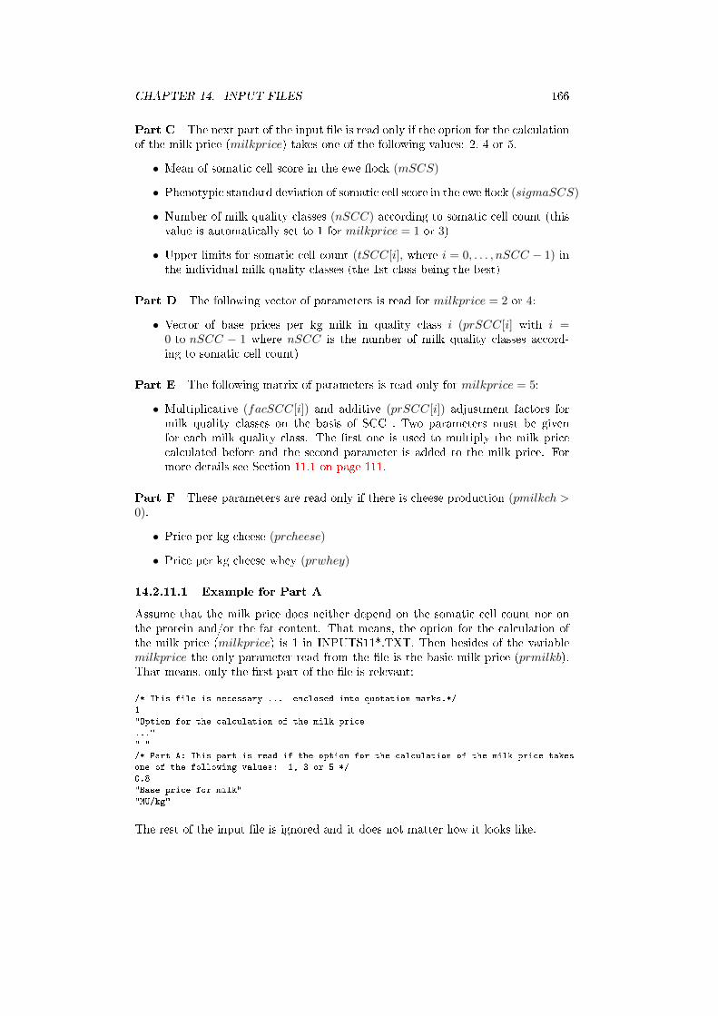
CHAPTER 14. INPUT FILES 166
Part C The next part of the input �le is read only if the option for the calculationof the milk price (milkprice) takes one of the following values: 2, 4 or 5.
• Mean of somatic cell score in the ewe �ock (mSCS)
• Phenotypic standard deviation of somatic cell score in the ewe �ock (sigmaSCS)
• Number of milk quality classes (nSCC) according to somatic cell count (thisvalue is automatically set to 1 for milkprice = 1 or 3)
• Upper limits for somatic cell count (tSCC[i], where i = 0, . . . , nSCC − 1) inthe individual milk quality classes (the 1st class being the best)
Part D The following vector of parameters is read for milkprice = 2 or 4:
• Vector of base prices per kg milk in quality class i (prSCC[i] with i =0 to nSCC − 1 where nSCC is the number of milk quality classes accord-ing to somatic cell count)
Part E The following matrix of parameters is read only for milkprice = 5:
• Multiplicative (facSCC[i]) and additive (prSCC[i]) adjustment factors formilk quality classes on the basis of SCC . Two parameters must be givenfor each milk quality class. The �rst one is used to multiply the milk pricecalculated before and the second parameter is added to the milk price. Formore details see Section 11.1 on page 111.
Part F These parameters are read only if there is cheese production (pmilkch >0).
• Price per kg cheese (prcheese)
• Price per kg cheese whey (prwhey)
14.2.11.1 Example for Part A
Assume that the milk price does neither depend on the somatic cell count nor onthe protein and/or the fat content. That means, the option for the calculation ofthe milk price (milkprice) is 1 in INPUTS11*.TXT. Then besides of the variablemilkprice the only parameter read from the �le is the basic milk price (prmilkb).That means, only the �rst part of the �le is relevant:
/* This file is necessary ... enclosed into quotation marks.*/
1
"Option for the calculation of the milk price
..."
" "
/* Part A: This part is read if the option for the calculation of the milk price takes
one of the following values: 1, 3 or 5 */
0.8
"Base price for milk"
"MU/kg"
The rest of the input �le is ignored and it does not matter how it looks like.
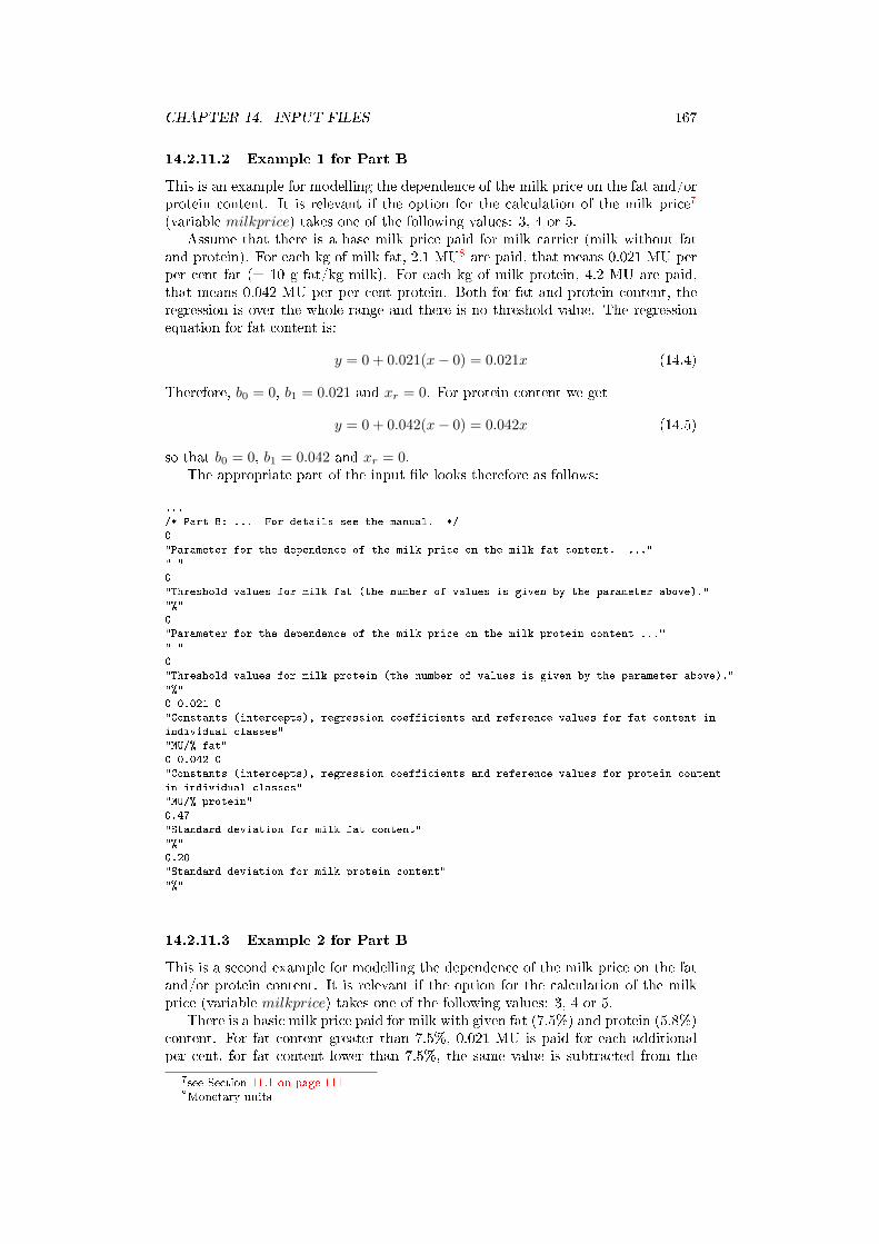
CHAPTER 14. INPUT FILES 167
14.2.11.2 Example 1 for Part B
This is an example for modelling the dependence of the milk price on the fat and/orprotein content. It is relevant if the option for the calculation of the milk price7
(variable milkprice) takes one of the following values: 3, 4 or 5.Assume that there is a base milk price paid for milk carrier (milk without fat
and protein). For each kg of milk fat, 2.1 MU8 are paid, that means 0.021 MU perper cent fat (= 10 g fat/kg milk). For each kg of milk protein, 4.2 MU are paid,that means 0.042 MU per per cent protein. Both for fat and protein content, theregression is over the whole range and there is no threshold value. The regressionequation for fat content is:
y = 0 + 0.021(x− 0) = 0.021x (14.4)
Therefore, b0 = 0, b1 = 0.021 and xr = 0. For protein content we get
y = 0 + 0.042(x− 0) = 0.042x (14.5)
so that b0 = 0, b1 = 0.042 and xr = 0.The appropriate part of the input �le looks therefore as follows:
...
/* Part B: ... For details see the manual. */
0
"Parameter for the dependence of the milk price on the milk fat content. ..."
" "
0
"Threshold values for milk fat (the number of values is given by the parameter above)."
"%"
0
"Parameter for the dependence of the milk price on the milk protein content ..."
" "
0
"Threshold values for milk protein (the number of values is given by the parameter above)."
"%"
0 0.021 0
"Constants (intercepts), regression coefficients and reference values for fat content in
individual classes"
"MU/% fat"
0 0.042 0
"Constants (intercepts), regression coefficients and reference values for protein content
in individual classes"
"MU/% protein"
0.47
"Standard deviation for milk fat content"
"%"
0.20
"Standard deviation for milk protein content"
"%"
14.2.11.3 Example 2 for Part B
This is a second example for modelling the dependence of the milk price on the fatand/or protein content. It is relevant if the option for the calculation of the milkprice (variable milkprice) takes one of the following values: 3, 4 or 5.
There is a basic milk price paid for milk with given fat (7.5%) and protein (5.8%)content. For fat content greater than 7.5%, 0.021 MU is paid for each additionalper cent, for fat content lower than 7.5%, the same value is subtracted from the
7see Section 11.1 on page 1118Monetary units
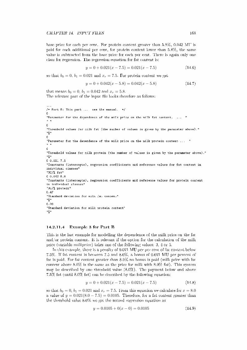
CHAPTER 14. INPUT FILES 168
base price for each per cent. For protein content greater than 5.8%, 0.042 MU ispaid for each additional per cent, for protein content lower than 5.8%, the samevalue is subtracted from the base price for each per cent. There is again only oneclass for regression. The regression equation for fat content is:
y = 0 + 0.021(x− 7.5) = 0.021(x− 7.5) (14.6)
so that b0 = 0, b1 = 0.021 and xr = 7.5. For protein content we get
y = 0 + 0.042(x− 5.8) = 0.042(x− 5.8) (14.7)
that means b0 = 0, b1 = 0.042 and xr = 5.8.The relevant part of the input �le looks therefore as follows:
...
/* Part B: This part ... see the manual. */
0
"Parameter for the dependence of the milk price on the milk fat content. ... "
" "
0
"Threshold values for milk fat (the number of values is given by the parameter above)."
"%"
0
"Parameter for the dependence of the milk price on the milk protein content ... "
" "
0
"Threshold values for milk protein (the number of values is given by the parameter above)."
"%"
0 0.021 7.5
"Constants (intercepts), regression coefficients and reference values for fat content in
individual classes"
"MU/% fat"
0 0.042 5.8
"Constants (intercepts), regression coefficients and reference values for protein content
in individual classes"
"MU/% protein"
0.47
"Standard deviation for milk fat content"
"%"
0.20
"Standard deviation for milk protein content"
"%"
14.2.11.4 Example 3 for Part B
This is the last example for modelling the dependence of the milk price on the fatand/or protein content. It is relevant if the option for the calculation of the milkprice (variable milkprice) takes one of the following values: 3, 4 or 5.
In this example, there is a penalty of 0.021 MU per per cent of fat content below7.5%. If fat content is between 7.5 and 8.0%, a bonus of 0.021 MU per percent offat is paid. For fat content greater than 8.0% no bonus is paid (milk price with fatcontent above 8.0% is the same as the price for milk with 8.0% fat). This systemmay be described by one threshold value (8.0%). The payment below and above7.5% fat (until 8.0% fat) can be described by the following equation:
y = 0 + 0.021(x− 7.5) = 0.021(x− 7.5) (14.8)
so that b0 = 0, b1 = 0.021 and xr = 7.5. From this equation we calculate for x = 8.0a value of y = 0.021(8.0 − 7.5) = 0.0105. Therefore, for a fat content greater thanthe threshold value 8.0% we get the second regression equation as
y = 0.0105 + 0(x− 0) = 0.0105 (14.9)
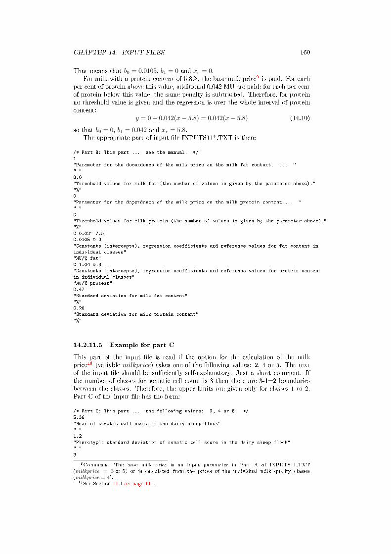
CHAPTER 14. INPUT FILES 169
That means that b0 = 0.0105, b1 = 0 and xr = 0.For milk with a protein content of 5.8%, the base milk price9 is paid. For each
per cent of protein above this value, additional 0.042 MU are paid; for each per centof protein below this value, the same penalty is subtracted. Therefore, for proteinno threshold value is given and the regression is over the whole interval of proteincontent:
y = 0 + 0.042(x− 5.8) = 0.042(x− 5.8) (14.10)
so that b0 = 0, b1 = 0.042 and xr = 5.8.The appropriate part of input �le INPUTS11*.TXT is then:
/* Part B: This part ... see the manual. */
1
"Parameter for the dependence of the milk price on the milk fat content. ... "
" "
8.0
"Threshold values for milk fat (the number of values is given by the parameter above)."
"%"
0
"Parameter for the dependence of the milk price on the milk protein content ... "
" "
0
"Threshold values for milk protein (the number of values is given by the parameter above)."
"%"
0 0.021 7.5
0.0105 0 0
"Constants (intercepts), regression coefficients and reference values for fat content in
individual classes"
"MU/% fat"
0 1.04 5.8
"Constants (intercepts), regression coefficients and reference values for protein content
in individual classes"
"MU/% protein"
0.47
"Standard deviation for milk fat content"
"%"
0.20
"Standard deviation for milk protein content"
"%"
14.2.11.5 Example for part C
This part of the input �le is read if the option for the calculation of the milkprice10 (variable milkprice) takes one of the following values: 2, 4 or 5. The textof the input �le should be su�ciently self-explanatory. Just a short comment. Ifthe number of classes for somatic cell count is 3 then there are 3-1=2 boundariesbetween the classes. Therefore, the upper limits are given only for classes 1 to 2.Part C of the input �le has the form:
/* Part C: This part ... the following values: 2, 4 or 5. */
5.36
"Mean of somatic cell score in the dairy sheep flock"
" "
1.2
"Phenotypic standard deviation of somatic cell score in the dairy sheep flock"
" "
3
9Comment: The base milk price is an input parameter in Part A of INPUTS11.TXT(milkprice = 3 or 5) or is calculated from the prices of the individual milk quality classes(milkprice = 4).
10See Section 11.1 on page 111.
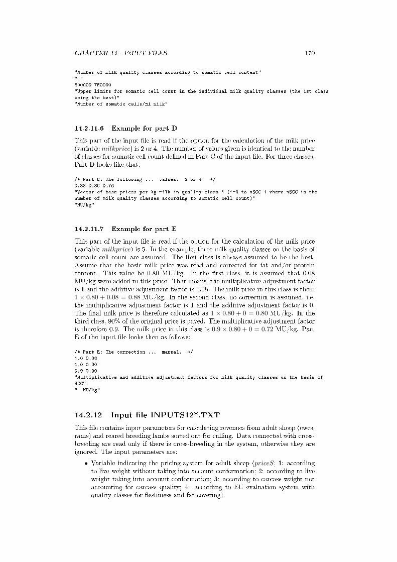
CHAPTER 14. INPUT FILES 170
"Number of milk quality classes according to somatic cell content"
" "
300000 750000
"Upper limits for somatic cell count in the individual milk quality classes (the 1st class
being the best)"
"Number of somatic cells/ml milk"
14.2.11.6 Example for part D
This part of the input �le is read if the option for the calculation of the milk price(variablemilkprice) is 2 or 4. The number of values given is identical to the numberof classes for somatic cell count de�ned in Part C of the input �le. For three classes,Part D looks like that:
/* Part D: The following ... values: 2 or 4. */
0.88 0.80 0.76
"Vector of base prices per kg milk in quality class i (i=0 to nSCC-1 where nSCC is the
number of milk quality classes according to somatic cell count)"
"MU/kg"
14.2.11.7 Example for part E
This part of the input �le is read if the option for the calculation of the milk price(variable milkprice) is 5. In the example, three milk quality classes on the basis ofsomatic cell count are assumed. The �rst class is always assumed to be the best.Assume that the basic milk price was read and corrected for fat and/or proteincontent. This value be 0.80 MU/kg. In the �rst class, it is assumed that 0.08MU/kg were added to this price. That means, the multiplicative adjustment factoris 1 and the additive adjustment factor is 0.08. The milk price in this class is then:1 × 0.80 + 0.08 = 0.88 MU/kg. In the second class, no correction is assumed, i.e.the multiplicative adjustment factor is 1 and the additive adjustment factor is 0.The �nal milk price is therefore calculated as 1 × 0.80 + 0 = 0.80 MU/kg. In thethird class, 90% of the original price is payed. The multiplicative adjustment factoris therefore 0.9. The milk price in this class is 0.9 × 0.80 + 0 = 0.72 MU/kg. PartE of the input �le looks then as follows:
/* Part E: The correction ... manual. */
1.0 0.08
1.0 0.00
0.9 0.00
"Multiplicative and additive adjustment factors for milk quality classes on the basis of
SCC"
"- MU/kg"
14.2.12 Input �le INPUTS12*.TXT
This �le contains input parameters for calculating revenues from adult sheep (ewes,rams) and reared breeding lambs sorted out for culling. Data connected with cross-breeding are read only if there is cross-breeding in the system, otherwise they areignored. The input parameters are:
• Variable indicating the pricing system for adult sheep (priceS; 1: accordingto live weight without taking into account conformation; 2: according to liveweight taking into account conformation; 3: according to carcass weight notaccounting for carcass quality; 4: according to EU evaluation system withquality classes for �eshiness and fat covering)
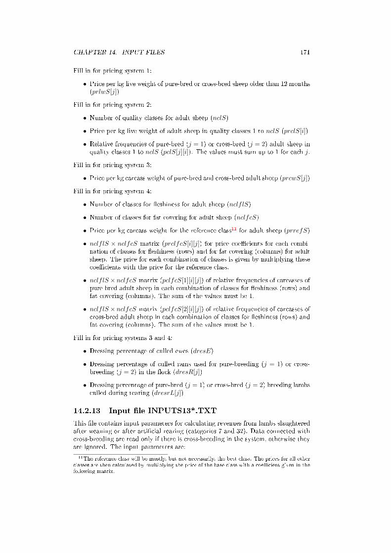
CHAPTER 14. INPUT FILES 171
Fill in for pricing system 1:
• Price per kg live weight of pure-bred or cross-bred sheep older than 12 months(prlwS[j])
Fill in for pricing system 2:
• Number of quality classes for adult sheep (nclS)
• Price per kg live weight of adult sheep in quality classes 1 to nclS (prclS[i])
• Relative frequencies of pure-bred (j = 1) or cross-bred (j = 2) adult sheep inquality classes 1 to nclS (pclS[j][i]). The values must sum up to 1 for each j.
Fill in for pricing system 3:
• Price per kg carcass weight of pure-bred and cross-bred adult sheep (prcwS[j])
Fill in for pricing system 4:
• Number of classes for �eshiness for adult sheep (nclflS)
• Number of classes for fat covering for adult sheep (nclfcS)
• Price per kg carcass weight for the reference class11 for adult sheep (prrefS)
• nclflS × nclfcS matrix (prclfcS[i][j]) for price coe�cients for each combi-nation of classes for �eshiness (rows) and for fat covering (columns) for adultsheep. The price for each combination of classes is given by multiplying thesecoe�cients with the price for the reference class.
• nclflS × nclfcS matrix (pclfcS[1][i][j]) of relative frequencies of carcasses ofpure-bred adult sheep in each combination of classes for �eshiness (rows) andfat covering (columns). The sum of the values must be 1.
• nclflS × nclfcS matrix (pclfcS[2][i][j]) of relative frequencies of carcasses ofcross-bred adult sheep in each combination of classes for �eshiness (rows) andfat covering (columns). The sum of the values must be 1.
Fill in for pricing systems 3 and 4:
• Dressing percentage of culled ewes (dresE)
• Dressing percentage of culled rams used for pure-breeding (j = 1) or cross-breeding (j = 2) in the �ock (dresR[j])
• Dressing percentage of pure-bred (j = 1) or cross-bred (j = 2) breeding lambsculled during rearing (dresrL[j])
14.2.13 Input �le INPUTS13*.TXT
This �le contains input parameters for calculating revenues from lambs slaughteredafter weaning or after arti�cial rearing (categories 7 and 32). Data connected withcross-breeding are read only if there is cross-breeding in the system, otherwise theyare ignored. The input parameters are:
11The reference class will be mostly, but not necessarily, the best class. The prices for all otherclasses are then calculated by multiplying the price of the base class with a coe�cient given in thefollowing matrix.
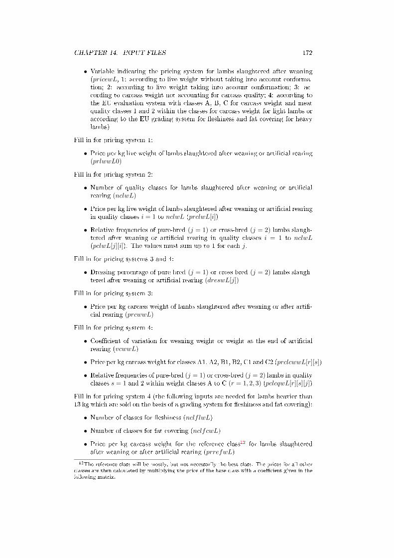
CHAPTER 14. INPUT FILES 172
• Variable indicating the pricing system for lambs slaughtered after weaning(pricewL, 1: according to live weight without taking into account conforma-tion; 2: according to live weight taking into account conformation; 3: ac-cording to carcass weight not accounting for carcass quality; 4: according tothe EU evaluation system with classes A, B, C for carcass weight and meatquality classes 1 and 2 within the classes for carcass weight for light lambs oraccording to the EU grading system for �eshiness and fat covering for heavylambs)
Fill in for pricing system 1:
• Price per kg live weight of lambs slaughtered after weaning or arti�cial rearing(prlwwL0)
Fill in for pricing system 2:
• Number of quality classes for lambs slaughtered after weaning or arti�cialrearing (nclwL)
• Price per kg live weight of lambs slaughtered after weaning or arti�cial rearingin quality classes i = 1 to nclwL (prclwL[i])
• Relative frequencies of pure-bred (j = 1) or cross-bred (j = 2) lambs slaugh-tered after weaning or arti�cial rearing in quality classes i = 1 to nclwL(pclwL[j][i]). The values must sum up to 1 for each j.
Fill in for pricing systems 3 and 4:
• Dressing percentage of pure-bred (j = 1) or cross-bred (j = 2) lambs slaugh-tered after weaning or arti�cial rearing (dreswL[j])
Fill in for pricing system 3:
• Price per kg carcass weight of lambs slaughtered after weaning or after arti�-cial rearing (prcwwL)
Fill in for pricing system 4:
• Coe�cient of variation for weaning weight or weight at the end of arti�cialrearing (vcwwL)
• Price per kg carcass weight for classes A1, A2, B1, B2, C1 and C2 (prclcwwL[r][s])
• Relative frequencies of pure-bred (j = 1) or cross-bred (j = 2) lambs in qualityclasses s = 1 and 2 within weight classes A to C (r = 1, 2, 3) (pclcqwL[r][s][j])
Fill in for pricing system 4 (the following inputs are needed for lambs heavier than13 kg which are sold on the basis of a grading system for �eshiness and fat covering):
• Number of classes for �eshiness (nclflwL)
• Number of classes for fat covering (nclfcwL)
• Price per kg carcass weight for the reference class12 for lambs slaughteredafter weaning or after arti�cial rearing (prrefwL)
12The reference class will be mostly, but not necessarily the best class. The prices for all otherclasses are then calculated by multiplying the price of the base class with a coe�cient given in thefollowing matrix.
CHAPTER 14. INPUT FILES 173
• Matrix for price coe�cients (prclfcwL[i][j]) for each combination of classes for�eshiness (rows) and fat covering (columns). The price for each combination ofclasses is given by multiplying these coe�cients with the price for the referenceclass.
• Matrix of relative frequencies of carcasses (pclfcwL[1][i][j]) of pure-bred lambsin each combination of classes for �eshiness (rows) and fat covering (columns).The sum of the values must be 1.
• Matrix of relative frequencies of carcasses (pclfcwL[2][i][j]) of cross-bred lambsin each combination of classes for �eshiness (rows) and fat covering (columns).The sum of the values must be 1.
14.2.14 Input �le INPUTS14*.TXT
This �le contains input parameters for calculating revenues from lambs in fattening(categories 8-12, 33-37 and 43-47). The �le is only read if there is fattening in thesystem. Data connected with cross-breeding are read only if there is cross-breedingin the system, otherwise they are ignored. The input parameters are:
• Variable indicating the pricing system for fattened lambs (pricefL) The levelsof this variable have the same meaning as the levels of the variable priceS,the �rst input parameter in �le INPUTS12*.TXT (see Subsection 14.2.12).
Fill in for pricing system 1:
• Price per kg live weight of pure-bred and cross-bred fattened lambs (prlwfL[j])
Fill in for pricing system 2:
• Number of quality classes for fattened lambs (nclfL)
• Price per kg live weight of fattened lambs in quality classes 1 to nclfL(prclfL[i])
• Relative frequencies of pure-bred (j = 1) or cross-bred (j = 2) fattened lambsquality classes 1 to nclfL (pclfL[j][i]). The values must sum up to 1 for eachj.
Fill in for pricing systems 3 and 4:
• Dressing percentage of pure-bred (j = 1) and cross-bred (j = 2) lambs ofsex s (s = 1 : females, s = 2 : males, s = 0 : castrates) fattened to target l(dresfL[s][l][j]) where l = 1, . . . lf [s]
Fill in for pricing system 3:
• Price per kg carcass weight of fattened lambs (prcwfL0)
Fill in for pricing system 4:
• Number of classes for �eshiness for fattened lambs (nclflfL)
• Number of classes for fat covering for fattened lambs (nclfcfL)
• Price per kg carcass weight for the reference class13 for fattened lambs (prreffL)
13The reference class will be mostly, but not necessarily, the best class. The prices for all otherclasses are then calculated by multiplying the price of the base class with a coe�cient given in thefollowing matrix.
CHAPTER 14. INPUT FILES 174
• nclflfL×nclfcfL matrix (prclfcfL[i][j]) for price coe�cients for each com-bination of classes for �eshiness (rows) and fat covering (columns) for fattenedlambs. The price for each combination of classes is given by multiplying thesecoe�cients with the price for the reference class.
• Two nclflfL× nclfcfL matrices (pclfcfL[j][i][k]) (for pure-bred and cross-bred animals, respectively) of relative frequencies of carcasses of fattenedlambs in each combination of classes for �eshiness (rows) and fat covering(columns). The sum of the values must be 1 for each j.
14.2.15 Input �le INPUTGFS03.TXT
This input �le is originally thought to be used for the program GFSH and is de-scribed in the correspondig manual in detail [21]. The program EWSH2 reads onlythe �rst two parameters in the �rst run for production system 2 (for breed A):
• Proportion of ewes of breed A in the production system (pdA)
• Proportion of ewes of breed B in the production system (pdB)
14.3 TEXTS2_OUT.TXT
This �le contains text which is used for printing the results. It contains headingsof sections of the results �les, comments and names of variables the values of whichare printed in the results �les. For editing the �le read carefully the remarks at thebeginning of Chapter 14 on page 144.
Chapter 15
Files for data transfer
In production system 2, several runs of the program EWSH2 are carried out. Itis necessary to transfer data between these runs. Therefore, the following �les areused. They are output �les in one run and input �les in the subsequent run. Theycontain only values of variables and no additional text. Do not edit these �les, theyare generated automatically.
15.1 TRANSFER01.TXT
This �le is written in the �rst run of EWSH2 which is for breed B. It is read in thesecond run of EWSH which is for breed A. It contains only the value of the variablensoldMPA (number of rams of breed A sold to �ocks of breed B per ewe of �ocksof breed A per reproductive cycle).
15.2 TRANSFER02.TXT
This �le is written in the second run of EWSH2 which is for breed A and is readin the third run of EWSH2 which is also for breed A. It contains the variablespsp[2][i][1] for i = 1, . . . , csp[2], e.g. the fractions of pure-bred weaned surplus maleprogeny sold in di�erent categories i. These categories are:
• 1: sold at weaning for slaughter
• 2: sold as breeding animals
• 3: castrated
• 4, . . . , 8 : fattened to target 1 to 5, respectively.
15.3 TRANSFER03.TXT
This �le is written in the third run of EWSH2 which is for breed A and is read inthe forth run of EWSH2 which is for breed B. The following variables or expressionsare written to the �le during the run for breed A:
• mwE[1] (mature weight of ewes of breed A)
• mwR[1] (mature weight of rams of breed A)
• psold[2][1][1]×agetP [38][1]+(1−psold[2][1][1])×agetP [40][1] (average weightof male progeny of breed A used for crossing in breed B)
175
CHAPTER 15. FILES FOR DATA TRANSFER 176
• psold[2][1][1]×wP [38][1]+(1−psold[2][1][1])×wP [40][1] (average age of maleprogeny of breed A used for crossing in breed B)
• psold[2][1][1]×revsbL[38][1]+(1−psold[2][1][1])×revsbL[40][1] (average priceof male progeny of breed A used for crossing in breed B)
In the next run of EWSH2 which is for breed B these variables and expressions areread as mwE2, mwR[2], agepurMP [2], wpurMP [2] and prbR[2], respectively.
15.4 ERROR.TXT
This �le contains only the value of the variable errmess. At the start of eachcalculation this �le is read with the value 0 for errmess. If there occurs an errorduring the calculation of the program EWSH2, the value of errmess is changed to1 and written to the �le ERROR.TXT. In the next run of EWSH2 or in the runof the program GFSH, the �le ERROR.TXT is read again. If errmess = 1, allsubsequent programs will stop and write an error message.
Chapter 16
Program output
16.1 The results �le
The name of the �le the results are written to is automatically generated. It hasthe structure res*# where '*' is the breed for which the calculation is carried out(A or B) and '#' is the number of the run of EWSH (01 in production system1, 01 to 04 in production system 2). Therefore, in production system 1 only theresults �le resA01 is generated and in production system 2 the �les resB01, resA02,resA03 and resB04 are produced. If you want to carry out more calculations in thesame directory, copy the results �les �rst to a secure place before starting a newcalculation, otherwise they will be overwritten by the new results.
The �rst part of the results �le contains information on the version of the pro-gram, copyright and contact to the authors and the values of the system variablesread from P00.TXT and PARAS*.TXT (see Section 14.1). The second part of the�le copies more or less the data input �les INPUTS#*.TXT where '#' is to bereplaced by the corresponding numbers (01, 02, 03 etc.) and '*' by the breed (A orB). The information read from the input �les is selected according to the parame-ters given in the parameter �le. Therefore, the results �le does not contain a simplecopy of the input �les, but only data from input �les which will be needed for thegiven calculation.
The third part of the results �le contains the results in the following order:
• Structure of the ewe �ock
• Survival and reproduction characteristics of the ewe �ock
• Structure of the ram population
• Characteristics of progeny
� Structure of the progeny
� Growth characteristics of lambs till weaning
� Growth characteristics of lambs in arti�cial rearing
� Growth characteristics of breeding lambs in rearing
• Weight and age of ewes at lambing
• Weight and age of rams when entering the �ock
• Milk production
• Nutrition costs
177
CHAPTER 16. PROGRAM OUTPUT 178
� Ewes
� Rams
� Lambs
• Non-feed and total costs
� Ewes
� Rams of the breed of the �ock
� Rams of the breed used for crossing in the �ock
� Cost per pure-bred lamb till weaning or till the end of arti�cial rearing
� Cost per cross-bred lamb till weaning or till the end of arti�cial rearing
� Cost per pure-bred female breeding lamb
� Cost per cross-bred female breeding lamb
� Cost per pure-bred male breeding lamb
� Cost per cross-bred male breeding lamb
� Cost per fattened lamb
• Meat prices and revenues
� Meat prices
� Revenues per ewe and reproductive cycle
� Revenues per ram of the breed of the �ock and reproductive cycle
� Revenues per ram of the breed used for crossing in the �ock and perreproductive cycle
� Revenues per pure-bred lamb till weaning and till the end of arti�cialrearing
� Revenues per cross-bred lamb till weaning and till the end of arti�cialrearing
� Revenues per pure-bred female breeding lamb
� Revenues per cross-bred female breeding lamb
� Revenues per pure-bred male breeding lamb
� Revenues per cross-bred male breeding lamb
� Revenues per fattened lamb
� Revenues per lamb died in fattening
• Summing-up of revenues and costs for some types of animals from birth tillselling, till slaughter or till entering the �ock
� Total revenues and costs per replacement female or male
� Total revenues and costs per sold female or male pure-bred lamb
� Total revenues and costs per sold female or male cross-bred lamb
� Final age and weight and total revenues and costs per fattened lamb
� Total revenues from milk and cheese
• Miscellaneous
� Mean classes for quality of life animals or for carcass quality for slaughteranimals
CHAPTER 16. PROGRAM OUTPUT 179
� Costs for purchasing replacement
• Pro�t
• Marginal economic values for all traits i. If there is no crossing, only val-ues evp[i][1] for pure-bred progeny are printed. Otherwise, if there is cross-ing, both evp[i][1] and evp[i][2], i.e. the values for pure-bred and cross-bredprogeny are printed.
Remark. A dense network of conditions was used in the program to ensure print-ing out only the items relevant for the given production system. But it cannot fullybe guaranteed that no variables not meaningful for the given calculation slippedthrough the meshes. In these cases don't worry, as the values of these variables are(hopefully) ignored in the calculation.
16.2 Files CHECKS*# and CHECKS*#a
In the names of these �les, '*' is the breed for which the calculation is carried out(A or B) and '#' is the number of the run of EWSH2 (01 in production system 1,01 to 04 in production system 2). Therefore, in production system 1 only the �lesCHECKSA01 and CHECKSA01a are generated and in production system 2 the�les CHECKSB01, CHECKSB01a, CHECKSA02, CHECKSA02a, CHECKSA03,CHECKSA03a, CHECKSB04 and CHECKSB04a are produced.
The �les CHECKS*# and CHECKS*#a are mainly thought as a help in pro-gramming. The �le CHECKS*#a is printed after loop 1 of the program before theeconomic values are calculated. The �le CHECKS*# is printed after the last loopof the program when all economic values have been calculated. Both �les containonly the names and the values of all variables in alphabetic order without furtherexplaining text. The names of all variables are given in Appendix B. Both �lesshould be identical to a great part if the program works correctly. File CHECKS*#contains the economic values additionally to �le CHECKS*#a and di�ers in thenumber of the loop of the program (zr). Further di�erences should be observedonly in temporary variables or should be rounding errors.
16.3 File INPUTGFS01A for program GFSH
This �le is generated for the program GFSH. In production system 1 it is writtenin the �rst (the only) run for breed A and in production system 2 it is written inthe third run of EWSH2 which is for breed A. It contains the following values forbreed A (only numbers, no text):
• Annual discount rate (u)
• Number of breeding cycles for rams of breed A (RR)
• Proportion of rams of breed A entering each breeding cycle (l4R[i])
• Number of reproductive cycles for ewes of breed A(LL)
• Proportion of ewes of breed A entering each reproductive cycle (l4E[i])
• Marginal economic values for all traits of breed A in the unit as they areprinted (evp[i][1]). The value 0.000000 is inserted for economic values whichwere not calculated in the given system.
CHAPTER 16. PROGRAM OUTPUT 180
• Age of rams of breed A used for pure-breeding at the beginning of the �rstbreeding cycle (ageR[1][1])
• Age of ewes of breed A at �rst lambing (ageE[1])
When reading the �le to program GFSH, most of the variables get di�erent namesas breeds A and B have to be di�erentiated in GFSH.
16.4 File INPUTGFS01B for program GFSH
This �le is generated for the program GFSH only for production 2. It is writtenduring the forth run of EWSH2 which is for breed B. It contains the following inputvalues for breed B (only numbers, no text):
• Number of breeding cycles for rams of breed B (RR)
• Proportion of rams of breed B entering each breeding cycle (l4R[i])
• Number of reproductive cycles for ewes of breed B (LL)
• Proportion of ewes entering each reproductive cycle (l4E[i])
• Marginal economic values for all traits expressed in pure-bred animals of breedB (j = 1) or in cross-bred animals A×B (j = 2) in the unit as they areprinted (evp[i][j]). The values for all traits of pure-bred animals are given�rst followed by the values for cross-bred animals. The value 0.000000 isinserted for economic values which were not calculated in the given system.
• Age of rams of breed B at the beginning of the �rst breeding cycle (ageR[1][1])
• Age of rams of breed A used for crossing with ewes of breed B at the beginningof the �rst breeding cycle (ageR[1][2])
• Age of ewes of breed B at �rst lambing (ageE[1])
• Fraction of ewes of breed B crossed with rams of breed A for reproductivecycles i = 0, . . . , LL− 1. pcrossE[0] is the fraction of female lambs crossed.
Bibliography
[1] AFRC (1990): Nutritive requirements of ruminant animals: Energy. TechnicalCommittee on Responses to Nutrients, Report No. 5. Nutr. Abs & Rev., SeriesB 60, 729-804. CAB International, Wallingford, Oxon.
[2] AFRC (1995): Energy and protein requirements of ruminants. An advisorymanual prepared by AFRC Technical Committee on Responses to Nutrients.Wallingford, CAB, 159 pp.
[3] Ali, A. K. A.; Shook, G.E. (1980): An optimum transformation for somaticcell concentration in milk. J. Dairy Sci. 63, 487-490.
[4] ARC (1980): The Nutrient Requirements of Ruminant Livestock. TechnicalReview by an Agricultural Research Council Working Party, CommonwealthAgricultural Bureau, Farmham Royal, UK. 351 pp.
[5] Cannas, A.; Tadeschi, L. O.; Fox, D. G.; Pell, A. N.; Van Soest, P. J. (2004): Amechanistic model for predicting the nutrient requirements and feed biologicalvalues for sheep. J. Anim. Sci. 82, 149-169.
[6] Da, Y.; Grossman, M.; Misztal, I.; Wiggans, G.R. (1992): Estimation of geneticparameters for somatic cell score in Holsteins. J. Dairy Sci. 75, 2265-2271.
[7] Groenewald, P. C. N; Ferreira, A.V.; van der Merwe, H.J.; Slippers, S.C. (1995):A mathematical model for describing and predicting the lactation curve ofMerino ewes. Anim. Sci. 61, 95-101.
[8] Infascelli, F.; Moniello, G.; Cutrignelli, M.I.; Bovera, F. (2005): Vitamin andwater requirements of dairy sheep. Ital. J. Anim. Sci. 4, Suppl. 1 (Evaluationof requirements of dairy sheep. Special issue), 75-83.
[9] International Committee for Animal Recording (2007): International agree-ment of recording practices. Approved by the General Assembly held in Kuopio,Finland, on 9 June 2006.
[10] Jaeggi, J.J.; Wendor�, W.L.; Johnson, M.E.; Romero, J.; Berger, Y. (2004):Milk composition and cheese yield from hard and soft cheese manufactured fromsheep milk. In: 51th Biennal Spooner Sheep Day, August 28, 2004, SpoonerAgricultural Research Station, University of Wisconsin-Madison, Spooner,Wisconsin, 12 pp.
[11] Jalvingh, A.W.; Dijkhuizen, A.A.; van Arendonk, J.A.M. (1992): Dynamicprobabilistic modelling of reproduction and replacement management in sowherds. General aspects and model description. Agric. Systems 39, 133-152.
[12] Legarra, A.; Ramón, M.; Ugarte, E.; Péréz-Guzmán, M.D.; Arranz, J. (2007):Economic weights of somatic cell score in dairy sheep. Animal 1, 205-212.
181
BIBLIOGRAPHY 182
[13] NRC (1981): E�ect of Environment on Nutrient Requirements of DomesticAnimals. National Academy Press, Washington, DC. 152 pp.
[14] Ponzoni, R.W. (1988): The derivation of economic values combining incomeand expense in di�erent ways: An example with Australian Merino Sheep. J.Anim. Breed. Genet. 105, 143-153.
[15] Reinsch, N.; Demp�e, L. (1998): Investigations on functional traits in Sim-mental: 3. Economic weights at the stationary state of a Markov chain. Arch.Tierz. 41, 211-224.
[16] Sakul, H.; Boylan, W.J. (1992): Lactation curves of several US sheep breeds.Anim. Prod. 54, 229-233.
[17] Snowder, G.D.; Glimp, H.A. (1991): In�uence of breed, number of sucklinglambs, and stage of lactation on ewe milk production and lamb growth underrange conditions. J. Anim. Sci. 69, 923-930.
[18] Theodorou, M.K.; France, J., eds. (2000): Feeding systems and and feed eval-uation models. CABI Publishing, Wallingford, UK, 481 pp.
[19] Tyrrell, H.F.; Reid, J.T. (1965): Prediction of the energy value of cows milk.J. Dairy Sci. 48, 1215-1223.
[20] Van Slyke, L.L. (1894): Investigation relating to the manufacture of cheese.New York Agric. Exp. Stn. Bull. 65.
[21] Wolf, J.; Wolfová, M. (2011): User's manual for the program packageECOWEIGHT (C programs for calculating economic weights in livestock), Ver-sion 5.1.1. Part 3B: Program GWSH for gene �ow in sheep, Version 1.0.3. 47pp.
[22] Wolf, J.; Wolfová, M.; Krupová, Z.; Krupa, E. (2011): User's manual for theprogram package ECOWEIGHT (C programs for calculating economic weightsin livestock), Version 5.1.1. Part 2: Program EWSH1 for sheep, Version 1.1.6.223 pp.
[23] Wolf, J.; Wolfová, M.; Krupa, E. (2011): User's manual for the program pack-age ECOWEIGHT (C programs for calculating economic weights in livestock),Version 5.1.1. Part 1: Programs EWBC (version 2.2.1) and EWDC (version2.1.2) for cattle. 198 pp.
[24] Wolfová, M.; Wolf, J.; Hyánek, J. (1995): Economic weights for beef productiontraits in the Czech Republic. Livest. Prod. Sci. 43, 63-73.
[25] Wolfová, M.; Wolf, J.; Krupová, Z.; Kica, J. (2009): Estimation of economicvalues for traits of dairy sheep: I. Model development. J. Dairy Sci. 92, 2183-2194.
[26] Wolfová, M.; Wolf, J.; Krupová, Z.; Margetín, M. (2009): Estimation of eco-nomic values for traits of dairy sheep: II. Model application to a system withone lambing per year. J. Dairy Sci. 92, 2195-2203.
[27] Wolfová, M.; Wolf, J.; P°ibyl, J.; Zahrádková, R.; Kica, J. (2005): Breed-ing objectives for beef cattle used in di�erent production systems: 1. Modeldevelopment. Livest. Prod. Sci. 95, 201-215.
[28] Wood, P.D.P. (1967): Algebraic model of the lactation curve in cattle. Nature216, 164-165.
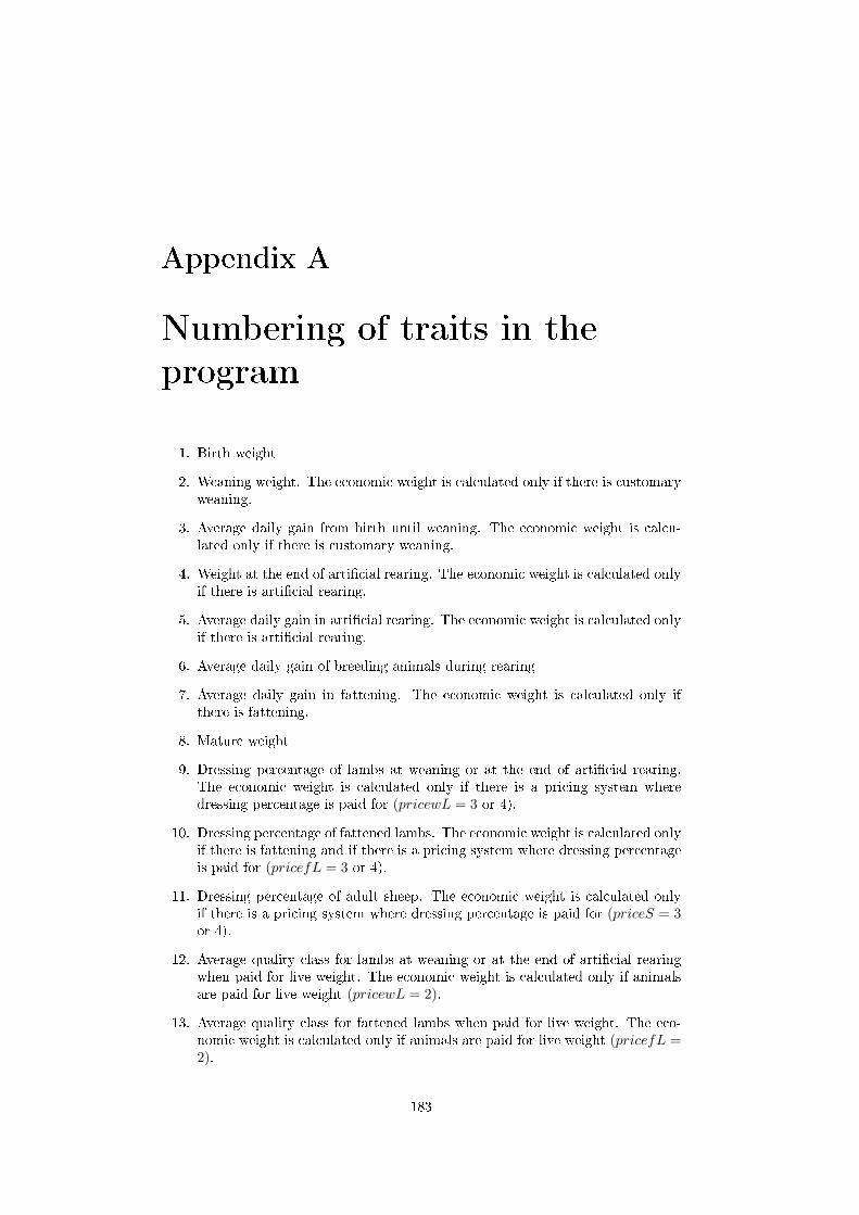
Appendix A
Numbering of traits in the
program
1. Birth weight
2. Weaning weight. The economic weight is calculated only if there is customaryweaning.
3. Average daily gain from birth until weaning. The economic weight is calcu-lated only if there is customary weaning.
4. Weight at the end of arti�cial rearing. The economic weight is calculated onlyif there is arti�cial rearing.
5. Average daily gain in arti�cial rearing. The economic weight is calculated onlyif there is arti�cial rearing.
6. Average daily gain of breeding animals during rearing
7. Average daily gain in fattening. The economic weight is calculated only ifthere is fattening.
8. Mature weight
9. Dressing percentage of lambs at weaning or at the end of arti�cial rearing.The economic weight is calculated only if there is a pricing system wheredressing percentage is paid for (pricewL = 3 or 4).
10. Dressing percentage of fattened lambs. The economic weight is calculated onlyif there is fattening and if there is a pricing system where dressing percentageis paid for (pricefL = 3 or 4).
11. Dressing percentage of adult sheep. The economic weight is calculated onlyif there is a pricing system where dressing percentage is paid for (priceS = 3or 4).
12. Average quality class for lambs at weaning or at the end of arti�cial rearingwhen paid for live weight. The economic weight is calculated only if animalsare paid for live weight (pricewL = 2).
13. Average quality class for fattened lambs when paid for live weight. The eco-nomic weight is calculated only if animals are paid for live weight (pricefL =2).
183
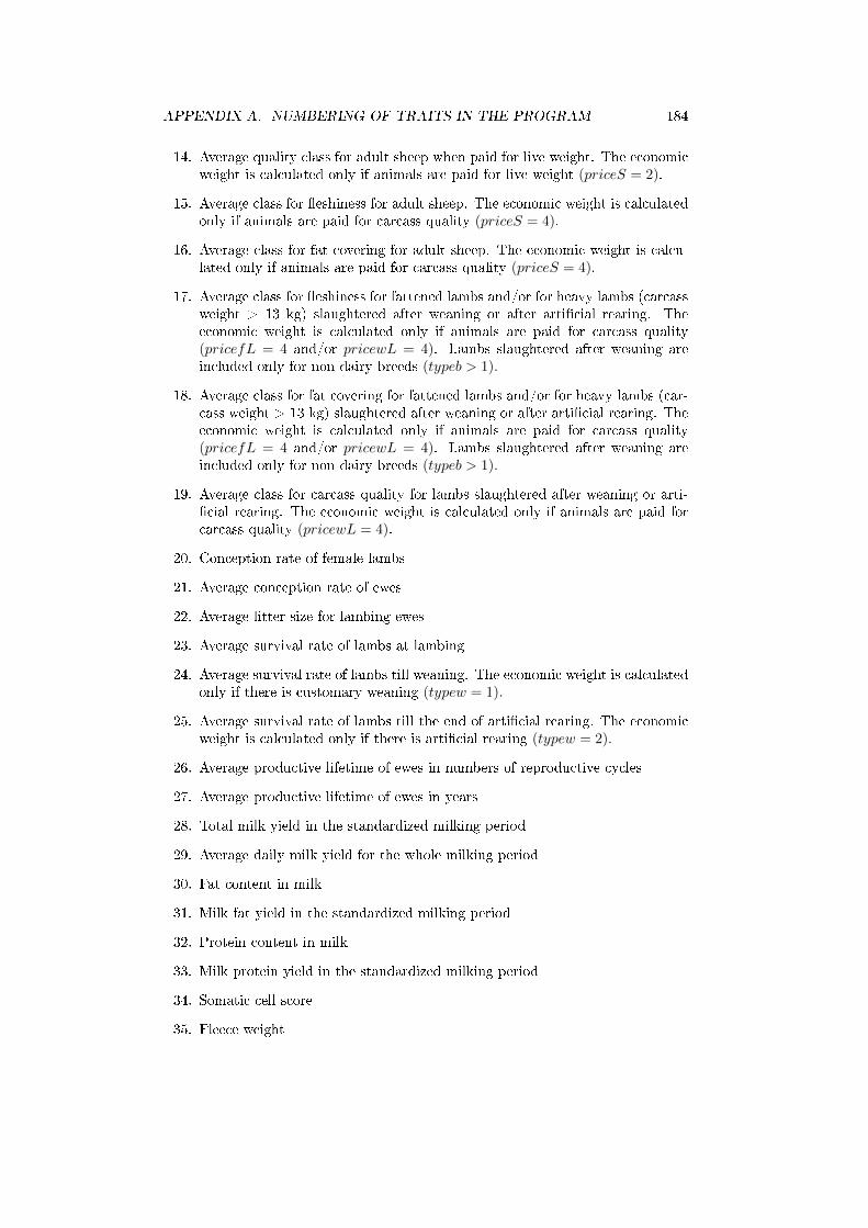
APPENDIX A. NUMBERING OF TRAITS IN THE PROGRAM 184
14. Average quality class for adult sheep when paid for live weight. The economicweight is calculated only if animals are paid for live weight (priceS = 2).
15. Average class for �eshiness for adult sheep. The economic weight is calculatedonly if animals are paid for carcass quality (priceS = 4).
16. Average class for fat covering for adult sheep. The economic weight is calcu-lated only if animals are paid for carcass quality (priceS = 4).
17. Average class for �eshiness for fattened lambs and/or for heavy lambs (carcassweight > 13 kg) slaughtered after weaning or after arti�cial rearing. Theeconomic weight is calculated only if animals are paid for carcass quality(pricefL = 4 and/or pricewL = 4). Lambs slaughtered after weaning areincluded only for non-dairy breeds (typeb > 1).
18. Average class for fat covering for fattened lambs and/or for heavy lambs (car-cass weight > 13 kg) slaughtered after weaning or after arti�cial rearing. Theeconomic weight is calculated only if animals are paid for carcass quality(pricefL = 4 and/or pricewL = 4). Lambs slaughtered after weaning areincluded only for non-dairy breeds (typeb > 1).
19. Average class for carcass quality for lambs slaughtered after weaning or arti-�cial rearing. The economic weight is calculated only if animals are paid forcarcass quality (pricewL = 4).
20. Conception rate of female lambs
21. Average conception rate of ewes
22. Average litter size for lambing ewes
23. Average survival rate of lambs at lambing
24. Average survival rate of lambs till weaning. The economic weight is calculatedonly if there is customary weaning (typew = 1).
25. Average survival rate of lambs till the end of arti�cial rearing. The economicweight is calculated only if there is arti�cial rearing (typew = 2).
26. Average productive lifetime of ewes in numbers of reproductive cycles
27. Average productive lifetime of ewes in years
28. Total milk yield in the standardized milking period
29. Average daily milk yield for the whole milking period
30. Fat content in milk
31. Milk fat yield in the standardized milking period
32. Protein content in milk
33. Milk protein yield in the standardized milking period
34. Somatic cell score
35. Fleece weight
Appendix B
List of variables and constants
This list contains all variables used in the program. Some additional variables whichare used only in the manual as they are useful for a clear arrangement and whichare explained there are not part of the list.
a Used in the calculation of the stationary state of the ewe �ock
a1 Convergence criterion used in the calculation of the stationary state ofthe ewe �ock or the ram population
a2 Temporary variable
a3 Temporary variable
a4 Temporary variable
ach Constant (intercept) in regression equation (6.16)
adg[i][j] Temporary variable: Average daily gain for di�erent periods for pure-bred (j = 1) or cross-bred (j = 2) female (i = 1) or male (i = 2)lambs
adgb[k][i][j] Temporary variable: Average daily gain for di�erent periods for pure-bred (j = 1) or cross-bred (j = 2) female (k = 1) or male (k = 2) lambsborn in litter size i (i = 1, . . . , clt)
adgbwL[k][i][j] Average daily gain from birth to weaning for pure-bred (j = 1) orcross-bred (j = 2) female (k = 1) or male (k = 2) lambs born in littersize i (i = 1, . . . , clt)
adgE Average daily gain of ewes between �rst and second lambing
adgfE Extra daily gain of ewes in the �ushing period
adgfL Extra daily gain of female breeding lambs in the �ushing period
adgP[i][j] Average daily gain of category i (i = 1, ..., PP ) of pure-bred (j = 1) orcross-bred (j = 2) progeny
adgR[i] Average daily gain of rams of the breed of the �ock (i = 1) or of ramsof the breed used for crossing in the �ock (i = 2) between the �rst andsecond breeding cycle
185
APPENDIX B. LIST OF VARIABLES AND CONSTANTS 186
adgr[k][i][j] Average daily gain of pure-bred (j = 1) or cross-bred (j = 2) female(k = 1) or male (k = 2) breeding progeny from weaning to the �rstbreeding season (i = 1) and from breeding season i − 1 to breedingseason i (i = 2, . . . , bs[k])
adgwarL[k][i][j] Average daily gain from weaning to the end of arti�cial rearing forpure-bred (j = 1) or cross-bred (j = 2) female (k = 1) or male (k = 2)lambs born in litter size i (i = 1, . . . , clt)
agearL Age of lambs at the end of arti�cial rearing
ageE[i] Age of ewe at lambing i (i = 1, . . . , LL)
agelFP[i] Age at lambing of female lambs conceived in breeding season i (i =1, . . . , bs[1])
agepurMP[j] Age of purchased male of breed j (j = 1 : breed of the �ock, j = 2:breed used in the �ock for crossing)
ageR[i][j] Age of rams of the breed of the �ock (j = 1) or of the breed usedfor crossing in the �ock (j = 2) at the beginning of breeding cycle i(i = 1, . . . , RR)
ager[k][i] Age of female (k = 1) or male (k = 2) breeding lambs at the beginningof breeding season i (i = 1, . . . , bs[k])
agetP[i][j] Age of category i (i = 1, . . . , PP ) of pure-bred (j = 1) or cross-bred(j = 2) progeny at the end of the time interval these categories exist
agewL Age of lambs at weaning
AkharL Number of man-hours per lamb in the period of arti�cial rearing
AkhE Number of man-hours per ewe and year (including lambs till weaning,excluding milking and cheese production and shearing if done by exter-nal workers)
AkhfL Number of man-hours per male or female lamb or castrate in fatteningper year
AkhR Number of man-hours per ram and year
AkhrL Number of man-hours per female or male breeding lamb in rearing peryear
avclfL[j] Average quality class for pure-bred (j = 1) or cross-bred (j = 2) fattenedlambs when animals are paid for live weight
avclS[j] Average quality class for pure-bred (j = 1) or cross-bred (j = 2) adultsheep when animals are paid for live weight
avclwL[j] Average quality class for pure-bred (j = 1) or cross-bred (j = 2) lambsat weaning or at the end of arti�cial rearing when animals are paid forlive weight
avconrateE Average conception rate of ewes (averaged over reproductive cycles)
avcqwL[j] Average class for carcass quality in pure-bred (j = 1) or cross-bred(j = 2) lambs slaughtered after weaning or arti�cial rearing
APPENDIX B. LIST OF VARIABLES AND CONSTANTS 187
avfcfL[j] Average class for fat covering in pure-bred (j = 1) or cross-bred (j = 2)fattened lambs
avfcL[j] Average class for fat covering in pure-bred (j = 1) or cross-bred (j = 2)fattened lambs and/or heavy lambs (carcass weight > 13 kg) slaughteredafter weaning or arti�cial rearing. The variable avfcL[j] is calculatedas the weighted mean of avfcfL[j] and avfcwL[j].
avfcS[j] Average class for fat covering in pure-bred (j = 1) or cross-bred (j = 2)adult sheep
avfcwL[j] Average class for fat covering in pure-bred (j = 1) or cross-bred (j =2) heavy lambs (carcass weight > 13 kg) slaughtered after weaning orarti�cial rearing
av�eshfL[j] Average class for �eshiness in pure-bred (j = 1) or cross-bred (j = 2)fattened lambs
av�eshL[j] Average class for �eshiness in pure-bred (j = 1) or cross-bred (j = 2)fattened lambs and/or heavy lambs (carcass weight > 13 kg) slaughteredafter weaning or arti�cial rearing. The variable avfleshL[j] is calculatedas the weighted mean of avfleshfL[j] and avfleshwL[j].
av�eshS[j] Average class for �eshiness in pure-bred (j = 1) or cross-bred (j = 2)adult sheep
av�eshwL[j] Average class for �eshiness in pure-bred (j = 1) or cross-bred (j =2) heavy lambs (carcass weight > 13 kg) slaughtered after weaning orarti�cial rearing
avlifelE Productive lifetime of ewes in number of reproductive cycles
avlifeyE Productive lifetime of ewes in years
avlitlE Average litter size per ewe lambing
avlitpE[i] Average litter size per ewe lambing in reproductive cycle i (i = 1, . . . , LL)
avmilkd Average daily milk production in the whole lactation (from lambing tilldrying o�)
avsur24hL[j] Average survival rate of pure-bred (j = 1) or cross-bred (j = 2) lambsat lambing (until 24 hours after birth)
avsurarL[j] Average survival rate of pure-bred (j = 1) or cross-bred (j = 2) lambsfrom 24 hours after birth till the end of arti�cial rearing
avsurwL[j] Average survival rate of pure-bred (j = 1) or cross-bred (j = 2) lambsfrom 24 hours after birth till weaning
avwar[i][j] Average weight of pure-bred (j = 1) or cross-bred (j = 2) female (i = 1)or male (i = 2) lambs at the end of arti�cial rearing
avww[i][j] Average weaning weight of pure-bred (j = 1) or cross-bred (j = 2)female (i = 1) or male (i = 2) lambs
awo Parameter a for lactation curve (6.1)
basemilkm Milk yield from weaning to the end of the milking period per ewe lamb-ing calculated for the standard lactation curve (6.1)
APPENDIX B. LIST OF VARIABLES AND CONSTANTS 188
basemilkw Milk yield until weaning per ewe lambing calculated for the standardlactation curve (6.1)
basemilkws[i] Milk yield until weaning per ewe lambing calculated for the standardlactation curve (6.1) in feeding season i (i = 1, . . . , nfs)
bch Regression coe�cient for fat content in equation (6.16)
breed Breed for which the calculation is carried out; for details see Subsec-tion 14.1.1 on page 144
BS Maximal number of breeding seasons for female or male progeny + 1(set to 5, used for dimensioning arrays in the program)1
bs[i] Number of breeding seasons for female (i = 1) or male (i = 2) progeny(�xed to 3 for female and to 2 for male progeny)
bwL[k][i][j] Birth weight of female (k = 1) or male (k = 2) progeny within eachlitter size i and breeding type j (i = 1, . . . clt, j = 1, 2; j = 1: pure-bredlambs, j = 2: cross-bred lambs)
bwo Parameter b for lactation curve (6.1)
C Maximal number of ewe categories + 1 (set to 100, used for dimensioningarrays in the program, see footnote on this page)
c1[i] to c3[i] Constants in the equations for the calculation of net energy require-ment for lambs; i = 1 : female lambs, i = 2 : male lambs, i = 0 :castrates.
c4[i] to c6[i] Constants in the equations for the calculation of protein requirementfor lambs; i = 1 : female lambs, i = 2 : male lambs, i = 0 : castrates.
calc Number of the calculation; for details see Subsection 14.1.1 on page 144
casprot Casein as fraction of protein in milk
CB Di�erentiates between cross-breeding and pure-breeding (set to 3, usedfor dimensioning arrays in the program)
cch Regression coe�cient for protein content in equation (6.16)
cheesewhey Amount of cheese whey per kg cheese
cheesey Cheese yield in kg from 1 kg milk
clf[k][i] This variable indicates if target i (i = 1, . . . lf [k]) in fattening of progeny(k = 1 : female progeny, k = 2 : male progeny, k = 0 : castrates) isapplied only to pure-bred (clf [k][i] = 1) or cross-bred (clf [k][i] = 2)progeny or both to pure-bred and cross-bred progeny (clf [k][i] = 0).
CLT Maximal number of classes for litter size + 1 (e.g. singles, twins, triplets,set to 5, used for dimensioning arrays in the program, see footnote onthis page)
clt Number of classes for litter size (e.g. singles, twins, triplets) for thegiven calculation (maximal value 4)
1Numbering of elements in arrays in the C language starts with 0. As in the program the �rstelement of the array mostly is not used and only elements with numbers 1, 2, . . . , n are occupied,the dimension of the array must be n+ 1.
APPENDIX B. LIST OF VARIABLES AND CONSTANTS 189
coninsE Average conception rate of ewes after insemination
conrateE[i] Conception rate of ewes in reproductive cycle i (i = 1, . . . , LL− 1)
conrateFP[i][j] Conception rate of pure-bred (j = 1) or cross-bred (j = 2) femaleprogeny in the individual breeding seasons (i = 1, . . . , bs[1])
costAkh Cost per man-hour (including insurance)
costbedE[i] Cost for bedding per housed ewe of category i (i = 1, . . . , TE) includinglambs till weaning and per reproductive cycle
costbedL[i][j] Cost for bedding per housed pure-bred (j = 1) or crossbed (j = 2)lamb of category i (i = 1, . . . , PP )
costbedR[i][j] Cost for bedding per housed ram of category i (i = 1, . . . , TR) andbreed j (j = 1 : breed of the �ock, j = 2 : breed used for crossing in the�ock) per breeding cycle
costbreedE[i] Cost for breeding per ewe of category i (i = 1, . . . , TE) and perreproductive cycle
costbreedL[i][j] Cost for breeding per pure-bred (j = 1) or cross-bred (j = 2) femalelamb of category i
costcheese0E Cost for processing 1 kg milk to cheese (facilities, labour, etc. withoutcosts for milk)
costcheeseE[i] Cost for producing cheese (facilities, labour, etc. without costs formilk) per ewe of category i (i = 1, . . . , TE)
costdead Cost for removing and rendering a dead animal (per kg weight)
costdiedE[i] Cost per died ewe of category i (i = 1, . . . , TE)
costdiedL[i][j] Cost per died pure-bred (j = 1) or cross-bred (j = 2) lamb of cate-gory i (i = 1, . . . , PP )
costE[i] Total costs per ewe of category i (i = 1, . . . , TE) per reproductive cycle
costfE[i] Total feeding costs per ewe of category i (i = 1, . . . , TE) and per repro-ductive cycle
cost�x0E Fixed costs per stable place per day for ewes (including lambs till wean-ing)
cost�x0R Fixed costs per stable place per day for rams
cost�xarL Fixed costs per stable place per day for lambs in arti�cial rearing
cost�xE[i] Fixed costs per stable place per reproductive cycle for ewes (includinglambs till weaning) of category i (i = 1, . . . , TE)
cost�xfL Fixed costs per stable place per day for lambs in fattening
cost�xL[i][j] Fixed costs per pure-bred (j = 1) or cross-bred (j = 2) lamb of cate-gory i (i = 1, . . . , PP )
cost�xR[i][j] Fixed costs per stable place per ram of category i (i = 1, . . . , TR) andbreed j (j = 1 : breed of the �ock, j = 2 : breed used for crossing in the�ock) and per breeding cycle
APPENDIX B. LIST OF VARIABLES AND CONSTANTS 190
cost�xrL Fixed costs per stable place per day per female or male breeding lamb
costfL[i][j] Total feeding costs per pure-bred (j = 1) or cross-bred (j = 2) lamb ofcategory i (i = 1, . . . , PP )
costfR[i][j] Total feeding costs per ram of category i (i = 1, . . . , TR) of the breedof the �ock (j = 1) or of the breed used for crossing in the �ock (j = 2)and per breeding cycle
costins[j] Cost per insemination (price for dose and labour) for pure-breeding(j = 1) and cross-breeding (j = 2)
costL[i][j] Total costs per pure-bred (j = 1) or cross-bred (j = 2) lamb of categoryi (i = 1, . . . , PP )
costlabE[i] Total labour costs per ewe of category i (i = 1, . . . , TE) and per repro-ductive cycle
costlabL[i][j] Total labour costs per pure-bred (j = 1) or cross-bred (j = 2) lamb ofcategory i (i = 1, . . . , PP )
costlabR[i][j] Total labour costs per ram of category i (i = 1, . . . , TR) and breed j(j = 1 : breed of the �ock, j = 2 : breed used for crossing in the �ock)and per breeding cycle
costlamb Costs (reduced by revenues) for ewes and rams which should be allottedto one weaned (or arti�cially reared) lamb
costmarkbR Marketing costs (e.g. transport, advertising) per breeding ram
costmarkcul Marketing costs (e.g. transport, advertising) per animal to be culled
costmarkE[i] Marketing costs per ewe of category i and per reproductive cycle
costmarkfL Marketing costs (e.g. transport, advertising) per kg live weight of lambssold after fattening
costmarkL[i][j] Marketing costs per pure-bred (j = 1) or cross-bred (j = 2) lamb ofcategory i (i = 1, . . . , PP )
costmarkR[i][j] Marketing costs per ram of category i (i = 1, . . . , TR) and breed j(j = 1 : breed of the �ock, j = 2 : breed used for crossing in the �ock)
costmarkrL[i] Marketing costs (e.g. transport, advertising) per female (i = 1) ormale (i = 2) breeding lamb
costmarkwL Marketing costs (e.g. transport, advertising) per kg live weight oflambs sold at weaning or at the end of arti�cial rearing
costmilk0E Cost for milking per kg milk (variable costs, i.e. for energy for cooling,labour, etc.)
costmilkE[i] Cost for milking (variable costs, i.e. for energy for cooling, labour,etc.) per ewe of category i (i = 1, . . . , TE)
costnfE[i] Total non-feed costs per ewe of category i (i = 1, . . . , TE) and perreproductive cycle
costnfL[i][j] Total non-feed costs per pure-bred (j = 1) or cross-bred (j = 2) lambof category i (i = 1, . . . , PP )
APPENDIX B. LIST OF VARIABLES AND CONSTANTS 191
costoein Cost for induction and oestrus synchronisation per ewe and reproductivecycle
costoeinFP Cost for induction and oestrus synchronisation per female lamb perbreeding season
costpurchFP Cost for purchasing female breeding lambs per ewe per reproductivecycle
costpurchR[i][j] Cost for purchasing rams per ram of category i (i = 1, . . . , nstgR)of the breed of the �ock (j = 1) or of the breed used for crossing in the�ock (j = 2)
costR[i][j] Total costs per ram of category i (i = 1, . . . , TR) of the breed of the�ock (j = 1) or of the breed used for crossing in the �ock (j = 2)
costreins[j] Costs per re-insemination for pure-breeding (j = 1) and cross-breeding(j = 2)
costshe0E Cost per shearing a ewe
costshe0L Costs per shearing a lamb
costshe0R Cost per shearing a ram
costsheE[i] Total shearing costs per ewe of category i (i = 1, . . . , TE) and perreproductive cycle
costsheL[i][j] Total shearing costs per pure-bred (j = 1) or cross-bred (j = 2) lambof category i (i = 1, . . . , PP )
costsheR[i][j] Total shearing costs per ram of category i (i = 1, . . . , TR) and breedj (j = 1 : breed of the �ock, j = 2 : breed used for crossing in the �ock)and per breeding cycle
costskE[i] Costs for tanning skin per ewe of category i (i = 1, . . . , TE) and perreproductive cycle
costskL[i][j] Costs for tanning skin per pure-bred (j = 1) or cross-bred (j = 2) lambof category i (i = 1, . . . , PP )
costtan Costs for tanning skin
costvetE[i] Veterinary costs per ewe of category i (i = 1, . . . , TE) and per repro-ductive cycle
costvetL[i][j] Veterinary costs per pure-bred (j = 1) or cross-bred (j = 2) lamb ofcategory i (i = 1, . . . , PP )
costvetR[i][j] Veterinary costs per ram of category i (i = 1, . . . , TR) and breed j(j = 1 : breed of the �ock, j = 2 : breed used for crossing in the �ock)and per breeding cycle
costwatE[i] Total costs for water per ewe of category i (i = 1, . . . , TE) and perreproductive cycle
costwatL[i][j] Total costs for water per pure-bred (j = 1) or cross-bred (j = 2) lambof category i (i = 1, . . . , PP )
APPENDIX B. LIST OF VARIABLES AND CONSTANTS 192
costwatR[i][j] Total costs for water per ram of category i (i = 1, . . . , TR) of thebreed of the �ock (j = 1) or of the breed used for crossing in the �ock(j = 2) and per breeding cycle
CR Maximal number of categories for rams + 1 (set to 30, used for dimen-sioning arrays in the program, see footnote on page 188)
crossing Type of progeny (1: only pure-bred progeny, 2: pure-bred and cross-bredprogeny)
CSP Maximal number of groups of surplus progeny + 1 (set to 10, used fordimensioning arrays in the program, see footnote on page 188)
csp[i] Number of groups of surplus female (i = 1) or male (i = 2) progenyor castrates (i = 0). In the given version of the program is csp[0] ≤ 5,csp[1] ≤ 7 and csp[2] ≤ 8.
cullbsMP[i][j] Culling rate of male progeny from weaning (for i = 1) or from breed-ing season i− 1 (for i > 1) to breeding season i (i = 1, . . . , bs[2]); bs[2]is �xed to 2 in the given version of the program.
cwo Parameter c for lactation curve (6.1)
cy Indicator variable which takes value 1 if regression equation (6.16) isused for the calculation of the milk amount needed for 1 kg cheese andwhich takes value 2 if van Slyke's formula (6.17) to (6.19) is used
datbbs Date of the beginning of the breeding season2
datconFP[i] Date of conceiving of female progeny in breeding season i (i = 1, . . . , bs[1])
datdry Date of drying o� of dairy ewes
datchfs[i] Date of a change in the feeding season (i = 1, . . . , nchfs)
datebs End date of the breeding season
datlamb Date of lambing (start date of the reproductive cycle)
datwL Date of weaning lambs
dcE[i] Length of the time period in the reproductive cycle of the occurrence ofnon-feed costs for ewes of category i (i = 1, . . . , TE)
dcL[i][j] Length of the time period of the occurrence of non-feed costs for pure-bred (j = 1) or cross-bred (j = 2) lambs of category i (i = 1, . . . , PP )
dcR[i] Length of the time period in the breeding cycle of the occurrence ofnon-feed costs for rams of category i (i = 1, . . . , TR)
dmilkst Length of the standardized milking period in days
dnpregcE Interval between the end of the appropriate breeding season and timeof culling ewes for failure to conceive
dnpregcFP Interval between the end of the appropriate breeding season and timeof culling female lambs for failure to conceive
2All variables referring to dates are expressed in days from January 1st of year zero in theprogram. Input of dates (compare Subsection 14.2.1) must be in the format �year month day�where year is relative and the time scale starts with year zero always.
APPENDIX B. LIST OF VARIABLES AND CONSTANTS 193
dpregsFP Days of pregnancy when pregnant female lambs are sold
dresE Dressing percentage of culled ewes
dresfL[s][l][j] Dressing percentage of pure-bred (j = 1) and cross-bred (j = 2) lambsof sex s (s = 1 : females, s = 2 : males, s = 0 : castrates) fattened totarget l = 1, . . . , lf [s]
dresR[j] Dressing percentage of culled rams used for pure-breeding (j = 1) orcross-breeding (j = 2) in the �ock
dresrL[j] Dressing percentage of pure-bred (j = 1) or cross-bred (j = 2) breedinglambs culled during rearing
dreswL[j] Dressing percentage of pure-bred (j = 1) and cross-bred (j = 2) lambsslaughtered after weaning or after arti�cial rearing
drymE[i][j] Dry matter content in fresh matter for seasonal variant j (j = 1, . . . , nfs)of feeding ration i (i = 1, . . . , fE) for ewes
drymL[i][j] Dry matter content in fresh matter for seasonal variant j (j = 1, . . . , nfs)of feeding ration i (i = 1, . . . , fL) for lambs
drymR[i][j] Dry matter content in fresh matter for seasonal variant j (j = 1, . . . , nfs)of feeding ration i (i = 1, . . . , fR) for rams
dselR Time interval from the end of the breeding season to selling of breedingrams
dshpE Length of the period of high pregnancy where a special feeding rationis applied to ewes
dwatE[k][l] Daily amount of water (in litres) per ewe fed with seasonal variant l(l = 1, . . . , nfs) of feeding ration k (k = 1, . . . , fE)
dwatL[k][l] Daily amount of water (in litres) per lamb fed with seasonal variant l(l = 1, . . . , nfs) of feeding ration k (k = 1, . . . , fL)
dwatR[k][l] Daily amount of water (in litres) per ram fed with seasonal variant l(l = 1, . . . , nfs) of feeding ration k (k = 1, . . . , fR)
dwoolptE Daily wool production of ewes
dwoolptR[j] Daily wool production of rams of the breed of the �ock (j = 1) or ofthe breed used for crossing in the �ock (j = 2)
dwoolptrL[i][j] Daily wool production of a female (i = 1) or male (i = 2) pure-bred(j = 1) or cross-bred (j = 2) lamb in the rearing period or in fattening
dwoolptwL Daily wool production of lambs until weaning
dwoolptarL Daily wool production per lamb in arti�cial rearing
errmess Variable indicating the presence (errmess = 1) or the absence (errmess =0) of an error during the calculation when running EWSH2. The valueof this variable is forwarded to the next run of EWSH2 and to GFSHand causes the following calculations to stop if an error occurred in oneof the preceding programs.
APPENDIX B. LIST OF VARIABLES AND CONSTANTS 194
ev[i][j] Marginal economic weight of trait i expressed in pure-bred (j = 1) orcross-bred (j = 2) animals calculated for changing the trait mean by±0.5%. For numbering of traits see Appendix A.
ev0[i][j] Marginal economic weight of trait i expressed in pure-bred (j = 1) orcross-bred (j = 2) animals calculated for changing the trait mean by±1%.
evdi�[i][j] Di�erence between the marginal economic weight calculated for chang-ing the trait mean by ±0.5% and the marginal economic weight calcu-lated for changing the trait mean by ±1%, expressed in %:
evdiff [i][j] = 100× ev[i][j]− ev0[i][j]
ev[i][j]
evp[i][j] Marginal economic weight of trait i expressed in pure-bred (j = 1) orcross-bred (j = 2) animals with units used for printing the results
ewopt Option for calculating economic weights (for details see Section 14.1.1)
facSCC[i] Multiplicative adjustment factors for milk quality classes on the basisof SCC quality class i (i = 1, ..., NSCC)
fat Fat content in milk
fatcb Variable that indicates the presence (fatcb = 1) or the absence (fatcb =0) of fattening of cross-bred animals
fatch Fat content in cheese in %
fatpb Variable that indicates the presence (fatpb = 1) or the absence (fatpb =0) of fattening of pure-bred animals
fatymst Fat yield in the standardized milking period in kg
favfL[j] Weighting factor for pure-bred (j = 1) or cross-bred (j = 2) fattenedlambs in the calculation of the average class for �eshiness (avfleshL)and fat covering (avfcL), 0 ≤ favfL[j] ≤ 1
favwL[j] Weighting factor for pure-bred (j = 1) or cross-bred (j = 2) heavy lambs(carcass weight > 13 kg) slaughtered after weaning or after arti�cialrearing in the calculation of the average class for �eshiness (avfleshL)and fat covering (avfcL), 0 ≤ favwL[j] ≤ 1
fdm Fat in dry matter of cheese in %
FE Maximal number of di�erent feed rations for ewes + 1 (set to 6, usedfor dimensioning arrays in the program, see footnote on page 188)
fE Number of di�erent feed rations for ewes (fE = 5 in the given versionof the program)
feE[i][k][l] Fresh feed requirement (without considering wasting of feed) calculatedfrom the net energy content in feed per ewe of category i (i = 1, . . . , TE)fed with seasonal variant l (l = 1, . . . , nfs) of feeding ration k (k =1, . . . , fE)
feedcost Option for calculating feed costs (1: Feed costs are calculated from thenet energy and protein requirements, 2: Feed costs are calculated onlyfrom the net energy requirements)
APPENDIX B. LIST OF VARIABLES AND CONSTANTS 195
feL[i][j][k][l] Fresh feed requirement (without considering wasting of feed) calculatedfrom the net energy content in feed per pure-bred (j = 1) or cross-bred(j = 2) lamb of category i (i = 1, . . . , PP ) fed with seasonal variant l(l = 1, . . . , nfs) of feeding ration k (k = 1, . . . , fL)
femrep Option for female replacement (1: Own replacement females are reared,2: A part of replacement females are purchased)
feR[i][j][k][l] Fresh feed requirement (without considering wasting of feed) calculatedfrom net energy content in feed per ram of category i (i = 1, . . . , TR)of the breed of the �ock (j = 1) or of the breed used for crossing inthe �ock (j = 2) fed with seasonal variant l (l = 1, . . . , nfs) of feedingration k (k = 1, . . . , fR)
�E[i][k][l] Fresh feed requirement (including wasting of feed) per ewe of categoryi (i = 1, . . . , TE) fed with seasonal variant l (l = 1, . . . , nfs) of feedingration k (k = 1, . . . , fE)
�L[i][j][k][l] Fresh feed requirement (including wasting of feed) per pure-bred (j =1) or cross-bred (j = 2) lamb of category i (i = 1, . . . , PP ) fed withseasonal variant l (l = 1, . . . , nfs) of feeding ration k (k = 1, . . . , fL)
�R[i][j][k][l] Fresh feed requirement (including wasting of feed) per ram of categoryi (i = 1, . . . , TR) of the breed of the �ock (j = 1) or of the breed used forcrossing in the �ock (j = 2) fed with seasonal variant l (l = 1, . . . , nfs)of feeding ration k (k = 1, . . . , fR)
FL Maximal number of di�erent feed rations for lambs + 1 (set to 21, usedfor dimensioning arrays in the program, see footnote on page 188)
fL Number of di�erent feed rations for lambs. In the given version of theprogram fL = 20. That means that 20 di�erent feeding rations arede�ned but normally not all de�ned feeding rations are used.
�ushabE Length of the �ushing period for ewes after the start of the breedingseason
�ushabL Length of the �ushing period for female breeding lambs after the startof the breeding season
�ushbbE Length of the �ushing period for ewes before the start of the breedingseason
�ushbbL Length of the �ushing period for female breeding lambs before the startof the breeding season
�ushbbR Length of the �ushing period for males before the start of the breedingseason
fpdiE[i][k][l] Fresh feed requirement (without considering wasting of feed) calculatedfrom the protein content in feed per ewe of category i (i = 1, . . . , TE)fed with seasonal variant l (l = 1, . . . , nfs) of feeding ration k (k =1, . . . , fE)
fpdiL[i][j][k][l] Fresh feed requirement (without considering wasting of feed) calcu-lated from the protein content in feed per pure-bred (j = 1) or cross-bred(j = 2) lamb of category i (i = 1, . . . , PP ) fed with seasonal variant l(l = 1, . . . , nfs) of feeding ration k (k = 1, . . . , fL)
APPENDIX B. LIST OF VARIABLES AND CONSTANTS 196
fpdiR[i][j][k][l] Fresh feed requirement (without considering wasting of feed) cal-culated from the protein content in feed per ram of category i (i =1, . . . , TR) of the breed of the �ock (j = 1) or of the breed used forcrossing in the �ock (j = 2) fed with seasonal variant l (l = 1, . . . , nfs)of feeding ration k (k = 1, . . . , fR)
FR Maximal number of di�erent feed rations for rams + 1 (set to 3, usedfor dimensioning arrays in the program, see footnote on page 188)
fR Number of di�erent feed rations for rams (fR = 2 in the given versionof the program)
hetmw Heterotic e�ect for mature weight
HS Maximal number of sheep husbandry systems + 1 (set to 4, used fordimensioning arrays in the program, see footnote on page 188)
hs Number of sheep husbandry systems (set to 3)
i Index variable
i1 Index variable
i2 Index variable
i3 Index variable
icb Index for the category of cross-bred animals in fattening which is usedas reference value in the calculation of economic weights
ilcb Index for the target of fattening of cross-bred animals which is used asreference value in the calculation of economic weights
ilpb Index for the target of fattening of pure-bred animals which is used asreference value in the calculation of economic weights
intml Interval between mating and lambing in days
intlm Interval between lambing and mating in days
ipb Index for the category of pure-bred animals in fattening which is usedas reference value in the calculation of economic weights
iscb Index for sex of cross-bred animals which is used as reference value inthe calculation of economic weights of fattening traits
ispb Index for sex of pure-bred animals which is used as reference value inthe calculation of economic weights of fattening traits
j Index variable
j1 Index variable
ja Index variable
jb Index variable
k Index variable
APPENDIX B. LIST OF VARIABLES AND CONSTANTS 197
k0[i][j] Number of the �rst class for fattening progeny (i = 1 : female progeny,i = 2 : male progeny, i = 0 : castrates, j = 1 : pure-bred progeny, j = 2 :cross-bred progeny). k0[i][j] is an integer in the range from 1 to lf [i].Mathematically expressed, k0[i][1] is the minimal value of k for whichholds that clf [i][k] = 1 or clf [i][k] = 0 and k0[i][2] is the minimal valueof k for which holds that clf [i][k] = 2 or clf [i][k] = 0.
k1 index variable
k2 index variable
k3 index variable
k4 index variable
k5 index variable
k6 index variable
k7 index variable
kadgbw[k][i][j] Ratio of daily gain from birth to weaning of female (k = 1) or male(k = 2) progeny within litter size i (i = 1, . . . clt) and breeding typej (j = 1: pure-bred lambs, j = 2: cross-bred lambs) and daily gainfrom birth to weaning of female progeny born as singles (i = 1) withinbreeding type j
kadgfat[k][i][j] Ratio of the average daily gain in fattening of progeny (k = 1 :female progeny, k = 2 : male progeny, k = 0 : castrates) of breedingtype j (j = 1: pure-bred lambs, j = 2: cross-bred lambs) to targeti (i = 1, . . . , lf [k]) and the average daily gain of a reference animalof the given breeding type. For female progeny the reference trait isadgP [7 + l][j] with l = k0[1][j]. For male progeny the reference traitis also adgP [7 + l][j] with l = k0[1][j] if female progeny is fattened.Otherwise the reference trait is adgP [32 + l][j] with l = k0[2][j]. Forcastrates the reference trait is adgP [7 + l][j] with l = k0[1][j] if femaleprogeny is fattened. If there is no fattening of female progeny, butfattening of male progeny exists, the reference trait is adgP [32 + l][j]with l = k0[2][j]. If there is only fattening of castrates, the referencetrait is adgP [42 + l][j] with l = k0[0][j].
kadgr[k][i][j] Ratio (within breeding type j with j = 1 : pure-bred progeny andj = 2 : cross-bred progeny) of average daily gain in rearing of female(k = 1) or male (k = 2) progeny from weaning to breeding season 1or from breeding season i − 1 to i (i = 2, . . . , bs[k]) and average dailygain in rearing of female progeny from weaning to breeding season 1.In cross-bred animals it can happen that there are only male animalsbut no females. Then average daily gain of cross-bred male progenyfrom weaning to the �rst breeding season is used as reference trait forcross-bred animals. For details see eq. (5.10) and (5.11).
kadgwar[k][i][j] Ratio of daily gain in arti�cial rearing of female (k = 1) or male(k = 2) progeny within litter size i (i = 1, . . . clt) and breeding typej (j = 1: pure-bred lambs, j = 2: cross-bred lambs) and daily gainin arti�cial rearing of female progeny born as singles (i = 1) withinbreeding type j
APPENDIX B. LIST OF VARIABLES AND CONSTANTS 198
kbw[k][i][j] Ratio of birth weight of female (k = 1) or male (k = 2) progeny withinlitter size i (i = 1, . . . clt) and breeding type j (j = 1: pure-bred lambs,j = 2: cross-bred lambs) and birth weight of female progeny born assingles (i = 1) within breeding type j
kconrateFP[i][j] Ratio of the conception rate of pure-bred (j = 1) or cross-bred(j = 2) female progeny in breeding season i (i = 1, . . . , bs[1]) and theconception rate in breeding season 1:
kconrateFP [i][j] =conrateFP [i][j]
conrateFP [1][j]
kdif Price coe�cient for purchasing replacement. The coe�cient expressesthe relative price of purchased replacement compared to the costs ofown replacement.
kdresER Ratio dresR[1]/dresE
kdresEL Ratio dresrL[1]/dresE
kdresfL[k][i][j] Ratio of dressing percentage of fattened animals of progeny k (k = 1 :female progeny, k = 2 : male progeny, k = 0 : castrates) of breedingtype j (j = 1: pure-bred lambs, j = 2: cross-bred lambs) to target i(i = 1, . . . , lf [k]) and dressing percentage of a reference animal of thegiven breeding type. For details see variable kadgfat[k][i][j].
kdresRL Ratio dresrL[2]/dresR[2]
kE Number of iterations in the calculation of the stationary state of thestructure of the ewe �ock
kmilkcE Coe�cient expressing the decrease of the milk yield in ewes culled forhealth problems or died during the reproductive cycle in relation to eweswith complete normal lactations
kmwRE[j] Ratio of mature weight of rams to mature weight of ewes (j = 1 : breedof the �ock, j = 2 : breed used for crossing in the �ock)
kR Number of iterations in the calculation of the stationary state of thestructure of the population of rams in the �ock
ktE[i] Coe�cient for activity allowance for housed ewes (i = 1), for lowlandewes out-of-door (i = 2) or for ewes on hill grazing (i = 3)
ktL[i] Coe�cient for activity allowance for housed lambs (i = 1), for lowlandlambs out-of-door (i = 2) or for lambs on hill grazing (i = 3)
ktlp[i] Adjustment factors for the lactation curve for each parity i (i = 1, . . . , LL)
ktlsl[i] Adjustment factors for the lactation curve for the number of suckledlambs i (i = 0, . . . , clt)
kwarL[i][j] Ratio of �eece weight of pure-bred (j = 1) or cross-bred (j = 2) female(i = 1) or male (i = 2) lambs at the end of arti�cial rearing to �eeceweight of rams
kwE Ratio of �eece weight of ewes to �eece weight of rams
kwfL[i][j] Ratio of �eece weight of pure-bred (j = 1) or cross-bred (j = 2) female(i = 1) or male (i = 2) fattened lambs to �eece weight of rams
APPENDIX B. LIST OF VARIABLES AND CONSTANTS 199
kwrL[i][j] Ratio of �eece weight of pure-bred (j = 1) or cross-bred (j = 2) female(i = 1) or male (i = 2) breeding lambs to �eece weight of rams
kwwL[i][j] Ratio of �eece weight of pure-bred (j = 1) or cross-bred (j = 2) female(i = 1) or male (i = 2) weaned lambs to �eece weight of rams
L Maximal number of reproductive cycles + 1 (set to 16, used for dimen-sioning arrays in the program, see footnote on page 188)
l1_0[i] Needed for the calculation of l1E[i] in the iteration process
l1aR[i][j] Probability that in the stationary state of the whole production system,a ram of the breed of �ock (j = 1) or of the breed used for crossing inthe �ock (j = 2) belongs to category i (i = 1, ..., TR)
l1E[i] Probability that in the stationary state of the whole production systema ewe belongs to category i (i = 1, ..., TE)
l1L[i][j][k] Frequency of progeny per ewe and reproductive cycle in category i (i =1, ..., PP ), for the type of breeding j (j = 0, 1, 2; j = 1 : pure-bredanimals, i = 2: cross-bred animals, i = 0: sum of pure-bred and cross-bred animals) and for litter size k (k = 1, . . . , clt); the frequency wasderived from the stationary state of the ewe �ock
l1R[i] Probability that in the stationary state of the whole production system,a ram belongs to category i (i = 1, ..., TR)
l1skL[i][j] Frequency of progeny per ewe and reproductive cycle in category i (i =1, ..., PP ) and for the type of breeding j (j = 0, 1, 2; j = 1 : pure-bredanimals, i = 2: cross-bred animals, i = 0: sum of pure-bred and cross-bred animals); the frequency was derived from the stationary state ofthe ewe �ock; l1skL[i][j] is calculated from l1L[i][j][k] by summing overk = 1, . . . , clt.
l3E[i] Ewes lambing in reproductive cycle i (i = 1, ..., LL) expressed as pro-
portion of ewes entering any reproductive cycle (∑LL
i=1 l3E[i] ≤ 1)
l4E[i] Ewes entering reproductive cycle i (i = 1, ..., LL) expressed as propor-
tion of ewes entering any reproductive cycle (∑LL
i=1 l4E[i] = 1)
l4R[i] Rams entering breeding cycle i (i = 1, ..., RR) expressed as proportion
of rams entering any breeding cycle (∑RR
i=1 l4R[i] = 1)
l5R[i][j] Rams of the breed of the �ock (j = 1) or of the breed used for crossingin the �ock (j = 2) entering breeding cycle i (i = 1, ..., RR) expressed as
proportion of rams entering any breeding cycle (∑RR
i=1
∑crossingj=1 l5R[i] =
1)
lengthmp Length of the milking period after weaning
lengthrc Length of reproductive cycle in days
LF Maximal number of targets for fattening + 1 (set to 6, used for dimen-sioning arrays in the program, see footnote on page 188)
lf[i] Number of targets for fattening for female (i = 1) or male (i = 2)progeny or castrates (i = 0), read from the parameter �le PARAS*.TXT.It must hold that 0 ≤ lf [i] ≤ 5.
APPENDIX B. LIST OF VARIABLES AND CONSTANTS 200
LL Number of reproductive cycles for the given calculation
lossfE[i][j] Feed losses through wasting for seasonal variant j (j = 1, . . . , nfs) offeeding ration i (i = 1, . . . , fE) for ewes
lossfL[i][j] Feed losses through wasting for seasonal variant j (j = 1, . . . , nfs) offeeding ration i (i = 1, . . . , fL) for lambs
lossfR[i][j] Feed losses through wasting for seasonal variant j (j = 1, . . . , nfs) offeeding ration i (i = 1, . . . , fR) for rams
lpreg Length of pregnancy
manarL Amount of manure per lamb per day in arti�cial rearing
manbL Amount of manure per male or female breeding lamb in rearing per dayif the animals are housed
manE Amount of manure per ewe (including lambs till weaning) per day if theewes are housed
manfL Amount of of manure per female or male lamb or castrate in fatteningper day if the animals are housed
manR Amount of manure per ram per day
mcwwL[i][j] Mean carcass weight for pure-bred (j = 1) or cross-bred (j = 2) female(i = 1) and male (i = 2) lambs slaughtered after weaning or arti�cialrearing (categories 7 and 32)
milkch Amount of milk needed per kg cheese
milkmpar[j] Milk yield from weaning to the end of the milking period per ewelambing in parity j (j = 1, . . . , LL) (weighted average over milk yieldfor all possible numbers of suckled lambs)
milkmrel[i][j] Milk yield from weaning to the end of the milking period per ewe lamb-ing with i (i = 0, . . . , clt) suckled lambs in lactation j (j = 1, . . . , LL)
milkprice Option for the calculation of the milk price (for details see Section14.2.11)
milksw[i] Amount of milk milked for sale until weaning in lactation i (i = 1, . . . , LL)
milkw0L[j] Amount of milk from ewes without lambs available from birth to wean-ing per lamb from ewes with two or more suckled lambs in feeding seasonj (j = 1, . . . , nfs)
milkwL[i][j] Total milk amount available from birth to weaning for a lamb from a lit-ter with litter size i (i = 1, . . . , clt) in feeding season j (j = 1, . . . , nfs).In this variable, litter size is to be understood as the number of suckledlambs.
milkwrel[i][j] Milk yield until weaning per ewe lambing with i (i = 0, . . . , clt) suckledlambs in lactation j (j = 1, . . . , LL)
milkws[i][j][k] Milk yield until weaning per ewe lambing in the �ock per reproductivecycle for ewes with i (i = 0, . . . , clt) suckled lambs in lactation j (j =1, . . . , LL) in feeding season k (k = 1, . . . , nfs)
APPENDIX B. LIST OF VARIABLES AND CONSTANTS 201
milkwsrel[i][j][k] Milk yield until weaning per ewe lambing with i (i = 0, . . . , clt)suckled lambs in lactation j (j = 1, . . . , LL) in feeding season k (k =1, . . . , nfs)
minw[i][j] Minimal weight of pure-bred (j = 1) or cross-bred (j = 2) female (i = 1)or male (j = 1) breeding lambs required for �rst mating
moich Moisture of cheese in %
mSCS Mean of somatic cell score in the sheep �ock
mwE[j] Mature weight of pure-bred (j = 1) or crossbreed (j = 2) ewes
mwE2 Mature weight of ewes from the breed used in the �ock for crossing
mwMP[j] Mature weight of pure-bred (j = 1) or crossbreed (j = 2) male progeny(mwMP [1] = mwR[1])
mwR[j] Mature weight of rams of the breed of the �ock (j = 1) or of the breedused for crossing in the �ock (j = 2)
Na24hL[i] Number of lambs alive at 24 hours after birth per ewe per reproductivecycle summed over litter size for the type of breeding (i = 0, 1, 2; i = 1 :pure-bred lambs, i = 2: cross-bred lambs, i = 0: sum of pure-bred andcross-bred lambs)
na24hL[i][j] Number of lambs alive at 24 hours after birth per ewe per reproductivecycle for the type of breeding (i = 0, 1, 2; i = 1 : pure-bred lambs, i = 2:cross-bred lambs, i = 0: sum of pure-bred and cross-bred lambs) andfor each litter size (j = 1, . . . , clt)
NarL[i] Number of lambs per ewe and reproductive cycle at the end of arti�cialrearing for type of breeding i (i = 0, 1, 2; i = 1 : pure-bred lambs,i = 2: cross-bred lambs, i = 0: sum of pure-bred and cross-bred lambs)summed over litter size
narL[i][j] Number of lambs per ewe and reproductive cycle at the end of arti�cialrearing for type of breeding i (i = 0, 1, 2; i = 1 : pure-bred lambs, i = 2:cross-bred lambs, i = 0: sum of pure-bred and cross-bred lambs) andfor each litter size (j = 1, . . . , clt)
NbtL[i] Number of lambs born per ewe per reproductive cycle summed overlitter size for the type of breeding (i = 0, 1, 2; i = 1 : pure-bred lambs,i = 2: cross-bred lambs, i = 0: sum of pure-bred and cross-bred lambs)
nbtL[i][j] Number of lambs born per ewe per reproductive cycle for the type ofbreeding (i = 0, 1, 2; i = 1 : pure-bred lambs, i = 2: cross-bred lambs,i = 0: sum of pure-bred and cross-bred lambs) and for each litter size(j = 1, . . . , clt)
NCHFS Maximal number of changes of the feeding period for the whole timeperiod from the beginning of the reproductive cycle to the time thelast animals of the progeny enter the �ock + 1 (set to 30, used fordimensioning arrays in the program, see footnote on page 188)
nchfs Number of changes of the feeding period during the year
nchfst Total number of changes of the feeding period for the whole time periodfrom the beginning of the reproductive cycle to the time the last animalsof the progeny enter the �ock
APPENDIX B. LIST OF VARIABLES AND CONSTANTS 202
NCL Maximal number of quality classes + 1 (value set to 6)
NCLCQ Maximal number of quality classes + 1 for lambs slaughtered after wean-ing or after arti�cial rearing (value set to 4)
nclcqwL Number of quality classes for lambs slaughtered after weaning or afterarti�cial rearing (value set to 2)
NCLCW Maximal number of classes for carcass weight for lambs + 1 (value setto 5)
nclcwwL Number of classes for carcass weight for lambs slaughtered after weaningor after arti�cial rearing (value set to 3)
NCLFC Maximal number classes for fat covering + 1 (value set to 8)
nclfcfL Number of classes for fat covering for fattened lambs
nclfcS Number of classes for fat covering for adult sheep
nclfcwL Number of classes for fat covering for lambs slaughtered after weaningor after arti�cial rearing
NCLFL Maximal number classes for �eshiness + 1 (value set to 8)
nclfL Number of quality classes for fattened lambs
ncl�fL Number of classes for �eshiness for fattened lambs
ncl�S Number of classes for �eshiness for adult sheep
ncl�wL Number of classes for �eshiness for lambs slaughtered after weaning orafter arti�cial rearing
nclS Number of quality classes for adult sheep
nclwL Number of quality classes for lambs slaughtered after weaning
ndiedfat[k][i][j] Number of pure-bred (j = 1) or cross-bred (j = 2) female (k = 1)or male (k = 2) progeny or castrates (k = 0) died in fattening to targeti (i = 1, . . . , lf [k])
nd[i] Number of days in feeding season i (i = 1, . . . , nfs)
nebL[b][i][j][k][l] Total net energy requirement for a pure-bred (j = 1) or cross-bred (j = 2) lamb of category i (i = 1, . . . , PP ) from a litter with sizeb (b = 1, . . . clt) fed with feeding ration k (k = 1, . . . , fL) in feedingseason l (l = 1, . . . , nfs)
nectoparL Number of treatments against ecto-parasites per lamb from early wean-ing till the end of arti�cial rearing
nectopclFP Number of treatments against ecto-parasites per female breeding lambfrom conceiving to lambing
nectopE Number of treatments against ecto-parasites per ewe per reproductivecycle
nectopf[i][j] Number of treatments against ecto-parasites per female lamb (i = 1),male lamb (i = 2) or castrate (i = 0) in fattening to target j (j =1, . . . , lf [i])
APPENDIX B. LIST OF VARIABLES AND CONSTANTS 203
nectopR Number of treatments against ecto-parasites per ram per breeding cycle
nectoprL[i] Number of treatments against ecto-parasites per female or male breed-ing lamb from weaning or the end of arti�cial rearing till the 1st breedingseason (i = 1) or from the 1st to 2nd (or from the 2nd to 3rd) breedingseason (i = 2)
nectopwL Number of treatments against ecto-parasites per lamb till weaning
nedE[i][j] Net energy content in dry matter for seasonal variant j (j = 1, . . . , nfs)of feeding ration i (i = 1, . . . , fE) for ewes
nedL[i][j] Net energy content in dry matter for seasonal variant j (j = 1, . . . , nfs)of feeding ration i (i = 1, . . . , fL) for lambs
nedR[i][j] Net energy content in dry matter for seasonal variant j (j = 1, . . . , nfs)of feeding ration i (i = 1, . . . , fR) for rams
neE[i][k][l] Total net energy requirement for lactation per ewe of category i (i =1, . . . , TE) which will be fed with feeding ration k (k = 1, . . . , fE) infeeding season l (l = 1, . . . , nfs)
nefE[i][k][l] Net energy requirement for �ushing per ewe of category i (i = 1, . . . , TE)fed with feeding ration k (k = 3) in feeding season l (l = 1, . . . , nfs)
nefL[i][j][k][l] Net energy requirement for �ushing per pure-bred (j = 1) or cross-bred (j = 2) lamb of category i (i = 1, . . . , PP ) fed with feeding rationk (k = 3) in feeding season l (l = 1, . . . , nfs)
negbL[b][i][j][k][l] Net energy requirement for growth for a pure-bred (j = 1) orcross-bred (j = 2) lamb of category i (i = 1, . . . , PP ) from a litterwith size b (b = 1, . . . clt) which will be fed with feeding ration k (k =1, . . . , fL) in feeding season l (l = 1, . . . , nfs)
negL[i][j][k][l] Net energy requirement for growth for a pure-bred (j = 1) or cross-bred (j = 2) lamb of category i (i = 1, . . . , PP ) which will be fed withfeeding ration k (k = 1, . . . , fL) in feeding season l (l = 1, . . . , nfs)
negL14m[j][l] Net energy requirement for growth for a pure-bred (j = 1) or cross-bred (j = 2) lamb of category 14 to be mated which will be fed withfeeding ration 4 in feeding season l (l = 1, . . . , nfs)
negL14nm[j][l] Net energy requirement for growth for a pure-bred (j = 1) or cross-bred (j = 2) lamb of category 14 not to be mated which will be fed withfeeding ration 4 in feeding season l (l = 1, . . . , nfs)
neglE[i][k][l] Net energy requirement for growth for a lambing ewe of category i(i = 1, . . . , TE); the ewe is fed with feeding ration k (k = 1, . . . fE) infeeding season l (l = 1, . . . , nfs)
negnlE[i][k][l] Net energy requirement for growth for a barren ewe of category i(i = 1, . . . , TE); the ewe is fed with feeding ration k (k = 1, . . . fE) infeeding season l (l = 1, . . . , nfs)
negR[i][j][k][l] Net energy requirement for growth for a ram of category i (i =1, . . . , TR) of the breed of the �ock (j = 1) or the breed used for crossingin the �ock (j = 2) ; the ram is fed with feeding ration k (k = 1, . . . fR)in feeding season l (l = 1, . . . , nfs)
APPENDIX B. LIST OF VARIABLES AND CONSTANTS 204
neL[i][j][k][l] Net energy requirement for a pure-bred (j = 1) or cross-bred (j =2) lamb of category i (i = 1, . . . , PP ) fed with feeding ration k (k =1, . . . , fL) in feeding season l (l = 1, . . . , nfs)
nelbE[b][i][k][l] Net energy requirement for lactation per ewe lambing of category i(i = (j − 1)× nstgE + i1 where i1 = 3, . . . , nstgE for j = 1, . . . , LL− 1and i1 = 3 for j = LL, j is the number of the reproductive cycle)with litter size b (b = 1, . . . clt) which will be fed with feeding ration k(k = 1, 2) in feeding season l (l = 1, . . . , nfs)
nelE[i][k][l] Net energy requirement for lactation per ewe lambing of category i(i = (j − 1)× nstgE + i1 where i1 = 3, . . . , nstgE for j = 1, . . . , LL− 1and i1 = 3 for j = LL, j is the number of the reproductive cycle)which will be fed with feeding ration k (k = 1, 2) in feeding season l(l = 1, . . . , nfs), averaged over litter size
nelwL[i][j] Net energy available from milk per lamb from a litter with litter size3 i(i = 1, . . . , clt) in feeding season j (j = 1, . . . , nfs)
nembL[b][i][j][k][l] Net energy requirement for maintenance for a pure-bred (j = 1)or cross-bred (j = 2) lamb of category i (i = 1, . . . , PP ) from a litterwith size b (b = 1, . . . clt) which will be fed with feeding ration k (k =1, . . . , fL) in feeding season l (l = 1, . . . , nfs)
nemilk Net energy content of milk (nutrition value for lambs)
nemL[i][j][k][l] Net energy requirement for maintenance for a pure-bred (j = 1) orcross-bred (j = 2) lamb of category i (i = 1, . . . , PP ) which will be fedwith feeding ration k (k = 1, . . . , fL) in feeding season l (l = 1, . . . , nfs)averaged over litter size
nemL14m[j][l] Net energy requirement for maintenance for a pure-bred (j = 1) orcross-bred (j = 2) lamb of category 14 to be mated which will be fedwith feeding ration 4 in feeding season l (l = 1, . . . , nfs)
nemL14nm[j][l] Net energy requirement for maintenance for a pure-bred (j = 1) orcross-bred (j = 2) lamb of category 14 not to be mated which will befed with feeding ration 4 in feeding season l (l = 1, . . . , nfs)
nemlE[i][k][l] Net energy requirement for maintenance for a ewe lambing of categoryi (i = 1, . . . , TE); the ewe is fed with feeding ration k (k = 1, . . . fE) infeeding season l (l = 1, . . . , nfs)
nemnlE[i][k][l] Net energy requirement for maintenance for a barren ewe of categoryi (i = 1, . . . , TE); the ewe is fed with feeding ration k (k = 1, . . . fE) infeeding season l (l = 1, . . . , nfs)
nemR[i][j][k][l] Net energy requirement for maintenance for a ram of category i(i = 1, . . . , TR) of the breed of the �ock (j = 1) or the breed usedfor crossing in the �ock (j = 2) ; the ram is fed with feeding ration k(k = 1, . . . fR) in feeding season l (l = 1, . . . , nfs)
nendoparL Number of drenchings against worm (endo-parasites) from early wean-ing till the end of arti�cial rearing
3For this variable, litter size is to be understood as the number of suckled lambs and not as thenumber of lambs born.
APPENDIX B. LIST OF VARIABLES AND CONSTANTS 205
nendopclFP Number of drenchings against worm (endo-parasites) per female breed-ing lamb from conceiving to lambing
nendopE Number of drenchings against worm (endo-parasites) per ewe per repro-ductive cycle
nendopf[i][j] Number of drenchings against worm (endo-parasites) per female lamb(i = 1), male lamb (i = 2) or castrate (i = 0) in fattening to target j(j = 1, . . . , lf [i])
nendopR Number of drenchings against worm (endo-parasites) per ram per breed-ing cycle
nendoprL[i] Number of drenchings against worm (endo-parasites) per female ormale breeding lamb from weaning or the end of arti�cial rearing till the1st breeding season (i = 1) or from the 1st to 2nd (or from the 2nd to3rd) breeding season (i = 2)
nendopwL Number of drenchings against worm (endo-parasites) per lamb till wean-ing
nepbE[b][i][k][l] Net energy requirement for pregnancy for a ewe of category i (i =nstgE, 2 × nstgE, . . . , (LL − 1) × nstgE) with expected litter size b(b = 1, . . . clt) which will be fed with feeding ration k (k = 4, 5) infeeding season l (l = 1, . . . , nfs)
nepE[i][k][l] Net energy requirement for pregnancy for a ewe of category i (i =nstgE, 2×nstgE, . . . , (LL− 1)×nstgE) which will be fed with feedingration k (k = 4, 5) in feeding season l (l = 1, . . . , nfs), averaged overexpected litter size
nepbL[b][i][j][k][l] Net energy requirement for pregnancy for a pure-bred (j = 1) orcross-bred (j = 2) female of category i (i = 15, 16, 19, 20, 23, 24) withexpected litter size b (b = 1, . . . clt) which will be fed with feeding rationk (k = 4, 5) in feeding season l (l = 1, . . . , nfs)
nepL[i][j][k][l] Net energy requirement for pregnancy for a pure-bred (j = 1) orcross-bred (j = 2) female of category i (i = 15, 16, 19, 20, 23, 24) whichwill be fed with feeding ration k (k = 4, 5) in feeding season l (l =1, . . . , nfs), averaged over expected litter size
neR[i][j][k][l] Total net energy requirement for a ram of category i (i = 1, . . . , TR)of the breed of the �ock (j = 1) or the breed used for crossing in the�ock (j = 2) ; the ram is fed with feeding ration k (k = 1, . . . fR) infeeding season l (l = 1, . . . , nfs)
neweR[i] Number of rams needed per ewe per reproductive cycle. The rams areeither of the same breed as the breed of the ewes (i = 1) or of a breeddi�erent from the breed of the ewes (i = 2). In the �rst case pure-bred progeny is produced and the second case will result in cross-bredprogeny.
newbL[b][i][j][k][l] Net energy requirement for wool for a pure-bred (j = 1) or cross-bred (j = 2) lamb of category i (i = 1, . . . , PP ) from a litter with sizeb (b = 1, . . . clt) which will be fed with feeding ration k (k = 1, . . . , fL)in feeding season l (l = 1, . . . , nfs)
APPENDIX B. LIST OF VARIABLES AND CONSTANTS 206
newL[i][j][k][l] Net energy requirement for wool for a pure-bred (j = 1) or cross-bred (j = 2) lamb of category i (i = 1, . . . , PP ) which will be fed withfeeding ration k (k = 1, . . . , fL) in feeding season l (l = 1, . . . , nfs)
newL14m[j][l] Net energy requirement for wool for a pure-bred (j = 1) or cross-bred(j = 2) lamb of category 14 to be mated which will be fed with feedingration 4 in feeding season l (l = 1, . . . , nfs)
newL14nm[j][l] Net energy requirement for wool for a pure-bred (j = 1) or cross-bred (j = 2) lamb of category 14 not to be mated which will be fed withfeeding ration 4 in feeding season l (l = 1, . . . , nfs)
newlE[i][k][l] Net energy requirement for growth of wool for a ewe lambing of cat-egory i (i = 1, . . . , TE); the ewe is fed with feeding ration k (k =1, . . . fE) in feeding season l (l = 1, . . . , nfs)
newnlE[i][k][l] Net energy requirement for growth of wool for a barren ewe of cat-egory i (i = 1, . . . , TE); the ewe is fed with feeding ration k (k =1, . . . fE) in feeding season l (l = 1, . . . , nfs)
newR[i][j][k][l] Net energy requirement for growth of wool for a ram of categoryi (i = 1, . . . , TR) of the breed of the �ock (j = 1) or the breed usedfor crossing in the �ock (j = 2); the ram is fed with feeding ration k(k = 1, . . . fR) in feeding season l (l = 1, . . . , nfs)
NFAT Maximal number of threshold values for milk fat content in the milkpricing system
nfat Number of thresholds for milk fat content in the milk pricing system
nfattar[k][i][j] Number of pure-bred (j = 1) or cross-bred (j = 2) female (k = 1)or male (k = 2) progeny or castrates (k = 0) reaching the appropriatetarget i (i = 1, . . . , lf [k]) in fattening, per ewe per reproductive cycle
NFS Maximal number of di�erent feeding seasons during the year + 1 (set to5, used for dimensioning arrays in the program, see footnote on page 188)
nfs Number of di�erent feeding seasons during the year (e.g. summer andwinter feeding periods, dry and wet feeding periods). The maximal valueof nfs is 4.
nherd[i] Number of weaned female (i = 1) or male (i = 2) lambs per ewe perreproductive cycle that must be reared for own �ock replacement
Nlamb Number of lambings in the �ock per ewe and reproductive cycle
nmatFP[i][j] Number of reared surplus breeding pure-bred (j = 1) or cross-bred(j = 2) female lambs mated in breeding season i (i = 1, ..., bs[1]) perewe and reproductive cycle
NPROT Maximal number of threshold values for milk protein content in the milkpricing system
nprot Number of thresholds for milk protein content in the milk pricing system
npurchFP Number of female replacement per ewe and reproductive cycle purchasedfrom outside the �ock
APPENDIX B. LIST OF VARIABLES AND CONSTANTS 207
npurchMP[i] Number of rams per ewe and reproductive cycle purchased from out-side the �ock. The rams are either of the same breed as the breed of theewes (i = 1) or of a breed di�erent from the breed of the ewes (i = 2).
nramMP[i] Number of weaned male lambs that must enter the �ock per ewe perreproductive cycle (i = 0, 1, 2; i = 1 : males of the breed of the �ock,i = 2: males of the breed which is used for crossing in the �ock, i = 0:sum of males of both breeds)
nrcull[k][i][j] Number of pure-bred (j = 1) or cross-bred (j = 2) female (k = 1)progeny determined for replacement and culled after breeding season i(i = 1, . . . , bs[1]) or number of pure-bred (j = 1) or cross-bred (j = 2)male lambs (k = 2) determined for replacement and culled from weaningto breeding season 1 (i = 1) or from breeding season i − 1 to breedingseason i (i = 1, . . . , bs[2])
nrdied[k][i][j] Number of pure-bred (j = 1) or cross-bred (j = 2) female progeny(k = 1) determined for replacement and died from weaning (for i = 1)or from breeding season i − 1 (for i > 1) to breeding season i (i =1, . . . , bs[1]) or number of pure-bred (j = 1) or cross-bred (j = 2) maleprogeny (k = 2) determined for replacement and died from weaning (fori = 1) or from breeding season i − 1 (for i > 1) to breeding season i(i = 1, . . . , bs[2])
nrdiedmlFP[i] Number of pure-bred (i = 1) or cross-bred (i = 2) female lambs forreplacement died from mating (conceiving) till lambing
nreins Number of re-inseminations per oestrus
nrmatFP[i] Number of female progeny for replacement mated in breeding season i(i = 1, . . . , bs[1])
NSCC Maximal number of milk quality classes according to somatic cell contentin the sheep �ock
nSCC Number of milk quality classes according to somatic cell content in thesheep �ock
nshearL Number of shearings per lambs from birth until the end of arti�cialrearing
nsheE Number of shearings per ewe per reproductive cycle
nshefL[i][j] Number of shearings per female lamb (i = 1), male lamb (i = 2) orcastrate (i = 0) in fattening to target j (j = 1, . . . , lf [i])
nsheFP Number of shearings per female breeding lamb from conceiving to lamb-ing
nsheR[j] Number of shearings per ram of the breed of the �ock (j = 1) or of thebreed used for crossing in the �ock (j = 2) per breeding cycle
nsherL[i] Number of shearings per female (or male) breeding lamb in rearing fromweaning or the end of arti�cial rearing till breeding season i = 1 andfrom breeding season i− 1 to breeding season i (i = 1, . . . , bs[1])
nshewL Number of shearings per lambs from birth until weaning
nsl Number of suckled lambs for which the lactation curve was de�ned
APPENDIX B. LIST OF VARIABLES AND CONSTANTS 208
nsold[k][i][j] Number of pure-bred (j = 1) or cross-bred (j = 2) surplus femaleprogeny (k = 1) sold as breeding females before mating (i = 0) or aspregnant animals after breeding season i (i = 1, . . . , bs[1]) and numberof pure-bred (j = 1) or cross-bred (j = 2) surplus male progeny (k = 2)sold as breeding males before breeding season i (i = 1, . . . , bs[2])
nsoldMPA Number of rams of breed A sold to �ocks of breed B per ewe of �ocksof breed A per reproductive cycle
nsp[k][i][j] Number of pure-bred (j = 1) or cross-bred (j = 2) weaned surplusfemale (k = 1) or male (k = 2) progeny or castrates (k = 0) soldin di�erent categories i (i = 1, . . . , csp[k]). Female and male progeny:i = 1 : sold at weaning for slaughter, i = 2: sold as breeding animals.Male progeny: i = 3 : castrated animals. Female progeny: i = 3, . . . , 7 :fattened to target 1 to 5, respectively. Male progeny: i = 4, . . . , 8 :fattened to target 1 to 5, respectively. Castrates: i = 1, . . . , 5 : fattenedto target 1 to 5, respectively.
nspcull[k][i][j] Number of pure-bred (j = 1) or cross-bred (j = 2) surplus fe-male (k = 1) or male (k = 2) progeny originally determined for sell-ing as breeding animals that were culled after breeding season i (i =1, . . . , bs[1]) because of failure to conceive (female progeny) or that wereculled before breeding season i (i = 1, . . . , bs[2], male progeny)
nspdied[k][i][j] Number of pure-bred (j = 1) or cross-bred (j = 2) surplus femaleprogeny (k = 1) originally determined for selling as breeding animalsthat died from weaning till the �rst breeding season (i = 1) or frombreeding season i− 1 to breeding season i for i = 2, . . . , bs[1] or numberof surplus male progeny (k = 2) originally determined for selling asbreeding animals that died from weaning till the �rst breeding season(i = 1) or from breeding season i − 1 to breeding season i for i =2, . . . , bs[2].
nstg1E Number of stages for ewes which occur in all reproductive cycles (=3)
nstg1R Number of stages for rams which occur in all reproductive cycles (=3)
nstg2E Number of stages for ewes which do not occur in the last reproductivecycle (=2)
nstg2R Number of stages for rams which do not occur in the last reproductivecycle (=1)
nstgE Maximal number of stages for ewes within a reproductive cycle (nstgE =nstg1E + nstg2E = 5)
nstgR Maximal number of stages for rams within a breeding cycle (nstgR =nstg1R+ nstg2R = 4)
NT Number of traits + 1
NwL[i] Number of lambs weaned per ewe per reproductive cycle summed overlitter size for type i of breeding (i = 1 : pure-bred lambs, i = 2: cross-bred lambs, i = 0: sum of pure-bred and cross-bred lambs)
nwL[i][j] Number of lambs weaned per ewe per reproductive cycle for type i ofbreeding (i = 1 : pure-bred lambs, i = 2: cross-bred lambs, i = 0: sumof pure-bred and cross-bred lambs) and for litter size j (j = 1, . . . , clt)
APPENDIX B. LIST OF VARIABLES AND CONSTANTS 209
nwsp[i][j] Number of surplus pure-bred (j = 1) or cross-bred (j = 2) female (i = 1)or male (i = 2) progeny per ewe per reproductive cycle
opsbL Option for the price for breeding lambs (1: lambs are paid per animal,2: lambs are paid per kg live weight)
P Maximal number of categories for progeny + 1 (set to 52, used fordimensioning arrays in the program, see footnote on page 188)
parL[i][j] Proportion of pure-bred (j = 1) or cross-bred (j = 2) lambs at the endof arti�cial rearing in litter size i (i = 1, . . . , clt)
pbarrE[i] Fraction of barren ewes in reproductive cycle i (i = 1, . . . , LL− 1) keptto the next breeding season
pbarrFP[i][j] Fraction of barren pure-bred (j = 1) or cross-bred (j = 2) femaleprogeny after breeding season i kept to the next breeding season (i =1, . . . , bs[1]− 1)
pbtba[i][j] Probability that the number of suckled lambs is j for a ewe who hasborn i (i ≥ j) lambs
pcastMP Castrates in fattening as proportion of the sum of male lambs and cas-trates in fattening
pcl0[i] Temporary variable in the calculation of economic weights saving origi-nal values of pclS[j][i], pclfL[j][i] and pclwL[j][i] for j = 1 or 2
pcl00[i][k] Temporary variable in the calculation of economic weights saving origi-nal values of pclfcfL[j][i][k] or pclfcS[j][i][k] for j = 1 or 2
pcl11[i][k] Temporary variable in the calculation of economic weights saving origi-nal values of pclfcwL[j][i][k] for j = 1 or 2
pclcqwL[r][s][j] Relative frequencies of pure-bred (j = 1) or cross-bred (j = 2) lambsslaughtered after weaning or arti�cial rearing (categories 7 and 32) inquality classes s = 1 or 2 within weight class r (r = 1, . . . , 3)
pclcwL[i][r][s][j] Relative frequencies for the combinations of weight classes A to C(r = 1, . . . , 3) and quality classes 1 and 2 (s = 1, 2) for pure-bred (j = 1)or cross-bred (j = 2) female (i = 1) and male (i = 2) lambs slaughteredafter weaning or arti�cial rearing (categories 7 and 32)
pclcwwL[i][r][j] Relative frequencies in carcass weight classes A to C (r = 1, . . . , 3)or in the class for heavy lambs (r = 4) for pure-bred (j = 1) or cross-bred (j = 2) female (i = 1) or male (i = 2) lambs slaughtered afterweaning or arti�cial rearing (categories 7 and 32)
pclfcfL[j][i][k] nclflfL × nclfcfL matrices speci�c for breeding type (j = 1 forpure-bred and j = 2 for cross-bred animals) of relative frequencies ofcarcasses of fattened lambs in each combination of classes for �eshiness(rows) and for fat covering (columns). The sum of the values must be 1for each j.
pclfcS[k][i][j] nclflS × nclfcS matrix of relative frequencies of carcasses of pure-bred (k = 1) or cross-bred (k = 2) adult sheep in each combination ofclasses for �eshiness (rows) and for fat covering (columns). The sum ofthe values must be 1 for each k.
APPENDIX B. LIST OF VARIABLES AND CONSTANTS 210
pclfcwL[j][i][k] nclflwL × nclfcwL matrices speci�c for breeding type (j = 1 forpure-bred and j = 2 for cross-bred animals) of relative frequencies ofcarcasses of �heavy� lambs (>13 kg) slaughtered after weaning or afterarti�cial rearing in each combination of classes for �eshiness (rows) andfor fat covering (columns). The sum of the values must be 1 for each j.
pclfL[j][i] Relative frequencies of fattened pure-bred (j = 1) or cross-bred (j = 2)lambs in quality classes i = 1 to nclfL. The values must sum up to 1for each j.
pclS[j][i] Relative frequencies of pure-bred (j = 1) or cross-bred (j = 2) adultsheep in quality classes i = 1 to nclS. The values must sum up to 1 foreach j.
pclwL[j][i] Relative frequencies of pure-bred (j = 1) or cross-bred (j = 2) lambsslaughtered after weaning in quality classes i = 1 to nclwL. The valuesmust sum up to 1 for each j.
pclwLql[i] Temporary variable in the calculation of economic weights: abscissa ofthe upper border of the ith quality class in the shifted standardizednormal distribution
pclwLqm[i] Temporary variable in the calculation of economic weights: abscissaof the upper border of the ith quality class in the standardized normaldistribution
pconE[i] Pregnant ewes in reproductive cycle i (i = 1, . . . , LL− 1) as proportionof ewes mated in this cycle
pconstayE[i] Probability that a ewe entering reproductive cycle i (i = 1, . . . , LL−1)will become pregnant in the cycle and stay to the next cycle
pcrossE[i] Fraction of ewes crossed with other breeds in reproductive cycle i (i =1, . . . , LL− 1). pcrossE[0] is the fraction of female lambs crossed withother breeds.
pcrosst Ewes mated with rams of a di�erent breed as proportion of all matedewes
pctE[i] Fraction of ewes naturally mated in pure-breeding (i = 1) or in cross-breeding (i = 2). The sum pctE[1] + pctE[2] is smaller than 1 if thereis also arti�cial insemination.
pcullE[i] Fraction of ewes entering reproductive cycle i (i = 1, . . . , LL) that wereinvoluntarily culled for reasons other than infertility
pcullfcE0 Relative frequency of ewes involuntarily culled for failure to conceiveaveraged over all reproductive cycles
pcullfcEp Ewes involuntarily culled for failure to conceive as percentage of ewesreplaced per reproductive cycle
pcullhE[i] Fraction of ewes entering reproductive cycle i (i = 1, . . . , LL) that wereinvoluntarily culled for health problems other than failure to conceive
pcullhE0 Relative frequency of ewes involuntarily culled for health problems otherthan failure to conceive averaged over all reproductive cycles
pcullhEp Ewes involuntarily culled for health problems other than failure to con-ceive as percentage of ewes replaced per reproductive cycle
APPENDIX B. LIST OF VARIABLES AND CONSTANTS 211
pcullmE[i] Fraction of ewes entering reproductive cycle i (i = 1, . . . , LL) that werevoluntarily culled for low milk production
pcullmE0 Relative frequency of ewes voluntarily culled for low milk productionaveraged over all reproductive cycles
pcullmEp Ewes voluntarily culled for low milk production as percentage of ewesreplaced per reproductive cycle
pcullR[i] Fraction of rams entering breeding cycle i (i = 1, . . . , RR) that wereculled for health or for age
pdA Proportion of ewes of breed A in the production system
pdB Proportion of ewes of breed B in the production system
pdibL[b][i][j][k][l] Total protein requirement for a pure-bred (j = 1) or cross-bred(j = 2) lamb of category i (i = 1, . . . , PP ) from a litter with sizeb (b = 1, . . . clt) fed with feeding ration k (k = 1, . . . , fL) in feedingseason l (l = 1, . . . , nfs)
pdidE[i][j] Protein content in dry matter for seasonal variant j (j = 1, . . . , nfs) offeeding ration i (i = 1, . . . , fE) for ewes
pdidL[i][j] Protein content in dry matter for seasonal variant j (j = 1, . . . , nfs) offeeding ration i (i = 1, . . . , fL) for lambs
pdidR[i][j] Protein content in dry matter for seasonal variant j (j = 1, . . . , nfs) offeeding ration i (i = 1, . . . , fR) for rams
pdiE[i][k][l] Total protein requirement per ewe of category i (i = 1, . . . , TE) whichwill be fed with feeding ration k (k = 1, . . . , fE) in feeding season l(l = 1, . . . , nfs)
pdiedarL[i][j] Pure-bred (j = 1) or cross-bred (j = 2) lambs died from early weaningtill the end of arti�cial rearing with milk replacer as proportion of lambsalive at early weaning for litter size i (i = 1, . . . , clt)
pdiedbL[i][j] Fraction of pure-bred (j = 1) or cross-bred (j = 2) lambs stillborn ordied until 24 hours for the individual classes for litter size (i = 1, . . . , clt)
pdiedbtL[i][j] Fraction of lambs stillborn or died until 24 hours for the individ-ual classes for number of dead lambs j within each litter size i (i =
1, . . . , clt; j = 1, . . . , i). It must be∑i
j=1 pdiedbtL[i][j] = pdiedbL[i][1].
pdiedE[i] Fraction of ewes died after entering reproductive cycle i (i = 1, . . . , LL)
pdiedE0 Dead rate of ewes averaged over all reproductive cycles
pdiedEp Ewes died as percentage of ewes replaced per reproductive cycle
pdiedR[i] Fraction of rams that died in breeding cycle i (i = 1, . . . , RR)
pdiedwL[i][j] Pure-bred (j = 1) or cross-bred (j = 2) lambs died till weaning asproportion of lambs born alive (lambs alive at 24 hours after birth) forall classes of litter size (i = 1, . . . , clt)
pdifE[i][k][l] Protein requirement for �ushing per ewe of category i (i = 1, . . . , TE)fed with feeding ration k (k = 3) in feeding season l (l = 1, . . . , nfs)
APPENDIX B. LIST OF VARIABLES AND CONSTANTS 212
pdifL[i][j][k][l] Protein requirement for �ushing per pure-bred (j = 1) or cross-bred(j = 2) lamb of category i (i = 1, . . . , PP ) fed with feeding ration k(k = 3) in feeding season l (l = 1, . . . , nfs)
pdigbL[b][i][j][k][l] Protein requirement for growth for a pure-bred (j = 1) or cross-bred (j = 2) lamb of category i (i = 1, . . . , PP ) from a litter with sizeb (b = 1, . . . clt) which will be fed with feeding ration k (k = 1, . . . , fL)in feeding season l (l = 1, . . . , nfs)
pdigL[i][j][k][l] Protein requirement for growth for a pure-bred (j = 1) or cross-bred(j = 2) lamb of category i (i = 1, . . . , PP ) which will be fed with feedingration k (k = 1, . . . , fL) in feeding season l (l = 1, . . . , nfs)
pdigL14m[j][l] Protein requirement for growth for a pure-bred (j = 1) or cross-bred(j = 2) lamb of category 14 to be mated which will be fed with feedingration 4 in feeding season l (l = 1, . . . , nfs)
pdigL14nm[j][l] Protein requirement for growth for a pure-bred (j = 1) or cross-bred (j = 2) lamb of category 14 not to be mated which will be fed withfeeding ration 4 in feeding season l (l = 1, . . . , nfs)
pdiglE[i][k][l] Protein requirement for growth for a lambing ewe of category i (i =1, . . . , TE) fed with feeding ration k (k = 1, . . . fE) in feeding season l(l = 1, . . . , nfs)
pdignlE[i][k][l] Protein requirement for growth for a barren ewe of category i (i =1, . . . , TE) fed with feeding ration k (k = 1, . . . fE) in feeding season l(l = 1, . . . , nfs)
pdigR[i][j][k][l] Protein requirement for growth for a ram of category i (i = 1, . . . , TR)of the breed of the �ock (j = 1) or the breed used for crossing in the�ock (j = 2) ; the ram is fed with feeding ration k (k = 1, . . . fR) infeeding season l (l = 1, . . . , nfs)
pdiL[i][j][k][l] Protein requirement for a pure-bred (j = 1) or cross-bred (j = 2) lambof category i (i = 1, . . . , PP ) fed with feeding ration k (k = 1, . . . , fL)in feeding season l (l = 1, . . . , nfs)
pdilbE[b][i][k][l] Protein requirement for lactation per ewe lambing of category i(i = (j − 1)× nstgE + i1 where i1 = 3, . . . , nstgE for j = 1, . . . , LL− 1and i1 = 3 for j = LL, j is the number of the reproductive cycle)with litter size4 b (b = 1, . . . clt) which will be fed with feeding ration k(k = 1, 2) in feeding season l (l = 1, . . . , nfs)
pdilE[i][k][l] Protein requirement for lactation per ewe lambing of category i (i =(j − 1) × nstgE + i1 where i1 = 3, . . . , nstgE for j = 1, . . . , LL − 1and i1 = 3 for j = LL, j is the number of the reproductive cycle)which will be fed with feeding ration k (k = 1, 2) in feeding season l(l = 1, . . . , nfs), averaged over litter size
pdilwL[i][j] Digestible protein (PDI) available from milk per lamb from a litter withlitter size i (i = 1, . . . , clt) in feeding season j (j = 1, . . . , nfs)
pdimbL[b][i][j][k][l] Protein requirement for maintenance for a pure-bred (j = 1)or cross-bred (j = 2) lamb of category i (i = 1, . . . , PP ) from a litterwith size b (b = 1, . . . clt) which will be fed with feeding ration k (k =1, . . . , fL) in feeding season l (l = 1, . . . , nfs)
4For this variable, litter size is to be understood as the number of suckled lambs and not as thenumber of lambs born.
APPENDIX B. LIST OF VARIABLES AND CONSTANTS 213
pdimilk Protein content (PDI) in milk (nutrition value for lambs)
pdimL[i][j][k][l] Protein requirement for maintenance for a pure-bred (j = 1) orcross-bred (j = 2) lamb of category i (i = 1, . . . , PP ) which will be fedwith feeding ration k (k = 1, . . . , fL) in feeding season l (l = 1, . . . , nfs)
pdimL14m[j][l] Protein requirement for maintenance for a pure-bred (j = 1) orcross-bred (j = 2) lamb of category 14 to be mated which will be fedwith feeding ration 4 in feeding season l (l = 1, . . . , nfs)
pdimL14nm[j][l] Protein requirement for maintenance for a pure-bred (j = 1) orcross-bred (j = 2) lamb of category 14 not to be mated which will befed with feeding ration 4 in feeding season l (l = 1, . . . , nfs)
pdimlE[i][k][l] Protein requirement for maintenance for a lambing ewe of categoryi (i = 1, . . . , TE) fed with feeding ration k (k = 1, . . . fE) in feedingseason l (l = 1, . . . , nfs)
pdimnlE[i][k][l] Protein requirement for maintenance for a barren ewe of categoryi (i = 1, . . . , TE) fed with feeding ration k (k = 1, . . . fE) in feedingseason l (l = 1, . . . , nfs)
pdimR[i][j][k][l] Protein requirement for maintenance for a ram of category i (i =1, . . . , TR) of the breed of the �ock (j = 1) or the breed used for crossingin the �ock (j = 2) ; the ram is fed with feeding ration k (k = 1, . . . fR)in feeding season l (l = 1, . . . , nfs)
pdipbE[b][i][k][l] Protein requirement for pregnancy for a ewe of category i (i =nstgE, 2 × nstgE, . . . , (LL − 1) × nstgE) with expected litter size b(b = 1, . . . clt) which will be fed with feeding ration k (k = 4, 5) infeeding season l (l = 1, . . . , nfs)
pdipE[i][k][l] Protein requirement for pregnancy for a ewe of category i (i = nstgE, 2×nstgE, . . . , (LL−1)×nstgE) fed with feeding ration k (k = 4, 5) in feed-ing season l (l = 1, . . . , nfs), averaged over expected litter size
pdipbL[b][i][j][k][l] Protein requirement for pregnancy for a pure-bred (j = 1) orcross-bred (j = 2) female of category i (i = 15, 16, 19, 20, 23, 24) withexpected litter size b (b = 1, . . . clt) which will be fed with feeding rationk (k = 4, 5) in feeding season l (l = 1, . . . , nfs)
pdipL[i][j][k][l] Protein requirement for pregnancy for a pure-bred (j = 1) or cross-bred (j = 2) female of category i (i = 15, 16, 19, 20, 23, 24) which will befed with feeding ration k (k = 4, 5) in feeding season l (l = 1, . . . , nfs),averaged over expected litter size
pdiR[i][j][k][l] Total protein requirement for a ram of category i (i = 1, . . . , TR) ofthe breed of the �ock (j = 1) or the breed used for crossing in the �ock(j = 2) ; the ram is fed with feeding ration k (k = 1, . . . fR) in feedingseason l (l = 1, . . . , nfs)
pdiwbL[b][i][j][k][l] Protein requirement for wool for a pure-bred (j = 1) or cross-bred (j = 2) lamb of category i (i = 1, . . . , PP ) from a litter with sizeb (b = 1, . . . clt) which will be fed with feeding ration k (k = 1, . . . , fL)in feeding season l (l = 1, . . . , nfs)
pdiwL[i][j][k][l] Protein requirement for wool for a pure-bred (j = 1) or cross-bred(j = 2) lamb of category i (i = 1, . . . , PP ) fed with feeding ration k(k = 1, . . . , fL) in feeding season l (l = 1, . . . , nfs)
APPENDIX B. LIST OF VARIABLES AND CONSTANTS 214
pdiwL14m[j][l] Protein requirement for wool for a pure-bred (j = 1) or cross-bred(j = 2) lamb of category 14 to be mated and fed with feeding ration 4in feeding season l (l = 1, . . . , nfs)
pdiwL14nm[j][l] Protein requirement for wool for a pure-bred (j = 1) or cross-bred(j = 2) lamb of category 14 not to be mated and fed with feeding ration4 in feeding season l (l = 1, . . . , nfs)
pdiwlE[i][k][l] Protein requirement for growth of wool for a lambing ewe of categoryi (i = 1, . . . , TE) fed with feeding ration k (k = 1, . . . fE) in feedingseason l (l = 1, . . . , nfs)
pdiwnlE[i][k][l] Protein requirement for growth of wool for a barren ewe of categoryi (i = 1, . . . , TE) fed with feeding ration k (k = 1, . . . fE) in feedingseason l (l = 1, . . . , nfs)
pdiwR[i][j][k][l] Protein requirement for growth of wool for a ram of category i(i = 1, . . . , TR) of the breed of the �ock (j = 1) or the breed usedfor crossing in the �ock (j = 2) ; the ram is fed with feeding ration k(k = 1, . . . fR) in feeding season l (l = 1, . . . , nfs)
pf[i] Temporary variable in the calculation of economic weights containingthe changed marginal frequencies of a matrix
pf0[i] Temporary variable in the calculation of economic weights saving theoriginal marginal frequencies of a matrix
pf1[i] Temporary variable in the calculation of economic weights saving theoriginal marginal frequencies of a matrix
Pherd[i] Fraction of pure-bred weaned female lambs conceived (i = 1) or of pure-bred weaned male lambs (i = 2) that entered the �ock summed over allbreeding seasons
pherd[i][j] Fraction of pure-bred weaned female (i = 1) lambs conceived in breedingseason j (j = 1, . . . , bs[1]) and entered the �ock or fraction of pure-bredweaned male (i = 2) lambs that entered the �ock in breeding season j(j = 1, . . . , bs[2])
pherdyMP Pure-bred young rams (rams used in the �rst breeding season followingtheir weaning) that entered the �ock as proportion of the total numberof pure-bred rams that entered the �ock
Phicwl[r] Temporary variable necessary for calculating the relative frequencies(pclcwwL[i][r][j]) in carcass weight classes A to C (r = 1, . . . , 3)
Phiscc[i] Cumulative frequency up to the ith class of milk quality due to somaticcell count (i = 0, ..., nSCC − 2)
pinsE[j] Proportion of insemination in ewes intended for pure-breeding (j = 1)and for cross-breeding (j = 2)
pinsFP[j] Proportion of insemination in pure-bred (j = 1) or cross-bred (j = 2)female progeny
placE Parity for which the lactation curve was de�ned
plambE[i] Proportion of lambing ewes in category i (i = 1, . . . , TE)

APPENDIX B. LIST OF VARIABLES AND CONSTANTS 215
Pltype[i][j] Fraction of lambings in individual classes for litter size (i = 1, . . . , clt)for all reproductive cycles (j = 1, . . . , LL)
pmatE[i] Fraction of ewes entering reproductive cycle i (i = 1, . . . , LL − 1) thatwill be mated in this cycle
pmat[k][i][j] Fraction of reared breeding pure-bred (j = 1) or cross-bred (j = 2)female lambs (k = 1) mated in breeding season i (i = 1, ..., bs[1]) orfraction of reared breeding male lambs (k = 2) that can be �rst used forbreeding in breeding season i (i = 1, ..., bs[2]) following their weaning
pmilkch Proportion of milk produced in the �ock for cheese production
pmilkwm Proportion of milk for sale produced by ewes from lambing till weaning
pnconE[i] Fraction of ewes entering reproductive cycle i (i = 1, . . . , LL − 1) thatwill not conceive in this cycle
pnconculE[i] Probability that a ewe entering reproductive cycle i (i = 1, . . . , LL−1)will not conceive in this cycle and will be culled
pnconstayE[i] Probability that a ewe entering reproductive cycle i (i = 1, . . . , LL−1) will not conceive in this cycle and will stay to the next cycle
pnlambE[i] Proportion of not lambing ewes in category i (i = 1, . . . , TE)
PP Number of categories for progeny, set to 48 in the given version of theprogram. For numbering of the categories see Section 4.2 on page 23.
ppurchFP Fraction of replacement females purchased from outside the �ock
ppurchMP Fraction of replacement males purchased from outside the �ock
prbR[j] Price per breeding ram purchased for pure-breeding (j = 1) or cross-breeding (j = 2)
prcheese Price per kg cheese
prclcwwL[r][s] Price per kg carcass weight in the combinations of weight classesA to C (r = 1, . . . , 3) and quality classes 1 and 2 (s = 1, 2) for lambsslaughtered after weaning or arti�cial rearing (categories 7 and 32)
prclfcfL[i][j] nclflfL×nclfcfL matrix for price coe�cients for each combination ofclasses for �eshiness (rows) and for fat covering (columns) for fattenedlambs. The price for each combination of classes is given by multiplyingthese coe�cients with the price for the reference class prreffL.
prclfcS[i][j] nclflS × nclfcS matrix for price coe�cients for each combination ofclasses for �eshiness (rows) and fat covering (columns) for adult sheep.The price for each combination of classes is given by multiplying thesecoe�cients with the price for the reference class prrefS.
prclfcwL[i][j] nclflwL×nclfcwL matrix for price coe�cients for each combinationof classes for �eshiness (rows) and fat covering (columns) for �heavy�lambs (>13 kg) slaughtered after weaning or arti�cial rearing. The pricefor each combination of classes is given by multiplying these coe�cientswith the price for the reference class prrefwL.
prclfL[i] Price per kg live weight of fattened lambs in quality class i (i = 1, . . . , nclfL).
APPENDIX B. LIST OF VARIABLES AND CONSTANTS 216
prclS[i] Price per kg live weight of adult sheep in quality classes i = 1 to nclS
prclwL[i] Price per kg live weight of lambs slaughtered after weaning in qualityclass i (i = 1, . . . , nclwL).
prconFP[i][j] Fraction of pure-bred (j = 1) or cross-bred (j = 2) weaned femalelambs conceived in breeding season i (i = 1, . . . , bs[1])
prcwawL[i][j] Average price per kg carcass weight for pure-bred (j = 1) or cross-bred (j = 2) female (i = 1) or male (i = 2) light lambs (carcass weight≤ 13 kg) slaughtered after weaning or arti�cial rearing (categories 7 and32)
prcwbwL[j] Average price per kg carcass weight for pure-bred (j = 1) or cross-bred(j = 2) heavy lambs (carcass weight > 13 kg) slaughtered after weaningor arti�cial rearing (categories 7 and 32)
prcwcwL[i][j] Average price per kg carcass weight for pure-bred (j = 1) or cross-bred (j = 2) female (i = 1) or male (i = 2) lambs slaughtered afterweaning or arti�cial rearing (categories 7 and 32)
prcwfL[j] Average price per kg carcass weight for pure-bred (j = 1) or cross-bred(j = 2) fattened lambs
prcwS[j] Average price per kg carcass weight of pure-bred (j = 1) or cross-bred(j = 2) adult sheep
prcwwL[j] Price per kg carcass weight of pure-bred (j = 1) or cross-bred (j = 2)weaned lambs or lambs after arti�cial weaning
prectop Costs for drugs per treatment against ecto-parasites and per animal
prendop Costs for drugs per kg life weight and per drenching against worm (endo-parasites)
prfE[i][j] Price per kg fresh feed for seasonal variant j (j = 1, . . . , nfs) of feedingration i (i = 1, . . . , fE) for ewes
prfL[i][j] Price per kg fresh matter for seasonal variant j (j = 1, . . . , nfs) offeeding ration i (i = 1, . . . , fL) for lambs
prfR[i][j] Price per kg fresh feed for seasonal variant j (j = 1, . . . , nfs) of feedingration i (i = 1, . . . , fR) for rams
pricefL Variable indicating the pricing system for lambs slaughtered after fat-tening (till 12 months of age). Takes the same values as priceS.
priceS Variable indicating the pricing system for adult sheep (1: accordingto live weight without taking into account conformation; 2: accordingto live weight taking into account conformation; 3: according to carcassweight not accounting for carcass quality; 4: according to EU evaluationsystem with quality classes for �eshiness and fat covering)
pricewL Variable indicating the pricing system for lambs slaughtered after wean-ing (1: according to live weight without taking into account conforma-tion; 2: according to live weight taking into account conformation; 3:according to carcass weight not accounting for carcass quality; 4: ac-cording to the EU evaluation system with classes A, B, C for carcassweight and meat quality classes 1 and 2 within the classes for carcassweight for light lambs or according to the EU grading system for �eshi-ness and fat covering for heavy lambs)
APPENDIX B. LIST OF VARIABLES AND CONSTANTS 217
prlwfL[j] Average price per kg live weight of a pure-bred (j = 1) or cross-bred(j = 2) fattened lamb
prlwS[j] Average price per kg live weight of pure-bred (j = 1) or cross-bred(j = 2) adult sheep
prlwwL[j] Average price per kg live weight of a pure-bred (j = 1) or cross-bred(j = 2) lamb at weaning or at the end of arti�cial rearing
prman Price per kg manure
prmilk Price per kg milk of given fat and protein content and given somatic cellcount
prmilkb Base milk price per kg milk, input parameter
prmilkf[i] Bonus or penalty for fat content per kg milk in the ith class of fat content(i = 0, ..., nfat)
prmilkfp Milk price corrected for fat and protein content and not yet correctedfor milk quality classes (per kg milk)
prmilkp[i] Bonus or penalty for protein content per kg milk in the ith class ofprotein content (i = 0, ..., nprot)
prods Production system; for details see Subsection 14.1.1 on page 144
profnsub Pro�tability of the production system excluding subsidies
profsub Pro�tability of the production system including subsidies
prot Protein content in milk
protymst Protein yield in the standardized milking period in kg
prre�L Price per kg carcass weight for the reference class for fattened lambs
prrefS Price per kg carcass weight for the reference class for adult sheep
prrefwL Price per kg carcass weight for the reference class for lambs slaughteredafter weaning or after arti�cial rearing
prsbL[i][j] Price for sold breeding lambs of category i (i = 13, 15, 19, 23, 26, 38 or40) and breeding type j (j = 1 : pure-bred lambs, j = 2 : cross-breedlambs) per kg live weight
prsbR[j] Price per sold breeding ram of breed j
prSCC[i] Vector of base prices per kg milk in quality class i (i = 1, ..., NSCC) foroptions 2 and 4 for the calculation of the milk price (see Section 11.1on page 111); vector of additive adjustment factors for the milk priceper kg milk in quality class i for option 5 for the calculation of the milkprice
prscc Temporary variable for calculating the milk price
prskrE Price per raw skin of ewes
prskrL[j] Price per raw skin from pure-bred (j = 1) and cross-bred (j = 2) lambs
prskrR[j] Price per raw skin from rams of breed j (j = 1 : rams for pure-breeding,j = 2: rams for cross-breeding)

APPENDIX B. LIST OF VARIABLES AND CONSTANTS 218
prsktE Price per tanned skin of ewes
prsktL[j] Price per tanned skin from pure-bred (j = 1) or cross-bred (j = 2)lambs
prsktR[j] Price per tanned skin from rams of breed j (j = 1 : rams for pure-breeding, j = 2 : rams for cross-breeding)
prstraw Price of material for bedding
prwat Price per litre water
prwhey Price per kg cheese whey
prwoolE Price per kg wool of ewes
prwoolL[j] Price per kg wool of pure-bred (j = 1) and cross-bred (j = 2) lambs
prwoolR[j] Price per kg wool of rams of breeding type j (j = 1: rams for pure-breeding, j = 2: rams for cross-breeding)
ps13[j] Fraction of not mated pure-bred (j = 1) or cross-bred (j = 2) weanedsurplus female progeny sold before the �rst breeding season
pSCC[i] Vector of proportions of sold milk in quality class i (i = 0, ..., nSCC−1)
pskarL Proportion of lambs after arti�cial rearing that give skin to the shepherd
pskE Proportion of culled ewes that give skin to the shepherd
pskfL Proportion of lambs slaughtered after fattening that give skin to theshepherd
pskR Proportion of culled rams that give skin to the shepherd
pskrL Proportion of slaughtered breeding lambs that give skin to the shepherd
pskwL Proportion of lambs after weaning that give skin to the shepherd
psold[k][i][j] Fraction of reared pure-bred (j = 1) or cross-bred (j = 2) femaleprogeny (k = 1) intended for selling as breeding animals before mating(i = 0) or as pregnant animals after breeding season i (i = 1, . . . , bs[1]) orfraction of reared male progeny (k = 2) intended for selling as breedinganimals before breeding season i (i = 1, . . . , bs[2])
psoldR[i] Fraction of rams sold as breeding animals in breeding cycle i (i =1, . . . , RR)
psp[k][i][j] Fraction of pure-bred (j = 1) or cross-bred (j = 2) weaned surplusfemale (k = 1) or male (k = 2) progeny or castrates (k = 0) soldin di�erent categories i (i = 1, . . . , csp[k]). The categories for femaleprogeny are: i = 1: sold at weaning for slaughter, i = 2: sold as breed-ing animals, i = 3, . . . , 7: fattened to target 1 to 5, respectively. Thecategories for male progeny are: i = 1: sold at weaning for slaughter,i = 2: sold as breeding animals, i = 3 : castrated, i = 4, . . . 8: fat-tened to target 1 to 5, respectively. The categories for castrates are:i = 1, . . . , 5: fattened to target 1 to 5, respectively. Generally it must
be∑csp[k]
i=1 psp[k][i][j] = 1 for all j and k for the input values. In theprogram the values for castrates (�rst index 0) are converted so thatthey are expressed as fraction of the weaned surplus male progeny so
that holds∑lf [0]
i=1 psp[0][i][j] = psp[2][3][j] for j = 1, 2.
APPENDIX B. LIST OF VARIABLES AND CONSTANTS 219
pstayR[i] Probability that a ram entering breeding cycle i (i = 1, . . . , RR−1) willstay to the next cycle
PsuckE[i][j] Number of ewes with i suckled lambs (i = 0, . . . , clt) in lactation j(j = 1, . . . , LL) expressed as proportion of all ewes in the �ock
pt[i] Temporary variable in the calculation of economics the values of whichrepresent threshold values of the standardized normal distribution
ptskarL Proportion of skins from lambs after arti�cial rearing which are sold astanned skin
ptskE Proportion of skins of ewes which are sold as tanned skin
ptskfL Proportion of skins of lambs slaughtered after fattening sold as tannedskin
ptskR Proportion of skins of rams which are sold as tanned skin
ptskrL Proportion of skins of slaughtered breeding lambs sold as tanned skin
ptskwL Proportion of skins from lambs after weaning which are sold as tannedskin
pwL[i][j] Proportion of weaned pure-bred (j = 1) or cross-bred (j = 2) lambs ineach litter size i (i = 1, . . . , clt)
pwrepFP[i] Proportion of mature weight at which pure-bred (i = 1) or cross-bred(i = 2) female progeny can be mated for the �rst time
pwrepMP Proportion of mature weight at which pure-bred males can be used forbreeding
pyoungMP[i] Proportion of young pure-bred (i = 1) or cross-bred (i = 2) rams inthe �ock
qaveE[i] Discounting coe�cients for revenues or costs that occur continuouslyover the whole time period the ewes of category i (i = 1, ..., TE) arekept or at any (unknown) time (e.g. feed costs, revenues from wool)
qaveR[i][j] Discounting coe�cients for revenues or costs that occur continuouslyover the whole time period the rams of category i (i = 1, ...TR) andbreed j (j = 1: rams for pure-breeding, j = 2: rams for cross-breeding)are kept or at any (unknown) time
qaveL[i][j] Discounting coe�cients for revenues or costs that occur continuouslyover the whole time period the lambs of category i (i = 1, ...PP ) andbreeding type j (j = 1 : pure-bred lambs, j = 2 : cross-breed lambs) arekept or at any (unknown) time
qbreedE[i] Discounting coe�cients for breeding costs for ewes of category i (i =1, ..., TE)
qbreedL[i] Discounting coe�cients for breeding costs for female breeding lambs ofcategory i
qcl0[i] Temporary variable in the calculation of economic weights saving origi-nal values of vectors and returning them later on to the main program
APPENDIX B. LIST OF VARIABLES AND CONSTANTS 220
qendE[i] Discounting coe�cients for revenues or costs that occur at the end ofthe keeping period for ewes of category i (i = 1, ..., TE) (e.g. marketingcosts, revenues from culled animals)
qendR[i][j] Discounting coe�cients for revenues or costs that occur at the end ofthe keeping period for rams of category i (i = 1, ...TR) and breed j(j = 1: rams for pure-breeding, j = 2: rams for cross-breeding)
qendL[i][j] Discounting coe�cients for revenues or costs that occur at the end ofthe keeping period for lambs of category i (i = 1, ...PP ) and breedingtype j (j = 1 : pure-bred lambs, j = 2 : cross-breed lambs)
qmilkE[i] Discounting coe�cients for revenues from milk and/or cheese and forcosts connected with milking sheep of category i (i = 1, . . . , TE)
qpurchR Discounting coe�cient for costs to purchase breeding rams
R Maximal number of breeding cycles for rams + 1 (set to 8, used fordimensioning arrays in the program, see footnote on page 188)
ratiooldR Ewes to old ram ratio in the breeding season
ratioR Average ewes to ram ratio in the breeding season
ratioyoungR Ewes to young ram ratio in the breeding season
rcas Casein recovered in cheese as fraction
revcE[i] Revenues per culled ewe of category i (i = 1, ..., TE) and per reproduc-tive cycle
revcheeseE[i] Revenues from cheese per ewe of category i (i = 1, ..., TE) and perreproductive cycle
revcL[i][j] Revenues per culled lamb of category i (i = 1, ..., PP ) and breeding typej (j = 1 : pure-bred lambs, j = 2 : cross-breed lambs)
revcR[i][j] Revenues per culled ram of category i (i = 1, ..., TR) and breed j (j = 1 :rams for pure-breeding, j = 2 : rams for cross-breeding)
revE[i] Total revenues per ewe of category i (i = 1, ..., TE)
revL[i] Total revenues per lamb of category i (i = 1, ..., PP )
revmanE[i] Revenues from manure per ewe of category i (i = 1, ..., TE) and perreproductive cycle
revmanL[i][j] Revenues from manure per lamb of category i (i = 1, ..., PP ) andbreeding type j (j = 1 : pure-bred lambs, j = 2 : cross-bred lambs)
revmanR[i][j] Revenues from manure per ram of category i (i = 1, ...TR) and breedj (j = 1 : rams for pure-breeding, j = 2 : rams for cross-breeding)
revmilkE[i] Revenues from milk per ewe of category i (i = 1, ..., TE) and per repro-ductive cycle
revR[i] Total revenues per ram of category i (i = 1, ..., TR)
revsbL[i][j] Revenues per sold breeding lamb of category i (i = 13, 15, 19, 23, 26, 38or 40) and breeding type j (j = 1 : pure-bred lambs, j = 2 : cross-breedlambs)
APPENDIX B. LIST OF VARIABLES AND CONSTANTS 221
revskrE[i] Revenues from raw skin per ewe of category i (i = 1, ..., TE) and perreproductive cycle
revskrL[i][j] Revenues from raw skin per lamb of category i (i = 1, ..., PP ) andbreeding type j (j = 1 : pure-bred lambs, j = 2 : cross-bred lambs)
revskrR[i][j] Revenues from raw skin per ram of category i (i = 1, ..., TR) and breedj (j = 1 : rams for pure-breeding, j = 2 : rams for cross-breeding)
revsktE[i] Revenues from tanned skin per ewe of category i (i = 1, ..., TE) and perreproductive cycle
revsktL[i][j] Revenues from tanned skin per lamb of category i (i = 1, ..., PP ) andbreeding type j (j = 1 : pure-bred lambs, j = 2 : cross-bred lambs)
revsktR[i][j] Revenues from tanned skin per ram of category i (i = 1, ..., TR) andbreed j (j = 1 : rams for pure-breeding, j = 2 : rams for cross-breeding)
revsoldR[i][j] Revenues per sold ram of category i (i = 1, ...TR) and breed j (j = 1 :rams for pure-breeding, j = 2 : rams for cross-breeding)
revwE[i] Revenues from wool per ewe of category i (i = 1, ..., TE) and per repro-ductive cycle
revwL[i][j] Revenues from wool per lamb of category i (i = 1, ...PP ) and breedingtype j (j = 1 : pure-bred lambs, j = 2 : cross-breed lambs)
revwR[i][j] Revenues from wool per ram of category i (i = 1, ...TR) and breed j(j = 1: rams for pure-breeding, j = 2: rams for cross-breeding)
rf[i][j] Coe�cients for the regression of the milk price on milk fat content.i = 0: intercept, i = 1 : linear regression coe�cient, i = 2 : referencevalue for fat content; j (j = 0, ..., nfat) refers to the class for fat content.
rfat Fat recovered in cheese as fraction
rp[i][j] Coe�cients for the regression of the milk price on the milk proteincontent. i = 0: intercept, i = 1 : linear regression coe�cient, i = 2 :reference value for protein content; j (j = 0, ..., nprot) refers to the classfor protein content.
RR Number of breeding cycles for rams for the given calculation (inputparameter)
rs Coe�cient in van Slyke's formula (6.17) to (6.19) representing othermilk solids and added salt recovered in cheese
sl1E Sum of elements of vector l1E (sl1E =∑TE
i=1 l1E[i]); this sum must be1 if the calculation is correct
sl1R Sum of elements of vector l1R (sl1R =∑TR
i=1 l1R[i]); this sum must be1 if the calculation is correct
sexrbf Parameter related to the sex ratio of born animals: proportion of fe-males; set to 0.5
sexrbm Parameter related to the sex ratio of born animals: proportion of males;set to 0.5
APPENDIX B. LIST OF VARIABLES AND CONSTANTS 222
sigmacwwL[i][j] Standard deviation of carcass weight for pure-bred (j = 1) or cross-bred (j = 2) female (i = 1) and male (i = 2) lambs slaughtered afterweaning or arti�cial rearing (categories 7 and 32)
sigmafat Phenotypic standard deviation for milk fat content
sigmaprot Phenotypic standard deviation for milk protein content
sigmaSCS Phenotypic standard deviation of somatic cell score in the ewe �ock
sigmawr[i][j] Standard deviation of the weight of female (i = 1) or male (i = 2)breeding lambs at the �rst breeding season after weaning for breedingtype j (j = 1 : pure-bred progeny, j = 2 : cross-bred progeny)
SP Number of genders in progeny (set to 3, used for dimensioning arrays inthe program, see footnote on page 188)
strawarL Amount of material for bedding per lamb per day in arti�cial rearing
strawE Amount of material for bedding per housed ewe (including lambs tillweaning) per day
strawfL Amount of material for bedding per female or male lamb or castrate infattening per day if lambs are housed
strawR Amount of material for bedding per ram per day
strawrL Amount of material for bedding per male or female breeding lamb inrearing per day if lambs are housed
subE Governmental subsidy per ewe and year
subR Governmental subsidy per sold breeding ram
surbs[k][i][j] Survival rate of pure-bred (j = 1) or cross-bred (j = 2) female (k = 1)or male (k = 2) progeny from weaning (for i = 1) or from breedingseason i− 1 (for i > 1) to breeding season i (i = 1, . . . , bs[k])
surfat[k][i][j] Survival rate of pure-bred (j = 1) or cross-bred (j = 2) female (k = 1)or male (k = 2) progeny or castrates (k = 0) in fattening to target i(i = 1, . . . , lf [k])
surmlFP[i] Survival rate of pure-bred (i = 1) or cross-bred (i = 2) female progenyfrom mating to lambing
sw[i][j] Temporary variable: Start weight for di�erent periods of growth forpure-bred (j = 1) or cross-bred (j = 2) female (i = 1) or male (i = 2)lambs
swb[k][i][j] Temporary variable: Start weight for di�erent periods of growth forpure-bred (j = 1) or cross-bred (j = 2) female (k = 1) or male (k = 2)lambs born in litter size i (i = 1, . . . , clt)
tave[i][j] Age of pure-bred (j = 1) or cross-bred (j = 2) lambs of category i(i = 1, . . . , PP ) in the middle of the time period of the existence of thecategory
Tcosts Total costs in the whole production system per ewe and year
TcostsE Total costs for ewes per ewe and reproductive cycle
APPENDIX B. LIST OF VARIABLES AND CONSTANTS 223
TcostsR Total costs for rams per ewe and reproductive cycle
TE Dimension of the transmission matrix for the ewe �ock in the givencalculation (= Number of ewe categories)
te[i][j] Elements of the transmission matrix for the calculation of the structureof the ewe �ock (i, j = 1, ..., TE)
techbL[i] Sheep husbandry system for breeding lambs in feeding season i (i =1, . . . , nfs). techbL[i] can take only three values: 1 for housed lambs,2 for lowland lambs out-of-doors or 3 for lambs on hill grazing. Thenumbering of seasons starts on 1 January, i.e. the value of techbL[1] isthe value which is valid on 1 January.
techE[i] Sheep husbandry system for ewes in feeding season i (i = 1, . . . , nfs).techE[i] can take only three values: 1 for housed ewes, 2 for lowlandewes out-of-doors or 3 for ewes on hill grazing. The numbering of seasonsstarts on 1 January, i.e. the value of techE[1] is the value which is validon 1 January.
techfatL[i] Sheep husbandry system for fattened lambs in feeding season i (i =1, . . . , nfs). techfatL[i] can take only three values: 1 for housed lambs,2 for lowland lambs out-of-doors or 3 for lambs on hill grazing. Thenumbering of seasons starts on 1 January, i.e. the value of techfatL[1]is the value which is valid on 1 January.
tend[i][j] Age of pure-bred (j = 1) or cross-bred (j = 2) lambs of category i(i = 1, . . . , PP ) at the end of the time period of the existence of thecategory
thfat[i] Threshold values for milk fat content in the milk pricing system (i =0, ..., nfat− 1)
thprot[i] Threshold values for milk protein content in the milk pricing system(i = 0, ..., nprot− 1)
tmilkm Total milk yield from weaning to the end of the milking period per ewein the �ock per reproductive cycle
tmilkmst Milk yield in the standardized milking period in kg
tmilkw Total milk yield until weaning per ewe in the �ock per reproductivecycle
tmilkw0[i] Total amount of milk from ewes without lambs available from birthto weaning for lambs (per ewe in the �ock) in feeding season i (i =1, . . . , nfs)
tp[i] Average temperature during feeding season i (i = 1, . . . , nfs)
Tprof Total pro�t per ewe and year
Tprofh In the calculation of economic weights: Value of Tprof for the increasedvalue of the trait
Tpro� In the calculation of economic weights: Value of Tprof for the decreasedvalue of the trait
Tprofm In the calculation of economic weights: Value of Tprof for the averagevalue of the trait
APPENDIX B. LIST OF VARIABLES AND CONSTANTS 224
TR Dimension of the transmission matrix for the ram population in thegiven calculation (Number of ram categories)
tr[i][j] Elements of the transmission matrix for the calculation of the structureof the ram population (i, j = 1, ..., TR)
Trev Total revenues from all animal categories of the given breed per ewe andyear
TrevE Total revenues from ewes per ewe and reproductive cycle
TrevR Total revenues from rams per ewe and reproductive cycle
tSCC[i] Upper limits for somatic cell count in milk quality class i (i = 0, ..., nSCC−2) the 1st class being the best one
tSCS[i] Upper limits for somatic cell score in milk quality class i (i = 0, ..., nSCC−2) (the 1st class being the best one)
Tsub Total subsidies per ewe and year
tv2h In the calculation of economic weights: increased value of a 2nd trait
tv2l In the calculation of economic weights: decreased value of a 2nd trait
tv2m In the calculation of economic weights: average value of 2nd trait
tvh In the calculation of economic weights: increased value of the trait
tvl In the calculation of economic weights: decreased value of the trait
tvm In the calculation of economic weights: average value of the trait
twL[i][j] Total litter weight at birth when i (i = 1, . . . , clt) lambs are born inreproductive cycle j (j = 1, ..., LL)
typeb Type of sheep breed (1: dairy sheep, 2: meat sheep)
typew Type of weaning (1: customary weaning, 2: early weaning followed byarti�cial rearing with milk replacer)
u Annual discount rate
ulf[k][i] Indicator for the unit for target i (i = 1, . . . , lf [k]) of fattening of female(k = 1) or male (k = 2) progeny or castrates (k = 0). Two values areallowed: 1 for kg and 2 for days.
valfs[i] Code (or value) of feeding season from January 1st (i = 0) or afterthe ith change of the feeding season (i = 1, . . . , nchfs). The values ofvalfs[i] must be integers in the range from 1 to nfs.
vcwr[i][j] Coe�cient of variation of the weight of female (i = 1) or male (i = 2)breeding lambs at the �rst breeding season after weaning for breedingtype j (j = 1 : pure-bred progeny, j = 2 : cross-bred progeny)
vcwwL Coe�cient of variation for weaning weight or weight at the end of arti-�cial rearing
vetarL Average costs for veterinary service and drugs (except of parasite treat-ment) per lamb in arti�cial rearing
APPENDIX B. LIST OF VARIABLES AND CONSTANTS 225
vetclFP Average costs for veterinary service and drugs (except of parasite treat-ment) per female breeding lamb from conceiving to lambing
vetE Average costs for veterinary service and drugs (except for parasite treat-ment) per ewe per reproductive cycle
vetf[i][j] Average costs for veterinary service and drugs (except of parasite treat-ment) per female lamb (i = 1), male lamb (i = 2) or castrate (i = 0) infattening to target j (j = 1, . . . , lf [i])
vetR Average costs for veterinary service and drugs (except of parasite treat-ment) per ram and breeding cycle
vetrL[i] Average costs for veterinary service and drugs (except of parasite treat-ment) per female or male breeding lamb from weaning (or the end ofarti�cial rearing) till the 1st breeding season (i = 1) or from the 1st tothe 2nd (or from the 2nd to the 3rd) breeding season (i = 2)
vetwL Average costs for veterinary service and drugs (except of parasite treat-ment) per lamb till weaning
vlf[k][i] Value (age or weight) of target i (i = 1, . . . , lf [k]) of fattening of female(k = 1) or male (k = 2) progeny or castrates (k = 0). Be careful toinsert the right number, have in mind that unit ulf [k][i] belongs to thisvalue.
warL[k][i][j] Weight of female (k = 1) or male (k = 2) progeny within litter sizei and breeding type j (i = 1, . . . clt, j = 1, 2; j = 1: pure-bred lambs,j = 2: cross-bred lambs) at the end of arti�cial rearing
watE[i][k][l] Water requirement per ewe of category i (i = 1, . . . , TE) fed withfeeding ration k (k = 1, . . . fE) in feeding season l (l = 1, . . . , nfs)
watL[i][j][k][l] Water requirement per pure-bred (j = 1) or cross-bred (j = 2) lambof category i (i = 1, . . . , PP ) fed with feeding ration k (k = 1, . . . fL)in feeding season l (l = 1, . . . , nfs)
watL14m[j][l] Water requirement for a pure-bred (j = 1) or cross-bred (j = 2) lambof category 14 to be mated which will be fed with feeding ration 4 infeeding season l (l = 1, . . . , nfs)
watL14nm[j][l] Water requirement for a pure-bred (j = 1) or cross-bred (j = 2)lamb of category 14 not to be mated which will be fed with feedingration 4 in feeding season l (l = 1, . . . , nfs)
watlE[i][k][l] Water requirement per ewe lambing of category i (i = 1, . . . , TE) fedwith feeding ration k (k = 1, . . . fE) in feeding season l (l = 1, . . . , nfs)
watnlE[i][k][l] Water requirement per barren ewe of category i (i = 1, . . . , TE) fedwith feeding ration k (k = 1, . . . fE) in feeding season l (l = 1, . . . , nfs)
watR[i][j][k][l] Water requirement per ram of category i (i = 1, . . . , TR) of the breedof the �ock (j = 1) or the breed used for crossing in the �ock (j = 2);the ram is fed with feeding ration k (k = 1, . . . fR) in feeding season l(l = 1, . . . , nfs).
wbR[i][j] Weight of rams of the breed of the �ock (j = 1) or of the breed usedfor crossing in the �ock (j = 2) at the beginning of breeding cycle i(i = 1, . . . , RR)

APPENDIX B. LIST OF VARIABLES AND CONSTANTS 226
wgfE Live weight gain during �ushing of ewes
wgfL Live weight gain during �ushing of female breeding lambs
wlE[i] Weight of ewes at lambing i (i = 1, . . . , LL)
wlFP[i] Weight at �rst lambing of female lambs conceived in breeding season i(i = 1, . . . , bs[1])
wmat[i][j] Average weight of pure-bred (j = 1) or cross-bred (j = 2) female (i = 1)or male (i = 2) lambs mated in the �rst breeding season following theirweaning
wnmat[i][j] Average weight of pure-bred (j = 1) or cross-bred (j = 2) female (i = 1)or male (i = 2) lambs not mated in the �rst breeding season followingtheir weaning
woolptE Wool production per ewe and reproductive cycle
woolptR[j] Wool production per ram of the breed of the �ock (j = 1) or of thebreed used for crossing in the �ock (j = 2) and per breeding cycle
wP[i][j] Weight of pure-bred (j = 1) or cross-bred (j = 2) progeny of categoryi (i = 1, . . . , PP ) at the end of the time period de�ned for the givencategory. For numbering the categories of progeny see Section 4.2 onpage 23.
wpurMP[j] Weight of purchased male of breeding type j (j = 1: pure-bred male,j = 2: male for cross-breeding)
wrL[k][i][j] Average weight of pure-bred (j = 1) or cross-bred (j = 2) female (k = 1)or male (k = 2) breeding lambs at the beginning of breeding season i(i = 1, . . . , bs[k]) following their weaning
wshearL[s][j] Amount of wool gained per shearing per pure-bred (j = 1) or cross-bred (j = 2) female (s = 1) or male (s = 2) lamb in arti�cial rearing
wsheE Amount of wool gained per shearing per ewe
wshefL[s][j] Amount of wool gained per shearing per pure-bred (j = 1) or cross-bred (j = 2) female (s = 1) or male (s = 2) lamb or castrate (s = 0) infattening
wsherL[s][j] Amount of wool gained per shearing per reared pure-bred (j = 1) orcross-bred (j = 2) breeding female (s = 1) or male (s = 2) lamb
wsheR[j] Amount of wool gained per shearing per ram of breeding type j (j = 1 :rams for pure-breeding, j = 2 : rams for cross-breeding)
wshewL[s][j] Amount of wool gained per shearing per pure-bred (j = 1) or cross-bred (j = 2) female (s = 1) or male (s = 2) lamb from birth to weaning
wwL[k][i][j] Weaning weight of female (k = 1) or male (k = 2) progeny born inlitter size i and breeding type j (i = 1, . . . clt, j = 1, 2; j = 1 : pure-bredlambs, j = 2 : cross-bred lambs)
z1 Variable used for numbering the headlines in the results �le
z2 Variable used for numbering the headlines in the results �le
zr Number of the loop of the program
Index
adult sheep, 114age at �rst lambing, 49age at slaughter, 22age of ewes, 180age of rams, 180arti�cial rearing, 22, 43average class, 133
batch �le, 140, 141birth weight, 125breed A, 179breed B, 180breeding cycle, 19, 179, 180breeding season, 28, 33, 35, 44, 46
carcass quality, 113, 118, 126, 128carcass traits, 126carcass weight, 114, 115, 118castrates, 35, 91categorical traits, 133categories of animals, 14, 15, 19, 20, 23CHECKGFS, 141, 143checks of input parameters, 143CHECKSA01, 141CHECKSA01a, 141CHECKSA02, 143CHECKSA02a, 143CHECKSA03, 143CHECKSA03a, 143CHECKSB01, 143CHECKSB01a, 143CHECKSB04, 143CHECKSB04a, 143cheese, 54coe�cient of variation, 44compilation, 139conception rate, 128, 146conformation, 113, 118costs, 97
breeding, 97, 108�xed, 97, 106for bedding, 107labour, 97, 105marketing, 100, 109milking, 97
shearing, 105veterinary, 101
crossbreeding, 18crossing, 13, 21, 77, 124culled animals, 113culling
involuntary, 18voluntary, 18
currency, 144customary weaning, 22Cygwin, 139cygwin1.dll, 137
daily gain in fattening, 125daily gain in rearing, 125dam breed, 13date of
conception, 45drying ewes, 147end of breeding season, 147lambing, 147start of breeding season, 147weaning, 147
developmental stages, 15, 20di�erence quotient, 133digestibility of milk protein, 79discount rate, 57, 179discounting, 57dressing percentage, 126dystocia, 125
economic values, 132growth traits, 124
ECOWEIGHT03_5_1_1.tgz, 139ERROR.TXT, 137ewe �ock
structure, 14ewes
barren, 65, 146culled, 16, 146dead rate, 18died, 146fraction lambing, 17fraction mated, 16fraction pregnant, 16
227
INDEX 228
staying to next cycle, 16ewes-to-ram ratio, 33ewsh2.exe, 137
failure to conceive, 18fat covering, 113, 115, 119, 120, 127, 133fattening, 22, 30, 34, 35, 40, 42, 48, 58,
91, 120, 125, 126feed losses, 77feeding rations, 64
ewes, 64lambs, 65rams, 65
feeding season, 63�xed slaughter age, 48�xed slaughter weight, 48�eshiness, 113, 115, 119, 120, 127, 133�ushing, 66, 70, 89functional traits, 128
gcc compiler, 139gfsh.c, 139gfsh.exe, 137growth, 39growth curve, 39, 124growth phases, 39growth traits, 124
health problems, 18
input �les, 138, 144input of dates, 147INPUTGFS#.TXT, 138, 140, 141INPUTS01*.TXT, 57, 130INPUTS02*.TXT, 20INPUTS05*.TXT, 48INPUTS06*.TXT, 51�54, 131INPUTS07*.TXT, 52INPUTS08*.TXT, 63, 65, 68, 79, 93INPUTS10*.TXT, 122INPUTS11*.TXT, 111�113INPUTS12*.TXT, 113, 173INPUTS13*.TXT, 126INPUTS14*.TXT, 126INPUTS#A.TXT, 138, 140, 141INPUTS#B.TXT, 138, 141interval
lambing to mating, 15mating to lambing, 15
iteration, 17
lactation, 71lactation curve, 51lambs
arti�cial rearing, 82
breeding, 22, 35, 44, 46, 59, 84fattened, 91, 120slaughtered after weaning, 118sold for slaughter, 84till weaning, 79
language, 144license, 3, 138litter size, 26, 43, 71, 80, 129
arti�cial rearing, 26at weaning, 26
litter weight at birth, 66live weight, 113, 115, 118, 126losses, 22, 23, 74
marginal economic value, 132, 179, 180Markov chain, 17, 21mathematical functions, 139mating period, 22mature weight, 22, 45, 47, 49, 125milk, 164milk carrier, 167milk fat, 111, 112, 131, 154, 164milk price, 111, 164milk production traits, 130milk protein, 111, 112, 131, 154, 164milk replacer, 22milk yield, 131
for sale, 53from weaning, 53until weaning, 52, 80
milking period, 53, 131monetary unit, 144MU, 144multi-phase growth curve, 39
normal distribution, 45, 47, 112number of lambings, 14number of suckled lambs, 23
P01_00.TXT, 137P02_00.TXT, 137PARAGFS.TXT, 138, 140, 141parameter �le, 138PARASA.TXT, 138, 140, 141PARASB.TXT, 138, 141PARAS*.TXT, 36, 74, 77, 82, 92pregnancy, 15, 66, 69, 88pricing system for
fattened lambs, 120milk, 111, 164slaughter animals, 113, 115, 118, 126
production state, 64production system, 144production system 1, 138, 140
INDEX 229
production system 2, 138, 141productive lifetime, 130pro�t, 124, 132pro�t function, 132pro�tability, 124progeny, 23ps1A.bat, 138, 140ps1A.sh, 138, 140ps2AB.bat, 138, 141ps2AB.sh, 138, 141purchase, 30, 34, 100
quality class, 126quotation marks in input �les, 144
ram population, 19rams
young, 33reference trait, 125regression, 112replacement, 14, 18, 19, 22, 28�30, 32,
33reproductive cycle, 14, 146, 179, 180resA01, 141resA02, 142resA03, 142resB01, 142resB04, 142resgfps01, 141resgfps02, 142results �le, 144, 174revenues from
culled ewes, 113culled lambs, 118culled rams, 115fattened lambs, 120manure, 114, 115, 121milk, 114skin, 114, 115, 121sold breeding lambs, 122sold rams, 115wool, 113
sale, 22, 30, 31, 34, 35shell script, 140, 141sire breed, 13size, 23slaughter animals, 113slaughter weight, 22somatic cell count, 111, 112, 132, 164somatic cell score, 132, 164source code, 139stage, 14, 19stationary state, 17, 21
subsidies, 123supplement feeding, 81surplus female progeny, 30surplus male progeny, 34survival, 125survival rate, 22survival rate at lambing, 129survival rate till weaning, 129
target for fattening, 48terminal crossing, 13TEXTGFS_OUT.TXT, 137TEXTS2_OUT.TXT, 137threshold model, 133total costs, 123total revenues, 123transition matrix, 15�17, 20transition probability, 15, 17
uncompressing, 139underlaying normal distribution, 133
wasting, 74, 77weaning, 43weight
female progeny, 45male progeny, 47
weight at �rst lambing, 45, 49weight of females at mating, 44weight of males at mating, 47Wood function, 51