Use of a Production Function to Estimate the Impact of Work Fragmentation on Labor Productivity

Gerald H. Williams, Jr.

Construction Research, Inc., Portland, OR 97205 - USA Abstract--Labor makes up the largest variable cost in

building construction and numerous other industrial applications. Fragmentation of labor operations, frequent starts and stops, ramping up and ramping down of a workforce is recognized as having a negative impact on labor productivity. Several methods have been developed to estimate the impact of work fragmentation, however these methods generally do not work well in projects were severe systemic fragmentation occurs. This paper propose a theoretical method based on a production function model and test this model using data from a highly fragmented office building project. The analyses found that the use of a production function can provide evidence of the impact to labor productivity resulting from work fragmentation; however some statistical methods still appear to provide a more accurate estimate of the actual impact to labor productivity and its cost.

I. INTRODUCTION

Since 1990, between 4.2% and 5.7% of the United States workforce was directly employed in the Construction Sector according to data obtained online from the Oregon Office of Economic Analysis. The construction of buildings, from single family residences to multi-story high rise office towers makes up about half of all “Construction,” and the labor is the largest single component of construction costs. Labor costs are also the “major variable risk component on a construction project.” [1] For that reason, labor productivity, or more specifically the variables which impact labor productivity and therefore the construction contractor’s cost of production, has been widely studied1 and a number of methods have been developed to measure or estimate the magnitude of that impact. [2, 3]. The proper and accurate estimating the costs of labor productivity impacts, particularly in the construction industry, in order for a contractor to seek and obtain payment (a remedy) for those damages. Both State and Federal courts in the United States require a two part analysis for disputes: 1) the claimant must establish she has been damaged and is entitled to recover damages; and 2) that the damages she is seeking are reasonably accurate. In short hand, this is often referred to as: Establish Entitlement and Calculate Quantum.

This paper does not address the “Entitlement” aspect of a request for additional payment. The sole purpose of this paper is to introduce a production function technique for estimating the quantum or damages resulting from impacts to

1 In fact, the entire field of study we call “Scientific Management” which dates back to the turn of the 20th Century, is focused on methods to measure and improve worker productivity, defined as: Outputs/Labor Input (usually in units of work per man-hour).

productivity on projects where the work highly fragmented and compare the results against some other common methods which have similarly devised to estimate those costs.

II. BACKGROUND AND PREVIOUS RESEARCH

Estimating the cost of labor on a construction project

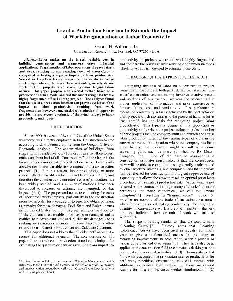
sometime in the future is both part art, and part science. The art of construction cost estimating involves creative means and methods of construction, whereas the science is the proper application of information and prior experience to forecast future costs and productivity. Past performance: records of productivity actually achieved by the contractor on prior projects which are similar to the project at hand, is (or at least should be) the basis for estimating project labor productivity. This typically begins with a production or productivity study where the project estimator picks a number of prior projects that the company built and extracts the actual labor productivity rates for the various types of work in the current estimate. In a situation where the company has little prior history, the estimator might consult a standard estimating guide such as those published by RS Means Company, Inc. One of the baseline assumptions a construction estimator must make, is that the construction crew will be able to complete a task, generally unobstructed by other workers, materials, and equipment, and that the work will be released for construction in a logical sequence and of a quantity that allows the crew to reach an optimal (or at least predictable or estimated) production rate. When work is not released to the contractor in large enough “chunks” to make performing the work economical, we call that “work disruption”[4] resulting in “fragmentation.” Gould [5] provides an example of the trade off an estimator assumes when forecasting or estimating productivity: the larger the quantity of consecutive work a crew will perform, the less time the individual item or unit of work will take to accomplish.

This shape is striking similar to what we refer to as a “Learning Curve.”[6] Oglesby notes that “Learning (experience) curves have been used in industry for many years to give a mathematical means for predicting or measuring improvements in productivity when a process or task is done over and over again.”[7] They have also been applied to the construction field to estimate such things as the final cost of a series of activities. [8, 9] Thomas states that “It is widely accepted that production rates or productivity for performing repetitive construction tasks will improve with additional experience and practice. … There are several reasons for this: (1) Increased worker familiarization; (2)

improved equipment and crew coordination; (3) improved job organization; (4) better engineering support; (5) better day –to-day management and supervision; (6) development of more efficient techniques and methods; (7) development of more efficient material supply systems; and (8) stabilized design leading to fewer modifications and rework.”[6]

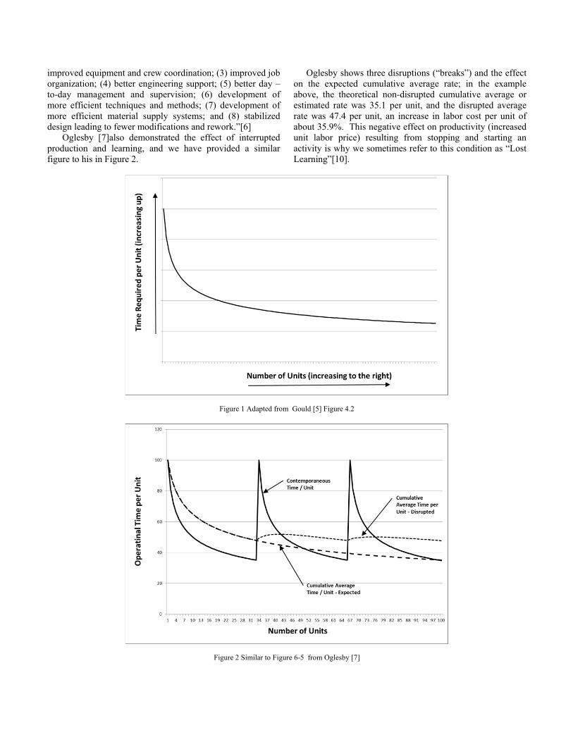
Oglesby [7]also demonstrated the effect of interrupted production and learning, and we have provided a similar figure to his in Figure 2.

Oglesby shows three disruptions (“breaks”) and the effect on the expected cumulative average rate; in the example above, the theoretical non-disrupted cumulative average or estimated rate was 35.1 per unit, and the disrupted average rate was 47.4 per unit, an increase in labor cost per unit of about 35.9%. This negative effect on productivity (increased unit labor price) resulting from stopping and starting an activity is why we sometimes refer to this condition as “Lost Learning”[10].

Figure 1 Adapted from Gould [5] Figure 4.2

Figure 2 Similar to Figure 6-5 from Oglesby [7]

There has been a significant amount of research on Learning Curves and their ability to model costs of repetitive operations in the construction industry. Most recently, Gottlieb and Haughbolle, published a report [11] for the Danish Building Research Institute which was a review of the literature in the field, dating back to the 1930’s. Another significant contribution was Thomas and Smith’s 1990 report on the, “Loss of Labor Productivity Due to Inefficiencies and Disruptions”[12]. Both Gottlieb and Thomas reference a 1965 Economic Commission for Europe study titled “Effects of Repetition on Building Operations and Processes on Site” as probably the first major study on Learning Curves applied to the construction industry. Since that time, much of the Learning Curve research has been directed toward comparing different learning models and deriving proper learning rate variables to certain construction operations [6, 8, 9].

It is nearly universally accepted that “acceleration, delays and disruptions are frequently encountered on construction projects and one of the main reasons for productivity loss” [13]. Thomas lists: “Out-of-sequence work; Interruptions and delays; Long-term delays and remobilizations; Congestion and overcrowding; Restricted access; and, Rework” as six (6) of the eight (8) “Primary Root Causes” “of Productivity Losses”[12]2 He states that, “most authors agree that the effect of out-of-sequence work is very detrimental” and that one researcher “calculated a 75 percent loss of productivity on days when there were work sequencing problems.” All of these factors describe “work fragmentation.” While it may not seem so on the surface, even acceleration, restricted access, and congestion have been found to be highly correlated with the other more generally acknowledged fragmentation variables [14].

Disruptions resulting from an extraordinary number of changes and which cause a reduction in labor productivity, even to non-changed work, was first studied by Leonard[15], with significant contributions by Hanna [16-19], Ibbs [3, 20-23], Moselhi [24, 25] and Thomas[12, 26]. These papers generally deal more with the result of changes impact on labor productivity as opposed to the mechanics of why productivity is reduced. The acknowledged facts are however, that changes cause a disruption in the flow of work, frequently resulting in: delays, ramp-down ramp-up or demobilization and remobilization of workers, rework, and on occasion: acceleration, crowding and trade stacking.

The most widely accepted method for calculating the impact of a disruption is by applying the “Measured Mile” productivity developed by Zink [27, 28]. “A measured-mile inefficiency claim compares the claimant’s productivity in performing work during the claimed or impacted period with the productivity achieved during an un-impacted or least-impacted time period”[29] (see also [4] at §15:116). “The strength of the Measured Mile Approach stems from two

2 The other two “Primary Root Causes” are: Temperature and humidity; and, “Weather events.”

factors. First it relates, or links, actual events in the field to various productivity levels realized on the project. Second, the use of actual productivity data as the baseline eliminates criticisms related to the reasonableness of the contractor’s estimate. By using actual productivity data the contractor is demonstrating productivity levels that he or she actually achieved and presumably could have continued to achieve but for the [disruptions].” [30] Further, “this technique is most effective when the comparison periods are close in time, involve similar types of work, and occur on the same contract” or project. “A good example is comparing productivity levels during the periods in which successive floors of a multi-story office building are constructed.”[31] On rare occasions, a contractor has been allowed to use a measured mile developed from un-impacted work from the same project which was not similar, but related, to the work that was impacted[32]3.

It is generally accepted that the impacted work period should be the exceptional period during a given project not the ordinary; in fact Thomas [33] refers to the impacted period as “the cataclysmic event.” But there is no universal agreement on how long the un-impacted period must be in order to develop a measured mile, though most would agree that a single day’s performance does not qualify as a measured mile.

Adrian provides an example where the measured mile is two thirds of the total performance period[34]. But, as Thomas points out that “finding both an un-impacted and an impacted period can be a formidable challenge” [33] Both Thomas [35] and Ibbs [36] have both pointed out that there are projects which have become so disrupted that a measured mile is virtually impossible to acquire, and both have provided methods for dealing with highly disrupted or fragmented projects. Thomas hypothesized that poor performing projects would exhibit high variability in individual daily or unit productivity, whereas high performing projects would record more consistent unit productivities. His “Baseline Productivity” method utilizes the ten (10) percent of days or other units which have the highest recorded productivity, taking the median of that data as the “Baseline” measured mile. Ibbs counters that, “the basis for using 10% is clearly arbitrary” and that there “is no evidence that 10% of the whole daily productivity is a reasonable or well-accepted percentage to represent the best performance a contractor could achieve.” Ibbs proposes a statistical clustering method (K-means) with two assumed groups and using the median of the upper or higher performing group as the measured mile or baseline productivity. (Note that when the upper cluster is close to 10% of the total data, both Ibbs and Thomas’s methods yield similar results.)

3 Citing: Appeal of P.J. Dick, Incorporated V.A.B.C.A. No. 5597, 01-2 B.C.A. ¶ 3,647 (2001).

Production functions have been used to estimate the costs of a system since first proposed by Knut Wicksell and formalized by economist Paul Douglas and mathematician Charles Cobb, in the early part of the 20th century. The general Cobb-Douglas model:

Y = d*X1α * X2

β (1)

Where “the d, α1 and β

2 are constants for a particular production system.”[37] There are a number of similar mathematical forms of this function which take on a substantially similar form.

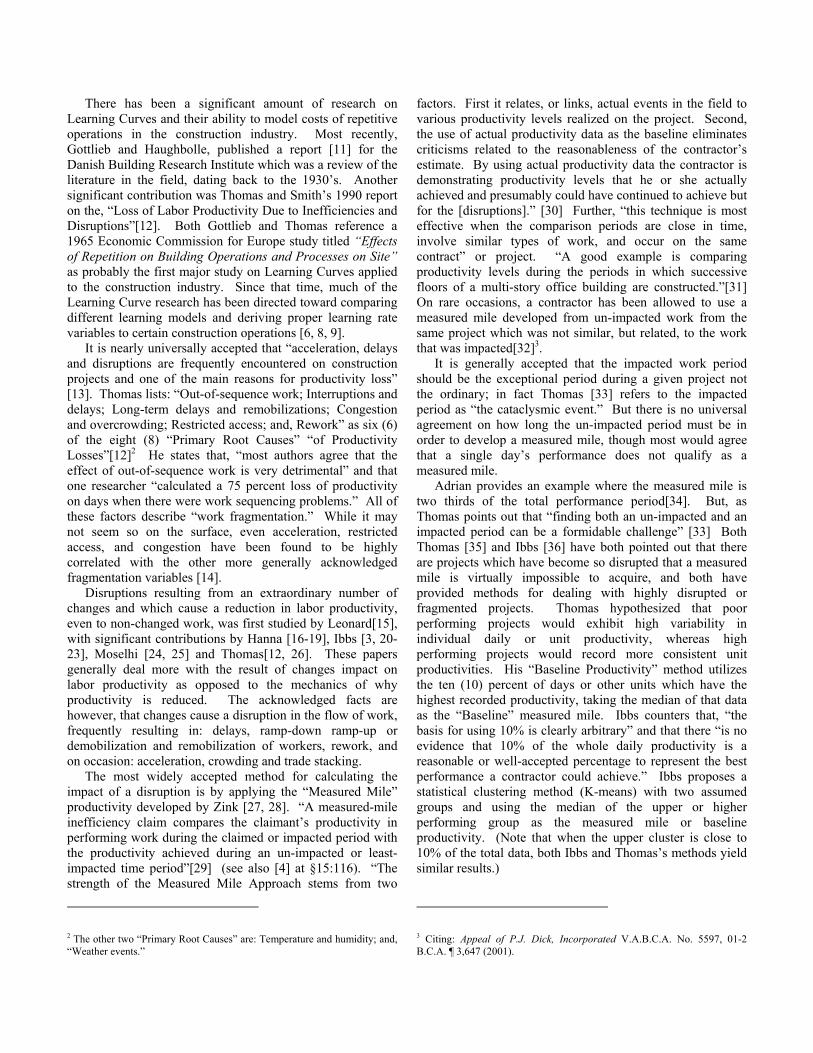
Figure 3 Production Function General Form

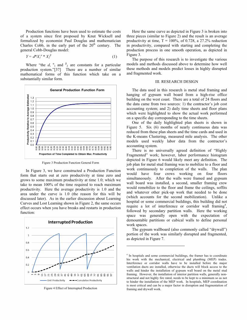
In Figure 3, we have constructed a Production Function form that starts out at zero productivity at time zero and grows to some maximum productivity at time 1.0; which we take to mean 100% of the time required to reach maximum productivity. Here the average productivity is 1.0 and the area under the curve is 1.0 (the reason for this will be discussed later). As in the earlier discussion about Learning Curves and Lost Learning shown in Figure 2, the same occurs effect occurs when you have breaks and restarts in production function:

Figure 4 Effect of Interrupted Production

Here the same curve as depicted in Figure 3 is broken into three pieces (similar to Figure 2) and the result is an average productivity at time, T = 100%, of 0.728, a 27.2% reduction in productivity, compared with starting and completing the production process in one smooth operation, as depicted in Figure 3.

The purpose of this research is to investigate the various models and methods discussed above to determine how well these methods and models predict losses in highly disrupted and fragmented work.

III. RESEARCH DESIGN

The data used in this research is metal stud framing and hanging of gypsum wall board from a high-rise office building on the west coast. There are a total of 24 floors and the data came from two sources: 1) the contractor’s job cost accounting system; and 2) daily time sheets and floor plans which were highlighted to show the actual work performed on a specific day corresponding to the time sheets.

One of the daily highlighted plan sheets is shown in Figure 5. Six (6) months of nearly continuous data was reduced from these plan sheets and the time cards and used in the K-means Clustering, measured mile analysis. The other models used weekly labor data from the contractor’s accounting system.

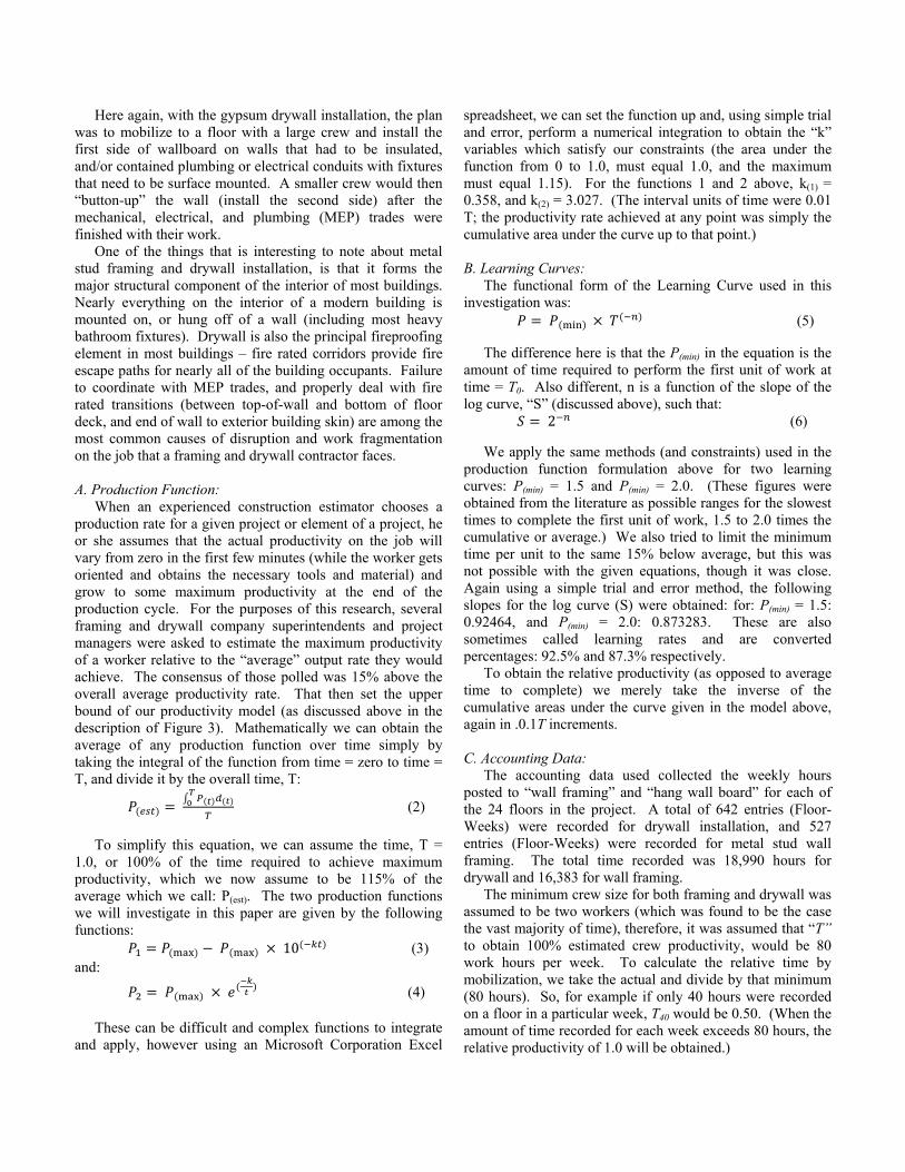
There is no universally agreed definition of “Highly Fragmented” work; however, labor performance histogram depicted in Figure 6 would likely meet any definition. The job plan for metal stud framing was to mobilize to a floor and work continuously to completion of the walls. The plan would have four crews working on four floors simultaneously. After the walls were framed and gypsum wall board was installed, a second, smaller framing crew would remobilize to the floor and frame the ceilings, soffits and whatever other pick-up work that needed to be done (which accounts for the second mobilization). Unlike a hospital or some commercial buildings, this building did not require a lot of interference or corridor wall framing4, followed by secondary partition walls. Here the working space was generally open with the expectation of demountable partitions or cubical walls to define personal work spaces.

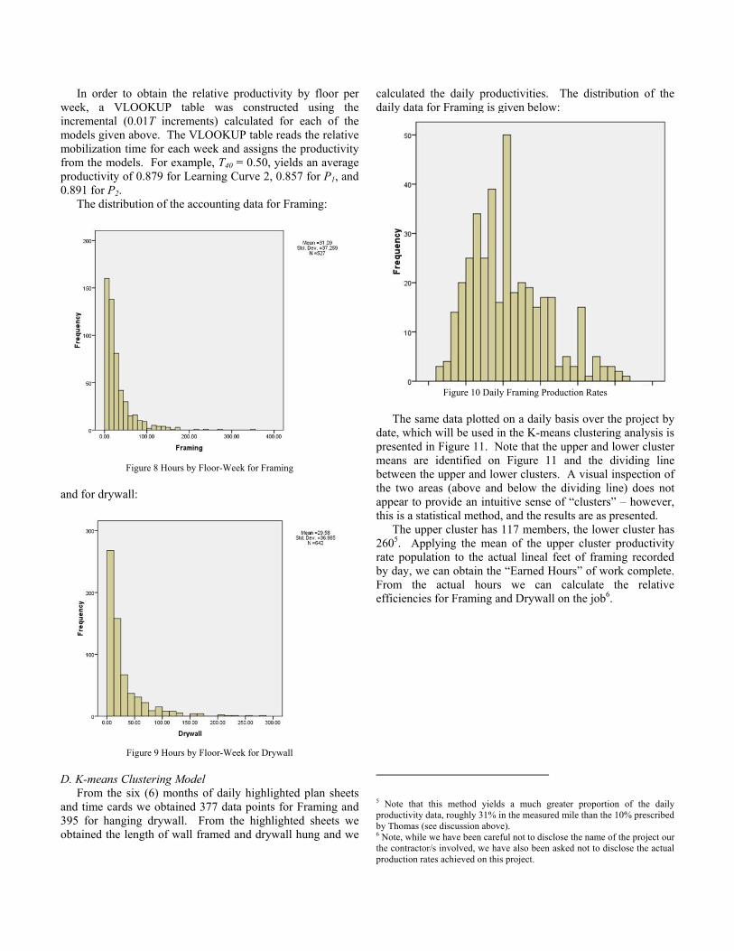
The gypsum wallboard (also commonly called “drywall”) portion of the work was similarly disrupted and fragmented, as depicted in Figure 7.

4 In hospitals and some commercial buildings, the framer has to coordinate his work with the mechanical, electrical and plumbing (MEP) trades. Interference or corridor walls have to be installed before the major ventilation ducts are installed, otherwise the ducts will block access to the walls and hinder the installation of gypsum wall board on the metal stud framing. However, the installation of interior partition walls, generally non-structural and not highly fire rated, needs to be kept to a minimum so as not to hinder the installation of the MEP work. In hospitals, MEP coordination is most critical and can be a major factor in disruption and fragmentation of framing and drywall work.

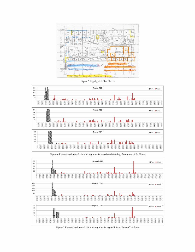
Figure 5 Highlighted Plan Sheets

Figure 6 Planned and Actual labor histograms for metal stud framing, from three of 24 Floors

Figure 7 Planned and Actual labor histograms for drywall, from three of 24 floors

Here again, with the gypsum drywall installation, the plan was to mobilize to a floor with a large crew and install the first side of wallboard on walls that had to be insulated, and/or contained plumbing or electrical conduits with fixtures that need to be surface mounted. A smaller crew would then “button-up” the wall (install the second side) after the mechanical, electrical, and plumbing (MEP) trades were finished with their work.

One of the things that is interesting to note about metal stud framing and drywall installation, is that it forms the major structural component of the interior of most buildings. Nearly everything on the interior of a modern building is mounted on, or hung off of a wall (including most heavy bathroom fixtures). Drywall is also the principal fireproofing element in most buildings – fire rated corridors provide fire escape paths for nearly all of the building occupants. Failure to coordinate with MEP trades, and properly deal with fire rated transitions (between top-of-wall and bottom of floor deck, and end of wall to exterior building skin) are among the most common causes of disruption and work fragmentation on the job that a framing and drywall contractor faces. A. Production Function:

When an experienced construction estimator chooses a production rate for a given project or element of a project, he or she assumes that the actual productivity on the job will vary from zero in the first few minutes (while the worker gets oriented and obtains the necessary tools and material) and grow to some maximum productivity at the end of the production cycle. For the purposes of this research, several framing and drywall company superintendents and project managers were asked to estimate the maximum productivity of a worker relative to the “average” output rate they would achieve. The consensus of those polled was 15% above the overall average productivity rate. That then set the upper bound of our productivity model (as discussed above in the description of Figure 3). Mathematically we can obtain the average of any production function over time simply by taking the integral of the function from time = zero to time = T, and divide it by the overall time, T:

(2)

To simplify this equation, we can assume the time, T =

1.0, or 100% of the time required to achieve maximum productivity, which we now assume to be 115% of the average which we call: P(est). The two production functions we will investigate in this paper are given by the following functions:

10 (3) and:

(4)

These can be difficult and complex functions to integrate and apply, however using an Microsoft Corporation Excel

spreadsheet, we can set the function up and, using simple trial and error, perform a numerical integration to obtain the “k” variables which satisfy our constraints (the area under the function from 0 to 1.0, must equal 1.0, and the maximum must equal 1.15). For the functions 1 and 2 above, k(1) = 0.358, and k(2) = 3.027. (The interval units of time were 0.01 T; the productivity rate achieved at any point was simply the cumulative area under the curve up to that point.) B. Learning Curves:

The functional form of the Learning Curve used in this investigation was:

(5)

The difference here is that the P(min) in the equation is the amount of time required to perform the first unit of work at time = T0. Also different, n is a function of the slope of the log curve, “S” (discussed above), such that:

2 (6)

We apply the same methods (and constraints) used in the production function formulation above for two learning curves: P(min) = 1.5 and P(min) = 2.0. (These figures were obtained from the literature as possible ranges for the slowest times to complete the first unit of work, 1.5 to 2.0 times the cumulative or average.) We also tried to limit the minimum time per unit to the same 15% below average, but this was not possible with the given equations, though it was close. Again using a simple trial and error method, the following slopes for the log curve (S) were obtained: for: P(min) = 1.5: 0.92464, and P(min) = 2.0: 0.873283. These are also sometimes called learning rates and are converted percentages: 92.5% and 87.3% respectively.

To obtain the relative productivity (as opposed to average time to complete) we merely take the inverse of the cumulative areas under the curve given in the model above, again in .0.1T increments. C. Accounting Data:

The accounting data used collected the weekly hours posted to “wall framing” and “hang wall board” for each of the 24 floors in the project. A total of 642 entries (Floor-Weeks) were recorded for drywall installation, and 527 entries (Floor-Weeks) were recorded for metal stud wall framing. The total time recorded was 18,990 hours for drywall and 16,383 for wall framing.

The minimum crew size for both framing and drywall was assumed to be two workers (which was found to be the case the vast majority of time), therefore, it was assumed that “T” to obtain 100% estimated crew productivity, would be 80 work hours per week. To calculate the relative time by mobilization, we take the actual and divide by that minimum (80 hours). So, for example if only 40 hours were recorded on a floor in a particular week, T40 would be 0.50. (When the amount of time recorded for each week exceeds 80 hours, the relative productivity of 1.0 will be obtained.)

In order to obtain the relative productivity by floor per week, a VLOOKUP table was constructed using the incremental (0.01T increments) calculated for each of the models given above. The VLOOKUP table reads the relative mobilization time for each week and assigns the productivity from the models. For example, T40 = 0.50, yields an average productivity of 0.879 for Learning Curve 2, 0.857 for P1, and 0.891 for P2.

The distribution of the accounting data for Framing:

Figure 8 Hours by Floor-Week for Framing

and for drywall:

Figure 9 Hours by Floor-Week for Drywall

D. K-means Clustering Model

From the six (6) months of daily highlighted plan sheets and time cards we obtained 377 data points for Framing and 395 for hanging drywall. From the highlighted sheets we obtained the length of wall framed and drywall hung and we

calculated the daily productivities. The distribution of the daily data for Framing is given below:

Figure 10 Daily Framing Production Rates

The same data plotted on a daily basis over the project by

date, which will be used in the K-means clustering analysis is presented in Figure 11. Note that the upper and lower cluster means are identified on Figure 11 and the dividing line between the upper and lower clusters. A visual inspection of the two areas (above and below the dividing line) does not appear to provide an intuitive sense of “clusters” – however, this is a statistical method, and the results are as presented.

The upper cluster has 117 members, the lower cluster has 2605. Applying the mean of the upper cluster productivity rate population to the actual lineal feet of framing recorded by day, we can obtain the “Earned Hours” of work complete. From the actual hours we can calculate the relative efficiencies for Framing and Drywall on the job6.

5 Note that this method yields a much greater proportion of the daily productivity data, roughly 31% in the measured mile than the 10% prescribed by Thomas (see discussion above). 6 Note, while we have been careful not to disclose the name of the project our the contractor/s involved, we have also been asked not to disclose the actual production rates achieved on this project.

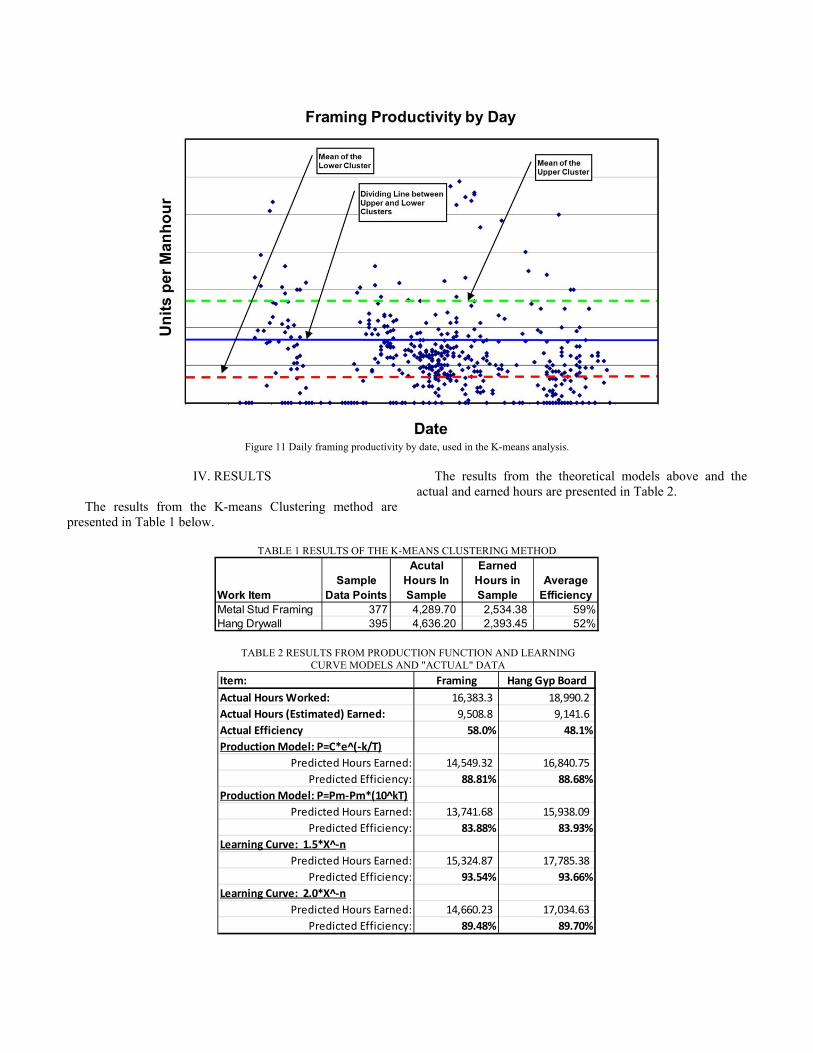
Figure 11 Daily framing productivity by date, used in the K-means analysis.

IV. RESULTS

The results from the K-means Clustering method are

presented in Table 1 below.

The results from the theoretical models above and the actual and earned hours are presented in Table 2.

TABLE 1 RESULTS OF THE K-MEANS CLUSTERING METHOD

TABLE 2 RESULTS FROM PRODUCTION FUNCTION AND LEARNING CURVE MODELS AND "ACTUAL" DATA

Work ItemSample

Data Points

Acutal Hours In Sample

Earned Hours in Sample

Average Efficiency

Metal Stud Framing 377 4,289.70 2,534.38 59%Hang Drywall 395 4,636.20 2,393.45 52%

Item: Framing Hang Gyp Board

Actual Hours Worked: 16,383.3               18,990.2                   

Actual Hours (Estimated) Earned: 9,508.8                 9,141.6                     

Actual Efficiency 58.0% 48.1%

Production Model: P=C*e^(‐k/T)

Predicted Hours Earned: 14,549.32            16,840.75                

Predicted Efficiency: 88.81% 88.68%

Production Model: P=Pm‐Pm*(10^kT)

Predicted Hours Earned: 13,741.68            15,938.09                

Predicted Efficiency: 83.88% 83.93%

Learning Curve:  1.5*X^‐n

Predicted Hours Earned: 15,324.87            17,785.38                

Predicted Efficiency: 93.54% 93.66%

Learning Curve:  2.0*X^‐n

Predicted Hours Earned: 14,660.23            17,034.63                

Predicted Efficiency: 89.48% 89.70%

V. DISCUSSION AND CONCLUSIONS

All of the theoretical models, Production Functions and Learning Curves significantly underestimated the actual impact due to work fragmentation on this project, though the Production Function Model yielded results that were closer to the actual impact than the Learning Curve Model used in this paper. The K-means Clustering method yielded results that were much closer to the actual losses suffered on the project. This does not mean that the mathematical models are not useful at all: it merely means that the underlying assumptions in the models were probably poor. For example, the maximum productivity rates use 115% of the average is obviously disproven by the K-means data. Note in Figure 10, the maximum rate achieved is clearly more than double the average7.

What the Production and Leaning Curve Functions do tell us is that there clearly is an impact, based on the underlying assumptions, but also perhaps, that the more detailed information used in the K-means Clustering method, yielded much better, and more accurate results. (Or at least in this example, yielded results that were closer to the actual efficiencies estimated and witnessed on the project). It is clear that the variables and constraints assumed and derived in the theoretical models needs additional examination.

In construction productivity impact claims, particularly those that are adjudicated in US courtrooms, it is always best to use as many methods for estimating labor inefficiency. However, no matter what the analyst calculates as the contractor’s damages (due to inefficiency resulting from disruption and fragmentation), the maximum he normally can recover is limited to his actual losses. For that reason, it is often times best to calculate the Adjusted or Modified Total Cost Method, which should capture all of the contractor’s losses8 as another comparison.

The next step in these analyses should be to refine the assumptions and constraints used in the previous analyses and recalculate the losses using the revised models. Hopefully these will better reflect the actual losses suffered by construction contractors on projects where work releases and other disruptions and delays cause the work to be highly fragmented.

REFERENCES

[1] W. Schwartzkopf, Calculating lost labor productivity in construction

claims. New York: Wiley, 1995. [2] D. F. McDonald and J. G. Zack, "Estimating Lost Labor Productivity in

Construction Claims," AACE International April 13, 2004 2004.

7 Here again we have cut-off the actual productivity numbers, but the high productivity was actually 2.5 times the mean, and about 3 standard deviations from the mean. 8 The ATCM is not discussed in this paper, however it is discussed in detail in "Impact to Productivity in Steel Framing and the Installation and Finishing of Gypsum Wallboard," Northwest Wall & Ceiling Bureau © 2009.

[3] W. Ibbs, L. D. Nguyen, and S. Lee, "Quantified impacts of project change," Journal of Professional Issues in Engineering Education and Practice, vol. 133, pp. 45-52, 2007.

[4] P. L. Bruner and P. J. O'Connor, Bruner & O'Connor on CONSTRUCTION LAW, vol. 5, 1st ed. Danvers, MA: West Group, 2002, 2010.

[5] F. E. Gould, Managing the Construction Process: Estimating, Scheduling, and Project Control, 3rd ed. Upper Saddle River, NJ: Pearson Prentice Hall, 2005.

[6] H. R. Thomas, C. T. Matthews, and J. G. Ward, "Learning Curve Models of Construction Productivity," Journal of Construction Engineering and Management, vol. 112, pp. 16, 1986.

[7] C. H. Oglesby, H. W. Parker, and G. A. Howell, Productivity Improvement in Construction: Mcgraw-Hill, 1989.

[8] J. G. Everett and S. H. Farghal, "Learning Curve Predictors for Construction Field Operations," Journal of Construction Engineering and Management, vol. 120, 1994.

[9] S. H. Farghal and J. G. Everett, "Learning Curves: Accuracy in Predicting Future Performance," Journal of Construction Engineering and Management, vol. 123, pp. 5, 1997.

[10] D. A. Norfleet, "Loss of learning in disruption claims," presented at 2004 AACE International Transactions - 48th AACE International Annual Meeting, Washington, DC, United States, 2004.

[11] S. C. Gottlieb and K. Haugbolle, "The repetition effect in building and construction works: A literature review," in SBi 2010:03 Aalborg Municipality, Denmark: SBi, Statens Byggeforskningsinstitut 2010.

[12] H. R. Thomas and G. R. Smith, "Loss of Construction Labor Productivity Due to Inefficiencies and Disruptions: The Weight of Expert Opinion.," The Pennsylvania Transportation Institute 1990b.

[13] W. Ibbs and M. Liu, "System Dynamic Modeling of Delay and Disruption Claims," Cost Engineering, vol. 47, 2005.

[14] G. H. Williams and T. R. Anderson, "Impact to Productivity in Steel Framing and the Installation and Finishing of Gypsum Wallboard," Northwest Wall & Ceiling Bureau, Seattle, WA August 2009 2009.

[15] C. Leonard, "The Effect of Change Orders on Productivity," Concordia University, Montreal, Quebec, Canada 1987.

[16] A. S. Hanna, R. Camlic, and P. A. Peterson, "Cumulative Effect of Project Changes for Electrical and Mechanical Construction," Journal of Construction Engineering and Management, vol. 130, pp. 762-71, 2004.

[17] A. S. Hanna, R. Camlic, P. A. Peterson, and E. V. Nordheim, "Quantitative definition of projects impacted by change orders," Journal of Construction Engineering and Management, vol. 128, pp. 57-64, 2002.

[18] A. S. Hanna, J. S. Russell, T. W. Gotzion, and E. V. Nordheim, "Impact of change orders on labor efficiency for mechanical construction," Journal of Construction Engineering and Management, vol. 125, pp. 176-184, 1999a.

[19] A. S. Hanna, J. S. Russell, E. V. Nordheim, and M. J. Bruggink, "Impact of change orders on labor efficiency for electrical construction," Journal of Construction Engineering and Management, vol. 125, pp. 224-232, 1999b.

[20] C. W. Ibbs, "The Cumulative Impact of Change of Construction Productivity," in The Challenges of Lost Productivity: Proving and Quantifying a Claim

Bethesda, MD: ConstructionClaims.com, 2008, pp. 1-6. [21] C. W. Ibbs and W. E. Allen, "Quantitative impacts of project change,"

in Construction Industry Institute. Austin, Texas: University of Texas at Austin, 1995.

[22] W. Ibbs, "Quantitative Impacts of Project Change: Size Issues," Journal of Construction Engineering and Management, vol. 123, pp. 308-311, 1997.

[23] W. Ibbs, "Impact of change's timing on labor productivity," Journal of Construction Engineering and Management, vol. 131, 2005.

[24] O. Moselhi, I. Assem, and K. El-Rayes, "Change orders impact on labor productivity," Journal of Construction Engineering and Management, vol. 131, pp. 354-359, 2005.

[25] O. Moselhi, C. Leonard, and P. Fazio, "Impact of change orders on construction productivity," Canadian Journal of Civil Engineering, vol. 18, pp. 484-492, 1991.

[26] H. R. Thomas and C. L. Napolitan, "Quantitative effects of construction changes on labor productivity," Journal of Construction Engineering and Management, vol. 121, pp. 290-296, 1995.

[27] D. A. Zink, "Measured mile: Proving construction inefficiency costs," Cost Engineering, vol. 28, pp. 19-21, 1986.

[28] D. A. Zink, "Impacts and construction inefficiency," Cost Engineering, vol. 32, pp. 21-23, 1990.

[29] S. B. Shapiro, B. R. Philips, D. D. Haire, and C. A. Feeley, "Pricing of Claims," in Federal Government Construction Contracts, M. A. Branca, A. L. Bastianelli, A. D. Ness, and J. D. West, Eds., 2nd ed. Chicago, Ill: American Bar Association, 2010, pp. 571-608.

[30] R. F. Cushman, C. J.D., P. J. Gorman, and D. F. Coppi, Construction Disputes: Representing the Contractor, 1st ed. New York, NY: Aspen Publishers, Inc., 2001.

[31] J. M. Wickwire, T. J. Driscoll, S. B. Hurlbut, and S. B. Hillman, Construction Scheduling: Preparation, Liability, and Claims, 2nd ed. New York, NY: Wolters Kluwer, 2003.

[32] J. W. Ralls and O. J. Shean, "Hard Hat Case Notes," Construction Lawyer, Journal of the Fourm on the Construction Industy, vol. 22, pp. 1, 2002.

[33] H. R. Thomas, "Resultant Injury and the Measured Mile," in The Challenges of Lost Productivity: Proving and Quantifying a ClaimBethesda, MD: ConstructionClaims.com, 2008, pp. 29-31.

[34] J. J. Adrian, Construction Claims: A Quantitative Approach. Champaign, Illinois: Stripes Publishing L.L.C., 1993.

[35] H. R. Thomas, "Construction Baseline Productivity: Theory and Practice," Journal of Construction Engineering & Management, vol. 125, pp. 295-303, 1999.

[36] W. Ibbs and M. Liu, "Improved measured mile analysis technique," Journal of Construction Engineering and Management, vol. 131, pp. 1249-1256, 2005.

[37] J. J. Adrian, Quantitative Methods in Construction Management. New York, NY: American Elsevier Publishing Company, Inc., 1973.