US Coast Guard Research and Development Center - DTIC

U.S. Coast Guard Research and Development Center 1082 Shennecossett Road, Groton, CT 06340-6096

Report No. CG-D-04-00

EFFECTS OF WEATHERING ON THE FLAMMABILITY OF OILS

^tfJ>. FINAL REPORT

SEPTEMBER 1999

This document is available to the U.S. public through the National Technical Information Service, Springfield, VA 22161

Prepared for:

U.S. Department of Transportation United States Coast Guard

Marine Safety and Environmental Protection (G-M) Washington, DC 20593-0001

DwcQrjALITyiNSPBClEDj 20000417 184

NOTICE

This document is disseminated under the sponsorship of the Department of Transportation in the interest of information exchange. The United States Government assumes no liability for its contents or use thereof.

The United States Government does not endorse products or manufacturers. Trade or manufacturers' names appear herein solely because they are considered essential to the object of this report.

This report does not constitute a standard, specification, or regulation.

Marc B. Mandler, Ph.D. Technical Director United States Coast Guard Research & Development Center 1082 Shennecossett Road Groton, CT 06340-6096

n

"echnical Report Documentation Page I.Report No.

CG-D-04-00

2. Government Accession Number 3. Recipient's Catalog No.

4. Title and Subtitle

EFFECTS OF WEATHERING ON THE FLAMMABILITY OF OILS

5. Report Date

SEPTEMBER 1999

6. Performing Organization Code

Project No. 4120.6.3

7. Author(s)

Robert K. Jones

8. Performing Organization Report No.

R&DC-33-99 9. Performing Organization Name and Address

National Oceanic and Atmospheric Administration 7600 Sand Point Way, NE Seattle, Washington 98115

U.S. Coast Guard Research and Development Center 1082 Shennecossett Road Groton, CT 06340-6096

10. Work Unit No. (TRAIS)

11. Contract or Grant No.

DTCG39-98-XE00266

12. Sponsoring Organization Name and Address

U.S. Department of Transportation United States Coast Guard Marine Safety and Environmental Protection (G-M)

Washington, DC 20593-0001

13. Type of Report & Period Covered

Final

14. Sponsoring Agency Code Commandant (G-MSO) U.S. Coast Guard Headquarters Washington, DC 20593-0001

15. Supplementary Notes The R&D Center's technical point of contact is Mr. Kenneth Bitting, 860-441-2733, email: [email protected].

16. Abstract (MAXIMUM 200 WORDS)

Many crude oils and fuel oils are flammable and pose a significant fire hazard if not handled properly. When an oil is accidentally spilled and exposed to the environment, the flammability characteristics of the oil can change significant: y as it evaporates. A numerical weathering model that simulates the weathering and consequent changes in flammability was developed. The time required for a representative group of flammable oils to weather to a non-flammable state under various spill conditions was estimated. The effects of the level of mixing caused by environmental factors were closely examined.

Results of simulations indicate that flammable crude oils weather very slowly when there are no natural mixing mechanisms at work. In these cases weathering times are very sensitive to the thickness of the oil. In contrast, if there are effective mechanisms for mixing the oil, it weathers much more quickly and the weathering time is less sensitive to thickness.

Simulations indicate that flammable fuel oils are less likely to become non-flammable during weathering. Weathered gasoline remains flammable until it is almost completely evaporated.

17. Keywords

petroleum, oil spill, flammability, flash point, evaporation

18. Distribution Statement

This document is available to the U.S. public through the National Technical Information Service, Springfield, VA 22161

19. Security Class (This Report)

UNCLASSIFIED

20. Security Class (This Page)

UNCLASSIFIED 21. No of Pages 22. Price

111

[ This page intentionally left blank. ]

IV

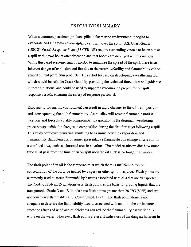
EXECUTIVE SUMMARY

When a common petroleum product spills in the marine environment, it begins to

evaporate and a flammable atmosphere can form over the spill. U.S. Coast Guard

(USCG) Vessel Response Plans (33 CFR 155) require responding vessels to be on site at

a spill within two hours after detection and that booms are deployed within one hour.

While this rapid response time is needed to minimize the spread of the spill, there is an

inherent danger of explosion and fire due to the natural volatility and flammability of the

spilled oil and petroleum products. This effort focused on developing a weathering tool

which would benefit the Coast Guard by providing the technical foundation and guidance

in these situations, and could be used to support a rule-making project for oil spill

response vessels, ensuring the safety of response personnel.

Exposure to the marine environment can result in rapid changes to the oil's composition

and, consequently, the oil's flammability. An oil slick will remain flammable until it

weathers and loses its volatile components. Evaporation is the dominant weathering

process responsible for changes in composition during the first few days following a spill.

This study employed numerical modeling to examine how the evaporation and

flammability characteristics of some representative flammable oils change after a spill in

a confined area, such as a boomed area in a harbor. The model results predict how much

time must pass from the time of an oil spill until the oil slick is no longer flammable.

The flash point of an oil is the temperature at which there is sufficient airborne

concentration of the oil to be ignited by a spark or other ignition source. Flash points are

commonly used to assess flammability hazards associated with oils that are transported.

The Code of Federal Regulations uses flash points as the basis for grading liquids that are

transported. Grade D and E liquids have flash points greater than 26.7°C (80°F) and are

not considered flammable (U.S. Coast Guard, 1997). The flash point alone is not

adequate to describe the flammability hazard associated with an oil in the environment,

since the effects of wind and oil thickness can reduce the flammability hazard for oils

while on the water. However, flash points are useful indicators of the dangers inherent in

v

handling oils recovered from a spill. If the flash point of an oil is below the ambient

temperature, the vapors in a vessel containing the oil may form a fuel-air mixture that can

be ignited by a spark or other ignition source.

The numerical model developed for this study was specially constructed for oil slicks

confined by booms and in fairly calm waters (i.e., in a harbor.) This model was used to

simulate oil evaporation and flash point changes for cases where sufficient mixing from

wind and sea occurs to keep the oil homogeneous (well-mixed oils), and for cases where

there was no mixing and the conditions are calm. These represent the extremes of mixing

that possibly occur in a spill and bound the operational conditions. The time required for

some representative flammable oils to weather to Grade D, flash point reaching or

exceeding 26.7°C (80°F), were computed for various conditions of mixing, temperature,

and slick thickness. The weathering of five flammable crude oils and gasoline were

modeled. It was not necessary to model diesel fuel since it is not a flammable liquid in

an unweathered state. The weathering times were generally very sensitive to the

thickness and to the level of mixing.

All five stratified crude oils thicker than one centimeter, except Avalon at 30°C, were

predicted to take over 100 hours to weather to Grade D. In contrast, the same five crude

oils under well-mixed conditions weathered to Grade D in less than three hours. This

study indicated that flammable crude oils in thick slicks under calm conditions lose their

volatile components very slowly and remain flammable for days following a spill. Crude

oils that spread thin in open-water spills, or those effectively mixed by wave action, lose

their volatile components in a matter of hours.

For gasoline, this study predicted that even after most of the gasoline evaporates, it

remains a flammable mixture. Given the uncertainties in the models and the variability

of gasolines, it seems prudent to treat all weathered gasolines as flammable liquids.

The results of the information obtained in this study will be used to write standards for

classifying oil spill response vessels that work in flammable atmospheres during various

types of fuel or oil spills. This information indicates how long various crude oils, diesel

VI

and gasoline are flammable or explosive after the spill, and therefore, how much

precaution must be taken in vessel design to preclude explosions, ignition or fire when

the vessel is exposed to vapors.

Vll


Vlll

TABLE OF CONTENTS

SYMBOLS x

1.0 INTRODUCTION 1

2.0 BACKGROUND 2

3.0 MODEL DEVELOPMENT 6

4.0 SELECTION OF OILS AND SPILL CONDITIONS 10

5.0 RESULTS AND DISCUSSION 12

6.0 UNCERTAINTY ANALYSIS 15

7.0 CONCLUSIONS 17

8.0 RECOMMENDATIONS 18

REFERENCES 23

APPENDIX A: FINITE DIFFERENCE FORMULATION A-l

APPENDIX B: SERIES SOLUTION TO THE DIFFUSION EQUATION B-l

APPENDIX C: PROPERTY DATA FOR OILS C-l

IX

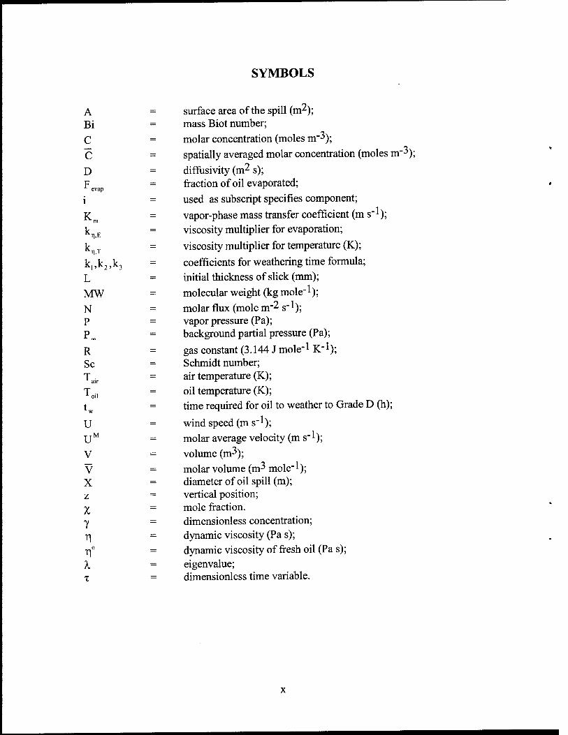
SYMBOLS

A = surface area of the spill (m2); Bi = mass Biot number; C = molar concentration (moles m"3); C = spatially averaged molar concentration (moles m'3);

D = diffusivity (m^ s); F = fraction of oil evaporated;

evap *

i = used as subscript specifies component;

K = vapor-phase mass transfer coefficient (m s" *); k E = viscosity multiplier for evaporation;

k T = viscosity multiplier for temperature (K);

k, ,k2 ,k3 = coefficients for weathering time formula; L = initial thickness of slick (mm); MW = molecular weight (kg mole-1);

N = molar flux (mole m"2 s~l); P = vapor pressure (Pa); P^ = background partial pressure (Pa);

R = gas constant (3.144 J mole- * K" *); Sc = Schmidt number; Tair = air temperature (K); Toil = oil temperature (K); t w = time required for oil to weather to Grade D (h);

U = wind speed (ms-*); UM = molar average velocity (ms"1); V = volume (m^); V = molar volume (m^ mole"!); X = diameter of oil spill (m); z = vertical position; % = mole fraction. -y = dimensionless concentration; r\ - dynamic viscosity (Pa s); t]° = dynamic viscosity of fresh oil (Pa s); X = eigenvalue; x = dimensionless time variable.

1.0 INTRODUCTION

The U.S. Coast Guard (USCG) plays a central role in managing the emergency response to, and

mitigation of, marine oil spills. Many of the crude oils and refined products involved in spills

are flammable and pose a serious fire hazard if suitable precautions in handling and storage are

not used. The USCG classifies oils according to their flammability characteristics, and

establishes guidelines and regulations for response vessels with regard to their suitability for

handling petroleum products (USCG, 1997).

Fuel oils and crude oils are the most common petroleum products spilled in the marine

environment. In storage and transport their composition and flammability properties can be

readily characterized to ensure compatibility with the vessels used to transport them; however,

following a spill an oil's composition and flammability characteristics can change rapidly.

Highly flammable oils can lose their volatile components and become less hazardous after being

exposed to the environment. This "stabilization" with regard to flammability can happen quickly

in spills where there are no confining structures to limit the spread of the oil; once the oil spreads

to submillimeter thicknesses, the weathering processes that stabilize the oil are fast. However,

spills that occur in harbors or other areas where the oil is kept from freely spreading may weather

much more slowly.

Though the weathering processes for oils involved in open-water spills has been studied

extensively, very little work has been devoted to understanding the weathering and consequent

evolution of the flammability characteristics of confined thick oil spills. This study was

designed to examine how the flammability characteristics of volatile crude oils and some select

fuel oils evolve with time following spills in confined areas. This information may be used as

part of the technical basis for setting design and operation standards for oil spill response vessels

involved in recovering flammable oils.

No attempt was made to simulate the weathering of all transported flammable oils, rather a small

representative sample of oils were chosen for case studies. The behavior of these oils can

provide some insight into how other flammable oils will behave, and has implications for

precautions that should be taken when handling oils.

2.0 BACKGROUND

Alkanes are the dominant constituents of crude oils (Speight, 1980). The chemical model of

combustion of alkanes provides a useful way to conceptualize how oils burn. Alkanes are

molecules containing carbon and hydrogen atoms linked by single bonds only. The combustion

reaction of an alkane molecule containing n carbon atoms consumes a number of oxygen

molecules defined by the stoichiometric ratio and yields carbon dioxide and water:

C„H2n+2 3n + ln

+ —z—O? -» nC02+(n + l)H20. (1)

Generally, this reaction can only occur in the gas phase, since the reactants must mix at the

molecular level. The ability of a liquid petroleum oil to ignite and sustain a combustion depends

on the ratio of fuel to oxygen in the air; this depends on how much of the fuel can vaporize and

the confinement of the vapors. The vapor concentration must meet or exceed the "lean limit of

flammability" (LLF) to be ignited (Kanury, 1995).

At any given temperature the vapor-phase concentration cannot exceed the saturation

concentration, which is the maximum concentration allowed thermodynamically. Generally, the

saturation concentration of a volatile liquid decreases sharply as the temperature decreases. So

even in cases where the vapors are confined, such as a closed-cup flash point tester, the fluid will

not burn if the temperature is so low that the saturation concentration falls below the LLF.

(There are some exceptions to this rule, notably when the liquid is in the form of an aerosol.)

One way to ensure that a liquid does not burn accidentally is to guarantee the temperature is low

enough to keep the saturation concentration below the LLF.

LLFs for many chemicals have been measured and compiled (Kanury, 1995). For small

hydrocarbons, the LLF is reached when the molar ratio of fuel to air is about 1:100. For these

chemicals the problem of determining whether a chemical can burn in a confined environment

can be reduced to determining the saturation concentration. A more common method for

evaluating whether a liquid poses a flammability hazard bypasses the examination of the LLF

and saturation concentration, and relies on a direct observation of combustion. Flash point

devices are designed to detect the temperature at which there is a possibility that the airborne

concentration of fuel is sufficient to sustain a flame. Since flash points are defined by a

measurement protocol, they can vary significantly from method to method. A closed-cup flash

point is approximately the temperature at which the saturation concentration equals the LLF

(Kanury, 1995).

Flash point measurements for chemical mixtures, such as crude oils, can be problematic. As an

oil is heated in a flash point device some of the volatile chemicals can be vaporized and lost; by

the time the flash point is reached the composition of the sample may have changed significantly.

In addition, if there is no mechanism for stirring the sample, the surface of the sample, which

determines the concentration in the vapor phase, may be depleted of volatiles and no longer be

representative of the bulk composition. Despite the inherent difficulties in measuring flash

points, they are indicators of whether an oil stored in a closed tank poses a threat of combustion

or explosion, and are used in Federal regulations as the basis for characterizing crudes and fuel

oils. Grade D oils have a flash point greater than 26.7°C (80°F) (USCG, 1997).

There have been many efforts to predict flash points from composition or other properties of a

sample. The estimation methods for flash points of pure substances and mixtures fall into two

categories: those based on boiling point; and those based on composition. The former correlate

flash point with the boiling point and have been proposed for pure substances (Li & Moore,

1977; Patil, 1988; Sayanarayana & Kakati, 1991), and for petroleum distillates (Factory Mutual

Engineering Corporation, 1967). Compositional methods are based on the concentrations and

properties of the individual constituents and have been used for petroleum mixtures, commonly

middle distillates (Wickey & Chittenden, 1963; Lenoir, 1975; Butler et al, 1956). The key

constituents for oils with low flash points are the low molecular weight compounds, those

compounds generally contain fewer than nine carbon atoms.

It should be noted that flash points are less useful in assessing the flammability hazard associated

with oils that are not contained in closed vessels. For unconfined spills the effects of wind and

thickness can be as important as the flash point in assessing the flammability hazard associated

with the spill. For oils with flash points below the ambient temperature, the presence of wind

disperse the vapors and prevent ignition (Murad et al., 1970). Furthermore, when a slick

preads to a thickness on the order of 0.5 millimeter, as would be expected in unconfined spills,

oils with very low flash points do not pose a flammability hazard (Stensaas, 1992).

can

s

even

After oil is released into a marine environment it immediately starts to change. Evaporation is

the dominant process affecting the composition of the floating oil during the first week of a spill

(Fingas, 1995) The low molecular weight (lighter) compounds are more volatile and evaporate

more quickly than the heavier compounds. With progressive evaporation the oil composition

changes and, as a result, its physical properties can change dramatically. Any attempt to estimate

the time-evolution of flash point depends critically on the ability to predict the evaporation.

Many oil evaporation models have been proposed during the last 30 years (Fingas, 1995). The

model proposed by Mackay and Matsugu (1973) has provided the foundation of most of the

subsequent models. Their model incorporated many of the fundamental tenets of the evaporation

theory described by Dalton in 1802 (Brutsaert, 1982). Mackay and Matsugu recognized that

since oil is a multi-component mixture, the evaporation rate could be limited by diffusion within

the liquid phase or by diffusion in the vapor phase above the pool. However, their model

incorporated a vapor-phase diffusion mechanism only and effectively assumed that the liquid

phase remains homogenous. This so-called "well-mixed" condition has been used in most oil

spill evaporation models to date. The model described the evaporative flux as a simple function

of a vapor-phase mass transfer coefficient, Km, which characterizes the diffusion in the vapor

phase, and the difference between the vapor pressure of the oil (P) and the natural background

partial pressure of the oil (P«,),

1 dN_ K^P-Pj (2)

A'dt R-Tair

The natural background pressure of the oil is usually considered negligible.

The application of this model has largely followed two general approaches. So-called pseudo-

component models approximate the oil as an ideal mixture of a relatively small number of

components. Commonly, a volume flux is used to describe the evaporation of the im component,

1 dV;_ K.rV,-x.-P, A dt R.T,. ' *■ )

The total evaporative flux is set equal to the sum of the fluxes of the individual components.

Payne and coworkers (Payne et al., 1984) created a pseudo-component model that has been used

by the National Oceanic and Atmospheric Administration (NOAA) and the U.S. Mineral

Management Service. Payne also proposed mechanisms that could account for the mechanical

mixing of oils for open-water spills, providing some justification for imposing a well-mixed

condition. Jones (1997) developed a simplified version of a pseudo-component model that will

be incorporated into the next version of ADIOS, a comprehensive oil weathering model

developed by NOAA (Lehr et al., 1997).

Stiver and Mackay (1984) proposed a different approach that has been widely used and is

referred to as the Analytical Model. The oil is treated as a single substance with a vapor pressure

that varies with the fraction evaporated. In this approach only one equation needs to be solved

and it can usually be solved analytically,

Recently, a conceptually different approach based on small-scale laboratory measurements has

been proposed by Fingas (1996). In a break with the fundamentals proposed in earlier models,

Fingas proposed that the evaporation of oil is not limited by diffusion processes in the vapor

phase and can be described by equations that are a function of temperature and time alone. He

developed a series of evaporation prediction equations for specific oils based on laboratory

measurements.

Thibodeaux used a two-resistance mass-transfer model that accounts for diffusion in both the

liquid and gas phases to model the loss of volatile chemicals from thick waste oil ponds

(Thibodeaux & Carver, 1997). The method employed an overall mass transfer coefficient

constructed from the mass transfer coefficients in the individual phases. Such methods are

commonly used in modeling chemical manufacturing processes but are generally not used for

marine oil spills.

3.0 MODEL DEVELOPMENT

A numerical model was developed and used to simulate the change in flash point of an oil

following a marine spill. Specifically, the model was designed to find the time required for the

flash point to reach or exceed 26.7 °C (80 °F). Once the flash point is above this temperature,

the liquid is no longer defined as a "flammable liquid" under Coast Guard regulations (USCG,

1997). The model was intended to capture the dominant effects of weathering on oils spilled in

protected and confined areas, such as boomed areas in harbors. Accidental spills of this type

might occur during fueling, transfer of crude oil cargo, or a collision in a harbor. In such cases,

the compositional changes of the oil over the first week can be attributed almost entirely to

evaporation. This model did not include effects from many of the weathering processes that can

be significant in open water spills where the oil can be subjected to high winds and breaking

waves.

As noted above, the evaporation of an oil involves two diffusive processes: the diffusive

migration of constituent chemicals through the liquid phase to the surface of the oil where they

quickly migrate to the air directly over the surface; and the gas-phase diffusion of the chemicals

away from the surface. The latter is dominated by the turbulent mixing caused by the wind. For

this study a pseudo-component evaporation model was developed that includes the effects of the

both liquid-phase and gas-phase diffusion. This model was used to predict the changes in

composition of some representative oils as they weather. An established correlation (Butler et

al., 1956) was used to determine the flash point from composition.

The pseudo-component evaporation model developed for this study treats the oil as a mixture of

a relatively few distinct constituents. Since crude oils can contain thousands of distinct chemical

compounds, this approach groups a large number of compounds as a single component with a

distinct set of physical properties. The construction of the pseudo-components follows the form

of the data collected using distillation methods. Oil is commonly characterized through a

conventional distillation procedure such as the ASTM D86 method or gas Chromatographie

methods that simulate a conventional distillation (ASTM, 1995). As the oil undergoes a

fractional distillation, the volume and boiling point of the distillate are measured.

The model developed for this study uses the same methodology for constructing pseudo-

components as that which will be used in the next version of ADIOS (Jones, 1997) Each volume

fraction collected between consecutive temperature measurements was considered a component.

The boiling points of the components were equated to the average of the bounding temperature

measurements. The vapor pressures of the components at ambient temperature were derived

from their boiling points using Antoine's equation (Lyman et al., 1990). The molecular weights

and molar volumes of the components were based on boiling point correlations for a series of

alkanes from butane to eicosane.

The oil was assumed to be a slick of uniform thickness floating on water, and confined to an area

that is not changing in time. Transport was limited to the direction normal to the surface of the

water. Each pseudo-component within the oil was governed by the advection-diffusion equation

in one dimension:

ac, d% a(uM-c,) 8t ' dz2 dz '

The second term on the right hand side was neglected since advection was insignificant in this

study. The flux at the oil-water interface was assumed to be insignificant. This interface was

used to define the zero of the z axis, so the flux at z=0 was set to zero,

^(0,t)=0. (5) dz

At the oil-air interface the diffusive flux in the oil was matched to the evaporative flux. The

expression for the evaporative flux is consistent with the work of Mackay & Matsugu (1973),

Payne et al. (1984), and Jones (1997) and is given by the right hand side of the following

equation:

n^ftA - K--',P'I C|(L't) I (6) D'8z(L'0 - R-T„ lEc/UOJ (<"

Since the evaporative flux depends on the sum of the concentrations at the surface, the diffusion-

advection equations for the individual pseudo-components were coupled through the boundary

condition at the oil-air interface.

The value of the gas-phase mass transfer coefficient was based on the work of Mackay and

Matsugu (Mackay & Matsugu, 1973),

Km. = 0.0048 • l/9 • X/9 ■ Sc^. (7)

The value used for the liquid-phase diffusivity, Df, depended upon the specific implementation of

the model. In cases where the molecular diffusivity was used, it was based on an estimation

method of Wilke and Chang (Hines & Maddox, 1985)

5.864 ■ltr'7MWi1/2Tnn m

Since the viscosity of the oil is very sensitive to the temperature, the molecular diffusivity is also

strongly dependent on the temperature. The Andrade correlation (Reid et al., 1977) was used to

determine the viscosity of the oil at the ambient temperature:

In ( \

- kn/r f_L___L^ V i oil,2 ^ oil, 1 ^

(9)

The reference viscosity and the proportionality constant, kn T, were based on measured values

compiled by the Emergencies Science Division of Environment Canada (Jokuty et al., 1996).

The viscosity can increase by orders of magnitude as an oil evaporates. Consequently, the

molecular diffusivity can decrease significantly with increasing evaporation. This relationship

between viscosity and fraction of oil evaporated was described by a exponential function

(Mackayetal, 1983):

r^Tfe1^"*. (10)

The proportionality constant, kn E, was based on measured values compiled by Environment

Canada (Jokuty et al., 1996).

The evaporation model provided the basis for estimating the composition of the oil as a function

of time. A correlation derived for middle distillate petroleum products (Butler et al., 1956) was

used to predict the flash point in the oil based on composition. The vapor pressures of the

components, Pj, are functions of temperature. The flash point is the temperature at which the

following equality holds, and was solved implicitly:

I^/ci(z,tw)dz) > 1 MWi.:pi

L — =104.7. (11)

X 1 Jc^t^z L«

Determining the composition and flash point of an oil as it evaporates involved solving the

coupled set of advection-diffusion equations with time-dependent diffusivity and auxiliary

conditions, one for each pseudo-component. A backward-time, centered-space finite difference

formulation (Hoffman, 1992) of the coupled diffusion-advection equations was implemented and

solved on a personal computer. At the end of each time step, a spatially averaged liquid-phase

diffusivity and the total molar concentration at the oil-air interface were computed for use in the

subsequent time step. See Appendix A for details.

4.0 SELECTION OF OILS AND SPILL CONDITIONS

The selection of crude oils for this study was based on measured flash points, the completeness

of physical property data, and the perceived quality of the data. Only oils with measured flash

points below 26.7 °C (80°F) were considered. The estimation method developed for this study

required distillation data and viscosities as a function of temperature and fraction evaporated.

The database of oil properties compiled by Environment Canada (Jokuty et al., 1996) is the most

extensive source of data of this type, so the search was narrowed to oils from this database.

Data quality was difficult to assess. Since flash points of oils depend critically on the most

volatile constituents, oils with closely spaced distillation cuts at the low-temperature end of the

range were selected. To eliminate any errors from mixing data from two different samples from

the same well, oils with data collected from different labs were eliminated. Only 21 oils in the

Environment Canada database satisfied all these conditions, they are listed in Table 1. From this

short list, five crude oils were selected for case studies: Arabian Light; West Texas Sour; Point

Arguello Light; South Pass Block 67; and Avalon. The data used in this study for these five oils

are in Appendix C.

Only data for one unleaded gasoline were available in the Environment Canada database, and no

viscosity data were available for that sample. The viscosity was estimated based on

measurements of other gasolines in the database.

To reduce the number of simulations only spill parameters that have the largest impacts on

weathering times were varied; these include liquid phase diffusivities, temperature, and

thickness. Realistic worst-case values were used for other environmental parameters.

10

During an actual spill, waves and wind may provide enough mechanical agitation to cause some

vertical mixing of the oil. The degree of mixing of the oil has a pronounced effect on the

effective liquid-phase diffusivities and, consequently, on the weathering times. In cases where

waves and wind are effective at keeping the oils completely mixed, weathering is limited by

diffusion in the vapor phase; these cases are referred to as "well-mixed" and represent one

extreme in the range of possibilities. At the other extreme, oil confined by a boom in calm

waters my undergo minimal agitation and chemicals migrate to the surface of the oil through

molecular diffusion only. These cases are referred to as "stratified" since concentration gradients

can develop in the oil. The extremes of mixing were studied and are reported here.

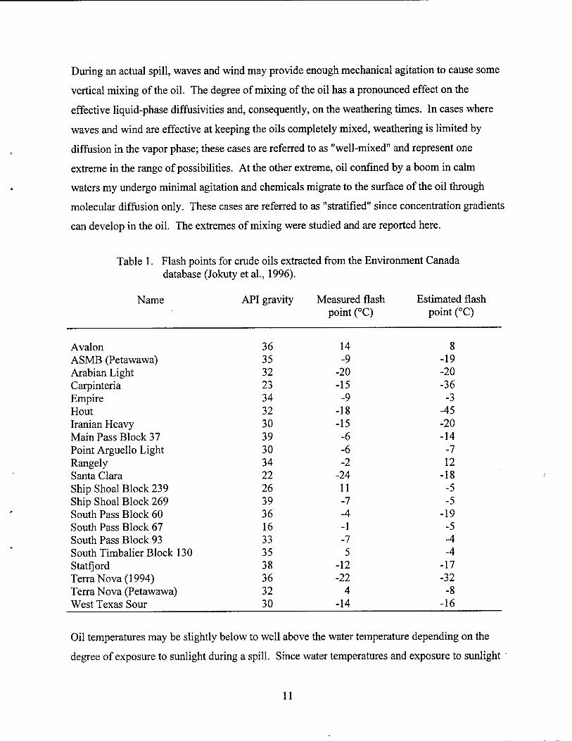
Table 1. Flash points for crude oils extracted from the Environment Canada database (Jokuty et al., 1996).

Name API gravity Measured flash Estimated flash point (°C) point (°C)

Avalon 36 14 8 ASMB (Petawawa) 35 -9 -19 Arabian Light 32 -20 -20 Carpinteria 23 -15 -36 Empire 34 -9 -3 Hout 32 -18 -45 Iranian Heavy 30 -15 -20 Main Pass Block 37 39 -6 -14 Point Arguello Light 30 -6 -7 Rangely 34 -2 12 Santa Clara 22 -24 -18 Ship Shoal Block 239 26 11 -5 Ship Shoal Block 269 39 -7 -5 South Pass Block 60 36 -4 -19 South Pass Block 67 16 -1 -5 South Pass Block 93 33 -7 -4 South Timbalier Block 130 35 5 -4 Statfjord 38 -12 -17 Terra Nova (1994) 36 -22 -32 Terra Nova (Petawawa) 32 4 -8 West Texas Sour 30 -14 -16

Oil temperatures may be slightly below to well above the water temperature depending on the

degree of exposure to sunlight during a spill. Since water temperatures and exposure to sunlight

11

vary significantly during times and in locations where this study might be applied, a single

"worst-case" temperature was not selected. Three temperatures were used to show the effect that

temperature variability has on the weathering times.

The thickness of an oil has a large impact on the weathering time. Open-water spills quickly

spread to sub-millimeter thicknesses (Belen et al., 1983), but spills confined by booms may be

quite thick. Thicknesses up to 10 centimeters were considered in this study.

Other environmental and spill parameters were selected that would most closely represent

realistic worst case conditions during a spill in a harbor. Generally, oil weathers more slowly

under lower wind speeds, so a wind speed of 1.5 meters per second was selected to be consistent

with that used in recent U.S. Environmental Protection Agency regulations governing the

reporting of risk management plans for industrial facilities (U.S. Environmental Protection

Agency, 1999). Wind speeds have very little effect on the predicted weathering times for

stratified oils since the weathering times are limited by diffusion within the liquid oil. Even for

well-mixed oils the effects of wind speeds are limited; doubling the wind speed decreased

weathering times by about 40 percent.

For a given thickness, weathering times increased slightly with increasing area. A spill area of

1000 m2 was chosen as a realistic worst-case. It should be noted that area effects are minimal;

for example, doubling the area increased the weathering time less than 7 percent.

5.0 RESULTS AND DISCUSSION

Equation (11) was used with the pseudo-component analysis to predict the flash point of the

unweathered crude oils used for this study. Comparisons of measured and predicted flash points

for the 21 oils that met the selection criteria are presented in Table 1 and Figure 1. The root-

mean-square deviation between the measured and predicted flash points was 11°C.

Some of the difficulties associated with measuring flash points of crude oils are addressed above.

The Emergencies Science Division of Environment Canada modified a commercial flash point

12

instrument to overcome some of these difficulties. Steve Whiticar, one the authors of the

database, suggested that the measured flash points are reproducible to within 3°C but gave no

estimates of systematic errors. (Whiticar, 1998).

A numerical simulation was used to predict how the average composition and flash points of five

representative oils change as they weather. As the oils weathered the lighter components, which

contribute to the low initial flash points of these oils, were preferentially lost to evaporation. The

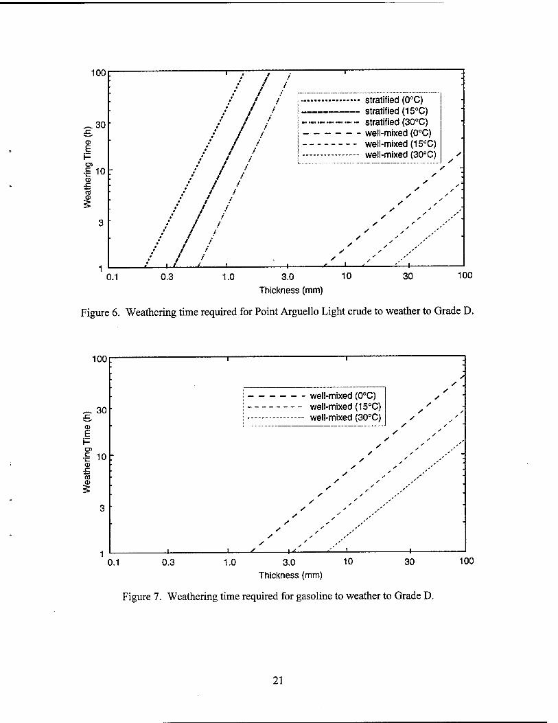
times required for the oils to weather to Grade D (flash point > 26.7°C) are presented graphically

in figures 2 through 6. An algebraic formula for weathering times as a function of thickness was

also developed using a least-squares fit to the numerically generated data:

K = Ke{^^?} (12)

where the thickness, L, is in millimeters and the weathering time, tw , is in hours. This formula

is valid for weathering greater than one hour and less than 100 hours. The values for the

coefficients, k,,k2,k3, depend on the oil, the degree of mixing, and the oil temperature; they are

listed in Table 2. In all but one case k3 = 0, and the formula reduces to

tw = VLk>. (13)

The weathering times for well-mixed oils was linearly related to the thickness (k2 =1).

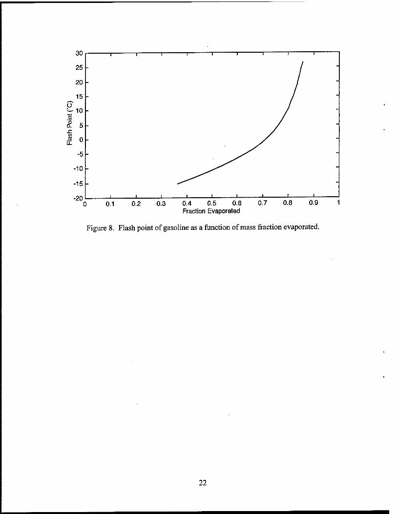
Gasoline was modeled using only the well-mixed conditions and the results are presented in

Figure 7. The magnitude of the errors associated with the stratified model when applied to

gasoline precluded its use. Furthermore, since there is less resistance to vertical circulation in

low viscosity fluids like gasoline, a well-mixed model is more reasonable even under a broad

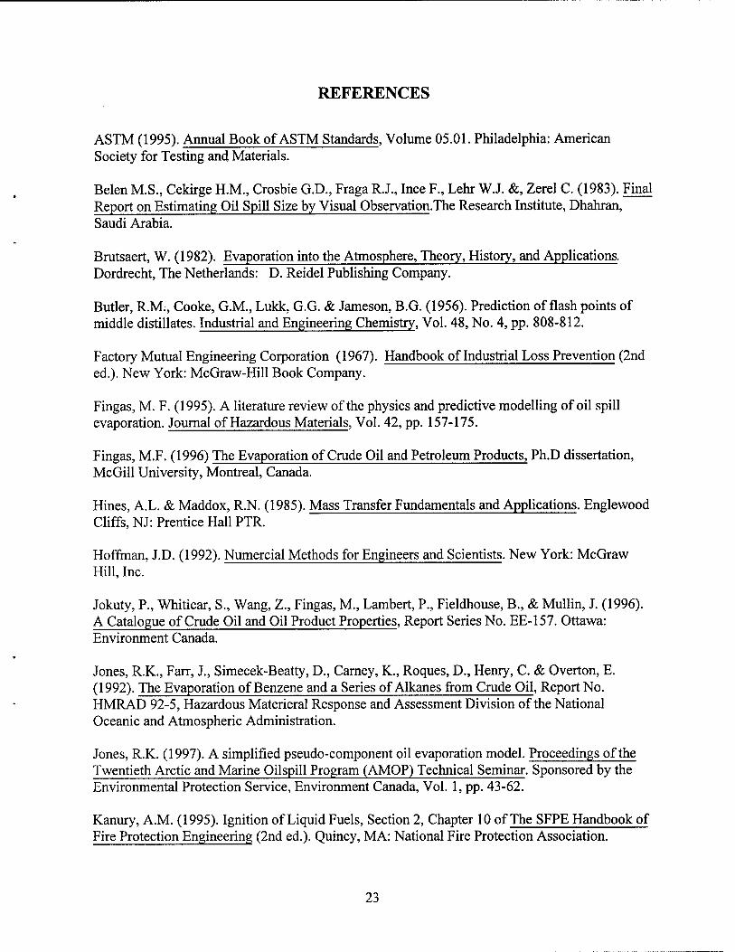
range of conditions. A more revealing result is presented in Figure 8 that shows the flash point

as a function of the fraction of the gasoline that evaporates. Since gasoline is composed of

mostly low flash point chemicals, most of it must evaporate for the flash point to reach 26.7 °C.

13

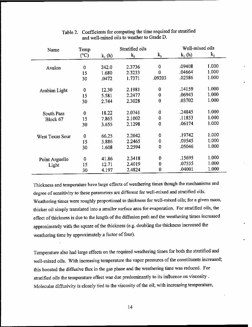
Table 2. Coefficients for computing the time required for stratified and well-mixed oils to weather to Grade D.

Name Temp Stratified oils Well-mixed oils

(°C)

0

k,(h)

242.0

k2

2.3736

k3

0

k,(h)

.09408

k2

Avalon 1.000

15 1.680 2.3233 0 .04664 1.000

30 .0472 1.7371 .09203 .02586 1.000

Arabian Light 0 12.30 2.1981 0 .14159 1.000

15 5.581 2.2477 0 .06943 1.000

30 2.744 2.3028 0 .03702 1.000

South Pass 0 18.22 2.0741 0 .24845 1.000

Block 67 15 7.865 2.1002 0 .11853 1.000

30 3.655 2.1298 0 .06174 1.000

West Texas Sour 0 66.25 2.2042 0 .19742 1.000

15 5.886 2.2465 0 .09545 1.000

30 1.608 2.2594 0 .05046 1.000

Point Arguello 0 41.86 2.3418 0 .15695 1.000

Light 15 12.71 2.4019 0 .07555 1.000

30 4.197 2.4824 0 .04001 1.000

Thickness and temperature have large effects of weathering times though the mechanisms and

degree of sensitivity to these parameters are different for well-mixed and stratified oils.

Weathering times were roughly proportional to thickness for well-mixed oils; for a given mass,

thicker oil simply translated into a smaller surface area for evaporation. For stratified oils, the

effect of thickness is due to the length of the diffusion path and the weathering times increased

approximately with the square of the thickness (e.g. doubling the thickness increased the

weathering time by approximately a factor of four).

Temperature also had large effects on the required weathering times for both the stratified and

well-mixed oils. With increasing temperature the vapor pressures of the constituents increased;

this boosted the diffusive flux in the gas phase and the weathering time was reduced. For

stratified oils the temperature effect was due predominantly to its influence on viscosity .

Molecular diffusivity is closely tied to the viscosity of the oil; with increasing temperature,

14

diffusivity increased, and weathering times decreased. Of the five oils studied, the weathering

times for Avalon Crude were the most sensitive to temperature because its viscosity is the most

sensitive to temperature.

The differences between oils was largely due to differences in volatile components and viscosity.

Viscosities change as an oil weathers so the initial viscosities alone cannot be used to rank the

expected weathering times of stratified oils with similar initial flash points. However, there is a

general trend in the relationship between viscosity and weathering time.

The differences between the stratified and well-mixed oils are dramatic. Molecular diffusion,

which was most often the rate limiting process for stratified oils, was generally much slower for

volatile constituents than the gas-phase diffusion which limited the well-mixed rate. Under most

circumstances the stratified oils weathered very slowly. In all cases except Avalon at 30 °C, a

stratified slick thicker than 1 centimeter required over 100 hours to weather. In actual spills

weathering will occur much more quickly if there are natural mechanisms for mixing the oil. For

the five crude oils in this study, well-mixed slicks up to a one centimeter thick weathered within

three hours even at low ambient temperatures.

6.0 UNCERTAINTY ANALYSIS

Possible sources of error can be conveniently divided into those inherent to the formulation of

the model (model errors), those associated with numerical implementation (numerical errors),

and those associated with input parameters (parametric errors). Model errors arise from the

inaccuracies in the model assumptions or descriptions of the physical processes. The magnitude

of model errors are difficult to estimate in the absence of experimental data. Numerical errors

can arise when the fundamental equations used to describe the processes are implemented and

solved numerically using a computer; for this study these errors were easy to assess and

minimize. Parametric errors are best described as the errors in the output of a model caused by

errors in the input. In applying the results of this study to any actual spill, the dominant errors in

the weathering times are expected from the large uncertainties in the input data.

15

Uncertainty in the liquid-phase diffusivity of the oil is probably the largest source of uncertainty

in the model output. Errors in the diffusivity can arise from the uncertainties in the level of

mixing, the temperature of the oil, the viscosity of the oil, and from inherent errors in the

correlation used to determine the molecular diffusivity (equation 8). Of these, the level of

mixing probably introduces the largest uncertainty. As stated above, it is possible for wind and

waves to agitate and cause some vertical mixing of the oil. There is no easy way to assess the

effectiveness of this mixing so the results from the two extreme cases are presented: no vertical

mixing (stratified oil) and complete mixing (well-mixed oil). Errors in the viscosity of the oil

can also have a pronounced effect on results; the rate of diffusion in the liquid phase decreases

with increasing viscosity. The correlation itself yields results that are reliable to within about 30

percent (Hines & Maddox, 1985).

Errors in temperature affect the vapor pressure of the components and the viscosity values used

to compute molecular diffusivity. Depending on the circumstance of a spill, it can be extremely

difficult to estimate the temperature of an oil. On sunny days, solar heating of the oil surface can

be dramatic. During an experimental spill in Mobile Alabama, Jones et al. (1992) observed the

surface temperature of a six-centimeter oil slick rise 23 °C above the water temperature due to

solar radiation. On the other hand, spills at night or kept in the shade can be expected to have a

lower temperature than the water due to evaporative cooling. These effects are accentuated for

very thick stratified slicks. Figures 2 through 6 show results for a range of temperatures so the

reader can estimate the possible bounds on the weathering times based on the particular

conditions of the spill.

The process of spilling and skimming oil is usually effective at mixing the oil. How long the

mixing occurs and how thick the oil is during this process cannot be known and the processes

would be difficult to model. It should be noted that the mixing and spreading that occurs during

the release and skimming may play a larger part in the weathering of the oil than the many hours

spent on the water's surface. This study did not account for these processes.

16

7.0 CONCLUSIONS

This study was limited to low wind speeds. This limitation was not significant for stratified oils

since weathering was relatively insensitive to wind speed. However at higher wind speeds well-

mixed oils weathered more quickly; doubling wind speeds reduced weathering times by about 40

percent. In actual spills, uncertainties in temperature, thickness, oil composition and viscosity

would be expected to introduce significant ambiguities.

This study indicates that the time required for any of the five crude oils to weather to Grade D

depends critically on whether it is stratified or well-mixed. These represent the extremes that

bound the conditions expected in an actual spill. There are a variety of possible mechanism for

mixing: the process of releasing the oil and the process of skimming are effective at mixing the

oil, but may only persist for a few minutes; wave action can cause the slick to alternately be

squeezed and stretched; winds can cause the oil to pile up against a boom and promote vertical

circulation; and thermal instabilities may initiate convective currents. Some mixing is likely

during a spill; however, the analysis of these mechanisms and the quantification of the effects are

beyond the scope of this study.

The results suggest a different approach for refined products. Most common fuels, like diesel

fuel, have flash points well above 26.7 °C before any evaporation occurs so no modeling is

needed. Gasoline contains constituents with boiling points that fall within a relatively narrow

range. Since it is mostly made up of volatile components, about 85 percent of the gasoline must

evaporate before it weathers to Grade D. It seems prudent and reasonable to treat any floating

gasoline as a flammable substance with a low flash point.

This study was intended to be applied to oil contained in a boom and should not be applied to

cases where oil is released, spreads freely, and is subsequently boomed. When oil is released

and is allowed to spread, it quickly thins to less than 1 mm. Even if the oil is stratified it

weathers quickly when thin. Subsequent booming will also promote weathering through mixing.

17

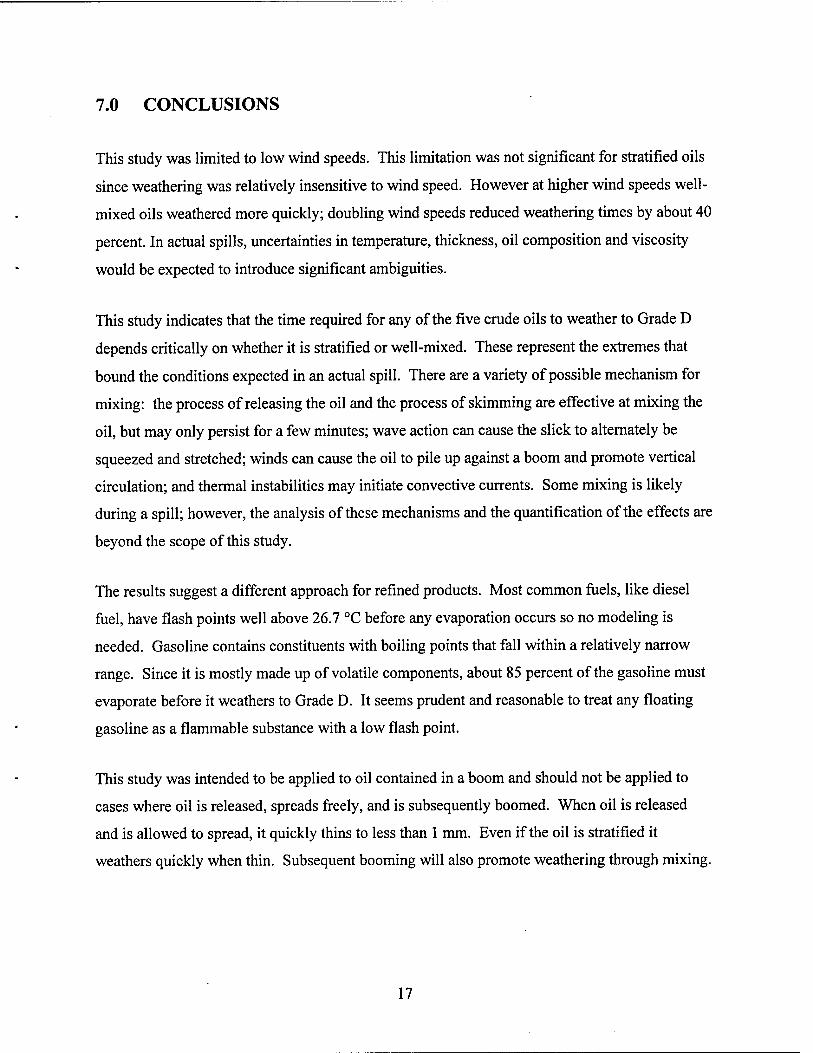
8.0 RECOMMENDATIONS

Models of complicated natural phenomena are prone to error. Though every attempt was made

to assess the possible errors and account for the largest, there was no way to estimate model

errors in the absence of experimental evidence. The numerical results presented here should be

verified experimentally.

The work was motivated by the USCG's need to set guidelines for vessels responding to confined

oil spills. The large differences between the weathering times for completely stratified oils and

well-mixed oils combined with the inherent difficulty in determining the degree of mixing during

many, if not most, actual spill events poses a serious challenge to those attempting to estimate

safe response times. In the absence of direct observation, the results of this study may prove

useful in assessing the possible range of weathering times; however, direct measurements of

flammability at the time of spill are preferred.

-50 -40 -30 -20 -10 0 Measured flash point (°C)

10 30

Figure 1. Measured and estimated flash points for 21 unweathered crude oils. The straight line indicates perfect agreement.

18

100r

30

a> E »- f 10

to a> 5

r : 1 / I' " / • / / /

* * #

• #

/ 1

•

• stratified (15°C) • ~ stratified (30°C) -

* • - well-mixed (0°C) - well-mixed (15°C) - well-mixed (30°C) < ,* / .

/ / • . / / y

• / .' s / ' / ' ,' -

♦ / ' / ' ♦ / / s .- •

/ i ' ,' / / S ' / /

, ' 1...... JL-l 1 L \_t cl i_^l 1

0.1 0.3 1.0 10 30 3.0

Thickness (mm)

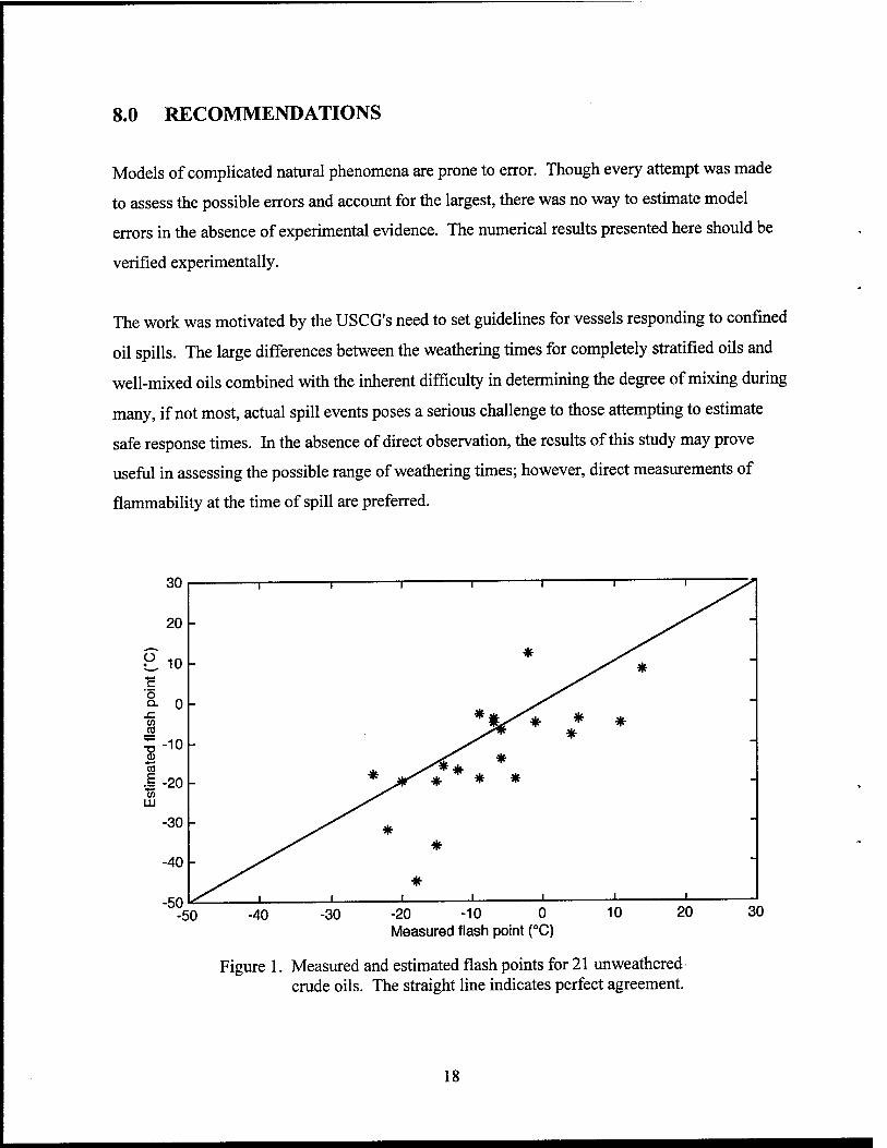
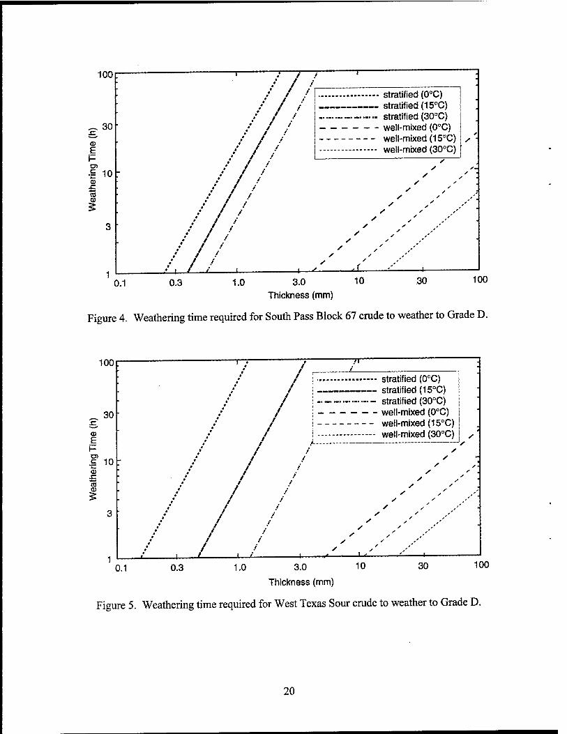
Figure 2. Weathering time required for Avalon crude to weather to Grade D.

100

100r

30

CD

E

C 10 CD

JZ m CD

1 0.1

/// / / /

/ / / ' / •'

/ / .' •' / ••' / ' '

: / / /

/ / .'

/ / / / / /

/// \JL 1 1 1 1

7 1 "

stratified (15°C^ ».......«.........- ctratifiprf ^n°n\

well-mixed (0°C) well-mixed (15°C) weii-mixcu \<3u L^

s

/ /

/L-S c CA

0.3 1.0 10 30 3.0

Thickness (mm)

Figure 3. Weathering time required for Arabian Light crude to weather to Grade D.

100

19

100

^ 30 jr_

a> E i-

§ 10 a> x: CO

5

T

stratified (0°C) stratified (15°C) stratified (30°C) well-mixed (0°C) well-mixed (15°C) well-mixed (30°C)

,- i / ~o_

0.1 0.3 1.0 3.0 10

Thickness (mm)

30 100

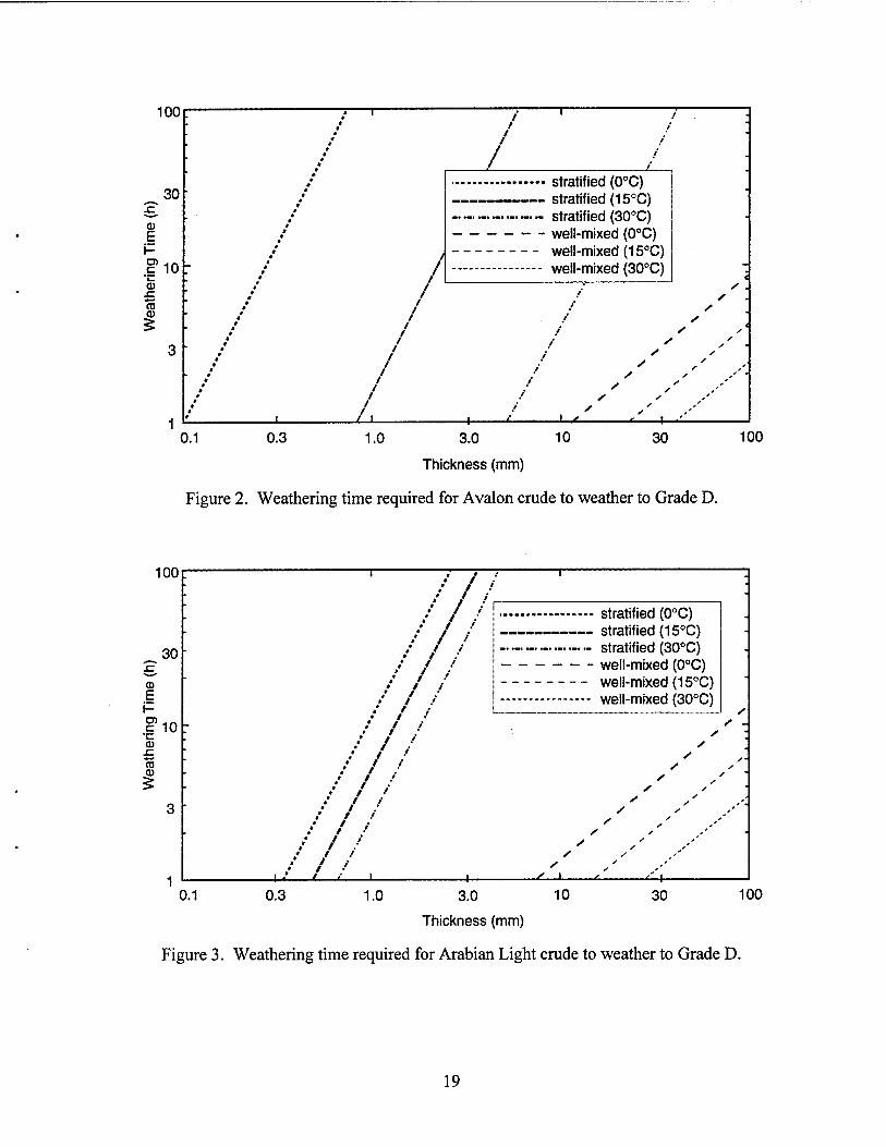
Figure 4. Weathering time required for South Pass Block 67 crude to weather to Grade D.

100r

_. 30

CD

E

f 10

5

•- stratified (0°C) - stratified (15°C) - stratified (30°C) - well-mixed (0°C)

- well-mixed (15°C) - well-mixed (30°C)

J L.

S

J-t.

0.1 0.3 1.0 3.0 10 30 100

Thickness (mm)

Figure 5. Weathering time required for West Texas Sour crude to weather to Grade D.

20

100

_30

o e H D> .§10 0)

JC "5

1 / / / / / /

/

r- :

• stratified (15°C) ■

.• / ' . stratified (30°C) ■

•' / / well-mixed (0°C) / / / well-mixed (15°C)

/ / * / \»/oll-mi¥Prl f?o°r"^

/ •

/ / / s ; -• / / s / / / /

♦' / ' ' . / • / .' ' / / ' ' .- ■

/ / / * ' / '* ' ' / S y .' • / ' / •' / '

i i ■ s x y .•••; 0.1 0.3 1.0 3.0

Thickness (mm)

10 30 100

Figure 6. Weathering time required for Point Arguello Light crude to weather to Grade D.

100

_ 30

CD E i- o>

■§ 10 CD

to a>

. , , .

• s .

. well-mixed (0°C) s s

. well-mixed (15°C) well-mixed (30°C) '

' • '

' / ' .' - ' s' / :

S ' '

S s

' / ' ' / '

' / s

' / s

' 1 1 *■ v*- ^ 1 1 1

0.1 0.3 1.0 3.0 10 Thickness (mm)

30 100

Figure 7. Weathering time required for gasoline to weather to Grade D.

21

0.1 0.2 0.3 0.4 0.5 0.6 0.7 0.8 0.9 Fraction Evaporated

Figure 8. Flash point of gasoline as a function of mass fraction evaporated.

22

REFERENCES

ASTM (1995). Annual Book of ASTM Standards, Volume 05.01. Philadelphia: American Society for Testing and Materials.

Belen M.S., Cekirge H.M., Crosbie G.D., Fraga R.J., Ince F., Lehr W.J. &, Zerel C. (1983). Final Report on Estimating Oil Spill Size by Visual Observation.The Research Institute, Dhahran, Saudi Arabia.

Brutsaert, W. (1982). Evaporation into the Atmosphere, Theory, History, and Applications. Dordrecht, The Netherlands: D. Reidel Publishing Company.

Butler, R.M., Cooke, G.M., Lukk, G.G. & Jameson, B.G. (1956). Prediction of flash points of middle distillates. Industrial and Engineering Chemistry, Vol. 48, No. 4, pp. 808-812.

Factory Mutual Engineering Corporation (1967). Handbook of Industrial Loss Prevention (2nd ed.). New York: McGraw-Hill Book Company.

Fingas, M. F. (1995). A literature review of the physics and predictive modelling of oil spill evaporation. Journal of Hazardous Materials, Vol. 42, pp. 157-175.

Fingas, M.F. (1996) The Evaporation of Crude Oil and Petroleum Products, Ph.D dissertation, McGill University, Montreal, Canada.

Hines, A.L. & Maddox, R.N. (1985). Mass Transfer Fundamentals and Applications. Englewood Cliffs, NJ: Prentice Hall PTR.

Hoffman, J.D. (1992). Numercial Methods for Engineers and Scientists. New York: McGraw Hill, Inc.

Jokuty, P., Whiticar, S., Wang, Z., Fingas, M., Lambert, P., Fieldhouse, B., & Mullin, J. (1996). A Catalogue of Crude Oil and Oil Product Properties, Report Series No. EE-157. Ottawa: Environment Canada.

Jones, R.K., Fair, J., Simecek-Beatty, D., Carney, K., Roques, D., Henry, C. & Overton, E. (1992). The Evaporation of Benzene and a Series of Alkanes from Crude Oil, Report No. HMRAD 92-5, Hazardous Materieral Response and Assessment Division of the National Oceanic and Atmospheric Administration.

Jones, R.K. (1997). A simplified pseudo-component oil evaporation model. Proceedings of the Twentieth Arctic and Marine Oilspill Program (AMOP) Technical Seminar. Sponsored by the Environmental Protection Service, Environment Canada, Vol. 1, pp. 43-62.

Kanury, A.M. (1995). Ignition of Liquid Fuels, Section 2, Chapter 10 of The SFPE Handbook of Fire Protection Engineering (2nd ed.). Quincy, MA: National Fire Protection Association.

23

Lehr, W., Overstreet, R., Jones, R, Eclipse, L. & Simecek-Beatty, D. (1997). The next generation in oil weathering modeling. Proceedings of the 1997 International Oil Spill Conference. American Petroleum Institute publication no. 4651, pp. 986-987

Lenoir, J.M. (1975). Predict flash points accurately. Hydrocarbon Processing, Vol. 54, pp. 95-99.

Li, C.C. & Moore, J.B. (1977). Estimating flash points of organic compounds." Journal of Fire and Flammability, Vol. 8, pp. 38-40.

Lyman, J.L., Reehl, W.F. & Rosenblatt D.A. (1990). Handbook of Chemical Property Estimation Methods. Washington D.C.: American Chemical Society.

Mackay, D. & Matsugu, R. (1973). Evaporation rates of liquid hydrocarbon spills on land and water. Canadanian Journal of Chemical Engineering, Vol. 511, pp. 434-439.

Mackay, D., Stiver, W. & Tebeau, P.A. (1983). Testing of crude oils and petroleum products for environmental purposes. Proceedings of the 1983 International Oil Spill Conference. American Petroleum Institute publication no. 4356, pp. 331-337.

Murad, R.J., Lamendola, J., Isoda, H. & summerfield, M. (1970). A study of some factors influencing the ignition of a liquid fuel pool. Combustion and Flame, Vol. 15, pp. 289-298.

Patil, G.S. (1988). Estimation of flash points. Fire and Materials, Vol. 12, No. 3, pp. 127 -131.

Payne, J.R., Kirstein, B.E., McNabb, G.D., Lambach, J.L., Redding, R, Jordan, RE., Horn, W., De Oliveira, C, Smith, G.S., Baxter, D.M., & Gaegel, R (1984). Multivariate Analysis of Petroleum Weathering in the Marine Environment - sub Arctic. OCSEAP Final Reports, Vol. 21, U.S. Department of Commerce, National Oceanic and Atmospheric Administration, & U.S. Department of Interior, Minerals Management Service.

Reid, R.C, Prausnitz, J.M., Sherwood, T.K. (1977). The Properties of Gases and Liquids (3rd edition). New York: McGraw-Hill Book Company.

Satyanarayana, K., and Kakati, M.C. (1991). Correlation of flash points. Fire and Materials, Vol. 15, No. 2, pp. 97-100.

Speight, J.G. (1980). The Chemistry and Technology of Petroleum. New York: Marcel Decker,Inc.

Stensaas, J.P. (1992). Fire on the Sea - state of the art and need for future research, Report No. STF25 A92035, SINTEF NBL - Norwegian Fire Research Laboratory (NTIS No. PB93-201648).

Stiver, W. & Mackay, D. (1984). Evaporation rate of spills of hydrocarbons and petroleum mixtures. Environmental Science and Technology, Vol. 18, pp. 834-840.

24

Thibodeaux, L.J. & Carver, J.C. (1997). Hindcasting volatile chemical emissions to air from ponded recycle oil. Environmental Progress, Vol. 16, No. 2, pp. 106-115.

USCG (1997). Code of Federal Regulations, Title 46, Part 30. Washington, D.C.: U.S. Government Printing Office.

U.S. Environmental Protection Agency (1999). Risk Management Program Guidance for Offsite Consequence Analysis. Available on-line at http://www.epa.gov/ceppo/pubs.html.

Wickey, R.O. & Chittenden, D.H. (1963). Flash points of blends correlated. Hydrocarbon Processing and Petroleum Refinery, Vol. 42, No. 6, pp. 157 -158.

Whiticar, S. (1998). Emergencies Science Division, Environment Canada. Private communication.

25


26

APPENDIX A

FINITE DIFFERENCE FORMULATION

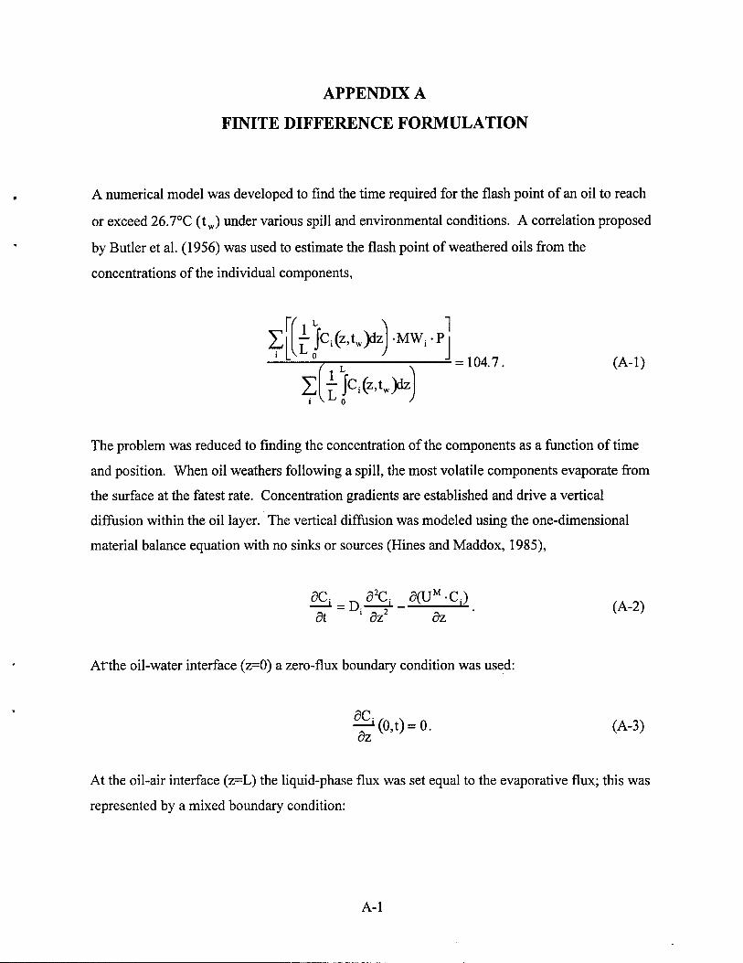
A numerical model was developed to find the time required for the flash point of an oil to reach

or exceed 26.7°C (tw) under various spill and environmental conditions. A correlation proposed

by Butler et al. (1956) was used to estimate the flash point of weathered oils from the

concentrations of the individual components,

?L^/Ci(z'tw)dz)"MWi'pJ Sl^Jc.fcOiz

= 104.7. (A-l)

The problem was reduced to finding the concentration of the components as a function of time

and position. When oil weathers following a spill, the most volatile components evaporate from

the surface at the fatest rate. Concentration gradients are established and drive a vertical

diffusion within the oil layer. The vertical diffusion was modeled using the one-dimensional

material balance equation with no sinks or sources (Hines and Maddox, 1985),

dt ' dz2 dz v

Atthe oil-water interface (z=0) a zero-flux boundary condition was used:

8C —L(0,t)=0. (A-3) öz

At the oil-air interface (z=L) the liquid-phase flux was set equal to the evaporative flux; this was

represented by a mixed boundary condition:

A-l

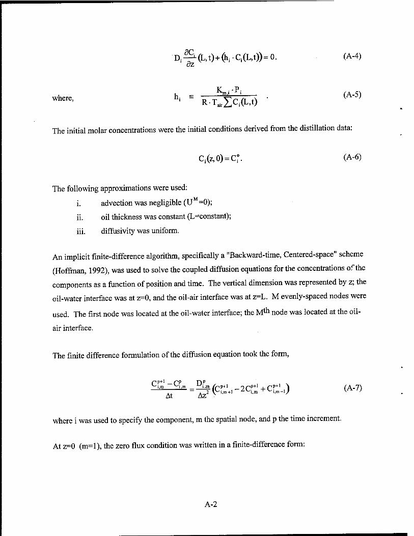
dz

v .P where' h| R-T^sc.a-t) • l

The initial molar concentrations were the initial conditions derived from the distillation data:

Ci(z,0) = C°. (A-6)

The following approximations were used:

i. advection was negligible (U =0);

ii. oil thickness was constant (Inconstant);

iii. diffusivity was uniform.

An implicit finite-difference algorithm, specifically a "Backward-time, Centered-space" scheme

(Hoffman, 1992), was used to solve the coupled diffusion equations for the concentrations of the

components as a function of position and time. The vertical dimension was represented by z; the

oil-water interface was at z=0, and the oil-air interface was at z=L. M evenly-spaced nodes were

used. The first node was located at the oil-water interface; the M™ node was located at the oil-

air interface.

The finite difference formulation of the diffusion equation took the form,

/-ip+l _ pp TAP

Z -~T^i,m+rzti,n,+(-i,ra-i;l ^ ') At Az

where i was used to specify the component, m the spatial node, and p the time increment.

At z=0 (m=l), the zero flux condition was written in a finite-difference form:

A-2

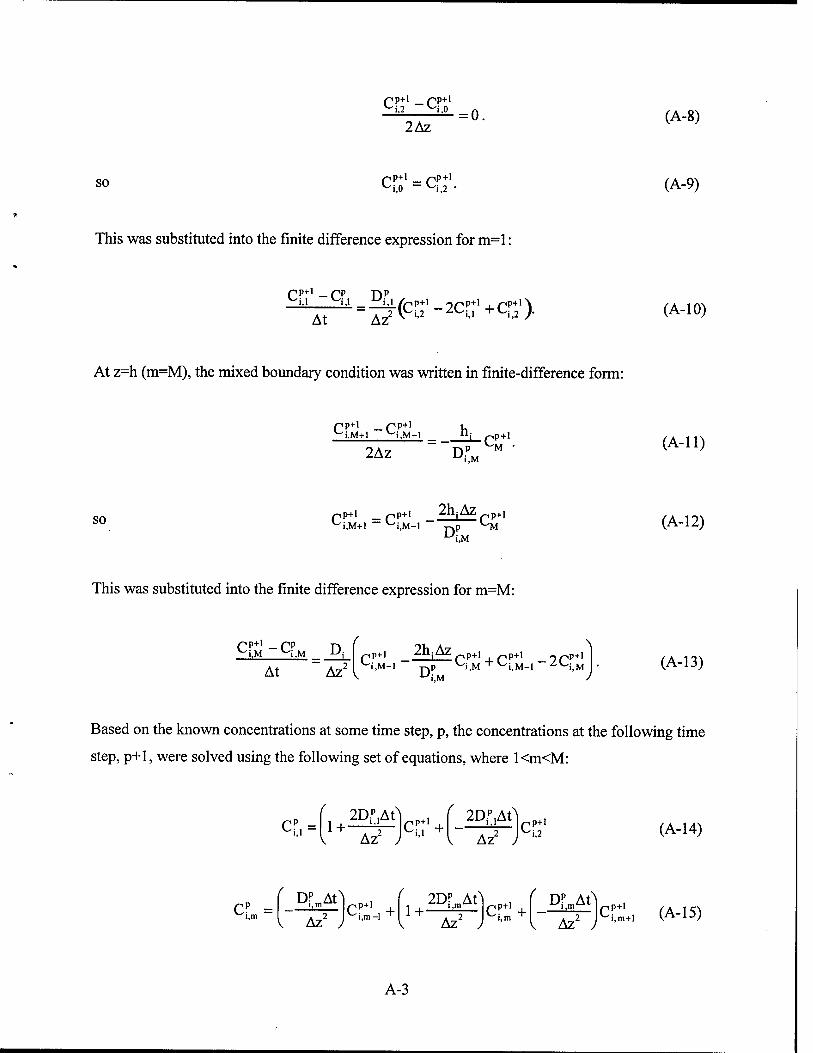
pp+1 _pp+l

2Az = 0. (A-8)

so pp+l _ pp+1 î,0 — î,2 • (A-9)

This was substituted into the finite difference expression for m=l:

u ü=-^(cp;' -2er;1 +cft\ At Az2 v ''2 '-1 ''2 J (A-10)

At z=h (m=M), the mixed boundary condition was written in finite-difference form:

/-.p+l _pp+l r, î,M+l î.M-l n

2Az D i_pp+i

p "^M i,M

(A-ll)

so pp+i _ pp+i _ 2hjAz p+1

D i,M

(A-12)

This was substituted into the finite difference expression for m=M:

PP+I _/~.p n

At Az' p+1 Zhinz p+1 p+1 _~r,p+i i,M-l T^P î,M "t"L'i,M-l ZnM Dp (A-13)

Based on the known concentrations at some time step, p, the concentrations at the following time

step, p+1, were solved using the following set of equations, where l<m<M:

Cp = 1+- 2DPAt

^ Az u r,p+1

,CP + 2D? At) i,l

^ Az' ; .2 P-i,2 (A-14)

( Cp = i,m

DP At^\ ( 2DP \\\ ( Dp At\ —i^HZ- Pp+1 j. 1 , Z1î,mAl p.p+1 , L>i,mAl

V Az y v Az y V Az y 2 CK+I (A-15)

A-3

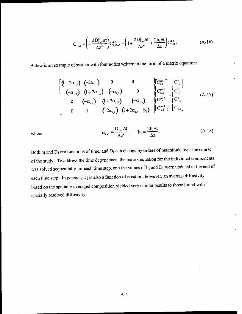
cp = f 2D? AOI i,m

AZZ ; CK-.+ i+-

2D? At 2h;At i,m

Az2 Az J -,P+I (A-16)

Below is an example of system with four nodes written in the form of a matrix equation:

r(l + 2au) (-2a,,) 0

[ (-au) (l+2ai>2) (-au)

o "lie?;1! fcp.l

c p+1 i,2

I 0 (-au) (l+2ai,3) Ou)

0 (-2aM) (l+2ai4 + ßi)

er;1

er;.

cp

cp

rp . i,4.

(A-17)

where Df,mAt _ 2h,At (A-18)

Both hi and Di are functions of time, and Di can change by orders of magnitude over the course

of the study. To address the time dependence, the matrix equation for the individual components

was solved sequentially for each time step, and the values of hi and Di were updated at the end of

each time step. In general, Di is also a function of position; however, an average diffusivity

based on the spatially averaged composition yielded very similar results to those found with

spatially resolved diffusivity.

A-4

APPENDIX B

SERIES SOLUTION TO THE DIFFUSION EQUATION

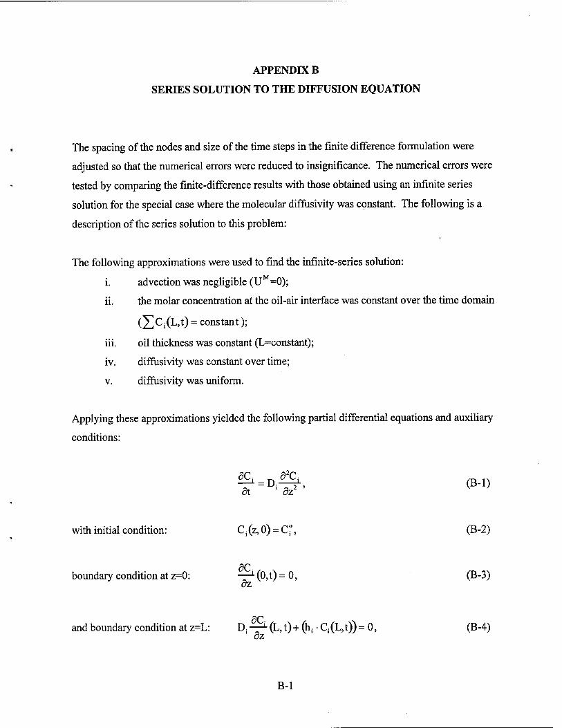
The spacing of the nodes and size of the time steps in the finite difference formulation were

adjusted so that the numerical errors were reduced to insignificance. The numerical errors were

tested by comparing the finite-difference results with those obtained using an infinite series

solution for the special case where the molecular diffusivity was constant. The following is a

description of the series solution to this problem:

The following approximations were used to find the infinite-series solution:

i. advection was negligible (U =0);

ii. the molar concentration at the oil-air interface was constant over the time domain

(XCi(L't)= constant);

iii. oil thickness was constant (L=constant);

iv. diffusivity was constant over time;

v. diffusivity was uniform.

Applying these approximations yielded the following partial differential equations and auxiliary

conditions:

^=Ä (B-l) at ' dz2

with initial condition: C; (z, 0) = C °, (B-2)

boundary condition at z=0: —-L(0,t)=0, (B-3) dz

and boundary condition at z=L: D( —L (L, t) + (h( • Cs(L,t)) = 0, (B-4)

dz

B-l

K -P Where' "' * R-T.SC.'fr.O ■ (B"5)

These equations were reformulated in terms of dimensionless variables:

^1 = -^ (B-6)

where Yi"c^; ^~^'' Ti-"7^ (B_7)

ST ^

S- z L

7 *i _D,t = L2

&1i (o, *)= = 0. The boundary condition at z=0 became: —r (0, x) = 0. (B-8)

And the boundary condition at z=L became: —L(l,x)+Bi-yj(l,T) = 0. (B-9)

where the mass Biot number is a measure of the relative importance of diffusion versus

evaporation and is defined

(B-10) Bis = D; ;

The initial condition became: y {fe 0) = 1 (B-11)

In the initial formulation of the problem, the components were coupled through the boundary

conditions. Approximation (ii) permitted them to be uncoupled. In this treatment, the Biot

number was held constant. The equations for each component could then be solved

independently.

For each time step the concentration of each component was calculated and averaged over the

volume of the spill. These average concentrations were used to test the flash point condition. If

the flash point was below 26.7°C (80°F) the time was incrementally stepped.

B-2

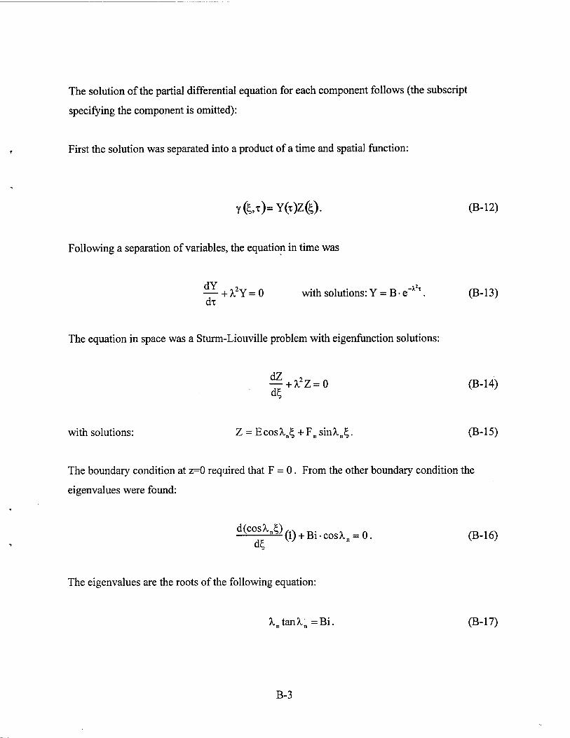
The solution of the partial differential equation for each component follows (the subscript

specifying the component is omitted):

First the solution was separated into a product of a time and spatial function:

yfe,T)=Y(x)Z©. (B-12)

Following a separation of variables, the equation in time was

— + JL2Y=0 with solutions: Y = B-e~x\ (B-13)

dx

The equation in space was a Sturm-Liouville problem with eigenfunction solutions:

—+ X2Z=0 (B-14) d^ V

with solutions: Z = EcosXn£ + Fnsin^n£. (B-15)

The boundary condition at z=0 required that F = 0. From the other boundary condition the

eigenvalues were found:

d(cos^)(l) + B. cos^ = 0 (B16)

The eigenvalues are the roots of the following equation:

Xntan^n=Bi. (B-17)

B-3

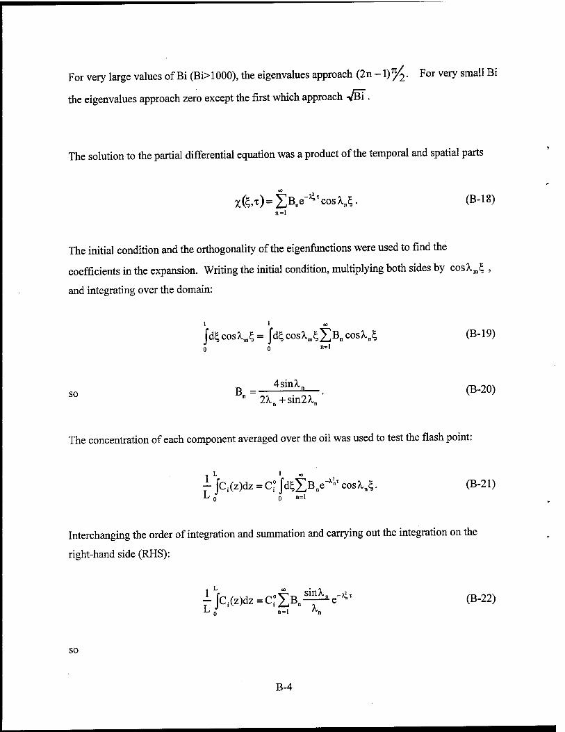
For very large values of Bi (Bi>1000), the eigenvalues approach (2n -1)%. For very small Bi

the eigenvalues approach zero except the first which approach VBi .

The solution to the partial differential equation was a product of the temporal and spatial parts

xfe^lB^cosU. (B-18) n=l

The initial condition and the orthogonality of the eigenfunctions were used to find the

coefficients in the expansion. Writing the initial condition, multiplying both sides by cosA,m£ ,

and integrating over the domain:

Jd4 cosA^ = Jd£ cos^fX cosXJ^ (B-19) n=l

Bn= 4sin^ ■ (B-20) S0 n 2An+sin2?Sl

The concentration of each component averaged over the oil was used to test the flash point:

f JCi(z)dz = C° JdsIXe-* cos^. (B-21) L 0 0 n=l

Interchanging the order of integration and summation and carrying out the integration on the

right-hand side (RHS):

fjC.Czjdz-crSB^e-*' (B-22) i- n n=l ^n

SO

B-4

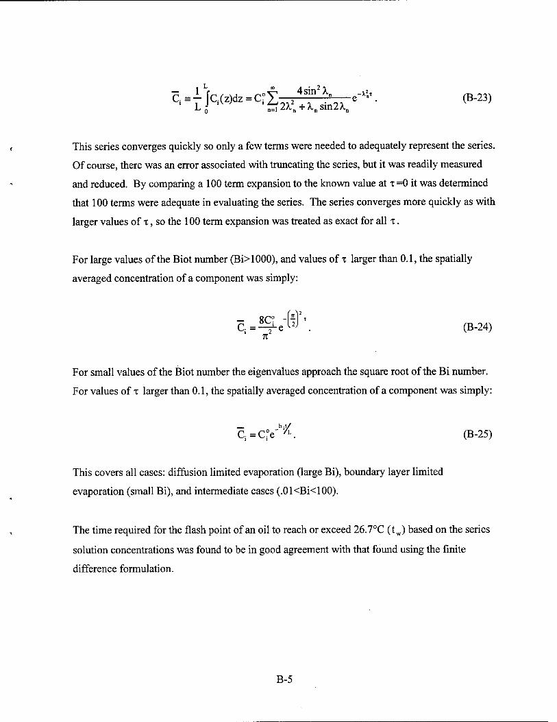
C.^-Lfc.(z)dz=C°y 24sin2?l" e-x-\ (B-23)

This series converges quickly so only a few terms were needed to adequately represent the series.

Of course, there was an error associated with truncating the series, but it was readily measured

and reduced. By comparing a 100 term expansion to the known value at x =0 it was determined

that 100 terms were adequate in evaluating the series. The series converges more quickly as with

larger values of x, so the 100 term expansion was treated as exact for all x.

For large values of the Biot number (Bi>1000), and values of x larger than 0.1, the spatially

averaged concentration of a component was simply:

C.=Se~W\ (B-24) 71

For small values of the Biot number the eigenvalues approach the square root of the Bi number.

For values of x larger than 0.1, the spatially averaged concentration of a component was simply:

G=C°e~/L. (B-25)

This covers all cases: diffusion limited evaporation (large Bi), boundary layer limited

evaporation (small Bi), and intermediate cases (.01<Bi<100).

The time required for the flash point of an oil to reach or exceed 26.7°C (tw) based on the series

solution concentrations was found to be in good agreement with that found using the finite

difference formulation.

B-5


B-6

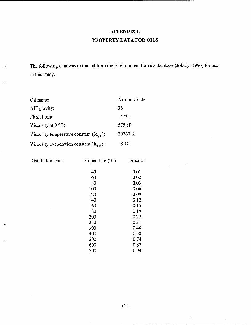
APPENDIX C

PROPERTY DATA FOR OILS

The following data was extracted from the Environment Canada database (Jokuty, 1996) for use

in this study.

Oil name: Avalon Crude

API gravity: 36

Flash Point: 14 °C

Viscosity at 0 °C: 575 cP

Viscosity temperature constant (knJ): 20760 K

Viscosity evaporation constant (knE): 18.42

Distillation Data: Temperature (°C) ] Fraction

40 0.01 60 0.02 80 0.03

100 0.06 120 0.09 140 0.12 160 0.15 180 0.19 200 0.22 250 0.31 300 0.40 400 0.58 500 0.74 600 0.87 700 0.94

C-l

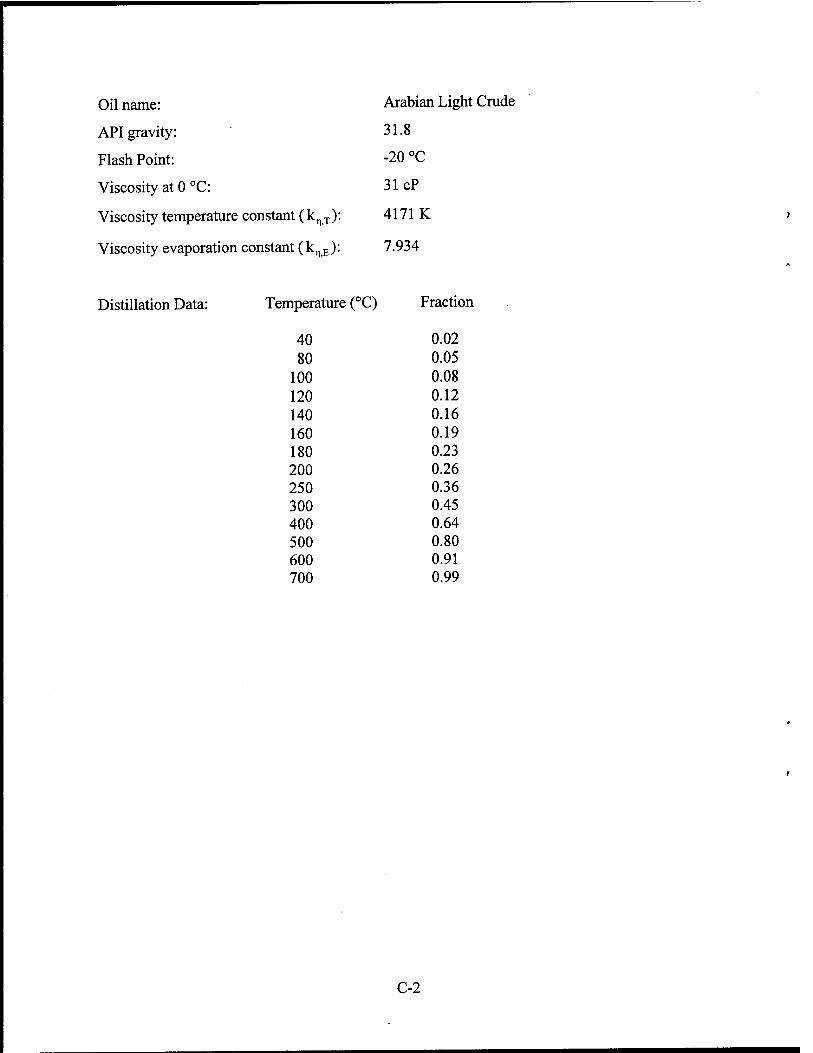
Oil name: Arabian Light Crude

API gravity: 31.8

Flash Point: -20 °C i


Viscosity temperature constant (knT): 4171 K


Distillation Data: Temperature (°C) Fraction

40 0.02 80 0.05

100 0.08 120 0.12 140 0.16 160 0.19 180 0.23 200 0.26 250 0.36 300 0.45 400 0.64 500 0.80 600 0.91 700 0.99

C-2

Oil name: South Pass Block 67 Crude

API gravity: 16.4

Flash Point: -1°C


Viscosity temperature constant (knT): 4329 K



40 0.01 60 0.02 80 0.04

100 0.08 120 0.12 140 0.16 160 0.21 180 0.26 200 0.31 250 0.42 300 0.53 400 0.72 500 0.86 600 0.95

C-3

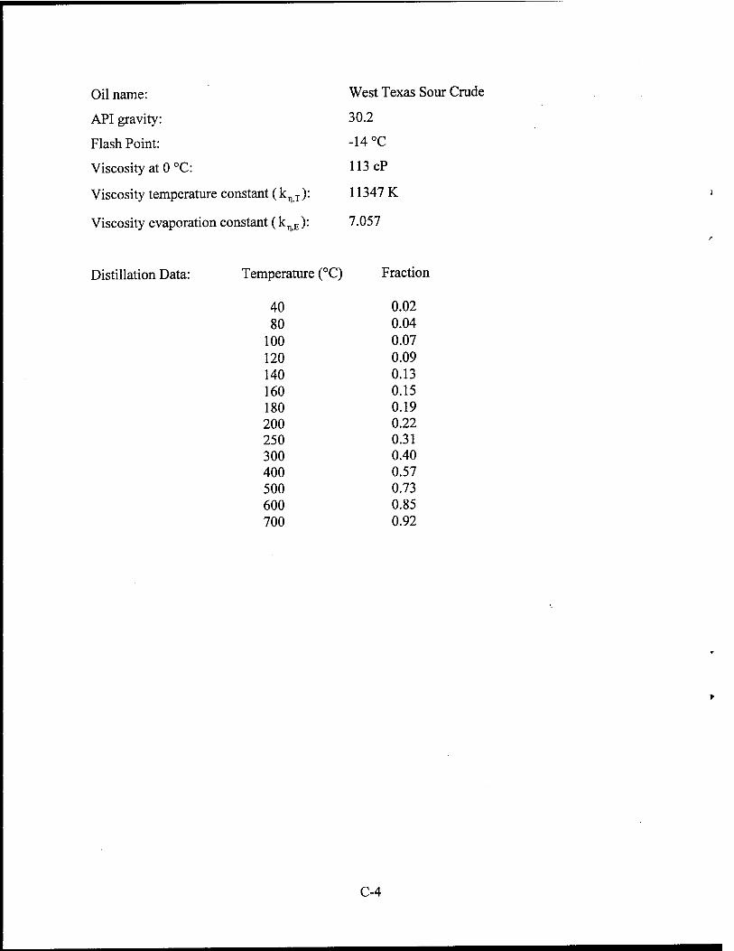
Oil name: West Texas Sour Crude

API gravity: 30.2

Flash Point: -14 °C i


Viscosity temperature constant (knT): 11347K


Distillation Data: Temperature (°C) ] fraction

40 0.02 80 0.04

100 0.07 120 0.09 140 0.13 160 0.15 180 0.19 200 0.22 250 0.31 300 0.40 400 0.57 500 0.73 600 0.85 700 0.92

C-4

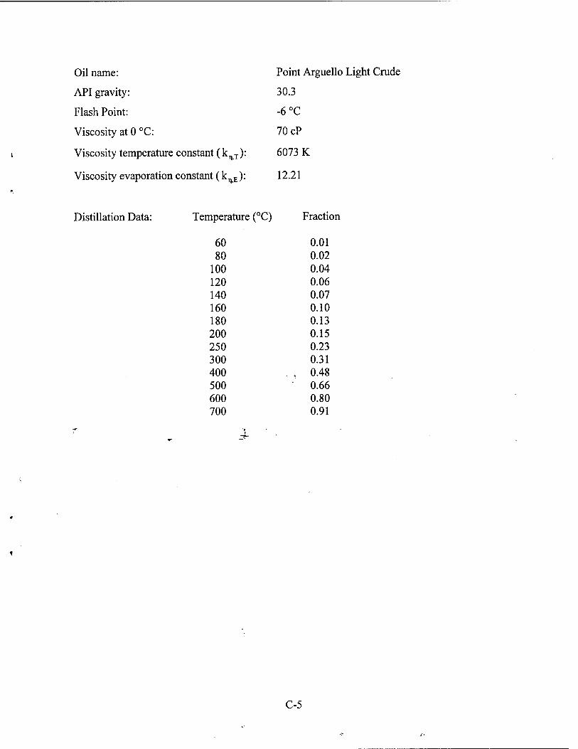
Oil name: Point Arguello Light Crud

API gravity: 30.3

Flash Point: -6°C


Viscosity temperature constant (k^): 6073 K

Viscosity evaporation constant (k^): 12.21


60 0.01 80 0.02

100 0.04 120 0.06 140 0.07 160 0.10 180 0.13 200 0.15 250 0.23 300 0.31 400 V 0.48 500 0.66 600 0.80 700 0.91

C-5

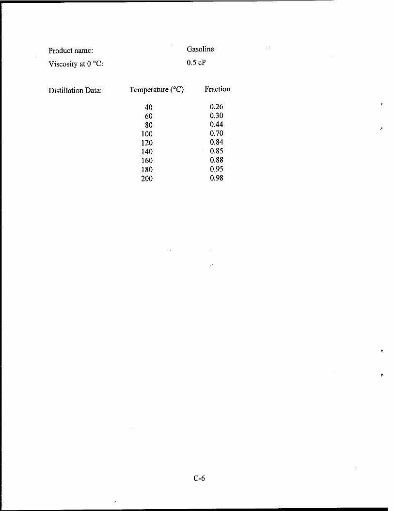
Product name: Gasoline

Viscosity at 0 °C: 0.5 cP

Distillation Data: Temperature (°C) Fracti<

40 0.26 60 0.30 80 0.44

100 0.70 120 0.84 140 0.85 160 0.88 180 0.95 200 0.98

C-6

US Coast Guard Research and Development Center - DTIC

Documents

Transcript of US Coast Guard Research and Development Center - DTIC