Urquhart's Law: Probability and the Management of Scientific and Technical Journal Collections Part...

Urquhart’s Law:Probability and the Management

of Scientific and TechnicalJournal Collections

Part 1.The Law’s Initial Formulation

and Statistical Bases

Stephen J. Bensman

ABSTRACT. The topic of this paper is a law formulated by Donald J.Urquhart on the use of scientific and technical (sci/tech) journals throughinterlibrary loan and central document delivery. The paper will be pub-lished in three parts. Part 1 discusses the genesis of the law and theprobabilistic theory on which it is based. A primary aim of this part isto teach librarians about the probability distributions underlying li-brary use and how to identify these distributions through simple mathe-matical and graphical techniques. [Article copies available for a fee fromThe Haworth Document Delivery Service: 1-800-HAWORTH. E-mail address:<[email protected]> Website: <http://www.HaworthPress.com>© 2005 by The Haworth Press, Inc. All rights reserved.]

KEYWORDS. Donald J. Urquhart, scientific journals, interlibrary loan,document delivery, library use, probability, Poisson Process

Stephen J. Bensman, MLS, PhD (History), is Technical Services Librarian, LSU Li-braries, Louisiana State University, Baton Rouge, LA 70803 (E-mail: [email protected]).

Science & Technology Libraries, Vol. 26(1) 2005Available online at http://www.haworthpress.com/web/STL

© 2005 by The Haworth Press, Inc. All rights reserved.doi:10.1300/J122v26n01_04 31

http://www.HaworthPress.com

http://www.haworthpress.com/web/STL

INTRODUCTION

This paper analyzes Urquhart’s Law of Supralibrary Use. Supra-library use is defined as the use by a given library’s patrons of materialssupplied from outside the library through either interlibrary loan or cen-tral document delivery. It is contrasted to intralibrary use, which is theuse of a library’s own materials by its own patrons. Stated in its simplestform, Urquhart’s Law specifies that the supralibrary use of scientificand technical (sci/tech) journals is positively correlated with the num-ber of libraries holding these journals in a system and therefore is a mea-sure of their aggregate use within the library system, including theirintralibrary use at the individual libraries of the system. The law wasformulated by Donald J. Urquhart, who established the National Lend-ing Library for Science and Technology (NLL) that later was mergedinto the British Library Lending Division (BLLD), now called the Brit-ish Library Document Supply Centre (BLDSC). Urquhart was the firstlibrarian to investigate scientifically the nature of sci/tech journal useand apply probability to it.

The paper will be published in three parts in three separate issues ofthis journal. Part 1 discusses the initial formulation of the law and itsstatistical bases; Part 2 will analyze how Urquhart applied probability tocreate and manage a central document delivery collection; and Part 3will be dedicated to the implications of the law for all the libraries of agiven library system. Each part will have an introduction, which will layout not only what it will discuss but will also summarize the discussionsand conclusions of the preceding parts. The purpose of these introduc-tions is threefold: (1) to provide the reader with a roadmap of the overallstructure and logic of the paper; (2) to enable, as much as possible, eachpart to be read independently from the others; and (3) to highlight theimportant points for the reader.

Part 1 shows Urquhart’s Law as a natural outgrowth of the Law ofScattering formulated in the early 1930s by S. C. Bradford, director ofthe Science Museum Library (SML) in London. Bradford’s Law de-scribes the distribution of articles on a given scientific subject acrossjournal titles. In doing so, it demonstrates the inability of sci/tech librar-ies to hold all the titles necessary to their patrons, proving the need ofsuch libraries for document delivery support from either other sci/techlibraries at their level or a comprehensive central scientific library.Bradford aspired to convert the SML into a central document deliverylibrary, and Urquhart fulfilled these aspirations by establishing theNLL. To prepare for the establishment of this library, Urquhart con-

32 SCIENCE & TECHNOLOGY LIBRARIES

ducted a study of the loans made by the SML to outside organizations in1956. This study laid the bases for his law of supralibrary use.

The primary focus of Part 1 is the statistical analysis of Urquhart’sdata on the external loans made by the SML in 1956. These data areutilized here for the didactic purpose of teaching librarians about theprobability distributions underlying library use as well as how to iden-tify these distributions through simple mathematical calculations andgraphical techniques. Part 1 analyzes the set structure of sci/tech jour-nals arising from Bradford’s Law and the stochastic processes underly-ing these journals’ use. Using Lexian analysis, it demonstrates howthese stochastic processes are partly a function of this set structure.The binomial and the Poisson processes are discussed, and the greaterapplicability of the Poisson process to library use is demonstrated. Asa component of this, Part 1 explains the crucial importance for librarycollection management of Bortkiewicz’s Law of Small Numbers, whichestablishes the theoretical basis for the stability and permanence of thelow-use classes. There are presented both the simple Poisson distribu-tion and compound Poisson distributions, the key one of which is thenegative binomial distribution. Compound Poisson distributions areproven to be the best model of library use due to their ability to captureall the stochastic processes operative in this use. Part 1 concludes withan explanation of the various indices of dispersion, which can be uti-lized to identify the stochastic processes and resulting probability distri-butions operative in library use.

GENESIS OF URQUHART’S LAW

Two of the most important libraries in the historical development oflibrary and information science were the Science Museum Library(SML) in South Kensington, London, and the National Lending Libraryfor Science and Technology (NLL), a direct predecessor of the pres-ent-day British Library Document Supply Centre (BLDSC), in BostonSpa, Yorkshire. The first was the prototype for the second. Each of theselibraries is closely associated with an important bibliometric law formu-lated by the person serving as its head.

The SML is linked to Bradford’s Law of Scattering. This law was de-rived by S. C. Bradford (1934), who was the chief librarian there for theperiod 1925-1938. It deals with the distribution of articles on a givenscientific subject across journals, positing that such articles concentratein a small nucleus of journals specifically devoted to the subject, and

Stephen J. Bensman 33

then scatter in ever decreasing numbers across other groups or zones ofjournals. As a result of this phenomenon, Bradford came to the conclu-sion that special libraries could never collect the complete literature ontheir subject, and in his classic book Documentation, Bradford (1953,102-122) advocated the establishment of a national central library forscience and technology, one of whose major functions would be “ex-ternal lending” or “the lending of books to research workers and stu-dents through the medium of approved institutions and lending agencies”(p. 117). Bradford assiduously worked to convert the SML into such alibrary. Prior to his tenure as chief librarian, this library had served theScience Museum and the neighboring Imperial College of Science andTechnology. Upon taking charge of it, Bradford strove to develop itsholdings into a comprehensive collection of the world’s scientific andtechnical (sci/tech) literature, making these resources available to scien-tists nationwide through approved institutions with which they were as-sociated.

Bradford’s vision of a national central library of science and technol-ogy was implemented by Donald J. Urquhart. The two men were similarin that they both had science doctorates. Urquhart began his library ca-reer at the SML, obtaining a job at this institution in 1938 at the timeBradford retired as its head. His service there was interrupted by WorldWar II, but after the war he returned to the SML, where he stayed until1948 when he moved to the Department of Scientific and Industrial Re-search. As its name implies, the Department of Scientific and IndustrialResearch, or DSIR, was the agency through which the British govern-ment supported scientific research and ensured that industry utilizednew scientific findings.

Urquhart rose to prominence at the Royal Society Scientific Informa-tion Conference of 1948, contributing three papers to this conference. Inone of these papers entitled “The Organization of the Distribution ofScientific and Technical Information” Urquhart (1948, 526) proposed anational library that would have “a specific responsibility for organiz-ing the library service for scientific and technical literature.” At the endof 1956, DSIR formed a Lending Library Unit headed by Urquhart witha staff of four, of whom the most important was Miss R. M. Bunn. Thisunit planned the creation of the National Lending Library for Scienceand Technology (NLL). It was in the establishment and operation of thislibrary that Urquhart developed what will be termed in this paper“Urquhart’s Law of Supralibrary Use.”


THE ANALYSIS OF 1956 SCIENCE MUSEUM LIBRARY (SML)EXTERNAL LOANS

The first step in the creation of the NLL was an analysis of the loansof sci/tech journals made by the SML to outside organizations during1956. This analysis was the first large-scale scientific study of journaluse, and it must be emphasized that it was a study of supralibrary use.Supralibrary use may be defined as the use by patrons of a given libraryof materials not owned by that library but supplied from the outsidethrough either some form of centralized document delivery or fromother libraries by means of interlibrary loan. It is to be contrasted withintralibrary use, which is the use by the patrons of a given library of ma-terials held by that library. Therefore, the analysis of the SML externalloans of sci/tech journals in 1956 was a study of United Kingdom (UK)supralibrary use of these materials in that year.

Urquhart (1959) reported on this analysis in a paper to the Interna-tional Conference on Scientific Information held in Washington, DC, inNovember,1958. Another report on the SML analysis was published byUrquhart and Bunn (1959) the following year. The key findings of thestudy of the 1956 SML external loans of sci/tech journals were two. Onewas that the distribution of supralibrary use of sci/tech journals is highlyskewed. This distributional finding was summarized by Urquhart andBunn (1959, 21) thus:

In general it seems that a small percentage of the current serial ti-tles account for a large percentage of the use of all serials. In theScience Museum in 1956 about 350 titles accounted for 50 percent. of the total use of serials, and about 1200 titles for 80 percent.of the total use. This, despite the fact that in 1956 the Science Mu-seum Library contained 9120 current serials, and possibly an equalnumber of dead ones. In general terms it appeared that, excludingless than 2000 titles, the total national interlibrary loan use couldbe satisfied by one loan copy.

By use of this information, it was possible to approximate the shapeof the distribution of journals by number of 1956 SML external loans aswell as to estimate its key statistical characteristics. These goals wereaccomplished in the following manner. First, the loan classes from 1 to382 loans and the number or frequency (f) of titles in these classes weretaken from Table VII in Urquhart (1959, 291). The total number of titlesactually loaned was 5,632. From the above statement that the SML had


9,120 current serials and an equal number of dead ones, the total SMLserial holdings were estimated to be 18,000 titles, and the number ofjournals in the zero class was calculated by subtracting the number ofserials loaned, or 5,632, from 18,000 to arrive at 12,368 titles.

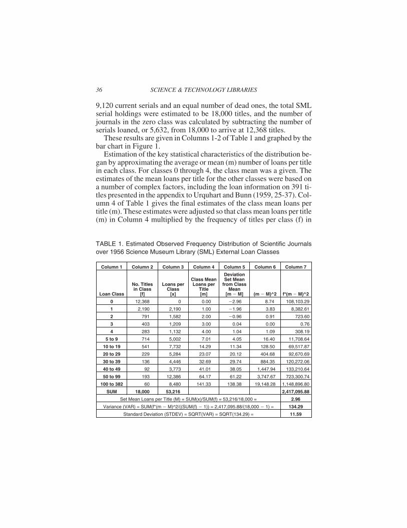
These results are given in Columns 1-2 of Table 1 and graphed by thebar chart in Figure 1.

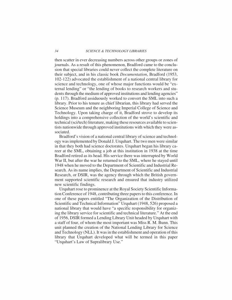
Estimation of the key statistical characteristics of the distribution be-gan by approximating the average or mean (m) number of loans per titlein each class. For classes 0 through 4, the class mean was a given. Theestimates of the mean loans per title for the other classes were based ona number of complex factors, including the loan information on 391 ti-tles presented in the appendix to Urquhart and Bunn (1959, 25-37). Col-umn 4 of Table 1 gives the final estimates of the class mean loans pertitle (m). These estimates were adjusted so that class mean loans per title(m) in Column 4 multiplied by the frequency of titles per class (f) in


TABLE 1. Estimated Observed Frequency Distribution of Scientific Journalsover 1956 Science Museum Library (SML) External Loan Classes

Column 1 Column 2 Column 3 Column 4 Column 5 Column 6 Column 7

Loan Class

No. Titlesin Class

[f]

Loans perClass

[x]

Class MeanLoans per

Title[m]

DeviationSet Mean

from ClassMean

[m M] (m M)^2 f*(m M)^2

0 12,368 0 0.00 �2.96 8.74 108,103.29

1 2,190 2,190 1.00 �1.96 3.83 8,382.61

2 791 1,582 2.00 �0.96 0.91 723.60

3 403 1,209 3.00 0.04 0.00 0.76

4 283 1,132 4.00 1.04 1.09 308.19

5 to 9 714 5,002 7.01 4.05 16.40 11,708.64

10 to 19 541 7,732 14.29 11.34 128.50 69,517.87

20 to 29 229 5,284 23.07 20.12 404.68 92,670.69

30 to 39 136 4,446 32.69 29.74 884.35 120,272.06

40 to 49 92 3,773 41.01 38.05 1,447.94 133,210.64

50 to 99 193 12,386 64.17 61.22 3,747.67 723,300.74

100 to 382 60 8,480 141.33 138.38 19,148.28 1,148,896.80

SUM 18,000 53,216 2,417,095.88

Set Mean Loans per Title (M) = SUM(x)/SUM(f) = 53,216/18,000 = 2.96

Variance (VAR) = SUM(f*(m � M)^2/((SUM(f) � 1)) = 2,417,095.88/(18,000 � 1) = 134.29

Standard Deviation (STDEV) = SQRT(VAR) = SQRT(134.29) = 11.59

Column 2 yielded loans per class (x) in Column 3 that in turn summed tothe total number of reported loans of 53,216.

The summary of the key distributional findings by Urquhart andBunn above suggests two methods of aggregating the frequency distri-bution of sci/tech journals across 1956 SML external loans into broaderloan classes. These methods are shown in Table 2. The first method is toaggregate the distribution into two loan classes: low (0 to 9 loans) andhigh (100 to 382 loans). This method of aggregation played a key role inUrquhart’s management of the NLL journal collection. Inspection ofthe high loan class reveals that it contained 1,251 titles that comprised6.95% of the titles and accounted for 79.11% of the loans. This accordswell with the statement by Urquhart (1959, 293) in his 1958 conferencereport that “about 1,250 serials (or less than 10% of those available ifthe non-current serials are included) are sufficient to meet 80% of thedemand for serial literature.” The second method is to aggregate thejournals into three loan classes: low (0 to 9 loans), high (10 to 39 loans),and super high (40 to 382 loans). It can be seen that the super high classencompassed 345 titles or 1.92% that accounted for 46.30% of theloans. This comes close to the above statement in Urquhart and Bunnthat “about 350 titles accounted for 50 per cent of the total use of seri-


14,000

12368

100 to382

50 to99

40 to49

30 to39

20 to29

10 to19

5 to9

4321

2190

791 403 283714 541 229 136 92 193 60

Loan Frequency Class

Nu

mb

ero

fJo

urn

als

12,000

10,000

8,000

6,000

4,000

2,000

00

FIGURE 1. Frequency Distribution of Scientific Journals by Urquhart’s 1956Science Museum Library (SML) External Loan Classes

als.” From these facts it can be seen that the above estimate of the fre-quency distribution of sci/tech journals across the 1956 SML externalloans is a good approximation of the one that was actually observed.

The above approximation can now be utilized to calculate certain keystatistical characteristics of the frequency distribution of sci/tech jour-nals across 1956 SML external loans. In making such calculations, Ex-cel spreadsheet notation is utilized in this paper. The first characteristicis the arithmetic mean or average loans per title. AVERAGE is the Ex-cel function for arithmetic mean. This is a measure of central tendency,and for the entire set of SML journals it is derived by dividing the totalnumber of journals into the total number of external loans. In Table 1,the set mean is designated by M to distinguish it from the class means m.Using the terminology of Table 1, the calculation of M is the following:

AVERAGE (M) = SUM(x)/SUM(f) = 53,216/18,000 = 2.96

The next two statistical characteristics are both measures of the disper-sion of the external loans of individual titles around the set mean M. Ofthese, the basic measure is sample variance. Variance is a measure ofthe variability or dispersion of the values of a dataset found by averagingthe squared deviations about the mean. Table 1 demonstrates a shorthand


TABLE 2. Two Methods of Aggregating 1956 Science Museum Library (SML)External Loan Classes

1. Two classes

Loan ClassNo. Titles in

ClassMean Loans

per TitleLoans per

Class% Titles per

Class% Loans per

Class

Low( 0 to 9)

16,749 0.66 11,115 93.05% 20.89%

High(10 to 382)

1,251 33.65 42,101 6.95% 79.11%

SUM 18,000 53,216 100.00% 100.00%

2. Three Classes

Loan ClassNo. Titles in

ClassMean Loans

per TitleLoans per

Class% Titles per

Class% Loans per

Class

Low( 0 to 9)

16,749 0.66 11,115 93.05% 20.89%

High(10 to 39)

906 19.27 17,462 5.03% 32.81%

Super High(40-382)

345 71.42 24,638 1.92% 46.30%

SUM 18,000 53,216 100.00% 100.00%

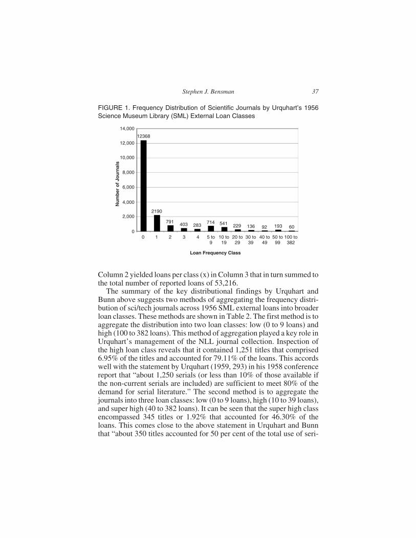
method of calculating variance that is of great utility in library research.With this method, one first groups the observations into classes as isdone in Columns 1-2. Then, as was done in Column 4, one estimates ei-ther the midpoint or mean for each of these classes–in this case, m. Thenext steps are to subtract the set mean M from each class mean m (Col-umn 5), square these remainders (Column 6), and multiply the squaredremainders by the number or frequency of observations f in each class(Column 7). These products are then added, and the resulting sum isthen divided by the sum of the observations f. For technical reasons, it isbest to subtract 1 from the sum of the observations. The result is thevariance. In the Table 1 terms, the calculation is the following:

VAR = SUM(f*(m�M^ 2)/(SUM(f)�1) = 2,417,095.88/(18,000�1) = 134.29

The other measure of dispersion is the sample standard deviation, whichis found by taking the square root of the sample variance thus:

STDEV = SQRT(VAR) = SQRT(134.29) = 11.59

It is to be noted that the set variance is much greater than the set meanand that the bulk of the variance–82.97%–derives from the titles in thesuper high loan class.

In his report to the 1958 scientific information conference, Urquhart(1959, 289-291) related the distribution of sci/tech journals by supra-library use to the number of library holdings of these journals. The re-sult comprised the second key finding of the analysis of 1956 SMLexternal loans. To do this, he first listed in descending rank order thetop 10 journals by 1956 SML external loans and their correspondinglibrary holdings as given by the British Union Catalogue of Periodicals(BUCOP). One is struck by the prestigious nature of most of these top10 journals. The highest one was the Proceedings of the Royal Societyof London (Series A) with 382 external loans, and among these top jour-nals were Science and the Journal of the Chemical Society. Their meannumber of external loans was 232.5. Urquhart then took samples of 10journals from those titles with respectively 20, 2, and 0 external loans.He averaged the BUCOP holdings of these four samples and summa-rized the results in a table that is replicated by Table 3. Here is visiblethe strong correlation of SML external loans with BUCOP holdings,with the average number of these holdings skewing rapidly downwardfrom 57 for the top ten titles by SML loans, to 22.4 for the titles with 20


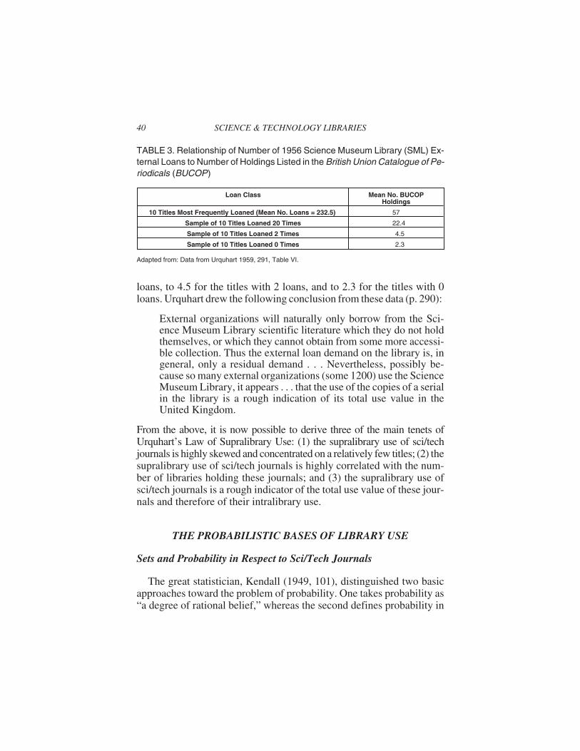
loans, to 4.5 for the titles with 2 loans, and to 2.3 for the titles with 0loans. Urquhart drew the following conclusion from these data (p. 290):

External organizations will naturally only borrow from the Sci-ence Museum Library scientific literature which they do not holdthemselves, or which they cannot obtain from some more accessi-ble collection. Thus the external loan demand on the library is, ingeneral, only a residual demand . . . Nevertheless, possibly be-cause so many external organizations (some 1200) use the ScienceMuseum Library, it appears . . . that the use of the copies of a serialin the library is a rough indication of its total use value in theUnited Kingdom.

From the above, it is now possible to derive three of the main tenets ofUrquhart’s Law of Supralibrary Use: (1) the supralibrary use of sci/techjournals is highly skewed and concentrated on a relatively few titles; (2) thesupralibrary use of sci/tech journals is highly correlated with the num-ber of libraries holding these journals; and (3) the supralibrary use ofsci/tech journals is a rough indicator of the total use value of these jour-nals and therefore of their intralibrary use.

THE PROBABILISTIC BASES OF LIBRARY USE

Sets and Probability in Respect to Sci/Tech Journals

The great statistician, Kendall (1949, 101), distinguished two basicapproaches toward the problem of probability. One takes probability as“a degree of rational belief,” whereas the second defines probability in


TABLE 3. Relationship of Number of 1956 Science Museum Library (SML) Ex-ternal Loans to Number of Holdings Listed in the British Union Catalogue of Pe-riodicals (BUCOP)

Loan Class Mean No. BUCOPHoldings

10 Titles Most Frequently Loaned (Mean No. Loans = 232.5) 57

Sample of 10 Titles Loaned 20 Times 22.4



Adapted from: Data from Urquhart 1959, 291, Table VI.

terms of “frequencies of occurrence of events, or by relative proportionsin ‘populations’ or ‘collectives.’” In this paper, we will be concernedwith the frequency theory of probability. The most cogent developmentof the frequency theory was done by Von Mises (1957), who basedprobability on relative frequencies within what he termed the “collec-tive” but may also be considered a “set.” Von Mises defined the collec-tive as “a sequence of uniform events or processes which differ bycertain observable attributes, say colours, numbers, or anything else”(p. 12), and he admonished, “It is possible to speak about probabilitiesonly in reference to a properly defined collective” (p. 28). Von Mises(pp. 16-18) used as an example of this requirement the fact that a per-son’s probability of dying at a given age is dependent on whether thisperson is defined as belonging to a collective containing both men andwomen or only men. Mises’ requirement of well-defined sets poses oneof the central problems for the application of the frequency theory ofprobability in library and information science.

Set definition in respect to sci/tech journals is governed by Brad-ford’s Law of Scattering. Starting from the principle of the unity of sci-ence by which every scientific subject is related to every other scientificsubject, Bradford (1934, 1986) gave the following verbal formulationof his Law of Scattering:

. . . the law of distribution of papers on a given subject in scientificperiodicals may thus be stated: if scientific journals are arranged inorder of decreasing productivity of articles on a given subject, theymay be divided into a nucleus of periodicals more particularly de-voted to the subject and several groups or zones containing thesame number of articles as the nucleus and succeeding zones willbe as 1 : n : n2 . . .

Bensman (2001, 238) interpreted Bradford’s Law as “a mathematicaldescription of a probabilistic model for the formation of fuzzy sets.”Classical set theory is based upon the binary “crisp set,” whose ele-ments are either clearly members of the set–numerically represented by1–or not members of the set–numerically represented by 0. In contrast, a“fuzzy set” consists of elements that are not always fully in the set andcan have membership grades ranging from 0 to 1.

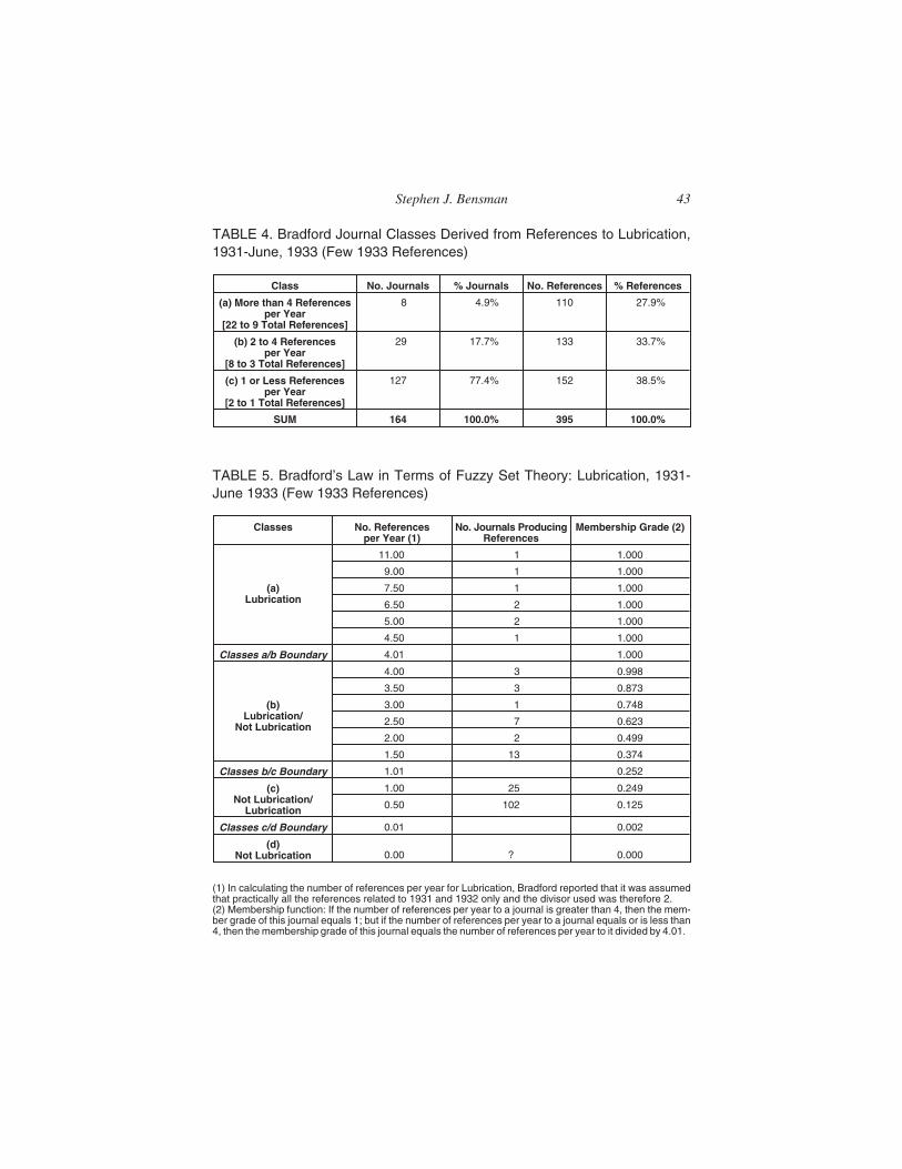
The relationship of the Law of Scattering to fuzzy set theory can bedemonstrated with the data presented by Bradford (1934) on the distri-bution of articles on the subject Lubrication over a set of 164 journalsduring the period 1931 through June 1933. These data were compiled


from references to Lubrication articles in a current bibliography beingprepared at the Science Museum Library. Bradford aggregated his datainto 3 classes: (a) journals producing more than 4 references per year;(b) journals producing more than one and not more than 4 references peryear; and (c) journals producing 1 or less references per year. The re-sults are shown in Table 4, and it can be seen that the distribution is verysimilar to the distribution of journals by 1956 SML external loans ob-served by Urquhart more than 20 years later. In the terms of Bradford’sLaw of Scattering, class a is the “nucleus of periodicals more particu-larly devoted to the subject,” whereas classes b and c are the “severalgroups or zones containing the same number of articles as the nucleus.”Thus, class a is comprised of 4.9% of the journals that produced 27.9%of the Lubrication references, and the number of journals in classes band c has to rise exponentially from 17.7% to 77.4% to produce approx-imately the same percentage of Lubrication references. Bradford’s threeclasses can also be defined by their decreasing subject membershipgrade in the following manner: (a) Lubrication; (b) Lubrication/Not Lu-brication; and (c) Not Lubrication/Lubrication. Using these definitions,it is possible to construct the following function for quantifying themembership grade of the 164 journals in the Lubrication set:

If the number of references per year to a journal is greater than 4,then the membership grade of this journal equals 1; but if the num-ber of references per year equals or is less than 4, then the member-ship grade of this journal equals the number of references per yeardivided by 4.01.

Applying this function to Bradford’s Lubrication data yields the re-sults shown in Table 5. Here is seen a small core of journals fully in theLubrication set with a membership grade of 1, and outside this core themembership grade of the journals skews rapidly downward from 0.998to 0.125 as the number of journals skews rapidly upward from 3 to 102.As the proportion of Lubrication articles decreases in the journals,scope opens in the journals for articles on other subjects. A zeroclass–(d) Not Lubrication–has been added in the table with a questionmark for the number of journals in it. The number of journals in the zeroclass has been deliberately left open, as this is an exceedingly complexquestion, which Bradford himself never successfully resolved.

Bradford’s Law of Scattering mandates that subject sets of sci/techjournals will not be crisp ones but complex composites of various sub-ject subsets. Moreover, the inability to determine the zero class means



TABLE 4. Bradford Journal Classes Derived from References to Lubrication,1931-June, 1933 (Few 1933 References)

Class No. Journals % Journals No. References % References

(a) More than 4 Referencesper Year

[22 to 9 Total References]

8 4.9% 110 27.9%

(b) 2 to 4 Referencesper Year


29 17.7% 133 33.7%

(c) 1 or Less Referencesper Year


127 77.4% 152 38.5%

SUM 164 100.0% 395 100.0%

TABLE 5. Bradford’s Law in Terms of Fuzzy Set Theory: Lubrication, 1931-June 1933 (Few 1933 References)

Classes No. Referencesper Year (1)

No. Journals ProducingReferences

Membership Grade (2)

(a)Lubrication

11.00 1 1.000

9.00 1 1.000

7.50 1 1.000

6.50 2 1.000

5.00 2 1.000

4.50 1 1.000

Classes a/b Boundary 4.01 1.000

(b)Lubrication/

Not Lubrication

4.00 3 0.998

3.50 3 0.873

3.00 1 0.748

2.50 7 0.623

2.00 2 0.499

1.50 13 0.374

Classes b/c Boundary 1.01 0.252

(c)Not Lubrication/

Lubrication

1.00 25 0.249

0.50 102 0.125

Classes c/d Boundary 0.01 0.002

(d)Not Lubrication 0.00 ? 0.000

(1) In calculating the number of references per year for Lubrication, Bradford reported that it was assumedthat practically all the references related to 1931 and 1932 only and the divisor used was therefore 2.(2) Membership function: If the number of references per year to a journal is greater than 4, then the mem-ber grade of this journal equals 1; but if the number of references per year to a journal equals or is less than4, then the membership grade of this journal equals the number of references per year to it divided by 4.01.

that there are no clear lines of demarcations between subject sets andsubsets. Librarians have long been aware of this characteristic of sci/tech journals. In his standard work on serials, Osborn (1980, 268-288)states that libraries can operate excellently without classifying their pe-riodicals and satisfactorily without providing subject headings for them.He advanced indexing as a better method of providing subject access tojournals.

However, while these practical implications of Bradford’s Law arewell understood, the same cannot be said for its probabilistic conse-quences. As a result of this law, sci/tech journal distributions are mostoften complex amalgams of various distributions resulting from the dif-ferent underlying probabilities of the component subject subsets. Thisphenomenon is also characteristic of distributions of other library mate-rials. Given the fuzzy nature of these sets and subsets, these distribu-tions are often not amenable to precise mathematical formulation.

The Calculation of Probability and the Normal Distribution

Probability is calculated by a mathematical equation called the prob-ability density or probability mass function that determines what can bedescribed generically as the proportion of members of a given set thathave a specific characteristic. For example, this can be the proportion ofa set of coins that are heads or–in terms of the question under analy-sis–the proportions of the sci/tech journal collection of the SML that in1956 were externally loaned 0, 1, 2, 3, etc., times. A crucial element ofthe equation is a numerical constant called the parameter, which can belogically known a priori or estimated a posteriori from the data. Proba-bility can be represented visually by means of a curve on a graph, onwhose X, or horizontal axis, are the measures of the characteristic andon whose Y, or vertical axis, are the measures of the proportion or num-ber of occurrences of this characteristic. Total probability is numeri-cally defined as 1.00, and this number is assigned to the total area underthe mathematical curve. The probability of the characteristic is the pro-portion or percent of the area under the curve that is above a definedsegment of the X axis.

These basics of probability will be demonstrated with the normaldistribution, which is graphically represented in Figure 2. The equa-tion for the normal distribution has two parameters–the arithmeticmean and the standard deviation. This equation results in some form ofthe bell-shaped curve that is shown in Figure 2. Looking at the graph, itcan be seen that with the normal distribution the area under the curve on


the segment of the X axis between the mean and one standard deviationabove the mean is 34% of the total area under the curve and, therefore,contains 0.34 of the observations or members of the set. If one turns toFigure 1 with the bar chart of the frequency distribution of sci/tech jour-nals by SML external loans in 1956 and mentally constructs a curve byconnecting the tops of the bars with lines, one can see by comparingcurves that this frequency distribution is nowhere near being repre-sented by the normal distribution or any approximation to it.

The normal distribution was developed in the 18th and early 19thcentury as a law of error in astronomy and geodesy. Eisenhart (1983,530) defines laws of error as “probability distributions assumed to de-scribe the distribution of the errors arising in repeated measurement of afixed quantity,” and he states that they had the purpose of demonstratingthe utility of taking the arithmetic mean of these measurements as agood choice for the value of the magnitude of this quantity. This ex-plains the shape of the normal distribution. The mean is the same as themode, or the point of the most frequently occurring value in a set of ob-servations, and the symmetrical shape of the curve mandates that thereis a 50/50 chance of an observation being on either side of the mean.During the 19th century, the normal distribution was thought to de-


Y

X2% 2%

�3 �2 �1 Mean Variable68%

95.44%

99.74%

+1 +2 +3

13% 13%34% 34%

FIGURE 2. Probability as a Proportion of the Area Under the Normal Curve

A normal distribution indicating placement of 1, 2, and 3 standard deviation units on either side of the mean.Source: Carpenter, Ray L., and Ellen Storey Vasu. 1978. Statistical methods for librarians. Chicago: Ameri-can Library Asoociation, p. 23. Reprinted with permission.

scribe not only the distribution of error but also of all physical and socialmeasurements. But this idea was refuted, and Snedecor and Cochran(1989, 40 and 44-50) state that the single most important reason for useof the normal curve is the central limit theorem, by which the distribu-tion of the means of samples from even a non-normal population tendsto become normal as the size of the sample increases.

The Binomial Distribution

The normal distribution is a continuous distribution in that it de-scribes the distribution of variables that can take on any value includingfractional ones. However, for the most part, library data consists of dis-crete integer counts and therefore requires discrete or discontinuousprobability distributions. The basic ones of the latter type are the bino-mial distribution and the Poisson distribution.

Of these two distributions the binomial is historically the most im-portant one, as it was the first probability distribution from which all theothers were ultimately derived. The binomial distribution is based uponthe repeated drawing of samples of a given size s from a population con-sisting of two classes (success-failure, yes-no, etc.). Besides the samplesize s, its density function has one other constant, the parameter p orprobability, which is the proportion of successes in the total population.Concerning the other population class, the proportion of failures is des-ignated by q, so that q = 1 � p and p + q = 1. The distribution itself is cal-culated by the expansion of the binomial (p + q)^s. Of great importancein the binomial distribution is the close connection of the arithmeticmean with probability. The arithmetic mean is the size of the sample smultiplied by the probability of success p, so that:

AVERAGE = s*p

This close connection caused Rietz (1927, 14-16) to equate the meanwith “the mathematical expectation of the experimenter.” It is also im-portant to note for the discussion below that the variance and standarddeviation of a binomial distribution can be calculated by the followingtwo equations:

VARbinom = s*p*qSTDEVbinom = SQRT(s*p*q) = SQRT(VARbinom)

The binomial distribution will now be demonstrated with Urquhart’s1956 SML external loan data on the a priori assumption that p = 0.5 or


the probability of heads on the flipping of a fair coin. A major problemof applying the binomial distribution to library use is that it requiresknowledge of not only the number of successes but also the number offailures. However, while it is relatively easy to count the number oftimes a journal has been loaned, it is not possible to count the numberof times a journal has not been loaned. This makes it difficult to de-termine the size of the binomial sample s and to estimate the param-eter p. One way around this difficulty is to utilize the techniquesuggested by Grieg-Smith (1983, 57-58) and recommended by Elliott(1977, 17). The technique requires that one first define the size of the bi-nomial sample s by determining the maximum possible number of oc-currences for any given member of the set. The journal most frequentlyborrowed by outside organizations from the SML in 1956 was the Pro-ceedings of the Royal Society of London (Series A), which accounted for382 external loans, and it is logical to use this number for the size of thebinomial sample s. From the perspective of binomial theory, each jour-nal now becomes a sample of 382 possible loans. Having done this, it isnow possible to make the following calculations:

Number of SML Journals (n) = 18,000s = 382p = 0.5

q = 1 � 0.5 = 0.5Total Possible Loans (Tpos) = n*s = 18,000*382 = 6,876,000

Total Actual Loans (Tact) = Tpos*p = 6,876,000*0.5 = 3,438,000AVERAGE = Tact/n = 3,438,000/18,000 = 191

AVERAGE = s*p = 382*0.5 = 191VARbinom = s*p*q = 382*0.5*0.5 = 95.51

STDEVbinom = SQRT(VARbinom) = SQRT(95.51) = 9.77

The two ways of calculating AVERAGE demonstrate the close con-nection of the arithmetic mean with probability. To provide a furtherunderstanding of the binomial distribution, 382 and 0.5 were respec-tively used as the constants s and p in the binomial density function, andthe resulting distribution of journals by number of external loans wasboth calculated and graphed. Figure 3 graphs the binomial distributionof titles at p = 0.5 over each possible number of 1956 SML externalloans from 0 to 382. A look at Figure 3 in conjunction with Figure 2 il-lustrates the close connection of the binomial distribution with the nor-mal law of error, as both frequency curves have the same symmetrical,bell-shaped form. According to Snedecor and Cochran (1989, 117-119and 130), as s increases, the discrete binomial distribution approximates


more and more the continuous normal distribution. The size of the s re-quired for this approximation is dependent on the value of p, beingsmallest at p = 0.5, where the approximation is good with s as low as 10.

At p = 0.5, all 18,000 titles in the SML collection would have concen-trated in the Loan Class (100 to 382), which is the upper level of theSuper High Loan Class in Section 2 of Table 2. However, a glance atTables 1-2 and Figure 1 demonstrates that this was obviously not thecase, because in reality an estimated 16,749 titles or 93.05% were con-centrated in the Low Loan Class (0 to 9). Moreover, a comparison of theobserved set mean of 2.96 loans per title to the theoretical set mean of191 loans per title at p = 0.5 is proof that the actual overall probability oftitles being loaned was extremely low. Using the same techniques asabove but basing ourselves on the total number of 53,216 external loansactually observed, we can calculate a posteriori the binomial character-istics of the distribution of sci/tech journal titles by 1956 SML externalloans thus:

Number of SML Journals (n) = 18,000s = 382

Total Possible Loans (Tpos) = n*s = 18,000*382 = 6,876,000Total Observed Loans (Tobs) = 53,216

p = Tobs/Tpos = 53,216/6,876,000 = 0.01


0

100

200

300

400

500

600

700

800

0 17 34 51 68 85102

119136

153170

187204

221238

255272

289306

323340

357374

Number of External Loans

Nu

mb

ero

fJo

urn

als

FIGURE 3. Distribution of Scientific Journals by Number of 1956 Science Mu-seum Libary (SML) External Loans on Assumption of Binomial with p of 0.5

q = 1 � p = 1 � 0.01 = 0.99AVERAGE = Tobs/n = 53,216/18,000 = 2.96

AVERAGE = s*p = 382*0.01 = 2.96VARbinom = s*p*q = 382*0.01*0.99 = 2.93

STDEVbinom = SQRT(VARbinom) = SQRT(2.93) = 1.71

These calculations demonstrate that in 1956 the overall probability ofSML external loans was only 0.01.

The Poisson Distribution

As probability becomes extremely low, the binomial distribution istransformed into the Poisson distribution. The latter distribution is themost important probability distribution for modeling library use. Its im-portance in this respect arises not only from its characteristics that makeit suitable for this purpose but also from its overall importance. Thus,R. A. Fisher (1970, 54), one of the founders of modern inferential sta-tistics, ranked the normal distribution as the most important of thecontinuous distributions and the Poisson as the most important of thediscontinuous distributions. The name of this distribution is taken fromthat of Siméon Denis Poisson, who is generally credited with being thefirst to derive this distribution as a limit to the binomial in an 1837 bookon judicial decisions.

What makes the Poisson distribution particularly fit for modeling li-brary use are the following characteristics. First, it is a discontinuousdistribution, and library use is measured by integer counts. Second, itarises as a limit to the binomial as p becomes very small, and the proba-bility governing library use is usually very small. As has been seenabove, the binomial p of external loans for all sci/tech journals in theSML collection in 1956 was 0.01, and this probability was much re-duced in respect to individual titles. For example, the probability of themost highly loaned title, the Proceedings of the Royal Society of London(Series A), was 0.00006. Third, the process by which the Poisson arisesis suited to library use. Thus, whereas the binomial distribution is basedupon the repetitive taking of samples of a given size containing bothsuccesses and failures, the Poisson distribution is based on mean rate ofoccurrence–technically called lambda (λ)–over some defined contin-uum such as time or space. With library use, space can be defined interms of either individual titles or subject classes. Lambda is the onlyparameter of the Poisson density function, and it is much easier to esti-mate from library use data than the binomial p. With the binomial p, one


has to make an estimate not only of the number of times items were usedbut also the number of times items were not used, whereas the Poissonlambda can be estimated by simply counting the number of uses oversome observation period and then dividing by the number of items sub-ject to use. The Poisson’s versatility in respect to library use is enhancedby the fact that, when p is small, the binomial and the Poisson are equiv-alent and can be substituted for each other. A key feature of the Poissondistribution is that lambda is equal to both the mean and the variance.

This is expressed by the following identity:

λ = AVERAGE = VAR

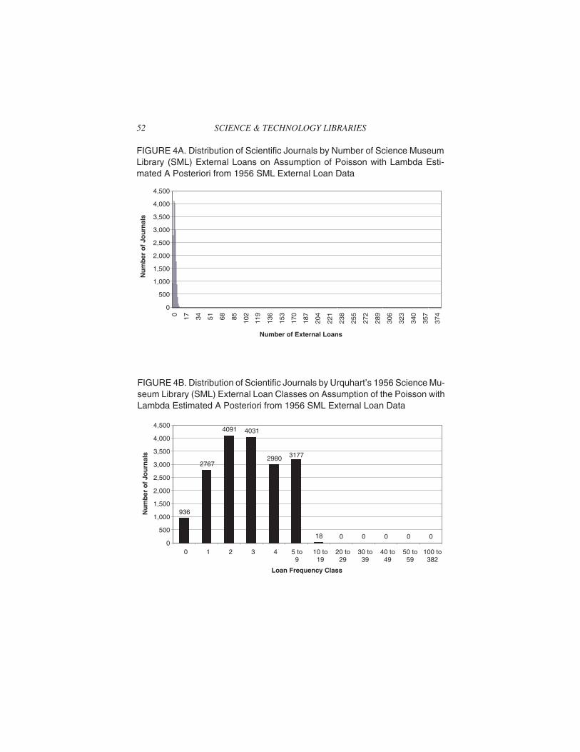
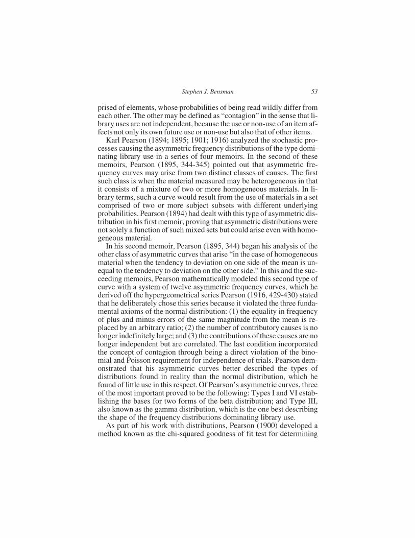
To demonstrate the Poisson in terms of the distribution of sci/techjournals by 1956 SML external loans, the mean of these loans per ti-tle–2.96–was utilized as lambda in the Poisson density function. Thismean was selected to make the Poisson equivalent to the binomial withp = 0.01. The resulting frequency distribution of these titles was tabu-lated in terms of Urquhart’s 1956 SML external loan classes presentedin Table 1, and the tabulation is given in Table 6 next to the observeddistribution of titles across these classes. This hypothetical Poisson dis-tribution is graphed by Figures 4A and 4B above in two different ways.Figure 4A shows the correct theoretical shape of the distribution,whereas Figure 4B utilizes the same bar chart structure by Urquhart’sclasses as Figure 1 to facilitate comparison of the hypothetical Poissondistribution to the distribution actually observed in 1956. Comparingthe tabulations of the hypothetical Poisson distribution against the ob-served distribution in Table 6 and Figure 4B against Figure 1 revealsthat the Poisson distribution differs from the observed frequency distri-bution in two key ways: (1) the observed number of titles in LoanClasses 2, 3, and 4 around the mean of 2.96 is much lower than the num-ber predicted by the Poisson; and (2) the observed number of titles in theloan classes at the two extremes–0 as well as 10 and above–is muchhigher than the number predicted by the Poisson. It should be noted thatequivalent tabulations and graphs of the hypothetical binomial distri-bution with p = 0.01 were virtually identical to those of the Poisson withλ = 2.96. Moroney (1956, 127) counsels that the Poisson distributioncan always be used as an approximation to the binomial distributionwhenever p in the binomial is small with the approximation becomingbetter as p approaches zero.


The Stochastic Processes of Library Use:Pearson and Asymmetric Distributions

The poor fit of both the binomial and the Poisson distributions to thefrequency distribution of sci/tech journals by 1956 external loans indi-cates that there are stochastic or random processes affecting library usewhich limit the applicability of these distributions. Since the Poisson isa special case of the binomial, the requirements for these distributionsare similar. Thus, in respect to the binomial, Rietz (1927, 24) states tworequirements: (1) p must remain constant from sample to sample; and(2) the samples must be mutually independent in that the results of asample should not depend in any significant degree on the results of pre-vious samples. As for the Poisson distribution, Elliott (1977, 22) listsfour such requirements: (1) p must be constant and small; (2) the num-ber of successes per sampling unit must be well below the maximumnumber that can occur in a sampling unit; (3) the occurrence of a suc-cess must not increase or decrease the probability of another success;and (4) the samples must be small relative to the population. Library useviolates these requirements in two important ways. The first may be cat-egorized as “heterogeneity,” namely, that library collections are com-


TABLE 6. Comparison of Observed Frequency Distribution of Scientific Journalsover 1956 Science Museum Library (SML) External Loan Classes to Hypo-thetical Poisson and Negative Binomial Distributions with Parameters EstimatedA Posteriori from 1956 SML External Loan Data

Loan Class Observed TitleFrequency Distribution

Hypothetical PoissonDistribution

Hypothetical NegativeBinomial Distribution

0 12,368 936 12,368

1 2,190 2,767 1,357

2 791 4,091 728

3 403 4,031 494

4 283 2,980 370

5 to 9 714 3,177 1,060

10 to 19 541 18 852

20 to 29 229 0 356

30 to 39 136 0 179

40 to 49 92 0 97

50 to 99 193 0 128

100 to 382 60 0 13

SUM 18,000 18,000 18,000


0

500

1,000

1,500

2,000

2,500

3,000

3,500

4,000

4,500

0 17 34 51 68 85 102

119

136

153

170

187

204

221

238

255

272

289

306

323

340

357

374


Nu

mb

ero

fJo

urn

als

FIGURE 4A. Distribution of Scientific Journals by Number of Science MuseumLibrary (SML) External Loans on Assumption of Poisson with Lambda Esti-mated A Posteriori from 1956 SML External Loan Data

936

2767

4091 4031

2980 3177

18 0 0 0 0 00

500

1,000

1,500

2,000

2,500

3,000

3,500

4,000

4,500

0 1 2 3 4 5 to9

10 to19

20 to29

30 to39

40 to49

50 to59

100 to382


Nu

mb

ero

fJo

urn

als

FIGURE 4B. Distribution of Scientific Journals by Urquhart’s 1956 Science Mu-seum Library (SML) External Loan Classes on Assumption of the Poisson withLambda Estimated A Posteriori from 1956 SML External Loan Data

prised of elements, whose probabilities of being read wildly differ fromeach other. The other may be defined as “contagion” in the sense that li-brary uses are not independent, because the use or non-use of an item af-fects not only its own future use or non-use but also that of other items.

Karl Pearson (1894; 1895; 1901; 1916) analyzed the stochastic pro-cesses causing the asymmetric frequency distributions of the type domi-nating library use in a series of four memoirs. In the second of thesememoirs, Pearson (1895, 344-345) pointed out that asymmetric fre-quency curves may arise from two distinct classes of causes. The firstsuch class is when the material measured may be heterogeneous in thatit consists of a mixture of two or more homogeneous materials. In li-brary terms, such a curve would result from the use of materials in a setcomprised of two or more subject subsets with different underlyingprobabilities. Pearson (1894) had dealt with this type of asymmetric dis-tribution in his first memoir, proving that asymmetric distributions werenot solely a function of such mixed sets but could arise even with homo-geneous material.

In his second memoir, Pearson (1895, 344) began his analysis of theother class of asymmetric curves that arise “in the case of homogeneousmaterial when the tendency to deviation on one side of the mean is un-equal to the tendency to deviation on the other side.” In this and the suc-ceeding memoirs, Pearson mathematically modeled this second type ofcurve with a system of twelve asymmetric frequency curves, which hederived off the hypergeometrical series Pearson (1916, 429-430) statedthat he deliberately chose this series because it violated the three funda-mental axioms of the normal distribution: (1) the equality in frequencyof plus and minus errors of the same magnitude from the mean is re-placed by an arbitrary ratio; (2) the number of contributory causes is nolonger indefinitely large; and (3) the contributions of these causes are nolonger independent but are correlated. The last condition incorporatedthe concept of contagion through being a direct violation of the bino-mial and Poisson requirement for independence of trials. Pearson dem-onstrated that his asymmetric curves better described the types ofdistributions found in reality than the normal distribution, which hefound of little use in this respect. Of Pearson’s asymmetric curves, threeof the most important proved to be the following: Types I and VI estab-lishing the bases for two forms of the beta distribution; and Type III,also known as the gamma distribution, which is the one best describingthe shape of the frequency distributions dominating library use.

As part of his work with distributions, Pearson (1900) developed amethod known as the chi-squared goodness of fit test for determining


how well an actual frequency distribution matches a theoretical frequencydistribution. This test is based upon the chi-squared distribution, whichis a particular case of his Type III or gamma distribution. R. A. Fisher(1966, 195-196) identified the essence of Pearson’s chi-squared test as acomparison of the variance estimated from a sample with the true vari-ance.

As a result of Pearson’s work, it is possible to summarize the problemof analyzing the asymmetric distributions dominating library use underthe following points. First, such distributions may arise not only fromheterogeneous sets comprised of various subsets with differing proba-bilities but also from homogeneous sets whose individual elements mayhave differing probabilities. Second, the underlying causes may be cor-related, and, therefore, a contagious process may be taking place,whereby the occurrence of an event affects its probability of reoccur-rence. And, third, the amount of variance is one of the key characteris-tics that distinguish one type of distribution from another.

The Lexian System of Distributions

The pioneering work on Pearson’s first class of asymmetric distribu-tions–those arising from a mixture of two more homogeneous materi-als–was done by the German economist, Wilhelm Lexis, who expoundedhis theories in a series of articles and monographs published in the pe-riod 1875-1879. Two of the most cogent English expositions of Lexis’ideas were written by Rietz (1924) and A. Fisher (1922, 117-126).

The basis of Lexis’ ideas was to test for the structure of a set by com-paring its actual variance to its theoretical binomial variance throughthe Lexis Ratio (L). This is done by first calculating the standard devia-tion (STDEV) directly off the data as was demonstrated in Table 7 thenits theoretical binomial standard deviation (STDEVbinom), and finallydividing the direct standard deviation by the theoretical binomial stan-dard deviation thus:

L = STDEV/STDEVbinom

Both Rietz (1924) and A. Fisher (1922) use urn models to demonstrateset structure, and this practice will be followed here.

The urn model for the binomial distribution can be a single urn filledwith black and white balls in constant proportions, where the drawing ofa white ball is considered a success. Samples are drawn from this urnand replaced so that the proportion or probability of white balls from


sample to sample remains constant and the results of one sample doesnot affect the results of another sample. Under these conditions–homo-geneity and independent trials–the Lexis Ratio should equal or approxi-mate 1, indicating that the actual variance directly calculated from thedata equals its theoretical binomial variance. Given the binomial’s closerelationship to the normal distribution, a Lexis Ratio of 1 indicates thatthe dispersion around the mean is primarily due to random error.

However, a Lexis Ratio greater than 1 means that the actual varianceis greater than the theoretical binomial variance, and Lexian theory di-vides the variance into two components: the “ordinary or unessential”binomial component and the “physical” component (Rietz 1924, 86).The binomial component may be defined as that variance due to randomerror, whereas the excess variance is interpreted as resulting from thediffering probabilities of the component subsets and is a sign of theLexis distribution. A model for the Lexis distribution is a number ofseparate urns each containing different proportions of black and whiteballs. The urns thus represent subsets with different probabilities ofwhite balls. Samples are fully drawn from the various urns and replacedin rotation so that the probabilistic heterogeneity of the urns is empha-sized. Replacement of the samples maintains independence of trials.This is actually a good model for the binomial sampling of journal use.Under it, journals can be conceptualized as use samples of size s drawnfully in rotation from urns with differing proportions of uses andnon-uses.

According to Lexian theory, the variance of a Poisson distribution isless than the corresponding variance of a binomial, so that a Lexis Ratiosignificantly less than 1 is indicative of the former distribution. The urnmodel for the Poisson distribution is the same as that for the Lexis distri-bution, in that it, too, consists of urns with differing proportions or prob-abilities of white balls. However, instead of the samples being fullydrawn from the urns in rotation, they are constructed by taking 1 ball at atime from each urn, thereby randomizing the heterogeneous probabili-ties. It should be emphasized that a variance lower than the theoreticalbinomial variance is not necessarily a sign of the Poisson. Rietz (1924),for example, utilized binomial distributions with an overall p = 0.5 todemonstrate that randomizing the heterogeneous probabilities in theabove fashion significantly reduces the variance below that theoreti-cally expected with the binomial. The tendency of randomizing theprobabilities to reduce the amount of variance plays an important role ina statistical law that is of crucial importance for the modeling of libraryuse–Bortkiewicz’s Law of Small Numbers.


Ladislaus von Bortkiewicz was a student of Lexis, and he is bestknown for uncovering the importance of the Poisson distribution. Ac-cording to Haight (1967, 115), although Poisson discovered the mathe-matical formula, Bortkiewicz discovered the probability distribution.His Law of Small Numbers is so closely connected with the Poisson dis-tribution that it is often confused with it, but this is a misunderstandingof the Lexian bases of his work. Bortkiewicz set forth his law in a pam-phlet published in 1898, and this pamphlet has been analyzed by Winsor(1947), who modernized the mathematical notation and translated keysections of it. To develop his law, Bortkiewicz analyzed the rate soldierswere kicked to death by horses in 14 Prussian Army corps in the 20-yearperiod 1875-1894. These corps had different probabilities of soldiersbeing killed, so that the mean rate of deaths–or the lambda–differedfrom corps to corps. Nevertheless, when Bortkiewicz aggregated thedata for all the corps, he found that the resulting frequency distributionclosely fitted the Poisson. This caused him to formulate his Law ofSmall Numbers, which can be summarized simply in the followingmanner: If the field of observation is restricted to a set defined by infre-quent occurrences, the resulting frequency distribution will fit the Pois-son, whatever the differing probabilities of the elements or subsetscomprising that set. The main requirement is that the number of occur-


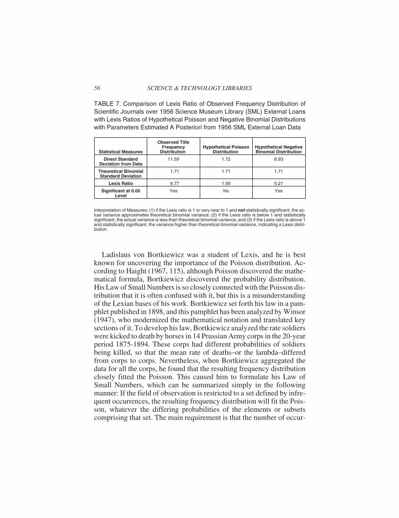
TABLE 7. Comparison of Lexis Ratio of Observed Frequency Distribution ofScientific Journals over 1956 Science Museum Library (SML) External Loanswith Lexis Ratios of Hypothetical Poisson and Negative Binomial Distributionswith Parameters Estimated A Posteriori from 1956 SML External Loan Data

Statistical Measures

Observed TitleFrequency

DistributionHypothetical Poisson

DistributionHypothetical NegativeBinomial Distribution

Direct StandardDeviation from Data

11.59 1.72 8.93

Theoretical BinomialStandard Deviation

1.71 1.71 1.71

Lexis Ratio 6.77 1.00 5.21

Significant at 0.05Level

Yes No Yes

Interpretation of Measures: (1) if the Lexis ratio is 1 or very near to 1 and not statistically significant, the ac-tual variance approximates theoretical binomial variance; (2) if the Lexis ratio is below 1 and statisticallysignificant, the actual variance is less than theoretical binomial variance; and (3) if the Lexis ratio is above 1and statistically significant, the variance higher than theoretical binomial variance, indicating a Lexis distri-bution.

rences be small out of a large population, and the more this requirementis met, the better the fit to the Poisson. It should be noted that thismethod of restricting of the field of observation has the effect of ran-domizing the probabilities since the occurrences are happening haphaz-ardly over elements or subsets with differing probabilities, and Lexiantheory dictates that the actual variance should therefore be less than thetheoretically expected one.

Bortkiewicz’s Law of Small Numbers has enormous implications forthe evaluation and management of library collections, for it means thatif the set is restricted to those items manifesting low use, no matter whatthe items or their subject class, one can expect not only that the set willhave a low overall mean rate of use but also that the use of any compo-nent of this set will not deviate very far from this mean.

Lexian analysis was applied to 1956 SML external loans, and the re-sults are presented in Table 7. Binomial theory required that all 18,000journals be considered individual urns with differing probabilities ofexternal loans, from which samples of 382 possible external loans arefully drawn in rotation. The theoretical binomial standard deviation ofthis journal set was calculated to be 1.71 above (p. 19-20). In respect tothe distribution actually observed in 1956, the direct standard deviationwas found to be 11.59 utilizing the method demonstrated in Table 1.These values yield the following Lexis Ratio for the observed distribu-tion:

L = STDEV/STDEVbinom = 11.59/1.71 = 6.77

The distribution of scientific journals by 1956 SML external loanswas thus a Lexis one, and it is possible to hypothesize that one reasonfor this excess variance is that Urquhart aggregated the loan figures forthe SML journal collection as a whole instead of presenting the loandata in terms of well defined subject subsets, thereby controlling for onesource of probabilistic heterogeneity. The direct standard deviation wasalso calculated for the Poisson distribution, whose λ parameter was esti-mated a posteriori from the 1956 SML external loan data, and it was1.72. Dividing it by the theoretical binomial standard deviation of 1.71results in a Lexis Ratio of 1 indicating the binomial distribution. Thisexperiment demonstrates that Lexian theory is rather problematic on thedistinction between binomial and the Poisson, for at the low level ofprobability, where the Poisson distribution arises, the two distributionstend to be equivalent.


Heterogeneity vs. Contagion

Probabilistic heterogeneity in the use of sci/tech journals and other li-brary materials involves two basic, interacting factors. First, there is theLexian factor of the various subject classes having different probabili-ties of being used. This factor is inherent in library use due to Bradford’sLaw of Scattering, which dictates that virtually every subject set of li-brary materials will contain subject subsets with different underlyingprobabilities of being read. Second, there is the Pearsonian factor of theprobabilistic differences of members of homogeneous subject sets be-ing used due to such causes as importance or quality, size, age, com-pleteness, language, etc. The main vehicle for modeling probabilisticheterogeneity has been the compound distribution, which is a distribu-tion that results when the parameter–p in the binomial case, λ in thePoisson case–has its own distribution sometimes termed the “mixingdistribution.” One of the chief uses of Pearson’s asymmetric distribu-tions has been to serve as such mixing distributions.

Properly conceived, the Lexis distribution is a mixture of binomialdistributions, and it was the forerunner of the compound binomial dis-tribution. Moran (1968, 76), as well as Johnson and Kotz (1969, 79), de-scribe the beta distribution, which was pioneered by Pearson, as the“natural” mixing distribution for p in the compound binomial distribu-tion. This form of the compound binomial is sometimes named the betabinomial distribution. However, for a number of reasons, it is the com-pound Poisson distribution that is more applicable for modeling libraryuse. The most important compound Poisson distribution is the negativebinomial distribution (NBD). One reason for the importance of theNBD is that it results not only from the stochastic process of heteroge-neity but also from that of contagion. The heterogeneity form of theNBD is a compound Poisson model, which was developed by Green-wood and Yule (1920) on the basis of industrial accidents among Brit-ish female munitions workers during World War I.

The Greenwood and Yule model can be explained simply in the fol-lowing manner. Each female worker was considered as having a meanaccident rate over a given period of time or her own lambda. Thus, theaccident rate of each female worker was represented by a simple Pois-son distribution. However, the various female workers had different un-derlying probabilities of having an accident and therefore differentlambdas. Greenwood and Yule posited that these different lambdaswere distributed in a skewed fashion described by Pearson’s Type III or


gamma distribution, and therefore, certain workers had a much higheraccident rate than the others and accounted for the bulk of the accidents.They found that this model fitted the data very well. Given its construc-tion, the Greenwood and Yule form of the negative binomial distribu-tion is called the gamma Poisson model. This form of the negativebinomial distribution can be considered as modeling the probabilisticheterogeneities of members of a homogeneous set, and it used Pearson’sgamma distribution as the mathematical description of accident prone-ness.

Eggenberger and Pólya (1984) formulated the contagious form of theNBD in a 1923 paper that analyzed the number of deaths from smallpoxin Switzerland in the period 1877-1900. They derived their model off anurn scheme that involved drawing balls of two different colors from anurn and not only replacing a ball that was drawn but also adding to theurn a new ball of the same color. In this way, numerous drawings of agiven color increased the probability of that color being drawn and de-creased the chance of the other color being drawn.

In a key paper, Feller (1943) stated that Eggenberger and Pólya hadindependently rediscovered a distribution originally found by Green-wood and Yule. He then analyzed the different stochastic bases of thePólya-Eggenberger and Greenwood-Yule derivations of the negative bi-nomial. According to Feller, the Pólya-Eggenberger form was a productof “true contagion,” because each favorable event increases (or de-creases) the probability of future favorable events, while the Green-wood-Yule model represented “apparent contagion,” since the eventsare strictly independent and the distribution is due to the heterogeneityof the population. Given that Greenwood-Yule and Pólya-Eggenbergerreached the NBD on different stochastic premises–the first on heteroge-neity, the second on contagion–Feller posed the conundrum that onetherefore does not know which process is operative when one finds thenegative binomial, and he pointed out that this also applies to othertypes of contagious distributions. Feller’s conundrum certainly holdstrue for library use. Thus, one does not really know whether a given sci-entific journal circulates more than others, because it is qualitatively orquantitatively different, because patrons have used and recommendedit, or because these two factors are operating interactively.

To test the applicability of the NBD as a model of library use, one suchdistribution was constructed by deriving its parameters off Urquhart’s1956 SML external loan data. This probability distribution has two pa-rameters: the arithmetic mean and a negative exponent s, which Elliott(1977, 23) describes as a measure of the excess variance in a population.


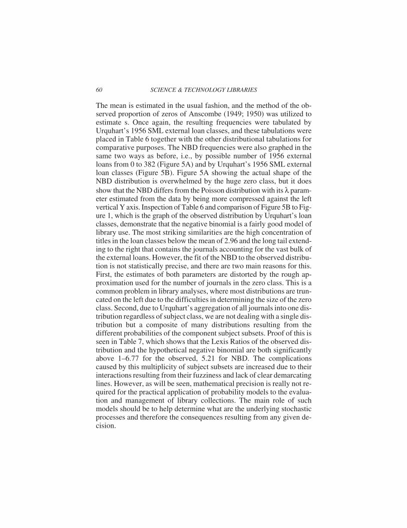
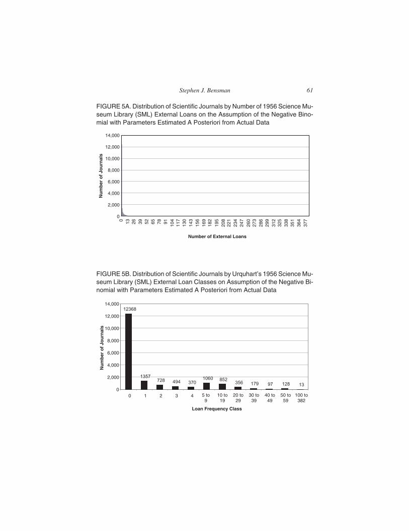
The mean is estimated in the usual fashion, and the method of the ob-served proportion of zeros of Anscombe (1949; 1950) was utilized toestimate s. Once again, the resulting frequencies were tabulated byUrquhart’s 1956 SML external loan classes, and these tabulations wereplaced in Table 6 together with the other distributional tabulations forcomparative purposes. The NBD frequencies were also graphed in thesame two ways as before, i.e., by possible number of 1956 externalloans from 0 to 382 (Figure 5A) and by Urquhart’s 1956 SML externalloan classes (Figure 5B). Figure 5A showing the actual shape of theNBD distribution is overwhelmed by the huge zero class, but it doesshow that the NBD differs from the Poisson distribution with its λ param-eter estimated from the data by being more compressed against the leftvertical Y axis. Inspection of Table 6 and comparison of Figure 5B to Fig-ure 1, which is the graph of the observed distribution by Urquhart’s loanclasses, demonstrate that the negative binomial is a fairly good model oflibrary use. The most striking similarities are the high concentration oftitles in the loan classes below the mean of 2.96 and the long tail extend-ing to the right that contains the journals accounting for the vast bulk ofthe external loans. However, the fit of the NBD to the observed distribu-tion is not statistically precise, and there are two main reasons for this.First, the estimates of both parameters are distorted by the rough ap-proximation used for the number of journals in the zero class. This is acommon problem in library analyses, where most distributions are trun-cated on the left due to the difficulties in determining the size of the zeroclass. Second, due to Urquhart’s aggregation of all journals into one dis-tribution regardless of subject class, we are not dealing with a single dis-tribution but a composite of many distributions resulting from thedifferent probabilities of the component subject subsets. Proof of this isseen in Table 7, which shows that the Lexis Ratios of the observed dis-tribution and the hypothetical negative binomial are both significantlyabove 1–6.77 for the observed, 5.21 for NBD. The complicationscaused by this multiplicity of subject subsets are increased due to theirinteractions resulting from their fuzziness and lack of clear demarcatinglines. However, as will be seen, mathematical precision is really not re-quired for the practical application of probability models to the evalua-tion and management of library collections. The main role of suchmodels should be to help determine what are the underlying stochasticprocesses and therefore the consequences resulting from any given de-cision.



117

0

2,000

4,000

6,000

8,000

10,000

12,000

14,000


Nu

mb

ero

fJo

urn

als

130

130

143

156

169

182

195

208

221

234

247

260

273

286

299

312

325

338

351

364

37726 39 52 65 78 91 104

FIGURE 5A. Distribution of Scientific Journals by Number of 1956 Science Mu-seum Library (SML) External Loans on the Assumption of the Negative Bino-mial with Parameters Estimated A Posteriori from Actual Data

5 to9

10 to19

20 to29

30 to39

40 to49

50 to59

100 to382

12368

1357728 494 370

1060 852356 179 97 128 13

0

2,000

4,000

6,000

8,000

10,000

12,000

14,000

0 1 2 3 4


Nu

mb

ero

fJo

urn

als

FIGURE 5B. Distribution of Scientific Journals by Urquhart’s 1956 Science Mu-seum Library (SML) External Loan Classes on Assumption of the Negative Bi-nomial with Parameters Estimated A Posteriori from Actual Data

The negative binomial distribution has found numerous applicationsin the biological and social sciences. One of its most important biologi-cal applications is in ecology, where Elliott (1977, 50-51) describes it asprobably the most useful mathematical model for distributions of spe-cies within given geographic areas. In respect to the social sciences, theNBD serves as the model of the zero sum game. This utilization can bedemonstrated with Urquhart’s 1956 SML external loan data in the fol-lowing manner. For any given period–say, the year 1956–there can beonly so many external loans. If a given journal has a greater probabilitybeing loaned, then it can achieve its higher loan rate only at the expenseof other journals having a lower or even zero loan rate. The higher theprobability of certain journals for being loaned, the lower must be theprobability for other journals of being loaned. This results in what istechnically called “over-dispersion” or the dispersion of journals awayfrom the mean to both extremes of the distribution. Such a phenomenonis clearly visible in both the observed frequency distribution and the hy-pothetical NBD with the heavy concentration of titles in the zero classand the long tail to the right. In this respect, both the observed distribu-tion and negative binomial distributions stand in sharp contrast to thehypothetical Poisson distribution, where the journals are heavily con-centrated in the loan classes around the mean and there is no long tail tothe right. Another name for “over-dispersion” in the social and informa-tion sciences is the “Matthew Effect.” This term is derived from the gos-pel of St. Matthew (13:12), which states: “For whoever has, to him shallmore be given, and he shall have an abundance; but whoever does nothave, even what he has shall be taken away from him.”

Indices of Dispersion

In his classic textbook, R. A. Fisher (1970, 57-61, 68-70) presentedtwo tests–one for the binomial, the other for the Poisson–that utilizePearson’s chi-squared distribution as an index of dispersion. These testscomprise the easiest ways to determine the type of probability distribu-tion and stochastic processes governing a set of data. An examination ofFisher’s equation for chi-squared in his binomial test reveals it to bebased upon a comparison of the actual variance of a set of data to its the-oretical binomial variance. The relationship to the Lexis Ratio is obvi-ous, and Fisher himself states (p. 80), “In the many references inEnglish to the method of Lexis, it has not, I believe, been noted that thediscovery of the distribution of [chi-squared] in reality completed themethod of Lexis.” He then outlined a method by which a given


chi-squared could be transformed into its equivalent Lexis Ratio.Fisher’s equation for chi-squared in his index of dispersion test for thePoisson is based upon a comparison of the actual variance of a set to thearithmetic mean of the set. However, since under the conditions of thePoisson, the mean is equal to the variance, this test is also a comparisonof actual variance to the theoretical variance. Given this identity, the ra-tio of the variance to the mean serves for the Poisson the same functionas does the Lexis Ratio for the binomial, i.e., indicates the hypothesizeddistribution, if equal or approximate to 1.

Fisher’s index of dispersion tests were further developed by Cochran(1954), who placed them within the system of hypothesis testing whichis the standard method in statistics today. This system involves null andalternative hypotheses. Given Fisher’s linking of his binomial index ofdispersion test with the Lexis Ratio, one can define the hypotheses forhis binomial index of dispersion test in accordance with Lexian theoryand its further development through the compound binomial distribu-tion. This results in a two-tailed test. The null hypothesis is the binomialdistribution. If the actual variance is significantly less than the theoreti-cal binomial variance, the alternative hypothesis is that the distributionhas the subnormal dispersion indicative of the Poisson distribution; ifthe actual variance is significantly greater than the theoretical binomialvariance, the alternative hypothesis is that the distribution has the super-normal dispersion characteristic of the Lexian distribution or a com-pound binomial such as the beta binomial. Thus, Fisher’s binomialindex of dispersion test can be considered from the Lexian viewpoint atest for whether a set is homogeneous or composed of subsets governedby differing probabilities. The latter case is the most frequent one in li-brary use, where Bradford’s Law of Scattering mandates that each sub-ject set will be comprised of subsets from various subject fields.

The hypotheses for Fisher’s Poisson index of dispersion test havebeen defined by Elliott (1977, 40-44). In the system presented by him,the null hypothesis is the Poisson distribution. If the variance is signifi-cantly less than the mean, Elliott defines the alternative hypothesis as “aregular distribution”; if the variance is significantly greater than themean, he states the alternative hypothesis as “a contagious distribu-tion.” According to Elliott (1977, 46 and 50-51), the positive binomialdistribution is the approximate mathematical model for a regular distri-bution, whereas the negative binomial is the most useful mathematicalmodel for the diverse patterns of contagious distributions. Fisher’s in-dex of dispersion test for the Poisson is more applicable to library usethan his index of dispersion test for the binomial. The main reason is


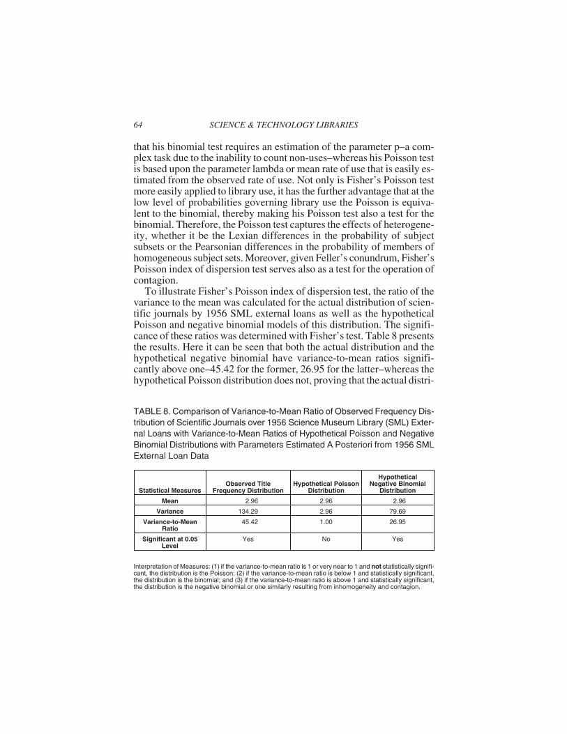
that his binomial test requires an estimation of the parameter p–a com-plex task due to the inability to count non-uses–whereas his Poisson testis based upon the parameter lambda or mean rate of use that is easily es-timated from the observed rate of use. Not only is Fisher’s Poisson testmore easily applied to library use, it has the further advantage that at thelow level of probabilities governing library use the Poisson is equiva-lent to the binomial, thereby making his Poisson test also a test for thebinomial. Therefore, the Poisson test captures the effects of heterogene-ity, whether it be the Lexian differences in the probability of subjectsubsets or the Pearsonian differences in the probability of members ofhomogeneous subject sets. Moreover, given Feller’s conundrum, Fisher’sPoisson index of dispersion test serves also as a test for the operation ofcontagion.

To illustrate Fisher’s Poisson index of dispersion test, the ratio of thevariance to the mean was calculated for the actual distribution of scien-tific journals by 1956 SML external loans as well as the hypotheticalPoisson and negative binomial models of this distribution. The signifi-cance of these ratios was determined with Fisher’s test. Table 8 presentsthe results. Here it can be seen that both the actual distribution and thehypothetical negative binomial have variance-to-mean ratios signifi-cantly above one–45.42 for the former, 26.95 for the latter–whereas thehypothetical Poisson distribution does not, proving that the actual distri-


TABLE 8. Comparison of Variance-to-Mean Ratio of Observed Frequency Dis-tribution of Scientific Journals over 1956 Science Museum Library (SML) Exter-nal Loans with Variance-to-Mean Ratios of Hypothetical Poisson and NegativeBinomial Distributions with Parameters Estimated A Posteriori from 1956 SMLExternal Loan Data

Statistical MeasuresObserved Title

Frequency DistributionHypothetical Poisson

Distribution

HypotheticalNegative Binomial

Distribution

Mean 2.96 2.96 2.96

Variance 134.29 2.96 79.69

Variance-to-MeanRatio

45.42 1.00 26.95

Significant at 0.05Level

Yes No Yes

Interpretation of Measures: (1) if the variance-to-mean ratio is 1 or very near to 1 and not statistically signifi-cant, the distribution is the Poisson; (2) if the variance-to-mean ratio is below 1 and statistically significant,the distribution is the binomial; and (3) if the variance-to-mean ratio is above 1 and statistically significant,the distribution is the negative binomial or one similarly resulting from inhomogeneity and contagion.

bution is better modeled by the negative binomial than by the Poisson.Comparison of Table 8 to Table 7 containing the results of the Lexis Ra-tio tests provides interesting insights. First, the results of the vari-ance-to-mean ratio test validate the findings of the Lexis Ratio test thatalso demonstrated that the NBD is the better model of the actual distri-bution than the Poisson. Second, whereas the Lexis test indicates thathypothetical Poisson distribution is a binomial distribution due to theratio being 1, the variance-to-mean test shows the hypothetical Pois-son distribution to be a Poisson distribution, because once again theratio is 1. This is proof of the equivalency of the binomial and Poissondistributions at the low levels of probability governing library use.Taken all together, these tests demonstrate the operation of both sto-chastic processes of heterogeneity and contagion in the observed distri-bution, which was affected by probabilistic heterogeneity betweensubject subsets as well as within subject subsets, where the loan ornon-loan of a journal affected its later probability of loan or non-loan.

CONCLUSION

Urquhart’s analysis of the 1956 loans of the Science Museum Library(SML) to outside organizations embodied two major advances. Thefirst was distributional and pertained to the history of science as awhole. This aspect of Urquhart’s work has been discussed in detail intwo articles by Bensman (2000; 2005). During the 19th century, statisti-cal analysis was based upon the normal paradigm, according to whichthe distributions of all phenomena are governed by the normal law of er-ror. The late 19th century witnessed a scientific revolution, which ledto the discovery that, on the contrary, many if not most phenom-ena–but particularly biological and social ones–have distributions thatare highly and positively skewed. Two key figures in this scientific rev-olution were Wilhelm Lexis and Karl Pearson. Britain became the pri-mary locus of the revolution due to Darwinism that stimulated thedevelopment of modern inferential statistics in this country. From thisperspective, the studies conducted by Bradford and Urquhart at theSML must be viewed as extensions of this scientific revolution, becausethese studies were among the first to demonstrate that the probabilitydistributions governing library and information science are also for themost part highly and positively skewed.

The second advance was conceptual and concerned specifically li-braries. It resulted from Urquhart’s focus on supralibrary use and must


be counted as Urquhart’s original contribution to library and informa-tion science. The conceptual breakthrough was that there is no sharpdistinction between supralibrary use and intralibrary use. As a result ofthis, in terms of the usage of their materials, all libraries function as partof a unified distributional system. Although this may seem a simple in-sight, it has manifold and complex ramifications. The next two parts ofthis paper will analyze these ramifications in respect to a central docu-ment delivery library and all the other libraries supported by such a li-brary.

Received: August 23, 2004Revised: January 13, 2005

Accepted: February 10, 2005

REFERENCES

Anscombe, F.J. 1949. The statistical analysis of insect counts based on the negative bi-nomial distribution. Biometrics 5(2): 165-173.

______. 1950. Sampling theory of the negative binomial and logarithmic series distri-butions. Biometrika 37 (3/4): 358-382.

Bensman, Stephen J. 2000. Probability distributions in library and information science:A historical and practitioner viewpoint. Journal of the American Society for Infor-mation Science 51 (9): 816-833.

______. 2001. Bradford’s Law and fuzzy sets: Statistical implications for library anal-yses. IFLA Journal 27 (4): 238-246.

______. 2005. Urquhart and probability: The transition from librarianship to libraryand information science. Journal of the American Society for Information Scienceand Technology 56 (2): 189-214.

Bradford, S.C. 1934. Sources of information on specific subjects. Engineering 137:85-86.

______. 1953. Documentation. 2d. ed. London: Crosby, Lockwood.Carpenter, Ray L., and Ellen Storey Vasu. 1978. Statistical methods for librarians.

Chicago: American Library Association.Cochran, William G. 1954. Some methods for strengthening the common χ2 tests.

Biometrics 10 (4): 417-451.Eggenberger, F., and George Pólya. 1984. Ûber die Statistik verketteter Vorgänge. In

George Pólya, Probability; Combinatorics; Teaching and learning in mathematics,edited by Gian-Carlo Rota, 94-104. Collected papers/George Pólya, vol. 4. Mathe-maticians of our times, vol. 22. Cambridge, Mass.: MIT Press.

Eisenhart, Churchill. 1983. Laws of error, I: Development of the concept. In Encyclo-pedia of statistical sciences, ed. Samuel Kotz and Norman L. Johnson, vol. 4:530-547. New York: John Wiley.


Elliott, J.M. 1977. Some methods for the statistical analysis of samples of benthic in-vertebrates. 2d ed. Freshwater Biological Association scientific publication, no. 25.Ambleside, England: Freshwater Biological Association.

Feller, William. 1943. On a general class of “contagious” distributions. Annals ofMathematical Statistics 14 (4): 389-400.

Fisher, Arne. 1922. The mathematical theory of probabilities and its applications tofrequency curves and statistical methods. Vol. 1, Mathematical probabilities, fre-quency curves, homograde and heterograde statistics. 2d ed. Translated by Char-lotte Dickson and William Bonynge. New York: Macmillan.

Fisher, Ronald A. 1966. The design of experiments. 8th ed. Edinburgh: Oliver andBoyd.

______. 1970. Statistical methods for research workers. 14th ed. New York: Hafner.Greenwood, Major, and George Udny Yule. 1920. An inquiry into the nature of fre-

quency distributions representative of multiple happenings with particular refer-ence to the occurrence of multiple attacks of disease or of repeated accidents.Journal of the Royal Statistical Society 83 (2): 255-279.

Grieg-Smith, P. 1983. Quantitative plant ecology. 3d ed. Studies in ecology, vol. 9.Berkeley: University of California Press.

Haight, Frank A. 1967. Handbook of the Poisson distribution. Publications in opera-tions research, no. 11. New York: John Wiley.

Johnson, Norman L., and Samuel Kotz. 1969. Discrete distributions. Distributions instatistics. Boston: Houghton Mifflin.

Kendall, Maurice G. 1949. On the reconciliation of theories of probability. Biometrika36 (1/2): 101-116.

Moran, P.A.P. 1968. An introduction to probability theory. Oxford: Clarendon Press.Moroney, M.J. 1956. Facts from figures. 3rd ed. Baltimore, Md.: Penguin Books.Osborn, Andrew D. 1980. Serial publications: their place and treatment in libraries.

3rd ed. Chicago: American Library Association.Pearson, Karl. 1894. Contributions to the mathematical theory of evolution. Philo-

sophical Transactions of the Royal Society of London, A, 185: 71-110.______. 1895. Contributions to the mathematical theory of evolution, II: Skew varia-

tion in homogeneous material. Philosophical Transactions of the Royal Society ofLondon, Series A, 186: 343-414.

______. 1900. On the criterion that a given system of deviations from the probable inthe case of a correlated system of variables is such that it can be reasonably sup-posed to have arisen from random sampling. The London, Edinburgh, and DublinPhilosophical Magazine and Journal of Science 50 (5th Series): 157-75.

______. 1901. Mathematical contributions to the theory of evolution, X: Supplementto a memoir on skew variation. Philosophical Transactions of the Royal Society ofLondon, Series A, 197: 443-59.

______. 1916. Mathematical contributions to the theory of evolution, XIX: Secondsupplement to a memoir on skew variation. Philosophical Transactions of the RoyalSociety of London, Series A, 216: 429-57.

Rietz, Henry Lewis. 1924. Bernoulli, Poisson, and Lexis distributions. In Handbook ofmathematical statistics, ed. H.L. Rietz, 82-91. Boston: Houghton Mifflin.

______. 1927. Mathematical statistics. The Carus mathematical monographs, no. 3.Chicago: Published for the Mathematical Association of America by Open CourtPublishing Co.


Snedecor, George W., and William G. Cochran. 1989. Statistical methods. 8th ed.Ames: Iowa State University Press.

Urquhart, Donald J. 1948. The organization of the distribution of scientific and techni-cal information. In The Royal Society Scientific Information Conference, 21 June-2July 1948: reports and papers submitted, 524-527. London: The Royal Society.

______. 1959. Use of scientific periodicals. In Proceedings of the International Con-ference on Scientific Information, Washington, D.C., November 16-21, 1958, vol. 1,287-300. Washington, D.C.: National Academy of Sciences, National ResearchCouncil.

Urquhart, Donald J., and R.M. Bunn. 1959. A national loan policy for scientific serials.Journal of Documentation 15 (1): 21-37.

Von Mises, Richard. 1957. Probability, statistics and truth. 2nd rev. English ed. pre-pared by Hilda Geiringer. New York: Macmillan.

Winsor, Charles P. 1947. Das Gesetz der kleinen Zahlen. Human Biology 19 (3):154-161.


For FACULTY/PROFESSIONALS with journal subscriptionrecommendation authority for their institutional library . . .

Please send me a complimentary sample of this journal:

(please write complete journal title here–do not leave blank)

If you have read a reprint or photocopy of this article, would you like tomake sure that your library also subscribes to this journal? If you havethe authority to recommend subscriptions to your library, we will send youa free complete (print edition) sample copy for review with your librarian.

1. Fill out the form below and make sure that you type or write out clearly both the nameof the journal and your own name and address. Or send your request via e-mail [email protected] including in the subject line “Sample Copy Request”and the title of this journal.

2. Make sure to include your name and complete postal mailing address as well as yourinstitutional/agency library name in the text of your e-mail.

[Please note: we cannot mail specific journal samples, such as the issue in which a specific article appears.Sample issues are provided with the hope that you might review a possible subscription/e-subscription withyour institution's librarian. There is no charge for an institution/campus-wide electronic subscriptionconcurrent with the archival print edition subscription.]

I will show this journal to our institutional or agency library for a possible subscription.Institution/Agency Library: ______________________________________________

Name: _____________________________________________________________

Institution: __________________________________________________________

Address: ___________________________________________________________

City: ____________________Return to: Sample Copy Department,The Haworth Press, Inc.,

10 Alice Street, Binghamton, NY 13904-1580

State: __________ Zip: ____________________

Urquhart's Law: Probability and the Management of Scientific and Technical Journal Collections Part...

Documents

Transcript of Urquhart's Law: Probability and the Management of Scientific and Technical Journal Collections Part...