International Review of Economics and Finance 18 (2009) 631–642

Contents lists available at ScienceDirect

International Review of Economics and Finance

j ourna l homepage: www.e lsev ie r.com/ locate / i re f

Urban informal sector and poverty

Saibal Kar a,b,⁎, Sugata Marjit a

a Centre for Studies in Social Sciences, Calcutta, Indiab HWWI, Hamburg, Germany

a r t i c l e i n f o

⁎ Corresponding author. Centre for Studies in Social SE-mail address: saibal@cssscal.org (S. Kar).

1059-0560/$ – see front matter © 2008 Elsevier Inc.doi:10.1016/j.iref.2008.06.009

a b s t r a c t

Article history:Received 6 February 2007Received in revised form 27 May 2008Accepted 17 June 2008Available online 5 July 2008

Many studies have explored the connection between trade and poverty theoretically andempirically for the developingworld.We offer another look at the possible implications of tradeliberalization on urban poverty by using the urban informal sector as a catalyst. The theoryshows that trade liberalization in the import competing sector raises informal wage acrossoccupational types, and expands production and employment in the informal industrialsegment. Further, using Indian provincial data on wage, capital stock and value added in theinformal sector we show that real informal wage increased with trade reform and transmittedfavorable impact on urban poverty reduction.

© 2008 Elsevier Inc. All rights reserved.

JEL classification:F11F16O17

Keywords:Trade reformInformal sectorNon-traded sectorPovertyIndia

1. Introduction

The phenomenal expansion of the third world metropolis over the last decade or so has unleashed a plethora of questionsentrenched in various socio-political and economic aspects. The growth and expansion, even by the most conservative estimates,has been rather skewed and has sharply widened the disparity across regions or locationswithin a given country. Themost strikingcomparison of the situation is visible for growing cities in the South, where co-existence of extremely rich pockets with that ofstark poverty has become a reality more than ever before. While the recent development on a global scale has largely favored themore skilled workforce, it has pushed a larger share of workers and the population dependent on them towards the margin,economically and socially.

As in other developing countries, an overwhelmingly large proportion (approximately 93% and excluding agriculture, about78%) of the workforce in India is employed in the so-called unorganized and/or informal sectors. A substantial portion of suchemployment opportunities is generated in the urban or semi-urban areas and not surprisingly a majority of this workforce iseconomically marginalized. High incidence of poverty among these groups exposed to difficult and hazardous working conditions,non-existent social security or health benefit schemes other than poorly functioning state-provided medical facilities, and etc., isquite common. Sustained improvements in the living standards of these groups can only be brought about by capital accumulation,productivity gains and wage increases in this sector. These countries regularly suffer from access to dedicated funds for povertyalleviation and impacts on poverty are often byproducts of other policies, such as trade liberalization (Bowles, 1999; Demery &Squire, 1996; Dollar, 1992; Topalova, 2005; Winters, 2000, to name a few). It has also been established earlier that dedicated

ciences, Calcutta, R-1, B.P. Township, Kolkata 700 094, India. Tel.: +9133 2462 7252; fax: +9133 2462 6183

All rights reserved.

.

632 S. Kar, S. Marjit / International Review of Economics and Finance 18 (2009) 631–642

policies towards urban employment generation and poverty reduction often increases both in the presence of poverty-strickenrural sectors and high levels of rural–urban migration (see, Basu, 1984).

This study offers another look at the connection between trade liberalization and poverty reduction, with a particular focus onthe informal sectorworkers in urban regions of the developingworld.More specifically, we are looking at the channel between howtrade reform affects urban informal workers and how that in turn affects urban poverty. It has been shown elsewhere (Kar andMarjit, 2001) that the informal sectorworkers arehardpressed to accept low-paid jobs in the cities rather thanwait indefinitely for aformal high-paying urban employment to open up. This can significantly explain the persistence of urban poverty in many cities ofthe third world. We offer a theoretical section that is quite generic and replicates the conditions of urban informal sector in mostdeveloping countries, and subsequently use data from India to provide an example. In particular, we distinguish the urban informalsector as comprising of an industrial section that uses some amount of capital as input and another as using raw labor as the onlyinput. To the best of our knowledge, and despite increasing interest in the subject, such distinction has not been made earlier. For aone country example such as India, the overwhelming volume of workers using only physical labor towards menial occupationsas domestic help, mainly women and child labor, household cook, drivers, daily wage labor and etc. is too large to be clubbed asone indivisible informal unit. And yet, frequently this is considered as transitory in nature and thus denied space in most policydiscussions.

While the nature of the occupations may certainly differ in other countries, use of manual labor to service wealthier sections ofthe population is almost universal in the developing world and usually outside the purview of formal industries and servicesectors. We argue that the impact of trade liberalization should be felt palpably by such groups and may even be favorable to mostunder plausible conditions.

We do not claim the empirical section to be an exact estimate of the propositions raised in the theoretical part, but argue thatthe impact of trade reform and capital accumulation on the wages of the informal workers is a reflection of our basic hypothesis.The empirical section offers an aggregative look at the wage movements for informal workers in India at the provincial level andexplained by changes in the levels of real fixed assets and real value added in the same. In fact, the theoretical section and theempirical section are distinct, except for the common thread of informal wage in both.

The most appropriate empirical exercise in this area would be one that narrows down the focus to specific industries in bothformal and informal sectors. While this is certainly a plausible way of drawing the connection and should be tried at length, it mayalso be rather limited in explaining the phenomenon on a wider scale. Thus leaving such issues for future considerations, here weoffer a broader look principally to acquaint the larger audience with the conditions and scope. Our theoretical result predicts thatthe informal wage should rise if there is trade liberalization and that there would be an expansion in the urban informal industrialbase. The aggregative empirical results test just this: the growth in the informal wage and factors that explain it best when there isexpansion in the sector. Additionally, we estimate if such wage growth is capable of reducing urban poverty.

Section 2 offers a brief overview of the perspective onwhich this study is built; Section 3 offers the model and results; Section 4describes the empirical models and discusses the outcomes. Section 5 concludes.

2. Brief overview

In the existing literature, welfare implications of trade reforms, with the informal sector as an important part of the economy,have recently come up for much discussion (Marjit & Kar, 2007; Marjit, Kar, & Beladi, 2007; Chaudhuri & Banerjee, 2007;Chaudhuri, 2003; Marjit, 2003; Chaudhuri & Mukhopadhyay, 2002; Chen, 2000 etc). A primary reason perhaps, is that, leaving outthe informal sector fails to capture the actual impact of such policy reforms since on an average 70% of the labor force in the LDCswork under arrangements outside the purview of what is typically known as the formal/organized sector. Data from SoutheastAsian, East European, African, and Latin American countries show varying rates of urban informal sector employment within therange of 15% to 20% in Turkey and Slovakia to 80% in Zambia, or even more, to about 83% in Myanmar. Moreover, considering thestate of agricultural and rural activities in these countries, it is quite apparent that the total shares of the informal sector in thesecountries are quite high (ILO, 1999). This is also corroborated by some of the other studies (for example, Turnham, 1993), whichprovide evidence that in low-income countries like Nigeria, Bangladesh, Ivory Coast, India, and elsewhere, the share of the urbaninformal sector is at least as high as 51%. Alternatively, seen from the point of view of the ‘minimum wage’ earners, only 11% ofTunisia's labor force, for example, is subject to minimumwage; in Mexico and Morocco, a substantive number earns less than theminimum wage; in Taiwan, the minimum wage received by many is less than half of the average wage and etc. (Agenor, 1996).

There is some evidence, which suggests that the level of informalization in a country increases as the economic reforms areinitiated. Amore general concern that follows is that such expansionwill reduce informal wagewith retrenchedworkers crowdingin from the formal sector. Some of the above mentioned studies show that despite contraction of the previously protected or state-run formal sector as a consequence of trade liberalization, and relocation of relatively unskilled and often older workers into theinformal segment, informal wage can still rise if capital also relocates into the informal sector.

The term ‘informal sector’ as it is commonly interpreted was initially coined by ILO (1972) to mean, “illicit or illegal activities byindividuals operating outside the formal sphere for the purpose of evading taxation or regulatory burden.” In alternative parlancesinformal sector implies, “very small enterprises that use low-technologymodels and do not refer to legal status” (Webster & Fidler,1996). Although generally, the informal sector activity pertains to non-traded items in the economy, from street vendors todomestic helps, in many countries they produce intermediate goods, processed exportable and import substitutes withsubcontracts from the formal sector. In such cases, the formal sector often adds the capital content (like, the brand name) only. Inmany other cases, informal industries that produce garments, leather goods, small tools and machinery are known to export

633S. Kar, S. Marjit / International Review of Economics and Finance 18 (2009) 631–642

directly often bypassing the formal regulations and procedures, made effective through border trade.1 Apart from that, in all thedeveloping countries, agriculture, poultry and fisheries are pre-dominantly outside the formal sphere and consumer non-durablessuch as vegetables, fish and meat are procured from such agents, processed and traded. Analyzing the impact of industrial tradereform on these activities and on the workers employed therein should offer a wider view in favor of appropriate policyformulations. It is to be noted that given the considerably large share of employment in these sectors even small positive gains inthe real wage, can increase the economic attainments of millions in most developing and transition countries.

3. The model

Consider a small open economy with two formal sectors, X and Y that produce traded commodities. X is an import competingcommodity manufactured with capital and skilled labor and is protected by an import tariff, t. The skilled wage is fixed at wS byprior negotiations with the labor unions as an outcome of a bargaining process. We do not model this wage fixation explicitly.2

Commodity Y is an export item produced with skilled labor, capital and an intermediate commodity I, which in turn is produced inthe informal sector. Since Y is traded at exogenously given world prices the price of commodity I, PI is determined from its fixed-coefficient production relation with Y. The production of I requires use of capital and unskilled labor available in large stock whichreceives a wagew b wS. This wage, we argue is the subsistence wage that lives the workers on or below the urban poverty line andany improvement may pull them above or closer to the same.

We consider I as one of the several intermediate commodities ranging from leather and rubber products to electronicequipments produced under informal arrangements that are often sold by the formal export industries after appropriate valueadditions. The third commodity we consider is non-traded, uses unskilled labor as the only input and represents very low-skilledactivities such as domestic help or small vendors with little or no use of capital. It may be considered as an informal service sector.The price relations for a competitive market accommodating the above commodity types are given by Eqs. (1)–(4). All the factorsof production are fully employed as shown by Eqs. (5)–(8). The typical nature of the urban informal sector allows us to consider afull-employment competitive model of this nature, since for all practical purposes the reservation wage for unskilled informalworkers in poor countries is quite low. For the relatively unskilled workers who do not succeed in getting formal employment, theinformal sector offers the only available alternative compared to involuntary unemployment. Moreover, in this model while capitalis homogeneous and moves freely between all the sectors, labor is heterogeneous and the skilled workers receive a higherpremium. The production follows standard neo-classical assumptions of constant returns to scale technology, diminishingmarginal productivity for the factor inputs part of the perfectly competitive market. The input coefficients are functions of thefactor prices and the symbols used here follow the depictions in Jones (1971).

The model uses the following symbols:

wS: Formal skilled wage;rj: Return to capital in sector j;Y: Output of formal export sector;I: Output of intermediate good (informal);w: Informal flexible wageX: Output of formal import competing sector;(Pj⁎): Exogenous price of jth goodZ: Output of non-traded good (informal)L : Stock of unskilled labor;K : Total supply of capital;(aij, aKj): Per unit labor and capital use in sector j = X, Y, I, Z, i = L, S, IS : Stock of skilled labort: Import tariff rate

‘^’ represents percentage changes for each variable (for example, x = dxx ) and detailed algebraic derivations of all the results are

provided in Appendix A.The competitive price conditions are given by,

1 Earlinto the

2 Chacontext

wSaSX + raKX = P⁎X 1 + tð Þ ð1Þ

wSaSY + raKY + PIaIY = P⁎Y ð2Þ

waLI + raKI = PI ð3Þ

waLZ = PZ ð4Þ

ier, De Soto (2000) pointed out that a heavy burden of taxes, bribes and inflexible bureaucratic regulations in the formal sector drives many producersinformal sector.udhuri (2003) provides examples of how the negotiations regarding wage settlements between employers and labor unions may take place in a similar.

634 S. Kar, S. Marjit / International Review of Economics and Finance 18 (2009) 631–642

And, the full-employment conditions require

aSXX + aSYY = S ð5Þ

aLII + aLZZ = L ð6Þ

aKXX + aKYY + aKII = K ð7Þ

aIYY = I ð8Þ

e determination of four price variables (r, w, PI, PZ) and four output variables (X, Y, I, and Z) from the set of eight equations

Thproceeds in the following way. Given the skilled wage and the exogenous price for commodity X, the return to capital is obtainedfrom Eq. (1). Substituting r in Eq. (2) we get the price of the intermediate commodity I, and from (3) the unskilled wage is directlyobtained. Substitution ofw in Eq. (4) generates the price of the non-traded informal service, Z. Similarly, for the factor markets, wesubstitute the output level of informal intermediate commodity I from Eq. (8) into Eq. (7). Eqs. (5) and (7) then form a pair ofsimultaneous equations that solve for equilibrium output levels of X and Y given the endowments of capital K and skilled labor S.Substituting back the equilibrium value of Y in Eq. (8) we determine the equilibrium output of I in the economy. Finally, from Eq.(6) we determine the equilibrium value of Z, the output of the informal service sector.

We are principally interested in observing the impact of a tariff reduction in the formal import competing sector on the level ofoutput and employment in the two informal sectors under consideration. While the detailed algebraic proof is provided in theAppendix, let us offer an intuitive explanation of the phenomenon here subsequent to the following proposition.

Proposition 1. A reduction in the import tariff raises product prices and wages in both informal sectors. However, the sector producingthe intermediate good expands in output and employment, while the one producing non-traded services, contracts.

A reduction in the tariff rate lowers the return to capital in sector X alone, since the skilled wage is exogenous and fixed.Consequently, sector X must contract, which suitably captures the experience in most developing and emerging economieswhere adoption of freer trade policies and removal of tariff and non-tariff barriers have affected the local import competing(many under public sector control) sectors adversely. Employment levels of both labor and capital in sector X must also shrinkunder the circumstances and relocation in other sectors become necessary. Since skilled labor is used specifically in sectors X and Y,therefore the latter may draw inmore skilled workers and its outputmay grow if the sector is more skill-intensive compared to theformer.

This is an exemplification of the Rybczynski effect (see, A.11 and A.12, in the Appendix A). On the other hand, capital may moveto sector Y or sector I, or both. As discussed, sector I's output level is completely dependent on that of sector Y since it is the soleuser of the intermediate commodity produced informally. If the capital moves into sector Y, the price of the informal intermediatecommodity must improve, given the competitive price conditions. However, since by assumption, the intermediate commoditymust be used in fixed proportions with any other combination of capital and labor, thus its outputmust also increase. The sequenceof events follows the derivations in the Appendix.

A rise in the price of I, and a factor-led growth in sector Y both contribute to an increase in the output of the informalcommodity. This is a significant result in itself, because, it implies that a contraction of the formal import competing sector leads toan improvement in the formal export production and given its connectionwith the informal sector through the intermediate input,the informal production also increases. Once again, empirical analyses for some of the countries do exhibit the above patterns inthe post-reform phases, where, many formal industries survive and grow by sub-contracting their production to the informalsector. Even within the bastions of labor union dominated public and other formal sectors, one observes growing tendenciestowards informal and contractual employment practices, often without access to many facilities previously enjoyed by the formalworkers.

The contraction of the formal import competing sector also demonstrates that the unskilled wage rises in the process, anotherimpact quite clearly visible in many of the developing economies including India. In fact, (Fig. 1 Appendix B) shows that for most ofthe provinces in India, the average wage for workers in the unorganized non-directory manufacturing sector have risen by at least10% on an annual basis. The results from this short theoretical representation further reveal that the informal service sector mayshrink on account of an expansion in the production of the informal intermediate commodity. This operates through the mobilityof the unskilled workers away from the service sector and into the intermediate manufacturing sector, although wages increase inboth.

Consequently, one may argue that this is welfare inducing in various ways. First, the direct improvement in wages has aclear impact for poverty reduction in the informal sector that we also establish in the empirical section. Second, the flow ofworkers into an industrial set-up, albeit informal, and away from morally degrading and highly insecure non-traded servicesector jobs such as street side vendors, low-level construction workers or simply domestic helps may be treated as not onlyan expansion of industrial or service sector base, but also rewarding in terms of increasing the visibility of labor involvementin the economy.

Similarly, if there is a ceteris paribus rise in the price of the export good Y, price of the intermediate good increases, and as therehas been no change in the return to capital, the informal wage must go up. This in turn raises the price of the informal service.

635S. Kar, S. Marjit / International Review of Economics and Finance 18 (2009) 631–642

Clearly, the rise in the price of the intermediate good expands its production and draws labor away from the service sector into theindustrial base. Thus,

Proposition 2. A rise in the price of the export good, Y, shall raise the prices of both the intermediate good and the non-traded good. Theinformal wage must rise, and labor moves to the intermediate sector thus lowering output and employment in the non-traded sectordespite a higher price per unit.

4. Empirical evidence from India

It is best to admit that relating informal wage and poverty to trade liberalization is a more difficult job empirically, thantheoretically. The empirical structure is highly dependent on the availability and reliability of data on informal sector. For India,however, there exist surveys of informal units by the National Sample Survey Organization (NSSO) — usually five-yearly samplesdrawn from almost all the provinces and union territories (i.e., centrally/federally administered regions, such as Delhi) in the morerecent years. The survey covers the average yearly wage, employment, major occupational categories by broad industry types, gender,fixed assets and value added of the informal units classified as Non-Directory Manufacturing Enterprises (NDMEs) and Own AccountEnterprises (OAEs), both rural and urban in either case. The sample size varies from less than 100units in relatively remote locationstomore than 10,000 inmajor cities. Given this, our next concern is which variables to use that serve the focus of the paper best. To thisendwe take up only urban NDMEs given their strong inter-linkagewith the urban formal sector for five consecutive rounds,1984–85,1989–90, 1994–95, 1999–2000 and 2000–01, for 17 states in the first period as per availability that extends to all states and unionterritories for the remaining time period. We intend to show that the period of gradual trade liberalization in India, i.e. the post-1991decade which led to closures of many formal and traditional industries releasing unskilled labor in large numbers coincidessignificantly with annual (real) growths in (i) urban informal wage (IW), (ii) urban informal fixed assets (as a proxy for capitalformation, FA) and (iii) urban informal value added (VA). The latter two variables are used to explain the movement of the first.

The logic behind suchmodeling emanates from the observation that trade liberalization drives capital and labor into the informalsector and yet thewage rises across states, steeply for some andmoderately for the rest leading to an average annual realwage growthof 10% somewhat contrary to conventional wisdom (see Appendix B, Fig. 1, and also for abbreviations for provinces and unionterritories). What could possibly explain the post-reform average rise in the wage if more unskilled labor formerly part of theorganized sector flows into the informal counterpart due to contraction of the formal industries and consequent unemployment?Weuse the available data and estimate the annual growth in real wages (deflated by 1989–90 consumer price index of India) in theNDMEs with respect to the annual growth in real FA and real VA in those units. A rise in FA, an equivalent to capital formation, isexpected to affect the informal wage positively as would a rise in the value added of each such unit. We run individual cross-sectionsfor each year and then pool the data for all the available years to run a panel regression on the same set of variables to capture theoverall impact on real informal wage (Figs. 2 and 3 provide the annual growth rates of real FA and real VA respectively). Table 1(Appendix B) offers detailed descriptive statistics for the variables under consideration and Table 2 shows that there does not existsubstantial problem of multi-collinearity among the variables. It should be noted that there are many other important variables thatare potential candidates in the exercise, such as gender wages, specific occupational types and so on, which are excluded here mainlyto provide an aggregative explanation of the driving relationship, the growth of the informalwage in a period dominated by industrialtrade liberalization and its effect on the percentage of people in the Below Poverty Line (BPL) category.3

The first of the two explanatory variables, informal fixed assets (real FA) grew at a temperate rate between 1984–85 and 1989–90 for many states (Fig. 2, Appendix B), although Assam (AS), Haryana (HY), Kerala (KE), Tripura (TR) and West Bengal (WB)registered negative growth. However, during 1989–90 and 1994–95 immediately after the reforms took effect in India, informalfixed asset shows high growth rate in most of the states while some report negative growth (BH, HP, LA, ME, etc.). Between 1994–95 and 1999–2000 informal fixed assets grew positively (10% to 150%) for 29 out of 30 locations in India, with the exception ofManipur (MA). The pattern, however, seems dampened for many states during 1999–00 and 2000–01.

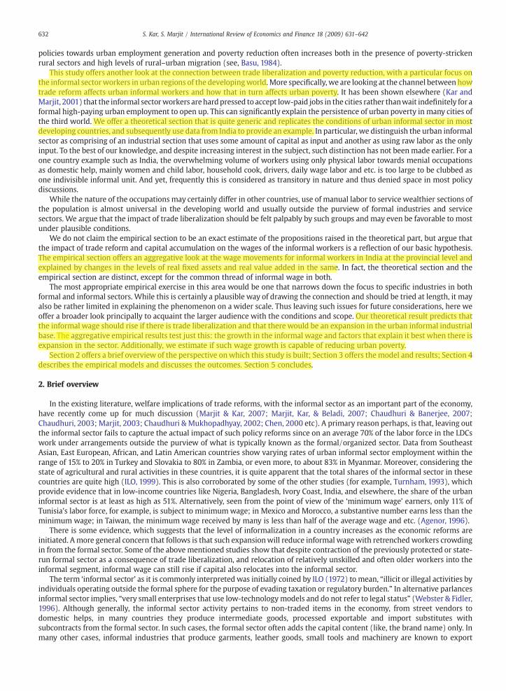
The second explanatory variable real value added (VA) also registered a negative trend for all states except Gujarat and WestBengal during 1984–85 and 1989–90. It undergoes a turn around in the post-reform period, whenmost states and union territoriesshow significant increase in the value added. Finally between 1999–00 and 2000–01 it reports negative growth rates inmost states.

The dependent variable in our model, the growth rate of real informal wage (IW) shows a negative growth for all the statesbetween 1984–85 and 1989–90 (Fig. 1). The trend shifted substantially in favor of informal workers in the period immediatelyfollowing the introduction of economic reforms in India. All the states including, GJ, MH, OR (22%), TN, RJ (32%), AP (38%) showedsignificant positive annual growth in informal wages. Between 1994–95 and 1999–00, twenty-nine out of thirty locations, exceptWB (− 2%) showmoderate positive annual growth of informal wage and the post-reform average annual growth in informal wageis recorded at between 15 and 20% with a variance of 26% between states.

Using the simple empirical model

3 Thewe inte

wt = at + β1 FAð Þt + β2 VAð Þt + et ð9Þ

, a is constant,w is real informal wage, t is year, ε the error term and rest as defined, we offer results from a generalized least

wheresquare regression (Table 3), after correcting for presence of heteroscedasticity in the error terms. Between 1984–85 and 1989–90

authenticity of the BPL list is far from acceptable due to strong political incentives attached to such enlistment in a fragmented society such as India, andnd to use other measures of poverty and further evidence on the informal labor mobility across sectors, in future.

636 S. Kar, S. Marjit / International Review of Economics and Finance 18 (2009) 631–642

(denoted as 1989–90 in Table 3), all the elements significantly explain changes in the informal real wage. Notably, the interceptterm is negative. Admittedly, the explanatory power of the regression (Adjusted R-squares) analysis declines over.

Subsequently, we offer a pooled (a pseudo panel) regression for these variables:

4 See

wit = α + βXit + eit ð10Þ

, wit = real informal wage pooled for i states and t periods, i = 1..N, the number of states, β is the coefficient vector for the

whereexplanatory variables (X), t = 1..T the time periods and ε follows N (0,σ2). The findings are reported in Table 4. The panelregression tests for whether the fixed effects (FE) or the random effects (RE) model is consistent with the data, given that the FE/RE is the natural choice over classical regression (CR) model since the value of the Lagrange Multiplier is very large. Further,between FE and RE the results from the Hausman Test suggests that FE is the appropriate model to use. Consequently, we use themethodology of Least Squares Dummy Variables after correcting for heteroscedasticity.4 According to this model, however, the realFA is not significant, although, with a positive impact on real IW. Real VA on the other hand is positive and highly significant (at 1%level) in explaining the increase in real IW. The panel regression is consistent with the cross-section results, in that, the real VAcontinues to be significant in explaining the real informal wage while the FA is not, although the general direction is positive asexpected.

Finally, let us deal with the relationship between changes in informal wage in the different states and union territories in Indiaover the years and the changes in the percentage of people registered under the Below Poverty Line (BPL) category in these states.It is to be noted that the informal sector data and the BPL data are not from the same samples and no data set that captures both,exists. We still venture into the relationship between informal wage and poverty for one major reason. A large part of the urbanpoor in India works and lives under the so-called informal sector arrangements and that any improvement in the wages of theinformal workers may reflect significantly on the incidence of poverty in the same domain. There is a reasonable possibility thatthere is significant overlap between the two sets. This would not be the case in the rural areas, because in comparison to the ruralinformal sector a larger share of the poor is engaged in agriculture. Thus, we test for the relationship between Urban Head CountRatio (UHCR) and the urban informal wage (NDMEs). The exercise is carried out in two stages: first, we regress the current period'sBPL percentage on previous periods Annual Informal Wage growth, where the results of the OLS suggests a negative relationshipsignificant at 5% level (Table 5, Appendix B). Second, we run the analysis as a panel of the states and union territories, which revealsthe presence of random effects and closely matches with the OLS results. However, as it can be seen from Table 6 (Appendix B) thecoefficient of IWPREV (real informal wage in the previous period) is still negative but now significant at 1% level. To summarize,therefore, one may state that the effect of an improvement in the annual wage growth in the informal sector has negative andsignificant impact on the incidence of urban poverty across states and union territories in India.

5. Concluding remarks

In what we have discussed so far, it becomes quite clear that the level of informal activity is sharply increasing in India ingeneral although not without usual business cycles. The present study not only documents some of these tendencies, but alsooffers a theoretical explanation of how the informal sector through its linkages to formalmanufacturing or independently as a non-traded service sector is expected to behave during a period dominated by the changing patterns of trade related protectionism inthe developing countries. For India, it is observed empirically that the wage and employment growth in the urban informal sectorswhich typically include the non-directory manufacturing sector is positive and considerable. Albeit we did not provide a fullerempirical account, the data from NSSO also reveals that the own account enterprises or the self-employed units within theinformal sector also experience positive growth in prices, output and participation. These empirical features characterizing theinformal sector are reflected in the short theoretical model. In fact, the theory predicts that the wage of informal workers shouldincrease and the informal industrial commodity expand in production if the formal import competing sector contracts due towithdrawal of trade protection. The growth in value added and fixed assets in the NDMEs are approximations to this end.

Finally, the growth in informal wage is shown to be capable of reducing the incidence of urban poverty. Although therelationship is sought out fromdisparate data sources, the overwhelming presence of informal workers and the glaring existence ofurban poverty cannot be completely unrelated. A substantive improvement in these results may require large scale primarysurveys on urban informal sector and the poverty status of the respondents to arrive at a dedicated relationship.

Acknowledgements

This work was carried out with financial and scientific support from the Poverty and Economic Policy (PEP) Research Network,which is financed by the Government of Canada through the International Development Research Centre (IDRC), CanadianInternational Development Agency (CIDA), and Australian Agency for International Development (AusAID). Saibal Kar also thanksthe Humboldt Foundation for the grant of fellowship. The comments from two anonymous referees of this journal and participantsin PEP general meetings in Colombo and Addis Ababa and PEP-World Bank conference at the CSSSC are duly acknowledged. Theusual disclaimer applies.

Greene (2003) for details on the methodology.

637S. Kar, S. Marjit / International Review of Economics and Finance 18 (2009) 631–642

Appendix A

A reduction in the tariff rate and the consequent equations of change are given below. Two generic derivations are given belowand the rest follows the same procedure.

Suc

dwS

w S

aSXwS

P⁎X 1 + tð Þ +

daSXaSX

aSXwS

P⁎X 1 + tð Þ +

drr

aKXrP⁎X 1 + tð Þ +

dakXakX

akXwS

P⁎X 1 + tð Þ =

dP⁎X

P⁎X 1 + tð Þ P

⁎X 1 + tð Þ + dt

tt

P⁎X 1 + tð Þ P

⁎X

ce wS and PX⁎ do not change, and using the envelope condition daSXa

aSXwS⁎ + dakX

aakXwS

⁎ = 0� �

, the above expression

SinSX PX 1 + tð Þ KX PX 1 + tð Þ

yields:

θKX r = α t;where;α = t = 1 + tð Þ ðA:1Þ

ere, θKX = aKXr⁎ , the income share of capital in sector X, and more generally, all θij's are income shares of factor i in the

Wh

PX 1 + tð Þprice of commodity j.

Thus, r = α tθKXb0

, as, t b 0Now using Eq. (2),

PI = − θKYθIY

α tθKX

N 0; as; tb0 ðA:2Þ

ing Eq. (3) and substituting the above information yields:

Deriv

w = − α tθKX

θKYθLI

1 +1θIY

� �N 0; as; tb0 ðA:3Þ

ally, from Eq. (4),

Fin

θLZ w = PZ ; such that; PZ = − α tθLZθKX

θKYθLI

1 +1θIY

� �N 0 ðA:4Þ

e above implies that, (ŵ − r) N 0

ThSimilarly, Eq. (5) may be derived in the following way:

dXX

aSXX

S+

daSXaSX

aSXX

S+

dYY

aSXY

S+

daSYaSY

aSXY

S=

dS

S

h that;

λSX X + λSY Y = − λSX aSX − λSY aSY

ðA:5Þ

, λSX = aSXXS, the skill endowment does not change and more generally, all λij's represent ith factor's physical contribution to

where

the production of commodity j. Using factor price changes and the degree of substitution between factors, Eq. (A.5) yields,

λSX X + λSY Y = − λSXθKXσX + λSYθKYσY½ � r ðA:6Þ

ain from Eq. (7), assuming that the informal intermediate input is used in fixed proportions without any substitution with

Agcapital or labor, we get,

λKX X + λKY Y = − λKX aKX − λKY aKY − λKI aKI + I� �

ðA:7Þ

wever, from Eq. (8), λIY (aIY + Y) = I

HoSince I is used in fixed proportions in the production of Y, thus, aIY = 0 and the above relationship becomes,

λIY Y = I ðA:8Þ

stituting Eq. (A.8) in Eq. (A.7), we get, λKXX + λKYŶ = − λKXâKX − λKXâKY − λKIλIYŶ

Subi.e.,

λKX X + λKY + λKIλIYð ÞY = λKXθSXσX + λKYθSYσY½ � r ðA:9Þ

ese two equations solve for X and Y simultaneously.

ThDenote λ

~KY = (λKY + λKI λIY), i.e., direct and indirect (via production of I) use of capital in the production of Y.

638 S. Kar, S. Marjit / International Review of Economics and Finance 18 (2009) 631–642

Thus,

or

λSX λSXλKX

fλ KY

� �X Yh i

= − λSXθKXσX + λSYθKYσYð Þ r λKXθSXσX + λKYθSYσYð Þ r� ðA:10Þ

ing Cramer's rule on Eq. (A.10),

Us

X = −λe KY λSXθKXσX + λSYθKYσYð Þ r − λSY λKXθSXσX + λKYθSYσYð Þ rλSXeλKY − λKXλSY

� �

X = − reλKYλSXθKX + λSYλKXθSX� �

σX + eλKYλSYθKY + λSYλKYθSY� �

σY

λSXeλKY − λKXλSY

� � ðA:11Þ

note, Δ = (λSXλ~KY − λKXλSY) b 0, which implies that sector X is more capital intensive compared to sector Y.

De

Consequently, X b 0, as, r b 0 and Δ b 0.Conversely, Y = λSX λKXθSXσX + λKYθSYσYð Þ r + λKX λSXθKXσX + λSYθKYσYð Þ r

λSXeλKY − λKXλSY

�N 0

i.e.

Y = λSX rλKXσX + λKY 1− θIYð ÞσY½ �

λSXeλKY − λKXλSY

� � N 0 ðA:12Þ

. (8) then yields: Î = λIYŶ or, I = λIYλSXα t λKXσX + λKY 1 − θIYð ÞσY½ � � N 0 and finally from Eq. (6),

Eq θKX λSXeλKY − λKXλSY

Z N 0; iff ;λIYλSX λKXσX + λKY 1− θIYð ÞσY½ � N σ I

fθKYθIY

+ θKY

!

, θ~KY = (θKY + θKIθIY). □

where

Proof of Proposition II follows similarly.

Appendix B

Fig. 1. Annual growth rate of real informal wage. Source: NSS Reports, various rounds and own calculations. List of Abbreviations for States and Union Territories inIndia. AP — Andhra Pradesh, AS — Assam, BH — Bihar, GJ — Gujarat, HY — Haryana, HP — Himachal Pradesh, KA — Karnataka, KE — Kerala, MP — Madhya Pradesh,MH—Maharastra, OR— Orissa, PN— Punjab, RJ— Rajasthan, TN— Tamil Nadu. TR— Tripura, UP— Uttar Pradesh, WB—West Bengal, AN— Andaman and NicobarIslands, Ch — Chandigarh, DN— Dadra and Nagar Haveli, DH — Delhi, LA — Lakshadweep, PO — Pondicherry, GO — Goa, JK— Jammu and Kashmir, MA —Manipur.ME — Meghalaya, MI — Mizoram, NA — Nagaland, SI — Sikkim.

639S. Kar, S. Marjit / International Review of Economics and Finance 18 (2009) 631–642

Fig. 2. Annual growth rates of informal fixed assets.

Fig. 3. Annual growth rates of informal value added. Source: NSS Various rounds, ASI Reports, GOI and own calculations.

640 S. Kar, S. Marjit / International Review of Economics and Finance 18 (2009) 631–642

Table 1Descriptive statistics for the variables (year-wise).

Year

Variables Mean SD Skewness Kurtosis Minimum Maximum Observations

1989–90

IW (−) 15.08 3.45 0.97 3.16 (−) 18.96 (−) 6.75 17 FA 4.71 9.29 0.54 3.18 (−) 10.75 26.92 17 VA (−) 7.90 7.12 1.20 4.20 (−) 19.04 10.00 17

1994–95

IW 20.72 10.97 0.22 3.03 (−) 0.43 47.97 30 FA 3.23 12.93 1.36 5.99 (−) 19.28 47.98 30 VA 5.89 13.31 1.98 7.94 (−) 12.24 56.44 30

1999–2000

IW 1.29 7.65 1.26 4.76 (−) 9.07 25.49 30 FA 58.50 50.32 1.35 4.16 (−) 13.24 208.01 30 VA 42.05 32.67 1.47 4.93 3.48 140.38 30

2000–2001

IW 44.18 28.51 (−) 0.52 3.30 (−) 37.11 90.74 30 FA (−) 10.52 35.77 0.87 4.19 (−) 69.15 99.74 30 VA (−) 40.18 25.04 0.82 4.42 (−) 94.69 26.49 30

All years

IW 16.16 26.84 0.81 3.20 (−) 37.11 90.74 107 FA 15.10 43.33 1.69 7.54 (−) 69.15 208.01 107 VA 0.92 38.68 0.59 4.54 (−) 94.69 140.38 107

Description of the variables:IW=Annual growth rate of real informal wage.FA=Annual growth rate of real fixed assets.VA=Annual growth rate of real value added.

Table 2

Correlation coefficient matrix (year-wise).

IW

FA VA

1989–90

IW 1.000 .4276 .4737 FA .4276 1.000 .3775 VA .4737 .3775 1.000

1994–95

IW 1.000 .3393 .2704 FA .3393 1.000 .0486 VA .2704 .0486 1.000

1999–2000

IW 1.000 .0635 .3544 FA .0635 1.000 .1344 VA .3544 .1344 1.000

2000–2001

IW 1.000 .1512 .4451 FA .1512 1.000 − .2026 VA .4451 − .2026 1.000

Table 3

Regression results for individual time-points corrected for heteroscadasticity.

Methodology: generalized least squaresDependent variable: annual growth rate of IW

Year

Exp. variables Coeff. t-ratio R2 Adj. R2 AIC LL

1989–90

CONSTANT (−) 11.35 (−) 6.70473⁎ 0.48 0.36 5.01 (−) 39.10 FA 0.102 2.588⁎ VA 0.233 5.098⁎

1994–95

CONSTANT 15.89 8.846⁎ 0.23 0.14 7.59 (−) 109.98 FA 0.278 2.190⁎ VA 0.183 1.744⁎⁎

1999–2000

CONSTANT (−) 3.76 (−) 1.622 0.16 0.06 6.961 (−) 100.42 FA 0.014 0.4587 VA 0.083 2.041⁎⁎

2000–2001

CONSTANT 69.56 5.691⁎ 0.30 0.23 9.41 (−) 137.09 FA 0.152 0.8636 VA 0.607 2.239

Note: ⁎ Denotes significance at 5% level & ⁎⁎ denotes significance at 10% level.Adj. R2=adjusted R2.AIC=Akaike Information Criterion.LL=Log-likelihood.

641S. Kar, S. Marjit / International Review of Economics and Finance 18 (2009) 631–642

Table 4

Unbalanced panel regression.

Random effects model: v(i, t)=e(i, t)+u(i)Methodology: 2-step GLSLagrange multiplier test=157.18 (1 df, prob value=.00(High values of LM favor FEM/REM over CR model.)Fixed vs. random effects (Hausman)=2.07 (3 df, prob value=.5584)(High (low) values of H favor FEM (REM).)⇒RE model is inconsistent, which leads us to use a Fixed Effects Model. The results from the LSDV (group Dummy) model is given below.Least squares with group dummy variablesOrdinary least squares regression Weighting variable=noneDependent variable=REALIW, Mean=16.16, S.D.=26.83Model size: observations=107, Parameters=7, df=100Residuals: sum of squares=25107.46, S.D.=15.84Fit: R-squared=.6711, Adjusted R-squared=.6513Model test: F [6, 100]=34.01, Probability value=.00Diagnostic: Log-L=−443.83, Restricted (b=0) Log-L=−503.32Log Amemiya probability criterion.=5.589, Akaike info. criterion=8.427Estimated autocorrelation of e (i, t) .1392White/heteroscedasticity corrected covariance matrix used.Results from heteroscedasticty-corrected panel (fixed effects) regression⁎⁎ Significant at 1% level.

Explanatory variable

Coefficient Standard error t-ratio

REALFA

0.0304 0.0494 0.616 REALVA 0.2567⁎⁎ 0.0704 3.647

Table 5Regressing current period's BPL percentage on previous year's annual growth of informal wage.

Dependent variable: BPLPERMethodology: OLS

Exp. variables

Coeff. t-ratio R2 AIC Log-likelihood

IWPREV

(−) 0.236 (−) 2.57⁎ 0.13 7.883 (−) 183.24 CONSTANT 27.85 14.53⁎

Note: BPLPER=BPL percentage.IWPREV=Previous year's growth rate of informal wage.

Table 6Unbalanced panel regression of current period's BPL percentage on previous year's annual growth of informal wage.

Dependent variable: BPLPERModel: random effects model

Exp. variables

Coeff. t-ratio

IWPREV

(−) 0.229 (−) 5.17⁎ CONSTANT 27.12 11.98⁎ Diagnostics tests for the model:Random effects model: v(i, t)=e(i, t)+u(i)Fixed vs. random effects (Hausman)=.01 (1 df, prob value=.940154)(High (low) values of H favor FEM (REM).) Sum of squares .6723 R-squared .1248

Note: BPLPER=BPL percentage.IWPREV=Previous year's growth rate of informal wage.

References

Agenor, P. (1996). The labor market and economic adjustment. IMF Staff Papers, 32, 261−335.Basu, Kaushik (1984). The Less Developed Economy — A Critique of Contemporary Theory. Delhi: Oxford University Press.Bowles, S. (1999). Globalization and Poverty, Paper to the World Bank Summer Workshop on Poverty, July.Chaudhuri, S., & Mukhopadhyay, U. (2002). Economic liberalization and welfare in a model with an informal sector. The Economics of Transition, The European Bank

for Reconstruction and Development, 10, 143−172.Chaudhuri, Sarbajit (2003). How and how far to liberalize a developing economy with informal sector and factor market distortions. Journal of International Trade

and Economic Development, 12, 403−428.Chaudhuri, Sarbajit, & Banerjee, D. (2007). Economic liberalization, capital mobility and informal wage in a small open economy: A theoretical analysis. Economic

Modelling, 24, 924−940.Chen, Martha (2000). Women in the informal sector: a global picture, the global movement. Washington DC: World Bank http://info.worldbank.org/etools/docs/

library/76309/dc2002/proceedings/pdfpaper/module6mc.pdf

642 S. Kar, S. Marjit / International Review of Economics and Finance 18 (2009) 631–642

De Soto, Hernando (2000). The Mystery of Capital. USA: Basic Books.Demery, L., & Squire, L. (1996). Macroeconomic adjustment and poverty in Africa: An emerging picture. World Bank Research Observer, 11, 39−59.Dollar, D. (1992). Outward-oriented developing economies really do grow more rapidly: Evidence from 95 LDCs, 1976–1985. Economic Development and Cultural

Change, 40, 523−544.Greene, William H. (2003). Econometric Analysis, 5th Edition. NY: Prentice Hall.International Labour Organisation. (1972). Employment, Incomes and Equality: A Strategy for Increasing Productive Employment in Kenya Geneva: ILO.International Labour Organisation (ILO). (1999). Key indicators of the labour market. Geneva: International Labour Office.Jones, R. W. (1971). The specific- factor model in trade, theory and history. In J. N. Bhagwati (Ed.), Trade, Balance of Payments and Growth North Holland:

Amsterdam.Kar, S., & Marjit, S. (2001). Informal sector in general equilibrium: Welfare effects of trade policy reforms. International Review of Economics and Finance, 10,

289−300.Marjit, S., & Kar, S. (2007). Urban informal sector and poverty— Effects of trade reform and capital mobility in India. PEP-MPIA working paper # 2007–09, Canada.Marjit, S., Kar, S., & Beladi, H. (2007). Trade reform and informal wage. Review of Development Economics, 11, 313−320.Marjit, Sugata (2003). Economic reform and informal wage — A general equilibrium analysis. Journal of Development Economics, 72, 371−378.National Sample Survey organization of India (NSSO). (1985–2001). Survey of UnorganizedManufacturing Sector in India, Department of Statistics and Programme

Implementation, Government of India — various issues.Topalova, Petia. (2005). Trade Liberalization, Poverty and Inequality: Evidence from Indian Districts. NBER Working Paper No. 11614, MA: NBER.Turnham, D. (1993). Employment And Development — A New Review Of Evidence. Paris: Development Centre Studies, OECD.Webster, L., & Fidler, P. (1996). The Informal Sector And Microfinance In West Africa. Washington, DC: World Bank Regional and Sectoral Studies, World Bank.Winters, L.A. (2000). Trade, Trade Policy and Poverty: What are the Links? Discussion Paper No. 2382, Centre for Economic Policy Research, London.