(

I

RESUMEN

Los océanos cubren un 70 % de la superficie de la Tierra y juegan un papel muy

importante en la mayoría de los procesos que ocurren en el planeta. Así mismo, son el

hábitat de miles de especies de organismos. Desafortunadamente, han sido afectados

por fuentes de contaminación antropogénicas durante mucho tiempo y, entre otras, por

las emisiones de CO2 a la atmósfera y el consecuente cambio climático.

Estas emisiones, debidas sobre todo a la quema de combustibles fósiles, ha

incrementado la concentración atmosférica de CO2 desde 280 ppm en tiempos

preindustriales a alrededor de 400 ppm hoy en día. Se estima que este valor seguirá

subiendo y que podría llegar a alcanzar las casi 1000 ppm para el año 2100.

Una de las consecuencias del incremento de CO2 atmosférico es el llamado fenómeno

de acidificación de los océanos. El CO2 se disuelve en el agua de mar que debido al

equilibrio de este sistema pasa a ser bicarbonato a la vez que libera protones, lo que

conlleva una bajada del pH. Por otra parte, el exceso de protones reacciona con el

carbonato libre debido a su capacidad tampón para formar bicarbonato. Esto conlleva

una disminución en la concentración libre de carbonato, lo que a su vez disminuye el

estado de saturación del agua de mar con respecto a la calcita y el aragonito, que son

las principales formas minerales del calcio carbonato.

Si el estado de saturación con respecto a estas fases minerales baja de 1 se consideraría

que esas aguas estarían insaturadas, lo podría afectar directamente la capacidad de los

organismos con exoesqueletos calcáreos para formar sus conchas pudiendo debilitarlas

y afectar sobre todo a aquellas especies cuyas conchas o esqueletos estén formados de

aragonito, ya que este mineral es más soluble.

Por otra parte, la disminución del pH podría afectar la especiación de metales en aguas

naturales. La disminución de iones OH- y CO32- podría afectar la solubilidad, absorción

y toxicidad de los metales. Teniendo en cuenta que uno de los estuarios estudiados en

este trabajo es el estuario de Nerbioi-Ibaizabal, que tiene una amplia historia de

(c)2018 LEIRE KORTAZAR OLIVER

II

contaminación metálica, este efecto de la acidificación podría ser muy perjudicial ya

que aumentaría de forma importante la presencia de metales tóxicos en las aguas.

Po lo tanto, los estudios sobre la acidificación en aguas de estuario resultan muy

interesantes y útiles para comprender cómo y en qué medida estos sistemas

hidrográficos están siendo afectados.

En este trabajo se han querido estudiar tres estuarios de la costa de Bizkaia, como son

el estuario de Urdaibai (declarado Reserva de la Biosfera por la UNESCO en 1984), el

estuario de Plentzia y el estuario del Nerbioi-Ibaizabal, que es un estuario

históricamente contaminado debido a la masiva industrialización acaecida en el siglo

XIX en la zona urbana de Bilbao. Para ello, se realizaron muestreos periódicos

trimestrales (con el fin de verificar la existencia de variaciones estacionales) durante un

periodo de tres años. Se recogieron 12 muestras en los estuarios de Urdaibai y Plentzia

en 6 puntos de muestreo, tanto en la superficie como en el fondo del cauce, y una más

en las zonas no mareales (ríos) de cada estuario. En Nerbioi-Ibaizabal, al ser un

estuario más largo, se recogieron 22 muestras en 11 puntos de muestreo y la de río. En

cada punto de muestreo se realizó un perfil utilizando una sonda multiparamétrica

(YSI EXO2) que recogió los siguientes parámetros fisicoquímicos: profundidad,

conductividad y temperatura (con lo que calcula la salinidad), pH, potencial rédox,

oxígeno disuelto y materia orgánica disuelta fluorescente. Por otra parte, se recogieron

muestras para medir el oxígeno disuelto, la concentración total de carbono orgánico

(TOC), la alcalinidad, el carbono orgánico disuelto (DIC) y las concentraciones de

amonio, nitrato, fosfato y silicato.

Las concentraciones de amonio y silicato fueron determinadas mediante

potenciometría con electrodo de ión selectivo (ISE) y para evitar el efecto matriz

causado por las diferencias de salinidad entre muestras se utilizó la metodología de

adiciones estándar. Las concentraciones de fosfato y silicato se determinaron mediante

análisis por inyección en flujo (FIA) usando en ambos casos en método del azul de

molibdeno. En el caso del fosfato se evitó el efecto matriz utilizando la muestra como

disolución transportadora y en el caso del silicato no fue necesario realizar ninguna

modificación importante ya que el efecto matriz era mínimo. El TOC se determinó

III

realmente como carbono orgánico no-purgable (NPOC) ya que las concentraciones de

carbono orgánico eran tan bajas en comparación con las de carbono inorgánico que no

era posible medirlo mediante la diferencia entre el carbono total y el inorgánico (TOC =

TC – IC). El NPOC se determinó mediante acidificación de la muestra para eliminar el

carbono inorgánico y posterior determinación del carbono orgánico por combustión. El

oxígeno disuelto se determinó mediante el método Winkler, es decir, por volumetría

redox clásica.

Los parámetros relacionados con la acidificación son cuatro: alcalinidad (TA), carbono

inorgánico disuelto (DIC), pH y la presión parcial de CO2 (pCO2) o fugacidad (fCO2).

Debido a la relación termodinámica existente entre estos parámetros, solamente es

necesario medir dos de ellos para poder calcular los otros dos. En este trabajo se han

determinado la alcalinidad y el DIC.

La definición de la alcalinidad más aceptada a día de hoy es la siguiente:

“La alcalinidad total de una agua natural está definida como el número de moles del ión

hidrógeno equivalentes al exceso de aceptores de protones (bases formadas de ácidos débiles con

constantes de disociación K ≤10-4.5, a 25 °C y cero fuerza iónica) sobre los donantes de protones

(ácidos con K > 10-4.5) en un kilogramo de muestra.”

Y se expresa como:

TA = [HCO3-] + 2[CO32-] + [B(OH)4-] + [OH-] + [HPO42-] + 2[PO43-] + [SiO(OH)3 -] + [HS-] +

2[S2-] + [NH3] - [H+] – [HSO4-] – [HF] – [H3PO4] + [organic bases] – [organic acids]

Como se puede observar, el sistema ácido-base del agua de mar está gobernado por

diferentes especies ácido-base. El sistema más importante, debido a su abundancia, es

el del carbonato. Sin embargo, es necesario tener en cuenta otros sistemas ácido-base

menores, como pueden ser el del ácido bórico, el ácido fosfórico, el ácido silícico y el

amonio, entre otros. Algunos autores también mencionan la importancia de la

alcalinidad aportada por la materia orgánica. Ignorar la contribución de estas especies

menores produciría importantes errores a la hora de determinar la alcalinidad y,

consecuentemente, el resto de parámetros relacionados con la acidificación.

IV

El DIC es la suma de las especies del sistema del carbonato y se expresa de la siguiente

manera:

DIC= [H2CO3] + [HCO3-] + [CO32-]

En este trabajo, ambos parámetros fueron medidos con el equipo VINDTA 3C que

manipula la muestra y los determina de manera automatizada para minimizar posibles

errores. La determinación de la alcalinidad se lleva a cabo mediante valoración

potenciométrica utilizando HCl 0.1 mol. L-1 como valorante. Para ello se usa un

electrodo de vidrio junto con uno de referencia con objeto de medir la concentración de

protones a lo largo de la valoración. Además, para evitar fluctuaciones o derivas del

sistema electródico debido al uso de bombas peristálticas, este equipo realiza una

medida potenciométrica diferencial donde la diferencia en la fuerza electromotriz entre

el electrodo de vidrio y el de referencia se mide contra un electrodo auxiliar, que en

este caso es un cable de titanio conectado a tierra. El DIC se mide mediante la

acidificación de la muestra para transformar todas las especies inorgánicas del sistema

del carbono a CO2 (g) que se transporta a una celda donde se valora

coulombimétricamente con ayuda de un sistema de detección espectrofotométrica.

El mayor problema para poder estudiar el sistema del CO2 en aguas de estuario reside

en la falta de información y bibliografía en lo referente a estudios de acidificación en

aguas de estuario, fundamentalmente sobre cómo lidiar con las variaciones de

salinidad a la hora de tratar los datos o llevar a cabo las valoraciones potenciométricas

o a la falta de ecuaciones para el cálculo de constantes estequiométricas de equilibrio

en intervalos de salinidad que varían de 0.2 a 40.

Por lo tanto, el objetivo principal de este trabajo es estudiar la forma de tratar los datos

potenciométricos para determinar de una manera exacta la alcalinidad de las muestras

de estuarios con salinidades tan variables. En primer lugar, y debido al gran número

de constantes de acidez existentes en la bibliografía para el sistema del carbonato, se

decidió estudiar las más frecuentemente utilizadas y se concluyó la necesidad de

desarrollar un nuevo conjunto de constantes mezclando otros existentes. A pesar de

obtener resultados muy buenos en general, se vio la necesidad de refinar uno de los

V

parámetros de dependencia con la fuerza iónica para obtener mejores ajustes en el

conjunto de todas las muestras. Con objeto de determinar la alcalinidad, se estudiaron

diferentes aproximaciones. Las más prometedoras fueron dos basadas en un

procedimiento de ajuste por mínimos cuadrados no lineales de los datos (e.m.f., v) de

las valoraciones potenciométricas utilizando dos programas: Microsoft Office Excel y

OriginPro 2017. El primero utiliza el algoritmo de Levenberg-Marquardt, que solo

tiene en cuenta el error en la variable dependiente (volumen en este caso) y el segundo

utiliza un algoritmo de regresión de distancia ortogonal que tiene en cuenta el error en

las variables dependiente (volumen) e independiente (e.m.f.). A pesar de que ambas

aproximaciones proporcionaban resultados muy buenos y estadísticamente

comparables con un nivel de confianza del 95 %, en lo sucesivo se empleó OriginPro

2017 para la determinación de la alcalinidad.

En este trabajo también se ha desarrollado una ecuación para explicar de forma precisa

la dependencia de la constante de acidez del indicador ácido-base rojo de fenol con la

fuerza iónica cuando se emplea para la determinación espectrofotométrica del pH en

aguas de estuario. Como ocurre con la alcalinidad, poco se encuentra en la bibliografía

sobre el uso de este método en aguas de estuario y sobre la variación de las constantes

de acidez en un intervalo de salinidad tan amplio. Para estudiar la validez de la

ecuación desarrollada, se midió un material de referencia certificado (con TA y DIC

conocidos) y se calculó su pH. Por otra parte, se calculó el pH utilizando los valores de

TA y DIC y con la ayuda del programa CO2SYS. Los resultados obtenidos de ambas

formas resultaron estadísticamente comparables con un nivel de confianza del 95 %, lo

que confirma la validez de la ecuación.

Por otra parte, en este trabajo también se han estudiado las variaciones estacionales y

en los últimos tres años de los nutrientes, NPOC, DO y algunos parámetros

fisicoquímicos en los distintos estuarios escogidos. Las variaciones y valores obtenidos

en Urdaibai y Plentzia han sido normales. Sin embargo, el estudio realizado en

Nerbioi-Ibaizabal mostraba altas concentraciones de fosfato y NPOC entrando por el

río Galindo (uno de los afluentes de este estuario) y unas aguas casi anóxicas en el

fondo de los puntos de muestreo en Bilbao.

VI

Finalmente, los parámetros del sistema del CO2 se calcularon utilizando el programa

CO2SYS y se realizó un estudio preliminar con objeto de comprobar el estado en el que

se encuentran los estuarios. En este caso, otra vez, Urdaibai y Plentzia mostraron

valores razonables, excepto en los ríos que presentaban valores altos de TA, DIC y pH

e insaturación con respecto a calcita y aragonito. Nerbioi-Ibaizabal otra vez mostraba

valores anómalos en ciertos puntos. Galindo mostró una increíblemente alta fugacidad

y valores muy bajos de pH y estados de saturación. Algunas muestras tomadas en el

fondo de los puntos de muestreo de Bilbao también mostraban esta tendencia. Por lo

tanto, teniendo en cuenta estos datos y los de los nutrientes, queda claro que el estuario

Nerbioi-Ibaizabal no está completamente recuperado de su contaminación histórica y

también parece demostrado que algún tipo de contaminación hace su entrada por el río

Galindo de manera constante.

Por último, cabe señalar que teniendo en cuenta los valores de fugacidad obtenidos en

los tres estuarios, éstos son una fuente de emisión de CO2 a la atmósfera en vez de un

sumidero, como ocurre en los océanos.

Chapter 1

General Introduction

General Introduction

3

1.1 Ocean acidification

Oceans cover around a 70% of the planet surface and play a key role in the Earth’s

major processes. They are also the habitat for thousands of species of organisms that

live in the oceans in a variety of ecosystems. Therefore, they are one of the most

important ecosystems in the planet and it is crucial to look after them. Unfortunately,

oceans have been affected by anthropogenic sources for a long time, being highly

influenced by the carbon dioxide (CO2) emissions to the atmosphere and the

consequent climate change.

CO2 is being produced and emitted to the atmosphere in important quantities.

Emissions of CO2 from fossil fuel combustion, with contributions from cement

manufacture, are responsible for about 80% of the increase in atmospheric CO2

concentration since pre-industrial times. The remainder of the increase comes from

land use changes dominated by deforestation (and associated biomass burning) with

contributions from changing agricultural practices [1]. The CO2 concentration in the

atmosphere has increased from pre-industrial level of around 280 parts per million

(ppm) to around 391 ppm in 2011 [2] (40 % increment) and 404 ppm in November

20171. Atmospheric CO2 levels are predicted to rise and may reach levels of around 936

ppm by the year 2100 according to the Representative Concentration Pathway (RCP)

8.5 of the Intergovernmental Panel on Climate Change (IPCC) which is the “worst case

scenario” [2], [3].

One of the most important effects of the increase in atmospheric levels of CO2 is the rise

of the global mean surface temperatures. Another effect of the atmospheric CO2

increase is the phenomenon known as ocean acidification. Around 30 % of this emitted

CO2 is absorbed by the oceans, lowering its concentration in the atmosphere but

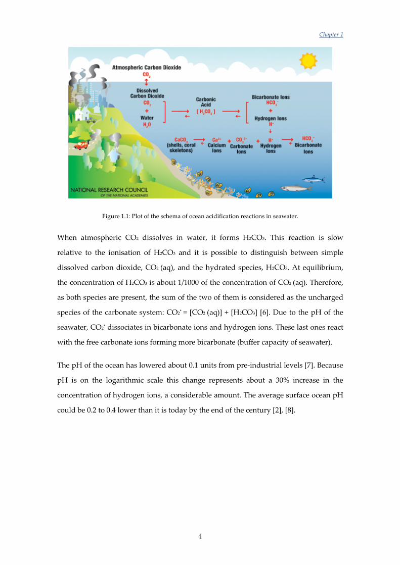
making the oceans more acidic (see Figure 1.1) [1], [2], [4], [5].

1 Updated regularly at: https://www.esrl.noaa.gov/gmd/ccgg/trends/

Chapter 1

4

Figure 1.1: Plot of the schema of ocean acidification reactions in seawater.

When atmospheric CO2 dissolves in water, it forms H2CO3. This reaction is slow

relative to the ionisation of H2CO3 and it is possible to distinguish between simple

dissolved carbon dioxide, CO2 (aq), and the hydrated species, H2CO3. At equilibrium,

the concentration of H2CO3 is about 1/1000 of the concentration of CO2 (aq). Therefore,

as both species are present, the sum of the two of them is considered as the uncharged

species of the carbonate system: CO2* = [CO2 (aq)] + [H2CO3] [6]. Due to the pH of the

seawater, CO2* dissociates in bicarbonate ions and hydrogen ions. These last ones react

with the free carbonate ions forming more bicarbonate (buffer capacity of seawater).

The pH of the ocean has lowered about 0.1 units from pre-industrial levels [7]. Because

pH is on the logarithmic scale this change represents about a 30% increase in the

concentration of hydrogen ions, a considerable amount. The average surface ocean pH

could be 0.2 to 0.4 lower than it is today by the end of the century [2], [8].

General Introduction

5

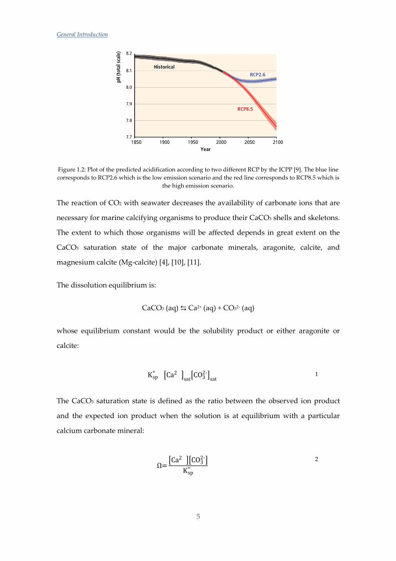
Figure 1.2: Plot of the predicted acidification according to two different RCP by the ICPP [9]. The blue line corresponds to RCP2.6 which is the low emission scenario and the red line corresponds to RCP8.5 which is

the high emission scenario.

The reaction of CO2 with seawater decreases the availability of carbonate ions that are

necessary for marine calcifying organisms to produce their CaCO3 shells and skeletons.

The extent to which those organisms will be affected depends in great extent on the

CaCO3 saturation state of the major carbonate minerals, aragonite, calcite, and

magnesium calcite (Mg-calcite) [4], [10], [11].

The dissolution equilibrium is:

CaCO3 (aq) Ca2+ (aq) + CO32- (aq)

whose equilibrium constant would be the solubility product or either aragonite or

calcite:

Ksp* =Ca2+satCO3

2-sat 1

The CaCO3 saturation state is defined as the ratio between the observed ion product

and the expected ion product when the solution is at equilibrium with a particular

calcium carbonate mineral:

Ω=Ca2+CO3

2-Ksp

* 2

Chapter 1

6

Therefore, seawater is at equilibrium with respect to that mineral when Ω = 1,

supersaturated when Ω > 1 (which promotes inorganic precipitation), and is

undersaturated when Ω < 1 (which promotes inorganic dissolution). Thus, the

saturation state of seawater with respect to aragonite or calcite has been widely used in

assessing the potential risks of ocean acidification [4], [12], [13]. Besides the

calcite/aragonite saturation state, an increasing number of studies involve other

parameters such as pH and buffering capacity to assess the risk of ocean acidification.

The choice of pH instead of the CaCO3 saturation state or carbonate ion concentration

to assess the risk is being more used because pH is a more generic variable for

describing ocean acidification and, thus, concerns many more processes than solely

calcification [14]–[16]. Ocean acidification is weakening the buffer capacity of seawater

and this fact has also been used to estimate the acidification effect [17]. For this

purpose, some researchers use the Revelle factor (β) (or buffer factor) which relates the

partial pressure of CO2 in the ocean to the total ocean CO2 concentration at constant

temperature, alkalinity and salinity. It is a useful parameter for examining the

distribution of CO2 between the atmosphere and the ocean, and measures in part the

amount of CO2 that can be dissolved in the mixed surface layer [6], [15], [16], [18], [19].

Marine calcifying organisms such as corals, coccolithophores, molluscs, and

brachiopods are considered to be the most susceptible to ocean acidification due to the

predicted reduction in the availability of carbonate ions that are required for shell or

skeletal production. The different groups of calcifying organisms differ in the crystal

structure and chemical composition of their carbonate skeletons. Corals and a group of

molluscs called pteropods produce aragonite, while coccolithophores (calcifying

phytoplankton) and foraminifera (protist plankton) produce calcite, generally in

internal compartments. Mollusc shells consist of layers of either all aragonite or inter-

layered aragonite and calcite. Echinoderms, which include sea urchins, sea stars and

brittle stars, form calcite structures that are high in magnesium. Calcareous benthic

algae precipitate either high magnesium calcite or aragonite. Lower pH reduces the

carbonate saturation of the seawater, making calcification harder and also weakening

any structures that have been formed [20]. Aragonite is about 1.5 times more soluble

than calcite. Mg-calcite is a variety of calcite with calcium ions substituted for

General Introduction

7

magnesium ions. Its solubility is lower than that of calcite at low (< 4%) mole fractions

of magnesium whereas it is higher at high (> 12%) mole fractions [21]. Although calcite

is less soluble than aragonite, making it less susceptible to pH changes, the

incorporation of magnesium into either form increases their solubility.

In the past decade, numerous studies have been performed with different organisms to

study their response. Nonetheless, although some observed trends appear relatively

consistent for some organisms there are still inconsistencies and substantial variations

between results [22]. On the one hand, some studies have shown a reduction in

survival, calcification, growth, development and abundance when calcifying

organisms such as molluscs were exposed to elevated CO2 and decreased Ω conditions

[23]–[25]. It has also been revealed that larval stages of molluscs are extremely sensitive

to acidification [23], [26], [27]. Some of these studies have been performed by changing

both the CO2 concentration in the water and also the temperature, which is expected to

increase in the oceans with climate change [2], [25], [28]–[30]. The effects are

particularly appreciable in deeper and/or colder water, where dissolved CO2 levels are

naturally higher (and pH lower) [31] and also the solubilization of CaCO3 is promoted

[10]. On the other hand, an increasing number of studies are demonstrating tolerant

species or their ability to accommodate to a decrease in pH [36]–[38] and also to

warmer temperatures [35]. Some studies have also shown no effect on sperm

swimming speed, sperm motility, and fertilization kinetics [36]. There are several

works that summarize previous results on the effects of acidification on organisms. For

example, in the book “Ocean Acidification” by Gattuso and Hanssen [4] there are

extensive tables summarizing the results of many studies in all kind of marine

organisms, showing both positive and negative results. Kroeker at al. [23] performed a

meta-analysis in which they synthesised 228 studies examining biological responses to

ocean acidification. In the Intergovernmental Panel on Climate Change (IPCC) report

of 2014 (Contribution of Working Group II to the Fifth Assessment Report of the

Intergovernmental Panel on Climate Change) there is a review of the effects of CO2 on

marine organisms and ecosystems [9] and also Fabry et al. [10] summarise some of

these effects.

Chapter 1

8

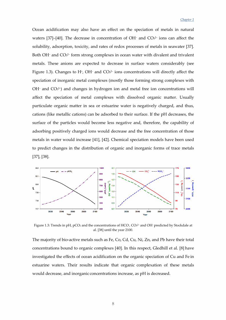
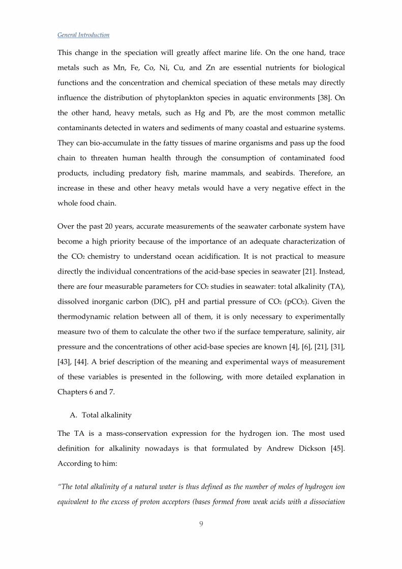
Ocean acidification may also have an effect on the speciation of metals in natural

waters [37]–[40]. The decrease in concentration of OH– and CO32– ions can affect the

solubility, adsorption, toxicity, and rates of redox processes of metals in seawater [37].

Both OH– and CO32– form strong complexes in ocean water with divalent and trivalent

metals. These anions are expected to decrease in surface waters considerably (see

Figure 1.3). Changes to H+, OH– and CO32– ions concentrations will directly affect the

speciation of inorganic metal complexes (mostly those forming strong complexes with

OH– and CO32–) and changes in hydrogen ion and metal free ion concentrations will

affect the speciation of metal complexes with dissolved organic matter. Usually

particulate organic matter in sea or estuarine water is negatively charged, and thus,

cations (like metallic cations) can be adsorbed to their surface. If the pH decreases, the

surface of the particles would become less negative and, therefore, the capability of

adsorbing positively charged ions would decrease and the free concentration of those

metals in water would increase [41], [42]. Chemical speciation models have been used

to predict changes in the distribution of organic and inorganic forms of trace metals

[37], [38].

Figure 1.3: Trends in pH, pCO2 and the concentrations of HCO-, CO32– and OH- predicted by Stockdale at al. [38] until the year 2100.

The majority of bio-active metals such as Fe, Co, Cd, Cu, Ni, Zn, and Pb have their total

concentrations bound to organic complexes [40]. In this respect, Gledhill et al. [8] have

investigated the effects of ocean acidification on the organic speciation of Cu and Fe in

estuarine waters. Their results indicate that organic complexation of these metals

would decrease, and inorganic concentrations increase, as pH is decreased.

General Introduction

9

This change in the speciation will greatly affect marine life. On the one hand, trace

metals such as Mn, Fe, Co, Ni, Cu, and Zn are essential nutrients for biological

functions and the concentration and chemical speciation of these metals may directly

influence the distribution of phytoplankton species in aquatic environments [38]. On

the other hand, heavy metals, such as Hg and Pb, are the most common metallic

contaminants detected in waters and sediments of many coastal and estuarine systems.

They can bio-accumulate in the fatty tissues of marine organisms and pass up the food

chain to threaten human health through the consumption of contaminated food

products, including predatory fish, marine mammals, and seabirds. Therefore, an

increase in these and other heavy metals would have a very negative effect in the

whole food chain.

Over the past 20 years, accurate measurements of the seawater carbonate system have

become a high priority because of the importance of an adequate characterization of

the CO2 chemistry to understand ocean acidification. It is not practical to measure

directly the individual concentrations of the acid-base species in seawater [21]. Instead,

there are four measurable parameters for CO2 studies in seawater: total alkalinity (TA),

dissolved inorganic carbon (DIC), pH and partial pressure of CO2 (pCO2). Given the

thermodynamic relation between all of them, it is only necessary to experimentally

measure two of them to calculate the other two if the surface temperature, salinity, air

pressure and the concentrations of other acid-base species are known [4], [6], [21], [31],

[43], [44]. A brief description of the meaning and experimental ways of measurement

of these variables is presented in the following, with more detailed explanation in

Chapters 6 and 7.

A. Total alkalinity

The TA is a mass-conservation expression for the hydrogen ion. The most used

definition for alkalinity nowadays is that formulated by Andrew Dickson [45].

According to him:

“The total alkalinity of a natural water is thus defined as the number of moles of hydrogen ion

equivalent to the excess of proton acceptors (bases formed from weak acids with a dissociation

Chapter 1

10

constant K ≤10-4.5, at 25°C and zero ionic strength) over proton donors (acids with K > 10-4.5) in

one kilogram of sample.”

And the expression would be the following one:

AT = [HCO3-] + 2[CO32-] + [B(OH)4-] + [OH-] + [HPO42-] + 2[PO43-] + [SiO(OH)3 -] +

[HS-] + 2[S2-] + [NH3] - [H+] – [HSO4-] – [HF] – [H3PO4] + [organic bases] –

[organic acids]

3

As can be seen, the acid-base system of seawater is governed by the different acid-base

species in it. The most important system, because it is the most abundant one, is the

carbonate system. But, besides this, it is necessary to take into account other minor

acid-base species that affect the pH of the water. Those other systems are the boric acid,

phosphoric acid, silicic acid and ammonia systems, among others. Millero [46]

gathered the contribution of these species to the total alkalinity in a review. According

to this review, the contribution of borate at pH = 8, S = 35 and T = 25 °C would be 85.8

µmol kg-1 (for a total concentration of 412 µmol kg-1). In the same conditions, the

contribution of OH- would be 1.6 µmol kg-1, the phosphate system 4 µmol kg-1 (for a

total concentration of 3.2 µmol kg-1) and the silicate system 4.6 µmol kg-1 (for a total

concentration of 170 µmol kg-1). The contribution of ammonia can be quite big for some

anoxic waters. For example, a total concentration of 1600 µmol kg-1 NH4+, would entail

a contribution of 32 µmol kg-1 to the total alkalinity [46].

There are software packages for the seawater CO2 system calculations to account for

the contributions of carbonate, borate, phosphate and silicate to the total alkalinity [47],

[48]. The contribution from organic species such as the bases of humic and fulvic acids

are usually assumed to be negligible. However, a number of studies have shown that

TA contributions from dissolved organic carbon (DOC) can be significant, especially in

river, estuary and coastal waters, where the concentration of DOC is usually higher

[49]–[52]. Deviations on the value of the measured TA and calculated TA (from two

other parameters) of around 30 µmol kg-1 have been found and attributed to dissolved

organic matter in the Baltic Sea [53], [54]. However, since neither the detailed nature of

General Introduction

11

DOC nor the dissociation constants for organic acids are well known, the effect of

organic acids on the alkalinity is very difficult to estimate [55]. Different attempts have

been made to calculate the organic alkalinity. For example, Byrne et al. [56] used

spectrophotometric titration data to develop a model in order to assess the dissociation

constants of the organic acids. Kulinski et al. [53] calculated what they called a bulk

dissociation constant to represent all weak acidic functional groups present in the

organic matter. Turner et al. [54] used Kulinski’s data and showed that, indeed, that

excess of alkalinity is due to the DOC contribution by a chemical speciation model.

They used a humic ion-binding model coupled to the Pitzer model (see Section 1.2) to

explain the contribution of organic alkalinity in the Baltic Sea.

Ignoring the contribution of these minor acid-base systems would produce important

errors when determining alkalinity and subsequently, the rest of the parameters for

studying ocean acidification.

The experimental measurement of alkalinity will be explained and discussed in

Chapter 6.

B. Dissolved Inorganic Carbon (DIC, CT)

DIC is the sum of the three species of the carbonate system in water: dissolved CO2,

bicarbonate and carbonate. At the typical surface seawater pH of 8.2, approximately

89% of the total DIC is present as bicarbonate ion; the proportion of carbonate ion is

about a factor of 10 less (10.5%), and that of unionised carbon dioxide yet another

factor of 10 less (0.5%) [4], [21]. The relative proportion of the three species of the DIC

reflects the pH of seawater.

The carbonate system in seawater can be summarized in these equilibria:

CO2 (g) CO2* (aq)

This reaction refers to the solubility equilibrium of carbon dioxide between air and

seawater.

CO2* (aq) + H2O (l) HCO3- (aq) + H+ (aq)

Chapter 1

12

HCO3- (aq) CO3-2 (aq) + H+ (aq)

These reactions refer to the acid dissociation reactions of the neutral species CO2* (aq)

and bicarbonate, respectively.

The different experimental techniques for the DIC determination will be discussed in

Chapter 6.

C. pH

The pH refers to the hydrogen ion concentration (or activity). There are different pH

scales that can be used which consider other different ions, apart from the proton, in

their definitions of pH (see Chapter 7 Section 7.1.1). This inconsistency between scales,

and the fact that sometimes in the literature the used scale is not defined, makes the

field of pH measurement, scales and, in general, the study of acid-base reactions in

seawater one of the more confusing areas in marine chemistry according to Dickson

[57]. There are two common methods for the determination of the pH: the

potentiometric technique and the spectrophotometric technique. These techniques will

be explained in detail in Chapter 7.

D. Partial pressure of CO2 (pCO2)

The partial pressure of CO2 in air in equilibrium with a seawater sample is a measure

of the degree of saturation of the sample with CO2 gas. In thermodynamics, the

fugacity of a real gas replaces the mechanical partial pressure used for ideal gases. In

other words, the relationship between fugacity and partial pressure is analogous to

that between activity and concentration [6].

The pCO2 is measured as follows: A known amount of sea water is placed in a closed

system containing a small known volume of air (containing a known initial amount of

CO2) and maintained at a constant, known temperature and pressure. Once the water

and air are in equilibrium a sample of the air is analyzed for CO2 content using

generally an infrared detector. Such systems can run autonomously, which make them

desirable for in-situ measurements, but it is difficult to use them in small-scale

General Introduction

13

experiments. They usually require a flowing stream of seawater, so this parameter is

not the most common one for laboratory measurements [21], [58].

The optimal choice of experimental variables to measure is dictated by the nature of

the problem being studied and the availability of equipment. Thus, even if there is no

optimal choice, according to Dickson [59], the best combination to measure open ocean

samples are TA and DIC. The main advantages of using those parameters are that they

are quite easy to measure and the sample can be easily stored for several months [21].

Also, the availability of the Certified Reference Materials (CRM’s) for the measurement

of these parameters in seawater samples makes the choice of TA and DIC the most

suitable one in terms of accuracy. Nevertheless, there are occasions where the

interpretation of the alkalinity is difficult because of a higher contribution of the minor

species. In those situations, he recommends the combination of DIC and pH (measured

spectrophotometrically). In this case the uncertainty of the calculated parameters is

typically dominated by the uncertainty in the pH measurement. Unfortunately, there is

a lack of CRM’s for the determination of pH in seawater media. The advantage of

using these two parameters is that they allow a description of the CO2 system without

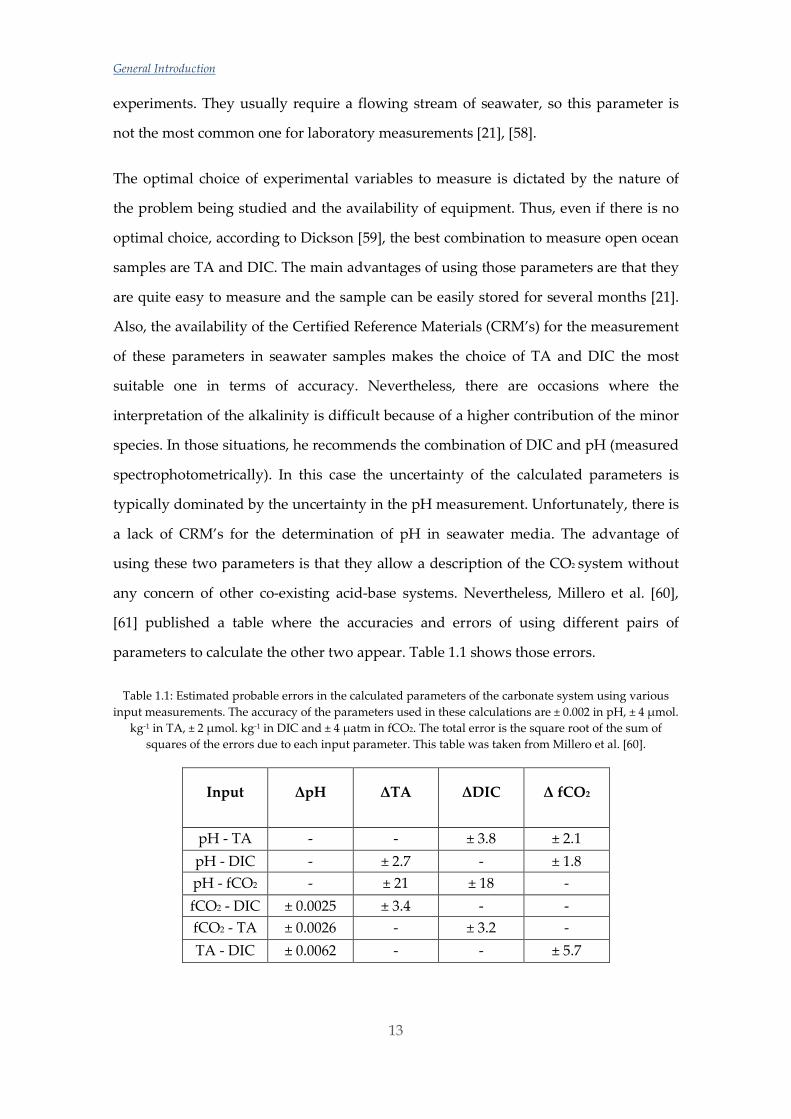
any concern of other co-existing acid-base systems. Nevertheless, Millero et al. [60],

[61] published a table where the accuracies and errors of using different pairs of

parameters to calculate the other two appear. Table 1.1 shows those errors.

Table 1.1: Estimated probable errors in the calculated parameters of the carbonate system using various input measurements. The accuracy of the parameters used in these calculations are ± 0.002 in pH, ± 4 µmol.

kg-1 in TA, ± 2 µmol. kg-1 in DIC and ± 4 µatm in fCO2. The total error is the square root of the sum of squares of the errors due to each input parameter. This table was taken from Millero et al. [60].

Input ΔpH ΔTA ΔDIC Δ fCO2

pH - TA - - ± 3.8 ± 2.1 pH - DIC - ± 2.7 - ± 1.8 pH - fCO2 - ± 21 ± 18 - fCO2 - DIC ± 0.0025 ± 3.4 - - fCO2 - TA ± 0.0026 - ± 3.2 - TA - DIC ± 0.0062 - - ± 5.7

Chapter 1

14

This work is focused on the acidification in estuaries. There are just a few studies

regarding the acidification in estuaries, mostly because of the difficulties arising from

their different structures and high seasonal and tidal variations in them. Moreover,

apart from the dissolution of the CO2 in estuaries there are other processes that raise

the acidity. Human inputs of nutrients to coastal waters can lead to the excessive

production of algae (eutrophication). The microbial consumption of this organic matter

lowers oxygen levels in the water and produces carbon dioxide due to microbial

respiration which also increases acidity [17], [62]–[65].

Nevertheless, it also must be taken into account that there are different types of

estuaries and that the seawater and fresh water mixing regimes can be very different.

In the following Section, a brief review about the most relevant estuary characteristics

is presented.

1.2 Estuaries

Estuaries are the transition zones between rivers and maritime environments. They are

dynamic ecosystems having a connection to the open sea through which the sea

water enters with the rhythm of the tides. The sea water entering the estuary is diluted

by the fresh water flowing from rivers and streams [66]. There have been several

proposals to define an estuary but the most complete one is “semi-enclosed body of

water connected to the sea as far as the tidal limit or the salt intrusion limit and

receiving freshwater runoff; however the freshwater inflow may not be perennial, the

connection to the sea may be closed for part of the year and tidal influence may be

negligible" [67]. This definition includes fjords, lagoons, river mouths, and tidal creeks.

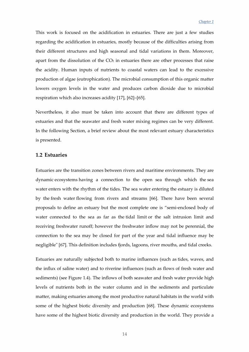
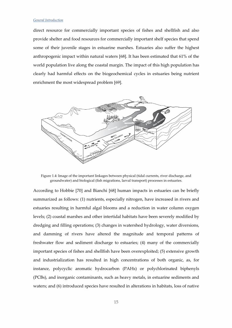
Estuaries are naturally subjected both to marine influences (such as tides, waves, and

the influx of saline water) and to riverine influences (such as flows of fresh water and

sediments) (see Figure 1.4). The inflows of both seawater and fresh water provide high

levels of nutrients both in the water column and in the sediments and particulate

matter, making estuaries among the most productive natural habitats in the world with

some of the highest biotic diversity and production [68]. These dynamic ecosystems

have some of the highest biotic diversity and production in the world. They provide a

General Introduction

15

direct resource for commercially important species of fishes and shellfish and also

provide shelter and food resources for commercially important shelf species that spend

some of their juvenile stages in estuarine marshes. Estuaries also suffer the highest

anthropogenic impact within natural waters [68]. It has been estimated that 61% of the

world population live along the coastal margin. The impact of this high population has

clearly had harmful effects on the biogeochemical cycles in estuaries being nutrient

enrichment the most widespread problem [69].

Figure 1.4: Image of the important linkages between physical (tidal currents, river discharge, and groundwater) and biological (fish migrations, larval transport) processes in estuaries.

According to Hobbie [70] and Bianchi [68] human impacts in estuaries can be briefly

summarized as follows: (1) nutrients, especially nitrogen, have increased in rivers and

estuaries resulting in harmful algal blooms and a reduction in water column oxygen

levels; (2) coastal marshes and other intertidal habitats have been severely modified by

dredging and filling operations; (3) changes in watershed hydrology, water diversions,

and damming of rivers have altered the magnitude and temporal patterns of

freshwater flow and sediment discharge to estuaries; (4) many of the commercially

important species of fishes and shellfish have been overexploited; (5) extensive growth

and industrialization has resulted in high concentrations of both organic, as, for

instance, polycyclic aromatic hydrocarbon (PAHs) or polychlorinated biphenyls

(PCBs), and inorganic contaminants, such as heavy metals, in estuarine sediments and

waters; and (6) introduced species have resulted in alterations in habitats, loss of native

Chapter 1

16

species, and a reduction in commercially important species. This list does not include

acidification between the human impacts, which agrees with the lack of studies and

information regarding this phenomenon in estuaries. As Feely et al. [63] have pointed

out “While ocean acidification has been studied in oceanic waters, little is known

regarding its status in estuaries”. However, the effect that the increment of CO2 has in

estuarine and coastal waters is being registered by different research studies [63], [64],

[71].

There are many ways to classify estuaries. In 1966 Hansen and Rattray [72] first

introduced the idea of using stratification or circulation of both seawater and fresh

water to classify estuaries. This classification for estuaries is the most interesting one

for this work because understanding the stratification of the estuaries under study may

help to better interpret and understand the obtained results. As stated above, the sea

water entering the estuary is diluted by the fresh water flowing from rivers and

streams. The pattern of dilution varies between different estuaries and depends on the

volume of fresh water, the tidal range, and the extent of evaporation of the water in the

estuary. In all estuaries, less dense freshwater from rivers flow over higher density

seawater and the water masses will mix at their boundaries. There are different kinds

of estuaries which can be defined according to this mixing [73]:

A) Salt-wedge estuaries

Salt-wedge estuaries are the most stratified or least mixed, of all estuaries [74], [75].

They are also called highly stratified estuaries. Salt-wedge estuaries occur when a

rapidly flowing river discharges into the ocean where tidal currents are weak and have

minor importance. The force of the river pushes fresh water out to sea instead of tidal

currents transporting seawater upstream. A sharp boundary is created between the

water masses, with fresh water floating on top and a wedge of saltwater on the bottom.

There is some mixing at the boundary between the two water masses, but it is

generally slight. Marrow estuaries with low tidal ranges and limited wave activity also

promote salt-wedge conditions.

B) Slightly stratified or partially mixed estuaries

General Introduction

17

Slightly stratified estuaries form where tidal activity is strong and river volume is

moderate. Here, seawater and freshwater mix at all depths; however, the lower layers

of water typically remain saltier than the upper layers. Salinity is highest at the mouth

of the estuary and decreases upstream [76].

C) Vertically mixed or well mixed estuaries

A vertically mixed or well-mixed estuary occurs when river flow is low and tidally

generated currents are moderate to strong. Tidal mixing forces exceed river output,

resulting in a well mixed water column and the disappearance of the vertical salinity

gradient. The freshwater-seawater boundary is eliminated due to the intense turbulent

mixing and eddy effects. The estuary's salinity is highest nearest the ocean and

decreases as one moves up the river [74]. This type of water circulation is often found

in large, shallow estuaries.

D) Reverse or inverse estuaries

Reverse estuaries are a rare type of estuary found in very arid regions where

precipitation is low and evaporation rates are high. In reverse estuaries there is little to

no freshwater input, and flow is inverted from usual conditions. This type forms when

rivers stop flowing and the evaporation of seawater in the upper part of the estuary

causes water to flow from the ocean into the estuary, producing a salinity gradient of

increasing salinity from the ocean to the estuary’s upper reaches. The bottom has a

higher density layer that flows towards the sea while the surface, with a lower-salinity

water, flows toward the head of the estuary [67].

E) Fjord estuaries

These estuaries are deep, narrow and created in glaciated valleys. They have small

surface areas, high river input and little tidal mixing. River water tends to flow

seaward at the surface with little contact with the seawater below. Circulation in fjord

estuaries is often limited because of the presences of a sediment ledge or bedrock at the

mouth of the estuary called sill. Generally, circulation only exists in the upper layers of

Chapter 1

18

the water above the level of the sill which often produces cold bottom waters with little

oxygen and nutrients.

Thus, it is logical to suppose that with the different mixings the chemical and chemico-

physical characteristics of the estuarine waters will vary greatly depending on the

position and the tidal situation at the specific sampling moment.

Nowadays, due to its important ecological and economical interest, research studies

concerning the acidification in estuaries have increased. For instance, Hu at al. [65]

examined the effect that eutrophication has on the acidification due to its usually lower

dissolved oxygen concentration. Some works involve seasonal variations for longer or

shorter periods on the carbonate chemistry [71], [77], [78]. Hu et al. [79] used a long

term data set (over 40 years) to examine changes in estuarine carbonate chemistry and

Mucci et al. [80] studied the historical and current pH evolution in the Gulf of Mexico

and St. Lawrence estuary (eastern Canada) respectively. Mosley et al. [81] developed

an equilibrium model based on the CO2 system to account for the pH variation

throughout the estuary salinity range using the composition of the river and seawater

end members. The concern of acidification in estuaries is increasing.

In estuaries, salinity plays a key role, as it does for any natural water chemical study.

The mixing between seawater and fresh water results on different salinities (and

therefore different compositions) along the estuary that range between S= 0.2 (river)

and S= 40 (sea) according to the present study. Knowledge about salinity and seawater

composition are as old as marine chemistry. Different definitions for salinity have been

proposed since Georg Forchhammer presented this concept in 1865. A small historical

summary on marine chemistry and seawater composition that follows will help to

understand the chemistry of estuaries and some important concepts.

1.3 Marine chemistry and seawater composition

The first marine chemistry studies were concerned with the composition of salts in sea

water. The results of that kind of work were published first in 1674 by Robert Boyle

[82], who has been called the “father of chemical oceanography” [83]. In 1772, Antoine

General Introduction

19

Lavoisier published the first analysis of seawater using a method of evaporation

followed by solvent extraction [84]. In 1784, Olof Bergman published results of the

analysis of seawater weighing precipitated salts, a method developed by him.

Between 1824 and 1836, the technique of volumetric titration was developed by Joseph

Louis Gay-Lussac. With this method he determined that the salt content of open ocean

seawater is almost geographically constant [85]. This conclusion was confirmed by

John Murray in 1818 [86] and by Alexander Marcet in 1819-1822 [87]. Marcet had

obtained samples of water from the Artic and Atlantic Oceans and the Mediterranean,

Black, Baltic, China and White Seas. He determined the dissolved matter in each of

these samples by evaporation followed by drying the residue at 100 °C. Both Murray

and Marcet realized that it was possible to carry out gravimetric analysis in order to

make precise and accurate measurements of the chemical composition of seawater.

Marcet also proposed that seawater contained small quantities of all soluble substances

and that the relative abundances of some of them were constant. This hypothesis is

known nowadays as Marcet's Principle or Principle of Constant Composition [83].

The first extensive investigation of the composition of seawater was carried out in 1865

by Georg Forchhammer who determined chloride, sulphate, magnesium, calcium and

potassium directly, and sodium by difference in 260 surface waters from all parts of the

world. He also introduced the concept of salinity. He reported that the ratios of the

major constituents were subject to only “very slight variations” for different parts of

the ocean if the results for the Mediterranean, Black, Caribbean and Baltic Seas and

German Ocean were omitted [88]. But his investigation was justifiably criticized on the

grounds that all of his samples were surface waters and that his analytical methods

were inaccurate. However, his suggestion that variations in composition do occur was

not completely ignored.

Following Forchhammer’s work, the major highlight of chemical oceanography was

the Challenger expedition with which the modern era of oceanography began. The

Challenger Expedition, which lasted between 1873 and 1876, was not the first

oceanographic expedition, but it was the biggest and most comprehensive up to that

Chapter 1

20

time. In this expedition, 77 seawater samples were collected and in 1884 the results

were published by William Dittmar [89]. The major criticisms which can be made of

these analyses are that the samples were stored for as long as two years in glass bottles

before examination and that they did not include any samples of Artic, Antartic and

Mediterranean waters. Dittmar’s approach to what are still very difficult to solve

problems of chemical analysis is, however, much less open to criticism. In each of the

methods which he adopted for the seven major ions (chloride, calcium, magnesium,

potassium, sulphate, bromide and sodium) he adhered rigidly to a modus operandi so

that any errors would be constant and might be eliminated by subsequent

investigation. Dittmar’s results were self-consistent and agreed fairly well with those of

Forchhammer. In general, he regarded his results as extending Forchhammer’s

proposition from surface waters to ocean waters from all depths.

Since Dittmar’s time, many workers have studied the ratio of single constituents to

chlorinity. Assessment of these results is not easy but some of the variations cannot be

dismissed as experimental error.

In discussing the implications of variations in ionic ratios, in 1959 Carpenter and

Carritt pointed out a tendency which has crept into the literature to consider the

relative composition of seawater as constant and to completely disregard the fact that

variations have been reported. Admittedly, the variations found are small and are

often of the same magnitude as the experimental error of the analytical methods used

and for many purposes they may be regarded as negligible [90]. A more accurate

assessment of their magnitudes and, if possible, their causes is still required [91], [92].

As the ratios between the concentrations of the main ionic constituents in sea water

keep reasonably constant, it is possible to characterize the composition by measuring

only one component that is easy to measure and has a conservative behaviour. A

conservative component of seawater is one that is unreactive and for which the

changes from place to place are due to the addition or loss of water. This component is

the salinity

General Introduction

21

In 1899, the International Council for the Exploration of the Sea (ICES) named Martin

Knudsen chairman of a commission assigned to examine the definition of the salinity

and density of seawater. The procedural definition of salinity was stated by Knudsen

in 1902:

“Salinity is the amount (in grams) of dissolved solid material in a kilogram of seawater after all

the bromine has been replaced by an equivalent quantity of chlorine, all the carbonate converted

to oxide, and all of the organic matter destroyed”

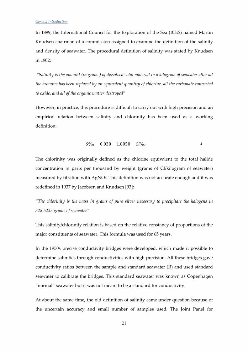
However, in practice, this procedure is difficult to carry out with high precision and an

empirical relation between salinity and chlorinity has been used as a working

definition:

𝑆𝑆‰ = 0.030 + 1.8050 × 𝐶𝐶𝐶𝐶‰ 4

The chlorinity was originally defined as the chlorine equivalent to the total halide

concentration in parts per thousand by weight (grams of Cl/kilogram of seawater)

measured by titration with AgNO3. This definition was not accurate enough and it was

redefined in 1937 by Jacobsen and Knudsen [93]:

“The chlorinity is the mass in grams of pure silver necessary to precipitate the halogens in

328.5233 grams of seawater”

This salinity/chlorinity relation is based on the relative constancy of proportions of the

major constituents of seawater. This formula was used for 65 years.

In the 1950s precise conductivity bridges were developed, which made it possible to

determine salinities through conductivities with high precision. All these bridges gave

conductivity ratios between the sample and standard seawater (R) and used standard

seawater to calibrate the bridges. This standard seawater was known as Copenhagen

“normal” seawater but it was not meant to be a standard for conductivity.

At about the same time, the old definition of salinity came under question because of

the uncertain accuracy and small number of samples used. The Joint Panel for

Chapter 1

22

Oceanographic Tables and Standards (JPOTS), sponsored by UNESCO (United Nations

Educational, Scientific, and Cultural Organization), ICES, IAPSO (International

Association of Physical Sciences of Ocean), and SCOR (Scientific Committee on

Oceanic Research), was appointed to develop a conductivity standard for salinity.

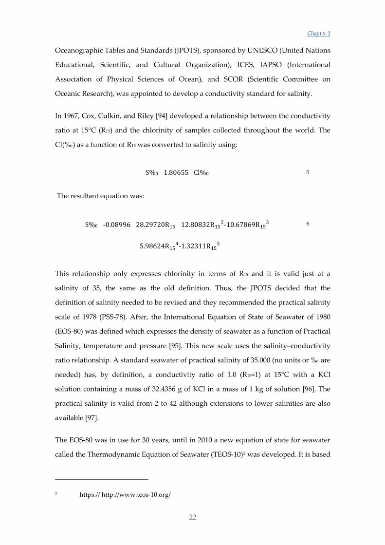
In 1967, Cox, Culkin, and Riley [94] developed a relationship between the conductivity

ratio at 15°C (R15) and the chlorinity of samples collected throughout the world. The

Cl(‰) as a function of R15 was converted to salinity using:

S‰=1.80655×Cl‰ 5

The resultant equation was:

S‰=-0.08996+28.29720R15+12.80832R152-10.67869R15

3

+5.98624R154-1.32311R15

5

6

This relationship only expresses chlorinity in terms of R15 and it is valid just at a

salinity of 35, the same as the old definition. Thus, the JPOTS decided that the

definition of salinity needed to be revised and they recommended the practical salinity

scale of 1978 (PSS-78). After, the International Equation of State of Seawater of 1980

(EOS-80) was defined which expresses the density of seawater as a function of Practical

Salinity, temperature and pressure [95]. This new scale uses the salinity–conductivity

ratio relationship. A standard seawater of practical salinity of 35.000 (no units or ‰ are

needed) has, by definition, a conductivity ratio of 1.0 (R15=1) at 15°C with a KCl

solution containing a mass of 32.4356 g of KCl in a mass of 1 kg of solution [96]. The

practical salinity is valid from 2 to 42 although extensions to lower salinities are also

available [97].

The EOS-80 was in use for 30 years, until in 2010 a new equation of state for seawater

called the Thermodynamic Equation of Seawater (TEOS-10)2 was developed. It is based

2 https:// http://www.teos-10.org/

General Introduction

23

on a Gibbs function formulation from which all thermodynamic properties of seawater

(density, enthalpy, entropy, sound speed, etc.) can be derived in a thermodynamically

consistent manner. TEOS-10 was adopted by the Intergovernmental Oceanographic

Commission at its 25th Assembly in June 2009 to replace EOS-80 as the official

description of seawater and ice properties in marine science. A significant change is

that TEOS-10 uses Absolute Salinity SA (mass fraction of salt in seawater) as instead of

Practical Salinity SP (which is essentially a measure of the conductivity of seawater) to

describe the salt content of seawater. It also replaces the potential temperature for the

conservative temperature. Salinities on this scale are determined by combining

electrical conductivity measurements with other information that can account for

regional changes in the composition of seawater. They can also be determined by

making direct density measurements. Ocean salinities now have units of g/kg.

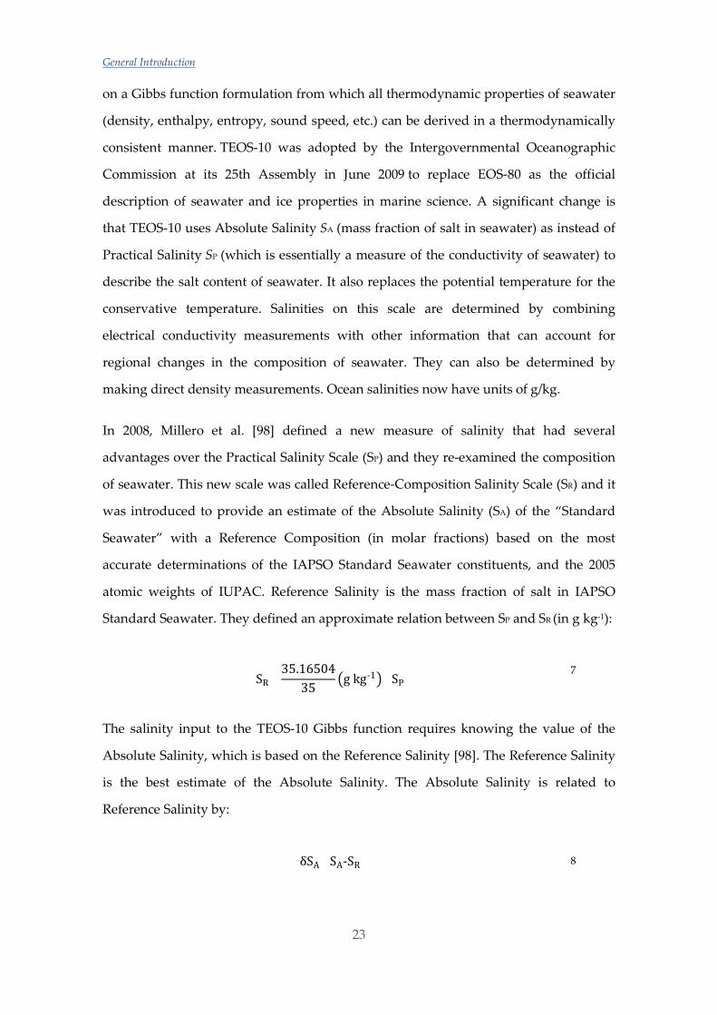
In 2008, Millero et al. [98] defined a new measure of salinity that had several

advantages over the Practical Salinity Scale (SP) and they re-examined the composition

of seawater. This new scale was called Reference-Composition Salinity Scale (SR) and it

was introduced to provide an estimate of the Absolute Salinity (SA) of the “Standard

Seawater” with a Reference Composition (in molar fractions) based on the most

accurate determinations of the IAPSO Standard Seawater constituents, and the 2005

atomic weights of IUPAC. Reference Salinity is the mass fraction of salt in IAPSO

Standard Seawater. They defined an approximate relation between SP and SR (in g kg-1):

SR=35.16504

35 g kg-1×SP 7

The salinity input to the TEOS-10 Gibbs function requires knowing the value of the

Absolute Salinity, which is based on the Reference Salinity [98]. The Reference Salinity

is the best estimate of the Absolute Salinity. The Absolute Salinity is related to

Reference Salinity by:

δSA=SA-SR 8

Chapter 1

24

Where δSA is the salinity correction and can be estimated from the difference between

the measured densities and the values determined from the equation of state of

seawater as a function of salinity and temperature [96].

Millero et al. [98] also re-examined the composition on the Reference Seawater and the

ionic composition can be found in Table 1.2. Table 1.3 shows a recipe to prepare 1 kg of

artificial seawater [96].

Table 1.2: Composition of Reference Seawater (SP = 35.000, pCO2 = 337 µatm, and T = 25°C)

gi (g kg-1)

AW (g mol-1)

mi (mol kg H2O-1)

Ii (mol kg H2O-1)

Na+ 10.78145 22.9898 0.4860573 0.4860573 Mg2+ 1.28372 24.305 0.0547419 0.2189674 Ca2+ 0.41208 40.078 0.0106566 0.0426266 K+ 0.3991 39.0983 0.0105796 0.0105796

Sr2+ 0.00795 87.62 0.000094 0.0003762 Cl– 19.35271 35.453 0.5657619 0.5657619

SO42– 2.71235 96.0626 0.0292642 0.1170567 HCO3– 0.10481 61.0168 0.0017803 0.0017803

Br– 0.06728 79.904 0.0008727 0.0008727 CO32– 0.01434 60.0089 0.0002477 0.0009907

B(OH)4– 0.00795 78.8404 0.0001045 0.0001045 F– 0.0013 18.9984 0.0000709 0.0000709

OH– 0.00014 17.0073 0.0000085 0.0000085 B(OH)3 0.01944 61.833 0.0003259

CO2 0.00042 44.0095 Σ= 35.16504 1.1605659 1.4452533

H2O 964.83496 0.580283 0.722627

General Introduction

25

Table 1.3: Preparation of 1 kg of SP =35.00 of Artificial Seawater

Gravimetric Salts g (g kg-1) m (mol kg-1) MW (g mol-1) NaCl 24.878 0.42568 58.4428 Na2SO4 4.1566 0.02926 142.0372 KCl 0.7237 0.00971 74.555 NaHCO3 0.1496 0.00178 84.007 KBr 0.1039 0.00087 119.006 B(OH)3 0.0266 0.00043 61.8322 NaF 0.003 0.00007 41.9882 Σ= 30.0413 Volumetric Salts* MgCl2 5.2121 0.05474 95.211 CaCl2 1.1828 0.01066 110.986 SrCl2 0.0149 0.00009 158.526 * Use 1 mol L-1 MgCl2, CaCl2, and SrCl2 (standardized). From those solutions 52.8 mL of MgCl2, 10.3 mL of CaCl2, and 0.1 mL of SrCl2 are needed. The densities of these solutions are 1.017 g mL-1, 1.013 g mL-1, and 1.131 g mL-1, respectively, for the solutions at 1 mol L-1. The grams of water in each solution are given by H2O = gSOLN – gSALT = mL × density – gSALT Addition of Water gH2O to add = 1000 – gH2O from MgCl2, CaCl2, and SrCl2

As the ratios between the concentrations of the main ionic constituents in sea water

keep reasonably constant, even if Table 1.3 corresponds to SP = 35.000, a solution with a

different salinity can be prepared by making the corresponding solution. This

consistency on the major constituents can be also found in estuarine waters and several

studies used the dilution of this SP = 35 recipe to prepare synthetic estuarine water [99],

[100].

As is well known [101], the equilibrium constants vary with the ionic strength, and,

therefore, with the salinity. Consequently, when measuring natural waters calculations

must be made at the specific sample’s ionic strength. Although in open ocean water the

salinity variation is small, in coastal areas and estuaries, where freshwater inputs are

important, salinity variations are much larger. Hence, the equilibrium constants of all

acid-base systems in these waters must be known at different ionic strengths.

Chapter 1

26

For a better understanding of the need of equilibrium constants at different ionic

strengths for acidification studies in estuaries and how they are determined, a small

introduction about solution thermodynamics will follow.

1.4 Solution thermodynamics and equilibria

The word “thermodynamics” was proposed by William Thompson (Lord Kelvin) in

1849 [102] and it has been suggested to come from the Greek words “therme” (heat)

and “dynamis” (power).

Essentially, thermodynamics provide two major kinds of information: whether a

particular process could happen spontaneously under specific conditions and also

about the composition of reactants and products of a reaction system at equilibrium. In

a chemical reaction, equilibrium is reached when the concentrations of reactants and

products do not tend to change with time.

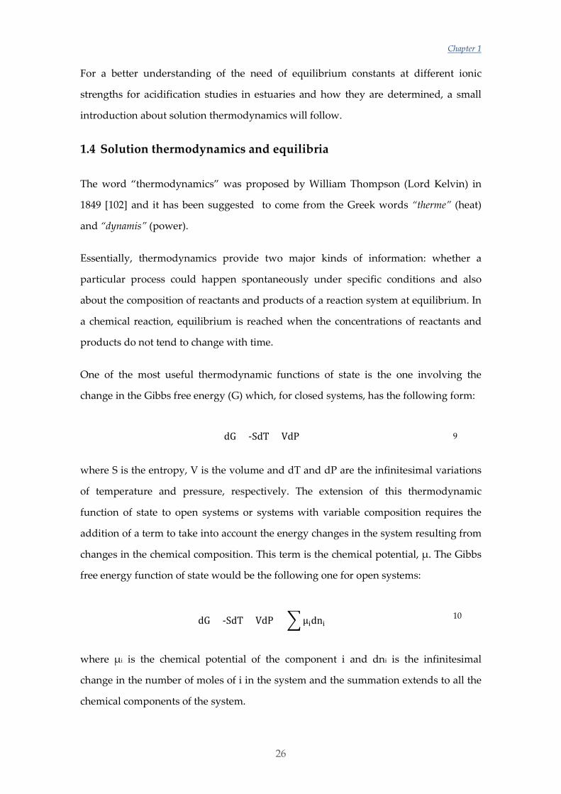
One of the most useful thermodynamic functions of state is the one involving the

change in the Gibbs free energy (G) which, for closed systems, has the following form:

dG = -SdT + VdP 9

where S is the entropy, V is the volume and dT and dP are the infinitesimal variations

of temperature and pressure, respectively. The extension of this thermodynamic

function of state to open systems or systems with variable composition requires the

addition of a term to take into account the energy changes in the system resulting from

changes in the chemical composition. This term is the chemical potential, µ. The Gibbs

free energy function of state would be the following one for open systems:

dG = -SdT + VdP + µidni 10

where µi is the chemical potential of the component i and dni is the infinitesimal

change in the number of moles of i in the system and the summation extends to all the

chemical components of the system.

General Introduction

27

When a system is at equilibrium and at constant temperature and pressure the

following condition is fulfilled:

dG = µidni = 0 11

The chemical potential represents the variation of the free energy of the system with

respect of the number of moles of a given substance (i) at constant T, P and chemical

composition of the system (except for i).

Therefore, considering the following reaction of the protonation of the species A:

A- + H+ HA

and taking into account that

dnA- + dnH+ = dnHA 12

at equilibrium the following will fulfil:

µA- + µH+ = µHA 13

The position of the equilibrium will depend of the contribution of each of the species to

the free energy. These contributions depend on the nature and concentration of the

species as well as P and T and also could be influenced by the rest of the substances in

solution.

The chemical potential of a species A in an ideal solution is expressed by:

µA = µA0 + RT lnCA 14

where CA represents the generic concentration of A and R is the gas constant

(8.314 J.mol -1.K-1).

Chapter 1

28

Due to the relation between the different concentration scales, it is possible to write the

equation above in other scales. For example, for solutes in ideal solutions it could be

expressed like this:

µA = µA0 + RT ln[A] 15

where [A] is the molar concentration of the species A.

However, in most real solutions, the chemical potential does not follow the equation

above and component A behaves as if it would be in a different concentration. Instead,

the chemical potential of A is proportional to an apparent concentration which is

known as activity, denoted by . Thus,

µA =µ A0 + RT lnA 16

where A is the activity of A, a dimensionless quantity, and µA0 is the chemical

potential in the standard state of A, defined as the chemical potential of A when the

activity is equal to one. The activity is defined as:

A = CA.γA 17

being γA the activity coefficient of A, which is also dimensionless. The activity

coefficient depends on the concentration scale of CA (molarity, molality, etc.) so it is

important to notice in which scale it is considered.

The activity is a measure of the effective (or thermodynamic) concentration of a species

in a real solution. The difference between activity and other measures of concentration

is that molecules in non-ideal solutions interact with each other and the activity takes

into account these interactions. In general, the activity depends on any factor that alters

the chemical potential, such as concentration, temperature, pressure, interactions

between chemical species, electric fields, etc. Depending on the circumstances, some of

these factors may be more important than others. As stated above, the activity is a

dimensionless quantity because it actually represents a ratio of the reactivity of a

General Introduction

29

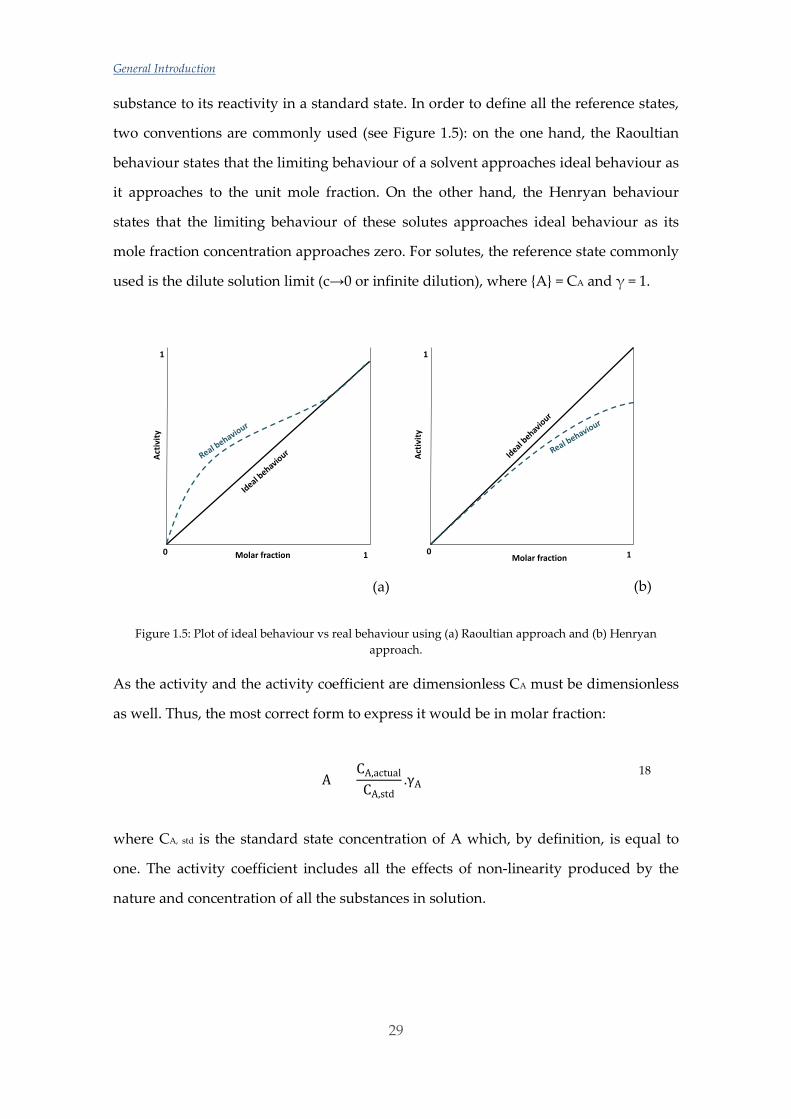
substance to its reactivity in a standard state. In order to define all the reference states,

two conventions are commonly used (see Figure 1.5): on the one hand, the Raoultian

behaviour states that the limiting behaviour of a solvent approaches ideal behaviour as

it approaches to the unit mole fraction. On the other hand, the Henryan behaviour

states that the limiting behaviour of these solutes approaches ideal behaviour as its

mole fraction concentration approaches zero. For solutes, the reference state commonly

used is the dilute solution limit (c→0 or infinite dilution), where A = CA and γ = 1.

(a)

(b)

Figure 1.5: Plot of ideal behaviour vs real behaviour using (a) Raoultian approach and (b) Henryan approach.

As the activity and the activity coefficient are dimensionless CA must be dimensionless

as well. Thus, the most correct form to express it would be in molar fraction:

A = CA,actual

CA,std.γA

18

where CA, std is the standard state concentration of A which, by definition, is equal to

one. The activity coefficient includes all the effects of non-linearity produced by the

nature and concentration of all the substances in solution.

Molar fraction

Activ

ity

0 1

1

Molar fraction0 1

1

Activ

ity

Chapter 1

30

As stated above, at equilibrium µA- + µH+ = µHA. This means that:

µA-0 + RT lnA- + µH+0 + RT lnH+ = µHA

0 + RT lnHA

19

RT lnHA

A-H+ = µA-0 + µH+

0 - µHA0

20

HAA-H+

= eµA-0 +µH+

0 -µHA0

RT = K 21

The ratio between the activities in equation 21 corresponds to a relation between the

activities of the species at equilibrium. This relation is constant at a given P and T

because the chemical potentials in the standard state are also constant. This constant

relation is known as the thermodynamic equilibrium constant.

As stated above, the reference state for a particular solute is the solution following the

Henryan behaviour, in which the solute is assumed to behave ideally, and the activity

is equal to the concentration as γ is equal to one. But the choice for the ideal solution is

an arbitrary one and thus, different standard states can be defined. The most common

standard states are the following two:

(1) Standard state of Infinite Dilution

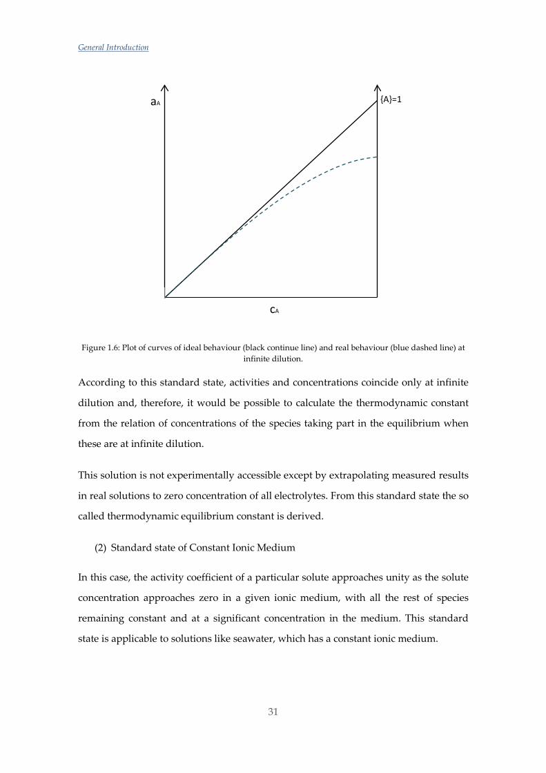
This standard state, assumes that the activity coefficients of all solutes approach unity

as the concentrations of all species in the solution approach zero. If the activity of a

solute changes with the concentration as in the curve in Figure 1.6, a tangent to the

curve at c = 0 represents the hypothetical behaviour that the solute has in infinite

dilution in the whole interval.

General Introduction

31

Figure 1.6: Plot of curves of ideal behaviour (black continue line) and real behaviour (blue dashed line) at infinite dilution.

According to this standard state, activities and concentrations coincide only at infinite

dilution and, therefore, it would be possible to calculate the thermodynamic constant

from the relation of concentrations of the species taking part in the equilibrium when

these are at infinite dilution.

This solution is not experimentally accessible except by extrapolating measured results

in real solutions to zero concentration of all electrolytes. From this standard state the so

called thermodynamic equilibrium constant is derived.

(2) Standard state of Constant Ionic Medium

In this case, the activity coefficient of a particular solute approaches unity as the solute

concentration approaches zero in a given ionic medium, with all the rest of species

remaining constant and at a significant concentration in the medium. This standard

state is applicable to solutions like seawater, which has a constant ionic medium.

aA

cA

A=1

Chapter 1

32

One of the advantages of this standard state is that the activity coefficient of an

electrolyte depends strongly on the concentration at low electrolyte concentration of

the ionic medium, but less in more concentrated solutions. Thus, it is usually

convenient to carry out physical measurements in the presence of a high concentration

of an inert electrolyte. If the concentration of the background electrolyte is about 10-100

times the concentration of the solvent, the activity coefficient is considered to be close

enough to the unity so the a = c [103], [104]. The disadvantage of it is that the constants

determined in this standard state are only valid in that specific ionic medium.

From this standard state the so-called stoichiometric equilibrium constant is derived.

When calculating stability constants, as it is not possible to determine the activities,

concentrations and activity coefficients are used. Concentrations are determined by

analytical methods and for the determination of activity coefficients several theoretical

calculation theories have been proposed.

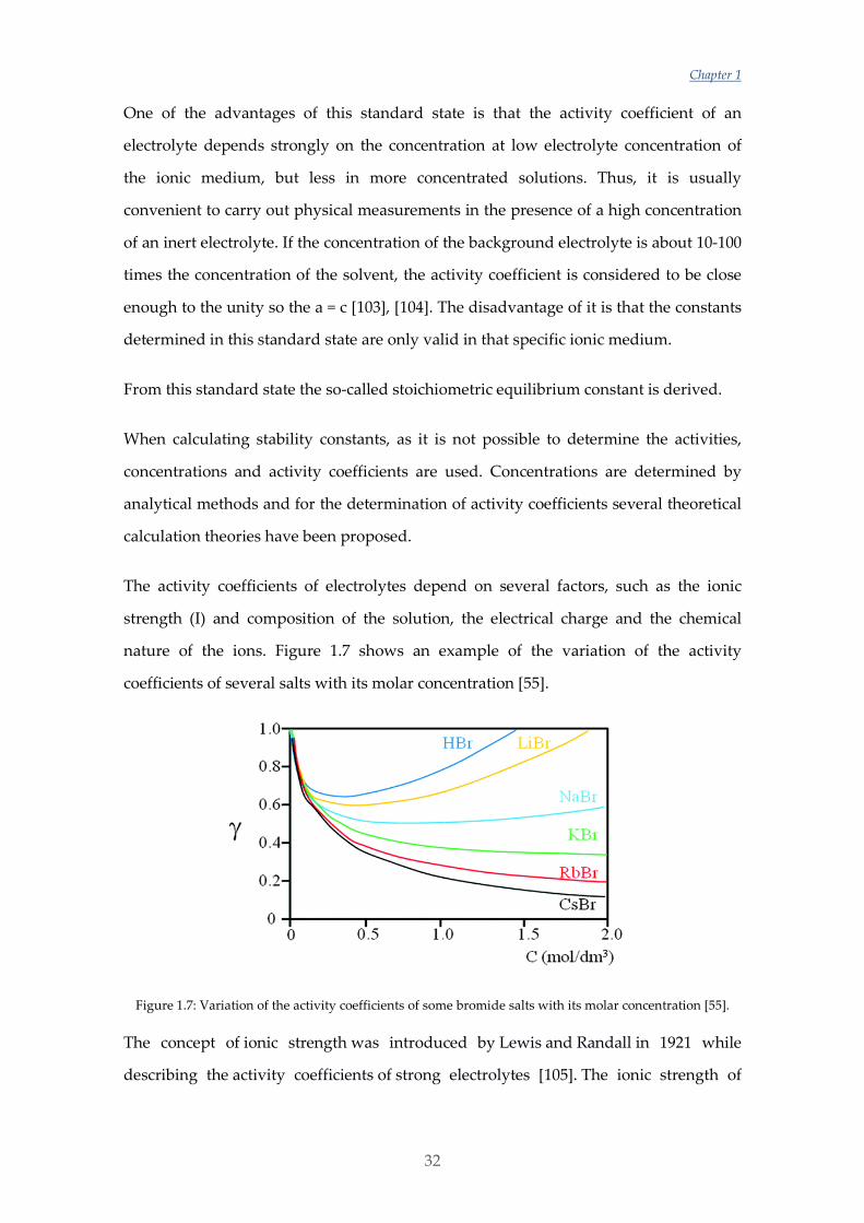
The activity coefficients of electrolytes depend on several factors, such as the ionic

strength (I) and composition of the solution, the electrical charge and the chemical

nature of the ions. Figure 1.7 shows an example of the variation of the activity

coefficients of several salts with its molar concentration [55].

Figure 1.7: Variation of the activity coefficients of some bromide salts with its molar concentration [55].

The concept of ionic strength was introduced by Lewis and Randall in 1921 while

describing the activity coefficients of strong electrolytes [105]. The ionic strength of

General Introduction

33

a solution is a measure of the concentration of ions in a solution, taking into account

their charge. It is related to the ion-ion interactions in a solution. It is defined as:

I = 12

ci|zi|2

i

22

where zi is the charge of ion i and ci is its concentration, and the summation takes into

account all anions and cations. As can be seen, the ionic strength is a measure of

the concentration of ions in a solution, weighted according to the square of the charge

of each ion.

Since it is not possible to have a solution that contains only a single ion, it is only

possible to measure the activity coefficient of a complete electrolyte (i.e. γHγA or γ±)

[106]. Usually, this information is obtained by measuring the deviation from ideality of

the colligative properties of solutions. Colligative properties of solutions are those that

depend on the ratio of the number of solute molecules to the number of solvent

molecules in a solution, and not on the nature of the chemical species present. These

properties are the freezing point depression, boiling point elevation, lowering of

vapour pressure and osmotic pressure. In solving ionic equilibrium problems that

involve mixtures of salts, mean ionic activity coefficients are of little direct use. Even if

they do not have a full thermodynamic meaning, single ion activity coefficients are

needed to calculate the activity of a specific ion to determine stability constants. In

order to calculate single ion activity coefficients, several calculation theories have been

proposed along the years. For that purpose, it is important to go through the historical

development of these theories for a better understanding of the more modern ones (see

Table 3.3 for a summary).

In 1894 van Laar [107] pointed out the importance of electrostatic forces to explain the

characteristics of ionic solutions. Later, in 1906, Bjerrum proposed that the behaviour of

strong electrolytes in diluted solutions could be described by the hypothesis of a

complete dissociation and a proper consideration of the effects of interionic attraction.

He proposed the same idea when he attended the 7th International Congress of

Chapter 1

34

Applied Chemistry in London and presented a paper entitled “A new form for the

electrolytic dissociation theory” [108]. The work published by Milner in 1912 [109] was

the first attempt to express mathematically these ideas but he only got approximated

results.

The equations proposed by Lewis [105], [110] and Harned [111] were subject to

important extrapolation errors, and the activity coefficients presented a precision of

about ± 0.1, due to the lack of knowledge on the theoretical bases of the problem.

In the early 20’s the research in this area was focused on the behaviour of concentrated

electrolyte solutions instead of using the simplest approaches provided by diluted

solutions. Bronsted [112] and Bjerrum [113] studied the variation of activity coefficients

with concentration at high concentration solutions, becoming the pioneers of the

Specific Interaction Theory (SIT) and Ionic Hydration theories, respectively. Although

later these theories would be re-examined and used, they were left in a second place

for years because of the growing importance of research on diluted solutions due to the

introduction of the theories of Debye and Hückel [114].

Debye and Hückel predicted quantitatively the behaviour of strong electrolytes in

diluted solutions. Their work was published in 1923 [114] explaining what they called

the Debye-Hückel (DH) limiting law:

logγi = -Azi2√I 23

where A is a parameter that depends on the dielectric constant on the medium and

temperature and it has a value of 0.5109 mol-1/2.kg1/2 in water at 25 °C, and zi is the

charge of the ion. This theory assumes that the central ion is a point charge and that the

other ions are spread around the central ion with a Gaussian distribution. All ions with

the same charge would have the same value for the activity coefficient. This theory is

limited to I < 0.01 mol. L-1.

Due to the limited usability of the DH equation, the so-called extended Debye-Hückel

(EDH) theory was postulated:

General Introduction

35

logγi = -Azi2 √I

1+B.a√I

24

where B is another parameter that depends on the dielectric constant of the medium

and the temperature, which has a value of 0.3286 Å-1.mol-1/2.kg1/2 at 25 °C, and a is a

new parameter introduced in the equation called the ion size parameter that takes into

account the fact that ions have a finite radius and they are not point charges. The EDH

equation is accurate up to I ≤ 0.1 mol. L-1.

Various other extensions have been proposed, including the Davies equation [115] who

added an empirical linear term in I to improve the fit with experimental data:

logγi = -Azi2

√I1+√I

- 0.2I 25

The second term in I (-0.2 I) improves the fit of the equations at higher ionic strengths,

and thus, the usability of this equation goes up to I ≤ 0.5 mol. L-1.

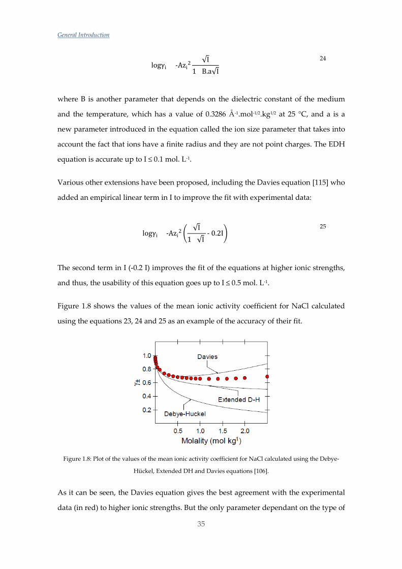
Figure 1.8 shows the values of the mean ionic activity coefficient for NaCl calculated

using the equations 23, 24 and 25 as an example of the accuracy of their fit.

Figure 1.8: Plot of the values of the mean ionic activity coefficient for NaCl calculated using the Debye-

Hückel, Extended DH and Davies equations [106].

As it can be seen, the Davies equation gives the best agreement with the experimental

data (in red) to higher ionic strengths. But the only parameter dependant on the type of

Chapter 1

36

ion is the charge, and thus, for electrolytes with the same stoichiometry, the activity

coefficient values would be the same.

Due to the experimental observation that the activity coefficients show linear relation

with the ionic strength at high concentrations, Hückel extended his equation in order

to get a better fit at higher ionic strengths. He considered that the dielectric constant of

the medium change linearly with the concentration of the ion and he introduced a new

arbitrary constant, C [116]:

logγi = -Azi2

√I1+B.a√I

+ C.c 26

where c is the concentration of the ion. This equation has been used up to I = 1 mol. L-1.

In this equation, two different terms can be distinguished: an electrostatic term and a

statistical term. The electrostatic term takes into account the long-range Coulombic

interactions and they are commonly expressed by the extended Debye-Hückel

equation (EDH), with slight modifications on the election of the term B.a. The statistical

term has caused the major disagreements. This term intends to obtain semi-empirical

equations to relate the activity with the composition of the solution. This term should

have a correct sense from a thermodynamic point of view and allow fitting

experimental data with the minimum number of parameters possible, in order to make

proper extrapolations and interpolations.

The models to express this statistical term can be either physical or chemical. The

physical models are based on the specific interactions between the ions in solution

(Specific Interaction Theories, SIT). The chemical models try to explain the deviations

of the electrostatic term by the elimination of free ions due to the formation of new

ionic species caused by electrostatic interactions (Ion Association Models) or by

considering the interaction of ions with water molecules (Ionic Hydration Theories).

This work is more focused on the theories based on specific interaction models and

thus, these theories will be more extensively explained bellow.

General Introduction

37

1.3.1 Theories based on specific interaction models

1.3.1.1 Specific Interaction Theory (SIT)

This theory arises from the need to derive activity coefficients of solutes when their

concentrations are too high to be predicted by the Debye-Hückel theory. Although

there are several specific interaction theories, the original one was introduced by

Brönsted in 1922 [112] and reformulated by Guggenheim in 1935 [117]. Finally

Scatchard also made some important contributions to this theory [118]–[120].

Scatchard’s most recent contribution gave a value of 1.5 to the term B.a [121]. This

model considers that ions with opposite charge get close together causing interactions

that are specific for every pair of ions M and X. The most recent version of the equation

would be the following one for the free ion activity coefficient of ion M (γM) with a

charge zM. The same equation would be applicable for anion X (γX) with a charge zX but

multiplying for the molal concentration of the cation in the last summation.

logγM = -A|zM.zX|√I

1+B.a√I + ε

x

(M,X,I)mX 27

As can be appreciated, the first term of this equation is the extended Debye-Hückel

equation (DH) but using zM and zX as the charges of the cation and the anion

respectively. The term ε (M,X,I) is the so-called interaction coefficient, which is specific

for every pair of ions (M - X) and in which its possible variation with the ionic strength

(I) is considered. The ionic strength is in mol. kg-1, as mx is the molal concentration of X.

The sum extends to all X ions present in solution with opposite charge to the M ion.

This theory assumes that there are no interactions between ions with the same sign. In

order to calculate the interaction coefficient of the M-X ion pair, it is necessary to know

the experimental value of its mean ion activity coefficient in a solution that only

contains that electrolyte, γMX0 [122].

ε(M,X,I) = (zM + zX)2

4I logγMX0 + |zMzX|.D

28

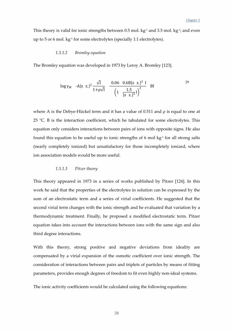
Chapter 1

38

This theory is valid for ionic strengths between 0.5 mol. kg-1 and 3.5 mol. kg-1; and even

up to 5 or 6 mol. kg-1 for some electrolytes (specially 1:1 electrolytes).

1.3.1.2 Bromley equation

The Bromley equation was developed in 1973 by Leroy A. Bromley [123].

log γM =-A|z+z-|2 √I1+ρ√I

+(0.06+0.6B|z+z-|2)I

1+ 1.5|z+z-|2 I

2 +BI 29

where A is the Debye-Hückel term and it has a value of 0.511 and 𝜌𝜌 is equal to one at

25 °C. B is the interaction coefficient, which he tabulated for some electrolytes. This

equation only considers interactions between pairs of ions with opposite signs. He also

found this equation to be useful up to ionic strengths of 6 mol kg-1 for all strong salts

(nearly completely ionized) but unsatisfactory for those incompletely ionized, where

ion association models would be more useful.

1.3.1.3 Pitzer theory

This theory appeared in 1973 in a series of works published by Pitzer [124]. In this

work he said that the properties of the electrolytes in solution can be expressed by the

sum of an electrostatic term and a series of virial coefficients. He suggested that the

second virial term changes with the ionic strength and he evaluated that variation by a

thermodynamic treatment. Finally, he proposed a modified electrostatic term. Pitzer

equation takes into account the interactions between ions with the same sign and also

third degree interactions.

With this theory, strong positive and negative deviations from ideality are

compensated by a virial expansion of the osmotic coefficient over ionic strength. The

consideration of interactions between pairs and triplets of particles by means of fitting

parameters, provides enough degrees of freedom to fit even highly non-ideal systems.

The ionic activity coefficients would be calculated using the following equations:

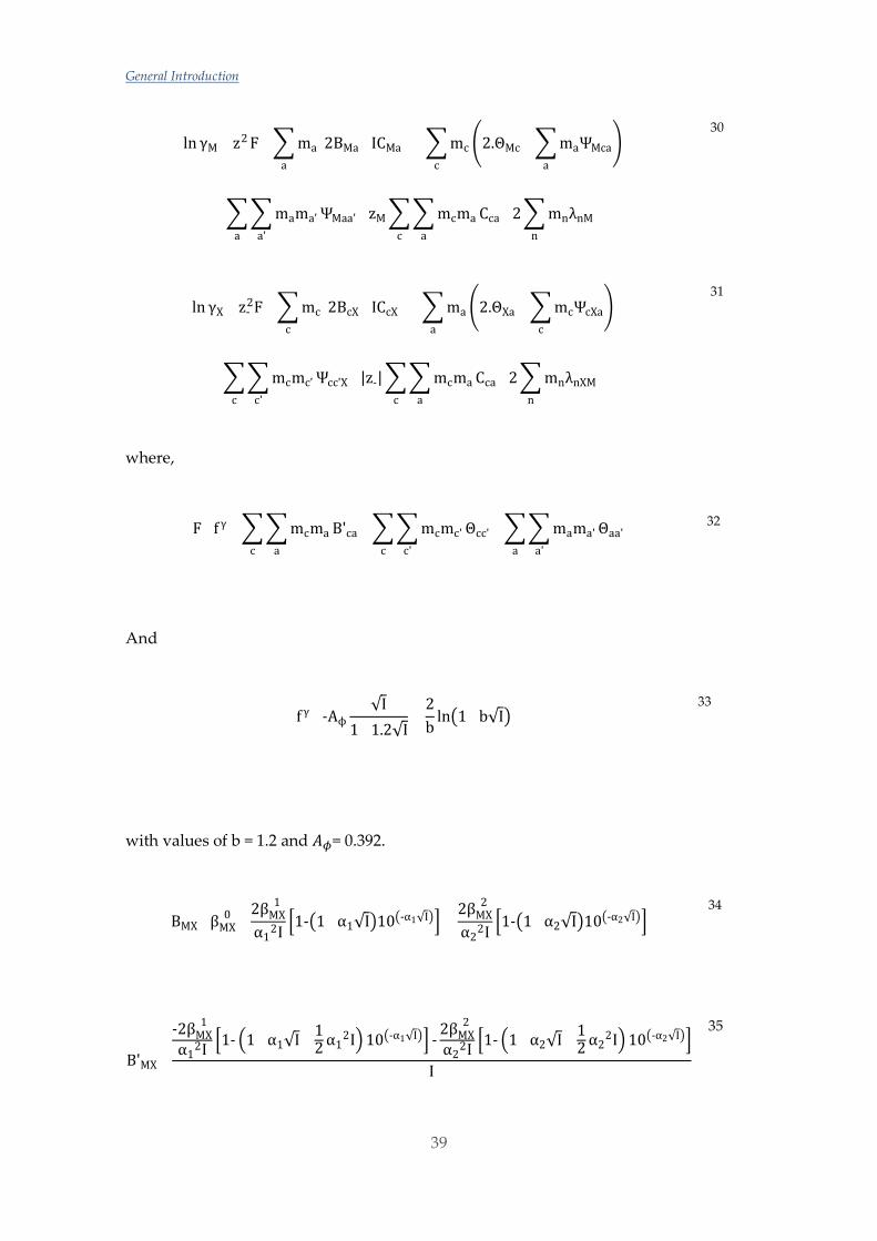
General Introduction

39

ln γM =z+2 F+ ma(2BMa+ICMa)

a

+ mc 2.ΘMc+ maΨMcaa

c

+

mama'a'a

ΨMaa'+zM mcmaac

Cca+2 mnλnMn

30

ln γX =z-2F+ mc(2BcX+ICcX)

c

+ ma 2.ΘXa+ mcΨcXac

a

+

mcmc'c'c

Ψcc'X+|z-| mcmaac

Cca+2 mnλnXMn

31

where,

F=f γ+ mcmaac

B'ca+ mcmc'c'c

Θcc'+ mama'a'a

Θaa'

32

And

f γ=-Aϕ√I

1+1.2√I+

2b

ln1+b√I

33

with values of b = 1.2 and 𝐴𝐴𝜙𝜙= 0.392.

BMX=βMX(0)+

2βMX(1)

α12I 1-1+α1√I10-α1√I +

2βMX(2)

α22I 1-1+α2√I10-α2√I

34

B'MX=

-2βMX(1)

α12I 1- 1+α1√I+ 1

2 α12I 10-α1√I -

2βMX(2)

α22I 1- 1+α2√I+ 1

2 α22I 10-α2√I

I

35

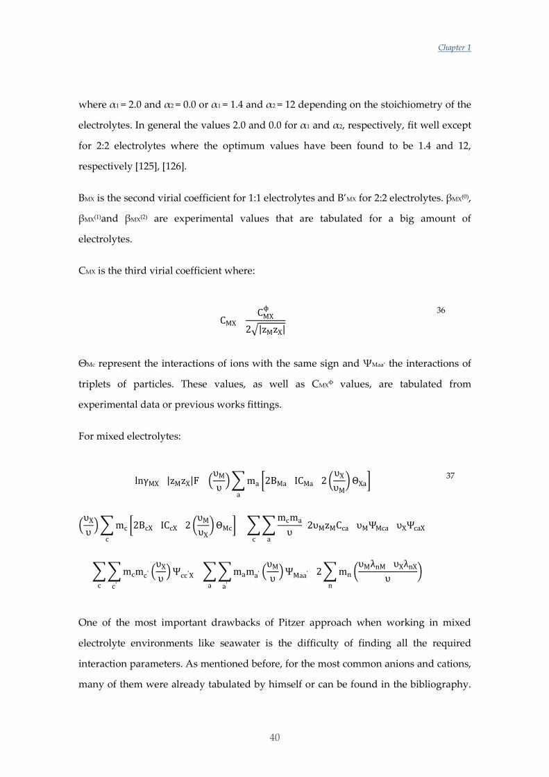
Chapter 1

40

where α1 = 2.0 and α2 = 0.0 or α1 = 1.4 and α2 = 12 depending on the stoichiometry of the

electrolytes. In general the values 2.0 and 0.0 for α1 and α2, respectively, fit well except

for 2:2 electrolytes where the optimum values have been found to be 1.4 and 12,

respectively [125], [126].

BMX is the second virial coefficient for 1:1 electrolytes and B’MX for 2:2 electrolytes. βMX(0),

βMX(1)and βMX(2) are experimental values that are tabulated for a big amount of

electrolytes.

CMX is the third virial coefficient where:

CMX=CMX

ϕ

2|zMzX|

36

ΘMc represent the interactions of ions with the same sign and ΨMaa’ the interactions of

triplets of particles. These values, as well as CMXФ values, are tabulated from

experimental data or previous works fittings.

For mixed electrolytes:

lnγMX=|zMzX|F+ υM

υ ma 2BMa+ICMa+2

υX

υM ΘXa

a

+

υX

υ mc 2BcX+ICcX+2

υM

υX ΘMc

c

+ mcma

υac

[2υMzMCca+υMΨMca+υXΨcaX]+

mcmc'

c'c

υX

υ Ψcc'X+ mama'

a'a

υM

υ ΨMaa'+2 mn

n

υMλnM+υXλnX

υ

37

One of the most important drawbacks of Pitzer approach when working in mixed

electrolyte environments like seawater is the difficulty of finding all the required

interaction parameters. As mentioned before, for the most common anions and cations,

many of them were already tabulated by himself or can be found in the bibliography.

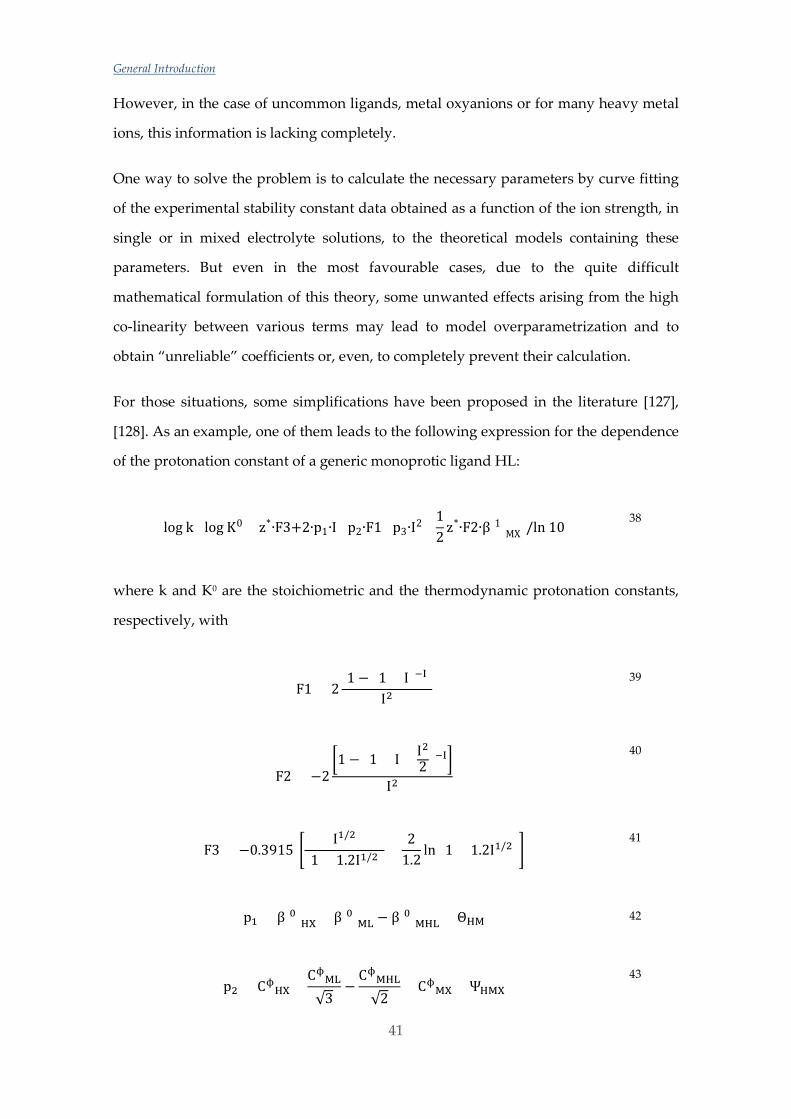
General Introduction

41

However, in the case of uncommon ligands, metal oxyanions or for many heavy metal

ions, this information is lacking completely.

One way to solve the problem is to calculate the necessary parameters by curve fitting

of the experimental stability constant data obtained as a function of the ion strength, in

single or in mixed electrolyte solutions, to the theoretical models containing these

parameters. But even in the most favourable cases, due to the quite difficult

mathematical formulation of this theory, some unwanted effects arising from the high

co-linearity between various terms may lead to model overparametrization and to

obtain “unreliable” coefficients or, even, to completely prevent their calculation.

For those situations, some simplifications have been proposed in the literature [127],

[128]. As an example, one of them leads to the following expression for the dependence

of the protonation constant of a generic monoprotic ligand HL:

log k=log K0+[z*∙F3+2∙p1∙I+p2∙F1+p3∙I2+12

z*∙F2∙β(1)MX]/ln 10

38

where k and K0 are the stoichiometric and the thermodynamic protonation constants,

respectively, with

F1 = 2[1 − (1 + I)−I]

I2 39

F2 = −21 − (1 + I + I2

2 )−I

I2

40

F3 = −0.3915 I1/2

(1 + 1.2I1/2)+

21.2

ln (1 + 1.2I1/2) 41

p1 = β(0)HX + β(0)

ML − β(0)MHL + ΘHM 42

p2 = CϕHX +

CϕML

√3−

CϕMHL

√2+ Cϕ

MX + ΨHMX 43

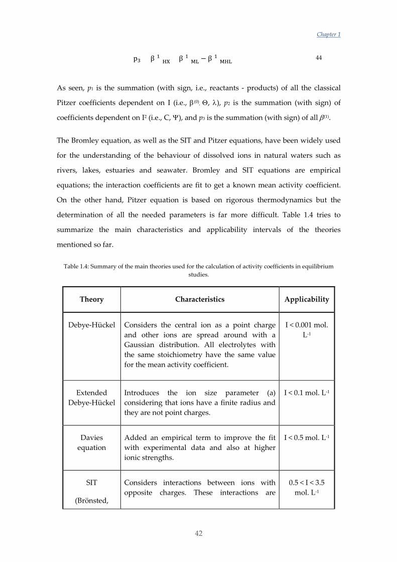
Chapter 1

42

p3 = β(1)HX + β(1)

ML − β(1)MHL 44

As seen, p1 is the summation (with sign, i.e., reactants - products) of all the classical

Pitzer coefficients dependent on I (i.e., β(0), Θ, λ), p2 is the summation (with sign) of

coefficients dependent on I2 (i.e., C, Ψ), and p3 is the summation (with sign) of all β(1).

The Bromley equation, as well as the SIT and Pitzer equations, have been widely used

for the understanding of the behaviour of dissolved ions in natural waters such as

rivers, lakes, estuaries and seawater. Bromley and SIT equations are empirical

equations; the interaction coefficients are fit to get a known mean activity coefficient.

On the other hand, Pitzer equation is based on rigorous thermodynamics but the

determination of all the needed parameters is far more difficult. Table 1.4 tries to

summarize the main characteristics and applicability intervals of the theories

mentioned so far.

Table 1.4: Summary of the main theories used for the calculation of activity coefficients in equilibrium studies.

Theory Characteristics Applicability

Debye-Hückel Considers the central ion as a point charge and other ions are spread around with a Gaussian distribution. All electrolytes with the same stoichiometry have the same value for the mean activity coefficient.

I < 0.001 mol. L-1

Extended Debye-Hückel

Introduces the ion size parameter (a) considering that ions have a finite radius and they are not point charges.

I < 0.1 mol. L-1

Davies equation

Added an empirical term to improve the fit with experimental data and also at higher ionic strengths.

I < 0.5 mol. L-1

SIT

(Brönsted,

Considers interactions between ions with opposite charges. These interactions are

0.5 < I < 3.5 mol. L-1

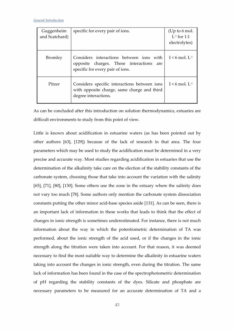
General Introduction

43

Guggenheim and Scatchard)

specific for every pair of ions. (Up to 6 mol. L-1 for 1:1

electrolytes)

Bromley Considers interactions between ions with opposite charges. These interactions are specific for every pair of ions.

I < 6 mol. L-1

Pitzer Considers specific interactions between ions with opposite charge, same charge and third degree interactions.

I < 6 mol. L-1

As can be concluded after this introduction on solution thermodynamics, estuaries are

difficult environments to study from this point of view.

Little is known about acidification in estuarine waters (as has been pointed out by

other authors [63], [129]) because of the lack of research in that area. The four

parameters which may be used to study the acidification must be determined in a very

precise and accurate way. Most studies regarding acidification in estuaries that use the

determination of the alkalinity take care on the election of the stability constants of the

carbonate system, choosing those that take into account the variation with the salinity

[65], [71], [80], [130]. Some others use the zone in the estuary where the salinity does

not vary too much [78]. Some authors only mention the carbonate system dissociation

constants putting the other minor acid-base species aside [131]. As can be seen, there is

an important lack of information in these works that leads to think that the effect of

changes in ionic strength is sometimes underestimated. For instance, there is not much

information about the way in which the potentiometric determination of TA was

performed, about the ionic strength of the acid used, or if the changes in the ionic

strength along the titration were taken into account. For that reason, it was deemed

necessary to find the most suitable way to determine the alkalinity in estuarine waters

taking into account the changes in ionic strength, even during the titration. The same

lack of information has been found in the case of the spectrophotometric determination

of pH regarding the stability constants of the dyes. Silicate and phosphate are

necessary parameters to be measured for an accurate determination of TA and a

Chapter 1

44

posterior analysis of the acidification trends. Furthermore, some other nutrients as well

as other chemical and physico-chemical parameters also give important information

regarding the quality of the water and help to set in an adequate context the possible

conclusions extracted from the acidification studies.

1.5 References

[1] C. Le Quéré, “Closing the global budget for CO2,” Glob. Change, vol. 74, pp. 28–31,

2009.

[2] Intergovernmental Panel on Climate Change (IPCC), 2013, Climate Change 2013 -

The Physical Science Basis: Working Group I Contribution to the Fifth Assessment Report

of the IPCC. Cambridge: Cambridge University Press, 2013.

[3] R. H. Moss et al., “The next generation of scenarios for climate change research and

assessment,” Nature, vol. 463, no. 7282, p. nature08823, 2010.

[4] J.-P. Gattuso and L. Hansson, Ocean Acidification, 1st ed. New York: Oxford

University Press, 2011.

[5] C. Le Quéré et al., “Global Carbon Budget 2016,” Earth Syst. Sci. Data, vol. 8, no. 2,

pp. 605–649, 2016.

[6] R. E. Zeebe and D. Wolf-Gladrow, CO2 in Seawater: Equilibrium, Kinetics, Isotopes.

Elsevier, 2001.

[7] K. Caldeira and M. E. Wickett, “Anthropogenic carbon and ocean pH,” Nature, vol.

425, p. 365, 2003.

[8] M. Gledhill, E. P. Achterberg, K. Li, K. N. Mohamed, and M. J. A. Rijkenberg,

“Influence of ocean acidification on the complexation of iron and copper by

organic ligands in estuarine waters,” Mar. Chem., vol. 177, pp. 421–433, 2015.

[9] Intergovernmental Panel on Climate Change (IPCC), 2014, Climate Change 2014:

Impacts, Adaptation, and Vulnerability. Part A: Global and Sectoral Aspects. Contribution

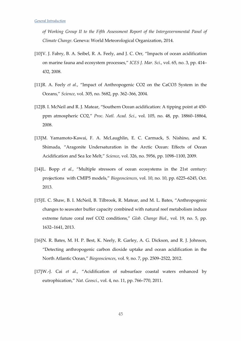
General Introduction

45

of Working Group II to the Fifth Assessment Report of the Intergovernmental Panel of

Climate Change. Geneva: World Meteorological Organization, 2014.

[10] V. J. Fabry, B. A. Seibel, R. A. Feely, and J. C. Orr, “Impacts of ocean acidification

on marine fauna and ecosystem processes,” ICES J. Mar. Sci., vol. 65, no. 3, pp. 414–

432, 2008.

[11] R. A. Feely et al., “Impact of Anthropogenic CO2 on the CaCO3 System in the

Oceans,” Science, vol. 305, no. 5682, pp. 362–366, 2004.

[12] B. I. McNeil and R. J. Matear, “Southern Ocean acidification: A tipping point at 450-

ppm atmospheric CO2,” Proc. Natl. Acad. Sci., vol. 105, no. 48, pp. 18860–18864,

2008.

[13] M. Yamamoto-Kawai, F. A. McLaughlin, E. C. Carmack, S. Nishino, and K.

Shimada, “Aragonite Undersaturation in the Arctic Ocean: Effects of Ocean

Acidification and Sea Ice Melt,” Science, vol. 326, no. 5956, pp. 1098–1100, 2009.

[14] L. Bopp et al., “Multiple stressors of ocean ecosystems in the 21st century:

projections with CMIP5 models,” Biogeosciences, vol. 10, no. 10, pp. 6225–6245, Oct.

2013.

[15] E. C. Shaw, B. I. McNeil, B. Tilbrook, R. Matear, and M. L. Bates, “Anthropogenic

changes to seawater buffer capacity combined with natural reef metabolism induce

extreme future coral reef CO2 conditions,” Glob. Change Biol., vol. 19, no. 5, pp.

1632–1641, 2013.

[16] N. R. Bates, M. H. P. Best, K. Neely, R. Garley, A. G. Dickson, and R. J. Johnson,

“Detecting anthropogenic carbon dioxide uptake and ocean acidification in the

North Atlantic Ocean,” Biogeosciences, vol. 9, no. 7, pp. 2509–2522, 2012.

[17] W.-J. Cai et al., “Acidification of subsurface coastal waters enhanced by

eutrophication,” Nat. Geosci., vol. 4, no. 11, pp. 766–770, 2011.

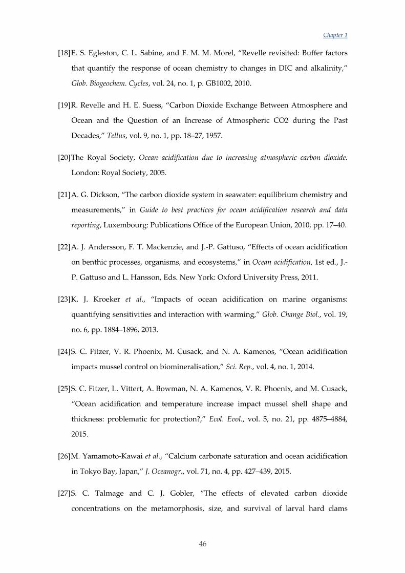
Chapter 1

46

[18] E. S. Egleston, C. L. Sabine, and F. M. M. Morel, “Revelle revisited: Buffer factors

that quantify the response of ocean chemistry to changes in DIC and alkalinity,”

Glob. Biogeochem. Cycles, vol. 24, no. 1, p. GB1002, 2010.

[19] R. Revelle and H. E. Suess, “Carbon Dioxide Exchange Between Atmosphere and

Ocean and the Question of an Increase of Atmospheric CO2 during the Past

Decades,” Tellus, vol. 9, no. 1, pp. 18–27, 1957.

[20] The Royal Society, Ocean acidification due to increasing atmospheric carbon dioxide.

London: Royal Society, 2005.

[21] A. G. Dickson, “The carbon dioxide system in seawater: equilibrium chemistry and

measurements,” in Guide to best practices for ocean acidification research and data

reporting, Luxembourg: Publications Office of the European Union, 2010, pp. 17–40.

[22] A. J. Andersson, F. T. Mackenzie, and J.-P. Gattuso, “Effects of ocean acidification

on benthic processes, organisms, and ecosystems,” in Ocean acidification, 1st ed., J.-

P. Gattuso and L. Hansson, Eds. New York: Oxford University Press, 2011.

[23] K. J. Kroeker et al., “Impacts of ocean acidification on marine organisms:

quantifying sensitivities and interaction with warming,” Glob. Change Biol., vol. 19,

no. 6, pp. 1884–1896, 2013.

[24] S. C. Fitzer, V. R. Phoenix, M. Cusack, and N. A. Kamenos, “Ocean acidification

impacts mussel control on biomineralisation,” Sci. Rep., vol. 4, no. 1, 2014.

[25] S. C. Fitzer, L. Vittert, A. Bowman, N. A. Kamenos, V. R. Phoenix, and M. Cusack,

“Ocean acidification and temperature increase impact mussel shell shape and

thickness: problematic for protection?,” Ecol. Evol., vol. 5, no. 21, pp. 4875–4884,

2015.

[26] M. Yamamoto-Kawai et al., “Calcium carbonate saturation and ocean acidification

in Tokyo Bay, Japan,” J. Oceanogr., vol. 71, no. 4, pp. 427–439, 2015.

[27] S. C. Talmage and C. J. Gobler, “The effects of elevated carbon dioxide

concentrations on the metamorphosis, size, and survival of larval hard clams

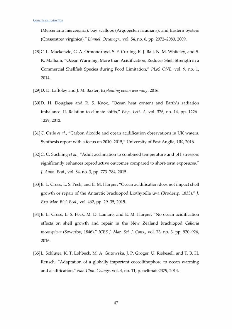
General Introduction

47

(Mercenaria mercenaria), bay scallops (Argopecten irradians), and Eastern oysters

(Crassostrea virginica),” Limnol. Oceanogr., vol. 54, no. 6, pp. 2072–2080, 2009.

[28] C. L. Mackenzie, G. A. Ormondroyd, S. F. Curling, R. J. Ball, N. M. Whiteley, and S.

K. Malham, “Ocean Warming, More than Acidification, Reduces Shell Strength in a

Commercial Shellfish Species during Food Limitation,” PLoS ONE, vol. 9, no. 1,

2014.

[29] D. D. Laffoley and J. M. Baxter, Explaining ocean warming. 2016.

[30] D. H. Douglass and R. S. Knox, “Ocean heat content and Earthʼs radiation

imbalance. II. Relation to climate shifts,” Phys. Lett. A, vol. 376, no. 14, pp. 1226–

1229, 2012.

[31] C. Ostle et al., “Carbon dioxide and ocean acidification observations in UK waters.

Synthesis report with a focus on 2010–2015,” University of East Anglia, UK, 2016.

[32] C. C. Suckling et al., “Adult acclimation to combined temperature and pH stressors

significantly enhances reproductive outcomes compared to short-term exposures,”

J. Anim. Ecol., vol. 84, no. 3, pp. 773–784, 2015.

[33] E. L. Cross, L. S. Peck, and E. M. Harper, “Ocean acidification does not impact shell

growth or repair of the Antarctic brachiopod Liothyrella uva (Broderip, 1833),” J.

Exp. Mar. Biol. Ecol., vol. 462, pp. 29–35, 2015.

[34] E. L. Cross, L. S. Peck, M. D. Lamare, and E. M. Harper, “No ocean acidification

effects on shell growth and repair in the New Zealand brachiopod Calloria

inconspicua (Sowerby, 1846),” ICES J. Mar. Sci. J. Cons., vol. 73, no. 3, pp. 920–926,

2016.

[35] L. Schlüter, K. T. Lohbeck, M. A. Gutowska, J. P. Gröger, U. Riebesell, and T. B. H.

Reusch, “Adaptation of a globally important coccolithophore to ocean warming

and acidification,” Nat. Clim. Change, vol. 4, no. 11, p. nclimate2379, 2014.

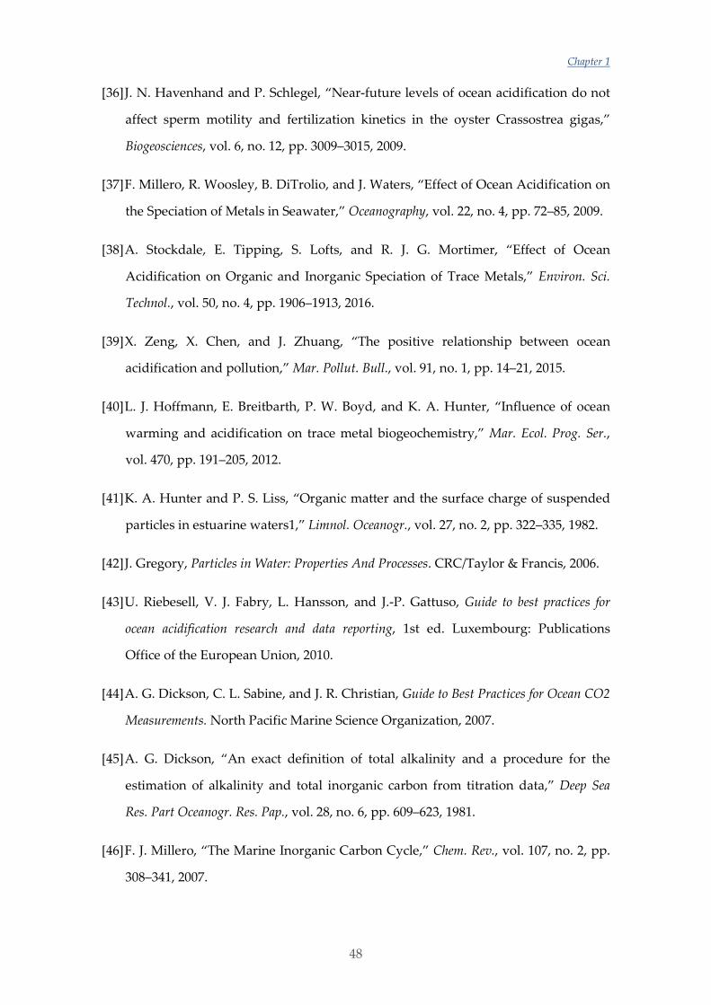
Chapter 1

48

[36] J. N. Havenhand and P. Schlegel, “Near-future levels of ocean acidification do not

affect sperm motility and fertilization kinetics in the oyster Crassostrea gigas,”

Biogeosciences, vol. 6, no. 12, pp. 3009–3015, 2009.

[37] F. Millero, R. Woosley, B. DiTrolio, and J. Waters, “Effect of Ocean Acidification on

the Speciation of Metals in Seawater,” Oceanography, vol. 22, no. 4, pp. 72–85, 2009.

[38] A. Stockdale, E. Tipping, S. Lofts, and R. J. G. Mortimer, “Effect of Ocean

Acidification on Organic and Inorganic Speciation of Trace Metals,” Environ. Sci.

Technol., vol. 50, no. 4, pp. 1906–1913, 2016.

[39] X. Zeng, X. Chen, and J. Zhuang, “The positive relationship between ocean

acidification and pollution,” Mar. Pollut. Bull., vol. 91, no. 1, pp. 14–21, 2015.

[40] L. J. Hoffmann, E. Breitbarth, P. W. Boyd, and K. A. Hunter, “Influence of ocean

warming and acidification on trace metal biogeochemistry,” Mar. Ecol. Prog. Ser.,

vol. 470, pp. 191–205, 2012.

[41] K. A. Hunter and P. S. Liss, “Organic matter and the surface charge of suspended

particles in estuarine waters1,” Limnol. Oceanogr., vol. 27, no. 2, pp. 322–335, 1982.

[42] J. Gregory, Particles in Water: Properties And Processes. CRC/Taylor & Francis, 2006.

[43] U. Riebesell, V. J. Fabry, L. Hansson, and J.-P. Gattuso, Guide to best practices for

ocean acidification research and data reporting, 1st ed. Luxembourg: Publications

Office of the European Union, 2010.

[44] A. G. Dickson, C. L. Sabine, and J. R. Christian, Guide to Best Practices for Ocean CO2

Measurements. North Pacific Marine Science Organization, 2007.

[45] A. G. Dickson, “An exact definition of total alkalinity and a procedure for the

estimation of alkalinity and total inorganic carbon from titration data,” Deep Sea

Res. Part Oceanogr. Res. Pap., vol. 28, no. 6, pp. 609–623, 1981.

[46] F. J. Millero, “The Marine Inorganic Carbon Cycle,” Chem. Rev., vol. 107, no. 2, pp.

308–341, 2007.

General Introduction

49

[47] E. Lewis, D. Wallace, and L. Allison, “Program developed for CO2 system

calculations,” Carbon Dioxide Information Analysis Center, managed by Lockheed

Martin Energy Research Corporation for the US Department of Energy, 1998.

[48] J. C. Orr, J.-M. Epitalon, and J.-P. Gattuso, “Comparison of ten packages that

compute ocean carbonate chemistry,” Biogeosciences, vol. 12, no. 5, pp. 1483–1510,

2015.

[49] Y. H. Ko, K. Lee, K. H. Eom, and I.-S. Han, “Organic alkalinity produced by

phytoplankton and its effect on the computation of ocean carbon parameters,”

Limnol. Oceanogr., vol. 61, no. 4, pp. 1462–1471, 2016.

[50] W.-J. Cai, Y. Wang, and R. E. Hodson, “Acid-Base Properties of Dissolved Organic

Matter in the Estuarine Waters of Georgia, USA,” Geochim. Cosmochim. Acta, vol. 62,

no. 3, pp. 473–483, 1998.

[51] H.-C. Kim and K. Lee, “Significant contribution of dissolved organic matter to

seawater alkalinity,” Geophys. Res. Lett., vol. 36, no. 20, p. L20603, 2009.

[52] C. W. Hunt, J. E. Salisbury, and D. Vandemark, “Contribution of non-carbonate

anions to total alkalinity and overestimation of pCO2 in New England and New

Brunswick rivers,” Biogeosciences, vol. 8, no. 10, pp. 3069–3076, 2011.

[53] K. Kuliński, B. Schneider, K. Hammer, U. Machulik, and D. Schulz-Bull, “The

influence of dissolved organic matter on the acid–base system of the Baltic Sea,” J.

Mar. Syst., vol. 132, pp. 106–115, 2014.

[54] D. R. Turner, A. Ulfsbo, K. Kuliński, and L. G. Anderson, “Modelling organic

alkalinity in the Baltic Sea using a Humic-Pitzer approach,” Mar. Chem., vol. 168,

pp. 18–26, 2015.

[55] F. J. Millero et al., “Dissociation constants for carbonic acid determined from field

measurements,” Deep Sea Res. Part Oceanogr. Res. Pap., vol. 49, no. 10, pp. 1705–

1723, 2002.

Chapter 1

50

[56] R. H. Byrne, B. Yang, and M. Lindemuth, “Contributions of organic alkalinity to

total alkalinity in coastal waters: A spectrophotometric approach,” Mar. Chem., vol.

176, pp. 199–207, 2015.

[57] A. G. Dickson, “pH scales and proton-transfer reactions in saline media such as sea

water,” Geochim. Cosmochim. Acta, vol. 48, no. 11, pp. 2299–2308, 1984.

[58] C. J. M. Hoppe, G. Langer, S. D. Rokitta, D. A. Wolf-Gladrow, and B. Rost,

“Implications of observed inconsistencies in carbonate chemistry measurements

for ocean acidification studies,” Biogeosciences, vol. 9, no. 7, pp. 2401–2405, 2012.

[59] A. G. Dickson, C. L. Sabine, and J. R. Christian, Guide to best practices for ocean CO2

measurements. PICES Special Publication 3, 2007.

[60] F. J. Millero et al., “The internal consistency of CO2 measurements in the equatorial

Pacific,” Mar. Chem., vol. 44, no. 2, pp. 269–280, 1993.

[61] F. J. Millero, “Thermodynamics of the carbon dioxide system in the oceans,”

Geochim. Cosmochim. Acta, vol. 59, no. 4, pp. 661–677, 1995.

[62] C. M. Duarte et al., “Is Ocean Acidification an Open-Ocean Syndrome?

Understanding Anthropogenic Impacts on Seawater pH,” Estuaries Coasts, vol. 36,

no. 2, pp. 221–236, 2013.

[63] R. A. Feely et al., “The combined effects of ocean acidification, mixing, and

respiration on pH and carbonate saturation in an urbanized estuary,” Estuar. Coast.

Shelf Sci., vol. 88, no. 4, pp. 442–449, 2010.

[64] R. B. Wallace, H. Baumann, J. S. Grear, R. C. Aller, and C. J. Gobler, “Coastal ocean

acidification: The other eutrophication problem,” Estuar. Coast. Shelf Sci., vol. 148,

no. Supplement C, pp. 1–13, 2014.

[65] X. Hu et al., “Effects of eutrophication and benthic respiration on water column

carbonate chemistry in a traditional hypoxic zone in the Northern Gulf of Mexico,”

Mar. Chem., 2017.

General Introduction

51

[66] D. S. McLusky and M. Elliott, The Estuarine Ecosystem: Ecology, Threats and

Management. New York: Oxford University Press, 2004.

[67] E. Wolanski, Estuarine Ecohydrology, 2nd ed. Amsterdam: Elsevier, 2007.

[68] T. S. Bianchi, Biogeochemistry of Estuaries, 1st ed. Oxford, New York: Oxford

University Press, 2006.

[69] R. W. Howarth, N. Jaworski, D. Swaney, A. Townsend, and G. Billen, “Some

approaches for assessing human influences on fluxes of nitrogen and organic

carbon to estuaries,” in Estuarine Science: A Synthetic Approach to Research and

Practice, J. E. Hobbie, Ed. Washington DC: Island Press, 2000, pp. 17–42.

[70] J. E. Hobbie, “Estuarine science: the key to progress in coastal ecological research,”

in Estuarine Science: A Synthetic Approach to Research and Practice, Washington DC:

Island Press, 2000, pp. 1–11.

[71] C. A. Vargas, P. Y. Contreras, C. A. Pérez, M. Sobarzo, G. S. Saldías, and J.

Salisbury, “Influences of riverine and upwelling waters on the coastal carbonate

system off Central Chile and their ocean acidification implications,” J. Geophys. Res.

Biogeosciences, vol. 121, no. 6, p. 2015JG003213, 2016.

[72] D. V. Hansen and M. Rattray, “New Dimensions in Estuary Classification,” Limnol.

Oceanogr., vol. 11, no. 3, pp. 319–326, 1966.

[73] E. N. Dolgopolova and M. V. Isupova, “Classification of estuaries by

hydrodynamic processes,” Water Resour., vol. 37, no. 3, pp. 268–284, 2010.

[74] D. A. Ross, Introduction to Oceanography. New York, NY: Harpercollins College Div,

1995.

[75] M. Molles, Ecology: Concepts and Applications, 5 edition. Dubuque, IA: McGraw-Hill

Science/Engineering/Math, 2009.

[76] M. J. Kennish, Ecology of Estuaries: Physical and chemical aspects. CRC Press, 1986.

Chapter 1

52

[77] B. Hales, A. Suhrbier, G. G. Waldbusser, R. A. Feely, and J. A. Newton, “The

Carbonate Chemistry of the ‘Fattening Line,’ Willapa Bay, 2011–2014,” Estuaries

Coasts, vol. 40, no. 1, pp. 173–186, 2017.

[78] J. C. P. Reum, S. R. Alin, R. A. Feely, J. Newton, M. Warner, and P. McElhany,

“Seasonal Carbonate Chemistry Covariation with Temperature, Oxygen, and

Salinity in a Fjord Estuary: Implications for the Design of Ocean Acidification

Experiments,” PLOS ONE, vol. 9, no. 2, p. e89619, 2014.

[79] X. Hu, J. B. Pollack, M. R. McCutcheon, P. A. Montagna, and Z. Ouyang, “Long-

Term Alkalinity Decrease and Acidification of Estuaries in Northwestern Gulf of

Mexico,” Environ. Sci. Technol., vol. 49, no. 6, pp. 3401–3409, 2015.

[80] A. Mucci, M. Starr, D. Gilbert, and B. Sundby, “Acidification of Lower St. Lawrence

Estuary Bottom Waters,” Atmosphere-Ocean, vol. 49, no. 3, pp. 206–218, 2011.

[81] L. M. Mosley, B. M. Peake, and K. A. Hunter, “Modelling of pH and inorganic

carbon speciation in estuaries using the composition of the river and seawater end

members,” Environ. Model. Softw., vol. 25, no. 12, pp. 1658–1663, 2010.

[82] R. Boyle, “An Account of the Honourable Robert Boyle’s Way of Examining Waters

as to Freshness and Saltness,” Philos. Trans. R. Soc. Lond., vol. 17, no. 192–206, pp.

627–641, 1693.

[83] M. E. Q. Pilson, An Introduction to the Chemistry of the Sea. Prentice Hall, 1988.

[84] A. L. Lavoisier, “Mémoire sur l’usage de l’esprit-de-vin dans l’analyse des eaux

minérales,” vol. 2, Paris: Memoires de l’Academie Royale des Sciences, 1772, pp.

555–563.

[85] J. L. Gay-Lussac, “Note sur la salure de l’ocean atlantique,” Ann. Chim. Phys., vol. 6,

pp. 426–436, 1817.

[86] J. Murray, “An analysis of sea-water; with observations on the analysis of salt-

brines,” Trans. R. Soc. Edinb., vol. 8, pp. 205–244, 1818.

General Introduction

53

[87] A. Marcet, “On the Specific Gravity, and Temperature of Sea Waters, in Different

Parts of the Ocean, and in Particular Seas; With Some Account of Their Saline

Contents,” Philos. Trans. R. Soc. Lond., vol. 109, pp. 161–208, 1819.

[88] G. Forchhammer, “On the Composition of Sea-Water in the Different Parts of the

Ocean,” Philos. Trans. R. Soc. Lond., vol. 155, pp. 203–262, 1865.

[89] W. Dittmar, “Report on researches into the composition of ocean-water, collected

by h.m.s. challenger, during the years 1873-1876,” in Physics and chemistry, vol. 1, C.

W. Thomson and J. Murray, Eds. London: Longmans, 1884.

[90] D. E. Carritt and J. H. Carpenter, “The composition of sea water and the salinity-

chlorinitydensity problems,” in Physical and Chemical Properties of Sea Water,

Washington DC: The National Academies of Sciences, National Research Council,

Washington, Pub. 600, 1958.

[91] F. Culkin, “The Major Constituents,” in Chemical Oceanography, 1st ed., vol. 1, J. P.

Riley and G. Skirrow, Eds. New York: Academic Press, 1965, pp. 121–161.

[92] S. Libes, Introduction to Marine Biogeochemistry, 2nd ed. London: Elsevier, 2009.

[93] J. P. Riley and R. Chester, Introduction to Marine Chemistry. London, New York:

Academic Press, 1971.

[94] R. A. Cox, F. Culkin, and J. P. Riley, “The electrical conductivity/chlorinity

relationship in natural sea water,” Deep Sea Res. Oceanogr. Abstr., vol. 14, no. 2, pp.

203–220, 1967.

[95] Unesco, “The Practical Salinity Scale 1978 and the International Equation of State of

Seawater 1980,” 1981.

[96] F. J. Millero, Chemical Oceanography, 4 edition. Boca Raton: CRC Press, 2013.

[97] K. Hill, T. Dauphinee, and D. Woods, “The extension of the Practical Salinity Scale

1978 to low salinities,” IEEE J. Ocean. Eng., vol. 11, no. 1, pp. 109–112, 1986.

Chapter 1

54

[98] F. J. Millero, R. Feistel, D. G. Wright, and T. J. McDougall, “The composition of

Standard Seawater and the definition of the Reference-Composition Salinity Scale,”

Deep Sea Res. Part Oceanogr. Res. Pap., vol. 55, no. 1, pp. 50–72, 2008.

[99] V. N. L. Wong, S. G. Johnston, E. D. Burton, R. T. Bush, L. A. Sullivan, and P. G.

Slavich, “Seawater-induced mobilization of trace metals from mackinawite-rich

estuarine sediments,” Water Res., vol. 47, no. 2, pp. 821–832, 2013.

[100] S. Zhao, C. Feng, D. Wang, Y. Liu, and Z. Shen, “Salinity increases the mobility

of Cd, Cu, Mn, and Pb in the sediments of Yangtze Estuary: Relative role of

sediments’ properties and metal speciation,” Chemosphere, vol. 91, no. 7, pp. 977–

984, 2013.

[101] F. J. C. Rossotti and H. Rossotti, The determination of stability constants: and other

equilibrium constants in solution. McGraw-Hill, 1961.

[102] W. Thomson, “XXXVI.— An Account of Carnot’s Theory of the Motive Power

of Heat; with Numerical Results deduced from Regnault’s Experiments on Steam,”

Trans. R. Soc. Edinb., vol. 16, no. 5, pp. 541–574, 1849.

[103] F. Rossotti and H. Rossotti, The Determination of Stability Constants. New York:

McGraw-Hill Science/Engineering/Math, 1961.

[104] A. Avdeef, Absorption and Drug Development: Solubility, Permeability, and Charge

State. John Wiley & Sons, 2012.

[105] G. N. Lewis and M. Randall, “The activity coefficient of strong electrolytes.,” J.

Am. Chem. Soc., vol. 43, no. 5, pp. 1112–1154, 1921.

[106] K. A. Hunter, Acid base Chemistry of Aquatic Systems. An introduction to the

chemistry of acid-base equilibria with emphasis on the carbon dioxide system in natural

waters. Dunedin, 1998.

[107] J. J. van Laar, “Über die genauen Formeln für den osmotischen Druck, für die

Änderungen der Löslichkeit, für Gefrierpunkts- und Siedepunktsänderungen, und

General Introduction

55

für die Lösungs- und Verdünnungswärmen bei in Lösung dissociierten Körpern,”

Z. Für Phys. Chem., vol. 15, no. 1, pp. 457–497, 1894.

[108] N. Bjerrum, “A New Form for the Electrolytic Dissociation Theory,” presented

at the Seventh International Congress of Applied Chemistry, London, 1909, pp. 55–

60.

[109] S. R. Milner, “The virial of a mixture of ions,” Philos. Mag., vol. 23, no. 136, pp.

551–578, 1912.

[110] G. N. Lewis and G. A. Linhart, “The degree of ionization of very dilute

electrolytes,” J. Am. Chem. Soc., vol. 41, no. 12, pp. 1951–1960, 1919.

[111] H. S. Harned, “The thermodynamic properties of the ions of some strong

electrolytes and of the hydrogen ion in solutions of tenth molal hydrochloric acid

containing uni-univalent salts,” J. Am. Chem. Soc., vol. 42, no. 9, pp. 1808–1832,

1920.

[112] J. N. Brönsted, “Studies on solubility. IV. The principle of the specific

intercation of ions,” J. Am. Chem. Soc., vol. 44, no. 5, pp. 877–898, 1922.

[113] N. Bjerrum, “Der Aktivitätskoeffizient der lonen,” Z. Für Anorg. Allg. Chem., vol.

109, no. 1, pp. 275–292, 1919.

[114] P. Debye and E. Hückel, “Zur Theorie der Elektrolyte. I.

Gefrierpunktserniedrigung und verwandte Erscheinungen,” Phys. Z., vol. 24, no. 9,

pp. 185–206, 1923.

[115] C. W. Davies, Ion association. London: Butterworths, 1962.

[116] E. Hückel, “Zur Theorie konzentrierter wässeriger Lösungen starker

Elektrolyte,” Phys. Z., vol. 26, pp. 93–147, 1925.

[117] E. A. Guggenheim, “Specific thermodynamic properties of aqueous solutions of

uni-univalent electrolytes,” Philos. Mag., vol. 19, pp. 588–643, 1935.

Chapter 1

56

[118] G. Scatchard, “Excess free energy and related properties of solutions containing

electrolytes,” J. Am. Chem. Soc., vol. 90, no. 12, pp. 3124–3127, 1968.

[119] G. Scatchard, “Osmotic Coefficients and Activity Coefficients in Mixed

Electrolyte Solutions,” J. Am. Chem. Soc., vol. 83, no. 12, pp. 2636–2642, 1961.

[120] G. Scatchard, “Concentrated Solutions of Strong Electrolytes.,” Chem. Rev., vol.

19, no. 3, pp. 309–327, 1936.

[121] G. Scatchard, Equilibrium in Solutions; Surface and Colloid Chemistry. Harvard

University Press, 1976.

[122] M. P. Elizalde and J. L. Aparicio, “Current theories in the calculation of activity

coefficients-II. Specific interaction theories applied to some equilibria studies in

solution chemistry,” Talanta, vol. 42, no. 3, pp. 395–400, 1995.

[123] L. A. Bromley, “Thermodynamic properties of strong electrolytes in aqueous

solutions,” AIChE J., vol. 19, no. 2, pp. 313–320, 1973.

[124] K. S. Pitzer, “Thermodynamics of electrolytes. I. Theoretical basis and general

equations,” J. Phys. Chem., vol. 77, no. 2, pp. 268–277, 1973.

[125] M. C. Simoes, K. J. Hughes, D. B. Ingham, L. Ma, and M. Pourkashanian,

“Estimation of the Pitzer Parameters for 1–1, 2–1, 3–1, 4–1, and 2–2 Single

Electrolytes at 25 °C,” J. Chem. Eng. Data, vol. 61, no. 7, pp. 2536–2554, 2016.

[126] K. S. Pitzer, Ed., Activity coefficients in electrolyte solutions, 2. ed. Boca Raton: CRC

Press, 1991.

[127] C. Bretti, A. Giacalone, A. Gianguzza, D. Milea, and S. Sammartano, “Modeling

S-carboxymethyl-l-cysteine protonation and activity coefficients in sodium and

tetramethylammonium chloride aqueous solutions by SIT and Pitzer equations,”

Fluid Phase Equilibria, vol. 252, no. 1, pp. 119–129, 2007.

[128] P. Crea, A. De Robertis, C. De Stefano, D. Milea, and S. Sammartano, “Modeling

the Dependence on Medium and Ionic Strength of Glutathione Acid−Base Behavior

General Introduction

57

in LiClaq, NaClaq, KClaq, RbClaq, CsClaq, (CH3)4NClaq, and (C2H5)4NIaq,” J.

Chem. Eng. Data, vol. 52, no. 3, pp. 1028–1036, 2007.

[129] A. W. Miller, A. C. Reynolds, C. Sobrino, and G. F. Riedel, “Shellfish Face

Uncertain Future in High CO2 World: Influence of Acidification on Oyster Larvae

Calcification and Growth in Estuaries,” PLoS ONE, vol. 4, no. 5, p. e5661, 2009.

[130] F. J. Millero, “Carbonate constants for estuarine waters,” Mar. Freshw. Res., vol.

61, no. 2, pp. 139–142, 2010.

[131] A. W. Miller, A. C. Reynolds, C. Sobrino, and G. F. Riedel, “Shellfish Face

Uncertain Future in High CO2 World: Influence of Acidification on Oyster Larvae

Calcification and Growth in Estuaries,” PLoS ONE, vol. 4, no. 5, p. e5661, 2009.

Chapter 2

Objectives

Objectives

61

The study of estuarine waters poses a big analytical challenge due to their variable

salinity, which entails changes in ionic strength, density and many other physical and

chemical properties. Many analytical techniques are subjected to matrix effects and

therefore it is necessary to either eliminate them or to recalculate the results taking into

account these effects. In the same way, as explained in the Introduction, the use of

stability constants is needed for the calculation of the parameters related to the

acidification. The stability constants values depend to a great extent on the ionic media

and strength and, therefore, adequate sets of constants must be used for each sample.

Taking all of this into account, the main objective of this work is to develop new

strategies for the determination of the parameters related to the acidification in

estuarine waters. Within this scenario, the following sub-objectives were established:

1. To revise the analytical techniques and methodologies used for the

determination of phosphate, silicate, ammonium, nitrate, TOC and Dissolved

Oxygen (DO) in estuarine waters. The silicate and phosphate concentrations are

needed in the acidification studies. The other parameters could provide

important information about the quality of the water of the studied estuaries

and help to interpret the possible conclusions extracted from the acidification

studies. Therefore, in the first place, it is necessary to set the appropriate

methodologies for the determination of each analyte, as well as to identify the

possible matrix effects and how to eliminate or, at least, how to correct them.

2. To study the seasonal variability of all the chemical and physico-chemical

parameters measured in order to understand their general variation in estuaries

along different seasons and years. For this purpose, different sampling

campaigns will be carried out every three months (every season) for three years

in three different estuaries of the coast of Biscay: Plentzia, Urdaibai and

Nerbioi-Ibaizabal. These estuaries are chosen because of their contamination

history and different location. While Nerbioi-Ibaizabal crosses the city of Bilbao

and it had an important pollution history since the industrialisation, Urdaibai

was declared to be a Biosphere Reserve in 1984. Plentzia would be an

intermediate estuary considering the pollution and urbanisation situation.

Chapter 2

62

3. To determine the DIC and total alkalinity of the estuarine waters in the selected

sampling points of the estuaries along the established time period for a

posterior determination of all the parameters related to the acidification. For the

determination of the total alkalinity different strategies will be used in order to

treat the potentiometric data as well as different sets of stability constants,

always taking into account the variability of the ionic strength in the samples

and along the titrations.

4. To study the variation of the parameters of the CO2 system in order to spot

seasonal and/or other trends along these years and to understand the CO2

mobilisation along the estuaries. Also, to compare the three estuaries in terms

of these parameters.

5. To develop a method for the spectrophotometric determination of pH using

phenol red, an uncommon dye for the measurement of the pH values of

estuarine waters. As these values are usually lower that in open ocean water

and phenol red was found to have a more suitable pka value (around 8), the use

of this dye seems an appropriate option. This dye is not very well studied and

therefore, one of the sub-objectives is to determine the variation of its stability

constant with the ionic strength in NaCl and synthetic seawater media. The

goodness of the determined stability constants in synthetic seawater media will

be tested using a certified reference material.

Chapter 3

Sampling

Sampling

65

3.1 Studied area

In this work, three different estuaries of Biscay (Basque Country, Northern Iberian

Peninsula) have been analysed and compared: Nerbioi-Ibaizabal (NI) (43°16'06.37"N

2°56'15.58"W), Plentzia(PL) (43°24'18.35"N 2°56'47.94"W) and Urdaibai (UR)

(43°23'34.86"N 2°41'12.84"W) (see Figure 3.1). These estuaries, despite their proximity,

have a very different history and environmental pressure resulting in very distinct

pollution levels. These levels range from the clean Urdaibai estuary, declared

biosphere reserve by UNESCO in 1984 [1], [2] to a historically polluted estuary, due to

the heavy industrialization from the 19th century in the Bilbao area, as the Nerbioi-

Ibaizabal. The Butroi estuary might be considered in an intermediate situation among

the other two.

Figure 3.1: Location of the three estuaries under study: Nerbioi-Ibaizabal (43º16'06.37"N 2º56'15.58"W), Butroi

(43º24'18.35"N 2º56'47.94"W) and Urdaibai (43º23'34.86"N 2º41'12.84"W).

The Nerbioi-ibaizabal estuary is located in the south-east corner of the Bay of Biscay

and it is one of the most populated areas on the Cantabrian coast (about one million

people ).It crosses the Metropolitan area of Bilbao, with a total of 17 towns generating

urban wastewaters and effluents from more than 2700 industrial facilities [3].

Nowadays the estuary is 15 km long and an average of 100 m width. The depth ranges

from 2 m in the upper estuary to 9 m at the mouth. This estuary is the tidal part of the

sum of both Nerbioi River and Ibaizabal River, which are the main freshwater inputs in

the estuary (68%), while the rest comes from smaller tributaries like Kadagua, Galindo,

Asua and Gobelas [4], [5]. The tidal channel discharges into a wide marine bay called

Chapter 3

66

El Abra with an average width of 3-5 km and a depth of 10-20 m. Tides are semidiurnal

and range from 4-6 m in spring to 1-2 m during neap tides. This estuary shows a high

degree of stratification with an average flow rate of 30 m3 s-1. Due to the wealth of

mineral resources, mostly iron, metallurgical activity started around the estuary at the

end of the 19th century. The next 100 years were characterized by a constant

degradation, with an uncontrolled release of organic and inorganic pollutants into the

system. Even if originally the estuary was the most extensive estuary on the Cantabrian

coast, it was rapidly reduced due to the exploitation of abundant local iron ore and

today it is a largely artificial system which has little resemblance to the original one. It

has been calculated that the total amount of the original estuarine surface lost through

human activity is approximately 1000 Ha [4].The decrease of industrial activities,

treatment of domestic and industrial sewage and both political environmental

protection policies and actions, have led to a considerable improvement on the estuary

water quality since the early 80s [6]. But still a lot of research is being done around this

estuary because there are still significant levels of contamination in water and

sediments [7], [8].

The Plentzia estuary is the tidal part of the Butron River. It is 7 km long and it has an

average width of 20 m. It is a mesotidal area with semidiurnal tides ranging from 4-5 m

during spring tides to 0-1 m during neap conditions. Around 80% of the estuarine

surface is exposed at low tide[9].It is a relative unpolluted estuary that passes through

a small town with no significant industrial activity but with a huge increase in

population density during the summer months[10]. In some works it has been used as

a reference estuary to represent original conditions [11].

The Urdaibai estuary is formed by the tidal part of the Oka River. It is 13 km long and

it has an average width of 500 m. The maritime traffic is limited and although the main

human activity around it is agriculture, some industries can be found such as

metallurgic industries, shipyards, treatment of surfaces, dyes and manufacture of

cutlery, which are concentrated in the surroundings of the main town in the area,

Gernika-Lumo[12].Due to its unique landscape and to its good balance between human

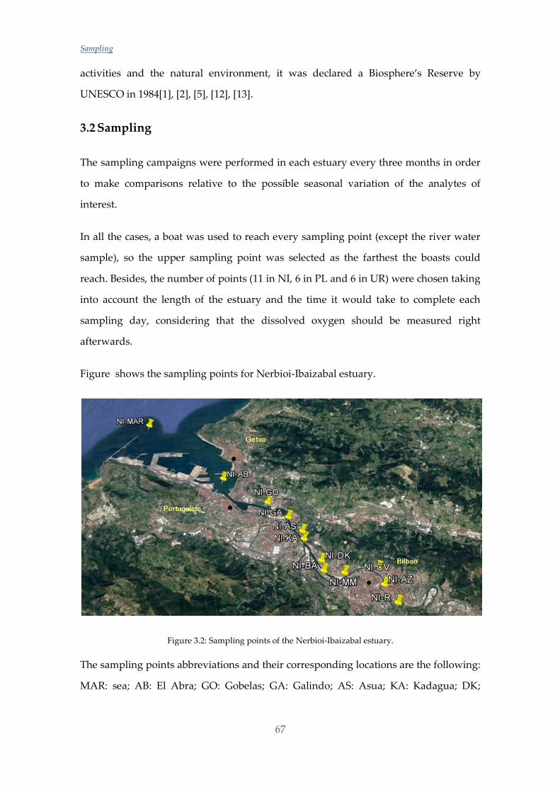
Sampling

67

activities and the natural environment, it was declared a Biosphere’s Reserve by

UNESCO in 1984[1], [2], [5], [12], [13].

3.2 Sampling

The sampling campaigns were performed in each estuary every three months in order

to make comparisons relative to the possible seasonal variation of the analytes of

interest.

In all the cases, a boat was used to reach every sampling point (except the river water

sample), so the upper sampling point was selected as the farthest the boasts could

reach. Besides, the number of points (11 in NI, 6 in PL and 6 in UR) were chosen taking

into account the length of the estuary and the time it would take to complete each

sampling day, considering that the dissolved oxygen should be measured right

afterwards.

Figure shows the sampling points for Nerbioi-Ibaizabal estuary.

Figure 3.2: Sampling points of the Nerbioi-Ibaizabal estuary.

The sampling points abbreviations and their corresponding locations are the following:

MAR: sea; AB: El Abra; GO: Gobelas; GA: Galindo; AS: Asua; KA: Kadagua; DK;

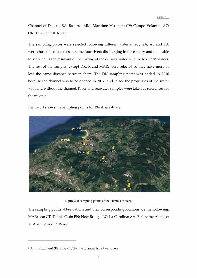
Chapter 3

68

Channel of Deusto; BA: Basurto; MM: Maritime Museum; CV: Campo Volantín; AZ:

Old Town and R: River.

The sampling places were selected following different criteria: GO, GA, AS and KA

were chosen because those are the four rivers discharging in the estuary and to be able

to see what is the resultant of the mixing of the estuary water with these rivers’ waters.

The rest of the samples, except DK, R and MAR, were selected so they have more or

less the same distance between them. The DK sampling point was added in 2016

because the channel was to be opened in 20171 and to see the properties of the water

with and without the channel. River and seawater samples were taken as references for

the mixing.

Figure 3.1 shows the sampling points for Plentzia estuary.

Figure 3.1: Sampling points of the Plentzia estuary.

The sampling points abbreviations and their corresponding locations are the following:

MAR: sea; CT: Tennis Club; PN: New Bridge; LC: La Carolina; AA: Before the Abanico;

A: Abanico and R: River.

1 At this moment (February 2018), the channel is not yet open.

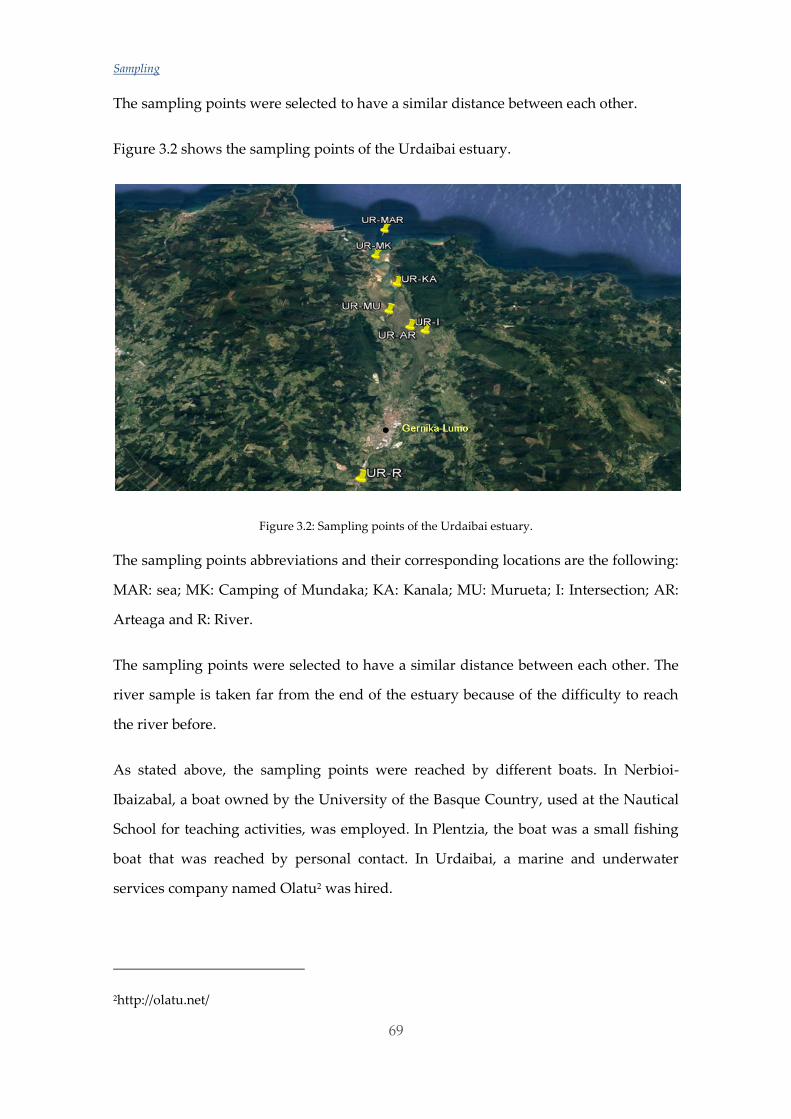
Sampling

69

The sampling points were selected to have a similar distance between each other.

Figure 3.2 shows the sampling points of the Urdaibai estuary.

Figure 3.2: Sampling points of the Urdaibai estuary.

The sampling points abbreviations and their corresponding locations are the following:

MAR: sea; MK: Camping of Mundaka; KA: Kanala; MU: Murueta; I: Intersection; AR:

Arteaga and R: River.

The sampling points were selected to have a similar distance between each other. The

river sample is taken far from the end of the estuary because of the difficulty to reach

the river before.

As stated above, the sampling points were reached by different boats. In Nerbioi-

Ibaizabal, a boat owned by the University of the Basque Country, used at the Nautical

School for teaching activities, was employed. In Plentzia, the boat was a small fishing

boat that was reached by personal contact. In Urdaibai, a marine and underwater

services company named Olatu2 was hired.

2http://olatu.net/

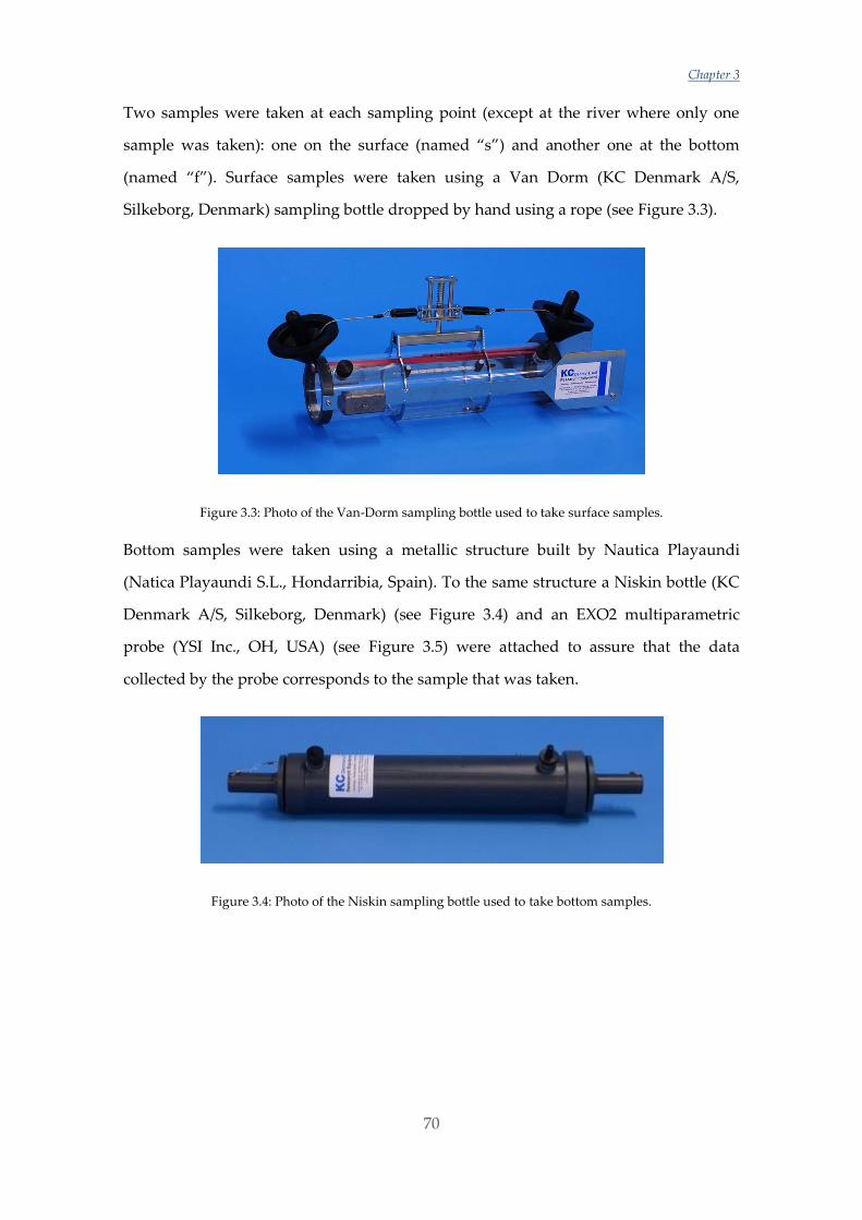
Chapter 3

70

Two samples were taken at each sampling point (except at the river where only one

sample was taken): one on the surface (named “s”) and another one at the bottom

(named “f”). Surface samples were taken using a Van Dorm (KC Denmark A/S,

Silkeborg, Denmark) sampling bottle dropped by hand using a rope (see Figure 3.3).

Figure 3.3: Photo of the Van-Dorm sampling bottle used to take surface samples.

Bottom samples were taken using a metallic structure built by Nautica Playaundi

(Natica Playaundi S.L., Hondarribia, Spain). To the same structure a Niskin bottle (KC

Denmark A/S, Silkeborg, Denmark) (see Figure 3.4) and an EXO2 multiparametric

probe (YSI Inc., OH, USA) (see Figure 3.5) were attached to assure that the data

collected by the probe corresponds to the sample that was taken.

Figure 3.4: Photo of the Niskin sampling bottle used to take bottom samples.

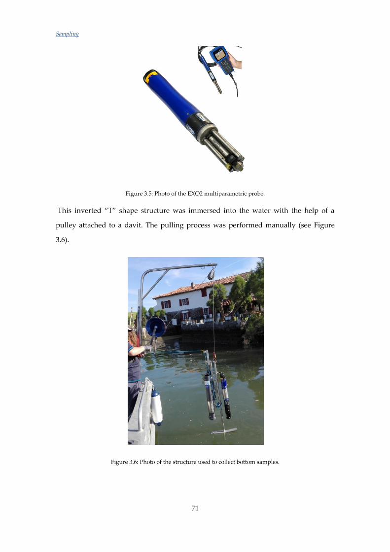
Sampling

71

Figure 3.5: Photo of the EXO2 multiparametric probe.

This inverted “T” shape structure was immersed into the water with the help of a

pulley attached to a davit. The pulling process was performed manually (see Figure

3.6).

Figure 3.6: Photo of the structure used to collect bottom samples.

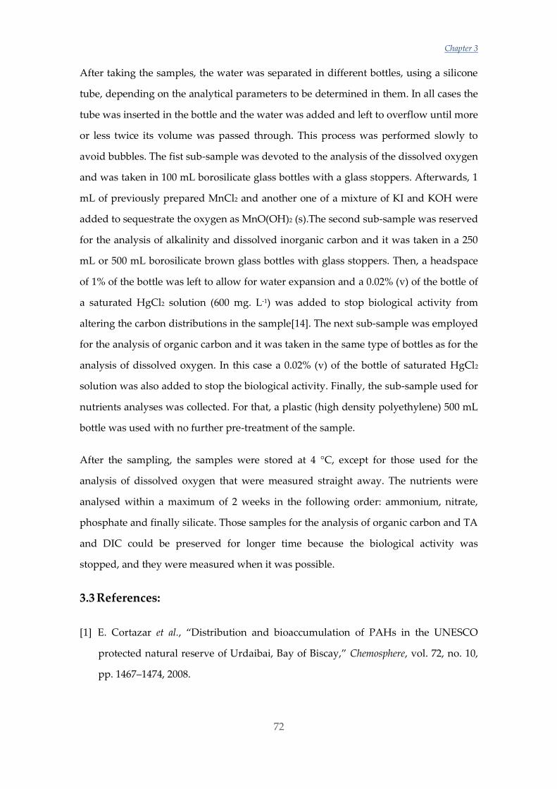
Chapter 3

72

After taking the samples, the water was separated in different bottles, using a silicone

tube, depending on the analytical parameters to be determined in them. In all cases the

tube was inserted in the bottle and the water was added and left to overflow until more

or less twice its volume was passed through. This process was performed slowly to

avoid bubbles. The fist sub-sample was devoted to the analysis of the dissolved oxygen

and was taken in 100 mL borosilicate glass bottles with a glass stoppers. Afterwards, 1

mL of previously prepared MnCl2 and another one of a mixture of KI and KOH were

added to sequestrate the oxygen as MnO(OH)2 (s).The second sub-sample was reserved

for the analysis of alkalinity and dissolved inorganic carbon and it was taken in a 250

mL or 500 mL borosilicate brown glass bottles with glass stoppers. Then, a headspace

of 1% of the bottle was left to allow for water expansion and a 0.02% (v) of the bottle of

a saturated HgCl2 solution (600 mg. L-1) was added to stop biological activity from

altering the carbon distributions in the sample[14]. The next sub-sample was employed

for the analysis of organic carbon and it was taken in the same type of bottles as for the

analysis of dissolved oxygen. In this case a 0.02% (v) of the bottle of saturated HgCl2

solution was also added to stop the biological activity. Finally, the sub-sample used for

nutrients analyses was collected. For that, a plastic (high density polyethylene) 500 mL

bottle was used with no further pre-treatment of the sample.

After the sampling, the samples were stored at 4 °C, except for those used for the

analysis of dissolved oxygen that were measured straight away. The nutrients were

analysed within a maximum of 2 weeks in the following order: ammonium, nitrate,

phosphate and finally silicate. Those samples for the analysis of organic carbon and TA

and DIC could be preserved for longer time because the biological activity was

stopped, and they were measured when it was possible.

3.3 References:

[1] E. Cortazar et al., “Distribution and bioaccumulation of PAHs in the UNESCO

protected natural reserve of Urdaibai, Bay of Biscay,” Chemosphere, vol. 72, no. 10,

pp. 1467–1474, 2008.

Sampling

73

[2] J. C. Raposo et al., “Trace metals in oysters, Crassotrea sps., from UNESCO

protected natural reserve of Urdaibai: space-time observations and source

identification,” Bull. Environ. Contam. Toxicol., vol. 83, no. 2, pp. 223–229, 2009.

[3] J. M. García-Barcina, M. Oteiza, and A. de la Sota, “Modelling the faecal coliform

concentrations in the Bilbao estuary,” in Nutrients and Eutrophication in Estuaries

and Coastal Waters, E. Orive, M. Elliott, and V. N. de Jonge, Eds. Springer

Netherlands, 2002, pp. 213–219.

[4] A. Cearreta, M. J. Irabien, E. Leorri, I. Yusta, I. W. Croudace, and A. B. Cundy,

“Recent Anthropogenic Impacts on the Bilbao Estuary, Northern Spain:

Geochemical and Microfaunal Evidence,” Estuar. Coast. Shelf Sci., vol. 50, no. 4, pp.

571–592, 2000.

[5] A. Landajo, G. Arana, A. de Diego, N. Etxebarria, O. Zuloaga, and D. Amouroux,

“Analysis of heavy metal distribution in superficial estuarine sediments (estuary of

Bilbao, Basque Country) by open-focused microwave-assisted extraction and ICP-

OES,” Chemosphere, vol. 56, no. 11, pp. 1033–1041, 2004.

[6] M. P. Cajaraville et al., “Health status of the Bilbao estuary: A review of data from a

multidisciplinary approach,” Estuar. Coast. Shelf Sci., vol. 179, pp. 124–134, 2016.

[7] S. Fdez-Ortiz de Vallejuelo, G. Arana, A. de Diego, and J. M. Madariaga, “Risk

assessment of trace elements in sediments: The case of the estuary of the Nerbioi–

Ibaizabal River (Basque Country),” J. Hazard. Mater., vol. 181, no. 1–3, pp. 565–573,

2010.

[8] A. Gredilla, J. M. Amigo Rubio, S. Fdez-Ortiz de Vallejuélo, A. de Diego, R. Bro,

and J. M. Madariaga, “Identification of contamination sources in estuarine water

by multiway data analysis: A case of study: estuary of the nerbioi-ibaizabal river,”

in 7o Colloquium Chemiometricum Mediterraneun (CCM VII 2010-Granada).

[9] A. Cearreta, M. J. Irabien, I. Ulibarri, I. Yusta, I. W. Croudace, and A. B. Cundy,

“Recent Salt Marsh Development and Natural Regeneration of Reclaimed Areas in

Chapter 3

74

the Plentzia Estuary, N. Spain,” Estuar. Coast. Shelf Sci., vol. 54, no. 5, pp. 863–886,

2002.

[10] A. Orbea, I. Marigómez, C. Fernández, J. V. Tarazona, I. Cancio, and M. P.

Cajaraville, “Structure of Peroxisomes and Activity of the Marker Enzyme Catalase

in Digestive Epithelial Cells in Relation to PAH Content of Mussels from Two

Basque Estuaries (Bay of Biscay): Seasonal and Site-Specific Variations,” Arch.

Environ. Contam. Toxicol., vol. 36, no. 2, pp. 158–166, 1999.

[11] J. A. González-Oreja and J. I. Saiz-Salinas, “Loss of Heterotrophic Biomass

Structure in an Extreme Estuarine Environment,” Estuar. Coast. Shelf Sci., vol. 48,

no. 3, pp. 391–399, 1999.

[12] E. Puy-Azurmendi et al., “Origin and distribution of polycyclic aromatic

hydrocarbon pollution in sediment and fish from the biosphere reserve of Urdaibai

(Bay of Biscay, Basque country, Spain),” Mar. Environ. Res., vol. 70, no. 2, pp. 142–

149, 2010.

[13] E. Puy-Azurmendi et al., “An integrated study of endocrine disruptors in

sediments and reproduction-related parameters in bivalve molluscs from the

Biosphere’s Reserve of Urdaibai (Bay of Biscay),” Mar. Environ. Res., vol. 69 Suppl,

pp. S63-66, 2010.

[14] A. G. Dickson, C. L. Sabine, and J. R. Christian, Guide to best practices for ocean CO2

measurements. PICES Special Publication 3, 2007.

Chapter 4

Analytical methods

Analytical methods

77

This work is focused on the determination of the parameters related to the study of

acidification. For that purpose, some other minor acid-base systems, apart from the

carbonate one, must be known in order to achieve an accurate alkalinity value (see

Introduction). Thus, phosphate and silicate concentrations should be determined. As

will happen all along this work, the salinity differences between samples make the

determinations more complicated because matrix effects must be avoided. Apart from

silicate and phosphate and, considering the differences in water quality derived from

the history and the location of the three estuaries studied here (see Sampling), it was

found interesting to measure some other nutrients, as well as the dissolved oxygen and

some of the physico-chemical parameters of the samples. Hopefully, this extra

information could help to understand the differences on the acidification parameters

and would give a hint on the quality of the water as well as the mixing of both

seawater and fresh water. The physico-chemical parameters measured were the

conductivity (and its related parameters, like salinity), temperature, pH, oxidation-

reduction potential (ORP), Optical Dissolved Oxigen (ODO), Fluorescent Dissolved

Organic Matter (fDOM) and depth. The chemical parameters measured were the

dissolved oxygen (DO), ammonium, nitrate, phosphate and silicate concentrations.

This chapter gathers all the analytical methods used to determine each one of those

parameters and will try to explain how the matrix effect was avoided or minimised.

The measurement of those parameters directly related to the acidification, TA, DIC and

pH, will be explained in the following chapters.

4.1 Physico-chemical parameters

Any change on the chemical composition of an estuary or coastal water body would

lead to a change on its physico-chemical parameters. So, monitoring the physico-

chemical parameters could give an early and fast idea about the water quality

condition[1], [2]. Therefore, at every sampling campaign, along with the sampling

bottle, a multiparametric probe was submerged to collect some information about the

physico-chemical characteristics of the sample that was taken. In this work the EXO2

probe that collects water quality data was used. This probe has up to six user-

replaceable sensors and an integral pressure transducer to detect a variety of physical,

Chapter 4

78

chemical, and biological properties of natural waters under changing environmental

conditions. The EXO2 probe used in this work had the following sensors:

(1) Depth and level: it measures the depth with a non-vented strain gauge. The

accuracy of the depth is ±0.04% in shallow waters (0-10 m), ±0.13% in medium

depth waters (10-100 m) and ±0.33% in deep waters (100-250 m).

(2) Conductivity/Temperature: The conductivity data are used to calculate salinity,

non-linear function (nLF) conductivity, specific conductance, and total

dissolved solids. It compensates for changes in the density of water (as a

function of temperature and salinity) in depth calculations if a depth sensor is

installed. The salinity is a key parameter in this work. The salinity is

determined automatically from the conductivity and temperature readings

according to algorithms found in Standard Methods for the Examination of

Water and Wastewater[3]. The use of the Practical Salinity Scale results in

values that are unitless, since the measurements are carried out in reference to

the conductivity of standard seawater at 15 °C. The accuracy of the

conductivity sensor is ± 0.5% for lower conductivities (0-100mS. cm-1) and ± 1%

for higher conductivities (100-200mS. cm-1). In the case of the temperature

sensor, the accuracy is ± 0.01 °C from -5 °C to +35 °C, and ±0.05 °C from +35 °C

to +50 °C.

(3) pH and oxidation reduction potential (ORP): The pH sensor is a glass

combination electrode while for the ORP a platinum button is used. The

accuracy of pH is ±0.1 pH units within 10 °C of calibration temperature and

±0.2 pH units for the rest of temperatures. For the ORP sensor, the accuracy is

±20 mV in redox standard solution.

(4) Dissolved oxygen (DO): The principle of operation is based on the concept that

DO quenches the intensity and the lifetime of the luminescence associated with

a carefully chosen chemical dye. The accuracy of the measurement is ±1% of the

reading for concentrations ranging from 0 to 20 mg. L-1, and ± 1% between 20

and 50 mg. L-1. The probe gives the dissolved oxygen as in oxygen saturation or

concentration (mg. L-1).

Analytical methods

79

(5) Fluorescent Dissolved Organic Matter (fDOM): It detects the fluorescent

component of DOM when it is exposed to near-ultraviolet (UV) light. For its

calibration, quinine sulphate is used as a surrogate because in acid solution,

fluoresces similarly to DOM. The units of fDOM are quinine sulphate units

(QSUs) where 1 QSU = 1 µg. L-1 quinine sulphate. The measuring range is 0-300

µg. L-1 QSU and its LOD is 0.07µg. L-1 QSU.

This probe has the advantage of being able to collect and save data with a determined

frequency which can be used to make a profile of each of the parameters of the water

column. This is very useful when measuring estuarine waters because it allows seeing

the mixture of fresh water and seawater. The recording frequency of data collection

during this work was 4 Hz and the trigger was a change in the conductivity. Thus,

when the probe detected a change of conductivity due to its immersion in the water, it

would start collecting the data.

The EXO sensors (except temperature) require periodic calibration to assure high

performance.

(1) Depth and level: this parameter must be calibrated just before its use and the

sensor must be in air and not immersed in any solution.

(2) Conductivity: The conductivity was calibrated at 12.88 mS. cm-1 (at 25 °C) with

a standard solution supplied by Crison (Crison Instruments S.A., Barcelona,

Spain).

(3) pH: A three-point calibration was performed. pH 4.01, 7.00 and 10.00 (at 25 °C)

buffer solutions (Hamilton Bonaduz AG., Bonaduz, Switzerland) were used.

ORP: A 475 mV (at 25 °C) buffer solution (Hamilton Bonaduz AG., Bonaduz,

Switzerland) was used to perform a one-point calibration.

(4) DO: A one-point DO % saturation calibration was performed. For that, in

the calibration cup containing around 3 mm of water, the probe was placed,

and the temperature and oxygen pressure were allowed to equilibrate for 15

minutes before proceeding to calibrate it.

Chapter 4

80

(5) fDOM: It was calibrated using sulphate quinine in an 0.05 mol. L-1 sulphuric

acid solution. A two-point calibration was performed: the blank (0.05 mol. L-1

sulphuric acid) and 300 µg. L-1 quinine sulphate (in 0.05 mol. L-1 sulphuric acid)

supplied by Merck (Merck kGaA, Darmstadt, Germany).

4.2 Dissolved oxygen determination

4.2.1 Introduction

Dissolved oxygen (DO) refers to the level of free, non-bounded oxygen present in

water or other liquids. Aquatic living organisms need sufficient levels of DO in water

to survive. Fish and invertebrates take the oxygen for respiration through their gills,

while plants and phytoplankton need DO when there is no light for photosynthesis [4],

[5]. The amount of DO in an estuary’s water will determine the type and abundance of

organisms that can live there.

Dissolved oxygen enters water through the air (air diffusion or mixing quickly through

aeration) or as a plant waste product of photosynthesis from phytoplankton, algae,

seaweed and other aquatic plants [3], [4].

Thus, DO concentrations are affected by diffusion and aeration, photosynthesis,

respiration and decomposition. But DO levels also change with temperature, salinity

and pressure. The highest the salinity and the temperature, the lowest is the oxygen

solubility[5]. Therefore, in an estuary important seasonally variations can be found,

with lower levels in summer and higher levels in winter. The weather can also be a

factor in the DO concentration variation. During dry seasons, water levels decrease and

as the flow rate of rivers slow down, it mix less with the air and thus, DO concentration

decreases. The opposite would happen during rainy seasons.

Estuary stratification based on salinity distributions can be horizontal, with DO levels

decreasing from inland to open ocean, or vertical, with the fresh and oxygenated water

flowing over the lower oxygenated seawater (See Chapter 1 Section 1.2). If an estuary

presents stratification, higher DO lever are on the surface than on the bottom[6].

Analytical methods

81

In summary, DO levels are indicators of estuaries’ health and environment conditions,

and, therefore, DO is one of the most important substances to monitor it.

Several techniques and methods have been used for the analysis of the dissolved

oxygen concentration, i.e. the Winkler or iodometric method and its modifications, the

electrometric method using membrane electrodes[3], [7], or now also the optical sensor

method (based on luminescence quenching) [8], [9].The choice of procedure depends

mostly on the interferences present in the samples and the accuracy desired.

Membrane electrodes have been used for DO measurements in lakes and reservoirs, for

stream survey and control of industrial effluents, for continuous monitoring of DO,

and for estuarine and oceanographic studies. Membrane electrodes are completely

submersible which makes them suitable for analysis in situ and their portability, ease

of operation and maintenance make them particularly convenient for field

applications. These electrodes are recommended for use especially under conditions

that are unfavourable for the use of the iodometric method, or when that test and its

modifications are subject to serious errors caused by interferences[3], [6],

[10].Electrochemical sensor technology is quickly being replaced by optical technology,

which allows the user to acquire stable and accurate results and also significantly

reduce maintenance costs whilst it can be used for the same situations. The

disadvantages of the optical sensors are their higher price and the longest stabilisation

time that they need.

The iodometric test is the most precise and reliable titrimetric procedure for DO

analysis. It is known as the Winkler method and it was proposed by Winkler [11]. Since

its publication in 1888 the method has suffered several modifications. In fact, the

Winkler method used nowadays is actually a modification presented by Carpenter in

1965 [12]. Due to discrepancies during oceanographic expeditions, Carpenter evaluated

the accuracy of the Winkler method by dissolving known quantities of oxygen in

oxygen-free water. Carpenter considered the following to be the sources of the

analytical errors when the Winkler method was used: air oxidation of iodine,

volatilization of iodine, oxygen contribution by the reagent solutions, iodate

contamination of the iodide solutions, consumption or production of iodine by

Chapter 4

82

contamination of the reagents and a difference between titration end point and

equivalence end point. He concluded that all were negligible except for the oxygen

contribution by the reagent solutions. The modification presented by Carpenter

resulted in a simpler and faster method with a reduction in the errors due to

manipulation. The iodine loss by volatilization was eliminated by optimizing the

concentrations of the reagents and by using the whole bottle for the titration instead of

transferring a smaller aliquot to another vessel for the titration [12], [13].

In the Winkler iodometric determination divalent manganese, added to the sample and

precipitated by an alkaline-iodide reagent, is oxidized by dissolved molecular oxygen.

Under subsequent acidification, the manganese oxidizes iodide into iodine. Iodine is

usually titrated by thiosulphate but can also be measured by spectrophotometry[14],

[15].

In this work the Carpenter modification of the Winkler method, as described below,

was used.

4.2.2 Materials and methods

4.2.2.1 Reagents and materials

All solutions were prepared using ultrapure water obtained from a MilliQ Element

A10 water purification system (Millipore Co., MA, USA). All analytical grade reagents

were supplied by Merck (Merck kGaA, Darmstadt, Germany) unless specified

otherwise.

The following solutions were prepared: MgCl2.4H2O was prepared by dissolving 60 g

in 100 mL water. Alkaline iodide was prepared by dissolving 60g KI and 30g KOH and

making that up to 100 mL. A starch solution was prepared by dissolving 1 g of soluble

starch in 100 mL of water at 100°C. A 1:1 solution of H2SO4 was also prepared. Finally,

a 0.02 mol. L-1 solution of Na2S2O3.5H2O and a 1.667 mmol. L-1 solution of KIO3 were

prepared.

4.2.2.2 Procedure

In the iodometric titration, the sampling process is crucial. DO is a very changeable

parameter and samples must be taken very carefully. Samples must not be in contact

Analytical methods

83

with air for a long time or be agitated, because either condition causes a change in its

gaseous content. Thus, when a sampling bottle is taken, the bottle for the DO analysis

must be the first one to collect.

The bottles used for the DO determination are 100 mL glass-stoppered. The empty

bottles have to be weighted clean, dry and marked and vacuum grease must be spread

on the stopper to avoid oxygen exchange.

The oxygen has to be fixed in situ using the MgCl2.4H2O and the alkaline iodide. 1 mL

of each reagent has to be added to the bottle right after this one is filled. A brown

precipitate appears which correspond to the MnO(OH)2(s). The bottle is closed then

and shaken to spread the reagents all over the sample. Samples might be stored for a

few hours without change in the DO contents after adding the reagents.

Reagent blank

During the evaluation of the Winkler method made by Carpenter [12] he concluded

that the oxygen contribution by the reagent solutions was an important source of error.

Thus, he proposed a blank of the reagents to consider their contribution in the

calculation of the DO concentration.

1 mL of the standard potassium iodate is added into a flask and a stir bar. Then, 1 mL

of MgCl2.4H2O, 1 mL of the alkaline iodide and 1mL of the sulphuric acid are added

mixing thoroughly after each addition. Finally 1 mL of the starch indicator solution is

added. After mixing all of it, the sides of the flask are rinsed with deionised water and

filled until 100 mL. The titration must start immediately to avoid the air oxidation of

iodine or its volatilization. For the titration, a Dosimat 665 (Metrohm, Herisau,

Switzerland) were used with a 20 mL cylinder. Small amounts of the titrant are added

while stirring, until the purple colour of the solution is completely gone. Then, a

second 1 mL of the standard is added to the same solution which is again titrated to the

end point. The difference in volume between both end points is the potassium iodate

blank that should be considered in the equation for the DO determination. The reagent

blank calculation is repeated two more times.

Standardization of thiosulphate

Chapter 4

84

The thiosulphate is not a primary standard and, therefore, it must be standardized

with one, usually KIO3. 10 mL of the standard potassium iodate are added into a flask

and a stir bar. Then, 1 mL of MgCl2.4H2O, 1 mL of the alkaline iodide and 1mL of

H2SO4are added mixing thoroughly after each addition. Finally 1 mL of the starch

solution is added. After mixing all of it, the sides of the flask are rinsed with deionised

water and filled until 100 mL. The titration is immediately started as when the blank

reagent determination is performed. The standardisation is then repeated two more

times. These are the reactions of the titration:

IO3- + 8I- + 6H+ 3I3- + 3 H2O

I3- + 2S2O3-23I- + S4O6-2

As can be seen, each mol of iodate is titrated by 6 mol of tiosulphate.

Sample analysis

After the sampling the outer surface of the bottles is cleaned and carefully dried and

then the bottles are weighted. The difference of the full bottle and empty bottle will

correspond to the amount of sample in the bottle. After that, the neck is carefully

removed, taking care to minimize disturbance of the precipitate. The temperature of

the liquid sample is measured to calculate the density afterward. Around 15 mL (when

possible) of the liquid part of the sample are removed very carefully avoiding taking

the precipitate. Then, a stir bar, 1 mL of sulphuric acid and 1 mL of the starch solution

are added and the titration is immediately started as stated above. These are the

reactions that take place in the DO determination:

Mn+2 + 2OH- Mn(OH)2 (s)

2 Mn(OH)2 (s) + ½ O2 + H2O 2 MnO(OH)2(s)

2 MnO(OH)2(s) + 3I- + 4H+ 2Mn+2 + I2 + 3H2O

I2 + I- I3-

I3- + 2S2O32- 3I- + S4O62-

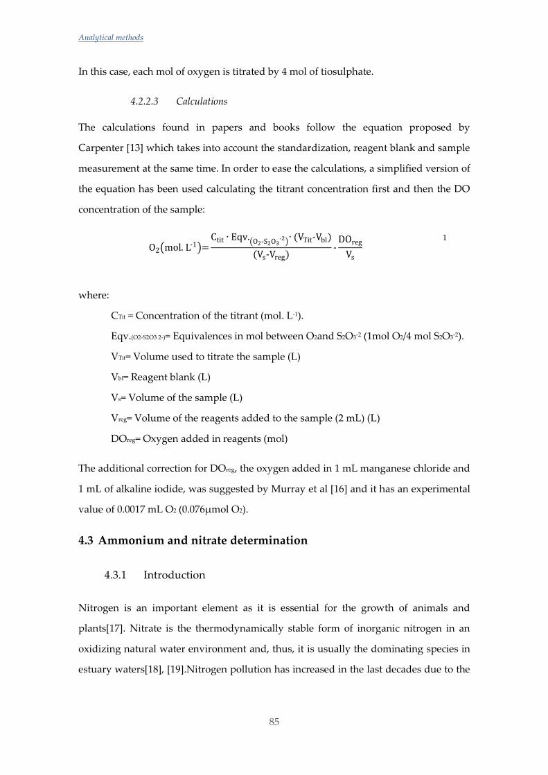
Analytical methods

85

In this case, each mol of oxygen is titrated by 4 mol of tiosulphate.

4.2.2.3 Calculations

The calculations found in papers and books follow the equation proposed by

Carpenter [13] which takes into account the standardization, reagent blank and sample

measurement at the same time. In order to ease the calculations, a simplified version of

the equation has been used calculating the titrant concentration first and then the DO

concentration of the sample:

O2(mol. L-1)=Ctit ∙ Eqv.

(O2-S2O3-2)

∙ (VTit-Vbl)

(Vs-Vreg)-

DOreg

Vs

1

where:

CTit = Concentration of the titrant (mol. L-1).

Eqv.(O2-S2O3 2-)= Equivalences in mol between O2and S2O3-2 (1mol O2/4 mol S2O3-2).

VTit= Volume used to titrate the sample (L)

Vbl= Reagent blank (L)

Vs= Volume of the sample (L)

Vreg= Volume of the reagents added to the sample (2 mL) (L)

DOreg= Oxygen added in reagents (mol)

The additional correction for DOreg, the oxygen added in 1 mL manganese chloride and

1 mL of alkaline iodide, was suggested by Murray et al [16] and it has an experimental

value of 0.0017 mL O2 (0.076µmol O2).

4.3 Ammonium and nitrate determination

4.3.1 Introduction

Nitrogen is an important element as it is essential for the growth of animals and

plants[17]. Nitrate is the thermodynamically stable form of inorganic nitrogen in an

oxidizing natural water environment and, thus, it is usually the dominating species in

estuary waters[18], [19].Nitrogen pollution has increased in the last decades due to the

Chapter 4

86

increased use of N-rich fertilizers. Because of these, N pollution is one of the biggest

consequences of human activity on the coastal oceans of the world[20].

An excess of nitrate is one of the causes of eutrophication which have important

ecological consequences, such as increased algal blooms, the formation of hypoxia (low

contents of oxygen) or even anoxia (lack of oxygen) in the bottom waters and changes

in the phytoplankton species composition[21].Eutrophication happens when the input

of excess nutrients into a water body stimulates excessive growth (algal bloom), which

then reduces the dissolved oxygen in the water when the organic material decomposes

[22].But even if reduced nitrogen, such as, ammonia, ammonium and amines, is the

least known part of the nitrogen cycle, it has a crucial role in ecology and in the

environment. Emissions of ammonia to the atmosphere, for instance, can contribute to

particulate matter formation affecting human health, and also to the eutrophication

and acidification of aquatic environments (in the form of ammonium)[17]. Besides the

contribution of atmospheric emissions, plants and animals excrete ammonia; it is

produced by the decomposition of organisms and by the activity of micro

organisms[23]. Ammonia exists in natural waters as both ionized ammonium, NH4+,

and dissolved ammonia, NH3, and the proportion of ammonia depends on the

temperature, pH and ionic strength [24], [25]. NH3 contributes about 10% to the total

seawater ammonium concentration at a pH of 8.2 and temperature of 25 °C[26].

Ocean acidification has an important impact not only in the change of the pH of the

water and equilibrium reactions, but it can also impact biological processes and change

nutrient cycles. In the case of nitrogen, an increase in the partial pressure of CO2 could

enhance nitrogen fixation and reduce marine nitrification[27].

In ocean waters the concentration of other bases is quite low compared to the dissolved

inorganic carbon amount, and ammonium is usually considered negligible. However,

in anoxic conditions, ammonium can have a considerable contribution to TA [28], [29].

Thus, taking into account that it might contribute to TA and the toxicity of the

component, ammonium is an important parameter to be measured.

Analytical methods

87

Different techniques have been used for the determination of both ammonium and

ammonia in seawater. Several authors have used the indophenol blue method with

spectrophotometric [30], [31] or fluorescence detection [32]. Šraj et al. [33]published a

review work summarizing the advantages of the different methods published about

the use of flow based methodologies for ammonia determination in estuary waters and

seawater.

In the case of nitrate analysis, the most common technique is spectrophotometry, used

generally in flow injection analysis (FIA) systems, where nitrite is measured and then,

nitrate is converted to nitrite and measured again. The difference between both values

would be the nitrate content. The reduced nitrate plus the nitrite originally present in

the sample react with the Griess reagent (sulfanilamide and N-1-

naphthylethylenediamine dihydrochloride) under acidic conditions. The resulting pink

azo dye can be detected at 540 nm [34].Recent studies have focused on the nitrate

reduction approaches using copper-coated cadmium columns[35] or zinc columns[36],

among others.

Ma et al. [37] discussed the different techniques for the determination of nutrients at

nanomolar levels, including both ammonium and nitrate.

Ion-selective electrode (ISE) potentiometry has also been used for both ammonium (as

NH4+ or NH3) [38], [39]and nitrate [40]–[42]determinations [43].Even if its sensitivity is

not as good as the techniques and methods mentioned before, its ease of use, speed

and simplicity make this technique a very good option when the measurement of low

levels is not necessary. It is also suitable for monitoring studies [44]. In fact, this is the

technique selected in this work to measure ammonium and nitrate in estuarine waters.

The eternal problem of dealing with estuary waters is the matrix differences between

the samples. Thus, every time the ionic strength of the samples affects the

measurements, certain measures must be taken in order to avoid the matrix effect. ISE

determinations are commonly based on a previous calibration using a standard

solution. In this case, the ionic strength of the sample would affect the liquid junction

potential of the reference electrode and, therefore, the accuracy of the results will not

be acceptable (see Chapter 7 Section 7.1.2). The best solution for this problem is the use

Chapter 4

88

of the Standard Addition Method (SAM) in which known amounts of the standard

solution are added straight to the sample and the matrix effect is normally avoided

[39], [45]. The SAM has been widely used before with different techniques to avoid

matrix effects [46], [47].

The method used in this work was validated in terms of linearity, limits of detection

and quantification, precision and robustness.

4.3.2 Materials and methods

4.3.2.1 Reagents and materials

All solutions were prepared using ultrapure water obtained from a Millipore water

purification system (Millipore Co., MA, USA).

All analytical grade reagents were supplied by Merck (Merck kGaA, Darmstadt,

Germany).

For ammonium analysis two standard solutions were prepared (50 mg. L-1 and

7000 mg. L-1) by dissolving the exact amount of NH4Cl in 50 mL flasks.

For nitrate analysis two standard solutions were prepared (7000 mg. L-1 and 25000 mg.

L-1) by dissolving the exact amount of NaNO3 in 50 mL flasks.

In both cases an Ag(s)/AgCl(s) reference electrode (Metrohm AG, Herisau,

Switzerland) was used coupled to a 692 pH/Ion Meter potentiometer (Metrohm AG,

Herisau, Switzerland) with a precision of 0.1 mV. The measuring electrodes were a

NH4 selective electrode (Crison, Hach Lange Spain S.L.U., Barcelona, Spain) and a NO3-

selective electrode (Thermo Orion, Thermo Fisher Scientific, MA, USA).

4.3.2.2 Procedure

Ammonium and nitrate determinations were carried out by ion selective electrode

(ISE) potentiometry. To avoid matrix effects due to salinity differences a standard

addition method (SAM) was used using two different standards for the wide

concentration range. The analyses were performed at a constant stirring and constant

temperature of 25 °C using a Lauda MT thermostat (Lauda ULTRACOOL S.L.,

Analytical methods

89

Barcelona, Spain). 20 mL of the sample were added into a jacketed vessel using a

Metrohm 700 Dossino automatic burette controlled by a 711 Liquino liquid handling

system, both from Metrohm AG (Herisau, Switzerland). Additions of the smallest

amounts of the standards, made with the help of Eppendorf micropipettes (Eppendorf

AG, Hamburg, Germany), were always made to avoid big changes in the total volume.

4.3.2.3 Calculations

The calculations are based on the Nernst equation.

E = E0 + ln 10 ∙R. T

n. F× log a

2

where:

E= Measured potential (V or J. C-1)

Eº= Reference potential (V or J. C-1) which is characteristic of the particular

ISE/reference pair.

R= Ideal gas constant (8.314 J. K-1 mol-1)

T= Temperature (K)

n = number of mols of electrons

F= Faraday constant (96485 C. mol-1)

a = Activity of the measuring ion (mol. L-1)

If the ionic strength is fairly constant, the Nernst equation may be rewritten to describe

the electrode response to the concentration, C, of the measured ion species. The

expression ln 10R.T

n.F for an ion with n=1 in standard condition (298K) could be replaced

for k= 59.16 mV. The equation can be arranged to give:

C = 10E−E0

k =10

E

k

10E0

k

3

The analyte ion concentration after any addition of the standard is given by:

C =(C0 ∙ V0) + (Cstd ∙ Vstd)

(V0 + Vstd)

4

where:

C0= The analyte concentration before any standard is added (mg. L-1)

V0= The volume of the sample before any standard is added (0.020 L)

Cstd= The concentration of the standard (mg. L-1)

Vstd= The volume of the standard solution that is added (L)

The combination of equations 3 and 4 gives:

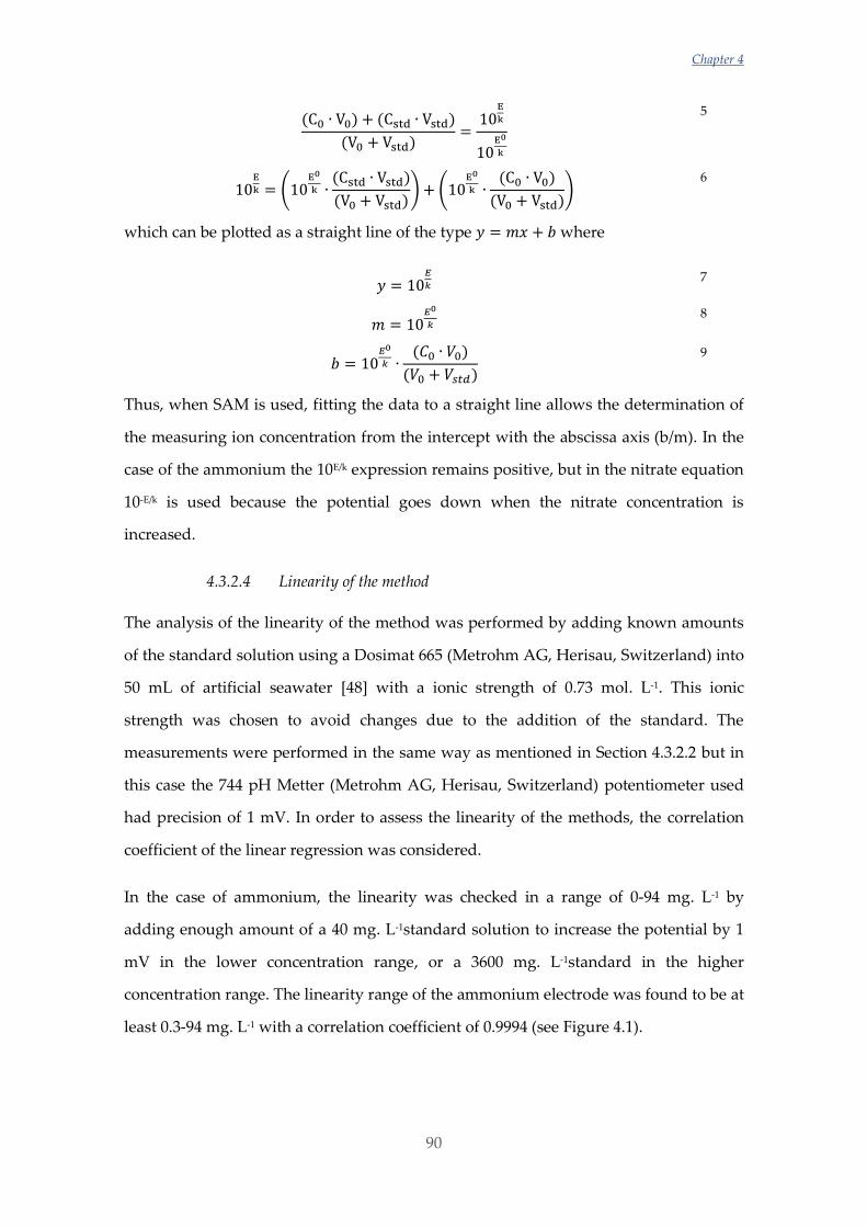
Chapter 4

90

(C0 ∙ V0) + (Cstd ∙ Vstd)

(V0 + Vstd)=

10E

k

10E0

k

5

10E

k = (10E0

k ∙(Cstd ∙ Vstd)

(V0 + Vstd)) + (10

E0

k ∙(C0 ∙ V0)

(V0 + Vstd))

6

which can be plotted as a straight line of the type 𝑦 = 𝑚𝑥 + 𝑏 where

𝑦 = 10𝐸

𝑘 7

𝑚 = 10𝐸0

𝑘 8

𝑏 = 10𝐸0

𝑘 ∙(𝐶0 ∙ 𝑉0)

(𝑉0 + 𝑉𝑠𝑡𝑑)

9

Thus, when SAM is used, fitting the data to a straight line allows the determination of

the measuring ion concentration from the intercept with the abscissa axis (b/m). In the

case of the ammonium the 10E/k expression remains positive, but in the nitrate equation

10-E/k is used because the potential goes down when the nitrate concentration is

increased.

4.3.2.4 Linearity of the method

The analysis of the linearity of the method was performed by adding known amounts

of the standard solution using a Dosimat 665 (Metrohm AG, Herisau, Switzerland) into

50 mL of artificial seawater [48] with a ionic strength of 0.73 mol. L-1. This ionic

strength was chosen to avoid changes due to the addition of the standard. The

measurements were performed in the same way as mentioned in Section 4.3.2.2 but in

this case the 744 pH Metter (Metrohm AG, Herisau, Switzerland) potentiometer used

had precision of 1 mV. In order to assess the linearity of the methods, the correlation

coefficient of the linear regression was considered.

In the case of ammonium, the linearity was checked in a range of 0-94 mg. L-1 by

adding enough amount of a 40 mg. L-1standard solution to increase the potential by 1

mV in the lower concentration range, or a 3600 mg. L-1standard in the higher

concentration range. The linearity range of the ammonium electrode was found to be at

least 0.3-94 mg. L-1 with a correlation coefficient of 0.9994 (see Figure 4.1).

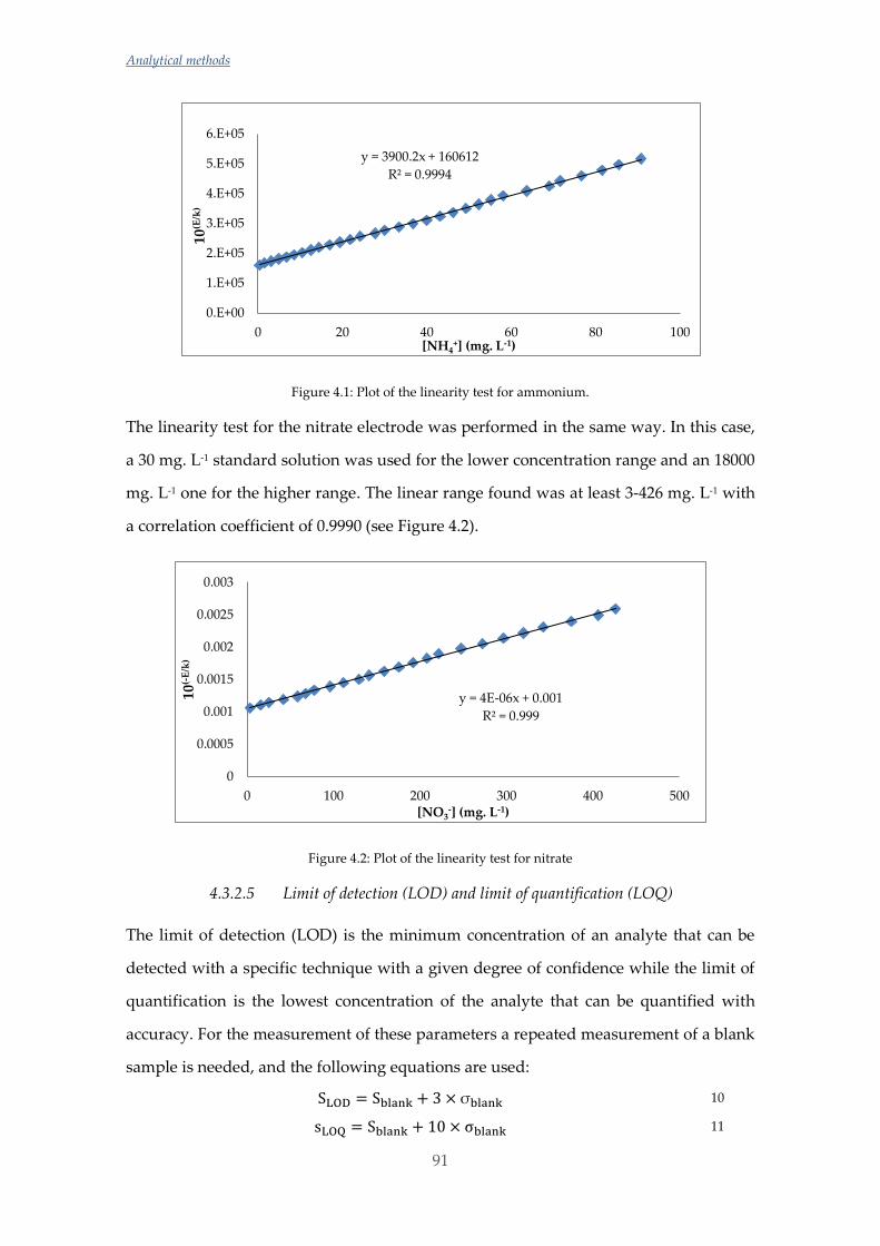
Analytical methods

91

Figure 4.1: Plot of the linearity test for ammonium.

The linearity test for the nitrate electrode was performed in the same way. In this case,

a 30 mg. L-1 standard solution was used for the lower concentration range and an 18000

mg. L-1 one for the higher range. The linear range found was at least 3-426 mg. L-1 with

a correlation coefficient of 0.9990 (see Figure 4.2).

Figure 4.2: Plot of the linearity test for nitrate

4.3.2.5 Limit of detection (LOD) and limit of quantification (LOQ)

The limit of detection (LOD) is the minimum concentration of an analyte that can be

detected with a specific technique with a given degree of confidence while the limit of

quantification is the lowest concentration of the analyte that can be quantified with

accuracy. For the measurement of these parameters a repeated measurement of a blank

sample is needed, and the following equations are used:

SLOD = Sblank + 3 × σblank 10

sLOQ = Sblank + 10 × σblank 11

y = 3900.2x + 160612

R² = 0.9994

0.E+00

1.E+05

2.E+05

3.E+05

4.E+05

5.E+05

6.E+05

0 20 40 60 80 100

10(E

/k)

[NH4+] (mg. L-1)

y = 4E-06x + 0.001

R² = 0.999

0

0.0005

0.001

0.0015

0.002

0.0025

0.003

0 100 200 300 400 500

10(-

E/k

)

[NO3-] (mg. L-1)

Chapter 4

92

where Sblank is the average value of the signal of the blank and σblank is its standard

deviation. To determine the concentrations the slope and the y-axis intercept are used.

In this case, as the SAM is used, there is no blank because the sample (containing the

analyte) is used during the whole procedure and, therefore, the minimum

concentration of NH4+or NO3-needed to increase 1 mV of the potential was considered

as both LOD and LOQ. Thus, it was 0.3 mg. L-1 for ammonium and 3 mg. L-1 for nitrate.

4.3.2.6 Uncertainty of the results

The uncertainty of the concentration of ammonium and nitrate was determined as the

square root of the sum of the intrinsic variance, and the variances with respect to the

repeatability and the reproducibility. Equation 12 is used to calculate the uncertainty of

a linear regression model[45].

SxE =sy/x

b√

1

n+

< 𝑦 >2

b2 ∑(xi−< 𝑥 >)2

12

where:

sy/x= Standard deviation of y-residuals

b= Slope of the regression line

n= Number of points taken into account for the regression

<y>= Mean of the y values

xi= Value of x at each point of the regression calibration curve

<x>= Mean of the x values

To analyse the repeatability and reproducibility, a sample was measured 10 times in a

row in three consecutive days.

For the intrinsic variance, repeatability and reproducibility, the higher uncertainties

were used in order for it to be the worst case scenario.

Figure shows the values of ammonium concentrations and its uncertainties calculated

as the square root of the sum of the intrinsic variance and the variance due to the

repeatability (using the highest values).

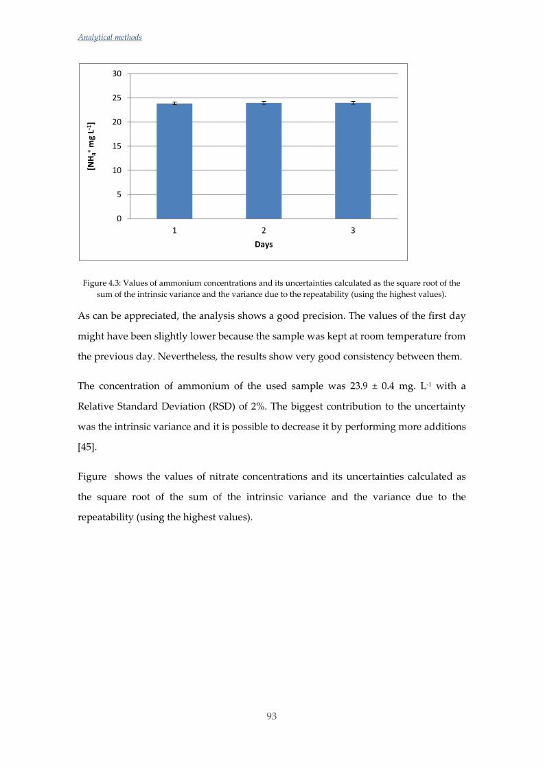
Analytical methods

93

Figure 4.3: Values of ammonium concentrations and its uncertainties calculated as the square root of the

sum of the intrinsic variance and the variance due to the repeatability (using the highest values).

As can be appreciated, the analysis shows a good precision. The values of the first day

might have been slightly lower because the sample was kept at room temperature from

the previous day. Nevertheless, the results show very good consistency between them.

The concentration of ammonium of the used sample was 23.9 ± 0.4 mg. L-1 with a

Relative Standard Deviation (RSD) of 2%. The biggest contribution to the uncertainty

was the intrinsic variance and it is possible to decrease it by performing more additions

[45].

Figure shows the values of nitrate concentrations and its uncertainties calculated as

the square root of the sum of the intrinsic variance and the variance due to the

repeatability (using the highest values).

0

5

10

15

20

25

30

1 2 3

[NH

4+m

g L-1

]

Days

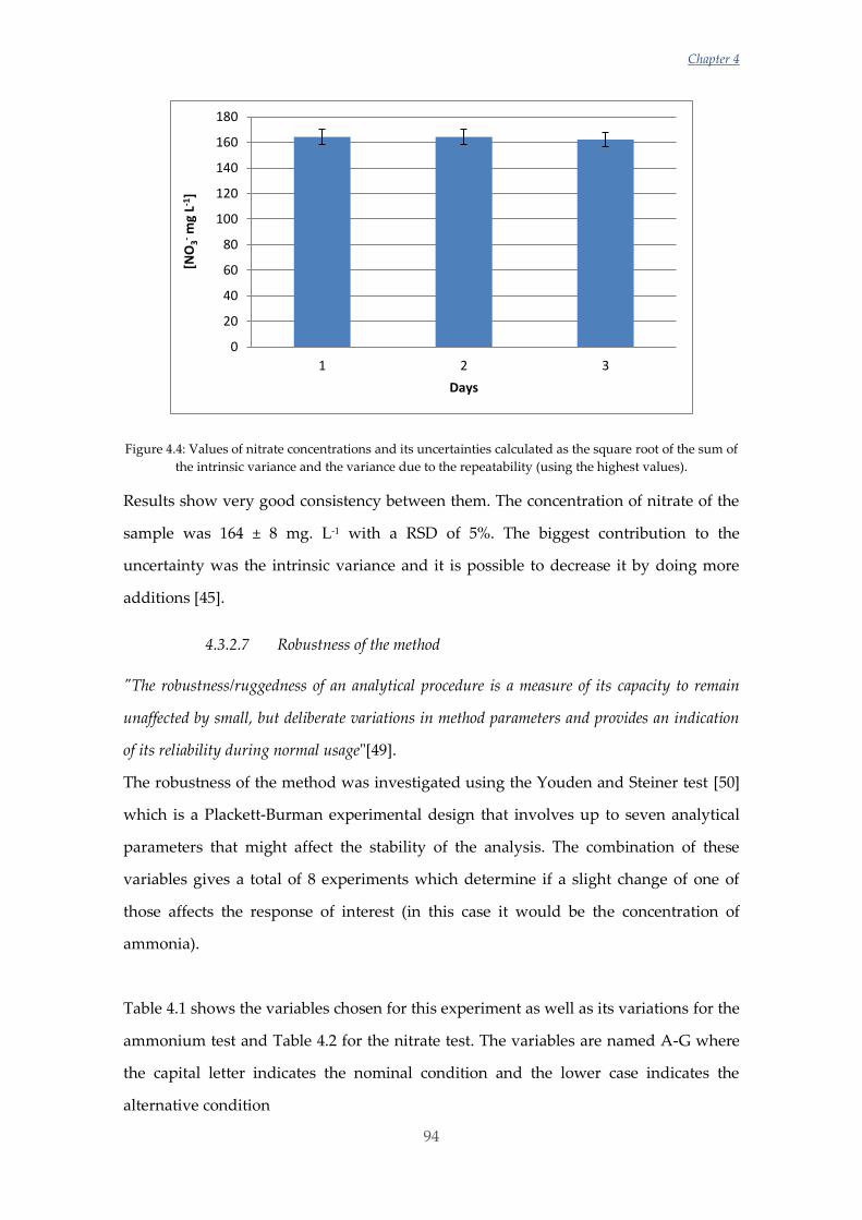
Chapter 4

94

Figure 4.4: Values of nitrate concentrations and its uncertainties calculated as the square root of the sum of

the intrinsic variance and the variance due to the repeatability (using the highest values).

Results show very good consistency between them. The concentration of nitrate of the

sample was 164 ± 8 mg. L-1 with a RSD of 5%. The biggest contribution to the

uncertainty was the intrinsic variance and it is possible to decrease it by doing more

additions [45].

4.3.2.7 Robustness of the method

"The robustness/ruggedness of an analytical procedure is a measure of its capacity to remain

unaffected by small, but deliberate variations in method parameters and provides an indication

of its reliability during normal usage"[49].

The robustness of the method was investigated using the Youden and Steiner test [50]

which is a Plackett-Burman experimental design that involves up to seven analytical

parameters that might affect the stability of the analysis. The combination of these

variables gives a total of 8 experiments which determine if a slight change of one of

those affects the response of interest (in this case it would be the concentration of

ammonia).

Table 4.1 shows the variables chosen for this experiment as well as its variations for the

ammonium test and Table 4.2 for the nitrate test. The variables are named A-G where

the capital letter indicates the nominal condition and the lower case indicates the

alternative condition

0

20

40

60

80

100

120

140

160

180

1 2 3

[NO

3-m

g L-1

]

Days

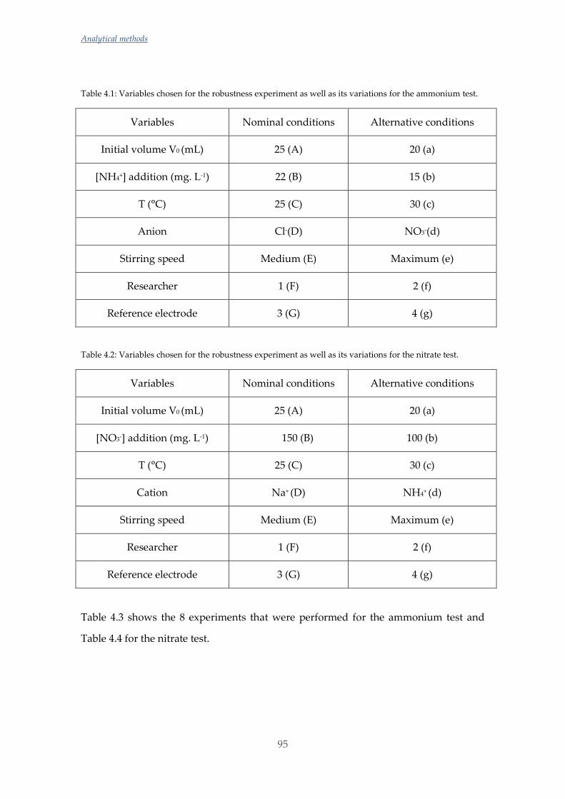
Analytical methods

95

Table 4.1: Variables chosen for the robustness experiment as well as its variations for the ammonium test.

Variables Nominal conditions Alternative conditions

Initial volume V0 (mL) 25 (A) 20 (a)

[NH4+] addition (mg. L-1) 22 (B) 15 (b)

T (ᵒC) 25 (C) 30 (c)

Anion Cl-(D) NO3-(d)

Stirring speed Medium (E) Maximum (e)

Researcher 1 (F) 2 (f)

Reference electrode 3 (G) 4 (g)

Table 4.2: Variables chosen for the robustness experiment as well as its variations for the nitrate test.

Variables Nominal conditions Alternative conditions

Initial volume V0 (mL) 25 (A) 20 (a)

[NO3-] addition (mg. L-1) 150 (B) 100 (b)

T (ᵒC) 25 (C) 30 (c)

Cation Na+ (D) NH4+ (d)

Stirring speed Medium (E) Maximum (e)

Researcher 1 (F) 2 (f)

Reference electrode 3 (G) 4 (g)

Table 4.3 shows the 8 experiments that were performed for the ammonium test and

Table 4.4 for the nitrate test.

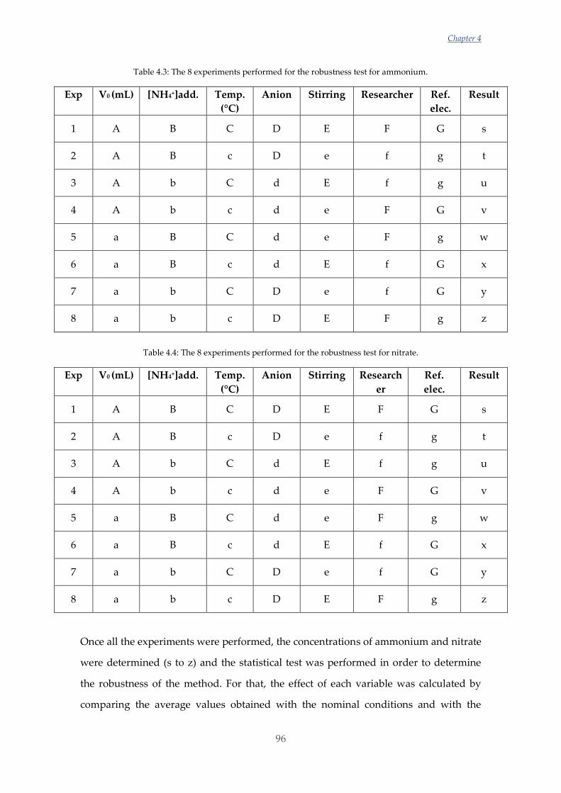
Chapter 4

96

Table 4.3: The 8 experiments performed for the robustness test for ammonium.

Exp V0 (mL) [NH4+]add. Temp.

(°C)

Anion Stirring Researcher Ref.

elec.

Result

1 A B C D E F G s

2 A B c D e f g t

3 A b C d E f g u

4 A b c d e F G v

5 a B C d e F g w

6 a B c d E f G x

7 a b C D e f G y

8 a b c D E F g z

Table 4.4: The 8 experiments performed for the robustness test for nitrate.

Exp V0 (mL) [NH4+]add. Temp.

(°C)

Anion Stirring Research

er

Ref.

elec.

Result

1 A B C D E F G s

2 A B c D e f g t

3 A b C d E f g u

4 A b c d e F G v

5 a B C d e F g w

6 a B c d E f G x

7 a b C D e f G y

8 a b c D E F g z

Once all the experiments were performed, the concentrations of ammonium and nitrate

were determined (s to z) and the statistical test was performed in order to determine

the robustness of the method. For that, the effect of each variable was calculated by

comparing the average values obtained with the nominal conditions and with the

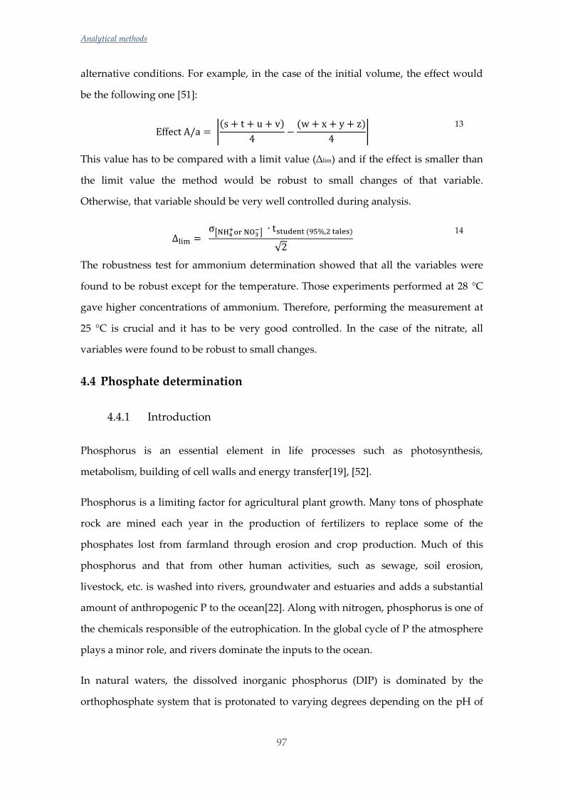
Analytical methods

97

alternative conditions. For example, in the case of the initial volume, the effect would

be the following one [51]:

Effect A/a = |(s + t + u + v)

4−

(w + x + y + z)

4|

13

This value has to be compared with a limit value (∆lim) and if the effect is smaller than

the limit value the method would be robust to small changes of that variable.

Otherwise, that variable should be very well controlled during analysis.

Δlim = σ[NH4

+or NO3−] ∙ tstudent (95%,2 tales)

√2

14

The robustness test for ammonium determination showed that all the variables were

found to be robust except for the temperature. Those experiments performed at 28 °C

gave higher concentrations of ammonium. Therefore, performing the measurement at

25 °C is crucial and it has to be very good controlled. In the case of the nitrate, all

variables were found to be robust to small changes.

4.4 Phosphate determination

4.4.1 Introduction

Phosphorus is an essential element in life processes such as photosynthesis,

metabolism, building of cell walls and energy transfer[19], [52].

Phosphorus is a limiting factor for agricultural plant growth. Many tons of phosphate

rock are mined each year in the production of fertilizers to replace some of the

phosphates lost from farmland through erosion and crop production. Much of this

phosphorus and that from other human activities, such as sewage, soil erosion,

livestock, etc. is washed into rivers, groundwater and estuaries and adds a substantial

amount of anthropogenic P to the ocean[22]. Along with nitrogen, phosphorus is one of

the chemicals responsible of the eutrophication. In the global cycle of P the atmosphere

plays a minor role, and rivers dominate the inputs to the ocean.

In natural waters, the dissolved inorganic phosphorus (DIP) is dominated by the

orthophosphate system that is protonated to varying degrees depending on the pH of

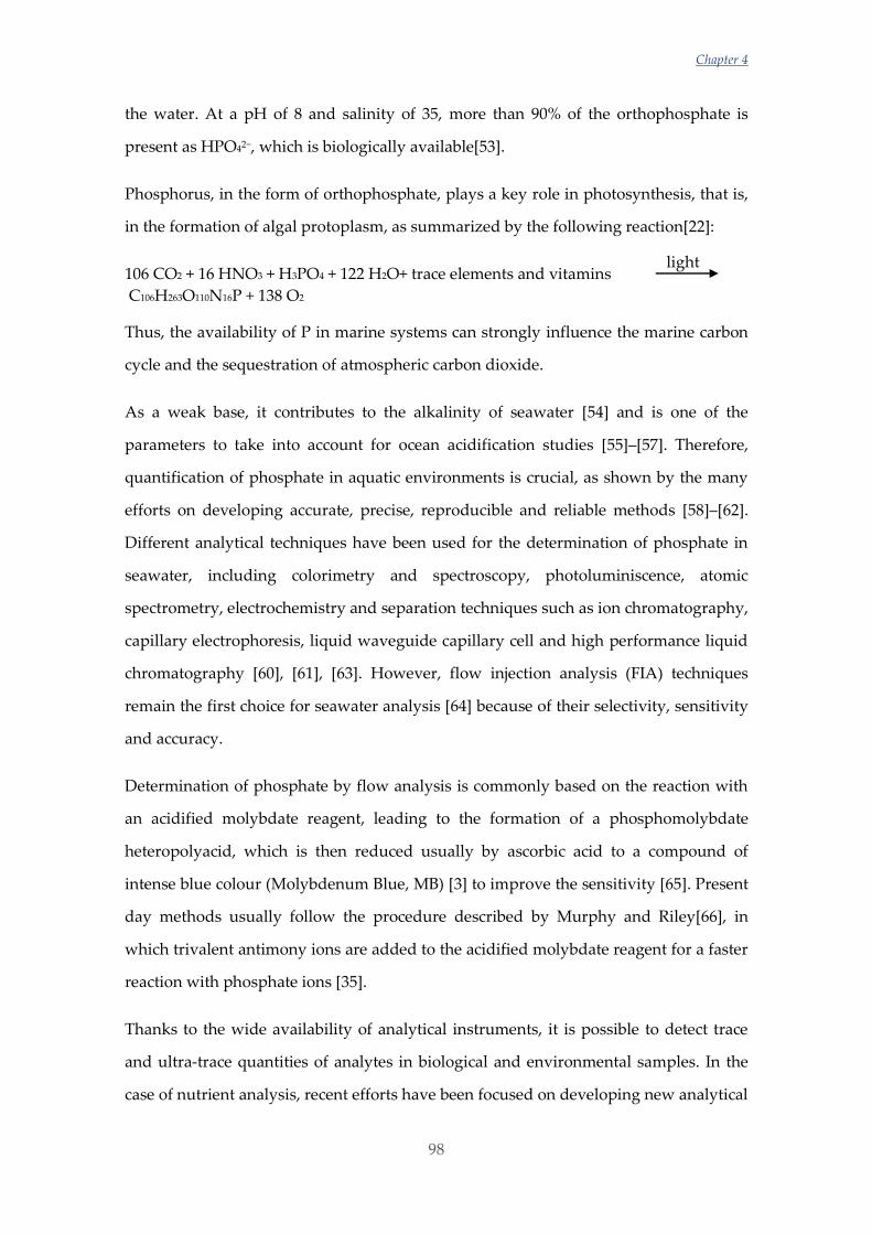
Chapter 4

98

the water. At a pH of 8 and salinity of 35, more than 90% of the orthophosphate is

present as HPO42−, which is biologically available[53].

Phosphorus, in the form of orthophosphate, plays a key role in photosynthesis, that is,

in the formation of algal protoplasm, as summarized by the following reaction[22]:

106 CO2 + 16 HNO3 + H3PO4 + 122 H2O+ trace elements and vitamins

C106H263O110N16P + 138 O2

Thus, the availability of P in marine systems can strongly influence the marine carbon

cycle and the sequestration of atmospheric carbon dioxide.

As a weak base, it contributes to the alkalinity of seawater [54] and is one of the

parameters to take into account for ocean acidification studies [55]–[57]. Therefore,

quantification of phosphate in aquatic environments is crucial, as shown by the many

efforts on developing accurate, precise, reproducible and reliable methods [58]–[62].

Different analytical techniques have been used for the determination of phosphate in

seawater, including colorimetry and spectroscopy, photoluminiscence, atomic

spectrometry, electrochemistry and separation techniques such as ion chromatography,

capillary electrophoresis, liquid waveguide capillary cell and high performance liquid

chromatography [60], [61], [63]. However, flow injection analysis (FIA) techniques

remain the first choice for seawater analysis [64] because of their selectivity, sensitivity

and accuracy.

Determination of phosphate by flow analysis is commonly based on the reaction with

an acidified molybdate reagent, leading to the formation of a phosphomolybdate

heteropolyacid, which is then reduced usually by ascorbic acid to a compound of

intense blue colour (Molybdenum Blue, MB) [3] to improve the sensitivity [65]. Present

day methods usually follow the procedure described by Murphy and Riley[66], in

which trivalent antimony ions are added to the acidified molybdate reagent for a faster

reaction with phosphate ions [35].

Thanks to the wide availability of analytical instruments, it is possible to detect trace

and ultra-trace quantities of analytes in biological and environmental samples. In the

case of nutrient analysis, recent efforts have been focused on developing new analytical

light

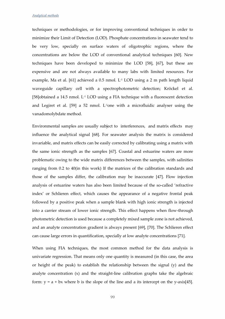
Analytical methods

99

techniques or methodologies, or for improving conventional techniques in order to

minimize their Limit of Detection (LOD). Phosphate concentrations in seawater tend to

be very low, specially on surface waters of oligotrophic regions, where the

concentrations are below the LOD of conventional analytical techniques [60]. New

techniques have been developed to minimize the LOD [58], [67], but these are

expensive and are not always available to many labs with limited resources. For

example, Ma et al. [61] achieved a 0.5 nmol. L-1 LOD using a 2 m path length liquid

waveguide capillary cell with a spectrophotometric detection; Kröckel et al.

[58]obtained a 14.5 nmol. L-1 LOD using a FIA technique with a fluorescent detection

and Legiret et al. [59] a 52 nmol. L-1one with a microfluidic analyser using the

vanadomolybdate method.

Environmental samples are usually subject to interferences, and matrix effects may

influence the analytical signal [68]. For seawater analysis the matrix is considered

invariable, and matrix effects can be easily corrected by calibrating using a matrix with

the same ionic strength as the samples [67]. Coastal and estuarine waters are more

problematic owing to the wide matrix differences between the samples, with salinities

ranging from 0.2 to 40(in this work) If the matrices of the calibration standards and

those of the samples differ, the calibration may be inaccurate [47]. Flow injection

analysis of estuarine waters has also been limited because of the so-called ‘refractive

index’ or Schlieren effect, which causes the appearance of a negative frontal peak

followed by a positive peak when a sample blank with high ionic strength is injected

into a carrier stream of lower ionic strength. This effect happens when flow-through

photometric detection is used because a completely mixed sample zone is not achieved,

and an analyte concentration gradient is always present [69], [70]. The Schlieren effect

can cause large errors in quantification, specially at low analyte concentrations [71].

When using FIA techniques, the most common method for the data analysis is

univariate regression. That means only one quantity is measured (in this case, the area

or height of the peak) to establish the relationship between the signal (y) and the

analyte concentration (x) and the straight-line calibration graphs take the algebraic

form: y = a + bx where b is the slope of the line and a its intercept on the y-axis[45].

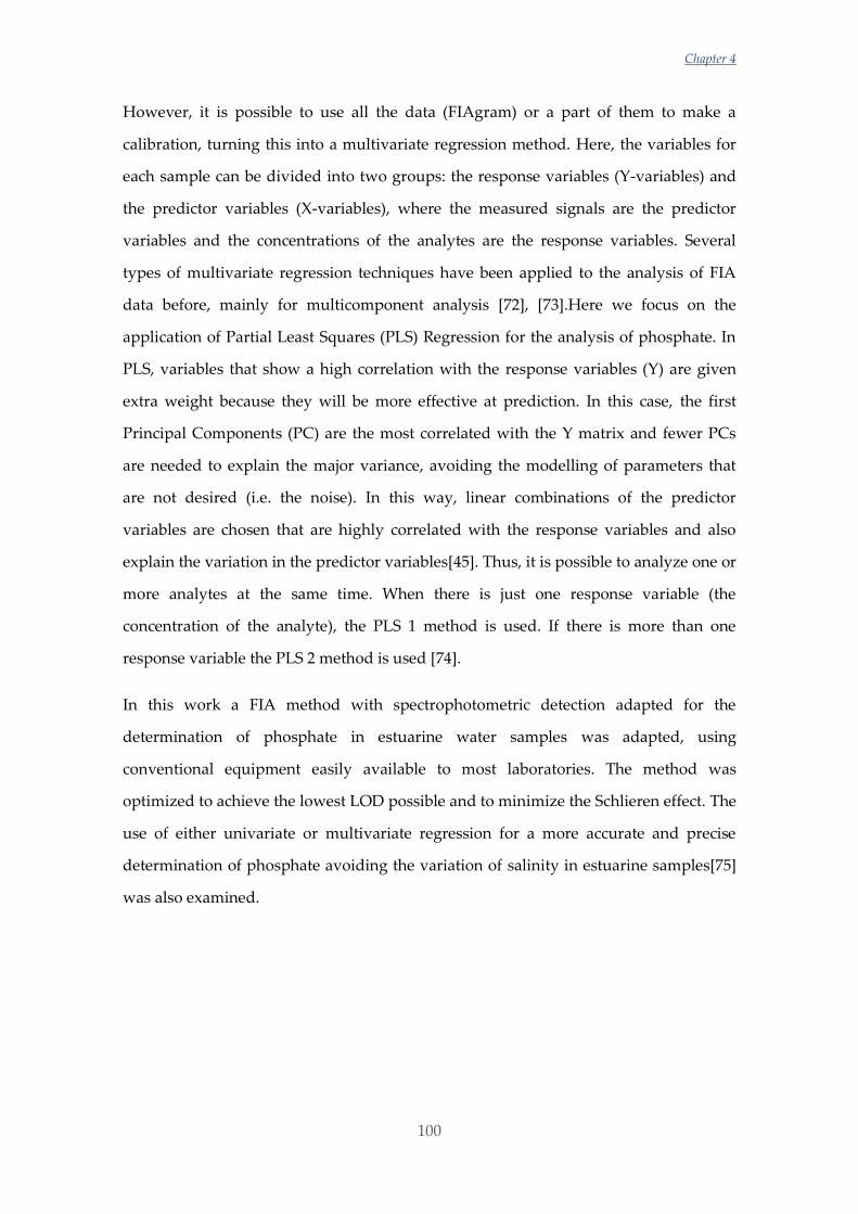
Chapter 4

100

However, it is possible to use all the data (FIAgram) or a part of them to make a

calibration, turning this into a multivariate regression method. Here, the variables for

each sample can be divided into two groups: the response variables (Y-variables) and

the predictor variables (X-variables), where the measured signals are the predictor

variables and the concentrations of the analytes are the response variables. Several

types of multivariate regression techniques have been applied to the analysis of FIA

data before, mainly for multicomponent analysis [72], [73].Here we focus on the

application of Partial Least Squares (PLS) Regression for the analysis of phosphate. In

PLS, variables that show a high correlation with the response variables (Y) are given

extra weight because they will be more effective at prediction. In this case, the first

Principal Components (PC) are the most correlated with the Y matrix and fewer PCs

are needed to explain the major variance, avoiding the modelling of parameters that

are not desired (i.e. the noise). In this way, linear combinations of the predictor

variables are chosen that are highly correlated with the response variables and also

explain the variation in the predictor variables[45]. Thus, it is possible to analyze one or

more analytes at the same time. When there is just one response variable (the

concentration of the analyte), the PLS 1 method is used. If there is more than one

response variable the PLS 2 method is used [74].

In this work a FIA method with spectrophotometric detection adapted for the

determination of phosphate in estuarine water samples was adapted, using

conventional equipment easily available to most laboratories. The method was

optimized to achieve the lowest LOD possible and to minimize the Schlieren effect. The

use of either univariate or multivariate regression for a more accurate and precise

determination of phosphate avoiding the variation of salinity in estuarine samples[75]

was also examined.

Analytical methods

101

4.4.2 Materials and methods

4.4.2.1 Reagents and solutions

All analytical grade reagents were supplied by Merck (Merck kGaA, Darmstadt,

Germany). The phosphate standard (1000 mg L-1) was supplied by Fluka (Sigma-

Aldrich Co., MO, USA).

Both the blank and the calibration samples were prepared with the same matrix. To

prove the effectiveness of the method to avoid matrix effects, that matrix was either

ultrapure water or a 0.7 mol. L-1 NaCl solution. The NaCl was supplied by Sigma-

Aldrich (Sigma-Aldrich Co., MO, USA).

All solutions were prepared using ultrapure water obtained from a Millipore water

purification system (Millipore Co., MA, USA).

The following reagents’ concentrations were used for the calibrations and were

established after an optimisation experimental design, as will be explained in Section

4.4.3.1.

A mixed reagent (MR) was prepared by dissolving 18.5 g of (NH4)6Mo7O24·4H2O in 400

mL of deionised water. Then 22.4 mL of concentrated H2SO4 were added and finally,

6.25 mL of 40 g L-1 potassium antimony tartrate (K2(SbO)2C8H4O10.3H2O). The solution

was then made up to 500 mL.

Ascorbic acid was prepared by dissolving 20 g in 400 mL water. Then, 22.4 mL of

concentrated H2SO4 were added and it was made up to 500 mL. Most procedures use

the sulphuric acid only in the mixed reagent. In this work, the acid was added in both

reagents in order to minimize the Schlieren effect.

4.4.2.2 Apparatus and analytical procedure

In FIA, the sequence of addition of the constituents is critical to achieve the best signal

possible. The quick reaction between molybdate and ascorbic acid leaves the reduced

form of molybdate readily available for reaction with phosphate (A). However, when

the phosphate is injected directly into the molybdate, the yellow molybdophosphate is

formed, which is not as reactive and results in a slower reduction and hence generation

of MB (B)[65].

(A)

fast

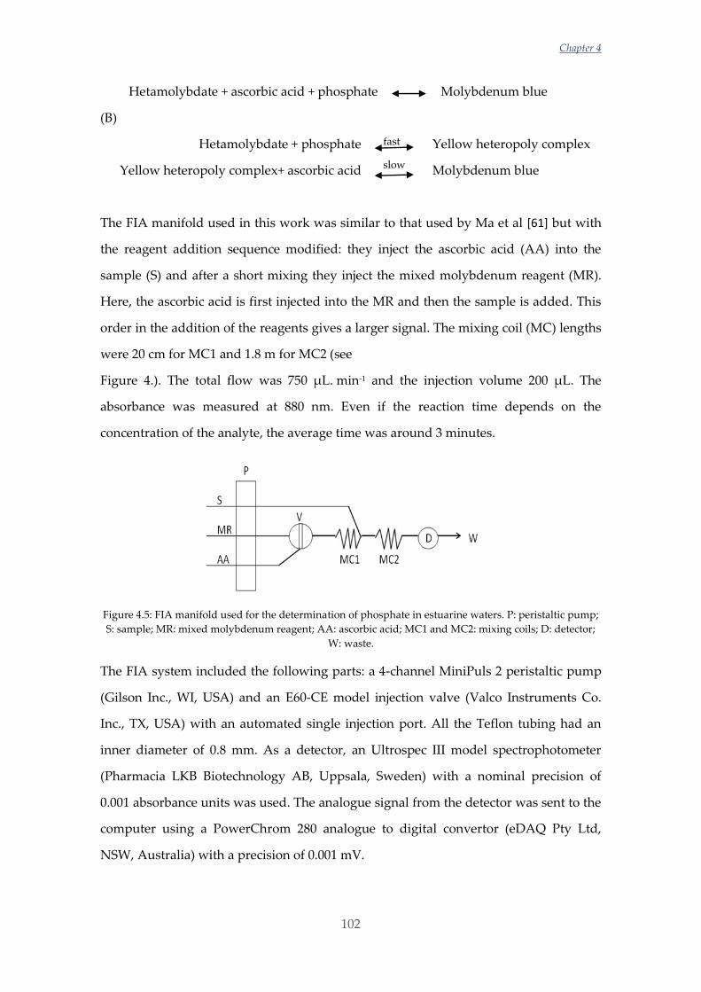
Chapter 4

102

Hetamolybdate + ascorbic acid + phosphate Molybdenum blue

(B)

Hetamolybdate + phosphate Yellow heteropoly complex

Yellow heteropoly complex+ ascorbic acid Molybdenum blue

The FIA manifold used in this work was similar to that used by Ma et al [61] but with

the reagent addition sequence modified: they inject the ascorbic acid (AA) into the

sample (S) and after a short mixing they inject the mixed molybdenum reagent (MR).

Here, the ascorbic acid is first injected into the MR and then the sample is added. This

order in the addition of the reagents gives a larger signal. The mixing coil (MC) lengths

were 20 cm for MC1 and 1.8 m for MC2 (see

Figure 4.). The total flow was 750 µL. min-1 and the injection volume 200 µL. The

absorbance was measured at 880 nm. Even if the reaction time depends on the

concentration of the analyte, the average time was around 3 minutes.

Figure 4.5: FIA manifold used for the determination of phosphate in estuarine waters. P: peristaltic pump;

S: sample; MR: mixed molybdenum reagent; AA: ascorbic acid; MC1 and MC2: mixing coils; D: detector;

W: waste.

The FIA system included the following parts: a 4-channel MiniPuls 2 peristaltic pump

(Gilson Inc., WI, USA) and an E60-CE model injection valve (Valco Instruments Co.

Inc., TX, USA) with an automated single injection port. All the Teflon tubing had an

inner diameter of 0.8 mm. As a detector, an Ultrospec III model spectrophotometer

(Pharmacia LKB Biotechnology AB, Uppsala, Sweden) with a nominal precision of

0.001 absorbance units was used. The analogue signal from the detector was sent to the

computer using a PowerChrom 280 analogue to digital convertor (eDAQ Pty Ltd,

NSW, Australia) with a precision of 0.001 mV.

fast

slow

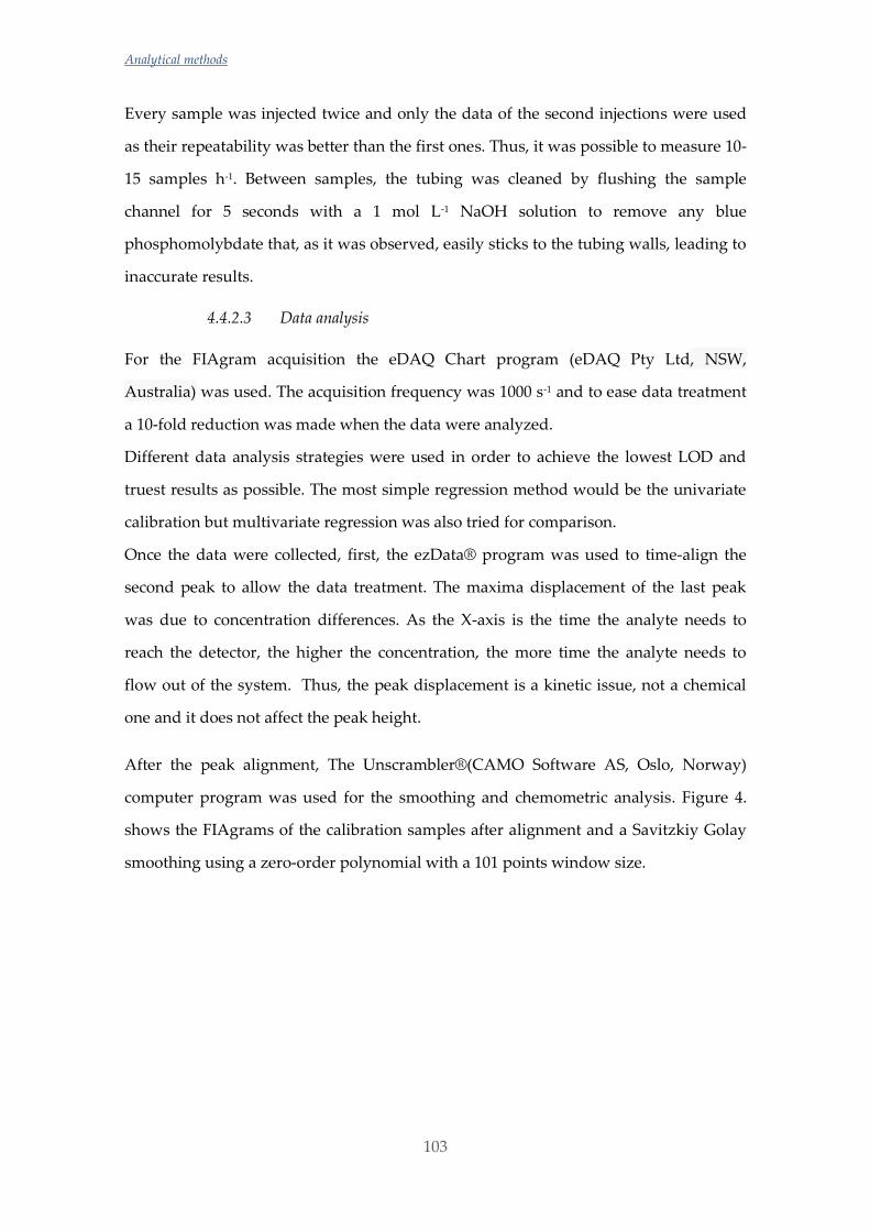
Analytical methods

103

Every sample was injected twice and only the data of the second injections were used

as their repeatability was better than the first ones. Thus, it was possible to measure 10-

15 samples h-1. Between samples, the tubing was cleaned by flushing the sample

channel for 5 seconds with a 1 mol L-1 NaOH solution to remove any blue

phosphomolybdate that, as it was observed, easily sticks to the tubing walls, leading to

inaccurate results.

4.4.2.3 Data analysis

For the FIAgram acquisition the eDAQ Chart program (eDAQ Pty Ltd, NSW,

Australia) was used. The acquisition frequency was 1000 s-1 and to ease data treatment

a 10-fold reduction was made when the data were analyzed.

Different data analysis strategies were used in order to achieve the lowest LOD and

truest results as possible. The most simple regression method would be the univariate

calibration but multivariate regression was also tried for comparison.

Once the data were collected, first, the ezData® program was used to time-align the

second peak to allow the data treatment. The maxima displacement of the last peak

was due to concentration differences. As the X-axis is the time the analyte needs to

reach the detector, the higher the concentration, the more time the analyte needs to

flow out of the system. Thus, the peak displacement is a kinetic issue, not a chemical

one and it does not affect the peak height.

After the peak alignment, The Unscrambler®(CAMO Software AS, Oslo, Norway)

computer program was used for the smoothing and chemometric analysis. Figure 4.

shows the FIAgrams of the calibration samples after alignment and a Savitzkiy Golay

smoothing using a zero-order polynomial with a 101 points window size.

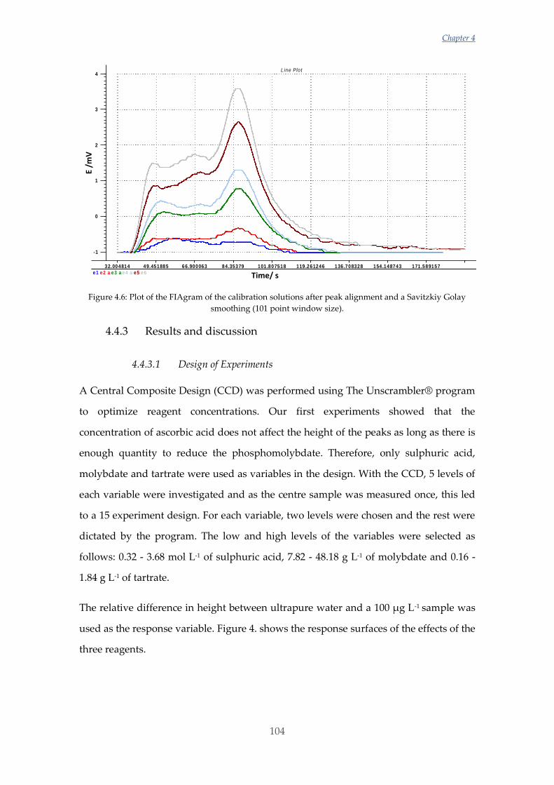
Chapter 4

104

Figure 4.6: Plot of the FIAgram of the calibration solutions after peak alignment and a Savitzkiy Golay

smoothing (101 point window size).

4.4.3 Results and discussion

4.4.3.1 Design of Experiments

A Central Composite Design (CCD) was performed using The Unscrambler® program

to optimize reagent concentrations. Our first experiments showed that the

concentration of ascorbic acid does not affect the height of the peaks as long as there is

enough quantity to reduce the phosphomolybdate. Therefore, only sulphuric acid,

molybdate and tartrate were used as variables in the design. With the CCD, 5 levels of

each variable were investigated and as the centre sample was measured once, this led

to a 15 experiment design. For each variable, two levels were chosen and the rest were

dictated by the program. The low and high levels of the variables were selected as

follows: 0.32 - 3.68 mol L-1 of sulphuric acid, 7.82 - 48.18 g L-1 of molybdate and 0.16 -

1.84 g L-1 of tartrate.

The relative difference in height between ultrapure water and a 100 µg L-1 sample was

used as the response variable. Figure 4. shows the response surfaces of the effects of the

three reagents.

-1

0

1

2

3

4

32.004814 49.451885 66.900063 84.35379 101 .807518 119 .261246 136 .708328 154 .148743 171 .589157

e1 e2 a e3 a e4 a e5 e6

Variab les

Line Plot

E /m

V

Time/ s

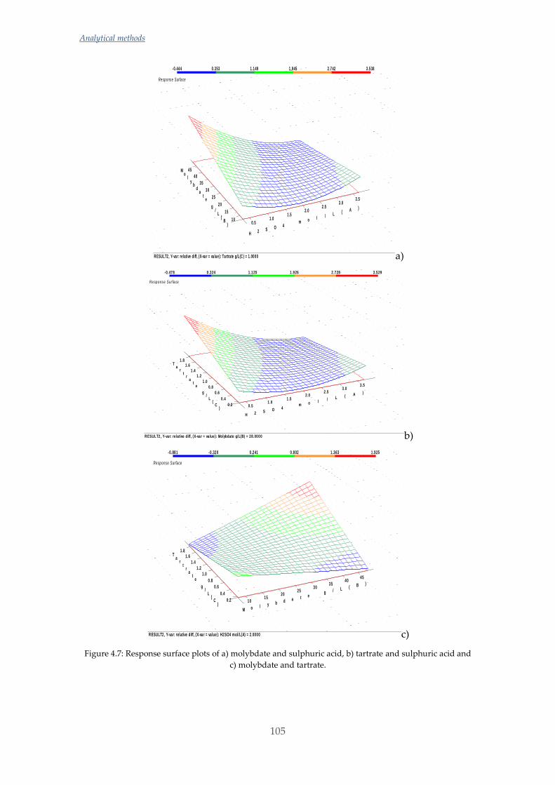
Analytical methods

105

a)

b)

c)

Figure 4.7: Response surface plots of a) molybdate and sulphuric acid, b) tartrate and sulphuric acid and

c) molybdate and tartrate.

R ESULT2, Y-var: relative diff, (X-var = va lue ): Tartra te g/L(C ) = 1.0000

Response Surface

45

40

35

30

25

20

15

100 .5

1 .01 .5

2 .02 .5

3 .03 .5

Mo

ly

bd

at

e

g/

L(

B)

H 2 S O 4 m o l / L ( A )

-0.444 0 .353 1 .149 1 .945 2 .742 3 .538

R ESULT2, Y-var: relative diff, (X-var = va lue ): Molybdate g/L(B) = 28.0000

Response Surface

1 .81 .6

1 .4

1 .2

1 .0

0 .8

0 .6

0 .4

0 .2 0 .51 .0

1 .52 .0

2 .53 .0

3 .5

Ta

rt

ra

te

g

/L

(C

)

H 2 S O 4 m o l / L ( A )

-0.478 0 .324 1 .125 1 .926 2 .728 3 .529

R ESULT2, Y-var: relative diff, (X-var = va lue ): H2SO4 mol/L(A) = 2.0000

Response Surface

1 .81 .6

1 .4

1 .2

1 .0

0 .8

0 .6

0 .4

0 .2 1015

2025

3035

4045

Ta

rt

ra

te

g

/L

(C

)M o l y b d a t e g / L ( B )

-0.881 -0.320 0 .241 0 .802 1 .363 1 .925

Chapter 4

106

Sulphuric acid was the most critical reagent. Above 1 mol L-1 the signal was too noisy

(which increases the LOD) and the peaks were too low. But below 0.7 mol. L-1 the MR

started to become bluish and its intensity increased during the day (which affected the

repeatability).

In the case of molybdate and tartrate, the higher the concentration the larger the

sample signal. So, depending on the expected sample concentration, it is possible to

change them. However, it must be considered that the addition of too much tartrate in

the acidic molybdate solution leads to the appearance of a yellow precipitate.

Taking the results of this design into account, as well as the considerations mentioned

above, the concentrations of the reagents used for the calibration and measurement of

the samples were those stated in Section 4.4.2.2.

4.4.3.2 Data analysis

First of all, a PLS 2 regression method was applied using both phosphate and density

as response variables to see the effect of salinity differences on the peaks. Even if the

regression parameters of the model were good, the predicted values for the samples

were not reasonable. In addition, a lot of Principal Components (PC) had to be used in

order to achieve a good model. The calibration samples also showed that the salinity

difference has no effect on the last peak while it has a bigger influence on the signal at

the beginning of the FIAgram (see Figure 4.). Therefore, as the last peak was not

affected by salinity differences, this peak was used for both the univariate and the

multivariate regressions. These were carried out using the maximum value for the first

one and around 10 s of the FIAgram, with the maximum value in the middle (leading

to a number of predictor variables of 1000 points), for the second one.

In order to choose the best regression model, different calibrations were made in

different days measuring several times the blank for the LOD determination and a

certain sample of intermediate salinity (called “Sample A” in Table 4.) to study both

short and long-time repeatability.

Figure 4. shows the PLS 1 multivariate and univariate regressions of the calibration

samples, which go between 0.02 mg. L-1 and 0.2 mg. L-1 phosphate in one of those days.

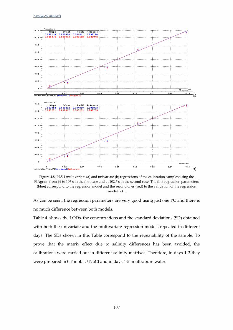
Analytical methods

107

a)

b)

Figure 4.8: PLS 1 multivariate (a) and univariate (b) regressions of the calibration samples using the

FIAgram from 99 to 107 s in the first case and at 102.7 s in the second case. The first regression parameters

(blue) correspond to the regression model and the second ones (red) to the validation of the regression

model [74].

As can be seen, the regression parameters are very good using just one PC and there is

no much difference between both models.

Table 4. shows the LODs, the concentrations and the standard deviations (SD) obtained

with both the univariate and the multivariate regression models repeated in different

days. The SDs shown in this Table correspond to the repeatability of the sample. To

prove that the matrix effect due to salinity differences has been avoided, the

calibrations were carried out in different salinity matrixes. Therefore, in days 1-3 they

were prepared in 0.7 mol. L-1 NaCl and in days 4-5 in ultrapure water.

0

0 .02

0 .04

0 .06

0 .08

0 .10

0 .12

0 .14

0 .16

0 0 .02 0 .04 0 .06 0 .08 0 .10 0 .12 0 .14 0 .16

multivariate, (Y-var, PC): ( fosf ppm,1) ( fosf ppm,1)

1

23

5

6

7

91

23

5

6

7

9

Slope Offset RMSE R-Square0 .992110 0 .000406 0 .004811 0 .9921100 .985476 0 .000903 0 .006188 0 .986948

Measured Y

Predicted Y

0

0 .02

0 .04

0 .06

0 .08

0 .10

0 .12

0 .14

0 .16

0 0 .02 0 .04 0 .06 0 .08 0 .10 0 .12 0 .14 0 .16

multivariate, (Y-var, PC): ( fosf ppm,1) ( fosf ppm,1)

1

23

5

6

7

91

23

5

6

7

9

Slope Offset RMSE R-Square0 .992110 0 .000406 0 .004811 0 .9921100 .985476 0 .000903 0 .006188 0 .986948

Measured Y

Predicted Y

0

0 .02

0 .04

0 .06

0 .08

0 .10

0 .12

0 .14

0 .16

0 0 .02 0 .04 0 .06 0 .08 0 .10 0 .12 0 .14 0 .16

univariate, (Y-var, PC): ( fosf ppm,1) ( fosf ppm,1)

1

23

5

6

7

91

23

5

6

7

9

Slope Offset RMSE R-Square0 .991983 0 .000412 0 .004850 0 .9919830 .985271 0 .000917 0 .006231 0 .986765

Measured Y

Predicted Y

0

0 .02

0 .04

0 .06

0 .08

0 .10

0 .12

0 .14

0 .16

0 0 .02 0 .04 0 .06 0 .08 0 .10 0 .12 0 .14 0 .16

univariate, (Y-var, PC): ( fosf ppm,1) ( fosf ppm,1)

1

23

5

6

7

91

23

5

6

7

9

Slope Offset RMSE R-Square0 .991983 0 .000412 0 .004850 0 .9919830 .985271 0 .000917 0 .006231 0 .986765

Measured Y

Predicted Y

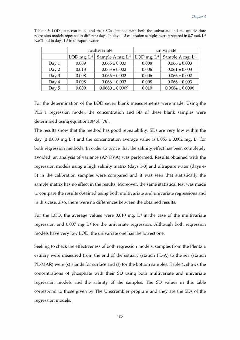
Chapter 4

108

Table 4.5: LODs, concentrations and their SDs obtained with both the univariate and the multivariate

regression models repeated in different days. In days 1-3 calibration samples were prepared in 0.7 mol. L-1

NaCl and in days 4-5 in ultrapure water.

multivariate univariate

LOD mg. L-1 Sample A mg. L-1 LOD mg. L-1 Sample A mg. L-1

Day 1 0.009 0.065 ± 0.003 0.008 0.066 ± 0.003

Day 2 0.013 0.063 ± 0.002 0.006 0.061 ± 0.003

Day 3 0.008 0.066 ± 0.002 0.006 0.066 ± 0.002

Day 4 0.008 0.066 ± 0.003 0.008 0.066 ± 0.003

Day 5 0.009 0.0680 ± 0.0009 0.010 0.0684 ± 0.0006

For the determination of the LOD seven blank measurements were made. Using the

PLS 1 regression model, the concentration and SD of these blank samples were

determined using equation10[45], [76].

The results show that the method has good repeatability. SDs are very low within the

day (≤ 0.003 mg L-1) and the concentration average value is 0.065 ± 0.002 mg. L-1 for

both regression methods. In order to prove that the salinity effect has been completely

avoided, an analysis of variance (ANOVA) was performed. Results obtained with the

regression models using a high salinity matrix (days 1-3) and ultrapure water (days 4-

5) in the calibration samples were compared and it was seen that statistically the

sample matrix has no effect in the results. Moreover, the same statistical test was made

to compare the results obtained using both multivariate and univariate regressions and

in this case, also, there were no differences between the obtained results.

For the LOD, the average values were 0.010 mg. L-1 in the case of the multivariate

regression and 0.007 mg L-1 for the univariate regression. Although both regression

models have very low LOD, the univariate one has the lowest one.

Seeking to check the effectiveness of both regression models, samples from the Plentzia

estuary were measured from the end of the estuary (station PL-A) to the sea (station

PL-MAR) were (s) stands for surface and (f) for the bottom samples. Table 4. shows the

concentrations of phosphate with their SD using both multivariate and univariate

regression models and the salinity of the samples. The SD values in this table

correspond to those given by The Unscrambler program and they are the SDs of the

regression models.

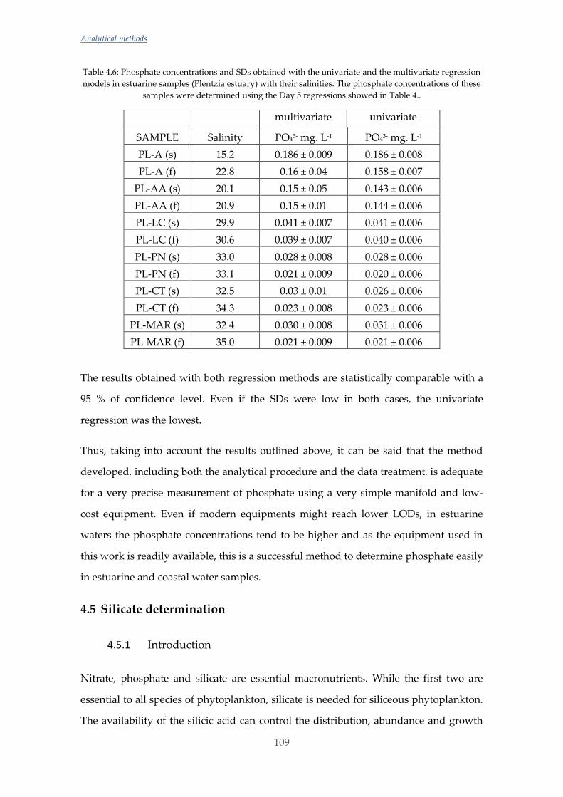
Analytical methods

109

Table 4.6: Phosphate concentrations and SDs obtained with the univariate and the multivariate regression

models in estuarine samples (Plentzia estuary) with their salinities. The phosphate concentrations of these

samples were determined using the Day 5 regressions showed in Table 4..

multivariate univariate

SAMPLE Salinity PO43- mg. L-1 PO43- mg. L-1

PL-A (s) 15.2 0.186 ± 0.009 0.186 ± 0.008

PL-A (f) 22.8 0.16 ± 0.04 0.158 ± 0.007

PL-AA (s) 20.1 0.15 ± 0.05 0.143 ± 0.006

PL-AA (f) 20.9 0.15 ± 0.01 0.144 ± 0.006

PL-LC (s) 29.9 0.041 ± 0.007 0.041 ± 0.006

PL-LC (f) 30.6 0.039 ± 0.007 0.040 ± 0.006

PL-PN (s) 33.0 0.028 ± 0.008 0.028 ± 0.006

PL-PN (f) 33.1 0.021 ± 0.009 0.020 ± 0.006

PL-CT (s) 32.5 0.03 ± 0.01 0.026 ± 0.006

PL-CT (f) 34.3 0.023 ± 0.008 0.023 ± 0.006

PL-MAR (s) 32.4 0.030 ± 0.008 0.031 ± 0.006

PL-MAR (f) 35.0 0.021 ± 0.009 0.021 ± 0.006

The results obtained with both regression methods are statistically comparable with a

95 % of confidence level. Even if the SDs were low in both cases, the univariate

regression was the lowest.

Thus, taking into account the results outlined above, it can be said that the method

developed, including both the analytical procedure and the data treatment, is adequate

for a very precise measurement of phosphate using a very simple manifold and low-

cost equipment. Even if modern equipments might reach lower LODs, in estuarine

waters the phosphate concentrations tend to be higher and as the equipment used in

this work is readily available, this is a successful method to determine phosphate easily

in estuarine and coastal water samples.

4.5 Silicate determination

4.5.1 Introduction

Nitrate, phosphate and silicate are essential macronutrients. While the first two are

essential to all species of phytoplankton, silicate is needed for siliceous phytoplankton.

The availability of the silicic acid can control the distribution, abundance and growth

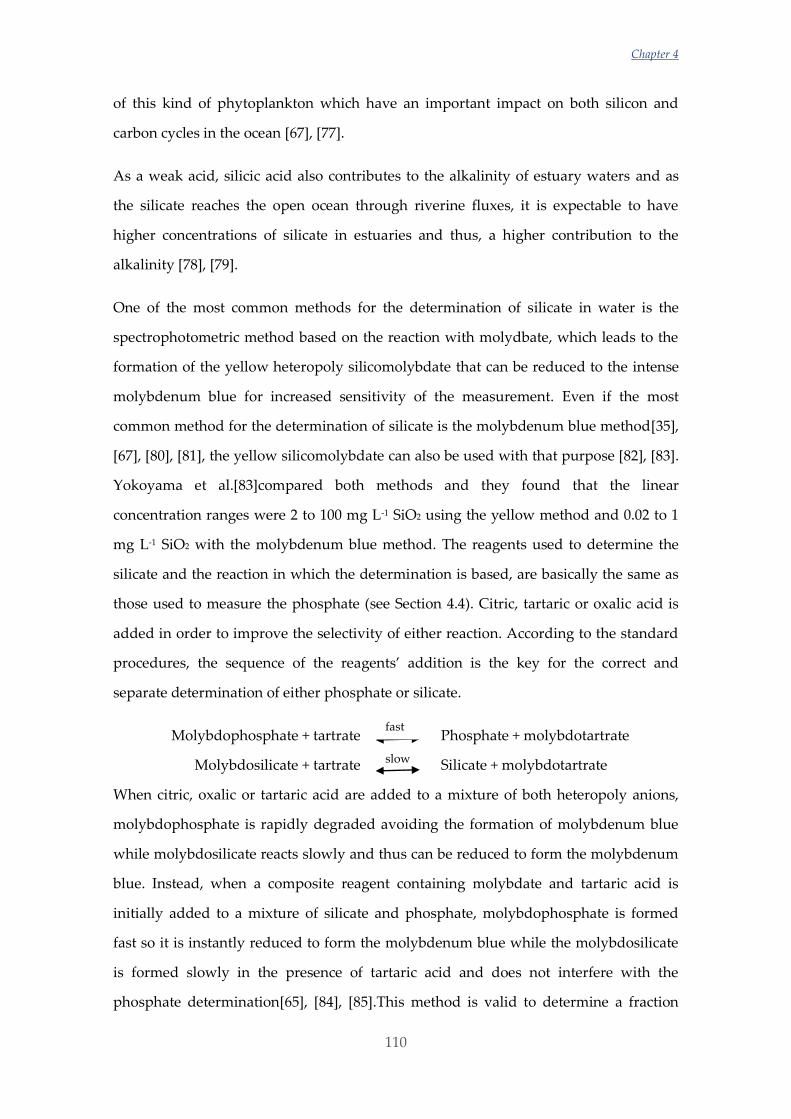
Chapter 4

110

of this kind of phytoplankton which have an important impact on both silicon and

carbon cycles in the ocean [67], [77].

As a weak acid, silicic acid also contributes to the alkalinity of estuary waters and as

the silicate reaches the open ocean through riverine fluxes, it is expectable to have

higher concentrations of silicate in estuaries and thus, a higher contribution to the

alkalinity [78], [79].

One of the most common methods for the determination of silicate in water is the

spectrophotometric method based on the reaction with molydbate, which leads to the

formation of the yellow heteropoly silicomolybdate that can be reduced to the intense

molybdenum blue for increased sensitivity of the measurement. Even if the most

common method for the determination of silicate is the molybdenum blue method[35],

[67], [80], [81], the yellow silicomolybdate can also be used with that purpose [82], [83].

Yokoyama et al.[83]compared both methods and they found that the linear

concentration ranges were 2 to 100 mg L-1 SiO2 using the yellow method and 0.02 to 1

mg L-1 SiO2 with the molybdenum blue method. The reagents used to determine the

silicate and the reaction in which the determination is based, are basically the same as

those used to measure the phosphate (see Section 4.4). Citric, tartaric or oxalic acid is

added in order to improve the selectivity of either reaction. According to the standard

procedures, the sequence of the reagents’ addition is the key for the correct and

separate determination of either phosphate or silicate.

Molybdophosphate + tartrate Phosphate + molybdotartrate

Molybdosilicate + tartrate Silicate + molybdotartrate

When citric, oxalic or tartaric acid are added to a mixture of both heteropoly anions,

molybdophosphate is rapidly degraded avoiding the formation of molybdenum blue

while molybdosilicate reacts slowly and thus can be reduced to form the molybdenum

blue. Instead, when a composite reagent containing molybdate and tartaric acid is

initially added to a mixture of silicate and phosphate, molybdophosphate is formed

fast so it is instantly reduced to form the molybdenum blue while the molybdosilicate

is formed slowly in the presence of tartaric acid and does not interfere with the

phosphate determination[65], [84], [85].This method is valid to determine a fraction

slow

fast

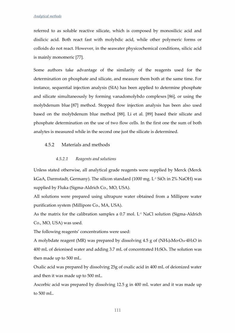
Analytical methods

111

referred to as soluble reactive silicate, which is composed by monosilicic acid and

disilicic acid. Both react fast with molybdic acid, while other polymeric forms or

colloids do not react. However, in the seawater physicochemical conditions, silicic acid

is mainly monomeric [77].

Some authors take advantage of the similarity of the reagents used for the

determination on phosphate and silicate, and measure them both at the same time. For

instance, sequential injection analysis (SIA) has been applied to determine phosphate

and silicate simultaneously by forming vanadomolybdo complexes [86], or using the

molybdenum blue [87] method. Stopped flow injection analysis has been also used

based on the molybdenum blue method [88]. Li et al. [89] based their silicate and

phosphate determination on the use of two flow cells. In the first one the sum of both

analytes is measured while in the second one just the silicate is determined.

4.5.2 Materials and methods

4.5.2.1 Reagents and solutions

Unless stated otherwise, all analytical grade reagents were supplied by Merck (Merck

kGaA, Darmstadt, Germany). The silicon standard (1000 mg. L-1 SiO2 in 2% NaOH) was

supplied by Fluka (Sigma-Aldrich Co., MO, USA).

All solutions were prepared using ultrapure water obtained from a Millipore water

purification system (Millipore Co., MA, USA).

As the matrix for the calibration samples a 0.7 mol. L-1 NaCl solution (Sigma-Aldrich

Co., MO, USA) was used.

The following reagents’ concentrations were used:

A molybdate reagent (MR) was prepared by dissolving 4.5 g of (NH4)6Mo7O24·4H2O in

400 mL of deionised water and adding 3.7 mL of concentrated H2SO4. The solution was

then made up to 500 mL.

Oxalic acid was prepared by dissolving 25g of oxalic acid in 400 mL of deionized water

and then it was made up to 500 mL.

Ascorbic acid was prepared by dissolving 12.5 g in 400 mL water and it was made up

to 500 mL.

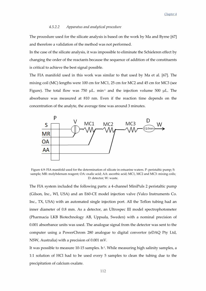
Chapter 4

112

4.5.2.2 Apparatus and analytical procedure

The procedure used for the silicate analysis is based on the work by Ma and Byrne [67]

and therefore a validation of the method was not performed.

In the case of the silicate analysis, it was impossible to eliminate the Schieleren effect by

changing the order of the reactants because the sequence of addition of the constituents

is critical to achieve the best signal possible.

The FIA manifold used in this work was similar to that used by Ma et al. [67]. The

mixing coil (MC) lengths were 100 cm for MC1, 25 cm for MC2 and 45 cm for MC3 (see

Figure). The total flow was 750 µL. min-1 and the injection volume 500 µL. The

absorbance was measured at 810 nm. Even if the reaction time depends on the

concentration of the analyte, the average time was around 3 minutes.

Figure 4.9: FIA manifold used for the determination of silicate in estuarine waters. P: peristaltic pump; S:

sample; MR: molybdenum reagent; OA: oxalic acid; AA: ascorbic acid; MC1, MC2 and MC3: mixing coils;

D: detector; W: waste.

The FIA system included the following parts: a 4-channel MiniPuls 2 peristaltic pump

(Gilson, Inc., WI, USA) and an E60-CE model injection valve (Valco Instruments Co.

Inc., TX, USA) with an automated single injection port. All the Teflon tubing had an

inner diameter of 0.8 mm. As a detector, an Ultrospec III model spectrophotometer

(Pharmacia LKB Biotechnology AB, Uppsala, Sweden) with a nominal precision of

0.001 absorbance units was used. The analogue signal from the detector was sent to the

computer using a PowerChrom 280 analogue to digital convertor (eDAQ Pty Ltd,

NSW, Australia) with a precision of 0.001 mV.

It was possible to measure 10-15 samples. h-1. While measuring high salinity samples, a

1:1 solution of HCl had to be used every 5 samples to clean the tubing due to the

precipitation of calcium oxalate.

Analytical methods

113

Due to the expected differences in concentrations in the samples analysed, 3 calibration

ranges were always prepared: a low concentration range (0.05 – 0.3 mg. L-1 Si), a

medium concentration range (0.3– 1.5 mg. L-1 Si) and a high concentration range (1.5 –

6 mg. L-1 Si). In every case 3 blank solutions were also measured. Each of these

calibration samples, as well as the real samples, was measured once.

4.5.2.3 Data analysis

For the FIAgram acquisition the eDAQ Chart program (eDAQ Pty Ltd, NSW,

Australia) was used. The acquisition frequency was 1000 s-1 and to ease data treatment

a 10-fold reduction was made when the data were analyzed. The area of the peak was

used as the measured parameter and for the integration of it the OPUS software

(Schaumburg, IL, USA) was used.

4.5.3 Results and discussion

To study the importance of the Schieler effect, 5 sets of calibration solutions were

studied at 5 different ionic strengths prepared by adding NaCl. These ionic strengths

were 0 (ultrapure water), 0.17, 0.35, 0.55, and 0.7 mol. L-1, respectively, and calibration

solutions, ranging from 0 to 1.2 mg. L-1Si, were prepared in each matrix. Figure shows

the linear regressions of these samples:

Figure 4.10: Plot of the 5 calibration sets prepared in matrixes with different ionic strengths with

concentrations of Si ranging from 0 to 1.2 mg. L-1.

-5000

0

5000

10000

15000

20000

25000

30000

35000

40000

45000

50000

0 0.2 0.4 0.6 0.8 1 1.2 1.4

Are

a

I mol. L-1

MQ

I = 0.17

I = 0.35

I = 0.55

I = 0.7

Chapter 4

114

As can be seen, for concentrations < 0.3 mg. L-1 the area of the peaks are the same,

despite the differences in the matrixes. On the other hand, for concentrations > 0.3 mg.

L-1, no significant differences were found between matrixes containing NaCl but those

calibration samples prepared in Milli-Q water showed bigger areas. Table 4.7 shows

the prediction of the 1.2 mg. L-1 sample prepared in 0.7 mol. L-1 NaCl and predicted by

the lineal regression of the 5 sets of calibrations. The uncertainty corresponds only to

the uncertainty of the regression.

Table 4.7: The prediction of the 1.2 mg. L-1 sample prepared in 0.7 mol. L-1 NaCl and predicted by the lineal

regression of the 5 sets of calibrations.

Si mg. L-1

MQ 1.07 ± 0.02

0.17 mol. L-1 NaCl 1.19 ± 0.02

0.35mol. L-1 NaCl 1.21 ± 0.03

0.55mol. L-1 NaCl 1.18 ± 0.03

0.7 mol. L-1 NaCl 1.20 ± 0.02

Therefore, the only affected samples by the Schieleren effect could be the river samples.

However, this may not be always the case since these samples may be rather different

from ultrapure water.

The LOD and LOQ were calculated using a low concentration regression model. In this

case the LOD was 0.021 mg. L-1 and the LOQ was 0.044 mg. L-1.

4.6 Total Organic Carbon determination

4.6.1 Introduction

The delivery of organic carbon from rivers to the coast through estuaries is an

important component of the global carbon cycle and it also affects the aquatic

ecosystem [90]. The Total Organic Carbon (TOC) does not affect directly to the human

health but its determination is important because it does affect, both indirectly and

directly, to the ecosystem of the aquatic environments. Organic carbon is an energy

source for microorganisms and it is an important part of many chemical and

photochemical reactions. The organic carbon affects the ecosystem in many ways: it

Analytical methods

115

impacts on the colour, it attenuates both UV and visible light, it binds metals, affecting

their toxicity and bioaccumulation and also nutrients, controlling their bioavailability

and mobility. TOC comes from both natural and anthropogenic sources and its value

in water is very variable and it is affected by many factors such as temperature,

salinity, pH, microbial activity and surrounding vegetation, among others [91], [92].

Dissolved organic carbon (DOC) in rivers and estuarine waters is formed by fulvic

acids and is referred to as humic substances which have complicated structures and

different acidities [93]. As acidic substances, they can affect the pH of the water, and

hence, the alkalinity (see Chapter 1 Section 1.1). However, the insufficient knowledge

on the effect of organic components on the acid-base system can difficult the

interpretation of some AT data. And if the organic component of the water is high,

ignoring its contribution to the total alkalinity may generate errors in the calculation of

acid-base parameters [93]–[95]. For example, the differences between measured and

computed parameters are usually bellow 5% but some authors have found

discrepancies in pCO2 of about 30%, which they correlated with a high DOM [95]–[97].

However, the organic carbon could be a complex mixture of compounds whose

contribution to the TA can be very difficult to determine since precise knowledge of the

acid-base stability constants for these compounds are needed in the calculations.

During the 1991 Seattle DOC/DON Workshop, High Temperature Catalytic Oxidation

(HTCO) was recognised as the most precise and efficient technique for the oxidation of

dissolved organic material in seawater. HTCO is typically based on the direct injection

of filtered (for DOM), acidified and decarbonated seawater into a Pt-coated catalyst at

high temperature (≥ 600 °C) in an atmosphere of high purity air or inert gas [98]–[100].

Due to its automation, ease of use and its accuracy and precision, this is nowadays the

most useful technique for the determination of organic carbon [101], [102] and it is the

technique used in this work.

Nevertheless, there is another method, known as wet oxidation, that has been used and

it is still in use. In this case, the sample is acidified, purged to remove inorganic carbon,

and oxidized with persulphate in an autoclave at temperatures from 116 to 130 °C. The

Chapter 4

116

resultant carbon dioxide is measured by non-dispersive infrared (NDIR)

spectrometry[103], [104].

4.6.2 Materials and methods

4.6.2.1 Reagents and material

All solutions were prepared using ultrapure water obtained from a Millipore water

purification system (Millipore Co., MA, USA).

All analytical grade reagents were supplied by Merck (Merck kGaA, Darmstadt,

Germany) unless stated otherwise.

For the calibration samples, as the source of organic carbon, a 100 mg. L-1potassium

hydrogen phthalate solution was used. For the robustness test, a glucose solution was

also used as the alternative source of organic carbon. Both reagents were supplied by

Panreac (Panreac Química S.L.U, Barcelona, Spain).

The carrier gas used in this work was a high purity air, Zero K50S, %99.999 free of CO2

(Carburos Metálicos, Cornellà de Llobregat (Barcelona), Spain). And for the

acidification of the samples a concentrated (≈ 2 mol. L-1) HCl solution (Bernd Kraft

Gmbh, Duisburg, Germany) is used, as recommended by the manufacturer.

The equipment used for the determination of the organic carbon in the estuary samples

was a TOC-VCSH with an automatic sampler (Shimadzu Corporation, Kyoto, Japan).

The measurement is performed by a catalytic oxidation of the carbon compounds by

combustion at 680 °C on a Pt-coated aluminium catalyst that converts all the carbon

into CO2 which is afterwards measured by a non-dispersive infrared (NDIR) detector.

The area of the peak obtained is proportional to the carbon concentration.

This equipment can measure total carbon (TC), different types of organic carbon (OC)

and inorganic carbon (IC).

4.6.2.2 Procedure

The most common ways to get the organic carbon concentration from this equipment

are the following two: (1) The TOC can be measured by the difference between TC and

Analytical methods

117

IC. The TC is measured by combusting all the sample while the IC is measured by

acidifying the sample to have all the species of the CO32- system as CO2 gas and

analyzing it directly. (2) The second option is to measure the non-purgeable organic

carbon (NPOC) or, which is the same, the non-volatile part of the organic carbon. This

measurement is based on the acidification, by HCl addition, and purge of the sample

as a first step, to eliminate the inorganic carbon, followed by the measurement of the

TC. The volatile short chain hydrocarbons are eliminated along with the IC but the

amount of these organic compounds should be negligible in normal conditions. The

first strategy for TOC determination is useful for high OC concentrations or when the

OC and IC concentrations are not extremely different. In seawater, where the IC is

known to be around 2400 mg. L-1 and the OC can be around 1-5 mg. L-1, the difference

between TC and IC may be smaller than the error of the measurement leading to

negative concentrations. Thus, the best measurement of the OC in seawater and

estuary water using this equipment is the NPOC.

One of the advantages of this technique is that the sample can be measured directly,

without any further pre-treatment. However, due to the high salinity of some of the

samples, the combustion column is progressively enriched in NaCl near its top, which

can lead to its obstruction, and, therefore, the Pt-catalyst must be cleaned every 40-60

samples.

For the determination of the NPOC, 20 mL of the calibration standards, blanks and

samples are placed into the automatic sampler carrousel. The calibration solutions

range from 0 to 5 mg. L-1 of C. Every 10 samples a blank is performed and after 30

samples a second calibration set is measured to check the quality of the results. At the

start of the measurement cycle, 20 µL of concentrated HCl are added on each sample,

which is followed by 1.5 minutes purge with the carrier gas to eliminate the IC as CO2.

Then, 100 µL of the acidified sample is injected to the combustion column. Each sample

is injected 5 times to check the precision of the results. In this way, sample throughput

is about 20 samples per hour.

Chapter 4

118

The software of the TOC equipment integrates the peaks and calculates the values for

the areas, which can be transformed to concentrations of carbon by the linear

regression of the calibration samples.

4.6.2.3 Linearity of the method

According to the user’s manual, the linearity of the method is 0-25000 mg L-1. Previous

experiments indicate that the NPOC in these estuarine samples do not reach higher

concentrations than 10 mg. L-1 and hence, it was not checked further than that.

4.6.2.4 Limit of detection (LOD) and limit of quantification (LOQ)

For the measurement of these parameters a repeated measurement of a blank sample

was performed and equations 10 and 11 were used as well as the slope and the y-axis

intercept of the calibration line.

Using this equipment and this method, the LOD was 0.1 mg. L-1 of C while the LOQ

was 0.3 mg. L-1 of C. In this work, all the results were >LOD and >LOQ.

4.6.2.5 Uncertainty of the results

The uncertainty of the concentration of NPOC was determined as the square root of the

sum of the variances respective to the error propagation, the repeatability and the

reproducibility.

For the uncertainty of the calibration curve, Sx0, the following equation was used [45]:

𝑆𝑥0 =𝑠𝑦/𝑥

𝑏√

1

𝑛+

1

𝑚+

(𝑦0− < 𝑦 >)2

𝑏2 ∑(𝑥𝑖−< 𝑥 >)2

where:

sy/x = Standard deviation of y-residuals

b = Slope of the regression line

n = Number of points taken into account for the regression

m = Number of replicates of the repeated value of the calibration

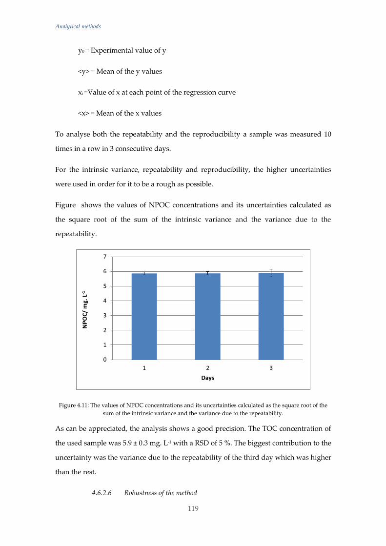
Analytical methods

119

y0 = Experimental value of y

<y> = Mean of the y values

xi =Value of x at each point of the regression curve

<x> = Mean of the x values

To analyse both the repeatability and the reproducibility a sample was measured 10

times in a row in 3 consecutive days.

For the intrinsic variance, repeatability and reproducibility, the higher uncertainties

were used in order for it to be a rough as possible.

Figure shows the values of NPOC concentrations and its uncertainties calculated as

the square root of the sum of the intrinsic variance and the variance due to the

repeatability.

Figure 4.11: The values of NPOC concentrations and its uncertainties calculated as the square root of the

sum of the intrinsic variance and the variance due to the repeatability.

As can be appreciated, the analysis shows a good precision. The TOC concentration of

the used sample was 5.9 ± 0.3 mg. L-1 with a RSD of 5 %. The biggest contribution to the

uncertainty was the variance due to the repeatability of the third day which was higher

than the rest.

4.6.2.6 Robustness of the method

0

1

2

3

4

5

6

7

1 2 3

NP

OC

/ m

g. L

-1

Days

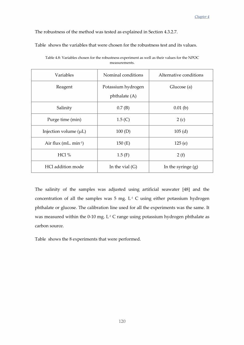
Chapter 4

120

The robustness of the method was tested as explained in Section 4.3.2.7.

Table shows the variables that were chosen for the robustness test and its values.

Table 4.8: Variables chosen for the robustness experiment as well as their values for the NPOC

measurements.

Variables Nominal conditions Alternative conditions

Reagent Potassium hydrogen

phthalate (A)

Glucose (a)

Salinity 0.7 (B) 0.01 (b)

Purge time (min) 1.5 (C) 2 (c)

Injection volume (µL) 100 (D) 105 (d)

Air flux (mL. min-1) 150 (E) 125 (e)

HCl % 1.5 (F) 2 (f)

HCl addition mode In the vial (G) In the syringe (g)

The salinity of the samples was adjusted using artificial seawater [48] and the

concentration of all the samples was 5 mg. L-1 C using either potassium hydrogen

phthalate or glucose. The calibration line used for all the experiments was the same. It

was measured within the 0-10 mg. L-1 C range using potassium hydrogen phthalate as

carbon source.

Table shows the 8 experiments that were performed.

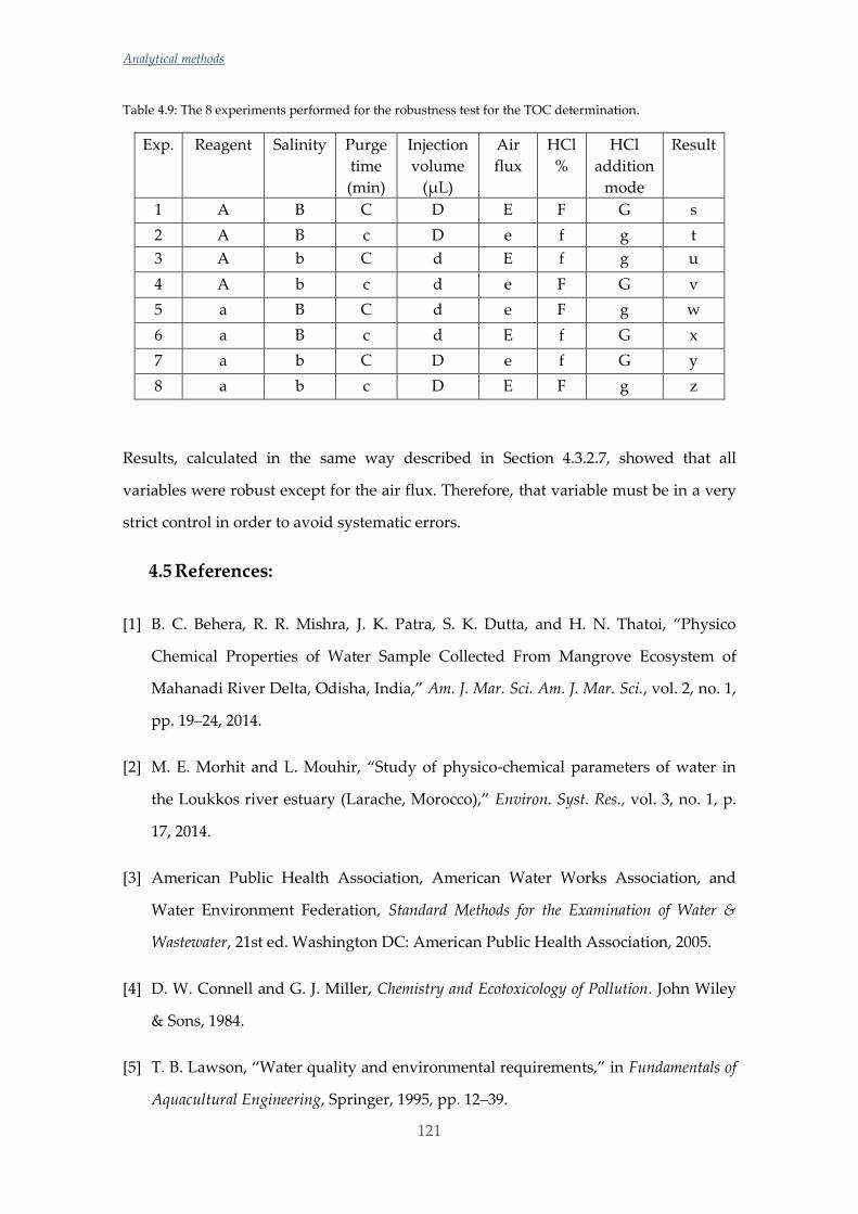
Analytical methods

121

Table 4.9: The 8 experiments performed for the robustness test for the TOC determination.

Exp. Reagent Salinity Purge

time

(min)

Injection

volume

(µL)

Air

flux

HCl

%

HCl

addition

mode

Result

1 A B C D E F G s

2 A B c D e f g t

3 A b C d E f g u

4 A b c d e F G v

5 a B C d e F g w

6 a B c d E f G x

7 a b C D e f G y

8 a b c D E F g z

Results, calculated in the same way described in Section 4.3.2.7, showed that all

variables were robust except for the air flux. Therefore, that variable must be in a very

strict control in order to avoid systematic errors.

4.5 References:

[1] B. C. Behera, R. R. Mishra, J. K. Patra, S. K. Dutta, and H. N. Thatoi, “Physico

Chemical Properties of Water Sample Collected From Mangrove Ecosystem of

Mahanadi River Delta, Odisha, India,” Am. J. Mar. Sci. Am. J. Mar. Sci., vol. 2, no. 1,

pp. 19–24, 2014.

[2] M. E. Morhit and L. Mouhir, “Study of physico-chemical parameters of water in

the Loukkos river estuary (Larache, Morocco),” Environ. Syst. Res., vol. 3, no. 1, p.

17, 2014.

[3] American Public Health Association, American Water Works Association, and

Water Environment Federation, Standard Methods for the Examination of Water &

Wastewater, 21st ed. Washington DC: American Public Health Association, 2005.

[4] D. W. Connell and G. J. Miller, Chemistry and Ecotoxicology of Pollution. John Wiley

& Sons, 1984.

[5] T. B. Lawson, “Water quality and environmental requirements,” in Fundamentals of

Aquacultural Engineering, Springer, 1995, pp. 12–39.

Chapter 4

122

[6] M. E. Borsuk, C. A. Stow, R. A. Luettich, H. W. Paerl, and J. L. Pinckney,

“Modelling oxygen dynamics in an intermittently stratified estuary: Estimation of

process rates using field data,” Estuar. Coast. Shelf Sci., vol. 52, no. 1, pp. 33–49,

2001.

[7] U. S. Environmental Protection Agency, Methods for Chemical Analysis of Water and

Wastes, Section 9.3, EPA/600/4-79/020. Cincinnati, 1983.

[8] I. Klimant and O. S. Wolfbeis, “Oxygen-Sensitive Luminescent Materials Based on

Silicone-Soluble Ruthenium Diimine Complexes,” Anal. Chem., vol. 67, no. 18, pp.

3160–3166, 1995.

[9] A. Mills and M. Thomas, “Fluorescence-based Thin Plastic Film Ion-pair Sensors

forOxygen,” Analyst, vol. 122, no. 1, pp. 63–68, 1997.

[10] J. J. McKeown, L. C. Brown, and G. W. Gove, “Comparative studies of dissolved

oxygen analysis methods,” J. - Water Pollut. Control Fed., vol. 39, no. 8, pp. 1323–

1336, 1967.

[11] L. W. Winkler, “Die bestimmung des im wasser gelösten sauerstoffes,” Berichte

Dtsch. Chem. Ges., vol. 21, no. 2, pp. 2843–2854, 1888.

[12] J. H. Carpenter, “The accuracy of the Winkler method for dissolved oxygen

analysis,” Limnol. Oceanogr., vol. 10, no. 1, pp. 135–140, 1965.

[13] J. H. Carpenter, “The Chesapeake Bay Institute Technique for the Winkler

Dissolved Oxygen Method,” Limnol. Oceanogr., vol. 10, no. 1, pp. 141–143, 1965.

[14] T. Labasque, C. Chaumery, A. Aminot, and G. Kergoat, “Spectrophotometric

Winkler determination of dissolved oxygen: re-examination of critical factors and

reliability,” Mar. Chem., vol. 88, no. 1–2, pp. 53–60, 2004.

[15] S.-C. Pai, G.-C. Gong, and K.-K. Liu, “Determination of dissolved oxygen in

seawater by direct spectrophotometry of total iodine,” Mar. Chem., vol. 41, no. 4,

pp. 343–351, 1993.

Analytical methods

123

[16] C. N. Murray, J. P. Riley, and T. R. S. Wilson, “The solubility of oxygen in Winkler

reagents used for the determination of dissolved oxygen,” in Deep Sea Research and

Oceanographic Abstracts, 1968, vol. 15, pp. 237–238.

[17] J. W. Erisman, A. Bleeker, J. Galloway, and M. S. Sutton, “Reduced nitrogen in

ecology and the environment,” Environ. Pollut., vol. 150, no. 1, pp. 140–149, 2007.

[18] O. Johansson and M. Wedborg, “The ammonia-ammonium equilibrium in

seawater at temperatures between 5 and 25°C,” J. Solut. Chem., vol. 9, no. 1, pp. 37–

44, 1980.

[19] P. J. Statham, “Nutrients in estuaries — An overview and the potential impacts of

climate change,” Sci. Total Environ., vol. 434, pp. 213–227, 2012.

[20] R. W. Howarth and R. Marino, “Nitrogen as the limiting nutrient for

eutrophication in coastal marine ecosystems: Evolving views over three decades,”

Limnol. Oceanogr., vol. 51, no. 1part2, pp. 364–376, 2006.

[21] J. Xu et al., “Temporal and spatial variations in nutrient stoichiometry and

regulation of phytoplankton biomass in Hong Kong waters: Influence of the Pearl

River outflow and sewage inputs,” Mar. Pollut. Bull., vol. 57, no. 6–12, pp. 335–348,

2008.

[22] A. Paytan and K. McLaughlin, “The Oceanic Phosphorus Cycle,” Chem. Rev., vol.

107, no. 2, pp. 563–576, 2007.

[23] F. B. Eddy, “Ammonia in estuaries and effects on fish,” J. Fish Biol., vol. 67, no. 6,

pp. 1495–1513, 2005.

[24] T. G. Bell, M. T. Johnson, T. D. Jickells, and P. S. Liss, “Ammonia/ammonium

dissociation coefficient in seawater: A significant numerical correction,” Environ.

Chem., vol. 4, no. 3, pp. 183–186, 1800.

[25] T. G. Bell, M. T. Johnson, T. D. Jickells, and P. S. Liss, “Corrigendum to:

Ammonia/ammonium dissociation coefficient in seawater: A significant numerical

correction,” Environ. Chem., vol. 5, no. 3, pp. 258–258, 2008.

Chapter 4

124

[26] P. K. Quinn, K. J. Barrett, F. J. Dentener, F. Lipschultz, and K. D. Six, “Estimation of

the air/sea exchange of ammonia for the North Atlantic Basin,” Biogeochemistry, vol.

35, no. 1, pp. 275–304, 1996.

[27] J. Louis, C. Guieu, and F. Gazeau, “Nutrient dynamics under different ocean

acidification scenarios in a low nutrient low chlorophyll system: The Northwestern

Mediterranean Sea,” Estuar. Coast. Shelf Sci., vol. 186, Part A, pp. 30–44, 2017.

[28] K. Lukawska-Matuszewska, “Contribution of non-carbonate inorganic and organic

alkalinity to total measured alkalinity in pore waters in marine sediments (Gulf of

Gdansk, S-E Baltic Sea),” Mar. Chem., vol. 186, pp. 211–220, 2016.

[29] F. J. Millero, “The Marine Inorganic Carbon Cycle,” Chem. Rev., vol. 107, no. 2, pp.

308–341, 2007.

[30] Y. Zhu, D. Yuan, Y. Huang, J. Ma, S. Feng, and K. Lin, “A modified method for on-

line determination of trace ammonium in seawater with a long-path liquid

waveguide capillary cell and spectrophotometric detection,” Mar. Chem., vol. 162,

pp. 114–121, 2014.

[31] F. Hashihama, J. Kanda, A. Tauchi, T. Kodama, H. Saito, and K. Furuya, “Liquid

waveguide spectrophotometric measurement of nanomolar ammonium in

seawater based on the indophenol reaction with o-phenylphenol (OPP),” Talanta,

vol. 143, pp. 374–380, 2015.

[32] Y. Zhu, D. Yuan, Y. Huang, J. Ma, and S. Feng, “A sensitive flow-batch system for

on board determination of ultra-trace ammonium in seawater: Method

development and shipboard application,” Anal. Chim. Acta, vol. 794, pp. 47–54,

2013.

[33] L. O. Šraj, M. I. G. S. Almeida, S. E. Swearer, S. D. Kolev, and I. D. McKelvie,

“Analytical challenges and advantages of using flow-based methodologies for

ammonia determination in estuarine and marine waters,” TrAC Trends Anal. Chem.,

vol. 59, pp. 83–92, 2014.

Analytical methods

125

[34] S. Wang, K. Lin, N. Chen, D. Yuan, and J. Ma, “Automated determination of nitrate

plus nitrite in aqueous samples with flow injection analysis using vanadium (III)

chloride as reductant,” Talanta, vol. 146, pp. 744–748, 2016.

[35] H. P. Hansen and F. Koroleff, “Determination of nutrients,” in Methods of Seawater

Analysis, K. Grasshoff, K. Kremling, and nfred Ehrhardt, Eds. Wiley-VCH Verlag

GmbH, 1999, pp. 159–228.

[36] P. S. Ellis, A. M. H. Shabani, B. S. Gentle, and I. D. McKelvie, “Field measurement

of nitrate in marine and estuarine waters with a flow analysis system utilizing on-

line zinc reduction,” Talanta, vol. 84, no. 1, pp. 98–103, 2011.

[37] J. Ma, L. Adornato, R. H. Byrne, and D. Yuan, “Determination of nanomolar levels

of nutrients in seawater,” TrAC Trends Anal. Chem., vol. 60, pp. 1–15, 2014.

[38] S. W. Willason and K. S. Johnson, “A rapid, highly sensitive technique for the

determination of ammonia in seawater,” Mar. Biol., vol. 91, no. 2, pp. 285–290, 1986.

[39] C. Garside, G. Hull, and S. Murray, “Determination of submicromolar

concentrations of ammonia in natural waters by a standard addition method using

a gas-sensing electrode1,” Limnol. Oceanogr., vol. 23, no. 5, pp. 1073–1076, 1978.

[40] A. Hulanicki, R. Lewandowski, and M. Maj, “Determination of nitrate in water

with a new construction of ion-selective electrode,” Anal. Chim. Acta, vol. 69, no. 2,

pp. 409–414, 1974.

[41] P. J. Milham, A. S. Awad, R. E. Paull, and J. H. Bull, “Analysis of plants, soils and

waters for nitrate by using an ion-selective electrode,” Analyst, vol. 95, no. 1133, pp.

751–757, 1970.

[42] E. H. Hansen, A. K. Ghose, and J. Růžička, “Flow injection analysis of

environmental samples for nitrate using an ion-selective electrode,” Analyst, vol.

102, no. 1219, pp. 705–713, 1977.

[43] R. De Marco, G. Clarke, and B. Pejcic, “Ion-Selective Electrode Potentiometry in

Environmental Analysis,” Electroanalysis, vol. 19, no. 19–20, pp. 1987–2001, 2007.

Chapter 4

126

[44] S. Winkler, L. Rieger, E. Saracevic, A. Pressl, and G. Gruber, “Application of ion-

sensitive sensors in water quality monitoring,” Water Sci. Technol., vol. 50, no. 11,

pp. 105–114, 2004.

[45] J. N. Miller and J. C. Miller, Statistics and Chemometrics for Analytical Chemistry.

Prentice Hall/Pearson, 2010.

[46] G. Bagur, M. Sánchez-Viñas, D. Gázquez, M. Ortega, and R. Romero, “Estimation

of the uncertainty associated with the standard addition methodology when a

matrix effect is detected,” Talanta, vol. 66, no. 5, pp. 1168–1174, 2005.

[47] L. Kortazar, J. Sáez, J. Agirre, J. K. Izaguirre, and L. A. Fernández, “Application of

multivariate analysis to the turbidimetric determination of sulphate in seawater,”

Anal. Methods, vol. 6, no. 10, pp. 3510–3514, 2014.

[48] C. De Stefano, C. Foti, S. Sammartano, A. Gianguzza, and C. Rigano, “Equilibrium

Studies in Natural Fluids. Use of Synthetic Seawaters and Other Media as

Background Salts,” Ann. Chim., vol. 84, pp. 159–175, 1994.

[49] International Conference on Harmonisation, ICH, “ICH Topic Q 2B. Validation of

Analytical Procedures: Methodology.” 2005.

[50] W. J. Youden and E. H. Steiner, Statistical manual of the Association of Official

Analytical Chemists. Washington DC: AOAC International, 1975.

[51] I. da C. César and G. A. Pianetti, “Robustness evaluation of the chromatographic

method for the quantitation of lumefantrine using Youden’s test,” Braz. J. Pharm.

Sci., vol. 45, no. 2, pp. 235–240, 2009.

[52] T. Tyrrell, “The relative influences of nitrogen and phosphorus on oceanic primary

production,” Nature, vol. 400, no. 6744, pp. 525–531, 1999.

[53] M. D. Patey, M. J. A. Rijkenberg, P. J. Statham, M. C. Stinchcombe, E. P.

Achterberg, and M. Mowlem, “Determination of nitrate and phosphate in seawater

at nanomolar concentrations,” TrAC Trends Anal. Chem., vol. 27, no. 2, pp. 169–182,

2008.

Analytical methods

127

[54] D. A. Wolf-Gladrow, R. E. Zeebe, C. Klaas, A. Körtzinger, and A. G. Dickson,

“Total alkalinity: The explicit conservative expression and its application to

biogeochemical processes,” Mar. Chem., vol. 106, no. 1–2, pp. 287–300, 2007.

[55] U. Riebesell, V. J. Fabry, L. Hansson, and J.-P. Gattuso, Guide to best practices for

ocean acidification research and data reporting, 1st ed. Luxembourg: Publications

Office of the European Union, 2010.

[56] J.-P. Gattuso and L. Hansson, Ocean Acidification, 1st ed. New York: Oxford

University Press, 2011.

[57] A. G. Dickson, C. L. Sabine, and J. R. Christian, Guide to best practices for ocean CO2

measurements. PICES Special Publication 3, 2007.

[58] L. Kröckel, H. Lehmann, T. Wieduwilt, and M. A. Schmidt, “Fluorescence detection

for phosphate monitoring using reverse injection analysis,” Talanta, vol. 125, pp.

107–113, 2014.

[59] F.-E. Legiret et al., “A high performance microfluidic analyser for phosphate

measurements in marine waters using the vanadomolybdate method,” Talanta, vol.

116, pp. 382–387, 2013.

[60] Q. P. Li, D. A. Hansell, and J.-Z. Zhang, “Underway monitoring of nanomolar

nitrate plus nitrite and phosphate in oligotrophic seawater,” Limnol. Oceanogr.

Methods, vol. 6, no. 7, pp. 319–326, 2008.

[61] J. Ma, D. Yuan, M. Zhang, and Y. Liang, “Reverse flow injection analysis of

nanomolar soluble reactive phosphorus in seawater with a long path length liquid

waveguide capillary cell and spectrophotometric detection,” Talanta, vol. 78, no. 1,

pp. 315–320, 2009.

[62] E. Anagnostou and R. M. Sherrell, “MAGIC method for subnanomolar

orthophosphate determination in freshwater,” Limnol. Oceanogr. Methods, vol. 6, no.

1, pp. 64–74, 2008.

Chapter 4

128

[63] L. M. L. Nollet and L. S. P. De Gelder, Handbook of water analysis, 3rd ed. New York:

Taylor & Francis Group, 2014.

[64] J. M. Estela and V. Cerdà, “Flow analysis techniques for phosphorus: an

overview,” Talanta, vol. 66, no. 2, pp. 307–331, 2005.

[65] E. H. Hansen and M. Miró, “How flow-injection analysis (FIA) over the past 25

years has changed our way of performing chemical analyses,” TrAC Trends Anal.

Chem., vol. 26, no. 1, pp. 18–26, 2007.

[66] J. Murphy and J. P. Riley, “A modified single solution method for the

determination of phosphate in natural waters,” Anal. Chim. Acta, vol. 27, pp. 31–36,

1962.

[67] J. Ma and R. H. Byrne, “Flow injection analysis of nanomolar silicate using long

pathlength absorbance spectroscopy,” Talanta, vol. 88, pp. 484–489, 2012.

[68] K. Grasshoff, M. Ehrhardt, K. Kremling, and L. G. Anderson, Methods of seawater

analysis, 3rd ed. Weinheim; New York: Wiley-VCH, 1999.

[69] A. C. B. Dias, E. P. Borges, E. A. G. Zagatto, and P. J. Worsfold, “A critical

examination of the components of the Schlieren effect in flow analysis,” Talanta,

vol. 68, no. 4, pp. 1076–1082, 2006.

[70] E. A. G. Zagatto and P. Worsfold, Flow Analysis with Spectrophotometric and

Luminometric Detection, 1st ed. Elsevier, 2012.

[71] I. D. McKelvie, D. M. W. Peat, G. P. Matthews, and P. J. Worsfold, “Elimination of

the Schlieren effect in the determination of reactive phosphorus in estuarine waters

by flow-injection analysis,” Anal. Chim. Acta, vol. 351, no. 1, pp. 265–271, 1997.

[72] P. MacLaurin, P. J. Worsfold, P. Norman, and M. Crane, “Partial least squares

resolution of multianalyte flow injection data,” Analyst, vol. 118, no. 6, pp. 617–622,

1993.

Analytical methods

129

[73] J. Saurina and S. Hernández-Cassou, “Quantitative determinations in conventional

flow injection analysis based on different chemometric calibration statregies: a

review,” Anal. Chim. Acta, vol. 438, no. 1–2, pp. 335–352, 2001.

[74] K. H. Esbensen, D. Guyot, F. Westad, and L. P. Houmoller, Multivariate Data

Analysis: In Practice : an Introduction to Multivariate Data Analysis and Experimental

Design. Multivariate Data Analysis, 2002.

[75] L. Kortazar, S. Alberdi, E. Tynan, and L. A. Fernández, “An adapted flow injection

analysis method of phosphate for estuarine samples avoiding matrix effects,”

Microchem. J., vol. 124, pp. 416–421, 2016.

[76] P. R. Loconto, Trace Environmental Quantitative Analysis: Principles: Techniques, and

Applications. CRC Press, 2001.

[77] P. Rimmelin-Maury, T. Moutin, and B. Quéguiner, “A new method for nanomolar

determination of silicic acid in seawater,” Anal. Chim. Acta, vol. 587, no. 2, pp. 281–

286, 2007.

[78] H. H. Dürr, M. Meybeck, J. Hartmann, G. G. Laruelle, and V. Roubeix, “Global

spatial distribution of natural riverine silica inputs to the coastal zone,”

Biogeosciences, vol. 8, no. 3, pp. 597–620, 2011.

[79] E. S. Eiriksdottir, E. H. Oelkers, J. Hardardottir, and S. R. Gislason, “The impact of

damming on riverine fluxes to the ocean: A case study from Eastern Iceland.,”

Water Res., vol. 113, pp. 124–138, 2017.

[80] R. Ramachandran and P. K. Gupta, “An improved spectrophotometric

determination of silicate in water based on molybdenum blue,” Anal. Chim. Acta,

vol. 172, pp. 307–311, 1985.

[81] N. Amornthammarong and J.-Z. Zhang, “Liquid-waveguide spectrophotometric

measurement of low silicate in natural waters,” Talanta, vol. 79, no. 3, pp. 621–626,

2009.

Chapter 4

130

[82] Y. Yokoyama, T. Danno, M. Haginoya, Y. Yaso, and H. Sato, “Simultaneous

determination of silicate and phosphate in environmental waters using pre-column

derivatization ion-pair liquid chromatography,” Talanta, vol. 79, no. 2, pp. 308–313,

2009.

[83] T. Yokoyama, Y. Hirai, N. Yoza, T. Tarutani, and S. Ohashi, “Spectrophotometric

determination of silicic acid by flow injection analysis,” Bull. Chem. Soc. Jpn., vol.

55, no. 11, pp. 3477–3481, 1982.

[84] R. A. Chalmers and A. G. Sinclair, “Analytical applications of β-heteropoly acids,”

Anal. Chim. Acta, vol. 34, pp. 412–418, 1966.

[85] E. H. Hansen, “Exploiting kinetic-based flow-injection methods for qunatitative

chemical assays,” Anal. Chim. Acta, vol. 261, no. 1, pp. 125–136, 1992.

[86] F. Mas-Torres and V. Cerdà, “Simultaneous Determination of Phosphate and

Silicate in Waste Water by Sequential Injection Analysis,” Analyst, vol. 122, no. 10,

pp. 1033–1038, 1997.

[87] C. X. Galhardo and J. C. Masini, “Spectrophotometric determination of phosphate

and silicate by sequential injection using molybdenum blue chemistry,” Anal.

Chim. Acta, vol. 417, no. 2, pp. 191–200, 2000.

[88] K. Grudpan et al., “Stopped-flow injection simultaneous determination of

phosphate and silicate using molybdenum blue,” Talanta, vol. 58, no. 6, pp. 1319–

1326, 2002.

[89] Y.-S. Li, Y. Muo, and H.-M. Xie, “Simultaneous determination of silicate and

phosphate in boiler water at power plants based on series flow cells by using flow

injection spectrophotometry,” Anal. Chim. Acta, vol. 455, no. 2, pp. 315–325, 2002.

[90] R. P. Moyer, C. E. Powell, D. J. Gordon, J. S. Long, and C. M. Bliss, “Abundance,

distribution, and fluxes of dissolved organic carbon (DOC) in four small sub-

tropical rivers of the Tampa Bay Estuary (Florida, USA),” Appl. Geochem., vol. 63,

pp. 550–562, 2015.

Analytical methods

131

[91] G. Visco, L. Campanella, and V. Nobili, “Organic carbons and TOC in waters: an

overview of the international norm for its measurements,” Microchem. J., vol. 79,

no. 1–2, pp. 185–191, 2005.

[92] P. Porcal, J.-F. Koprivnjak, L. A. Molot, and P. J. Dillon, “Humic substances—part

7: the biogeochemistry of dissolved organic carbon and its interactions with

climate change,” Environ. Sci. Pollut. Res., vol. 16, no. 6, pp. 714–726, 2009.

[93] W.-J. Cai, Y. Wang, and R. E. Hodson, “Acid-Base Properties of Dissolved Organic

Matter in the Estuarine Waters of Georgia, USA,” Geochim. Cosmochim. Acta, vol. 62,

no. 3, pp. 473–483, 1998.

[94] K. Kuliński, B. Schneider, K. Hammer, U. Machulik, and D. Schulz-Bull, “The

influence of dissolved organic matter on the acid–base system of the Baltic Sea,” J.

Mar. Syst., vol. 132, pp. 106–115, 2014.

[95] W. Koeve and A. Oschlies, “Potential impact of DOM accumulation on fCO2 and

carbonate ion computations in ocean acidification experiments,” Biogeosciences, vol.

9, no. 10, pp. 3787–3798, 2012.

[96] C. J. M. Hoppe, G. Langer, S. D. Rokitta, D. A. Wolf-Gladrow, and B. Rost,

“Implications of observed inconsistencies in carbonate chemistry measurements

for ocean acidification studies,” Biogeosciences, vol. 9, no. 7, pp. 2401–2405, 2012.

[97] T. Tyrrell, S. Loucaides, B. Kelly-Gerreyn, and E. Achterberg, “Interactive comment

on ‘On CO2 pertubation experiments: over-determination of carbonate chemistry

reveals inconsistencies’ by C.J.M. Hoppe et al,” Biogeosciences Discuss., vol. 7, p.

C257, 2010.

[98] J. H. Sharp, R. Benner, L. Bennett, C. A. Carlson, R. Dow, and S. E. Fitzwater, “Re-

evaluation of high temperature combustion and chemical oxidation measurements

of dissolved organic carbon in seawater,” Limnol. Oceanogr., vol. 38, no. 8, pp. 1774–

1782, 1993.

[99] X. A. Álvarez-Salgado and A. E. J. Miller, “Simultaneous determination of

dissolved organic carbon and total dissolved nitrogen in seawater by high

Chapter 4

132

temperature catalytic oxidation: conditions for precise shipboard measurements,”

Mar. Chem., vol. 62, no. 3–4, pp. 325–333, 1998.

[100] J. H. Sharp, “Marine dissolved organic carbon: Are the older values correct?,”

Mar. Chem., vol. 56, no. 3, pp. 265–277, 1997.

[101] G. Spyres, M. Nimmo, P. J. Worsfold, E. P. Achterberg, and A. E. J. Miller,

“Determination of dissolved organic carbon in seawater using high temperature

catalytic oxidation techniques,” TrAC Trends Anal. Chem., vol. 19, no. 8, pp. 498–

506, 2000.

[102] A. Stubbins and T. Dittmar, “Low volume quantification of dissolved organic

carbon and dissolved nitrogen,” Limnol. Oceanogr. Methods, vol. 10, no. 5, pp. 347–

352, 2012.

[103] J. H. Sharp, “Total organic carbon in seawater — comparison of measurements

using persulfate oxidation and high temperature combustion,” Mar. Chem., vol. 1,

no. 3, pp. 211–229, 1973.

[104] P. Avramidis, K. Nikolaou, and V. Bekiari, “Total Organic Carbon and Total

Nitrogen in Sediments and Soils: A Comparison of the Wet Oxidation – Titration

Method with the Combustion-infrared Method,” Agric. Agric. Sci. Procedia, vol. 4,

pp. 425–430, 2015.

Chapter 5

Study of the seasonal and interannual

variability of the physico-chemical

parameters and nutrients

Study of the seasonal and interannual variability of the physico-chemical parameters and nutrients

135

5.1 Introduction

Most estuaries and coastal waters receive large amounts of nutrients and pollutants

from urban, agricultural and industrial effluents [1]. Therefore, it is crucial to collect as

much information as possible about their distribution and behaviour. The distribution

of nutrients in these waters shows significant variations depending on their

environment and history, mostly due to anthropogenic sources. Nitrate and phosphate

contributions usually come from land use, fertilizer application and population density

while silicate appears in surface waters as a result of the weathering of sedimentary

and crystalline rocks [2]. Inorganic nitrogen and phosphate are among the most

important substances playing a key role in phytoplankton growth and abundance [3],

[4], and an excess of biologically available nutrient content can lead to eutrophication,

loss of oxygen and, consequently, loss of biodiversity [5]–[7]. Hence, it is fundamental

to control the nutrient content of estuaries and coastal waters as these are one of the

most productive natural ecosystems.

A change on the chemical composition of an estuary or coastal water body would lead

to a change on its physico-chemical parameters. So, monitoring the physico-chemical

parameters could give an early and fast idea about the water quality condition [8], [9].

If the estuary is in a good condition, according to Marcet's Principle, the dilution

produced by the river freshwater should be proportional for each component. This

means that those substances have a conservative mixing in the estuary. But when that

is not the case, it might be due to polluted environments, accidental spills or even

extraordinary weather conditions [10].

Therefore, even if the main objective of this work is more closely related to estuarine

acidification, it could be interesting to study the variability of these nutrients and

physico-chemical parameters in order to assess the quality of the waters of these

estuaries as well as their seasonal variation through these four years. As explained in

Chapter 3, the three estuaries studied in this work have a very different pollution

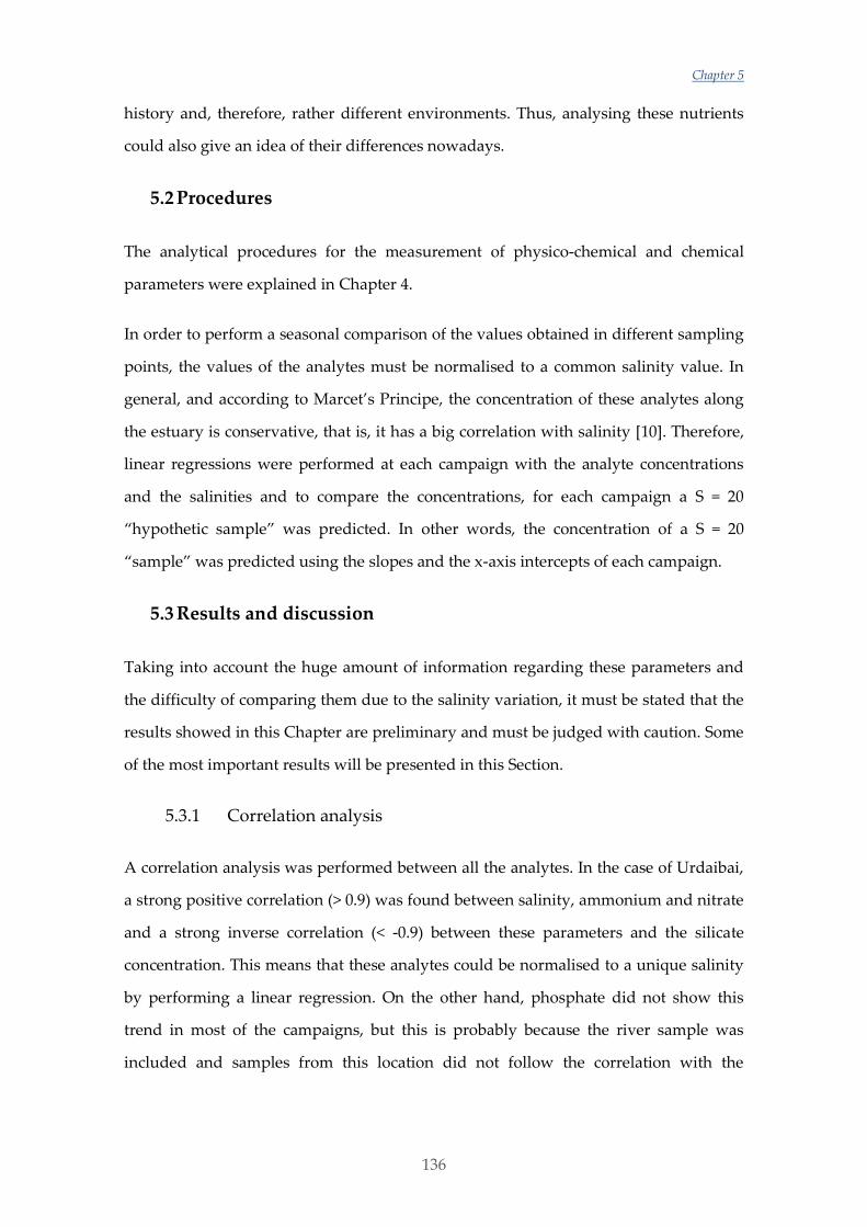
Chapter 5

136

history and, therefore, rather different environments. Thus, analysing these nutrients

could also give an idea of their differences nowadays.

5.2 Procedures

The analytical procedures for the measurement of physico-chemical and chemical

parameters were explained in Chapter 4.

In order to perform a seasonal comparison of the values obtained in different sampling

points, the values of the analytes must be normalised to a common salinity value. In

general, and according to Marcet’s Principe, the concentration of these analytes along

the estuary is conservative, that is, it has a big correlation with salinity [10]. Therefore,

linear regressions were performed at each campaign with the analyte concentrations

and the salinities and to compare the concentrations, for each campaign a S = 20

“hypothetic sample” was predicted. In other words, the concentration of a S = 20

“sample” was predicted using the slopes and the x-axis intercepts of each campaign.

5.3 Results and discussion

Taking into account the huge amount of information regarding these parameters and

the difficulty of comparing them due to the salinity variation, it must be stated that the

results showed in this Chapter are preliminary and must be judged with caution. Some

of the most important results will be presented in this Section.

5.3.1 Correlation analysis

A correlation analysis was performed between all the analytes. In the case of Urdaibai,

a strong positive correlation (> 0.9) was found between salinity, ammonium and nitrate

and a strong inverse correlation (< -0.9) between these parameters and the silicate

concentration. This means that these analytes could be normalised to a unique salinity

by performing a linear regression. On the other hand, phosphate did not show this

trend in most of the campaigns, but this is probably because the river sample was

included and samples from this location did not follow the correlation with the

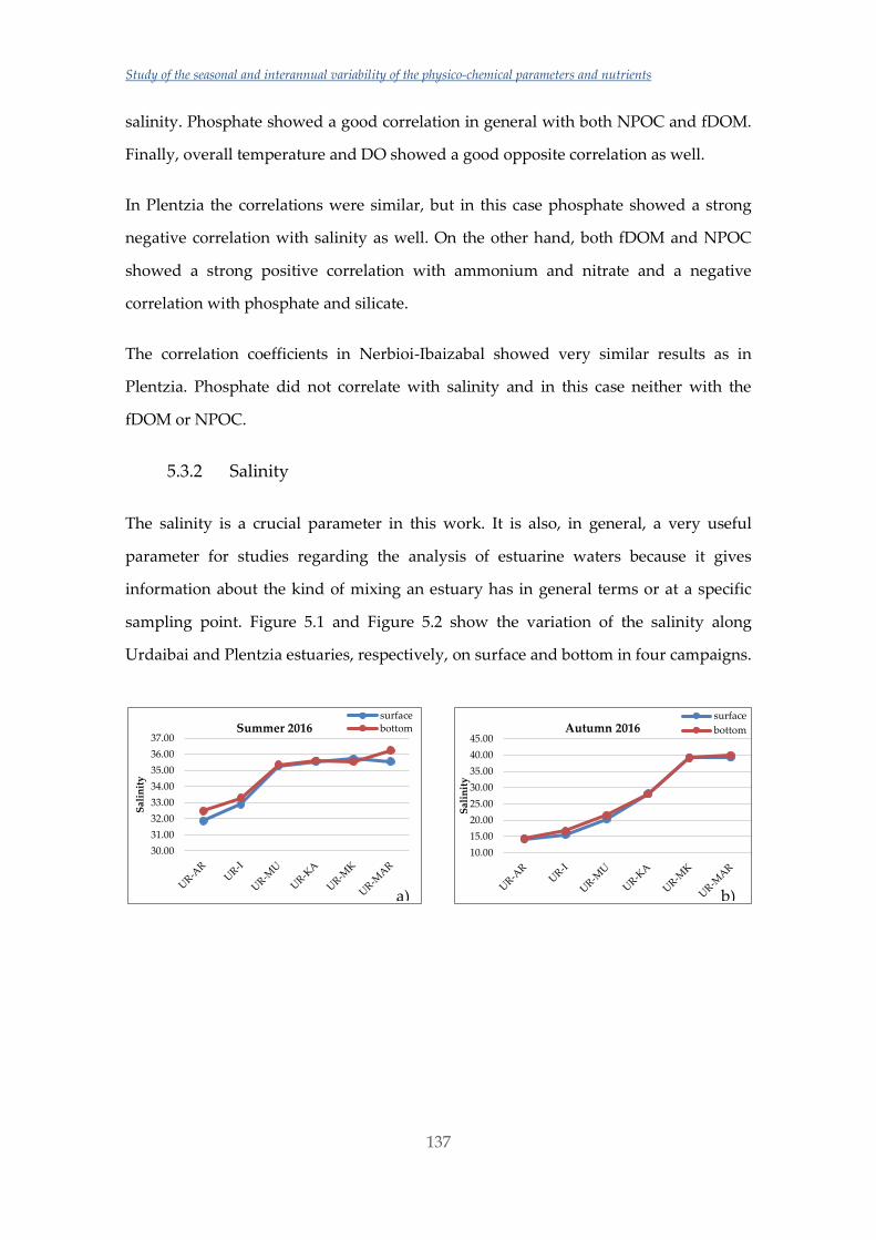
Study of the seasonal and interannual variability of the physico-chemical parameters and nutrients

137

salinity. Phosphate showed a good correlation in general with both NPOC and fDOM.

Finally, overall temperature and DO showed a good opposite correlation as well.

In Plentzia the correlations were similar, but in this case phosphate showed a strong

negative correlation with salinity as well. On the other hand, both fDOM and NPOC

showed a strong positive correlation with ammonium and nitrate and a negative

correlation with phosphate and silicate.

The correlation coefficients in Nerbioi-Ibaizabal showed very similar results as in

Plentzia. Phosphate did not correlate with salinity and in this case neither with the

fDOM or NPOC.

5.3.2 Salinity

The salinity is a crucial parameter in this work. It is also, in general, a very useful

parameter for studies regarding the analysis of estuarine waters because it gives

information about the kind of mixing an estuary has in general terms or at a specific

sampling point. Figure 5.1 and Figure 5.2 show the variation of the salinity along

Urdaibai and Plentzia estuaries, respectively, on surface and bottom in four campaigns.

30.00

31.00

32.00

33.00

34.00

35.00

36.00

37.00

Sal

init

y

Summer 2016surface

bottom

10.00

15.00

20.00

25.00

30.00

35.00

40.00

45.00

Sal

init

y

Autumn 2016surface

bottom

a) b)

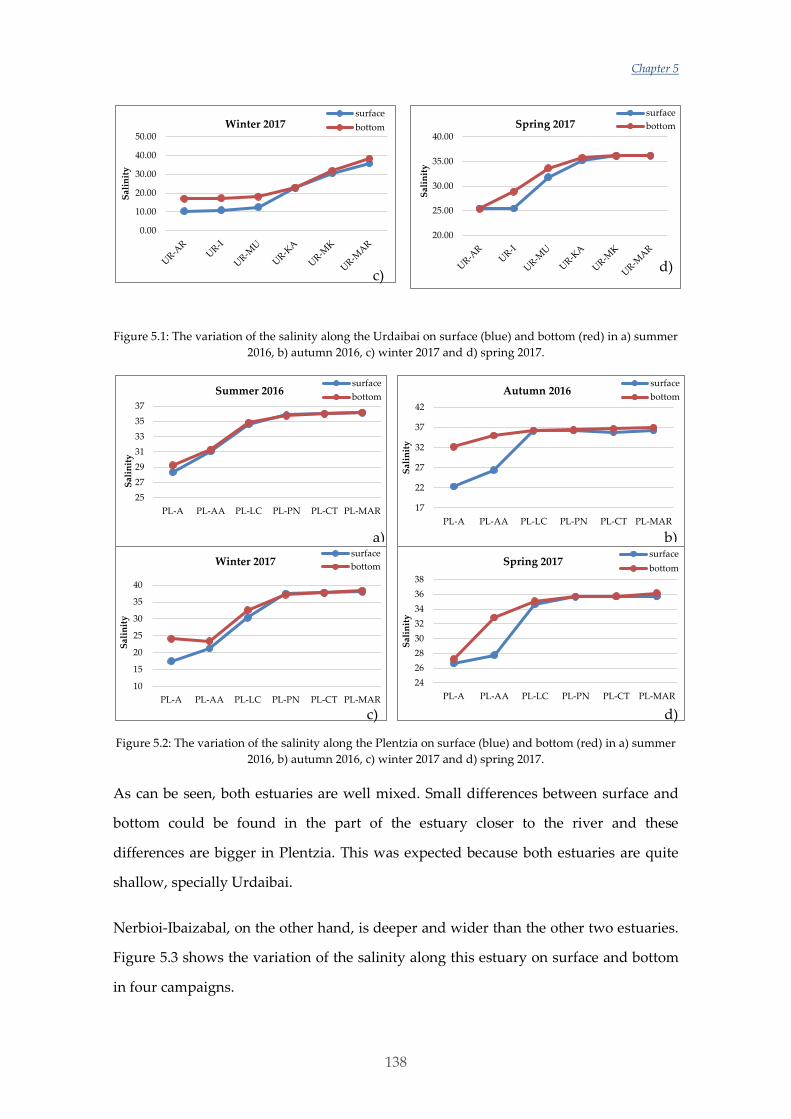
Chapter 5

138

Figure 5.1: The variation of the salinity along the Urdaibai on surface (blue) and bottom (red) in a) summer

2016, b) autumn 2016, c) winter 2017 and d) spring 2017.

Figure 5.2: The variation of the salinity along the Plentzia on surface (blue) and bottom (red) in a) summer

2016, b) autumn 2016, c) winter 2017 and d) spring 2017.

As can be seen, both estuaries are well mixed. Small differences between surface and

bottom could be found in the part of the estuary closer to the river and these

differences are bigger in Plentzia. This was expected because both estuaries are quite

shallow, specially Urdaibai.

Nerbioi-Ibaizabal, on the other hand, is deeper and wider than the other two estuaries.

Figure 5.3 shows the variation of the salinity along this estuary on surface and bottom

in four campaigns.

0.00

10.00

20.00

30.00

40.00

50.00

Sal

init

yWinter 2017

surface

bottom

20.00

25.00

30.00

35.00

40.00

Sal

init

y

Spring 2017surface

bottom

25

27

29

31

33

35

37

PL-A PL-AA PL-LC PL-PN PL-CT PL-MAR

Sal

init

y

Summer 2016surface

bottom

17

22

27

32

37

42

PL-A PL-AA PL-LC PL-PN PL-CT PL-MAR

Sal

init

y

Autumn 2016surface

bottom

10

15

20

25

30

35

40

PL-A PL-AA PL-LC PL-PN PL-CT PL-MAR

Sal

init

y

Winter 2017surface

bottom

24

26

28

30

32

34

36

38

PL-A PL-AA PL-LC PL-PN PL-CT PL-MAR

Sal

init

y

Spring 2017surface

bottom

c) d)

a) b)

c) d)

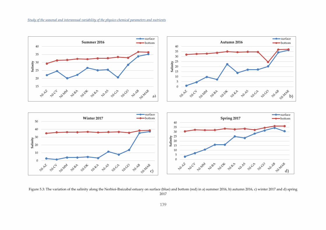
Study of the seasonal and interannual variability of the physico-chemical parameters and nutrients

139

Figure 5.3: The variation of the salinity along the Nerbioi-Ibaizabal estuary on surface (blue) and bottom (red) in a) summer 2016, b) autumn 2016, c) winter 2017 and d) spring

2017

15

20

25

30

35

40

Sal

init

y

Summer 2016surface

bottom

0

5

10

15

20

25

30

35

40

Sal

init

y

Autumn 2016surface

bottom

0

10

20

30

40

50

Sal

init

y

Winter 2017surfacebottom

0

5

10

15

20

25

30

35

40

Sal

init

y

Spring 2017surfacebottom

c)

a) b)

d)

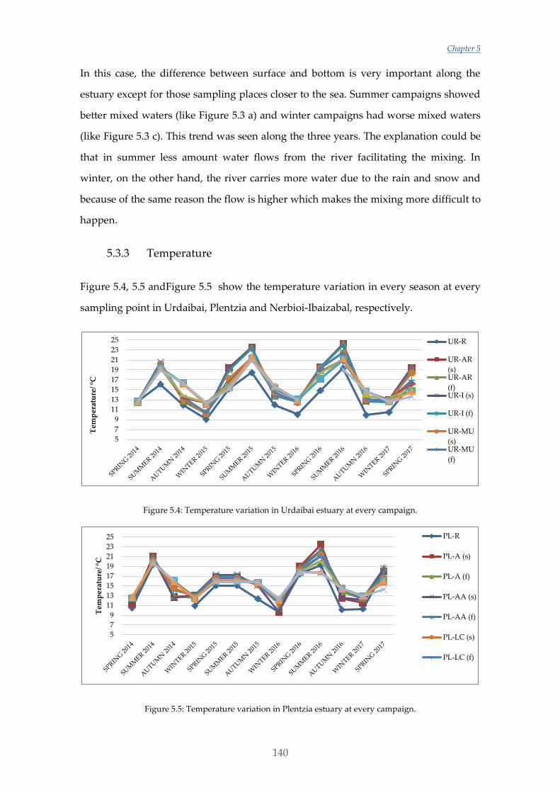
Chapter 5

140

In this case, the difference between surface and bottom is very important along the

estuary except for those sampling places closer to the sea. Summer campaigns showed

better mixed waters (like Figure 5.3 a) and winter campaigns had worse mixed waters

(like Figure 5.3 c). This trend was seen along the three years. The explanation could be

that in summer less amount water flows from the river facilitating the mixing. In

winter, on the other hand, the river carries more water due to the rain and snow and

because of the same reason the flow is higher which makes the mixing more difficult to

happen.

5.3.3 Temperature

Figure 5.4, 5.5 andFigure 5.5 show the temperature variation in every season at every

sampling point in Urdaibai, Plentzia and Nerbioi-Ibaizabal, respectively.

Figure 5.4: Temperature variation in Urdaibai estuary at every campaign.

Figure 5.5: Temperature variation in Plentzia estuary at every campaign.

5

7

9

11

13

15

17

19

21

23

25

Tem

per

atu

re/ °

C

UR-R

UR-AR

(s)UR-AR

(f)UR-I (s)

UR-I (f)

UR-MU

(s)UR-MU

(f)

5

7

9

11

13

15

17

19

21

23

25

Tem

per

atu

re/ °

C

PL-R

PL-A (s)

PL-A (f)

PL-AA (s)

PL-AA (f)

PL-LC (s)

PL-LC (f)

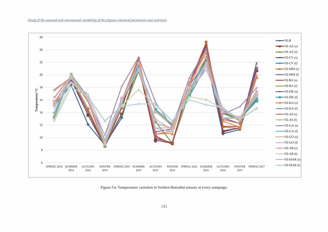
Study of the seasonal and interannual variability of the physico-chemical parameters and nutrients

141

Figure 5.6: Temperature variation in Nerbioi-Ibaizabal estuary at every campaign.

6

8

10

12

14

16

18

20

22

24

26

SPRING 2014 SUMMER

2014

AUTUMN

2014

WINTER

2015

SPRING 2015 SUMMER

2015

AUTUMN

2015

WINTER

2016

SPRING 2016 SUMMER

2016

AUTUMN

2016

WINTER

2017

SPRING 2017

Tem

per

atu

re/ °

C

NI-R

NI-AZ (s)

NI-AZ (f)

NI-CV (s)

NI-CV (f)

NI-MM (s)

NI-MM (f)

NI-BA (s)

NI-BA (f)

NI-DK (s)

NI-DK (f)

NI-KA (s)

NI-KA (f)

NI-AS (s)

NI-AS (f)

NI-GA (s)

NI-GA (f)

NI-GO (s)

NI-GO (f)

NI-AB (s)

NI-AB (f)

NI-MAR (s)

NI-MAR (f)

Chapter 5

142

Even if it is difficult to appreciate everything due to the large amount of information,

some conclusions could be obtained. The trends were quite similar in all the cases. As

is obvious, the highest temperatures were obtained in summer and the lowest in

winter. In general, higher temperatures were obtained in spring than in autumn.

Comparing the values within the same campaign, seawaters were warmer in autumn

and winter while the low salinity samples were warmer in spring and summer. This

makes sense, since the water in the estuary has less volume and hence, it is more likely

to change according to the temperature of the environment. Moreover, the river sample

seems to have the lowest temperatures in general. Even if it is not possible to

appreciate it well in Figure 5.4 and Figure 5.5, no big differences between surface and

bottom temperatures were found in Urdaibai and Plentzia estuaries, which can be

explained because they are the shallowest estuaries. However, in the Nerbioi-Ibaizabal

estuary, big differences were found between surface and bottom. These differences

depend on the season, where surface samples were warmer in spring and summer and

bottom samples were warmer in autumn and winter. This is due to the big

stratification of this estuary, where seawater flows in the bottom while freshwater

flows on the surface.

5.3.4 Dissolved oxygen

Figure 5.7, Figure 5.8 and Figure 5.9 show the distribution of the dissolved oxygen in

every season at every sampling point in Urdaibai, Plentzia and Nerbioi-Ibaizabal,

respectively. These data correspond to the measurements made with the Winkler

method (see Chapter 4 Section 4.2).

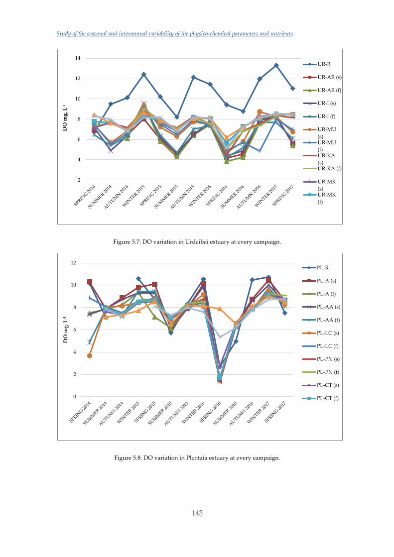
Study of the seasonal and interannual variability of the physico-chemical parameters and nutrients

143

Figure 5.7: DO variation in Urdaibai estuary at every campaign.

Figure 5.8: DO variation in Plentzia estuary at every campaign.

2

4

6

8

10

12

14D

O m

g. L

-1UR-R

UR-AR (s)

UR-AR (f)

UR-I (s)

UR-I (f)

UR-MU

(s)UR-MU

(f)UR-KA

(s)UR-KA (f)

UR-MK

(s)UR-MK

(f)

0

2

4

6

8

10

12

DO

mg

. L-1

PL-R

PL-A (s)

PL-A (f)

PL-AA (s)

PL-AA (f)

PL-LC (s)

PL-LC (f)

PL-PN (s)

PL-PN (f)

PL-CT (s)

PL-CT (f)

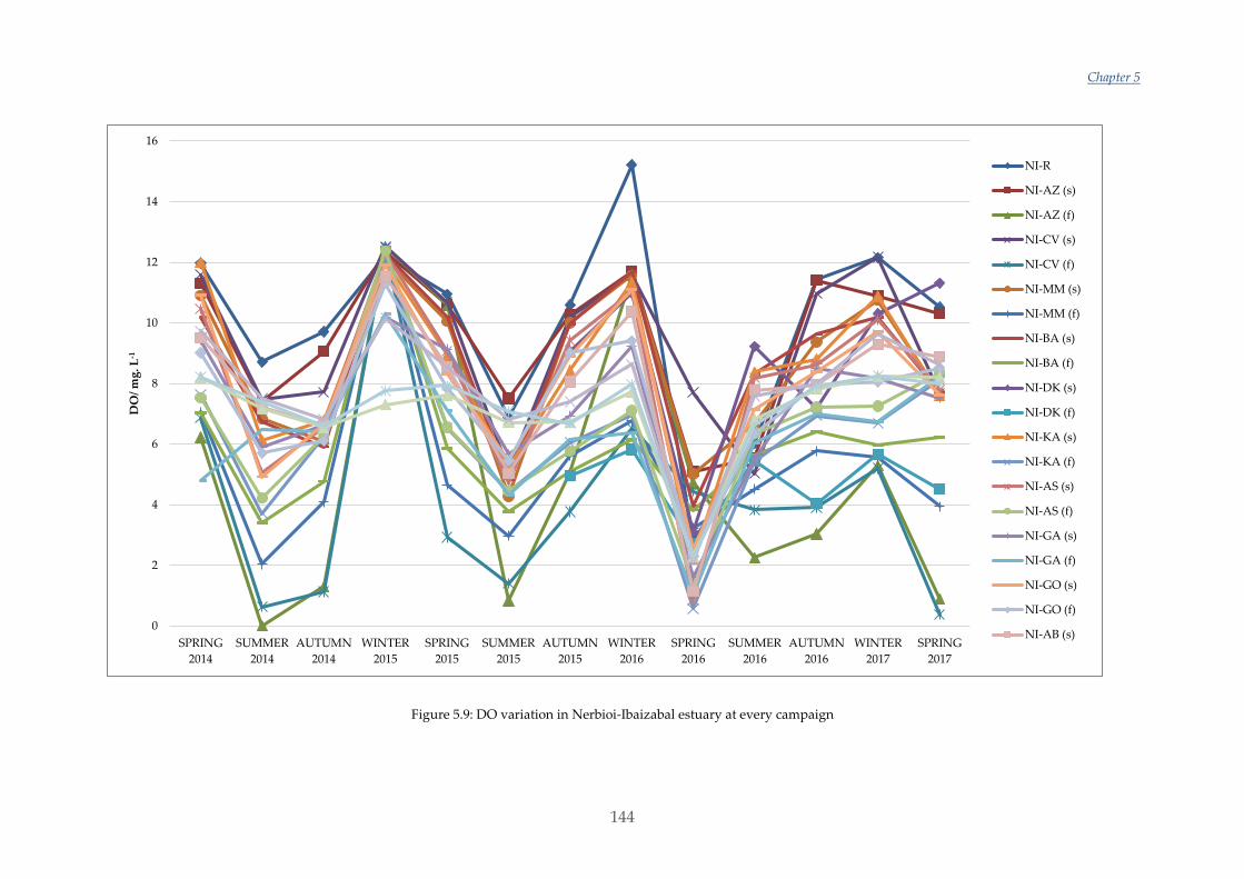
Chapter 5

144

Figure 5.9: DO variation in Nerbioi-Ibaizabal estuary at every campaign

0

2

4

6

8

10

12

14

16

SPRING

2014

SUMMER

2014

AUTUMN

2014

WINTER

2015

SPRING

2015

SUMMER

2015

AUTUMN

2015

WINTER

2016

SPRING

2016

SUMMER

2016

AUTUMN

2016

WINTER

2017

SPRING

2017

DO

/ m

g. L

-1

NI-R

NI-AZ (s)

NI-AZ (f)

NI-CV (s)

NI-CV (f)

NI-MM (s)

NI-MM (f)

NI-BA (s)

NI-BA (f)

NI-DK (s)

NI-DK (f)

NI-KA (s)

NI-KA (f)

NI-AS (s)

NI-AS (f)

NI-GA (s)

NI-GA (f)

NI-GO (s)

NI-GO (f)

NI-AB (s)

Study of the seasonal and interannual variability of the physico-chemical parameters and nutrients

145

As can be appreciated, the DO concentration in Urdaibai was much higher in the river

sample than anywhere else, while in Plentzia and Nerbioi-Ibaizabal was not so much

higher. The trend within each campaign follows the opposite to that of the temperature

in Urdaibai and Plentzia; that is, in winter and autumn higher concentrations were

found closer to the river, while in spring and summer more oxygenated waters were

found at the mouth of the estuary. Also, winter samples had higher DO concentrations

than summer samples owing to the higher oxygen solubility in cooler temperatures.

The Nerbioi-Ibaizabal estuary, due to its stratification showed different trends. Surface

waters showed a similar behaviour as the other two estuaries while bottom waters

show less or even much less oxygen concentration, mostly in those sampling points

farther away from the sea. Bottom samples of AZ and CV showed extremely low DO

concentration in some campaigns. This might be because of the lower movement of the

bottom waters in these areas that make it difficult for the water to oxygenate. The low

DO concentration at the spring campaign of 2016 indicates an error in the sampling,

storage or measurement. ODO concentrations from the probe do not show such small

concentrations.

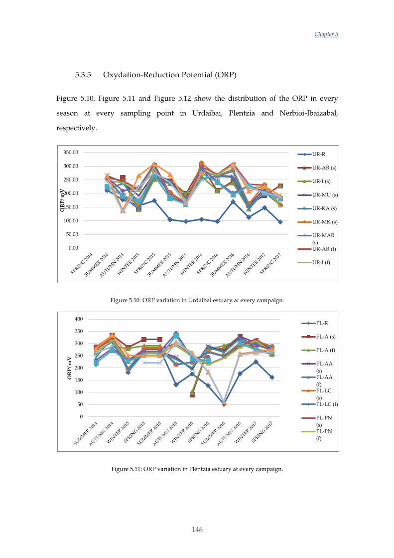
Chapter 5

146

5.3.5 Oxydation-Reduction Potential (ORP)

Figure 5.10, Figure 5.11 and Figure 5.12 show the distribution of the ORP in every

season at every sampling point in Urdaibai, Plentzia and Nerbioi-Ibaizabal,

respectively.

Figure 5.10: ORP variation in Urdaibai estuary at every campaign.

Figure 5.11: ORP variation in Plentzia estuary at every campaign.

0.00

50.00

100.00

150.00

200.00

250.00

300.00

350.00

OR

P/

mV

UR-R

UR-AR (s)

UR-I (s)

UR-MU (s)

UR-KA (s)

UR-MK (s)

UR-MAR

(s)UR-AR (f)

UR-I (f)

0

50

100

150

200

250

300

350

400

OR

P/

mV

PL-R

PL-A (s)

PL-A (f)

PL-AA

(s)PL-AA

(f)PL-LC

(s)PL-LC (f)

PL-PN

(s)PL-PN

(f)

Study of the seasonal and interannual variability of the physico-chemical parameters and nutrients

147

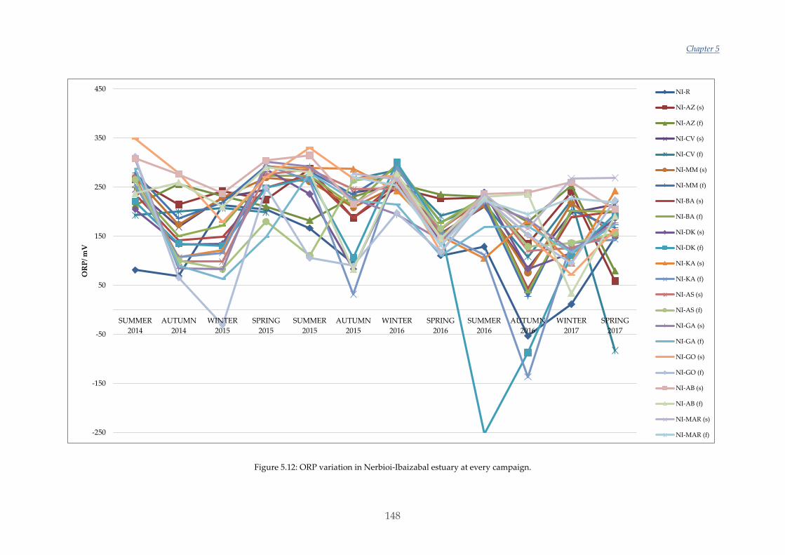
Chapter 5

148

Figure 5.12: ORP variation in Nerbioi-Ibaizabal estuary at every campaign.

-250

-150

-50

50

150

250

350

450

SUMMER

2014

AUTUMN

2014

WINTER

2015

SPRING

2015

SUMMER

2015

AUTUMN

2015

WINTER

2016

SPRING

2016

SUMMER

2016

AUTUMN

2016

WINTER

2017

SPRING

2017

OR

P/

mV

NI-R

NI-AZ (s)

NI-AZ (f)

NI-CV (s)

NI-CV (f)

NI-MM (s)

NI-MM (f)

NI-BA (s)

NI-BA (f)

NI-DK (s)

NI-DK (f)

NI-KA (s)

NI-KA (f)

NI-AS (s)

NI-AS (f)

NI-GA (s)

NI-GA (f)

NI-GO (s)

NI-GO (f)

NI-AB (s)

NI-AB (f)

NI-MAR (s)

NI-MAR (f)

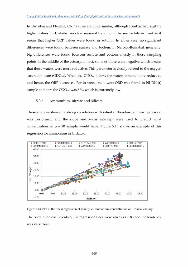
Study of the seasonal and interannual variability of the physico-chemical parameters and nutrients

149

In Urdaibai and Plentzia, ORP values are quite similar, although Plentzia had slightly

higher values. In Urdaibai no clear seasonal trend could be seen while in Plentzia it

seems that higher ORP values were found in autumn. In either case, no significant

differences were found between surface and bottom. In Nerbioi-Ibaizabal, generally,

big differences were found between surface and bottom, mostly in those sampling

points in the middle of the estuary. In fact, some of those were negative which means

that those waters were more reductive. This parameter is closely related to the oxygen

saturation state (ODOsat). When the ODOsat is low, the waters became more reductive

and hence, the ORP decreases. For instance, the lowest ORD was found in NI-DK (f)

sample and here the ODOsat was 8 %, which is extremely low.

5.3.6 Ammonium, nitrate and silicate

These analytes showed a strong correlation with salinity. Therefore, a linear regression

was performed, and the slope and x-axis intercept were used to predict what

concentration an S = 20 sample would have. Figure 5.13 shows an example of this

regression for ammonium in Urdaibai.

Figure 5.13: Plot of the linear regression of salinity vs. ammonium concentration of Urdaibai estuary.

The correlation coefficients of the regression lines were always > 0.85 and the tendency

was very clear.

-10.00

0.00

10.00

20.00

30.00

40.00

50.00

60.00

0.00 5.00 10.00 15.00 20.00 25.00 30.00 35.00 40.00 45.00

[NH

4+ ]/

mg

. L-1

Salinity

SPRING 2014 SUMMER 2014 AUTUMN 2014 WINTER 2015 SPRING 2015

SUMMER 2015 AUTUMN 2015 WINTER 2016 SPRING 2016 SUMMER 2016

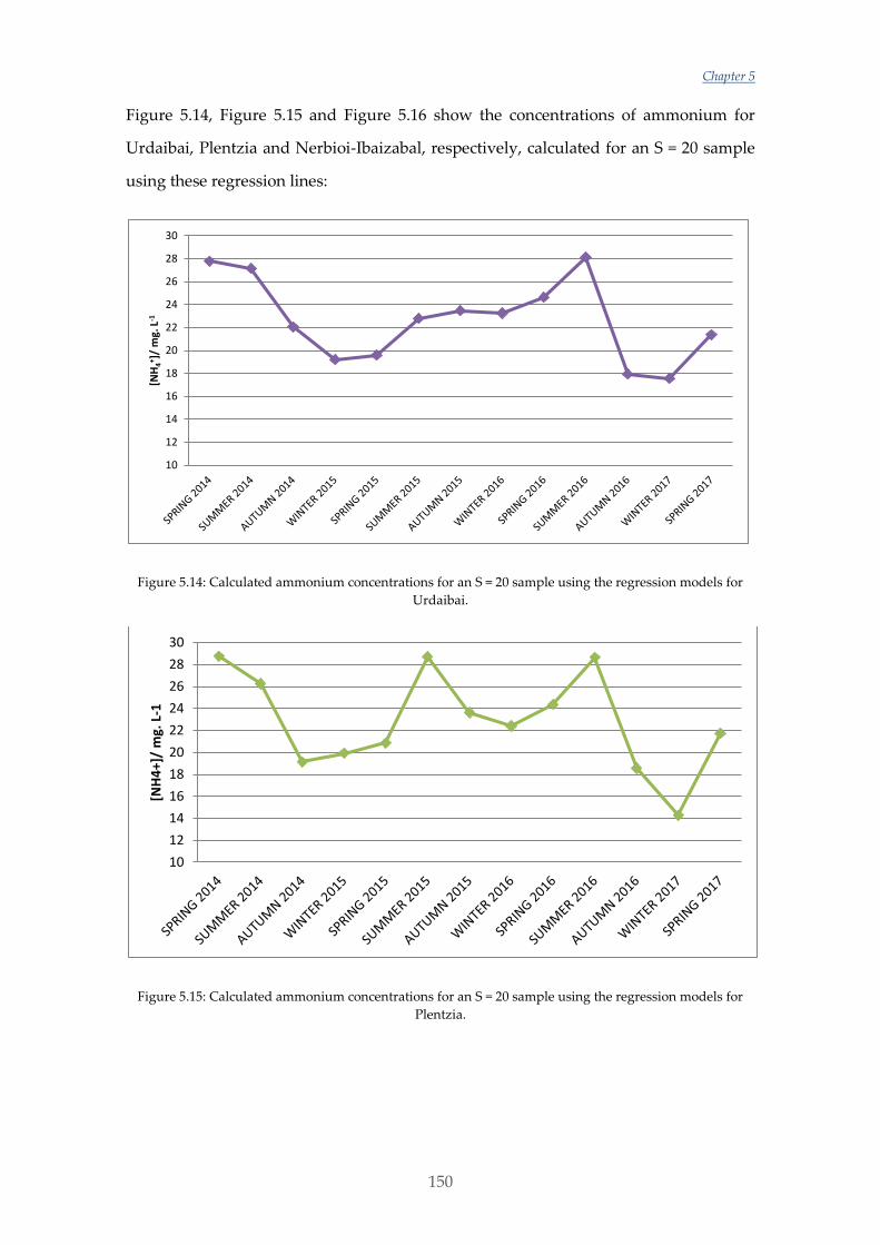
Chapter 5

150

Figure 5.14, Figure 5.15 and Figure 5.16 show the concentrations of ammonium for

Urdaibai, Plentzia and Nerbioi-Ibaizabal, respectively, calculated for an S = 20 sample

using these regression lines:

Figure 5.14: Calculated ammonium concentrations for an S = 20 sample using the regression models for

Urdaibai.

Figure 5.15: Calculated ammonium concentrations for an S = 20 sample using the regression models for

Plentzia.

10

12

14

16

18

20

22

24

26

28

30

[NH

4+]/

mg.

L-1

10

12

14

16

18

20

22

24

26

28

30

[NH

4+]

/ m

g. L

-1

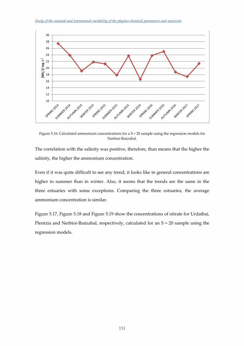
Study of the seasonal and interannual variability of the physico-chemical parameters and nutrients

151

Figure 5.16: Calculated ammonium concentrations for a S = 20 sample using the regression models for

Nerbioi-Ibaizabal.

The correlation with the salinity was positive, therefore, than means that the higher the

salinity, the higher the ammonium concentration.

Even if it was quite difficult to see any trend, it looks like in general concentrations are

higher in summer than in winter. Also, it seems that the trends are the same in the

three estuaries with some exceptions. Comparing the three estuaries, the average

ammonium concentration is similar.

Figure 5.17, Figure 5.18 and Figure 5.19 show the concentrations of nitrate for Urdaibai,

Plentzia and Nerbioi-Ibaizabal, respectively, calculated for an S = 20 sample using the

regression models.

10

12

14

16

18

20

22

24

26

28

30

[NH

4+ ]

/ m

g. L

-1

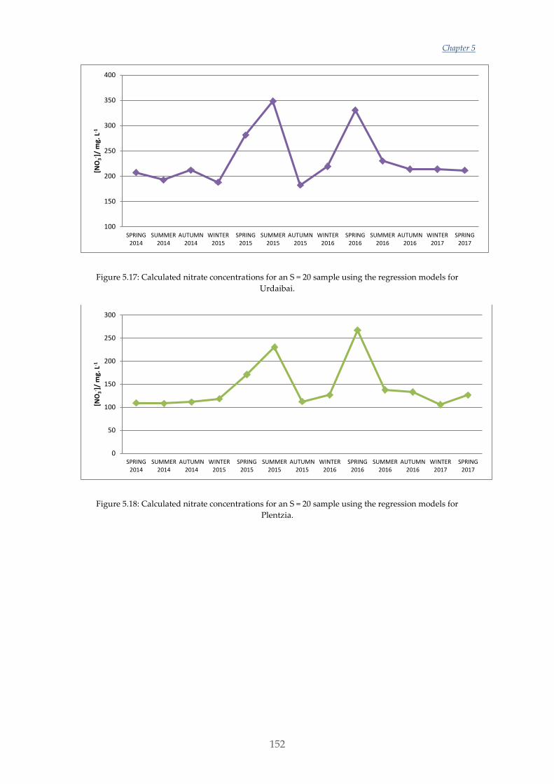
Chapter 5

152

Figure 5.17: Calculated nitrate concentrations for an S = 20 sample using the regression models for

Urdaibai.

Figure 5.18: Calculated nitrate concentrations for an S = 20 sample using the regression models for

Plentzia.

100

150

200

250

300

350

400

SPRING2014

SUMMER2014

AUTUMN2014

WINTER2015

SPRING2015

SUMMER2015

AUTUMN2015

WINTER2016

SPRING2016

SUMMER2016

AUTUMN2016

WINTER2017

SPRING2017

[NO

3- ]

/ m

g. L

-1

0

50

100

150

200

250

300

SPRING2014

SUMMER2014

AUTUMN2014

WINTER2015

SPRING2015

SUMMER2015

AUTUMN2015

WINTER2016

SPRING2016

SUMMER2016

AUTUMN2016

WINTER2017

SPRING2017

[NO

3- ]/

mg.

L-1

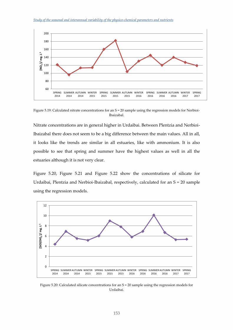
Study of the seasonal and interannual variability of the physico-chemical parameters and nutrients

153

Figure 5.19: Calculated nitrate concentrations for an S = 20 sample using the regression models for Nerbioi-

Ibaizabal.

Nitrate concentrations are in general higher in Urdaibai. Between Plentzia and Nerbioi-

Ibaizabal there does not seem to be a big difference between the main values. All in all,

it looks like the trends are similar in all estuaries, like with ammonium. It is also

possible to see that spring and summer have the highest values as well in all the

estuaries although it is not very clear.

Figure 5.20, Figure 5.21 and Figure 5.22 show the concentrations of silicate for

Urdaibai, Plentzia and Nerbioi-Ibaizabal, respectively, calculated for an S = 20 sample

using the regression models.

Figure 5.20: Calculated silicate concentrations for an S = 20 sample using the regression models for

Urdaibai.

60

80

100

120

140

160

180

200

SPRING2014

SUMMER2014

AUTUMN2014

WINTER2015

SPRING2015

SUMMER2015

AUTUMN2015

WINTER2016

SPRING2016

SUMMER2016

AUTUMN2016

WINTER2017

SPRING2017

[NO

3- ]

/ m

g. L

-1

0

2

4

6

8

10

12

SPRING2014

SUMMER2014

AUTUMN2014

WINTER2015

SPRING2015

SUMMER2015

AUTUMN2015

WINTER2016

SPRING2016

SUMMER2016

AUTUMN2016

WINTER2017

SPRING2017

[SiO

(OH

) 3- ]

/ m

g. L

-1

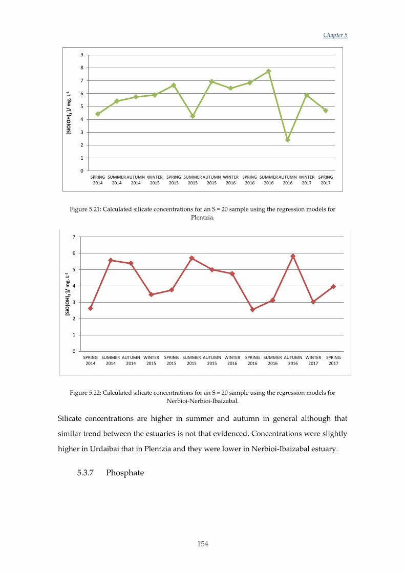
Chapter 5

154

Figure 5.21: Calculated silicate concentrations for an S = 20 sample using the regression models for

Plentzia.

Figure 5.22: Calculated silicate concentrations for an S = 20 sample using the regression models for

Nerbioi-Nerbioi-Ibaizabal.

Silicate concentrations are higher in summer and autumn in general although that

similar trend between the estuaries is not that evidenced. Concentrations were slightly

higher in Urdaibai that in Plentzia and they were lower in Nerbioi-Ibaizabal estuary.

5.3.7 Phosphate

0

1

2

3

4

5

6

7

8

9

SPRING2014

SUMMER2014

AUTUMN2014

WINTER2015

SPRING2015

SUMMER2015

AUTUMN2015

WINTER2016

SPRING2016

SUMMER2016

AUTUMN2016

WINTER2017

SPRING2017

[SiO

(OH

) 3- ]

/ m

g. L

-1

0

1

2

3

4

5

6

7

SPRING2014

SUMMER2014

AUTUMN2014

WINTER2015

SPRING2015

SUMMER2015

AUTUMN2015

WINTER2016

SPRING2016

SUMMER2016

AUTUMN2016

WINTER2017

SPRING2017

[SiO

(OH

) 3- ]

/ m

g. L

-1

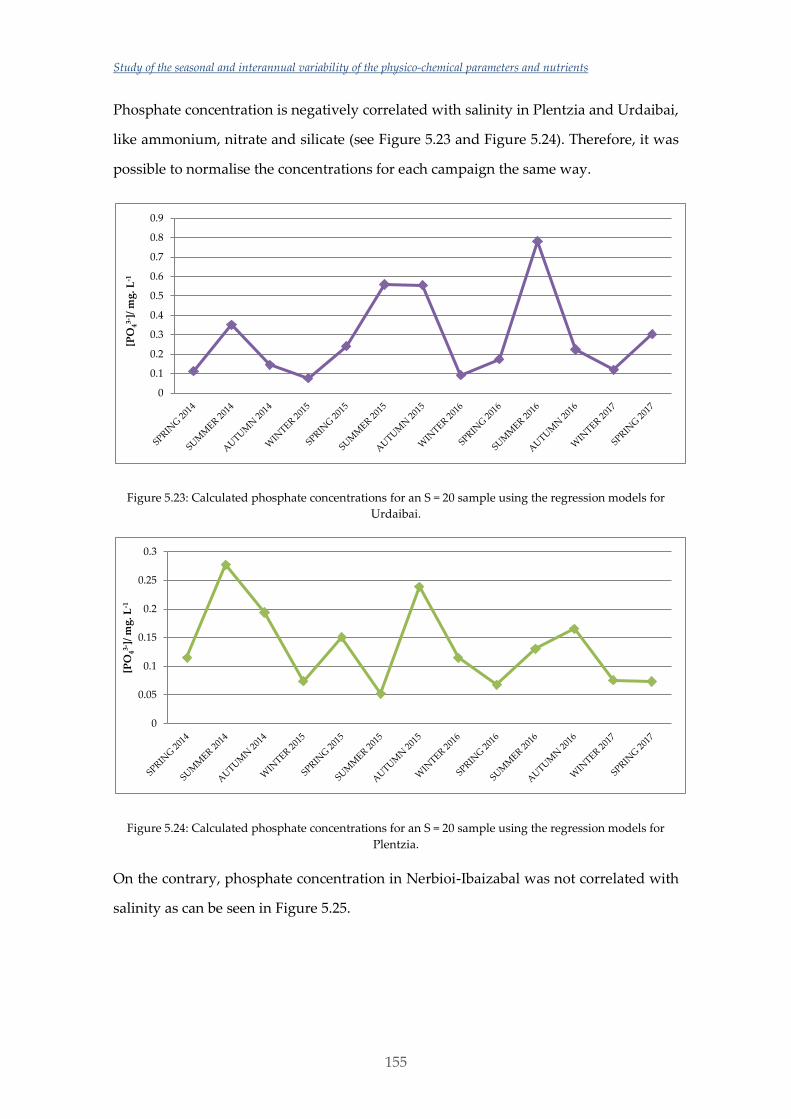
Study of the seasonal and interannual variability of the physico-chemical parameters and nutrients

155

Phosphate concentration is negatively correlated with salinity in Plentzia and Urdaibai,

like ammonium, nitrate and silicate (see Figure 5.23 and Figure 5.24). Therefore, it was

possible to normalise the concentrations for each campaign the same way.

Figure 5.23: Calculated phosphate concentrations for an S = 20 sample using the regression models for

Urdaibai.

Figure 5.24: Calculated phosphate concentrations for an S = 20 sample using the regression models for

Plentzia.

On the contrary, phosphate concentration in Nerbioi-Ibaizabal was not correlated with

salinity as can be seen in Figure 5.25.

0

0.1

0.2

0.3

0.4

0.5

0.6

0.7

0.8

0.9

[PO

43-]/

mg

. L-1

0

0.05

0.1

0.15

0.2

0.25

0.3

[PO

43-]/

mg

. L-1

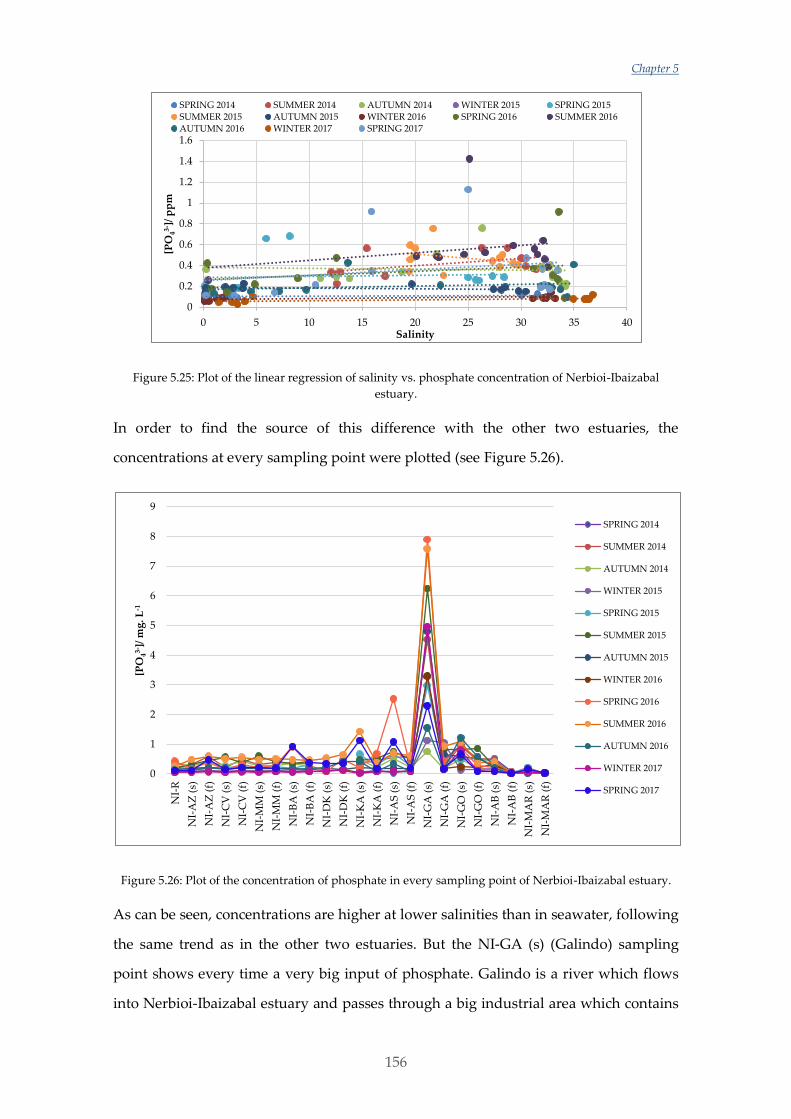
Chapter 5

156

Figure 5.25: Plot of the linear regression of salinity vs. phosphate concentration of Nerbioi-Ibaizabal

estuary.

In order to find the source of this difference with the other two estuaries, the

concentrations at every sampling point were plotted (see Figure 5.26).

Figure 5.26: Plot of the concentration of phosphate in every sampling point of Nerbioi-Ibaizabal estuary.

As can be seen, concentrations are higher at lower salinities than in seawater, following

the same trend as in the other two estuaries. But the NI-GA (s) (Galindo) sampling

point shows every time a very big input of phosphate. Galindo is a river which flows

into Nerbioi-Ibaizabal estuary and passes through a big industrial area which contains

0

0.2

0.4

0.6

0.8

1

1.2

1.4

1.6

0 5 10 15 20 25 30 35 40

[PO

43-]/

pp

m

Salinity

SPRING 2014 SUMMER 2014 AUTUMN 2014 WINTER 2015 SPRING 2015SUMMER 2015 AUTUMN 2015 WINTER 2016 SPRING 2016 SUMMER 2016AUTUMN 2016 WINTER 2017 SPRING 2017

0

1

2

3

4

5

6

7

8

9

NI-

R

NI-

AZ

(s)

NI-

AZ

(f)

NI-

CV

(s)

NI-

CV

(f)

NI-

MM

(s)

NI-

MM

(f)

NI-

BA

(s)

NI-

BA

(f)

NI-

DK

(s)

NI-

DK

(f)

NI-

KA

(s)

NI-

KA

(f)

NI-

AS

(s)

NI-

AS

(f)

NI-

GA

(s)

NI-

GA

(f)

NI-

GO

(s)

NI-

GO

(f)

NI-

AB

(s)

NI-

AB

(f)

NI-

MA

R (

s)

NI-

MA

R (

f)

[PO

43-]/

mg

. L-1

SPRING 2014

SUMMER 2014

AUTUMN 2014

WINTER 2015

SPRING 2015

SUMMER 2015

AUTUMN 2015

WINTER 2016

SPRING 2016

SUMMER 2016

AUTUMN 2016

WINTER 2017

SPRING 2017

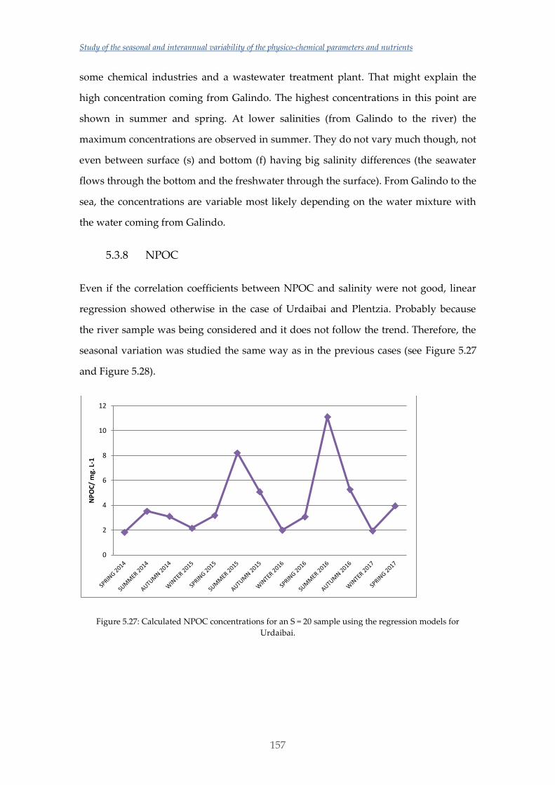
Study of the seasonal and interannual variability of the physico-chemical parameters and nutrients

157

some chemical industries and a wastewater treatment plant. That might explain the

high concentration coming from Galindo. The highest concentrations in this point are

shown in summer and spring. At lower salinities (from Galindo to the river) the

maximum concentrations are observed in summer. They do not vary much though, not

even between surface (s) and bottom (f) having big salinity differences (the seawater

flows through the bottom and the freshwater through the surface). From Galindo to the

sea, the concentrations are variable most likely depending on the water mixture with

the water coming from Galindo.

5.3.8 NPOC

Even if the correlation coefficients between NPOC and salinity were not good, linear

regression showed otherwise in the case of Urdaibai and Plentzia. Probably because

the river sample was being considered and it does not follow the trend. Therefore, the

seasonal variation was studied the same way as in the previous cases (see Figure 5.27

and Figure 5.28).

Figure 5.27: Calculated NPOC concentrations for an S = 20 sample using the regression models for

Urdaibai.

0

2

4

6

8

10

12

NP

OC

/ m

g. L

-1

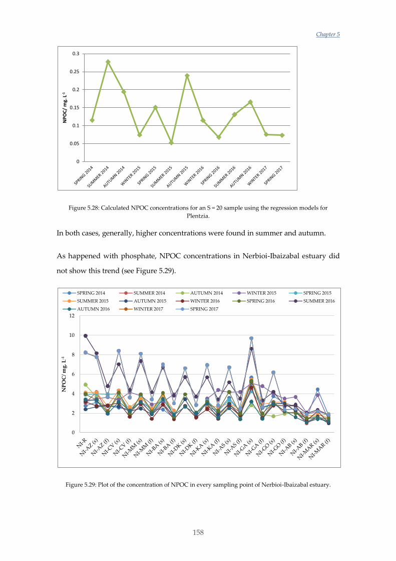
Chapter 5

158

Figure 5.28: Calculated NPOC concentrations for an S = 20 sample using the regression models for

Plentzia.

In both cases, generally, higher concentrations were found in summer and autumn.

As happened with phosphate, NPOC concentrations in Nerbioi-Ibaizabal estuary did

not show this trend (see Figure 5.29).

Figure 5.29: Plot of the concentration of NPOC in every sampling point of Nerbioi-Ibaizabal estuary.

0

0.05

0.1

0.15

0.2

0.25

0.3

NP

OC

/ m

g. L

-1

0

2

4

6

8

10

12

NP

OC

/ m

g. L

-1

SPRING 2014 SUMMER 2014 AUTUMN 2014 WINTER 2015 SPRING 2015

SUMMER 2015 AUTUMN 2015 WINTER 2016 SPRING 2016 SUMMER 2016

AUTUMN 2016 WINTER 2017 SPRING 2017

Study of the seasonal and interannual variability of the physico-chemical parameters and nutrients

159

In this case as well, Galindo was an important source of organic carbon. The highest

concentrations were found in summer and spring, while the lowest ones were found in

autumn. Big differences were also found between surface and bottom samples, being

the first ones the most concentrated ones. It can also be appreciated that higher

concentrations are found closer to the river than closer to the sea.

5.4 Conclusions

A seasonal study of some physico-chemical and chemical parameters was carried out

in three different estuaries of Biscay in order to see (1) the seasonal variability of these

substances and parameters in the estuaries and (2) the differences between the

estuaries that have a very different background and pollution levels.

Nutrients have different sources in the estuaries. While ammonium and nitrate get into

the estuaries from the coast, phosphate and silicate came from the rivers. The silicate

might be depending on the soil nearby and the phosphate from the use of detergents

and from agricultural sources. All the chemical substances monitored show a

conservative mixing in Plentzia and Urdaibai, but in Nerbioi-Ibaizabal, phosphate

shows a great increase coming from the Galindo River, mostly in summer and spring.

NPOC shows the same increase as for phosphate in Galindo. Most of the nutrient

concentrations rise in summer. As nutrients have significant direct or indirect impacts

on plant growth, oxygen concentrations, water clarity, and sedimentation rates and the

higher the nutrient concentrations are, the higher the phytoplankton amount is, this

fact can also explain the decrease of dissolved oxygen in summer, together with its

lower solubility at higher temperatures. The good mixing in Plentzia and Urdaibai

leads to a constant DO in the surface and bottom. In the Nerbioi-Ibaizabal estuary there

are big differences between the surface and the bottom, being surface waters much

better oxygenated. Near the sea, the differences decrease but nearer the river the

surface waters have a similar DO comparing with the other estuaries although the

bottom is nearly anoxic at some points. As the rest of the parameters do not show

anything odd, the most probable explanation is that the water movement at the bottom

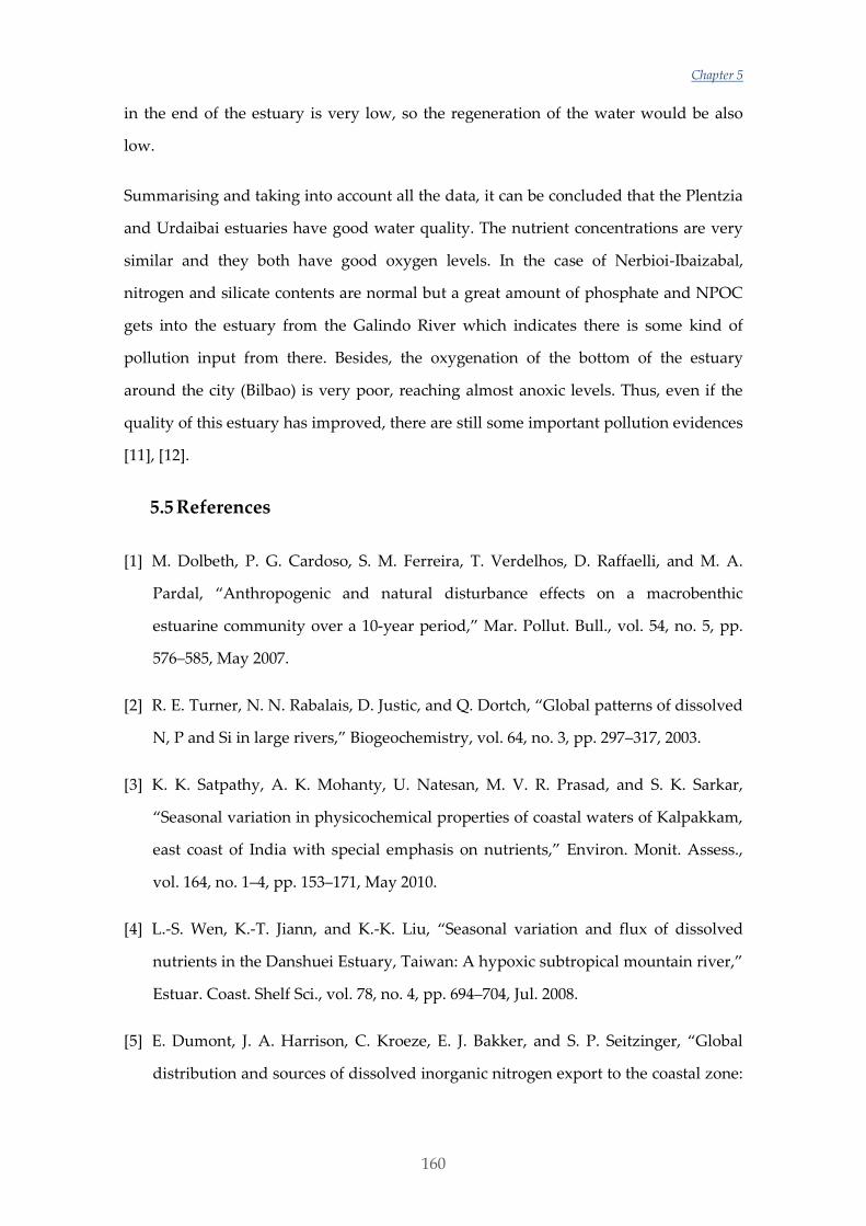
Chapter 5

160

in the end of the estuary is very low, so the regeneration of the water would be also

low.

Summarising and taking into account all the data, it can be concluded that the Plentzia

and Urdaibai estuaries have good water quality. The nutrient concentrations are very

similar and they both have good oxygen levels. In the case of Nerbioi-Ibaizabal,

nitrogen and silicate contents are normal but a great amount of phosphate and NPOC

gets into the estuary from the Galindo River which indicates there is some kind of

pollution input from there. Besides, the oxygenation of the bottom of the estuary

around the city (Bilbao) is very poor, reaching almost anoxic levels. Thus, even if the

quality of this estuary has improved, there are still some important pollution evidences

[11], [12].

5.5 References

[1] M. Dolbeth, P. G. Cardoso, S. M. Ferreira, T. Verdelhos, D. Raffaelli, and M. A.

Pardal, “Anthropogenic and natural disturbance effects on a macrobenthic

estuarine community over a 10-year period,” Mar. Pollut. Bull., vol. 54, no. 5, pp.

576–585, May 2007.

[2] R. E. Turner, N. N. Rabalais, D. Justic, and Q. Dortch, “Global patterns of dissolved

N, P and Si in large rivers,” Biogeochemistry, vol. 64, no. 3, pp. 297–317, 2003.

[3] K. K. Satpathy, A. K. Mohanty, U. Natesan, M. V. R. Prasad, and S. K. Sarkar,

“Seasonal variation in physicochemical properties of coastal waters of Kalpakkam,

east coast of India with special emphasis on nutrients,” Environ. Monit. Assess.,

vol. 164, no. 1–4, pp. 153–171, May 2010.

[4] L.-S. Wen, K.-T. Jiann, and K.-K. Liu, “Seasonal variation and flux of dissolved

nutrients in the Danshuei Estuary, Taiwan: A hypoxic subtropical mountain river,”

Estuar. Coast. Shelf Sci., vol. 78, no. 4, pp. 694–704, Jul. 2008.

[5] E. Dumont, J. A. Harrison, C. Kroeze, E. J. Bakker, and S. P. Seitzinger, “Global

distribution and sources of dissolved inorganic nitrogen export to the coastal zone:

Study of the seasonal and interannual variability of the physico-chemical parameters and nutrients

161

Results from a spatially explicit, global model:,” Glob. Biogeochem. Cycles, vol. 19,

no. 4, p. n/a-n/a, Dec. 2005.

[6] Y. Ouyang, P. Nkedi-Kizza, Q. T. Wu, D. Shinde, and C. H. Huang, “Assessment of

seasonal variations in surface water quality,” Water Res., vol. 40, no. 20, pp. 3800–

3810, Dec. 2006.

[7] J. Xu et al., “Temporal and spatial variations in nutrient stoichiometry and

regulation of phytoplankton biomass in Hong Kong waters: Influence of the Pearl

River outflow and sewage inputs,” Mar. Pollut. Bull., vol. 57, no. 6–12, pp. 335–348,

Jan. 2008.

[8] B. C. Behera, R. R. Mishra, J. K. Patra, S. K. Dutta, and H. N. Thatoi, “Physico

chemical properties of water sample collected from mangrove ecosystem of

Mahanadi River Delta, Odisha, India,” Am. J. Mar. Sci., vol. 2, no. 1, pp. 19–24,

2014.

[9] M. El Morhit and L. Mouhir, “Study of physico-chemical parameters of water in

the Loukkos river estuary (Larache, Morocco),” Environ. Syst. Res., vol. 3, no. 1,

pp. 1–9, 2014.

[10] L. Kortazar, J. Sáez, E. Astigarraga, N. Goienaga, and L. Fernández, “Chemometrics

for the classification and calibration of seawater using the H+ affinity spectrum,”

Talanta, vol. 116, pp. 108–114, Nov. 2013.

[11] S. Fdez-Ortiz de Vallejuelo, G. Arana, A. de Diego, and J. M. Madariaga, “Risk

assessment of trace elements in sediments: The case of the estuary of the Nerbioi–

Ibaizabal River (Basque Country),” J. Hazard. Mater., vol. 181, no. 1–3, pp. 565–573,

2010.

[12] A. Gredilla, J. M. Amigo Rubio, S. Fdez-Ortiz de Vallejuélo, A. de Diego, R. Bro,

and J. M. Madariaga, “Identification of contamination sources in estuarine water

by multiway data analysis: A case of study: estuary of the nerbioi-ibaizabal river,”

in 7o Colloquium Chemiometricum Mediterraneun (CCM VII 2010-Granada).

Chapter 6

Determination of Alkalinity and DIC

Determination of Alkalinity and DIC

165

6.1 Introduction

6.1.1 Developments in solution chemistry and different influences

The study of electrolyte solutions suffered important changes in the 19th century. In the

1830s, Faraday’s experiments on the electrolysis of salt solutions showed that electricity

could break up molecules into ions. Hittorf and Kohlrausch showed that salts were

made by ions and that oppositely charged particles must exist in solution, which was a

revolutionary idea. By the 1850s, chemists started to recognise that when a reaction

happened to produce substances at a definite rate, those substances could react to

produce the starting substances, and that a time must come when a balanced

equilibrium must be reached. This fact was first seen in 1803 when Claude Louis

Berthollet found that some chemical reactions were reversible. However, this concept

of dynamic equilibrium did not become popular with chemists at first. The form of

what is now referred to as Law of Chemical Equilibrium was first exposed along with

the study of reaction rates. In 1862, Marcellin Berthelot and Péan de St. Gilles reported

results from a study of the hydrolysis of esters. These results showed a clear

relationship between the concentration of product formed and that of the reactant,

ethanol. But since only the formation of esters was studied, and not their hydrolysis,

they failed to recognize the dynamic equilibrium involved in the reactions. Indeed, this

was first recognised and expressed in a general form in 1863 by the Norwegian

chemists C. M. Guldberg and P. Waage. They argued that a reacting system

maintained chemical equilibrium in a dynamic manner by the balancing of the rates of

reaction in both directions. Thus, for the general chemical reaction

A + B C + D

the rate of the forward reaction would be proportional to the concentrations of A and

B, while the rate of the backward reaction would be proportional to those of C and D.

At equilibrium, forward and backwards rates would be equal:

Chapter 6

166

Kforward [A] [B] = Kbackward [C] [D] 1

which easily rearranges to:

K=[C][D]

[A][B]

2

This equation became known as the Law of Mass Action, and the constant K as

equilibrium constant. It provides a quantitative expression for relating the concentrations

of reactant and product species in a chemical reaction that is at equilibrium. But their

first work, published in Norwegian in 1864 [1], [2], was ignored. Even their second

attempt, written in French and published in 1867 [3] with a modification of the law and

supported with experimental data, was ignored. Their work was not recognised until

1879, when they published it in a leading German journal [4]. The form of the

equilibrium constant that they presented is correct even from the modern perspective,

apart from using concentrations instead of activities (the concept of chemical activity

was developed by Josiah Willard Gibbs, in the 1870s, but was not widely known in

Europe until the 1890s) (see Chapter 1 Section 1.4).

Svante Arrhenius put all these ideas together and presented his dissociation theory in

1883 (which he published 4 years later in 1887). His theory established that when a salt

is dissolved, it immediately partially dissociates into ions. Besides that, the first

modern definition of acids and bases was devised by him in 1884 as a part of his

dissertation on electrolytic conductivity. His point of view was so revolutionary that it

was not well taken. On his dissertation he said that solid crystalline salts dissociate into

paired charged particles when dissolved, for which he won the 1903 Nobel Prize in

Chemistry. According to his theory, acids produce hydrogen ions in aqueous solution

and bases produce hydroxide ions in aqueous solution. The neutralization of hydrogen

and hydroxide ions forms water and thus, water and a salt are formed as products.

Determination of Alkalinity and DIC

167

Thus, by the end of the 19th century the basic groundwork for an understanding of the

chemistry of acids and bases in salt solutions had been laid. However, it took a long

time for those concepts to trespass the disciplinary barriers separating general

chemistry from what we now know as marine chemistry. It was not until Sørensen

developed methods for the determination of hydrogen ion concentration in 1909 [5],

that the way was not laid open for the successful interpretation of alkalinity, and of the

equilibrium in the carbonic acid system [6].

In the 20th century, the chemistry of electrolyte solutions was progressing. In 1918 Niels

Bjerrum proposed that electrolytes were completely dissociated in solution [7] and

Lewis published his concept of activity (see Chapter 1 Section 1.4) and his views on

chemical thermodynamics [8]. Also, Johannes Nicolaus Brønsted in Denmark [9] and

Thomas Martin Lowry in England [10] independently proposed the theory that carries

their names, the 4th of May of 1923 the first one and the 10th of January of 1923 the

second one. Their theory defined an acid as a species with a tendency to lose a

hydrogen ion (proton donors) and a base as a species with a tendency to gain a

hydrogen ion (proton acceptors). They extended the concept of acid–base chemistry

beyond aqueous solutions explicitly dictating that acids generate different conjugate

acids depending on the solvent used [11].

Debye and Hückel, also in 1923, showed how the activity of ions in simple electrolyte

solutions could be calculated from a simple physical theory which was based on the

concept of complete electrolytic dissociation [12]. Also, the study published by

Brønsted in 1928 [13] about acid-base equilibria in different media and the incomplete

dissociation of some acids and bases opened the way for Buch's work into the

dissociation of carbonic acid in seawater [14].

These developments allowed a gradual refinement of the concept of alkalinity, and of

the general understanding of the carbon dioxide system in seawater [6].

6.1.2 Alkalinity and Dissolved Inorganic Carbon (DIC): definitions and

calculations

Chapter 6

168

The first definition of alkalinity for natural waters was given by Rakestraw in 1949 [15]

when he put together all the ideas of the moment. He pointed out that the Bronsted-

Lowry definition could be used to define the alkalinity as the excess of bases (proton

acceptors) over acids (proton donors) in seawater.

“The 'alkalinity' of the water is the result of the predominance of base effectiveness over acid

effectiveness. When we titrate by adding HCl we choose an endpoint at which the HCO3-,

H2BO3-, and CO32- are completely combined with protons to form H2CO3 and H3BO3. Only the

relatively strong acids and bases are involved, so that chloride, bromide, sulfate, and the

principal metal cations are unimportant. Hydrogen and hydroxyl ions, although respectively

strong acid and base, are too dilute.

So that, finally, our definition of excess base, in terms of equivalents of acid added,

A = [HCO3-] + 2[CO32-] + [H2BO3-],

is an exact definition of what we mean by excess bases, not something which is merely

equivalent to it.”

While this definition is still in use, it has been modified further.

An important paper by Hansson and Jagner published in 1973 [16] proposed to take

into account other minor acid-base components of seawater. According to them, the

equivalence point for the alkalinity would be the next one:

[H+] + [HSO4] + [HF] = [HCO3-] + 2[CO32-] + [B(OH)4-] + [OH-] 3

This form of equation is known as a proton condition [17]. It is a type of mass-balance

equation for hydrogen ions in which the amounts of hydrogen ion are measured

relative to a defined neutral condition or zero level of protons. In the case of this

equation, the appropriate zero level of protons is defined by the unionized carbonic

acid, boric acid, and water species. Thus, it can be seen that the left-hand side of

equation consists of those species with more protons than the zero level, whilst the

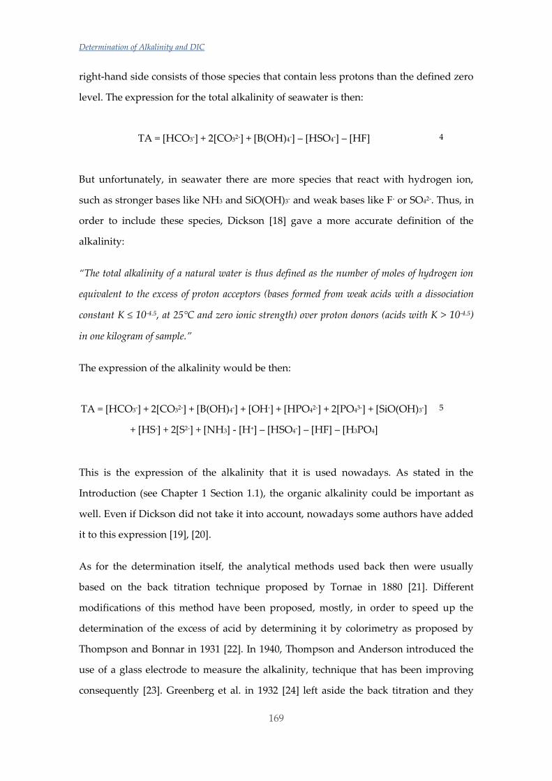
Determination of Alkalinity and DIC

169

right-hand side consists of those species that contain less protons than the defined zero

level. The expression for the total alkalinity of seawater is then:

TA = [HCO3-] + 2[CO32-] + [B(OH)4-] – [HSO4-] – [HF] 4

But unfortunately, in seawater there are more species that react with hydrogen ion,

such as stronger bases like NH3 and SiO(OH)3- and weak bases like F- or SO42-. Thus, in

order to include these species, Dickson [18] gave a more accurate definition of the

alkalinity:

“The total alkalinity of a natural water is thus defined as the number of moles of hydrogen ion

equivalent to the excess of proton acceptors (bases formed from weak acids with a dissociation

constant K ≤ 10-4.5, at 25°C and zero ionic strength) over proton donors (acids with K > 10-4.5)

in one kilogram of sample.”

The expression of the alkalinity would be then:

TA = [HCO3-] + 2[CO32-] + [B(OH)4-] + [OH-] + [HPO42-] + 2[PO43-] + [SiO(OH)3-]

+ [HS-] + 2[S2-] + [NH3] - [H+] – [HSO4-] – [HF] – [H3PO4]

5

This is the expression of the alkalinity that it is used nowadays. As stated in the

Introduction (see Chapter 1 Section 1.1), the organic alkalinity could be important as

well. Even if Dickson did not take it into account, nowadays some authors have added

it to this expression [19], [20].

As for the determination itself, the analytical methods used back then were usually

based on the back titration technique proposed by Tornae in 1880 [21]. Different

modifications of this method have been proposed, mostly, in order to speed up the

determination of the excess of acid by determining it by colorimetry as proposed by

Thompson and Bonnar in 1931 [22]. In 1940, Thompson and Anderson introduced the

use of a glass electrode to measure the alkalinity, technique that has been improving

consequently [23]. Greenberg et al. in 1932 [24] left aside the back titration and they

Chapter 6

170

titrated seawater directly with HCl to a pH of approximately 4.5, using methyl orange

as an indicator, technique that is in use nowadays. They also identified a first end-point

in this titration, and attributed it to the titration of carbonate ion itself. The precision of

alkalinity determinations was improved by the use of potentiometric titrations with a

glass electrode. This approach was suggested by Dyrssen in 1965 [25] who was the first

using the Gran technique [26] to estimate the equivalence point for an alkalinity

titration. The idea was further elaborated by Dyrssen and Sillen in 1967 [27]. According

to them, if the seawater is titrated with a strong acid with the same ionic strength as the

sample, the liquid junction potential can be neglected or assumed constant. In those

cases, the relationship between E and [H+] is the next one:

E=E0+k∙ log [H+] where [H+]=10(E-E0

k)

6

where k = ln10·R·T·F-1 which has a value of 59.16 mV at 25 °C.

They calculated accurate values for the equivalence volumes using the auxiliary

functions F1, F2 and F3, which are obtained from the electrode potential and the acid

volumes added (see Figure 6.1).

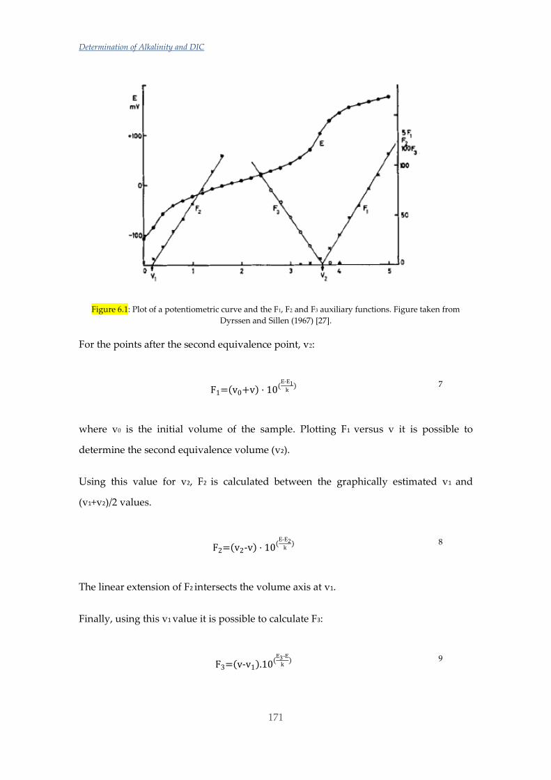
Determination of Alkalinity and DIC

171

Figure 6.1: Plot of a potentiometric curve and the F1, F2 and F3 auxiliary functions. Figure taken from

Dyrssen and Sillen (1967) [27].

For the points after the second equivalence point, v2:

F1=(v0+v) · 10(E-E1

k)

7

where v0 is the initial volume of the sample. Plotting F1 versus v it is possible to

determine the second equivalence volume (v2).

Using this value for v2, F2 is calculated between the graphically estimated v1 and

(v1+v2)/2 values.

F2=(v2-v) · 10(E-E2

k)

8

The linear extension of F2 intersects the volume axis at v1.

Finally, using this v1 value it is possible to calculate F3:

F3=(v-v1).10(E3-E

k)

9

Chapter 6

172

and the linear extension of F3 intersects the volume axis at v2, which is a check of the

first value obtained for v2. The values for the constants E1, E2 and E3 are immaterial

(they are arbitrary constants).

This method was widely used in the following years. Later, in 1970, Edmond

developed a closed-cell titration technique based on the Gran approach to calculate

both alkalinity and total carbon dioxide concentration [28]. In 1973 an important paper

by Hansson and Jagner [16] went on to examine in detail the consequences of using the

simplified model of acid-base chemistry employed by Dyrssen and Sillen and by

Edmond. They presented a modification of the Gran plots which permits to take into

consideration the other minor acid-base components of seawater [16]. According to

them, the original Gran plots assumed only one dominating main reaction in all parts

of the titration and neglecting the side-reactions would increase considerably the

systematic errors. Their “modified Gran plots” were capable of locating the

equivalence points with a greater accuracy. These equations were more complicated

and they used the computer program HALTAFALL [29] to solve them. This program is

based on the use of stability constants and total concentrations relevant to the titration

under consideration and calculates the free concentrations, in all titration points, of all

the species involved. According to their work, the values obtained for the total

alkalinity and carbonate content using the original Gran plots were strongly dependent

on the volume intervals used for F1 and F2 and systematic errors of about 1% of the

result could be obtained. They reached this conclusion by calculating the F2 values with

HALTAFALL using different volume intervals. On the contrary, that did not happen

using their approach.

The modified Gran equations according to Hansson and Jagner would be the following

ones1:

1 F’2 would correspond to F1 on the paper by Dyrssen and Sillen (for v > v2) and F’1 would

correspond to F2 (for v1 < v < v2).

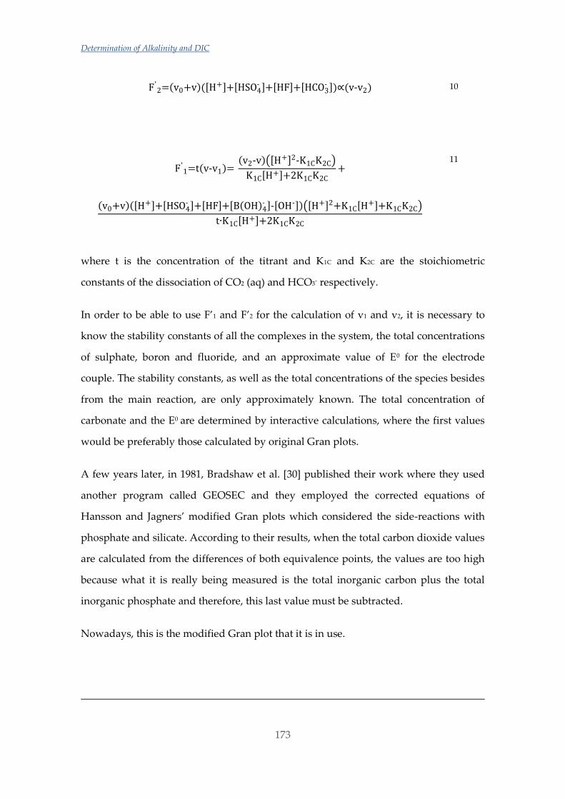
Determination of Alkalinity and DIC

173

F'2=(v0+v)([H+]+[HSO4

- ]+[HF]+[HCO3- ])∝(v-v2)

10

F'1=t(v-v1)=

(v2-v)([H+]2-K1CK2C)

K1C[H+]+2K1CK2C+

(v0+v)([H+]+[HSO4- ]+[HF]+[B(OH)4

- ]-[OH-])([H+]2+K1C[H+]+K1CK2C)

t∙K1C[H+]+2K1CK2C

11

where t is the concentration of the titrant and K1C and K2C are the stoichiometric

constants of the dissociation of CO2 (aq) and HCO3- respectively.

In order to be able to use F’1 and F’2 for the calculation of v1 and v2, it is necessary to

know the stability constants of all the complexes in the system, the total concentrations

of sulphate, boron and fluoride, and an approximate value of E0 for the electrode

couple. The stability constants, as well as the total concentrations of the species besides

from the main reaction, are only approximately known. The total concentration of

carbonate and the E0 are determined by interactive calculations, where the first values

would be preferably those calculated by original Gran plots.

A few years later, in 1981, Bradshaw et al. [30] published their work where they used

another program called GEOSEC and they employed the corrected equations of

Hansson and Jagners’ modified Gran plots which considered the side-reactions with

phosphate and silicate. According to their results, when the total carbon dioxide values

are calculated from the differences of both equivalence points, the values are too high

because what it is really being measured is the total inorganic carbon plus the total

inorganic phosphate and therefore, this last value must be subtracted.

Nowadays, this is the modified Gran plot that it is in use.

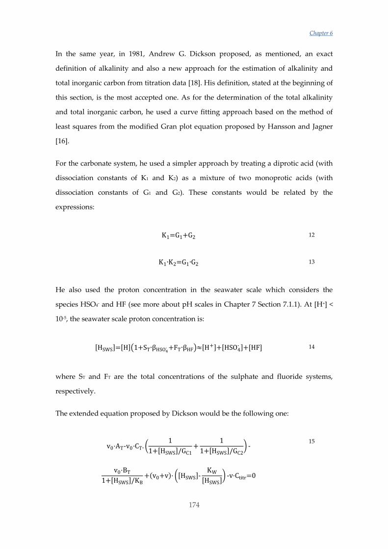
Chapter 6

174

In the same year, in 1981, Andrew G. Dickson proposed, as mentioned, an exact

definition of alkalinity and also a new approach for the estimation of alkalinity and

total inorganic carbon from titration data [18]. His definition, stated at the beginning of

this section, is the most accepted one. As for the determination of the total alkalinity

and total inorganic carbon, he used a curve fitting approach based on the method of

least squares from the modified Gran plot equation proposed by Hansson and Jagner

[16].

For the carbonate system, he used a simpler approach by treating a diprotic acid (with

dissociation constants of K1 and K2) as a mixture of two monoprotic acids (with

dissociation constants of G1 and G2). These constants would be related by the

expressions:

K1=G1+G2 12

K1∙K2=G1∙G2 13

He also used the proton concentration in the seawater scale which considers the

species HSO4- and HF (see more about pH scales in Chapter 7 Section 7.1.1). At [H+] <

10-5, the seawater scale proton concentration is:

[HSWS]=[H](1+ST∙βHSO4- +FT∙βHF)≈[H+]+[HSO4

- ]+[HF] 14

where ST and FT are the total concentrations of the sulphate and fluoride systems,

respectively.

The extended equation proposed by Dickson would be the following one:

v0·AT-v0·CT. (1

1+[HSWS]/GC1+

1

1+[HSWS]/GC2) -

v0·BT

1+[HSWS]/KB+(v0+v)· ([HSWS]-

KW

[HSWS]) -v·Ctitr=0

15

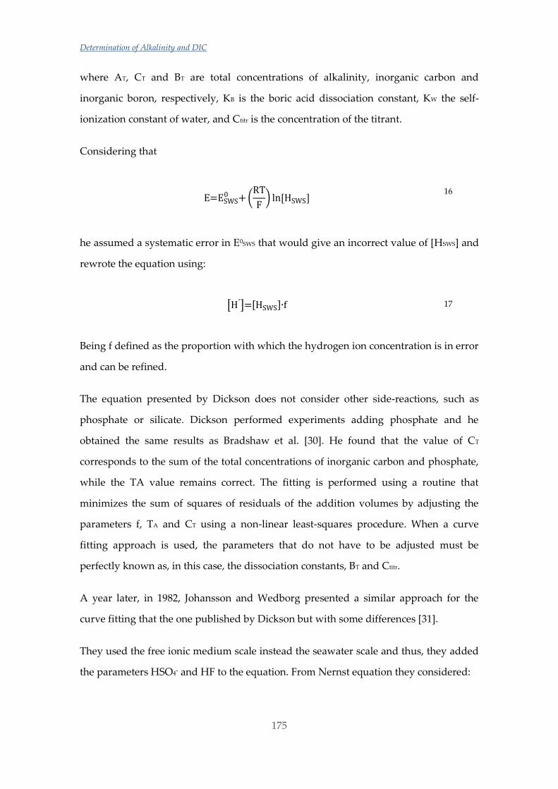
Determination of Alkalinity and DIC

175

where AT, CT and BT are total concentrations of alkalinity, inorganic carbon and

inorganic boron, respectively, KB is the boric acid dissociation constant, KW the self-

ionization constant of water, and Ctitr is the concentration of the titrant.

Considering that

E=ESWS0 + (

RT

F) ln[HSWS]

16

he assumed a systematic error in E0SWS that would give an incorrect value of [HSWS] and

rewrote the equation using:

[H']=[HSWS]∙f 17

Being f defined as the proportion with which the hydrogen ion concentration is in error

and can be refined.

The equation presented by Dickson does not consider other side-reactions, such as

phosphate or silicate. Dickson performed experiments adding phosphate and he

obtained the same results as Bradshaw et al. [30]. He found that the value of CT

corresponds to the sum of the total concentrations of inorganic carbon and phosphate,

while the TA value remains correct. The fitting is performed using a routine that

minimizes the sum of squares of residuals of the addition volumes by adjusting the

parameters f, TA and CT using a non-linear least-squares procedure. When a curve

fitting approach is used, the parameters that do not have to be adjusted must be

perfectly known as, in this case, the dissociation constants, BT and Ctitr.

A year later, in 1982, Johansson and Wedborg presented a similar approach for the

curve fitting that the one published by Dickson but with some differences [31].

They used the free ionic medium scale instead the seawater scale and thus, they added

the parameters HSO4- and HF to the equation. From Nernst equation they considered:

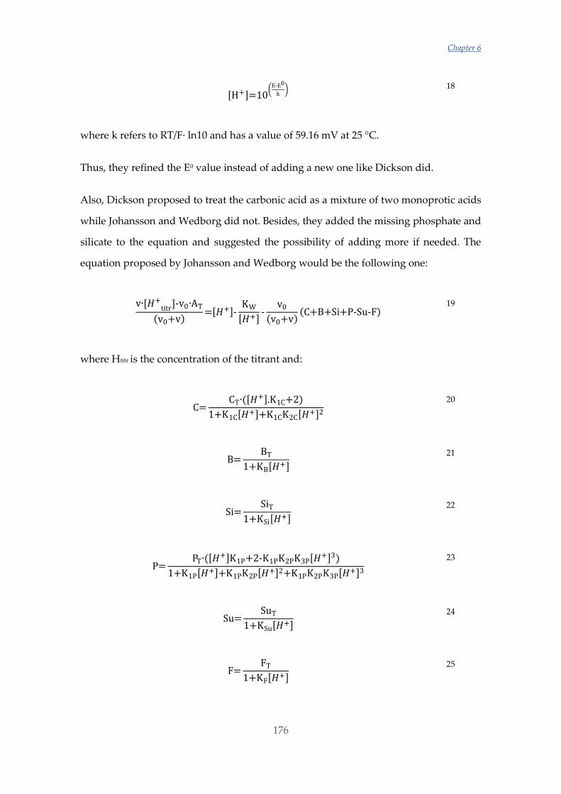
Chapter 6

176

[H+]=10(

E-E0

k)

18

where k refers to RT/F· ln10 and has a value of 59.16 mV at 25 °C.

Thus, they refined the E0 value instead of adding a new one like Dickson did.

Also, Dickson proposed to treat the carbonic acid as a mixture of two monoprotic acids

while Johansson and Wedborg did not. Besides, they added the missing phosphate and

silicate to the equation and suggested the possibility of adding more if needed. The

equation proposed by Johansson and Wedborg would be the following one:

v∙[𝐻+titr

]-v0∙AT

(v0+v)=[𝐻+]-

KW

[𝐻+]-

v0

(v0+v)(C+B+Si+P-Su-F)

19

where Htitr is the concentration of the titrant and:

C=CT∙([𝐻+].K1C+2)

1+K1C[𝐻+]+K1CK2C[𝐻+]2

20

B=BT

1+KB[𝐻+]

21

Si=SiT

1+KSi[𝐻+]

22

P=PT∙([𝐻+]K1P+2-K1PK2PK3P[𝐻+]3)

1+K1P[𝐻+]+K1PK2P[𝐻+]2+K1PK2PK3P[𝐻+]3

23

Su=SuT

1+KSu[𝐻+]

24

F=FT

1+KF[𝐻+]

25

Determination of Alkalinity and DIC

177

where CT, BT, SiT, PT, SuT and FT are the sum of the concentrations of all the species

containing their respective systems.

The equation is solved with the same procedure as Dickson’s: with a curve fitting

approach based on the method of least squares from the modified Gran plot equation

proposed by Hansson and Jagner [16]. Some parameters have to be chosen to be

refined and the rest must be known with a high accuracy.

These last two approaches are known to be the most accurate ones for the

determination on total alkalinity from potentiometric titration data and they are still in

use.

Summarizing, apart from some historical developments and few spectrophotometrical

approaches [32], [33], today alkalinity is determined mostly by titration of seawater

with a strong acid, following the potential of a proton sensitive electrode. The location

of the endpoint is crucial; for instance, in order to obtain a precision of 1µmol kg-1 in

TA from the titration of 100 mL of sample with 0.1 mol L-1 HCl, the endpoint has to be

located exactly to ± 1 µL. Making additions of that amount of HCl would require very

expensive equipments like automated micro-syringes and the commonly used

automatic titrators, although having those nominal precision values for the dispensed

volumes, cannot reach more than a 5 µL practical precision. Moreover, performing one

single titration at such low volume intervals would require a very long time. Thus, that

precision can be very seldom reached experimentally.

The acid consumption up to the second point is equal to the total alkalinity. From this

value, the carbonate alkalinity, which is wanted for the adequate description of the

marine carbonate system, needs to be calculated by subtracting the contributions to the

titration alkalinity resulting from other ions present in seawater. Refinement of the

algorithms used to calculate the equivalence point has further improved the precision

of this technique. But the accuracy of the analytical technique remains as important as

the precision in the data treatment.

Chapter 6

178

In the 1990s a group of researchers decided to document the techniques that they were

using for open ocean studies of the carbon dioxide system in seawater. The resulting

handbook [34] was updated in 2007 and it was published as the Guide to best practices

for ocean CO2 measurements [35] by PICES2. Even if there are a variety of approaches to

measure the carbon cycle parameters, the oceanographic community studying this

cycle has made available this guide describing the state-of-the-art techniques for these

parameters.

One of the most important reasons for the improvement of the accuracy of the

potentiometric TA determination is considered to be the commercialization of Certified

Reference Materials (CRM). Moreover, the use of CRM samples for the determination

of TA can provide, more likely, statistical stability between different studies or

traceability. Andrew Dickson’s laboratory at the Scripps Institution of Oceanography

(La Jolla, CA, USA) started producing seawater-based reference materials3 for total

dissolved carbon since 1990 (Batch 1) and began to certify them for total alkalinity in

1996 (Batch 33). The alkalinity of the CRM is determined by a two stage potentiometric

open-cell titration [36]. This technique is based on the acidification on the sample until

pH = 3.6 with a single addition of the titrant. Then it is stirred for about 10 minutes to

allow all the species of the carbonate system to escape as CO2 (g). Then, the titration is

continued until pH = 3. The titration is monitored using a glass electrode/reference

electrode pair and the total alkalinity is computed from the added titrant volume and

e.m.f. data using a non-linear least-squares approach that corrects for the reaction of

sulphate and fluoride ions [36]. As can be seen, this determination relies completely on

the data for the titration of the solution after the ‘classical’ equivalence point, where all

the titrable bases in the original sample are already protonated. In the calculations,

only the concentrations of main species, regarding the acid-base equilibria, present in

the 3 < pH < 3.6 range are considered. These species are the free proton, hydrogen

sulphate and hydrogen fluoride, mainly. This is a clever way to perform the alkalinity

2 http://cdiac.ornl.gov/oceans/Handbook_2007.html

3 http://cdiac.ornl.gov/oceans/Dickson_CRM/batches.html

Determination of Alkalinity and DIC

179

determination because it does not need to consider all the rest of the acid-base

equilibria involved. However, it must be perfectly known what species are present in

that pH range. Also, the initial pH of the sample should be known with a reasonable

accuracy in order to calculate how much of the titrant must be added in the initial

addition to reach pH = 3.6. This may not be a problem in oceanic waters where the

expected variation in the initial pH is very low, but it is definitely not the best option

for estuarine waters where that pH is very variable (see Chapter 8).

However, the most commonly used way for the total alkalinity determination is the

open-cell titration performed by adding the titrant into a sample volume placed in a

cell. The titration is monitored using a glass electrode/reference electrode pair and the

total alkalinity is computed from the added titrant volume and e.m.f. data using either

a least-squares procedure based on a non-linear curve fitting approach [18], [31] or on a

modified Gran approach [16], [30], [35]. Although this technique has been in use for

more than 45 years, the automation of nearly all the steps, the control of the

temperature and the use of CRMs have increased its accuracy considerably. This

titration can also be performed in closed cell (along with the DIC determination) since

Edmond developed it in 1970 [28] but due to its higher difficulty it is almost

exclusively performed in open cells [37].

These techniques are described in the Guide to best practices for ocean CO2 measurements

[35] stated above. Nowadays, there are several commercial equipments able to measure

the alkalinity with a high automation degree and they are available with computer

programs that calculate the value of the alkalinity. The most used commercial

equipments are the VINDTA 3S or 3C systems manufactured by Marianda (Marianda-

marine analytics and data, Kiel, Germany) although there are other commercially

available instruments from Apollo SciTech, Metrohm or Mettler Toledo, for instance.

Other scientists have also used in-house designs for the potentiometric titration [37].

DIC, also referred to as total carbonate (CT or CT), is essentially the sum of all species of

the dissolved carbon system:

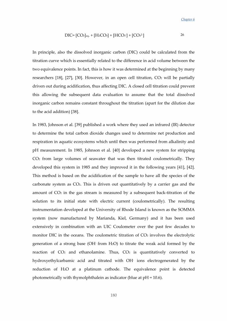
Chapter 6

180

DIC= [CO2]aq. + [H2CO3] + [HCO3-] + [CO32-] 26

In principle, also the dissolved inorganic carbon (DIC) could be calculated from the

titration curve which is essentially related to the difference in acid volume between the

two equivalence points. In fact, this is how it was determined at the beginning by many

researchers [18], [27], [30]. However, in an open cell titration, CO2 will be partially

driven out during acidification, thus affecting DIC. A closed cell titration could prevent

this allowing the subsequent data evaluation to assume that the total dissolved

inorganic carbon remains constant throughout the titration (apart for the dilution due

to the acid addition) [38].

In 1983, Johnson et al. [39] published a work where they used an infrared (IR) detector

to determine the total carbon dioxide changes used to determine net production and

respiration in aquatic ecosystems which until then was performed from alkalinity and

pH measurement. In 1985, Johnson et al. [40] developed a new system for stripping

CO2 from large volumes of seawater that was then titrated coulometrically. They

developed this system in 1985 and they improved it in the following years [41], [42].

This method is based on the acidification of the sample to have all the species of the

carbonate system as CO2. This is driven out quantitatively by a carrier gas and the

amount of CO2 in the gas stream is measured by a subsequent back-titration of the

solution to its initial state with electric current (coulometrically). The resulting

instrumentation developed at the University of Rhode Island is known as the SOMMA

system (now manufactured by Marianda, Kiel, Germany) and it has been used

extensively in combination with an UIC Coulometer over the past few decades to

monitor DIC in the oceans. The coulometric titration of CO2 involves the electrolytic

generation of a strong base (OH- from H2O) to titrate the weak acid formed by the

reaction of CO2 and ethanolamine. Thus, CO2 is quantitatively converted to

hydroxyethylcarbamic acid and titrated with OH- ions electrogenerated by the

reduction of H2O at a platinum cathode. The equivalence point is detected

photometrically with thymolphthalein as indicator (blue at pH = 10.6).

Determination of Alkalinity and DIC

181

The reactions that take place are the following ones:

Absorption of CO2 by the cathode solution (Cathode reaction):

CO2 + HOCH2CH2NH2 HOCH2CH2NHCOOH

monoethanolamine hydroxyethylcarbamic acid

With the generation of hydroxyethylcarbamic acid, the blue colour fades increasing the

transmittance.

Electrochemical generation of OH- (Cathode reaction):

2 H2O + 2 e- → H2 (g) + 2 OH-

Anode reaction:

Ag0 → Ag+ + e-

Neutralization of absorbed CO2 reaction product by electrochemically generated

OH-:

HOCH2CH2NHCOOH + OH- HOCH2CH2NHCOO- + H2O

The solution is titrated with electrogenerated OH- until the transmittance value goes

down to the original one.

The coulometric titration is based on Faraday’s Law. In coulometry the electricity

required to convert all of a chemical species to a different chemical state is measured.

The amount converted, in moles, is related to the quantity of electricity by Faraday's

constant (96485.34 coulombs mol-1). Taking into account that 1 coulomb can be

transformed into a 1 ampere·second (A·sec) and that 1 count, which is the base unit

that the UIC coulometric system used in this work employs, is equal to 0.02 mA·sec, it

is possible to calculate how many counts correspond to 1 µmol C.

Chapter 6

182

Thus:

96485.34 coulomb

1 mol C×

1 A.sec

1 coulomb×

1 count

0.00002 A.sec×

1 mol C

106 μmol C=4824.3 counts μmol C-1

This relation can be used to get the DIC concentration from the counts the coulometer

measures.

As stated above, the SOMMA system was the first equipment commercially available

to perform DIC measurements with coulometric detection. Nowadays, different

instruments are available including the VINDTA 3D and 3C systems by Marianda

(Marine Analytics and Data, Kiel, Germany). This method for the DIC determination is

the most used one and it is the recommended one in the Guide to best practices for ocean

CO2 measurements [35] stated above. Nevertheless, other techniques are also used for

the DIC determination. These techniques use a similar acidification strategy, but they

quantify the CO2 gas using a non-dispersive infrared sensor (NDIR). The Apollo

SciTech DIC analyzer (Apollo SciTech, LLC, Newark, USA) was the most common

instrument using this detection technique but in the last years a similar equipment

developed by Marianda (Marianda-marine analytics and data, Kiel, Germany), the

AIRICA system, has been also used. The NDIR based instruments use a much smaller

sample size and the analysis time is shorter, but the precision and accuracy might be a

little bit worse [37].

6.2 Experimental procedure

6.2.1 Instrumentation

In this work the commercially available VINDTA 3C system (Marianda, Kiel,

Germany) was used (see Figure ).

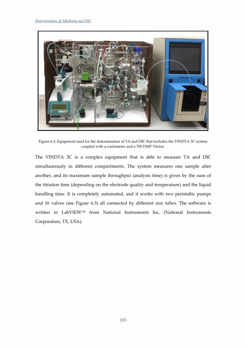
Determination of Alkalinity and DIC

183

Figure 6.2: Equipment used for the determination of TA and DIC that includes the VINDTA 3C system

coupled with a coulometer and a 785 DMP Titrino.

The VINDTA 3C is a complex equipment that is able to measure TA and DIC

simultaneously in different compartments. The system measures one sample after

another, and its maximum sample throughput (analysis time) is given by the sum of

the titration time (depending on the electrode quality and temperature) and the liquid

handling time. It is completely automated, and it works with two peristaltic pumps

and 16 valves (see Figure 6.3) all connected by different size tubes. The software is

written in LabVIEWTM from National Instruments Inc. (National Instruments

Corporation, TX, USA).

Chapter 6

184

Figure 6.3: Plot of the connection of the different parts of the VINDTA 3C system.

The usual total analysis time is around 20 minutes if a fast response glass electrode is

used. The TA pipette (sample dispenser) is about 100 mL while the DIC pipette is

about 20 mL and both must be calibrated (by known density liquid’s weight) every

time a tube is changed. The equipment uses sensors to know when pipettes are full.

For the alkalinity titration, the use of separate glass and reference electrodes is

recommended by the manufacturer for better quality results. For the latter, the

Metrohm (Metrohm AG, Herisau, Switzerland) double junction Ag(s)/AgCl(s)

reference electrode was used with a 0.7 mol. L-1 NaCl solution as filling for the outer

chamber (the inner filling solution was 3M KCl). As a glass electrode, the ORION-

ROSS electrode (Thermo Orion, Thermo Fisher Scientific, MA, USA) was used due to

its fast response. The E0 of the combination with the AgCl-reference was in the range

600 - 630 mV. Since this system is a kind of flow through system, because of the use of

the peristaltic pump, the sample could get in contact with electric ground. This would

eventually show up as a steadily drifting electrode signal and would make standard

Determination of Alkalinity and DIC

185

potentiometry impossible. To overcome this, the measurement in this equipment is

done using differential potentiometry where the e.m.f difference between both

electrodes, glass and reference, is measured against an auxiliary electrode (Marianda,

Kiel, Germany), which is a titanium wire placed in the cell. The auxiliary electrode is

connected to ground. A 785 DMP Titrino, which is a combination of an automated

burette and a pH-meter, fitted with a 5 mL glass burette unit and a 728 stirrer were

used for the titrant addition, e.m.f measurement and solution stirring, respectively.

They were all supplied by Metrohm (Metrohm AG, Herisau, Switzerland).

For the DIC determination, a CM5015 Coulometer with the CM5011 emulator supplied

by UIC Inc. (UIC Inc., Rockdale, IL, USA) was used. The borosilicate cell, silver anode,

platinum cathode and stirrer were also supplied by UIC Inc.

6.2.2 Reagents and solutions

All solutions were prepared using ultrapure water obtained from a MilliQ Element

A10 water purification system (Millipore Co., MA, USA).

For the alkalinity titration 0.1 mol. L-1 HCl (Tracepur) (Merck KGaA, Darmstadt,

Germany) was used as titrant which was fortified to the ionic strength of seawater

adding 0.6 mol. L-1 NaCl (Panreac Química SLU, Barcelona, Spain) to avoid any

problems caused by density gradients. This is the recommended way to work for open

ocean water samples. In the case of estuarine waters, that would mean the use of a

different titrant for nearly every sample, which is very inconvenient taking into

account that the titrant must be standardized. Another option was to use an

intermediate ionic strength but in the end it was decided to use a titrant with a total

ionic strength of 0.7 mol. L-1 to measure all the samples and correct the change on the

ionic strength afterwards. A 10 L rinsing solution of 0.7 mol. L-1 NaCl (VWR

International Eurolab S. L., Barcelona, Spain) was prepared as often as needed to clean

the titration cell between samples. The need to use a rinsing solution with NaCl is to

minimize diffusion from the acid tip and/or reference electrode, and therefore, it

should have about the same density as the acid.

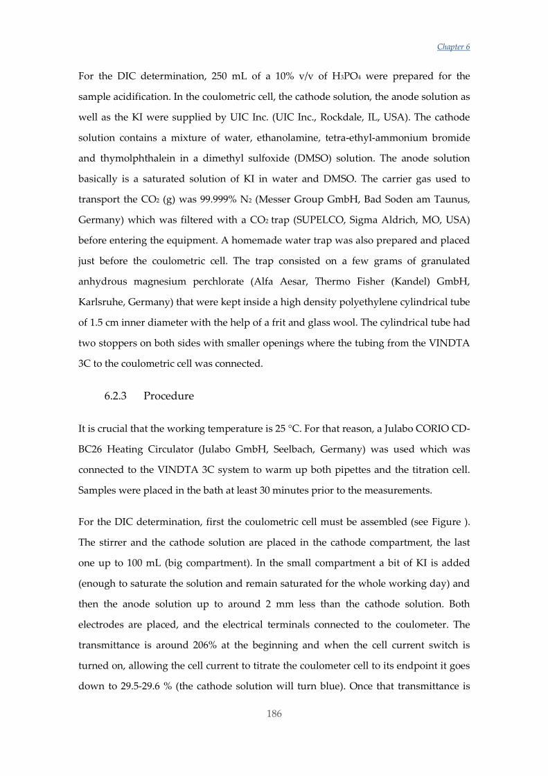
Chapter 6

186

For the DIC determination, 250 mL of a 10% v/v of H3PO4 were prepared for the

sample acidification. In the coulometric cell, the cathode solution, the anode solution as

well as the KI were supplied by UIC Inc. (UIC Inc., Rockdale, IL, USA). The cathode

solution contains a mixture of water, ethanolamine, tetra-ethyl-ammonium bromide

and thymolphthalein in a dimethyl sulfoxide (DMSO) solution. The anode solution

basically is a saturated solution of KI in water and DMSO. The carrier gas used to

transport the CO2 (g) was 99.999% N2 (Messer Group GmbH, Bad Soden am Taunus,

Germany) which was filtered with a CO2 trap (SUPELCO, Sigma Aldrich, MO, USA)

before entering the equipment. A homemade water trap was also prepared and placed

just before the coulometric cell. The trap consisted on a few grams of granulated

anhydrous magnesium perchlorate (Alfa Aesar, Thermo Fisher (Kandel) GmbH,

Karlsruhe, Germany) that were kept inside a high density polyethylene cylindrical tube

of 1.5 cm inner diameter with the help of a frit and glass wool. The cylindrical tube had

two stoppers on both sides with smaller openings where the tubing from the VINDTA

3C to the coulometric cell was connected.

6.2.3 Procedure

It is crucial that the working temperature is 25 °C. For that reason, a Julabo CORIO CD-

BC26 Heating Circulator (Julabo GmbH, Seelbach, Germany) was used which was

connected to the VINDTA 3C system to warm up both pipettes and the titration cell.

Samples were placed in the bath at least 30 minutes prior to the measurements.

For the DIC determination, first the coulometric cell must be assembled (see Figure ).

The stirrer and the cathode solution are placed in the cathode compartment, the last

one up to 100 mL (big compartment). In the small compartment a bit of KI is added

(enough to saturate the solution and remain saturated for the whole working day) and

then the anode solution up to around 2 mm less than the cathode solution. Both

electrodes are placed, and the electrical terminals connected to the coulometer. The

transmittance is around 206% at the beginning and when the cell current switch is

turned on, allowing the cell current to titrate the coulometer cell to its endpoint it goes

down to 29.5-29.6 % (the cathode solution will turn blue). Once that transmittance is

Determination of Alkalinity and DIC

187

reached and stabilized (it needs around 30 minutes) the cell is ready to start working.

First, a test sample, commonly called junk, is measured and then a blank must be run.

10 drops of phosphoric acid are added to the stripper by a membrane pump and the N2

starts bubbling. Counts are measured for 10 minutes every minute and the average

amount of counts per minute would be the value of the blank. Usually that value is

changed to a slightly higher one to avoid being on the limit and thus, to shorten the

analysis time. For the determination of the samples, 10 drops of phosphoric acid are

placed in the stripper and the N2 starts bubbling. The equipment makes now a “clear

and ready check” which means that it measures the counts every half minute and it

waits until the increment is below half the blank. After that, the sample is taken with

the help of a peristaltic pump. A small amount of the sample is used to clean the tubes

and the bottom of the small pipette from the previous sample. Then the pipette is filled,

and the sample is placed into the stripper. Here, the phosphoric acid converts all the

species of the carbonate system into CO2 which is expelled from the solution by

bubbling the sample with N2. The CO2 (g) passes through a condenser (that is at 1 - 4

°C) to eliminate the water vapour and it is transported to the coulometric cell through

the perchlorate trap to avoid any water to enter the cell. There, the blue colour will

decrease (and the transmittance increase) and the coulometric titration will start and

will produce enough OH- ions so that the transmittance goes back to 29.5 - 29.6 %. The

titration will finish when the increment of counts, measured in a minute interval, goes

below the blank four times (or after a default time of 20 minutes). For the DIC

determination the total amount of counts, the value of the blank, the analysis time and

the density are considered. The whole analysis time is usually around 12-15 minutes.

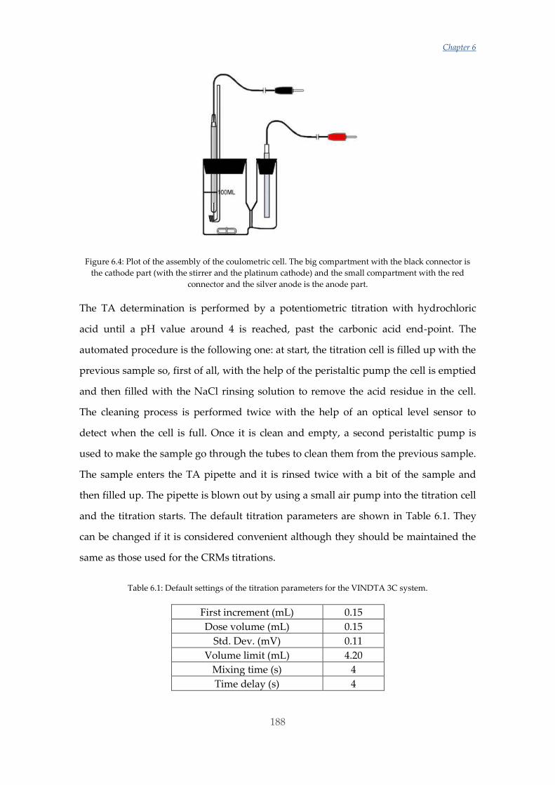
Chapter 6

188

Figure 6.4: Plot of the assembly of the coulometric cell. The big compartment with the black connector is

the cathode part (with the stirrer and the platinum cathode) and the small compartment with the red

connector and the silver anode is the anode part.

The TA determination is performed by a potentiometric titration with hydrochloric

acid until a pH value around 4 is reached, past the carbonic acid end-point. The

automated procedure is the following one: at start, the titration cell is filled up with the

previous sample so, first of all, with the help of the peristaltic pump the cell is emptied

and then filled with the NaCl rinsing solution to remove the acid residue in the cell.

The cleaning process is performed twice with the help of an optical level sensor to

detect when the cell is full. Once it is clean and empty, a second peristaltic pump is

used to make the sample go through the tubes to clean them from the previous sample.

The sample enters the TA pipette and it is rinsed twice with a bit of the sample and

then filled up. The pipette is blown out by using a small air pump into the titration cell

and the titration starts. The default titration parameters are shown in Table 6.1. They

can be changed if it is considered convenient although they should be maintained the

same as those used for the CRMs titrations.

Table 6.1: Default settings of the titration parameters for the VINDTA 3C system.

First increment (mL) 0.15

Dose volume (mL) 0.15

Std. Dev. (mV) 0.11

Volume limit (mL) 4.20

Mixing time (s) 4

Time delay (s) 4

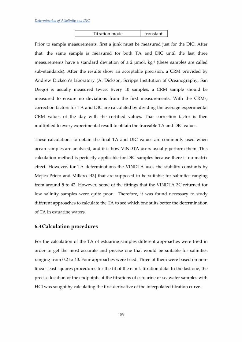
Determination of Alkalinity and DIC

189

Titration mode constant

Prior to sample measurements, first a junk must be measured just for the DIC. After

that, the same sample is measured for both TA and DIC until the last three

measurements have a standard deviation of ± 2 µmol. kg-1 (these samples are called

sub-standards). After the results show an acceptable precision, a CRM provided by

Andrew Dickson’s laboratory (A. Dickson, Scripps Institution of Oceanography, San

Diego) is usually measured twice. Every 10 samples, a CRM sample should be

measured to ensure no deviations from the first measurements. With the CRMs,

correction factors for TA and DIC are calculated by dividing the average experimental

CRM values of the day with the certified values. That correction factor is then

multiplied to every experimental result to obtain the traceable TA and DIC values.

These calculations to obtain the final TA and DIC values are commonly used when

ocean samples are analysed, and it is how VINDTA users usually perform them. This

calculation method is perfectly applicable for DIC samples because there is no matrix

effect. However, for TA determinations the VINDTA uses the stability constants by

Mojica-Prieto and Millero [43] that are supposed to be suitable for salinities ranging

from around 5 to 42. However, some of the fittings that the VINDTA 3C returned for

low salinity samples were quite poor. Therefore, it was found necessary to study

different approaches to calculate the TA to see which one suits better the determination

of TA in estuarine waters.

6.3 Calculation procedures

For the calculation of the TA of estuarine samples different approaches were tried in

order to get the most accurate and precise one that would be suitable for salinities

ranging from 0.2 to 40. Four approaches were tried. Three of them were based on non-

linear least squares procedures for the fit of the e.m.f. titration data. In the last one, the

precise location of the endpoints of the titrations of estuarine or seawater samples with

HCl was sought by calculating the first derivative of the interpolated titration curve.

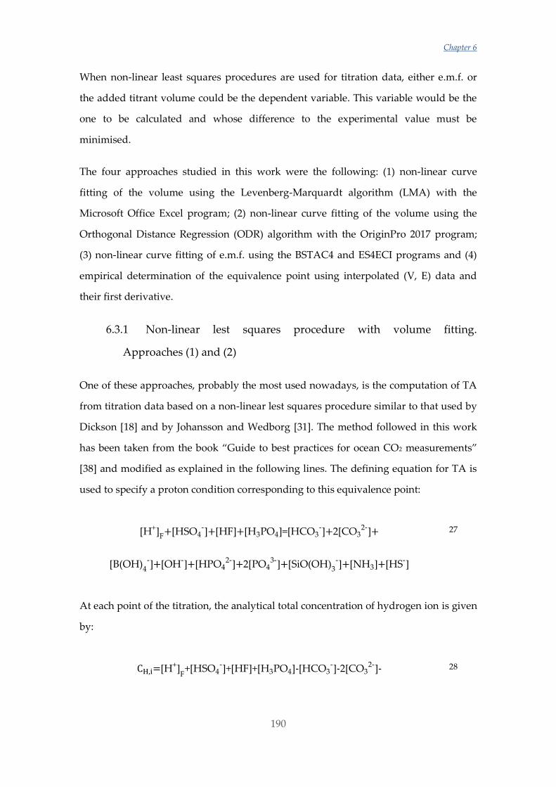
Chapter 6

190

When non-linear least squares procedures are used for titration data, either e.m.f. or

the added titrant volume could be the dependent variable. This variable would be the

one to be calculated and whose difference to the experimental value must be

minimised.

The four approaches studied in this work were the following: (1) non-linear curve

fitting of the volume using the Levenberg-Marquardt algorithm (LMA) with the

Microsoft Office Excel program; (2) non-linear curve fitting of the volume using the

Orthogonal Distance Regression (ODR) algorithm with the OriginPro 2017 program;

(3) non-linear curve fitting of e.m.f. using the BSTAC4 and ES4ECI programs and (4)

empirical determination of the equivalence point using interpolated (V, E) data and

their first derivative.

6.3.1 Non-linear lest squares procedure with volume fitting.

Approaches (1) and (2)

One of these approaches, probably the most used nowadays, is the computation of TA

from titration data based on a non-linear lest squares procedure similar to that used by

Dickson [18] and by Johansson and Wedborg [31]. The method followed in this work

has been taken from the book “Guide to best practices for ocean CO2 measurements”

[38] and modified as explained in the following lines. The defining equation for TA is

used to specify a proton condition corresponding to this equivalence point:

[H+]F+[HSO4-]+[HF]+[H3PO4]=[HCO3

-]+2[CO32-]+

[B(OH)4

-]+[OH-]+[HPO42-]+2[PO4

3-]+[SiO(OH)3

-]+[NH3]+[HS-]

27

At each point of the titration, the analytical total concentration of hydrogen ion is given

by:

CH,i=[H+]F+[HSO4

-]+[HF]+[H3PO4]-[HCO3-]-2[CO3

2-]- 28

Determination of Alkalinity and DIC

191

[B(OH)4

-]-[OH-]-[HPO42-]-2[PO4

3-]-[SiO(OH)3

-]-[NH3]-[HS-]

Thus, the initial analytical concentration of hydrogen ion in the solution is the negative

of the total alkalinity. At each titration point a mass m of the acid with concentration

CH0 (mol. kgsw-1) is added to an initial mass of the sample m0, thus:

𝐶𝐻,𝑖 =−𝑚0 ∙ 𝑇𝐴 + 𝑚 ∙ 𝐶𝐻

0

𝑚0 + 𝑚

29

Combining equations 28 and 29 the following expression is obtained:

−𝑚0 ∙ 𝑇𝐴 + 𝑚 ∙ 𝐶𝐻0

𝑚0 + 𝑚= [H+]F+[HSO4

-]+[HF]+[H3PO4]-[HCO3-]-2[CO3

2-]-

[B(OH)4-]-[OH-]-[HPO42-]-2[PO43-]-[SiO(OH)3-]-[NH3]-[HS-]

30

To ease the equations, to the expression on the right side of equation 30 will be called

“term” from now on.

The concentration of [HF+] + [HSO3+] is computed from an initial estimate of E0 using

the Nernst equation (since the total proton scale is used):

E= E0-ln 10∙RT

Flog[𝐻+]

31

The concentrations of the rest of the species on the right side of the expression are

obtained using the total concentrations, mass balance equations for all the components

in the chemical system considered (Carbonate, Phosphate, etc.) and the stoichiometric

constants at the different salinities (or ionic strengths) of each titration point. In the

case of DIC, silicate and phosphate the total concentrations were experimentally

determined (see Chapter 4). In the case of sulphate [44], borate [45] and fluoride [44]

empirical equations were used to calculate their concentrations in mol. kgsw-1 at

different salinities.

Chapter 6

192

𝑆𝑇 = 0.02824 ∙𝑆

35

32

𝐵𝑇 = 0.000412 ∙𝑆

35

33

𝐹𝑇 = 0.00007 ∙𝑆

35

34

mcalc values are calculated with the help of equation 35 which includes the parameters

to be calculated in each titration: E0 and either [HCl] or TA, depending if a CRM or a

sample is titrated, respectively.

𝑚𝑐𝑎𝑙𝑐,𝑖 =𝑚0 ∙ (𝑡𝑒𝑟𝑚 − 𝑇𝐴)

𝐶𝐻0 − 𝑡𝑒𝑟𝑚

35

As the VINDTA program records the acid addition in volume, mcalc,i values are

transformed into volume for the minimisation by dividing by the density of the acid

[38].

Mathematically, either of the experimental variables, V or E, can be selected as the

dependent variable and, thus, the one that will be fitted. But equation 30 is a linear

equation with respect to V while of higher degree with respect to E. Thus, the choice of

dependent variable is important for the effectiveness of the mathematical procedure.

Since it is simpler to solve an explicit linear equation, the best choice by this means is

that V is selected as the dependent variable while E is defined as the independent

variable.

Most procedures used for the refinement of parameters by non-lineal least-square

regression are based on the minimisation of the residual sum of squares (RRS), also

known as the sum of squared residuals (SSR) or the sum of squared errors of

prediction (SSE) which are the deviations predicted from the actual empirical values of

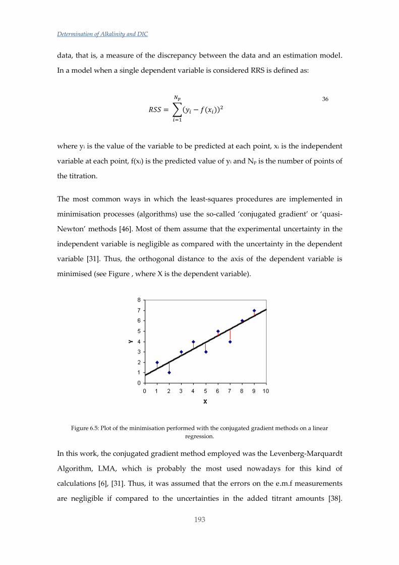
Determination of Alkalinity and DIC

193

data, that is, a measure of the discrepancy between the data and an estimation model.

In a model when a single dependent variable is considered RRS is defined as:

𝑅𝑆𝑆 = ∑(𝑦𝑖 − 𝑓(𝑥𝑖))2

𝑁𝑝

𝑖=1

36

where yi is the value of the variable to be predicted at each point, xi is the independent

variable at each point, f(xi) is the predicted value of yi and Np is the number of points of

the titration.

The most common ways in which the least-squares procedures are implemented in

minimisation processes (algorithms) use the so-called ‘conjugated gradient’ or ‘quasi-

Newton’ methods [46]. Most of them assume that the experimental uncertainty in the

independent variable is negligible as compared with the uncertainty in the dependent

variable [31]. Thus, the orthogonal distance to the axis of the dependent variable is

minimised (see Figure , where X is the dependent variable).

Figure 6.5: Plot of the minimisation performed with the conjugated gradient methods on a linear

regression.

In this work, the conjugated gradient method employed was the Levenberg-Marquardt

Algorithm, LMA, which is probably the most used nowadays for this kind of

calculations [6], [31]. Thus, it was assumed that the errors on the e.m.f measurements

are negligible if compared to the uncertainties in the added titrant amounts [38].

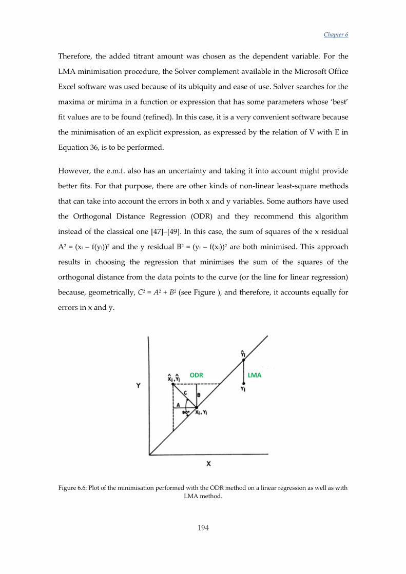
Chapter 6

194

Therefore, the added titrant amount was chosen as the dependent variable. For the

LMA minimisation procedure, the Solver complement available in the Microsoft Office

Excel software was used because of its ubiquity and ease of use. Solver searches for the

maxima or minima in a function or expression that has some parameters whose ‘best’

fit values are to be found (refined). In this case, it is a very convenient software because

the minimisation of an explicit expression, as expressed by the relation of V with E in

Equation 36, is to be performed.

However, the e.m.f. also has an uncertainty and taking it into account might provide

better fits. For that purpose, there are other kinds of non-linear least-square methods

that can take into account the errors in both x and y variables. Some authors have used

the Orthogonal Distance Regression (ODR) and they recommend this algorithm

instead of the classical one [47]–[49]. In this case, the sum of squares of the x residual

A2 = (xi – f(yi))2 and the y residual B2 = (yi – f(xi))2 are both minimised. This approach

results in choosing the regression that minimises the sum of the squares of the

orthogonal distance from the data points to the curve (or the line for linear regression)

because, geometrically, C2 = A2 + B2 (see Figure ), and therefore, it accounts equally for

errors in x and y.

Figure 6.6: Plot of the minimisation performed with the ODR method on a linear regression as well as with

LMA method.

LMAODR

Determination of Alkalinity and DIC

195

For the calculations with the ODR method, the OriginPro 2017 program was used

because it is one of the few programs that has this algorithm already implemented.

In the case of LMA the equation used in this work in the minimisation of the sum of

squared errors in V defined by:

𝑅𝑆𝑆 = ∑ 𝑊𝑖 ∙ (𝑉𝑒𝑥𝑝,𝑖 − 𝑉𝑐𝑎𝑙𝑐,𝑖)2

𝑁𝑝

𝑖=1

37

For each titration point Vexp,i is the volume of acid added, Vcalc,i is the calculated volume

according to equation 35 (and a posterior division by the density of the acid) and Wi is

the statistical weight.

Although most works that calculate TA by means of curve fitting do not use weight, it

has been proposed that weighting experimental data around the equivalence point

heavier than in other regions of the titration curve generally give more accurate results.

In this work, a derivative weighting scheme has been used, as shown in equation 38,

[50] for both the LMA and ODR algorithms.

𝑊𝑖 =𝑝𝐻𝑖+1 − 𝑝𝐻𝑖−1

𝑉𝑖+1 − 𝑉𝑖−1

38

Taking into account that one of the refined parameters is the E0 and considering

equation 31, which relates E0, E and pH, the statistical weight could not, in principle, be

calculated until the minimisation is performed. However, as the proposed weight uses

the first derivative of the pH against the volume, only the relative differences in pH are

meaningful and not the absolute pH values. Thus, as it may be easily shown, the

weights remain independent of the E0 value and may be calculated before the

minimizations starts using just an initial E0 estimation.

It is important to mention that the ionic strength (and therefore the salinity) was

calculated at every addition of the acid, the same as stability constants and

Chapter 6

196

concentrations of all the species. In this way the variation of the ionic strength due to

the addition of the acid was taken into account. For that purpose, the conversions

between salinities and ionic strengths (in mol. kgsw-1) were performed using the

following equation [38], [44]:

𝐼 =19.924 ∙ 𝑆

1000 − 1.005 ∙ 𝑆

39

The calculation of the ionic strength after each addition of acid was done like this:

𝐼𝑖 =𝐼0 ∙ 𝑚0 + 𝐼𝑡𝑖𝑡𝑟 ∙ 𝑉𝑒𝑥𝑝,𝑖

𝑚𝑖 + 𝑉𝑒𝑥𝑝,𝑖 ∙ 𝛿𝑡𝑖𝑡𝑟

40

where I0 is the initial ionic strength of the sample, Ititr is the ionic strength of the titrant

in mol. L-1 and δtitr is the density of the titrant.

Concerning the calculation strategy, in the first place, the titrant acid concentration was

calculated using the CRM’s by fixing the certified DIC and TA values. In this way, the

C0H and E0 were refined in each CRM titration.

After that, using the obtained acid concentration, the alkalinity, E0 and ammonium

concentration were refined for the same CRM and the rest of the samples. Results

showed that better curve fits were obtained by letting the ammonium concentration to

be refined as well.

All the equations to determine the stoichiometric constants were in the total proton

scale and in the mol. kgsw-1 scale. Those originally expressed in other scales were

converted to these ones. The equations for the boric acid, phosphate system, sulphuric

acid and hydrogen fluoride were taken from the book “CO2 in Seawater: Equilibrium,

Kinetics, Isotopes” [44]. The equation for ammonium was taken from the work by

Millero [45]. For the constants of the carbonate system K1 and K2, different equations

were tested because this system is the one with the greatest influence in TA and, thus,

it is crucial to use the most adequate set of constants. The tested constants were chosen

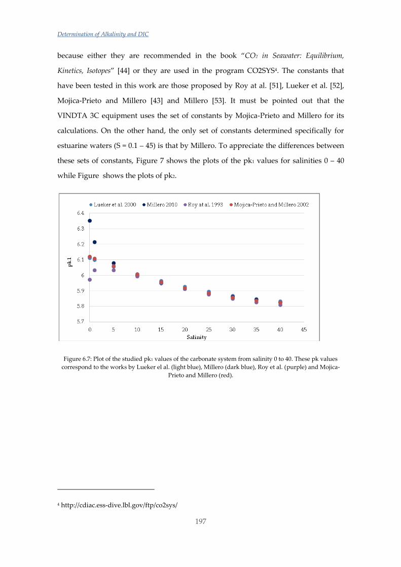
Determination of Alkalinity and DIC

197

because either they are recommended in the book “CO2 in Seawater: Equilibrium,

Kinetics, Isotopes” [44] or they are used in the program CO2SYS4. The constants that

have been tested in this work are those proposed by Roy at al. [51], Lueker et al. [52],

Mojica-Prieto and Millero [43] and Millero [53]. It must be pointed out that the

VINDTA 3C equipment uses the set of constants by Mojica-Prieto and Millero for its

calculations. On the other hand, the only set of constants determined specifically for

estuarine waters (S = 0.1 – 45) is that by Millero. To appreciate the differences between

these sets of constants, Figure 7 shows the plots of the pk1 values for salinities 0 – 40

while Figure shows the plots of pk2.

Figure 6.7: Plot of the studied pk1 values of the carbonate system from salinity 0 to 40. These pk values

correspond to the works by Lueker el al. (light blue), Millero (dark blue), Roy et al. (purple) and Mojica-

Prieto and Millero (red).

4 http://cdiac.ess-dive.lbl.gov/ftp/co2sys/

Chapter 6

198

Figure 6.8: Plot of the studied pk2 values of the carbonate system from salinity 0 to 40. These pk values

correspond to the works by Lueker el al. (light blue), Millero (dark blue), Roy et al. (purple) and Mojica-

Prieto and Millero (red).

As can be seen, the constants are quite similar at higher salinities (from S ~ 15 onwards)

but rather different at values lower than that. This difference is more pronounced in

the pk1 values. To decide which of the constant sets is the best for the calculations, a

CRM was used to check the accuracy of the results. As the TA of the CRM is known,

the correct set of constants should give the same value after the curve fitting procedure.

This provides a hint of which sets of constants are the most adequate for higher

salinities. To test the constants at the lowest salinities, the goodness of the fit of both a

river and a low salinity samples were used as no low salinity CRM is available.

6.3.2 Non-linear lest squares procedure with e.m.f. fitting. Approach (3)

There are some computer programs available that use the e.m.f. as the dependent

variable. In this work, a set of programs developed by the research group led by Prof.

Silvio Sammartano at the University of Messina (Italy) were used. The main programs

were LIANA [54], BSTAC4 [55] and ES4ECI [55], [56].

First, the proper set of constants have to be chosen. In this work, the same constants

were used for every approach. All these programs work in the mol. L-1 scale, so the

constants were converted to this scale by multiplying by the density. LIANA is a

Determination of Alkalinity and DIC

199

computer program written in the PASCAL language that is based on a rigorous

algorithm that was devised to fit any linear or non-linear equation. It uses the general

Levenberg-Marquart-Gauss-Newton method for the fitting. In this case, the equation

fitted by LIANA was a Debye-Hückel type equation that takes into account the

dependence on ionic strength proposed by the same research group and applied

successfully in many systems [57]–[61]. They developed this equation following the

hypothesis that it is possible to express the dependence on ionic strength of formation

constants by a simple equation independent of the type of reactants, and only

dependent of the type of reaction. Therefore, activity coefficients would depend on

charge only [55]:

log β = log β0 -z* A√I

1+Ba√I+CI+DI

3

2+EI2 41

where A and B are the coefficients of the Debye-Hückel equation dependent on

temperature and dielectric constant of the solvent; a is an empirical parameter

depending on the effective dimensions of the ions (see introduction). In this work A

and B.a were used as 0.5 and 1.5, respectively. C, D and E are ionic strength

dependence parameters and z* is defined by:

z*= ∑ (charge)reactants2 - ∑ (charge)products

2 42

The parameters to be refined by LIANA were log β0 and the ionic strength dependence

parameters C, D and/or E (in some cases the three of them were used but mostly C and

D only).

LIANA had to be used because both BSTAC4 and ES4ECI work with this type of

equation.

Computer program BSTAC is derived from SUPERQUAD [62]. It is written in BASIC

language and it is used to refine stability constants and other titration parameters

Chapter 6

200

related to potentiometric titrations by means of non-linear least squares procedure by

minimising the RSS of the experimental and calculated e.m.f. (E):

RSS = ∑ Wi ∙ (Eexp,i − Ecalc,i)2

Np

i=1

43

Weights for each point of the titration curves are given as:

W =1

s2

44

where

s2 = sE2 +

δE

δv∙ sv

2 45

where sE is the uncertainty of the e.m.f. determination (0.1 mV) and sv is the precision

of the addition of the titrant (0.005 mL).

The input file distinguishes between components and species. Components are the

compounds that can be represented in the form of different chemical species, through

reactions among them, and whose mass balance equations must be solved. In this case

the components are CO32-, B(OH)4-, PO43-, SiO(OH)3-, NH3, F- and H+. The species are the

acid or base species taking part in the mass balance for every component. In this case:

HCO3-, H2CO3, H3BO3, HPO42-, H2PO4-, H3PO4, Si(OH)4, NH4+, HF and OH-.

The main advantage of this program over others that are available, is that BSTAC4

takes into account the variation in ionic strength along the titration. This program,

besides refining stability constants, can also be used to refine the ionic strength

dependence parameters, the initial concentration of reagents on the titration vessel and

instrumental parameters such as standard potential E0 or liquid junction potential [55],

[63].

Determination of Alkalinity and DIC

201

In this work, the C parameters were refined as well as the E0 and the initial total

concentration of protons.

Once all the refined parameters are obtained, these were incorporated into the

ES4GRAPH2 program which is the graphic interface for the ES4ECI program. It is

generally used to draw speciation diagrams and to calculate species formation

percentages [60], [64]–[66]. This program solves all the mass balance equations

simultaneously to find the free concentrations of the species. It uses the Newton-

Raphson algorithm to find these free concentrations by an iterative procedure [55], [56].

Errors in the free concentrations, arising from errors in formation constants (given by

LIANA) and in analytical concentrations, can be calculated by variance propagation

using this program.

Finally, equation 5 is used to get the TA value by summing or subtracting the free

concentrations of the involved species. Also, as the uncertainties of these free

concentrations are obtained, in this work the intrinsic variance of the TA value was

calculated by error propagation of the single uncertainties using the Kragten method

[67].

As these programs do not calculate the HCl concentration, the average value obtained

by Microsoft Origin Excel and OriginPro 2017 was used.

6.3.3 Empirical determination of the equivalence volume. Approach (4)

The last approach tested in this work is completely empirical in the sense that it does

not rely at all on the underlying chemistry of the sample, that is, on its specific

composition in relation with the chemical systems present like carbonate, phosphate,

and so on. Instead, it looks back at the times when the TA values were simply

determined by the amount of HCl consumed up to an end-point in visually indicated

titrations with the help of acid base indicators and, later, with the help of pH electrodes

(see Section 6.1.2). Taking into account the high degree of complexity shown in the

previous approaches, it was considered worth to try a much simpler approximation

and check if its results can compare with the previous ones.

Chapter 6

202

According to a long-standing tradition in Analytical Chemistry, the location of the

equivalence points in potentiometric and other instrumental titrations has to be done

by mathematical means since simpler visual-only inspections of the titration data

would not give sufficiently accurate results. Therefore, methods using some kind of

transformation of the original (E, V) data are required. Some of them, like the popular

Gran linearizations and its modifications [16], [26], [30] have already been mentioned

in this context (see Section 6.1.2). However, most of these methods, again, rely on a

more or less detailed description of the chemical composition of the system and,

therefore, their different degree of success. Few methods remain to be used that are

not dependent on the underlying chemistry. One of them is the classical determination

of the end point by locating the inflection point in the titration curve with the help of

the first or second derivatives of the (E, V) data.

Taking into account the requirements regarding precision in the determination of TA

values, one of the first conclusions would be that a titration carried out at 0.15 mL

increments could never yield the required precision. As pointed out before, this could

only be achieved at 0.001 mL increments, which is both difficult and impractical to

achieve. However, there are mathematical interpolation techniques that allow

populating an experimental curve, such as the titration curve, with an adequate

amount of ‘artificial’ points between two ‘experimental’ points. This is an old problem

in calculus concerning the theory and methods of function approximation which has

been addressed in different ways [46]. Using these methods it is possible to transform,

for instance, a 30 (v, E) pairs data set in another containing hundreds or even

thousands of interpolated points. Among the most popular methods, apart from the

obvious linear interpolation between any two data pairs, are the so-called spline

methods which owe their name to the splines5 and Lesbian rules6 that the draughtsmen

used in the old times.

5 See https://en.wikipedia.org/wiki/Flat_spline

6 https://en.wikipedia.org/wiki/Lesbian_rule

Determination of Alkalinity and DIC

203

Mathematically speaking, a spline is a special function defined piecewise normally by

polynomials subjected to diverse constraints. In the mathematical subfield of numerical

analysis, a B-spline, or basis spline, is a spline function that has minimal support with

respect to a given degree, smoothness, and domain partition. Any spline function of

given degree can be expressed as a linear combination of B-splines of that degree.

Cardinal B-splines have knots that are equidistant from each other. B-splines are most

commonly used for curve-fitting and numerical differentiation of experimental data.

In interpolation problems like the one at hand, spline interpolation is often preferred to

polynomial interpolation because it yields similar results, even when using low degree

polynomials, while avoiding the artifacts that appear when using higher degree

polynomials. Spline interpolation is a feature that most mathematically oriented

programs used in chemistry like Matlab, Mathematica, Origin, etc. provide nowadays

and it is being incorporated in common spreadsheet programs like Excel.

In this work four different interpolation functions have been used: linear interpolation,

spline interpolation, B-spline interpolation and Akima-Spline interpolation [68].

The following task in this approach is to take the derivatives of the interpolated data.

The maximum point would correspond to the volume of the endpoint and assuming a

stoichiometry of 1:1 between HCl and TA, it would be possible then to calculate the

TA.

For the determination of the HCl concentration, the procedure would be the same but

TA would be the known value and HCl would be the calculated one.

6.4 Results and discussion

6.4.1 Interpolations for approach (4) and performance of the first

derivative

Figure shows the results of interpolating a titration curve with different types of

splines. For this, the OriginPro 2017 program was used. In all cases, the total number of

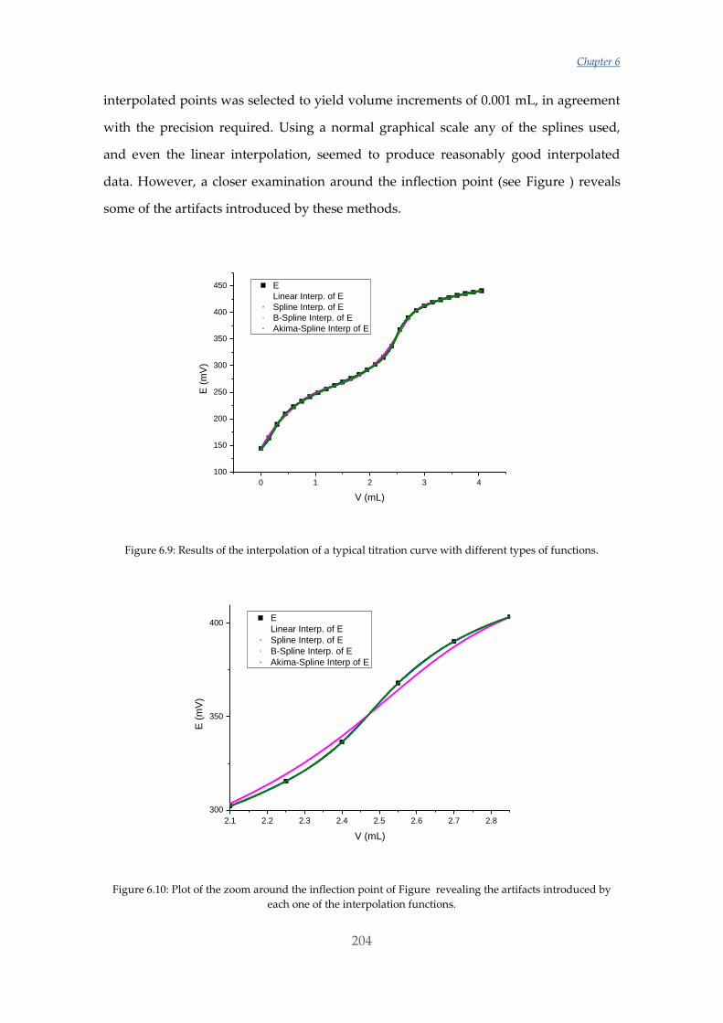
Chapter 6

204

interpolated points was selected to yield volume increments of 0.001 mL, in agreement

with the precision required. Using a normal graphical scale any of the splines used,

and even the linear interpolation, seemed to produce reasonably good interpolated

data. However, a closer examination around the inflection point (see Figure ) reveals

some of the artifacts introduced by these methods.

Figure 6.9: Results of the interpolation of a typical titration curve with different types of functions.

Figure 6.10: Plot of the zoom around the inflection point of Figure revealing the artifacts introduced by

each one of the interpolation functions.

0 1 2 3 4

100

150

200

250

300

350

400

450 E

Linear Interp. of E

Spline Interp. of E

B-Spline Interp. of E

Akima-Spline Interp of E

E (

mV

)

V (mL)

2.1 2.2 2.3 2.4 2.5 2.6 2.7 2.8

300

350

400E

Linear Interp. of E

Spline Interp. of E

B-Spline Interp. of E

Akima-Spline Interp of E

E (

mV

)

V (mL)

Determination of Alkalinity and DIC

205

As may be appreciated, the common spline and the Akima spline provide the best

approximations to the experimental (E, V) data. Since the Akima splines have been

pointed out for yielding lower errors in the interpolated data than common splines,

mostly when there are ‘defects’ or outliers in the data set, these will be used in the

following. As seen in Figure , the maxima in this first derivative, obtained with the

help of the OriginPro 2017 program, allow the location of the equivalence volumes

with a 0.001 mL precision. In some cases, depending on the initial pH of the sample

being titrated, this approach can even locate the position of the first equivalence point,

which is normally assigned to the titration of the initial carbonate present in the sample

to hydrogen carbonate. However, as these titrations are carried out in open vessels, the

information provided by these data is of questionable quality, as discussed previously.

Figure 6.11: First derivative of an interpolated set of (E, V) values for the titration of a CRM sample

showing the position of the two equivalence volumes.

There were situations, as shown in Figure , in which, due to the noise originally

present in the (E, V) titration data, some artifacts are revealed in the derivatives. In this

0.225

2.476

0 2 4

0

100

200

1st D

eri

v. o

f "A

kim

a-S

plin

e In

terp

. E

"

Interp. V (mL)

1st Derivative of "Akima-Spline Interp. E"

Peak Centers of "Derivative Y2"

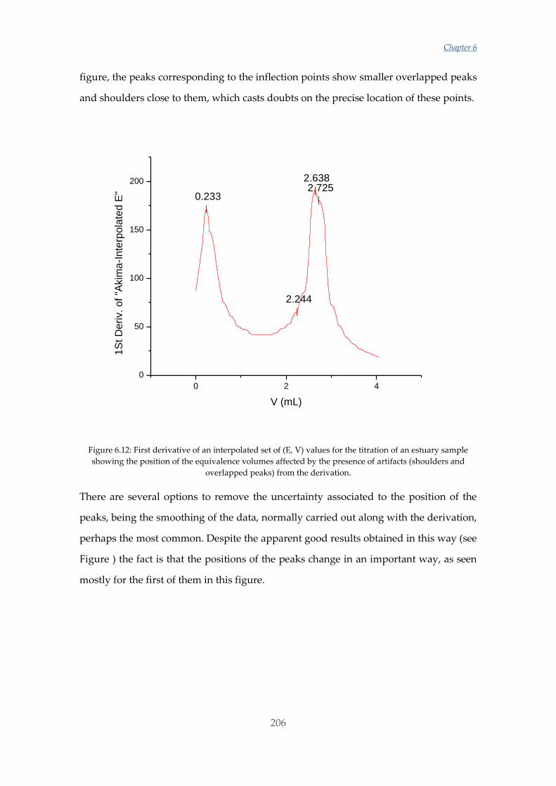
Chapter 6

206

figure, the peaks corresponding to the inflection points show smaller overlapped peaks

and shoulders close to them, which casts doubts on the precise location of these points.

Figure 6.12: First derivative of an interpolated set of (E, V) values for the titration of an estuary sample

showing the position of the equivalence volumes affected by the presence of artifacts (shoulders and

overlapped peaks) from the derivation.

There are several options to remove the uncertainty associated to the position of the

peaks, being the smoothing of the data, normally carried out along with the derivation,

perhaps the most common. Despite the apparent good results obtained in this way (see

Figure ) the fact is that the positions of the peaks change in an important way, as seen

mostly for the first of them in this figure.

0.233

2.244

2.6382.725

0 2 4

0

50

100

150

200

1S

t D

eri

v. o

f "A

kim

a-I

nte

rpo

late

d E

"

V (mL)

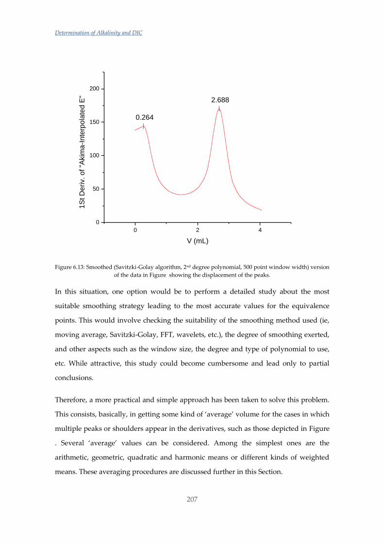
Determination of Alkalinity and DIC

207

Figure 6.13: Smoothed (Savitzki-Golay algorithm, 2nd degree polynomial, 500 point window width) version

of the data in Figure showing the displacement of the peaks.

In this situation, one option would be to perform a detailed study about the most

suitable smoothing strategy leading to the most accurate values for the equivalence

points. This would involve checking the suitability of the smoothing method used (ie,

moving average, Savitzki-Golay, FFT, wavelets, etc.), the degree of smoothing exerted,

and other aspects such as the window size, the degree and type of polynomial to use,

etc. While attractive, this study could become cumbersome and lead only to partial

conclusions.

Therefore, a more practical and simple approach has been taken to solve this problem.

This consists, basically, in getting some kind of ‘average’ volume for the cases in which

multiple peaks or shoulders appear in the derivatives, such as those depicted in Figure

. Several ‘average’ values can be considered. Among the simplest ones are the

arithmetic, geometric, quadratic and harmonic means or different kinds of weighted

means. These averaging procedures are discussed further in this Section.

0.264

2.688

0 2 4

0

50

100

150

200

1S

t D

eri

v. o

f "A

kim

a-I

nte

rpo

late

d E

"

V (mL)

Chapter 6

208

6.4.2 Choice of the best k1 and k2 for the carbonate system

In order to decide which of the different approaches outlined above for the calculation

of TA is the best one in terms of accuracy and precision, a whole campaign of

measurements of the Nerbioi-Ibaizabal estuary was analysed, mainly due to the higher

stratification observed for this estuary, which provides a wider variation in salinities.

Besides, this estuary has four tributary rivers to the main one and has suffered a big

anthropogenic pollution since the pre-industrial times (see sampling). Therefore, this

estuary is the most complex one of the three studied estuaries and, perhaps, the most

difficult to interpret.

Regarding the curve fitting by the non-linear lest squares procedure, first of all some of

the available pk1 and pk2 values for the carbonate system in literature were tested due

to the already mentioned incongruities between authors. All the samples were

measured in two different days and, therefore, two sets of CRM values are compared.

Table and Table show for day 1 and day 2, respectively, the averages of the refined

values of the TA after the same CRM’s were used to calculate the titrant HCl

concentration using the different pk1 and pk2 values. The uncertainty corresponds to

the square root of the sum of the variances due to the repetition and the variance of the

Solver-derived parameters that was calculated with the help of an Excel macro called

SolverAid7. In order to check which set of constants provides the best fit, Table and

Table also show the average values of the residual sum of squares (RSS). The CRM

used for this experiment was the Batch 165 which has a referenced TA value of 2214.09

± 0.41 µmol. kgsw-1.

7 http://www.bowdoin.edu/~rdelevie/excellaneous/

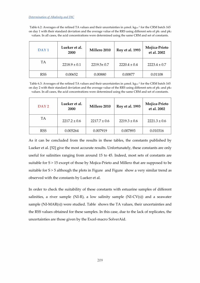
Determination of Alkalinity and DIC

209

Table 6.2: Averages of the refined TA values and their uncertainties in µmol. kgsw-1 for the CRM batch 165

on day 1 with their standard deviation and the average value of the RRS using different sets of pk1 and pk2

values. In all cases, the acid concentrations were determined using the same CRM and set of constants.

DAY 1 Lueker et al.

2000 Millero 2010 Roy et al. 1993

Mojica-Prieto

et al. 2002

TA

2218.9 ± 0.1 2219.5± 0.7 2220.4 ± 0.4 2223.4 ± 0.7

RSS 0.00652 0.00880 0.00877 0.01108

Table 6.3: Averages of the refined TA values and their uncertainties in µmol. kgsw-1 for the CRM batch 165

on day 2 with their standard deviation and the average value of the RRS using different sets of pk1 and pk2

values. In all cases, the acid concentrations were determined using the same CRM and set of constants.

DAY 2 Lueker et al.

2000 Millero 2010 Roy et al. 1993

Mojica-Prieto

et al. 2002

TA

2217.2 ± 0.6 2217.7 ± 0.6 2219.3 ± 0.6 2221.3 ± 0.6

RSS 0.005264 0.007919 0.007893 0.010316

As it can be concluded from the results in these tables, the constants published by

Lueker et al. [52] give the most accurate results. Unfortunately, these constants are only

useful for salinities ranging from around 15 to 45. Indeed, most sets of constants are

suitable for S > 15 except of those by Mojica-Prieto and Millero that are supposed to be

suitable for S > 5 although the plots in Figure and Figure show a very similar trend as

observed with the constants by Lueker et al.

In order to check the suitability of these constants with estuarine samples of different

salinities, a river sample (NI-R), a low salinity sample (NI-CV(s)) and a seawater

sample (NI-MAR(s)) were studied. Table shows the TA values, their uncertainties and

the RSS values obtained for these samples. In this case, due to the lack of replicates, the

uncertainties are those given by the Excel-macro SolverAid.

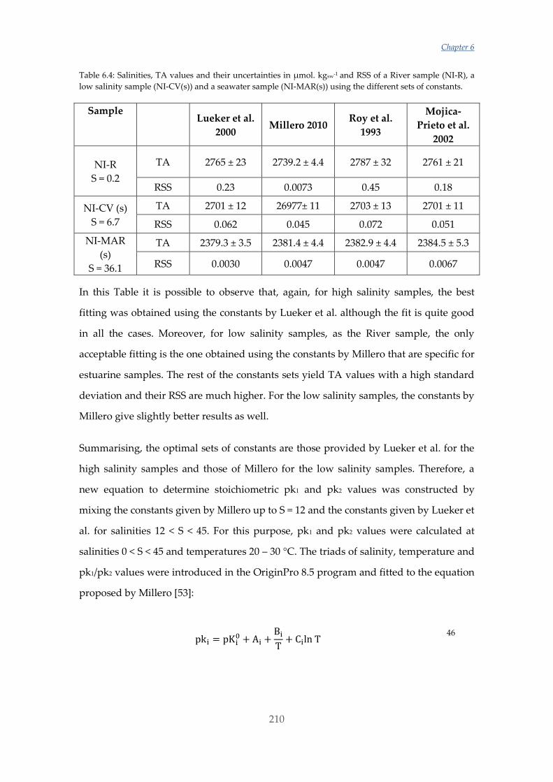
Chapter 6

210

Table 6.4: Salinities, TA values and their uncertainties in µmol. kgsw-1 and RSS of a River sample (NI-R), a

low salinity sample (NI-CV(s)) and a seawater sample (NI-MAR(s)) using the different sets of constants.

Sample

Lueker et al.

2000 Millero 2010

Roy et al.

1993

Mojica-

Prieto et al.

2002

NI-R

S = 0.2

TA 2765 ± 23 2739.2 ± 4.4 2787 ± 32 2761 ± 21

RSS 0.23 0.0073 0.45 0.18

NI-CV (s)

S = 6.7

TA 2701 ± 12 26977± 11 2703 ± 13 2701 ± 11

RSS 0.062 0.045 0.072 0.051

NI-MAR

(s)

S = 36.1

TA 2379.3 ± 3.5 2381.4 ± 4.4 2382.9 ± 4.4 2384.5 ± 5.3

RSS 0.0030 0.0047 0.0047 0.0067

In this Table it is possible to observe that, again, for high salinity samples, the best

fitting was obtained using the constants by Lueker et al. although the fit is quite good

in all the cases. Moreover, for low salinity samples, as the River sample, the only

acceptable fitting is the one obtained using the constants by Millero that are specific for

estuarine samples. The rest of the constants sets yield TA values with a high standard

deviation and their RSS are much higher. For the low salinity samples, the constants by

Millero give slightly better results as well.

Summarising, the optimal sets of constants are those provided by Lueker et al. for the

high salinity samples and those of Millero for the low salinity samples. Therefore, a

new equation to determine stoichiometric pk1 and pk2 values was constructed by

mixing the constants given by Millero up to S = 12 and the constants given by Lueker et

al. for salinities 12 < S < 45. For this purpose, pk1 and pk2 values were calculated at

salinities 0 < S < 45 and temperatures 20 – 30 °C. The triads of salinity, temperature and

pk1/pk2 values were introduced in the OriginPro 8.5 program and fitted to the equation

proposed by Millero [53]:

pki = pKi0 + Ai +

Bi

T+ Ciln T

46

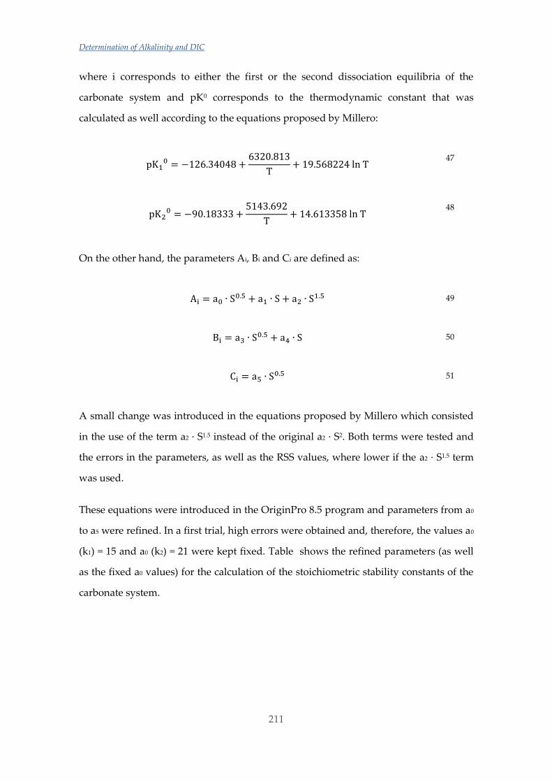
Determination of Alkalinity and DIC

211

where i corresponds to either the first or the second dissociation equilibria of the

carbonate system and pK0 corresponds to the thermodynamic constant that was

calculated as well according to the equations proposed by Millero:

pK10 = −126.34048 +

6320.813

T+ 19.568224 ln T

47

pK20 = −90.18333 +

5143.692

T+ 14.613358 ln T

48

On the other hand, the parameters Ai, Bi and Ci are defined as:

Ai = a0 ∙ S0.5 + a1 ∙ S + a2 ∙ S1.5 49

Bi = a3 ∙ S0.5 + a4 ∙ S 50

Ci = a5 ∙ S0.5 51

A small change was introduced in the equations proposed by Millero which consisted

in the use of the term a2 · S1.5 instead of the original a2 · S2. Both terms were tested and

the errors in the parameters, as well as the RSS values, where lower if the a2 · S1.5 term

was used.

These equations were introduced in the OriginPro 8.5 program and parameters from a0

to a5 were refined. In a first trial, high errors were obtained and, therefore, the values a0

(k1) = 15 and a0 (k2) = 21 were kept fixed. Table shows the refined parameters (as well

as the fixed a0 values) for the calculation of the stoichiometric stability constants of the

carbonate system.

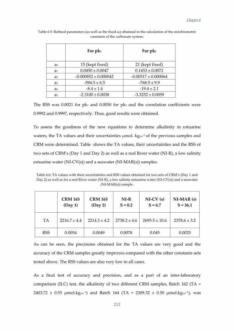
Chapter 6

212

Table 6.5: Refined parameters (as well as the fixed a0) obtained in the calculation of the stoichiometric

constants of the carbonate system.

For pk1 For pk2

a0 15 (kept fixed) 21 (kept fixed)

a1 0.0450 ± 0.0047 0.1453 ± 0.0072

a2 -0.000852 ± 0.000042 -0.00517 ± 0.000064

a3 -594.5 ± 6.5 -768.5 ± 9.9

a4 -8.4 ± 1.4 -19.4 ± 2.1

a5 -2.3100 ± 0.0038 -3.3252 ± 0.0059

The RSS was 0.0021 for pk1 and 0.0050 for pk2 and the correlation coefficients were

0.9992 and 0.9997, respectively. Thus, good results were obtained.

To assess the goodness of the new equations to determine alkalinity in estuarine

waters, the TA values and their uncertainties µmol. kgsw-1 of the previous samples and

CRM were determined. Table shows the TA values, their uncertainties and the RSS of

two sets of CRM’s (Day 1 and Day 2) as well as a real River water (NI-R), a low salinity

estuarine water (NI-CV(s)) and a seawater (NI-MAR(s)) samples.

Table 6.6: TA values with their uncertainties and RSS values obtained for two sets of CRM’s (Day 1 and

Day 2) as well as for a real River water (NI-R), a low salinity estuarine water (NI-CV(s)) and a seawater

(NI-MAR(s)) sample.

CRM 165

(Day 1)

CRM 165

(Day 2)

NI-R

S = 0.2

NI-CV (s)

S = 6.7

NI-MAR (s)

S = 36.1

TA 2216.7 ± 4.4 2214.3 ± 4.2 2738.2 ± 4.6 2695.5 ± 10.6 2378.6 ± 3.2

RSS 0.0054 0.0049 0.0078 0.045 0.0025

As can be seen, the precisions obtained for the TA values are very good and the

accuracy of the CRM samples greatly improves compared with the other constants sets

tested above. The RSS values are also very low in all cases.

As a final test of accuracy and precision, and as a part of an inter-laboratory

comparison (ILC) test, the alkalinity of two different CRM samples, Batch 162 (TA =

2403.72 ± 0.55 µmol.kgsw–1) and Batch 164 (TA = 2309.32 ± 0.50 µmol.kgsw–1), was

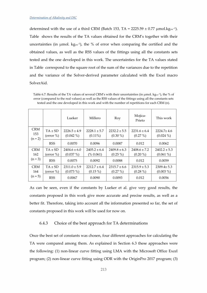
Determination of Alkalinity and DIC

213

determined with the use of a third CRM (Batch 153, TA = 2225.59 ± 0.77 µmol.kgsw–1).

Table shows the results of the TA values obtained for the CRM’s together with their

uncertainties (in µmol. kgsw-1), the % of error when comparing the certified and the

obtained values, as well as the RSS values of the fittings using all the constants sets

tested and the one developed in this work. The uncertainties for the TA values stated

in Table correspond to the square root of the sum of the variances due to the repetition

and the variance of the Solver-derived parameter calculated with the Excel macro

SolverAid.

Table 6.7: Results of the TA values of several CRM’s with their uncertainties (in µmol. kgsw-1), the % of

error (compared to the real values) as well as the RSS values of the fittings using all the constants sets

tested and the one developed in this work and with the number of repetitions for each CRM (n).

Lueker Millero Roy Mojica-

Prieto This work

CRM

153

(n = 2)

TA ± SD

(error %)

2226.5 ± 4.9

(0.042 %)

2228.1 ± 5.7

(0.11%)

2232.2 ± 5.5

(0.30 %)

2231.6 ± 6.4

(0.27 %)

2224.7± 4.6

(0.024 %)

RSS 0.0070 0.0096 0.0087 0.012 0.0062

CRM

162

(n = 3)

TA ± SD

(error %)

2404.6 ± 6.0

(0.037 %)

2405.2 ± 6.4

(% 0.061)

2409.8 ± 6.3

(0.25 %)

2408.6 ± 7.2

(0.20 %)

2402.2 ± 5.3

(0.061 %)

RSS 0.0075 0.0092 0.0088 0.012 0.0059

CRM

164

(n = 5)

TA ± SD

(error %)

2311.0 ± 5.9

(0.073 %)

2212.7 ± 6.4

(0.15 %)

2315.7 ± 6.6

(0.27 %)

2315.9 ± 5.3

(0.28 %)

2309.4± 5.3

(0.003 %)

RSS 0.0067 0.0090 0.0093 0.012 0.0056

As can be seen, even if the constants by Lueker et al. give very good results, the

constants proposed in this work give more accurate and precise results, as well as a

better fit. Therefore, taking into account all the information presented so far, the set of

constants proposed in this work will be used for now on.

6.4.3 Choice of the best approach for TA determinations

Once the best set of constants was chosen, four different approaches for calculating the

TA were compared among them. As explained in Section 6.3 these approaches were

the following: (1) non-linear curve fitting using LMA with the Microsoft Office Excel

program; (2) non-linear curve fitting using ODR with the OriginPro 2017 program; (3)

Chapter 6

214

non-linear curve fitting using the BSTAC4 and ES4ECI programs and (4) empirical

determination of the equivalence point using interpolated (V, E) data and their first

derivative. In order to choose among these approaches, the accuracy and precision of

the TA values obtained must be taken into account. It must be pointed out that when

the “quality” of analytical measurements is being tested it is very important to take

into account the scientific application that they are required for and the maximum

uncertainty that is considered appropriate for that application, that is, to apply the

principle of ‘fitness for purpose’. A quite recent report describing plans for a Global

Ocean Acidification Observing Network (GOA-ON) articulates two such applications:

a “weather” goal and a “climate” goal [69]. The “weather” goal is defined as

measurements of quality sufficient to identify relative spatial patterns and short-term

variations, supporting mechanistic responses to the impact on local, immediate ocean

acidification dynamics. This implies an uncertainty of ~10 μmol. kg−1 in measurements

of TA and DIC (~ 0.5 %). The “climate” goal is defined as measurements of quality

sufficient to assess long-term trends with a defined level of confidence, supporting

detection of the long-term anthropogenically driven changes in hydrographic

conditions. This objective is far more demanding and implies an uncertainty of ~2

μmol. kg−1 in measurements of TA and DIC (~ 0.1 %). These “weather” and “climate”

goals were used by Bockmon and Dickson [37] at their inter-laboratory comparison

studies. Thus, in this work, a ~ 0.1 % in accuracy and precision will be considered as

the acceptable uncertainty level. For the first three approaches, it was observed in

previous experiments that while the (V, E) titration data fitting was very good for

medium to high salinities, some of the low salinity samples did not give a good fit and

the precision was sometimes less than the 0.1 % recommended. Therefore, it was

decided to optimize also the parameters a0 in approaches (1) and (2) and C in approach

(3). By doing this, the precision was increased more than twice and this is the way the

non-linear least-squares procedures were performed.

Before comparing the different approaches and according to what was stated in Section

6.4.1, several averaging procedures were studied for those peaks that show an unclear

maximum. The studies procedures were the arithmetic, geometric, quadratic and

Determination of Alkalinity and DIC

215

harmonic means or different kinds of weighted means. In order to choose the correct

procedure, some CRM samples that were used for an ILC study were used. To

determine the HCl concentration CRM Batch 153 was used. With this HCl value, the

TA of CRM’s Batch 162 and Batch 164 were determined.

In the determination of the HCl concentration, made in duplicate, the equivalence

volume obtained was 2.477 mL in both cases, leading to an HCl concentration of

0.095817 ± 0.000002 mol. kg-1 (considering only the standard deviation). Only one peak,

like that shown in Figure , was observed in these cases. However, in the TA

determinations of Batch 162 and Batch 164 two peaks were observed in the first

derivative around the volumes corresponding to the second equivalence point, like

shown in Figure . Table presents the results of the volumes corresponding to those

peaks, together with the TA values (in µmol. kg-1) obtained by considering different

mean values of those volumes. Also, the mean TA values with their uncertainties,

calculated only by means of the standard deviation of the TA values, the RSDs and the

errors in % respecting to the certified CRM values: 2403.72 µmol. kg-1 and 2309.32

µmol. kg-1 for CRM Batches 162 and 164, respectively.

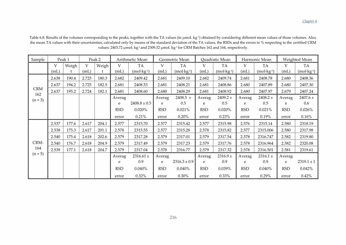
Chapter 6

216

Table 6.8: Results of the volumes corresponding to the peaks, together with the TA values (in µmol. kg-1) obtained by considering different mean values of those volumes. Also,

the mean TA values with their uncertainties, calculated only by means of the standard deviation of the TA values, the RSDs and the errors in % respecting to the certified CRM

values: 2403.72 µmol. kg-1 and 2309.32 µmol. kg-1 for CRM Batches 162 and 164, respectively.

Sample Peak 1 Peak 2 Arithmetic Mean Geometric Mean Quadratic Mean Harmonic Mean Weighted Mean

V

(mL)

Weigh

t

V

(mL)

Weigh

t

V

(mL)

TA

(mol·kg-1)

V

(mL)

TA

(mol·kg-1)

V

(mL)

TA

(mol·kg-1)

V

(mL)

TA

(mol·kg-1)

V

(mL)

TA

(mol·kg-1)

CRM

162

(n = 3)

2.638 190.4 2.725 180.3 2.682 2409.42 2.681 2409.10 2.682 2409.74 2.681 2408.78 2.680 2408.36

2.637 194.2 2.725 182.5 2.681 2408.53 2.681 2408.21 2.681 2408.86 2.680 2407.89 2.680 2407.30

2.637 195.2 2.724 182.1 2.681 2408.60 2.680 2408.29 2.681 2408.92 2.680 2407.97 2.679 2407.24

Averag

e 2408.8 ± 0.5

Averag

e

2408.5 ±

0.5

Averag

e

2409.2 ±

0.5

Averag

e

2408.2 ±

0.5

Averag

e

2407.6 ±

0.6

RSD 0.020% RSD 0.021% RSD 0.020% RSD 0.021% RSD 0.026%

error 0.21% error 0.20% error 0.23% error 0.19% error 0.16%

CRM-

164

(n = 5)

2.537 177.6 2.617 204.1 2.577 2315.70 2.577 2315.42 2.577 2315.98 2.576 2315.14 2.580 2318.19

2.538 175.3 2.617 201.1 2.578 2315.55 2.577 2315.28 2.578 2315.82 2.577 2315.006 2.580 2317.98

2.540 175.4 2.618 202.6 2.579 2317.28 2.579 2317.01 2.579 2317.54 2.578 2316.747 2.582 2319.80

2.540 176.7 2.618 204.9 2.579 2317.49 2.579 2317.23 2.579 2317.76 2.578 2316.964 2.582 2320.08

2.539 177.1 2.618 204.7 2.579 2317.04 2.578 2316.77 2.579 2317.32 2.578 2316.501 2.581 2319.61

Averag

e

2316.61 ±

0.9

Averag

e 2316.3 ± 0.9

Averag

e

2316.9 ±

0.9

Averag

e

2316.1 ±

0.9

Averag

e 2319.1 ± 1

RSD 0.040% RSD 0.040% RSD 0.039% RSD 0.040% RSD 0.042%

error 0.32% error 0.30% error 0.33% error 0.29% error 0.42%

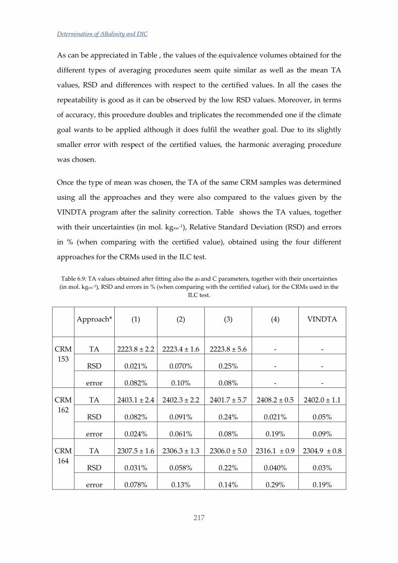
Determination of Alkalinity and DIC

217

As can be appreciated in Table , the values of the equivalence volumes obtained for the

different types of averaging procedures seem quite similar as well as the mean TA

values, RSD and differences with respect to the certified values. In all the cases the

repeatability is good as it can be observed by the low RSD values. Moreover, in terms

of accuracy, this procedure doubles and triplicates the recommended one if the climate

goal wants to be applied although it does fulfil the weather goal. Due to its slightly

smaller error with respect of the certified values, the harmonic averaging procedure

was chosen.

Once the type of mean was chosen, the TA of the same CRM samples was determined

using all the approaches and they were also compared to the values given by the

VINDTA program after the salinity correction. Table shows the TA values, together

with their uncertainties (in mol. kgsw-1), Relative Standard Deviation (RSD) and errors

in % (when comparing with the certified value), obtained using the four different

approaches for the CRMs used in the ILC test.

Table 6.9: TA values obtained after fitting also the a0 and C parameters, together with their uncertainties

(in mol. kgsw-1), RSD and errors in % (when comparing with the certified value), for the CRMs used in the

ILC test.

Approach* (1) (2) (3) (4) VINDTA

CRM

153

TA 2223.8 ± 2.2 2223.4 ± 1.6 2223.8 ± 5.6 - -

RSD 0.021% 0.070% 0.25% - -

error 0.082% 0.10% 0.08% - -

CRM

162

TA 2403.1 ± 2.4 2402.3 ± 2.2 2401.7 ± 5.7 2408.2 ± 0.5 2402.0 ± 1.1

RSD 0.082% 0.091% 0.24% 0.021% 0.05%

error 0.024% 0.061% 0.08% 0.19% 0.09%

CRM

164

TA 2307.5 ± 1.6 2306.3 ± 1.3 2306.0 ± 5.0 2316.1 ± 0.9 2304.9 ± 0.8

RSD 0.031% 0.058% 0.22% 0.040% 0.03%

error 0.078% 0.13% 0.14% 0.29% 0.19%

Chapter 6

218

* The uncertainties of (1), (2) and (3) where calculated as the square root of the sum of the variances due to

the repetition and the variance of the fitted parameters calculated with the SolverAid macro in Excel or

directly in OriginPro 2017 or by the error propagation of the errors of the free species given by ES4ECI,

respectively. The uncertainties of (4) and VINDTA correspond to the standard deviation due to the

repetition. Values of CRM 153 calculated by approach (4) and VINDTA are missing because it does not

make sense to re-calculate the concentrations of these samples because they were used to calculate the

equivalence volume or the correction factor, respectively (see Section 6.2.3).

The inter-laboratory comparison test was very helpful to determine the accuracy of

each approach because the real concentrations of the two CRM samples to be tested are

well known. As can be observed in the approach (1), the obtained accuracies are

slightly worse than when the a0 parameters were fixed but the precision is much better

than in Table . In this case, all the accuracies and precisions are below 0.1 %. In the case

of the second approach, the RSD values and accuracies are slightly higher. The TA

values are a little bit but systematically smaller than when approach 1 was used. In the

case of CRM 164 the error percentage was higher than 0.1 % but not much. In the case

of approach (3) the errors and therefore the RSD values are rather high. This is

expectable since the uncertainties of all the equilibrium constants that were used, along

with those of the total concentrations, were used for the prediction of the uncertainties

of the free concentrations. These errors could be more realistic than the other two. As

for the accuracy, in general values are a little be smaller than the certified ones (as it

happens with the other two approaches) but within a reasonable margin. In the case of

approach (4) and as stated before, even if the repeatability is good, the accuracy is quite

far from fulfilling the climate goal of an 0.1 % error. Finally, all of these results were

compared to those given by the VINDTA program after the salinity correction was

applied. These results were those presented in the ILC test. In this case as well, the fit

does not provide an error estimation for the TA values and, therefore, the uncertainty

and the RSD are only based on the standard deviation due to the repetition, which is

the reason why there are so low in Table . The accuracy, on the other hand, although it

is acceptable in the case of CRM 162, it nearly doubles the recommended uncertainty

for this kind of studies in CRM 164. It must be pointed out though, that the results

given by the VINDTA program should be accurate at high salinities. Given the smaller

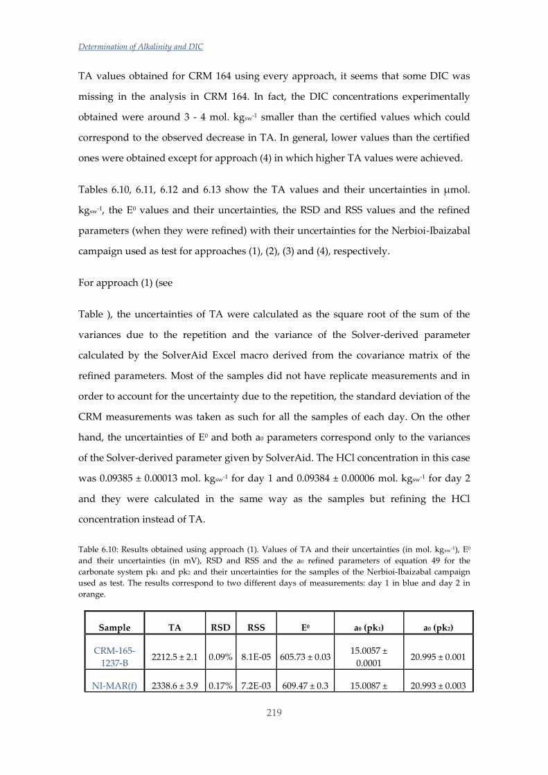
Determination of Alkalinity and DIC

219

TA values obtained for CRM 164 using every approach, it seems that some DIC was

missing in the analysis in CRM 164. In fact, the DIC concentrations experimentally

obtained were around 3 - 4 mol. kgsw-1 smaller than the certified values which could

correspond to the observed decrease in TA. In general, lower values than the certified

ones were obtained except for approach (4) in which higher TA values were achieved.

Tables 6.10, 6.11, 6.12 and 6.13 show the TA values and their uncertainties in µmol.

kgsw-1, the E0 values and their uncertainties, the RSD and RSS values and the refined

parameters (when they were refined) with their uncertainties for the Nerbioi-Ibaizabal

campaign used as test for approaches (1), (2), (3) and (4), respectively.

For approach (1) (see

Table ), the uncertainties of TA were calculated as the square root of the sum of the

variances due to the repetition and the variance of the Solver-derived parameter

calculated by the SolverAid Excel macro derived from the covariance matrix of the

refined parameters. Most of the samples did not have replicate measurements and in

order to account for the uncertainty due to the repetition, the standard deviation of the

CRM measurements was taken as such for all the samples of each day. On the other

hand, the uncertainties of E0 and both a0 parameters correspond only to the variances

of the Solver-derived parameter given by SolverAid. The HCl concentration in this case

was 0.09385 ± 0.00013 mol. kgsw-1 for day 1 and 0.09384 ± 0.00006 mol. kgsw-1 for day 2

and they were calculated in the same way as the samples but refining the HCl

concentration instead of TA.

Table 6.10: Results obtained using approach (1). Values of TA and their uncertainties (in mol. kgsw-1), E0

and their uncertainties (in mV), RSD and RSS and the a0 refined parameters of equation 49 for the

carbonate system pk1 and pk2 and their uncertainties for the samples of the Nerbioi-Ibaizabal campaign

used as test. The results correspond to two different days of measurements: day 1 in blue and day 2 in

orange.

Sample TA RSD RSS E0 a0 (pk1) a0 (pk2)

CRM-165-

1237-B 2212.5 ± 2.1 0.09% 8.1E-05 605.73 ± 0.03

15.0057 ±

0.0001 20.995 ± 0.001

NI-MAR(f) 2338.6 ± 3.9 0.17% 7.2E-03 609.47 ± 0.3 15.0087 ± 20.993 ± 0.003

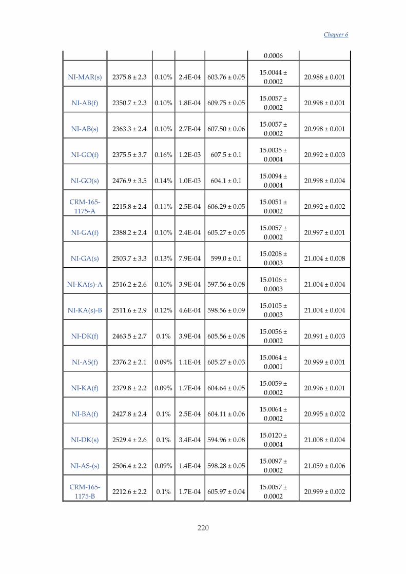
Chapter 6

220

0.0006

NI-MAR(s) 2375.8 ± 2.3 0.10% 2.4E-04 603.76 ± 0.05 15.0044 ±

0.0002 20.988 ± 0.001

NI-AB(f) 2350.7 ± 2.3 0.10% 1.8E-04 609.75 ± 0.05 15.0057 ±

0.0002 20.998 ± 0.001

NI-AB(s) 2363.3 ± 2.4 0.10% 2.7E-04 607.50 ± 0.06 15.0057 ±

0.0002 20.998 ± 0.001

NI-GO(f) 2375.5 ± 3.7 0.16% 1.2E-03 607.5 ± 0.1 15.0035 ±

0.0004 20.992 ± 0.003

NI-GO(s) 2476.9 ± 3.5 0.14% 1.0E-03 604.1 ± 0.1 15.0094 ±

0.0004 20.998 ± 0.004

CRM-165-

1175-A 2215.8 ± 2.4 0.11% 2.5E-04 606.29 ± 0.05

15.0051 ±

0.0002 20.992 ± 0.002

NI-GA(f) 2388.2 ± 2.4 0.10% 2.4E-04 605.27 ± 0.05 15.0057 ±

0.0002 20.997 ± 0.001

NI-GA(s) 2503.7 ± 3.3 0.13% 7.9E-04 599.0 ± 0.1 15.0208 ±

0.0003 21.004 ± 0.008

NI-KA(s)-A 2516.2 ± 2.6 0.10% 3.9E-04 597.56 ± 0.08 15.0106 ±

0.0003 21.004 ± 0.004

NI-KA(s)-B 2511.6 ± 2.9 0.12% 4.6E-04 598.56 ± 0.09 15.0105 ±

0.0003 21.004 ± 0.004

NI-DK(f) 2463.5 ± 2.7 0.1% 3.9E-04 605.56 ± 0.08 15.0056 ±

0.0002 20.991 ± 0.003

NI-AS(f) 2376.2 ± 2.1 0.09% 1.1E-04 605.27 ± 0.03 15.0064 ±

0.0001 20.999 ± 0.001

NI-KA(f) 2379.8 ± 2.2 0.09% 1.7E-04 604.64 ± 0.05 15.0059 ±

0.0002 20.996 ± 0.001

NI-BA(f) 2427.8 ± 2.4 0.1% 2.5E-04 604.11 ± 0.06 15.0064 ±

0.0002 20.995 ± 0.002

NI-DK(s) 2529.4 ± 2.6 0.1% 3.4E-04 594.96 ± 0.08 15.0120 ±

0.0004 21.008 ± 0.004

NI-AS-(s) 2506.4 ± 2.2 0.09% 1.4E-04 598.28 ± 0.05 15.0097 ±

0.0002 21.059 ± 0.006

CRM-165-

1175-B 2212.6 ± 2.2 0.1% 1.7E-04 605.97 ± 0.04

15.0057 ±

0.0002 20.999 ± 0.002

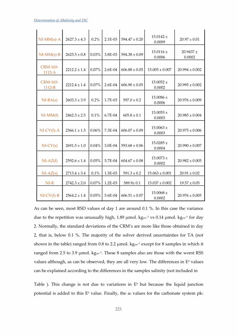
Determination of Alkalinity and DIC

221

NI-MM(s)-A 2627.3 ± 4.3 0.2% 2.1E-03 594.47 ± 0.20 15.0142 ±

0.0009 20.97 ± 0.01

NI-MM(s)-B 2625.5 ± 0.8 0.03% 3.8E-03 594.38 ± 0.09 15.0116 ±

0.0006

20.9437 ±

0.0002

CRM-165-

1112-A 2212.2 ± 1.4 0.07% 2.6E-04 606.88 ± 0.05 15.005 ± 0.007 20.994 ± 0.002

CRM-165-

1112-B 2212.4 ± 1.4 0.07% 2.6E-04 606.90 ± 0.05

15.0052 ±

0.0002 20.995 ± 0.002

NI-BA(s) 2603.3 ± 3.9 0.2% 1.7E-03 597.0 ± 0.2 15.0086 ±

0.0006 20.976 ± 0.009

NI-MM(f) 2462.3 ± 2.5 0.1% 6.7E-04 605.8 ± 0.1 15.0055 ±

0.0003 20.985 ± 0.004

NI-CV(f)-A 2566.1 ± 1.5 0.06% 7.3E-04 606.07 ± 0.09 15.0063 ±

0.0003 20.975 ± 0.006

NI-CV(s) 2691.5 ± 1.0 0.04% 3.0E-04 593.68 ± 0.06 15.0285 ±

0.0004 20.990 ± 0.007

NI-AZ(f) 2592.6 ± 1.4 0.05% 5.7E-04 604.67 ± 0.08 15.0073 ±

0.0002 20.982 ± 0.005

NI-AZ(s) 2713.4 ± 3.4 0.1% 1.3E-03 591.3 ± 0.2 15.063 ± 0.001 20.91 ± 0.02

NI-R 2742.3 ± 2.0 0.07% 1.2E-03 589.9± 0.1 15.037 ± 0.002 19.57 ± 0.05

NI-CV(f)-B 2564.2 ± 1.4 0.05% 5.6E-04 606.51 ± 0.07 15.0068 ±

0.0002 20.976 ± 0.005

As can be seen, most RSD values of day 1 are around 0.1 %. In this case the variance

due to the repetition was unusually high, 1.89 µmol. kgsw-1 vs 0.14 µmol. kgsw-1 for day

2. Normally, the standard deviations of the CRM’s are more like those obtained in day

2, that is, below 0.1 %. The majority of the solver derived uncertainties for TA (not

shown in the table) ranged from 0.8 to 2.2 µmol. kgsw-1 except for 8 samples in which it

ranged from 2.5 to 3.9 µmol. kgsw-1. These 8 samples also are those with the worst RSS

values although, as can be observed, they are all very low. The differences in E0 values

can be explained according to the differences in the samples salinity (not included in

Table ). This change is not due to variations in E0 but because the liquid junction

potential is added to this E0 value. Finally, the a0 values for the carbonate system pk1

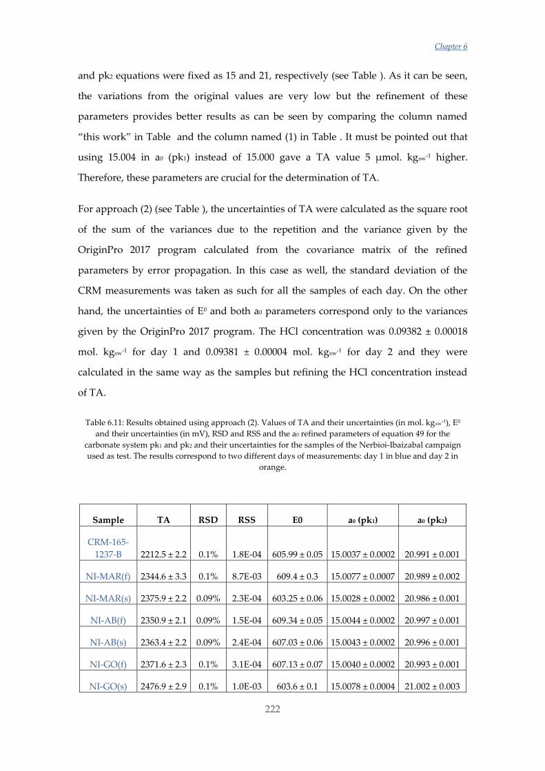
Chapter 6

222

and pk2 equations were fixed as 15 and 21, respectively (see Table ). As it can be seen,

the variations from the original values are very low but the refinement of these

parameters provides better results as can be seen by comparing the column named

“this work” in Table and the column named (1) in Table . It must be pointed out that

using 15.004 in a0 (pk1) instead of 15.000 gave a TA value 5 µmol. kgsw-1 higher.

Therefore, these parameters are crucial for the determination of TA.

For approach (2) (see Table ), the uncertainties of TA were calculated as the square root

of the sum of the variances due to the repetition and the variance given by the

OriginPro 2017 program calculated from the covariance matrix of the refined

parameters by error propagation. In this case as well, the standard deviation of the

CRM measurements was taken as such for all the samples of each day. On the other

hand, the uncertainties of E0 and both a0 parameters correspond only to the variances

given by the OriginPro 2017 program. The HCl concentration was 0.09382 ± 0.00018

mol. kgsw-1 for day 1 and 0.09381 ± 0.00004 mol. kgsw-1 for day 2 and they were

calculated in the same way as the samples but refining the HCl concentration instead

of TA.

Table 6.11: Results obtained using approach (2). Values of TA and their uncertainties (in mol. kgsw-1), E0

and their uncertainties (in mV), RSD and RSS and the a0 refined parameters of equation 49 for the

carbonate system pk1 and pk2 and their uncertainties for the samples of the Nerbioi-Ibaizabal campaign

used as test. The results correspond to two different days of measurements: day 1 in blue and day 2 in

orange.

Sample TA RSD RSS E0 a0 (pk1) a0 (pk2)

CRM-165-

1237-B 2212.5 ± 2.2 0.1% 1.8E-04 605.99 ± 0.05 15.0037 ± 0.0002 20.991 ± 0.001

NI-MAR(f) 2344.6 ± 3.3 0.1% 8.7E-03 609.4 ± 0.3 15.0077 ± 0.0007 20.989 ± 0.002

NI-MAR(s) 2375.9 ± 2.2 0.09% 2.3E-04 603.25 ± 0.06 15.0028 ± 0.0002 20.986 ± 0.001

NI-AB(f) 2350.9 ± 2.1 0.09% 1.5E-04 609.34 ± 0.05 15.0044 ± 0.0002 20.997 ± 0.001

NI-AB(s) 2363.4 ± 2.2 0.09% 2.4E-04 607.03 ± 0.06 15.0043 ± 0.0002 20.996 ± 0.001

NI-GO(f) 2371.6 ± 2.3 0.1% 3.1E-04 607.13 ± 0.07 15.0040 ± 0.0002 20.993 ± 0.001

NI-GO(s) 2476.9 ± 2.9 0.1% 1.0E-03 603.6 ± 0.1 15.0078 ± 0.0004 21.002 ± 0.003

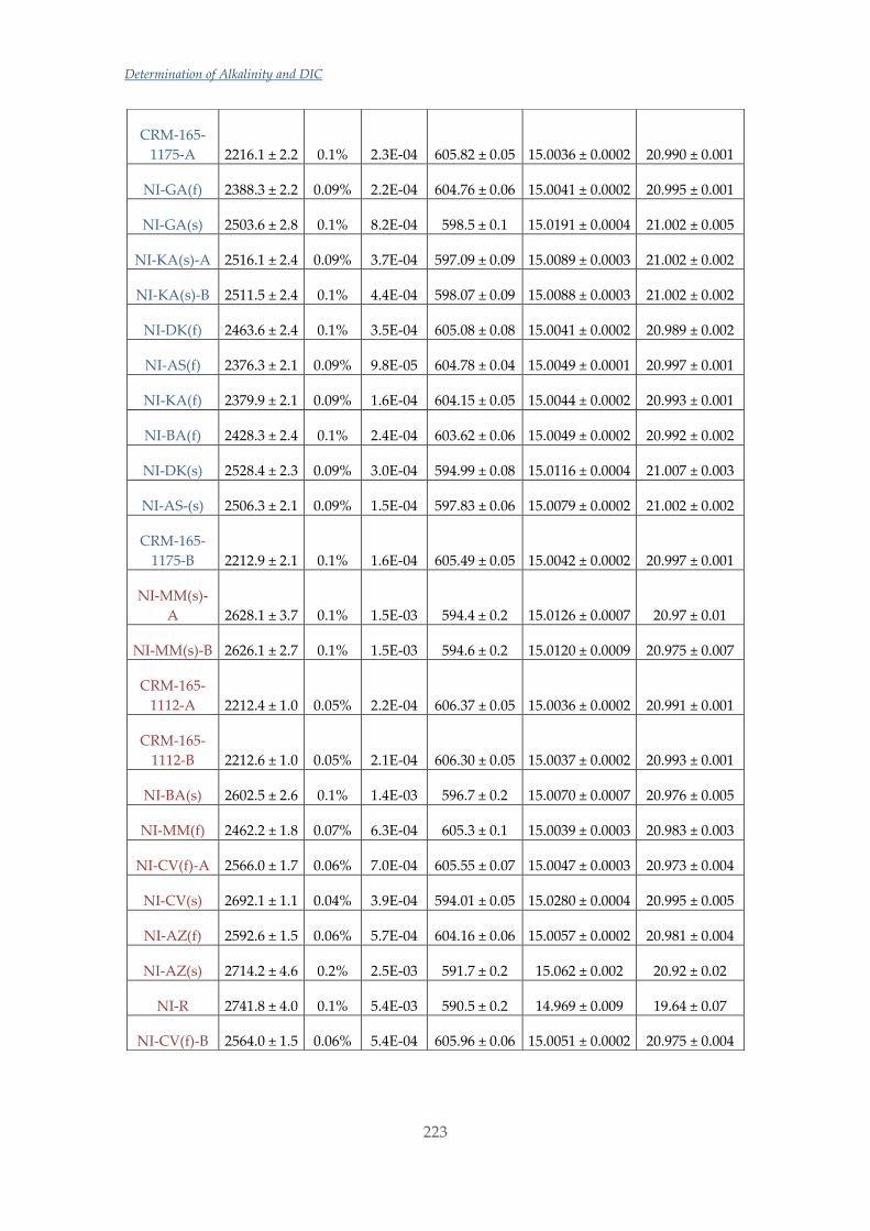
Determination of Alkalinity and DIC

223

CRM-165-

1175-A 2216.1 ± 2.2 0.1% 2.3E-04 605.82 ± 0.05 15.0036 ± 0.0002 20.990 ± 0.001

NI-GA(f) 2388.3 ± 2.2 0.09% 2.2E-04 604.76 ± 0.06 15.0041 ± 0.0002 20.995 ± 0.001

NI-GA(s) 2503.6 ± 2.8 0.1% 8.2E-04 598.5 ± 0.1 15.0191 ± 0.0004 21.002 ± 0.005

NI-KA(s)-A 2516.1 ± 2.4 0.09% 3.7E-04 597.09 ± 0.09 15.0089 ± 0.0003 21.002 ± 0.002

NI-KA(s)-B 2511.5 ± 2.4 0.1% 4.4E-04 598.07 ± 0.09 15.0088 ± 0.0003 21.002 ± 0.002

NI-DK(f) 2463.6 ± 2.4 0.1% 3.5E-04 605.08 ± 0.08 15.0041 ± 0.0002 20.989 ± 0.002

NI-AS(f) 2376.3 ± 2.1 0.09% 9.8E-05 604.78 ± 0.04 15.0049 ± 0.0001 20.997 ± 0.001

NI-KA(f) 2379.9 ± 2.1 0.09% 1.6E-04 604.15 ± 0.05 15.0044 ± 0.0002 20.993 ± 0.001

NI-BA(f) 2428.3 ± 2.4 0.1% 2.4E-04 603.62 ± 0.06 15.0049 ± 0.0002 20.992 ± 0.002

NI-DK(s) 2528.4 ± 2.3 0.09% 3.0E-04 594.99 ± 0.08 15.0116 ± 0.0004 21.007 ± 0.003

NI-AS-(s) 2506.3 ± 2.1 0.09% 1.5E-04 597.83 ± 0.06 15.0079 ± 0.0002 21.002 ± 0.002

CRM-165-

1175-B 2212.9 ± 2.1 0.1% 1.6E-04 605.49 ± 0.05 15.0042 ± 0.0002 20.997 ± 0.001

NI-MM(s)-

A 2628.1 ± 3.7 0.1% 1.5E-03 594.4 ± 0.2 15.0126 ± 0.0007 20.97 ± 0.01

NI-MM(s)-B 2626.1 ± 2.7 0.1% 1.5E-03 594.6 ± 0.2 15.0120 ± 0.0009 20.975 ± 0.007

CRM-165-

1112-A 2212.4 ± 1.0 0.05% 2.2E-04 606.37 ± 0.05 15.0036 ± 0.0002 20.991 ± 0.001

CRM-165-

1112-B 2212.6 ± 1.0 0.05% 2.1E-04 606.30 ± 0.05 15.0037 ± 0.0002 20.993 ± 0.001

NI-BA(s) 2602.5 ± 2.6 0.1% 1.4E-03 596.7 ± 0.2 15.0070 ± 0.0007 20.976 ± 0.005

NI-MM(f) 2462.2 ± 1.8 0.07% 6.3E-04 605.3 ± 0.1 15.0039 ± 0.0003 20.983 ± 0.003

NI-CV(f)-A 2566.0 ± 1.7 0.06% 7.0E-04 605.55 ± 0.07 15.0047 ± 0.0003 20.973 ± 0.004

NI-CV(s) 2692.1 ± 1.1 0.04% 3.9E-04 594.01 ± 0.05 15.0280 ± 0.0004 20.995 ± 0.005

NI-AZ(f) 2592.6 ± 1.5 0.06% 5.7E-04 604.16 ± 0.06 15.0057 ± 0.0002 20.981 ± 0.004

NI-AZ(s) 2714.2 ± 4.6 0.2% 2.5E-03 591.7 ± 0.2 15.062 ± 0.002 20.92 ± 0.02

NI-R 2741.8 ± 4.0 0.1% 5.4E-03 590.5 ± 0.2 14.969 ± 0.009 19.64 ± 0.07

NI-CV(f)-B 2564.0 ± 1.5 0.06% 5.4E-04 605.96 ± 0.06 15.0051 ± 0.0002 20.975 ± 0.004

Chapter 6

224

In this case, as well, most RSD values of day 1 are around 0.1 % because of the same

reason discussed for approach (1). However, using this approach the RSD values are

slightly smaller. In day 2, the RSD values remain very similar as in approach (1) with

some values being randomly smaller or higher. The variances due to repetition were a

bit higher for day 1 (1.95 µmol. kgsw-1) and a bit smaller in day 2 (0.11 µmol. kgsw-1).

The majority of the uncertainties for TA derived from the fitting and given by the

OriginPro 2017 program (not in the table) ranged from 0.7 to 2.2 µmol. kgsw-1 except for

6 samples in which it ranged from 2.6 to 4.6 µmol. kgsw-1. These samples correspond to

some of those with worse RSS values using approach (1) and also are those with the

highest RSS values (> 1.0E-3) although they are all very low. The differences in E0

values can be accounted in the same way as for approach (1). Finally, the a0 values for

the carbonate system pk1 and pk2 varied only slightly from the original. In general, the

values of a0 (pk1) are somewhat higher in approach (2) while a0 (pk2) are a little bit

higher in approach (1).

All in all, no big differences were found in the TA values when either approach (1) or

approach (2) were used. Most of the samples show higher TA values using approach

(2) but those differences were as much as ± 1 µmol. kgsw-1 in most cases. Statistical

analysis of all repeated samples was performed (F test and a posterior Student t-test)

and in all cases the results between both approaches were comparable.

For approach (3) (see Table ), the fitting parameters were the C parameters in equation

41 along with the E0 and the H+ total concentration. The uncertainties of TA were

calculated as the square root of the sum of the variances due to the repetition and the

variance calculated by error propagation of the free concentrations of both components

and species using the Kragten method [67]. The problem with this approach is that it is

not possible to refine the HCl concentration in the same manner as the TA. Different

programs could be used for that purpose but in order to compare the results given by

with the previous approaches and taking into account that good results that were

obtained with them, the average value of the HCl concentrations obtained using

approaches (1) and (2) was used in this approach. These concentrations were

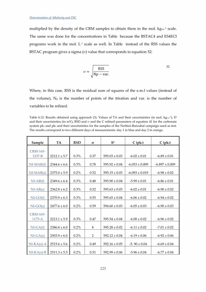
Determination of Alkalinity and DIC

225

multiplied by the density of the CRM samples to obtain them in the mol. kgsw-1 scale.

The same was done for the concentrations in Table because the BSTAC4 and ES4ECI

programs work in the mol. L-1 scale as well. In Table instead of the RSS values the

BSTAC program gives a sigma (σ) value that corresponds to equation 52:

σ = √RSS

Np − var.

52

Where, in this case, RSS is the residual sum of squares of the e.m.f values (instead of

the volume), Np is the number of points of the titration and var. is the number of

variables to be refined.

Table 6.12: Results obtained using approach (3). Values of TA and their uncertainties (in mol. kgsw-1), E0

and their uncertainties (in mV), RSD and σ and the C refined parameters of equation 41 for the carbonate

system pk1 and pk2 and their uncertainties for the samples of the Nerbioi-Ibaizabal campaign used as test.

The results correspond to two different days of measurements: day 1 in blue and day 2 in orange.

Sample TA RSD σ E0 C (pk1) C (pk2)

CRM-165-

1237-B 2212.1 ± 5.7 0.3% 0.37 595.03 ± 0.03 -6.02 ± 0.01 -6.89 ± 0.01

NI-MAR(f) 2344.6 ± 6.6 0.3% 0.78 595.92 ± 0.04 -6.053 ± 0.009 -6.897 ± 0.009

NI-MAR(s) 2375.0 ± 5.9 0.2% 0.52 595.15 ± 0.03 -6.093 ± 0.019 -6.98 ± 0.02

NI-AB(f) 2349.6 ± 6.4 0.3% 0.48 595.90 ± 0.04 -5.99 ± 0.01 -6.86 ± 0.01

NI-AB(s) 2362.8 ± 6.2 0.3% 0.52 595.63 ± 0.03 -6.02 ± 0.01 -6.90 ± 0.02

NI-GO(f) 2370.9 ± 6.3 0.3% 0.55 595.65 ± 0.04 -6.06 ± 0.02 -6.94 ± 0.02

NI-GO(s) 2477.6 ± 6.0 0.2% 0.59 594.60 ± 0.03 -6.05 ± 0.03 -6.90 ± 0.03

CRM-165-

1175-A 2213.1 ± 5.9 0.3% 0.47 595.54 ± 0.04 -6.08 ± 0.02 -6.96 ± 0.02

NI-GA(f) 2386.8 ± 6.0 0.2% 8 595.28 ± 0.02 -6.11 ± 0.02 -7.01 ± 0.02

NI-GA(s) 2503.9 ± 6.0 0.2% 2 592.12 ± 0.04 -6.19 ± 0.06 -6.92 ± 0.06

NI-KA(s)-A 2515.6 ± 5.6 0.2% 0.49 592.16 ± 0.05 -5. 90 ± 0.04 -6.69 ± 0.04

NI-KA(s)-B 2511.3 ± 5.5 0.2% 0.51 592.99 ± 0.06 -5.96 ± 0.04 -6.77 ± 0.04

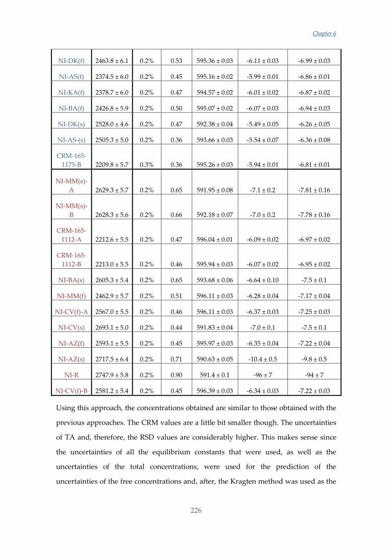
Chapter 6

226

NI-DK(f) 2463.8 ± 6.1 0.2% 0.53 595.36 ± 0.03 -6.11 ± 0.03 -6.99 ± 0.03

NI-AS(f) 2374.5 ± 6.0 0.2% 0.45 595.16 ± 0.02 -5.99 ± 0.01 -6.86 ± 0.01

NI-KA(f) 2378.7 ± 6.0 0.2% 0.47 594.57 ± 0.02 -6.01 ± 0.02 -6.87 ± 0.02

NI-BA(f) 2426.8 ± 5.9 0.2% 0.50 595.07 ± 0.02 -6.07 ± 0.03 -6.94 ± 0.03

NI-DK(s) 2528.0 ± 4.6 0.2% 0.47 592.38 ± 0.04 -5.49 ± 0.05 -6.26 ± 0.05

NI-AS-(s) 2505.3 ± 5.0 0.2% 0.36 593.66 ± 0.03 -5.54 ± 0.07 -6.36 ± 0.08

CRM-165-

1175-B 2209.8 ± 5.7 0.3% 0.36 595.26 ± 0.03 -5.94 ± 0.01 -6.81 ± 0.01

NI-MM(s)-

A 2629.3 ± 5.7 0.2% 0.65 591.95 ± 0.08 -7.1 ± 0.2 -7.81 ± 0.16

NI-MM(s)-

B 2628.3 ± 5.6 0.2% 0.66 592.18 ± 0.07 -7.0 ± 0.2 -7.78 ± 0.16

CRM-165-

1112-A 2212.6 ± 5.5 0.2% 0.47 596.04 ± 0.01 -6.09 ± 0.02 -6.97 ± 0.02

CRM-165-

1112-B 2213.0 ± 5.5 0.2% 0.46 595.94 ± 0.03 -6.07 ± 0.02 -6.95 ± 0.02

NI-BA(s) 2605.3 ± 5.4 0.2% 0.65 593.68 ± 0.06 -6.64 ± 0.10 -7.5 ± 0.1

NI-MM(f) 2462.9 ± 5.7 0.2% 0.51 596.11 ± 0.03 -6.28 ± 0.04 -7.17 ± 0.04

NI-CV(f)-A 2567.0 ± 5.5 0.2% 0.46 596.11 ± 0.03 -6.37 ± 0.03 -7.25 ± 0.03

NI-CV(s) 2693.1 ± 5.0 0.2% 0.44 591.83 ± 0.04 -7.0 ± 0.1 -7.5 ± 0.1

NI-AZ(f) 2593.1 ± 5.5 0.2% 0.45 595.97 ± 0.03 -6.35 ± 0.04 -7.22 ± 0.04

NI-AZ(s) 2717.5 ± 6.4 0.2% 0.71 590.63 ± 0.05 -10.4 ± 0.5 -9.8 ± 0.5

NI-R 2747.9 ± 5.8 0.2% 0.90 591.4 ± 0.1 -96 ± 7 -94 ± 7

NI-CV(f)-B 2581.2 ± 5.4 0.2% 0.45 596.39 ± 0.03 -6.34 ± 0.03 -7.22 ± 0.03

Using this approach, the concentrations obtained are similar to those obtained with the

previous approaches. The CRM values are a little bit smaller though. The uncertainties

of TA and, therefore, the RSD values are considerably higher. This makes sense since

the uncertainties of all the equilibrium constants that were used, as well as the

uncertainties of the total concentrations, were used for the prediction of the

uncertainties of the free concentrations and, after, the Kragten method was used as the

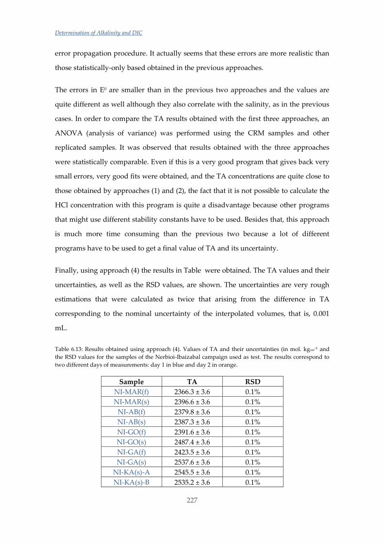
Determination of Alkalinity and DIC

227

error propagation procedure. It actually seems that these errors are more realistic than

those statistically-only based obtained in the previous approaches.

The errors in E0 are smaller than in the previous two approaches and the values are

quite different as well although they also correlate with the salinity, as in the previous

cases. In order to compare the TA results obtained with the first three approaches, an

ANOVA (analysis of variance) was performed using the CRM samples and other

replicated samples. It was observed that results obtained with the three approaches

were statistically comparable. Even if this is a very good program that gives back very

small errors, very good fits were obtained, and the TA concentrations are quite close to

those obtained by approaches (1) and (2), the fact that it is not possible to calculate the

HCl concentration with this program is quite a disadvantage because other programs

that might use different stability constants have to be used. Besides that, this approach

is much more time consuming than the previous two because a lot of different

programs have to be used to get a final value of TA and its uncertainty.

Finally, using approach (4) the results in Table were obtained. The TA values and their

uncertainties, as well as the RSD values, are shown. The uncertainties are very rough

estimations that were calculated as twice that arising from the difference in TA

corresponding to the nominal uncertainty of the interpolated volumes, that is, 0.001

mL.

Table 6.13: Results obtained using approach (4). Values of TA and their uncertainties (in mol. kgsw-1 and

the RSD values for the samples of the Nerbioi-Ibaizabal campaign used as test. The results correspond to

two different days of measurements: day 1 in blue and day 2 in orange.

Sample TA RSD

NI-MAR(f) 2366.3 ± 3.6 0.1%

NI-MAR(s) 2396.6 ± 3.6 0.1%

NI-AB(f) 2379.8 ± 3.6 0.1%

NI-AB(s) 2387.3 ± 3.6 0.1%

NI-GO(f) 2391.6 ± 3.6 0.1%

NI-GO(s) 2487.4 ± 3.6 0.1%

NI-GA(f) 2423.5 ± 3.6 0.1%

NI-GA(s) 2537.6 ± 3.6 0.1%

NI-KA(s)-A 2545.5 ± 3.6 0.1%

NI-KA(s)-B 2535.2 ± 3.6 0.1%

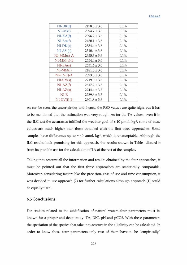
Chapter 6

228

NI-DK(f) 2478.5 ± 3.6 0.1%

NI-AS(f) 2394.7 ± 3.6 0.1%

NI-KA(f) 2396.2 ± 3.6 0.1%

NI-BA(f) 2460.1 ± 3.6 0.1%

NI-DK(s) 2554.4 ± 3.6 0.1%

NI-AS-(s) 2510.4 ± 3.6 0.1%

NI-MM(s)-A 2655.3 ± 3.6 0.1%

NI-MM(s)-B 2654.4 ± 3.6 0.1%

NI-BA(s) 2631.6 ± 3.6 0.1%

NI-MM(f) 2481.3 ± 3.6 0.1%

NI-CV(f)-A 2593.8 ± 3.6 0.1%

NI-CV(s) 2719.0 ± 3.6 0.1%

NI-AZ(f) 2617.2 ± 3.6 0.1%

NI-AZ(s) 2744.4 ± 3.7 0.1%

NI-R 2789.6 ± 3.7 0.1%

NI-CV(f)-B 2601.8 ± 3.6 0.1%

As can be seen, the uncertainties and, hence, the RSD values are quite high, but it has

to be mentioned that the estimation was very rough. As for the TA values, even if in

the ILC test the accuracies fulfilled the weather goal of ± 10 µmol. kg-1, some of these

values are much higher than those obtained with the first three approaches. Some

samples have differences up to ~ 40 µmol. kg-1, which is unacceptable. Although the

ILC results look promising for this approach, the results shown in Table discard it

from its possible use for the calculation of TA of the rest of the samples.

Taking into account all the information and results obtained by the four approaches, it

must be pointed out that the first three approaches are statistically comparable.

Moreover, considering factors like the precision, ease of use and time consumption, it

was decided to use approach (2) for further calculations although approach (1) could

be equally used.

6.5 Conclusions

For studies related to the acidification of natural waters four parameters must be

known for a proper and deep study: TA, DIC, pH and pCO2. With these parameters

the speciation of the species that take into account in the alkalinity can be calculated. In

order to know those four parameters only two of them have to be “empirically”

Determination of Alkalinity and DIC

229

determined and with their thermodynamic relations the other two could be predicted

(see Chapter 8). In this work, DIC and TA were chosen as the “empirically” determined

parameters for what the VINDTA 3C system was used and to assure the accuracy -

more likely, the statistical stability- of the results, CRM’s provided by Andrew

Dickson’s laboratory (Scripps Institution of Oceanography, La Jolla, CA, USA) were

used. It is crucial then, that the DIC and TA values are as accurate and precise as

possible to be certain that the derived parameters (pH and pCO2, in this case) are also

accurate and precise. The DIC determination was performed using the data given by

the VINDTA and corrected using a correction factor calculated with a set of CRM

measurements. The correction factors are calculated by dividing the average

experimental CRM values of the day with the certified values. That correction factor is

then multiplied to every experimental result to obtain the real DIC values. In the case

of the alkalinity the calculations are far more complicated. For seawater samples the

same calculations as for DIC can and are performed. But when the TA of estuarine

waters, whose salinities range from 0.2 to 40, has to be calculated it is not as simple as

that because the stability constants for the carbonate system used by the VINDTA

program are not suitable for low salinities and also because it does not take into

consideration the variation of the ionic strength along the titrations due to the addition

of the titrant, which is rather significant when low salinity samples are measured. The

first problem addressed in this work was to find a proper set of stability constants for

the carbonate system that could be used in whole salinity range of estuaries. The

constants proposed by Lueker et al. gave very good results for high salinity samples

while those by Millero were better for lower salinity samples. Therefore, in this work

new sets of constants were developed by “mixing” the two previously mentioned.

Once the constants were selected, different approaches were tested for the

determination of TA. These were: (1) non-linear curve fitting using LMA with the

Microsoft Office Excel program; (2) non-linear curve fitting using ODR with the help of

the OriginPro 2017 program; (3) non-linear curve fitting using the BSTAC4 and ES4ECI

programs and (4) empirical determination of the equivalence point using interpolated

(V, E) titration data and their first derivative.

Chapter 6

230

Approach (1) is very easy to use once the stability constants are chosen and it has the

big advantage that only Microsoft Office Excel is needed for its use. The fittings

obtained when the a0 parameters for the set of constants developed in this work are

refined are very good, as well as the accuracy and precision of the TA values obtained.

Approach (2) is very similar to (1). Their main difference is the algorithm that it is used

for the fitting (LMA in (1) and ODR in (2)) but the constants are the same. In this case,

the precision was slightly better than in (1) in most cases and the accuracy was very

good as well. As was expected, results obtained with both approaches were statistically

comparable. In the case of approach (3), the RSD values obtained were rather high but

they considered the errors in the stability constants as well as the errors in the total

concentrations, which could be more realistic. This approach has two main

disadvantages: on the one hand, the HCl concentration cannot be refined using

BSTAC4 and therefore, it must be calculated with another program which could use

different sets of constants, which, in turn, would not make much sense. On the other

hand, this approach is far more time consuming that the first two because different

programs have to be used with very specific input files. First (and only once) LIANA

must be used to calculate the stability constants and ionic strength dependence

parameters. Then, BSTAC and ES4ESI must be used for each sample after preparing

specific input files for each. As none of these programs can be used for the refinement

of the HCl concentration, this must be calculated using other strategies or programs.

Finally, the sum and subtraction of the free concentrations of the species and

components as well as the error propagation must be also done elsewhere (ie, using

Microsoft Office Excel).

In order to compare the results given by the first three approaches, an ANOVA was

performed, and it was concluded that results were statistically comparable with a

confidence level of 95 %.

A fourth approach was also tested, which was totally empirical and in which the

titration curve was interpolated to get a better precision of the volume of the endpoint

calculated by the first derivative. Different averaging procedures were studied for

Determination of Alkalinity and DIC

231

those cases where there was not a clear maximum peak and even if the accuracy of the

results obtained for the ILC samples was not good, it did fulfil the weather goal.

However, the use of this approach with real estuarine samples gave TA values up to 40

µmol. kg-1 higher than those obtained using the rest of the approaches and, therefore,

approach (4) was considered unsuitable for determining the TA of either seawater or

estuarine water samples.

Therefore, as discussed above, and taking into account the precision, accuracy and ease

of use of these approaches, approach (2) was finally chosen as the most suitable one,

although approach (1) could be used as well. This approach was used for the

calculation of TA of all the samples in this work.

6.6 References

[1] P. Waage and C. M. Guldberg, “Studier i affiniteten,” Forhandelinger Vidensk.

Christ., pp. 35–45, 1864.

[2] P. Waage and C. M. Guldberg, “Studies concerning affinity (translation by Henry I.

Abrash),” J. Chem. Educ., vol. 63, no. 12, pp. 1044–1047, 1986.

[3] C. M. Guldberg and P. Waage, Études sur les affinitès chimiques. Brøgger & Christie,

1867.

[4] C. M. Guldberg and P. Waage, “Ueber die chemische Affinität,” J. Für Prakt. Chem.,

vol. 19, no. 1, pp. 69–114, 1879.

[5] S. P. L. Sørensen, “Enzymstudien. II: Mitteilung. Über die Messung und die

Bedeutung der Wasserstoffionenkoncentration bei enzymatischen Prozessen,”

Biochem. Z., vol. 21, pp. 131–304, 1909.

[6] A. G. Dickson, “The development of the alkalinity concept in marine chemistry,”

Mar. Chem., vol. 40, no. 1, pp. 49–63, 1992.

[7] N. Bjerrum, “Die Dissoziation der Starken Elektrolyte,” Z. Für Elektrochem. Angew.

Phys. Chem., vol. 24, no. 19–20, pp. 321–328, 1918.

Chapter 6

232

[8] G. N. Lewis, “Outlines of a New System of Thermodynamic Chemistry,” Proc. Am.

Acad. Arts Sci., vol. 43, no. 7, pp. 259–293, 1907.

[9] J. N. Brönsted, “Einige Bemerkungen über den Begriff der Säuren und Basen,” Recl.

Trav. Chim. Pays-Bas, vol. 42, no. 8, pp. 718–728, 1923.

[10] T. M. Lowry, “The uniqueness of hydrogen,” J. Soc. Chem. Ind., vol. 42, no. 3, pp.

43–47, 1923.

[11] G. L. Miessler, P. J. Fischer, and D. A. Tarr, Inorganic Chemistry, 5th ed. Pearson

Prentice Hall, 2014.

[12] P. Debye and E. Hückel, “Zur Theorie der Elektrolyte. I.

Gefrierpunktserniedrigung und verwandte Erscheinungen,” Phys. Z., vol. 24, no. 9,

pp. 185–206, 1923.

[13] J. N. Bronsted, “Acid and Basic Catalysis.,” Chem. Rev., vol. 5, no. 3, pp. 231–338,

1928.

[14] K. Buch, H. W. Harvey, H. Wattenberg, and S. Gripenberg, Über das

Kohlensäuresystem im Meerwasser, vol. 79. Copenhague: Andr. Fred. Høst & Fils,

1932.

[15] N. W. Rakestraw, “The conception of alkalinity or excess base of seawater,” J. Mar.

Res., vol. 8, pp. 14–20, 1949.

[16] I. Hansson and D. Jagner, “Evaluation of the accuracy of gran plots by means of

computer calculations,” Anal. Chim. Acta, vol. 65, no. 2, pp. 363–373, 1973.

[17] J. N. Butler, Ionic equilibrium: a mathematical approach. Reading, Massachusetts:

Addison-Wesley Educational Publishers Inc., 1964.

[18] A. G. Dickson, “An exact definition of total alkalinity and a procedure for the

estimation of alkalinity and total inorganic carbon from titration data,” Deep Sea

Res. Part Oceanogr. Res. Pap., vol. 28, no. 6, pp. 609–623, 1981.

Determination of Alkalinity and DIC

233

[19] K. Kuliński, B. Schneider, K. Hammer, U. Machulik, and D. Schulz-Bull, “The

influence of dissolved organic matter on the acid–base system of the Baltic Sea,” J.

Mar. Syst., vol. 132, pp. 106–115, 2014.

[20] W.-J. Cai, Y. Wang, and R. E. Hodson, “Acid-Base Properties of Dissolved Organic

Matter in the Estuarine Waters of Georgia, USA,” Geochim. Cosmochim. Acta, vol. 62,

no. 3, pp. 473–483, 1998.

[21] H. Tornøe, “On the carbonic acid in seawater,” in The Norwegian North-Atlantic

expedition 1876-1878, Christiana, Norway: Grøndahl and Sons, 1880.

[22] T. G. Thompson and R. U. Bonnar, “The buffer capacity of sea water,” Ind. Eng.

Chem. Anal. Ed., vol. 3, no. 4, pp. 393–395, 1931.

[23] D. h. Anderson and R. j. Robinson, “Rapid Electrometric Determination of

Alkalinity of Sea Water Using Glass Electrode,” Ind. Eng. Chem. Anal. Ed., vol. 18,

no. 12, pp. 767–769, 1946.

[24] D. M. Greenberg, E. G. Moberg, and E. C. Allen, “Determination of carbon dioxide

and titratable base in sea water,” Ind. Eng. Chem. Anal. Ed., vol. 4, no. 3, pp. 309–

313, 1932.

[25] D. Dyrssen, “A Gran titration of seawater on board Sagitta,” Acta Chem. Scand., vol.

19, no. 5, p. 1265, 1965.

[26] G. Gran, “Determination of the equivalence point in potentiometric titrations. Part

II,” Analyst, vol. 77, no. 920, pp. 661–671, 1952.

[27] D. Dyrssen and L. G. Sillén, “Alkalinity and total carbonate in sea water. A plea for

p-T-independent data,” Tellus, vol. 19, no. 1, pp. 113–121, 1967.

[28] J. M. Edmond, “High precision determination of titration alkalinity and total

carbon dioxide content of sea water by potentiometric titration,” Deep Sea Res.

Oceanogr. Abstr., vol. 17, no. 4, pp. 737–750, 1970.

Chapter 6

234

[29] N. Ingri, W. Kakołowicz, L. G. Sillén, and B. Warnqvist, “High-speed computers as

a supplement to graphical methods--V. HALTAFALL, a general program for

calculating the composition of equilibrium mixtures,” Talanta, vol. 14, no. 11, pp.

1261–1286, 1967.

[30] A. L. Bradshaw, P. G. Brewer, D. K. Shafer, and R. T. Williams, “Measurements of

total carbon dioxide and alkalinity by potentiometric titration in the GEOSECS

program,” Earth Planet. Sci. Lett., vol. 55, no. 1, pp. 99–115, 1981.

[31] O. Johansson and M. Wedborg, “On the evaluation of potentiometric titrations of

sea-water with hydrochloric-acid,” Oceanol. Acta, vol. 5, no. 2, pp. 209–218, 1982.

[32] X. Liu, R. H. Byrne, M. Lindemuth, R. Easley, and J. T. Mathis, “An automated

procedure for laboratory and shipboard spectrophotometric measurements of

seawater alkalinity: Continuously monitored single-step acid additions,” Mar.

Chem., vol. 174, pp. 141–146, 2015.

[33] W. Yao and R. H. Byrne, “Simplified seawater alkalinity analysis: Use of linear

array spectrometers,” Deep Sea Res. Part Oceanogr. Res. Pap., vol. 45, no. 8, pp. 1383–

1392, 1998.

[34] A. G. Dickson and C. Goyet, Eds., DOE, 1994. Handbook of Methods for the Analysis of

the Various Parameters of the Carbon Dioxide System in Sea Water. ORNL/CDIAC-74,

1994.

[35] A. G. Dickson, C. L. Sabine, and J. R. Christian, Guide to best practices for ocean CO2

measurements. PICES Special Publication 3, 2007.

[36] A. G. Dickson, J. D. Afghan, and G. C. Anderson, “Reference materials for oceanic

CO2 analysis: a method for the certification of total alkalinity,” Mar. Chem., vol. 80,

no. 2–3, pp. 185–197, 2003.

[37] E. E. Bockmon and A. G. Dickson, “An inter-laboratory comparison assessing the

quality of seawater carbon dioxide measurements,” Mar. Chem., vol. 171, pp. 36–43,

2015.

Determination of Alkalinity and DIC

235

[38] A. G. Dickson, C. L. Sabine, and J. R. Christian, Guide to Best Practices for Ocean CO2

Measurements. North Pacific Marine Science Organization, 2007.

[39] K. Johnson, C. Burney, and J. Sieburth, “Precise and Accurate Determination by

Infrared Photometry of CO, Dynamics in Marine Ecosystems,” Mar. Ecol. Prog. Ser.,

pp. 251–256, 1983.

[40] K. M. Johnson, A. E. King, and J. M. Sieburth, “Coulometric TCO2 analyses for

marine studies; an introduction,” Mar. Chem., vol. 16, no. 1, pp. 61–82, 1985.

[41] K. M. Johnson, J. M. Sieburth, P. J. leB Williams, and L. Brändström, “Coulometric

total carbon dioxide analysis for marine studies: Automation and calibration,” Mar.

Chem., vol. 21, no. 2, pp. 117–133, 1987.

[42] K. M. Johnson, K. D. Wills, D. B. Butler, W. K. Johnson, and C. S. Wong,

“Coulometric total carbon dioxide analysis for marine studies: maximizing the

performance of an automated gas extraction system and coulometric detector,”

Mar. Chem., vol. 44, no. 2, pp. 167–187, 1993.

[43] F. J. Mojica-Prieto and F. J. Millero, “The values of pK1 + pK2 for the dissociation of

carbonic acid in seawater,” Geochim. Cosmochim. Acta, vol. 66, no. 14, pp. 2529–2540,

Jul. 2002.

[44] R. E. Zeebe and D. Wolf-Gladrow, CO2 in Seawater: Equilibrium, Kinetics, Isotopes.

Elsevier, 2001.

[45] F. J. Millero, “The Marine Inorganic Carbon Cycle,” Chem. Rev., vol. 107, no. 2, pp.

308–341, 2007.

[46] W. H. Press, S. A. Teukolsky, W. T. Vetterling, and B. P. Flannery, Numerical

Recipes: The Art of Scientific Computing, 1st ed. Cambridge (MA): Cambridge

University Press, 1986.

Chapter 6

236

[47] J. Poch and I. Villaescusa, “Orthogonal Distance Regression: A Good Alternative to

Least Squares for Modeling Sorption Data,” J. Chem. Eng. Data, vol. 57, no. 2, pp.

490–499, 2012.

[48] E. C. de Oliveira and P. F. de Aguiar, “Least squares regression with errors in both

variables: case studies,” Quím. Nova, vol. 36, no. 6, pp. 885–889, 2013.

[49] P. J. Cornbleet and N. Gochman, “Incorrect least-squares regression coefficients in

method-comparison analysis.,” Clin. Chem., vol. 25, no. 3, pp. 432–438, 1979.

[50] J. Burnett and W. A. Burns, “Using a spreadsheet to Fit experimental pH titration

data to a theoretical expression: Estimation of analyte concentration and Ka,” J

Chem Educ, vol. 83, no. 8, p. 1190, 2006.

[51] R. N. Roy et al., “The dissociation constants of carbonic acid in seawater at salinities

5 to 45 and temperatures 0 to 45°C,” Mar. Chem., vol. 44, no. 2, pp. 249–267, 1993.

[52] T. J. Lueker, A. G. Dickson, and C. D. Keeling, “Ocean pCO2 calculated from

dissolved inorganic carbon, alkalinity, and equations for K1 and K2: validation

based on laboratory measurements of CO2 in gas and seawater at equilibrium,”

Mar. Chem., vol. 70, no. 1, pp. 105–119, 2000.

[53] F. J. Millero, “Carbonate constants for estuarine waters,” Mar. Freshw. Res., vol. 61,

no. 2, pp. 139–142, 2010.

[54] C. De Stefano, S. Sammartano, P. Mineo, and C. Rigano, “Computer Tools for the

Speciation of Natural Fluids,” in Marine Chemistry - An Environmental Analytical

Chemistry Approach, A. Gianguzza, E. Pelizzetti, and S. Sammartano, Eds.

Amsterdam: Kluwer Academic Publishers, 1997, pp. 71–83.

[55] C. De Stefano, P. Mineo, C. Rigano, and S. Sammartano, “Ionic strength

dependence of formation constants: XVII. The calculation of equilibrium

concentrations and formation constants,” Ann. Chim. Rome, vol. 83, pp. 243–277,

1993.

Determination of Alkalinity and DIC

237

[56] A. de Robertis, C. de Stefano, S. Sammartano, and C. Rigano, “The calculation of

equilibrium concentrations in large multimetal/multiligand systems,” Anal. Chim.

Acta, vol. 191, pp. 385–398, 1986.

[57] F. Crea, A. D. Robertis, and S. Sammartano, “Medium and Alkyl Chain Effects on

the Protonation of Dicarboxylates in NaCl<Subscript>(aq)</Subscript> and

Et<Subscript>4</Subscript>NI<Subscript>(aq)</Subscript> at 25°C,” J. Solut. Chem.,

vol. 33, no. 5, pp. 499–528, 2004.

[58] C. De Stefano, C. Foti, S. Sammartano, A. Gianguzza, and C. Rigano, “Equilibrium

Studies in Natural Fluids. Use of Synthetic Seawaters and Other Media as

Background Salts,” Ann. Chim., vol. 84, pp. 159–175, 1994.

[59] A. De Robertis, C. De Stefano, S. Sammartano, and A. Gianguzza, “Equilibrium

studies in natural fluids: a chemical speciation model for the major constituents of

sea water,” Chem. Speciat. Bioavailab., vol. 6, no. 2–3, pp. 65–84, 1994.

[60] C. De Stefano, D. Milea, and S. Sammartano, “Speciation of phytate ion in aqueous

solution. Dimethyltin(IV) interactions in NaClaq at different ionic strengths,”

Biophys. Chem., vol. 116, no. 2, pp. 111–120, 2005.

[61] C. De Stefano, P. Mineo, C. Rigano, and S. Sammartano, “Ionic Strength

Dependence of Formation Constants. XVII. the Calculation of Equilibrium

Concentrations and Formation Constants,” Ann. Chim., vol. 83, pp. 243–277, 1993.

[62] P. Gans, A. Sabatini, and A. Vacca, “SUPERQUAD: an improved general program

for computation of formation constants from potentiometric data,” J. Chem. Soc.

Dalton Trans., vol. 0, no. 6, pp. 1195–1200, 1985.

[63] C. De Stefano, C. Foti, O. Giuffrè, P. Mineo, C. Rigano, and S. Sammartano,

“Binding of tripolyphosphate by aliphatic amines: Formation, stability and

calculation problems,” Ann. Chim., vol. 86, no. 5, pp. 257–280, 1996.

Chapter 6

238

[64] C. Bretti, A. Giacalone, A. Gianguzza, and S. Sammartano, “Speciation of

dimethyltin(IV) – and trimethyltin(IV) – carbocysteinate and – glutamate systems

in aqueous media,” Chem. Speciat. Bioavailab., vol. 20, no. 3, pp. 137–148, 2008.

[65] R. M. Cigala, F. Crea, C. De Stefano, G. Lando, D. Milea, and S. Sammartano,

“Modeling the acid-base properties of glutathione in different ionic media, with

particular reference to natural waters and biological fluids,” Amino Acids, vol. 43,

no. 2, pp. 629–648, 2012.

[66] C. Bretti, A. Giacalone, A. Gianguzza, D. Milea, and S. Sammartano, “Modeling S-

carboxymethyl-l-cysteine protonation and activity coefficients in sodium and

tetramethylammonium chloride aqueous solutions by SIT and Pitzer equations,”

Fluid Phase Equilibria, vol. 252, no. 1, pp. 119–129, 2007.

[67] J. Kragten, “Tutorial review. Calculating standard deviations and confidence

intervals with a universally applicable spreadsheet technique,” Analyst, vol. 119,

no. 10, pp. 2161–2165, 1994.

[68] H. Akima, “A method of smooth curve fitting,” Washington DC, ERL 101-ITS 73,

1969.

[69] J. A. Newton, R. A. Feely, E. B. Jewett, P. Williamson, and J. Mathis, “Global ocean

acidification observing network: requirements and governance plan.,” 2014.

Chapter 7

Determination of the pka of phenol

red for spectrophotometric

determination of pH

Determination of the pka of phenol red for spectrophotometric determination of pH

241

7.1 Introduction

Acids and bases have been known for a very long time. One of the first and most

important historic theories of acidity was provided by Antoine Lavoisier in 1776 [1].

His idea was that acidity was caused by the presence of oxygen and he defined the

acids by their content in oxygen. He postulated that all acids were compounds of what

he called an acidificable base (such as sulphur, nitrogen or phosphorus) with the

“acidifying principle” which was oxygen. In fact, he named the oxygen from the Greek

names “oxys” = sour or acid + “genes” = born; meaning “acid maker” or “acid former”.

Even if his idea turned to be wrong, it is important because he was the first to attempt

to chemically characterize acids and bases [1]–[3]. Many chemists became convinced of

this theory but by the early 19th century many compounds had been discovered that

did not contain oxygen but showed acidic behaviour. In 1789, Berthollet showed that

hydrocyanic acid and hydrogen sulphide did not contain oxygen. But these acids were

so weak that they were not considered true acids. Humphry Davy and Louis Joseph

Gay-Lussac showed conclusively that hydrohalic acids did not contain oxygen. In fact,

it was Davy’s work the one which definitely invalidated Lavoisier’s theory of acids in

1810 [4], [5]. The actual understanding of the nature of acids came from the work of

Justus Liebig. In 1838 he postulated what is known as the “hydrogen theory of acids”

which defines the acids as “compounds containing hydrogen, in which the hydrogen can be

replaced by a metal” [6].

In 1884, as a part of his dissertation, Svante Arrhenius postulated the first modern

definition of acids and bases. He proposed that acids were substances that

produced hydrogen ions in solution and, conversely, bases were substances that

produced hydroxide ions in solution. According to his theory, when acids and bases

react, the hydrogen and hydroxide ions neutralise each other forming water. The

Arrhenius view of acids and bases explained many of the properties of acids and bases

known at that time, but it also had some limitations. For example, it was only correct

for those acids and bases that are completely dissociated in solution and it only

considered aqueous solutions.

Chapter 7

242

Also, Johannes Nicolaus Brønsted in Denmark [7] and Thomas Martin Lowry in

England [8] independently proposed the theory that carries their names: the 4th of May

of 1923 the first one and the 10th of January of 1923 the second one. Their theory

defined an acid as a species with a tendency to lose a hydrogen ion (proton donors)

and a base as a species with a tendency to gain a hydrogen ion (proton acceptors). They

extended the concept of acid–base chemistry beyond aqueous solutions explicitly

dictating that acids generate different conjugate acids depending on the solvent used

[6].

Also in 1923 Gilbert Newton Lewis [9] refined the acid and base concept in terms of

electron-pair transfer rather than proton transfer. According to his theory, a base is a

substance that donates an electron pair while an acid is the one accepting the electron

pair. His theory was published in 1923, but it was not elaborated by him until 1938 and

it is considered the “modern” definition of acids and bases. The Lewis scheme is

valuable because it unites not only proton-transfer reactions but also those in which

free protons are not involved. However, the important contribution of the Brønsted-

Lowry approach is the concept of acid-base conjugate pairs.

Besides the definition of acids and bases, whose discussion was more or less over after

the Lewis definition, some very important contributions were made on the 20th century

regarding acids and bases. One of the most important scientists was Søren Peder

Lauritz Sørensen. In 1909 he published a paper where taking into account the

contemporary definition of acids as functions of hydrogen concentration (Arrhenius

definition), he proposed the idea of expressing the acidity as the negative logarithm of

the hydrogen ion concentration, which he termed PH, in order to ease the calculations.

This PH value was changed to the known pH by W.M. Clark in 1920 [10] apparently for

typographical convenience.

pH= -log10[H+] 1

This is what he wrote (translated from the German from the original paper) [11]:

Determination of the pka of phenol red for spectrophotometric determination of pH

243

"The magnitude of the hydrogen ion concentration will accordingly be represented by means of

the normality factor with regard to the hydrogen ion, and this factor will be written in the form

of a negative potenz (power) of 10. Since I refer to the above in a later section (see page 159),

here I will mention only that I employ the name "hydrogen ion exponent" and the symbol pH

for the numerical value of this potenz (power)."

In the same paper he developed the principles and technique of colorimetric pH

determinations and he reviewed the electrometric determination of pH by the

hydrogen electrode and identified the many sources of error of this technique. He also

introduced the concept of buffer solutions (as solutions of weak acids and their

respective salts with strong bases) and he developed buffer solutions to maintain

constant the pH of solutions (Sørensen buffers) [12]. From then on, the measurement of

pH was progressively considered of greater and greater importance until becoming the

standardised way of characterising acids and bases.

After that, the efforts of scientists were focussed on improving the accuracy of pH

measurement. With that purpose, the glass electrode, invented also in 1909 by Haber

and Klemensiewicz [13], was improved in the following years by trying different

compositions of the glass. The modern measurement of pH was revolutionized by two

major innovations. The first was the development by Duncan McInnes and Malcolm

Dole in 1930 of a superior glass electrode capable of responding to hydrogen ions [14].

The second occurred in 1934, when Arnold Orville Beckman invented the “acidometer”

(which is known nowadays as pH-meter) to measure the acidity of lemon juice.

7.1.1. Modern definitions of pH

The concept of pH as a measure of the acidity of a solution is well known, but it is not

as simple to define the scale in which pH is measured. This difficulty arises from the

impossibility of using primary electrochemical measurements to exactly determine

neither the molal proton concentration (mH) nor the activity (aH). And as the solution

acidity is usually expressed by either mH or aH and it is immeasurable, a convention

based on electrolyte theory is necessary to define the solution pH.

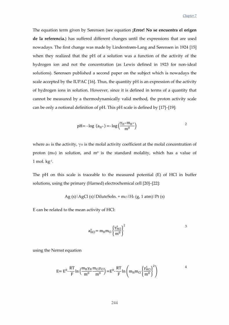
Chapter 7

244

The equation term given by Sørensen (see equation ¡Error! No se encuentra el origen

de la referencia.) has suffered different changes until the expressions that are used

nowadays. The first change was made by Linderstrøm-Lang and Sørensen in 1924 [15]

when they realized that the pH of a solution was a function of the activity of the

hydrogen ion and not the concentration (as Lewis defined in 1923 for non-ideal

solutions). Sørensen published a second paper on the subject which is nowadays the

scale accepted by the IUPAC [16]. Thus, the quantity pH is an expression of the activity

of hydrogen ions in solution. However, since it is defined in terms of a quantity that

cannot be measured by a thermodynamically valid method, the proton activity scale

can be only a notional definition of pH. This pH scale is defined by [17]–[19]:

pH= - log (aH+)=- log (γH+mH+

m0) 2

where aH is the activity, γH is the molal activity coefficient at the molal concentration of

proton (mH) in solution, and m0 is the standard molality, which has a value of

1 mol. kg-1.

The pH on this scale is traceable to the measured potential (E) of HCl in buffer

solutions, using the primary (Harned) electrochemical cell [20]–[22]:

Ag (s)|AgCl (s)|DiluteSoln. + mCl|H2 (g, 1 atm)|Pt (s)

E can be related to the mean activity of HCl:

aHCl± = mHmCl

γHCl±

m0

2

3

using the Nernst equation

E= E0-RT

Fln (

mHγHm0

mClγClm0

)=E0-RT

Fln (mHmCl

γHCl±

m0

2

) 4

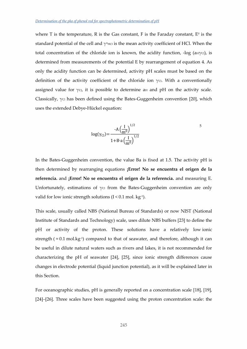
Determination of the pka of phenol red for spectrophotometric determination of pH

245

where T is the temperature, R is the Gas constant, F is the Faraday constant, E0 is the

standard potential of the cell and γ±HCl is the mean activity coefficient of HCl. When the

total concentration of the chloride ion is known, the acidity function, -log (aHγCl), is

determined from measurements of the potential E by rearrangement of equation 4. As

only the acidity function can be determined, activity pH scales must be based on the

definition of the activity coefficient of the chloride ion γCl. With a conventionally

assigned value for γCl, it is possible to determine aH and pH on the activity scale.

Classically, γCl has been defined using the Bates-Guggenheim convention [20], which

uses the extended Debye-Hückel equation:

log(γCl)=-A (

Im0)

1/2

1+B∙a (Im0)

1/2

5

In the Bates-Guggenheim convention, the value Ba is fixed at 1.5. The activity pH is

then determined by rearranging equations ¡Error! No se encuentra el origen de la

referencia. and ¡Error! No se encuentra el origen de la referencia. and measuring E.

Unfortunately, estimations of γCl from the Bates-Guggenheim convention are only

valid for low ionic strength solutions (I < 0.1 mol. kg-1).

This scale, usually called NBS (National Bureau of Standards) or now NIST (National

Institute of Standards and Technology) scale, uses dilute NBS buffers [23] to define the

pH or activity of the proton. These solutions have a relatively low ionic

strength ( ≈ 0.1 mol.kg-1) compared to that of seawater, and therefore, although it can

be useful in dilute natural waters such as rivers and lakes, it is not recommended for

characterizing the pH of seawater [24], [25], since ionic strength differences cause

changes in electrode potential (liquid junction potential), as it will be explained later in

this Section.

For oceanographic studies, pH is generally reported on a concentration scale [18], [19],

[24]–[26]. Three scales have been suggested using the proton concentration scale: the

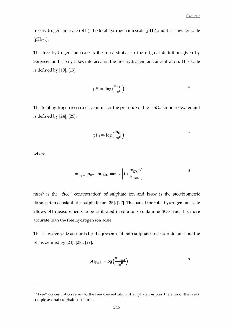
Chapter 7

246

free hydrogen ion scale (pHF), the total hydrogen ion scale (pHT) and the seawater scale

(pHSWS).

The free hydrogen ion scale is the most similar to the original definition given by

Sørensen and it only takes into account the free hydrogen ion concentration. This scale

is defined by [18], [19]:

pHF=- log (mH+

m0) 6

The total hydrogen ion scale accounts for the presence of the HSO4- ion in seawater and

is defined by [24], [26]:

pHT=- log (mHT

m0)

7

where

mHT = mH++mHSO4-=mH+ [1+

mSO42-

kHSO4-]

8

mSO42- is the “free” concentration1 of sulphate ion and kHSO4- is the stoichiometric

dissociation constant of bisulphate ion [25], [27]. The use of the total hydrogen ion scale

allows pH measurements to be calibrated in solutions containing SO42- and it is more

accurate than the free hydrogen ion scale.

The seawater scale accounts for the presence of both sulphate and fluoride ions and the

pH is defined by [24], [28], [29]:

pHSWS=- log (mHSWS

m0)

9

1 “Free” concentration refers to the free concentration of sulphate ion plus the sum of the weak

complexes that sulphate ions form.

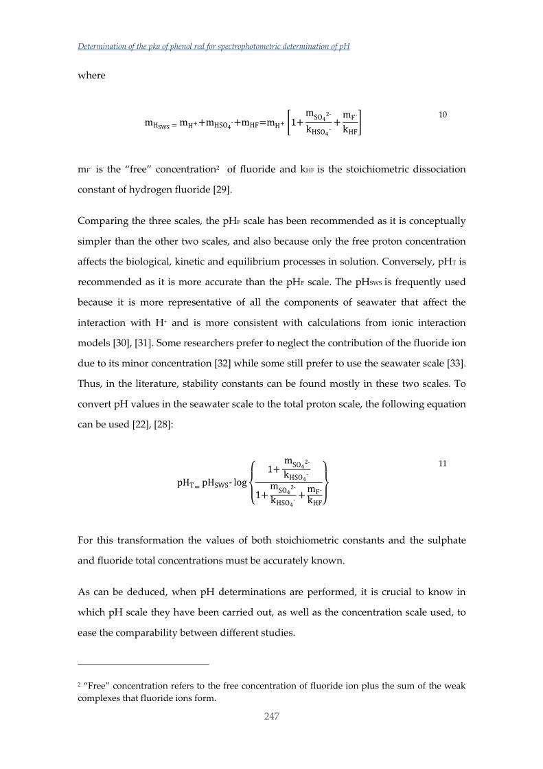
Determination of the pka of phenol red for spectrophotometric determination of pH

247

where

mHSWS = mH++mHSO4-+mHF=mH+ [1+

mSO42-

kHSO4-+mF-

kHF]

10

mF- is the “free” concentration2 of fluoride and kHF is the stoichiometric dissociation

constant of hydrogen fluoride [29].

Comparing the three scales, the pHF scale has been recommended as it is conceptually

simpler than the other two scales, and also because only the free proton concentration

affects the biological, kinetic and equilibrium processes in solution. Conversely, pHT is

recommended as it is more accurate than the pHF scale. The pHSWS is frequently used

because it is more representative of all the components of seawater that affect the

interaction with H+ and is more consistent with calculations from ionic interaction

models [30], [31]. Some researchers prefer to neglect the contribution of the fluoride ion

due to its minor concentration [32] while some still prefer to use the seawater scale [33].

Thus, in the literature, stability constants can be found mostly in these two scales. To

convert pH values in the seawater scale to the total proton scale, the following equation

can be used [22], [28]:

pHT= pHSWS- log

1+ mSO4

2-

kHSO4-

1+mSO4

2-

kHSO4-+mF-

kHF

11

For this transformation the values of both stoichiometric constants and the sulphate

and fluoride total concentrations must be accurately known.

As can be deduced, when pH determinations are performed, it is crucial to know in

which pH scale they have been carried out, as well as the concentration scale used, to

ease the comparability between different studies.

2 “Free” concentration refers to the free concentration of fluoride ion plus the sum of the weak

complexes that fluoride ions form.

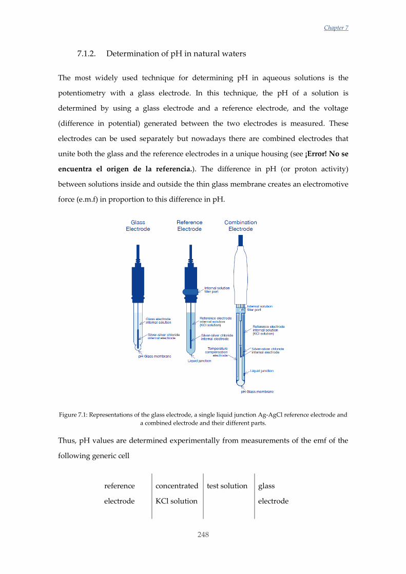
Chapter 7

248

7.1.2. Determination of pH in natural waters

The most widely used technique for determining pH in aqueous solutions is the

potentiometry with a glass electrode. In this technique, the pH of a solution is

determined by using a glass electrode and a reference electrode, and the voltage

(difference in potential) generated between the two electrodes is measured. These

electrodes can be used separately but nowadays there are combined electrodes that

unite both the glass and the reference electrodes in a unique housing (see ¡Error! No se

encuentra el origen de la referencia.). The difference in pH (or proton activity)

between solutions inside and outside the thin glass membrane creates an electromotive

force (e.m.f) in proportion to this difference in pH.

Figure 7.1: Representations of the glass electrode, a single liquid junction Ag-AgCl reference electrode and

a combined electrode and their different parts.

Thus, pH values are determined experimentally from measurements of the emf of the

following generic cell

reference

electrode

concentrated

KCl solution

test solution glass

electrode

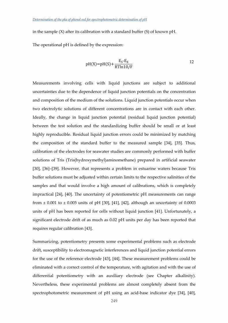
Determination of the pka of phenol red for spectrophotometric determination of pH

249

in the sample (X) after its calibration with a standard buffer (S) of known pH.

The operational pH is defined by the expression:

pH(X)=pH(S)+ES-EX

RTln10/F

12

Measurements involving cells with liquid junctions are subject to additional

uncertainties due to the dependence of liquid junction potentials on the concentration

and composition of the medium of the solutions. Liquid junction potentials occur when

two electrolytic solutions of different concentrations are in contact with each other.

Ideally, the change in liquid junction potential (residual liquid junction potential)

between the test solution and the standardizing buffer should be small or at least

highly reproducible. Residual liquid junction errors could be minimized by matching

the composition of the standard buffer to the measured sample [34], [35]. Thus,

calibration of the electrodes for seawater studies are commonly performed with buffer

solutions of Tris (Tris(hydroxymethyl)aminomethane) prepared in artificial seawater

[30], [36]–[39]. However, that represents a problem in estuarine waters because Tris

buffer solutions must be adjusted within certain limits to the respective salinities of the

samples and that would involve a high amount of calibrations, which is completely

impractical [24], [40]. The uncertainty of potentiometric pH measurements can range

from ± 0.001 to ± 0.005 units of pH [30], [41], [42], although an uncertainty of 0.0003

units of pH has been reported for cells without liquid junction [41]. Unfortunately, a

significant electrode drift of as much as 0.02 pH units per day has been reported that

requires regular calibration [43].

Summarizing, potentiometry presents some experimental problems such as electrode

drift, susceptibility to electromagnetic interferences and liquid junction potential errors

for the use of the reference electrode [43], [44]. These measurement problems could be

eliminated with a correct control of the temperature, with agitation and with the use of

differential potentiometry with an auxiliary electrode (see Chapter alkalinity).

Nevertheless, these experimental problems are almost completely absent from the

spectrophotometric measurement of pH using an acid-base indicator dye [34], [40],

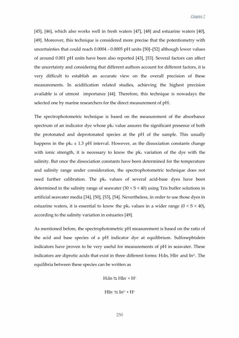
Chapter 7

250

[45], [46], which also works well in fresh waters [47], [48] and estuarine waters [40],

[49]. Moreover, this technique is considered more precise that the potentiometry with

uncertainties that could reach 0.0004 - 0.0005 pH units [50]–[52] although lower values

of around 0.001 pH units have been also reported [43], [53]. Several factors can affect

the uncertainty and considering that different authors account for different factors, it is

very difficult to establish an accurate view on the overall precision of these

measurements. In acidification related studies, achieving the highest precision

available is of utmost importance [44]. Therefore, this technique is nowadays the

selected one by marine researchers for the direct measurement of pH.

The spectrophotometric technique is based on the measurement of the absorbance

spectrum of an indicator dye whose pka value assures the significant presence of both

the protonated and deprotonated species at the pH of the sample. This usually

happens in the pka ± 1.3 pH interval. However, as the dissociation constants change

with ionic strength, it is necessary to know the pka variation of the dye with the

salinity. But once the dissociation constants have been determined for the temperature

and salinity range under consideration, the spectrophotometric technique does not

need further calibration. The pka values of several acid-base dyes have been

determined in the salinity range of seawater (30 < S < 40) using Tris buffer solutions in

artificial seawater media [34], [50], [53], [54]. Nevertheless, in order to use those dyes in

estuarine waters, it is essential to know the pka values in a wider range (0 < S < 40),

according to the salinity variation in estuaries [49].

As mentioned before, the spectrophotometric pH measurement is based on the ratio of

the acid and base species of a pH indicator dye at equilibrium. Sulfonephtalein

indicators have proven to be very useful for measurements of pH in seawater. These

indicators are diprotic acids that exist in three different forms: H2In, HIn- and In2-. The

equilibria between these species can be written as

H2In HIn- + H+

HIn- In2- + H+

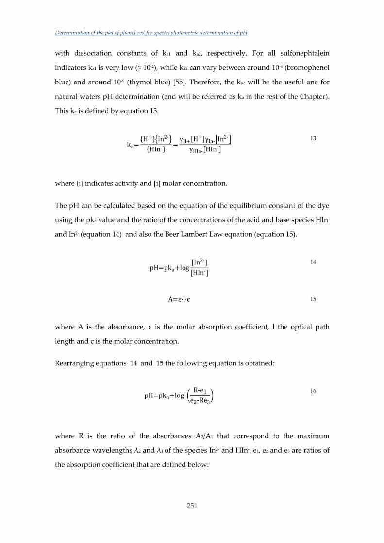
Determination of the pka of phenol red for spectrophotometric determination of pH

251

with dissociation constants of ka1 and ka2, respectively. For all sulfonephtalein

indicators ka1 is very low (≈ 10-2), while ka2 can vary between around 10-4 (bromophenol

blue) and around 10-9 (thymol blue) [55]. Therefore, the ka2 will be the useful one for

natural waters pH determination (and will be referred as ka in the rest of the Chapter).

This ka is defined by equation 13.

ka=H+In2-

HIn-=γH+[H

+]γIn-[In2-]

γHIn-[HIn-]

13

where i indicates activity and [i] molar concentration.

The pH can be calculated based on the equation of the equilibrium constant of the dye

using the pka value and the ratio of the concentrations of the acid and base species HIn-

and In2- (equation 14) and also the Beer Lambert Law equation (equation 15).

pH=pka+log[In2-]

[HIn-]

14

A=ɛ·l·c 15

where A is the absorbance, ε is the molar absorption coefficient, l the optical path

length and c is the molar concentration.

Rearranging equations 14 and 15 the following equation is obtained:

pH=pka+log (R-e1e2-Re3

) 16

where R is the ratio of the absorbances A2/A1 that correspond to the maximum

absorbance wavelengths λ2 and λ1 of the species In2- and HIn-. e1, e2 and e3 are ratios of

the absorption coefficient that are defined below:

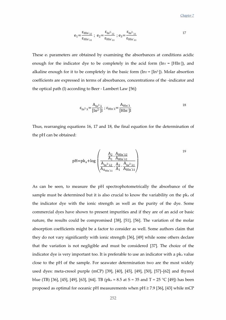
Chapter 7

252

e1=εHIn-λ2εHIn-λ1

; e2=εIn2-λ2εHIn-λ1

; e3=εIn2-λ1εHIn-λ1

17

These ei parameters are obtained by examining the absorbances at conditions acidic

enough for the indicator dye to be completely in the acid form (InT = [HIn-]), and

alkaline enough for it to be completely in the basic form (InT = [In2-]). Molar absortion

coefficients are expressed in terms of absorbances, concentrations of the -indicator and

the optical path (l) according to Beer - Lambert Law [56]:

εIn2-λ=AIn2-λ[In2-]l

; εHIn-λ=AHIn-λ[HIn-]l

18

Thus, rearranging equations 16, 17 and 18, the final equation for the determination of

the pH can be obtained:

pH=pka+log

(

A2A1-AHIn-λ2AHIn-λ1

AIn2-λ2

AAHIn-λ1-A2A1∙AIn2-λ1

AHIn-λ1)

19

As can be seen, to measure the pH spectrophotometrically the absorbance of the

sample must be determined but it is also crucial to know the variability on the pka of

the indicator dye with the ionic strength as well as the purity of the dye. Some

commercial dyes have shown to present impurities and if they are of an acid or basic

nature, the results could be compromised [38], [51], [56]. The variation of the molar

absorption coefficients might be a factor to consider as well. Some authors claim that

they do not vary significantly with ionic strength [36], [49] while some others declare

that the variation is not negligible and must be considered [37]. The choice of the

indicator dye is very important too. It is preferable to use an indicator with a pka value

close to the pH of the sample. For seawater determination two are the most widely

used dyes: meta-cresol purple (mCP) [39], [40], [45], [49], [50], [57]–[62] and thymol

blue (TB) [36], [45], [49], [63], [64]. TB (pka ≈ 8.5 at S = 35 and T = 25 °C [49]) has been

proposed as optimal for oceanic pH measurements when pH ≥ 7.9 [36], [43] while mCP

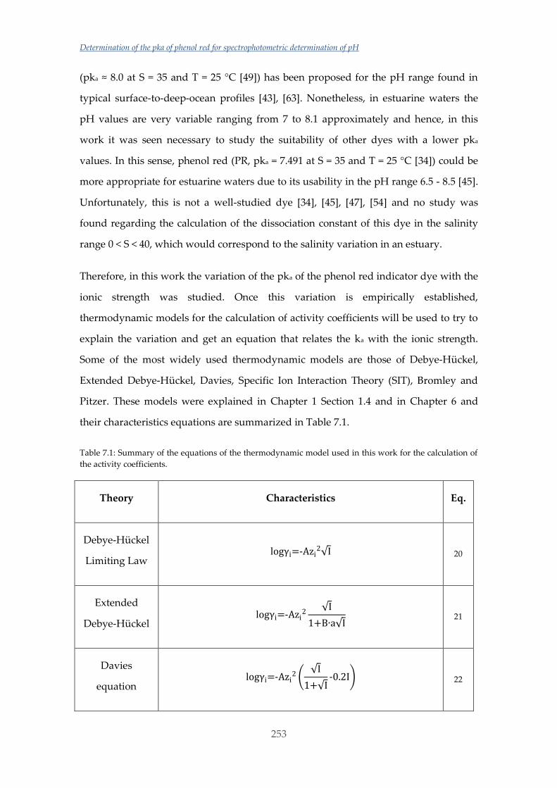
Determination of the pka of phenol red for spectrophotometric determination of pH

253

(pka ≈ 8.0 at S = 35 and T = 25 °C [49]) has been proposed for the pH range found in

typical surface-to-deep-ocean profiles [43], [63]. Nonetheless, in estuarine waters the

pH values are very variable ranging from 7 to 8.1 approximately and hence, in this

work it was seen necessary to study the suitability of other dyes with a lower pka

values. In this sense, phenol red (PR, pka = 7.491 at S = 35 and T = 25 °C [34]) could be

more appropriate for estuarine waters due to its usability in the pH range 6.5 - 8.5 [45].

Unfortunately, this is not a well-studied dye [34], [45], [47], [54] and no study was

found regarding the calculation of the dissociation constant of this dye in the salinity

range 0 < S < 40, which would correspond to the salinity variation in an estuary.

Therefore, in this work the variation of the pka of the phenol red indicator dye with the

ionic strength was studied. Once this variation is empirically established,

thermodynamic models for the calculation of activity coefficients will be used to try to

explain the variation and get an equation that relates the ka with the ionic strength.

Some of the most widely used thermodynamic models are those of Debye-Hückel,

Extended Debye-Hückel, Davies, Specific Ion Interaction Theory (SIT), Bromley and

Pitzer. These models were explained in Chapter 1 Section 1.4 and in Chapter 6 and

their characteristics equations are summarized in Table 7.1.

Table 7.1: Summary of the equations of the thermodynamic model used in this work for the calculation of

the activity coefficients.

Theory Characteristics Eq.

Debye-Hückel

Limiting Law logγi=-Azi

2√I 20

Extended

Debye-Hückel logγi=-Azi

2 √I

1+B∙a√I 21

Davies

equation logγi=-Azi

2 (√I

1+√I-0.2I) 22

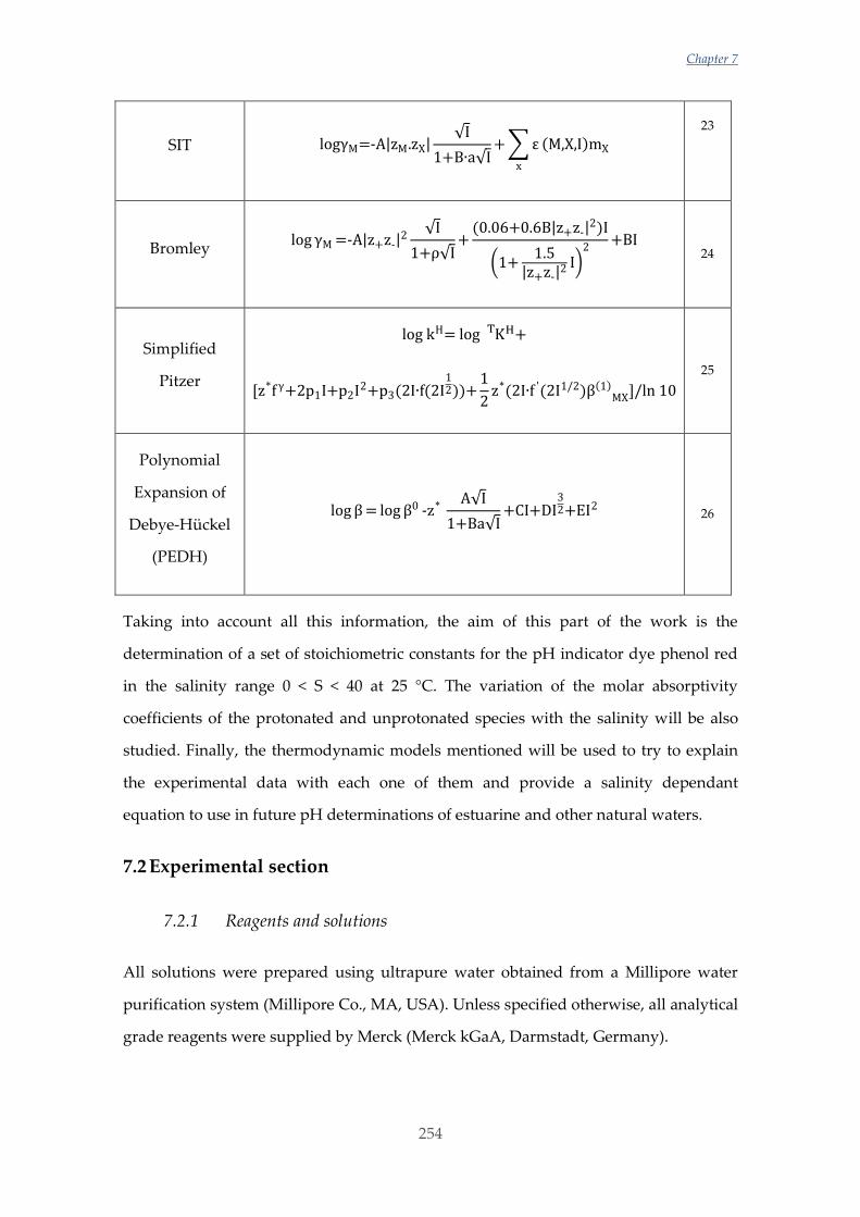
Chapter 7

254

SIT logγM=-A|zM.zX|√I

1+B∙a√I+∑ε

x

(M,X,I)mX 23

Bromley log γM=-A|z+z-|

2 √I

1+ρ√I+(0.06+0.6B|z+z-|

2)I

(1+1.5

|z+z-|2 I)

2+BI

24

Simplified

Pitzer

log kH= log KT H+

[z*fγ+2p1I+p2I2+p3(2I∙f(2I

12))+

1

2z*(2I∙f '(2I1/2)β(1)MX]/ln 10

25

Polynomial

Expansion of

Debye-Hückel

(PEDH)

log β= log β0 -z* A√I

1+Ba√I+CI+DI

32+EI2 26

Taking into account all this information, the aim of this part of the work is the

determination of a set of stoichiometric constants for the pH indicator dye phenol red

in the salinity range 0 < S < 40 at 25 °C. The variation of the molar absorptivity

coefficients of the protonated and unprotonated species with the salinity will be also

studied. Finally, the thermodynamic models mentioned will be used to try to explain

the experimental data with each one of them and provide a salinity dependant

equation to use in future pH determinations of estuarine and other natural waters.

7.2 Experimental section

7.2.1 Reagents and solutions

All solutions were prepared using ultrapure water obtained from a Millipore water

purification system (Millipore Co., MA, USA). Unless specified otherwise, all analytical

grade reagents were supplied by Merck (Merck kGaA, Darmstadt, Germany).

Determination of the pka of phenol red for spectrophotometric determination of pH

255

The reagents used in this section of the work were: sodium chloride, boric acid, phenol

red, sodium acetate, magnesium chloride hexahydrate, sodium sulphate (Panreac

Química S.L.U, Barcelona, Spain), tris(hidroximetil)aminomethane (tris), potassium

chloride (Panreac Química S.L.U, Barcelona, Spain), calcium chloride dehydrate

(Panreac Química S.L.U, Barcelona, Spain) and sodium hydroxide (Fluka Chemie,

Hannover, Germany).

Synthetic seawater (SSW) was prepared according to the recipe by De Stefano et al.

[70], [71] with a salinity of 45 (I= 0.929 mol. L-1). Lower salinity samples were prepared

by diluting this one with ultrapure water until the desired salinity. Altogether 9

samples were prepared with the following ionic strengths: 0.01 mol. L-1, 0.101 mol. L-1,

0.201 mol. L-1, 0.303 mol. L-1, 0.405 mol. L-1, 0.509 mol. L-1, 0.612 mol. L-1, 0.717 mol. L-1 y

0.823 mol. L-1. These ionic strengths correspond to the following salinities: 0.5, 5, 10, 15,

20, 25, 30, 35, 40, respectively.

Solutions with the same ionic strengths but made of NaCl were also prepared.

A 100 mg. L-1 stock solution of phenol red was prepared in ultrapure water and then 5

mg. L-1 of phenol red solutions were prepared in each one of the SSW and NaCl

solutions. All these solutions were also used as matrixes for the buffers solutions.

7.2.2 Procedure

In this work the pka values of the pH indicator dye phenol red have been determined at

the different ionic strengths mentioned above and in both NaCl and synthetic seawater

(SSW) media. For that purpose, it was necessary to measure the absorbance of the

solutions containing phenol red at different pHs. These pH values were measured

potentiometrically.

7.2.2.1 Calibration of the potentiometric system and pH measurement

It is crucial that the potentiometrically measured pH values during the experiments are

as accurate and precise as possible because these values, along with the

spectrophotometric measurements, constitute the basis for the pka determinations.

Chapter 7

256

Therefore, before starting each experiment, the pH-meter and the electrode system

were rigorously calibrated at each of the nine ionic strengths in both matrixes. For that,

a 692 pH/Ion Meter pH-meter (Metrhom, Herisau, Switzerland) with a 6.0726 model

combined glass and Ag/AgCl(s) reference electrode in 0.7 mol. L-1 NaCl medium

solution (Metrhom, Herisau, Switzerland) were used. The following cell was used:

reference

electrode

NaCl

0.7 mol. L-1

test solution glass

electrode

As stated before, one of the purposes was to determine the molar absorption

coefficients for the dye’s acidic and basic species. For this, the absorbance spectra from

pH = 4 to pH = 10 - 11 were needed and thus, the pH-meter must be calibrated in that

pH range. For the calibration three buffers were prepared at each one of the ionic

strengths and ionic media studied: A) Sodium acetate 0.1 mol. L-1 at pH = 4.5; B) Tris

0.1 mol. L -1 at pH = 7.5 and C) boric acid 0.1 mol. L-1 at pH = 10. In the case of the lower

salinity sample (S = 0.5), these buffers were 0.01 mol. L-1. In the case of the NaCl

medium the boric acid buffer was prepared at pH = 10 and the spectrophotometric

experiments were performed in the pH range from 4 to 11. On the contrary, in the SSW

medium the boric acid buffer was prepared at pH = 9 and the experiments were done

in the pH range from 4 to 10. This was necessary because the synthetic seawater

contained calcium and magnesium ions that would precipitate as hydroxides at pH

values higher than 10.

In order to achieve the desired pH in the buffers, previously prepared 1 mol. L-1

solutions of hydrochloric acid and sodium hydroxide were used. These solutions were

standardised by a potentiometric titration using the VINDTA 3C equipment (Marianda

Lab., Kiel, Germany). For the standardisation of HCl a tris solution (Certipur quality,

traceable to a NIST certified reference material) was used, while for the NaOH

standardisation the previously standardised HCl solution was used. The equivalence

volume of each of the titrations was determined using the Gran plots [72].

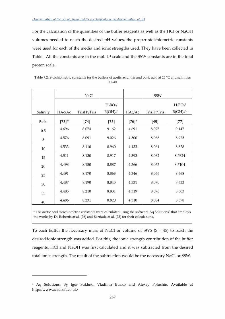
Determination of the pka of phenol red for spectrophotometric determination of pH

257

For the calculation of the quantities of the buffer reagents as well as the HCl or NaOH

volumes needed to reach the desired pH values, the proper stoichiometric constants

were used for each of the media and ionic strengths used. They have been collected in

Table . All the constants are in the mol. L-1 scale and the SSW constants are in the total

proton scale.

Table 7.2: Stoichiometric constants for the buffers of acetic acid, tris and boric acid at 25 °C and salinities

0.5-40.

Salinity

NaCl SSW

HAc/Ac- TrisH+/Tris

H3BO3/

B(OH)4-- HAc/Ac- TrisH+/Tris

H3BO3/

B(OH)4---

Refs. [73]* [74] [75] [76]* [49] [77]

0.5 4.696 8.074 9.162 4.691 8.075 9.147

5 4.576 8.091 9.026 4.500 8.068 8.925

10 4.533 8.110 8.960 4.433 8.064 8.828

15 4.511 8.130 8.917 4.393 8.062 8.7624

20 4.498 8.150 8.887 4.366 8.063 8.7104

25 4.491 8.170 8.863 4.346 8.066 8.668

30 4.487 8.190 8.845 4.331 8.070 8.633

35 4.485 8.210 8.831 4.319 8.076 8.603

40 4.486 8.231 8.820 4.310 8.084 8.578

* The acetic acid stoichiometric constants were calculated using the software Aq Solutions3 that employs

the works by De Robertis at al. [76] and Barriada at al. [73] for their calculations.

To each buffer the necessary mass of NaCl or volume of SWS (S = 45) to reach the

desired ionic strength was added. For this, the ionic strength contribution of the buffer

reagents, HCl and NaOH was first calculated and it was subtracted from the desired

total ionic strength. The result of the subtraction would be the necessary NaCl or SSW.

3 Aq Solutions: By Igor Sukhno, Vladimir Buzko and Alexey Polushin. Available at

http://www.acadsoft.co.uk/

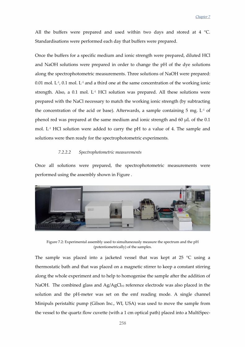
Chapter 7

258

All the buffers were prepared and used within two days and stored at 4 °C.

Standardisations were performed each day that buffers were prepared.

Once the buffers for a specific medium and ionic strength were prepared, diluted HCl

and NaOH solutions were prepared in order to change the pH of the dye solutions

along the spectrophotometric measurements. Three solutions of NaOH were prepared:

0.01 mol. L-1, 0.1 mol. L-1 and a third one at the same concentration of the working ionic

strength. Also, a 0.1 mol. L-1 HCl solution was prepared. All these solutions were

prepared with the NaCl necessary to match the working ionic strength (by subtracting

the concentration of the acid or base). Afterwards, a sample containing 5 mg. L-1 of

phenol red was prepared at the same medium and ionic strength and 60 µL of the 0.1

mol. L-1 HCl solution were added to carry the pH to a value of 4. The sample and

solutions were then ready for the spectrophotometric experiments.

7.2.2.2 Spectrophotometric measurements

Once all solutions were prepared, the spectrophotometric measurements were

performed using the assembly shown in Figure .

Figure 7.2: Experimental assembly used to simultaneously measure the spectrum and the pH

(potentiometrically) of the samples.

The sample was placed into a jacketed vessel that was kept at 25 °C using a

thermostatic bath and that was placed on a magnetic stirrer to keep a constant stirring

along the whole experiment and to help to homogenise the sample after the addition of

NaOH. The combined glass and Ag/AgCl(s) reference electrode was also placed in the

solution and the pH-meter was set on the emf reading mode. A single channel

Minipuls peristaltic pump (Gilson Inc., WI, USA) was used to move the sample from

the vessel to the quartz flow cuvette (with a 1 cm optical path) placed into a MultiSpec-

Determination of the pka of phenol red for spectrophotometric determination of pH

259

1501 UV-Vis Diode Array spectrophotometer (Shimadzu Corp., Kyoto, Japan) and back

to the vessel. This transportation was performed with inert Teflon tubes with an inner

diameter of 0.8 mm. Experiments started at pH = 4 and the pH was increased until 10

or 11 by adding small amounts of NaOH (in order to change the total volume as less as

possible). For the additions of NaOH far from the pka of the indicator dye, the most

concentrated solutions of NaOH were used while for those nearby the pka very small

additions of the most diluted NaOH solution were made (because the pH here changes

drastically). After each addition, it was necessary to wait for the sample to homogenise

and the emf reading to stabilise. When these conditions were attained, the peristaltic

pump was stopped, the emf value written down and the absorbance spectrum was

recorded from 200 to 800 nm. This process was repeated for the whole pH interval.

Through all experiments, N2 (g) washed through a solution containing the ionic media

of each experiment was bubbled into the sample to avoid dissolution of CO2.

7.2.2.3 Calculation procedure

For the basic pre-treatment of the spectra the SpectraGryph4 program was used. With

this program, the baseline was aligned at zero absorbance using the wavelengths in the

spectra where no absorbance in the solutions was found (usually from 650 to 800 nm).

Then, a moving average smoothing was performed using a rectangular averaging

function with a window of 4 points.

After the pre-treatment of the spectra, the program HypSpec5 was used for the

calculation of the stability constants of the phenol red at each media and ionic strength.

To perform this calculation, the absorbance values at the selected wavelength interval

were introduced as input along with their respective pH values and the concentrations

of phenol red (taking into account the dilution originated by the NaOH additions).

These pH values were calculated from the emf values of the experiments and the slope

and y-axis intercept of the pH-meter calibration with the buffers. With this

information, the program was able to calculate the stability constants along with their

4 Dr. Friedrich Menges. http://www.effemm2.de/spectragryph/down.html 5 Dr. Peter Gans. http://www.hyperquad.co.uk/HypSpec.htm

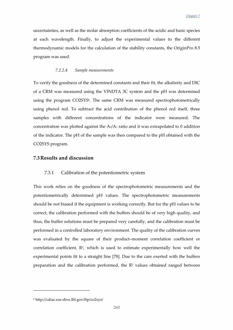
Chapter 7

260

uncertainties, as well as the molar absorption coefficients of the acidic and basic species

at each wavelength. Finally, to adjust the experimental values to the different

thermodynamic models for the calculation of the stability constants, the OriginPro 8.5

program was used.

7.2.2.4 Sample measurements

To verify the goodness of the determined constants and their fit, the alkalinity and DIC

of a CRM was measured using the VINDTA 3C system and the pH was determined

using the program CO2SYS6. The same CRM was measured spectrophotometrically

using phenol red. To subtract the acid contribution of the phenol red itself, three

samples with different concentrations of the indicator were measured. The

concentration was plotted against the A2/A1 ratio and it was extrapolated to 0 addition

of the indicator. The pH of the sample was then compared to the pH obtained with the

CO2SYS program.

7.3 Results and discussion

7.3.1 Calibration of the potentiometric system

This work relies on the goodness of the spectrophotometric measurements and the

potentiometrically determined pH values. The spectrophotometric measurements

should be not biased if the equipment is working correctly. But for the pH values to be

correct, the calibration performed with the buffers should be of very high quality, and

thus, the buffer solutions must be prepared very carefully, and the calibration must be

performed in a controlled laboratory environment. The quality of the calibration curves

was evaluated by the square of their product–moment correlation coefficient or

correlation coefficient, R2, which is used to estimate experimentally how well the

experimental points fit to a straight line [78]. Due to the care exerted with the buffers

preparation and the calibration performed, the R2 values obtained ranged between

6 http://cdiac.ess-dive.lbl.gov/ftp/co2sys/

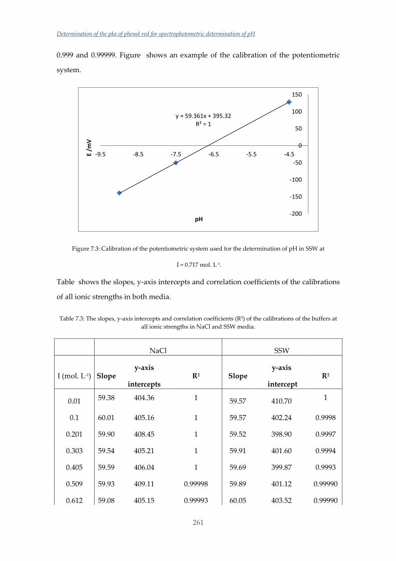
Determination of the pka of phenol red for spectrophotometric determination of pH

261

0.999 and 0.99999. Figure shows an example of the calibration of the potentiometric

system.

Figure 7.3: Calibration of the potentiometric system used for the determination of pH in SSW at

I = 0.717 mol. L-1.

Table shows the slopes, y-axis intercepts and correlation coefficients of the calibrations

of all ionic strengths in both media.

Table 7.3: The slopes, y-axis intercepts and correlation coefficients (R2) of the calibrations of the buffers at

all ionic strengths in NaCl and SSW media.

NaCl SSW

I (mol. L-1) Slope y-axis

intercepts R2 Slope

y-axis

intercept R2

0.01 59.38 404.36 1 59.57 410.70 1

0.1 60.01 405.16 1 59.57 402.24 0.9998

0.201 59.90 408.45 1 59.52 398.90 0.9997

0.303 59.54 405.21 1 59.91 401.60 0.9994

0.405 59.59 406.04 1 59.69 399.87 0.9993

0.509 59.93 409.11 0.99998 59.89 401.12 0.99990

0.612 59.08 405.15 0.99993 60.05 403.52 0.99990

y = 59.361x + 395.32R² = 1

-200

-150

-100

-50

0

50

100

150

-9.5 -8.5 -7.5 -6.5 -5.5 -4.5E /m

V

pH

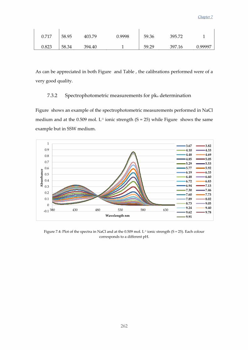
Chapter 7

262

0.717 58.95 403.79 0.9998 59.36 395.72 1

0.823 58.34 394.40 1 59.29 397.16 0.99997

As can be appreciated in both Figure and Table , the calibrations performed were of a

very good quality.

7.3.2 Spectrophotometric measurements for pka determination

Figure shows an example of the spectrophotometric measurements performed in NaCl

medium and at the 0.509 mol. L-1 ionic strength (S = 25) while Figure shows the same

example but in SSW medium.

Figure 7.4: Plot of the spectra in NaCl and at the 0.509 mol. L-1 ionic strength (S = 25). Each colour

corresponds to a different pH.

-0.1

0

0.1

0.2

0.3

0.4

0.5

0.6

0.7

0.8

0.9

1

380 430 480 530 580 630

Ab

sorb

ance

Wavelength nm

3.67 3.82

4.10 4.33

4.48 4.69

4.85 5.05

5.29 5.53

5.77 5.92

6.19 6.33

6.48 6.60

6.72 6.83

6.94 7.13

7.30 7.46

7.60 7.73

7.89 8.02

8.73 9.05

9.24 9.40

9.62 9.78

9.91

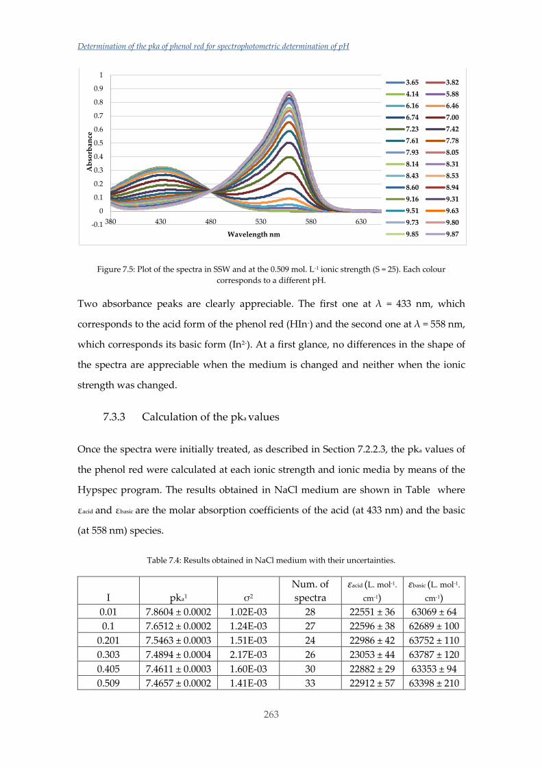
Determination of the pka of phenol red for spectrophotometric determination of pH

263

Figure 7.5: Plot of the spectra in SSW and at the 0.509 mol. L-1 ionic strength (S = 25). Each colour

corresponds to a different pH.

Two absorbance peaks are clearly appreciable. The first one at λ = 433 nm, which

corresponds to the acid form of the phenol red (HIn-) and the second one at λ = 558 nm,

which corresponds its basic form (In2-). At a first glance, no differences in the shape of

the spectra are appreciable when the medium is changed and neither when the ionic

strength was changed.

7.3.3 Calculation of the pka values

Once the spectra were initially treated, as described in Section 7.2.2.3, the pka values of

the phenol red were calculated at each ionic strength and ionic media by means of the

Hypspec program. The results obtained in NaCl medium are shown in Table where

εacid and εbasic are the molar absorption coefficients of the acid (at 433 nm) and the basic

(at 558 nm) species.

Table 7.4: Results obtained in NaCl medium with their uncertainties.

I pka1 σ2

Num. of

spectra

𝜀acid (L. mol-1.

cm-1)

𝜀basic (L. mol-1.

cm-1)

0.01 7.8604 ± 0.0002 1.02E-03 28 22551 ± 36 63069 ± 64

0.1 7.6512 ± 0.0002 1.24E-03 27 22596 ± 38 62689 ± 100

0.201 7.5463 ± 0.0003 1.51E-03 24 22986 ± 42 63752 ± 110

0.303 7.4894 ± 0.0004 2.17E-03 26 23053 ± 44 63787 ± 120

0.405 7.4611 ± 0.0003 1.60E-03 30 22882 ± 29 63353 ± 94

0.509 7.4657 ± 0.0002 1.41E-03 33 22912 ± 57 63398 ± 210

-0.1

0

0.1

0.2

0.3

0.4

0.5

0.6

0.7

0.8

0.9

1

380 430 480 530 580 630

Ab

sorb

ance

Wavelength nm

3.65 3.82

4.14 5.88

6.16 6.46

6.74 7.00

7.23 7.42

7.61 7.78

7.93 8.05

8.14 8.31

8.43 8.53

8.60 8.94

9.16 9.31

9.51 9.63

9.73 9.80

9.85 9.87

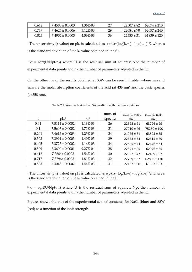
Chapter 7

264

0.612 7.4503 ± 0.0003 1.36E-03 27 22507 ± 82 62074 ± 210

0.717 7.4624 ± 0.0006 3.12E-03 29 22684 ± 70 62057 ± 240

0.823 7.4902 ± 0.0003 4.56E-03 36 22583 ± 31 61839 ± 120

1 The uncertainty (± value) on pka is calculated as s(pka)=[log(ka+s) - log(ka-s)]/2 where s

is the standard deviation of the ka value obtained in the fit.

2 σ = sqrt(U/Npt-np) where U is the residual sum of squares; Npt the number of

experimental data points and np the number of parameters adjusted in the fit.

On the other hand, the results obtained at SSW can be seen in Table where εacid and

εbasic are the molar absorption coefficients of the acid (at 433 nm) and the basic species

(at 558 nm).

Table 7.5: Results obtained in SSW medium with their uncertainties.

I pka1 σ2

num. of

spectra 𝜀acid (L. mol-1.

cm-1) 𝜀basic (L. mol-1.

cm-1)

0.01 7.8114 ± 0.0002 1.18E-03 26 22628 ± 21 63726 ± 99

0.1 7.5607 ± 0.0002 1.71E-03 31 27010 ± 46 75250 ± 190

0.201 7.4615 ± 0.0003 1.25E-03 34 21976 ± 31 63525 ± 55

0.303 7.3991 ± 0.0003 1.40E-03 29 22533 ± 34 62515 ± 69

0.405 7.3727 ± 0.0002 1.16E-03 34 22525 ± 44 62676 ± 64

0.509 7.3600 ± 0.0001 9.27E-04 28 22841 ± 25 62976 ± 55

0.612 7.3684± 0.0003 1.56E-03 30 22652 ± 47 62459 ± 92

0.717 7.3796± 0.0003 1.81E-03 32 22709 ± 37 62802 ± 170

0.823 7.4013 ± 0.0002 1.44E-03 31 22187 ± 30 61363 ± 83

1 The uncertainty (± value) on pka is calculated as s(pka)=[log(ka+s) - log(ka-s)]/2 where s

is the standard deviation of the ka value obtained in the fit.

2 σ = sqrt(U/Npt-np) where U is the residual sum of squares; Npt the number of

experimental data points and np the number of parameters adjusted in the fit.

Figure shows the plot of the experimental sets of constants for NaCl (blue) and SSW

(red) as a function of the ionic strength.

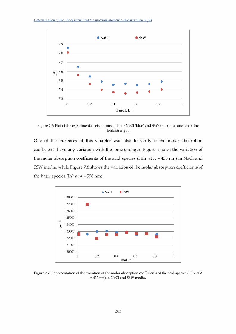
Determination of the pka of phenol red for spectrophotometric determination of pH

265

Figure 7.6: Plot of the experimental sets of constants for NaCl (blue) and SSW (red) as a function of the

ionic strength.

One of the purposes of this Chapter was also to verify if the molar absorption

coefficients have any variation with the ionic strength. Figure shows the variation of

the molar absorption coefficients of the acid species (HIn- at λ = 433 nm) in NaCl and

SSW media, while Figure 7.8 shows the variation of the molar absorption coefficients of

the basic species (In2- at λ = 558 nm).

Figure 7.7: Representation of the variation of the molar absorption coefficients of the acid species (HIn- at λ

= 433 nm) in NaCl and SSW media.

7.3

7.4

7.5

7.6

7.7

7.8

7.9

0 0.2 0.4 0.6 0.8 1

pk

a

I mol. L-1

NaCl SSW

20000

21000

22000

23000

24000

25000

26000

27000

28000

0 0.2 0.4 0.6 0.8 1

ε(a

cid

)

I mol. L-1

NaCl SSW

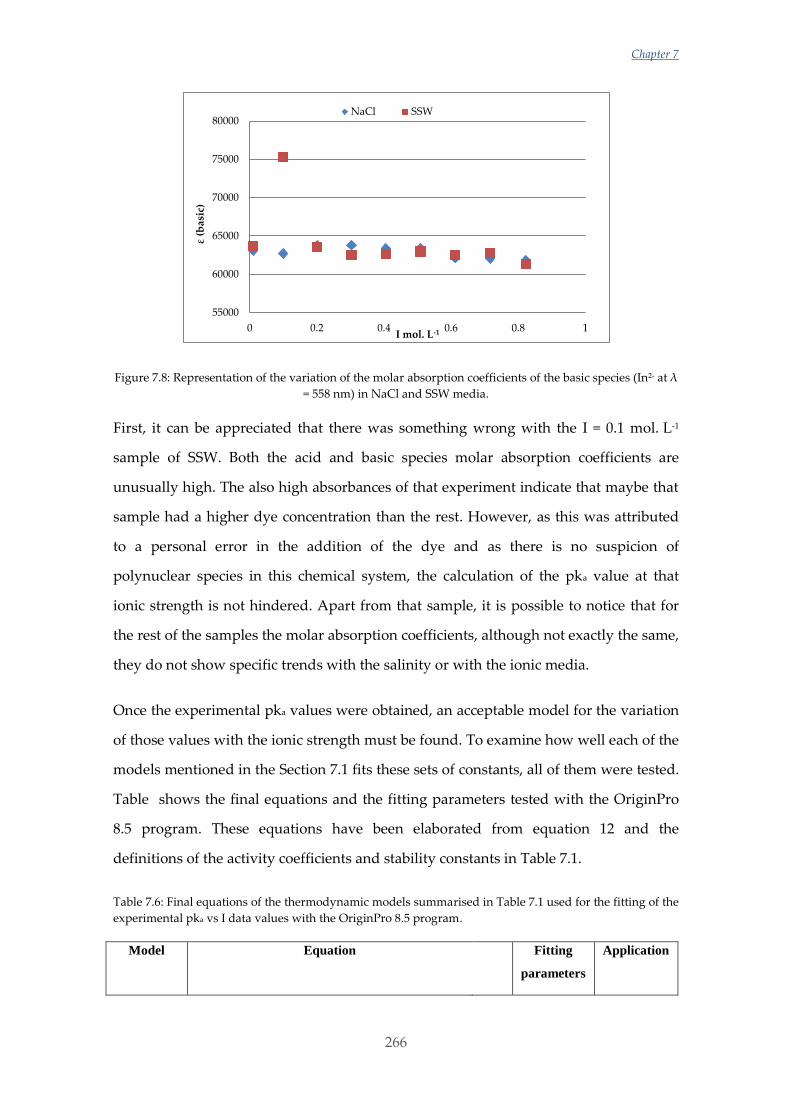
Chapter 7

266

Figure 7.8: Representation of the variation of the molar absorption coefficients of the basic species (In2- at λ

= 558 nm) in NaCl and SSW media.

First, it can be appreciated that there was something wrong with the I = 0.1 mol. L-1

sample of SSW. Both the acid and basic species molar absorption coefficients are

unusually high. The also high absorbances of that experiment indicate that maybe that

sample had a higher dye concentration than the rest. However, as this was attributed

to a personal error in the addition of the dye and as there is no suspicion of

polynuclear species in this chemical system, the calculation of the pka value at that

ionic strength is not hindered. Apart from that sample, it is possible to notice that for

the rest of the samples the molar absorption coefficients, although not exactly the same,

they do not show specific trends with the salinity or with the ionic media.

Once the experimental pka values were obtained, an acceptable model for the variation

of those values with the ionic strength must be found. To examine how well each of the

models mentioned in the Section 7.1 fits these sets of constants, all of them were tested.

Table shows the final equations and the fitting parameters tested with the OriginPro

8.5 program. These equations have been elaborated from equation 12 and the

definitions of the activity coefficients and stability constants in Table 7.1.

Table 7.6: Final equations of the thermodynamic models summarised in Table 7.1 used for the fitting of the

experimental pka vs I data values with the OriginPro 8.5 program.

Model Equation

Fitting

parameters

Application

55000

60000

65000

70000

75000

80000

0 0.2 0.4 0.6 0.8 1

ε(b

asic

)

I mol. L-1

NaCl SSW

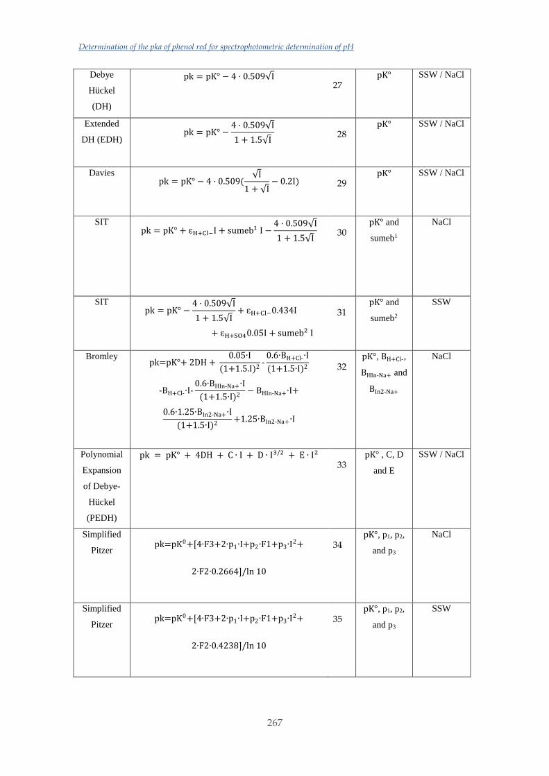
Determination of the pka of phenol red for spectrophotometric determination of pH

267

Debye

Hückel

(DH)

pk = pK° − 4 · 0.509√I 27

pK° SSW / NaCl

Extended

DH (EDH) pk = pK° −

4 · 0.509√I

1 + 1.5√I 28

pK° SSW / NaCl

Davies pk = pK° − 4 · 0.509(

√I

1 + √I− 0.2I) 29

pK° SSW / NaCl

SIT pk = pK° + ɛH+Cl−I + sumeb

1 I −4 · 0.509√I

1 + 1.5√I 30

pK° and

sumeb1

NaCl

SIT pk = pK° −

4 · 0.509√I

1 + 1.5√I+ ɛH+Cl−0.434I

+ ɛH+SO40.05I + sumeb2 I

31

pK° and

sumeb2

SSW

Bromley pk=pK°+ 2DH +

0.05∙I

(1+1.5.I)2-0.6∙BH+Cl-∙I

(1+1.5∙I)2

-BH+Cl-∙I-0.6∙BHIn-Na+∙I

(1+1.5∙I)2− BHIn-Na+∙I+

0.6∙1.25∙BIn2-Na+∙I

(1+1.5∙I)2+1.25∙BIn2-Na+∙I

32

pK°, BH+Cl-,

BHIn-Na+ and

BIn2-Na+

NaCl

Polynomial

Expansion

of Debye-

Hückel

(PEDH)

pk = pK° + 4DH + C ∙ I + D ∙ I3/2 + E ∙ I2

33

pK° , C, D

and E

SSW / NaCl

Simplified

Pitzer pk=pK0+[4∙F3+2∙p1∙I+p2∙F1+p3∙I

2+

2∙F2∙0.2664]/ln 10

34 pK°, p1, p2,

and p3

NaCl

Simplified

Pitzer pk=pK0+[4∙F3+2∙p1∙I+p2∙F1+p3∙I

2+

2∙F2∙0.4238]/ln 10

35 pK°, p1, p2,

and p3

SSW

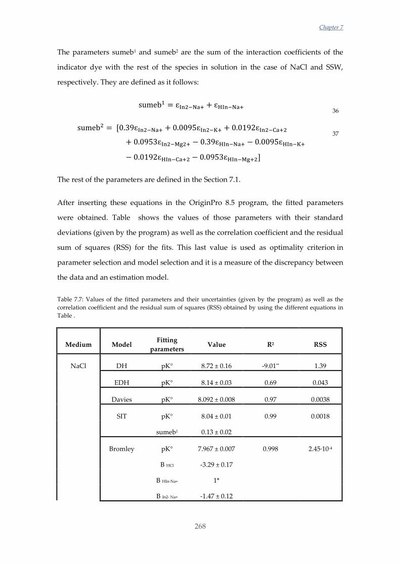
Chapter 7

268

The parameters sumeb1 and sumeb2 are the sum of the interaction coefficients of the

indicator dye with the rest of the species in solution in the case of NaCl and SSW,

respectively. They are defined as it follows:

sumeb1 = ɛIn2−Na+ + ɛHIn−Na+ 36

sumeb2 = [0.39ɛIn2−Na+ + 0.0095ɛIn2−K+ + 0.0192ɛIn2−Ca+2

+ 0.0953ɛIn2−Mg2+ − 0.39ɛHIn−Na+ − 0.0095ɛHIn−K+

− 0.0192ɛHIn−Ca+2 − 0.0953ɛHIn−Mg+2]

37

The rest of the parameters are defined in the Section 7.1.

After inserting these equations in the OriginPro 8.5 program, the fitted parameters

were obtained. Table shows the values of those parameters with their standard

deviations (given by the program) as well as the correlation coefficient and the residual

sum of squares (RSS) for the fits. This last value is used as optimality criterion in

parameter selection and model selection and it is a measure of the discrepancy between

the data and an estimation model.

Table 7.7: Values of the fitted parameters and their uncertainties (given by the program) as well as the

correlation coefficient and the residual sum of squares (RSS) obtained by using the different equations in

Table .

Medium Model Fitting

parameters Value R2 RSS

NaCl DH pK° 8.72 ± 0.16 -9.01** 1.39

EDH pK° 8.14 ± 0.03 0.69 0.043

Davies pK° 8.092 ± 0.008 0.97 0.0038

SIT pK° 8.04 ± 0.01 0.99 0.0018

sumeb1 0.13 ± 0.02

Bromley pK° 7.967 ± 0.007 0.998 2.45·10-4

B HCl -3.29 ± 0.17

B HIn-Na+ 1*

B In2- Na+ -1.47 ± 0.12

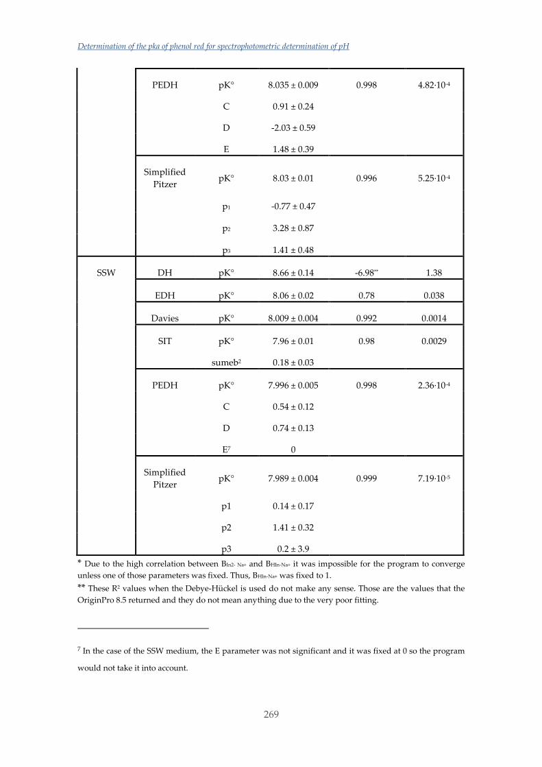
Determination of the pka of phenol red for spectrophotometric determination of pH

269

PEDH pK° 8.035 ± 0.009 0.998 4.82·10-4

C 0.91 ± 0.24

D -2.03 ± 0.59

E 1.48 ± 0.39

Simplified

Pitzer pK° 8.03 ± 0.01 0.996 5.25·10-4

p1 -0.77 ± 0.47

p2 3.28 ± 0.87

p3 1.41 ± 0.48

SSW DH pK° 8.66 ± 0.14 -6.98** 1.38

EDH pK° 8.06 ± 0.02 0.78 0.038

Davies pK° 8.009 ± 0.004 0.992 0.0014

SIT pK° 7.96 ± 0.01 0.98 0.0029

sumeb2 0.18 ± 0.03

PEDH pK° 7.996 ± 0.005 0.998 2.36·10-4

C 0.54 ± 0.12

D 0.74 ± 0.13

E7 0

Simplified

Pitzer pK° 7.989 ± 0.004 0.999 7.19·10-5

p1 0.14 ± 0.17

p2 1.41 ± 0.32

p3 0.2 ± 3.9

* Due to the high correlation between BIn2- Na+ and BHIn-Na+ it was impossible for the program to converge

unless one of those parameters was fixed. Thus, BHIn-Na+ was fixed to 1.

** These R2 values when the Debye-Hückel is used do not make any sense. Those are the values that the

OriginPro 8.5 returned and they do not mean anything due to the very poor fitting.

7 In the case of the SSW medium, the E parameter was not significant and it was fixed at 0 so the program

would not take it into account.

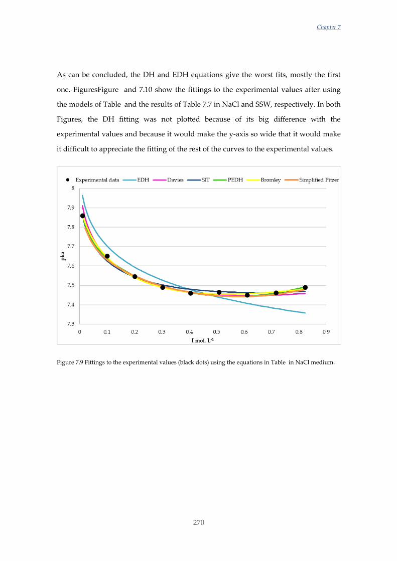
Chapter 7

270

As can be concluded, the DH and EDH equations give the worst fits, mostly the first

one. FiguresFigure and 7.10 show the fittings to the experimental values after using

the models of Table and the results of Table 7.7 in NaCl and SSW, respectively. In both

Figures, the DH fitting was not plotted because of its big difference with the

experimental values and because it would make the y-axis so wide that it would make

it difficult to appreciate the fitting of the rest of the curves to the experimental values.

Figure 7.9 Fittings to the experimental values (black dots) using the equations in Table in NaCl medium.

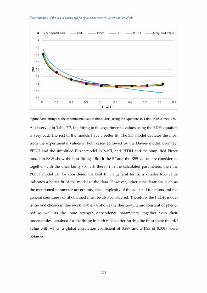
Determination of the pka of phenol red for spectrophotometric determination of pH

271

Figure 7.10: Fittings to the experimental values (black dots) using the equations in Table in SSW medium.

As observed in Table 7.7, the fitting to the experimental values using the EDH equation

is very bad. The rest of the models have a better fit. The SIT model deviates the most

from the experimental values in both cases, followed by the Davies model. Bromley,

PEDH and the simplified Pitzer model in NaCl, and PEDH and the simplified Pitzer

model in SSW show the best fittings. But if the R2 and the RSS values are considered,

together with the uncertainty (of lack thereof) in the calculated parameters, then the

PEDH model can be considered the best fit. In general terms, a smaller RSS value

indicates a better fit of the model to the data. However, other considerations such as

the mentioned parameter uncertainty, the complexity of the adjusted functions and the

general soundness of fit obtained must be also considered. Therefore, the PEDH model

is the one chosen in this work. Table 7.8 shows the thermodynamic constant of phenol

red as well as the ionic strength dependence parameters, together with their

uncertainties, obtained for the fitting in both media after forcing the fit to share the pK0

value with which a global correlation coefficient of 0.997 and a RSS of 0.0013 were

obtained.

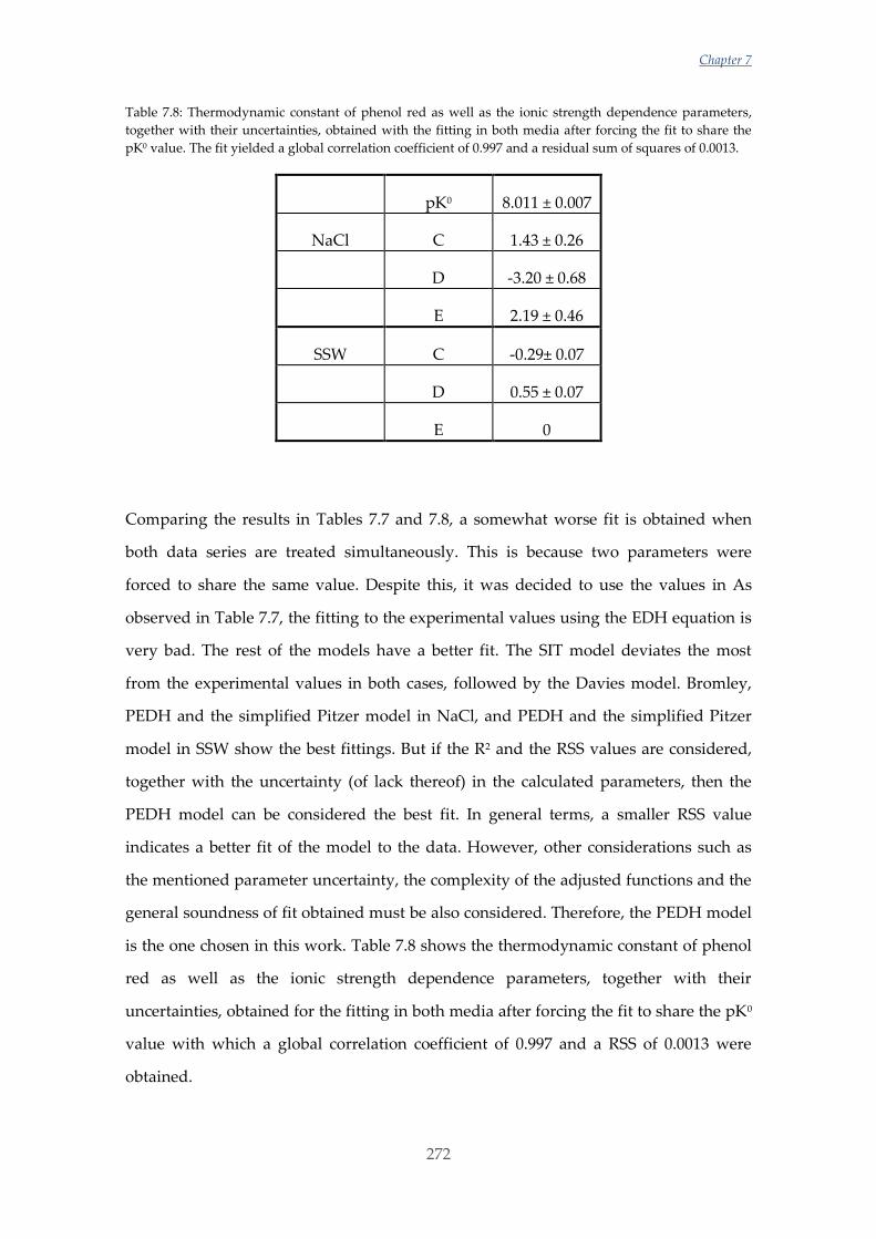
Chapter 7

272

Table 7.8: Thermodynamic constant of phenol red as well as the ionic strength dependence parameters,

together with their uncertainties, obtained with the fitting in both media after forcing the fit to share the

pK0 value. The fit yielded a global correlation coefficient of 0.997 and a residual sum of squares of 0.0013.

pK0 8.011 ± 0.007

NaCl C 1.43 ± 0.26

D -3.20 ± 0.68

E 2.19 ± 0.46

SSW C -0.29± 0.07

D 0.55 ± 0.07

E 0

Comparing the results in Tables 7.7 and 7.8, a somewhat worse fit is obtained when

both data series are treated simultaneously. This is because two parameters were

forced to share the same value. Despite this, it was decided to use the values in As

observed in Table 7.7, the fitting to the experimental values using the EDH equation is

very bad. The rest of the models have a better fit. The SIT model deviates the most

from the experimental values in both cases, followed by the Davies model. Bromley,

PEDH and the simplified Pitzer model in NaCl, and PEDH and the simplified Pitzer

model in SSW show the best fittings. But if the R2 and the RSS values are considered,

together with the uncertainty (of lack thereof) in the calculated parameters, then the

PEDH model can be considered the best fit. In general terms, a smaller RSS value

indicates a better fit of the model to the data. However, other considerations such as

the mentioned parameter uncertainty, the complexity of the adjusted functions and the

general soundness of fit obtained must be also considered. Therefore, the PEDH model

is the one chosen in this work. Table 7.8 shows the thermodynamic constant of phenol

red as well as the ionic strength dependence parameters, together with their

uncertainties, obtained for the fitting in both media after forcing the fit to share the pK0

value with which a global correlation coefficient of 0.997 and a RSS of 0.0013 were

obtained.

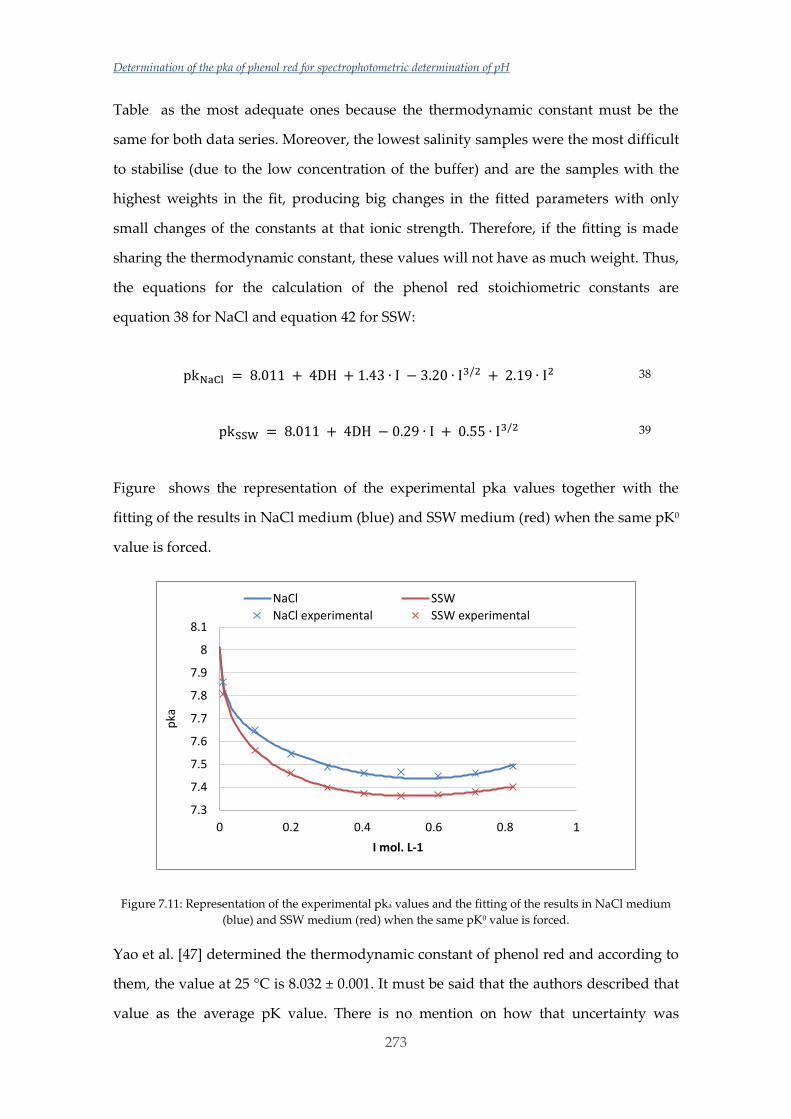
Determination of the pka of phenol red for spectrophotometric determination of pH

273

Table as the most adequate ones because the thermodynamic constant must be the

same for both data series. Moreover, the lowest salinity samples were the most difficult

to stabilise (due to the low concentration of the buffer) and are the samples with the

highest weights in the fit, producing big changes in the fitted parameters with only

small changes of the constants at that ionic strength. Therefore, if the fitting is made

sharing the thermodynamic constant, these values will not have as much weight. Thus,

the equations for the calculation of the phenol red stoichiometric constants are

equation 38 for NaCl and equation 42 for SSW:

pkNaCl = 8.011 + 4DH + 1.43 ∙ I − 3.20 ∙ I3/2 + 2.19 ∙ I2 38

pkSSW = 8.011 + 4DH − 0.29 ∙ I + 0.55 ∙ I3/2 39

Figure shows the representation of the experimental pka values together with the

fitting of the results in NaCl medium (blue) and SSW medium (red) when the same pK0

value is forced.

Figure 7.11: Representation of the experimental pka values and the fitting of the results in NaCl medium

(blue) and SSW medium (red) when the same pK0 value is forced.

Yao et al. [47] determined the thermodynamic constant of phenol red and according to

them, the value at 25 °C is 8.032 ± 0.001. It must be said that the authors described that

value as the average pK value. There is no mention on how that uncertainty was

7.3

7.4

7.5

7.6

7.7

7.8

7.9

8

8.1

0 0.2 0.4 0.6 0.8 1

pka

I mol. L-1

NaCl SSW

NaCl experimental SSW experimental

Chapter 7

274

calculated but it leads to believe that it is the standard deviation of a series of pK

values. The value determined in this work is not exactly the same, but it compares very

favourably.

As stated above, the suitability of the obtained constants and of the whole procedure

for the measurement of the pH of estuarine and seawater samples was tested by

comparing the pH values obtained with the CO2SYS program and those measured

spectrophotometrically. For that purpose, the Batch 165 seawater sample provided by

Andrew Dickson’s laboratory (Scripps Institution of Oceanography, La Jolla, CA, USA)

was used, which, according to the CO2SYS program has a pHT of 7.766 ± 0.003. This

value was obtained using the constants of the carbonate system determined by Lueker

et al. [79], the bisulphate constant determined by Dickson [80] and the boron

concentration determined by Lee et al. [81]. The uncertainty was considered as the

standard deviation of three measurements and thus, the real uncertainty would be

higher. The use of the VINDTA system, which is a high precision equipment because of

the lack of personal manipulation, suggests that the error propagation will be small.

But the uncertainty on the constants that the CO2SYS program uses is not considered

anywhere. The spectrophotometric determination of the CRM was performed

according to the procedure described in Section 2.2.4. The e1, e2 and e3 parameters in

equation 16 were calculated using the average of the molar absorption coefficients

obtained in this work (except for the outliers) because of their consistency with salinity.

This equation gave a result of 7.763 ± 0.003. Thus, both the goodness of the constants

and the used procedure have been corroborated because statistically comparable

results were obtained with a confidence level of 95 %.

7.4 Conclusions

Stoichiometric constants for the acid-base equilibrium of the pH indicator phenol red

have been obtained. Phenol red is an indicator that has a lower pka than the others

typically used for the spectrophometric determination of pH is seawater. This fact is

crucial for those natural waters that have lower pH values such as some estuarine

waters, rivers, lakes, etc.

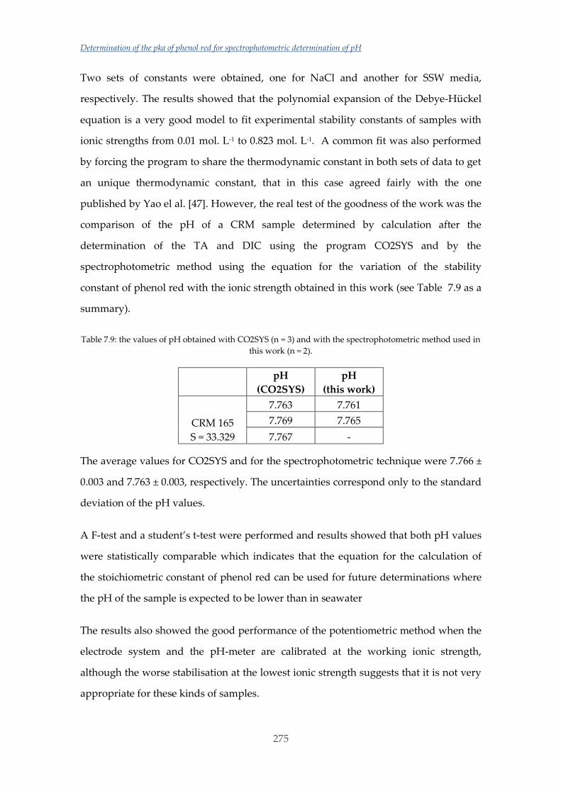
Determination of the pka of phenol red for spectrophotometric determination of pH

275

Two sets of constants were obtained, one for NaCl and another for SSW media,

respectively. The results showed that the polynomial expansion of the Debye-Hückel

equation is a very good model to fit experimental stability constants of samples with

ionic strengths from 0.01 mol. L-1 to 0.823 mol. L-1. A common fit was also performed

by forcing the program to share the thermodynamic constant in both sets of data to get

an unique thermodynamic constant, that in this case agreed fairly with the one

published by Yao el al. [47]. However, the real test of the goodness of the work was the

comparison of the pH of a CRM sample determined by calculation after the

determination of the TA and DIC using the program CO2SYS and by the

spectrophotometric method using the equation for the variation of the stability

constant of phenol red with the ionic strength obtained in this work (see Table 7.9 as a

summary).

Table 7.9: the values of pH obtained with CO2SYS (n = 3) and with the spectrophotometric method used in

this work (n = 2).

pH

(CO2SYS)

pH

(this work)

CRM 165

S = 33.329

7.763 7.761

7.769 7.765

7.767 -

The average values for CO2SYS and for the spectrophotometric technique were 7.766 ±

0.003 and 7.763 ± 0.003, respectively. The uncertainties correspond only to the standard

deviation of the pH values.

A F-test and a student’s t-test were performed and results showed that both pH values

were statistically comparable which indicates that the equation for the calculation of

the stoichiometric constant of phenol red can be used for future determinations where

the pH of the sample is expected to be lower than in seawater

The results also showed the good performance of the potentiometric method when the

electrode system and the pH-meter are calibrated at the working ionic strength,

although the worse stabilisation at the lowest ionic strength suggests that it is not very

appropriate for these kinds of samples.

Chapter 7

276

7.5 References:

[1] A. L. Lavoisier, “Considérations générales sur la nature des acides, et sur les

principes dont ils sont composés,” Mém. L’Académie Sci., pp. 248–260, 1778.

[2] W. de Vos and A. Pilot, “Acids and Bases in Layers: The Stratal Structure of an

Ancient Topic,” J. Chem. Educ., vol. 78, no. 4, p. 494, Apr. 2001.

[3] N. F. Hall, “Systems of acids and bases,” J. Chem. Educ., vol. 17, no. 3, p. 124, Mar.

1940.

[4] A. G. Dickson, “The development of the alkalinity concept in marine chemistry,”

Mar. Chem., vol. 40, no. 1, pp. 49–63, Nov. 1992.

[5] H. M. Leicester, The Historical Background of Chemistry. New York: Dover

Publications Inc., 1956.

[6] G. L. Miessler, P. J. Fischer, and D. A. Tarr, Inorganic Chemistry, 5th ed. Pearson

Prentice Hall, 2014.

[7] J. N. Brönsted, “Einige Bemerkungen über den Begriff der Säuren und Basen,” Recl.

Trav. Chim. Pays-Bas, vol. 42, no. 8, pp. 718–728, Jan. 1923.

[8] T. M. Lowry, “The uniqueness of hydrogen,” J. Soc. Chem. Ind., vol. 42, no. 3, pp.

43–47, Jan. 1923.

[9] G. N. Lewis, Valence and the Structure of Atoms and Molecules. Chemical Catalog

Company, Incorporated, 1923.

[10] W. M. Clark, The Determination of Hydrogen Ions: An Elementary Treatise on the

Hydrogen Electrode, Indicator and Supplementary Methods with an Indexed Bibliography

on Applications. Williams & Wilkins, 1922.

Determination of the pka of phenol red for spectrophotometric determination of pH

277

[11] S. P. L. Sørensen, “Enzymstudien. II: Mitteilung. Über die Messung und die

Bedeutung der Wasserstoffionenkoncentration bei enzymatischen Prozessen,”

Biochem. Z., vol. 21, pp. 131–304, 1909.

[12] L. Rosenfeld, Four Centuries of Clinical Chemistry. CRC Press, 1999.

[13] F. Haber and Z. Klemensiewicz, “Über elektrische Phasengrenzkräfte,” Z. Für Phys.

Chem., vol. 67U, no. 1, pp. 385–431, 1909.

[14] D. A. MacInnes and M. Dole, “The behavior of glass electrodes of different

compositions,” J. Am. Chem. Soc., vol. 52, no. 1, pp. 29–36, 1930.

[15] F. G. Baucke, “New IUPAC recommendations on the measurement of pH –

background and essentials,” Anal. Bioanal. Chem., vol. 374, no. 5, pp. 772–777, Nov.

2002.

[16] R. P. Buck et al., “Measurement of pH. Definition, standards, and procedures

(IUPAC Recommendations 2002),” Pure Appl. Chem., vol. 74, no. 11, pp. 2169–2200,

2002.

[17] R. G. Bates, “Definitions of pH Scales.,” Chem. Rev., vol. 42, no. 1, pp. 1–61, Feb.

1948.

[18] K. H. Khoo, R. W. Ramette, C. H. Culberson, and R. G. Bates, “Determination of

hydrogen ion concentrations in seawater from 5 to 40.degree.C: standard

potentials at salinities from 20 to 45%,” Anal. Chem., vol. 49, no. 1, pp. 29–34, Jan.

1977.

[19] R. W. Ramette, C. H. Culberson, and R. G. Bates, “Acid-base properties of

tris(hydroxymethyl)aminomethane (Tris) buffers in sea water from 5 to

40.degree.C,” Anal. Chem., vol. 49, no. 6, pp. 867–870, May 1977.

[20] R. G. Bates and E. A. Guggenheim, “Report on the standardization of pH and

related terminology,” Pure Appl. Chem., vol. 1, no. 1, pp. 163–168, 1960.

[21] R. G. Bates and V. E. Bower, “Standard Potential of the Silver-Silver-Chloride

Electrod from 0° to 95° C and the Thermodynamic Properties of Dilute

Chapter 7

278

Hydrochloric Acid Solutions,” J. Res. Natl. Bur. Stand., vol. 53, no. 5, pp. 283–290,

1954.

[22] F. J. Millero et al., “The use of buffers to measure the pH of seawater,” Mar. Chem.,

vol. 44, no. 2, pp. 143–152, Dec. 1993.

[23] R. G. Bates, Determination of pH: theory and practice. John Wiley & Sons, 1973.

[24] A. G. Dickson, “pH scales and proton-transfer reactions in saline media such as sea

water,” Geochim. Cosmochim. Acta, vol. 48, no. 11, pp. 2299–2308, Nov. 1984.

[25] F. J. Millero, “The pH of estuarine waters,” Limnol. Oceanogr., vol. 31, no. 4, pp.

839–847, Jul. 1986.

[26] I. Hansson, “A new set of pH-scales and standard buffers for sea water,” Deep Sea

Res. Oceanogr. Abstr., vol. 20, no. 5, pp. 479–491, May 1973.

[27] A. G. Dickson, “Standard potential of the reaction: AgCl(s) + 12H2(g) = Ag(s) +

HCl(aq), and and the standard acidity constant of the ion HSO4− in synthetic sea

water from 273.15 to 318.15 K,” J. Chem. Thermodyn., vol. 22, no. 2, pp. 113–127, Feb.

1990.

[28] A. G. Dickson and F. J. Millero, “A comparison of the equilibrium constants for the

dissociation of carbonic acid in seawater media,” Deep Sea Res. Part Oceanogr. Res.

Pap., vol. 34, no. 10, pp. 1733–1743, Oct. 1987.

[29] A. G. Dickson and J. P. Riley, “The estimation of acid dissociation constants in

seawater media from potentionmetric titrations with strong base. I. The ionic

product of water—Kw,” Mar. Chem., vol. 7, no. 2, pp. 89–99, 1979.

[30] J. F. Waters and F. J. Millero, “The free proton concentration scale for seawater

pH,” Mar. Chem., vol. 149, no. Supplement C, pp. 8–22, Feb. 2013.

[31] F. J. Millero, “Carbonate constants for estuarine waters,” Mar. Freshw. Res., vol. 61,

no. 2, pp. 139–142, Mar. 2010.

Determination of the pka of phenol red for spectrophotometric determination of pH

279

[32] A. G. Dickson, “pH buffers for sea water media based on the total hydrogen ion

concentration scale,” Deep Sea Res. Part Oceanogr. Res. Pap., vol. 40, no. 1, pp. 107–

118, Jan. 1993.

[33] F. J. Millero, “The Marine Inorganic Carbon Cycle,” Chem. Rev., vol. 107, no. 2, pp.

308–341, Feb. 2007.

[34] G. L. Robert-Baldo, M. J. Morris, and R. H. Byrne, “Spectrophotometric

determination of seawater pH using phenol red,” Anal. Chem., vol. 57, no. 13, pp.

2564–2567, Nov. 1985.

[35] A. G. Dickson, C. L. Sabine, and J. R. Christian, Guide to best practices for ocean CO2

measurements. PICES Special Publication 3, 2007.

[36] H. Zhang and R. H. Byrne, “Spectrophotometric pH measurements of surface

seawater at in-situ conditions: absorbance and protonation behavior of thymol

blue,” Mar. Chem., vol. 52, no. 1, pp. 17–25, Mar. 1996.

[37] V. M. C. Rérolle, C. F. A. Floquet, A. J. K. Harris, M. C. Mowlem, R. R. G. J.

Bellerby, and E. P. Achterberg, “Development of a colorimetric microfluidic pH

sensor for autonomous seawater measurements,” Anal. Chim. Acta, vol. 786, no.

Supplement C, pp. 124–131, Jul. 2013.

[38] M. C. Patsavas, R. H. Byrne, and X. Liu, “Purification of meta-cresol purple and

cresol red by flash chromatography: Procedures for ensuring accurate

spectrophotometric seawater pH measurements,” Mar. Chem., vol. 150, no.

Supplement C, pp. 19–24, Mar. 2013.

[39] J. A. Gallego-Urrea and D. R. Turner, “Determination of pH in estuarine and

brackish waters: Pitzer parameters for Tris buffers and dissociation constants for

m-cresol purple at 298.15K,” Mar. Chem., vol. 195, no. Supplement C, pp. 84–89,

Oct. 2017.

Chapter 7

280

[40] K. Hammer, B. Schneider, K. Kuliński, and D. E. Schulz-Bull, “Precision and

accuracy of spectrophotometric pH measurements at environmental conditions in

the Baltic Sea,” Estuar. Coast. Shelf Sci., vol. 146, pp. 24–32, Jun. 2014.

[41] P. Y. Tishchenko, D.-J. Kang, R. V. Chichkin, A. Y. Lazaryuk, C. Shing Wong, and

W. Keith Johnson, “Application of potentiometric method using a cell without

liquid junction to underway pH measurements in surface seawater,” Deep Sea Res.

Part Oceanogr. Res. Pap., vol. 58, no. 7, pp. 778–786, Jul. 2011.

[42] G. M. Marion, F. J. Millero, M. F. Camões, P. Spitzer, R. Feistel, and C.-T. A. Chen,

“pH of seawater,” Mar. Chem., vol. 126, no. 1–4, pp. 89–96, Sep. 2011.

[43] V. M. C. Rérolle, C. F. A. Floquet, M. C. Mowlem, D. P. Connelly, E. P. Achterberg,

and R. R. G. J. Bellerby, “Seawater-pH measurements for ocean-acidification

observations,” TrAC Trends Anal. Chem., vol. 40, no. Supplement C, pp. 146–157,

Nov. 2012.

[44] A. G. Dickson, “The measurement of sea water pH,” Mar. Chem., vol. 44, no. 2, pp.

131–142, Dec. 1993.

[45] D. W. King and D. R. Kester, “Determination of seawater pH from 1.5 to 8.5 using

colorimetric indicators,” Mar. Chem., vol. 26, no. 1, pp. 5–20, Feb. 1989.

[46] M. Tapp, K. Hunter, K. Currie, and B. Mackaskill, “Apparatus for continuous-flow

underway spectrophotometric measurement of surface water pH,” Mar. Chem., vol.

72, no. 2, pp. 193–202, Dec. 2000.

[47] W. Yao and R. H. Byrne, “Spectrophotometric Determination of Freshwater pH

Using Bromocresol Purple and Phenol Red,” Environ. Sci. Technol., vol. 35, no. 6,

pp. 1197–1201, Mar. 2001.

[48] C. R. French, J. J. Carr, E. M. Dougherty, L. A. K. Eidson, J. C. Reynolds, and M. D.

DeGrandpre, “Spectrophotometric pH measurements of freshwater,” Anal. Chim.

Acta, vol. 453, no. 1, pp. 13–20, Feb. 2002.

Determination of the pka of phenol red for spectrophotometric determination of pH

281

[49] L. M. Mosley, S. L. G. Husheer, and K. A. Hunter, “Spectrophotometric pH

measurement in estuaries using thymol blue and m-cresol purple,” Mar. Chem.,

vol. 91, no. 1, pp. 175–186, Nov. 2004.

[50] T. D. Clayton et al., “The role of pH measurements in modern oceanic CO2-system

characterizations: Precision and thermodynamic consistency,” Deep Sea Res. Part II

Top. Stud. Oceanogr., vol. 42, no. 2, pp. 411–429, Jan. 1995.

[51] X. Liu, M. C. Patsavas, and R. H. Byrne, “Purification and Characterization of

meta-Cresol Purple for Spectrophotometric Seawater pH Measurements,” Environ.

Sci. Technol., vol. 45, no. 11, pp. 4862–4868, Jun. 2011.

[52] R. H. Byrne, S. McElligott, R. A. Feely, and F. J. Millero, “The role of pHT

measurements in marine CO2-system characterizations,” Deep Sea Res. Part

Oceanogr. Res. Pap., vol. 46, no. 11, pp. 1985–1997, Nov. 1999.

[53] B. R. Carter, J. A. Radich, H. L. Doyle, and A. G. Dickson, “An automated system

for spectrophotometric seawater pH measurements,” Limnol. Oceanogr. Methods,

vol. 11, no. 1, pp. 16–27, Jan. 2013.

[54] R. G. J. Bellerby, D. R. Turner, G. E. Millward, and P. J. Worsfold, “Shipboard flow

injection determination of sea water pH with spectrophotometric detection,” Anal.

Chim. Acta, vol. 309, no. 1, pp. 259–270, Jun. 1995.

[55] R. H. Byrne, “Standardization of standard buffers by visible spectrometry,” Anal.

Chem., vol. 59, no. 10, pp. 1479–1481, May 1987.

[56] W. Yao, X. Liu, and R. H. Byrne, “Impurities in indicators used for

spectrophotometric seawater pH measurements: Assessment and remedies,” Mar.

Chem., vol. 107, no. 2, pp. 167–172, Oct. 2007.

[57] R. H. Byrne and J. A. Breland, “High precision multiwavelength pH

determinations in seawater using cresol red,” Deep Sea Res. Part Oceanogr. Res. Pap.,

vol. 36, no. 5, pp. 803–810, May 1989.

Chapter 7

282

[58] M. C. Patsavas, R. H. Byrne, and X. Liu, “Purification of meta-cresol purple and

cresol red by flash chromatography: Procedures for ensuring accurate

spectrophotometric seawater pH measurements,” Mar. Chem., vol. 150, no.

Supplement C, pp. 19–24, Mar. 2013.

[59] N. K. Douglas and R. H. Byrne, “Achieving accurate spectrophotometric pH

measurements using unpurified meta-cresol purple,” Mar. Chem., vol. 190, no.

Supplement C, pp. 66–72, Mar. 2017.

[60] M. C. Patsavas, R. H. Byrne, and X. Liu, “Physical–chemical characterization of

purified cresol red for spectrophotometric pH measurements in seawater,” Mar.

Chem., vol. 155, no. Supplement C, pp. 158–164, Sep. 2013.

[61] B. Yang, M. C. Patsavas, R. H. Byrne, and J. Ma, “Seawater pH measurements in

the field: A DIY photometer with 0.01 unit pH accuracy,” Mar. Chem., vol. 160, no.

Supplement C, pp. 75–81, Mar. 2014.

[62] N. K. Douglas and R. H. Byrne, “Spectrophotometric pH measurements from river

to sea: Calibration of mCP for 0≤S≤40 and 278.15≤T≤308.15K,” Mar. Chem., Oct.

2017.

[63] M. Chierici, A. Fransson, and L. G. Anderson, “Influence of m-cresol purple

indicator additions on the pH of seawater samples: correction factors evaluated

from a chemical speciation model,” Mar. Chem., vol. 65, no. 3, pp. 281–290, Jun.

1999.

[64] S. M. Ohline, M. R. Reid, S. L. G. Husheer, K. I. Currie, and K. A. Hunter,

“Spectrophotometric determination of pH in seawater off Taiaroa Head, Otago,

New Zealand: Full-spectrum modelling and prediction of pCO2 levels,” Mar.

Chem., vol. 107, no. 2, pp. 143–155, Oct. 2007.

[65] C. De Stefano, C. Foti, A. Gianguzza, and D. Piazzese, “Equilibrium studies in

natural fluids: interactions of -PO43− , -P2O74− and -P3O105− with the major

constituents of sea water,” Chem. Speciat. Bioavailab., vol. 10, no. 1, pp. 19–26, Jan.

1998.

Determination of the pka of phenol red for spectrophotometric determination of pH

283

[66] A. De Robertis, C. De Stefano, S. Sammartano, and A. Gianguzza, “Equilibrium

studies in natural fluids: a chemical speciation model for the major constituents of

sea water,” Chem. Speciat. Bioavailab., vol. 6, no. 2–3, pp. 65–84, Jan. 1994.

[67] C. De Stefano, P. Mineo, C. Rigano, and S. Sammartano, “Ionic Strength

Dependence of Formation Constants. XVII. the Calculation of Equilibrium

Concentrations and Formation Constants,” Ann. Chim., vol. 83, pp. 243–277, 1993.

[68] P. G. Daniele, C. Rigano, and S. Sammartano, “Ionic strength dependence of

formation constants. Part II: potentiometric study of the copper(II)-malonate-

glycinate system in the range 0.01≤I≤1.0,” Transit. Met. Chem., vol. 7, no. 2, pp. 109–

112, Apr. 1982.

[69] P. G. Daniele, C. Rigano, and S. Sammartano, “Ionic strength dependence of

formation constants—V: Protonation constants of some nitrogen-containing

ligands at different temperatures and ionic strengths,” Talanta, vol. 32, no. 1, pp.

78–80, Jan. 1985.

[70] C. De Stefano, C. Foti, S. Sammartano, A. Gianguzza, and C. Rigano, “Equilibrium

Studies in Natural Fluids. Use of Synthetic Seawaters and Other Media as

Background Salts,” Ann. Chim., vol. 84, pp. 159–175, 1994.

[71] A. De Robertis, C. De Stefano, S. Sammartano, and A. Gianguzza, “Equilibrium

studies in natural fluids: a chemical speciation model for the major constituents of

sea water,” Chem. Speciat. Bioavailab., vol. 6, no. 2–3, pp. 65–84, Jan. 1994.

[72] G. Gran, “Determination of the equivalence point in potentiometric titrations. Part

II,” Analyst, vol. 77, no. 920, pp. 661–671, 1952.

[73] J. L. Barriada, I. Brandariz, and M. E. Sastre de Vicente, “Acid−Base Equilibria of

Monocarboxylic Acids in Various Saline Media:  Analysis of Data Using Pitzer

Equations,” J. Chem. Eng. Data, vol. 45, no. 6, pp. 1173–1178, Nov. 2000.

Chapter 7

284

[74] F. J. Millero, J. P. Hershey, and M. Fernandez, “The pK∗ of TRISH+ in Na-K-Mg-

Ca-Cl-SO4 brines—pH scales,” Geochim. Cosmochim. Acta, vol. 51, no. 3, pp. 707–

711, Mar. 1987.

[75] J. P. Hershey, M. Fernandez, P. J. Milne, and F. J. Millero, “The ionization of boric

acid in NaCl, Na-Ca-Cl and Na-Mg-Cl solutions at 25°C,” Geochim. Cosmochim.

Acta, vol. 50, no. 1, pp. 143–148, 1986.

[76] A. De Robertis, C. De Stefano, C. Foti, A. Gianguzza, D. Piazzese, and S.

Sammartano, “Protonation Constants and Association of Polycarboxylic Ligands

with the Major Components of Seawater,” J. Chem. Eng. Data, vol. 45, no. 6, pp.

996–1000, Nov. 2000.

[77] A. G. Dickson, “Thermodynamics of the dissociation of boric acid in synthetic

seawater from 273.15 to 318.15 K,” Deep Sea Res. Part Oceanogr. Res. Pap., vol. 37, no.

5, pp. 755–766, 1990.

[78] J. N. Miller and J. C. Miller, Statistics and Chemometrics for Analytical Chemistry.

Prentice Hall/Pearson, 2010.

[79] T. J. Lueker, A. G. Dickson, and C. D. Keeling, “Ocean pCO2 calculated from

dissolved inorganic carbon, alkalinity, and equations for K1 and K2: validation

based on laboratory measurements of CO2 in gas and seawater at equilibrium,”

Mar. Chem., vol. 70, no. 1, pp. 105–119, May 2000.

[80] A. Dickson, “Standard potential of the reaction: AgCl(s) + 1/2 H2(g) = Ag(s) +

HCl(aq), and the standard acidity constant of the ion HSO4− in synthetic sea water

from 273.15 to 318.15 K,” J. Chem. Thermodyn., vol. 22, pp. 113–127, 1990.

[81] K. Lee, T.-W. Kim, R. H. Byrne, F. J. Millero, R. A. Feely, and Y.-M. Liu, “The

universal ratio of boron to chlorinity for the North Pacific and North Atlantic

oceans,” Geochim. Cosmochim. Acta, vol. 74, no. 6, pp. 1801–1811, Mar. 2010.

Chapter 8

Study of the seasonal and interannual

variability of the parameters of the

CO2 system

Study of the seasonal and interannual variability of the parameters of the CO2 system

287

8.1 Introduction

8.2 Calculation procedure

In this work the Microsoft Office Excel macro1 developed by Pierrot et al. [9] was used

with a modification. Instead of using the equations for the stoichiometric constants of

the carbonate system available in the macro, it was modified to include the equations

developed in this work (see Chapter 6) Apart from the equations to calculate the

stability constants for the carbonate system, there are two options for the stability

constant of the bisulphate, two options for the boron concentration and, of course, the

three pH scales. In this work, the kHSO4- used was the one by Dickson [10], the BT the

one by Uppström [11] and the pH scale selected was the total proton scale.

To start the calculations, the following input condition parameters must be entered:

salinity, temperature, pressure (depth), silicate concentration, phosphate concentration

and the two known CO2 parameters. On the other hand, as output conditions, the

temperature and pressure in which the results are wanted (that is, the in situ T and P)

must be specified. After the macro is run, the program writes back both the input

(laboratory) and output (in situ) conditions, the other two parameters (in reality three,

because both the fugacity and the partial pressure of CO2 are provided), the

contributions to the alkalinity of all the species, the carbonate speciation, the degree of

saturation for aragonite and calcite and the Revelle factor.

The calculation procedure is usually fast and easy. The input information must be

entered and then the macro must be run. However, in this work, the a0 parameters of

the dependency of the ionic strength were refined (see Chapter 6 Section 6.4.2) and

therefore, they had to be changed for each sample.

For the study of the variation of the acidification parameters different programs are

generally used that plot the values of the measured parameters into cartographic maps.

1 http://cdiac.ess-dive.lbl.gov/ftp/co2sys/CO2SYS_calc_XLS_v2.1/

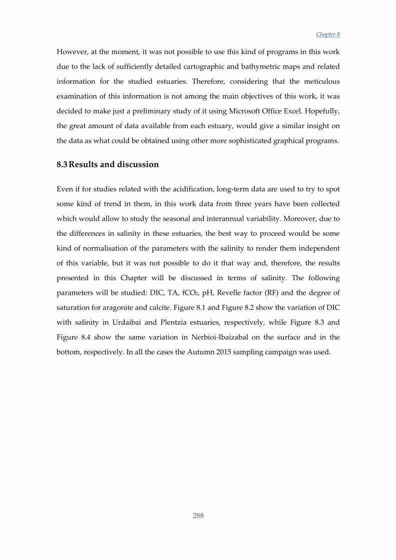
Chapter 8

288

However, at the moment, it was not possible to use this kind of programs in this work

due to the lack of sufficiently detailed cartographic and bathymetric maps and related

information for the studied estuaries. Therefore, considering that the meticulous

examination of this information is not among the main objectives of this work, it was

decided to make just a preliminary study of it using Microsoft Office Excel. Hopefully,

the great amount of data available from each estuary, would give a similar insight on

the data as what could be obtained using other more sophisticated graphical programs.

8.3 Results and discussion

Even if for studies related with the acidification, long-term data are used to try to spot

some kind of trend in them, in this work data from three years have been collected

which would allow to study the seasonal and interannual variability. Moreover, due to

the differences in salinity in these estuaries, the best way to proceed would be some

kind of normalisation of the parameters with the salinity to render them independent

of this variable, but it was not possible to do it that way and, therefore, the results

presented in this Chapter will be discussed in terms of salinity. The following

parameters will be studied: DIC, TA, fCO2, pH, Revelle factor (RF) and the degree of

saturation for aragonite and calcite. Figure 8.1 and Figure 8.2 show the variation of DIC

with salinity in Urdaibai and Plentzia estuaries, respectively, while Figure 8.3 and

Figure 8.4 show the same variation in Nerbioi-Ibaizabal on the surface and in the

bottom, respectively. In all the cases the Autumn 2015 sampling campaign was used.

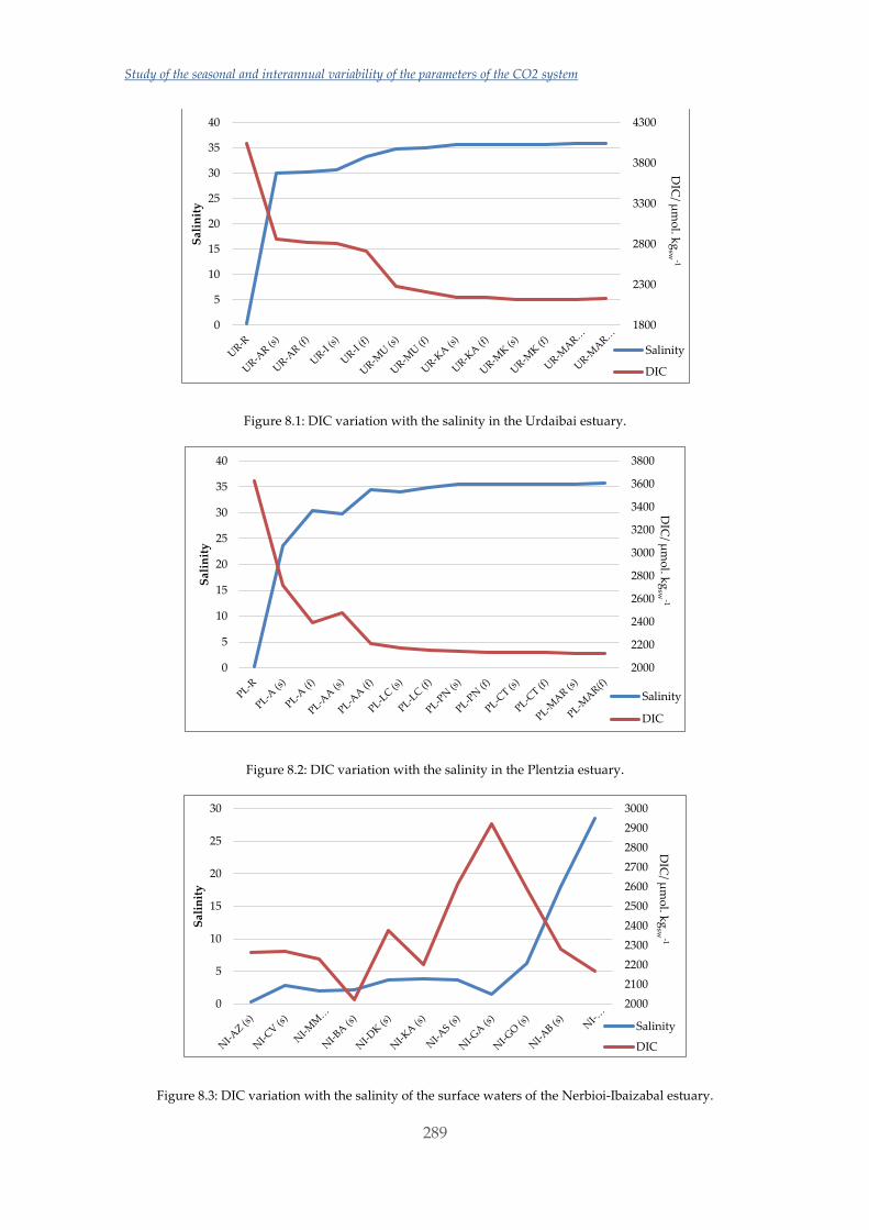
Study of the seasonal and interannual variability of the parameters of the CO2 system

289

Figure 8.1: DIC variation with the salinity in the Urdaibai estuary.

Figure 8.2: DIC variation with the salinity in the Plentzia estuary.

Figure 8.3: DIC variation with the salinity of the surface waters of the Nerbioi-Ibaizabal estuary.

1800

2300

2800

3300

3800

4300

0

5

10

15

20

25

30

35

40

Sal

init

y

Salinity

DIC

DIC

/µ

mo

l. kg

sw-1

2000

2200

2400

2600

2800

3000

3200

3400

3600

3800

0

5

10

15

20

25

30

35

40

Sal

init

y

Salinity

DIC

DIC

/µ

mo

l. kg

sw-1

2000

2100

2200

2300

2400

2500

2600

2700

2800

2900

3000

0

5

10

15

20

25

30

Sal

init

y

Salinity

DIC

DIC

/µ

mo

l. kg

sw-1

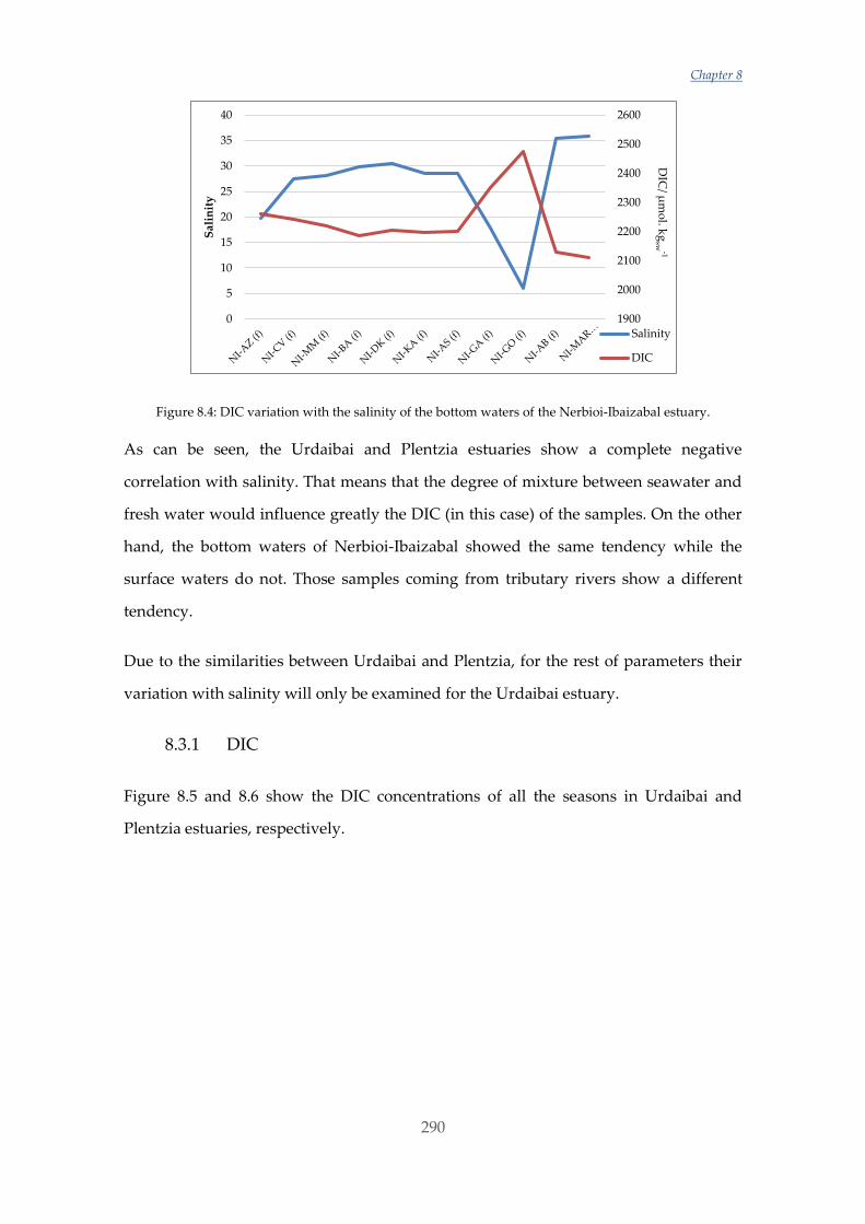
Chapter 8

290

Figure 8.4: DIC variation with the salinity of the bottom waters of the Nerbioi-Ibaizabal estuary.

As can be seen, the Urdaibai and Plentzia estuaries show a complete negative

correlation with salinity. That means that the degree of mixture between seawater and

fresh water would influence greatly the DIC (in this case) of the samples. On the other

hand, the bottom waters of Nerbioi-Ibaizabal showed the same tendency while the

surface waters do not. Those samples coming from tributary rivers show a different

tendency.

Due to the similarities between Urdaibai and Plentzia, for the rest of parameters their

variation with salinity will only be examined for the Urdaibai estuary.

8.3.1 DIC

Figure 8.5 and 8.6 show the DIC concentrations of all the seasons in Urdaibai and

Plentzia estuaries, respectively.

1900

2000

2100

2200

2300

2400

2500

2600

0

5

10

15

20

25

30

35

40

Sal

init

y

Salinity

DIC

DIC

/µ

mo

l. kg

sw-1

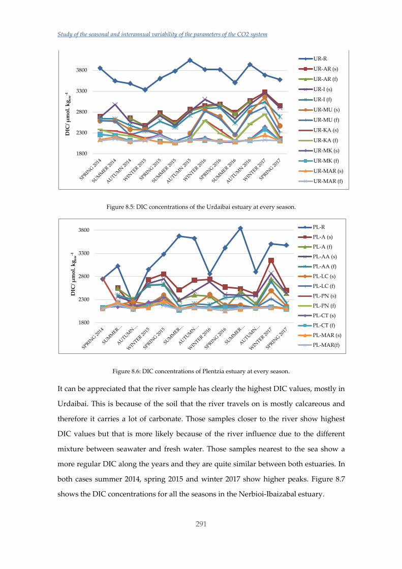
Study of the seasonal and interannual variability of the parameters of the CO2 system

291

Figure 8.5: DIC concentrations of the Urdaibai estuary at every season.

Figure 8.6: DIC concentrations of Plentzia estuary at every season.

It can be appreciated that the river sample has clearly the highest DIC values, mostly in

Urdaibai. This is because of the soil that the river travels on is mostly calcareous and

therefore it carries a lot of carbonate. Those samples closer to the river show highest

DIC values but that is more likely because of the river influence due to the different

mixture between seawater and fresh water. Those samples nearest to the sea show a

more regular DIC along the years and they are quite similar between both estuaries. In

both cases summer 2014, spring 2015 and winter 2017 show higher peaks. Figure 8.7

shows the DIC concentrations for all the seasons in the Nerbioi-Ibaizabal estuary.

1800

2300

2800

3300

3800D

IC/

µm

ol.

kg

sw-1

UR-R

UR-AR (s)

UR-AR (f)

UR-I (s)

UR-I (f)

UR-MU (s)

UR-MU (f)

UR-KA (s)

UR-KA (f)

UR-MK (s)

UR-MK (f)

UR-MAR (s)

UR-MAR (f)

1800

2300

2800

3300

3800

DIC

/ µ

mo

l. k

gsw

-1

PL-R

PL-A (s)

PL-A (f)

PL-AA (s)

PL-AA (f)

PL-LC (s)

PL-LC (f)

PL-PN (s)

PL-PN (f)

PL-CT (s)

PL-CT (f)

PL-MAR (s)

PL-MAR(f)

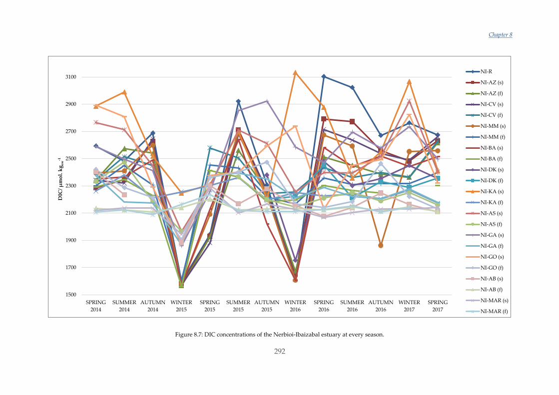
Chapter 8

292

Figure 8.7: DIC concentrations of the Nerbioi-Ibaizabal estuary at every season.

1500

1700

1900

2100

2300

2500

2700

2900

3100

SPRING

2014

SUMMER

2014

AUTUMN

2014

WINTER

2015

SPRING

2015

SUMMER

2015

AUTUMN

2015

WINTER

2016

SPRING

2016

SUMMER

2016

AUTUMN

2016

WINTER

2017

SPRING

2017

DIC

/ µ

mo

l. k

gsw

-1

NI-R

NI-AZ (s)

NI-AZ (f)

NI-CV (s)

NI-CV (f)

NI-MM (s)

NI-MM (f)

NI-BA (s)

NI-BA (f)

NI-DK (s)

NI-DK (f)

NI-KA (s)

NI-KA (f)

NI-AS (s)

NI-AS (f)

NI-GA (s)

NI-GA (f)

NI-GO (s)

NI-GO (f)

NI-AB (s)

NI-AB (f)

NI-MAR (s)

NI-MAR (f)

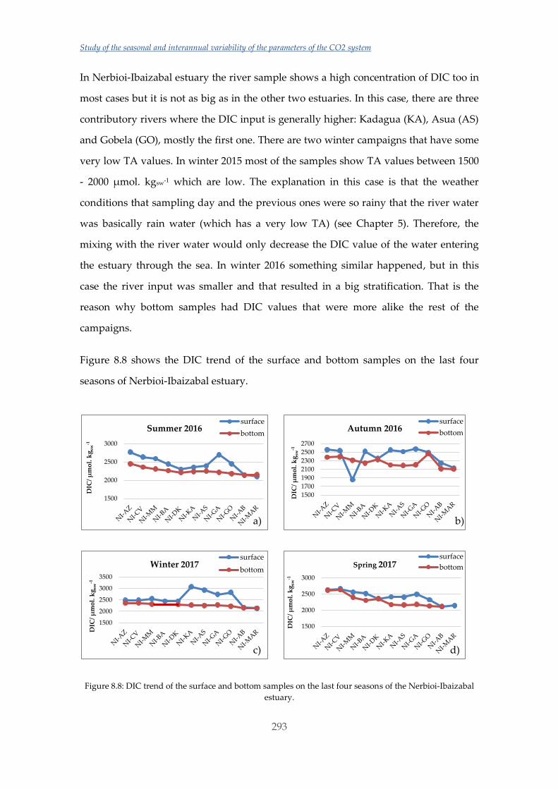
Study of the seasonal and interannual variability of the parameters of the CO2 system

293

In Nerbioi-Ibaizabal estuary the river sample shows a high concentration of DIC too in

most cases but it is not as big as in the other two estuaries. In this case, there are three

contributory rivers where the DIC input is generally higher: Kadagua (KA), Asua (AS)

and Gobela (GO), mostly the first one. There are two winter campaigns that have some

very low TA values. In winter 2015 most of the samples show TA values between 1500

- 2000 µmol. kgsw-1 which are low. The explanation in this case is that the weather

conditions that sampling day and the previous ones were so rainy that the river water

was basically rain water (which has a very low TA) (see Chapter 5). Therefore, the

mixing with the river water would only decrease the DIC value of the water entering

the estuary through the sea. In winter 2016 something similar happened, but in this

case the river input was smaller and that resulted in a big stratification. That is the

reason why bottom samples had DIC values that were more alike the rest of the

campaigns.

Figure 8.8 shows the DIC trend of the surface and bottom samples on the last four

seasons of Nerbioi-Ibaizabal estuary.

Figure 8.8: DIC trend of the surface and bottom samples on the last four seasons of the Nerbioi-Ibaizabal

estuary.

1500

2000

2500

3000

DIC

/ µ

mo

l. k

gsw

-1

Summer 2016surface

bottom

1500

1700

1900

2100

2300

2500

2700

DIC

/ µ

mo

l. k

gsw

-1

Autumn 2016surface

bottom

1500

2000

2500

3000

3500

DIC

/ µ

mo

l. k

gsw

-1

Winter 2017surface

bottom

1500

2000

2500

3000

DIC

/ µ

mo

l. k

gsw

-1

Spring 2017surface

bottom

a) b)

c) d)

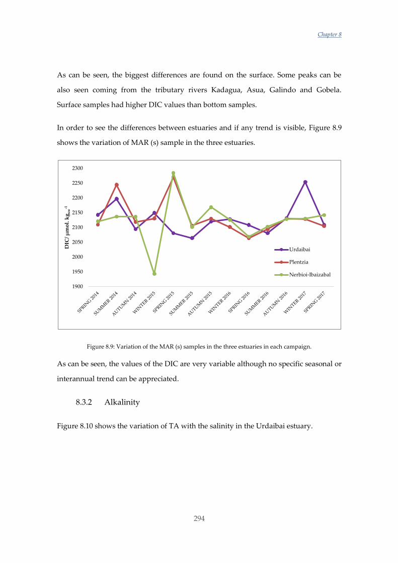
Chapter 8

294

As can be seen, the biggest differences are found on the surface. Some peaks can be

also seen coming from the tributary rivers Kadagua, Asua, Galindo and Gobela.

Surface samples had higher DIC values than bottom samples.

In order to see the differences between estuaries and if any trend is visible, Figure 8.9

shows the variation of MAR (s) sample in the three estuaries.

Figure 8.9: Variation of the MAR (s) samples in the three estuaries in each campaign.

As can be seen, the values of the DIC are very variable although no specific seasonal or

interannual trend can be appreciated.

8.3.2 Alkalinity

Figure 8.10 shows the variation of TA with the salinity in the Urdaibai estuary.

1900

1950

2000

2050

2100

2150

2200

2250

2300

DIC

/ µ

mo

l. k

gsw

-1

Urdaibai

Plentzia

Nerbioi-Ibaizabal

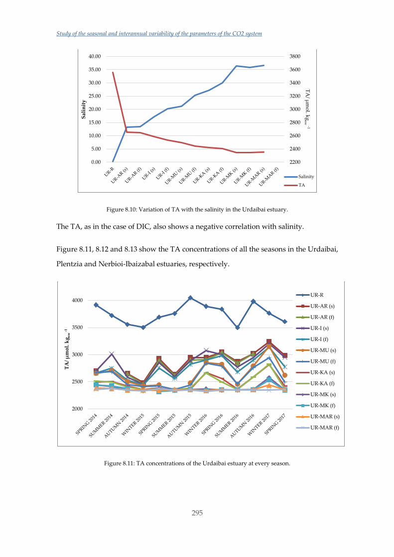
Study of the seasonal and interannual variability of the parameters of the CO2 system

295

Figure 8.10: Variation of TA with the salinity in the Urdaibai estuary.

The TA, as in the case of DIC, also shows a negative correlation with salinity.

Figure 8.11, 8.12 and 8.13 show the TA concentrations of all the seasons in the Urdaibai,

Plentzia and Nerbioi-Ibaizabal estuaries, respectively.

Figure 8.11: TA concentrations of the Urdaibai estuary at every season.

2200

2400

2600

2800

3000

3200

3400

3600

3800

0.00

5.00

10.00

15.00

20.00

25.00

30.00

35.00

40.00

Sal

init

y

Salinity

TA

TA

/ µm

ol. k

gsw

-1

2000

2500

3000

3500

4000

TA

/ µ

mo

l. k

gsw

-1

UR-R

UR-AR (s)

UR-AR (f)

UR-I (s)

UR-I (f)

UR-MU (s)

UR-MU (f)

UR-KA (s)

UR-KA (f)

UR-MK (s)

UR-MK (f)

UR-MAR (s)

UR-MAR (f)

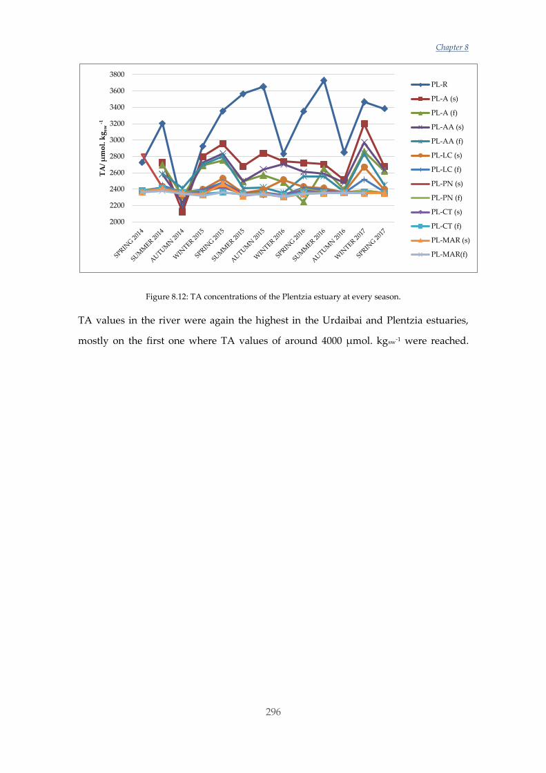
Chapter 8

296

Figure 8.12: TA concentrations of the Plentzia estuary at every season.

TA values in the river were again the highest in the Urdaibai and Plentzia estuaries,

mostly on the first one where TA values of around 4000 µmol. kgsw-1 were reached.

2000

2200

2400

2600

2800

3000

3200

3400

3600

3800

TA

/ µ

mo

l. k

gsw

-1

PL-R

PL-A (s)

PL-A (f)

PL-AA (s)

PL-AA (f)

PL-LC (s)

PL-LC (f)

PL-PN (s)

PL-PN (f)

PL-CT (s)

PL-CT (f)

PL-MAR (s)

PL-MAR(f)

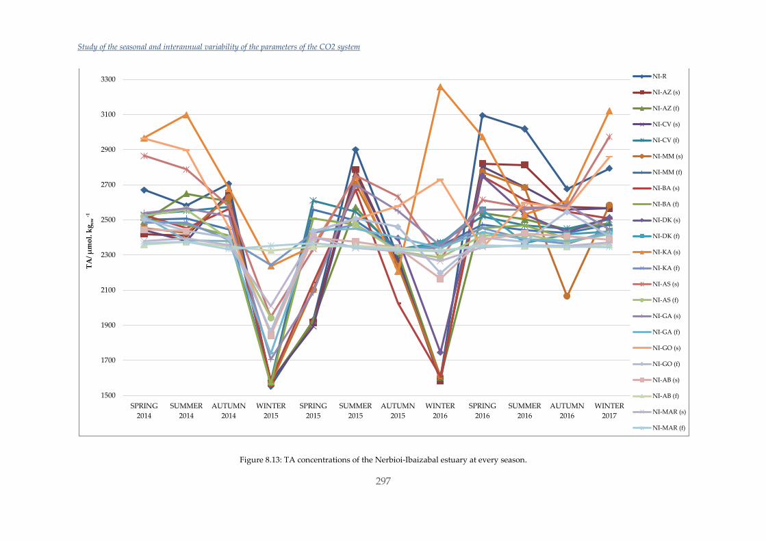
Study of the seasonal and interannual variability of the parameters of the CO2 system

297

Figure 8.13: TA concentrations of the Nerbioi-Ibaizabal estuary at every season.

1500

1700

1900

2100

2300

2500

2700

2900

3100

3300

SPRING

2014

SUMMER

2014

AUTUMN

2014

WINTER

2015

SPRING

2015

SUMMER

2015

AUTUMN

2015

WINTER

2016

SPRING

2016

SUMMER

2016

AUTUMN

2016

WINTER

2017

TA

/ µ

mo

l. k

gsw

-1

NI-R

NI-AZ (s)

NI-AZ (f)

NI-CV (s)

NI-CV (f)

NI-MM (s)

NI-MM (f)

NI-BA (s)

NI-BA (f)

NI-DK (s)

NI-DK (f)

NI-KA (s)

NI-KA (f)

NI-AS (s)

NI-AS (f)

NI-GA (s)

NI-GA (f)

NI-GO (s)

NI-GO (f)

NI-AB (s)

NI-AB (f)

NI-MAR (s)

NI-MAR (f)

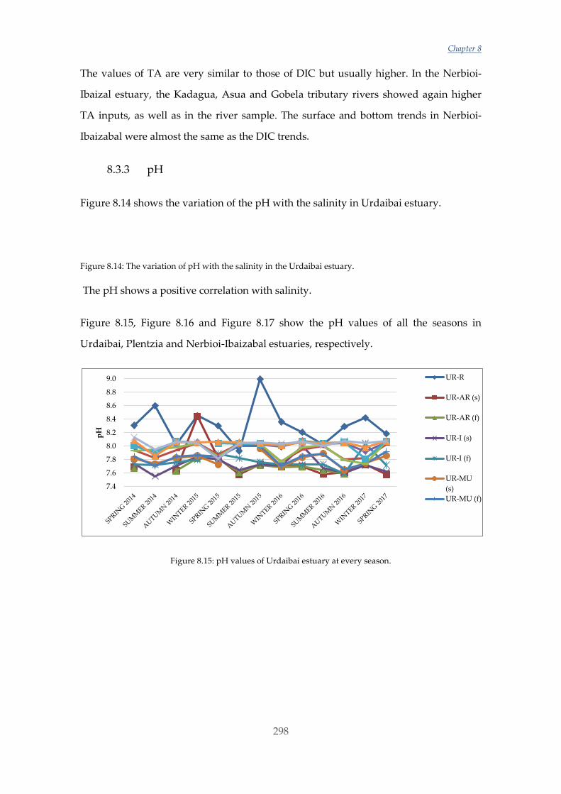
Chapter 8

298

The values of TA are very similar to those of DIC but usually higher. In the Nerbioi-

Ibaizal estuary, the Kadagua, Asua and Gobela tributary rivers showed again higher

TA inputs, as well as in the river sample. The surface and bottom trends in Nerbioi-

Ibaizabal were almost the same as the DIC trends.

8.3.3 pH

Figure 8.14 shows the variation of the pH with the salinity in Urdaibai estuary.

Figure 8.14: The variation of pH with the salinity in the Urdaibai estuary.

The pH shows a positive correlation with salinity.

Figure 8.15, Figure 8.16 and Figure 8.17 show the pH values of all the seasons in

Urdaibai, Plentzia and Nerbioi-Ibaizabal estuaries, respectively.

Figure 8.15: pH values of Urdaibai estuary at every season.

7.4

7.6

7.8

8.0

8.2

8.4

8.6

8.8

9.0

pH

UR-R

UR-AR (s)

UR-AR (f)

UR-I (s)

UR-I (f)

UR-MU

(s)

UR-MU (f)

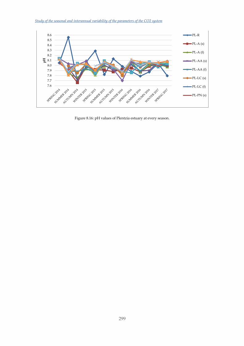
Study of the seasonal and interannual variability of the parameters of the CO2 system

299

Figure 8.16: pH values of Plentzia estuary at every season.

7.6

7.7

7.8

7.9

8.0

8.1

8.2

8.3

8.4

8.5

8.6

pH

PL-R

PL-A (s)

PL-A (f)

PL-AA (s)

PL-AA (f)

PL-LC (s)

PL-LC (f)

PL-PN (s)

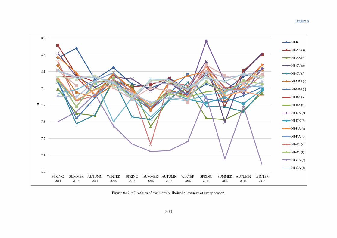
Chapter 8

300

Figure 8.17: pH values of the Nerbioi-Ibaizabal estuary at every season.

6.9

7.1

7.3

7.5

7.7

7.9

8.1

8.3

8.5

SPRING

2014

SUMMER

2014

AUTUMN

2014

WINTER

2015

SPRING

2015

SUMMER

2015

AUTUMN

2015

WINTER

2016

SPRING

2016

SUMMER

2016

AUTUMN

2016

WINTER

2017

pH

NI-R

NI-AZ (s)

NI-AZ (f)

NI-CV (s)

NI-CV (f)

NI-MM (s)

NI-MM (f)

NI-BA (s)

NI-BA (f)

NI-DK (s)

NI-DK (f)

NI-KA (s)

NI-KA (f)

NI-AS (s)

NI-AS (f)

NI-GA (s)

NI-GA (f)

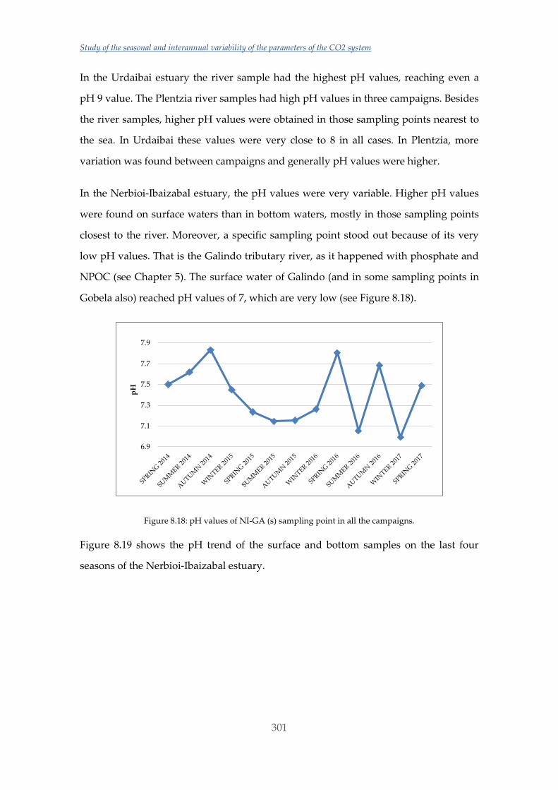
Study of the seasonal and interannual variability of the parameters of the CO2 system

301

In the Urdaibai estuary the river sample had the highest pH values, reaching even a

pH 9 value. The Plentzia river samples had high pH values in three campaigns. Besides

the river samples, higher pH values were obtained in those sampling points nearest to

the sea. In Urdaibai these values were very close to 8 in all cases. In Plentzia, more

variation was found between campaigns and generally pH values were higher.

In the Nerbioi-Ibaizabal estuary, the pH values were very variable. Higher pH values

were found on surface waters than in bottom waters, mostly in those sampling points

closest to the river. Moreover, a specific sampling point stood out because of its very

low pH values. That is the Galindo tributary river, as it happened with phosphate and

NPOC (see Chapter 5). The surface water of Galindo (and in some sampling points in

Gobela also) reached pH values of 7, which are very low (see Figure 8.18).

Figure 8.18: pH values of NI-GA (s) sampling point in all the campaigns.

Figure 8.19 shows the pH trend of the surface and bottom samples on the last four

seasons of the Nerbioi-Ibaizabal estuary.

6.9

7.1

7.3

7.5

7.7

7.9

pH

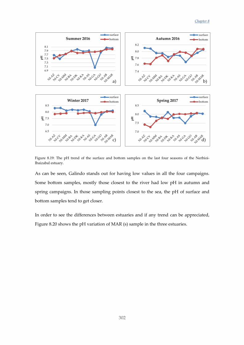
Chapter 8

302

Figure 8.19: The pH trend of the surface and bottom samples on the last four seasons of the Nerbioi-

Ibaizabal estuary.

As can be seen, Galindo stands out for having low values in all the four campaigns.

Some bottom samples, mostly those closest to the river had low pH in autumn and

spring campaigns. In those sampling points closest to the sea, the pH of surface and

bottom samples tend to get closer.

In order to see the differences between estuaries and if any trend can be appreciated,

Figure 8.20 shows the pH variation of MAR (s) sample in the three estuaries.

6.9

7.1

7.3

7.5

7.7

7.9

8.1

pH

Summer 2016surface

bottom

7.4

7.6

7.8

8.0

8.2

pH

Autumn 2016surface

bottom

6.5

7.0

7.5

8.0

8.5

pH

Winter 2017surface

bottom

7.0

7.5

8.0

8.5

pH

Spring 2017surface

bottom

a) b)

c) d)

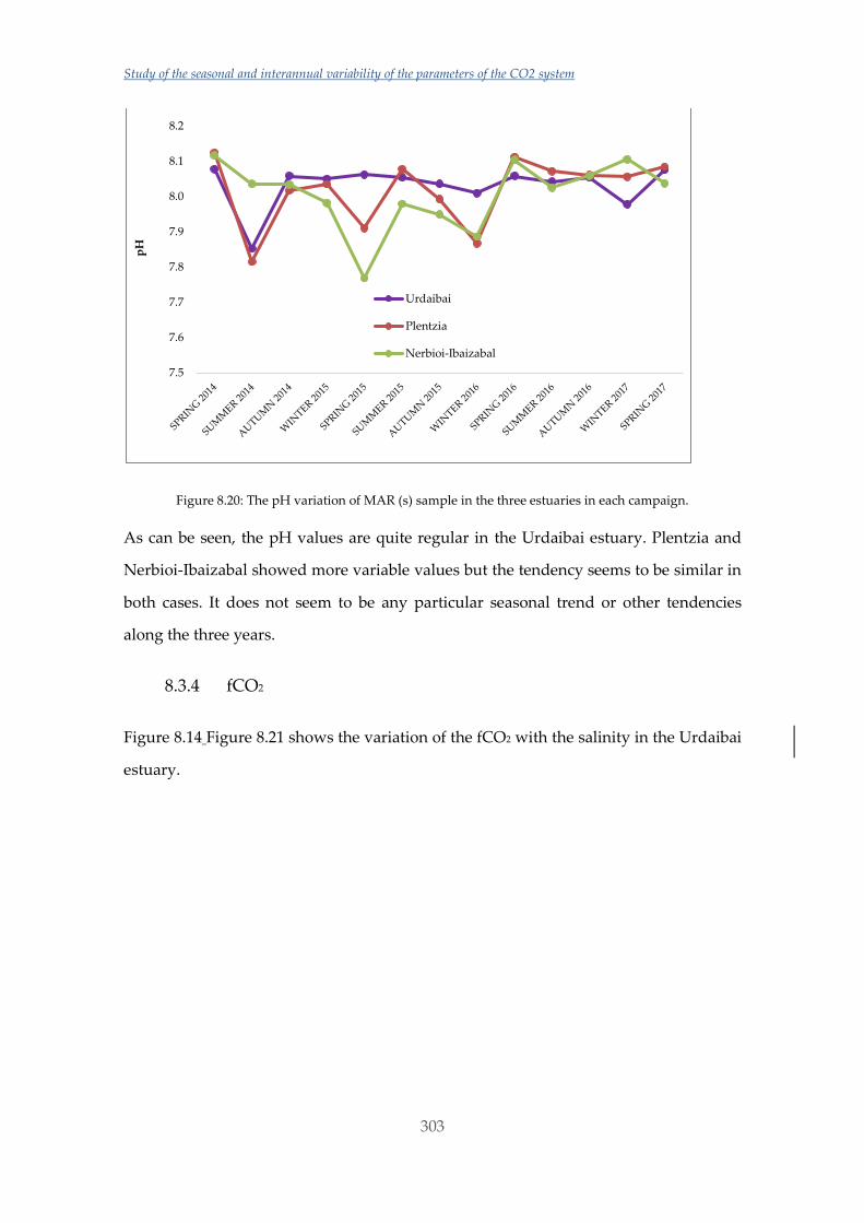
Study of the seasonal and interannual variability of the parameters of the CO2 system

303

Figure 8.20: The pH variation of MAR (s) sample in the three estuaries in each campaign.

As can be seen, the pH values are quite regular in the Urdaibai estuary. Plentzia and

Nerbioi-Ibaizabal showed more variable values but the tendency seems to be similar in

both cases. It does not seem to be any particular seasonal trend or other tendencies

along the three years.

8.3.4 fCO2

Figure 8.14 Figure 8.21 shows the variation of the fCO2 with the salinity in the Urdaibai

estuary.

7.5

7.6

7.7

7.8

7.9

8.0

8.1

8.2p

H

Urdaibai

Plentzia

Nerbioi-Ibaizabal

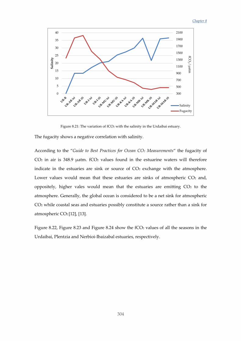
Chapter 8

304

Figure 8.21: The variation of fCO2 with the salinity in the Urdaibai estuary.

The fugacity shows a negative correlation with salinity.

According to the “Guide to Best Practices for Ocean CO2 Measurements“ the fugacity of

CO2 in air is 348.9 µatm. fCO2 values found in the estuarine waters will therefore

indicate in the estuaries are sink or source of CO2 exchange with the atmosphere.

Lower values would mean that these estuaries are sinks of atmospheric CO2 and,

oppositely, higher vales would mean that the estuaries are emitting CO2 to the

atmosphere. Generally, the global ocean is considered to be a net sink for atmospheric

CO2 while coastal seas and estuaries possibly constitute a source rather than a sink for

atmospheric CO2 [12], [13].

Figure 8.22, Figure 8.23 and Figure 8.24 show the fCO2 values of all the seasons in the

Urdaibai, Plentzia and Nerbioi-Ibaizabal estuaries, respectively.

300

500

700

900

1100

1300

1500

1700

1900

2100

0

5

10

15

20

25

30

35

40

Sal

init

y

Salinity

Fugacity

fCO

2/ µ

atm

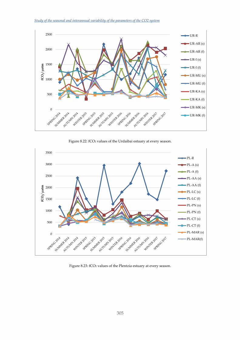
Study of the seasonal and interannual variability of the parameters of the CO2 system

305

Figure 8.22: fCO2 values of the Urdaibai estuary at every season.

Figure 8.23: fCO2 values of the Plentzia estuary at every season.

0

500

1000

1500

2000

2500

fCO

2/ µ

atm

UR-R

UR-AR (s)

UR-AR (f)

UR-I (s)

UR-I (f)

UR-MU (s)

UR-MU (f)

UR-KA (s)

UR-KA (f)

UR-MK (s)

UR-MK (f)

0

500

1000

1500

2000

2500

3000

3500

fCO

2/ µ

atm

PL-R

PL-A (s)

PL-A (f)

PL-AA (s)

PL-AA (f)

PL-LC (s)

PL-LC (f)

PL-PN (s)

PL-PN (f)

PL-CT (s)

PL-CT (f)

PL-MAR (s)

PL-MAR(f)

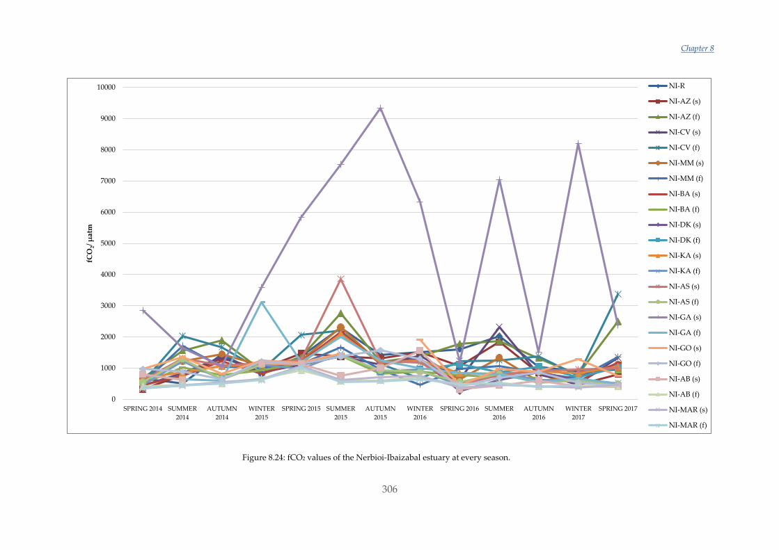
Chapter 8

306

Figure 8.24: fCO2 values of the Nerbioi-Ibaizabal estuary at every season.

0

1000

2000

3000

4000

5000

6000

7000

8000

9000

10000

SPRING 2014 SUMMER

2014

AUTUMN

2014

WINTER

2015

SPRING 2015 SUMMER

2015

AUTUMN

2015

WINTER

2016

SPRING 2016 SUMMER

2016

AUTUMN

2016

WINTER

2017

SPRING 2017

fCO

2/ µ

atm

NI-R

NI-AZ (s)

NI-AZ (f)

NI-CV (s)

NI-CV (f)

NI-MM (s)

NI-MM (f)

NI-BA (s)

NI-BA (f)

NI-DK (s)

NI-DK (f)

NI-KA (s)

NI-KA (f)

NI-AS (s)

NI-AS (f)

NI-GA (s)

NI-GA (f)

NI-GO (s)

NI-GO (f)

NI-AB (s)

NI-AB (f)

NI-MAR (s)

NI-MAR (f)

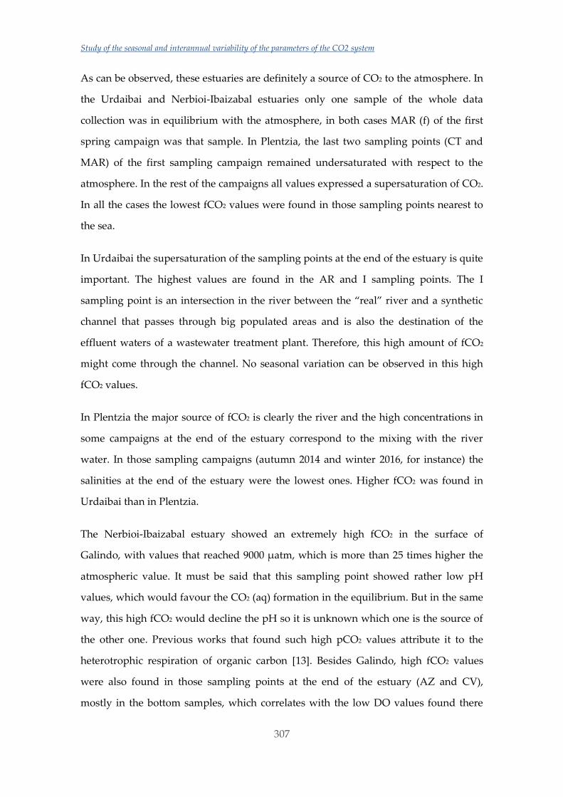
Study of the seasonal and interannual variability of the parameters of the CO2 system

307

As can be observed, these estuaries are definitely a source of CO2 to the atmosphere. In

the Urdaibai and Nerbioi-Ibaizabal estuaries only one sample of the whole data

collection was in equilibrium with the atmosphere, in both cases MAR (f) of the first

spring campaign was that sample. In Plentzia, the last two sampling points (CT and

MAR) of the first sampling campaign remained undersaturated with respect to the

atmosphere. In the rest of the campaigns all values expressed a supersaturation of CO2.

In all the cases the lowest fCO2 values were found in those sampling points nearest to

the sea.

In Urdaibai the supersaturation of the sampling points at the end of the estuary is quite

important. The highest values are found in the AR and I sampling points. The I

sampling point is an intersection in the river between the “real” river and a synthetic

channel that passes through big populated areas and is also the destination of the

effluent waters of a wastewater treatment plant. Therefore, this high amount of fCO2

might come through the channel. No seasonal variation can be observed in this high

fCO2 values.

In Plentzia the major source of fCO2 is clearly the river and the high concentrations in

some campaigns at the end of the estuary correspond to the mixing with the river

water. In those sampling campaigns (autumn 2014 and winter 2016, for instance) the

salinities at the end of the estuary were the lowest ones. Higher fCO2 was found in

Urdaibai than in Plentzia.

The Nerbioi-Ibaizabal estuary showed an extremely high fCO2 in the surface of

Galindo, with values that reached 9000 µatm, which is more than 25 times higher the

atmospheric value. It must be said that this sampling point showed rather low pH

values, which would favour the CO2 (aq) formation in the equilibrium. But in the same

way, this high fCO2 would decline the pH so it is unknown which one is the source of

the other one. Previous works that found such high pCO2 values attribute it to the

heterotrophic respiration of organic carbon [13]. Besides Galindo, high fCO2 values

were also found in those sampling points at the end of the estuary (AZ and CV),

mostly in the bottom samples, which correlates with the low DO values found there

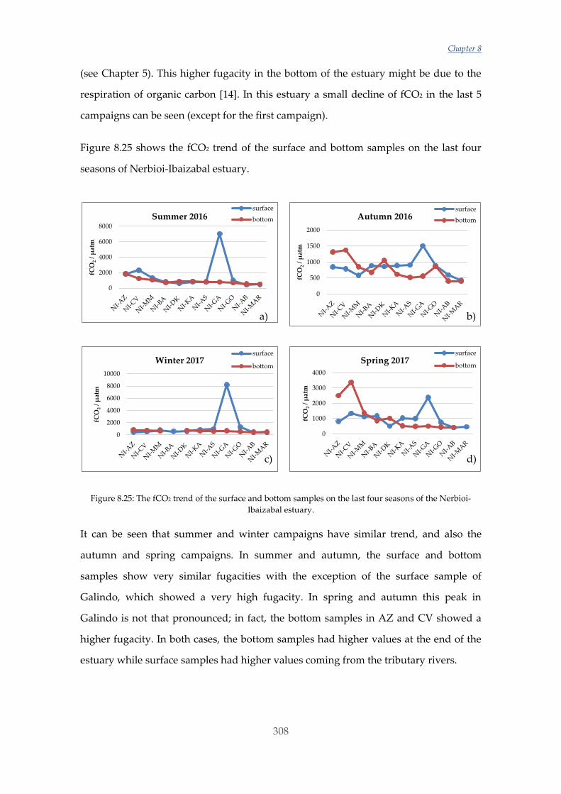
Chapter 8

308

(see Chapter 5). This higher fugacity in the bottom of the estuary might be due to the

respiration of organic carbon [14]. In this estuary a small decline of fCO2 in the last 5

campaigns can be seen (except for the first campaign).

Figure 8.25 shows the fCO2 trend of the surface and bottom samples on the last four

seasons of Nerbioi-Ibaizabal estuary.

Figure 8.25: The fCO2 trend of the surface and bottom samples on the last four seasons of the Nerbioi-

Ibaizabal estuary.

It can be seen that summer and winter campaigns have similar trend, and also the

autumn and spring campaigns. In summer and autumn, the surface and bottom

samples show very similar fugacities with the exception of the surface sample of

Galindo, which showed a very high fugacity. In spring and autumn this peak in

Galindo is not that pronounced; in fact, the bottom samples in AZ and CV showed a

higher fugacity. In both cases, the bottom samples had higher values at the end of the

estuary while surface samples had higher values coming from the tributary rivers.

0

2000

4000

6000

8000

fCO

2/

µat

m

Summer 2016surface

bottom

0

500

1000

1500

2000

fCO

2/

µat

m

Autumn 2016surface

bottom

0

2000

4000

6000

8000

10000

fCO

2/

µat

m

Winter 2017surface

bottom

0

1000

2000

3000

4000

fCO

2/

µat

m

Spring 2017surface

bottom

a) b)

c) d)

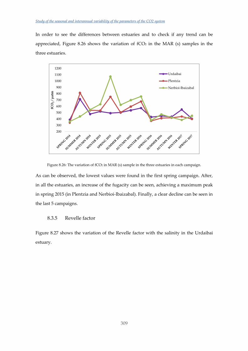
Study of the seasonal and interannual variability of the parameters of the CO2 system

309

In order to see the differences between estuaries and to check if any trend can be

appreciated, Figure 8.26 shows the variation of fCO2 in the MAR (s) samples in the

three estuaries.

Figure 8.26: The variation of fCO2 in MAR (s) sample in the three estuaries in each campaign.

As can be observed, the lowest values were found in the first spring campaign. After,

in all the estuaries, an increase of the fugacity can be seen, achieving a maximum peak

in spring 2015 (in Plentzia and Nerbioi-Ibaizabal). Finally, a clear decline can be seen in

the last 5 campaigns.

8.3.5 Revelle factor

Figure 8.27 shows the variation of the Revelle factor with the salinity in the Urdaibai

estuary.

200

300

400

500

600

700

800

900

1000

1100

1200

fCO

2/

µat

m

Urdaibai

Plentzia

Nerbioi-Ibaizabal

Chapter 8

310

Figure 8.27: The variation of the Revelle factor with the salinity in Urdaibai estuary.

The Revelle factor shows a negative correlation with salinity.

The Revelle factor or buffer factor is the ratio of instantaneous change in CO2 to the

change in DIC. It is a measure of the resistance to atmospheric CO2 being absorbed by

the ocean surface. The Revelle factor is defined as the ratio of (ΔpCO2/pCO2)

to Δ[DIC]/[DIC] and reflects, inversely, the system’s buffer capacity (a higher Revelle

factor means a lower buffer capacity)[14]. Revelle factors in open ocean range from 8 to

about 15 [15], [16].

Figure 8.28, Figure 8.29 and Figure 8.30 show the Revelle factor values of all the

seasons in the Urdaibai, Plentzia and Nerbioi-Ibaizabal estuaries, respectively.

8

10

12

14

16

18

20

0

5

10

15

20

25

30

35

40

Sal

init

y

Salinity

Revelle f.

Rev

elle factor

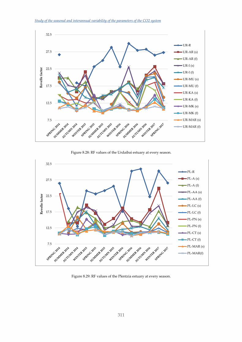
Study of the seasonal and interannual variability of the parameters of the CO2 system

311

Figure 8.28: RF values of the Urdaibai estuary at every season.

Figure 8.29: RF values of the Plentzia estuary at every season.

7.5

12.5

17.5

22.5

27.5

32.5

Re

vel

le f

acto

r

UR-R

UR-AR (s)

UR-AR (f)

UR-I (s)

UR-I (f)

UR-MU (s)

UR-MU (f)

UR-KA (s)

UR-KA (f)

UR-MK (s)

UR-MK (f)

UR-MAR (s)

UR-MAR (f)

7.5

12.5

17.5

22.5

27.5

32.5

Re

vel

le f

acto

r

PL-R

PL-A (s)

PL-A (f)

PL-AA (s)

PL-AA (f)

PL-LC (s)

PL-LC (f)

PL-PN (s)

PL-PN (f)

PL-CT (s)

PL-CT (f)

PL-MAR (s)

PL-MAR(f)

Chapter 8

312

Figure 8.30: RF values of the Nerbioi-Ibaizabal estuary at every season.

5.0

10.0

15.0

20.0

25.0

30.0

35.0

SPRING

2014

SUMMER

2014

AUTUMN

2014

WINTER

2015

SPRING

2015

SUMMER

2015

AUTUMN

2015

WINTER

2016

SPRING

2016

SUMMER

2016

AUTUMN

2016

Re

vel

le f

acto

rNI-R

NI-AZ (s)

NI-AZ (f)

NI-CV (s)

NI-CV (f)

NI-MM (s)

NI-MM (f)

NI-BA (s)

NI-BA (f)

NI-DK (s)

NI-DK (f)

NI-KA (s)

NI-KA (f)

NI-AS (s)

NI-AS (f)

NI-GA (s)

NI-GA (f)

NI-GO (s)

NI-GO (f)

NI-AB (s)

NI-AB (f)

NI-MAR (s)

NI-MAR (f)

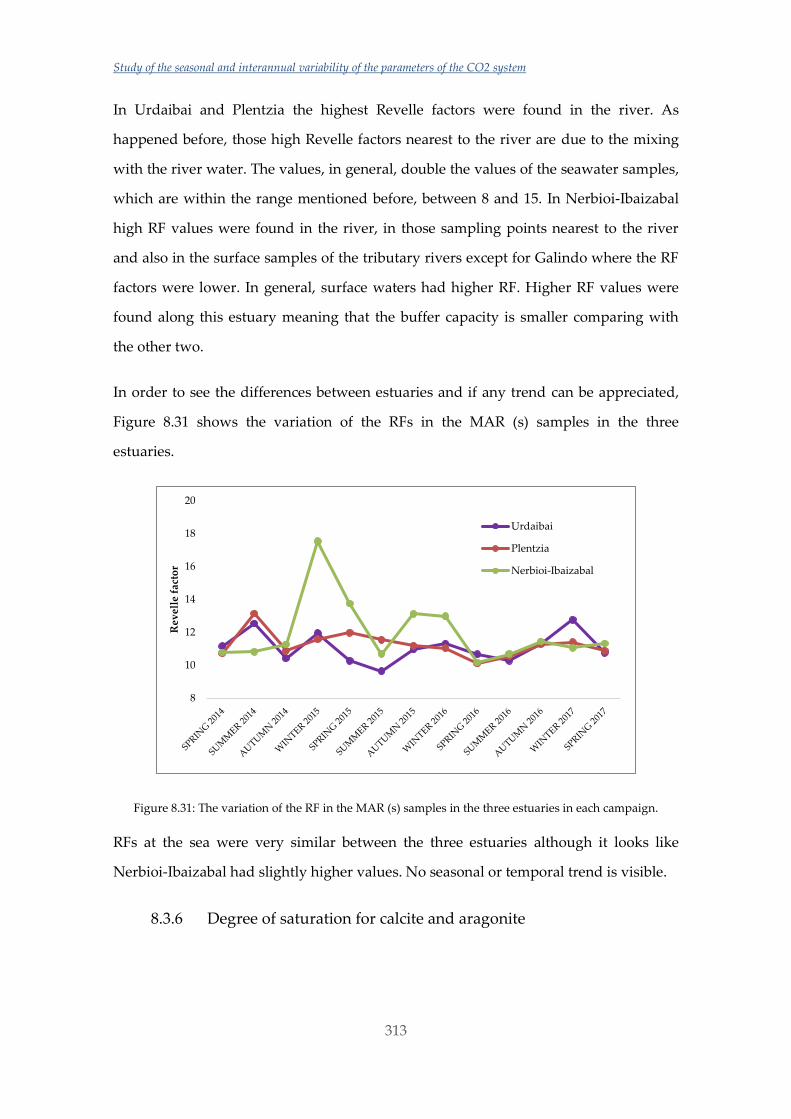
Study of the seasonal and interannual variability of the parameters of the CO2 system

313

In Urdaibai and Plentzia the highest Revelle factors were found in the river. As

happened before, those high Revelle factors nearest to the river are due to the mixing

with the river water. The values, in general, double the values of the seawater samples,

which are within the range mentioned before, between 8 and 15. In Nerbioi-Ibaizabal

high RF values were found in the river, in those sampling points nearest to the river

and also in the surface samples of the tributary rivers except for Galindo where the RF

factors were lower. In general, surface waters had higher RF. Higher RF values were

found along this estuary meaning that the buffer capacity is smaller comparing with

the other two.

In order to see the differences between estuaries and if any trend can be appreciated,

Figure 8.31 shows the variation of the RFs in the MAR (s) samples in the three

estuaries.

Figure 8.31: The variation of the RF in the MAR (s) samples in the three estuaries in each campaign.

RFs at the sea were very similar between the three estuaries although it looks like

Nerbioi-Ibaizabal had slightly higher values. No seasonal or temporal trend is visible.

8.3.6 Degree of saturation for calcite and aragonite

8

10

12

14

16

18

20

Re

vel

le f

acto

r

Urdaibai

Plentzia

Nerbioi-Ibaizabal

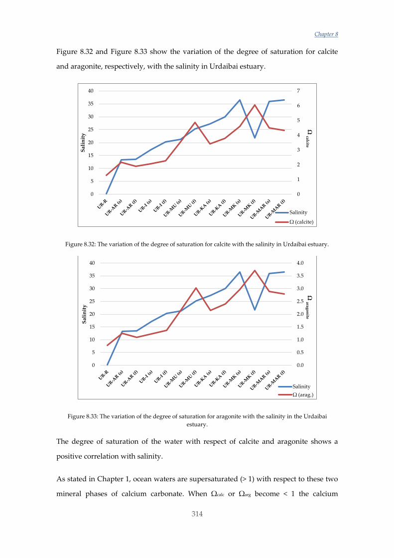
Chapter 8

314

Figure 8.32 and Figure 8.33 show the variation of the degree of saturation for calcite

and aragonite, respectively, with the salinity in Urdaibai estuary.

Figure 8.32: The variation of the degree of saturation for calcite with the salinity in Urdaibai estuary.

Figure 8.33: The variation of the degree of saturation for aragonite with the salinity in the Urdaibai

estuary.

The degree of saturation of the water with respect of calcite and aragonite shows a

positive correlation with salinity.

As stated in Chapter 1, ocean waters are supersaturated (> 1) with respect to these two

mineral phases of calcium carbonate. When Ωcalc or Ωarg become < 1 the calcium

0

1

2

3

4

5

6

7

0

5

10

15

20

25

30

35

40

Sal

init

y

Salinity

Ω (calcite)

Ωcalcite

0.0

0.5

1.0

1.5

2.0

2.5

3.0

3.5

4.0

0

5

10

15

20

25

30

35

40

Sal

init

y

Salinity

Ω (arag.)

Ωarag

on

ite

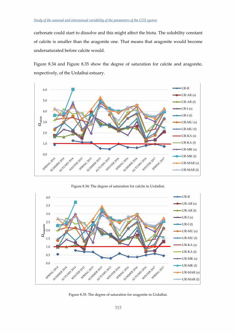
Study of the seasonal and interannual variability of the parameters of the CO2 system

315

carbonate could start to dissolve and this might affect the biota. The solubility constant

of calcite is smaller than the aragonite one. That means that aragonite would become

undersaturated before calcite would.

Figure 8.34 and Figure 8.35 show the degree of saturation for calcite and aragonite,

respectively, of the Urdaibai estuary.

Figure 8.34: The degree of saturation for calcite in Urdaibai.

Figure 8.35: The degree of saturation for aragonite in Urdaibai.

0.0

1.0

2.0

3.0

4.0

5.0

6.0

Ωca

lcit

e

UR-R

UR-AR (s)

UR-AR (f)

UR-I (s)

UR-I (f)

UR-MU (s)

UR-MU (f)

UR-KA (s)

UR-KA (f)

UR-MK (s)

UR-MK (f)

UR-MAR (s)

UR-MAR (f)

0.0

0.5

1.0

1.5

2.0

2.5

3.0

3.5

4.0

Ωar

ago

nit

e

UR-R

UR-AR (s)

UR-AR (f)

UR-I (s)

UR-I (f)

UR-MU (s)

UR-MU (f)

UR-KA (s)

UR-KA (f)

UR-MK (s)

UR-MK (f)

UR-MAR (s)

UR-MAR (f)

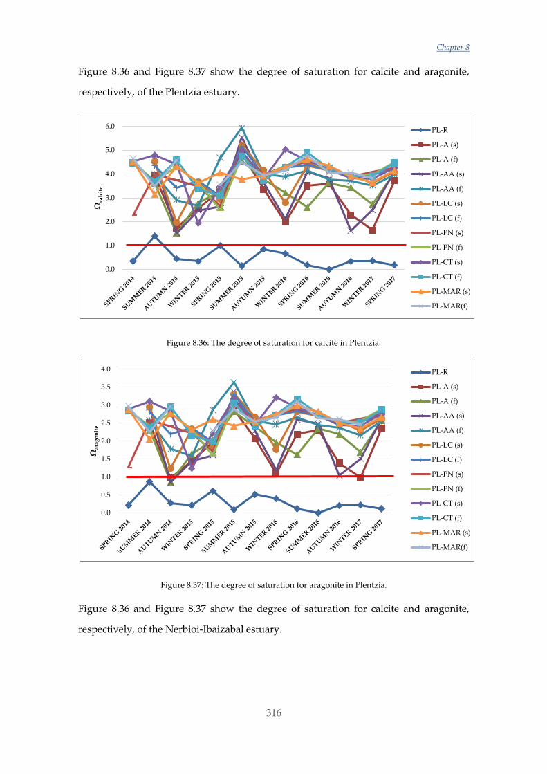
Chapter 8

316

Figure 8.36 and Figure 8.37 show the degree of saturation for calcite and aragonite,

respectively, of the Plentzia estuary.

Figure 8.36: The degree of saturation for calcite in Plentzia.

Figure 8.37: The degree of saturation for aragonite in Plentzia.

Figure 8.36 and Figure 8.37 show the degree of saturation for calcite and aragonite,

respectively, of the Nerbioi-Ibaizabal estuary.

0.0

1.0

2.0

3.0

4.0

5.0

6.0

Ωca

lcit

e

PL-R

PL-A (s)

PL-A (f)

PL-AA (s)

PL-AA (f)

PL-LC (s)

PL-LC (f)

PL-PN (s)

PL-PN (f)

PL-CT (s)

PL-CT (f)

PL-MAR (s)

PL-MAR(f)

0.0

0.5

1.0

1.5

2.0

2.5

3.0

3.5

4.0

Ωar

ago

nit

e

PL-R

PL-A (s)

PL-A (f)

PL-AA (s)

PL-AA (f)

PL-LC (s)

PL-LC (f)

PL-PN (s)

PL-PN (f)

PL-CT (s)

PL-CT (f)

PL-MAR (s)

PL-MAR(f)

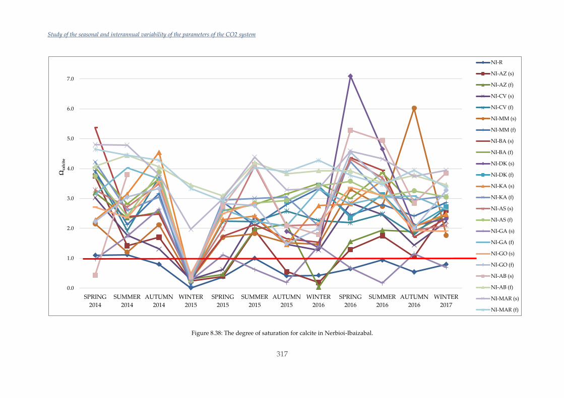
Study of the seasonal and interannual variability of the parameters of the CO2 system

317

Figure 8.38: The degree of saturation for calcite in Nerbioi-Ibaizabal.

0.0

1.0

2.0

3.0

4.0

5.0

6.0

7.0

SPRING

2014

SUMMER

2014

AUTUMN

2014

WINTER

2015

SPRING

2015

SUMMER

2015

AUTUMN

2015

WINTER

2016

SPRING

2016

SUMMER

2016

AUTUMN

2016

WINTER

2017

Ωca

lcit

eNI-R

NI-AZ (s)

NI-AZ (f)

NI-CV (s)

NI-CV (f)

NI-MM (s)

NI-MM (f)

NI-BA (s)

NI-BA (f)

NI-DK (s)

NI-DK (f)

NI-KA (s)

NI-KA (f)

NI-AS (s)

NI-AS (f)

NI-GA (s)

NI-GA (f)

NI-GO (s)

NI-GO (f)

NI-AB (s)

NI-AB (f)

NI-MAR (s)

NI-MAR (f)

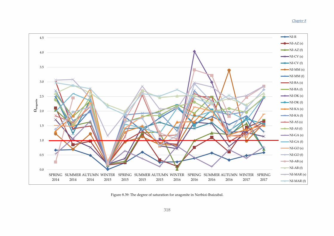
Chapter 8

318

Figure 8.39: The degree of saturation for aragonite in Nerbioi-Ibaizabal.

0.0

0.5

1.0

1.5

2.0

2.5

3.0

3.5

4.0

4.5

SPRING

2014

SUMMER

2014

AUTUMN

2014

WINTER

2015

SPRING

2015

SUMMER

2015

AUTUMN

2015

WINTER

2016

SPRING

2016

SUMMER

2016

AUTUMN

2016

WINTER

2017

SPRING

2017

Ωar

ago

nit

eNI-R

NI-AZ (s)

NI-AZ (f)

NI-CV (s)

NI-CV (f)

NI-MM (s)

NI-MM (f)

NI-BA (s)

NI-BA (f)

NI-DK (s)

NI-DK (f)

NI-KA (s)

NI-KA (f)

NI-AS (s)

NI-AS (f)

NI-GA (s)

NI-GA (f)

NI-GO (s)

NI-GO (f)

NI-AB (s)

NI-AB (f)

NI-MAR (s)

NI-MAR (f)

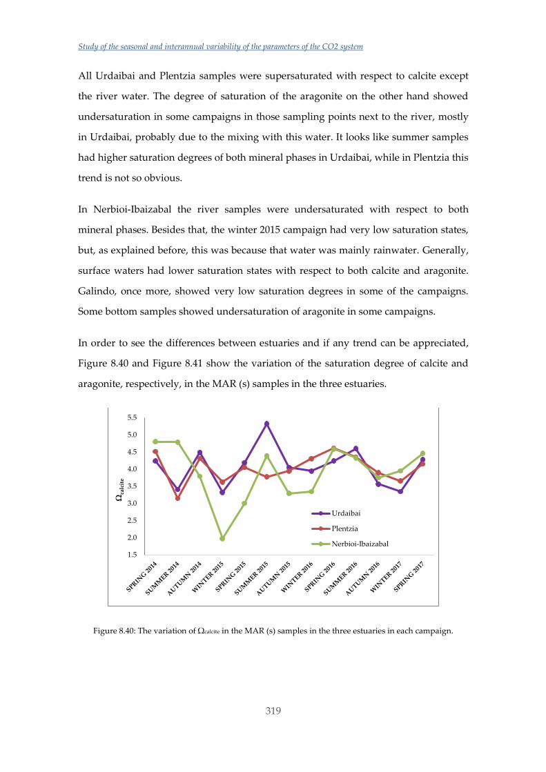
Study of the seasonal and interannual variability of the parameters of the CO2 system

319

All Urdaibai and Plentzia samples were supersaturated with respect to calcite except

the river water. The degree of saturation of the aragonite on the other hand showed

undersaturation in some campaigns in those sampling points next to the river, mostly

in Urdaibai, probably due to the mixing with this water. It looks like summer samples

had higher saturation degrees of both mineral phases in Urdaibai, while in Plentzia this

trend is not so obvious.

In Nerbioi-Ibaizabal the river samples were undersaturated with respect to both

mineral phases. Besides that, the winter 2015 campaign had very low saturation states,

but, as explained before, this was because that water was mainly rainwater. Generally,

surface waters had lower saturation states with respect to both calcite and aragonite.

Galindo, once more, showed very low saturation degrees in some of the campaigns.

Some bottom samples showed undersaturation of aragonite in some campaigns.

In order to see the differences between estuaries and if any trend can be appreciated,

Figure 8.40 and Figure 8.41 show the variation of the saturation degree of calcite and

aragonite, respectively, in the MAR (s) samples in the three estuaries.

Figure 8.40: The variation of Ωcalcite in the MAR (s) samples in the three estuaries in each campaign.

1.5

2.0

2.5

3.0

3.5

4.0

4.5

5.0

5.5

Ωca

lcit

e

Urdaibai

Plentzia

Nerbioi-Ibaizabal

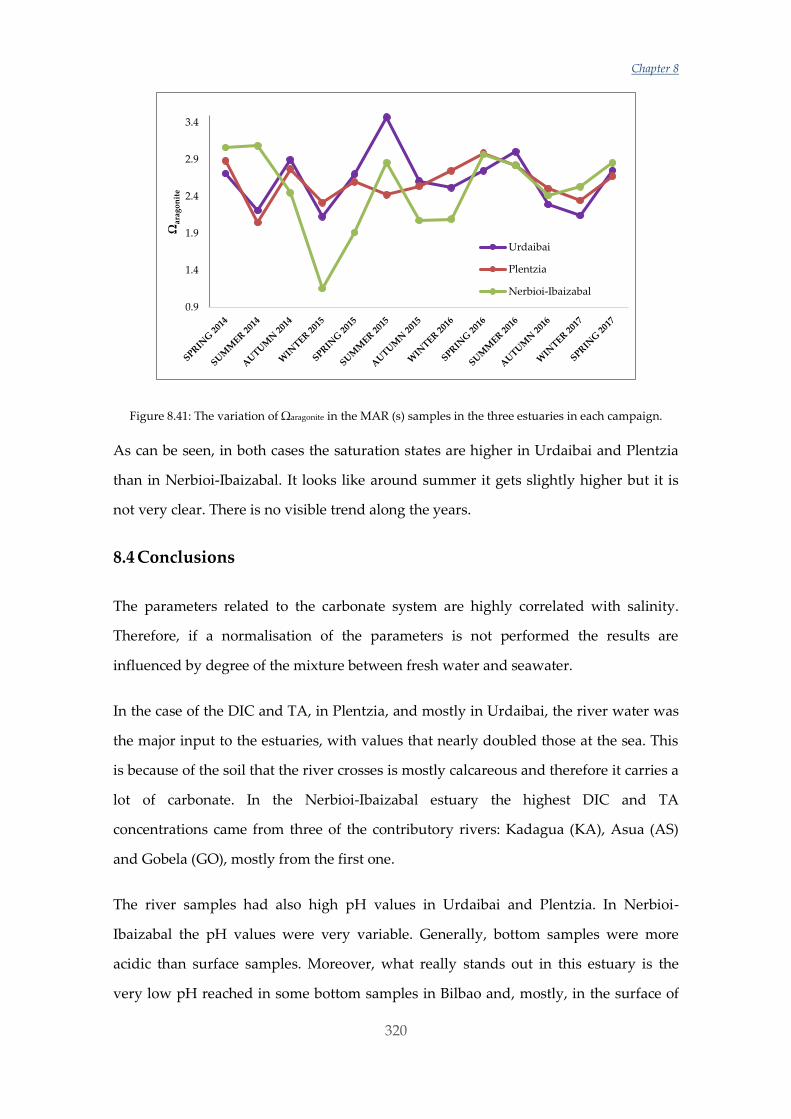
Chapter 8

320

Figure 8.41: The variation of Ωaragonite in the MAR (s) samples in the three estuaries in each campaign.

As can be seen, in both cases the saturation states are higher in Urdaibai and Plentzia

than in Nerbioi-Ibaizabal. It looks like around summer it gets slightly higher but it is

not very clear. There is no visible trend along the years.

8.4 Conclusions

The parameters related to the carbonate system are highly correlated with salinity.

Therefore, if a normalisation of the parameters is not performed the results are

influenced by degree of the mixture between fresh water and seawater.

In the case of the DIC and TA, in Plentzia, and mostly in Urdaibai, the river water was

the major input to the estuaries, with values that nearly doubled those at the sea. This

is because of the soil that the river crosses is mostly calcareous and therefore it carries a

lot of carbonate. In the Nerbioi-Ibaizabal estuary the highest DIC and TA

concentrations came from three of the contributory rivers: Kadagua (KA), Asua (AS)

and Gobela (GO), mostly from the first one.

The river samples had also high pH values in Urdaibai and Plentzia. In Nerbioi-

Ibaizabal the pH values were very variable. Generally, bottom samples were more

acidic than surface samples. Moreover, what really stands out in this estuary is the

very low pH reached in some bottom samples in Bilbao and, mostly, in the surface of

0.9

1.4

1.9

2.4

2.9

3.4

Ωar

ago

nit

e

Urdaibai

Plentzia

Nerbioi-Ibaizabal

Study of the seasonal and interannual variability of the parameters of the CO2 system

321

the Galindo tributary river, reaching even values of pH 7. Oppositely, surface waters of

Galindo showed the highest fugacities. Values 25 times higher than the fugacity of the

atmosphere were observed. In Urdaibai, the river sample and those sampling points

closest to the river showed the highest fugacities while in Plentzia the river samples

stood out. All in all, the fCO2 values indicate that these estuaries are a source of CO2 to

the atmosphere rather than a sink. Moreover, the last sampling campaigns showed a

decrease in the fCO2 values.

The Revelle factor had common values in Urdaibai and Plentzia except for the river

water and some sampling points nearest to it. In Nerbioi-Ibaizabal, surface waters had

lower buffer capacity than bottom samples and generally this estuary showed higher

Revelle factors than the other two, meaning that Nerbioi-Ibaizabal is slightly less

buffered.

Finally, Urdaibai and Plentzia presented supersaturation with respect to calcite except

for the river samples and in some cases the aragonite was found undersaturated in

some sampling points at the end of the estuary. In Nerbioi-Ibaizabal the river samples

were undersaturated with respect of both mineral phases, as well as some bottom

samples. Galindo again showed very low saturation states. It must be pointed out that

even if in most cases for the three estuaries the saturation states were above 1, the fact

that in some cases the water is undersaturated might be of some concern for the biota.

Taking into account all of this information, it can be concluded that Urdaibai and

Plentzia show quite similar behaviour in regard to their CO2 systems. It must be

remembered that these two estuaries are rather shallow, which helps the mixing

between surface and bottom and, also, that Plentzia does not have any meaningful

tributary river so the variation is uniform along the estuary. Urdaibai has the

contribution of a channel, which showed to be an important input of fCO2. Nerbioi-

Ibaizabal is a complete different case. It has a very important pollution history. Besides,

it has 4 tributary rivers that seemed to be the input of the most abnormalities on the

parameters which might indicate that they are sources of some kind of pollution.

Among them all, Galindo stood out all along this work showing the biggest

Chapter 8

322

irregularities, being the very low pH, very high fCO2 and very low saturation states

with respect to calcite and aragonite the ones that raise most concern.

8.5 References

[1] A. G. Dickson, C. L. Sabine, and J. R. Christian, Guide to Best Practices for Ocean CO2

Measurements. North Pacific Marine Science Organization, 2007.

[2] J.-P. Gattuso and L. Hansson, Ocean Acidification, 1st ed. New York: Oxford

University Press, 2011.

[3] J. C. Orr, J.-M. Epitalon, and J.-P. Gattuso, “Comparison of ten packages that

compute ocean carbonate chemistry,” Biogeosciences, vol. 12, no. 5, pp. 1483–1510,

2015.

[4] A. C. Wittmann and H.-O. Pörtner, “Sensitivities of extant animal taxa to ocean

acidification,” Nat. Clim. Change, vol. 3, no. 11, p. 995, Nov. 2013.

[5] K. J. Kroeker et al., “Impacts of ocean acidification on marine organisms:

quantifying sensitivities and interaction with warming,” Glob. Change Biol., vol. 19,

no. 6, pp. 1884–1896, 2013.

[6] E. Lewis, D. Wallace, and L. Allison, “Program developed for CO2 system

calculations,” Carbon Dioxide Information Analysis Center, managed by Lockheed

Martin Energy Research Corporation for the US Department of Energy, 1998.

[7] A. G. Dickson and C. Goyet, Eds., DOE, 1994. Handbook of Methods for the Analysis of

the Various Parameters of the Carbon Dioxide System in Sea Water. ORNL/CDIAC-74,

1994.

[8] F. J. Millero, “Thermodynamics of the carbon dioxide system in the oceans,”

Geochim. Cosmochim. Acta, vol. 59, no. 4, pp. 661–677, 1995.

[9] D. Pierrot, G. N. Lewis, and D. W. R. Wallace, “MS Excel Program Developed for

CO2 System Calculations. ORNL/CDIAC-105a.,” Carbon Dioxide Information

Study of the seasonal and interannual variability of the parameters of the CO2 system

323

Analysis Center, Oak Ridge National Laboratory, U.S. Department of Energy, Oak

Ridge, Tennessee, USA, 2006.

[10] A. Dickson, “Standard potential of the reaction: AgCl(s) + 1/2 H2(g) = Ag(s) +

HCl(aq), and the standard acidity constant of the ion HSO4− in synthetic sea water

from 273.15 to 318.15 K,” J. Chem. Thermodyn., vol. 22, pp. 113–127, 1990.

[11] L. R. Uppström, “The boron/chlorinity ratio of deep-sea water from the Pacific

Ocean,” Deep Sea Res. Oceanogr. Abstr., vol. 21, no. 2, pp. 161–162, Feb. 1974.

[12] S. Brasse, M. Nellen, R. Seifert, and W. Michaelis, “The carbon dioxide system in

the Elbe estuary,” Biogeochemistry, vol. 59, no. 1–2, pp. 25–40, May 2002.

[13] M. Frankignoulle and A. V. Borges, “Direct and indirect pCO 2 measurements in a

wide range of pCO 2 and salinity values (the Scheldt estuary),” Aquat. Geochem.,

vol. 7, no. 4, pp. 267–273, 2001.

[14] W.-J. Cai et al., “Acidification of subsurface coastal waters enhanced by

eutrophication,” Nat. Geosci., vol. 4, no. 11, pp. 766–770, Nov. 2011.

[15] C. L. Sabine et al., “The Oceanic Sink for Anthropogenic CO2,” Science, vol. 305, no.

5682, pp. 367–371, Jul. 2004.

[16] R. A. Feely et al., “The combined effects of ocean acidification, mixing, and

respiration on pH and carbonate saturation in an urbanized estuary,” Estuar. Coast.

Shelf Sci., vol. 88, no. 4, pp. 442–449, Aug. 2010.

Chapter 9

General conclusions

General conclusions

327

The main objective of this work was to develop strategies and methodologies to study

the acidification in estuaries with salinities ranging from 0 to 40. This was needed

because a lack of information of this phenomenon in estuaries was found in the

literature.

In this sense, we think this work is a positive step for this kind of studies in estuarine

waters. A new set of stability constant was developed that worked well for the

salinities found in these estuaries (0.2 to 40). Even if the equations worked very well,

for some samples it was necessary to refine a parameter of the dependence of ionic

strength to get even better fittings. Therefore, and in order to be uniform, that

parameter was refined for all samples. Although very good results were obtained the

equation should be improved so it would not be necessary to refine any parameter

from the equation.

Apart from that different approaches were studied for the determination on alkalinity

from potentiometric titrations. The most successful ones were those involving non-

linear curve fitting of either the volume or the e.m.f. of the potentiometric titrations

carried out to determine the Total Alkalinity of the samples, being those involving the

volume the most convenient due to the lower uncertainties, time consumption and

ease of use. One of the positive aspects of the finally used approach is that the program

itself (OriginPro 2017) returns uncertainties for the refined parameters, although there

is a publicly available Microsoft Office Excel macro that does the same for Excel. Other

programs that are used for acidification studies do not seem to care much about this.

Summarising, Origin and Excel templates have been developed for the treatment of

potentiometric data considering all the species involved in the alkalinity definition. The

resulting fittings are very good and the calculated uncertainties are generally very low.

This overall strategy greatly alleviates the task of calculating the alkalinity of estuarine

samples by means of potentiometric titrations in which the ionic strength changes

along them either because of the nature of the samples or of the titrant itself.

The same problem was found for the determination of the pH of estuarine waters

using the spectrophotometric technique. Very little was found in the literature about

Chapter 9

328

the variation of the stability constants of the pH indicator dyes with the salinity. The

stability constants for the meta-cresol purple are available but due to the wide pH

range found in these estuaries, it was deemed necessary to study another dye with a

lower pka. In this work, the stability constants for the indicator dye phenol red were

calculated for ionic strengths ranging from 0.01 to 0.823 mol. L-1. The obtained equation

for the pka variability with ionic strength was tested by measuring a CRM (with known

TA and DIC values) and by comparing the pH values using the spectrophotometric

technique and the calculated pH using the CO2SYS program. The results obtained

were statistically comparable at a 95 % of confidence level which indicates that this

developed equation can be used for the determination of pH in estuarine waters and it

should work in the same way for any kind of natural water with lower pH values.

However, this indicator dye might not be suitable for the river waters measured in this

work due to their usually higher pH.

One of the main aspects that can be appreciated after reading this work, is the big

amount of stability constants available, mostly for the carbonate system. This may be

both an advantage and a problem and makes the work more difficult because of the

need to choose between them, since different sets have been deemed more adequate for

different salinity ranges. The fact that different pH scales have been proposed in the

literature and, thus, different concentration scales are derived when it comes to

stability constants, is something that should be also corrected. Given the importance of

this kind of studies, both for Analytical Chemistry and Chemical Oceanography, in the

last few decades, an agreement must be reached on the way to express the parameters

and constants.

Besides the development of methodologies or strategies for the study of the

acidification in estuarine waters, some analytical methods were tested and modified to

determine ammonium, nitrate, phosphate and silicate avoiding the matrix effect due to

the differences in salinities. For ammonium and nitrate, the ISE method was used, and

matrix effects were avoided by using the standard addition method. For silicate and

phosphate, FIA methods were used. A method found in literature for silicate was used

General conclusions

329

without further modification. In the case of phosphate, by changing the order in which

the reagents and the sample were injected, the matrix effect was completely eliminated.

Taking into account the pollution history of the estuaries and their location, it was

found interesting to compare the mentioned nutrients as well as the dissolved oxygen,

the non-purgable organic carbon (NPOC) and some physico-chemical parameters in

the three estuaries and to check if seasonal variations were appreciable. In the case of

Urdaibai and Plentzia, all nutrients and the NPOC were highly correlated with salinity

(except for the river samples in some cases) and the expected variation was found:

higher concentration of the nutrients in spring and summer and higher DO in winter.

Nerbioi-Ibaizabal, on the other hand, showed a high correlation of ammonium, nitrate

and silicate with the salinity but phosphate and NPOC did not. There has been an

extremely high input of these two parameters getting into the estuary from the Galindo

tributary river. Also, some bottom samples in Bilbao showed nearly anoxic conditions.

All of this indicates that even if the quality of the Nerbioi-Ibaizabal water has

improved, there are still strong indicators of pollution and it seems that, despite the

efforts made in the last decades, it is still getting polluted through the tributary rivers.

The same was done with the obtained parameters to study the CO2 system and the

variation of the DIC, TA, pH, fCO2, Revelle factor and the degree of saturation of

calcite and aragonite. Plentzia and Urdaibai showed reasonable values in general. In

both cases the river waters had very high TA and DIC concentrations, high pH,

fugacity and Revelle factors and presented undersaturation with respect to calcite and

aragonite. Besides that, the samples in the estuary and at the sea were normal except

for a high fCO2. In Nerbioi-Ibaizabal, on the other hand, a high variability was found

along the estuary. Once more, Galindo showed extremelly high fCO2, low pH and

undersaturation with respect to calcite and aragonite. Therefore, and as concluded

after studying the nutrient variability, there is polluted water entering the estuary

through the tributary rivers and mostly from Galindo. Seasonal variations or other

trends were not seen in any of the three estuaries along the years, probably due to the

little amount of data available. Up to this point, perhaps the most interesting

Chapter 9

330

conclusion obtained was that these three estuaries are definitely sources of CO2 to the

atmosphere and not sinks, as it happens in ocean waters.

To summarize, this work is a necessary first step towards the settlement of adequate

methodologies for the monitorisation of the acidification of estuarine waters. In this

sense, it is a very useful tool for this kind of studies.