University of New MexicoUNM Digital Repository

Electrical and Computer Engineering ETDs Engineering ETDs

5-1-2016

Experimental Verification of the Concept of theRelativistic Magnetron with Simple ModeConverterJeremy McConaha

Follow this and additional works at: https://digitalrepository.unm.edu/ece_etds

This Thesis is brought to you for free and open access by the Engineering ETDs at UNM Digital Repository. It has been accepted for inclusion inElectrical and Computer Engineering ETDs by an authorized administrator of UNM Digital Repository. For more information, please contactdisc@unm.edu.

Recommended CitationMcConaha, Jeremy. "Experimental Verification of the Concept of the Relativistic Magnetron with Simple Mode Converter." (2016).https://digitalrepository.unm.edu/ece_etds/260

i

ii

Experimental Verification of the Concept of the Relativistic Magnetron

with Simple Mode Converter

By

Jeremy McConaha

B.S., Electrical Engineering, University of New Mexico, 2014

THESIS

Submitted in Partial Fulfillment of the Requirements for the Degree of

Masters of Science Electrical Engineering

The University of New Mexico

Albuquerque, New Mexico

May, 2016

iii

DEDICATIONS

I would like to dedicate this thesis to everyone who has believed in me, and given me the

chance to prove myself.

iv

ACKNOWLEDGMENTS

I would like to thank my committee members. My chair and advisor, Professor Edl

Schamiloglu, for accepting me as his student. He has given me a once in a lifetime opportunity,

and I am truly grateful. I want to give special thanks to my committee member, mentor, and

friend Dr. Sarita Prasad. Without her immeasurable knowledge and expertise this thesis would

not have been possible. Thank you for all your patience, understanding and guidance. I have

learned so much and have been privileged to have worked with you. A sincere thanks to Dr.

Mark Gilmore for his helpful suggestions and enjoyable discussions.

I would also like to thank Dr. Mikhail Fuks; the relativistic magnetron with simple mode

converter which was investigated in this thesis was his brain child, and I am grateful to of had

the opportunity to be a part of this research. I am grateful for the help Dr. Jerald Buchenauer

provided throughout my time at UNM. He provided a wealth of wisdom on our experimental

systems and diagnostics. Thanks to Dr. Christopher Leach for all his help with my research, and

for keeping the atmosphere in the lab comedic and enjoyable. Thanks to Ralph Kelly for welding

many of the system’s parts, and Jason Church and Chad Roybal for machining many of the parts

needed for experiments. I want to thank Georgia Kaufman for her support and editing prowess. I

also want to thank all my fellow graduate and undergraduate students who have made coming to

school over the years fun and exciting.

The research presented in this thesis was supported by ONR Grants N00014-13-1-0565,

N00014-15-1-2700, and N00014-16-1-2000, Dr. Joong Kim, Program Officer.

v

Experimental Verification of the Concept of the Relativistic Magnetron

with Simple Mode Converter

By Jeremy McConaha

B.S., Electrical Engineering, University of New Mexico, 2014

M.S., Electrical Engineering, University of New Mexico, 2016

Abstract

A compact A6 relativistic magnetron with a simple mode converter for axial TE11-mode

extraction was recently designed at the University of New Mexico. With the standard A6

magnetron operating in the 𝜋-mode it is possible to implement a simple mode converter to

radiate a TE11-mode axially through a cylindrical waveguide whose radius is the same as the

anode cavity radius. The proposed mode converter implements an anode end cap that electrically

opens diametrically opposite cavities that produce an electric field polarization corresponding to

that of the of the TE11-mode in a cylindrical waveguide. The TE11-mode has a Gaussian-like

profile with maximum electric field on axis, and is desirable for applications.

In this work an extensive parametric sweep was conducted using the three dimensional

particle-in-cell (PIC) code MAGIC to optimize the mode converter design. The cathode used is

the transparent cathode with a radius chosen to favor 𝜋-mode operation of the magnetron.

The trends observed in simulation have been verified experimentally. Simulations

showed magnetron operation in π-mode at 2.33 GHz, and the output waveguide mode for these

operating conditions was verified to be the TE11-mode. In experiments performed at

approximately the same operating magnetic field a single frequency RF signal at 2.33 GHz was

detected. A neon grid used for mode detection confirmed a maximum in the center, which is

indicative of the TE11-mode. The radiated power is in the order of ~100’s of MW.

vi

Table of Contents

DEDICATIONS ............................................................................................................................................... iii

ACKNOWLEDGMENTS .................................................................................................................................. iv

Abstract ......................................................................................................................................................... v

List of Figures ............................................................................................................................................. viii

Chapter 1 Introduction ................................................................................................................................. 1

1.1.1 Magnetron History ..................................................................................................... 1

1.1.2 Applications of HPM ................................................................................................. 2

1.2.1 Summary of Axial Extraction Designs ...................................................................... 2

1.2.2 The Simple Mode Converter ...................................................................................... 6

Chapter 2 Theory of Magnetron Operation, and Concept of Simple Mode Converter ................................ 8

2.1.1 Physics of Magnetron Operation ............................................................................... 8

2.1.2 Hull Cut-Off Condition and Buneman-Hartree Synchronous Condition .................. 9

2.1.3 Magnetron Operating Modes and Dispersion Diagram ........................................... 10

2.3.1 Mode Converter ....................................................................................................... 13

Chapter 3 Simulation Setup and Results ..................................................................................................... 18

3.1.1 Description of MAGIC ............................................................................................ 18

3.2.1 Simulation Setup ...................................................................................................... 18

3.2.2 Convergence Test..................................................................................................... 19

3.2.3 Cathode Length Optimization .................................................................................. 21

3.3.1 Simulation Results ................................................................................................... 24

Chapter 4 Experimental Setup .................................................................................................................... 28

4.1.1 PULSERAD-110A ................................................................................................... 28

4.1.2 Marx Bank ............................................................................................................... 29

4.1.3 The 2 ns Self-Break Oil Switch ............................................................................... 31

4.2.1 Electromagnetic Circuit ........................................................................................... 33

4.3.1 Voltage Diagnostics ................................................................................................. 36

4.3.2 Current Diagnostics ................................................................................................. 36

4.3.3 RF Diagnostics ......................................................................................................... 38

4.3.4 HPM Calorimeter ..................................................................................................... 38

4.4.1 Magnetron and Hardware ........................................................................................ 39

4.4.2 Beam Dump ............................................................................................................. 40

4.4.3 Conical Horn Antenna ............................................................................................. 41

vii

Chapter 5 Experimental Results .................................................................................................................. 43

5.1.1 Final Assembly ........................................................................................................ 43

5.1.2 Conclusion ............................................................................................................... 52

5.1.3 Recommendations for Future Work ......................................................................... 53

REFERENCES ................................................................................................................................................ 54

viii

List of Figures

Figure 1.1 The ideal dimensions of the 70% efficient MDO from UNM [6]. ................................ 3

Figure 1.2 The design of the Chinese tapered TE11-mode converter, (A) is a 3D view of the

setup, (B) shows the negative of the interior of the magnetron, and (C) is a side view

showing the different features in more detail [12]. ................................................................. 4

Figure 1.3 The overall design of the TE10-mode converter is displayed in A. B shows the

negative of the interior of the magnetron, and C shows the conversion of the 6-cavity

magnetron to the diametrically opposite cavities, and finally to the rectangular waveguide

section [13].............................................................................................................................. 5

Figure 1.4 The view from the extraction port of the A6 magnetron, with the simple mode

converter installed. .................................................................................................................. 6

Figure 1.5 The mode converter configuration for (a) a 6-cavity magnetron yields two possible

solutions, (b) a 10-cavity magnetron yields four possible solutions, (c) a 14-cavity

magnetron yields 6 possible solutions [15]. ............................................................................ 7

Figure 2.1 The Hull cutoff and Buneman-Hartree curves, illustrating the region of operation for a

magnetron operating in the π-mode. ..................................................................................... 10

Figure 2.2 The azimuthal RF electric field distribution in adjacent cavities for the π-mode (top)

and 2π-mode (bottom) [18]. .................................................................................................. 11

Figure 2.3 Dispersion relation of the first two passbands for the A6 relativistic magnetron. The

black dashed line is the intersection of these bands with the phase velocity [5]. ................. 12

Figure 2.4 (A) is the electric field distribution and corresponding electron spokes for the 2𝛑/3

mode; (B) is the π-mode; (C) is the 4π/3-mode; and (D) is the 2π-mode. ............................ 13

Figure 2.5 The distribution of the electric field in a cylindrical waveguide for the TE11-mode

(left), and the Gaussian distribution of the same electric field (right). ................................. 14

Figure 2.6 Schematic of the MDO. Leakage electrons from the interaction space are dumped

onto a cylindrical waveguide before the microwave window. ............................................. 15

Figure 2.7 Schematic of the compact magnetron.......................................................................... 15

Figure 2.8 The two cavity mode converter (left) and the four cavity scheme (right), with the

electric field distribution within these diametrically opposed cavities [15]. ........................ 16

Figure 2.9 Photograph of the mode converter with the transparent cathode. ............................... 17

Figure 3.1 The compact A6 magnetron viewed from the r-z plane. ............................................. 19

ix

Figure 3.2 Spatial grid resolution in the r-z plane. ....................................................................... 20

Figure 3.3 (Left) is the A6 magnetron viewed form the r-θ plane. (Right) is the A6 magnetron

viewed form the r-θ plane, showing the mode converter attached to the downstream end of

the anode vane....................................................................................................................... 20

Figure 3.4 The radiated power for the four spatial grid regimes of 10, 13, 20, and 25 grids. ...... 21

Figure 3.5 The output power of the compact magnetron as the downstream cathode strips are

varied in increments of 0.5 cm. ............................................................................................. 23

Figure 3.6 The output power of the compact magnetron as the upstream cathode shank is varied

in 0.5 cm increments. ............................................................................................................ 23

Figure 3.7 The power and frequency dependence on the applied magnetic field. ........................ 24

Figure 3.8 Anode (top) and leakage current (bottom) vs. time with an applied magnetic field of

0.61 T and voltage of 350 kV. .............................................................................................. 25

Figure 3.9 Output power vs. time (top), RF envelope (middle), and FFT (bottom) at an applied

magnetic field of 0.61 T and voltage of 350 kV. .................................................................. 26

Figure 3.10 The electron spokes (top left) and contour plot showing the TE11 output mode (top

right). (Bottom) is the vector plot also illustrating the TE11-mode. ...................................... 27

Figure 4.1 The MAGIC results for the output power of the compact magnetron with simple mode

converter for input voltage risetimes of 1 ns, 15 ns, and 20 ns............................................. 28

Figure 4.2 The breakdown of the PULSERAD accelerator and its charging system. .................. 29

Figure 4.3 An equivalent circuit diagram of the Marx bank (left), and a photograph of the Marx

bank being maintained before installation in the accelerator (right). ................................... 30

Figure 4.4 The low-inductance self-break oil switch design. The spherical electrode is affixed to

the PFL while the transmission line has a smooth planar surface. ....................................... 31

Figure 4.5 Photographs of the 2 ns self-break oil switch during switch characterization. Looking

though the view port before firing (left), and during firing (right). ...................................... 32

Figure 4.6 Plot of the voltages measured from the D-dot probes. (top) is the upstream D-dot

probe (voltage of the PFL), and (bottom) is the downstream D-dot probe (voltage on the

load). ..................................................................................................................................... 33

Figure 4.7. PULSERAD’s pulsed electromagnet circuit. ............................................................. 34

Figure 4.8 Required thyristor current waveform [27],[9]. ............................................................ 35

Figure 4.9 The layout of a traditional Rogowski coil. .................................................................. 38

x

Figure 4.10 The design of the microwave calorimeter [9]. ........................................................... 39

Figure 4.11 The isometric AutoCAD drawing of the transparent cathode. .................................. 40

Figure 4.12 The FEMM simulation of the Helmholtz coils, showing the distance at which the

electrons will be deposited. ................................................................................................... 41

Figure 5.1 (Top) is a photograph of the physical setup where A is the waveguide detector, B is

the conical horn antenna, C is the vacuum system, and D is the lead brick shielding over the

magnetron. (Bottom) is a photograph of the area shielded by the lead bricks where E is the

beam dump, F is the Rogowski coils, G is the Helmholtz coils, and H is the A6 magnetron.

............................................................................................................................................... 44

Figure 5.2 The optimal location of the cathode strips. ................................................................. 44

Figure 5.3 The PFL and load voltage dependence on the applied magnetic field. ....................... 46

Figure 5.4 The anode and leakage current dependence on the applied magnetic field. ............... 46

Figure 5.5 The power and frequency dependence on the applied magnetic field. ........................ 46

Figure 5.6 Photograph of the neon grid captured with a long exposure digital camera indicating

the TE11-mode (left), and the FFT of the RF signal for this shot (right). ............................ 47

Figure 5.7 Photograph of the neon grid captured with a long exposure digital camera indicating

mode competition (left), and the FFT of the RF signal for this shot (right). ........................ 47

Figure 5.8 The normalized power dependence on the applied magnetic field for simulated and

experimental data. ................................................................................................................. 49

Figure 5.9 Comparison of the anode and leakage current dependence on the applied magnetic

field. ...................................................................................................................................... 49

Figure 5.10 Frequency dependence on the applied magnetic field. .............................................. 50

Figure 5.11 (Left) experimental results at a magnetic field of 0.58 T; (right) simulation results

with updated code showing agreement with experiments. ................................................... 51

1

Chapter 1

Introduction

The objective of this study is to demonstrate the viability of a novel type of mode

converter for the standard A6 magnetron. This chapter details the history of magnetrons, and the

applications of high power microwaves. Several extraction designs are discussed.

1.1.1 Magnetron History

The first magnetron was invented in 1912 by Arthur W. Hull of General Electric Research

Laboratory while searching for an alternative to the vacuum-tube diode [1]. However, this

magnetron had a smooth bore anode block, which exhibited very low output power and poor

efficiency. In 1924, Czechoslovakian scientist August Zacek and German scientist Erich Habann

produced oscillations of 100 MHz to 1 GHz using a cylindrical split anode magnetron [1]. This

discovery led to the search for a more reliable and higher power source in the 10 cm wavelength

region [2]. The motivation for finding this short-wavelength source was early research into radar

systems for the impending global crisis which came to be called the Second World War [1].

During this period, the radar systems primarily used the frequency stable but low power

klystrons designed by the Varian brothers in 1937 [3].

In 1940, Harry Boot and John Randall realized that in order to generate higher output

powers, higher current electron beams were needed. At the time it was not possible to increase

the current of the beams in klystrons, but it was possible to incorporate high input powers with

the coaxial magnetron designs. This led to the combination of the slow wave (cavity) structures

of klystrons with magnetron designs [2]. This discovery led to the development of a cavity

magnetron operating in the 10 cm wavelength range with a microwave output power of roughly

10 kW, compared to the 10’s W produced by klystrons. Although the early magnetrons were not

very frequency stable, Boot and Randall were able to build radar systems capable of detecting a

submarine periscope at a range of 7 miles by September 1940. It is now widely believed that the

advancements in radar made by the Allies during the war had a greater effect on its outcome than

the advent of the atomic bomb [1].

2

With advancements in modern pulsed power techniques in the late 1960’s, cavity

magnetrons and many other microwave devices were further explored with the added capabilities

of much higher operating voltages, in the 100’s of kV range, and currents in the 1-10’s kA range.

One such development was the 6-cavity (A6) magnetron in the relativistic regime introduced by

Palevsky and Bekefi at MIT in 1979 (1976), which had microwave power levels exceeding 900

MW in the S-band with an applied voltage of 400 kV. This magnetron has become the most

widely studied device for the generation of high power microwaves [4].

1.1.2 Applications of HPM

The applications of high power microwave (HPM) systems range from short pulse radars to

directed energy weapons designed for the suppression of or interference with radio-electronic

devices [5]. The latter are designed to cause physical damage or temporary disruption to

electronic systems. Additionally, HPM systems are used for jamming RF radar receivers, as well

as spoofing the radar systems. Another recently developed less-than-lethal weapon is the active

denial systems (ADS), designed for riot control and mob dispersion. It works by transmitting a

high frequency, highly directed beam that is absorbed by the outer layer of the individual’s skin,

causing an intense burning sensation. Some additional applications of HPM systems are the

heating of plasma for fusion devices, powering accelerator cavities, power beaming, and the

excitation of gas lasers, among others [5].

Although there are many applications of HPM systems, the most researched application

is directed energy weapons. Examples are E-bombs [5] and CHAMP, which is an HPM system

built into a cruise missile. CHAMP was a joint venture led by Boeing and the Air Force Research

Laboratory, that was successfully tested in 2012.

It is very important when designing a HPM system to consider the efficiency of the

system and the source, the output power of the source, and the size of the system. The A6

relativistic magnetron is an ideal candidate for use in HPM systems due to its high efficiency and

its GW class power production capability.

1.2.1 Summary of Axial Extraction Designs

The A6 magnetron, like most relativistic magnetrons, utilizes a radial extraction scheme

for radiating the microwaves generated in the interactions of the magnetron. Radial extraction is

accomplished by radiating the power through a slot located in one or more of the cavities.

3

Conversely, axial extraction employs a scheme to radiate the power through the axial end of the

cavities (slow-wave structure). This allows the operating mode of the magnetron (π or 2π-mode)

to excite a mode of interest in the output waveguide of the magnetron. Axial extraction in a

relativistic magnetron was first tested in Russia in the late 1970’s [19]. This scheme is known as

the magnetron with diffraction output (MDO), and is accomplished by adding deep flaring

cavities in a conical horn antenna. However, the initial attempt at demonstrating this design

reported very low efficiencies. This was due to the output waveguide aperture being below cutoff

and the shallow cavity flare [6]. In 2007, the MDO was revisited by Daimon and Jiang at the

Nagaoka University of Technology in Japan. They presented improvements to the efficiency up

to 37% [7], which were also experimentally demonstrated [8]. This led to further investigation of

the MDO at the University of New Mexico (UNM), where efficiencies of ~70% and output

powers above 1 GW in a TE31-mode were presented and experimentally verified [9],[10]. This

was accomplished by optimizing the cavity and vane flare, and implementing the transparent

cathode [11]. The optimized MDO design is shown in Fig. 1.1.

Figure 1.1 The ideal dimensions of the 70% efficient MDO from UNM [6].

Additionally, the MDO can be modified to output a TE11-mode, at a reduced power and

efficiency. However, the MDO is a very large package, requiring a beam dump with a sufficient

length to capture the leakage electrons.

The second design, which was presented by the Chinese National University of Defense

Technology, is similar to the early MDO designs in that the magnetron vanes are continued into

the output waveguide by means of a gradual taper. However, the main difference is that the

4

radius of the output waveguide is the same as that of the magnetron, which allows for a much

more compact source design. When the magnetron is operating in the π-mode, this design allows

a TE11-mode to be excited in the output waveguide. The simulations for this show efficiencies as

high as 42% [12]. This design is shown in Fig. 1.2.

Figure 1.2 The design of the Chinese tapered 𝐓𝐄𝟏𝟏-mode converter, (A) is a 3D view of the setup,

(B) shows the negative of the interior of the magnetron, and (C) is a side view showing the different

features in more detail [12].

However, this design presents the issue of complex geometries which are not sufficiently

presented and could not be reproduced. Additionally, these simulations were performed using

CST’s PIC code, and there is some debate as to whether this code provides accurate results when

dealing with complex particle motion.

The third design, presented by the same Chinese group, is a compact TE10-mode

converter [13]. This design employs a similar vane extension; however, the output aperture is

5

converted axially to a rectangular waveguide with dimensions L=82.2 mm and W=20 mm. This

design is shown in Fig. 1.3.

Figure 1.3 The overall design of the 𝐓𝐄𝟏𝟎-mode converter is displayed in A. B shows the negative of

the interior of the magnetron, and C shows the conversion of the 6-cavity magnetron to the

diametrically opposite cavities, and finally to the rectangular waveguide section [13].

The reported efficiency of design three is 25.3% with an output power of 436 MW and a

frequency of 2.52 GHz. The use of a rectangular output aperture is an interesting concept, but

this design could not be recreated due to limited information in the paper.

The fourth design is the simple mode converter. This consists of thin metal end caps

attached directly to the downstream vanes of the A6 magnetron [14]. This allows for a standard

radial extraction magnetron to be converted to an axial extraction scheme. This design will be

discussed in further detail in the next section.

A B

C

6

1.2.2 The Simple Mode Converter

The simple mode converter implements a cavity end cap with openings which allow the

RF to propagate into the circular waveguide. Figure 1.4 is a photograph of the simple mode

converter installed on the A6 magnetron. These cavity openings in the end cap are designed such

that they electrically open diametrically opposite cavities which exhibit an instantaneous electric

field corresponding to that of the TE11-mode [14]. This is possible since for a magnetron

operating in the 𝜋-mode the electric field distribution in adjacent cavities is 180° out of phase.

This ensures that the RF that is allowed to propagate into the cylindrical waveguide has the

proper electric field distribution. Additionally, this design implements the transparent cathode

designed at UNM [11], [14]. For a 6 cavity magnetron such as the A6, this leads to two

extraction schemas; where two diametrically opposite cavities are opened, and where four

cavities are opened. This design can be implemented on any magnetron with an even number of

cavities, such as 10 and 14 cavity setups [15]. These mode converter configurations are shown in

Fig.1.5.

Figure 1.4 The view from the extraction port of the A6 magnetron, with the simple mode

converter installed.

7

Figure 1.5 The mode converter configuration for (a) a 6-cavity magnetron yields two possible

solutions, (b) a 10-cavity magnetron yields four possible solutions, (c) a 14-cavity magnetron yields

6 possible solutions [15].

Additionally, as the output waveguide has the same radius as the magnetron cavities, the

electromagnet circuit can be replaced with a high strength neodymium permanent magnet. This

addition would greatly reduce the footprint of the HPM system [16], [17]. The rapidly diverging

magnetic fields provided by the permanent magnet negate the need for a beam dump, as the

leakage electrons will be deposited on the walls of the magnetron, thereby protecting the

dielectric output window from damage.

The organization of this thesis is as follows; Chapter 2 discusses the theory of magnetron

operation, and design of the simple mode converter. Chapter 3 presents the simulation setup, and

optimization of the compact A6 magnetron with simple mode converter. Chapter 4 details the

experimental setup used for the verification of the simple mode converter. Finally, Chapter 5

presents the experimental results and conclusion of this thesis.

8

Chapter 2

Theory of Magnetron Operation, and Concept of Simple Mode Converter

This chapter discusses the basic theory of the magnetron operation, as well as the concept

of the simple mode converter.

2.1.1 Physics of Magnetron Operation

Cross-field devices such as magnetrons generate microwaves by converting the potential

energy of an electron cloud between the anode and cathode into RF energy. The most common

type of magnetron is the cavity magnetron, where a resonant circuit consisting of a number of

closely coupled cavities is contained within the anode of the magnetron. The term cross-field

device arises from the orthogonal nature of the of the electric and magnetic fields vectors. In the

case of a coaxial magnetron, such as MIT’s A6 [5], this means that the applied electric field

creates a field vector in the radial direction and the magnetic field is applied along the axis of the

device.

The surface of the cathode has microprotrusions. When a high voltage is applied across

the anode cathode (A-K) gap, the electric field lines concentrate at the tips of these

microprotrusions, causing them to ionize and creating a layer of plasma around the cathode. The

electrons from this plasma accelerate towards the anode under the influence of the radial electric

field [5]. However, the orthogonal magnetic field causes the electrons to undergo an E x B drift

about the guiding center. For the cylindrical geometry of a magnetron, this drift νθ is in the

azimuthal direction,

νθ =Er

Bz Equation 2.1

where Er is the applied radial electric field and Bz is the applied axial magnetic field [5].

Although the physics of magnetron operation is complicated, especially in the relativistic

regime, it can be described by two guiding equations: the Hull cutoff and the Buneman-Hartree

(B-H) conditions. The Hull cutoff condition gives the minimum magnetic field that prevents an

electron from reaching the anode, whereas the B-H condition is a synchronous condition related

to a specific mode that gives the maximum magnetic field that will result in stable oscillations.

These conditions are described in detail in the following section.

9

2.1.2 Hull Cut-Off Condition and Buneman-Hartree Synchronous Condition

The slow wave structure of a cavity magnetron must be tuned to produce modes with a

phase velocity that matches the electron drift velocity produced by the E x B fields. This leads to

the first condition of magnetron operation. If the magnetic field is not sufficiently strong the

electrons will not undergo a sufficient radial bend back towards the cathode and will, instead,

bombard the anode, resulting in the shorting of the magnetron. The minimum magnetic field for

a fixed voltage that will sufficiently alter the trajectory of the electrons is given by the Hull cut-

off condition,

Bc =mc

|e|d∗√2|e|V

mc2 + (|e|V

mc2)2

Equation 2.2.1

where Bc is the critical magnetic field, m is the mass of an electron, |e| is the electron charge, V

is the applied voltage across the A-K gap, c is the speed of light, and d∗ is a geometric factor

given by

d∗ =ra

2−rc2

2ra Equation 2.2.2

where 𝑟a is the anode radius, and rc is the anode vane radius [5].

The second condition for magnetron operation is the synchronous condition, which states

that for a slow-wave structure the phase velocity of the propagating wave of interest will equal

the electron drift velocity given by

νPhase =ω

k= νθ Equation 2.2.3

where ν𝑝ℎ𝑎𝑠𝑒 is the phase velocity of the wave for a RF field of frequency 𝜔 and wavenumber k.

This resonant state is described by the B-H condition, which gives the maximum magnetic field

that will result in stable oscillation for a given mode, expressed by

B𝐵𝐻 =mc2n

|e|ωnrad∗(

|e|V

mc2+ 1 − √1 − (

raωn

cn)

2

) Equation 2.2.4

where ωn = 2πf is the frequency of the mode of interest, and n is the magnetron mode number.

A graphical representation of the B-H and Hull cut-off conditions can be seen in Fig. 2.1.

10

Figure 2.1 The Hull cutoff and Buneman-Hartree curves, illustrating the region of operation for a

magnetron operating in the π-mode.

2.1.3 Magnetron Operating Modes and Dispersion Diagram

The synchronous condition for magnetron operation is satisfied when νPhase ≈ νdrift.

This is accomplished by a slow wave structure constructed from cavities in the anode block. The

magnetron geometry and operating conditions (applied voltage and magnetic field) will favor the

growth of a particular mode from the background noise seeded by the rotating electron cloud.

When the amplitude of the RF electric field for the mode of interest becomes sufficiently strong,

the tangential component of the RF electric field leads to modulation of the electron cloud, which

leads to spoke formation. When this occurs, the electron potential energy is transferred to the

electromagnetic energy of the synchronous mode. These modes are described by the mode

number n, which is the number of times the azimuthal RF electric field pattern repeats during

one revolution around a magnetron. In a magnetron with N cavities, the angular spacing between

cavities is given by Δθ = 2π/N, with the phase shift between adjacent cavities for the nth order

mode given by Δθ = 2πn/N. For example, in a magnetron the two common modes are π-mode,

where the RF fields are 180° out of phase in adjacent cavities, and 2π-mode, where the RF fields

are in phase, as shown in Fig. 2.2.

11

These electromagnetic modes for the 6 cavity A6 magnetron, with a cathode radius of

rcathode = 1.58 cm, an anode radius of rc = 2.11 cm, and an anode block radius of ra =

4.11 cm, occur along a characteristic dispersion relation curve. Figure 2.3 shows the frequency

versus the phase shift plot for the standard A6 magnetron. The frequency of these modes are

given by

fn =ωn

2π≈

c

4La Equation 2.1.5

where ωn is the angular velocity of the RF mode, c is the speed of light, and La = ra − rc; as

mentioned earlier, the phase shift between cavities is given by Δθ = 2πn/N, where N is the

number of cavities, and n is the mode of interest [5], [18].

The dispersion diagram in Fig 2.3 shows the discrete oscillation frequencies supported by

the A6 magnetron for one period of the first two passbands. Oscillations can occur when the

beam line intersects a TE mode. We can see from Fig 2.3 that the lowest order non-degenerate

mode is the π-mode, and it would be expected that the A6 magnetron would favor this mode.

However, experimentally it has been shown that the A6 prefers the 2π-mode, but it can be forced

to oscillate in the π-mode by means of straps or by tuning the magnetron A-K gap [11].

Figure 2.2 The azimuthal RF electric field distribution in adjacent cavities for the π-mode (top) and

2π-mode (bottom) [18].

12

Figure 2.3 Dispersion relation of the first two passbands for the A6 relativistic magnetron. The

black dashed line is the intersection of these bands with the phase velocity [5].

The common operating modes in a magnetron are the π and 2π-modes, which in a 6-

cavity magnetron would form three and 6 spokes respectively. Other degenerate modes can also

exist, for example the 2π

3 and

4π

3 modes, but they are not desirable. Figure 2.4 shows the electron

spokes for these modes.

For the π-mode, the electric field in adjacent cavities is 180°out of phase, as shown in

Fig. 2.4 (B). For the 2π-mode, the electric field is in phase in all the cavities, as shown in Fig. 2.4

(D). The degenerate mode 2π

3 has the electric field distribution shown in Fig. 2.4 (A).

Furthermore, the degenerate 4π

3 mode is shown in Fig. 2.4 (C).

13

Figure 2.4 (A) is the electric field distribution and corresponding electron spokes for the 2𝛑/3 mode;

(B) is the π-mode; (C) is the 4π/3-mode; and (D) is the 2π-mode.

2.3.1 Mode Converter

In this work, a simple mode converter is proposed which converts a circular waveguide

TE31-mode into a TE11-mode that has a Gaussian like profile [14], [15]. The field distribution of

a TE11-mode in a cylindrical waveguide, as well as the Gaussian distribution of the electric field,

can be seen in Fig. 2.5. The Gaussian distribution of the TE11-mode is especially useful for

directed energy weapons applications because the maximum amplitude of the electric field is

B

D C

A

14

found on axis. This field distribution allows for higher power on target, simple aperture antenna

designs, and beam steering [5].

Figure 2.5 The distribution of the electric field in a cylindrical waveguide for the 𝑻𝑬𝟏𝟏-mode (left),

and the Gaussian distribution of the same electric field (right).

In recent studies performed at UNM, the original magnetron with diffraction output

(MDO) [6] design was optimized, and a maximum electronic efficiency of ~70% was achieved

[9]. In the MDO, the anode vanes and cavities are tapered outward radially at an optimal angle in

the form of a conical horn antenna, until a final radius is reached that allows the modes of

interest to be successfully radiated. Since this scheme extracts microwaves axially, the

microwave window needs to be protected from leakage electrons streaming from the interaction

space along the magnetic field lines, which requires a rather large beam dump. A simple

illustration of the MDO and leakage electrons is shown in Fig. 2.6.

The MDO design yields a very high electronic efficiency and is capable of radiating

various modes at the cost of a larger system size. The mode converter proposed in this research

offers several advantages, its compactness being one of the main features. Figure 2.7 shows the

schematic of the compact magnetron with simple mode converter.

15

Figure 2.6 Schematic of the MDO. Leakage electrons from the interaction space are dumped onto a

cylindrical waveguide before the microwave window.

Figure 2.7 Schematic of the compact magnetron.

16

The concept of a simple mode converter implemented in this research is similar to ones

previously demonstrated [19], where the microwaves are extracted axially through a cylindrical

waveguide by opening the diametrically opposite cavities whose electric field distribution

corresponds to the polarization of the TE11-mode. In order to successfully radiate a Gaussian like

TE11-mode, the following conditions must be satisfied:

1. The magnetron has to oscillate in the π-mode, where the electric field profiles in alternating

cavities are 180° out of phase.

2. The frequency of the radiated wave has to be greater than the cutoff frequency of the

cylindrical waveguide.

Figure 2.8, below, shows the electric field profile of the π- mode and the corresponding mode

converter designs with two or four diametrically opposite cavities opened in an A6 magnetron.

Figure 2.8 The two cavity mode converter (left) and the four cavity scheme (right), with the electric

field distribution within these diametrically opposed cavities [15].

The mode converter openings must be symmetric about a line of symmetry which

segregates the magnetron into identical halves, such that the cavity field components of the

opened cavities are perpendicular to this line. For a 6 cavity magnetron this allows for two

possible mode converter schemes, a two cavity design and a four cavity design, which can be

seen in Fig. 2.8. In these figures, the dark grey signifies the location of the magnetron vanes, the

17

light grey signifies the location of cavity fields that are suppressed by the mode converter, the

white slots represent the cavities and other areas that are not suppressed by the mode converter,

and the red arrows are the electric field polarization of the cavities in the π-mode. It is to be

expected that the mode conversion efficiency would be greater for designs with a greater number

of opened cavities.

The mode converter is fabricated out of a thin metal plate and attaches directly to the

downstream vanes of the magnetron, as shown in Fig. 2.9. This has the effect of shorting several

of the cavities, causing the magnetron to favor a mode other than the π-mode. This issue can be

mitigated by choosing a smaller cathode radius that favors π-mode operation. Moreover, the use

of an upstream strap can force the magnetron to operate in the π-mode.

Extensive simulations were performed to verify the concept of the simple mode

converter. These are discussed in detail in Chapter 3. It is noteworthy that the cathode used in

this study was a 6-strip transparent cathode. It was chosen for its many advantages over other

cathode designs [20].

Figure 2.9 Photograph of the mode converter with the transparent cathode.

18

Chapter 3

Simulation Setup and Results

This chapter details the simulation efforts involved in optimizing the compact A6

magnetron with simple mode converter. Discussed herein is a brief description of the software

used, the simulation setup, considerations to optimize the simulations, and finally the results of

the simulations.

3.1.1 Description of MAGIC

MAGIC is a three-dimensional, fully electromagnetic and fully relativistic, particle-in-

cell (PIC) code. MAGIC utilizes a Finite-Difference Time-Domain solver (FDTD) [21] in which

the problem is divided into finite grids. The numerical solution is calculated by solving

Maxwell’s equations for each grid cell, and stepping through the grid with a time step which is

determined by the gridding of the overall problem. MAGIC is capable of adaptive gridding,

which allows the user to specify finer gridding in regions which require a higher degree of

resolution. Beginning from a specified initial state, the code simulates a physical process as it

evolves in time. The full set of Maxwell’s time-dependent equations is solved to obtain the

electromagnetic fields. Similarly, the complete Lorentz force equation is solved to obtain the

relativistic particle trajectories, and the continuity equation is solved to provide current and

charge densities for Maxwell's equations [22]. This provides the self-consistent interaction

between the fields and particles. MAGIC is ideal for modeling complex geometries, material

properties, ionization of gaseous media, and emission processes, as well as interactions between

waves and particles.

3.2.1 Simulation Setup

The setup for the simulation is shown in Fig. 3.1. From this figure we can see the various

diagnostic areas, as well as the input and output ports of the magnetron. The input power of the

magnetron is injected via the input port, which feeds a short coaxial section with a voltage pulse

amplitude of 350 kV, a duration of 30 ns, and a risetime of 2 ns.

19

Figure 3.1 The compact A6 magnetron viewed from the r-z plane.

The emission process used for the diode is the explosive emission model in MAGIC. This

ensures that the electrons are emitted at the cathode surface when the normal electric field

reaches a specified value of 100 kV/cm. The magnetic field is defined using a function which

keeps the axial magnetic field constant at a specified level throughout the interaction space, and

diverges very rapidly to the waveguide wall. This function closely approximates the magnetic

field generated by a solenoidal coil.

The current diagnostic shown in Figure 3.1 measures the total current flowing from the

cathode to the anode by defining a cylindrical surface in the r- θ plane, which is arbitrarily close

to the anode. This area encompasses the entire interaction region, and measures the current as it

passes through. Additionally, the downstream leakage current is measured by creating an area in

the r-θ plane downstream of the slow wave structure. The RF measurements are made at the

output port, shown in Fig. 3.1. The port command in MAGIC [22] allows the RF to leave the

defined area, but does not allow any reflections to reinter the port. From these observations we

can discern the output power, operating frequency, and the TE11-mode pattern.

3.2.2 Convergence Test

The accuracy of the MAGIC simulations is highly dependent on the gridding of the

simulation volume. This is due to how the FDTD algorithm progressively solves for the field

quantity in the grid cells. Additionally, the duration of the simulation is determined by the time

step, which is calculated based on the number of grid cells contained in the simulation volume.

20

As such, it is very important to build the simulation file with proper gridding. In order to ensure

that proper gridding was used, a convergence test was performed [23].

The majority of the physics which requires a high degree of resolution occurs within the

interaction region. A convergence test was performed by varying the radial grid within this

region from 10 to 25 grids, while the azimuthal and axial gridding were held constant at 5

degrees and 5 mm, respectively. The axial and radial grid resolution in the interaction space can

be seen in Figs. 3.2 and 3.3.

Figure 3.2 Spatial grid resolution in the r-z plane.

Figure 3.3 (Left) is the A6 magnetron viewed form the r-θ plane. (Right) is the A6 magnetron

viewed form the r-θ plane, showing the mode converter attached to the downstream end of the

anode vane.

21

The convergence test simulations were run with the same input voltage and magnetic

field parameters, and the output parameters, such as the anode and leakage current, frequency,

and total output power, were recorded. By comparing the results, we determined the acceptable

gridding for the interaction region of the magnetron.

Figure 3.4 shows the time dependence of microwave output power for various radial grid

resolutions, and shows that the final saturation power was approximately the same for all the

cases, with some differences in the risetimes. Since these results exhibit very similar behavior,

the rest of the simulations were conducted at 10 grid radial resolution to save time.

Figure 3.4 The radiated power for the four spatial grid regimes of 10, 13, 20, and 25 grids.

3.2.3 Cathode Length Optimization

As discussed in Chapter 2, in order for the mode converter to radiate a TE11-mode it is

necessary for the magnetron to oscillate in the π-mode. Additionally, to provide maximum

conversion efficiency, it was necessary to optimize the radius and the length of the emission

region of the cathode. The cathode radius was chosen to be Rc=1.45 cm. This value was

determined through simulation, by varying the radius and performing a B-field sweep at each

new radius value. The input parameters for these simulations were held constant, and the output

22

parameters, such as the output power, power saturation time, π-mode electron spoke formation,

and the range of B-fields for which the π-mode was observed, were considered. This led to the

conclusion that a cathode radius of 1.45 cm is ideal for B-fields ranging from 0.50 T to 061 T.

The transparent cathode used for the radial extraction A6 magnetron consists of cathode

strips which extend past the slow wave structure, as well as a cylindrical ring at the end of the

cathode designed to reduce the leakage current. However, it was noticed that using this cathode

design resulted in decreased output power, and led to mode competition [11]. Therefore, cathode

length optimization was conducted. It was found that the π-mode operation was enhanced and

the microwave output power reached 500 MW when the cathode strips were flush with the end

of the anode block. The power dropped to 100 MW and 60 MW when the cathode strips

extended ±1 cm past the anode block, respectively. The result of this optimization is shown in

Fig. 3.5.

Furthermore, it was found that the upstream end of the cathode strips needed to start at or

slightly before the edge of the anode block for stable behavior. The results of this parameter

sweep are shown in Fig. 3.6. The cathode for experimentation was manufactured based on these

results.

23

Figure 3.5 The output power of the compact magnetron as the downstream cathode strips are

varied in increments of 0.5 cm.

.

Figure 3.6 The output power of the compact magnetron as the upstream cathode shank is varied in

0.5 cm increments.

24

3.3.1 Simulation Results

Figure 3.7 is the power and frequency dependence on the applied magnetic field. It can

be seen that over the magnetic field range of 0.51 T to 0.61 T the magnetron oscillates at a single

frequency with an output power greater than 400 MW.

Figure 3.7 The power and frequency dependence on the applied magnetic field.

Figure 3.8 shows the anode and leakage current with relation to time for an applied

magnetic field of 0.61 T. The anode and leakage currents saturate at 11 kA and 4 kA,

respectively. Figure 3.9 shows the microwave output power, along with the RF electric field and

its corresponding Fast Fourier Transform (FFT). The microwave power reaches saturation in 15

ns, with an amplitude of 480 MW at 2.43 GHz. Figure 3.10 displays the electron spokes in the

magnetron confirming π-mode operation, as well as the electric field contour and vector plots

measured at the output port. This indicates the TE11-mode, with some angular polarization. Plots

were recorded for a complete period to verify that the mode was not a rotating mode.

25

Figure 3.8 Anode (top) and leakage current (bottom) vs. time with an applied magnetic field of

0.61T and voltage of 350 kV.

26

Figure 3.9 Output power vs. time (top), RF envelope (middle), and FFT (bottom) at an applied

magnetic field of 0.61 T and voltage of 350 kV.

480 MW

f = 2.43 GHz

f = 2.43 GHz

27

Figure 3.10 The electron spokes (top left) and contour plot showing the TE11 output mode (top

right). (Bottom) is the vector plot also illustrating the TE11-mode.

28

Chapter 4

Experimental Setup

This chapter details the experimental setup used for the verification of the compact A6

magnetron with simple mode converter. The PULSERAD accelerator and its constituents are

discussed, as well as the diagnostics and peripherals needed for these experiments.

4.1.1 PULSERAD-110A

The PULSERAD PI-110A accelerator, manufactured by The Physics International

Corporation, is a Marx bank pulser that has been redesigned to provide a 350 kV, 30 ns voltage

pulse with a risetime less than 4 ns into a 20 Ω load [24]. Simulations have shown that long

voltage risetimes in relativistic magnetrons can lead to mode competition and decreased output

powers, as shown in Fig. 4.1. This results from the synchronous condition (Buneman-Hartree)

for various modes being satisfied during the risetime of the voltage front. The self-excitation of

oscillations in resonant microwave sources strongly depends on the relation between the cavity

fill-time 𝑡𝑠of the 𝑠th mode, and the voltage risetime 𝑡𝑣 [25], or, more correctly, on the time of

increasing azimuthal electron drift velocity as the voltage grows. For the π-mode and 2π-mode of

the A6 magnetron, 𝑡𝑠 ≈ 4 − 5 ns [20]

Figure 4.1 The MAGIC results for the output power of the compact magnetron with simple mode

converter for input voltage risetimes of 1 ns, 15 ns, and 20 ns.

29

Figure 4.2 is the schematic of PULSERAD, which consists of a 6-stage Marx that charges

a 20 Ω, 30 ns coaxial pulse forming line (PFL) followed by a self-break oil switch, which

discharges into a 20 Ω transmission line. In the following sections the components of

PULSERAD will be discussed.

4.1.2 Marx Bank

The circuit diagram for the Marx bank, as well as a photograph of the Marx during

routine maintenance can be seen in Fig 4.3. The Marx bank consists of 6 bipolar, 0.050 µF case-

center-grounded capacitors, which are charged in parallel to ~±20-35 kV and discharged in series

via 7 gas switches pressurized with SF6. The switches on the first three stages are externally

triggered by means of a 50 kV pulse delivered by an external krytron trigger circuit. When the

Marx is triggered, the negative voltage output of the Marx feeds directly into a 7 Ω CuSO4

(copper sulfate) resistor and a 20 Ω coaxial PFL.

Figure 4.2 The breakdown of the PULSERAD accelerator and its charging system.

30

Figure 4.3 An equivalent circuit diagram of the Marx bank (left), and a photograph of the Marx

bank being maintained before installation in the accelerator (right).

PULSERAD is designed to provide a ringing gain of 1.74 by making the Marx

capacitance greater than the PFL capacitance. When this condition is met, the voltage delivered

to the PFL will be roughly 1.74 times that of the Marx discharge voltage, as shown in Equation

4.1.1.

Vpfl = Vmarx(Cm

Cm+Cpfl)(1 − cos (ωt)) Equation 4.1.1

Here Vpfl is the voltage on the Pulse Forming Line (PFL), Vmarx is the discharge voltage

of the Marx bank, Cm = 8.33 nF is the equivalent series capacitance of the Marx bank, and

Cpfl = 1.2 nF is the capacitance of the coaxial PFL. We can see from Equation 4.1.1 that when

the cosine term is -1 and the ratio of the Marx capacitance to PFL capacitance is 0.871 this leads

to a maximum gain factor of 1.74. The discharge voltage is determined by the oil switch gap.

The self-break oil switch design is discussed in the next section.

31

4.1.3 The 2 ns Self-Break Oil Switch

In order to achieve a voltage pulse with a risetime less than the fill-time of the magnetron

(which is about 7-8 ns), a low-inductance peaking switch was designed. This switch was

designed as a spherical point to plane self-break switch immersed in oil which has a dielectric

constant of 𝜀𝑟 = 2.1. This design is crucial for limiting the inductance, and subsequently the

risetime, of the switch channel by ensuring only one breakdown path forms. A diagram of the oil

switch can be seen in Figure 4.4.

Figure 4.4 The low-inductance self-break oil switch design. The spherical electrode is affixed to the

PFL while the transmission line has a smooth planar surface.

The risetime of the switch can be determined by equations 4.1.2-4.1.5.

τt = (τR2 + τL

2)1

2 Equation 4.1.2

where 𝜏𝑡is the total risetime, τR is the time for the resistive phase of the switch, τL is the

inductive contribution to the risetime given by

τR =5

(NZE4)13

Equation4.1.3

τL =L

NZ Equation 4.1.4

L = 2dln (b

a) Equation 4.1.5

Here N is the number of channels (1), Z is the impedance of the driving circuit (40 Ω), E is the

mean electric field (980 kV/cm), L is the inductance per switch channel, d is the switch gap

32

(roughly 0.61 cm), a is the radius of the channel (0.01 cm), and b is the radius of the disc feeding

the channel (0.005 cm). This leads to a 10-90% risetime τt = 3.5 ns [24].

The gap of the oil breakdown switch is externally adjustable via an O-ring-sealed wrench.

The gap adjustment was designed on a 1:1 turns ratio, meaning one full turn of the wrench

translates to one turn of the PFL electrode. As the PFL electrode rotates, it moves in or out at a

rate of 14 threads per inch, or 1.814 mm per turn of the wrench. Additionally, the electrode’s

maximum extension is 25.40 mm (1 inch), and its minimum extension is 15.60 mm (0.614

inches) [9].

The oil switch was designed to give a voltage pulse with a risetime of less than 4 ns. In

order to characterize the of self-break switch design, a switch calibration was performed. This

was accomplished by replacing the magnetron load with a 20 Ω copper sulfate resistive load.

Figure 4.5 is a photograph of the oil switch during this switch characterization.

Figure 4.5 Photographs of the 2 ns self-break oil switch during switch characterization. Looking

though the view port before firing (left), and during firing (right).

To determine the risetime of the oil switch, D-dot sensors were used to capture the

voltage waveforms during testing. These waveforms are shown in Fig. 4.6. Additionally, the 10-

90% risetime of the load voltage shows a ~2 ns risetime into a matched resistive load.

33

Figure 4.6 Plot of the voltages measured from the D-dot probes. (top) is the upstream D-dot probe

(voltage of the PFL), and (bottom) is the downstream D-dot probe (voltage on the load).

4.2.1 Electromagnetic Circuit

The pulsed electromagnet circuit was designed and constructed to provide the external

insulating magnetic field required for crossed-field operation of the magnetron. This system was

designed to power a Helmholtz coil pair, which provides a high degree of uniformity of the

magnetic field in the magnetron interaction region. The Helmholtz coil configuration is two

identical coils connected in series, where the average distance between the coils is equivalent to

the average radius of the coils. For the radial extraction magnetron, this spacing between the

coils is needed to accommodate the output waveguide. [11]

The pulsed electromagnet circuit was designed to switch a 3 kV, 1.6 mF capacitor bank

capable of delivering 7.2 kJ of energy into a 2.5 mH, 7 Ω electromagnet load by means of a

thyristor switch. Due to the LRC design, the current through the coils, and subsequently the

Time [s]

Time [s]

34

magnetic field, does not reach its peak value until 24 ms after the initial trigger signal has been

sent. As such, this system was designed to be triggered 24 ms prior to the PULSERAD. The

pulsed electromagnet circuit can be seen in Fig. 4.7 [9],[26].

Figure 4.7. PULSERAD’s pulsed electromagnet circuit.

The diagnostics of this circuit are capable of providing real-time feedback on the voltage

and the current of the capacitor bank. The voltage diagnostic used was a 1000:1 voltage divider,

and a precision 0.0053 Ω current viewing resister (CVR) was used measures the current

delivered to the electromagnetic coils.

In order to discharge the capacitor bank into the coils, a high power thyristor switch was

used. The thyristor was triggered with an optically-isolated fiber optic link to avoid triggering

due to RF coupling. An additional consideration for triggering the thyristor was the input

35

waveform. According to information provided by the manufacturer, the trigger signal should

match that of Fig. 4.8 [26], [27].

Triggering of the thyristor was accomplished with an optically-isolated transmitter and

receiver. However, in order to satisfy the triggering requirements of the thyristor, a triggering

circuit was designed. The current waveform needed for triggering the thyristor, in order to

minimize damage while discharging a short, high power pulse, can be seen in Fig. 4.8.

.

Figure 4.8 Required thyristor current waveform [27],[9].

To provide a large-magnitude short pulse followed by a small-magnitude long pulse, a

compact toroid tape-wound current transformer with two primary coils, one secondary coil, and

one saturation coil was used. This transformer was driven by two monostables LM555 timers,

which converted the incoming optical pulse into two pulses of different lengths, which in turn

activate two separate high current, 15 V MOSFET drivers. The output of the drivers was

delivered to the two of the primary coils of the toroid transformer, where the signals were

summed to provide the desired waveform. Additionally, a reverse saturation coil was added to

the transformer to eliminate voltage sag on the output due to saturation memory of the core [26].

36

The secondary coil was delivered to the gate of the thyristor, discharging the 1.6 mF

capacitor bank into the Helmholtz coils. For the charging of the capacitor bank, an 8 kV, 250 mA

Glassman power supply was used. This power supply was voltage and current controlled and

monitored via a USB2.0-boosted cable using software provided by Glassman High Voltage Inc.

4.3.1 Voltage Diagnostics

To measure the voltage at the load, as well as the voltage of the PFL, D-dot probes were

implemented. These probes are imbedded in the outer conductor of the coaxial transmission line

upstream and downstream of the oil breakdown switch, and measured the voltage on the PFL and

the voltage supplied to the load, respectively. In Fig. 4.1 the location of the D-dot sensors can be

seen [28].

Traditional D-dot voltage sensors are based on the electric field coupling principle and

can be used to measure high voltage. D-dot sensors output a voltage signal that is proportional to

the first-order differential component of the electric displacement current over the sensor area

with respect to time (Ḋ or εdE/dt). The probes used are modified N-type connectors with the

center conductor extending to the inside wall of the transmission line. Additionally, these sensors

were calibrated at 3.4x10−13[ V−1] for the PFL and 3.74x10−13[ V−1] for the downstream

transmission line [9].

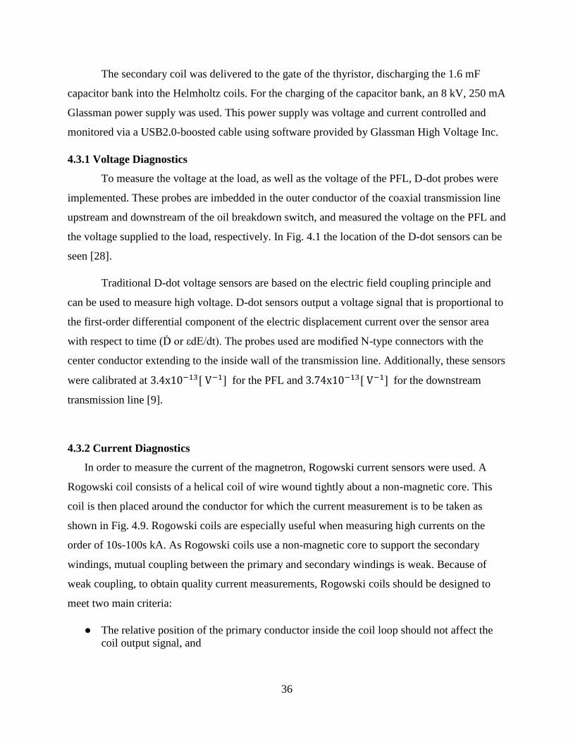
4.3.2 Current Diagnostics

In order to measure the current of the magnetron, Rogowski current sensors were used. A

Rogowski coil consists of a helical coil of wire wound tightly about a non-magnetic core. This

coil is then placed around the conductor for which the current measurement is to be taken as

shown in Fig. 4.9. Rogowski coils are especially useful when measuring high currents on the

order of 10s-100s kA. As Rogowski coils use a non-magnetic core to support the secondary

windings, mutual coupling between the primary and secondary windings is weak. Because of

weak coupling, to obtain quality current measurements, Rogowski coils should be designed to

meet two main criteria:

The relative position of the primary conductor inside the coil loop should not affect the

coil output signal, and

37

The impact of nearby conductors that carry high currents on the coil output signal should

be minimal.

To satisfy the first criterion, the mutual inductance M must have a constant value for any

position of the primary conductor inside the coil loop. M is given by

M = μ0 ∙ n ∙ S Equation 4.4.1

where 𝜇0 is the permeability of free space, n is the number of turns, and S is the cross-sectional

area of the coil shown in Figure 4.9. This can be achieved if the windings on the non-magnetic

core have a constant cross-section S, are perpendicular to the center line of the core, and have a

constant turn density n. The output voltage Vs(t), which is measured as a voltage drop across the

resistor RR, is proportional to the rate of change of the measured current given by [29]

Vs(t) = −Mdip(t)

dt Equation 4.4.2

where ip(t) is the current measured, Vs(t) is the proportional differential voltage of the

Rogowski, and M is the mutual inductance described in Equation 4.4.1.

The Rogowski coils that were used to measure the total and leakage currents are able to

approximate a self-integrating coil, meaning the output voltage of the coil is proportional to the

observed current. This was accomplished by designing the coil such that the RL time constant 𝜏

of the coil is significantly longer than the current pulse to be measured, τ = L

R. This leads to the

simplification of Equation 4.4.2 to [11], [30]

Vs =ip(t)

nRR Equation 4.4.3

Here 𝑉𝑠 is the voltage across the resistor 𝑅𝑅, n is the total number of turns, and 𝑖𝑝(𝑡) is the current

to be measured.

38

Figure 4.9 The layout of a traditional Rogowski coil.

4.3.3 RF Diagnostics

The measurements of RF frequency and pulse shape were captured with a D-band

rectangular waveguide detector, which was placed in front of the horn antenna. The signal was

coupled out of the waveguide into a RG-241 cable by a waveguide-to-coax adapter. From this

measurement we could determine the duration of the RF pulse, as well as the frequency by

applying a Fast Fourier transform (FFT) [31]. For the mode diagnostic, a neon bulb array was

used. This board consists of low-voltage neon bulbs arranged in a grid, which light up due to the

RF electric field. The mode pattern can be photographed using an open shutter DSLR camera.

4.3.4 HPM Calorimeter

A microwave calorimeter, previously constructed for the MDO experiments, was used for

power estimation. The main advantage of using a calorimeter is its ability to measure any

radiated mode, even if multiple degenerate modes exist simultaneously. The calorimeter

structure consists of two round sections of clear acrylic (polystyrene), which sandwich a 40 cm

diameter, 0.9525 cm thick layer of pure ethanol. At the frequencies of interest, the typical power

absorption coefficient was ~61%. This was calculated using two identical horn antennas and a

network analyzer [9], [32].

The calorimeter operates by absorbing the microwave energy, which causes expansion of

the alcohol volume. The alcohol is allowed to expand into a 1 mm glass capillary tube with two

39

parallel filaments. This causes a change in resistance that corresponds to the amount of energy

deposited. This measurement can easily be converted into power by considering the duration of

the RF pulse. Figure 4.10 is a diagram of the calorimeter design [33].

Figure 4.10 The design of the microwave calorimeter [9].

4.4.1 Magnetron and Hardware

The radial extraction A6 magnetron was manufactured out of 304 stainless steel using

wire EDM techniques by a local machining company, with a tolerance of one thousandth of an

inch (0.001”). For the verification of the compact magnetron with simple mode converter, which

is an axial extraction schema, only minor modifications are needed, such as a cap for the radial

extraction port. The simple mode converter, which was optimized through simulations, was

manufactured out of 1/8" stainless steel with a precision CNC mill. Both two and four cavity

extraction designs were manufactured. Details of the design for the mode converter are described

in Chapter two.

Since the radius of the cathode was reduced to 1.45 cm, a cathode shank and a new

cathode needed to be manufactured. The cathode shank was manufactured in-house out of

stainless steel. The cathode used was the transparent cathode developed at UNM [20]. It was

constructed of low-porosity, vacuum compatible POCO graphite. Graphite was the material of

40

choice because of its excellent field emission characteristics, small erection delay, and ease of

machining. Figure 4.11 is a photograph of the finished cathode.

Figure 4.11 The isometric AutoCAD drawing of the transparent cathode.

4.4.2 Beam Dump

In magnetron design it is important to consider the leakage electrons and where they are

dumped. This is because high-energy leakage electrons can damage the dielectric output window

of the waveguide. In an axial extraction scheme such as the compact A6 magnetron, the

downstream leakage current is in the range of 3-4 kA, which is sufficient energy to damage the

polycarbonate window.

In order to prevent this damage, a beam dump was designed such that the leakage

electrons would be deposited on the walls of a stainless steel tube. To determine the necessary

length of the beam dump, FEMM, a finite element 2-dimensional magnetostatic code [34], was

used to simulate the system. Figure 4.12 shows the magnetic field lines from the Helmholtz coils

as they intersect with the wall of the beam dump, indicating where the electrons will be

deposited. Simulations showed that the leakage electrons would deposit 21 cm downstream of

the magnetron. For this reason a cylindrical waveguide with a length of 30 cm was needed to

serve as a beam dump.

41

Figure 4.12 The FEMM simulation of the Helmholtz coils, showing the distance at which the

electrons will be deposited.

4.4.3 Conical Horn Antenna

Horn antennas are among the simplest and most widely used microwave antennas. The

antenna is needed to radiate the RF with minimal reflections due to the impedance mismatch, as

well as to increase the directivity and gain of the radiation pattern. Since we used an existing

antenna design, it was necessary to ensure that the output aperture could handle the power that

would be transmitted. This was done by calculating the electric field at the vacuum/atmosphere

aperture. This calculation can be performed using equation 4.3.1 [5]

PTE =πr0

2

2Z0[1 − (

fCO

f)

2]

1

2

[1 + (Vρm

2

ρ)

2

]Ewall,max2 Equation 4.3.1

where PTE is the maximum power expected to be generated (500 MW), r0 is the radius of the

aperture (10.16 cm), 𝑍0 is the impedance of free space (377 Ω), fCO is the TE11 cutoff frequency

of the aperture, 𝑓 is the operating frequency (2.43 GHz), Vρm is the Bessel function crossing

used for the TE11-mode (1.841), and 𝜌 is from the TEρm.

fCO =C

2π(

Vρm

ro)=8.652 MHz Equation 4.3.2

42

500 MW =π0.10162

2∗(377)[1 − (

8.652 MHz

2.43 GHz)

2]

1

2[1 + (

1.8412

1)

2

]Ewall,max2

Ewall,max = 9.981 × 105 [V

m] = 9.98 [

kV

cm]

It has been shown experimentally that the dielectric strength of air is roughly 30 [kV

cm]; thus, we

can see that the aperture of the conical horn antenna is more than sufficient to radiate 500 MW.

43

Chapter 5

Experimental Results

In this chapter the final assembly and experimental results are presented. The initial

results did not show good agreement; therefore, some supplementary simulations were conducted

to match the experimental results. These comparisons and the conclusions drawn from them are

presented.

5.1.1 Final Assembly

The magnetron was attached to the pulser. The electromagnets were installed around the

magnetron in the Helmholtz configuration to provide a uniform magnetic field in the interaction

space of the magnetron, as shown in Fig. 5.1. The transparent cathode was installed with a

precision of 0.001” radially. Furthermore, the cathode strip was oriented such that its leading

edge was positioned 5° off of the edge of the vane, as shown in Fig. 5.2. Simulations showed this

to be the optimal angle at which maximum power was observed [11]. The beam dump was

attached downstream of the magnetron to collect the leakage current and prevent damage to the

dielectric window of the conical horn antenna which follows the beam dump. The final aperture

of conical horn antenna was optimized for maximum power radiation. Lead bricks surround the

magnetron to absorb the X-rays produced by the high-energy electrons bombarding the anode

block.

The oil-breakdown switch gap was set to 5.9 mm to provide a load voltage of

approximately 350 kV. Two D-dot probes, located before and after the oil-breakdown switch,

respectively measured the PFL voltage and the load voltage. Two Rogowski coils were installed

upstream and downstream of the anode block to measure the total and leakage currents,

respectively. A D-band waveguide detector was positioned opposite the conical horn antenna in

the maximum field region to capture the RF signal and measure the frequency.

44

Figure 5.1 (Top) is a photograph of the physical setup where A is the waveguide detector, B is the

conical horn antenna, C is the vacuum system, and D is the lead brick shielding over the

magnetron. (Bottom) is a photograph of the area shielded by the lead bricks where E is the beam

dump, F is the Rogowski coils, G is the Helmholtz coils, and H is the A6 magnetron.

Figure 5.2 The optimal location of the cathode strips.

45

The vacuum system used consisted of a Tri-scroll roughing pump in conjunction with a

turbo pump. The vacuum level achieved was 5.2x10-6

Torr. The Marx bank switches were

pressurized with SF6 to 19-23 psi, and charged to 34-36 kV. The operating conditions for the

Marx trigger circuit were 54 psi and 54 kV.

A Stanford delay generator was used to send two trigger signals; the first signal

discharges the pulsed electromagnetic circuit, to generate the magnetic field, and the second

signal is sent after a delay of 24 ms to discharge the Marx bank. This was done to ensure the

magnetic field was at maximum during the time of operation of the magnetron.

With the load voltage held fixed at ~350 kV, a magnetic field (B-field) scan in the range

of 0.40 T to 0.60 T was conducted. The PFL voltage, load voltage, anode current, leakage

current, and RF frequency were recorded for each magnetic field.

Figure 5.3 shows the PFL and load voltage dependence on the applied magnetic field.

The data shows that these voltages were fairly constant over the range of magnetic fields. The

PFL and load voltages are 700 kV and ~350 kV, respectively. Figure 5.4 shows how the anode

and leakage current vary with magnetic field. As expected, the anode current decreased and the

leakage current increased with increasing magnetic field. The maximum anode current was

measured to be 12.5 kA, and the leakage current was 3 kA. Interestingly, the experimentally

measured anode current was rather less than current seen in simulations.

Figure 5.5 is a graphical summary of the microwave power and frequency dependence on

magnetic field. The power presented in this curve was determined from the RF amplitude, with

the waveguide detector held at a fixed position. The RF frequency was calculated by performing

an FFT using a MATLAB script [31]. The power had a tendency to increase as the magnetic

field increased, with some fluctuations corresponding to the fluctuations observed in the anode

current. Furthermore, a frequency of 2.33 GHz was detected over a wide range of magnetic

fields. However, this varied from the 2.43 GHz expected frequency from simulations. A neon

grid was used to confirm the RF mode pattern at 2.33 GHz; it is clear that the TE11-mode is

dominant, as indicated from the brightness of the neon bulbs in the center of the pattern shown in

Fig. 5.6. As a sanity check, a photograph was also taken at a non-optimal magnetic field, which

exhibited multiple frequencies, as shown in Fig. 5.7. Clearly the photograph captured does not

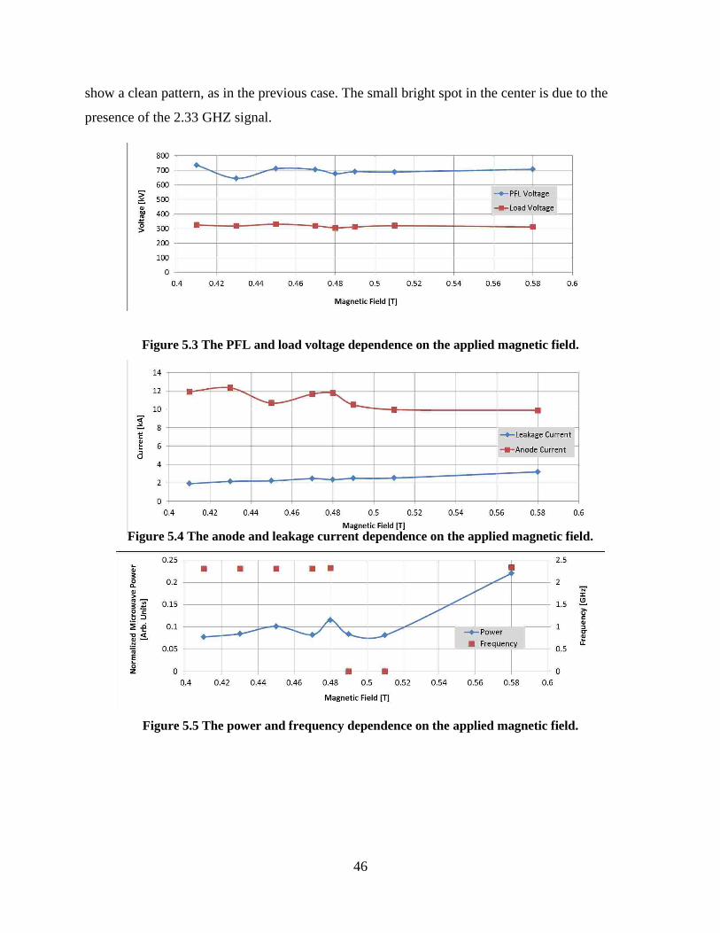
46

show a clean pattern, as in the previous case. The small bright spot in the center is due to the

presence of the 2.33 GHZ signal.

Figure 5.3 The PFL and load voltage dependence on the applied magnetic field.

Figure 5.4 The anode and leakage current dependence on the applied magnetic field.

Figure 5.5 The power and frequency dependence on the applied magnetic field.

47

Figure 5.6 Photograph of the neon grid captured with a long exposure digital camera indicating the

𝐓𝐄𝟏𝟏-mode (left), and the FFT of the RF signal for this shot (right).

Figure 5.7 Photograph of the neon grid captured with a long exposure digital camera indicating

mode competition (left), and the FFT of the RF signal for this shot (right).

48

Since the experimentally measured frequency corresponding to the TE11-mode

contradicted the initial simulation results, supplementary simulations were performed to gain

further understanding. The emission region of the cathode in the simulations was set to match the

manufactured cathode dimensions. Furthermore, the magnetic field function that dumps the

leakage electrons was optimized to match the leakage current measured experimentally. Further

investigation is being carried out with the MAGIC code development team to better understand

the code anomalies. With these modifications, agreement between simulations and experiments

was achieved, and the results are presented below.

Figure 5.8 is a comparison of the normalized experimental and simulation microwave

power, showing similar trends. Figure 5.9 displays the anode and leakage current variation. The

anode current was much greater in simulations compared to experiments, but the general trend

was similar across the B-field range. It is recommended that the current emission model in

MAGIC be studied more carefully to gain an understanding of this discrepancy. The leakage

current for the two cases was in good agreement.

The experimentally observed frequencies were reproduced in simulations and the

summary is presented in Fig. 5.10. Figure 5.11 is a chart comparing the experimental data at 0.58

T and the simulations at 0.56 T, showing very close agreement. The power and frequency

waveforms shown indicate that the 2.33 GHz frequency was dominant early on, but that mode

competition took over towards the end of the pulse. This was caused by the mode converter

effectively loading two of the magnetron cavities. This loading naturally favored the 4𝜋

3 –mode,

making it difficult to enforce the π-mode. However, through the use of an upstream anode strap,

this issue could be mitigated.

49

Figure 5.8 The normalized power dependence on the applied magnetic field for simulated and

experimental data.

Figure 5.9 Comparison of the anode and leakage current dependence on the applied magnetic field.

50

Figure 5.10 Frequency dependence on the applied magnetic field.

Red – Simulation Blue - Experiment

51

Figure 5.11 (Left) experimental results at a magnetic field of 0.58 T; (right) simulation results with

updated code showing agreement with experiments.

52

5.1.2 Conclusion

A compact relativistic A6 magnetron with a simple mode converter for axial TE11-mode

extraction was proposed. The simple mode converter implements a cavity end cap, with openings

which allow the RF to propagate into a circular waveguide. With the magnetron operating in the

π-mode, these cavity openings are positioned such that they electrically open the diametrically

opposite cavities that exhibit an instantaneous electric field corresponding to the TE11-mode in a

waveguide. An extensive parameter sweep was conducted using MAGIC in order to optimize the

design of the mode converter. This design was then manufactured and experiments were

performed to demonstrate the concept.

Through simulations it was shown that the π-mode could be enforced over a wide range

of magnetic fields by reducing the radius of the transparent cathode. For maximum power

additional alterations to the cathode were needed, for example it was shown that the length of the

cathode strips should start slightly before the anode block, and should not be extend past the

downstream end of the interaction space. These simulations showed a very stable π-mode

operation with a frequency of 2.43 GHZ over a range the magnetic fields from 0.50 T to 0.60 T.

A very clean TE11-mode with a microwave output power of ~480 MW was seen at these

parameters. The mode converter and cathode were constructed based on these findings and

experimental verification was performed. However, the experimental results showed poor

agreement with the initial simulations, in both the frequency seen and the pulse durations of the

RF. The frequency of the TE11-mode for the same range of magnetic fields was shown in

experiments to be 2.33 GHz, with a pulse width of 15 ns to 20 ns. The pulse shortening was due

to the mode competition caused by the mode converter effectively loading the magnetron to

favor the 4𝜋

3 –mode, which takes over towards the end of the pulse. Therefore, several

modifications to the code were introduced to achieve a better match with the experimental

results. This involved building the cathode to match the one which was manufactured. An

additional change to the simulation setup was to force the magnetic field function to dump the

electrons further away from the interaction space. These changes led to simulations reproducing

the experimental results. Due to time constraints and issues with PULSERAD’s Marx bank, this

design could not be investigated further; however, the concept of the simple mode converter

producing a TE11-mode was demonstrated.

53

5.1.3 Recommendations for Future Work

The experimental results show some discrepancies with the simulations, most notably the

increased anode current in simulations. This issue is possibly due to the emission model used by

MAGIC, hence further investigation is needed to better understand this discrepancy.

Additionally, due to the mode competition observed, the incorporation of an anode strap for

enforcing the π-mode should be considered. Using a cathode end cap would eliminate the

leakage current, as well as increase the overall efficiency. Another recommendation is to perform

an absolute power measurement of the simple mode converter with the HPM calorimeter.

54

REFERENCES

[1] J. E. Brittain, “The Magnetron and the Beginnings of the Microwave Age,” Phys. Today, vol. 38,

no. 7, p. 60, 1985.

[2] J. T. Randall, “The Cavity Magnetron,” Proc. Phys. Soc., vol. 58, no. 3, pp. 247–252, 1946.

[3] H. A. H. Boot and J. T. Randall, “Historical Notes on the Cavity Magnetron,” IEEE Trans.

Electron Devices, vol. 23, no. 7, pp. 51–70, 1976.

[4] A. Palevsky, “Generation of Intense Microwave Radiation By The Relativistic e-Beam Magnetron

Experimental and Numerical Simulation,” Massachusetts Institute of Technology, 1980.

[5] J. Benford, J. Swegle, and E. Schamiloglu, “High Power Microwaves, 3rd

Ed. (CRC Press, Boca

Raton, FL, 2016).

[6] E. Schamiloglu, M. I. Fuks, and S. Member, “70 % Efficient Relativistic Magnetron With Axial

Extraction of Radiation Through a Horn Antenna,” vol. 38, no. 6, pp. 1302–1312, 2010.

[7] M. Daimon and W. Jiang, “Modified Configuration of Relativistic Magnetron with Diffraction

Output for Efficiency Improvement,” Appl. Phys. Lett., vol. 91, no. 19, pp. 10–13, 2007.

[8] M. Daimon, K. Itoh, G. Imada, and W. Jiang, “Experimental Demonstration of Relativistic

Magnetron with Modified Output Configuration,” Appl. Phys. Lett., vol. 92, no. 19, 2008.

[9] C. J. Leach, “High Efficiency Axial Diffraction Output Schemes for the A6 Relativistic

Magnetron,” Ph.D. Dissertation (University of New Mexico, Albuquerque, NM, 2014).

[10] M. Fuks and E. Schamiloglu, “High Efficiency Relativistic Magnetron With Diffraction Output,”

pp. 74–80, 2009.

[11] S. Prasad, “Fast Start of Oscillations in a Short-Pulse Relativistic Magnetron Driven by a

Transparent Cathode,” Ph.D. Dissertation (University of New Mexico, Albuquerque, NM 2010).

[12] D.-F. Shi, B.-L. Qian, H.-G. Wang, and W. Li, “A Novel TE 11 Mode Axial Output Structure for a

Compact Relativistic Magnetron,” J. Phys. D. Appl. Phys., vol. 49, no. 13, p. 135103, 2016.

[13] D. F. Shi, B. L. Qian, H. G. Wang, W. Li, and Y. W. Wang, “A Compact Mode Conversion

Configuration in Relativistic Magnetron with a TE10 Output Mode,” IEEE Trans. Plasma Sci., vol.

43, no. 10, pp. 3512–3516, 2015.

[14] S. Prasad, C. Leach, M. I. Fuks, and E. Schamiloglu, “Compact Relativistic Magnetron with

Gaussian Beam Radiation Pattern,” in 18th IEEE Int. Conf Pulsed Power (Chicago, June 19- 23,

2011).

[15] C. Leach, S. Prasad, M. I. Fuks, and E. Schamiloglu, “Compact Relativistic Magnetron with

Gaussian Radiation Pattern,” IEEE Trans. Plasma Sci., vol. 40, no. 11, pp. 3116–3120, 2012.

[16] J. McConaha, P. C. Leach, and M. Fuks, “Compact A6 Magnetron with a Neodymium Permanent

Magnet,” Jeremy McConaha, Sarita, Prasad Chris Leach, Mikhail Fuks, and Edl Schamiloglu,”

vol. 40, no. 2012, p. 3120.

[17] C. Leach, S. Prasad, M. Fuks, and E. Schamiloglu, “Compact A6 Magnetron with Permanent

Magnet,” 2012 IEEE 13th Int. Vac. Electron. Conf. IVEC 2012, pp. 491–492, 2012.

[18] V. L. Granatstein, High-Power Microwave Sources, (Artech House, Norwood, MA, 1987).

[19] M. I. Fuks, N. F. Kovalev, A. D. Andreev, and E. Schamiloglu, “Mode Conversion in a Magnetron

55

with Axial Extraction of Radiation,” IEEE Trans. Plasma Sci., vol. 34, no. 3, 2006.

[20] H. Bosman, S. Prasad, and M. Fuks, “Rapid Startup In Magnetrons Using The Transparent

Cathode,” Vacuum Electronics Conference 2006 (held jointly with 2006 IEEE International

Vacuum Electron Sources) (Albuquerque, NM, April 25-27, 2006), p. 127-128.

[21] K. S. Yee, “Numerical Solution of Initial Boundary Value Problems Involving Maxwell’s

Equations in Isotropic Media,” IEEE Trans. Antennas Propag., vol. 14, no. 3, pp. 302–307, 1966.

[22] B. Goplen, L. Ludeking, D. Smith, and G. Warren, “User-Configurable MAGIC for

Electromagnetic PIC Calculations,” Comput. Phys. Commun., vol. 87, nos. 1–2, pp. 54–86, May

1995.

[23] A. J. Woods and L. D. Ludeking, “MAGIC FDTD EM-PIC Solution Improvements and

Demonstration on a Plasma Actuator,” 2013 International Conference on Electromagnetics in

Advanced Applications (ICEAA) (Torino, Italy, September 9-13, 2013), pp. 78–81.

[24] S. Prasad, C. Leach, K. Prestwich, C. J. Buchenauer, M. Fuks, and E. Schamiloglu, “Experimental

Demonstration of the Output Characteristics of the A6 Magnetron on PULSERAD 110a, a Very

Short Risetime Accelerator at UNM,” Proc. 2012 IEEE International Vacuum Electronics

Conference (Monterey, CA, 24-26 April, 2012), p. 495-496.

[25] M. Fuks, S. Prasad, and E. Schamiloglu, ”Increased Efficiency and Faster Turn-on in Magnetrons

using the Transparent Cathode,” Proc. CAVMAG2010 (Bournemouth, UK, April 19-20, 2010), p.

76-81.

[26] J. H. Black, “Solid State Capacitor Discharge Pulsed Power Supply Design for Railguns,” M.S.

Thesis, Naval Postgraduate School (Monterey, CA, 2007).

[27] T. S. Björn Backlund and E. C. Jürg Waldmeyer, “Gate-Drive Recommendations for Phase

Control and Bi-directionally Controlled Thyristors,” ABB Application Note 5SYA 2034-02 (2013).

[28] J. Wang, C. Gao, and J. Yang, “Design, Experiments and Simulation of Voltage Transformers on

the Basis of a Differential Input D-dot Sensor,” Sensors (Basel)., vol. 14, no. 7, pp. 12771–12783,

2014.

[29] I. A. Metwally, “Design of Different Self-integrating and Differentiating Rogowski Coils for

Measuring Large-Magnitude Fast Impulse Currents,” IEEE Trans. Instrum. Meas., vol. 62, no. 8,

pp. 2303–2313, 2013.

[30] L. A. Kojovic and R. Beresh, “Practical Aspects of Rogowski Coil Applications to Relaying,”

IEEE PSRC Spec. Rep., no. September, pp. 1–72, 2010.

[31] W. Huang and D. L. Macfarlane, “Fast Fourier Transform and MATLAB Implementation”

https://www.utdallas.edu/~dlm/3350%20comm%20sys/FFTandMatLab-wanjun%20huang.pdf.

[32] A. G. Shkvarunets, “A Broadband Microwave Calorimeter of Large Cross Section,” Instruments

Exp. Tech., vol. 39, no. 4, pp. 535–538, 1996.

[33] A. I. Klimov, P. V. Vykhodtsev, A. A. Elchaniniov, O. B. Kovalchuk, I. K. Kurkan, S. D. Polevin,

E. M. Totmeninov, and V. V. Rostov, “A Calorimeter for High Power Microwave Pulse

Measurement,” Proc. 15th Int. Symp. High Current Electron., pp. 422-424, 2008.

[34] D. Meeker, “Finite Element Method Magnetics Version 4.2 User Manual,” p. 158, 2015

(http://www.femm.info/Archives/doc/manual42.pdf).