University of Huddersfield Repository - CORE

University of Huddersfield Repository

Smallbone, Kirsty Louise

Mapping ambient urban air pollution at the small area scale : a GIS approach

Original Citation

Smallbone, Kirsty Louise (1998) Mapping ambient urban air pollution at the small area scale : a GIS approach. Doctoral thesis, University of Huddersfield.

This version is available at http://eprints.hud.ac.uk/4731/

The University Repository is a digital collection of the research output of theUniversity, available on Open Access. Copyright and Moral Rights for the itemson this site are retained by the individual author and/or other copyright owners.Users may access full items free of charge; copies of full text items generallycan be reproduced, displayed or performed and given to third parties in anyformat or medium for personal research or study, educational or not-for-profitpurposes without prior permission or charge, provided:

• The authors, title and full bibliographic details is credited in any copy;• A hyperlink and/or URL is included for the original metadata page; and• The content is not changed in any way.

For more information, including our policy and submission procedure, pleasecontact the Repository Team at: [email protected].

http://eprints.hud.ac.uk/

MAPPING AMBIENT URBAN AIR POLLUTIONAT THE SMALL AREA SCALE:

A GIS APPROACH

KIRSTY LOUISE SMALLBONE

Department of GeographyThe University of Huddersfield

A thesis submitted to the University of Huddersfieldin partial fulfilment of the requirements for the degree

of Doctor of Philosophy

March 1998

"People look down on stuff like geography and

meteorology, and not only because they are standing on one

and being soaked by the other. They don't look quite like

real science. But geography is only physics slowed down

and with a few trees stuck on it, and meteorology is full of

exciting fashionable chaos and complexity"

(Prachett 1996).

i

ABSTRACT

Air pollution is an emotive and complex issue, affecting materials, vegetation

growth and human health. Given that over half the world's population live

within urban areas and that those areas are often highly polluted, the ability to

understand the patterns and magnitude of pollution at the small area (urban

environment) level is increasingly important. Recent research has highlighted,

in particular, the apparent relationship between traffic-related pollution and

respiratory health, while the increasing prevalence of asthma, especially

amongst children, has been widely attributed to exposure to traffic-related air

pollution. The UK government has reacted to this growing concern by

publishing the UK National Air Quality Strategy (DOE 1996) which forces all

Local Authorities in England and Wales to review air quality in their area and

designate any areas not expected to meet the 2005 air quality standards as Air

Quality Management Areas (AQMAs), though what constitutes AQMAs and

how to define them remains vague.

Against this background, there is a growing need to understand the patterns and

magnitude of urban air pollution and for improvements in pollution mapping

methods. This thesis aims to contribute to this knowledge. The background to

air pollution and related research has been examined within the first section of

this report. A review of sampling methods was conducted, a sampling strategy

devised and a number of surveys conducted to investigate both the spatial

nature of air pollution and, more specifically, the dispersion of pollution with

varying characteristics (distance to road, vehicle volume, height above ground

level etc). The resultant data was analysed and a number of patterns identified.

The ability of linear dispersion models to accurately predict air pollution was

also considered. A variety of models were examined, ranging from the

simplistic (e.g. DMRB) to the more complex (e.g. CALINE4) model. The

model best able to predict pollution at specific sites was then used to predict

concentrations over the entire urban area which were then compared to actual

monitored data. The resultant analysis, indicated that the dispersion model is

not a good method for predicting pollution concentrations at the small area

level, and therefore an alternative method of mapping was investigated. Using

the ARC/INFO geographical information system (GIS) a regression analysis

approach was applied to the study area. A number of variables including

altitude, landuse type, traffic volume and composition etc, were examined and

their ability to predict air pollution tested using data on nitrogen dioxide from

intensive field surveys. The study area was then transformed into a grid of

10m2, regression analysis was performed on each individual square and the

results mapped. The monitored data was then intersected with the resultant

map and monitored and modeled concentrations compared. Results of the

analysis indicated that the regression analysis could explain up to 61 per cent of

the variation in nitrogen dioxide concentrations and thus performed

significantly better than the dispersion model method. The ease of application

and transferability of the regression method means it has a wide range of

applied and academic uses that are discussed in the final section.

ACKNOWLEDGEMENTS

There are many people I would like to thank for their help and supportthroughout this thesis.

David Briggs, my supervisor, has my heartfelt thanks, for his help, support,patience and ability to read copious drafts with only occasional page losses andwithout whom the original spark that formed this project would never have been.

Ann Briggs, for putting up with the telephone calls (always during dinner!)

Andrew Sheard of Kirklees Scientific Services for his help, humor and allowingaccess to Kirklees pollution data.

The people at BETS for their cooperation in road-side sampling and forproviding traffic data.

Those people involved in the SAVIAH study especially Hans, Erik, Paul,Hendrick, Sue and Powel to name but a few.

All those Yorkshire folk who allowed me to wander through their gardens to findsuitable diffusion tube homes and for allowing even stranger people to turn up,wander around their property and disappear again in the blink of an eye leavingonly a small plastic tube behind. Without their cooperation this project wouldhave taken a very different shape. In particular I would like to mention thefamily in Sheepridge who moved 'down the row' with every visit (if they didn'twant to participate in any more sampling they only had to say!).

All those friends and colleagues who 'volunteered' to join in the 'great diffusiontreasure hunt' through the sunshine, the snow and the Castle Hill lunches.Special thanks go to Emma, Kees, Sally and Fiona for their constant support,encouragement and equal enthusiasm for pizza, alcohol and rugby (Ooh go onthen).

Finally I would like to thank my family, especially my mother (thanks mum) forher support and belief in me throughout my education, mama for her supply of'food parcels' and letters and Aunt Jeanette for the hugs.

Table of Contents

List of Tables

List of Figures vii

CHAPTER 1 INTRODUCTION

1

1.1. Aims and objectives 3

CHAPTER 2 BACKGROUND TO AIR POLLUTION

6

2.1 Background to air quality legislation 6

2.1.1 European influence on UK legislation 92.2 Air pollution and health 11

2.2.1 Trends 11

2.2.2 Acute studies 13

2.2.3 Chronic studies 14

2.2.4 Nitrogen dioxide 15

2.2.5 Ozone 15

2.2.6 Particulates 16

2.2.7 Proxy exposure indicators 162.3 Methods of mapping 182.4 Summary 21

CHAPTER 3 POLLUTION MONITORING 22

3.1 The study area 223.2 Sampling methods 25

3.2.1 Fixed-site monitors 26

3.2.2 Active portable monitors 27

3.2.3 Passive monitors 303.2.3.1 Absorption samplers 303.2.3.2 Permeation samplers 313.2.3.3 Diffusion samplers 323.2.3.4 Choice of sampler 32

3.3 Comparison and selection of passive diffusion monitors 34

3.3.1 Palmes tubes 35

3.3.2 Willems badges 38

3.3.3 Comparison of passive samplers — a pilot study 413.3.3.1 Accuracy of samplers 453.3.3.2 Precision of samplers 473.3.3.3 Choice of samplers 48

14 Summary 49

CHAPTER 4 SURVEY DESIGN 50

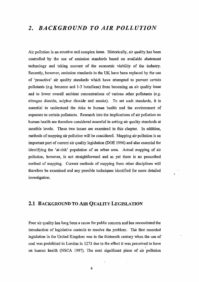
4.1 Routine surveys 514.2 Consecutive surveys 564.3 Annual mean concentrations 584.4 Special surveys 59

4.4.1 Roadside surveys 604.4.2 Vertical surveys 63

4.5 Sampling protocol 654.6 Summary 69

CHAPTER 5 SOURCES, PATTERNS AND MAGNITUDE OF VARIATION 70

5.1 Sources of variation 705.1.1 Sources of spatial variation 71

5.1.1.1 Factors influencing spatial emission patterns 715.1.1.2 Factors influencing spatial dispersion patterns 72

5.1.2 Sources of temporal variation 735.1.2.1 Factors influencing temporal patterns of emissions 735.1.2.2 Factors influencing temporal patterns of dispersion 74

5.1.3 Sources of error 755.1.3.1 Measurement error 755.1.3.2 Sampling error 76

5.2 Components of variation 765.2.1 Influence of variation in traffic volume 775.2.2 Variation with distance to road 795.2.3 Variation attributable to land cover 845.2.4 Variation attributable to altitude 935.2.5 Pollutant variation with vertical distance 985.2.6 Variation in measurement and sampling error 1035.2.7 Spatial and temporal variation 1065.2.8 Temporal variation 1075.2.9 Spatio-temporal variation 1105.2.10 Temporal 'affinity areas' 111

5.3 Conclusion 115

CHAPTER 6 DISPERSION MODELING 117

6.1 Principles and developments of dispersion modeling 117

6.2 Linear dispersion models 1246.3 Description of the models 125

6.3.1 The DMRB model 1286.3.2 The CAR-INTERNATIONAL model 1316.3.3 The CALINE3 model 1346.3.4 The CALINE4 model 138

6.4 Model validation 1396.4.1 DMRB 143

6.4.1.1 Processing 1436.4.1.2 Results 143

6.4.2 CAR-INTERNATIONAL 1446.4.2.1 Processing 1446.4.2.2 Results 14'7

11

6.4.3 CALINE3 1496.4.3.1 Processing 1496.4.3.2 Results 150

6.4.4 CALINE4 1526.4.4.1 Processing 1526.4.4.2 Results 153

6.5 Model application 1556.5.1 Processing 1556.5.2 Results 156

6.6 Conclusion 160

CHAPTER 7 REGRESSION MAPPING 161

7.1 Introduction 1617.2 The regression approach 1637.3 Pollution data 1667.4 Pollution indicators 167

7.4.1 Traffic volume (TVOLBUFF) 1697.4.1.1 Data collection 1697.4.1.2 Processing 170

7.4.2 Built land 1777.4.2.1 Data collection 1777.4.2.2 Processing 179

7.4.3 Other variables 1827.4.3.1 Altitude 1827.4.3.2 Sample height 1827.4.3.3 Relative relief 1847.4.3.4 Local topographic exposure 1847.4.3.5 Very low density housing 184

7.5 Creation of regression model 1857.5.1 Regression analysis on modelled mean 1857.5.2 Traffic volume variable 187

7.6 Mapping 1887.7 Validation 200

7.7.1 Within-period testing 2007.7.1.1 Within-period testing: variable sites 2017.7.1.2 Within-period testing: consecutive sites 205

7.7.2 Temporal (annual) data 2097.7.3 Pre-period testing 2107.7.4 Post-period testing 210

7.8 Conclusion 214

CHAPTER 8 DISCUSSION 216

8.1 The story so far 2178.1.1 Sources of variation 2178.1.2 Dispersion modeling 2208.1.3 Regression analysis 222

8.2 The next steps 224

BIBLIOGRAPHY 228

111

Appendix 1Appendix 2Appendix 3Appendix 4Appendix 5Appendix 6

Description of site measurementsSite plansProtocol for fieldworkersField and laboratory logsLand cover classificationPasquill stability class program

252256258264274276

iv

List of Tables

CHAPTER 2 BACKGROUND TO AIR POLLUTION

2.1 UK national air quality standards and objectives 8

2.2 EU air quality standards 10

2.3 Use of proxy indicators of pollution in epidemiological research 18

CHAPTER 3 POLLUTION MONITORING

3.1 Assessment of the suitability of continuous monitors 28

3.2 Assessment of the suitability of portable monitors 29

3.3 Assessment of the suitability of passive diffusion monitors 33

3.4 Summary of the pilot survey structure 45

3.5 Comparison of accuracy in the NO2 monitoring methods 47

3.6 Comparison of within site variation (precision) 47

3.7 Types of sampling device for each survey 48

CHAPTER 4 SURVEY DESIGN

4.1 Summary of the routine surveys 52

4.2 Results of the routine surveys (ug/m 3) 55

4.3 Summary of consecutive survey NO 2 results (tg/m3) 58

4.4 Regression analysis of the multilevel modeling (MLM) concentrations 59

4.5 Summary of information collected for each site during roadside surveys(NO2 concentrations in ag/m3) 63

4.6 A summary of information collected for the vertical surveys(NO2 concentrations in ug/m3) 65

CHAPTER 5 SOURCES, PATTERNS AND MAGNITUDE OF VARIATION

5.1 Regression analysis of variation with traffic volume 77

5.2 Regression analysis of variation with distance to road 80

5.3 Standardized regression analysis of variation with distance to road 82

5.4 Summary statistics for NO2 (1-Igim3) variation by the degree of urbanization 85

5.5 Analysis of variance for degree of urbanization 87

5.6 Summary statistics for NO2 (1-tgim3) variation by DETR classification 88

5.7 One-way analysis of variance for distance to emission source 89

5.8 Land use classification 90

5.9 Summary statistics of NO 2 (ptg/m3) variation with local land use category 90

5.10 Analysis of variance attributed to Land cover at the small scale 92

5.11 Correlation analysis significance values for local area land cover 93

5.12 Altitudinal survey statistics (mA0D) 94

5.13 Regression analysis (r2 values) of the effects of altitude on NO 2 concentrations(All sites) , 95

v

5.14 Regression analysis (r2 values) of the effects of altitude on NO2 concentrations(Non-urban sites) 98

5.15 Curvilinear regression analysis of variation with vertical distance(R2 values) 99

5.16 Standardized curvilinear regression analysis of variation with verticaldistance (R2 values) 103

5.17 Comparison of laboratory and field blank accuracy 104

5.18 One-way analysis of variance of the error effect 106

5.19 Regression analysis of data stability 110

5.20 Spatio-temporal one-way analysis of variance 110

5.21 Final statistics of Factor Analysis 113

5.22 Factor Matrix 114

5.23 Summary of Factor loadings by group 114

CHAPTER 6 DISPERSION MODELING

6.1 General dispersion model data requirements 126

6.2 Data requirements for the DMRB model 132

6.3 Data requirements for the CAR-INTERNATIONAL model 135

6.4 Data requirements for the CALINE3 model 137

6.5 Data requirements for the CALINE4 model 140

6.6 DMRB regression analysis results 144

6.7 Regression analysis results for CAR-INTERNATIONAL 149

6.8 Regression analysis results for CALINE3 150

6.9 Regression analysis results for CALINE4 153

6.10 Regression analysis results for CALINE4 for 80 core sites 159

CHAPTER 7 REGRESSION MAPPING

7.1 Preliminary list of independent variables for the creation ofthe pollution equation 168

7.2 Evaluation of traffic buffer zones 176

7.3 Results of regression analysis for nitrogen dioxide and traffic volume,for individual and the modeled annual mean (M.) 177

7.4 Land cover classes and codes used in preliminary analysis of variance 178

7.5 Results of analysis of variance for NO 2 concentrations by land cover class 179

7.6 Results of regression analysis using traffic volume variables 189

7.7 Regression analysis results of the within-period testing 212

7.8 Results of temporal testing 212

7.9 Results of pre-period testing 212

7.10 Results of post-period testing 213

vi

List of Figures

CHAPTER 3 POLLUTION MONITORING

3.1 Map of the study area 23

3.2 Schematic diagram of available sampling technology 26

3.3 Components of a passive diffusion tube 35

3.4 Components of a Willems badge 39

3.5 Cross-section of a badge, indicating paths of resistively 41

3.6 Distribution of sample sites in the study area 43

3.7 Position of the badge and tube samplers on the bracket 44

CHAPTER 4 SURVEY DESIGN

4.1 Location of sample sites for routine and consecutive surveys 54

4.2 Box plot of Consecutive sites 57

4.3 Location of sampling sites for near-source surveys 61

4.4 Example of sampler location at a roadside site 62

4.5 Location map of sample sites used in vertical surveys 64

CHAPTER 5 SOURCES, PATTERNS AND MAGNITUDE OF VARIATION

5.1 Relationship between Kerbside NO2 concentrations and traffic volume 785.2 Relationship between NO2 concentrations and receptor distance to road 815.3 Regression analysis of Standardised NO2 concentrations and receptor

distance to road 81' 5.4 Relationship between standardised NO2 concentrations and the

Logarithmic receptor distance to road 835.5 Mean and standard deviation of the degree of urbanization 865.6 Mean and standard deviation of the DETR classification 865.7 Mean and standard deviation of the local area land cover 915.8 Relationship between NO2 concentrations and altitude 965.9 Selected curvilinear relationships between NO 2 concentrations and altitude 965.10 Relationship between NO2 concentrations and altitude by DETR land class 975.11 Selected curvilinear relationships between NO 2 concentrations and altitude

- Non urban sites only 975.12 Relationship between NO 2 concentrations and height (Oldgate House) 1005.13 Relationship between NO2 concentrations and height

(The University of Brighton) 1005.14 Relationship between NO 2 concentrations and height (Technical College) 1015.15 Relationship between NO 2 concentrations and height (St Peters House) 1015.16 Relationship between standardized NO2 concentrations and height above

ground (m) - For all sites 1025.17 Comparison of NO2 concentrations at a site (Survey S 3) 1055.18 Comparison of NO2 concentrations at a site (Survey S4) 1055.19 Comparison of NO2 concentrations between Surveys - (S 2 and S3) 1085.20 Comparison of NO2 concentrations between Surveys - (S 3 and S4) 1085.21 Comparison of NO2 concentrations between Surveys - (S 2 and S4) 109 I

vii

CHAPTER 6 DISPERSION MODELING

6.1 Schematic diagram of mathematical models 119

6.2 Diagram of the Gaussian plume 122

6.3 Diagrammatic explanation of the DMRB model 130

6.4 Relationship between observed and predicted NO 2 concentrations usingDMRB (excluding meteorology) 145

6.5 Relationship between observed and predicted NO 2 concentrations usingDMRB (including meteorology) 145

6.6 Analysis of residual values for DMRB (excluding meteorology) 146

6.7 Analysis of residual values for DMRB (including meteorology) 146

6.8 Relationship between observed and predicted NO 2 concentrations usingCAR-INTERNATIONAL 148

6.9 Relationship between observed and predicted NO 2 concentrations usingCALINE3 151

6.10 Analysis of residual values for CALINE3 151

6.11 Relationship between observed and predicted NO 2 concentrations usingCALINE4 154

6.12 Analysis of residual values for CALINE4 154

6.13 Relationship between observed and predicted NO 2 concentrationsusing CALINE4 for the core data sites (Survey S2) 157



6.16 Relationship between observed and predicted NO 2 concentrationsusing CALINE4 for the core data sites (annual mean concentrations) 158

CHAPTER 7 REGRESSION ANALYSIS

7.1 Distribution of the road network, traffic volume and road type 171

7.2 Example of a circular buffer used in GRID 173

7.3 Example of a moving buffer 173

7.4 Correlation of NO 2 values and traffic volume with radial distancefrom sampling site 175

7.5 Altitude map of the study area 183

7.6 Traffic volume weighting curve produced using CALINE4 dispersionmodel 188

7.7 Weighted coverage of traffic volume (TVOLBUFF) 191

7.8 Weighted coverage of land use (HIGHDEN) 193

7.9 Regression map of nitrogen dioxide concentrations, survey S2 194



7.12 Regression map of nitrogen dioxide concentrations, Annual Mean 198

7.13 Regression map of nitrogen dioxide concentrations in Huddersfield towncentre - Survey S2 199

7.14 Relationship between predicted and observed NO2 for variable sitesin Survey S2 202 i

viii

(

observed annual mean NO2

2 202observed NO2 for variable sites in

203predicted annual mean NO 2 values

203observed NO2 for variable sites in

204predicted annual mean NO2 values

204predicted NO2 values for





208predicted annual mean NO 2 values for

208predicted NO2 pre-period testing

211predicted NO2 pre-period testing

211

7.15 Relationship between predicted andvalues for variable sites in Survey S

7.16 Relationship between predicted andSurvey S3

7.17 Relationship between observed andfor variable sites in Survey S3

7.18 Relationship between predicted andSurvey S4

7.19 Relationship between observed andfor variable sites in Survey S4

7.20 Relationship between observed andconsecutive sites in Survey S2

7.21 Relationship between observed andfor consecutive sites in Survey 52


7.23 Relationship between observed andfor consecutive sites in Survey S3



7.26 Relationship between observed and—survey SA

7.27 Relationship between observed and—survey SB

ix

I. INTRODUCTION

The 'London Smog' of 1952 dramatically focused both public and political

attention on the problems of air pollution and health. Between December 4th and

7th, the daily death rate in the capital rose from ca. 120 to over 500, as pollution

levels rose in association with a stable high pressure front over south-east

England. During the week ending on December 13th, 2484 people died, some

4.5 times the rate the previous month. Applications for hospital admission for

respiratory illness grew three-fold over the period; emergency admissions for

cardiovascular diseases doubled; applications for sick benefit rose 50% (Ministry

of Public Health 1954, quoted in Schwartz 1994).

Since then, much has changed. Technological advances, economic restructuring

and environmental policy have combined to reduce levels of many traditional air

pollutants, such as black smoke and sulphur dioxide. Over the same period,

however, new concerns have arisen, particularly about the apparent link between

rising levels of traffic-related pollution and increases in respiratory and cardio-

respiratory illness (e.g. Britton 1992; Lean 1993; Parliamentary Office of Science

and Technology 1994; Royal Commission on Environmental Pollution 1995).

In recent years, these concerns have driven the search for both technological and

legislative solutions which could reduce levels of air pollution and related health

risks. Nevertheless, the scientific basis for intervention remains weak. Whilst a

growing number of studies have demonstrated links between traffic-related air

pollution and respiratory health, these have been hampered by a number of

factors not least the limited knowledge about spatial patterns of air pollution, the

limited availability of monitored pollution data, and consequent poor estimates of

exposure (Briggs 1992). As a result, it has proved difficult to quantify the true

risks to health posed by traffic-related and other air pollutants or to establish

definitive air quality standards and control strategies (Committee on the Medical

1

Effects of Air Pollutants 1995). In recommending air quality standards for

particulates, for example, the Expert Panel on Air Quality Standards (EPAQS)

stated:

"Because of the many uncertainties surrounding the evidence upon which ourrecommendations are based we believe that the recommended Air QualityStandards should be reviewed in the light of United Kingdom experience and of anynew data, within the next five years" (Expert Panel on Air Quality Standards 1995).

Similarly the National Air Quality Strategy, launched in 1996, notes that:

"Central to the further development of air quality policy, is an understandingof the relationship between the different levels at which air pollution is generatedand, in consequence, controlled" (DoE 1996).

The Royal Commission on Environmental Pollution set up by the UK

government concluded that :

"We recommend that further research be carried out into the health effects both ofindividual transport-related pollutants and substances in combination. Thisresearch should include further epidemiological (and) further study of the effects ofpollutants" (Royal Conunission on Environmental Pollution 1994).

Such statements indicate that there is a recognised need for further investigation

into spatial variation of air pollution, particularly in urban areas, for use in

epidemiological studies. A particular need is the ability to map air pollution at

the small-area scale. Air pollution maps are potentially powerful tools. They can

help to identify `hotspots' in need of special intervention or monitoring; they can

help to design and implement monitoring networks; they can provide a basis for

evaluating the effects of management or policy; they can help to estimate

personal exposure to air pollution, and thus provide valuable data for

epidemiological studies and health risk assessments. They can also be an

effective means of communicating information on air pollution to users, whether

researchers, policy-makers or members of the public. In recent years, the potential

for air pollution mapping has advanced considerably, as a result of improvements

in methods of dispersion modelling and in the use of GIS. Nevertheless, the

ability to produce detailed air pollution maps, at a scale and level of accuracy

which can meet these needs, remains undeveloped.

2

1.1 AIMS AND OBJECTIVES

The project reported in this thesis was aimed at addressing the lack of detailed

pollution data at the small area level by investigating patterns and sources of air

pollution at the small area level, and by developing and testing a range of

mapping methods, including dispersion models and GIS-based methods. The

specific aims were as follows:

• To examine the magnitude, source and patterns of small areaspatial variation in traffic-related air pollution in an urbanenvironment.

• To investigate methods of mapping traffic-related air pollution at asmall area scale.

• To evaluate the implications of small area variations in airpollution for the design of pollution monitoring networks and airquality management areas.

To this end, the study involved the following objectives:

• the collection of monitored data for a dense network of sites within amixed urban-rural study area (Huddersfield, UK).

• examination of sources of variation in air pollution concentrationswithin the area.

• testing and comparison of different methods of pollution mapping,including dispersion modelling, interpolation and empiricaltechniques.

• on the basis of these results, production of a 'best approximation'pollution map for the study area.

3

The project was carried out partly in association with an EU Third Framework

funded project entitled SAVIAH (Small Area Variation In Air pollution and

Health). The aim of the SAVIAH study was to develop and test methods for

examining the relationship between chronic respiratory symptoms in children and

environmental (air) pollution. The study was carried out in four European

countries: Amsterdam (Netherlands), Huddersfield (United Kingdom), Prague

(Czech Republic ) and Poznan (Poland). The study employed a range of

techniques including: questionnaire surveys to obtain data on health, family

background and home circumstances of children aged 7-11 years; low-cost

passive sampling devices to monitor air pollution levels at a dense network of

sites in each study area; GIS methods for the modelling and mapping of air

pollution and to determine personal exposure at the individual level; small-area

statistical methods to analyse spatial patterns in health outcome and relationships

between exposure and health. Results of the SAVIAH study are reported by

Briggs et al. (1997), Lebret et al. (in press), van Reeuwijk et al. (in press) and

Pikhart et al. (in press). The research reported here includes work undertaken

both within the context of the SAVIAH study and outside that study (see, also,

Collins et al. 1995).

The thesis is arranged as follows:

Chapter 2 reviews the history of air quality legislation in Britain, examines

existing knowledge concerning the relationship between air pollution and health,

looks at possible mapping techniques and identifies key research needs.

Chapter 3 describes the study area, outlines the atmospheric processes involved

in air pollution, evaluates the available monitoring technology and identifies the

most suitable sampling methodology which fulfils the aims and objectives of this

project. The sampling procedures used in the study are described in detail.

Chapter 4 describes the various surveys used in the project. The sampling

protocol used in each survey is also described.

4

Chapter 5 examines and quantifies sources of variation in pollution levels in both

a spatial and temporal framework. The contribution of traffic volume, distance

from road, land cover, sampling height and measurement error are all

investigated.

Chapter 6 investigates the capability of traditional methods of dispersion

modelling to describe these variations in air pollution at the small area scale. A

number of different dispersion models are used and compared, and the results are

validated against a subset of the pollution data obtained in the pollution surveys.

One method is then applied to map pollution levels across the study area.

Chapter 7 develops and evaluates the use of GIS-based regression analysis as a

basis for air pollution mapping.

Chapter 8 discusses the relative merits and disadvantages of each of the

techniques and considers the implications of the results of the study for air

pollution management and monitoring, and for environmental epidemiological

research. The extent to which the aims and objectives of this project have been

achieved is examined and the conclusions discussed.

5

2. BACKGROUND TO AIR POLLUTION

Air pollution is an emotive and complex issue. Historically, air quality has been

controlled by the use of emission standards based on available abatement

technology and taking account of the economic viability of the industry.

Recently, however, emission standards in the UK have been replaced by the use

of 'proactive' air quality standards which have attempted to prevent certain

pollutants (e.g. benzene and 1-3 butadiene) from becoming an air quality issue

and to lower overall ambient concentrations of various other pollutants (e.g.

nitrogen dioxide, sulphur dioxide and smoke). To set such standards, it is

essential to understand the risks to human health and the environment of

exposure to certain pollutants. Research into the implications of air pollution on

human health are therefore considered essential in setting air quality standards at

sensible levels. These two issues are examined in this chapter. In addition,

methods of mapping air pollution will be considered. Mapping air pollution is an

important part of current air quality legislation (DOE 1996) and also essential for

identifying the 'at-risk' population of an urban area. Actual mapping of air

pollution, however, is not straightforward and as yet there is no prescribed

method of mapping. Current methods of mapping from other disciplines will

therefore be examined and any possible techniques identified for more detailed

investigation.

2.1 BACKGROUND TO AIR QUALITY LEGISLATION

Poor air quality has long been a cause for public concern and has necessitated the

introduction of legislative controls to resolve the problem. The first recorded

legislation in the United Kingdom was in the thirteenth century when the use of

coal was prohibited in London in 1273 due to the effect it was perceived to have

on human health (NSCA 1997). The next significant piece of air pollution

6

legislation in the UK was not introduced until the nineteenth century and

followed the realisation that crops, vegetation, human health, materials and tools

were severely damaged by emissions from alkali works. The 1863 Alkali Act

thus required a 95 per cent reduction in emissions from alkali factories, and the

dilution of the remaining 5 per cent before release to the atmosphere. It also

instituted the National Inspectorate of Pollution and gave them powers of

enforcement. Emissions from alkali works subsequently fell from 14,000 tonnes

to 45 tonnes per year (NSCA 1997, Elsom 1992, Coils 1997).

Attempts to control the ever changing problems of air pollution, especially within

urban areas, have been based on a number of different philosophies. In Europe

and the USA, legislative air quality standards are set. Emitters must show that

their emissions would not cause air quality standards to be exceeded.

Conversely, the UK has historically relied on emission standards to control air

pollution, the assumption being that if controls were set on emissions, ambient air

quality targets would therefore be achieved. Emission standards for the UK have

been based on the pragmatic concept of 'Best Practicable Means (RPM)' as

stated in the 1874 second Alkali Act. This allowed the economic viability of the

industry concerned to be considered in deciding the level of abatement

technology necessary (Colls 1997; NSCA 1997).

The concept of best practicable means in controlling air pollution continued until

the 1980s when heightened interest in the environment, combined with new EU

legislation, forced recognition of the cross-media movement of pollution: i.e. that

air pollution had implications for water quality and land contamination.

Consequently, it was felt that an integrated approach to pollution control would

be more able to control the movement of pollution across different media. This

concept entered British law in the 1990 Environmental Protection Act. The

Environmental Protection Act (1990) resulted in the replacement of BPM by

BATNEEC (best available techniques not entailing excessive cost). As with the

BPM approach, however, the concept of BATNEEC and the inclusion of the

words 'best' and 'excessive' naturally entails a subjective judgement to be made

on the part of the assessor and thus is open to appeals and abuse.

7

PollutantBenzene

1,3 Butadiene

Carbon monoxide

Lead

Nitrogen dioxide

Legislation to control air pollution within the UK could therefore be considered

as reactive instead of proactive in approach. The situation changed, however,

with the introduction of the UK National Air Quality Strategy in 1996. This

strategy drew together current thinking on air quality management and for the

first time set down national standards for air quality in the UK. The strategy

identified standards for nine pollutants based on the effects of human health (see

Table 2.1). Furthermore, the strategy stated that Local Authorities should review

pollution levels and identify possible `hotspots' or 'Air Quality Management

Areas' where it was thought the air quality standards would not be met by 2005.

Once identified, a management plan for that area would then be drawn up to take

account of local factors such as meteorology, topography, population density,

vehicle volume and composition and specialised sources (e.g. airports) and then

implemented within a given time period (DOE 1996).

Table 2,1 UK national air quality standards and objectives

Conc Reference period5 ppb Running annual mean

1 ppb Running annual mean

10 ppm Running 8 hour mean

0.51.tg/m3 Annual mean

104.6ppb 1 hour mean

20 ppb Annual mean

Exceedence Allowance

2005

2005

2005

2005 8 hours exceedenceallowed per year

99.9th percentileby 2005

Target Date2005

Ozone

Particulates (PMio)

Sulphur dioxide

50 ppb Running 8 hour mean

501.1.g/m3 Running 24 hour mean

100 ppb 15 minute mean

97th percentileby 2005

99th percentileby 2005

99.9th percentileby 2005

10 day exceedenceallowed per year

4 day exceedenceallowed per year

99.9 per cent ofmeasurements below100ppb (DOE 1996)

8

2.1.1 EUROPEAN INFLUENCE ON UK LEGISLATION

The European Union has historically adopted a proactive approach to air quality

and, instead of setting emission standards, chose to control air pollution by the

introduction and enforcement of air quality standards. This was undertaken by

the introduction of a series of directives into European Community Law in the

1980s which have since passed into law in the respective countries.

The first standards introduced into law were as a result of increasing concern

regarding the effects of sulphur dioxide and black smoke on the environment,

particularly the influence of acid rain on vegetation and fresh water lakes. The

sulphur dioxide and suspended particulate directive (80/779/EEC) set both limit

values (mandatory) and guide values (non-mandatory) for these pollutants, both

of which are detailed in Table 2.2. This directive has since been renegotiated in

the Helsinki Protocol and the UK has agreed to reduce sulphur emissions from

1980 levels by 50 per cent by 2000, 70 per cent by 2005 and 80 per cent by 2010

(NSCA 1997).

Similarly a directive detailing air quality standards for nitrogen dioxide

(85/203/EEC) was introduced in 1985 and has been renegotiated in 1991

following the ratification of the 1988 Sofia Protocol (see Table 2.2). Similar

standards for ozone, carbon dioxide, carbon monoxide and volatile organic

compounds (VOCs) have been set or are due for adoption (NSCA 1997).

The influence of the European community on UK legislation should not be

underestimated, however, and has played a great part in the change in UK

legislation from standards based on emission levels to those based on air quality

standards summed up in the recent UK National Air Quality Strategy (DOE

1996).

9

50p.g/m3 at the 50thpercentile calculated fromthe mean values per hourannually

135m/m3 at the 98thpercentile calculated asabove

Table 2.2 EU Air Quality Standards

Limit ValueSulphur Dioxide 80m/m3 if smoke > 401.1g/m3 or 120

gg/m3 if smoke 5 401.tg/m3 (as themedian of daily mean values takenannually)

180i.tg/m3 if smoke > 601.tg/m3 or 130ttg/m3 if smoke 601.tg/m3 (as themedian of winter daily values)

2501-tg/m3 if smoke > 150m/m3 or3501.tg/m3 if smoke 51501.tg/m3 (as the98th percentile of daily valuesannually)

Nitrogen Dioxide 2001.tg/m 3 at the 98th percentilecalculated from the mean values perhour annually.

Lead 21.1g/m3 as an annual mean

Guide Value 100-150n/m3 as a 24hour mean

40-601.1g/m3 as an annualmean

(NSCA 1997)

Finally it should be noted that, although possessing no powers of enforcement,

the World Health Organisation (WHO) has also published recommended air

quality guidelines which have been used as a basis for the EU air quality

standards. Although not mandatory, WHO guidelines are generally accepted as

levels which should not be exceeded if healthy air is to be maintained.

These 'agencies' have been fundamental in shaping air quality legislation in the

UK and the replacement of emissions standards by air quality standards in the

1990s. Adoption and enforcement of the UK National Air Quality Strategy is not

yet complete, however, owing to the recent change in government, although it is

generally accepted that the strategy will by implemented with only minor

alterations.

10

2.2 AIR POLLUTION AND HEALTH

2.2.1 TRENDS

The implications of the effects of air pollution on human health have been of

growing concern in recent years. This concern is reflected in both the number

and subject of recent epidemiological studies. Many researchers have noted that

there has been a gradual rise in the prevalence of respiratory illness, particularly

asthma and wheeze, concurrent with increases in road traffic volume over the last

20 or so years (Anderson et al. 1994; Britton 1992; Burney 1988; Burney et al.

1990; Haathela et al. 1994; Oosterlee et al. 1996; NILU 1991; Wardlaw 1993).

During the same time period there has been a dramatic increase in the incidence

of acute asthma attacks. For example, the rate of reported attacks in the

population as a whole more than doubled from 10.7 per 100,000 patients per

week in 1974 to 27.1 in 1991; the rate among 0 - 4 year old children increased

more than five-fold, from 13.5 to 74.4 per 100,000 per week (Action Asthma

1991). In addition, the Committee on the Medical Effects of Air Pollutants

(1995) notes that:

"with regards asthma, it is probable that a substantial proportion [of thepopulation] remain undiagnosed." (Committee on the Medical Effects of AirPollutants, 1995).

These increases in asthma are paralleled throughout the developed world and

cannot therefore be dismissed as the result solely of changes in diagnosis or

reporting strategies (Britton 1992). Along with increases in respiratory illness,

there have been reported increases in mortality rates linked to air pollution and

specifically to increased road traffic volumes. For example, during 3 days in

December 1991, the death rate in London increased by 10% concurrent with

extremely high air pollution levels linked to a traffic-induced smog (Association

of London Authorities et al. 1994). This and similar reports (e.g. Pope et al.

11

1992, Dockery et al. 1989; 1993) are put into perspective when it is considered

that, in western society, four out of five people live and work in urban

conurbations and that it is in these urban areas that air pollution levels are

highest. As a result, a large percentage of western society is potentially exposed

to high levels of air pollution whether at school, work or home.

As noted earlier, traditional concern about links between air pollution and health

have focused on pollutants such as smoke and sulphur dioxide, carbon dioxide

and lead. Restructuring, of heavy industry, improved pollution abatement

technologies and the introduction of emission legislation (e.g. The Clean Air Acts

of 1956, 1968 and 1993, the Control of Pollution Act 1974 and the

Environmental Protection Act 1990) have helped reduce levels of many of these

pollutants. This decline in traditional pollutants has been offset by increases in

the levels of a range of 'new' pollutants including nitrogen dioxide, ozone, non-

methane volatile organic compounds, carbon monoxide and fine particulates,

largely as a result of increasing levels of road transport (QUARG 1993). In

1991, for instance, vehicle pollution in the UK was responsible for almost 90 per

cent of all emissions of carbon monoxide in the atmosphere, just over half of all

emissions of nitrogen oxides, 36 per cent of all volatile organic compounds

emissions and 2 per cent of sulphur dioxide emissions. This effect is more

pronounced in urban areas, where road traffic contributes as much as 99 per cent

of carbon monoxide emissions, up to 76 per cent emissions of nitrogen dioxide

and 22 per cent of sulphur dioxide emissions. Notwithstanding efforts to

improve vehicle fuel and engine design, levels of traffic-related air pollution

seem likely to increase, for UK predictions for the next 20-30 years suggest a

further growth of at least 40% in traffic volume (Gillham et al. 1992; QUARG

1993; Royal Commission on Environmental Pollution 1995). Furthermore,

although all new cars manufactured after January 1994 have had to be fitted with

catalytic converters, nearly two thirds of all pollutants are emitted in the first few

minutes of the journey when the catalysts are still cold (Lean 1993; Russell-Jones

1987; Royal Commission on Environmental Pollution 1995). Thus the effect of

catalytic converters on reducing air pollution will be limited. With regards to

health, pollution emitted from vehicles is of more concern than that emitted from

12

industrial sources as industrial releases are emitted at a higher level and therefore

have less impact on local air quality (Read 1994).

2.2.2 ACUTE STUDIES

In the last decade, a number of epidemiological studies have investigated the

health effects of exposure to a wide range of traffic-related pollutants. Particular

attention has been focused on fine particulates, ozone and nitrogen dioxide.

Many of these studies have focused on short term (acute) effects of exposure to

brief periods of moderate or high levels of pollution. This concentration on acute

health effects is due to a number of factors, not least the relative ease of

collecting the necessary health data. Long term studies, conversely, require

health data to be collected over a long period (e.g. 1-10 years) with increased risk

of non-co-operation by subjects, high drop-out rates and the subjects moving out

of the study area. Recent research, conducted both in Europe and the USA, has

suggested that at acute concentrations below the current air quality guidelines, air

pollution concentrations may be associated with rising mortality, hospital

admissions, respiratory symptoms (such as bronchitis, asthma, wheeze) and

decreasing lung function (Dockery and Pope 1994; Dockery et al. 1993;

Wardlaw 1988). More specifically, studies in Finland indicated an association

between nitrogen dioxide levels and hospital admissions for respiratory disease

and asthma (Ponka 1991; Rossi et al. 1993). Short term increases in NO2 have

been shown to be associated with decreasing respiratory function (Brunkreef et

al. 1989; Goldstein et al. 1988; WHO 1987). Schwartz et al. (1990) found an

association between ambient NO2 levels and sore throats, phlegm and eye

irritation in healthy student nurses in Los Angeles. Relationships were also

identified between reduction in peak flow and increases in symptoms and use of

respiratory medication and daily levels of PMio particulates (Brunkreef et al.

1989; Hoek et al. 1992; Pope et al. 1992). Furthermore, research in the USA by

Dockery eta!. (1992) and Pope et al. (1992) suggested that there was a 16-17 per

cent rise in the overall death rate for every 100iug/m3 rise in particulate

concentrations.

13

Ozone is a secondary pollutant, the health effects of which have also been noted

by a number of researchers. Again, results from studies in the US and Europe

have been remarkably consistent in demonstrating reductions in pulmonary

functions at ambient ozone levels of between 80 and 250 ppb (Hoek et al. 1993;

Lioy et al. 1985; Spektor et al. 1988). Interestingly, it has been noted that, unlike

most other pollutants, the effects of ozone are not confined to those who already

suffer respiratory problems (Spelctor et al. 1988).

2.2.3 CHRONIC STUDIES

In contrast, there have been relatively few studies which attempt to examine the

effects of long term exposure to low levels of air pollution. Most of those which

have been conducted tend to have small sample sizes and compare areas of low

pollution with areas of high concentrations of numerous pollutants, thus making

it difficult to determine which pollutant is responsible for any observed effects

and to remove the confounding effects of difference in lifestyle, social conditions

and health service provision (Read 1994). The various studies have also used

different measures of exposure to different pollutants, and therefore comparisons

are difficult.

Chronic studies are especially severely affected by problems of confounding

factors. Confounding factors may either dilute or artificially inflate the

correlation between air pollution and health. Thus relationships between a

specific pollutant and an aspect of human health may be incorrectly identified.

The most obvious confounding factor which may effect health is smoking

(Hawthorne 1978; Lambert et al. 1970; McCarthy et al. 1985). Children whose

parents smoke are 50 per cent more likely to be admitted to hospital with

bronchitis and pneumonia (USDHE1S 1986). Similarly, a cohort study of 10,000

British children found that there was a 14 per cent increase in childhood wheezy

bronchitis and asthma when mothers smoked (Neuspiel et al. 1989). Other factors

which affect respiratory function, especially asthma and wheeze, are exercise

(Coughlin 1988), type and age of housing (McCarthy et al. 1985), damp housing

14

(Strachen and Sanders 1989), and dust (Anto and Sunyer 1990; Sunyer et al.

1989a; 1989b). People who suffer from allergic asthma may also be affected by

animal fur or feathers, dust mites, mould, and a range of pollen including birch

spores and timothy grass.

In order to circumvent some of the influence of confounding factors, a number of

studies have examined the specific effects of long-term exposure to traffic-related

pollution and health. Occupational studies of those working in confmed spaces

with vehicles such as police (Speizer et al. 1973), tunnel workers (Evans et al.

1988), bus garage workers (Gambel et al. 1987) and ferry vehicle workers

(Ulfvarson et al. 1990) demonstrated either an increased prevalence of

respiratory symptoms or a reduction in lung function or both.

2.2.4 NITROGEN DIOXIDE

Nitrogen dioxide is a known oxidant, which can reduce airway capacity and

pulmonary function in susceptible individuals at high concentrations. At ambient

concentrations, however, the effects are less clear and results of recent studies

have been somewhat contradictory. Several studies reported no overall effect on

the prevalence of respiratory disease of NO2 (Dockery et al. 1989; Euler et al.

1988; van Mutius et al. 1992). Other studies, however, have shown an increase

in prevalence of respiratory disease in polluted areas, though this is not specific

to NO2 (Detels et al. 1991; Jaakola et al. 1991). A national study in 44 cities in

the USA showed an association between particulates, nitrogen dioxide and ozone

and the risk of low lung function when adjusted for confounding factors

(Schwartz 1989).

2.2.5 OZONE

Ozone is a powerful oxidant, which can cause significant impairment of

pulmonary function at high concentrations (WHO 1987). In addition, 10 per cent

of the population are particularly susceptible to the effects of ozone 'and may

15

suffer headaches, eye and throat irritation at ambient concentrations (EPAQ

1994; Elsom 1992). As with nitrogen dioxide, relatively few long term studies

have been conducted to investigate the health effects of ozone. Detels et al.

(1991) found that, in general, the prevalence of respiratory symptoms was higher

and the lung function lower in more polluted areas. •Abbey et al. (1991)

demonstrated an association between prevalence of asthma and ozone levels in

excess of 100 ppb. Studies by Zwick et al. (1991) also identified an association

between levels of ozone and lung function and bronchial reactivity.

2.2.6 PARTICULATES

The effects of exposure to particulates on human health is of growing

importance, demonstrated by the recent introduction of an air quality guideline

for PK () in 1996 by the UK government. Examination of literature indicates that

a number of studies identified an association between levels of particulates and

respiratory symptoms (Melina et al. 1981; Euler et al. 1988). Chronic cough,

bronchitis and chest illnesses were found to be associated with particulates (PMis

and PM2.5) in six cities in the USA (Dockery et al. 1989). A significant

association was also demonstrated between mortality (particularly from

cardiopulmonary disease) and PM2 . 5 in adults (Dockery et al. 1993). Similar

results were found in the Czech Republic by Bobak et al. (1992). Generally,

recent research has suggested that the finer particulates (PM 2. 5), which are more

reactive and can penetrate further in to the lungs, are more important in terms of

their health effects.

2.2.7 PROXY EXPOSURE INDICATORS

In almost all the epidemiological studies undertaken to investigate relationships

between air pollution and health, the main limitation is the lack of accurate

exposure data. This shortcoming is mainly due to the limited availability of

nationally measured pollution data (e.g. there are only 26 automatic NO2

monitoring stations, 31 0 3 monitoring stations and only 14 PM 10 Monitoring

16

stations for the whole of the UK), and the high cost of conducting purpose-

designed surveys to obtain the relevant data. In many cases, therefore, proxy

indicators of traffic-related pollution levels have been used. Studies in Germany,

for example, found a significant relationship between respiratory function and the

prevalence of recurrent wheeze and breathlessness and traffic flow (see Table

2.3). Residential distance to road was used as an estimate of pollution in other

studies (see Table 2.3). Nitta et al. (1993), for example, reported increased levels

of respiratory and allergic symptoms in areas of high exposure to vehicle

emissions. Similarly Wichmann et al. (1989) found a raised prevalence of

asthma in areas of high concentrations of NO2 and CO associated with road

traffic. Use of proxy indicators such as distance from road or traffic volume

inevitably generates uncertainties in exposure estimates, and may act to dilute or

distort relationships with health outcome.

Direct measurements of exposure, however, are generally impracticable due to

their costs and problems of recruiting volunteers. Improved estimates of exposure

are thus likely to come mainly from the use of methods to model air pollution

levels at the small area level. Indeed, two recent studies (Oosterlee et al. 1996;

NILU 1991; Pershagen et al. 1994) have already used such methods to provide

exposure estimates in studies of traffic-related pollution and respiratory health and

identified significant relationships (see Table 2.3).

2.3 METHODS OF MAPPING

From the above research it is clear that there is a need for a method of mapping

air quality and thus providing better estimates of exposure to air pollution. Use

of dispersion models provides one means of mapping, and in recent years a wide

range of models have been developed, some with inbuilt graphical capabilities,

for both point and line sources. Application of dispersion modelling, however, is

17

Table 2.3 Use of proxy indicators of pollution in epidemiological research.

Proxy indicator

Residential distanceto road










Traffic flow

Traffic flow

Traffic flow

Traffic density

Residential distance toindustry

Residential distance toindustryOccupation

Air pollution models




Author Date Location Exposure Health outcomeIndicator

Blumer & Reicht 1980 Switzerland Particulates/ Lead Occurrence of cancer

Edwards eta! 1994 UK Traffic-related Asthmapollution

Elliott eta! 1992 UK Industrial emissions Cancer of Larynx andLung

Ishizaki et al 1987 Japan Traffic-related Respiratory symptomspollution

Livingstone 1996 UK Traffic-related Respiratory symptomspollution

Murakami eta! 1990 Japan Traffic-related Respiratory symptomsPollution

Nitta eta! 1993 Japan Traffic-related Respiratory symptomsPollution

Waldron et al 1995 UK Traffic-related Asthmapollution

Wichman eta! 1989 Germany Traffic-related Prevalence of croupPollution Syndrome

Whitelegg 1994 UK Traffic-related Respiratory symptomsPollution

Edwards 1993 UK Traffic-related Respiratory symptomsPollution

Romieu et al 1992 Germany Traffic-related Prevalence of recurrentPollution wheeze & breathlessness

Wjst eta! 1993 Germany Traffic-related Respiratory functionPollution

Weiland eta! 1994 Germany Traffic-related Wheeze & allergicpollution Rhinitis

Halliday eta! 1993 Australia Industrial Wheeze & respiratoryemissions symptoms

Shy eta! 1970 USA NO2, Particulates Respiratory functions

Hall & Wynder 1984 USA Traffic-related Lung cancerpollution

NILU 1991 Norway Traffic-related Respiratory symptomsPollution

Oosterlee et al 1996 Netherlands NO2 Respiratory symptoms

Pershangen et al 1995 Sweden NO2Occurrence ofWheezing Bronchitis

POnka 1991 Finland NO, CO, Ozone Asthma

18

often limited by the availability of the required input data (e.g. on emissions,

meteorology, topography) as well as the inherent limitations of the models themselves.

Although often used for specific site-level investigations (e.g. highway development),

they have been less extensively used to map air pollution for entire towns or cities.

Alternatively, pollution surveys can be generated by spatial interpolation techniques.

Interpolation can be defmed as;

'the estimation of the values of an attribute at an unsampled location frommeasurements made at surrounding sites' (Burroughs 1986)

Interpolation from a point (or monitoring site) to an area (in which people may

live and work) is not as straightforward as it may first appear and has long been a

source of interest and research for geographers and cartographers. Many

methods of interpolation have been developed and have, in recent years, been

enhanced by the development of Geographical Information Systems (GIS) such

as ARC/INFO, SPANS and MAHNFO which enables the spatial handling,

manipulation and analysis of vast amounts of data. In addition there is a wide

range of spatial interpolation techniques which are available as part of statistical

packages (such as Splus, Minitab and SPSS). These include triangulation, thin

plate spline techniques (Hutchinson 1982; Dubrule 1984), moving window

methods (Jones 1996; Bailey and GatTell 1995), trend surface analysis and

various methods of kriging (Oliver and Webster 1993; Myers 1995;). These

methods have been widely used in environmental mapping, including air

pollution (e.g. SEIPH 1996; 1997; Dorling and Fairbain 1997), though

interestingly few attempts have been made to use them for air pollution mapping

in urban areas. Several studies have also compared the different methods of

interpolation (e.g. Burroughs 1986; Lam 1983), albeit without any definitive

conclusions: in general, performance varies according to the quality of the data

and the nature of the underlying spatial patterns being investigated. In addition,

the more sophisticated techniques pose severe demands of data quality and

uniformity of distribution which cannot always be met in natural sampling

situations.

The rational behind most methods of spatial interpolation is that, on average,

points closer together are more likely to have similar values than those further

19

apart. Contouring (triangulation), for example, is one of the most widely used

methods of spatial interpolation for air pollution. Originally developed as a

cartographic technique for indicating terrain elevation, Ostad and Brakensiek

(1968) stated that methods of contouring could be transferred to 'concept space'

and was not therefore restricted to 'geographic space'. Contouring has been

widely used in a number of fields including meteorology, hydrology (Cooper and

Burt 1986), geology (Bott and Trantrigola 1987; Reid and McManus 1987);

transport studies (Murayama 1994; Dundon-smith and Gibb 1994), location

analysis (Haggett, Cliff and Frey 1997) and air pollution (Campbell 1988;

Greenland and Yorty 1985; Vit 1995).

Such methods of interpolation, however, suffer from a number of problems when

applied to urban air pollution. Maps produced in this way, although allowing for

gradation in variation over space, imply linear variation between locations. In

addition, the occurrence of closed basins and summits means that the

interpolation can become very complex, especially where there is marked local

variation in the modelled surface. Furthermore, to achieve a representative

pollution surface, a large number of data points with sufficient spatial variation

are needed. This is often problematic as the number of monitoring stations for

urban areas are few. It should also be noted that many forms of spatial

interpolation, by relying solely on monitoring data, fail to consider other

potentially useful information such as emission data, local topography and

climatic influences, all of which may help to explain and predict variation in

urban air pollution (Dorling and Fairbairn 1997).

A final point to consider is the use that such maps will be put to. Increasingly,

maps are being used not only to inform research, but also as important tools for

management, policy and decision-making. As such, the accuracy of the maps has

important implications, both in terms of cost and ultimately, life. A map of flood

risk developed by Prof. Clark at Southampton University, for example, was

recently used by local insurance companies to control insurance risks and was in

danger of creating planning blight in the area labelled as a 'high risk Dine' (Clark

20

1997). The public perception of an air pollution map and the fact that many

people believe maps without question, should also be considered and every effort

made to ensure that the mapping technique chosen represents the actual spatial

distribution of air pollution as accurately as possible.

2.4 SUMMARY

This chapter has shown that there has been significant changes in the policy and

philosophy behind air pollution legislation, culminating in a shift away from

emission standards and towards air quality standards as used by the European

Union and the World Health Organisation. This change in policy can be

attributed in part, to developments within the EU and increasing concern about

the possible links between air pollution and health in recent years, most notably

as a result of increasing volumes of road traffic and an apparent increase in

respiratory illness. To date, epidemiological studies have been hampered by the

difficulty in obtaining reliable measures of exposure at the small area of

individual level. To a large extent, this reflects the limited spatial resolution of

routine pollution monitoring, and thus the need to rely on exposure proxies.

Finally methods of air pollution mapping to date were examined as a basis for

further work which will be undertaken within this thesis. This research is aimed

at examining the magnitude and patterns of small area spatial variation in air

pollution within an urban environment and at developing and testing

interpolation and dispersion based methods of pollution mapping, through a

detailed investigation in the Huddersfield area, in West Yorkshire, UK.

21

3. POLLUTION MONITORING

3.1 THE STUDY AREA

The research project was conducted in the Huddersfield area of West Yorkshire. The

area chosen for study was that of the, now defunct, Huddersfield Health Authority

boundary (Figure 3.1). This area was chosen for a number of reasons. Firstly it was

expected to facilitate the collection of medical statistics if required. Secondly, the

area provided a good example of a medium sized provincial town in the UK, with

large variations in pollution levels and a wide range of emission sources. Thirdly,

good working links had been formed between the centre of study (The University of

Huddersfield) and Kirklees Metropolitan Council and West Yorkshire Health

Authority. Both of these were considered essential in order to allow data access and

information exchange. Finally the area was convenient to the centre of study.

Subsequently, the study area was selected as one of the four centres for the SAVIAH

study — an EU-funded project which aimed to investigate the relationship between air

pollution and respiratory health of children and allowed the comparison of

prevalence of childhood respiratory symptoms and its determinants across countries

based on a standardised method (Fischer et al. In press).

The study area is 305 km2 and topographically very complex. It ranges from the

Pennine Hills in the west to the margins of the Vale of York in the east.

Geologically, the area is underlain by rocks of Carboniferous age which form a

sequence of gently dipping strata, inclined to the west, and dissected by a number of

deep river valleys (e.g. the Holme and Colne). The area ranges in altitude from

22

23

Te0AT:

1,44

„g ...tV11;04. t.:41 S?'

80m in the east (near FlocIcton) to 582m in the south-west (Black Hill) and it is this

combination of geological structures, river valleys and altitude which have combined

to influence the location and nature of the urban settlements.

The traditional industry of the area has been the woollen mills which were

concentrated at the headwaters of the river valleys in order to take advantage of the

clear, clean Pennine water. Although many of the textile mills have now given way

to cloth recycling, dying and chemical industries (e.g. Holiday Dyes and Chemicals,

Dawson Dyers and Zenica), many of these are still located in the river valley

bottoms. Consequently, the majority of the settlements and infrastructure of the area

is located around these industries.

On the plateaux, above the river valleys, much of the land is used for agricultural

purposes. In the west of the study area, where the valleys are more pronounced and

the soil of a poor quality, most of the land is used for sheep farming. In the east,

however, the topography is gently undulating, which produces conditions conducive

for arable farming.

The population of the study area was ca. 211,300 in 1991 (OPCS Census 1991), the

majority of which is concentrated in the urban settlements of Huddersfield (pop

148,000) and Holmfirth (pop 30,636). The remaining population (32,664) is spread

throughout the surrounding satellite villages, (e.g. Slaithwaite and Linthwaite in the

Colne valley, Holmfirth and New Mill in the Holme valley and the Skelmanthorpe,

Clayton West, Shelley and Denby Dale in the Dearne valley). Most of these villages

are now used as commuter centres for people travelling to Huddersfield, Dewsbury,

Leeds, Sheffield and Bradford. Major routeways include the A62 which runs along

the Colne, the A616/A35, which follows the Holme and the A635 which follows the

Dearne. In addition, the M62 provides a major transport link across the north-west

of the area.

24

3.2 SAMPLING METHODS

The primary aim of this project was to investigate the nature of small area

variation in traffic-related air pollution in urban areas, and to examine methods

of mapping urban air pollution as a basis for exposure assessment. In order to

fulfil these aims it was necessary to obtain pollution data on levels of pollution

which could be used both to describe and investigate patterns of variation, and to

test the accuracy of the resultant maps.

As noted earlier, the study area has a complex topographic and socio-economic

make-up. No permanent, fixed site monitoring stations existed in the area (one

was added by the local authority, however, towards the end of the project), and

although Kirklees Council was conducting some monitoring using passive

diffusion samplers, this was considered inadequate for the needs of this study.

Obtaining representative detailed pollution data was, therefore, possible only by

undertaking an intensive, purpose-designed monitoring programme. The

following criteria were considered when selecting the monitoring method for this

project:

• within the financial constraints of this project, the sampling techniquemust provide the best possible spatial coverage of the study area.

• the methods must be accurate, reliable and be a recognised method ofair pollution monitoring within the scientific community. Resultsshould be comparable to governmental standards.

• the method should not require extensive maintenance nor expensivecalibration due to the possible remoteness of some sites and financialconsiderations of the project.

• analysis of the samples should be quick and simple.

• samplers must be weatherproof and as far as possible vandal proof.

25

Fixed-site IPermeatior AbsorptiorDiffusion

• the chosen sampling method should be able to be left unattended forsignificant periods of time at any location and be easy to transport.

Monitoring methods can be divided into active monitors (which physically

capture air to be analysed in either real-time or at a later date) and passive

samplers (which allow air to diffuse onto/into the sampling medium) on the basis

of sampler type and output (Figure 3.2). The choice of monitoring technique was

important to the project as it would influence the survey design and the extent of

the spatial coverage of data. The remainder of this section examines the range of

monitoring techniques available and explores their possible use within the

limiting requirements of this study.

Figure 3.2 Schematic diagram of available sampling technology.

AVAILABLE MONITORINGTECHNIQUES

IACTIVE MONITORS I IPASSIVE MONITORS I

3.2.1 FIXED-SITE MONITORS

Fixed-site (or continuous) monitors have been developed for the detection of a

range of gaseous pollutants. They provide a continuous readout of pollution

levels at a particular site, and are therefore useful for studies requiring data on

26

detailed variation in pollution levels. Continuous monitors, specific to the

measurement of nitrogen dioxide, are based on the gas-phase chemiluminescent

method. These monitors records emissions of photons from the gas-phase

reaction of NO with ozone. Concentrations of ambient air are drawn into

chemiluminescent monitor and the initial amount of NO within the sample of air

is determined (V1). The NO 2 in the sample of air is then reduced to NO (NO +

NO2) providing a second measurement (V2). The monitor then subtracts V2

from V1 providing a measurement of the volume of NO 2 in the original ambient

air sample.

Yocom and McCarthy (1991), Tardiff and Goldstien (1991), Lodge (1989),

Harrop et al. (1990) and Atkins (1986; 1991) have all noted the numerous

advantages and disadvantages of using continuous monitors for measuring

pollution. These are summarised in Table 3.1.

In the light of these considerations, it was decided to reject this type of monitor

for the sampling required in this project. The primary reasons for this decision

were the high cost and the difficulties in siting the equipment, which would

seriously reduce the number of possible sampling sites. Although detailed

information on the temporal variation of pollution would be obtained,

insufficient insight into the spatial variation of NO 2 would be gained. Due to the

reliable and accurate nature of continuous monitors, however, it was decided to

use this method as a reference for the calibration and validation of the selected

monitoring technique.

3.2.2 ACTIVE PORTABLE MONITORS

Portable monitors were first developed for industrial exposure monitoring, but

have since been adapted to measure the lower concentrations experienced in

27

Advantages Disadvantages

Table 3.1 Assessment of the suitability of continuous monitors.

- provide data on the relationship betweenNO and NO2, and NO2 decay rates

- well established and acceptable method,for comparison with EU and UK ambientair quality guidelines

- provide a continuous record of pollution

- allow short term peaks and troughs inpollution levels to be identified

- method is highly sensitive, reliable, andaccurate

- results are immediately available

- when operated in conjunction withrelevant technology, can provide real-timedata

- equipment can be operated unattended forextended time-periods

- can be multiplexed to allow differentlocations to be sampled thus providingcost-effective use of equipment

- equipment is expensive to purchase

- cost of the equipment tends to limit thenumber of samplers in a network; thereforepoor spatial resolution

- due to cost of monitor, equipment failurebecomes significant

- location and height of the sampler willaffect the results, thus creating samplingbiases

- good ventilation is required due to theby-product of ozone

- monitoring sites may be limited inresidential areas by the production ofaudible noise

- monitoring sites must be weatherproof,vandal proof, provide an external dedicatedpower supply and be large enough toaccommodate the monitor

- if relocated or disconnected from thepower supply, the equipment requiresrecalibration

- require extensive maintenance

urban areas. Most portable monitors are attached to, or contain, a pump (either

battery or manual) which enables them to draw a known volume of air though the

sampling device over a known period of time. The sampling device is dependent

upon the type of pollutant. It may take the form of an absorbent medium, a

membrane containing a reagent, or a liquid through which the air is bubbled.

28

The quantity of the measured pollutant is determined in the laboratory using

standard chemical procedures. As with fixed-site monitoring stations, the use of

portable monitors has a number of advantages and disadvantages, as described in

Table 3.2

Table 3.2 Assessment of the suitability of portable monitors

Advantages

Disadvantages

- samplers are versatile and can be adaptedto monitor a large range of pollutants

- method is considered sensitive

- samplers can be operated unattended fora significant time period

- small size of the equipment allowsmonitoring in locations inaccessible tocontinuous monitors

- samplers are light and easy to transport

- can be used as personal monitors to recordactual human exposure

- can be moved around, and measurementstaken at several geographically distantlocations

- with appropriate technology, monitors canbe multiplexed to produce a series of timedsamples for later analysis in the laboratory

- samplers are relatively expensive, reducingthe number of monitoring locations

- samplers provide only an integratedreading

- analysis of the samplers is ofien timeconsuming as no automation can beapplied to the process

- samplers are reliant on power operatedpumps and therefore require either adedicated power supply or are limited bythe battery operation time

- portable monitors require calibration andmaintenance

- many of the pumps are not weatherproofor vandal proof, thus limiting their use tomeasure outdoor pollution

Again, the cost of the monitoring equipment and the siting difficulties were

considered to be the main constraints on their use in this project.

29

3.2.3 PASSIVE MONITORS

In the light of the inherent limitations of traditional active, fixed-site and portable

monitoring techniques, considerable effort has been devoted in recent years to

developing low-cost passive monitors. Passive monitors provide only average

pollution data for the full exposure period (Archibold and Crisp 1983; Goodman

et al 1974; Atkins et al 1986). They can be divided into absorption, permeation

and diffusion monitors. Each of these will be briefly examined and their

suitability for the project assessed.

3.2.3.1 ABSORPTION SAMPLERS

Absorption samplers allow the required pollutant to be absorbed on to the

sampling medium with little control over the rate of absorption. Such samplers

can in turn be divided into biological and non-biological passive absorption

samplers:

a) Biological Absorption Samplers. Biological samplers include devices such as

moss-bags, commonly used to measure heavy metals, and lichens used to

measure ambient levels of sulphur dioxide (SO2) and nitrogen dioxide (NO2)

(Treshow and Anderson 1989).

Lichen, sensitive to sulphur dioxide concentrations are a living organism used in

many pollution surveys (Hawksworth and Rose 1976; Gilbert 1974; Kauppi and

Halonen 1992; Seaward 1992). Different species of lichen have different

tolerances to pollution and thus can be used to map approximate levels of air

pollution. Unfortunately there are many constraints on the use of lichen as

pollution monitors, not least the difficulty in identification, substrate distribution

and the time-lag which exists between actual pollution levels and the lichen.

30

Consequently, lichens therefore only provide an indication of pollution levels at

an indeterminate time in the past. Lichen surveys were therefore not considered

practicable for this project.

b) Non-Biological Absorption Samplers. Non-biological samplers are based on

the principles of absorption and include corrosion plates to monitor rainfall

acidity, rubber strips to monitor ozone and the Leclerc apparatus to monitor

sulphur dioxide etc. No reliable non-biological sampler suitable for monitoring

traffic-related pollution has yet been developed.

3.2.3.2 PERMEATION SAMPLERS

Permeation monitors were developed in the late 1970s and consist of a sampling

body (or badge) which is filled with the relevant 'sink' or trapping medium. A

permeation membrane is placed between the reactive medium and the ambient

air. The membrane, therefore, acts as the diffusion path for the air passing into

the reactive medium. Each permeation sampler is calibrated in the laboratory

before exposure. The samplers are then exposed for between 1 and 5 days and

returned to the laboratory for analysis. Pollution concentrations of the samplers

are calculated using Fick's First Law of Diffusion (Section 3.3). Due to the small

size and lightweight nature of the samplers they can be placed in a wide range of

locations, while the short exposure time and calibration before exposure provides

relatively accurate results. The samplers can also be validated and tested against

more established methods such as continuous monitors (Fowler 1982).

Nevertheless, they are expensive and time consuming to prepare and analyse as

each sampler requires individual calibration before exposure. For these reasons

they have not been widely used for air pollution studies (Fowler 1982; McGinlay

et al. 1996; Pio 1992).

31

3.2.3.3 DIFFUSION SAMPLERS

Diffusion samplers have been developed for a wide range of pollutants, including

NO2, SO2, benzene and ammonia. Diffusion samplers have been used in a large

number of studies (e.g. Bailey et al 1992, Hewitt 1991, Loxen eta! 1988, Martin

et al 1981, Noy et al 1990, Harrop et al 1990, Spengler et al 1983). Based on

Fick's First Law of Diffusion (Section 3.3), the monitors typically consist of a

tube or badge, one end of which is exposed to ambient air while the other

contains an absorbent reagent on a membrane. A diffusion zone is created by the

body of the monitor, through which air passes into the pollution sink (i.e. the

reactive material). The rate of pollution uptake can be controlled by altering the

dimensions of the sampler, i.e. diffusion width/length (Palmes et al. 1973; 1976;

Atkins et al. 1986; Brown 1981). The problems and advantages of using

diffusion samplers have been discussed by a number of researchers (Atkins et al.

1986; 1978; Apling et al. 1979; Boleij et al. 1986; Hangartner et al. 1989;

Moschandres et al. 1990) and are summarised in Table 3.3.

3.2.4 CHOICE OF SAMPLER

In considering the variety of techniques and designs of air pollution monitors, it

is clear that a compromise is needed between the accuracy of the data and the

spatial density of the sampling network. In order to fulfil the aims of this project,

the main requirement of the sampling technique was clearly for a method which

provided good geographical resolution at an acceptable level of accuracy.

Detailed temporal data were of less concern. As previously stated, active fixed-

site monitors, and in particular chemiluminescent monitors, clearly provide the

greatest accuracy but are inhibited by the cost and difficulties of locating the

32

Table 3.3 Assessment of the suitability of passive diffusion monitors

Advantages

Disadvantages

- the sensitivity of the device can be alteredby changing the dimensions of the sampler

- Diffusion samplers are considered reliableand comparable with the well establishedchemiluminescent monitors

- total cost of the samplers is low, allowing alarge number of samplers to used in asurvey thus providing good spatialresolution

- diffusion samplers are simple to analyseand can be recycled

- the samplers can be left unattendedthroughout the exposure period

- the samplers contain no moving parts anddo not need a power supply

- the samplers are weatherproof, small andtherefore suitable for fixing to streetfurniture

- the use of a dense network of samplersreduces the significance of individualsampler failure

- results are not immediately available asthere may be a delay between the end ofsampling and the analysis

- samplers provide only an integratedreading of pollution for the exposure period

- the small size and numerous locations ofthe samplers incur problems of vandalismand theft

- samplers are subject to possiblecontamination during storage and transit

samplers. They were therefore rejected as the dominant sampling method,

though they were used as a reference method in order to provide calibration and

validation for the final choice of monitor. Active portable monitors were also

rejected on the basis of cost and the problems of using them at unattended sites

for long periods of time. Permeation monitors were rejected on the grounds of

expense, difficulties in calibration and the time consuming process of sampler

construction. Diffusion monitors were, therefore, chosen as the primary method

of sampling for this project.

33

3.3 COMPARISON AND SELECTION OF PASSIVE DIFFUSIONMONITORS

Most passive diffusion monitors are based on the principle of diffusion of a

pollutant onto an absorption or reactive medium. Sampling occurs when air

passes into the sampler by molecular diffusion and the specified pollutant is

absorbed by the absorbent medium. Different media are used to sample specific

pollutants. The rate of diffusion can be controlled by varying the dimensions of

the sampler and is based on Fick's First Law of Diffusion (Atkins et al. 1986,

Palmes 1978; Bocken et al. 1992):

F = D*A*(C-00)

Where: F = mass flux (ug/s)D = Diffusion coefficient (m2/s)A = surface diffusion opening (m2)C = external gas concentration (ug/m31)Co = gas concentration at the surface of the reaction filter (pg/m3)

Z Diffusion length (m)

A number of diffusion samplers have been developed. Most are designed as

either a badge or tube. Examples include the Yanagisawa badge (Yanagisawa &

Niskimura 1982), Willems badge (Willems 1990), PRO-TEK badge (Kring

1981), Walden badge (Tompkins and Goldsmith 1977), the SVO tube (Bocken et

al. 1992) and the Palmes tube (Palmes 1976, Atkins et al. 1986). Palmes tubes

were the first passive diffusion sampler to be widely used. Originally designed

for measuring occupational exposure to SO2, they were later modified to

measure NO2 in ambient conditions (Palmes et al. 1976). Badge type samplers

were developed in response to a number of limitations inherent in tube type

34

A = Red End Cap and Mesh Holder.B = Reactive Mesh.C = Polyethylene Tube.D = Yellow End Cap.

samplers. Both the Palmes tube and the Willems badge were evaluated for this

study.

3.3.1 PALMES TUBES

The structure of the Palmes tube is shown in Figure 3.3. It consists of a tube

with a mesh holder (A) which forms the cap of one end of the tube. The reactive

grid (B) comprises a stainless steel mesh with a 0.21mm grid width and a

0.15mm wire thickness. The grid is inert and the spacing of the wire is small

enough to allow a film of the absorbent reagent to be formed. The tube (C) is

made of polyacryl and acts as the diffusive chamber through which the air passes.

Both ends of the tube are machined to ensure that a good seal is formed with the

caps. The end cap (D) is removed on sampling and replaced after exposure.

Both caps A and D are made from inert polyethylene. Each of the caps is colour

coded to facilitate identification in the field.

Figure 3.3 Components of a passive diffusion tube.

Triethanolaime (TEA) is used as the absorbent reagent for nitrogen dioxide. It is

considered an effective absorbent, having near-perfect absorption (absorbent

35 .

efficiency of more than 95%) and unity of analysis (Palmes et al. 1976; Apling et

al. 1979; Blacker 1973; Levaggi eta!. 1973; Atkins et al. 1978).

For sampling, the diffusion tubes are mounted vertically with the large cap (A)

containing the absorbent uppermost. In order to prevent deposition from the

surrounding surface, a fixture (or bracket) should be used, as recommended in

Brown et al. (1981). Sampling is started by the removal of the lower end cap (D)

which is replaced at the end of sampling. The caps are colour coded to allow

ease of identification. Details of the location, start and end time, and date should

be recorded for purposes of analysis.

The accuracy and precision of passive diffusion tubes and their optimal operating

conditions have been examined by a number of studies (e.g. Palmes et al. 1976;

Apling et al. 1979; Blacker 1973; Levaggi et al. 1973). Comparison of diffusion

tubes with standard chemiluminescent NO2 monitors have been carried out by

Apling et al. (1979), Atkins et al. (1986), Hollowell (1979), Cadoff et al. (1979),

Heon et al. (1984), Boleij et al. (1986), Hangartner and Burni (1987) and Gair et

al. (1991). Accuracy of the tubes relative to chemiluminescent monitors was

generally found to be better than ±10%. Replication of the samplers was also

reported to indicate an absolute difference of no more than 10%. Atkins et al.

(1986), however, stated that although precision was "generally very satisfactory"

for NO2 concentrations greater than 5ppb, below 5ppb precision declined

rapidly. Better results can be achieved by longer exposure periods at very low

concentrations.

The effects of meteorology on diffusion tubes has also been investigated. A

number of researchers (Brown eta!. 1991; Boleij et al. 1986; Atkins et al. 1986)

have reported that ambient air movements may create a turbulent mixing zone

around the mouth of the diffusion tube, thus creating a resistance to diffusion.

The turbulence generally causes the tubes to overestimate concentrations

36

(Bocken 1992; Girman et al. 1983; Heal and Cape 1997). Further research has

indicated that, at low wind speeds (0.05-0.1cm/s), air within the tube stagnates,

adversely affecting sampler performance (Boleij et al. 1986; Scheeren et al.

1991). Atkins et al. (1986), however, stated that although the diffusion tube

samplers show a wind speed dependence, it is too small to be detectable. The

effects of temperature on the performance of the tubes are also important.

Girman (1983) observed a 15% fall in collection efficiency of the absorbent

medium TEA, between 27 -15°C. He attributed this to the liquid-solid transition

of TEA at 21°C. From the comparison between chemiluminescent monitor and

the diffusion tubes, however, Atkins et al. (1986) concluded that no temperature

bias could been seen in their data.

A further consideration in using passive diffusion tubes is the potential of the

thermal and photochemical reaction of NO, NO2 and 03 in the air inside the

diffusion tube to be modified, thus affecting the results. According to Atkins et

al. (1986), this effect is only of importance during daylight hours and would not

affect the precision of the tubes. Also of importance is potential interference on

the absorption rate by peroxy acetyl nitrate (PAN) which gives rise to nitrate ions

on hydrolysis. In most cases, however, neither PAN nor nitrate ions are likely to

be present in sufficient concentrations, or over sufficiently long periods, to cause

serious problems (Atkins et al. 1986, Gair 1991, Hisham and Grosjean 1990).

As mentioned previously, problems of contamination during preparation, storage

and analysis of the diffusion tube also exist. These problems are not normally

serious, however, and can be overcome by careful and meticulous laboratory

procedures and by proper storage facilities (Miller 1988; Bocken et al. 1992).

37

3.3.2 WILLEMS BADGES

Passive diffusion badges have been developed to measure a range of pollutants

(e.g. Yanagisawa and Nishimura 1982; Mulik et al. 1989; Kring 19** and

Scheeren 1991). Most badges have been based on a similar design principle.

The Willems badge, chosen for use in this study, is one of the more widely used

and extensively tested versions (Bocken et al. 1992; Willems 1993; van

Reeuwijk and Lebret, 1993). It was developed by J.J.H. Willems in 1987 at

Wageningen Agricultural University (Willems 1990). Originally developed for

measuring NH3, it was later adapted for monitoring 03 (Scheeren 1991) and

NO2 (van Reeuwijk 1991). The body of the badge (Figure 3.4) consists of a

circular vessel made of perspex (B), into which is placed a Whatman GF-A glass

fibre filter (C). The filter is coated in Triethanolamine (TEA), an absorbent

reagent for NO2. A spacer ring (D) is then inserted, followed by a hydrophobic

Teflon membrane (Schleicher and Schuell TE-38, 51im) (E). The membrane is

re-enforced with polyester fibres to ensure sufficient stiffness, while the 51.tm

pores allow air to penetrate into the inner chamber and circulate. The Teflon

membrane is used to reduce the effects of turbulence. The inclusion of polyester

fibres in the membrane ensures that the membrane will not vibrate during

exposure, as this would create a pump-like situation resulting in an over-

estimation of the measured concentration. Finally, a fixation ring (F) is placed in

the badge to ensure that the Teflon membrane remains fixed in place and to that

no movement occurs when removing the lid (G). The lid is made of inert

polyethylene. The badge is attached to its fixture or bracket using Velcro to

allow easy installation/removal. The bracket is designed to act as a rain shield

for the badge.

38

A

Where A = VelcroB = Outer casingC = Reaction filterD = Spacer ringE = Teflon membraneF = Fixation ringG = Lid

Figure 3.4. Components of Willems Badge

Analysis of the badges is based on the established Saltzman colorimetric method

(Saltzman 1954). The exposed reaction filter (C) is placed in contact with a

modified Saltzman reagent (Palmes et al. 1976) which causes a colour alteration

in the solution. The degree of colour change is measured with a photometer (X =

540nm) and is proportional to the amount of captured NO2. The actual amount

of NO2 captured by the badges is calculated using Fick's First Law of Diffusion,

allowing for the transport resistance.

Although NO2 badges are still subject to a number of problems common to most

diffusion samplers, such as interference from PAN and the effect of temperature

on sampling rates, the badge is designed to eliminate many of the other

limitations found with diffusion tube samplers. The most obvious is exposure

time. As already stated, by reducing or increasing the diffusion length, the rate

of sampling can be altered (Atkins et al. 1986; Hangartner 1987). The geometry

of the badge, with its large surface area and short diffusion pathway, allows

39

greatly reduced exposure times compared to the PaImes tubes. Exposure times

of 1-2 days may be used. The shorter diffusion path also reduces the effect of

turbulence on the sampler.

The Teflon membrane (E), however, adds a new problem to the sampler - that of

resistance (Figure 3.5). The membrane and the shape of the badge affects the

flux of NO2 molecules. In reaching the reaction filter (C), the molecules

experience three transport resistances: the boundary layer resistance at the mouth

of the badge (Rb), the Teflon membrane resistance (Rtm) and the diffusion

resistance (Rd). The boundary layer resistance (Rb) is due to the short distance

between the rim of the badge and the Teflon membrane. This resistance would

be removed if the Teflon filter were placed over the end of the badge. The rim,

however, is needed to create space for the cap to be fixed in place. The shape

and resistance of the boundary layer is dependent on the turbulence around the

mouth of the badge. As wind speed and therefore turbulence increases, the effect

of the boundary layer resistance decreases. The Teflon membrane, used to

prevent undesirable absorption reactions and to reduce turbulence in the badge,

forms the second resistance barrier (Rtm). The resistance from this barrier is

assumed to be constant (VVillems 1990; van Reeuwijk et al. 1993). The third

resistance is the diffusion resistance (Rd). This is a function of free moving

molecules in the area between the Teflon membrane and the reaction filter. The

diffusion resistance is expressed as a measure of the diffusion length (z) and the

diffusion coefficient of NO2 (D):

Rd = z

The diffusion coefficient (D) is dependent on temperature and pressure. van

Reeuwijk (1991) stated that a fourth "chemical" resistivity factor could be

assumed due to the influence of humidity on the absorbance rate of NO2 on

40

Teflon Membrane

— Spacer Rings

— Outer Casing

— Reaction Filter

TEA. As the factors needed to calculate the resistivity factor of the badges,

namely meteorological factors, cannot be measured at every site due to lack of

monitoring equipment, certain assumptions must be made by the analysing

laboratory based on reference devices and meteorological data, thus creating an

additional source of error.

Figure 3.5 Cross-section of a badge, indicating paths of resistivity.

3.3.3 COMPARISON OF PASSIVE SAMPLERS - A PILOT STUDY

In order to make a selection between badges and tubes for this project, a pilot

study was undertaken, in which both devices were used in combination at a

number of sample sites. The study was conducted in all four participating

SAVIAH centres (i.e. Poznan in Poland, Amsterdam in Netherlands, Prague in

the Czech Republic and Huddersfield in the UK). The Polish study, however,

primarily concentrated on measuring levels of SO2 and is therefore excluded

from these discussions. All other centres monitored NO2 levels. The planning

and preparation for the Huddersfield study were conducted as part of the project

41 -

reported here. Eighty sites within the study area were selected in accordance

with the standard protocol for air pollution sampling (Section 4.5). The sites

were distributed to provide both a wide range of pollution levels and a good

geographical coverage (Figure 3.6). Sites were chosen as either regional

background sites or kerbside sites in accordance with the Department of

Environment's regulations for the siting of air pollution monitoring sites

(QUARG 1993). Each site was first visited to check its suitability and to obtain

permission where necessary. Metal brackets, designed to hold both tubes and

badges (Figure 3.7), were then affixed to suitable street or garden furniture.

Information on the site character (appendix 1) was also recorded in order to help

interpret any variations in performance.

From previous studies conducted in the Netherlands (Bocken et al. 1992) and a

review of published literature concerning both badges and tubes (Harssema

1992), it was initially expected that the pilot survey results would favour The use

of badges over tubes. It was this expectation that resulted in the decision to use

the Willems badge at all eighty sites for the pilot survey. Palmes tubes were

placed at only twenty of these eighty sites, due to financial restrictions, as a basis

• for comparison of the monitoring techniques to be undertaken.

For the pilot survey, duplication of both types of sampler occurred at each site to

allow at-site variations to be examined. In addition, a number of sites were

located at fixed-site monitoring stations in order to allow calibration of the

samplers (Ladybower (rural) and Dewsbury (urban)). Although both the

Ladybower and Dewsbury sites were outside the confines of the study area, they

were included in the surveys as they were the locations of the nearest available

chemiluminescent monitors. In Huddersfield, further reference sites were used:

two urban and two rural were used to test the absorption rates on unexposed

samplers (i.e. field blanks). Duplicate field blank samplers were placed at the

42

aCNI

•c)

t:34

•nI

—

43

Figure 3.7 Position of the badge and tube samplers on the bracket.

View A: Side Plan Veiw B: Front Plan

above locations next to their exposed counterparts during the survey. In each

case the seals on the blanks were deliberately broken and then immediately

replaced. Four laboratory blank samplers were also used. These were stored in a

refrigerator (Girman 1983) for the duration of the sampling period and used to

assess sampler contamination and TEA breakdown during storage and

transportation. When not in use, all samplers were stored in a refrigerator at 40C

(Girman 1983; Atkins et al. 1986) and were transported in insulated packaging

by courier post between the laboratories.

Four teams of two field workers were used to place the samplers in the field, thus

reducing the time-lag between exposure of the first and last sampler. Samplers

were exposed for a two week period during June 1993. On collection, it was

noted that a number of the badge samplers had suffered damage through the

collapse of the Teflon membrane onto the reactive filter. Although the damaged

badges were returned to the laboratory for inspection, analysis was not

undertaken as in all cases the filter was thought to have been contaminated. At

one site, the samplers (both the badges and tubes) had been stolen, thus further

reducing the number of sites for which data were available. Similar sampling

44

protocols were used in the other study centres. A summary of the survey

structure is given in Table 3.4.

Table 3.4 Summary of the pilot survey structure.

Centre Name

No of Samplers

No of Missing / No of Blanks(inc blanks)

Damaged SamplersBadges Tubes Badges Tubes Badges Tubes

Huddersfield, UK 170 45 13 2 8 8Amsterdam, NL 152 36 14 4 8 9Poznan, PL 16 70 8 6Prague, CZ 168 34 20 8 6 8

3.3.3.1 ACCURACY OF SAMPLERS

Although both the badge and tube samplers have been assessed for systematic

error in laboratory conditions (Boleij et al. 1986), performance under such

conditions does not necessarily give a true indication of performance in the field.

Unfortunately, under field conditions, the true pollution concentrations are rarely

known. Assessments of sampler accuracy are therefore normally made by

comparing results from the samplers with a reference method, normally a

chemiluminescent monitor. In this case, it was hoped that results from both

badge and tubes could be compared with chemiluminescent monitors at two

sites: the rural site at Ladybower and the urban site at Dewsbury. Unfortunately,

comparison of the diffusion badge samplers with the results from the

chemiluminescent monitor, were not possible, owing to the factor of resistivity.

As noted, the resistivity factor affects the measured concentrations of NO 2 and

therefore must be considered. No standard resistivity factor exists, however, so it

must be determined individually for each badge. This is ideally accomplished by

comparing the concentrations of NO2 with independent measurements of

pressure, temperature and wind velocity etc. As these cannot be Measured at

45

each sample site, it is usual to compare the sampling results with an independent

reference method, i.e. the cherniluminescent monitors. Thus the badge samplers

are actually calibrated to the very device which would be used to assess their

accuracy. This process effectively eliminates the possibility of calculating the

accuracy of the badges. The calibration process for the badges is explained in

more detail by van Reeuwijk et al. (in press).

Results from the pilot survey (Table 3.5) indicate that the diffusion tubes

recorded higher levels of NO2 than the chemiluminescent monitor at the

Ladybower site (rural) but not at the Dewsbury site (urban) (Table 3.5).

Differences between readings at the Ladybower site may be because the diffusion

tubes were not immediately adjacent to the sniffer pipe inlet of the

chemiluminescent monitor; this was rectified in later surveys

Analysis of the samplers (4 at each site) placed adjacent to the continuous

monitors indicated that, overall, tubes at the Ladybower site did not provide a

close resemblance to pollution levels obtained from the reference method (see

Table 3.5). Diffusion tubes as the urban Dewsbury site did, however, record

much closer resemblance to the continuous monitor (reference method). There

may be a number of explanations for this result. In field trials conducted by

Tromp et al. (1987), it was found that, on average, the accuracy of the PaImes

diffusion tubes was worse in a street location than in a rural location. This may

be due to the increase in very localised turbulence associated with vehicle wakes.

Similarly, a study by Hem and Tulleken in 1990, reported an overestimation of

the diffusion tubes of 12% in rural sites, compared to an overestimation of 0-

36% for urban sites. A number of researchers have stated that the diffusion tubes

tend to overestimate at low concentrations (Atkins 1986; Atkins et al. 1995; Heal

and Cape 1997). The chemiluminescent monitors may also be a subject of error.

Bailey et al. (1992) stated that measurements from a - calibrated

46

Centre Name

Huddersfield, UKAmsterdam, NLPrague, CZ

Within Site Variation(Badges) as a %

7.415.67.4

Within Site Variation(Tubes) as a %

3.14.92.0

chemiluminescent monitor may be inaccurate due to interference present in the

field. It is also noteworthy that, unlike the Ladybower chemilurninescent

monitor, the Dewsbury monitor was not calibrated to the Warren Spring

Laboratory national monitoring network, and thus the accuracy of the monitor is

uncertain.

Table 3.5 Comparison of accuracy in the NO2 monitoring methods.

Site Name Diffusion Tube

Chemiluminescent MonitorConcentrations (ug/m3)

Concentrations (ug/m3)Ladybower 15.2

12.11

Dewsbury 38.8

40.57

3.3.3.2 PRECISION OF SAMPLERS

The ability of both the tubes and badges to provide consistent readings under

uniform conditions was investigated. This was accomplished by replicating

measurements at all sites. The results from the Huddersfield pilot survey were

analysed using the SPSS statistical package using Oneway Analysis of Variance,

to assess within-site and between-site variation. In the case of the tubes, within-

site variation accounted for only 3.1% of the total variation. For the badges,

however, within-site variation was 15.6% of the total. Similar analysis was

undertaken at the remaining three centres and all indicated similar results (Table

3.6). These results show that both the badge and tube samplers gave high levels

of precision although, overall, the tubes performed better than the badges.

Table 3.6 Comparison of within site variation (precision).

47

3.3.3.3 CHOICE OF SAMPLERS

Based on the relative performance of the badge and tube samplers in the pilot

survey, it was decided to use the diffusion tubes for subsequent surveys. Crucial

factors in this decision were the slightly better precision of the tubes and the

tendency of the badges to suffer damage by membrane collapse. Initially, tubes

were obtained from Warren Spring Laboratory and from Rotherham

Environmental Laboratory. Comparison under field conditions showed no

obvious differences in the performance of the tubes from different sources, so the

decision was taken to adopt samplers from Rotherham Environmental Laboratory

as standard, since these were already being used in the Kirklees MC surveys and

were also cheaper.

Subsequently however, further comparisons, as part of the SAVIAH study

(sections 3.3.2 and 3.3.3) resulted in the decision to adopt tubes supplied and

analysed by Wageningen Agricultural University, as standard throughout the

SAVIAH study. For those surveys in Huddersfield conducted as part of the

SAVIAH project, therefore, tubes were supplied and analysed by Wageningen

Agricultural University. For other surveys, outside the scope of the SAVIAH

project, tubes supplied and analysed by Rotherham Environmental Laboratory

were used, to ensure consistency with Kirklees MC (Table 3.7).

Table 3.7 Type of sampling device for each survey.

Survey Used For Date MonitoringDevice

Tubes Obtained From:

General Survey June 1992 Tube Warren SpringGeneral Survey Mar 1992 Tube Rotherham LabGeneral Survey June 1993 Tube / Badge Wageningen & Rotherham LabGeneral Survey Oct 1993 Tube Wageningen & Rotherham LabGeneral Survey Mar 1994 Tube Wageningen & Rotherham LabGeneral Survey May 1994 Tube Wageningen & Rotherham LabGeneral Survey July 1994 Tube Wageningen & Rotherham LabLinear Surveys July - Dec 1993 Tube Rotherham Lab '

48

3.4 SUMMARY

This chapter has investigated the range of air pollution sampling techniques

available to this study. After careful consideration of the aims and objectives of

this study, it was apparent that a compromise would have to be reached between

data accuracy and the spatial coverage of the surveys. On reflection, therefore, it

was decided that passive diffusion samplers would enable the maximum spatial

coverage to be achieved whilst retaining an acceptable level of accuracy. Field

trials of both diffusion tube and badge samplers were conducted. On the basis of

these results, it was decided to use passive diffusion tubes as the primary

sampling device. Two chemiluminescent monitors would be used as reference

monitors for validation purposes. The following chapter details the survey

design and formulates the sampling structure for this project.

49

4. SURVEY DESIGN

Considerable variation in levels of air pollution occurs within urban areas which

leads to marked differences in both levels of human exposure and in the potential

for environmental damage, as noted in chapter 2. In order to investigate the

sources and patterns of this local variation in air pollution, this study required

detailed data on pollution levels, across a range of environments and conditions.

A series of air pollution surveys were undertaken for this purpose. Three

different types of survey can be distinguished, as described below:

Routine Surveys: These were designed to provide a basis for mapping

air pollution in the study area. They also provided

data for the validation and testing of the final air

pollution maps.

Consecutive Surveys: Consecutive surveys were designed to provide a

long-term description of temporal variations

throughout the year and to assess whether the routine

surveys provided a valid estimate of the annual mean

concentrations

Special Surveys: These surveys examined specific aspects of spatial

variation in air pollution at the micro scale.

The three types of surveys are discussed in detail in the following section.

50

4.1 ROUTINE SURVEYS

The routine surveys, as stated above, were designed to fulfil two distinct

purposes. First, they provided information on the spatial variation in pollution at

the local and microscale within the study area, as a basis for air pollution

mapping. Second, they provided data which could be used for the validation and

testing of the final pollution maps. In addition, the pilot surveys were used to

help compare and select the sampling methods and develop a general

understanding of spatial patterns of pollution in the study area.

The large degree of variation in levels of urban air pollution observed in previous

studies (e.g. Hewitt 1991; Loxen and Noordally 1987) implies that a relatively

large number of data points are required to describe pollution patterns.

Consideration of cost and logistics, however, limited the number of sites and

surveys which were practicable within this study. Nevertheless a total number of

seven surveys were conducted between June 1991 and July 1994. In each case,

between 80 and 120 sample sites were used in any one survey and each survey

period lasted for two weeks. The nature and purpose of each of the surveys is

summarised in Table 4.1.

As indicated in Table 4.1, surveys SA and SB were used to assess the use of

passive sampling techniques and surveying methodology, as discussed in chapter

3. These surveys also provided pollution data for validation of the air pollution

maps in the pre (before June 1993) study period. Survey S5 was similarly used to

provide data for validation of the air pollution maps in the post survey period

(after June 1994). No data from any of these surveys were used in the

construction of the air pollution maps.

51

Table 4.1. Summary of the routine surveys

SurveyNo

Date No ofSamplers

CoreData

Validation

SA Jun 1992 80 0 80

SB Mar 1993 120 0 120

S I Jun 1993 80 20 60

S2 Oct 1993 120 80 40

S3 Feb 1994 120 80 40

S4 May 1994 120 80 40

S5 Jul 1994 60 0 60

Purpose

Pilot survey. To test the samplingdevices. To test sampling methods andexamine general levels of variation withinthe study area. To provide validation andtest data for the pre-study period.

Pilot survey. To test sampling methodsand examine general levels of variationwithin the study area. To providevalidation and test data for the pre-studyperiod.

Core Data. Incorporated field trials toassess the performance and suitability ofthe badge and tube samplers for use in theEU-SAVIAH study.

Core Data. To provide the basis formapping air pollution and for the testingand validation of the maps.



To provide validation and test data for thepost-study period.

Surveys S i , S2, S3 and S4 provided the core data used in the creation of the air

pollution maps. Survey S2, 53 and S4 also provided data for the validation and

testing of the air pollution maps during the same time period. Two types of

sample sites can be defined in these surveys: core sites and variable sites.

• Core sites. Eighty core sites were selected to represent and describe the

variation in pollution levels across the study area while providing a good

52

spatial distribution of sites (Figure 4.1). These sites remained constant

throughout the sampling period and provided the data which formed the

basis of the air pollution mapping. The core sites were not used for any

validation purposes.

• Variable sites. Variable sites were used in survey S2, S3 and S4 to

provide information for the testing and validation of the air pollution

maps during the survey period. These sites were not at any stage used in

the creation of the pollution maps. Forty variable sites were used in each

survey, sites being relocated on each occasion to provide a different

network of test sites. In the latter surveys (S3 and S4), the variable sites

focused on assessing variation in pollution concentrations at urban

background sites, i.e. at sites which did not appear to be influenced by

any nearby pollution source (e.g. main road, industrial factory). The

distribution of the variable sites is shown in Figure 4.1.

Survey S i was also used to help select the sampling devices for the routine

surveys. As noted in chapter 3, it was initially expected that Willems badges

would be selected as the dominant sampling device, and these were therefore

installed at the majority of sites. In practice, however, the Pahnes tubes proved

to be more reliable and were chosen for subsequent surveys. Only 20 sites from

survey S i were thus used to examine the patterns of, and methods of mapping,

traffic-related air pollution. As explained later (section 4.3), the imbalance in the

number of core sites in the various surveys was allowed for through the use of

multi-level modelling techniques.

The results of the routine surveys are summarised in Table 4.2. As can be seen, a

number of samplers were lost due to vandalism and theft. Survey S2 suffered

most from this problem, as sites in surveys SA, SB and S i tended to be on private

53 s

(ki

0

54

land (e.g. in gardens) or in rural areas. Due to the nature of the remaining

surveys(i.e. to monitor variation across the study area), however, it was necessary

to place the samplers in more public and exposed areas. At sites which proved

prone to vandalism in survey S2, samplers were raised to a height of 3m, thus

reducing this threat in succeeding surveys (Table 4.2).

Table 4.2 Results of the routine surveys (ug/m3)

Survey No Date No of Type of No of Min Max Mean S. D.Sampler Sampler Missing NO2 NO2

Samplers Cone Cone

SA June 1992 80 Tube 3 15.2 58.9 31.50 10.59

SB Mar 1993 140 Tube 7 22.0 66.0 33.00 7.29

S i June 1993 80 Badge/ 6 10.5 88.4 29.06 14.50Tube

S2 Oct 1993 120 Tube 15 27.7 79.5 46.45 10.30

S3 Feb 1994 120 Tube 6 8.8 51.5 24.50 9.77

S4 May 1994 120 Tube 0 14.4 69.4 31.29 12.79

S5 Jul 1994 80 Tube 2 11.8 48.2 22.25 8.46

As can be observed from Table 4.2, all the surveys recorded a wide range of

pollution concentrations, indicating that considerable spatial variation in

pollution levels existed in the study area. A three- to eight-fold variation was

seen between minimum and maximum concentrations, with standard deviations

of between 7.29 and 14.5 ug/m3 (20-50% variation around the mean). Survey S2

- the winter survey - had the highest mean concentration (46.5 ug/m 3); survey S4

- in July 1994 - had the lowest mean concentration (22.3 ug/m3). No obvious

seasonal pattern in the results is, however, apparent.

55

4.2 CONSECUTIVE SURVEYS

In order to understand temporal variation in air pollution levels in the study area,

it was necessary to undertake continuous monitoring at a number of sites. No

fixed-site chemiluminescent monitors existed within the study area.

Consequently, for calibration purposes, data from cherniluminescent monitors

were obtained from the nearest sites - a rural site at Ladybower Reservoir (part of

the national network run by AEA Technology) and an urban site at Dewsbury

(run by Kirklees Council MC). Consecutive monitoring using diffusion tubes

identical to those used in the routine and special surveys was also undertaken at

the Ladybower and Dewsbury sites, in order to provide calibration against the

fixed-site monitors. In addition, a series of eight sites was defined within the

study area at which passive samplers were again operated on a continuous basis

throughout the period October 1993 to September 1994. These sites were

selected to provide both a geographic coverage of the study area and to represent

different types of land use. At each site (the 8 consecutive and 2

chemiluminescent locations), diffusion tubes were exposed consecutively for

four-week periods. In order to provide data which coincides with, and is

therefore comparable to, the routine surveys, however, and thus to provide

additional opportunities for validation of the maps, the samplers were exposed

only for a two-week time period during the routine surveys. The locations of all

ten consecutive sites are shown on Figure 4.1. The results from the consecutive

surveys are shown in Table 4.3.

From the results of the consecutive surveys, it is clear that a number of sites are

consistently low (e.g. 101, 106) while others remain consistently high (e.g. 102,

108) (Figure 4.2). This indicates that the sites are reasonably consistent over

time, but do describe spatial variations in air pollution. The ten sites also show

patterns of seasonal variation, with most sites recording higher concentrations in

56

+.>•

-Cn

a)Cr%0

c) Cl)

a)00 00

_ 0

Cri

0CID

••-• X-C -sd

0

>

I., 00ta.iii

>

1

•Zt"

(Ew/Bn) uo 4v4uo3u0D ZON

57

the winter months and lower concentrations in the summer months (Table 4.3).

Further discussion and analysis of these results is undertaken in the following

chapter.

Table 4.3 Summary of consecutive survey NO2 results (11g/m3).

Date 101 102 103 104 105 106 107 108 109 11018/10/93 23.0 50.7 43.3 40.6 50.6 31.9 33.7 59.3 48.2 49.401/11/93 33.3 59.6 47.4 47.1 46.6 33.5 34.2 59.3 46.7 53.001/12/93 12.5 46.8 30.5 27.1 37.0 25.7 24.1 46.2 26.4 43.031/12/93 16.5 51.8 39.8 39.9 39.3 39.7 28.3 49.4 32.9 42.528/01/94 22.0 34.2 45.3 40.6 23.8 17.3 47.6 29.8 40.5 45.516/03/94 10.5 37.7 20.5 21.3 22.6 14.1 11.3 33.6 15.9 30.813/04/94 11.6 43.0 18.5 15.5 299 12.6 12.9 38.8 34.913/05/94 18.0 53.4 26.8 18.5 39.0 16.4 14.1 58.4 34.9 53.427/05/94 8.5 35.0 20.8 17.5 28.6 11.8 12.2 33.4 19.5 32.924/06/94 8.6 37.1 21.3 17.2 31.5 12.7 11.0 42.3 29.1 40.426/07/94 12.0 48.2 37.8 22.9 29.7 13.8 13.4 45.2 32.9 44.609/08/94 10.0 38.5 25.3 21.2 31.1 14.8 13.4 41.0 23.9 34.908/09/94 20.9 58.5 41.0 40.3 48.5 26.0 26.9 61.7 39.9 53.5Min Conc 8.5 34.2 18.5 15.5 22.6 11.8 11.0 29.8 15.9 30.8Max Conc 33.3 59.6 47.4 47.1 50.6 39.7 47.6 61.7 48.2 53.5Mean 15.9 45.7 32.2 28.4 35.3 20.8 21.8 46.0 32.6 42.9S.D. 7.3 8.8 10.6 11.4 9.1 9.4 11.7 10.9 10.2 7.9

4.3 ANNUAL MEAN CONCENTRATIONS

The ability of the four core surveys to predict annual mean pollution

concentrations was assessed using data from the 8 consecutive sites. Simple

averaging of the data for each site was not used due to the effects of vandalism

and damaged samplers which resulted in an incomplete data set. In order to

consider the effects of the missing pollution values, multi-level modelling was

therefore undertaken. A mixed effect model was applied, using terms for site,

survey and sampler effects, plus interactions. Analysis was carried out by RIVM,

58

Bilthoven (The Netherlands), as part of the SAVIAH project. A comparison was

subsequently conducted between the modelled mean values and the arithmetic

mean of the diffusion tube data obtained from the 8 consecutive sites. Results

shown in Table 4.4.

Table 4.4 Regression analysis of the multilevel modeling (MLM) concentrations

Annual MeanDegrees of Freedom 1/7Multiple R 0.939R2 0.883Adjusted R2 0.863Standard Error 2.554Slope Value 0.727Constant 8.568F value 152.803Significance F 0.000

The results clearly show a high degree of correlation between the modelled mean

for the four surveys and the actual mean from the eight consecutive monitoring

sites (r2=0.86, SEE=2.55 ug/m 3, p<0.0001). Similarly high levels of correlation

were also found in other centres in the SAVIAH study (Briggs et al. 1997). Thus

the four core surveys may be assumed to provide a reliable estimate of mean

annual concentrations across the study area.

4.4 SPECIAL SURVEYS

A number of special surveys were designed to assess the micro scale variation in

pollution levels within the study area. The surveys were conducted to examine

two main sources of variation:

59

Roadside Surveys: Roadside surveys were designed to examine

variation in air pollution in relation to traffic flow

and distance from road.

Vertical Surveys: These surveys were designed to assess variation in

pollution concentrations with sampling height.

The number of sample sites used in each of the above surveys varied depending

on local characteristics. Each sample site was chosen in accordance with the

sampling protocol described in Section 4.3 (below) and each survey period lasted

for two-weeks. The following sections describe each of the two types of special

survey in turn and examines their specific aims, requirements and initial survey

outcomes.

4.4.1 ROADSIDE SURVEYS

Roadside surveys were conducted at a number of roads within and adjacent to

Kirklees (Figure 4.4). A variety of roads were chosen. These ranged from dual

carriageways (e.g. site N422 - A638 near Cleckheaton) to minor country roads

(e.g. site U101 - Hopton Lane). All roadside surveys were undertaken

simultaneously with surveys of road traffic volume conducted by HETS (West

Yorkshire Highways, Engineering and Technical Services). Hence it was

possible to gain detailed information on the traffic volume at the time of

sampling. This information allowed the effect of traffic volume on pollution

concentrations to be examined.

60

•

c,§

§

4 t 8alor)

6 1

62

Sample sites were chosen in accordance with the siting protocol (Section 4.3), at

points perpendicular to the road (Figure 4.5). At every site, information was

collected on the site characteristics and recorded on site description forms

(appendix 1). The number of sites at each survey location was dependent on

access to the site and the availability of suitable street or garden furniture (Table

4.5). Thus the number of sample sites varied from a maximum of nine sites at

location N401 to a minimum of two sites at N420. As far as possible, samplers

were located on both sides of the road with at least one sampler placed on the

kerbside, and others located in transects ranging up to 200m from the road-axis.

In a number of cases, however, it was only possible to place samplers on one side

of the road. This was especially true in town centre areas (e.g. site N420 - A649,

at Hartshead Moor), where access was restricted.

Weather data was also collected during the sampling period at the weather

stations closest to the sample site (either Huddersfield University station or

Leeds Meteorological station). The data was used to examine dispersion

conditions throughout the sampling period and as input data for dispersion

modelling (see Chapter 6).

Figure 4.5 Example of sampler locations at a roadside site.

Table 4.6 Summary of information collected for each site during roadside surveys(NO2 concentrations in pg/m3)

Site-ID

Road Name RoadWidth

(m)

StartDate

No ofTubes

No ofMissingtubes

MinNO2Conc.

Max.NO2Conc.

Mean S.D.

N401 A62 Leeds Rd 9.3 19/07/93 9 16 37 22.33 5.93

N402 A644 Kirklees 7.5 19/07/93 4 34 60 49.75 10.11Hall

N403 A649 Hartshead 7.5 19/07/93 4 28 37 32.50 3.20Moor Side

N420 A649 Hartshead 10.0 26/07/93 2 20 22 21.00 1.00Moor

N421 A649 7.0 26/07/93 6 16 29 23.17 4.80Liversedge

N422 A638 Littletown 14.0 26/07/93 6 2 21 30 24.25 3.69

U101 Hopton Lane 7.0 26/07/93 4 16 31 23.75 6.38

U106 A642 Stanley 6.0 26/07/93 4 2 21 23 22.00 1.00

4.4.2 VERTICAL SURVEYS

Vertical surveys were conducted to examine the variation in pollution levels with

sampling height. A number of surveys have been conducted by various

researchers to study the effects of NO2 variation with height (Loxen et al. 1988;

Loxen and Noordally 1987; den Tonkelaar et al. 1987). While indicating that

such variation could be identified, the studies were mostly conducted in major

urban conurbations to a height of 3-4 storeys (9 - 12 metres). No published

studies, however, have been identified in which the NO2 variation has been

examined to heights of greater than about 5 storeys in a relatively small urban

centre.

A number of buildings of between 18 and 23 metres were identified within the

town centre and permission for access obtained (Figure 4.6). A number of

buildings outside the town centre were also considered for this study, but

63

LL-

A

.1 41A

g MinA• k

--

----- 0

-r

64

II

- ------

n IT-1 \

r- - ' rig , -.T"'9A-1,:,';'. '-'--i-^";:i,"''!...---,i.I4t,S ..,„ –..-'6".• --.--:-.1,---:.74, 4- •:4 ,

..). '4 i,,, . • V '

Pr'

st,,,,3

n V.

C-,

subsequently rejected, for a number of reasons: either permission for sampling

was denied, or a suitable emission source near the building was not identified, or

the buildings were working industrial premises which would influence the

results. Where possible a diffusion tube was placed on the outside of the

building at every floor, in accordance with the sampling protocol. In some cases,

however, access was either restricted (i.e. windows would not open) or the

conditions of the sampling protocol were not met. On a number of floors,

therefore, sampling could not be conducted. Again, concurrent meteorological

data was collected from the University of Huddersfield weather station. Survey

format and preliminary results are shown in Table 4.6.

Table 4.6 A summary of information collected for the vertical surveys(NO2 concentrations in lg/m3)

Building No of Start No of No of Min Max Mean S.D.Floors Date Tubes Missing NO2 NO2

Tubes Conc. Conc.Oldgate House 9 20/07/93 9 22 31 25.22 2.57Tech. College 8 15/08/94 8 24 45 31.630 7.01

University 10 15/08/94 10 21 41 30.50 5.50St Peters 10 15/08/94 10 22 33 25.00 3.19

4.5 SAMPLING PROTOCOL

hi order to ensure representativness and replication of results, it was essential

that the choice of site locations was carefully controlled. A number of studies

have indicated that choice of site location is very important, and have

consequently suggested several factors which should be taken into account in

siting the diffusion tubes (Brown 1981; Hargartner 1989; Munn 1981; Noll and

Miller 1977; Bower 1991). Based on these recommendations, the following

protocol was developed:

65

Siting Protocol.

1. Sampler locations should be chosen to be representative of their

surroundings.

2. Care should be taken to avoid areas of uneven terrain (where the height of

the sampler cannot be accurately ascertained) and sites which may be

prone to vandalism.

3. Urban background sites should be between 50-100m from a major road.

4. Where possible, the presence of buildings or large obstacles which may

distort the air flow should be avoided.

5. In order to retain as much similarity as possible, samplers should be

located perpendicular to buildings or walls etc. In the case of major

roads, samplers should be placed with their brackets parallel to the road.

6. Samplers should not be sited in areas of exposed or stagnant air.

7. Samplers should not be sited near emission sources, e.g. extractor fans,

gas flues etc.

8. Samplers should be placed in an upright position (a variation of 10-15 0 is

considered acceptable).

9. Samplers should be set between 2 and 3m from ground level (3m is

acceptable in areas prone to vandalism).

10. Samplers should be attached via 'Velcro' or a 'terry clip' to a bracket to

prevent deposition from the immediate surroundings.

11. The brackets should be attached by waterproof PVC tape or self

amalgamating rubber tape to suitable fixtures (e.g. drain pipe, clothes

post, garden furniture, free standing post).

12. At all sites, specific measurements and site plans should be taken during

the field visit (see appendix 1).

66

Once suitable sites had been identified with respect to the above siting protocol

and necessary permission obtained, the following siting procedure was

undertaken. Prior to each survey, each site was visited 1-2 weeks in advance, in

order to attach the sampling bracket in the selected position. In order to obtain

information which might help explain the variation in pollution concentrations,

details of the site characteristics were recorded at each site (appendix 1). On

returning from the field, this information was transferred to a database for ease of

analysis. A site and area plan were drawn for each site to aid the field-workers in

locating the sites during the surveys. This site plan would also allow the exact

position of the samplers to be found for future surveys (appendix 2). At the end

of the sampling period, each bracket was removed to prevent vandalism and

theft.

On each occasion, samplers were exposed for either a two week or, in the case of

the consecutive surveys, a four week period. As noted in Chapter 3, different

samplers were used on various occasions and replicates were used at most sites.

For all core and consecutive surveys, except survey S2, all site measurements

were duplicated. In addition both field and laboratory blanks were used to assess

the accuracy of the tubes. Laboratory blanks remained in a refrigerator at the

required temperature for the entirety of the sampling period. This allowed tube

contamination during storage and long distance transit to be investigated. Field

blanks were installed adjacent to operational diffusion tubes and the seals broken

to allow comparison of contamination during sampling and local transit to be

examined.

Installation of the tubes was conducted by four teams of two field-workers. Each

sampling team was allocated a number of colour coded sites and briefed fully on

how to place the tubes in the field, how to deal with the blank samplers, what to

do in an emergency (e.g. transportation failure, inability to locate a site, lack of

67

time, etc) and what to record in the field log. A fifth team attended all briefing

sessions, but remained on standby in case of emergencies. Each of the sampling

teams was given a field-worker protocol which reinforced the briefing

requirements and could be consulted in the field (appendix 3). The field logs

were designed to be simple to use in the field. They contained information on

site-ID, address, start/end time, date and tube number. After the samplers had

been placed in the field, the field logs were cross-referenced with the laboratory

check list which contained all the tube numbers. Any errors (e.g. duplicate tube

numbers in the field logs) could then be queried on sampler collection. This

process was repeated with the 'end of sampling' field logs. Each tube number

consisted of a four digit number which included a code for survey number (see

appendix 4).

To reduce further the possibility of human error, a laboratory check list which

recorded the unique identification code of each tube was provided with each

shipment of tubes (appendix 4). On arrival in Huddersfield, each tube was

rechecked against the laboratory check list to ensure that the required number of

tubes had arrived and to prevent the possibility of duplicated tube numbers. It

also allowed each sampler to be examined for damage during shipment. Each

tube number was then allocated to a sampling team. Cross-referencing of this

check list against the field logs occurred during and after sampling as noted

above. Missing or damaged samplers were also recorded on the list. All

samplers recovered, including the blank samplers, were returned to the laboratory

blind, along with a list of tube numbers. Field logs were sent separately to the

co-ordinating centre in the Agricultural University of Wageningen, Netherlands.

Laboratory analysis of the samplers were conducted blind and the results sent to

the co-ordinating centre in the Netherlands for matching against the field logs in

order to obtain exposure times and therefore allow the calculation of

68,

concentrations of NO2. The site-id and tube number remained constant

throughout this process to allow each tube to be traced through the system.

4.6 SUMMARY

This chapter has described in detail the survey methodology used in this research.

A range of surveys was undertaken, with different objectives. The sampling

methodology used in each survey, and the selection of sample sites, was kept as

rigorous and consistent as possible in order to reduce the number of confounding

factors and effects of human error. The next chapter examines the data collected

in these surveys.

69 •

5. SOURCES, PATTERNS AND MAGNITUDE

OF VARIATION

A sound understanding of the magnitude, source and patterns of air pollution

variation at the small area level is essential as a basis for air quality

management. Without this, it remains difficult to predict or interpret patterns

of variation in air quality, and thus to generate reliable pollution maps. Nor is

it possible accurately to assess either human exposure to air pollution or

potential health effects.

Research in this area has been limited, spasmodic and piecemeal. Most

studies have focused on small areas (e.g. a single street canyon) or a

particular aspect of variation (e.g. distance from roads). Few studies have

attempted to quantify or compare the effect of different factors on air

pollution across an entire area.

This chapter, therefore, examines the sources of variation in air pollution in

the study area. It considers both spatial and temporal components of

variation and assesses the extent to which each of these, first individually and

then collectively, can explain patterns of variation in the study area.

5.1 SOURCES OF VARIATION

In general terms, three main components of variation in air pollution may be

identified: spatial variation, temporal variation and measurement error. Each

of these, however, derives from a number of sources , as explained below.

70

5.1.1 SOURCES OF SPATIAL VARIATION.

Spatial variation, defined as the variation over space in one time period, is

exceedingly complex and can be considered to occur on both the horizontal

and vertical plane. Horizontal or geographic variation normally dominates

spatial variation. Hewitt (1991) stated that variation in NO 2 concentrations

could be related to traffic volume and land cover. In addition, within urban

environments, complex patterns of variation can also be perceived on the

vertical plane. Loxen and Noordally (1987), for example, noted that traffic-

related NO2 concentrations varied between 54 and 90 tig/m3 with height from

ground level in a canyon street in London. Spatial variation can therefore be

considered to be three-dimensional. The amount of spatial variation in

pollution concentrations is dependent on two factors: that of emission

patterns and dispersion patterns. The factors which determine the dispersion

and emission patterns are discussed below.

5.1.1.1 FACTORS INFLUENCING SPATIAL EMISSION PATTERNS

Emission patterns and characteristics, whether they be from line, point or area

sources (e.g. roads, chimneys or residential housing estates), will greatly

influence the three dimensional patterns of spatial variation. The land cover

type will influence the magnitude of pollution levels. The distribution of the

road network, for example, will affect emission patterns in an area (Williams

et al. 1988; Harrop et al. 1990; Eggleston et al. 1992; Hewitt 1991; Davison

and Hewitt 1996; Green and Gebhart 1997). Additionally, central and local

government structure plans, by actively encouraging or restricting the location

of industry and housing development, will also influence the age of

developments and thus the distribution of emission sources. For example, the

type of heating fitted, age (affects the amount of building insulation), and

type of property (detached, semi-detached, terraced house, flat, warehouse)

71

and nature of use (i.e. residential, commercial, industrial usage) will all affect

the magnitude of emissions contributing to ambient air pollution.

Variation within those land cover types will also influence emissions. For

example, variation in the emission characteristics of a particular source type

(i.e. linear, point or area) such as road traffic will be affected by traffic

volume and composition, speed, fuel type, the age of the vehicle and the

driving habits of the user (i.e. heavy acceleration and deceleration).

The presence of abatement technology such as catalytic converters in the case

of road transport and scrubbers (cyclones, electrostatic precipitators, etc) in

the case of industrial point sources, contribute to a reduction in emissions and

therefore affect the magnitude of spatial emission patterns. The presence of

abatement technology is expected to improve in light of recent changes in air

pollution legislation and this will affect the magnitude of pollution in the

future.

Meteorological factors such as external temperature will affect the efficiency

of control technology (e.g. in cold weather emissions from vehicles fitted

with catalytic converters will be higher owing to the inefficiency of the

technology at low temperatures).

5.1.1.2 FACTORS INFLUENCING SPATIAL DISPERSION PATTERNS

The dispersion of pollutants on both a horizontal and vertical plane is also

important in understanding patterns of pollution in the urban environment.

The spatial patterns of dispersion as with emission patterns, however, can be

influenced by a number of factors. Emission characteristics such as exit

temperature, emission rate and emission height will initially influence the

dispersion of a gas or particulate. For example, hot gases with a high fast

release rate will have greater initial buoyancy and therefore the potential for

greater dispersion. Meteorology is also an important consideration. Wind

72

speed, wind direction, ambient temperature, the amount of sunshine/cloud

cover and therefore the stability of the air will affect the amount of

turbulence, buoyancy of the emission 'parcel', likelihood of temperature

inversions, development of photochemical smog and the level of scavenging

(removal of pollutants from ambient air by a range of processes including

chemical conversions and wet and dry deposition etc). These, in turn,

influence both the rate and direction of dispersion. A further influence on the

spatial dispersion of pollution is topography. At a regional scale the presence

of valleys may help to concentrate pollution and prevent dispersion. At a

more localized scale, building characteristics and land cover type may

influence dispersion patterns. For example, canyon streets concentrate

pollution while open ground such as playing fields allows the wider

dispersion of the pollutant (Colls 1997).

5.1.2 SOURCES OF TEMPORAL VARIATION

Temporal variation, like spatial variation, is a complex issue. Pollution can

vary with an amplitude of a few microseconds to an amplitude of months and

years. The level of temporal variation identified is dependent to a great

extent on the type of monitoring devices (e.g. continuous monitors can

identify variation by minutes while passive diffusion tubes provide average

pollution concentrations over the full exposure period). The following

discussion, however, will be focused on temporal variation relevant to this

study. Like spatial variation, therefore, there are two main factors affecting

patterns of temporal variation: emission patterns and dispersion patterns.

5.1.2.1 FACTORS INFLUENCING TEMPORAL PATTERNS OF EMISSIONS

Temporal variation in emissions, whether line source or area, will influence

concentrations in air pollution in a number of ways. For example, variations

73

in emission from a line source (i.e. from vehicles) will vary minute by minute

due to driving conditions. Similarly, industrial emissions may vary

depending on whether the source is a continuous process or batch process

which may therefore produce intermittent emissions.

The amplitude of these variations is dependent on both external

environmental and sociological factors. Emissions from road transport, for

example, vary over time with changes in traffic volume, reflecting the

influence of factors such as traffic-control devices (e.g. traffic lights -minute

variation), rush hours (hourly variation) or seasonal traffic (e.g. work days

versus holidays). Similar temporal patterns will also be seen in industrial or

point emissions as many factories reduce or halt emissions at nights,

weekends or over seasonal holiday periods (e.g. Christmas).

The influence of meteorology is also important. In cold weather, emissions

from residential areas, for example, will increase due to the increased use of

space heating. Similarly poor driving conditions due to inclement weather

will increase transport emissions. In cold temperatures, catalytic converters,

the most common form of vehicle abatement technology, do not function

effectively. In addition, reduced visibility due to precipitation, will slow

vehicle speeds, therefore increasing emissions.

5.1.2.2 FACTORS INFLUENCING TEMPORAL PATTERNS OF DISPERSION

As with emissions, the pattern and magnitude of the dispersion of pollutants

will also vary over time due to the influence of a number of factors. Any

variation in emission conditions will, by its very nature, lead to changes in

dispersion rates. Meteorological variations in wind speed, wind direction,

temperature, humidity and the effects of scavenging will all vary over time

from a few seconds to weekly and seasonal changes. Equally, changes in

environmental conditions (e.g. installation of temporary traffic-lights,

construction of new buildings, creation of pedestrian areas and alterations to

74

road layouts) - however short term - will all affect the distribution of

pollution over time.

Finally the influence of the emission characteristics will themselves influence

the temporal patterns of dispersion. The exit temperature and emission

release rate will vary over time (especially from vehicle exhausts) and the

influence of building or vehicle (vehicle wake) induced turbulence will all

influence the dispersion of pollutants.

5.1.3 SOURCES OF ERROR

As well as the sources of spatial and temporal variation mentioned above,

variation at a site at one point in time and space (i.e. between adjacent

samples at one site exposed for identical time periods) may occur. This error-

induced variation can be decomposed into two main sources - measurement

error and sampling error - each of which will now be examined in turn.

5.1.3.1 MEASUREMENT ERROR

Measurement error may occur due to a wide range of effects including

inaccuracies in laboratory procedure, differential effects of storage and

transportation, calculation errors (e.g. conversion of results from 1.tg/m 3 to

ppb) and reporting and transcription errors. Much of this error can be

controlled or eliminated by careful, rigorous methods of cross-checking of

data, laboratory procedures and by the use of analytical field and laboratory

blank samplers. These procedures are explained in more detail in section

3.3.1 and 3.3.2.

75

5.1.3.2 SAMPLING ERROR

Sampling error relates, in part, to the ability of the monitoring device (i.e. the

diffusion tube) to provide consistent readings under uniform conditions.

Error may occur due to the influence of meteorological conditions such as

low temperatures, humidity and turbulence, all of which may adversely affect

the ability of the monitoring device to measure accurately the concentration

of a pollutant. Error may also occur due to variations in the diffusive rate of

the individual tubes or differences in absorption rates (receptivity) of the

absorption medium (see Section 3.3.1). Investigations into the NO/NO 2 ratio,

for example, have indicated that passive diffusion tubes will over-predict by

between 8 and 14 per cent in winter months. Heal and Cape (1997) stated

that this over-estimation may be attributed to high wind speeds and

independent within-tube chemistry — but that there is no simple method for

retrospectively correcting the NO 2 measurements, especially in urban areas.

5.2 COMPONENTS OF VARIATION

In order to assess the contribution of these various sources of variation to

measured patterns of air pollution in the study area, a series of special surveys

were conducted, as outlined in Section 4.3. These examined the effects of:

• traffic volume

• distance from emission source

• land cover

• altitude

• sampling height

• measurement and sampling error

• temporal variation

76

Based on these results, the contribution of spatial, temporal and error effects

to overall levels of variation were assessed. In addition, attempts were made

to decompose variation in the study area into its spatial and temporal

components, and to define 'affinity areas' (McGregor 1996)

5.2.1 INFLUENCE OF VARIATION IN TRAFFIC VOLUME

Most NO2 pollution in urban areas is attributed to emissions from road traffic

(Farber et al. 1997; Green and Gebhart 1997; DoE 1996). Variation in traffic

volume may thus be expected to account for much of the variation in

pollution levels within an urban environment. In order to analyse the

relationship between NO2 and road traffic volume, a number of surveys were

undertaken at kerbside locations with varying traffic volumes in and around

the study area in conjunction with HETS (West Yorkshire Highway engineers

and Transport Consultants) (see Section 4.2). A total of 20 surveys were

undertaken and in each case passive diffusion samplers were placed on either

side of the road to allow for the influence of wind direction. A number of

samplers were lost or damaged due to vandalism.

Data on traffic flows and pollution concentrations obtained from the surveys

were entered into the SPSS statistical package and regression analysis

conducted in order to analysis relationships between traffic volume and NO2

concentrations. The results are shown in Table 5.1 and in Figure 5.1.

Table 5.1 Regression analysis of variation with traffic volume

All RoadsDegrees of Freedom 32/1Multiple R 0.7479

R2 0.5593

Adjusted R2 0.5455

Standard Error 4.2620Slope Value 0.0268Constant 20.8345F value 40.6095Significance F 0.0000

77

•

•

U IN

0—

—VD

00

00

0CCs1

(£u0n) uoIlailimouoD ZON

78

The results of the analysis indicate that traffic volume explains 54.6 per cent

of the recorded variation in pollution concentrations and that this relationship

is significant at the 0.001 per cent level. Graphically the data indicates that

the relationship, while broadly linear, does have a number of outliers. These

can be attributed to local conditions or the open aspect of some sites, which

may increase turbulence. The constant value of 20.83 pg/m 3 is consistent

with the background concentrations measured at a number of locations in and

around the study area.

This study confirms that traffic volume is an important determinant of

variation in NO2 concentrations in the study area. This implies that NO2

concentrations can, indeed, be considered as a reliable marker for traffic-

related pollution. Nevertheless, 45 per cent of the variation in NO2

concentrations at these sites remains unexplained. A proportion of this may

be attributable to emissions from non-road sources. Part may also reflect

changing weather conditions between the different surveys. Much, however,

is probably a result of differences in unmeasured characteristics of road traffic

at the various sites, for example, traffic composition, vehicle speed, waiting

time, cold starts, and local factors such as terrain, building height and the

presence of trees. The results thus serve as a useful reminder that traffic

volume alone is not a perfect indicator of exposure to traffic-related pollution.

This undoubtedly has implications for those epidemiological studies that have

used traffic volume as an exposure indicator.

5.2.2 VARIATION WITH DISTANCE TO ROAD

Pollution concentrations naturally tend to decline with distance from their

source, as a result of dispersion and atmospheric chemical processes (Colls

1997; Green and Gebhart 1997). The degree of variation in pollution levels

with distance from traffic-related emission sources is therefore important for

the quantification and subsequent understanding of the spatial' patterns of

79

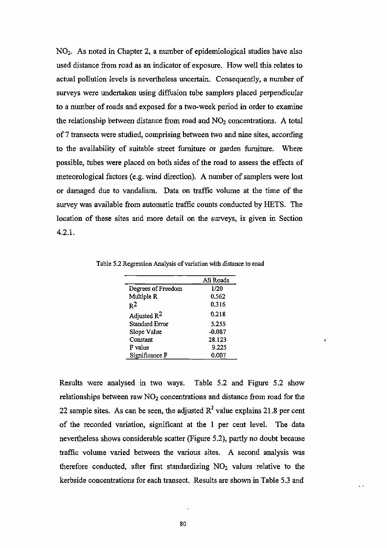
NO2. As noted in Chapter 2, a number of epidemiological studies have also

used distance from road as an indicator of exposure. How well this relates to

actual pollution levels is nevertheless uncertain. Consequently, a number of

surveys were undertaken using diffusion tube samplers placed perpendicular

to a number of roads and exposed for a two-week period in order to examine

the relationship between distance from road and NO 2 concentrations. A total

of 7 transects were studied, comprising between two and nine sites, according

to the availability of suitable street furniture or garden furniture. Where

possible, tubes were placed on both sides of the road to assess the effects of

meteorological factors (e.g. wind direction). A number of samplers were lost

or damaged due to vandalism. Data on traffic volume at the time of the

survey was available from automatic traffic counts conducted by BETS. The

location of these sites and more detail on the surveys, is given in Section

4.2.1.

Table 5.2 Regression Analysis of variation with distance to road

All RoadsDegrees of Freedom 1/20Multiple R 0.562

R2 0.316

Adjusted R2 0.218

Standard Error 5.255Slope Value -0.087Constant 28.123F value 9.225Significance F 0.007

Results were analysed in two ways. Table 5.2 and Figure 5.2 show

relationships between raw NO 2 concentrations and distance from road for the

22 sample sites. As can be seen, the adjusted R 2 value explains 21.8 per cent

of the recorded variation, significant at the 1 per cent level. The data

nevertheless shows considerable scatter (Figure 5.2), partly no doubt because

traffic volume varied between the various sites. A second analysis was

therefore conducted, after first standardizing NO 2 values relative to the

kerbside concentrations for each transect. Results are shown in Table 5.3 and

80

40

30

10

0 20 40 I60 80 100 120 140 160Rsq = 0.3156

Figure 5.2 Relationship Between NO2 Concentrations

And Receptor Distance to Road

•

• II

▪ • .20 -

Distance to Road (m)

Figure 5.3 Regression analysis of Standardised

NO2 Concentrations and Receptor Distance from Road11 0 -

U

Rsq = 0.35400 20 40 60 80 100 120 140 160

Distance to Road (m)

81

Figure 5.3. The linear model gave a slight improvement in the adjusted R2

value (R2 = 32.2 per cent, significant at the 1 per cent level). Further analysis

of the data indicated that a better fit was obtained using a logarithmic model

(adjusted R2 value = 56.0 per cent, significant at the 0.001 level). Results are

shown in Table 5.3 and Figure 5.4.

From the results it is clear that NO 2 concentrations decrease rapidly within

the first 40 metres from the road. Concentrations then appear to tail off at

approximately 60 metres from the road, at which point it may be assumed

that background concentrations have been achieved and therefore the

influence of road traffic on pollution levels is minimal (see Figure 5.2). The

remaining 44.1 per cent unexplained variation may again reflect the influence

of non-road source emissions, topographical factors and meteorological

conditions as explained in the previous section.

Table 5.3 Standardized regression analysis of variation with distance to road

Linear LogDegrees of Freedom 1/20 1/20Multiple R 0.595 0.761

R2 0.354 0.580

Adjusted R2 0.322 0.559

Standard Error 14.437 11.645Slope Value -0.261 -7.793Constant 90.920 102.056F value 10.961 27.590Significance F 0.004 0.000

The results were presented in both the raw and standardized format as it was

felt important to examine the effect that standardization has on the data, as

most epidemiological studies use unstandardised distance to road / NO 2 as a

proxy variable for air pollution and therefore may not be presenting a true

picture of the relationship between air pollution and respiratory health.

Overall, the results indicate that, despite the effects of variation in site

characteristics and traffic volume, physical distance to vehicular emission

sources is a meaningful predictor of NO2 concentrations.

82

n0

In

.

'Tr

rn

CA

—

-o

tna)i..,0tA.,-,

4-1

..,1CD.--.

I

CDC

I

CDON

I

C00

I

CDr---

1

CDVJ

CDkr)

(Eu1/2n) ZON POSIgrePuulS

83

5.2.3 VARIATION ATTRIBUTABLE TO LAND COVER

Whilst factors such as road traffic volume and distance from road clearly

account for much of the spatial variation in air pollution, they are unlikely to

provide a complete explanation of pollution patterns at the small-area scale.

Important variation may also occur as a result of the effects of emissions from

non-rural sources, and due to the effects of buildings and vegetation and

dispersion processes. Both these effects may be expected to relate to patterns

of land cover and usage. In order to investigate these effects a land cover

map (1:10,000) was created from the interpretation of detailed (1:5,000)

aerial photographs. Originally, 20 classes of land cover were used ranging

from high density commercial land cover to moorland (See Appendix 5 for

full classification). The number of categories was later reduced owing to the

fact that some groupings did not have enough sample sites to make them

statistically significant, nor did they contribute to explaining pollution levels

(e.g. there was felt to be very little difference between heathland and

grassland).

Once the classifications had been determined, pollution data from the 80 core

sites in the routine surveys (S2, S3 and S4) and the annual average were used

(as four separate data sets) to examine the effects of land cover on patterns of

NO2 variation. Land classification for each site was obtained in the field and

cross-checked with the land classification map. A more detailed explanation

of this procedure and the sampling regime is explained in Section 4.1.

Analysis of the data was conducted in SPSS statistical package. Data were

analyzed at three different levels of classification as follows:

• Degree of urbanization

• DETR site type classification

• Land cover

84

a) Degree of urbanization. Data from the routine pollution surveys was

initially classified into 3 broad categories, reflecting the level of urbanization:

• Urban More than 70 per cent of land surrounding thesample site is occupied by buildings.

• Suburban Between 20-69 per cent of land surrounding thesample site is occupied by buildings.

• Rural Less than 20 per cent of land surrounding thesample site is occupied by buildings.

The extent to which NO2 levels varied in relation to these land cover

categories was then investigated for the three surveys (S2, S3 and S4) and the

annual average (see Table 5.4). Further investigation was undertaken using

Analysis of Variance in SPSS and the results are shown in Table 5.5 and

Figure 5.5.

Table 5.4 Summary statistics for NO2 (j2g/m3) variation by the degree of urbanisation

Group Survey No of Minimum Maximum Mean S.D.Number Cases

UrbanS2 23 37.06 78.5 55.4 8.6S3 23 18.7 51.5 32.9 8.5S4 23 27.1 69.4 44.7 10.9Am 23 25.6 57.6 41.5 7.7

SuburbanS2 50 27.7 66.6 45.0 9.1S3 50 9.5 42.7 22.8 7.8S4 50 15.7 52.3 28.7 9.8Am 50 17.8 46.9 29.8 7.6

RuralS2 7 31.3 50.0 39.3 6.5S3 7 12.2 49.0 23.0 12.2S4 7 15.6 54.7 25.9 13.4Am 7 20.3 52.9 28.2 11.4

The results indicate that significant differences in pollution levels do occur

between the three groups, with mean concentrations consistently being

highest in the urban areas, intermediate levels in the suburban 'areas and

85

Annual Average

7

3

Survey S2

Survey S3

Survey S4

70

60 -

50

40

30 -

20 1

10

Urban Rural

ISurvey S2

Survey S3

Kerbside

60

50

30 -

20

10

Survey S40

Annual Average

Figure 5.5 Mean and Standard Deviation of the

Degree of Urbanisation

Degree of Urbanisation

Figure 5.6 Mean and Standard Deviation of the

DETR classification

DETR Site Type Classification

86

lowest in the rural areas (see Figure 5.5). This clearly matches expectations,

and largely reflects the distribution of road sources and traffic emissions in

these three zones. What is perhaps more surprising is that within group

variation still accounts for the large majority of variation in the measured data

- from 65.5 per cent in S4 to 77 per cent in survey S3. The implication is that

considerable small area variation occurs within each of these land cover

zones.

Table 5.5 Analysis of variance for degree of urbanization.

D.F. Sum ofSquare

Mean ofSquare

F Sig. of F %

Survey S2 Between Group 2 1925.033 962.517 12.349 0.000 27.23

Within Group 66 5144.423 77.946 72.77Total 68 7069.457




Within Group 77 8409.625 109.216 65.49Total 79 12840.72%

Annual Between Group 2 2327.761 1163.881 18.329 0.000 22.30Average Within Group 77 4889.145 63.499 67.7

Total 79 7217.145

b) DETR site type classification. In order to further investigate the effects

of broad-scale variation in land cover further, a second classification, based

broadly on the Department of the Environment, Transport and the Regions'

classification for the siting of NO 2 continuous monitors was devised as

follows:

• Kerbside Within 20m of an emission source, ineither a rural or urban location.

• Urban background

Within an urban (built-up) conurbation,not less than 20m from the nearestemission source.

87

• Rural background

Excluding urban conurbations andat a distance of more than 20mfrom the nearest emission source.

Once classified, the data for the 80 core sites was transferred into the SPSS

statistical package and summary statistics calculated (see Table 5.6). Oneway

Analysis of Variance was then conducted. The results are shown in Table 5.7

and Figure 5.6.

The results indicate that kerbside sites had the highest concentration in all

three surveys, and for the annual average (ranging from 30.5 for S3 to 53.4

tig/m3 for S2). The urban background sites for all surveys were consistently

lower than the kerbside sites (21.2 to 43.3 gg/m 3) but higher than the rural

background sites (19.1 to 37.4gg/m3). This is expressed clearly in Figure 5.6.

Examination of the results of the Oneway Analysis of Variance shows that

these differences are statistically significant but that most of the variation

occurring in the surveys was again within groups as opposed to between

groups: between group variation accounts for between 26.8 and 46.8 per cent

of the total recorded variation (Survey S3 and S4).

Table 5.6 Summary statistics for NO2 (.g/m3) variation by DETR classification

Group SurveyNumber

No ofCases

Minimum Maximum Mean S.D.

KerbsideS2S3S4Am

41414141

37.010.119.622.4

78.551.569.457.6

53.430.541.539.0

9.39.611.58.6

Urban backgroundS2 31 27.7 56.8 43.3 8.2S3 31 9.5 33.3 21.2 6.4S4 31 15.7 46.6 25.0 6.3Am 31 17.8 41.0 27.4 5.5

Rural backgroundS2 8 31.3 42.0 37.4 3.6S3 8 12.2 33.8 19.1 7.0S4 8 15.6 37.6 21.5 7.1Am 8 20.3 38.6 . 24.5 6.0

88

Table 5.7 Oneway Analysis of Variance for distance to emission source.

D.F. Sum ofSquare

Mean ofSquare

F Ratio Sig. of F %







Annual Between Group 4 1207.156 301.789 3.767 0.007 16.7Average


c) Local Area Land Cover. The preceding analysis indicated that broad-

scale variation in pollution levels in the study reflects the underlying patterns

of land cover and site types. Much of the variation inherent in the pollution

data nevertheless remains unexplained. Much of this may be expected to be a

result of local land cover effects, especially in urban areas. These were,

therefore, further investigated using data from the three surveys and the

annual average results. Sites were first selected and divided into five classes,

reflecting differences in intensity of land cover (Table 5.8). Summary

statistics were calculated for each survey and the results collated in Table 5.9.

Differences in levels of NO 2 across these classes were then analysed using

Oneway Analysis of Variance in SPSS. Results are shown in Table 5.10 and

Figure 5.7.

89

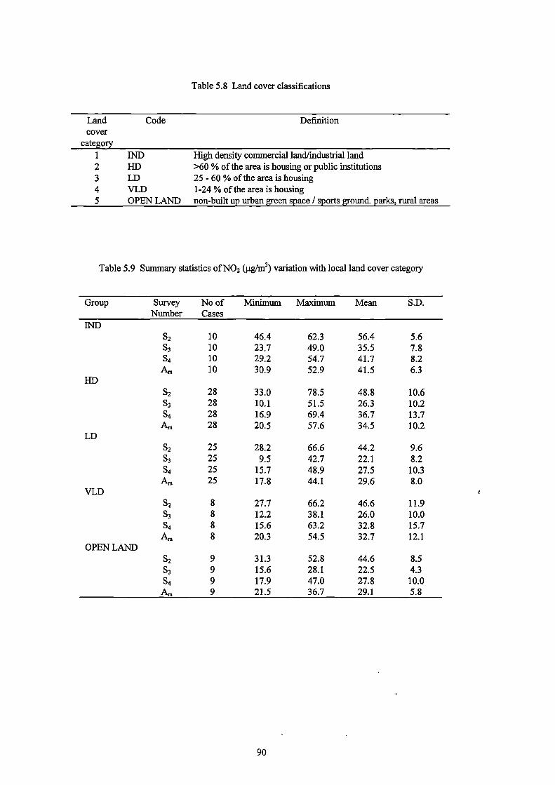
Table 5.8 Land cover classifications

Landcover

category

Code Definition

1 IND High density commercial land/industrial land2 HD >60 % of the area is housing or public institutions3 LD 25 - 60 % of the area is housing4 VLD 1-24 % of the area is housing5 OPEN LAND non-built up urban oven space / sports ground. parks, rural areas

Table 5.9 Summary statistics of NO2 (pg/m3) variation with local land cover category

Group Survey No of Minimum Maximum Mean S.D.Number Cases

INDS2 10 46.4 62.3 56.4 5.6S3 10 23.7 49.0 35.5 7.8S4 1 0 29.2 54.7 41.7 8.2

Am 10 30.9 52.9 41.5 6.3HD

52 28 33.0 78.5 48.8 10.6S3 28 10.1 51.5 26.3 10.2S4 28 16.9 69.4 36.7 13.7

Am 28 20.5 57.6 34.5 10.2LD

S2 25 28.2 66.6 44.2 9.6S3 25 9.5 42.7 22.1 8.2S4 25 15.7 48.9 27.5 10.3

Am 25 17.8 44.1 29.6 8.0VLD

S2 8 27.7 66.2 46.6 11.9S3 8 12.2 38.1 26.0 10.0S4 8 15.6 63.2 32.8 15.7Am 8 20.3 54.5 32.7 12.1

OPEN LANDS2 9 31.3 52.8 44.6 8.5S3 9 15.6 28.1 22.5 4.3S4 9 17.9 47.0 27.8 10.0Am 9 21.5 36.7 29.1 5.8

90

I— 1

0

Es,

NVD V) C/)

fli>,

ai

EV) V) V)

I-10 HH

(cuy2n) suogeguaouoj zoN

91

Table 5.10 Analysis of Variance attributed to land cover at the small scale

D.F. Sum ofSquare

Mean ofSquare

F Ratio Sig. of F %







Annual Between Group 2 3062.783 1531.392 28.384 0.000 42.40Average


The summary statistics indicate that levels of NO 2 for all surveys decrease in

the first three groups (see Figure 5.7). Mean concentrations are highest in the

industrial zone for all surveys (33.5 to 56.2 Kg./m3). Levels then decrease

with high density housing (26.3 to 48.8 gg./m3) and a further fall is noted in

the low density housing land cover group (22.1 to 44.2 gg./m3).

Concentrations recorded in the open land category are similar to those

recorded in low density housing group although the standard deviation is

smaller. Concentrations recorded in the very low density housing group are

higher than those recorded within low density housing cover. This may be

due to the historical land cover patterns of the study area, as many large

houses were built to accommodate mill owners on roads which have now

become busy dual carrageways.

Results of the Oneway Analysis of Variance indicate that, for all three

surveys and the annual average data, the majority of the variation in NO2

concentrations occurs within the land cover groups (ranging from 53 — 57 per

cent in S4 and the annual mean, to 84 - 86 per cent in surveys S2 S3).

Nevertheless, differences between land cover classes are significant at the

92

0.001 per cent level for all surveys except survey S2, and for the annual mean.

More detailed comparisons between the five land cover classes using the

annual average data (see Table 5.11) show that most of this variation occurs

in land cover class 1 (Industry). This is significantly different (at the 0.05 per

cent level) from all other land cover classes except 4 (very low density

housing). Otherwise, none of the land cover groups differ from each other at

the 0.05 significance level.

Table 5.11 Correlation analysis significance values for local area land cover

Groups 1 2 3 4 51 0.019 0.000 0.094 0.0002 0.019 0.056 0.711 0.0583 0.000 0.056 0.509 0.8354 0.094 0.711 0.509 0.4535 0.000 0.058 0.835 0.453

In conclusion, the results of the analysis indicate that most of the variation in

NO2 concentrations occurs within land cover groups, whichever the system

used. Relatively little variation occurs between the groups. The only

exception to this are the results using the local area land cover results for

surveys S4 and Am where between-group variation accounted for 46.8 and

42.4 per cent of the total variation respectively. Overall, therefore, the

influence of land cover on patterns and magnitude of pollutant dispersion is

small, most of the variation occurring at scales below that of the land cover

class. This may be the result of factors such as traffic volume and local

topographic conditions, which cannot entirely be controlled. These results

are again a reminder that the use of land cover as a proxy for air pollution

levels, as used in some epidemiological studies (see Table 2.2), is of only

limited validity.

93

5.2.4 VARIATION ATTRIBUTABLE TO ALTITUDE

As noted in Chapter 3, the study area comprises a complex terrain, with a

series of relatively deep valleys dissecting the plateau margins of the

Pennines. These variations in altitude may be expected to affect pollution

patterns in a number of ways. Historically, they have acted to influence the

distribution of settlements, industry and infrastructure in the area and thus

have exerted a major control on the patterns of emission sources. The pattern

of relief also affects local weather conditions, with sheltered areas,

characterized by frequent inversions, in the valley floors, and with exposed

areas with high average wind speeds in the hilltops. At the same time, it is

likely that the higher areas in the west of the region are more affected by

long-range transport from the Manchester Metropolitan area. Together,

therefore, these effects are expected to be reflected in the pattern of pollution

across the area.

These effects were investigated using concentration data from the 80 core

sites used in the routine surveys (S 2 S3 and S4) and from the annual mean

adjusted for missing values (A.). Initially all core data sites were examined

Subsequent analyses were conducted on sites classed as rural or urban

background only, in order to remove the confounding effects of nearby

emission sources. Corresponding heights in metres above OD for each

sample site were calculated using a Digital Terrain Model (DTM) and cross-

checked against data from 1:10,000 OS maps of the area. The information

was entered into the SPSS statistical package and descriptive statistical

techniques conducted (Table 5.12).

Table 5.12 Altitudinal survey statistics (mA0D)

Altitude No of Cases Min Max Mean S.D.S2 80 45 455 153.49 68.32S3 80 45 475 155.23 74.54S4 80 45 475 158.11 78.81

Am 80 45 475 158.11 78.81

94

The summary statistics indicated that sampling in all surveys had been

conducted across a similar range of altitudes, but that there was significant

variation with height within each survey. After examination of the data in

graphical format (see Figure 5.8), curvilinear regression analysis was

conducted. The results are shown in Table 5.13 and Figure 5.9.

Table 5.13 Regression analysis (r2 values) of the effects of altitude on NO2 concentrations

(All sites)

S2 S3 54 Am

Degrees of Freedom 1/67 1/74 1/78 1/78Linear 0.227 0.207 0.136 0.205Logarithmic 0.244 0.276 0.169 0.257Inverse 0.209 0.293 0.170 0.261Quadratic 0.247 0.274 0.168 0.251Cubic 0.251 0.302 0.180 0.278Compound 0.244 0.197 0.146 0.215Power 0.254 0.254 0.177 0.259S 0.215 0.259 0.172 0.253Growth 0.244 0.197 0.146 0.215Exponential 0.244 0.197 0.146 0.215Logistic 0.244 0.197 0.146 0.215

Results of the analysis indicate that the relationship between NO2

concentrations and altitude is not linear and can best be explained by using

either a cubic or power equation. The power equation explains 25.4 and 17.7

per cent of the variation in NO2 concentrations for surveys S2 and S4

respectively. Surveys S2 and A. are best explained using a cubic equation

(30.2 and 27.8 per cent respectively). The influence of factors such as the

distance of the sample site to a road, vehicle volume and land cover,

however, may distort the relationship between NO2 concentrations and

altitude. Consequently the analysis was rerun using only sites not classed as

urban sites according to the DETR classification used in the previous section

(See Figure 5.10). Non-urban results for the curvilinear analysis are shown in

Table 5.14 and Figure 5.11. The subsequent analysis indicates that inverse,

cubic and compound equations provide the most accurate explanation of NO2

concentrations in this case (explaining between 8.4 and 13.4 percent of the

95

40

30

20-

10

0

•

100

200

300

400

500

• Observed

Linear

Cubic

Power


a

oz

a

c-)

60

50

40

30

20

10

•

•

•

•

•••• •

••

•

•

• a • •

•:

• p

a•

.

•

•

•

•••

111

•

• •

• • Ii•

•

and Altitude

• • •

••

••

• "•

•

0 100 200 300 400 500

Altitude (m)

Figure 5.9 Selected Curvilinear Relationships Between

NO2 Concentrations and Altitude

Altitude (m)

96

Observed

Inverse

Cubic

Compound


and Altitude by DETR Landclass60

50 -

.. .

40. .. .

. •

II '.

• •. a

30

.a

. •

. ..

mI

.

.1

.

• xi. •• .. • • .

20

: •UI

•• •I

isDETR Classification

r3 Rural Background

• Urban Background

10 • Kerbside

0 100 200 300 400 500

Altitude (m)

Figure 5.11 Selected Curvilinear Relationships Between NO2

Concentrations and Altitude - Non Kerbside Sites Only

100 200 300 400 500

Altitude (m)

97

variation for surveys S4 and Ain respectively). The outcome of the analysis

indicates that the removal of the urban locations does not improve the

overall explanation of the relationship between NO 2 concentrations and

altitude. By using all sites between 17.7 and 30.2 per cent of the variation in

NO2 can be explained by altitude. This suggests that, although altitude does

explain a significant amount of variation in NO2, this relationship is not

straightforward. Indeed, it seems likely that much of the apparent altitudinal

effect on levels of air pollution is indirect, through the influence of altitude on

land cover and the distribution of emission sources.

Table 5.14 Regression analysis(r 2 values) of the effects of altitude on NO2 concentrations

(Non urban sites)

S2 S3 S4 A.

Degrees of Freedom 1/47 1/53 1/55 1/55Linear 0.103 0.080 0.032 0.072Logarithmic 0.103 0.115 0.053 0.102Inverse 0.087 0.138 0.074 0.125Quadratic 0.104 0.106 0.044 0.085Cubic 0.112 0.131 0.084 0.134Compound 0.118 0.073 0.037 0.080Power 0.115 0.102 0.054 0.104S 0.095 0.114 0.069 0.118Growth 0.118 0.073 0.037 0.080Exponential 0.118 0.073 0.037 0.080Logistic 0.118 0.073 0.037 0.080

5.2.5 POLLUTANT VARIATION WITH VERTICAL DISTANCE

Several previous studies (e.g. Loxen and Noordally 1987; Loxen et al. 1988;

den Tonkelaar et al. 1987) have shown that NO2 concentrations typically

decline with height above ground, as a result of the effects of dispersion,

deposition and atmospheric chemical reactions. Nevertheless, the importance

of sampling height as a component of urban air pollution variation has not

been extensively studied. This source of variation was examined here by

conducting a number of surveys, during which diffusion tubes were placed at

98

regular vertical intervals on the outside of tall buildings within the study area.

Buildings over five stories were chosen to maximize the possible number of

sites at each location. Four buildings within the study area were considered

suitable, and between 7 and 9 samplers were used at each site. At each site,

tubes were exposed for a two-week period. Details are given in section 4.2.2.

Data were entered into SPSS, and relationships between sampler height and

concentrations analyzed using curvilinear regression analysis. The results are

shown in Table 5.15 and Figures 5.12 to 5.15.

Table 5.15 Curvilinear Regression Analysis of Variation with Vertical Distance (R2 values)

Oldgate House University of TechnicalHuddersfield College

St PetersHouse

Number of Floors 8 9 7 9Degrees of Freedom 1/7 1/8 1/6 1/8Linear 0.335 0.744 0.886 0.565Logarithmic 0.467 0.821 0.979 0.784Inverse 0.600 0.771 0.924 0.910Quadratic 0.393 0.763 0.955 0.731Cubic 0.563 0.971 0.977 0.894Compound 0.335 0.741 0.934 0.594Power 0.455 0.760 0.976 0.794

0.572 0.670 0.871 0.890Growth 0.335 0.741 0.934 0.594Exponential 0.335 0.741 0.934 0.594Logistic 0.335 0.741 0.934 0.594

As can be seen, trends with height are generally curvilinear, and are variously

described by cubic, inverse or logarithmic models (with R2 values of between

0.910 and 0.979 for three of the four buildings). The exception is Oldgate

House for which the R2 value is relatively low (R2 value of 0.600):

concentrations around the building may have been affected by the emissions

from vehicles on the nearby inner ringroad and the associated traffic-

generated turbulence.

In order to analyse the data collectively, concentrations for each of the

buildings were first standardised relative to the ground level value. The

results of this analysis can be seen in Table 5.16 and Figure 5.16.

99

'2.0 3.6 6.0 8.4 10.8 13.2 15.6 18.0 20.4 22.8

20

22 -

3.6

Figure 5.12 Relationship Between NO2 Concentrations and Height

(Oldgate House)32

30 -

Height Above Ground Level (m)


(The University of Huddersfield)50 -

40 -

30 -

20 -I

10I I

6:0 8.4 10.8 13.2 15.6 18.0 20.4 22.8


100

(Technical College)

50

•2.0 3.6 6.0 8.4 10.8 13.2 15.6 18.0 20.4 22.8

20

, , ,2.0 3:6 6.0 8.4 10.8 13.2 15.6 18.0 20.4 22.8


101

34

32

30

28

26

24

20




(St Peters House)

00 r--

0

on

(Etui2n) uopenuaouop zoN pasmiepuels

102

Table 5.16 Standardised Curvilinear Regression Analysis of Variation with Vertical Distance(R2 values)

All verticalheight data

Degrees of Freedom 1/35Linear 0.426Logarithmic 0.388Inverse 0.343Quadratic 0.481Cubic 0.483Compound 0.416Power 0.384

0.344Growth 0.416Exponential 0.416Logistic 0.416

Various regression models were then used on all the data, and interestingly,

linear, cubic and quadratic models provided the best fit, accounting for ca. 42

to 48 per cent of the variation in NO2 concentrations. Overall, although it

tends to provide a slightly lower concentration in some cases, the linear

model may be considered an adequate fit, given its simpler form. Model

parameters for this are as follows:

NO2 (as a percentage of ground level concentrations) = 5.333 + (Height above ground Level * 0.426)

5.2.6 VARIATION IN MEASUREMENT AND SAMPLING ERROR

In order to examine the effect of possible errors from laboratory and field

procedures, the amount of nitrogen dioxide recorded in the blank tubes was

assessed. Measurements from the blanks tubes for the three centres in the

SAVIAH study using diffusion tubes were analyzed and tested for deviation

from zero. Results are shown in Table 5.17.

103

Table 5.17 Comparison of laboratory and field blank accuracy

Centre

Lab Blank (Rg/m3) Field Blank (pg/m3) pValue

Mean S.D. Mean S.D.Huddersfield, UK 0.472 0.254 0.297 0.042 0.264Amsterdam, NL 0.355 0.042 0.399 0.149 0.430Prague, CZ 0.287 0.069 0.615 0.306 0.028

These results indicate that, for all centres, the amount of measured nitrogen

dioxide was very small (i.e. below 1 gg/m 3) in both field and laboratory

blanks. The standard deviation of the tubes was also very small.

Contamination of the tubes, and thus errors induced by either laboratory or

field procedures, can be consequently considered to be negligible.

A second way of examining the error effect is by comparing results for tubes

at each site in the routine surveys. For two surveys (S 3 and S4) duplicate

tubes were placed at each of the routine and variable sample sites (see section

4.1). Comparability between the duplicates was assessed for these surveys by

examining the correlation between each of pair of tubes. Results are shown

graphically in Figure 5.17 to 5.18. These graphs show that there is very good

correlation between the data at a site with the slope values almost at unity (R2

values of 83 and 93 per cent for surveys S3 and S4 respectively), thus

indicating that the error effect is small. Further investigation was conducted

using Oneway analysis of variance. Results of this analysis is shown in Table

5.18.

Results of the Oneway analysis of variance indicated that approximately 96

and 98 per cent of the variation (recorded in surveys S3 and S4 respectively)

occurred between the sites with only 4.2 and 1.7 per cent variation at a site

(i.e. between two tubes at a site). These results indicate that less than 5 per

104

a0

a

a

Figure 5.17 Comparison of NO2 concentrations at a site

60

50

40

30

20

10

•

•

(Survey S3)

•

• 4m

I.•

•• 'h.a.%

14,26 •• •giA

•

7".4

VRsq = 0.8348

1020 30 40 50 60

NO2 concentrations (ug/m3)

Figure 5.18 Comparison of NO2 concentrations at a site

70 -

60 -

50 -

40 -

30 -

20 -

10

116

11‘.

.% •Nei •

I:s.

•I.

16,•de

(Survey S4)

aI

• •

Rsq = 0.9334

10 20 310 40 50 60 70 , 80

NO2 concentration (ug/m3)

105

cent of the recorded variation can be attributed to the error effect — i.e.

sampling and measurement error. Further decomposition of this source of

variation is not possible in this analysis due to the sampling techniques used.

For the purposes of this study, however, such variation can be considered

negligible.

Table 5.18 One-way Analysis of Variance of the error effect

Sum of D.F. Mean of F Sig. of %Square Square

Survey S3 Between-site 13181.213 75 175.750 21.979 0.0000 95.8variation

At-Site variation 583.715 73 7.996 4.2

Total 13764.928 148

Survey S4 Between-site 25513.105 79 322.951 56.497 0.0000 98.3variation

At-site variation 445.870 78 5.716 1.7

Total 25958.975 157

5.2.7 SPATIAL AND TEMPORAL VARIATION

The preliminary analysis of the sources of variation in NO 2 concentrations in

the study area, reported in the previous sections of this chapter, indicated that

a large proportion (ca. 40 per cent) of the total variation in pollution levels

could be attributed to temporal effects. These temporal effects suggested that

further investigation was necessary for a number of reasons. Firstly, there

was the question of whether the temporal variation discerned in the data can

be explained in terms of seasonal or meteorological factors. Secondly, there

was the question of the spatial character of the temporal variations. For

example, is the spatial variation spread evenly across the area or concentrated

in a few sites: in other words, do some sites vary over time while others

106

remain constant? Alternatively, do different types of site show distinctive

patterns of temporal variation, as implied by the recognition of so-called 'air

pollution affmity areas' (McGregor 1996). The following investigations

attempt to address these questions.

5.2.8 TEMPORAL VAIUATION

The analysis of spatial patterns of variation in NO 2 concentrations in the

study area, reported in the previous section, has shown that considerable

small area variation occurs in pollution levels, related to factors such as

traffic volume, landcover and altitude. As noted earlier, however, this is not

the only source of variation. Significant temporal variation may also be

expected, as a result of meteorological and seasonal effects.

With the available data, it is not possible to examine short-term variations in

the study area. Results for the routine surveys can, however, be used to

examine variation at the seasonal scale (between-surveys).

Temporal patterns in the data were analysied by comparing measured

concentrations at each of the 80 core sites, between surveys, using regression

analysis. In this way it was possible to determine to what extent patterns of

pollution remain broadly the same over time - i.e. whether concentrations at

that site at one time help to predict concentrations at that site at a later time

(temporal auto-correlation). Survey S5 was not used in this analysis as S5 was

not a routine survey and did not contain the core sites and therefore was not

directly comparable. Results are shown in Table 5.19 and Figures 5.19 to

5.21.

The results demonstrate that patterns of pollution are broadly stable.

Adjusted R2 values between surveys are between 58.1 and 69.4 per cent, with

standard errors of 5.4 to 8.3 Rg/m3. Slope coefficients between surveys S2

107

V_ z• • NV

• z• • .„./ •

• . • . • • •• .rzz"

•••

• •ieasse

• •N.

Rsq = 0.56960

Figure 5.19 Comparison of NO2 Concentrations

Between Surveys - (S2 and S3)80

0

40 60 80

Survey S3 NO2 Concentrations (ug/m3)

Figure 5.20 Comparison of NO2 Concentrations

Between Surveys - (S3 and S4)

•

70

60

50

40

30

20

10

0

....„-- ..------ --

....,,-----

4

It

• ma

14 •U

e •

S

• •N %

las ••.• • le•

e.

s a,

.

••

•• e

a

•

•

•

1

•

.1:1 •

Rsq = 0.5228

10 20 30 40 510 60 70

Survey S4 NO2 Concentrations (ug/m3)

108

•

•

•••••

a

•

•

c>oo N n4::) kr) re-)

(Euy2n) suoggivaaouop zoN Zs Aaiuns

109

and S4, and surveys S3 and S4 are close to unity, though the constants vary,

indicating that while absolute levels of pollution may vary from one survey to

another, the inter-site differences remains broadly the same. For survey S2

versus survey S3, the slope coefficient is flatter, reflecting the relatively lower

concentrations in the latter survey.

Table 5.19 Regression analysis of data stability

S2 V S3 S3 V S4 S4 V S2

Degrees of Freedom 1/74 1/79 1/77Multiple R 0.7621 0.7659 0.8329R2 0.5808 0.5866 0.6937Adjusted R2 0.5751 0.5832 0.6898Standard Error 5.3788 8.3019 7.1904Slope Value 0.6217 1.0061 1.0400Constant -4.8179 -6.6718 -16.7806F Value 102.5295 171.6903 174.4068Significance F 0.0000 0.0000 0.0000

5.2.9 SPATIO-TEMPORAL VARIATION

The previous section has shown that many factors contribute to variation in

air pollution levels in the study area, including spatial, temporal and error

components. In order to estimate the relative contribution of all these

components to variation in NO2 concentrations, oneway analysis of variation

was conducted on the 80 core sample sites. Data for surveys S2, S3 and S4

only were used in this analysis. The outcome of the analysis is show in

tabular format in Table 5.20.

Table 5.20 Spatio-temporal Oneway Analysis of Variance

Sum ofSquare

D.F. Mean ofSquare

F Sig. of F %

Main effect 37459.843 81 462.467 16.248 0.000 85.40Spatial effect 33319.183 79 429.480 14.817 0.000 88.95Temporal effect 3529.538 1 3529.538 124.001 0.000 9.42Error effect 3.864 1 3.864 0.136 0.713 0.01

Explained 37459.843 81 462.467 16.248 0.000 85.40Interaction effect 6404.368 225 28.464 14.60Total 43864.211 306 143.347 100.0

110

As these results show, 85.4 per cent of the variation can be explained by

spatial, temporal and error effect acting independently. Only a small

percentage, 0.01 per cent is attributable to variation between duplicates,

reinforcing the view that this in an unimportant source of variation in the data

(as stated in section 5.1.3). Temporal variation accounts for 9.42 per cent of

the explained variation, while spatial (between-site) variation accounts for

88.9 per cent of the total explained variation. From these results, it is

apparent that the most significant component of variation is the spatial effect.

Temporal variation represents only a relatively small contribution to the total

(<10%), while the effects of measurement and sampling error is negligible.

As stated in section 5.1, however, the dispersion and emission patterns of air

pollution vary over time and space in a complex, three dimensional way. The

interaction between spatial and temporal variation and the effects of

measurement error were thus found to explain 14.6 per cent of the recorded

variation.

5.2.10 TEMPORAL 'AFFINITY AREAS'

The concept of air pollution 'affinity areas' was evolved recently by

McGregor (1996). Using data from 15 fixed site monitoring stations in

Birmingham, he showed that groups of sites could be discerned which

showed similar temporal patterns of air pollution, yet differed from other

groups. These groups were defined as affinity areas. Recognition of affinity

areas in this way has considerable implications, for it provides a basis on

which to judge the representativeness of fixed-site monitoring stations, to

plan monitoring campaigns and to extrapolate from monitoring sites to wider

areas. The monitoring carried out as part of the current study was insufficient

for identifying affinity areas: data at core sites were available for too few

locations. Monitoring carried out by Kirklees M.C., however, are appropriate

for this purpose. Kirklees Scientific Services have been conducting surveys

since 1992 at 20-30 sites, using passive diffusion tubes deployed on a

111

monthly basis. A number of sites have been relocated on several occasions,

and problems of vandalism have resulted in some gaps in the coverage so a

full set of data for the whole period was not available. More or less complete

data do exist, however, for 25 sites, covering the period from 1992 to 1995.

These were kindly made available by Andrew Sheard of the Scientific

Services.

In order to investigate whether there was a quantifiable pattern in the

behaviour of the sites (i.e. whether pollution levels at the sites vary

concordantly), factor analysis was conducted on the data. Factor analysis

assumes that variation within the data set can be represented as a linear

combination of a smaller number of index variables, plus the residuals, which

reflect the extent to which they are independent of the other variables

(Chapman and Collins 1995; Manly 1994). By representing cases (i.e. sites)

as variables and measurement events (i.e. survey periods) as cases, Q mode

Factor Analysis allows the 25 sites included in the Kirklees data to be

grouped into a smaller number of 'site types'. Factor analysis was therefore

undertaken in SPSS. Results of the analysis are shown in Tables 5.21 to 5.23.

As Table 5.21 indicates, three main factors were identified, the first of which

explained 67.1 per cent of the communal variation in pollution concentrations

in the data. The second and third factors explained 15.5 and 9.8 per cent of

the communal variation respectively. Factor analysis using only three factors

thus explained 92.4 per cent of the communal variation in pollution patterns

in the data, leaving only 7.6 per cent of the variation to be explained by the

remaining 22 factors. Following the procedures recommended by Chatfield

and Collins (1995), these additional factors were rejected, since all had

eigenvalues of less than 1. The importance, or weighting of each factor for

each site, was tested in Table 5.22 and is summarised in Table 5.23.

112

Table 5.21 Final Statistics of Factor Analysis

Factor Eigenvalue Pct of Variance Cumulative Percentage1 16.783 67.1 67.12 3.885 15.5 82.73 2.442 9.8 92.44 0.944 3.8 96.25 0.849 3.4 99.66 0.553 2.2 100.07 0.426 1.7 100.08 0.328 1.3 100.09 0.206 0.8 100.010 0.114 0.5 100.011 0.100 0.4 100.012 0.069 0.3 100.013 0.049 0.2 100.014 0.028 0.1 100.015 0.021 0.1 100.016 0.008 0.0 100.017 0.004 0.0 100.018 -0.002 -0.0 100.019 -0.003 -0.0 100.020 -0.033 -0.1 99.821 -0.058 -0.2 99.622 -0.134 -0.5 99.123 -0.193 -0.8 98.324 -0.300 -1.2 97.125 -1.080 -4.3 100.0

From the tables (Table 5.22 and 5.23) it is apparent that the majority of the

sites are heavily loaded on factor 1; only two sites loaded heavily on factor 2

and three sites loaded on factor 3. Further investigation of the data indicates

that there is some degree of coherence within these groups in terms of site

characteristics. Group 3 contains only residential sites in out of town or

pedestrian areas. Group 2, although accounting for only 2 sites, depicted sites

within suburban town centers. Sites within group 1 were less homogeneous.

Core members of this group, with the highest loading on factor 1, comprised

busy town centre sites (sites 11,8, 13, 12, 23 and 14). As loadings on factor 1

fall, however, the sites become progressively more residential in character,

and sites 10, 19 and 16 all of which are relative marginal members of the

group, relate to less busy, residential locations.

113

Table 5.22 Factor Matrix

Grouping Site No Factor 1 Factor 2 Factor 3 One 11 0.983 -0.179 -0.026

08 0.977 -0.217 0.08713 0.967 -0.064 0.01512 0.965 0.163 0.04023 0.963 -0.190 -0.65914 0.962 -0.020 -0.08528 0.942 0.148 -0.29627 0.885 0.175 -0.00909 0.879 -0.293 0.11602 0.870 0.231 -0.26907 0.864 0.261 0.24826 0.860 0.152 0.05517 0.841 0.113 0.29321 0.829 0.312 0.10124 0.770 -0.624 0.07103 0.723 0.364 0.49905 0.714 0.492 -0.26210 0.694 0.186 0.38419 0.616 -0.198 0.58416 0.601 -0.387 0.548

Two 18 0.111 0.987 0.07520 0.272 0.977 0.053

Three 06 -0.817 0.302 0.90115 0.018 -0.297 0.88322 0.536 0.051 0.608

5.23 Summary of Factor Loadings by Group

Grouping Factor 1 Factor 2 Factor 3 One 1 2 3Two 2 1 3Three 2 3 1

In addition, concentrations between the three groups vary by approximately

101.1g/m3 in each case. Group 2, consisting of suburban town centre sites,

recorded the highest mean pollution concentration over the sampling period

of 64.0 pg/m3. Groups 1 (urban) and 3 (residential) recorded mean

concentrations of 56.814/m 3 and 43.714/m3 respectively.

This analysis is inevitably limited for several reasons: the number of sites is

small, and the averaging period (one month) relatively long and the survey

114

period (ca. 12 months) short. Little information is available (e.g. on changes

in traffic conditions, meteorology or site characteristics) on which to build

explanations of the patterns identified. Nevertheless, the analysis does

suggest that, while most sites follow a broadly similar pattern of variation

over time, some show a distinctively different pattern. With more data it may

thus be possible to define 'affinity areas', as proposed by McGregor (1996),

and thereby establish a framework for analysing spatio-temporal variation in

air pollution. In the meantime, the strong grouping of most sites in the study

area again show that patterns of pollution are, for the main part, stable over

time. This is a crucial finding, for it implies that data from a monitoring

campaign or period may indeed be used to predict patterns of pollution at

other times. It thus helps to explain the high degree of correlation found

between the core surveys conducted in Huddersfield and the annual mean

mentioned at the consecutive sites (Section 4.1 and 4.2) . It also means that

pollution maps generated from the available data may have relatively long

lasting relevance, and that patterns of human exposure to air pollution are

likely to be geographically consistent from season to season and perhaps from

year to year.

5.3 CONCLUSION

This chapter has examined the temporal and spatial influence of both

emission and dispersion patterns and the influence of measurement error.

The effects of measurement error on NO2 variation have been examined and

considered negligible. The influence of spatial emission and dispersion

patterns is one of great complexity. Relationships have been identified,

however, between NO2 concentrations and vehicle volume, distance to road

and altitude. The influence of land cover on the spatial patterns of variation

is more complex although some relationship does appear to exist. Temporal

115

patterns of emission and dispersion characteristics were also investigated.

Investigation of inter-survey relationships indicated that the patterns of

pollution are broadly stable over time. The concept of air pollution 'affinity

areas' (i.e. the defmition of areas showing broadly similar temporal patterns

of pollution) was applied to the study area and three 'pollution groupings'

identified. The data thus suggests that patterns of pollution remain stable

over time within the 'groupings'.

The results of this analysis have provided some interesting finding which will

be of great use in the development of methods for mapping air pollution at

the small area scale. The following chapters attempt to examine a variety of

methods for mapping air pollution.

116

6. DISPERSION MODELLING

The marked levels of local variation in urban air pollution, illustrated in the

previous chapter, indicate the problems which face attempts to map and predict

air pollution concentrations, and to assess levels of human exposure at the small

area scale. An approach which may nevertheless appear to offer an effective

means of pollution mapping is the use of dispersion models. Dispersion

modelling may be defined as a process by which an understanding of the

processes of emission and dispersion is used to estimate atmospheric pollutant

concentrations in the ambient environment (Seinfield 1986). This approach has a

long history with a wide variety of dispersion models being developed in recent

years. Nevertheless, the application of these models for pollution mapping and

exposure assessment has so far been surprisingly limited, and the extent to which

they can provide valid estimates of pollution levels, in the context of this high

degree of local variation, remains uncertain. This chapter will thus examine a

number of dispersion models in order to assess their capability for predicting and

mapping urban air pollution at the small area level.

6.1 PRINCIPLES AND DEVELOPMENT OFDISPERSION MODELLING

The development of dispersion modelling paralleled the introduction of air

quality legislation in the western world. Such models offered an efficient and

117

relatively simple method of allowing the relevant regulatory bodies to assess

compliance with specific government standards. Dispersion models also acted as

a guide for governments, in implementing emission control strategies to improve

air quality, to assess planning applications for new emission sources and for

devising responses to air pollution events (McCrae and Hickman 1988; 1990;

Calvert et al. 1993; Simpson et al. 1993; Szpesi and Fekete 1987; Eskridge and

Hunt 1979; Elsom 1995; DOE 1996). Russell (1988), for example, stated that:

'only after the impact of sources have been correctly assessed, will it be possible todevise and implement rational, convincing and effective polices to improve airpollution.'

Dispersion modelling can be divided into two categories. The first, physical

models, aim to create simulations of the 'real-world' within a laboratory

environment (e.g. wind tunnels to test street canyon effects (Bachlin et al. 1996;

Hall et al. 1996; Dabbed and Hoydysh 1991)). The second, mathematical

models, attempt to describe air pollution concentrations on the basis of physical

and chemical processes. Mathematical dispersion modelling can be subdivided

into three types: empirical/statistical modelling, analytical/deterministic

modelling and photochemical modelling (Russell 1988; Colls 1996; Pavageau et

al. 1996). A schematic diagram of these models is shown in figure 6.1.

Empirical or statistical models were amongst the first forms of dispersion

modelling to be developed. They do not directly apply knowledge of dispersion

processes, but instead endeavour to establish and apply statistical relationships

between observed levels of air pollution within an area and the source emission

patterns (Calvert et al. 1993; Russell 1988; Simpson et al. 1985; Lee and Pielke

1996). Analytical/deterministic models were developed in the 1970s to describe

the complex transport and chemical processes occurring in the environment.

These are typically based upon a combination of physical and/or chemical

principles, and empirically derived relationships to determine air pollution

118

MATHEMATICAL MODELLING

Empirical / StatisticalModels

Analytical / DeterministicModels

PhotochemicalModels

Rollback Receptor Gaussianplume

Markedparticle

Eulerian

Lagrangiantrajectory

Box Eulerian

Model Grid

Lagrangiantrajectory

concentrations as a function of meteorological, topographical and source

characteristics and simple chemical transformations. Photochemical modelling

represents the most recent development in dispersion modelling. Photochemical

models were developed in the early 1980s to predict concentrations of reactive

gasses such as NO2 and 03 as a function of emissions. They incorporate

complex chemical sub models and are especially useful in urban areas.

Figure 6.1 Schematic diagram of mathematical models

Each of these modelling approaches has both advantages and disadvantages.

Empirical models are considered useful as first instance screening models. A

major drawback to the accuracy of these models, however, is the simplistic and

restricted view of the chemical and meteorological factors involved (Seinfield

1975; Lee and Pielke 1996; Jankowski and Haddock 1996). Photochemical

models are considered accurate for detailed analysis, but require extremely

detailed input data which is not always available. As all models are only as good

as their input data, this seriously reduces the use of photochemical models for

broader (e.g. regional) scale applications where such data is not available.

119

Analytical models are thus probably the most widely used, especially for routine

application, and they thus provide the focus of attention in this chapter.

Analytical models can be divided into four basic types: Eulerian models,

Lagrangian trajectory models, marked particle models and Gaussian plume

models.

Eulerian models are potentially the most powerful air quality models, allowing

both spatial and temporal variation in the parameters to be estimated. They are

consequently the most computationally intensive. They calculate the

concentrations of a pollutant at a specific geographical point for a set time-

period. The model predicts concentrations based on the effect of new emissions,

transport in and out of the area, chemical reactions and dilution on the ambient

concentrations. Eulerian models can thus provide very detailed pollution

information at a fine geographical and temporal resolution. Nevertheless, they

are expensive to develop and use and require detailed and complex input data.

The second type of model, Lagrangian trajectory models, examine the trajectory

of a column of air based on meteorological conditions. Simultaneously the

model describes the vertical diffusion of the pollutants, deposition, dilution,

chemical reactions and the addition of 'new' emissions. Lagrangian trajectory

models, although less complex and data-demanding than the previous type,

enable chemical reactions and the effect of new sources of pollution to be

examined. To be effective, however, they require spatially and temporally

resolved wind fields, mixing heights, deposition parameters and data on the

spatial distribution of emissions. Another problem is their assumption that the

effects of vertical wind shear and horizontal diffusion are negligible (Liu and

Seinfield 1975; Lee and Pielke 1996).

120

Marked particle models are based on the Lagrangian trajectory model. They

examine the centre of a mass of parcels of emissions, travelling at local wind

velocity. Diffusion about the centre of the mass is simulated by additional

random translation which corresponds to the atmospheric diffusion rate (Cass

1981). Again they require extremely detailed input data and thus their

application in this project was considered inappropriate.

The most widely used model is the Gaussian plume model. The Gaussian plume

approach is based on the distribution of pollutants across the plume in the

horizontal (y) and vertical (z) directions. The 'spread' or diffusivity of the

pollution plume is characterised by the standard deviation (a) in a 'normal' or

Gaussian distribution. This is shown in Figure 6.2.

Gaussian plume models have been widely used since they are easy to apply,

plume dispersion data is readily available, they are not computationally difficult

and they have proved to be relatively accurate (Emak 1977; Taylor et al. 1985;

1987; Sawford and Ross 1985; Elsom 1995; Calvert et al. 1993). The main

advantage of Gaussian plume modelling is that it:

'recognises that practical considerations of cost and data availability limit theadvantages to be gained from more complex models and that other simpleapproaches .... are fundamentally incorrect in some situations of interest ( e.g. closeto the emission source)' (Sawford and Ross, 1985)

In the quest for a balance between accuracy and simplicity, however, the

Gaussian model makes a number of assumptions (Hewitt and Harrison 1986,

Lyons and Scott 1990). The major assumptions are as follows:

121

x,y = horizontal or geographic directionz = vertical direction

= diffusivity of the pollution plume

Where;

• Deposition does not occur from the plume at ground level.

• Dispersion downwind is negligible compared with transportation of thepollutant downwind.

• There is no effect from surface obstructions.

• No chemical processes take place within the plume which may affect thepollutant levels.

• Constituents are normally distributed, both horizontally and vertically,across the plume in a Gaussian distribution.

• Wind speed and wind direction are constant, spatially, temporally andwith height.

Figure 6.2 Diagram of the Gaussian plume from a point source (chimney).(after Turner, 1969)

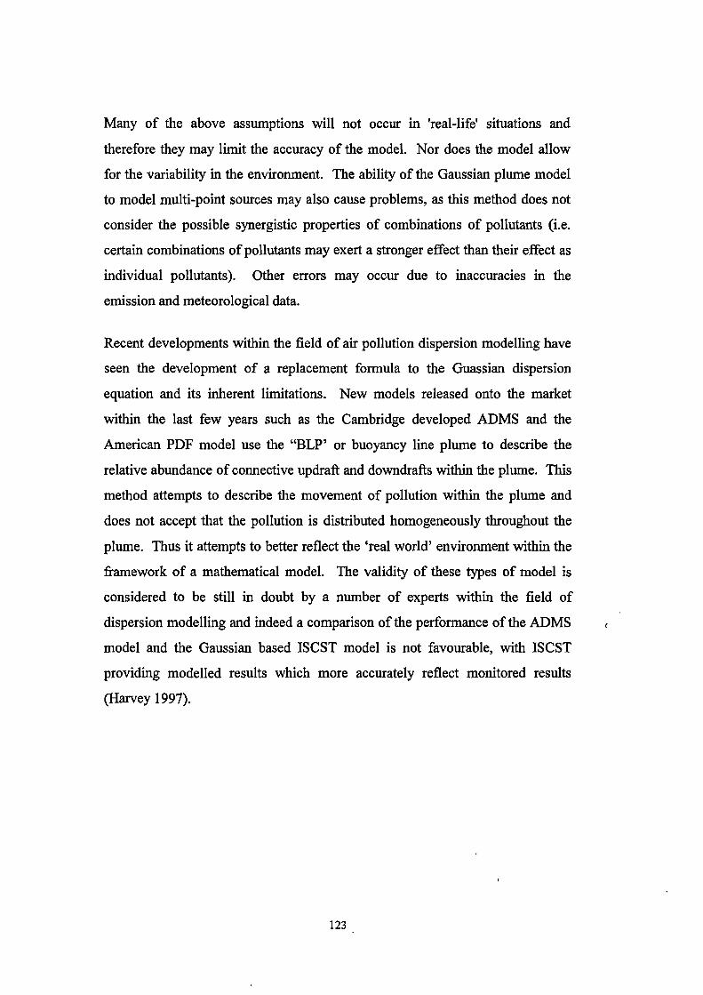
Many of the above assumptions will not occur in 'real-life' situations and

therefore they may limit the accuracy of the model. Nor does the model allow

for the variability in the environment. The ability of the Gaussian plume model

to model multi-point sources may also cause problems, as this method does not

consider the possible synergistic properties of combinations of pollutants (i.e.

certain combinations of pollutants may exert a stronger effect than their effect as

individual pollutants). Other errors may occur due to inaccuracies in the

emission and meteorological data.

Recent developments within the field of air pollution dispersion modelling have

seen the development of a replacement formula to the Guassian dispersion

equation and its inherent limitations. New models released onto the market

within the last few years such as the Cambridge developed ADMS and the

American PDF model use the "BLP' or buoyancy line plume to describe the

relative abundance of connective updraft and downdrafts within the plume. This

method attempts to describe the movement of pollution within the plume and

does not accept that the pollution is distributed homogeneously throughout the

plume. Thus it attempts to better reflect the 'real world' environment within the

framework of a mathematical model. The validity of these types of model is

considered to be still in doubt by a number of experts within the field of

dispersion modelling and indeed a comparison of the performance of the ADMS

model and the Gaussian based ISCST model is not favourable, with ISCST

providing modelled results which more accurately reflect monitored results

(Harvey 1997).

123

6.2 LINE DISPERSION MODELS

Dispersion modelling was initially developed for point sources, and thus much of

the early literature is concentrated on this aspect. Increases in road traffic,

however, and the subsequent increase in pollution related to vehicle exhausts, led

to the diversification of dispersion models into estimating pollution from line

sources (Hickman and Colwill 1982).

Since the development of the Gaussian plume dispersion equation for use in line

dispersion modelling, a number of modifications have been made to Pasquill's

(1961; 1974) original dispersion curves in order to improve the predictive ability

of the models (e.g. Chock 1978; Benson 1979; 1982; 1992; Eskridge et al 1991;

Gifford and Hanna 1977; 1978; Hunt and Eskridge 1979; Calder 1973; Aron

1983; Matzoros and van Vliet 1992). Such modifications include addition of

vertical and horizontal dispersion curves (Benson 1982; McCrae et al 1988); a

measure of aerodynamic roughness (i.e. type of landuse surrounding the road);

the effects of vehicle induced turbulence, buoyancy and vehicle wake (Eskridge

at al 1991; Spangler 1986; McCrae and Hickman 1990); emission rates (McCrae

et al 1988; Benson et al 1982); the perception of line sources as a finite line

source and not a series of point sources (Benson 1982; Eskridge et al 1991); and

varying meteorological conditions (Simpson et al 1985; Hanna, 1978). The

choice of parameters and model formulation, however, varies from model to

model. The available models also vary in complexity from Chock's (1978) G.M.

model and Hanna's (1978) ATDL simple line dispersion model, to statistically

complex models that attempt to allow for almost every traffic-induced and

meteorological situation (e.g. Benson 1982; Taylor et al 1985; Maddukuri 1982;

Matzoros and van Vliet 1992).

124

The ability of a line dispersion model accurately to represent the concentrations

of pollution around a road depends to a great extent on the accuracy of its input

data. The volume of input data for a model is often a reflection of its statistical

complexity. The following section will examine standard data requirements for

line dispersion models in general and then investigate specific data requirements

and sources of information for each of the line dispersion models used here, in

turn.

Data requirements of the different models vary enormously and are often a factor

of the model's age, its statistical complexity and the amount of desired accuracy

of the estimated pollution levels required. Nevertheless, it is possible to classify

data needs into six general categories listed in Table 6.1.

6.3 DESCRIPTION OF THE MODELS

A number of line dispersion models have been selected for study here. These

range from the more complex models, based on the Buoyancy Line Plume and

Gaussian equations, to simpler models, which are less data intensive. On the

basis of this investigation, the most accurate dispersion model will be identified,

and then further used and tested as a basis for mapping air pollution in the study

area.

From the available range of simple line dispersion models, two screening

models were chosen: the UK Department of Transport DMRB (Design

Manual for Roads and Bridges) model (DoT 1994) and Dutch government's

125

Table 6.1 General dispersion model data requirements.

Name

Definition

Emission Rates

TrafficCharacteristics

Road Characteristics

Site Characteristics

Receptor Location

Meteorological Data

A measure of the vehicle emissions at rest and at speed. Generally measured ing/km, emission factors vary between models, and may be broken down byvehicle speed and composition.

Most dispersion models include a combination of the following parameters:traffic volume (a measure of the flow of traffic on the specific road, usuallyover time), traffic composition (the percentage or fraction of HGV's, buses,light vans, cars, motorcycles etc on a specific road), traffic speed (averagespeed of vehicles travelling on the road, usually expressed in kilometres/hour)

The width (defined as the "travelled way". i.e. the road over which vehiclestravel), height (defined as the road's height (in metres) above or below groundlevel) and type (i.e. intersection, junction, with/without traffic lights, straightroad, presence of slip roads etc) of a road will affect the dispersioncharacteristics of the pollution emitted by the vehicle

Information on the terrain surrounding the road is important in determining thepath of dispersion.

This defines the point at which concentrations will be calculated. The placingof the receptors must be considered carefully, as most line dispersion modelsstate minimum and maximum distance values outside of which the model is nolonger considered reliable

These vary greatly from model to model, although most models require somecombination of: Wind Speed (velocity of the wind, in metres per second), WindDirection (measured in degrees), Temperature (ambient temperature at 10mabove the ground, measured in degrees Celsius), Atmospheric Stability (oftenmeasured using Pasquill's stability classification), Mixing Heights (the height ofthe boundary layer, measured in metres)

CAR-INTERNATIONAL (Calculation of Air pollution from Road traffic,

International version) model (Eerens et al. 1993). Two more complex models

were also selected for investigation: the CAL1NE3 (Rao and Visalli 1985) and

CAL1NE4 (Benson 1992) models, developed on behalf of the US Environmental

Protection Agency. The UK ADMS was not selected due to the academic

uncertainty surrounding this model and the financial restrictions of this project.

126

These four models listed above were selected for a number of reasons. One

important factor was their availability for this study. Together, they also provide

a range of models of varying complexity. Whereas DMRB and CAR

International have relatively simple data requirements, making them easy to

apply, the CALlNE models have more data demands. All the models are also

widely used. The DMRB model, for example, is used as the 'official' model for

road and bridge design in the UK; the CAR model is extensively used by the

twelve municipalities in the Netherlands for road and transport management and

environmental impact assessment. The CALlNE models have been widely used

in the USA as a basis for environmental impact assessment of highways, and

have also been used to some extent as a research tool in environmental

epidemiology. Whilst all the models have undergone previous testing and

validation (e.g. Eerens and Sliggers 1993, Heida et al. 1989, Rao and VisaIli

1985, Benson 1992), however, a number of limitations are evident in these

assessments. In the case of CALlNE, for example, some of the data used for

testing was collected in carefully controlled conditions, several years before the

creation of the models themselves. The vehicles were travelling at a constant

speed and thus real driving conditions were not experienced. CAR International

has also not yet been rigorously validated outside the Netherlands. Differences

in street layout and urban morphology (both important components of the CAR

model) may be expected to be significant in this context. None of the models

also appears to have been extensively tested and validated at the urban scale, nor

used for city-wide pollution mapping.

The four models selected for study vary in terms of their purpose, aims and

requirements. The following section examines each of the models in turn and

reviews the rationale behind the models and possible limitations which may

affect their application.

127

6.3.1 THE DMRB MODEL

The DMRB (Design Manual for Roads and Bridges) was developed by the

Department of Transport in 1993 to assess the impact of road construction and

modifications on the environment. It also ensured UK government compliance

with the EU Directive on Environmental Assessment (EC/85/337). The DMRB

was developed to examine all possible impacts of road traffic schemes on the

environment including water quality, geology, ecology and cultural heritage etc.

Volume 11 of the DMRB, however, deals specifically with calculating the

impacts of air pollution (DoT 1994).

The DMRB was developed as a graphical screening model which used carbon

monoxide concentrations as a marker for other pollutants. DMRB evolved from

the Department of Transport's earlier 'Manual of Environmental Appraisal'

(MEA) which was reviewed in 1991 by the Standing Advisory Committee on

Trunk Road Assessment (SACTRA). SACTRA recommended radical changes

to MEA to allay increasing concerns over regional and global environmental

issues and to ensure compliance with the EU Directive (EC/85/337) (SACTRA

1991).

The aim of the DMRB was to provide a screening model for a range of pollutants

including carbon monoxide, nitrogen dioxide, particulates and volatile organic

compounds, which could be used by non-scientific personnel who would have

little or no training in dispersion modelling. In attempting to keep the DMRB

model as simple and easy to operate as possible, however, a number of

limitations were accepted as part of the model design. Most seriously the model

takes no account of monitored meteorological conditions, especially wind

direction, and thus does not allow for the transportation of pollution into / out of

an area by wind. Consequently these factors may cause the model to

overestimate pollution concentrations close to the source under windy

128

conditions. Assumptions were also made concerning the numerical traffic-

related values given in the models and the inter-relationships between those

variables. For example, vehicle emission factors have been greatly simplified

due to the assumption that vehicle composition conforms to national statistics

produced by the Department of Transport and that those vehicles operate at the

optimum emission standards (DoT 1994). No account has been taken of the

effects of local variation in traffic composition and cold engine starts etc, thus

further increasing the possibility of model inaccuracies. In addition, much of the

DMRB model structure was based on forecasts of future trends (e.g. vehicle

growth), thus increasing the uncertainties inherent in the model. Similarly, the

model relies on modelled dispersion curves (of pollution concentrations with

distance from roads) supplied by the Transport Road Research Laboratory

(TRRL). The dispersion curves were originally only supplied and validated for

CO, but were then extrapolated to provide similar information for other

pollutants such as nitrogen dioxide, benzene and particulates. In addition, only

limited account is taken of aerodynamic roughness: i.e. the model allows the area

surrounding the road to be described as either rural (predominantly open land,

with few or no buildings), suburban (low density residential or light

industrial/commercial areas with a high proportion (>20%) of open space,

gardens etc), or urban (high density, town centre or built up area, characterised

by multi-storey blocks and/or road canyons). No account of the effects of

topography was considered. Despite these limitations, however, the model

provides a potentially useful means of estimating long-term pollution levels,

either for a specific sites or for a network of sites across and area.

As an integral part of the procedure for air quality impact assessment of new or

existing roads, the model was designed to be used manually, through a series of

look-up tables or graphs. Vehicle traffic flow (in vehicles per hour) by

composition (light vehicles, less than 3.5 tonnes; and heavy vehicles, more than

3.5 tonnes) must be defined. Emission rates for both heavy and light vehicle

129

Total EmissionFactor

11,Mean Peak HourConcentrationby receptor

Correction factor forLight vehicle speed

flows are then calculated from the look-up tables or graphs and a correction

factor for vehicle speed applied. A 'total emission factor' is therefore produced

which is a combination of vehicle speed, type and volume. Next, the distance

from each receptor, at which pollution concentrations will be modelled, to the

road is calculated. From look-up tables (dispersion curves of vehicle speed

against distance from road), the pollution values for each receptor is calculated

and combined with the 'total emission factor' to produce an average peak hourly

concentration for each receptor. This process is explained graphically in Figure

6.3.

Figure 6.3 Diagrammatic explanation of the DMRB model.

Caluculation of Heavy andLight traffic flows

Calculation ofReceptor Distances

Calculation of Heavyvehicle emission flows

Calculation of Lightvehicle emission flows

Determination of pollutionvalue at each receptor for

correct vehicle speed factor

Correction factor forHeavy vehicle speed

Owing to the numerous calculations involved in modelling pollution

concentrations for the receptors, the procedures and lookup tables of the DMRB

were programmed, for this study, into the DBASE database package.

Additionally, weighting factors for wind speed and wind direction were

programmed into the DBASE - DMRB model by defining the proportion of time

130

in which the wind blows in each of the eight compass bearings. Data

requirements for the model are contained in Table 6.2.

6.2.2 THE CAR-INTERNATIONAL

The development of CAR (Calculation of Air pollution from Road traffic) was

commissioned by the Dutch Environmental Ministry on behalf of the Dutch

Government in the mid 1980s. At this time, the Dutch government believed that

local air quality limits for carbon monoxide (CO), lead (Pb), nitrogen dioxide

(NO2), benzene and suspended particulates were being exceeded in

approximately 1000-2500 urban streets in medium-sized and large cities

throughout the Netherlands (Eerens et al 1993, RIVM 1988). The major source

of these pollutants in cities was thought to be from road vehicle traffic.

Therefore, it was necessary to identify which streets were contravening the 1995

Air Pollution Act (EU/COM(95)312) as a basis for assessing future planning,

economic and social decisions. In order to identify those streets exceeding the

limit values, a line dispersion model was used. Once identified, measures could

then be taken to reduce the air pollution levels in that area.

Most existing line dispersion models assumed homogeneity in terrain around the

road and minimal building influence, e.g. HIWAY (Zimmerman and Thompson

1974), CALINE (Beaton 1972, Benson 1979), CALINE2 (Ward et al 1975), and

the GM model (Chock 1978). Where the effect of the terrain (e.g. buildings,

trees) surrounding the road was considered, it was usually in terms of

aerodynamic surface roughness and not with regards to the effect of street

131

0

f=1

40o

V) • 4.) 0 C4

E-I .4 . 6[--,

P)a) CI

•S E"

• 05 ('-' I 0

c i,

a e0

..) t.0

7, g 0 0 0...

.5 "E cc 0 la. =

V = "0 0 g4 g ci) .. •.

•

tO s .o

0, 4E4 o 5'0 (0. E 04

RI3 g •zi 4

CU Mt C+.rf).1.u• .4

.5 u 14 -0 .5 E-. ;') 6

-8 .-g, 5 5 s t 5 e3 E o o 0

ca ca ca "E 0 a)o o ca

c.) co .5 c°-0 -0 .cpo :11) . .-0 44‘)0 g

.5 .5a.) et.5

. 5 °d

tE oa .5 -ci_ .5 Q. S •S .,...0 w .0 a) 0 .0 •-•

E-1 2 oP. o c“..) o g

ca 4.a) __,4. Ea.) .5 o •.- •WC.3 0 1-, "g)

0X CA 0 .0 0 aj C4), Ctl4.) OD 1-4 F-' 0.5 g S o r. .. co

0 a .0 fa..-GA

''t.0c.) .....u3 et>' 0 c/1 4-' r.., 0

O '1:1 g 0 „X 0 ij '1:1 ..a0 c.) •T:i „ aO "C1 1:1

5-, "C; al C.) 0 • c73 Po-, co04 0cn o-0a.) ,..,4.. ...E. i t A :1-.(i) .

c, 0

J

.....o gic.)2

,_ ..i,-; .5 5

0 al

5 AO .- Y 0 • -4 .::4-, '-',,, 0 >,' 0 w A

2 ..r, ..o .- 5

•E0

a)g"C)

0 CA CA0:, C- ,11 di 0 -• 3 . to

Oa) CA 2=1.171 E 2, g o .0-,.

0 0.)0 E "g) az>1 ' 7")-" I

' 0 0 tO 04.-. 0 0 Oa)co c.․) 41000E cl)

• - 1..,

2 tc. N ,,,. z 5; ...9 a 0 rd

A. 2 c. •Cl c) A a, ts .c ,zz, c.) 0.oo g o Q.,0 7:, ON,-., 0-

N $_, g .4::, 0 .., 1-. "r3 4. ,-.

b.0

-0 k. 4-. ..c a>

E #al e. ,,, I t... ,-, 0, 0

a, 0CII t ' z' bi) 04: o qz o cp oc,V w ,,,,D = 0 0 ,-; .E 2,-- - C.) 0 u (-) -0o ti 0

.4), .....cn A = 4 73 0 44...2 >, r) :-. -0 co

O . c,) 4,) 0U 0.9.,t) zgg .E0 5 (4,a.) 04 :0 u 0.) 0 g ..in c+..r1

U yei) t "CI ;) 48 ,.Q0FA

0 111) 0 0 oCQ g g60 0

03 mu

a) 1:1u, „ag

'0 cil• .. .4.a) 0 CA .0

00a).0 = bp 8) / . a .4..1.5 0 • E tg () "0

.2 > 1 gcriO E .

=

•

eD ;.,> -0 CA' CI)0.)'S

CI) 0... .,:l

Eg0 80.

•- 1::3c0>, = 0 4-1

8 • cE$. =.2 0

g 8 g..0 ta.cna)

'a -g e•h) 14 0. a) to

>, -0 0 _to 4_, o 0 1..0 8 .55 g

Et)

-C1LI Tidi ds

0 >, a .0co ca.,

1_, 1:1.0 S

0 4. 0 > 0 ,, a) a) 0 ,9 o

-0. -6) t 0 1' 0 0 0. b 0

_ o a.) co >, cc) 0 a.) 0 0 4u...0 n-4 cl,

tus 4.1

0 4..) ›N 0 E .„:" >-, e,1...

a) .4a a .5 73p3 . 0 >,,

0

4.10

,,,4) 0 424 0 0 0 +el -0 0.) 'r.,' N 0CA • '-' 00 0 0a.) .40 li 0 ...-. -0 E 111 g ,0 •0 L, Eh-. Z .13tn. 0 g .,-E5,,

G., . ,,.) 0 A - 5, . a,

g -0 "V) c..) al ci 17i 4 .s 5 2cl.. ..0

In

132

canyons, e.g. PAL (Turner and Peterson, 1975), CALINE3 (Benson 1992). In

some cases, specific street canyon sub-models have been employed, (e.g.

Johnson et al 1973; Yamartimo and Wiegand 1986), but these did not allow

for road junctions, a major feature in urban cities. Furthermore, most of the

existing models concentrated on calculating concentrations for CO only; no

measure of NO2 and particulates could be estimated. Thus the CAR model

was developed to improve on existing models, to fit the specific requirements

of the Dutch government.

The aim of CAR was to provide a screening model which could be used by

non-scientific personnel who had little experience of dispersion modelling, in

order to identify streets contravening the air pollution limits. To this end the

model had to fulfil a range of quality criteria set down by the Dutch

government (listed in Dekker et al. 1991) - i.e. to consider the effect of street

canyons, be easy to use and to employ input data which was easily collected.

CAR was based on a previous T'NO traffic model which was found to be too

detailed and complex. Consequently, the most significant factors in the TNO

model were simplified for input into the CAR model. This permitted an

acceptable level of simplicity in the calculations without sacrificing accuracy.

CAR INTERNATIONAL, the version used here, represented a later

development of the original CAR model. CAR-INTERNATIONAL includes

modifications of certain parameters, such as emission factors and

meteorological conditions, in order to allow the model to be used in other

countries.

CAR INTERNATIONAL thus provides a simple to use screening model

based on line dispersion principles. Model calculations within CAR allow it

to consider intersections, the composition of traffic and the style of driving,

133

local street emissions, city specific contributions, recirculation contributions

and the non-linearity of NO — NO2 relationships. A further advantage of

CAR over the more complex line dispersion models is the limited amount of

input data required, most of which is easily obtained from site visits and

traffic census or local councils. Due to the design specifications, however,

CAR-INTERNATIONAL does not have the flexibility of the more complex

line dispersion models. Meteorological parameters are defmed only by an

annual average wind speed. No account is made of the effect of wind

direction, wind velocity, temperature, stability class and mixing heights

during the measurement period, all of which affect the NO — NO2

relationship and the dispersion characteristics of the pollutants. Data

requirements of CAR are shown in Table 6.3.

6.2.3 CALINE3

In 1972 Caltrans published a line dispersion model in response to the

American National Environmental Policy Act of 1969. The model, CALINE

(California Line Source Dispersion Model), was an attempt to estimate

pollution dispersion from roads for inert gases (Beaton 1972). The model

consisted of lookup-tables and nomographs and was the forerunner of the

present CALINE models. Three years later a FORTRAN version, CALINE2,

was developed which was modified to calculate concentrations for depressed

roadways and parallel wind conditions. Model verification indicated that

CALINE2 gave a two- to five-fold overestimation in concentrations for stable

parallel wind conditions (Ward et al. 1975). Noll (1977), however, concluded

that CALlNE2 over-predicted concentrations for parallel wind conditions by

66% for all stability classes. In addition, road length, surface roughness and

the type of road could not be specified in CALINE2, thus limiting the number

134

-10M43C) En

.1 1...oI..2E.)

2°bta rn.S 4 =o••-• o '8 us .00 E.-..

Ed64ta.0

=t bg o g o CO):53 m

4)4)o 8 ts .`g-0 •- 0.0 000i!....

14) 0 w 3 1 E

v-n 00 n•n•11

135

.‘gC/3

4- 00 -otoa) o 'M .s'' = g-o -o-.

-̀1 'It ri § 80 c/i E c%) go -043›.‘ E4-.0 f#, 5 '8 5 T.,' >,5 5

0 0 .02 40 5 a:-„ >,

.., •iii c.) •ocl) t.G -o

El 0.0 .a17; 2 ...' g ...4 :9.. .

CI 73 4 = 5.... -

=c.)

41 0.5 o

Efiacd5

>. u.0 cn01-o 0v)...o

',.74.!.L.'7,........,a

10

o 0 trEl 7, .6 "rE)

fa. 4.)

a) §0 cn t -, .49 -5 a.= -§ F,, -o 3

.* 1 'h9t' g u, 4, c...) =0

. 2 g I 1 i .0 .g. -65°°.0 1 1 1. I-o0,, 0

cl e ,,i

Z:dj, S 2

o

0 cd01 o

.00 E cri .7:1,. z 0> I luat ...aloin g Q .̀'d tg -0 .... •._. .°4 .... „.., ...%A c.o. 41 'CI

-a .g e . 5 e 5 ; :q . 5 .;

5 . .̀ 2. „.9 5 cm E .5 E--. 5 g3 E 4 g 0 0 0 ..0 0 0 -

1ve 5 .,40 40 40 3 -a Ea 3 41 44 g ,0 o 0 „_,

= o '91 .1=7 111 "C3 -o ,,s _. 4: *4 4:10 2,'0 d ,,cn •,,:s a .04)4) a r.) :4 g 0 -= .,,, 5 ...9 FA' = o41 .4-n 0 u 0 "CI g -0 ,I ,)u cn :-•

a .2, E 00 3.2 1 1 ..0 cj B -0 o a R A A 0. ..8E-n o 8 u . 0 2 az 0

0 8 2 O.° Vu P. =0 e o-cz .0 4.) JD 00 A 0 .5

......a 2 0

b ° 0 e,O w3 a o 4

O ,., > op 0 cu =IN) co 0 .-E ,,n. . 5 5 E 0 :5 3(#4.,..,

1 t)> 0cd ..-, = ,....

- 0 .r.:g L) enPCI

c4.., '0gA -c4-• 40 5 .09 ,

0_ 0

• oo .0 0 -, .0 ..0 ri, 0 0u „, 20 4,b -o 43o 0'Er,c a

g-e, g 2 > -- .1.-1 15 0a 8 m 4.9 -a 40

a > c's -6° ,--,,, 2 g t.. 8 cn0..0° 2 g 8 60 ° .s > 6, 0., w ° E......,:9 " Ec; 1,._,> > E .2. 0 "P• 0 0en.0 ..= 4. 'II,§ 0 ^ Po .5 ° E - 6/3 14::,., g ezi g 1 8 o 0 o o

,o) (4-• .... En EA * c./.1 4_, f, '4-40 0 8 . 8 4

g1 . z) .c.2 :.), = =

1=b0 .,:) b0 '0 -E - lo 2 8

A 8 .1 c-e. f: °-) 8 . 6 2 a at ) 2" ( .1.1)

43 01 :4-g. 01'4 w) (04

I En 04) „ rA ,t)

0 = mr z), c ...., o

o."gIt 0

o 0 nc4

o .ig cnce. V

-S

a Et E..., 5 CO ,144.1 o 41 •5

..... o a a 0 -Id

o•- oo

O=6'

• ..a.=

cg 2O ..0 0 -0Q ui c4-.o

u == •-•

. O 0En g 0 >-n 43t...0. 0-C3 a -0-

us -0 g(11 8 . en .0 a . 2 tb'S EA

.o a C a B... 0 0 0.XO X 0 000

a. 2

., .o .= '0 c) -o atU

C.) ''' '1" ''' tct0 0 X ..p0 =O , "7 i 7 0 71 0 It5' • .-• "0 0,I- 4)O En o.... a

o 4. = =04 0 7,1

= 0 "0 6.) ED 4.) C.) EAI. ...-• to 0 Cd 0

d) = 7-"E =C °.44.- A 1= E -c) 2 '5 Et to Ir..--al cng. -.

. 0 .. . .. 0 . . . ecu 2 a.e. o 0 1... ..sd 0 t0

6,i, 6 olz c.... u > cdu

4" E 0 ti,co) 0C.) = '8

o8 g0 .0

O goaO a 44

• . n4

•

0

.!....). -4 oo = 0 = 2 2 g EA

4.) <A 00 CO = ••' 41I. = cn 0. ..10 • .-. o ..),.$2 5 .-o> a .= 0, X 5 .-.3 04..) E 0 b 41 2Et C) v . .... _41 a) = a)4) 4) o co) -o 0 -a'- g .5

..= 0 5 .5 E = a 0 0 tU 0 Xts.0 rd 4.) 15 2 .5 " 2o 4 03

4 .5 0 -8a 5 g' 5 -E3 0 0').0.5*a' .3 8 a0 0 a.) c," 0 ". >, >. 2 .- b. 0 al0

2 0 o a y, .0 -8 Eto 0 7:4 En UO ° 1... • U .4:1

2 'a' -ocil ,.. =

> 8 di = g 0 0a.)Ia. 2

..: .h)a ''g41

0 o.,cn a) ° 04) 2

= ..0 es 4-- cd '-c4 2o

04 a - 0 EnEn .... Uft 43 o

04' E-' 0.5 (..) cci

csi

of situations which could be modelled. A third version of CALINE was

developed by Benson in 1979. CALlNE3 retained the basic Gaussian

dispersion equation, common to all three models, but increased its flexibility

with the introduction of new horizontal and vertical dispersion curves to

allow for the effects of averaging times, vehicle-induced turbulence and

surface roughness. Unlike its predecessors, CALlNE3 viewed vehicle

emissions in terms of an equivalent finite line source and not, as previously, a

series of point sources. CALINE3 also allowed multiple roads to be

considered simultaneously. Validation of CALlNE 3 was conducted by Rao

and Visalli (1985) who found it to be similar to other published line

dispersion models. In 1980 the Environmental Protection Agency (EPA) in

America authorised CALlNE3 for 'use in estimating concentrations of non-

reactive pollutants near highways' (Benson 1992).

The major advantage of using CALlNE3 over its predecessor was its ability

to view emissions of the pollutant as a line source and not a modified point

source. Consequently, the final prediction of pollution increased in accuracy.

The model also allowed for greater flexibility and thus increased the number

of situations for which concentrations could be predicted. Finally, although

CALINE3 was designed for modelling carbon monoxide (CO), the

introduction of a molecular weight variable within the program has enabled

the model to be applied to other inert gases and particulates (Benson 1979).

A number of limitations, however, must be considered when using the model.

CALINE3 cannot model complex topography and therefore assumptions are

made on the homogeneity of the terrain surrounding the road and the

meteorological conditions within the study area. Street canyons and bluffs

cannot be modelled with any degree of accuracy. The occurrence of very low

wind speeds, coupled with parallel wind conditions, still causes the model to

over-predict pollutant concentrations (Dabbert and Hoydysh 1991; Hall 1996;

Matzoros and Vilet 1992). A further disadvantage of CALINE3 over the

simpler line dispersion models such as DMRB and CAR INTERNATIONAL

136

is that it requires more complicated and voluminous input data. A basic

knowledge of line dispersion modelling is assumed. Data requirements for

CAL1NE3 are shown in Table 6.4.

6.2.4 CALINE4

CALINE4, the latest in the CALINE family, was developed in 1984 by

Benson (Benson 1992). CAL1NE4 refmed and extended the capabilities of its

sister model, CALINE3, in an attempt to increase its flexibility and to reduce

the problem of over-prediction in stable, parallel wind conditions. The range

of pollutants which could be estimated was extended and allowance was

made for chemical reactions of the exhaust gases, using a 'reactive chemical

sub-model'. The effects of street canyons, bluffs and intersections were also

incorporated by inclusion of an altered vertical dispersion curve.

Deceleration, idling, acceleration and cruise speed of a vehicle approaching

an intersection were considered in the model as they would affect the

concentrations and behaviour of the pollutants. A drawback to the use of

intersections, however, is the need for separate emission factors for each of

the different stages of a vehicle's approach to an intersection, thus creating the

need for a large amount of input data. Lateral plume spread and vehicle-

induced thermal turbulence were added to the model using modified

horizontal dispersion curves and vehicle-induced heat flux algorithms. In this

way, CALINE4 dealt with some of the limitations of CALINE3. The greatest

improvement of CAL1NE4 over CAUNE3, however, is its increased

flexibility to handle a greater number of situations.

Validation of early versions of this model was carried out by Rao and Visalli

(1985) and Benson (1984) who both found that the modifications to

CALINE4 produced only slight improvements in the accuracy of the

predictions compared to CALINE3. Over-predictions in concentrations still

occurred for roads with parallel winds of a low wind speed. Furthermore

137

8 5cc

c,

4.4

r•T•

0

60 co o

-a ...=

9

.0

0oOA • aC 11.1

• 74

0 . Z.)

cn 5 3.) 0

E-, '•O 6 §

5 t ..o 80 •-.o .- ...Ne

0 4= 2 .5..0

A 17 t) °••

co ° 6 0, -0I ...,...

,- 00 0 N

.0 .0 t0 4

•0 0.0 0= = € ,9,'

eh' 8 4.9

.,s c.)ct-o 5 "5

3 o ,,,,49 aO4_)=0 -0

U0u

0 0 g0

§ A 0.. 0 .0 4,0 o o

co ''',?, ii)Ce' l 0 . 6c...... 8 2o g

..6

US5 8 •-• g 8

-s08 c...) cn

3 tr-.7 pj0 ..g ai 0 o)OD u ..... e..) • C).-. .

.00

. F... . .=.....tu 'VI

rn u . .0V.t • •0 .1 n,••••

0 0 ,-. ..) =8 -o-o

g u 5 S.1 5 8 5 E E

a.) = C tl.) 5

•-o .....- .0

-a2 ccl CCI .17 0E E it g 'ao o•

,..... co o.5 0, .0 20 -

.g3..... 5

5 U C./ ••-n VI i

'S 47 14 0 .4... 0

4:10 0

-o 7:1 0 0 0.0

e 11.1 col

5 0 8 .0 0 cA 2 .5 2 'a •a•s > .0

Oo OSJD 0 :80 5 0

0>.0 .00

. 2 2

0t.t) co o.0

..3.-...3.) )..., 0 0" 9 0-10

co

00 6 t..) c,„- - es 6•

U .E

...Au o.0. e.- 40 4-4 ..."

1../9

. .... ai .9 C t.3 P0 5 8' t > o 73 6

..0.5 4 • V, -E,:,

0 = g',• •n•

00

00

.0 • ... 2 0 73; 5 .0 o

>, 5 0 '5 7. .5 0 u ., t

.0 o , 0c....o .... -o 8 00 a) 75

..e 4•-

9 o. -E. o"C1 0 go 01 =o0 r,' a 0 co • -

e -0 0'

.9 > 6‘... . E

C) .o 5 •--o

cO.0

-3)

E -0 76 0 6 0 ti =a.) 0 0

c) "6;)

= 0 o n••: .k" .0 .5 0. - o.2 >

0 .30

•.-..7

. C.)-.5 Ea" ...,0>4

,3)1...

a.. 5 -52'

A 0 0 co a .>

2 4-4 g

2

4g B ,,%.' E•_0 .1. .,.-.;g >0' n, -c

3619 .0 -,-. 13

-o.Et‘ '''E 5

.g -60. c).

o3.)E

o 3,310" CRC) '8co . to -° > 0 448

0 ,o4- 0 0 co .,- ,..., co 73 to° o 0

.5 .2 .5 t '7,u -o 0 LI

• •n•0

0. a c .90.0.o U

4-, 07 ° • 0E1,...

.2 .7 = .0 .17 ...a 4-, 0 .0.9 2 R '5 a 5

49 3 'to 3 0 o to 6 a) ...,7.4 E 't ..t o al

‘... E ' S el g iv, 8 .3.) 0 0 0 2. g ." . „.

7 Cr.1 0 0 0 o el, M . 00 2 0 •6 g

. - . 1,11 RI -" 0 t (1)° en = g = a g 8 os 5 0 0en 0 2

"no

g

0.a .1. c 0

'g..c .c."? -a 8 -E-..,

U ..,

-0f-. 0.0 0

u

OD 0 0 bp .1 4'.7 x 0 .0 i.

W IQ 2. 4 15 . a1

b E R t . ,'a R> 0 .... 0 .a r. 0 .) 0

cn = =

r)ooJ0 0

1n1

138

CALlNE4, like its predecessor, still assumed homogeneity of the terrain

surrounding the road and the meteorological conditions, and therefore the

model is likely to give incorrect results in complex terrain situations. A

further drawback to the use of this model, however, is still the large amount

of input data necessary to run the model, and the assumption that the user has

a basic knowledge of line dispersion modelling; without such knowledge

there is a significant risk of misapplication of the model, or misinterpretation

of the results. Data requirements for CALINE4 are summarised in Table 6.5.

6.4 MODEL VALIDATION

In order to examine the predictive ability of these various models within this

study it was necessary to obtain detailed and simultaneous information on

NO2 concentrations and traffic flows at a range of locations. A detailed

monitoring programme of both traffic flows and air pollution levels was

therefore undertaken.

i. Traffic Flow data.

Traffic flow data was provided by West Yorkshire Highways Engineering

(BETS) who undertook a traffic counting programme within and around the

study area. All provisional sites were inspected prior to installation of the

automatic traffic counting devices. If considered suitable (i.e. required

amount of accessible street / garden furniture available; sites unaffected by

industrial pollution sources etc) air pollution monitoring was conducted at the

same time as the traffic counting began. Information on traffic flows was

provided by HETS at the end of the monitoring period for each road in the

study.

139

01)

V

0

c-f)

g v aU) 0.) o

[-. cl)0 .....

2 .0 rn>1

Encc: 2

..., a) a)O "0 tl) cil 01 0

O 414 . S ° :'-45

4-, 1EL : E i aal Liz t-0 cl. a4 o ,- ...,...

,,,, a) 4 0 cn

...., gfil '0 rn f4 ..c.:

1.4 0C'S CIO 0 g t. 4 .....

6 .0 C.) .2.. t v ,_.1 0cu •-• 0 0n•I 0 o C0 5 ..:4

-'4 2 E2 cr, .4- L)

..o Ls <4.9 § 01) 0 C.) 4-,•44

.

•

n U .5 f-i.5 .5to c.,.., .0 =

0 0

0(1) 0u, u5 g

ci) cri ....

E -0 43 ia-

0> u 0

O 00 cl • .- c0 4c-O.3 >= -6 . 7.: .1:1 5 "c1 'V '10

.5o o = al v 0,_(..) cz 0

E to ,,," .5 0., 4C-% E' E 4) . S 5

.4-,

E 4.., .4=_''' C4.1 2

, a ..... -8 '' c..)0 C/)a)

C/)a)

6 0 OE0 0)E-

010 0

0 0MI 4. 4....a, c) -9a. .-.., .....O ci, cncn .ti:

...i..

O v4.. v..... .O o u =...., cr) 0 LO 0'Ca' .2 •-n-n

i 0) .2u v o 04. 4) 0.5 ....4n• .nI

112 = 4"-j3 re,E E c̀izi E 8O o° 0

40 4z -48 oz "re'"0 1O .0 "0 'CIC) a) v v 0.5 vi .5 -0 .5 8

c.45 (-4 cc' O. V 2.00

.0 C.)0 E

.0 CU0 E

M

.5 E a 1/)-tio cg 'ILI

.v)... E. 0O -0

02 011v

5 g E g.).4,... 0 0 .1,,. E2 = g o a..) .9 "5 ,-. cdc„,-, =cc:9 . .-,S

•

0-6 -.8 .... ,0 E

Ea ,... c; 0•- 0,00)cn

.5 .4 •S ,....;E t...-cai MI '0 • = 0 M.4 ou)

2 4) E clo0 S 0 a) -2

[-"! ag 4 4 (NI w),-,

(1)

,L., ,--, g I49. ic4 =

v) °v) 0 4 a

=

.0 a) TA ...., V "O c1

p.., g .4 o ---. ..= -ci a)co n-n >. 0

.0 .g 4.-t 0 = "0a) 73 o ,- a 0. og

E

0 .r, a) .....0 th-ovs = ea .0 40 cn `4-. -

ge)o ›. ..= ? 0,-

O to

..0 a., ...., 5))-, 'a (.- 0 „ ,,,....- -0 -av

0.) a) > >,, U)) E a .o 4,- ...., a - C.)0> L. .0

.0 CO 03 2 "g) ... 4. "0 .0 2 0-E 0 mi

.0 5 v) E a, -= o4.. ._ `g 0 7.') 0

>, u at = "0 0

0, o ,-,,i -o .... ..o . 1-4 oi.., ... 4j. X g .2 0C)=

•N..O E ,.= a, 4-)to c.3 41)0c.) b u ..c,_ .0 v 17). .0 T.')(5 .... 'V .011 . WO ......

.4n. = 0 0 CL 7:1 .. >.n CU 14

•

.0

E 0 o c„ '" 4. 8 E 8 co 0) "0..

•

.72.0) •R 0 8

).74 p. •.- a.) .5' a) S.., = CO i- V, ..g 0 ..0

A i474

ad c) 0 c.)o - .`"4 . Ee'n g 4 tu 8 >, u . ..=- '0 '0 E >c)4-, .- ..z -0 -2, a) 0 a o

a) 0 o,.., to I. "CI $_,0 • •-. 0 •-• 0 0 ,2L. 0

c .) t "2 0 04.

B E 0 0

0. 0 0 - 5 - ,,,,0 .5 4̀-' 3 -,- CD •-•> 0 0 cn Mt

4-, 0 CO i..9 CO M .,.. S.4) 0

01)4...4.4 ,L,3 03 M ,.)4).E s 4-,

•

U)(1) a.9 g .0 0 0 P01 01.-0 an =a, ' 0Co f.• g

fa. E4-n

0 .0 =a)O c/) 0

0a) 0 ...,

0 c

'S • -, -a4c5.1.,n ,g

01'0 g tii - ..‘ - FDIv) 0 t a) 0 •-• n .0 0, ", v) •.. ,...,0 ,..) th 4. 12,. til .0 ci.) 6 rn

0) 4-3 .° -0 a - 4) ,7)

= 4. • ,-. 0 4.)E -'-' L." e) ....,,3 ;Go 4n, •-•

Cd ... 0.3 co v bo Eu '.. V)a)

.-cil ;-n3 0

< " 4.1 2U) . 4-. n^-En 4) C.) 0"

0 1.., I. • 7,0 E a. '-'4.) u 'FaO 0 -5." -,,:j r.:1 0

..= "o 0as c.)

ID t a)

a 5 o ..-,

-a2Ct 4'‘ >.E. c'.a g (.1 4i...) 0- 2 g ...' =,,)°.:./2 . >

10U

O -0CO"c1Z g (1)

0c.t. • 41 N

o

1/1 .-, • 00ed .=-0 Ea •

▪

x

00 ON

140

0

••-c-d cl)a)

u)a.)

cn0

-0 c) C..) (..) 0

• E • E

O 0 v)a.)

rip0

C/)a)

5 o..0 1...(ID 0 o c.) c..) o

tg tg tg.1. '"'

Ct3 n rn rut) .... ..... .....

O 0 1., V V V

A cocu ,, ...a) .,..cu ...a)

-0 c) o c)

el „,c-)ed •-_, (/) En (/)cu cu ,,..,q.,6 c)

3 IACI3

a)(,)O

f/30

'tt C

C= 0 CU a>

1Z (5‘ 0 . 0 . 0 .0- 0O --. a) /CS

C7) --'E•- .2 .2 °....5 t.,_, E V 5 b-' 5 +4CC1

o 2 o o .) 0" 0 VS

C.ICI LPI CJCI b.° OCI bp (ICI

.

•

..... ID 0 0 CD go .5 -0 .E -0 15::-0 -0 .3 cl) v' • » > > V'- a) I--, a)

.5 .5 ti.5 0 0 o o o . 5 -2 . 5 2 .E 2.> 0 .0 43 ..o .c) E 5 -n.'g '0 E 5

45 -E .. . as ct cz o..0 .0 0 :-5-. ..0 0 ..0 o .0 0

0 0 En 2 2 2 2 0E OE 0 E

a)-0

V g....Ii "0.....al .0 "a

XO

06)

76 0.9 • iv' 0 bl).:-...) M. -0 4..) 00 0 0 obf) 0 IDA a 0 -0 0 0 0.... ..... •-n • •-n •.-nO -0 .5 o -.±. 0 ,-.4

40. '• E 0 4.0.1...O .a...) 09 .9 5 .,.„„ 09

E4, . ... 0 . . ... .G.) q 0 E 0

§< 0° < 0

go a)cs1 c") ^z1" 14")v—I •—n

141

ii. Air Pollution Data.

Air pollution monitoring was conducted using passive diffusion samplers to

measure NO2 concentrations at locations where automatic traffic counts were

planned to be conducted. Samplers were placed along transects,

perpendicular to, and on both sides of, the roads (as described in Section

4.4.1). The location of the samplers was limited, however, by the suitability

of street furniture and willingness of householders. As monitoring was

undertaken concomitant to the collection of traffic flow data, the siting of the

automatic traffic counts dictated the location and time frame of the NO2

monitoring. Most surveys, however, lasted for a two-week period.

Monitored values obtained from the surveys were then correlated against the

predicted estimates of NO2 obtained from each of the models.

This set of data was an important input parameter for all of the dispersion

models (see Section 6.2.1) It should be noted, however, that site N402 was

rejected from the study as the results appeared to be anomalous compared to

the other surveys - i.e. concentrations appeared to increase with distance from

road as opposed to decreasing. This may have been due to the influence of

other nearby sources (e.g. the nearby motorway, which may have an indirect

influence on the sample site).

It should also be noted that all the models used here provide estimates only of

the additional NO2 concentration derived from the modelled road sources;

they take no account of regional background concentrations, attributable to

other sources. They will therefore tend to underestimate the measured

concentrations by an amount equivalent to the regional background levels

(typically 15-25vg/m3). Assuming that the background concentration is

constant across the study area, this will not, of course, affect the results of the

strength of the relationship between modelled and measured concentrations.

It will, however, result in a large intercept value in any regression analysis

comparing measured and modelled concentrations.

142

6.4.1 DMRB

6.4.1.1 PROCESSING

Data for each of the input parameters required by DMRB was input into the

model. The model was run twice, both with and without the meteorological

data to allow the effects of this parameter to be investigated. Meteorological

data was obtained from the University of Huddersfield and from Leeds

Weather station.

6.4.1.2 RESULTS

Modelled pollution concentrations were regressed against the monitored NO2

values obtained from the sampling programme within the SPSS statistical

package. Results of the analysis are shown in tabular form in Table 6.6 and

graphically in Figures 6.4 and 6.5.

Results of the regression analysis indicate that the DMRB (excluding

meteorological factors) model explains 21.2 per cent of the variation in NO2

levels (significant at the 10 per cent level). As Figure 6.4 shows, the model

gives an intercept value of ca. 19g/m 3, close to the monitored background

concentrations in rural sites. The slope value (0.514), however, when

compared to the monitored results suggests that the model's trend is to over-

estimate road traffic pollution at higher pollution levels.

The basic DMRB model does not include any allowance for meteorological

factors; as noted in Section 6.3.1; consequently, the model was adapted to

include wind direction. This, however, failed to improve the model

143

performance (see Figure 6.5), and the adjusted R2 value actually fell to 17.4

per cent, significant only at the 5 per cent level.

Table 6.6 DMRB regression analysis results

Parameters ExcludingMeteorology

IncludingMeteorology

Degrees of Freedom 1/15 1/15R Value 0.511 0.475R2 0.261 0.225Adjusted R2 0.212 0.174Standard Error 5.267 5.463Slope Value 0.514 0.136Constant 18.844 20.6489F value 5.303 4.360Significance F Value 0.036 0.054

In an attempt to determine whether performance of the DMRB model was

dependent on distance from road, residuals from the regression analysis (both

with and without meteorological factors) were plotted against distance from

road (Figure 6.6 and 6.7). In both cases, no clear distance-effect is evident,

suggesting that errors in the results are inherent in the dispersion model and

are not simply a result of poor controls for factors such as surface roughness

or the effect of fugitive or more distant emission sources.

6.4.2 CAR-INTERNATIONAL.

6.4.2.1 PROCESSING

Data for each of the input parameters required by CAR-INTERNATIONAL

were entered into the model. Where necessary, information given in the CAR

144

30.

U

• •

.

/.--

. . a

U

Figure 6.4 Relationship Between Observed and Predicted

NO2 Concentrations Using DMRB (Excluding Meteorology)40-

.

.

10-

Rsq = 0.2612

0

10 20 30 40

DMRB (ug/m3)


NO2 Concentrations Using DMRB (Including Meteorology)80-

70 -

60 -

50 -E

40-

c0 .

Z 30 -

20-. a U

a

10

0

I I0 10 20 30 41',/ 50 60 70 80

.

Rsq = 0.2252

DMRB (ug/m3)

145

20

..

U

•

0

I

.I0

" 1; 1(,) 40 60 80 100 120

Rsq = 0.0651-20

0

Figure 6.6 Analysis of Residual values for DMRB

(Excluding Meteorology)

.S

.S

-10 Rsq = 0.1198

2.0 40 60 80 100 120

Distance (m)

Figure 6.7 Analysis of Residual values for DMRB

(Including Meteorology)

-)0

10-

I

U

• a

-10 -

Distance (in)

146

users' manual was used to interpret the field codes used by CAR (see Table

6.3). Certain parameters within CAR-INTERNATIONAL were also altered

to enable the model to consider the effects of local conditions (i.e. parameters

such as wind speed, emission factors etc which vary from country to country

and from city to city). Meteorological data was obtained from the University

of Huddersfield Meteorology station and from Leeds Weather Station.

Owing to the receptor limitations of CAR-INTERNATIONAL (i.e. it can

only handle 2 receptors per modelling run), once the data had been input into

the model, it was run a number of times with increasing receptor distances

from the road. This allowed information on the 'shape' of the dispersion

curve (i.e. how pollution concentrations alter with increasing distance from a

road) to be obtained for each road. The inability of CAR-INTERNATIONAL

to predict pollution concentrations at a distance of over 30 metres from the

road, combined with the difficulties in siting tubes at regular intervals within

this distance, meant that only a small number of monitored sites was

available for analysis. The results of the model and the subsequent analysis

are noted in the section below.

6.4.2.2 RESULTS

Both the predicted (those obtained from the model) and the observed (those

obtained from the monitoring programme) levels of NO 2 were input into the

SPSS statistical package and regression analysis performed. Results are

shown in Table 6.7 and in Figure 6.8.

147

•

• • • •

a

(Ctu/Bn) ZON

•

•

0

en0

CL)4-1C.)

Z"CS 0a)

A.4'-' Pi-0 4t

cc;73

CL) WE—I

a) 4Cl)..10

0

1

a)>a) C..)

4 bk,cu

al:1• --i

.1=L•

Cl)

,4Cl)

CI

00 • ,..i.47-:

-164cidi.-n

Tll'la'r=4 a)C)

00

n43 0

a) C..)$—.

C`,...!bA V471 Z

148

Table 6.7 Regression analysis results for CAR-INTERNATIONAL

Parameters ValuesDegrees of Freedom 1/11R Value 0.179R2 0.032Adjusted R2 0.048Standard Error 9.780Slope Value -0.236Constant 37.380F value 0.399Significance F Value 0.540

Results of the analysis indicates that CAR-INTERNATIONAL fails to predict

monitored NO2 concentrations at the survey sites. The adjusted R 2 values are

extremely low (Adj R2 = 4.8 per cent), and not significant at the 5 per cent

level. In part, this may be due to the effect of an extreme outlier in the upper

left hand corner of Figure 6.8. This site was one of a series of 9

perpendicular to the A62, Leeds Road, at a distance of 30 metres from the

road. The reason for this anomaly is not clear, but may relate to the specific

character of the site (e.g. wind direction perpendicular to the road). Removal

of the site for the analysis considerably improves the R2 value but the

correlation is still not significant at the 5 per cent level. As such, the CAR

model is seen to be ineffective in this area.

6.4.3 CALINE3

6.4.3.1. PROCESSING

Data for each of the input parameters required by CAL1NE3 (Table 6.4) were

entered into the model using the information given in the CAL1NE3 user's

manual (Benson 1979). One of the requirements of the meteorology

parameter was stability class. This was not available from Huddersfield

149

University campus weather data. A programme was written, therefore, to

calculate stability classes, based on the Pasquill stability class (see appendix

6) (Clark 1979). The meteorological conditions were measured at 15 minute

intervals at the university. CAL1NE3, however, would only allow a

maximum of 400 meteorological conditions to be used. Therefore the data

was averaged to 1 hour periods, providing 288 meteorological conditions for

the two week period of sampling. CALINE3 was then run for each road in

turn. The model predictions of pollution were written to an output file which

contained estimated concentrations at the receptor sites for every set of

meteorological conditions entered. The output files were converted to a

database format (dBASE) and miscellaneous information stripped from the

files to allow easier data manipulation. The pollutant concentrations at each

receptor point were averaged to produce the estimated pollution concentration

at each receptor point for every road. Unlike CAR-INTERNATIONAL,

CAL1NE3 allowed the receptors to be spatially referenced and therefore

receptor locations were specified on both sides of the road, thus enabling the

effect of wind direction to be considered.

6.4.3.2 RESULTS.

As with data from the previous models, the results from CAL1NE3 were input

into the SPSS statistical package. Regression analysis was conducted on the

data and the results shown in Table 6.8 and graphically in Figure 6.9 to 6.10.

Table 6.8 Regression analysis results for CALINE3.

Parameters ValuesDegrees of Freedom 1/15R Value 0.663R2 0.439Adjusted R2 0.402Standard Error 4.424Slope Value 0.609Constant 7.188F value 11.759Significance F Value 0.004

150

-10


3Cl

50

40-

30

20

10

NO2 Concentrations Using CALINE3

• ••

• •

Rsq = 0.4394

10 30

CALINE3 (ug/m3)

4(1

Figure 6.10 Analysis of Residual values for CALINE3

20-

Rsq = 0.0238

0 20 40 60 80 100 120

Distance (m)

151

Results indicate that, in comparison to both DMRB and CAR-

INTERNATIONAL, the CALINE3 model works well. The intercept value of

7.2p,g/m3 is rather low for background concentrations in the study area - and

the slope of the regression line is 0.609, so that the underlying tendency is to

over-estimate actual concentrations at higher levels. The fit of the modelled

data to the monitored data is relatively good, however, with an adjusted R2

value of 40 per cent and a standard error of only 4.42n/m 3 , significant at the

0.4 per cent level.

Figure 6.10 shows variations in the residuals for the model with distance

from the road. No clear pattern is visible though there is perhaps a tendency

for the residuals to become more negative over the first 25-30 metres, beyond

which they remain broadly constant at about 3-51.tg/m3.

6.4.4 CALINE4

6.4.4.1. PROCESSING

Data for each of the input parameters required by CALINE4 (Table 6.5) were

entered into the model. Meteorological data was obtained from the

University of Huddersfield and stability class computed based on the Pasquill

stability class as explained in Section 6.4.3.1. CALINE4 allows for the

chemical conversion of pollutants in the atmosphere and therefore it was

necessary to obtain data on average ozone, nitric oxide and ambient nitrogen

dioxide concentrations. These data were obtained from Kirklees Scientific

Services and input into the model. The model was run for each road in the

monitoring programme and the results of the monitored and modelled

concentrations at each site input into the SPSS statistical package.

152

6.4.4.2 RESULTS

Regression analysis was conducted on the modelled and monitored data and

the results shown in Table 6.9 and graphically in Figure 6.11 and 6.12.

Results of the analysis indicate that the CAL1NE4 model is a small

improvement on its sister model (CAL1NE3) in predicting NO2

concentrations of pollution, with an adjusted R2 value of 0.522, significant at

the 0.06 per cent level and a standard error of 3.954m 3 . The constant of

6.711g/m3 is again rather low compared to the monitored background levels in

the area. The slope value, however, of 0.735 is closer to unity than the other

methods. In addition, there is a marked reduction in the scatter around the

regression line (Figure 6.11) which may reflect the increased sophistication of

the model. No relationship exists, however, between the distribution of the

residuals and the distance from roads (see Figure 6.12), thus suggesting that

the model is equally effective at coping with the directional dispersion of

road transport emissions for up to 120 metres distance from the road.

Table 6.9 Regression analysis results for CALINE4.

Parameters ValuesDegrees of Freedom 1/15R Value 0.743R2 0.552Adjusted R2 0.522Standard Error 3.954Slope Value 0.735Constant 6.695F value 18.503Significance F Value 0.0006

153

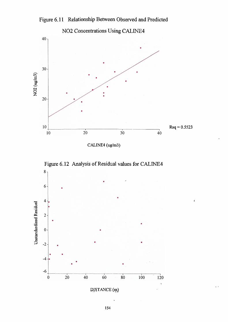
10 20 30 410

Rsq = 0.5523

40

30,

ril

oNCZ

20

10

.

.

6

4 - ..

.-4 - .

-6

.

.

..

.

..


NO2 Concentrations Using CALlNE4

CALINE4 (ug/m3)

Figure 6.12 Analysis of Residual values for CALlNE48-

.

0 90 40 60 80 100 120

COTANCE (rn)

154

6.5 MODEL APPLICATION

The above section (Section 6.4) indicated a clear trend in the results of testing

the various dispersion models, in that the more sophisticated the model, the

greater the accuracy of its predictions of NO2 concentrations. It should be

remembered, however, that this analysis related to a small number of specific

point locations. The ability of line dispersion models to predict accurately air

pollution concentrations over a larger area, for example, the entire study area,

could not therefore be evaluated from this data. In order to investigate the

mapping capabilities of the dispersion model which had proved most accurate

in the preceding tests (CAL1NE4), pollution concentrations were modelled

over the entire study area. For various reasons this was likely to be even more

difficult: mapping requires the ability to estimate concentrations across the

entire study area (not just the areas close to the roads), and the large number

of road sources means that model performance is likely to be limited by data

availability.

It was intended that the modelled concentrations could then be compared to

monitored concentrations at the 80 core data monitoring sites within the

routine NO2 surveys (S2, S3 and S4) (see Section 4.1) and for the modelled

mean of the surveys.

6.5.1 PROCESSING

Location of all motorways, trunk roads, A and B roads was obtained from OS

maps. Data on traffic flow was obtained from a combination of automatic

and manual traffic counts provided by Kirklees MC. Where traffic flow data

was not available, data was extrapolated from similar sites according to roads

types (i.e. motorways, trunk roads, A roads, B roads). For example,

information on traffic flows for some rural B roads were particularly, difficult

155

to obtain and therefore traffic flows were assigned to roads of a similar type

(i.e. rural B roads). Minor roads were not modelled due to the difficulties in

obtaining traffic flow information and the shear volume of data required.

Meteorological data was obtained from Huddersfield University weather

station for the time periods when the surveys took place. Again, ambient

pollution data (i.e. ozone etc) was acquired from Kirklees Scientific Services.

The model was run using time-specific data for each of the 3 survey periods

and for the annual mean values to provide estimates for each of the 80 core

sites.

6.5.2 RESULTS

Results from the various CALlNE4 model 'runs' were input into the SPSS

statistical package along with the relevant NO2 data. Linear regression

analysis was conducted on the data and the results shown in Table 6.10 and

Figures 6.13 to 6.16.

Results of the analysis show that the CALINE4 model is able to explain only

a small proportion of the variation in NO2 concentrations in the study area.

For Surveys S2 and S3, the adjusted R2 values were only 4.8 and 5.2 per cent

respectively (significant at the 5 per cent level). For survey S4, the model

explained only 0.2 per cent of the variation in pollution levels and this

relationship was not significant at the 5 per cent level. The predictive ability

of the model improved somewhat when results of the annual mean

concentrations were considered (adjusted R2 =-- 11.7 per cent significant at the

5 per cent level). Nevertheless, as Figure 6.16 indicates the fit of the

modelled results to the measured data is still poor.

156

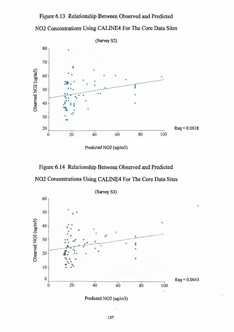
30 -

/0

10


NO2 Concentrations Using CALINE4 For The Core Data Sites

0

c)

0

80

70

60

50

40

30 -

/0

• •ENO

• •

•

% •U.

•

•

•

:

.

•

(Survey S2)

41

•

Rsq = 0.0618

20 40 60 80100

Predicted NO2 (ug/m3)



(Survey S3)

60

50 -

40 -

J

•• „▪ •

I%• Ii 3

all

II .1

11

Rsq = 0.0643410 610 8.0 100


157

•

I20 30 40 50 60 70 80 90 100

Rsq = 0.04861010



c'a'a)z

0

70

60

50

40

30

20

10

•

•

••

•••

me

•

U.

•••

• .

•

•

•

• •

(Survey S4)

•

••

. . ••

Rsq = 0.014240 60 80 100




(Annual Mean Concentrations)

DETR Classification

• ' Rural Background••

• Urban Background

• Kerbside

70-

60-

c.a •

o50 - • •

I:

X40 - •

-oI • •

30 •.1 .

I I

0 I • ••••

•• .•

20


158

Table 6.10 Regression analysis results for CALINE4 for 80 sites.

Parameters Survey S2 Survey S3 Survey S4 Annual MeanDegrees of Freedom 1/67 1/74 1/78 1/79R Value 0.249 0.254 0.119 0.220R2 0.062 0.064 0.014 0.049Adjusted R2 0.048 0.052 0.002 0.117Standard Error 9.979 9.227 12.711 10.188Slope Value 0.129 0.127 0.079 0.119Constant 43.939 22.163 30.875 32.041F value 4.415 5.088 1.126 3.983Significance F Value 0.039 0.027 0.292 0.049

For all surveys including the annual mean concentrations, five sites, with a

predicted NO2 value of approx. 75pg/m 3 appeared to be anomalies, common

to all surveys and located in due/ carriageway and town centre locations.

When these sites were removed, however, no improvement in the regression

equation was perceived. Further examination of the graphs indicated that

there may be two curves in the data - which may be related to urban/rural

locations. Thus the data was re-plotted based on the urban, background and

rural classification used in the previous chapter (see Section 5.5.3). Results

indicated, however, that there was no effect of land cover type on the data

(see Figure 6.16). Overall, therefore, the ability of the model to map small

area variation in air pollution, especially in urban areas, is seen to be poor.

As previously, in examining these results, it is important to remember that the

model does not allow for variation in background concentrations, attributable

to sources other than the modelled roads (i.e. most continuous monitors are in

kerbside or rural locations neither of which provides data suitable for

suburban background concentrations). This may account - at least in part -

for the large intercept value seen in Figures 6.13 and 6.16 and in Table 6.10.

This analysis is admittedly approximate. It suggests, however, that the

dispersion models perform relatively poorly across the range of pollution

levels measured in this area. At low concentrations, the model tends to over-

predict pollution levels; at high concentrations, it under-predicts. Overall, it

159

is not surprising that the model does not predict NO 2 concentrations

accurately at the small area level as dispersion models are not generally

designed for this purpose. The suggested use of such dispersion models in

the UK national air quality strategy (DOE 1996), however, for the definition

of 'air quality management areas' should be treated with concern.

6.6 CONCLUSION

From results of the analysis contained within this chapter it is clear that the

more sophisticated dispersion models (such as CALINE3 and CALINE4)

provide reasonable, though not wholly accurate, estimates of pollution

concentrations in the vicinity of roads when detailed site, receptor and

meteorological information is known. The predictive ability of these models

decreases, however, when large areas are modelled which contain more

numerous linear sources and for which less detailed input data is available.

Under these conditions, the models are unable to act as a reliable basis for air

pollution mapping.

The less sophisticated models (DMRB and CAR-INTERNATIONAL)

performed badly in the preliminary tests, and were clearly unsuitable as a

basis for air pollution prediction or mapping. In some ways this is not

surprising, for the models are, by their very nature, great simplifications of

reality, and do not, for example, consider complex meteorological,

photochemical or topographic effects of dispersion. The results are,

nevertheless, of some significance for air quality legislation in the UK.

160

7. REGRESSION MAPPING

7.1 INTRODUCTION

Air pollution dispersion models (as described in chapter 6) form an integral part

of the UK governments National Air Quality Strategy (DOE 1996) and have

been widely used in epidemiological studies (Ponka 1991; Pershangen et al.

1995; Oosterlee 1996; NILU 1991). Nevertheless, the models tested in the

previous chapter do not appear to provide a true representation of the spatial

variation observed from monitored pollution data at the small area level, and as

such may be considered unsuitable for air pollution mapping or exposure

assessment. Consequently, alternative methods of describing and mapping urban

air pollution variation are needed to meet the requirements of both air pollution

policy and management and environmental epidemiological research.

The available alternatives are extremely limited. Much effort has been put in

recent years into improving dispersion models, and this is likely to enhance their

ability to predict pollution levels in the complex conditions which characterise

urban environments. More sophisticated dispersion models, however, demand

more detailed data, and as has been seen limitations of data availability already

inhibit the use of many models. New generation dispersion models are therefore

unlikely to provide practicable tools in many situations.

161

As noted in Chapter 2, the main alternative is to use methods of spatial

interpolation to map air pollution on the basis of monitored pollution data.

These methods have also been greatly enhanced in recent years, not least through

the development of GIS. Thus, a wide range of spatial interpolation techniques

are now available, as free-standing packages, as part of statistical packages (such

as SPlus or SAS), or as part of proprietary GIS. These include triangulation, thin

plate splines techniques (Hutchinson 1982), moving window methods (Bailey

and Gatrell 1995) and kriging in its various forms (Oliver and Webster 1993,

Myers 1995).

These methods have been widely used for environmental mapping, including air

pollution (e.g. Wagner 1995) though interestingly few attempts have been made

to use them for air pollution mapping in urban areas. Several studies have also

compared the different methods (e.g. SEIPH 1996; 1997; Hutchinson 1982;

Lajournie 1984; Lam and Swayne 1991) albeit without any definitive

conclusions: in general, performance varies according to the. ciuz,lit *Le, data

and the nature of the underlying spatial patterns which are being investigated. In

this context, most methods of spatial interpolation suffer from a number of

problems when applied to urban air pollution. As was shown in Chapter 5,

patterns of spatial variation are extremely complex, with steep pollution

gradients in some areas. On the other hand, monitoring is often relatively sparse,

so that there are few data points available on which to base spatial interpolation.

For many practical applications, access may also not exist to the more advanced

interpolation programs which are available only in the more expensive GIS (e.g.

ArcInfo) or in specially developed software packages (e.g. GSLib). It may also

be noted that many forms of spatial interpolation, by relying solely on data from

measurement points, explicitly ignore other potentially useful information, such

as data on emission sources or surrounding topography. As Chapter 5 has

shown, however, these can help to explain and predict variations in air pollution

in urban areas.

162

What is needed, therefore, is a relatively simple procedure which can perform

more effectively than the simpler dispersion models, is less data demanding than

the more powerful new generation models, yet makes better use of the available

data than most methods of spatial interpolation. One such method, explored

here, is regression mapping.

7.2 THE REGRESSION APPROACH

Regression analysis has been widely used as a method for descriptive and

inferential purposes, as well as for predictive purposes, in a wide range of

disciplines and geographical fields. Regression techniques have been used, for

example, to analysis trends in stream runoff (Smith and Bennett 1994),

relationships between salmon catches and acidification (Waters 1991), temporal

variations in crop production (Tarrant 1984), crop-environment relationships

(Briggs 1981; Carter and Jones 1993; Tong 1992), the spread of Rhododendron

in North Wales (Thomson et al 1993) and spatial patterns in landscape quality

(Briggs and France 1981; Gregory and Davis 1993)

Regression analysis has customarily been used as a basis either for explanation or

prediction. In a few cases, however, this method has also been used for the

purpose of mapping. Rodrigue (1994), for example, mapped transportation land

use utility values by using regression analysis to provide a weighted equation

which was fed into a geographical information system to create a map of possible

utility values of land use in Shanghai, China. He then compared the modelled

map to the existing situation and identified areas where the land was not being

used to its full potential. Similarly, Briggs and France (1981) used a regression

equation, developed from an analysis of landscape preferences of a survey team,

163 ,

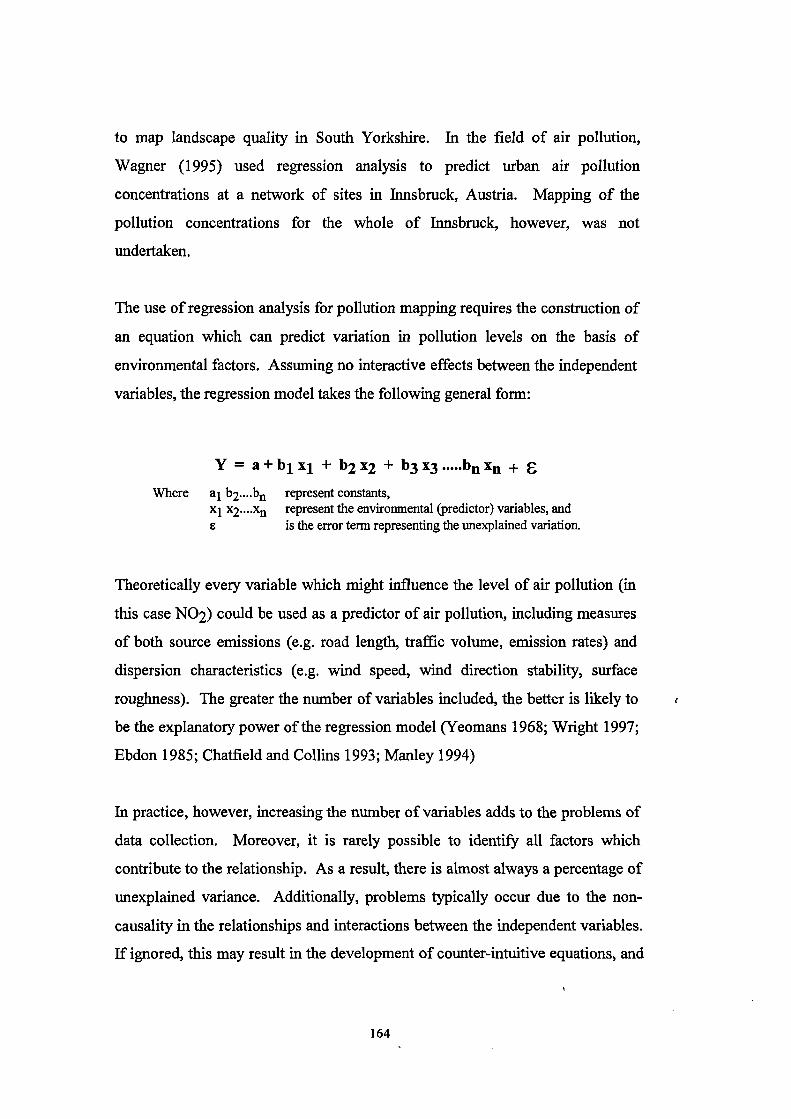
to map landscape quality in South Yorkshire. In the field of air pollution,

Wagner (1995) used regression analysis to predict urban air pollution

concentrations at a network of sites in Innsbruck, Austria. Mapping of the

pollution concentrations for the whole of Innsbruck, however, was not

undertaken.

The use of regression analysis for pollution mapping requires the construction of

an equation which can predict variation in pollution levels on the basis of

environmental factors. Assuming no interactive effects between the independent

variables, the regression model takes the following general form:

Y = a + bi xi + b2 x2 + b3 x3 bn xn 6Where a l b2....bn represent constants,

x1 x2....xn represent the environmental (predictor) variables, andis the error term representing the unexplained variation.

Theoretically every variable which might influence the level of air pollution (in

this case NO2) could be used as a predictor of air pollution, including measures

of both source emissions (e.g. road length, traffic volume, emission rates) and

dispersion characteristics (e.g. wind speed, wind direction stability, surface

roughness). The greater the number of variables included, the better is likely to

be the explanatory power of the regression model (Yeomans 1968; Wright 1997;

Ebdon 1985; Chatfield and Collins 1993; Manley 1994)

In practice, however, increasing the number of variables adds to the problems of

data collection. Moreover, it is rarely possible to identify all factors which

contribute to the relationship. As a result, there is almost always a percentage of

unexplained variance. Additionally, problems typically occur due to the non-

causality in the relationships and interactions between the independent variables.

If ignored, this may result in the development of counter-intuitive equations, and

164

in considerable redundancy in the analysis. Only variables which provide a

logical link between environmental factors and air pollution and which

significantly add to the level of explanation should thus be used.

The main limitations of using regression analysis as a method for air pollution

mapping are as follows:

• statistical requirements: regression analysis requires data measured at an

interval scale, which conforms to a normal distribution. More

specifically, the residuals should have a normal distribution and be

independent of each other (i.e. they should be randomly arranged along

the regression line). With regards to air pollution, this often does not

occur, thus decreasing the validity of regression analysis.

• regression analysis requires the use of preliminary logic and

understanding of the variables in order to select variables for inclusion in

the regression equation.

• The complexity of the air pollution system means that a large number of

variables may be needed to produce the best regression equation possible.

However this requires a large commitment to data collection and

validation. Also the variables used may not reflect underlying causal

relationships. Consequently the final regression equation may not be

stable and may reflect relationships which are unique only to that

particular data set.

Bearing such limitations in mind, however, regression analysis has been used in

this study for a number of reasons:

• it lessens the need for a large scale network of monitoring sites.

165

• it allows exogenous information (e.g. on emission sources) to be used in

the interpolation process.

• it provides rigorous methods for assessing the goodness of fit of the

regression models to the field data, thereby giving reliability estimates for

the results

• if a stable predictive equation can be generated, the equation can be

transferred to different time periods and different areas.

• the equation, if stable, could be used to assess different scenarios, e.g. the

effect of increasing traffic volume along a certain road.

Details of the methodology are described below. A further explanation, and

comparison with regression-based methods carried out in other SAVIAH study

areas is given in Briggs eta!. (1997).

7.3 POLLUTION DATA

As noted in chapter 3, data on the distribution of nitrogen dioxide (NO2) were

collected at a large number of sampling sites within the study area and at two

sites outside this boundary. This monitored data formed the dependent variable

for the regression analysis used in the production of air pollution exposure maps.

Data from the 80 core sites collected in the routine surveys (S 2, S3 S4) was used

in the creation of the air pollution maps (Section 4.1). Multi-level modelling was

undertaken to provide an annual mean pollution concentration for each site

(Section 4.1.3). As noted previously, an additional set of the monitored data (see

Section 3.1) was reserved to enable validation and testing of the finished

pollution maps. Validation of the maps was undertaken using data from three

166

different time periods: within-period testing, pre-period testing and post-period

testing (Section 4.1). Pre-period testing used data collected in the time period

prior to surveys S2, S3 and S4 (i.e. survey SA, June 1992, and survey SB, March

1993). Within-period testing used data from the 40 variable sites (which were

also measured as part of the routine surveys) and data from the 10 consecutive

sites (measured in the consecutive surveys). Temporal data obtained from

Kirklees MC which was within the relevant time period was also used to validate

the maps. Finally, post-period testing of the maps was conducted using data

collected in a fifth survey in June 1994 (S5).

7.4 POLLUTION INDICATORS

A wide range of variables may potentially be selected as a basis for modelling of

urban air pollution levels. These include indicators relating both to emission

sources and processes (e.g. emission rates, traffic volume, energy consumption)

and indicators relating to pollutant dispersal (e.g. wind velocity, wind direction,

atmospheric stability, surface roughness). In practice the choice of variables is

greatly constrained by data availability and costs of data collection. As noted

earlier, there are also benefits in minimising the number of variables used in

regression analysis, since this helps to keep the equation simple and

interpretable, and to reduce the problem of spurious or counter-intuitive

relationships.

167

VLD250

TVOLBUFF

TRAFFCAL

land use map

traffic counts fromKirklees Council

traffic counts fromKirklees Council

Table 7.1 Preliminary list of independent variables for the creation of the pollution equation.

Variable Name Data Source

DefinitionTOPEX site measurements

HIGH DENSITY land use mapHOUSING

INDUSTRY land use map

Local topographic exposure (degrees)

Regional topographic exposure (m)

Altitude at site (m)

Height of the sampler above ground level (m)

Amount of land in which more than 60 per cent of thearea is housing

Amount of land in which industry is located

RELREL

digital terrain model

ALTITUDE

digital terrain model

SAMPLEHT

site characteristics

Total amount of very low density residential housing ata distance of 250m from each site

Weighted area traffic volumes for bands of 0-40m and40-300m radius from each site

CALINE4 weighted traffic distance from all 20m bandsof traffic volume up to a distance of 300m from eachsite

The variables considered for inclusion in regression analysis for this study are

listed in Table 7.1. Several variables were subsequently rejected, either because

of doubts about data reliability or because other variables were considered to

provide more accurate indicators of pollution. Others were transformed or

combined to produce compound indicators. The following indicators were

therefore used in the final analysis:

TVOLBUFF

HIGHDEN

ALTITUDE

TOPEX

RELREL

SAMPLEHT

- Traffic volume in a measured distance around the site.

- Area of high density built-up land in a measured distance around the site.

- Altitude at the site.

- Local topographical exposure.

- Regional topographic exposure.

- Height of the sampler above ground.

The construction and measurement of each of these variables is described below.

168

7.4.1 TRAFFIC VOLUME (TVOLBUFF)

7.4.1.1 DATA COLLECTION

The amount of NO2 emitted from vehicles is clearly a major determinant of

pollution levels in urban areas (Tolley 1995). Unfortunately, accurate data on

vehicle emissions were not available for the study area and, thus, traffic volume

was used as a proxy indicator.

Traffic flows, this time for the entire study area, were obtained from two sources,

as described in Chapter 4. West Yorkshire Highways and Technical Services

Joint Committee, Leeds, provided automatic traffic counts. These were

measured at 80 locations within Kirklees and 3 sites at the motorway. Each

count provided a 24 hour average traffic flow. Manual traffic counts were

obtained from Kirklees Highways Services, Huddersfield. These provided traffic

flows in each direction at a site for 30 minute intervals between 07.00 and 18.00

hours, measured on several occasions within the specified time period. However

there are a number of limitations in using such data:

• not all roads were covered by traffic counts

• a number of roads had a combination of automatic and manual trafficcounts.

• manual traffic counts did not cover a 24 hour period

In order to circumvent these problems of missing traffic data the following

protocol was adopted;

169

• wherever possible automatic traffic counts were used

• if automatic traffic counts were not available, manual counts were used.Information from the nearest automatic count was used to augment andextrapolate the data.

• where no information on road traffic volume was available, local knowledgeand field visits to assess the type and location of the roads was used toassign the road a traffic volume.

This provided traffic flow per 24 hours per road-length for A and B roads in

Kirklees. This information was then averaged to provide traffic flow in vehicles

per hour. Data on traffic flow for minor and estate roads was not available in

most cases, and therefore was estimated, on the following basis: roads > 4m wide

were given a traffic flow of 11 vehicles per hour, roads <4m wide were given a

traffic flow of 5 vehicles per hour. Tracks and unmetaled roads were allocated a

traffic flow of 2 vehicles per hour.

7.4.1.2 PROCESSING

Once collected, the information on the traffic factors was imported into

ARC/INFO (UNIX). The road system in the area was digitised into the GIS and

each road length given a 'type' classification.

• Data on traffic volume in vehicles per hour was attached to the road

segments as attribute data and hence a coverage was created in the GIS for

the whole of the study area, showing each road by type (i.e. motorway, duel

carriageway, A road, B road, minor roads) and traffic volume (see Figure

7.1). The length of each road section (in metres) was also attached to the

coverage as attribute data. A fine mesh (10m 2) was then overlaid onto the

coverage creating a grid coverage (TRAFFVOL).

170

#ft

15% 14: ten Alt t'4144.

171

tr)

tr1 c."14/1

mr 4-4

7?; "§ 4 4 01:4 A V

EI 04"@ 3 A

• The grid co-ordinates of the 80 sample sites were also transformed from

DOS to UNIX and then imported into the GIS. Using the GENERATE and

BUILD commands, the sites were transformed to a point coverage and then

to a grid of the same size as before - i.e. to a mesh cell size of 10m2

(MONSITES).

• A circular buffer made up of grid cells with a radius of 300m was then

drawn around the 80 sample sites (see Figure 7.2); everything outside the

buffer was discarded, effectively performing cookie cutting or masking over

the coverage to create MONalES_1.

• The modified MONSITES 1 coverage was then intersected with the

TRAFFVOL coverage to create a third grid coverage (TRAFFFILTER_300)

which contained all the information on traffic volume by road length and by

road type per grid cell within a radius of 300m from the sample point.

• The road length/type and traffic volume within each buffer was calculated

using the FOCALSUM command. The command summed every value

within a specified buffer zone and placed it in the central gridcell of that

zone. The process was then repeated for the next gridcell in the coverage

(Figure 7.3).

• The FOCALSLTM command was repeated for different buffer zone bands of

different radius ranging from 20m to 300m at 20m intervals.

It would clearly be possible to use the traffic volumes from each of these bands

as independent variables in a regression model to predict NO2 concentrations.

For a number of reasons, however, this approach was eschewed. Firstly, it is

apparent that complex interdependence actually exists between the component

traffic volumes in the different bands, and in reality they are not mutually

independent. Secondly, it must be accepted that the data used to compute traffic

volumes in each of the bands is open to some doubt. Using so many variables

172

•

4

...... -•

•.......

was therefore seen to be likely to compound errors in the analysis. Thirdly,

introducing all these variables into the analysis was likely to lead to unstable and

counter-intuitive relationships with some bands having negative effects in the

equation.

For these reasons, it was considered appropriate to develop a more aggregated

indicator of traffic volume by combining the data from different bands in a

weighted aggregation procedure. The logic behind this step was that the

pollution at any location is a product of contributions from all sources within the

surrounding area, but that nearby sources contribute more than distant sources.

A way was thus needed to define the weights to be attached to each band, based

upon their relative contribution to the pollution level. A combination of

correlation and regression analysis was used for this purpose.

Figure 7.2 Example of a Circular Buffer

Figure 7.3 Example of a Moving Bufferused in GRID

Central grid cellcontaining samplepoint

Boundary ofbuffer

Grid cells

Analysis was conducted using the SPSSPC+ statistical package. Correlations

were calculated between the arithmetic mean nitrogen dioxide concentrations

(Am) and the calculated traffic volume for each band for the 80 core sample

173

sites. The R2 value for each site was plotted (Figure 7.4) and examined to

identify possible ways of combining the data into broader bands. No immediate

banding was perceived, however, although the R2 values did tend to peak in the

80-140m zone. Consequently it was felt that more analysis was necessary.

Therefore stepwise regression analysis, using all traffic bands (i.e. 20, 40, 60

etc.) as independent variables, was undertaken, again in order to identify possible

band combinations. Again no immediately identifiable 'cut-off points for the

zones were distinguishable. Finally, multiple regression analysis was undertaken

on a trial and error basis, to seek the best combination of bands to use as a

predictor of traffic volume. This was achieved by defining two, three or four

zones of varying width around each site, and then using the traffic volumes of the

combined zone (e.g. 10-40, 40-160, 160-300) as independent variables against

the modelled mean nitrogen dioxide concentrations (Mm). The performance of

the different equations were compared in terms of the R2 value. Results for 13 of

the 'best' analyses on this basis are shown in Table 7.2.

On the basis of these results, equation G (with zones of 0-40 and 40-300m) was

selected as the optimal equation. Results from the analysis also provided a

means of determining weights to combine the two buffer zones into a single,

compound traffic volume indicator. The relative contribution of the two zones to

the prediction of NO2 concentrations was shown by the slope value (B). As can

be seen, for equation G, the value of B was 0.00008 for the 0-40 metre zone and

0.0000055 for the 40-300 metre zone. The ratio of the two zones was thus

approximately 15:1, allowing a compound traffic volume indicator to be

compiled as follows:

TVOLBUFF = (15 * Traffic') + (1 * Traffic2)

Where; Traffic' is the calculated traffic volume in a 40m radius from a point.Traffic2 is the calculated traffic volume in a radius of between 40m and

300m around a point.

174

•

U

00N

00,--.

C3• vl .4. en Cl

.1- en NCOD Cl) C/)

.. >No

0 ai" a)>'

..t Cl)o o

Cl)o

Cl)

• • a

-= 1

- a

a • •

• il •

11 -IF

• • • a

ni

0

anwn al

. 175

Table 7.2 Evaluation of traffic buffer zones

Buffer Size Slope ValueB

Degrees ofFreedom

Order ofEquation

AdjustedR2

Constant SignificantValue

A 0-20 0.00013200 76/3 2 41.08 26.754 0.000020-100 0.00001960 3

100-300 0.00000421 1B 0-20 0.00012180 76/3 2 41.34 26.698 0.0000

20-80 0.00002430 380-300 0.00000504 1

C 0-20 0.00009580 76/3 2 42.45 26.673 0.000020-40 0.00007420 340-300 0.00000546 1

D 0-20 0.00017150 77/2 2 39.13 27.102 0.000020-300 0.00000585 1

E 0-20 0.00009580 76/3 2 42.45 26.673 0.000020-40 0.00007420 340-300 0.00000483 1

F 0-40 0.00007750 76/3 2 42.5 26.659 0.000040-120 0.00000853 1

120-300 0.00000483 3G 0-40 0.00008050 77/2 2 43.14 26.669 0.0000

40-300 0.00000546 1H 0-40 0.00007520 76/3 2 42.61 26.62 0.0000

40-100 0.00001040 3100-300 0.00000495 1

I 0-40 0.00007695 75/4 2 42.03 26.621 0.000040-100 0.00000932 3

100-200 0.00000674 4200-300 0.00000389 1

J 0-40 0.00007480 75/4 2 41.8 26.745 0.000040-80 0.00001070 380-120 0.00000748 4

120-300 0.00000493 1K 0-60 0.00003888 75/4 2 37.43 26.991 0.0000

60-120 0.00001139 3120-240 0.00000378 4240-300 0.00000453 1

L 0-100 0.00002714 76/3 2 38.00 26.943 0.0000100-20 0.00000361 3200-300 0.00000372 1

M 0-100 0.00002710 77/2 2 38.85 26.943 0.0000100-300 0.00000368 1

This variable was then entered as the single independent variable in a regression

analysis against the modelled mean NO 2 concentrations, and the residuals and

regression parameters calculated. The process was then repeated using NO2

concentrations for each independent survey as the dependent variable, and again

176

the residuals and regression parameters were calculated. Table 7.3 shows the

results obtained from these analyses.

Table 7.3 Results of regression analysis for nitrogen dioxide and traffic volume, for individualand the modelled annual mean (M„,)

Survey D.F Adjusted R2 Slope Constant Significance FNo Value Value (B)Mm 75/4 43.9 0.004 40.94 0.000

S2 66/2 33.4 0.004 40.83 0.000S3 73/2 29.4 0.003 58.06 0.000S4 76/3 44.4 0.007 20.04 0.000

7.4.2 BUILT LAND

7.4.2.1 DATA COLLECTION

Land cover was also considered to be an important predictor of air pollution, in

two different ways. On the one hand, areas of commercial, industrial and

residential land may act as stationary emission sources. On the other hand, urban

topography (e.g. the density, size and distribution of buildings) affects dispersion

processes.

A land cover map had been created using aerial photographs, at a detailed scale

(1:10,000), as described in Chapter 4. Oneway Analysis of Variance was

conducted, using the SPSSPC+ statistical package, to identify areas of high

pollution levels in urban areas. For this analysis, it was decided to disregard

rural areas for two reasons: firstly the contribution to emissions of NO2 from

rural sites was likely to be minimal (see section 4.3.3.1), and secondly, the effect

of vegetation on dispersion was small in relation to the scale of the project. The

177

main variation were therefore expected to occur within urban areas, as indicated

by the results of the analysis of spatial variation (Chapter 5).

The analysis was conducted on seven land cover classes derived from the land

cover map and detailed in Table 7.4. These were compared in terms of their

NO2 concentrations for each of the three surveys (S2, S3, S4) and the annual

modelled mean (M.); results are presented in Table 7.5. Broadly similar levels

of NO2 are seen across all land cover classes in survey S2. For all other surveys,

however, and the annual modelled mean, apparent differences in mean annual

concentration are discernible: highest concentrations occur in areas of high

density commercial (MC), industry (IND) and very low density housing; lower

values occur in areas of very high density housing, low density housing and

disused/recreational land and urban green space. In part, this pattern is

understandable. The main exception is the high levels of NO2 seen in the areas

of very low density housing. No obvious explanation can be offered, though it

may reflect local siting factors for sites in this land class. Examination of the

probability estimates from the Oneway Analysis of Variance showed that the

differences in NO2 concentrations between urban land use classes for surveys S2

and S3 were not significant (0.1240, and 0.635 respectively). For survey S4 and

the modelled mean, however, the differences were significant (0.0035 and

0.0173).

Table 7.4 Land cover classes and codes used in preliminary analysis of variance

CLASS

LAND COVERCODE

High Density CommercialIndustryVery High Density Housing/Public InstitutesHigh density HousingLow Density HousingVery low density HousingDisused & Sequestered Land/Recreation/Urban Green Space

(UDC)(IND)(VHD/PI)(}DID(LDH)(VLD)(DIS/REC/UGS)

178

Table 7.5 Results of analysis of variance for NO2 concentrations (Rim) by land cover class

LANDCOVERCODE S2 S3

MEAN

S4Mm

95 % CONFIDENCE

S9 S3

INTERVAL FOR THE

S4

MEAN

MT„

HDC 56.64 33.84 41.05 40.54 50.99 - 62.29 27.12 -40.56 34.14 - 47.96 36.17 - 44.91IND 56.06 33.96 42.01 40.85 44.49 - 67.62 26.26 - 41.67 29.59 - 54.43 32.07 - 49.64VHD/PI 55.60 19.87 19.13 24.20 1.01- 110.19 2.44 - 37.29 3.49 - 34.77 6.05 - 42.36HDH 50.78 25.49 38.64 35.83 44.58 - 56.97 18.81 - 32.18 29.71 - 47.56 29.01 - 42.64LDH 45.95 24.36 30.21 31.29 42.16- 49.74 21.30 - 27.41 26.32 - 34.09 28.36 - 34.22VLD 54.43 30.37 48.63 41.36 47.45- 61.42 25.01 - 35.72 37.95 - 59.32 38.98 - 43.74DIS/REC/ 47.80 28.76 28.38 32.59 42.96- 52.64 11.11 -46.41 17.29 - 39.47 20.27 - 44.92UGS

7.4.2.2 PROCESSING

The information on all land cover classes was digitised into the GIS, in order to

allow subsequent reclassification and disaggregation, if necessary. Separate

coverages of the seven land use classes listed in Table 7.5 were then created. A

similar operation to that described for the traffic volume variable was then

conducted.

• A fine mesh (10m2) was overlaid onto each land use coverage (e.g. high

density housing (I-IDH)) thus creating a grid coverage (HDH GM).

• The grid coverage of the 80 core sample sites, which had been previously

created using cookie cutting for the traffic volume variable (MONSUES _1)

(see section 7.4.1.2), was intersected with each of the land use grid

coverages (e.g. HDH_GRID) to create a third series of binary grid coverages

(e.g. HDI-1_300). This contained information on the presence or absence of

each land use type in each grid cell within a radius of up to 300m from the

sample point.

• The amount of each land use type (e.g. high density housing) within each

buffer was calculated using the FOCALSUM command. The command

summed every value within a specified buffer band and placed it in the

179

central gridcell of that band. The process was then repeated for the next

gridcell in the coverage, as shown in Figure 7.3.

• The FOCALSUM command was repeated for three different sizes of buffer

bands, with radii of 40m, 250m and 300m.

• The whole process of cookie cutting and FOCALSUM, was then repeated

for all seven land use classes, on a grid coverage for the whole study area,

using buffer bands of 20m intervals, ranging from 20 to 300m radius. This

allowed the buffers to be weighted (i.e. higher for nearby buffers, lower for

more distant buffers), if necessary, in order to provide a better estimate of

land use. This produced a series of new coverages, one for each land use

class, which could be used for subsequent mapping of a combined land

cover variable.

The creation of the seven land use coverages at differing buffer distances was

conducted for a number of reasons: firstly, to reduce the difficulties of data

collection; secondly to decrease the complexity of the regression equation; and

thirdly because introducing all these variables into the analysis was likely to

lead to unstable and counter-intuitive relationships with some land uses having

negative effects in the equation. Not all of the land use categories, however,

would be expected to affect pollution levels to the same extent. For example,

an industrial area might be expected to have a greater effect than an area of

open land (e.g. recreation ground). Thus a weighted aggregated variable was

needed based upon the relative contribution of each land use type to the

pollution level. A combination of analysis of variance, correlation and

regression analysis was used for this purpose.

Analysis was conducted in the SPSSPC+ Statistical package. Correlations were

calculated between the levels of nitrogen dioxide and the entire urban built-up

land at different distances, from 20m to 300m radius. Built up land was defined

180

as the area of total built land for each band. The results showed that the R2 value

increased gradually with distance from the central point. Consequently, three

arbitrary band widths of 40m, 250m and 300m radius for each of the seven land

use classes or variables was chosen to allow the buffer zones to be weighted if

necessary.

Multiple regression analysis was conducted to identify which of the land use

variables and which band radii to use. The residuals from the previous analysis

of TVOLBUFF (see section 7.4.1.2) were used as the dependent variables in the

regression analysis, to eliminate the effect of TVOLBUFF (i.e. to allow only the

unexplained variation, which remained after the use of the TVOLBUFF variable,

to be examined).

Different combinations of land use and distance were entered into the equation

until the best explanation of variance was found (i.e. the combination giving the

highest R2 value). The results showed that most land use classes did not

contribute significantly to the relationship. Also some land use classes produced

counter-intuitive results (i.e. gave negative correlations). Strong positive

correlations, however, were formed with high density housing and industry, both

for a radius of 300m (HDH 300 and IND 300). Positive correlations were also

sometimes formed with very low density housing at a band width of 250m

(VLD 250). This was considered spurious and therefore the variable was not

included in the subsequent analysis. HDH_300 and IND_300 were regressed

against the residual values and the B value examined. The weights were then

calculated to create a measure of urban land, HEGHDEN:

HIGHDEN = (1.8 * HDH_300) + (1 * 1ND_300)

HDH_300 A measure of the amount of high density housing in a 300 metre radiusaround the site

IND_300

A measure of the amount of industrial land use in a 300 metre radius aroundthe site.

181

The GIS was then used to create a HIGHDEN coverage based on the above

equation. The processes involved in the formation of the coverage is explained

in section 7.4.1.

7.4.3 OTHER VARIABLES

7.4.3.1 ALTITUDE

Altitude was used as a proxy variable for climatic data at each site, as it was

thought that the higher the altitude the lower the pollution levels. This was based

on the expectation that most pollution sources lay in the valley bottoms, and that

increased wind speed at higher altitudes would aid dispersion and reduce

pollution levels. Altitude was defined as the height above ordnance datum at a

sample point. Calculations of altitude for the whole of the study area were taken

from a DTM of the area (Figure 7.5). Preliminary analysis suggested that the

relationship between altitude and nitrogen dioxide concentrations was not linear,

and that this non-linearity persisted when altitude was plotted against the

residuals derived from the TVOLBUFF analysis. Logarithmic transformations of

altitude were therefore used in the subsequent regression analysis.

7.4.3.2 SAMPLE HEIGHT

Sample height was defined as the 'height of the diffusion tube above ground

level'. An attempt was made to keep all samplers at a standard height but, due to

the risks of vandalism in densely populated areas, some samplers were placed

higher. This was expected to have a small effect on the measured results and so

sampler height was also introduced into the regression analysis. In this way, it

182

—

183

on Aim

was possible to standardise subsequent pollution maps to a receptor height of

2.5m.

7.4.3.3 RELATIVE RELIEF

Relative relief (RELREL) was defined as the 'altitudinal variation around the

site'. It is thus a measure of the topographical 'openness' of the site. It was

calculated from the DTM in the GIS as the mean difference between the altitude

of the 10m2 cell in which the site lay and the nine adjacent cells.

7.4.3.4 LOCAL TOPOGRAPHICAL EXPOSURE

The local topographical index (TOPEX) was defmed as 'a measure of the degree

of topographic exposure or openness in the immediate vicinity of a site'. This

allows for the influence of buildings within the vicinity, and was based on the

premise that the more exposed a site (i.e. with few surrounding buildings), the

greater the likelihood of NO2 dispersion and, thus, the lower the pollution levels.

To calculate TOPEX values, a clinometer was used to measure the angle to the

visible horizon for each of the eight compass bearings from the site, and these

values were averaged. The computation of TOPEX is explained in more detail in

Appendix 1.

7.4.3.5 VERY LOW DENSITY HOUSING

As noted above (section 7.4.2), areas of very low density housing showed

relatively high concentrations of NO 2. Because of the counter-intuitive nature of

this pattern, the variable was not included in the compound Built Land factor

184

(HIGHDEN), but it was incorporated as a separate variable in subsequent

analysis, to determine whether it added significantly to levels of explanation.

7.5 CREATION OF REGRESSION MODEL

All potential independent variables mentioned in Section 7.2 were input into an

unconstrained regression analysis using the modelled mean (M.) as the

dependent variable. Those independent variables which best explained the

variation in air pollution concentrations were identified. The resultant regression

equation was applied to the individual surveys (S2, S3, and S4) in order to

determine the extent to which the equation could explain pollution variation

within the surveys (i.e. was the equation temporally stable). This process is

explained in more detail below.

7.5.1 REGRESSION ANALYSIS ON MODELLED MEAN

The modelled mean NO2 values (M.) were entered as the dependent variable in

the regression analysis. The independent variables were as follows:

TVOLBUFF amount of weighted traffic volume by band (1000 vehicle km/hr)

HIGHDEN amount of weighted high density housing and industry (ha)

VLD_250 amount of very low density housing (ha)

ALT altitude (variously transformed) (metres)

RELREL altitudinal variation around the site (metres)

TOPEX local topographical exposure (degrees)

SAMPLEHT height of the sampler above ground level (metres)

185

All of the above variables were initially entered into the regression equation

using unconstrained stepwise analysis. Results showed that VLD_250, TOPEX

and RELREL did not contribute to the equation at a significance level of 0.05,

and were therefore discarded from the analysis. The analysis was then resumed

utilising the remaining four variables, using the enter method. A number of

essentially similar equations were generated, with similar levels of explanation of

NO2 concentrations. The equation which gave marginally the highest R 2 value

explained 60.7 per cent (with 75/4 D.F) of the variation of NO2 in the study area

is:

NO2 = 11.83 + (6.777 * SAMPLEHT) + (0.268 * HIGHDEN) + (0.00398 * TVOLBUFF) + (-0.0355 * LNALT)

The method was then repeated for the three individual surveys (S2, S3, S4) again

using first the stepwise method to obtain the independent variables. Again

VLD 250, TOPEX and RELREL were rejected from the equation. The

remaining variables were once more regressed using the enter method to produce

the fmal equations for the individual surveys. Once more, several similar

regression equations could have been generated, those with the highest R2 were

used. From the results it was found that the equation for survey S2 explained

38.7 per cent (with 64/4 D.F). For survey S3 it explained 39.8 per cent (with

71/4 D.F); for survey S4 it explained 55.0 per cent (75/4 D.F) of the variation in

pollution levels.

Survey 2 (S2)

NO2 = 48.81 + (1.97853 * SAMPLEHT) + (0.0000218 * HIGHDEN) + (0.000004163 *TVOLBUFF) + ( -2.29468 * LNALT)

Survey 3 (Si)

NO2 = 50.475 + (1.8663 * SAMPLEHT) + (0.0000098496 * IIIGHDEN) + (0.000002767 *TVOLBUFF) + (-6.74495 * LNALT)

186

Survey 4 (S4)

NO2 = 21.14 + (2.56504 * SAMPLEHT) + (0.000039129 * HIGHDEN) + (0.0000061359 *TVOLBUFF) + (-0.87704 * LNALT)

7.5.2 TRAFFIC VOLUME VARIABLE

The traffic volume variable clearly accounted for the largest proportion of the

variation in NO2 in all surveys. The traffic volume variable used, however, was

somewhat arbitrary in its construction. Efforts were therefore made to improve

this variable. For this purpose, the line dispersion model, CALINE3, was used to

provide weightings for the total traffic volume in the area surrounding the sample

points, as follows:

• The traffic volumes for each of the buffer bands was computed from the GIS

for intervals of 20m ranging from 20m to 300m radius. These were

intersected with the MONSITES_1 coverage (the sample point coverage) to

produce the traffic volume by buffer band for each sample site. The values

were exported from UNIX to DOS as a database.

• The mid-point of each buffer band (i.e. 5m, 15m, 25m,.. 290m) was input

into the CAL1NE4 linear dispersion model, and a weighting curve under

average meteorological conditions (calculated from 15 minute interval

weather data obtained from the University of Huddersfield weather station

for 1 year) was produced (Figure 7.6).

• The values obtained from the curve were used in following equation which

was then applied to all sample sites:

Total Traffic Volume = (1 * traff 20) + (0.455 * traff 40) + + (0.06800 * traff 300)

187

/

N

/

CD-N

cr)

CD-00

N

0- -71-N

C:)- CDN

04:)

C)N,-1

C)00

0.1.

000

MITA Di

188

Traffic Variable

TVOLBUFFTRAFFCAL

Indicator: traffic volumeonly

Adjusted R2 value

S2 S3 S4

Mm

33.4 29.4 44.4 43.9

29.3 29.6 37.7 40.2

Indicator: complete range of variablesincluding HIGHDEN & SAMPLEHT

Adjusted R2 value S2 S3 S4 Mm

38.32 38.50 56.80 55.82

35.20 38.90 53.45 54.20

Thus a new weighted traffic volume variable (TRAFFCAL) was created. This

variable was then entered into the regression analysis in place of TVOLBUFF,

and equations for the modelled mean and the individual surveys re-computed.

Results are summarised in Table 7.6. This shows that the fmal level of

explanation of variations in NO2 using the TRAFFCAL variable (as shown by

the R2 value) is lower than that using TVOLBUFF in all surveys except survey

S3. The original equation (section 7.5.1) were therefore used for subsequent

mapping.

Table 7.6 Results of regression analysis using traffic volume variables

Complete equations.

TVOLBUFF = (15*Traffic buffer zone of 40m) + (1 *Traffic Buffer zone of 40-300 m)

TRAFFCAL = (1*traff20) + (0.455*traff40) + (0.318 * traff60) + (0.25 * traff80) + (0.21 *traff100) + (0.18*traff120) + (0.16*traff140) + (0.14*traff160) + (0.11*traff180)+ (0.11*traff200) + (0.09*1raff220) + (0.09*traff240) + (0.07*traff260) +(0.07*traff280) + (0.05*traff300)

7.6 MAPPING

In order to allow the estimated value of NO2 concentrations to be calculated at

any one point in the study area, it was necessary to extrapolate the final equation

to the entire area. This was carried out by producing air pollution maps within

the GIS. In order do this, coverages for the variables, HIGHDEN and

189

TVOLBUFF, were created for the entire study area using the following

procedures:

TVOLBUFF

• In order to create a coverage based on the equation Tvolbuff (section

7.4.1.2), it was first necessary to produce coverages of the variables, Traffic]

(calculated as traffic volume in a 40m radius from a point), and Traffic2

(calculated as traffic volume in a 40 to 300m radius from a point) used in the

equation. This was accomplished using a similar process to that described in

section 7.4.2.1.

• First, coverages TRAFFIC_1 and TRAFFIC_2 were created by again

applying the FOCALSUM command to the original TRAFFVOL coverage.

The resultant coverages contained information on the total traffic volume

within a 40m radius around each gridcell (TRAFFIC_1) and the total traffic

volume within a 40-300m radius around each gidcell (TRAFFIC_2), for the

entire coverage.

• The two TRAFFIC coverages were then combined using the Tvolbuff

equation to create a weighted coverage of total traffic volume (TVOLBUFF)

(Figure 7.7).

HIGHDEN

• In order to produce a coverage based on the Highden equation (Section

7.3.2.2), it was first necessary to reproduce coverages of the variables,

Hdh 300 (calculated as the amount of high density housing in a 300m radius

for every gridcell), and Ind 300 (calculated as the amount of industry in a

300m radius for every gridcell) for the entire study area. This was

accomplished using a similar process to that described in section 7.4.2.2.

190

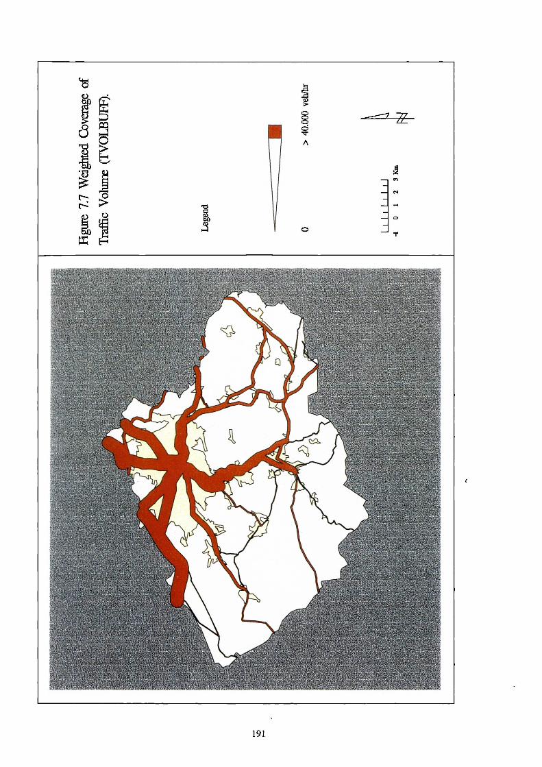
1§gA

-I 0 -

191

• Again the FOCALSUM command was applied to the original HDH_GRID

and IND GRID coverages in order to create the two coverages used in the

Highden equation, Hdh_300 and Ind_300. The resultant coverages

contained information on the amount of high density housing in a 300m

radius for every gridcell (HDH 300) and the amount of industry in a 300m

radius for every gridcell (IND_300), for the entire coverage.

• The Highden equation was then applied to the HDH_300 and IND_300

coverages to create a combined weighted coverage, (HIGHDEN) (Figure

7.8).

Once these coverages were created, the final equation, involving all the variables,

was entered into the GIS and a map of the estimated air pollution was produced.

In this analysis, sample height was set to a standard level of 2.0 metres. This

step was repeated for each of the three individual surveys and for the modelled

mean values. Results from this procedure are shown in Figures 7.9 to 7.13.

All the pollution maps show broadly similar patterns of relative NO2

concentrations, although the absolute concentrations do vary, with survey S2

producing the highest concentrations and survey S3 the lowest.

For survey S2 (Figure 7.9), highest concentrations were found, not surprisingly,

along the motorway (M62), Leeds road (A62), the Sheffield road (A616) and

near the ring road, as these are heavily used roads, which logically would be

expected to produce high amounts of vehicular emissions. In all cases, areas of

high pollution are associated with major infrastructure and settlements (e.g.

within the first 3 - 4 km from the town centre). Lowest concentrations were

found in the south-west, an area of moor land, in or near the Peak National Park.

Interestingly, for all four maps, increased concentrations are associated with the

village of Meltham, in the west, and the B-road which serves it. Overall, the map

192

for survey S2 indicates a more concentrated pollution gradient than the other

maps, with levels changing rapidly over a short distance.

Survey S3 (Figure 7.10) shows broadly similar pattern of pollution to survey S29

with the highest concentrations again associated with the motorway (M62), the

Sheffield road (A616) and the town centre. An area in the south-east associated

with Denby Dale and Skelmanthorpe also indicated concentrations which were

higher than the surrounding area. On the whole, however, the range of pollution

values and the gradient between the 'highly polluted' and 'non polluted' areas are

much lower than for all other maps. Again, the lowest concentrations are found

in the south-west.

The pollution map for survey S4 (Figure 7.11) again displays a similar pattern of

pollution to that of survey S2. The villages of Denby Dale and Skelmanthorpe

are again noticeable as pollution hotspots (concentrations of 50-60 gg/m3

compared to concentrations in the surrounding area of 20 to 30 gig/m3).

Interestingly, although in comparison to the major urban areas, pollution levels

associated with the A640 Buckstones road in the north-west of the study area are

low compared to the major urban areas, there is a clearly defined pollution

corridor allied with the A640 which is not obvious on the other three maps

(Figures 7.9 - 7.12).

The annual mean pollution map (Figure 7.12) again displays similar pollution

patterns. Areas of pollution which were high in the previous maps are also high

in the annual pollution map. A similar pattern emerges for areas of low

pollution.

The regression model used in the creation of the maps allows the generation

of high resolution pollution maps, as Figure 7.13, an enlargement of the

195

—

•-•

196

MEM

a.)

197

11111111111111

/

198

5

s

r=4

Cn1

r-:

0.1=1ga8

00

en

-

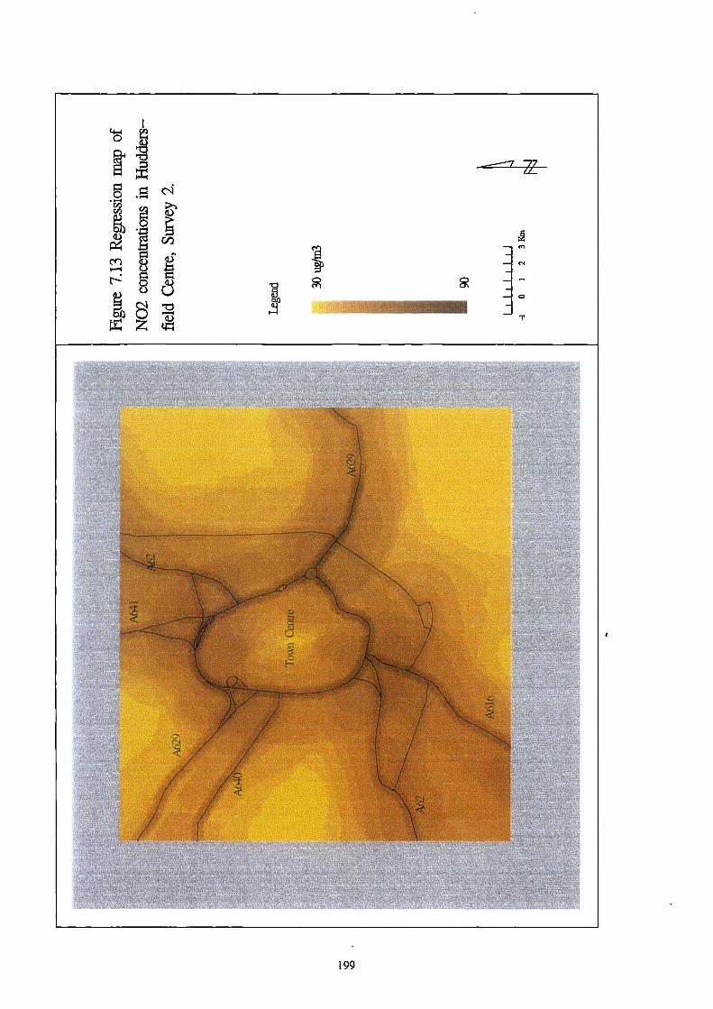
(41tc

8 .1=1

---

-ER -

-

cs,

—

0

s71.3

--

Z

199

Huddersfield town centre, illustrates. Notably, even at this scale, considerable

variations in pollution levels are visible, reflecting the local variations recorded

by Loxen and Noordally (1988) and Hewitt (1991) in detailed studies of small

areas. The effect of traffic volume on the maps can also be seen, with the Leeds

road (A62) and the Sheffield road (A616) showing much higher levels of NO2

than the Halifax road (A629) and New Hey Road (A640).

7.7 VALIDATION

The results of the regression mapping were validated against independent data.

Subsets of the NO2 data had previously been withheld from the creation of the

model for this purpose (section 4.1). A testing regime was devised to evaluate

the capability of the maps to predict actual levels during three different survey

periods: concurrent with the modelled period (within-period testing), prior to the

modelled period (pre-period testing) and following the survey period (post-

period testing).

7.7.1 WITHIN-PERIOD TESTING

From the three individual surveys, NO2 data from 40 variable and 8 consecutive

sites had been reserved for testing and validation purposes. The location and

unique identification number (site-id number) of all the sites (the 40 and the 8

sites) were input into the data base and transferred into the GIS.

200

Comparisons were made between:

• the monitored values at the 40 variable sites for each survey period

(S2, S3, S4) predicted from the map for that survey;

• the monitored values at the 40 variable sites for each survey period

and the mean annual map;

• the monitored values at the 8 consecutive sites for each survey period

and the values predicted from the map for that period;

• the mean concentration for the 8 consecutive sites and the mean

annual map.

Results of the analysis are shown in Table 7.7 (see page 212) and Figure 7.14 to

7.25.

7.7.1.1 WITHIN-PERIOD TESTING: VALUABLE SITES

From these results it appears that, on the whole, the maps are a good predictor of

monitored NO2 concentrations for the within-time-period. The 40 variable sites

from the third survey (S 3) achieved an R2 value for the individual map of 35.0

per cent and 44.3 per cent for the annual modelled mean map (Mm). These

figures compare favourably with the R 2 values of 38.7 per cent and 56.5 per cent

for the individual and modelled mean map derived from the regression equations

developed in Section 7.5.1. The results indicate that both the individual survey

map and the annual modelled mean map are good predictors of pollution for the

40 variables sites monitored in survey S3 . This can be seen in graphical form in

Figures 7.16 and 7.17 and in tabular form in Table 7.7. The slope value for the

analysis of both maps was similar (1.42 and 1.37 respectively), reflecting the

tendency for the pollution map to overpredict actual pollution levels at the higher

concentrations in both cases.

201,

Figure 7.14 Relationship Between Predicted and Observed NO2

0

0

70

60 -

50 -

40 -

30

For Variable sites in Survey S2

• • •• • •

•• •

• • •

.1 Rsq = 0.2781

30 40 50


610


Annual Mean NO2 Values For Variable Sites in Survey S270

60 -

50 -

40

30 -

at

CI

•

11

3II

71

a

VI

11

•1Ai

a

11

Rsq = 0.2790

30 40 50 60 70

Predicted Annual Mean NO2 (ug/m3)

202

50 -

40 -

30

90

10

0

Figure 7.16 Relationship Between Observed and Predicted NO2

Values For Variable Sites in Survey S3

'@)

c•I

-0

60

50 -

40

30

10

0

•

•

• •

•

Rsq = 0.3677

1 10 20'-

30 410 50 60




Rsq = 0.4581

10 20 30 40 50 60

Predicted Annual Mean (ug/m3)

203

90 30 4.0 50 610 710

-

10

10

Rsq = 0.5598


Values For Variable Sites in Survey S4

El

z

0

70 -

60 -

50

40 -

30

20

10

•

•

•

•

••

•

1

Rsq = 0.5363

10

30 40 50 60 70

Predicted NO2 (uein3)



60 -

r:

50

40

30 -

Predicted Amp.' Mnpq NO2 (.1g/m3)

204

A similar picture was observed from survey S4. Results showed increased R2

values of 52.4 per cent (S 4) and 54.8 per cent (Mm) (compared with an R2 value

of 55.0 per cent derived from the equations in Section 7.4.1) indicating that the

map gave good predictions for the variable sites (Figure 7.18 and 7.19). The

slope values were also similar to those obtained in survey S3 (1.28 and 1.8

respectively).

For survey S2, results from both the individual and the annual pollution maps

gave an R2 value of only 25.7 per cent (expected R2 value, 38.7 per cent) Again

this distribution is represented graphically in Figures 7.14 and 7.15. When the

slope values are examined, both graphs showed a slope of close to unity: B =

0.99 for the individual maps and 0.804 for the mean annual map. Although the

fit to the observed data is poorer in this survey, overall, the maps again imply

some consistency between the predicted and measured concentrations.

7.7.1.2 WITHIN-PERIOD TESTING: CONSECUTIVE SITES

Results from the analysis of the consecutive sites (8 sites) for survey S2 produced

a high R2 value. The R2 value for the individual map was 72.9 per cent, while an

R2 value of 74.8 per cent was recorded for the annual map. This is represented

graphically in Figures 7.20 and 7.21. The slope values are again close to unity,

1.14 (S2) and 1.06 (Mm) . For survey S3, again, the results from the analysis of

the consecutive sites was higher than results from the variable sites (Figure 7.22

and 7.23). The R2 value for the individual map was 74.3 per cent (B value of

1.08) and for the annual pollution map 55.5 per cent (B value of 0.87). Results

from survey S4 also showed high levels of correlation, with R2 values of 69.0 per

cent for the individual survey and 82.0 per cent for the annual pollution map

(Figure 7.24 and 7.25). However, slope values for this survey were 1.52 for the

individual map and 2.15 for the annual pollution map, indicating a tendency to

205

3

a

40


(14

0

70

60

50

40

30

Values For Consecutive Sites in Survey S2

Rsq = 0.7625

30 410 50


60 710


Annual Mean NO2 Values For Consecutive Sites in Survey S260

50

za30

)0 Rsq = 0.7793

30 50 60

Annual Mean NO2 (ug/tn3)

206


40

30

")0

10

values For Variable Sites in Survey S3

• a

Rsq = 0.7752

10 20 30 40



Annual Mean NO2 values For Consecutive Sites in Survey S350-

40

-@)

307:3

0"-)0

.1

10

l0 ?TO 30 40

Rsq= 0.6105

Annual Mean NO2 (ug/m3)

207


values For Variable Sites in Survey S460

50

40

-cs30

0

0

Rsq = 0.7289

10

20 30 40 50 60



Annual Mean NO2 values For Consecutive Sites in Survey S460-

50

40

30

0

10/

11

Rsq = 0.8427

10 20 30 40 50 60

10

Annual Mean Predicted NO2 (ughn3)

208

over-predict at lower concentrations and under-predict at high concentrations.

Overall, therefore, results from the consecutive sites appeared to indicate that

they were representative of pollution levels in the study area and that the

regression maps performs well.

7.7.2 TEMPORAL (ANNUAL) DATA

Data was obtained from 28 sites monitored by Kirklees MC using consecutive

diffusion tubes. The location of the Kirklees monitoring sites was identified and

those on the edge or outside the study area were labelled as such and initially

discarded leaving 15 sites in total. The process of intersection, described in

section 7.4, was undertaken. In the first instance each of the sites within the

study area were intersected with the annual modelled mean pollution map.

Regression analysis was used to compare the monitored and predicted

concentrations. This process was repeated using both the 15 sites inside the

study area and those remaining Kirklees sites previously considered on the

boundary of the study area (total of 21 sites). (The validity of the results of these

sites was questionable as the maps edge effects were unknown). The results of

the analysis are shown in Table 7.8.

Results from this analysis appear to indicate that a relationship exists between

the annual pollution map (Mm) and the data obtained from Kirklees MC. The

analysis conducted on all sites (21 sites in total) and only those sites within the

study area (selected sites) (15 sites in total), gave an R2 value of 33.9 per cent

and 31.5 per cent respectively. In interpreting these results, it is important to

note that the Kirklees sample sites were, in most cases, deliberately positioned in

areas of high pollution in order to fulfil local government policy. They thus

show less spatial variation in pollution levels than the other data sets used. In

209

this context, the results again imply that the regression maps give a satisfactory

prediction of pollution levels recorded by the Kirklees MC sites.

7.7.3 PRE-PERIOD TESTING

Two surveys, (S A and SB) were conducted prior to the collection of data used in

the formation of the equations. These surveys were used to examine whether the

regression maps accurately predicted pre-survey pollution levels, and thus

whether the pollution map is stable over time. Again the LATTICESPOT

command was used within the GIS to intersect the location of each of the sample

points from the two surveys with the annual mean estimated pollution map. The

resultant estimated concentrations were regressed against the monitored NO2

values by site. Results are summarised in Table 7.9 and Figure 7.26 and 7.27.

The results show that R2 values are somewhat lower that those obtained for the

survey period, suggesting that the mean annual pollution map does not provide

such a good predictor of past pollution levels. The R2 value for survey SA (June

1992), however, was 39.7 per cent and the slope value was close to unity (1.01),

indicating a satisfactory prediction. The same could not be said of survey SB

(March 1993): for this survey, the annual modelled mean pollution map gave an

R2 value of 14.9 per cent. The slope value was also low (0.61). For this survey,

therefore, the annual mean modelled map for 1993-1994 does not provide a

satisfactory estimate of pollution levels.

7.7.4 POST PERIOD TESTING

A further test of the temporal predictivity of the regression map, and the stability

of the map over time, a post-period survey was conducted in July 1994 (S5).

210

70

60


0

60

50

40

30

20

10 .//

Pre-Period Testing - Survey Sa

NI 1 WI • IllU 3II

• Al

01 I WND •LI •

WI • • •We • • •

a• •

111

•

Rsq = 0.4054

10 210 30 40 50 610



Pre-Period Testing - Survey Sb

• •

•• •

111 • •• • • • • •• • ••

• • • • •

30

20 ••

•• ••••••• 11

1111 •

••• ••

•mi

•

••

•

• ••

••• •

I 1

Rsq = 0.1583

0

30 50 60 70


211

.-I '1' 005,--n ON Men ON ON-.. en ir)Cl tel ciInN •:1-

1-4 en. I I

0tnM%.0re;.

0

11)

cn vz,r-:N -o

4-1V)

N<4 f:4

VD ON

en-

0c M•0 0 en 00000000.

en

cn

en00

en tenQ\ en00 0

C>000000cz; cz3

00 In\0 0\

MC). ‘C!

V")

4n4 v-4 C v-4

0000 CD 0 00 00 0

N ON0 0 N0000 O. 0 0

0

l"---NO.-.•kr)M0

00en"04-")rer)4--•

.-d11---NooVDv-;I

NO.-.1,1CA.--1--.,—.

Moo4-4

ON(1o4nII

enr-0•:1-k()0.64-4I

kO Illr-- ..crN kr)0 N.-. v-)NN

1 I

cn enen en

0000•:1- ,•-n

0

0

4-n0

CO

• 4-44-1Cl)

CU 0el) -00.)) tt)A el.: vz)

vnI

N

•0

104 U)az.

04 Ez t--0 Z 0 C:PN

ce)

CA V)

055> >NN00Z ZE E

-o -oV CU

E E

U.1

ONONC)

CrelONn-n

C.)

cnenC).

ooN en1/40 tr)00

ci

N 00 'et ,-.4 1' ON ". 1' '1' N In N NN tr) 00 —0-00.--. 00 N CT v--. N t--r- oo V- 0 en en .0- en t-- 0 0 cl

on vi c.i 4 ,e; 4 .1: Lei c•i 4 c:, c,i vz)N CNI t•--- t-- cri .cr r-- tn in tr) nC) 00 S

ON tr) t-- en N oo 00 r- N0000ooM- oo kr) N kr) oo N NO oo 0 en cr) 00oo cn N 0 D CD .cl• 0 oo NO en .1 1/4000 C.) .tr ,C) ,--I l"--- 00 N N as N In •:1'

,--n .--•C7N 00 CR .1. en C! C.3 cl N. 111 '—'00 CD ,--• 1n4 1n4 tsi 1nI

,%.0 N-

en en C--men

0 0 0 0 0 0 0 0 0411- NI- 4-4 4 1 1[1- 'It. T-4 44-4

V) V) cA cA cA EA EA0 V V d.) V CL) t) V 4.)

0 0 0 0 0 0 0En CA EA En0.) V 4.)

0

rA V) V)0.) 0.)

0 0(tt tci ccl> > > >NNNN0000zzz z

gggg

CO CCICZCI> > > >NNNN0000Z Z Z Z

(1en /T) C0 0 "0 0

CL) d.)cci

Iu

.gEEg

V) V) V) VICU CU 00 0 0 0atc0c1> > > >NNNN0000

ZZ

gggg00 00en

CA V) VI CACL) CU CL)

0c0 c0

> > > >NNNN0000Z Z Z

Vat' ca*.cai4 .4 4 4

212

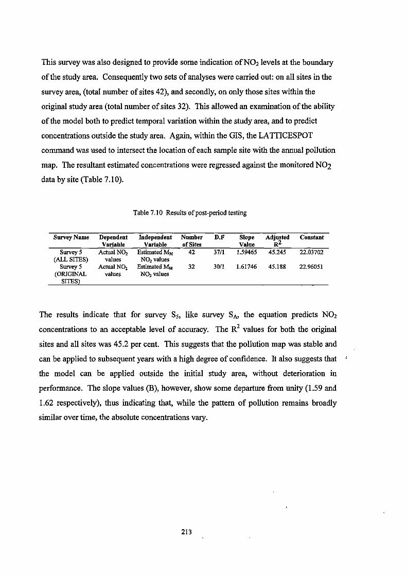
This survey was also designed to provide some indication of NO 2 levels at the boundary

of the study area. Consequently two sets of analyses were carried out: on all sites in the

survey area, (total number of sites 42), and secondly, on only those sites within the

original study area (total number of sites 32). This allowed an examination of the ability

of the model both to predict temporal variation within the study area, and to predict

concentrations outside the study area. Again, within the GIS, the LATTICESPOT

command was used to intersect the location of each sample site with the annual pollution

map. The resultant estimated concentrations were regressed against the monitored NO2

data by site (Table 7.10).

Table 7.10 Results of post-period testing

Survey Name Dependent Independent Number D.F Slope Adjusted ConstantVariable Variable of Sites Value R2

Survey 5(ALL SITES)

Actual NO2values

Estimated MmNO2 values

42 37/1 1.59465 45.245 22.03702

Survey 5(ORIGINAL

Actual NO2values

Estimated MmNO2 values

32 30/1 1.61746 45.188 22.96051

SITES)

The results indicate that for survey S5, like survey SA, the equation predicts NO2

concentrations to an acceptable level of accuracy. The R2 values for both the original

sites and all sites was 45.2 per cent. This suggests that the pollution map was stable and

can be applied to subsequent years with a high degree of confidence. It also suggests that

the model can be applied outside the initial study area, without deterioration in

performance. The slope values (B), however, show some departure from unity (1.59 and

1.62 respectively), thus indicating that, while the pattern of pollution remains broadly

similar over time, the absolute concentrations vary.

213

7.8. CONCLUSION

On the basis of the results presented here, it appears that the regression model provides a

relatively accurate and reliable map of air pollution within the study area. The regression

model appears to be able to predict both forward and backwards in time with comparative

confidence. Further monitoring in the study area, during which 20 sites were monitored

over a 21 consecutive period (October 1994 to September 1995) confirmed that the

predictive performance of the pollution map was maintained. The R2 value for the

relationship between mapped and monitored concentrations was 0.59, with a slope of

approximately 1.5. Subsequent research (de Hoogh pers comm.) has also shown that the

model developed here can be applied, without modification, in other urban areas, with

similar levels of success.

Within the time and resource constraints of a rapid survey (i.e. a 2 to 4 week time period),

therefore, it may be concluded that the regression approach offers a practical and effective

method of mapping urban air pollution. Certainly compared to the dispersion modelling

approaches outlined in chapter 6, it appears that the regression approach performs

satisfactorily in the Huddersfield area. Nevertheless, improvements in the regression

method are no doubt possible. Improved indicators of traffic emissions may be

obtainable, for example, given better data on traffic volume and composition. Better

indicators of the effects of urban morphology and land use may also be possible, which

would reflect the effects on dispersion patterns. Above all, it would be interesting to

include in the model temporal indicators (e.g. season, wind speed, etc) which would allow

more specific estimates to be made for particular survey periods and conditions. These

and other implications and developments of the methodology are discussed in the next

chapter.

Further modification to this model may be undertaken in an attempt to increase its

accuracy, for example, by further investigating the effects of weather patterns on pollution

variation. In terms of this project however, such modification were thought to complicate

214

the modelling procedure further, thus reducing the possible uses of this model by non-

scientific personnel and were also limited due to time constraints. The value of this

model is discussed in more detail in the following chapter.

215

8 DISCUSSION

"There has been a significant increase in the availability of monitored airpollution data in the UK in recent years with an increase in the number ofmonitoring sites and the range of pollutants measured. There is, however, still arequirement for maps of pollutant concentrations at a much higher spatialresolution than can be calculated by simple interpolation between monitoringsites" (AEA 1997).

This statement indicates the continuous need for the development of accurate

methods of calculation and mapping of air pollution, especially in urban

environments. Moreover, the UK National Air Quality Strategy (DOE 1996)

stipulates that areas of poor air quality should be identified through monitoring

and modelling techniques and, where necessary, air quality management areas

defined - something which is only possible by a method of interpolating from

point data to create an air pollution map. In addition, increasing traffic volume

and growing concern about the effects of traffic-related pollution on health

reinforces the justification for this thesis, namely that there is a need to map

traffic-related air pollution at the small area (urban) scale for use in a wide range

of fields - from epidemiology to transport planning and the development of

structure plans. This chapter will examine the extent to which the research has

been successful in fulfilling the aims and objectives stated in Chapter 1, i.e:

• examination of the magnitude, source and patterns of small area

variation in traffic-related air pollution in an urban environment, and

thus building on such information to allow the;

• investigation of methods of mapping traffic-related air pollution at a

small area level.

216

It will then consider the implications of the research for the wider body of users,

both in other research areas and for management and policy and any contribution

made to the understanding of variation in pollution levels at the small area level

within the urban environment will be assessed.

8.1 THE STORY SO FAR

8.1.1 SOURCES OF VARIATION

Aim: to examine the magnitude, source and patterns of small areaspatial variation in traffic-related pollution.

Patterns of variations in air pollution concentrations within the study area are

complex and affected by both emission patterns and dispersion characteristics, on

a spatial and temporal level. In addition, error propagated during laboratory and

fieldwork procedures (measurement error) acts as a third possible influence on

the patterns and magnitude of recorded variation in pollution concentrations.

To investigate the importance of these sources of variation, a number of purpose-

designed surveys were conducted. Each survey was designed to investigate a

particular facet of possible variation in air pollution. The influence of emission

factors, including volume of road traffic and land cover type, on patterns of

spatial variation in air pollution were considered. Equally, the dispersion

characteristics of pollution were examined with surveys designed to investigate

the amount of variation in pollution with distance to road, height above ground

level and altitude. Inter-survey variations in pollution concentrations were also

217

assessed. The ability to defme 'temporal affmity areas' in the study area was

investigated and the relationship between spatio-temporal variation explored.

Surveys were conducted using passive diffusion tubes deployed as required by

the individual investigation (e.g. variation with distance from road was measured

using transects perpendicular to the road; for variation with height diffusion

tubes were placed at regular intervals up the side of buildings). A detailed

description of the sampling regime and preliminary results of the analysis are

given in Chapter 4. Results of the appropriate statistical analysis are given in

Chapter 5.

Results of the analysis indicated that the effect of measurement error was small

(accounting for only between 1.7 and 4.2 per cent of the total variation recorded

in a survey), and could therefore be considered negligible. With regard to the

spatial and temporal effect on pollution concentrations, however, a number of

interesting patterns of variation in pollution levels were identified.

Results indicated that both traffic volume and distance from the nearest road (up

to a distance of 60 metres) were good predictors of variation, although these

accounted for only 54.6 and 55.9 per cent of the total measured variation

respectively. Sampler height above ground also proved important in predicting

urban air pollution and explained ca. 42 per cent of the recorded variation with

height. Conversely, neither land cover type (examined in several different ways)

nor altitude were perceived to be major determinants of air pollution levels,

although both showed weak correlations with measured concentrations.

Temporal influences on patterns and magnitude of pollution concentrations were

investigated in a variety of ways. Comparison between data from the 80 routine

survey sites indicated that the pollution surface remained stable over time (Adj

R2 of between 57.5 to 70.0 per cent); thus while absolute pollution levels may

218

vary from one survey to another, the inter-site differences remain broadly the

same.

The presence of temporal affinity areas for the study area, as developed by

McGregor (1996) were investigated using pollution data which had been

collected over a number of years by the local council (Kirklees M.C.) (See

Chapter 4). Factor analysis was performed on the data and the results indicated

that 92.4 per cent of the variation could be explained by using only three

communal factors and that there was coherence between the land cover type of

sites in the 3 factor groupings. This has considerable significance for the design

of monitoring networks. It means that extrapolation from one site to the

surrounding area should be valid within the affmity area of that site. On the

other hand, extrapolation to sites in other affinity areas is likely to be misleading.

It also suggests that, within any affinity area, the pollution map is broadly stable

over time: whilst absolute concentrations may vary, the pattern of variation

should remain largely the same. In this study, the large majority of the sites were

seen to group into one affinity area, indicating that the pollution maps were thus

stable over most of the study area.

Interactions between spatial and temporal influences were also considered using

data from the 80 routine surveys. Results indicated that a large proportion of the

recorded variation was attributed to spatial influences (ca. 89 per cent) while

only ca. 9 per cent was due to temporal variation. Interestingly, 14.6 per cent of

the total variation recorded (both explained and unexplained variation) was

attributed to the interaction effect between both spatial and temporal variation,

indicating that the effect of interactive spatio-temporal variation although

relatively small in comparison to spatial variation alone should not be neglected.

From the results of the analysis, it is clear that the sources and patterns of

variation are inherently complex and cannot be simply explained by examining

219

those factors which influence spatial and/or temporal variation in NO2

concentrations individually. Any attempt at mapping variation in air pollution

should allow for the effects of both spatial and temporal variation in emission

sources and dispersion characteristics.

8.1.2 DISPERSION MODELLING

Aim: to investigate methods of mapping traffic-related airpollution at a small area level

The usefulness of dispersion models for air pollution mapping and management

was highlighted in the recent UK National Air Quality Strategy (DOE 1997)

which advised Local Authorities that, in auditing levels of air quality for

compliance with UK government legislation,

"monitoring itself cannot provide all the information necessary to manage airquality effectively and efficiently" and that "numerical modelling is a poweifultool which aims to relate the emissions of a pollutant to the concentrationsmeasured at an air quality monitoring station (DOE 1996)".

The suggestion is thus that dispersion modelling should be used to provide

additional information for the definition of air quality management areas.

Several recent epidemiological studies have also attempted to use dispersion

modelling as a basis for deriving exposure estimates (e.g. NILU 1991;

Pershangen et al. 1994; Oosterlee et al. 1996).

The ability of these models to provide maps of air pollution across a wide area

remains uncertain (see Section 2.3), and relatively few attempts have been made

to test and validate these models under such conditions. Chapter 6 consequently

investigated the extent to which dispersion models provide valid estimates of

traffic-related pollution levels and, given the high degree of local variation noted

220

in the previous section, examined the capability of these models to predict and

map urban pollution at the small area scale.

The study compared the performance of four dispersion models; DMRB, CAR-

INTERNATIONAL, CALINE3 and CALINE4. A number of surveys were

designed and conducted to provide NO 2 data for validation of the chosen models.

The sampling strategy is explained in detail in Section 4.5.

Results of the preliminary analysis using a small number of sites for which real-

time traffic-counts were available indicated that the less sophisticated models

such as CAR-INTERNATIONAL and DMRB did not adequately explain

variation in pollution (with R2 values between predicted and monitored pollution

levels of ca. 4.8 and 21.2 per cent respectively). Use of CALlNE3, which

allowed for meteorological data and topographical characteristics, improved the

level of explanation (Adj R2 = 40.2 per cent). The best performance, however,

was achieved by the more sophisticated dispersion model, CAL1NE4, which

allowed for the influences of meteorology, topology and photochemical reactions

(Adj R2 = 52.2 per cent). Based on these results, the entire A, B and motorway

road network for the study area was modelled using the CAL1NE4 programme.

Concentrations were calculated at receptor sites which matched the geographical

location of the routine sample sites (see Chapter 4 for sampling design), thus

allowing comparison of the modelled and monitored results to be undertaken.

Under these conditions, CAL1NE4 performed markedly less well, explaining

only 4.8 to 11.7 per cent of the total measured variation in NO 2 concentrations.

The main reasons for this are likely to be both weaknesses in the model itself

(e.g. its inability to cope with complex terrain) and errors and inadequacies in the

input data (e.g. the use of estimated traffic flows and data from only two

meteorological sites and one continuous monitoring site for ozone for the entire

study area).

221

The ability of less sophisticated dispersion models for mapping variation in air

pollution in an urban area thus appears to be poor, and their use for air pollution

management systems or epidemiological studies is questionable. More

sophisticated line dispersion models appear to perform better, so long as good

quality input data (i.e. traffic volume, road wide, meteorological factors and

surface roughness) is available. This requirement cannot always be met for

urban-scale analysis and, in this case, it seems that these models, too, may not be

reliable. Recent developments within the field of modelling, however, have seen

the release of 'second generation' dispersion models. These have overcome a

number of limitations associated with the Gaussian based models (e.g.

replacement of emission factors with fuel efficiency factor; substitution of

Gaussian plume equation with the buoyancy line plume). In addition, models

such as UK ADMSURBAN can consider a combination of emission sources

(point, line and area emissions) within one modelling package. These models

have not yet been rigorously validated and are reliant on large amounts of input

data and therefore were not considered for use in this thesis. Further validation

of these models, using the type of data available in this study would be

appropriate.

8.1.3 REGRESSION ANALYSIS

Aim: To investigate methods of mapping traffic-related airpollution at a small area scale.

The inability of dispersion models to provide a true representation of the

variation observed in monitored pollution data at the small area level meant that

an alternative method of mapping traffic-related air pollution was required.

Regression analysis, used in a wide range of fields for descriptive and predictive

purposes, has not been widely used for mapping purposes. A range of variables

relating to emission sources and dispersion characteristics which best explained

222

variation in concentrations were selected (e.g. traffic volume and distance from

road). Other variables related to field and desktop measurements for each site

(e.g. RELREL and TOPEX). A full list of variables is given in Chapter 7.

Regression analysis was conducted to identify those variables which best

explained variation in pollution levels measured in the routine surveys (see

Chapter 4). Once identified the selected variables were input into ARC/INFO

GIS and regression analysis conducted for each 10m grid square for the entire

study area. The resultant pollution surface was then compared to monitored data

not used in the construction of the regression equation (i.e. 40 variable and 10

consecutive sites; pre-period surveys and a post-period survey), to assess the

validity of the resultant maps.

Results of the analysis were divided into three time periods, pre-period testing,

within-period testing and post-period testing. Comparison of within-period data

from the variable and consecutive sites indicated that the regression method was

able to explain between ca. 30 to 56 per cent of the variation in pollution

concentrations. For the eight consecutive sites the level of explanation was

between 61 and 84 per cent. Pre-period testing explained between 16 and 41 per

cent of the measured variation in NO2 concentrations. It should be noted that the

lower result was obtained from a survey that was not designed specifically to

provide good spatial coverage and therefore may be biased. Post-period testing

again indicated that the regression method provided a good explanation of

variation in NO2 concentrations (adjusted R2 = ca. 45 per cent). These results

indicate that the regression model provides a relatively accurate and reliable map

of air pollution for the study area which is able to predict both forwards and

backwards in time — indicating a stable pollution surface. This agrees with

results obtained from the temporal affinity area analysis and the inter-survey

correlation (see Chapter 5).

223

The ability of the regression model to provide accurate and reliable maps of air

pollution for a specific area using limited input data is an improvement on the

dispersion modelling approach to pollution mapping. Much of the data required

for the regression model is easily obtained from local structure plans held by the

relevant Local Authority. Data on traffic flows and the road network can be

obtained from the relevant Highways Authority and the Ordnance Survey

respectively; information on altitude can similarly be obtained from the 0/S

equivalent sources if required. Indeed the requirement for each Local Authority

to conduct a phase one assessment and review of air quality for their district as

required by the UKNAQS (DOE 1996) means that much of the data on emission

sources and land cover and traffic flows will be readily available. The simplicity

of the model enables it to be used by a wide range of people in a variety of

locations for numerous purposes. The use of such a mapping methodology will

be examined in the following section.

8.2 PRESENT AND FUTURE OPPORTUNITIES

For a research project to be of value, it needs to make a useful contribution to the

theoretical and/or applied research community and to the wider society as a

whole. The critical evaluation of the project and specifically the results of the

regression model detailed in the previous section pre-supposes an exploration of

the possible uses of such research and naturally the investigation of further

avenues of research.

The application of the results of this work and subsequent further areas of

research can be subdivided into three overlapping but distinct areas: management

strategy development, policy making and enforcement and research. In terms of

224

policy, significant developments in the field of air quality have occurred over the

last year. In order to fulfil the requirements of the 1995 Environment Act, the

Secretary of State was required to prepare and publish a national air quality

strategy for public consultation. The subsequent consultation document was

released in August 1996, with the revised document published in 1997 —

although this is still to become a white paper and thus enforceable. The first

stage of the national strategy requires all Local Authorities to conduct a review

and assessment of air quality to highlight areas which are not expected to meet

the 2005 air quality standards and designate them air quality management areas

(AQMAs) (DoE 1997). The government tentatively suggests that dispersion

modelling could be used to identify such areas and to undertake further

investigation of these areas; the regression method of pollution mapping at the

small area level, however, provides a better estimate of the dispersion and

magnitude of pollution. Moreover, unlike the more sophisticated dispersion

models (e.g. ADMS, CAL1NE4), the regression model does not teoluite. Nast

quantities of input data, nor detailed knowledge of dispersion modelling for

operation. Compliance is also an important issue related to policy. The

successful application of the regression model to other areas (de Hoogh pers

comm) enables local and central government to ensure that legislation is being

adhered to and also to ensure that standards set are achievable. It could even be

used to enforce legislation in certain areas if necessary.

The management of air pollution and related issues could be enhanced by the use

of the regression map. Air pollution is inherently linked, although not directly, to

land use, and thus planning. Consequently, using the regression model, scenario

modelling could be conducted to assess the impact of various ideas in the

development of local structure plans and in the licensing of industrial processes

(both process A and B's). Thus, it would be useful to both the Environment

Agency and local government respectively. In addition, this approach could be

beneficial in the development and preparation of Environmental Statements for

225

Environmental Impact Assessment (especially in the screening, scoping and

mitigation stages). A further use of the regression approach could be within the

field of health care. The model provides a simple and easy way of mapping

pollution at the small area scale and thus of identifying `hotspots' — this

knowledge could then be used to concentrate epidemiological studies, health care

provision, personal monitoring and abatement strategies in areas of greatest need.

Although useful in its present form as shown above, the research project has

opened a number of avenues of unanswered questions and opportunities for

further research. One of the most obvious questions to be answered relates to

the monitoring strategy that is needed. For example, how many monitoring sites

would be needed to maintain the pollution surface? - what quantity would be

necessary to reflect variations on a seasonal or annual basis? In addition, it

would be interesting to see if the regression approach could be transferred to

other pollutants such as CO and PK () — a useful adaptation given the expense of

monitoring the latter pollutant.

The ability of the model to predict over long and short-term periods would also

be a valid research question. Short-term predictions could be used to advise the

public on their activities (as is currently done in Paris, France). Long-term

predictions would enable the development of appropriate air quality management

strategies at the local area instead of national level.

Examination of the variables used, and particularly the inclusion of a

meteorological variable for predictive purposes, may lead to an increase in the

accuracy and predictive ability of the model. The effect of introducing additional

variables, not available at the time of this research — such as a detailed emissions

inventory - would be interesting to investigate. Taking the opposite approach, it

would be equally useful to investigate the ability of the regression approach to

226

map air quality in areas where air pollution is known to be a major problem, but

which has poorer quality data and little or no resources to fund a monitoring

program (e.g. Indonesia, India and Brazil all of whom have major urban air

quality problem related to traffic).

Finally, the regression model to date has, out of necessity, concentrated on

predicting traffic-related air pollution. It would be interesting to investigate how

well this approach could be expanded to other air pollution sources, such as

industry or to other types of pollution, such as noise.

227 ,

BIBLIOGRAPHY

Abbey, D.E. Mills, P.K. Petersen, F.F. Beeson, W.I (1991) Long-term ambientconcentrations of total suspended particulates and oxidants as related toincidence of chronic disease in California USA Seventh Day Adventists.Environmental Health Perspective. (94) 43-50.

Action Asthma (1991) The Occurrence and Cost of Asthma. CambridgeMedical Publications, West Sussex, U.K.

AEA (1997) Pollution forcast page [on line] AEA Technology. Available from:http://www.aeat.co.uk/products/centres/netcen/airqual/bulletins/forcasts.html[Accessed on 7th July 1997].

Anderson, H.R. Butland, B.K. Strachan, D.P. (1994) Trends in prevalence andseverity of childhood asthma. British Medical Journal. (308) 1600-1604.

Anto, J.M. Sunyer, J. (1990) Exposure to Soyabean dust and acute asthma.WHO Consultation of Data Requirements and Methods for Analysing SpatialPatterns of Disease in Small Areas. Rome 22-24 October, 1990.

Apling, A.J. Stevenson, K.J. Goldstein, B.C. Melia, R.J.W. and Atkins, D.H.F.(1979) Air pollution variation in homes: Validation of diffusion timemeasurements of nitrogen dioxide. LR311 (A), Warren Spring Laboratory.

Archibold, O.W. and Crisp, P.T. (1983) The distribution of airborne metals inthe Illawarra region of New South Wales, Australia. Applied Geography. 3 (4)331-344.

Aron, R (1983) Mixing height- an inconsistent indicator of potential airpollution concentrations. Atmospheric Environment. 17 (11) 1193-2197.

Association of London Authorities, London Boroughs Association, South EastInstitute of Public Health (1994) Air Quality in London. The First Report of theLondon Air Quality Network. February 1994.

Atkins, D.H.F. Sandalls, J. Law, D.V. Hough, A.M. Stevenson, K. (1986) Themeasurement of nitrogen dioxide in the outdoor environment using passivediffusion tube samplers. UK Atomic Energy Authority, Harwell, Report AERER 12133

228

Atkins, D.H.F. and Lee, D.S. (1991) Spatial and temporal variation of ruralnitrogen dioxide concentrations across the UK. Atmospheric Environment (29)223-239.

Ayres, J.G. Noah, N.D. Flemming, D.M. (1993) Incidence of episodes of acuteasthma and acute bronchitis in general practise 1976-1987. British Journal ofGeneral Practice. (43) 361-364.

Bachlin, W. Theurer, W. Plate, E.J. (1991) Windfield and dispersion in a built-up area — a comparison between field measurements and wind tunnel data.Atmospheric Environment. (25A). pp1135 — 1145.

Bailey, J. Campbell, G. Kibblewhite, M. McInnes, G and Porter, D. (1992) Airquality audit - BP Chemicals, Baglan Bay. Warren Spring Laboratory. LR 905(AP/CA).

Bailey, T.C. and Gatrell, A.C. (1995) Interactive Spatial Data Analysis.Longman.

Bates, D.V. Sizto, R. (1987) Air pollution and hospital admissions in SouthernOntario: the acid summer haze effect. Environmental Resources. (43), 317-331.

Beaton, J.L. Ranzieri, A.J. Shirley, E.C. and Skog, J.B. (1972) MathematicalApproach to Estimating Highway Impact on Air Quality, 4 FederalAdministration, FHWA-RD-72-36, Washington, D.C.

Bentham, G. (1990) Chernobyl fallout and perinatal mortality in England andWales. Fourth International Symposium in Medical Geography Proceedings.Norwich, U.K.

Benson, P.E. (1979) CALINE3 - A versatile dispersion model for predicting airpollution levels near highways and arterial streets. FHWA-CA-TL-79-23.

Benson, P.E. (1982) Modifications to the gaussian vertical dispersionparameter, az, near roadways. Atmospheric Environment. 16 (6) 1399-1405.

Benson, P.E. (1992) A review of the development and application of theCAL1NE3 and 4 models. Atmospheric Environment. 26b (3) 379-390.

Blacker, J.H. (1973) Triethanolamine for collecting nitrogen dioxide in the TVLrange. Journal of American Industrial Hygiene Assocaition. 34 390-395.

Blumer, W and Reich, T. (1980) Leaded gasoline - a cause of cancer.Environment International (3) 465-471.

229

Bobak, M. Leon, D.A. (1992) Air pollution and infant mortality in the CzechRepublic, 12986-88. The Lancet. (340) 1010-1014

Bocken, P. Michorius, J. van Reeuwijk, H. and Schellevis, L. (1992) A passivesampler for measuring NO2 in ambient air; networks, performance and inter-comparison of methods in Prague city. Department of Air Pollution,Agricultural University of Wageningen, the Netherlands. V-310.

Boleij, J.S.M, Lebret, E. Hoek, F. Noy, D. and Brunekreef, B. (1986) The use ofPalmes diffusion tubes for measuring NO2 in homes. Atmospheric Environment.20 597-600.

Bott, M.H.P. and Tantrigoda, D.A. (1987) Interpretation of the gravity andmagnetic anomalies over the Mull Tertiary intrusive complex, N.W. Scotland.Journal of the Geological Society. (144) 17-28.

Bower, J. Boughton, G. Dando, M. Lees, A. Stevenson, K. Lampert, J. Sweeney,B. Parker, V. Driver, G. Waldo, C. Wood, A. (1991) Urban NO2 concentrationsin the U.K. Atmospheric Environment. 25B(2), 267-283.

Bower, J.S. Broughton, G.F.J. and Willis, P.G. (1993) Measurements of UrbanPhotochemical Oxidants. In Cocks A.T. (ed) The Chemistry and Deposition ofNitrogen Species in The Troposphere. Royal Society of Chemistry. Cambridge.

Bradshaw, J.M. Ford, K.M. Adamswebber, J.R. Boose, J.H. (1993) Beyond therepertory grid — new appracohes to constructist knowledge aquision tooldevelopment. International Journal of Intelligent Systems. 8(2) 287-333.

Briggs, D.J. (1981) Environmental influences on the yield of spring barley inEngland and Wales. Geoforum, 12(1) 99-106.

Briggs, D.J. (1992) Mapping environmental exposure. IN Elliott, P. Cuzick, Z.English, D. Stern, R (eds) Geographical and Environmental Epidemiology:Methods for Small-Area Studies. Oxford University Press. Oxford. UK. 158-176.

Briggs, D.J. and France, J. (1981) Mapping noise pollution from road traffic forregional environmental planning. Journal of Environmental Management. 14173-179.

Briggs, D.J. Collins, S. Elliott, P. Kingham, S. Fischer, P. Lebret, W. vanReeuwijk, H. Van der Veen, A. Pry!, K. Smallbone, K. (1997) Mapping urban

230 s

air pollution using GIS: a regression based approach. International Journal ofGeographical Information Systems. 11(7) 699-718.

Britton, J. (1992) Asthma's changing prevalence. British Medical Journal. 304857-858.

Brown, R.H. Charlton, J. Saunders, K.J. The development of an improveddiffusion sampler. Journal of American Industrial Hygiene Association 42 865-869.(1981)

Brown, R.H. (1991) Feasibility study on the use of diffusive passive samplersform monitoring ambient air. Health and Safety Executive; Research andLaboratory service division.

Brunkreef, B. Lebret, E. Hoek, G. von Kessel, A. (1991) Effects of ozone onlung function in children living in the Netherlands. Archives of EnvironmentalHealth. (1991) (46) 119-120.

Brunlcreef, B. Lumens, H. Hoek, G. (1989) Pulmonary function changesassociated with an air pollution episode in January 1987. Journal of AirPollution Control Association. (39) 1444-1447.

Burney, P. (1988) Asthma deaths in England and Wales 1931-1985: evidencefor a true increase in asthma mortality. Journal of Epidemiology and CommunityHealth. (42) 316-320.

Burney, P. Chinn, S. Rona, R.J. (1990) Has the prevalence of asthma increasedin children? Evidence from a national study of health and growth 1973-1986.British Medical Journal. (300) 1306-1310

Burrough, P.A. (1986) Principles of geographical information systems for landresource assessment. Oxford University Press, Oxford.

Cadoff, B.C. Knox, S.F. and Hodgeson, J.A. (1979) Persona Exposure Samplesfor nitrogen dioxide. National Bureau of Standards, Washington D.C.

Calder, K.L. (1973) On estimating air pollution concentrations from a highwayin an oblique wind. Atmospheric Environment. (7) 863-868.

Calvert, J.G, Heywood, J.B. Sawyer, R.F and Seinfield, J.H. (1993) Achievingacceptable air quality: some reflections on controlling vehicle emissions.Science. (261) 37-45

231,

Campbell, G.W. (1988) Measuring nitrogen dioxide concentrations at rural sitesin the United Kingdom using diffusion tubes. Environmental Pollution. (55),251-270.

Campbell, G.W. Steadman, J.R. Stevenson, K. (1994) A survey of nitrogendioxide concentrations in the UK using diffusion tubes — July to Dec 1991.Atmospheric Environmental (28) 477-486

Carter, S.E. and Jones, P.G. (1993) A model of the distribution of cassava inAfrica. Applied Geography, (13), 353-371.

Cass, G.R. (1981) Sulphate air quality control strategy design, AtmosphericEnvironment. (15) 1227-1249

Chatfield, C. and Collins, A.J. (1993) Introduction to Multivariate Analysis.Chapman and Hall. London. UK.

Chock, D.P. (1978) A simple line-source model for dispersion near roadways.Atmospheric Environment. (12) 823-829

Clark, R.H. (1979) A Model for Short and Medium Range Dispersion ofRadionuclides Released to the Atmosphere. National Radiological ProtectionBoard. Harwell. Oxon NRPB-R91

Clark, M (1997) Geographical Information System Applications in Hydrology.Paper presented to the British Hydrological Society, 30 th April 1997. ImperialCollege. London. UK.

Collins, S. Smallbone, K. and Briggs, D.J. (1995) A GIS approach to modellingsmall area variation in air pollution within a complex urban environment. INFisher, P. (eds) Innovations in GIS 2. Taylor and Francis. London. 245-253.

Coils, J. (1997) Air Pollution: an introduction. E &FN Spon. London.

Committee on the Medical Effects of Air Pollution. (1995) Asthma andOutdoor Air Pollution. HMSO. London.

Cooper, S.E. and Burt, T.P. (1986) Topographic controls on rainfall and runoffReport to US Army. European Research Office. NATO.

Coughlin, S.P. (1988) Sport and the asthmatic child: a study of exercise inducedasthma and the resultant handicap. Journal of the Royal College of GeneralPractitioners. (38) 253-255.

232 -

Dabbert, W.F. Hoydysh, W.G. (1991) Street canyon dispersion: Sensitivity toblock shape and entrainment

Davison, G and Hewitt, C. N. (1996) Air Pollution in the United Kingdom. TheRoyal Society of Chemistry. Cambridge.

Dekker, C.M. Groenendijk, A. Sliggers, C.J. and Verboom, G.K. (1991)Quality Criteria for Models to Calculate Air Pollution. Publication Series Air,90, Staatsuitgeverij DOP, 's-Gravenhage.

Delvin, R.B. McDonnell, W.F. Mann, R. Becker, S. House, D.E.Schreinemachers, D. Koren, H.S. (1991) Exposure of humans to ambient levelsif ozone for 6.6 hours causes cellular and biochemical changes in the lung.American Journal of Respiratory Cellular Molecular Biology. (4) 72-81.

Department of the Environment (1996) United Kingdom National Air QualityStrategy. HMSO.

Department of Transport (1994) The Design Manual for Roads and Bridges.Vol 11. Environmental Assessment. HMSO. London.

Detels, R. Sayre, J.W. Coulson, A.H. (1981) The UCLA population studies ofchronic obstructive lung disease IV: respiratory effect of long term exposure tophotochemical oxidants, nitrogen dioxide and sulphates on current and neversmokers. American Review of Respiratory Disease. (49) 20-39.

Detels, R. Tashkin, D.P. Sayre, J.W. (1991) The UCLA population studies ofCORD:X. A cohort study of changes in respiratory function associated withchronic exposure to SO,, NO and hydrocarbons. American Review ofRespiratory Disease. (81) 350-359.

Dockery, D.W. Pope, C.A (1994) Acute respiratory effects of particulate airpollution. Annual Review of Public Health. (15) 107-132.

Dockery, D.W. Pope, C.A. Xu Xiping, Spengler, J.D. (1993) An associationbetween air pollution and mortality in six US cities. New England Journal ofMedicine. (329) 1735-1739.

Dockery, D.W. Spengler, J.D. Reed, M.P. and Ware, J. (1992) Relationshipsamong personal, indoor and outdoor NO2 measurements. EnvironmentInternational. 5 101-107.

233

Dockery, D.W. Spiezer, F.E. Stram, D.O. (1989) Effects of inhaled particles onrespiratory health of children. American Review of Respiratory Disease. (139),587-594.

Dorling, D and Fairbairn, D. (1997) Mapping ways of measuring the world.Longman. Essex.

Dubrule, 0. (1984) Comparing splines and kriging. ComputationalGeoscience. Mathematical Geology 101 327-338.

Dundon-smith D.M. and Gibb, R.A. (1994) The channel tunnel project andregional economic development. Journal of Transport Geography. 2(3) 178-189.

Ebdon, D. (1985) Statistics in Geography. Blacicwells, Oxford.

Edwards, J. Walters, S. Ayres, J.G. (1994) Hospital admissions for asthma inpre-school children - relationship to major roads in Birmingham, UnitedKingdom. Archives of Environmental Health. 49 223-227.

Eerens, H.C. Sliggers, C.J. and van den Hout, K.D. (1993) The CAR model: theDutch method to determine city street air quality. Atmospheric Environment27B (4) 389-399.

Eggleston, S. Hackman, M.P. Heyes, C.A. Irwin, J.G. Timmis, R.J. Williams,M.L. (1992) Trends in urban air pollution in the United Kingdom during recentdecades. Atmospheric Environment. 26(B) 227-239.

Elliott, P. Hills, M. Beresford, J. Kleinschmidt, L. Jolley, D. Pattenden, S.Rodrigues, L. Westlake, A. Rose, G. (1992) Incidence of cancers of the Larynxand Lung near incinerators of waste solvents and oils in Great Britain. TheLancet April 4. 854-858.

Elsom, D. (1992) Atmospheric pollution. Basil Blackwell.

Elsom, D. (1995) Smog Alert — managing urban air quality. Earthscan

Emark, D.L. (1977) An analytical model for air pollutant transport anddeposition from a point source. Atmospheric Environment. 11 231-237.

Eskridge, R.E. and Hunt, J.C.R. (1979) Highway modelling part 1: prediction ofvelocity and turbulence fields in the wake of vehicles. Journal of AppliedMeteorology. 18(4) 387-412.

234.

Eskridge, R.E. Peterson, W.B. Rao, S.T. (1991) Turbulent diffusion behindvehicles: effects of traffic speed on pollutant concentrations. Journal of Air andWaste Management Association. 41 312-317.

Euler, G.L. Abbey, D.E. Hodgkin, J.E. (1988) Chronic obstructive pulmonarydisease symptom effects of long-term cumulative exposure to ambient levels oftotal oxidants and nitrogen dioxide in California Seventh Day Adventistresidents. Archives of Environmental Health. 43 25-36.

Evans, R.G. Webb, K. Homas, S. Ayres, S.M. (1988) Cross-sectional andlongitudinal changes in pulmonary function associated with automobile pollutionamong bridge and tunnel officers. American Journal of Industrial Hygiene. 1425-36.

Expert Panel on Air Quality Standards (1994) Ozone. HMSO London.

Expert Panel on Air Quality Standards (1996) Nitrogen Dioxide. HMSOLondon.

Expert Panel on Air Quality Standards (1995) Sulphur Dioxide. HMSOLondon.

Farber, H.J. Wattigney, W. Berenson, G. (1997) Trends in Asthma prevelance:the Bogolvsa heart study. Annuals of Allergy, Asthma and Immunology. 78 (3)265-269.

Fischer, P.H. Bohumir, K. Martuzzi, M. Wojtyniak, B. Lebret, E. van Reeuwijk,H. Pukhart, H. Briggs, D.J. Gorynski, P. Elliott, P. (in press) Prevalence andrisk factors of childhood respiratory health in four countries in Western andCentral Europe in the study on small area variation in air quality and health(SAVIAH) Submitted to Atmospheric Environment.

Fowler, W.K. (1982) Fundamentals of passive vapour samplers. AmericanLaboratory. 81 80-87.

Gair, A.J. Penkett, S.A. and Oyola, P. (1991) A simple passive diffusiontechnique for the determination of nitrogen dioxide in remote continentallocations. Atmospheric Environment. 25(A) 1929-1939.

Gambel, J. Jones, W. Minshall, S. (1987) Epidemiological environmental studyof diesel bus garage workers: acute effects of NO2 and respiratable particles onthe respiratory system. Environmental Resources. 42 201-214.

235

Gifford, F.A. and Hanna, S.R. (1973) Modelling urban air pollution.Atmospheric Environment. 1 131-136.

Gilbert, O.L. (1974) An air pollution survey by school children. EnvironmentalPollution. 6 174-180.

Gillham, C. Leech, P. Egglestone, H. (1992) UK Emissions of Air Pollutants;1970-1990. Warren Spring Laboratory report, LR 887(AP) ISBN 0 85624 7472.

Girman, J.R. Hodgson, A.T. Robinson, B.K. and Traynor, G.W. (1983)Laboratory studies of the temperature dependence of the Palmes NO2 passivesampler. Lawrence Berkeley Laboratory Report LBL 16302, Berkeley.

Goldsmith, J.R. Griffth, H.L. Detals, R. (1993) Emergency room admissions,meteorological variables and air pollutants: a path analysis. American Journal ofEpidemiology. 118, 759-778.

Goldstein, I. Leiber, K. Andrews, L. Kazembe, F. Foutralds, G. Huang, P. Hayes,C. (1988) Acute respiratory effects of short term exposure to nitrogen dioxide.Archives of Environmental Health. 43, 138-142

Goodman, G.T. Smith, S. Parry, G.D.R. and Insldp, M.J. (1974) The use ofmoss-bags as deposition gauges for air-borne metals. Proceedings of the 41stConference of the National Society of Clean Air, Brighton, UK. 1-16.

Green, M.C. and Gebhart, K.A. (1997) Clean air corridors: A geographic andmeteorological charicterisation. Journal of Air and Waste ManagementAssocitaion. 47(3) 403-410.

Greenland, D and Yorty, R.A. (1985) The spatial distribution of particulateconcentrations in the Denver metropolitan area. Annuals of the Assocaition ofAmerican Geographers. 75(1) 69-82.

Gregory, K.J. and Davis, R.J. (1993) The perception of riverscape aesthetics: anexample from two Hampshire rivers. Journal of Environmental Management,39, 171-185.

Haathela, T. Lindholm, H. Bjorksoen, F. Koskenvuo, K. Laitinen, I.A. (1994)Prevalence of asthma in Finnish young men. British Medical Journal. 301(6746). 266-268.

Haggett, P. Cliff, A.D. Frey, A, (1977) Locational Models. Edward Arnold.

236

Hall, D.J. Spanton, A.M. MacDonald, R. Walker, S. (1996) A review ofrequirements for simple urban dispersion models. Report for DoE,Environmental Technical Unit.

Hall, N.E.L & Wynder, E. (1984) Diesel exhaust exposure and lung cancer: acase-control study. Environmental Research. 34, 77-86.

Halliday, J. Henry, R. Hankin, R. and Hensley, M. (1993) Increased wheeze butnot bronchial hyper-reactivity near power stations. Journal of Epidemiology andCommunity Health. 47, 282-286.

Hangartner, M. (1989) Passive sampling of nitrogen dioxide, sulphur dioxideand ozone in ambient air. Department of Hygiene and Applied Ergonomics,Federal Institue of Technology, Zurich.

Hangarther, M and Burn, P. (1987) Passive sampling of nitrogen dioxide andsulphur dioxide in ambient air. In: Diffusive Sampling - An AlternativeApproach. Ed: Berlin, A. Brown, R.H. and Saunders, K.J. CEC Publishers10555EN. Brussels-Luxembourg.

Hanna, S.R. (1978) Diurnal variation of the stability factor in the simple ATDLurban dispersion model. Journal of Air Pollution Control Association. 31 851-860. Prevalence of asthma in Finish young men. British Medical Journal. 301266-268.

Hanna, S.R. and Gifford, F.A. (1977) Application of the ATDL simple urbandispersion model to Frankfurt, West Germany. Proceedings of the NATO/CCMS8th International Technical Meeting on Air Pollution Modelling and itsApplication. Louvain - la - Neuve, Belgium. 20-23 September 1977.

Harrop, D.O. Mumby, K. Ashworth, J. Nolan, J. Price, M. Peppers, B. (1990)Air quality in the vicinity of urban roads. Science of the Total Environment. 93285-292.

Harvey, D. (1997) Comparison of point source dispersion models. Paperpresented to UK National Dispersion Modelling Workshop. 11 November 1997.Olympia. London.

Hassema, H. (1993) Passive sampling methods. A comparision. Paperpresented to the EU-SAVIAH Working Group. Wageningen University. April5th. 1993.

Hawksworth, D.L. and Rose, F. (1976) Lichens as Pollution Monitors. EdwardArnold Ltd.

237

Haywood, I. and Cornelius, S. (1988) Managing Environmental RadioactivityMonitoring Data: a GIS Approach. NE.RRL Research Report 87/88. Universityof Newcastle. Newcastle upon Tyne. UK.

Hawthorne, V.M. Fry, J.S. (1978) Smoking and health; The associationbetween smoking behaviour, total morbidity and cardio-vascular symptoms inWest Central Scotland. Journal of Epidemiology and Community Health. 32,260-266

Heal, R.M. and Cape, J.N. (1997) A numerical evaluation of chemicalinterference in the measurement of ambient nitrogen dioxide by passive diffusionsamplers. Atmospheric Environment. 31(13) 1911-1923.

Heida, H. de Jong, A.L. and Huygen, C. (1989) Model calculations of street-aftconcentrations for carbon monoxide and nitrogen dioxide in Amsterdam. In Manand his Ecosystem. Proceedings of the 8 th World Clean Air Congress. (Ed,Brasser, L.J. and Mulder, W. 3 233-238 Elsevier, Amsterdam.

van der Hem, A and Tulleken, R. (1990) Een Strategie voor het meten vanLuchtverontreiniging in Steden met Behulp van een Passive Methode. Report V-267 Department of Air Pollution, Wageningen Agricultural University. TheNetherlands.

Heon, P.J. Leaderer, B.P. and Stolwijk, J.A.J. (1984) Continuous monitoring inoccupied residences of air contaminants from unvented combustion sources. In:Indoor Air; Chemical characterisation and personal exposure. Swedish Councilfor Building Research, Stockholm. Vol 4 277-283

Hewitt, C.N. (1991) Spatial variation in nitrogen dioxide concentrations in andurban area. Atmospheric Environment. 25B(3) 429-434.

Hewitt, C.N. and Harrison, R.M. (1986) Monitoring in Hester R.E.Understanding our environment. The Royal Society of Chemistry. London

Hickman, A.J. and Colwill, D.M. (1982) The estimation of air pollutionconcentrations from road traffic. TRRL Laboratory Report 1052.

Hisham, M.W.M. and Grosjean, D. (1990) Sampling of atmospheric nitrogendioxide using trethanolatnine: interference from peroxyacetyl nitrate.Atmospheric Environment. 24(A). 2325-2523.

238

Hoek, G. Brunlcreef, B. Roemer, W. (1992) Acute effects of moderatelyelevated wintertime air pollution on respiratory health of children. AmericanReview of Respiratory Disease. 142 4 (2).

Hoek, G. Fisher, P. Brunkreef, B. (1993) Acute effects of ambient ozone onpulmonary function of children in the Netherlands. American Review ofRespiratory Disease. 147 11-117.

Hollowell, C. (1979) Building ventilation and indoor air quality. AnnualTechnical Review. Lawrence Berkeley Laboratory.

Hoy, 0. Larssen, S. (1984) Street canyon concentrations of nitrogen dioxide inOslo, measurements and model calculations. Environmental Science andTechnology. 18, 82-87.

Hutchinson, M.F. (1982) Interpolating mean rainfall with thin plate smoothingsplines. International Journal of Geographical Information Systems. 9(4) 385-403.

Ishizald, T. Knizumi, K. Ikemori, R. Ishiyatna, Y. Kushibiki, E. (1987) Studiesof prevalence of Japanese ceder pollinosis among the residents in a denselycultivated area. Annals of Allergy. 58 265-270.

Jaakola, J.K. Paunio, N. Virtanen, M (1991) Low levels air pollution and upperrespiratory infections in children. American Journal of Public Health. 81,1060-1063.

Jankowski, P. Haddock, G (1996) Integrated non-point source pollutionmodelling system. IN Goodchild, M.F., Steyart, L.T. & Parks,B.O. Johnstone,C. Maudment, D. Crane, M. & Glendinning, S. (Ed). GIS & EnvironmentalModelling. Progress and Research Issues. GIS World Books. USA.

Johnson, W.B. (1973) Field study of near-roadway diffusion using fluorescentdye tracer. Symposium on Atmospheric Diffusion and Air Pollution. 261-266.American Meteorological Society, Boston.

Jones, C. (1996) Geographical Information Systems and ComputerCartography. Longman. Harlow. UK.

Kauppi, M and Halonen, P. (1992) Lichens as indicators of air pollution inOulu, Northern Finland. Annuals of Botanici Fennici. 29(1) 1-9.

239

Kingham, S.P. (1993) Air pollution and respiratory health in Preston: A GISapproach. Ph.D. thesis, Department of Geography, Lancaster University,Lancaster.

Kinnsey, P.L. Ozkaynak, H. (1991) Associations of daily mortality and airpollution in Los Angeles County. Environmental Resources. 54, 99-120.

Kring, E.V. William, J. Lautenberger, W.J. Baker, W.B. Douglas, J.J. (1981) Anew passive colourmetric air monitoring badge system for ammonia, sulphateand nitrogen dioxide. Journal of American Industrial Hygiene Association. 42373-375.

Lajournie, C. (1984) A geostatistical approach to air pollution modelling.Geostatistics for Natural Resource Characterisation 2 877-891.

Lam, D.C.L. and Swayne, D.A. (1991) Integrating database. spreadsheet,graphics, GIS, statistics, simulation models and expert systems: experiences withthe Raison system on microcomputers. NATO AIS Service Vol G26, 429-459.

Lambert, P.M. Reid, D.D. (1970) Smoking, air pollution and bronchitis inBritain. The Lancet. i, 853-857.

Lean, G. (1993) Gasping for Breath. Independent on Sunday. (10.10.93) 19.

Lebret E. Briggs, D.J. Smallbone, K. van Reeuwijk, H. Fischer, P. Harsemma, H.Kriz, B. Gorynski, P. and Elliott, P. (in Press) Small area variations in ambientnitrogen dioxide exposure in four European areas: the SAVIAH study. Acceptedfor publication in Atmospheric Environment.

Lee, T.J. & Pielke, R.A. (1996) GIS and atmospheric modelling - a case study.IN Goodchild, M.F., Steyart, L.T. & Parks, B.O. Johnstone, C. Maudment, D.Crane, M. & Glendirming, S. (Ed). GIS & Environmental Modelling : Progressand Research Issues. GIS World Books. USA.

Levaggi, D.A. Sui, W. Fieldstein, M. (1973) Quantitative separation of nitricoxide from nitrogen dioxide at atmospheric concentrations. EnvironmentalScience and Technology. 6 250-252.

Lioy, P.G. Vollmjuth, T.A. Limpann, M. (1985) Persistence of peak flowdecrement in children following ozone exposures exceeding the NationalAmbient Air Quality Standard. Journal of Air Pollution Control Association.35, 1068-1071.

240

Liu, M.K. and Seinfield, J.H. (1975) On the validity of grid and trajectorymodels of urban air pollution. Atmospheric Environment. 9 555-574.

Livingstone, A.E. Shaddick, G. Grundy, C. Elliott, P. (1996) Do people livingnear inner-city main roads have more asthma needing treatment? BritishMedical Journal. 312 676-677.

Lodge, J.P. (1989) (eds) Methods of Air Sampling and Analysis. LewisPublishers, Michigan, USA.

Loxen, D. Jepson, R. Brooks, K. (1988) Nitrogen dioxide at the building facadein relation to distance from road traffic. Indoor Ambient Air Quality, Silver,London.

Loxen, D and Noordally, E. (1987) Nitrogen dioxide distribution in streetcanyons. Atmospheric Environment. 21(9), 1899-1903.

Lyons, T. and Scott, B. (1990) Principles of Air Pollution Meteorology.Belhaven Press. London

Maddukuri, C.S. (1982) A numerical model of diffusion of carbon monoxidenear highways. Journal of Air Pollution Control Association. 32 834-836.

Manahan, S.E. (1991) Environmental Chemistry, Fifth Edition. LewisPublishers, Michigan, USA.

Manley, B.F.J. (1994) Multivariate Statistical Methods: A Primer. Chapmanand Hall. London. UK.

Martin, A. and Barter, A. (1981) Sulphur dioxide, oxides of nitrogen and ozonemeasured continuously for 2 years at a rural site. Atmospheric Environment 15676-677.

Matzoros, A and van Vliet, D. (1992) A model of air pollution from roadtraffic, based on the characteristics of interrupted flow and junction control: part2-model results. Transportational Research. 26A (4) 331-355.

McCarthy, P. Byrn, D. Harrision, S. Keithley, J. (1985) Respiratory conditions:effects of housing and other factors. Journal of Epidemiology and CommunityHealth. 39, 15-19.

McCrae, I.S Hamilton, R.S. Revitt, D.M. and Harrop, D.O. (1988) Modellingthe dispersion of vehicle-emitted pollutants. Association of Air Pollution

241 ,

Control and Hazardous Waste Management. 81 st Annual Meeting, DaIles,Texas, June 1988.

McCrae, I.S. and Hickman, A.J. (1990) Air pollution from traffic intopographically complex locations. The Science of the Total Environment. 93331-338.

McGinlay, J. Vallance-Plews, J. and Bower, J.S. (1996) Air quality monitoring:A handbook for Local Authorities. AEA/RAMP/20029001. AEA Technologyprepared for the Department of the Environment.

McGregor, G.R. (1996) Identification of air quality affmity areas inBirmingham, UK. Applied Geography. 16 (2) 109-122.

Melina, R.J. Florey, C.D. Chinn, S. (1981) Respiratory illness in Britishschoolchildren and atmospheric smoke and sulphur dioxide 1973-1977. Journalof Epidemiology and Community Health. 35 168-173

Miller, D.P. (1988) Low-level determination of Nitrogen Dioxide in ambient airusing Palmes tubes. Atmospheric Environment 22 (5) 945-947.

Moschandres, D.J. Relwani, S.M. Taylor, K.C. Mulik, J.D. (1990) A laboratoryevaluation of a nitrogen dioxide personal sampling device. AtmosphericEnvironment. 24(A) 2807-2811.

Mulik, J. Lewis, R.G. McLeany, W.A. (1989) Modifications of a highefficiency passive sampler to determine nitrogen dioxide or formaldehyde in air.Analytical Chemistry 61 87-89.

Munn, R.E. (1981) The design of air quality monitoring networks. The Institutefor Environmental Studies, University of Toronto, Toronto. MacMillanPublishers, London.

Murakami, M. Ono, M Tamura, K. (1990) Health problems of residents alongheavy traffic roads. Journal of Human Ecology. (Tokyo). 19 101-106.

Murayama, Y. (1994) The impact of railways on accessibility in the Japaneseurban system. Journal of Transport Geography.

von Mutius, E. Martinez, F.D. Fritzsch, C (1992) Prevalence of asthma andatopy in two areas of Wet and East Germany. American Journal of Respiratoryand Critical Care Medicine. 149 358-364.

242

Myers, D.E. (1995) Pseudo-cross variograms, positive — definiteness and co-lcriging. Mathematical Geology. 23 805-816.

National Society of Clean Air and Environmental Protection (1997) PollutionHandbook. NSCA. Brighton. UK.

Neuspiel, D.R. Rush, D. Butler, N.R. Golding, J. Bijur, P.E. Kurzon, M. (1989)Parental smoking and post-infancy wheezing in children; a prospective cohortstudy. American Journal of Public Health and Human Services. 79(2) 168-171.

NILU (1991) The health effects of traffic pollution as measured in theValerenga area of Oslo. Summary report. Lillestrom: Norsk Institut furLuftforskning

Nitta, H. Sart°, T. Nalci, S. Maeda, K. Aoki, S. Ono, M. (1993) Respiratoryhealth associated with exposure to automobile exhaust:: I Results of cross-sectional studies in 1979, 1982 and 1983. Archives of Environmental Health.48, 53-58.

Noll, K.E. and Miller, T.L. (1977) Air Monitoring Survey Design. Ann Arbor:Arbor Science.

Noy, D. Brunkreef, B. Boleij, J.S.M. Houthuijs, D. de Koning, R. (1990) Theassessment of personal exposure to nitrogen dioxide in epidemiological studies.Atmospheric Environment. 24(A) 2903-2909.

Oliver, M.A. and Webster, R. (1993) Kriging: a method of interpolation forgeographical information systems. International Journal of GeographicalInformation Systems. 4 313-332.

Oosterlee, A. Drijver, M. Lebret, E. Brunekreef, B. (1996) Chronic respiratorysymptoms in children and adults living along streets with high density traffic.Occupational and Environmental Medicine. 53(4) 241-247.

OPCS (1991) Kirklees Census Data. HMSO. UK

Ostad, C.A. and Brakensiek, D.L. (1968) Watershed simulation by stream pathanalogy. Water Resources Research. (4) 965-971.

Palmes, E.D. and Gunnision, A.F. (1973) Personal monitoring device forgaseous containment's. Journal of American Industrial Hygiene Association. 3478-81.

243

Palmes, E.D. Gunnision, A.F. Dimattio, J. and Tomczyk, C. (1976) Personalsampler for nitrogen dioxide. Journal of American Industrial HygieneAssociation. 37 570-576

Parliamentary Office of Science and Technology (1994) Breathing in OurCities - Urban Air Pollution and Respiratory Health. Parliamentary Office ofScience and Technology. Feb 1994.

Pasquill, F. (1961) The estimation of the dispersion of windbourne materials.Meteorological Magazine 90 33-49.

Pasquill, F. (1974) Atmospheric Diffusion. John Wiley, New York.

Pavageau, M. Rafailidis, S. Schatzmann, M. (1996) Physical modelling ofwind-driven car pollution dispersion. Proceedings of the symopsium on TrafficInduced Air pollution, Emission Impact and Air Quality. 29-30 April 1996

Pershangen, G. Rylander, E. Norberg, S (1994) Air pollution involving NO2exposure and wheezing bronchitis in children. International Journal ofEnvironmental. (submitted for publication).

Pilchart, H. Bobak, M. Kriz, B. Danova, J. Celko, M. Prikazsky, V. Pryl, K.Briggs, D.J. and Elliott, P. (in press) Outdoor concentrations of nitrogen dioxideand sulphur dioxide and prevalence of wheezing in school children in twodistricts of Prague. Accepted for publication in American Journal ofEpidemiology.

Pio, C. (1992) Measurements of NO2 and NH3 in the atmosphere. Evaluation ofthe Rome field intercomparision exercise. Development of AnalyticalTechniques for Atmospheric Pollutants, CEC and CNR workshop, April 1992.239-252.

Pope, C.A. Dockery, D.W. (1992) Acute health effects of PM10 pollution onsymptomatic and asymptomatic children. American Review of RespiratoryDisease. 145, 1123-1128.

Ponka, A. (1991) Asthma and low level air pollution in Helsiniki. Archives ofEnvironmental Health. 46 262-270.

Quality of Urban Air Review Group (1993) Urban air Quality in the UnitedKingdom. London: Quality of Urban Air Review Group.

244

Rao, S.T. and Visalli, J.R. (1985) On the comparative assessment of theperformance of air quality models. Journal of Air Pollution Control Association.31 851-860.

Read, C. (ed) (1994) How Vehicle pollution Affects Our Health. Symposium onVehicle Pollution and Health, July 1994, Ashden Trust. Red Lion Court.London

Van Reeuwijk, J. (1991) Passive Monstername van NO2 met de WilliamsBadge. Wageningen. Vakgroup Lutchygeine en — verontreoninging IV —Landbouwunversitiet. Nederlands.

van Reeuwijk, H. Fischer, P.H. Harssema, H. Briggs, D.J. and Lebret, E. (inpress) Field comparison of two nitrogen dioxide passive samplers to assessspatial variation. Accepted for publication in Environmental Monitoring andAssessment.

Reid, G. and McManus, J. (1987) Sediment exchange along the coastal marginof the morey firth, Eastern Scotland. Journal of Geographical Society. 144.179-185.

RIVM. (1988) Concern for Tomorrow: A national Environmental Survey1985:2010 Publication of the National Institute of Public Health andEnvironmental Protection, Bilthoven, The Netherlands

Rodrigue, J.P. (1994) The utility value of landuse, theoretical foundations andapplication to Shanghai. Journal of Transport Geography, 2(1), 41-54.

Romieu, I. Lugo, M.C. Velasco, R.S. Sanchez, S. Meneses, F. Hernandez, M.(1992) Air pollution and school absenteeism among children in Mexico City.Journal of American Epidemiology. 1936, 1524-1531.

Rossi, O.V.J. Kirmula, V.T. Tienari, J. Huhti, E. (1993) Association of severeasthma attacks with weather, pollen and air pollutants. Thorax. 48 244-248.

Royal Commission On Environmental Pollution (1995) Transport and theEnvironment. Oxford University Press. Oxford.

Russell, A.G. (1988) Mathematical modelling of the effect of emission sourceson atmospheric pollutant concentrations. In, Air Pollution, the Automobile, andPublic Health. Ed Kennedy, D. Health Effects Institute, National AcademyPress, Washington, D.C.

245

Russell-Jones, E.W. (1987) The Health Effect of Vehicle Emissions. Institute ofMechanical Engineers. C355/87.

SACTRA (1991) Assessing the Environmental Impact of Road Schemes.Department of Environment. HMSO. London. UK.

Saltzman, B.E. (1954) colourmetric microdetermination of nitrogen dioxide inthe atmosphere. Analytical Chemistry. 26 1949-1955.

Sawford , B.L. and Ross, D.G. (1985) Regulatory Air Quality Modelling inAustralia - 8th International Clean Air Conference. Clean Air, August 1985.

Scheeren, H.A (1991) A passive monitoring method for the measurement ofambient sulphur dioxide. Wageningen Agricultural University, Department ofAir Quality. Report No V-299.

Schwartz, J. (1989) Lung Function and chronic exposure to air pollution: across-sectional analysis of NHANES ll. Environmental Resources. 56 1-14.

Schwartz, J. (1994) What are people dying of on high air pollution days?Environmental Resources 64, pp26-35.

Schwartz, J Zeger, S. (1990) Passive smoking, air pollution and acuterespiratory symptoms in a diary study of nurses. American Review ofRespiratory Disease. 141 62-67.

Seaward, M.R.D. (1992) Distribution maps of Lichens in Britain.Lichenologist. 24(1) 104-105.

Seinfield, J.H. (1975) Air Pollution: Physical and Chemical Fundamentals.McGrow-Hill, New York.

Shy, C.M. Creason, J.P. Pearlman, M.E. McClain, K.E. Benson, F.B. Young,M.M. (1970) The Chattanooga school children's study: effects of communityexposure to nitrogen dioxide. Journal of Air Pollution Control Association20(8) 539-545.

Simpson, R. Daly, N. Jakeman, A. (1983) The prediction of maximum airpollution concentrations for total suspended particulates and carbon monoxideusing Larssens model and ATDL model. Atmospheric Environment. 17, 2497-2503

246 ,

Simpson, R.W. Jakeman, A.J. and Daily, N.J. (1985) The relationship betweenthe ATDL model and the statistical distribution of wind speed and pollution data.Atmospheric Environment. 19(1) 75-82.

Simpson, D. Perrin, D. Varley, J. Williams, M. (1990) Dispersion modelling ofnitrogen dioxide in the U.K. Atmospheric Environment 24(A) pp917-924.

Smith, K. and Bennett, A.M. (1994) Recently increased river discharge inScotland: effects on flow hydrology and some implications for watermanagement. Applied Geography, 14, 123-133.

Sobottks, H. and Leisen, P. (1980) Pollutant dispersion of vehicle exhaustgasses in street canyons. Proceedings of the 5111 International Clean AirCongress 953-959.

South East Institute of Public Health (1996) Air Quality in London 1995: TheThird Report of the London Air Quality Network. SETH. Tunbridge Wells. UK

South East Institute of Public Health (1997) The AIM Project and Air Quality inLondon (1996) : The Fourth Report of the London Air Quality Network. SETH.Tunbridge Wells. UK

Spangler, T.C. (1986) The role of near terrain turbulence in the prediction ofground level pollutant concentrations in a complex terrain. AtmosphericEnvironment. (20)5 861-865.

Speizer, F.E. Ferris, B.G. (1973) Exposure to automobile exhaust I Prevalenceof respiratory disease II pulmonary function measurements. Archives ofEnvironmental Health. 26 313-324.

Spektor, D.M. Lippmarm, M. Lioy, P.J. Thurston, G.D. (1988) Effects ofambient ozone on respiratory function in active, normal children. AmericanReview of Respiratory Disease. 137 313-320

Spengler, J.D. Duffey, C.P. Letz, R. Tibbits, T. Ferris, B.G. (1983) Nitrogendioxide inside and outside 137 homes and implications for ambient air qualitystandards and health effects research. Environmental Science and Technology.17 164-168.

Stanners, D. Bordeau, P (eds) (1995) Europe's environment. The DobrisAssessment. Copenhagen: European Environmental Agency.

247

Strachen, D.P. Sanders, C.H. (1989) Damp housing and childhood asthma;respiratory effects of indoor air temperature and relative humidity. Journal ofEpidemiology and Community Health. 43 7-14.

Sunyer, J. Anto, M.J. Murillo, C. Saez, M. (1989a) Effects of urban a pollutionon emergency room admissions for chronic obstructive pulmonary disease.American Journal of Epidemiology. 74, 102-114.

Sunyer, J, Anto, J.M. Rodriguez-Roisin, R. Suarez-Cervera, M. Vazquez, L.(1989b) Community outbreaks of asthma associated with inhalation of soybeandust. New England Journal of Medicine. 320(17), 1097-1102.

Szpesi, D.J. and Fekete, K.E. (1987) Background levels of air and precipitationquality for Europe. Atmospheric Environment. 21(7) 1623-1630.

Tardiff, R.G. and Goldstien, B.D. (1991) Methods of Assessing Exposure ofHuman and Non-Human Biota. Scope 46: IPSC Joint Symposia 13. Preparedfor WHO and UNEP. Wiley. Chichester. UK.

Tarrant, J.R. (1984) Predicting USSR wheat production. Applied Geography,4, 47-57.

Taylor, G.A. Simpson, R.W. Jakeman, A.J. (1987) A hybrid model forpredicting the distribution of sulphur dioxide concentrations observed nearelevated point sources. Ecological Modelling. 36(3/4), 269-296.

Taylor, J.A. Simpson, R.W. and Jakeman, A.J. (1985) A hybrid model forpredicting the distribution of pollutants dispersed from line sources. The Scienceof the Total Environment. 46 191-213.

Thomson, A.G. Radford, G.L. Norris, D.A. Good, J.E.G. (1993) Factorsaffecting the distribution and spread of Rhododendron in North Wales. Journalof Environmental Management, 39, 199-212.

Tolley, R. (1995) (eds) The Greening of Urban Transport: Planning forWalking and Cycling in Western Cities. Wiley. Chichester. UK.

Tompkins, F.C. and Goldsmith, R.L. (1977) A new personal dosimeter for themonitoring of industrial pollutants. Analytical Chemistry. 50 1871-1873.

Tong, S.T.Y. (1992) The use of non-metric multi-dimensional scaling as anordination technique in resource survey and evaluation: a case study from south-east Spain. Applied Geography, 12, 243-260.

248

den Tonkelaar, W. Baars, H van den lout, K. (1987) Effect of drivingconditions and structures of built-up areas on average levels of air pollution inurban roads. The Science of the Total Environment. 59, 233-242.

Treshow, M and Anderson, F.K. (1989) Plant Stress from Air Pollution. Wiley.Chichester. UK.

Tromp S.W. (1987) Influence of weather and climate on asthma and bronchitis.Review Allergy. 22 1027-1029.

Turner, D.B. And Peterson, W.B. (1975) A gaussian plume algorithm for point,area and line sources. 6th CCMS International Technical Meeting on AirPollution Modelling, Batelle Institute, Frankfurt/Main.

UKPORG. (1993) Ozone in the United Kingdom. Photochemical OxidantsReview Group, HMSO. ISBN 0 7058 1683 4.

Ulfvarson, U. Alexandersson, R. (1990) Reduction in adverse effect onpulmonary function after exposure to filtered diesel exhaust. American Journalof Industrial Medicine. 17 341-347.

USDHEIS (1986) The Health Consequences of Involuntary Smoking: a Report ofthe Surgeon General. US Department of Human and Health Services.Washington D.C.

Vit, M. Kantor, C. Tomasek, L. Volf, J. (1995) Evaluation of lung cancer riskfor coke emissions in Ostrava. Department of Toxicology, Czech Republic.

Vogt, K and Geiss, H. (1976) Tracer Experiments on Dispersion of Plumesover Terrain of Major Surfaces Roughness. Mich Research Centre. Publication1131

Wagner, E. (1995) Impacts on air pollution in urban areas. EnvironmentalManagement 18 759-765.

Waldron, G. Pottle, B. Dod, J. (1995) Asthma and motorways - one district'sexperience. Journal of Public Health Medicine. 17 85-89.

Walters, S. Phupinyokul, M. Ayres, J. (1995) Hospital admission rates forasthma and respiratory disease in the West Midlands: their relationship to airpollution levels. Thorax. 50, 948-954.

Ward, C. and Ranzieri, A. (1975) Caline2: The California Line SourceDispersion Model. California Department of Transportation, Sacramento.

249

Wardlaw, A.J.(1993) The role of air pollution in asthma. Clinical Exp. Allergy.23, 81-96.

Waters, D. (1991) Relating salmon catch trends to acid deposition andcatchment characteristics. Applied Geography, 11, 227-243.

Weiland, S.K. Mundt, K.A. Rueclunann, A. Keil, U. (1994) Self reportedwheezing and allergic rhinits in children and traffic density on streets ofresidence. Annuals of Epidemiology. 4 243-247.

Weiland, S.K. Mundt, K.A. Ruckmann, A and Keil, U (1994) Reportedwheezing and allergic rhinitis in children and traffic density on streets ofresidents. AIR 4 79-83.

Whitelegg, N. (1994) Traffic and Health. Greenpeace.

Wichmann, H.E. Hubner, H.R. Malin, E. (1989) The relevance of health risksby ambient air pollution, demonstrated by a cross-sectional study of croupsyndrome in Baden-Wurttemburg. Off Gesundheitwes , 51, 414-440

Willems, J.J.H. (1990) Proceedings of the field inter-comparison exercise onammonia and ammonium measurement. Commission of the EuropeanCommunities. Rome, April 1990.

Willems, M. L (1993) Monitoring of Exposure to air pollution. The Science ofthe Total Environment. 168 169-174.

Wjst, M. Reitmeir, P. Dold, S. (1993) Road traffic and adverse effects onrespiratory health in children. British Medical Journal. 307 596-600.

World Health Organisation (1987) Air Quality Guidelines for Europe, WHO,European Office, Copenhagen.

Wright, D.B. (1997) Understanding Statistics; An Introduction for the SocialSciences. Sage Publications. London. UK.

Yamartimo, R.J. and Wiegand, G. (1986) Development and evaluation ofsimple models for the flow, turbulence and pollution concentration fields withina street canyon. Atmospheric Environment. 20(11) 2137-2156.

Yanagisawa, Y. and Nishimura, H. (1982) A badge-type personal sampler forthe measurements of personal exposure to NO2 and NO in ambient air.Environmental International. 8 235-242

250

Yeomans, K.A (1968) Statistics for the social scientist: 2 Applied Statistics.Penguin Books Ltd Middlesex, UK.

Yocom, J.E. and McCarthy, S.M. (1991) Measuring Indoor Air Quality: APractical Guide. Wiley. Chichester. UK.

Zimmerman, J.R. and Thompson, R.S. (1974) HIWAY: A Highway AirPollution Model. Environmental Protection Agency, Research Triangle Park,N.C.

Zwick, H. Poop, W. Wagner, C. (1991) Effects of ozone on the respiratoryhealth, allergic sensitisation and cellular immune system in children. AmericanReview of Respirator)) Disease. 144 1075--1079.

251

APPENDIX ONE

DESCRIPTION OF SITE MEASUREMENTS

252

SITE DESCRIPTION NOTES

For every sample site a site plan must be drawn and the following measurements recorded using thesite record sheets.

1. SITE ID - The unique number/code used to identify this site

2. SITE NAME/ADDRESS - The street name or name of location used to identify the site location

3. CEO-REFERENCE - The grid reference (e.g. UTM or national grid reference) or geographic co-ordinates (latitude, longitude in degrees, minutes, seconds) of the site. This allows the exactlocation of the site to be identified. It should be split in to two separate fields, the first fieldcontaining the X co-Ordinate or the latitude, the second field containing the Y co-ordinate orlongitude. Please indicate in the space available the geo-referencing method used (e.g. Lat/Long;UTM)

4. ALTITUDE - Indicate the surface altitude (height above mean sea level of the ground)to the nearest 5m

5. PQLLUTANT(S) - Indicate the pollutant(s) measured.c.

6. SAMPLER TYPE(S) - Indicate the type of sampler(s) used.T = TubeB= BadgeC— Continuous monitors

7. FIXTURE - Indicate the fixture to which the sampler is attached.I = Free Standing Post (i.e. street light, traffic sign, telegraph pole, cloths post)2= Drainpipe on a building etc3 = Wall (eg. directly attached to a wall, or window).4 = Tree5 = Other

8. SAMPLER HEIGHT,r Record • height of the sampler above ground level (in metres).

9. LAND CLASS - Indicate the land cover class which best describes the area in which the samplesite lies (ca. 50m radius of the site). If two or more land cover classes are present the mostdominant should be chosen. See appendix 1 for examples of site classifications.

10. SOURCE TYPE = Indicate the nearest known major point or line source(s) of pollution whichmay affect the site (e.g. motorway, road, chimney). All sources should where possible be indicatedand numbered on the site plan.

11. DISTANCE TO SOURCE - Give the direct line distance (in metres) to the nearest known majorpoint or line source(s)

12. SLOPE ANGLE - Give the slope angle (in degrees or percent) at the site for approximately 20meither side of the site. Indicate the units of measurement used, as appropriate.

13. SLOPE DIRECTION - Record the down-slope direction (in degrees) to the nearest 45°,

14. ASPECT - Indicate the direction the sampler is facing in degrees (to the nearest 45,0).

253

15. EXPOSURE VALUE - This measurement will be used to give the topex value. At each sitemeasure the angle to the horizon (in degrees) for the eight compass points (i.e. N, NW, W, SW, S,SE, E, NE). The horizon is defuied in each case as the visible skyline (i.e. the ground level, top ofbuildings) except in cases of open or very irregular features such as hedgerows, trees etc where themid-line of the feature should be taken as the horizon.

16. TOPEX VALUE - The topex value is an estimate of topographic exposure (i.e. openness) of thesite. It is calculated using the following formula

T = 90 -Ici8

Where: T is the TOPEX valuea is the angle to the horizon in degrees.

254

SNW SW NESEWN E

SITE DESCRIPTION FORM

SITE D) :

SITE NAME/ADDRESS:

GEO REFERENCE :(specify units) ALTITUDE (m )

SAMPLER CHARACTERISTICS

POLLUTANT(S) MEASURED Please ring as appropriate::NO2 SO2 Other (please specify):

SAMPLER TYPE(S) Please ring as appropriateBadge Tube Other (please specify):

FIXTURE: Please ring oneFree Standing Post Drainpipe Building TreeOther (please specify):

SAMPLER HEIGHT ABOVE GROUND (metres):

SITE CHARACTERISTICS

LAND CLASS Please ring one:HDC I HRH HDLD VLD PI UGSR RG P ABT CT MT QDL M PS B

SOURCE TYPE / DISTANCE (m) Indicate only sources which directly affect the site:

DistanceType .

Source1

Source2

Source3

Source4

Source5

Source6

Motorway (M)Road (R)Industry (I)Other (0)

c

SLOPE ANGLE: (% or degrees) SLOPE DIRECTION:

ASPECT (please ring one): N NW W SW S SE E NE

EXPOSURE: (degrees): Complete the table below:

TOPEX VALUE

For explanation, see SiteDescription Notes

255

APPENDIX TWO

SITE PLANS

IDNO:SURVEY SITE PLANS

SITE NAME:

GRID REF:

AREA PLANS

SITE PLAN

..

257

APPENDIX THREE

PROTOCOL FOR FIELD WORKERS

258

PROTOCOL FOR FIELD WORKERS.

AIR POLLUTION SURVEYS. ,

PLEASE READ CAREFULLY.

IF YOU HAVE ANY PROBLEMS, QUESTIONS,

PLEASE ASK ME.

By Kirsty Smallbone.

1. GENERAL INFORMATION

In the field precise and accurate registration of data is required to enable a correct andcomplete record for all samplers. You should make brief notes of anything which may be ofinterest. This should be done as part of the field log.

There are two types of samplers: badges (these are fastened with Velcro) and tubes (these arefastened with metal clips).

2. START OF THE SAMPLING PERIOD

,

At the start of the sampling period you will be presented with a field workers pack. Pleasecheck that this pack has all the equipment listed below:

2.1 FIELD EQUIPMENT

1. A list of sites to be visited (Field log)2. Enough samplers for your sites plus at least two spares.3. Site plans of those places you are to visit.4. 1:50 000 scale 0/S map of the Huddersfield area.5. A-Z of kirklees.6. Spare tape7. Spare brackets8. Steps or a bin (in case you have to reach a high sampler)9. 2 x waterproof pens10. 2 x biro pens11. 2x pencils12. Watch13. Scissors/knife14. Clip bags in which the tubes are sealed during transport.15. Letter of identification16. Letters to say the sampler has been placed/removed from the property.17. On collection make sure you have enough caps/lids for the number of

samplers you are to collect plus some spares.

260

Clip

Tube

-

Velcro

Badge

BEFORE YOU START.

I. Check you have all the things listed above, that you know how to get to your sitesand that you have worked out a route to follow.

2. Check that you know the contact number which you MUST CONTACT AT THEEND OF YOUR SAMPLING. You must also contact this number if you think you arerunning seriously behind schedule.

3. Check that you understand exactly how the tubes/badges are to be fixed to the bracket.It is imperative that the tubes be placed in the bracket red end upper most, that theyellow cap is removed and that the red cap of the tube rests on the top part of thebracket.

, .Diagram Of Sampler positioning.

NOTE: AT ANY TIME THE SURVEY RING THE CONTACT NUMBER IN THEEVENT OF PROBLEMS.

261

3. START SAMPLING.

At a site:

1. Take the number/type of samplers for that site.

2. Note on the field log for the site :the ID number of the sampler.the time that each sampler was exposed in 24 HR time.any comments you might decide that the local co-ordinator should know.

3. Sampling starts by carefully removing the YELLOW cap from the tubes, or theWHITE lid from the badges. The caps should be kept as they will be needed oncollection. If you are given field blanks to be put out attach them to the clips in thesame way but DO NOT REMOVE THE CAPS !

4. Place the badges horizontally, and the tubes vertically.

5 For badges you must;A. Before attaching the badges check that the membrane has been fixedproperly, i.e. it does not appear loose or damaged. If this is the case replaceit with a spare sampler.B. DO NOT touch the membranes.

4. END OF SAMPLING

Again compare all equipment with the field log to ensure that you have enough caps/lids.Also ensure you have the equipment listed in 2.1 (Field Equipment list). Start visiting thesites.

At a site

1. Check the membrane of the badges if they appear damaged note this in the field logand recap the sampler.

2. When removing the tubes please press the caps on VERY FIRMLY.

3. Note in the field log beside the site the tube number and time the cap was put on in 24HR clock.

4. If the sampler ID number is hard to read please copy the number from the field logonto the tube with a waterproof pen.

N.B. Please remove the brackets at this time as well as the tubes.

When you have visited all sites return to I.E.P.A and deliver all material left.PLACE ALL SAMPLERS IN THE REFRIGERATOR.

CONTACT THE SURVEY CO-ORDINATOR AT I.E.P.A. OR ON THE NUMBERPROVIDED TO REPORT THAT YOU HAVE FINISHED.

262

I.E.P.A. TEL: 541946 Do not just leave a message on the450802 answer machine, make sure you

speak to the survey co-ordinator.

SURVEY CO-ORDINATOR:

AFTER 18.00hr THE SURVEY CO-ORDINATOR IS:

TEL:

CONTACT ADDRESSES:

YOU MUST CONTACT ONE OF THESE NUMBERS IF YOU FEEL YOUARE RUNNING SERIOUSLY BEHIND SCHEDULE, IF YOU HAVE ANYPROBLEMS AND WHEN YOU FINISH THE SURVEY.

PLEASE MAKE SURE ALL THESE DETAILS ARECORRECT AND THAT YOU UNDERSTAND EVERY THING

BEFORE YOU START THE SURVEY.

263

APPENDIX FOUR

FIELD AND LABORATORY LOGS

264

LABORATORY LOGS

265

/ BADGESCOUNTRY

Use the following symbols:

TICK LIST

Number of SamplesLABsends

LCreceives

FIELD LCreturns

LABreceives

'Normal' 4:312 . .I3. . .CO TKO ÷ 2%O

Fieldblanks 69 ? - b\cnn ks ?

40(2,0 No5 5. 10j i IC._15 9,. 1

Atzli,•(-kil

Spares 5- ....a . ...,,i-xkcv!, S

Total 2Z3 ‘., Q.i. t.6.5.

erLoLkLosi- blEibtanived .

Notate remarks at the last page.

266

/ BADGESCOUNTRY

030290940

S. 14rc

ID LAD LC LC LAB

5001 l 15002. I X5003 I I

I II II I

11

I IA 1501.0cull

n111

n

i.N50,3501i.-

I5 I_

9

50 1501 MINI50 2.350 2 II

02. 6

.502

5031f. IU550

0Z503 I504-0 I

ID LAD LC LC LAD

5O Lfi I I5 Li-5 4 3

14- 1-t- I I5050 !I-

LI- I

Q L III500.1 1

II

1 ii5 4--50 5

525I

I

506

666 I

50 40504.1. i

li1111111/111111

Iv-

50 1-250 i350 -1.- It503-550 1-650 1-1.-501Z I501-850 SO

267

COUNTRY EQ1CtnC1. BADGES

070290E140

C.14

U?

I

t

I

II

1

\

II I # A

1

1

51014-

-1.0610 q- 1

510ESlodl

I

*

_

ID LAD LC LC LAD

'5115 '5124 X51255126512-1-51235123513051315132r5J-335131j.5135513 I X513;513 3 J_(51395141514.9. I5 14.3 I5141+51145,511465141-514251_4-9_5150 5151 1

15_15

1II

5156 15154- * lk515851585160 1 I5161 • •

9162 15163 * *

51 64- 1 .1

268

ID LAB LC LC LAB

k055W6,

5085-209

5211511'2521352 52 15 5216 5211-521? -52,19 5210521 1 529, 5213

2_

52,2.5 5224

51a2

Amilmor1di1arsam~0.61011.11

L I t.,I-I•1

COUNTRY C.n.abfri

0302'30840 S. 14

ID ,AB

TIU1LC LC

RI

LAB

1.5

II

IIhu

•

riI.

520 14" -

269

/ BADGES

-k-ube 5O h(:),6 been -\c‘rnperia21u.itW. -1-1(NereCbii2, 1 SU et.

o•nelkk es kV cov(Q_Cok 1722v110

COUNTRY 1K

./Y 02_.

BLANKS:

ID LAB LC LC LAB

51 5 6 I I5155 I 15152 1 I5151 I 15153 1 I5159 I I5160 1 I5161 I

SPARES:

ID LAB LC , LC /AB

510. \i6. 1A- I

51e14 I. 1 ,516'3 1 15166 i

Remarks:- 'non tt-hs80 h-e s / c Awe .ecl A,

Co4eint42a5 S e?...Artph;75 p/-ects-e esi-ore 6h epei / ;i eA-et-e i,e9era.8-04- c.tm 1 a e (

a Ca prvie r - LS care /1'...sfed Z4-6 on 6A.9

p r e we;e5e p 49 c cep te-c) cz- A e c Ceez On es.„

t...)Aich ones Ce-r-e S-ed (11.-le/) 46/LinZS Qt7.1

-S,ar es. G'IL Ace /e/LI ez (4S p4se 4e b„ 1,e)/( , L7z . e g: 6-4 e c2r-e /Z11 E.

kk)e, Wacta u'6e._ Mara Ware s --beccme we

NCt.C) -1-6.AAS pcthN cut --iobea 2

fedo-- elk& motqL -11/TAA I spo4vL 6000 ce auk--f-ecx\As

270

FIELD LOGS

271

START FINISHSITE.

oADDRESS AREA TUBE

NoSTARTTIME

TUBENo

ENDTIME

41 6 Pcqt tcAre_ ./ tbrdsEciciz 506 1 ------- i3:0

I II IN RnI,Ione Rd iSouare - unct- Iffeecon 50411- ---- 091( /As

Ve.k 504- cl --- soir, )0:115eLe.iNse- PUT Qv -Tux) Qek.....6

4rui365-- Per-'-----rtiis GM/ 1014

to:45.... 1.1._ Iixt opp 66 AbloN rd i aleplN 5X4- , ' Weir )(7(i49

i5 4-6 Abln id (Asciadon) V ) 1,12ple 5,;Vi.. _------ .500 10: ve

11 as- IpsV- outs& 3-1- amerlicl e _no% 5 ow .--- Sok 11: 14_

ti ci 10 wakefieti NA atie 6051 50s1 114.11

a0 10- (3‘-kde /C1"arne'le ra Intie, 5055 /-- 505 Y1:010

9,, 1 4 PopulcAr fise. Strnr;7- 504-6 _/"--- SC146 1) : M,in

-cievirfo, pci.e.. NI- chur-0,\ cal

sornsle rcl / svrin Rrove.3cisseet- 50 51 .'-- sv5 II 6.20

52 3q 114 I vtchrtcA rt.\ Con iettsrph pclecvpictr 5owl .„__ 5014 II :13.

II II II 1 COil oclii e ll ,S" 0011 ./ volZ in;

19,3 I,* to° 4, Scxv t It e 51- I ScAloo 1 Leine Ern\ e 60 ILO ------- 501i0 Ii ; la

2 eDne."Zonc'L I.T..̀ ket,',McArOU‘ea-°-17nEE()z e("i" 5060 i96() 11: 445‘,„ dcek , cto LP wn tcccee t cxzl--‘\ ./w4rcavnzie .4:z,e,,,\%..e, %o -co so 4 0 __________ 9.,710 ii :

5 8 RUkkiNCA Sli- TICCIStRA041 -2YEN ri:05:

5 . =IA63+ /1367/7 l'd- ' rooer 5°3-1 -.--- WZ., ra :At

4.5 \psi- oviscie 6 GriecAves 1-b,>se I-err 11-ePi-or\ 5109 ---"" Sioq . 1 ? ; zz

24 6 Ips\- cx-N comer 4 Clreckves itae tlic.riaeo i t.eiolorN 5-0(1 1 ,------ 501i Q; � I•

‘./

LM, 11-hr Clock

START DATE: /101

END DATE : I (51

NAME: tic4 , pLase ,FiLL 11.1

4-

272

START DATE: IN

END DATE : 1 / / NAME: (Y) N)

START FINISH

SITENo

ADDRESS AREA TUBENo

STARTTIME

TUBENo

ENDTIME

/53 I-i erootckin Ave flaion 5o65 5065 (7:2(1Ips1- Ve 'MA. , out•sicte 14-X Lorn LowNe_

Wton 5066 s410 4* °kAV, etissActli2__ Drwe.

dclrea‘ 505C) -/------ S-0.5t )7* <

, .

,

,

,

273

APPENDIX FIVE

LAND COVER CLASSIFICATION

274

Land Cover Classification(Classification used to compile both the land cover map and sample site characteristics

HDC High Density Commercial

Industry

VHD Very High Density Housing

HD

High Density Housing

LD

Low Density

VLD Very Low Density

PI

Public Institutes

Recreation Facilities

RG

Rough Grassland

Pasture

Cultivated

BT

Broadleaf Trees

CT

Coniferous Trees

MT Mixed Trees

Quarries

DL

Disused Land

Health

PS

Peat Sedge

Bracken

MG Moorland Grass

Office blocks, shopping centres

>80% of area is industrial

Tower blocks, residential buildings over 4stories high>60% of area is housing; excluding road area

25-60% of area is housing; excluding road area

<25% of area is housing; excluding road area

Hospitals, schools etc

Sports grounds, parks etc

Unimproved pasture

Permanent pasture

Crop land at the time of the survey

>80% of area is broadleaf

>80% of area is evergreen

20-80% of area is both broadleaf and evergreen

Used and disused excavation

Wasteland, derelict land, sequestered land

Heather, ling and associated species

Peat hags with thin vegetation/bare peat

>75% of area is covered with bracken

Mollinia, Juncus etc

275

APPENDIX SIX

PASQU1LL STABILITY CLASS PROGRAM

276

Stability Program(Calculates Pasquills stability class from meteorological data withinthe DBASE4 database)

GO TOPA=1DO WHILE .NOT. EOF()

REPLACE SEQ WITH AA=A+1SKIPENDDO

GOTO 1REPLACE ALL RAINCLASS WITH 1 FOR RAINFALL <0.1REPLACE ALL RAINCLASS WITH 2 FOR RAINFALL =>0.1 .AND. RAINFALL <.5REPLACE ALL RAINCLASS WITH 3 FOR RAINFALL =>.5 .AND. RAINFALL <1REPLACE ALL RAINCLASS WITH 4 FOR RAINFALL >.99 .and. rainfall <2replace all

goto 1replace all

rainclass

tempclass

with

with

5

6

for rainfall

for temp <5

>1.99

replace all tempclass with 5 for temp >5 .and. temp =<10replace all tempclass with 4 for temp >10 .and. temp =<15replace all tempclass with 3 for temp >15 .and. temp =<20replace all tempclass with 2 for temp >20 .and. temp =<25replace all

goto 1

tempclass with 1 for temp >25

REPLACE ALL DAYTIME WITH 1 FOR TIME =>'06:00' .AND. TIME <'20:00'REPLACE ALL DAYTIME WITH 2 FOR TIME =>'20:00' .AND. TIME <'24:00'REPLACE ALL DAYTIME WITH 2 FOR TIME => 1 00:00 1.AND. TIME <'06:00'

GOTO 1REPLACE ALL WINDDEG1 WITH 1 FOR WINDDEG =>0 .AND. WINDDEG <22.5REPLACE ALL WINDDEG1 WITH 1 FOR WINDDEG =>337.5 .AND. WINDDEG =<360REPLACE ALL WINDDEG1 WITH 2 FOR WINDDEG =>22.5 .AND. WINDDEG <67.5REPLACE ALL WINDDEG1 WITH 3 FOR WINDDEG =>67.5 .AND. WINDDEG <112.5REPLACE ALL WINDDEG1 WITH 4 FOR WINDDEG =>112.5 .AND. WINDDEG <157.5REPLACE ALL WINDDEG1 WITH 5 FOR WINDDEG =>157.5 .AND. WINDDEG <202.5REPLACE ALL WINDDEG1 WITH 6 FOR WINDDEG =>202.5 .AND. WINDDEG <247.5REPLACE ALL WINDDEG1 WITH 7 FOR WINDDEG =>247.5 .AND. WINDDEG <292.5REPLACE ALL WINDDEG1 WITH 8 FOR WINDDEG =>292.5 .AND. WINDDEG <337.5

GOTO 1REPLACE ALL WINDVEL1 WITH WINDVEL*(1000/3600)

GOTO 1REPLACE ALL WINDVEL2 WITH 1 FOR WINDVEL1 <2GOTO 1REPLACE ALL WINDVEL2 WITH 2 FOR WINDVEL1 =>2 .AND. WINDVEL1 <3REPLACE ALL WINDVEL2 WITH 3 FOR WINDVEL1 =>3 .AND. WINDVEL1 <5REPLACE ALL WINDVEL2 WITH 4 FOR WINDVEL1 =>4.99 .AND. WINDVEL1 <6REPLACE ALL WINDVEL2 WITH 5 FOR WINDVEL1 >5.99

GOTO 1REPLACE ALL WINDVEL2 WITH 1 FOR WINDVEL1 <2GOTO 1REPLACE ALL WINDVEL2 WITH 2 FOR WINDVEL1 =>2 .AND. WINDVEL1 <3

277

REPLACE ALL WINDVEL2 WITH 3 FOR WINDVEL1 =>3 .AND. WINDVEL1 <5REPLACE ALL WINDVEL2 WITH 4 FOR WINDVEL1 =>4.99 .AND. WINDVEL1 <6REPLACE ALL WINDVEL2 WITH 5 FOR WINDVEL1 >5.99

and.

and.

and.

and.

and.

replace allwindvel2=1replace allwindvel2=2replace allwindvel2=3replace allwindvel2=4replace allwindvel2=5

stabl with 1 for.and. daytime=1stabl with 2 for.and. daytime=1stabl with 2 for.and. daytime=1stabl with 3 for.and. daytime=1stabl with 3 for.and. daytime=1

rainclass =1 .and.

rainclass=1 .and.

rainclass=1 .and.

rainclass=1 .and.

rainclass=1 .and.

tempclass=1 .

tempclass=1 .

tempclass=1 .

tempclass=1 .

tempclass=1 .

replace allwindvel2 =1 .replace allwindvel2=2replace allwindvel2=3 .replace allwindvel2=4 .replace allwindvel2=5 .

replace alltempclass<5replace alltempclass<5replace alltempclass<5replace alltempclass<5replace alltempclass<5

replace allwindvel2=1 .replace allwindvel2=2 .replace allwindvel2=3 .replace allwindvel2=4 .replace allwindvel2=5 .


stabl with 1 forand. daytime=1stabl with 2 forand. daytime=1stabl with 2 forand. daytime=1stabl with 3 forand. daytime=1stabl with 3 forand. daytime=1

stabl with 2 for.and. windvel2=1stabl with 2 for.and. windvel2=2stabl with 3 for.and. windvel2=3stabl with 3 for.and. windvel2=4stabl with 4 for.and. windvel2=5


stab1 with 1 forand. daytime=1stabl with 2 forand. daytime=1stabl with 2 forand. daytime=1stabl with 3 forand. daytime=1stabl with 3 forand. daytime=1

rainclass=1 .and.

rainclass=1 .and.

rainclass=1 .and.

rainclass=1 .and.

rainclass=1 .and.

rainclass=1 .and..and. daytime=1rainclass=1 .and..and. daytime=1rainclass=1 .and..and. daytime=1rainclass=1 .and..and. daytime=1rainclass=1 .and..and. daytime=1

rainclass=1 .and.

rainclass=1 .and.

rainclass=1 .and.

rainclass=1 .and.

rainclass=1 .and.

rainclass=2 .and.

rainclass=2 .and.

rainclass=2 .and.

rainclass=2

rainclass=2 .and.

tempclass=2 .

tempclass=2 .

tempclass=2 .

tempclass=2 .

tempclass=2 .

tempclass >2

tempclass >2

tempclass >2

tempclass >2

tempclass >2

tempclass>4 .

tempclass>4 .

tempclass>4 .

tempclass>4 .

tempclass>4 .

tempclass =1 .and.

tempclass =1 .and.

tempclass =1 •and.

tempclass =1 .and.

tempclass =1 .and.

and.

and.

and.

and.

and.

.and.

.and.

.and.

.and.

.and.

and.

and.

and.

and.

and.

replace allwindvel2=1 .replace allwindvel2=2 .

stabl with 1 for rainclass=2 .and.and. daytime=1stabl with 2 for rainclass=2 .and.and. daytime=1

tempclass =2 .and.

tempclass =2 .and.

278

tempclass >2

tempclass >2

tempclass >2

tempclass >2

tempclass >2

.and.

.and.

.and.

.and.

.and.

tempclass >1

tempclass >1

tempclass >1

tempclass >1

tempclass >1

.and.

.and.

.and.

.and.

.and.

tempclass >4

tempclass >4

tempclass >4

tempclass >4

tempclass >4

.and.

.and.

.and.

.and.

.and.

replace allwindvel2=3 .replace allwindvel2 =4 .replace allwindvel2=5 .

stabl with 2 forand. daytime=1stabl with 3 forand. daytime=1stabl with 3 forand. daytime=1

rainclass=2 .and.

rainclass=2 .and.

rainclass=2 .and.

tempclass =2

tempclass =2

tempclass =2

.and.

.and.

.and.

replace all stabltempclass <5 .and.replace all stabltempclass <5 .and.replace all stabltempclass <5 .and.replace all stabltempclass <5 .and.replace all stabltempclass <5 .and.

with 2 for rainclass=2 .and.windvel2=1 .and. daytime=1


with 3 for rainclass=2 .and.windvel2=3 .and. daytime.'



replace allwindvel2=1 .replace allwindvel2=2 .replace allwindvel2=3 .replace allwindvel2 =4 .replace allwindvel2=5 .

replace allwindvel2 =1 .replace allwindvel2=2 .replace allwindvel2=3 .replace allwindvel2 =4 .replace allwindvel2=5 .



rainclass=2 .and.

rainclass=2 .and.

rainclass=2 .and.

rainclass=2 .and.

rainclass=2 .and.

rainclass=3 .and.

rainclass=3 .and.

rainclass=3 .and.

rainclass=3 .and.

rainclass=3 .and.

tempclass >4

tempclass >4

tempclass >4

tempclass >4

tempclass >4

tempclass =1

tempclass =1

tempclass =1

tempclass =1

tempclass =1

.and.

.and.

.and.

.and.

.and.

.and.

.and.

.and.

.and.

.and.

replace all stabltempclass <5 .and.replace all stabltempclass <5 .and.replace all stabltempclass <5 .and.replace all stabltempclass <5 .and.replace all stabltempclass <5 .and.






replace allwindvel2 =1 .replace allwindvel2=2 .replace allwindvel2=3 .replace allwindvel2=4 .replace allwindvel2=5 .

stabl with 2 for rainclass=3 .and.and. daytime=1stabl with 3 for rainclass=3 .and.and. daytime=1stabl with 3 for rainclass=3 .and.and. daytime=1stabl with 4 for rainclass=3 .and.and. daytime=1stabl with 4 for rainclass=3 .and.and. daytime=1

279

tempclass

tempclass =>1

tempclass =>1

tempclass

tempclass =71

.and.

.and.

.and.

.and.

.and.

replace all stabltempclass <4 .and.replace all stabltempclass <4 .and.replace all stabltempclass <4 .and.replace all stabltempclass <4 .and.replace all stabltempclass <4 .and





with 4 for rainclass=4 .and.. windvel2=5 .and. daytime=1

and.

and.

and.

and.

and.


replace allwindvel2=1 .replace allwindvel2=2 .replace allwindvel2=3 .replace allwindvel2 =4 .replace allwindvel2=5 .



rainclass=4 .and.

rainclass=4 .and.

rainclass=4 .and.

rainclass=4 .and.

rainclass=4 .and.

rainclass=5 .and.

rainclass=5 .and.

rainclass=5 .and.

rainclass=5 .and.

rainclass=5 .and.

tempclass >3 •

tempclass >3 •

tempclass >3 •

tempclass >3 •

tempclass >3 •

tempclass =>1 .and.

tempclass =71 .and.

tempclass =>1 .and.

tempclass =>1 .and.

tempclass =>1 .and.

replace all stabltempclass <5 .andreplace all stabltempclass <5 .andreplace all stabltempclass <5 .andreplace all stabltempclass <5 .andreplace all stabltempclass <5 .and

with 6 for rainclass=1 .and.. windvel2=1 .and. daytime=2with 6 for rainclass=1 .and.. windvel2=2 .and. daytime=2with 5 for rainclass=1 .and.. windvel2=3 .and. daytime=2with 4 for rainclass=1 .and.. windvel2 =4 .and. daytime=2with 4 for rainclass=1 .and.. windvel2 =5 .and. daytime=2

tempclass =>1 .and.

tempclass =>1 .and.

tempclass =>1 .and.

tempclass =>1 .and.

tempclass =>1 .and.

replace allwindvel2=1 .replace allwindve12=2 .replace allwindvel2=3 .replace allwindvel2=4 .replace allwindvel2=5 .

stabl with 5 for rainclass=1 .and.and. daytime=2stabl with 5 for rainclass=1 .and.and. daytime=2stabl with 4 for rainclass=1 .and.and. daytime=2stabl with 4 for rainclass =1 .and.and. daytime=2stabl with 4 for rainclass=1 .and.and. daytime=2

tempclass >4 .and.

tempclass >4 .and.

tempclass >4 .and.

tempclass >4 .and.

tempclass >4 .and.

replace all stabltempclass <6 .and.replace all stabltempclass <6 .and.replace all stabltempclass <6 .and.

with 5 for rainclass >1 .andwindvel2=1 .and. daytime=2

with 5 for rainclass >1 .and.windvel2=2 .and. daytime=2with 4 for rainclass >1 .and.windvel2=3 .and. daytime=2

.and.

.and.

. tempclass =>1

tempclass =>1

tempclass =>1

280

.and.

.and.

.and.

.and.

.and.

tempclass >4 .

tempclass >4 .

tempclass >4 .

tempclass >4 .

tempclass >4 .

and.

and.

and.

and.

and.

replace all stabl with 4 for rainclass >1 .and. tempclass =>1 .and.tempclass <6 .and. windvel2=4 .and. daytime=2replace all stabl with 4 for rainclass >1 .and. tempclass =>1 .and.tempclass <6 .and. windvel2=5 .and. daytime=2

replace allwindvel2=1replace allwindvel2=2replace allwindvel2=3replace allwindvel2=4replace allwindvel2=5

stabl with 5 for rainclass >1.and. daytime=2stabl with 5 for rainclass >1.and. daytime=2stabl with 4 for rainclass >1.and. daytime=2stabl with 4 for rainclass >1.and. daytime=2stabl with 4 for rainclass >1.and. daytime=2

281

University of Huddersfield Repository - CORE

Documents

Transcript of University of Huddersfield Repository - CORE