UNIVERSITY OF CALIFORNIA

Los Angeles

Evolution and Population Genomics of Loliginid Squids

A dissertation submitted in partial satisfaction of the

requirements for the degree of Doctor of Philosophy

in Biology

by

Samantha Hue Tone Cheng

2015

 

  ii  

ABSTRACT OF THE DISSERTATION

Evolution and Population Genomics of Loliginid Squids

by

Samantha Hue Tone Cheng

Doctor of Philosophy in Biology

University of California, Los Angeles, 2015

Professor Paul Henry Barber, Chair

Globally, rampant harvesting practices have left vital marine resources in sharp decline

precipitating a dramatic loss of the biodiversity and threatening the health and viability of natural

populations. To protect these crucial resources and ecosystems, a comprehensive assessment of

biodiversity, as well as a rigorous understanding of the mechanisms underlying it, is urgently

needed. As global finfish fisheries decline, harvest of cephalopod fisheries, squid, in particular,

has exponentially increased. However, while much is known about the evolution and population

dynamics of teleost fishes, much less is understood about squids. This dissertation provides a

robust, in-depth examination of these mechanisms in commercially important squids using a

novel approach combining genetics and genomics methods. In the first chapter, a suite of genetic

markers is used to thoroughly examine the distribution and evolution of a species complex of

bigfin reef squid (Sepioteuthis cf. lessoniana) throughout the global center of marine

biodiversity, the Coral Triangle, and adjacent areas. Phylogenetic analyses and species

delimitation methods unequivocally demonstrate the presence of at least three cryptic lineages

  iii  

sympatrically distributed throughout the region. While these putative species are reciprocally

monophyletic, they are difficult to distinguish morphologically and little is known about how

they differ in life history and ecology. To this end, in chapter 2, patterns of population structure

over the Coral Triangle and adjacent regions were examined using genetic and genomic methods

to identify important processes shaping both genetic and demographic connectivity in two of

these cryptic species. Using both mitochondrial DNA (cytochrome oxidase subunit 1) and

genome-wide single nucleotide polymorphisms (generated from restriction site associated digest

(RAD) sequencing), we find strong, but discordant, patterns of population structure between

these sympatric sibling taxa suggesting contrasting dispersal life histories. Moreover, detection

of putative outlier loci highlights the possible role of selective pressures from regional

environmental differences in shaping ongoing divergence. Given the fine-scale resolution

achieved in chapter 2 with using RAD sequencing, in chapter 3, we apply these methods to

examine potential population structure in the highly valuable market squid fishery (Doryteuthis

opalescens) in California. This fishery has long been hypothesized to be two separate stocks due

to different spawning peaks and areas. Using genome-wide SNPs and a rigorous temporal

sampling scheme, we determined that northern and southern regions do not represent two distinct

spatial stocks. Rather, complex patterns of temporal population structure lend support to

continual spawning of genetically distinct cohorts at both sites throughout the 2014 harvest

season. Collectively, these results demonstrate that squid biodiversity and population structure is

much more complex than previously thought. Through the use of genetic and genomic

technologies, we can delineate populations and identify the mechanisms driving connectivity to

provide key information for fisheries management and conservation.

  iv  

The dissertation of Samantha Hue Tone Cheng is approved.

Frank E. Anderson

Howard Bradley Shaffer

Paul Henry Barber, Committee Chair

University of California, Los Angeles

2015

  v  

TABLE OF CONTENTS

Epigraph ……………………………………………………………………………… vi List of Tables ………………………………………………………………………… vii List of Figures ………………………………………………………………………... ix Acknowledgements …………………………………………………………………... xi Vita/Biographical Sketch …………………………………………………………….. xvi Introduction …………………………………………………………………………... 1

References ……………………………………………………………………. 6

Chapter 1. Molecular evidence for co-occuring cryptic lineages within the Sepioteuthis cf. lessoniana species complex in the Indian and Indo-West Pacific Oceans ………………………………………………………………...

9

Chapter 2. (Not) going the distance: contrasting patterns of geographical subdivision in sibling taxa of reef squid (Loliginidae: Sepioteuthis cf. lessoniana) in the Coral Triangle ……………………………………………..

34 Figures and Tables …………………………………………………………… 67 References ……………………………………………………………………. 83

Chapter 3. Genome-wide SNPs reveal complex fine-scale population structure in

the California market squid fishery (Doryteuthis opalescens) …………………...

95 Figures and Tables …………………………………………………………… 124 References ……………………………………………………………………. 138

  vi  

EPIGRAPH

We need the tonic of wilderness…At the same time that we are earnest to explore and learn all things, we require all things be mysterious and unexplorable, that land and sea be infinitely wild, unsurveyed and unfathomed by us because unfathomable. We can never have enough of Nature. – Walden; or, Life in the Woods, Henry David Thoreau My soul is full of longing for the secrets of the sea, and the heart of the great ocean sends a thrilling pulse through me.

– The Secret of the Sea, Henry Wadsworth Longfellow

  vii  

LIST OF TABLES

Table 2.1 Sampling localities and sample sizes for mitochondrial and SNP datasets. Note, sample sizes for SNP data reflect how many individuals were retained following stringent filtering for quality and coverage (denoted by *) ………

67

Table 2.2 Summary statistics for mitochondrial and genome-wide single nucleotide polymorphisms employed in this study ……………………………………...

68

Table 2.3 Genetic differentiation over hypothesized barriers to dispersal for Lineage B using SNP and mtDNA CO1 datasets. Significance indicated by + = p < 0.1,* = p < 0.05, ** = p < 0.01………………………………………….........

69

Table 2.4 Genetic differentiation over hypothesized barriers to dispersal for Lineage C using SNP and mtDNA CO1 datasets. Significance indicated by + = p < 0.1,* = p < 0.05, ** = p < 0.01……………………………………………….

69

Table 2.5 Back-assignment proportions of individuals to original sampling locations using discriminant analysis of principal components………………………..

70

Table 2.6 Pairwise FST between sampling locations for Lineage B. Values above the diagonals represent analysis with neutral loci and values below represent outlier loci. Values in bold are statistically significant (p<0.0001)………….

70

Table 2.7 Pairwise FST between sampling locations for Lineage C. Values above the diagonals represent analysis with neutral loci and values below represent outlier loci. Values in bold are statistically significant (p<0.0001)………….

70

Table 3.1 Sample collection of D. opalescens from northern and southern California landings during the 2014 harvest season……………………………………..

124

Table 3.2a List of morphometric measurements made for each individual squid ……… 125 Table 3.2b Description of maturity scale employed for D. opalescens (after Evans

1976) ………………………………………………………………………… 125

Table 3.3 Average differences in morphometric measurements between individuals grouped by sex by region (A) and location by time (B). Bold values indicate average measurements between comparisons that are significantly different as indicated by Tukey HSD tests (p>0.05). Groups for sex by region (A) are north males (NM), north females (NF), south males (SM) and south females (SF). Groups for location by time (B) are as follows: North - May (N5), June (N6), July (N7), August (N8); South – June (S6), July (S7), August (S8), September (S9). Morphometric measurements abbreviated as DML (dorsal mantle length), FW (fin width), and FL (fin length). Negative differences signify that the second group is larger than the first group……

126

Table 3.4 Summary statistics: Number of successfully sequenced individuals (n) per sampling location, expected heterozygocity (He), observed heterozygocity (Ho), percent polymorphic loci (%)…………………………………………..

127

Table 3.5A Pairwise FST between temporal replicates in northern California. FST with p>0.05 indicated in bold……………………………………………………...

128

Table 3.5B Pairwise FST between temporal replicates in southern California. FST with p>0.05 indicated in bold……………………………………………………...

128

Table 3.5C Pairwise FST between temporal replicates from northern vs. southern

  viii  

California. FST with p>0.05 indicated in bold……………………………….. 128 Table 3.6 Estimated migration rates between temporal replicates in northern and

southern California fishing regions for D. opalescens. Columns indicate sampling locations where migrants are coming from and rows indicate where they are migrating to. Values in italics indicate level of self-recruitment……………………………………………………………………

129

  ix  

LIST OF FIGURES

Figure 2.1 Sampling locations through the Coral Triangle and adjacent regions. Gray shading indicates exposed continental shelf during low sea level stands during the Pleistocene (after Voris 2000). Primary oceanographic features are illustrated as well (after Wykrti 1971): NEC = North Equatorial Current, NGCC = New Guinea Coastal Current, SECC = Southeast Counter Current, ME = Makassar Eddy, HE = Halmahera Eddy…………...

71

Figure 2.2 Commonly hypothesized phylogeographic breaks in the region (after Carpenter et al. 2010)………………………………………………………..

72

Figure 2.3 Putative outlier loci within each lineage were detected using a probabilistic method (Bayescan, Foll and Gaggiotti 2008) and a summary statistic method (Lositan, Antao et al. 2008). Outliers were called at 0.05 false discovery rate for Bayescan (a, c) and at 0.1 false discovery rate and 0.99 confidence interval for Lositan (b, d)……………………………………….

73

Figure 2.4 Minimum spanning tree for lineage B derived from mitochondrial CO1 data. Colors indicate clades separated by at least 10 mutational steps. Hash marks indicate how many mutational steps separate haplotypes. No hash marks indicate 1 mutational step……………………………………………

74

Figure 2.5 Minimum spanning tree for lineage C from derived from mitochondrial CO1 data. Colors indicate clades separated by at least 10 mutational steps. Hash marks indicate how many mutational steps separate haplotypes. No hash marks indicate 1 mutational step………………………………………

75

Figure 2.6a & b

Individual ancestry plots for lineage B inferred from neutral and outlier SNPs using ADMIXTURE………………………………………………….

76

Figure 2.7a & b

Discriminant analysis of principal components indicate varying patterns of clustering with different data types for lineage B…………………………...

77

Figure 2.8a & b

Individual ancestry plots for lineage C inferred from neutral and outlier SNPs using ADMIXTURE………………………………………………….

78

Figure 2.9a & b

Discriminant analysis of principal components indicate varying patterns of clustering with different data types for lineage C…………………………...

79

Figure 2.10 Isolation by distance was detected in Lineage C but not in Lineage B…….. 80 Figure 2.11 Distribution of mitochondrial clades over the sampling regions in the Coral

Triangle and peripheral areas for lineage B. Gray shading indicates exposed continental shelf during low sea level stands during the Pleistocene (after Voris 2000). Primary oceanographic features are illustrated as well (after Wykrti 1971): NEC = North Equatorial Current, NGCC = New Guinea Coastal Current, SECC = Southeast Counter Current, ME = Makassar Eddy, HE = Halmahera Eddy…………………….

81

Figure 2.12 Distribution of mitochondrial clades over the sampling regions in the Coral Triangle and peripheral areas for lineage C. Gray shading indicates exposed continental shelf during low sea level stands during the Pleistocene (after Voris 2000). Primary oceanographic features are illustrated as well (after Wykrti 1971): NEC = North Equatorial Current,

  x  

NGCC = New Guinea Coastal Current, SECC = Southeast Counter Current, ME = Makassar Eddy, HE = Halmahera Eddy…………………….

82

Figure 3.1 Sampling sites during 2014 fishing season in northern and southern California…………………………………………………………………….

129

Figure 3.2 General external morphology of Doryteuthis opalescens with morphometric measurements indicated……………………………………...

130

Figure 3.3 Morphometric measurements of growth and gonad condition. Ranges, means and standard deviations indicated in boxplots and compared between sexes (A), regions divided by sex (B), and sampling locations (C). Abbreviations are as follows: F – all females, M - all males, N_F – all females collected in the northern region, N_M - all males collected in the northern region, S_F – all females collected in the southern region, S_M – all males collected in the southern region, N5 – samples collected in May in the northern region, N6 – north-June, N7 – north-July, N8 – north-August, S6 – south-June, S7 – south-July, S8 – south-August, S9 – south-September……………………………………………………………………

131

Figure 3.4 Analysis of covariance of regression indicates no significant interaction between sex and weight, fin width (FW) and fin length (FL) with DML as the independent variable…………………………………………………….

132

Figure 3.5 Comparison of regression lines indicates significant interaction between regions (by sex) and weight, fin width (FW) and fin length (FL) with DML as the independent variable………………………………………………….

133

Figure 3.6 Discriminant analysis of principal components (DAPC) of morphometric data and region divided by sex (A) and by sampling location (B). DAPC of SNP data and region divided by sex (C) and by sampling location (D)…….

134

Figure 3.7 Distribution of FSTs and the probability (log10Q) of each SNP being classified as an “outlier” loci as determined by the probabilistic method used in Bayescan (Foll and Gaggiotti 2009)………………………………...

135

Figure 3.8 An individual based ancestry model (implemented in ADMIXTURE, Alexander et al. 2009) testing for likelihood of different numbers of populations (k=1 to k=3). The model with the lowest cross-validation error is k=1 over all sampling groups……………………………………………..

136

Figure 3.9 Total landings of market squid (mt) in northern and southern regions of the California fishery in 2014 derived from landing receipts publically available from California Department of Fish and Wildlife. Months sampled in this study are highlighted in the red box, asterisks represent samples taken only from one region during that month……………………..

137

  xi  

ACKNOWLEDGEMENTS

First, and foremost, I would like to thank my advisor, mentor, and friend, Paul Barber, for

always believing in me and encouraging me to pursue my interests. Since I began as a summer

intern in 2007, he has always been there for me – whether helping me to hone my research ideas,

work on my writing, or find myself as a scientist. He’s been my constant cheerleader in graduate

school, letting me explore my interests and, equally as important, insisting that the best things

learned are often outside of the lab, with your fellow graduate students, over beers. For all the

wisdom and encouragement, I am incredibly grateful.

Past and present lab members of the Barber lab, I am so thankful for all the support and

laughter throughout our years together in the lab and especially in the field. I would especially

like to thank Timery DeBoer and Elizabeth Jones Sbrocco who taught me everything about PCR

and appeasing the thermocycler deities; Josh Drew for inspiring fish dreams; Craig Starger and

Eric Crandall for teaching me how to spear fish, collect corals, tackle sea stars, and bang for pods

all at the same time; and to Michele Weber for being such an inspirational scientist and terrific

friend in the field. Upon starting graduate school, I knew I had met a kindred spirit in Allison

Fritts-Penniman, when we shared street beers in Two Harbors. From the lab, to the field, to

traveling and at home, thank you for being the best of friends! Thank you to Sara Simmonds, for

being an invaluable friend and sounding board for all things science and family. Hayley Nuetzel,

you inspire me everyday with your enthusiasm for the marine realm and for life. Thank you for

letting me steal you to escape into the forests for our often wandering hikes. Demian Willette,

thank you for being my mentor and involving me in the myriad of PIRE activities around the

  xii  

world! Rita Rachmawati, Aji Anggoro, Dita Cahyani, Dian Pertiwi, and Andre Sembiring - thank

you for introducing me to Indonesia and welcoming me to the Indonesian Biodiversity Research

Center! I would also like to thank all the members of the NSF-PIRE team from UCLA and Old

Dominion University, in particular, Amanda Ackiss, Brian Stockwell, Jeremy and Mia Raynal,

Adam Hanson, and Kent Carpenter. Without all of you, fieldwork would have been impossible.

Thank you for your hard work and patience in everything. Finally, to Kelcie Chiquillo, Zack

Gold, Vanson Liu, and Rosalia Aguilar, thanks for all your support and friendship!

I want to thank my dissertation committee members for all their tireless efforts to help me

develop my research and providing valuable comments on the manuscripts. Thomas Smith, Brad

Shaffer, and Frank (Andy) Anderson met with me numerous times to hone my ideas and build

my knowledge. In particular, I would like to thank Andy for helping me take my first foray into

cephalopods and for tackling all the Loliginid projects with me.

The majority of my research is conducted overseas and would not have been possible

without the efforts of numerous field offices and dive operators. In particular, I would like to

thank Mark Erdmann and the staff at the Conservation International field office in Raja Ampat,

Ross Pooley and the staff at Kri Eco Resort, the staff at Prince John Resort in Donggala, and

Dimpy Jacobs and the staff at Critters@Lembeh for helping me collect samples. I would also

like to thank Dr. Zainal Muchlisin and his students (Aidia MJ, Aris Muhammed, Ahmad

Muhadjier, and I. Zulkarnaini) for a fantastic collaboration on understanding the life history of

bigfin reef squid in Banda Aceh.

I would like to thank my best friend, Lily Johnson for constantly being there for me

through our lives. In particular, for always listening to my rants and for handling a myriad of

questionable subletters while I was in the field! Thank you, for being the best friend anyone

  xiii  

could hope for. Thank you to all the graduate cohorts of the Ecology and Evolutionary Biology

department for being the most supportive graduate community. Coming to UCLA knowing

nothing about what the department might be like, I am so lucky to have gotten to know you all!

Through all the good times and bad – thank you for your empathy and ridiculousness; you have

made graduate school an unforgettable time in my life. Finally, to the international coral reef

biology and genetics community and all the members of the Cephalopod International Advisory

Council – thank you for being so welcoming to graduate students and early career scientists. As I

was first starting out, I was amazed to receive such positive reception and genuine interest in my

research and in my growth as a scientist. Without your continued support and interest, this

dissertation would not have been possible. In particular, thank you to the cephalosquad for

keeping me sane and entertained during the last weeks of writing this manuscript!

Last, but certainly, not least, I would like to thank my parents, Annie and Peter Cheng.

Since I was small, you have always told me that I can do whatever I set my mind to. Every

decision I have made, no matter how ridiculous it seemed, you were there to support me (even

when you thought I was little crazy). Thanks to my amazing aunt and uncle, Cecilia and Jim

Chin, who came out to visit me numerous times in the field and often brought direly needed last

minute supplies! Finally, to my husband, Simon Tuffley, thank you for being patient with the

constant global escapades and the unending squid-themed chatting. You have been a pillar of

support and I cannot thank you enough.

I would like to thank the funding agencies that have made my time in graduate school and

this dissertation research possible. The National Science Foundation Graduate Research

Fellowship program (NSF-GRFP), the Paulay Fellowship, Ecology and Evolution Biology

Regent’s grants, and teaching fellowships from UCLA funded my time in the graduate program,

  xiv  

to which I am infinitely grateful. My dissertation research occurred in six different countries and

was funded by grants from the Explorer’s Club, the Department of Ecology and Evolutionary

Biology at UCLA, the Lemelson Foundation and the Center for Southeast Asian Studies at

UCLA, Save Our Coasts Foundation, Okinawa Institute for Science and Technology (OIST), and

funding from NSF Partnerships in International Research and Education (PIRE) and USAID

grants to my advisor, Paul Barber.

I thank my co-authors on these chapters for their tireless work and fruitful collaborations.

Chapter one is a reproduction of: Cheng SH, Anderson FE, Bergman A, Mahardika GN,

Muchlisin ZA, Dang BT, Calumpong HP, Mohamed KS, Sasikumar G, Venketesan V, Barber

PH. 2014. Molecular evidence for co-occuring cryptic lineages within the Sepioteuthis cf.

lessoniana species complex in the Indian and Indo-West Pacific Oceans. Hydrobiologia 725(1):

165-188. DOI: 10.1007/s10750-013-1778-0. SHC collected samples, performed molecular work,

analysed data, drafted and revised manuscript and created all figures. AB performed molecular

work. FEA discussed and consulted on analysis and helped revise manuscript. ZAM helped

design sampling scheme and collect samples from Banda Aceh. GNM, BTD, and HPC helped

coordinate sampling permits in Indonesia, Vietnam and the Philippines. KSM, GS, and VV

collected samples in India. PHB helped design the overall approach, interpret findings, revise

manuscript and provided funding. Chapter two is currently being prepared for submission and

would not have been possible without the efforts from my co-author, P.H. Barber who helped

develop the scope of the manuscript and with drafting. Chapter three is also currently being

prepared for submission and I would like to thank my co-authors: M. Gold, B. Brady, D. Porzio,

N. Rodriguez, and P.H. Barber. M. Gold contributed substantially to the development of the

project and helped facilitate connections with relevant fisheries managers. B. Brady, D. Porzio,

  xv  

and N. Rodriguez conducted all sample collections and helped develop the project scope. P.H.

Barber helped develop the project scope and helped to revise the manuscript.

  xvi  

VITA/BIOGRAPHICAL SKETCH

2006-2009 NOAA Ernest F. Hollings Scholarship, Scripps College

2009 Bachelor of Arts, Honors, in Organismal Biology and Ecology, Scripps College 2010 Fulbright Scholar, Indonesia 2010 Pauley Fellowship, Department of Ecology and Evolutionary Biology, University

of California, Los Angeles 2010 National Science Foundation (NSF) Graduate Research Fellowship, University of

California, Los Angeles 2011 Lemelson Fellow, University of California, Los Angeles 2013-present Metrics Research Consultant, Betty and Gordon Moore Center for Science and

Oceans, Conservation International 2014-2015 Technical Liaison, Evidence-based decision making Working Group, Science for

Nature and People, National Center for Ecology Analysis and Synthesis, University of California, Santa Barbara

2015 Doctoral Candidate, Biology, University of California, Los Angeles

PUBLICATIONS

Barber PH, Cheng SH, Erdmann MV, Tenggardjaja K, Ambariyanto (2011) Evolution and conservation of marine biodiversity in the Coral Triangle: Insights from stomatopod Crustacea in Phylogeography and Population Genetics of Crustacea in Crustacean Issues: CRC Press

Anderson FE, Bergman A, Cheng SH, Pankey MS, Valinassab Y. (2014) Lights out: the evolution of bacterial bioluminescence in Loliginidae. Hydrobiologia 725(1): 189-203

Cheng SH, Anderson FE, Bergman A, Mahardika GN, Muchlisin ZA, Thuy DB, Calumpong HP, Mohamed KS, Sasikumar G, Venketesan V, Barber PH. (2014) Molecular evidence for co-occuring cryptic lineages within the Sepioteuthis cf. lessoniana species complex in the Indian and Indo-West Pacific Oceans. Hydrobiologia 725(1): 165-188

Bottrill M, Cheng S, Garside R, Wongbusarakum S, Roe D, Holland M, Edmond J, Turner WR. (2014) What are the Impacts of Nature Conservation Interventions on Human Well-Being: A Systematic Map Protocol. Environmental Evidence 3(16): 1-22

McKinnon MC, Cheng SH, Garside R, Masuda YJ, Miller DC. Map the evidence. Nature 528: 185-188

1

INTRODUCTION

Marine resources, such as fisheries, support global livelihoods and food security. Despite

management efforts, fisheries have drastically declined in the past thirty years (Myers and Worm

2003). These crashes highlight major gaps in information for maintaining sustainable resources.

In particular, accurate identification of harvested species is crucial to successful management.

While such information seems fundamental, increasingly, genetic evidence is demonstrating that

many harvested marine species are composed of multiple different species, prompting serious

concern that we are “managing in the dark” (Bickford et al. 2007). This lack of information can

lead to serious miscalculations and inferences about the health and abundance of harvested

populations.

While correct species identification lays the groundwork for successful marine resource

management, in order to manage populations, we need information regarding where and when

and how to protect vulnerable populations. Spatial marine management is a conservation practice

where resource managers and conservationists delineate specific areas to focus specific

conservation efforts. However, this management practice requires robust and well-validated

information on species connectivity patterns, or how individuals and genes exchange among

populations and geographic areas (Sale et al. 2005). Variations in connectivity influences how

populations change in abundance and diversity over time. This variation is important to

understand, as connectivity is essential for maintaining viable population sizes and increase

genetic diversity, which together allow populations to be more resilient to environmental and

anthropogenic change.

2

As global finfish fisheries have declined, exploitation of cephalopod species has

exponentially risen (Caddy and Rodhouse 1998). Currently, cephalopod species comprise a

substantial portion of global landings, often dominating regional fisheries economics (e.g. the

Agulhas Current, Patagonian Shelf) (Hunsicker et al., 2010), however, much less is understood

about their population dynamics and evolution than of teleost fishes (Piatkowski et al., 2001).

Thus, this dissertation focuses on using genetic and genomic tools to resolve issues of species

identity (chapter 1) and to delineate spatial patterns of population connectivity (chapters 2 and 3)

in two valuable species of squids. The first, the bigfin reef squid, Sepioteuthis cf. lessoniana, is

the most understudied, yet one of the most heavily harvested species in the tropical and

subtropical Pacific and Indian Oceans, Mediterranean and Red Seas. Mounting evidence

indicates that this widely distributed squid species is likely composed of multiple unidentified

species (termed a “species complex”) (Segawa et al., 1993). However, little is known about how

many species exist, where they occur, how they differ. The second, market squid, Doryteuthis

opalescens, ranges from Alaska to Baja, and is the largest and most valuable fishery in California

(Vojkovich, 1998; Zeidberg, 2013). The market squid fishery has suffered from a few major

collapses in the past few decades, prompting concern that current management is insufficient. In

particular, concentration of fishing efforts over spawning areas has raised questions regarding the

level of connectivity between distinct spawning grounds. The results from these studies are

providing comprehensive information and tools that can and are being used in designing current

management strategies.

In chapter 1, I use traditional phylogenetic methods to determine the extent and

distribution of the S. cf. lessoniana species complex using a multi-gene dataset generated from

almost 400 individuals collected from locations throughout the Indian and Indo-West Pacific

3

Oceans. Using both maximum likelihood and Bayesian inference along with rigorous validation

methods (species tree estimations and species delimitation), the dataset indicated three

reciprocally monophyletic lineages within the species complex with no distinct morphological

differences. There is no evidence that these putative species are geographically separated on a

broad spatial scale (1000s of km). Moreover, different putative species were often brought in

from the same reef fishing area, indicating widespread sympatric occurrence at fine and broad

spatial scales. This adds significant resolution to the decades-long debate about species identity

in this group and raises questions about how these different species co-occur.

In chapter 2, I use a comparative phylogeographic approach to compare patterns of

population structure and connectivity in sympatric species of bigfin reef squid, S. cf. lessoniana

(lineages B and C, (Cheng et al. 2014)) to assess potential barriers to gene flow in a vital

fisheries species that is not under any specific management regime except in Japan and Thailand,

despite being harvested in over 20 countries (Jereb and Roper 2006, FAO). Although most

studies on marine connectivity use one or two molecular markers (Hellberg et al. 2002), I

employ next-generation sequencing because it reflects small genetic changes happening over

shorter and more ecological relevant time scales, allowing for more accurate estimates of

connectivity (Allendorf et al. 2010). Specially, I examined possible barriers to gene flow over the

dynamic Coral Triangle region and adjacent areas using a combination of mitochondrial CO1

data (from 165 and 498 individuals from lineages B and C, respectively) and genome-wide

single nucleotide polymorphisms. Using a restriction site associate digest (RAD) sequencing

method (Wang et al. 2012), I generated ~2,000 genome-wide single nucleotide polymorphisms

from 53 and 116 individuals of each sympatric species (lineages B and C) over a subset of

locations over the region. Patterns of strong, but discordant, genetic structure were found in both

4

species that do not precisely correspond to previously hypothesized barriers to gene flow in the

area (e.g. Pleistocene glaciation cycles (Ludt and Rocha 2014) and prevailing oceanographic

currents (Barber et al. 2006)). These results also highlight likely differences in dispersal life

history between the two cryptic species, with lineage B showing patterns more similar to

restricted dispersers (e.g. benthic and strongly reef associated organisms) (Barber et al. 2006;

DeBoer et al. 2008) and lineage C showing patterns corresponding to wide dispersal capacity

similar to pelagic organisms such as tunas (Jackson et al. 2014). Indications of strong limitations

to demographic connectivity suggest that these reef squid should be managed on a local scale,

rather than a broad regional scale. Moreover, as these cryptic species are sympatric and often

harvested together, the most conservative approach would be to manage harvest of S. cf.

lessoniana species based on limited dispersal ability.

In chapter 3, I use genome-wide SNPs to determine whether any spatial or temporal

population structure exists in the market squid (Doryteuthis opalescens) fishery in California.

Market squid are currently managed as one population in California despite distinct peaks of

abundance north and south of Point Conception. It has been theorized that these peaks could

indicate two separate populations with different spawning times, however studies have been

inconclusive (Reichow and Smith 2001). Using the same RAD sequencing technique from

chapter 2, I specifically test whether separate northern and southern populations exist to

determine if there is a need to reorganize existing management. This project is in collaboration

with California Fish and Wildlife (CDFW) who are responsible for management. Examination of

temporally paired replicates through five months of the 2014 harvest season failed to find clear

patterns of spatial structure. However, pairwise examination of sampled replicates indicates a

complex pattern of temporal structure suggesting that spawning individuals recruiting to

5

different spawning grounds at different times are genetically distinct. This lends preliminary

support to the existence of smaller distinct cohorts constantly recruiting in California (Jackson &

Domeier 2003) rather than two major spawning aggregations (Hixon 1983; Spratt 1979).

Moreover, this study demonstrates the utility of genome-wide SNPs add fine-scale resolution to

investigating population structure in squid populations where previous markers have not been

able to.

Collectively, the results from this dissertation highlight the complexity of patterns of

population structure and processes driving gene flow and evolution in commercially valuable

neritic squid species. Generally, these results add to the growing compendium of evidence that

pelagic and neritic squids do not have as wide-ranging dispersal capacity as has been long

assumed (Aoki et al. 2008; Brierley et al. 1995; Buresch et al. 2006; Sin et al. 2009; Thorpe et al.

1986). Rather, using genome-wide scale analyses, I observe complex patterns of connectivity in

both the S. cf. lessoniana species complex and in D. opalescens. Evidence of limited dispersal

and complex temporal population structure in lineage B and D. opalescens suggests that

availability of spawning sites may be an important driver of population divergence, as has been

theorized for some squids (Brierley et al. 1993; Buresch et al. 2006), and in a number of other

marine organisms, such as salmon (Seeb et al. 2011) and other migratory fish (Adams et al.

2006; Skjæraasen et al. 2011). Moreover, this study provides a practical demonstration of both

the utility of mitochondrial DNA for illustrating broad-scale patterns of population connectivity

and the insights that can be gained through the use of genome-wide SNP data. The results from

this dissertation illustrate that harvested squid populations have unexpectedly complicated

patterns of spatial and temporal population structure that need to be taken into account for

planning effective conservation and management.

6

REFERENCES Adams CE, Hamilton DJ, Mccarthy I, Wilson AJ, Grant A, Alexander G, Waldron S, Snorasson SS, Ferguson MM, Skúlason S. 2006. Does Breeding Site Fidelity Drive Phenotypic and Genetic Sub-Structuring of a Population of Arctic Charr? Evol. Ecol. 20:11–26.

Allendorf FW, Hohenlohe PA, Luikart G. 2010. Genomics and the future of conservation genetics. Nat. Rev. Genet. 11:697–709.

Aoki M, Imai H, Naruse T, Ikeda Y. 2008. Low genetic diversity of oval squid, Sepioteuthis cf. lessoniana (Cephalopoda: Loliginidae), in Japanese waters inferred from a mitochondrial DNA non-coding region. Pacific Sci. 62:403–411.

Barber PH, Erdmann MV, Palumbi SR. 2006. Comparative phylogeography of three codistributed stomatopods: origins and timing of regional lineage diversification in the Coral Triangle. Evolution 60:1825–1839.

Bickford D, Lohman DJ, Sodhi NS, Ng PKL, Meier R, Winker K, Ingram KK, Das I. 2007. Cryptic species as a window on diversity and conservation. Trends Ecol. Evol. 22:148–155.

Brierley AS, Rodhouse PG, Thorpe J, Clarke MR. 1993. Genetic evidence of population heterogeneity and cryptic speciation in the ommastrephid squid Martialia hyadesi from the Patagonian Shelf and Antarctic Polar Frontal Zone. Mar. Biol. 116:593–602.

Brierley AS, Thorpe M R Clarke JR, Pierce R R Boyle GJ. 1995. Genetic variation in the neritic squid Loligo forbesi (Myopsida: Loliginidae) in the northeast Atlantic Ocean Isle of Man. Mar. Biol. 122:79–86.

Buresch KC, Gerlach G, Hanlon RT. 2006. Multiple genetic stocks of longfin squid Loligo pealeii in the NW Atlantic: stocks segregate inshore in summer, but aggregate offshore in winter. Mar. Ecol. Prog. Ser. 310:263–270.

Caddy JF, Rodhouse PG. 1998. Cephalopod and groundfish landings: evidence for ecological change in global fisheries? Environment 444:431–444.

Cheng SH, Anderson FE, Bergman A, Mahardika GN, Muchlisin ZA, Dang BT, Calumpong HP, Mohamed KS, Sasikumar G, Venkatesan V, Barber PH. 2014. Molecular evidence for co-occurring cryptic lineages within the Sepioteuthis cf. lessoniana species complex in the Indian and Indo-West Pacific Oceans. Hydrobiologia 725:165–188.

DeBoer TS, Subia MD, Erdmann MV, Kovitvongsa K, Barber PH. 2008. Phylogeography and limited genetic connectivity in the endangered boring giant clam across the Coral Triangle. Conserv. Biol. 22:1255–1266.

Hellberg ME, Burton RS, Neigel JE, Palumbi SR. 2002. Genetic assessment of connectivity

7

among marine populations. Bull. Mar. Sci. 70:273–290.

Hixon RF. 1983. Loligo opalescens. In: Boyle PR, editor. Cephalopod Life Cycles Volume 1: Species accounts. Academic Press, Berkeley. p.95-142.

Hunsicker ME, Essington TE, Watson R, Sumaila UR. 2010. The contribution of cephalopods to global marine fisheries: can we have our squid and eat them too? Fish & Fisheries 11:421–438.

Jackson AM, Ambariyanto, Erdmann MV, Toha AHA, Stevens LA, Barber PH. 2014. Phylogeography of commercial tuna and mackerel in the Indonesian Archipelago. Bull. Mar. Sci. 90:471–492.

Jackson GD, Domeier ML. 2003. The effects of an extraordinary El Nino/La Nina event on the size and growth of the squid Loligo opalescens off Southern California. Mar. Biol. 142:925–935.

Ludt WB, Rocha LA. 2014. Shifting seas  : The impacts of Pleistocene sea- level fluctuations on the evolution of tropical marine taxa. J. Biogeogr. 42:25–38.

Myers RA, Worm B. 2003. Rapid worldwide depletion of predatory fish communities. Nature 423:280–283.

Piatkowski U, Pierce GJ, Morais da Cunha M. 2001. Impact of cephalopods in the food chain and their interaction with the environment and fisheries: An overview. Fish. Res. 52:5–10.

Reichow D, Smith MJ. 2001. Microsatellites reveal high levels of gene flow among populations of the California squid Loligo opalescens. Mol. Ecol. 10:1101–1109.

Sale P, R C, Danilowicz B, Jones G, Kritzer J, Lindeman K, Planes S, Polunin N, Russ G, Sadovy Y. 2005. Critical science gaps impede use of no-take fishery reserves. Trends Ecol. Evol. 20:74–80.

Seeb JE, Carvalho G, Hauser L, Naish K, Roberts S, Seeb LW. 2011. Single-nucleotide polymorphism (SNP) discovery and applications of SNP genotyping in nonmodel organisms. Mol. Ecol. Resour. 11:1–8.

Segawa S, Hirayama S, Okutani T. 1993. Is Sepioteuthis lessoniana in Okinawa a Single Species? In: Okutani T, O’Dor RK, Kubodera T, editors. Recent Advances in Fisheries Biology. p. 513–521.

Sin YW, Yau C, Chu KH. 2009. Morphological and genetic differentiation of two loliginid squids, Uroteuthis (Photololigo) chinensis and Uroteuthis (Photololigo) edulis (Cephalopoda: Loliginidae), in Asia. J. Exp. Mar. Bio. Ecol. 369:22–30.

Skjæraasen JE, Meager JJ, Karlsen Ø, Hutchings J a., Fernö A. 2011. Extreme spawning-site fidelity in Atlantic cod. ICES J. Mar. Sci. 68:1472–1477.

Spratt J. 1979. Age and growth of the market squid. CalCOFI Rep. 20:58–64.

8

Thorpe JP, Havenhand JN, Patterson KR. 1986. Report of the University of Liverpool to the Falkland Islands Development corporation on stock and species identities of Patagonian Shelf Illex argentinus. to. Falkland Islands Corporation, Port Stanley, Falkland Islands.

Vojkovich M. 1998. The California Fishery For Market Squid (Loligo opalescens). CalCOFI Reports 39:55–60.

Wang S, Meyer E, McKay JK, Matz M V. 2012. 2b-RAD: a simple and flexible method for genome-wide genotyping. Nat. Methods 9:808–810.

Zeidberg LD. 2013. Doryteuthis opalescens, Opalescent Inshore Squid. In: Rosa R, O'Dor R, Pierce G, editors. Advances in Squid Biology, Ecology and Fisheries: Part I - Myopsid Squids. Nova Science Publishers, New York, p. 159-204.

9

CHAPTER 1

Molecular evidence for co-occuring cryptic lineages within the Sepioteuthis cf. lessoniana

species complex in the Indian and Indo-West Pacific Oceans

10

CEPHALOPOD BIOLOGY AND EVOLUTION

Molecular evidence for co-occurring cryptic lineageswithin the Sepioteuthis cf. lessoniana species complexin the Indian and Indo-West Pacific Oceans

S. H. Cheng • F. E. Anderson • A. Bergman • G. N. Mahardika •

Z. A. Muchlisin • B. T. Dang • H. P. Calumpong • K. S. Mohamed •

G. Sasikumar • V. Venkatesan • P. H. Barber

Received: 18 December 2012 / Accepted: 30 November 2013! Springer Science+Business Media Dordrecht 2013

Abstract The big-fin reef squid, Sepioteuthis cf.

lessoniana (Lesson 1930), is an important commodityspecies within artisanal and near-shore fisheries in the

Indian and Indo-Pacific regions. While there has been

some genetic and physical evidence that supports theexistence of a species complex within S. cf. lessoniana,

these studies have been extremely limited in scopegeographically. To clarify the extent of cryptic diver-

sity within S. cf. lessoniana, this study examines

phylogenetic relationships using mitochondrial genes(cytochrome oxidase c, 16s ribosomal RNA) and

nuclear genes (rhodopsin, octopine dehydrogenase)

from nearly 400 individuals sampled from throughout

the Indian, Indo-Pacific, and Pacific Ocean portions ofthe range of this species. Phylogenetic analyses using

maximum likelihood methods and Bayesian inference

identified three distinct lineages with no clear geo-graphic delineations or morphological discrimina-

tions. Phylogeographic structure analysis showedhigh levels of genetic connectivity in the most wide-

spread lineage, lineage C and low levels of connectiv-

ity in lineage B. This study provides significantphylogenetic evidence for cryptic lineages within this

complex and confirms that cryptic lineages of S. cf.

lessoniana occur in sympatry at both small and largespatial scales. Furthermore, it suggests that two closely

related co-occurring cryptic lineages have pronounced

differences in population structure, implying that

Guest editors: Erica A. G. Vidal, Mike Vecchione & Sigurdvon Boletzky / Cephalopod Life History, Ecology andEvolution

S. H. Cheng (&) ! P. H. BarberDepartment of Ecology and Evolutionary Biology,University of California-Los Angeles, Los Angeles, CA,USAe-mail: scheng87@ucla.edu

F. E. Anderson ! A. BergmanDepartment of Zoology, Southern Illinois University,Carbondale, IL, USA

G. N. MahardikaFakultas Kedokteran Hewan, Universitas Udayana,Sesetan-Denpasar, Bali, Indonesia

Z. A. MuchlisinKoordinatorat Kelautan dan Perikanan, Universitas SyiahKuala, Banda Aceh, Indonesia

B. T. DangInstitute of Biotechnology and the Environment, NhaTrang University, Nha Trang, Vietnam

H. P. CalumpongInstitute of the Environment and Marine Science, SillimanUniversity, Dumaguete, Philippines

K. S. Mohamed ! V. VenkatesanMolluscan Fisheries Division, Central Marine FisheriesResearch Institute (CMFRI), Cochin, Kerala, India

G. SasikumarResearch Centre Mangalore, Central Marine FisheriesResearch Institute (CMFRI), Mangalore, Karnataka, India

123

Hydrobiologia

DOI 10.1007/s10750-013-1778-0

11

underlying differences in ecology and/or life history

may facilitate co-occurrence. Further studies are

needed to assess the range and extent of crypticspeciation throughout the distribution of this complex.

This information is extremely useful as a starting point

for future studies exploring the evolution of diversitywithin Sepioteuthis and can be used to guide fisheries

management efforts.

Keywords Cryptic diversity ! Marine !Myopsidae ! Sepioteuthis ! Squids !Phylogenetics

Introduction

Tropical coral reefs contain approximately one-third ofall described marine organisms. However, it is widely

acknowledged that biodiversity counts in marine

environments are grossly underestimated (Sala &Knowlton, 2006; Bickford et al., 2007) and only 10%

of existing reef species (*93,000 species) have been

discovered and described (Reaka-Kudla, 1997). Inpart, this underestimation is due to high levels of

cryptic/sibling species (Knowlton, 1993, 2000). This

presents a huge challenge to cataloguing marinebiodiversity as such species complexes lack traditional

morphological differences and may differ in physiol-

ogy, behavior, or chemical cues (Knowlton, 1993)which would only be obvious with sufficient observa-

tion and comparison. In particular, the global epicenter

of marine biodiversity, a region called the CoralTriangle (Fig. 1) comprises just 1% of global ocean

area yet contains the highest number of describedspecies in the marine realm (Briggs, 1999), including

many cryptic and/or endemic species (Allen & Werner,

2002; Allen, 2008; Anker, 2010). Furthermore, stronggenetic breaks across many taxonomic groups (e.g.,

Carpenter et al., 2011) including damselfish (Drew

et al., 2008; Leray et al., 2010), giant clams (DeBoeret al., 2008; Nuryanto & Kochzius, 2009), gastropods

(Crandall et al., 2008), seastars (Williams & Benzie,

1997), pelagic fishes (Fauvelot & Borsa, 2011), benthiccrustaceans (Barber & Boyce, 2006; Barber et al.,

2006, 2011), and neritic reef fishes (Planes & Fauvelot,

2002; Ovendon et al., 2004; Gaither et al., 2009, 2011),indicate a potential for many more cryptic taxa.

However, most of the above studies have focused on

benthic invertebrates. Considerably less is known

about larger organisms, especially those of commercialimportance such as pelagic fishes and cephalopods.

Recent revisions within the Indo-West Pacific region

(including the Coral Triangle) documented numerousnew cephalopod species particularly among Sepiidae

(cuttlefishes), Loliginidae (neritic myopsid squids), and

littoral octopods (Natsukari et al., 1986; Norman &Sweeney, 1997; Norman & Lu, 2000; Okutani, 2005).

Genetic evidence for cryptic species complexes in

cuttlefishes (Anderson et al., 2011), myopsid squids(Vecchione et al., 1998; Okutani, 2005), and neritic

loliginid and cuttlefish species (Yeatman & Benzie,

1993; Izuka et al., 1994, 1996a, b; Triantafillos &Adams, 2001, 2005; Anderson et al., 2011) suggests that

the diversity of cephalopods in the Indo-Pacific exceeds

current taxonomic delineations and needs to be exploredfurther. However, to date, many studies suggesting

cryptic diversity within these groups have been limited

in geographic scope and use different sources ofinformation to infer cryptic species, making compre-

hensive diversity assessments very difficult.

One nominal cephalopod species in particular, thebig-fin reef squid Sepioteuthis cf. lessoniana, Lesson,

1830 is a common, commercially harvested squid

throughout the Indo-Pacific region. Substantial mor-phological and genetic evidence indicate that extre-

mely high levels of cryptic diversity exist within this

taxon. A taxonomic revision by Adam (1939), synon-omized 12 Indo-West Pacific Sepioteuthis species into

S. cf. lessoniana, relegating any noted differences to

geographic variability. S. cf. lessoniana ranges fromthe central Pacific Ocean (Hawaii) to the western

Indian Ocean (Red Sea) and into the eastern Mediter-

ranean via Lessepsian migration (Salman, 2002; Mie-nis, 2004; Lefkaditou et al., 2009). Evidence for cryptic

species in S. cf. lessoniana first arose in Japan, with the

recognition of three distinct color morphs and corre-sponding isozyme differentiation in S. cf. lessoniana

harvested from around Ishigakijima in Okinawa Pre-

fecture in Southwestern Japan (Izuka et al., 1994,1996a). These delineations have been furthered cor-

roborated by differences in egg case morphology andsize (Segawa et al., 1993a), chromatophore arrange-

ment (Izuka et al., 1996b), and temperature-mediated

distributions (Izuka et al., 1996a). Triantafillos &Adams (2005) found similar allozyme evidence for

two cryptic species within Western Australia, and

theorized that evident spatial and temporal heteroge-neity of growth and life history may maintain species

Hydrobiologia

123

12

boundaries (Jackson & Moltschaniwsky, 2002). How-

ever, these studies only document cryptic diversity intwo point locations within a very broad range.

Despite their importance in sustaining local econ-

omies and food security of Indo-West Pacific com-munities, near-shore cephalopods, including S. cf.

lessoniana, within the Coral Triangle and the sur-

rounding Indo-West Pacific are relatively understud-ied. This study aims to provide an in-depth assessment

of S. cf. lessoniana cryptic diversity in the region.

Given the wide applicability of molecular methods forcryptic species detection, both mitochondrial and

nuclear DNA evidence will be used to provide a

phylogenetic assessment of the species complex.

Methods

Collection localities and sampling techniques

A total of 377 juvenile and adult S. cf. lessoniana

specimens were collected from local fish markets and

via hand jigging (day and night) from 14 locations

throughout Indonesia, the Philippines, Vietnam, and

Southern India (Fig. 1; Table 1) from 2011 to 2012.Fishing localities of most samples were not more than

*10–20 km offshore judging from interviews with

fishermen and type of vessel and motor used. Samplesobtained from the markets had been collected primarily

using hand jigs over reef and sea grass beds and

occasionally via beach seines in sea grass habitats(Ticao, Luzon, Philippines). Fishing for S. cf. lesson-

iana mostly took place at night, with the exception of

samples caught in Pulau Seribu, Indonesia. Mantletissue was preserved in 95% ethanol. Voucher speci-

mens were preserved in 10% formalin when available.

DNA extraction and amplification

Total genomic DNA was extracted from 1 to 2 mg ofethanol-preserved mantle tissue using Chelex (Walsh

et al., 1991). Two mitochondrial and two nuclear

genes were amplified in this study: mitochon-drial cytochrome oxidase subunit 1 (CO1 or cox1),

16s ribosomal RNA (rrnL), rhodopsin, and octo-

pine dehydrogenase (ODH). From the inferred

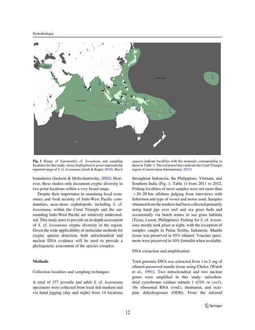
Fig. 1 Range of Sepioteuthis cf. lessoniana and samplinglocalities for this study. Areas highlighted in green represent thereported range of S. cf. lessoniana (Jereb & Roper, 2010). Black

squares indicate localities with the numerals corresponding tothose in Table 1. The red dotted lines indicate the Coral Triangleregion (Conservation International, 2012)

Hydrobiologia

123

13

mitochondrial lineages, two nuclear genes wereamplified from a subset of individuals. The mitochon-

drial genes were amplified together using a multiplex-

ing approach using a Qiagen Multiplex kit followingthe standard published protocol for 25 ll reactions.

CO1 and 16s were amplified using universal HCO-2198and LCO-1490 primers (Folmer et al., 1994) and

16sAR and 16sBR primers (Kessing et al., 1989),

respectively. Rhodopsin and ODH were amplifiedusing cephalopod specific primers (Strugnell et al.,

2005) in 25 ll Amplitaq Hotstart PCR reactions. PCR

thermal cycling parameters were as follows: initialdenaturation for 94!C for 120 s, then cycling 94!C for

15 s, 36–68!C for 30 s, and 72!C for 30 s for 25–30

cycles, following by a final extension step of 72!C for7 min. The following annealing temperatures were

used: 36!C for CO1, 42!C for 16s, 55!C for rhodopsin,

and 68!C for ODH. The resulting amplified productswere cleaned up and sequenced at the UC Berkeley

DNA Sequencing Facility. Samples collected from

India were amplified and sequenced at the Anderson labat Southern Illinois University-Carbondale following

the protocols outlined in Anderson et al. (2011).

Data analysis

DNA sequences were edited and checked in Sequencherv 4.1 (Gene Codes, Ann Arbor, MI, US). Sequences for

each gene region were aligned using the CLUSTALWplug-in implemented in Geneious. As the 16s alignment

was characterized by a number of large gaps (n = 5), the

initial alignment was realigned to an invertebrate 16sstructural constraint sequence (Apis mellifera) with

RNAsalsa (Stocsits et al., 2009) using default parame-ters. Unique haplotypes were identified among the

sampled individuals for all gene regions using the

DNAcollapser tool in FaBox (Villesen, 2007). For eachindividual gene dataset, Kimura-2-parameter distances

and haplotype diversity (with standard error) were

calculated within and between each lineage in Arlequin3.5.1.2 (Excoffier & Lischer, 2010).

Individual gene alignments were first analyzed with

both maximum likelihood methods (RAxML 7.3.2)and Bayesian inference (MrBayes 3.1.2) on the

CIPRES Science Gateway (Miller et al., 2010) using

sequences of Sepioteuthis australis, Loligo bleekeri,and Sthenoteuthis oualaniensis obtained from Gen-

Bank (Table 2) as outgroups. Total sequence data

from 87 representative individuals were then concat-enated in Mesquite into three datasets—mitochondrial

genes, nuclear genes, and all genes. After comparing

the results from individual and concatenated datasets,the mitochondrial dataset were run using 70 additional

individuals that were not amplified for nuclear genes

to assign lineage identity. Sepioteuthis sepioidea andS. australis sequences from GenBank were used as

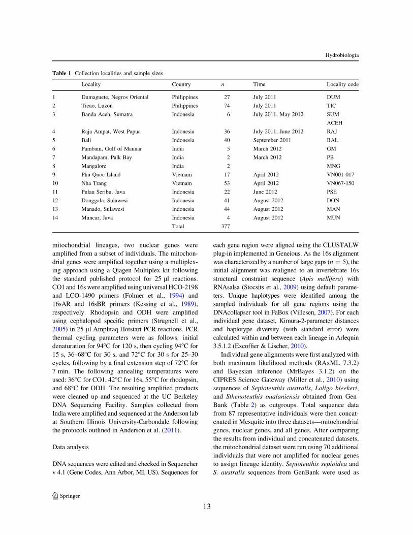
Table 1 Collection localities and sample sizes

Locality Country n Time Locality code

1 Dumaguete, Negros Oriental Philippines 27 July 2011 DUM

2 Ticao, Luzon Philippines 74 July 2011 TIC

3 Banda Aceh, Sumatra Indonesia 6 July 2011, May 2012 SUM

ACEH

4 Raja Ampat, West Papua Indonesia 36 July 2011, June 2012 RAJ

5 Bali Indonesia 40 September 2011 BAL

6 Pambam, Gulf of Mannar India 5 March 2012 GM

7 Mandapam, Palk Bay India 2 March 2012 PB

8 Mangalore India 2 MNG

9 Phu Quoc Island Vietnam 17 April 2012 VN001-017

10 Nha Trang Vietnam 53 April 2012 VN067-150

11 Pulau Seribu, Java Indonesia 22 June 2012 PSE

12 Donggala, Sulawesi Indonesia 41 August 2012 DON

13 Manado, Sulawesi Indonesia 44 August 2012 MAN

14 Muncar, Java Indonesia 4 August 2012 MUN

Total 377

Hydrobiologia

123

14

outgroups (Table 2). Each concatenated dataset waspartitioned into individual genes. RAxML was run for

single and combined datasets using the GTR-

GAMMA model for both bootstrapping and maximumlikelihood search. Node support was estimated using

1,000 rapid bootstrap replicates and nodes with greater

than 50% support were used to construct the finalconsensus tree. Bayesian phylogenetic analyses were

implemented in MrBayes 3.1.2. Default values for

prior parameters were used in the analysis. Eachdataset was run for 5,000,000–7,500,000 generations

after which the average standard deviation of split

frequencies fell below the stop value of 0.01. Datasetswere run with a mixed model and gamma rate

distribution (?G). The final consensus tree was

constructed using the fifty-percent majority rule andresulting posterior probability values for each node

were used as estimates of clade support.

The previous methods estimated gene trees, indi-cating the history of that particular gene, and not

necessarily the lineages or species. Incomplete lineage

sorting can result in discordance between inferredgene trees and between the gene trees and species

trees, resulting in incorrect inferences about phyloge-

netic relationships (Maddison, 1997; Nichols, 2001).All four genes were concatenated into a partitioned

dataset and analyzed using a multi-locus, multi-

species coalescent framework employed in *BEAST(Heled & Drummond, 2010) to estimate the most

likely species tree. Each of the 87 individuals wasassigned to one of three distinct lineages (lineage A, B,

or C) identified in the concatenated datasets. Nucle-

otide substitution model parameters were estimatedfor each individual gene dataset using jModelTest

(Guindon & Gascuel, 2003; Darriba et al., 2012).

Models with the best AIC score that could beimplemented in *BEAST were chosen. Each MCMC

analysis was conducted for 100,000,000 generations

(sampling every 1,000 steps with a 15% burn-indetermined from trace plots and estimated samples

sizes). A Yule process tree prior and an uncorrelated

lognormal relaxed clock branch length prior were usedfor all analyses. All other priors were left at default

values. Convergence of the posterior and parameters

was assessed by examining likelihood plots in Tracerv1.4 (Rambaut & Drummond, 2007). Final best tree

was determined from 255,000 combined post-in

samples from the three runs.

Validation of lineages

To explore the validity of lineages inferred from the

previous gene and species tree techniques, we used a

Bayesian species delimitation method implementedthrough the Bayesian Phylogenetics and Phylogeog-

raphy (BP&P version 2.2) program (Yang & Rannala,

2010). This coalescent-based method is designed toestimate the posterior distribution for different species

delimitation models using a reversible-jump Markov

chain Monte Carlos (rjMCMC) algorithm on a user-provided guide tree with priors for ancestral popula-

tion size (h) and root age (s0). At each bifurcation of

the guide tree, the rjMCMC algorithm estimates themarginal posterior probability of speciation (from here

on, termed ‘‘speciation probability’’). We invoked the50% majority rule for inferring the likelihood of a

speciation or splitting event.

We used BP&P to estimate the posterior probabilitiesof splitting events to validate the lineages inferred from

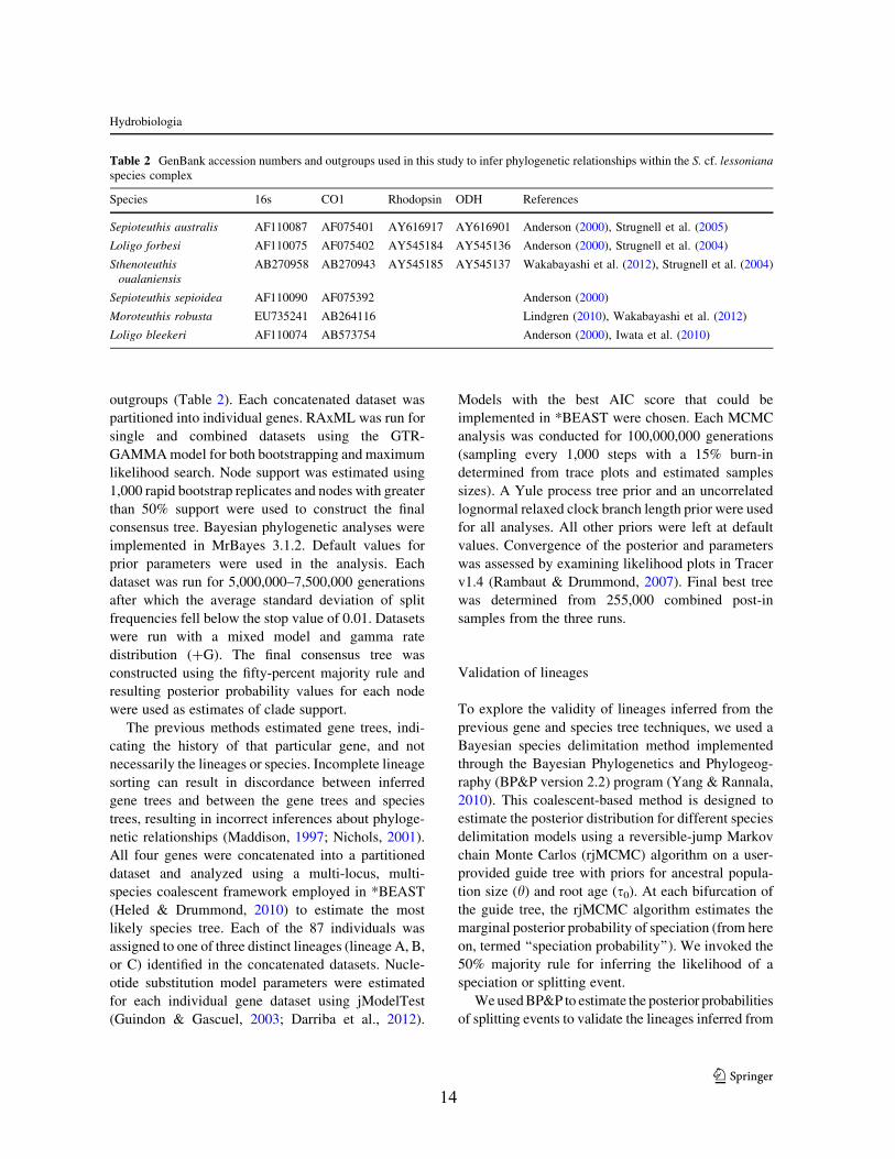
Table 2 GenBank accession numbers and outgroups used in this study to infer phylogenetic relationships within the S. cf. lessonianaspecies complex

Species 16s CO1 Rhodopsin ODH References

Sepioteuthis australis AF110087 AF075401 AY616917 AY616901 Anderson (2000), Strugnell et al. (2005)

Loligo forbesi AF110075 AF075402 AY545184 AY545136 Anderson (2000), Strugnell et al. (2004)

Sthenoteuthisoualaniensis

AB270958 AB270943 AY545185 AY545137 Wakabayashi et al. (2012), Strugnell et al. (2004)

Sepioteuthis sepioidea AF110090 AF075392 Anderson (2000)

Moroteuthis robusta EU735241 AB264116 Lindgren (2010), Wakabayashi et al. (2012)

Loligo bleekeri AF110074 AB573754 Anderson (2000), Iwata et al. (2010)

Hydrobiologia

123

15

our phylogenetic analyses using all combined loci.

The rjMCMC analyses were each run for 300,000

generations (sampling interval of five) with a burn-inperiod of 24,000, producing consistent results for all

separate analyses. For each analysis, we used algo-

rithm 0 with fine-tuning to achieve dimensionmatching between delimitation models with different

numbers of parameters. Each species delimitation

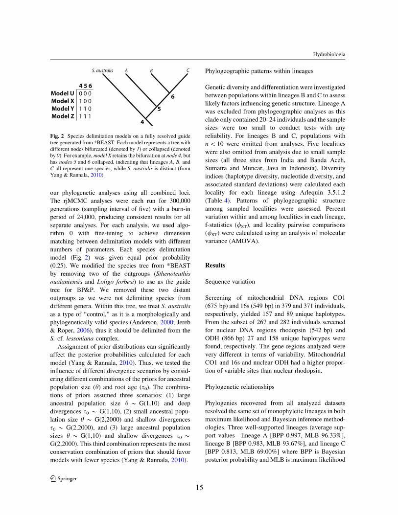
model (Fig. 2) was given equal prior probability(0.25). We modified the species tree from *BEAST

by removing two of the outgroups (Sthenoteuthisoualaniensis and Loligo forbesi) to use as the guide

tree for BP&P. We removed these two distant

outgroups as we were not delimiting species fromdifferent genera. Within this tree, we treat S. australis

as a type of ‘‘control,’’ as it is a morphologically and

phylogenetically valid species (Anderson, 2000; Jereb& Roper, 2006), thus it should be delimited from the

S. cf. lessoniana complex.

Assignment of prior distributions can significantlyaffect the posterior probabilities calculated for each

model (Yang & Rannala, 2010). Thus, we tested the

influence of different divergence scenarios by consid-ering different combinations of the priors for ancestral

population size (h) and root age (s0). The combina-

tions of priors assumed three scenarios: (1) largeancestral population size h * G(1,10) and deep

divergences s0 * G(1,10), (2) small ancestral popu-

lation size h * G(2,2000) and shallow divergencess0 * G(2,2000), and (3) large ancestral population

sizes h * G(1,10) and shallow divergences s0 *G(2,2000). This third combination represents the mostconservation combination of priors that should favor

models with fewer species (Yang & Rannala, 2010).

Phylogeographic patterns within lineages

Genetic diversity and differentiation were investigatedbetween populations within lineages B and C to assess

likely factors influencing genetic structure. Lineage A

was excluded from phylogeographic analyses as thisclade only contained 20–24 individuals and the sample

sizes were too small to conduct tests with any

reliability. For lineages B and C, populations withn \ 10 were omitted from analyses. Five localities

were also omitted from analysis due to small sample

sizes (all three sites from India and Banda Aceh,Sumatra and Muncar, Java in Indonesia). Diversity

indices (haplotype diversity, nucleotide diversity, and

associated standard deviations) were calculated eachlocality for each lineage using Arlequin 3.5.1.2

(Table 4). Patterns of phylogeographic structure

among sampled localities were assessed. Percentvariation within and among localities in each lineage,

f-statistics (/ST), and locality pairwise comparisons

(/ST) were calculated using an analysis of molecularvariance (AMOVA).

Results

Sequence variation

Screening of mitochondrial DNA regions CO1

(675 bp) and 16s (549 bp) in 379 and 371 individuals,respectively, yielded 157 and 89 unique haplotypes.

From the subset of 267 and 282 individuals screened

for nuclear DNA regions rhodopsin (542 bp) andODH (866 bp) 27 and 158 unique haplotypes were

found, respectively. The gene regions analyzed were

very different in terms of variability. MitochondrialCO1 and 16s and nuclear ODH had a higher propor-

tion of variable sites than nuclear rhodopsin.

Phylogenetic relationships

Phylogenies recovered from all analyzed datasetsresolved the same set of monophyletic lineages in both

maximum likelihood and Bayesian inference method-

ologies. Three well-supported lineages (average sup-port values—lineage A [BPP 0.997, MLB 96.33%],

lineage B [BPP 0.983, MLB 93.67%], and lineage C

[BPP 0.813, MLB 69.00%] where BPP is Bayesianposterior probability and MLB is maximum likelihood

Fig. 2 Species delimitation models on a fully resolved guidetree generated from *BEAST. Each model represents a tree withdifferent nodes bifurcated (denoted by 1) or collapsed (denotedby 0). For example, model X retains the bifurcation at node 4, buthas nodes 5 and 6 collapsed, indicating that lineages A, B, andC all represent one species, while S. australis is distinct (fromYang & Rannala, 2010)

Hydrobiologia

123

16

bootstrap support) were resolved in each dataset,comprising the same individuals in each analysis.

Topologies resolved between mitochondrial and

nuclear datasets were not always concordant. In bothmaximum likelihood and Bayesian consensus trees for

the all gene dataset and the mitochondrial gene

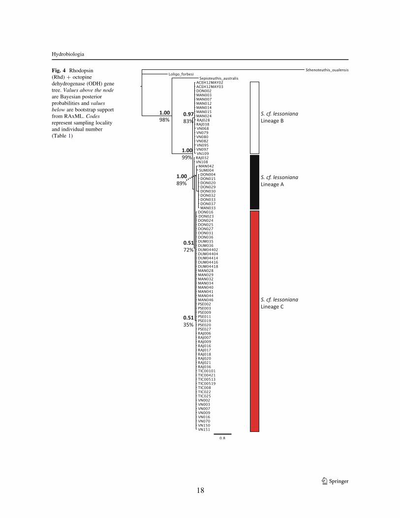
dataset, lineages B and C were sister to each other(Figs. 3, 5). However, in the nuclear genes dataset,

lineages A and C were sister to each other (Fig. 4).

However, for all datasets, the support values for thatparticular node are low (BPP 0.51–0.89, MLB

49–72%), indicating that the relationship between

those lineages is not well-resolved and further statis-tical assessment is needed. The maximum clade

credibility species tree topology (determined from

255,000 post burn-in tree topologies) is concordantwith the hypothesis of three distinct lineages within S.

cf. lessoniana (Fig. 6). Similar to the maximum

likelihood and Bayesian analyses of the concatenateddatasets, each lineage had very high support values

and large divergences between lineages.

The results from the Bayesian species delimitationfor this species complex show variable support for

three independent lineages (Fig. 7). When assuming

large ancestral population sizes and deep divergencesor large ancestral population sizes and shallow diver-

gences, there was strong support for the bifurcation

between lineages A and B (posterior probability[0.50) as well as between lineages A and C (posterior

probability[0.50) (Fig. 7). Our outgroup, S. australis,

consistently demonstrated independence with strongsupport (posterior probability = 1.00). However,

under a divergence scenario with small ancestral

population sizes and shallow divergence, we did nothave any support for bifurcation of any nodes on the

guide tree, including between the S. cf. lessoniana

species complex and S. australis (posterior probabil-ity = 0.00, Fig. 7). Previous simulations with varia-

tions in the h prior indicate that BP&P is particularly

sensitive to small ancestral population sizes, and thusthis outcome is likely a result of this (Leache & Fujita,

2010; Yang & Rannala, 2010). The topology of theguide tree also influenced the number of evolutionary

lineages inferred, for example, our second and third

guide trees support three independent lineages(Fig. 7). Placement of divergent lineages as sister

taxa can inflate what BP&P regards as a speciation

event (Leache & Fujita, 2010). This emphasizes theneed for a reliable guide tree for accurate species

delimitation estimates as random rearrangements ofthe tips impacts how many species are delimited.

BP&P supports two to three evolutionary lineages

depending on the guide tree topology.While all three lineages were consistently recov-

ered from all individual and concatenated genetic

datasets, average divergence between each lineagevaried depending on the gene region in question. In all

datasets, distance between lineages was always much

higher than intra-lineage values (Table 3). However,K2P distances between mitochondrial lineages were

much greater than the distance separating the same

lineages in the nuclear datasets (Table 3). This isreflected in the deeper phylogenetic relationships that

were resolved in the mitochondrial trees (Fig. 5).

Furthermore, genetic substructuring within the mito-chondrial lineages was present and absent in the

nuclear lineages (Table 3). Comparing lineages, hap-

lotype diversity was comparatively similar in lineagesB and C in all genes analyzed. Lineage A had

comparatively much lower haplotype diversity than

lineages B and C in all genes, except CO1 (Table 4). Inthe analyses with representative individuals, lineage C

seemed to be the most commonly found among all

sampled sites (Fig. 8). When examining the frequencyof each lineage in all sampled individuals (including

individuals with identical haplotypes), the representa-

tions of lineages B and C were much more commonthan lineage A (Fig. 8; Table 5).

Distribution and phylogeography

Examining the distribution of each lineage throughout

the sampled localities, it is clear that geography doesnot delimit these cryptic lineages (Fig. 8). Lineages B

and C are present in nearly all sampled localities,

while lineage A seems to be only found in centralIndonesia (Donggala, Manado, Raja Ampat) and in

Banda Aceh. Lineage B was predominant in samples

from both Vietnamese locations (Nha Trang and PhuQuoc Island), in southern (Bali) and central Indonesia

(Manado), and in the northern Philippines (Ticao).Lineage C was predominant throughout most Indone-

sian sites (Pulau Seribu, Muncar, Donggala, Raja

Ampat), southern India, and in the central Philippines(Dumaguete). In terms of abundance, lineage C was

most commonly sampled followed by lineage B with

lineage A being rare (Table 5). However, these resultsmust be taken purely at descriptive value and not as a

Hydrobiologia

123

17

S. cf. lessoniana Lineage A

S. cf. lessoniana Lineage C

S. cf. lessoniana Lineage B

1.00100%

1.0073%

1.00100%

0.97 ??%

1.00??%

1.00??%

Fig. 3 All gene markers concatenated. Values above the node are Bayesian posterior probabilities and values below are bootstrapsupport from RAxML. Codes represent sampling locality and individual number (Table 1)

Hydrobiologia

123

18

S. cf. lessoniana Lineage A

S. cf. lessoniana Lineage C

S. cf. lessoniana Lineage B

0.97 83%

1.00 98%

1.00 99%

1.00 89%

0.51 72%

0.51 35%

Fig. 4 Rhodopsin(Rhd) ? octopinedehydrogenase (ODH) genetree. Values above the nodeare Bayesian posteriorprobabilities and valuesbelow are bootstrap supportfrom RAxML. Codesrepresent sampling localityand individual number(Table 1)

Hydrobiologia

123

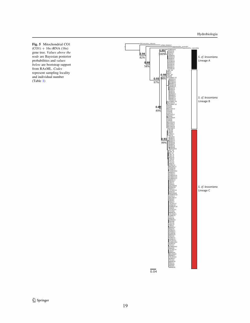
19

Fig. 5 Mitochondrial CO1(CO1) ? 16s rRNA (16s)gene tree. Values above thenode are Bayesian posteriorprobabilities and valuesbelow are bootstrap supportfrom RAxML. Codesrepresent sampling localityand individual number(Table 1)

Hydrobiologia

123

20

true indicator of occurrence as sample sizes between

locations are extremely varied (Table 5). Haplotypediversity within each lineage was very high for the

mitochondrial genes and for ODH (Table 5). Therewas not a clear pattern of difference between each

lineage in terms of haplotype diversity as they were all

similarly high. Rhodopsin had much lower levels ofhaplotype diversity, particularly for lineages A and C

(Table 5). This corresponded to very low levels of

variation between individuals seen in this gene region.AMOVA results suggest that there is significant

genetic substructuring between the three localities

(Bali, Manado and Nha Trang) sampled in lineage B.Overall /ST was very high for all gene regions for

lineage B with the majority of variation explained by

among population differentiation. Comparing thepopulation pairwise /ST values from all gene regions,

samples from Manado were significantly strongly

differentiated from Bali and Nha Trang (Table 6).There was low differentiation between Bali and Nha

Trang, but this value was not significant. Haplotype

diversity of each population from the mitochondrialdata indicated that diversity is comparably high in

Manado and Bali, but slightly lower in Nha Trang

(Table 5). Nucleotide diversity is low for all localities.Conversely, AMOVA results for lineage C suggest

limited genetic substructuring between eight geo-

graphic localities sampled (Donggala, Dumaguete,Manado, Nha Trang, Phu Quoc, Pulau Seribu, Raja

Ampat, and Ticao). Overall /ST was fairly low for all

gene regions with the majority of variation explained

by within locality differentiation (Table 6). Amongpopulation variation is driven by high levels of genetic

0.03

Fig. 6 Maximum clade credibility species tree determinedfrom 255,000 post burn-in topologies from *BEAST. Values atthe nodes are posterior probabilities

Fig. 7 Bayesian species delimitation results for the Sepioteu-this cf. lessoniana species complex assuming four species guidetrees with the species tree from *BEAST denoted with aasterisk. Speciation probabilities from each combination ofpriors for h and s0 are provided for each node with probabilitiesgreater than 0.50 highlighted in bold and italics. Top h ands0 * G(1,10); middle h and s0 * G(2,2000); bottomh * G(1,10); and s0 * G(2,2000). Different arrangements oftaxa on the tips results in different speciation probabilities forone of the nodes within the complex

Hydrobiologia

123

21

differentiation in mitochondrial gene regions between

both Nha Trang and Raja Ampat and all localities.

This pattern was not observed in the ODH dataset,rather only Raja Ampat was significantly differenti-

ated from all localities save Nha Trang and Phu Quoc.All other localities at all gene regions had very low

levels of differentiation in relationship to each

other (Table 5). All populations were characterizedby high haplotype diversity and low nucleotide

diversity in both mitochondrial genes and the ODH

gene (Table 5). Rhodopsin had very low levels ofhaplotype and nucleotide diversity (Table 5) and was

found to contain numerous individuals with identical

sequences.

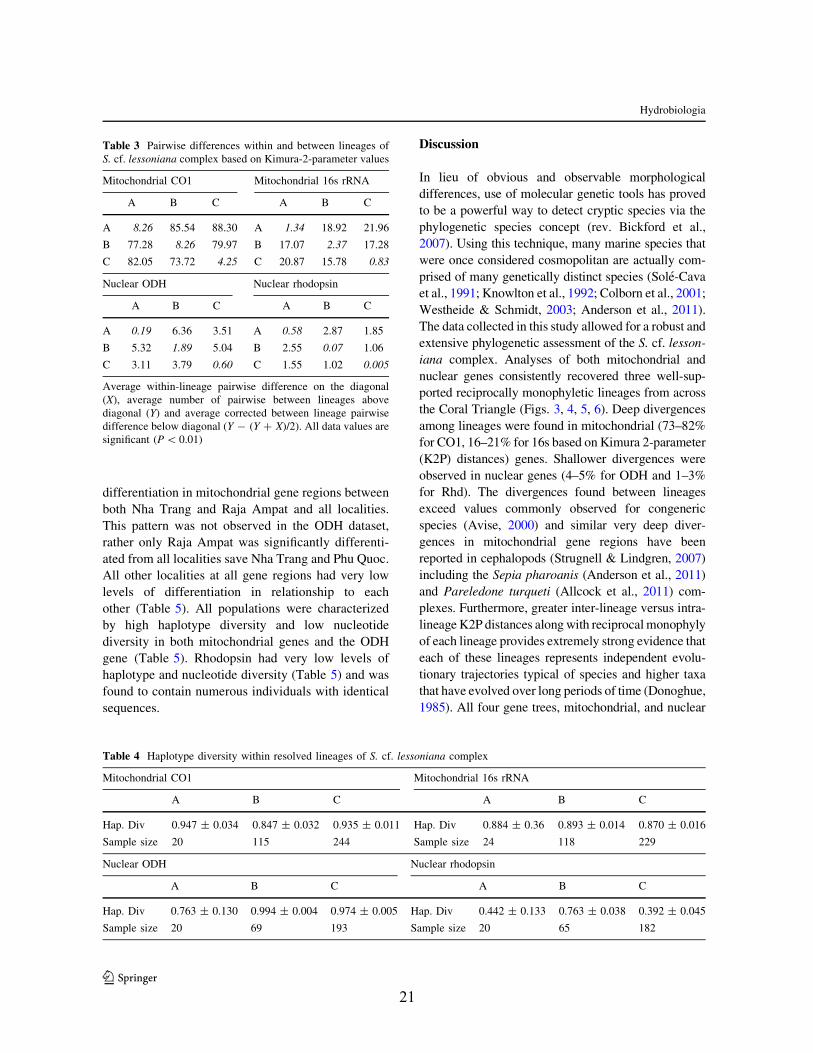
Discussion

In lieu of obvious and observable morphologicaldifferences, use of molecular genetic tools has proved

to be a powerful way to detect cryptic species via the

phylogenetic species concept (rev. Bickford et al.,2007). Using this technique, many marine species that

were once considered cosmopolitan are actually com-

prised of many genetically distinct species (Sole-Cavaet al., 1991; Knowlton et al., 1992; Colborn et al., 2001;

Westheide & Schmidt, 2003; Anderson et al., 2011).

The data collected in this study allowed for a robust andextensive phylogenetic assessment of the S. cf. lesson-

iana complex. Analyses of both mitochondrial and

nuclear genes consistently recovered three well-sup-ported reciprocally monophyletic lineages from across

the Coral Triangle (Figs. 3, 4, 5, 6). Deep divergences

among lineages were found in mitochondrial (73–82%for CO1, 16–21% for 16s based on Kimura 2-parameter

(K2P) distances) genes. Shallower divergences were

observed in nuclear genes (4–5% for ODH and 1–3%for Rhd). The divergences found between lineages

exceed values commonly observed for congeneric

species (Avise, 2000) and similar very deep diver-gences in mitochondrial gene regions have been

reported in cephalopods (Strugnell & Lindgren, 2007)

including the Sepia pharoanis (Anderson et al., 2011)and Pareledone turqueti (Allcock et al., 2011) com-

plexes. Furthermore, greater inter-lineage versus intra-

lineage K2P distances along with reciprocal monophylyof each lineage provides extremely strong evidence that

each of these lineages represents independent evolu-

tionary trajectories typical of species and higher taxathat have evolved over long periods of time (Donoghue,

1985). All four gene trees, mitochondrial, and nuclear

Table 3 Pairwise differences within and between lineages ofS. cf. lessoniana complex based on Kimura-2-parameter values

Mitochondrial CO1 Mitochondrial 16s rRNA

A B C A B C

A 8.26 85.54 88.30 A 1.34 18.92 21.96

B 77.28 8.26 79.97 B 17.07 2.37 17.28

C 82.05 73.72 4.25 C 20.87 15.78 0.83

Nuclear ODH Nuclear rhodopsin

A B C A B C

A 0.19 6.36 3.51 A 0.58 2.87 1.85

B 5.32 1.89 5.04 B 2.55 0.07 1.06

C 3.11 3.79 0.60 C 1.55 1.02 0.005

Average within-lineage pairwise difference on the diagonal(X), average number of pairwise between lineages abovediagonal (Y) and average corrected between lineage pairwisedifference below diagonal (Y - (Y ? X)/2). All data values aresignificant (P \ 0.01)

Table 4 Haplotype diversity within resolved lineages of S. cf. lessoniana complex

Mitochondrial CO1 Mitochondrial 16s rRNA

A B C A B C

Hap. Div 0.947 ± 0.034 0.847 ± 0.032 0.935 ± 0.011 Hap. Div 0.884 ± 0.36 0.893 ± 0.014 0.870 ± 0.016

Sample size 20 115 244 Sample size 24 118 229

Nuclear ODH Nuclear rhodopsin

A B C A B C

Hap. Div 0.763 ± 0.130 0.994 ± 0.004 0.974 ± 0.005 Hap. Div 0.442 ± 0.133 0.763 ± 0.038 0.392 ± 0.045

Sample size 20 69 193 Sample size 20 65 182

Hydrobiologia

123

22

datasets produced concordant topologies indicating theabsence of hybridization or introgression and the

presence of reproductive isolation (Mayr, 1942; Dobz-

hansky, 1970) despite co-occurrence at multiple sites.Inferences from species tree estimations and species

delimitation methods support at least two to three

evolutionary independent lineages (Figs. 6, 7) under aconservative approach. Fulfillment of multiple species

concept criteria lends very strong support for species

status to these cryptic lineages of S. cf. lessoniana.Of all Loliginidae, S. cf. lessoniana has the largest

distribution. Within this genus, S. sepioidea is restricted

to the Caribbean and S. australis to southern Australiaand New Zealand (Jereb & Roper, 2010). Past biogeo-

graphic hypotheses for Sepioteuthis indicate the migra-

tion of a Tethyan relic following the break-up ofPangaea from the Atlantic into the Pacific Ocean

(Anderson, 2000). For S. cf. lessoniana, Anderson

(2000) hypothesized that it diverged from its Caribbeansister taxon and spread through the Pacific through the

Indian Ocean and eventually to the Red Sea and

Mediterranean, subsequently becoming extinct in theEast Pacific (2000). With a nearly cosmopolitan

distribution, one would assume that S. cf. lessoniana

must have much greater dispersal potential than its

sister taxa. However, characteristics of paralarval andadult life history indicate that S. cf. lessoniana is likely

the least dispersive of all Loliginidae. Hatchlings of S.

cf. lessoniana are among the largest (4–10 mm)(Segawa, 1987; Jivaluk et al., 2005) in the family.

These large hatchlings possess well-developed nervous

systems (Shigeno et al., 2001) and are strong swimmers(Kier, 1996; Thompson & Kier, 2001), thus highly

unlikely to behave as a ‘‘passive’’ disperser. In fact,

even among other loliginid species with much smallersizes at hatching (e.g., Loligo opalescens 3–4 mm;

Fields, 1965) there is strong evidence for advanced

paralarval navigation in order to entrain themselves infavorable oceanographic areas (Okutani & McGowan,

1969; Zeidberg & Hamner, 2002). Specifically, para-

larval S. cf. lessoniana orient over dark areas indicatingactive navigation to reef habitat (Lee et al., 1994) and

demonstrate active hunting and shoaling behavior

shortly after hatching (Choe, 1966; Sugimoto & Ikeda,2012).

Similarly, the movement of adults is restricted to

coastal habitats, possibly extending no more than16.2 km (S. cf. lessoniana—Ueta & Jo, 1990) to

35 km (S. australis—Pecl et al., 2006) along the coast

during its short lifetime. S. cf. lessoniana commonly

Fig. 8 Distribution of cryptic lineages throughout sampling range. Size of pie diagrams corresponds to sample size from that locality

Hydrobiologia

123

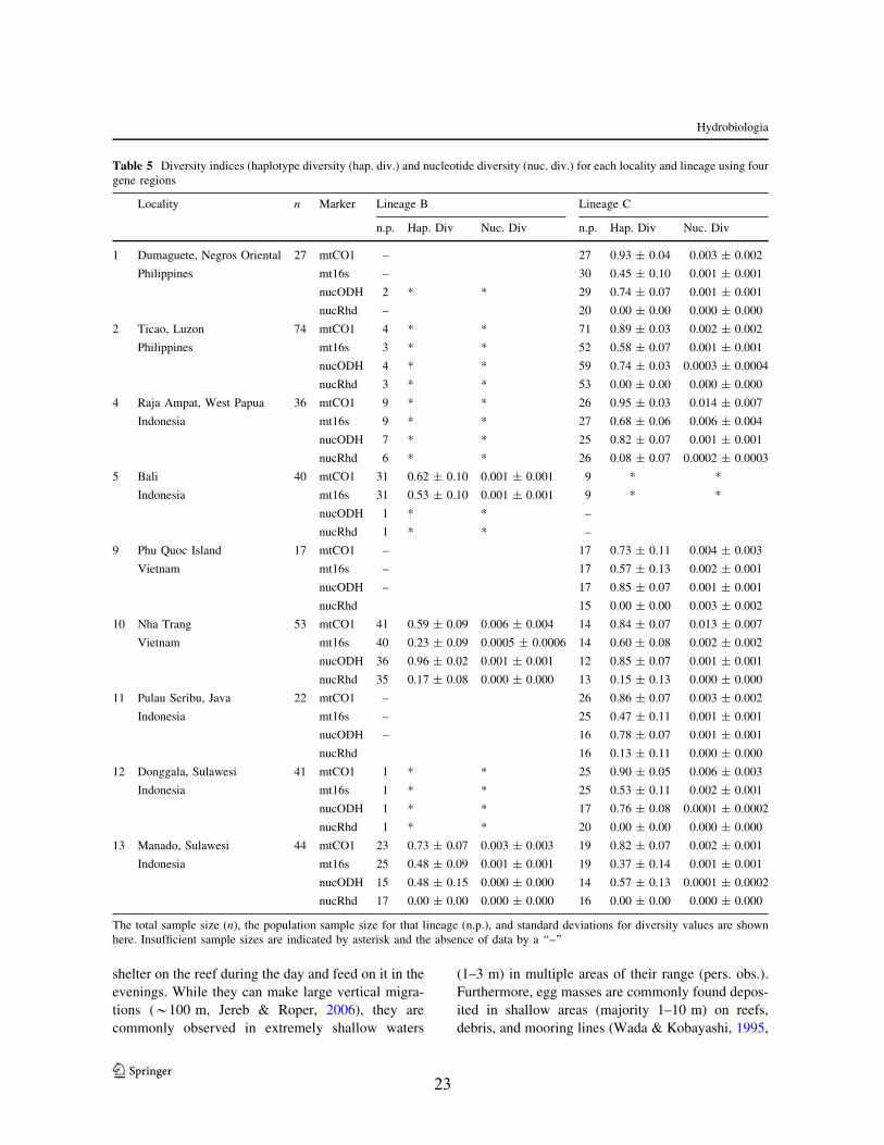
23

shelter on the reef during the day and feed on it in the

evenings. While they can make large vertical migra-tions (*100 m, Jereb & Roper, 2006), they are

commonly observed in extremely shallow waters

(1–3 m) in multiple areas of their range (pers. obs.).

Furthermore, egg masses are commonly found depos-ited in shallow areas (majority 1–10 m) on reefs,

debris, and mooring lines (Wada & Kobayashi, 1995,

Table 5 Diversity indices (haplotype diversity (hap. div.) and nucleotide diversity (nuc. div.) for each locality and lineage using fourgene regions

Locality n Marker Lineage B Lineage C

n.p. Hap. Div Nuc. Div n.p. Hap. Div Nuc. Div

1 Dumaguete, Negros Oriental

Philippines

27 mtCO1 – 27 0.93 ± 0.04 0.003 ± 0.002

mt16s – 30 0.45 ± 0.10 0.001 ± 0.001

nucODH 2 * * 29 0.74 ± 0.07 0.001 ± 0.001

nucRhd – 20 0.00 ± 0.00 0.000 ± 0.000

2 Ticao, Luzon

Philippines

74 mtCO1 4 * * 71 0.89 ± 0.03 0.002 ± 0.002

mt16s 3 * * 52 0.58 ± 0.07 0.001 ± 0.001

nucODH 4 * * 59 0.74 ± 0.03 0.0003 ± 0.0004

nucRhd 3 * * 53 0.00 ± 0.00 0.000 ± 0.000

4 Raja Ampat, West Papua

Indonesia

36 mtCO1 9 * * 26 0.95 ± 0.03 0.014 ± 0.007

mt16s 9 * * 27 0.68 ± 0.06 0.006 ± 0.004

nucODH 7 * * 25 0.82 ± 0.07 0.001 ± 0.001

nucRhd 6 * * 26 0.08 ± 0.07 0.0002 ± 0.0003

5 Bali

Indonesia

40 mtCO1 31 0.62 ± 0.10 0.001 ± 0.001 9 * *

mt16s 31 0.53 ± 0.10 0.001 ± 0.001 9 * *

nucODH 1 * * –

nucRhd 1 * * –

9 Phu Quoc Island

Vietnam

17 mtCO1 – 17 0.73 ± 0.11 0.004 ± 0.003

mt16s – 17 0.57 ± 0.13 0.002 ± 0.001

nucODH – 17 0.85 ± 0.07 0.001 ± 0.001

nucRhd 15 0.00 ± 0.00 0.003 ± 0.002

10 Nha Trang

Vietnam

53 mtCO1 41 0.59 ± 0.09 0.006 ± 0.004 14 0.84 ± 0.07 0.013 ± 0.007

mt16s 40 0.23 ± 0.09 0.0005 ± 0.0006 14 0.60 ± 0.08 0.002 ± 0.002

nucODH 36 0.96 ± 0.02 0.001 ± 0.001 12 0.85 ± 0.07 0.001 ± 0.001

nucRhd 35 0.17 ± 0.08 0.000 ± 0.000 13 0.15 ± 0.13 0.000 ± 0.000

11 Pulau Seribu, Java

Indonesia

22 mtCO1 – 26 0.86 ± 0.07 0.003 ± 0.002

mt16s – 25 0.47 ± 0.11 0.001 ± 0.001

nucODH – 16 0.78 ± 0.07 0.001 ± 0.001

nucRhd 16 0.13 ± 0.11 0.000 ± 0.000

12 Donggala, Sulawesi

Indonesia

41 mtCO1 1 * * 25 0.90 ± 0.05 0.006 ± 0.003

mt16s 1 * * 25 0.53 ± 0.11 0.002 ± 0.001

nucODH 1 * * 17 0.76 ± 0.08 0.0001 ± 0.0002

nucRhd 1 * * 20 0.00 ± 0.00 0.000 ± 0.000

13 Manado, Sulawesi

Indonesia

44 mtCO1 23 0.73 ± 0.07 0.003 ± 0.003 19 0.82 ± 0.07 0.002 ± 0.001

mt16s 25 0.48 ± 0.09 0.001 ± 0.001 19 0.37 ± 0.14 0.001 ± 0.001

nucODH 15 0.48 ± 0.15 0.000 ± 0.000 14 0.57 ± 0.13 0.0001 ± 0.0002

nucRhd 17 0.00 ± 0.00 0.000 ± 0.000 16 0.00 ± 0.00 0.000 ± 0.000

The total sample size (n), the population sample size for that lineage (n.p.), and standard deviations for diversity values are shownhere. Insufficient sample sizes are indicated by asterisk and the absence of data by a ‘‘–’’

Hydrobiologia

123

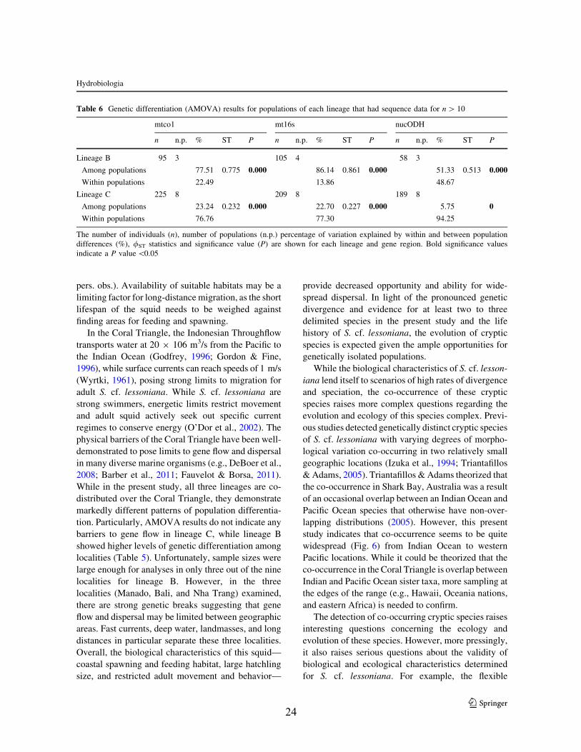
24

pers. obs.). Availability of suitable habitats may be a

limiting factor for long-distance migration, as the short

lifespan of the squid needs to be weighed againstfinding areas for feeding and spawning.

In the Coral Triangle, the Indonesian Throughflow

transports water at 20 9 106 m3/s from the Pacific tothe Indian Ocean (Godfrey, 1996; Gordon & Fine,

1996), while surface currents can reach speeds of 1 m/s

(Wyrtki, 1961), posing strong limits to migration foradult S. cf. lessoniana. While S. cf. lessoniana are

strong swimmers, energetic limits restrict movementand adult squid actively seek out specific current

regimes to conserve energy (O’Dor et al., 2002). The

physical barriers of the Coral Triangle have been well-demonstrated to pose limits to gene flow and dispersal

in many diverse marine organisms (e.g., DeBoer et al.,

2008; Barber et al., 2011; Fauvelot & Borsa, 2011).While in the present study, all three lineages are co-

distributed over the Coral Triangle, they demonstrate

markedly different patterns of population differentia-tion. Particularly, AMOVA results do not indicate any

barriers to gene flow in lineage C, while lineage B

showed higher levels of genetic differentiation amonglocalities (Table 5). Unfortunately, sample sizes were

large enough for analyses in only three out of the nine

localities for lineage B. However, in the threelocalities (Manado, Bali, and Nha Trang) examined,

there are strong genetic breaks suggesting that gene

flow and dispersal may be limited between geographicareas. Fast currents, deep water, landmasses, and long

distances in particular separate these three localities.

Overall, the biological characteristics of this squid—coastal spawning and feeding habitat, large hatchling

size, and restricted adult movement and behavior—

provide decreased opportunity and ability for wide-

spread dispersal. In light of the pronounced genetic

divergence and evidence for at least two to threedelimited species in the present study and the life

history of S. cf. lessoniana, the evolution of cryptic

species is expected given the ample opportunities forgenetically isolated populations.

While the biological characteristics of S. cf. lesson-

iana lend itself to scenarios of high rates of divergenceand speciation, the co-occurrence of these cryptic

species raises more complex questions regarding theevolution and ecology of this species complex. Previ-

ous studies detected genetically distinct cryptic species

of S. cf. lessoniana with varying degrees of morpho-logical variation co-occurring in two relatively small

geographic locations (Izuka et al., 1994; Triantafillos

& Adams, 2005). Triantafillos & Adams theorized thatthe co-occurrence in Shark Bay, Australia was a result

of an occasional overlap between an Indian Ocean and

Pacific Ocean species that otherwise have non-over-lapping distributions (2005). However, this present

study indicates that co-occurrence seems to be quite

widespread (Fig. 6) from Indian Ocean to westernPacific locations. While it could be theorized that the

co-occurrence in the Coral Triangle is overlap between

Indian and Pacific Ocean sister taxa, more sampling atthe edges of the range (e.g., Hawaii, Oceania nations,

and eastern Africa) is needed to confirm.

The detection of co-occurring cryptic species raisesinteresting questions concerning the ecology and

evolution of these species. However, more pressingly,

it also raises serious questions about the validity ofbiological and ecological characteristics determined

for S. cf. lessoniana. For example, the flexible

Table 6 Genetic differentiation (AMOVA) results for populations of each lineage that had sequence data for n [ 10

mtco1 mt16s nucODH

n n.p. % ST P n n.p. % ST P n n.p. % ST P

Lineage B 95 3 105 4 58 3

Among populations 77.51 0.775 0.000 86.14 0.861 0.000 51.33 0.513 0.000

Within populations 22.49 13.86 48.67

Lineage C 225 8 209 8 189 8

Among populations 23.24 0.232 0.000 22.70 0.227 0.000 5.75 0

Within populations 76.76 77.30 94.25

The number of individuals (n), number of populations (n.p.) percentage of variation explained by within and between populationdifferences (%), /ST statistics and significance value (P) are shown for each lineage and gene region. Bold significance valuesindicate a P value \0.05

Hydrobiologia

123

25

reproductive strategies demonstrated by Pecl (2001)and Jackson & Moltschaniwsky (2002) which identi-

fied marked spatial and temporal heterogeneity for

growth and life history characteristics in S. cf.lessoniana, may actually represent different life

histories between the cryptic species. Furthermore,

these squids have been observed to spawn at differentseasons, on different substrates, and with different egg

morphologies throughout their range (Rao, 1954;

Segawa, 1987; Ueta & Jo, 1989; Chotiyaputta, 1993;Segawa et al., 1993a, b; Izuka et al., 1994) raising the

possibility that these variations may actually be fixed

characteristics for each species.The three lineages were present in markedly different

abundances at all sites (Fig. 6). Lineage C was appears

to be most abundant, while Lineages B and A were lessabundant, but co-occurred with lineage C and occasion-

ally each other (Fig. 6). Analyses were not conducted

for lineage A due to small sample size. However, the lowabundance of lineage A suggests that it either occurs in

habitats not usually fished or it has a much more

restricted distribution. While these differences may bedue to differences in sampling effort or gear used, they

may be rooted in different ecological, behavioral, or

biological characteristics of the three cryptic species.Particularly, sympatric co-occurrence of closely related

species in marine environments has been attributed to

factors such as climatic gradients, asynchrony ofmaturation, habitat specificity, and ecological niche

partitioning [e.g., Aurelia aurita (Schroth et al., 2002),

marine microbes (rev. Fenchel, 2005), Micromonasmicroeukaryotic alga (Slapeta et al., 2006), Amphipholis

squamata brittle stars complex (Sponer & Roy, 2002)].

S. cf. lessoniana’s large range encompasses a plethora ofdiverse physical and biological factors resulting in many

different habitats, ecological communities, and ocean-

ographic regimes that could facilitate co-occurrence.However, these questions require much more in-depth

investigations.

Conclusions

These results expand on previous studies of S. cf.

lessoniana in Shark Bay, Australia (Triantafillos &Adams, 2005) and Ishigaki, Japan (Segawa et al.,

1993b; Izuka et al., 1994), which suggested thepresence of cryptic co-occurring lineages. These

studies in Australia and Japan only focused on small

spatial areas and found evidence for sympatric crypticspecies with limited morphological differences. Upon

expanding the range of study to the Indo-Pacific and

Indian Oceans, we found similar results of crypticspecies occurring sympatrically (Fig. 6). Like these

previous studies, recovered cryptic lineages from this

study were strongly differentiated and separated bylarge genetic distances (Tables 3, 5). However,

because these studies employed allozymes, it is

impossible to determine whether these are the samecryptic lineages detected in this study or whether there

may more than three cryptic species of S. cf. lesson-

iana. Our use of CO1 DNA sequence data, theuniversal barcode marker (Hebert et al., 2003; Allcock

et al., 2011) will lay the groundwork for comparison of

squid populations from other regions, allowing thedetermination of how many cryptic species exist in this

taxon. However, this study provides a phylogenetic

basis for species delimitation, but for a comprehensivetaxonomic reassessment, these results need be com-

bined with detailed morphological characterizations.

S. cf. lessoniana is of economic interest throughoutits range, supporting commercial, and artisanal fish-

eries (Chikuni, 1983; Soselisa et al., 1986; Sudjoko,

1987; Chotiyaputta, 1993; Tokai & Ueta, 1999;Nateewathana et al., 2000; FAO, 2009). Maintenance

of sustainable fisheries is dependent on accurate life

history and growth information, particularly as suc-cessful recruitment and population abundance for

squids are dependent on specific environmental con-

ditions (Boyle & Boletzky, 1996; Forsythe et al., 2001;Agnew et al., 2005; Pecl & Jackson, 2008). Thus,

flexible growth and reproductive strategies may rep-

resent a viable natural mechanism to cope withchanging conditions, avoiding major crashes in pop-

ulation biomass. However, in light of the genetic

evidence of widespread co-occurring cryptic speciespresented in this study, it is absolutely crucial that

efforts are undertaken to accurately determine specificlife histories for each species.

The GenBank accession numbers for all origi-

nal sequences from this study are included inTable 7.

Hydrobiologia

123

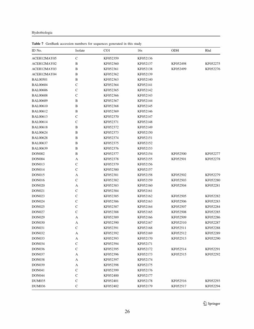
26

Table 7 GenBank accession numbers for sequences generated in this study

ID No. Isolate CO1 16s ODH Rhd

ACEH12MAY05 C KF052359 KF052136

ACEH12MAY02 B KF052360 KF052137 KF052498 KF052275

ACEH12MAY03 B KF052361 KF052138 KF052499 KF052276

ACEH12MAY04 B KF052362 KF052139

BAL00501 B KF052363 KF052140

BAL00604 C KF052364 KF052141

BAL00606 C KF052365 KF052142

BAL00608 C KF052366 KF052143

BAL00609 B KF052367 KF052144

BAL00610 B KF052368 KF052145

BAL00612 B KF052369 KF052146

BAL00613 C KF052370 KF052147

BAL00614 C KF052371 KF052148

BAL00618 B KF052372 KF052149

BAL00624 B KF052373 KF052150

BAL00628 B KF052374 KF052151

BAL00637 B KF052375 KF052152

BAL00639 B KF052376 KF052153

DON002 B KF052377 KF052154 KF052500 KF052277

DON004 A KF052378 KF052155 KF052501 KF052278

DON013 C KF052379 KF052156

DON014 C KF052380 KF052157

DON015 A KF052381 KF052158 KF052502 KF052279

DON016 C KF052382 KF052159 KF052503 KF052280

DON020 A KF052383 KF052160 KF052504 KF052281

DON021 C KF052384 KF052161

DON023 C KF052385 KF052162 KF052505 KF052282

DON024 C KF052386 KF052163 KF052506 KF052283

DON025 C KF052387 KF052164 KF052507 KF052284

DON027 C KF052388 KF052165 KF052508 KF052285

DON029 A KF052389 KF052166 KF052509 KF052286

DON030 A KF052390 KF052167 KF052510 KF052287

DON031 C KF052391 KF052168 KF052511 KF052288

DON032 A KF052392 KF052169 KF052512 KF052289

DON033 A KF052393 KF052170 KF052513 KF052290

DON034 C KF052394 KF052171

DON036 C KF052395 KF052172 KF052514 KF052291

DON037 A KF052396 KF052173 KF052515 KF052292

DON038 A KF052397 KF052174

DON039 A KF052398 KF052175

DON041 C KF052399 KF052176

DON044 C KF052400 KF052177

DUM035 C KF052401 KF052178 KF052516 KF052293

DUM036 C KF052402 KF052179 KF052517 KF052294

Hydrobiologia

123

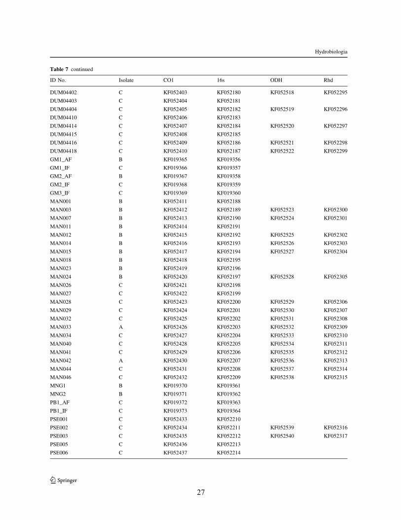
27

Table 7 continued

ID No. Isolate CO1 16s ODH Rhd

DUM04402 C KF052403 KF052180 KF052518 KF052295

DUM04403 C KF052404 KF052181

DUM04404 C KF052405 KF052182 KF052519 KF052296

DUM04410 C KF052406 KF052183

DUM04414 C KF052407 KF052184 KF052520 KF052297

DUM04415 C KF052408 KF052185

DUM04416 C KF052409 KF052186 KF052521 KF052298

DUM04418 C KF052410 KF052187 KF052522 KF052299

GM1_AF B KF019365 KF019356

GM1_IF C KF019366 KF019357

GM2_AF B KF019367 KF019358

GM2_IF C KF019368 KF019359

GM3_IF C KF019369 KF019360

MAN001 B KF052411 KF052188

MAN003 B KF052412 KF052189 KF052523 KF052300

MAN007 B KF052413 KF052190 KF052524 KF052301

MAN011 B KF052414 KF052191

MAN012 B KF052415 KF052192 KF052525 KF052302

MAN014 B KF052416 KF052193 KF052526 KF052303

MAN015 B KF052417 KF052194 KF052527 KF052304

MAN018 B KF052418 KF052195

MAN023 B KF052419 KF052196

MAN024 B KF052420 KF052197 KF052528 KF052305

MAN026 C KF052421 KF052198

MAN027 C KF052422 KF052199

MAN028 C KF052423 KF052200 KF052529 KF052306

MAN029 C KF052424 KF052201 KF052530 KF052307

MAN032 C KF052425 KF052202 KF052531 KF052308

MAN033 A KF052426 KF052203 KF052532 KF052309

MAN034 C KF052427 KF052204 KF052533 KF052310

MAN040 C KF052428 KF052205 KF052534 KF052311

MAN041 C KF052429 KF052206 KF052535 KF052312

MAN042 A KF052430 KF052207 KF052536 KF052313

MAN044 C KF052431 KF052208 KF052537 KF052314

MAN046 C KF052432 KF052209 KF052538 KF052315

MNG1 B KF019370 KF019361

MNG2 B KF019371 KF019362

PB1_AF C KF019372 KF019363

PB1_IF C KF019373 KF019364

PSE001 C KF052433 KF052210

PSE002 C KF052434 KF052211 KF052539 KF052316

PSE003 C KF052435 KF052212 KF052540 KF052317

PSE005 C KF052436 KF052213

PSE006 C KF052437 KF052214

Hydrobiologia

123

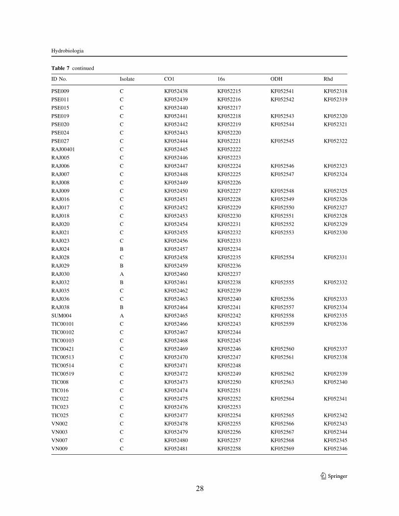
28

Table 7 continued

ID No. Isolate CO1 16s ODH Rhd

PSE009 C KF052438 KF052215 KF052541 KF052318

PSE011 C KF052439 KF052216 KF052542 KF052319

PSE015 C KF052440 KF052217

PSE019 C KF052441 KF052218 KF052543 KF052320

PSE020 C KF052442 KF052219 KF052544 KF052321

PSE024 C KF052443 KF052220

PSE027 C KF052444 KF052221 KF052545 KF052322

RAJ00401 C KF052445 KF052222

RAJ005 C KF052446 KF052223

RAJ006 C KF052447 KF052224 KF052546 KF052323

RAJ007 C KF052448 KF052225 KF052547 KF052324

RAJ008 C KF052449 KF052226

RAJ009 C KF052450 KF052227 KF052548 KF052325

RAJ016 C KF052451 KF052228 KF052549 KF052326

RAJ017 C KF052452 KF052229 KF052550 KF052327

RAJ018 C KF052453 KF052230 KF052551 KF052328

RAJ020 C KF052454 KF052231 KF052552 KF052329

RAJ021 C KF052455 KF052232 KF052553 KF052330

RAJ023 C KF052456 KF052233

RAJ024 B KF052457 KF052234

RAJ028 C KF052458 KF052235 KF052554 KF052331

RAJ029 B KF052459 KF052236

RAJ030 A KF052460 KF052237

RAJ032 B KF052461 KF052238 KF052555 KF052332

RAJ035 C KF052462 KF052239

RAJ036 C KF052463 KF052240 KF052556 KF052333

RAJ038 B KF052464 KF052241 KF052557 KF052334

SUM004 A KF052465 KF052242 KF052558 KF052335

TIC00101 C KF052466 KF052243 KF052559 KF052336

TIC00102 C KF052467 KF052244

TIC00103 C KF052468 KF052245

TIC00421 C KF052469 KF052246 KF052560 KF052337

TIC00513 C KF052470 KF052247 KF052561 KF052338

TIC00514 C KF052471 KF052248

TIC00519 C KF052472 KF052249 KF052562 KF052339

TIC008 C KF052473 KF052250 KF052563 KF052340

TIC016 C KF052474 KF052251

TIC022 C KF052475 KF052252 KF052564 KF052341

TIC023 C KF052476 KF052253

TIC025 C KF052477 KF052254 KF052565 KF052342

VN002 C KF052478 KF052255 KF052566 KF052343

VN003 C KF052479 KF052256 KF052567 KF052344

VN007 C KF052480 KF052257 KF052568 KF052345

VN009 C KF052481 KF052258 KF052569 KF052346

Hydrobiologia

123

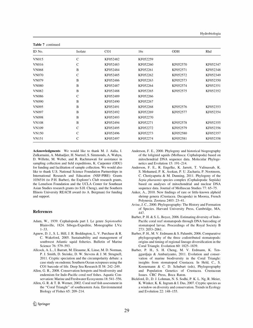
29

Acknowledgments We would like to thank M. J. Aidia, I.Zulkarnaini, A. Muhadjier, H. Nuetzel, S. Simmonds, A. Wahyu,D. Willette, M. Weber, and R. Rachmawati for assistance insampling collection and field expeditions, K. Carpenter (ODU)for funding and facilitation of sample collection. We would alsolike to thank U.S. National Science Foundation Partnerships inInternational Research and Education (NSF-PIRE) Grants1036516 (to P.H. Barber), the Explorer’s Club research grants,the Lemelson Foundation and the UCLA Center for SoutheastAsian Studies research grants (to S.H. Cheng), and the SouthernIllinois University REACH award (to A. Bergman) for fundingand support.

References

Adam, W., 1939. Cephalopoda part I. Le genre SepioteuthisBlainville, 1824. Siboga-Expeditie, Monographie LVa:1–33.

Agnew, D. J., S. L. Hill, J. R. Beddington, L. V. Purchase & R.C. Wakeford, 2005. Sustainability and management ofsouthwest Atlantic squid fisheries. Bulletin of MarineScience 76: 579–593.

Allcock, A. L., I. Barratt, M. Eleaume, K. Linse, M. D. Norman,P. J. Smith, D. Steinke, D. W. Stevens & J. M. Strugnell,2011. Cryptic speciation and the circumpolarity debate: acase study on endemic Southern Ocean octopuses using theCO1 barcode of life. Deep Sea Research II 58: 242–249.

Allen, G. R., 2008. Conservation hotspots and biodiversity andendemism for Indo-Pacific coral reef fishes. Aquatic Con-servation: Marine and Freshwater Ecosystems 18: 541–556.

Allen, G. R. & T. B. Werner, 2002. Coral reef fish assessment inthe ‘‘Coral Triangle’’ of southeastern Asia. EnvironmentalBiology of Fishes 65: 209–214.

Anderson, F. E., 2000. Phylogeny and historical biogeographyof the loliginid squids (Mollusca: Cephalopoda) based onmitochondrial DNA sequence data. Molecular Phyloge-netics and Evolution 15: 191–214.

Anderson, F. E., R. Engelke, K. Jarrett, T. Valinassab, K.S. Mohamed, P. K. Asokan, P. U. Zacharia, P. Nootmorn,C. Chotiyaputta & M. Dunning, 2011. Phylogeny of theSepia pharaonis species complex (Cephalopoda: Sepiida)based on analyses of mitochondrial and nuclear DNAsequence data. Journal of Molluscan Studies 77: 65–75.

Anker, A., 2010. New findings of rare or little-known alpheidshrimp genera (Crustacea. Decapoda) in Moorea, FrenchPolynesia. Zootaxa 2403: 23–41.

Avise, J. C., 2000. Phylogeography: The History and Formationof Species. Harvard University Press, Cambridge, MA.447.

Barber, P. H. & S. L. Boyce, 2006. Estimating diversity of Indo-Pacific coral reef stomatopods through DNA barcoding ofstomatopod larvae. Proceedings of the Royal Society B273: 2053–2061.

Barber, P. H., M. V. Erdmann & S. Palumbi, 2006. Comparativephylogeography of the three codistributed stomatopods:origins and timing of regional lineage diversification in theCoral Triangle. Evolution 60: 1825–1839.

Barber, P. H., S. H. Cheng, M. V. Erdmann, K. Ten-ggardjaja & Ambariyanto, 2011. Evolution and conser-vation of marine biodiversity in the Coral Triangle:insights from stomatopod Crustacea. In Held, C., S.Koenemann & C. D. Schubart (eds), Phylogeographyand Population Genetics of Crustacea. CrustaceanIssues. CRC Press, Boca Raton.

Bickford, D., D. J. Lohman, N. S. Sodhi, P. K. L. Ng, R. Meier,K. Winker, K. K. Ingram & I. Das, 2007. Cryptic species asa window on diversity and conservation. Trends in Ecologyand Evolution 22: 148–155.

Table 7 continued

ID No. Isolate CO1 16s ODH Rhd

VN015 C KF052482 KF052259

VN016 C KF052483 KF052260 KF052570 KF052347

VN068 B KF052484 KF052261 KF052571 KF052348

VN070 C KF052485 KF052262 KF052572 KF052349

VN079 B KF052486 KF052263 KF052573 KF052350

VN080 B KF052487 KF052264 KF052574 KF052351

VN082 B KF052488 KF052265 KF052575 KF052352

VN086 C KF052489 KF052266

VN090 B KF052490 KF052267

VN095 B KF052491 KF052268 KF052576 KF052353

VN097 B KF052492 KF052269 KF052577 KF052354

VN098 B KF052493 KF052270

VN108 B KF052494 KF052271 KF052578 KF052355

VN109 C KF052495 KF052272 KF052579 KF052356

VN150 C KF052496 KF052273 KF052580 KF052357

VN151 C KF052497 KF052274 KF052581 KF052358

Hydrobiologia

123

30

Boyle, P. & S. V. Boletzky, 1996. Cephalopod populations:definitions and dynamics. Philosophical Transactions ofthe Royal Society B: Biological Sciences 351: 985–1002.

Briggs, J. C., 1999. Coincident biogeographic patterns: Indo-West Pacific Ocean. Evolution 53: 326–335.

Carpenter, K. E., P. H. Barber, E. D. Crandall, M. C. A. Ablan-Lagman, Ambariyanto, G. N. Mahardika, B. M. Manjaji-Matsumoto, M. A. Juinio-Menez, M. D. Santos, C.J. Starger & A. H. A. Toha, 2011. Comparative phyloge-ography of the Coral Triangle and implications for marinemanagement. Journal of Marine Biology 2011: 1–14.

Chikuni, S., 1983. Cephalopod resources in the Indo-Pacificregion. In Caddy, J. F. (ed.), Advances in Assessment ofWorld Cephalopod Resources. FAO Fisheries TechnicalPaper 231: 264–305.

Choe, S., 1966. On the eggs, rearing, habits of the fry, andgrowth of some Cephalopoda. Bulletin of Marine Science16: 330–348.

Chotiyaputta, C., 1993. Cephalopod resources of Thailand. InOkutauni, T., R. O’Dor & T. Kubodera (eds), RecentAdvances in Fisheries Biology. Tokai University Press,Tokyo: 71–80.

Colborn, J., R. E. Crabtree, J. B. Shaklee, E. Pfeiler & B.W. Bowen, 2001. The evolutionary enigma of bonefishes(Albula spp.): cryptic species and ancient separations in aglobally distributed shorefish. Evolution 55: 807–820.

Conservation International, 2012. Coral Triangle Initiative Map.http://www.conservation.org/where/oceans/CTI/Pages/map.aspx. Accessed November 3, 2012.

Crandall, E. D., M. A. Frey, P. K. Grosberg & P. H. Barber,2008. Contrasting demographic history and phylogeo-graphical patterns in two Indo-Pacific gastropods. Molec-ular Ecology 17: 611–626.

Darriba, D., G. L. Taboada, R. Doallo & D. Posada, 2012.jModelTest 2: more models, new heuristics and parallelcomputing. Nature Methods 9: 772.

DeBoer, T. S., M. D. Subia, M. V. Erdmann, K. Kovitvongsa& P. H. Barber, 2008. Phylogeography and limitedgenetic connectivity in the endangered boring giant clamacross the Coral Triangle. Conservation Biology 22:1255–1266.

Dobzhansky, T., 1970. Genetics of the Evolutionary Process.Columbia University Press, New York.

Donoghue, M. J., 1985. A critique of the biological speciesconcept and recommendations for a phylogenetic alterna-tive. The Bryologist 88: 172–181.

Drew, J., G. R. Allen, L. Kaufman & P. H. Barber, 2008.Endemism and regional color and genetic differences infive putatively cosmopolitan reef fishes. ConservationBiology 22: 965–975.

Excoffier, L. & H. E. L. Lischer, 2010. Arlequin suite ver 3.5: anew series of programs to perform population geneticsanalyses under Linux and Windows. Molecular EcologyResources 10: 564–567.

FAO, 2009. FAO Yearbook. Fishery and Aquaculture Statistics.Food and Agriculture Organization of the United Nations,Rome.

Fauvelot, C. & P. Borsa, 2011. Patterns of genetic isolation in awidely distributed pelagic fish, the narrow-banded Spanishmackerel (Scomberomorus commerson). Biological Jour-nal of the Linnean Society 104: 886–902.

Fenchel, T., 2005. Cosmopolitan microbes and their ‘‘cryptic’’species. Aquatic Microbial Ecology 41: 49–54.

Fields, W.G., 1965. The structure, development, food relations,reproduction, and life history of the squid Loligo opale-scen Berry. California Department of Fish and Game,Fisheries Bulletin 131: 108.

Folmer, O., M. Black, W. Hoeh, R. Lutz & R. Vrijenhoek, 1994.DNA primers for amplification of mitochondrial cyto-chrome c oxidase subunit 1 from diverse metazoan inver-tebrates. Molecular Marine Biology and Biotechnology 3:294–299.

Forsythe, J. W., L. S. Walsh, P. E. Turk & P. G. Lee, 2001.Impact of temperature on juvenile growth and age at firstegg-laying of the Pacific reef squid Sepioteuthis lessonianareared in captivity. Marine Biology 138: 103–112.

Gaither, M. R., R. J. Toonen, D. R. Robertson, D. Planes & B.W. Bowen, 2009. Genetic evaluation of marine biogeo-graphical barriers: perspectives from two widespread Indo-Pacific snappers (Lutjanus kasmira and Lutjanus fulvus).Journal of Biogeography 2009: 1–15.

Gaither, M. R., B. W. Bowen, T. Bordenave, L. A. Rocha, S.J. Newman, J. A. Gomez, L. van Herwerden & M. T. Craig,2011. Phylogeography of the reef fish Cephalopholis argus(Epinephelidae) indicates Pleistocene isolation across theIndo-Pacific barrier with contemporary overlap in theCoral Triangle. BMC Evolutionary Biology 11: 189–204.

Godfrey, J. S., 1996. The effect of the Indonesian throughflowon ocean circulation and heat exchange with the atmo-sphere: a review. Journal of Geophysical Research 101:12217–12237.

Gordon, A. L. & R. A. Fine, 1996. Pathways of water betweenthe Pacific and Indian oceans in the Indonesian seas. Nature379: 146–149.

Guindon, S. & O. Gascuel, 2003. A simple, fast and accuratemethod to estimate large phylogenies by maximum-like-lihood. Systematic Biology 52: 696–704.

Hebert, P. D. N., A. Cywinska, S. L. Ball & J. R. DeWaard,2003. Biological identifications through DNA barcodes.Proceedings of the Royal Society London B 270: 313–321.

Heled, J. & A. J. Drummond, 2010. Bayesian inference ofspecies trees from multilocus data. Molecular Biology andEvolution 27: 570–580.

Iwata, Y., P. Show, E. Fujiwara, K. Shiba, Y. Kakiuchi & N.Hirohashi, 2010. Postcopulatory sexual selection drivesintra-specific sperm dimorphism. Unpublished. GenBankDirect Submission. Accessed September 1, 2012.

Izuka, T., S. Segawa, T. Okutani & K. Numachi, 1994. Evidenceon the existence of three species in the oval squid Sepio-teuthis lessoniana complex in Ishigaka Island, Okinawa,Southwestern Japan, by isozyme analysis. The JapaneseJournal of Malacology Venus 53: 217–228.

Izuka, T., S. Segawa & T. Okutani, 1996a. Biochemical study ofthe population heterogeneity and distribution of the ovalsquid Sepioteuthis lessoniana complex in southwesternJapan. American Malacological Bulletin 12: 129–135.

Izuka, T., S. Segawa & T. Okutani, 1996b. Identification of threespecies in oval squid, Sepioteuthis lessoniana complex bychromatophore arrangements on the funnel. The JapaneseJournal of Malacology Venus 55: 139–142.

Jackson, G. D. & M. N. Moltschaniwsky, 2002. Spatial andtemporal variation in growth rates and maturity in the Indo-

Hydrobiologia

123

31

Pacific squid Sepioteuthis lessoniana (Cephalopoda: Loli-ginidae). Marine Biology 140: 747–754.

Jereb, P. & C. F. E. Roper, 2006. Cephalopods of the IndianOcean. A review. Part I. Inshore squids (Loliginidae) col-lected during the International Indian Ocean Expedition.Proceedings of the Biological Society of Washington119(1): 91–136.

Jereb, P. & C. F. E. Roper, 2010. Cephalopods of the World: AnAnnotated and Illustrated Catalogue of Cephalopod Spe-cies Known to Date. Volume 2. Myopsid and OegopsidSquids. FAO Species Catalogue for Fishery Purposes. No.4, Vol. 2. Rome.

Jivaluk, J., J. Nabhitabhata, A. Nateewathana & P. Wtprasit,2005. Description of the Thai type of bigfin reef squid,Sepioteuthis lessoniana, hatchling with note on compari-son to Japanese types. Phuket Marine Biological CenterResearch Bulletin 66: 117–126.

Kessing, B., H. Croom, A. Martin, C. McIntosh, W. O. McMil-lan & S. Palumbi, 1989. A Simple Fool’s Guide to PCR.Department of Zoology, University of Hawaii, Honolulu.

Kier, W. M., 1996. Muscle development in squid: ultrastructuraldifferentiation of a specialized muscle fiber type. Journal ofMorphology 229: 271–288.

Knowlton, N., 1993. Sibling species in the sea. Annual Reviewof Ecology and Systematics 24: 189–216.

Knowlton, N., 2000. Molecular genetic analyses of speciesboundaries in the sea. Hydrobiologia 420: 73–90.

Knowlton, N., E. Weil, L. A. Weigt & H. M. Guzman, 1992.Sibling species in Montastraea annularis, coral bleachingand the coral climate record. Science 255: 330–333.

Leache, A. D. & M. K. Fujita, 2010. Bayesian species delimi-tation in West African forest geckos (Hemidactylus fasci-atus). Proceedings of the Royal Society B 277: 3071–3077.

Lee, P. G., P. E. Turk, W. T. Yang & R. T. Hanlon, 1994.Biological characteristics and biomedical applications ofthe squid Sepioteuthis lessoniana cultured through multiplegenerations. The Biological Bulletin 186: 328–341.

Lefkaditou, E., M. Corsini-Foka & G. Kondilatos, 2009.Description of the first Lessepsian squid migrant, Sepio-teuthis lessoniana (CEPHALOPODA: Loliginidae), theAegean Sea (Eastern Mediterranean). MediterraneanMarine Science 10: 87–97.

Leray, M., R. Beldade, S. J. Holbrook, R. J. Schmitt, S. Planes &G. Bernardi, 2010. Allopatric divergence and speciation incoral reef fish: the three-spot dascyllus, Dascyllus trima-culatus, species complex. Evolution 64: 1218–1230.

Lindgren, A. R., 2010. Molecular inference of phylogeneticrelationships among Decapodiformes (Mollusca: Cepha-lopoda) with special focus on the squid Order Oegopsida.Molecular Phylogenetics and Evolution 56: 77–90.

Maddison, W. P., 1997. Gene trees in species trees. SystematicBiology 46: 523–536.

Mayr, E., 1942. Systematics and the Origin of Species.Columbia University Press, New York.

Mienis, H. K., 2004. New data concerning the presence ofLessepsian and other Indo-Pacific migrants among themolluscs in the Mediterranean Sea with emphasis on thesituation in Israel. Turkish Journal of Aquatic Life 2:117–131.

Miller, M. A., M. T. Holder, R. Vos, P. E. Midford, T. Liebo-witz, L. Chan, P. Hoover & T. Warnow, 2010. The CIPRES

Portals. CIPRES. 2009-08-04. http://www.phylo.org/sub_sections/portal. Accessed August 4, 2009 (Archived byWebCite(r) at http://www.webcitation.org/5imQlJeQa).

Nateewathana, A., A. Munprasit & P. Dithachey, 2000. Sys-tematics and distribution of oceanic cephalopods in theSouth China Sea, Area 3: Western Philippines. In Pro-ceedings of the Third Technical Seminar on Marine Fish-ery Resources Survey in the South China Sea, Area 3:Western Philippines, 13–15 July 1999, Bangkok, Thailand,Vol. 41: 76–100.

Natsukari, Y., Y. Nishiyama & Y. Nakanishi, 1986. A pre-liminary study on the isozymes of the loliginid squid,Photololigo edulis (Hoyle, 12885). Report on CooperativeStudy on Photololigo edulis in Southwestern Japan Sea:145–151.

Nichols, R., 2001. Gene trees and species trees are not the same.Trends in Ecology and Evolution 16: 358–364.

Norman, M. D. & C. C. Lu, 2000. Preliminary checklist of thecephalopods of the South China Sea. The Raffles Bulletinof Zoology Supplement 8: 539–567.

Norman, M. D. & M. J. Sweeney, 1997. The shallow-wateroctopuses (Cephalopoda: Octopodidae) of the Philippines.Invertebrate Taxonomy 11: 89–140.

Nuryanto, A. & M. Kochzius, 2009. Highly restricted gene flowand deep evolutionary lineages in the giant clam Tridacnamaxima. Coral Reefs 28: 607–619.

O’Dor, R. K., S. Adamo, J. P. Aitken, Y. Andrade, J. Finn, R.T. Hanlon & G. D. Jackson, 2002. Currents as environ-mental constraints on the behavior, energetics and distri-bution of squid and cuttlefish. Bulletin of Marine Science71: 601–617.

Okutani, T., 2005. Past, present and future studies on cephalo-pod diversity in tropical west Pacific. Phuket Marine Bio-logical Center Research Bulletin 66: 39–50.

Okutani, T. & J. A. McGowan, 1969. Systematics, distribution,and abundance of the epiplanktonic squid (Cephalopoda,Decapoda) larvae of the California Current, April, 1954–March, 1957. In Arrhenius, G. O. S., C. S. Cox, E. W. Fager,C. H. Hand, T. Newberry & M. B. Schaefer (eds), Bulletin ofthe Scripps Institution of Oceanography 14.

Ovendon, J. R., J. Salini, S. O’Connor & R. Street, 2004. Pro-nounced genetic population structure in a potentially vagilefish species (Pristipomoides multidens, Teleosteo; Perci-formes; Lutjanidae) from the East Indies triangle. Molec-ular Ecology 12: 1991–1999.

Pecl, G. T., 2001. Flexible reproductive strategies in tropical andtemperate Sepioteuthis squids. Marine Biology 138:93–101.

Pecl, G. T. & G. C. Jackson, 2008. The potential impacts of climatechange on inshore squid: biology, ecology and fisheries.Reviews in Fish Biology and Fisheries 18: 373–385.

Pecl, G. T., S. Tracey, J. Semmens & G. D. Jackson, 2006. Useof acoustic telemetry for spatial management of southerncalamary, Sepioteuthis australis, a highly mobile inshoresquid species. Marine Ecology Progress Series 328: 1–15.

Planes, D. & C. Fauvelot, 2002. Isolation by distance andvicariance drive genetic structure of a coral reef fish in thePacific Ocean. Evolution 56: 378–399.

Rambaut, A. & A. J. Drummond, 2007. Tracer v1.4. Availablefrom http://beast.bio.ed.ac.uk/Tracer. Accessed October10, 2012.

Hydrobiologia

123

32

Rao, K. V., 1954. Biology and fishery of the Palk Bay squid,Sepioteuthis arctipinnis Gould. Indian Journal of Fisheries1: 37–66.

Reaka-Kudla, M. L., 1997. The global biodiversity of coralreefs: a comparison with rain forests. In Reaka-Kudla, M.L., D. E. Wilson & E. O. Wilson (eds), Biodiversity II:Understanding and Protecting Our Biological Resources.National Academies Press, Washington, DC: 83–108.

Sala, E. & N. Knowlton, 2006. Global marine biodiversitytrends. Annual Review of Environmental Resources 31:93–122.

Salman, A., 2002. New report of the loliginid squid Sepioteuthislessoniana Lesson, 1830 in the Mediterranean. IsraelJournal of Zoology 48: 249–250.

Schroth, W., G. Jarms, B. Streit & B. Schierwater, 2002. Spe-ciation and phylogeography in the cosmopolitan marinemoon jelly, Aurelia sp. BMC Evolutionary Biology 2: 1.

Segawa, S., 1987. Life history of the oval squid, Sepioteuthislessoniana in Kominato and adjacent waters central Hon-shu, Japan. Journal of the Tokyo University of Fisheries 74:67–105.

Segawa, S., T. Izuka, T. Tamashiro & T. Okutani, 1993a. A noteon mating and egg deposition by Sepioteuthis lessoniana inIshigaki Island, Okinawa, southwestern Japan. Venus,Japanese Journal of Malacology 52: 101–108.

Segawa, S., S. Hirayama & T. Okutani, 1993b. Is Sepioteuthislessoniana in Okinawa a single species? In Okutani, T., R.K. O’Dor & T. Kubodera (eds), Recent Advances inCephalopod Fisheries Biology. Tokai University Press,Tokyo: 513–521.

Shigeno, S., K. Tsuchiya & S. Segawa, 2001. Embryonic andparalarval development of the central nervous system ofthe loliginid squid Sepioteuthis lessoniana. The Journal ofComparative Neurology 437: 449–475.

Slapeta, J., P. Lopex-Garcia & D. Moreira, 2006. Global dis-persal and ancient cryptic species in the smallest marineeukaryotes. Molecular Biology and Evolution 23: 23–29.

Sole-Cava, A. M., M. Klautau, N. Boury-Esnault, R. Borojecic& J. P. Thorpe, 1991. Genetic evidence for cryptic speci-ation in allopatric populations of two cosmopolitan speciesof the calcareous sponge genus Clathrina. Marine Biology111: 381–386.

Soselisa, J., S. Marjuki & W. Subani, 1986. Production andfishing season of squids (Loligo spp.) in Lombok (WestNusa Tenggara) and adjacent waters. Journal of PenelitianPerikanan Lautan 34: 79–90.

Sponer, R. & M. S. Roy, 2002. Phylogeographic analysis of thebrooding brittle star Amphipholis squamata (Echinoder-mata) along the coast of New Zealand reveals high crypticgenetic variation and cryptic dispersal potential. Evolution56: 1954–1967.

Stocsits, R. R., H. Letsch, J. Hertel, B. Misof & P. F. Stadler,2009. Accurate and efficient reconstruction of deep phy-logenies from structured RNAs. Nucleic Acids Research37: 6184–6193.

Strugnell, J. M. & A. R. Lindgren, 2007. A barcode of lifedatabase for the Cephalopoda? Considerations and con-cerns. Reviews in Fish Biology and Fisheries 17: 337–344.

Strugnell, J., M. Norman, A. J. Drummond & A. Cooper, 2004.Neotenous origins for pelagic octopuses. Current Biology14: R300–R301.

Strugnell, J., M. Norman, J. Jackson, A. J. Drummond & A.Cooper, 2005. Molecular phylogeny of coleoid cephalo-pods (Mollusca: Cephalopoda) using a multigeneapproach; the effect of data partitioning on resolvingphylogenies in a Bayesian framework. Molecular Phylog-enetics and Evolution 37: 426–441.

Sudjoko, B., 1987. Catch composition of squids (Cephalopods)by using bagan (lift net) in Probolinggo waters, East Java.Journal of Penelitian Perikanan Lautan 41: 81–89.

Sugimoto, C. & Y. Ikeda, 2012. Ontogeny of schooling behaviorin the oval squid Sepioteuthis lessoniana. Fisheries Science78: 287–294.

Thompson, J. T. & W. M. Kier, 2001. Ontogenetic changes inmantle kinematics during escape-jet locomotion in the ovalsquid, Sepioteuthis lessoniana Lesson, 1830. BiologicalBulletin 201: 16–154.

Tokai, T. & Y. Ueta, 1999. Estimation of size selectivity for ovalsquid Sepioteuthis lessoniana in the squid jigging fishery ofTokushima Prefecture. Fishery Science 65: 448–454.

Triantafillos, L. & M. Adams, 2001. Allozyme analysis reveals acomplex population structure in the southern calamarySepioteuthis australis from Australia and New Zealand.Marine Ecology Progress Series 212: 193–209.

Triantafillos, L. & M. Adams, 2005. Genetic evidence that thenorthern calamari (Sepioteuthis lessoniana), is a speciescomplex in Australian waters. ICES Journal of MarineScience 62: 1665–1670.

Ueta, Y. & Y. Jo, 1989. Notes on ecology of the oval squidSepioteuthis lessoniana in outer waters adjacent to the KiiChannel. Nippon Suisan Gakkaishi 55: 1699–1702.

Ueta, Y. & Y. Jo, 1990. Migration of the oval squid, Sepioteuthislessoniana around Tokushima Prefecture. Suisanzohoku38: 221–226.

Vecchione, M., T. F. Brakoniecki, Y. Natsukari & R. T. Hanlon,1998. A provisional generic classification of the familyLoliginidae. In Voss, N. A., M. Vecchione, R. B. Toll & M.J. Sweeney (eds), Systematics and Biogeography ofCephalopods. Smithsonian Contributions to Zoology 586:215–222.

Villesen, P., 2007. FaBox: an online toolbox for FASTAsequences. Molecular Ecology Notes 7: 965–968.

Wada, Y. & T. Kobayashi, 1995. On an iteroparity of oval squidSepioteuthis lessoniana. Nippon Suisan Gakkaishi 61:151–158.

Wakabayashi, T., N. Suzuki, M. Sakai, T. Ichii & S. Chow,2012. Phylogenetic relationships among the family Om-mastrephidae (Mollusca: Cephalopoda) inferred from twomitochondrial DNA gene sequences. Marine Genomics 7:11–16.

Walsh, P. S., D. A. Metzger & R. Higuchi, 1991. Chelex 100 as amedium for simple extraction of DNA for PCR-based typingfrom forensic material. BioTechniques 10: 506–513.

Westheide, W. & H. Schmidt, 2003. Cosmopolitan versuscryptic meiofaunal polychaete species: an approach to amolecular taxonomy. Helgoland Marine Research 57: 1–6.

Williams, S. T. & J. A. H. Benzie, 1997. Indo-West Pacificpatterns of genetic differentiation in the high-dispersalstarfish Linckia laevigata. Molecular Ecology 6: 559–573.

Wyrtki, K., 1961. Physical Oceanography of the SoutheastAsian Waters. Scripps Institute of Oceanography, Uni-versity of California, La Jolla, CA.

Hydrobiologia

123

33

Yang, Z. & B. Rannala, 2010. Bayesian species delimitationusing multilocus sequence data. Proceedings of theNational Academy of Sciences 107(20): 9264–9269.

Yeatman, J. M. & J. A. H. Benzie, 1993. Cryptic speciation inLoligo from northern Australia. In Okutani, T., R. K. O’Dor& T. Kubodera (eds), Recent Advances in CephalopodFisheries Biology. Tokai University Press, Tokyo: 641–652.

Zeidberg, L. & W. Hamner, 2002. Distribution of squidparalarvae, Loligo opalescens (Cephalopoda: Myopside),in the Southern California Bight in the three yearsfollowing the 1997–1998 El Nino. Marine Biology 141:111–122.

Hydrobiologia

123

34

CHAPTER 2

(Not) going the distance: contrasting patterns of geographical subdivision in sibling taxa of reef

squid (Loliginidae: Sepioteuthis cf. lessoniana) in the Coral Triangle

Abstract

Diversification in the marine environment has long been assumed to be driven by

primarily allopatric (i.e. physical) barriers to gene flow. Recent studies indicate that this

explanation is too simplistic and that a multitude of both physical and ecological drivers exist

and interact to generate and maintain diversity. However, insight into these drivers as limited as

most previous studies focused on benthic organisms and they depended on primarily, single

markers, lacking sufficient power to illuminate fine-scale patterns of population structure. In

light of this, this study uses a comparative population genomic approach to examine barriers to

gene flow in two co-occurring, cryptic species of the bigfin reef squid (Sepioteuthis cf.

lessoniana), a neritic organism within the center of marine biodiversity (the Coral Triangle). We

used mitochondrial COI and ~2,000 genome-wide single nucleotide polymorphisms generated

using a restriction enzyme associated digest method (RADseq) (2b-RAD, Wang et al. 2012) to

examine population structure across the Coral Triangle. We found that previously hypothesized

barriers to gene flow in this region (Pleistocene glaciation cycles and prevailing physical

oceanographic patterns) do not equally shape population structure in these reef squids. We

observe drastically discordant patterns of connectivity between these sibling taxa, implying that

lineage B has much more limited dispersal capacity than lineage C, highlighting the importance

of dispersal life history for shaping individual species responses to physical drivers of gene flow.

Genomic-scale examinations also allowed us to identify fine-scale patterns of very limited

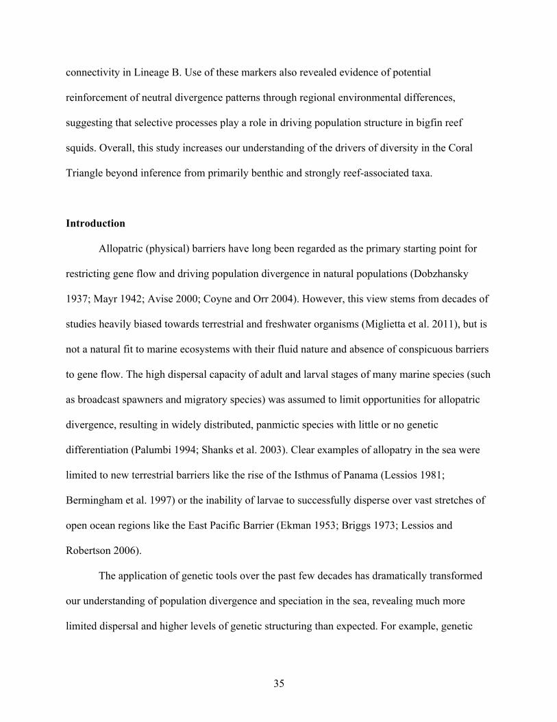
35

connectivity in Lineage B. Use of these markers also revealed evidence of potential

reinforcement of neutral divergence patterns through regional environmental differences,

suggesting that selective processes play a role in driving population structure in bigfin reef

squids. Overall, this study increases our understanding of the drivers of diversity in the Coral

Triangle beyond inference from primarily benthic and strongly reef-associated taxa.

Introduction

Allopatric (physical) barriers have long been regarded as the primary starting point for

restricting gene flow and driving population divergence in natural populations (Dobzhansky

1937; Mayr 1942; Avise 2000; Coyne and Orr 2004). However, this view stems from decades of

studies heavily biased towards terrestrial and freshwater organisms (Miglietta et al. 2011), but is

not a natural fit to marine ecosystems with their fluid nature and absence of conspicuous barriers

to gene flow. The high dispersal capacity of adult and larval stages of many marine species (such

as broadcast spawners and migratory species) was assumed to limit opportunities for allopatric

divergence, resulting in widely distributed, panmictic species with little or no genetic

differentiation (Palumbi 1994; Shanks et al. 2003). Clear examples of allopatry in the sea were

limited to new terrestrial barriers like the rise of the Isthmus of Panama (Lessios 1981;

Bermingham et al. 1997) or the inability of larvae to successfully disperse over vast stretches of

open ocean regions like the East Pacific Barrier (Ekman 1953; Briggs 1973; Lessios and

Robertson 2006).

The application of genetic tools over the past few decades has dramatically transformed

our understanding of population divergence and speciation in the sea, revealing much more

limited dispersal and higher levels of genetic structuring than expected. For example, genetic

36

studies revealed that many cosmopolitan species are, in fact, comprised of species complexes

(Solé-Cava et al. 1991; Knowlton 1993; Schroth et al. 2002). Marine populations can by highly

structured (Hellberg et al. 2002; Swearer et al. 2002) as larvae fail to reach their dispersal

potential due to behavioral and environmental factors mediating effective dispersal (Kingsford et

al. 2002; Pineda et al. 2007; Jones et al. 2009). Moreover, an increasing number of studies

highlight the importance of selective processes in shaping marine population structure and

divergence – such as host specificity, post-settlement survival, and ecological niche

diversification (Johannesson 2001; Faucci et al. 2007; Vigliola et al. 2007). Combined, these and

other studies indicate that the factors affecting marine larval dispersal and population diversity

are much more complex than previously thought (Palumbi 1992; Shanks et al. 2003).

Spanning Indonesia, Malaysia, Papua New Guinea, the Philippines, and East Timor, the

Coral Triangle is the world’s most biodiverse marine ecosystem (Hoeksema 2007; Veron et al.

2009), spawning considerable interest in the processes generating this diversity (Bowen et al.

2013; Barber and Meyer 2015). Prevailing theories suggest that high levels of inter- and intra-

specific diversity can be attributed to the dynamic geological history of the Coral Triangle and to

its complex oceanographic patterns. Numerous phylogeographic studies in a wide diversity of

marine taxa provide strong evidence for allopatric divergence over the Sunda Shelf, which was

repeatedly exposed during Pleistocene glaciation cycles creating a land barrier between the

Pacific and Indian Oceans (Barber et al. 2002; Barber et al. 2006; Crandall et al. 2008a;b;

DeBoer et al. 2008; Drew and Barber 2009; Gaither et al. 2011; Carpenter et al. 2011). Similarly,

phylogeographic studies (Barber et al. 2006; Barber et al. 2011; Ackiss et al. 2013; Timery S

DeBoer et al. 2014) as well as coupled bio-physical dispersal models (Kool et al. 2011; Treml

and Halpin 2012) suggest that physical oceanographic processes in the western boundary

37

currents can also promote isolation and divergence. Yet, large-scale comparative

phylogeographic meta-analyses indicate an abundance of discordant phylogeographic patterns,

even amongst closely related species, as well as potential cryptic species with substantial regions

of sympatry (Meyer et al. 2005; Plaisance et al. 2009; Barber et al. 2011; Carpenter et al. 2011),

despite the expectation that broad-scale physical processes should result in similar structure in

co-distributed taxa (Avise 2000).

Mitochondrial DNA has been the steady workhorse in studies of marine diversification

(Bowen et al. 2014), illuminating the complexity of processes shaping gene flow, isolation, and

divergence in marine environments (Hedgecock 1994; Hellberg 2009), particularly in the Coral

Triangle. While mitochondrial DNA and microsatellites have been (and still are) valuable tools

for elucidating patterns of population differentiation (Bowen et al. 2014), they lack power to

precisely estimate the relative effects of demographic factors (e.g. gene flow, drift) versus

selection and adaptive variation (rev. Storz 2005; Narum et al. 2013). Moreover, while

traditional genetic markers are extraordinarily useful for historical connectivity and divergence,

their ability to understand connectivity on ecologically relevant timescales is limited (Hedgecock

et al. 2007; Allendorf et al. 2010). This limits our understanding the physical and biological

processes underlying contemporary patterns of gene flow.

The advent of next-generation sequencing (NGS) technology exponentially increases our

ability to tease apart the relative contributions of neutral versus non-neutral processes governing

gene flow and divergence at historical and contemporary time scales. NGS allows for

simultaneous screening of thousands to tens of thousands of putative loci throughout the genome.

This increased power has the potential to increase the reliability and accuracy of estimates of

demographic and population parameters (Brumfield et al. 2003) as well as identify putative

38

adaptive loci to detect ongoing speciation and adaptive divergence (Feder and Nosil 2010),

processes that could contribute to discordant patterns of population genetic structure in co-

distributed taxa. The application of such genomic markers in marine species are few, but steadily

growing (Willette et al. 2014). Specifically, RAD sequencing has been used to great success in

detecting broad and fine-scale population structure in wild populations such as clownfish (Planes

et al. 2009), herring (Lamichhaney et al. 2012), and anchovies (Zarraonaindia et al. 2012).

Another challenge to inferring barriers to gene flow and processes driving divergence in

the Coral Triangle is that most studies to date have focused on reef-associated and inshore taxa,

largely to the exclusion of mobile neritic marine taxa. Theoretically, the high fecundity, high

levels of active migration and passive dispersal typical of pelagic and neritic marine organisms

are predicted to result in dynamic, unstructured populations over large spatial areas (Waples

1998). However, the few studies to date of pelagic and neritic marine species in the Coral

Triangle indicate fine-scale patterns of differentiation (Perrin and Borsa 2001; Borsa 2003;

Jackson et al. 2014). In addition, these studies focus exclusively on teleost fishes. Even though

cephalopods play key roles in marine trophic webs and ecosystems (Clarke 1996; Piatkowski et

al. 2001), to date, there has been very little research conducted on genetic structure in

cephalopods, much less squid, in the Indo-West Pacific (however, see Yeatman and Benzie

1994; Sin et al. 2009; Anderson et al. 2010; Tomano et al. 2015), and none within the Coral

Triangle.

The bigfin reef squid (Sepioteuthis cf. lessoniana, Lesson 1830) is common in the

tropical coastal waters of the Indo-West Pacific region. Recent genetic studies confirmed that

this commercially valuable species is comprised of at least three reciprocally monophyletic, but

co-distributed cryptic species (Cheng et al. 2014). Previous population-level studies in this

39

species complex demonstrated restricted gene flow over deep ocean basins and extremely large

geographic distances (e.g., between Japan and Thailand, Aoki et al. 2008), although the scope

and resolution of these single and multilocus studies was limited.

The goal of this study is to advance our understanding of evolution of marine biodiversity

in the Coral Triangle by specifically investigating: 1) patterns of connectivity in neritic taxa and

2) the relative roles of neutral versus non-neutral processes in governing gene flow and

divergence. We aim to address these using a comparative phylogeographic analysis of

sympatrically distributed populations of sibling taxa of the neritic bigfin reef squid (S. cf.

lessoniana). Using a multilocus approach using both traditional (mitochondrial) and next-

generation sequencing methodologies (genome-wide SNPs from RAD-based sequencing), we

compared two widely co-occurring sibling lineages of S. cf. lessoniana (B and C, Cheng et al.

2014) in the Coral Triangle and peripheral areas to test for divergence across multiple known

phylogeographic barriers. We also searched for outlier loci that might indicate adaptive

divergence. As large-scale physical processes should produce similar patterns of regional genetic

structure in organisms with similar dispersal life histories and ecologies (Avise et al. 1987),

comparing sibling taxa allows for a robust test of the relative influence of previously

hypothesized physical barriers to gene flow. Furthermore, by utilizing genome-wide markers, we

can begin to tease apart the relative roles of neutral versus selective processes in shaping gene

flow in neritic organisms, allowing for a broader understanding of the processes underlying the

center of marine biodiversity.

Methodology

Specimen collection

40

We collected a total of 706 embryos, hatchlings, juveniles and adults from local fish

markets and by hand-jigging from small boats and shores (day and night) at 17 locations

throughout the Indo-West Pacific range of S. cf. lessoniana (Figure 2.2.1) (Table 2.2.1). For

juveniles and adults, a 1-2 cm piece of tissue from the ventral opening of the mantle was

preserved in 95% ethanol. Embryos and/or hatchlings were excised from individual capsules and

preserved in 95% ethanol. We used mitochondrial CO1 as a barcoding marker (as proposed in

Cheng et al. 2014) to assign all individual samples to either lineage B or C. Because of variation

in abundances of these lineages at each location, we excluded sampling sites with less than 10

individuals sampled.

Tissue preparation and mitochondrial DNA sequencing

We extracted high-quality genomic DNA from preserved mantle tissue using a modified

phenol-chloroform method employed in the E.Z.N.A Mollusc DNA extraction kit (Omega).

Building upon previous mtDNA work in Sepioteuthis (Cheng et al. 2014), we amplified a 686-bp

fragment of mitochondrial (mtDNA) cytochrome oxidase subunit 1 (CO1) sequence following

the methods described therein.

RAD library preparation and sequencing

We generated genome-wide single nucleotide polymorphism (SNP) data using a type of

RAD (restriction site-associated DNA tag) sequencing method, called 2b-RAD (Wang et al.

2012). We chose RAD sequencing as this method allows for simultaneous single nucleotide

polymorphism discovery and genotyping in large numbers of samples without established

genomic resources (i.e. non-model organisms) (Baird et al. 2008). Furthermore, the simultaneous

41

discovery and genotyping characteristic of RAD significantly reduces issues caused by

ascertainment bias arising from developing SNP panels from a subset of populations (Clark et al.

2007). The 2b-RAD method employed here features the use of IIB restriction enzymes, which

generate a specific-sized fragment with the restriction site in the center, resulting in uniform

fragment sizes (Wang et al. 2012). We chose this method as it is extremely flexible and simple in

comparison to more typical RAD sequencing techniques, making it ideal for screening of large

numbers of individuals in population-scale studies.

Library preparation followed the protocol developed by the Matz laboratory at the

University of Texas-Austin (http://www.bio.utexas.edu/research/matz_lab/matzlab/Methods.

html), with a few modifications detailed below. We chose to amplify between 10-15 individuals

per sampling location for each lineage to maximize spatial coverage and sequencing efficiency.

Preparation started with digestion of ~800-1000 ng genomic DNA using AlfI restriction enzyme.

Library-specific adaptors designed for 1/16th representation of digestion sites were then ligated to

digested samples. Ligated products were then amplified with Illumina platform specific primers

and unique 6-bp barcodes for 24 cycles in preparation for sequencing. Amplified products were

individually run on a 2% agarose gel with SYBR SAFE fluorescent dye in 1X TBE buffer at 150

V for 90 minutes or until product bands were significantly separated. The ~176 bp target band

was then excised from the gel and the PCR product extracted and purified using a commercially

available gel extraction kit (Qiagen QIAquick). Purified PCR samples were then further cleaned

and brought to appropriate volume and concentration using Ampure XP beads using a standard

clean-up protocol (Beckman-Coulter).

The University of California-Berkeley Vincent J. Coates Genomic Sequencing Facility

performed all sequencing on an Illumina Hi-Seq 2000 with single-end 50-bp reads with 40-55

42

samples per lane at approximately 20X coverage. This facility also performed initial quality

control and demultiplexing. We used an informatics pipeline from the Meyer Lab at Oregon

State University specifically designed for the 2b-RAD method (E. Meyer, pers. comm.

http://people.oregonstate. edu/~meyere/tools.html) to conduct read processing and filtering. First,

terminal tag positions associated with ligation sites were removed from each resultant 50-bp read

(keeping positions 1-36). Reads were then stringently filtered for quality, removing any reads

with ambiguous base calls and any low-quality positions (more than 1 position with quality less

than 10); reads consisting only of adaptors were also removed.

We used a Stacks-like informatics pipeline specifically designed for analysis of 2b-RAD

generated data to conduct de novo reference construction, mapping, and genotype calling (M.

Matz, https://github.com/z0on/2bRAD_denovo). We also attempted mapping to an unpublished,

unannotated draft genome (~40X coverage Illumina HiSeq) of another loliginid squid,

Doryteuthis (formerly Loligo) pealei (C. Titus Brown, http://ivory.idyll.org/blog/2014-loligo-

transcriptome-data.html) as the reference. AlfI sites were extracted from the D. pealeii genome,

resulting in a reference assembly of 198,008 unique tags (7,128,288 total basepairs). A de novo

reference was constructed using a custom perl script that finds unique tag sequences for each

individual (analogous to creating “stacks” using Stacks) (M. Matz, pers. comm.). Because initial

mapping to the D. pealeii reference was extremely poor (~50% reads matched), we proceeded

with the de novo reference (~95% reads matched). Using cd-hit-est (Li and Godzik 2006; Fu et

al. 2012), unique reads were clustered into pseudoalleles, and subsequently into pseudosites

allowing for a maximum of 3 mismatches. Final de novo references were built from 393,032

clusters (from 993,505 unique tags) and 397,706 clusters (from 1,139,465 unique tages) for

lineages B and C respectively. Reads per individual sample were then mapped onto the de novo

43

reference using a custom perl script (M. Matz), filtering by read depth (min 5) and strand bias

(min 5).

SNP calling and validation

Genotypes appearing in at least 2 individuals were called with a maximum of 0.5 allowed

heterozygocity and high total read depth (20X). They were then filtered to exclude the lowest

quality 20% of data. We discarded loci with too many heterozygotes (>75%) as they likely

indicated lumped paralogs. Lastly, from this resultant set, loci with more than 25% missing data

were also excluded. We then thinned the SNP data set keeping the site with the highest minor

allele frequency (MAF) for each tag, to control for any effects of linkage disequilibrium.

DATA ANALYSIS

Sample statistics and detection of outlier loci

Identifying the relative effects of genetic drift and natural selection is necessary to

accurately estimate the demographic history of population. In theory, loci under directional or

balancing selection should display either higher or lower genetic differentiation than that

expected under neutral theory (termed “outlier loci”) (Lewontin and Krakauer 1973). As

inclusion of outlier loci can bias estimates of population parameters (Morin et al. 2004), data

were analyzed in three sets: 1) including all loci, 2) excluding outlier loci, and 3) only including

outlier loci. We employed two different outlier detection approaches. We first used Bayescan,

which directly estimates the posterior probability of individual loci being under selection by

explicitly testing two models, one with and one without selection, using a reversible-jump Monte

Carlo Markov chain approach (Foll and Gaggiotti 2008). Bayescan was run with a panel of

44

putatively neutral loci with 20 pilot runs (5000 steps) and a final run for 100,000 generations

sampling every 10 steps and a 50% burn-in. Outlier loci were called under a false discovery rate

of 0.05. Second, we employed a more traditional summary statistic approach using fdist as

applied in Lositan (Antao et al. 2008). To rigorously test for outlier loci from a panel that likely

contains neutral and selected loci, we first ran a pilot run using all loci to estimate mean neutral

FST. All loci that fell outside of a 99% confidence interval were removed as candidate selected

loci, and a new mean neutral FST was recalculated with the remaining putative loci. We then

optimized for deviations from model assumptions by comparing the average simulated FST from

the first 10,000 simulations with the empirical average FST and iteratively slicing and sampling

the range between the two values to reach optimal error margins. We ran Lositan for 50,000

simulations and called outlier loci as those outside the 99% confidence interval with a false

discovery rate of 0.1.

Sample statistics for SNP and CO1 datasets were calculated in Arlequin 3.5 (Excoffier

and Lischer 2010). Allele frequencies and observed and expected heterozygocities were

estimated for neutral and outlier loci SNP panels as well as the CO1 datasets. Nucleotide and

haplotype diversity were also calculated for the CO1 datasets. Population pairwise F-statistics

(after Weir and Cockerham 1984) were calculated within an analysis of molecular variance

(AMOVA) framework for all datasets.

Population assignment and clustering

For CO1 datasets, we inferred minimum spanning trees of unique haplotypes based on

pairwise distances (p-distance) in Arlequin 3.5 (Excoffier and Lischer 2010) to estimate the

likely number of clades within each lineage. Clades were defined as groups of haplotypes

45

separated by 10 or more mutational steps (~1.5% sequence differentiation). To visualize genetic

structure in the two lineages over geography, we mapped the frequencies of each clade over all

sampling locations.

For the SNP datasets, we did initial tests of population assignment using two methods to

determine the most likely number and composition of populations without a priori assumptions.

We first conducted an assignment test for the likely number of populations within the SNP

sample sets using ADMIXTURE (Alexander et al. 2009). ADMIXTURE estimates ancestry of

unrelated individuals and population allele frequencies using a maximum likelihood approach.

We tested population sizes ranging from k=1 to k=8, with the maximum value for k equaling the

total number of distinct samples collected over time and space. The k value with the lowest

cross-validation error indicates the most likely number of populations. Second, we used

discriminant analyses of principal components (DAPC) to look for likely genetic clustering.

DAPC and other principal components based analyses have been shown to demonstrate similar

power to detect population structure model-based clustering methods (e.g. Structure, Pritchard et

al. 2000) (Patterson et al. 2006). We used the ade4/adegenet package in R (Jombart 2008;

Jombart et al. 2010) to conduct DAPC analyses for all data sets (mtDNA, neutral and outlier

SNPs). We employed a cross-validation method implemented in adegenet (xValDapc) to

determine the optimal number of principal components to include in the analysis in order to

maximize inference and minimize chances of overfitting.

Testing for population structure

We conducted analysis of molecular variance (AMOVA) to test both a priori and ad hoc

hypotheses of population structure. Specifically, we first tested specific a priori hypotheses of

46

structure or limited gene flow over known spatial barriers in the Coral Triangle (summarized in

Carpenter et al. 2011; Bowen et al. 2013) (Figure 2.2). These include: restricted gene flow 1)

over the Sunda shelf at the Thai peninsula/western Sumatra region (Williams and Benzie 1998;

Barber and Bellwood 2005; Barber et al. 2006), 2) east and west of the Halmahera Eddy (Barber

et al. 2002; Barber et al. 2006; DeBoer et al. 2008; Barber et al. 2011; Ackiss et al. 2013; Timery

S DeBoer et al. 2014), 3) over deep ocean basins between Japan and the Ryuyku archipelago and

the Coral Triangle (Aoki et al. 2008), 4) over the Sulu Sea between the Philippines and Indonesia

(Lourie et al. 2005), and finally, 5) absence of genetic structure. Second, we then tested for

differentiation between identified clusters from ADMIXTURE within the SNP datasets.

Similarly, we tested for differentiation between identified mitochondrial clades identified in the

minimum spanning trees. All AMOVA analyses were conducted in Arlequin with 10,000

permutations (Excoffier and Lischer 2010) using all successfully sequenced individuals with n ≥

4 per sampling location.

Testing for isolation by distance

The presence of isolation by distance can result in gradual clines of genetic differentiation

that may result in false positives when testing for hierarchical structure (AMOVA) (Meirmans

2012). We tested for isolation by distance for the neutral and outlier datasets using Mantel tests

controlling for ADMIXTURE cluster and geographic distance. Geographic distance was

calculated as the shortest distance over water between sampling points, as straight-line Euclidean

distances are not appropriate for marine organisms for which crossing land is not possible.

Geographic distances were estimated using custom algorithms implemented within ArcGIS 9.3

(Etherington 2011). Pairwise non-Euclidean distance (Nei’s distance) was estimated between

47

individuals, and isolation-by-distance calculations were carried out with 9999 permutations,

using the package adegenet in R (Jombart 2008).

Results

Mitochondrial DNA

Building on Cheng et al. (2014), we successfully sequenced CO1 (~686 bp) from 72 and

273 additional individuals from lineages B (8 locations) and C (19 locations) respectively. In

total, 165 and 498 individual sequences for lineages for B and C yielded 62 and 174 unique

haplotypes, respectively.

SNP discovery and quality filtering

We sequenced 53 individuals from 7 locations for lineage B and 116 individuals from 9

locations for lineage C (Table 2.1). We obtained between 1 million to 5 million raw reads per

individual, with ~3% sequences lost after removing adaptors and ambiguous reads, and stringent

quality filtering. Combining all genotypes for Lineage B, out of 379,127 basepairs, 11.52%

(43,703) passed stringent genotype calling filters, of which 16.78% (7335) were polymorphic (at

least 2 genotypes). For lineage C, out of 563,830 putative SNPs, 6.77% (38,205) passed

genotyping filters, of which, 24.96% (9537) were polymorphic. Filtering these polymorphic

SNPs for coverage, excess heterozygotes, and missing data resulted in 2,108 and 2,920 loci at

20X coverage for lineages B and C, respectively. After thinning to one SNP per tag, 1,653 and

2,229 loci remained for analysis. Lastly, individuals with more than 25% missing genotypes

were also removed – resulting in 48 individuals from 7 locations for lineage B and 105

individuals from 8 locations for lineage C.

48

Outlier detection and molecular diversity

Within lineage B, moderate levels of observed (average Ho = 0.220) and expected

(average He = 0.249) heterozygocity were detected for all loci (Table 2.2). Percentage of

polymorphic SNPs in each sampling location ranged from 45.9% to 77.9% (Table 2.2).

Comparatively, within lineage C, we observed lower levels of observed (average Ho = 0.168) and

expected (average He = 0.171) heterozygocity over all loci (Table 2.2). Percentage of

polymorphic SNPs in each sampling location ranged from 24.0% to 77.6% (Table 2.2). Bayescan

recovered 54 and 12 outlier loci (under diversifying selection) for B and C with a false discovery

rate of 0.05 (Figure 2.3). Comparatively, Lositan recovered 40 and 152 outliers respectively for

B and C (Figure 2.3). A total of 35 loci for lineage B and 10 loci for lineage C were detected as

outliers in both analyses and only these “outlier sets” were used for downstream analysis.

Patterns of population assignment and clustering

Mitochondrial DNA

The minimum spanning tree (MST) of lineage B revealed two distinct clades separated by

12 mutational steps (~1.75% uncorrected sequence divergence). Clade 1 was comprised of

eastern and central Indonesia sampling locations (Raja Ampat, Lembeh, Manado, and Timor

Leste) and indicated slightly more partitioning between Timor Leste and the rest of the samples

(4 mutational steps) (Figures 2.4 & 2.11). Clade 2 included samples from the Indian Ocean, the

Philippines, central Indonesia, and the Southeast Asian peninsula (Aceh, Bali, Ticao, and Nha

Trang) (Figures 2.4 & 2.11). The MST generated for lineage C has three star-like clusters each

representing a distinct clade separated by 12 mutational steps each (~1.75% uncorrected

sequence divergence) (Figures 2.5 & 2.12). The largest, Clade 1, consisted of samples from the

49

majority of our sampling locations with the exception of the three Ryukyu Archipelago locations

and approximately half the samples from Raja Ampat. Samples from the Ryuykus (Okinawa,

Ishigaki and Iriomote) comprised the majority of Clade 2 while Clade 3 only included 12

samples from Raja Ampat (Figures 2.5 & 2.12).

AMOVA analyses imposing regional structure based on these clade identities indicated

high levels of differentiation within Lineage B (FCT = 0.903, p < 0.05) (Table 2.3);

differentiation between clades in Lineage C were not as pronounced nor was it statistically

significant (FCT = 0.345, p = 0.07) (Table 2.4). Rather, observed levels of genetic variation could

be equally well explained by both between group variance as by within group variance.

Neutral and outlier SNPs

Similar population structure was detected in neutral and outlier loci for Lineage B

employing both population assignment and clustering methods. A two-population scheme (k=2)

was most well supported for lineage B using neutral loci (CV =0.28484), while three populations

(k=3) was supported when examining only outlier loci (CV= 0.36900) (Figure 2.6a & b). With

k=2, ADMIXTURE indicated very little mixing of inferred population groups between

geographic sampling locations and the presence of two populations corresponding to the western

Coral Triangle (Banda Aceh, Bali, Nha Trang, and Ticao) and central/eastern Indonesia

(Lembeh, Manado and Raja Ampat) (Figure 2.6a), concordant with patterns from CO1 (Figures

2.4, 2.11). Using outlier loci and k=3, individuals from Aceh separated as a distinct third

population with a significant amount of admixture from the western Coral Triangle population

(Figure 2.6b). Support from neutral loci for k=2 vs. k=3 was equivocal (28.75% vs 24.35%

respectively), while mtDNA indicated that three populations accounted for most of the genetic

50

variation (though the difference was not statistically significant) (Table 2.3). However, the level

of differentiation was much higher when examining outlier loci (FCT = 0.855, p < 0.05). Under

this three-population scheme for the outlier loci, between-group variation accounted for 82.17%

of the variation (Table 2.3).

DAPCs conducted for lineage B with neutral loci showed that DF1 accounted for the

distinction between the two populations while DF2 distinguished between all sampling locations,

except for Bali (Indonesia) and Bulan (Bicol, Philippines) which completely overlapped,

signaling high rates of connectivity (Figure 2.7a). In contrast, while outlier loci similarly

accounted for the distinction between the two populations in DF1, there was substantial overlap

between sampling locations within populations. (e.g., Bali and Ticao; Aceh and Nha Trang). DF2

accounted for the separation of Lembeh from Manado and Raja Ampat in the central/eastern

Indonesia population (Figure 2.7b).

In contrast to Lineage B, analysis of Lineage C revealed non-concordant patterns of

population assignment between neutral and outlier loci. Neutral loci indicated k=3, with

populations in 1) the Ryuykus, 2) Raja Ampat, and 3) the western Coral Triangle/central

Indonesia (Bali, Aceh, Donggala, Andaman Sea and Gulf of Thailand) (Figure 2.8a). While this

pattern is concordant with mtDNA, neutral SNPs recovered much lower levels of differentiation

(FCT = 0.060, p < 0.01 for SNPs vs. FCT = 0.345, p < 0.05 for mtDNA) (Table 2.4). Moreover,

DAPC with neutral loci not only distinguished the three groups above, but also was able to

distinguish among all three Ryukyu islands (Okinawa, Ishigaki, Iriomote) (Figure 2.8a).

ADMIXTURE analysis of Lineage C outlier loci (n=10), in contrast, recovered 8

populations (k=8) with no clear geographic patterns. ADMIXTURE is designed to rapidly assess

ancestry in a large number of markers, making it ideal for next-generation sequencing

51

applications. However, the outlier dataset for lineage C only contained 10 loci, thus making it

highly unlikely for this low number of loci to distinguish any signals from noise. Running this

dataset through Structure revealed that k=2 was most well-supported (using the Delta K method,

Evanno et al. 2005). DAPC of outlier loci also indicated two groups with some degree of overlap

(Figure 2.9b). Populations from the western Coral Triangle/central Indonesia populations tightly

clustered together and individuals from Raja Ampat formed a cluster along DF2; however, a

number of individuals fell within the western Coral Triangle/central Indonesia group. Along

DF1, the Ryuykus emerged as another group albeit with more variation among individuals.

Examination of the ADMIXTURE plot for outliers (k=3) indicates a significant amount of mixed

ancestry between the three populations (Figure 2.8b). Among these outlier loci, however, we

observed higher levels of differentiation between the three populations than either neutral loci or

CO1 indicated (FCT = 0.444, p < 0.01).

Given the different patterns of population assignment, we assessed the ability of neutral

versus outlier loci to assign individuals back to their original sampling location using DAPCs.

Overall, neutral loci performed much better than outlier sets at assigning individuals back to

original sampling locations (Table 2.5). Neutral loci for lineage B assigned nearly 100% of

individuals back to their original sampling locations, while assignment proportions were much

lower for lineage C. In particular, neutral loci were able to successfully assign Ryuyku

Arichipelago and Raja Ampat individuals; however, individuals from the more widely

distributed western Coral Triangle/central Indonesia population were not often successfully

reassigned.

Testing hypotheses of spatial population structure

52

AMOVA showed significant genetic structure within both lineages of Sepioteuthis cf.

lessoniana (Table 2.3 & 4). However, none supported differentiation across the Halmahera Eddy,

Java Sea, or Sulu Sea. Within Lineage B, strong differentiation was only supported between the

three groups inferred by ADMIXTURE. While neutral SNPs revealed strong structure (FCT =

0.2875, p<0.001), mtDNA and outlier loci indicate near fixation between these groups (FCT =

0.9025, FCT=0.8554, p<0.0001, respectively). In lineage C, AMOVA only supported a genetic

break between the Ryuyku Archipelago and the Coral Triangle with all datasets, although

mtDNA showed significantly low levels of connectivity across the Halmahera Eddy (Table 2.4).

Lineage C had much lower levels of overall differentiation (FST =0.0479, p<0.0001) than

lineage B (FST =0.2024, p<0.0001) when comparing differentiation inferred from neutral loci.

Comparatively, global levels of differentiation were much higher for both lineages when

examined with outlier loci (B: FST=0.7821, p<0.0001, C: FST=0.3720, p<0.0001). This high level

of differentiation in outlier loci is reflected as well in the very strong differentiation observed in

CO1 data (B: FST=0.8782, p<0.0001, C: FST=0.6238, p<0.05).

We did not detect any signals of IBD in lineage B (r2 = 0.0001-0.02914, p>0.05) in any of

the datasets. After accounting for population structure, no signal of IBD was detected in either

the western Coral Triangle population or in the central/eastern Indonesia population (Figure

2.10a & b). Comparatively, there was a significant pattern of isolation by distance (IBD) in

lineage C for all populations at all loci (r2=0.0347-0.2313, p<0.05) (Figure 2.10c & d). However,

underlying population structure can confound estimations of IBD, thus when we tested for IBD

just within the Coral Triangle (omitting the divergent Japan population), we did not recover any

patterns of isolation by distance.

53

Discussion

Numerous studies of nearshore and reef-associated taxa using mtDNA data have shown

strong differentiation among populations spanning the Sunda Shelf and Halmahera Eddy (rev.

Carpenter et al. 2011; Ludt and Rocha 2014). However, these putative filters to gene flow do not

appear to equally impact lineages of Sepioteuthis c.f. lessoniana, suggesting that highly mobile

neritic taxa may not be influenced by sea level changes and physical oceanography the same way

as reef-associated species that only disperse as larvae. This study does reveal strong, contrasting

patterns of genetic structure between these sibling taxa highlighting that even slight differences

in life history can result in drastically different patterns of connectivity. Moreover, the use of

genome-wide SNPs adds substantial resolution for identifying fine-scale patterns of connectivity

and for detecting potential selective processes at play. Specifically, the use of genomic markers

in this study reveals that limited gene flow can in fact, occur in neritic taxa and that regional

environmental differences may play a much larger role than expected in shaping divergence

patterns.

Lineage B exhibits overall broad-scale structure distinguishing Sunda Shelf populations

from oceanic island populations to the north and east (Figure 2.11). This pattern is similar to

patterns from snails (Reid et al. 2006), seahorses (Lourie and Vincent 2004), and mackerel

(Rohfritsch and Borsa 2005). Genome-wide SNPs add substantial resolution to recovered

patterns of population structure, revealing strong distinctions not only between inferred

populations, but between sampling localities as well, indicating that lineage B has very limited

dispersal (Figure 2.7a). Moreover, divergent patterns detected with outlier loci indicate that

selective processes stemming from regional environmental differences likely plays a role in

population structure (Figure 2.6b, 2.7b). In contrast, we do not detect strong signals of structure

54

in lineage C, lending support to it having wide dispersal capacity (Table 2.4, Figures 2.8, 2.9,

2.12). However, the separation of the Ryuku Islands from the remainder of the Coral Triangle

suggests that distance may limit gene flow among these regions. Combined insight from

mitochondrial and genomic markers reveal that both neutral and non-neutral processes both play

a significant role in shaping patterns of population divergence in neritic species in the Coral

Triangle.

Consolidation of cryptic species identities over Pacific and Indian Oceans

While numerous efforts have been made to determine the identity, number and

characteristics of cryptic species within S. cf. lessoniana, insight from these studies has been

limited because these studies used different sets of information and were spatially limited,

making it extremely difficult to compare between studies and regions (e.g. Segawa et al.

1993a;b; Izuka et al. 1994; Izuka et al. 1996; Triantafillos and Adams 2005). CO1 barcoding of

samples in the Pacific and Indian Oceans conducted by Cheng et al. (2014) and expanded upon

in this study confirm that lineage C corresponds to the shiro-ika type (sensu Segawa et al. 1993)

also known as species 2 (sensu Izuka et al. 1996; Imai and Aoki 2009). Lineage A, which was

not examined on the population level in this study, corresponds with kua-ika (sensu Segawa et al.

1993) also known as species 3 (sensu Izuka et al. 1996; Imai and Aoki 2009). While lineage B

was not detected in individuals sampled in the Ryuykus in this study, barcoding of existing

sequences from GenBank indicate that lineage B corresponds to aka-ika (sensu Segawa et al.

1993) also known as species 1 (sensu Izuka et al. 1996) (S. Tomano, pers. comm.).

Population structure in neritic taxa in the Coral Triangle

55

Phylogeographic structure inferred with mtDNA and genome-wide SNPs of these two

lineages of reef squid do not precisely correspond to the two most commonly cited

phylogeographic barriers in the Coral Triangle, the Sunda Shelf and Halmahera Eddy (Barber et

al. 2011; Carpenter et al. 2011; Ludt and Rocha 2014). For lineage B, our results indicate a

distinct Sunda Shelf population and an oceanic island populations roughly corresponding to

divisions between western and central/eastern Indonesia (Figures 2.6, 2.11). As lineage B is not

as common as lineage C, sampling for this lineage was much coarser (Cheng et al. 2014), thus

the precise location of this break is unclear. Traditionally, the Sunda Shelf break stemming from

Pleistocene glaciation is situated along the southern margins of the Sunda Shelf (corresponding

to modern day Java and Sumatra). While ample evidence supports Indian/Pacific Ocean

vicariance during low sea level stands, the contact point between these two regions is highly

variable across taxa (rev. Ludt and Rocha 2014, Barber et al. 2000, 2006, DeBoer et al. 2008,

2014, Ackiss et al. 2013, Jackson et al. 2013, Crandall et al. 2008a, 2008b, 2011). For lineage B,

it is possible that the Sunda Shelf population represents the edge of an Indian Ocean population

that has recolonized more rapidly than the Pacific Ocean population following sea level rises.

Extremely high levels of differentiation in mitochondrial CO1 along with high differentiation

genome-wide support this theory of allopatric divergence and subsequent recolonization (Table

2.3).

On the other hand, the strong break observed in Lineage B also suggests significant

influence of prevailing oceanography in limiting gene flow in this species. Western and

central/eastern Indonesia are separated by the Makassar Strait between the islands of Sulawesi

and Kalimantan (Figure 2.11). The Indonesian Throughflow moves nearly 20 million m3/s of

water from the Pacific Ocean to the Indian Ocean (Godfrey 1996) through this narrow strait, at

56

velocities topping 1m/sec (Wyrtki 1961). Coupled biophysical larval dispersal models suggest

that this fast current is a significant physical barrier for east/west dispersal of larvae and adults

within the Coral Triangle (Kool et al. 2011), and as a neritic species, it is unlikely that S. c.f.

lessoniana would purposely navigate this span of deep and fast-moving water. Data supporting

genetic structure on either side of the Makassar Strait has been found in a number of diverse

marine organisms including giant clams (Tridacna maxima, Nuryanto and Kochzius 2009,

DeBoer et al. 2014), snails (Reid et al. 2006), and scad mackerel (Decapterus russelli, Rohfritsch

and Borsa 2005). High levels of admixture and clustering highlighted by genome-wide SNPs

between Philippines and Bali samples is likely the result of high connectivity facilitated by the

Indonesian Throughflow, lending further support to the influence of oceanography to shaping

patterns of gene flow in lineage B. Coupled biophysical larval dispersal models predict that the

Indonesian Throughflow facilitates high rates of gene flow and dispersal from the Philippines to

central and southern Indonesia (Kool et al. 2011). Similarly, the moderate levels of admixture

between the Philippines and Vietnam are likely the result of westerly currents in the South China

Sea (SCS) (Figures 2.6a, 2.7a).

Despite the well-known filters to gene flow in marine species in the Coral Triangle (see

above) we do not observe significant limits to dispersal and gene flow in Lineage C across most

of this region (Table 2.4 & 6, Figures 2.8, 2.9 & 2.12). Instead, genetic differentiation over all

locations can be explained by isolation by distance (Figure 2.10c & d), although this pattern is

driven by divergence between the Coral Triangle and the Ryuyku archipelago (mtDNA:

FCT=0.9386, p<0.001; N: FCT =0.1363, p<0.001; O: FCT =0.4406, p<0.001); within the Coral

Triangle, there is no significant signal of IBD. Intuitively, divergence between the Ryuykus and

the Coral Triangle is expected given the considerable distance of deep water (~3000 km from the

57

center) separating the two regions, which poses a significant dispersal barrier for a neritic

species. For the majority of Indo-West Pacific marine organisms, the Ryukyus represent the

northern limits of ranges (Briggs 1999). For many of these species, strong divergence is often

observed between populations in this peripheral portion of the range and those in the center of

the range (Nakajima et al. 2014; He et al. 2015). Divergence between Japan and areas from the

South China Sea and further afield have been detected before in the shiro-ika form of S. cf.

lessoniana (lineage C) (Aoki et al. 2008).

Results also support differentiation between Raja Ampat and the rest of the Coral

Triangle, a pattern that likely results from the isolating effects of the Halmahera Eddy. This

isolation is predicted by coupled biophysical models (Kool et al. 2011; Treml and Halpin 2012)

and is seen in a diversity of phylogeographic studies, including in fish (Timm and Kochzius

2008; Jackson et al. 2014), giant clams (DeBoer et al. 2008; 2014a; 2014b; Kochzius and

Nuryanto 2008), stomatopods (Barber et al 2006, 2011), nautilus (Wray et al. 1995), and other

invertebrates (Crandall et al. 2008; 2012). However, the position of this break is unclear, as we

do not have samples across the Maluku Sea, but rather from either end of it at Lembeh and Raja

Ampat. Overall however, historical sea level changes and physical oceanographic patterns do not

seem to strongly influence patterns of connectivity in lineage C.

Non-concordance of population structure in sibling taxa

Comparison of population structure over the Coral Triangle and peripheral regions

reveals a stark contrast in divergence patterns between two sibling taxa. This result suggests that

differences in traits such as life history, dispersal capacity and behavior, habitat preference and

recruitment can result in massively differential responses to regional-scale physical processes

58

(Kingsford et al. 2002; Pineda et al. 2007). The low levels of differentiation in lineage C are

more similar to highly dispersive pelagic organisms such as mackerel (Perrin and Borsa 2001)

and tuna (Jackson et al. 2014) while the strong differentiation in lineage B is more similar to the

patterns observed in less mobile, benthic and reef-associated taxa (see references above).

Limited disperser (Lineage B)

Although Sepioteuthis sp. are members of the neritic squid family Loliginidae, they

display morphological and life history traits that more closely resemble benthic cuttlefish (family

Sepiidae) (Segawa 1987; Segawa et al. 1993; Anderson 2000; Jereb and Roper 2010). Their main

feeding areas and spawning areas are found in shallow coastal and reef habitats, rarely extending

out over the continental shelf (Wada and Kobayashi 1995; Jereb and Roper 2010), and adults shy

away from strong currents (pers. obs, LEK from Indonesian fisherman). Tagging studies of S.

australis in Australia (Pecl et al. 2006) and S. cf. lessoniana in Japan (Ueta and Jo 1990) suggest

that spawning adults may only travel between 10-40 km along the coast. Given these similarities

to cuttlefish life history (Boycott 1965), perhaps it is not surprising that patterns of population

structure detected in lineage B resemble limited regional scale connectivity in pharaoh cuttlefish

(Sepia pharoanis) in this area (Anderson et al. 2010), suggesting similar responses to prevailing

physical processes in the region.

Strong distinctions between sampling locations could also stem from specific

requirements defining recruitment instead of, if not in addition to, limited dispersal capacity.

Both myopsid and oegopsid squid are known to display spawning site fidelity, which may drive a

significant degree of self-recruitment (e.g. Buresch et al. 2006; Thorpe et al. 1986, Brierley et al.

1993). Like other Loliginidae, Sepioteuthis species spawn in aggregations of varying sizes

59

(Jackson and Pecl 2003; Moltschaniwskyj and Pecl 2007; Venkatesan and Rajagopal 2012) at

different reef habitats. Studies suggest that differences in spawning site are fixed between the

three cryptic lineages of S. cf. lessoniana (Imai and Aoki 2009). On the same reef, aka-ika

(Lineage B) is observed to spawn at much deeper depths than shiro-ika (Lineage C) (Tomano et

al. unpubl.). If the availability of deeper reef habitat may be more limited compared to shallow

habitats, this would limit the degree of connectivity between more far-flung sampling locations.

Thus, even within a population, there may be limited exchange of individuals between spawning

sites driving the signals of low connectivity observed with genome-wide data. However, very

few studies have examined movement and migration in specific lineages within the species

complex. Thus, further research is needed to investigate the specifics of dispersal behavior and

capacity in lineage B.

Broad disperser (Lineage C).

Conversely, low overall levels of differentiation suggest that lineage C is a broad-scale

disperser (Figures 2.8, 2.9, 2.12), more similar to Loligo/Doryteuthis (family Loliginidae). While

lineage C shows strong evidence for wide dispersal capacity, we do observe a significant break

between the Coral Triangle and the Ryuyku Islands (Figure 2.12), reflecting results from

previous studies suggesting limited dispersal over the fast-moving Kuroshio Current (Aoki et al.

2008). Past genetic studies detect evidence of founder effects in species 2 (lineage C, shiro-ika)

around mainland Japan (Aoki et al. 2008, Tomano et al. 2015), suggesting colonization by a few

long-distance dispersers lending additional support to limited dispersal over this region. Within

the Ryuykus, neutral SNPs indicated moderate levels of structure between individual islands

(Figure 2.9) (Table 2.7) that were not detected with mitochondrial DNA (Figure 2.5). Ishigaki,

60

Iriomote and Okinawa are relatively close together, ranging from ~50 km to 500 km apart, but

these distances span areas of deep ocean. Decreased dispersal between islands may be attributed

to lack of contiguous coastline as has been observed between mainland Japan and the Ryukyus,

but this hypothesis has had mixed support in studies of S. cf. lessoniana (Aoki et al. 2008, Imai

and Aoki 2009, Tomano et al. 2015, Izuka et al. 1996, Yokogawa and Ueta 2000). Samples from

the Ryukyu Islands in this study were collected from individual embryos from egg masses laid at

approximately the same time, suggesting that simultaneously spawning individuals for each

island are significantly differentiated. Overall, these results lend strong support for the

hypothesis that deep water and non-contiguous coastlines are important barriers to dispersal for

lineage C.

 

Role of selective processes

One of the major criticisms of relying solely on mitochondrial DNA is that it cannot

indicate whether observed divergence stems from selective or neutral processes, hindering our

understanding of the mechanisms underlying diversification (Edwards and Beerli 2000; Edwards

et al. 2005 but see Bowen et al. 2014 for counter-argument). Using a genome-wide approach, we

were able to identify putative outlier loci, which represent portions of the genome that may be

under divergent selection. This novel approach allowed for us to infer when selective processes

may be important in shaping historical and ongoing patterns of gene flow. For these sibling

species of reef squid, outlier loci revealed that regional environmental differences likely play a

significant role in reinforcing divergence from neutral processes.

Using outlier loci, Lineage B distinguishes Aceh as a third distinct region (Figure 2.6b).

Although most studies have attributed this pattern to Pleistocene vicariance (Williams and

61

Benzie 1998; Duda Jr and Palumbi 1999; Barber and Bellwood 2005; Ackiss et al. 2013) the

coupled biophysical models of Kool et al. suggest that currents can limit flow between the Indian

Ocean and the Java Sea (2011). Given that the low estimates of genetic differentiation between

Aceh and the rest of the western Coral Triangle population for Lineage B, this divergence is

likely recent and may argue for a physical oceanographic origin, rather than Pleistocene sea level

fluctuations. Alternatively, strong divergence in outlier loci but not in neutral loci in Aceh may

reflect ongoing divergence with gene flow in the region. The mechanisms of ecological

speciation in marine environments are not well understood and at times, controversial, however,

there is increasing genetic evidence hinting that it is more common than previous thought (e.g.

Rocha et al. 2005; Faucci et al. 2007, Fritts-Penniman et al. unpubl, Simmonds et al. unpub.).

Unique abiotic characteristics of the waters around Banda Aceh may drive divergence.

Furthermore, a significant portion of reef biomass and available reef habitat was extirpated in the

region following the devastating tsunami in 2004 (Paris et al. 2007; Rao et al. 2007). Selective

pressure may stem from any of these forces; however, further investigation is required to

determine this.

Complete concordance in population structure between neutral, outlier and mtDNA loci

in Lineage C may suggest a complementary role of selective and neutral processes. The breaks

observed in lineage C with all loci correspond to major breaks between biogeographic provinces

in the Indo-West Pacific (Spalding et al. 2007). The biogeographic provinces are defined by the

presence of distinct biotas, which have arisen due to both historical isolation and distinctive

abiotic features including geomorphological, hydrographic, and geochemical features (Spalding

et al. 2007). The Ryuyku Archipelago and the Coral Triangle are in different marine provinces,

thus selective pressures imposed differences in abiotic features likely plays a role in reinforcing

62

patterns driven by neutral divergence. While Raja Ampat and rest of the Coral Triangle are

within the same marine province, they are in different ecoregions, suggesting that specific

differences in biogeographic shaping factors between these regions may also serve to reinforce

neutral divergence. However, this study only represents the first step towards disentangling the

effect of selective processes from neutral processes in diversification of marine organisms.

Further research on the specific life histories and ecologies of these reef squid are required

before we can make solid inferences about the specific role of selection.

Population structure inferred from mitochondrial DNA versus SNPs

The majority of phylogeographic studies in marine systems use mtDNA because of its

ability to readily discern phylogeographic patterns and the relative ease of obtaining sequence

data (rev. Avise 2000). The growing ability and the decreasing cost of generating and examining

hundreds to thousands of loci across the genome has terrific potential to revolutionize our

understanding of the evolutionary history of species and processes shaping population patterns

(Brumfield et al. 2003; Helyar et al. 2011). However, comparatively, conducting a population-

scale study with sufficient spatial coverage using NGS markers is still prohibitively expensive,

particularly for researchers in developing countries, such as those within the Coral Triangle

(Willette et al. 2014).

Within lineage B, mtDNA and ~1,650 neutral and outlier SNPs support divergence

among a western Indonesia population and a central/eastern Indonesia population. Given the

strong signal of divergence in neutral SNPs, there is no reason to implicate selective sweeps in

shaping mtDNA patterns. Similarly, although lineage C has lower levels of differentiation, both

mtDNA and SNPs distinguish the Ryuyku Archipelago from the remainder of the Coral Triangle.

63

Thus, SNPs provided a minimal advantage in discerning broad-scale patterns of differentiation.

Similar conclusions come from mtDNA and microsatellite analyses of giant clams in this region

(Timery S DeBoer et al. 2014). However, neutral and outlier SNP panels detected fine-scale

structure not detected by CO1 alone, such as distinguishing among the three Ryukus sampling

sites in Lineage C, echoing results from other studies that detected population boundaries in

marine organisms that were difficult to discern using traditional markers (Freamo et al. 2011;

Karlsson et al. 2011). Furthermore, outlier loci in Lineage B show more structure than neutral

loci, suggesting that selection may be reinforcing other physical or behavioral isolating forces. In

Lineage C, lower levels of clustering in outlier loci than neutral loci suggests that neutral

processes are the main drivers of divergence in this lineage and that all locations have similar

responses to shared selective pressures. Despite several caveats regarding detecting loci under

selection (Foll and Gaggiotti 2008), if care is taken to reduce false positives by using multiple

outlier tests (Luikart et al. 2003; Bonin et al. 2006), these and other results show the utility of

genome-wide SNP assays (Eckert et al. 2010; Hohenlohe et al. 2010; Freamo et al. 2011;

Bradbury et al. 2013; Nadeau et al. 2013).

Implications for conservation and fisheries management

Marine ecosystems provide a significant portion of global food supplies as well as

support national economies and livelihoods (Pauly et al. 2005). Effective management and

sustainability of these critical ecological and economic resources requires accurate data to

delineate management units and assess harvesting pressure. Conservation and fisheries biologists

are increasingly emphasizing the utility of genetic data (Frankham et al. 2002; Frankham 2005),

both as an inherent biological element to be conserved (Lande 1988; Crozier 1997; Amos and

64

Balmford 2001) and as a vital tool to inform conservation planning and management, particularly

for harvested natural resources (Frankham 2010). In the marine realm, genetic information is

particularly useful for informing 1) correct species identification and 2) spatial and temporal

structure of populations (Hilborn and Waters 1992; Palumbi 1994), elements key to delineating

management units and conservation areas.

The results from this study have two major implications for management of this fishery.

First, the strong differentiation among populations revealed by SNPs indicates strong limits to

connectivity among populations. Even within the Ryuku Islands, gene flow is insufficient to

limit differentiation among reefs. This fine-scale genetic differentiation suggests strong limits to

demographic exchange, and that management efforts may need to focus on the local, rather than

regional, scale. Second, Lineages B and C have very different patterns of genetic structure and

connectivity, yet they are caught in the same nets on the same reefs. Given that these cryptic taxa

can only be distinguished genetically at present, the most judicious approach to management of

this mixed fishery would be to manage for lineage with the more restricted dispersal, Lineage B.

Rapid development of genetic tools and methods of analyses have propelled the study of

conservation genetics into the new era of conservation genomics (Kohn et al. 2006; Allendorf et

al. 2010; Avise 2010). However, the use of the most technologically advanced or most recent

tools may not generate directly relevant information needed for rapid decision making, as is

needed by practitioners. Our study demonstrates that SNP data can detect fine-scale patterns of

genetic with significant management implications for this fishery. However, in developing

countries, such as those in the Coral Triangle, access to facilities and equipment required to

collect cutting-edge genetic information is extremely limited (Barber et al. 2014) and cost-

prohibitive (Willette et al. 2014). Thus, while SNP data refines our understanding of the

65

dynamics of the bigfin reef squid fisheries, financial limitations in developing countries may

preclude the application of these techniques. As such, mitochondrial DNA may remain an

important tool for management as it can provide important insights to population structure at a

fraction of the cost.

ACKNOWLEDGEMENTS This research would not have been possible without the efforts from numerous people in

collecting samples and facilitating this project over multiple countries. We would like to thank

H. Nuetzel, A. Fritts-Penniman, S. Simmonds, M. Weber, R. Rachmawati, D. Willette (UCLA),

M.J. Aidia, I. Zulkarnaini, A. Muhadjier (Universitas Syiah Kuala), S. Suzuki, K. Toda, E.

Edsinger-Gonzalez (OIST), S. Lui (National Sun Yat-sen University), A. Reid (Australian

Museum), R. Pooley (UK), B. Stockwell, A. Ackiss (Old Dominion University), Bret Grasse

(Monterey Bay Aquarium) and the Indonesian Biodiversity Research Center for assisting in

sample collections. We would also like to thank the efforts of G. N. Mahardika (Universitas

Udayana), H. P. Calumpong (Silliman University), B.T. Dang (Nha Trang University), A.

Prathep (Prince of Songkhla University), and S. Mitarai (OIST) for facilitating permits and

collections. In particular, we would like to thank the generosity of S. Mitarai and OIST for

inviting the lead author as a visiting researcher to Japan. We would also like to thank E. Meyer

(Oregon State University) and M. Matz (University of Texas-Austin) for their advice and

guidance in data analysis. We would like to thank our funding sources: U.S. National Science

Foundation Partnerships in International Research and Education (NSF-PIRE) Grants 1036516

(to P.H. Barber and K. Carpenter), United States Agency for International Development

(USAID) grant (to P.H. Barber), Explorer’s Club Research Grant (to S.H. Cheng), the Lemelson

66

Foundation and UCLA Center for Southeast Asian Studies research grant (to S.H. Cheng),

UCLA Graduate Division Research Travel Award (to S.H. Cheng), and funding from UCLA’s

Department of Ecology and Evolutionary Biology (to S.H. Cheng). Lastly, we would like to

thank F.E. Anderson (Univ. of Illinois-Carbondale), T.B. Smith and H.B. Shaffer (UCLA) for

providing comments on the drafts of this manuscript.

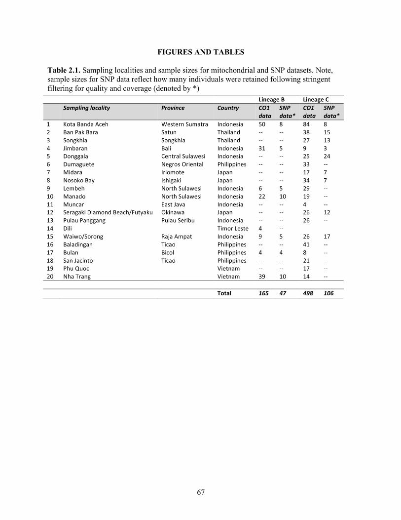
67

FIGURES AND TABLES Table 2.1. Sampling localities and sample sizes for mitochondrial and SNP datasets. Note, sample sizes for SNP data reflect how many individuals were retained following stringent filtering for quality and coverage (denoted by *)

        Lineage  B   Lineage  C     Sampling  locality   Province   Country   CO1  

data  SNP  data*  

CO1  data  

SNP  data*  

1   Kota  Banda  Aceh   Western  Sumatra   Indonesia   50   8   84   8  2   Ban  Pak  Bara   Satun   Thailand   -­‐-­‐   -­‐-­‐   38   15  3   Songkhla   Songkhla   Thailand   -­‐-­‐   -­‐-­‐   27   13  4   Jimbaran   Bali   Indonesia   31   5   9   3  5   Donggala   Central  Sulawesi   Indonesia   -­‐-­‐   -­‐-­‐   25   24  6   Dumaguete   Negros  Oriental   Philippines   -­‐-­‐   -­‐-­‐   33   -­‐-­‐  7   Midara   Iriomote   Japan   -­‐-­‐   -­‐-­‐   17   7  8   Nosoko  Bay   Ishigaki   Japan   -­‐-­‐   -­‐-­‐   34   7  9   Lembeh   North  Sulawesi   Indonesia   6   5   29   -­‐-­‐  10   Manado   North  Sulawesi   Indonesia   22   10   19   -­‐-­‐  11   Muncar   East  Java   Indonesia   -­‐-­‐   -­‐-­‐   4   -­‐-­‐  12   Seragaki  Diamond  Beach/Futyaku   Okinawa   Japan   -­‐-­‐   -­‐-­‐   26   12  13   Pulau  Panggang   Pulau  Seribu   Indonesia   -­‐-­‐   -­‐-­‐   26   -­‐-­‐  14   Dili     Timor  Leste   4   -­‐-­‐      15   Waiwo/Sorong   Raja  Ampat   Indonesia   9   5   26   17  16   Baladingan   Ticao   Philippines   -­‐-­‐   -­‐-­‐   41   -­‐-­‐  17   Bulan   Bicol   Philippines   4   4   8   -­‐-­‐  18   San  Jacinto   Ticao   Philippines   -­‐-­‐   -­‐-­‐   21   -­‐-­‐  19   Phu  Quoc     Vietnam   -­‐-­‐   -­‐-­‐   17   -­‐-­‐  20   Nha  Trang     Vietnam   39   10   14   -­‐-­‐                         Total   165   47   498   106  

68

Tabl

e 2.

2 . S

umm

ary

stat

istic

s for

mito

chon

dria

l and

gen

ome-

wid

e si

ngle

nuc

leot

ide

poly

mor

phis

ms e

mpl

oyed

in th

is st

udy  

!!

!Line

age!B!

Line

age!C!

!!

!mtCO1!

SNPs!

mtCO1!

SNPs!

Coun

try!

Region

!Locality!

Hap.!div.!

Nuc.!d

iv.!

H o!

H e!

%!poly!

Hap.!div.!

Nuc.!d

iv.!

H o!

H e!

%!poly!

Indo

nesia

)Western)

Sumatra)

Kota)Ban

da)

Aceh

)1.00

0)±)0.00

4)0.00

1)±)0.00

1)0.29

5)±)0.18

6)0.29

3)±)0.14

4)62

.6%)

1.00

0)±)0.00

2)0.00

3)±)0.00

2)0.27

7)±)0.17

9)0.27

5)±)0.14

2)57

.5%)

Thailand

)Satun)

Ban)Pak)Ba

ra)

))

))

)1.00

0)±)0.00

6)0.00

2)±)0.00

2)0.23

0)±)0.16

7)0.22

9)±)0.14

9)66

.2%)

Thailand

)Songkhla)

Songkhla)

))

))

)1.00

0)±)0.01

0)0.00

9)±)0.00

5)0.25

1)±)0.17

9)0.23

8)±)0.14

7)70

.0%)

Indo

nesia

)Ba

li)Jim

baran)

1.00

0)±)0.00

8)0.00

1)±)0.00

1)0.41

7)±)0.24

3)0.38

4)±)0.15

3)45

.9%)

))

0.52

2)±)0.26

9)0.49

5)±)0.17

9)24

.0%)

Indo

nesia

)Ce

ntral)

Sulawesi)

Donggala)

))

))

)1.00

0)±)0.01

1)0.00

6)±)0.00

3)0.21

0)±)0.16

0))

0.21

0)±)0.14

7)71

.9%)

Philipp

ines)

Negros)

Orie

ntal)

Dumague

te)

))

))

)1.00

0)±)0.00

7)0.00

3)±)0.00

2))

))

Japa

n)Iriom

ote)

Midara)

))

))

)1.00

0)±)0.02

0)0.00

1)±)0.00

1)0.32

3)±)0.20

1)0.31

1)±)0.14

9)37

.6%)

Japa

n)Ishigaki)

Nosoko)Ba

y))

))

))

1.00

0)±)0.00

7)0.00

1)±)0.00

1)0.33

1)±)0.21

6)0.31

8)±)0.14

9)36

.2%)

Indo

nesia

)North)

Sulawesi)

Lembe

h)1.00

0)±)0.09

6)0.00

3)±)0.00

3)0.42

3)±)0.22

9)0.37

4)±)0.13

6)54

.4%)

1.00

0)±)0.00

1)0.00

3)±)0.00

2))

))

Indo

nesia

)North)

Sulawesi)

Man

ado)

1.00

0)±)0.01

3)0.00

3)±)0.00

2)0.28

0)±)0.18

7)0.26

2)±)0.14

3)62

.5%)

1.00

0)±)0.01

6)0.01

4)±)0.00

8))

))

Indo

nesia

)East)Ja

va)

Mun

car)

))

))

)1.00

0)±)0.17

7)0.00

0)±)0.00

0))

))

Japa

n)Okina

wa)

Seragaki))

))

))

)1.00

0)±)0.01

1)0.00

1)±)0.00

1)0.27

3)±)0.18

5)0.26

6)±)0.15

4)51

.2%)

Indo

nesia

)Pu

lau)

Serib

u)Pu

lau)

Panggang)

))

))

)1.00

0)±)0.01

1)0.00

3)±)0.00

2))

))

Timor)Leste)

)Dili)

1.00

0)±)0.17

7)0.00

1)±)0.00

1))

))

))

))

)Indo

nesia

)Ra

ja)

Ampa

t)Waiwo/)

Sorong)

1.00

0)±)0.05

2)0.00

3)±)0.00

2)0.43

3)±)0.24

9)0.37

3)±)0.13

9)47

.4%)

1.00

0)±)0.01

1)0.01

4)±)0.00

8)0.27

6)±)0.18

5)0.26

0)±)0.14

9)80

.4%)

Philipp

ines)

Ticao)

Baladingan

))

))

))

1.00

0)±)0.00

5)0.00

3)±)0.00

2))

))

Philipp

ines)

Bicol)

Bulan)

1.00

0)±)0.17

7)0.00

2)±)0.00

2)0.49

4)±)0.24

4)0.41

0)±)0.12

1)55

.8%)

1.00

0)±)0.06

3)0.00

3)±)0.00

2))

))

Philipp

ines)

Ticao)

San)Jacinto)

))

))

)1.00

0)±)0.01

5)0.00

3)±)0.00

2))

))

Vietna

m)

)Ph

u)Quo

c))

))

))

1.00

0)±)0.02

0)0.00

4)±)0.00

3))

))

Vietna

m)

)Nha

)Trang)

1.00

0)±)0.00

6)0.00

1)±)0.00

1)0.30

8)±)0.20

4)0.27

4)±)0.14

7)77

.9%)

1.00

0)±)0.02

4)0.02

6)±)0.01

4))

))

!

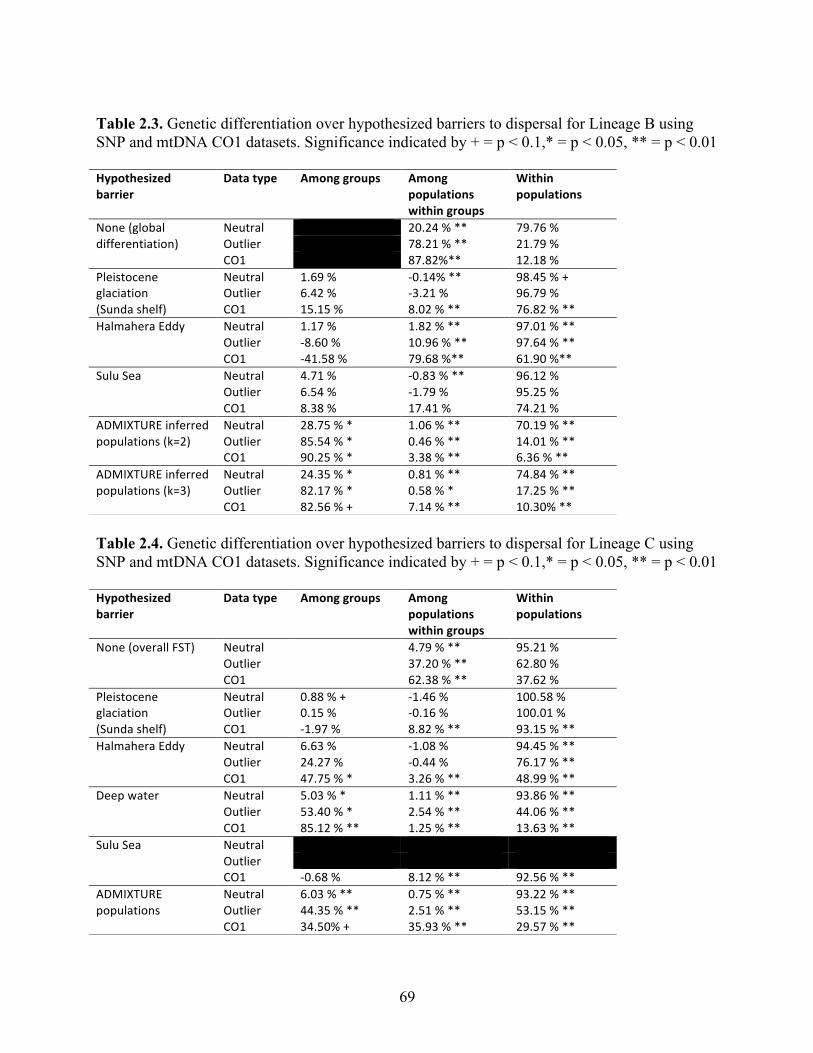
69

Table 2.3. Genetic differentiation over hypothesized barriers to dispersal for Lineage B using SNP and mtDNA CO1 datasets. Significance indicated by + = p < 0.1,* = p < 0.05, ** = p < 0.01

Table 2.4. Genetic differentiation over hypothesized barriers to dispersal for Lineage C using SNP and mtDNA CO1 datasets. Significance indicated by + = p < 0.1,* = p < 0.05, ** = p < 0.01

Hypothesized  barrier  

Data  type   Among  groups   Among  populations  within  groups  

Within  populations  

None  (global  differentiation)  

Neutral     20.24  %  **   79.76  %  Outlier     78.21  %  **   21.79  %  CO1     87.82%**   12.18  %  

Pleistocene  glaciation    (Sunda  shelf)  

Neutral   1.69  %     -­‐0.14%  **   98.45  %  +  Outlier   6.42  %   -­‐3.21  %   96.79  %  CO1   15.15  %   8.02  %  **   76.82  %  **  

Halmahera  Eddy   Neutral   1.17  %   1.82  %  **   97.01  %  **  Outlier   -­‐8.60  %     10.96  %  **   97.64  %  **  CO1   -­‐41.58  %   79.68  %**   61.90  %**  

Sulu  Sea   Neutral   4.71  %   -­‐0.83  %  **   96.12  %  Outlier   6.54  %   -­‐1.79  %   95.25  %  CO1   8.38  %   17.41  %   74.21  %  

ADMIXTURE  inferred  populations  (k=2)  

Neutral   28.75  %  *   1.06  %  **   70.19  %  **  Outlier   85.54  %  *   0.46  %  **   14.01  %  **  CO1   90.25  %  *   3.38  %  **   6.36  %  **  

ADMIXTURE  inferred  populations  (k=3)  

Neutral   24.35  %  *   0.81  %  **   74.84  %  **  Outlier   82.17  %  *   0.58  %  *   17.25  %  **  CO1   82.56  %  +   7.14  %  **   10.30%  **  

Hypothesized  barrier  

Data  type   Among  groups   Among  populations  within  groups  

Within  populations  

None  (overall  FST)   Neutral     4.79  %  **   95.21  %  Outlier     37.20  %  **   62.80  %  CO1     62.38  %  **   37.62  %  

Pleistocene  glaciation    (Sunda  shelf)  

Neutral   0.88  %  +   -­‐1.46  %   100.58  %  Outlier   0.15  %   -­‐0.16  %   100.01  %  CO1   -­‐1.97  %   8.82  %  **   93.15  %  **  

Halmahera  Eddy   Neutral   6.63  %   -­‐1.08  %   94.45  %  **  Outlier   24.27  %   -­‐0.44  %   76.17  %  **  CO1   47.75  %  *   3.26  %  **   48.99  %  **    

Deep  water   Neutral   5.03  %  *   1.11  %  **   93.86  %  **  Outlier   53.40  %  *   2.54  %  **   44.06  %  **  CO1   85.12  %  **   1.25  %  **   13.63  %  **  

Sulu  Sea   Neutral        Outlier        CO1   -­‐0.68  %     8.12  %  **   92.56  %  **  

ADMIXTURE  populations  

Neutral   6.03  %  **   0.75  %  **   93.22  %  **  Outlier   44.35  %  **   2.51  %  **   53.15  %  **  CO1   34.50%  +   35.93  %  **   29.57  %  **  

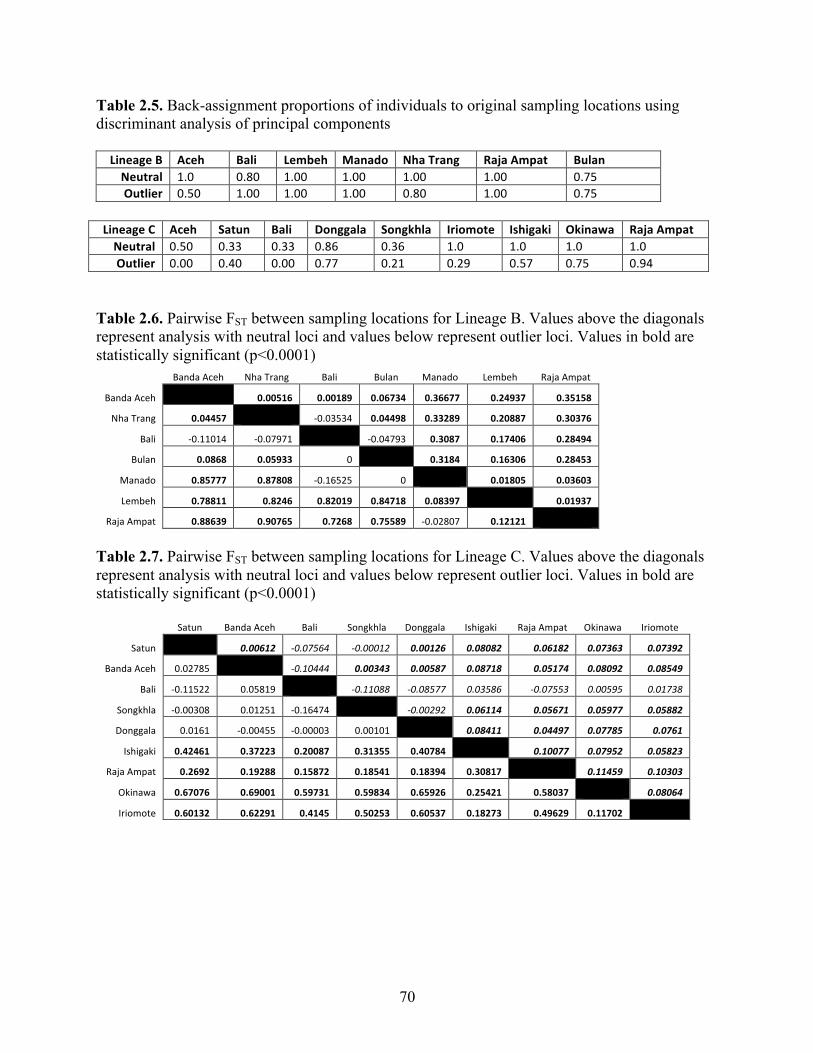
70

Table 2.5. Back-assignment proportions of individuals to original sampling locations using discriminant analysis of principal components

Lineage  B   Aceh                 Bali               Lembeh   Manado   Nha  Trang   Raja  Ampat   Bulan  Neutral   1.0   0.80   1.00   1.00   1.00   1.00   0.75  Outlier   0.50   1.00   1.00   1.00   0.80   1.00   0.75  

Lineage  C   Aceh                Satun   Bali               Donggala   Songkhla              Iriomote   Ishigaki                Okinawa                          Raja  Ampat  Neutral   0.50   0.33   0.33   0.86   0.36   1.0   1.0   1.0   1.0  Outlier   0.00   0.40   0.00   0.77   0.21   0.29   0.57     0.75   0.94  

Table 2.6. Pairwise FST between sampling locations for Lineage B. Values above the diagonals represent analysis with neutral loci and values below represent outlier loci. Values in bold are statistically significant (p<0.0001)

 Banda  Aceh   Nha  Trang   Bali   Bulan   Manado   Lembeh   Raja  Ampat  

Banda  Aceh       0.00516   0.00189   0.06734   0.36677   0.24937   0.35158  

Nha  Trang   0.04457   0   -­‐0.03534   0.04498   0.33289   0.20887   0.30376  

Bali   -­‐0.11014   -­‐0.07971   0   -­‐0.04793   0.3087   0.17406   0.28494  

Bulan   0.0868   0.05933   0    

0.3184   0.16306   0.28453  

Manado   0.85777   0.87808   -­‐0.16525   0   0   0.01805   0.03603  

Lembeh   0.78811   0.8246   0.82019   0.84718   0.08397   0   0.01937  

Raja  Ampat   0.88639   0.90765   0.7268   0.75589   -­‐0.02807   0.12121   0  

Table 2.7. Pairwise FST between sampling locations for Lineage C. Values above the diagonals represent analysis with neutral loci and values below represent outlier loci. Values in bold are statistically significant (p<0.0001)

 Satun   Banda  Aceh   Bali   Songkhla   Donggala   Ishigaki   Raja  Ampat   Okinawa   Iriomote  

Satun       0.00612   -­‐0.07564   -­‐0.00012   0.00126   0.08082   0.06182   0.07363   0.07392  

Banda  Aceh   0.02785       -­‐0.10444   0.00343   0.00587   0.08718   0.05174   0.08092   0.08549  

Bali   -­‐0.11522   0.05819   0   -­‐0.11088   -­‐0.08577   0.03586   -­‐0.07553   0.00595   0.01738  

Songkhla   -­‐0.00308   0.01251   -­‐0.16474   0   -­‐0.00292   0.06114   0.05671   0.05977   0.05882  

Donggala   0.0161   -­‐0.00455   -­‐0.00003   0.00101   0   0.08411   0.04497   0.07785   0.0761  

Ishigaki   0.42461   0.37223   0.20087   0.31355   0.40784   0   0.10077   0.07952   0.05823  

Raja  Ampat   0.2692   0.19288   0.15872   0.18541   0.18394   0.30817   0   0.11459   0.10303  

Okinawa   0.67076   0.69001   0.59731   0.59834   0.65926   0.25421   0.58037   0   0.08064  

Iriomote   0.60132   0.62291   0.4145   0.50253   0.60537   0.18273   0.49629   0.11702      

71

Figure 2.1. Sampling locations through the Coral Triangle and adjacent regions. Gray shading indicates exposed continental shelf during low sea level stands during the Pleistocene (after Voris 2000). Primary oceanographic features are illustrated as well (after Wykrti 1971): NEC = North Equatorial Current, NGCC = New Guinea Coastal Current, SECC = Southeast Counter Current, ME = Makassar Eddy, HE = Halmahera Eddy.

HE

ME

Kuroshio

Indo

nesia

n Th

roug

hflow

NGCC

NEC

SECC

Ryukyu Archipelago

Ticao Island/Bicol

1 23

4

5

6

1920

9 1015

1411

13

7

8

12

17

16

18

72

Figure 2.2. Commonly hypothesized phylogeographic breaks in the region (after Carpenter et al. 2010)

1

2

5

3

4

73

Figure 2.3. Putative outlier loci within each lineage were detected using a probabilistic method (Bayescan, Foll and Gaggiotti 2008) and a summary statistic method (Lositan, Antao et al. 2008). Outliers were called at 0.05 false discovery rate for Bayescan (a, c) and at 0.1 false discovery rate and 0.99 confidence interval for Lositan (b, d).

0.0 �� �� �� �� �� ��

����

����

����

����

����

ORJ���T�value)

fst

���

���

���

���

���

������������

����

�������� ����

0 ï� ï� ï� ï�

���

���

���

���

���

���

ORJ���T�value)

fst

��

�

�����

�

�

�

�

��

��� �

���

� ��

�����

�������� � ����

� ��� ����� �

�

���

�� ���

��

���

�

�����

�

���

�

������� ���� �

�

�

�

� �� ���� �

���

���� �

� �

��

�

��

�� �

�

��

���

�

� �

�

���

�� ����

��

�

�

�

���� ���

� ���

���

�

�

�

�

���

���

�

���� �� ���

��

�

���

�� �����

��

�

��

����

�

��

�

�����

�

�

���

�

�

�

���

��� �

�����������

�

������� ��

��� ���

��

�

���

��

�

��

� ����

�

�

� ����

�

��� � �

��� ������������

�

������� ����

��

� ����

�������

���

�

� ���

��

�

���

�

�

�

�

��

��� �

�

� ���

�� �

�

�����

�

���

�������

�

������������

�� ������ �� �������

�����

��

�

����

� ��������

������

�

�������

�

�

� �

�

�

������ ��

�

�

��� ���

���

����

�

�����

��

�

��� ��� �� ��� ��

�����

��

�

�������� ����

�� ��� �

�

��

�

��

�

����� � �����

� �

��� ���

�

����

�

����

��� ���

��

�

�

��

�

�

�

���� ��

� �

�

��

�����

��

���

�

�

������� ���������

�

����

������ ���

����

�

�

���

�

�

��

�

� ���� ��

�

��

���

����

�

��� ����

�

�

����

�

����� � ����

���

�����

�

�� ��

�

����

�

���� ������ ���

���� ��

��

�

��

�

�

�

��� ����

�

���

�

����

�

������

�

������������ �

���� ����

�

���� ���

������������

� ��

�

�������

��

� ���

� ��

�

�

���� ����

�

�

�

�

�

� �

�

��

�

�����

�

�

�

��

�����

� ����� ��

��

����

�

����

�����

�

��

� �� ���� �

����� �����

��

� �

�

��� �

����

�

�� ������ �� ���

����

�������

���

��

�

�

�

�

��

�

�

�

�

���� ���

���

��

����

�

��

��

�

�

��

� ����

�

�

� ��� ���

� ��

�

��������

�

�

�

������

�

���

��� ����

�

��

��

���

�

�

�

������� �� ���

���

������

���

�

��

�

� ���

�

��

�

�� ��

�

�

�

������� �� � �� ��

��

�

��� �

�

�����

�

�

�

� ��

�

�� ����

��

�

��

�

�

����

�� ��

�

�

��

�

�

���

��

� �������

��

�

��

�

�� �� ��

����

�

�

�

�� ���

����

�

��

�

���

���

�

����

��

�

�

��� ����

�

� ��

�

�

�

�

����

�

��� ���� �����

��

��

� ���

�

�

�

���

��

�

�

�

�� ���

�

�� ����

�

�

�����

�� ���

�

� ���� ��� �

�

���

�

������

�

�

�

���

�

����

�

�

����� � ���

��

���

�

�

�

���������

�

�

�

��

�

��

�

��

�

��� � �

�

�

�

�

�

���

�

����� ���

��������

�� ��

�

��

�

����� ���

�

��

�

��� ���

��

��� �

�

�� ��

�

��

�����

�

���

�

����

��

�

���

�

�

�������

����

�

���

����� ����

�

�������� � �����

�

���

�

� ����

�� ���

�������

��

��

��� ���

�

����

��� ��� ��

�

��

�

�

�

����� �������

���� �����

��

�

��

� ��

���

����

�

�

�������

� ���

� ��������

�

�

�

��

�

������

�

� �����

�����

�

�

�

�

�

�

���� �

�

��

�

�� ���

�

���

�

����

�� ���

�

���

�

�

�

���� �

������

�

��� �����

��

��

��

���

���

���

���

���

������

��� ���

���

���

������

���

������

���

���

���

��� ����

����

����

��������

����

����

����

����

����

��������

����

����

����

����

����

����

����

��������

����

��������

����

����

����

a

b d

c

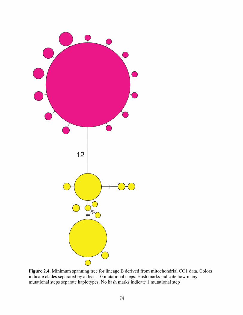
74

Figure 2.4. Minimum spanning tree for lineage B derived from mitochondrial CO1 data. Colors indicate clades separated by at least 10 mutational steps. Hash marks indicate how many mutational steps separate haplotypes. No hash marks indicate 1 mutational step

12

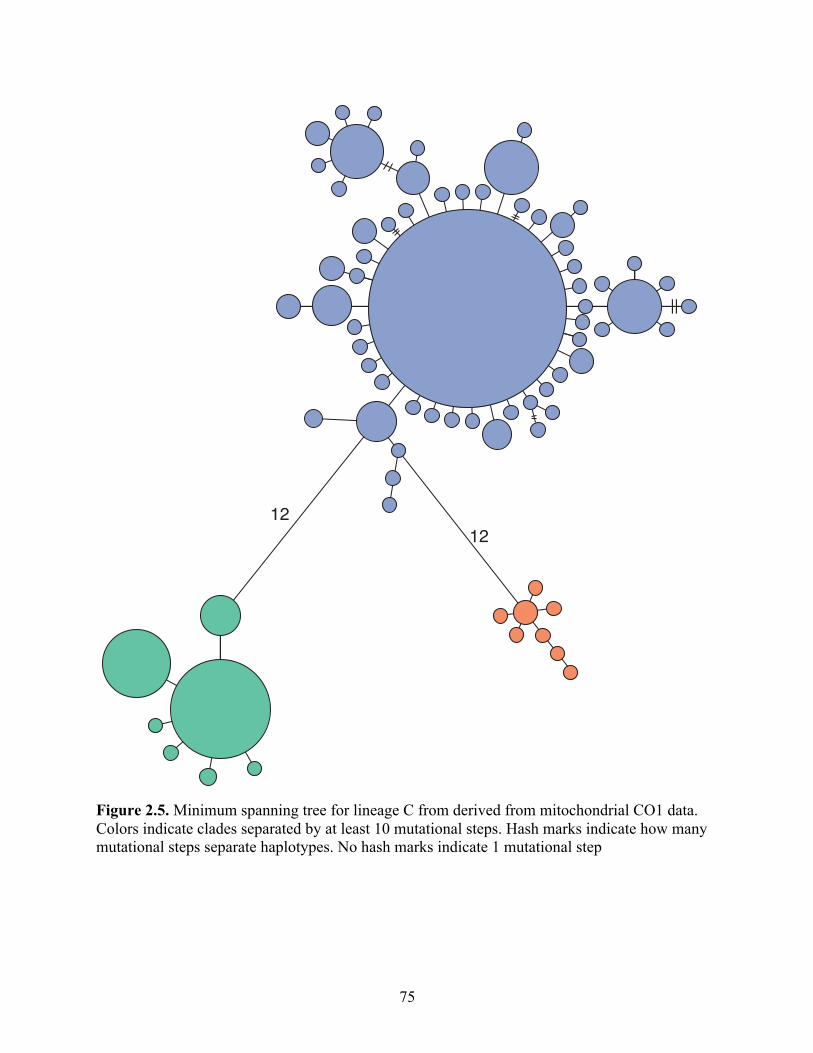
75

Figure 2.5. Minimum spanning tree for lineage C from derived from mitochondrial CO1 data. Colors indicate clades separated by at least 10 mutational steps. Hash marks indicate how many mutational steps separate haplotypes. No hash marks indicate 1 mutational step

1212

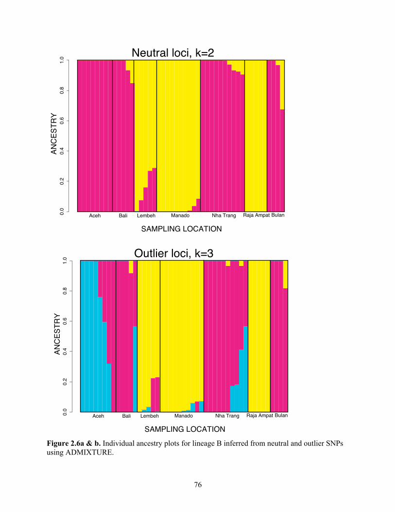
76

Figure 2.6a & b. Individual ancestry plots for lineage B inferred from neutral and outlier SNPs using ADMIXTURE.

0.0

0.2

0.4

0.6

0.8

1.0

SAMPLING LOCATION

AN

CE

STR

Y

Aceh Bali Lembeh Manado Nha Trang Raja Ampat Bulan

0.0

0.2

0.4

0.6

0.8

1.0

SAMPLING LOCATION

AN

CE

STR

Y

Aceh Bali Lembeh Manado Nha Trang Raja Ampat Bulan

Neutral loci, k=2

Outlier loci, k=3

77

Figure 2.7a & b. Discriminant analysis of principal components indicate varying patterns of clustering with different data types for lineage B

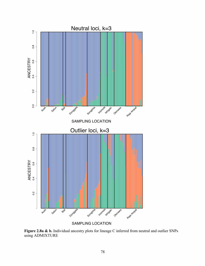
78

Figure 2.8a & b. Individual ancestry plots for lineage C inferred from neutral and outlier SNPs using ADMIXTURE

SAMPLING LOCATION

AN

CE

STR

Y0.

00.

20.

40.

60.

81.

0

Aceh

Satun

Bali

Dongg

ala

Songk

hla

Iriomote

Ishiga

ki

Okinaw

a

Raja A

mpat

Neutral loci, k=30.

20.

40.

60.

81.

0

SAMPLING LOCATION

AN

CE

STR

Y

Aceh

Satun

Bali

Dongg

ala

Songk

hla

Iriomote

Ishiga

ki

Okinaw

a

Raja A

mpat

Outlier loci, k=3

79

 

Figure 2.9a & b. Discriminant analysis of principal components indicate varying patterns of clustering with different data types for lineage C

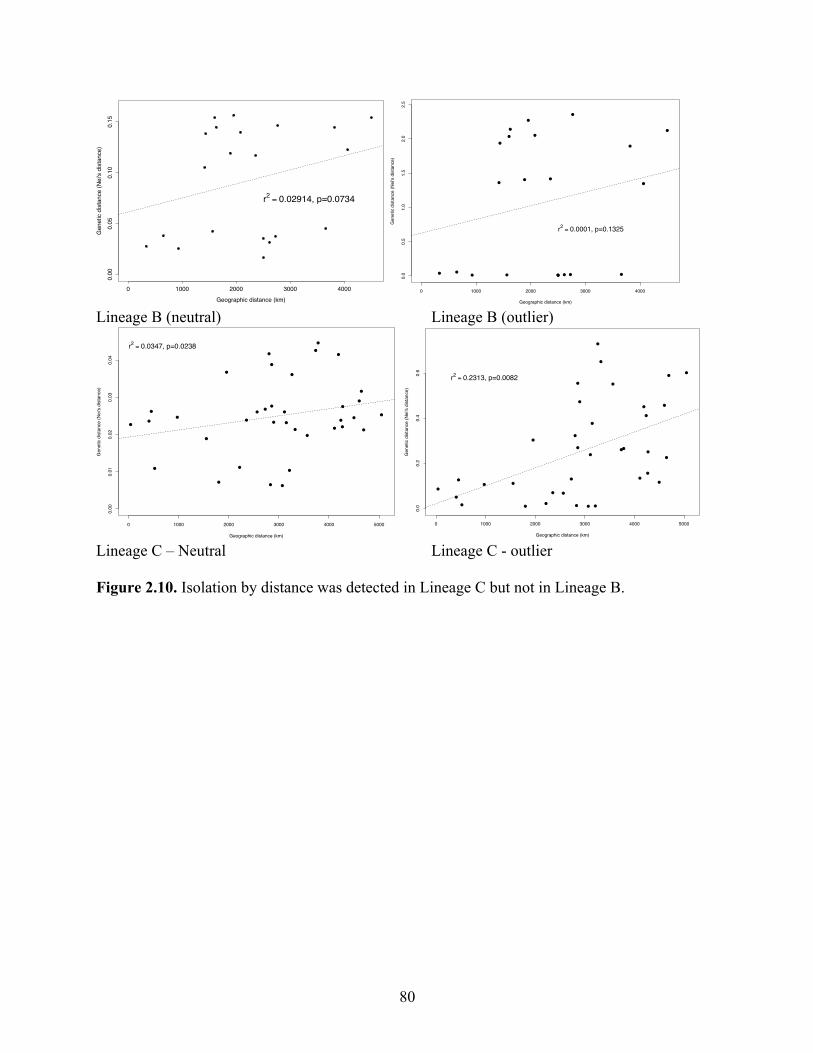
80

Lineage B (neutral) Lineage B (outlier)

Lineage C – Neutral Lineage C - outlier Figure 2.10. Isolation by distance was detected in Lineage C but not in Lineage B.

0 1000 2000 3000 4000

0.00

0.05

0.10

0.15

Geographic distance (km)

Gen

etic

dis

tanc

e (N

ei's

dist

ance

)

r2 = 0.02914, p=0.0734

●

●

●

●

●

●

●

●

●

●

●●

●

●

●

●

●

●

●

●

●

0 1000 2000 3000 4000

0.0

0.5

1.0

1.5

2.0

2.5

Geographic distance (km)

Gen

etic

dis

tanc

e (N

ei's

dist

ance

)

r2 = 0.0001, p=0.1325

●

●

●●

●

●

●●

●

●●

●

●

●●

●●

●

●

●

●

●

●

●

●

●

●

●

●

●

●●

●

●

●

●

0 1000 2000 3000 4000 5000

0.00

0.01

0.02

0.03

0.04

Geographic distance (km)

Gen

etic

dis

tanc

e (N

ei's

dist

ance

)

r2 = 0.0347, p=0.0238

●

●

●●

●

●

●

●

●

●●

●

●

●

●

●

●

●●

●

●

●

●

●

●

●

●

●

●

●

●

●

●

●

●

●

0 1000 2000 3000 4000 5000

0.0

0.2

0.4

0.6

Geographic distance (km)

Gen

etic

dis

tanc

e (N

ei's

dist

ance

)

r2 = 0.2313, p=0.0082

81

Figure 2.11. Distribution of mitochondrial clades over the sampling regions in the Coral Triangle and peripheral areas for lineage B. Gray shading indicates exposed continental shelf during low sea level stands during the Pleistocene (after Voris 2000). Primary oceanographic features are illustrated as well (after Wykrti 1971): NEC = North Equatorial Current, NGCC = New Guinea Coastal Current, SECC = Southeast Counter Current, ME = Makassar Eddy, HE = Halmahera Eddy.

HE

ME

Kuroshio

Indo

nesia

n Th

roug

hflow

NGCC

NEC

SECC

mt Clade 1mt Clade 2

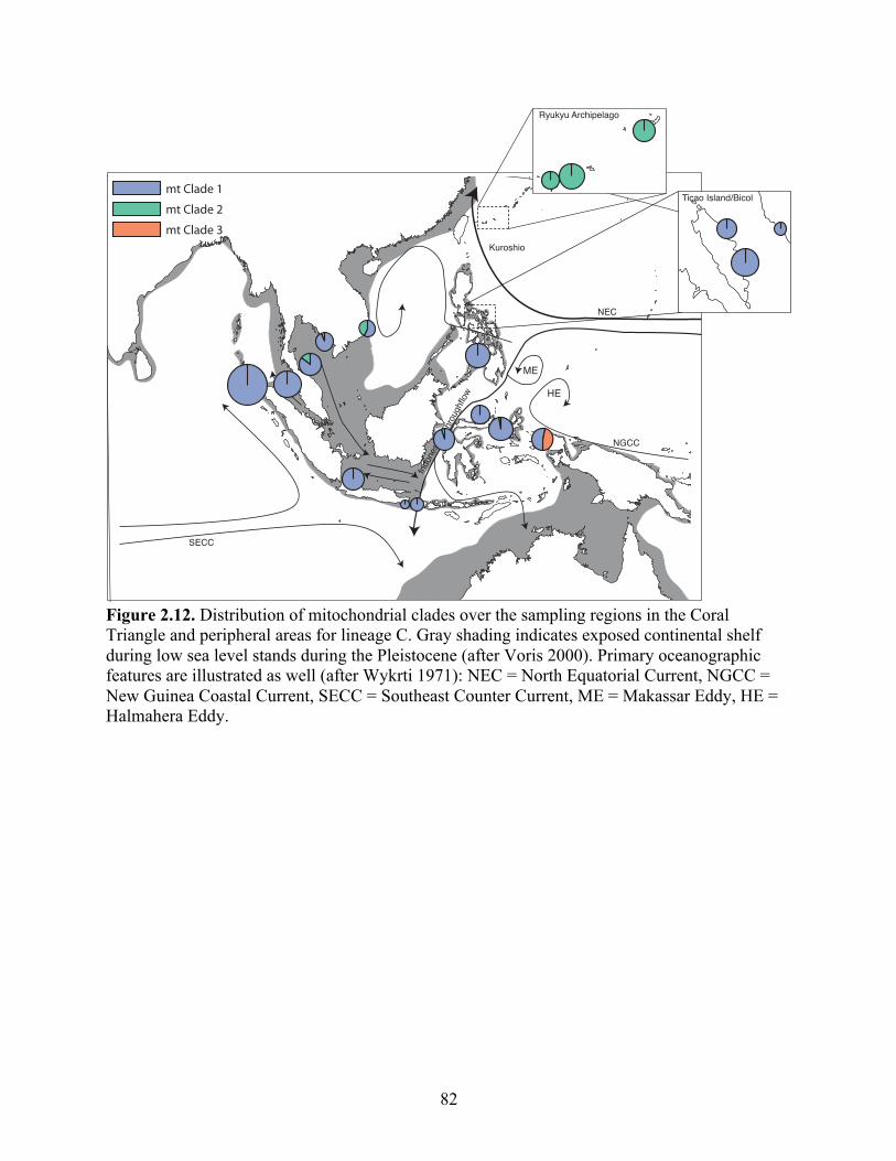
82

Figure 2.12. Distribution of mitochondrial clades over the sampling regions in the Coral Triangle and peripheral areas for lineage C. Gray shading indicates exposed continental shelf during low sea level stands during the Pleistocene (after Voris 2000). Primary oceanographic features are illustrated as well (after Wykrti 1971): NEC = North Equatorial Current, NGCC = New Guinea Coastal Current, SECC = Southeast Counter Current, ME = Makassar Eddy, HE = Halmahera Eddy.

HE

ME

Kuroshio

Indo

nesia

n Th

roug

hflow

NGCC

NEC

SECC

Ryukyu Archipelago

Ticao Island/Bicol7mt Clade 1

mt Clade 2

mt Clade 3

83

REFERENCES

Ackiss AS, Pardede S, Crandall ED, Ablan-Lagman MCA, Romena N, Barber PH, Carpenter KE. 2013. Pronounced genetic structure in a highly mobile coral reef fish, Caesio cuning, in the Coral Triangle. Mar. Ecol. Prog. Ser. 480:185–197.

Alexander DH, Novembre J, Lange K. 2009. Fast model-based estimation of ancestry in unrelated individuals. Genome Res. 19:1655–1664.

Allendorf FW, Hohenlohe PA, Luikart G. 2010. Genomics and the future of conservation genetics. Nat. Rev. Genet. 11:697–709.

Amos W, Balmford A. 2001. When does conservation genetics matter? Heredity 87:257–265.

Anderson FE. 2000. Phylogeny and historical biogeography of the loliginid squids (Mollusca: cephalopoda) based on mitochondrial DNA sequence data. Mol. Phylogenet. Evol. 15:191–214.

Anderson FE, Engelke R, Jarrett K, Valinassab T, Mohamed KS, Asokan PK, Zacharia PU, Nootmorn P, Chotiyaputta C, Dunning M. 2010. Phylogeny of the Sepia pharaonis species complex (Cephalopoda: Sepiida) based on analyses of mitochondrial and nuclear DNA sequence data. J. Molluscan Stud. 0:1–11.

Antao T, Lopes A, Lopes RJ, Beja-Pereira A, Luikart G. 2008. LOSITAN: a workbench to detect molecular adaptation based on a Fst-outlier method. BMC Bioinformatics 9:323.

Aoki M, Imai H, Naruse T, Ikeda Y. 2008. Low genetic diversity of oval squid, Sepioteuthis cf. lessoniana (Cephalopoda: Loliginidae), in Japanese waters inferred from a mitochondrial DNA non-coding region. Pacific Sci. 62:403–411.

Avise JC. 2000. Phylogeography: The History and Formation of Species. Harvard University Press. Boston (MA): Harvard University Press.

Avise JC. 2010. Perspective: Conservation genetics enters the genomics era. Conserv. Genet. 11:665–669.

Avise JC, Arnold J, Ball RM, Bermingham E, Lamb T, Neigel JE, Reeb CA, Saunders NC. 1987. Intraspecific Phylogeography: The Mitochondrial DNA Bridge Between Population Genetics and Systematics. Annu. Rev. Ecol. Syst. 18:489–522.

Baird NA, Etter PD, Atwood TS, Currey MC, Shiver AL, Lewis ZA, Selker EU, Cresko WA, Johnson EA. 2008. Rapid SNP Discovery and Genetic Mapping Using Sequenced RAD Markers. PLoS One 3:e3376.

Barber PH, Cheng SH, Erdmann M, Tengardjaja K. 2011. Evolution and conservation of marine biodiversity in the Coral Triangle: insights from Stomatopod Crustacea. Crustac. Issues 19:129–

84

156.

Barber PH, Meyer CP. 2015. Pluralism explains diversity in the Coral Triangle. In: Mora C, editor. Ecology of Fishes on Coral Reefs. Cambridge: Cambridge University Press. p. 258-263.

Barber PH, Ablan-Lagman MCA, Ambariyanto, Berlinck RG, Cahyani D, Crandall ED, Ravago-Gotanco R, Juinio-Menez MA, Mahardika ING, Shankar K, Starger CJ, Toha AHA, Anggoro AW, Willette DA. 2014. Advancing biodiversity research in developing countries: the need for changing paradigms. Bull. Mar. Sci. 90:187–210.

Barber PH, Bellwood DR. 2005. Biodiversity hotspots: evolutionary origins of biodiversity in wrasses (Halichoeres: Labridae) in the Indo-Pacific and new world tropics. Mol. Phylogenet. Evol. 35:235–253.

Barber PH, Erdmann MV, Palumbi SR. 2006. Comparative phylogeography of three codistributed stomatopods: origins and timing of regional lineage diversification in the Coral Triangle. Evolution 60:1825–1839.

Barber PH, Palumbi SR, Erdmann MV, Moosa MK. 2002. Sharp genetic breaks among populations of Haptosquilla pulchella (Stomatopoda) indicate limits to larval transport: Patterns, causes, and consequences. Mol. Ecol. 11:659–674.

Bermingham E, MacCafferty S, Martin A. 1997. Fish Biogeography and Molecular Clocks: Perspectives from the Panamanian Isthmus. In: Kochner TD, Stepien CA, editors. Molecular Systematics of Fishes. New York: Academic Press. p. 113-128.

Bonin A, Taberlet P, Miaud C, Pompanon F. 2006. Explorative Genome Scan to Detect Candidate Loci for Adaptation Along a Gradient of Altitude in the Common Frog (Rana temporaria). Mol. Biol. Evol. 23:773–783.

Borsa P. 2003. Genetic structure of round scad mackerel Decapterus macrosoma (Carangidae) in the Indo-Malay archipelago. Mar. Biol. 142:575–581.

Bowen BW, Rocha LA, Toonen RJ, Karl SA, the ToBo Laboratoratory. 2013. The origins of tropical marine biodiversity. Trends Ecol. Evol. 28:359–366.

Bowen BW, Yasuda N, Celia M, Malay MD, Selkoe KA, Barber PH, Williams ST, Lessios HA, Crandall ED, Bernardi G, Meyer CP, Carpenter KE, Toonen RJ. 2014. Phylogeography unplugged: comparative surveys in the genomic era. Bull. Mar. Sci. 90:13–46.

Boycott B. 1965. A comparison of living Sepioteuthis sepioidea and Doryteuthis plei with other squids, and with Sepia officinalis. J. Zool. 147:344–351.

Bradbury IR, Hubert S, Higgins B, Bowman S, Borza T, Paterson IG, Snelgrove PVR, Morris CJ, Gregory RS, Hardie D, Hutchings JA, Ruzzante DE, Taggart CT, Bentzen P. 2013. Genomic islands of divergence and their consequences for the resolution of spatial structure in an

85

exploited marine fish. Evol. Appl. 6:450–61.

Brierley AS, Rodhouse PG, Thorpe J, Clarke MR. 1993. Genetic evidence of population heterogeneity and cryptic speciation in the ommastrephid squid Martialia hyadesi from the Patagonian Shelf and Antarctic Polar Frontal Zone. Mar. Biol. 116:593–602.

Briggs JC. 1973. Operation of zoogeographic barriers. Syst. Zool. 23:248–256.

Briggs JC. 1999. Modes of Speciation: Marine Indo-West Pacific. Bull. Mar. Sci. 65:645–656.

Brumfield RT, Beerli P, Nickerson DA, Edwards SV. 2003. The utility of single nucleotide polymorphisms in inferences of population history. Trends Ecol. Evol. 18:249–256.

Buresch KC, Gerlach G, Hanlon RT. 2006. Multiple genetic stocks of longfin squid Loligo pealeii in the NW Atlantic: stocks segregate inshore in summer, but aggregate offshore in winter. Mar. Ecol. Prog. Ser. 310:263–270.

Carpenter KE, Barber PH, Crandall ED, Ablan-lagman MCA, Mahardika GN, Manjaji-matsumoto BM, Juinio-Menez MA, Santos MD, Starger CJ, Toha AHA. 2011. Comparative Phylogeography of the Coral Triangle and Implications for Marine Management. J. Mar. Biol. 2011:1–14.

Cheng SH, Anderson FE, Bergman A, Mahardika GN, Muchlisin ZA, Dang BT, Calumpong HP, Mohamed KS, Sasikumar G, Venkatesan V, Barber PH. 2014. Molecular evidence for co-occurring cryptic lineages within the Sepioteuthis cf. lessoniana species complex in the Indian and Indo-West Pacific Oceans. Hydrobiologia 725:165–188.

Clark RM, Schweikert G, Toomajian C, Ossowski S, Zeller G, Shinn P, Warthmann N, Hu TT, Fu G, Hinds DA, Chen H, Frazer KA, Huson DH, Schölkopf B, Nordborg M, Rätsch G, Ecker JR, Weigel D. 2007. Common Sequence Polymorphisms. Science 317:338–342.

Clarke MR. 1996. The role of cephalopods in the world’s oceans: an introduction. Philos. Trans. Biol. Sci. 351:979–983.

Coyne J, Orr H. 2004. Speciation. Sunderland (MA): Sinauer Associates.

Crandall ED, Frey MA, Grosberg RK, Barber PH. 2008. Contrasting demographic history and phylogeographical patterns in two Indo-Pacific gastropods. Mol. Ecol. 17:611–626.

Crandall ED, Jones ME, Muñoz MM, Akinronbi B, Erdmann M V., Barber PH. 2008. Comparative phylogeography of two seastars and their ectosymbionts within the Coral Triangle. Mol. Ecol. 17:5276–5290.

Crandall ED, Treml EA, Barber PH. 2012. Coalescent and biophysical models of stepping-stone gene flow in neritid snails. Mol. Ecol. 21:5579–5598.

Crozier RH. 1997. Preserving the Information Content of Species: Genetic Diversity, Phylogeny,

86

and Conservation Worth. Annu. Rev. Ecol. Syst. 28:243–268.

DeBoer TS, Naguit MRA, Erdmann M V, Ablan-Lagman MCA, Carpenter KE, Toha AHA, Barber PH. 2014. Concordant phylogenetic patterns inferred from mitochondrial and microsatellite DNA in the giant clam Tridacna crocea. Bull. Mar. Sci. 90:301–329.

DeBoer TS, Naguit MRA, Erdmann MV, Ablan-Lagman MCA, Ambariyanto A, Carpenter KE, Toha AHA, Barber PH. 2014. Concordance between phylogeographic and biogeographic boundaries in the Coral Triangle: Conservation implications based on comparative analyses of multiple giant clam species. Bull. Mar. Sci. 90:277–300.

DeBoer TS, Subia MD, Erdmann MV, Kovitvongsa K, Barber PH. 2008. Phylogeography and limited genetic connectivity in the endangered boring giant clam across the Coral Triangle. Conserv. Biol. 22:1255–1266.

Dobzhansky T. 1937. Genetics and the Origin of Species. Columbia University Press. New York: Columbia University Press.

Drew J, Barber PH. 2009. Molecular Phylogenetics and Evolution Sequential cladogenesis of the reef fish Pomacentrus moluccensis (Pomacentridae) supports the peripheral origin of marine biodiversity in the Indo-Australian archipelago. Mol. Phylogenet. Evol. 53:335–339.

Duda T, Palumbi S. 1999. Population structure of the black tiger prawn, Penaeus monodon, among western Indian Ocean and western Pacific populations. Mar. Biol. 134:705–710.

Eckert AJ, Bower AD, González-Martínez SC, Wegrzyn JL, Coop G, Neale DB. 2010. Back to nature: Ecological genomics of loblolly pine (Pinus taeda, Pinaceae). Mol. Ecol. 19:3789–3805.

Edwards SV, Beerli P. 2000. Perspective: gene divergence, population divergence, and the variance in coalescence time in phylogeographic studies. Evolution 54:1839–1854.

Edwards SV, Kingan SB, Calkins JD, Balakrishnan CN, Jennings WB, Swanson WJ, Sorenson MD. 2005. Speciation in birds: genes, geography, and sexual selection. Proc. Natl. Acad. Sci. 102(Suppl):6550–6557.

Ekman S. 1953. Zoogeography of the sea. London: Sidgwick & Jackson.

Etherington TR. 2011. Python based GIS tools for landscape genetics: visualising genetic relatedness and measuring landscape connectivity. Methods Ecol. Evol. 2:52–55.

Evanno G, Regnaut S, Goudet J. 2005. Detecting the number of clusters of individuals using the software structure: a simulation study. Mol. Ecol. 14:2611–2620.

Excoffier L, Lischer HEL. 2010. Arlequin suite ver 3.5: A new series of programs to perform population genetics analyses under Linux and Windows. Mol. Ecol. Resour. 10:564–567.

Faucci A, Toonen RJ, Hadfield MG. 2007. Host shift and speciation in a coral-feeding

87

nudibranch. Proc. R. Soc. B Biol. Sci. 274:111–119.

Feder JL, Nosil P. 2010. The Efficacy of Divergence Hitchhiking in Generating Genomic Islands During Ecological Speciation. Evolution 64:1729–1747.

Foll M, Gaggiotti O. 2008. A Genome-Scan Method to Identify Selected Loci Appropriate for Both Dominant and Codominant Markers: A Bayesian Perspective. Genetics 180:977–993.

Frankham R. 2005. Conservation Biology: Ecosystem recovery enhanced by genotypic diversity. Heredity 95:183–183.

Frankham R. 2010. Challenges and opportunities of genetic approaches to biological conservation. Biol. Conserv. 143:1919–1927.

Frankham R, Briscoe DA, Ballou JD. 2002. Introduction to Conservation Genetics. Cambridge: Cambridge University Press.

Freamo H, O’Reilly P, Berg PR, Lien S, Boulding EG. 2011. Outlier SNPs show more genetic structure between two Bay of Fundy metapopulations of Atlantic salmon than do neutral SNPs. Mol. Ecol. Resour. 11:254–267.

Fu L, Niu B, Zhu Z, Wu S, Li W. 2012. CD-HIT: Accelerated for clustering the next-generation sequencing data. Bioinformatics 28:3150–3152.

Gaither MR, Bowen BW, Bordenave TR, Rocha LA, Newman SJ, Gomez JA, van Herwerden L, Craig MT. 2011. Phylogeography of the reef fish Cephalopholis argus (Epinephelidae) indicates Pleistocene isolation across the Indo-pacific barrier with contemporary overlap in the Coral Triangle. BMC Evol. Biol. 11:189.

He L, Mukai T, Chu KH, Ma Q, Zhang J. 2015. Biogeographical role of the Kuroshio Current in the amphibious mudskipper Periophthalmus modestus indicated by mitochondrial DNA data. Scientific Reports 5:1–12.

Hedgecock D. 1994. Temporal and Spatial Genetic Structure of Marine Animal Populations. CalCOFI Reports 35:73–81.

Hedgecock D, Barber PH, Edmands S. 2007. Genetic Approaches to Measuring Connectivity. Oceanography 20:70–79.

Hellberg ME. 2009. Gene Flow and Isolation among Populations of Marine Animals. Annu. Rev. Ecol. Evol. Syst. 40:291–310.

Hellberg ME, Burton RS, Neigel JE, Palumbi SR. 2002. Genetic assessment of connectivity among marine populations. Bull. Mar. Sci. 70:273–290.

Helyar SJ, Hemmer-Hansen J, Bekkevold D, Taylor MI, Ogden R, Limborg MT, Cariani A, Maes GE, Diopere E, Carvalho GR, Nielsen EE. 2011. Application of SNPs for population

88

genetics of nonmodel organisms: new opportunities and challenges. Mol. Ecol. Resour. 11:123–136.

Hilborn R, Walters CJ. 1992. Quantitative Fisheries Stock Assessment: Choice, Dynamics, and Uncertainty. New York: Chapman Hall.

Hoeksema BW. 2007. Delineation of the Indo-Malayan Centre of Maximum Marine Biodiversity: The Coral Triangle. In: Renama W, editor. Biogeography, Time, and Place: Distributions, Barriers, and Islands. Springer. p. 117–178.

Hohenlohe PA, Phillips PC, Cresko WA. 2010. Using population genomics to detect selection in natural populations: key concepts and methodological considerations. Int. J. Plant Sci. 171:1059–1071.

Imai H, Aoki M. 2009. Genetic Diversity and Genetic Heterogeneity of Bigfin Reef Squid Sepioteuthis lessoniana Species Complex in Northwestern Pacific Ocean. In: Caliskan M, editor. Analysis of Genetic Variation in Animals. InTech. p. 372.

Izuka T, Segawa S, Okutani T. 1996. Identification of Three Species in Oval Squid, Sepioteuthis lessoniana Complex by Chromatophore Arrangements on the Funnel. VENUS (Jap. Jour. Malac.) 55:139–142.

Izuka T, Segawa S, Okutani T, Numachi K. 1994. Evidence on the Existence of Three Species in the Oval Squid Sepioteuthis lessoniana Complex in Ishigaki Island, Okinawa, Southwestern Japan, by Isozyme Analyses. VENUS (Jap. Jour. Malac.) 53:217–228.

Jackson AM, Ambariyanto, Erdmann MV, Toha AHA, Stevens LA, Barber PH. 2014. Phylogeography of commercial tuna and mackerel in the Indonesian Archipelago. Bull. Mar. Sci. 90:471–492.

Jackson GD, Pecl G. 2003. The dynamics of the summer-spawning population of the loliginid squid (Sepioteuthis australis) in Tasmania , Australia — a conveyor belt of recruits. ICES J. Mar. Sci. 60:290–296.

Jereb P, Roper C. 2010. Cephalopods of the world. An annotated and illustrated catalogue of cephalopod species known to date, vol 2. Myopsid and Oegopsid Squids. FAO Species Cat. Fish. Purp. 2:649.

Johannesson K. 2001. Parallel speciation: A key to sympatric divergence. Trends Ecol. Evol. 16:148–153.

Jombart T. 2008. adegenet: a R package for the multivariate analysis of genetic markers. Bioinformatics 24:1403–1405.

Jombart T, Devillard S, Balloux F. 2010. Discriminant analysis of principal components: a new method for the analysis of genetically structured populations. BMC Genet. 11:94.

89

Jones GP, Almany GR, Russ GR, Sale PF, Steneck RS, van Oppen MJH, Willis BL. 2009. Larval retention and connectivity among populations of corals and reef fishes: history, advances and challenges. Coral Reefs 28:307–325.

Karlsson S, Moen T, Lien S, Glover KA, Hindar K. 2011. Generic genetic differences between farmed and wild Atlantic salmon identified from a 7K SNP-chip. Mol. Ecol. Resour. 11:247–253.

Kingsford MJ, Leis JM, Shanks A, Lindeman KC, Morgan SG, Pineda J. 2002. Sensory environments, larval abilities and local self-recruitment. Bull. Mar. Sci. 70:309–340.

Knowlton N. 1993. Sibling species in the sea. Annu. Rev. Ecol. Syst. 24:189–216.

Kochzius M, Nuryanto A. 2008. Strong genetic population structure in the boring giant clam, Tridacna crocea, across the Indo-Malay Archipelago: Implications related to evolutionary processes and connectivity. Mol. Ecol. 17:3775–3787.

Kohn MH, Murphy WJ, Ostrander EA, Wayne RK. 2006. Genomics and conservation genetics. Trends Ecol. Evol. 21:629–637.

Kool JT, Paris CB, Barber PH, Cowen RK, Young CE, South D. 2011. Connectivity and the development of population genetic structure in Indo-West Pacific coral reef communities. Global Ecology and Biogeography 20(5):695–706.

Lamichhaney S, Barrio AM, Rafati N, Sundstrom G, Rubin CJ, Gilbert ER, Berglund J, Wetterbom A, Laikre L, Webster MT, Grabherr M, Ryman N, Andersson L. 2012. Population-scale sequencing reveals genetic differentiation due to local adaptation in Atlantic herring. Proc. Natl. Acad. Sci. 109:19345–19350.

Lande R. 1988. Genetics and demography in biological conservation. Science 241:1455–1460.

Lessios H., Robertson D. 2006. Crossing the impassable: genetic connections in 20 reef fishes across the eastern Pacific barrier. Proc. R. Soc. B Biol. Sci. 273:2201–2208.

Lessios HA. 1981. Divergence in Allopatry: Molecular and Morphological Differentiation between Sea Urchins Seperated by the Isthmus of Panama. Evolution 35:618–634.

Lewontin R, Krakauer J. 1973. Distribution of gene frequency as a test of the theory of the selective neutrality of polymorphisms. Genetics 74:175–195.

Li W, Godzik A. 2006. Cd-hit: A fast program for clustering and comparing large sets of protein or nucleotide sequences. Bioinformatics 22:1658–1659.

Lourie SA, Vincent ACJ. 2004. A marine fish follows Wallace’s Line: The phylogeography of the three-spot seahorse (Hippocampus trimaculatus, Syngnathidae, Teleostei) in Southeast Asia. J. Biogeogr. 31:1975–1985.

90

Lourie SA, Green DM, Vincent ACJ. 2005. Dispersal, habitat differences, and comparative phylogeography of Southeast Asian seahorses (Syngnathidae: Hippocampus). Mol. Ecol. 14:1073–1094.

Ludt WB, Rocha LA. 2014. Shifting seas: The impacts of Pleistocene sea- level fluctuations on the evolution of tropical marine taxa. J. Biogeogr. 42:25–38.

Luikart G, England PR, Tallmon D, Jordan S, Taberlet P. 2003. The power and promise of population genomics: from genotyping to genome typing. Nat. Rev. Genet. 4:981–994.

Mayr E. 1942. Systematics and the origin of species, from the viewpoint of a zoologist. Boston: Harvard University Press.

Meirmans PG. 2012. The trouble with isolation by distance. Mol. Ecol. 21:2839–2846.

Meyer CP, Geller JB, Paulay G. 2005. Fine scale endemism on coral reefs: archipelagic differentiation in turbinid gastropods. Evolution 59:113–125.

Miglietta MP, Faucci A, Santini F. 2011. Speciation in the sea: Overview of the symposium and discussion of future directions. Integr. Comp. Biol. 51:449–455.

Moltschaniwskyj NA, Pecl GT. 2007. Spawning aggregations of squid (Sepioteuthis australis) populations: A continuum of “microcohorts.” Rev. Fish Biol. Fish. 17:183–195.

Morin PA, Luikart G, Wayne RK, the SNP workshop group. 2004. SNPs in ecology, evolution and conservation. Trends Ecol. Evol. 19:208–216.

Nadeau NJ, Martin SH, Kozak KM, Salazar C, Dasmahapatra KK, Davey JW, Baxter SW, Blaxter ML, Mallet J, Jiggins CD. 2013. Genome-wide patterns of divergence and gene flow across a butterfly radiation. Mol. Ecol. 22:814–826.

Nakajima Y, Matsuki Y, Lian C, Fortes MD, Uy WH, Campos WL, Nakaoka M, Nadaoka K. 2014. The Kuroshio Current influences genetic diversity and population genetic structure of a tropical seagrass, Enhalus acoroides. Mol. Ecol. 23:6029–6044.

Narum SR, Buerkle CA, Davey JW, Miller MR, Hohenlohe PA. 2013. Genotyping-by-sequencing in ecological and conservation genomics. Mol. Ecol. 22:2841–2847.

Nuryanto A, Kochzius M. 2009. Highly restricted gene flow and deep evolutionary lineages in the giant clam Tridacna maxima. Coral Reefs 28:607–619.

Palumbi SR. 1992. Marine speciation on a small planet. Trends Ecol. Evol. 7:114–118.

Palumbi SR. 1994. Genetic divergence, reproductive isolation, and marine speciation. Annu. Rev. Ecol. Syst. 25:547–572.

Paris R, Lavigne F, Wassmer P, Sartohadi J. 2007. Coastal sedimentation associated with the

91

December 26, 2004 tsunami in Lhok Nga, west Banda Aceh (Sumatra, Indonesia). Mar. Geol. 238:93–106.

Patterson N, Price AL, Reich D. 2006. Population Structure and Eigenanalysis. PLoS Genet. 2:e190.

Pauly D, Watson R, Alder J. 2005. Global trends in world fisheries: impacts on marine ecosystems and food security. Philos. Trans. R. Soc. B Biol. Sci. 360:5–12.

Pecl GT, Tracey SR, Semmens JM, Jackson GD. 2006. Use of acoustic telemetry for spatial management of southern calamary Sepioteuthis australis, a highly mobile inshore squid species. Mar. Ecol. Prog. Ser. 328:1–15.

Perrin C, Borsa P. 2001. Mitochondrial DNA analysis of the geographic structure of Indian scad mackerel in the Indo-Malay archipelago. J. Fish Biol. 59:1421–1426.

Piatkowski U, Pierce GJ, Morais da Cunha M. 2001. Impact of cephalopods in the food chain and their interaction with the environment and fisheries: An overview. Fish. Res. 52:5–10.

Pineda J, Hare J, Sponaugle S. 2007. Larval Transport and Dispersal in the Coastal Ocean and Consequences for Population Connectivity. Oceanography 20:22–39.

Plaisance L, Knowlton N, Paulay G, Meyer C. 2009. Reef-associated crustacean fauna: biodiversity estimates using semi-quantitative sampling and DNA barcoding. Coral Reefs 28:977–986.

Planes S, Jones GP, Thorrold SR. 2009. Larval dispersal connects fish populations in a network of marine protected areas. Proc. Natl. Acad. Sci. 106:5693–5697.

Pritchard JK, Stephens M, Donnelly P. 2000. Inference of Population Structure Using Multilocus Genotype Data.

R Core Team. 2013. R: A language and environment for statistical computing. R Foundation for Statistical Computing, Vienna, Austria. URL http://www.R-project.org/.

Rao KN, Vardhan DA, Subraelu P. 2007. Coastal Topography and Tsunami Impact: GIS/GPS Based Mobile Mapping of the Coastal Sectors Affected by 2004 Tsunami in Krishna-Godavari Delta Region. East. Geogr. XIII:67–74.

Reid DG, Lal K, Mackenzie-Dodds J, Kaligis F, Littlewood DTJ, Williams ST. 2006. Comparative phylogeography and species boundaries in Echinolittorina snails in the central Indo-West Pacific. J. Biogeogr. 33:990–1006.

Rocha LA, Robertson DR, Roman J, Bowen BW. 2005. Ecological speciation in tropical reef fishes. Proc. R. Soc. B Biol. Sci. 272:573–579.

Rohfritsch A, Borsa P. 2005. Genetic structure of Indian scad mackerel Decapterus russelli:

92

Pleistocene vicariance and secondary contact in the Central Indo-West Pacific Seas. Heredity 95:315–26.

Schroth W, Jarms G, Streit B, Schierwater B. 2002. Speciation and phylogeography in the cosmopolitan marine moon jelly, Aurelia sp. BMC Evol. Biol. 2:1.

Segawa S. 1987. Life history of the oval squid, Sepioteuthis lessoniana in Kominato and adjacent waters central Honshu, Japan. J. Tokyo Univ. Fish. 74:67-105.

Segawa S, Hirayama S, Okutani T. 1993. Is Sepioteuthis lessoniana in Okinawa a Single Species? In: Okutani T, O’Dor RK, Kubodera T, editors. Recent Advances in Fisheries Biology. p. 513–521.

Segawa S, Izuka T, Tamashiro T, Okutani T. 1993. A Note on Mating and Egg Deposition by Sepioteuthis lessoniana in Ishigaki Island, Okinawa, Southwestern Japan. VENUS (Jap. Jour. Malac.) 52:101–108.

Shanks AL, Grantham BA, Carr MH. 2003. Propagule dispersal distance and the size and spacing of marine reserves. Ecol. Appl. 13:159–169.

Sin YW, Yau C, Chu KH. 2009. Morphological and genetic differentiation of two loliginid squids, Uroteuthis (Photololigo) chinensis and Uroteuthis (Photololigo) edulis (Cephalopoda: Loliginidae), in Asia. J. Exp. Mar. Bio. Ecol. 369:22–30.

Solé-Cava AM, Klautau M, Boury-Esnault N, Borojecic R, Thorpe JP. 1991. Genetic evidence for cryptic speciation in allopatric populations of two cosmopolitan species of the calcareous sponge genus Clathrina. Mar. Biol. 111:381–386.

Spalding MD, Fox HE, Allen GR, Davidson N, Ferdaña Z a., Finlayson M, Halpern BS, Jorge MA, Lombana A, Lourie SA, Martin KD, McManus E, Molnar J, Recchia CA, Robertson J. 2007. Marine Ecoregions of the World: A Bioregionalization of Coastal and Shelf Areas. Bioscience 57:573-583.

Storz JF. 2005. Using genome scans of DNA polymorphism to infer adaptive population divergence. Mol. Ecol. 14:671–688.

Swearer SE, Shima JS, Hellberg ME, Thorrold SR, Jones GP, Robertson DR, Morgan SG, Selkoe KA, Ruiz GM, Warner RR. 2002. Evidence of self-recruitment in demersal marine populations. Bull. Mar. Sci. 70:251–271.

Thorpe JP, Havenhand JN, Patterson KR. 1986. Report of the University of Liverpool to the Falkland Islands Development corporation on stock and species identities of Patagonian Shelf Illex argentinus. to. Falkland Islands Corporation, Port Stanley, Falkland Islands.

Timm J, Kochzius M. 2008. Geological history and oceanography of the Indo-Malay Archipelago shape the genetic population structure in the false clown anemonefish (Amphiprion

93

ocellaris). Mol. Ecol. 17:3999–4014.

Tomano S, Sanchez G, Ueno K, Ueta Y. 2015. Microsatellite DNA variation of oval squid Sepioteuthis sp . 2 reveals a single fishery stock on the coastline of mainland Japan. Fish. Sci. 81:839–847.

Treml EA, Halpin PN. 2012. Marine population connectivity identifies ecological neighbors for conservation planning in the Coral Triangle. Conserv. Lett. 5:441–449.

Triantafillos L, Adams M. 2005. Genetic evidence that the northern calamary, Sepioteuthis lessoniana, is a species complex in Australian waters. ICES J. Mar. Sci. 62:1665–1670.

Ueta Y, Jo Y. 1990. Migration of the Oval Squid, Sepioteuthis lessoniana around Tokushima Prefecture. Suisanzoshoku 38:221–226.

Venkatesan V, Rajagopal S. 2012. Reproductive Biology of Commercially Valuable Squid , Sepioteuthis lessoniana (Lesson, 1830) Taken as By-Catch in a Tropical Trawl Fishery. Not. Sci. Biol. 4:14–19.

Veron JEN, Devantier LM, Turak E, Green AL, Kininmonth S, Stafford-Smith M, Peterson N. 2009. Delineating the Coral Triangle. Galaxea, J. Coral Reef Stud. 11:91–100.

Vigliola L, Doherty PJ, Meekan MG, Drown DM, Jones ME, Barber PH. 2007. Genetic identity determines risk of post-settlement mortality of a marine fish. Ecology 88:1263–77.

Wada Y, Kobayashi T. 1995. On an Iteroparity of the Oval Squid Sepioteuthis lessoniana. Nippon Suisan Gakkaishi 61:151–158.

Wang S, Meyer E, McKay JK, Matz M V. 2012. 2b-RAD: a simple and flexible method for genome-wide genotyping. Nat. Methods 9:808–810.

Waples RS. 1998. Separating the weat from the chaff patterns of genetic diferrenciation in high gene flow species. J. Hered. 89:438–456.

Weir BS, Cockerham CC. 1984. Estimating F-statistic for the analysis of population structure. Evolution 38:1358–1370.

Willette DA, Allendorf FW, Barber PH, Barshis DJ, Carpenter KE, Crandall ED, Cresko WA, Fernandez-Silva I, Matz MV, Meyer E, Santos MD, Seeb LW, Seeb JE. 2014. So, you want to use next-generation sequencing in marine systems? Insight from the Pan-Pacific Advanced Studies Institute. Bull. Mar. Sci. 90:79–122.

Williams ST, Benzie JAH. 1998. Evidence of a phylogeographic break between populations of a high-dispersal starfish: congruent regions within the Indo-West Pacific defined by color morphs, mtDNA and allozyme data. Evolution 52:87–99.

Wray CG, Landman NH, Saunders WB, Bonacum J. 1995. Genetic Divergence and Geographic

94

Diversification in Nautilus. Paleobiology 21:220–228.

Wyrtki K. 1961. Physical Oceanography of the Southeast Asian Waters. NAGA Rep. Vol.2, Sci. Results Mar. Investig. South China Sea Gulf Thail. 1951-1961 2.

Yeatman J, Benzie J. 1994. Genetic structure and distribution of Photololigo spp. in Australia. Mar. Biol. 87:79–87.

Yokogawa K, Ueta Y. 2000. Genetic analysis of oval squid (Sepioteuthis lessoniana) around Japan. Japanese J. Malacol. 59(1):

Zarraonaindia I, Iriondo M, Albaina A, Pardo MA, Manzano C, Grant WS, Irigoien X, Estonba A. 2012. Multiple SNP Markers Reveal Fine-Scale Population and Deep Phylogeographic Structure in European Anchovy (Engraulis encrasicolus L.). PLoS One 7:e42201.

95

CHAPTER 3

Genome-wide SNPs reveal complex fine-scale population structure in the California market

squid fishery (Doryteuthis opalescens)

Abstract

Marine fisheries are critical for supporting local economies and sustaining local and

global food security. In California, market squid (Doryteuthis opalescens) is one of the largest

and most valuable fisheries. Understanding the extent and distribution of genetic structure is

crucial for informing effective conservation and management for this commercially important

species. We generated 662 single nucleotide polymorphism markers from across the genome and

along with corresponding morphometric data, aimed to determine whether multiple breeding

stocks of D. opalescens occur within the California fishery. A total of 156 individuals were

amplified from five monthly sampling groups (May-September 2014) in the northern (Monterey)

and southern (Southern California) regions of the fishery (n = 8). Overall, low levels of genetic

differentiation were detected between all sampling groups (FST=0.008, p>0.05) with no

significant differentiation between all northern and southern samples (FCT=-0.006, p > 0.05).

Closer inspection of sampling groups using discriminant analysis of principal components and

pairwise comparisons of genetic differentiation reveal unexpected complex patterns of fine-scale

population structure. Specifically, we observe that some spawning groups recruiting to spawning

grounds at different times are genetically distinct. These results lend preliminary support to the

existence of smaller genetically distinct cohorts that continually spawn in California (Jackson

and Domeier 2003), as opposed to the prevailing notion that spawning occurs in two

asynchronous peaks in the northern and southern regions of the fishery (Hixon 1983, Spratt

96

1979). This study represents the first in-depth genomic examination of temporal-spatial

population structure in D. opalescens and demonstrates the applicability of genome-wide SNPs

for detecting fine-scale structure in squid fisheries. However, this study only covered part of one

harvest season and thus, to accurately inform changes in fisheries management, a systematic

analysis using fisheries independent data over multiple spawning seasons is required.

Introduction

Management of marine resources depends heavily on information regarding spatial and

temporal structure of populations (Hilborn and Walters 1992, Palumbi 1994). Generally,

management of harvested mobile marine organisms centers around catch limits, spatial and

temporal delimitations for harvest, and size restrictions. Therefore, it is vital to have accurate

information about the timing and location of breeding populations, and the connectivity among

these populations (Sale 2004). Physically observing movement of individuals and connectivity

among marine populations is extremely difficult given the fluid and expansive nature of the

ocean. Inference of these parameters is, therefore, limited to other sources of data (e.g. tag-

recapture, modeling, etc…) (Semmens et al. 2007). Advances in genetic resources have made it

possible to detect both historical and contemporary patterns of population structure and assess

demographic parameters, revolutionizing our understanding of wild populations and how to

manage them. For example, the use of genetic methodologies in marine management has been

extremely successful in distinguishing breeding populations of harvested oceanic salmon and

assigning them back to their natal streams (Waples et al. 1990; Larson et al. 2014).Genetic

methods using markers ranging from allozymes to mitochondrial DNA and microsatellites have

been increasingly applied over the past few decades to numerous commercially important species

97

for identifying stocks and populations (Carvalho and Hauser 1994; Morin et al. 2010).

Population genetic approaches can help delineate populations, indicate patterns of gene

flow (Slatkin 1987; Waples and Gaggiotti 2006), identify adaptive variation (Beaumont and

Balding 2004), detect inbreeding (Charlesworth and Willis 2009) and tease apart parentage

(Chakraborty et al. 1988). However, traditional population genetic methods (e.g. mtDNA,

microsatellites, etc) typically employ a relatively small number of loci, limiting inferences of

demographic and population patterns due to low power and high error rates (Knowles and

Maddison 2002) and thus, can only provide limited insight for fisheries management and

conservation (rev. Allendorf et al. 2010). In contrast, modern genomic approaches can generate

millions of reads from across the entire genome, allowing the detection of hundreds to thousands

of putative genetic variants, including single nucleotide polymorphisms (SNPs). This advance is

exponentially increasing the reliability and accuracy of estimates of demographic and population

parameters (Brumfield et al. 2003). While the field of population genomics is still in its infancy,

numerous studies have demonstrated its potential to lend deep insight into the dynamics of

natural populations (Hohenlohe et al. 2010; Bourret et al. 2013; Larson et al. 2014).

California market squid (Doryteuthis opalescens, formerly Loligo opalescens Berry;

Anderson 2000; Vecchione et al. 2005) is the most valuable fishery resource in California,

currently valued at $73.3 million a year in 2010 (Pacific Fishery Management Council 2011).

This neritic loliginid squid ranges widely along the west coast of North America, from

southeastern Alaska (Wing and Mercer 1990) to Baja California (Fields 1965). While the fishery

for market squid in California has been active since 1863 (Fields 1965), it was historically

perceived as an underutilized resource until as late as 1978 (Vojkovich 1998). The fishery

rapidly increased in the 1980s and 1990s due to rising international demand for squid and the

98

precipitous decline of the regional Pacific anchovy fishery. Today, market squid comprises the

largest biomass of any harvested species in the coastal California fisheries (Rogers-Bennett and

Pearse 2001). Not only are market squid ranked as the highest value of any California fishery,

but they are a crucial link in the coastal food web. Market squid are a primary prey/forage

species for at least 38 species of fish, birds and mammals (Morejohn et al. 1978). As such, a

major loss in abundance of this important prey resource could have significant impacts on the

California coastal marine ecosystem. Effective and appropriate management of market squid

must encompass this species' extremely high economic and ecological importance.

Despite the tremendous importance of the market squid fishery, it is still unclear whether

the fishery is composed of one or multiple breeding stocks. Despite its wide latitudinal range,

major spawning areas and concentrated abundance are only known from central and southern

California (Fields 1965). Market squid have sub-annual recruitment in two major events from

April-August in Monterey Bay and from November-March in southern California (Vojkovich

1998; Zeidberg et al. 2006). Active harvest of market squid typically runs from mid spring until

the established tonnage quota has been landed, typically in late summer/early fall depending on

the season (Zeidberg 2013); thus, the majority of the harvest spans both reported spawning

peaks. Spatial and temporal separation of spawning events indicates the likelihood of either

separate populations or sub-populations, and consequentially, the potential need for distinct

regional management plans.

Morphometric examinations conducted on samples both from within (Fields 1965; Evans

1976) California and throughout the species range (Kashiwada and Recksiek 1978) suggested

possible geographically distinct populations and temporally separated spawning stocks, but

results were inconclusive. Early genetic studies using protein assays and isozymes were similarly

99

ambiguous, hinting at the potential of two populations (Ally and Keck 1978; Christofferson et al.

1978). Most recently, Reichow and Smith (2001) used microsatellites to determine the level of

gene flow between different parts of the range, concluding there was high genetic connectivity

(exchange of genes) from Alaska to Baja California. However, the inference from this study is

limited as it pooled samples from multiple years and used relatively low numbers of loci. The

absence of genetic differentiation should not necessarily be interpreted as support for one

panmictic population (Lowe and Allendorf 2010). For species with very large effective

population sizes, like pelagic and neritic fish and invertebrates, low migration rates (m < 0.001)

can still result in differentiation (FST) values near zero (Waples 1998). This low number of

migrants, while sufficient to achieve measurements of high gene flow, is likely not sufficient to

maintain demographic connectivity which is a critical element for population and species

persistence (Hedgecock et al. 2007; Waples and Gaggiotti 2006). Understanding both of these

connectivity patterns is vital to ensure the sustainability of this commercial valuable fishery.

Here we employ genome-wide single nucleotide polymorphism loci (SNPs) in

conjunction with morphometric data to test for the possibility of spatial or temporal connectivity

between the northern and southern fishing grounds during the 2014 harvest season for D.

opalescens.

Methodology

Specimen collection

A total of 400 whole adult samples were collected during regular monitoring activities by

California Fish and Wildlife staff in both northern (Monterey landings) and southern California

(San Pedro, Catalina landings) ports during the active fishing seasons in 2014 (Figure 3.1).

100

Temporally paired samples (n=50 per location per month) were collected from June through

August. Only northern samples were collected in May, and only southern samples in September

due to no or low numbers of landings (Table 3.1). Adults were frozen and transported to the

University of California, Los Angeles for processing. Squid were subsampled for genetic

analyses by excising a 1-2 cm piece of mantle tissue from the ventral side of the mantle opening

and preserving in 95% ethanol.

RAD library preparation and sequencing

We generated genome-wide single nucleotide polymorphism (SNP) data using a type of

RAD (restriction site-associated DNA tag) sequencing method, called 2b-RAD (Wang et al.

2012). We chose RAD sequencing as this method allows for simultaneous single nucleotide

polymorphism disδ15covery and genotyping in large numbers of samples without established

genomic resources (i.e. non-model organisms) (Baird et al. 2008). Furthermore, the simultaneous

discovery and genotyping characteristic of RAD significantly reduces issues caused by

ascertainment bias arising from developing SNP panels from a subset of populations (Clark et al.

2007). The 2b-RAD method employed here features the use of IIB restriction enzymes, which

generate a specific-sized fragment with the restriction site in the center, resulting in uniform

fragment sizes (Wang et al. 2012). We chose this method because it is extremely flexible and

simple in comparison to more typical RAD sequencing techniques, making it ideal for screening

of large numbers of individuals in population-scale studies.

We extracted high-quality genomic DNA from preserved mantle tissue using a modified

phenol-chloroform method employed in the E.Z.N.A Mollusc DNA extraction kit (Omega).

Library preparation followed the most recent protocol publically available on the Matz

101

laboratory website at the University of Texas-Austin, with a few modifications

(http://www.bio.utexas.edu/research/matz_lab/matzlab/Methods.html). Preparation started with

digestion of ~800-1000 ng genomic DNA using AlfI restriction enzyme. In the interest of

increasing the number of individuals sequenced per lane, we reduced total marker density by

1/16th (of all digestion sites) using library-specific adaptors. Ligated products were then

amplified with Illumina platform-specific primers and unique 6-bp barcodes for 24 cycles in

preparation for sequencing. Amplified products were individually run on a 2% agarose gel with

SYBR SAFE fluorescent dye in 1X TBE buffer at 150 V for 90 minutes or until product bands

were significantly separated. The ~176 bp target band was excised from the gel and the PCR

product extracted and purified using a commercially available gel extraction kit (Qiagen

QIAquick). Purified PCR samples were further cleaned and brought to appropriate volume and

concentration using Ampure XP beads using standard clean-up protocol (Beckman-Coulter).

Sequencing was performed at the University of California-Berkeley Vincent J. Coates

Genomic Sequencing Facility on an Illumina Hi-Seq 2000 with single-end 50-bp reads with 40-

55 samples per lane. Initial quality control and demultiplexing were performed by the UC

Berkeley facility. Read processing, filtering, mapping and genotype calling were conducted

using a pipeline from the Meyer Lab at Oregon State University, specifically designed for the 2b-

RAD method (E. Meyer, pers. comm. http://people.oregonstate.edu /~meyere/tools.html). First,

terminal tag positions were removed from each 50-bp read (keeping positions 1-36) to remove

sections associated with ligation sites. Reads were then stringently filtered for quality; removing

any reads with ambiguous base calls and any low-quality positions (more than 1 position with

quality less than 10). From these high-quality reads, any reads consisting only of adaptors were

also removed.

102

We constructed a reference assembly using an unpublished, unannotated draft genome of

a closely related species of squid to D. opalescens – Doryteuthis (formerly Loligo) pealei. This

draft genome is publicly available from C. Titus Brown (University of California, Davis)

(http://ivory.idyll.org/blog/2014-loligo-transcriptome-data.html) and was generated from ~40X

coverage Illumina HiSeq reads. AlfI sites were extracted from the D. pealei genome, resulting in

a reference assembly of 198,008 unique tags (7,128,288 total basepairs). Reads per individual

sample were then mapped onto the reference assembly using gmapper employed in SHRiMP

(Rumble et al. 2009), with stringent settings to minimize mismatches (maximum 2 mismatches

per read). Mapped reads were filtered to remove weak, partial, and ambiguous mappings in

SHRiMP, which tests the likelihood that strong matches would be found by chance given the

characteristics of the reads and the reference (Rumble et al. 2009). Mapped reads were then

converted to a readable format for SNP calling using prettyprint as implemented in SHRiMP.

Nucleotide frequencies at sites with at least 5x coverage excluding the AlfI recognition site were

then counted for genotype calling. Genotypes were called with maximum 0.01 minor allele

frequency (homozygous calls), minimum 0.25 minor allele frequency (heterozygous calls) and

minimum 10x coverage.

SNP calling and validation

We combined genotypes from all mapped samples to detect putative single nucleotide

polymorphisms (SNPs). SNPs were called optimizing for polymorphism rate (maximum 2 per

tag), low coverage (individuals must have at least 5000 loci genotyped) and missing data (loci

must be genotyped in at least 75% of individuals). The dataset was then filtered to remove

repetitive tags by detecting highly variable tags containing too many SNPs. This was set to a

103

maximum of 2 SNPs per tag as there is fairly low likelihood of having more than 2 variable sites

in the 29 total bases around a 6-bp recognition site (E. Meyer, pers. comm.).

Morphometric measurements

To complement genetic assessment of population structure, we measured macro-

morphological characters on all successfully sequenced individuals. Eight individual

measurements were made (Table 3.2a, Figure 3.2). DML and weight are standard measures of

size commonly used in squid, particularly as DML reflects the size of the rigid structure in squid,

the pen. Anecdotal evidence suggests that fin width and fin length could be useful in

differentiating populations (Evans 1976). Mantle thickness and gonad condition were chosen to

estimate stages of maturity. As squids mature, their mantle grows thicker; however, post-

spawning as they progress into senescence, the mantle tissue deteriorates. Given that there is

ample evidence for distinct spawning peaks between northern and southern fishing areas

(Zeidberg et al. 2006), estimating maturity allowed us to compare genetic information with

temporal changes in spawning. All measurements and features were determined as follows in

Table 3.2a.

DATA ANALYSIS

Sample statistics and population assignment

Allele frequencies, observed and expected heterozygocities, and departures from Hardy-

Weinberg equilibrium (HWE) were estimated using Arlequin 3.5 (Excoffier and Lischer 2010).

Departure from HWE was calculated for each locus in each population using an analogous

method to Fisher’s exact test as implemented in Arlequin (1,000,000 steps in the Markov chain

104

and 100,000 dememorization steps). As multiple tests were conducted over populations, we

applied a sequential Bonferroni correction procedure (Holm 1979) in order to minimize the

number of significant departures due to chance (Waples 2015). While we already controlled for

linkage disequilibrium by picking one SNP per 2bRAD tag, we also conducted tests of linkage

disequilibrium between remaining pairs of SNP loci in each population in Arlequin. Any

additional SNPs demonstrating high levels of linkage disequilibrium were removed from the

final panel of neutral loci. Pairwise F-statistics (after Weir and Cockerham 1984)were calculated

between each sampling group (temporal-spatial groups) within an analysis of molecular variance

(AMOVA) framework also in Arlequin. Mean, standard deviation, median, and mode of

morphometric measurements were calculated for each sampling group and each region (north

and south) and compared between sexes, sampling groups and regions using analysis of variance

(ANOVA), Tukey HSD tests, and unpaired Student’s t-tests as implemented in R (R Core Team

2013).

In order to avoid biased estimates of population parameters, outlier loci that may reflect

areas of the genome under selection were separately analysed (Luikart et al. 2003). We employed

a reversible-jump Monte Carlo Markov chain method to explore models with and without

selection to identify candidate non-neutral loci from a dataset using Bayescan (Foll and Gaggiotti

2008). Bayescan was run with 20 pilot runs (5000 steps) and a final run for 100,000 generations

sampling every 10 steps and a 50% burn-in. Outlier loci discovered with a false discovery rate of

0.05 were then separated from the dataset to obtain a neutral panel of SNPs.

We conducted tests of population assignment to determine the most likely number and

composition of populations without a priori assumptions using ADMIXTURE (Alexander et al.

2009). ADMIXTURE estimates ancestry of unrelated individuals and population allele

105

frequencies using a maximum likelihood approach. We tested population sizes ranging from k=1

to k=8, representing hypotheses of increasing population structure from one panmictic

population (k=1), two spatially distinct populations (k=2) all the way to testing the likelihood

that each sampling group was a separate population (k=8). The k value with the lowest cross-

validation error indicates the most likely number of populations.

Testing for population structure

Using an analysis of molecular variance (AMOVA), we tested a specific hypothesis of

structure or limited gene flow between northern and southern fishing areas. All AMOVA

analyses were conducted in Arlequin with 10,000 permutations (Excoffier and Lischer 2010).

We also tested for population structure with morphometric data combined with genetic

data. Prior to the proliferation of genetic methodologies to examine population structure,

differences in morphometric variables were used to distinguish between different stocks or

populations, thus we tested for differentiation of morphometric characteristics between northern

and southern samples (rev. Cadrin 2000) using linear regressions combined with analysis of

covariance (ANCOVA) and analysis of variance (ANOVA) implemented in R (R Core Team

2013). First, we conducted ANCOVAs comparing regression slopes with sex as the covariate

within northern and southern sites as well as for all sites combined to determine if any sexual

dimorphism exists in our samples. In order to thoroughly test the different measures of growth,

we compared regression slopes of DML vs. weight, FW, and FL respectively, between sexes. We

used DML as the independent variable as it reflects the most accurate measurement of size

(Fields 1965). Two models were examined within the ANCOVA – one with an interaction

between sex and the dependent variable and one without the interaction. The fit of these models

106

was then tested using an Analysis of Variance (ANOVA) with significance level set to p < 0.05.

These tests were then repeated using sampling site (northern or southern) as the covariate to

explicitly test for differences in growth pattern between harvest regions.

In addition, we employed multivariate analyses using 1) just the morphometric dataset

and 2) the SNP dataset and the morphometric dataset combined, to assess biological or

geographic determinants of genetic clustering of individuals. To do this we, used a discriminant

analysis of principal components (DAPC) conducted in the adegenet package in R (Jombart

2008; Jombart et al. 2010) in order to describe observed clustering of genetic and morphometric

data. First, we tested whether variation in morphometric variables could capture differences in

sampling location and region. Retaining too few principal components (PC) sacrifices power for

discrimination between groups, while on the other hand, retaining too many PCs increases the

chance of overfitting. Thus, we used a cross-validation method implemented in adegenet

(xvalDapc) to find the optimal number of PCs for each comparison. Using a DAPC on the log-

transformed morphometric data (DML, weight, FL, FW), we mapped sampling group (time and

location) and region divided by sex on to the first two discriminant functions and described

resultant clusters. Second, we used DAPC to examine the clusters described by the SNP data

using the same mapping scheme with region by sex and sampling group.

Estimating migration rates and direction

Beyond understanding if population structure exists, determining the direction and rate of

migration is also crucial for informing fisheries management as it helps illustrate rates of

connectivity over more relevant ecological timescales (Allendorf et al. 2010). We therefore

estimated population pairwise migration rates and direction using a Bayesian approach as

107

employed in BAYESASS+ (Wilson and Rannala 2003). Unlike other estimators of migration

rate which estimate long-term gene flow based on the FST/Nm model (rev. (Pearse and Crandall

2004), BAYESASS+ uses multi-locus genotypes to probabilistically identify source populations

of known individuals and estimate inbreeding coefficients, population allele frequencies, and

population migration rates (Wilson and Rannala 2003). Notably, BAYEASS+ also has few

assumptions, making it ideal for examining migration in wild populations, which may not be in

equilibrium. As BAYESASS+ can only run a certain number of loci due to memory and CPU

limits, we ran 3 randomized subsets of 400 loci each from the dataset. Each subset was run 3

times and migration rates averaged from all three runs and subsets. In order to optimize mixing,

parameters were adjusted for each run for each subset to keep the acceptance rate between 20%

and 60%. Final runs for each subset and replicate were run for 1,000,000 generations sampling

every 1,000 steps with a 10% burn-in and random start seed, resulting in 900 sampling points per

run. Final estimates of population pairwise migration rates and inbreeding coefficients (FIS) were

averaged over all runs and subsets.

Results

Temporal and spatial variation in life history data

The majority of individuals sampled were either in maturity stage 3 or 4 (gravid or spent)

(Figure 3.3A). On average, males were larger than females in terms of all measures of growth

(Figure 3.3A). Males were also generally significantly larger than females in weight (Student’s t-

test, t=3.30, df=126.97, p=0.001) but not significantly different in any other measure. In contrast,

all measures of growth (dorsal mantle length, weight, fin length, fin width) were significantly

different between males and females in the north and south fishing regions (ANOVA, DML:

108

F=9.51, p>0.0001, weight: F=24.07, p > 0.0001, FL: F=6.51, p=0.0004, FW: F=3.60, P=0.015)

(Figure 3.3A). Upon closer examination of these pairwise comparisons, males and females

caught in northern fishing areas were larger than those caught in the south; however, not all of

these differences were significant (Table 3.3). Within the northern region, we observed that

individuals were generally larger earlier in the season than at the end, while in the southern

region, differences in size between months were not as pronounced (Figure 3.3B & C, Table

3.3).

Comparing regression slopes for growth between sexes did not yield a significant

interaction (ANCOVA, F=3.049, p=0.083), indicating that males and females generally grow at

the same rate in general, but that males are generally larger at maturity than females (Figure 3.4).

However, when we split males and females between regions, there was a significant interaction

between region/sex in the relationship between DML and weight (ANCOVA, F=5.23,

p=0.0019). This significant covariance stems from the males (ANCOVA, F=5.80, p=0.019) and

not the females (ANCOVA, F=3.32, p=0.073) (Figure 3.5). Discriminant analysis of principal

components indicated subtle clustering of individuals from northern and southern regions with

the majority of variation defined by discriminant function 1 (DF1) with weight contributing the

largest proportion of loadings (Figure 3.6A). However, the proportion of successful

reassignments of individuals to regions by sex was only moderate (31.4%-69.2%) indicating

likely admixture, or incomplete differentiation based on these morphological characters. On a

finer scale, morphometric data was able to slightly discriminate between temporal replicates

within the northern and southern regions, as well as between them (without separating out sexes)

(Figure 3.6B). Temporal replicates in the south were discriminated by DF1, with weight

contributing 81.2% of loadings. DF2 (FW and FL) indicated slight differentiation between

109

northern samples as well as between northern and southern samples. However, successful

reassignments to sampling groups were fairly low for all groups (10.0%-50%) except for July

and August samples from both regions (69.6%-88.9%). Combined, while these morphometric

data indicate some difference in size between northern and southern regions and sampling

groups, reassignment probabilities were too low to reliably use this data as an indicator for

separate populations.

Sequencing, SNP discovery and quality filtering

Out of 174 individuals submitted for sequencing, we discarded 18 individuals due to low

number and quality of reads and 4% of sequences after stringent quality filtering. This resulted in

156 total samples with an average of 3 million to 11 million raw reads per individual. An average

of 76% of quality-filtered reads mapped to the D. pealeii reference. Combining all genotypes, we

had 384,469 loci over all individuals, of which 5.83% (22422) were polymorphic (at least 2

genotypes). We optimized for the highest number of loci genotyped in the most individuals,

keeping 5,000 loci genotyped in 149 out of 156 samples. We then discarded loci that had more

than 25% missing data over individuals (3982 putative SNP loci remaining) and subsequently,

tags with more than 2 SNPs sites (925 loci remaining). After thinning for 1 SNP per tag, a total

of 662 loci representing 149 individuals from 8 sampling points (4 time points each from

northern and southern California fishing grounds) were included in the final dataset.

Molecular diversity and outlier detection

Varying levels of observed (Ho = 0.07098-0.15245) and expected (He = 0.07044-0.14576)

heterozygocity were detected across sampled locations (Table 3.4). Levels were similar between

110

samples collected in northern California in May, July and August and in southern California in

August. In comparison, southern samples from June and July had slightly higher He and Ho and

samples from Ventura had higher He and Ho than all other samples. Samples collected in June

from northern California stood out as having much higher Ho and He than all other sampling

locations. The mean percentage of polymorphic SNPs in each sampling location ranged from

14.59% to 27.85% (Table 3.4). After testing for HWE and sequential Bonferroni correction

(Holm 1979), one locus showed significant departures from HWE at more than half of the

locations sampled and was excluded from the final dataset. Over all 661 loci in all sampling

locations, Bayescan did not detect any outlier loci. Furthermore, results from a less conservative

(log10PO>1.5) and more stringent criteria (log10PO>2) also revealed that no outliers were

detected (Figure 3.7). Thus, we proceeded on the assumption that the panel of SNPs generated

were neutral, however, it could also be the case that outliers were not detected because we did

not have sufficient power.

Patterns of population assignment and structure

AMOVA results indicate that there is no significant genetic differentiation between

northern and southern California (FCT=-0.006, p > 0.05) with overall high rates of gene flow (FST

=0.008, p>0.05). ADMIXTURE indicated that a one-population scheme was most well-

supported (CV=0.10265) (Figure 3.8). When we examine patterns of individual ancestry

assuming k=2, there was no clear spatial patterns between northern and southern regions (Figure

3.8). While this suggests a single spawning stock, pairwise comparisons from different sampling

locations and times throughout the season indicate that patterns of genetic structure throughout

the season is not so straightforward. We found varying patterns of differentiation between

111

temporal replicates from each region (Tables 3.5A-C). Examining paired temporal replicates, we

observe significant spatial differentiation in July and August (Table 3.5C). However, looking at

all samples, pairwise comparisons suggest temporal differentiation between samples collected in

May/June and those collected in July-September (Table 3.5C).

Within each region, pairwise genetic differentiation is higher as time between temporal

replicates increases. For example, in northern region samples, all monthly samples were not

significantly different from each other except for increased differentiation between samples

collected in May with those in August (FST =0.01041, p<0.05) (Table 3.5A). In southern

samples, differentiation is more pronounced between monthly samples (Table 3.5B).

Specifically, we observe that samples collected at least two months apart tend to have low levels

of differentiation. Interestingly, while overall we did not recover any significant indicators of

structure between northern and southern California during the fishing season as a whole, we do

observe significant levels of differentiation between northern and southern California during July

and August (FST =0.014 and 0.0072 respectively, p>0.05), as well as recover signals of temporal

differentiation independent of region (Tables 3.5A-C). These complex patterns of subtle

structuring between temporal replicates at each region indicate that patterns of gene flow are not

symmetrical over time and space.

Given the complex differences in morphometric measurements and SNP data, we used

discriminant analysis on principal components to tease apart spatial and temporal determinants of

differentiation. Initial scatterplots of individuals over the first two discriminant functions

(representing the first 40 PCs) indicates slight partitioning between northern and southern

regions, but stronger distinctions between males and females in the north (Figure 3.6C).

However, the SNP dataset only had a moderate ability to reassign individuals back to northern or

112

southern region by sex (68.57%-79.49%). Discriminant analysis of the first 40 PCs indicated

stronger partitioning between temporal replicates, particularly between samples collected early in

the season (May and June) and those collected later (July-September) (Figure 3.6D).

Discriminant function analysis had variable success in assigning individuals back to their

original sampling groups (~69.57%-100.00%) lending some support for subtle differentiation

between certain locations and times. Overall, the DAPC analyses indicate that despite the

likelihood of one population sampled during the fishing season, substantial fine-scale structuring

does exist between specific time periods in the season and between fishing regions.

Direction and magnitude of migration

The means of immigration rates (averaged over posterior probabilities of subsets and

replicate runs) between sampling locations indicate a high degree of self-recruitment. All spatial-

temporal sampling groups (e.g. North-June, North-July, etc..) indicated a self-recruitment rate of

0.65 to 0.69, except for Southern California samples in August that had much higher self-

recruitment (0.92) (Table 3.6). Migration rates in both directions between all sampling times and

locations were fairly consistent at m ~ 0.010-0.018. While migration rates were symmetrical for

all sampling locations, migration rates were higher (m=0.20-0.26) coming from samples

collected in southern California in August and all other sites. However, it is worth noting that for

seven out of eight sampling locations, the rate of self-recruitment closely approached the

threshold for the immigration rate prior (0.70) defined by the program (Wilson and Rannala

2003). Thus, it is distinctly possible that these results do not reflect the realistic migration rates

and that we may be getting these values due to the chain getting trapped in local optima (see

Discussion).

113

Discussion

Distinct size groups combined with the stark discordance in spawning peaks between

northern and southern California has long suggested the presence of more than one population of

D. opalescens in California. Previous studies using morphometric (Evans 1976; Kashiwada and

Recksiek 1978), electrophoretic (Ally and Keck 1978), allozyme (Christofferson et al. 1978), and

microsatellite data (Reichow and Smith 2001) have been unable to definitely resolve population

structure of D. opalescens in California. Similarly, in this study, when compared with genomic

data, morphometric data was unable to resolve similar patterns of population structure. However,

results from this study using genomic data reveal a subtle but distinct signal of temporally

mediated spatial structure in California during the 2014 summer harvest season. This stands in

contrast to previous studies (above) and current management policy that assumes a temporally

stable single stock with high gene flow between northern and southern California. Rather,

evidence from this study suggests that 1) genetically distinct spawning groups are recruiting to

spawning grounds at different times and 2) inconsistent patterns of spatial distinctions, indicating

variations in recruitment patterns and preferences. This insight into the complex nature of

population structure in market squid necessitates a change in current fisheries management plans.

Temporally mediated population structure

Examination between temporal replicates reveals complex population patterns in market

squid harvested in 2014. While morphometric data was unable to clearly resolve any temporal or

spatial patterns (Figure 3.6C), we recovered a subtle but distinct signal of differentiation between

northern and southern California in July and August (FST = 0.014 and 0.007 respectively,

114

p<0.05), however not in June (FST =-0.05, p>0.05) This indicates that population structure is not

as straightforward as previously thought (Figure 3.6). As the season progressed, we observed

more differentiation between northern and southern regions. Pairwise comparisons of individuals

present at each temporal replication within each region indicate that individuals spawning in the

southern fishing area in August-September were significantly different from those present in

June and July (Table 3.5B). We also observed that individuals present in August in the north

were significantly different from those present earlier (Table 3.5A). These patterns observed with

genome-wide SNP data indicates that 1) monthly regional catches may be dominated by distinct

spawning groups that change over time and 2) spatial distinction between northern and southern

regions does exist, but is not temporally consistent.

Growth in squid is strongly tied to environmental conditions at both development and

maturation (Jackson and Forsythe 1997; Jackson and Domeier 2003; Forsythe 2004), thus

morphometric and morphological characters may be used to distinguish between populations

experiencing different environments or displaying different responses to shared environments.

While in this study, northern samples were generally larger at maturity than southern samples

(Figure 3.3B) (ANOVA, p<0.05) we did not consistently observe this difference. In fact, there

was a significant amount of overlap in morphometric indicators between sampling groups

(Figure 3.3B). Similarly, studies employing growth (Evans 1976) and other morphological

measurements, such as beak morphology (Kashiwada and Recksiek 1979), arm length

(Kashiwada 1981) and tentacle suckers (Kashiwada and Recksiek 1978) were also not able to

distinctly resolve distinct geographical differences. The size of recruiting adult D. opalescens is

highly variable depending on specific hatching conditions (Reiss et al. 2004). Thus, the

115

variability detected in this study suggests that different sized individuals stem from different

cohorts hatched and matured under different environmental conditions.

Strong spawning site fidelity has been observed to drive divergence in other marine

species such as salmon (Banks et al. 2000), artic charr (Adams et al. 2006), cod (Skjæraasen et

al. 2011; Zemeckis et al. 2014), and pike (Miller et al. 2001). Numerous physical tagging studies

as well as genetic studies using a variety of molecular markers, including microsatellites and

genome-wide SNPs, have found distinct spawning stocks that correspond to spawning sites in

specific river basins and streams that mix offshore (Seeb et al. 2011; Larson et al. 2014).

Similarly, consistent temporal lags in recruitment have also been observed to drive divergence as

a form of temporal reproductive isolation. For example, gel electrophoresis was able to detect

different populations of salmon between fall and spring spawning in the Gulf of St. Lawrence

(Kornfheld and Gagnon 1982).

The prevalence of spawning aggregations at specific shallow-water sites within loliginid

species (Boyle and Boletzky 1996) suggests that within these species, population structure could

derive from spawning site fidelity as well. Examinations with allozyme data resolved at least

three separate populations of D. pealeii in the NW Atlantic (Garthwaite et al. 1989). More in-

depth investigation using microsatellite loci indicated that populations corresponded to distinct

inshore spawning aggregations with populations occurring together in offshore feeding grounds

(Buresch et al. 2006). Pelagic (oegopsid) squids, which have much higher dispersal capacity and

range than neritic (myopsid) squids (including loliginids) were also found to have genetically

distinct spawning populations recruiting into the same spawning site at different times

throughout the year (Thorpe et al. 1986; Brierley et al. 1993). Similarly, D. opalescens are

observed to utilize the same spawning sites along the California coastline (Fields 1965;

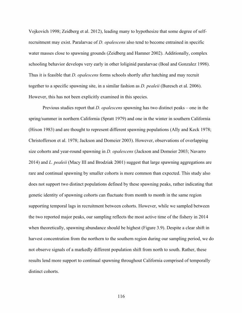
116

Vojkovich 1998; Zeidberg et al. 2012), leading many to hypothesize that some degree of self-

recruitment may exist. Paralarvae of D. opalescens also tend to become entrained in specific

water masses close to spawning grounds (Zeidberg and Hamner 2002). Additionally, complex

schooling behavior develops very early in other loliginid paralarvae (Boal and Gonzalez 1998).

Thus it is feasible that D. opalescens forms schools shortly after hatching and may recruit

together to a specific spawning site, in a similar fashion as D. pealeii (Buresch et al. 2006).

However, this has not been explicitly examined in this species.

Previous studies report that D. opalescens spawning has two distinct peaks – one in the

spring/summer in northern California (Spratt 1979) and one in the winter in southern California

(Hixon 1983) and are thought to represent different spawning populations (Ally and Keck 1978;

Christofferson et al. 1978; Jackson and Domeier 2003). However, observations of overlapping

size cohorts and year-round spawning in D. opalescens (Jackson and Domeier 2003; Navarro

2014) and L. pealeii (Macy III and Brodziak 2001) suggest that large spawning aggregations are

rare and continual spawning by smaller cohorts is more common than expected. This study also

does not support two distinct populations defined by these spawning peaks, rather indicating that

genetic identity of spawning cohorts can fluctuate from month to month in the same region

supporting temporal lags in recruitment between cohorts. However, while we sampled between

the two reported major peaks, our sampling reflects the most active time of the fishery in 2014

when theoretically, spawning abundance should be highest (Figure 3.9). Despite a clear shift in

harvest concentration from the northern to the southern region during our sampling period, we do

not observe signals of a markedly different population shift from north to south. Rather, these

results lend more support to continual spawning throughout California comprised of temporally

distinct cohorts.

117

Low levels of genetic differentiation

Recovery of overall low levels of genetic differentiation is not unexpected in this highly

mobile marine species. In fact, the majority of research on population structure of neritic

loliginids indicates either very little or no population structure (e.g., Sepioteuthis lessoniana

(Aoki et al. 2008), D. opalescens (Reichow and Smith 2001), Loligo forbesi (Shaw et al. 1999),

L. forbesi (Brierley et al. 1995). Previous studies of D. opalescens also found high levels of gene

flow over wide spatial scales (Ally and Keck 1978; Christofferson et al. 1978; Reichow and

Smith 2001). Small-scale tagging studies on D. opalescens indicate that these squid have the

capability to travel long distances, potentially up to 400-500 km in their lifetime (Zeidberg 2004;

Payne et al. 2006). However, with large population sizes, even low migration rates (m < 0.001)

can result in very low values of genetic differentiation (FST) (Waples and Gaggiotti 2006; Lowe

and Allendorf 2010). While there are no reliable estimates of total biomass for D. opalescens,

models based on egg-escapement place the number of spawning females at a few million during

seasons of low abundance (Dorval et al. 2013). Thus, under the assumption of large population

sizes, a small number of individuals migrating between spawning cohorts or between regions

could result in the low levels of genetic differentiation observed in this study.

The hundreds of genome-wide markers utilized in this study significantly increased

power to make more robust estimates of population parameters, such as migration rate and

number of migrants (rev. Brumfield et al. 2003). Specifically, we wanted to determine if there

was evidence for long-distance migration between spawning grounds within a season. Using

Bayesian methods employed in BAYESASS indicated ~⅔ self-recruitment at all sampling

points, with wildly varying rates of migration between sampling points. While some migration

rates may have been physically feasible, others indicate significant migration backwards in time

118

(Table 3.6). Critical examinations of BAYESASS have revealed major issues with convergence

when used to on datasets where overall FST is very low (<0.05) and migration rates are generally

high (priors limited to maximum ⅓ migrant composition) (Faubet et al. 2007), as in the case

here. Thus, as purely a heuristic measure, we estimated Nm from the overall FST for all sampling

points using the assumptions put forward by Sewall Wright (1931) and find that as few as 31

individuals migrating would be sufficient to maintain this low level of genetic differentiation.

Previous estimates of the likely number of migrants between northern and southern California

using microsatellite data indicate anywhere between ~20-80 individuals migrating per generation

may be enough to maintain observed levels of genetic homogeneity (Reichow and Smith 2001).

Although these methods of estimation are fraught with assumptions and the subject of substantial

debate (see Whitlock and McCauley 1999), they do support a theory of low levels of migration is

possible between spawning grounds and spawning groups.

Applicability of SNP and RAD-seq methodology for market squid fishery examination

Investigating population structure and dynamics in cephalopods, as for most marine

organisms, has historically been limited due to the difficult of physically observing or tracking

migration and movement during very dispersive life stages and for very large population sizes

(Semmens et al. 2007). Specifically, developments in next-generation sequencing methods allow

for the detection and development of hundreds to thousands of molecular markers that can be

used to assign individuals to source populations (Bernatchez and Duchesne 2000; Luikart et al.

2003) and make more accurate estimates of demographic parameters (Brumfield et al. 2003). To

date, studies utilizing genome-wide markers to estimate population parameters and migration

patterns in marine species are steadily growing. Specifically, RAD sequencing and other

119

approaches have been used to great success in detecting broad and fine-scale population structure

in non-model organisms and in wild marine populations such as clownfish (Planes et al. 2009),

herring (Lamichhaney et al. 2012), and anchovies (Zarraonaindia et al. 2012). However,

genome-wide markers have not yet been applied to cephalopod populations, despite their

tremendous potential to inform spatial and temporal management of extremely dynamic and

valuable fisheries species. Understanding population structure and population dynamics in

cephalopod fisheries is particularly pressing as the elusive nature of cephalopod species, squid in

particular, result in management plans founded on very limited data. Moreover, as world finfish

stocks are in rapid decline, we have also seen a rapid increase in exploitation of cephalopod

fishery stocks. Without clear understanding of what is being harvested and how populations are

genetically and demographically connected, we cannot sustainably manage the fisheries.

To date, this study and the one documented in the previous chapter are the first to use

genome-wide single nucleotide polymorphisms to examine population differentiation in

cephalopod species. The SNPs in this study show tremendous potential for teasing apart fine-

scale variation that was previously undetected using traditional morphometric techniques and

allozyme and microsatellite loci. However, inferences on spatial and temporal structure of the

fishery cannot be based on one pilot study alone. Based on the patterns observed in this study,

we were not able to confidently make inferences about why this pattern of temporally mediated

spatial structure exists. This was not because the genetic data were insufficient,, but rather that

there is insufficient information concerning life history and reproductive behavior over both the

species range and multiple generations. In order for genomic-scale data to fulfill its potential for

highlighting population dynamics, it needs to be implemented within a rigorous and well-

structured sampling scheme and as a complement to other types of data so as to provide a full

120

picture of the biological and physical processes governing population structure.

Current situation of fishery and potential threats

Current management is comprised of annual landings limits, weekend closures, limited

vessel entry and spatial closures in spawning habitats located in California Marine Protected

Areas (California Fish and Wildlife). Policies are based on landings and egg escapement

modeling (Macewicz et al. 2004; Dorval et al. 2013). However, the short life cycle and sub-

annual recruitment schedule means that population abundance is completely dependent on the

previous season's spawning success. Genetic evidence from this study reveals that the fishery in

California is very likely not composed of one population, and the spatial and temporal patterns of

population structure are more complex than previously thought. This raises serious questions

regarding the origin of recruiting adults and the dynamics of population connectivity between

these major spawning and fishing grounds. For example, our study suggests that there is

substantial monthly variation in the composition of catch in both northern and southern regions.

Within the five months sampled in 2014, we detect signals of genetically distinct groups present

at different times. During months where one population dominates both northern and southern

California, if spawning is severely impacted in one site, overall abundance and spawning success

may not be severely impacted. However, when genetically different populations dominate

northern and southern regions, and there is heavy harvest pressure on one site or another, this

could severely impact future abundance and recruitment of one or both populations. Moreover,

major population crashes in the past from strong El Nino events highlight the extreme sensitivity

of D. opalescens populations to environmental changes. Ongoing research indicates that the

availability of suitable habitat for spawning drastically decreases during strong El Nino events

121

(Zeidberg et al. 2012; Navarro 2014). It is then critical to understand whether genetically distinct

populations are defined by a degree of spawning site fidelity in order to understand how

populations may be affected by strong climatic events. Thus, understanding the nuances and

complexities of the spatio-temporal composition and dynamics of spawning populations is

absolutely vital for informing distribution of fishing effort.

While SNPs add tremendous resolution into the complexities of market squid population

structure, recommendations and insight for informing management is still limited as the samples

collected in this study are fisheries dependent. This reflects a growing issue in fisheries studies,

in that it is often difficult to obtain sufficient sample sizes and sampling range for highly mobile

fisheries species. While the insight we’ve gained in this study may be helpful, they still only

reflect what is happening with the bounds of the fishery and does not necessarily reflect the

biological processes underlying this complex temporal population structure. Therefore, in order

to corroborate and expand upon these findings, we need to conduct further research combining

both fisheries dependent and independent data as well as expand sampling over multiple

generations to get an idea of 1) the stability of these population patterns and 2) identify where

these populations come from and 3) when they recruit in order to accurately inform long-term

sustainable management of this economically critical species. Finding the answers to these

questions is absolutely crucial to sustainably managing market squid as not only do they support

California fishing economy and local livelihoods, but also for understanding the dynamics of the

populations in the context of climate change.

Conclusions

Despite examining a very small time window and just a portion of the total range of the

122

species, single nucleotide polymorphisms were still able to detect subtle differentiation between

sampling locations and sampling times. The findings from this study lend support to the idea that

more than one population of D. opalescens likely exists within California and that effective

dispersal is more restricted than expected, despite overall high levels of gene flow. Given that we

did not find consistent patterns of spatial separation at all sampling times, it is likely that these

populations are not present year-round and varies in abundance over time. However, further

research is required to determine where they come from and where they go (e.g. offshore, areas

outside of the target range of the fishery, etc…). Furthermore, complex patterns of differentiation

suggest that gene flow varies with season and that the occurrence of different spawning

populations fluctuates over time. While this study demonstrates the remarkable utility of RAD-

sequencing for examining population structure in a highly dynamic fishery species, it also

highlights limitations of using genomic data in wild populations. Despite the capability for

delineating population structure with high resolution and assigning individuals, our inference

into the biological implications of our findings is limited by the use of fisheries dependent data

and the lack of comprehensive information on the life history and migration patterns of D.

opalescens. While the location of some large and small spawning beds are known along the

range, very little is known about where the squid are before they come inshore to spawn. Thus, in

order to more fully understand the population structure of these vital commercial species, an

integrated approach is absolutely necessary.

Acknowledgements

This research would not have been possible without the support of California Fish and

Wildlife (CDFW) staff in Los Alamitos and Monterey. We would like to thank the Conservation

Genomics initiative group at UCLA (H.B. Shaffer, T.B. Smith, R.K. Wayne, D. Jacobs, M.

123

Alfaro) for encouraging this project and including it in initial proposals to the CDFW

Commission Board. We would like to thank H. Nuetzel, S. Anjani, and B. Dang for their

assistance in molecular work on this project. The Save Our Coasts Foundation generously

provided funding for this project.

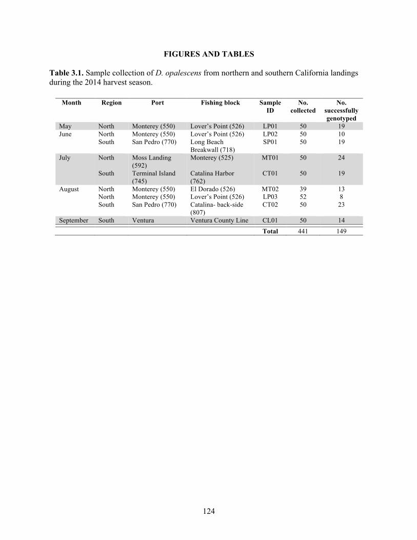
124

FIGURES AND TABLES Table 3.1. Sample collection of D. opalescens from northern and southern California landings during the 2014 harvest season.

Month Region Port Fishing block Sample ID

No. collected

No. successfully genotyped

May North Monterey (550) Lover’s Point (526) LP01 50 19 June North Monterey (550) Lover’s Point (526) LP02 50 10

South San Pedro (770) Long Beach Breakwall (718)

SP01 50 19

July North Moss Landing (592)

Monterey (525) MT01 50 24

South Terminal Island (745)

Catalina Harbor (762)

CT01 50 19

August North Monterey (550) El Dorado (526) MT02 39 13 North Monterey (550) Lover’s Point (526) LP03 52 8 South San Pedro (770) Catalina- back-side

(807) CT02 50 23

September South Ventura Ventura County Line CL01 50 14

Total 441 149

125

Table 3.2a. List of morphometric measurements made for each individual squid Dorsal mantle length (DML) From tip of the rostrum to the posterior end of the mantle (+/- 0.1

cm) (Figure 3.3). Weight Measured after defrosting animals and draining of excess liquid

but not allowing bodily fluids to escape (+/- 0.01 g). Fin length (FL) Dorsal side up, from the posterior end of the mantle to the

insertion point of the fin into the mantle (+/- 0.1 cm) (Figure 3.3). Fin width (FW) Ventral side up, perpendicular to the longitudinal axis from the

side of the mantle to the most distal part of the fin (+/- 0.1 cm) (Figure 3.3).

Mantle thickness Measured after the ventral side of the mantle had been split anterior to posterior. Thickness was measured anterior to the fin (+/- 0.01 cm).

Sex Determined by examining internal morphology of each individual (Figure 3.3).

Gonad condition Estimated using a four-stage maturity scale (Table 3.2b).

Table 3.2b. Description of maturity scale employed for D. opalescens (after Evans 1976)

Female stages Male stages 1 Ovary small without visible eggs Testis small; spermatophoric sac without

visible spermatophores 2 Ovary medium with some eggs; mantle

moderately thick and firm Testis medium sized; spermatophoric sac with some spermatophores; mantle somewhat thick and firm

3 Oviduct and ovary full of eggs, large and completely filling posterior of mantle cavity; nidamental and oviducal glands large, firm and white; accessory nidamental glands orange red; mantle thick and firm

Testis large; spermatophoric organ large and firm, spermatophoric sac full of spermatophores and extending to end of posterior end of mantle cavity; mantle thick and firm

4 Oviduct and ovary has few eggs; nidamental and oviducal gland small and flaccid, accessory nidamental glands light pink; mantle thin and limp

Testis small; spermatophoric sac small with few spermatophores; mantle thin and limp

126

Table 3.3. Average differences in morphometric measurements between individuals grouped by sex by region (A) and location by time (B). Bold values indicate average measurements between comparisons that are significantly different as indicated by Tukey HSD tests (p>0.05). Groups for sex by region (A) are north males (NM), north females (NF), south males (SM) and south females (SF). Groups for location by time (B) are as follows: North - May (N5), June (N6), July (N7), August (N8); South – June (S6), July (S7), August (S8), September (S9). Morphometric measurements abbreviated as DML (dorsal mantle length), FW (fin width), and FL (fin length). Negative differences signify that the second group is larger than the first group.

DML (cm) Weight (g) FW (cm) FL (cm) NM – NF 0.4895 9.4412 0.0680 0.2830

SF – NF -0.9360 -11.0489 -0.2901 -0.3363 SM – NF -0.7079 -6.5624 -0.0371 -0.3708 SF – NM -1.4255 -20.4901 -0.3581 -0.6193

SM – NM -1.1974 -16.0036 -0.1051 -0.6538 SM – SF 0.2281 4.4865 0.2529 -0.0345

DML (cm) Weight (g) FW (cm) FL (cm) N5 N6 0.1353 -0.7022 0.0858 -0.2600 N7 0.4719 10.2025 0.0825 0.2333 N8 -1.5185 -12.5323 -0.5271 -0.7952 S6 -1.5558 -12.1148 0.2825 -1.0000 S7 -1.0725 -12.5764 -0.3231 -0.7222 S8 -1.3121 -15.7068 -0.6842 -0.4739 S9 -1.4090 -15.2949 -0.3985 -0.6000 N6 N7 0.3367 10.9047 -0.0033 0.4933 N8 -1.6538 -11.8301 -0.6129 -0.5352 S6 -1.6911 -11.4126 0.1967 -0.7400 S7 -1.2078 -11.8742 -0.4089 -0.4622 S8 -1.4474 -15.0046 -0.7700 -0.2139 S9 -1.5443 -14.5927 -0.4843 -0.3400 N7 N8 -1.9905 -22.7348 -0.6095 -1.0286 S6 -2.0278 -22.3172 0.2000 -1.2333 S7 -1.5444 -22.7789 -0.4056 -0.9556 S8 -1.7841 -25.9093 -0.7667 -0.7072 S9 -1.8810 -25.4974 -0.4810 -0.8333 N8 S6 -0.0373 0.4175 0.8095 -0.2048 S7 0.4460 -0.0441 0.2040 0.0730 S8 0.2064 -3.1745 -0.1571 0.3213 S9 0.1095 -2.7626 0.1286 0.1952 S6 S7 0.4833 -0.4617 -0.6056 0.2778 S8 0.2437 -3.5921 -0.9667 0.5261 S9 0.1468 -3.1802 -0.6810 0.4000 S7 S8 -0.2396 -3.1304 -0.3611 0.2483 S9 -0.3365 -2.7185 -0.0754 0.1222 S8 S9 -0.0969 0.4119 0.2857 -0.1261

A  

B  

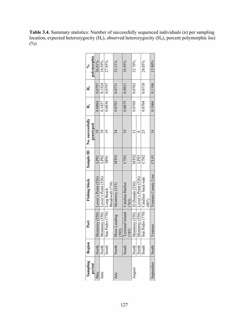
127

Table 3.4. Summary statistics: Number of successfully sequenced individuals (n) per sampling location, expected heterozygocity (He), observed heterozygocity (Ho), percent polymorphic loci (%)

Sam

plin

g pe

riod

R

egio

n Po

rt

Fish

ing

bloc

k Sa

mpl

e ID

N

o. s

ucce

ssfu

lly

geno

type

d H

e H

o %

po

lym

orph

ic

May

N

orth

M

onte

rey

(550

) Lo

ver’

s Po

int (

526)

LP

01

19

0.08

04

0.07

97

26.0

1%

June

N

orth

M

onte

rey

(550

) Lo

ver’

s Po

int (

526)

LP

02

10

0.14

57

0.15

24

14.5

9%

Sout

h Sa

n Pe

dro

(770

) Lo

ng B

each

B

reak

wal

l (71

8)

SP01

19

0.

0836

0.

0797

27

.85%

July

N

orth

M

oss

Land

ing

(592

) M

onte

rey

(525

) M

T01

24

0.07

03

0.07

31

23.2

1%

Sout

h Te

rmin

al Is

land

(7

45)

Cat

alin

a H

arbo

r (7

62)

CT0

1 19

0.

0875

0.

0921

18

.95%

Aug

ust

Nor

th

Mon

tere

y (5

50)

El D

orad

o (5

26)

MT0

2 13

0.

0769

0.

0782

22

.70%

N

orth

M

onte

rey

(550

) Lo

ver’

s Po

int (

526)

LP

03

8 So

uth

San

Pedr

o (7

70)

Cat

alin

a- b

ack-

side

(8

07)

CT0

2 23

0.

0704

0.

0710

24

.05%

Sept

embe

r So

uth

Ven

tura

V

entu

ra C

ount

y Li

ne

CL0

1 14

0.

1066

0.

1106

15

.90%

!

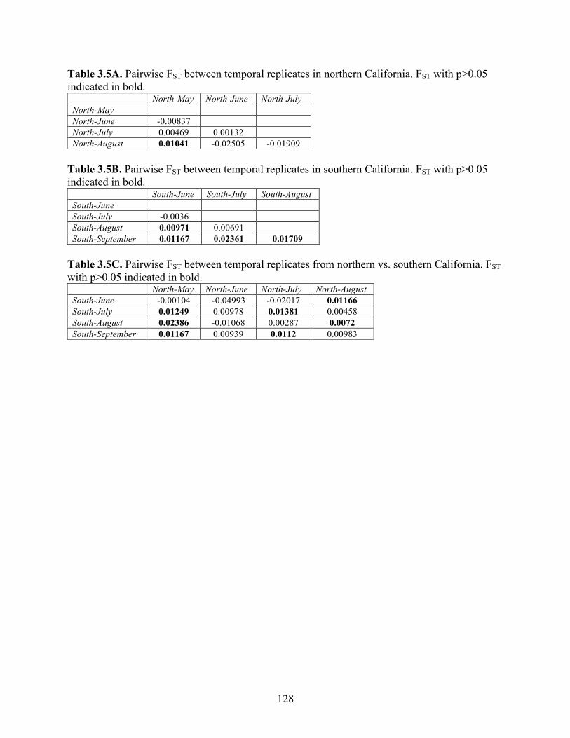
128

Table 3.5A. Pairwise FST between temporal replicates in northern California. FST with p>0.05 indicated in bold.

North-May North-June North-July North-May North-June -0.00837 North-July 0.00469 0.00132 North-August 0.01041 -0.02505 -0.01909  Table 3.5B. Pairwise FST between temporal replicates in southern California. FST with p>0.05 indicated in bold.

South-June South-July South-August South-June South-July -0.0036 South-August 0.00971 0.00691 South-September 0.01167 0.02361 0.01709  Table 3.5C. Pairwise FST between temporal replicates from northern vs. southern California. FST with p>0.05 indicated in bold.

North-May North-June North-July North-August South-June -0.00104 -0.04993 -0.02017 0.01166 South-July 0.01249 0.00978 0.01381 0.00458 South-August 0.02386 -0.01068 0.00287 0.0072 South-September 0.01167 0.00939 0.0112 0.00983

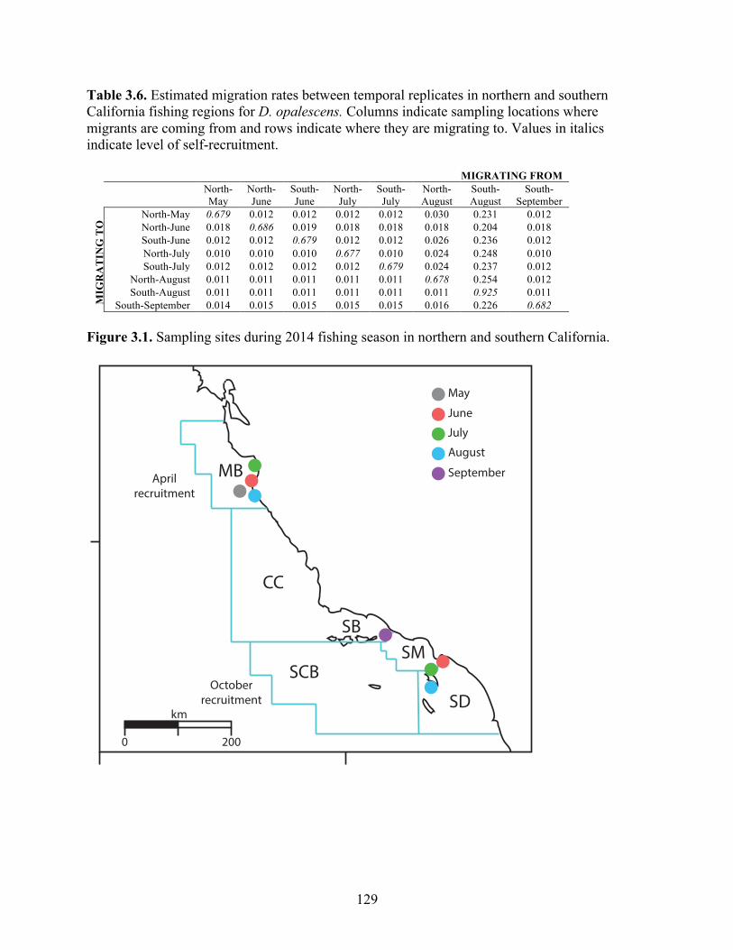
129

Table 3.6. Estimated migration rates between temporal replicates in northern and southern California fishing regions for D. opalescens. Columns indicate sampling locations where migrants are coming from and rows indicate where they are migrating to. Values in italics indicate level of self-recruitment.

MIGRATING FROM

MIG

RA

TIN

G T

O

North-May

North-June

South-June

North-July

South-July

North-August

South-August

South-September

North-May 0.679 0.012 0.012 0.012 0.012 0.030 0.231 0.012 North-June 0.018 0.686 0.019 0.018 0.018 0.018 0.204 0.018 South-June 0.012 0.012 0.679 0.012 0.012 0.026 0.236 0.012 North-July 0.010 0.010 0.010 0.677 0.010 0.024 0.248 0.010 South-July 0.012 0.012 0.012 0.012 0.679 0.024 0.237 0.012

North-August 0.011 0.011 0.011 0.011 0.011 0.678 0.254 0.012 South-August 0.011 0.011 0.011 0.011 0.011 0.011 0.925 0.011

South-September 0.014 0.015 0.015 0.015 0.015 0.016 0.226 0.682 Figure 3.1. Sampling sites during 2014 fishing season in northern and southern California.

MB

CC

SCB

SBSM

SDkm

0 200

April recruitment

Octoberrecruitment

May

June

July

August

September

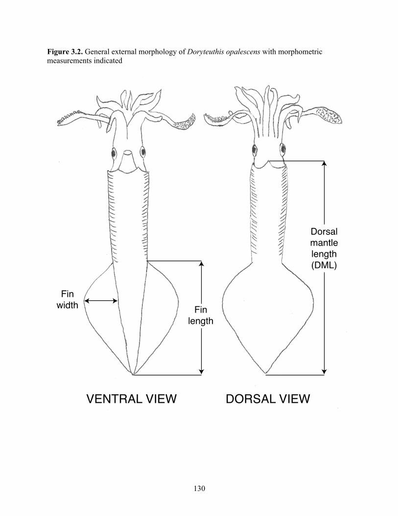
130

Figure 3.2. General external morphology of Doryteuthis opalescens with morphometric measurements indicated

VENTRAL VIEW DORSAL VIEW

Dorsal mantle length (DML)

Fin length

Fin width

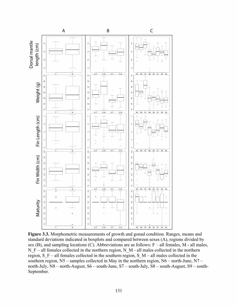
131

Figure 3.3. Morphometric measurements of growth and gonad condition. Ranges, means and standard deviations indicated in boxplots and compared between sexes (A), regions divided by sex (B), and sampling locations (C). Abbreviations are as follows: F – all females, M - all males, N_F – all females collected in the northern region, N_M - all males collected in the northern region, S_F – all females collected in the southern region, S_M – all males collected in the southern region, N5 – samples collected in May in the northern region, N6 – north-June, N7 – north-July, N8 – north-August, S6 – south-June, S7 – south-July, S8 – south-August, S9 – south-September.

F M

810

1214

Sex

N_F N_M S_F S_M

810

1214

Sex by region

Dor

sal m

antle

leng

th

N5 N6 N7 N8 S6 S7 S8 S9

810

1214

Sampling location and time

Dor

sal m

antle

leng

th

F M

1020

3040

5060

70

Sex

N_F N_M S_F S_M

1020

3040

5060

70

Sex by region

Wei

ght

N5 N6 N7 N8 S6 S7 S8 S9

1020

3040

5060

70

Sampling location and time

Wei

ght

F M

34

56

7

Sex

N_F N_M S_F S_M

34

56

7

Sex by region

Fin

leng

th

N5 N6 N7 N8 S6 S7 S8 S9

34

56

7

Sampling location and time

Fin

leng

th

F M

1.0

1.5

2.0

2.5

3.0

3.5

4.0

Sex

N_F N_M S_F S_M

1.0

1.5

2.0

2.5

3.0

3.5

4.0

Sex by region

Fin

wid

th

N5 N6 N7 N8 S6 S7 S8 S9

1.0

1.5

2.0

2.5

3.0

3.5

4.0

Sampling location and time

Fin

wid

th

F M

1.0

1.5

2.0

2.5

3.0

3.5

4.0

N_F N_M S_F S_M

1.0

1.5

2.0

2.5

3.0

3.5

4.0

Mat

urity

Sta

ge

N5 N6 N7 N8 S6 S7 S8 S9

1.0

1.5

2.0

2.5

3.0

3.5

4.0

Mat

urity

Sta

ge

Dor

sal m

antle

le

ngth

(cm

)W

eigh

t (g)

Fin

Leng

th (c

m)

Fin

Wid

th (c

m)

Mat

urity

A B C

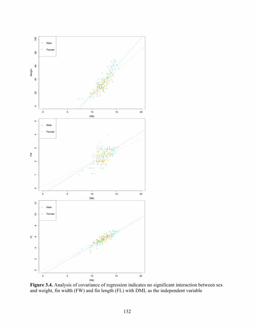
132

Figure 3.4. Analysis of covariance of regression indicates no significant interaction between sex and weight, fin width (FW) and fin length (FL) with DML as the independent variable

0 5 10 15 20

020

4060

80100

DML

Weight

Male

Female

0 5 10 15 20

01

23

45

DML

FW

Male

Female

0 5 10 15 20

02

46

810

12

DML

FL

Male

Female

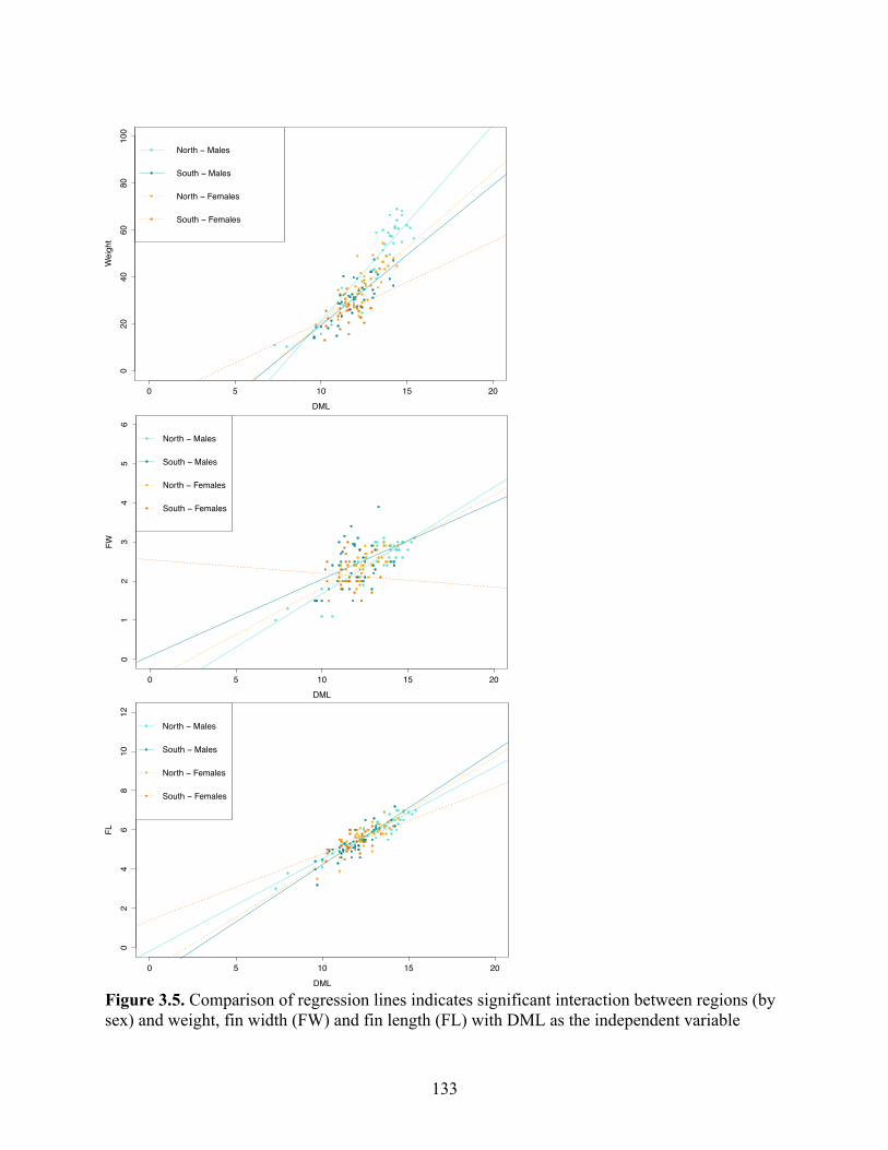
133

Figure 3.5. Comparison of regression lines indicates significant interaction between regions (by sex) and weight, fin width (FW) and fin length (FL) with DML as the independent variable

0 5 10 15 20

020

4060

8010

0

DML

Wei

ght

North − Males

South − Males

North − Females

South − Females

0 5 10 15 20

01

23

45

6

DML

FW

North − Males

South − Males

North − Females

South − Females

0 5 10 15 20

02

46

810

12

DML

FL

North − Males

South − Males

North − Females

South − Females

134

Figure 3.6. Discriminant analysis of principal components (DAPC) of morphometric data and region divided by sex (A) and by sampling location (B). DAPC of SNP data and region divided by sex (C) and by sampling location (D)

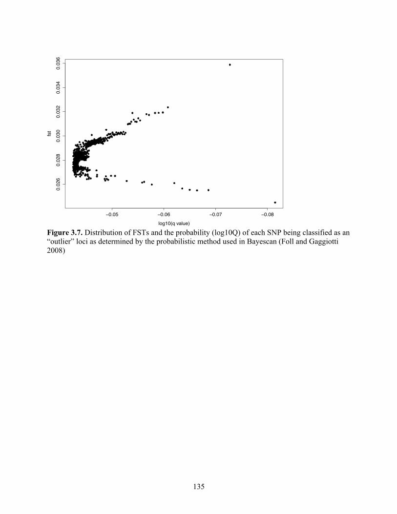
135

Figure 3.7. Distribution of FSTs and the probability (log10Q) of each SNP being classified as an “outlier” loci as determined by the probabilistic method used in Bayescan (Foll and Gaggiotti 2008)

−0.05 −0.06 −0.07 −0.08

0.02

60.

028

0.03

00.

032

0.03

40.

036

log10(q value)

fst

136

Figure 3.8. An individual based ancestry model (implemented in ADMIXTURE, Alexander et al. 2009) testing for likelihood of different numbers of populations (k=1 to k=3). The model with the lowest cross-validation error is k=1 over all sampling groups.

K=1

0.0

0.4

0.8

K=2

Ancestry

0.0

0.4

0.8

K=3

0.0

0.4

0.8

North-May

North-June

South

-June

North-July

South

-July

North-August

South

-August

South

-September

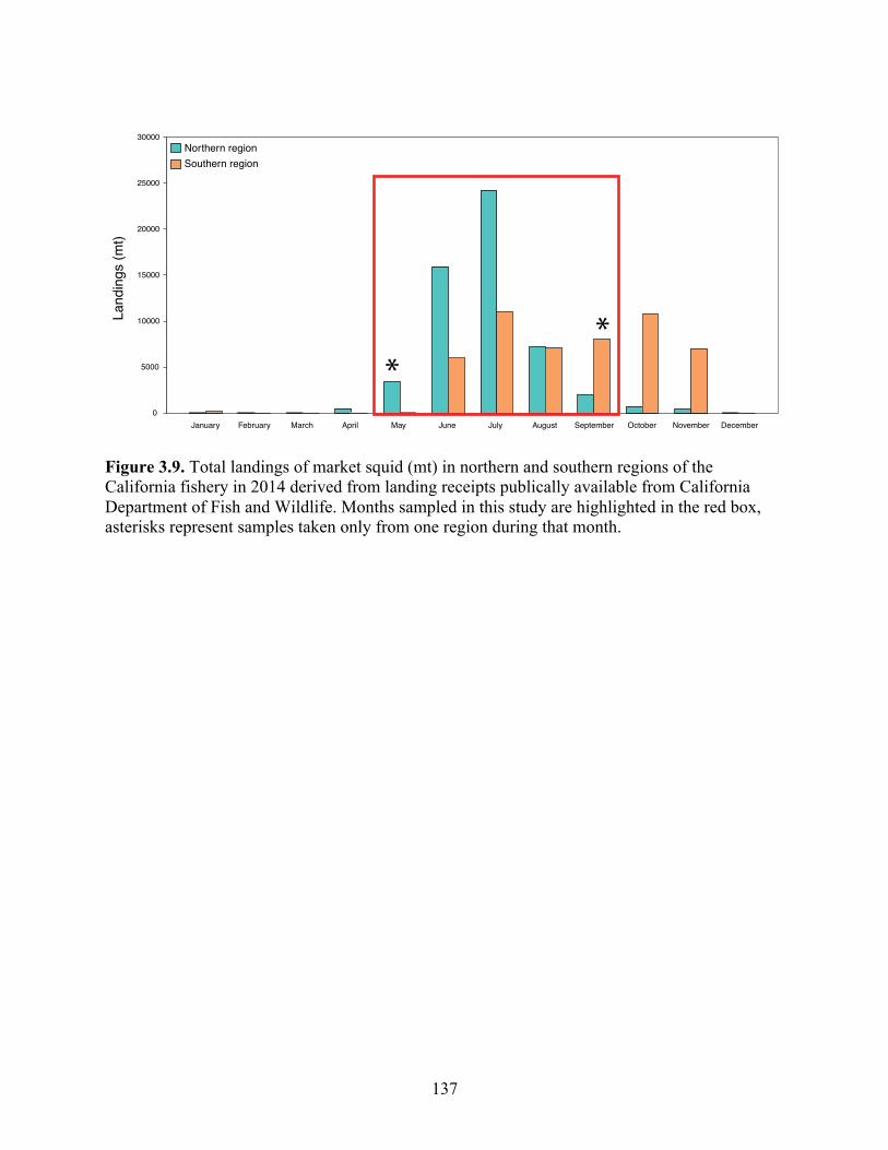
137

Figure 3.9. Total landings of market squid (mt) in northern and southern regions of the California fishery in 2014 derived from landing receipts publically available from California Department of Fish and Wildlife. Months sampled in this study are highlighted in the red box, asterisks represent samples taken only from one region during that month.

January February March April May June July August September October November December

Northern regionSouthern region

Land

ings

(mt)

0

5000

10000

15000

20000

25000

30000

**

138

REFERENCES

Adams CE, Hamilton DJ, Mccarthy I, Wilson AJ, Grant A, Alexander G, Waldron S, Snorasson SS, Ferguson MM, Skúlason S. 2006. Does Breeding Site Fidelity Drive Phenotypic and Genetic Sub-Structuring of a Population of Arctic Charr? Evol. Ecol. 20:11–26.

Alexander DH, Novembre J, Lange K. 2009. Fast model-based estimation of ancestry in unrelated individuals. Genome Res. 19:1655–1664.

Allendorf FW, Hohenlohe PA, Luikart G. 2010. Genomics and the future of conservation genetics. Nat. Rev. Genet. 11:697–709.

Ally JRR, Keck SA. 1978. A biochemical-genetic population structure study of market squid, Loligo opalescens, along the California coast. Calif. Fish Game, Fish Bull. 169:113–121.

Anderson FE. 2000. Phylogeny and historical biogeography of the loliginid squids (Mollusca: cephalopoda) based on mitochondrial DNA sequence data. Mol. Phylogenet. Evol. 15:191–214.

Aoki M, Imai H, Naruse T, Ikeda Y. 2008. Low genetic diversity of oval squid, Sepioteuthis cf. lessoniana (Cephalopoda: Loliginidae), in Japanese waters inferred from a mitochondrial DNA non-coding region. Pacific Sci. 62:403–411.

Baird NA, Etter PD, Atwood TS, Currey MC, Shiver AL, Lewis ZA, Selker EU, Cresko WA, Johnson EA. 2008. Rapid SNP Discovery and Genetic Mapping Using Sequenced RAD Markers. PLoS One 3:e3376.

Banks M, VK R, Calavetta M, Dean C, Hedgecock D. 2000. Analysis of microsatellite DNA resolves genetic structure and diversity of chinook salmon (Oncorhynchus tshawytscha) in California’s Central Valley. Can. J. Fish. Aquat. Sci. 57:915–927.

Beaumont MA, Balding DJ. 2004. Identifying adaptive genetic divergence among populations from genome scans. Mol. Ecol. 13:969–980.

Bernatchez L, Duchesne P. 2000. Individual-based genotype analysis in studies of parentage and population assignment: how many loci, how many alleles? Can. J. Fish. Aquat. Sci. 57:1–12.

Boal JG, Gonzalez SA. 1998. Social Behaviour of Individual Oval Squids (Cephalopoda, Teuthoidea, Loliginidae, Sepioteuthis lessoniana) within a Captive School. Ethology 104:161–178.

Bourret V, Kent MP, Primmer CR, Vasemägi A, Karlsson S, Hindar K, McGinnity P, Verspoor E, Bernatchez L, Lien S. 2013. SNP-array reveals genome-wide patterns of geographical

139

and potential adaptive divergence across the natural range of Atlantic salmon (Salmo salar). Mol. Ecol. 22:532–551.

Boyle PR, Boletzky S. 1996. Cephalopod Populations: Definition and Dynamics. Philos. Trans. R. Soc. B Biol. Sci. 351:985–1002.

Brierley AS, Rodhouse PG, Thorpe J, Clarke MR. 1993. Genetic evidence of population heterogeneity and cryptic speciation in the ommastrephid squid Martialia hyadesi from the Patagonian Shelf and Antarctic Polar Frontal Zone. Mar. Biol. 116:593–602.

Brierley AS, Thorpe M R Clarke JR, Pierce R R Boyle GJ. 1995. Genetic variation in the neritic squid Loligo forbesi (Myopsida: Loliginidae) in the northeast Atlantic Ocean Isle of Man. Mar. Biol. 122:79–86.

Brumfield RT, Beerli P, Nickerson DA, Edwards S V. 2003. The utility of single nucleotide polymorphisms in inferences of population history. Trends Ecol. Evol. 18:249–256.

Buresch KC, Gerlach G, Hanlon RT. 2006. Multiple genetic stocks of longfin squid Loligo pealeii in the NW Atlantic: stocks segregate inshore in summer, but aggregate offshore in winter. Mar. Ecol. Prog. Ser. 310:263–270.

Cadrin SX. 2000. Advances in morphometric identification of fishery stocks. Rev. Fish Biol. Fish. 10:91–112.

Carvalho GR, Hauser L. 1994. Molecular genetics and the stock concept in fisheries. Rev. Fish Biol. Fish. 4:326–350.

Chakraborty R, Meagher TR, Smouse PE. 1988. Parentage analysis with genetic markers in natural populations. I. The expected proportion of offspring with unambiguous paternity. Genetics 118:527–536.

Charlesworth D, Willis JH. 2009. The genetics of inbreeding depression. Nat. Rev. Genet. 10:783–796.

Christofferson JP, Foss A, Lambert WE, Welge B. 1978. An electrophoretic study of select proteins from the market squid, Loligo opalescens Berry. Calif. Fish Game, Fish Bull. 169:123–133.

Clark RM, Schweikert G, Toomajian C, Ossowski S, Zeller G, Shinn P, Warthmann N, Hu TT, Fu G, Hinds DA, Chen H, Frazer KA, Huson DH, Schölkopf B, Nordborg M, Rätsch G, Ecker JR, Weigel D. 2007. Common Sequence Polymorphisms. Science 317:338–342.

Dorval E, Crone PR, McDaniel JD. 2013. Variability of egg escapement, fishing mortality and spawning population in the market squid fishery in the California Current Ecosystem. Mar. Freshw. Res. 64:80.

140

Evans R. 1976. Aspects of the population biology of the California market squid (Loligo opalescens, Berry).

Excoffier L, Lischer HEL. 2010. Arlequin suite ver 3.5: A new series of programs to perform population genetics analyses under Linux and Windows. Mol. Ecol. Resour. 10:564–567.

Faubet P, Waples RSR, Gaggiotti OE. 2007. Evaluating the performance of a multilocus Bayesian method for the estimation of migration rates. Mol. Ecol. 16:1149–1166.

Fields W. 1965. The structure, development, food relations, reproduction and life history of the squid Loligo opalescens Berry. Fish Bull. 131:1–108.

Foll M, Gaggiotti O. 2008. A Genome-Scan Method to Identify Selected Loci Appropriate for Both Dominant and Codominant Markers: A Bayesian Perspective. Genetics 180:977–993.

Forsythe JW. 2004. Accounting for the effect of temperature on squid growth in nature: from hypothesis to practice. Mar. Freshw. Res. 55:331.

Garthwaite RL, Berg Jr. CJ, Harrigan J. 1989. Population Genetics of the Common Squid Loligo pealei LeSueur, 1821, from Cape Cod to Cape Hatteras. Biol. Bull. 177:287–294.

Hedgecock D, Barber PH, Edmands S. 2007. Genetic Approaches to Measuring Connectivity. Oceanography 20:70–79.

Hilborn R, Walters CJ. 1992. Quantitative Fisheries Stock Assessment: Choice, Dynamics, and Uncertainty. Chapman Hall, New York.

Hixon RF. 1983. Loligo opalescens. In: Boyle PR, editor. Cephalopod Life Cycles Volume 1: Species accounts. Academic Press, Berkeley. p.95-142.

Hohenlohe P, Bassham S, Etter PD, Stiffler N, Johnson EA, Cresko WA. 2010. Population genomics of parallel adaptation in threespine stickleback using sequenced RAD tags. PLoS Genet. 6:e1000862.

Holm S. 1979. A Simple Sequentially Rejective Multiple Test Procedure. Scand. J. Stat. 6:65–70.

Jackson G, Forsythe J. 1997. Age, growth, and maturation of Lolliguncula brevis (Cephalopoda: Loliginidae) in the northwestern Gulf of Mexico with a comparison of length-frequency versus. Can. J. Fish. Aquat. Sci. 54:2907–2919.

Jackson GD, Domeier ML. 2003. The effects of an extraordinary El Nino/La Nina event on the size and growth of the squid Loligo opalescens off Southern California. Mar. Biol. 142:925–935.

141

Jombart T. 2008. adegenet: a R package for the multivariate analysis of genetic markers. Bioinformatics 24:1403–1405.

Jombart T, Devillard S, Balloux F. 2010. Discriminant analysis of principal components: a new method for the analysis of genetically structured populations. BMC Genet. 11:94.

Kashiwada J, Recksiek C. 1978. Possible morphological indicators of population structure in the market squid, Loligo opalescens. Calif Dep Fish Game Fish Bull. 169: 99-110.

Kashiwada J, Recksiek CW. 1979. Beaks of the market squid, Loligo opalescens, as tools for predator studies. CalCOFI 20:65–69.

Kashiwada JV. 1981. The use of morphological variation in distinguishing fishery stocks.

Knowles L, Maddison W. 2002. Satistical phylogeography. Mol. Ecol. 11:2623–2635.

Kornfheld IR V, Gagnon PS. 1982. Stock Definition in Atlantic Herring (Clupea harengus harengus): Genetic Evidence for Discrete Fall and Spring Spawning Populations. Can. J. Fish. Aquat. Sci. 39:1610–1622.

Lamichhaney S, Barrio AM, Rafati N, Sundstrom G, Rubin C-J, Gilbert ER, Berglund J, Wetterbom A, Laikre L, Webster MT, Grabherr M, Ryman N, Andersson L. 2012. Population-scale sequencing reveals genetic differentiation due to local adaptation in Atlantic herring. Proc. Natl. Acad. Sci. 109:19345–19350.

Larson WA, Seeb LW, Everett M V., Waples RK, Templin WD, Seeb JE. 2014. Genotyping by sequencing resolves shallow population structure to inform conservation of Chinook salmon (Oncorhynchus tshawytscha). Evol. Appl. 7:355–369.

Lowe WH, Allendorf FW. 2010. What can genetics tell us about population connectivity? Mol. Ecol. 19:3038–51.

Luikart G, England PR, Tallmon D, Jordan S, Taberlet P. 2003. The power and promise of population genomics: from genotyping to genome typing. Nat. Rev. Genet. 4:981–994.

Macewicz BJ, Hunter JR, Lo NCH, Lacasella EL. 2004. Fecundity, egg deposition, and mortality of market squid (Loligo opalescens). Fish. Bull. 102:306–327.

Macy III WK, Brodziak JKT. 2001. Seasonal maturity and size at age of Loligo pealeii in waters of southern New England. ICES J. Mar. Sci. 58:852–864.

Miller LM, Kallemeyn L, Senanan W. 2001. Spawning-Site and Natal-Site Fidelity by Northern Pike in a Large Lake: Mark–Recapture and Genetic Evidence. Trans. Am. Fish. Soc. 130:307–316.

Morejohn GV, Harvey JT, Krasnow LT. 1978. The Importance of Loligo opalescens in the Food Web of Marine Vertebrates in Monterey Bay, California. Fish Bull. 169:67–97.

142

Morin PA, Martien KK, Archer FI, Cipriano F, Steel D, Jackson J, Taylor BL. 2010. Applied conservation genetics and the need for quality control and reporting of genetic data used in fisheries and wildlife management. J. Hered. 101:1–10.

Navarro MO. 2014. Consequences of environmental variability for spawning and embryo development of inshore market squid Doryteuthis opalescens.

Pacific Fishery Management Council. 2011. Status of the Pacific Coast Coastal Pelagic Species Fishery and Recommended Acceptable Biological Catches. Stock Assess. Fish. Eval.

Palumbi SR. 1994. Genetic divergence, reproductive isolation, and marine speciation. Annu. Rev. Ecol. Syst. 25:547–572.

Payne JC, Olson RJ, Young JW. 2006. Comparing squid optimal cost of transport speeds to actual field migrations: new data from 40-g Loligo opalescens. In: Payne J, Olson R, Young J. Global Ocean Ecosystem Dynamics. p. 16–18.

Pearse DE, Crandall KA. 2004. Beyond FST: Analysis of population genetic data for conservation. Conserv. Genet. 5:585–602.

Planes S, Jones GP, Thorrold SR. 2009. Larval dispersal connects fish populations in a network of marine protected areas. Proc. Natl. Acad. Sci. 106:5693–5697.

R Core Team. 2013. R: A language and environment for statistical computing. R Foundation for Statistical Computing. Vienna, Austria. URL http://www.R-project.org/.

Reichow D, Smith MJ. 2001. Microsatellites reveal high levels of gene flow among populations of the California squid Loligo opalescens. Mol. Ecol. 10:1101–1109.

Reiss CS, Maxwell MR, Hunter JR, Henry A. 2004. Investigating environmental effects on population dynamics of Loligo opalescens in the southern California Bight. CalCOFI Rep 45:87–97.

Rogers-Bennett L, Pearse J. 2001. Review of some California fisheries for 2000: Market squid, sea urchin, prawn, white abalone, groundfish, ocean salmon, Pacific sardine, Pacific herring. Calif Coop Ocean. Fish Invest Rep.

Rumble SM, Lacroute P, Dalca A V., Fiume M, Sidow A, Brudno M. 2009. SHRiMP: Accurate Mapping of Short Color-space Reads. PLoS Comput. Biol. 5:e1000386.

Sale PF. 2004. Connectivity, Recruitment Variation, and the Structure of Reef Fish Communities. Integr. Comp. Biol. 44:390–399.

Seeb JE, Carvalho G, Hauser L, Naish K, Roberts S, Seeb LW. 2011. Single-nucleotide polymorphism (SNP) discovery and applications of SNP genotyping in nonmodel organisms. Mol. Ecol. Resour. 11:1–8.

143

Semmens JM, Pecl GT, Gillanders BM, Waluda CM, Shea EK, Jouffre D, Ichii T, Zumholz K, Katugin ON, Leporati SC, Shaw PW. 2007. Approaches to resolving cephalopod movement and migration patterns. Rev. Fish Biol. Fish. 17:401–423.

Shaw PW, Pierce GJ, Boyle PR. 1999. Subtle population structuring within a highly vagile marine invertebrate, the veined squid Loligo forbesi, demonstrated with microsatellite DNA markers. Mol. Ecol. 8:407–417.

Skjæraasen JE, Meager JJ, Karlsen Ø, Hutchings JA, Fernö A. 2011. Extreme spawning-site fidelity in Atlantic cod. ICES J. Mar. Sci. 68:1472–1477.

Slatkin M. 1987. Gene flow and the geographic structure of natural populations. Science 236:787–792.

Spratt J. 1979. Age and growth of the market squid. CalCOFI Rep. 20:58–64.

Thorpe JP, Havenhand JN, Patterson KR. 1986. Report of the University of Liverpool to the Falkland Islands Development corporation on stock and species identities of Patagonian Shelf Illex argentinus. to. Falkland Islands Corporation, Port Stanley, Falkland Islands.

Vecchione M, Shea E, Bussarawit S, Anderson F, Alexeyev D, Lu C, Okutani T, Roeleveld M, Chotiyaputta C, Roper C, Jorgensen E, Sukramongkol N. 2005. Systematics of Indo-West Pacific Loliginids. Phuket mar. biol. Cent. Res. Bull. 66:23–26.

Vojkovich M. 1998. The California Fishery For Market Squid (Loligo opalescens). CalCOFI Reports 39:55–60.

Wang S, Meyer E, McKay JK, Matz M V. 2012. 2b-RAD: a simple and flexible method for genome-wide genotyping. Nat. Methods 9:808–810.

Waples RS. 1998. Separating the weat from the chaff patterns of genetic diferrenciation in high gene flow species. J. Hered. 89:438–456.

Waples RS. 2015. Testing for Hardy-Weinberg Proportions: Have We Lost the Plot? J. Hered. 106:1–19.

Waples RS, Gaggiotti O. 2006. What is a population? An empirical evaluation of some genetic methods for identifying the number of gene pools and their degree of connectivity. Mol. Ecol. 15:1419–39.

Waples RS, Winans GA, Utter FM, Mahnken C. 1990. Genetic Approaches to the Management of Pacific Salmon. Fisheries 15:19–25.

Weir BS, Cockerham CC. 1984. Estimating F-statistic for the analysis of population structure. Evolution 38:1358–1370.

144

Whitlock MC, McCauley DE. 1999. Indirect measures of gene flow and migration: FST not equal to 1/(4Nm + 1). Heredity 82 (Pt 2):117–125.

Wilson GA, Rannala B. 2003. Bayesian Inference of Recent Migration Rates Using Multilocus Genotypes. Genetics 163:1177–1191.

Wing B, Mercer R. 1990. Temporary northern range extension of the squid Loligo opalescens in Southeast Alaska. The Veliger.

Wright S. 1931. Evolution in Mendelian populations. Genetics 16:97–159.

Zarraonaindia I, Iriondo M, Albaina A, Pardo MA, Manzano C, Grant WS, Irigoien X, Estonba A. 2012. Multiple SNP Markers Reveal Fine-Scale Population and Deep Phylogeographic Structure in European Anchovy (Engraulis encrasicolus L.). PLoS One 7:e42201.

Zeidberg LD. 2004. Allometry measurements from in situ video recordings can determine the size and swimming speeds of juvenile and adult squid Loligo opalescens (Cephalopoda: Myopsida). J. Exp. Biol. 207:4195–4203.

Zeidberg LD. 2013. Doryteuthis opalescens, Opalescent Inshore Squid. In: Rosa R, O'Dor R, Pierce G, editors. Advances in Squid Biology, Ecology and Fisheries: Part I - Myopsid Squids. Nova Science Publishers, New York, 159-204.

Zeidberg LD, Butler JL, Ramon D, Cossio A, Stierhoff KL, Henry A. 2012. Estimation of spawning habitats of market squid (Doryteuthis opalescens) from field surveys of eggs off Central and Southern California. Mar. Ecol. 33:326–336.

Zeidberg LD, Hammer WM, Nezlini NP, Henry A. 2006. The fishery for California market squid (Loligo opalescens) (Cephalopoda: Myopsida), from 1981 through 2003. Fish. Bull. 104:46–59.

Zeidberg LD, Hamner WM. 2002. Distribution of squid paralarvae, Loligo opalescens (Cephalopoda: Myopsida), in the Southern California Bight in the three years following the 1997-1998 El Nino. Mar. Biol. 141:111–122.

Zemeckis DR, Hoffman WS, Dean MJ, Armstrong MP, Cadrin SX. 2014. Spawning site fidelity by Atlantic cod (Gadus morhua) in the Gulf of Maine: implications for population structure and rebuilding. ICES J. Mar. Sci. 71:1356–1365.