Universidad de Concepción Métodos de Elementos Finitos para ...
150
Universidad de Concepci ´ on Direcci ´ on de Postgrado Concepci ´ on-Chile M ´ etodos de Elementos Finitos para Problemas en Bioelectromagnetismo Tesis para optar al grado de Doctor en Ciencias Aplicadas con menci´on en Ingenier´ ıaMatem´atica Jessika Pamela Cama ˜ no Valenzuela Junio 2013 Facultad de Ciencias F´ ısicas y Matem´ aticas Departamento de Ingenier´ ıa Matem´ atica
-
Upload
khangminh22 -
Category
Documents
-
view
0 -
download
0
Transcript of Universidad de Concepción Métodos de Elementos Finitos para ...
Universidad de ConcepcionDireccion de Postgrado
Concepcion-Chile
Metodos de Elementos Finitos para
Problemas en Bioelectromagnetismo
Tesis para optar al grado de
Doctor en Ciencias Aplicadas con mencion en Ingenierıa Matematica
Jessika Pamela Camano Valenzuela
Junio 2013
Facultad de Ciencias Fısicas y Matematicas
Departamento de Ingenierıa Matematica

METODOS DE ELEMENTOS FINITOS PARA PROBLEMAS EN
BIOELECTROMAGNETISMO
Jessika Pamela Camano Valenzuela
Directores de Tesis: Rodolfo Rodrıguez, Universidad de Concepcion, Chile.
Alberto Valli, Universita degli Studi di Trento, Italia.
Ana Alonso Rodrıguez, Universita degli Studi di Trento, Italia.
Director de Programa: Prof. Raimund Burger, Universidad de Concepcion, Chile
COMISION EVALUADORA
Prof. Salim Meddahi, Universidad de Oviedo, Espana.
Prof. Peter Monk, University of Delaware, E.E.U.U.
Prof. Ilaria Perugia, Universita degli Studi di Pavia, Italia.
COMISION EXAMINADORA
Firma:Prof. Gabriel N. Gatica.
Universidad de Concepcion, Chile.
Firma:Prof. Carlos Jerez-Hanckes.
Pontificia Universidad Catolica de Chile, Chile.
Firma:Prof. Rodolfo Rodrıguez.
Universidad de Concepcion, Chile.
Firma:Prof. Alberto Valli.
Universita degli Studi di Trento, Italia.
Fecha Examen de Grado:
Calificacion:
Concepcion–Junio de 2013

AGRADECIMIENTOS
Quisiera comenzar agradeciendo a mi director de tesis, Rodolfo Rodrıguez, a quien admiro
y aprecio mucho. Le agradezco infinitamente su paciencia, su buena disposicion, su apoyo y el
tiempo que invirtio en mi formacion. Cada vez que lo necesite, siempre estuvo allı para brindarme
su ayuda. Gran parte de lo que he logrado durante la etapa de tesis ha sido, sin duda, gracias
al respaldo de Rodolfo. La verdad fue un gusto trabajar bajo su direccion.
Vorrei anche ringraziare Ana Alonso Rodrıguez e Alberto Valli per la dedizione e l’appoggio
dimostratomi. Li ringrazio per l’ospitalita e l’interesse che hanno sempre mostrato per me du-
rante il periodo di sviluppo della tesi. Mi sento fortunata ad aver lavorato con persone di tale
livello accademico ed umano. Li ringrazio anche per avermi dato l’opportunita di lavorare ed
imparare da loro, per la buona volonta e l’energia investita in ognuno dei lavori intrapresi in-
sieme. Vorrei evidenziare il grande appoggio manifestato in particolare nella parte finale del
mio percorso: senza il loro aiuto sarebbe stato molto piu difficile finire entro i termini previsti.
Infine un grazie per le volte che mi hanno accolto a Trento, permettendomi di vivere un’ottima
esperienza.
Agradezco a mi esposo, Ricardo, por el apoyo y la comprension que me brindo todos estos
anos de doctorado. Le agradezco por acompanarme en los momentos difıciles, tambien por
compartir mis alegrıas, por su lealtad, por su complicidad y por ser mi companero y mi amigo.
Ricardo es una persona de la cual dıa a dıa voy aprendiendo y agradezco a la vida por haberlo
puesto en mi camino.
Tambien agradezco de todo corazon a mi familia, principalmente a mis padres quienes siempre
me brindaron su apoyo y a quienes les debo lo que soy. Gracias por el apoyo con el que siempre
he contado, tanto en lo academico como en mi formacion como persona, gracias por los valores
que he recibido de ustedes, por vibrar con mis logros y por acompanarme en mis penas, gracias
por guiarme para que fuera una persona de bien. Tambien por ayudarme y aconsejarme cada
vez que lo he necesitado. Gracias por ser unos excelentes padres.
A todos y cada uno de los profesores del Programa que me brindaron su tiempo y conocimiento.
En particular, agradezco al profesor Gabriel Gatica quien aparte de ser un excelente profesional,
de lo cual no cabe ninguna duda, es una gran persona, siempre preocupado no solo del alumno,
sino de la persona que hay detras. Gracias por la preocupacion mostrada, por los concejos y por
el carino que siempre sentı de su parte, el cual es mutuo. Tambien agradezco el apoyo que recibı
cuando decidı ingresar a este doctorado.
A mis companeros del doctorado a quienes les tengo un carino muy grande, en especial a
v
Pablo Venegas y a quien fue estudiante de este doctorado, Bibiana Lopez Rodrıguez. Gracias
por los lindos momentos que tuvimos la oportunidad de compartir. La verdad a ambos los siento
mucho mas que companeros, son mis amigos.
A Lorena, Angelina y Eduardo con los cuales tuve la oportunidad de compartir momenos
muy agradables y me quedan lindos recuerdos de aquello.
Agradezco tambien a mis amigos, amigos de mi ninez que siempre me han apoyado y querido.
Tambien a los amigos que he conocido en la universidad, en particular le agradezco a Renee
Mateluna y a Viviana Solano quienes llegaron a ser personas relevantes en mi vida y ocupan un
lugar en mi corazon.
A mis amigos Trentinos los cuales fueron una gran companıa las veces que estuve en Italia.
A los profesores Freddy Paiva y Carlos Mora por apoyarme en esta aventura de ingresar al
doctorado.
Al proyecto MECESUP UCO0713, al CI2MA, a CONICYT, a direccion de postgrado de la
Universidad de Concepcion y a Becas Chile.
Agradezco a la vida porque me ha entregado mucho mas de lo que imaginaba.

RESUMEN
El objetivo principal de esta tesis es proponer, analizar y testear modelos matematicos y
computacionales eficientes a traves de los cuales poder localizar actividad cerebral a partir de
mediciones de los campos electricos y magneticos en la superficie de la cabeza. Estas mediciones
se pueden obtener a traves de un electroencefalograma y un magnetoencefalograma. En terminos
matematicos, esta tesis se centra en resolver un problema inverso.
En primer lugar se estudia el problema inverso usando como modelo las ecuaciones de co-
rrientes inducidas. Igual que para el sistema completo de ecuaciones de Maxwell, se demuestra
que una fuente de corriente volumetrica no puede ser identificada por el conocimiento de las
componentes tangenciales de los campos electromagneticos sobre la frontera, y se caracteriza el
espacio de las fuentes no radiantes. Por otro lado, se prueba que el problema inverso tiene una
unica solucion si la fuente esta soportada en la frontera de un subdominio o si es la suma de un
numero finito de dipolos. Tambien este trabajo se enfoca en la aplicabilidad de estos resultados
para la localizacion de la actividad cerebral a partir de las mediciones que se obtienen mediante
la electroencefalografıa y la magnetoencefalografıa.
Posteriormente, se analiza el problema electrostatico con fuente de corriente dipolar. Este es
un problema singular, ya que tal modelo considera derivadas de primer orden de una distribucion
delta de Dirac. Su solucion pertenece a Lp, con 1 ≤ p < 3/2 en el caso tridimensional y con
1 ≤ p < 2 en el caso bidimensional. Se consideran la aproximacion numerica del problema
directo a traves de elementos finitos lineales a trozos y continuos. Se prueba una estima a priori
del error en norma Lp. Ademas, se propone un estimador de error a posteriori de tipo residual.
Se demuestra que tal estimador es confiable y eficiente. Por ultimo, se utiliza este estimador
para guiar un procedimiento adaptativo, el cual experimentalmente muestra un orden optimo
de convergencia.
Luego, se comparan distintos metodos de approximacion de la solucion del problema directo
considerando un dominio con varias regiones con diferentes conductividades. Para el problema
directo, se analiza el caso en el que el dipolo se encuentra en una interfaz. En este caso especıfico,
se usa una aproximacion de la distribucion delta de Dirac ya que los otros metodos considerados
anteriormente no estan definidos. Por otro lado, para el problema inverso, se analizan los resul-
tados obtenidos utilizando los distintos metodos ya usados en el problema directo y se anaden
a estos, un ultimo metodo que consiste en usar un procedimiento adaptativo guiado por el es-
timador de error a posteriori encontrado en el Capıtulo 4. Se consideran dos situaciones: una
fuente dipolar situada en una region con conductividad regular y lejana a la interfaz y por otra
parte, el caso en el que la tal fuente es cercana a una interfaz. Se estudia tambien el caso de una

vii
fuente distribuida y se compara las matrices de influencia cuando el soporte de dicha fuente se
encuentra dentro de una region homogenea y es lejana a la interfaz y en el caso en que el soporte
es cercano a la interfaz.
Por ultimo, se considera el problema de corrientes inducidas dependiente del tiempo. Se
formula el problema en terminos de dos variables, una definida solo en el dominio conductor y
la otra, en la frontera del dominio. Se combinan el metodo de elementos finitos (FEM) y los
elementos de frontera (BEM) para obtener una formulacion variacional acoplada FEM-BEM.
Se establece la existencia y unicidad de la solucion en el caso continuo y en el caso totalmente
discreto. Finalmente, se investiga el orden de convergencia del esquema totalmente discreto.

ABSTRACT
The main goal of this thesis is to propose, test and analyze mathematical and computa-
tional efficient models for the localization of brain activity from measurements of the electric
and magnetic fields on the surface of the head. These measurements can be obtained using
electroencephalography or magnetoencephalography. In mathematical terms, this thesis focus in
the study of an inverse problem.
First, we consider the inverse source problem for the eddy current approximation of Maxwell
equations. We show that as for the full system of Maxwell equations, a volume current source
cannot be uniquely identified by the knowledge of the tangential components of the electromag-
netic fields on the boundary, and we characterize the space of non-radiating sources. On the other
hand, we prove that the inverse source problem has a unique solution if the source is supported
on the boundary of a subdomain or if it is the sum of a finite number of dipoles. We address
the applicability of this result for the localization of brain activity from electroencephalography
and magnetoencephalography measurements.
Afterwards, we analyze the electrostatics problem with a current dipole source. This is a
singular problem, since the current dipole model involves first-order derivatives of a Dirac delta
measure. Its solution lies in Lp for 1 ≤ p < 3/2 in three dimensional domains and 1 ≤ p < 2 in
the two dimensional case. We consider the numerical approximation of the forward problem by
means of standard piecewise linear continuous finite elements. We prove a priori error estimates
in Lp norm. Then, we propose a residual-type a posteriori error estimator. We prove that it is
reliable and efficient; namely, it yields global upper and local lower bounds for the corresponding
norms of the error. Finally, we use this estimator to guide an adaptive procedure, which is
experimentally shown to lead to an optimal order of convergence.
Subsequently, we compare different approximation methods for the solution of the direct
problem in the case of a domain with several regions with different conductivities. For the
direct problem, we analyze the case in which the dipole is located at an interface between two
regions with different conductivities. In this specific case we use an approximation of the delta
function since other methods are not defined in this situation. On the other hand, for the inverse
problem, we analyze the results obtained using the previous methods and one last method that
incorporates an adaptive procedure guided by the a posteriori error estimator found in Chapter
4. Two situations are considered: a source located within a homogeneous region and the case
where the source is close to an interface. We study also the case of a distributed source and we
compare the lead field matrices when the support of such source is located within a homogeneous

ix
region and when its support is close to an interface.
Finally, the three-dimensional eddy current time-dependent problem is considered. We for-
mulate it in terms of two variables, one lying only on the conducting domain and the other on
its boundary. We combine finite elements (FEM) and boundary elements (BEM) to obtain a
FEM-BEM coupled variational formulation. We establish the existence and uniqueness of the
solution in the continuous and the fully discrete case. Finally, we investigate the convergence
order of the fully discrete scheme.

Contents
1 Introduccion 1
1.1 Modelizacion del problema . . . . . . . . . . . . . . . . . . . . . . . . . . . . . . . 3
1.2 Organizacion de la tesis . . . . . . . . . . . . . . . . . . . . . . . . . . . . . . . . 7
2 Introduction 11
2.1 Modelization the problem . . . . . . . . . . . . . . . . . . . . . . . . . . . . . . . 13
2.2 Organization of the thesis . . . . . . . . . . . . . . . . . . . . . . . . . . . . . . . 17
3 Inverse source problems for eddy current equations 21
3.1 Introduction . . . . . . . . . . . . . . . . . . . . . . . . . . . . . . . . . . . . . . . 21
3.2 Non-uniqueness of volume currents . . . . . . . . . . . . . . . . . . . . . . . . . . 25
3.3 Uniqueness of surface currents . . . . . . . . . . . . . . . . . . . . . . . . . . . . . 28
3.4 Uniqueness for dipole sources . . . . . . . . . . . . . . . . . . . . . . . . . . . . . 29
3.4.1 Explicit determination of the dipole source . . . . . . . . . . . . . . . . . 33
3.5 Application to EEG/MEG . . . . . . . . . . . . . . . . . . . . . . . . . . . . . . . 35
4 A posteriori error estimates for the problem of electrostatics with a dipole
source 37
4.1 Introduction . . . . . . . . . . . . . . . . . . . . . . . . . . . . . . . . . . . . . . . 37
4.2 Model problem . . . . . . . . . . . . . . . . . . . . . . . . . . . . . . . . . . . . . 38
4.2.1 Continuous problem . . . . . . . . . . . . . . . . . . . . . . . . . . . . . . 39
4.2.2 Discrete problem . . . . . . . . . . . . . . . . . . . . . . . . . . . . . . . . 40
4.3 Preliminary results . . . . . . . . . . . . . . . . . . . . . . . . . . . . . . . . . . . 43
4.4 An a posteriori error estimator . . . . . . . . . . . . . . . . . . . . . . . . . . . . 48
4.4.1 Reliability . . . . . . . . . . . . . . . . . . . . . . . . . . . . . . . . . . . . 49
4.4.2 Efficiency . . . . . . . . . . . . . . . . . . . . . . . . . . . . . . . . . . . . 50
4.5 Three-dimensional case . . . . . . . . . . . . . . . . . . . . . . . . . . . . . . . . . 57
4.6 Numerical experiments . . . . . . . . . . . . . . . . . . . . . . . . . . . . . . . . . 59
xi

CONTENTS xii
4.6.1 Test 1. Isotropic constant conductivity . . . . . . . . . . . . . . . . . . . . 59
4.6.2 Test 2. Anisotropic non-constant conductivity . . . . . . . . . . . . . . . . 63
4.6.3 Test 3. Anisotropic constant conductivity . . . . . . . . . . . . . . . . . . 64
5 Numerical behavior of different approximation methods for the direct and
inverse problems of electrostatics with a dipole source 67
5.1 Introduction . . . . . . . . . . . . . . . . . . . . . . . . . . . . . . . . . . . . . . . 67
5.1.1 Continuous problem . . . . . . . . . . . . . . . . . . . . . . . . . . . . . . 68
5.1.2 Discrete problem . . . . . . . . . . . . . . . . . . . . . . . . . . . . . . . . 72
5.2 General considerations for x0 on the interface between two regions with different
conductivities . . . . . . . . . . . . . . . . . . . . . . . . . . . . . . . . . . . . . . 75
5.2.1 Test 1. . . . . . . . . . . . . . . . . . . . . . . . . . . . . . . . . . . . . . . 75
5.2.2 Test 2. . . . . . . . . . . . . . . . . . . . . . . . . . . . . . . . . . . . . . . 82
5.3 Inverse problem . . . . . . . . . . . . . . . . . . . . . . . . . . . . . . . . . . . . . 83
5.3.1 Test 3. . . . . . . . . . . . . . . . . . . . . . . . . . . . . . . . . . . . . . . 85
5.3.2 Test 4. . . . . . . . . . . . . . . . . . . . . . . . . . . . . . . . . . . . . . . 88
5.4 Lead field matrix . . . . . . . . . . . . . . . . . . . . . . . . . . . . . . . . . . . . 89
5.4.1 Test 5. . . . . . . . . . . . . . . . . . . . . . . . . . . . . . . . . . . . . . . 94
5.4.2 Test 6. . . . . . . . . . . . . . . . . . . . . . . . . . . . . . . . . . . . . . . 97
5.4.3 Test 7. . . . . . . . . . . . . . . . . . . . . . . . . . . . . . . . . . . . . . . 98
5.5 Conclusions . . . . . . . . . . . . . . . . . . . . . . . . . . . . . . . . . . . . . . . 99
6 Analysis of a FEM-BEM model posed on the conducting domain for the time-
dependent eddy current problem 101
6.1 Introduction . . . . . . . . . . . . . . . . . . . . . . . . . . . . . . . . . . . . . . . 101
6.2 Preliminaries . . . . . . . . . . . . . . . . . . . . . . . . . . . . . . . . . . . . . . 102
6.2.1 Basic spaces for time dependent problems . . . . . . . . . . . . . . . . . . 103
6.3 The model problem . . . . . . . . . . . . . . . . . . . . . . . . . . . . . . . . . . . 103
6.4 A FEM-BEM coupling variational formulation . . . . . . . . . . . . . . . . . . . 107
6.4.1 Existence and Uniqueness. . . . . . . . . . . . . . . . . . . . . . . . . . . . 111
6.5 Fully-discrete scheme . . . . . . . . . . . . . . . . . . . . . . . . . . . . . . . . . . 112
6.5.1 Matrix form . . . . . . . . . . . . . . . . . . . . . . . . . . . . . . . . . . . 118
6.6 Error estimates . . . . . . . . . . . . . . . . . . . . . . . . . . . . . . . . . . . . . 120
7 Conclusiones y trabajo futuro 127
7.1 Conclusiones . . . . . . . . . . . . . . . . . . . . . . . . . . . . . . . . . . . . . . 127

CONTENTS xiii
7.2 Trabajo futuro . . . . . . . . . . . . . . . . . . . . . . . . . . . . . . . . . . . . . 129
Bibliography 131


Chapter 1
Introduccion
El lograr reconstruir las fuentes de corrientes del cerebro humano es materia de interes en la
investigacion cognitiva y en la rutina clınica. Tal reconstruccion es posible a traves de medidas
del potencial electrico y del flujo magnetico generados. El potencial electrico se mide mediante
electrodos fijados en el cuero cabelludo (EEG) y el flujo magnetico, mediante magnetometros
particularmente sensibles, situados a poca distancia de la superficie de la cabeza (MEG).
La actividad electromagnetica del cerebro se debe al movimiento de iones en las regiones
activadas. Este movimiento genera las llamadas corrientes impresas (o corrientes primarias) que
a su vez generan las corrientes ohmicas en el medio que las rodea llamadas corrientes de retorno.
Las mediciones que se obtienen mediante EEG y MEG corresponden a ambas corrientes, pero
la fuente de interes son las corrientes impresas, dado que ellas representan el area de actividad
neuronal asociada a un estımulo sensorial.
El primer EEG en una persona fue efectuado por H. Berger en 1924. El midio diferencias
de potencial electrico entre pares de electrodos ubicados en el cuero cabelludo. Hoy en dıa estos
electrodos pueden ser pegados directamente a la piel o insertados en una gorra elastica, y es
usual que hayan hasta 256 electrodos.
El primer MEG fue realizado a finales de 1960 por D. Cohen. La senal magnetica en relacion
con la actividad cerebral es extremadamente debil, aproximadamente 100 veces menor que el
campo geomagnetico de la tierra. Su medicion solo llega a ser posible con el magnetometro
SQUID (Superconducting QUantum Interface Devices) introducido por Zimmerman [70]. Esta
instrumentacion mide algunas componentes de la induccion magnetica en diferentes ubicaciones,
hoy en dıa hasta 100, cercanas pero externas a la cabeza.
La localizacion de la fuente es un problema inverso: conociendo el valor del campo magnetico
o del campo electrico sobre la superficie de la cabeza (o, posiblemente, externo a la cabeza, pero
cercano a su superficie), el objetivo es determinar la posicion y algunas caracterısticas fısicas de
1

2
la densidad de corriente que ha generado esos valores.
Dado que la distribucion dentro de un conductor no se puede recuperar unicamente a partir
del conocimiento del campo electromagnetico fuera del conductor, el problema matematico no
tiene una unica solucion si no se asumen algunas condiciones adicionales sobre la fuente (ver
Sarvas [61]). Han sido utilizados principalmente dos aproximaciones distintas para reconstruir
la fuente de actividad cerebral: el modelo dipolar y de corriente distribuida con espacios de
parametros discretos. En el modelo dipolar la densidad de corriente primaria es representada
como
Jp = pδx0 ,
donde x0 corresponde a la localizacion del dipolo y p = 0, recibe el nombre de polarizacion.
Este enfoque es coherente con la realidad dado que las corrientes impresas son unidireccionales
y se deben a la activacion de un gran numero de celulas piramidales concentradas en una region
pequena. En general, se asume que la densidad de corriente primaria se puede descomponer
como una suma de un numero fijo (y no muy alto) de dipolos. Encontrar la posicion de estos
dipolos, se transforma en una busqueda no lineal por mınimos cuadrados.
Por otra parte, en el caso de la fuente distribuida con espacio de parametros discretos, se dis-
cretiza la region del cerebro donde se sabe que se genera la corriente impresa. Despues se resuelve
un problema de tipo lineal donde solo los momentos dipolares tienen que ser reconstruidos, no
la localizacion ni la orientacion.
Dado que el espectro de frecuencias para senales electrofisiologicas en EEG y MEG esta bajo
los 1000 Hz, frecuentemente entre 0.1 y 100 Hz, la mayorıa de los trabajos teoricos sobre aplica-
ciones biomedicas, tales como [29, 34, 36, 44, 67] usan la aproximacion estatica de las ecuaciones
de Maxwell en la cual la variacion temporal tanto del campo electrico como magnetico se omiten.
El modelo estatico no es la unica simplificacion posible de las ecuaciones de Maxwell. Otros mo-
delos que se pueden tener en cuenta son el modelo electro-cuasiestatico, en el cual la variacion
temporal de la induccion magnetica no es considerada, y el modelo magneto-cuasiestatico o
ecuaciones de corrientes inducidas, las cuales se derivan de las ecuaciones de Maxwell donde
lo que se desprecia es la derivada temporal del campo electrico. Tambien es posible estudiar el
problema usando el sistema completo de Maxwell. Algunas referencias respecto a este punto de
vista son [7, 3, 40].
El objetivo de esta tesis es analizar y proponer nuevos modelos en el estudio matematico,
teorico y numerico de la electroencefalografıa y la magnetoencefalografıa. Se ha comenzado
estudiando el modelo de corrientes inducidas y la posibilidad de usarlo en este contexto. En
relacion a estas ecuaciones, dentro de esta tesis se ha analizado un nuevo metodo numerico.
Tambien se ha estudiado el modelo electrostatico usado generalmente en estas aplicaciones. En

1.1 Modelizacion del problema 3
concreto, para el modelo estatico se ha desarrollado un analisis a priori y a posteriori del error
en la aproximacion mediante elementos finitos. El estimador encontrado se ha utilizado para
idear una estrategia computacional mediante la cual es posible resolver el problema inverso en
modo eficiente. Se han investigado tambien nuevos modelos para la aproximacion de la corriente
primaria, robustos desde el punto de vista computacional.
A continuacion se introducen en forma detallada cada uno de los conjuntos de ecuaciones
previamente mencionados.
1.1 Modelizacion del problema
Las ecuaciones de Maxwell son un conjunto de cuatro ecuaciones que describen por completo
los fenomenos electromagneticos. James Clerk Maxwell contribuyo reuniendo en estas ecuaciones
largos anos de resultados experimentales, debidos a Coulomb, Gauss, Ampere, Faraday y otros.
El sistema completo de ecuaciones de Maxwell corresponde a
∂D∂t
+ J = curlH (ley de Maxwell - Ampere)
∂B∂t
+ curl E = 0 (ley de Faraday)
divD = ρ (ley Electrica de Gauss)
divB = 0 (ley Magnetica de Gauss)
(1.1)
donde E es el campo electrico, D es el desplazamiento electrico, H es el campo magnetico, B es
la induccion magnetica, J es la densidad de corriente y ρ es la densidad de carga libre. Todos los
campos que aparecen en estas ecuaciones son funciones vectoriales que dependen de la variable
espacial x ∈ R3 y del tiempo t.
Los distintos campos E , D, B y H estan relacionados por medio de las leyes constitutivas, las
cuales dependen de los materiales que forman el dominio de estudio. Usualmente se asume una
dependencia lineal de la forma D = εE , B = µH, donde ε y µ reciben el nombre de permitividad
electrica y permeabilidad magnetica, respectivamente. En los problemas mas interesantes de la
fısica e ingenierıa, la region de interes esta compuesta de un medio no homogeneo y no isotropico:
esto es, ε y µ no son constantes, pero son matrices simetricas y uniformemente definidas positi-
vas con coeficientes que son funciones acotadas dependientes de la posicion. En general, tambien
puede considerarse una dependencia no lineal entre D y E , B y H (por ejemplo, para problemas
de histeresis). Sin embargo en esta tesis, se considerara solo una dependencia de tipo lineal.
El sistema se completa con la ley de Ohm que relaciona la densidad de corriente en el

1.1 Modelizacion del problema 4
conductor con el campo electrico de la siguiente manera:
J = σE ,
donde σ recibe el nombre de conductividad electrica, la cual, en regiones conductoras se supone
que es una matriz simetrica y definida positiva (con coeficientes que son funciones acotadas
dependientes de la posicion), mientras que es nula en regiones no conductoras o dielectricos.
Cuando el problema esta dado por una densidad de corriente aplicada Je, uno necesita con-
siderar la ley de Ohm generalizada J = σE+Je. Como consecuencia de la ecuacion de Maxwell-
Ampere y la ecuacion electrica de Gauss, es necesario asumir que divJe = 0 en cualquier region
no conductora y libre de cargas.
Esta tesis, con excepcion del Capıtulo 6, se centra en problemas en donde las cantidades
fısicas varıan periodicamente en el tiempo, lo cual generalmente sucede cuando la densidad de
corriente aplicada Je es una corriente alterna, a saber,
Je(x, t) = J∗(x) cos(ωt+ φ) ,
donde J∗ es una funcion vectorial en R3, ω = 0 es la frecuencia angular y ϕ es el angulo de fase.
Esto es equivalente a la representacion
Je(x, t) = Re[J∗(x)ei(ωt+ϕ)] = Re[Je(x)e
(iωt)]
donde se ha introducido la funcion de variable compleja Je(x) = J∗(x)eiωϕ. De acuerdo a esto,
se busca una solucion periodica en el tiempo dada por
E(x, t) = Re[E(x)e(iωt)] ,
H(x, t) = Re[H(x)e(iωt)] ,
donde E y H son funciones vectoriales cuyas entradas corresponden a valores complejos (a
menudo llamadas “fasores”). Las ecuaciones de Maxwell armonicas en el tiempo que correspon-
den a las siguientes: curlH − (iωε+ σ)E = Je en Ω ,
curlE + iωµH = 0 en Ω ,(1.2)
donde Ω corresponde al dominio fısico. Tales ecuaciones se derivan directamente del sistema
completo bajo las suposiciones que se hicieron previamente.
Notar que la ecuacion magnetica de Gauss div (µH) = 0 es una consecuencia de la ecuacion
de Faraday.
Como se ha observado en experimentos y tambien establece la ley de Faraday, una variacion
temporal del campo magnetico genera un campo electrico. Por tanto, en cada conductor surge
1.1 Modelizacion del problema 5
una densidad de corriente Jeddy = σE; este termino expresa la presencia en un medio conductor
de las corrientes inducidas.
Cuando el termino de desplazamiento de corriente ∂D∂t (o en forma equivalente, iωεE) es
despreciado, el sistema de ecuaciones que se obtiene recibe el nombre de aproximacion por
corrientes inducidas de las ecuaciones de Maxwell (o aproximacion magneto-cuasiestatica). En
el caso armonico en el tiempo, el sistema de ecuaciones corresponde acurlH − σE = Je en Ω ,
curlE + iωµH = 0 en Ω ,
div (εE) = 0 en ΩI ,
(1.3)
donde ΩI corresponde al dielectrico. Como en el caso del sistema completo de Maxwell, se debe
asumir que
divJe = 0 en ΩI . (1.4)
Tambien se desprende de este conjunto de ecuaciones la restriccion div (µH) = 0, la cual se
sigue de la ley de Faraday. Finalmente, notamos que en la aproximacion por corrientes inducidas
div (εE) = 0 en ΩI , lo que asegura que la carga electrica se anula en el dielectrico, lo cual no es
una consecuencia de la ecuacion de Ampere ni de (1.4).
Cuando se condideran problemas dependientes del tiempo y la variacion temporal de los
campos es lenta, uno puede simplificar el modelo de ecuaciones de Maxwell, despreciando las
derivadas temporales ∂D∂t y ∂B
∂t (o en el caso de las ecuaciones armonicas en el tiempo, esto
equivale a considerar ω = 0). Tal modelo recibe el nombre de modelo electro-magnetostatico.
En el caso armonico en el tiempo, las ecuaciones corresponden a
curlH − σE = Je en Ω ,
curlE = 0 en Ω ,
div (µH) = 0 en Ω ,
div (εE) = 0 en ΩI .
(1.5)
De la segunda ecuacion de (1.5), se deriva que el campo electrico es un gradiente de un
potencial escalar E = −∇V y por tanto, de la primera ecuacion en (1.5) se obtiene
div (σ∇V ) = divJe .

1.1 Modelizacion del problema 6
Ası, se obtiene el siguiente sistema de ecuaciones:
div (σ∇V ) = divJe en ΩC ,
curlH − σ∇V = Je en Ω ,
div (µH) = 0 en Ω ,
div (ε∇V ) = 0 en ΩI .
(1.6)
donde ΩC corresponde al conductor. Ahora se presentan las geometrıas, propiedades de las
cantidades fısicas y ecuaciones junto con condiciones de frontera, que se utilizaron en cada
capıtulo de esta tesis.
En el Capıtulo 3 se considera un conductor ΩC ⊂ R3, el cual representa una parte del cuerpo
humano. Se asume que ΩC es un dominio acotado con una frontera Lipschitz y conexa Γ. En
el conductor, la conductividad es una matriz simetrica y uniformemente definida positiva con
coeficientes en L∞. Tambien se considera un dominio computacional Ω ⊂ R3, que contiene
completamente a ΩC . El dominio Ω es un dominio acotado y simplemente conexo y con frontera
Lipschitz ∂Ω. El dielectrico se define como ΩI := Ω \ ΩC . Este es un conjunto conexo y corres-
ponde al aire que rodea la cabeza. La permeabilidad magnetica y la permitividad electrica son
matrices simetricas y uniformemente definidas positivas con coeficientes en L∞. Por otra parte,
en la frontera exterior ∂Ω se impone la condicion de frontera magnetica H × n = 0. Ademas,
agregamos la condicion necesaria para la unicidad div (εE) = 0 en ΩI . Cuando se impone una
condicion de frontera magnetica sobre la frontera, se debe imponer otra condicion de frontera
necesaria: εE · n = 0 sobre ∂Ω. Ası, el sistema de ecuaciones se convierte en
curlH − σE = Je en Ω ,
curlE + iωµH = 0 en Ω ,
div (εE) = 0 , en ΩI
εE · n = 0 sobre ∂Ω ,
H × n = 0 sobre ∂Ω ,
(1.7)
donde la fuente Je es una fuente distribuida (Je ∈ (L2(ΩC))2) o una corriente superficial (Je ∈
H−1/2(div τ ; ∂B) con B ⊂ R3 abierto y conexo, con frontera Lipschitz ∂B y satisface B ⊂ ΩC)
o una corriente dipolar (Je =∑M
k=1 pkδxk, con xk punto interior de ΩC , k = 1, ...,M). Seran
necesarias condiciones adicionales sobre la conductividad σ, condiciones sobre las cuales se dara
mas detalle en este capıtulo.
En Capıtulos 4 y 5, se considera el modelo electrostatico, en el cual solo es de interes encontrar
el campo electrico y deriva del modelo electro-magnetostatico. Como conductor, se considera un
1.2 Organizacion de la tesis 7
abierto acotado ΩC ⊂ Rd, donde d puede tomar los valores 2 o 3 en Capıtulo 4 y toma el valor 2
en Capıtulo 5. Se considera como condicion de frontera (σ∇V ) ·n = 0 sobre ∂ΩC , la cual viene
del hecho que div (Je −σ∇V ) = div (curlH) = 0 en Ω, de aquı (Je −σ∇V ) ·n no tiene saltos
sobre ∂ΩC . Ademas Je se localiza en el interior de la cabeza y la conductividad se anula fuera
de ella. Por tanto, el conjunto de ecuaciones que modelan tal problema es el siguiente: div (σ∇V ) = div (pδx0) en ΩC ,
(σ∇V ) · n = 0 sobre ∂ΩC .(1.8)
La conductividad σ corresponde a una matriz simetrica y uniformemente definida positiva,
con coeficientes en L∞(ΩC). Para probar existencia y unicidad de solucion de tal problema, es
necesario asumir una mayor regularidad de σ en un entorno del soporte de la delta; en concreto
los coeficientes de la matriz σ deben pertenecer a W 1,∞(Br0(x0)), donde Br0(x0) := x ∈ Rd :
|x− x0| < r0 para un r0 adecuado.
Finalmente, en el Capıtulo 6, se considera como dominio conductor ΩC ⊂ R3 el cual es un
poliedro conexo, acotado, con frontera Γ conexa y Lipschitz continua. El dielectrico, corresponde
a ΩI := R3 \ΩC el cual tambien es conexo. Se consideran las ecuaciones de corrientes inducidas
dependientes del tiempo que corresponden a
∂t(µH) + curlE = 0 in R3 × (0, T ),
curlH − σE = Je in R3 × [0, T ],
div (εE) = 0 in ΩI × [0, T ],
H(x, t), E(x, t) = O(|x|−1) as |x| → ∞,
H(x, 0) = H0(x) x ∈ R3,
(1.9)
donde T > 0, la densidad de corriente Je ∈ L2(0, T ; (L2(ΩC))3) y ademas tiene soporte com-
pacto en el conductor. La cuarta condicion de (1.9) se satisface uniformemente en [0, T ]. El
dato inicial H0 ∈ (L2(ΩC))3 y satisface div (µH0) = 0 en R3. Los coeficientes σ, µ y ε son
matrices simetricas con componentes acotadas. La conductividad es nula en el dielectrico. La
permeabilidad magnetica µ es definida positiva en todo R3 y satisface µ = µ0I en ΩI , donde
I se entiende como la matriz identidad. La permitividad electrica ε es necesaria solo en el
dielectrico en esta formulacion y se asume satisfacer ε = ε0I en ΩI ; µ0 y ε0 son los coeficientes
correspondientes en el vacıo.
1.2 Organizacion de la tesis
Este trabajo se organiza de la siguiente manera. En el Capıtulo 3, se estudia la unicidad de
la solucion del problema inverso para el problema de corrientes inducidas, siguiendo el enfoque

1.2 Organizacion de la tesis 8
propuesto por Albanese y Monk [3] para el sistema de ecuaciones de Maxwell. Como fuente de
corriente, se han considerado tres situaciones distintas: una fuente de corriente distribuida, una
corriente superficial y finalmente, una corriente dipolar. En relacion a la primera, se demuestra
que cuando la fuente esta en L2 el problema inverso no tiene una unica solucion y se caracteriza
el espacio de fuentes no radiantes. Con respecto a la segunda, se demuestra que conociendo
la componente tangencial del campo electrico sobre la frontera del dominio, existe una unica
corriente superficial que la genera. En el caso de la fuente dipolar, primero se demuestra existencia
y unicidad del problema directo y posteriormente, se analiza el problema inverso. Como en el
caso de la corriente superficial se demuestra que la componente tangencial del campo electrico
en el borde del conductor determina de manera unica el numero de dipolos, localizacion y
polarizacion. Ademas, se presenta una formula mediante el cual es posible encontrar la fuente
dipolar, sabiendo a priori la componente tangencial del campo electrico sobre la frontera del
dominio. Finalmente, se estudia como encontrar la componente tangencial del campo electrico
a partir de los datos medidos a traves de EEG y MEG. Este capıtulo esta constituido por el
siguiente artıculo:
A. Alonso Rodrıguez, J. Camano and A. Valli, Inverse source problems for eddy
current equations. Inverse Problems, vol. 28, 1, (2012).
En el Capıtulo 4 usando la formulacion estudiada por Valli [65], se desarrolla un analisis a
priori y a posteriori para una formulacion variacional del problema electrostatico, el cual es un
problema con singularidad dado que la fuente de corriente contiene derivadas de primer orden de
la distribucion delta de Dirac. En [65] se demostro que la solucion de este problema pertenece a
Lp para 1 ≤ p < 3/2 en dominios tridimensionales y siguiendo la misma tecnica de demostracion,
se prueba que la solucion en el caso bidimensional tambien pertenece a Lp, con 1 ≤ p < 2. En
este capıtulo, se da una estima de error a priori en norma Lp, valida para mallas cuasiuniformes,
y se propone un estimador de error a posteriori, el cual se demuestra que resulta confiable y
eficiente bajo las hipotesis de convexidad del dominio y mayor regularidad de la conductividad.
Todo este analisis se presenta inicialmente en un dominio bidimensional y posteriormente en
un dominio tridimensional, pero este ultimo caso bajo suposiciones mas restrictivas (geometrıa
cubica y conductividad constante). Finalmente, el estimador se usa para guiar un procedimiento
adaptativo, el cual muestra experimentalmente un orden optimo de convergencia. Este capıtulo
esta constituido por el siguiente artıculo:
A. Alonso Rodrıguez, J. Camano, R. Rodrıguez and A. Valli, A posteriori error
estimates for the problem of electrostatics with a dipole source. (enviado).
1.2 Organizacion de la tesis 9
En el Capıtulo 5 se compara la solucion aproximada del problema directo usando el metodo
de substraccion y el metodo directo en el caso concreto de un dominio con varias regiones con
distintas conductividades. Para el problema directo, se analiza el caso en el cual el dipolo se
localiza cerca o exactamente en una interfaz entre dos regiones con conductividades diferentes.
Se estudia tambien un tercer metodo que aproxima a la distribucion delta de Dirac usando la
funcion caracterıstica. Numericamente se observa que en esta situacion el tercer modelo es el
unico que da buenos resultados. Para el problema inverso se analizan los resultados obtenidos
usando los tres metodos ya mencionados y se agrega a estos tres, un ultimo metodo que corres-
ponde a trabajar el metodo directo en conjunto con un procedimiento adaptativo guiado por el
estimador encontrado en el Capıtulo 4. Se consideran dos situaciones: una fuente localizada en el
interior de una region y el caso en que la fuente es cercana a una interfaz. Se estudia tambien el
caso de una fuente distribuida y se comparan las matrices de influencia en distintas situaciones.
Este capıtulo esta constituido por el siguiente artıculo:
A. Alonso Rodrıguez, J. Camano, R. Rodrıguez and A. Valli, Numerical behavior
of different approximation methods for the direct and inverse problems of electrostatics with
a dipole source. (en preparacion).
Finalmente, en paralelo al trabajo que se presenta en el Capıtulo 3, en el Capıtulo 6 se
estudia un nuevo metodo numerico para las ecuaciones de corrientes inducidas dependientes del
tiempo en un dominio conductor acotado contenido en R3. El problema se reformula expresando
los campos magnetico y electrico en terminos de nuevas variables que resultan ser mas conve-
nientes: la primitiva temporal del campo electrico la cual desempena el papel de un potencial
vectorial para el campo magnetico en el conductor y la traza del potencial escalar magnetico en
el aislante. Luego, se deriva una formulacion FEM-BEM y se demuestra existencia y unicidad
de solucion para el problema. Se discretiza el problema usando como espacios de discretizacion
el de elementos finitos de Nedelec para la variable definida en el conductor y funciones lineales a
trozos y continuas para una variable adicional en la frontera del dominio, la cual surge a partir
de las ecuaciones integrales. Para la discretizacion temporal se usa un metodo backward Euler.
Finalmente, se prueba que el esquema discreto converge con un orden optimo a la solucion. Este
capıtulo esta constituido por el siguiente artıculo:
J. Camano and R. Rodrıguez, Analysis of a FEM-BEM model posed on the conduc-
ting domain for the time-dependent eddy current problem. Journal of Computational and
Applied Mathematics, vol. 236, issue 13, pp. 3084-3100, (2012).
Es importante resaltar que con respecto al problema inverso, en el primer capıtulo son nece-
sarias tanto las mediciones que se obtienen con EEG como con MEG, no ası en el tercer y cuarto

1.2 Organizacion de la tesis 10
capıtulo, donde lo que se estudia es el modelo electrostatico y por esta misma razon, los unicos
datos necesarios son los que se obtienen mediante EEG.

Chapter 2
Introduction
The reconstruction of electromagnetic sources in the human brain is of great interest in
cognitive research and in clinical routine. Such reconstruction is possible through measurements
of the scalp electric potential and the external magnetic flux. The electric potential is measured
by electrodes attached to the scalp (EEG) and magnetic flux through particularly sensitive
magnetometers, located within short distance from the surface of the head (MEG).
Electromagnetic activity of the brain is due to the motion of ions in activated regions.
This movement generates the so called impressed currents (or primary currents) that in turn
create ohmic currents in the surrounding environment called return currents. The measurements
obtained by EEG and MEG correspond to both currents, but the source of interest are the
impressed currents, since they represent the area of neural activity associated with sensory
stimuli.
The first EEG was performed by H. Berger in 1924. He measured the electric potential diffe-
rences between pairs of electrodes placed on the scalp. Today these electrodes can be attached
directly to the skin or inserted into an elastic cap. Up to 256 electrodes can be used.
The first MEG was realized in late 1960 by D. Cohen. The magnetic signal due to brain
activity is extremely weak, approximately 100 times less than the geomagnetic field of the
earth. Its measurement becomes possible only with the SQUID magnetometer (Superconducting
QUantum Interface Devices) introduced by Zimmerman [70]. This instrumentation measures
some components of the magnetic induction in different locations; today these can reach the
quantity of 100, near but outside the head.
The location of the source is an inverse problem: knowing the value of the magnetic field
or the electric field on the surface of the head (or possibly outside the head, but close to the
surface), the goal is to determine the position and some physical characteristics of the current
density that generated these values.
11

12
Since the distribution inside a conductor can not be recovered only from knowledge of the
electromagnetic field outside the conductor, the mathematical problem does not have a unique
solution unless some additional conditions are assumed on the source (see Sarvas [61]). There
have been used mainly two different approaches to reconstruct the source of the brain activity:
the dipole model and the model of a distributed source (with a discrete spaces). The primary
current density in the dipolar model is modeled as
Jp = pδx0 ,
where x0 corresponds to the location of the dipole and p = 0 is called polarization. This is a
good approximation of unidirectional impressed currents, due to activation of a large number of
pyramidal cells concentrated in a small region. It can also be assumed that the primary current
density is decomposed as the sum of a fixed number (not too high) of dipoles. Finding the
position of these dipoles becomes a nonlinear least squares search.
On the other hand, in the case of a distributed source with a discrete parameter space, the
region of the brain where it is known that the impressed current is generated is triangulated
and dipolar sources are placed at fixed points of each element. Then, a linear inverse problem is
solved where only the dipole moments have to be rebuilt, not the locations.
Since the frequency spectrum for electrophysiological signals in EEG and MEG is below 1000
Hz, often between 0.1 and 100 Hz, most theoretical works on biomedical applications, such as
[29, 34, 36, 44, 67], use the static approximation of the Maxwell equations in which the time
variation of both electric and magnetic fields are disregarded. The static model is not the only
possible simplification of the Maxwell equations. Other models that can be taken into account
are the electro-quasistatic model, in which the time variation of the magnetic induction is not
considered and the magneto-quasistatic model or eddy current equations, which are derived from
the Maxwell equations neglecting is the time derivative of the electric field. It is also possible to
study the problem using the full system of Maxwell. Some references on this last approach are
[7, 3, 40].
The aim of this thesis is to analyze and to propose new models in the mathematical theoretical
and numerical study of electroencephalography and magnetoencephalography. We start studying
the eddy currents model and the possibility of using it in this context. We analyze a new
numerical method for this model. We have also studied the electrostatic model, which is more
often used in these applications. Specifically, for the static model a priori and a posteriori analysis
of the error in the finite element approximation have been developed. The estimate found has
been used to devise a computational strategy by which it is possible to solve the inverse problem
in an efficient way. We have also investigated new models for the approximation of the primary
current, that are robust from the computational point of view.

2.1 Modelization the problem 13
In the next section each of the aforementioned sets of equations are introduced in detail.
2.1 Modelization the problem
Maxwell equations are a set of four equations completely describing electromagnetic pheno-
mena. James Clerk Maxwell gathered in these equations, after long years of experimental results,
due to Coulomb, Gauss, Ampere, Faraday and others.
The full system of Maxwell equations reads
∂D∂t
+ J = curlH (Maxwell - Ampere equation)
∂B∂t
+ curl E = 0 (Faraday equation)
divD = ρ (Gauss electrical equation)
divB = 0 (Gauss magnetic equation)
(2.1)
where E is the electric field, D is the electric displacement, H is the magnetic field, B is the
magnetic induction, J is the current density and ρ is the free charge density. All the fields that
appear in these equations are vector functions that depend on the spatial variable x ∈ R3 and
the time t.
The fields E , D, B and H are related by constitutive laws, which depend on the materials
that constitute the considered physical domain. Usually a linear dependence of the form D = εE ,B = µH is assumed, where ε and µ are called electric permittivity and magnetic permeability,
respectively. In physiological applications the media are non-homogeneous and anisotropic: that
is, ε and µ are not constant, but are symmetric and uniformly positive definite matrices with
coefficients that are bounded functions of the position.
The system is completed by Ohm law relating the current density in the conductor with the
electric field as follows:
J = σE ,
where σ is called electric conductivity, is a symmetric and positive definite matrix in conduc-
tive regions (with coefficients that are bounded functions of the position), while it is null in
nonconductive regions or dielectrics.
When the problem is driven by an applied current density Je, the generalized Ohm law
J = σE + Je is considered. As a consequence of the Maxwell-Ampere equation and the Gauss
electrical equation, it is necessary to assume that divJe = 0 in any free of charge non-conductive
region.

2.1 Modelization the problem 14
This thesis, with the exception of Chapter 6, is centered on problems where the physical
quantities vary periodically in time, which usually happens when the current density Je is an
alternating current, namely
Je(x, t) = J∗(x) cos(ωt+ ϕ) ,
where J∗ is a vector function in R3, ω = 0 is the angular frequency and ϕ is the phase angle.
This is equivalent to the representation
Je(x, t) = Re[J∗(x)ei(ωt+ϕ)] = Re[Je(x)e
(iωt)]
where the complex variable function Je(x) = J∗(x)eiωϕ has been introduced. Accordingly, we
look for a periodic in time solution given by
E(x, t) = Re[E(x)e(iωt)] ,
H(x, t) = Re[H(x)e(iωt)] ,
where E and H are vector functions whose entries correspond to complex values (often called
“ phasors ”). The time-harmonic Maxwell equations read: curlH − (iωε+ σ)E = Je in Ω ,
curlE + iωµH = 0 in Ω ,(2.2)
where Ω corresponds to the physical domain. They are derived directly from the complete system
under the assumptions above.
Note that the Gauss magnetic equation div (µH) = 0 is a consequence of the Faraday
equation.
A time-variation of the magnetic field generates an electric field. Therefore, in each conductor
a current density Jeddy = σE arises; this term expresses the presence in conducting media of
the so-called eddy current.
When the displacement current term ∂D∂t (or equivalently, iωεE) is neglected, the system of
equations obtained is called eddy current approximation of the Maxwell equations (or magneto-
quasistatic approximation). In the time-harmonic case, the system of equations iscurlH − σE = Je in Ω ,
curlE + iωµH = 0 in Ω ,
div (εE) = 0 in ΩI ,
(2.3)
where ΩI corresponds to the dielectric. As for the full-Maxwell system, it must be assumed that
divJe = 0 in ΩI . (2.4)

2.1 Modelization the problem 15
From Faraday law it follows that div (µH) = 0. Equation div (εE) = 0 in ΩI ensures that
the electric charge vanishes in the dielectric, which is not a consequence of the Ampere equation
or (2.4).
When time-dependent problems are considered and time-variation of the fields is slow, one
can simplify the model of the Maxwell equations, neglecting both time derivatives ∂D∂t and ∂B
∂t
(or in the time-harmonic case, this is equivalent to consider ω = 0). Such a model is called
electro-magnetostatic model. In the time-harmonic case, the equations are
curlH − σE = Je in Ω ,
curlE = 0 in Ω ,
div (µH) = 0 in Ω ,
div (εE) = 0 in ΩI .
(2.5)
From the second equation in (2.5), for a simply-connecetd domain Ω it follows that the
electric field is a gradient of a scalar potential E = −∇V and therefore from the first equation
in (2.5) we obtain
div (σ∇V ) = divJe .
Thus, we have the following system of equations:
div (σ∇V ) = divJe in ΩC ,
curlH − σ∇V = Je in Ω ,
div (µH) = 0 in Ω ,
div (ε∇V ) = 0 in ΩI ,
(2.6)
where ΩC corresponds to the conductor. In the chapters of this thesis we consider different
electromagnetic models.
In Chapter 3 we focus on the time-harmonic eddy-current model. We consider a conductor
ΩC ⊂ R3, which represents a part of the human body. We assume that ΩC is a bounded
domain with a Lipschitz and connected boundary Γ. In the conductor, the conductivity is a
symmetric and uniformly positive definite matrix with coefficients in L∞. Also we consider a
computational domain Ω ⊂ R3, which completely contains ΩC . The domain Ω is a bounded and
simply-connected domain with Lipschitz boundary ∂Ω. The dielectric is defined as ΩI := Ω\ΩC .It is assumed to be connected and corresponds to the air surrounding the head. The magnetic
permeability and the electric permittivity are symmetric and uniformly positive definite matrices
with coefficients in L∞. Moreover, at the external border ∂Ω we impose a magnetic boundary
condition H × n = 0. Also, we add the condition div (εE) = 0 in ΩI that is necessary for

2.1 Modelization the problem 16
uniqueness. When we impose a magnetic boundary condition on the boundary, we must impose
the other necessary boundary condition εE ·n = 0 on ∂Ω. Thus, the system of equations becomes
curlH − σE = Je in Ω ,
curlE + iωµH = 0 in Ω ,
div (εE) = 0 , in ΩI ,
εE · n = 0 on ∂Ω ,
H × n = 0 on ∂Ω ,
(2.7)
where the source Je is a distributed source (Je ∈ (L2(ΩC))2) or a surface current (Je ∈
H−1/2(div τ ; ∂B) with B ⊂ R3 open and connected, with Lipschitz boundary ∂B and satisfying
B ⊂ ΩC) or a current dipole (Je =∑M
k=1 pkδxk, with xk an internal point of ΩC , k = 1, ...,M).
Additional necessary conditions on the conductivity σ, have to be added, and about them we
give more details in this chapter.
In Chapters 4 and 5 we consider the electrostatic model, a reduced form of the electro-
magnetostatic model. We work in an open bounded conductor domain ΩC ⊂ Rd, where d can
take the values 2 or 3 in Chapter 4 and take the value 2 in Chapter 5. The boundary condition
is (σ∇V ) ·n = 0 on ∂ΩC . This comes from the fact that div (Je −σ∇V ) = div (curlH) = 0 in
Ω, hence (Je − σ∇V ) · n does not jump on ∂ΩC ; moreover, Je is located inside the head and
conductivity vanishes outside it. Therefore, the boundary value problem that we study is: div (σ∇V ) = div (pδx0) in ΩC ,
(σ∇V ) · n = 0 sobre ∂ΩC .(2.8)
The conductivity σ corresponds to a symmetric and uniformly positive definite matrix, with
coefficients in L∞(ΩC). To prove existence and uniqueness of solution of this problem, it is
necessary to assume higher regularity of σ in a vicinity of the support of the delta distribution,
in particular the coefficients of σ must belong to W 1,∞(Br0(x0)), where Br0(x0) := x ∈ Rd :
|x− x0| < r0 for a suitable r0.
Finally, in Chapter 6 we focus on the time-dependent eddy current model in the whole space.
The conductor ΩC ⊂ R3 is a bounded connected polyhedron with boundary Γ connected and
Lipschitz continuous. The dielectric, ΩI := R3 \ ΩC is assumed to be connected. The boundary
value problem reads:

2.2 Organization of the thesis 17
∂t(µH) + curlE = 0 in R3 × (0, T ),
curlH − σE = Je in R3 × [0, T ],
div (εE) = 0 in ΩI × [0, T ],
H(x, t), E(x, t) = O(|x|−1) as |x| → ∞,
H(x, 0) = H0(x) x ∈ R3,
(2.9)
where T > 0, the current density Je ∈ L2(0, T ; (L2(ΩC))3) and has compact support in the
conductor. The fourth condition of (2.9) is satisfied uniformly in [0, T ]. The initial datum satisfies
H0 ∈ (L2(ΩC))3 and div (µH0) = 0 in R3. The coefficients σ, µ and ε are symmetric matrices
with bounded elements. The conductivity vanishes in the dielectric. The magnetic permeability
µ is positive definite at all R3 and satisfies µ = µ0I in ΩI , where I is the identity matrix. In
this formulation the electric permittivity ε appears only in the dielectric in this formulation and
therefore we assume that ε = ε0I in ΩI ; µ0 and ε0 are the corresponding coefficients in the
vacuum.
2.2 Organization of the thesis
This thesis is organized as follows. In Chapter 3, we study the uniqueness of the solution of
the inverse problem for the eddy current problem, following the approach proposed by Albanese
and Monk [3] for the complete system of Maxwell equations. We considere three different kinds
of current sources: a distributed source, a surface current source and a dipole source. Concerning
to the first one, we show that the inverse problem has not a unique solution when the source is
in L2 and we characterize the space of non-radiating sources. On the other hand, we prove that
the inverse problem has a unique solution if we assume that the source is supported on a surface
internal to Ω. In the case of the dipole source, we first prove existence and uniqueness of the
direct problem and then we analyze the inverse problem. As in the case of the surface current
we show that the tangential component of the electric field at the boundary of the conductor
uniquely determines the number of dipoles, location and polarization. In addition, we present a
formula by which it is possible to determine the source dipole, knowing a priori the tangential
component of the electric field on the boundary of the domain. Finally, we study how to find
the tangential component of the electric field from the measured data through EEG and MEG.
This chapter has been published in:
A. Alonso Rodrıguez, J. Camano and A. Valli, Inverse source problems for eddy
current equations. Inverse Problems, vol. 28, 1, (2012).

2.2 Organization of the thesis 18
In Chapter 4 we use the formulation studied by Valli [65], and we develop an a priori and
a posteriori analysis for a variational formulation of the electrostatic problem. This is a singular
problem since the current source contains first-order derivatives of the Dirac delta distribution.
In [65] it is proved that the solution belongs to Lp for 1 ≤ p < 3/2 in three-dimensional domains
and following the same demonstration technique, we prove that the solution in the bidimensional
case belongs to Lp, with 1 ≤ p < 2. In this chapter, we give an a priori error estimate in Lp-
norm, which is valid for quasiuniform meshes, and we propose an a posteriori error estimator.
We show that it is reliable and efficient under the hypothesis of convexity of domain and higher
regularity of the conductivity. All this analysis is presented initially in a two-dimensional domain
and then in a three-dimensional domain, but in the last case under more restrictive assumptions
(cubic geometry and constant conductivity). Finally, the estimator is used to guide an adaptive
procedure, which shows experimentally optimal convergence rate. This chapter corresponds to
the following article:
A. Alonso Rodrıguez, J. Camano, R. Rodrıguez and A. Valli, A posteriori error
estimates for the problem of electrostatics with a dipole source. (submitted).
In Chapter 5 we compare the approximate solution of the direct problem using different
methods, including the subtraction method and the direct method, in the case of a domain with
several regions with different conductivities. We analyze the cases in which the dipole is close to
or exactly located at an interface between two regions with different conductivities. Numerically
we see that, when the source is on the interface, the only method that gives good results is
a third one, in which the delta distribution is approximated by a characteristic function. For
the inverse problem we analyze the results obtained using the three methods mentioned above
and a last one that corresponds to the direct method with an adaptive procedure guided by
the estimates found in Chapter 4. Two situations are considered: the case of a source located
well inside a homogeneous region and the case of a source close to an interface between two
homogeneous regions. We study also the case of a distributed source (the sum of several dipoles)
and we compare the lead field matrices in different situations. This chapter corresponds to the
following article:
A. Alonso Rodrıguez, J. Camano, R. Rodrıguez and A. Valli, Numerical behavior
of different approximation methods for the direct and inverse problems of electrostatics with
a dipole source. (in preparation).
Finally, in parallel to the work presented in Chapter 3, in Chapter 6 we study a new
numerical method for the time-dependent eddy currents equations in a conductor bounded

2.2 Organization of the thesis 19
domain contained in R3. The problem is reformulated by expressing the electric and magnetic
fields in terms of new variables that turn out to be more convenient: the temporal primitive
electric field which plays the role of a vector potential for the magnetic field in the conductor, and
the magnetic scalar potential trace on the interface. Then, we derive a FEM-BEM formulation
and prove existence and uniqueness of the solution to the problem. It is discretized using Nedelec
finite elements for the variable defined in the conductor and piecewise linear and continuous
finite elements for an additional variable on the boundary of the domain. For the temporal
discretization we use the backward Euler method. Finally, we prove that the discrete scheme
converges with optimal order to the solution. This chapter has been published in:
J. Camano and R. Rodrıguez, Analysis of a FEM-BEM model posed on the conduc-
ting domain for the time-dependent eddy current problem. Journal of Computational and
Applied Mathematics, vol. 236, issue 13, pp. 3084-3100, (2012).

Chapter 3
Inverse source problems for eddy
current equations
3.1 Introduction
Electroencephalography (EEG) and magnetoencephalography (MEG) are two non-invasive
techniques used to localize electric activity in the brain from measurements of external electro-
magnetic signals. EEG measures the scalp electric potential, while MEG measures the external
magnetic flux. From the mathematical point of view the goal is to solve an inverse problem for
determining the source current distribution in a heterogeneous media from boundary measure-
ments of the fields.
The frequency spectrum for electrophysiological signals in EEG and MEG is typically below
1000 Hz, most frequently between 0.1 and 100 Hz. For this reason most theoretical works on
biomedical applications focus on the static approximation of the Maxwell equations, in which
the time variation of both electric and magnetic fields is disregarded.
Recently He and Romanov [40], Ammari et al. [7] and Albanese and Monk [3] investigated
the localization of brain activity through the inverse source problem for the full Maxwell system
of equations. In this chapter we analyze the inverse source problem for an alternative model:
the eddy current (or low frequency approximation) of Maxwell equations. In the eddy current
model the time variation of the electric field is disregarded, while time variation of the magnetic
field is kept.
Let us consider electromagnetic phenomena at frequency ω = 0. The time-harmonic full
Maxwell system of equations read
curlH − iωϵE = σE + Je (Maxwell–Ampere equation)
curlE + iωµH = 0 (Faraday equation).(3.1)
21

3.1 Introduction 22
HereE,H denote the electric and magnetic fields, respectively; Je is the applied current density;
ϵ is the electric permittivity, µ the magnetic permeability and σ the electric conductivity.
The eddy current model is formally obtained by neglecting the displacement current term:
curlH = σE + Je
curlE + iωµH = 0 .(3.2)
Let us consider a conductor ΩC ⊂ R3, say, the human head. We assume that ΩC is a bounded
domain with a Lipschitz and connected boundary Γ. In ΩC the conductivity σ is a symmetric
and uniformly positive definite matrix with entries in L∞(ΩC). We consider also a computational
domain Ω ⊂ R3, say, the room where the problem is studied. We assume that Ω is a bounded
simply-connected domain, completely containing ΩC and with Lipschitz boundary ∂Ω. Moreover
we assume that ΩI := Ω \ ΩC is connected. ΩI is an insulator, the air surrounding the head,
hence σ is vanishing in ΩI . We also assume that the electric permeability µ and the electric
permittivity ϵ are symmetric and uniformly positive definite matrices with entries in L∞(Ω).
On the boundary ∂Ω, we can impose either the magnetic boundary condition H ×n = 0 or
the electric boundary condition E ×n = 0 (Here n denotes the unit outward normal vector on
∂Ω).
Since σ is equal zero in insulators, equations (3.2) do not completely determine the electric
field in ΩI . In that region, one has to add div (ϵE) = 0 because there are no charges in an
insulator. This is a “gauge” condition necessary for having uniqueness. When imposing the
magnetic boundary condition, the additional “gauge” condition ϵE·n = 0 on ∂Ω is also necessary.
From Faraday law, µ−1 curlE = −iωH and inserting this result in Ampere law one has
curl(µ−1 curlE) = −iω(σE + Je). So the E-based formulation of the eddy current model readscurl(µ−1 curlE) + iωσE = −iωJe in Ω
div (ϵE) = 0 in ΩI
(µ−1 curlE)× n = 0 on ∂Ω
ϵE · n = 0 on ∂Ω
(3.3)
for the magnetic boundary condition, andcurl(µ−1 curlE) + iωσE = −iωJe in Ω
div (ϵE) = 0 in ΩI
E × n = 0 on ∂Ω
(3.4)
for the electric boundary condition. In this chapter, we will focus on problem (3.3); the same
results can be proved for problem (3.4).
3.1 Introduction 23
In the static approximation also the time variation of the magnetic field is disregarded; thus,
one has:curlH = σE + Je
curlE = 0(3.5)
(where Je can still depend on time, which has to be regarded as a parameter). From the second
equation in (3.5), the electric field is the gradient of a scalar potential E = − gradV and then
from the first equation in (3.5), we obtain div (σ gradV ) = divJe in ΩC . On the other hand,
σE+Je is divergence free in Ω; hence, we have (σ gradV −Je|ΩC) ·nΓ = −Je|ΩI
·nΓ on Γ, with
nΓ being the unit normal vector on Γ pointing outwards ΩC . Since we are interested in electric
sources located in the conductor, namely suppJe ⊂ ΩC , the boundary condition for the static
approximation is the homogeneous Neumann boundary condition σ gradV · nΓ = 0 on Γ. The
static problem thus reads div (σ gradV ) = divJe in ΩC
σ gradV · nΓ = 0 on Γ ,(3.6)
and the related magnetic field is computed in terms of the primary current Je and the return
current σE = −σ gradV using the Biot–Savart law in R3:
H(x) =1
4π
∫ΩC
[Je(y)− σ gradV (y)]× x− y
|x− y|3dy . (3.7)
The inverse source problem consists in the determination of the current source Je from
boundary measurements of the electromagnetic fields. Helmholtz had already observed that this
problem does not have a unique solution. For instance, if the source is a radial dipole, the
magnetic field given by (3.7) vanishes outside a spherical conductor ΩC (see, e.g., Sarvas [61]),
hence, when using the static model, knowledge of the magnetic field on Γ does not contribute
to the localization of radial dipoles.
The characterization of the source currents that can be reconstructed from suitable measure-
ments on the boundary is not an easy task and depends on the model considered. For the static
model in Kress et al. [44], the authors prove that the Biot–Savart operator has a non-trivial
null space. Fokas et al. [36] characterized which part of a volume current source in a spheri-
cal conductor can be reconstructed from knowledge of the magnetic field on the boundary. In
the same framework, Dassios and Hadjiloizi [29] determined which part of the source can be
reconstructed from the electric potential. Instead, concerning dipole sources, He and Romanov
[40] showed that the measurement of the electric potential on the boundary of the conductor
is enough to identify their location and polarization, and proposed an identification procedure.
In the case of a layered spherical model, Dassios and Fokas [27] derived an algorithm for the
identification of a source consisting of a finite number of dipoles from measurements of the elec-
tric potential or the magnetic potential. For a general layered domain, El Badia and Nara [34]

3.1 Introduction 24
proposed an algebraic algorithm for the identification of the number, locations and moments of
the dipoles from knowledge of the tangential components of the electric and magnetic fields.
Considering the full Maxwell system, the existence of non-radiating sources was proved in
Bleistein and Cohen [18]. On the other hand, He and Romanov [40] showed that the location
and the polarization of a current dipole in a conducting object can be uniquely determined by
measuring at a fixed frequency the magnetic field and its normal derivative on the whole surface.
The same result was obtained by Ammari et al. [7] from knowledge of the tangential component
of either the electric or the magnetic field on Γ. Albanese and Monk [3] have characterized which
part of a volume source confined in ΩC can be uniquely identified from measurements of the
tangential component of the electric field on Γ. Moreover, they also proved the uniqueness of
the inverse source problem if the source is supported on the surface of a priori known subdo-
main contained in ΩC or if it is the sum of a finite number of dipole sources. In the last case,
the tangential component of the electric field uniquely determines the number, position and
polarization of the dipoles.
The reconstruction of a current source from boundary measurements of the electromagnetic
fields is interesting also for other types of applications. For instance, the imaging of small electro-
magnetic inclusions can be reduced to inverse source problems for the full Maxwell system where
the current is a sum of a finite number of dipoles. Localization techniques for these problems
have been developed by Ammari et al. [12], [11], [10].
The aim of this chapter is to study the uniqueness of the solution of the inverse source pro-
blem for the eddy current approximation of Maxwell equations, mainly following the approach
proposed by Albanese and Monk [3] for the full Maxwell system of equations. The outline
of the chapter is as follows. Section 3.2 is devoted to volume source currents. We prove that
when looking for Je ∈ (L2(ΩC))3, the inverse problem does not have a unique solution and we
characterize the space of non-radiating sources. In Section 3.3, we obtain the uniqueness result
for a source current supported on the boundary of a subdomain of ΩC ; it is worth noting that
the support of the surface source is not assumed to be known, but it is uniquely determined
from the boundary data. In Section 3.4, we consider the case of dipole sources. First, we study
the well-posedness of the direct problem, that is, the existence and uniqueness of the solution
for the eddy current model assuming that the source is a finite sum of dipoles. Then we prove
uniqueness of the inverse source problem, determining the number, location and polarization
of the dipole source. We also present an algebraic algorithm for the determination of a dipole
source assuming that the tangential component of the electric field on Γ is known. In the last
section, we study how to recover the tangential component of the electric field on Γ, the data
that we use in the inverse problem, from the data that are measured in MEG and EEG.
3.2 Non-uniqueness of volume currents 25
To conclude this section, let us introduce some notation that will be used in the following. The
space H(curl; Ω) indicates the set of real or complex vector valued functions v ∈ (L2(Ω))3 such
that curlv ∈ (L2(Ω))3. We also use the spacesH−1/2(curlτ ; Γ) :=(nΓ × v × nΓ)|Γ |v ∈ H(curl; ΩC)
and H−1/2(divτ ; Γ) :=
(v × nΓ)|Γ |v ∈ H(curl; ΩC)
. These two spaces are in duality and the
following formula of integration by parts holds true:∫ΩC
(w · curlv − curlw · v) =∫Γ(w × nΓ) · v ∀w, v ∈ H(curl; ΩC) .
The last integral is indeed the duality paring betweenw×nΓ ∈ H−1/2(divτ ; Γ) and nΓ×v×nΓ ∈H−1/2(curlτ ; Γ).
3.2 Non-uniqueness of volume currents
In this section, we investigate the uniqueness of the inverse source problem assuming that
the unknown source Je is a function in (L2(ΩC))3. First we will prove that without additional
information, the source cannot be reconstructed from the knowledge of the tangential component
of the electric field on Γ. We then characterize the space of non-radiating sources (those sources
in (L2(ΩC))3 that generate an electric field normal to the surface Γ) and prove that sources Je ∈
(L2(ΩC))3 that are orthogonal to the space of non-radiating sources are uniquely determined by
the tangential component on Γ of the electric field. The result is analogous to the one obtained
by Albanese and Monk [3] for the full Maxwell system.
If Je ∈ (L2(ΩC))3, it is known that problems (3.3) has a unique solution E and the magnetic
field can be computed from Faraday law: H = −(iωµ)−1 curlE in Ω.
Multiplying the first equation in (3.3) by a regular enough test function z, integration by
parts in ΩC easily yields
−iω∫ΩC
Je · z =
∫ΩC
E · [curl(µ−1 curl z) + iωσz]−∫Γ[E × nΓ · (µ−1 curl z)− iωH × nΓ · z] .
Therefore, if z ∈ H(curl; ΩC) is such that
curl(µ−1 curl z)− iωσz = 0 in ΩC ,
the current density Je satisfies the representation formula∫ΩC
Je · z = (iω)−1
∫ΓE × nΓ · (µ−1 curl z)−
∫ΓH × nΓ · z . (3.8)
The right hand term in (3.8) has been called reciprocity functional, taking the name from the
Lorentz reciprocity principle in electromagnetism, or else the Maxwell–Betti reciprocity principle
in elastostatics (see, e.g., Andrieux and Ben Abda [14], El Badia and Ha-Duong [33]). It is often
3.2 Non-uniqueness of volume currents 26
used in the analysis of inverse source problems (see, e.g., Novikov [55], Isakov [41], Ammari and
Kang [9]).
Let us define
W = z ∈ H(curl; ΩC) | curl(µ−1 curl z)− iωσz = 0 inΩC .
It is clear that W is not a trivial subspace of (L2(ΩC))3, since both µ and σ are bounded and
uniformly positive definite in Ω; for each ξ ∈ H−1/2div,τ (Γ), there exists a unique u(ξ) ∈ H(curl; ΩC)
such that u(ξ) ∈ W and u(ξ)× nΓ = ξ on Γ.
Denoting by W the closure of W in (L2(ΩC))3 we have the orthogonal splitting
(L2(ΩC))3 =W ⊕W⊥ .
Lemma 3.2.1 Consider η ∈ (C∞0 (ΩC))
3 and set ϕ = curl(µ−1 curlη) + iωση. Then ϕ ∈ W⊥
(and W⊥ is not a trivial subspace).
Proof. Take z ∈ W . Then∫ΩC
ϕ · z =
∫ΩC
[curl(µ−1 curlη) + iωση] · z
=
∫ΩC
η · [curl(µ−1 curl z) + iωσz] = 0 ,
and a density argument shows that ϕ ∈W⊥.
Note that, if η is a non-vanishing real vector field, one obtains Imϕ = 0, hence W⊥ is not a
trivial subspace. 2
Let us split the current density Je as
Je = J ♯e + J⊥e , J ♯e ∈W , J⊥
e ∈W⊥ .
Theorem 3.2.1 (i) Let us assume that Je = J ♯e ∈W and that E♯ is the corresponding solution
of the eddy current problem. Then knowledge of E♯ × nΓ on Γ uniquely determines J ♯e.
(ii) Let us assume that Je = J⊥e ∈W⊥ and that E⊥ is the corresponding solution of the eddy
current problem. Then E⊥ × nΓ = 0 and H⊥ × nΓ = 0 on Γ, namely, J⊥e is a non-radiating
source.
Proof. (i) The electric field in the insulator satisfies
curl(µ−1 curlE♯) = 0 in ΩI
div (ϵE♯) = 0 in ΩI
(µ−1 curlE♯)× n = 0 on ∂Ω
ϵE♯ · n = 0 on ∂Ω .
3.2 Non-uniqueness of volume currents 27
If E♯ × nΓ = 0 on Γ, multiplying the first equation by E♯ and integrating by parts, one easily
finds curlE♯ = 0, then E♯ = 0 in ΩI . Consequently, H♯ = −(iωµ)−1 curlE♯ = 0 in ΩI and
in particular H♯ × nΓ = 0 on Γ. Therefore, from (3.8), we know that∫ΩC
J ♯e · z = 0 for each
z ∈ W, hence, by a density argument, for each z ∈W . Taking z = J ♯e ∈W , the thesis follows.
(ii) Since J⊥e ∈W⊥, from (3.8), we have that for all z ∈W∫
ΓE⊥ × nΓ · (µ−1 curl z)− iω
∫ΓH⊥ × nΓ · z = 0 . (3.9)
For each η ∈ H−1/2div,τ (Γ), we denote by Z ∈ H(curl; Ω) the solution to
curl(µ−1 curlZ)− iωσZ = 0 in ΩC ∪ ΩI
div (ϵZ) = 0 in ΩI
(µ−1 curlZ)× n = 0 on ∂Ω
ϵZ · n = 0 on ∂Ω
(µ−1 curlZ)|ΩC× nΓ = (µ−1 curlZ)|ΩI
× nΓ + η on Γ ,
(3.10)
which in weak form reads
find Z ∈ V :
∫Ω(µ−1 curlZ · curlv − iωσZ · v) =
∫Γη · v ∀ v ∈ V ,
where V := v ∈ H(curl; Ω) : div (ϵv) = 0 in ΩI and ϵv · n = 0 on ∂Ω. It is well known that
the sesquilinear form on the left-hand side is coercive in V (see Alonso Rodrıguez and Valli [5],
theorem 2.3); therefore, the problem is uniquely solvable.
As a test function in (3.9) we can thus select Z |ΩC∈W , obtaining∫
ΓE⊥ × nΓ · µ−1 curlZ |ΩC
= −∫ΓE⊥ · η −
∫ΓE⊥ · (µ−1 curlZ |ΩI
× nΓ)
= −∫ΓE⊥ · η +
∫ΩI
µ−1 curlE⊥ · curlZ |ΩI
−iω∫ΓH⊥ × nΓ ·Z |ΩC
= −∫Γµ−1 curlE⊥ ·Z |ΩI
× nΓ
= −∫ΩI
µ−1 curlE⊥ · curlZ |ΩI.
In conclusion, we have found ∫ΓE⊥ · η = 0
for each η ∈ H−1/2div,τ (Γ), hence nΓ ×E⊥ × nΓ = 0 on Γ.
Proceeding as in the proof of (i), we show that E⊥ ×nΓ = 0 on Γ, implies H⊥ ×nΓ = 0 on
Γ, and the proof is complete. 2

3.3 Uniqueness of surface currents 28
3.3 Uniqueness of surface currents
In this section, we prove that if the source current is known to be supported on the surface
of a subdomain contained in ΩC , then both the surface and the value of the surface current are
uniquely determined by the tangential component of the electric field on Γ. A similar result, but
assuming that the surface is a priori known, has been previously obtained for the full Maxwell
systems (see Albanese and Monk [3]).
First, we start by considering a surface current J∗ ∈ H−1/2(divτ ; ∂B), where B is an open
connected set with Lipschitz and connected boundary ∂B and satisfying B ⊂ ΩC .
The direct problem reads
curlE∗ + iωµH∗ = 0 in Ω
curlH∗ = σE∗ in B ∪ (Ω \B)
div (ϵE∗) = 0 in ΩI
H∗ × n = 0 on ∂Ω
ϵE∗ · n = 0 on ∂Ω
H∗|B × nB −H∗|Ω\B × nB = J∗ on ∂B ,
(3.11)
where nB is the unit normal vector on ∂B, pointing outward B. It is easy to see that its weak
formulation in terms of the electric field is
find E∗ ∈ V :
∫Ω(µ−1 curlE∗ · curlv + iωσE∗ · v) = −iω
∫∂B
J∗ · v ∀ v ∈ V ,
with V being the space introduced for the weak formulation of (3.10). Since the sesquilinear
form at the left hand side is coercive, for each given J∗ ∈ H−1/2(divτ ; ∂B) the direct problem
has a unique solution.
Our first result in this section is the following.
Theorem 3.3.1 Assume that the coefficients µ and σ are Lipschitz continuous and piecewise
C1 scalar functions in ΩC , and that the discontinuity surfaces of their gradients are Lipschitz
surfaces. Let (E∗,H∗) be the solution of the eddy current problem driven by the surface current
J∗ ∈ H−1/2(divτ ; ∂B). The knowledge of E∗ × nΓ on Γ uniquely determines J∗.
Proof. It is enough to show that if E∗ × nΓ = 0 on Γ, then J∗ = 0 on ∂B. As in the
preceding case, by solving the problem in ΩI , we easily show that E∗ × nΓ = 0 on Γ also gives
E∗ = 0 in ΩI , H∗ = 0 in ΩI and in particular H∗×nΓ = 0 on Γ. By virtue of the assumptions
on the coefficients µ and σ, we can apply the unique continuation principle in ΩC \B (see Okaji
[56]) and deduce that E∗ = 0 and H∗ = 0 in Ω \B.

3.4 Uniqueness for dipole sources 29
Multiplying the second equation in (3.11) by a function z ∈ H(curl;B) with curl(µ−1 curl z) ∈(L2(B))3 and integrating by parts, we have∫
BσE∗ · z =
∫BcurlH∗ · z = −
∫∂B
H∗|B × nB · z +
∫BH∗ · curl z .
Since H∗ = −(iωµ)−1 curlE, taking into account that E∗×nB = 0 on ∂B, another integration
by parts gives∫BσE∗ · z = −
∫∂B
H∗|B × nB · z − (iω)−1
∫BE∗ · curl(µ−1 curl z) .
Hence for each z ∈ H(curl;B) such that curl(µ−1 curl z)− iωσz = 0 in B, one finds∫∂BH∗|B×
nB · z = 0. Therefore,∫∂B
J∗ · z =
∫∂B
[H∗|B × nB −H∗|Ω\B × nB
]· z = 0
for each z ∈ H(curl;B) such that curl(µ−1 curl z)− iωσz = 0 in B.
Given ρ ∈ H−1/2(curlτ ; Γ), we can choose z ∈ H(curl;B), the solution tocurl(µ−1 curl z)− iωσz = 0 in B
z × nB = ρ× nB on ∂B .
Hence∫∂B J∗·ρ = 0 for each ρ ∈ H−1/2(curlτ ; Γ), and this space is the dual space ofH−1/2(divτ ; Γ).
This ends the proof. 2
Remark 3.3.1 Proceeding as in Section 3.2, we can obtain a representation formula similar to
(3.8), namely ∫∂B
J∗ · z = (iω)−1
∫ΓE∗ × nΓ · (µ−1 curl z)−
∫ΓH∗ × nΓ · z (3.12)
for each z ∈ H(curl; ΩC) satisfying
curl(µ−1 curl z)− iωσz = 0 in ΩC .
3.4 Uniqueness for dipole sources
Let us consider now the eddy current problem with a dipole sourcecurl(µ−1 curlE) + iωσE = −iωp0δx0 in Ω
div(ϵE) = 0 in ΩI
(µ−1 curlE)× n = 0 on ∂Ω
ϵE · n = 0 on ∂Ω ,
(3.13)

3.4 Uniqueness for dipole sources 30
where p0 = 0, x0 ∈ ΩC and δx0 denotes the Dirac delta distribution centered at x0.
First, we study the well posedness of this problem. We will assume that the magnetic per-
meability µ and the conductivity σ satisfy the homogeneity condition: there exist r0 > 0, µ0 > 0
and σ0 > 0 such that
µ(x) = µ0I and σ(x) = σ0I for each x ∈ Br0(x0) , (3.14)
where I is the identity matrix and Br0(x0) := x ∈ Ω : |x− x0| < r0.We set κ2 = −iωµ0σ0 and q0 = −iωµ0p0. The following result is quite classical (and also
appears in the theory of linear elasticity, see, e.g., [45]). It can be found in Ammari et al. [7],
and we report the proof for the sake of completeness.
Theorem 3.4.1 The fundamental solution K of the operator curl curl−κ2I, that is, the solutionto
curl curlK − κ2K = q0δ0 ,
is given by
K(x) = q0eiκ|x|
4π|x|+
1
κ2(q0 · grad) grad
eiκ|x|
4π|x|. (3.15)
Proof. We start from the fundamental solution Φ of the Helmholtz operator
−∆Φ− κ2Φ = δ0 ,
which, as it is well known, is given by
Φ(x) =eiκ|x|
4π|x|.
From this, we obtain at once
−∆(q0Φ)− κ2(q0Φ) = q0δ0 .
Then we look for K in the form
K = q0Φ+ q ,
and we have
curl curlK − κ2K
= −∆(q0Φ) + grad div (q0Φ)− κ2(q0Φ) + curl curl q − κ2q
= q0δ0 + grad div (q0Φ) + curl curl q − κ2q .
Hence, q has to satisfy
curl curl q − κ2q = − grad div (q0Φ) ,
3.4 Uniqueness for dipole sources 31
and we easily find
q =1
κ2grad div (q0Φ) .
In conclusion, we have obtained
K(x) = q0Φ(x) +1κ2
grad div (q0Φ(x))
= q0eiκ|x|
4π|x|+
1
κ2(q0 · grad) grad
eiκ|x|
4π|x|,
namely, the representation formula (3.15). 2
Note that the fundamental solution K is much more singular than the fundamental solution
of the Laplace or the Helmholtz operator; while the first term belongs to L2loc, the second one
has a singularity like |x|−3. It can also be remarked that setting K(x) := K(x− x0), we have
K ∈ H−2(Ω), the dual space of H20 (Ω); however, K is a regular function far from x = x0; in
particular, it is regular in ΩI .
Theorem 3.4.2 Assuming that condition (3.14) is satisfied, there exists a solution E ∈ H−2(Ω)
to (3.13), satisfying (E − K) ∈ H(curl; Ω). It is unique among all the solutions E∗ such that
(E∗ − K) ∈ H(curl; Ω).
Proof. We split the solution to (3.13) in the following way: E(x) = K(x) +Q(x). It is easily
seen that we have to look for the solution Q ∈ H(curl; Ω) tocurl(µ−1 curlQ) + iωσQ = J in Ω
div(ϵQ) = −div(ϵK) in ΩI
(µ−1 curlQ)× n = −(µ−1 curl K)× n on ∂Ω
ϵQ · n = −ϵK · n on ∂Ω ,
(3.16)
where
J(x) :=
0 if x ∈ Br0(x0)
− curl(µ−1 curl K)(x)− iωσK(x) if x ∈ Ω \Br0(x0) .
We introduce now the solution ηI ∈ H1(ΩI) of the mixed problemdiv(ϵ grad ηI) = −div(ϵK) in ΩI
ϵ grad ηI · n = −ϵK · n on ∂Ω
ηI = 0 on Γ ,
which exists and is unique since K |ΩI∈ (L2(ΩI))
3; we also define
η(x) :=
0 if x ∈ ΩC
ηI(x) if x ∈ ΩI ,

3.4 Uniqueness for dipole sources 32
and we see at once that η ∈ H1(Ω).
We are now in a position to finish the construction of the solution to (3.13). The solution Q
to (3.16) will be found in the form Q = Q∗ + grad η, where Q∗ ∈ H(curl; Ω) is the solution tocurl(µ−1 curlQ∗) + iωσQ∗ = J in Ω
div(ϵQ∗) = 0 in ΩI
(µ−1 curlQ∗)× n = −(µ−1 curl K)× n on ∂Ω
ϵQ∗ · n = 0 on ∂Ω .
The existence and uniqueness of such a solution follows from the fact that the compatibility
conditionsdivJ |ΩI
= −div [curl(µ−1 curl K |ΩI)] = 0 in ΩI
J · n = − curl(µ−1 curl K) · n = −divτ (µ−1 curl K × n) on ∂Ω
are satisfied (see Alonso Rodrıguez and Valli [5], chapter 3).
We have thus found a solution E = K + grad η + Q∗ of (3.13). Concerning uniqueness,
suppose that we have another solution E∗ such that (E∗ − K) ∈ H(curl; Ω). We can write it as
E∗ = K + (E∗ − K), and it is readily verified that E∗ − K is a solution to (3.16), a problem
for which uniqueness holds in H(curl; Ω). Therefore E∗ − K = Q = E − K, and uniqueness is
proved. 2
Concerning the uniqueness of the inverse problem, suppose that the source is a finite sum of
dipoles, in different positions and with non-vanishing polarizations, namely,
J† =M∑k=1
pkδxk, (3.17)
where xk ∈ ΩC , xk = xj for k = j, pk = 0.
Theorem 3.4.3 Assume that µ and σ are Lipschitz continuous and piecewise C1 scalar func-
tions in ΩC and that the discontinuity surfaces of their gradients are Lipschitz surfaces. Assume
also that there exists the solution E† of the eddy current problem (3.3) driven by the surface
current J† introduced in (3.17), with the same properties reported in Theorem 3.4.2. Knowledge
of E† × nΓ on Γ uniquely determines J†, namely the number, the position and the polarization
of the dipoles.
Proof. We start proving that the number and the position of the dipoles are uniquely
determined.
By contradiction, let us denote by Q1 and Q2 two different sets of points where the dipoles
are located, and by E†,1, H†,1 and E†,2, H†,2 the corresponding solutions, with the same value
3.4 Uniqueness for dipole sources 33
E† ×nΓ on Γ. As in the preceding cases, by solving the problem in ΩI with datum E† ×nΓ on
Γ, we obtain that E†,1 = E†,2 and H†,1 = H†,2 in ΩI .
From the unique continuation principle, it follows that E†,1 = E†,2 in Ω \ (Q1 ∪Q2). Let x∗
be a point belonging, say, to Q1 but not to Q2. We have that E†,2 is bounded in a neighborhood
of x∗, while E†,1 is unbounded there, a contradiction since E†,1 and E†,2 coincide around x∗.
Therefore Q1 = Q2.
Let us now prove that the polarizations are uniquely determined. It is not restrictive to
assume thatM = 1 and that x1 = 0. We can writeE†,1 = K1+E†,1 andE†,2 = K2+E†,2, where
K1 and K2 are defined as in (3.15), with two different polarizations q0,1 and q0,2; in particular,
we know that E†,1 and E†,2 belong to H(curl; Ω). Proceeding as before, the unique continuation
principle yields E†,1 = E†,2 in Ω \ Br(0) for each r > 0; therefore, K1 − K2 = E†,2 − E†,1
in Ω \ Br(0). Since (E†,2 − E†,1) ∈ (L2(Ω))3, it follows that K1 − K2 ∈ (L2(Ω))3, and this
is not possible, due to the singularity of the fundamental solution, unless K1 = K2, namely
q0,1 = q0,2. 2
Remark 3.4.1 In Theorem 3.4.2, we have proved the existence and uniqueness of the solu-
tion E† under the homogeneity assumption (3.14). We do not have similar result under the
assumption of Theorem 3.4.3.
3.4.1 Explicit determination of the dipole source
For the sake of simplicity, consider a source given by only one dipole: Je = p∗δx∗ . Proceeding
as in the proof of (3.8), one obtains the representation formula
p∗ · z(x∗) = (iω)−1
∫ΓE∗ × nΓ · (µ−1 curl z)−
∫ΓH∗ × nΓ · z , (3.18)
for each z ∈ H(curl; ΩC), continuous around x∗ and satisfying
curl(µ−1 curl z)− iωσz = 0 in ΩC . (3.19)
To determine the source, we have to find the polarization p∗ and the position x∗: therefore, the
components of these two vectors, on the whole six unknowns. The natural idea is to choose in a
suitable way six functions z in (3.18), and solve the corresponding nonlinear system.
Let us assume that µ and σ are constants. The usual choice is to take z(x) = beiκd·x, with
κ ∈ C, b ∈ R3, d ∈ R3. In order that z is a solution to (3.19) we need
κ2 = iωµσ , b · d = 0 .
Hence, κ =√
ωµσ2 (1 + i) if ω > 0 and κ =
√|ωµσ|
2 (1 − i) if ω < 0. It is not restrictive to
assume |d| = |b| = 1.

3.4 Uniqueness for dipole sources 34
The values of p∗ and x∗ are uniquely determined by solving the nonlinear system (3.18)
obtained by suitable selections of b and d. For instance, taking b = e1, d = e2, or b = e2,
d = e3, or b = e3, d = e2, where ei represents the standard euclidean basis, one has
−iωp∗1e−iκx∗2 = A1,2 , −iωp∗2e−iκx
∗3 = A2,3 , −iωp∗3e−iκx
∗2 = A3,2 . (3.20)
Here, Ai,j denotes the right hand side in equation (3.18), hence a computable complex number,
corresponding to the choice z(x) = beiκd·x, with b = ei, d = ej . Since p∗ = 0, at least one of
its components is different from 0; hence at least one of the values A1,2, A2,3 or A3,2 is different
from 0. Let us assume for instance that p∗1 = 0, A1,2 = 0. Taking b = e1, d = e3 and b = e1,
d = 1√2(e2 + e3) one has
−iωp∗1e−iκx∗3 = A1,3 , −iωp∗1e
−iκ 1√2(x∗2+x
∗3) = A1,23 ,
where A1,23 is obtained as before from the latter choice of b and d. Hence
e−iκ(x∗3−x∗2) =
A1,3
A1,2, e
−iκ[
1√2(x∗2+x
∗3)−x∗2
]=A1,23
A1,2,
For the sake of simplicity let us assume ω > 0, so that −iκ = −√
ωµσ2 (1 + i) and
|e−iκ(x∗3−x∗2)| = e−√
ωµσ2
(x∗3−x∗2) =∣∣∣A1,3
A1,2
∣∣∣|e−iκ
[1√2(x∗2+x
∗3)−x∗2
]| = e
−√
ωµσ2
[1√2(x∗2+x
∗3)−x∗2
]=∣∣∣A1,23
A1,2
∣∣∣ .Therefore one has the following linear system for x∗2 and x∗1
x∗3 − x∗2 = −√
2ωµσ log
∣∣∣A1,3
A1,2
∣∣∣ ,1√2(x∗2 + x∗3)− x∗2 = −
√2
ωµσ log∣∣∣A1,23
A1,2
∣∣∣ ,obtaining
x∗2 =√2+1√ωµσ
[log∣∣∣A1,3
A1,2
∣∣∣−√2∣∣∣A1,23
A1,2
∣∣∣]x∗3 =
1√ωµσ
[log∣∣∣A1,3
A1,2
∣∣∣− (2 +√2)∣∣∣A1,23
A1,2
∣∣∣] .Replacing in (3.20) we can compute the three components of p∗.
It remains to compute x∗1. If p∗ has two components different from zero, say, p∗1 = 0 and
p∗2 = 0, taking b = e2 and d = e1 we have the equation
−iωp∗2e−iκx∗1 = A2,1 ,
from which we determine x∗1. Otherwise, taking b = 1√2(e1+e2) and d = 1√
2(e1−e2) we obtain
−iω 1√2p∗1e
−iκ 1√2(x∗1−x∗2) = A12,12 ,
with the usual notation for A12,12.

3.5 Application to EEG/MEG 35
3.5 Application to EEG/MEG
MEG measures the magnetic induction along a certain direction depending on the mag-
netometer. Typically, it measures the normal component of the magnetic induction, namely
µH · nΓ. On the other hand, EEG measures the electric potential on the surface of the head.
We have obtained some explicit relations between the source and the tangential component of
the electric field and the magnetic field on Γ (equations (3.8), (3.12) and (3.18)). We will show
that, when using the eddy current model, both (E × nΓ)|Γ and (H × nΓ)|Γ can be computed
from the normal component of the magnetic induction (µH · nΓ)|Γ and the electric potential
V|Γ.
We have already seen that knowledge of (E ×nΓ)|Γ furnishes HI in ΩI , hence in particular
(H×nΓ)|Γ (see for instance the arguments in the proof of Theorem 3.2.1, (i)). Thus it is enough
to show that (E × nΓ)|Γ can be determined from (µH · n)|Γ and V|Γ.
Now we need some preliminaries concerning tangential differential operators. The standard
definition of the tangential gradient and the tangential curl on the flat surface x3 = 0 with
unit normal vector n = (0, 0, 1) is
gradτϕ = (∂1ϕ, ∂2ϕ, 0) Curlτϕ = gradτϕ× n = (∂2ϕ,−∂1ϕ, 0) .
Using local coordinates, it is possible to define the operators gradτ and Curlτ for function belon-
ging to H1(Γ). By a duality argument, the adjoin operators divτ and curlτ are also introduced,
as well as the Laplace–Beltrami operator ∆τ := divτgradτ = −curlτCurlτ .
On Γ one has the following Hodge decomposition of the electric field (see Buffa et al. [22]):
nΓ ×E × nΓ = gradτ v +Curlτ q , (3.21)
with q ∈ H1(Γ)/C such that
∆τq = −curlτ Curlτ q = −curlτ (nΓ ×E × nΓ)
= −divτ (E × nΓ) = − curlE · nΓ = iωµH · nΓ ,
and v ∈ H1/2(Γ), v = V|Γ with V ∈ H1(ΩC) and gradτ v = nΓ×gradV ×nΓ. Hence, nΓ×E×nΓ
can be obtained from knowledge of µH · nΓ and V on Γ.
Remark 3.5.1 Though it could sound strange, it is not completely clear what we say when
we speak about the measure of the scalar electric potential (see, e.g., [53], [19], and references
therein). In fact, with the exception of the static case, the electric field is not irrotational; there-
fore it has not a scalar potential.
As it is well known, the electric field E can be split into the sum of a gradient and a solenoidal
field, but this can be done in several different way (see, e.g., Alonso Rodrıguez and Valli [5],

3.5 Application to EEG/MEG 36
Sect. A.3). Hence, here we are saying that, if the measure obtained by a voltmeter is the scalar
v appearing in (3.21) (up to an additive constant) and the measure obtained by a magnetometer
is µH · nΓ, then we can reconstruct the value of nΓ ×E × nΓ on Γ.
In real-life applications, the measurements are only made on a subset of the boundary Γm ⊂Γ. Also in this case it is possible to obtain a representation formula for the source in terms of the
tangential components of the electric and the magnetic fields on Γm. Following Albanese and
Monk [3], it is easy to show formally that for any z ∈ H(curl; Ω\Γm) such that curl(µ−1 curl z)−iωσz = 0 in Ω \ Γm and (µ−1 curl z)× n = 0 on ∂Ω, we have
⟨Je, z⟩ = (iω)−1
∫Γm
E × nΓ · [[µ−1 curl z]]T −∫Γm
H × nΓ · [[z]]T , (3.22)
where [[v]]T denotes the jump of the tangential trace of v ∈ H(curl; Ω \ Γm) across Γm and
⟨Je, z⟩ =∫ΩC
Je · z for volume currents Je ∈ (L2(ΩC))3, ⟨Je, z⟩ =
∫∂B Je · z for surface
currents Je ∈ H−1/2(divτ ; ∂B) and ⟨Je, z⟩ = p∗ · z(x∗) for a dipole source Je = p∗δx∗ .
Also, in this case the tangential component of the electric field on Γm can be obtained from
the electric potential and the normal component of the magnetic induction, provided that the
measured electric potential V is such that
grad V · t = E · t on ∂Γm ,
where t is the unit tangent vector on ∂Γm. In this way q ∈ H1(Γm)/C is the solution of∆τq = iωµH · nΓ in Γm
Curlτ q · t = 0 on ∂Γm .
However, if we know E ×nΓ only on Γm and not in the whole boundary Γ, it is not possible to
obtain (H×nΓ)|Γm. So in order to use the representation formula (3.22) in an inversion scheme,
it would be necessary to measure also the tangential component of the magnetic field on Γm.

Chapter 4
A posteriori error estimates for the
problem of electrostatics with a
dipole source
4.1 Introduction
Electroencephalography (EEG) is a widely used technique for reconstruction of brain activity.
The task is to estimate the cerebral current sources underlying a measured distribution of the
scalp electric potential. The inverse problem requires a model for the forward problem, i.e., the
computation of the scalp potential given a neural current source. Since the frequency spectrum
for electrophysiological signal is frequently between 0.1 and 100 Hz, most works on biomedical
applications focus on the static approximation of Maxwell equations. Concerning the source, the
activity measured in EEG is the result of movement of ions that, creating an electrical potential
difference, generates the so-called primary current. Since the source is localized, it is generally
modeled as a current dipole centered at a point x0 with moment p.
For computing the solution of the forward problem, the finite element method has become
popular because it allows a realistic representation of the geometry and conductivity of the
different tissues. In particular it allows to deal with anisotropic conductivities. In this case the
forward problem is non-standard and it is usually solved by the subtraction approach (see [16],
[67], [46]). Recently the well-posedness of the problem was studied in [65] using the duality
method. There it is proved that, in the three dimensional (3D) case, the solution belongs to
Lp for 1 ≤ p < 3/2. The same arguments allow proving that in the two dimensional case (2D)
the solution belongs to Lp for 1 ≤ p < 2. Finite elements have been used in practice for both
approaches: the subtraction method and the direct one. For the former, a sound mathematical
37

4.2 Model problem 38
and numerical analysis can be found in [67] under the assumption that there is a neighborhood
of the source position x0 with constant conductivity. On the other hand, the direct approach
is widely used in source reconstruction (see e.g. [68], [21], [66], [62]) and can be used even for
a variable conductivity (smooth in a neighborhood of x0). However it has not been rigorously
analyzed yet. The aim of this chapter is to take advantage of the method in [65] to provide such
analysis.
In spite of the fact that the solution is only in Lp, it can be approximated by standard finite
elements. Specifically we use piecewise linear continuous elements on polyhedral or polygonal
domains. Even though the original problem is three dimensional we present the results in more
detail in the 2D framework. Under the assumption that the computational domain Ω is bounded,
convex and polygonal, we develop a priori and a posteriori error analyses in Lp norm for this
problem. In particular, we prove an a priori error estimate under the assumption that the meshes
are quasiuniform. Since the solution is highly singular at x0, quasiunformity is an excessively
restrictive assumption in practice. This is the reason why we also derive an a posteriori error
analysis which does not need the quasiuniformity assumption. We introduce a posteriori error
indicators and prove their reliability and efficiency. Subsequently, we briefly discuss the 3D case
and present similar results under more stringent assumptions on the geometry of the domain
and the electric conductivity. We use these error indicators to guide an adaptive scheme, which
experimentally exhibits optimal order of convergence.
The chapter is organized as follows. In Section 4.2 we state the model problem, a finite
element discretization (in 2D and 3D), and give an a priori estimate of the error in Lp norm
for the 2D case. In Section 4.3, we introduce some generalized bubble functions and prove some
technical lemmas, which will be used in the sequel. The main result is presented in Section
4.4, where we perform the a posteriori error analysis for the 2D case. In Section 4.5, we briefly
analyze the a priori and a posteriori estimates in 3D. Finally, in Section 4.6, we report some
numerical results illustrating the performance of the adaptive scheme.
4.2 Model problem
In this section we introduce the model problem, propose a variational formulation and recall
the existence and uniqueness of solution. Then, we consider a finite element discretization and
give an a priori error estimate.
4.2 Model problem 39
4.2.1 Continuous problem
We start introducing the Maxwell equations:curlH − ϵ
∂E
∂t= σE + Jp ,
curlE + µ∂H
∂t= 0 ,
whereE andH are the electric and magnetic fields, respectively, Jp is the source current density,
ϵ the electric permittivity, µ the magnetic permeability and σ the electric conductivity.
By disregarding the time variation one obtains the static model:curlH = σE + Jp ,
curlE = 0 .
If we consider a simply connected domain D ⊂ R3, then there exists a scalar potential u
such that E = −∇u in D. As a consequence, calculating the divergence of the first equation, we
obtain
div (σ∇u) = div Jp in D .
If Ω is a conductive domain completely included in D and D\Ω is not conductive, then, due
to the properties of the div operator, the equation above is equivalent to div (σ∇u−Jp)|Ω = 0
in Ω, div (σ∇u−Jp)|D\Ω = 0 and (σ∇u−Jp)|Ω ·n = (σ∇u−Jp)|D\Ω ·n on the interface ∂Ω,
being n the outer unit normal vector to ∂Ω. Since σ vanishes outside Ω and Jp is assumed to
be supported in Ω, the electrostatics problem readsdiv (σ∇u) = div Jp in Ω ,
(σ∇u) · n = 0 on ∂Ω .
This is the model more frequently used for the electrical brain activity (see e.g. [61], [39], [51]).
Let us assume that a small activated region is centered at a point x0 and that the observation
point is far from it. In this case the primary current Jp is typically modeled as a dipole. So, in the
following, we consider the electrostatic problem with a dipole as source term and homogeneous
Neumann boundary condition:div (σ∇u) = div (p δx0) in Ω ,
(σ∇u) · n = 0 on ∂Ω .(4.1)
Here x0 is an inner point of Ω, and p = 0 is the polarization vector. The conductivity σ is a
matrix with entries in L∞(Ω) and uniformly positive definite, namely, there exists a positive
constant σ0 such that
3∑i,j=1
ξiσi,j(x)ξj ≥ σ0
3∑i=1
ξ2i ∀ ξ ∈ R3 , a.e. x ∈ Ω. (4.2)

4.2 Model problem 40
Moreover we assume that there exists r0 > 0 such that σi,j ∈ W 1,∞(Br0(x0)) for i, j = 1, 2, 3,
where Br0(x0) := x ∈ R3 : |x− x0| < r0. This is a technical assumption used in [65] for the
proof of the well-posedness of the problem by means of a duality argument.
Let us consider the following weak formulation of (4.1) given in [65]: find u ∈ Lp(Ω) such
that ∫Ωudiv (σ∇φ) = −p · ∇φ(x0) ∀φ ∈ Xq ,∫
Ωu = 0 ,
(4.3)
where
Xq := φ ∈W 1,q(Ω) : φ ∈ C1(Br∗(x0)), div (σ∇φ) ∈ Lq(Ω), (σ∇φ) · n = 0 on ∂Ω,
being r∗ a fixed number such that 0 < r∗ < r0. Moreover, here and thereafter 1p +
1q = 1 .
The second condition of (4.3) filters out additive constants and therefore is suitable for
assuring uniqueness of the solution u.
The following theorem, which is proved in [65, Remark 3.3], ensures the existence and unique-
ness of solution to (4.3):
Theorem 4.2.1 For all p with 1 ≤ p < 3/2, there exists a unique solution u ∈ Lp(Ω) to (4.3),
which is the same for all p in this range.
Remark 4.2.1 The same arguments used for the previous theorem allow us to prove the well-
posedness of the problem in the 2D case; in such a case, we have existence and uniqueness of a
solution u ∈ Lp(Ω) for each p with 1 ≤ p < 2.
4.2.2 Discrete problem
We assume that Ω is either a Lipschitz polyhedron (3D) or a Lipschitz polygon (2D).
We consider a regular family of tetrahedral (or triangular) meshes Th of Ω (see, for instance,
[23]). As usual, h denotes the mesh size: h := maxT∈Th hT , hT being the diameter of T . We
consider the space of Lagrange finite elements of degree one:
Hh := vh ∈ C(Ω) : vh|T ∈ P1 ∀T ∈ Th .
(Pk denotes the set of polynomials with degree not larger than k ∈ N.) Notice that Hh ⊂ Lp(Ω)
for all p ≥ 1.
Let T0 ∈ Th be such that x0 ∈ T0. Usually x0 will be an inner point of an element of Th,however if x0 belongs to more than one T ∈ Th, any element T0 containing x0 can be chosen.

4.2 Model problem 41
The finite element approximation of (4.3) reads: find uh ∈ Hh such that∫Ωσ∇uh · ∇vh = p · ∇(vh|T0)(x0) ∀ vh ∈ Hh ,∫
Ωuh = 0 .
(4.4)
Although some average of the gradients of different elements containing x0 could also be
used, our analysis shows that the simplest minded approach of choosing a particular arbitrary
element works fine.
To find an a priori error estimate in Lp(Ω), with 1 ≤ p < 2 in the 2D case and 1 ≤ p < 3/2 in
the 3D case, we will use a duality argument. With this end, we consider the following auxiliary
problem: given ψ ∈ Lq(Ω), find φ ∈ H1(Ω) such thatdiv (σ∇φ) = ψ − 1
|Ω|
∫Ωψ in Ω ,
(σ∇φ) · n = 0 on ∂Ω ,∫Ωφ = 0 .
(4.5)
This problem is well-posed if q > 1 (2D case) or q > 6/5 (3D case). Since q will be the dual
exponent of p, we will consider this problem for q > 2 (2D case) or q > 3 (3D case).
We will need the solution of this problem to be in W 2,q(Ω). This is true under suitable
assumptions. First of all, we require that σ ∈ [C1(Ω)]2×2 (note that this not a realistic assump-
tion when modeling the brain conductivity, which presents discontinuities across the different
tissues). Moreover, we assume that Ω is convex. Then the arguments used to prove [31, Coro-
llary 3.12] allow us to show that φ ∈ W 2,q(Ω) for each q such that 2 < q < q0, for a suitable q0
(for the Laplace operator in the 2D case, it is known that q0 =2
2−π/θ , θ being the largest inner
angle of Ω). Moreover
∥φ∥2,q,Ω ≤ C∥ψ∥0,q,Ω . (4.6)
We do not know if, for a general convex polyhedron, one has q0 > 3. Therefore, despite
the original problem is set in the 3D case, from now on we will present our results in the
2D framework. In Section 4.5, we will extend them to the 3D case, although under additional
stringent assumptions. So, in the following we will consider a convex Lipschitz polygon Ω ⊂ R2.
In what follows we will denote vI ∈ Hh the Lagrange interpolant of v. Notice that, in
particular, φI is well defined because φ ∈ W 2,q(Ω). Let us recall the following 2D interpolation
error estimates. For their proof see, e.g., [20, Theorem 4.4.4 and Corollary 4.4.7].
Proposition 4.2.1 Suppose 1 < q ≤ ∞ and m > 2q . Then, for 0 ≤ i ≤ m and v ∈ Wm,q(T ),
T ∈ Th, we have
|v − vI |i,q,T ≤ Chm−iT |v|m,q,T , (4.7)

4.2 Model problem 42
|v − vI |i,∞,T ≤ Chm−i−2/qT |v|m,q,T . (4.8)
Here and thereafter C, as well as C ′, denote strictly positive constants, not necessarily the
same at each occurrence, but always independent of the mesh size.
Moreover we have the following error estimate for the elliptic projection:
Lemma 4.2.1 Let Ω be a convex Lipschitz polygon. Let Th be a quasiuniform family of subdi-
visions of Ω (namely, there exists a positive constant τ , independent of h, such that τh ≤ hT ≤ h
for all T ∈ Th and for all Th). Assume that σ ∈ [C1(Ω)]2×2. Consider a function ξ ∈ W 2,q(Ω)
for q > 2 and let ξP ∈ Hh be the unique solution of∫Ωσ∇vh · ∇ξP =
∫Ωσ∇vh · ∇ξ ∀ vh ∈ Hh ,∫
ΩξP = 0 .
(4.9)
Then there exists h0 > 0 such that
|ξ − ξP |1,∞,T ≤ Ch1−2/q∥ξ∥2,q,Ω ∀T ∈ Th (4.10)
for 0 < h < h0.
Proof. This is a standard estimate for the elliptic projection; we include a brief proof for
completeness. We consider an arbitrary T ∈ Th. Using (4.8) and an inverse estimate (see [20,
Lemma 4.5.3]) we have
|ξ − ξP |1,∞,T ≤ |ξ − ξI |1,∞,T + |(ξ − ξP )I |1,∞,T
≤ C(h1−2/qT |ξ|2,q,T + h
−2/qT ∥(ξ − ξP )I∥1,q,T
).
On the other hand,
∥(ξ − ξP )I∥1,q,Ω ≤ ∥ξ − ξI∥1,q,Ω + ∥ξ − ξP ∥1,q,Ω ≤ Ch|ξ|2,q,Ω
(see, for instance, [20, Theorem 4.4.4 and equation (8.5.4)]), and the desired result follows by
using the quasiuniformity of the meshes.
Now we are in a position to prove an a priori error estimate for the proposed finite element
scheme.
Theorem 4.2.2 Let Th be a quasiuniform family of subdivisions of the convex Lipschitz polygon
Ω and assume that σi,j ∈ C1(Ω) for each i, j = 1, 2. Let u and uh be the respective solutions to
problems (4.3) and (4.4). Then there exists h0 > 0 such that
∥u− uh∥0,p,Ω ≤ Ch2/p−1
for all 0 < h < h0 and for all p such that q0q0−1 < p < 2, where q0 is the maximal regularity
exponent in (4.6).
4.3 Preliminary results 43
Proof. Given ψ ∈ Lq(Ω) with 1p + 1
q = 1, we know that the solution φ of (4.5) satisfies φ ∈W 2,q(Ω) for 2 < q < q0. By using (4.3) and integration by parts, we obtain∫
Ω(u− uh)ψ =
∫Ω(u− uh)
(div (σ∇φ) + 1
|Ω|
∫Ωψ
)(4.11)
=
∫Ωudiv (σ∇φ)−
∫Ωuhdiv (σ∇φ)
= −p · ∇φ(x0) +
∫Ωσ∇uh · ∇φ
= −p · ∇φ(x0) +
∫Ωσ∇uh · ∇φP
= −p · ∇φ(x0) + p · ∇(φP |T0)(x0) ,
where φP is the unique solution to problem (4.9) (with φ at the right hand side instead of ξ).
From Lemma 4.2.1 we have
|∇φ(x0)−∇φP (x0)| ≤ Ch1−2/q∥φ∥2,q,Ω ≤ Ch1−2/q∥ψ∥0,q,Ω ,
where the last inequality follows from (4.6). Therefore we have
∥u− uh∥0,p,Ω = supψ∈Lq(Ω)
∫Ω(u− uh)ψ
∥ψ∥0,q,Ω≤ Ch1−2/q = Ch2/p−1 .
The quasiuniformity assumption on the meshes seems unfitting for this problem, because
the strong singularity of the solution at x0 suggests using meshes highly refined in the vicinity
of this point. In what follows we will introduce a posteriori estimators of the Lp norm of the
error which will be proved to be efficient and reliable without the need of the quasiuniformity
assumption. Later on these estimates will be used to devise an adaptive scheme which will lead
to an optimal order of convergence in terms of the number of degrees of freedom.
4.3 Preliminary results
For the a posteriori analysis, we will have to deal with three kinds of bubble functions, one
associated with triangles, another associated with edges and the last one associated with the
point x0. In this section we introduce these bubble functions and prove some properties that
will be used in the sequel. From now on n will denote a generic unit vector normal to a curve
which will be clear from the context.
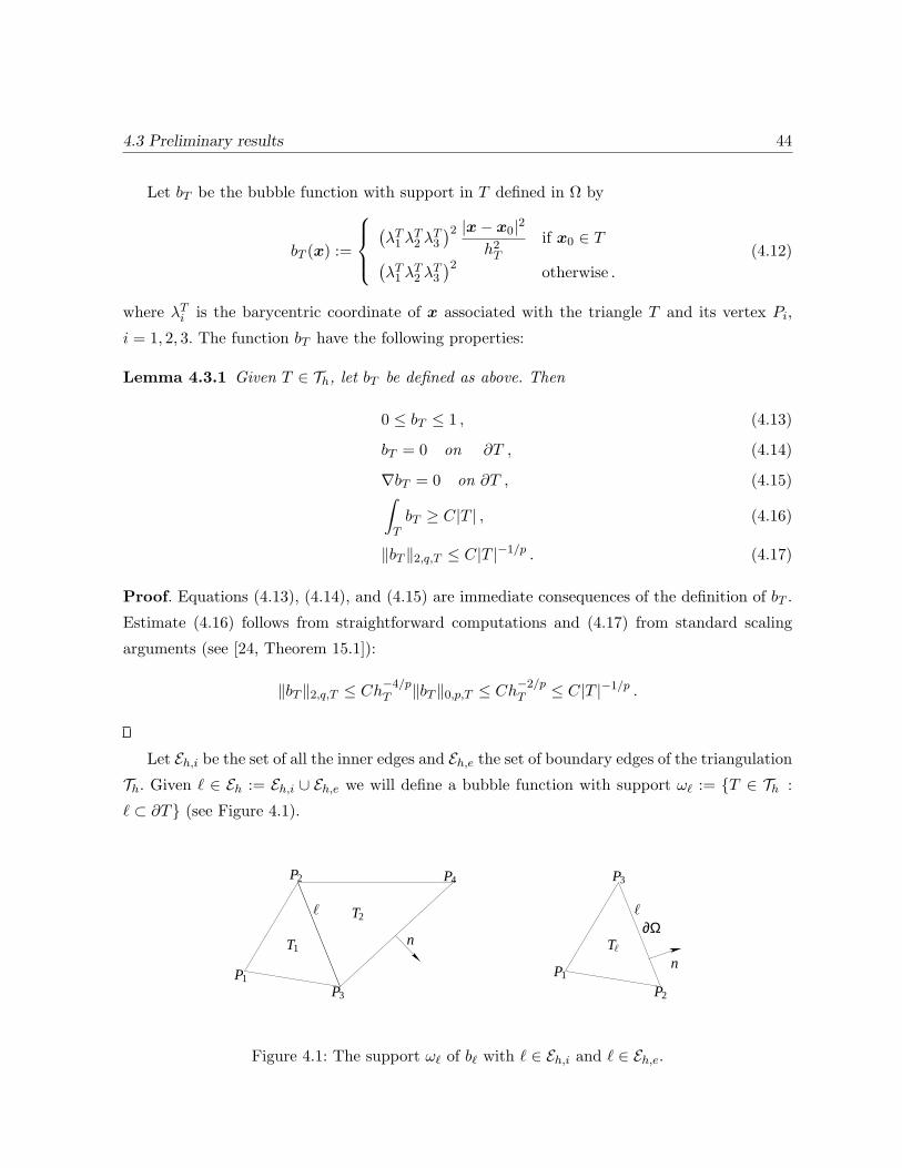
4.3 Preliminary results 44
Let bT be the bubble function with support in T defined in Ω by
bT (x) :=
(λT1 λ
T2 λ
T3
)2 |x− x0|2
h2Tif x0 ∈ T(
λT1 λT2 λ
T3
)2otherwise .
(4.12)
where λTi is the barycentric coordinate of x associated with the triangle T and its vertex Pi,
i = 1, 2, 3. The function bT have the following properties:
Lemma 4.3.1 Given T ∈ Th, let bT be defined as above. Then
0 ≤ bT ≤ 1 , (4.13)
bT = 0 on ∂T , (4.14)
∇bT = 0 on ∂T , (4.15)∫TbT ≥ C|T | , (4.16)
∥bT ∥2,q,T ≤ C|T |−1/p . (4.17)
Proof. Equations (4.13), (4.14), and (4.15) are immediate consequences of the definition of bT .
Estimate (4.16) follows from straightforward computations and (4.17) from standard scaling
arguments (see [24, Theorem 15.1]):
∥bT ∥2,q,T ≤ Ch−4/pT ∥bT ∥0,p,T ≤ Ch
−2/pT ≤ C|T |−1/p .
Let Eh,i be the set of all the inner edges and Eh,e the set of boundary edges of the triangulation
Th. Given ℓ ∈ Eh := Eh,i ∪ Eh,e we will define a bubble function with support ωℓ := T ∈ Th :
ℓ ⊂ ∂T (see Figure 4.1).
P4
T1
T2ℓ
n
P2
P3
P1
ℓ
nP1
∂ΩTℓ
P2
P3
Figure 4.1: The support ωℓ of bℓ with ℓ ∈ Eh,i and ℓ ∈ Eh,e.

4.3 Preliminary results 45
In the case ℓ ∈ Eh,i we define bℓ for x ∈ ωℓ by
bℓ(x) :=
(λT12 λ
T13 λ
T22 λ
T23
)2 |x− x0|2
|ℓ|2if x0 ∈ ωℓ(
λT12 λT13 λ
T22 λ
T23
)2if x0 ∈ ωℓ ,
(4.18)
where |ℓ| denotes the length of ℓ. Since λTji is a linear function in the whole plane, bℓ is a
polynomial in ωℓ.
It remains to define bubble functions bℓ for ℓ ∈ Eh,e, which, in particular, must satisfy
(σ∇bℓ) · n = ∇bℓ · (σn) = 0 on ℓ for all ℓ ∈ Eh,e .
Let Tℓ be the triangle in Th that contains ℓ. For simplicity we assume that x0 /∈ Tℓ. Let (xi, yi)
be the coordinates of the vertices Pi, i = 1, 2, 3, of the triangle Tℓ, as shown in Figure 4.2. Let
Fℓ : R2 → R2 be defined by
Fℓ
(x
y
)=
(x2
y2
)+Q
(x
y
)
where Q =
(x3 − x2 −(y3 − y2)
y3 − y2 x3 − x2
). Notice that Q = |ℓ|
(t −n
)(see Figure 4.2) and that
QtQ = |ℓ|2I. Hence, denoting Tℓ := F−1ℓ (Tℓ), the triangles Tℓ and Tℓ are similar (in particular,
both have the same aspect ratio). Let us set σ := Qt(σ Fℓ)Q; this matrix is symmetric
and positive definite for all (x, y) ∈ Tℓ. It is easy to show that there exists δ > 0 such that
[1/2− δ, 1/2+ δ]× (0, 2δ] is contained in the interior of Tℓ (see Figure 4.3). Since δ only depends
on the aspect ratio of the triangle Tℓ, hence of that of Tℓ, it can be bounded from above and from
below by two positive constants, uniformly with respect to h. Now let g1 ∈ D((1/2− δ, 1/2+ δ))be such that g1 ≥ 0 and
∫R g1 = 1, and let g2 ∈ C∞(R) be such that 0 ≤ g2 ≤ 1, g2|(−∞,δ) = 1,
g2|(2δ,+∞) = 0 and |g′2| ≤ Cδ−1. We first define
b(x, y) := g1(x)− g1(x)σ12(x, 0)
σ22(x, 0)g2(y) y ,
then
bℓ := b F−1ℓ |Tℓ . (4.19)
Notice that σ22(x, 0) cannot vanish because σ is positive definite. Since ∂b∂x(x, 0) = g′1(x) and
∂b∂y (x, 0) = −g1(x) σ12(x,0)σ22(x,0)
, straightforward computations allow us to show that (σn)t∇bℓ =
|ℓ|−2(σn)t∇b = 0.
Now it is easy to prove the following result for bℓ:
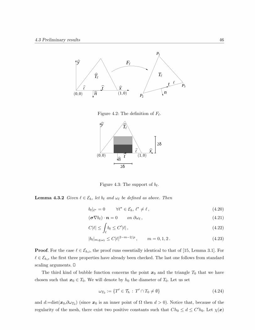
4.3 Preliminary results 46
y
n
Tℓ
(0,0)x(1,0)
tℓ
Fℓ
ℓ
n P2
P1
t P3
Tℓ
Figure 4.2: The definition of Fℓ.
(1,0)(0,0)xℓ
nt
y Tℓ
2δ
2δ
Figure 4.3: The support of bℓ.
Lemma 4.3.2 Given ℓ ∈ Eh, let bℓ and ωℓ be defined as above. Then
bℓ|ℓ∗ = 0 ∀ℓ∗ ∈ Eh, ℓ∗ = ℓ , (4.20)
(σ∇bℓ) · n = 0 on ∂ωℓ , (4.21)
C|ℓ| ≤∫ℓbℓ ≤ C ′|ℓ| , (4.22)
|bℓ|m,q,ωℓ≤ C|ℓ|2−m−2/p , m = 0, 1, 2 . (4.23)
Proof. For the case ℓ ∈ Eh,i, the proof runs essentially identical to that of [15, Lemma 3.1]. For
ℓ ∈ Eh,e the first three properties have already been checked. The last one follows from standard
scaling arguments.
The third kind of bubble function concerns the point x0 and the triangle T0 that we have
chosen such that x0 ∈ T0. We will denote by h0 the diameter of T0. Let us set
ωT0 := T ′ ∈ Th : T ′ ∩ T0 = ∅ (4.24)
and d:=dist(x0,∂ωT0) (since x0 is an inner point of Ω then d > 0). Notice that, because of the
regularity of the mesh, there exist two positive constants such that Ch0 ≤ d ≤ C ′h0. Let χ(x)

4.3 Preliminary results 47
be the convolution of the characteristic function of the set x ∈ Ω : |x − x0| < d/2 with an
appropriate mollifier, so that χ(x) = 1 if |x − x0| ≤ d/4, χ(x) = 0 if |x − x0| ≥ 3d/4 and
|∇χ(x)| ≤ Cd−1.
We define the bubble function
b0(x) := p · (x− x0)χ(x) . (4.25)
x0
d
T
d
T
x0
Figure 4.4: Two examples of ωT0 .
The support of b0 is contained in ωT0 . Moreover the following results hold true:
Lemma 4.3.3 Let b0 be defined as above. Then
∇b0(x0) = p , (4.26)
∇b0 = 0 on ∂ωT0 , (4.27)
b0(x) = p · (x− x0) ∀x ∈ Ω : |x− x0| ≤d
4, (4.28)
b0(x) = 0 ∀x ∈ Ω : |x− x0| ≥3d
4, (4.29)
|b0|m,∞,ωT0≤ Cd1−m , m = 0, 1, 2 . (4.30)
Proof. It follows from straightforward calculations. In particular, (4.30) follows by combining
that |χ|m,∞,ωT0≤ Cd−m (see [15, equation (3.8)]) with the fact that p · (x − x0) is linear and
continuous.
Corollary 4.3.1 Let b0 and ωT0 be defined as above. Then,
|b0|m,q,ωT0≤ Ch
3−m−2/p0 , m = 0, 1, 2 ,
and, for all edge ℓ,
∥b0∥0,q,ℓ ≤ C|ℓ|2−1/p .

4.4 An a posteriori error estimator 48
Proof. Using (4.30) and the fact that h0 ≤ Cd ≤ Ch0, we have
|b0|m,q,ωT0≤ |b0|m,∞,ωT0
|ωT0 |1/q ≤ Cd1−mh2/q0 ≤ Ch
3−m−2/p0 .
Moreover, using that
∥v∥0,q,∂T ≤ C∥v∥1−1/q0,q,T ∥v∥1/q1,q,T ∀v ∈W 1,q(T )
(see [20, Theorem 1.6.6]), we have
∥b0∥0,q,ℓ ≤ C∥b0∥1−1/q0,q,ωT0
∥b0∥1/q1,q,ωT0≤ C|ℓ|(3−2/p)(1−1/q)|ℓ|(2−2/p)(1/q) = C|ℓ|2−1/p .
To end this section, we recall an error estimate for the Lagrange interpolant vI ∈ Hh of a
function v ∈ C(Ω).
Lemma 4.3.4 Given ℓ ∈ Eh, let ωℓ be defined as above. There holds
∥v − vI∥0,q,ℓ ≤ C|ℓ|1+1/p|v|2,q,ωℓ∀ v ∈W 2,q(ωℓ) , 1 < q <∞ .
Proof. See, for instance, [15, Lemma 3.4].
4.4 An a posteriori error estimator
According to Remark 4.2.1 the solution of problem (4.3) belongs to Lp(Ω) with 1 ≤ p < 2.
In this section we will define an a posteriori error estimator in the Lp(Ω)-norm for the finite
element approximation error u−uh. We will prove the reliability and efficiency of the estimator
for a particular range of p. Let us emphasize that this proof holds for a regular family of meshes
and does not need the quasiuniformity assumption, so that the error estimator can be used to
drive an adaptive scheme.
For all T ∈ Th we define
εT,p :=
h2pT ∥div (σ∇uh)∥p0,p,T +1
2
∑ℓ∈E(T )∩Eh,i
|ℓ|p+1∥[[σ∇uh · n ]]∥p0,p,ℓ
+∑
ℓ∈E(T )∩Eh,e
|ℓ|p+1∥σ∇uh · n∥p0,p,ℓ
1/p
,
where E(T ) is the set of the edges of T and [[ g ]] denotes the jump of g across an edge. We define
the local a posteriori error indicator ηT,p for all T ∈ Th as follows:
ηT,p :=
(h2−p0 + εpT0,p
)1/pif T = T0 ,
εT,p otherwise .

4.4 An a posteriori error estimator 49
Next, we define the global error estimator from these indicators as follows:
ηp :=
∑T∈Th
ηpT,p
1/p
.
4.4.1 Reliability
To show that this estimator is reliable, we prove the following theorem which is based on a
duality argument as that used for Theorem 4.2.2.
Theorem 4.4.1 Let Ω be a convex Lipschitz polygon and let σi,j ∈ C1(Ω) for each i, j = 1, 2.
Let ηp be defined as above with p ∈ ( q0q0−1 , 2), where q0 > 2 is the maximal regularity exponent in
(4.6). Then, the following estimate holds true:
∥u− uh∥0,p,Ω ≤ Cηp .
Proof. Given ψ ∈ Lq(Ω), let φ ∈W 2,q(Ω) be the solution of (4.5). Proceeding as in (5.13), using
(4.4) tested with vh = φI (the Lagrange interpolant of φ), and integrating by parts, we obtain∫Ω(u− uh)ψ = −p · ∇φ(x0) +
∫Ωσ∇uh · ∇φ (4.31)
= p · (∇φI(x0)−∇φ(x0)) +
∫Ωσ∇uh · ∇(φ− φI)
= p · (∇φI(x0)−∇φ(x0))−∑T∈Th
∫Tdiv (σ∇uh)(φ− φI)
+∑ℓ∈Eh,i
∫ℓ[[σ∇uh · n ]](φ− φI) +
∑ℓ∈Eh,e
∫ℓσ∇uh · n(φ− φI) .
Using Holder inequality, Proposition 4.2.1, and Lemma 4.3.4 we estimate each term on the
right hand side as follows:
|p · ∇(φ− φI)(x0)| ≤ |p||φ− φI |1,∞,T0 ≤ Ch1−2/q0 |φ|2,q,T0 ,
∑T∈Th
∫Tdiv (σ∇uh)(φ− φI) ≤
∑T∈Th
∥div (σ∇uh)∥0,p,T ∥φ− φI∥0,q,T
≤ C∑T∈Th
h2T ∥div (σ∇uh)∥0,p,T |φ|2,q,T
≤ C
∑T∈Th
h2pT ∥div (σ∇uh)∥p0,p,T
1/p
|φ|2,q,Ω ,
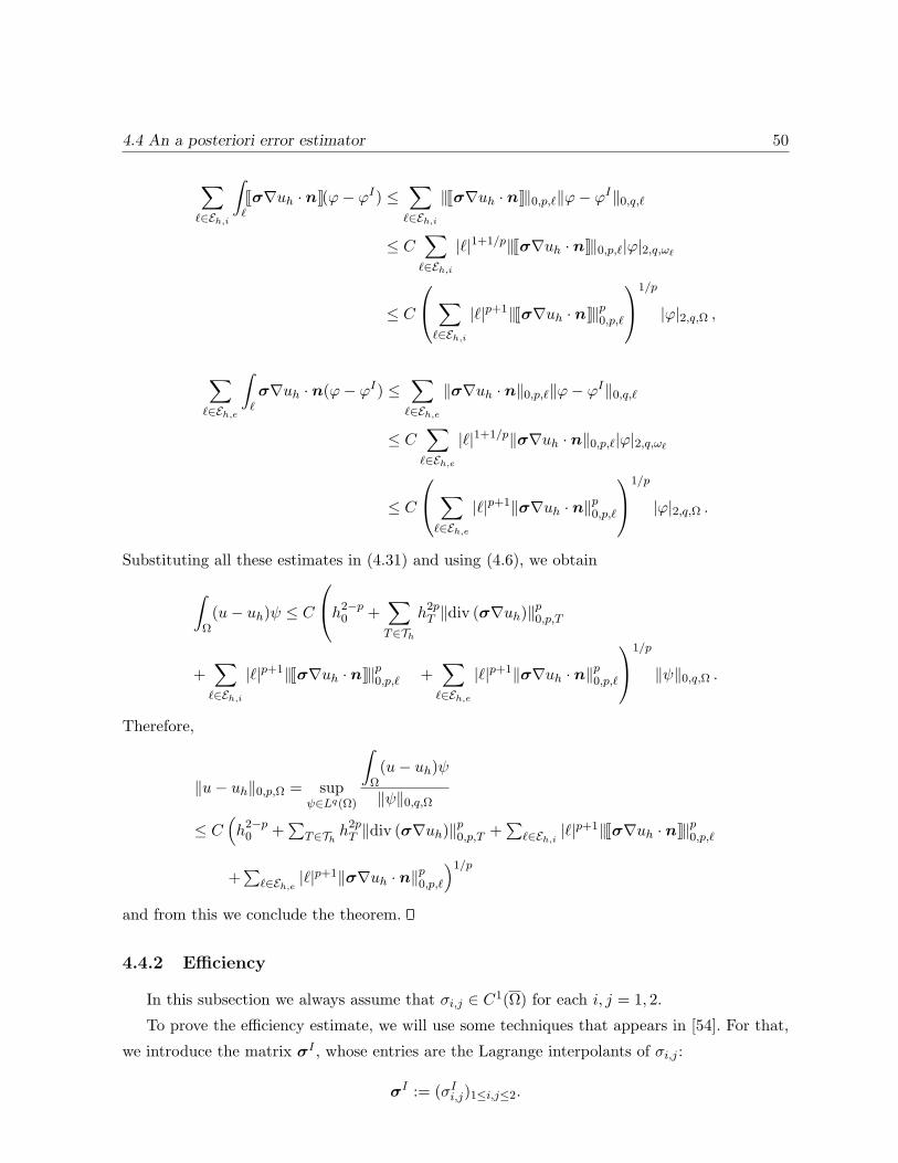
4.4 An a posteriori error estimator 50
∑ℓ∈Eh,i
∫ℓ[[σ∇uh · n ]](φ− φI) ≤
∑ℓ∈Eh,i
∥[[σ∇uh · n ]]∥0,p,ℓ∥φ− φI∥0,q,ℓ
≤ C∑ℓ∈Eh,i
|ℓ|1+1/p∥[[σ∇uh · n ]]∥0,p,ℓ|φ|2,q,ωℓ
≤ C
∑ℓ∈Eh,i
|ℓ|p+1∥[[σ∇uh · n ]]∥p0,p,ℓ
1/p
|φ|2,q,Ω ,
∑ℓ∈Eh,e
∫ℓσ∇uh · n(φ− φI) ≤
∑ℓ∈Eh,e
∥σ∇uh · n∥0,p,ℓ∥φ− φI∥0,q,ℓ
≤ C∑ℓ∈Eh,e
|ℓ|1+1/p∥σ∇uh · n∥0,p,ℓ|φ|2,q,ωℓ
≤ C
∑ℓ∈Eh,e
|ℓ|p+1∥σ∇uh · n∥p0,p,ℓ
1/p
|φ|2,q,Ω .
Substituting all these estimates in (4.31) and using (4.6), we obtain
∫Ω(u− uh)ψ ≤ C
h2−p0 +∑T∈Th
h2pT ∥div (σ∇uh)∥p0,p,T
+∑ℓ∈Eh,i
|ℓ|p+1∥[[σ∇uh · n ]]∥p0,p,ℓ +∑ℓ∈Eh,e
|ℓ|p+1∥σ∇uh · n∥p0,p,ℓ
1/p
∥ψ∥0,q,Ω .
Therefore,
∥u− uh∥0,p,Ω = supψ∈Lq(Ω)
∫Ω(u− uh)ψ
∥ψ∥0,q,Ω
≤ C(h2−p0 +
∑T∈Th h
2pT ∥div (σ∇uh)∥p0,p,T +
∑ℓ∈Eh,i |ℓ|
p+1∥[[σ∇uh · n ]]∥p0,p,ℓ
+∑
ℓ∈Eh,e |ℓ|p+1∥σ∇uh · n∥p0,p,ℓ
)1/pand from this we conclude the theorem.
4.4.2 Efficiency
In this subsection we always assume that σi,j ∈ C1(Ω) for each i, j = 1, 2.
To prove the efficiency estimate, we will use some techniques that appears in [54]. For that,
we introduce the matrix σI , whose entries are the Lagrange interpolants of σi,j :
σI := (σIi,j)1≤i,j≤2.

4.4 An a posteriori error estimator 51
The following four lemmas provide upper bounds for each term defining ηpT,p. Here and
thereafter div (·) must be understood in the following row-wise sense: (div (σ))j =∑
i∂σi,j∂xi
.
Lemma 4.4.1 The following estimate holds true:
h2pT ∥div (σ∇uh)∥p0,p,T ≤ C(∥σ∥p1,∞,T ∥u− uh∥p0,p,T + h2pT ∥[div (σ − σI)] · ∇uh∥p0,p,T
)for all T ∈ Th.
Proof. Let us consider an arbitrary T ∈ Th, the bubble function bT defined in (4.12) and the
function ψT defined in Ω as
ψT := div (σI∇uh) bT in T .
Like bT , this function is supported in T .
The fact that div (σI∇uh)|T ∈ P0, (4.16), (4.14), (4.15), and integration by parts yield
∥div (σI∇uh)∥20,p,T = |T |2/p−1∥div (σI∇uh)∥20,2,T≤ C|T |2/p−1∥b1/2T div (σI∇uh)∥20,2,T
= C|T |2/p−1
(∫Tdiv (σ∇uh)ψT +
∫Tdiv ((σI − σ)∇uh)ψT
)= C|T |2/p−1
(∫Tuhdiv (σ∇ψT ) +
∫T[div (σI − σ)] · ∇uh ψT
).
Next we notice that, since u is solution of (4.3) and ∇bT (x0) = 0, one has∫Tudiv (σ∇ψT ) = −p · ∇ψT (x0) = 0 .
Therefore, we can write
∥div (σI∇uh)∥20,p,T
≤ C|T |2/p−1
(∫T(uh − u)div (σ∇ψT ) +
∫T[div (σI − σ)] · ∇uh ψT
).
For the first term we have∣∣∣∣∫T(uh − u)div (σ∇ψT )
∣∣∣∣ ≤ 2∥u− uh∥0,p,T ∥σ∥1,∞,T ∥ψT ∥2,q,T
and, using (4.17),
∥ψT ∥2,q,T = |div (σI∇uh)|∥bT ∥2,q,T
≤ C|div (σI∇uh)||T |−1/p ≤ C∥div (σI∇uh)∥0,p,T |T |−2/p .

4.4 An a posteriori error estimator 52
For the second one,∣∣∣∣∫T[div (σI − σ)] · ∇uhψT
∣∣∣∣ ≤ ∥[div (σI − σ)] · ∇uh∥0,p,T ∥ψT ∥0,q,T
and, now using (4.13),
∥ψT ∥0,q,T ≤ C|div (σI∇uh)||T |1/q ≤ C∥div (σI∇uh)∥0,p,T |T |1/q−1/p .
Hence
∥div (σI∇uh)∥0,p,T ≤ C(h−2T ∥σ∥1,∞,T ∥u− uh∥0,p,T + ∥[div (σI − σ)] · ∇uh∥0,p,T
)from which we easily obtain the desired result.
Lemma 4.4.2 The following estimate holds true
|ℓ|p+1∥[[σ∇uh · n ]]∥p0,p,ℓ
≤ C
∥σ∥p1,∞,ωℓ∥u− uh∥p0,p,ωℓ
+∑T ′⊂ωℓ
h2pT ′∥[div (σI − σ)] · ∇uh∥p0,p,T ′
,
for all ℓ ∈ Eh,i.
Proof.
We consider an arbitrary ℓ ∈ Eh,i, the bubble function bℓ defined in (4.18) and
ψℓ := [[∇uh · n ]] bℓ in Ω .
Like bℓ, this function is supported in ωℓ.
We know that the entries of σ belong to L∞(Ω) and, therefore, we have
∥[[σ∇uh · n ]]∥0,p,ℓ ≤ C∥[[∇uh · n ]]∥0,p,ℓ = C∥[[∇uh ]]∥0,p,ℓ , (4.32)
because the jump of the tangential component of ∇uh is zero.
On the other hand, from (4.22) and the uniform positivity of σ we obtain
∥[[∇uh ]]ℓ∥20,p,ℓ = |ℓ|2/p−1∥[[∇uh ]]ℓ∥20,2,ℓ
≤ C|ℓ|2/p−1∥b1/2ℓ [[∇uh ]]ℓ∥20,2,ℓ
≤ C|ℓ|2/p−1
∫ℓbℓ [[∇uh ]]tℓσ[[∇uh ]]ℓ
= C|ℓ|2/p−1
∫ℓ[[σ∇uh · n ]]ψℓ .
(4.33)

4.4 An a posteriori error estimator 53
Taking ψℓ as a test function in (4.3), using that ∇bℓ(x0) = 0, integrating by parts, and
recalling (4.20) and (4.21), we have∫ωℓ
(u− uh)div (σ∇ψℓ) = −∑T ′⊂ωℓ
∫T ′uhdiv (σ∇ψℓ)
= −∑T ′⊂ωℓ
∫T ′
div (σ∇uh)ψℓ +∫ℓ[[σ∇uh · n ]]ψℓ .
Hence ∫ℓ[[σ∇uh · n ]]ψℓ =
∑T ′⊂ωℓ
∫T ′
div (σ∇uh)ψℓ +∫ωℓ
(u− uh)div (σ∇ψℓ)
≤ C (∥div (σ∇ψℓ)∥0,q,ωℓ∥u− uh∥0,p,ωℓ
+∑
T ′⊂ωℓ∥div (σ∇uh)∥0,p,T ′∥ψℓ∥0,q,T ′
)≤ C (∥σ∥1,∞,ωℓ
∥u− uh∥0,p,ωℓ∥ψℓ∥2,q,ωℓ
+∑
T ′⊂ωℓ∥div (σ∇uh)∥0,p,T ′∥ψℓ∥0,q,T ′
)(4.34)
From standard scaling arguments and (4.23), we have
∥ψℓ∥0,q,ωℓ≤ |[[∇uh ]]ℓ|∥bℓ∥0,q,ωℓ
≤ C∥[[∇uh ]]ℓ∥0,p,ℓ|ℓ|2−3/p (4.35)
and
∥ψℓ∥2,q,ωℓ≤ C|ℓ|−2∥ψℓ∥0,q,ωℓ
≤ C∥[[∇uh ]]ℓ∥0,p,ℓ|ℓ|−3/p . (4.36)
Hence, from (4.33) and (4.34), we write
∥[[∇uh ]]ℓ∥0,p,ℓ ≤ C|ℓ|2/p−1(|ℓ|−3/p∥σ∥1,∞,ωℓ
∥u− uh∥0,p,ωℓ
+∑
T ′⊂ωℓ|ℓ|2−3/p∥div (σ∇uh)∥0,p,T ′
)and, from (4.32),
|ℓ|p+1∥[[σ∇uh · n ]]∥p0,p,ℓ ≤ C(∥σ∥p1,∞,ωℓ
∥u− uh∥p0,p,ωℓ
+∑
T ′⊂ωℓh2pT ′∥div (σ∇uh)∥p0,p,T ′
).
We conclude the proof by using Lemma 4.4.1 to bound the last term.
Lemma 4.4.3 The following estimate holds true
|ℓ|p+1∥σ∇uh · n∥p0,p,ℓ ≤ C(∥σ∥p1,∞,Tℓ
∥u− uh∥p0,p,Tℓ + h2pTℓ∥[div (σI − σ)] · ∇uh∥p0,p,Tℓ
+|ℓ|p+1∥(σ − σℓ)∇uh · n∥p0,p,ℓ),
for all ℓ ∈ Eh,e, where σℓ is any constant matrix.

4.4 An a posteriori error estimator 54
Proof.
We consider an arbitrary ℓ ∈ Eh,e, the bubble function bℓ defined in (4.19) and
ψℓ := σℓ∇uh · n bℓ in Ω.
Like bℓ, this function is supported in Tℓ.
Since σℓ is constant and bℓ satisfies (4.22), it is easy to prove that
∥σℓ∇uh · n∥20,p,ℓ = |ℓ|2/p−1∥σℓ∇uh · n∥20,2,ℓ
≤ C|ℓ|2/p−1∥b1/2ℓ σℓ∇uh · n∥20,2,ℓ
= |ℓ|2/p−1
(∫ℓ(σℓ − σ)∇uh · nψℓ +
∫ℓσ∇uh · nψℓ
).
(4.37)
On the other hand, using that ∥ψℓ∥0,q,ℓ ≤ C|ℓ|−1/q∥ψℓ∥0,q,Tℓ and the arguments used for
proving the previous result, we obtain∫ℓ(σℓ − σ)∇uh · nψℓ ≤ C∥(σℓ − σ)∇uh · n∥0,p,ℓ|ℓ|−1/q∥ψℓ∥0,q,Tℓ
≤ C∥(σℓ − σ)∇uh · n∥0,p,ℓ|ℓ|1−2/p∥σℓ∇uh · n∥0,p,ℓand ∫
ℓσ∇uh · nψℓ =
∫Tℓ
(u− uh) div (σ∇ψℓ) +∫Tℓ
div (σ∇uh)ψℓ
≤ C(∥σ∥1,∞,Tℓ∥u− uh∥0,p,Tℓ |ℓ|−3/p
+ ∥div (σ∇uh)∥0,p,Tℓ |ℓ|2−3/p)∥σℓ∇uh · n∥0,p,ℓ.
Substituting these expressions in (4.37), we have
∥σℓ∇uh · n∥0,p,ℓ ≤ C|ℓ|2/p−1(|ℓ|−3/p∥σ∥1,∞,Tℓ∥u− uh∥0,p,Tℓ+ |ℓ|2−3/p∥div (σ∇uh)∥0,p,Tℓ
+ |ℓ|1−2/p∥(σℓ − σ)∇uh · n∥0,p,ℓ)
and, therefore,
|ℓ|p+1∥σℓ∇uh · n∥p0,p,ℓ ≤ C(∥σ∥p1,∞,Tℓ
∥u− uh∥p0,p,Tℓ + h2pTℓ∥div (σ∇uh)∥p0,p,Tℓ
+ |ℓ|p+1∥(σℓ − σ)∇uh · n∥p0,p,ℓ).
Thus, using this result, Lemma 4.4.1, and the fact that
∥σ∇uh · n∥0,p,ℓ ≤ ∥(σℓ − σ)∇uh · n∥0,p,ℓ + ∥σℓ∇uh · n∥0,p,ℓ ,
we conclude the proof.

4.4 An a posteriori error estimator 55
Lemma 4.4.4 The following estimate holds true:
h2−p0 ≤ C
∥σ∥p1,∞,ωT0∥u− uh∥p0,p,ωT0
+∑
T ′⊂ωT0
h2pT ′∥[div (σ − σI)] · ∇uh∥p0,p,T ′
.
Proof. Let E0h be the set of edges ℓ of triangles T ⊂ ωT0 , such that ℓ ⊂ ∂ωT0 . Testing equation
(4.3) with the bubble function b0 defined in (4.25), we obtain
|p|2 = p · ∇b0(x0) = −∫Ω(u− uh) div (σ∇b0)−
∫Ωuh div (σ∇b0)
≤ ∥u− uh∥0,p,ωT0∥div (σ∇b0)∥0,q,ωT0
−∑
T ′⊂ωT0
∫T ′
div (σ∇uh) b0+∑ℓ∈E0
h
∫ℓ[[σ∇uh ]]ℓ b0
≤ C(∥u− uh∥0,p,ωT0
∥σ∥1,∞,ωT0∥b0∥2,q,ωT0
+∥b0∥0,q,ωT0
∑T ′⊂ωT0
∥div (σ∇uh)∥0,p,T ′ +∑
ℓ∈E0h∥[[σ∇uh · n ]]∥0,p,ℓ∥b0∥0,q,ℓ
),
where we have used (4.26), integration by parts, and Holder inequality.
We estimate ∥b0∥2,q,ωT0, ∥b0∥0,q,ωT0
, and ∥b0∥0,q,ℓ by Corollary 4.3.1. Thus, we have
|p|2 ≤ Ch1−2/p0
∥σ∥1,∞,ωT0∥u− uh∥0,p,ωT0
+ h20∑
T ′⊂ωT0
∥div (σ∇uh)∥0,p,T ′
+∑ℓ∈E0
h
|ℓ|1+1/p∥[[σ∇uh · n ]]∥0,p,ℓ
.
Since h0 ≤ ChT ′ for each T ′ ⊂ ωT0 , this estimate together with Lemmas 4.4.1 and 4.4.2 lead to
the desired result.
Now we are in a position to conclude an efficiency estimate by collecting the previous four
lemmas. Notice that these lemmas hold true for any p ∈ (1, 2) (and not only for p ∈ ( q0q0−1 , 2) as
Theorem 4.31).
Theorem 4.4.2 Let σi,j ∈ C1(Ω) for each i, j = 1, 2. Let u and uh be the solutions of (4.3)
and (4.4), respectively. Then, for all p ∈ (1, 2) and for all T ∈ Th
ηT,p ≤ C
∥σ∥p1,∞,ωT∥u− uh∥p0,p,ωT
+∑T ′⊂ωT
h2pT ′∥[div (σI − σ)] · ∇uh∥p0,p,T ′
+∑
ℓ∈E(T )∩Eh,e
|ℓ|p+1∥(σ − σℓ)∇uh · n∥p0,p,ℓ
1/p
,
where ωT := T ′ ∈ Th : T ∩ T ′ = ∅, and for each ℓ ∈ E(T ) ∩ Eh,e, σℓ is any constant matrix.

4.4 An a posteriori error estimator 56
Notice that the last term in the estimate above vanishes for all triangles which do not intersect
∂Ω.
The above inequalities are actual efficiency estimates if we show that the terms∑T ′⊂ωT
h2pT ′∥[div (σI − σ)] · ∇uh∥p0,p,T ′ ,∑
ℓ∈E(T )∩Eh,e
|ℓ|p+1∥(σ − σℓ)∇uh · n∥p0,p,ℓ
are negligible. In what follows we will show that this holds true under some additional assump-
tions; we also note that our final result is true on the whole domain Ω (and not locally, as it
would be preferable).
Regarding the term∑
ℓ∈E(T )∩Eh,e |ℓ|p+1∥(σ−σℓ)∇uh ·n∥p0,p,ℓ, since σℓ is any arbitrary cons-
tant matrix, it clearly vanishes when σ|ℓ is already constant: namely, when the tissue on the
scalp is piecewise homogeneous, which is a realistic assumption in practice. On the other hand,
an alternative proof for Lemma 4.4.3 also holds true when the conductivity on ∂Ω is of the form
σ = σI, with σ a scalar function; namely, when the tissue of the scalp is isotropic. In fact, in
that case we have the following result.
Lemma 4.4.5 We have
|ℓ|p+1∥σ∇uh · n∥p0,p,ℓ ≤ C(∥σ∥p1,∞,Tℓ
∥u− uh∥p0,p,Tℓ + h2pTℓ∥[div (σI − σ)] · ∇uh∥p0,p,Tℓ)
for all ℓ ∈ Eh,e, provided σ|ℓ = σI, with σ : ℓ −→ R a scalar function, belonging to C1(Tℓ).
Proof. We consider an arbitrary ℓ ∈ Eh,e, the bubble function bℓ defined in (4.19) and
ψℓ := σ0∇uh · n bℓ in Ω ,
with σ0 as in (4.2). Like bℓ, this function is supported in Tℓ.
From (4.22) and (4.2), we have that∫ℓ bℓσ ≥ Cσ0|ℓ|. Using this result, we obtain
∥σ∇uh · n∥20,p,ℓ ≤ ∥σ∥20,∞,ℓ∥∇uh · n∥20,p,ℓ
= ∥σ∥20,∞,ℓ|ℓ|2/p−1|ℓ||∇uh · n|2
≤ C∥σ∥20,∞,ℓ
σ20
|ℓ|2/p−1
∫ℓσ∇uh · nψℓ .
The rest of the proof runs almost identically as that of Lemma 4.4.2, by using that
∥ψℓ∥0,q,Tℓ ≤ ∥bℓ∥0,q,Tℓ |ℓ|−1/p∥σ∇uh · n∥0,p,ℓ ≤ C|ℓ|2−3/p∥σ∇uh · n∥0,p,ℓ
and
∥ψℓ∥2,q,Tℓ ≤ C|ℓ|−2∥ψℓ∥0,q,Tℓ ≤ C|ℓ|−3/p∥σ∇uh · n∥0,p,ℓ
4.5 Three-dimensional case 57
instead of (4.35) and (4.36), respectively.
In order to prove that the term∑
T ′⊂ωTh2pT ′∥[div (σI − σ)] · ∇uh∥p0,p,T ′ in Theorem 4.4.2
is globally negligible, we proceed as in [54] and make the following additional non-degeneracy
assumption: there exists C > 0 such that
∥u− uh∥0,p,Ω ≥ Ch2. (4.38)
As explained in [54], this assumption looks quite reasonable.
In such a case we conclude with the following result.
Theorem 4.4.3 Let us assume that for each ℓ ∈ Eh,e, either σ|ℓ is a constant matrix, or
σ|ℓ = σI with σ : ℓ −→ R a scalar function. Moreover, we assume that σ ∈ [C1(Ω)]2×2 and
σ ∈ [W 2,∞(T )]2×2 for all T ∈ Th. Let u and uh be the solutions of (4.3) and (4.4), respectively.
If (4.38) holds true, then
ηp ≤ C∥u− uh∥0,p,Ω
for all p ∈ (1, 2).
Proof. It is enough to estimate the last term in the inequality of Theorem 4.4.2:∑T∈Th
∑T ′⊂ωT
h2pT ′∥[div (σI − σ)] · ∇uh∥p0,p,T ′
≤∑T∈Th
∑T ′⊂ωT
h2pT ′∥div (σI − σ)∥p0,∞,T ′∥∇uh∥p0,p,T ′
≤ C∑T∈Th
∑T ′⊂ωT
h2pT ′hpT ′∥σ∥p2,∞,T ′h
−pT ′ ∥uh∥p0,p,T ′
≤ Ch2p(maxT∈Th ∥σ∥p2,∞,ωT
)∑T∈Th
∥uh∥p0,p,ωT
≤ Ch2p(∥u− uh∥p0,p,Ω + ∥u∥p0,p,Ω)
≤ C∥u− uh∥p0,p,Ω + C∥u− uh∥p0,p,Ω∥u∥p0,p,Ω ,
where we have used (4.38) for the last inequality.
4.5 Three-dimensional case
In what follows we briefly discuss the results that are preserved in 3D. First, let us recall
that the existence and uniqueness of solution of the model problem (4.3) was proved in [65] in
the 3D case for all p ∈ [1, 3/2).
To obtain a priori and a posteriori error estimates for the numerical solution, we resort to
the auxiliary problem (4.5). The critical point is the regularity of the solution of this problem.

4.5 Three-dimensional case 58
We need that the solution belongs to W 2,q(Ω) for q > 3 (namely, q such that 1p + 1
q = 1 with
1 ≤ p < 3/2). In [30, Theorem 2] it is proved that if Ω is a cube and the conductivity σ is a
positive constant, (i.e. isotropic homogeneous material), then the solution of (4.5) belongs to
W 2,q(Ω) for all q > 1. Therefore, within this section we assume that Ω is a cube in R3 and
that σ = σI with σ a positive constant. In such a case we have the following result, that is the
analogue in the 3D case of Theorem 4.2.2.
Theorem 4.5.1 Let Th be a quasiuniform family of subdivisions of the cube Ω. Let u and uh
be the solutions to problems (4.3) and (4.4) respectively. Then the following estimate holds true
∥u− uh∥0,p,Ω ≤ Ch3/p−2 ,
for all p ∈ (1, 3/2).
Proof. The proof runs as that of Theorem 4.2.2.
The a posteriori error analysis also extends to the 3D framework. Let Fh,i be the set of all
the inner faces and Fh,e that of external faces of the mesh Th. Let Fh := Fh,i ∪ Fh,e. For all
T ∈ Th we define
εT,p :=(12
∑F∈F(T )∩Fh,i
|F |(p+3)/2|[[∇uh · nF ]]|p
+∑
F∈F(T )∩Fh,e|F |(p+3)/2|∇uh · nF |p
)1/p,
where F(T ) is the set of faces of T and |F | is the area of F .
We define the local a posteriori error indicator ηT,p for all T ∈ Th by
ηT,p :=
(h3−2p0 + εpT0,p
)1/pif T = T0 ,
εT,p otherwise ,
where h0 := hT0 , and the global error estimator from these indicators as follows:
ηp :=
∑T∈Th
ηpT,p
1/p
.
Note that, as we are assuming that σ is constant, the second and third terms that appear
in Theorem 4.4.2 vanish in the estimate of ηT,p. The following results are obtained by adapting
to the 3D framework the proofs of Theorem 4.4.1, and Lemmas 4.4.2 and 4.4.4. We have the
following result regarding the reliability of the estimator:
Theorem 4.5.2 Let u and uh be the solutions of (4.3) and (4.4), respectively. Then, the follo-
wing estimate holds true:
∥u− uh∥0,p,Ω ≤ Cηp .

4.6 Numerical experiments 59
The efficiency follows from these two lemmas:
Lemma 4.5.1 Let us set ωF := T ∈ Th : F ⊂ ∂T. The following estimates hold true:
|F |(p+3)/2|[[∇uh · nF ]]|p ≤ C∥u− uh∥p0,p,ωF, for all F ∈ Fh,i
and
|F |(p+3)/2|∇uh · nF |p ≤ C∥u− uh∥p0,p,ωF, for all F ∈ Fh,e.
Lemma 4.5.2 Let ωT0 be defined as in (4.24). Then,
h3−2p0 ≤ C∥u− uh∥p0,p,ωT0
.
Notice that no negligible higher order term appears in this case in the efficiency estimate.
Therefore, we have the following version of Theorem 4.4.3: under the more stringent assumptions
we have required, the result now holds locally on each triangle T .
Theorem 4.5.3 Let u and uh be the solutions of (4.3) and (4.4), respectively. Then
ηT,p ≤ C∥u− uh∥0,p,ωT ,
for all T ∈ Th and p ∈ (1, 3/2).
4.6 Numerical experiments
In this section we report some numerical experiments in 2D. The adaptive procedure consists
in solving problem (4.4) on a sequence of meshes up to finally attain a solution with an estimated
error within a prescribed tolerance. Each mesh is a local refinement of the previous one. We
compute the local error indicators ηT,p for all T in the ‘old’ mesh Th, and then we refine those
elements T with ηT,p ≥ θmaxηT,p : T ∈ Th, where θ ∈ (0, 1) is a prescribed parameter. In
particular we take θ = 1/2 in all our experiments.
The algorithm is implemented in a Matlab code using the mesh generator Triangle. This
generator allows creating successively refined meshes based on a hybrid Delaunay refinement
algorithm (see [64]).
4.6.1 Test 1. Isotropic constant conductivity
The first test consists of solving problem (4.4) in a regular polygon of 16 edges inscribed in a
circumference centered at (0, 0) with radius 1. The dipole is located at x0 = (0.2605,−0.3054),
the polarization is p = (−0.2425, 0.9701) and the conductivity is assumed to be the identity.

4.6 Numerical experiments 60
Since σ = 1, we can obtain an accurate solution by means of the subtraction technique. This
technique uses a particular function u0 satisfying div (σ∇u0) = div (pδx0), which is analytically
known. Subtracting u0 to the solution of problem (4.4) leads to a non-homogeneous Neumann
problem, whose solution is not singular at x0. Therefore, this problem can be accurately solved
by using standard finite elements (see [67] for more details). The solution computed by this
subtraction technique in the finest mesh of the adaptive procedure will be taken as the reference
solution, uref(x).
Figure 4.5 shows some of the successively refined meshes created in the process driven by
ηT,p with p = 1.25. Parameters “iter” and “d.o.f.” refer to the iteration number and the total
number of vertices of the corresponding mesh.
iter=1, d.o.f.= 54 iter=17, d.o.f.= 569 iter=30, d.o.f.=3.905
Figure 4.5: Test 1. Meshes obtained with ηT,p; p = 1.25.
iter=30, d.o.f.=3.905
Figure 4.6: Test 1. Zooms of the mesh for iter=30.
Figure 4.6 shows two successive zooms around the singularity of the finer mesh in Figure
4.5. Each figure is a 200% zoom of the previous one. It can be appreciated that the mesh is
extremely refined in the neighborhood of the singular point. Such a behavior can be expected
from the singularity of the solution at x0, which can be seen from Figure 4.7, which shows the
computed solution on some of the coarser meshes. (Notice that the vertical scales are different
on each subfigure.)

4.6 Numerical experiments 61
iter=1 iter=3
−1
−0.5
0
0.5
1
−1
−0.5
0
0.5
1−1.5
−1
−0.5
0
0.5
1
1.5
−1
−0.5
0
0.5
1
−1
−0.5
0
0.5
1−4
−3
−2
−1
0
1
2
3
4
iter=7 iter=19
−1
−0.5
0
0.5
1
−1
−0.5
0
0.5
1−15
−10
−5
0
5
10
15
−1
−0.5
0
0.5
1
−1
−0.5
0
0.5
1−8000
−6000
−4000
−2000
0
2000
4000
6000
8000
Figure 4.7: Test 1. Approximate solutions on some coarser meshes.
This extremely singular behavior is the reason why the adaptively created meshes are so
localized. This can be appreciated in Figure 4.8, which contains two graphs. The one on the
left shows the plot of the discrete solution corresponding to the different meshes on the segment
x = x0 + tp, t ∈ [−0.002, 0.002]. The right subfigure is a zoom of previous the plot.
The behavior of the (absolute) error along the adaptive process can be seen from Figure 4.9.
We report log-log plots of the estimated error and the “reference error” versus the number of
degrees of freedom. The “reference error” is computed by comparing the solution of problem
(4.4) with the reference solution. The figure also shows a line of slope −1 which corresponds to
the optimal order of convergence for the finite elements used. It can be seen that the estimated
and the reference errors both attain this optimal order.
In Table 4.1 we compare the reference (relative) error for the solution of problem (4.4)
computed using adapted meshes and a quasiuniform mesh with approximately the same number
of nodes (5780). It can be seen that, to obtain a solution with an error around 5 %, the number
of d.o.f. in the uniform mesh is 40 times the number of d.o.f. in the adapted mesh. Moreover,
with almost the same number of d.o.f., the adaptive algorithm yields a computed solution with
an error 50 times smaller than the one obtained with a uniform mesh.
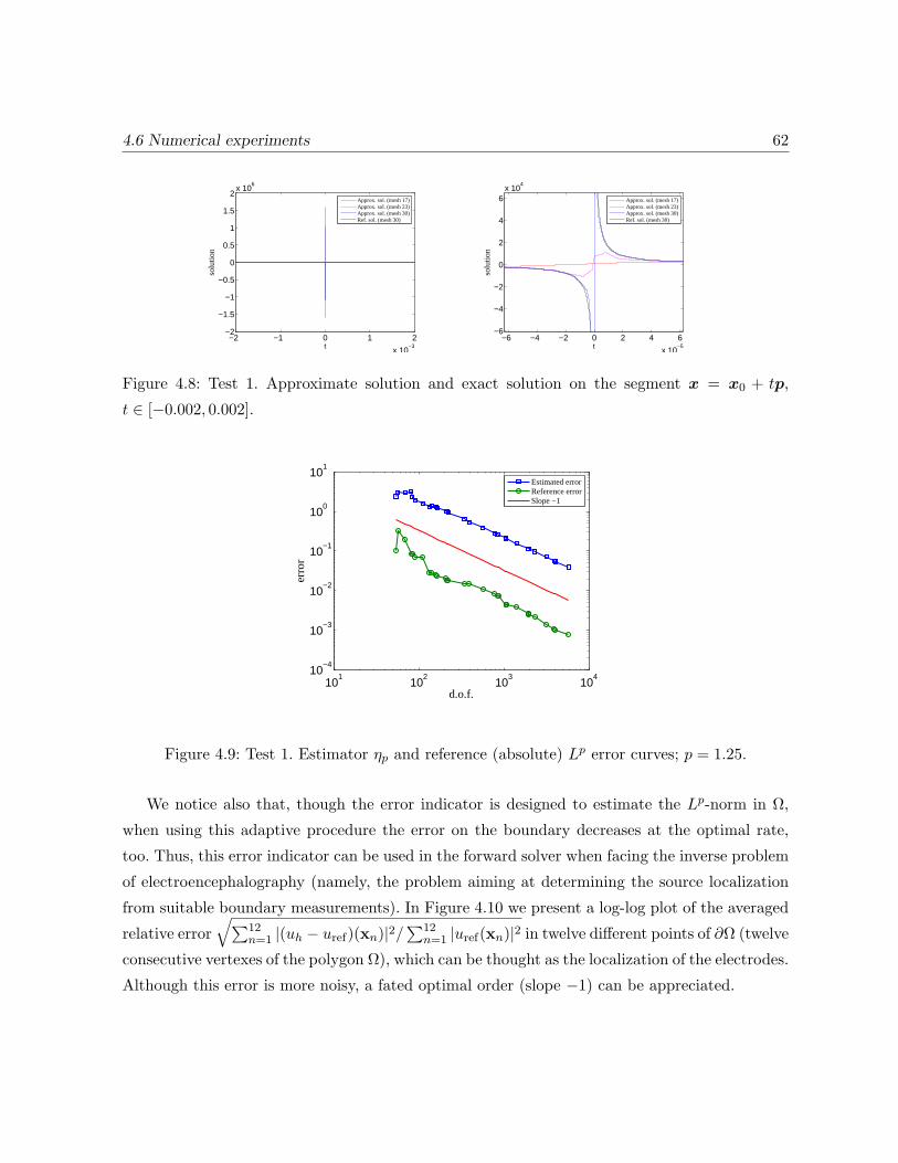
4.6 Numerical experiments 62
−2 −1 0 1 2
x 10−3
−2
−1.5
−1
−0.5
0
0.5
1
1.5
2x 10
6
solu
tion
t
Approx. sol. (mesh 17)Approx. sol. (mesh 23)Approx. sol. (mesh 30)Ref. sol. (mesh 30)
−6 −4 −2 0 2 4 6
x 10−5
−6
−4
−2
0
2
4
6x 10
4
solu
tion
t
Approx. sol. (mesh 17)Approx. sol. (mesh 23)Approx. sol. (mesh 30)Ref. sol. (mesh 30)
Figure 4.8: Test 1. Approximate solution and exact solution on the segment x = x0 + tp,
t ∈ [−0.002, 0.002].
101
102
103
104
10−4
10−3
10−2
10−1
100
101
erro
r
d.o.f.
Estimated errorReference errorSlope −1
Figure 4.9: Test 1. Estimator ηp and reference (absolute) Lp error curves; p = 1.25.
We notice also that, though the error indicator is designed to estimate the Lp-norm in Ω,
when using this adaptive procedure the error on the boundary decreases at the optimal rate,
too. Thus, this error indicator can be used in the forward solver when facing the inverse problem
of electroencephalography (namely, the problem aiming at determining the source localization
from suitable boundary measurements). In Figure 4.10 we present a log-log plot of the averaged
relative error√∑12
n=1 |(uh − uref)(xn)|2/∑12
n=1 |uref(xn)|2 in twelve different points of ∂Ω (twelve
consecutive vertexes of the polygon Ω), which can be thought as the localization of the electrodes.
Although this error is more noisy, a fated optimal order (slope −1) can be appreciated.

4.6 Numerical experiments 63
Degrees of freedom Lp relative error
Adapted mesh 9 141 0.4368 10−1
Adapted mesh 32 5794 0.1152 10−2
Quasiuniform mesh 5780 0.5508 10−1
Table 4.1: Test 1. The Lp relative error for p = 1.25 in three different meshes
101
102
103
104
10−5
10−4
10−3
10−2
10−1
100
erro
r
d.o.f.
Point wise errorSlope −1
Figure 4.10: Test 1. Averaged relative error at boundary points.
4.6.2 Test 2. Anisotropic non-constant conductivity
In the second test, Ω is a square centered at (0, 0) with side-length 2. The dipole is located
at x0 = (−0.25000,−0.08333), and the polarization is p = (0.9015, 0.4327). We consider a
non-constant anisotropic conductivity
σ =
(4x2 + 1 0
0 2y2 + 1
).
The results are very similar to those of the previous example. Figure 4.11 contains the meshes
corresponding to three different iterations of the adaptive scheme and Figure 4.12 shows two
successive zooms around the singularity.
We report in Figure 4.13 a log-log plot of the estimated error versus the number of degrees
of freedom. The slope is close to −1 which confirms the success of the approach. In this case
we have not a reference solution because the subtracting approach can not be used in this case,
since the conductivity is not constant around the point where the source is located.

4.6 Numerical experiments 64
iter=1, d.o.f.= 41 iter=18, d.o.f.= 785 iter=28, d.o.f.=3786
Figure 4.11: Test 2. Meshes obtained with ηT,p; p = 1.25.
iter=28, d.o.f.=3786
Figure 4.12: Test 2. Zooms of the mesh for iter=28.
4.6.3 Test 3. Anisotropic constant conductivity
Finally, we consider a strongly anisotropic conductivity: σ =
(10 0
0 0.1
). The domain Ω
is a square centered at (0, 0), with side-length 2. The dipole is located at x0 = (0, 0) and the
polarization is p = (1, 1). Since the conductivity is constant, as in the first test we can compute
the reference solution using the subtraction approach.
We show in Figure 4.14 the meshes corresponding to three different iterations of the adap-
tive scheme. Figure 4.15 shows two successive zooms around the singularity of the finest mesh
considered (iter=45, d.o.f.=4168).
It can be clearly seen that in this case the meshes are not only refined around the singular
point. The reason for this is that, because of the anisotropy of the conductivity, the solution
has an inner layer at x2 = 0. In fact, the fundamental solution (which is the only source of
singularity) reads in this case
u0(x) =1
2π
x1 + 100x2x21 + 100x22
.
Therefore, it is easy to check that the slope of the graph in the x2-direction is approximately 100x21
at x2 = 0. This can be seen from Figure 4.16, which shows the plot of the fundamental solution

4.6 Numerical experiments 65
101
102
103
104
10−3
10−2
10−1
100
101
erro
r
d.o.f.
Estimated errorSlope −1
Figure 4.13: Test 2. Estimator ηp curve; p = 1.25.
iter=1, d.o.f.= 41 iter=15, d.o.f.= 257 iter=30, d.o.f.= 1124
Figure 4.14: Test 3. Meshes obtained with ηT,p; p = 1.25.
in a uniform mesh with 8321 vertices.
We notice from Figure 4.17 that the computed order of convergence is not optimal in this
example. In fact, the fitted slope is close to −0.57. Very likely, the reason for this suboptimal
order is that our adaptive scheme only uses regular meshes, while appropriate anisotropic meshes
seem to be necessary around the inner layer. Nevertheless, the use of our adaptive procedure
turns out to be convenient, as can be seen by comparison with the results obtained with uniform
refinement (see Table 4.2).

4.6 Numerical experiments 66
iter=45, d.o.f.= 4168
Figure 4.15: Test 3. Zooms of the mesh around the singular point for iter=45.
−1
−0.5
0
0.5
1
−1
−0.5
0
0.5
1−30
−20
−10
0
10
20
Figure 4.16: Test 3. Fundamental solution.
101
102
103
104
10−1
100
101
102
erro
r
d.o.f.
Estimated errorReference errorSlope−0.56786
Figure 4.17: Test 3. Lp (absolute) error
curves for p = 1.25: estimated and refer-
ence error on adapted meshes.
Degrees of freedom Lp relative error
Adapted mesh 15 257 0.7217 10−1
Adapted mesh 38 2118 0.3007 10−1
Quasiuniform mesh 2113 0.7417 10−1
Table 4.2: Test 3. The Lp relative error for p = 1.25 in three different meshes.

Chapter 5
Numerical behavior of different
approximation methods for the
direct and inverse problems of
electrostatics with a dipole source
5.1 Introduction
It is common practice in cognitive research to reconstruct current sources in the human
brain by means of their electric potentials, measured with electrodes which are fixed on the
scalp (EEG).
Electromagnetic activity of the brain is due to the motion of ions in the active regions of
the brain. This movement generates the so called impressed current (or primary currents) that
in turn create ohmic currents in the surrounding environment calls return currents. We are
interested in determining the impressed current.
The reconstruction of the position and of some physical characteristics of the current density
that has given rise to the EEG measurements is called the inverse problem. For an accurate
reconstruction of the primary current it is important to be able to realistically model tissue
conductivity inhomogeneities.
In this chapter we present a series of numerical computations in order to compare different
methods used for the approximation of the direct and inverse problem when the conductivity is
not continuous across the interface of the different tissues (we recall that this is the case in the
real physiological situation). We study in particular the case of a dipolar source located close to
67

5.1 Introduction 68
the interface between two regions with different conductivities.
The obtained results have to be seen as a first step towards a better understanding of which
is the most accurate procedure to use in this context.
We start introducing the equations.
5.1.1 Continuous problem
In almost all the studies concerning the neural generation of electromagnetic fields the static
approximation of Maxwell equations is considered
divD = ρ ,
curlE = 0 ,
curlH = J ,
divB = 0 ,
(5.1)
where E and D are the electric field and electric displacement, respectively, ρ the electric field
charge density and J is the electric current density. By H and B we denote the magnetic field
and the magnetic induction, respectively.
For biological tissues, the linear constitutive equationsD = εE andB = µH can be assumed
(see Plonsey and Heppner [57]), where ε and µ correspond to the electric permittivity and the
magnetic permeability, respectively. It can be assumed that µ is constant over the whole space
and equal to the permeability of vacuum [61].
From second equation of (5.1), we conclude that there exists a scalar potential u such that
E = −∇u. From Ohm law the total current density J is the sum of the impressed currents plus
the return currents
J = Jp + σE = Jp − σ∇u ,
where σ is the conductivity, which is a uniformly positive definite matrix with entries in L∞.
From the third equation in (5.1) it follows that
0 = divJ = div (Jp − σ∇u) .
Hence u is solution of the equation
div (σ∇u) = divJp ,
Let Ω be an open connected bounded set with Lipschitz continuous boundary ∂Ω included
in Rd, where d = 2 or d = 3 (Ω represents the human head). We assume that Jp is supported

5.1 Introduction 69
in Ω. Since J · n|Ω = J · n|Rd\Ω = 0 and Jp · n = 0 on the interface ∂Ω, then (σ∇u) · n = 0 on
∂Ω. We define n to be the outer unit normal vector on ∂Ω. Then, we obtain this problem:div (σ∇u) = div (Jp) in Ω ,
(σ∇u) · n = 0 on ∂Ω .(5.2)
Let us assume that a small activated region is centered at a point x0 and that the observation
point is far from it. In this case the primary current Jp is typically modeled as a dipole. So, in the
following, we consider the electrostatic problem with a dipole as source term and homogeneous
Neumann boundary condition:div (σ∇u) = div (pδx0) in Ω ,
(σ∇u) · n = 0 on ∂Ω .(5.3)
where x0 is an inner point of Ω, and p = 0 is the polarization vector. In [65] the existence and
uniqueness of solution u ∈ Lp(Ω), 1 ≤ p < 3/2 of this problem has been studied under of the
assumption of more regularity of σ in a vecinity of x0 and d = 3. We give more details later on.
The singularity of the dipole source can also be trated using the so-called subtraction ap-
proach. We explain in more detail this technique below. We need to assume that there exists a
nonempty open subdomain Ω0 ⊂ Ω around the source position x0 with constant conductivity
σ0 (in general, a matrix). The conductivity σ is then split into two parts,
σ = σ0 + σs , (5.4)
so that σ0 is constant over the whole domain Ω and σs is zero in the subdomain Ω0, i.e.,
σs(x) = 0 for all x ∈ Ω0. The total potential u can be split into two parts,
u = u0 + us, (5.5)
where u0 denotes the solution in a infinity homogeneous conductor. The potential u0 satisfies
div (σ0∇u0) = div (pδx0) in Rd . (5.6)
An analytic formula for u0 in the case of a homogeneous and isotropic conductivity σ0 = σ0I,
σ0 ∈ R is
u0(x) =
⟨p, (x− x0)⟩2πσ0|x− x0|2
if d = 2 ,
⟨p, (x− x0)⟩4πσ0|x− x0|3
if d = 3 .
When the conductivity σ0 is homogeneous and anisotropic (namely, σ0 is a constant matrix),
we find

5.1 Introduction 70
u0(x) =
⟨p, (σ0)
−1(x− x0)⟩
2π√detσ0 ⟨(σ0)−1(x− x0), (x− x0)⟩
if d = 2 ,⟨p, (σ0)
−1(x− x0)⟩
4π√detσ0 ⟨(σ0)−1(x− x0), (x− x0)⟩3/2
if d = 3 .
Replacing (5.4), (5.5) in (5.3) and using that u0 satisfies (5.6) , we obtain
div [(σ0 + σs)∇(u0 + us)] = div (pδx0) = div (σ0∇u0) ,
and hence,
div (σ∇us) = div [(σ0 + σs)∇us] = −div (σs∇u0) .
On the other hand, since
0 = (σ∇u) · n = (σ∇(u0 + us)) · n on ∂Ω ,
then we obtain the Neumann boundary condition:
(σ∇us) · n = −(σ∇u0) · n on ∂Ω .
In conclusion u0 is known and us solves the boundary value problemdiv (σ∇us) = −div (σs∇u0) in Ω ,
(σ∇us) · n = −(σ∇u0) · n on ∂Ω ,∫Ωus = 0 .
(5.7)
The last condition of (5.7) filters out additive constants and therefore is suitable for assuring
uniqueness of the solution us.
The goal of the reformulation using the explicit representation of u0 is to obtain a problem
with a more regular source, eliminating the singularity at x0: notice that the potential u0 has
a singularity at x = x0 but it is smooth for x = x0. Therefore, the Neumann datum in (5.7) is
smooth and moreover, σs vanishes in Ω0 which implies that σs∇u0 ∈ L∞(Ω).
An alternative approach is the direct method studied by Valli in [65] (d = 3) and also in the
previous chapter of this thesis (d = 2). Notice that to prove that the following weak formulation
has a unique solution, it is necessary to assume that there exists r0 > 0 such that the entries
of σ belong to W 1,∞(Br0(x0)), where Br0(x0) := x ∈ Rd : |x− x0| < r0. We recall the weak
formulation: find u ∈ Lp(Ω) such that∫Ωudiv (σ∇φ) = −p · ∇φ(x0) ∀φ ∈ Xq ,∫
Ωu = 0 ,
(5.8)
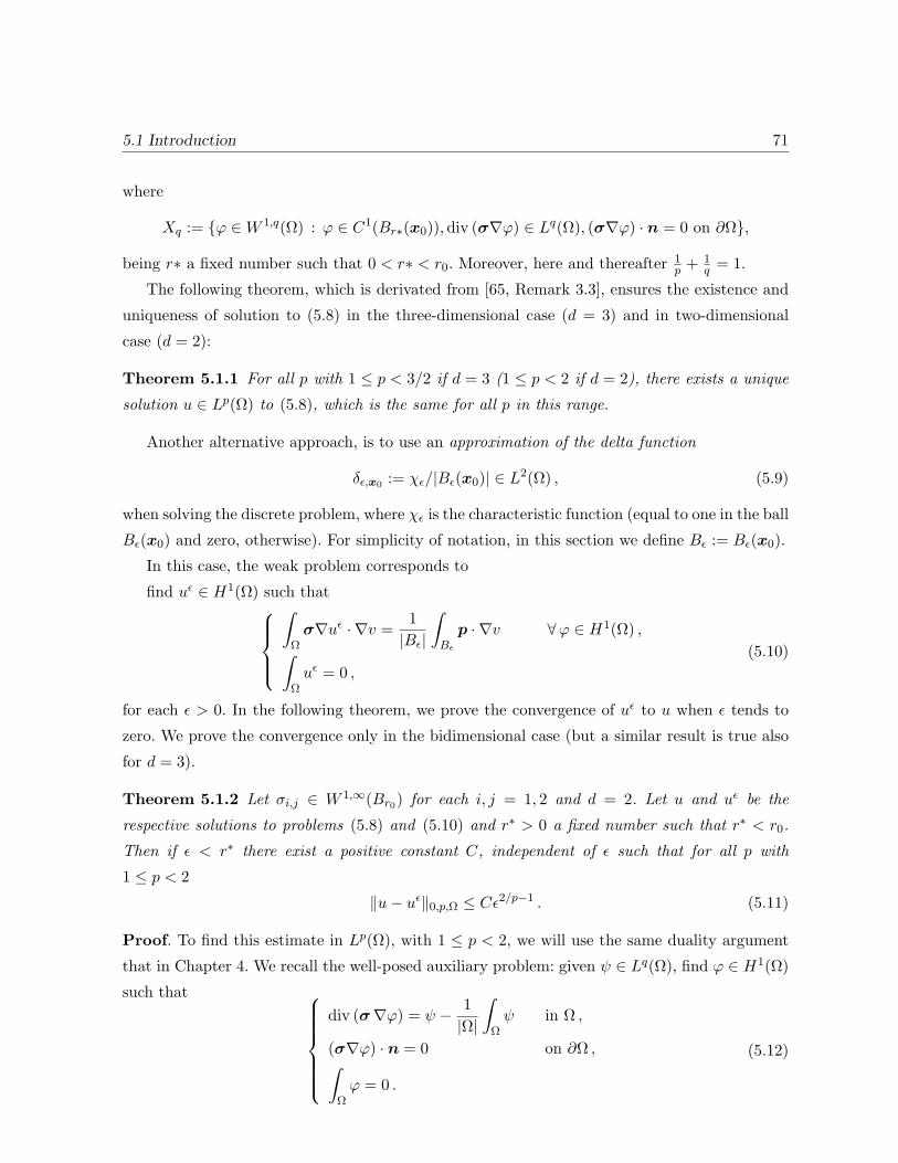
5.1 Introduction 71
where
Xq := φ ∈W 1,q(Ω) : φ ∈ C1(Br∗(x0)), div (σ∇φ) ∈ Lq(Ω), (σ∇φ) · n = 0 on ∂Ω,
being r∗ a fixed number such that 0 < r∗ < r0. Moreover, here and thereafter 1p +
1q = 1.
The following theorem, which is derivated from [65, Remark 3.3], ensures the existence and
uniqueness of solution to (5.8) in the three-dimensional case (d = 3) and in two-dimensional
case (d = 2):
Theorem 5.1.1 For all p with 1 ≤ p < 3/2 if d = 3 (1 ≤ p < 2 if d = 2), there exists a unique
solution u ∈ Lp(Ω) to (5.8), which is the same for all p in this range.
Another alternative approach, is to use an approximation of the delta function
δϵ,x0 := χϵ/|Bϵ(x0)| ∈ L2(Ω) , (5.9)
when solving the discrete problem, where χϵ is the characteristic function (equal to one in the ball
Bϵ(x0) and zero, otherwise). For simplicity of notation, in this section we define Bϵ := Bϵ(x0).
In this case, the weak problem corresponds to
find uϵ ∈ H1(Ω) such that∫Ωσ∇uϵ · ∇v =
1
|Bϵ|
∫Bϵ
p · ∇v ∀φ ∈ H1(Ω) ,∫Ωuϵ = 0 ,
(5.10)
for each ϵ > 0. In the following theorem, we prove the convergence of uϵ to u when ϵ tends to
zero. We prove the convergence only in the bidimensional case (but a similar result is true also
for d = 3).
Theorem 5.1.2 Let σi,j ∈ W 1,∞(Br0) for each i, j = 1, 2 and d = 2. Let u and uϵ be the
respective solutions to problems (5.8) and (5.10) and r∗ > 0 a fixed number such that r∗ < r0.
Then if ϵ < r∗ there exist a positive constant C, independent of ϵ such that for all p with
1 ≤ p < 2
∥u− uϵ∥0,p,Ω ≤ Cϵ2/p−1 . (5.11)
Proof. To find this estimate in Lp(Ω), with 1 ≤ p < 2, we will use the same duality argument
that in Chapter 4. We recall the well-posed auxiliary problem: given ψ ∈ Lq(Ω), find φ ∈ H1(Ω)
such that div (σ∇φ) = ψ − 1
|Ω|
∫Ωψ in Ω ,
(σ∇φ) · n = 0 on ∂Ω ,∫Ωφ = 0 .
(5.12)
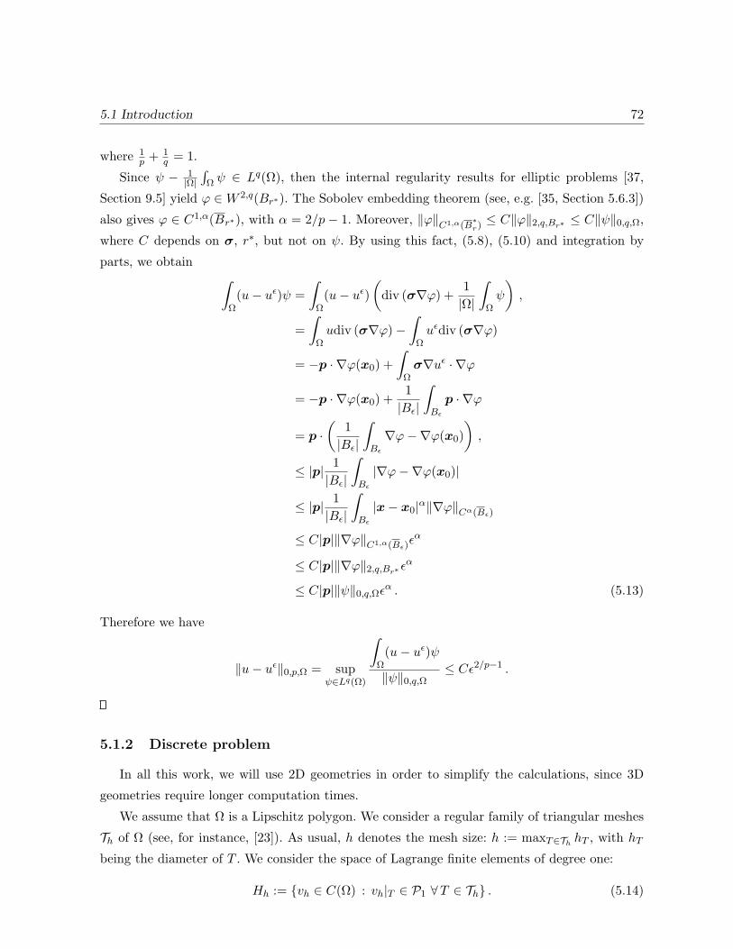
5.1 Introduction 72
where 1p +
1q = 1.
Since ψ − 1|Ω|∫Ω ψ ∈ Lq(Ω), then the internal regularity results for elliptic problems [37,
Section 9.5] yield φ ∈W 2,q(Br∗). The Sobolev embedding theorem (see, e.g. [35, Section 5.6.3])
also gives φ ∈ C1,α(Br∗), with α = 2/p− 1. Moreover, ∥φ∥C1,α(B∗r)
≤ C∥φ∥2,q,Br∗ ≤ C∥ψ∥0,q,Ω,where C depends on σ, r∗, but not on ψ. By using this fact, (5.8), (5.10) and integration by
parts, we obtain ∫Ω(u− uϵ)ψ =
∫Ω(u− uϵ)
(div (σ∇φ) + 1
|Ω|
∫Ωψ
),
=
∫Ωudiv (σ∇φ)−
∫Ωuϵdiv (σ∇φ)
= −p · ∇φ(x0) +
∫Ωσ∇uϵ · ∇φ
= −p · ∇φ(x0) +1
|Bϵ|
∫Bϵ
p · ∇φ
= p ·(
1
|Bϵ|
∫Bϵ
∇φ−∇φ(x0)
),
≤ |p| 1
|Bϵ|
∫Bϵ
|∇φ−∇φ(x0)|
≤ |p| 1
|Bϵ|
∫Bϵ
|x− x0|α∥∇φ∥Cα(Bϵ)
≤ C|p|∥∇φ∥C1,α(Bϵ)ϵα
≤ C|p|∥∇φ∥2,q,Br∗ ϵα
≤ C|p|∥ψ∥0,q,Ωϵα . (5.13)
Therefore we have
∥u− uϵ∥0,p,Ω = supψ∈Lq(Ω)
∫Ω(u− uϵ)ψ
∥ψ∥0,q,Ω≤ Cϵ2/p−1 .
5.1.2 Discrete problem
In all this work, we will use 2D geometries in order to simplify the calculations, since 3D
geometries require longer computation times.
We assume that Ω is a Lipschitz polygon. We consider a regular family of triangular meshes
Th of Ω (see, for instance, [23]). As usual, h denotes the mesh size: h := maxT∈Th hT , with hT
being the diameter of T . We consider the space of Lagrange finite elements of degree one:
Hh := vh ∈ C(Ω) : vh|T ∈ P1 ∀T ∈ Th . (5.14)

5.1 Introduction 73
The finite element approximation of the solution of (5.7) reads: find us,h ∈ Hh such that∫Ωσ∇us,h · ∇vh = −
∫Ωσs∇u0 · ∇vh −
∫∂Ω
σ0∇u0 · n vh ∀ vh ∈ Hh ,∫Ωus,h = 0 ,
(5.15)
In [67] the convergence of us,h to us has been studied.
The finite element approximation of the direct method reads: find uh ∈ Hh such that∫Ωσ∇uh · ∇vh = p · ∇(vh|T0)(x0) ∀ vh ∈ Hh ,∫
Ωuh = 0 ,
(5.16)
where T0 is any triangle that contains x0. In this case, we have proved an a priori error estimate
in Chapter 4, under certain assumptions:
Theorem 5.1.3 Let Th be a quasiuniform family of subdivisions of the convex Lipschitz polygon
Ω and assume that σi,j ∈ C1(Ω) for each i, j = 1, 2. Let u and uh be the respective solutions to
problems (5.8) and (5.16). Then there exists h0 > 0 such that
∥u− uh∥0,p,Ω ≤ Ch2/p−1
for all 0 < h < h0 and for all p such that q0q0−1 < p < 2, where q0 is the maximal regularity
exponent such that the solution φ of problem (5.12) belongs to W 2,q(Ω), and moreover satisfies
∥φ∥2,q,Ω ≤ C∥ψ∥0,q,Ω, with 2 < q < q0.
In the case of the approximation of the delta (5.9), we have the following discrete problem:
find uϵh ∈ Hh such that∫Ωσ∇uϵh · ∇vh =
1
|Bϵ|
∫Bϵ
p · ∇vh ∀ vh ∈ Hh ,∫Ωuϵh = 0 ,
(5.17)
for each ϵ > 0. To give an a priori error estimate of this problem, we need to assume that Ω
is a convex Lipschitz polygon, σi,j ∈ C1(Ω), i, j = 1, 2, and more regularity of the source used.
Let δϵ,x0 be a smoothing of δϵ,x0 |Bϵ to Ω with support in Bϵ. Then, δϵ,x0 is globally smooth and
therefore, div (pδϵ,x0) ∈ L∞(Ω). The solutions of the problems (5.10) and (5.17) with source
div (pδϵ,x0) will be called uϵ and uϵh respectively. It is known that in this case, uϵ ∈ H2(Ω), for
each ϵ > 0 and therefore, ∥uϵ − uϵh∥0,Ω ≤ Ch2∥uϵ∥2,Ω, for each ϵ > 0. We are interested in to
show that uϵh is converging to u. The following theorem give us an a priori error estime in this
case.

5.1 Introduction 74
Theorem 5.1.4 Let Ω be a convex Lipschitz polygon and σi,j ∈ C1(Ω) for each i, j = 1, 2. Let
u and uϵh be the respective solutions to problems (5.8) and the problem (5.17), respectively. The
last one, computed with sourse div (pδϵ,x0). Then for each η > 0 there exist ϵ0(η) and h0(η) such
that
∥u− uϵ0h ∥0,p,Ω ≤ η , ∀h < h0(η) .
Proof. From Theorem 5.1.2 and the results above, we know that ∥u − uϵ∥0,p,Ω ≤ Cϵ2/p−1
and ∥uϵ − uϵh∥0,Ω ≤ Ch2∥uϵ∥2,Ω, for each ϵ > 0. Given η > 0 we can choose ϵ0 = ϵ0(η) such
that ∥u − uϵ0∥0,p,Ω ≤ Cϵ2/p−10 < η/2 and ∥uϵ0 − uϵ0h ∥0,Ω ≤ Ch2∥uϵ0∥2,Ω. Also, we can choose
h0 = h0(η) such that ∥uϵ0 − uϵ0h0∥0,Ω ≤ Ch20∥uϵ0∥2,Ω ≤ η/2. Then, using that ∥u − uϵ0h ∥0,p,Ω ≤∥u− uϵ0∥0,p,Ω + ∥uϵ0 − uϵ0h ∥0,p,Ω and the fact that L2(Ω) ⊂ Lp(Ω), 1 ≤ p < 2, we conclude that
for each h < h0(η) we have that ∥u− uϵ0h ∥0,p,Ω ≤ η
Notice that to have uniqueness of the problem we can change the second condition in problems
(5.15), (5.16) and (5.17). It is enough to set equal to zero the value of the potential u in a point.
This new assumption simplifies the computations at computational level. We will consider a
reference electrode with given potential, i.e.,
u(xref ) = 0 .
Moreover, this is a realistic condition since EEG measures electric potential differences respect
to a fix electrode.
Notice that, in order to prove existence and uniqueness of solution, in all the preciding
sections we have required some regularity of σ in a vicinity of x0. If σ is piecewise regular and
x0 is on the interface between two regions with different conductivities, we do not know how to
formulate the problem in a suitable variational way.
In this chapter we study experimentally the behavior of the methods when x0 tends to the
interface. The direct approach and the characteristic function approach are well defined if σ
is piecewise constant; however, we have not a proof of the convergence of the corresponding
finite element solutions. The characteristic function approach is well defined also for x0 on the
interface. Let us also recall that the error bound in the subtraction approach deteriorates when
x0 tends to the interface (see [67]).
In Section 5.2 we show that the solution computed with the direct method is more stable
than the one computed with the subtraction approach. We also consider the case when x0 is
on the interface. We use the characteristic function approach (the only one that is well defined
in this situation) and we study the behavior when ϵ tends to zero. In Section 5.3 we study the
inverse source problem. Also in this case σ is piecewise regular. We analyze the results obtained
using the three methods and also the adaptive procedure studied in Chapter 4. We consider

5.2 General considerations for x0 on the interface between two regions with differentconductivities 75
two different situations: a source internal to a regular region and a source close to the interface
between two regions. In Section 5.4 we study the case of a distributed source and we compare
the lead field matrices in different situations. Also here we are interested in the case when σ is
piecewise regular. We analyze the results obtained using the methods already presented and two
other methods that will be introduced in the same section. We consider the same two situations
that in the previous section: a source completely contained in a regular region and a source close
to the interface between two regions with different conductivities. Finally, in Section 5.5 we give
some conclusions.
5.2 General considerations for x0 on the interface between two
regions with different conductivities
The aim of this section is to investigate the behavior of the different approximation methods,
when the source is located very close to the interface between two different regions.
The subtraction method requires to assume that around the source position x0 we can find a
nonempty open subdomain Ω0 ⊂ Ω with homogeneous constant conductivity σ0. This technique
has showed to give good results when one solves the inverse problem in a point internal to a
regular region [67]. However, if x0 is a point on the interface between two regions with differents
conductivities, the fundamental solution cannot be used, and therefore the subtraction technique
is not well defined.
Also the solution obtained by means of the direct method has a good behavior when x0 is an
internal point. However, when the point belongs to an interface, it does not seem to be reliable,
as it has a different behavior if we take a sequence of locations x0,k converging to x0 from one
side or from the other. An alternative in such case is to consider an approximation of the delta
function. In particular, we consider (5.9). This approximation is independent of the mesh, and
is well-defined even when x0 lies on the interface.
The first experiment is performed in order to obtain information on what is happening to
the solution obtained by using the subtraction method or the direct method for x0,k tending
to x0 on an interface. In a second test, we analyze the behavior of the characteristic function
approach when x0 is exactly on the interface, considering differents choices of the side-length of
the square where this function is supported.
5.2.1 Test 1.
This experiment consists in taking two sequences of seven points both of them converging at
the same point on the interface, one sequence coming from one region and the other one, coming

5.2 General considerations for x0 on the interface between two regions with differentconductivities 76
from other region. After that, we fix the source on these points and we solve the problem (5.3)
with a fixed polarization, by using subtraction method and direct method. We compare the
values of both solutions in twelve nodes on the external boundary, that correspond to the nodes
in Table 5.1.
Nodes 1 2 3 4 5 6 7 8 9 10 11 12
x -1 -0.5 0 0.25 0.5 1 1 1 1 1 1 1
y -1 -1 -1 -1 -1 -1 -0.5 0 0.25 0.5 0.75 1
Table 5.1: Twelve nodes on the external boundary.
The domain Ω is a multi-layer square centered at (0, 0) with side-length 2. It has three differ-
ent layers: Ω1 = Ω\ (−0.92, 0.92)2, Ω2 = [−0.92, 0.92]2 \ (−0.87, 0.87)2 and Ω3 = [−0.87, 0.87]2.
The conducting σ is assumed isotropic on each layer and equal to σ|Ω1 = σ|Ω3 = 0.33 and
σ|Ω2 = 0.0042. Notice that the values of the conductivities have not been chosen random. These
correspond to real values in the brain.
We focus on the interface between the region 1 and region 2. We consider the points in
Table 5.2 that are converging to the point (0.0012634, 0.92). The computations were done in the
meshes in Table 5.3.
Figure 5.1: Domain Ω.
Notice that each row in Table 5.2 contains a point in region 1 and a point in region 2 which
are at the same distance of the point on the interface (0.0012634, 0.92). The points on the first
row were chosen at a distance 0.025 to (0.0012634, 0.92), the points on the second row at half
of the above distance and so on.
In Table 5.4 we find twelve values for each one of the seven solutions corresponding to dipoles
placed at the seven points in region 1 in Table 5.2. The polarization p = (−0.2425, 0.9701) is
the same in all the cases. Moreover, the last row contains the values of the Lp norm of the

5.2 General considerations for x0 on the interface between two regions with differentconductivities 77
Points Sequence in region 1 Sequence in region 2
1 (0.0012634, 0.945) (0.0012634, 0.8950)
2 (0.0012634, 0.9325) (0.0012634, 0.9075)
3 (0.0012634, 0.9263) (0.0012634, 0.9075)
4 (0.0012634, 0.9232) (0.0012634, 0.9169)
5 (0.0012634, 0.9216) (0.0012634, 0.9169)
6 (0.0012634, 0.9208) (0.0012634, 0.9192)
7 (0.0012634, 0.9204) (0.0012634, 0.9196)
Table 5.2: The two sequences of points converging to (0.0012634, 0.92).
Mesh Degrees of freedom Elements Elem. region 1 Elem. region 2 Elem. region 3
1 86718 172751 27146 31581 114024
2 544135 1086493 171571 199069 715853
Table 5.3: Meshes used in Tests 1 and 2.
solutions computed in all the domain Ω, with p = 5/4. Table 5.5 contains the same information,
but the solutions were computed by using direct method. In Tables 5.6 and 5.7 we report the
same computations, but now the seven points correspond to the points in region 2. In Tables
5.8, 5.9, 5.10 and 5.11, we repeat the same procedure, but with a finer mesh, mesh 2 in Table
5.3.
Notice that in the direct method, in Tables 5.5, 5.7, 5.9 and 5.11 there are columns that
are the same although we are computing the solution using differents points as support of the
delta. The reason is that some points of the Table 5.2 are contained in a same triangle of the
mesh, and the direct method is not reading the exact position of the point, as only considers
the triangle that contains it. This method is a little imprecise respect to the position because
all the points inside a triangle produce the same solution.
We obtain several conclusions from this experiment: first, the subtraction method has an
oscillating behavior when x0 gets closer and closer to the interface. This is illustrating in Tables
5.4, 5.6, 5.8 and 5.10. In the coarser mesh the oscillatory behavior is more evident, while in the
finer mesh it can be seen only in the last columns, that correspond to the nearest points to the
interface. With this experiment, we see the non-robustness of the subtraction approach when x0
can be very close to the interface. A theoretical analysis about this statement can be found in
[67, Lemma 3.10].

5.2 General considerations for x0 on the interface between two regions with differentconductivities 78
Nodes Point 1 Point 2 Point 3 Point 4 Point 5 Point 6 Point 7
1 0.3481 0.3338 0.3279 0.3531 0.5448 0.6506 0.0752
2 0.2915 0.2753 0.2685 0.2965 0.5269 0.7037 0.1247
3 0.2398 0.2229 0.2157 0.2445 0.4923 0.7111 0.1538
4 0.2165 0.1997 0.1926 0.2209 0.4684 0.6957 0.1597
5 0.1945 0.1782 0.1713 0.1986 0.4395 0.6672 0.1599
6 0.1555 0.1413 0.1353 0.159 0.3712 0.578 0.1451
7 0.1052 0.0949 0.0904 0.1077 0.2633 0.4183 0.1087
8 0 0 0 0 0 0 0
9 -0.0852 -0.0754 -0.0712 -0.0873 -0.235 -0.3879 -0.1071
10 -0.2029 -0.1782 -0.1676 -0.2082 -0.5822 -0.9743 -0.2744
11 -0.3665 -0.3194 -0.2991 -0.3764 -1.0925 -1.8518 -0.5312
12 -0.5316 -0.4607 -0.4301 -0.5461 -1.6243 -2.7753 -0.8051
∥u∥0,p,Ω 1.4196 1.3727 1.3501 1.3745 2.2112 4.2001 1.5887
Table 5.4: Subtraction method in region 1, using mesh 1.
Nodes Point 1 Point 2 Point 3 Point 4 Point 5 Point 6 Point 7
1 0.3452 0.3388 0.3216 0.3216 0.3243 0.3243 0.3243
2 0.2882 0.281 0.2613 0.2613 0.2646 0.2646 0.2646
3 0.2363 0.2288 0.2083 0.2083 0.2117 0.2117 0.2117
4 0.213 0.2056 0.1853 0.1853 0.1887 0.1887 0.1887
5 0.1911 0.1839 0.1643 0.1643 0.1676 0.1676 0.1676
6 0.1526 0.1463 0.1291 0.1291 0.132 0.132 0.132
7 0.1031 0.0985 0.086 0.086 0.088 0.088 0.088
8 0 0 0 0 0 0 0
9 -0.0831 -0.0788 -0.067 -0.067 -0.0689 -0.0689 -0.0689
10 -0.1978 -0.1868 -0.1571 -0.1571 -0.1619 -0.1619 -0.1619
11 -0.3567 -0.3358 -0.279 -0.279 -0.288 -0.288 -0.288
12 -0.5168 -0.4852 -0.3999 -0.3999 -0.4133 -0.4133 -0.4133
∥u∥0,p,Ω 1.4222 1.3941 1.3457 1.3457 1.3476 1.3476 1.3476
Table 5.5: Direct method in region 1, using mesh 1.

5.2 General considerations for x0 on the interface between two regions with differentconductivities 79
Nodes Point 1 Point 2 Point 3 Point 4 Point 5 Point 6 Point 7
1 -6.7323 -6.6863 -6.6744 -7.0787 -10.6393 -19.4138 -28.3595
2 -7.7854 -7.7411 -7.7283 -8.0862 -11.232 -18.9606 -26.8082
3 -8.1971 -8.1531 -8.1389 -8.4487 -11.1721 -17.8444 -24.5941
4 -8.1307 -8.0872 -8.0725 -8.3582 -10.8717 -17.0226 -23.2353
5 -7.8782 -7.8358 -7.8209 -8.0822 -10.3829 -16.0076 -21.6812
6 -6.9044 -6.8668 -6.853 -7.0668 -8.9518 -13.5547 -18.1898
7 -5.0424 -5.0144 -5.0038 -5.1514 -6.4544 -9.633 -12.8291
8 0 0 0 0 0 0 0
9 4.7534 4.7254 4.7141 4.8386 5.9426 8.6302 11.3244
10 12.0118 11.9392 11.9091 12.2105 14.8913 21.4121 27.9406
11 22.9467 22.8044 22.7441 23.2973 28.2308 40.2215 52.212
12 34.501 34.2835 34.19 35.0007 42.2446 59.8415 77.424
∥u∥0,p,Ω 52.5596 78.6864 52.8219 55.3922 61.7053 80.2363 108.0021
Table 5.6: Subtraction method in region 2, using mesh 1.
Nodes Point 1 Point 2 Point 3 Point 4 Point 5 Point 6 Point 7
1 -6.7504 -6.6292 -6.6869 -6.6327 -6.6327 -6.6613 -6.6613
2 -7.8019 -7.689 -7.7389 -7.6895 -7.6895 -7.7155 -7.7155
3 -8.2128 -8.1022 -8.1497 -8.1018 -8.1018 -8.1269 -8.1269
4 -8.1463 -8.0367 -8.0838 -8.0363 -8.0363 -8.0613 -8.0613
5 -7.8935 -7.7864 -7.8327 -7.7862 -7.7862 -7.8106 -7.8106
6 -6.918 -6.8224 -6.8642 -6.8225 -6.8225 -6.8444 -6.8444
7 -5.0527 -4.9812 -5.0128 -4.9815 -4.9815 -4.998 -4.998
8 0 0 0 0 0 0 0
9 4.7647 4.6914 4.7253 4.6927 4.6927 4.7099 4.7099
10 12.0399 11.8474 11.9384 11.8521 11.8521 11.8976 11.8976
11 23.0075 22.6253 22.8098 22.6369 22.6369 22.7282 22.7282
12 34.5989 34.0097 34.298 34.0299 34.0299 34.1715 34.1715
∥u∥0,p,Ω 51.9 52.3894 54.1701 54.6374 54.6374 55.7171 55.7171
Table 5.7: Direct method in region 2, using mesh 1.
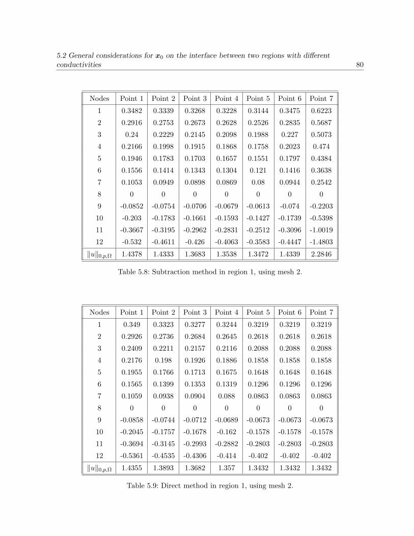
5.2 General considerations for x0 on the interface between two regions with differentconductivities 80
Nodes Point 1 Point 2 Point 3 Point 4 Point 5 Point 6 Point 7
1 0.3482 0.3339 0.3268 0.3228 0.3144 0.3475 0.6223
2 0.2916 0.2753 0.2673 0.2628 0.2526 0.2835 0.5687
3 0.24 0.2229 0.2145 0.2098 0.1988 0.227 0.5073
4 0.2166 0.1998 0.1915 0.1868 0.1758 0.2023 0.474
5 0.1946 0.1783 0.1703 0.1657 0.1551 0.1797 0.4384
6 0.1556 0.1414 0.1343 0.1304 0.121 0.1416 0.3638
7 0.1053 0.0949 0.0898 0.0869 0.08 0.0944 0.2542
8 0 0 0 0 0 0 0
9 -0.0852 -0.0754 -0.0706 -0.0679 -0.0613 -0.074 -0.2203
10 -0.203 -0.1783 -0.1661 -0.1593 -0.1427 -0.1739 -0.5398
11 -0.3667 -0.3195 -0.2962 -0.2831 -0.2512 -0.3096 -1.0019
12 -0.532 -0.4611 -0.426 -0.4063 -0.3583 -0.4447 -1.4803
∥u∥0,p,Ω 1.4378 1.4333 1.3683 1.3538 1.3472 1.4339 2.2846
Table 5.8: Subtraction method in region 1, using mesh 2.
Nodes Point 1 Point 2 Point 3 Point 4 Point 5 Point 6 Point 7
1 0.349 0.3323 0.3277 0.3244 0.3219 0.3219 0.3219
2 0.2926 0.2736 0.2684 0.2645 0.2618 0.2618 0.2618
3 0.2409 0.2211 0.2157 0.2116 0.2088 0.2088 0.2088
4 0.2176 0.198 0.1926 0.1886 0.1858 0.1858 0.1858
5 0.1955 0.1766 0.1713 0.1675 0.1648 0.1648 0.1648
6 0.1565 0.1399 0.1353 0.1319 0.1296 0.1296 0.1296
7 0.1059 0.0938 0.0904 0.088 0.0863 0.0863 0.0863
8 0 0 0 0 0 0 0
9 -0.0858 -0.0744 -0.0712 -0.0689 -0.0673 -0.0673 -0.0673
10 -0.2045 -0.1757 -0.1678 -0.162 -0.1578 -0.1578 -0.1578
11 -0.3694 -0.3145 -0.2993 -0.2882 -0.2803 -0.2803 -0.2803
12 -0.5361 -0.4535 -0.4306 -0.414 -0.402 -0.402 -0.402
∥u∥0,p,Ω 1.4355 1.3893 1.3682 1.357 1.3432 1.3432 1.3432
Table 5.9: Direct method in region 1, using mesh 2.

5.2 General considerations for x0 on the interface between two regions with differentconductivities 81
Nodes Point 1 Point 2 Point 3 Point 4 Point 5 Point 6 Point 7
1 -6.7298 -6.6822 -6.657 -6.6215 -6.1482 -1.8834 11.0224
2 -7.7837 -7.7376 -7.713 -7.6803 -7.262 -3.5241 7.7403
3 -8.1949 -8.1492 -8.1247 -8.0946 -7.732 -4.5192 5.1254
4 -8.1285 -8.0832 -8.0589 -8.0304 -7.6954 -4.7389 4.1212
5 -7.8761 -7.832 -7.8083 -7.7814 -7.4745 -4.7751 3.3033
6 -6.9022 -6.8629 -6.8419 -6.8191 -6.5673 -4.3626 2.2236
7 -5.0399 -5.0107 -4.9951 -4.9788 -4.8046 -3.285 1.2473
8 0 0 0 0 0 0 0
9 4.7519 4.7228 4.7072 4.6921 4.5439 3.2633 -0.5432
10 12.0083 11.9328 11.8922 11.854 11.4937 8.3904 -0.8209
11 22.9412 22.7931 22.7133 22.6405 21.9762 16.2778 -0.6133
12 34.5175 34.291 34.1687 34.059 33.082 24.7214 -0.0381
∥u∥0,p,Ω 52.2292 57.1387 53.8755 55.4943 55.6164 51.5907 64.26
Table 5.10: Subtraction method in region 2, using mesh 2.
Nodes Point 1 Point 2 Point 3 Point 4 Point 5 Point 6 Point 7
1 -6.7258 -6.6673 -6.6755 -6.644 -6.6505 -6.6316 -6.6316
2 -7.7801 -7.7239 -7.7301 -7.7003 -7.706 -7.6888 -7.6888
3 -8.1915 -8.1358 -8.1414 -8.1121 -8.1175 -8.1008 -8.1008
4 -8.1251 -8.07 -8.0756 -8.0465 -8.0518 -8.0353 -8.0353
5 -7.8728 -7.819 -7.8245 -7.7961 -7.8014 -7.7852 -7.7852
6 -6.8991 -6.8513 -6.8564 -6.8311 -6.8358 -6.8213 -6.8213
7 -5.0376 -5.002 -5.006 -4.9871 -4.9907 -4.9798 -4.9798
8 0 0 0 0 0 0 0
9 4.7496 4.7138 4.7184 4.6991 4.703 4.6916 4.6916
10 12.0019 11.909 11.9217 11.871 11.8813 11.8512 11.8512
11 22.9287 22.7461 22.7726 22.6719 22.6928 22.6325 22.6325
12 34.4987 34.219 34.2613 34.1058 34.1385 34.045 34.045
∥u∥0,p,Ω 52.1918 53.0541 54.1383 55.3545 55.8542 56.0896 56.0896
Table 5.11: Direct method in region 2, using mesh 2.

5.2 General considerations for x0 on the interface between two regions with differentconductivities 82
Nodes ϵ = 0.01 ϵ = 0.001 ϵ = 0.0001 ϵ = 0.00001
1 -3.1643 -3.1657 -3.1685 -3.1685
2 -3.7218 -3.7229 -3.7254 -3.7254
3 -3.9542 -3.9551 -3.9576 -3.9576
4 -3.9329 -3.9338 -3.9363 -3.9363
5 -3.8182 -3.8191 -3.8215 -3.8215
6 -3.3532 -3.3541 -3.3562 -3.3562
7 -2.4527 -2.4534 -2.4550 -2.4550
8 0 0 0 0
9 2.3180 2.3188 2.3205 2.3205
10 5.8613 5.8634 5.8679 5.8679
11 11.2066 11.2111 11.2201 11.2201
12 16.8581 16.8651 16.8791 16.8791
∥u∥0,p,Ω 26.5281 27.7785 27.9054 27.9054
Table 5.12: Dipole position on the interface, mesh 1.
On the contrary, the direct method is stable when the dipole position is in region 1 or 2, near
or far from the interface. We also clearly see that the solution converges to different functions
when x0 tends to the interface from one side or from the other. This confirms that the variational
formulation for x0 lying exactly on the interface must have a different structure from the case in
which x0 is internal to the middle layer. Nevertheless, for that case we can show some numerical
results obtained by approximating the delta distribution in a suitable way.
5.2.2 Test 2.
In this test we want to analyze what happens if x0 is on the interface. To this end, we consider
the approximation of the delta distribution in (5.9). It is supported on a square centered at x0
and with side-length 2ϵ, with the same polarization that in the previous test. We solve the
problem four times, with four different values of ϵ. As in the previous test, we consider twelve
values of the solution corresponding to the same twelve external nodes in Table 5.1 and also we
compute the Lp norm in all Ω, with p = 5/4. This procedure was done with the two meshes in
Table 5.3. In Table 5.12, we find the results corresponding to the mesh 1 and in Table 5.13, to
the mesh 2. We can obtain as a conclusion that this approximation performs in a satisfactory
way.
Notice that if we take the last column of Tables 5.5 and 5.7 and we do an average, we obtain

5.3 Inverse problem 83
Nodes ϵ = 0.01 ϵ = 0.001 ϵ = 0.0001 ϵ = 0.00001
1 -3.1638 -3.1581 -3.1563 -3.1563
2 -3.7218 -3.7164 -3.7148 -3.7148
3 -3.9541 -3.9488 -3.9473 -3.9473
4 -3.9328 -3.9275 -3.9260 -3.9260
5 -3.8180 -3.8130 -3.8114 -3.8115
6 -3.3529 -3.3483 -3.3470 -3.3470
7 -2.4520 -2.4486 -2.4476 -2.4476
8 0 0 0 0
9 2.3176 2.3141 2.3130 2.3130
10 5.8610 5.8518 5.8490 5.8490
11 11.2048 11.1864 11.1808 11.1808
12 16.8658 16.8374 16.8287 16.8288
∥u∥0,p,Ω 26.6009 28.0923 28.6901 28.6971
Table 5.13: Dipole position on the interface, mesh 2.
a result quite similar to the last column in Table 5.12. The same happens for mesh 2 in Table
5.3.
However from a physiological point of view, people are interested in considering impulses
coming from the middle region. Specifically, people study the neuronal impulses which are
generated in that region, but close to the interface between regions 1 and 2. Then, from the
computational results we can conclude that the subtraction approach in this real situation is
not the best one and it is better to choose an alternative approach.
5.3 Inverse problem
In this section we study the inverse problem and specifically, we are interested in finding the
localization and the polarization of a dipole source, knowing a priori some measurements on the
boundary of the domain. We analyze the case of a single dipole, but in different positions, and
present some numerical results.
Since we are interested in a single dipole, we need to find only four parameters that minimize
the least-square function
ϕ(x, qx) = ∥m−mref∥22 (5.18)
where x is the coordinates of the dipole location and qx is the polarization. We assume that

5.3 Inverse problem 84
we can obtain the measurements at some boundary nodes of the domain. In this equation, m is
a n-dimensional vector (with n the number of measurements) which contains the values of the
potential computed using FEM, and mref is a vector which contains the values of the measured
potential (indeed, the measured potential is simulated by using the values computed with one
of the aforementioned techniques using FEM in a very fine mesh). It is clear that this problem
is non-linear.
For any given dipole location x we can find the optimal polarization px = p1e1 + p2e2 (e1
and e2 are the cartesian orientations) as follows: we define as m1,i the value of an approximated
solution at the same points Pi, 1 ≤ i ≤ n on ∂Ω where the solution that produces mref is
evaluated, obtained by using as localization x and as polarization e1. Similarly, m2,i corresponds
to the value of an approximated solution at the same points Pi, 1 ≤ i ≤ n on the boundary
obtained by using the same localization and as polarization e2. Then, we define the n×2 matrix
M := (m1 m2). By linearity, the values of the approximated solution corresponding to px are
given by
m = Mpx .
Thus, finding px which minimize ϕ(x, qx) = ∥m − mref∥22 in the least squares sense, is
equivalent to solve
M tMpx = M tmref . (5.19)
After having computed the optimal polarization for each possible dipole position x, the
function ϕ reduces to a least-squares function ψ which is only a function of x, that is
ψ(x) = ∥Mpx −mref∥22 . (5.20)
We use the pattern-search optimization method to find the optimum dipole position x by
minimizing the function ψ(x). This minimization algorithm is already implemented in MATLAB
and corresponds to the command patternsearch.
We are interested in solving the inverse problem by using the aforementioned methods. From
Chapter 4 we know that there exists an a posteriori error estimator for the direct method which
enables to improve the obtained results. We must recall that this estimator was defined in the
case in which the matrix σ has entries in C1(Ω). We use the estimator to devise a strategy to
solve the inverse problem.
According to Theorem 5.1.1 the solution of problem (5.8) belongs to Lp(Ω) with 1 ≤ p < 2
when σ is regular enough. We will recall the a posteriori error estimator in the Lp(Ω)-norm for
the finite element approximation error u − uh defined in Chapter 4. We proved the reliability
and efficiency of the estimator for a particular range of p.

5.3 Inverse problem 85
For all T ∈ Th we define
εT,p :=
h2pT ∥div (σ∇uh)∥p0,p,T +1
2
∑ℓ∈E(T )∩Eh,i
|ℓ|p+1∥[[σ∇uh · n ]]∥p0,p,ℓ
+∑
ℓ∈E(T )∩Eh,e
|ℓ|p+1∥σ∇uh · n∥p0,p,ℓ
1/p
,
where Eh,i is the set of all the inner edges of the triangulation Th, Eh,e is the set of boundary
edges of the triangulation Th, E(T ) is the set of the edges of T and [[ g ]] denotes the jump of g
across an edge. We define the local a posteriori error indicator ηT,p for all T ∈ Th as follows:
ηT,p :=
(h2−p0 + εpT,p
)1/pif T = T0 ,
εT,p otherwise ,
where we denote by T0 the triangle that contains the point x0 and by h0, its diameter.
Next, we define the global error estimator from these indicators as follows:
ηp :=
∑T∈Th
ηpT,p
1/p
. (5.21)
In Tests 3 and 4 we are interested in finding the localization and polarization of the dipole
from certain measurements that have been generated by using the subtraction approach or the
direct method (depending if the localization is inside a region or near the interface). The exact
solution is computed in the finest mesh in Table 5.14.
5.3.1 Test 3.
This experiment consists in reconstructing the position and the polarization of the dipole
source from boundary measurements, by using four different techniques: subtraction approach,
direct method, direct method accompanied by an adaptive procedure and the characteristic
function approach. We use the same domain Ω in Test 1. We recall that Ω is a multi-layered
square as in Figure 5.1, with three regions, the external and internal layers (which correspond
to regions 1 and 3, respectively) with conductivities 0.33 and the layer in between (region 2)
with conductivity 0.0042. As in the other test, it is important to recall that these values of the
conductivity correspond to a real values.
Notice that when we solve the inverse problem by using the direct method (or direct method
with adaptivity), the minimization algorithm find a triangle, not a position. Then, we will
consider as x0 the barycenter of this triangle.
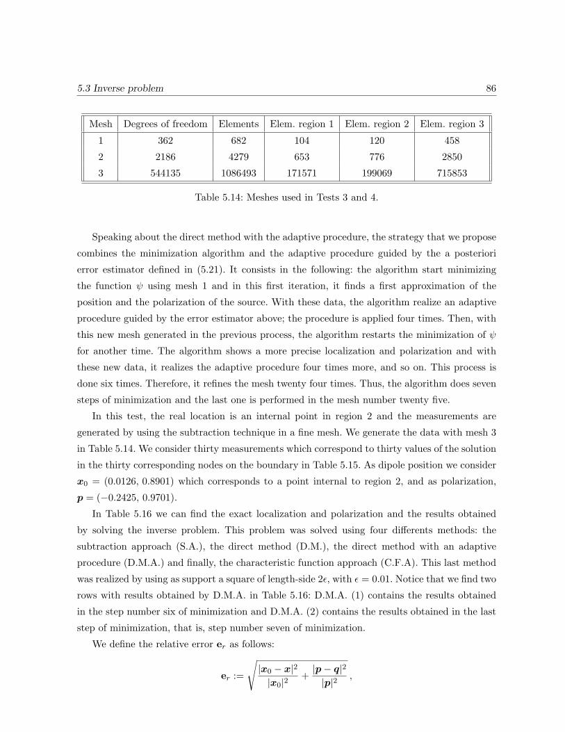
5.3 Inverse problem 86
Mesh Degrees of freedom Elements Elem. region 1 Elem. region 2 Elem. region 3
1 362 682 104 120 458
2 2186 4279 653 776 2850
3 544135 1086493 171571 199069 715853
Table 5.14: Meshes used in Tests 3 and 4.
Speaking about the direct method with the adaptive procedure, the strategy that we propose
combines the minimization algorithm and the adaptive procedure guided by the a posteriori
error estimator defined in (5.21). It consists in the following: the algorithm start minimizing
the function ψ using mesh 1 and in this first iteration, it finds a first approximation of the
position and the polarization of the source. With these data, the algorithm realize an adaptive
procedure guided by the error estimator above; the procedure is applied four times. Then, with
this new mesh generated in the previous process, the algorithm restarts the minimization of ψ
for another time. The algorithm shows a more precise localization and polarization and with
these new data, it realizes the adaptive procedure four times more, and so on. This process is
done six times. Therefore, it refines the mesh twenty four times. Thus, the algorithm does seven
steps of minimization and the last one is performed in the mesh number twenty five.
In this test, the real location is an internal point in region 2 and the measurements are
generated by using the subtraction technique in a fine mesh. We generate the data with mesh 3
in Table 5.14. We consider thirty measurements which correspond to thirty values of the solution
in the thirty corresponding nodes on the boundary in Table 5.15. As dipole position we consider
x0 = (0.0126, 0.8901) which corresponds to a point internal to region 2, and as polarization,
p = (−0.2425, 0.9701).
In Table 5.16 we can find the exact localization and polarization and the results obtained
by solving the inverse problem. This problem was solved using four differents methods: the
subtraction approach (S.A.), the direct method (D.M.), the direct method with an adaptive
procedure (D.M.A.) and finally, the characteristic function approach (C.F.A). This last method
was realized by using as support a square of length-side 2ϵ, with ϵ = 0.01. Notice that we find two
rows with results obtained by D.M.A. in Table 5.16: D.M.A. (1) contains the results obtained
in the step number six of minimization and D.M.A. (2) contains the results obtained in the last
step of minimization, that is, step number seven of minimization.
We define the relative error er as follows:
er :=
√|x0 − x|2|x0|2
+|p− q|2|p|2
,

5.3 Inverse problem 87
Nodes x y Nodes x y Nodes x y
1 0.5 -1 11 -1 -0.25 21 1 0.5
2 -0.5 -1 12 -1 0.75 22 1 -0.5
3 0.25 -1 13 -1 -0.75 23 1 0.25
4 -0.25 -1 14 0 1 24 1 -0.25
5 0.75 -1 15 0.5 1 25 1 0.75
6 -0.75 -1 16 -0.5 1 26 1 -0.75
7 -1 0 17 0.25 1 27 0.75 1
8 -1 0.5 18 -0.25 1 28 0.125 -1
9 -1 -0.5 19 -0.75 1 29 -0.125 -1
10 -1 0.25 20 1 0 30 -1 0.125
Table 5.15: Thirty nodes on the external boundary.
where x and q correspond to the approximations of x0 and p obtained by solving the inverse
problem using the different approaches.
Solution x0 p er Degrees of freedom
Exact (0.0126, 0.8901) (-0.2425, 0.9701) - 544135
S.A. (-0.0383, 0.8941) (1.6646, 0.9545) 1.9081 2186
D.M. (0.0260, 0.9123) (-0.2734, 0.9761) 0.0429 2186
D.M.A. (1) (0.0062, 0.8877) (-0.0691, 0.9741) 0.1736 1193
D.M.A. (2) (0.0152, 0.8896) (-0.2502, 0.9715) 0.0085 3030
C.F.A. (0.0104, 0.8838) (-0.3137, 0.9799) 0.0723 2186
Table 5.16: Results obtained by solving the inverse problem.
Notice that the strategy that combines the direct method with the adaptive procedure start
from mesh 1 in Table 5.14. In Table 5.17 we see the results given by the minimization algorithm
the seven times that the process was done. The last mesh in this iterative process contained 3030
nodes. We see that this strategy is giving a better approximation of the data in the last iteration
that in the case of the direct method without an adaptive procedure. However, we want also
to underline that the results obtained by means of the direct method with adaptive procedure
are somehow oscillating from a refinement step to another. This phenomenon is seen also in the
numerical results in Section 5.4. On the other hand, the direc method and the characteristic
function approach, are giving good results.

5.3 Inverse problem 88
Iteration x0 p
1 (0.0400, 0.9033) (0.0796, 0.9896)
2 (0.0288, 0.9143) (-0.3975, 0.9786)
3 (-0.0211, 0.9114) (0.1494, 0.9757)
4 (0.0169, 0.8852) (-0.3318, 0.9766)
5 (0.0169, 0.8852) (-0.3228, 0.9756)
6 (0.0062, 0.8877) (-0.0691, 0.97411)
7 (0.0152, 0.8896) (-0.2503, 0.9716)
Table 5.17: Data found using the direct method with adaptive procedure.
5.3.2 Test 4.
This experiment is similar to Test 3. The difference is the position of the dipole source we
want to find. We are interested in the behavior of the four aforementioned methods in Test 3
when we solve the inverse problem with a dipole located very close to the interface. In this test
we use the same geometry of Test 3. Since we need to generate the measurements and we know
that the subtraction method cannot be used in this situation, we use the direct approach to
compute the data in the finest mesh in Table 5.14 (this corresponds to mesh 3). Note that if ϵ
is so small that the square centered at x0 of side size 2ϵ is inside one triangle, the characteristic
function approach is giving the same result. For a larger ϵ, the characteristic function approach
has to be used being carefull that the square centered in x0 and with side-length 2ϵ, is not
intersecting the interface, as in Section 5.2. We have seen that the location of the delta function
on the interface is giving rise to a problem that is not the one obtained by taking the limit from
one or the other side.
The dipole position is x0 = (0.0126 , 0.917), which belongs to region 2 and it is close to the
interface between regions 1 and 2. We consider thirty measurements that correspond to the thirty
nodes on the boundary in Table 5.15. The polarization is the same that in the experiment above,
i.e., p = (−0.2425, 0.9701). To compute the inverse problem in the case of the characteristic
function approach, we use as support a square of length-side 2ϵ with ϵ = 0.003.
As in the previous experiment, we can find the results in Table 5.18.
From these two experiments, we can conclude that the direct method combined with the
adaptive procedure is giving good results in both cases respect to the other methods (despite this
estimator is not well suited when the entries of σ are piecewise constant). However, this method
is giving data that are converging in a oscillatory way, then we have to be carefull when we
use this technique. On the other hand, the other alternatives that are giving reasonable results

5.4 Lead field matrix 89
Solution x0 p er Degrees of freedom
Exact (0.0126 , 0.917) (-0.2425, 0.9701) - 544135
S.A. (0.1283, 0.9343) (-2.1445, -35.6436) 36.6651 2186
D.M. (-0.0019 , 0.9007) (0.0096 , 0.9807) 0.2535 2186
D.M.A. (1) (0.0183, 0.9141) (-0.3718, 0.9741) 0.1296 1014
D.M.A. (2) (0.0108, 0.9159) (-0.2305, 0.9729) 0.0125 1802
C.F.A. (0.0127, 0.9039) (-0.1513, 0.9821) 0.0931 2186
Table 5.18: Results obtained by solving the inverse problem.
Iteration x0 p
1 (-0.0367, 0.9033) (-0.1486, 0.9957)
2 (0.0037, 0.9098) (-0.0294, 0.9837)
3 (0.0158, 0.9098) (-0.3244, 0.9770)
4 (0.0068, 0.9181) (-0.1264, 0.9759)
5 (0.0128, 0.9147) (-0.2422, 0.9758)
6 (0.0183, 0.9141) (-0.3718, 0.9741)
7 (0.0108, 0.9159) (-0.2305, 0.9729)
Table 5.19: Data found using the direct method with adaptive procedure.
are the characteristic function approach and the direct method. Notice that the subtraction
approach in this last test is giving the worst results.
5.4 Lead field matrix
In the previous section the inverse problem in the case of only one dipole was analyzed (but
this analysis can be extended to a small quantity of dipoles). In the standard dipolar method the
parameters of the dipoles (location and polarization) are found using a nonlinear leastsquares
search. However, there exists another way to study the inverse problem: it is to assume that the
current density is a distributed source and, in such case, the measurements are assumed to be
generated by many dipoles placed in a certain region of the mesh. We will focus in this point of
view.
In the EEG forward model a given primary current density Jp in the head Ω generates a
measurement data vector m (the electric potential values). In the numerical simulation of the

5.4 Lead field matrix 90
inverse problem, the unknown is a finite dimensional vector z, which is linked to the measurement
data m through the system of linear equations m = Lz, the so-called lead field matrix L.
The goal of this section is to construct the lead field matrix with each one of the methods
in Section 5.1 (and with one new method that we add in this section). First, we discuss how to
construct this lead field matrix in each case. After that, we want to compare each one of these
lead field matrices with a reference lead field matrix.
For a mesh consisting of N nodes, the approximate value of the potential can be expressed
as an element of the set Hh defined in (5.14) as follows
uh =N∑i=1
αiλi
where λi is a basis function in Hh associated with node i, for all i = 1, ..., N . In the most of the
subsections, we are interested in analyzing problem (5.2) with
Jp =M∑k=1
pkδxk, (5.22)
where pk is a non null vector and xk in an inner point of Ω, for all k = 1, ...,M . We will specify
when we need to use a different definition for the current density Jp.
Subtraction method
The vector pk in (5.22) can be written in the following way pk = yk1e1 + yk2e2, where e1
and e2 are the cartesian orientations, for all k = 1, ...,M . Then, the current density also can be
written as Jp =∑M
k=1
∑2j=1 y
kj ejδxk
or in a more structured way,
Jp =2M∑k=1
zkdk , (5.23)
where
zk :=
yk1 if 1 ≤ k ≤M ,
yk−M2 if M + 1 ≤ k ≤ 2M ,and dk :=
e1δxk
if 1 ≤ k ≤M ,
e2δxk−Mif M + 1 ≤ k ≤ 2M .
(5.24)
Assuming that we can find nonempty subdomains Ωk0 of Ω around each one of the source
positions xk with homogeneous constant conductivity σ0,k, we can solve these 2M subproblems
by using (5.15) and then we use (5.5) with the corresponding data in each case.
The coefficients αi, i = 1, ..., N and zk, k = 1, ..., 2M define unknown coordinate vectors α
and z, which satisfy the linear system Sα = Gsz, where the entries of the matrices S and Gs
are given by

5.4 Lead field matrix 91
sij :=
∫Ωσ∇λi · ∇λj ,
and
gsik :=
−∫Ωσs,k∇u10,k · ∇λi −
∫∂Ω
(σ0,k∇u10,k · n)λi 1 ≤ k ≤M ,
−∫Ωσs,k−M∇u20,k−M · ∇λi −
∫∂Ω
(σ0,k−M∇u20,k−M · n)λi M + 1 ≤ k ≤ 2M ,
where σs,k = σ − σ0,k, k = 1, ...,M and we have denoted by uj0,k, j = 1, 2 the fundamental
solution of this problem:
div (σ0,k∇uj0,k) = div (ejδxk) in Ω , for j = 1, 2 and k = 1, ...,M .
Since we know from (5.5) that the solution can be written as a singular part plus a part
obtained by means of FEM, then, we define theN times 2M matrixU0 whose entries corresponds
to
u0ik :=
u10,k(xi) 1 ≤ k ≤M ,
u20,k−M (xi) M + 1 ≤ k ≤ 2M ,
for i = 1, ..., N . We assume that the dipole positions are not nodes, so that the fundamental
solutions can be evaluated in all the nodes of the mesh. Associating the EEG sensor locations
with basis functions λi1 , ..., λiL and the zero potential reference with the mean value of the
electrode voltages, the EEG lead field matrix is given by L = R(S−1Gs +U0), in which R is a
L×N restriction matrix with entries
rsl :=
1 if l = is ,
0 if l = is ,
l = 1, ..., N and s = 1, ..., L.
Direct method
As in the subtraction method, Jp can be written as above:
Jp =
2M∑k=1
zkdk ,
where zk and dk are defined as in (5.24).
From (5.16), we see that we construct the matrix S as in the previous case. The entries of
Gd are given by
gdik :=
e1 · ∇(λi|Txk )(xk) 1 ≤ k ≤M ,
e2 · ∇(λi|Txk−M)(xk−M ) M + 1 ≤ k ≤ 2M .
(5.25)
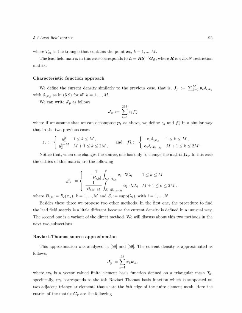
5.4 Lead field matrix 92
where Txk is the triangle that contains the point xk, k = 1, ...,M .
The lead field matrix in this case corresponds to L = RS−1Gd , whereR is a L×N restriction
matrix.
Characteristic function approach
We define the current density similarly to the previous case, that is, Jp :=∑M
k=1 pkδϵ,xk
with δϵ,xkas in (5.9) for all k = 1, ...,M .
We can write Jp as follows
Jp :=
2M∑k=1
zkfϵk
where if we assume that we can decompose pk as above, we define zk and f ϵk in a similar way
that in the two previous cases
zk :=
yk1 1 ≤ k ≤M ,
yk−M2 M + 1 ≤ k ≤ 2M ,and f ϵk :=
e1δϵ,xk
1 ≤ k ≤M ,
e2δϵ,xk−MM + 1 ≤ k ≤ 2M .
Notice that, when one changes the source, one has only to change the matrix Gϵ. In this case
the entries of this matrix are the following
gϵik :=
1
|Bϵ,k|
∫Si∩Bϵ,k
e1 · ∇λi 1 ≤ k ≤M
1
|Bϵ,k−M |
∫Si∩Bϵ,k−M
e2 · ∇λi M + 1 ≤ k ≤ 2M .
where Bϵ,k := Bϵ(xk), k = 1, ...,M and Si := supp(λi), with i = 1, ..., N .
Besides these three we propose two other methods. In the first one, the procedure to find
the lead field matrix is a little different because the current density is defined in a unusual way.
The second one is a variant of the direct method. We will discuss about this two methods in the
next two subsections.
Raviart-Thomas source approximation
This approximation was analyzed in [58] and [59]. The current density is approximated as
follows:
Jp :=
M∑k=1
xkwk ,
where wk is a vector valued finite element basis function defined on a triangular mesh Th,specifically, wk corresponds to the kth Raviart-Thomas basis function which is supported on
two adjacent triangular elements that share the kth edge of the finite element mesh. Here the
entries of the matrix Gr are the following

5.4 Lead field matrix 93
gri,k =
∫Ωwk · ∇λi .
As in the direct method or the characteristic function approach, L = RS−1Gr. Notice that,
this lead field matrix cannot be comparable with the other ones, because it was constructed in
a different way.
In [58], Pursiainen associates each cartesian source element with a single triangle; for each
triangle, a dipole position is fixed.
We explain the strategy used in [58]. In a first stage, each basis function wk is given a dipole
moment by qk =∫Ωwk and the dipole position rk is defined as the midpoint of the line segment
between the two nodes that belong to the support of wk but do not belong to the common
edge (see point (D) Figure 3 in [59]). The position of the dipole source for a given triangle T is
obtained as the mean
r = (r1 + r2 + r3)/3 (5.26)
of the dipole positions r1, r2 and r3 corresponding to the basis functions w1, w2 and w3
supported on T , respectively. Notice that in a uniform mesh r coincides with the barycenter of
the triangle T .
We denote by v1, v2 and v3 the simulated data vectors obtained by solving (5.3) with Jp
corresponding to w1, w2 and w3, respectively. The simulated dipole data associated with T are
given by
[v1 v2] = [v1 v2 v3][q1 q2 q3]⊥ (5.27)
in which ⊥ denotes the Moore-Penrose pseudo-inverse and v1 and v2 form the final data for
the perpendicular directions e1 and e2, respectively. In simple words, in (5.27) was used a “base
change”. Thus, it is possible to obtain a lead field matrix comparable with the others trough
the lead field matrix computed by means of the Raviart-Thomas sources.
Direct method with adaptive procedure
To find the lead field matrix, we use Jp as in the subsection Direct method and to improve
the way of solving the 2M problems, we use an adaptive procedure guided by the a posteriori
error estimator in (5.21). We explain later on the strategy used in this method.
Now, we are in a position to give some numerical results. Before starting with the ex-
periments, we give some definitions. With each method, one lead field matrix of the form
L = (I1, I2, ..., I2M ) is produced. For 1 ≤ k ≤ M , the column Ik of L corresponds to a

5.4 Lead field matrix 94
single source location xk and the cartesian orientation e1. If M + 1 ≤ k ≤ 2M , the column Ik
corresponds also to a single source location, xk−M and the cartesian orientation, e2.
The relative error (RE) is defined as follows:
RE :=
√√√√√√√√√√2M∑k=1
∥∥∥Ik − Irefk
∥∥∥22
2M∑k=1
∥∥∥Irefk ∥∥∥22
,
where Lref = (Iref1 , Iref2 , ..., Iref2M ) is a reference lead field matrix computed by some of the above
methods (which will be indicated case by case) in the finest mesh in Table 5.21.
We define by RE1, RE2, RE3, RE4 and RE5 the relative errors computed between a reference
lead field matrix and the lead field matrices obtained using the subtraction approach, the direct
method, the characteristic function approach, the Raviart-Thomas source approximation and
the direct method with adaptive procedure, respectively.
5.4.1 Test 5.
In this test we are interested in analyzing the lead field matrix constructed by using the
direct method with an adaptive procedure respect to the lead field constructed by means of the
subtraction approach in two different situations: constant conductivity and piecewise constant
conductivity in the domain Ω.
The domain Ω is a square centered at (0.5 , 0.5) with side-length 1. As in the previous
tests, this domain consists of layers formed by squares completely contained in Ω. It has three
different layers: Ω1 = Ω \ (0.2, 0.8)2, Ω2 = [0.2, 0.8]2 \ (0.4, 0.6)2 and Ω3 = [0.4, 0.6]2. Unlike
the other tests, the meshes in Table 5.21 are uniform meshes. A property of these meshes is that
the barycenter of each one of the triangles in mesh 1 are barycenters of some triangles in the
following meshes. It is the same for mesh 2, and so on. Henceforth, we consider the locations of
the dipoles only in region 2.
For this test, we consider only one point and the cartesian orientations e1 and e2 as the
polarizations. The point considered x0 = (0.2417 , 0.4333) corresponds to an internal point in
region 2 which is a barycenter of a triangle in mesh 1. In this first experiment, we consider a
constant conductivity equal to one in the three regions.
In Table 5.22, we found the relative errors RE1 and RE5, computed using the lead field
matrices calculated by means of the subtraction approach and the direct method with adaptive
procedure in meshes 1, 2 and 3 in Table 5.21. In the first column we compute RE1 defined
above, considering as the reference lead field matrix the one computed by means of the direct

5.4 Lead field matrix 95
method with adaptive procedure. Notice that the strategy consists in starting with a coarse
initial mesh (mesh 1 in Table 5.21) and by means of an adaptive procedure to refine the mesh
using as stopping criterion the quantity of d.o.f. In this case, the adaptive procedure stops when
the d.o.f. overtake the d.o.f. of mesh 3 in Table 5.21. On the other hand, in the second column
we compute RE5 using as reference lead field matrix the one computed by using the subtraction
method in the finest mesh, that is, mesh 5 in Table 5.21. In this case the adaptive procedure
stops when the d.o.f. overtake the d.o.f. of the mesh we use to compare the relative errors. Notice
that, since the adaptive procedure starts refining mesh 1, the first relative error in the second
column in Table 5.22 was computed without refinement.
We consider twelve “measurements” on the boundary of Ω computed in the twelve nodes in
Table 5.20. So in each case, the lead field matrix is a 12× 2 matrix.
Nodes 1 2 3 4 5 6 7 8 9 10 11 12
x 0 0.2 0.4 0.6 0.8 0.8 1 1 1 1 1 1
y 0 0 0 0 0 1 0 0.2 0.4 0.6 0.8 1
Table 5.20: Twelve nodes on the external boundary.
Mesh Degrees of freedom Elements Elem. region 1 Elem. region 2 Elem. region 3
1 1681 3200 2048 1024 128
2 6561 12800 8192 4096 512
3 25921 51200 32768 16384 2048
4 103041 204800 131072 65536 8192
5 410881 819200 524288 262144 32768
Table 5.21: Meshes used in Tests 5, 6 and 7.
Mesh RE1 RE5
1 0.0010 0.0273
2 0.0004 0.0004
3 0.0002 0.0002
Table 5.22: Subtraction approach versus direct method with adaptive procedure.
In Table 5.23 we find the references lead field matrices. L1 corresponds to the lead field

5.4 Lead field matrix 96
L1 L5
-0.7755 -0.6768 -0.7754 -0.6768
-0.5840 -0.6507 -0.5839 -0.6509
-0.2403 -0.4596 -0.2403 -0.4597
-0.0596 -0.2042 -0.0594 -0.2041
-0.0088 -0.0480 -0.0087 -0.0479
-0.0752 0.4747 -0.0751 0.4747
0 0 0 0
0.0055 0.0453 0.0055 0.0453
0.0077 0.1632 0.0077 0.1632
-0.0124 0.3016 -0.0124 0.3017
-0.0436 0.4030 -0.0436 0.4030
-0.0583 0.4387 -0.0583 0.4387
Table 5.23: Reference lead field matrices.
matrix computed by means of subtraction approach and L5 to the lead field matrix computed
using the direct method with the adaptive procedure. Notice that both solutions are similar.
Now, we focus on the case of a piecewise constant conductivity. Henceforth, the conducting
σ is assumed isotropic on each layer and equal to σ|Ω1 = σ|Ω3 = 0.33 and σ|Ω2 = 0.0042.
This experiment is similar to the previous one. We consider an internal point in region 2,
x0 = (0.3667 , 0.3833) which is a barycenter of a triangle of mesh 1 in Table 5.21. As in the
previous case, we compute a reference lead field matrix by means of the subtraction approach in
the finest mesh and by means of the direct method with adaptive procedure starting with mesh
1 but now using as stopping criterion 30.000 d.o.f. We can see these reference matrices in Table
5.25.
In Table 5.24 we find in the first two columns the relative errors RE1 and RE5 computed
by using as reference lead field matrix the one obtained by the subtraction approach that corre-
sponds to L1 in Table 5.25. The other columns correspond to compute the same relative errors
RE1 and RE5, but now considering as the reference lead field matrix the one obtained by means
of the direct method with adaptive procedure. This matrix corresponds to L5 in Table 5.25. All
these computations were done in the first three meshes in Table 5.21.
We can see from Table 5.24 that the relative error in the case of the direct method with
adaptive procedure is increasing in the last mesh. We see a non-monotone behavior of this
method. It is important to recall that here we are using this estimator even if it is not proved

5.4 Lead field matrix 97
S.A. D.M.A.
RE1 RE5 RE1 RE5
0.0349 0.1001 0.0358 0.1014
0.0125 0.0011 0.0136 0.0027
0.0046 0.0231 0.0061 0.0259
Table 5.24: Subtraction approach versus direct method with adaptive procedure.
L1 L5
-13.7644 -6.0037 -13.7540 -6.0048
-12.3147 -6.9000 -12.3073 -6.8986
-8.2128 -7.2754 -8.2065 -7.2705
-3.8710 -4.5372 -3.8669 -4.5305
-1.0194 -1.3208 -1.0175 -1.3173
2.4304 7.8903 2.4278 7.8388
0 0 0 0
0.9520 1.2863 0.9512 1.2829
2.7839 4.0433 2.7812 4.0326
3.5683 6.1806 3.5643 6.1584
3.1712 7.2751 3.1676 7.2379
2.8320 7.6067 2.8286 7.5617
Table 5.25: Reference lead field matrices.
to be suitable when the conductivity is piecewise constant.
5.4.2 Test 6.
In this test we are interested in analyzing the behavior of the first four methods in this
section, when the conductivity is a piecewise constant and the localizations of the dipoles are
inside region 2 and far enough from the interface. Since the points are inside region 2 and we
have seen that in this situation the subtraction approach has shown to be quite efficient, we
consider as reference lead field matrix the one computed by using the subtraction approach in
the finest mesh in Table 5.21, that corresponds to mesh 5.
First, we consider only one point x0 = (0.3667 , 0.3833) which corresponds to a barycenter
of a triangle of mesh 1. In Table 5.26 we can see the relative errors RE1, RE2, RE3 and RE4

5.4 Lead field matrix 98
Mesh RE1 RE2 RE3 RE4
1 0.0349 0.1001 0.1001 0.1673
2 0.0125 0.0595 0.0595 0.0332
3 0.0046 0.0205 0.0134 0.0243
4 0.0014 0.0127 0.0016 0.0083
Table 5.26: Relatives errors using one
dipole.
Mesh RE1 RE2 RE3 RE4
1 0.2468 0.0671 0.0671 0.0532
2 0.0643 0.0312 0.0312 0.0362
3 0.0143 0.0150 0.0109 0.0121
4 0.0027 0.0072 0.0023 0.0060
Table 5.27: Relative errors using fifty
dipoles.
in the first four meshes in Table 5.21. It is important to note that it is possible to work with
the Raviart-Thomas source approximation because we are in a uniform mesh, and therefore the
localization r defined in (5.26) for each triangle corresponds to the barycenter; thus we are sure
that the lead field matrices are constructed with the same localization points. When the mesh
is not uniform, we cannot compare this method with the other ones in this way.
Notice that the support of the characteristic function used to compute RE3 in Table 5.26 is
a square of side-length 2ϵ. We consider ϵ = 0.002 in the four cases. Notice that ϵ can be chosen
in different ways. We seen a dependence on that choice. The options of choice is something we
have not considered.
We follow the same procedure, but now we consider fifty points that corresponds to fifty
barycenters of fifty triangles inside the region 2 in mesh 1. The relative errors in this case are
reported in Table 5.27. To compute RE3 we use the same choice that in Table 5.26.
In Tables 5.26 and 5.27 we can see that the characteristic function approach gives good
results, similar to those of the subtraction approach. The other two methods are performing
reasonably well, though not at the same level of precision of the first two methods.
5.4.3 Test 7.
This experiment is similar to the previous one. The difference here is that now we are
considering points inside region 2, but close to the interface between region 1 and region 2.
Since the points are near the boundary, we consider as the reference lead field matrix the one
computed by means of the direct method. We compute this matrix in the finest mesh in Table
5.21, that is, mesh 5.
As in the previous experiment, first we consider only one position x0 = (0.2083 , 0.2042)
which corresponds to a barycenter of a triangle in mesh 2 of Table 5.21, with an edge belonging
to the interface. We can see the relatives errors RE1, RE2, RE3 and RE4 computed in Table
5.28. RE3 was computed by using ϵ as in the previous experiment. We use this choice to be

5.5 Conclusions 99
Mesh RE1 RE2 RE3 RE4
1 7.3765 0.3050 0.3050 -
2 3.8599 0.1712 0.1712 0.2295
3 1.2979 0.0293 0.0351 0.0936
4 0.3232 0.0547 0.0182 0.0107
Table 5.28: Relative errors with one dipole.
Mesh RE1 RE2 RE3 RE4
1 3.5643 0.0993 0.0993 -
2 1.2753 0.0454 0.0454 0.2191
3 0.2471 0.0144 0.0104 0.0233
4 0.0596 0.0149 0.0036 0.0037
Table 5.29: Relative errors with fifty
dipoles.
sure that the support of the characteristic function is contained in region 2. Notice that x0 is a
barycenter of a triangle in mesh 2 and therefore, it is not a barycenter of a triangle in mesh 1.
Then, we have not computed RE4 in mesh 1.
We repeat this experiment considering fifty barycenters of fifty triangles in mesh 2, close to
the interface between regions 1 and 2. We compute RE3 with the same ϵ than before since we
are sure that in the fifty problems, the supports of the characteristic function are inside region
2. We can see the results in Table 5.29.
From Tables 5.28 and 5.29 we can conclude that as in the case before, the best results are
achieved by the characteristic function approach and the Raviart-Thomas source approximation.
As conclusion, we see that the subtraction approach is always giving the worst performance, and
sometimes its relative error is one order of magnitude larger than the other relative errors. This
leads to say that, when the locations of x0 are close to the interface, it is better to resort to a
different approach, for instance to the characteristic function approach or the other methods.
5.5 Conclusions
It is important to recall that all the methods here introduced require more regularity of σ
in a vicinity of the dipole position. We are testing what happens if we do not consider this
restriction and, despite this fact, which method can still give good results.
From Section 5.2, we can conclude that when the dipole source is located close to the interface,
the solution obtained by means of subtraction approach is not robust. These computational
results are backed by the theory in [67]. On the other hand, the direct method is stable when
the locations are closer and closer to the interface; however, the results obtained in that section,
clearly show that a discontinuity occurs there, namely, approaching the interface from differents
sides gives quite different results. When the source is exactly on the interface, there is only one
method that is well defined: the characteristic function approach. We have seen that this method
gives reasonable results in that specific case.

5.5 Conclusions 100
In Section 5.3 we have seen that it is possible to reconstruct the localization and the po-
larization using the direct method; however, we can obtain better results when we use the
direct method with the adaptive procedure. However, we want also to underline that the results
obtained by means of this method are somehow oscillating from a refinement step to another.
Another competitive method is the characteristic function approach, which has given accurate
results. The subtraction approach is not performing well, especially when the location x0 is close
to the interface between two regions with different conductivities.
In Section 5.4, we see that, when the conductivity is constant, the lead field matrix compu-
ted by using the direct method with an adaptive procedure is similar to the lead field matrix
constructed by means of the subtraction approach; in particular, the relatives error are falling
down in the same way when we use a finer mesh. When the conductivity is piecewise constant,
we conclude that, when the dipole positions are inside a region, the best results are given by
the characteristic function approach and the subtraction approach; the others techniques are
also giving good results. When the points are close to the interface we can conclude that the
relatives errors have a difference behavior, and the subtraction approach does not seem to be
very reliable. Instead, the characteristic function approach is always furnishing good results, as
well as the Raviart-Thomas source approximation.

Chapter 6
Analysis of a FEM-BEM model
posed on the conducting domain for
the time-dependent eddy current
problem
6.1 Introduction
The eddy current model is commonly used in many problems in sciences and industry, for
example, in induction heating, electromagnetic braking, electric generation, etc. An overview of
the mathematical analysis of the eddy current model and its numerical solution in harmonic
regime can be found in the recent book [5], which provides a large list of references on this
subject.
In this chapter, we deal with the numerical solution of the time-dependent eddy current
problem, which is naturally formulated in the whole space, with adequate decay conditions at
infinity. The literature on the numerical analysis of time-dependent problems of this kind is more
scarce. Among the few papers devoted to this subject, both in bounded and unbounded domains,
by using finite element (FEM), boundary element (BEM) or coupled FEM-BEMmethods, we can
mention [1, 2, 42, 43, 47, 49, 69]. These articles differ from each other by the physical quantities
chosen for the formulation (magnetic field, electric field or different kind of potentials) and by
the way of treating the decay condition to reduce the problem to a bounded domain.
We consider a FEM-BEM method to compute the eddy currents generated in a three-
dimensional conductor ΩC by a time-dependent source current. The problem is reformulated
101

6.2 Preliminaries 102
by expressing the magnetic and the electric fields in terms of convenient new variables. We use
FEM only on the conducting domain ΩC , the integral conditions being imposed on its boundary
∂ΩC . Therefore, the domain where FEM is used results as small as possible, leading to a more
efficient method as compared, for instance, with [1, 2], where similar formulations but involving
FEM in part of the dielectric domain are considered. Another important feature of this ap-
proach is that it preserves the coercivity of the original problem. The purpose of this chapter
is to analyze the convergence of a fully discrete FEM-BEM scheme for this formulation and to
investigate the convergence order.
The chapter is organized as follows. In Section 6.2 we give some basic definitions. In Sec-
tion 6.3 we introduce the model problem and the assumptions over the data. Then, we introduce
a new variable, the time-primitive of the electric field, which plays the role of a vector potential
for the magnetic field. In Section 6.4 we introduce the integral operators and recall their prop-
erties. Then, we derive the FEM-BEM formulation and show the existence and uniqueness of
the solution to the problem. In Section 6.5, we introduce a space-discretization of the problem
based on Nedelec edge elements in ΩC and piecewise linear continuous elements for the variable
on ∂ΩC arising from the integral equations. Then, a backward Euler method is employed for the
time discretization. Finally, the results presented in Section 6.6 prove that the proposed fully
discrete scheme is convergent with optimal order.
6.2 Preliminaries
In the sequel we deal with real valued functions. Boldface letters will denote vectors (in Rn)or vector-valued functions, as well as matrices. The symbol | · | will represent the Euclidean norm
for n-dimensional vectors:
|v|2 = v · v :=
n∑i=1
v2i .
In all the chapter the conductor ΩC ⊂ R3 is a bounded connected polyhedron, with a
Lipschitz-continuous connected boundary Γ := ∂ΩC , so that the insulator ΩI := R3 \ΩC is also
connected.
We remark that, under the above conditions, ΩC and ΩI have the same number of non-
bounding cycles L; namely, there exist L disjoint connected open “cutting” surfaces Σintj ⊂ ΩC
(respectively Σextj ⊂ ΩI), j = 1, . . . , L, such that ΩC := ΩC \
∪Lj=1Σ
intj (respectively ΩI :=
ΩI \∪Lj=1Σ
extj ) is simply connected. The boundary curves ∂Σint
j and ∂Σextj lie on Γ.
We denote by
(f, g)0,Ω∗:=
∫Ω∗
fg dx
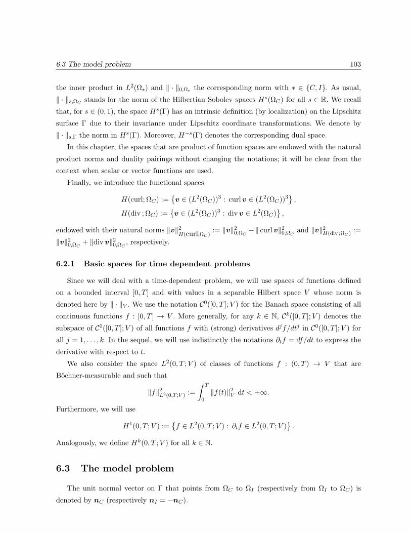
6.3 The model problem 103
the inner product in L2(Ω∗) and ∥ · ∥0,Ω∗ the corresponding norm with ∗ ∈ C, I. As usual,
∥ · ∥s,ΩCstands for the norm of the Hilbertian Sobolev spaces Hs(ΩC) for all s ∈ R. We recall
that, for s ∈ (0, 1), the space Hs(Γ) has an intrinsic definition (by localization) on the Lipschitz
surface Γ due to their invariance under Lipschitz coordinate transformations. We denote by
∥ · ∥s,Γ the norm in Hs(Γ). Moreover, H−s(Γ) denotes the corresponding dual space.
In this chapter, the spaces that are product of function spaces are endowed with the natural
product norms and duality pairings without changing the notations; it will be clear from the
context when scalar or vector functions are used.
Finally, we introduce the functional spaces
H(curl; ΩC) :=v ∈ (L2(ΩC))
3 : curlv ∈ (L2(ΩC))3,
H(div ; ΩC) :=v ∈ (L2(ΩC))
3 : div v ∈ L2(ΩC),
endowed with their natural norms ∥v∥2H(curl;ΩC)
:= ∥v∥20,ΩC+ ∥ curlv∥20,ΩC
and ∥v∥2H(div ;ΩC) :=
∥v∥20,ΩC+ ∥div v∥20,ΩC
, respectively.
6.2.1 Basic spaces for time dependent problems
Since we will deal with a time-dependent problem, we will use spaces of functions defined
on a bounded interval [0, T ] and with values in a separable Hilbert space V whose norm is
denoted here by ∥ · ∥V . We use the notation C0([0, T ];V ) for the Banach space consisting of all
continuous functions f : [0, T ] → V . More generally, for any k ∈ N, Ck([0, T ];V ) denotes the
subspace of C0([0, T ];V ) of all functions f with (strong) derivatives djf/dtj in C0([0, T ];V ) for
all j = 1, . . . , k. In the sequel, we will use indistinctly the notations ∂tf = df/dt to express the
derivative with respect to t.
We also consider the space L2(0, T ;V ) of classes of functions f : (0, T ) → V that are
Bochner-measurable and such that
∥f∥2L2(0,T ;V ) :=
∫ T
0∥f(t)∥2V dt < +∞.
Furthermore, we will use
H1(0, T ;V ) :=f ∈ L2(0, T ;V ) : ∂tf ∈ L2(0, T ;V )
.
Analogously, we define Hk(0, T ;V ) for all k ∈ N.
6.3 The model problem
The unit normal vector on Γ that points from ΩC to ΩI (respectively from ΩI to ΩC) is
denoted by nC (respectively nI = −nC).

6.3 The model problem 104
Let E(x, t) be the electric field and H(x, t) the magnetic field. Given a time-dependent
compactly supported current density J , our aim is to furnish an approximate solution to the
problem below:
∂t(µH) + curlE = 0 in R3 × (0, T ),
curlH − σE = J in R3 × [0, T ],
div (εE) = 0 in ΩI × [0, T ],
H(x, t), E(x, t) = O(|x|−1) as |x| → ∞,
H(x, 0) = H0(x) x ∈ R3,
(6.1)
where the asymptotic behavior (6.1)4 holds uniformly in [0, T ].
The initial data H0 ∈ (L2(R3))3 has to satisfy div (µH0) = 0 in R3. Coefficients σ, µ and
ε are assumed to be symmetric matrices with bounded entries. The electric conductivity σ is
positive definite in ΩC and vanishes in ΩI . The magnetic permeability µ is positive definite in
all R3 and satisfies µ = µ0I in ΩI (I being the identity matrix). The electric permittivity ε is
only needed in the dielectric domain in this formulation and we assume it satisfies ε = ε0I in ΩI ;
µ0 and ε0 being the corresponding coefficients in vacuum. Finally, we assume that the source
current is supported in ΩC . Moreover, we consider J ∈ L2(0, T ; (L2(ΩC))3).
We define HC := H|ΩCand HI := H|ΩI
; analogously, HC,0 := H0|ΩC, HI,0 := H0|ΩI
,
EC := E|ΩC, EI := E|ΩI
, etc.
We consider the space H(ΩC), defined as
H(ΩC) :=v ∈ (L2(ΩC))
3 : curlv = 0, div (σv) = 0, σv · nC = 0 on Γ.
We recall that each cutting surface Σintj , j = 1, . . . , L, “cuts” an independent non-bounding cycle
in ΩC . They are connected orientable Lipschitz surfaces with ∂Σintj ⊂ Γ, such that every curl-
free vector field in ΩC has a global potential in ΩC . A basis of H(ΩC) is given by the functions
ωj which are the (L2(ΩC))3-extension of ∇pj , where pj ∈ H1(ΩC \ Σint
j ) is the solution of the
problem
div (σ∇pj) = 0 in ΩC \ Σintj ,
σ∇pj · nC = 0 on Γ \ ∂Σintj ,
[[σ∇pj · nintj ]]
Σintj
= 0, j = 1, . . . , L,
[[ pj ]]Σintj
= 1, j = 1, . . . , L,
having denoted by [[ · ]]Σintj
the jump across the surface Σintj and by nint
j a unit normal vector on
Σintj .
In order to obtain a suitable formulation for problem (6.1), we introduce the variable
AC(x, t) := −∫ t
0EC(x, s) +AC,0(x) (6.2)
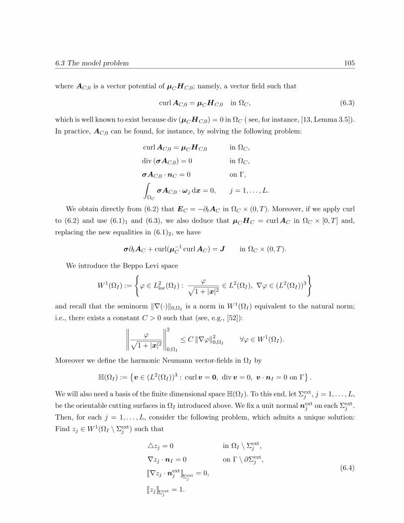
6.3 The model problem 105
where AC,0 is a vector potential of µCHC,0; namely, a vector field such that
curlAC,0 = µCHC,0 in ΩC , (6.3)
which is well known to exist because div (µCHC,0) = 0 in ΩC ( see, for instance, [13, Lemma 3.5]).
In practice, AC,0 can be found, for instance, by solving the following problem:
curlAC,0 = µCHC,0 in ΩC ,
div (σAC,0) = 0 in ΩC ,
σAC,0 · nC = 0 on Γ,∫ΩC
σAC,0 · ωj dx = 0, j = 1, . . . , L.
We obtain directly from (6.2) that EC = −∂tAC in ΩC × (0, T ). Moreover, if we apply curl
to (6.2) and use (6.1)1 and (6.3), we also deduce that µCHC = curlAC in ΩC × [0, T ] and,
replacing the new equalities in (6.1)2, we have
σ∂tAC + curl(µ−1C curlAC) = J in ΩC × (0, T ).
We introduce the Beppo Levi space
W 1(ΩI) :=
φ ∈ L2
loc(ΩI) :φ√
1 + |x|2∈ L2(ΩI), ∇φ ∈ (L2(ΩI))
3
and recall that the seminorm ∥∇(·)∥0,ΩI
is a norm in W 1(ΩI) equivalent to the natural norm;
i.e., there exists a constant C > 0 such that (see, e.g., [52]):∥∥∥∥∥ φ√1 + |x|2
∥∥∥∥∥2
0,ΩI
≤ C ∥∇φ∥20,ΩI∀φ ∈W 1(ΩI).
Moreover we define the harmonic Neumann vector-fields in ΩI by
H(ΩI) :=v ∈ (L2(ΩI))
3 : curlv = 0, div v = 0, v · nI = 0 on Γ.
We will also need a basis of the finite dimensional space H(ΩI). To this end, let Σextj , j = 1, . . . , L,
be the orientable cutting surfaces in ΩI introduced above. We fix a unit normal nextj on each Σext
j .
Then, for each j = 1, . . . , L, consider the following problem, which admits a unique solution:
Find zj ∈W 1(ΩI \ Σextj ) such that
zj = 0 in ΩI \ Σextj ,
∇zj · nI = 0 on Γ \ ∂Σextj ,
[[∇zj · nextj ]]
Σextj
= 0,
[[ zj ]]Σextj
= 1.
(6.4)

6.3 The model problem 106
The set ∇zj : j = 1, . . . , L, where ∇zj are the (L2(ΩI))3-extension of ∇zj , is a basis of H(ΩI)
(see, for instance, [49]).
We have the following representation of curl-free vector-fields in ΩI (see, e.g., [32, Remark 7]).
Lemma 6.3.1 There holdsu ∈ (L2(ΩI))
3 : curlu = 0 in ΩI= ∇(W 1(ΩI))⊕H(ΩI).
Moreover, this is an L2(ΩI)-orthogonal decomposition.
We know from (6.1)2 that curlHI = 0 in ΩI at all time t ∈ [0, T ]. Then, the previous lemma
ensures the existence, at each time t ∈ [0, T ], of a function ψI(t) in W1(ΩI) and real constants
αj(t)Lj=1 such that
HI(x, t) = ∇ψI(x, t) +L∑j=1
αj(t)∇zj(x) in ΩI × [0, T ]. (6.5)
Moreover, taking divergence in the equation (6.1)1 and using that µ = µ0I in ΩI , we obtain
that ∂t(divHI) = 0 in ΩI × (0, T ). Hence, since we know that divHI(x, 0) = divHI,0 = 0 in
ΩI , we conclude that divHI = 0 in ΩI × [0, T ]. Then, using (6.5) and (6.4)1, we obtain that
ψI = 0 in ΩI × [0, T ].
On the other hand, multiplying (6.1)1 by ∇zi, using a Green’s formula and the fact that EI ×nI = −EC × nC , we obtain∫
ΩI
∂t(µ0HI) · ∇zi dx = −∫ΓEC × nC · ∇zi dζ, i = 1, . . . , L.
Replacing HI by ∇ψI +∑L
j=1 αj∇zj and EC by −∂tAC , using the orthogonality between
∇W 1(ΩI) and H(ΩI) and integrating by parts in ΩI , we obtain
µ0
L∑j=1
α′j(t)
∫ΩI
∇zj · ∇zi dx =
∫Γ∂tAC(t)× nC · ∇zi dζ, i = 1, . . . , L.
Next, integrating in time between 0 and s (0 < s < T ) and recalling that AC(x, 0) = AC,0(x),
we obtain
µ0
L∑j=1
αj(s)
∫ΩI
∇zj · ∇zi dx−∫ΓAC(s)× nC · ∇zi dζ
= µ0
L∑j=1
αj(0)
∫ΩI
∇zj · ∇zi dx−∫ΓAC,0 × nC · ∇zi dζ, (6.6)

6.4 A FEM-BEM coupling variational formulation 107
with i = 1, . . . , L. From (6.4), Green’s formula yields∫ΩI
∇zj · ∇zi dx =
∫Σext
j
∂zi∂nj
dζ,
for all i, j = 1, . . . , L. Then, we introduce the matrix
N :=
(∫Σext
j
∂zi∂nj
dζ
)1≤i,j≤L
. (6.7)
It is clear that N is symmetric and positive definite. We also define the matrix Z and the vector
α by
Z :=[∇z1 · · · ∇zL
]tand α :=
[α1 · · · αL
]t. (6.8)
Thus, we can write equation (6.6) as follows:
µ0Nα−∫ΓZ (AC × nC) dζ = µ0Nα0 −
∫ΓZ (AC,0 × nC) dζ,
where α0 := α(0) is known.
In conclusion, we are led to the following problem:
Find AC ∈ L2(0, T ;H(curl; ΩC)) ∩ H1(0, T ; (L2(ΩC))3), ψI ∈ L2(0, T ;W 1(ΩI)) and α ∈
L2(0, T ;RL) such that
σ∂tAC + curl(µ−1C curlAC) = J in ΩC × (0, T ),
µ0Nα−∫ΓZ (AC × nC) dζ = µ0Nα0 −
∫ΓZ (AC,0 × nC) dζ,
ψI = 0 in ΩI × [0, T ],(µ−1C curlAC
)× nC +
(∇ψI +Ztα
)× nI = 0 on Γ× [0, T ],
curlAC · nC + µ0∇ψI · nI = 0 on Γ× [0, T ],
AC(x, 0) = AC,0 in ΩC .
(6.9)
Equations (6.9)4 and (6.9)5 come from the fact that H ∈ H(curl;R3) and µH ∈ H(div ;R3)
and, hence, HC × nC = −HI × nI and µCHC · nC = −µ0HI · nI on Γ, respectively.
6.4 A FEM-BEM coupling variational formulation
In what follows we reduce problem (6.9) to the bounded domain ΩC . To do this we will use
Costabel’s symmetric FEM-BEM coupling technique (cf. [25, 26]). We introduce on Γ the single
and double layer potentials, which are formally defined by
S : H−1/2(Γ) → H1/2(Γ), S(ξ)(x) :=∫Γ
1
4π |x− y|ξ(y) dζy,
D : H1/2(Γ) → H1/2(Γ), D(η)(x) :=
∫Γ
x− y
4π |x− y|3· η(y)nC(y) dζy,

6.4 A FEM-BEM coupling variational formulation 108
respectively, and the hypersingular operator H : H1/2(Γ) → H−1/2(Γ), which is formally defined
as the following normal derivative:
H(η)(x) := −∇x
(∫Γ
x− y
4π |x− y|3· η(y)nC(y) dζy
)· nC(x).
Let us remark that the restrictions to the boundary as well as the normal derivative above have
to be understood in a weak sense; for rigorous definitions see, for instance, McLean [48]. The
three operators are linear and bounded. Let D′ : H−1/2(Γ) → H−1/2(Γ) denote the adjoint
operator of D.
In what follows, we recall some basics properties of these operators (see, e.g., McLean [48]
and Nedelec [52] for the corresponding proofs).
Theorem 6.4.1 Let φ ∈ W 1(ΩI) be a harmonic function. Then, the following identities hold
on Γ: (1
2I − D
)(φ|Γ)− S
(∂φ
∂nI
)= 0,
−(1
2I +D′
)(∂φ
∂nI
)+H (φ|Γ) = 0.
Lemma 6.4.1 (i) There exists k1 > 0 such that∫ΓS(η)η dζ ≥ k1 ∥η∥2−1/2,Γ ∀η ∈ H−1/2(Γ).
(ii) There exists k2 > 0 such that∫ΓH(φ)φ dζ ≥ k2 ∥φ∥21/2,Γ ∀φ ∈ H
1/20 (Γ),
where
H1/20 (Γ) :=
φ ∈ H1/2(Γ) :
∫Γφ dζ = 0
.
Lemma 6.4.2 H(1) = 0, D(1) = −1/2 and∫ΓH(η) dζ = 0 ∀η ∈ H1/2(Γ).
Here and thereafter, for the ease of notation, we use the integration symbol on Γ instead of the
duality pairing between H−1/2(Γ) and H1/2(Γ); namely,∫ΓH(η) dζ = ⟨H(η), 1⟩H−1/2(Γ)×H1/2(Γ).
Theorem 6.4.2 The linear operator H : H1/2(Γ)/R → H−1/20 (Γ), where
H−1/20 (Γ) :=
η ∈ H−1/2(Γ) :
∫Γη dζ = 0
,
defines an isomorphism.

6.4 A FEM-BEM coupling variational formulation 109
Let (AC , ψI ,α) satisfying (6.9). Let ψ(t) := ψI |Γ(t)− c(t), where c : [0, T ] → R is such that
ψ(t) ∈ H1/20 (Γ). By using (6.9)3 and (6.9)5, according to Theorem 6.4.1 and Lemma 6.4.2, for
all t ∈ [0, T ] we have
− 1
2ψ −D(ψ) +
1
µ0S(curlAC · nC) = −ψI on Γ, (6.10)
1
2µ0curlAC · nC +
1
µ0D′(curlAC · nC) +H(ψ) = 0 on Γ. (6.11)
The following is a variational formulation of problem (6.9), where
V := H(curl; ΩC).
Find AC ∈ L2(0, T ;V) ∩ H1(0, T ; (L2(ΩC))3), ψ ∈ L2(0, T ;H
1/20 (Γ)) and α ∈ L2(0, T ;RL)
such that
d
dt
∫ΩC
σAC ·wC dx+
∫ΩC
µ−1C curlAC · curlwC dx
+
∫Γ
[−1
2ψ −D(ψ) +
1
µ0S(curlAC · nC)
]curlwC · nC dζ
+αt
∫ΓZ (wC × nC) dζ =
∫ΩC
J ·wC dx,∫Γ
[1
2curlAC · nC +D′(curlAC · nC) + µ0H(ψ)
]η dζ = 0,
µ0βtNα− βt
∫ΓZ (AC × nC) dζ = µ0β
tNα0 − βt
∫ΓZ (AC,0 × nC) dζ,
(6.12)
for all wC ∈ V , η ∈ H1/20 (Γ) and β ∈ RL, with
AC(0) = AC,0 in ΩC .
In fact, to derive (6.12)1, we have multiplied (6.9)1 by wC , integrated by parts in ΩC and
used (6.9)4, the identity ∫ΓnI ×∇ψI ·wC dζ =
∫ΓψI curlwC · nC dζ, (6.13)
(which in its turn follows by integration by parts, too) and (6.10). On the other hand, Eqs.
(6.12)2 and (6.12)3 follow directly from (6.11) and (6.9)2.
For the theoretical analysis it is convenient to eliminate α and ψ from the previous formu-
lation. With this aim, we introduce the linear operator T : V → RL defined by
T(wC) :=
∫ΓZ (wC × nC) dζ.

6.4 A FEM-BEM coupling variational formulation 110
We eliminate α from (6.12)3 and replace it in (6.12)1. Then, the fourth term of this equation
reads
αt
∫ΓZ (wC × nC) dζ =
(T(wC)
)tα
= µ−10
(T(wC)
)tN−1T(AC) +
(T(wC)
)tα0
− µ−10
(T(wC)
)tN−1T(AC,0).
Moreover, we introduce the operator R : H−1/20 (Γ) → H
1/20 (Γ) given by∫
ΓH(R(ξ))η dζ =
∫Γξη dζ ∀η ∈ H
1/20 (Γ), ∀ξ ∈ H
−1/20 (Γ). (6.14)
It is straightforward to show, from Lemma 6.4.1(ii) and the Lax-Milgram lemma, that R is well
defined and bounded. Therefore, the second equation of (6.12) may be equivalently written
ψ = −µ−10 R
(1
2curlAC · nC +D′(curlAC · nC)
).
Consequently, (6.12) admits the following equivalent reduced form:
Find AC ∈ L2(0, T ;V) ∩H1(0, T ; (L2(ΩC))3) such that
d
dt(AC(t),wC)σ +A(AC(t),wC) + B(AC(t),wC) = (J(t),wC)0,ΩC
+ g(wC) (6.15)
for all wC ∈ V , with
AC(0) = AC,0 in ΩC ,
where
(H,G)σ :=
∫ΩC
σH ·Gdx ∀H,G ∈ (L2(ΩC))3,
A : V × V → R, A(H,G) :=
∫ΩC
µ−1C curlH · curlGdx
+ µ−10
∫ΓS(curlH · nC) curlG · nC dζ,
B : V × V → R, B(H,G) := µ−10
∫ΓK(G)R(K(H)) dζ
+ µ−10
(T(G)
)tN−1T(H),
K : V → H−1/20 (Γ), K(H) :=
1
2curlH · nC +D′(curlH · nC),
g : V → R, g(H) := µ−10
(T(H)
)tN−1T(AC,0)−
(T(H)
)tα0.
Notice that A and B are bounded, symmetric and non-negative definite bilinear forms.
Remark 6.4.1 The norm ∥ · ∥0,ΩCis equivalent to ∥ · ∥σ and, therefore, ∥ · ∥V is equivalent to
∥ · ∥σ + ∥ curl(·)∥0,ΩC.

6.4 A FEM-BEM coupling variational formulation 111
6.4.1 Existence and Uniqueness.
As shown in the following lemma, problem (6.15) is well posed.
Lemma 6.4.3 There exists a unique solution to (6.15) and
∥AC∥2L∞(0,T ;V) + ∥∂tAC∥2L2(0,T ;(L2(ΩC))3)
≤ C∥J∥2L2(0,T ;(L2(ΩC))3) + ∥AC,0∥2V + |α0|2
(6.16)
for some constant C > 0, independent of the problem data J , AC,0 and α0.
Proof. The classical theory for parabolic problems (see, for instance, [32]) allows us to show
that Problem (6.15) has a unique solution AC ∈ L2(0, T ;V) ∩ H1(0, T ;V ′). Moreover, since
AC,0 ∈ V and the right hand side of (6.15) is the sum of two terms, (J(t),wC)0,ΩCwith
J ∈ L2(0, T ; (L2(ΩC))3) and g(wC) with g ∈ V ′ independent of t, it is straightforward to show
that actually ∂tAC ∈ L2(0, T ; (L2(ΩC))3) and the estimate (6.16) holds true (In fact, we may
proceed as in the proof of Theorem 7.1.5 from [35] for the first term, and use Theorem A.1 from
[17] for the second one).
Remark 6.4.2 Problems (6.12) and (6.15) are actually equivalent. In fact, for AC being a
solution of (6.15), if we define ψ := −µ−10 R(K(AC)) and α := α0+µ
−10 N−1(T(AC)−T(AC,0)),
then (AC , ψ,α) is a solution of (6.12). Moreover this problem has a unique solution, because
AC has to be the unique solution of (6.15) and ψ and α are determined via (6.12)2 and (6.12)3,
respectively.
Problems (6.9) and (6.12) are also equivalent. In fact, we derived (6.12) from (6.9). In what
follows, we show the converse implication:
Theorem 6.4.3 Let (AC , ψ,α) be the solution to problem (6.12). Then, there exists ψI ∈L2(0, T ;W 1(ΩI)) and a function c : [0, T ] → R such that ψ = ψI |Γ − c and (AC , ψI ,α) satisfies
(6.9).
Proof. Testing (6.12)1 with wC ∈ (C∞0 (ΩC))
3 we obtain
σ∂tAC + curl(µ−1C curlAC
)= J in ΩC (6.17)
a.e. in [0, T ]. Then, testing (6.12)2 with η ∈ H1/2(Γ) and using Lemma 6.4.2 we have
1
2curlAC · nC +D′(curlAC · nC) + µ0H(ψ) = 0 on Γ. (6.18)
6.5 Fully-discrete scheme 112
Now, let ψI ∈W 1(ΩI) be the solution of the following problem:
ψI = 0 in ΩI ,
µ0∇ψI · nI = − curlAC · nC on Γ.(6.19)
Since ψI ∈W 1(ΩI) is a harmonic function, Theorem 6.4.1 ensures that
1
2ψI |Γ −D(ψI |Γ) +
1
µ0S(curlAC · nC) = 0,
1
2curlAC · nC +D′(curlAC · nC) + µ0H(ψI |Γ) = 0.
(6.20)
Subtracting (6.18) from (6.20)2, we obtain H(ψ − ψI) = 0 on Γ. Therefore, we conclude from
Theorem 6.4.2 that ψI(t) = ψ(t) + c(t) on Γ, where, for each t ∈ [0, T ], c(t) is a constant. As a
consequence, from (6.20)1 we have
− 1
2ψ|Γ −D(ψ|Γ) +
1
µ0S(curlAC · nC)
= −1
2(ψI |Γ − c)−D(ψI |Γ − c) +
1
µ0S(curlAC · nC) = −ψI |Γ.
Now, replacing this equality in (6.12)1, using (6.13) and testing with wC ∈ H(curl; ΩC), we
obtain (µ−1C curlAC
)× nC +
(∇ψI +Ztα
)× nI = 0 on Γ.
Let us emphasize that the first term on the left hand side is well defined in H−1/2(Γ), since
µ−1C curlAC ∈ H(curl; ΩC), which in turn follows because of (6.17) and the facts that J ∈
L2(0, T ; (L2(ΩC))3) and the solution to Problem (6.12) satisfies ∂tAC ∈ L2(0, T ; (L2(ΩC))
3).
Finally (6.9)2 and (6.9)3 follows from (6.12)3 and the initial condition of problem (6.12), respec-
tively.
6.5 Fully-discrete scheme
Let Th(ΩC)h be a regular family of tetrahedral meshes of ΩC . As usual, h stands for the
largest diameter of the tetrahedra K in Th(ΩC). Furthermore, we consider the corresponding
family of triangulations induced on Γ, Th(Γ)h. Let N ∈ N, ∆t := T/N and tn = n∆t,
n = 0, . . . , N .
We define a fully-discrete version of (6.12) by means of Nedelec finite elements. The local
representation on K of the lowest-order Nedelec finite element is given by
N (K) :=a× x+ b : a, b ∈ R3, x ∈ K
.

6.5 Fully-discrete scheme 113
The corresponding global space Vh is the space of vector fields that are locally in N (K) for all
K in ΩC and globally in V = H(curl; ΩC). Moreover, we define
Lh(Γ) :=η ∈ H
1/20 (Γ) : η|F ∈ P1(F ) ∀F ∈ Th(Γ)
,
which approximates the space H1/20 (Γ), where Pk(F ) is the set of polynomial functions defined
in F of degree not greater than k.
When ΩC is not simply connected, problem (6.12) involves the matrices N and Z defined by
(6.7) and (6.8), respectively. To compute these matrices we also need to approximate numerically
the basis ∇zkLk=1 of the harmonic Neumann vector-fields space H(ΩI). A similar need arose
in [49], where the authors proposed a coupled FEM-BEM method to compute the entries of a
matrix Nh approximating N. For the sake of completeness, in what follows, we briefly describe
the method introduced in [49] to approximate N and the corresponding error estimate proved
in this reference.
Consider a convex polyhedron Ω such that ΩC ∪(∪L
k=1Σextk
)⊂ Ω. Set
Q0 := Ω \ΩC ∪
( L∪k=1
Σextk
), Q := Ω \ ΩC and Λ := ∂Ω.
From (6.4), pk := ∇zk|Q, k = 1, . . . , L, belong to the closed subspace of H(div ;Q)
Y :=q ∈ (L2(Q))3 : div q = 0 in Q and q · nI = 0 on Γ
and satisfies the variational equation∫
Qpk · q dx−
∫Σext
k
q · nk dζ +∫Λq · nzk dζ ∀q ∈ Y,
where n correspond to the unit normal vector on Λ outer to Q. Furthermore, as zk is harmonic
in R3 \ Ω, the last equation may be coupled with boundary integral equations relating zk and
its normal derivative pk ·n on Λ. This leads to the following weak formulation (see [50] for more
details)
Find pk ∈ Y and ϕk ∈ H1/2(Λ)/R such that∫Qpk · q dx+
∫ΛS(pk · n)q · n dζ −
∫Λ
[1
2ϕk +D(ϕk)
]q · n dζ
=
∫Σext
k
q · nk dζ,∫Λ
[1
2χ+D(χ)
]pk · n dζ +
∫ΛH(ϕk)χdζ = 0,
(6.21)
for all functions q ∈ Y and χ ∈ H1/2(Λ)/R. The variable ϕk represents (up to and additive
constant) the trace of zk on Λ. Now, consider a regular family of triangulations Th(Q)h of Q by

6.5 Fully-discrete scheme 114
tetrahedra K of diameter no greater than h > 0. Assume that, for any h, the set Th(ΩC)∪Th(Q)
is a triangulation of Ω. This implies that the triangulation induced by Th(Q) on Γ is identical
to Th(Γ). It can be assumed, without loss of generality, that, for each mesh, the cutting surfaces
Σextk are union of faces of tetrahedra in Th(Q). Finally, denote by Th(Λ) the triangulation induced
by Th(Q) on Λ.
Consider a conforming discretization of H(div ;Q):
RT h(Q) := q ∈ H(div ;Q) : q|K ∈ RT (K) ∀K ∈ Th(Q) ,
RT (K) :=ax+ b : a ∈ R, b ∈ R3, x ∈ K
being the lowest-order Raviart-Thomas element.
The following is a convenient way of discretizing problem (6.21) (for more details, see [49]):
Find pkh ∈ RT 0h(Q), ϕkh ∈ Φh/R and βkh ∈Mh such that∫
Qpkh · q dx+
∫ΛS(pkh · n)q · n dζ −
∫Λ
[1
2ϕkh +D(ϕkh)
]q · n dζ
+
∫Qβkhdiv q dx =
∫Σext
k
q · nk dζ,∫Λ
[1
2χ+D(χ)
]pkh · n dζ +
∫ΛS(curl
τϕkh) curl
τχ dζ = 0,∫
Qdiv pkhv dx = 0,
(6.22)
for all functions q ∈ RT 0h(Q), χ ∈ Φh/R and v ∈Mh, where
RT 0h(Q) := q ∈ RT h(Q) : q|Γ · nI = 0,
Φh := η ∈ C0(Λ) : η|F ∈ P1(F ) ∀F ∈ Th(Λ),
Mh := v ∈ L2(Q) : v|K ∈ P0(K) ∀K ∈ Th(Q).
Moreover, curlτ denotes the surface curl on Λ (see, for instance, [5, Section A.1]).
We know from [50] that (6.22) is a well posed problem. Once the functions pkh, 1 ≤ k ≤ L,
are computed, the matrix N can be approximated by
Nh :=
(∫Σext
j
pkh · nj dζ
)1≤k,j≤L
. (6.23)
Note that this matrix is symmetric and positive definite. Error estimates for the approximation
Nh of N has been obtained in [49]. With this end, an additional regularity result has been also
proved therein. In the sequel, we denote by sQ ∈ (1/2, 1) the exponent of maximal regularity inQof the solution of the Laplace operator with L2(Q) right-hand side and homogeneous Neumann
boundary data.

6.5 Fully-discrete scheme 115
Theorem 6.5.1 If (pk, ϕk) is the solution to problem (6.21), k = 1, . . . , L, then pk ∈ (Hs(Q))3
for all s ∈ (1/2, sQ).
Proof. See [49, Theorem 7.1].
Finally we recall the error estimates obtained in [49]. Here and thereafter C denotes a generic
positive constant not necessarily the same at each occurrence, but always independent of the
mesh size h and the time step ∆t.
Theorem 6.5.2 Problems (6.21) and (6.22) are well posed and
∥pk − pkh∥0,Q + ∥ϕk − ϕkh∥H1/2(Λ)/R ≤ Chs∥pk∥s,Q + ∥ϕk∥s+1/2,Λ
holds, with s as in Theorem 6.5.1.
Proof. See [49, Theorem 7.2].
Theorem 6.5.3 There exists h0 > 0 such that Nh is invertible for all h ∈ (0, h0). Moreover,
the error estimate
∥N−Nh∥+∥∥N−1 −N−1
h
∥∥ ≤ Chs max1≤k≤L
∥pk∥s,Q + ∥ϕk∥s+1/2,Λ
holds, with s as in Theorem 6.5.1.
Proof. See [49, Corollary 7.3].
Notice that ∥ϕk∥s+1/2,Λ is clearly bounded, since ϕk is the trace on Λ of the solution zk to
problem 6.4.
To compute an approximation of the entries of Z, we need to resort to a different strategy.
In fact, the previous methods yields good approximation of pk|Γ · nI = ∇zk|Γ · nI , but not of
∇zk|Γ×nI (which are the terms defining the entries of Z). A similar situation happened in [49],
too. However, in this case, we follow an alternative approach that we think is simpler.
It is easy to show that the solution of (6.4) satisfies the following variational formulation:
Find zk ∈ H1(Q \ Σextk )/R such that [[ zk ]]Σext
k= 1 and∫
Q\Σextk
∇zk · ∇φdx =
∫Λpk · nφ dζ ∀φ ∈ H1(Q)/R. (6.24)
We introduce
Lh(Q) :=θ ∈ H1(Q) : θ|K ∈ P1(K) ∀K ∈ Th(Q)
,
Lh(Q \ Σextk ) :=
θ ∈ H1(Q \ Σext
k ) : θ|K ∈ P1(K) ∀K ∈ Th(Q)

6.5 Fully-discrete scheme 116
and consider the following discrete version of problem (6.24):
Find zkh ∈ Lh(Q \ Σextk )/R such that [[ zkh ]]Σext
k= 1 and∫
Q\Σextk
∇zkh · ∇φdx =
∫Λpkh · nφdζ ∀φ ∈ Lh(Q)/R. (6.25)
Lemma 6.5.1 Let zk and zkh be the solutions to problems (6.24) and (6.25), respectively. Then∥∥∇zk − ∇zkh∥∥0,Q ≤ Chs,
with s as in Theorem 6.5.1.
Proof. Let zk ∈ C∞(Q \ Σextk ) be such that [[ zk ]]Σext
k= 1. Let zIk be the Lagrange intepolant of
zk in Q \ Σextk . Notice that [[ zIk ]]Σext
k= 1, too. We write
zk = zk + zk and zkh = zIk + zkh,
with zk ∈ H1(Q)/R and zkh ∈ Lh(Q)/R. Substituting these expressions in problems (6.24) and
(6.25), respectively, and using the first Strang lemma (see, for instance, [23, Theorem 4.4.1]), we
obtain
∥∇zk −∇zkh∥0,Q ≤ C infφ∈Lh(Q)/R
∥∇zk −∇φ∥0,Q
+ C supφ∈Lh(Q)/R
∣∣∣− ∫Q\Σextk
∇(zk − zIk) · ∇φ dx+∫Λ(pk − pkh) · nφ dζ
∣∣∣∥∇φ∥0,Q
.
The second term on the right-hand side above is bounded as follows:∣∣∣∣∣−∫Q\Σext
k
∇(zk − zIk) · ∇φdx+
∫Λ(pk − pkh) · nφdζ
∣∣∣∣∣≤∥∥∇zk −∇zIk
∥∥0,Q\Σext
j∥∇φ∥0,Q + C ∥pk − pkh∥0,Q ∥∇φ∥0,Q ,
where we have used that div pk = div pkh = 0 in Q and the fact that ∥∇(·)∥0,Q is equivalent to
∥ · ∥1,Q on H1(Q)/R.On the other hand, from Theorem 6.5.1 we know that ∇zk|Q ∈ (Hs(Q))3. Hence,
infφ∈Lh(Q)/R
∥∇zk −∇φ∥0,Q ≤∥∥∇zk −∇zIk
∥∥0,Q ≤ Chs ∥∇zk∥s,Q .
Thus, using the last two estimates and Theorem 6.5.2, we obtain
∥∇zk −∇zkh∥0,Q ≤ Chs∥∇zk∥s,Q\Σext
k+ ∥pk∥s,Q + ∥ϕk∥s+1/2,Λ + ∥∇zk∥s,Q
.

6.5 Fully-discrete scheme 117
Therefore, as a consequence of Theorem 6.5.1,∥∥∇zk − ∇zkh∥∥0,Q ≤ Chs
and we conclude the proof.
Now, we are in a position to introduce the following full discretization of problem (6.12):
For n = 1, . . . , N , find (AnCh, ψ
nh ,α
nh) ∈ Vh × Lh(Γ)× RL such that∫
ΩC
σ∂AnCh ·wC dx+
∫ΩC
µ−1C curlAn
Ch · curlwC dx
+
∫Γ
[−1
2ψnh −D(ψnh) +
1
µ0S(curlAn
Ch · nC)]curlwC · nC dζ
+ (αnh)
tTh(wC) =
∫ΩC
J(tn) ·wC dx,∫Γ
[1
2curlAn
Ch · nC +D′(curlAnCh · nC) + µ0H(ψnh)
]η dζ = 0,
µ0βtNhα
nh − βtTh(An
Ch) = µ0βtNhα0 − βtTh(AC,0),
(6.26)
for all (wC , η,β) ∈ Vh × Lh(Γ)× RL, with
A0Ch = ACh,0 in ΩC ,
where ACh,0 ∈ Vh is an approximation of AC,0, ∂AnCh := (An
Ch −An−1Ch )/∆t and the linear and
continuous operator Th : V → RL is defined by
Th(w) :=
∫ΓZh (w × nC) dζ, with Zh :=
[∇z1h · · · ∇zLh
]t.
To prove the existence and uniqueness of solution to (6.26), first we proceed as in the con-
tinuous case and obtain a discrete form of Problem (6.15). Let Rh : H−1/20 (Γ) → Lh(Γ) be the
operator defined by∫ΓH(Rh(ξ))η dζ =
∫Γξη dζ ∀η ∈ Lh(Γ), ∀ξ ∈ H
−1/20 (Γ).
Note that this is a Galerkin discretization of the elliptic problem (6.14). Consequently, using the
Galerkin orthogonality and the continuity and ellipticity of H (cf. Lemma 6.4.1(ii)), we have the
following Cea estimate:
∥Rξ −Rhξ∥1/2,Γ ≤ C infη∈Lh(Γ)
∥Rξ − η∥1/2,Γ ∀ξ ∈ H−1/20 (Γ). (6.27)
Now, using again that ψnh := −µ−10 Rh (K(An
Ch)) (cf. (6.26)2) we obtain the following equi-
valent formulation of (6.26):
6.5 Fully-discrete scheme 118
For n = 1, . . . , N , find AnCh ∈ Vh such that(
∂AnCh,wC
)σ+A(An
Ch,wC) + Bh(AnCh,wC) = (J(tn),wC)0,ΩC
+ gh(wC) (6.28)
for all wC ∈ Vh, with
A0Ch = ACh,0 in ΩC ,
where
Bh : Vh × Vh → R, Bh(H,G) := µ−10
∫ΓK(G)Rh(K(H)) dζ
+ µ0(Th(G)
)tN−1h Th(H),
gh : Vh → R, gh(H) := µ−10
(Th(H)
)tN−1h Th(AC,0)−
(Th(H)
)tα0.
Hence, at each iteration, we have to find AnCh ∈ Vh such that
(AnCh,wC)σ +∆t [A(An
Ch,wC) + Bh(AnCh,wC)]
= ∆t[(J(tn),wC)0,ΩC
+ gh(wC)]+(An−1Ch ,wC
)σ. (6.29)
Since Bh and A are non-negative definite, the existence and uniqueness of AnCh, n = 1, . . . , N ,
is immediate.
Remark 6.5.1 It is easy to prove that if ψnh := −µ−10 Rh(K(An
Ch)) as defined above and αnh :=
α0 + µ−10 N−1
h (Th(AnCh) − Th(AC,0)), then (An
Ch, ψnh ,α
nh) is a solution of (6.26). This solution
is unique, because H is elliptic in Lh(Γ) ⊂ H1/20 (Γ) and Nh is a symmetric and positive definite
matrix.
6.5.1 Matrix form
To have it clear the kind of problem we have to solve in practice, we will write the fully discrete
scheme (6.26) in matrix form. Let ϕ1, . . . ,ϕJ and λ1, . . . , λM be bases of Vh and Lh(Γ),respectively, and e1, . . . , eL the canonical basis of RL. We write the solution (An
Ch, ψnh ,α
nh),
n = 1, . . . , N , to problem (6.26), in these bases:
AnCh =
J∑j=1
anjϕj , ψnh =M∑j=1
bnj λj , αnh =
L∑j=1
cnj ej , n = 1, . . . , N.
Analogously, we write
ACh,0 =J∑j=1
a0jϕj and α0 =L∑j=1
c0jej .

6.5 Fully-discrete scheme 119
We set an := (ani )1≤i≤J , cn := (cni )1≤i≤L , with n = 0, . . . , N , and bn := (bni )1≤i≤M , with
n = 1, . . . , N . We also set Fn := (Fni )1≤i≤J , where
Fni :=
∫ΩC
J(tn) · ϕi dx.
We introduce the matrices W := (Wij)1≤i,j≤J , D := (Dij)1≤i≤J,1≤j≤M , H := (Hij)1≤i,j≤M ,
R := (Rij)1≤i,j≤J , Q := (Qij)1≤i≤J,1≤j≤L and S := (Sij)1≤i,j≤J , where
Wij :=
∫ΩC
σϕi · ϕj dx, Dij :=
∫Γ
[−1
2λj −D(λj)
]curlϕi · nC dζ,
Hij :=
∫ΓH(λi)λj dζ, Rij :=
∫ΩC
µ−1C curlϕi · curlϕj dx,
Qij := etj
∫ΓZh (ϕi × nC) dζ, Sij :=
∫ΓS(curlϕi · nC) curlϕj · nC dζ.
Hence, we write problem (6.26) in block matrix form as follows:W +∆t (R+ S) ∆tD ∆tQ
∆tDt −∆tH O
∆tQt O −∆tNh
an
bn
cn
=
∆tFn +Wan−1
O
∆t(Qta0 −Nhc
0) .
As already mentioned in Remark 6.5.1, problem (6.26) has a unique solution, so that the matrix
on the left hand side is non singular.
Matrices Zh and Nh are both readily obtained once the solution pkh to problem (6.22) is
computed. In what follows we write down the matrix form of this problem. Let u1, . . . ,uA,v1, . . . , vB and w1, . . . , wC be bases of RT 0
h(Q), Φh/R and Mh, respectively. Then, we write
the solution of problem (6.22) in these bases as follows:
pkh =
A∑j=1
φkjuj , ϕkh =
B∑j=1
γkjvj and βkh =
C∑j=1
ηkjwj .
Next, we define φk := (φki)1≤i≤A, γk := (γki)1≤i≤B, ηk := (ηki)1≤i≤C and G := (Gi)1≤i≤A,
where
Gi :=
∫Σext
k
ui · nk dζ.
Moreover, we introduce the matricesU := (Uij)1≤i,j≤A,V := (Vij)1≤i,j≤A,K := (Kij)1≤i≤A,1≤j≤B,
E := (Eij)1≤i≤A,1≤j≤C and T := (Tij)1≤i,j≤A, where
Uij :=
∫Qui · uj dx, Vij :=
∫ΛS (ui · n)uj · n dζ,
Kij := −∫Λ
[1
2vj +D(vj)
]ui · ndζ, Eij :=
∫Qwjdivui dx,
Tij :=
∫ΛS(curlτvj
)curlτvi dζ.
6.6 Error estimates 120
Then, Problem (6.22) reads U+V K E
Kt −T O
Et O O
φk
γk
ηk
=
G
O
O
.It is proved in [50] that the matrix of the left hand side above is invertible. Finally, for a discussion
on the efficient computation of all the singular integrals appearing above, we refer to [63].
As a conclusion, we have that problem (6.26) is actually solvable. Although it involves the
solution of the auxiliary problem (6.22), this can be made off-line since it does not depend
on time. Once it is solved, the time domain problem (6.26) involves only a vector field on
the conducting domain and a scalar field on its boundary. Therefore, this approach allows to
minimizing the number of degrees of freedom needed in the discretization.
6.6 Error estimates
For any s ≥ 0, we consider the space
Hs(curl; ΩC) :=v ∈ (Hs(ΩC))
3 : curlv ∈ (Hs(ΩC))3
endowed with the norm ∥v∥2Hs(curl;ΩC)
:= ∥v∥2s,ΩC+ ∥ curlv∥2s,ΩC
. It is well known that the
Nedelec interpolation operator INh v ∈ Vh is well defined for any v ∈ Hs(curl; ΩC), with s > 1/2
(see, for instance, Lemma 4.7 of [13]). Moreover, for 1/2 < s ≤ 1, the following interpolation
error estimate holds true (see Proposition 5.6 of [6]):∥∥v − INh v∥∥V ≤ Chs ∥v∥Hs(curl;ΩC) ∀v ∈ Hs(curl; ΩC). (6.30)
To simplify the notation, we introduce for any w ∈ V
Gh(w) := ∥(R−Rh)K(w)∥1/2,Γ .
Lemma 6.6.1 Let (AC , ψ,α) and (AnCh, ψ
nh ,α
nh) be the solutions to problems (6.12) and (6.26),
respectively, the latter with initial data A0Ch := IN
h (AC,0). Assume that AC ∈ C1([0, T ];V) ∩C0([0, T ];Hs(curl; ΩC)), with s > 1/2. Moreover, let ρn := AC(tn)−IN
h AC(tn), δn := IN
h AC(tn)−AnCh and τn := ∂AC(tn)− ∂tAC(tn). Then, there exists C > 0, independent of h and ∆t, such

6.6 Error estimates 121
that
max1≤k≤n
∥∥∥δk∥∥∥2V+∆t
n∑k=1
∥∥∥∂δk∥∥∥2σ
≤ C
∆t
n∑k=1
[ ∥∥∥∂ρk∥∥∥2V+∥∥∥τ k∥∥∥2
V+ Gh(∂tAC(tk))
2
+(∥AC(tk)∥2V + ∥∂tAC(tk)∥2V
)(max1≤i≤L
∥∥∇zi − ∇zih∥∥20,Q +
∥∥N−1 −N−1h
∥∥2 )]+(∥AC,0∥2V + |α0|2
)(max1≤i≤L
∥∥∇zi − ∇zih∥∥20,Q +
∥∥N−1 −N−1h
∥∥2 )+ max
0≤k≤n
∥∥∥ρk∥∥∥2V+ max
0≤k≤nGh(AC(tk))
2
.
Proof. It is straightforward to show that(∂δk,v
)σ+A(δk,v) + Bh(δk,v)
= −(∂ρk,v
)σ+(τ k,v
)σ−A(ρk,v)− Bh(ρk,v)
+ Bh(AC(tk),v)− B(AC(tk),v) + g(v)− gh(v) ∀v ∈ Vh,
(6.31)
as well as the following inequalities:(∂δk, δk
)σ≥ 1
2∆t
(∥∥∥δk∥∥∥2σ−∥∥∥δk−1
∥∥∥2σ
),
A(δk, δk) ≥ µ−11
∥∥∥curl δk∥∥∥20,ΩC
,
B(AC(tk), δk)− Bh(AC(tk), δ
k)
≤ C ∥AC(tk)∥V∥∥∥δk∥∥∥
V
(max1≤i≤L
∥∥∇zi − ∇zih∥∥0,Q +
∥∥N−1 −N−1h
∥∥)+ C
∥∥∥curl δk∥∥∥0,ΩC
Gh(AC(tk)),
g(δk)− gh(δk)
≤ C(∥AC,0∥V + |α0|
) ∥∥∥δk∥∥∥V
(max1≤i≤L
∥∥∇zi − ∇zih∥∥0,Q +
∥∥N−1 −N−1h
∥∥).Constant µ1 on the second inequality is an upper bound in ΩC of the largest eigenvalue of µC .
Hence, choosing v = δk in (6.31) and using that Bh is non-negative, Cauchy-Schwarz inequality,
Remark 6.4.1 and Young’s inequality lead us to the following estimate:∥∥∥δk∥∥∥2σ−∥∥∥δk−1
∥∥∥2σ+∆tµ−1
1
∥∥∥curl δk∥∥∥20,ΩC
≤ ∆t
2T
∥∥∥δk∥∥∥2σ+ C∆t
[ ∥∥∥∂ρk∥∥∥2σ+∥∥∥τ k∥∥∥2
σ+∥∥∥ρk∥∥∥2
V+ Gh(AC(tk))
2
+ ∥AC(tk)∥2V(
max1≤i≤L
∥∥∇zi − ∇zih∥∥20,Q +
∥∥N−1 −N−1h
∥∥2 )+(∥AC,0∥2V + |α0|2
)(max1≤i≤L
∥∥∇zi − ∇zih∥∥20,Q +
∥∥N−1 −N−1h
∥∥2 )].(6.32)

6.6 Error estimates 122
Then, summing over k, using the discrete Gronwall’s lemma (see, for instance, [60, Lemma 1.4.2])
and taking into account that δ0 = 0, we obtain
∥δn∥2σ ≤ C
∆t
n∑k=1
[ ∥∥∥∂ρk∥∥∥2σ+∥∥∥τ k∥∥∥2
σ+∥∥∥ρk∥∥∥2
V+ Gh(AC(tk))
2
+ ∥AC(tk)∥2V(
max1≤i≤L
∥∥∇zi − ∇zih∥∥20,Q +
∥∥N−1 −N−1h
∥∥2 )]+(∥AC,0∥2V + |α0|2
)(max1≤i≤L
∥∥∇zi − ∇zih∥∥20,Q +
∥∥N−1 −N−1h
∥∥2 )
for n = 1, . . . , N . Inserting the last inequality in (6.32) and summing over k we have the estimate
∥δn∥2σ +∆t
n∑k=1
∥∥∥curl δk∥∥∥20,ΩC
≤ C
∆t
n∑k=1
[ ∥∥∥∂ρk∥∥∥2σ+∥∥∥τ k∥∥∥2
σ+∥∥∥ρk∥∥∥2
V+ Gh(AC(tk))
2
+ ∥AC(tk)∥2V(
max1≤i≤L
∥∥∇zi − ∇zih∥∥20,Q +
∥∥N−1 −N−1h
∥∥2 )]+(∥AC,0∥2V + |α0|2
)(max1≤i≤L
∥∥∇zi − ∇zih∥∥20,Q +
∥∥N−1 −N−1h
∥∥2 ) .(6.33)
Let us now take v = ∂δk in (6.31). We have∥∥∥∂δk∥∥∥2σ+A(δk, ∂δk) + Bh(δk, ∂δk)
= −(∂ρk, ∂δk
)σ+(τ k, ∂δk
)σ+A(∂ρk, δk−1) + Bh(∂ρk, δk−1)
+ B(τ k, δk−1)− Bh(τ k, δk−1) + B(∂tAC(tk), δk−1)
− Bh(∂tAC(tk), δk−1) + g(∂δk)− gh(∂δ
k)− 1
∆t(γk − γk−1) ,
(6.34)
where γk := A(ρk, δk) + Bh(ρk, δk)− Bh(AC(tk), δk) + B(AC(tk), δ
k).
On the other hand, since A is non-negative definite and symmetric, it is easy to check that
A(δk, ∂δk) ≥ 1
2∆t
[A(δk, δk)−A(δk−1, δk−1)
]
6.6 Error estimates 123
and similarly for Bh. Using these inequalities in (6.34) together with Cauchy-Schwarz inequality,
and, then, summing over k and recalling that Bh is non-negative, we deduce that
1
2
n∑k=1
∥∥∥∂δk∥∥∥2σ+
1
2∆tµ−11 ∥curl δn∥20,ΩC
≤n∑k=1
[∥∥∥∂ρk∥∥∥2σ+∥∥∥τ k∥∥∥2
σ
]
+n∑k=1
[ ∣∣∣A(∂ρk, δk−1)∣∣∣+ ∣∣∣Bh(∂ρk, δk−1)
∣∣∣+ ∣∣∣B(τ k, δk−1)− Bh(τ k, δk−1)∣∣∣
+∣∣∣B(∂tAC(tk), δ
k−1)− Bh(∂tAC(tk), δk−1)
∣∣∣ ]+
1
∆t|g(δn)− gh(δ
n)|+ 1
∆t|γn| .
(6.35)
The following bounds are easy to obtain from Young’s inequality and Remark 6.4.1:
n∑k=1
∣∣∣A(∂ρk, δk−1)∣∣∣ ≤ n∑
k=1
∥∥∥curl δk−1∥∥∥20,ΩC
+ C
n∑k=1
∥∥∥curl ∂ρk∥∥∥20,ΩC
,
n∑k=1
∣∣∣Bh(∂ρk, δk−1)∣∣∣ ≤ n∑
k=1
∥∥∥curl δk−1∥∥∥20,ΩC
+
n∑k=1
∥∥∥δk−1∥∥∥2σ+ C
n∑k=1
∥∥∥∂ρk∥∥∥2V,
n∑k=1
∣∣∣B(τ k, δk−1)− Bh(τ k, δk−1)∣∣∣
≤n∑k=1
∥∥∥curl δk−1∥∥∥20,ΩC
+n∑k=1
∥∥∥δk−1∥∥∥2σ+ C
n∑k=1
∥∥∥τ k∥∥∥2V,
n∑k=1
∣∣∣B(∂tAC(tk), δk−1)− Bh(∂tAC(tk), δ
k−1)∣∣∣
≤n∑k=1
∥∥∥curl δk−1∥∥∥20,ΩC
+n∑k=1
∥∥∥δk−1∥∥∥2σ+ C
n∑k=1
Gh(∂tAC(tk))2
+ Cn∑k=1
∥∂tAC(tk)∥2V(
max1≤i≤L
∥∥∇zi − ∇zih∥∥20,Q +
∥∥N−1 −N−1h
∥∥2 ),and
|g(δn)− gh(δn)|
≤ C(∥AC,0∥2V + |α0|2
)(max1≤i≤L
∥∥∇zi − ∇zih∥∥20,Q +
∥∥N−1 −N−1h
∥∥2 )+
1
8µ−11 ∥curl δn∥20,ΩC
+ ∥δn∥2σ ,
|γn| ≤1
8µ−11 ∥curl δn∥20,ΩC
+ ∥δn∥2σ
+ C[∥ρn∥2V + ∥AC(tn)∥2V
(max1≤i≤L
∥∥∇zi − ∇zih∥∥20,Q +
∥∥N−1 −N−1h
∥∥2 )].
6.6 Error estimates 124
Substituting all these inequalities in (6.35), using (6.33) and Remark 6.4.1, we obtain
∆t
n∑k=1
∥∥∥∂δkC∥∥∥2σ+ ∥curl δnC∥
20,ΩC
≤ C
∆t
n∑k=1
[ ∥∥∥∂ρk∥∥∥2V+∥∥∥τ k∥∥∥2
V+ Gh(∂t(AC(tk)))
2 +∥∥∥ρk∥∥∥2
V
+ ∥AC(tk)∥2V(
max1≤i≤L
∥∥∇zi − ∇zih∥∥20,Q +
∥∥N−1 −N−1h
∥∥2 )+ ∥∂tAC(tk)∥2V
(max1≤i≤L
∥∥∇zi − ∇zih∥∥20,Q +
∥∥N−1 −N−1h
∥∥2 )]+(∥AC,0∥2V + |α0|2
)(max1≤i≤L
∥∥∇zi − ∇zih∥∥20,Q +
∥∥N−1 −N−1h
∥∥2 )+ ∥ρn∥2V + Gh(AC(tn))
2
Combining this inequality with (6.33) and Remark 6.4.1, we end the proof.
Lemma 6.6.2 Let (AC , ψ,α) be the solution of (6.12). If we assume that AC ∈ H1(0, T ;Hs(curl; ΩC)),
1/2 < s < sQ, then ψ ∈ H1(0, T ;Hs+1/2(Γ)) and the following estimates hold true:
infη∈Lh(Γ)
∥ψ(t)− η∥1/2,Γ ≤ Chs ∥curlAC(t)∥s,ΩC, (6.36)
infη∈Lh(Γ)
∥∂tψ(t)− η∥1/2,Γ ≤ Chs ∥∂t(curlAC(t))∥s,ΩC. (6.37)
Proof. Let (AC , ψ,α) be the unique solution of (6.12). Let ψI be as in Theorem 6.4.3. As shown
in that theorem, ψI(t) = ψ(t) + c(t) with c(t) ∈ R and t ∈ [0, T ]. Moreover, a.e. in [0, T ], ψI |Qis the solution to
−ψI = 0 in Q,
µ0∂ψI∂nI
= − curlAC · nC on Γ,
ψI |Λ ∈ C∞(Λ).
(6.38)
Since AC ∈ C0([0, T ];Hs(curl; ΩC)) with 1/2 < s < sQ and Λ is the boundary of a convex
polyhedron, by applying classical results for the Laplace equation (see [38]) we have that ψI ∈Hs+1(Q) and
∥ψI∥s+1,Q ≤ C ∥curlAC · nC∥s−1/2,Γ ≤ C ∥curlAC∥s,ΩC. (6.39)
Since s > 1/2, the Lagrange interpolant ψII of ψI is well defined. Moreover, since ψI and ψ
only differ in a constant, (ψI − ψII
)∣∣Γ= ψ − ψIΓ ,
6.6 Error estimates 125
where ψIΓ ∈ Lh(Γ) denotes the 2D Lagrange surface interpolant on Γ. Therefore, because of the
trace theorem, standard estimates for the 3D Lagrange interpolant and (6.39), we have∥∥ψ − ψIΓ∥∥1/2,Γ
≤ C∥∥ψI − ψII
∥∥1,Q ≤ Chs ∥ψI∥s+1,Q ≤ Chs ∥curlAC∥s,ΩC
.
Thus, we conclude (6.36).
To prove (6.37), we recall that ψI is the solution to problem (6.19) (cf. the proof of Theo-
rem 6.4.3). Then, since AC ∈ H1(0, T ;Hs(curl; ΩC)), differentiating in time each equation in
(6.19), we obtain an estimate analogous to (6.39) for ∂tψI . On the other hand, since ψI(t) =
ψ(t) + c(t) with
c(t) =1
|Γ|
∫ΓψI(t) dζ,
we have that ∂tψ(t) = ∂tψI(t)− c′(t). Hence, the rest of the proof follows identically as above.
Now we are in a position to conclude the following asymptotic error estimate for the fully
discrete scheme.
Theorem 6.6.1 Let (AC , ψ,α) and (AnCh, ψ
nh ,α
nh), n = 1, . . . , N , be the solutions to problem
(6.12) and (6.26), respectively. Let us assume that AC ∈ H1(0, T ;Hs(curl; ΩC))∩H2(0, T ;H(curl; ΩC))
with s ∈ (1/2, sQ). Then, there exists h0 > 0 such that, for all h ∈ (0, h0), the following estimate
holds:
max1≤n≤N
∥AC(tn)−AnCh∥
2V +∆t
N∑n=1
∥∥∂(AC(tn)−AnCh)∥∥2σ
≤ Ch2s∫ T
0∥∂tAC(t)∥2Hs(curl;ΩC)
dt+ max1≤n≤N
∥∂t(curlAC(tn))∥2s,ΩC
+ max1≤n≤N
(∥AC(tn)∥2V + ∥∂tAC(tn)∥2V
)(max1≤k≤L
∥∥∇zk∥∥2s,Q + ∥zk∥2s+1/2,Λ
)+(∥AC,0∥2V + |α0|2
)(max1≤k≤L
∥∥∇zk∥∥2s,Q + ∥zk∥2s+1/2,Λ
)+ max
1≤n≤N∥AC(tn)∥2Hs(curl;ΩC)
+ (∆t)2
∫ T
0∥∂ttAC(t)∥2V dt
≤ C[(∆t)2 + h2s
] (∥AC∥2H2(0,T ;Hs(curl ΩC))
+ |α0|2),
where zk is the solution of problem (6.4), k = 1, . . . , L.
Proof. A Taylor expansion shows that
∂AC(tk) = ∂tAC(tk) +1
∆t
∫ tk
tk−1
(tk−1 − t) ∂ttAC(t) dt.
Consequently,n∑k=1
∥∥∥τ k∥∥∥2V≤ ∆t
∫ T
0∥∂ttAC(t)∥2V dt.

6.6 Error estimates 126
Moreover, we have from (6.30),
n∑k=1
∥∥∥∂ρk∥∥∥2V≤ 1
∆t
n∑k=1
∫ tk
tk−1
∥∥∂t(I − INh )AC(t)
∥∥2V dt
≤ Ch2s
∆t
∫ T
0∥∂tAC(t)∥2Hs(curl;ΩC)
dt.
We recall that ψ(t) = −µ−10 R(K(AC(t))) (cf. Remark 6.4.2). It follows from (6.27) that
Gh(AC(tn)) ≤ infη∈Lh(Γ)
∥ψ(tn)− η∥21/2,Γ ,
Gh(∂tAC(tn)) ≤ infη∈Lh(Γ)
∥∂tψ(tn)− η∥21/2,Γ .
Thus, using Lemma 6.6.2, we obtain
Gh(AC(tn)) ≤ Chs ∥curlAC(tn)∥s,ΩC,
Gh(∂tAC(tn)) ≤ Chs ∥∂t(curlAC(tn))∥s,ΩC.
(6.40)
Hence, the results follows by writing AC(tn) − AnCh = δn + ρn and using Lemma 6.6.1,
Lemma 6.5.1, Theorem 6.5.3 and (6.30).
Remark 6.6.1 Let us recall that ψ(tn) = −µ−10 R(K(AC(tn))) and ψnh = −µ−1
0 Rh(K(AnCh)).
Therefore, using (6.40) and the uniform boundedness of Rh with respect to h, we obtain
∥ψ(tn)− ψnh∥1/2,Γ ≤ Gh(AC(tn)) + ∥Rh(K(AC(tn)−AnCh))∥1/2,Γ
≤ Chs ∥curlAC(tn)∥s,ΩC
+ ∥AC(tn)−AnCh∥V
.
Then, using Lemma 6.6.2 and Theorem 6.6.1, under the assumptions of the latter, we conclude
that
∆t
N∑n=1
∥ψ(tn)− ψnh∥21/2,Γ ≤ C
[h2s + (∆t)2
].
Moreover under the same assumptions, since α(tn) = α0 − µ−10 N−1(T(AC(tn) − AC,0)) and
αnh = α0 − µ−1
0 N−1h (Th(An
Ch − AC,0)), from Theorem 6.5.3, Lemma 6.5.1 and Theorem 6.6.1,
we also conclude that
max1≤n≤N
|α(tn)−αnh|
2 ≤ C[h2s + (∆t)2
].
Chapter 7
Conclusiones y trabajo futuro
7.1 Conclusiones
El objetivo principal de la tesis presentada ha sido analizar y proponer nuevos modelos en
el estudio matematico de la electroencefalografıa y la magnetoencefalografıa. Se estudia inicial-
mente el modelo de corrientes inducidas como alternativa a los modelos usados clasicamente
para estudiar este tema. Para el modelo electrostatico, se ha desarrollado un analisis a priori y a
posteriori del error en la aproximacion mediante elementos finitos. Se ha utilizado tal estimador
para idear una estrategia computacional eficiente en la resolucion del problema inverso. Tambien
se han hecho comparaciones a nivel computacional en cuanto a la eficiencia de los diversos
metodos presentes en la literatura y los nuevos metodos propuestos respecto del problema directo
e inverso.
Las conclusiones principales de esta tesis, en orden de desarrollo, son:
1. Se propone una alternativa a los modelos ya existentes que abordan el estudio de la e-
lectroencefalografıa y la magnetoencelografıa: el modelo de corrientes inducidas. Se ha
estudiado desde un punto de vista teorico el problema inverso con este modelo. Como
fuente de corriente, se estudiaron tres casos: fuente distribuida, fuente superficial y fuente
dipolar. Se probo que en el caso de una fuente distribuida, no hay una unica solucion y
se caracterizo el espacio de fuentes no radiantes. En los otros dos casos se demostro que
la componente tangencial del campo electrico en toda la frontera del dominio determina
de forma unica la fuente. En el caso de una fuente dipolar, se ha encontrado una formula
mediante la cual es posible recobrar la posicion dipolar y la polarizacion. Tambien se
estudia como recobrar la componente tangencial del campo electrico a partir de mediciones
que se pueden obtener mediante un electroencefalograma y un magnetoencefalograma.
127

7.1 Conclusiones 128
2. Se estudia el modelo electrostatico en dominios bidimensionales y tridimensionales. En
ambos casos se demuestra una estima a priori y a posteriori bajo ciertas restricciones de
las geometrıas y conductividades. Se demuestra que tal estimador es confiable y eficiente
y finalmente, el estimador se usa para guiar un procedimiento adaptativo en un dominio
bidimensional y se prueba experimentalmente, un orden optimo de convergencia.
3. Se comparan la solucion aproximada que se obtiene mediante el problema directo usando
el metodo de substraccion y el metodo directo en el caso de un dominio con varias regiones
con distintas conductividades. El metodo de substraccion destaca por ser un metodo que
tiene un buen comportamiento cuando la posicion del dipolo esta totalmente contenida en
una region. Sin embargo, de esta comparacion se concluye que cuando el dipolo se ubica
cerca de una interfaz, el metodo de substraccion no es robusto y el metodo directo, sı.
Tambien se estudia el problema directo cuando la fuente dipolar se localiza en la interfaz.
En este caso particular, ninguno de los metodos ya mencionados esta bien definido y por
tanto, se utiliza un aproximante de la delta que da mejores resultados. Tambien se estudia
el problema inverso. Se comparan los tres metodos mencionados y un ultimo metodo
que combina el metodo directo con un procedimiento adaptativo guiado por el estimador
encontrado en el Capıtulo 4 de esta tesis, en dos situaciones diferentes: cuando la posicion
del dipolo esta completamente contenida en una region homogenea y cuando es cercana
a una interfaz. Se concluye que el metodo directo combinado con adaptatividad supera
al metodo directo sin adaptatividad en ambas situaciones. Sin embargo hay que destacar
que los resultados que se obtuvieron utilizando este metodo oscilan de un refinamiento
a otro. Por otra parte, se observa que el metodo del aproximante de la delta tambien es
competitivo en ambas situaciones. Por ultimo se analiza el caso de una fuente distribuida y
se estudian las matrices de influencia en dos situaciones: cuando la fuente distribuida esta
totalmente incluida en una region homogenea o cuando tal fuente es cercana a una interfaz.
En ambas situaciones se comparan errores relativos respecto de una matriz de influencia de
referencia. Primero se hace una comparacion entre el metodo de substraccion y el metodo
directo con adaptatividad y se observa que la convergencia en el caso de este ultimo, no
tiene un comportamiento monotono. Por otra parte, se observa que el aproximante de la
delta va convergiendo mas rapidamente que los demas metodos estudiados en este capıtulo
a medida que la malla es mas fina.
4. Se introduce un nuevo metodo numerico para las ecuaciones de corrientes inducidas depen-
dientes del tiempo en un dominio conductor acotado, contenido en R3. Se reformula el pro-
blema en termino de nuevas variables y finalmente se deriva una formulacion FEM-BEM.

7.2 Trabajo futuro 129
Se demuestra existencia y unicidad de solucion del problema. Se discretiza el problema
usando en la discretizacion temporal un metodo backward Euler. Tambien se demuestra
un orden optimo de convergencia a la solucion.
7.2 Trabajo futuro
1. En el Capıtulo 3, se ha encontrado una formula de representacion mediante la cual, bajo
ciertas suposiciones de las cantidades fısicas y asumiendo que la densidad de corriente es
una fuente dipolar y que se conocen las mediciones, es posible encontrar la localizacion y
polarizacion. Se implementara dicha formula, lo cual implica implementar el operador de
Laplace Beltrami en superficies.
Por otra parte, dentro de este mismo capıtulo se probo existencia y unicidad del problema
directo usando las ecuaciones de corrientes inducidas con fuente dipolar bajo la hipotesis de
homogeneidad de la permeabilidad magnetica y de la conductividad. Tambien se estudiara
la posibilidad de probar existencia y unicidad de tal problema, sin la necesidad de usar
esa hipotesis.
2. Se estudiara la posibilidad de encontrar un estimador a posteriori que sea confiable y
eficiente en relacion a algunos de los metodos numericos ya mencionados en Capıtulo
5 para resolver el problema electrostatico con fuente de corriente dipolar tales como el
metodo de substraccion [67] o el usar un aproximante de la delta que sea suave.
3. La ley de Biot-Savart permite encontrar el campo magnetico a partir del conocimiento
previo de la fuente de corriente y el potencial electrico. Se vera como aplicar los resultados
obtenidos en esta tesis para el estudio del problema inverso de la MEG desde el punto de
vista teorico y computacional.


Bibliography
[1] R. Acevedo and S. Meddahi, An E-based mixed FEM and BEM coupling for a time-
dependent eddy current problem. IMA Journal of Numerical Analysis, vol. 31,2,pp.667-697,
(2011).
[2] R. Acevedo, S. Meddahi and R. Rodrıguez, An E-based mixed formulation for a
time-dependent eddy current problem. Computational Geosciences, vol. 11, 3, pp. 207-218,
(2007).
[3] R. Albanese and P. B. Monk, The inverse source problem for Maxwell’s equations.
Inverse Problems, vol. 22, 3, pp. 1023-1035, (2006).
[4] A. Alonso Rodrıguez, J. Camano and A. Valli, A justification of eddy currents model
for the Maxwell equations. Inverse Problems, vol. 28, 1, 015001 (24pp), (2012).
[5] A. Alonso Rodrıguez and A. Valli, Eddy Current Approximation of Maxwell Equa-
tions. Modeling, Simulation and Applications, Springer-Verlag Italia, Milan, vol. 4, (2010).
[6] A. Alonso Rodrıguez and A. Valli, An optimal domain decomposition preconditioner
for low-frequency time-harmonic Maxwell equations. Mathematics of Computation, vol. 68,
226, pp.607-631, (1999).
[7] H. Ammari, G. Bao and J. L. Fleming, An inverse source problem for Maxwell’s equa-
tions in magnetoencephalography. SIAM Journal on Applied Mathematics, vol. 62, 4, pp.
1369-1382, (2002).
[8] H. Ammari, A. Buffa and J.-C. Nedelec, A justification of eddy currents model for the
Maxwell equations. SIAM Journal on Numerical Analysis, vol. 60, 5, pp. 1805-1823, (2000).
[9] H. Ammari and H. Kang, Reconstruction of small inhomogeneities from boundary mea-
surements. Lecture Notes in Mathematics. Springer-Verlag, Berlin, vol. 1846, pp. x=238,
2004.
131

BIBLIOGRAPHY 132
[10] H. Ammari, E. lakovleva, Dominique L. and Gaele P., MUSIC-type electromagnetic
imaging of a collection of small three-dimensional inclusions. SIAM Journal on Scientific
Computing, vol. 29, 2, pp. 674-709, (2007).
[11] H. Ammari, S. Moscow and M. S. Vogelius, Boundary integral formulae for the recon-
struction of electric and electromagnetic inhomogeneities of small volume. ESAIM: Control,
Optimisation and Calculus of Variations, vol. 9, pp. 49-66, (2003).
[12] H. Ammari, M. S. Vogelius and D. Volkov, Asymptotic formulas for perturbations in
the electromagnetic fields due to the presence of inhomogeneities of small diameter. II. The
full Maxwell equations. Journal de Mathematiques Pures et Appliquees. Neuvieme Serie,
vol. 80, 8, pp. 769-814, (2001).
[13] C. Amrouche, C. Bernardi, M. Dauge and V. Girault, Vector potentials in three-
dimensional non-smooth domains. Mathematical Methods in the Applied Sciences, vol. 21,
9, pp. 823-864, (1998).
[14] S. Andrieux and A. Ben Abda, Identification of planar cracks by complete overdeter-
mined data: inversion formulae. Inverse Problems, vol. 12, 5, pp. 553-563, (1996).
[15] R. Araya, E. Behrens and R. Rodrıguez, A posteriori error estimates for elliptic
problems with Dirac delta source terms. Numerische Mathematik, vol. 105, 2 , pp.193-216,
(2006).
[16] K. A. Awada, D.R. Jackson, J. T. Williams, D. R. Wilton, S.B. Baumann and
A. C. Papanicolaou, Computational aspects of finite element modeling in EEG source
localization. IEEE Transactions on Biomedical Engineering, vol. 44, pp.736-752, (1197).
[17] A. Bermudez, B. Lopez-Rodrıguez, R. Rodrıguez and P. Salgado, Numerical
solution of transient eddy current problems with input current intensities as boundary data.
IMA Journal of Numerical Analysis, vol. 32, 3, pp. 1001-1029, (2012).
[18] N. Bleistein and J. K. Cohen, Nonuniqueness in the inverse source problem in acoustics
and electromagnetics. Journal of Mathematical Physics, vol. 18, 2, pp. 194-201, (1977).
[19] A. Bossavit, What do voltmeters measure?. COMPEL. The International Journal for
Computation and Mathematics in Electrical and Electronic Engineering, vol. 27, 1, pp.
9-16, (2008).
[20] S. C. Brenner and L. R. Scott, The Mathematical Theory of Finite Element Methods.
Springer, New York, third ed., (2008).

BIBLIOGRAPHY 133
[21] H. Buchner, G. Knoll, M. Fuchs, A. Rienacker, R. Beckmann, M. Wagner, J.
Silny and J. Pesch, Inverse localization of electric dipole current sources in finite element
models of the human head. Electroenc. Clin. Neurophysiol., vol. 102, pp. 267-278, (1997).
[22] A. Buffa, M. Costabel and D. Sheen, On traces for H(curl,Ω) in Lipschitz domains.
Journal of Mathematical Analysis and Applications, vol. 276, 2, pp. 845-867, (2002).
[23] P. G. Ciarlet, The Finite Element Method for Elliptic Problems, in: Classics in Applied
Mathematics, vol. 40, Society for Industrial and Applied Mathematics (SIAM), Philadel-
phia, PA, (2002).
[24] P. G. Ciarlet, Basic error estimates for elliptic problems, in Handbook of Numerical
Analysis, Vol. II, P. G. Ciarlet and J.-L. Lions, eds., North-Holland, Amsterdam, pp. 17351,
(1991).
[25] M. Costabel, Symmetric methods for the coupling of finite elements and boundary ele-
ments. Boundary Elements IX, Vol. 1 (Stuttgart, 1987), pp. 411-420, (1987).
[26] M. Costabel, A symmetric method for the coupling of finite elements and boundary
elements. The Mathematics of Finite Elements and Applications, VI (Uxbridge, 1987), pp.
281-288, (1988).
[27] G. Dassios and A. S. Fokas, Electro-magneto-encephalography for a three-shell model:
dipoles and beyond for the spherical geometry. Inverse Problems, vol. 25, 3, pp. 035001, 20,
(2009).
[28] G. Dassios, A. S. Fokas and F. Kariotou, On the non-uniqueness of the inverse MEG
problem. Inverse Problems, vol. 21, 2, pp. L1-L5, (2005).
[29] G. Dassios and D. Hadjiloizi , On the non-uniqueness of the inverse problem associated
with electroencephalography. Inverse Problems, vol. 25, 11, pp. 115012, 18, (2009).
[30] M. Dauge, Problemes de Neumann et de Dirichlet sur un polyedre dans R3: regularite
dans des espaces de Sobolev Lp, C. R. Acad. Sci. Paris Ser. I Math., vol. 307, pp. 2732,
(1988).
[31] M. Dauge, Neumann and mixed problems on curvilinear polyhedra, Integral Equations
Operator Theory, vol. 15, pp. 227261, (1992).
[32] R. Dautray and J.-L. Lions, Analyse Mathematique et Calcul Numerique pour les
Sciences et les Techniques, Vol. 5, in : Collection Enseignement, vol. 5, INSTN, Masson,
Paris, (1988).
BIBLIOGRAPHY 134
[33] A. El Badia and T. Ha Doung, Some remarks on the problem of source identification
from boundary measurements. Inverse Problems, vol. 14, 4, pp. 883-891, (1998).
[34] A. El Badia and T. Nara, An inverse source problem for quasi-static Maxwell’s equa-
tions. Journal of Inverse and Ill-Posed Problems, vol. 18, 7, pp. 741-764, (2010).
[35] Lawrence C. Evans, Partial Differential Equations, second ed., in: Graduate Studies in
Mathematics, vol. 19, American Mathematical Society, Providence, RI, (2010).
[36] A. S. Fokas, Y. Kurylev and V. Marinakis, The unique determination of neuronal
currents in the brain via magnetoencephalography. Inverse Problems, vol. 20, 4, pp. 1067-
1082, (2004).
[37] D. Gilbarg and N.S. Trudinger , Elliptic Partial Differential Equations of Second
Order, second ed. Springer-Verlag, Berlin, (1983).
[38] P. Grisvard, Elliptic Problems in Nonsmooth Domains, in: Monographs and Studies in
Mathematics, vol. 24, Pitman, Boston, MA, (1985).
[39] M. Hamalainen, R. Hari, R. J. Ilmoniemi, J. Knuutila and O. V. Lounasmaa,
Magnetoencephalography – theory, instrumentation, and applications to noninvasive studies
of the working human brain, vol. 65, pp. 413-497, (1993).
[40] S. He and V. G. Romanov, Identification of dipole sources in a bounded domain for
Maxwell’s equations. Wave Motion, vol 28, 1, pp. 25-40, (1998).
[41] V. Isakov, Inverse Source Problems. Mathematical Surveys and Monographs, American
Mathematical Society, Providence, RI, pp. xiv+193, (1990).
[42] T. Kang and K. I. Kim, Fully discrete potential-based finite element methods for a tran-
sient eddy current problem. Computational Geosciences, vol. 11, 3, pp. 207-218, (2007).
[43] T.Kang, K.I.Kim and Z.Wu, An E-based splitting finite element method for time-
dependent eddy current equations. Journal of Computational and Applied Mathematics,
vol. 196, 2, pp.358-367, (2006).
[44] R. Kress, L. Kuhn and R. Potthast, Reconstruction of a current distribution from its
magnetic field. Inverse Problems, vol. 18, 4, pp. 1127-1146, (2002).
[45] V. D. Kupradze, Dynamical problems in elasticity. Progress in solid mechanics, North-
Holland, vol. III, (1963).

BIBLIOGRAPHY 135
[46] S. Lew, C. H. Wolters, T. Dierkes, C. Roer and R. S. MacLeod, Accuracy and run-
time comparison for differential potential approaches and iterative solvers in finite element
method based EEG source analysis, Applied Numerical Mathematics. An IMACS Journal,
vol. 59, 8, pp. 1970-1988, (2009).
[47] C. Ma, The finite element analysis of a decoupled T -ψ scheme for solving eddy-current
problems. Applied Mathematics and Computation, vol. 205, 1, pp.352-361, (2008).
[48] W. MacLean, Strongly Elliptic Systems and Boundary Integral Equations, Cambridge
University Press, Cambridge, (2000).
[49] S. Meddahi and V. Selgas, A mixed-FEM and BEM coupling for a three-dimensional
eddy current problem. M2AN. Mathematical Modelling and Numerical Analysis, vol. 37, 2,
pp. 291-318, (2003).
[50] S. Meddahi, J. Valdes, O. Menendez and P. Perez, On the coupling of boundary inte-
gral and mixed finite element methods. Journal of Computational and Applied Mathematics,
vol. 69, 1, pp. 113-124, (1996).
[51] J. C. Mosher, R. M. Leahy and P. S. Lewis, EEG and MEG: forward solutions for
inverse methods, vol. 46, pp. 245-259, (1999).
[52] J.-C. Nedelec, Acoustic and Electromagnetic Equations, in: Applied Mathematical Sci-
ences, vol. 144, Springer-Verlag, New York, (2001).
[53] H. W. Nicholson,What does the voltmeter read?. Am. J. Phys., vol. 73, 12, pp. 1194-1196,
(2005).
[54] R. Nochetto, Pointwise a posteriori error estimates for elliptic problems on highly graded
meshes, Mathematics of Computation, vol. 64, 209, pp. 1-22, (1995).
[55] P. S. Novikov, Sur le probleme inverse du potentiel. Doklady Akad. Nauk SSSR (N.S.),
vol. 18, pp. 165-168, (1983).
[56] T. Okaji, Strong unique continuation property for time harmonic Maxwell equations. Jour-
nal of the Mathematical Society of Japan, vol. 54, 1, pp. 89-122, (2002).
[57] R. Plonsey and D. B. Heppner, onsiderations of quasi-stationarity in electrophysiolog-
ical systems.. Bull. Math. Biophys. 29, pp. 657664 (1967).
[58] S. Pursiainen, Raviart-Thomas-type sources adapted to applied EEG and MEG: imple-
mentation and results. Inverse Problems, vol. 28, 6, (2012).

BIBLIOGRAPHY 136
[59] S. Pursiainen, A. Sorrentino, C. Campi and M. Piana, Forward simulation and
inverse dipole localization with the lowest order Raviart–Thomas elements for electroen-
cephalography. Inverse Problems, vol. 27, 4, (2011).
[60] A. Quarteroni and A. Valli, Numerical Approximation of Partial Differential Equa-
tions, in: Springer Series in Computational Mathematics, vol. 23, Springer-Verlag, (1994).
[61] J. Sarvas, Basic mathematical and electromagnetic concepts of the biomagnetic inverse
problem. Physics in Medicine and Biology, vol. 32, 1, pp. 11-22, (1987).
[62] P.H. Schimpf, C.R. Ramon and J. Haueisen,H, Dipole models for the EEG and MEG,
IEEE Trans. Biomed. Eng., vol. 49, 5, pp.409-418, (2002).
[63] V. Selgas, Analisis Matematico y Numerico de las Ecuaciones de Maxwell Cuasiestaticas,
Ph.D. Thesis, Universidad de Oviedo, Spain, (2005).
[64] J. R. Shewchuk, Delaunay refinement algorithms for triangular mesh generation, Com-
putational Geometry. Theory and Applications, vol. 22, 1-3,pp.21-74, (2002).
[65] A. Valli, Solving an electrostatics-like problem with a current dipole source by means of
the duality method. Appl. Math. Lett. 25(10), 1410-1414 (2012).
[66] Weinstein, D and Zhukov, L and Johnson, C., Lead-field Bases for Electroencephalog-
raphy Source Imaging, Annals of Biomedical Engineering, vol. 28, 9, pp. 1059-1066, (2000).
[67] C. H. Wolters, H. Kostler, C. Moller, J. Hardtlein, L. Grasedyck and W.
Hackbusch, Numerical mathematics of the subtraction method for the modeling of a cur-
rent dipole in EEG source reconstruction using finite element head models. SIAM J. Sci.
Comput., vol. 30, 1, pp. 24-45, (2007).
[68] Y. Yan and P.L. Nunez and R.T. Hart, Finite-element model of the human head: Scalp
potentials due to dipole sources, Med. Biol. Eng. Comput., vol. 29, pp. 475-481, (1991).
[69] W. Zheng, Z. Chen and L. Wang, An adaptive finite element method for the H-ψ
formulation of time-dependent eddy current problems. Numer. Math, vol. 103, pp. 667-689,
(2006).
[70] J. E. Zimmerman, P. Thiene and J. T. Harding, Design and operation of stable rf-
biased superconducting point-contact quantum devices, and a note on the properties of per-
fectly clean metal contacts. J. Appl. Phys., 41, pp.1572-1580 (1970).