89

Transformer

UNIT 4 TRANSFORMER

Structure

4.1 Introduction

Objectives

4.2 Basics of Transformer

4.2.1 Introduction

4.2.2 EMF Equation of a Transformer

4.2.3 Construction

4.3 Equivalent Circuit of Transformer

4.3.1 Equivalent Circuit of an Ideal Transformer at No Load

4.3.2 Equivalent Circuit of an Ideal Transformer on Load

4.3.3 Equivalent Circuit of a Real Transformer

4.3.4 Approximate Equivalent Circuit

4.4 Phasor Diagram and Voltage Regulation

4.4.1 Phasor Diagram at Load without Winding Resistance and Reactance

4.4.2 Phasor Diagram at Load with Winding Resistance and Reactance

4.4.3 Voltage Regulation

4.5 Losses and Efficiency of Transformer

4.5.1 Iron Losses or Core Losses

4.5.2 Copper Losses

4.5.3 Efficiency of a Single Phase Transformer

4.5.4 All Day Efficiency (Energy Efficiency)

4.6 Special Transformers

4.6.1 Auto-transformer

4.6.2 Instrument Transformers

4.7 Transformers in Three Phase Systems

4.7.1 Three-phase Bank of Single-phase Transformers

4.7.2 Three Phase Transformers

4.8 Summary

4.9 Answers to SAQs

4.1 INTRODUCTION

The transformer is a device that transfers electrical energy from one electrical circuit to

another electrical circuit. The two circuits may be operating at different voltage levels but

always work at the same frequency. Basically transformer is an electro-magnetic energy

conversion device. It is commonly used in electrical power system and distribution

systems.

In this unit, we will first get an understanding of the physical principle of operation and

construction of transformer. Thereafter, we will study in detail the operation of

transformer at load.

In particular, we will consider the representation of the transformer using equivalent

circuits for estimating voltage and efficiency at various loads. Apart from ac power

system, transformers are used for communication, instrumentation and control. In this

unit, you will be introduced to the salient features of instrument transformers.

This unit ends by considering the use of three phase transformers, and basics of thee phase

bank of single-phase transformers.

90

Electrical Technology Objectives

After studying this unit, you should be able to

• explain the voltage and current converting capability of the transformer,

• understand equivalent circuit representation of transformer and prediction of

voltage regulation and efficiency at different loads,

• determine the equivalent circuit parameters by conducting simple tests,

• understand operation of auto-transformers, instrument transformers, and

• understand transformers used in three phase systems.

4.2 BASICS OF TRANSFORMER

4.2.1 Introduction

In its simplest form a single-phase transformer consists of two windings, wound on an iron

core one of the windings is connected to an ac source of supply f. The source supplies a

current to this winding (called primary winding) which in turn produces a flux in the iron

core. This flux is alternating in nature (Refer Figure 4.1). If the supplied voltage has a

frequency f, the flux in the core also alternates at a frequency f. the alternating flux linking

with the second winding, induces a voltage E2 in the second winding (called secondary

winding). [Note that this alternating flux linking with primary winding will also induce a

voltage in the primary winding, denoted as E1. Applied voltage V1 is very nearly equal to

E1]. If the number of turns in the primary and secondary windings is N1 and N2

respectively, we shall see later in this unit that 2

1

2

1

N

N

E

E= . The load is connected across

the secondary winding, between the terminals a1, a2. Thus, the load can be supplied at a

voltage higher or lower than the supply voltage, depending upon the ratio 2

1

N

N.

–

+

E2 V

2

+

–

N2

–

+

E1

a1

a2

+

–

V = V sin tm ω N1

φ

φ

I1

I2

Primary Winding CORE (magnetic material) Secondary Winding

Figure 4.1 : Basic Arrangement of Transformer

When a load is connected across the secondary winding it carries a current I2, called load

current. The primary current correspondingly increases to provide for the load current, in

addition to the small no load current. The transfer of power from the primary side

(or source) to the secondary side (or load) is through the mutual flux and core. There is no

direct electrical connection between the primary and secondary sides.

In an actual transformer, when the iron core carries alternating flux, there is a power loss

in the core called core loss, iron loss or no load loss. Further, the primary and secondary

windings have a resistance, and the currents in primary and secondary windings give rise

to I2R losses in transformer windings, also called copper losses. The losses lead to

production of heat in the transformers, and a consequent temperature rise. Therefore, in

transformer, cooling methods are adopted to ensure that the temperature remains within

limit so that no damage is done to windings’ insulation and material.

91

Transformer

4.2.2 EMF Equation of a Transformer

In the Figure 4.1 of a single-phase transformer, the primary winding has been shown

connected to a source of constant sinusoidal voltage of frequency f Hz and the secondary

terminals are kept open.

The primary winding of N1 turns draws a small amount of alternating current of

instantaneous value i0, called the exciting current. This current establishes flux φ in the

core (+ve direction marked on diagram). The strong coupling enables all of the flux φ to be

confined to the core (i.e. there is no leakage of flux). Consequently, the flux linkage of

primary winding is

λ1 = N1 φ . . . (4.1)

and the flux linkage λ2 of the secondary winding is

λ2 = N2 φ . . . (4.2)

The time rate of change of these flux linkages induces emf in the windings given by

dt

dN

dt

de

φ−=

λ= 1

11 . . . (4.3)

and dt

dN

dt

de

φ−=

λ= 2

22 . . . (4.4)

As per Lenz’s law, the positive direction of the induced emf opposes the positive current

direction and is shown by (+) and (–) polarity marked on the diagram.

Assuming the ideal case of the windings possessing zero resistance, as per KVL, we can

write

v1 = e1 . . . (4.5)

Thus, both e1 and φ must be sinusoidal of frequency f Hz, the same as that of the voltage

source. (Consequently, e2 is also of same frequency and hence the definition of transformer

should incorporate the “same frequency” concept).

Let φ = φm sin ωt . . . (4.5a)

Where, ω = 2 π f, and φm is the peak (maximum) value of the flux.

From Eq. (4.3),

dt

dNe

φ−= 11

tN m ωωφ−= cos..1 . . . (4.6)

π+ωφω=

2sin)( 1 tN m

π+ω=

2sin

11 tEe m . . . (4.6a)

where, Em1 = ω N1 φm

From Eq. (4.4)

Similarly,

π+ω=

2sin22 tEe m . . . (4.6b)

where, Em2 = ω N2 φm

Eqs. (4.6a) and (4.6b) indicate that both E1 and E2 lag φ (Eq. (4.5a)) by 90o.

92

Electrical Technology RMS Value of Induced emf

The RMS values of the induced emf in the primary and secondary windings, E1, E2

are given by

22

22

11 and mm E

EE

E ==

or, mNE φω= 11 .2

1

mNf φπ= 12.2

1

mNf φπ= 12

mNf φ= 144.4 . . . (4.7)

Similarly, mNfE φ= 22 44.4 . . . (4.8)

Dividing Eqs. (4.7) by (4.8)

==1

2

1

2

N

N

E

Ek. . . . (4.9)

The turns ratio is denoted by ‘k’ and has no unit as it is a ratio.

If k < 1, the secondary-voltage is less than the primary voltage and the transformer

is called a step-down transformer. If k > 1, secondary voltage is more than the

primary voltage (step up transformer).

Example 4.1

A single-phase transformer has 500 primary and 1000 secondary turns. The net

cross-sectional area of core is 60 cm2. If the primary winding be connected to 50 Hz

supply at 400 V, calculate (a) the peak value of flux density in core, (b) the voltage

induced in the secondary winding and

(c) the turns ratio.

Solution

Primary induced emf E1 = V1 = 400 V

Supply frequency f = 50 Hz

No. of turns in primary winding = 500

Area of core = 60 cm2 = 0.006 m2

We know that

E1 = 4.44 φmax f N1

So 1Nf

E

44.4

1max =φ

3106.35005044.4

400 −×=××

= Webers

(a) Peak value of flux density

2

3max

maxm006.0

106.3

)(area

−×=

φ=

aB

Tesla6.0006.0

0036.0== (Weber/m

2)

93

Transformer

(b) Turns ratio 1

2

500

1000

1

2 ==N

N

(c) Induced voltage in secondary winding

2 1 . Turns RatioE E=

Volt8002400 =×= .

SAQ 1

A single phase transformer has a core, whose cross-sectional area is 150 cm2,

operates at a maximum flux density of 1.1 Wb/m2 from 50 Hz supply. The

secondary winding has 66 turns. Determine output in kVA when connected to a load

of 4 Ω impedance. Assume all voltage drops to be negligible.

4.2.3 Construction

Core-type and Shell-type Construction

Depending upon the manner in which the primary and secondary windings are

placed on the core, and the shape of the core, there are two types of transformers,

called (a) core type, and (b) shell type. In core type transformers, the windings are

placed in the form of concentric cylindrical coils placed around the vertical limbs of

the core. The low-voltage (LV) as well as the high-voltage (HV) winding are made

in two halves, and placed on the two limbs of core. The LV winding is placed next

to the core for economy in insulation cost. Figure 4.2(a) shows the cross-section of

the arrangement. In the shell type transformer, the primary and secondary windings

are wound over the central limb of a three-limb core as shown in Figure 4.2(b). The

HV and LV windings are split into a number of sections, and the sections are

interleaved or sandwiched i.e. the sections of the HV and LV windings are placed

alternately.

(a) Core Type (b) Shell Type

Figure 4.2 : Windings and Core in Core Type and Shell-Type Transformer

Core

The core is built-up of thin steel laminations insulated from each other. This helps in

reducing the eddy current losses in the core, and also helps in construction of the

transformer.

H.V. winding

Core

Limb or leg

L.V. Winding

L.V.

H.V.

L.V.

H.V. L.V.

Gaps

φ

φ

φ

φ

94

Electrical Technology The steel used for core is of high silicon content, sometimes heat treated to produce

a high permeability and low hysterisis loss. The material commonly used for core is

CRGO (Cold Rolled Grain Oriented) steel.

Conductor material used for windings is mostly copper. However, for small

distribution transformer aluminium is also sometimes used. The conductors, core

and whole windings are insulated using various insulating materials depending upon

the voltage.

Insulating Oil

In oil-immersed transformer, the iron core together with windings is immersed in

insulating oil. The insulating oil provides better insulation, protects insulation from

moisture and transfers the heat produced in core and windings to the atmosphere.

The transformer oil should posses the following quantities :

(a) High dielectric strength,

(b) Low viscosity and high purity,

(c) High flash point, and

(d) Free from sludge.

Transformer oil is generally a mineral oil obtained by fractional distillation of crude

oil.

Tank and Conservator

The transformer tank contains core wound with windings and the insulating oil. In

large transformers small expansion tank is also connected with main tank is known

as conservator. Conservator provides space when insulating oil expands due to

heating. The transformer tank is provided with tubes on the outside, to permits

circulation of oil, which aides in cooling. Some additional devices like breather and

Buchholz relay are connected with main tank.

Buchholz relay is placed between main tank and conservator. It protect the

transformer under extreme heating of transformer winding. Breather protects the

insulating oil from moisture when the cool transformer sucks air inside. The silica

gel filled breather absorbes moisture when air enters the tank. Some other necessary

parts are connected with main tank like, Bushings, Cable Boxes, Temperature

gauge, Oil gauge, Tappings, etc.

4.3 EQUIVALENT CIRCUIT OF TRANSFORMER

The performance of a transformer at no load and at load is influenced by mutual flux, the

leakage fluxes, the winding resistances and the iron losses. For the purpose of performance

evaluation, the effect of these is represented on an electrical circuit, in the form of

resistances and reactances. Such an electrical circuit is called “equivalent circuit.”

In this section, we will develop the equivalent circuit of a single-phase transformer in the

following steps :

(a) Equivalent circuit of an ideal transformer at no load

(b) Equivalent circuit of an ideal transformer on load

(c) Equivalent circuit at load

(d) Equivalent circuit referred to primary side

(e) Approximate equivalent circuit.

4.3.1 Equivalent Circuit of an Ideal Transformer at No Load

Under certain conditions, the transformer can be treated as an ideal transformer. The

assumptions necessary to treat it as an ideal transformer are :

95

Transformer

(a) Primary and secondary windings have zero resistance. This means that

ohmic loss (I2 R loss), and resistive voltage drops in windings are zero.

(b) There is no leakage flux, i.e. the entire flux is mutual flux that links both

the primary and secondary windings.

(c) Permeability of the core is infinite this means that the magnetizing current

needed for establishing the flux is zero.

(d) Core loss (hysteresis as well as eddy current losses) are zero.

We have earlier learnt that :

kN

N

E

E==

1

2

1

2

(k is a constant, known as voltage transformation ratio or turns ratio).

For an ideal transformer, V1 = E1 and E2 = V2.

∴ 2

1

2

1

2

1

N

N

E

E

V

V==

Even at no load, a transformer draws some active power from the source to provide the

following losses in the core :

(a) eddy-current loss, and

(b) hysteresis loss.

The current responsible for the active power is nearly in phase with V1 (applied voltage)

and is known as core-loss current. A transformer when connected to supply, draws a

current to produce the flux in the core. At no-load, this flux lags nearly by 90o behind the

applied voltage V1. The magnetizing current, denoted by Im is in phase with the flux φ and

thus, lags behind the applied voltage by nearly 90o. The phasor sum of the core loss

component of current Ic and the magnetizing current Im is equal to the no-load

current 0I .

0000 sinandcos φ=φ= IIII mc

Core loss = P0 = V1 I0 (cos φ0)

where φ0 is the phase angle between V1 and I0, and, (cos φ0) is the no load power factor.

The phase relationship between applied voltage V1, no-load current I0, and its components

Ic, Im is shown in Figure 4.3(a).

θ0

Ic

Im

E2

I0

φ

E1 = V1

IcIm

Rc XmV1

E1

+ +

– –

IO

(a) Phasor Diagram at No Load (b) Equivalent Circuit at No Load

96

Electrical Technology

Ic

Im

V1

E = V1 1

IO

Rc

Gc=

1

Xm

Bm

=1

(c) Equivalent Circuit Alternative Representation

Figure 4.3

In the form of equivalent circuit, this can be represented as Figure 4.3(b), in which Rc is a

resistance representing core loss and Xm is an inductive reactance (called magnetizing

reactance). Note that the current in the resistance is in phase with V1 and Xm being an

inductive reactance, the current Im in this branch lags V1 by 90o as shown in the phasor

diagram of Figure 4.3(a).

(The representation in Figure 4.3, assumes that V1 = E1 (equal to and in opposition to V1).

This implies that the primary winding resistance and leakage reactance are neglected.

Similarly, in the secondary winding of transformer mutually induced emf is antiphase with

V1 and its magnitude is proportional to the rate of change of flux and the number of

secondary turns. (You will learn about the concept of leakage reactance when you study

about the equivalent circuit at load).

The equivalent circuit parameters Rc and Xm can also be expressed as conductance and

susceptance Gc, Bm such that

ccc

cc RIPR

VI

P

VR 2

00

21 ,, ===

Also, m

mm

mX

VI

I

VX 11 or ==

Example 4.2

At no-load a transformer has a no-load loss of 50 W, draws a current of

2A (RMS) and has an applied voltage of 230V (RMS). Determine the

(i) no-load power factor, (ii) core loss current, and (iii) magnetizing current. Also,

calculate the no-load circuit parameter (Rc, Xm) of the transformer.

Solution

Pc = 40 W

I0 = 2 A

E1 = 230 V

Pc = V1 I0 cos φ0

⇒ 01

0cosIE

Pc=φ

108.02230

50=

×= lagging

⇒ φ0 = 83.76o

97

Transformer

Magnetizing current, Im = I0 sin φ0

= 2 sin (83.76o)

= 1.988 A

Core-loss current Ic = I0 cos φ0

= 2 × 0.108

= 0.216 A

2 2 2

21 11

230. 1.058 k

50c c c

c c

V VP G V R

R P= = ⇒ = = = Ω

3

2

500.945 10 (mho)

(230)cG

−= = ×

Also, 11.m m

m

VI B V

X= =

⇒ 1 230115.69

1.988m

m

VX

I= = = Ω

⇒ )mho(1064.8230

988.1 3

1

−×===V

IB m

m

This equivalent circuit is shown below.

IcIm

I0

0.945 × 10–3

8.64 × 10 –3

Figure

4.3.2 Equivalent Circuit of an Ideal Transformer on Load

Under certain conditions the transformer can be treated as an ideal transformer. The

idealizing assumptions are listed below :

(a) Both primary and secondary windings have zero resistance. This means,

no ohmic power loss and no resistive voltage drop.

(b) No leakage flux, i.e. all the flux produced is confined to the core and links

both the windings

(c) Infinite permeability of the core. This means no zero magnetizing current

is needed to establish the requisite amount of flux in the core, i.e. Im = 0.

(d) Core-loss (hysteresis as well as eddy-current loss) is zero, i.e. Ic = 0.

Assumptions (a), (b) and (d) mean that copper losses, and iron losses

being zero, the efficiency of the transformer is 100%. Since Im = Ic = 0, I0

= 0.

98

Electrical Technology

V1 V

2

a1

a2

e2

+

N2

+

–

A1

A2

N1

F1 F

2

i1 i2

–

φ

Mutual flux

Primary Leakage Flux Secondary Leakage Flux

Z2

Figure 4.4 : Transformer on Load

As per earlier derived equation

1

2

1

2

1

2

N

N

E

E

V

V==

where, V1 is supply voltage and V2 is voltage across load terminals.

When load is applied, let the impedance of load be ZL, as shown in Figure 4.4.

Sinusoidal current i2 flows through the secondary.

Therefore, secondary winding creates an mmf F2 = N2 i2 which opposes the flux φ.

But mutual flux φ is invariant with respect to load (otherwise v1 = e1 balance is disturbed).

As a result, the primary winding starts drawing a current i1 from the source so as to create

mmf F1 = N1 i1 which at all times cancels out the load-caused mmf N2 i2 so that φ is

maintained constant independent of the magnitude of the load current which flows in the

secondary winding. This implies that for higher load, more power will be drawn from the

supply.

Thus, 1 1 2 2N i N i= ⇒ 2 1 2

1 2 1

N i v

N i v= = ⇒ 1 1 2 2v i v i= . . .

(4.10)

(Instantaneous power into primary) = (Instantaneous power out of secondary)

In terms of rms values,

i.e. VA output = VA input, i.e. 2211 IVIV =

Since ,2

1

2

1

N

N

V

V=

So, 1

2

1

2

2

1

N

N

V

V

I

I== . . .

(4.11)

The circuit representation of Figure 4.4, can be simplified by referring the load impedance

and secondary current to the primary side. From Figure 4.4, we see that

V2 = I2 ZL

or LZN

NI

N

NV ...

2

11

1

21 =

or

2

11 1 1

2

.L L

NV I Z I Z

N

′= =

. . .

(4.12)

99

Transformer

where

2

1

2L L

NZ Z

N

′ =

is said to be the load impedance referred to the primary side.

From V2 = I2 ZL we can also easily obtain 2 2 LV I Z′ ′ ′= , where 12 2

2

NV V

N

′ =

is

secondary terminal voltage referred to primary side, and 22 2

1

NI I

N

′ =

is secondary

current referred to primary side. In the ideal transformer, 1 2I I ′= and 21 VV ′= .

4.3.3 Equivalent Circuit of a Real Transformer

In real conditions, in addition to the mutual flux which links both the primary and

secondary windings transformer, has a component of flux, which links either the primary

winding or the secondary, but not both. This component is called leakage flux. The flux

which links only with primary is called primary leakage flux, and the flux which links only

with secondary is called secondary leakage flux. Figure 4.4 shows schematically the

mutual and the leakage flux.

From our knowledge of magnetic circuits, we know that a flux lining with a winding is the

cause of inductance of the winding (Inductance = Flux linkage per ampere). Since in a

transformer the flux is alternating, its flux linkage gives rise to an induced voltage in the

winding. Thus, primary leakage flux (which is proportional to I1) causes an induced

voltage, which acts as a voltage drop. Similarly for the secondary leakage flux. The effect

of these induced EMFs are, therefore, represented as inductive leakage

reactances Xl1, Xl2.

Xl1 and Xl2 are called leakage reactances of the primary and secondary respectively. These

are also denoted as X1, X2.

The windings of the transformer have resistance R1, R2. These resistances cause a voltage

drop I1 R1 and I2 R2, as also ohmic loss 2221

21 and RIRI .

To sum up, in a Real Transformer,

(a) Both the primary and secondary windings possesses resistance. As a result,

the value of actual impressed voltage across the transformer is the voltage 1V

less the drop across the resistance 1R . Moreover, the copper loss in the

primary winding is )( 121 RI and in the secondary winding )( 2

22 RI .

(b) A Real Transformer has some leakage flux, as shown in the

Figure 4.4. These fluxes, as discussed earlier, lead to self-reactances 1l

X and

2lX for the two windings respectively.

(c) The magnetizing current cannot be zero. Its value is determined by the mutual

flux φm. The mutual flux also determines core-loss taking place in the iron-

parts of the transformer. The value of Io does not depend on load and hence

the iron-loss or core-loss is constant which is not zero.

Considering the effects of resistances and leakage reactances, a transformer can be

visualized as shown in Figure 4.5.

N2N1

φ

E1

E2

+

–

+

–

R1Xl1

Xi2 R2

V1

+

–

V1

+

–

I1 I2

100

Electrical Technology Figure 4.5 : Representation of Transformer Showing Leakage Reactances

In the form of equivalent circuit, this can be represented as in Figure 4.6.

I '2

E1

+

–

V1

+

–

I1

R1

Xl1R

2Xl2a

b

N : N1 2

I0

Im

Ic

Gc

Bm

E2

V2

+

–

I2

+

–

Ideal Transformer

Figure 4.6 : Exact Equivalent Circuit of Real Transformer

The use of this equivalent circuit is difficult and calculations involved are laborious. For

most practical purposes (like calculations of voltage regulation and efficiency) we need

only a simplified form of equivalent circuit. We will now proceed to first obtain a

simplified equivalent circuit and then to obtain an approximate equivalent circuit.

Equivalent Circuit Referred to Primary Side

We will now refer the impedance 22 lXjR + to the primary side i.e. to the left

hand side of the ideal transformer. We have seen earlier that a load impedance ZL

can be referred to primary side as LZ ′ , where

2

1

2L L

NZ Z

N

′ =

Similarly 222 lXjRZ += can be referred to the primary side as

2

12 2

2

NZ Z

N

′ =

. . .

(4.13)

where 2Z ′ is said to be the secondary winding impedance referred to the primary

side.

Eq. (4.13) can be re-written as

)(.22 2

2

2

12 ll XjR

N

NXjR +

=′+′

Equating real and imaginary parts

2

2

2

12 R

N

NR

=′

and 22

2

2

1ll X

N

NX

=′ . . .

(4.14)

2R′ is the secondary winding resistance referred to primary, and 2l

X ′ is the

secondary winding leakage reactance referred to primary side.

Figure 4.6 can now be modified (i.e. referring the secondary resistance and

reactance to the primary side) to get the equivalent circuit shown in Figure 4.7.

101

Transformer

I2

V1

+

–

E1

+

–

V1

+

–

I1R1 R'

2a

b

N : N1 2

+

–

V'2=

N

N1

2

V2.

IdealTrif.

I0

ImIc

Gc Bm

Xl1Xi2

Figure 4.7 : Exact Circuit with Secondary Parameters Referred to Primary Side

The secondary terminal voltage V2 and secondary current I2 can also be referred to

the primary side using the relations.

2 1

2 2

V N

V N

′=

and 1

2

2

2

N

N

I

I=

′

These referred quantities 2V ′ and 2I ′ are also marked in Figure 4.7.

4.3.4 Approximate Equivalent Circuit

Transformers which are used at a constant power frequency (say 50 Hz), can have very

simplified approximate equivalent circuits, without having a substantial effect on the

performance evaluation (efficiency and voltage regulation). It should be borne in mind that

‘higher the VA or KVA rating of the transformers, better are the approximation-based

evaluation results.’

It is assumed that 11 EV ≈ ( 1V is approximately equal to 1E ) even under conditions of

load. This assumption is justified because the values of winding resistance and leakage

reactances are very small. Therefore, the exciting current drawn by the parallel

combination of conductance Gc and susceptance Bm would not be affected significantly by

shifting it to the input terminals. With this change, the equivalent circuit becomes as

shown in Figure 4.8(a).

V1

+

–

I1R

1

+

–

= V'2

N

N1

2

V2.

I0

ImIc

Gc Bm

R'2

X'l2Xl1I1 – I0 I'2

(a) Equivalent Circuit Referred to Primary Side

Denoting 21 RR ′+ = R′eq

and eq21XXX ll ′=′+

The equivalent circuit becomes as shown in Figure 4.8(b) R′eq, eqX ′ are called the

equivalent resistance and equivalent reactance referred to primary side.

102

Electrical Technology I'2

V1

+

–

I1

Req

X'eq

I0

Im

Ic

Gc

Bm

V'2

+

–

(b) Approximate Equivalent Circuit

Figure 4.8

If only voltage regulation is to be calculated even the excitation branch can be neglected

and the equivalent circuit becomes as shown in Figure 4.9.

I

V1

+

–

I1Req

Xeq

V2

+

–

Figure 4.9 : Most Simplified Form of Approximate Equivalent Circuit

(Note that the equivalent circuit parameters, can be referred to the secondary side also.)

4.4 PHASOR DIAGRAM AND VOLTAGE

REGULATION

The phasor diagram or vector diagram of a transformer for the no load case was discussed

before. The phasor diagram for a loaded transformer depends on, whether the resistances

and reactances of the primary and secondary winding have been considered or neglected.

We shall stick to some of the approximate equivalent circuit.

4.4.1 Phasor Diagram at Load without Winding Resistance and

Reactance

The starting point of all phasor diagrams is the mutual flux phasor. The induced voltage in

the two windings lag behind the flux phasor by 90o. Now we will proceed to obtain the

phasor diagram for three specific load power factors, viz.,

(a) pure resistive load

(b) inductive or lagging pf load, and

(c) capacitive or leading pf load.

Resistance Load

The phasor diagram neglecting winding resistance and reactance is given in

Figure 4.10(a). E1, E2 lag behind φm by 90o. The load current I2 being at unity

power factor is in phase with E2. Corresponding to the load current the

primary draws an additional current 2I ′ (in addition to no load current). The

magnitude of 2I ′ is

1

2

N

N times the magnitude of I2. Phase position of 2I ′ is

opposite to that of I2, so that the ampere turns of secondary and primary can

balance each other.

103

Transformer

I2

I1Im

I'2

θ0

θ

I0

E = = R = V2

I2 L 2 V E1

− 1

Ic

(a) Phasor Diagram for Resistive Load (Neglecting Winding Resistance and Reactance)

The primary current I will be phasor sum of 2I ′ and no load current I0.

201 III ′+=

and mc III +=0

φ0 : Phase angle of at no-load

φ1 : Phase angle at load (between current I1 and V1).

For Inductive Load

For an inductive load (i.e. RL + j XL), the load current (i.e. secondary winding

current) I2 will lag the secondary voltage E2 by an angle φ2. 2I ′ is in direct

opposition to I2 in the phasor diagram. The primary current I1 is the phasor sum of

I0 and 2I ′ . Once again φ0 is the phase angle of the no load current and φ1 is the

phase angle of input current. The phasor diagram is shown in Figure 4.10(b).

Phasor diagram for a capacitive load (leading power factor), i.e. RL – j XL can be

similarly drawn, as shown in Figure 4.10(c).

E = V2 2 V = E1 1−

I2

I2 LR

I 2

LX

Ic

Im

φm

I'2

I1

φ2

φ0

φ1

(b) Phasor Diagram for Inductive Load (Neglecting Winding Resistance and Reactance)

E = V2 2

V = E1 1

−

I2

I2 LX

I2 LR

Ic

Im

φm

I'2

I1

φ2

φ1

I0

(c) Phasor Diagram for Capacitive Load (Neglecting Winding Resistance and Reactance)

Figure 4.10

SAQ 2

The magnetizing current on the HT side of a 440/220 V single-phase transformer is

2.8 A. Determine the HT current and the power factor for the following loads on the

LT side.

(i) 25 amperes at unity power factor.

104

Electrical Technology (ii) 25 amperes at 0.85 power factor lagging.

Neglect iron-loss component of no-load current.

4.4.2 Phasor Diagram at Load with Winding Resistance and Reactance

Since the basics of phasor diagram with resistive, inductive and capacitive loads have

already been considered in Figures 4.10(a), (b) and (c) respectively, we now restrict

ourselves to the more commonly occurring load i.e. inductive along with resistance, which

has a lagging power factor.

For drawing this diagram, we must remember that

)( 22222 lXjRIEV +−=

and )( 11211 lXjRIEV ++−=

E2

V22R2 − E1

I2

I0

I2 LR

I1 1R

I2 l2

X

I1 l1X

I2 LX

Ic

Im

φm

I'2

I1

φ2

φ0φ

1

Figure 4.11 : Complete Phasor Diagram of a Transformer

(for Inductive Load or Lagging pf)

(Note : Phasor diagram can also be drawn, using various approximations.)

4.4.3 Voltage Regulation

Under no load conditions, the voltage at the secondary terminals is E2 and 1

212 .

N

NVE ≈

(This approximation neglects the drop R1 and Xl1 due to small no load current). As load is

applied to the transformer, the load current or the secondary current increases.

Correspondingly, the primary current I1 also increases. Due to these currents, there is a

voltage drop in the primary and secondary leakage reactances, and as a consequence the

voltage across the output terminals or the load terminals changes. In quantitative terms this

change in terminal voltage is called Voltage Regulation.

Voltage regulation of a transformer is defined as the drop in the magnitude of load voltage

(or secondary terminal voltage) when load current changes from zero to full load value.

This is expressed as a fraction of secondary rated voltage

voltageratedSecondary

loadanyatvoltageterminalSecondaryloadnoatvoltageterminalSecondarygulationRe

−=

The secondary rated voltage of a transformer is equal to the secondary terminal voltage at

no load (i.e. E2), this is as per IS.

Voltage regulation is generally expressed as a percentage.

105

Transformer

Percent voltage regulation (% VR) 1002

22 ×−

=E

VE.

Note that E2, V2 are magnitudes, and not phasor or complex quantities. Also note that

voltage regulation depends not only on load current, but also on its power factor.

Using approximate equivalent circuit referred to primary or secondary, we can obtain the

voltage regulation.

From approximate equivalent circuit referred to the secondary side and phasor diagram for

the circuit.

2 2 2 2 2 2cos sineq eqE V I r I x= + φ ± φ

where 112eq rrr += (referred to secondary) 1

2 1ex x x= + (+ sign applies lagging power

factor load and – sign applies to leading pf load).

So 2 2 2 22 2

2 2

cos sineq eqI r I xE V

E E

φ ± φ−=

22

eq22

2

eq2

2

22 sincos φ±φ=−

E

xI

E

rI

E

VE

% Voltage regulation = (% resistive drop) cos φ2 ± (% reactive drop) sin φ2.

Ideally voltage regulation should be zero.

SAQ 3

A single-phase transformers has 2% resistive drops and 5% reactive drop. Calculate

its VR at (a) 0.8 lagging PF and (b) 0.8 leading PF.

4.5 LOSSES AND EFFICIENCY OF TRANSFORMER

A transformer does’t contain any rotating part so it is free from friction and windage

losses. In transformer the losses occur in iron parts as well as in copper coils. In iron core

the losses are sum of hysteresis and eddy current losses. The hysteresis losses are

Ph α f Bxmax and eddy current loss is equal to Pe α f

2 Bmax.

Where “f” is frequency “Bmax” is maximum flux density.

We know that the maximum flux density is directly proportional to applied voltage so if

the applied voltage is constant then the flux density is constant and the hysterises losses

are proportional to f and eddy current losses are proportional to f2.

4.5.1 Iron Losses or Core Losses

To minimize hysteresis loss in transformer, we use Cold Rolled Grain Oriented (CRGO)

silicon steel to build up the iron core.

Eddy Current Loss

When the primary winding variable flux links with iron core then it induces some

EMF on the surface of core. The magnitude of EMF is different at various points in

106

Electrical Technology core. So, there is current between different points in Iron Core having unequal

potential.

These currents are known at eddy currents. I2 R loss in iron core is known as eddy

current loss. These losses depends on thickness of core. To minimize the eddy

current losses we use the Iron Core which is made of laminated sheet stampings.

The thickness of stamping is around 0.5 mm.

Determination of Iron or Core Losses

Practically we can determine the iron losses by performing the open circuit test.

Open Circuit Test

We perform open circuit test in low voltage winding in transformer keeping the high

voltage winding open. The circuit is connected as shown in Figure 4.12(a). The

instruments are connected on the LV side. The advantage of performing the test

from LV side is that the test can be performed at rated voltage.

When we apply rated voltage then watt meter shows iron losses [There is some

copper loss but this is negligible when compared to iron loss]. The ammeter shows

no load current I0 which is very small [2-5 % of rated current]. Thus, the drops in

R1 and Xl1 can be neglected.

A

V

Single Phase

AC Supply

Open

Volt meter

Ammeter

cc

PC

Variac L.V. Winding H.V. Winding

Watt meter

(a) Open Circuit Test

We have W0 = iron loss

I0 = no load current

then 0

0cosIV

W

i

=φ

So φ= cos0IIe

and φ= sin0IIm .

Under no load conditions the PF is very low (near to 0) in lagging region.

By using the above data we can draw the equivalent parameter shown in

Figure 4.12(b).

Ie Im

I I0 1

=

R0 X0V = V1 2

E1

(b) No Load Equivalent Circuit from Open Circuit Test

Figure 4.12

107

Transformer

where eI

VR 1

0 =

and mI

VX 1

0 =

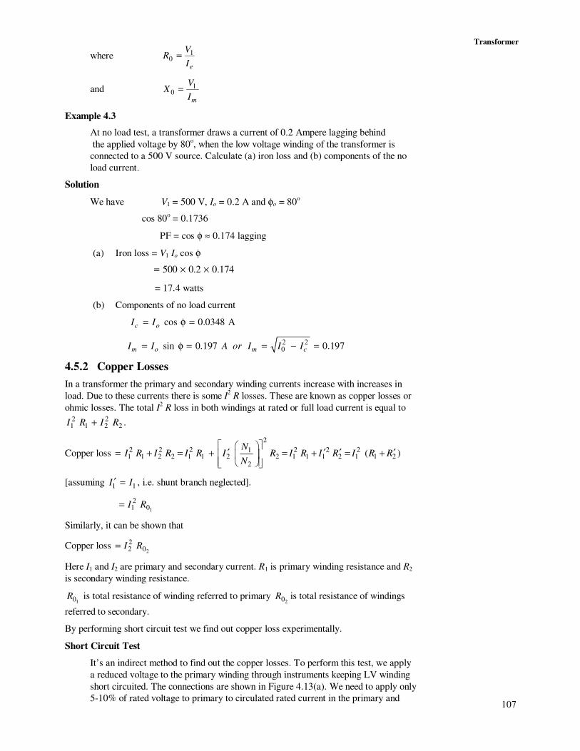
Example 4.3

At no load test, a transformer draws a current of 0.2 Ampere lagging behind

the applied voltage by 80o, when the low voltage winding of the transformer is

connected to a 500 V source. Calculate (a) iron loss and (b) components of the no

load current.

Solution

We have V1 = 500 V, Io = 0.2 A and φo = 80o

cos 80o = 0.1736

PF = cos φ ≈ 0.174 lagging

(a) Iron loss = V1 Io cos φ

500 0.2 0.174= × ×

= 17.4 watts

(b) Components of no load current

cos 0.0348 Ac oI I= φ =

2 20sin 0.197 0.197m o m cI I A or I I I= φ = = − =

4.5.2 Copper Losses

In a transformer the primary and secondary winding currents increase with increases in

load. Due to these currents there is some I2 R losses. These are known as copper losses or

ohmic losses. The total I2 R loss in both windings at rated or full load current is equal to

2221

21 RIRI + .

Copper loss

2

2 2 2 2 2 211 1 2 2 1 1 2 2 1 1 1 2 1 1 2

2

( )N

I R I R I R I R I R I R I R RN

′ ′ ′ ′= + = + = + = +

[assuming 1 1I I′ = , i.e. shunt branch neglected].

10

21 RI=

Similarly, it can be shown that

Copper loss 20

22 RI=

Here I1 and I2 are primary and secondary current. R1 is primary winding resistance and R2

is secondary winding resistance.

10R is total resistance of winding referred to primary 20R is total resistance of windings

referred to secondary.

By performing short circuit test we find out copper loss experimentally.

Short Circuit Test

It’s an indirect method to find out the copper losses. To perform this test, we apply

a reduced voltage to the primary winding through instruments keeping LV winding

short circuited. The connections are shown in Figure 4.13(a). We need to apply only

5-10% of rated voltage to primary to circulated rated current in the primary and

108

Electrical Technology secondary winding. The applied voltage is adjusted so that the ammeter shows rated

current of the winding. Under this condition, the watt-meter reading shows the

copper losses of the transformer. Because of low value of applied voltage, iron

losses, are very small and can be neglected.

As applied voltage is very small, small voltage across the excitation branch

produces very small percentage of exciting current in comparison to its full load

current and can therefore, be safely ignored. As a result, equivalent circuit with

secondary short circuited can be represented as Figure 4.13(b).

A

V

Single Phase

AC SupplyVolt meter

Ammeter

Variae H.V L.V

Watt meter

ISC

(a) Short Circuit Test

+

R1

VsShort CircuitIs

R′2X

L1 X′L2

(b) Transformer Equivalent Circuit with Secondary Short Circuited

Figure 4.13

At a rated current watt meter shows full load copper loss. We have

Vs = applied voltage

Is = rated current

Ws = copper loss

then, equivalent resistance Req 1 22

s

s

WR R

I′= = +

and equivalent impedance Zeq s

s

I

V=

So we calculate equivalent reactance

2 21 2eq eq eq L LX Z R X X ′= − = +

These Req and Xeq are equivalent resistance and reactance of both windings referred

in HV side. These are know as equivalent circuit resistance and reactance.

4.5.3 Efficiency of Single Phase Transformer

Generally we define the efficiency of any machine as a ratio of output power to the input

power, i.e.

efficiency PowerInput

lossesPowerInput

PowerInput

PowerOutput)(

−==η

1losses

Input Power= −

Alternatively, η LossesPowerOutput

PowerOutput

+=

109

Transformer

In a transformer, if Pi is the iron loss, and Pc is the copper loss at full load (when the load

current is equal to the rated current of the transformer, the total losses in the transformer

are Pi + Pc. In any transformer, copper losses are variable and iron losses are fixed.

When the load on the transformer is (x × full load), the copper loss will be total 2cx P and

total losses 2i cP x P= + .

Pc is full load copper loss and ‘x’ is the ratio of load current to the full load current. If the

output power of the transformer is x V2 I2 cos φ, then efficiency (η) becomes,

2 2

22 2

cos

cos i c

x V I

V I P x P

φη =

φ + +

or 2

Rating cos

Rating cos i c

x KVA

KVA P x P

× φη =

× φ + +

The efficiency varies with load. So, we can find the condition under which the η is

maximum. For maximum efficiency,

02

=η

Id

d

or 2 2

22 2 2 2

cos0

cos i c

x V Id d

d I d I x V I P x P

φη= =

φ + +

Solving this, we get 2i cP x P=

or iron loss = copper loss

The copper loss varies with load current I2 so when the copper losses are equal to the iron

losses for a particular load then efficiency (η) of the transformer is maximum. This is

called condition for maximum efficiency.

The maximum efficiency iPIVx

IVx

2cos

cos)(

22

22.max +φ

φ=η

Now, we determine the load at which the maximum efficiency occurs.

From the condition of maximum efficiency, we have

2i cP x P=

on i

c

Px

P=

Thus, the load at which efficiency is maximum occurs, is given by

x (Rated KVA) i

c

P

P= (Rated kVA)

Example 4.4

A 10 KVA transformer has 400 watt iron losses and 600 watt copper losses.

Determine maximum efficiency of the transformer at 0.8 power factor lagging. Also

calculate the load at which the ηmax. occurs.

Solution

We know that for efficiency to be maximum

Now 400 2

0.8165600 3

i

C

Px

P= = = =

Then load KVA at which the ηmax. occurs, i.e. output

110

Electrical Technology

kVA103

2×=

0.8165 10 kVA 8.165 kVA= × =

Copper loss = Iron loss

Then total losses = 2 × iron loss

= 2 × 400

= 800 watt = 0.8 kW;

lossesoutput

output

input

output

+==η

Now max.

kVA cos

kVA cos losses

x

x

× φη =

× φ +

0.8167 10 0.8

0.8910.1867 10 0.8 0.8

× ×= =

× × +

SAQ 4

(a) A single-phase 100/200 V, 1 kVA transformer has copper losses in h. v.

side at 5 A equal to 80 W and iron losses as 60 W. Find the efficiency of

the transformer at full load upf, and half load upf.

(b) Calculate full load efficiency at 0.8 power factor, for a 4 kVA, 200/400 V,

50 Hz, single-phase transformer with the following test results :

Open circuit test (LT side data) = 200 V, 0.8 Ampere, 70 Watts

Short circuit test (HT side data) = 17.5 V, 9 Ampere, 50 Watts

(c) A 440/110 V, 100 kVA, single-phase transformer has iron losses of

1.4 kW and a full load copper loss of 1.7 kW. Determine the kVA load for

maximum efficiency. Also find the efficiency at half load 0.8 pf lagging.

(d) The following data were obtained on a 50 kVA 2400/120 V transformer :

Open circuit test, instruments on low voltage side :

Waltmeter reading = 396 Watts

Ammeter reading = 9.65 amperes

Voltmeter reading = 120 Volts

Short circuit test, instruments on high voltage side :

Waltmeter reading = 810 Watts

Ammeter reading = 20.8 amperes

Voltmeter reading = 92 Volts

Find the efficiency when rated kVA is delivered to a load having a power

factor of 0.8 lagging.

4.5.4 All Day Efficiency (Energy Efficiency)

In electrical power system, we are interested to find out the all day efficiency of any

transformer because the load at transformer is varying in the different time duration of the

day. So all day efficiency is defined as the ratio of total energy output of transformer to the

total energy input in 24 hours.

All day efficiency = daytheduringinputkWh

dayaduringoutputkWh

here kWh is kilowatt hour.

111

Transformer

Example 4.5

For a 100 KVA 10 KV/500 V transformer the electrical loading for different time

durations in a day is shown below in Table 4.1.

Table 4.1

Time Duration Load PF

4 hrs Full load 0.9 lagging

6 hrs ½ load Unity PF

4 hrs Full load 0.8 PF lagging

10 hrs No load -

Determine the all day efficiency of the transformer, if the iron losses are

2 kW and full load copper losses are 4 kW.

Solution

For a transformer the iron loss are fixed total energy loss in iron loss, over 24 hours

kWh48242 =×= .

Energy loss due to copper loss at full load for 8 hours = (4 × 8) = 32 kWh.

Energy loss at half load due to copper losses

42

16

2

×

×=

kWh644

16 =××=

At no load there is no copper loss.

∴ The total energy loss due to copper loss in 24 hours

= (32 + 6) kWh = 38 kWh.

Total energy losses = Iron losses + Copper losses

= 48 + 38

= 86 kWh.

kWh Output for Transformer

At full load 0.9 lagging PF for 4 hrs kWh output

= 100 × 0.9 × 4 = 360 kWh

At half load unity PF for 6 hrs, kWh output

= 1/2 × 100 × 1 × 6 = 300 kWh

For full load at 0.8 PF for 4 hours

= 100 × 0.8 × 4 = 320 kWh

Now for rest 10 hr output is zero. So total kWh output in all day

= 360 + 300+ 320 = 980 kWh.

So all day efficiency %9.91or9193.086980

980)( =

+=η .

112

Electrical Technology 4.6 SPECIAL TRANSFORMERS

In order to meet various industrial applications, many transformers are constructed with

special design features. In this section you will be introduced to :

(a) autotransformers, and

(b) instrument transformers.

4.6.1 Auto-transformers

The transformers we have considered so far are two-winding transformers in which the

electrical circuit connected to the primary is electrically isolated from that connected to the

secondary. An auto-transformer does not provide such isolation, but has economy of cost

combined with increased efficiency. Figure 4.24 illustrates the auto-transformer which

consists of a coil of NA turns between terminals 1 and 2, with a third terminal 3 provided

after NB turns. If we neglect coil resistances and leakage fluxes, the flux linkages of the

coil between 1 and 2 equals NA φm while the portion of coil between 3 and 2 has a flux

linkage NB φm. If the induced voltages are designated as BA EE and , just as in a two-

winding transformer,

B

A

B

A

N

N

E

E=

+

EA

N

Turns

A

ZL

+

EA

φm

3 IB

IC

N

Turns

B

IA 1

d

Figure 4.14 : Auto-transformer

Neglecting the magnetizing ampere-turns needed by the core for producing flux, as in an

ideal transformer, the current AI flows through only (NA – NB) turns. If the load current is

BI , as shown by Kirchhoff’s current law, the current CI flowing from terminal 3 to

terminal 2 is ( AI − BI ). This current flows through NB turns. So, the requirement of a nett

value of zero ampere-turns across the core demands that

0)()( =−+− BBAABA NIIINN

or 0=− BBAA ININ

Hence, just as in a two-winding transformer,

A

B

B

A

N

N

I

I=

Consequently, as far as voltage, current converting properties are concerned, the

autotransformer of Figure 4.14 behaves just like a two-winding transformer. However, in

the autotransformer we don’t need two separate coils, each designed to carry full load

values of current.

4.6.2 Instrument Transformers

The generation and transmission parts of an electrical power system operate at voltages

ranging from tens to hundreds of kilovolts and currents ranging from tens to hundreds of

113

Transformer

Amperes. Despite this, such voltages are measured using voltmeters whose range is

typically 0 – 150 V and ammeters whose range is 0 – 5 A. This is achieved by the use of

instrument transformers, which are of two types namely potential transformers and

current transformers. If a potential transformer is used to measure the voltage of a high

voltage system, the primary is connected across the voltage to be measured while a low

range voltmeter is connected across (see Figure 4.15(a)) the secondary. Similarly, for the

measurement of current, the current to be measured passes through the primary of a

current transformer, and a low-range ammeter is connected across the secondary.

(a) Potential Transformer Connection (b) Current Transformer Connection

Figure 4.15

A potential transformer is a high precision transformer specially designed to maintain a

constant ratio between primary and secondary terminal voltages and ensure that these

voltages are almost exactly in phase. A current transformer is designed to function in a

similar manner as regards primary and secondary currents.

4.7 TRANSFORMERS IN THREE PHASE SYSTEMS

For a proper understanding of this section you will need to revise your knowledge of

balanced three phase systems. In particular, you should know

(a) the relations between line and phase quantities in star connected and delta

connected balanced three phase circuits;

(b) expressions for three phase power and volt-amperes; and

(c) equivalence relations between star-connected and delta-connected balanced

systems.

4.7.1 Three-phase Bank of Single-phase Transformers

Electric power is generated, transmitted and distributed in three-phase form. Even where

single-phase power is required, as in homes and small establishments, these are merely

tapped off from a basic three-phase system. Transformers are, therefore, required to

interconnect three phase systems at different voltage levels. This can be done using three

single-phase transformers, constituting what is often called a transformer bank. The

primary windings of three identical single-phase transformers can usually be connected

either in star or in delta to form a three-phase system. Similarly, the secondary windings

can also be connected in star or delta. We have, therefore, four methods of interconnection

of primary/secondary, viz., star/star, star/delta, delta/star and delta/delta.

114

Electrical Technology

V / 3L

√

A1

IL

VL

B1 C1

A , B ,C2 2 2

L1

L2

L3

V /k 3L

√

a1

kIL

a , b ,c2 2 2

l1

l2

l3

c1b

1

(a) Star/Star Connection (Y – Y)

IL kIL

V / 3L

√

√3A1

VL

B1 C1

A , B ,C2 2 2

L1

L2

L3

V /k 3L

√

a1

l1

l2

l3

c1

b2

b1

a2

c2

kIL

(b) Star/Delta Connection (Y – ∆∆∆∆)

√3 V /kL

a1

c1 b1

a , b ,c2 2 2

l1

L2

l3

k / 3IL

√

VL

IL

L1

L2

L3

C2

C1

A1

A2

B2

B1

IL/ 3√

(c) Delta/Star Connection (∆∆∆∆ −−−− Y)

V /kL

a1

l1

l2

l3

b1

c2

c1

a2

b2

k / 3IL √

kIL

VL

ILL

1

L2

L3

C2

C1

A1

A2

B2

B1

IL/ 3√

(d) Delta/Delta Connection (∆∆∆∆ −−−− ∆∆∆∆)

Figure 4.16 : Three Phase Transformer Connections

Let the primary to secondary turns ratio of each single-phase transformer be k. We will

identify these transformers by the letters A, B and C. Transformers A will be assumed to

have primary terminals A1, A2 and secondary terminals a1, a2, transformers B has terminals

B1, B2 and b1, b2 and similarly for transformer C. We will also designate the three phase

line terminals on the primary by A, B, C and the secondary line terminals by a, b, c.

Further, we will suppose that in all the transformers the winding sense is such that on

adopting a dot convention, dots would have to be marked next to primary and secondary

terminals having the suffix 1. The four types of transformers connection would be as

shown in Figure 4.16. The ratios of the primary and secondary line voltages is shown in

this diagram, where k is the transformation ratio of one phase.

4.7.2 Three-phase Transformers

Instead of a bank of three separate single-phase transformers, each having its own separate

iron-core, a single transformer can be designed to serve the same function. Such a single

unit, called a three-phase transformer, has three primary windings and three secondary

windings. These primary and secondary windings can be connected in star or in delta. The

115

Transformer

connections and voltage relations of Figure 4.16 apply in this case also. Such a

transformer differs from the single-phase transformers in the design of the iron-core. In the

single-phase transformer bank the fluxes associated with a particular phase utilize an iron-

core which serves only that phase, whereas in the three-phase transformer the iron-core

couples different phases together. Because of this sharing of the iron-core by the three

phases, such transformers can be built more economically. A three-phase transformer is

always cheaper than three single-phase transformers used for the same purpose, weighs

less and occupies less floor space.

Despite the above advantages, three single-phase transformers may be preferred if the

conditions of operation are such that provision must be made for replacement. When using

single-phase transformers it might be sufficient to provide just one single-phase

transformer as a spare. If a three-phase transformer is used another three-phase

transformer will be needed as a spare. While a three-phase transformer is cheaper than

three single-phase transformers, it is much more expensive than one single-phase

transformer. Secondly, there might exist situations like hydroelectric projects in remote

locations, where it is not feasible to transport and install a heavy three-phase transformer

and the use of three lighter single-phase transformers becomes the only feasible solution.

SAQ 5

It is proposed to transmit the power generated by a 200 MVA, 11 kV,

50 Hz, three-phase generator to a three-phase 220 kV transmission line using a bank

of three single-phase transformers. Find the turns ratio and the voltage and current

ratings for each single-phase transformer when the connections are

(a) Star/Star,

(b) Star/Delta,

(c) Delta/Star, and

(d) Delta/Delta.

4.8 SUMMARY

After going through this unit you should have understood the principles of operation of

transformers and learnt the significance of mutual flux, leakage fluxes, core losses and

winding resistances. You would be able to deduce the form of the exact equivalent circuit

from theoretical considerations and determine the parameters of the approximate

equivalent circuit from OC and SC tests. Based on this, you should be able to calculate

efficiency and voltage regulation of a transformer on load. You would also have a general

understanding of the use of transformers in power systems, including special transformers

like auto-transformers, instrument transformers.

4.9 ANSWERS TO SAQs

SAQ 1

Wb1065.1101501.124 −− ×=××=×=φ imm AB

2 24.44 mE f N= φ

= 4.44 × 50 × 66 × 1.65 × 10–2

= 24175.8 × 10–2

= 241.76

22

2

EI

Z=

116

Electrical Technology 2

241.7660.44 A

4.0I = =

Output 2 2 241.76 60.44 VAE I= = ×

3241.76 60.44 10 kVA 0.755 kVA

−= × × =

= 14.61 kVA

SAQ 2

Magnetizing current on the HT side = − j 2.8 amp.

Turns ratio 2220

440

2

1

2

1 ===V

V

N

N

(a) Load current on LT side = o25 180∠ −

Load current on HT side = oo 05.1202

25∠=∠

∴ H. T. current o6.1281.128.205.12 −∠=−∠= j

Power factor = cos (− 12.6o) = 0.976 lagging

(b) Load current on LT side 1 o25 ( cos 0.85 180 )−= ∠ − −

o o o25 ( 31.8 180 ) 25 211.8= ∠ − − = ∠ −

Load current on HT side o o125 ( 211.8 180 )

2= × ∠ − +

o8.315.12 −∠=

∴ HT current 8.28.315.12o

j−−∠=

10.623 6.58 2.8j j= − −

10.623 9.38j= −

o14.17 41.44= ∠ −

Power factor = cos (− 41.44o) = 0.75 lagging

SAQ 3

We know that

V. R. = % (Resistive drop) cos φ ± % (Reactive drop) sin φ

(a) For 0.8 lagging P. F.

V. R. = (% Resistive drop) cos φ + (% Reactive drop) sin φ

∵ cos φ = 0.8 so sin 6.0)8.0(12 =−=φ

Now V. R. %6.436.1)6.05()8.02( =+=×+×=

(b) For 0.8 leading P. F.

V. R. = (% Resistive drop) cos φ − (% Reactive drop) sin φ.

117

Transformer

∵ cos φ = 0.8 so sin 6.0)8.0(1 2 =−=φ

Now V. R. %4.136.1)6.05()8.02( −=−=×−×=

SAQ 4

(a) 100cos1000kVA

cos1000kVA2

×++φ××

φ××=η

ci

xPxPx

x

where x fraction of flux load. At full load

1000

5A2000

aI = = (as given)

∴ Pc = 80 W, Ps = 60 W

When x = 1, pf = 1,

So, %7.87100806011000

110001loadfull =×

++×

××=η

At half load; x = ½, pf = 1

%20.86100

4

806011000

2

1

1100012

1

loadhalf =×++××

×××=η

(b) Full load secondary current .amp10400

104 3

2 =×

=I

Copper loss at 9 amp = 50 W

∴ Copper loss at 10 amp W73.61509

102

=×

=

Iron loss = 70 W

Full load efficiency at 0.8 pf 2 2

2 2

cos

cos i c

E I

E I W W

φ=

φ + +

400 10 0.8

0.9605400 10 0.8 70 61.73

× ×=

× × + +

∴ Efficiency = 96.05%

(c) Let the kVA load for maximum efficiency be x kVA

Iron loss at maximum efficiency = 1.4 kW

Copper loss at maximum efficiency =

2

1.7 kVA100

x ×

At maximum efficiency, copper loss = iron loss

or kW75.904.17.1100

or2

==×

x

x

At half load copper loss = kW425.07.1100

502

=×

118

Electrical Technology

Efficiency at half load 100)4.1425.08.050(

8.050×

++×

×=

825.41

10040 ×= = 95.6%.

(d) At rated voltage, core loss = 396 W (from OC test)

Rated current on h. v. side 1

310kVA

V

×=

2400

1050 3×=

or I1 = 20.833 amp.

∴ Full load copper loss = 810 W

Total losses = 396 + 810 = 1206 W

Output = 50 kVA

)8.0cos(8.010503 =φ∴××=

= 40000 W

Efficiency 100lossesOutput

Output×=

+

40000 100

97.07%40000 1206

×= =

+

SAQ 5

Let subscripts 1 and 2 denote primary and secondary side with given data,

1 2

MVA11 kV, 220 kV, 66.67 MVA

PhaseL LV V= = =

1PV

(kV)

2PV

(kV)

1

2

1

2

P

P

VN=

N V

=!

1

66.67P

P

IV

(kA)

=2

2

66.67P

P

IV

(kA)

Y/Y 1 6.353

LV=

2 1273

LV= 1 : 20 10.49 0.52

Y/∆ 1 6.353

LV=

2220LV = 1 : 34.6 10.49 0.30

∆/Y 1

11LV = 2 1273

LV= 1 : 11.5 6.06 0.52

∆/∆ 1

11LV = 2

220LV = 1 : 20 6.06 0.30