Walden UniversityScholarWorks

Walden Dissertations and Doctoral Studies Walden Dissertations and Doctoral StudiesCollection

2017

Understanding the Impact of Foreclosed Homes inCharlotte NeighborhoodsJustice Uche UcheWalden University

Follow this and additional works at: https://scholarworks.waldenu.edu/dissertations

Part of the Public Administration Commons, and the Public Policy Commons

This Dissertation is brought to you for free and open access by the Walden Dissertations and Doctoral Studies Collection at ScholarWorks. It has beenaccepted for inclusion in Walden Dissertations and Doctoral Studies by an authorized administrator of ScholarWorks. For more information, pleasecontact ScholarWorks@waldenu.edu.

Walden University

College of Social and Behavioral Sciences

This is to certify that the doctoral dissertation by

Justice Uche

has been found to be complete and satisfactory in all respects,

and that any and all revisions required by

the review committee have been made.

Review Committee

Dr. Olivia Yu, Committee Chairperson,

Public Policy and Administration Faculty

Dr. Tanya Settles, Committee Member,

Public Policy and Administration Faculty

Dr. Kristie Roberts, University Reviewer,

Public Policy and Administration Faculty

Chief Academic Officer

Eric Riedel, Ph.D.

Walden University

2017

Abstract

Understanding the Impact of Foreclosed Homes in Charlotte Neighborhoods

by

Justice Uche

MPA, Strayer University, 2012

BSc, Imo State University of Nigeria, 2004

Dissertation Submitted in Partial Fulfillment

of the Requirements for the Degree of

Doctor of Philosophy

Public Policy and Administration

Walden University

July 2017

Abstract

Following the increase in foreclosures across the United States from 2007 to 2009, there

was concern that foreclosed homes could lead to higher rates of crime in certain

neighborhoods. Using social disorganization theory, the purpose of this difference-in-

difference research design was to study the link between foreclosure levels, and crime

rates in neighborhoods in Charlotte, North Carolina. Propensity score matching was used

to examine whether neighborhood foreclosure rates have an impact on neighborhood

crime level while controlling for neighborhood conditions. Data were acquired from

Charlotte Neighborhood Quality of Life Studies, conducted biannually in 173

neighborhoods in Charlotte, North Carolina. Data for the years 2004 and 2010 were used

for the analysis. The sample included 54 neighborhoods exposed to foreclosures (n = 27),

and neighborhoods not exposed to foreclosure (n = 27). Data were also acquired from the

Charlotte Mecklenburg Police Department and housing authorities for the same years.

Using hierarchical multiple regression analysis, a significant relationship was found

between neighborhood foreclosure level and neighborhood crime level, and school

dropout levels and neighborhood crime level (p <.05). The positive social change

stemming from this study includes recommendations to local policy makers and law

enforcement agencies to consider policies and strategies that reduce crime and address

larger neighborhood problems such as school dropouts and unemployment. Addressing

these policies may result in crime reductions, and improve the quality of life for

neighborhood residents.

Understanding the Impact of Foreclosed Homes in Charlotte Neighborhoods

by

Justice Uche

MPA, Strayer University, 2012

BSc, Imo State University of Nigeria, 2004

Dissertation Submitted in Partial Fulfillment

of the Requirements for the Degree of

Doctor of Philosophy

Public Policy and Administration

Walden University

July 2017

Dedication

This dissertation is dedicated to my family, especially my children – Grace,

Eunice, and Patrick for their endurance throughout this process.

Acknowledgments

I would like to thank Dr. Olivia Yu for her positive feedback and outstanding

work directing this study. Her keen eye for detail and extensive knowledge of many of

the areas covered in this study were invaluable. Thank you to my committee member, Dr.

Tanya Settles for her critical help in shaping and directing this dissertation. Thank you to

my colleagues for their contributions and many spirited discussions of the critical

components that make up this dissertation.

i

Table of Contents

List of Tables .......................................................................................................................v

List of Figures .................................................................................................................... vi

Chapter 1: Introduction to the Study ....................................................................................1

Organization of Chapter .................................................................................................2

Background of the Problem ...........................................................................................2

Problem Statement .........................................................................................................5

Purpose Statement ..........................................................................................................7

Research Questions and Hypotheses .............................................................................7

Research Question 1 ............................................................................................... 7

RQ1 Hypotheses ..................................................................................................... 7

Research Question 2 ............................................................................................... 8

RQ2 Hypotheses ..................................................................................................... 8

Theoretical Foundation ..................................................................................................8

Nature of the Study ......................................................................................................11

Definitions of Terms ....................................................................................................12

Assumptions .................................................................................................................15

Scope and Delimitations ..............................................................................................16

Limitations ...................................................................................................................16

Significance and Implication for Social Change .........................................................16

Summary ......................................................................................................................18

ii

Chapter 2: Literature Review .............................................................................................20

Introduction ..................................................................................................................20

Organization of Chapter ...............................................................................................20

Research Strategy.........................................................................................................21

Structure of the Literature Review ...............................................................................22

Theoretical Foundation ................................................................................................23

Social Disorganization Theory ............................................................................. 25

Broken Windows Theory ...................................................................................... 28

Routine Activity Theory ....................................................................................... 30

The Foreclosure Process ..............................................................................................31

Mortgage Foreclosure Trends ............................................................................... 33

Home Quality ........................................................................................................ 34

Home Value .......................................................................................................... 37

Vacant and Abandoned Homes ............................................................................. 39

Residential Mobility and Neighborhood Stability ................................................ 42

Neighborhood Desirability and Fear of Crime ..................................................... 44

Foreclosure and Crime .................................................................................................47

Prior Studies on Foreclosure and Crime ............................................................... 49

Recent Literature and the Mixed Results Linking Foreclosures to Crime ............ 50

Spurious Relationships.................................................................................................54

Socioeconomic and Demographic Conditions and Neighborhood Crime ...................57

iii

Theoretical Connection ......................................................................................... 59

Socioeconomic Conditions and Crime.................................................................. 60

Poverty Level and Crime ...................................................................................... 61

Recent Studies on Poverty and Crime .................................................................. 62

Population Heterogeneity and Crime .................................................................... 66

Physical Dilapidation and Crime .......................................................................... 69

Local Policy and Crime ........................................................................................ 71

Summary ......................................................................................................................73

Chapter 3: Research Method ..............................................................................................74

Introduction ..................................................................................................................74

Research Design and Rationale ...................................................................................74

Target Population .........................................................................................................77

Charlotte Neighborhood Quality of Life (CNQL) Studies (Secondary

Data) .......................................................................................................... 77

CNQL Methodology ............................................................................................. 79

Sampling and Sampling Procedures ............................................................................81

Rights Protection and Permission ................................................................................82

Instruments ...................................................................................................................83

Operationalization of Variables ...................................................................................84

Data Analysis Plan .......................................................................................................85

Threat to Validity .........................................................................................................86

iv

Ethical Procedures .......................................................................................................87

Summary ......................................................................................................................87

Chapter 4: Results ..............................................................................................................88

Introduction ..................................................................................................................88

Pre-Analysis Data Screening .......................................................................................88

List of Tables .......................................................................................................................v

List of Figures .................................................................................................................... vi

Chapter 1: Introduction to the Study ....................................................................................1

Organization of Chapter .................................................................................................2

Background of the Problem ...........................................................................................2

Problem Statement .........................................................................................................5

Purpose Statement ..........................................................................................................7

Research Questions and Hypotheses .............................................................................7

Research Question 1 ............................................................................................... 7

RQ1 Hypotheses ..................................................................................................... 7

Research Question 2 ............................................................................................... 8

RQ2 Hypotheses ..................................................................................................... 8

Theoretical Foundation ..................................................................................................8

Nature of the Study ......................................................................................................11

Definitions of Terms ....................................................................................................12

Assumptions .................................................................................................................16

v

Scope and Delimitations ..............................................................................................17

Limitations ...................................................................................................................18

Significance and Implication for Social Change .........................................................18

Summary ......................................................................................................................20

Chapter 2: Literature Review .............................................................................................22

Introduction ..................................................................................................................22

Organization of Chapter ...............................................................................................22

Research Strategy.........................................................................................................23

Structure of the Literature Review ...............................................................................25

Theoretical Foundation ................................................................................................25

Social Disorganization Theory ............................................................................. 27

Broken Windows Theory ...................................................................................... 30

Routine Activity Theory ....................................................................................... 31

The Foreclosure Process ..............................................................................................33

Mortgage Foreclosure Trends ............................................................................... 35

Home Quality ........................................................................................................ 36

Home Value .......................................................................................................... 39

Vacant and Abandoned Homes ............................................................................. 42

Residential Mobility and Neighborhood Stability ................................................ 44

Neighborhood Desirability and Fear of Crime ..................................................... 46

Foreclosure and Crime .................................................................................................49

vi

Prior Studies on Foreclosure and Crime ............................................................... 51

Recent Literature and the Mixed Results Linking Foreclosures to Crime ............ 52

Spurious Relationships.................................................................................................56

Socioeconomic and Demographic Conditions and Neighborhood Crime ...................59

Theoretical Connection ......................................................................................... 61

Socioeconomic Conditions and Crime.................................................................. 62

Poverty Level and Crime ...................................................................................... 63

Recent Studies on Poverty and Crime .................................................................. 65

Population Heterogeneity and Crime .................................................................... 68

Physical Dilapidation and Crime .......................................................................... 71

Local Policy and Crime ........................................................................................ 73

Summary ......................................................................................................................75

Chapter 3: Research Method ..............................................................................................76

Introduction ..................................................................................................................76

Research Design and Rationale ...................................................................................76

Target Population .........................................................................................................78

Charlotte Neighborhood Quality of Life (CNQL) Studies (Secondary

Data) .......................................................................................................... 78

CNQL Methodology ............................................................................................. 80

Sampling and Sampling Procedures ............................................................................83

Rights Protection and Permission ................................................................................84

vii

Instruments ...................................................................................................................85

Operationalization of Variables ...................................................................................86

Data Analysis Plan .......................................................................................................87

Threat to Validity .........................................................................................................88

Ethical Procedures .......................................................................................................89

Summary ......................................................................................................................89

Chapter 4: Results ..............................................................................................................91

Introduction ..................................................................................................................91

Pre-Analysis Data Screening .......................................................................................91

Descriptive and Inferential Statistics ...........................................................................93

Percentages of Demographic Data ........................................................................ 94

Descriptive Statistic of Continuous Variables ...................................................... 94

Reliability of the Propensity Score Matching ....................................................... 95

Restatement of the Research Questions and Hypotheses ............................................97

Research Question 1 and Hypotheses ..........................................................................97

Continuous Criterion ............................................................................................. 97

Two Related or Matched Pairs Assumption ......................................................... 97

Normality and Outliers Assumptions.................................................................... 98

Paired- Samples t test ............................................................................................ 99

Research Question 2 and Hypotheses ........................................................................101

Equality of Variance and Linearity Assumptions ............................................... 101

viii

Outlies Assumption ............................................................................................. 102

Normality Assumption ........................................................................................ 102

Homoscedasticity Assumption............................................................................ 103

Independence of Errors Assumption ................................................................... 103

Multicollinearity and singularity......................................................................... 104

Hierarchical Multiple Regression ....................................................................... 105

Summary ............................................................................................................. 108

Chapter 5: Discussions .....................................................................................................110

Introduction ................................................................................................................110

Summary of Results ...................................................................................................111

Research Question 1 ........................................................................................... 111

Research Question 2 ........................................................................................... 112

Limitations of the Study.............................................................................................112

Interpretation of the Findings.....................................................................................114

Recommendations for Future Research .....................................................................120

Implications for Positive Social Change ....................................................................122

Conclusion .................................................................................................................125

References ........................................................................................................................127

Appendix A: Neighborhood Name and Identification Numbers .....................................159

Appendix B: Sample Data ..............................................................................................160

Appendix C: Population Heterogeneity Index Scores by Neighborhood .......................162

ix

List of Tables

Table 1. Charlotte Area Residential Unit Sales ................................................................ 40

Table 2. Foreclosure and Crime Studies ........................................................................... 54

Table 3. Examples of Difference-in-Difference (DD) Design.......................................... 78

Table 4. Study Variables, Definitions, and Sources ......................................................... 82

Table 5. File of Matched Neighborhoods ......................................................................... 93

Table 6. Percentages of Demographic Data ..................................................................... .94

Table 7. Descriptive Statistics for Predictors and Neighborhood Crime Levels .............. 95

Table 8. Average Crime Rates of the two Groups of Neighborhoods: Foreclosure

Group (N=50) vs No Foreclosure Group (N=50) ................................................. 96

Table 9. Average Crime Rates of the two Groups of Neighborhoods: Foreclosure

Group (N=27) vs No Foreclosure Group (N=27) ................................................. 96

Table 10. Tests of Normality ............................................................................................ 98

Table 11. Paired-Samples t Test for 2004 and 2010 Crime Rates .................................. 100

Table 12. Model Summary ............................................................................................. 104

Table 13. Descriptive Statistics and Correlations Matrix ............................................... 107

Table 14. Summary, Hierarchical Regression Analysis of Variables Predicting

Crime Rates in Neighborhoods ........................................................................... 108

Table 17. Neighborhood Name and Identification Number ............................................159

Table 18. Beatties Ford/Trinity Neighborhood Sample Data (2004) ..............................160

Table 19. Beatties Ford/Trinity Neighborhood Sample Data (2010) ..............................161

x

List of Figures

Figure 1: Zone theory.......................................................................................................... 9

Figure 2. Causal framework of social disorganization. .................................................... 11

Figure 3. Characteristics of Zone 2. .................................................................................. 28

Figure 4. Mortgage foreclosure trends.. ............................................................................ 36

Figure 5. Home vacancy rates (in millions?) in the United States between 2005

and 2010. ............................................................................................................... 44

Figure 6. Property crime offenses by year. ....................................................................... 59

Figure 7. Violent crime offenses by year.. ........................................................................ 59

Figure 8. Composition of CNQL index. ........................................................................... 81

Figure 9. Power as a function of sample size.................................................................... 84

Figure 10. Normality and outliers of crime difference, 2004 and 2010.. ....................... ..99

Figure 11. Crime rate error bars, 2004 and 2010. ........................................................... 100

Figure 12. Assessment of normality and outliers............................................................ 102

Figure 13. Assessment of normality and outliers............................................................ 103

Figure 14. Residuals of homoscedasticity for variables predicting crime levels. ........... 104

1

Chapter 1: Introduction to the Study

Following the increase in foreclosures in most neighborhoods across the United

States between 2007 and 2009, during which home qualities and values declined, many

homeowners found themselves in negative equity situations, and trillions of dollars were

lost (Schwartz, 2015). More than 6 million homeowners received foreclosure notices

(Tsai, 2015). There was growing concern among homeowners, renters, property owners,

realtors, homeowners’ associations (HOAs), local governments, and other members of

the public that increased foreclosures in neighborhoods could lead to higher crime rates

(Immergluck, 2012; Wallace, Hedberg, & Katz, 2012) because foreclosed homes provide

opportunities for gangs, drug dealers, and other criminal acitivities to escalate crime in

neighborhoods. Soaring foreclosures have a negative effect on the housing market,

devaluing nearby homes and pushing homeowners into debt or negative equity; when

homeowners owe more on their mortgages than the current market value of the home

(Cahill, Pettit, & Bhati, 2014; Schwartz, 2015). For local governments, foreclosures

translate to tax losses, diminishing the ability to provide vital services such as public

safety and welfare (Ellen, Lacoe, & Sharygin, 2013; Katz, Wallace, & Hedberg, 2013;

Wallace et al., 2012; Williams, Galster, & Verma, 2013; Wolff, Cochran, & Baumer,

2014). In many recent studies, researchers have consistently maintained that foreclosed

homes are a key factor in promoting criminality in some neighborhoods across the

country (Baumer, Wolff, & Arnio, 2012; Lacoe & Ellen, 2014; Williams et al., 2013).

Understanding the effects of foreclosed homes in a neighborhood, and how foreclosures

impact crime levels, after controlling for other neighborhood conditions is vital when

2

designing strategies that can reduce crime in neighborhoods across the country. This

study sought to answer two key questions: (a) Do neighborhood foreclosure rates have an

impact on neighborhood crime rates? (b) How are neighborhood foreclosure rates related

to neighborhood crime rates, after controlling for other neighborhood conditions?

Organization of Chapter

Chapter 1 includes an introduction to the study, background of the problem,

problem statement, purpose of the study, and research questions and hypotheses. The

chapter also contains the theoretical foundation, nature of the study, definitions of terms,

assumptions, scope, limitations and delimitations, the significance of the study,

implication for social change, summary, and a transition to Chapter 2.

Background of the Problem

This foreclosure and crime study sought to determine whether there is a

relationship between neighborhood foreclosures and neighborhood crime rates, after

accounting for other neighborhood conditions. Ecologists, criminologists, urbanists, and

other scholars have long posited that there is a relationship between the neighborhood

environment or its characteristics, and crime (Lacoe & Ellen, 2014; Payton, Stucky, &

Ottensmann, 2015). Newman (1973) suggested that abandoned public structures are more

vulnerable to crime than occupied public structures. Most studies dedicated to

determining the relationship between crime rates and foreclosure rates in neighborhoods

across the country concluded that foreclosed homes and crime rates are related in a

complex manner (Arnio, Baumer, & Wolff, 2012; Cui & Walsh, 2015; Ellen et al., 2013;

Jones & Pridemore, 2012; Katz et al., 2013; Stucky, Ottensmann, & Payton, 2012;

3

Wallace et al., 2012). However, the results of these studies differed by crime types and

neighborhoods. For example, in most of the studies, researchers found that foreclosures

only increased property crimes (Arnio et al., 2012; Teasdale et al., 2012; Williams,

Galster, & Verna, 2014). Others found a link between foreclosures and violent crime

rates (Cui & Walsh, 2015; Ellen et al., 2013; Harris, 2011; Immergluck & Smith, 2006),

or between foreclosures and both violent and property crime rates (Arnio & Baumer,

2012; Katz et al., 2012; Payton et al., 2015). Some researchers found evidence that the

positive effect of foreclosures varies by neighborhood context and crime type (Arnio &

Baumer, 2012), and others found that the impact of foreclosure might be short, lasting

only three to four months (Katz et al., 2012; Williams et al., 2013).

Following the sharp increase in mortgage foreclosure rates in neighborhoods

across the country in 2007 and 2009, anecdotal evidence from the national media

suggested that foreclosed homes increased crime rates (Qazi, Trotter, & Hunt, 2015).

Attention from policy makers and scholars has focused on discovering how foreclosure

affects neighborhood crime rates. Despite the lack of definitive evidence indicating that

foreclosure alone increases crime rates in neighborhoods, several scholars, using

ecological theories such as routine activity, broken windows, and social disorganization,

and various other methods, have suggested that foreclosures increase vacancies or

unoccupied homes in neighborhoods, and increase the fear of crime among residents

(Payton et al., 2015; Wolff et al., 2014). Findings conducted by some scholars indicate

that foreclosure provides opportunities for gangs, drug dealers, and other criminals to

escalate crime (Cahill et al., 2014; Cui & Walsh, 2015). Moreover, the loss of tax revenue

4

from foreclosures limits the ability of municipal agencies to prevent crime in their

jurisdictions (Ellen et al., 2013; Wolff et al., 2014).

Recent researchers have reinforced these theoretical postulations (Baumer et al.,

2014; Cahill et al., 2014; Nassauer & Raskin, 2014; Payton et al., 2015; Qazi et al., 2015;

Raleigh & Galster, 2013). Cahill et al. (2014) and Nassauer and Raskin (2014) suggested

that foreclosures and crime are related in complex and reciprocal ways. Raleigh and

Galster (2013), and Nassauer and Raskin (2014) asserted that the physical appearance of

empty foreclosed homes diminishes the safety of the remaining residents in the

neighborhood. Other studies suggested that decay, litter, broken windows, and missing

doors from foreclosed homes provide an opportunity for disorder to take root in an area

(Batson & Monnat, 2013; Baumer et al., 2014; Teasdale, Clark, & Hinkle, 2012; Wilson

& Paulsen, 2010). Payton et al. (2015) and Wallace et al. (2012) posited that physical

dilapidation is likely to cause contagion effects within a neighborhood, which might

cause residents to feel unsafe, and increase migration out of the area.

Shaw and McKay’s (1972) social disorganization theory suggests that areas with

persistent poverty, racial heterogeneity, and dilapidation have higher likelihoods of

higher rates of crime than areas without these characteristics. Broken windows theory

suggests that the physical characteristics of a neighborhood are tied to functions in the

area, and the ability of these functions to prevent or tolerate criminal activity (Kelling &

Wilson, 1982). According to Kelling and Wilson (1982), litter, broken doors and

windows, and dilapidated foreclosed homes in neighborhoods impede the manner in

which those areas maintain social control. As explained by routine activity theory, the

5

increase in crime rates is the result of the convergence of soft targets, or those that lack

quality guidance and are motivated to engage in criminal acts in a place and time (Cohen

& Felson, 1979). These theories (social disorganization, broken windows, and routine

activity) suggest that ignoring the prevailing conditions (physical and social) in a

neighborhood results in an incomplete understanding of why crime in the increase (Ellen

et al., 2013; Wolff et al., 2014).

Despite these theoretical postulations and strong suggestions from scholars, it is

possible that the relationship between neighborhood foreclosures and crime rates might

be affected by other neighborhood conditions such as levels of poverty, the percentage of

residents receiving food stamps, the racial composition of the area or population

heterogeneity, among others (Wolff et al., 2014). For example, findings from Kirk and

Hyra (2012), and Jones and Pridemore (2012) indicated that the relationship between

foreclosed homes and neighborhood crime rates in most neighborhoods might be

spurious. Wolff et al. (2014) concluded that research methodologies, such as traditional

regression approaches, of scholars who found a positive relationship between

foreclosures and neighborhood crime rates might not have sufficiently accounted for

other preexisting differences present in these neighborhoods.

Problem Statement

Multiple studies on neighborhoods have revealed a link between foreclosures and

neighborhood crime rates; however, few of the researchers controlled for other significant

neighborhood socioeconomic and demographic conditions, which may have affected the

impact of these two social problems (Wolff et al., 2014). Even before the foreclosure

6

crisis (2007 to 2009) that plunged more than 12 million homeowners into negative equity

and eliminated more than $3.6 trillion in home equity, more than 6 million homeowners

had received foreclosure notices, home values and qualities declined, and the number of

abandoned homes had been on the increase (Schwartz, 2015; Tsai, 2015). The public

problems of crime, the fear of crime, and crime control or prevention in neighborhoods

has always fueled political debate, scholarly research, and major government spending,

and has been a key focus of neighborhood stabilization and housing policy throughout the

nation (Cahill et al., 2014; Cui & Walsh, 2015; Ellen et al., 2013; Harris, 2011).

Policymakers, researchers, homeowners, renters, property owners, realtors, HOAs, and

other members of the public share a growing concern that increased foreclosures in

neighborhoods across the nation could increase the rates of crime (Ellen et al., 2013;

Immergluck, 2012; Qazi et al., 2015).

Crime prevention has long been of the highest priority in most developed societies

(Kraft & Furlong, 2010); however, understanding the role played by other neighborhood

socioeconomic and demographic conditions has been limited (Wolff et al., 2014).

Understanding the effects of other influential neighborhood variables on the impact of

foreclosures on neighborhood crime rates can better equip local policy makers to generate

effective policies intended to mitigate crime increases and stabilize neighborhoods.

Developing a knowledge base of the key variables driving the crime trends in most

neighborhoods remains a critical challenge facing local policy makers, researchers, and

other stakeholders in the housing policy network. A study of the impact of foreclosures

on neighborhood crime rates, while controlling for other influential socioeconomic and

7

demographic conditions will illuminate the impact of neighborhood foreclosures, with

minimal noise from other correlates, on crime rates (Wolff et al., 2014).

Purpose Statement

The purpose of this study was to examine the relationship between the level of

foreclosures and crime rates in neighborhoods, while controlling for other neighborhood

conditions. Empirical studies on the relationship between foreclosures and neighborhood

crime rates suggest that understanding the impact of other neighborhood conditions on

neighborhood crime rates might help policy makers clearly define the impact of

foreclosure on crime rates – a main indicator of life quality at the community level

(Wolff et al., 2014). Findings from this study might guide policymakers in formulating

ordinances to assist in stabilizing disorganized neighborhoods (Cahill et al., 2014; Cui &

Walsh, 2015; Lacoe & Ellen, 2014). This research aimed to provide an understanding of

the impact of foreclosures on crime rates while controlling for other neighborhood

conditions.

Research Questions and Hypotheses

This study considered two specific research questions (RQs) and hypotheses (H).

Research Question 1

Do neighborhood foreclosure rates have an impact on neighborhood crime rates?

RQ1 Hypotheses

H01: Neighborhood foreclosure rates do not have an impact on neighborhood

crime rates.

8

Ha1: Neighborhood foreclosure rates do have an impact neighborhood crime

rates.

Research Question 2

How are neighborhoods foreclosure rates related to neighborhood crime rates

after controlling for other neighborhood conditions?

RQ2 Hypotheses

H02: Neighborhood foreclosure rates are not significantly related to neighborhood

crime rates after controlling for other neighborhood conditions.

Ha2: Neighborhood foreclosure rates are significantly positively related to

neighborhood crime rates after controlling for other neighborhood conditions.

Theoretical Foundation

The theoretical framework for this study was Shaw and McKay’s (1972) social

disorganization theory. The theory of social disorganization originates from the earliest

sociological effort to explain the growing urbanization that proceeded into the 20th

century in Chicago (Shaw & McKay, 1972). Shaw and McKay, using Park and Burgess’s

(1925) concentric zone theory (Figure 1) were first to study the characteristics, volumes,

and distribution of crime in the city of Chicago, especially in Zone 2, an area dominated

by new immigrants arriving primarily from Europe. After examining the distribution of

delinquency or juvenile incidents in 431 census tracts in Chicago (circa 1900, 1920, and

1930), Shaw and McKay recognized that transition zones—areas with deteriorated

housing, factories, and abandoned homes—have at least three common characteristics.

These characteristics are population heterogeneity, physical dilapidation, and higher

9

levels of poverty than surrounding areas. Regardless of the ethnic and racial composition

of the area, the rates of crime remained the same (Bursik & Grasmick, 1993; Shaw &

McKay, 1972). Figure 1 is a visual representation of the zone theory.

Figure 1. Zone theory.

These discoveries led Shaw and McKay (1972) to describe this transition zone

(Zone 2) as being socially disorganized, and they hypothesized that.

The characteristics of an area, not the residents who reside in them, regulate

the levels of crime.

Residents in these socially disorganized neighborhoods were not necessarily

bad people, but that crime and deviance were a normal response to abnormal

social conditions.

Transition zones are largely populated by immigrants.

Residents in disadvantaged neighborhoods are influenced by values and

techniques favorable to committing a crime, and that criminal behavior or

tradition is learned and transmitted among close-knit groups from one

generation to the next generation.

Commuter Zone (Suburrb)

Residential Zone

Working Class Zones

(Single Family )

Transition Zones

(zone that house recent

immigrant group)Central busness District

10

Criminal values in poor neighborhoods displace normal society values (i.e.,

criminal traditions become embedded in the area).

Social disorganization theory revolves around three variables: ethnic

heterogeneity, poverty, and physical dilapidation—represented in this study by

foreclosure (Shaw & McKay, 1972; Figure 2). When these variables are concentrated in a

neighborhood or community, the possibility of higher crime rates noticeably increases in

these areas (Akers & Sellers 2009; Bursik & Grasmick, 1993; Kubrin, Stucky, & Krohn,

2009; Sampson & Groves, 1989; Sampson, Raudenbush, & Earls, 1997; Shaw & McKay,

1972; Stucky et al., 2012; Wolff et al., 2014). Thus, increases in crime are possible in

neighborhoods with higher rates of poverty, dilapidation (foreclosure), residential

turnover, and heterogeneous populations. Given that most neighborhoods with higher

activity of foreclosure typically share similar characteristics such as the transition zones

in Shaw and McKay’s (1972) study—persistent poverty, population heterogeneity, and

physical dilapidation, social disorganization theory was utilized to understand the impact

of neighborhood foreclosure rates on neighborhood crime rates (Arnio et al., 2012;

Baumer et al., 2014; Harris, 2011; Hipp & Chamberlain, 2015; Kirk & Hyra, 2012; Lacoe

& Ellen, 2015; Pandit, 2011; Stucky et al., 2012; Sun, Triplett, & Gainey, 2004; Wolff et

al., 2014). The theory assumes that crime is a likely product of neighborhood dynamics

(Bursik & Grasmick, 1993; Shaw & McKay, 1972). Figure 2 is a visual representation of

the causal framework of social disorganization.

11

Figure 2. Causal framework of social disorganization.

Other ecological criminal theories were also utilized in this study, to understand

the effects of foreclosure levels on crime rates. These theories included routine activity,

which argues that for crime to occur in a place and at certain time, motivated criminals

must find unguarded targets. Broken windows theory uses the broken window metaphor

to illustrate how physical and social disorder contributes to more severe crime in a

neighborhood.

Nature of the Study

This study employed a quantitative method, and the difference-in-difference (DD)

research design, a nonexperimental approach. I selected a quantitative approach and

performed hierarchical multiple regression on the research variables of crime rates (the

dependent variable), foreclosure rates (the independent variable), and neighborhood

conditions (the control variables). First, I performed dependent t tests to determine the

effect of foreclosure on neighborhood crime levels, followed by hierarchical multiple

regression to explore the relationship between foreclosures, socioeconomic and

Poverty, Ethnic Heterogeniety, and Physical Dilapidation

Social Disorganization

Crime

12

demographic factors, and crime (Field, 2013). I conducted analyses to assess the research

assumptions, investigate the research questions, and validate the assumptions made for

the study (Pollock, 2012). The dependent variable for this study was crime rates (low,

medium, and high crime rates) and the independent variable was foreclosure rates

(foreclosure and no/zero foreclosure). The control variables were (a) poverty levels, as

measured in percentage of neighborhood residents on food stamps, school dropouts, and

unemployment levels; and (b) population heterogeneity, as measured by the population

distribution, percentage of seniors, and youth. Archival data from Charlotte

Neighborhood Quality of Life Studies (Metropolitan Studies Group, University of North

Carolina at Charlotte [MSG], 2004 and 2010) were analyzed using SPSS statistical

software (Pollock, 2012).

Definitions of Terms

Abandoned homes: Abandoned homes are residences that owners have voluntarily

surrendered or relinquished, and are no longer occupied (U.S. Department of Housing

and Urban Development [HUD], 2014).

Capable guardians: Capable guardians are law enforcement agents and other

residents such as homeowners, renters, family, neighbors, and friends (Cohen & Felson,

1979).

Charlotte Neighborhood Quality of Life Study (CNQL): The Charlotte

Neighborhood Quality of Life Study (CNQL) is a collection of economic, crime, social,

and physical or environmental conditions of the neighborhoods (MSG, 2004, 2010).

13

Default: Default is a condition that occurs when a homeowner fails to keep up

with the mortgage payments for the home (Schwartz, 2015, p. 419).

Difference-in-difference research design (DD): Difference-in-difference research

design (DD) is a design used to infer the impact of phenomena, programs, events, and

others by comparing the pre- and postprogram changes in the outcome of interest for the

exposed group, comparison group, or control group (Roberts & Whited, 2012).

Endogeneity: Endogeneity is a term used in regression to represent a correlation

between the error term and the explanatory variable; endogeneity issue is the possibility

that the dependent variable might be determined to some extent by other factors other

than the independent variable (Babones, 2014, p. 101; Roberts & Whited, 2012).

Equity: Equity is the value or interest that owners have in a home or property,

over and above any mortgage against the home or property (Schwartz, 2015, p. 418).

Foreclosure: Foreclosure is the legal process in which the mortgage holder seeks

to recover a mortgaged home that is in default (Cui & Walsh, 2015).

Foreclosed properties or homes: Foreclosed properties or homes are real

properties on which the former homeowners have defaulted their loan payments,

undergone the foreclosure process, and from which the former homeowners might have

been evicted ((Graves, 2012).

Foreclosure rates: Foreclosure rates represent the level of foreclosure or number

of properties undergoing foreclosure in an area relative to the number of properties not in

foreclosure (Cui & Walsh, 2015).

14

Geographically weighted regression (GWR): Geographically weighted regression

(GWR) is a regression analysis tool used by researchers to dissect and quantify spatial

patterns across study units of analysis, and offers noticeable improvement from other

traditional regression analysis models (Breyer, 2013).

Home value: Home value is a valuation of a home, primarily based on market

condition, conditions of sale, location, quality, features, and size of the home (Sirmans &

Macpherson, 2003).

Housing-Mortgage Stress Index (HMSI): The Housing-Mortgage Stress Index

(HMSI) is an index utilized in measuring crime rates (Jones & Pridemore, 2012).

Maintenance expenses: Maintenance expenses are costs incurred for home upkeep

(Annenberg & Kung, 2014).

Multiple listing service (MLS): The multiple listing service is a database of homes

or properties in a given area that have recently been sold, listed for sale, are about to be

sold, or are pending/in the process of being sold (National Association of Realtors, 2016).

Neighborhood quality: Neighborhood quality is a concept reflected in housing

quality, as well as the quality of municipal services and retail services, along with

recreational opportunities and demographic factors such as natural settings, street traffic,

and accessibility of transportation (Delmelle & Thill, 2014).

Negative equity: Negative equity is a condition that occurs when homes or

properties are worth less than their mortgages (Schwartz, 2015, p. 419).

Physical deterioration: Physical deterioration is a condition reflected in lack of

upkeep or neglected repairs, which results in a loss of value of a property (Skogan, 1990).

15

Population heterogeneity index (PHI): The population heterogeneity index (PHI)

is a version of the Herfindahl-Hirschman index (HHI), which is widely employed by

criminologists, ecologists, biologists, linguists, sociologists, economists, and

demographers to measure the degree of concentration of organisms or human populations

in an ecological environment (Pew Research Center, 2014).

Propensity score technique (PS): The propensity score technique (PS) is a

mechanism designed to control for confounding factors (Rosenbaum & Rubin, 1983).

Propensity score matching (PSM): Propensity score matching (PSM) is one of

several ways of using propensity score techniques to control for confounding factors

(Austin, 2011). PSM depends on the observed characteristics of the participants, which

are used to construct a comparison of groups.

Property tax: Property tax is a levy conditioned on the percentage of the valuation

of a home, or measured by its assessed value (ad valorem taxes), which means that the

homeowner’s tax liability is the product of the tax rate and the assessed valuation of the

home or property, determined by the city or local government jurisdiction (Mikesell,

2010, p. 341).

Real estate owned (REO): Real estate owned properties are unsold foreclosed

homes that are unoccupied (Graves, 2012).

Short sale: A short sale is a transaction in which the homeowner sells the home

for an amount that is less than the mortgage, and the banks agree to accept the proceeds

and forgive the difference (Daneshvary & Clauretie, 2012; Fisher & Lambie-Hanson,

2012).

16

Uniform crime reporting (UCR): Uniform crime reporting (UCR) is a statistical

program used by the Department of Justice to measure the impact, nature, and magnitude

of crime in the nation (U.S. Department of Justice, n.d.).

Vacant homes: For the purposes of the present study, vacant homes are boarded

homes without occupants or homes that lack homeowners (HUD, 2013).

Assumptions

When a researcher makes a choice to use a quantitative approach, much thought

should be giving to the assumptions underlying research methods (Hathaway, 1995).

Core assumptions underlying quantitative approach should be clearly stated to ensure that

the researcher is adhering to the primary goal of quantitative methods - to determine

whether the predictive generalization of a theory hold true. I remained independent,

objective, distant from what is being researched (the impact of foreclosure on crime rates

in Charlotte neighborhoods), and in no way contributed their bias or values. This study

was value-free and based on deductive logic. The researcher used archival data from the

CNQL studies. Descriptive statistics were calculated to describe the variables used in the

study. Strict methodological protocols such as screening of data prior to analysis for

accuracy and missing data, and to ensure that they could be analyzed using hierarchical

multiple regressions (Berman & Wang, 2012; Field, 2013). And verifying that the

underlying assumptions of these models held true (Berman & Wang, 2012; Field, 2013;

Freund & Wilson, 2003; Green & Salkind, 2011); ensuring the study was void of

subjective bias and objectivity was achieved.

17

The core assumptions underlying quantitative methods assumes (Kaplan, 2004)

that: results correspond to how things are out there in the world. Reality can be analyzed

objectively independent of the investigator. Moreover, that an investigator should remain

independent and distant of what is being studied (Hathaway, 1995). The quantitative

approach is based primarily on deductive forms of logic, and it provides for the testing of

theories and hypotheses through a statistical model in a cause and effect order (Kaplan,

2004). Where the goal is to develop generalization that adds to the theory that enables the

investigator to understand, explain, and predict a phenomenon (crime rate). Additionally,

assumptions for the methodological approach using hierarchical multiple regression holds

that the sample size required will depend on the size of an effect. Linearity, normality,

outliers and equality of variance and multicollinearity assumptions should be met when

using hierarchical multiple regression (Field, 2013; Green & Salkind, 2014; Nishishiba et

al., 2013). These assumptions allowed me to understand, explain, and predict the impact

of foreclosure and school dropout on neighborhood crime rates.

Scope and Delimitations

The scope of this research was to investigate how neighborhood foreclosure rates

relate to, and have an impact on neighborhood crime rates, after accounting for other

neighborhood conditions. The delimitations of the study were as follows:

The study was an archival study; the data were delimited to data reported in

the CNQL studies (MSG, 2004, 2010).

18

Data on crime, foreclosure, and neighborhood conditions were delimited to

those collected in the CNQL studies (MSG, 2004, 2010).

Limitations

This study was limited to data from the CNQL studies conducted by the MSG in

2004 and 2010. The study only involved analyses of crime data from the 2004 and 2010

studies, foreclosure data from the 2010 study, and neighborhood conditions data from the

2004 CNQL study (MSG, 2004, 2010). This study did not analyze data beyond these two

archival studies, nor analyze crime, foreclosure, or neighborhood conditions data from

HUD or private organizations. The study focused only on crime, foreclosure, and

neighborhood conditions data available from the 2004 and 2010 CNQL studies. The data

from the CNQL studies may be masking the impact of crime rates on neighborhoods

because some crimes that occur in vacant foreclosed homes are not reported to local law

enforcement agencies, and law enforcement agencies do not record or report the incidents

to UCR (Ellen et al., 2013).

Significance and Implication for Social Change

This study sought to examine how neighborhood foreclosure rates related to

neighborhood crime rates after controlling for other neighborhood socioeconomic and

demographic conditions. Crime, fear of crime, and crime control or prevention in

neighborhoods has long been a major public concern, a topic of scholarly research, and a

key focus of neighborhood stabilization and housing policy throughout the nation.

Studies have indicated that the interplay between foreclosure levels and neighborhood

crime rates depends on the characteristics of an area (Baumer et al., 2012; Payton et al.,

19

2015; Wolff et al., 2014). The crime prevention and neighborhood stabilization strategies

and policies at the federal, state, and local government level involve huge public

expenditures. For example, several billion dollars in grants that are authorized under

various special programs were provided to states, local governments, consortia of local

housing providers, and nonprofit organizations under the umbrella of federal policy

efforts (e.g., Home Affordable Foreclosure Alternative - HAFA, Home Affordable

Modification - HAMP, Home Affordable Refinance Program - HARP, and Neighborhood

Stabilization Program - NSP) with the intention of stabilizing neighborhoods, and

remediating foreclosures (HUD, 2016).

Understanding the link between foreclosures and neighborhood crime rates, and

how other ecological characteristics (e.g., percentage of residents on food stamp/SNAP,

dropout rates, homeowners, renters) and demographic factors (e.g., number of youth and

seniors in the neighborhood) affect the volume of crimes in some neighborhoods will

contribute to a knowledge base of crime trends, crime prevention, and neighborhood

stabilization programs. The knowledge of how these neighborhood conditions affect

crime might guide local policymakers to identify which variable(s) to target when

designing crime reduction strategies and in developing coherent policies—particularly in

neighborhood stabilization and crime prevention policies. With a better understanding of

how variations in socioeconomic and demographic variables, including foreclosures,

affect crime rates in different neighborhoods, policymakers can apply pragmatic

improvisation (Maynard-Moody & Musheno, 2012) to develop strategies or interventions

that are shaped and informed by the area’s local characteristics.

20

This study may bring about positive social change and contribute to neighborhood

stabilization by offering analyses that bring into view the socioeconomic and

demographic factors that appear to influence increasing crime rates in different

neighborhoods. Understanding the impact of these variables can lead to the development

of cost-effective strategies and policies on crime prevention. Better knowledge and

understanding of the major neighborhood socioeconomic and demographic conditions

that affect the impact of foreclosures on crime may allow community planners to forecast

and avert neighborhood crimes and foreclosures. This knowledge may help policy makers

configure strategies to specific neighborhoods instead of entire communities. The

foreclosure crisis can serve as an opportunity, to exercise creativity and gain a better

understand of the factors that accompany or lead to foreclosure, and to make informed

decisions about how to target limited government funds in forecasting and preventing

crime, and stabilizing neighborhoods. Given the funding limitations of most local

governments, capitalizing on this information may inspire local policy makers to avoid

rigid neighborhood stabilization programs in favor of smart and proven programs

(Pisano, 2016).

Summary

This introductory chapter contained a general summary of the research problem,

purpose, and questions for this study, the background of the study, gaps in the knowledge

base, the purpose of this research, and the problem statement. The purpose of the research

study was to investigate the link between the independent variable (foreclosure rates) and

the dependent variable (crime rates), using the theoretical foundation of Shaw and

21

McKay’s (1972) social disorganization theory. The nature of the study provided reasons

for choosing the quantitative method, and delineated the key variables of this research.

Chapter 1 provided a general summary of, and an introduction to, the problem and the

plan for further exploration. Chapter 2 includes a synopsis of studies that establish the

relevance of the problem through an in-depth analysis of literature on social

disorganization theory, foreclosures, and crime. Chapter 3 provides the research design

and rationale, population, methodology, sampling procedures, the operationalization of

variables, and threats to validity, and ethical concerns. Results are presented in Chapter 4.

A summary of the study results, interpretations, recommendations for future research,

implications for positive social change, and conclusions are included in Chapter 5.

22

Chapter 2: Literature Review

Introduction

Following the increase in mortgage foreclosure rates in neighborhoods during the

peak of the housing crisis between 2007 and 2009, scholars, policy makers, and others in

the housing policy network have focused on determining how foreclosures affect

neighborhood crime rates. Despite its salience in the public domain, there is no strong

evidence to show that other neighborhood conditions do not moderate the effect of

foreclosure rates on neighborhood crime rates in most neighborhoods across the nation

(Wolff et al., 2014). Much of the research dedicated to determining the relationship

between crime rates and foreclosure rates in neighborhoods across the country has

produced conflicting results (Arnio & Baumer, 2012; Ellen et al., 2013; Lacoe & Ellen,

2014; Nassauer & Raskin, 2014; Payton et al., 2015; Raleigh & Galster, 2014; Wallace et

al., 2012). This study sought to fill the gap of insufficient study by investigating the link

between the levels of foreclosures and crime rates in neighborhoods, while controlling for

other neighborhood conditions. Seminal and current studies related to the relationship

between foreclosures and crime rates, and the social disorganization theory, are

synthesized in this review of the literature.

Organization of Chapter

Chapter 2 introduces the literature search strategy and theoretical foundation. A

review of the literature is provided, and a concluding summary. This exploration of the

literature establishes the existence of the problem, presented as the problem statement.

The research strategy used to conduct the literature search is described.

23

Research Strategy

Published articles, and public and private documents for this literature review

were obtained from the following databases: Walden University Library, EBSCOhost,

ProQuest, Sage, Thoreau, Google Scholar, Academic Search Complete Premier, Political

Science Complete, and Policy Administration and Security. Other important materials

were located through the following sources: National Institute of Justice Studies, National

Fair Housing Alliance Studies, Federal Reserve Banks Studies, U.S. Government

Accountability Office, U.S. Department of Housing and Urban Development (HUD),

U.S. Department of Justice Office of Justice Programs, and Charlotte Housing Authority.

The researcher established an e-mail subscription with HUD to automatically obtain

newly released periodicals, research articles, news, publications, and commentaries on

neighborhood stabilization, housing, and other urban development issues, as well as print

copies of HUD periodicals such as Edge, Cityscape, and others.

Other materials for this review included documents from the websites of

Mecklenburg County, the City of Charlotte, and University of North Carolina at

Charlotte. The City of Charlotte government websites provided detailed data from the

Charlotte-Mecklenburg Quality of Life Studies on housing, crime rates, and

demographics, as well as information related to crime, foreclosures, North Carolina

foreclosure procedures, and many others. With the exclusion of some seminal works on

the impact of foreclosures, the search was focused on literature from 2011 to the present.

Pre-2011 articles discussed in this review were included to provide a historical context

for social disorganization theory and other related ecological theories, the foreclosure

24

process, and other mechanisms that explain how foreclosures affect neighborhood crime

rates. Mechanisms reported in articles published since 2011 represent existing evidence

linking foreclosures to neighborhood crime rates, especially the devaluation of homes,

negative equity, neighborhood stability, and desirability. The bulk of the cited sources

included in this review are peer-reviewed journal articles.

The following key terms and phrases were utilized in the literature search: home

foreclosures, impact of foreclosures, impact of foreclosed homes in neighborhoods,

impact of foreclosures on neighborhood crime rates, foreclosure and crime rates, and

spatial analysis of foreclosure. Other search phrases included foreclosure and abandoned

homes, foreclosure and home devaluation, foreclosure and local government budgets,

neighborhood instability, foreclosure and neighborhood heterogeneity, and foreclosure

and crime trends in the neighborhoods. Database searches produced approximately

37,330 results. There were 26,670 items after narrowing down to the years 2011 to 2015.

Structure of the Literature Review

The literature review provides support for the purpose of this study. Studies

included in this review addressed how foreclosures affect crime rates in neighborhoods,

census track, cities, grid cells, and police beats. Other relevant literature reviewed in this

chapter include topics on the foreclosure process, social disorganization theory, crime

and social disorganization theory, and the relationship between foreclosures and crime.

Theoretical Foundation

The theoretical framework for this study was Shaw and McKay’s (1972) social

disorganization theory. This theory posits that crime, the dependent variable for this

25

study, is more pronounced in socially disorganized neighborhoods (transition zones).

Socially disorganized neighborhoods are characterized by population heterogeneity,

persistent poverty, and physical dilapidation—or, simply put, foreclosure. Shaw and

McKay hypothesized that crime would be higher in transition zones, areas they described

as being socially disorganized.

Given the dramatic changes in urban dynamics, several studies (Cullen & Agnew,

2011; Cullen, Agnew, & Wilcox, 2014; Reiss, 1986; Schuerman & Kobrin, 1986) have

questioned the degree to which Shaw and McKay’s (1972) theory could still account for

crime variations in modern day neighborhoods. Some posited that Shaw and McKay did

not supply a refined discussion on how structural characteristics such as population

heterogeneity, poverty, and dilapidation cause variations in crime rates. For example,

Cullen et al. (2014) contended that while the structural antecedents are important in

identifying disorganized neighborhoods, they leave some questions unanswered;

primarily, the matter of what makes residents break the law besides structural conditions.

Similarly, Reiss (1986) pointed out that many so-called disorganized neighborhoods are

home to organized gangs and other crime syndicates. This observation suggests that some

neighborhoods with higher crime rates exhibit both disorganization and organization

simultaneously.

Contemporary social disorganization scholars (Bursik & Grasmick, 1993;

Sampson, 2012; Sampson & Groves, 1989) reformulated and modified social

disorganization theory to account for internal dynamics in modern neighborhoods, and

cities across the country (Bursik, & Grasmick, 1993; Sampson & Groves, 1989). For

26

example, Bursik and Grasmick (1993) emphasized the impact of social control in

regulating crime rates in neighborhoods. Besides the structural factors proposed by Shaw

and McKay in their original study of crime in 1942, Sampson et al.’s (1997) longitudinal

study in Chicago neighborhoods set out to illuminate how collective efficacy explains

neighborhood crime variations. Sampson et al. (1997) focused on the compositional

effect—the effect of residents with criminal histories or tendencies—on neighborhood

populations, as a contributor to variations in crime rates. Based on the composition of the

neighborhood or the compositional effects of resident traits, the contextual effect of

neighborhood crime rates can be assessed (Sampson et al., 1997). These scholars

revitalized the theory and furnished persuasive evidence that shows that social

disorganization theory is not tied to a particular historical period – but could provide

insights of internal dynamics in modern neighborhoods, and cities across the country

(Cullen & Agnew, 2011).

Collective efficacy evolved from the compositional and contextual effects of a

neighborhood on crime. Drawn on previous work (Sampson & Groves, 1989; Sampson et

al., 1997), collective efficacy is the amalgamation of the willingness of residents to

intervene (informal social control), the level of trust, and the social cohesion that exists in

an area. According to collective efficacy, the level of trust and cohesion in a

neighborhood has an impact on the rates of crime. Moreover, social control in an area is a

collective challenge that determines the rates of crime in that area (Hipp & Wo, 2015;

Sampson, 2012; Sampson & Groves, 1989).

27

Collective efficacy as a concept is embedded in the structural characteristics of

neighborhoods. Therefore, examining and understanding the poverty, physical

dilapidation level, and racial heterogeneity in neighborhoods could help to better

understand the variations in crime rates in neighborhoods—the dependent variable for

this study. In addition to applying the social disorganization theory to take into account

the components of poverty, physical dilapidation, and racial composition of the

neighborhood, broken windows theory and routine activity theory were also applied in

the study. Both theories posit that the physical conditions or characteristics of a

neighborhood or area have an effect on crime rates in the area (Cohen & Felson, 1979;

Kelling & Wilson, 1982; Skogan, 1990).

Social Disorganization Theory

The foundational elements of social disorganization theory can be traced to Park

and Burgess’s (1925) concept of human and urban ecology, or zone theory (Figure 1).

Following the population explosion in Chicago, and the rapid process of urbanization that

proceeded into the 20th century, scholars such as Park and Burgess were inspired to study

the internal dynamics of cities (Cullen & Agnew, 2011). Of particular interest was the

relationship between the local processes of social integration, and structural

socioeconomic conditions (Cullen & Agnew, 2011). Shaw and McKay (1972) advanced

studies by exploring the variations in crime rates in Chicago neighborhoods, focusing on

social juvenile delinquency in Zone 2-type neighborhoods or areas in transition.

After examining the distribution of youth referred to the juvenile court,

recidivism, and truancy in Chicago neighborhoods/transition zones around 1900, 1920,

28

and 1930, Shaw and McKay (1972) discovered that crime was more common in

neighborhoods characterized by physical dilapidation, persistent poverty, and racial

heterogeneity (Figure 3). These characteristics combine to inhibit collective efficacy and

social ties in the neighborhood; the cohesion that affects the ability of residents of the

community to enforce or maintain informal social control is compromised (Cullen &

Agnew, 2011). Figure 3 is a visual representation of the characteristics of Zone 2.

Figure 3. Characteristics of Zone 2.

Shaw and McKay noted that crime rates in these areas remain the same regardless

of the racial composition of the area. These findings led Shaw and McKay to draw four

conclusions:

The characteristics of a zone, not the residents who live there, regulate the

level of crime.

Iinhabitants in socially disorganized zones are not necessarily bad people, but

crime and deviance are normal responses to abnormal social conditions.

Criminal behavior in disadvantaged neighborhoods that are influenced by

values and techniques favorable to committing crime, is learned from

generation to generation.

Zone 2 areas or neighborhoods

Persistent Poverty

Population Heterogeneity

Phsical Dilapidation

29

Criminal values in disadvantaged neighborhoods displace normal society

values—criminal traditions become embedded in the area.

Sutherland (1947), using differential association theory, developed a similar

argument concerning the social learning process in disadvantaged neighborhoods. He

posited that areas with higher crime rates are not socially disorganized, but rather that

they are organized around different values that encourage criminal behavior. In these

neighborhoods, the values and techniques favorable to committing crimes and criminal

behavior are learned from one generation to the next.

Although Shaw and McKay (1972) used social disorganization theory to explain

the link between disorganized neighborhoods in Chicago and crime, several studies on

neighborhood foreclosures and crime have drawn on this theory to account for the

connection between physical dilapidation and foreclosure. How the neighborhood

characteristic of foreclosure increases residential turnover, mobility, family disruption,

and vacancies or home abandonments in neighborhoods across the country has been the

focus of several studies (Cui & Walsh, 2015; Lacoe & Ellen, 2014; Payton et al., 2015;

Wolff et al., 2014). Scholars in recent studies involving the theory of social

disorganization reached a number of conclusions:

Crime is a symptom of low collective efficacy or social ties/network

(Sampson, Morenoff, & Earls, 1999; Sampson & Raudenbush, 2001).

Collective efficacy—reduced friendship, neighborhood involvement, and lack

of social ties—is the primary cause of crime in a neighborhood (Sampson &

Groves, 1989).

30

Population heterogeneity and poverty combine with foreclosure to weaken

collective efficacy in the area, and the ability to exert social control efforts,

which increase crime levels in the area (Goodstein & Lee, 2010; Harris, 2011;

Kirk & Hyra, 2012; Pandit, 2011; Wolff et al., 2014).

Collective efficacy is a mediating variable between crime and neighborhood

structural characteristics such as poverty, physical dilapidation, and racial

heterogeneity (Sampson, 2012, p. 149).

Broken Windows Theory

Broken windows theory centers on the physical conditions of an area (Kelling &

Wilson, 1982). The theory posits that when one window in a home is broken and left

unrepaired, other windows in that same home will soon be broken (Kelling & Wilson,

1982). According to Kelling and Wilson (1982), neighborhood characteristics such as the

level of social disorder (e.g. presence of panhandlers, prostitutes, homeless people) and

physical disorders (e.g. dilapidated or decaying homes) in a neighborhood are tied to the

level of functioning in the area, and the ability of residents in the area to prevent or

tolerate criminal activity. The theory suggests that disorder, especially physical disorder

such as litter, broken doors, and windows—and dilapidated foreclosed homes in

neighborhoods-impede the manner in which those areas maintain social control (Kelling

& Wilson, 1982; Skogan, 1992). Motivated criminals interpret these visual elements of

disorder as a sign that the neighborhood is disorganized; they believe the residents are

careless and can neither control nor curtail much of the activities in the area (Kelling &

Coles, 1997; Kelling & Wilson, 1982; Skogan, 1990).

31

Kelling and Wilson (1982) used this hypothesis to illustrate how disorder and

crime are usually inextricably linked. For example, the theory suggests that the

dilapidated characteristics of foreclosed homes such as smashed windows and doors,

visible debris and trash or unkempt lawns, send signals to criminals that neighborhood

homeowners, renters, and property owners care little about their homes and neighborhood

(Kelling & Wilson, 1982). Researchers have used this theory extensively, to explain how

unoccupied foreclosed homes can increase crime rates (Baumer et al., 2012; Katz et al.,

2013; Nassauer & Raskin, 2014; Wallace et al., 2012). Despite its compelling argument

that minor social and physical disorder are precursors to more severe crime, broken

windows theory has been criticized for not clearly stating how disorder causes crime. As

proof that broken windows theory is not absolute, aggressive policing of disorder in

places such as New York City, Baltimore, and Los Angeles enabled transition zones in

these cities to experience reduced levels of crime (Michener, 2013). Sampson and

Raudenbush (1999) and Sampson (2012) argued that the theory fails to clarify whether

the disorder is part and parcel of the crime itself (i.e. social disorder behaviors such as

prostitution and loitering, and physical disorder elements such as graffiti and broken

windows are evidence of either crime or ordinance violation). Sampson (2012) asserted

that broken windows theory implies that “crime causes crime” (p. 126).

Routine Activity Theory

Routine activity theory (Cohen & Felson, 1979) asserts that for criminal activities

to escalate, there must be co-occurrence or convergence of motivated criminals, the

presence of a soft or suitable target, and the absence of guardians in time and place;

32

motivated criminals must find unguarded targets. Routine activity theory suggests that

abandoned foreclosed homes provide an opportunity for crime to increase in

neighborhoods. The theory uses crime situation dynamics to highlight the key factors that

must converge for a crime to occur (Stucky et al., 2012). Although routine activity theory

focuses on how the overarching social conditions in a neighborhood contextualize and

affect crime from a public policy point of view, the basic tenets of the theory suggest that

minimizing attractive or suitable targets can reduce the prevalence of crime in

neighborhoods.

Similar to broken windows theory and its focus on the physical conditions of

neighborhoods that mirror the foreclosure notification stage, routine activity theory

highlights the impact of completed and possibly abandoned foreclosed homes (Cohen &

Felson, 1979). According to the theory, the old look and bushy lawns of most abandoned

foreclosed homes signal to motivated criminals that these homes are suitable targets, and

lack capable guardians (Cahill et al., 2014). In neighborhoods with clusters of abandoned

and unsecured homes, evidence indicates that criminal activities escalate (Spelman,

1993); thus, the theory can be used to describe how the presence of abandoned foreclosed

homes acts as a change agent that affects the rates of crime. Although routine activity

theory illuminates how an unguarded suitable home or vacant property can serve as a

staging point for an offense, the theory relies on simple assumptions about the ways in

which crime occurs (e.g., in broad daylight, at night, and at the hands of strangers;

Degarmo, 2011).

33

The Foreclosure Process

A homeowner can lose his or her home either through property tax foreclosure or

mortgage foreclosure. A mortgage foreclosure is a legal procedure that enables the

lienholder to recover a home when the homeowner defaults on payments. In contrast,

property tax foreclosure is used when a homeowner defaults on the local property taxes.

In the present study, the focus was on mortgage foreclosures, which are the cause of the

majority of the abandoned homes in neighborhoods.

The mortgage foreclosure process enables the bank holding the lien to either sell

or take over ownership of the home from the borrower. The process may commence

when a payment default occurs (Cui & Walsh, 2015; Curtis, 2014). In most non-judicial

states, a notice of default is sent after the borrower misses 90 days of payments. In

Charlotte, North Carolina, the notice of default is placed prominently on the front door or

the entrance of the home.

For a lender to foreclose on a homeowner, the lender must follow the state

judicial process to repossess (foreclose) the property. There are two types of mortgage

foreclosure processes: non-judicial and judicial (Cui & Walsh, 2015). In a judicial

foreclosure, the lienholder files a lis pendens with the court; in a non-judicial foreclosure,

and a public default notice is filed (Mian, Sufi, & Trebbi, 2015). The judicial foreclosure

process involves a costly and a lengthy legal procedure. A lender in a judicial foreclosure

process state is required by law to sue the borrower (the homeowner) before the bank can

auction or sell the home (Cahill et al., 2014). First, the bank or lender must file a notice

with a judge detailing the history of the default and explain why the judge should permit

34

the bank or lender to auction or sell the home. Next, the borrower is notified of the

foreclosure filing and can respond to the lender's claim. If the judge finds that the

lender’s claim is valid, the bank will be permitted to foreclose on the borrower.

In contrast to the judicial foreclosure process, the non-judicial foreclosure process

does not require the lender to sue the borrower, to recover the property. Most mortgage

loan documents in the non-judicial foreclosure process include a power of sale clause.

This provision requires the borrower to agree that if he or she defaults on the loan, the

bank or lender has the authority to recover the home after providing only a notice of sale

to the homeowner (the borrower). North Carolina uses a non-judicial foreclosure

procedure in which the process begins when the homeowner defaults on the loan

payments, and the bank or lien holder pursues its right to recover the debt secured by the

home (Schwartz, 2015). However, even if the mortgage carries a power of sale clause, the

North Carolina foreclosure procedure requires the bank to strictly follow the foreclosure

process to avoid mortgage fraud litigation. The process requires that a preliminary

hearing be held to allow the power of sale clause to be invoked. If the court determines

that the bank has a valid claim and that the foreclosure process should proceed, a notice

of sale is issued. North Carolina G. S. 45-102 requires lenders or banks to follow this

process:

1. Send the notice of sale by first-class mail to the homeowner, at least 20 days

before the sale date.

35

2. Publish the notice of sale in the local newspaper in the county where the home

is located, once a week, with the last publication not less than 10 days from

the sale of the home.

3. Post the notice of sale on the front door of the courthouse 20 days before the

sale.

4. Include on the notice of sale the names of the bank or the lienholder and

borrower, and a detailed description of the home, along with the time, date

and place of the sale (Emergency Plan to Reduce Home Foreclosures, 2016).

Mortgage Foreclosure Trends

As indicated in Figure 4, mortgage foreclosure trends increased from 2006 to

2010 (Aliprantis & Kolliner, 2015; HUD, 2015.). During this period, the number of

foreclosure filings increased exponentially from 801,563 in 2006 to 3,843,548 in 2010,

due to mortgage delinquency or default. Completed foreclosures and the number of

homes repossessed also rose during this period, from 530,000 in 2006 to 3,500,000 in

2010, and from 268,532 in 2006 to 1,125,000 in 2010, respectively. While mortgage

delinquency could be attributed to several factors (e.g. loss of jobs, medical issues,

marital problems), studies show that negative equity plays a major role in homeowners

defaulting on their mortgages. When the value of a home is less than the outstanding

mortgage value—negative equity—there is less incentive for the homeowner to keep

paying the mortgage and continue to invest in home maintenance. Negative equity

situations contribute to the decline in home value and the quality of neighborhoods

(Schwartz, 2015). Based on the gap between the number of completed foreclosures and

36

homes repossessed (Figure 4), it is evident that foreclosures increase the number of

abandoned homes in neighborhoods. Figure 4, bar chart show mortgage foreclosure

trends – 2006 to 2010.

Figure 4. Mortgage foreclosure trends. Adapted from Neighborhood Poverty and Quality in the Moving to

Opportunity Experiment, by D. Aliprantis & D. Kolliner, 2015. Copyright 2015 by Federal Reserve Bank

of Cleveland.

Home Quality

Previous studies on the ecology of crime have shown that the condition of the

physical environment influences residents’ responses to the perceived danger or threat of

the offense (Kelling & Wilson, 1982). Physical dilapidation, a red flag under social

disorganization theory, is the result of damages to homes, disinvestment in upkeep of

homes, and home abandonment; these characteristics are all symptoms of foreclosure.

Apart from damages resulting from natural disasters and inclement weather, foreclosure-

related damages such as stripping, neglect, and poor maintenance are among the major

cause of physical dilapidation in neighborhoods (Daneshvary, Clauretie, & Kader, 2011;

Gerardi, Rosenblatt, Willien, & Yao, 2012; Melzer, 2012). Most foreclosed homes tend

to be in poorer condition than other homes, and the poor quality of foreclosed homes is

typically due to disinvestment in home maintenance (Campbell, Giglio, & Pathak, 2011;

0

1,000,000

2,000,000

3,000,000

4,000,000

5,000,000

2006 2007 2008 2009 2010

Foreclosure Filings Completed Foreclosure Home Repossesions

37

Cordell, Geng, Goodman, & Yang, 2013; Daneshvary et al., 2011; Fisher, Lambie-

Hansen, & Willen, 2014; Gerardi, Lambie-Hanson, & Willen, 2013; Hwang, 2015;

Lambie-Hanson 2014).

For example, Gerardi et al. (2012) determined that the most plausible explanation

for the poor quality of foreclosed homes is reduced maintenance. The authors noted that

because most homeowners undergoing the foreclosure process pay less attention to the

quality of their homes, homeowners’ disinvestment in upkeep reduces the quality of the

homes, as well as lowers the value of the foreclosed home and nearby residences. Gerardi

et al. (2012) concluded that well-maintained homes that experience foreclosure do not

harm the sale prices of neighboring homes. Hwang (2015) reported results that aligned

with those of Gerardi et al. (2012), but added that poorly maintained homes are rampant

in Boston neighborhoods where most of the residents are renters. Hwang’s (2015)

research suggests that areas where the homes are mostly owner-occupied are likely to

have occupants who are willing to maintain their homes.

Other studies have shown that as soon as homeowners receive a foreclosure notice

from a bank, they reduce their expenditure on home maintenance. Some owners

completely withdraw from maintaining their homes (Cordell et al., 2013; Haughwout,

Peach, & Tracy, 2010; Jagtiani & Lang, 2011; Li, 2013; Melzer, 2012; Raleigh &

Galster, 2014; Zhu & Pace, 2011). These behavioral changes by homeowners undergoing

foreclosure increase the degree of physical disorder in the vicinity. Jagtiani and Lang

(2011), and Zhu and Pace (2011) for example found that the foreclosure procedure period

is often characterized by changing priorities for the homeowners involved in foreclosure.

38

Jagtiani and Lang (2011) noted that homeowners who find themselves delinquent on their

loans have no incentive to invest in home maintenance. Similarly, Haughwout et al.

(2010) argued that most homeowners in the foreclosure process have negative equity in

their home; therefore, they have little to gain from investing in maintenance of the

property.

Haughwout et al. (2010) compared homeowner borrowers to renters, who are

much less likely to maintain or improve the homes they occupy because it is the investor

or property owner who realizes the economic benefits. Melzer (2012) examined a

consumer expenditure survey from the Bureau of Labor Statistics and found that most

homeowners with negative equity invest 30% less on home upkeep and improvements

than homeowners with positive equity. Likewise, Li’s (2013) study, conducted in

Madison, Wisconsin, reflected similar results regarding expenses and investment in home

maintenance. After controlling for selection bias, Li (2013) found that most homeowners

with negative equity and are undergoing foreclosure invest less in home upkeep than

homeowners with positive equity and are not undergoing foreclosure. Raleigh and Galster

(2014) also reported results consistent with Melzer and Li’s findings: homeowners in the

midst of the foreclosure process disinvest in home maintenance, and the presence of

abandoned homes in neighborhoods could increase the possibility of serious crimes in the

area.

39

Home Value

Within the body of literature on the effects of foreclosures, several studies have

investigated how foreclosures affect home values. The studies controlled for various

factors, including:

Home types/styles (e.g. single- and multiple-family homes, bungalow, Cape

Cod, colonial, condominium, split-level, and ranch).

Home sizes.

Home features (e.g. one-, two-, or more car garage).

Age of the home.

Condition (quality) of home.

Location of home (neighborhood characteristics).

Studies (e.g. Bian, Brastow, Waller, & Wentland, 2015; Charlotte Chamber

Economic Development, 2013; Center for Responsible Lending, 2013; Hartley, 2014;

Immergluck & Smith, 2006; McDonald & Stokes, 2013; Schwartz, 2015) suggest that

there are significant negative price externalities associated with foreclosed homes. For

example, Charlotte-area residential unit sales reported by Charlotte Chamber Economic

Development (2013; Table 1) indicate that the value and volume of homes sold in

Charlotte dropped due to the foreclosure crisis. Immergluck and Smith (2006) estimated

that the value of homes in Chicago declined by 1.34% ($1,870) when there was a

foreclosed home within an 8-mile radius. Wassmer (2011) found that each real estate

owned (REO) foreclosure sale diminishes the value of other homes in Sacramento,

California within a .10-mile radius by 0.6%. McDonald and Stokes (2013) utilized 3-

40

month intervals of time-series data sets drawn from 13 metropolitan areas (San Francisco;

Washington, DC; Denver; New York City; Las Vegas; Dallas; Seattle; Los Angeles;

Cleveland; Minneapolis; Phoenix; Portland; and San Diego), covering the period from

January 1998 to March 2011, to examine the impact of foreclosure on home value.

McDonald and Stokes (2013) concluded that metropolitan areas with high foreclosure

activity experienced a decline in home values. They also found that declines in the price

index were associated with a higher foreclosure rate (McDonald & Stokes, 2013).

McDonald and Stokes’ (2013) results are similar to the findings of Immergluck and

Smith (2006) suggesting that homeowners in areas with clusters of foreclosed homes are

likely to experience significant price discounts. Table 1, show Charlotte area unit sales –

2003 to 2010.

Table 1

Charlotte Area Residential Unit Sales

Year Total sold Average price ($) Total volume ($)

2003 25,425 192,042 4,882,859,892

2004 33,114 198,918 6,586,970,652

2005 38,818 209,901 8,147,937,018

2006 43,748 220,510 9,646,871,480

2007 39,983 231,170 9,242,870,110

2008 27,710 220,670 6,114,765,700

2009 22,998 201,036 4,623,425,928

2010 22,139 201,145 4,453,149,155

Note. Adapted from Charlotte in Detail, by Charlotte Chamber Economic Development, 2013, p. 16.

Copyright 2013 by Charlotte Chamber Services.

In a study similar to McDonald and Stokes’ (2013), and Immergluck and Smith’s

(2006), the Center for Responsible Lending (2013) documented the sizable price cut

experienced by nearby homeowners. Utilizing HMDA data, the Center for Responsible

41

Lending estimated that homeowners lost nearly $2.2 trillion because of discount

foreclosure sales between 2007 and 2011. Although price discount or a home devaluation

due to foreclosure does not directly increase crime, studies show that foreclosure-induced

price cuts have cost property owners trillions of dollars, and plunged millions of

homeowners into a negative equity situation (Schwartz, 2015). For example, Schwartz

(2015) examined data from the Federal Reserve System, from 2006 to the third quarter of

2013, and found that property owners lost $3.6 trillion in home equity, and that negative

equity among homeowners reached a peak in November 2009, when over 12 million

(22% of all single-family homes with loans) homeowners across the country were

experiencing negative equity, also referred to as being “under water” (Schwartz, 2015, p.

419). Negative equity is problematic because it reduces the incentive for property owners

to continue with regular maintenance of properties, or to keep making their loan

payments. This situation increases mortgage defaults (delinquencies), leading to more

foreclosures and neighborhood turnover, which destabilizes the area and may indirectly

increase crime.

Although none of the findings reported in these studies can be considered

definitive, the results suggest that foreclosures not only lead to disinvestment in home

maintenance—which may also devalue nearby homes—but also can affect residents’

attitude and response to the upkeep of homes and the neighborhood. Not only does

foreclosure socially destabilize or disorganize the neighborhood, it also creates more

vacancies, abandoned homes, and physical dilapidation.

42

Vacant and Abandoned Homes

Vacant homes are homes without occupants and those whose homeowners have

defaulted on their loans and have been evicted. Similarly, abandoned homes are homes

whose owners have voluntarily surrendered or succumbed to

repossession/relinquishment, and are thus no longer occupied (HUD, 2013). In addition

to Figure 5, which shows that home vacancy rates in the U.S. increased from 2.6 to 2.8

between 2006 and 2008, several studies suggest that foreclosures exerted negative

impacts through the abandoned and vacant homes they created in most neighborhoods

across the nation (Ellen et al., 2013; Lacoe & Ellen, 2014). The proliferation or

emergence of these unoccupied homes increases physical dilapidation, and also creates

costly problems for residents in most neighborhoods (Fisher, Lambie-Hanson, & Willen,

2014; NHFA, 2013). Some scholars have argued that abandoned and vacant homes

reduce the value of other homes in the neighborhood; thus, creating negative equity

which produces more foreclosures (Campbell et al., 2011; Hartley, 2014; Han, 2014;

Grave & Shuey, 2013). Others posited that vacant and abandoned foreclosed homes

facilitate crime by creating a suitable environment for it to flourish (Ellen et al., 2013).

The cumulative findings from academic literature on vacant and abandoned

homes (e.g. Beauregard, 2012; Cui & Walsh 2015; Madensen et al., 2011; Mallach, 2012;

Nassauer & Raskin, 2014; Payton et al., 2015; Whitaker & Fitzpatrick, 2013) suggests

that unoccupied and abandoned homes can potentially harm neighborhoods by:

1. Harboring squatters (homeless individuals), animals, and trash.

2. Serving as a magnet for criminals to perpetuate their illegal activities.

43

3. Providing targets for arson, theft, as well as other public disorder crimes such

as drug use and sale, squatting and vandalism.

For example, Ellen et al. (2013) determined that abandoned foreclosed homes

provided a haven for criminal activity in New York neighborhoods. Spelman (1993)

found that 83% of abandoned homes in economically disadvantaged areas of Austin, TX,

were involved in illegal activities. Beauregard (2012), and Nassauer & Raskin (2014)

also found that vacant homes in Detroit have been subjected to illegal dumping by

unscrupulous construction firms and homeowners. According to Nassauer & Raskin

(2014), some of the dumpings include unknown materials such as toxic chemicals and

construction waste. Because of the dumping in some parts of Detroit’s residential

neighborhoods, some areas are often caricatured as “prairie” by the local media (Mallach

& Brachman, 2013; Sommer, 2012).

Although some neighborhoods have always had to deal with the presence of

vacant homes in the past (before the foreclosure crisis), Pandit (2011) and Mallach (2012)

reported that the magnitude of the recent wave of abandoned, vacant homes due to the

increase in foreclosures is extreme. Neighborhoods with dilapidated structures, signal to

both potential investors and criminals that the area is disorganized and unstable (Cui &

Walsh, 2015; Kelling & Wilson, 1982; Lacoe & Ellen, 2014; Payton et al., 2015; Shaw &

McKay, 1972). The main ideas drawn from the aforementioned studies relate to how

physical dilapidation or their visual blight, socially disorganizes neighborhoods and

contributes to crime rates, with the central hypothesis that boarded, vacant homes are

mechanisms through which foreclosures disrupt collective efficacy, and subsequently

44

increase crime rates in neighborhoods. Moreover, this aligns with the social

disorganization theory hypothesis that crimes are more pronounced in areas characterized

by physical dilapidation –foreclosures, population heterogeneity, and poverty (Burchfield

& Silver, 2013; Ellen et al., 2013; Harris, 2011; Pandit, 2011; Shaw & McKay, 1972).

Figure 5, bar chart show Home Vacancy Rate in the United States between 2005 to 2010.

Figure 5. Home vacancy rates (in millions) in the United States between 2005 and 2010. Adapted from

HUD Policy Development & Research National Housing Market Summary Q4 2014, by HUD, 2015.

Residential Mobility and Neighborhood Stability

When homeowners are forced to move (possibly due to foreclosure) into new

neighborhoods, the extent to which the new residents trust their neighbors and have

concern for the homes is reduced. Higher rates of mobility in neighborhoods makes it less

likely for residents to build collective efficacy, the trust and ties necessary for individuals

to work together, to protect the neighborhood or maintain informal social control (Bursik,

1988; Cahill et al., 2014; Cui & Walsh, 2015; Ellen et al., 2013; Kornhauser, 1978; Shaw

& McKay, 1972; Spader, Schuetz, & Cortes, 2015; Whitaker & Fitzpatrick, 2013).

Residential migration of neighborhood homeowners diminishes the number of residents

and homeowners who may have been available to serve as guardians capable of

preventing the escalation of crime rates (Burchfield & Silver, 2013; Ellen et al., 2013;

1.92.4 2.7 2.8 2.6 2.6

2005 2006 2007 2008 2009 2010

45

Harris, 2011; Pandit, 2011). With residents constantly on the move, it is difficult to create

strong social ties or networks among residents. Social disorganization theory suggests

that residential mobility can weaken or inhibit collective efficacy, thus causing

neighborhoods to be socially disorganized.

Similar to abandoned and vacant homes, research on residential mobility and

neighborhood instability have yielded mixed results as determinants of social

disorganization of areas, for both crime and collective efficacy (Burchfield & Silver,

2013; Harris, 2011; Li & Morrow-Jones, 2010; Lowenkamp, Cullen, & Pratt, 2003;

Pandit, 2011; Sampson & Groves, 1989). Lowenkamp et al. (2003), and Sampson and

Groves (1989) found that neighborhood stability has a substantial direct impact on

neighborhood social ties or networks, meaning that as residential security increases,

mutual trust, social ties, and networks also increase. Harris (2011) examined the impact

residential mobility due to foreclosure might have on criminal activity in the

neighborhood, and found that movement diminishes ties among near neighbors. Li and

Morrow-Jones (2010) found that changes in the demographic composition of a particular

area or neighborhood, family disruption, and other factors can be associated with

increased foreclosure rates in the area.

Using a linear regression model, Pandit (2011) examined whether clusters or

concentrations of foreclosure homes undermine collective efficacy—residents’

willingness to work for the good of their environment or neighborhood stability—which

scholars (Burchfield & Silver, 2013; Skogan, 1990) argued is the underpinning of crime

control. Pandit (2011) compared the change in crime rates that occurred with the shift in

46

foreclosure rates between 2005 and 2008, and found that because foreclosed homes are

not maintained, foreclosure can be used to predict the level of crime in an area through

their effect on collective efficacy in the area.

Similarly, Burchfield, and Silver (2013) explored the degree to which collective

efficacy has an impact on neighborhood crime levels using data from Los Angeles, and

determined that collective efficacy and neighborhood instability were each linked with

crime rates. However, Madensen, Hart, and Miethe (2011) found that the displacement of

some homeowners had a positive impact on crime rates; in other words, in some cases,

foreclosure reduces crime rates. Mares (2010) found that in Chicago, some

neighborhoods with higher rates of instability experience lower rates of gang-related

crimes such as homicides. Lanier and Huff-Corzine (2006) also found that mobility—a

characteristic of instability—was not a good predictor of homicides among Native

American Indian populations. These findings are incompatible with social

disorganization theory (Shaw & McKay, 1972).

Neighborhood Desirability and Fear of Crime

A prevalent theme in much of the research regarding neighborhoods and crime is

that the level of physical dilapidation affects how homeowners, other residents, and

potential criminals view a neighborhood (Kelling & Wilson, 1982; Shaw & McKay,

1972; Skogan, 1990). This idea is similar to the hypothesis that boarded, vacant homes

are mechanisms through which foreclosure increases crime rates in neighborhoods (Cui,

2010; Cui & Walsh, 2015; Ellen et al., 2013; Lacoe & Ellen, 2014). Many previous

studies on neighborhood environments suggested that the level of physical dilapidation of

47

an area has an impact on the residents’ perceptions of safety, desirability, level of

satisfaction, social ties, and sometimes actual crime rates (Batson & Monnat, 2013;

Nassauer & Raskin, 2014; Pais, Batson, & Monnat, 2014). For example, Nassauer (2011)

found that physical appearance such as housing condition or home upkeep, the number of

abandoned homes in an area, and neighborhood cleanliness (cues to care, which include

neighborhoods with homes that are well-maintained, painted fences, properly mowed

lawns, beautiful gardens, clean sidewalks, and no litter) are related to the levels of

neighborhood satisfaction, trust, social ties, and the perception of safety. Both Batson and

Monnat (2014), and Pais et al. (2014) utilized surveys from Las Vegas, Nevada, and

found that residents’ willingness to work for the benefit of their environment (collective

efficacy) is positively associated with their perception of crime levels. Moreover, the

reduction in fear of crime is related to high cohesion.

Some studies suggest that because homeowners are more committed, attached,

and active in their neighborhoods than renters, neighborhoods with higher

homeownership rates experience lower levels of crime (Ni & Decker, 2009; Raleigh &

Galster, 2013; Rohe & Lindblad, 2013). Nassauer and Raskin (2014) reported similar

results when they examined the problem of abandoned homes, especially the empty

landscape in Detroit, and considered how social capital could be a major factor in

managing and understanding other neighborhoods experiencing similar problems. The

authors noted that in neighborhoods where residents demonstrate a human presence and

well-maintained homes, the perception of crime and real crime rates tend to be low. In

contrast, in areas with clusters of unoccupied homes, apathy and the fear of crime

48

diminishes the formation of social capital, thereby feeding a vicious cycle of

abandonment and emptiness. Nassauer and Raskin (2014) further noted that the physical

appearance of an area is related to the emotional bond residents have for their

neighborhood, and that fear of crime and apathy are more prevalent in areas with high

foreclosure and fewer homeowners.

Similarly, Branas et al. (2011) found that areas with well-maintained homes were

associated with low rates of property crime and a greater sense of security. The nature or

physical appearance of the environment signals to both residents and investors that there

is a level of safety, and that the inhabitants of the area care and are potentially watching,

ready to defend their neighborhood. Evidence shows that neighborhoods with well-

maintained homes are related to lower fear of crimes and crime rates in Baltimore,

Maryland (Nassauer & Raskin, 2014; Troy, Grove, & O’Neil-Dunne, 2012); these

findings did not apply to areas with clusters of unoccupied foreclosed homes.

Nassauer (2011), and Nassauer and Raskin (2014) argued that areas with well-

maintained properties suggest that the residents or caretakers are capable guardians with

adequate time and resources to prevent crime escalation. In contrast, evidence of

abandoned homes (cracked windows and doorways) and other signs of neglect may be

construed as a lack of care, and affect the perceptions of safety in the neighborhood

(Nassauer & Raskin, 2014). Hur and Nasar (2014) used survey data from Franklin

County, Ohio, to examine how physical disorder affects residents of the county, and

determined that although physical disorder or the dilapidated nature of foreclosed homes

may not directly result in serious crimes in the neighborhood, the physical conditions

49

increase the fear of criminal activity. Hur and Nasar (2014) further noted that

homeowners in an area with clusters of foreclosed homes viewed those homes as

potential incubators for adverse incidents. Their structural equation model showed that

the actual physical appearance of these foreclosed homes had indirect effects on the

perceived safety from crime, and neighborhood satisfaction in Franklin County.

Foreclosure and Crime

Drawing mostly from an ecological perspective and anecdotal evidence in the

media, the inference in most foreclosure and crime literature is that areas with higher

incidences of foreclosure are most likely to experience increased crime rates. Previous

studies used different units of analysis (e.g. large and small geographical units; Cui &

Walsh, 2015; Hipp & Chamberlain, 2014), crime constructs (i.e. violent, property, public

ordered and juvenile crime; Wilson & Behlendorf, 2009), sophisticated modeling

techniques or complex statistical design methods (e.g. PSM, geographically weighted

regression (GWR) and DD design; Arnio et al., 2012; Cui & Walsh, 2015; Lacoe &

Ellen, 2014; Wolff et al., 2014), and longitudinal data sets (Ellen et al., 2013; Lacoe &

Ellen, 2014; Wallace et al., 2012). Multiple studies have postulated that there is a

significant relationship between the changes in crime rates in an area, and the foreclosure

levels, although scholars have cautioned the relationship is dependent on crime type and

neighborhood conditions.

Cumulative findings of previous studies suggest that foreclosures (a) produce

vacant and abandoned homes in neighborhoods, which presents opportunities for

escalation in crimes (Cui & Walsh, 2015; Kelling & Wilson, 1982; Payton et al., 2015;

50

Wilson, 2014); (b) reduce the quality and values of homes; and (c) plunge homeowners

into negative equity and increase foreclosure notices. Previous studies have also

suggested that foreclosures (a) challenge the ability of local governments or

municipalities to respond to or prevent crime in their jurisdiction by draining local

government revenue (Alm, Buschman, & Sjoquist, 2014; Graves & Shuey, 2013;

Ihlanfeldt & Mayock, 2014a; Mallach, 2013; National Association of Counties [NACo],

2011; National Fair Housing Alliance [NHFA], 2013); (b) diminish public safety and

neighborhood desirability; and (c) reduce the ability of neighborhood residents to

successfully organize against crimes (Cahill et al., 2014; Cui & Walsh, 2015; Lacoe &

Ellen, 2015; Payton et al., 2015; Shaw & McKay, 1972; Wallace et al., 2012). Despite the

similarities among these studies, most of their results differ with regards to crime type

and neighborhood characteristics.

Many studies provide overwhelming evidence that foreclosure and crime are

related, however there are also studies that do not support this position. Some studies

suggest that the link between foreclosure and crime may be false or spurious (Kirk &

Hyra, 2012; Wolff et al., 2014). Others suggest that (a) variables other than foreclosure

might be responsible for the increase in crimes (Kleiman, 2014; Nagin, 2014; Rosenfeld,

2013, 2014; U.S. Justice Department, Federal Bureau of Investigation [FBI], 2009), and

(b) foreclosure decreases crime rates (Madensen et al., 2011; Rosenfeld, 2013). It is

useful to integrate and review relevant prior studies on the effect of foreclosure (seminal

works) for a historical perspective on the impact of foreclosure on crime. Although most

of these earlier studies were conducted before the foreclosure crisis and their data sets do

51

not cover the crisis period (2007 to 2009), they provide an overview of the impact of

foreclosures on neighborhoods in Charlotte, North Carolina, and in other neighborhoods

across the country.

Prior Studies on Foreclosure and Crime

Findings from pioneering studies on foreclosure established an understanding of

the problems with foreclosures, including the impact of foreclosures on neighborhood

crime rates. Before the foreclosure crisis (2007 to 2009), there was general agreement on

the impact of foreclosure on crime rates: foreclosure and crime are related, regardless of

severity of the foreclosure and pre-existing neighborhood conditions in the area (Bess,

2008; Clark & Teasdale, 2005; Goodstein & Lee, 2010; Immergluck & Smith, 2006;

Wilson & Behlendorf, 2013). For example, Clark and Teasdale (2005) used single cross-

sectional data on crimes and foreclosure from census tracts in Akron, Ohio, to investigate

the impact of foreclosures on crime rates in 2003. They failed to infer causality, but

found a link between foreclosure and public order crime (e.g. burglary, larceny, drug, and

other disorderly conduct crimes) in Akron (Clark & Teasdale, 2005). Immergluck and

Smith (2006) also utilized single cross-sectional data to identify a significant link

between foreclosures and crime rates (i.e. violent crime) in neighborhoods in Chicago;

the link did not apply to higher property and juvenile crime rates. Goodstein and Lee

(2010) also explored the impact of foreclosures during the 5-year period before the

foreclosure crisis, using a novel national county-level panel data set; they found robust

evidence that foreclosure is positively associated with larceny, aggravated assault, and

52

burglary. Goodstein and Lee (2010) found no impact on car theft, robbery, motor vehicle

theft, assault, or murder relative to foreclosure.

Two studies conducted in Charlotte, North Carolina, explored the effect of

foreclosures on the rates of crime, and had similar conclusions. Bess (2008) explored the

effect of foreclosures on crime patterns in 173 neighborhoods in Charlotte, North

Carolina, between 2003 and 2006, and reported an increase in violent crime in

neighborhoods with high foreclosure activity, and mixed outcomes in low foreclosure

neighborhoods. Wilson and Behlendorf (2013) utilized four crime constructs—property

crimes, violent crime, residential burglary, and minor property crimes from 2006 to

2007—and found that although the results differed between geographic units, the rates of

foreclosure had a positive connection to crime increases. Although the data sets used in

many seminal studies do not cover the foreclosure crisis period, these studies revealed

evidence of the relationship between foreclosure and crime (Bess, 2008; Clark &

Teasdale, 2005; Goodstein & Lee, 2010; Immergluck & Smith, 2006; Wilson &

Behlendorf, 2013). The conflicting results from these studies suggest that besides

foreclosure, other neighborhood conditions may be moderating the impact of foreclosure

on crime.

Recent Literature and the Mixed Results Linking Foreclosures to Crime

In addressing the various limitations of seminal works on foreclosures and crime,

recent studies have improved on the models, units of analysis, crime constructs, and

measuring metrics employed in researching the link between foreclosures and

neighborhood crime (Lacoe & Ellen, 2014; Wolff et al., 2014). For example, some

53

studies employed regression analysis to examine the impact of foreclosures, obtaining

mixed results (Baumer et al., 2014; Raleigh & Galster, 2014). Some studies employed a

spatial or geographical regression analysis tool to test whether the impact of foreclosure

varies across different neighborhoods, also obtaining mixed results (Arnio & Baumer,

2012; Zhang & McCord, 2014). Others employed DD to investigate the impact of

foreclosure (Cui & Walsh, 2015; Ellen et al., 2013; Lacoe & Ellen, 2015; Mian et al.,

2015; Wolff et al., 2014), and also got mix results (Table 2).

While the findings of many of these suggest the effect of foreclosures on crime

rates is dependent on neighborhood characteristics and the types of offenses (Arnio et al.,

2012; Cahill et al., 2014; Cui & Walsh, 2015), other studies (e.g., Lacoe & Ellen, 2014;

Madensen et al., 2011) suggest that the foreclosure metrics employed (e.g. completed

foreclosure metric, foreclosure filings, or sales) play a part in the mixed results. For

example, Arnio et al. (2012), Teasdale et al. (2012), and Williams et al. (2014), using

different models, metrics, and units of analysis, found that foreclosures increase property

crime. Cui and Walsh (2015), Ellen et al. (2013), and Harris (2011) using different

metrics, came to the same conclusion. However, Arnio and Baumer (2012), and Payton et

al. (2015), using different models, metrics, and units of analysis, found that foreclosures

increase both property crime rates and violent crime rates in some communities. Arnio et

al. (2012), and Arnio and Baumer (2012) also found evidence that the positive effect of

foreclosures is conditional on neighborhood characteristics and crime type. Katz et al.

(2013) and Williams et al. (2013) found that the impact of foreclosures might be as brief

as 3–4 months. Finally, some results show that the stage of foreclosure (e.g. filed versus

54

completed) affects the rates of crime in neighborhoods with foreclosures (Cui & Walsh,

2015; Ellen et al., 2013; Madensen et al., 2011). Table 2, show mix results linking

foreclosures to crime.

Table 2

Foreclosure and Crime Studies

Study

Foreclosure measure/status Crime researched

Unit of analysis Geographic area Positive results Notice Active Completed Property Violent

Public

disorder

Arnio & Baumer, 2012 X X X Census tract Chicago, IL Yes, varied

Arnio et al., 2012 X X X County National Yes

Baumer et al., 2012 X Census tract 50 large US cities Yes

Cahill et al., 2014 X X X Neighbor-hoods Yes

Hipp & Chamberlain, 2014 X X X X City Southern

California

Yes

Ihlanfeldt & Maycock, 2013 X MSA South Florida Yes

Jones & Pridemore, 2012 HMSI HMSI HMSI X X MSA National No

Katz et al., 2013 X X X X Census tract Glendale, AZ Short term

Madensen et al., 2011 X X X X Residential

subdivision

Las Vegas, NV No

Pandit, 2011 MSA National Yes

Payton et al., 2015 X X X 500-sf grid cells Indianapolis, IN Yes

Pfeiffer, Wallace, &

Chamberlain, 2015

X Chandler, AZ Yes

Teasdale et al., 2012 X X Census tract Akron, OH Yes

Wallace et al., 2012 X X X X Census tract Glendale, AZ Short term

Williams et al., 2013 X Chicago, IL Short term

Note. HMSI = Housing-Mortgage Stress Index.

55

Despite Wilson’s (2013) suggestion that the models, variables, constructs, and

units used in previous studies played a role in producing confusing results, there is broad

consensus that the variation in findings is likely due to the differences in the units of

analysis employed. Some studies (e.g. Cui & Walsh, 2015; Ellen et al., 2013; Lacoe &

Ellen, 2014; Stucky et al., 2012) suggested that the researchers' unit of analysis is vital

for capturing the impact of foreclosures on home quality, home values, local

governments, the economy, and residents, and that further assessment of how all of these

factors contribute to neighborhood crime rates is necessary.

Scholars have proposed that smaller units of analysis may contribute to an

understanding of the impact of foreclosures on a small vicinity; a small unit of analysis

allows researchers to have control over the area of study (Cui & Walsh, 2015; Ellen et al.,

2013; Payton et al., 2015; Stucky et al., 2012). Hipp and Chamberlain (2014) argued that

the effect of foreclosures might not be confined to the immediate vicinity of the

foreclosed homes, resulting in a loss to the homeowner experiencing foreclosure, and to

other homeowners throughout the city. To capture the full impact of foreclosures,

researchers need to focus on larger geographical units.

Neither small units nor large units have been proven to be biased or leading to

inconsistent parameter estimation. The mixed results highlight the challenges in

understanding crime variations and trends, and establishing a correlation between

foreclosures and crime rates in an area. Instead, these mixed results raise the question of

what role other neighborhood conditions might have played in the absence of supporting

evidence (Baumer et al., 2012; Bess, 2008; Payton et al., 2015; Teasdale et al., 2012).

56

Spurious Relationships

Despite the abundance of evidence that foreclosures and crime are related, the

effect of foreclosures on crime might depend on several factors such as the stages of

foreclosure, measurement metrics, foreclosure levels (low or high), and neighborhood

variations of socioeconomic status and racial composition. It is possible these differences

generate different crime types (Arnio & Baumer, 2012; Lacoe & Ellen, 2014; Payton et

al., 2015). Although the possibility of a positive link between foreclosures and crime

rates does exist, some studies suggest that the relationship might be spurious and that

other neighborhood conditions may be responsible for the variation in crime rates in

different areas (Kirk & Hyra, 2012; Jones & Pridemore, 2012; Wolff et al., 2014). Kirk

and Hyra (2012), for instance, utilized random effects models to study the foreclosure-

crime connection, and found that adjusting the analysis for time-invariant characteristics

eliminated the positive link between foreclosure and crime.

Jones and Pridemore (2012) addressed the problem of the spurious link between

foreclosures and crime by examining 142 metropolitan areas in Indiana, and found that

foreclosures are not related to serious property and violent crimes in most neighborhoods.

Finally, Wolff et al. (2014) reported that adjusting for sociodemographic characteristics

resulted in an insignificant relationship between crime and foreclosures; therefore,

sociodemographic characteristics might not be moderating the impact of foreclosures on

crime. Although these studies do not rule out the possibility that there is some causal

connection between foreclosure and crime, their findings align with the premise of social

57

disorganization theory, and prompt scholars to reconsider some of the untested

assumptions regarding the impact of foreclosures on crimes in different neighborhoods.

Methodologies in the studies reviewed in this section and the data sets used in

those studies are an improvement on previous studies that inferred a positive relationship

between foreclosures and crime rates. Jones and Pridemore (2012) employed HMSI to

compare the impact of foreclosure on six different crime types—burglary, car theft,

larceny, aggravated assault, homicide, and robbery—similar to crime types studied by

Goodstein and Lee (2010). Using the HMSI allowed the authors to control for these

crime types as well as other neighborhood conditions such as population density, poverty

rates, and unemployment, before and after the foreclosure upswing in the 142

metropolitan areas addressed in the study. Kirk and Hyra (2012) used the random effects

model to analyze the impact of foreclosure on crime in Chicago and determined that

adjusting for neighborhood conditions such as residential instability, community

disadvantage, and political factors, results in insignificant foreclosure-related crime.

Wolff et al. (2014) provided an example of the application of PSM technique and

DD design. In their study, DD and PSM techniques were used to better account for other

pre-existing neighborhood conditions that might bias the effect of foreclosure. Wolff et

al. (2014) constructed a control group that was as similar as possible to neighborhoods

that experienced foreclosures, thereby isolating other potential causal links between

foreclosure and crime. Consequently, they were able to show that once the pre-existing

differences between units with low and medium to high foreclosure rates were accounted

for, the link between foreclosure and crime disappears.

58

While most literature posits that foreclosure encourages criminal activity, some

studies suggest that foreclosure reduces crime. Rosenfeld (2013), for example, contended

that the increase in foreclosures contributed to the decline in crime rates in the country.

According to Rosenfeld (2015), when crises produce high unemployment rates, more

residents are forced to stay home and serve as guardians for their homes and those of

their neighbors. This situation might contribute to a decline in vandalism, burglaries, and

other similar crimes. Similarly, the results of Madensen et al.’s (2011) investigation of

the effect of 73,544 foreclosure filings in Clark County, Nevada, between 2006 and 2009,

suggest that crime rates in neighborhoods with higher levels of foreclosure were more

likely to decrease (p =. 002) than to increase. Madensen et al. (2011) found that

foreclosures displaced criminals from neighborhoods, thereby reducing crime levels in

those neighborhoods. Moreover, areas with foreclosures had lower property crime rates.

Property and violent crime rates (property and violent crime per 100,000 residents) in

Charlotte and the national rates in FBI crime statistics (Figure 6 and Figure 7) support

Rosenfeld’s (2013) and Madensen et al.’s (2011) findings. Despite the anticipated crime

spike from the foreclosure crisis, crime rates across the country have been steadily

trending downward for years. Figure 6 and 7, line charts shows Violent and Property

Crime Rate per 100,000 residents.

59

Figure 6. Violent crime rate over time. Adapted from FBI Crime Statistics (2011).

Figure 7. Property crime rate over time. Adapted from FBI Crime Statistics (2011).

Socioeconomic and Demographic Conditions and Neighborhood Crime

There has been considerable research conducted on the impact of foreclosures on

crime, much of which has expanded the policy options on how to prevent crime in

neighborhoods (Cahill et al., 2014; Cui & Walsh, 2015; Graves & Shuey, 2013; Lacoe &

763.32

479.34506.53428.12

0

200

400

600

800

1000

2003 2004 2005 2006 2007 2008 2009 2010 2011

Violent crime rate over time (violent crime per 100,000 resdents)

Charlotte National

5,396.33

3,618.26 3,346.58

0.00

1,000.00

2,000.00

3,000.00

4,000.00

5,000.00

6,000.00

2003 2004 2005 2006 2007 2008 2009 2010 2011

Property crime rate over time (property crime per 100,000 residents)

Charlotte National

60

Ellen, 2015; NFHA, 2013; Payton et al., 2015; Shaw & McKay, 1972; Wallace et al.,

2012). The aforementioned studies have created new opportunities to leverage insights

from the foreclosure crisis, and to commit resources more wisely to building affordable,

safe homes in newly stabilized neighborhoods across the country. Despite the progress in

this area, challenges remain. Many of the studies that found a link between foreclosures

and neighborhood crime rates did not control for other neighborhood socioeconomic and

demographic conditions, which might have affected the impact of these two social

problems (Wolff et al., 2014).

Neighborhood socioeconomic and demographic characteristics are often

conceptualized as the level of social, economic, and demographic realities that are present

in an area. Socioeconomic and demographic factors have long been cited as related to the

volume of crime and crime types that occur in an area (Nagin, 2014; Roeder, Eisen, &

Bowling, 2015; Rosenfeld, 2013). Longitudinal studies have documented the effects of

socioeconomic and demographic factors on urban neighborhoods across America

(Sorensen, Gamez, & Currie, 2014) and revealed they affect crime (Nagin, 2014; Roeder

et al., 2015; Rosenfeld, 2013). Extreme poverty—the hallmark of disadvantaged

neighborhoods—characterized by higher number of residents on food stamps, school

dropouts, unemployment, low homeownership, and dilapidated/depleted housing stock—

has always been linked to high crime (Cohen & Felson, 1979; Kelling & Wilson, 1982;

Sampson & Groves, 1989; Shaw & McKay, 1972; Skogan, 1990).

A growing body of studies documenting the impacts of socioeconomic and

demographic factors on neighborhoods point to the number of residents receiving food

61

stamps, school dropouts, homeowners and renters, income level, and unemployment level

as responsible. Demographic factors have been represented by the size of the

neighborhood, the housing units in the neighborhood, and the composition of the

neighborhood in numbers of seniors and youth (Baumer et al., 2014; FBI, 2012; Harris,

2011; Hipp & Chamberlain, 2015; Kirk & Hyra, 2012; Kleiman, 2014; Lacoe & Ellen,

2015; Males, 2015; Nagin, 2014; Pandit, 2011; Roeder et al., 2015). Other factors,

especially public policies or criminal justice policies, can also have an influence on the

rates of crime (Nagin, 2014; Roeder et al., 2015; Rosenfeld, 2013; Rosenfeld, 2015).

Theoretical Connection

The theoretical underpinning connecting neighborhood socioeconomic and

demographic characteristics or conditions and crime rates suggests that neighborhoods

with higher rates of poverty, dilapidated environments, and heterogeneous populations

are more likely to experience higher crime rates. Routine activity theory highlights how

structural characteristics and criminal behaviors are intertwined (Cohen & Felson, 1979),

and broken windows theory, which uses the broken window metaphor to outline how the

physical conditions of neighborhoods affect the variations in crime rates, focuses on the

physical characteristics of neighborhoods. Social disorganization theory, the theoretical

framework for this study, illustrates how neighborhoods with high levels of poverty,

racial heterogeneity, and physical dilapidation (social and physical disorder) are likely to

experience higher rates of crime over time (Sampson & Groves, 1989; Skogan, 1990), as

compared to neighborhoods lacking in these characteristics. In addition to the ecological

features or structural antecedents of neighborhoods that foster crime, the theory also

62

suggests that disadvantaged neighborhoods experience higher crime rates because they

lack the resources to achieve their common goal of maintaining a crime-free

environment.

Socioeconomic Conditions and Crime

Socioeconomic variables such as the level of education, income, unemployment,

percentage of renters, percentage of homeowners, and other measures of poverty in a

neighborhood are key drivers of crime rates. Neighborhood and criminological studies

have consistently shown a positive correlation between these variables and crime levels.

For example, studies have shown that unemployment levels in an area affect the volume

of offenses (Kelly & Witko, 2014; Melcik, 2003). The unemployment rate in a

neighborhood area represents the number or rate of individuals in that area who are

legitimately employed. A high unemployment rate in an area suggests that few people in

the area are gainfully employed. High unemployment creates economic discomfort or

hardship for the unemployed individuals, creating the need to resort to crime, and

resulting in the area having a high crime rate (Kelly & Witko, 2014).

There is a general belief that education guarantees a better economic future

(Billitteri, 2009). Studies show that educational levels affects employment, income, and

the poverty line, as well as the decision to engage in criminal behaviors. Even though not

every job requires a 4-year degree or higher education, more than 75% of employment in

Charlotte, North Carolina, requires training beyond high school (Billitteri, 2011). The

average earning of workers, and higher levels of education are linked to higher

employment and returns in the labor market (U.S. Census Bureau, 2016). Additionally,

63

the civic component of education increases residents’ moral stance, increases honesty,

promotes the virtues of hard work, and encourages service to the neighborhood (Kraft &

Furlong, 2010).

Neighborhoods with more educated residents are less likely to have high crime

rates, while those with high dropout rates are more apt to have high crime rates. A study

from the Alliance for Excellent Education (2013) found that the United States could save

up to $18.5 billion in annual crime costs, and the economy will benefit by as much as

$1.2 billion if the high school graduation rate among young men increased by as little as

5%. North Carolina could save up to $580 million in annual crime costs, and realize a

$608 million economic benefit from that same increase in high school graduate rates.

Even though dropping out of school does not necessarily mean the individual will resort

to crime, there is an indirect correlation between educational attainment and crime.

According to the Alliance for Excellent Education, approximately 56%, 67%, and 69% of

inmates in federal, state, and local jails, respectively, are high school dropouts.

Poverty Level and Crime

Some studies have linked persistent poverty with increasing crime rates (Cullen et

al., 2014; Ellen et al., 2013; Sampson & Groves, 1989; Sampson et al., 1997). The

literature on social disorganization theory postulates that neighborhoods with poverty

spawn a value system that nurtures and supports criminal behavior (Shaw & McKay,

1972). For example, findings from Olson, Laurikkala, Huff-Corzine, and Corzine (2009),

and Morenoff, Sampson, and Raudenbush (2001) revealed that poor or disadvantaged

neighborhoods experience higher rates of crime than neighborhoods where these

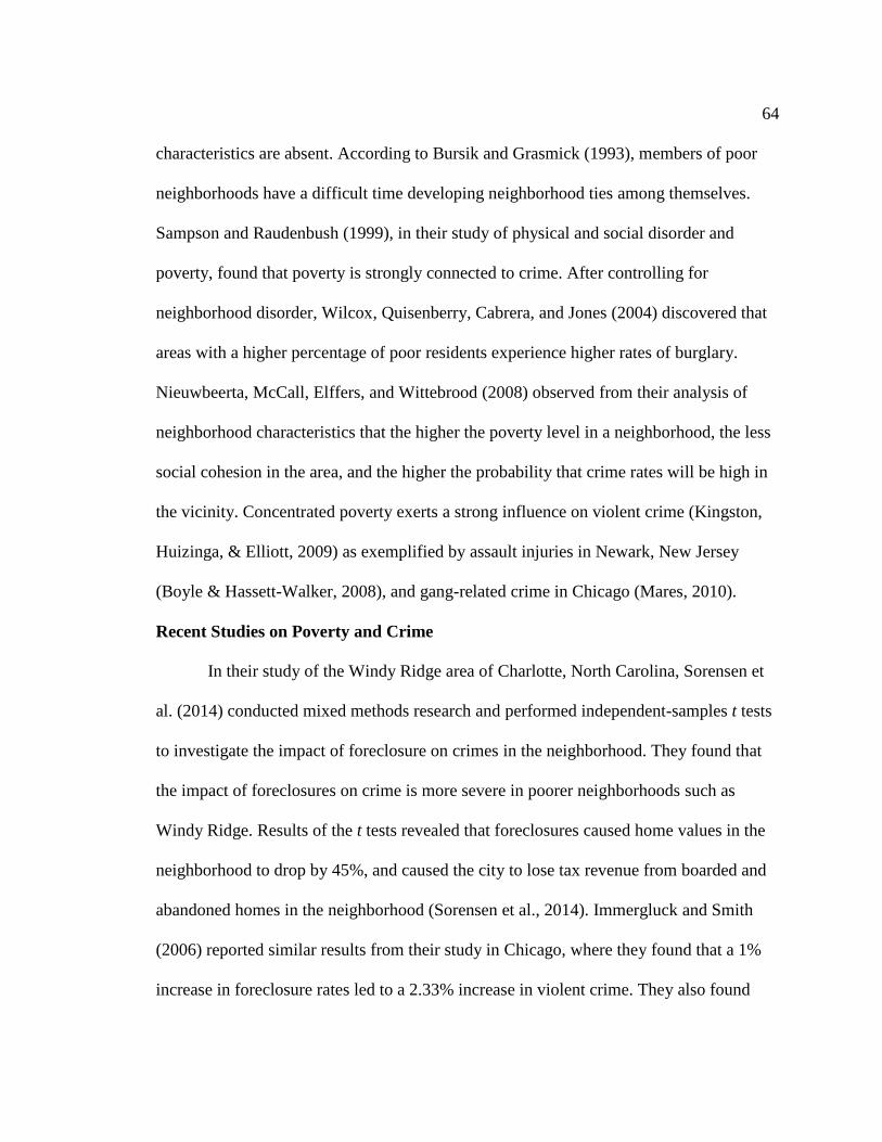
64

characteristics are absent. According to Bursik and Grasmick (1993), members of poor

neighborhoods have a difficult time developing neighborhood ties among themselves.

Sampson and Raudenbush (1999), in their study of physical and social disorder and

poverty, found that poverty is strongly connected to crime. After controlling for

neighborhood disorder, Wilcox, Quisenberry, Cabrera, and Jones (2004) discovered that

areas with a higher percentage of poor residents experience higher rates of burglary.

Nieuwbeerta, McCall, Elffers, and Wittebrood (2008) observed from their analysis of

neighborhood characteristics that the higher the poverty level in a neighborhood, the less

social cohesion in the area, and the higher the probability that crime rates will be high in

the vicinity. Concentrated poverty exerts a strong influence on violent crime (Kingston,

Huizinga, & Elliott, 2009) as exemplified by assault injuries in Newark, New Jersey

(Boyle & Hassett-Walker, 2008), and gang-related crime in Chicago (Mares, 2010).

Recent Studies on Poverty and Crime

In their study of the Windy Ridge area of Charlotte, North Carolina, Sorensen et

al. (2014) conducted mixed methods research and performed independent-samples t tests

to investigate the impact of foreclosure on crimes in the neighborhood. They found that

the impact of foreclosures on crime is more severe in poorer neighborhoods such as

Windy Ridge. Results of the t tests revealed that foreclosures caused home values in the

neighborhood to drop by 45%, and caused the city to lose tax revenue from boarded and

abandoned homes in the neighborhood (Sorensen et al., 2014). Immergluck and Smith

(2006) reported similar results from their study in Chicago, where they found that a 1%

increase in foreclosure rates led to a 2.33% increase in violent crime. They also found

65

that foreclosures in poorer neighborhoods harm the neighborhood because the abandoned

homes produce extended vacancies and increase crime (Immergluck & Smith, 2006).

Other similar studies (Arnio & Baumer, 2012; Hipp & Chamberlain, 2015;

Pfeiffer et al., 2015; Zhang & McCord, 2014) uncovered a consistently positive

correlation between economic disadvantage or higher poverty and crime, regardless of

the analytical model. For example, Hipp and Chamberlain (2015) used negative binomial

regression models to assess whether the relationship between foreclosures and

neighborhood crime rates, between 1996 and 2011, were stronger in cities in Southern

California with a combination of high economic disadvantage and segregation, and

whether the relationship was stronger in the towns with high racial/ethnic heterogeneity

and high racial segregation. They found that, with the exception of motor vehicle theft,

foreclosures increase all city level crime-burglary, robbery, and aggravated assault, and

that the impact of foreclosures on burglary, robbery, and aggravated assault is stronger in

cities with high levels of inequality, and low levels of economic segregation (Hipp &

Chamberlain, 2015).

Pfeiffer et al. (2015) used longitudinal modeling, and data from calls for service

made to 911 from local law enforcement agencies in Chandler, Arizona, to investigate the

link between foreclosure and crime in the neighborhood. They found that there are more

calls for service related to crime, in neighborhoods with higher rates of renters and fewer

homeowners than in areas with fewer renters and more homeowners. Williams et al.

(2013) performed Granger causality tests, and multilevel growth modeling in Chicago

neighborhoods utilizing data collected between 1998 and 2009, and realized results

66

consistent with those noted by Pfeiffer et al. (2015): in renter-occupied neighborhoods,

REO homes increase the level of property crime. Evidence indicates that the percentage

of residents receiving food stamps, unemployment benefits, housing vouchers or

controlled rents, and other types of welfare affect the rates of crime in the area (Wolff et

al., 2014).

Arnio and Baumer (2012) utilized the GWR statistical model to test for spatial

heterogeneity—the uneven distribution of crime—in the impact of demographic and

other predictors of neighborhood crime rates in Chicago. Of concern was whether the

relationship between foreclosures and crime vary across different neighborhoods in

Chicago. They found that the impact of residential stability on burglary rates and

socioeconomic disadvantage on robbery rates varies across Chicago census tracts. Using

multivariate regression models, Arnio et al. (2012) examined the endogeneity of

foreclosure and spatial dependence of crime, and found a positive association between

foreclosure and property crime. The authors noted that the positive effects of foreclosure

on crime are mostly conditioned or limited to counties with structural disadvantage and

higher foreclosure activity (Arnio et al., 2012).

Using a regression model, Baumer et al. (2012) examined whether several city-

level attributes such as levels of socioeconomic disadvantage, foreclosure rates, and prior

vacancy rates, the degree of recent new housing construction, housing affordability, and

the quantity and quality of policing, moderate the relationship between neighborhood

levels of foreclosure and crime in 5,517 census tracts in 50 large U.S. cities. Baumer et

al. (2012) found that disadvantaged neighborhoods with higher rates of foreclosure

67

experience higher rates of robbery, drawing the conclusion that foreclosure is more

strongly related to burglary rates in cities with little new home construction, and

declining police forces. Similarly, Baumer, Arnio, and Wolff (2013) explored the

capacity of mortgage fraud to produce high rates of foreclosure in some neighborhood,

and the possibility that neighborhoods with high foreclosure activity can exhibit spatial

dependence. Baumer et al. (2013) found that neighborhoods with a high level of

foreclosure activity could elevate the rate of foreclosures in nearby counties, concluding

that spatial variation in foreclosure rates appears to be due to additive effects of selected

factors rather than interactions of those factors.

Zhang and McCord (2014) reinforced the notion that spatial heterogeneity

compounds the relationship between foreclosures and neighborhood crime by examining

the effect of housing foreclosures on burglary, using foreclosure and crime data

aggregated to block groups in Louisville, Kentucky. Similar to Arnio and Baumer (2012),

Zhang and McCord (2014) employed GWR to tackle the uneven distribution of crime.

They found that although the connection between foreclosures and burglary varies across

different neighborhoods, neighborhood foreclosure rates are a strong predictor of

neighborhood burglary rates for disadvantaged urban neighborhoods, but not for more

affluent neighborhoods, after accounting for other contextual variables.

Although many studies have indicated that a link exists between foreclosure rates

and crime rates, other studies have yielded mixed results. For example, Sampson (1988)

and Sampson and Groves (1989) concluded that poverty might not be related to the

development of neighborhood ties. Sampson (1991) suggests that neighborhood social

68

networks are inversely linked to neighborhood networks. Lowenkamp et al. (2003),

utilizing British crime survey data, found that the level of poverty had statistically

significant unintended consequences on community networks. Similarly, in a study on

Native American homicides, Lanier and Huff-Corznie (2006) utilized social

disorganization theory and found no connection between crime and poverty among the

population. Although some studies found no significant effect of poverty on crime

(Lanier & Huff-Corzine, 2006; Lowenkemp et al., 2003), Sampson and Raudenbush’s

(1999) study and others consistently revealed lesser levels of trust and cohesion in poorer

neighborhoods. In other words, crimes are high in disadvantaged neighborhoods because

of the mediating effect of trust and cohesion on crime (Nieuwbeerta et al., 2008).

Population Heterogeneity and Crime

Population heterogeneity is one of the most regularly investigated ecological

characteristics of an area. In social science, population heterogeneity can be observed in

features that distinguish the population, or their observed variables. Ethnic heterogeneity

is a measure of the racial diversity in an area, while the age composition of a population

(e.g. residents above the age of 64 are seniors, and residents of ages 15 to 24 are youth)

are some of the measures of heterogeneity that can be used to define a population. The

question of how population heterogeneity in an area relates to crime rates in the area has

fascinated scholars (Shaw & McKay, 1972). Cumulative findings from literature on

neighborhoods and crime indicate that the population heterogeneity of a neighborhood

matters. For example, Shaw and McKay (1972) posited that racial heterogeneity, among

the other structural factors, contribute to the disruption of social organization in

69

neighborhoods, which accounts for differences in crime rates. Early scholars such as

Kornhauser (1978), and Sampson and Groves (1989) agreed that due to fewer common

and shared interests, neighborhoods or areas with greater racial heterogeneity are less

likely to build intimate social network ties among the different ethnic groups residing in

the area. Cultural and language differences are believed to affect solidarity, thus lowering

informal social control and subsequently increasing the possibility of crime within the

neighborhood (Kornhauser, 1978; Sampson & Groves, 1989).

Various scholars (e.g. Bellair, 1997; Kubrin, 2000; Mares, 2010; McNulty, 2001;

Olson et al., 2009; Osgood & Chambers, 2000; Peterson & Krivo, 2010; Warner &

Rountree, 1997) have reported similar findings; ethnic or population diversity has a

significant effect on crime rates. For example, Warner and Pierce (1993) analyzed 911

calls to law enforcement agencies made from 60 Boston neighborhoods and found that

racial diversity, though dependent on the rates of poverty, is a good predictor of burglary

rates in Boston neighborhoods. Bellair (1997) found that ethnic diversity impedes the

formation of social ties or networks. Both Kubrin (2000), and Warner and Rountree

(1997) found that population diversity has a direct positive effect on crime in

disadvantaged neighborhoods in Seattle, Washington. Analyzing youth violence in a rural

area, Osgood and Chambers (2000) found that racial heterogeneity is positively related to

higher crime rates (e.g. rape, homicide, aggravated assault, robbery, and weapons).

For example, Heitgard and Bursik (1987) examined the impact of changes in

ethnic composition, and other indicators of social disorganization on crime rates in

nearby neighborhoods, and found that crime rates increase as the racial composition of

70

adjoining areas rapidly change. McNulty (2001), and Peterson and Krivo (2010) found

that crime is more pronounced in areas where African Americans reside. McNulty (2001)

noted that crime rates, specifically those for murder, were higher in predominantly Black

neighborhoods in Atlanta than in other areas. Peterson and Krivo (2010) revealed that

while there was crime in predominantly Black neighborhoods in Atlanta, Chicago, and

New York, crime was more common in predominantly White neighborhoods in Seattle,

Washington. While Martinez (2014) observed that in areas with high levels of poverty,

both Blacks and Whites have similar homicide rates, presumably because both groups are

exposed to the same structural conditions.

Similarly, FBI crime statistics, particularly the crime index involving robbery,

homicide, aggravated assault, rape, larceny, burglary, and motor vehicle theft reveal that

demographic factors such as the age of the population, affect the rates of crime. As

indicated by the index, crimes tend to be committed by young people (FBI, 2012; Males

& Brown, 2013). The FBI crime statistics reinforce the general belief that youth

(primarily ages 14–24) are biologically driven to engage in risk-taking, dangerous, and

reckless behavior demonstrated by a lack self-control and impulsivity, although the same

can be said for adults (Brown & Males, 2011; Nagin & Paternoster, 2000; Ulmer &

Steffensmeier, 2014). The difference between adults and youth who commit crimes,

according to a research report from U.S. Department of Justice: Office of Justice

Programs, Office of Juvenile Justice and Delinquency Prevention (2007), is that youth are

more likely to get caught committing crimes than adults are. Additionally, Males (2015),

and Ulmer and Steffensmeier (2014) suggested that the factor of age alone is insufficient

71

for understanding crime trends. Ulmer and Steffensmeier (2014) contended that because

it is impossible to examine people outside their social contexts, the use of age as a factor

is overstated. Males and Brown (2013) also recommended that instead of age alone, a

sociodemographic analysis that includes age, gender, race, and other economic variables

can offer better explanations for crime trends, and provide significant implications for

crime prevention strategies in neighborhoods. The views expressed by these scholars

align well with social disorganization theory.

Taylor (1996) suggested that racial diversity in a community had no effect on

neighbors’ local ties or their responses to disorder in 66 neighborhoods in Baltimore,

Maryland. Lowenkamp et al. (2003) suggested that population diversity has unintended

consequences on local networks or ties. Sampson, Morenoff, and Raudenbush (2005) also

found no link between offenses committed by particular ethnic group members and the

collective efficacy of neighborhoods in Chicago.

Physical Dilapidation and Crime

Physical dilapidation refers to the physical conditions of an area (Skogan, 1990).

According to Skogan (1990), physical dilapidation in an area relates to (a) residents’

inability to maintain their neighborhood and homes, (b) unregulated neighborhood, (c)

lack of investment, and (d) the emergence of abandoned homes and the corresponding

degeneration over time. Shaw and McKay (1972) suggested that physical dilapidation,

particularly foreclosure, is one of the structural characteristics which when accompanied

by poverty and population heterogeneity, undermines the collective efficacy and social

ties/networks necessary for preventing crime in an area. Physical dilapidation or disorder

72

(Skogan, 1990) negatively affect neighborhood social networks, ties, and attachment

(Shaw & McKay, 1972; Skogan, 1990). Subsequent to the foreclosure crisis of 2007–

2009 throughout most neighborhoods in the United States, during which disinvestment in

maintenance contributed to the decline of home quality and values, blighted

neighborhoods resulted in the loss of trillions of dollars in household wealth (Mallach &

Brachman, 2013; Schwartz, 2015; Tsai, 2015).

The cumulative findings of copious literature on the impact of neighborhood

socioeconomic and demographic conditions on crime rates across the country suggest

that poor neighborhoods with poorly maintained, abandoned, and vacant homes resulting

from foreclosure, increase crime rates (Garvin, Branas, Keddem, Sellman, & Cannuscio,

2013; Hur & Nasar, 2014; Kondo, Keene, Hohl, MacDonald, & Branas, 2015; Sorensen

et al., 2014). For example, Garvin et al. (2013), and Hur and Nasar (2014) found that in

poor neighborhoods, higher levels of foreclosure activity are linked with fear of crime

and crime itself. Branas et al. (2012), and Garvin, Cannuscio, and Branas (2012) found a

positive link between vacant homes and an increased risk of victimization. Kondo et al.

(2015), and Nassauer (2011) revealed that the physical appearance of the neighborhood

(e.g. well-maintained homes, painted fences, properly mowed lawns, and clean

sidewalks—the hallmark of affluent neighborhoods) are linked to low rates of crime.

Evidence indicates that in disadvantaged neighborhoods such as areas with high levels of

school dropouts and unemployment, poverty affects residents’ ability to invest in home

maintenance, and to participate and contribute to programs designed to prevent crime

73

(Wolff et al., 2014). In other words, in some neighborhoods, physical dilapidation can be

a symptom of poverty.

Local Policy and Crime

Criminal justice studies suggest that the effectiveness of the prosecutorial,

correctional, judicial, and probational components of the justice system, and the rate of

incarceration, numbers of police, policing strategies, and social programs in an area, all

affect crime rates (Kleiman, 2014; Nagin, 2014; Rosenfeld, 2015). Rosenfeld (2013)

found that demographic changes, the criminogenic market like the employment level and

government policies that tend to incite criminal behavior, and the economy could affect

the rates of crime in an area. Roeder et al. (2015), Kleiman (2014), and Rosenfeld (2013,

2015) further suggested that proactive surveillance (installing cameras at every strategic

location in the area) and law enforcement agents’ improved strategies, affect the rates of

crime. Roeder et al. (2015) argued that these strategies make it more difficult for

individuals to commit a crime, even when opportunities such as boarded empty homes

are readily available to motivate offenders. Kleiman (2014), and Roeder et al. (2015) also

found that policing innovations such as CompStat, crowdsourcing, problem solving,

community policing, pulling levers, focused crackdowns, and procedural justice, have a

positive influence on crime rates, and contribute to a decline in crime rates in American

cities.

In addition to improved policing strategies, the level of incarceration may affect

the rates of crime (Kleiman, 2014; Nagin, 2014; Rosenfeld, 2015). A popular notion

among law enforcement agents and some criminologists is that incarcerating criminals

74

leaves fewer offenders on the streets to commit crimes, which is similar to Madensen et

al.’s (2011) argument that foreclosures displace criminals from neighborhoods. However,

the idea that mass incarceration reduces crime remains controversial (Stiglitz, 2015).

Although incarceration is believed to reduce crime by rehabilitating offenders, deterring

criminals, and incapacitating and interrupting criminal careers, there is evidence that

incarceration might not be efficient in stopping crime, and instead increases crime

(Nagin, 2014; Roeder et al., 2015; Rosenfeld, 2014). Rosenfeld (2014) argued that

incarceration can increase crime by cementing criminal identities, reducing legitimate

opportunities for released offenders, disrupting families and communities, and reducing

the stigma of punishment.

Most studies reviewed in establishing a foundation for the present study

connected foreclosures to crime rates, and found that socioeconomic and demographic

characteristics of neighborhoods played a role in the impact of foreclosure on crime;

however, these studies seldom controlled for most of the major neighborhood

socioeconomic and demographic conditions that might have affected the incidence of

these two social problems (Wolff et al., 2014). Some of the studies that stroved to capture

the impact of socioeconomic and demographic conditions did so in isolation of other

important neighborhood variables, with the exception of studies that used DD design (Cui

& Walsh, 2015; Ellen et al., 2011; Lacoe & Ellen, 2014), and Wolff et al. (2014), whose

study combined DD and PSM to control for other neighborhood conditions.

Similar to the present study, Wolff et al. (2014) utilized DD and PSM to identify

matching pairs of U.S. counties based on an extensive set of sociodemographic

75

characteristics. The matched pairs allowed the authors to identify “treatment” (high

foreclosure) and “control” (low foreclosure) counties with similar sociodemographic

characteristics, and to compare these two groups on the selected outcomes of burglary

and robbery rates. The results indicated that when sociodemographic characteristics are

included in the model, foreclosures and crime are not significantly related. Similar to

Wolff et al. (2014), the present study addressed this weakness in the literature by

measuring the influence of socioeconomic and demographic variables such as school

dropout, residents on food stamps, and others in Charlotte neighborhoods that

experienced heavy foreclosure rates and others that experienced fewer foreclosures.

Summary

Chapter 2 supplied a comprehensive review of the literature on foreclosures and

crime, as well as other neighborhood socioeconomic and demographic conditions that

influence both foreclosures and crime. The chapter presented a review of strategies, and

the theoretical foundation of the study and those of previous crime and foreclosure

studies. Social disorganization theory explains the link between population heterogeneity,

poverty and foreclosure, and crime. Studies conducted to date have reinforced the

hypothesis that foreclosure and neighborhood socioeconomic and demographic

conditions contribute to crimes in certain neighborhoods. Chapter 3 introduces the

research design and rationale; offers an overview of the Charlotte Neighborhood Quality

of Life Studies methodology; discusses the sample population, the sampling procedures,

the operationalization of variables, and the threats to validity; and concludes with a

discussion on ethical concerns.

76

Chapter 3: Research Method

Introduction

The purpose of this research was to study the relationship between levels of

foreclosure and neighborhood crime rates while controlling for other neighborhood

conditions. This chapter describes the research design, target population, sampling

procedures, instruments, data analysis plan, threats to validity, and ethical procedures.

The general review of this design includes the rationale for selecting the research design.

The target population, sample characteristics, as well as the description of the study

instruments are addressed.

Research Design and Rationale

This research used the difference-in-differences (DD) research design to compare

the crime rates for two groups (A and B) for two time periods (2004 and 2010). Group A,

the comparison group, was not exposed to foreclosure (the treatment) during either

period, but shared similar baseline characteristics with Group B. Group B, the treatment

group, was exposed to foreclosure in 2010 but not in 2004 (Table 3). This study used

secondary panel data—two-time series archival data with one intervention—from the

CNQL studies, subsequently renamed the Quality of Life Explorer.

The DD design was appropriate for this study because it can be used to estimate

the effects of foreclosure, and to compare changes in crime rates over the two-point

period or more (Cui & Walsh, 2015; Lechner, 2011; Wolff et al., 2014; Wooldridge,

2011). Similar to Wolff et al. (2014), and Cui and Walsh’s (2015) studies, crime rates

before and after the treatment (foreclosure) were compared between the treatment group

77

of neighborhoods exposed to foreclosure, and the comparison group of neighborhoods

not exposed to foreclosure. When DD is used, two differences in crime rates are

important: the difference after foreclosure versus before foreclosure in the treatment

group (Y1,pre – Y0,pre), and the difference after versus before foreclosure in the

unexposed group (Y1,post – Y0,pre; Table 3). The changes in crime rates that are related

to the foreclosure crisis beyond other neighborhood conditions can then be estimated

from the DD analysis as follows: (Y1,post – Y1,pre)- (Y0,post – Y0,pre). If there is no

relationship between foreclosure rates and subsequent crime rates, the DD estimate

should equal zero. In contrast, if the foreclosure rates are linked with the changes in

crime rates, then the increased crime rates following exposure to foreclosure will improve

to a greater extent in the exposed group.

Despite the debate over the validity of DD design due to non-random attrition in

quasi-experimental studies, some of the appeal or advantages of DD come from its

simplicity, as well as its ability to circumvent many of the endogeneity issues that

characterize comparisons between mixed neighborhoods (Wooldridge, 2011). Other

advantages include its descriptive nature and the potential to describe trends, track

changes over different time periods, and establish a baseline measure (Cui & Walsh,

2015; Dimick & Ryan, 2014; Ellen et al., 2013; Lacoe & Ellen, 2014; Mian et al., 2015;

Wolff et al., 2014). The two-time series data from the CNQL (MSG, 2004, 2010) enabled

repeated measures to explore, identify, and describe trends and changes over time

(Sartorius, 2013; Table 4). Table 3 is a visual representation of DD design.

78

Table 3

Examples of Difference-in-Difference (DD) Design

Treatment Group (Foreclosure)

Comparison Group (non-Foreclosure)

Difference

Pre-foreclosure

Y1,pre Y0,pre (Y1,pre – Y0,pre)

Post-foreclosure

Y1,post Y0,post (Y1,post – Y0,pre)

Change

(Y1,post – Y1,pre)

(Y0,post – Y0,pre)

∆= (Y1,post – Y1,pre)- (Y0,post – Y0,pre) =

(Y1,pre – Y0,pre) - (Y1,post – Y0,post)

Target Population

The target population for this archival study consisted of 173 neighborhoods in

Charlotte, North Carolina, referred to as neighborhood statistical areas (NSAs), in the

2004 and 2010 CNQL studies.

CNQL Studies (Secondary Data)

The 2004 and 2010 CNQL studies provided the primary data for this study. The

CNQL is an index that was created by the City of Charlotte, Mecklenburg County, and

UNC Charlotte Urban Institute to measure the neighborhood life of quality in all 173

NSAs in Charlotte. The CNQL is a biannual longitudinal study based on locally-derived

variables from the neighborhoods. According to Open Charlotte (n.d.), the NSAs in the

2004 and 2010 studies were developed using the 2000 and 2010 census block group

geography. Each NSA represents one census block group. A neighborhood can be

classified as stable, threatened or fragile, or transitioning or challenged, depending on the

data gathered from the neighborhood. The original purpose of the CNQL studies was to

help policy makers in Charlotte affirmatively advance the development of the city, as

well as provide baseline data for researchers to assess the economic, physical, criminal,

79

social, and environmental conditions in Charlotte neighborhoods (Furuseth, Smith, &

McDaniel, 2015). Another purpose of the CNQL studies was to aid city and county

policy makers, Charlotte-Mecklenburg schools, and other agencies in monitoring changes

and trends, developing work plans, identifying capacity-building opportunities, and

determining resource allocation.

The City of Charlotte provides this data set or the final reports of these biannual

studies to researchers and universities, realtors, government agencies, businesses,

residents, service providers, and other members of the public, free of charge (Appendix

B). Most of the statistical data, maps, graphs, tables, and charts are web-based and

housed online in open Charlotte websites. There are no elaborate procedures or

permissions required to gain access to the CNQL study reports. Users are allowed to

access this data set and customize the information based on their needs. Some local

library personnel in Charlotte are trained to assist researchers in using the data.

According to the City of Charlotte open data portal, the goal of access to the data set is to

stimulate innovation, promote community engagement, and increase productivity in the

City of Charlotte, Mecklenburg County, and beyond (Open Charlotte, n.d.).

The CNQL database contains foreclosure, crime, socioeconomic, and

demographic data that represent residents’ well-being, and neighborhood economic life.

The compilation of the database is facilitated every year and shared with realtors, HOAs,

homeowners, property owners, renters, and other members of the community, in a public

forum. The selection of variables to be incorporated into the study, and modifications to

the study are accomplished through the collaborative effort of the County, the City of

80

Charlotte, and the University of North Carolina Charlotte Urban Institute representatives

(Open Charlotte, n.d.). Delmelle and Thill (2014) utilized the CNQL studies to analyze

the impact of the great recession in Charlotte. This present study will analyze the impact

of foreclosure on crime in Charlotte neighborhoods.

CNQL Methodology

The CNQL is a composite index with four components: social, physical,

economic, and crime dimensions (Figure 7; Delmelle & Thill, 2014). The four elements

in the CNQL are weighted in the index as follows: Physical = 30%, Social = 30%, Crime

= 30%, and Economy = 10%. The CNQL index is calculated as follows for all of the

twenty variables in the study: a z-score is calculated for each of the 20 variables every

year, and then the values are linked with the four categories (physical, economic, social,

and crime), with the mean value set to zero, and each neighborhood’s score compared to

the City average (below or above the city average). A neighborhood with significant

positive scores indicates an area with high quality of life, while those with negative

values indicate low quality of life (Metropolitan Studies Group, University of North

Carolina at Charlotte, 2004; 2010). The crime rates for each neighborhood were derived

from measuring the crime rate and comparing it to the city area average, using location

quotient. When the value of the location quotient of a neighborhood falls below or above

1.00 (the city average), the value above or below 1.00 indicates the percentage

differences, or variation in crime trends in that neighborhood. Figure 8 is a visual

representation of the CNQL index.

81

Figure 7. Composition of CNQL index.

As mentioned earlier, the physical, crime, and social categories receive a weight

of 0.3 while the economic category is weighted at 0.1; this difference in weighting scores

is due to economic categories having the least number of variables (only two variables).

The advantages of this standardization technique are that it provides baseline

information; allows policymakers, researchers, and the public to observe macro changes,

trends, and progress; and prioritizes resource allocation to neighborhoods in transition.

The weakness of this approach is that it eliminates the possibility of pinpointing the

drivers of these local changes and trends in a neighborhood. For example, Williams et al.

(2013) examined several quality-of-life indicators during 2000–2009 and determined that,

while the foreclosure crisis negatively affected disadvantaged neighborhoods, crime

indicators during the same period did not exhibit the same effect.

Despite the fact that CNQL studies can be used to formulate projections, evaluate

the health of a neighborhood, identify trends, and recommend possible strategies. Full

understanding of whether other neighborhood conditions impacts crime rates remains a

challenge. This study will contribute to neighborhood and crime literature by

investigating whether neighborhoods with higher foreclosure activity experience higher

rates of crime after accounting for other neighborhood conditions. Although the 20

Economic dimension Sociail dimension

Crime dimension Physcal dimension

Quality of Life Index

82

variables included in the 2004 and 2010 studies covered the four neighborhood

categories, for this study, only the relevant variables (Table 5) will be incorporated. Table

5 provides a description of the variables derived from the CNQL database, as well as the

source of the data. A two-time series archival data with one intervention, 2004 and 2010,

will be used to determine whether neighborhood foreclosure rates are linked to

neighborhood crime rates, after accounting for other neighborhood conditions. The study

variables are presented in Table 4.

Table 4

Study Variables, Definitions, and Sources

Variable Definition/quotient Source *

Crime dimension

Property crime rate Location quotient of

burglaries, larcenies, vehicle

thefts, arsons, vandalism

Charlotte-Mecklenberg Police Department (2003,

2009)

Economic dimension

Percentage food

stamps

Percentage of population

receiving food stamps

Mecklenburg County Department of Social Service

Office of Planning and Evaluation (2003, 2009)

Social dimension

Dropout rate Percentage of high school

students who dropped out of

the school system

Charlotte-Mecklenberg School System (2003, 2009)

Physical dimension

Appearance index Index of code violations Neighborhood Development (2003, 2009)

Home ownership Percentage of owner-occupied

residential units

Mecklenburg County Property Records and Land

Management (2003, 2009)

Substandard housing Percentage of housing units in

neighborhood rated as

dilapidated

Housing Quality in the City of Charlotte Report

(2003, 2009)

Neighborhood profile

Population

distribution: race

Population distribution by race

in the neighborhood

U.S. Census Bureau (2010)

Population

distribution: youth

Population distribution by age

in the neighborhood—youth

Mecklenburg County Property Records and Land

Management (2003, 2009); Claritas (2003, 2009);

U.S. Census Bureau (2000)

Youth opportunity

index

A measure of the potential

opportunity for youth in the

neighborhood

Charlotte area YMCAs and YWCAs (2003, 2009);

Charlotte-Mecklenburg Library System (2003,

2009)

Number of foreclosure

homes

Number of foreclosures in

neighborhood

Employment Security Commission of North

Carolina (2009)

Note. * Adapted from Charlotte Neighborhood Quality of Life Study, by Metropolitan Studies Group,

University of North Carolina at Charlotte, 2004; 2010.

83

Sampling and Sampling Procedures

The CNQL, which has been conducted biannually in 173 neighborhoods in

Charlotte, North Carolina, provided the study’s primary data. To reduce sampling error,

the data of this study was limited to neighborhoods that were categorized as stable in the

2004 CNQL study. Among the 173 neighborhoods in the City of Charlotte in the 2004

CNQL study, 100 neighborhoods were categorized as stable, 48 as threatened, and 25 as

fragile on the crime classification scale (Metropolitan Studies Group, University of North

Carolina at Charlotte, 2004). A neighborhood’s crime condition is classified as stable

when the neighborhood’s crime rate is below that of the City of Charlotte (low crime

rate). Threatened neighborhoods are those with medium crime rates, above City rate, and

have lower scores on economic, social, and possibly physical dimensions. Fragile

neighborhoods are those with high levels of crime, and lower economic and social scores

(Metropolitan Studies Group, University of North Carolina at Charlotte, 2004).

To determine whether neighborhood foreclosure rates are linked to neighborhood

crime levels after accounting for other neighborhood conditions, three components,

namely, the sample size, the effect size, and the alpha level were used to establish the

power of this study (Cohen, 1988). Because G-power is easy to use, accurate in

conducting power analysis, and is freely available online, I used G-power 3.1 to

determine the sample size for this study (Marchant-Shapiro, 2015; Reid, 2014). A priori

power analysis, assuming a medium effect size (t = .37, alpha = .05), using paired sample

t test means: difference between two dependent means (matched pairs), a minimum

sample size of 47 was required to achieve a power lever of .80 (Field, 2013). To conduct

84

a fair evaluation of how foreclosures affect crime levels in neighborhoods, this study

utilized a sample size of 54 neighborhoods. And effect size of .343, or medium. In the

social sciences, an alpha level of .05 is within the acceptable limit. The significance level

was .05, and alpha level 5% to 95% Cl (Field, 2013). Figure 9 is a visual representation

of the power as a function of the sample size.

Figure 8. Power as a function of sample size.

Rights Protection and Permission

Archival data from CNQL Studies were used in this study; therefore, there was no

direct contact or interaction with homeowners, renters, property owners, and HOAs in the

relevant neighborhoods. These data sets are publicly available online, and therefore do

not pose any threat or setback for any individuals; consequently, there was no need to

85

safeguard the data set to ensure the confidentiality of participants, or to obtain permission

to use the data. The data composed of tables, graphs, maps, and textual materials were

downloaded from the City of Charlotte website. Permission to conduct research was

requested from and granted by Walden’s Institutional Review Board (approval #: 08-29-

16-0452657).

Instrumentation and Materials

The archival data for this research was drawn from information in the CNQL

(2004; 2010) studies. The 2004 CNQL study was conducted between July 2002 and June

2003, and the 2010 CNQL study was conducted between July 2008 and June 2009.

Property crimes include arsons, burglaries, vehicle thefts, vandalism, and larcenies

defined according to uniform crime reporting (UCR) standards, and were compiled by the

Charlotte-Mecklenburg Police Department. The rate of property crimes in each

neighborhood were determined by dividing the number of property offenses within the

area (neighborhood) by the population. The rate (property crime) per population of a

neighborhood is then compared to the rate per population for the City of Charlotte. The

Mecklenburg County Property Records and Land Management used the Completed

Foreclosure (CF) data metric to collect the total stock of foreclosed homes that have

either been auctioned or repossessed by the lender (REO).

Both property crimes as defined in UCR standards, and CF metric are known to

produce reliable and valid data. For example, the UCR is a statistical program employed

by the U.S. Department of Justice to measure the impact, nature, and magnitude of crimes

across the nation. UCR produces valuable and comprehensive information about the

86

incidence of crime across the nation, including monthly crime data from police

departments and other individual reports transmitted directly to the FBI (Cahill et al.,

2014; Cui & Walsh, 2015; Lacoe & Ellen, 2014; U.S. Department of Justice, n.d.).

Similarly, the CF metric captures and provides an accurate measure of the total stock of

foreclosed homes in neighborhoods (Cahill et al., 2014; Cui & Walsh, 2015; Lacoe &

Ellen, 2014). Table 5 includes all data that was used in this study.

Operationalization of Variables

Three key variables were used in this quasi-experimental design study:

foreclosure rates, crime levels (property crimes), and the comparable variables (Table 5).

The operationalization of these variables was as follows. The foreclosure rate is a

continuous level variable corresponding to the level of foreclosures in a neighborhood,

measured by rates of no-foreclosure and foreclosures. Exposure to foreclosure was

defined as neighborhoods with foreclosure rates higher than the average for the City of

Charlotte (14 per neighborhood) during the study period, while no-foreclosure was

defined as neighborhoods with foreclosures below the average for the City of Charlotte.

Though violent, juvenile, and property crimes are potentially relevant to the

foreclosure crisis from the social disorganization theory standpoint, for this study, higher

levels of foreclosures in neighborhoods were anticipated to be especially salient for

property crimes. Property crimes are strongly tied to physically dilapidated

neighborhoods with crime generators or crime attractors. The social disorganization

theory and other theories such as the routine activity theory and broken windows theory

suggest that neighborhoods plagued by foreclosures provide opportunities for crime to

87

escalate. The crime rate is a continuous level variable corresponding to the degree of

crime that occurs in a neighborhood, and the rates in an area is compared to Citywide

(City of Charlotte) average. The comparable variables are continuous level variables, and

were measured by their percentages in a neighborhood (Table 5).

Data Analysis Plan

SPSS Version 21.0 for Windows was used to analyze the data. Descriptive

statistics were calculated to describe the variables used in the study. Means and standard

deviations for the variables, foreclosure rates, crime rates, and the control variables were

calculated (Table 9).

Archival data from the CNQL studies were screened prior to analysis for accuracy

and missing data, and to ensure that they could be analyzed using dependent t tests and

hierarchical multiple regressions (Berman & Wang, 2012; Field, 2013). To obtain the

required valid results from t tests and hierarchical multiple regression, this study verified

that the underlying assumptions of these models held true. The assumptions are briefly

stated as follows (Berman & Wang, 2012; Field, 2013; Freund & Wilson, 2003; Green &

Salkind, 2011):

The two variables must be measured on a continuous scale (either interval or

ratio level).

The independent variable consists of two levels or categories (matched pairs).

The two samples are independent.

There are no significant outliers.

88

The data follow the normal probability distribution (Schapiro-Wilk test of

normality).

There was independence of observation (using Durbin- Watson statistic).

There was linearity and homoscedasticity (scatter plots).

Analysis was conducted in three stages. For the first stage, PSMs were utilized in

constructing balanced groups. For the second stage, dependent or paired-sample t tests

were used to determine whether there was a significant difference in crime rates of two

groups—A and B neighborhoods—that were tested at two time periods—2004 and 2010

(before and after foreclosure). Finally, hierarchical multiple regression models were used

to explore the relationship between foreclosures, socioeconomic, demographic, and crime

levels.

Threat to Validity

Given that DD design was used to analyze archival data in this study, there were

limited chances for instrumentation, and attrition or mortality threats (Nishishiba, Jones,

& Kraner, 2013). Despite the use of two-time series data with one intervention, which

increased internal validity, and the use of DD design, which permitted purposive

selection from a comparison group, the introduction of a comparison group increased the

possibility of selection bias. To limit selection bias and keep margins of error within

reasonable bounds, DD design was paired with PSM. PSM was conducted using SPSS,

where each neighborhood was assigned a probability score (0–1) that it would be selected

based on a summary index of relevant or baseline characteristics (Holmes, 2013).

89

Advantages of the PSM method include its capacity to allow the estimates to be

adjusted for different factors (e.g. socioeconomic and demographic characteristics) that

may differ between groups. This method increases analytical rigor and ensures that there

are no differences in unobservable characteristics (Austin, 2011; Sartorius, 2013). Other

potential threats to validity in this study were the possible confounds in the archived data

set. The confounding variables include the percentage of residents on food stamps and

others as indicated in Table 4. These potential confounding factors were examined as

covariates in the testing procedure.

Ethical Procedures

Archival data from CNQL studies were used for this study, and because these data

do not contain respondents’ personal information, the risk to respondents was minimized.

Because the researcher completed the NIH training course prior to beginning this study,

the researcher was aware of all the requirements for data management strategy designs,

necessary to protect participants’ personal information such as data storage, file

passwords, and computer backups. Hard drives were stored in a secure location, and data

will be retained for at least 5 years after completing the study, as per NIH standards, even

though it is not necessary, given that the archival data are open-source materials.

Summary

Chapter 3 explained the rationale for using the DD research design with two-time

series secondary data with one intervention, to test two research questions. The plan for

data analysis was presented and included the use of t tests to determine the significance

of the differences in crime rates, before and after the foreclosure crisis period. Also

90

included in the chapter were a description of the population, the methodology of the

CNQL study from which the data were derived, and the operation of the variables.

Threats to validity were discussed, and the ethical protection concerns were presented.

91

Chapter 4: Results

Introduction

The purpose of this research was to study the relationship between levels of

foreclosure and neighborhood crime rates, while controlling for other neighborhood

conditions. This chapter offers the results of the study, including the list of matched

samples (neighborhoods) from CNQL studies, and the analytical steps for the propensity

scores matching, followed by statistical analyses for the research questions, including the

paired-samples t test, and multiple linear regressions. Significance for statistical

assumptions and analyses was evaluated at the accepted alpha level, α = .05. From open-

source data of the 2004 CNQL studies, 54 of 100 stable neighborhoods were successfully

matched using PSM. A sample size of 58 neighborhoods was deemed adequate, given

that three independent variables (based on theoretical considerations) were used to match

the sample, and 10 independent variables were included in the analysis (Nishishiba et al.,

2013).

Pre-Analysis Data Screening

The data for this research were collected from CNQL studies (2004 and 2010).

The sample was composed of 100 neighborhoods that were classified as stable in the

2004 CNQL study, and were neighborhoods with low crime, and economic, physical, and

social needs. Fifty-four neighborhoods were matched using their propensity scores. The

sampling frame was composed of 173 neighborhoods in Charlotte, North Carolina. The

analyzed data were comprised of the following variables: crime rates (property crime),

foreclosure rates, and the comparable variables (Table 4). Crime data from the 2004 and

92

the 2010 CNQL studies were chosen to ensure that crime data covered the period before

and after the foreclosure crisis. The data were screened for accuracy, missing data, and

outliers. Descriptive statistics and frequency distributions were conducted to ensure that

outliers did not distort the data, and that the responses were within the range of values.

For this study, a sample size of 54 neighborhoods provided a power (1-ß) level of .80.

The PSM approach was utilized to construct balanced groups, and thus reduce the

imbalance in data matching. The study included theoretically relevant (social

disorganization theory) covariates such as school dropout rates, heterogeneity scores, and

appearance index, proxies for poverty, population heterogeneity, and physical

dilapidation, which may influence the likelihood of crime increase in neighborhoods

(Wolff et al., 2014). To illustrate the application of this method, data collected from the

100 neighborhoods were entered into logistic regression software (SPSS Version 22.0 for

Windows). The propensity score was estimated utilizing the foreclosure variable

(treatment assignment) as the outcome variable, and the selected covariates as predictors

(Austin, 2011; Thoemmes & Kim, 2011).

A total of 54 neighborhoods divided into two groups (Appendix A) were matched

based on school dropout rates, heterogeneity scores, and appearance index, proxies for

poverty, population heterogeneity, and physical dilapidation (social disorganization

theory). One group consisted of neighborhoods exposed to foreclosures (n = 27), and the

other group consisted of neighborhoods not exposed to foreclosure (n = 27). As a result,

46 neighborhoods of the 100 neighborhoods were not analyzed due to their non-

comparability (extreme probability scores). Thus, final descriptive and inferential

93

analyses were conducted on the sample of 54 neighborhoods with a power level of .80.

Statistical results were based on the research questions. The differences of the 54

matched neighborhoods are presented in Table 5.

Table 5

File of Matched Neighborhoods

NID Group HIS NID Group HIS Difference

62 no foreclosure 0.18898 1 Foreclosure 0.19476 0.005

65 no foreclosure 0.20496 26 Foreclosure 0.20889 0.003

33 no foreclosure 0.23172 2 Foreclosure 0.23172 0

170 no foreclosure 0.24542 171 Foreclosure 0.24945 0.004

194 no foreclosure 0.31118 105 Foreclosure 0.31656 0.005

108 no foreclosure 0.34894 118 Foreclosure 0.34922 0

179 no foreclosure 0.37037 37 Foreclosure 0.3596 0.01

159 no foreclosure 0.37319 117 Foreclosure 0.37348 0

50 no foreclosure 0.40215 187 Foreclosure 0.40379 0.001

175 no foreclosure 0.41125 107 Foreclosure 0.43547 0.024

53 no foreclosure 0.45794 120 Foreclosure 0.44063 0.017

69 no foreclosure 0.46372 106 Foreclosure 0.46205 0.001

160 no foreclosure 0.47764 119 Foreclosure 0.47136 0.006

184 no foreclosure 0.47768 123 Foreclosure 0.47963 0.001

185 no foreclosure 0.481 130 Foreclosure 0.48529 0.004

197 no foreclosure 0.49255 114 Foreclosure 0.48852 0.004

163 no foreclosure 0.50439 59 Foreclosure 0.51307 0.008

61 no foreclosure 0.56327 135 Foreclosure 0.56084 0.002

190 no foreclosure 0.5731 104 Foreclosure 0.56492 0.008

58 no foreclosure 0.5773 127 Foreclosure 0.57665 0

60 no foreclosure 0.60734 41 Foreclosure 0.62653 0.019

129 no foreclosure 0.63823 121 Foreclosure 0.63331 0.004

70 no foreclosure 0.69622 146 Foreclosure 0.6544 0.041

139 no foreclosure 0.69678 110 Foreclosure 0.7068 0.01

3 no foreclosure 0.73211 145 Foreclosure 0.72596 0.006

49 no foreclosure 0.77801 152 Foreclosure 0.77692 0.001

71 no foreclosure 0.78101 113 Foreclosure 0.78758 0.006

Note. 54 matched neighborhoods (n = 27 no foreclosure, n = 27 foreclosures).

Descriptive and Inferential Statistics

Percentages of demographic data. Percentages were examined for nominal

variables. The samples consisted of 54 neighborhoods, and the residents in these

neighborhoods consisted of fewer senior citizens (9.4%) than youth (25%). The majority

94

of residents were White (67%), followed by Black (24.42%) (Appendix C). The

percentages for the demographic data are presented in Table 6.

Table 6

Demographic distribution of the 54 neighborhoods

Demographic %

Ethnicity

White 67.00

Black 24.42

Hispanic 0.78

Native American 1.00

Asian 3.30

Pacific Islander 0.30

Two or more 3.20

Age

Youth 24.00

Senior (over age 64) 9.70

Others 66.30

Total 100.00

Note. N = 54, and due to rounding error, not all percentages may total to 100.

Descriptive statistics of continuous variables. Composite scores were computed

for the 10 variables of interest: 2004 crime rates, youth, school dropout, recipients of

food stamps, homeownership, substandard housing, unemployment, youth opportunity

index, appearance index, and population heterogeneity. A composite score was created

for these predictor variables by taking an average of the five corresponding items that

make up the scales, respectively. Descriptive statistics for the 10 composite scores are

presented in Table 7.

95

Table 7

Descriptive Statistics for Predictors and Neighborhood Crime Levels

Min Max M SD

Crime rates 10.00 150.00 62.22 34.5680

Youth 8.30 36.30 23.821 5.8725

Dropout .00 16.20 4.917 3.7438

Fstamps .00 42.10 6.889 7.5389

Howner 6.40 94.60 63.404 19.6943

SubHouse .00 21.40 1.513 3.9050

Un_Level .00 2.00 1.463 .7451

YO_Index .00 2.00 1.000 .6143

AP_Index .00 2.00 .222 .5379

H_Score .00 8.20 3.704 2.1408

Reliability of the propensity score matching. Matched results are considered

reliable when the non-equivalence in a group, or pre-group differences have been reduced

enough to permit meaningful estimation of the predictor effect. To assess the non-

equivalence of groups, the substantial difference and statistical significance of the groups

needs to be examined (Holmes, 2014). Groups (compared) are considered to be the same

if their differences (difference in means) are not statistically significant (Holmes, 2014).

Correlated sample tests were conducted to determine group differences, before and after

matching. Independent-sample t tests were first carried out on the sample of 100

neighborhoods (before matching), to determine the level of imbalance or differences-of-

differences in the groups (Holmes, 2014). The results indicated that there was a

significant difference in the rates of crime between the neighborhoods with no

foreclosure (M = 45.40, SD = 25.889) and the neighborhoods affected by foreclosure (M

= 69.20, SD = 32.629); t (98) = -4.040, p = 0.000 (Table 8). These results suggest that the

two groups are not the same, and substantial differences exist.

96

Table 8

Average Crime Rates of the Two Groups Neighborhoods: Foreclosure Group (N=50) vs No Foreclosure

Group (N=50)

Variable M SD

No foreclosure 45.40 25.889

Foreclosure 69.20 32.629

Total 57.30 31.165

t(99)=4.04, P=.00

A second independent sample t test was conducted on the sample of 54 matched

neighborhoods to determine whether the differences between neighborhoods affected by

foreclosure and neighborhoods not affected by foreclosure had been removed or reduced

enough to permit a meaningful estimation of foreclosure effects on crime rates. The

results indicated that there was no significant difference in the rates of crime in

neighborhoods with no foreclosure (M=53.33, SD=30.634) and neighborhoods affected

by foreclosure (M=71.11, SD=36.515); t (52) = -1.938, p = 0.058 (Table 10) for the 54

matched neighborhoods. The results from Table 8 and Table 9 are considered reliability

statistics because the differences for the 54 matched neighborhoods are not statistically

significant, which suggests that the compared groups are primarily the same.

Table 9

Average Crime Rates of the Two Groups Neighborhoods: Foreclosure Group (N=27) vs No Foreclosure

Group (N=27)

Variable M SD

No foreclosure 53.33 30.634

Foreclosure 71.11 36.515

Total 62.22 34.568

t(53)= -1.938, P=.058

97

Restatement of the Research Questions and Hypotheses

Research Question 1 and hypotheses. RQ1 and the related hypotheses were as

follows:

RQ1: Do neighborhood foreclosure rates have an impact on neighborhood crime

rates?

H01: Neighborhood foreclosure rates do not have an impact on neighborhood

crime rates.

Ha1: Neighborhood foreclosure rates do have an impact neighborhood crime

rates.

To address RQ1, a paired-samples t test was conducted to evaluate correlated or

matched samples of crime rates in neighborhoods in 2004 and 2010. Prior to analysis, the

following assumptions were assessed: (a) the dependent variable was continuous, (b) the

independent variables consisted of two related groups or matched pairs, (c) the samples

are related, (d) the distribution was normal, and (e) there were no significant outliers.

Continuous criterion. The dependent variable of crime rates meets the

continuous criterion (measured from 0 to 100). The independent variable of foreclosure

rates satisfies this assumption because each of the neighborhoods in the no foreclosure

group, and the foreclosure group was measured at two periods (2004 and 2010).

Two related or matched pairs assumption. The independent variables consist of

two categorically matched or related groups: pre-test for no foreclosure neighborhoods

and post-test for foreclosure neighborhoods. This assumption was met.

98

Normality and outliers assumptions. Outliers and normality of the dependent

variable were assessed with the normality tests, Kolmogorov-Smirnov, and Shapiro-Wilk

tests. The results of both the Kolmogorov-Smirnov and the Shapiro-Wilk tests indicated

statistical significance (p < .05), and the histogram shows that there are outliers;

therefore, the assumptions of outliers and normality were not met. Although these two

assumptions were not met, the normality and outliers assumptions are mostly relevant for

small sample sizes (N < 30). With N = 54 in this study, the paired-samples t test was

fairly robust (Green & Salkind, 2014; Nishishiba et al., 2013). The normality and outliers

results are presented in Table 10 and Figure 10.

Table 10

Tests of Normality Test

Normality Test

Difference

Statistic Df Sig.

Kolmogorov-Smirnova .180 54 .000

Shapiro-Wilk .939 54 .008

Note. a = a = Lilliefors corrected Kolmogorov-Smirnov test.

99

Figure 9. Normality and outliers of crime difference, 2004 and 2010.

Paired-samples t test. The paired-samples t test is an appropriate statistical

analysis when the goal of the research is to evaluate whether there is statistical evidence

that the mean difference between the pre-test and the post-test of the paired samples, is

significantly different from zero (Nishishiba et al., 2013). Results of the paired-samples t

test, conducted to compare the crime rates in 2004 (pre-test) and crime rates in 2010

(post-test), indicated that the mean crime rates for 2010 (M = 71.85, SD = 43.700) was

significantly greater than the mean crime rates for 2004 (M = 62.22, SD = 34.568); t(53)

=-2.708, p< .01. The standardized effect size index, d, was .342 (medium-sized effect).

The 95% CL for the mean difference between the two periods (2004 and 2010) was -

16.762 to -2.497. The crime rates’ error bars (Figure 11) and the results of the paired-

100

samples t test revealed that the foreclosure crisis from 2007 to 2009 did have an impact

on crime rates in the studied neighborhoods. The null hypothesis (H01) for RQ1 can be

rejected. The results of the paired-samples t test are presented in Table 11 and Figure 11.

Table 11

Paired-Samples t Test for 2004 and 2010 Crime Rates (N=54)

*P < .05

Figure 10. Crime rate error bars, 2004 and 2010.

Research Question 2 and related hypotheses. RQ2 and the related hypotheses

were as follows:

M SD t test

Pair 1 Pre-test 62.22 34.568 -2.708*

Post-test 71.85 43.700

101

RQ2: How are neighborhood foreclosure rates related to neighborhood crime rates

after controlling for other neighborhood conditions?

H02: Neighborhood foreclosure rates are not significantly related to neighborhood

crime rates after controlling for other neighborhood conditions.

Ha2: Neighborhood foreclosure rates are positively related to neighborhood crime

rates after controlling for other neighborhood conditions.

To address RQ2, a hierarchical multiple regression was conducted to evaluate

whether foreclosure rates and other covariates are useful in predicting crime levels in

neighborhoods. A sample size of 54 neighborhoods was deemed adequate, given that

there were 10 independent variables to be included in the analysis (Nishishiba et al.,

2013). Prior to conducting the series of hierarchical multiple regression, relevant

assumptions such as equality of variance, linearity, outliers, normal distribution, and

homoscedasticity, independence of errors, multicollinearity, and singularity were tested

(Field, 2013).

Equality of variance and linearity assumptions. Equality of variance and

linearity assumptions were tested by visual examination of the scatter plot (Figure 14)

and the model summary in Table 12. An examination of Figure 14 revealed that the

residual dots do not spread out in a triangular fashion, and that R2 = .13 for Step 1, ΔR2 =.

12 for Step 2, ΔR2 = .8 for Step 3, ΔR2 =. 1 for Step 4 (p < .05), both the linearity and

equality of variance assumptions were met.

Outliers assumption. The outliers assumption was tested by visual examination

of the Mahalanobis distance scores (Field, 2013; Tabachnick & Fidell, 2012). The

102

Mahalanobis distance scores indicated no multivariate outliers; thus, this assumption was

met.

Normality assumption. Normality was tested by visual examination of the

histogram and the normal P–P plots of the residuals (Figure 12 and Figure 13). The

residuals in the histogram are approximately normally distributed. While the data in the

P-P plots are approximating a line, the dashed line did not significantly deviate from the

straight line; thus, the normal distribution assumption was met. Visual assessment of

normality are presented in Figure 12 and 13.

Figure 11. Assessment of normality.

103

Figure 12. Assessment of normality.

Homoscedasticity assumption. The homoscedasticity assumption was tested by

visual examination of the scatterplot (Figure 14). Because the scatterplot of ZPRED

versus ZRESID does show a random pattern, there seemed to be no distinctive funneling,

meaning that there is no indication of heteroscedasticity; thus, this assumption is met.

Independence of errors assumption. Independence of errors assumption was

tested or checked using Durbin-Watson statistics in SPSS software. Because the value of

1.701 from the Durbin-Watson statistic test (Table 14) falls within the recommended

limits (boundaries of 1–3), the test suggests that errors are reasonably independent; thus,

the assumption is deemed to have been met (Field, 2013).

104

Table 12

Model Summary

Model R R2 Adjusted R2 Durbin-Watson

1 .360a .130 .113

2 .502b .252 .191

3 .574c .329 .227 1.701

4 .582d .339 .185

Note. a = predictors Constant and F-rates. b = predictors Constant, Dropout, Fstamps, and Un_Level. c =

predictors Constant, Sub_House, Homeownership, and App-Index. d = predictors Constant, H_Score,

Youth, and Youth_Op.

Figure 13. Residuals of homoscedasticity for variables predicting crime levels.

Multicollinearity and Singularity. The assumptions of multicollinearity and

singularity were satisfied. An examination of correlations (Table 14) indicated that the

independent variables were not a combination of other independent variables; while the

collinearity statistics (Tolerance and VIF) were all within acceptable limits (Field, 2013;

Green & Salkind, 2014; Nishishiba et al., 2013).

105

Hierarchical multiple regression. Hierarchical multiple regression analysis is an

appropriate statistical model when the goal is to investigate the relationship between

independent variable(s) and the dependent variable (Green & Salkind, 2014). A four-

stage hierarchical multiple regression was conducted with crime level as the dependent

variable. Foreclosure levels were entered at stage one of the regression to control for

foreclosures. The Poverty variables (school dropout, food stamps, and unemployment

level) were entered at Step two, Physical dilapidation variables (appearance index,

substandard housing, and homeownership) at stage three, and Population heterogeneity

variables (heterogeneity scores, youth, and youth opportunity index) at stage four. These

variables were introduced in this order based on theoretical (social disorganization

theory) consideration.

The hierarchical multiple regression results indicated that at Stage one,

foreclosure rates contributed significantly to the regression model, F (1, 52) = 7.753, p <

.05, and accounted for 13% of the variation in crime rates. Introducing the poverty

variables explained an additional 12% of the variation in crime rates, and this change in

R² was significant, F (3, 49) = 4. 136, p < .05. Adding physical dilapidation variables to

the regression model explained an additional 8% of the variation in crime rates, and this

change in R² was significant, F (3, 46) = 3. 223, p < .05. Finally, the addition of

population heterogeneity variables to the regression model explained an additional 1% of

the variation in crime rates, and this change in R² square was also significant, F (3, 43) =

2. 206, p < .05. Together the 10 independent variables accounted for 34% of the variance

in neighborhood crime levels.

106

When all 10 independent variables (Table 4) were included in Step four of the

regression model, eight predictor variables (heterogeneity score, youth opportunity index,

the population of youth, food stamps, unemployment level, appearance index,

substandard housing, and homeownership) were not significant predictors of

neighborhood crime levels. The most significant predictors of neighborhood crime levels

were foreclosure levels and school dropout rates. The model revealed that foreclosure

levels significantly predict the degree of crime, b = 19. 527, β = 9. 148, t = 2.135, p =

.039. Moreover, the model suggests that for every unit increase in foreclosure levels,

neighborhood crime levels increased by 19.5. Furthermore, school dropout rates

significantly predict the level of crime (b = 4.594, β = .341, t = 2.137, p = .038). The

model also suggests that for every unit increase in school dropout rates, neighborhood

crime levels increased by 4.6.

Finally, the results further revealed that out of the 10 predictor variables used in

this analysis (Table 4), only three (heterogeneity, youth opportunity index, and the

population of youth) were not correlated with the levels of crime in the neighborhoods.

Among the seven predictor variables (school dropout, food stamps, unemployment level,

appearance index, substandard housing, foreclosure rate, and homeownership), which

were significantly correlated with crime level in neighborhoods, the highest correlation

was between foreclosure rates and unemployment levels, which is significant at a .01

level (r = .656). One predictor variable, the percentage of homeownership, had a negative

relationship to crime rates (r = -.241, p < .05). The null hypothesis (H02) for RQ2 can be

107

rejected. The results of the intercorrelations between the multiple regression variables

were reported in Table 13, and the regression statistics in Table 14.

108

Table 14

Summary, Hierarchical Regression Analysis of Variables Predicting Crime Rates in Neighborhoods

Variable β t 𝑆𝑟2 R 𝑅2 ∆𝑅2

Step 1 .360 .130 .113

F-Rates .360 2.784** 0.130

Step 2 .502 .252 ..191

F-Rates .353 2.126* 0.069

Dropout .272 1.809 0.050

Fstamps .135 .881 0.012

Un-level -.162 -.979 0.015

Step 3 .574 .329 .227

F-Rates .413 2.437* 0.090

Dropout .321 2.106* 0.065

Fstamps .008 .045 0.000

Un-level -.177 -1.058 0.016

App-Ind .001 .006 0.000

SubHous .218 1.107 0.018

Home -.156 -1.009 0.015

Step 4 .582 .339 .185

F-Rates .405 2.135* 0.070

Dropout .341 2.137* 0.070

Fstamps -.038 -.212 0.001

Un-level -.160 -.924 0.013

App-Ind .000 .001 0.000

SubHous .247 1.173 0.021

Home -.124 -.713 0.008

H-Score .041 .306 0.001

Youth .068 .480 0.004

Youth-O .097 .623 0.006

Note. N=54; *p < .05, **p < .01, ***p < .001

Summary

The purpose of this quantitative research study was to examine the relationship

between foreclosures and crime rates in neighborhoods in Charlotte, North Carolina.

Results related to RQ1 indicate that neighborhood foreclosure rates had a statistically

significant impact on neighborhood crime rates. Thus, the null hypothesis (H01) was

rejected. Results related to RQ2 revealed that foreclosure levels and school dropout rates

were the most substantive predictors of crime rates in neighborhoods; thus, the null

hypothesis (H02) was rejected. These findings are discussed in greater detail in Chapter 5,

109

and are presented in relation to the current literature. The statistical findings are linked to

the research questions. Limitations of the study, recommendations for further research,

implications for positive social change, and the overall conclusion are presented in

Chapter 5.

110

Chapter 5: Discussions

Introduction

The purpose of this research was to study the relationship between levels of

foreclosure and neighborhood crime rates, while controlling for other neighborhood

conditions. In this chapter, summaries and interpretations of the results are presented, the

implications for social change and recommendations are discussed, and the conclusion is

presented. The summary of results is presented in the order in which the research

questions were examined and referenced in the literature review, followed by the

limitations encountered during analysis, and interpretation of the findings. The

recommendations for further research, implications for positive social change in public

policy and administration, and the conclusion derived from the study are also presented in

Chapter 5.

Based on the extant literature (Cahill et al., 2014; Cui & Walsh, 2015; Lacoe &

Ellen, 2014; Payton et al., 2015), this study predicted that neighborhoods affected by

foreclosures would experience significantly higher crime rates. Specifically, this study

predicted that vacant homes provide an easy target for trespassing, arson, vandalism, as

well as a haven for drug dealers, and theft of wires and appliances, and potentially

increase property crimes (Spelman, 1993). The impact of foreclosures is likely to be

magnified for neighborhoods with socioeconomic and demographic issues such as higher

school dropout rates, food stamps recipients, population heterogeneity, and substandard

housing. These theoretical predictions, derived from social disorganization theory, other

ecological theories, and prior research, were explored using paired-samples t tests and

111

multiple regression analyses. Paired-samples t tests were utilized in comparing crime

rates in 2004 and 2010, reflecting time periods before and after the foreclosure crisis of

2007–2009. The goal was to determine whether there is statistical evidence that the mean

difference between the paired samples is significantly different from zero. Multiple

regression analysis was used to explore variables causally related to increases in crime

rates (Field, 2013).

Summary of Results

Data from the study were analyzed using paired-samples t tests and hierarchical

multiple regression. The analyses were centered on the two central research questions

discussed below.

Research Question 1

RQ1: Do neighborhood foreclosure rates have an impact on neighborhood crime

rates?

The paired-samples t test results did not support the null hypothesis; therefore, the

null hypothesis was rejected. The model indicated that there was a statistical difference in

crime rates between neighborhoods that experience higher levels of foreclosure, and

neighborhoods that are not exposed to foreclosure (2004), suggesting that the mean

difference between the paired samples is significantly different from zero. The results

revealed that the two conditions yield a fairly large significant correlation coefficient (r =

.802, p < .01). Additionally, the difference between the means of the two conditions was

significant enough not to be a chance result (9. 63). The fact that the t value (-2.708) is a

negative number indicates that the 2004 crime rates had a smaller mean than 2010; thus,

112

foreclosures led to greater crime rates in Charlotte neighborhoods in 2010. The impact of

foreclosures on neighborhood crime levels conforms to social disorganization theory,

which postulates that crime is rampant in dilapidated neighborhoods.

Research Question 2

RQ2: How are neighborhood foreclosure rates related to neighborhood crime

rates after controlling for other neighborhood conditions?

There was no sufficient evidence from the study results to back the null

hypothesis. Thus, the null hypothesis was rejected. The hierarchical multiple regression

results revealed that foreclosure rates at Step 1; the introduction of poverty variables such

as school dropout rates, the percentage of food stamp recipients, and unemployment

levels in Step 2; physical dilapidation variables such as substandard housing,

homeownership level, and appearance index in Step 3; and the population heterogeneity

in Step 4, all contributed to a significant increase in crime levels in neighborhoods. The

model further revealed that when other variables are accounted for, foreclosure levels and

school dropout rates were the most influential drivers of crime rates in neighborhoods.

This important status or relationship between foreclosures and school dropout rates on

crime levels conforms to social disorganization theory, which postulates that these

variables (poverty, physical dilapidation, and population heterogeneity) influence the

variations of crime in neighborhoods (Shaw & McKay, 1972).

Limitations of the Study

The results of this research study should be viewed in light of the limitations.

Some of the principle limitations relate to external validity. The data in this study were

113

limited to data in the CNQL studies from 2004 and 2010. The research only analyzed

crime (property crime) data for 2004 and 2010, foreclosure data in the 2010 study, and

neighborhood conditions data in the 2004 CNQL study, all from the City of Charlotte,

Mecklenburg County. Compared to Glendale (Arizona), Chicago, Detroit, and Nevada,

Charlotte experienced fewer foreclosures (Madensen et al., 2011; Nassauer & Raskin,

2014; Sorensen et al., 2014; Wallace et al., 2012; Wolff et al., 2014). As a result, the

density, the degree of clustering of foreclosed homes, and the impact on crime rates may

be less than in other cities. Additionally, it is possible that the hierarchical nature of crime

reporting in UCR, utilized in the CNQL study data, may be masking the impact of crime

rates on neighborhoods, given that when a crime occurs in abandoned foreclosed homes,

some of the incidents are not reported to local law enforcement agencies, and thus the law

enforcement agencies do not record or report the incidents to UCR (Ellen et al., 2013).

For example, if the increases in crime rates are driven by the presence of squatters and

criminals in abandoned foreclosed homes, as posited in previous studies (Cui & Walsh,

2015; Payton et al., 2015), the extent to which the squatters who occupied these

abandoned foreclosed homes are themselves the perpetrators of the crime (e.g. vandalism

and burglary) is high, making it plausible that these offenses may not be reported to law

enforcement agents, and thus, the incidents will not be recorded in the UCR and the

identification of this impact (foreclosure effect) will remain unrecognized.

The normality test of the difference of the post-test and the pre-test (2004 and

2010 crime rates) did show a non-normal distribution. Although insufficient data can

cause a non-normal distribution, the researcher posits that a contributing factor could be

114

some extreme high and low values of crime levels from some neighborhoods. However,

Green and Salkind (2014), and Nishishiba et al. (2013) noted that the normality

assumption becomes less of a concern with sample sizes N > 30 (N = 54 in this study).

The social disorganization theory and previous studies (Cui & Walsh, 2015; Ellen

et al., 2013; Payton et al., 2015) suggest that neighborhoods plagued by foreclosures

provide opportunities for property crimes to escalate, and that vacant homes have a

significant impact on neighborhood crime rates (Qazi et al., 2015). Moreover, property

crime is strongly tied to neighborhoods with higher poverty, physical dilapidation, and

population heterogeneity (Hipp & Chamberlain, 2015; Katz et al., 2013). Based on social

disorganization theory, the researcher anticipated that higher levels of foreclosure in

neighborhoods should be especially salient for property crimes. The scope of this study

only covers property crime, and the predictors in this study do not include vacant homes,

which previous studies suggest have a negative impact on neighborhood crime rates

because they attract squatters, drug dealers, prostitutes, and burglers (Baumer et al., 2014;

Cahill et al., 2014; Ellen & Lacoe, 2015; Qazi et al., 2015). However, other studies show

that violent, juvenile, and public ordered crimes are potentially relevant to the foreclosure

crisis (Cahill et al., 2014; Teasdale et al., 2012).

Interpretation of the Findings

Following the foreclosure crisis (2007 to 2009) and the concern that foreclosed

homes could lead to higher rates of crime in some neighborhoods, this research set out to

find the relationship between levels of foreclosure and neighborhood crime rates, while

115

controlling for other neighborhood conditions. The use of CNQL study data (2004 and

2010) contributed to the extant empirical studies already available regarding the impact

of foreclosure on neighborhood crime level. This study concluded that foreclosure rates

and school dropout rates have an impact on, and are related to neighborhood crime rates,

after controlling for other neighborhood conditions.

Based on the statistical results in Chapter 4, the null hypotheses were rejected.

When the crime levels in 2004 and 2010 are considered; the paired sample results

revealed that neighborhoods not exposed to foreclosure in 2004 experiences fewer crime.

Moreover, also neighborhoods exposed to foreclosure in 2010 experienced higher crime

rates. As shown in Table 13 and Figure 11 (error bar) the mean crime levels in 2010 are

higher from crime levels in 2004, suggesting that foreclosures increase neighborhood

crime levels. The findings showed lower crime levels in 2004 before the foreclosure

crisis (2007 - 2009). The study gained a deeper understanding of how the foreclosure

crisis affects the variation in crime levels in neighborhoods in Charlotte. Consistent with

social disorganization theory, increases in crime in neighborhoods with higher

foreclosures shows that foreclosed homes make the area more attractive for crime

commission. Further, while the correlation between the two conditions (2004 and 2010

crime levels) yielded a relatively large correlation coefficient, these results provide

suggestive evidence that the foreclosure crisis from 2007 to 2009 contributed to crime

increases in Charlotte neighborhoods. The escalation in crime levels in 2010, conform to

the social disorganization theory and other ecological theories that suggest foreclosures

increase crime levels.

116

Shaw and McKay (1972) noted that higher crime levels are possible in zones

(neighborhoods) that are characterized by physical dilapidation. Kelling and Wilson

(1982) suggested that boarded homes, households with damaged roofs, windows, and

doors, and other physical disorders such as bushy lawns and piles of trash are a precursor

to serious crime. Skogan (1990) argued that neighborhoods with abandoned homes

heighten the fear of crime and real crime. Schwartz (2015) explained that foreclosures

increase the number of abandoned homes in neighborhoods. These findings not only

support the postulation from previous studies that abandoned homes, from foreclosures,

disorganize neighborhoods and create an opportunity for crime to increase, it also

illuminates the deleterious effects of foreclosures on residents and neighborhoods (Payton

et al., 2015; Wolff et al., 2014).

Increasingly, researchers are exploring ways in which social disorganization

theory enrich our understanding of how crime occurs in neighborhoods (Cui & Walsh,

2015; Lacoe & Ellen, 2015). This study extends this theoretical perspective by examining

the relationship between neighborhood foreclosure rates and neighborhood crime levels

after controlling for other neighborhood conditions. The study finds support for the core

assumptions of social disorganization theory. Based on the correlation coefficient

between every pair of the predictor variable and crime level (Table 14), the results

revealed that out of the 10 predictor variables studied (foreclosure rates, school dropout,

food stamps, unemployment levels, appearance index, substandard housing,

homeownership population heterogeneity, youth, and youth opportunity index), seven

variables (foreclosure rates, school dropout, food stamps, unemployment level,

117

appearance index, substandard housing, and homeownership) were meaningfully

correlated to neighborhood crime levels, and population heterogeneity, youth, and youth

opportunity index in neighborhoods were not correlated to neighborhood crime levels.

Not surprising, these findings mirror those of Cui and Walsh (2015), Ellen et al. (2013),

and Wolff et al. (2014), and conform to social disorganization theory, which posits that

these predictor variables affect crime levels in an area.

Among the seven predictor variables that correlated with neighborhood crime

levels, the highest correlation found was between foreclosure rates and the

unemployment levels. Although other factors such as a death in the family, health issues,

and divorce (not covered in this study) have been mentioned in other studies as possible

factors that may increase foreclosures (Cui & Walsh, 2015; Ellen et al., 2013), this study

determined that loss of job and income (unemployment) is the most influential driver of

foreclosure because unemployment may cut off a crucial source of mortgage payments

for families and individuals in neighborhoods (Herkenhoff & Ohanian, 2015).

This evidence is not surprising; rather, it reinforces the notion that residents,

families, and individuals do not have any margin of safety or insulation from having their

homes foreclosed on when they lose their jobs. Consequently, residents are at an

increased risk of foreclosure in the event they became unemployed. This finding suggests

that simply being unemployed makes foreclosure more likely, further reinforcing the

positive relationship between the two. Because this situation can increase crime levels,

the findings can be used to make changes to both foreclosure and crime prevention

policies.

118

Consistent with most recent studies, which indicate that homeownership has a

statistically significant effect on crime levels (Ni & Decker, 2009; Raleigh & Galster,

2013; Rohe & Lindblad, 2013), and similar to Ni and Decker (2009), who noted that

neighborhoods with higher homeownership rates experience low levels of crime, the

present study also determined that the percentage of homeownership in Charlotte

neighborhoods has a negative relationship to crime rates. Homeownership is not a perfect

proxy for higher income or low income due to several federal and state policy initiatives

that have been successful in promoting homeownership, particularly among low-income

families and individuals. Programs such as the Home Investment Partnership Program,

National Housing Trust Fund, and First Place Home Loans provide assistance to families

and individuals to defray closing costs, aid with down payment requirements, and provide

below-market rate financing. However, because homeowners are more committed,

attached, and active in their neighborhoods than renters (Ni & Decker, 2009; Rohe &

Lindblad, 2013), this finding reinforces the postulation promoted by Social

Disorganization Theory that collective efficacy explains neighborhood crime variations

(Sampson et al., 1997).

Finally, the summary of the hierarchical multiple regression analysis addressed

whether the relationships between the predictors and crime rates hold up, and further

provides a perspective on the importance of poverty, physical dilapidation, and

population heterogeneity in explaining crime level variations in neighborhoods. It was

determined that examining the extent of poverty, physical dilapidation, and population

heterogeneity in a neighborhood can significantly improve the ability to predict crime

119

rates in those neighborhoods. This evidence aligned with the postulate of social

disorganization theory that crime is possible in neighborhoods with the aforementioned

characteristics.

Another significant finding was that, in taking into account the percentage of

residents on food stamps, population of youth, unemployment levels, youth opportunity

index, homeownership, substandard housing, appearance index, heterogeneity score,

foreclosure levels, and school dropout rates of a neighborhood, the only variables that

were meaningfully related to neighborhood crime rates were foreclosure levels and

school dropout rates. Although several scholars have suggested that foreclosure levels

(Cui & Walsh, 2015; Lacoe & Ellen, 2014; Payton et al., 2015; Wolff et al., 2014) and

school dropout rates (Rumberger, 2013) are related to crime levels in neighborhoods, the

results of the present study provide empirical confirmation of these claims and conform

to social disorganization theory. Shaw and McKay (1972), and Skogan (1990) explained

that higher levels of crime are a possibility in poorer neighborhoods. Alliance for

Excellent Education (2013) noted that there is an indirect correlation between educational

attainment and crime because dropping out of school (a) decreases the possibility of

residents being gainfully employed and earning a living wage, (b) increases the

possibility that residents will be poor, (c) results in being more likely to depend on

welfare or public assistance (food stamps), and (d) creates economic discomfort that

pushes some residents to resort to crime (Kelly & Witko, 2014; Rumberger, 2013).

Neighborhoods with empty homes due to foreclosures provide opportunity for

criminals (Cahill et al., 2014; Wolff et al., 2015), and given that school dropouts, when

120

compared to those who graduate with certificates, diplomas, degrees, and advanced

degrees, may not have the means to provide adequate shelter for themselves, and may

thus face bleak social and economic prospects, they may resort to property crime

activities. This finding not only fills an important gap in the literature regarding the direct

link between poverty and physical disorder, it also serves as an important sign for policy

makers to take the issue of foreclosures and school dropouts seriously in neighborhoods.

Recommendations for Future Research

Recommendations for future research on the impact of foreclosure on crime rates

in neighborhoods are centered on the non-random distribution of the crime rate sampling

size, and expansion of the scope of the present study to cover other socioeconomic and

demographic variables such as job density, education level, and home characteristics.

This study was conducted using 54 neighborhoods, a sample size that might have

accounted for the non-random distribution of the crime differences (2004 and 2010) in

the paired-samples t tests. Moreover, this sample size might have prevented the outcome

of predictor variables (except foreclosure levels and school dropout rates) from reaching

a significant level of crime rates. A larger sample is required to increase the power of the

model.

This study should be replicated with archival data that combines UCR and

National Crime Victimization Survey data to estimate the rates and trends of crime in

neighborhoods. Although these results conform to social disorganization theory and other

criminological theories such as routine activity and broken windows, the results suggest

that higher rates of foreclosure increase the levels of crime. As such, it is not

121

unreasonable to hypothesize that the crime levels in neighborhoods can increase

foreclosures and poverty levels. Homeowners may decide to default on their mortgage

loans and exit neighborhoods with higher levels of crime. Further research should be

conducted to determine the causal order of these events.

Although this research failed to find statistically significant evidence indicating

that beyond foreclosure levels and school dropout rates, other predictors such as

unemployment levels, substandard housing, homeownership, and population

heterogeneity are key predictors of crime rates in neighborhoods, further investigation is

warranted to understand how the other variables might be influential in predicting crime

rates. Because previous research suggests that studies may be sensitive to the unit of

analysis chosen for aggregated data (Kobie & Lee, 2011), further studies incorporating

data collected by cities, counties, and states may be beneficial in revealing the

connections between foreclosures, socioeconomic and demographic variables, and crime

levels.

Similar to previous studies, this research study examined the relationship between

foreclosures and crime rates, albeit only for neighborhoods in the City of Charlotte, a

single city, which may limit the generalizability of the findings. Several studies suggest

that the interplay between foreclosures and crime rates may change drastically in

different neighborhoods, cities, counties, and states (Baumer et al., 2012; Payton et al.,

2015; Wolff et al., 2014); therefore, future research should focus on the effects of

foreclosures on different crime types in different neighborhoods, cities, counties, and

states, which will permit more meaningful comparisons from a broader perspective.

122

Implications for Positive Social Change

This study has multiple implications for positive social change. One implication

may be that understanding the impact of crime drivers on neighborhood crime levels may

provide a concise overview of how to revitalize urban neighborhoods and inner cities.

Another implication is that understanding the variables that explain increased crime

levels may be necessary for pinpointing the potential directions of crime trends, provide

the knowledge needed for explaining these trends, and support the intelligent forecast of

crimes. A better understanding of how variables such as school dropout rates,

unemployment, and foreclosures affect crime rates in neighborhoods could be addressed

within the context of smart strategies and policies designed to tackle these crime drivers.

Using the findings from this study and evidence provided by previous studies, city

planners, police, civic leaders, and other neighborhood stakeholders can better understand

the correlation between foreclosure and crime in neighborhoods (Qazi et al., 2015). They

can explore the introduction of ordinances that may prevent foreclosure, change policies

to reduce the impact of foreclosure, and address larger neighborhood problems such as

school dropouts, unemployment, and dilapidation, which might likely lead to higher

crime rates (Baumer et al., 2014; Cahill et al., 2014; Ellen & Lacoe, 2015; Qazi et al.,

2015).

The findings from this study provide knowledge on crime drivers and may help

local decision makers in generating effective policy initiatives that match the needs of the

residents, and address problems such as foreclosures and school dropouts. These findings

may further contribute to cost-effective and flexible strategies, and policies that are better

123

able to accommodate areas with unique characteristics. Increased knowledge of the

variables that drive crime could provide policy makers with the insights to not only

reduce crime rates in neighborhoods, but also provide what Sen, the 1998 Nobel Laureate

for economic science, described as social opportunities and economic facilities (Green &

Haines, 2012). Social opportunities and economic facilities refer to societal arrangements

or policy initiatives that provide opportunities and improve the quality of life for

residents.

Because this study also determined that foreclosure levels are strongly related to

unemployment levels, these findings suggest that policy initiatives that directly focus on

stopping criminals may not succeed in reducing crime rates in neighborhoods to

meaningful levels. For example, using policing strategies that directly “stop, question,

and frisk” suspected neighborhood residents contributes nothing to reducing foreclosures,

school dropout rates, unemployment levels, the percentage of neighborhood residents on

food stamps, and substandard housing in the neighborhoods (Kelling & Bratton, 2015).

Rather, these strategies increase unrest in some cities (e.g. Charlotte, Ferguson,

Baltimore, and New York). Given the rate of protests and violent riots some cities across

the country have experienced due to some preventive crime strategies, this approach may

not be the most cost-efficient and cost-effective strategy to utilize.

Further insight from this study suggests that city leaders should take steps to

formulate proactive strategies or policy initiatives that address the larger neighborhood

problems. Programs that directly address high school dropout rates, foreclosures,

unemployment, and other symptoms of crime such as higher numbers of residents on

124

food stamps and substandard housing may contribute to reducing the rates of crime.

Proactive policy initiatives could help cities avoid costly strategies that breed protests,

riots, and controversies, and widen the trust gap between law enforcement agents and

residents (Adams, Robinson, & Henderson, 2014; Kelling & Bratton, 2015). It is

important to avoid strategies that appear to have substantively unintended adverse effects

on the quality of life of neighborhood residents, and contribute nothing to reducing the

overall crime rates.

Many local governments are experiencing tight public budgets and policy makers

are being challenged to seek ways to use their limited resources as efficiently as possible.

Other stakeholders in the housing sector such as affordable housing providers, and

philanthropic organizations are increasingly compelled to invest their resources in

initiatives that guarantee financial returns while supporting a social good. A better

understanding of how school dropout rates and foreclosures affect crime levels in

different neighborhoods is not only necessary for enhancing the rationality for employing

such strategies, but it may also spur housing stakeholders and policy makers to embrace

and apply pragmatic improvisations in formulating public policies (Maynard-Moody &

Musheno, 2012). The practice of formulating flexible strategies or interventions that are

shaped and informed by the local characteristics of an area, are better able to

accommodate new situations or circumstances.

These findings also provide opportunities for policy makers to apply strategic

foresight in formulating preventive crime policies; reflective and smart policy initiatives

have lesser adverse effects on the neighborhood (Kamensky, 2015), and strategies and

125

initiatives that utilize best practices to address crime drivers (e.g. high rates of foreclosure

and school dropout) can provide social opportunities and economic support structures in

neighborhoods. For example, investing in strategies or public policies that (a) increase the

quality of education in cities; (b) ensure that children of school age and adults who desire

to go back to school, are not only enrolled, but can also complete their respective

schooling and programs; (c) provide job training and assistance; and (d) provide or

increase the safety net (welfare) for less privileged residents, might mitigate the factors

the drive crime and foreclosure. These initiatives or efforts for reducing school dropout

rates and unemployment in a neighborhood may not only succeed in reducing the number

of school dropouts in the neighborhood, but also decrease the levels of crime, thus

creating a healthy environment where most residents will have a real opportunity to live

productive and fruitful lives.

Conclusion

Several studies on neighborhood foreclosures have previously suggested that

foreclosure levels (Cui & Walsh, 2015; Lacoe & Ellen, 2014; Payton et al., 2015; Wolff

et al., 2014), and school dropout rates (Rumberger, 2013) are related to crime levels in

neighborhoods, with little empirical evidence to support the claims. The results of the

present study provide empirical confirmation of these claims, and conforms to social

disorganization theory. The present study provided evidence that foreclosure rates and

school dropout rates have an impact on, and are related to neighborhood crime rates, after

controlling for other neighborhood conditions. This study also fills a gap in the literature

regarding the direct link between poverty and physical disorder, and sends an important

126

signal for policy makers to take the issue of foreclosures and school dropouts seriously in

neighborhoods.

Although recent research on neighborhood stabilization has focused on

foreclosures as the only key influential variable increasing crime levels in neighborhoods,

the present study suggests that understanding and addressing larger neighborhood

problems such as school dropouts, unemployment, and substandard housing could reduce

crime levels. Findings from this study further suggest that policy initiatives or programs

that reduce school dropouts, provide job training and assistance, and reduce extreme

poverty and urban blight, thereby targeting the main drivers of crime in neighborhoods,

may not only reduce crime rates, but might also generate savings for local government

and help enhance public safety. Given that previous studies showed the potential gains

are substantial for program initiatives that address the larger neighborhood problems

(Payton et al., 2015; Qazi et al., 2016), and that neighborhood safety is enhanced when

social and economic programs that create opportunities for neighborhood residents are

utilized in crime prevention (HUD, 2016), the evidence from the present study provides

an opportunity and incentive for policy makers and others in the neighborhood

stabilization and housing policy network (police, affordable housing providers, and

scholars) to pursue smart and proactive policy initiatives. These initiatives could leverage

the correlation between crime drivers such as school dropout rates, foreclosures, and

unemployment, and the crime rates in a neighborhood, as a platform for high-impact

decisions that may reduce crime in neighborhoods.

127

References

Adams, M. O., Robinson, C. G., & Henderson, H. (2014, December 12). Post-Ferguson

public policy solutions. PA Times. Retrieved from http://patimes.org/post-

ferguson-public-policy-solutions/

Akers, R. L., & Sellers, C. S. (2009). Criminological theories: Introduction, evaluation,

and application (5th ed.). New York, NY: Oxford University Press

Aliprantis, D., & Kolliner, D. (2015). Neighborhood poverty and quality in the moving to

opportunity experiment. Retrieved from https://www.clevelandfed.org/newsroom-

and-events/publications/economic-commentary/2015-economic-commentaries/ec-

201504-neighborhood-poverty-and-quality-in-the-moving-to-opportunity-

experiment.aspx

Alliance for Excellent Education. (2013, September). Saving futures, saving dollars: The

impact of education on crime reduction and earnings. Retrieved from

http://all4ed.org/wp-content/uploads/2013/09/SavingFutures.pdf

Alm, J., Buschman, R. D., & Sjoquist, D. L. (2014). Foreclosures and local government

revenues from the property tax: The case of Georgia school districts. Regional

Science and Urban Economics, 46, 1–11. http://dx.doi.org/10.1016/

j.regsciurbeco.2014.01.007

Annenberg, E., & Kung, E. (2014). Estimates of the size and source of price decline due

to nearby foreclosures. American Economic Review, 104, 2527–2551.

http://dx.doi.org/10.1257/aer.104.8.2527

128

Arnio, A. N., & Baumer, E. P. (2012). Demography, foreclosure, and crime: Assessing

spatial heterogeneity in contemporary models of neighborhood crime rates.

Demographic Research, 26, 449–488. http://dx.doi.org/10.4054/

DemRes.2012.26.18

Arnio, A. N., Baumer, E. P., & Wolff, K. T. (2012). The contemporary foreclosure crisis

and US crime rates. Social Science Research, 41, 1598–1614. http://dx.doi.org/

10.1016/j.ssresearch.2012.05.013

Austin, P. C. (2011). An introduction to propensity score methods for reducing the effects

of confounding in observational studies. Multivariate Behavior Research, 46,

399–424. http://dx.doi.org/10.1080/00273171.2011.568786

Babones, S. J. (2014). Methods for quantitative macro-comparative research. Thousand

Oaks, CA: Sage.

Batson, C. D., & Monnat, S. M. (2013, April). Neighborhood disorder and resident

sentiment in the wake of the Las Vegas foreclosure crisis. Paper presented at the

Population Association of America 2013 Annual Meeting, New Orleans, LA.

Retrieved from http://paa2013.princeton.edu/papers/130790

Baumer, E. P., Wolff, K. T., Arnio, A. N., & Chiapputo, J. K. (2014). Assessing the link

between foreclosure and crime rates: A multi-level analysis of neighborhoods

across large U.S. Cities,” National Institute of Justice.

https://www.ncjrs.gov/pdffiles1/nij/grants/248336.pdf.

129

Baumer, E. P., Arnio, A. N., & Wolff, K. T. (2013). Assessing the role of mortgage

fraud, confluence, and spillover in the contemporary foreclosure crisis. Housing

Policy Debate, 23, 299–327. http://dx.doi.org/10.1080/10511482.2012.727843

Baumer, E. P., Wolff, K. T., & Arnio, A. N. (2012). A multicity analysis of foreclosure

and crime across neighborhoods. Social Science Quarterly, 93, 577–601.

http://dx.doi.org/10.1111/j.1540-6237.2012.00888.x

Bellair, P. E. (1997). Social interaction and community crime: Examining the importance

of neighborhood networks. Criminology, 35, 677–704. http://dx.doi.org/10.1111/

j.1745-9125.1997.tb01235.x

Berman, E. M., & Wang, X. (2012). Exercising essential statistics (3rd ed.). Thousand

Oaks, CA: Sage.

Bess, M. (2008). Assessing the impact of home foreclosures in Charlotte neighborhoods.

Geography and Public Safety, 1(3), 2–5. Retrieved from https://www.hsdl.org/

?view&did=5138

Bian, X., Brastow, R., Waller, B., & Wentland, S. (2015, January). Foreclosure

externalities and real estate liquidity. Paper presented at the 2015 Annual

Meeting of the American Economic Association, Boston, MA. Retrieved from

https://www.aeaweb.org/conference/2015/retrieve.php?pdfid=493

Billitteri, T. J. (2009, November 20). The value of a college education: Is a four-year

degree the only path to a secure future? CQ Researcher. Retrieved from

http://library.cqpress.com/cqresearcher/index.php

130

Boyle, D. J., & Hassett-Walker, C. (2008). Individual-level and socio-structural

characteristics of violence: An emergency department study. Journal of

Interpersonal Violence, 23, 1011–1026. http://dx.doi.org/10.1177/

0886260507313966

Branas, C. C., Cheney, R. A., MacDonald, J. M., Tam, V. W., Jackson, T. D., & Ten

Have, T. R. (2011). A difference-in-differences analysis of health, safety, and

greening vacant urban space. American Journal of Epidemiology, 174, 1296–

1306. http://dx.doi.org/10.1093/aje/kwr273

Branas, C. C., Rubin, D., & Guo, W. (2012). Vacant properties and violence in

neighborhoods. ISRN Public Health, 2012, Art. No. 246142. http://dx.doi.org/

10.5402/2012/246142

Breyer, B. (2013). Exploring local variability in statistical relationships with

geographically weighted regression. Retrieved from http://www.orurisa.org/

Resources/Documents/CCGISUG/CCGISUG_%20Breyer_2013_ExploringLocal

LariabilityInStatisticalRelationshipsWithGWR.pdf

Brown, E., & Males, M. (2011). Does age or poverty level best predict criminal arrest

and homicide rates? A preliminary investigation. Justice Policy Journal, 8(1), Art.

No. 5. Retrieved from http://www.cjcj.org/news/category/511

Burchfield, K. B., & Silver, E. (2013). Collective efficacy and crime in Los Angeles

neighborhoods: Implications for the Latino paradox. Sociological Inquiry, 83,

154–176. http://dx.doi.org/10.1111/j.1475-682X.2012.00429.x

131

Bursik, R. J., Jr. (1988). Social disorganization and theories of crime and delinquency:

Problems and prospects. Criminology, 26, 519–552. http://dx.doi.org/10.1111/

j.1745-9125.1988.tb00854.x

Bursik, R. J., Jr., & Grasmick, H. G. (1993). Neighborhoods and crime: The dimensions

of effective community control. New York, NY: Lexington Books.

Cahill, M., Pettit, K., & Bhatti, A. (with Downey, M., Pope, D. & Litschwartz, S.).

(2014). Foreclosures and crime: A space-time analysis [Research report].

Retrieved from https://www.ncjrs.gov/pdffiles1/nij/grants/248652.pdf

Campbell, J. Y., Giglio, S., & Pathak, P. (2011). Forced sales and house prices. American

Economic Review, 101, 2108–2131. http://dx.doi.org/10.1257/aer.101.5.2108

Charlotte Chamber Economic Development. (2013). Charlotte in detail. Retrieved from

http://www.aocresearch.com/docs/Charlotte_in_Detail.pdf

Center for Responsible Lending. (2013). 2013 Update: The spillover effects of

foreclosures. Retrieved from http://www.responsiblelending.org/mortgage-

lending/research-analysis/2013-crl-research-update-foreclosure-spillover-effects-

final-aug-19-docx.pdf

Charlotte City Council Housing and Neighborhood Development Committee. (2012).

Minutes of the committee on housing. Retrieved from

htp://charmeck.org/city/charlotte/focusareas/housingandndev/documents/041112

%20hnd%20committee%20summary%20package.pdf

Clark, L., & Teasdale, B. (2005, November). The impact of mortgage foreclosures on

neighborhood crime rate. Paper presented at the annual meeting of the American

132

Society of Criminology, Royal York, Toronto, CA. Abstract retrieved from

http://citation.allacademic.com/meta/p33959_index.html

Cohen, L. E., & Felson, M. (1979). Social change and crime rate trends: A routine

activity approach. American Sociological Review, 44, 588–608. http://dx.doi.org/

10.2307/2094589

Cordell, L., Geng, L., Goodman, L., & Yang, L. (2013). The cost of delay [Working

Paper No. 13-15]. Retrieved from https://www.philadelphiafed.org/-

/media/research-and-data/publications/working-papers/2013/wp13-15.pdf?la=en

Cui, L. (2010, November 10). Urban economics: Foreclosure, vacancy and crime. Paper

presented at meeting of Department of Economics, University of Pittsburgh, PA.

Retrieved from http://dx.doi.org/10.2139/ssrn.1773706

Cui, L., & Walsh, R. (2015, May). Foreclosure, vacancy and crime. Journal of Urban

Economics, 87, 72–84. http://dx.doi.org/10.1016/j.jue.2015.01.001

Cullen, F. T., & Agnew, R. (2011). Criminological theory: Past to present (4th ed).

Retrieved from http://www.d.umn.edu/~jmaahs/

Crime%20and%20Media/pdf%20files/cullen_agnew_socialD.pdf

Cullen, F. T., Agnew, R., & Wilcox, P. (2014). Criminological theory: Past to present.

(5th ed.). New York, NY: Oxford University Press.

Curtis, Q. (2014). State foreclosure laws and mortgage origination in the subprime.

Journal of Real Estate Finance and Economics, 49, 303–328. http://dx.doi.org/

10.1007/s11146-013-9437-9

133

Daneshvary, N., & Clauretie, T. M. (2012). Toxic neighbors: Foreclosures and short-sales

spillover effects from the current housing-market crash. Economic Inquiry, 50,

217–231. http://dx.doi.org/10.1111/j.1465-7295.2011.00380.x

Daneshvary, N., Clauretie, T. M., & Kader, A. (2011). Short-term own-price and

spillover effects of distressed residential properties: The case of a housing crash.

Journal of Real Estate Research, 33, 179–206. Retrieved from

http://pages.jh.edu/jrer/

Degarmo, M. (2011). Understanding the comparison of routine activities and contagious

distributions of victimization: Forming a mixed model of confluence and

transmission. International Journal of Criminology and Sociological Theory, 4,

584–603. Retrieved from http://ijcst.journals.yorku.ca/index.php/ijcst

Delmelle, E. C., & Thill, J.C. (2014). Neighborhood quality-of-life dynamics and the

great recession: The case of Charlotte, North Carolina. Environment and Planning

A, 46, 867–884. http://dx.doi.org/10.1068/a46161

Dimick, J. B., & Ryan, A. M. (2014). Methods for evaluating changes in health care

policy: The difference-in-differences approach. JAMA, 312, 2401–2402.

http://dx.doi.org/10.1001/jama.2014.16153

Ellen, I. G., Lacoe, L., & Sharygin, C. A. (2013). Do foreclosures cause crime? Journal

of Urban Economics, 74, 59–70. http://dx.doi.org/10.1016/j.jue.2012.09.003

Emergency Program to Reduce Home Foreclosures, NC Gen. Stat. §§ 45-100-107

(2016). Retrieved from http://www.ncleg.net/EnactedLegislation/Statutes/PDF/

ByArticle/Chapter_45/Article_11.pdf

134

Field, A. (2013). Discovering statistics using IBM SPSS statistics (4th Ed.). Thousand

Oaks, CA: Sage.

Fisher, L. M., & Lambie-Hanson, L. (2012). Are investors the bad guys? Tenure and

neighborhood stability in Chelsea, Massachusetts. Real Estate Economics, 40,

351–386. http://dx.doi.org/10.1111/j.1540-6229.2011.00317.x

Fisher, L. M., Lambie-Hansen, L., & Willen, P. (2014). The role of proximity in

foreclosure externalities: Evidence from condominiums. American Economic

Journal: Economic Policy, 7, 119–140. http://dx.doi.org/10.1257/pol.20130102

Freund, R. J., & Wilson, W. J. (2003). Statistical methods (2nd ed.). San Diego, CA:

Academic Press.

Furuseth, O., Smith, H., & McDaniel, P. (2015). Belonging in Charlotte: Multiscalar

differences in local immigration politics and policies. Geographical Review, 105,

1–19. http://dx.doi.org/10.1111/j.1931-0846.2014.12048.x

Garvin, E. C., Cannuscio, C. C., & Branas, C. C. (2012). Greening vacant lots to reduce

violent crime: A randomized controlled trial. Injury Prevention 19, 198–203.

http://dx.doi.org/10.1136/injuryprev-2012-040439

Garvin, E., Branas, C., Keddem, S., Sellman, J., & Cannuscio, C. (2013). More than just

an eyesore: Local insights and solutions on vacant land and urban health. Journal

of Urban Health, 90, 412–426. http://dx.doi.org/10.1007/s11524-012-9782-7

Gerardi, K., Lambie-Hanson, L., & Willen, P. S. (2013). Do borrower rights improve

borrower outcomes? Evidence from the foreclosure process. Journal of Urban

Economics, 73, 1–17. http://dx.doi.org/10.1016/j.jue.2012.06.003

135

Gerardi, K., Rosenblatt, E., Willen, P. S., & Yao, V. (2012). Foreclosure externalities:

Some new evidence (NBER Working Paper No. 18353). Retrieved from

http://www.nber.org/papers/w18353

Goodstein, R. M., & Lee, Y. Y. (2010). Do foreclosures increase crime? [FDIC Center

for Financial Research Working Paper No. 2010-05]. Retrieved from

https://www.fdic.gov/bank/analytical/cfr/2010/wp2010/CFR_WP_2010_05goodst

einlee.pdf

Graves, E. M. (2012). What do the neighbors think? Assessing the community impact of

the neighborhood stabilization efforts. New England Community Developments,

2012(1). Retrieved from http://www.bostonfed.org/commdev/necd/2012/issue1/

what-do-the-neighbors-think.pdf

Graves, E. M., & Shuey, E. (2013). The social impact of home rehabilitation in low-

income neighborhoods (Community Development Discussion Paper No. 2013-1).

Retrieved from https://www.bostonfed.org/-/media/Documents/cddp/

cddp1301.pdf

Green, G. P., & Haines, A. L. (2012). Asset building & community development (3rd ed.).

Thousand Oaks, CA: Sage.

Green, S. B., & Salkind, N. J. (2011). Using SPSS for Windows and Macintosh (6th ed.).

Upper Saddle River, NJ: Pearson.

Han, H.-S. (2014). The impact of abandoned properties on nearby property values.

Housing Policy Debate, 24, 311–334. http://dx.doi.org/10.1080/

10511482.2013.832350

136

Harris, P. L. (2011). The criminal consequences of changes in neighborhood structure

due to home foreclosure: A theoretical discussion. In M. Deflem (Ed.), Economic

crisis and crime: Sociology of crime, law, and deviance (pp. 145–169). Bingley,

United Kingdom: Emerald.

Hartley, D. (2014, November). The effect of foreclosures on nearby housing prices:

Supply or dis-amenity? Regional Science and Urban Economics, 49, 108–117.

http://dx.doi.org/10.1016/j.regsciurbeco.2014.09.001

Hathaway, R.S. (1995). Assumptions underlying quantitative and qualitative research:

Implications for institutional research. Research in Higher Education, 36(5), 535-

562.

Haughwout, A., Peach, R., & Tracy, J. (2010). The homeownership gap. Current Issues

in Economics and Finance, 16(5), 1–11. Retrieved from

https://www.newyorkfed.org/medialibrary/media/research/current_issues/ci16-

5.pdf

Heitgard, J. L., & Bursik, R. J., Jr. (1987). Extracommunity dynamics and the ecology of

delinquency. American Journal of Sociology, 92, 775–787. http://dx.doi.org/

10.1086/228582

Herkenhoff, K. F., & Ohanian, L. E. (2015). The impact of foreclosure delays on U.S.

employment. Retrieved from https://cla.umn.edu/sites/cla.umn.edu/files/

impact_foreclosure_herkenhoff_8_15.pdf

137

Hipp, J, R., & Chamberlain, A. W. (2015). Foreclosures and crime: A city-level analysis

in southern California of a dynamic process. Social Science Research, 51, 219–

232. http://dx.doi.org/10.1016/j.ssresearch.2014.09.009

Hipp, J. R., & Wo, J. C. (2015). Collective efficacy and crime. In J. D. Wright (Ed.),

International encyclopedia of the social & behavioral sciences (2nd ed., Vol. 4,

pp. 169–173). http://dx.doi.org/10.1016/B978-0-08-097086-8.45045-2

Holmes, W. M. (2013). Using propensity scores in a quasi-experimental design.

Thousand Oaks, CA: Sage.

Hur, M., & Nasar, J. L. (2014). Physical upkeep, perceived upkeep, fear of crime, and

neighborhood satisfaction. Journal of Environmental Psychology, 38, 186–194.

http://dx.doi.org/10.1016/j.jenvp.2014.02.001

Hwang, J. (2015). Racialized recovery: Post-foreclosure pathways in distressed

neighborhoods in Boston. Retrieved from http://www.jchs.harvard.edu/sites/

jchs.harvard.edu/files/w15-1_hwang.pdf

Ihlanfeldt, K., & Mayock, T. (2013). The impact of REO sales on neighborhoods and

their residents. Journal of Real Estate Finance and Economics, 53, 282–324.

http://dx.doi.org/10.1007/s11146-014-9465-0

Ihlanfeldt, K., & Mayock, T. (2014). The variance in foreclosure spillovers across

neighborhood types. Public Finance Review, 44, 80–108. http://dx.doi.org/

10.1177/1091142114535835

138

Immergluck, D. (2012). Related risks: Foreclosure, health problems and economic

insecurity in the USA. Housing, Theory & Society, 29, 25–30.

http://dx.doi.org/10.1080/14036096.2012.624880

Immergluck, D., & Smith, G. (2006). The external costs of foreclosure: The impact of

single-family mortgage foreclosures on property values. Housing Policy Debate,

17, 57–79. http://dx.doi.org/10.1080/10511482.2006.9521561

Jagtiani, J., & Lang, W. W. (2011). Strategic defaults on first and second lien mortgages

during the financial crisis. The Journal of Fixed Income, 20(4), 7–23.

http://dx.doi.org/10.3905/jfi.2011.20.4.007

Jones, R. W., & Pridemore, W. A. (2012). The foreclosure crisis and crime: Is housing-

mortgage stress associated with violent and property crime in U.S. metropolitan

areas? Social Science Quarterly, 93, 671–691. http://dx.doi.org/10.1111/j.1540-

6237.2012.00887.x

Kamensky, J. M. (2015, April). Can we foresee the use of strategic foresight? PA Times:

American Society for Public Administration, 1, 1, 10.

https://issuu.com/aspanational/docs/spring2015fin

Kaplan, D. (2004). The sage handbook of quantitative methodology for social science.

Thousand Oaks, CA: Sage.

Katz, C. M., Wallace, D., & Hedberg, E. C. (2013). A longitudinal assessment of the

impact of foreclosure on neighborhood crime. Journal of Research in Crime and

Delinquency, 50, 359–389. http://dx.doi.org/10.1177/0022427811431155

139

Kelling, G. L., & Bratton, W. J. (2015, Winter). Why we need broken windows policing.

City Journal Magazine, Art. No. 1. Retrieved from http://www.city-

journal.org/html/why-we-need-broken-windows-policing-13696.html.

Kelling, G. L., & Coles, C. M. (with Wilson, J. Q.). (1997). Fixing broken windows:

Restoring order and reducing crime in our communities. New York, NY: Simon

and Schuster.

Kelling, G. L., & Wilson, J. Q. (1982, March). Broken windows: The police and

neighborhood safety. The Atlantic Monthly, 127, 29–38. Retrieved from

https://www.theatlantic.com/

Kelly, N. J., & Witko, C. (2014). Government ideology and unemployment in the U.S.

states. State Policy & Policy Quarterly, 14, 389–413. http://dx.doi.org/10.1177/

1532440014550410

Kingston, B., Huizinga, D., & Elliott, D. S. (2009). A test of social disorganization theory

in high-risk urban neighborhoods. Youth & Society, 41, 53–79.

http://dx.doi.org/10.1177/0044118X09338343

Kirk, D. S., & Hyra, D. S. (2012). Home foreclosures and community crime: Causal or

spurious association? Social Science Quarterly, 93, 648–670. http://dx.doi.org/

10.1111/j.1540-6237.2012.00891.x

Kleiman, M. (2014). Innovation in the criminal judicial system. Retrieved from

http://sites.nationalacademies.org/cs/groups/dbassesite/documents/webpage/dbass

e_087941.pdf

140

Kobie, T. F., & Lee, S. (2011). The spatial-temporal impact of residential foreclosures on

single-family residential property values. Urban Affairs Review, 47, 3–30.

http://dx.doi.org/10.1177/1078087410376614

Kondo, M. C., Keene, D., Hohl, B., MacDonald, J., & Branas, C. C. (2015). Correction:

A difference-in-differences study of the effects of a new abandoned building

remediation strategy on safety. PLOS-One, 10, Art. no. e0136595.

http://dx.doi.org/10.1371/journal.pone.0136595

Kornhauser, R. R. (1978). Social sources of delinquency: An appraisal of analytic

models. Chicago, IL: University of Chicago Press.

Kraft, M. E., & Furlong, S. R. (2010). Public policy: Politics, analysis, and alternatives

(4th ed.). Thousand Oaks, CA: Sage.

Kubrin, C. E. (2000). Racial heterogeneity and crime: Measuring static and dynamic

effects. In D. A. Chekki (Ed.), Research in community sociology (Vol. 10, pp.

189–218). Stamford, CT: JAI Press.

Kubrin, C. E., Stucky, T. D., & Krohn, M. D. (2009). Researching theories of crime and

deviance. New York, NY: Oxford University Press.

Lacoe, J., & Ellen, I. G. (2014). Mortgage foreclosures and the shifting context of crime

in micro-neighborhoods [Working paper]. Retrieved from http://lusk.usc.edu/

sites/default/files/Lacoe-Ellen_Chicago-crime-and-foreclosures_Lusk-working-

paper-06.18.14.pdf

141

Lacoe, J., & Ellen, I. G. (2015). Mortgage foreclosures and the changing mix of crime in

micro-neighborhoods. Journal of Research in Crime and Delinquency, 52, 717–

746. http://dx.doi.org/10.1177/0022427815572633

Lambie-Hanson, L. (2014). When does delinquency result in neglect? Mortgage distress

and property maintenance in Boston. Retrieved from https://www.bostonfed.org/-

/media/Documents/Workingpapers/PDF/ppdp1301.pdf

Lanier, C., & Huff-Corzine, L. (2006). American Indian homicide: A county-level

analysis utilizing social disorganization theory. Homicide Studies, 10, 181–194.

http://dx.doi.org/10.1177/1088767906288573

Lechner, M. (2011). The estimation of causal effect by difference-in-difference methods.

Foundations and Trends in Economics, 4, 165–224. http://dx.doi.org/10.1561/

0800000014

Li, Y. I. (2011). Geography of opportunity and residential mortgage foreclosure: A

spatial analysis of a U.S. housing market. Journal of Urban and Regional

Analysis, 2: 195-214.

Li, Y., & Morrow-Jones, H. A. (2010). The impact of residential mortgage foreclosure on

neighborhood change and succession. Journal of Planning Education and

Research, 30, 22-39. https://doi.org/10.1177/0739456X10375305

Lowenkamp, C. T., Cullen, F. T., & Pratt, T. C. (2003). Replicating Sampson and

Grove’s test of social disorganization theory: Revisiting a criminological classic.

Journal of Research in Crime and Delinquency, 40(4): 351-373.

142

Madensen, T. D., Hart, T. C., & Miethe, T. D. (2011). The impact of foreclosures on

neighborhood crime in Nevada, 2006-09 (pp. 1–16). Las Vegas: Center for the

Analysis of Crime Data, University of Nevada, Las Vegas. Retrieved from

https://www.researchgate.net/publication/265201553_The_Impact_of_Foreclosur

es_on_Neighborhood_Crime_in_Nevada_2006-09

Males, M. A. (2015). Age, poverty, homicide, and gun homicide: Is young age or poverty level

the key issue? Sage Open, 5(1), Art. No. 53. https://dx.doi.org/10.1177/

2158244015573359

Males, M. A., & Brown, E. A. (2013). Teenagers’ high arrest rates: Features of young

age or youth poverty? Journal of Adolescent Research, 29, 3–24.

http://dx.doi.org/10.1177/0743558413493004

Mallach, A. (2013). Investors and housing markets in Las Vegas: A case study. Retrieved

from http://www.urban.org/sites/default/files/alfresco/publication-pdfs/412941-

Investors-and-Housing-Markets-in-Las-Vegas-A-Case-Study.pdf

Mallach, A., & Brachman, L. (2013). Regenerating America’s legacy cities. Retrieved

from http://www.lincolninst.edu/sites/default/files/pubfiles/regenerating-legacy-

cities-full_0.pdf

Marchant-Shapiro, T. (2015). Statistics for political analysis: Understanding the numbers

(14th ed.). Washington, DC: Sage Congressional Quarterly Press.

Mares, D. (2010). Social disorganization and gang homicides in Chicago: A

neighborhood level comparison of disaggregated homicides. Youth Violence and

Juvenile Justice, 8, 38–57. http://dx.doi.org/10.1177/1541204009339006

143

Martinez, R., Jr. (2014). On immigration and crime: An update. Retrieved from

http://sites.nationalacademies.org/cs/groups/dbassesite/documents/webpage/

dbasse_090045.pdf

Maynard-Moody, S., & Musheno, M. (2012, September 13). Social equities and

inequities in practice: Street-level workers as agents and pragmatists. Public

Administration Review, 72(Suppl. 1), S16–S23. Retrieved from

http://dx.doi.org/10.1111/j.1540-6210.2012.02633.x

McDonald, J. F., & Stokes, H. H. (2013). Monetary policy and the housing bubble.

Journal of Real Estate Finance and Economics, 46, 437– 451. http://dx.doi.org/

10.1007/s11146-011-9329-9

McNulty, T. L. (2001). Assessing the race-violence relationship at the macro level: the

assumption of racial invariance and the problem of restricted distributions.

Criminology, 39, 467–490. http://dx.doi.org/10.1111/j.1745-9125.2001.tb00930.x

Melcik, M. D. (2003). The relationship between crime and unemployment. The Park

Place Economist, 11(1), 30–36. Retrieved from http://digitalcommons.iwu.edu/

parkplace/vol11/iss1/13

Melzer, B. T. (2012). Mortgage debt overhang: Reduced investment by homeowners with

negative equity. Retrieved from http://www.kellogg.northwestern.edu/faculty/

melzer/papers/ce_debt_overhang_082210.pdf

Metropolitan Studies Group, University of North Carolina at Charlotte (MSG). (2004).

Charlotte neighborhood quality of life study.

144

http://charmeck.org/QOL/Documents/2004%20Quality%20Of%20Life%20Repor

t.pdf

Metropolitan Studies Group, University of North Carolina at Charlotte (MSG). (2010).

Charlotte neighborhood quality of life study. Retrieved from

http://charmeck.org/QOL/Documents/2010%20Quality%20Of%20Life%20Repor

t.pdf

Mian, A., Sufi, A., & Trebbi, F. (2015). Foreclosures, house prices, and the real

economy. The Journal of American Finance Association, 70, 2587–2634.

http://dx.doi.org/10.1111/jofi.12310

Michener, J. (2013). Neighborhood disorder and local participation: Examining the

political relevance of “broken windows.” Political Behavior, 35, 777–806.

http://dx.doi.org/10.1007/s11109-012-9217-x

Mikesell, J. L. (2010). Broad-based local taxes and development impact fees: The

contribution of local sales and income taxes to fiscal autonomy. In G. K. Ingram

& Y.-H. Hong (Eds.), The changing landscape of local public revenues (pp. 145–

178). Cambridge, MA: Lincoln Institute of Land Policy.

Morenoff, J. D., Sampson, R. J., & Raudenbush, S. (2001). Neighborhood inequality,

collective efficacy, and the spatial dynamics of urban violence. Criminology, 39,

517–558. http://dx.doi.org/10.1111/j.1745-9125.2001.tb00932.x

Nagin, D. S. (2014, April 29). Crime prevention effects of prison. Retrieved from

http://sites.nationalacademies.org/cs/groups/dbassesite/documents/webpage/dbass

e_087937.pdf

145

Nagin, D. S., & Paternoster, R. (2000). Population heterogeneity and state dependence:

State of the evidence and directions for future research. Journal of Quantitative

Criminology, 16, 117–144. http://dx.doi.org/10.1023/A:1007502804941

Nassauer, J. I. (2011). Care and stewardship: From home to planet. Landscape and Urban

Planning, 100, 321–323. http://dx.doi.org/10.1016/j.landurbplan.2013.10.008

Nassauer, J. I., & Raskin, J. (2014). Urban vacancy and land use legacies: A frontier for

urban ecological research, design, and planning. Landscape and Urban Planning,

125, 245–253. Retrieved from http://dx.doi.org/10.1016/

j.landurbplan.2013.10.008

National Association of Counties (NACo). (2011, July). Foreclosures–The fall and rise

of neighborhoods in counties across the country: An issue brief for county

officials [Issue brief]. Retrieved from http://www.naco.org/sites/default/files/

documents/Foreclosure-IssueBrief-July2011.pdf

National Association of Realtors. (2016). Section 1: Multiple listing services (MLS)

defined. In Handbook on multiple listing policy. Retrieved from

http://www.realtor.org/handbook-on-multiple-listing-policy/key-

definitions/section-1-multiple-listing-service-mls-defined

National Fair Housing Alliance (NFHA). (2013). The banks are back—Our

neighborhoods are not: Discrimination in the maintenance and marketing of REO

properties. Retrieved from http://www.nationalfairhousing.org/portals/33/

the_banks_are_back_web.pdf

146

Newman, O. (1972). Defensible space: Crime prevention through urban design. New

York, NY: Macmillan.

Ni, J., & Decker, C. (2009). The impact of homeownership on criminal activity:

Empirical evidence from United States’ county level data. Economics & Business

Journal: Inquiries & Perspectives, 2, 17–37. Retrieved from

http://ecedweb.unomaha.edu/neba/journal/EBJIP2009NiDecker.pdf

Nieuwbeerta, P., McCall, P. L., Elffers, H., & Wittebrood, K. (2008). Neighborhood

characteristics and individual homicide risks: Effects of social cohesion,

confidence in police, and socioeconomic disadvantage. Homicide Studies, 12, 90–

116. http://dx.doi.org/10.1177/1088767907310913

Nishishiba, M., Jones, M., & Kraner, M. (2013). Research methods and statistics for

public and nonprofit administrators: A practical guide. Thousand Oaks, CA:

Sage.

North Carolina Department of Justice. (2012). 2012 Crime statistics. Retrieved from

http://www.ncdoj.gov/Crime/View-Crime-Statistics.aspx

Olson, C. P., Laurikkala, M. K., Huff-Corzine, L., & Corzine, J. (2009). Immigration and

violence crime: Citizenship status and social disorganization. Homicide Studies,

13, 227–241. http://dx.doi.org/10.1177/1088767909336202

Open Charlotte. (n.d.). Retrieved from http://clt.charlotte.opendata.arcgis.com/

Osgood, D. W., & Chambers, J. M. (2000). Social disorganization outside the metropolis:

An analysis of rural violence. Criminology, 38, 81–116. http://dx.doi.org/10.1111/

j.1745-9125.2000.tb00884.x

147

Pais, J., Batson, C. D., & Monnat, S. M. (2014). Neighborhood reputation and resident

sentiment in the wake of the Las Vegas foreclosure crisis. Sociological

Perspectives, 57, 343–363. http://dx.doi.org/10.1177/0731121414533203

Pandit, C. (2011). The impact of foreclosures on crime in American cities. Sociological

Insight, 3, 82–109. Retrieved from https://repositories.lib.utexas.edu/bitstream/

handle/2152/11234/Sociological_insight_3.pdf?sequence=2#page=86

Park, R. E., & Burgess, E. W. (1925). The growth of the city. In R. E. Park, E. W.

Burgess, & R. D. McKenzie (with M. Janowitz), The city (pp. 47–62). Retrieved

from http://www.esperdy.net/wp-content/uploads/2009/09/Park-The-City.pdf

Payton, S. B., Stucky, T. D., & Ottensmann, J. R. (2015). The spatial extent of the effect

of foreclosures on crime. Social Science Research, 49, 288–298. Retrieved from

http://dx.doi.org/10.1016/j.ssresearch.2014.08.012

Peterson, R. D., & Krivo, L. J. (with Hagan, J.). (2010). Divergent social worlds:

neighborhood crime and the racial-spatial divide. New York, NY: Russell Sage

Foundation.

Pew Research Center. (2014). Table: Religious diversity index scores by country.

Retrieved from http://www.pewforum.org/2014/04/04/religious-diversity-index-

scores-by-country/

Pfeiffer, D., Wallace, D., & Chamberlain, A. (2015). Is investor purchasing of

foreclosures related to neighborhood crime? Evidence from a Phoenix suburb.

Housing Policy Debate, 25, 67–90. http://dx.doi.org/10.1080/

10511482.2014.923924

148

Pisano, M. (2016). How research can drive policy: Econometrics and the future of

California's infrastructure. Public Administration Review, 76, 538–539.

http://dx.doi.org/10.1111/puar.12595

Pollock, P. H., III. (2012). The essentials of political analysis (4th ed.). Washington, DC:

Sage Congressional Quarterly Press.

Qazi, F., Trotter, A. L., & Hunt, J. (2015, December). Looking for the link: The impact of

foreclosures on neighborhood crime rates. National Institute of Justice, 18–21.

Retrieved from https://www.nij.gov/journals/276/Pages/foreclosures-crime.aspx

Raleigh, E., & Galster, G. (2013). Neighborhood disinvestment, abandonment and crime

dynamics. Retrieved from http://datadrivendetroit.org/wp-

content/uploads/2013/03/Raleigh_Galster_WSU_020713.pdf

Raleigh, E., & Galster, G. (2014). Neighborhood disinvestment, abandonment, and crime

dynamics. Journal of Urban Affairs, 37, 367–396. http://dx.doi.org/10.1111/

juaf.12102

Reiss, A. J. (1986). “Why are communities important in understanding crime?” Pp. 1-33

in Albert J. Reiss, Jr., and Michael Tonry (eds.). Communities and Crime.

Chicago, IL: University of Chicago Press. The University of Chicago Press

Journal. Retrieved from

http://www.journals.uchicago.edu/doi/abs/10.1086/449118?journalCode=cj

Roberts, M. R., & Whited, T. M. (2012). Endogeniety in empirical corporate finance

(Simon School Working Paper No. FR 11-29). http://dx.doi.org/10.2139/

ssrn.1748604

149

Roeder, O., Eisen, L.-B., & Bowling, J. (with Stiglitz, J. E., & Chettiar, I.). (2015). What

caused the crime decline? Retrieved from https://www.brennancenter.org/

publication/what-caused-crime-decline

Rohe, W., & Lindblad, M. (2013). Reexamining the social benefits of homeownership

after the housing crisis. Retrieved from http://www.jchs.harvard.edu/sites/

jchs.harvard.edu/files/hbtl-04.pdf

Rosenbaum, P. R., & Rubin, D. B. (1983). The central role of the propensity score in

observational studies for causal effects. Biometrika, 70, 41–55.

http://dx.doi.org/10.1093/biomet/70.1.41

Rosenfeld, R. (2013).Crime and the great recession: Introduction to the special issue

[Editorial]. Journal of Contemporary Criminal Justice, 30, 4–6. http://dx.doi.org/

10.1177/1043986213509540

Rosenfeld, R. (2014). Mass imprisonment and crime trends. Retrieved from

http://sites.nationalacademies.org/cs/groups/dbassesite/documents/webpage/dbass

e_087938.pdf

Rosenfeld, R. (2015). Was there a “Ferguson Effect” on crime in St. Louis? [Policy

brief]. Retrieved from http://sentencingproject.org/wp-content/uploads/2015/

09/Ferguson-Effect.pdf

Rumberger, R. W. (2013). Poverty and high school dropouts: The impact of family and

community poverty on high school dropouts. The SES Indicator, 6, Art. No. 1.

Retrieved from http://www.apa.org/pi/ses/resources/indicator/index.aspx

150

Sampson, R. J. (1988). Local friendship ties and community attachment in mass society:

A multi-level systemic model. American Sociological Review, 53, 766–779.

http://dx.doi.org/10.2307/2095822

Sampson, R. J. (1991). Linking the micro- and macrolevel dimensions of community

social organization. Social Forces, 70, 43–64. http://dx.doi.org/10.1093/sf/70.1.43

Sampson, R. J. (with Wilson, W. J.). (2012). Great American city: Chicago and the

enduring neighborhood effect. Chicago, IL: University of Chicago Press.

Sampson, R. J., & Groves, W. B. (1989). Community structure and crime: Testing social-

disorganization theory. American Journal of Sociology, 94, 774–802. Retrieved

from http://dx.doi.org/10.1086/229068

Sampson, R. J., Morenoff, J. D., & Earls, F. (1999). Beyond social capital: Spatial

dynamics of collective efficacy for children. American Sociological Review, 64,

633–660. http://dx.doi.org/10.2307/2657367

Sampson, R. J., Morenoff, J. D., & Raudenbush, S. W. (2005). Social anatomy of racial

and ethnic disparities in violence. American Journal of Public Health, 95, 224–

232. http://dx.doi.org/10.2105/AJPH.2004.037705

Sampson, R. J., & Raudenbush, S. W. (1999). Systematic social observation of public

spaces: A new look at disorder in urban neighborhoods. American Journal of

Sociology, 105, 603–651. http://dx.doi.org/10.1086/210356

Sampson, R. J., & Raudenbush, S. W. (2001, February). Disorder in urban

neighborhoods—Does it lead to crime? National Institute of Justice Research in

Brief. Retrieved from https://www.ncjrs.gov/pdffiles1/nij/186049.pdf

151

Sampson, R. J., Raudenbush, S. W., & Earls, F. (1997). Neighborhoods and violent

crime: A multilevel study of collective efficacy. Science, 277, 918–924.

http://dx.doi.org/10.1126/science.277.5328.918

Sartorius, R. (with Anderson, T., Bamberger, M., de García, D., Pucilowski, M., &

Duthie, M.). (2013). Evaluation: Some tools, methods and approaches. Retrieved

from http://www.socialimpact.com/resource-center/downloads/evaluation-

toolkit.pdf

Schuerman, L., & Kobrin, S. (1986). Community careers in crime. Crime and Justice: A

Review of Research, 8, 67–100. http://dx.doi.org/10.1086/449120

Schwartz, A. F. (2015). Housing policy in the United States (3rd ed.). New York, NY:

Routledge.

Shaw, C. R., & McKay, H. D. (1972). Juvenile delinquency and urban areas (2nd ed.,

rev.). Chicago, IL: University of Chicago Press.

Sirmans, G. S., & Macpherson, D. A. (2003). The value of housing characteristics.

Retrieved from http://www.realtor.org/sites/default/files/reports/2003/value-

housing-characteristics-2003-12-executive-summary.pdf

Skogan, W. G. (1990). Disorder and decline: Crime and the spiral decay in American

neighborhoods. Berkeley: University of California Press.

Skogan, W. G. (1992). Impact of policing on social disorder: Summary of findings.

Washington, DC: U.S. Department of Justice, Office of Justice Programs.

152

Sorensen, J., Gamez, J. & Currie, M. (2014, July). Windy Ridge: A neighborhood built to

fail. Applied Geography, 51, 8–25. http://dx.doi.org/10.1016/

j.apgeog.2014.03.005

Spader, J., Schuetz, J., & Cortes, A. (2015). Fewer vacants, fewer crimes? Impacts of

neighborhood revitalization policies on crime (Finance and Economics

Discussion Series No. 2015-088). Washington, DC: Board of Governors of the

Federal Reserve System. http://dx.doi.org/10.17016/FEDS.2015.088

Spelman, W. (1993). Abandoned buildings: Magnets for crime? Journal of Criminal

Justice, 21, 481– 495. http://dx.doi.org/10.1016/0047-2352(93)90033-J

S&P/Case-Shiller U.S. National Home Price Index. (2017) Home price indices. Federal

Reserve Bank of St. Louis; https://fred.stlouisfed.org/series/CSUSHPINSA.

Stiglitz, J. E. (2015). Foreword. In O. Roeder, L.-B. Eisen, & J. Bowling, What caused

the crime decline? (pp. 1–2). Retrieved from

https://www.brennancenter.org/sites/default/files/analysis/Crime_rate_report_web

.pdf

Stucky, T. D., Ottensmann, J. R., & Payton, S. B. (2012). The effect of foreclosures on

crime in Indianapolis, 2003-2008. Social Science Quarterly, 93, 602–624.

http://dx.doi.org/10.1111/j.1540-6237.2012.00890.x

Sun, I. Y., Triplett, R., & Gainey, R. R. (2004). Neighborhood characteristics and crime:

A test of Sampson and Groves’ model of social disorganization. Western

Criminology Review, 5(1), 1–16. Retrieved from http://westerncriminology.org/

publications/western_criminology_review/

153

Sutherland, E. H. (1947). Principles of criminology (4th ed.). Philadelphia, PA:

Lippincott.

Tabachnick, B. G., & Fidell, L. S. (2012). Using multivariate statistics (6th ed.). Boston:

Pearson Education.

Taylor, R. B. (1996). Neighborhood responses to disorder and local attachments: The

systemic model of attachment, social disorganization, and neighborhood use

value. Sociological Forum, 11, 41–74. Retrieved from

http://onlinelibrary.wiley.com/journal/10.1111/(ISSN)1573-7861

Teasdale, B., Clark, L. M., & Hinkle, J. C. (2012). Subprime lending, foreclosures, crime,

and neighborhood disorganization: Beyond internal dynamics. American Journal

of Criminal Justice, 37, 163–178. http://dx.doi.org/10.1007/s12103-010-9093-z

Thoemmes, F., & Kim, E. S. (2011). A systematic review of propensity score methods in

the social sciences. Multivariate Behavioral Research, 46, 90–118.

http://dx.doi.org/10.1080/00273171.2011.540475

Troy, A., Grove, J. M., & O’Neil-Dunne, J. (2012). The relationship between tree canopy

and crime rates across an urban–rural gradient in the greater Baltimore region.

Landscape and Urban Planning, 106, 262–270. http://dx.doi.org/10.1016/

j.landurbplan.2012.03.010

Tsai, A. C. (2015). Home foreclosure, health, and mental health: A systematic review of

individual, aggregate, and contextual associations. PLoS ONE, 10, Art. No.

e0123182. http://dx.doi.org/10.1371/journal.pone.0123182

154

Ulmer, J. T., & Steffensmeier, D. (2014). The age and crime relationship: Social variation

and social explanation. In K. M. Beaver, J. C. Barnes, & B. B. Boutwell (Eds.),

The nurture versus biosocial debate in criminology: On the origins of criminal

behavior and criminality (pp. 377–396). Retrieved from

http://www.sagepub.com/sites/default/files/upm-binaries/60294_Chapter_23.pdf

U.S. Census Bureau. (2016). Historical income tables: Education. Retrieved from

http://www.census.gov/data/tables/time-series/demo/income-poverty/historical-

income-people.html

U.S. Department of Housing and Urban Development (HUD). (2014). Evidence matters.

Retrieved from

https://www.huduser.gov/portal/periodicals/em/winter14/highlight1.html

U.S. Department of Housing and Urban Development (HUD). (2015, July). Spotlight on

the housing market in the Charlotte-Concord-Gastonia, NC-SC MSA. Retrieved

from http://portal.hud.gov/hudportal/documents/

huddoc?id=charlottescorecard072015.pdf

U.S. Department of Housing and Urban Development (HUD). (2016, Summer). Housing,

inclusion, and public safety. Evidence Matters, Art. No. 1. Retrieved from

https://www.huduser.gov/portal/evidence.html

U.S. Department of Justice. (n.d.). Crime & crime prevention: Violent crime. Retrieved

from http://www.crimesolutions.gov/TopicDetails.aspx?ID=25

155

U.S. Department of Justice, Federal Bureau of Investigation (FBI). (2009). Uniform

crime report: Crime in the United States, 2008. Retrieved from

https://www2.fbi.gov/ucr/cius2008/offenses/index.html

U.S. Department of Justice, Federal Bureau of Investigation (FBI). (2012). Crime in the

United States, 2011 [Audio report]. Retrieved from https://www.fbi.gov/audio-

repository/news-podcasts-thisweek-crime-in-the-united-states-2011.mp3/view

U.S. Department of Justice, Office of Justice Programs, Office of Juvenile Justice and

Delinquency Prevention. (2007). How OJJDP is improving outcome for the

Nation’s Youth [2006-2007report]. Retrieved from

https://www.ncjrs.gov/pdffiles1/ojjdp/223612.pdf

Wallace, D., Hedberg, E. C., & Katz, C. M. (2012). The impact of foreclosures on

neighborhood disorder before and during the housing crisis: Testing the spiral of

decay. Social Science Quarterly, 93, 625–647. http://dx.doi.org/10.1111/j.1540-

6237.2012.00886.x

Warner, B. D., & Pierce, G. L. (1993). Reexamining social disorganization theory using

calls to the police as a measure of crime. Criminology, 31, 493–517.

http://dx.doi.org/10.1111/j.1745-9125.1993.tb01139.x

Warner, B. D., & Rountree, P.W. (1997). Local social ties in a community and crime

model: Questioning the systemic nature of informal social control. Social

Problems, 44, 520–536. http://dx.doi.org/10.1525/sp.1997.44.4.03x0235a

156

Wassmer, R. W. (2011). The recent pervasive external effects of residential home

foreclosure. Housing Policy Debate, 21, 247–265. http://dx.doi.org/10.1080/

10511482.2011.567290

Whitaker, S., & Fitzpatrick, T. J., IV. (2013). Deconstructing distressed property

spillovers: The effects of vacant, tax-delinquent, and foreclosed properties in

housing submarkets. Journal of Housing Economics, 22, 79–91. http://dx.doi.org/

10.1016/j.jhe.2013.04.001

Wilcox, P., Quisenberry, N., Cabrera, D. T., & Jones, S. (2004). Busy places and broken

windows? Toward defining the role of physical structure and process in

community crime models. The Sociological Quarterly, 45,185–207.

http://dx.doi.org/10.1111/j.1533-8525.2004.tb00009.x

Williams, S., Galster, G., & Verma, N. (2013). Home foreclosures as early warning

indicator of neighborhood decline. Journal of the American Planning Association,

79, 201–210. http://dx.doi.org/10.1080/01944363.2013.888306

Williams, S., Galster, G., & Verna, N. (2014). Home foreclosures and neighborhood

crime dynamics. Housing Studies, 29, 380–406.

Wilson, R. E. (2013). Changing geographic units and the analytical consequences: An

example of Simpson’s paradox. Cityscape: A Journal of Policy Development and

Research, 15, 289–304. Retrieved from

http://www.huduser.org/portal/periodicals/cityscpe/vol15num2/ch26.pdfhttp://ww

w.huduser.gov/portal/

periodicals/cityscpe/vol15num2/ch26.pdf

157

Wilson, R. E. (2014). The neighborhood context of foreclosures and crime. Cartography

and Geographic Information Science, 42, 167–177. Retrieved from

http://dx.doi.org/10.1080/15230406.2014.972455

Wilson, R. E., & Behlendorf, B. P. (2009, August). The neighborhood context of

foreclosures and crime. Paper presented at the 10th Crime Mapping Research

Conference, New Orleans, LA.

Wilson, R. E., & Paulsen, D. J. (2010). A theoretical underpinning of neighborhood

deterioration and the onset of long-term crime problems from foreclosures

(Working Paper No. 230450). Retrieved from https://www.ncjrs.gov/pdffiles1/

nij/grants/230450.pdf

Wolff, K. T., Cochran, J. C., & Baumer, E. P. (2014). Reevaluating foreclosure effects on

crime during the “great recession.” Journal of Contemporary Criminal Justice,

30, 41–69. http://dx.doi.org/10.1177/1043986213509025

Wooldridge, J. (2011, October 18). Difference-in-difference estimation [Powerpoint

presentation]. Retrieved from http://www.eief.it/files/2011/10/slides_6_

diffindiffs.pdf

Zhang, H., & McCord, E. S. (2014). A spatial analysis of the impact of housing

foreclosures on residential burglary. Applied Geography, 54, 27–34.

http://dx.doi.org/10.1016/j.apgeog.2014.07.007

Zhu, S., & Pace, R. K. (2011, September). Modeling spatially interdependent mortgage

decisions. Paper presented at the 2012 annual meeting of the Midwest Finance

158

Assocation, New Orleans, LA. Retrieved from http://dx.doi.org/10.2139/

ssrn.1929171

159

Appendix A: Neighborhood Name and Identification Number Table

Table A1

Neighborhood Name and Identification Number

NID Neighborhood Name NID Neighborhood Name

1 Clanton Park / Roseland 3 Jackson Homes

2 Pinecrest 33 Genesis Park

26 Biddleville 49 Country Club Heights

37 Druid Hills South 50 Plaza Midwood

41 Derita / Statesville 53 Chantilly

59 Grier Heights 58 Oakhurst

104 Yorkshire 60 Wendover / Sedgewood

105 Pleasant Hill Road 61 Cotswold

106 Steele Creek 62 Eastover

107 Dixie / Berryhill 65 Freedom Park

110 Wildwood 69 Ashbrook / Clawson Village

113 Westchester 70 Collingwood

114 Coulwood East 71 Colonial Village

117 Mountain Island 108 Harbor House

118 Oakdale North 129 Prosperity Church Road

119 Oakdale South 139 Newell South

120 Firestone / Garden Park 159 Sherwood Forest

121 Sunset Road 160 Stonehaven

123 Beatties Ford / Trinity 163 Lansdowne

127 Davis Lake / Eastfield 170 Providence Plantation

130 Highland Creek 175 Rain Tree

135 Harris-Houston 179 Mountainbrook

145 Robinson Church Road 184 Touchstone Village / Elm Lane

146 Bradfield Farms 185 Whiteoak

152 North Sharon Amity / Reddman Road 190 Seven Eagles

171 Providence Estates East 194 Quail Hollow

187 Ballantyne West 197 Madison Park

Note. * Adapted from Charlotte Neighborhood Quality of Life Study, by Metropolitan Studies Group,

University of North Carolina at Charlotte, 2010.

160

Appendix B: Sample Data from Charlotte Neighborhood Quality of Life Study

Section 1

2004 Sample Data from Charlotte Neighborhood Quality of Life Study

Table B1

Beatties Ford/Trinity Neighborhood Sample Data (2004)

Dimension Rating

Social Dimension Stable

Crime Dimension Stable

Physical Dimension Stable Economic Dimension Threaten

Profile NSA City Average

Population 3,357 600,128

Youth population 744 149,494 Number of Housing Units 1,101 259,855

Median Household income $58,679 $48,975 Average house Value $106,643 $166,825

Number of organizations 3 N/A

Area(Acres) 1,413 150,093 Unemployment Index High N/A

Social Dimension NSA Value City Value

% of persons the age of 64 6.3 8.6

Average Kindergarten Score 2.8 2.9 Dropout rate 1.3 4.9

% of Children Passing Competency exams 61.6 68.4

% of Birth to Adolescents 2.9 5.5 Youth Opportunity Index Medium N/A

Crime Dimension NSA Value City Value

Violent Crime Rate 0.3 1.0

Juvenile Arrest Rate 0.9 1.0 Property Crime Rate 0.6 1.0

Crime Hot Spots 0 0

Physical Dimension NSA Value City Value

Appearance Index Low N/A

% of Substandard Housing 0.0 1.2

% of Homeowners 73.0 54.7

% of persons with Access to Public Transportation

85.2 58.8

Projected Infrastructure Improvement

Costs

$2,000,000 N/A

% of persons with Access to Basic Retail 2.0 18.5

Pedestrian Friendliness Index Low Low

Economic Dimension NSA Value City Value

% of Persons Receiving Food Stamps 7.7 8.2 % of Change in Income 3.6 4.0

% of Change in House Value 2.0 4.6

Note. * Adapted from Charlotte Neighborhood Quality of Life Study, by Metropolitan Studies Group, University of North Carolina at Charlotte, 2004.

Section 2

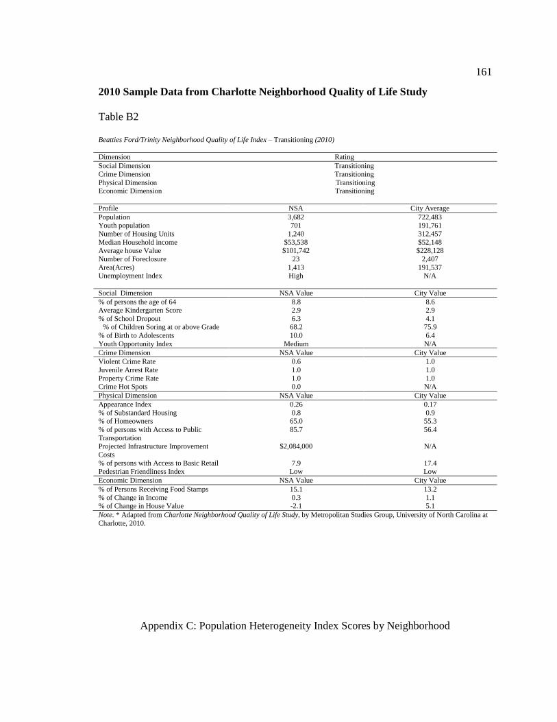
161

2010 Sample Data from Charlotte Neighborhood Quality of Life Study

Table B2

Beatties Ford/Trinity Neighborhood Quality of Life Index – Transitioning (2010)

Dimension Rating

Social Dimension Transitioning

Crime Dimension Transitioning

Physical Dimension Transitioning Economic Dimension Transitioning

Profile NSA City Average

Population 3,682 722,483 Youth population 701 191,761

Number of Housing Units 1,240 312,457

Median Household income $53,538 $52,148 Average house Value $101,742 $228,128

Number of Foreclosure 23 2,407

Area(Acres) 1,413 191,537 Unemployment Index High N/A

Social Dimension NSA Value City Value

% of persons the age of 64 8.8 8.6 Average Kindergarten Score 2.9 2.9

% of School Dropout 6.3 4.1 % of Children Soring at or above Grade 68.2 75.9

% of Birth to Adolescents 10.0 6.4

Youth Opportunity Index Medium N/A

Crime Dimension NSA Value City Value

Violent Crime Rate 0.6 1.0

Juvenile Arrest Rate 1.0 1.0

Property Crime Rate 1.0 1.0 Crime Hot Spots 0.0 N/A

Physical Dimension NSA Value City Value

Appearance Index 0.26 0.17

% of Substandard Housing 0.8 0.9 % of Homeowners 65.0 55.3

% of persons with Access to Public

Transportation

85.7 56.4

Projected Infrastructure Improvement

Costs

$2,084,000 N/A

% of persons with Access to Basic Retail 7.9 17.4

Pedestrian Friendliness Index Low Low

Economic Dimension NSA Value City Value

% of Persons Receiving Food Stamps 15.1 13.2

% of Change in Income 0.3 1.1 % of Change in House Value -2.1 5.1

Note. * Adapted from Charlotte Neighborhood Quality of Life Study, by Metropolitan Studies Group, University of North Carolina at

Charlotte, 2010.

Appendix C: Population Heterogeneity Index Scores by Neighborhood

162

Population Heterogeneity Index

Population Heterogeneity

Population heterogeneity or racial diversity can be defined by the plurality of

multiple racial groups within a specific neighborhood. The U.S. Census defines eight

racial and ethnic groups. This study utilized the Census categories but removed one of

them – “other races” – the study calculates Population Heterogeneity Index (PHI) scores

for Charlotte neighborhoods based on the shares of seven racial categories. The

categories used for this research include:

• White

• Black or African American

• Hispanic or Latino

• American Indian and Alaska native

• Asian

• Native Hawaiian and Other Pacific Islander

• Two or more races