INFORMATION TO USERS

This manuscript has been reproduced from the microfilm master. UMI

films the text directly from the original or copy submitted. Thus, some

thesis and dissertation copies are in typewriter face, while others may

be from any type of computer printer.

The quality of this reproduction is dependent upon the quality of the

copy submitted. Broken or indistinct print, colored or poor quality

illustrations and photographs, print bleedthrough, substandard margins,

and improper alignment can adverselyaffect reproduction.

In the unlikely event that the author did not send UMI a complete

manuscript and there are missing pages, these will be noted. Also, if

unauthorized copyright material had to be removed, a note will indicate

the deletion.

Oversize materials (e.g., maps, drawings, charts) are reproduced by

sectioning the original, beginning at the upper left-hand corner and

continuing from left to right in equal sections with small overlaps. Each

original is also photographed in one exposure and is included in

reduced form at the back of the book.

Photographs included in the original manuscript have been reproduced

xerographically in this copy. Higher quality 6" x 9" black and white

photographic prints are available for any photographs or illustrations

appearing in this copy for an additional charge. Contact UMI directly

to order.

U·M·IUniversityMicrofilmsInternational

A Bell & Howeu Intorrnanon Company300 North Zeeb Road, Ann Arbor. M148106·1346USA

313/761-4700 800/521-0600

Order Number 9325051

The global real value of the US dollar, 1950-1990

Ramos, Gil Rosero, Ph.D.

University of Hawaii, 1993

Copyright @1993 by Ramos, Gil Rosero. All rights reserved.

V·M·I300N. ZeebRd.AnnArbor, MI48106

THE GLOBAL REAL VALUE OF THE US DOLLAR

1950-1990

A DISSERTATION SUBMITTED TO THE GRADUATE DIVISION OF THEUNIVERSITY OF HAWAII IN PARTIAL FULFILLMENT OF THE

REQUIREMENTS FOR THE DEGREE OF

DOCTOR OF PHILOSOPHY

IN

ECONOMICS

MAY 1993

BY

Gil Rosero Ramos

Dissertation Committee

Burnham Campbell, ChairmanSeiji Naya

Marcellus SnowJames Marsh

Bruce Koppel

@Copyright 1993

by

Gil Rosero Ramos

iii

To Donna, my wife

and to my daughters -­Hanalei, Kylene, and Lianne

iv

v

ABSTRACT

Tracking the US dollar's real value remains important

because of its continuing role as the de facto world

currency. However, existing indices of the dollar do not

have the global scope that befits its international

currency status. with their narrow currency inclusion,

their use of trade weights, and their neglect of a weight

for the US dollar's host economy, existing dollar indices

do not reflect the full range of demand and supply factors

that impact on the doll ar' s global real val ue. To get a

fuller coverage of these factors and to better understand

the relation between changes in the theoretical

determinants of the dollar's value and the actual outcomes,

a new dollar index is developed -- the GR119 index.

GDP-based weights for 119 countries including the host

US economy are used in the GR index implementation. This

wide-currency trait of the index facilitates the

computation of s ub r Lndi.o es that detail region-wide and

country-specific contributions to the GR index value. The

use of period-specific moving weights allows the

decomposition of the sources of change in the GR119 index,

both in terms of factor components (relative price and non-

vi

relative price factors) and key regions, which is not

possibl e with other indices. This decomposition together

with the regional dimensions of the GRl19 index provides a

comprehensi ve measure of the doll ar' s real val ue that is

truly global in scope.

The GRl19 index and its decomposition results, show

that Purchasing Power Parity (PPP) factors do not control

the dollar's real value in either the fixed or the flexible

exchange periods. Non-PPP factors, 1ike reI ative income

growth, capi tal flows, and institutional shi fts are al so

important. The GR regional indices confirm the

significance of the Europe-Canada-Japan area in determining

the dollar's global val ue. But they also point out that

traditional dollar indices leave out significant

information by neglecting other important regions.

Country-level analysis of the GR indices also reveals the

'misal ignment' of currencies and the tendency of some

developing areas to indulge in extreme competitive

depreciation which adds to the real value of the us dollar.

vii

TABLE OF CONTENTS

Abst ract . . . . . . . . . . . . . . . . . . . . . . . . . . . . . . . . . . . . . . . . . . . . .. v

List of Tabl es. . . . . . . . . . . . . . . . . . . . . . . . . . . . . . . . . . . . . . .. i x

List of Figures....................................... xi i

List of Supplemental Tables xiv

Chapter 1: Introduction 1

Purpose of study 1The Importance of the US Dollar's Real Value 4

Chapter 2: Review of US Real Exchange Rate Indices 10

Purpose of Global Real Dollar Indices •••••...•..••• 10 ,Methods of Dollar Real Index Construction 12A Critique of Existing Dollar Real Indices 21Building a New Dollar Real Index 41

Chapter 3: The GDP-Weighted Real Indices 44

Why Use GDP Weights 44Index Implementation............................... 54Benchmark Comparisons.............................. 61The GR119 and its Regional Indices 87

Chapter 4: A Methodology for Explaining Factor-SpecificChanges in the Dollar's Real Value .... 122

The Base Value Index 122The Adjustment Value Index 129The Composition or Aggregation Effect 136Component Changes in GRIBDX 142Components of the Joint Effect Residual 150Sources Of Change for the GRl19 Index 165

viii

Chapter 5: Some Applications of the New Index •....... 175

A Framework for Using the GR Index 175The Fixed Exchange Period 185The Floating Rate Period 201Caveat Inquisitor 212

Chapter 6 : Summary and Conclusions 214

Summary 214An Agenda for Research 219

Appendix: Supplemental Tables 223

References 288

ix

LIST OF TABLES

Table

1.

2.

3.

4.

5.

6.

7 .

8.

9.

10.

11.

12.

Comparative Summary of Real Dollar Indices 23

Real Indices of the Dollar, ComparedSelected Quarterly Periods 27

Comparative Correlation, Quarterly DataUS Real Indices, 1971 - 1986 30

Belongia J-Test Results for Import Equations 33

out-of-Sample Forecast Statistics 37

Multilateral and Bilateral Weightsfor Major World Areas 39

Comparative Weights for the G-I0 CountriesTrade, Capital, and GDP flows 47

US Share of GWP and Relative Output Growthwith the US leading the Cycle 52

SDR, FRBRD, 7-Gr, RXI0l, and GRl19 IndexesAnnual 1971-1988, Base: 1973 63

The GR Indices and Benchmarks in Selected YearsLevels and Percent Changes 65

Comparative Correlation, GRl19 vis BenchmarkIndices, Levels and Percent Change 1971-1990 67

GR Indices Peak to Peak Recovery Ratios,1969 - 1985 71

13. GR Indices Trough to Trough Recovery Ratios,1978 - 1988 71

14. Trend Comparisons for the GR , FRBRD, and 7-GRIndices 1960 - 1990 72

15. Comparative Correlations, GR5, GR12, and GR38vis GRl19, Levels 77

xLIST OF TABLES(cont.)

Table

16. GRl19 and RX-101 with Sub-indices:Bel ected Years 80

17. Comparative Correlation of GR Indiceswith Benchmark Indices 83

18A. GR Index Value Effect By RegionTrough of 1969-1971 102

18B. GR Index Value Effect By RegionTrough of 1978-1980 Base:1973 103

18C. GR Index Value Effect By RegionPeak of 1984-1986, Base:1973 104

19. Contribution to the GR Index Value By AreaPeak of 1969-1971, Base: 1973 106

20. Contribution to the GR Index Value By AreaTrough of 1978-80, Base: 1973 110

21. Contribution to the GR Index Value By AreaPeak of 1984-86, Base: 1973 114

22. The GRl19 with its Base and Adjustment Values1950 - 1990 132

23. GR119, GRINDX, and GResid 1950-1990 138

24. Main Components of the Change in GRl19from Base Year Values (GRdelta) 1950-1990 146

25. Components of Delta4, 1950-1990 148

26. Components of Xresid - First Method1950-1990 153

27. Effects of Weighted Relative Prices, WeightedNominal Rates, and Residuals - Decomposed

1950-1990 157

xiLIST OF TABLES(cont.)

Table

28. GRdelta Decomposition Second Method1950-1990 161

29. Components of Xresid - Second Method1950-1990 163

30. Correlation Analysis: GRADJ & TBAL 187

xii

LIST OF FIGURES

Figure

1. US and ROW Share of Gross World Product 7

2. Exports as Percent of GDP, Compared 8

3. GRl19, FRBRD, and 7-Gr, Compared 68

4. GRl19, GR38, GR12, and GR5, ComparedFixed and Floating Period 74

5. GRl19, GR38, GR12, and GR5, ComparedFixed Period 75

6. GRl19, GR38, GR12, GR5, ComparedFloating Period II ••••••••••••••••• 76

Growth Rates

GRl19 versus

GR119 versus

GR119 versus

GR119 versus

GRl19 versus

GRl19 versus

GRl19 versus

GR119 versus15. Africa 98

16. GRl19 and GRl18 Compared, Fixedand Floating Periods 105

17. GRl19, its GRBase, and GRadj Components 134

xiii

LIST OF FIGURES(cont.)

Figure

18. Changes in the Composition Effect 166

19. Weight Share and Composition Effects 170

20. Component Changes, First Method 172

21. Component Effects, Second Method 173

22. Weighted Relative Price and Nominal Rates 186

23. Real Growth Differentials, US vIs Japan 195

24. Aggregated Growth Rates, US and ROW 195

25. World Exports as a Percent of GWP 196

26. US and ROW Inflation Compared 198

27. US Exports as Percent of ROW Imports 205

28. Trade Balance and the Adjustment Value 206

29. Real Interest Rates Compared 207

30. Real Interest Differentials, USvIs Japan and Germany 207

31. Capital & Current Account, 1955-1990 209

xiv

LIST OF SUPPLEMENTAL TABLES

Table

1.0

2.1

2.2

US and ROW Share of Gross World Product(in billions of US dollars) 223

Exports and Imports as a Percent of GOPUS, Germany, and Japan, 1950-1990 225

World Trade Growth in Billions of Current Dollars1950-1990 227

3.1 GRl19 and Narrow Currency GR Indices, Base: 1973 ... 229

3.2A GRl19 Sub-indices, 1950-1990, Base: 1973 231

3.2B GRl19 Sub-indices, 1950-1990, Base: 1973 233

3.3A Index Value Effect By Region and CountryPeak of 1969-1971, Base:1973 235

3.3B Index Value Effect By Region and CountryTrough of 1978-1980, Base:1973 239

3.3C Index Value Effect By Region and CountryPeak of 1984-1986, Base:1973 243

3.4A Trade Shares in billions of current Dollars1950-1990 247

3.4B Trade Shares as Percent of World Trade1950-1990 249

3.5 G-5 and G-10 Share of Gross World Productin billions of current US dollars 250

3.6 FRBRD and 7-Gr Index compared to GRl19 1960-1988 ... 251

4.1 Exchange Rates, Relative Prices, and Gross ProductShare with Changes from Base Period Levels ..... 252

4.2 Basegr2 and Nomgr2 and GResid as Percentof GRdelta 1950-1990 254

xv

LIST OF SUPPLEMENTAL TABLES(cont.)

Table

4.3

4.4

4.5

4.6

4.7

5.1

5.2

5.3

5.4

5.5

Delta4, Xresid, and GResid as Percentof GRdelta 1950-1990 ......•................ 256

Bresid, Nresid, and INDresid as Percentof GRdelta 1950-1990 258

Rdelta, Adelta, RWdelta, and AWdelta as Percentof GRdelta, 1950-1990 260

RAchng and Wchng as Percent of GRdeltaRAchng 1950-1990 •......................... 262

RAresid, Wresid, and WRAjoin as Percentof GRdelta 1950-1990 ....................•.. 264

Real Growth of USGNP, USGDP, ROWGDP, GWP,and USSHR 1950 - 1990 •••................... 266

Comparative Growth Rates of the G-5 Countries(based on constant local currency units) 268

How Real Interest Rates were derived 270

US Exports, Imports, and the US Trade Balance( in mi11ions) 271

Diminishing share of US exports in totalROW imports, 1948 to 1990 .•................... 273

5.6 Correlation Analysis for: TBAL GRADJ1950-1990 275

5.7 ROW Average Nominal Rates, Relative Prices,and the US Trade Balance, 1950-1990 276

5.8 US and ROW Consumer Price Index andInflation Rates, 1950 - 1971 278

Table

5.9

xvi

LIST OF SUPPLEMENTAL TABLES(cont.)

US, Germany, and Japanese Real Interest Rates1956 - 1971 280

5.10 The US Balance of Payments in Billions1955 - 1990 282

5.11 Components of the US Capital Account in Billions1953 - 1990 284

5.12 Reserves and Related Transactions 286

1

Chapter 1

INTRODUCTION

Purpose of study

This study is an attempt to better understand the

relation between changes in the theoretical determinants of

the dollar's value and the actual outcomes. To do this, a

new index is developed which is presented on a priori

grounds as a 'better' index than existing dollar indices.

Aside from its use of a different weighting scheme, the new

index allows decomposition of its value, both in terms of

components and key regions. The new index is then used to

discuss and explain the evolution of the dollar's real

value in the post-war years. Tracking the us dollar's real

value is important because of its continuing role as the de

facto world currency.

The study critiques existing real dollar indices in

terms of their ability to reflect the full range of demand

and supply factors that impact on the global dollar's real

value. The dearth of dollar indices for the fixed exchange

period is noted and the varying indications of real value

in existing indices are linked to the different methods

used in index construction. The argument is then made that

2

the existing dollar indices fall short of the study's

requirement and a new index is constructed.

A principal divergence between the existing real

indices and the new index is in the latter's use of GDP­

based weights as opposed to the usual trade weights. It is

contended that GDP weights account for the effects of both

trade and capital flows on the dollar's value. The

relationship between income and trade flows is amply

documented and needs little elaboration. In the case of

capital flows, the assumption is that such flows are

positively related to wealth and GDP is essentially the

return on wealth.

Another difference is in the use of period-specific

moving weights as opposed to a fixed weight or a moving

average weight. Fixed weights assume that the period on

which such weights are based is representative of the whole

time span for which the index is being constructed. A

moving average weight presumes to capture the impact of

insti tutional or systemic shifts in the economic context

underlying the index. The introduction of period-specific

weights, while also accounting for shifts in the world

economy, allows changes in the weight itself to impact

directly on the resulting index value.

Unlike the existing indices, changes in this index

value can therefore be directly linked to changes in the

3

component variables used in its construction on a period-

specific basis. This quality allows for a more complete

decomposition of sources of change in the index value than

is possible in other indices. By taking a point in time as

a base, the resulting index value can also be separated

into base and adjustment components that help us link the

dollar's real value to capital flows.

Aside from being a broad based index in terms of the

measure of commerce used, the new index is also a wide

currency index that lends itself easily to computation of

regional sub-indices. Such sub-indices are constructed to

give a disaggregated view of movements in the dollar's.

value in different parts of the world and are compared to

similar sub-indices constructed by the Federal Reserve Bank

of Dallas.

The new index, through its base and adjustment value

components as well as its regional sub-indices, is then

used to illuminate and organize the discussion of world

economic events. New insights derived from the exercise of

tracking the dollar's real value in this manner can be

used to inform relevant economic policy. A research agenda

as suggested by this study's findings is also outlined in

the concluding portion of the paper.

4

The Importance of the us Dollar's Real Value

The importance of the dollar's real value derives from

the fact that the dollar is the world's de facto currency.

When the dollar's gold window was closed in 1971 and the

world shifted from a fixed to a floating rate system, the

dollar's dominance in international transactions was

expected to diminish significantly. However, up to the

present time, the dollar continues in its hegemonial role

even without a definition of its value in gold. The

continuation of its accustomed usage as the principal world

currency despi te an exchange regime change, signal s that

international users of the dollar see an intrinsic value in

it that was masked in the past by the fiction of gold

exchange.

The experience of the US dollar after the regime change

of 1971 contrasted with that of the British pound. Use of

the pound as an international currency waned after the

regime change of 1945, while the us dollar's record of

international usage did not significantly diminish but was

even fortified after the regime change of 1971. An

inference that could be made here is that dollar to gold

convertibility was only one among many factors that

provided the validating context of the Bretton Woods system

which formally started in 1945. After dollar to gold

5

convertibility was dropped in 1971, the remaining

conditions proved sufficient to support the dollar in its

continued role as the de facto world currency. Among these

remaining conditions are certain special traits of the us

economy and polity which validate the us role as the ideal

host of the world's international currency.

In theory, a national money used as the international

currency must be stabl e compared to other currencies and

must be expected to remain stable in the future. A

necessary condition for stability is a stable monetary and

economic policy in a stable political environment. Aside

from this internal stability, a country whose currency is

used as an international reserve medium also has to be

relatively immune to world market instabilities. These

qualities of internal and external stability are important

because they give assurance that, whatever happens in the

Rest of the World (ROW), the real value of such a currency

will remain secure and relatively stable. This is in fact

a main component of safe haven theories of the us doll ar

valuation.

The economic dimension of a country's being relatively

immune to world market instabilities operationally means

that its economy must constitute a large part of the world

economy. In effect, an international currency's horne

economy constitutes the basis for its domestic real value

6

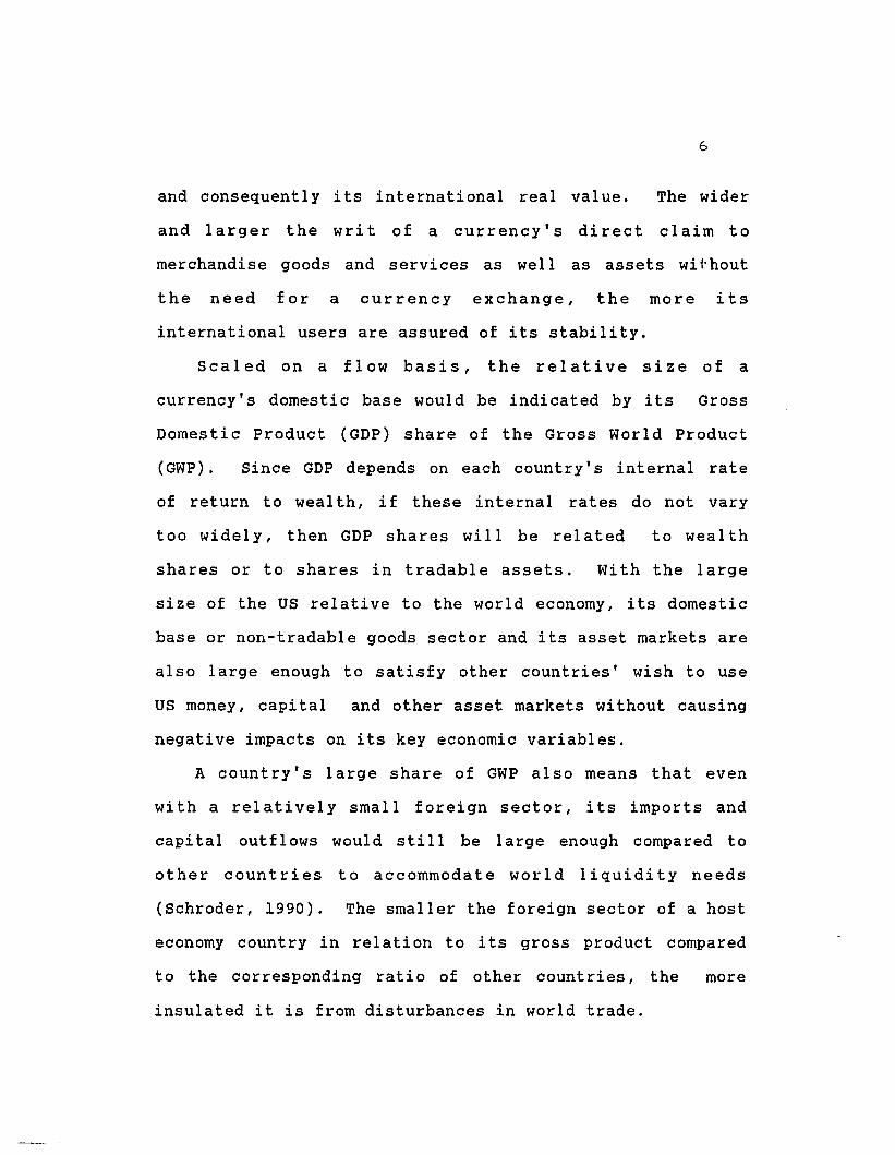
and consequently its international real value. The wider

and larger the writ of a currency's direct claim to

merchandise goods and services as well as assets wi rhout

the need for a currency exchange, the more its

international users are assured of its stability.

Scaled on a flow basis, the relative size of a

currency's domestic base would be indicated by its Gross

Domestic Product (GDP) share of the Gross World Product

(GWP). Since GDP depends on each country's internal rate

of return to weal th, if these i.nternal rates do not vary

too widely, then GDP shares will be related to wealth

shares or to shares in tradable assets. With the large

size of the US relative to the world economy, its domestic

base or non-tradable goods sector and its asset markets are

also large enough to satisfy other countries' wish to use

US money, capital and other asset markets without causing

negative impacts on its key economic variables.

A country's large share of GWP also means that even

with a relatively small foreign sector, its imports and

capital outflows would still be large enough compared to

other countries to accommodate world liquidity needs

(Schroder, 1990). The smaller the foreign sector of a host

economy country in relation to its gross product compared

to the corresponding ratio of other countries, the more

insulated it is from disturbances in world trade.

7

*Figure 1

US a nd ROW Share of Gross World Product'950 - '990 In Pen: en!

90...-----------------------,

Bo 1-------------------------170 !------------...in-ll-lII-lHII-IHJ.U.lJ.U.lHHkJ-IJl·lI-lll-ll-ll--l

60 ROIoI

ISO I---iHHHHHHHHHjHHl-lHl-lHJ-{HJ.-I.H~U4I-IHJ..II-II-IHJ.1II·U

40

3D

20

10

o

A comparison with other countries shows that the us

remains the world's largest economy in terms of yearlY

product flows (See Figure 1). However, the US share was

more than 40 percent in 1950 compared to onlY 23 percent in

1990. Trends in the size of the US share of GWP are

important because this ratio gives an indication of the

ability of the US economy to redeem dollar units in real

terms. As the issuer of the world's currency, the US

economy is acting as a banker to the whole world and

assuring all dollar holders that their dollars can claim

* Source: For data used please refer to Appendix Table 1.

8

real goods and assets from the us economy at any time. In

fact, the desirable quality of a host economy's being large

in relation to the world economy and having a relatively

smaller share of trade in total output, assures

international dollar users that if they opt to redeem their

dollars in the form of US goods or assets, the price impact

of their added demand in the domestic us market will be

relatively negligible.

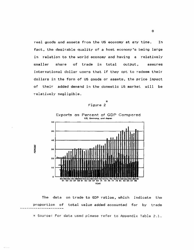
*Figure 2

Exports as Percent of GDP Comparedus, Dermany, end Japen

60,-----------------------,

DO 1------------------r~H_:___I_iI__-l

...0 1--------------.....+I-+l-H-++....I+Io-foiI--4

30 1------r1I-riI+~~I_H+I+I_H+++I-....H-++....t+H-II--4

J101---..........

o

The data on trade to GOP ratios, which indicate the

proportion of total value added accounted for by trade

* Source: For data used please refer to Appendix Table 2.1.

9

flows, show that, compared to the immediate postwar period,

trade in the US economy is now much more important than it

was. This information suggests that conditions supporting

the us dollar as an international currency have

deteriorated. The United states and the dollar are now

more vulnerable to economic disturbances in wor.ld markets.

The relative international independence of the us

economy compared to the host economies of competing

currencies like the Yen and the Deutschemark suggests that

these currencies are now poised to challenge the dollar's

world role. For the very first time, in 1988, Japan had a

lower trade to GDP ratio than the us (See Figure 2).

However, in 1989 and 1990, the us had a trade to GDP ratio

that slightly edged out that of Japan. As more and more

countries use the Yen and the Deutschemark to suppl ement

their international reserves, the us can only sustain the

dollar's international role in the context of sound fiscal

and monetary restraints.

10

Chapter 2

A REVIEW OF US REAL EXCHANGE RATE INDICES

Purpose of Global Real Dollar Indices

An international exchange rate index summarizes

information contained in the many bilateral exchange rates

that apply to a particular currency in order to gauge the

average value of that currency against others. There would

be no need for such an index if some single natural measure

of the doll ar' s real val ue existed. But instead of that

single value, what exist are a series of cross-rates

between the dollar and every other currency in the world.

Individual pair-wise exchange rates with the dollar

move in divergent directions and in different magnitudes.

A striking example here are the recent currency movements

between the Yen and the us dollar opposed to movements

between the currencies of the newly industrializing

countries ( NIC's ) and the us dollar. While the Yen has

shown dramatic gains against the us dollar, the NIC's and

Asia - particularly China - show strong gains for the

dollar as they pursue different degrees of competitive

depreciation. Thus, pair-wise rates do not give a uniform

indication of magnitude changes in the dollar's value and

may even go in conflicting directions. An index which

combines changes in these cross-rates into a single number

11

indicating trends in the dollar's global value becomes

necessary (Rosensweig, 1987).

Real exchange rate indices are in fact nominal exchange

rate indices deflated by indicators of relative prices. A

nominal index is a weighted summary of actually observed

cross-rates for the currencies included in the index. When

the impact of inflation differentials between countries is

purged out of a nominal index, the pure or real exchange

rate movement is isolated and identified and we get a real

index. Such an index should adequately measure the 'real

effects' of exchange rate changes on real phenomena and

vice-versa (Maciejewski, 1984).

Aside from indicating the 'real' appreciation or

depreciation of a given currency, real exchange rate

indi ces are al so regarded as appropri ate indi cators of

equilibrium exchange rates or of a country's international

competitiveness. Real exchange rate indices are also used

to measure the over or under val uation of a currency and

its expected future movements. They can also be used to

assess international monetary condi tions and tell holders

of a particular currency allover the world what is

happening to the value of their asset.

12

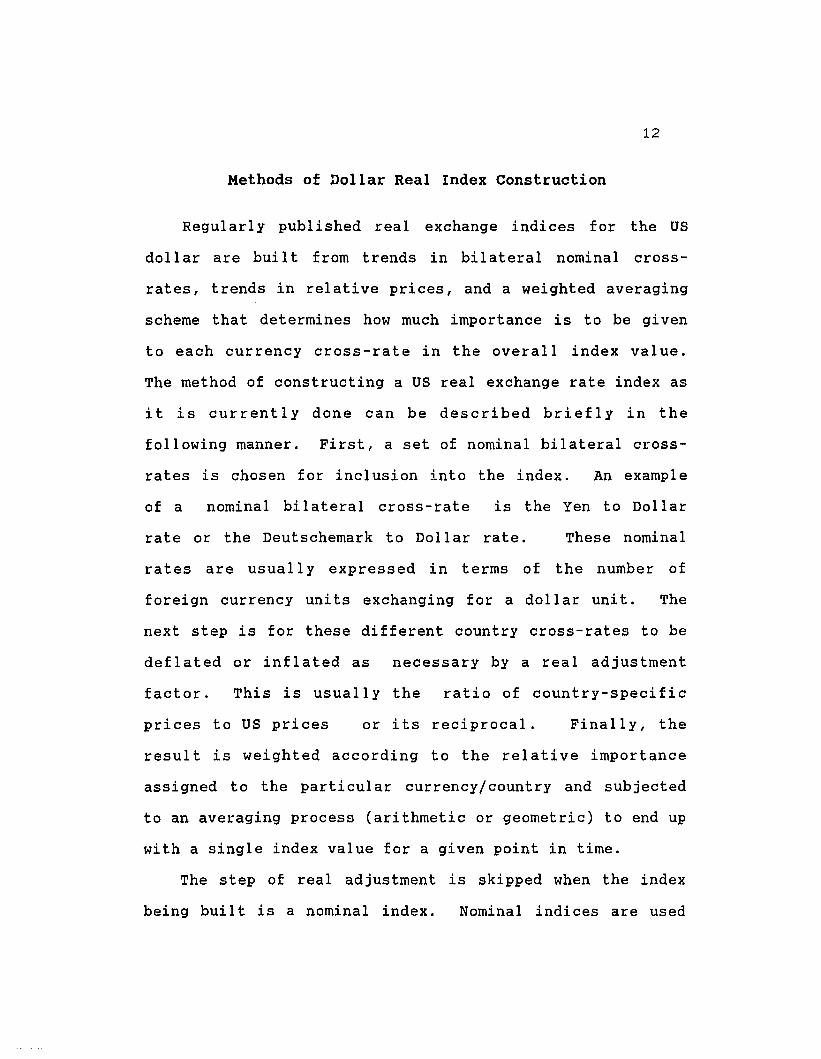
Methods of Dollar Real Index Construction

Regularly published real exchange indices for the us

doll ar are bui I t from trends in bi I ateral nominal cross­

rates, trends in relative prices, and a weighted averaging

scheme that determines how much importance is to be given

to each currency cross-rate in the overall index value.

The method of constructing a us real exchange rate index as

it is currently done can be described briefly in the

following manner. First, a set of nominal bilateral cross­

rates is chosen for incl usion into the index. An exampl e

of a nominal bilateral cross-rate is the Yen to Dollar

rate or the Deutschemark to Doll ar rate. These nominal

rates are usually expressed in terms of the number of

foreign currency uni ts exchanging for a dollar uni t. The

next step is for these different country cross-rates to be

deflated or inflated as necessary by a real adjustment

factor. This is usually the ratio of country-specific

prices to US prices or its reciprocal. Finally, the

result is weighted according to the relative importance

assigned to the particular currency/country and subjected

to an averaging process (arithmetic or geometric) to end up

with a single index value for a given point in time.

The step of real adjustment is skipped when the index

being bui 1t is a nominal index. Nominal indices are used

13

for specific modeling procedures and are perceived as a

summary measure of currency prices as opposed to a real

index which is seen as measuring the rate of exchange

between us goods and those of other countries. Another use

for nominal indices is as a proxy for real indices to give

more current information since there usually is a lag in

the collection of the price data required for real

adjustmen.t.

At present a variety of different us real exchange rate

indices exist. Despite their common label as us dollar

indices, they give quite different indications of the

dollar's real value (Belongia, 1987). This is principally

due to the divergent methods appl ied in putting together

the same basic components.

There are 1imi ted areas of unanimity 1ike the use of

nominal rates expressed in terms of foreign currency per

dollar. These rates are an average of noonday quotes for

either monthly, quarterly, or annual periods like the RF

series found in the International Financial Statistics

(IFS) data of the International Monetary Fund (IMF). A

degree of consensus on the use of a real adjustment factor

also exists. Consumer prices are the most widely used

deflators in constructing real exchange rate indices

because they are available on a relatively consistent basis

across countries (Pauls, 1987).

14

The CPI' s incl usion of non-traded i terns I ike housing

and a wide range of services is sometimes viewed as a

weakness (Hooper & Morton, 1978). However, it is

considered qui te reI evant for questions deal ing wi th the

macroeconomic relationships of the exchange rate to broad

scale competitive factors, like the relative cost of doing

business in one economy as compared wi th another. It is

contended that general indices for these purposes, should

use either the CPI or the GNP deflator (Hervey & strauss,

1987).

Another area of common practice is in the relative

consensus on the use of trade flows as the measure of

commerce for determining index weights. But this

consensus immediatel y breaks down wi th the question of

which subset of trade flows is to be used in determining

the relative weight finally assigned to a currency in an

index. Variations in emphasis, objectives, differences in

currency sets included, and multilateral versus bilateral

weights are in fact just di fferent aspects of this basic

disagreement.

In most of the early aggregate dollar indices,

decisions for currency inclusion were influenced by a

desire to cover currencies that are traded significantly

against the us dollar in exchange markets. The host

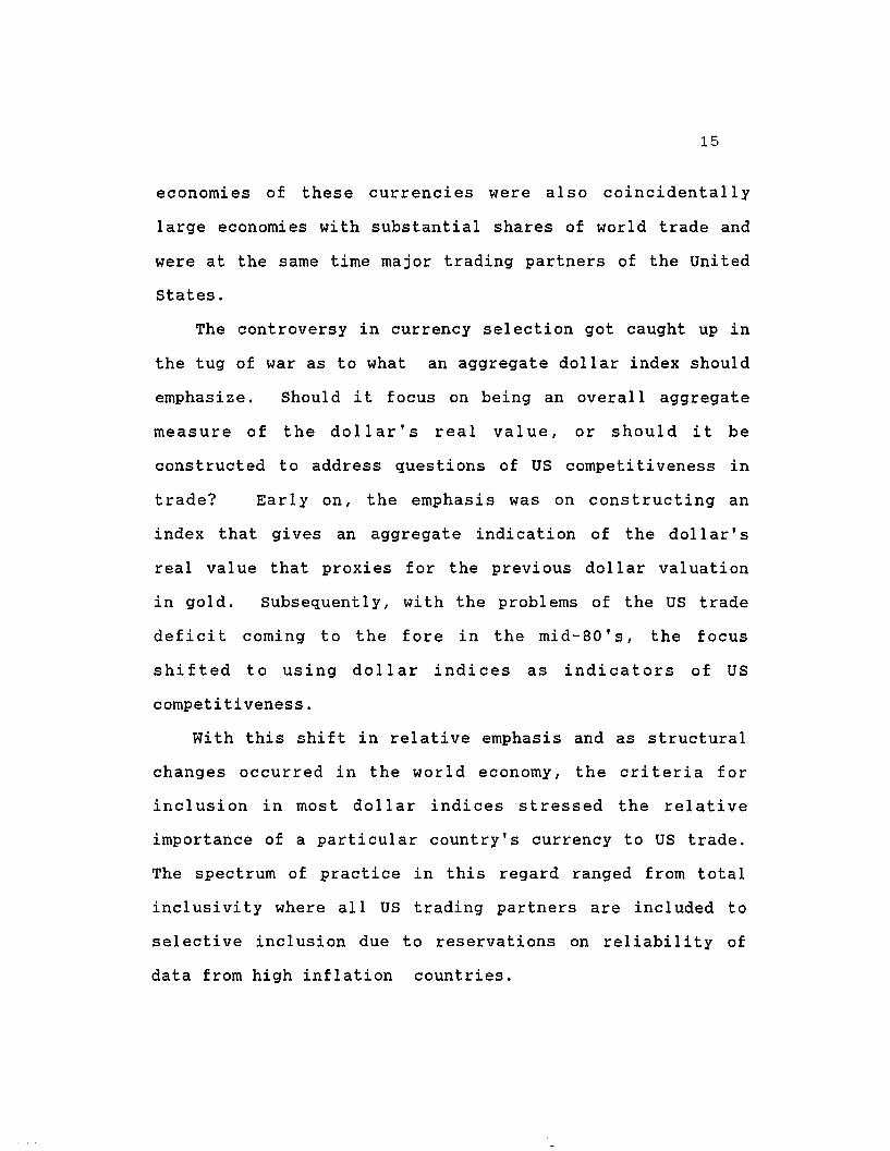
15

economies of these currencies were also coincidentally

large economies with substantial shares of world trade and

were at the same time major trading partners of the United

states.

The controversy in currency selection got caught up in

the tug of war as to what an aggregate dollar index should

emphasize. Should it focus on being an overall aggregate

measure of the dollar's real value, or should it be

constructed to address questions of US competitiveness in

trade? Early on, the emphasis was on constructing an

index that gives an aggregate indication of the dollar's

real value that proxies for the previous dollar valuation

in gold. Subsequently, with the problems of the US trade

deficit coming to the fore in the mid-80's, the focus

shifted to using dollar indices as indicators of US

competitiveness.

With this shift in relative emphasis and as structural

changes occurred in the world economy, the criteria for

inclusion in most dollar indices stressed the relative

importance of a particular country's currency to US trade.

The spectrum of practice in this regard ranged from total

inclusivity where all US trading partners are included to

selective inclusion due to reservations on reliability of

data from high inflation countries.

16

The differing objectives or emphasis in index rate

construction has led to suggestions that indices be

constructed to suit particular purposes and that decisions

regarding currency inclusion be made in accordance with

such purposes. For instance, if the problem is how to

determine the infl uence of exchange rates on world trade

and inflation, then countries with a significant share of

world trade should be part of the currency set selected for

inclusion. In studies that explain asset demands, then the

index should encompass countries whose assets are widely

traded in financial markets. There are also more specific

suggestions; if the study is about US exports of steel,

then only the currencies of countries that are large steel

producers should be included in the index (Pauls, 1987).

The quarrel on the currency set for inclusion has its

twin area of conflict in the weighting schemes which

determine the relative importance of the currencies handled

in the index. While it is common practice to use trade

flows as the measure of commerce to gauge the relative

importance of currencies in an index, variations come in

the form of the particular subset of trade flows finally

chosen as the weight-base. Should the flows just be export

flows or import flows or a combination of both? Should

these flows include a country's trade with the ROW or just

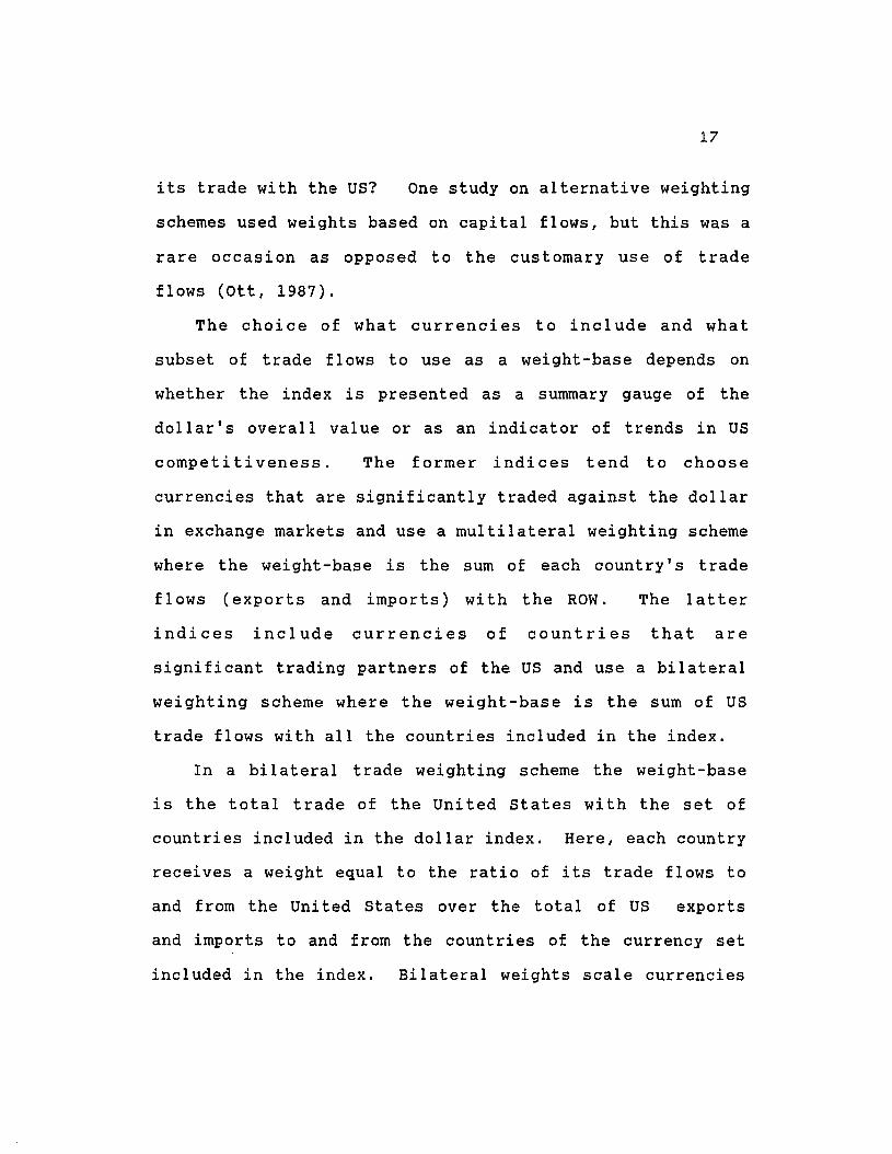
17

its trade with the US? One study on alternative weighting

schemes used weights based on capital flows, but this was a

rare occasion as opposed to the customary use of trade

flows (ott, 1987).

The choice of what currencies to include and what

subset of trade flows to use as a weight-base depends on

whether the index is presented as a summary gauge of the

dollar's overall value or as an indicator of trends in US

competitiveness. The former indices tend to choose

currencies that are significantly traded against the dollar

in exchange markets and use a multilateral weighting scheme

where the weight-base is the sum of each country's trade

flows (exports and imports) wi th the ROW. The I at ter

indices include currencies of countries that are

significant trading partners of the US and use a bilateral

weighting scheme where the weight-base is the sum of US

trade flows with all the countries included in the index.

In a bilateral trade weighting scheme the weight-base

is the total trade of the United States with the set of

countries included in the dollar index. Here, each country

receives a weight equal to the ratio of its trade flows to

and from the United States over the total of US exports

and imports to and from the countries of the currency set

included in the index. Bilateral weights scale currencies

18

on the basis of their countries' importance as individual

u.s. trading partners.

The use of bilateral schemes with a weight-base focused

on us trade is considered a way of stressing changes in the

dollar index value as a measure of US competitiveness. This

contrasts with the emphasis of multilateral weighted dollar

indices on the dollar's overall value. A bilateral

weighted index claims that the us dollar's value can best

be gauged by looking at what happens in a subset of world

trade experience that is directly related to the US. A

multilateral weighted index says that it is better to look

at a subset of world trade that is not just limited to US

trade but incl udes non-US trade as well. Given the fact

that US trade is just a subset of total world trade,

bilateral weighted indices would tend to have a smaller

weight-base compared to that of multilateral weighted

indices.

In some indices, the weights used are either fixed

weights computed as an average from a representati ve

period, or values of trade flow shares from a fixed point.

other indices use a moving average weight which usually

spans a period of three years or twel ve quarters. In an

index impl ementation wi th fixed weights, the question of

choosing the base period from which the weights are

computed is crucial. The norm is to choose a base period

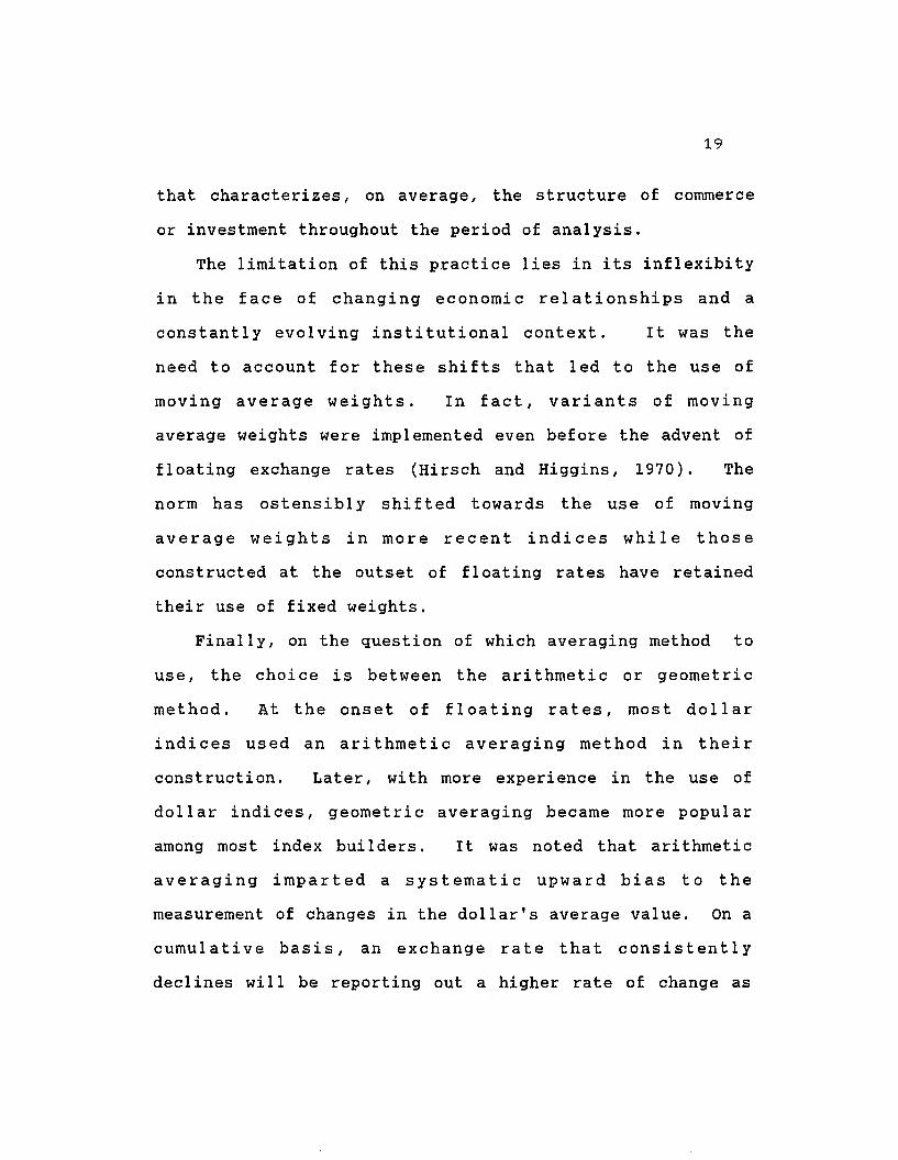
19

that characterizes, on average, the structure of commerce

or investment throughout the period of analysis.

The limitation of this practice lies in its inflexibity

in the face of changing economic relationships and a

constantly evolving institutional context. It was the

need to account for these shifts that led to the use of

moving average weights. In fact, variants of moving

average weights were implemented even before the advent of

floating exchange rates (Hirsch and Higgins, 1970). The

norm has ostensibl y shi fted towards the use of moving

average weights in more recent indices while those

constructed at the outset of floating rates have retained

their use of fixed weights.

Finally, on the question of which averaging method to

use, the choice is between the arithmetic or geometric

method. At the onset of floating rates, most dollar

indices used an arithmetic averaging method in their

construction. Later, wi th more experience in the use of

dollar indices, geometric averaging became more popular

among most index builders. It was noted that arithmetic

averaging imparted a systematic upward bias to the

measurement of changes in the dollar's average value. On a

cumulative basis, an exchange rate that consistently

declines will be reporting out a higher rate of change as

20

its base decreases while the opposite would be true for an

increasing value. 1

The different techniques of exchange rate index

construction just presented reveal a situation that easily

lends itself to anarchy in actual practice. It has been

argued that ultimately, the final arbiter in the

justification of the many choices and alternatives in index

rate construction is the purpose for which the index is

being constructed (Pauls, 1987). This is especial 1y true

in model building where the summary measure of exchange

rates for each application is made to reflect the specific

manner in which exchange rates influence the variable of

interest or vice-versa.

The use of different methods in constructing a real

index for the dollar can, however, be carried too far. For

instance, there is some consensus that what happens to the

1. If for instance an exchange rate moves from 2 to 4 thenbac k to 2, an ar i thmetic approach r epor t s a 100 percentincrease followed by a 50 percent decrease. If at the sametime another exchange rate moved from 4 to 2 and then backto 4, this would be reported as a 50 percent decreasefollowed by a 100 percent increase. In both cases, the twosets of rate movements nullified each other but thearithmetic approach reports the changes inaccurately. Thegeometr ic averagi ng technique emphasizes proportional andnot absolute changes and therefore yields the samepercentage change in an index even if the base period forthe index is changed and even if the exchange rates in theindex are defined in reciprocal terms (FRS, 1978;Rosensweig, 1987).

21

dollar's value internationally is related to the trade and

capital flow balances, the us domestic price level, asset

demands and monetary condi tions, and the real val ue of

wealth of US residents (Hooper & Morton, 1978; Pauls,

1987). If different US dollar indices were to be

constructed to suit each target variable in the set just

mentioned, then the discussion of how the whole set relates

to one another in a macroeconomic sense wi 11 be

disjointed with no fixed anchor in a common index of

the dollar's value.

A Critique of Existing Dollar Real Indices

One of the very first ways of valuing the dollar right

after the onset of floating rates was through the SDR.

Before 1971 there was a one to one correspondence between

an SDR and a US Dollar unit. After 1971, the SDR was

valued in terms of the cross-rates of a basket of 16

currencies. At present, an SDR unit is valued only in

terms of the G-5 basket of currencies. Forty two percent

of the SDR's value is determined by the US dollar and the

other 58 percent val uation comes from the other four G-5

countries. These countries are Germany, Japan, Bri tain,

and France. The SDR index incorporates a magnitude

indicator for the US itself since more than 40 percent of

the SDR's value is based on a 1 to 1 exchange with the

22

dollar. 2 Such a weight for the US economy is conspicuously

absent in later indices of the dollar's international real

value.

Wi th a US weight in the SDR-based doll ar index, it

explicitly states that a measure of US aggregate economic

activity together with what happens in significant parts of

the world impacts on the global real value of the dollar.

The SDR valuation based its weights on multilateral exports

plus imports of the G-S countries fixed at 1980-1984

levels. The unique process of SDR valuation which was

originally intended as an alternate to US dollar valuation

in gold gives an index value of the dollar that is

identical in terms of purpose to the dollar index that

woul d be most sui ted to the objecti ves of this study.

Thus, the SDR valuation provides a benchmark to launch our

probe into the other real indices of the US dollar. Table

3 shows the existing major indices of the dollar's real

value and how these indices differ from one another.

2. An index of the dollar's value wi th a 1973 base yearsimilar to the other indices was de r Lve.d by dividing theSDR to US dollar exchange rate for all years from 1971onwards with the 1973 exchange rate. Source: InternationalMonetary Fund - International Financial Statistics tape.

23

Table 1

Comparative Summary of Real Dollar Indices

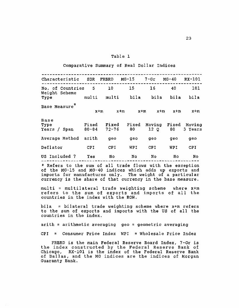
Characteristic SDR FRBRD MG-15 7-Gr MG-40 RX-101------------------------------------------------------------No. of Countries 5 10 15 16 40 101Weight SchemeType multi multi bila bila bila bila

Base Measure*x+m x+m x+m x+m x+m x+m

BaseType Fixed Fixed Fixed Moving Fixed MovingYears / Span 80-84 72-76 80 12 Q 80 3 Years

Average Method arith geo geo geo geo geo

Deflator CPI CPI WPI CPI WPI CPI

US Included ? Yes No No No No No

* Refers to the sum of all trade flows with the exceptionof the MG-15 and MG-40 indices which adds up exports andimports for manufactures only. The weight of a particularcurrency is the share of that currency in the base measure.

multi = multilateral trade weighting scheme where x+mrefers to the sum of exports and imports of all thecountries in the index with the ROW.

bila = bilateral trade weighting scheme where x+m refersto the sum of exports and imports with the US of all thecountries in the index.

arith = arithmetic averaging geo = geometric averaging

CPI = Consumer Price Index WPI = Wholesale Price Index

FRBRD is the main Federal Reserve Board Index, 7-Gr isthe index constructed by the Federal Reserve Bank ofChicago, RX-101 is the index of the Federal Reserve Bankof Dallas, and the MG indices are the indices of MorganGuaranty Bank.

24

Whi I e both the FRBRD and the SDR doll ar val ue on one

end and the Morgan indices on the other measure trends in

the dollar's real value, they emphasize different aspects

of that measure. This di fference ref I ects the dichotomy

between the national and the international roles of the us

dollar. The Morgan indices decidedly take a more us

oriented viewpoint in emphasizing a manufacturing measure

of US trade competitiveness, while the FRBRD and the SDR

indices take a broader approach in presenting index values

that are more consistent with the us dollar's international

currency role.

The FRBRD, SDR, and the Morgan Guaranty indices were

later followed by other aggregate measures of the dollar's

value including those of the IMF, the Treasury, the DECD,

and several indices from the regional Federal Reserve

Banks. Many of these new indices emerged in the second

half of the 80's as a reaction to the persistence of US

trade and current account deficits even with the dramatic

decline of the dollar's international real value. At this

time, the FRBRD index carne under heavy attack, being

characterized as dated in terms of its fixed weights, and

too narrow to reflect the movement of the dollar

accurately. In response to this perception, new and

more inclusive aggregate exchange rate measures were

developed. These' broader' indices were presented as

25

bet ter measures of the doll ar' s international real val ue

and could presumably offer a better explanation of us trade

flows.

Because they were mostly reactions to the existing

si tuati on in 1985, mos t of the indi ces deve loped were

oriented towards measuring the degree of us

competitiveness. Thus, they were mostly bilateral

weighted indices tracking the interaction between the us

and its trading partners. Only one of the indices which

emerged at that time, the Federal Reserve Bank of Atlanta

index, was multilaterally weighted. The IMF measure

which is also a multilateral index was developed much

earlier than 1985. However, these two indices are

impl emented onl y for nominal val ues and are therefore

excl uded from full consideration in this study. Two of

the indices constructed after 1985 were real dollar

indices: the 7-Gr index of the Federal Reserve Bank of

Chicago and the RX-101 index of the Federal Reserve Bank of

Dallas.

The RX-101 has the same focus on US competitiveness as

the Morgan indices. Wi th a country base covering 101

countries, it has the greatest number of currencies

included among regularly published indices. Unlike the

FRBRD, the RX-101 does not have fixed weights and instead

uses a three year moving average of bilateral trade

26

weights that changes annually for the computation of its

index. The countries included in the RX-101 start with the

10 countries in the FRBRD index and add 91 other countries

constituting a 97 percent coverage of total US trade in

1985. Among the indices being reviewed, only the RX-101

has implemented sub- indices for the different regions of

the world. In the construction of the (RX-101) Federal

Reserve Bank of Dallas index, there was an explicitly

stated purpose of shifting the emphasis of measurement to

the degree of US competitiveness in trade (Cox, 1987).

The 7-Gr index has the same stress on competitiveness

as the Morgan indices and the RX-101. There are 16

currencies covered in the 7-Gr and unlike the MG-15, it

includes representation from the Asian NIC's. The weight­

base used is the sum of US exports and imports for the 16

countries in the index. This makes its weight-kL~e bigger

than the MG-15 index. Compared with the MG-40 which

contains more currencies, the 7-Gr ends up with a much

larger weight-base since it accounts for total US trade

while the MG-40 only includes trade in manufactures. The

16 currency inclusion of the 7-Gr covered 71 percent of

total US trade in 1985. Using moving average weights like

the RX-101, the 7-Gr uses a 12-quarter span in its

implementation.

27

Table 2

Real Indices of the Dollar, Co~ared

Selected Quarterly Periods

------------------------------------------------------------Index 1980,Q3 1985,Q1 1986,Q4 1980-85 1985-86

%change %change------------------------------------------------------------

FRBRD 78.97 137.74 94.40 55.6 -37.8

MG-15 92.00 136.98 103.21 39.8 -28.3

7-Gr 86.57 120.08 94.60 32.7 -23.8

MG-40 90.34 133.02 107.22 38.7 -21. 6

RX-101 84.30 120.60 104.50 35.8 -14.3

SDR 87.18 118.98 95.41 31.1 -22.1

* With the exception of the SDR index values , datacame from a study made by the Federal Reserve Bank ofChicago on different indices of the dollar's value (Herveyand Strauss, 1987). The SDR index val ues were deri veddirectly from the IFS - IMF tapes.

FRBRDMG-157-GrMG-40RX-101SDR

- Federal Reserve Board Real Index- Morgan 15 country real index- Federal Reserve Bank of Chicago real index- Morgan 40 country real index- Federal Reserve Bank of Dallas index- Special Drawing Rights index

28

Many studies have already been conducted which compared

existing real indices of the dollar. Table 2 shows the

actual values of the real indices we have discussed for

selected years. Comparisons also have been made based on

correlations of levels as well as percent changes (Federal

Reserve Bank of Chicago in 1987). Some of the correlation

results relevant to our study are reproduced in Table 3.

The comparisons made by the Federal Reserve Bank of

Chicago did not include the SDR index which we introduced

in Table 2. When the 1980/Q3 values of the SDR are

compared with the corresponding values of the other real

indices, the Morgan index values are much higher than the

SDR value while the other real indices are lower. As noted

earlier, the SDR index differs from the other indices which

were compared by Hervey and Strauss because the SDR

includes a weight for the US not present in the other

indices. With a common base year in 1973 which was higher

than the dollar's all time low in 1978-1979/ the inclusion

of the US weight made the SDR index higher in the trough

years and lower during peak periods. The constant value of

one weighted by a measure of economic activity for the US

economy had this effect for the SDR index particularly in

troughs that were lower than one and peaks that were higher

than one. This pattern is evident when the SDR is compared

29

to the FRBRD, the 7-Gr, and the RX-101 but this was not

true in comparisons with the Morgan indices.

From 1980 to 1985, the SDR showed the lowest increment

as expected since it was moving from a higher trough to a

lower peak. The FRBRD' s increase for this period was

notably the highest compared to the other real indices.

For the 1985 to 1986 change, the SDR again showed much

lower val ues than the FRBRD and the 7-Gr. However, the

RX-101 index had the lowest value -- a difference in index

behavior that shows the effect of its wide currency

coverage.

The results in the Chicago study, while indeed showing

quite high correlations among the indices, also signal

important points of differences. For one, the dividing

line separating the Morgan indices from the rest is quite

noticeable. The use of the narrowest weight-base and a

different price deflator accounts for the lower correlation

of the Morgan indices wi th the others. The FRBRD, 7-Gr,

and the RX-101 have higher correlations with one another in

both levels and percent changes than with the Morgan

indices. The differences in indications are more

noticeabl e in the percent change correl ations. These

differences may be reflecting the sectoral focus on

manufacturing of the Morgan indices compared to the more

general orientation of the others.

30

Table 3

Comparative Correlation, Quarterly DataUS Real Indices, 1971 - 1986

Levels

FRBRD MG-15 7-Gr MG-40 RX-101

FRBRD

MG-15 0.9440

7-Gr 0.9851 0.9117

MG-40 0.9398 0.9906 0.9112

RX-101 0.9567 0.8844 0.9656 0.9129

% Change

FRBRD MG-15 7-Gr MG-40 RX-101

FRBRD 0.8910 0.9560 0.8513 0.9060

MG-15 0.9112 0.9849 0.8588

7-Gr 0.8829 0.9488

MG-40 0.8633

RX-101 -----

Source: (Hervey and Strauss, 1987)

Along with the Morgan indices the RX-I01 index with its

wide-currency inclusion also is shown by the correlation

results to be relatively different. The FRBRD and the 7-

31

Gr which have a narrow currency base tended to correlate

bet ter wi th one another than wi th the RX-IOl index. The

Morgan indices have the narrowest weight-base, while the

RX-IOl has the widest currency inclusion among all the

indices.

A distinction must now be made between a broad-based

index and a wide-currency index. In this study we will

refer to a broad-based or narrow-based index in relation to

the scale of the economic activity measure used in its

weight-base, and to a wide-currency or narrow-currency

index according to the number of currency cross-rates being

summarized into the index. Thus the FRBRD index wi 11 be

described in this context as a broad-based but narrow­

currency index while the RX-IOl in comparison to the FRBRD

will be called a wide-currency but a narrow-based index.

The resul ts of Hervey and strauss can therefore be

interpreted in relation to the differences in size of

weight-base and the breadth of currency inclusion found in

the real indices being compared. It appears that the

similarity in weight-base between the 7-Gr and the RX-IOl

has been overwhelmed by the closer similarity between the

FRBRD and the 7-Gr in terms of the currencies included in

the index. The closer similarity of the Morgan indices to

the FRBRD and 7-Gr in terms of currency inclusion was

clearly overwhelmed by the difference in weight-base used.

32

The MG-1S consistently showed the lowest correlation

with the RX-101 in both levels and growth rates since

it differed with RX-101 in both currency inclusion and size

of weight- base. Whil e the two Morgan indices correlate

well wi t h one another , they are rea 11 y a c 1ass unto

themsel ves since they correlate poorly wi th the other

indices having broader weight bases.

The narrower weight-base used by the Morgan indices may

have led to some loss of information relevant to the

dollar's valuation. This loss of information by using a

narrower weight-base finds some support in a study that

compared different indices of the dollar and the way they

perform in an empirical test (Belongia, 1987).

Belongia used a J-test to answer the question whether

an index contains more or better information compared to

another with regard to the dollar's value and trade flows.

A J-test establishes one specification as the null

hypothesis, then tests whether an alternative specification

adds to the explanatory power of the specification under

the null hypothesis (Davidson and Mackinnon, 1981).

Belongia found that whi 1e the resul ts for his exports

equations were vague, results in import equations clearly

showed that the FRBRD index adds to the information of all

the other indices.

33

Table 4

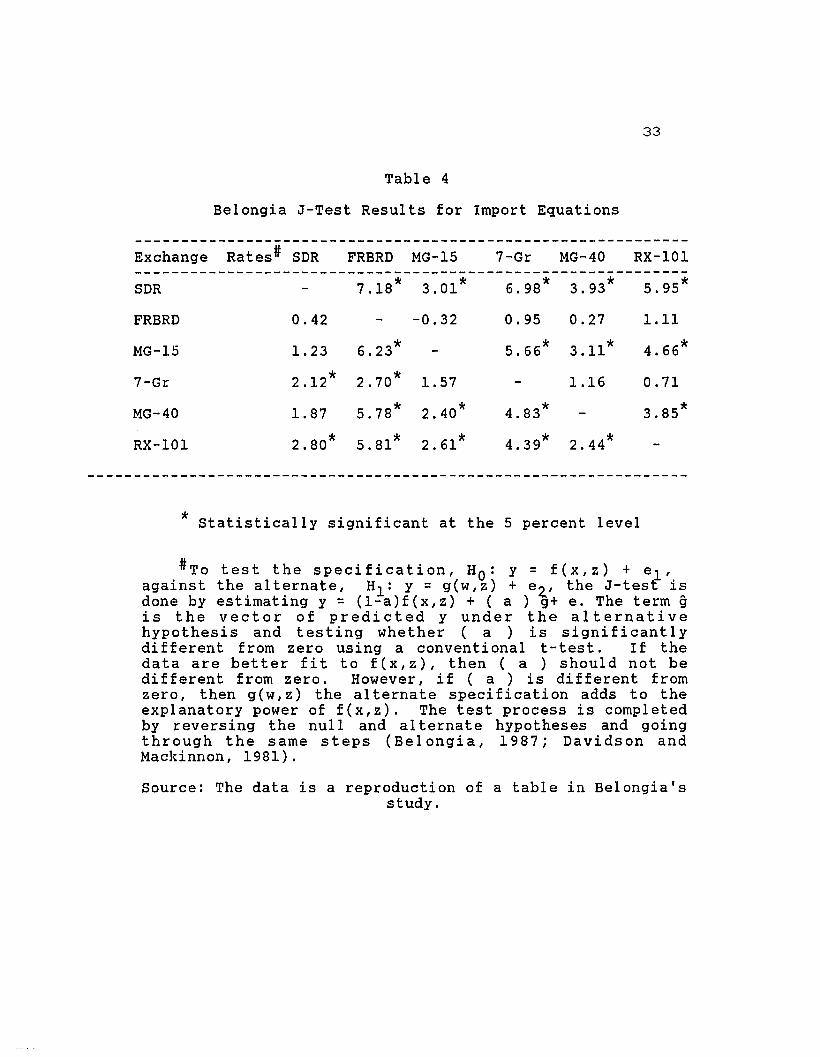
Belongia J-Test Results for Import Equations

Exchange Rates# SDR FRBRD MG-15 7-Gr MG-40 RX-101------------------------------------------------------------SDR 7.18* 3.01* 6.98* 3.93* 5.95*

FRBRD 0.42 -0.32 0.95 0.27 1.11

MG-15 1. 23 6.23* 5.66* 3.11* 4.66*

7-Gr 2.12* 2.70* 1.57 1.16 0.71

MG-40 1.87 5.78* 2.40* 4.83* 3.85*

RX-101 2.80* 5.81* 2.61* 4.39* 2.44*

* Statistically significant at the 5 percent level

#To test the specification, HO: y = f(x,z) + e1'against the alternate, H1: y = g(w,z) + e 4, the J-tesE isdone by estimating y = (l-a)f(x,z) + ( a ) g+ e. The term gis the vector of predicted y under the alternativehypothesis and testing whether ( a ) is significantlydifferent from zero using a conventional t-test. If thedata are better fit to f(x,z), then ( a ) should not bedifferent from zero. However, if ( a ) is different fromzero, then g(w,z) the alternate specification adds to theexplanatory power of f(x,z). The test process is completedby reversing the null and al ternate hypotheses and goingthrough the same steps (Belongia, 1987; Davidson andMackinnon, 1981).

Source: The data is a reproduction of a table in Belongia'sstudy.

34

The comparisons with the FRBRD were made against the

two Morgan indices, the 7-Gr, the RX-I01, and the SDR

dollar index. It was the 7-Gr that gave the second best

performance. The results of the test are shown in Table 4

where the t-statistics values are presented for each of the

aindices used alternately in a set of regressors explaining

imports. The exchange rate indices hypothesized as 'true'

under the null hypothesis are listed in the left hand

column. The other t-statistics are presented in the other

columns and they indicate whether the specification with an

alternative exchange rate index adds significant

information to the specification employing the index in the

left-hand column.

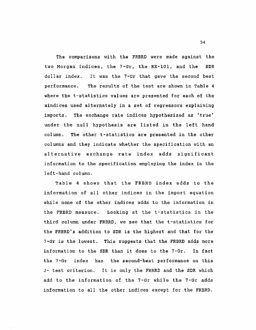
Table 4 shows that the FRBRD index adds to the

information of all other indices in the import equation

while none of the other indices adds to the information in

the FRBRD measure. Looking at the t-statistics in the

third column under FRBRD, we see that the t-statistics for

the FRBRD's addition to SDR is the highest and that for the

7-Gr is the lowest. This suggests that the FRBRD adds more

information to the SDR than it does to the 7-Gr. In fact

the 7-Gr index has the second-best performance on this

J- test criterion. It is only the FRBRD and the SDR which

add to the information of the 7-Gr while the 7-Gr adds

information to all the other indices except for the FRBRD.

35

The large t-statistic shown when the FRBRD substitutes for

the SDR is consistent with the FRBRD's having more

currencies included and a larger weight-base than the SDR.

The SDR and the RX-IOI are shown as being improved by

all the other indices. This result is consistent with the

hypothesis that the SDR has less information because of

having the narrowest currency inclusion among the indices

being compared. In the case of the RX-IOl, this result

suggests that the weight-base is more important than the

number of currencies covered.

Looking at the first and last rows, the Morgan indices

give the lowest significant t-statistics for the SDR and

the RX-IOl. This implies they contribute the least

information to the SDR and the RX-IOI. Reversing the

relation, the t-statistics indicative of the additional

information provided by the RX-IOI to the Morgan indices

are higher than vice- versa. This could imply that the

RX-IOI will sti 11 be seen as contributing information to

the Morgan indices at significance levels lower than 5

percent but the Morgan indices may no longer be seen as

adding information to the RX-IOI at those levels.

Another empirical result in Belongia's comparisons was

for out-of-sample forecast errors. Using reduced form

models for US real exports and US real non-petroleum

imports that were devised solely for the index comparison

36

exercises, he found that in the export equation the 7-Gr

index had the lowest mean absolute (MAE) and root mean

squared errors (RMSE). The MAE and the RMSE are measures

of the divergence between forecast data and actual observed

data of the variabl e being forecast. The small er the

values of these statistics, the better is the forecast.

The results show that the FRBRD and the SDR indices

performed nearly as well as the 7-Gr. The out-of­

sample error statistics for the us non-petroleum import

equations showed that the SDR and the FRBRD indices had the

small est error val ues in that order followed by the 7-Gr

index (See Table 5).

From his resul ts, Belongia concl uded that adopting a

wide-currency implementation does not improve on existing

real do 11ar indi ces . However, the use of a di f feren t

weight-base in most of the wide currency indices subjected

to the J-test particularly the RX-10l, somewhat confuses

the issue. Whi1e the FRBRD and the SDR use subsets of

total world trade, the RX-10l and the MG-40 use subsets of

US trade. This makes their weight-base much smaller than

the FRBRD and the SDR.

37

Table 5

Out-of-Sample Forecast Statistics*

Exchange Rate Index

EXPORT EQUATIONS

SDRFRBRDMG-157-GrMG-40RX-101

IMPORT EQUATIONS

SDRFRBRDMG-157-GrMG-40RX-101

Mean Error

0.006-0.009-0.0520.007

-0.0390.048

-0.015-0.024-0.0190.027

-0.0050.036

MAE

0.0260.0300.0580.0150.0510.048

0.0340.0380.0810.0560.0670.081

RMSE

0.0280.0350.0690.0180.0610.053

0.0420.0460.0900.0640.0740.103

* (Estimation Interval: I/1975 - III/1984;forecast interval: IV/1984 - III/1986)

Source: ( Belongia, 1987 ).

The criteria used by Belongia are trade related and may

not be entirely appropriate for the broader purpose of

evaluating a global dollar real value that does not use

trade weights. However, within the context of trade

questions his results support a rejection of indices with a

narrow weight-base and an acceptance of indices with wider

weight-bases like the SDR and the FRBRD. Since trade

acti vi ty is just a subset of the total range of economic

38

acti vi ties between nations, his resul ts suggest that

broader weights which go beyond trade relations may provide

an improvement over trade-based indices.

It is also shown in Belongia's study that the choice of

weight-base and weighting scheme has a significant impact

on an index's ultimate story. Our analysis reveals the

extent to which the choice between a multilateral or

bilateral weighting scheme translates into wide disparities

in the weight-base used. In the case of the Morgan indices

for instance, their narrow focus on the question of US

competitiveness in manufactures resulted in their use of a

very small subset of total world trade as an information

base. Apparently, as a narrower weight-base is chosen

over a wider weight-base, some information relevant to the

overall valuation of the dollar is lost.

The performance of the SDR, the FRBRD, and the 7-Gr in

the Belongia study needs to be expl ained. Here, we have

three indices of the dollar that process information

differently. They have different weight-bases with the 7­

Gr using a subset of us trade as its weight-base while the

FRBRD and the SDR use subsets of total world trade.

Because the 7-Gr and the RX-101 process information in very

simi I ar ways, the RX-101 correl ates better wi th the 7-Gr

than with the SDR and the FRBRD indices. However, the RX­

101 performs badly in the Belongia study while the 7-Gr

39

performs as well or bet ter than the SDR and the FRBRD

indices. It seems that this similarity in behavior of the

SDR, the FRBRD, and the 7-Gr results from the way they

weight the different cross-rates that they process.

Table 6

Multilateral and Bilateral Weightsfor Major World Areas

INDEX

MultilateralATLANTAIMFFRBRDSDR

us

0.00.00.0

42.0

EUROPE

59.652.977.343.0

CANADA

7.920.3

9.10.0

JAPAN

14.221. 313.615.0

OTHERS

18.304.900.000.0

TOTAL

100.0099.40

100.00100.00

BilateralMG-15 n.a 44.1 30.3 23.2 2.40 100.00MG-40 n.a 35.7 20.7 18.5 25.10 100.007-Gr n.a 32.1 29.8 21. 5 16.60 100.00RX-101 n.a 25.3 21.0 17.1 38.50 101.90X131 n.a 25.2 20.7 16.8 37.29 99.99

Sources: (Hervey and Strauss, 1987; Rosensweig ,1987). 1985values are shown for indices with moving weights.

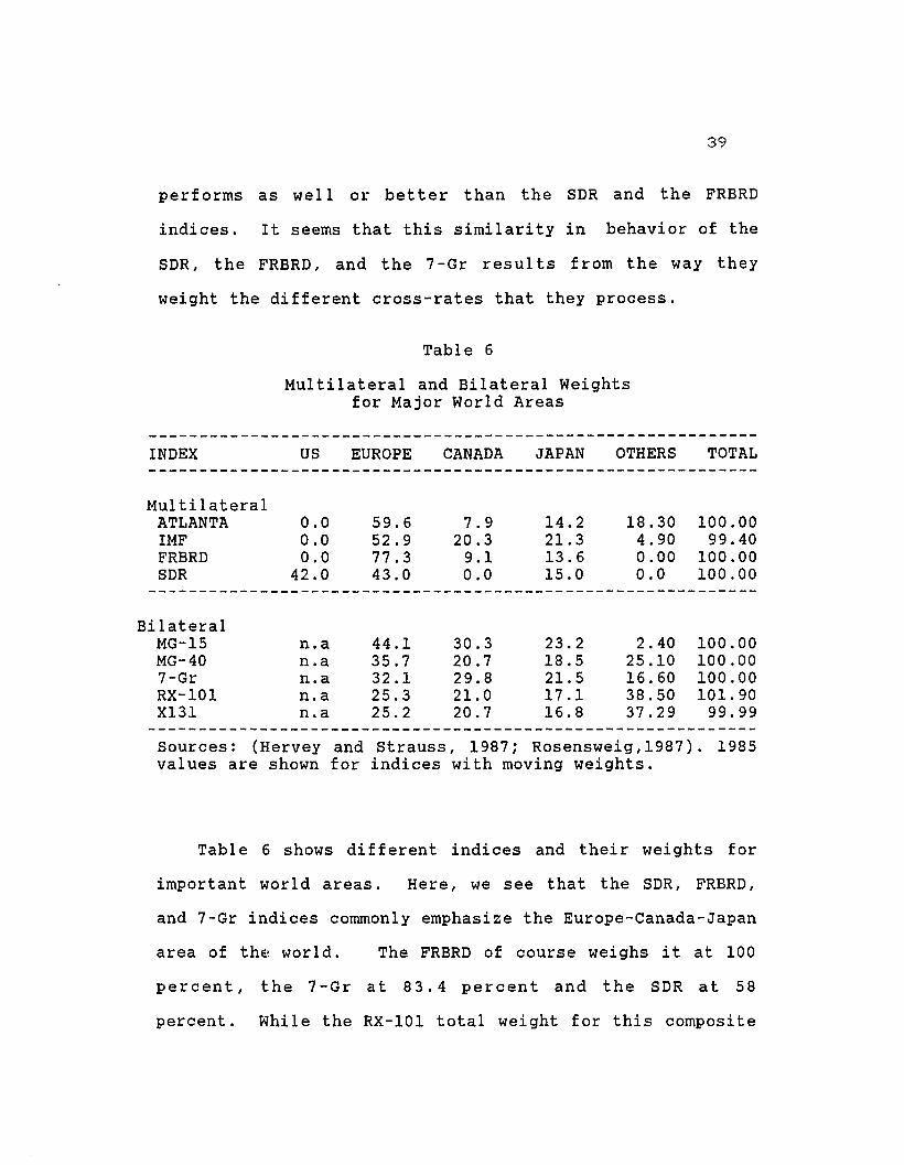
Table 6 shows different indices and their weights for

important world areas. Here, we see that the SDR, FRBRD,

and 7-Gr indices commonly emphasize the Europe-Canada-Japan

area of th~ world. The FRBRD of course weighs it at 100

percent, the 7-Gr at 83.4 percent and the SDR at 58

percent. While the RX-101 total weight for this composite

40

region is also 61.5 percent and higher than that of the

SDR, it processes addi tional exchange rates for 'others'

with a total combined weight of 38.5 percent. In

contrast, the SDR index just puts in the value 1 or 100 for

the US at the weight of 42 percent.

The wide-currency implementation of the RX-101 should,

with all things being equal, add to the information flow

being summarized into the doll ar' s val ue . However, this

could have been negated, as shown in Table 6, by its use of

a narrower weight-base on which the relative importance of

currencies is determined. A particular currency may have a

higher weight in the RX-101 index because its host economy

is an important US trading partner. However, in the

context of the international economy it may be relatively

unimportant and thus, its exchange rate will actually have

very little impact on the dollar's overall value. What

happens to the whole international economy seems more

relevant and important to the dollar's global value

compared to what happens to US trade and US trading

partners.

Table 6 also accents certain weaknesses attributed to

the weighting scheme used in most existing indices.

Mul tilateral trade weighted indices have been cri ticized

for putting too much emphasis on regions that trade a lot

with each other. This is particularly apparent in the case

41

of the FRBRD which gives a weight of more than 77 percent

to Europe. Bilateral trade weighted indices on the other

hand are guilty of putting too much emphasis on countries

with very strong trade relations with the us. This is

particularly noticeable in Canada and also observable to a

1esser degree in the case of Japan. Among other things,

the weighting scheme in an improved index of the dollar

should strive to correct for these imbalances.

Dropping the Morgan indices because of their sectoral

focus, we are left with four .real indices of the dollar

from which features for a new global dollar index can be

adopted. However, the SDR, FRBRD, RX-IOl, and 7-Gr differ

not only in terms of currency inclusion and size of

weight-base but also in terms of having fixed and moving

average weights. Guidelines as to which of these

conflicting features should go into our new index are not

clearly apparent. Ul timately, these decisions have to be

informed judgment calls dependent on what we consider as

most relevant to the dollar's role as the world currency.

Building a New Dollar Real Index

What becomes apparent in our review of existing dollar

indices is the absence of an index that is both broad-based

and wide-currency in implementation. There is also a lack

42

of attention to the implementation of regional sub-indices

and only one index includes the impact of the us economy

itself in its construction. A dollar index that is

sensitive to the us dollar's role as an international

currency should pay attention to these concerns. The newer

dollar indices which styled themselves as broader than the

traditional indices are really narrower in terms of weight­

base despite their inclusion of more currencies. Among the

existing real indices discussed, only the SDR includes the

US economy and it is only the RX-IOl which has implemented

regional sub-indices. A new index of the dollar should

fuse these essential elements to have a truly global scope.

Gi ven the ob j ecti ve of t racking the doll ar 's val ue

through an index that is sensitive to the dollar's role as

the international currency, a weighting scheme that

includes a magnitude indicator for the us economy is

desirable. This would explicitly include the intrinsic

influence on a currency's real value of the real goods and

assets it can command in its own host economy.

Furthermore, an index that includes a weight for the US

economy reflects one principal reason for the US dollar's

desirability as an international currency: the large size

of the US economy relative to Gross World Product flows and

the attendant expectation of stability in its currency

value because of this fact. This is a reason why any world

43

demand for dollars equation may be improved by including an

indicator for the us economy.

We would like to end up with an index of the dollar's

value that is both a broad-based and a wide-currency index.

Aside from the cross implication regarding the inclusion of

a us weight, using GDP flows as weights allows coverage of

economic activity beyond the trade sector. A wide-currency

implementation together with the use of broader weights

allows for a more meaningful disaggregation into regional

sub-indices which most existing dollar indices have not

paid attention to. At the same time an index where

currency inclusion is limited only by data availability

avoids arbitrariness in the decision to include or exclude

currencies.

A period-specific moving weight scheme will be used in

our new index. Such a scheme includes the effect of

structural shifts in the long term tracking of the dollar's

value. It automatically updates the relative importance of

currencies in the index, as the underlying pattern of

trade and investments among nations shifts through time.

The adoption of periodic moving weights together with the

inclusion of a weight for the US economy facilitates the

decomposition of factor component effects on the index

value.

44

Chapter 3

THE GDP-WEIGHTED REAL INDICES

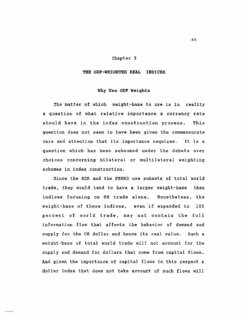
Why Use GDP Weights

The matter of which weight-base to use is in reality

a question of what relative importance a currency rate

should have in the index construction process. This

question does not seem to have been given the commensurate

care and attention that its importance requires. It is a

question which has been subsumed under the debate over

choi ces concerning bi I a tera I or mul ti I a tera I weighting

schemes in index construction.

Since the SDR and the FRBRD use subsets of total world

trade, they would tend to have a larger weight-base than

indices focusing on US trade alone. Nonethel ess, the

weight-base of these indices, even if expanded to 100

percent of world trade, may not contain the full

information flow that affects the behavior of demand and

supply for the US dollar and hence its real value. Such a

weight-base of total world trade will not account for the

supply and demand for dollars that corne from capital flows.

And given the importance of capital flows in this respect a

dollar index that does not take account of such flows will

45

not be truly reflective of the dollar's global value. If

complete data could be gathered to cobble together such a

weight, the ideal weight-base would be a combination of

trade and capital flows. However, there are many problems

with this approach.

One is that the data on capital flows are aggregated

net flows and are not equivalent to the gross flow

aggregation in trade weights. The netting out of capi tal

flows gives a much smaller figure than the flow which

actually moves through the exchange markets. Even with the

aggregation done by categories which can be an

improvement since no netting out then occurs across types

of capital flows, the gross flows left out can still be

substantial. In equi val ence to the trade weights, this

procedure of using capital flows would be similar to using

the net trade balance instead of the total of exports and

imports involved.

Using capital and trade flow weights in combination

will obviously be stumped by the intrinsic incompatibility

between gross and net flows. Wi th the flux in

international banking regulation and the confidential

nature of financial transactions, it would not be easy to

get relief from the problem of securing capital gross flow

figures outside of existing official sources. Furthermore,

the institutional shifts in capital and market regulations

46

came at different times in different countries and cannot

be as neatly accounted for as the international exchange

regime shifts which all happened in 1971.

International capital flows became much more important

than they were in the past, beginning in the late 60's

(Duffey, 1978). To build an index with weights based on

capital flows would meet problems of consistency with the

earl ier postwar years when national capi tal markets were

not as freewheeling as they are now. At the moment it

would seem that the use of capital flows as an indicator of

aggregate economic activi ty in index construction creates

more problems than it solves. These problems may be among

the reasons why there has been no rush to implement capital

weighted dollar indices.

The importance of capital flows as part of the

information stream that a dollar index should account for

does not go away with an enumeration of the problems in the

direct use of capital flows as weights. There seems to be

a need for a weight-base that could transcend shifts in

emphasis in international economic intercourse and that,-

contains information beyond that found in trade flows.

This is provided by weights based on country shares of

total world gross product. Table 7 shows how the 10

countries in the FRBRD index would be weighted with trade,

capital, and GDP flows. The capital flow weights are

47

aggregated net flows of capital flows in different

categories. These were the capital flow weights actually

used by ott in his implementation of a capital weighted

dollar index (see below).

Table 7

Comparative Weights for the G-10 CountriesTrade, Capital, and GDP flows

Country 1972-1976Trade Capital GDP

1979-1983Trade Capital GDP

German Mark .203

Japanese Yen .136

French Franc .129

UK Pound .118

Canadian Dollar .090

Italian Lira .090

Netherlands .084

Bel gian Franc .074

Swedish Krona .040

Swiss Franc .034

.103

.070

.243

.125

.072

.095

.058

.152

.014

.067

.197

.239

.151

.108

.081

.098

.039

.029

.032

.024

.203 .061 .177

.156 .103 .273

.130 .149.144

.119 .362 .120

.078 .046 .071

.095 .063 .102

.080 .032 .037

.071 .093 .026

.032 .016 .027

.033 .075 .024

Trade and Capital data are from the ott study (ott,1987). GDP flow weights were computed from IMF data (IMF­IFS Tapes). Note that the GDP weights correct for the veryhigh multilateral trade weights found in European countrieswhich trade heavily with one another. It also corrects forthe the very high bilateral weights for Canada. GDP weightsfor Japan are similar to bilateral weights (see Table 6).

48

Problems with the use of capital flow weights explain

why GDP flow weights are instead used in the new index

implementation. The present weights of the SDR and the

FRBRD indices which are based on trade flows can be

expanded to the limit of total world trade. But total

world trade is still just a subset of gross world product

and that would still leave a lot of economic activity out

of the index.

Furthermore, a dollar index that relates to

international monetary conditions theoretically should have

weights that reflect conditions and price sensitivities in

asset markets as well as the currency composition of asset

portfolios. Building an index to reflect monetary

conditions implicitly assumes that movements in exchange

rates are related to shifts in asset demands including the

demand for money. Since it is not easy to obtain reliable

data and estimates of these parameters, weights based on

gross national product as a proxy have been suggested

(Pauls, 1987).

Trade flows that relate to the value of the dollar as

indicator of demand for US goods by the ROWand vice-versa

are actually subsets of present GDP flows in both the US

and the ROW. Capital flows however are not subsets of

current production but are subsets of accumulated past

production (savings). Because the sources of capital flows

49

are savings built from portions of cumulative GDP flows, it

is not surprising for such capi tal flows to swamp the

effects of current transactions on the dollar's real value.

The statement therefore that the dollar's val uation does

not follow the purchasing power parity 'fundamentals' may

be misleading in the sense that it implies a blind spot for

the possibility that it is in fact the broader capital

market 'fundamentals' that have changed.

When capital flows into the us from the ROW,

accumulated savings are effectively being transferred from

the rest of the wod d to the US. Such flows do not onl y

corne for precautionary (including safe haven) reasons but

are also induced by expected returns from interest income,

capital gains, profit yields from investments, rent income

or value appreciation from acquisition of real estate. US

GDP roughly proxies for the potential yield of the assets

being acquired by such capital inflows into the US and thus

provides a link to such flows.

GDP, as opposed to GNP val ues, accounts for economi c

activity that is specifically domiciled in a particular

country. It therefore avoids the double counting that

would occur with the use of GNP values. GDP share weights

effectively scale the level of economic activity specific

to a currency in relation to total world economic activity

which in turn determines the relative importance of

50

currencies in the index computation. It may be argued that

such a weighting scheme will give too much emphasis to

countries with large GDP's and with a relatively small

export and import sector. This is not necessarily the case

since the GDP share also scales the ability of such country

to generate investment opportunities that can induce inward

capital flows, or its ability to sustain debt service.

With most international debt papers denominated in dollars,

this aspect also becomes increasingly relevant.

The decision to use the broadest possible weight-base

also impl ies the widest-currency incl usion possibl e. In

effect, we are taking issue with Belongia's interpretation

of his results when he suggests that a wide currency

impl ementation does not improve on existing indices. His

results can also be interpreted to imply the superiority of

indices with larger weight-bases like the FRBRD and the SDR

over indices with narrower weight-bases like the RX-IOI and

the Morgan indices. Even as this question remains

unresolved, use of a wide-currency implementation can be

justified by the fact that it allows us to compute regional

sub-indices.

The weights used in constructing the index which are

country shares of the Gross World Product (GWP) reflect the

way output expands in the US relative to the ROW at a

constant exchange rate and vice- versa. The movements in

51

the relative shares of the GWP for the us and the ROW are

therefore related to movements of the business cycles or

output cycles in these two different parts of the world. 3

Relative changes in income between the US and the ROW

affect the global real value of the dollar not just

directly though the Purchasing Power Parity equation but

also through the shifts they induce in dollar demand and

supply. These relative income changes are naturally

reflected in shifting shares of GWP. An example of the

expected relations over the cycle, given the above

assumptions about exchange rates, with us output growth

leading the cycle is shown in Table 8. If the ROW leads,

then the signs would be reversed. In the past, the US has

usually been the cyclical leader.

3. The assumption here is that relative pr ices move co­cyclically as well. If interest rates move co-cyclicallyand capital markets are integrated, this will reinforce theinitiating share changes.

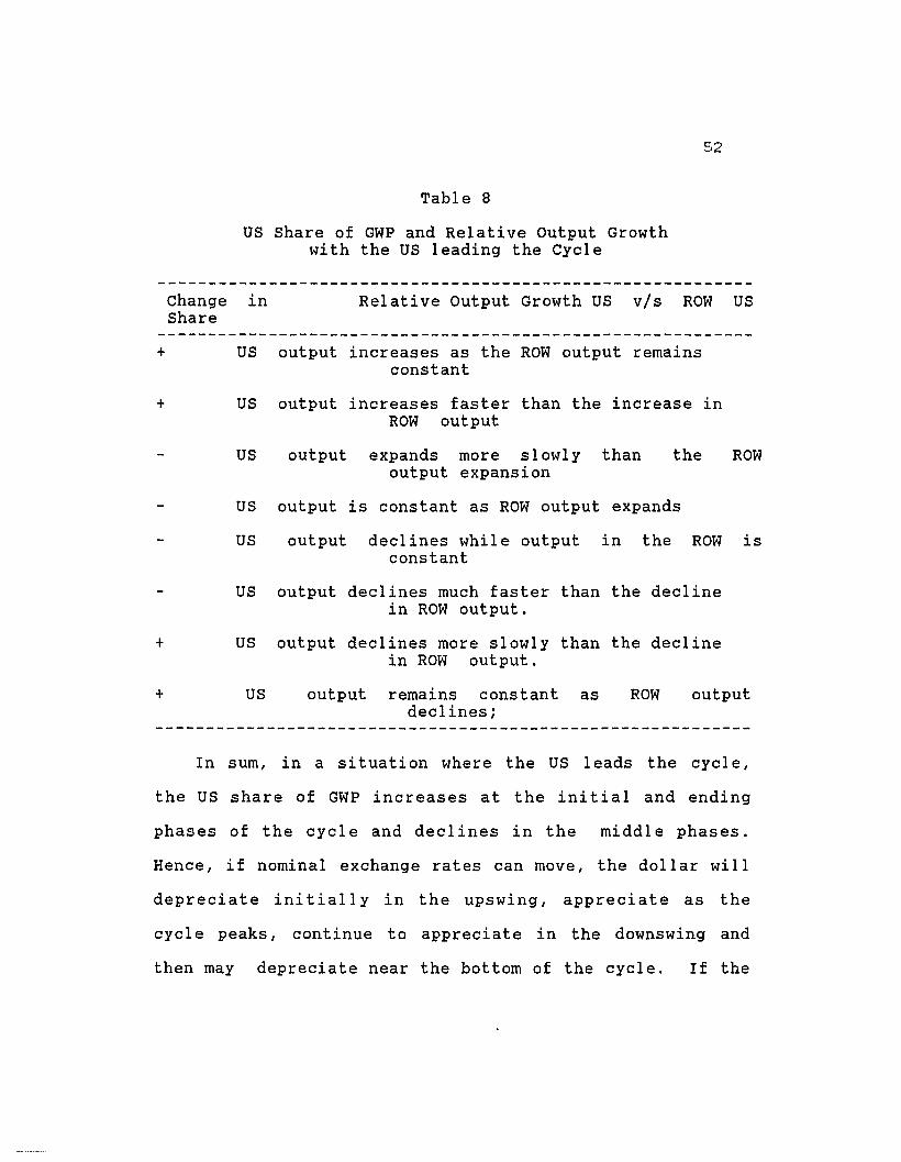
52

Table 8

us Share of GWP and Relative Output Growthwith the US leading the Cycle

Change inShare

Relative Output Growth US vIs ROW US

+ US output increases as the ROW output remainsconstant

+ US output increases faster than the increase inROW output

US output expands more slowly thanoutput expansion

the ROW

US output is constant as ROW output expands

US output declines while output in the ROW isconstant

US output declines much faster than the declinein ROW output.

+ US output declines more slowly than the declinein ROW output.

+ US output remains constant asdeclines;

ROW output

In sum, in a situation where the US leads the cycle,

the US share of GWP increases at the initial and ending

phases of the cycle and declines in the middle phases.

Hence, if nominal exchange rates can move, the dollar will

depreciate initially in the upswing, appreciate as the

cycle peaks, continue to appreciate in the downswing and

then may depreciate near the bottom of the cycle. If the

53

ROW leads, then this pattern is reversed, beginning with

the appreciation of the dollar in the upswing.

Clearly, GDP shares alone do not tell the whole story.

Shares of GDP cannot tell us with accuracy whether or not

demand for dollars in a particular country or the world is

increasing or decreasing. Even with GDP shares the same,

there can be shifts in the demand for dollars as a world

currency when levels of GDP change. There are also

problems with the use of GDP shares to proxy for the share

of wealth; with shares constant, the demand for dollars can

vary as wealth accumulates or decumulates. The use of real

GDP might have been better in constructing a GDP weighted

index since this would measure both share and level

effects. But this type of data, at the moment, is not

generally available.

54

Index Implementation

Certain aspects of our new index are more or less

settled issues. The question of currency inclusion is

limited only by data availability; the duration for which

the index is to be constructed has already been identified.

The new index uses the CPI as price deflator since it is

widely available in different countries on a more or less

standard basis. Where the CPI series is incomplete and

where GOP deflator data are available, the movements in

the GOP deflator series are grafted into the existing CPI

series. The cross-currency rates are based on averages for

the period rather than ending period values; the RF series

in the IMF tapes are used. The use of end period val ues

runs the risk of reflecting exchange rate levels that may

contain very short run speculative noise.

The new index differs from other existing indices in

several significant ways. (1) The measure of transactions

used is GOP shares instead of trade or capital flow

weights. (2) It is a broad-based, wide-currency index

which facili tates computation of regional sub-indices.

(3) Period-specific moving weights are used which

effectively include relative growth and cyclical

information in the index and allow for a decomposition of

index values.

55

With these innovations, the new index improves on

existing measures of the dollar's value by summarizing the

impact of a broader base of economic activity and thereby

accounting for more factors that affect the demand and

supply of us dollars. This includes the effect of having a

larger weight-base than any other index, taking account of

the stabi I i zing effect of the us economy on the doll ar' s

index val ue, faci I i tating the process of constructing

regional sub~indices, and providing for a way to decompose

the index value which improves on how the resulting index

is related to developments in the world economy.

Constructing the new indices invol ves a few s i mp l e

steps. First, the nominal cross-currency rates which state

how much a doll ar costs in terms of foreign currency are

rebased to 1973. The year 1973 is chosen because full

floating of currenci es started in March of that year ....

Since the other established indices use this year as base,

comparisons are facilitated by our use of the same base

year in our indices. Second, relative prices were obtained

by dividing a particular country's CPI by the CPI of the

US for the same time period. Depending on how this ratio

is used in the formula, the relative price variable can

have US prices in the numerator instead. Relative prices

were then rebased to 1973 by dividing all observations by

the obtaining ratio of prices for that country and the US

56

for 1973. Third, weights based on gross domestic product

were computed. Gross World Product was calculated by

summing local currency GDP's at current prices after

converting each to dollars using the RF exchange rate

series in the IMF tapes. This total was then used as the

denominator in computing a particular country's gross

product to world product ratio for a particular year. The

resulting GDP ratio is then used as that year's weight for

determining a particul ar country's relative importance in

arriving at a global real value for the us dollar.

In the process of aggregation, GDP conversion from

local currency into doll ars has to be done in nominal

terms. For our purposes this process creates unwanted

cross effects from nominal exchange rates and relative

prices on the resulting GWP shares. With a higher nominal

value for the dollar, GWP shares of the ROW would tend to

be lower and vice-versa. A second problem is that nominal

GDP will tend to overestimate the relative output share of

that part of the world where prices are increasing at a

faster pace.

From a point where real GWP is equally divided between

the us and the ROW, a doubl ing of pri ces in the us for

instance with real GDP shares and prices in the ROW

constant would lead to an increase in nominal GDP shares of

the us by fifty percent. The problem is not simply

57

corrected by deflating the resulting GDP in dollars by the

us price index keyed to the index base year. Where us

prices are moving faster than ROW prices, instead of

tending to overestimate US share, ROW share then will be

underestimated.

Deflating individual country GDP in dollars by relative

prices may be better but again the question of which

relative price index to use remains. If we settle on the

natural choice of the GDP deflator, the problem becomes

one of availability since only a few countries have this on

a uniform basis. At present the World Bank publishes PPP

adjusted real GDP data in dollars for selected countries

but not in the scope required for our index.

This problem of converting non-dollar GDP series into

dollars is not easily dealt with. At the moment, our

method of using the RF series to directly convert other

aggregated denominations into dollars is the same method

used by other indices. For our purposes of getting a GDP

share ratio, the price distortion is mitigated since

movement in prices is usually' directly related to movement

in real output. Thus the relative share used in our index

would be a good approximation of the direction of shifts in

shares although these estimates may overshoot actual

movements in real relative output. These distortions in

GDP weight shares may be more of a problem in a fixed

58

exchange system where relative price movements are not

ref 1ected in changes in nominal rates. They become less

of a problem in a regime of flexible exchanges where such

price movements are easily translated into nominal exchange

rate movements. In fact movements in nominal rates and

prices in a flexible system would impact on nominal dollar

GDP in opposite directions which may completely offset each

other.

While the use of nominal GDP shares can be qualified

with proper caveats in the interpretation of our results,

the ideal situation for our purposes is one where the

weight share can be computed independent of effects from

relative prices and nominal exchange rates. Since other

real dollar indices which use trade weights are also

subject to the same price and nominal rate distortions in

arriving at their weights, this problem is not unique to

our index. Thus, notwithstanding the limitations in

implementation, we settle for GDP shares computed in

nominal terms.

The data used for index construction -- exchange rates,

price indices, GDP deflators, and GDP flows were

gathered for as many countries as possibl e. These data

came from the IMF tapes, the Worl d Bank Tabl es, the

Handbook for Economic Statistics of the CIA, and the

National Trade Data Bank (NTDB) data files.

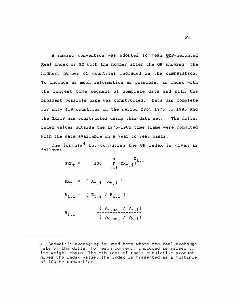
59

A naming convention was adopted to mean gDP-weighted

Real index or GR with the number after the GR showing the

highest number of countries incl uded in the computation.

To include as much information as possible, an index with

the longest time segment of complete data and with the

broadest possible base was constructed. Data was complete

for only 119 countries in the period from 1975 to 1985 and

the GRl19 was constructed using this data set. The dollar

index values outside the 1975-1985 time frame were computed

with the data available on a year to year basis.

The formula 4 for computing the GR index is given asfoIl ows:

100n Wt .r (RX .) /1

. 1 ttl1=

=

At . =,1

Rt . =/1

( At' Rt· )/1 /1

( pt/ us/ / Pt/i)-----------------

( Pb,us, / Pb/i)

4. Geometric averaging is used here where the real exchangerate of the dollar for each currency included is raised toits weight share. The nth root of their cumulative productgives the index value. The index is presented as a multipleof 100 by convention.

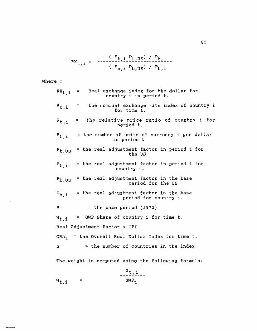
Where :

RX t . =,1

( Et,i Pt,US) / Pt,i--------------------------

60

RXt .,1

At .,1

Rt .,1

=

=

=

Real exchange index for the dollar forcountry i in period t.

the nominal exchange rate index of country ifor time t.

the relative price ratio of country i forperiod t.

Et .,1

Pt,US

P t .,1

Pb .,1

B

= the number of units of currency i per dollarin period t.

= the real adjustment factor in period t forthe US

= the real adjustment factor in period t forcountry i.

= the real adjustment factor in the baseperiod for the US.

= the real adjustment factor in the baseperiod for country i.

= the base period (1973)

Wt· = GWP Share of country i for time t.,1

Real Adjustment Factor = CPI

GRnt = the Overall Real Dollar Index for time t.

n = the number of countries in the index

The weight is computed using the following formula:

Gt ., 1

Wt .,1 =

with

Where :

nE

i=lWt .

,1 = 1

61

Wt .,1

Gt .,1

=

=

=

the gross product share of country iin year t

GDP of country i in time t

Gross World Product at time t

In log form, the formula can be restated as follows:

GRnt = 100n

exp E (Wt ii=l '

The SDR formula which is the only other index with a

weight for the US is given below for comparative purposes.

I ts main di f f erence wi th the GR f ormu1 a is its use of

arithmetic instead of geometric weights, its narrow

inclusion of currencies which are limited to just the G-5

nations, and its use of fixed weights.

= 1005E (Wi RXt,i)

i=l

Benchmark Comparisons

Comparing the GRl19 with other established real

dollar indices can help us assess the impact of the

62

different index construction method used in this study.

The difference in results with the benchmark indices will

indicate the extent to which the different indices are

summarizing unique sets of economic information streams.

This helps us focus on questions that could shed light on

how and to what degree those economic information streams

differ. strong similarities, on the other hand, can point

to the fact that despite the use of different methods the

indices are in effect capturing the same or substantially

over! apping economic infl uences that commonly affect the

dollar's real value.

The SDR, FRBRD, the RX-IOl, and the 7-Gr are used for

benchmark comparisons with the GRl19 because as was shown

earl ier, these indices contain features that have been

extended in our new index implementation. The SDR and the

FRBRD for instance have the broadest weight-base of all

existing real doll ar indices. The GR index extends this

feature by using GDP flows as weights, a measure of

commerce that is closest to a universal coverage of

economic activities.

The RX-IOI and the 7-Gr use moving averages in their

weights to account for the changing economic context of the

index value. The GR index extends this feature by using a

yearly moving weight that not only accounts for the

changing institutional context but also uses these changes

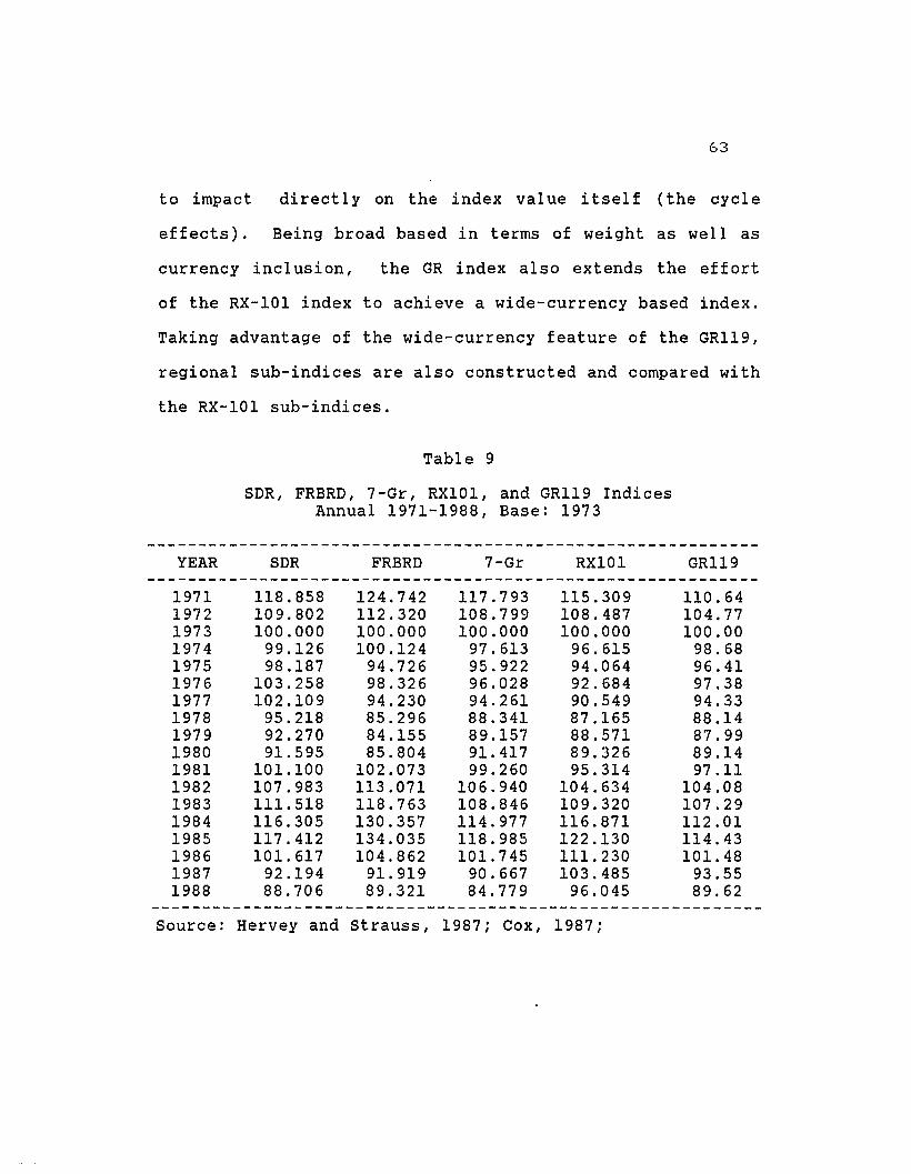
63

to impact directly on the index value itself (the cycle

effects). Being broad based in terms of weight as well as

currency incl usion, the GR index also extends the effort

of the RX-101 index to achieve a wide-currency based index.

Taking advantage of the wide-currency feature of the GRl19,

regional sub-indices are also constructed and compared with

the RX-101 sub-indices.

Table 9

SDR, FRBRD, 7-Gr, RX101, and GRl19 IndicesAnnual 1971-1988, Base: 1973

------------------------------------------------------------YEAR SDR FRBRD 7-Gr RX101 GRl19

------------------------------------------------------------1971 118.858 124.742 117.793 115.309 110.641972 109.802 112.320 108.799 108.487 104.771973 100.000 100.000 100.000 100.000 100.001974 99.126 100.124 97.613 96.615 98.681975 98.187 94.726 95.922 94.064 96.411976 103.258 98.326 96.028 92.684 97.381977 102.109 94.230 94.261 90.549 94.331978 95.218 85.296 88.341 87.165 88.141979 92.270 84.155 89.157 88.571 87.991980 91. 595 85.804 91. 417 89.326 89.141981 101.100 102.073 99.260 95.314 97.111982 107.983 113.071 106.940 104.634 104.081983 111.518 118.763 108.846 109.320 107.291984 116.305 130.357 114.977 116.871 112.011985 117.412 134.035 118.985 122.130 114.431986 101. 617 104.862 101. 745 111.230 101. 481987 92.194 91. 919 90.667 103.485 93.551988 88.706 89.321 84.779 96.045 89.62

------------------------------------------------------------Source: Hervey and Strauss, 1987; Cox, 1987;

64

The GRl19 index showed that the lowest trough in

dollar values occurred in 1979 for the period from 1950 to

1990. Compared to the benchmark indices, the GRl19 also

showed the smallest fall in dollar values from 1971 to the

1978-1980 trough, the period when the dollar showed the

longest downward trend in the post war era. This can be

attributed to the fact that it is the only index with both

a wide currency inclusion and an explicit us weight in its

implementation.

The behavior of the benchmark indices wi th regard to

their respective turning points in the trough of the 1978­

1980 period also seem to be related to their respective

currency inclusions. The SDR which is the narrowest index

showed the longest delay in an upward turn in dollar values

(1980). The SDR is followed by the FRBRD which gives its

turning point in 1979. The ear 1i es t t urning point, in

1978, is given by the relatively wider indices of the 7-Gr

and the RX101. However, the behavior of the GRl19 which

shows a turning point in 1979 despi te a wide currency

implementation suggests that it is the combination of

differences in currency incl usions and weighting schemes

that have resul ted in different turning points among the

benchmark indices.

Another way to compare the indices is with the use of

recovery ratios. A trough to trough recovery ratio

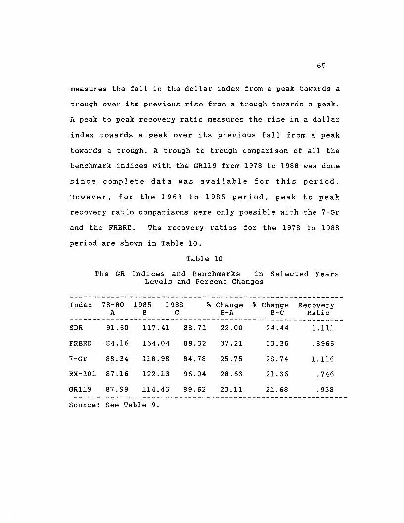
65

measures the fall in the dollar index from a peak towards a

trough over its previous rise from a trough towards a peak.

A peak to peak recovery ratio measures the rise in a dollar

index towards a peak over its previous fall from a peak

towards a trough. A trough to trough comparison of all the

benchmark indices with the GRl19 from 1978 to 1988 was done

since complete data was available for this period.

However, for the 1969 to 1985 period, peak to peak

recovery ratio comparisons were only possible with the 7-Gr

and the FRBRD. The recovery ratios for the 1978 to 1988

period are shown in Table 10.

Table 10

The GR Indi ces and Benchmarks in Sel ected YearsLevels and Percent Changes

Index 78-80 1985A B

1988C

% Change % Change RecoveryB-A B-C Ratio

SDR 91.60 117.41 88.71 22.00 24.44 1.111

FRBRD 84.16 134.04 89.32 37.21 33.36 .8966

7-Gr 88.34 118.98 84.78 25.75 28.74 1.116

RX-101 87.16 122.13 96.04 28.63 21. 36 .746

GRl19 87.99 114.43 89.62 23.11 21.68 .938------------------------------------------------------------

Source: See Table 9.

66

The differences in recovery ratios in Table 10 also

seem r e l ated to the number of countries incl uded in each

index. Of the FRBRD, the 7-Gr, and the RX-101, each

without an explicit us weight, the FRBRD and the 7-Gr which

are both narrow currency indices showed much higher

recovery ratios than the RX-101. The SDR and the GR119

both of which include a us weight also exhibit the same

pattern. Being both wide-currency indices, the difference

in recovery ratios between the RX-101 and the GR119 implies

that when viewed through trade share weights, the us

competitive position from 1978 to 1988 seems to have eroded

much more than when GDP share weights are used.

For the 1969-1985 period the FRBRD and the GR119

indices had 1.084 and 1.045 recovery ratios respectively as

opposed to the .929 ratio of the 7-Gr. This seems to

suggest that the GDP weights of the GR119 are in more

agreement with the multilateral trade weights of the FRBRD

than with the bilateral trade weights of the 7-Gr. Thus in

both the 1969-1985 and 1978-1988 periods, the FRBRD proves

to be the closest index to the GR119 in terms of recovery

ratios.

67

Table 11

Comparative Correlation GRl19 vIs BenchmarkLevels and Percent Change 1971-1988

Indices

Index

SDR

FRBRD

7-GR

RX-101

Levels

GRl19

0.94992

0.98755

0.97899

0.91882

Percent Change

LNGRl19

0.95248

0.97587

0.97573

0.92614

Based on data from Table 9.

The expectation that the GRl19 index would show more

simi 1ari ties wi th indices having broader weight-bases is

also borne out by the correlation results in Table 11.

Despi te having a wide-currency set 1ike the RX-101, the

GRl19 index correlated better with the FRBRD (See Table

11). The SDR, another index with a broad weight-base, also

showed higher correlations with the GRl19 than with the RX-

101.

68

*Figure 3

GR119, FRS, 7-Gr, Compared1960 - 19BB

1150r------------------------,

140

130

~ 120....J

~ 110

100

90

The results in Table 11 also show that the GRl19 was

closest to the FRBRD and the 7-Gr in that order. Plotted

together in Figure 3, what is particularly striking is how

the three indices bunch up together between 1972 and 1977.

This bunching up is explained by the fact that nominal

exchange rates were already in free float during this

period and aligned movement in ROW currencies versus the us

* Source: Data for the FRBRD and 7-Gr were provided by Dr.Jack Hervey of the Federal Bank of Chicago (see AppendixTable 3.6).

69

dollar may have mitigated the impact of different currency

inclusions. While the 7-Gr and the GR119 both used moving

weights the FRBRD's use of fixed weights did not make much

of a difference because its fixed trade weights were

computed for the period from 1972 to 1976. The difference

due to trade weights vIs GDP weights is mitigated by the

fact that GDP and trade based weights tended to move

together (see Table 7).

Outside of the 1973 to 1977 period, the FRBRD showed

the highest index values most of the time, the GR119 index

showed the lowest and the 7-Gr tended to keep the middle

ground between the other two indices. The exception to

this pattern occurs in the trough period from 1978-1980

when the FRBRD index showed the lowest values, the 7-Gr

showed the highest values with the GR119 staying in the

middle. At this point (1978-79), if we were to use the

GR119 index as the standard then we could say that the

FRBRD has undervalued the dollar while the 7-Gr has

slightly overvalued the dollar.

From 1976 onwards the FRBRD showed a marked difference

from the 7-Gr and the GR119 with the latter two tending to

move more closely together. This difference may be

principally due to the impact of fixed versus moving weight

schemes. Back towards the fixed exchange period the 7-Gr

and the GR119 widened their differences, indicating that

70

the use of different measures of commerce (trade vis gdp)

despite a similar moving weight implementation, tend to

result in wider discrepancies in the fixed compared to the

floating exchange period. The FRBRD shows much greater

difference from the GRl19 than that shown by the 7-Gr

because of its added difference of using fixed weights.

Our attempts to partly explain the causes of the

differences between the GRl19 and the benchmark indices

can only be tentative in nature since the comparisons are

impaired by the fact that the indices vary in terms of

weight-base, weighting scheme, and as well as in currency

inclusions. To get a fix on the impact of varying country

incl usion alone, we impl emented narrow currency versions

of the GRl19 and compared the results with the GRl19. The

GR38 index was constructed because it was the 1argest

currency set with complete available data from 1950 to

1990. GDP-weighted indices which are limited to the

currencies in the SDR or the G-10 set of countries were

also implemented through the GR5 and the GR12 indices. The

GR5 contained the SDR countries and the GR12 had the G-10

countries plus Switzerland and the United States.

Recovery ratios of the narrower GR indices showed a

stronger downward trend for dollar real values from 1969

to 1988. In the peak to peak ratios of 1969 to 1985,

narrower GR indices had lower recovery ratios than the

71

GRl19. In the trough to trough ratios of 1978 to 1988, the

narrower currency indices tended to have higher ratios than

the GRl19 (See Tables 12 and 13).5

Table 12

GR Indices Peak to Peak Recovery Ratios1969-1985

----------------------------------------------------------Index 69-70 78-79 1985 B-A B-C Ratio

A B C D E E/D----------------------------------------------------------

GR5 113.000 88.624 108.042 27.50 21.91 .797

GR12 113.950 89.005 111. 349 28.03 25.10 .896

GR38 114.476 89.126 113.722 28.44 27.60 .970

GRl19 113.280 87.99 114.430 28.74 30.05 1. 046

Tabla. 13

GR Indices Trough to Trough Recovery Ratios1978-1988

----------------------------------------------------------Index 78-79 1985 1988 B-A B-C Ratio

A B C D E E/D----------------------------------------------------------

GR5 88.624 108.042 85.012 17.97 21. 32 1.186

GR12 89.005 111. 349 86.290 20.07 22.50 1.121

GR38 89.126 113.722 88.224 21.63 22.42 1.037

GRl19 87.99 114.430 89.62 23.11 21.68 .938

5. For data source see Appendix Table 3.1

72

Table 14

Trend Comparisons for the GR , FRBRD, and 7-GR Indices1960 - 1990

Index

GR38

GRl19

FRBRD

7-Gr

Trend Coefficient

-0.678365

-0.626530

-1. 379570

-1.167700

T-Value

-4.214

-3.845

-4.266

-5.507

Sig Level

0.0003

0.0007

0.0002

0.0001

Based on Data in Appendix Table 3.6.

Regressions done to estimate trend coefficients for the

FRBRD and the 7-Gr confirms that from 1960 to 1990, the

trend in the dollar's real value was negative. The GRl19

index, however, shows a less pronounced downward trend

than the FRBRD (See Table 14). This implies that wider

currency indices are able to capture favorable trends in

dol 1 a r rea 1 val uesthat are neg 1 e c ted i rr the n a r row

traditional indices of the dollar. The overall downward

trend of the doll ar ' s global real val ue thus tends. to be

mitigated in wider currency indices implying that the

currency selection in most of the narrower indices show a

steeper downward trend for the dollar's real value.

The difference noted above may be related to the fact

that narrower currency indices mostly include the most

73

developed countries in the ROW. These countries are al so

the countries that had rapidly closed the technology gap

relative to the us and this fact is reflected in the

secul ar st rengthening of thei r currencies against the

dollar. A narrow index that includes only these strong

currencies and disregards other currencies which are

relatively weak (or being deliberately kept low for

competitive purposes) against the dollar will naturally

register a stronger negative secular trend in their dollar

index value.

A close scrutiny of Figures 4, 5, and 6, indicate that

the GR indices more closely tracked each other in the

flexible exchange period than in the years of fixed

exchange rates. This may indicate that currency

misalignments due to relative domestic price changes were

quite common in the fixed exchange rate system because

nominal rates were slow in adjusting to the price

movements. The nominal rate of exchange is after all just

another price and the fixed system of exchanges just

institutionalizes this price stickiness.

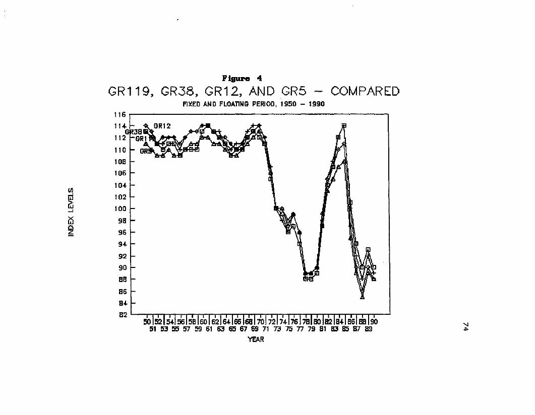
Figure 4

GR119, GR38, GR12, AND GR5F1~EO AN0 FLOATING PERIOD I 1950 - 1990

COMPARED

110

10B

106

10+

~ 102~ 100....J

~ 98

~ 96

9+

92

90

SB

86

B+

82.:.-.. I.", ..:~ 1=h::ale-oI"II co".,,1 co"~ 1~ 1m 1"'M I .,." I .,~ 1-7.:0 l-.al atIID1'l1la-~ lac: II:H:II on

""'J~

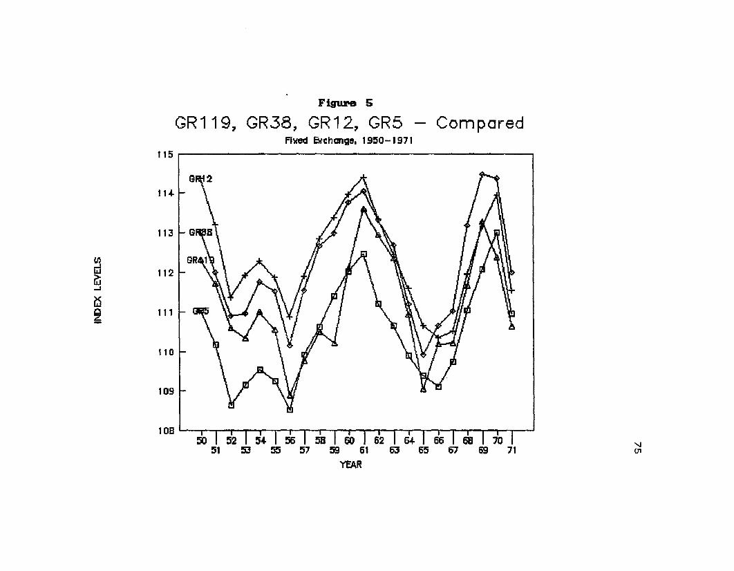
Figure S

GR119, GR38, GR12, GR5 ComparedFived E!tchange. 19~O-1971

115 I I

"(J17165

1DB Ii' iii i , • • I Iii iii iii , iii

109

110

112

111

113

11<4-

~~...J

~

~

Figure (,

GR119, GR38, GR12, AND GR5 - COMPAREDflOATING PERIOD, 1912 - 1990

116

11 +

112

110

lOB

106

10+

~ 102~ 100-'

~ 98

i 96

9+

92

90

BB

B6

B+

B2"Mo I 7+ I 76 I 7B I BO 182 I 6+1 B6 I BB I 90 '-J

73 15 77 79 81 BJ B5 81 B9 0'

YEAR

77

Table 15

Comparative Correlations, GR5, GRI2, and GR38vis GR119, Levels

1950-1971

GR119

GR119

GR5

0.776930.0001

GR5

0.926150.0001

GR12

0.796150.0001

1972-1990

GR12

0.960430.0001

GR38

0.859160.0001

GR38

0.987830.0001

Based on Data in Appendix 3.1.

The correlation results in Table 15 confirm that a

narrow currency index in the fixed exchange period that

only monitors changes in the dollar's value for a

relatively small portion of the world is not a good proxy

for the rest of the world. With the dollar's real value

moving in different directions in the different regions, a

wider currency implementation can do a better job of

tracking the dollar's global value. Hence, a wider

currency index appears to be preferable over a narrower

currency index in determining global trends in doll ar

values particularly for the fixed exchange period.

78

The closeness of movement of the narrow and wide

version of the GR index during the floating period,

suggests that the freeing of nominal rates also facilitated

the transmission of economic information on a worldwide

basis. We see this reflected in the GR indices which were

closely linked in the floating system despite disparity of

currency coverage. This resul t al so suggests that in the

context of a floating system, given a particular weighting

scheme, a well selected set of currencies even if limited

to just a few countries can usefully proxy the movements of

a global dollar index based on a wider set of currencies.

However, saying that a narrow currency index is an

effective proxy for a wider currency index implies that we

are using the wide-currency index as the standard. The

question of the exact meaning of the standard chosen

remains and our exercise of building a broad-based and wide

currency dollar index is in part an attempt to explore the

nature of a wide currency standard. The GRl19 index, as

the broadest-based and the widest currency index that can

be constructed out of the available data thus becomes the

main dollar index in this study and is used as a standard

for assessing 'how well' narrower indices reflect the wide

index.

79

The differences between the GRl19 and the benchmark

indices can be attributed largely to the varying currency

sets incl uded in each index. Di fferences in currency

inclusion also imply a difference in regional emphasis for

a particular index. Traditional dollar indices emphasize

the composite movement of the dollar in Europe, Japan and

Canada. Among the existing indices the RX-101 was first to

give significant weight to dollar values outside of these

traditional areas. This was reflected in comparative

correlations which showed that the RX-101 differed so much

from the other dollar indices.

An obvious advantage of a wide currency index is the

feasibility of its being broken down into sub-indices

covering various sections of the world. This is something

that cannot be done with a narrow index like the FRBRD and

can only be executed to a limited extent with the 7-Gr

index. The RX-101, a wide currency index of 101 countries

easi 1y 1ends i tsel f to computations of regional indices.

These RX-101 sub-indices show wide disparities in

comparison to the overall value reflected in the main RX­

101 index. Sub-indices for the GRl19 were also computed

and compared with those from the RX101 for selected years

in Table 16.

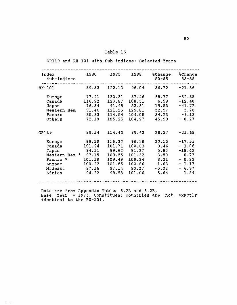
80

Table 16

GRl19 and RX-101 with Sub-indices: Selected Years

------------------------------------------------------------Index 1980 1985 1988 %Change %Change

Sub-Indices 80-85 85-88------------------------------------------------------------

RX-101 89.33 122.13 96.04 36.72 -21. 36

Europe 77.21 130.31 87.46 68.77 -32.88Canada 116.22 123.87 108.51 6.58 -12.40Japan 76.34 91. 48 53.31 19.83 -41. 72Western Hem 91.46 121.25 125.81 32.57 3.76Pacnic 85.33 114.54 104.08 34.23 -9.13Others 72.10 105.25 104.97 45.98 - 0.27

GRl19 89.14 114.43 89.62 28.37 -21. 68

Europe 89.39 116.32 96.18 30.13 -17.31Canada 101. 24 101. 71 100.63 0.46 - 1. 06Japan 94.11 99.62 81.27 5.85 -18.42Western Hem * 97.15 100.55 101.32 3.50 0.77Pacnic * 101.18 109.49 109.24 8.21 - 0.23Anzpac 100.22 101.85 100.66 1. 63 - 1.17Mideast 97.16 97.14 90.37 -0.02 - 6.97Africa 94.22 99.53 101.06 5.64 1. 54

Data are from Appendix Tables 3.2A and 3.2B,Base Year = 1973. Constituent countries are not exactlyidentical to the RX-101.

81

In the preceding Table the RX-101 sub-indices show a

very high appreciation in the dollars value from 1980 to

1985 in Europe. Japan showed a significant but much lower

level of appreciation for the same period and Canada, the

major US trading partner, showed very little change. In

the GR119 indices the regional relations are similar, but

the appreciation of the dollar is everywhere lower. The

GR119 sub-index for the Middle East shows that this region,

in contrast to the ROW, experienced a slight depreciation

in the dollar's value from 1980 to 1985.

The descent to the subsequent trough of 1988 by both

the RX-101 and the GR119 sub-indices is most intense in

Japan, with Europe a close second. The Western Hemisphere

has an increasing dollar value on both indices. The GRl19

indicates that this pattern was also true for Africa.

Particularly interesting is the behavior of the sub-index

for the Asia Pacific region which shows a continuing upward

trend in the dollar's value since 1971, even in the segment

when all the other sub-indices were moving downward to the

trough of 1979. An implicati on for trade flows of these

disparities in regional trends in the dollar's value is the

shift in sourcing of US imports from regions with a sinking

value of the dollar to regions where the dollar continues

to be highly valued (Cox, 1985).

82

By correlating the GR119 sub-indices with the benchmark

measures, we can also determine the regional bias that

each benchmark index shows. Tabl e 17 shows that the

European sub-index had a consistent pattern of agreement

with the main GR119 and the benchmark indices. This

indicates that what happens to the dollar's value in Europe

dominates the dollar's global real value. This also

explains why the narrow currency indices in the past showed

very high correlations with one another; they were in fact

reflecting a real value of the dollar that was mostly based

on a common composite area of the world - the Euro-Canada­

Japan (ECJ) area. By the same token, these resul ts show

that the traditional indices which have not implemented

regional sub-indices are not able to capture the very

different evolution of the dollar's value in parts of the

ROW outside of the Euro-Canada-Japan (ECJ) area. Viewing

the different indices from this regional perspective , it

appears that the FRBRD and the SDR are in effect only

regional indices of the GR119.

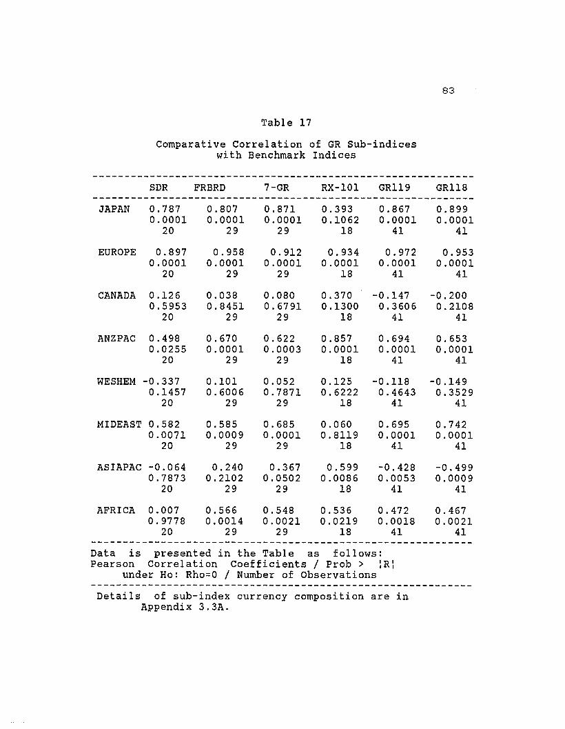
Table 17

Comparative Correlation of GR Sub-indiceswith Benchmark Indices

83

SDR

JAPAN 0.7870.0001

20

EUROPE 0.8970.0001

20

CANADA 0.1260.5953

20

ANZPAC 0.4980.0255

20

WESHEM -0.3370.1457

20

MIDEAST 0.5820.0071

20

ASIAPAC -0.0640.7873

20

AFRICA 0.0070.9778

20

FRBRD

0.8070.0001

29

0.9580.0001

29

0.0380.8451

29

0.6700.0001

29

0.1010.6006

29

0.5850.0009

29

0.2400.2102

29

0.5660.0014

29

7-GR

0.8710.0001

29

0.9120.0001

29

0.0800.6791

29

0.6220.0003

29

0.0520.7871

29

0.6850.0001

29

0.3670.0502

29

0.5480.0021

29

RX-101

0.3930.1062

18

0.9340.0001

18

0.3700.1300

18

0.8570.0001

18

0.1250.6222

18

0.0600.8119

18

0.5990.0086

18

0.5360.0219

18

GRl19

0.8670.0001

41

0.9720.0001

41

-0.1470.3606

41

0.6940.0001

41

-0.1180.4643

41

0.6950.0001

41

-0.4280.0053

41

0.4720.0018

41

GRl18

0.8990.0001

41

0.9530.0001

41

-0.2000.2108

41

0.6530.0001

41

-0.1490.3529

41

0.7420.0001

41

-0.4990.0009

41

0.4670.0021

41

Data is presented in the Table as follows:Pearson Correlation Coefficients / Prob > IRI

under Ho: Rho=O / Number of Observations

Details of sub-index currency composition are inAppendix 3.3A.

84

These differing regional values would appear to dilute

the usefulness of a global index value for the dollar.

However, a global value remains useful in the sense that it

gives a number that summarizes the overall dollar effect as

the different regions and nation-states manage their

monetary and fiscal targets in pursuit of their own varying

national agendas. Such efforts bring about a divergent

evolution of relative prices and nominal exchange values of

their currencies. Using a global real value index of the

dollar in conjunction with regional sub-indices gives us a

better picture of what is happening in the world economy

than mere reliance on one main aggregate index val ue . It

also gives dollar holders an idea of changes in the global

value of their asset.

Several important points emerge out of comparisons

between the GRl19 and the benchmark indices. Based on

recovery ratios, overall trends, and comparative

correl ati ons, the closer affini ty of the GRl19 GDP based

index with the broader trade base indices of the FRBRD and

the SDR is borne out. The inclusion of a US weight tended

to make the GRl19 values lower than the other indices

outside of the base year and made it closer to the SDR. But

despite a wide difference in index levels outside the base

year, recovery ratios and overall trends of the FRBRD were

amost similar to the GRl19. The inclusion of a US weight

85

also exerted a stabilizing influence on the GRl19 index

value as expected and this r e s u l t e d in narrower

fluctuations in the dollar's real value compared to

indications in the benchmark indices. Based on the GRl19,

the other indices tend to overestimate the fluctuations in

dollar values implying that the dollar's real value is

really more stable than is shown by the benchmark indices.

In comparison to moving weight indices that use trade

instead of GDP shares as weights, the value of the GRl19

tended to be significantly lower in the fixed exchange

period than it was in the flexible exchange period. This

implies that the difference in weights used have a more

significant impact in the fixed than in the flexible

period. The difference in index levels is much larger when

the GRl19 is compared to the FRBRD which used fixed

weights. This implies that the particular fixed weights

used by the FRBRD tend to add an upward bias in its index

values as the index moves away from the fixed weight base

period.

The difference in currency inclusions among the indices

is reflected in the degree of this negative trend for the

dollar's val ue in each index. A stronger negative trend

was directly related to narrower indices; the currency

selection in these narrower indices was usually limited to

countries whose currencies have experienced a secul ar

86

strengthening against the dollar while disregarding

currencies that have remained weak or those that have

del iberatel y indul ged in competi ti ve depreciati on. I f we

make the GR119 the standard, we could say that the other

indices have all overestimated the fall in dollar val ues

for the period from 1969 to 1980.

Currency selection is also related to the regional bias

of an index. The strong focus on currencies in the Europe­

Canada- Japan (ECJ) area by the t radi ti ona I indi ces has

shown the blind spot these indices have for the divergent

evolution of dollar values outside this area. The regional

indices of the RX-101 clearly showe9 this divergence which

was also" confirmed in our own implementation of regional

indices for the GR119. outside of the same pattern of

di f ferences exhibi ted between the GR119 and the other

benchmark indices, the GR119 regional indices showed the

same results as the RX-101 sub-indices.

Thus, in terms of the general pattern in the evolution

of the dollar's real value, while many similarities

between the GR119 and the conventional indices emerge

important differences remain. These differences are

directly attributable to the wide-currency nature and the

al terna ti ve weights and weighting scheme used in our new

index. Using the GR119 as our standard, we now focus

87

attention to what it tells us about the evolution of global

dollar values from 1950 to 1990.

The GRl19 and its Regional Indices

The GRl19 index shows high real values for the dollar

in the 50's compared to its real value in the 70's. During

the period from 1950 to 1971 the GRl19 index showed a

slight positive trend. The trend becomes clearly negative

from 1971 to 1979, positive from 1979 to 1985, then

negative once more from 1985 to 1988 and positive

afterwards. The wide fl uctuations in the fl oating period

gave the GRl19 index an overall negative trend from 1950 to

1990. This trend data is important in identifying the

existence of long-run causes for a secular decline or rise

in dollar values.

A cyc 1i cal regul ari ty wi thin a narrow range a 1so

appears in movements of the index value prior to the

floating regime. During the fixed exchange period, a clear

inverse relation between changes in the index value and US

GDP real growth up to 1965 was in evidence which was as

expected for a system of fixed exchanges (see Figure 7*).

After 1965 this relationship seems to have broken down with

* Source: see Appendix Table 5.1.

88

us inflation taking off as Vietnam war and Great Society

spending rose. The emergence of this relationship in the

index validates our notion of using GDP share weights. to

capture the effect of output cycles in our index.

Interpretation of this r e l ationship, which seem to have

persisted to some extent beyond the fixed exchange system,

becomes a little more difficult because of the stronger

impact of changes in nominal exchange rates on the weight

shares of our index.

With the GRl19 index encompassing 84 percent of the

total world population, approximately 64 percent of the

total world land area 6 and with its use of GDP based

weights, it is a much more comprehensive index of the US

dollar's real value compared to any of the benchmark

indices. However, despite its wide scope the GRl19 share

the emphasis on the ECJ area of the narrower benchmark

indices. Figure 8 shows the GRl19 and its Europe sub-index

with nearly identical movements (see Figure 8). But the

other GR regional sub-indices show that trends in the

dollar's value in Canada, the Australia/New Zealand area,

the Western Hemisphere, the Middle East, Asia, and Africa

substantially differ from trends of the traditional indices

6. Population (as of 1988) and land area data carne fromthe World Bank Tables in computer diskettes.

i~~e

10

B

6

....

2

o

-2

-....

-6

-8

-10

-12

Figupe 7

GROWTH RATES OF USGDP and GR1191950 -1990

Q)-D

C LUSCON

Figure B

GR119 versus EUROPE1950 - 1990

..0o

CI GR119

11B i ,

116

114­

112

110

lOB

106olD~ 104->~ 102

~ 100"l'.!: 9B

96

94­

92

90

8886 I '» , , iii ii' iii , i , , • , , ii' iii ii' • • • , iii • , iii I

120

115

110

105

lID"i 100:>-~x 95~

"C!.5

90

85

80

75

Figure 9

GR119 versus Japan1950 - 1990

[] GR119

-o....

92

which like the main GRl19 index also emphasize the European

region. 7 Figures 9 - 15 show the other regional indices

plotted with the GRl19 index.

The Japanese sub-index show a more pronounced downward

trend than the GRl19 index which reflects the fact that

Japan has played the game of technology catch up with the

US very well. From 1950 to 1970 the Japanese index showed

a clear positive trend which paralleled that of the wider

index without the cyclical regularity that is apparent in

the GRl19. The absence of the cycles seen in the wider as

well as the European index could be due to the fact that

the Japanese economy at this time had a very high growth

rate, compared to that of Europe as a whole, so that the

effect of the US output cycles on its index were muffled.

The fall of the Japanese index from 1970 to 1978 can be

reflecting a stretched out period of adjustment to the

extreme effect of the oil shocks on Japan as well as to the

new reality of floating rates.

7. For country inclusion in the regional sub-indices pleaserefer to Tables 19-21.

Figure 18

GR119 versus CANADA1~0 - 1990

116 r'---------------------.

114

112

110

lOB

106

104

102

100

98

96

94­

92

90

BB86 1 'ii' iii i • • • I I • I • I • Iii , , iii iii iii i I Iii , iii'

(I)

G>~

~":'.5

c GRl19

-DW

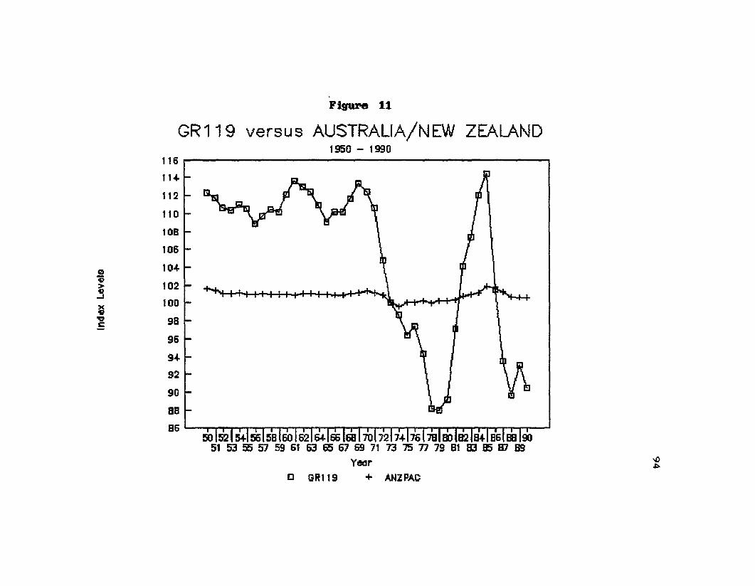
>D~

Figure 11

GR119 versus AUSTRALIA/NEW ZEALAND1950 - 1990

c GRl19

116 r'-----------~---------.,1104-

112

110

10B

106

1004­

102

100

98

96

904­

92

90

B8

86 ' iii' iii , , , iii , , ii' , , , i , , iii j , , , • , ii' • , Ii' '

~"C's::

eG>~

Figure 12

GR11 9 versus WESTERN HEMISPHERE1950 - 1990

-o01

c GR119

116 i i

11...

112

110

lOB

106

10...

102

100

9B

96

9<4­

92

90

BB

B6 'ii' • iii' iii ii' iii' , , i , , iii' ii' i , , • , , , , ii' I

oG:>-.s~~

.E

(/)

~>!i~

-..:JC

Figure 13

GR119 versus MIDDLE EAST1950 - 1990

116 i i

11<4­

112

110

108

106

104­

102

100

98

96

9<4­

92

90

BS86 ' Ii'" • i , • , iii , iii , i , , , i • iii i , , iii i • , • i , , , '

-oCJ'

[J GR119

oG

~~~

.5

Figure 14

GR119 versus ASIA PACIFIC1950 - 1990

116 i i

114­

112

110

lOB

106

104­

102

100

98

96

9.04­

92

90

BSI I86 iii ii' iii iii iii iii iii Iii iii iii iii iii , , , , j

\0~

D GRl19

Q)

G>~

~~

oS

Figure 15

GR11g versus AFRICA1950 - 1990

116 , i

114­

112

110

10B

106

10-4­

102

100

98

96

9-4­

92

90

BB

B6 ' Iii iii iii iii iii iii iii Iii iii i , Iii iii iii iii J

n GR119

-Dco

99

Without the need for dollar reserves as required in the

fixed exchange system and the increasing acceptability of

the Yen as an alternate vehicle currency in trade, the

Japanese found greater flexibility in the use of their

trade surplus earnings and this was reflected in a lower

demand for dollar balances. The subsequent rise of the

Japanese index from 1978 to 1982 can be due partly to a

market correction for the very steep fall in dollar values

from 1970 to 1978. It is interesting to see that the

Japanese index peaked at a much lower point than the wider

GR119 index in 1985 which shows the secular strengthening

of the Japanese currency during this period. Overall this

results in a downward trend in dollar values in the

Japanese index which was much stronger than the ROW during

the post Bretton Woods era.

The other regional indices show that for the most part

these areas have maintained a stable value with the dollar

during the fixed exchange period. The closeness to the

value of 100 during the fixed period for these other sub­

indices shows that they have very minimal impact on the

overall value of the dollar compared to the areas of Europe

and Japan.

While the regional sub-indices are best used in

comparisons of trends in dollar valuation between regions,

100

they do not explicitly measure the impact of each region or

country on the GR index value for each particular period.

By computing the difference in the overall GR index value

as each area is added to the computation,8 we are able to

determine the individual effects of these different

geographic units. Using this method, the regional impact

on the GR index values is shown for selected peaks and

troughs in Tables 16 to 18. The results shown in these

tables are in effect the decomposed contributions of each

region to the global dollar's value for a given period.

More detai I s in terms of country effects can also be

easily derived using the same procedure (see Tables 19 -

21).

These results may be useful in signaling currency

misalignments that are not sustained by fundamentals. For

instance when the average change in the global value shown

in GRl19 from the base period level is positive, we should

expect that the contribution from each country should

normally also be positive. If it is negative then that

currency may be overvaluing its currency than is warranted.

If the average change in the global value is negative and a

8. The contr ibution of each country or region iscomputed by taking the differences of sequentiallycumulative intermediate indices shown in Appendix Tables3.3A to 3.3C.

101

country's contribution is positive then it is probably

undervaluing its currency (as in the case of China in the

1978-1980 trough).

To see the dollar's overall trend without the effect of

China another index series, the GRl18, was constructed for

the 1950 to 1990 (See Figure 16). Like the FRBRD the peak

values for the GRl19 in 1985 are higher than its 1969

values, but this is so only when China is included. With

China excluded, the GR index follows the pattern of the 7­

Gr index. The different behavior of the GR index when

China is excluded suggests that the unprecedented peak

values of the dollar in 1985 may also be due to the very

high values given to the doll~r by countries like China

which engaged in extreme competitive depreciation to

promote their exports and encourage investment flows into

their economy. In fact, China's contribution to the global

index value exceeded that of Germany in the period from

1984 to 1986. The behavior of the Asia Pacific sub-index

with its dramatic rise in value may be due to this behavior

of China which was also shared to some extent by the other

NIC's in the area. The country-speci fic contributions to

the GR index value suggest that this is not an uncommon

practice among developing economies (see Tables 19-21).

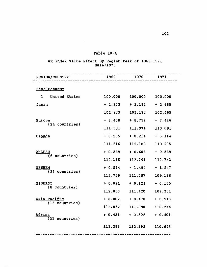
102

Table 18-A

GR Index Value Effect By Region Peak of 1969-1971Base:1973

REGION/COUNTRY 1969 1970 1971

Base Economy

1 United states 100.000 100.000 100.000

Japan + 2.973 + 3.182 + 2.665

102.973 103.182 102.665

Europe + 8.408 + 8.792 + 7.426(24 countries)

111.381 111. 974 110.091

Canada + 0.235 + 0.214 + 0.114

111. 616 112.188 110.205

ANZPAC + 0.569 + 0.603 + 0.538(6 countries)

112.185 112.791 110.743

WESHEM + 0.574 - 1. 494 - 1. 547(26 countries)

112.759 111.297 109.196

MIDEAST + 0.091 + 0.123 + 0.135(8 countries)

112.850 111. 420 109.331

Asia-Pacific + 0.002 + 0.470 + 0.913(13 countries)

112.852 111. 890 110.244

Africa + 0.431 + 0.502 + 0.401(31 countries)

113.283 112.392 110.645

----------------------------------------------------------

103

Table 18-B

GR Index Value Effect By Region Trough of 1978-1980Base:1973

REGION/COUNTRY 1978 1979 1980

Base Economy

1 United states 100.000 100.000 100.000

Japan -5.0420 -3.3210 -2.1480

94.958 96.679 97.852

Europe -4.9467 -7.1893 -6.4781(24 countries)

90.0113 89.4897 91. 3739

Canada + 0.1663 + 0.2862 + 0.3750

90.1776 89.7759 91. 7489

ANZPAC -0.0014 + 0.0569 + 0.0804(6 countries)

90.1762 89.8328 91. 8293

WESHEM -0.2513 -0.3693 -0.7810(26 countries)

89.9249 89.4635 91.0483

MIDEAST -0.8743 -0.6523 -0.7546(8 countries)

89.0506 88.8112 90.2937

Asia-Pacific + 0.1354 + 0.3883 + 0.4776(13 countries)

89.1860 89.1995 90.7713

Africa -1.0470 -1.2112 -1. 6294(31 countries)

88.1390 87.9883 89.1419

-------------------------------------------------------------

104

Table 18-C

GR Index Value Effect By Region Peak of 1984-1986Base:1973

REGION/COUNTRY 1984 1985 1986

Base Economy

1 United states 100.000 100.000 100.000

Japan -0.493 -0.275 -5.2190

99.507 99.725 94.781

Europe +9.442 +10.056 +3.0197(24 countries)

108.949 109.781 97.8007

Canada +0.556 +0.716 +0.5512

109.505 110.497 98.3519

ANZPAC +0.491 +0.766 +0.5489(6 countries)

109.996 111. 263 98.9008

WESHEM +0.131 + 0.216 + 0.5672(26 countries)

110.127 111.479 99.4680

MIDEAST -1.289 -1.313 -1.8459(8 countries)

108.838 110.166 97.6221

Asia-Pacific +3.763 +4.507 + 3.6429(13 countries)

112.601 114.673 101.265

Africa -0.588 -0.240 + 0.2180(31 countries)

112.013 114.433 101. 483

-------------------------------------------------------------

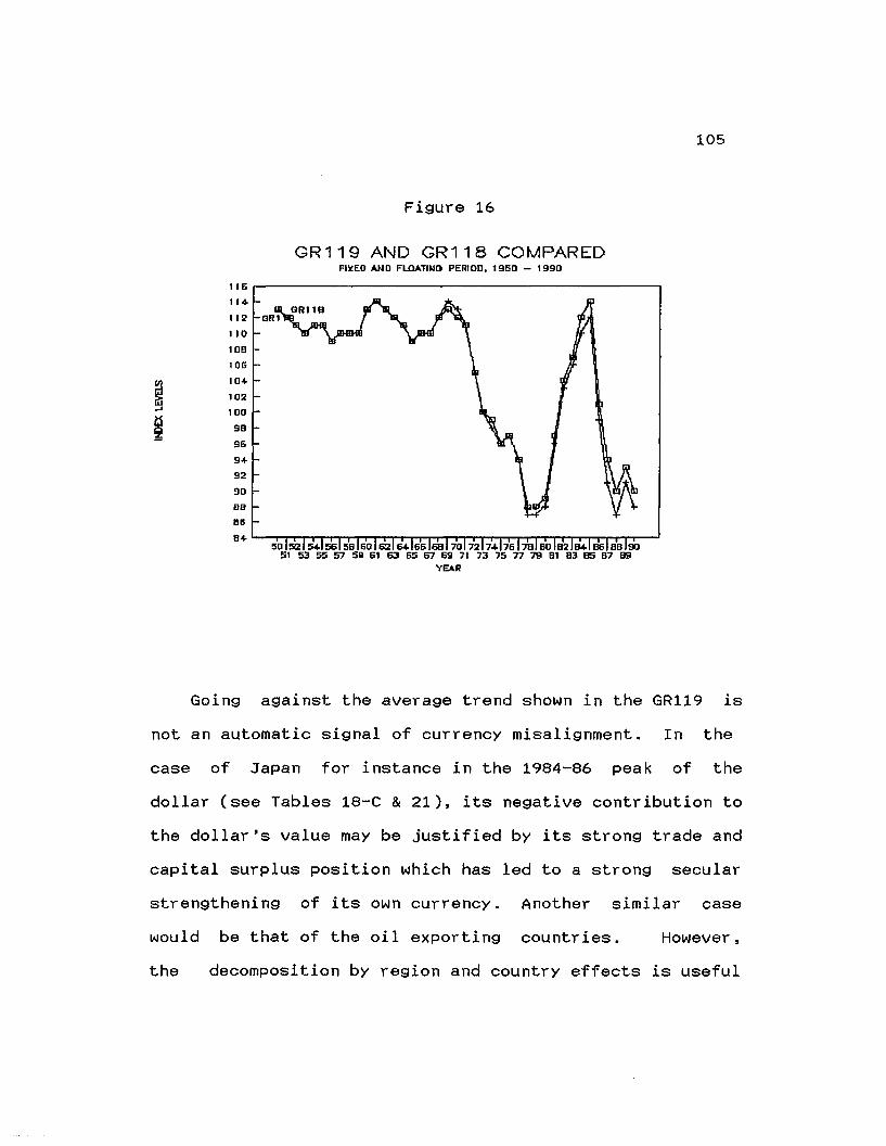
105

Figure 16

GR119 AND GR118 COMPAREDFIl(ED AND FlDATIWG PERIOD, 1950 - 1990

116,------------------------,

114­

112

lID

lOB

106

104

102

100

9B

96

94

92

90

BB

llll

84 L..-""T'"'ln-l~~""T"'1rT"'1_,_,.,...,,.,...,..,....,"T"T"T"T_r_r......""'T"'T............"T"T_._r"T"T~-J

Going against the average trend shown in the GRl19 is

not an automatic signal of currency misalignment. In the

case of Japan for instance in the 1984-86 peak of the

dollar (see Tables 18-C & 21), its negative contribution to

the dollar's value may be justified by its strong trade and

capital surplus position which has led to a strong secular

strengthening of its own currency. Another similar case

would be that of the oil exporting countries. However,

the decomposition by region and country effects is useful

Table 19

Contribution to the GR Index Value By AreaPeak of 1969-1971, Base: 1973

106

REGION/COUNTRY

GRl19

UNITED STATES

JAPAN

EUROPEGermany, Federal ReFranceUnited KingdomItalySpainNetherlandsSwedenswitzerlandBelgiumAustriaNorwayDenmarkFinlandTurkeyYugoslaviaCzechoslovakiaGreecePortugalHungaryIrelandLuxembourgIcelandCyprusMalta

CANADA

1969

113.283

100.000

2.973

2.7701.2830.8270.6130.5050.4710.3140.3300.3020.1910.1490.2050.084

-0.1150.3560.0000.0020.0680.0000.0310.0130.0040.0040.001

0.235

1970

112.392

100.000

3.182

2.6661.6090.8500.5900.6010.4950.3380.3670.3040.2160.1300.2030.1120.0330.1150.0000.0270.0850.0000.0290.0130.0040.0040.001

0.214

1971

110.645

100.000

2.665

2.3311.5370.4660.4140.4290.4020.2760.3010.2900.1920.1280.1800.0870.1040.1660.0000.0430.0500.0000.0140.0090.0020.0040.001

0.114

107

Table 19 (cont.)

Contribution to the GR Index Value By AreaPeak of 1969-1971, Base: 1973

----------------------------------------------------ANZPAC

AustraliaNew ZealandPapua New GuineaFijiSolomon IslandsTonga

WESHEMMexicoVenezuelaColombiaChileEcuadorGuatemalaTrinidad and TobagoEl SalvadorUruguayPanamaParaguayDominican RepublicCosta RicaHondurasBahamas, TheHaitiJamaicaBarbadosSurinameGuyanaAntigua and BarbudaBelizeGrenadast. Vincent and theDominicast. Kitts and Nevis

0.4800.0860.0000.0030.0000.000

0.788-0.014-0.0110.000

-0.015-0.0040.003

-0.003-0.196-0.0010.0010.0080.006

-0.0020.0010.0030.0080.0010.0010.0000.0000.0000.0000.0000.0000.000

0.5130.0870.0000.0030.0000.000

-0.228-0.0030.009

-1. 095-0.003-0.0020.005

-0.003-0.2000.0000.0030.0080.007

-0.0020.0010.0040.0030.0010.0010.0000.0000.0000.0000.0000.0000.000

0.4600.0670.0080.0030.0000.000

-0.155-0.0030.013

-1. 2320.0020.0030.007

-0.002-0.2060.0000.0040.0070.0070.0000.0000.0030.0020.0020.0010.0000.0000.0000.0000.0000.0000.000

----------------------------------------------------------

108

Table 19 (cont.)

Contribution to the GR Index Value By AreaPeak of 1969-1971, Base: 1973

MIDEASTIran, Islamic RepubSaudi ArabiaEgypt, Arab RepubliSyrian Arab RepubliKuwaitJordanBahrainYemen, PDR

ASIAPACChinaIndiaKorea, Republic ofIndonesiaThailandHong KongPhilippinesMalaysiaPakistanSingaporeBangladeshMyanmarSri LankaNepal

0.0510.042

-0.0170.0100.0000.0050.0000.000

-0.0230.217

-0.0360.027

-0.0020.044

-0.0500.040

-0.2440.0230.0000.007

-0.0030.002

0.0690.050

-0.0130.0100.0000.0040.0030.000

0.3520.177

-0.0460.0470.0160.0440.0430.048

-0.2510.0290.0000.014

-0.0030.000

0.0620.0580.0000.0090.0000.0030.0030.000

0.4640.187

-0.0340.0700.0260.0450.0240.047

-0.0670.0320.1010.018

-0.0020.002

109

Table 19 (cont.)

Contribution to the GR Index Value By AreaPeak of 1969-1971, Base: 1973

----------------------------------------------------AFRICA

NigeriaAlgeriaSouth AfricaMoroccoCameroonTunisiaCote d'IvoireTanzaniaSudanGhanaKenyaEthiopiaZimbabweZaireGabonUgandaSenegalMadagascarZambiaSomaliaCongo, People's RepRwandaNigerBurundiMalawiLiberiaMauritiusBurkina FasoSierra LeoneBotswanaChadTogoMauritaniaCentral African RepSwazilandLesothoGambia, TheSeychelles

0.0910.0490.0670.0390.0140.0110.0110.0040.0110.0180.0040.0070.0090.0410.0020.0120.0070.0060.010

-0.0010.0020.0010.0070.0000.0010.0010.0000.001-.0040.0010.0030.0020.0030.0010.0000.0000.0000.000

0.1250.0470.0680.0480.0150.0120.0130.0070.0140.0240.0030.0030.0100.0350.0040.0080.0110.0110.0120.0010.0030.0020.0090.0010.0010.0010.0000.002-.0020.0010.0040.0030.0030.0020.0000.0000.0010.000

0.0410.0440.0840.0470.0140.0110.0150.0090.0150.0010.0030.0050.0130.0320.0040.0040.0100.0090.0080.0010.0030.0020.0090.0010.0000.0020.0010.002-.0010.0000.0040.0020.0030.0010.0010.0000.0000.001

----------------------------------------------------

Table 20

Contribution to the GR Index Value By AreaTrough of 1978-80, Base: 1973

110

----------------------------------------------------REGION/COUNTRY 1978 1979 1980

----------------------------------------------------GRl19 88.1390 87.9880 89.1420

UNITED STATES 100.0000 100.0000 100.0000

JAPAN -5.0420 -3.3210 -2.1480

EUROPEGermany, Federal Re -1.0530 -1. 3040 -0.7330France -0.6720 -1. 0510 -1.1090United Kingdom -0.4170 -1.0070 -1. 8720Italy -0.0700 -0.3310 -0.5020Spain -0.3420 -0.7300 -0.6270Netherlands -0.2910 -0.2970 -0.3300Sweden -0.0980 -0.1200 -0.1270Switzerland -0.4080 -0.3890 -0.2900Belgium -0.3070 -0.3160 -0.2490Austria -0.1730 -0.1900 -0.1600Norway -0.0810 -0.0710 -0.0760Denmark -0.1570 -0.1790 -0.1120Finland -0.0760 -0.0900 -0.1100Turkey -0.1120 -0.2040 -0.0010Yugoslavia -0.5250 -0.7050 -0.0090Czechoslovakia -0.0311 -0.0149 0.0274Greece -0.0661 -0.0937 -0.0741Portugal -0.0283 -0.0293 -0.0332Hungary -0.0109 -0.0210 -0.0323Ireland -0.0139 -0.0308 -0.0455Luxembourg -0.0101 -0.0107 -0.0067Iceland -0.0065 -0.0063 -0.0076Cyprus 0.0011 0.0006 0.0005Malta 0.0011 0.0008 0.0004

CANADA 0.1663 0.2862 0.3750

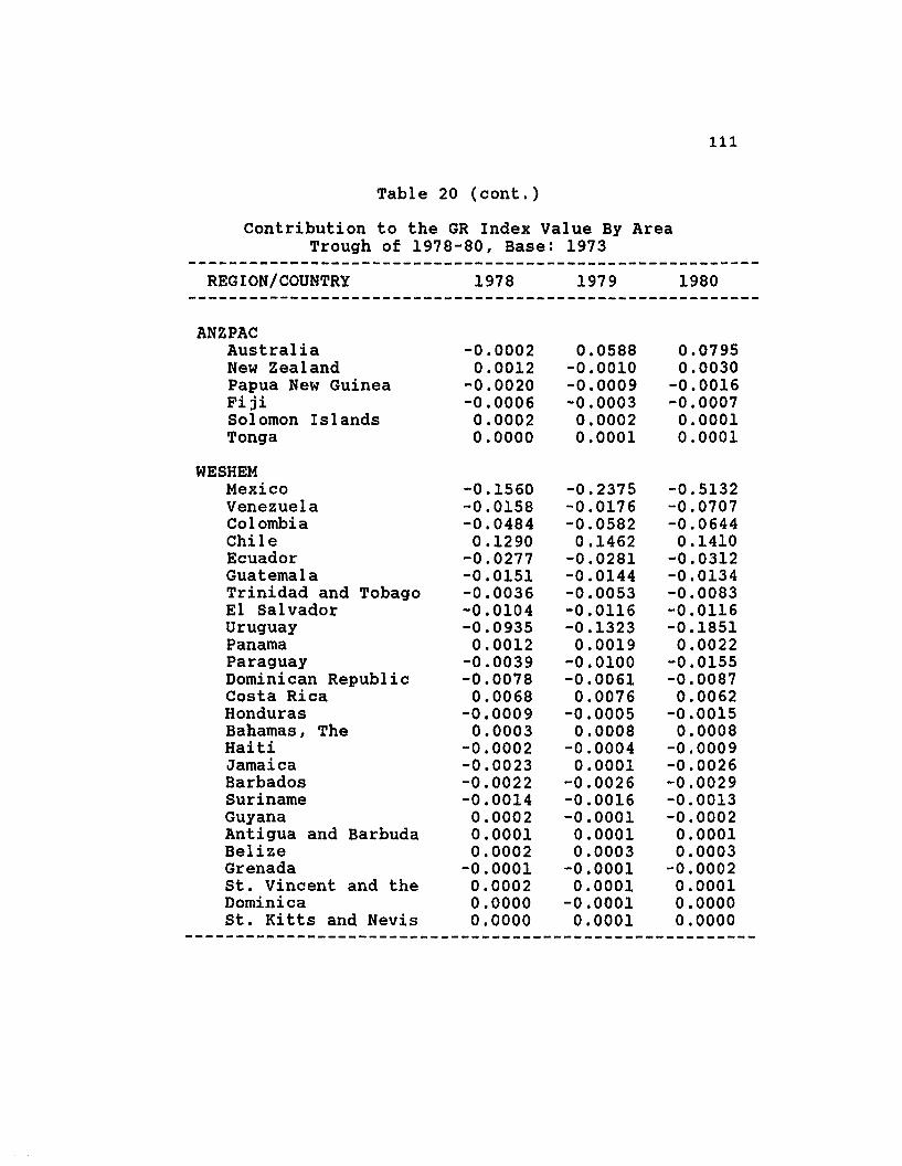
Table 20 (cont.)

Contribution to the GR Index Value By AreaTrough of 1978-80, Base: 1973

111

REGION/COUNTRY 1978 1979 1980

ANZPACAustralia -0.0002 0.0588 0.0795New Zealand 0.0012 -0.0010 0.0030Papua New Guinea -0.0020 -0.0009 -0.0016Fiji -0.0006 -0.0003 -0.0007Solomon Islands 0.0002 0.0002 0.0001Tonga 0.0000 0.0001 0.0001

WESHEMMexico -0.1560 -0.2375 -0.5132Venezuela -0.0158 -0.0176 -0.0707Colombia -0.0484 -0.0582 -0.0644Chile 0.1290 0.1462 0.1410Ecuador -0.0277 -0.0281 -0.0312Guatemala -0.0151 -0.0144 -0.0134Trinidad and Tobago -0.0036 -0.0053 -0.0083EI Salvador -0.0104 -0.0116 -0.0116Uruguay -0.0935 -0.1323 -0.1851Panama 0.0012 0.0019 0.0022Paraguay -0.0039 -0.0100 -0.0155Dominican Republic -0.0078 -0.0061 -0.0087Costa Rica 0.0068 0.0076 0.0062Honduras -0.0009 -0.0005 -0.0015Bahamas, The 0.0003 0.0008 0.0008Haiti -0.0002 -0.0004 -0.0009Jamaica -0.0023 0.0001 -0.0026Barbados -0.0022 -0.0026 -0.0029Suriname -0.0014 -0.0016 -0.0013Guyana 0.0002 -0.0001 -0.0002Antigua and Barbuda 0.0001 0.0001 0.0001Belize 0.0002 0.0003 0.0003Grenada -0.0001 -0.0001 -0.0002st. Vincent and the 0.0002 0.0001 0.0001Dominica 0.0000 -0.0001 0.0000st. Kitts and Nevis 0.0000 0.0001 0.0000

112

Table 20 (cont.)

Contribution to the GR Index Value By AreaTrough of 1978-80, Base: 1973

REGION/COUNTRY

MIDEASTIran, Islamic RepubSaudi ArabiaEgypt, Arab RepubliSyrian Arab RepubliKuwaitJordanBahrainYemen, PDR

ASIAPACChinaIndiaKorea, Republic ofIndonesiaThailandHong KongPhilippinesMalaysiaPakistanSingaporeBangladeshMyanmarSri LankaNepal

1978

-0.3021-0.4429-0.0743-0.0110-0.0219-0.0071-0.0146-0.0004

0.48910.1344

-0.1439-0.2790-0.0276-0.0081-0.04430.0009

-0.05900.00130.03350.00480.03100.0023

1979

-0.2985-0.36830.0637

-0.0051-0.0229-0.0084-0.0126-0.0002

0.53320.1950

-0.2016-0.0916-0.02320.0047

-0.06360.0062

-0.05080.00370.03360.00610.03310.0035

1980

-0.3443-0.43290.0690

-0.0121-0.0133-0.0100-0.0108-0.0002

0.60730.1796

-0.1172-0.1325-0.04030.0023

-0.07580.0162

-0.05200.00680.03430.01180.03390.0032

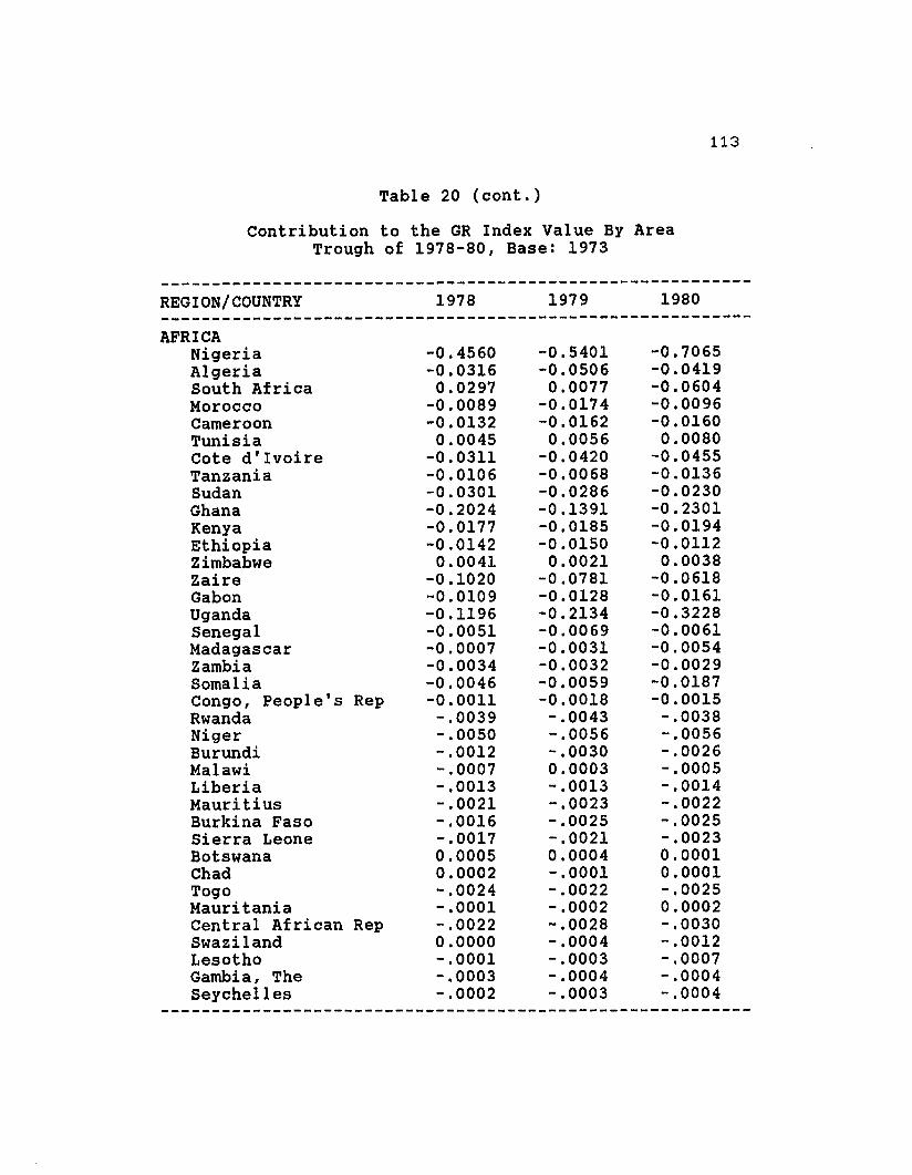
Table 20 (cont.)

Contribution to the GR Index Value By AreaTrough of 1978-80, Base: 1973

113

----------------------------------------------------------REGION/COUNTRY 1978 1979 1980----------------------------------------------------------AFRICA

Nigeria -0.4560 -0.5401 -0.7065Algeria -0.0316 -0.0506 -0.0419South Africa 0.0297 0.0077 -0.0604Morocco -0.0089 -0.0174 -0.0096Cameroon -0.0132 -0.0162 -0.0160Tunisia 0.0045 0.0056 0.0080Cote d'Ivoire -0.0311 -0.0420 -0.0455Tanzania -0.0106 -0.0068 -0.0136Sudan -0.0301 -0.0286 -0.0230Ghana -0.2024 -0.1391 -0.2301Kenya -0.0177 -0.0185 -0.0194Ethiopia -0.0142 -0.0150 -0.0112Zimbabwe 0.0041 0.0021 0.0038Zaire -0.1020 -0.0781 -0.0618Gabon -0.0109 -0.0128 -0.0161Uganda -0.1196 -0.2134 -0.3228Senegal -0.0051 -0.0069 -0.0061Madagascar -0.0007 -0.0031 -0.0054Zambia -0.0034 -0.0032 -0.0029Somalia -0.0046 -0.0059 -0.0187Congo, People's Rep -0.0011 -0.0018 -0.0015Rwanda -.0039 -.0043 -.0038Niger -.0050 -.0056 -.0056Burundi -.0012 -.0030 -.0026Malawi -.0007 0.0003 -.0005Liberia -.0013 -.0013 -.0014Mauritius -.0021 -.0023 -.0022Burkina Faso -.0016 -.0025 -.0025Sierra Leone -.0017 -.0021 -.0023Botswana 0.0005 0.0004 0.0001Chad 0.0002 -.0001 0.0001Togo -.0024 -.0022 -.0025Mauritania -.0001 -.0002 0.0002Central African Rep -.0022 -.0028 -.0030Swaziland 0.0000 -.0004 -.0012Lesotho -.0001 -.0003 -.0007Gambia, The -.0003 -.0004 -.0004Seychelles -.0002 -.0003 -.0004

----------------------------------------------------------

114

Table 21

Contribution to the GR Index Value By AreaPeak of 1984-86, Base: 1973

REGION/COUNTRY

GRl19

UNITED STATES

JAPAN

EUROPEGermany, Federal ReFranceUnited KingdomItalySpainNetherlandsSwedenSwitzerlandBelgiumAustriaNorwayDenmarkFinlandTurkeyYugoslaviaCzechoslovakiaGreecePortugalHungaryIrelandLuxembourgIcelandCyprusMalta

CANADA

1984

112.013

100.000

-0.493

2.5091. 9090.5861.1470.3870.4090.4140.0920.3680.1570.1200.1830.0660.2870.4260.1270.0890.0620.0450.0220.0150.0060.0110.005

0.556

1985

114.433

100.000

-0.275

2.7141.9690.6371.2380.3880.4580.4220.1260.3360.1730.1360.1950.0810.3040.4600.1440.1020.0630.0440.0260.0160.0060.0130.005

0.716

1986

101.483

100.000

-5.219

1. 2160.7040.0040.097

-0.0200.1090.215

-0.1600.119

-0.0270.0180.031

-0.0390.2430.3370.10540.03890.01840.0172

-0.02610.00730.00050.00840.0027

0.5512

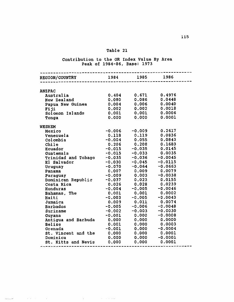
Table 21

Contribution to the GR Index Value By AreaPeak of 1984-86, Base: 1973

115

----------------------------------------------------------REGION/COUNTRY 1984 1985 1986----------------------------------------------------------ANZPAC

Australia 0.404 0.671 0.4976New Zealand 0.080 0.086 0.0448Papua New Guinea 0.004 0.006 0.0040Fiji 0.002 0.002 0.0018Solomon Islands 0.001 0.001 0.0006Tonga 0.000 0.000 0.0001

WESHEMMexico -0.006 -0.009 0.2617Venezuela 0.118 0.119 0.0836Colombia -0.004 0.055 0.0843Chile 0.206 0.208 0.1683Ecuador -0.015 -0.035 0.0145Guatemala -0.015 -0.033 0.0035Trinidad and Tobago -0.035 -0.036 -0.0045EI Salvador -0.030 -0.045 -0.0115Uruguay -0.070 -0.064 -0.0663Panama 0.007 0.009 0.0079Paraguay -0.009 0.003 -0.0038Dominican Republic -0.037 0.023 0.0155Costa Rica 0.026 0.028 0.0239Honduras -0.004 -0.005 -0.0046Bahamas, The 0.001 0.001 0.0002Haiti -0.003 -0.005 -0.0043Jamaica 0.009 0.011 0.0074Barbados -0.005 -0.006 -0.0048Suriname -0.002 -0.003 -0.0030Guyana -0.001 0.000 -0.0008Antigua and Barbuda 0.000 0.000 0.0000Belize 0.001 0.000 0.0003Grenada -0.001 0.000 -0.0004st. Vincent and the 0.000 0.000 0.0001Dominica 0.000 0.000 -0.0001st. Kitts and Nevis 0.000 0.000 0.0001

----------------------------------------------------------

Table 21 (cont.)

Contribution to the GR Index Value By AreaPeak of 1984-86, Base: 1973

116

REGION/COUNTRY 1984 1985 1986----------------------------------------------------------MIDEAST

Iran, Islamic Repub -1.066 -1.132 -1. 5933Saudi Arabia -0.145 -0.039 0.0159Egypt, Arab Republi -0.011 -0.053 -0.1242Syrian Arab Republi -0.064 -0.096 -0.1425Kuwait 0.016 0.020 0.0097Jordan -0.003 -0.001 -0.0051Bahrain -0.015 -0.011 -0.0064Yemen, PDR -0.001 -0.001 0.0000

ASIAPACChina 2.511 2.860 2.3164India 0.712 0.855 0.6295Korea, Republic of -0.006 0.079 0.0720Indonesia 0.114 0.172 0.1750Thailand 0.010 0.065 0.0460Hong Kong 0.098 0.098 0.0820Philippines 0.024 0.000 0.0260Malaysia 0.060 0.082 0.0670Pakistan 0.018 0.049 0.0460Singapore 0.028 0.037 0.0300Bangladesh 0.083 0.092 0.0710Myanmar 0.036 0.036 0.0190Sri Lanka 0.066 0.071 0.0550Nepal 0.009 0.011 0.0080

117

Table 21 (cont.)

Contribution to the GR Index Value By AreaPeak of 1984-86, Base: 1973

----------------------------------------------------------REGION/COUNTRY 1984 1985 1986----------------------------------------------------------AFRICA

NigeriaAlgeriaSouth AfricaMoroccoCameroonTunisiaCote d'IvoireTanzaniaSudanGhanaKenyaEthiopiaZimbabweZaireGabonUgandaSenegalMadagascarZambiaSomaliaCongo, People's RepRwandaNigerBurundiMalawiLiberiaMauritiusBurkina FasoSierra LeoneBotswanaChadTogoMauritaniaCentral African RepSwazilandLesothoGambia, TheSeychelles

-0.9750.0250.2270.0810.0180.0520.017

-0.030-0.013-0.0740.006

-0.0140.0190.0240.0060.0260.0070.0060.011

-0.0290.008-.0050.005-.0010.003-.0010.0020.005-.0080.0030.0040.0030.0020.0010.0000.0010.001-.001

-0.808-0.0100.3450.0910.0240.0540.018

-0.0440.007

-0.0380.008

-0.0200.0270.0290.0050.0200.0060.0080.015

-0.0120.009-.0060.006-.0010.0040.0000.0030.005-.0050.0060.0050.0030.0030.0000.0020.0010.001-.001

-0.0760-0.0860

0.23100.0690

-0.0030.038

-0.002-0.010-0.001-0.0130.006

-0.0110.0200.020

-0.0040.009

-0.0010.0040.015

-0.0020.002-.0070.003-.0020.0030.0000.0020.0020.0010.0050.0030.0010.002-.0020.0010.0010.001-.001

----------------------------------------------------------

118

in the sense of providing pointers where further

investigation of fundamental factors 9 may be required.

Tables 19 to 21 show that from 1969 to 1971, the

countries with the greatest impact on the dollar's global

value were Japan, Germany, France, and the United Kingdom,

in that order. These are also the G-5 nations on which the

SDR index is based. The rest of the G-10 countries, on

which the FRBRD index was based, follow in terms of order

of impact with the smallest effect coming from Canada. As

early as this period, strong effects on the dollar's value

were being registered by Spain, Austral ia, China, and

Mexico. All are countries excluded from the SDR and FRBRD

indices .10 Among the countries in Europe, onl y Turkey

showed the possibility of misalignment with a negative

impact on the index in 1969.

The region which shows a very strong possibility of

currency misalignments was the Western Hemisphere.

Countries in the list from Mexico to Honduras made negative

contributions to the dollar's value during the 1969-71 peak

9. Here we mean that nominal valuations and relative priceevolutions should be supported by sustainable levels in acountry's current and capital accounts.

10. The inclusion of Spain and some NIC's in the 16 countryindex of the 7-Gr poi nts to another reason why the 7-Grcorrelated well with the GR119 index.

119

period. This affirms trends in the Weshem regional index

which show a steeper fall in dollar values than the GRl19

index for this period. In the Middle East, it was only

Egypt which showed the possibility of misalignment. In the

Asia Pacific region, China, Thailand, and the Philippines

showed possibilities of an overvalued currency in 1969

during the 1969-71 peak period. Korea, Pakistan, and Sri

Lanka seem to have misaligned currencies for all of these

three years (1969-1971). In Africa, everything seems to be

in order in terms of alignment with the exception of

Somalia in 1969 and Sierra Leone for 1969 to 1971.

In the trough of 1978-80 Japan and most of Europe again

showed the expected al ignment. The onl y countries in

Europe which had 'misal igned' currencies were Cyprus and

Malta. Canada made positive contributions to the GR index

throughout this period and this could signal that Canada

had an undervalued currency for all of these three years.

There was also possible undervaluation in the Anzpac

countries with positive effects from Australia and New

Zealand for some years. For this period only small

countries like Antigua and Belize show some misalignment in

the Western Hemisphere. In the Asia Pacific region, the

strategy of competitive undervaluation seemed well

underway. During the 1978-80 period China, India,

Singapore, Malaysia, Bangladesh, Myanmar, Sri Lanka, and

120

Nepal all had a positive effect on the dollar's value in

all three years. Hong Kong had a positive impact in 1979

and 1980. In the African region, only South Africa and

Botswana showed the possibility of currency undervaluation

in this period. The reference to undervalued or overvalued

currencies is solely based on the misaligned currency

effect compared to the average direction signaled in the

overall index. As al ready noted, there coul d be other

fundamental factors that could justify such an effect.

During the peak of 1984-86, the impact of Japan was

interestingly negative but this seems justified by Japan's

status as a trade and capital exporter. Germany on the

other hand continued to have 'properly' aligned effects on

the dollar's global value. This comparative behavior would

seem to indicate that at that point, of the two currencies,

the Yen was much stronger than the Deutschemark in the

international financial system. In Europe, some

misalignment seem to be signaled by Spain, Switzerland,

Austria, Finland, and Ireland. A closer look to say what is

really happening may be required here as is the case with

Japan. Among the larger countries in the Western

Hemisphere, only Venezuela, Chile, Panama, Costa Rica, The

Bahamas, and Jamaica were 'aligned' with the dollar's

change. The other countries showed possibl e misal ignment.

In the Middle East, only Kuwait moved with the dollar. In

121

the Asia Pacific area only Korea showed a .move opposite to

the dollar and then only in 1984. During this period, a~

examination of the African region showed the possibility of

currency misalignment in most countries.

TQe GR119 index, being computable back to the 1950

period using period-specific weights also allows us to

track the evolution of the dollar on a long term basis

wi thout worrying about the effects of structural shifts.

The regional components of this index help us analyze the

evolution of the dollar's real value in a truly global

manner. By complementing these geographic component

changes with a decomposition of GR119 index changes

according to factor component effects, we should be able to

tell a more compl ete story about the evol ution of the

global dollar's real value. For this complete story, we

proceed to the next chapter where we decompose our index

changes into relative price and non-relative price effects.

122

Chapter 4

A METHODOLOGY FOR EXPLAINING FACTOR-SPECIFIC CHANGESIN THE DOLLAR'S REAL VALUE

The Base Value Index

Earlier, we identified the impact of regions and

countries on the dollar's global values. Using similar

methods which take advantage of the same unique period-

specific weights and the presence of a weight for the US

economy in the GR119, we can also decompose the changes in

our index to isolate effects of the factors used in its

construction. For this decomposition, choosing a base year

at which the dollar's global nominal value will be held

constant is a necessary first step. Usually, this choice

is essentially considered an arbitrary exercise. This was

true in the case of our decomposi tion of regional and

country speci fic effects which was not sensi ti ve to base

year choice. But, for a meaningful decomposition of our

index involving relative factors that cut across regions

and countries, and for other reasons detailed below, we

will have to look more closely at the selection of a base

year.

We used 1973 as the base year in our previous

computations of our GR indices to facilitate comparison

with the other real indices of the dollar. But, in

123

choosing a base year for decomposing our new index, we

will take advantage of the historical fact that 1979 is the

lowest trough year in dollar real values for the 40 year

period from 1950 to 1990. Thus, selecting 1979 will help

in our decomposition process by mitigating the distorting

effects of changes in nominal rates and relative prices on

shifts in GWP shares. With nominal exchange rates at

their lowest trough in the base period, their effect of

lowering the us share relative to the ROW share of GWP is

at its highest. At the peak of dollar values, the opposite

is true with the exchange rate effect's tendency to

increase us share of GWP at its highest.

The same distorting effects on GDP shares occur wi th

changes in relative prices. Increasing US relative prices

will tend to increase the us share as measured in nominal

values even without an actual shift in real output shares.

Thus, as the dollar's real value climbs out of our base

year trough towards a peak, the effect that is directly

related to ROW share of GWP is underestimated to the extent

that rising relative prices distort shifts in shares.

With a clear baseline regarding the distortions caused

by nominal exchange rates and relative prices on GWP

shares, we end up with a consistent compensating bias for

share effects. The danger then of overestimating changes

in the global real index that is attributed to shifts in

124

shares is mitigated and the possibility of drowning out the

impact of other factors effecting changes in the dollar's

real value with the share effect is reduced. With the us

share of GWP inversely related to the dollar's real value,

this implementation of the weights also serves to factor

in the stabilizing influence of the us economy on the

upward and downward swings in dollar values.

The base year sets the effective nominal dollar

exchange rate index and the weighted relative price index

(US/ROW) for the ROW equal to one. In effect, when we

choose a base year, we hypothetically conjure a composite

currency in the ROW with a unit of that currency buying a

bundle of ROW real goods equal in value to the bundle of

goods that one dollar can buy at base year prices. Since

one ROW nominal dollar buys a real bundle of goods in the

ROW that is equal in value to the bundle of US goods that

one US dollar can buy, then one real ROW dollar exchanges

for an exact one US real dollar in the base year. In this

sense, the whole world is effectively using a single

currency in our base year.

outside the base year, the ratio of US to ROW prices

and the nominal exchange rate between the US dollar and the

composite ROW currency can move away from one thus changing

the ROW real exchange rate. But as the base economy or

anchor point for evaluating the nominal exchange rate and

125

relative price changes of the other economies of the world,

the relative price index and the nominal exchange rate

index for the global dollar is always one in the us

economy.

The dollar's global real value index can be viewed as a

mapping of the evolution in real value of the goods and

services that a dollar unit commands through time given a

hypothetical situation where all the world's goods and

services are denominated in US dollars. As explained

above, it is also in fact a weighted average of the

dollar's real value both in the us and in the ROW. Since

we have initialized the real value of our nominal composite

ROW dollar to the real value that a US dollar can buy in

the base year, changes in the real exchange rates of the

ROWand the global dollar will be reflected in the global

real value index in terms of base year real values.

The choice of base year therefore determines the

constant US prices used by our index in tracking the global

dollar's real value. Given changing US prices, the real

value that one nominal dollar can buy in 1973 is not the

same as what one nominal dollar can buy in 1979. For

instance, if we use 1973 as our base year, our index

reference point for the dollar's global real value is what

one US dollar can buy in the US at 1973 prices. As we key

our composite nominal ROW doll ar to this val ue, the real

126

value that one ROW nominal dollar can buy in the ROW in the

base year , with the existing relative prices and nominal

rates becomes equal to one us real dollar at 1973 prices.

Therefore, in the base year, one real ROW dollar equals one

real us doll ar , At this point, the global real dollar's

index value is also one.

If the global dollar's real value falls below 1973 base

values as in 1979, the index simply states that with the

movements in relative prices and nominal rates, the 1979

US dollar has less real value than a 1973 us dollar in

terms of what it can buy not only in the us but also on a

worldwide basis. How much less is determined by the nega­

tive difference of the 1979 index value from the base value

in 1973. However, if rather than 1973 we use 1979 as our

base year, while the index still reflects the same fact

that a 1979 us dollar is less valuable than a 1973 US

doll ar in real terms, our global index is not below the

base year value since we have keyed the base year real

value of the composite ROW nominal dollar to one US real

1979 dollar.

The global rates' being below or above base values at

an initial point has implications for the effect of shifts

in GWP shares between the us and the ROW. Since the global

rate is the weighted average of the US dollar's value in

the US and the ROW, from a starting point where the ROW's

127

real exchange rate is above base values the global dollar

index will decrease with an increase in us share of GWP.

But from an initial point where the ROW's real exchange

rate is below base values the same increase in us share of

GWP will this time improve the global dollar index value.

In the first instance, the result is global dollar

depreciation as the average real value of a global dollar

goes down. In the second instance, the resul t is global

dollar appreciation as the average real value of a global

dollar goes up. By choosing a base year that is the lowest

trough point in global rates for the whole period, we give

the effects of GWP share changes a consistent bias until a

new low threshold of the dollar's global value is reached

at some future point in time.

At the base year, the value of our global dollar real

index is one and the corresponding global nominal dollar

index is also one. By holding this base year global

nominal val ue constant at one and defl ating through time

with the weighted relative price index, we are able to

trace the path of the dollar's global real value and the

full effects of weighted relative price changes, isolated

from the effects of other factors. In doing so, we have

effecti vel y frozen the demand and suppl y factors that

determine the level of the dollar's effective nominal rate

in the base year or assumed that these factors shift in

128

offsetting directions through time. We call our result the

base value index because it is a real value derived by

inflating or deflating the global nominal dollar in the

base year with the observed changes in weighted relative

prices.

The base value index gives us the real value a nominal

dollar at any time t would have, given the same or

equivalent set of nominal exchange rates between the us and

the ROW that prevailed in the base year after adjustments

for relative price movements. With nominal rates constant

and weighted relative prices ( US/ROW ) going up or down,

the base value index gives us the change required in the

dollar's global real value from its base year value of one

to validate a one to one intertemporal rate of exchange

between a nominal dollar at any time t and the nominal

dollar in the base year. In contrast, the global real

value index gives the real value of a nominal dollar at any

time t given the movements in relative prices together

with changes in nominal rates. The global real dollar

index indicates by how much more or how much less the real

value of a nominal dollar is at any time compared to its

real value in the base year.

129

The Adjustment Value Index

Since the global dollar real index varies with the

movements of weighted nominal exchange rates and relative

prices while the base value index varies only with the

movements in weighted relative prices, we would naturally

find deviations between the global and the base value index

as we move away from a common base year. This difference

between the two indices gives us an indication of the

extent to which factors other than changes in weighted

relative prices impact on the dollar's global real value.

The difference, which we will call the adjustment value

component, represents a downward or upward adjustment in

the ROW nominal exchange rate index that would bring the

global real dollar index to the level of its corresponding

base value index in any given year.

The size and the sign of the adjustment value component

are determined by the direction and extent to which the ROW

nominal index value deviates from the one to one valuation

of the dollar in the base year. If the base value of the

dollar at a certain point is higher than the computed real

index value, this means that the effective average nominal

value of the dollar in the ROW is lower than it was in the

base year and the adjustment component will be negative.

In the opposite case, the effective average nominal value

130

of the dollar in the ROW would be higher than its level in

the base year and the adjustment component will be

positive. So, while our base value index is principally

linked with movements in weighted relative prices, the

adjustment value component is mainly determined by

movements in weighted nominal rates.

The adjustment component gives us an indication of how

far the actual real index value of the dollar deviates from

the base real index value. In a flexible exchange system,

this could tell us whether or not the dollar is trading at

a premium or a discount compared to the change expected

on the basis of the weighted relative price movements. The

sign and magnitude of this difference can thus be used to

search for the other factors which have either reinforced

or mitigated the impact of weighted relative prices on the

dollar's global real value.

Ignoring weighting systems, we can summarize as

follows:

GR = A / P or GR = A R

GR = Real Value Index

A = Nominal Index

P = Ratio of ROW prices to US prices.

R = Ratio of US prices to ROW prices = 1 / P

131

A = 1 , P = 1 in the base year, therefore

GR = A / P = A * R = 1

Holding A at the constant base value of 1 we have

B = R = 1 / P = the value of the dollar resulting fromrelative price changes over base year,hereafter called the base value.

And X = GR - B = the adjustment value of the dollarresulting from all other sources of change.

Rearranging we get GR = B + X, showing B and X as

components of GR.

Expressed in terms of the Nominal index and the relative

price index

X = ( A / P ) - ( 1 / p) = ( A

or

X = (A * R) - R = R ( A - 1)

1 ) / P

In the base year A = 1 and therefore X = 0; outside the

base year, when A is less than one then X will be negative,

when A is greater than one then X will be positive. In the

base year, B = 1 and therefore GR is also equal to one.

Using the geometric weighting formula in Chapter 3 , the

GR119 index with its base and adjustment value component,

this time keyed to base year 1979, is presented in Table

22.

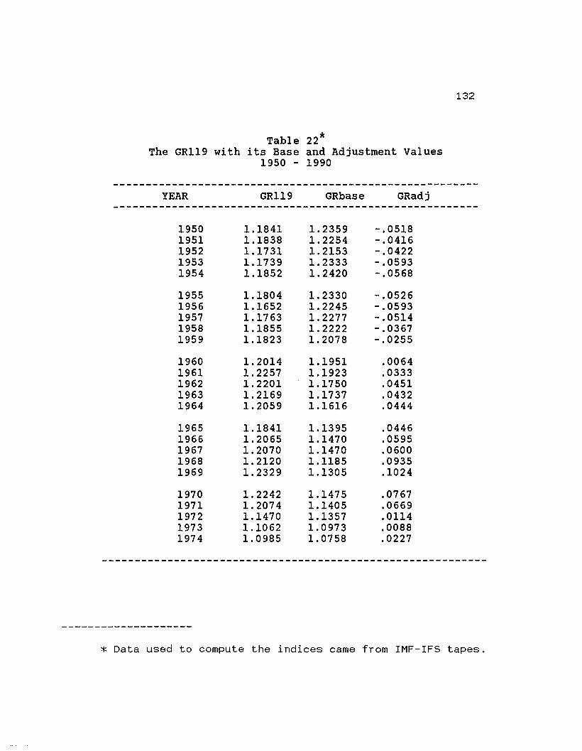
132

Table 22*The GR119 with its Base and Adjustment Values

1950 - 1990

--------------------------------------------------------YEAR GR119 GRbase GRadj

--------------------------------------------------------

1950 1.1841 1. 2359 -.05181951 1.1838 1.2254 -.04161952 1.1731 1. 2153 -.04221953 1.1739 1. 2333 -.05931954 1.1852 1. 2420 -.0568

1955 1.1804 1. 2330 -.05261956 1.1652 1. 2245 -.05931957 1.1763 1. 2277 -.05141958 1.1855 1.2222 -.03671959 1.1823 1.2078 -.0255

1960 1. 2014 1.1951 .00641961 1. 2257 1.1923 .03331962 1. 2201 1.1750 .04511963 1.2169 1.1737 .04321964 1. 2059 1.1616 .0444

1965 1.1841 1.1395 .04461966 1. 2065 1.1470 .05951967 1.2070 1.1470 .06001968 1.2120 1.1185 .09351969 1. 2329 1.1305 .1024

1970 1. 2242 1.1475 .07671971 1. 2074 1.1405 .06691972 1.1470 1.1357 .01141973 1.1062 1. 0973 .00881974 1. 0985 1.0758 .0227

* Data used to compute the indices came from IMF-IFS tapes.

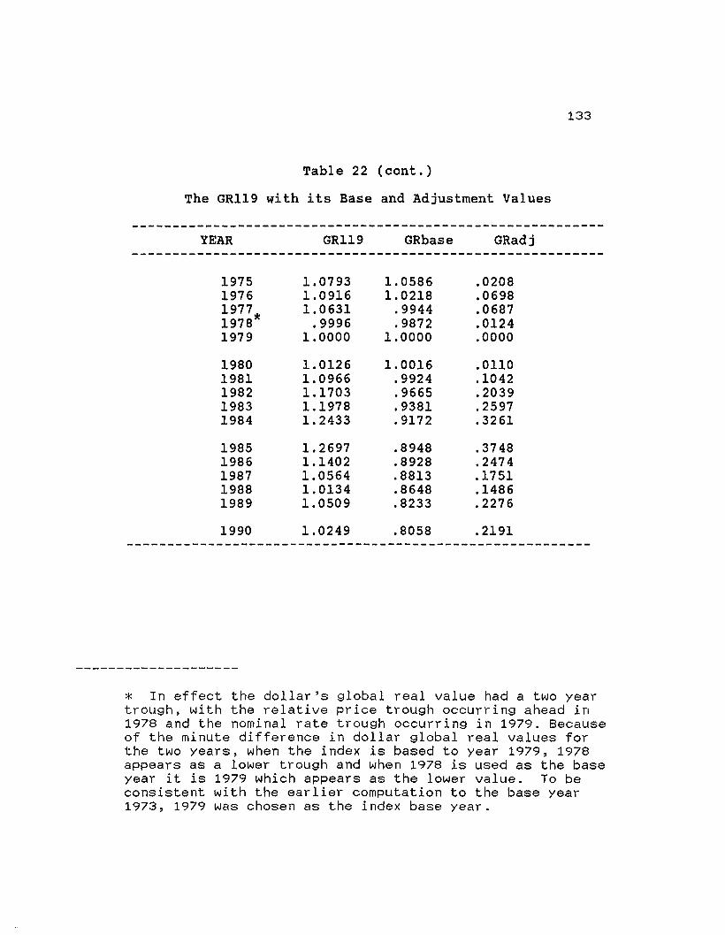
133

Table 22 (cont.)

The GRl19 with its Base and Adjustment Values

----------------------------------------------------------YEAR GRl19 GRbase GRadj

----------------------------------------------------------

1975 1.0793 1.0586 .02081976 1.0916 1.0218 .06981977* 1.0631 .9944 .06871978 .9996 .9872 .01241979 1.0000 1.0000 .0000

1980 1. 0126 1. 0016 .01101981 1. 0966 .9924 .10421982 1.1703 .9665 .20391983 1.1978 .9381 .25971984 1. 2433 .9172 .3261

1985 1. 2697 .8948 .37481986 1.1402 .8928 .24741987 1.0564 .8813 .17511988 1. 0134 .8648 .14861989 1.0509 .8233 .2276

1990 1.0249 .8058 .2191

* In effect the dollar's global real value had a two yeartrough, with the relative price trough occurring ahead in1978 and the nominal rate trough occurring in 1979. Becauseof the minute difference in dollar global real values forthe two years, when the index is based to year 1979, 1978appears as a lower trough and when 1978 is used as the baseyear it is 1979 which appears as the lower value. To beconsistent with the earlier computation to the base year1973, 1979 was chosen as the index base year.

134

Figure 17

GR119, its GR BASE and GRadJ COMPONENTS194B - 1990

QRadJ

GRl19

1-4-0r-----------------------,130

GR"":~~~~~l!i!!ll~~~~~n_I~O

110

100

90BO7060DO-4-030

2010

_I ~ ~-_;::;;:;;:;:;:;:;...~~~~~~~~~..L=------1

-20-3D '---.-..........._r..,.......,...,...T"T'",...,...,........,,...,..,:-r"T,..,...,.........--r,.,..T"T'"...-.-~,...,..,,..,....._r_._---J

C [)R119 oQ ORElCOOt.l

The *decomposition just presented highlights the

importance of base year choice because it would affect the

way we draw insights and conclusions from the resulting

indices. Since the adjustment value component would be

deliberately zero in the base year, choosing a year like

1985 with the highest real value for the dollar as the base

year would set the adjustment value component to zero in

1985 and make it negative for all the other years outside

* The data used for Figure 17 comes from Tables 17 and 18.Note the negative values of GRadj before 1960. Thisindicates that nominal values for the dollar are belowbase year values.

135

the base year. This happens because the nominal index

never exceeds its peak value in 1985. This would entail

reversing our approach to the interpretation of the index

results but basically, it would not change our conclusions.

The decision to use either the highest peak or the lowest

trough as the base year for our index is similar to the

choice of using either the ratio of US to ROW prices or its

reciprocal to represent relative prices. In both cases the

different alternatives can be used; it is the

interpretation of the results that matters. The

behavioral links of relative prices and relative output to

nominal exchange rates are, of course, unaffected by our

base year choices.

As shown in Tables 22 and 27, changes in our global

index come from changes in the base value index and from

the adjustment component. That decomposition separates the

effects of changes in weighted relative prices from changes

in weighted nominal exchange rates and other sources of

change. The base value index maps the effects of changes

in weighted relative prices. The adjustment value index

principally maps the impact of changes in weighted nominal

exchange rates on the GRl19 index. But since GRadj is a

residual resul t after the base val ue index is subtracted

from the GRl19 index, it also contains the joint effect of

the changes in the base value index and the changes in the

136

nominal value index, as well as the composition effect

which is the result of aggregating different countries with

different exchange rates.

The Composition or Aggregation Effect

The first step to get the aggregation component of the

GRl19 index is to compute the index again to suit a world

of only two countries: the traditional US and ROW

exposi tion in standard textbooks. For this purpose a

nominal exchange rate and a relative price had to be

computed for the ROW. This was done using the same gross

product shares to compute GRl19 as geometric weights, this

time rebased to fit a ROW aggregation.

The resulting version of the GRl19 index or GRINDX

deliberately ignores the joint effects of the weights and

the real exchange rate shifts of the different countries

and currencies aggregated into the global dollar index. In

the GRl19 formula, the real exchange rates of each country

is weighted individuall y in arriving at the global index

value and it therefore includes the joint effects from

country specific real exchange rates. The GRINDX takes a

geometric average of the ROW real exchange rate and then

weights it with the ROW share of GWP as an aggregate to get

the global dollar index value. The ROW average values show

137

one net direction of change for the ROW real exchange rate

and this determines the way the ROW weight share impacts

on the global value in the GRINDX. If the net direction in

ROW real exchange rates reflects the movements in country

specific real exchange rates aggregated in GRl19 then there

will be very little or no difference between these two

versions of the global index value (see Table 23).

Instances where a discrepancy exists between the GRl19 and

the GRINDX suggest that something is amiss.

Taking the difference between the GRl19 index and the

GRINDX we get a residual which gives us this joint effect

of the separate movements in the country specific real

exchange rates that are included in the GRl19 index but not

captured in a two country aggregation. GResid shows the

extent and direction of such effects since it is the

difference between the GRl19 and the GRINDX indices. It

will be positive when these simultaneous shifts in real

exchange rates are skewed towards increases in the dollar's

real value compared to the average shift for the ROW. It

will be negative, when the shifts in individually weighted

real exchange rates are skewed towards decreases in the

doll ar' s real val ue compared to the average shi ft in the

ROW. Thus, because of this characteristic, GResid can

also be used as a measure of currency misalignments.

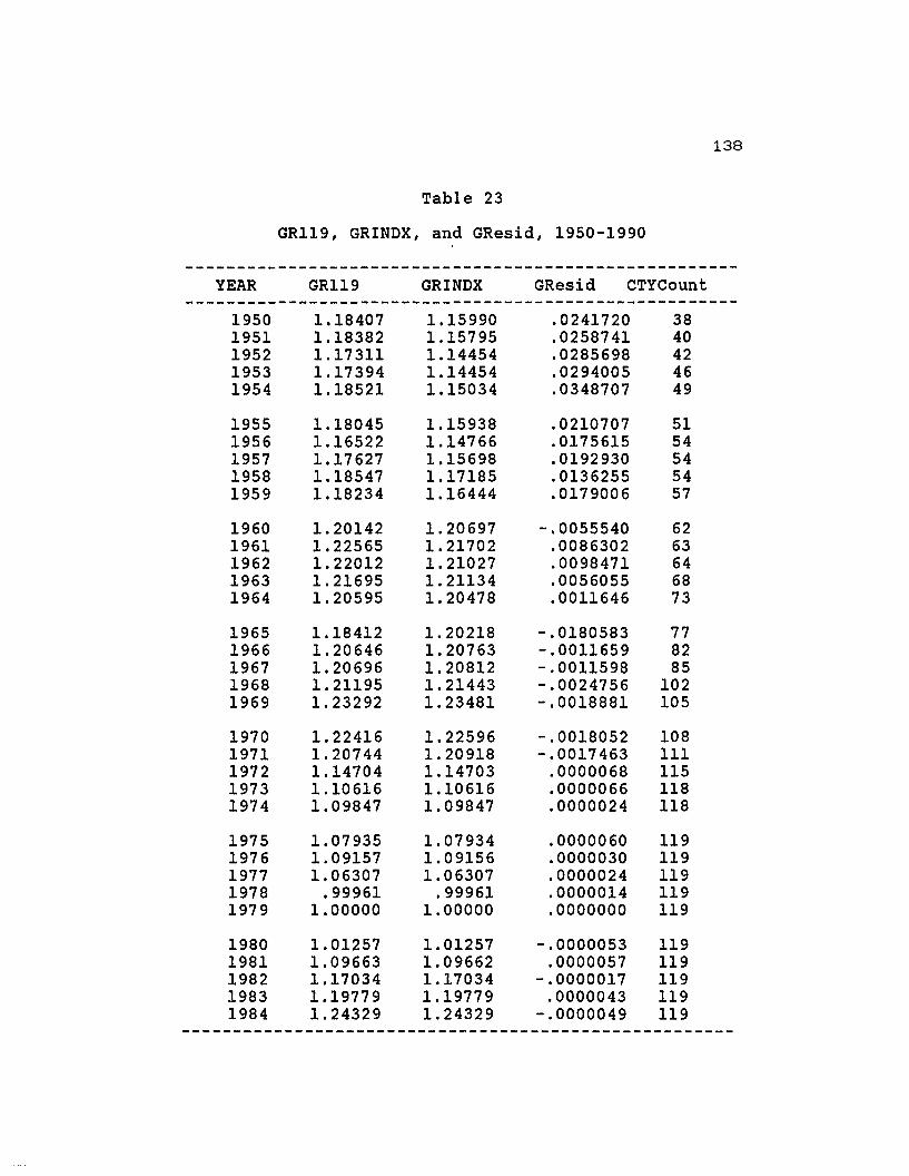
138

Table 23

GR119, GRINDX, and GResid, 1950-1990

------------------------------------------------------YEAR GRl19 GRINDX GResid CTYCount

------------------------------------------------------1950 1.18407 1.15990 .0241720 381951 1.18382 1.15795 .0258741 401952 1.17311 1.14454 .0285698 421953 1.17394 1.14454 .0294005 461954 1.18521 1.15034 .0348707 49

1955 1.18045 1.15938 .0210707 511956 1.16522 1.14766 .0175615 541957 1.17627 1.15698 .0192930 541958 1.18547 1.17185 .0136255 541959 1.18234 1.16444 .0179006 57

1960 1.20142 1. 20697 -.0055540 621961 1. 22565 1. 21702 .0086302 631962 1.22012 1.21027 .0098471 641963 1. 21695 1.21134 .0056055 681964 1.20595 1. 20478 .0011646 73

1965 1.18412 1.20218 -.0180583 771966 1. 20646 1. 20763 -.0011659 821967 1. 20696 1.20812 -.0011598 851968 1.21195 1.21443 -.0024756 1021969 1.23292 1.23481 -.0018881 105

1970 1. 22416 1. 22596 -.0018052 1081971 1.20744 1. 20918 -.0017463 1111972 1.14704 1.14703 .0000068 1151973 1.10616 1.10616 .0000066 1181974 1. 09847 1. 09847 .0000024 118

1975 1. 07935 1. 07934 .0000060 1191976 1. 09157 1. 09156 .0000030 1191977 1.06307 1. 06307 .0000024 1191978 .99961 .99961 .0000014 1191979 1.00000 1.00000 .0000000 119

1980 1.01257 1.01257 -.0000053 1191981 1.09663 1. 09662 .0000057 1191982 1.17034 1.17034 -.0000017 1191983 1.19779 1.19779 .0000043 1191984 1. 24329 1. 24329 -.0000049 119

------------------------------------------------------

139

Tabl e 23 (cont.)

GRl19, GRINDX, and GResid, 1950-1990

YEAR GRl19 GRINDX GResid CTYCount

1985 1. 26966 1. 26966 -.0000018 1191986 1.14020 1.14020 .0000035 1171987 1.05637 1.05637 .0000022 1171988 1.01343 1.01342 .0000026 1151989 1.05087 1.05163 -.0007605 111

1990 1. 02491 1. 02734 -.0024269 108

A column on number of countries included in the indexis also presented since changes in country composition maychange weight shares drastically and also affect GResid.Data used for GRINDX computation are in Appendix Table 4.1.

In a two country world ( us and the ROW), the value

for the global dollar index for any time t (GRINDXt) can be

represented as follows:

GRINDXt = (RRt) / (RRb) ** Wt

Wt = ROW share of GWP < 1

** = exponentiation operator

RRt = Real Rate at time t

RRb = Real Rate in the Base year

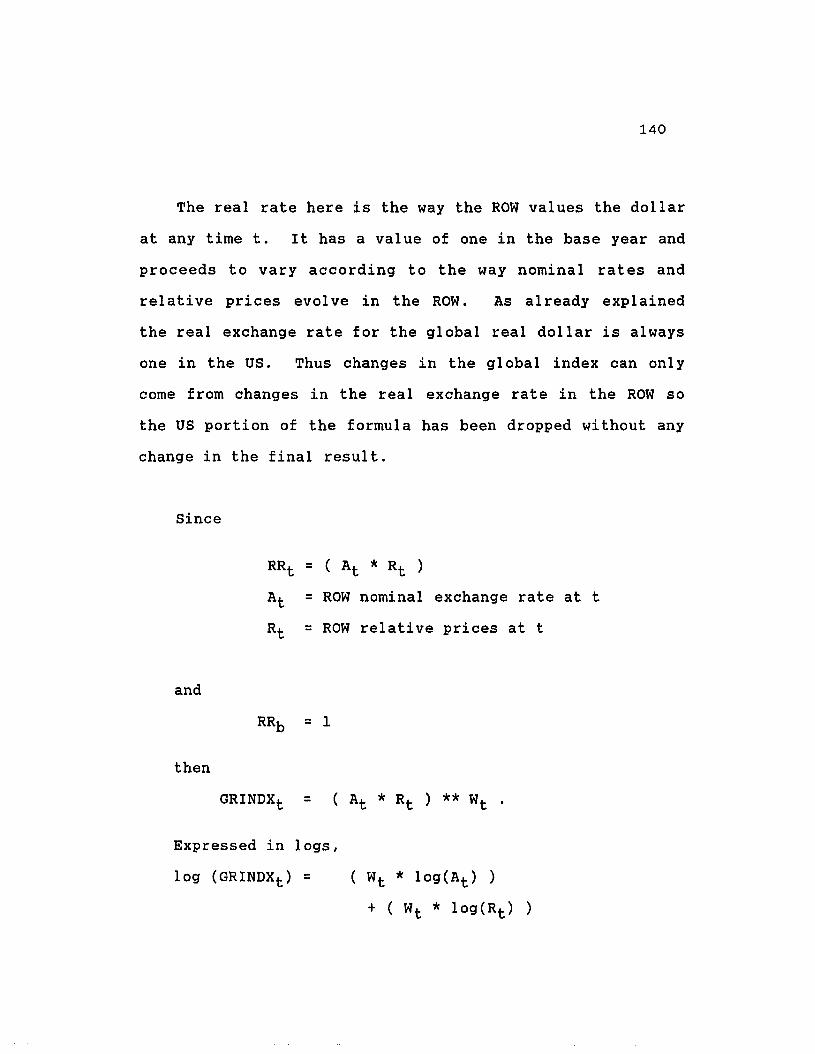
140

The real rate here is the way the ROW values the dollar

at any time t. It has a value of one in the base year and

proceeds to vary according to the way nominal rates and

reI ati ve prices evol ve in the ROW. As al ready expl ained

the real exchange rate for the global real dollar is always

one in the us. Thus changes in the global index can only

corne from changes in the real exchange rate in the ROW so

the us portion of the formula has been dropped without any

change in the final result.

Since

RRt = ( At * Rt )

At = ROW nominal exchange rate at t

Rt = ROW relative prices at t

and

then

GRINDXt =

Expressed in logs,

log (GRINDXt) = ( Wt * 10g(At) )

+ ( Wt * 10g(Rt) )

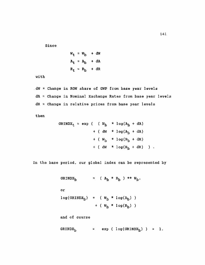
141

Since

Wt = Wb + dW

At = Ab + dA

Rt = Rb + dR

with

. dW = Change in ROW share of GWP from base year levels

dA = Change in Nominal Exchange Rates from base year levels

dR = Change in relative prices from base year levels

then

GRINDXt = exp ( ( Wb * log(Ab + dA)

+ ( dW * log(Ab + dA)

+ ( Wb * log(Rb + dR)

+ ( dW * log(Rb + dR) ) 0

In the base period, our global index can be represented by

GRINDXb = ( Ab * Rb ) ** Wb o

or

log(GRINDXb) = ( Wb * log(Ab) )

+ ( Wb * log(Rb) )

and of course

GRINDXb = exp ( log(GRINDXb) ) = 1.

142

where

b = 1979

exp = the antilog operator

* = multiplication operator

At = Nominal Dollar Rate in ROW for t

Rt = Relative price index in ROW for t

Wt = GWP share of ROW for t

and

Ab = Nominal Dollar Rate in ROW for the base year

Rb = Relative price index in ROW for the base year

Wb = GWP share of ROW for the base year.

Component Changes in GRINDX

At this point, we have decomposed the GRl19 value into

the GRINDX and GResid. The GRINDX can be decomposed

further to show the independent effects of relative prices,

nominal exchange rates and the separate effects of weight

shifts through relative prices and nominal exchange rates.

The change we are interested in decomposing is the change

of GRINDX from its base period levels shown as:

oGRINDXt = GRINDXt - GRINDX b

= exp ( 10g(GRINDXt)

143

exp ( 10g(GRINDXb) )

Since exp ( 10g(GRINDXb) ) = 1

then

oGRINDX = exp ( ( Wb * 109(Ab + dA)

+ ( dW * 10g(Ab + dA)

+ ( Wb * 10g(Rb + dR)

+ ( dW * 10g(Rb + dR) )

1 .

The independent effects of changes in the nominal

rates, relative prices, and the impact of share changes

through relative prices and through nominal rates on the

GRINDX value is easily computed by alternately setting the

relevant log terms in the argument of the antilog operator

to a non-zero value in the above equation.

Therefore:

Rdelta = exp ( Wb * 10g(Rb + dR) ) - 1

Adelta = exp ( Wb * 10g(Ab + dA) ) - 1

RWdelta = exp ( dW * 109(Rb + dR) ) - 1

AWdelta = exp ( dW * 10g(Ab + dA) ) - 1

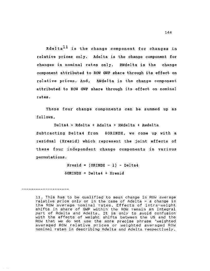
144

Rdelta 1 1 is the change component for changes in

relative prices only. Adelta is the change component for

changes in nominal rates only. RWdelta is the change

component attributed to ROW GWP share through its effect on

relative prices. And, AWdelta is the change component

attributed to ROW GWP share through its effect on nominal

rates.

These four change components can be summed up as

fo11 ows,

Delta4 = Rdelta + Adelta + RWdelta + Awdelta

subtracting Delta4 from &GRINDX, we come up with a

residual (Xresid) which represent the joint effects of

these four independent change components in various

permutations.

Xresid = (GRINDX - 1) - Delta4

&GRINDX = Delta4 + Xresid

11. This has to be qualified to mean change in ROW averagerelative price only or in the case of Adelta - a change inthe ROW average nominal rates. Effects of intra-weightshifts in share of GWP within the ROW remain an integralpart of Rdel ta and Adel ta. It is only to avoid confusionwi th the effects of weight shi fts between the US and theROW that we do not use the more precise phrase 'weightedaveraged ROW relative prices or weighted averaged ROWnominal rate~ in describing Rdelta and Adelta respectively.

145

Representing the change in the GRl19 index from its base

year values as,

GRdelta = GRl19 t - GRl19 b

then we have so far decomposed GRdelta into

GRdelta = oGRINDX + GResid or

GRdelta = Delta4 + Xresid + GResid

The computed component changes of GRINDX and related

variables are reported out in Tables 24 to 27.*

* Basic data for the results in these tables are inAppendix Table 4.1.

146

Table 24

Main Components of the Change in GR119from Base Year Values (GRdelta)

1950-1990

----------------------------------------------------~-- - - - -

YEAR GRDELTA DELTA4 XRESID GRESID-----------------------------------------------------------

1950 0.18407 0.21664 -0.0567300 0.0241721951 0.18382 0.21258 -0.0546300 0.0258741952 0.17311 0.19287 -0.0483400 0.0285701953 0.17394 0.20175 -0.0572100 0.0294011954 0.18521 0.20693 -0.0566000 0.034871

1955 0.18045 0.20844 -0.0490600 0.0210711956 0.16522 0.19182 -0.0441600 0.0175621957 0.17627 0.19891 -0.0419300 0.0192931958 0.18547 0.20608 -0.0342400 0.0136251959 0.18234 0.19486 -0.0304200 0.017901

1960 0.20142 0.22021 -0.0132400 -0.0055541961 0.22565 0.22855 -0.0115300 0.0086301962 0.22012 0.21794 -0.0076600 0.0098471963 0.21695 0.21733 -0.0059900 0.0056061964 0.20595 0.20809 -0.0033100 0.001165

1965 0.18412 0.20108 0.0011062 -0.0180581966 0.20646 0.20822 -0.0005917 -0.0011661967 0.20696 0.20843 -0.0003114 -0.0011601968 0.21195 0.21031 0.0041171 -0.0024761969 0.23292 0.22934 0.0054633 -0.001888

1970 0.22416 0.22125 0.0047083 -0.0018051971 0.20744 0.20499 0.0041910 -0.0017461972 0.14704 0.14816 -0.0011321 0.0000071973 0.10616 0.10616 -0.0000019 0.0000071974 0.09847 0.09721 0.0012596 0.000002

1975 0.07935 0.07833 0.0010090 0.0000061976 0.09157 0.09033 0.0012276 0.0000031977 0.06307 0.06366 -0.0005884 0.0000021978 -0.00039 -0.00022 -0.0001655 0.0000011979 0.00000 0.00000 0.0000000 0.000000

-----------------------------------------------------------

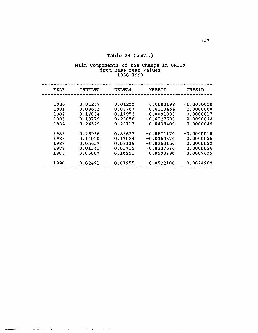
Table 24 (cont.)

Main Components of the Change in GRl19from Base Year Values

1950-1990

147

YEAR GRDELTA DELTA4 XRESID GRESID

1980 0.01257 0.01255 0.0000192 -0.00000501981 0.09663 0.09767 -0.0010454 0.00000601982 0.17034 0.17953 -0.0091830 -0.00000171983 0.19779 0.22056 -0.0227680 0.00000431984 0.24329 0.28713 -0.0438400 -0.0000049

1985 0.26966 0.33677 -0.0671170 -0.00000181986 0.14020 0.17524 -0.0350370 0.00000351987 0.05637 0.08139 -0.0250160 0.00000221988 0.01343 0.03719 -0.0237670 0.00000261989 0.05087 0.10251 -0.0508790 -0.0007605

1990 0.02491 0.07955 -0.0522100 -0.0024269

148

Table 25

Components of Delta4, 1950-1990

--------------------------------------------------------YEAR RDELTA ADELTA RWDELTA AWDELTA

--------------------------------------------------------1950 0.37857 -0.09169 -0.10351 0.0332701951 0.37141 -0.08420 -0.10648 0.0318501952 0.34435 -0.08703 -0.09599 0.0315401953 0.36857 -0.10574 -0.09885 0.0377701954 0.37118 -0.10570 -0.09418 0.035620

1955 0.35721 -0.08588 -0.09151 0.0286201956 0.33461 -0.08824 -0.08249 0.0279301957 0.33478 -0.08011 -0.08023 0.0244801958 0.32146 -0.05678 -0.07511 0.0165101959 0.30328 -0.04999 -0.07327 0.014840

1960 0.26692 0.01326 -0.05672 -0.0032401961 0.26539 0.02782 -0.05774 -0.0069101962 0.23976 0.04021 -0.05224 -0.0097901963 0.23277 0.04211 -0.04792 -0.0096301964 0.21203 0.04802 -0.04164 -0.010320

1965 0.17711 0.06908 -0.031915 -0.0131981966 0.19259 0.06844 -0.038260 -0.0145561967 0.19156 0.06858 -0.037388 -0.0143191968 0.14890 0.10747 -0.026499 -0.0195571969 0.16183 0.11391 -0.026945 -0.019453

1970 0.17674 0.08145 -0.024886 -0.0120511971 0.16572 0.07060 -0.021643 -0.0096881972 0.15419 0.01129 -0.016056 -0.0012671973 0.10550 0.00868 -0.007377 -0.0006381974 0.08002 0.02221 -0.003904 -0.001115

1975 0.06077 0.02033 -0.002066 -0.0007061976 0.02290 0.07180 -0.001076 -0.0032901977 -0.00587 0.07204 0.000232 -0.0027431978 -0.01298 0.01275 0.000196 -0.0001901979 0.00000 0.00000 0.000000 0.000000

--------------------------------------------------------

Table 25 (cont.)

Components of Delta4

149

--------------------------------------------------------YEAR RDELTA ADELTA RWDELTA AWDELTA

--------------------------------------------------------1980 0.00157 0.01081 0.000023 0.0001561981 -0.00777 0.10755 0.000175 -0.0022941982 -0.03513 0.22223 0.001653 -0.0092271983 -0.06632 0.29988 0.004681 -0.0176911984 -0.09166 0.40259 0.009741 -0.033541

1985 -0.11789 0.48435 0.014431 -0.0441111986 -0.11351 0.29687 0.007165 -0.0152871987 -0.12174 0.20462 0.003482 -0.0049721988 -0.13661 0.17395 0.001644 -0.0017921989 -0.17958 0.28297 0.003473 -0.004355

1990 -0.19228 0.27153 -0.002353 0.002653--------------------------------------------------------

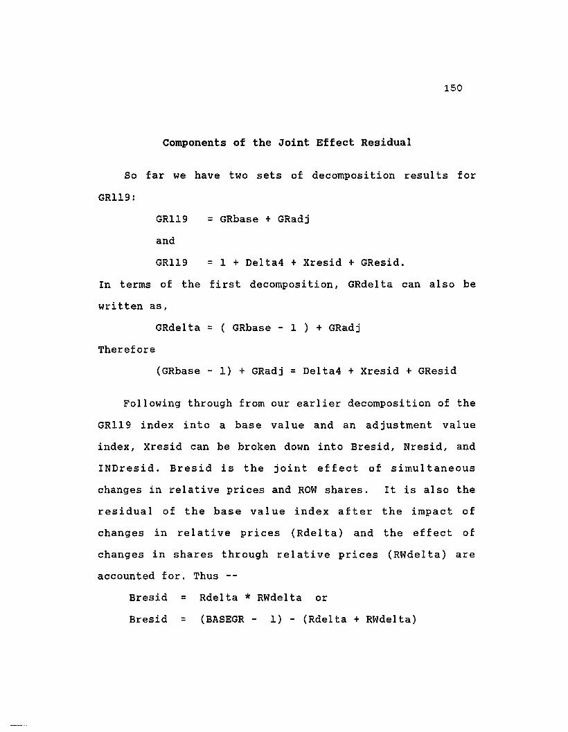
= GRbase + GRadj

150

Components of the Joint Effect Residual

So far we have two sets of decomposition resul ts for

GR119:

GR119

and

GR119 = 1 + Delta4 + Xresid + GResid.

In terms of the first decomposi tion, GRdel ta can also be

written as,

GRdelta = ( GRbase - 1 ) + GRadj

Therefore

(GRbase - 1) + GRadj = Delta4 + Xresid + GResid

Following through from our earlier decomposition of the

GR119 index into a base val ue and an adjustment val ue

index, Xresid can be broken down into Bresid, Nresid, and

INDresid. Bresid is the joint effect of simultaneous

changes in relative prices and ROW shares. It is also the

residual of the base value index after the impact of

changes in relative prices (Rdelta) and the effect of

changes in shares through relative prices (RWdelta) are

accounted for. Thus --

Bresid = Rdelta * RWdelta or

Bresid = (BASEGR - 1) - (Rdelta + RWdelta)

GRnom

151

BASEGR = exp « Wb * 10g(Rb + dR)

+ ( dW * 10g(Rb + dR) )

BASEGR, the base value index in a two country world is

al so identical to GRbase, because both are weighted

averages of the same set of relative prices. 12 Thus--

BASEGR - 1 = GRbase - 1 .

Nresid is the joint effect of simul taneous changes in

nominal rates and ROW shares

Nresid = Adelta * AWdelta.

or = (GRnom - 1) - ( Adelta + AWdelta )

where GRnom is the global nominal index in a two

country world.

= exp ( ( Wb * 10g(Ab + dA)

+ ( dW * 10g(Ab + dA) ).

The change component in the GRl19 index that is

attributable to changes in weighted nominal exchange rates

will be,

Nomgr2 t = GRnomt - GRnomb or

= Adelta + AWdelta + Nresid

12. Our method of geometric averaging and the fact that wehave a value of one for both the nominal index and therelative price index in the us economy, makes the basevalue index and the nominal index of GRINDX and GR119identical despite the slight difference in computation.

152

The corresponding change component accounted for by changes

in weighted relative prices will be,

Basegr2 t = GRbaset - GRbaseb

or

= Rdelta + RWdelta + Bresid

The joint effect of Nomgr2 and Basegr2 will then be,

INDresid = Basegr2 * Nomgr2

or

Since

INDresid =or

INDresid =

*

(GRINDX - 1) - ( Basegr2 + Nomgr2 )

( Rdelta + RWdelta + Bresid )

( Adelta + AWdelta + Nresid ).

GR119 = 1 + Basegr2 + Nomgr2 + INDresid + GResid.

and

GRbase = 1 + Basegr2, then

GRadj = Nomgr2 + INDresid + GResid. Thus­

Xresid = (GRbase - 1) + GRadj - Delta4 - GResid,

which is reduced to --

Xresid = Bresid + Nresid + INDresid.

The results of the foregoing computations are presented

in Tables 25 and 26.*-------------~------

* See Appendix Tables 4.1 to 4.7.

153

Table 26

Components of Xresid - First Method1950-1990

---------------------------------------------------------YEAR XRESID BRESID NRESID INDRES

---------------------------------------------------------1950 -0.056740 -0.0391900 -0.003051 -0.0144981951 -0.054630 -0.0395500 -0.002682 -0.0124021952 -0.048340 -0.0330500 -0.002745 -0.0125391953 -0.057210 -0.0364300 -0.003993 -0.0167881954 -0.056600 -0.0349600 -0.003765 -0.017873

1955 -0.049060 -0.0326900 -0.002457 -0.0139151956 -0.044160 -0.0276000 -0.002465 -0.0140931957 -0.041930 -0.0268600 -0.001961 -0.0131131958 -0.034240 -0.0241400 -0.000937 -0.0091571959 -0.030420 -0.0222200 -0.000742 -0.007459

1960 -0.013240 -0.0151400 -0.000043 0.0019441961 -0.011530 -0.0153300 -0.000192 0.0039841962 -0.007660 -0.0125200 -0.000394 0.0052541963 -0.005990 -0.0111500 -0.000406 0.0055711964 -0.003310 -0.0088300 -0.000496 0.006011

1965 0.0011054 -0.0056526 -0.000912 0.0076701966 -0.0005916 -0.0073686 -0.000996 0.0077731967 -0.0003111 -0.0071621 -0.000982 0.0078331968 0.0041165 -0.0039455 -0.002102 0.0101641969 0.0054634 -0.0043606 -0.002216 0.012040

1970 0.0047075 -0.0043985 -0.000982 0.0100881971 0.0041913 -0.0035867 -0.000684 0.0084621972 -0.0011318 -0.0024758 -0.000014 0.0013581973 -0.0000023 -0.0007783 -0.000006 0.0007821974 0.0012596 -0.0003124 -0.000025 0.001597---------------------------------------------------------

Table 26 (cont.)

Components of Xresid - First Method

154

---------------------------------------------------------YEAR XRESID BRESID NRESID INDRES

---------------------------------------------------------

1975 0.0010094 -0.0001256 -0.000014 0.0011491976 0.0012274 -0.0000246 -0.000236 0.0014881977 -0.0005884 -0.0000014 -0.000198 -0.0003891978 -0.0001655 -0.0000025 -0.000002 -0.0001611979 0.0000000 0.0000000 0.000000 0.000000

1980 0.0000190 0.0000000 0.000002 0.0000171981 -0.0010454 -0.0000014 -0.000247 -0.0007971982 -0.0091830 -0.0000581 -0.002050 -0.0070751983 -0.0227670 -0.0003104 -0.005305 -0.0171521984 -0.0438390 -0.0008929 -0.013503 -0.029443

1985 -0.0671170 -0.0017013 -0.021365 -0.0440511986 -0.0350370 -0.0008133 -0.004538 -0.0296861987 -0.0250160 -0.0004239 -0.001017 -0.0235751988 -0.0237680 -0.0002246 -0.000312 -0.0232311989 -0.0508790 -0.0006237 -0.001232 -0.049023

1990 -0.0522110 0.0004524 0.000720 -0.053383---------------------------------------------------------

= 1 + Rdelta + RWdelta + Bresid.

= Adelta + AWdelta + Nresid

+ INDresid + GResid

155

In this method of decomposing Xresid, Bresid would be

the joint effect of relative prices and weights given

nominal rates. Nresid would be the joint effect of nominal

rates and weight shares given relative prices. And

INDresid would roughly correspond to the joint effect of

relative prices, nominal rates, and weight shifts taken

simultaneously.

Expressing GRbase, GRadj, and GRl19 in terms consistent

with the earlier way we decomposed Xresid, we have the

fo11 owing:

GRbase

GRadj

GRl19 = 1 + (Rdelta + RWdelta + Bresid)

+ (Adelta + AWdelta + Nresid)

+ INDResid + GResid.

Here we see that changes in the GRbase - the Base Value

Index - come from the composite effect of changes in

relative prices and the impact of weight shares through

reI ati ve prices, together wi th the joint effect of these

two variabl es . Changes in the adjustment val ue index

contain not only the component effects of changes in

weighted nominal rates but also include the effects of

other sources of change that are not solely accounted for

156

by changes in weighted relative prices. The effects of

changes in weighted nominal rates consist of the effects of

(a) changes in nominal exchange rates, (b) changes in

weight shares through nominal rates, and (c) the joint

effect of simultaneous changes in nominal rates and GWP

shares. Aside from these, GRadj also includes the joint

effect of weighted relative prices and weighted nominal

exchange rates (INDresid) and the aggregation effect

(Gresid). Since we know that our base value index and the

adjustment val ue index are components of the global real

value index, then our main index at any time t is equal to

the sum of the component changes plus its value of one in

the base year.

The results of this exercise which details the

components of the joint effects residual (Xresid)

consistent with the principal decomposition of our index

into GRbase and GRadj are presented in Tables 27 and 28.*

* The basic data used are in Appendix 4.

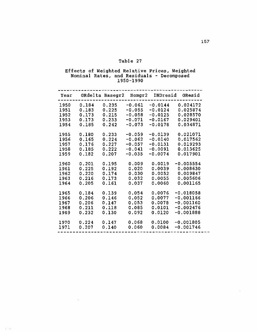
Table 27

Effects of Weighted Relative Prices, WeightedNominal Rates, and Residuals - Decomposed

1950-1990

Year GRdelta Basegr2 Nomgr2 INDresid GResid

157

19501951195219531954

19551956195719581959

19601961196219631964

19651966196719681969

19701971

0.1840.1830.1730.1730.185

0.1800.1650.1760.1850.182

0.2010.2250.2200.2160.205

0.1840.2060.2060.2110.232

0.2240.207

0.2350.2250.2150.2330.242

0.2330.2240.2270.2220.207

0.1950.1920.1740.1730.161

0.1390.1460.1470.1180.130

0.1470.140

-0.061-0.055-0.058-0.071-0.073

-0.059-0.062-0.057-0.041-0.035

0.0090.0200.0300.0320.037

0.0540.0520.0530.0850.092

0.0680.060

-0.0144-0.0124-0.0125-0.0167-0;0178

-0.0139-0.0140-0.0131-0.0091-0.0074

0.00190.00390.00520.00550.0060

0.00760.00770.00780.01010.0120

0.01000.0084

0.0241720.0258740.0285700.0294010.034871

0.0210710.0175620.0192930.0136250.017901

-0.0055540.0086300.0098470.0056060.001165

-0.018058-0.001166-0.001160-0.002476-0.001888

-0.001805-0.001746

Table 27 (cont.)

Effects of Weighted Relative Prices, WeightedNominal Rates, and Residuals - Decomposed

Year GRdelta Basegr2 Nomgr2 INDresid GResid

158

197219731974

19751976197719781979

19801981198219831984

19851986198719881989

1990

0.1470.1060.098

0.0790.0910.063

-0.0000.000

0.0120.0960.1700.1970.243

0.2690.1400.0560.0130.050

0.024

0.1350.0970.075

0.0580.021

-0.005-0.0120.000

0.001-0.007-0.033-0.061-0.082

-0.105-0.107-0.118-0.135-0.176

-0.194

0.0100.0080.021

0.0190.0680.0690.0120.000

0.0100.1050.2100.2760.355

0.4180.2770.1980.1710.277

0.274

0.00130.00070.0015

0.00110.0014

-0.0003-0.00010.0000

0.0000-0.0007-0.0070-0.0171-0.0294

-0.0440-0.0296-0.0235-0.0232-0.0490

-0.0533

0.0000070.0000070.000002

0.0000060.0000030.0000020.0000010.000000

-0.0000050.000006

-.00000170.0000043-.0000049

-.00000180.00000350.00000220.0000026-.0007605

-.0024269

159

Xresid can also be broken down to reflect the component

changes of the GRl19 index that come from relative prices

and nominal exchange rates independent of shifts in weight

shares. We proceed as follows:

RAresid = Rdelta * Adelta

Wresid = RWdelta * AWdelta

RAchng = Rdelta + Adelta + RAresid

Wchng = RWdelta + AWdelta + Wresid

WRAjoint = RAchng * Wchng

RAchng is the effect of relative prices and nominal

exchange rates alone without the influence of weight shifts.

Wchng would be the effect of the weight shifts both through

relative prices and nominal exchange rates. RAresid is the

joint effect of relative prices and nominal exchange rates,

and Wresid is the joint effect of the two component impacts

of weight shifts, one through relative prices and the other

through nominal exchange rates. WRAjoint would then be

close to a pure joint effect of relative prices, nominal

rates, and weight shifts taken simultaneously.

Thus

Xresid = RAresid + Wresid + WRAjoint

This decomposition of Xresid also shows the following

relations:

160

GR119 = 1 + RAchng + Wchng + WRAjoint + GResid

= 1 + Rdelta + Adelta + RAresid + RWdelta +

AWdelta + Wresid + WRAjoint + GResid

Hence --

(RAresid + Wresid + WRAjoint) = (Bresid + Nresid + INDresid)

By their derivation, we see a rough correspondence

between INDresid and WRAjoint. The equivalence between the

sum of Bresid + Nresid and the sum of RAresid and Wresid is

also apparent. The results of this alternative approach to

the decomposition of Xresid are presented in Tables 31 and

32. The major components of GRdelta implied in this

al ternate decomposi tion are also shown in Tabl es 29 and

30. Here there can be no clear correspondence between

GRbase and GRadj on one end and RAchng and Wchng on the

other end since the first method of decomposition separates

the effects of relative prices and their weights from the

effects of nominal exchange rates and the same weights.

The second decomposition on the other hand separates the

composi te effect of relative prices and nominal exchange

rates from the composite effect of the weights.

161

The results of this alternative method of further

decomposing the joint effects residual (Xresid) are

reported out in Table 29.*

Table 28

GRdelta Decomposition Second Method1950-1990

-----------------------------------------------------------YEAR RACHNG WCHNG WRAJOIN GRESID-----------------------------------------------------------

1950 0.25216 -0.073682 -0.018580 0.0241721951 0.25594 -0.078025 -0.019970 0.0258741952 0.22736 -0.067478 -0.015342 0.0285701953 0.22386 -0.064815 -0.014510 0.0294011954 0.22625 -0.061910 -0.014007 0.034871

1955 0.24065 -0.065513 -0.015766 0.0210711956 0.21685 -0.056856 -0.012329 0.0175621957 0.22785 -0.057717 -0.013151 0.0192931958 0.24643 -0.059838 -0.014746 0.0136251959 0.23812 -0.059511 -0.014171 0.017901

1960 0.28371 -0.059781 -0.016961 -0.0055541961 0.30059 -0.064255 -0.019314 0.0086301962 0.28961 -0.061520 -0.017817 0.0098471963 0.28468 -0.057089 -0.016252 0.0056061964 0.27023 -0.051528 -0.013925 0.001165

1965 0.25842 -0.044692 -0.011549 -0.0180581966 0.27422 -0.052259 -0.014330 -0.0011661967 0.27328 -0.051172 -0.013984 -0.0011601968 0.27237 -0.045537 -0.012403 -0.0024761969 0.29417 -0.045874 -0.013495 -0.001888

1970 0.27259 -0.036637 -0.009987 -0.0018051971 0.24802 -0.031121 -0.007719 -0.001746

-----------------------------------------------------------

* The basic data used for these computations are inAppendix Table 4.1.

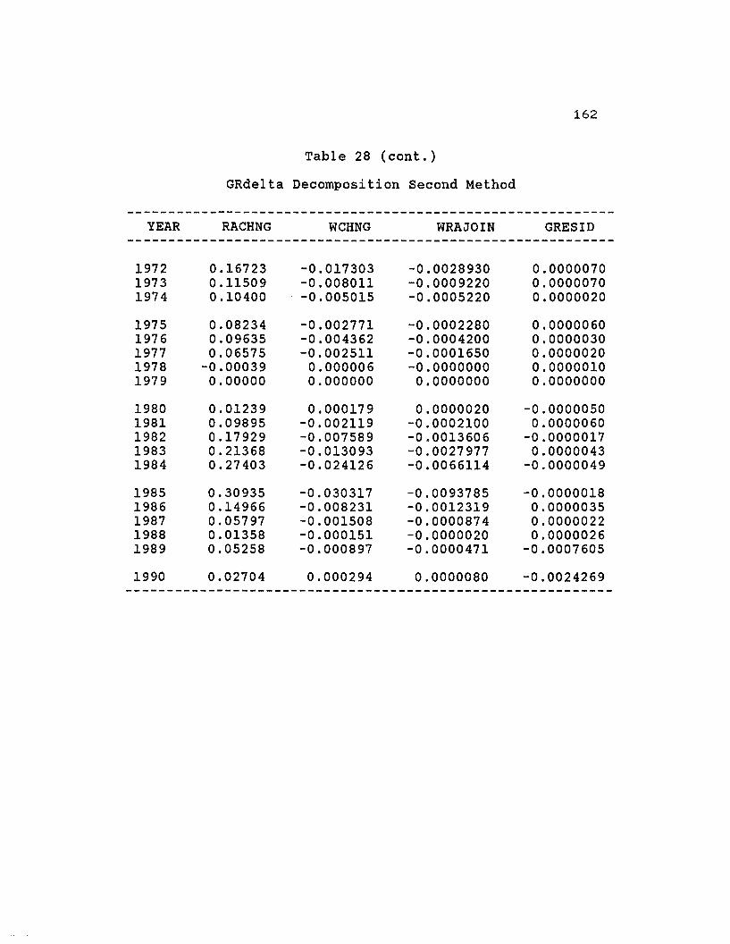
Table 28 (cont.)

GRdelta Decomposition Second Method

162

-----------------------------------------------------------YEAR RACHNG WCHNG WRAJOIN GRESID

-----------------------------------------------------------

1972 0.16723 -0.017303 -0.0028930 0.00000701973 0.11509 -0.008011 -0.0009220 0.00000701974 0.10400 -0.005015 -0.0005220 0.0000020

1975 0.08234 -0.002771 -0.0002280 0.00000601976 0.09635 -0.004362 -0.0004200 0.00000301977 0.06575 -0.002511 -0.0001650 0.00000201978 -0.00039 0.000006 -0.0000000 0.00000101979 0.00000 0.000000 0.0000000 0.0000000

1980 0.01239 0.000179 0.0000020 -0.00000501981 0.09895 -0.002119 -0.0002100 0.00000601982 0.17929 -0.007589 -0.0013606 -0.00000171983 0.21368 -0.013093 -0.0027977 0.00000431984 0.27403 -0.024126 -0.0066114 -0.0000049

1985 0.30935 -0.030317 -0.0093785 -0.00000181986 0.14966 -0.008231 -0.0012319 0.00000351987 0.05797 -0.001508 -0.0000874 0.00000221988 0.01358 -0.000151 -0.0000020 0.00000261989 0.05258 -0.000897 -0.0000471 -0.0007605

1990 0.02704 0.000294 0.0000080 -0.0024269-----------------------------------------------------------

163

Table 29

Components of Xresid - Second Method1950-1990

------------------------------------------------------------YEAR XRESID RARESID WRESID WRAJOIN------------------------------------------------------------

1950 -0.0567300 -0.034710 -0.00344400 -0.0185801951 -0.0546300 -0.031270 -0.00339100 -0.0199701952 -0.0483400 -0.029970 -0.00302700 -0.0153421953 -0.0572100 -0.038970 -0.00373300 -0.0145101954 -0.0566000 -0.039230 -0.00335500 -0.014007

1955 -0.0490600 -0.030680 -0.00261900 -0.0157661956 -0.0441600 -0.029520 -0.00230400 -0.0123291957 -0.0419300 -0.026820 -0.00196400 -0.0131511958 -0.0342400 -0.018250 -0.00124000 -0.0147461959 -0.0304200 -0.015160 -0.00108700 -0.014171

1960 -0.0132400 0.003540 0.00018400 -0.0169611961 -0.0115300 0.007380 0.00039900 -0.0193141962 -0.0076600 0.009640 0.00051200 -0.0178171963 -0.0059900 0.009800 0.00046200 -0.0162521964 -0.0033100 0.010180 0.00043000 -0.013925

1965 0.0011062 0.012234 0.00042121 -0.0115491966 -0.0005917 0.013182 0.00055691 -0.0143301967 -0.0003114 0.013137 0.00053536 -0.0139841968 0.0041171 0.016002 0.00051823 -0.0124031969 0.0054633 0.018434 0.00052417 -0.013495

1970 0.0047083 0.014395 0.00029990 -0.0099871971 0.0041910 0.011700 0.00020968 -0.007719

Table 29 (cont.)

Components of Xresid - Second Method

164

---------------------------------------------------------YEAR XRESID RARESID WRESID WRAJOIN

---------------------------------------------------------1972 -0.0011321 0.001741 0.00002034 -0.00289301973 -0.0000019 0.000915 0.00000471 -0.00092201974 0.0012596 0.001777 0.00000435 -0.0005220

1975 0.0010090 0.001236 0.00000146 -0.00022801976 0.0012276 0.001644 0.00000354 -0.00042001977 -0.0005884 -0.000423 -0.00000064 -0.00016501978 -0.0001655 -0.000165 -0.00000004 -0.00000001979 0.0000000 0.000000 0.00000000 0.0000000

1980 0.0000192 0.000017 0.00000000 0.00000201981 -0.0010454 -0.000835 -0.00000040 -0.00021001982 -0.0091830 -0.007808 -0.00001526 -0.00136061983 -0.0227680 -0.019887 -0.00008281 -0.00279771984 -0.0438400 -0.036902 -0.00032674 -0.0066114

1985 -0.0671170 -0.057102 -0.00063657 -0.00937851986 -0.0350370 -0.033696 -0.00010954 -0.00123191987 -0.0250160 -0.024912 -0.00001731 -0.00008741988 -0.0237670 -0.023762 -0.00000295 -0.00000201989 -0.0508790 -0.050817 -0.00001513 -0.0000471

1990 -0.0522100 -0.052212 -0.00000624 0.0000080-----------------------------------------------------------

165

Sources Of Change for the GRl19 Index

The decomposition of the sort made possible by our

approach is unique and not possible with any of the other

indices of the dollar's real value. Here we have isolated

the effect of weighted relative prices from other non­

relative price factors through our decomposition of the

GRl19 into the base value index and the adjustment value

component. The base value index was decomposed further into

the pure effects of relative prices (Rdelta), the effects

of shifts in weights through relative prices (RWdelta), and

their joint effects on the global index (Bresid). The

adjustment value index was further decomposed into the pure

effects of the nominal index rates (Adelta), the effect of

the shifts in weights through nominal rates (AWdelta), the

joint effects of weights and nominal rate changes (Nresid),

the joint effects of weighted relative prices and weighted

nominal rates (INDresid), and the composi tion or

aggregation effect (GResid). Adopting an alternate

arrangement of our decomposed elements, we have also

isol ated the composite effect of weights on one end, and

the pure relative price and nominal rate effects on the

other. This ability to see the direction and extent of

impact of the decomposed change components facilitates

linkage of our index trends to other economic factors.

166

Figure 18

CHANGES IN THE COMPOSITION EFFECT1950 - 1990

0.3,...-----------------------,0.2B0.26

0.:24­

0.220.2

0.18

0.16

0.1+

0.12

0.1

0.0110.05

0.04­

0.02

Ot-----~St"-~Mt_fc:l_..._+-+++++tttllf+++-H-t-+-IH-iroq=-__j

-0.02

- O. 0 + '--..,..,.-ro.,.,....,.,-,..,...........,...,-r-T"'1"'.,..,...,...,.,-,....,.,-T"T"T"T"TT'"rr-r-r-rr-r-1rr---'

c ORDEL.TA

What becomes clearly apparent in the preceding exercise

is the ability of the resulting index and its change

components to reflect the institutional changes in the

world's international payment system. For instance GResid

values reflect the divide between the fixed and flexible

exchange regime. Looking at the values of GResid from 1950

to 1990, an interesting pattern emerges (see Figure 18).

While GResid values were not significantly different from

zero in the floating period, this residual was relatively

more important in the fixed period. It is positive and

relatively large in the years associated with dollar

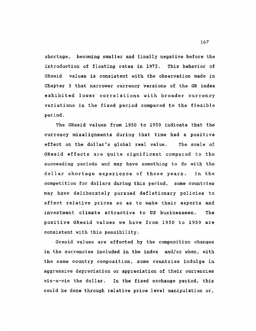
167

shortage, becoming smaller and finally negative before the

introduction of floating rates in 1972. This behavior of

GResid values is consistent with the observation made in

Chapter 3 that narrower currency versions of the GR index

exhibited lower correlations with broader currency

variations in the fixed period compared to the flexible

period.

The GResid values from 1950 to 1959 indicate that the

currency misalignments during that time had a positive

effect on the doll ar' s global real val ue . The seal e of

GResid effects are quite significant compared to the

succeeding periods and may have something to do with the

dollar shortage experience of those years. In the

competition for dollars during this period, some countries

may have deliberately pursued deflationary policies to

affect relative prices so as to make their exports and

investment cl imate at tracti ve to US businessmen. The

positive GResid values we have from 1950 to 1959 are

consistent with this possibility.

Gresid val ues are affected by the composition changes

in the currencies included in the index and/or when, with

the same country composition, some countries indulge in

aggressive depreciation or appreciation of their currencies

vis-a-vis the dollar. In the fixed exchange period, this

could be done through relative price level manipulation or,

168

in the flexible exchange system, through deliberately

depressed or inflated nominal values of currencies in the

context of a managed float.

With the return of exchange convertibility to the

industrial nations, these currency misal ignments were

mitigated after 1959. The insignificant difference of

GResid values from zero during the floating period signals

that such currency misal ignments have almost disappeared

during the flexible period. The reappearance of relatively

significant negative GResid values in 1989 and 1990

signals that target setting by the G5 countries as they try

to manage the dollar's real values may be promoting the re­

emergence of currency misalignments.

The reflection of the institutional changes in our

change components is also true with Wchng. Our further

decomposition of the elements in GRbase and GRadj and a

rearrangement of the resulting change components allows us

to look at the evolution of composite share effects

(Wchng). The impact of income shares which manifest their

effect through movements in relative prices and nominal

rates were thus traced from 1950 to 1990. The results, to

some extent, complemented the patterns shown in the

aggregation effect component (see Figure 19).

In the flexible period nominal exchange rates were able

to adjust freely in response to movements in relative

169

prices. As theory suggests, since these two would most

likely always move in opposite directions, the resulting

net effect from income shares became relatively

insignificant. But in the fixed exchange period, because

of the relative stickiness of prices, including nominal

exchange rates I currency misal ignments occurred giving a

larger role to income shares in determining the global

doll ar rate.

The long term trend in the weight change mirrors

GRdelta and serves to raise the real dollar rate. This

reflects the relative growth in the ROW economy, which,

taken alone, should raise the real dollar rate. The

negative dip of Wchng towards 1985 is also a mirror image

of the peak in nominal dollar rates and the corresponding

shrinkage in ROW share effects on the doll ar' s global

value.

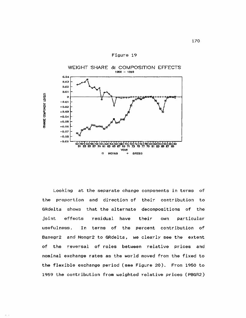
170

Figure 19

WEIGHT SHARE & COMPOSITION EFFECTS1950 - 1990

D.O.~----------------------,

0.03

0.02

0.01

°t------1tt---'hA';l;:::F=f:::po+-t-I-~;WIDi~rt_~H_I!r4DfJIl!£__;

-0,01

-0.02

-0.03

-0.004-

-0.05

-0.06

-0.07

-O.OB

- O.09 '-......,.....-r-rr"""'T'"rrT""r-r-'1r-nn-r"'T""T....-r..-r.,.,...,....,.......,....,......,,..,...,-.-.-r-T-,---J

C WCHNO

Looking at the separate change components in terms of

the proportion and direction of their contribution to

GRdelta shows that the alternate decompositions of the

joint effects residual have their own particular

usefulness. In terms of the percent contribution of

Basegr2 and Nomgr2 to GRdelta, we clearly see the extent

of the reversal of roles between relative prices and

nominal exchange rates as the world moved from the fixed to

the flexible exchange period (see Figure 20). From 1950 to

1959 the contribution from weighted relative prices (PBGR2)

171

and the component effect from weighted nominal exchange

rates (PNGR2) had opposite signs (see Appendix 4). In this

period, the global nominal index was below base year levels

while the global relative price index or the base value

index was way above its 1979 levels. However, from 1981 to

1990, it was the contribution from weighted relative prices

that turned negative while the effect of weighted nominal

rates was positive.

Between 1960 and 1976, the contribution of reI ati ve

prices and nominal rates were both positive but the

dominance of weighted relative prices lasted only up to

1975. In 1976, while the relative price effect was still

positive, it was only a third of the effect from nominal

rates. Not counting 1978 and 1979 since these years show

the base year effects, the relative price effects after

1976 became negative with the exception of 1980. The

change component from nominal rates continued with a

posi ti ve sign and starting wi th 1976 began growing in

r e l a ti ve importance. Nomina 1 exchange rates genera 11 y

dominated the changes in the dollar's global value with

very substantial increases in share after 1979. Thus in

the fixed exchange system, the component effect from

weighted relative prices dominated changes in the GR119

index while the effects of weighted nominal exchange rates

became relatively more important in the floating period.

~

~~

!zlAJZ~~

8lAJ

Io

Figure 28

COMPONENT CHANGES, First Method1950 - 1990

0.5 , i

0,+

0,3

0.2

0.1

oI ::~~"¢A~It*~~)()E~~ I-0.1

-0.2

-0.3 'ii i I Iii iii ii' iii iii iii I , iii iii iii iii iii Ii'

[] GROELTA + BASEGR2 ~ INORESIO x GRESIO

....'-Jf\)

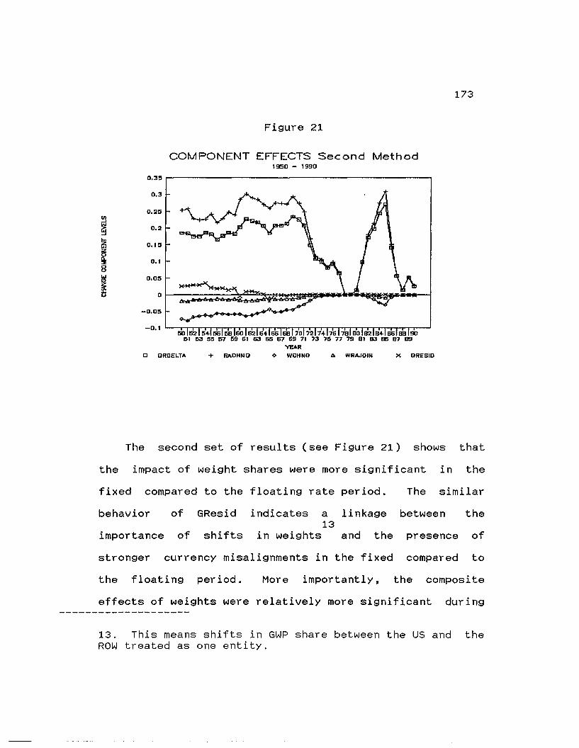
173

Figure 21

COMPONENT EFFECTS Second Method1950 - 1990

0.35,-----------------------,

0.3

0.25

0.2

0015

0.1

0.05

-0.05

C GROELTA + IlAOHND A WRAJOIN X ORE SID

The second set of results (see Figure 21) shows that

the impact of weight shares were more significant in the

fixed compared to the floating rate period. The similar

behavior of GResid indicates a linkage between the13

importance of shifts in weights and the presence of

stronger currency misalignments in the fixed compared to

the floating period. More importantly, the composite

effects of weights were relatively more significant during

13. This means shifts in GWP share between the us and theROW treated as one entity.

174

the fixed period than they were in the flexible period.

Ranging from a negative 42 percent contribution in 1951,

the composite weight effect went into negative single

digits during the floating period.

What we have done so far is just to note what is

immediately obvious from a cursory examination of the index

and its decomposition results. While that in itself is

significant, a deeper interpretation of the dynamics

invol ved is call ed for in the I ight of our purpose of

looking at the theoretical determinants and actual outcomes

of our index resul ts. In the next chapter, we attempt to

do just that as we try to tell a more textured story of how

and why global dollar values evolved as they did.

175

Chapter 5

SOME APPLICATIONS OF THE NEW INDEX

A Framework for Using the GR Index

Much work remains to be done to improve on the new

index and its components, but at the moment they can

suffice to add a little more to our understanding of the

factors behind the way global dollar values evolved. While

a fully developed analytical framework is missing this does

not prevent use of the new indices to better understand

sel ected economic episodes in the past. It must be noted

though that our purpose in this chapter is not a detailed

explanation of selected segments of the past record but

merely to illustrate possible uses for our decomposed

index.

By using the observable patterns in our indices and its

decomposed components we can approach the study of the

evolution of the world economy from 1950 to 1990 in a new

way. In looking back, (at what happened to the world

economy) tracing the changes i~ the global rate, the base

rate, the adjustment factor and the contribution of

composition changes in that factor can guide us to a more

correct explanation of economic events.

176

The GR index through its principal decomposition

(GRbase and GRadj), isolates the relative from the non­

relative price effects on the global dollar's real value.

Where the expected impact of r e l ati ve price movements on

the global dollar's value does not materialize, the GR

index provides us with a basis and a starting point for

looking deeper into such "special" periods.

The use of GDP shares to weigh the importance of

currencies included allows us to link the resulting index

to economic activities beyond trade sector behavior in the

world economy. The GRadj component, which roughly

corresponds to a measure of non-relative price factors (as

reflected in nominal exchange rate changes) that impact on

the global dollar's value, can be linked to other forms of

economic interaction among nations including the effects of

relative income share differentials as well as capital

flows across national borders.

Fundamentally, if the relative quality of us goods is

higher than ROW goods, ceteris paribus, then the dollar

would have a higher val ue since global taste preferences

would favor US goods and there would be a higher demand for

us exports. High values for the dollar also come with

increased usage as the international currency since this

would add to existing capital inflows into the US. strong

177

capital inflows into the us independent "o f its

international currency usage would also be associated with

high val ues for the us doll a r . Vice-versa, decreasing

relative quality of US goods over ROW goods implying lesser

us export demand, less usage of the dollar as the

international currency, and less US capital inflows or

. more capital outflows would be associated with a

decreasing global value for the dollar. Relative income

growth also affects the dollar's global real value. Faster

ROW growth would be associated with increasing demand for

US goods and an appreciation of dollar values. Vice-versa,

faster US growth would be linked to increased us imports

and a depreciation of the dollar.

In using the index we start by looking at GRl19, its

GRbase component, and the us trade balance and see if their

interaction is in accord with the established relations

between relative prices and trade flows. If it is, then

conventional macroeconomic relationships are affirmed; but

if it is otherwise, then the GRadj residual and its

components provide us wi th a starting point to determine

what other economic factors are involved.

If rates were truly fixed, movements in relative prices

should control the global rate (GRl19) and the adjustment

component (GRadj) should be small since the change

component coming from nominal rates (Adelta) would be zero.

178

The impact of income share changes through the nominal

rates (AWdelta) would also be zero and therefore changes in

income share would have no effect on the adjustment

component. The only effect of income share changes on the

global rate would be solely through relative prices

(RWdelta). Likewise, the effect of capital flows on the

dollar's real value would be exerted through changes in

relative prices directly as well as the indirectly through

the impact of such flows on relative income. us outfl.ows

would be associated with decreasing us relative prices and

incomes, and lower dollar global real values. Vice-versa,

us capital inflows would go together with increasing

relative prices and incomes, and higher real values for the

dollar. If there is a large positive or negative

adjustment factor, then either nominal rates were adjusted,

(this can be seen from the base data) or the composition

effect changed (GResid).

With the us having the lowest trade to GDP ratio among

the leading trading nations in the world, us prices can be

taken as largely determined by non-trade factors. All

other things equal a rise in relative prices (US/ROW)

should deteriorate the trade balance and a fall in relative

prices should improve the trade balance. In an adjustable

fixed exchange system, an increase in relative prices

brings pressure towards devaluation through an increasing

trade or current account deficit.

179

The pressure on fixed

exchange rates coming from a decrease in relative prices

over the base would be from a current account surplus and

so toward appreciation. In a system of flexible rates, the

link between relative prices and the nominal exchange rate

is more direct than is the case in a fixed system.

Exchange markets immediately factor in changes in relative

prices usually into opposite movements in nominal rates.

When relative prices change, we expect the adjustment

component and the trade balance to be positively related.

If the base index increases (through domestic inflation, or

foreign deflation), we expect the trade balance to worsen

and nominal rates to depreciate, by less than the base

index increases so the adjustment factor is negative. 1 4

Thus, a negative adjustment factor and a negative trade

balance should be paired in this instance. Conversely, if

the base index decreases, we expect to see the trade

14. In all instances when the argument is that the tradebalance worsens (improves), this simply means we look for acurrent situation to change so a surplus becomes smaller, adeficit appears, a deficit becomes worse ( a surplusbecomes larger, a surplus appears, a defici t becomessmaller). The argument is similar, with the difference of abase = 100, for a posi ti ve (negati ve ) adjustment factor.When we say a change wi 11 lead to a posi ti ve adjustmentfactor, that is so only compared to the base per iod.Compared to the last year, this means an existing positiveadjustment will get larger, a negative adjustment willbecome positive or a negative adjustment will get smaller.

180

bal ance improve and the nominal rate appreciate. The

result is a positive adjustment factor.

For instance, if relative prices fall, the dollar's

global real value may fall more than the base value. This

woul d happen if the fall in reI ati ve prices resul ts from

economic developments that look to give a long-run or

secular decline in relative prices, profits and income and

if large enough capital outflows result which bring down

the nominal rates. Thus in the long-run, if us supply

increases relative to supply elsewhere, this will tend to

reduce US reI ati ve prices. More rapid popul ation growth,

more rapid capital accumulation or more rapid technological

progress would all tend to lower the real value of the

dollar ceteris paribus. On the other hand, innovations

that increase the demand for US products may raise us

relative prices and raise the value of the dollar.

[Somewhat like the secular strengthening of the Mark and

the Yen]. Such conditions of relatively high secular

growth might attract inflows of capital to an open capital

market I ike the US. In this case, when the fall in

reI ati ve pri ces ref I ects increased producti vi ty, capi tal

inflows may offset all or part of the expected fall in

global rates.

However, if movements in relative prices represent

changes in the relative quality between US and ROW goods,

181

shi fts in taste can occur affecting el astici ty condi tions

which will negate the expected relation between relative

prices and the trade balance. In an instance where us

relative prices fall because quality of ROW goods are

improving and if the fall in us prices is not sufficient to

offset the improved quality of ROW goods (example high

quality Japanese electronic products that are priced at

very low margins) then this fall will result in a

deteriorating trade balance which will also be accompanied

by a fall in nominal rates. The adjustment value would be

negative if the fall in nominal rates is faster than the

fall in relative prices and it would be positive if the

fall in relative prices is faster or greater than nominal

rate movements. When the relative quality factor favors US

goods, then increasing relative prices would be related to

trade surpluses because despite the high relative prices of

American goods, their higher quality would more than

compensate for the price differential. This would imply

negative values for the adjustment factor.

When nominal rates appreciate because of an increasing

trade balance due to a fall in relative prices, the result

would be a positive adjustment factor. The expected

outcome is for global rates to fall. If global rates stay

the same or increase, there is a case for delving deeper.

If the adjustment factor becomes negative, meaning that

182

nominal rates went the wrong way or that composition

factors lowered the average nominal rate then there is also

a case for looking further.

The pressure of an independent increase in nominal

rates should be toward falling relative prices and a

posi tive adjustment factor; any other outcome means that

other factors are at work. For instance, a relative

interest rate induced capital inflow would increase the

nominal rate. This is most likely, but not necessarily,

related to an increase in relative prices. If relative

prices and nominal rates move in the same direction, giving

rise to a change in global rates also in the same

direction, this suggests that capital flows are dominating

other factors. I f nominal rates increase, we expect the

trade balance to worsen and relative prices to fall but not

enough to offset the nominal rate change (policy induced or

responding to interest rate differentials). Thus we expect

a positive adjustment factor and a worsening trade balance.

A dollar devaluation would give rise to an improvement

in the us trade bal ance and a negative adjustment factor

which would be larger, the larger the devaluation. This

should raise relative prices and increase the global real

rate. If the global real rate does not increase when

relative prices do, then there could have been a more than

offsetting decrease in nominal rates, or in nominal rates

pI us composi tion effect changes (Nomgr2 + GResid).

183

This

asymmetric response directs our attention to what else was

happening in the period. I f in these ci rcumstances a

positive adjustment factor results, this suggests a

special condition affecting either the nominal rates or the

composition effect.

In the instance where the us raises interest rates to

attract capital, [ or as a result of the deficit and tight

money] and capital comes in, that will appreciate the

currency and tend to create a trade deficit. This will

generally mean an inverse relation between the trade

balance and the adjustment factor. l S

Since nominal exchange rates and relative prices

changed partly because of money supplies that expanded and

contracted at different rates in the US and the ROW, the

impact of relative policy changes on the dollar's global

real value must also be considered. If the fall in US

relative prices results from better inflation control, this

affects other f actors I ike the expecta t i on of nomina I

currency appreciation. These changes in expectations may

induce capital inflows that can swamp the expected fall in

dollar global real rates.

15. This is an explanation of one source of the norn i nalchange case.

184

Where foreign demand increases [more rapid foreign

growth, need for us products - post-war period, etc.] this

change will raise nominal rates as they improve the trade

balance and also tend to raise relative prices. We would

expect to find the trade balance and the adjustment factor

positively related. Similarly, the opposite occurs for

decreases in foreign demand [foreign led cycles, shifts in

tastes, trade policies and the like]. If US income

increases in relative terms, this is the same as a

relative foreign decrease in income. We would expect the

bal ance of trade to worsen, the US doll ar to depreciate,

and r e l ati ve prices to increase. This shoul d I ead to a

negative adjustment factor and a worse trade balance.

If tariff increases and/or restrictive quotas occur in

the ROW, these will worsen the trade balance of the US and

depreciate the dollar. Relative price falls may partially

offset this development, but a negative adjustment factor

is likely. If these restrictive tariff and quotas occur in

the US, the doll ar appreciates. In this case, a posi ti ve

adjustment factor is expected but again a rise in relative

prices may partially offset this result.

Except for changes in relative quality which induce

shifts in tastes, and initiating nominal rate changes which

may result from central bank intervention or from capital

185

movements, the trade balance and the adjustment factor

would be expected to move together while relative prices

move in the opposite direction.

To give a better interpretation of our index results we

then have to understand the factors behind the declining

trend in us r e l ati ve prices. At the same time, wi th the

index focus on the adjustment component or the non-relative

price factors in the determination of the dollar's global

value we also need to have a good grasp of the economic

forces behind nominal index movements.

The Fixed Exchange Period

The influence of relative price factors was more

important in determining the global dollar rates in the

fixed compared to the flexible exchange period. This is

easily seen in values of the GRbase and the GRadj indices

and an examination of Figure 22 which graphs the

contributions of the base value and the nominal rate

indices to the change in GRl19. A correlation run between

the adjustment factor and the US trade balance for both the

fixed and the f 1exibl e system, al so provides us wi th an

indication of the extent that this was indeed the case. In

the fixed period no significant relation emerges between

the us trade balance and the adjustment factor although the

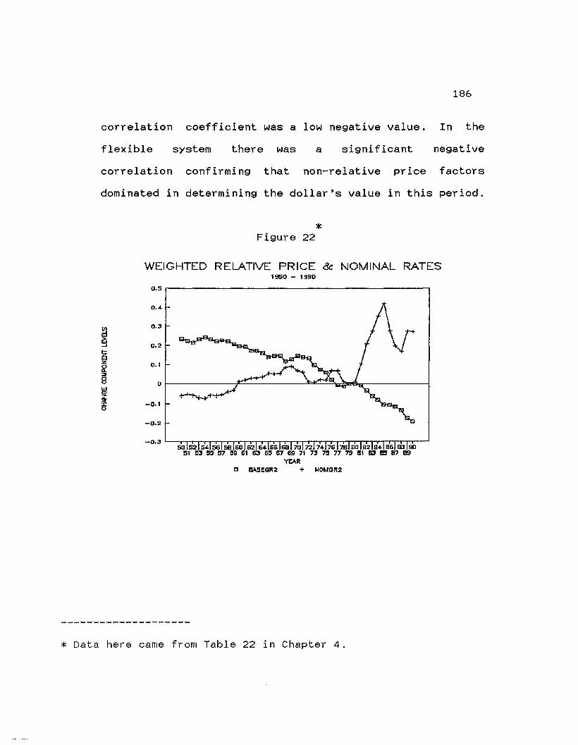
186

correlation coefficient was a low negative value. In the

flexible system there was a significant negative

correlation confirming that non-relative price factors

dominated in determining the dollar's value in this period.

*Figure 22

WEIGHTED RELATIVE PRICE & NOMINAL RATES1950 - 1990

0.5,-----------------------,

0.1

0.2

0.4-

1:I 5'SEGR2

of------j~------'J:::IC:~~~s;_------1

0.3

-0.1

-0.2

* Data here came from Table 22 in Chapter 4.

187

Table 30

Correlation Analysis : GRADJ & TBAL

Variables

GRADJ vIs TBAL

1950-1971

-0.243990.2738

1972-1990

-0.770760.0001

See Table 22, Appendix Tables 5.4 and 5.7.

Distinctive phases of the 1950-1990 period can be

identified based on the size and direction of the

adjustment value component of the GR index. Thus the fixed

period can be subdivided into two sub-phases: the phase

from 1950 to 1959 when the adjustment component was

negative which is also commonly identified as the dollar

shortage years, and the phase covering 1960 to 1971. In

contrast to the dollar shortage years, the adjustment

factor was posi ti ve in this 1at ter phase of the fixed

exchange period.

From 1950 to 1959, our adjustment value index showed

negative values because US relative prices were quite high

in the fifties compared to 1979 values. At the same time

the nominal exchange rate index had much lower values than

levels in 1979. This made the component; Adel ta negative

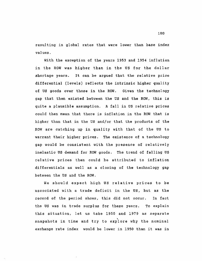
188

resulting in global rates that were lower than base index

values.

With the exception of the years 1953 and 1954 inflation

in the ROW was higher than in the us for the dollar

shortage years. It can be argued that the relative price

differential (levels) reflects the intrinsic higher quality

of US goods over those in the ROW. Given the technology

gap that then existed between the us and the ROW, this is

quite a plausible assumption. A fall in us relative prices

could then mean that there is inflation in the ROW that is

higher than that in the us and/or that the products of the

ROW are catching up in quality with that of the us to

warrant their higher prices. The existence of a technology

gap would be consistent with the presence of relatively

inelastic US demand for ROW goods. The trend of falling US

relative prices then could be attributed to inflation

di fferential s as well as a closing of the technology gap

between the us and the ROW.

We should expect high US relative prices to be

associated with a trade deficit in the US, but as the

record of the period shows, this did not occur. In fact

the US was in trade surplus for these years. To explain

this situation, let us take 1950 and 1979 as separate.

snapshots in time and try to explore why the nominal

exchange rate index would be lower in 1950 than it was in

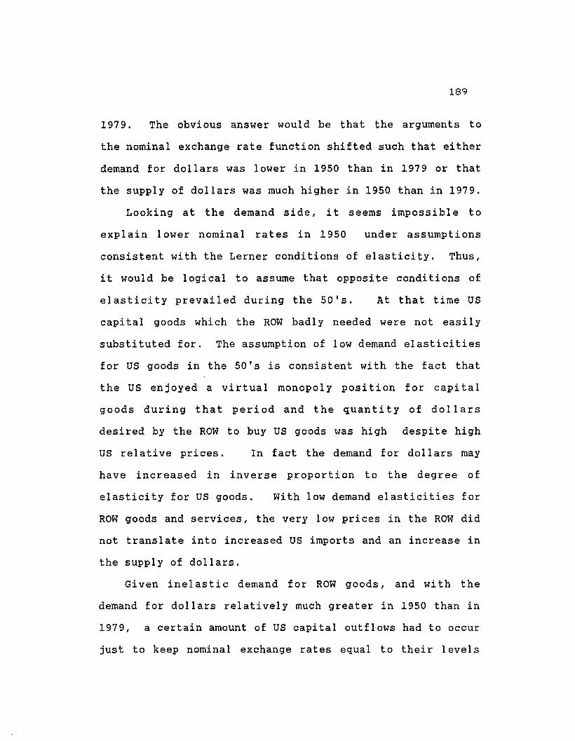
189

1979. The obvious answer would be that the arguments to

the nominal exchange rate function shifted such that either

demand for dollars was lower in 1950 than in 1979 or that

the supply of dollars was much higher in 1950 than in 1979.

Looking at the demand side, it seems impossible to

explain lower nominal rates in 1950 under assumptions

consistent with the Lerner conditions of elasticity. Thus,

it would be logical to assume that opposite conditions of

elasticity prevailed during the 50's. At that time US

capital goods which the ROW badly needed were not easily

substituted for. The assumption of low demand elasticities

for US goods in the 50's is consistent with the fact that

the US enjoyed a virtual monopoly position for capital

goods during that period and the quantity of dollars

desired by the ROW to buy US goods was high despite high

US relative prices. In fact the demand for dollars may

have increased in inverse proportion to the degree of

elasticity for US goods. With low demand elasticities for

ROW goods and services, the very low prices in the ROW did

not translate into increased US imports and an increase in

the supply of dollars.

Given inelastic demand for ROW goods, and with the

demand for dollars relatively much greater in 1950 than in

1979, a certain amount of US capital outflows had to occur

just to keep nominal exchange rates equal to their levels

in 1979. Since the nominal rate index in 1950

190

was

actually lower than the base year nominal rate, we can

conclude that US capital outflows had to be proportionately

greater than the levels required to keep nominal rates from

rising. 16 It is these capital outflows from the US which

provided the supply of dollars that not only offset the

high demand for US dollars due to the need of the ROW for

US capi tal goods but even overwhelmed it. Programs like

the Marshall Plan provided loans and grants to Europe and

together with US capital outflows produced a massive

suppl y of external doll ars which sustained and val idated

the low nominal exchange rates in those years.

With the exception of 1953, US relative prices steadily

declined from 1950 up to 1965 (see Appendix Table 5.7).

This is matched by a rising trend in the nominal exchange

rate index which continued on to 1969. Convertibility

returned to the other major currencies in 1959 and from

then on up the Bretton Woods System of adjustable fixed

rates was more fully observed (Cohen,1989). In the context

of continuing US net capital outflows which lasted up to

16. Without the US capital outflows that occured in thepost WW II period up to 1969, the us balance of paymentssurplus would be much higher and the pressure towards adollar revaluation and/or a devaluation of ROW currencieswould be that much greater. Hence the dollar nominal indexand consequently the dollar's real value would have beenhigher at all relative prices and incomes.

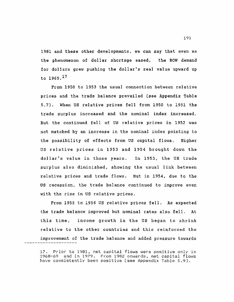
191

1981 and these other developments, we can say that even as

the phenomenon of doll ar shortage eased, the ROW demand

for dollars grew pushing the dollar's real value upward up

to 1969. 17

From 1950 to 1953 the usual connection between relative

prices and the trade balance prevailed (see Appendix Table

5.7). When us relative prices fell from 1950 to 1951 the

trade surpl us increased and the nominal index increased.

But the continued fall of us relative prices in 1952 was

not matched by an increase in the nominal index pointing to

the possibility of effects from us capital flows. Higher

us relative prices in 1953 and 1954 brought down the

dollar's value in those years. In 1953, the us trade

surplus also diminished, showing the usual link between

relative prices and trade flows. But in 1954, due to the

us recession, the trade balance continued to improve even

with the rise in us relative prices.

From 1955 to 1956 US relative prices fell. As expected

the trade balance improved but nominal rates also fell. At

this time, income growth in the us began to shrink

relative to the other countries and this reinforced the

improvement of the trade balance and added pressure towards

17. Prior to 1981, net capital flows were positive only in1968-69 and in 1979. From 1982 onwards, net capital flowshave consistently been positive (see Appendix Table 5.9).

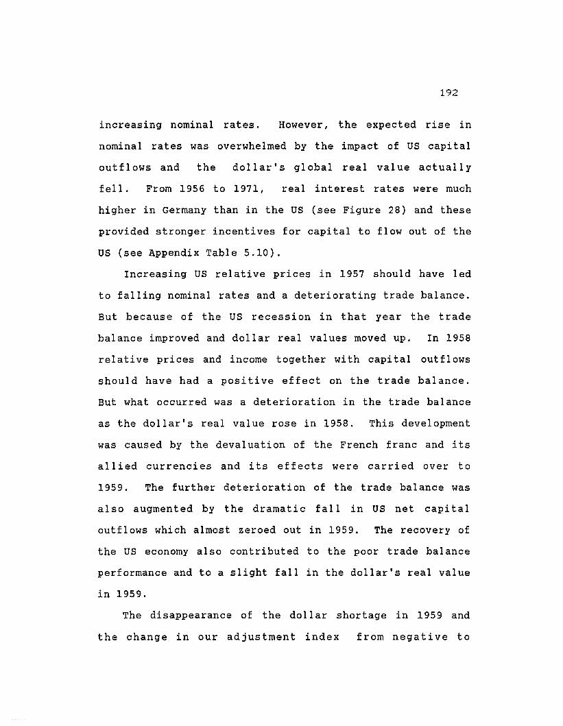
192

increasing nominal rates. However, the expected rise in

nominal rates was overwhelmed by the impact of us capital

outflows and the dollar's global real value actually

fell. From 1956 to 1971, real interest rates were much

higher in Germany than in the us (see Figure 28) and these

provided stronger incentives for capital to flow out of the

us (see Appendix Table 5.10).

Increasing US relative prices in 1957 should have led

to falling nominal rates and a deteriorating trade balance.

But because of the us recession in that year the trade

balance improved and dollar real values moved up. In 1958

relative prices and income together with capital outflows

should have had a positive effect on the trade balance.

But what occurred was a deterioration in the trade balance

as the doll ar' s real val ue rose in 1958. This development

was caused by the devaluation of the French franc and its

allied currencies and its effects were carried over to

1959. The further deterioration of the trade balance was

also augmented by the dramatic fall in us net capi tal

outflows which almost zeroed out in 1959. The recovery of

the us economy also contributed to the poor trade balance

performance and to a slight fall in the dollar's real value

in 1959.

The disappearance of the dollar shortage in 1959 and

the change in our adjustment index from negative to

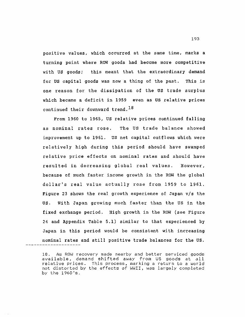
193

positive values, which occurred at the same time, marks a

turning point where ROW goods had become more competitive

wi th us goods; this meant that the extraordinary demand

for us capital goods was now a thing of the past. This is

one reason for the dissipation of the us trade surplus

which became a deficit in 1959 even as US relative prices

continued their downward trend. 18

From 1960 to 1965, US relative prices continued falling

as nominal rates rose. The us trade balance showed

improvement up to 1961. US net capital outflows which were

relatively high during this period should have swamped

relative price effects on nominal rates and should have

resulted in decreasing global real values. However,

because of much faster income growth in the ROW the global

dollar's real value actually rose from 1959 to 1961.

Figure 23 shows the real growth experience of Japan vIs the

us. With Japan growing much faster than the us in the

fixed exchange period. High growth in the ROW (see Figure

24 and Appendix Table 5.1) similar to that experienced by

Japan in this period would be consistent wi th increasing

nominal rates and still positive trade balances for the us.

18. As ROW recovery made nearby and better serviced goodsavailable, demand shifted away from us goods at allrelative prices. This process, marking a return to a worldnot distorted by the effects of WWII, was largely completedby the 1960's.

194

From 1961 to 1965, global real dollar values fell as growth

in the us picked up and ROW growth decelerated. In 1964,

while faster growth in the ROW improved the us trade

bal ance, it fai 1ed to pull nominal rates up sufficientl y

to increase the global dollar's real value.

strong us capital outflows from 1962 to 1965 helped

drag down the dollar's real value. While strong ROW growth

meant a continuing ROW demand for us capital goods beyond

the post WW II reconstruction needs, the required dollars

were more than amply supplied by these huge us capital

outf lows. This resul ted in the cornmon movement of the us

trade balance and the adjustment factor for most of this

period (1960-1965).

Figure 23

REAL GROWTH DIFFERENTIALS 1953 -1990us vI:> JAPAW

13,-------------------------..,12

11

10

g

8

7

6

IS

+3

21

Ot----lIJ---\1--------&---tt-t----i!HH-------j-1

-2-3- + L..---'T""T"'T""1-nr-r-rT.,...,r-o-rr,-,.....,r-rT""'T"'T""1-.-r-r"""'T'""1.,....rr"T""T-r;r---J

c LU50NP

Figure 24

AGGREGATED GROWTH RATES, 1950 -1990us, .....d ROW

:10,--------------------------..,IS16

14­

1210

8

6

+2

ol---t!t---.ld--------l!!I---1l-itJ---tlH-lW--I--+l!'I---l-2-4o-6

-8

-10-12-I + l-..-,-r-r-"""T""T"'T'""1-nr-rT'"T"T"T.....-..,.-,r-r-r-r-T""T""T""T...,.,-r;r-r-r-r-T"T"T""T-r-T-.J

c LU5CON

195

196

Figure 25

World Exports as a Percent of GWP1950 - '990

16,-------------------------,

III

I'"

~.....

13

12

It

10

9

B

The vigorous growth in world trade during the 1960­

1965 period increased the demand for dollars as the need19

for precautionary balances rose. With the return of

foreign exchange convertibility among industrial nations,

expansions in the ROW share of GWP also indicated increased

capacity for the ROW to buy goods or invest in the us; it

also increased the capacity of ROW countries to trade among

themselves and invest in each other's economies.

19. In Figure 25, world exports came from IMF-IFS data andGWP is in Appendix Table 1. Based on volume of trade data,trade expansion was quite dramatic in the 60's (Cohen,1989). World trade expansion continued onwards to 1970 andthe upward kink in 1973 reflects the inflation of tradevalues due to the oil shock.

197

Developments after 1965 indicated a significant

breakdown in US fi.scal discipline. US inflation started

creeping up as US spending on the Vietnam War intensified

(see Appendix Table 5.8). US relative prices increased in

1966 and stayed at almost the same high levels in 1967.

The deteriorating trade balance in 1966 was due to

increased US prices. Vice-versa, the fall of US re l ative

prices the following year showed an improvement in the

trade balance. The 1967 improvement in the trade balance

was also reinforced by faster income growth in the ROW. It

seems that from 1965 to 1967, the normal relationship

between US relative prices, nominal rates , and the trade

balance prevailed. With rising US prices and with a

relatively constant nominal index, the dollar's real value

rose during this period.

The dollar's real value continued rising from 1967 to

1969. The corresponding adjustment factor increased and

the trade balance turned negative in these years. The big

economic event of the 1967-1968 period was the devaluation

of the British pound and the rest of the Sterling area.

This is why we see a deterioration in the trade balance

despite a fall in relative prices and stronger relative

income growth in the ROW.

IJ ROW Inflation

....-0CD

Figure 26

US and ROW Inflation Compared1950 - 1990

15 ...., ---------------------,'1-4­

13

12

11

10

9

B,6

s-4­

32

1 Io I \ ",at

-1

-2 ,, , ii' , , i-3 'ii» , " ii' ii' i' , , i " , i i •• I ••••••••

s:poQ:c

(/)

.B~

199

us relative prices increased in 1969 and this should

have decreased nominal rates. The increasing net capital

inflows in that year also should have. the same effect on

nominal rates. However, nominal rates and the dollar's

real val uerose instead. Since growth in the ROW was

faster in 1969, the increasing dollar values indicate that

relative income effects dominated relative prices and

capital flows. In 1970, the US slid into recession and the

relative income effect should have increased dollar nominal

rates as the trade balance improves. But with US relative

prices rising and with capital outflows also increasing,

the dollar's value in nominal as well as in real terms

fell. Speculative capital outflows occurred because of

fear of dollar devaluation.

The 1971 fall in relative prices should have led to

increasing nominal rates as the demand for dollars

increased while improving the trade balance. But this time

the US was getting out of a recession and this tended to

worsen the trade balance and decrease nominal rates.

Despite the dollar devaluation in that year, the relative

income effect of the US recovery resulted in trade balance

deterioration as the dollar's real value fell.

In the fixed exchange period the relative price and

trade balance relation was being affected not only by

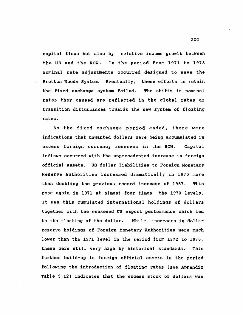
200

capital flows but also by relative income growth between

the us and the ROW. In the period from 1971 to 1973

nominal rate adjustments occurred designed to 'save the

Bretton Woods System. Eventually, these efforts to retain

the fixed exchange system failed. The shifts in nominal

rates they caused are reflected in the global rates as

transition disturbances towards the new system of floating

rates.

As the fixed exchange period ended, there were

indications that unwanted dollars were being accumulated in

excess foreign currency reserves in the ROW. Capi tal

inflows occurred with the unprecedented increase in foreign

official assets. US dollar liabilities to Foreign Monetary

Reserve Authorities increased dramatically in 1970 more

than doubling the previous record increase of 1967. This

rose again in 1971 at almost four times the 1970 levels.

It was this cumulated international holdings of dollars

together with the weakened US export performance which led

to the floating of the dollar. While increases in dollar

reserve holdings of Foreign Monetary Authorities were much

lower than the 1971 level in the period from 1972 to 1976,

these were sti11 very high by historical standards.· This

further build-up in foreign official assets in the period

following the introduction of floating rates (see..Appendix

Table 5.12) indicates that the excess stock of dollars was

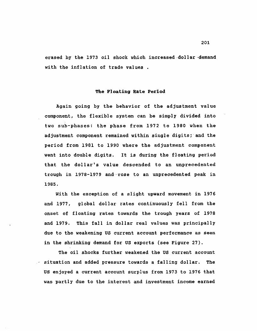
201

erased by the 1973 oil shock which increased dollar-demand

with the inflation of trade values .

The Floating Rate Period

Again going by the behavior of the adjustment value

component, the flexible system can be simply divided into

two sub-phases: the phase from 1972 to 1980 when the

adjustment component remained within single digits; and the

period from 1981 to 1990 where the adjustment component

went into double digits. It is during the floating period

that the dollar's value descended to an unprecedented

trough in 1978-1979 and-rose to an unprecedented peak in

1985.

With the exception of a slight upward movement in 1976

and 1977, global dollar rates continuously fell from the

onset of floating rates towards the trough years of 1978

and 1979. This fall in dollar real values was principally

due to the weakening US current account performance as seen

in the shrinking demand for US exports (see Figure 27).

The oil shocks further weakened the US current account

situation and added pressure towards a falling dollar. The

US enjoyed a current account surplus from 1973 to 1976 that

was partly due to the interest and investment income earned

through petro-dollar recycling. 20

202

However, the oi 1

recession dampened ROW demand for US products, encouraged

the growth of high return overseas financial markets, and

intensified US escalating inflation and had the overall

,..·.·-·~ect of pull ing down US doll ar values. Likewise, the new

context of floating exchanges, with no requirement to

maintain mandated levels of reserves, also further pulled

down the dollar's real values. The fall of the dollar's

real value during this period occurred despite the relative

price and income factors which favored an increase in

dollar values and the increased demand for dollars as world

trade expanded and as the effect of oil shocks inflated

trade values. The uniqueness of the dollar trough of'1978-

1979 is accented by the occurrence of exceptional financing

( US Treasury borrowing in foreign currencies ) for the

years from 1979 to 1980, the only occasion when it happened

in the post WW II period (see Appendix Table 5.12).

In 1980, the doll a r ' s real val ue started inching

upwards. us ~nflation which remained lower than ROW

inflation from 1972 to 1978 surged in 1979 and 1980

bringing us relative prices up. This rise in relative

20. The capital outflows in this period represent themovement of dollars earned by OPEC into Euro-dollars andAsian dollar markets. The 74-75 recession also helped thecurrent account.

203

prices and the return to capital outflows in 1980 should

have lowered nominal rates but the 1980 US recession had

the opposite effect on nominal rates aside from the fact

that it also dampened US capital outflows. The experience

from 1972 to 1980 shows the importance of non-relative

price factors in determining the doll ar' s real val ue and

the US trade balance.

From 1981 to 1985 the dollar's real value increased

dramatically. Even as relative prices and income move to

favor the US trade balance, we find a huge positive

adjustment factor and not a favorable but a much worsened

US trade balance (see Figure 28). For this period, income

growth was relatively higher in the US than in the ROW,

wi th the excepti on of 1982 when the US economy was in

recession. The positive adjustment factor is explained by

the continued capital inflows which kept nominal rates and

adjustment values at high levels.

In the 80's the US had the world's highest interest

rates for open capital market countries (see Figures 29 and

30) .21 These high rates induced the capital inflows that

21. Real interest rates tended to be higher in Germanythan in the US or Japan (see Figure 29). The differencebetween US and German (USGdif) as well as Japanese (USJdif)real interest rates are plotted in Figure 30. Positivevalues for USGdi f and USJdi f means that US real interestrates are higher; vice-versa negative values would meanthat US real interest rates are lower.

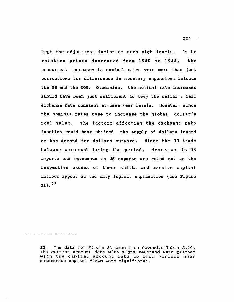
kept the adjustment factor at such high levels.

204

As US

relative prices decreased from 1980 to 1985, the

concurrent increases in nominal rates were more than just

corrections for differences in monetary expansions between

the us and the ROW. Otherwise, the nominal rate increases

should have been just sufficient to keep the dollar's real

exchange rate constant at· base year levels. However, since

the nominal rates rose to increase the global dollar's

real value, the factors affecting the exchange rate

function could have shifted the supply of dollars inward

or the demand for doll ars outward. Since the US trade

balance worsened during the period, decreases in US

imports and increases in US exports are rul ed out as the

respecti ve causes of these shifts and massive capi tal

inflows appear as the only'logical explanation (s~e Figure

31).22

22. The data for Figure 31 came from Appendix Table 5.10.The current account data with signs reversed were graphedwith the capital account data to show periods whenautonomous capital flows were significant.

Figure Z?

US EXPORTS AS PERCENT OF ROW IMPORTS1948 - 1990

25

24-

23

22

21

20

~ 19Q

~ 18

17

16

15

14-

13

12~al~I~I~~I~~IKaI~I~~le~I~I~I~I~~I~JI~I~~laftl~I~Jlael~~lon

I\)0(]1

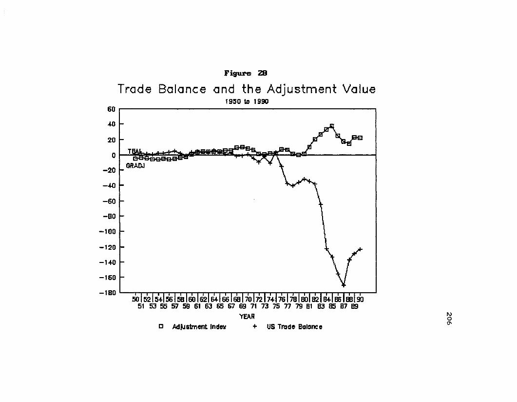
Figure 28

Trade Balance and the Adjustment Value19~0 to 1990

NoIJ'c Ad)Jstment. Indev

60

..w

20

O~-20 GRADJ

-40

-60

-BO

-100

-120

-140

-160

-180

207

Figure 29

REAL INTEREST RATES COMPARED 1971 - 1 990us. JAPAN. and GERIoAANY

90BBB678 BO 52

YEAR

100

BO

60

40I."

20

~0

Iii -20

~-40

-60

-BO

-100

-120

-140

-16071

72 74 76

Figure 30

REAL INTEREST DIFFERENTIALS 1956 -1990us vi:! JAPAN and lJERIoA.6.NY

USJDlf1:1 US[)DIF

120,----------------------------,

ItO10090BO70

60ISO403020tool------=_-....,..-=-+-~~--_\-____,I._--_tr_:;<;I;:_\_-_l

-to-20-30-40-:50-60-70-BO '---r-.......r-r..-.r-r-.......r-r-...-r--.-...-r--.-...-r-r-r-r-r-r-r-r-r-r.,....,..........,.--,r-r..,.--,r---'

208

The success of the US effort at containing inflation

also led to further confidence in the dollar and lowered

the cost of holding dollars. With positive real interest

rates for dollar assets much higher than foreign

alternatives and with strong confidence in the dollar, the

cost of holding dollars was very low. The relative

attractiveness of US real assets and financial investments,

incl uding higher returns on ho l ding doll ars, combined to

create a strong u~ward shift in the demand for dollars such

that nominal rates and the dollar's global real value

increased.

Aggressive currency depreciation as practiced by

countries like China (see regional sub-indices) further

increased the dollar's global real value in this period.

The high demand for the dollar and its consequent high real

val ues further encouraged US imports from the ROWand

further handicapped US exports and led not to an

improvement but instead to a worsening of the US trade

balance. As in the earlier part of the floating period,

the years after 1980 again show that the dollar's real

value and the US trade accounts had been strongly affected

by non-relative price factors.

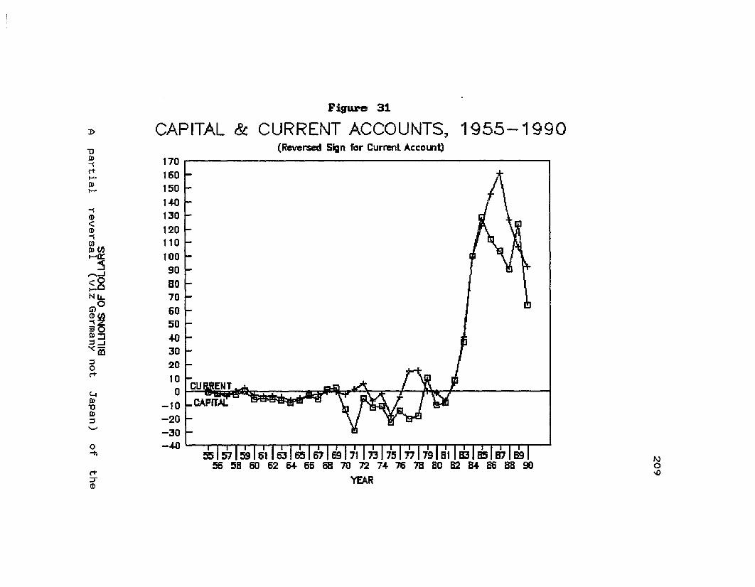
No-o

170 r'-----------------------.

160 i

150

1-40130

120110

10090BO706050

-40302010o~NT~ itEib.~ , ll.-T

-10 I ~6*61i' M~~q\T a'v't. f r& I-20-30-40 Iii iii iii iii iii iii iii i I • • • • • II Iii iii Ii·

Figure 31

CAPITAL & CURRENT ACCOUNTS, 1955-1990(Rever.sed Sign far Current Accatnt)

o-f)

C-ilD-0lD~......,

("t:J(!)

1>

....(!)

<(!)....~cn.....a::

::s........J

<g....NIL.G)O

~~lD::J~...J"(-m~

o("t

-0lD....("t....lD.....

210

A partial reversal (viz Germany not Japan) of the

interest rate situation and government intervention worked

to lower US nominal rates through the Plaza Accords. The

G5 nations agreed to make dollars freely available in the

international exchange markets and to talk down the

dollar's value so as to reverse positive dollar

expectations. Al though the international financial

authorities labeled their strategy as leaning with the

wind, it was more like fanning the air to create the wind

itself. There was a lot of talk at this time of target

zones and policy coordination among the central banks of

I eading financial countries. As al ready noted before,

these actions of the G-5 countries designed to manipulate

the dollar's value were reflected in our index through

changes in GResid values which indicated the re-emergence

of currency misalignments.

When the global dollar value fell in 1986, the

dollar's adjustment value component remained at levels

that were much higher than they were in the past episodes

when global rates fell. In 1973 and 1978, the trade

balance improved together with a fall in the adjustment

factor. But the post 1985 situation was different; even as

the trough of 1988 in global dollar values was reached,

the adjustment value component remained at high levels.

211

This behavior of the adjustment factor in the 80's

actually helps explain the laggard J-curve effect during

this period. The J curve is the description given the

behavior of the trade balance after a currency

depreciation where there is at first a deterioration then

finally an improvement over the trade balance prior to the

depreciation. After the fall in dollar values from 1985

peak levels, economists were puzzled by the length of time

for the J curve to take hold. In fact, the efforts to

construct new dollar indices were precipitated by this

delay in the improvement of the trade balance after the

dollar's value continuously fell for almost two years from

its peak val ue in 1985. In the past instances of dollar

depreciation, the us trade balance began to improve in 3

to 4 quarters (9 to 12 months). In the 1985 case, it took

eleven quarters (44 months or almost two years) before

improvement was seen in the us trade balance (Cohen, 1989).

In sum, the influence of non-price factors became much

more pronounced after 1980. Even as relative prices worked

to improve the us trade balance, the latter remained highly

negative just as the adjustment factor remained highly

positive. This is linked to continued capital inflows

(Japan) and structural probl ems in us exports. It seems

that after 1980 new factors were unleashed which have

sustained the high adjustment component values for the

212

dollar. This period could be reflecting a new dynamic in

international economic relations that is a prelude to

significant changes in the international payments system.

Caveat Inquisitor

The discussion so far just barely scratches the

surface. Definitely there is a lot more that can be done.

Our efforts included the attempt to empirically flesh out

within the greatest scope possible the US and ROW

dichotomy in the context of our objectives. With our index

value determined in a global context, the anchor points of

the small country context do not apply as everything

becomes r e l ative. In using our global index, we had to

deal with relative prices, relative income, relative

interest rates, and other relative factors between the US

and the ROW. This relative nature of the factors involved

is actually at the crux of what we have to wrestle with in

our interpretation of the rise and fall in global dollar

values.

The full story of why global dollar rates behaved as

they did from 1950 to 1990, is not an easy story to tell.

Our effort was merely a modest attempt to show how the GR

index and its components, together with its regional sub­

indices, can provide an integrating grid for the details of

213

a more complete and comprehensive story that future

research can provide.

Building the index and showing how it can be of use, is

the essential contribution of the present work. With the

use of broad based annually changing weights we were able

to track the relative effects of PPP and non-PPP factors on

real exchange rates. The wide currency incl usion of our

index also allows us to do this on a regional basis, in a

way no other index can. Our decomposition showed that PPP

factors do not control the dollar's real values.

From where we leave off, future efforts could proceed

in two major ways: one, to improve the index itself and its

components; the other is the work of fleshing out the

insights about the dollar's value that the index has

brought to the fore. This present study may not have

accomplished much, but stating the limits of our work

helps delineate the frontier boundaries from where

additional research can take off.

214

Chapter 6

SUMMARY AND CONCLUSIONS

Swmnary

The continuing international importance of the US

dollar underscores the need for studies of its global real

value. Since 1972, the world's payment system has been

operating on a fiat dollar standard, also called the

International Monetary Fund (IMF) Payments System. Despite

the US dollar's being divorced from any gold value, it must

still meet the usual responsibilities attached to an

international currency or to any currency for that matter

i. e., being an acceptabl e means of payment, a store of

value, and unit of account in world economic transactions.

As long as no long-run and highly volatile excess supply of

dollars emerges so that the dollar's value is not also

highly volatile around a long-run declining trend, the

dollar is likely to remain as the world's key currency for

some time to come. The question therefore of how the

global dollar's value is measured will remain an important

matter.

The review of existing real indices of the dollar

showed that no dollar index exists which is broad-based

both in terms of weights and currency inclusion. Wide-

215

currency indices that were billed in the literature as

broad-based were shown to have a narrower weight-base than

the traditional indices. In terms of relevance to the

dollar's value as a world currency, indices with a

narrower weight-base seemed to provide inferior information

compared to indices with a broader weight-base. A decision

was then made to go for the broadest possible weight-base

as a measure of economi cactivi ty, and GDP f low based

weights were used in the new index impl ementation. By

using weights that varied on a year to year basis, relative

income and output cycle effects were also directly injected

into the index construction process.

It was also noted that attention to weights for the

dollar's host economy was minimal or absent in most of the

indices studied. Inclusion of this feature became a

centerpiece of the new index. The weight for the host

economy is important because a compl ete accounting of

factors affecting world demand for dollars cannot afford to

ignore the home economy of that currency.

The use of GDP weights in index construction accounts

for the effects on the dollar's value of both trade and

capi tal flows. Changes in r e l ative real income cause net

exports for the country wi th the increasing income to

deteriorate. But improvements of a country's relative

income can also induce capital inflows since wealth holders

216

or capital owners are always interested in participating in

investment opportunities that give a higher return to

wealth.

If the arguments to the nominal exchange rate function

remain constant then the global dollar index always should

be equal to the base value index. However, in the real

world, arguments to the nominal exchange rate function

change and depending on the net effect of these changes,

the nominal rates move either upward or downward from the

base point. It is the effect of these nominal rate changes

on the global doll ar' s real val ue that is principal 1y

measured by the adjustment value component of the GR dollar

index.

The new input that the GR indices bring into the

discussion of the doll ar' s real value centers around the

GR's ability to distinguish between the base and the

adjustment components of the dollar's global real value in

a simple straightforward manner. The base value component

focuses on reI ative price effects , whi 1e the adjustment

value component pertains to non-relative price factors that

impact on the dollar's real value. The adjustment value

component of our index is also quite useful in explaining

why the J curve effects of a dollar depreciation may be

dampened as it was during the 1980' s . We are abl e to

effect the dichotomy just mentioned because of the use of

217

period specific moving weights in the index construction

process.

The use of weights based on country shares of the GWP

al so recognizes the fact that the doll ar' s real val ue

ultimately depends on the real goods and services produced

in the us and in the economies that use the dollar as

international currency. It is also a recognition of the

fact that in the modern international economy where

interaction through capital flows may have become more

important than tradi tional trade flows, all production

flows -- past, present, and future -- are basically 'on the

table' as far as international market forces are concerned.

The implementation of the new index involved the

gathering of data from different sources like the CIA

Handbook of Economic Statistics, the World Bank, and the

IMF tapes. In terms of currencies that were to be included

in the index, the objective was universal incl usi vi ty

limited only by data availability. Regional sub-indices

were also computed and these indices showed that the

dollar's real value moved in different directions in

various parts of the world. Nonetheless, the regional

indices confirmed the dominance of Europe and Japan in

determining the dollar's global real value.

The regional indices also showed a marked tendency for

some developing regions to indulge in extreme competitive

218

depreciation which adds to the real value of the US dollar.

Such behavior, I ike that of China, refl ects a strong

demand for hard currency that is required for development

purposes and results in upward pressure on dollar real

values.

By its construction, the GR index value is principally

determined by movements in weighted relative prices.

Deviations from expected global real dollar values as

suggested by movements in relative income and prices then

provide us wi th a way of identifying when and to what

extent other factors corne into play in the determination of

the dollar's global real value.

Our decomposition of the GR index suggests that the

period from 1950 to 1959 and the period from 1980 to 1990

were associ a ted wi th capi ta 1 flows that swamped the

expected macroeconomic relations between relative prices

and the dollar's real value. In the first instance,

capi tal outf lows from the US sustained very low real

val ues for the US doll ar; in the second, strong capital

inflows into the US sustained very high values for the

dollar that were unwarranted by a purchasing power parity

valuation of the dollar.

The GR Index with its international base value and

adjustment value component, improves on existing indices

of the dollar's real value. Through our index, we were

219

able to monitor pure PPP (relative prices) and pure

adjustment factor effects. Our resul ts show that even

during the fixed exchange period, PPP factors did not

control the doll ar' s real val ues. We also found non-PPP

factors to be quite dominant in the floating rate regime.

Our factor component dichotomy, when complemented with

Regional Sub-Indices and country-level components, show

that the GR Index provides a clearer picture of the

dollar's global real value and its relationship to the

World Economy.

An Agenda for Research

An important question for future research is what

constitutes a normal positive adjustment component

justified by the dollar's use as the international

currency. A positive adjustment component on the dollar's

real value acts like a tax on US exports and impairs the

international competitive ability of US industry (Ackerman

and MacEwan, 1973).

This problem seems to call for finding a positive

adjustment value component which can be considered a

justifiable return to the US for the use by the world of

its currency for international transactions. This val ue

must be high enough to compensate for the US trouble of

220

maintaining the politico-economic infrastructure of trade

and payments but not too high as to eliminate the

competitive edge of US products in international markets.

A more mundane but nonetheless important research

effort is the process of building quarterly and monthly

versions of the GR Indices. Such an effort would meet with

data probl ems since not all countries have the quarterly

or monthly information that would be necessary in computing

the index. Neverthel ess a research effort that would

explore the limits of what is available and devise methods

of estimation to fill in gaps in the latest data would be

worth doing.

Another key question that future research can answer

is the validity of the choice of 1979 as the dollar's base

year. In the present study, 1979 was chosen as the base

year for decomposition purposes because of the

unprecedented nature of the trough in the dollar's value in

that year. The choice of the lowest trough point as the

base year also facilitated our interpretation of GDP share

ef fects. However, if a year other than 1979 can be

identified as representing a dollar real value that is

equal to its equilibrium value then the GR index rebased

to that year will have more analytical implications than is

possible with a non-equilibrium base point.

221

The question of the GDP share effects could also be

addressed in future research. The use of a GWP share index

that is independent of exchange rate movements and relative

price changes would be a significant improvement.

Possibilities include the adjustment of computed US dollar

GDPs for each country by an exchange rate index and a

relative price index before aggregating them into a Gross

World Product in dollars series that becomes the base for

computing GDP shares. The resulting country specific GDPs

in dollars will then show the evolution of each country's

GDP in dollars with exchange rates and relative prices held

constant at a certain base year. It would be interesting

to see how the resulting index computed in this manner

would differ from our present results.

Another item for research is how regional values of the

dollar may signal the presence of triangular valuation of

the dollar induced by triangular trade or capital flows.

For example, if China values the dollar so highly and a lot

of other countries also want goods from China or

investments in China then they will also value the US

dollar highly. What goes for China can also be said of the

ANZPAC, WESHEM, and AFRICAN regions. The practice of

competi tive depreciation by these regions has the overall

effect of adding real value to the dollar.

222

Since the GR Index of the dollar measures a crucial

value in the world economy, there is almost no limit to

the questions that it can stimulate. others who may have

occasion to use the resul ts of this research effort will

develop their own particular set of questions depending on

their disciplines, lines of interests, and their research

abilities. The questions and research problems proposed

here are indeed but a small subset of the problem area

touched by the study.

Happy hunting!

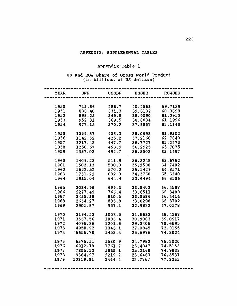
223

APPENDIX: SUPPLEMENTAL TABLES

Appendix Table 1

US and ROW Share of Gross World Product(in billions of US dollars)

--------------------------------------------------------YEAR GWP USGDP USSHR ROWSHR

--------------------------------------------------------1950 711. 66 286.7 40.2861 59.71391951 836.40 331.3 39.6102 60.38981952 898.25 349.5 38.9090 61. 09101953 952.31 369.5 38.8004 61.19961954 977.15 370.2 37.8857 62.1143

1955 1059.37 403.3 38.0698 61.93021956 1142.52 425.2 37.2160 62.78401957 1217.48 447.7 36.7727 63.22731958 1250.67 453.9 36.2925 63.70751959 1337.03 492.7 36.8503 63.1497

1960 1409.23 511.9 36.3248 63.67521961 1503.13 530.0 35.2598 64.74021962 1622.52 570.2 35.1429 64.85711963 1751.22 602.0 34.3760 65.62401964 1915.04 644.4 33.6494 66.3506

1965 2084.96 699.3 33.5402 66.45981966 2277.49 766.4 33.6511 66.34891967 2415.18 810.5 33.5586 66.44141968 2634.27 885.9 33.6298 66.37021969 2901.87 957.1 32.9822 67.0178

1970 3194.53 1008.3 31.5633 68.43671971 3537.56 1093.4 30.9083 69.09171972 4095.36 1201. 6 29.3405 70.65951973 4958.92 1343.1 27.0845 72.91551974 5655.78 1453.4 25.6976 74.3024

1975 6375.11 1580.9 24.7980 75.20201976 6912.78 1761. 7 25.4847 74.51531977 7855.13 1965.1 25.0168 74.98321978 9384.97 2219.2 23.6463 76.35371979 10819.81 2464.4 22.7767 77.2233

--------------------------------------------------------

224

Appendix Table 1 (cont.)

US and ROW Share of Gross World Product(in billions of US dollars)

YEAR GWP USGOP USSHR ROWSHR

1980 12245.17 2684.4 21.9221 78.07791981 12487.28 3000.5 24.0285 75.97151982 12294.84 3114.9 25.3350 74.66501983 12623.98 3355.9 26.5835 73.41651984 13085.55 3724.8 28.4650 71. 5350

1985 13599.27 3974.2 29.2236 70.77641986 15790.94 4205.4 26.6317 73.36831987 17928.47 4497.2 25.0841 74.91591988 19925.84 4840.2 24.2911 75.70891989 20967.52 5163.2 24.6248 75.3752

1990 23900.16 5423.4 22.6919 77.3081

Source: The raw data for this aggregation mostly came fromthe IMF-IFS tapes supplemented with informationfrom the World Bank and published estimates of theCIA for the USSR.

Note:

The preceding table shows the Gross World Product (GWP)together with US GOP in billions of dollars at currentprices and the US share of GWP (USSHR) and the correspondingRest of the World share (ROWSHR) in percent. The GWP figureswere based on the data of 143 countries. Countries withmissing data had their GOP's estimated backwards to 1950 byprogressively applying the same proportion of the GWP forthe block of countries with missing data based on theclosest proximate year with more complete data. For most ofthe earlier years China, USSR, and Taiwan were included inthis block of countries. The estimates were done in orderto get an idea of the scale of magnitudes involved.

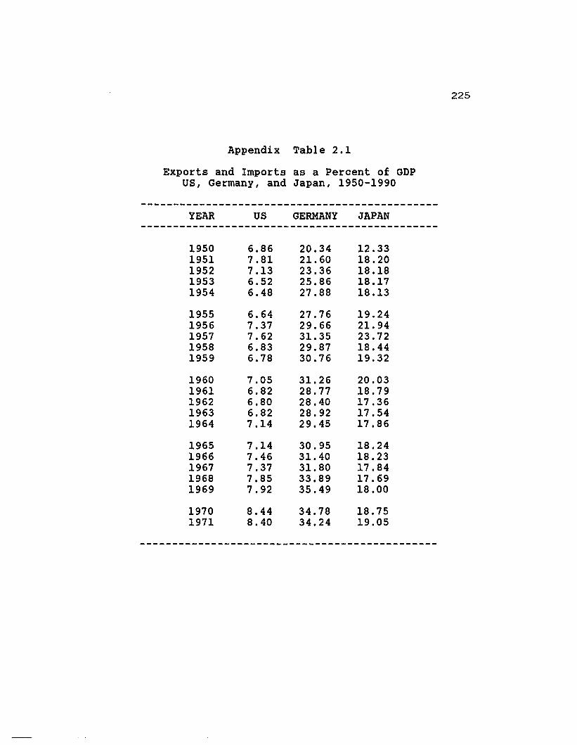
Appendix Table 2.1

Exports and Imports as a Percent of GDPUS, Germany, and Japan, 1950-1990

225

YEAR US GERMANY JAPAN

19501951195219531954

19551956195719581959

19601961196219631964

19651966196719681969

19701971

6.867.817.136.526.48

6.647.377.626.836.78

7.056.826.806.827.14

7.147.467.377.857.92

8.448.40

20.3421. 6023.3625.8627.88

27.7629.6631.3529.8730.76

31. 2628.7728.4028.9229.45

30.9531. 4031.8033.8935.49

34.7834.24

12.3318.2018.1818.1718.13

19.2421. 9423.7218.4419.32

20.0318.7917.3617.5417.86

18.2418.2317.8417.6918.00

18.7519.05

Appendix Table 2.1(cont.)

Exports and Imports as a Percent of GDPUS, Germany, and Japan, 1950-1990

----------------------------------------------YEAR US GERMANY JAPAN

----------------------------------------------1972 8.99 33.75 17.431973 10.72 35.68 18.301974 14.47 41.83 25.66

1975 13.58 39.56 22.741976 14.15 42.83 23.571977 14.43 42.65 22.071978 14.96 41. 34 18.351979 16.58 43.76 21.02

1980 17.98 46.81 25.651981 17.07 50.06 25.191982 15.13 50.69 24.851983 14.17 49.32 23.051984 15.31 52.64 24.38

1985 14.37 55.07 23.201986 14.52 48.81 17.271987 15.10 46.83 16.111988 16.13 47.74 15.901989 16.59 51. 72 16.88

1990 16.79 50.82 16.88

----------------------------------------------Source: Raw data came from the IMF-IFS Tapes.

226

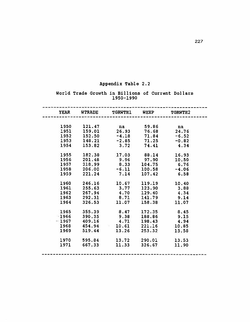
227

Appendix Table 2.2

World Trade Growth in Billions of Current Dollars1950-1990

-----------------------------------------------------------YEAR WTRADE TGRWTH1 WEXP TGRWTH2

-----------------------------------------------------------1950 121. 47 na 59.86 na1951 159.01 26.93 76.68 24.761952 152.50 -4.18 71.84 -6.521953 148.21 -2.85 71.25 -0.821954 153.82 3.72 74.41 4.34

1955 182.38 17.03 88.14 16.931956 201. 48 9.96 97.90 10.501957 218.99 8.33 104.75 6.761958 206.00 -6.11 100.58 -4.061959 221.24 7.14 107.42 6.58

1960 246.16 10.67 119.19 10.401961 255.63 3.77 123.90 3.881962 267.94 4.70 129.40 4.341963 292.31 8.71 141. 79 9.141964 326.53 11.07 158.38 11.07

1965 355.39 8.47 172.35 8.45'1966 390.35 9.38 188.86 9.15

"·1967 409.16 4.71 198.43 4.941968 454.94 10.61 221.16 10.851969 519.44 13.26 253.32 13.58

1970 595.84 13.72 290.01 13.531971 667.33 11.33 326.67 11.90

-----------------------------------------------------------

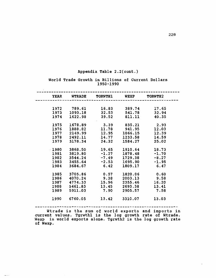
228

Appendix Table 2.2(cont.)

World Trade Growth in Billions of Current Dollars1950-1990

YEAR

197219731974

19751976197719781979

·19801981198219831984

19851986198719881989

1990

WTRADE

789.611093.181622.98

1678.891888.822149.992492.113178.34

3868.503819.803544.243455.643684.67

3705.864070.244774.335461. 835911.03

6760.05

TGRWTH1

16.8332.5339.52

3.3911. 7812.9514.7724.32

19.65-1. 27-7.49-2.53

6.42

0.579.38

15.9613.45

7.90

13.42

WEXP

389.74541. 78811.11

835.21941.95

1066.151233.581584.27

1910.641878.481729.381695.901809.17

1820.062003.132355.462693.382905.57

3310.07

TGRWTH2

17.6532.9440.35

2.9312.0312.3914.5925.02

18.73-1.70-8.27-1. 95

6.47

0.609.58

16.2013.41

7.58

13.03

Wtrade is the sum of world exports and imports incurrent val ues. Tgrwth1 is the log growth rate of Wtrade.Wexp is world exports alone. Tgrwth2 is the log growth rateof Wexp.

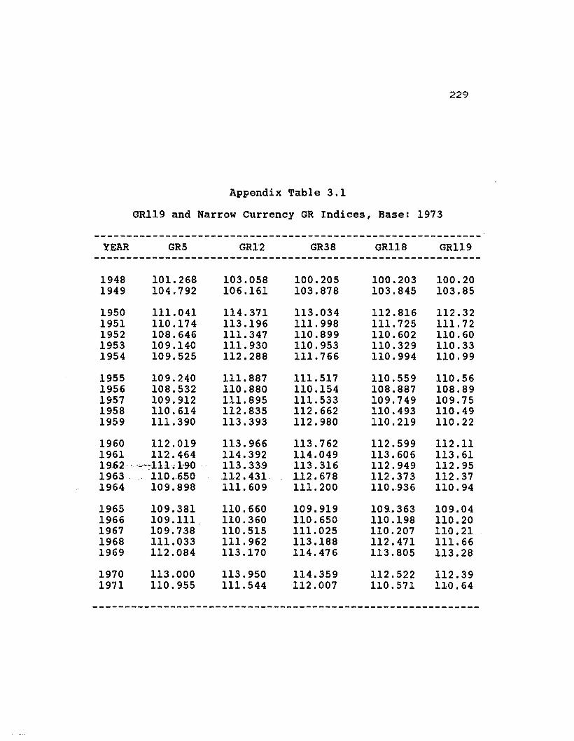
229

Appendix Table 3.1

GRl19 and Narrow Currency GR Indices, Base: 1973

------------------------------------------------------------YEAR GR5 GR12 GR38 GRl18 GRl19

------------------------------------------------------------1948 101.268 103.058 100.205 100.203 100.201949 104.792 106.161 103.878 103.845 103.85

1950 111. 041 114.371 113.034 112.816 112.321951 110.174 113.196 111.998 111. 725 111. 721952 108.646 111. 347 110.899 110.602 110.601953 109.140 111.930 110.953 110.329 110.331954 109.525 112.288 111. 766 110.994 110.99

1955 109.240 111. 887 111. 517 110.559 110.561956 108.532 110.880 110.154 108.887 108.891957 109.912 111. 895 111. 533 109.749 109.751958 110.614 112.835 112.662 110.493 110.491959 111.390 113.393 112.980 110.219 110.22

1960 112.019 113.966 113.762 112.599 112.111961 112.464 114.392 114.049 113.606 113.611962· ··;,--:,;"111.1-90 113.339 113.316 112.949 112.951963 .. 110 ..650 112.431. ll2.678 112.373 112.371964 109.898 111.609 111.200 110 ..936 110.94

1965 109.381 110.660 109.919 109.363 109.041966 109.111 110.360 110.650 110.198 110.201967 109.738 110.515 111.025 110.207 110.211968 111.033 111.962 113.188 112.471 111. 661969 112.084 113.170 114.476 113.805 113.28

1970 113.000 113.950 114.359 112.522 112.391971 110.955 111.544 112.007 110.571 110.64

------------------------------------------------------------

230

Appendix Table 3.1(cont.)

GRl19 and Narrow Currency GR Indices, Base: 1973

------------------------------------------------------------YEAR GR5 GR12 GR38 GRl18 GRl19

------------------------------------------------------------1972 106.090 106.100 106.684 104.716 104.771973 100.000 100.000 100.000 100.000 100.001974 100.016 99.787 98.386 98.361 98.68

1975 97.986 97.342 96.471 95.869 96.411976 99.242 99.045 98.571 96.685 97.381977 96.246 96.337 96.496 93.590 94.331978 88.624 89.005 89.354 87.321 88.141979 89.190 89.308 89.126 87.105 87.99

1980 90.244 90.359 89.828 88.208 89.141981 96.977 98.792 98.076 95.857 97.111982 103.174 105.108 105.350 102.516 104.081983 104.736 106.831 107.811 105.527 107.291984 107.312 110.330 111.984 109.780 112.01

1985 108.042 111.349 113.722 Ill. 874 114.431986 94.972 96.939 99.542 99.112 101.481987 88.563 89.625 91. 868 91.288 93.551988 85.012 86.290 88.224 87.464 89.621989 89.297 90.488 92.270 90.918 93.03

1990 87.885 87.541 88.797 88.083 90.43

-------------------------------------------------------------Source . Raw Data from IMF-IFS Tables..

231

Appendix Table 3.2A

GRl19 Sub-indices, 1950-1990, Base: 1973

YEAR

19501951195219531954

19551956195719581959

19601961196219631964

19651966196719681969

19701971

JAPAN

104.198104.314103.735103.621103.872

103.501103.959104.240104.569104.925

105.119105.663105.880105.418105.444

105.100105.363105.859105.797106.235

106.892105.614

EUROPE

112.330111.658109.965109.643111.481

109.314108.859109.738109.648109.794

Ill. 817112.065111.897110.576109.154

108.582108.460108.497110.119111.577

112.312109.819

CANADA

100.742100.497

99.74899.77899.985

99.796100.066

99.83699.90899.803

99.886100.199100.533100.606100.344

100.599100.583100.564100.539100.503

100.481100.174

ANZPAC

101.570101.444101.034101.016101.159

100.937100.933101.025101. 003100.956

100.958100.878101. 017101. 040100.927

100.940100.901100.922101.054101.200

101. 326101.172

232

Appendix Table 3.2A (cont. )

GRl19 Sub-indices, 1950-1990, Base: 1973

----------------------------------------------------------YEAR JAPAN EUROPE CANADA ANZPAC

----------------------------------------------------------1972 103.041 104.442 99.987 100.8681973 100.000 100.000 100.000 100.0001974 99.247 99.011 99.693 99.622

1975 99.712 96.547 99.978 100.0591976 98.076 98.522 99.415 99.9951977 95.539 97.108 100.131 100.2471978 88.459 92.055 100.549 99.9801979 91.923 89.058 101. 027 100.209

1980 94.113 89.390 101. 242 100.2161981 95.246 101. 334 101. 386 100.3471982 99.3086 106.733 101.162 100.7891983 98.6629 110.713 100.954 100.9991984 98.9953 115.256 101.324 101.202

1985 99.6189 116.324 101.705 101.8521986 89.3837 104.837 101.581 101.6311987 85.0976 97.646 101.287 101. 2521988 81. 2753 96.179 100.633 100.6571989 84.9342 100.042 100.349 100.634

1990 86.8691 92.232 100.261 100.604

----------------------------------------------------------

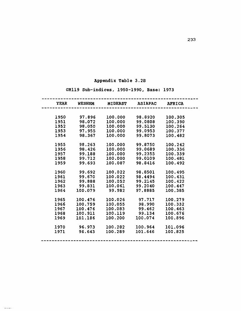
Appendix Table 3.2B

GRl19 Sub-indices, 1950-1990, Base: 1973

233

YEAR

19501951195219531954

19551956195719581959

19601961196219631964

19651966196719681969

19701971

WESHEM

97.89698.07298.05097.95598.367

98.26398.42699.18899.71299.693

99.69299.67099.88899.831

100.079

100.476100.759100.476100.911101.186

96.97396.643

MIDEAST

100.000100.000100.000100.000100.000

100.000100.000100.000100.000100.087

100.022100.022100.052100.061

99.982

100.026100.055100.083100.li9100.200

100.282100.289

ASIAPAC

98.892099.080899.513099.095399.8073

99.875099.068999.235599.010998.8416

98.850198.449499.214599.204097.8885

97.71798.99099.46299.134

100.074

100.964101. 646

AFRICA

100.305100.390100.264100.377100.482

100.242100.336100.339100.481100.492

100.495100.431100.422100.447100.385

100.279100.332100.463100.676100.896

101. 096100.825

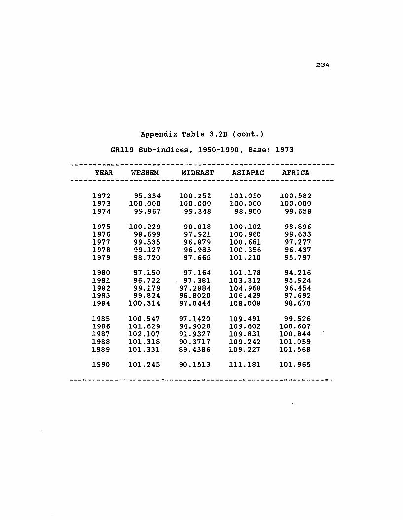
Appendix Table 3.2B (cont.)

GRl19 Sub-indices, 1950-1990, Base: 1973

234

YEAR

197219731974

19751976197719781979

19801981198219831984

19851986198719881989

1990

WESHEM

95.334100.000

99.967

100.22998.69999.53599.12798.720

97.15096.72299.17999.824

100.314

100.547101. 629102.107101. 318101. 331

101. 245

MIDEAST

100.252100.000

99.348

98.81897.92196.87996.98397.665

97.16497.381

97.288496.802097.0444

97.142094.902891.932790.371789.4386

90.1513

ASIAPAC

101. 050100.000

98.900

100.102100.960100.681100.356101. 210

101.178103.312104.968106.429108.008

109.491109.602109.831109.242109.227

111.181

AFRICA

100.582100.000

99.658

98.89698.63397.27796.43795.797

94.21695.92496.45497.69298.670

99.526100.607100.844101.059101.568

101.965

235

Appendix Table 3.3A

Index Value Cumulative Effect By Region and CountryPeak of 1969-1971, Base:1973

REGION/COUNTRY

Base Economy

1 United states

Japan Area

2 Japan

Europe (24 countries)

3 Germany, Federal Re4 France5 United Kingdom6 Italy7 Spain8 Netherlands9 Sweden

10 Switzerland11 Belgium12 Austria13 Norway14 Denmark15 Finland16 Turkey17 Yugoslavia18 Czechoslovakia19 Greece20 Portugal21 Hungary22 Ireland23 Luxembourg24 Iceland25 Cyprus26 Malta

Canada Area

27 Canada

1969

100.000

102.973

105.743107.026107.853108.466108.971109.442109.756110.086110.388110.579110.728110.933111. 017i.io, 902111.258111.258111. 260111. 328111. 328111. 359111. 372111. 376111.380111.381

111.616

1970

100.000

103.182

105.848107.457108.307108.897109.498109.993110.331110.698111. 002111. 218111.348111.551111.663111. 696111.811111.811111.838111.923111. 923111.952111.965111. 969111. 973111. 974

112.188

1971

100.000

102.665

104.996106.533106.999107.413107.842108.244108.520108.821109.111109.303109.431109.611109.698109.802109.968109.968110.011110.061110.061110.075110.084110.086110.090110.091

110.205

236

Appendix Table 3.3A (cont.)

Index Value Cumulative Effect By Region and CountryPeak of 1969-1971, Base:1973

-------------------------------------------------------------REGION/COUNTRY 1969 1970 1971

------------------------~------------------------------ - - - - - - -ANZPAC (6 countries)

28 Australia 112.096 112.701 110.66529 New Zealand 112.182 112.788 110.73230 Papua New Guinea 112.182 112.788 110.74031 Fiji 112.185 112.791 110.74332 Solomon Islands 112.185 112.791 110.74333 Tonga 112.185 112.791 110.743

WESHEM (26 countries)

34 Mexico 112.973 112.563 110.58835 Venezuela 112.959 112.560 110.58536 Colombia 112.948 112.569 110.59837 Chile 112.948 111.474 109.36638 Ecuador 112.933 111. 471 109.36839 Guatemala 112.929 111. 469 109.37140 Trinidad and Tobago 112.932 111.474 109.37841 EI Salvador 112.929 111. 471 109.37642 Uruguay 112.733 111. 271 109.17043 Panama 112.732 111. 271 109.17044 Paraguay 112.733 111. 274 109.17445 Dominican Republic 112.741 111.282 109.18146 Costa Rica 112.747 111. 289 109.18847 Honduras 112.745 111.287 109.18848 Bahamas, The 112.746 111. 288 109.18849 Haiti 112.749 111. 292 109.19150 Jamaica 112.757 111. 295 109.19351 Barbados 112.758 111. 296 109.19552 Suriname 112.759 111. 297 109.19653 Guyana 112.759 111.297 109.19654 Antigua and Barbuda 112.759 111. 297 109.19655 Belize 112.759 111. 297 109.19656 Grenada 112.759 111.297 109.19657 st. Vincent and the 112.759 111. 297 109.19658 Dominica 112.759 111. 297 109.19659 st. Kitts and Nevis 112.759 111. 297 109.196

--------------------------------------------------------------

237

Appendix Table 3.3A (cont.)

Index Value Cumulative Effect By Region and CountryPeak of 1969-1971, Base:1973

REGION/COUNTRY

MIDEAST (8 countries)

60 Iran, Islamic Repub61 Saudi Arabia62 Egypt, Arab Republi63 Syrian Arab Republi64 Kuwait65 Jordan66 Bahrain67 Yemen, PDR

Asia-Pacific (13 countries)

68 China69 India70 Korea, Republic of71 Indonesia72 Thailand73 Hong Kong74 Philippines75 Malaysia76 Pakistan77 Singapore78 Bangladesh79 Myanmar80 Sri Lanka81 Nepal

1969

112.810112.852112.835112.845112.845112.850112.850112.850

112.827113.044113.008113.035113.033113.077113.027113.067112.823112.846112.846112.853112.850112.852

1970

111. 366111.416111. 403111.413111. 413111. 417111.420111.420

111. 772111.949111.903111.950111.966112.010112.053112.101111.850111. 879111. 879111.893111.890111.890

1971

109.258109.316109.316109.325109.325109.328109.331109.331

109.795109.982109.948110.018110.044110.089110.113110.160110.093110.125110.226110.244110.242110.244

238

Appendix Table 3.3A (cont.)

Index Value Effect By Region and countryPeak of 1969-1971, Base:1973

-------------------------------------------------------------REGION/COUNTRY 1969 1970 1971

-------------------------------------------------------------Africa (31 countries)

82 Nigeria83 Algeria84 South Africa85 Morocco86 Cameroon87 Tunisia88 Cote d'Ivoire89 Tanzania90 Sudan91 Ghana92 Kenya93 Ethiopia94 Zimbabwe95 Zaire96 Gabon97 uganda98 senegal99 Madagascar

100 Zambia101 Somalia102 Congo, People's Rep103 Rwanda104 Niger105 Burundi106 Malawi107 Liberia108 Mauritius109 Burkina Faso110 Sierra Leone111 Botswana112 Chad113 Togo114 Mauritania115 Central African Rep116 Swaziland117 Lesotho118 Gambia, The119 Seychelles

112.943112.992113.059113.098113.112113.123113.134113.138113.149113.167113.171113.178113.187113.228113.230113.242113.249113.255113.265113.264113.266113.267113.274113.274113.275113.276113.276113.277113.273113.274113.277113.279113.282113.283113.283113.283113.283113.283

112.015112.062112.130112.178112.193112.205112.218112.225112.239112.263112.266112.269112.279112.314112.318112.326112.337112.348112.360112.361112.364112.366112.375112.376112.377112.378112.378112.380112.378112.379112.383112.386112.389112.391112.391112.391112.392112.392

110.285110.329110.413110.460110.474110.485110.500110.509110.524110.525110.528110.533110.546110.578110.582110.586110.596110.605110.613110.614110.617110.619110.628110.629110.629110.631110.632110.634110.633110.633110.637110.639110.642110.643110.644110.644110.644110.645

-------------------------------------------------------------

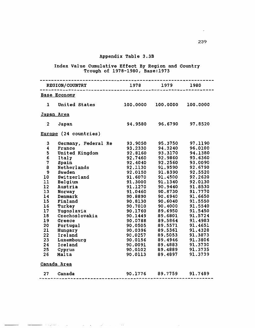
239

Appendix Table 3.3B

Index Value Cumulative Effect By Region and CountryTrough of 1978-1980, Base:1973

-------------------------------------------------------------REGION/COUNTRY 1978 1979 1980

-------------------------------------------------------------Base Economy

1 United states 100.0000 100.0000 100.0000

Japan Area

2 Japan 94.9580 96.6790 97.8520

Europe (24 countries)

3 Germany, Federal Re 93.9050 95.3750 97.11904 France 93.2330 94.3240 96.01005 United Kingdom 92.8160 93.3170 94.13806 Italy 92.7460 92.9860 93.63607 Spain 92.4040 92.2560 93.00908 Netherlands 92.1130 91.9590 92.67909 Sweden 92.0150 91.8390 92.5520

10 Switzerland 91. 6070 91.4500 92.262011 Belgium 91.3000 91.1340 92.013012 Austria 91.1270 90.9440 91.853013 Norway 91.0460 90.8730 91.777014 Denmark 90.8890 90.6940 91.665015 Finland 90.8130 90.6040 91.555016 Turkey 90.7010 90.4000 91. 554017 Yugoslavia 90.1760 89.6950 91. 545018 Czechoslovakia 90.1449 89.6801 91. 572419 Greece 90.0788 89.5864 91. 498320 Portugal 90.0505 89.5571 91. 465121 Hungary 90.0396 89.5361 91. 432822 Ireland 90.0257 89.5053 91. 387323 Luxembourg 90.0156 89.4946 91. 380624 Iceland 90.0091 89.4883 91. 373025 Cyprus 90.0102 89.4889 91. 373526 Malta 90.0113 89.4897 91.3739

Canada Area

27 Canada 90.1776 89.7759 91. 7489-------------------------------------------------------------

240

Appendix Table 3.3B (cont.)

Index Value Cumulative Effect By Region and CountryTrough of 1978-1980, Base:1973

REGION/COUNTRY

ANZPAC (6 countries)

28 Australia29 New Zealand30 Papua New Guinea31 Fiji32 Solomon Islands33 Tonga

WESHEM (26 countries)

34 Mexico35 Venezuela36 Colombia37 Chile38 Ecuador39 Guatemala40 Trinidad and Tobago41 EI Salvador42 Uruguay43 Panama44 Paraguay45 Dominican Republic46 Costa Rica47 Honduras48 Bahamas, The49 Haiti50 Jamaica51 Barbados52 Suriname53 Guyana54 Antigua and Barbuda55 Belize56 Grenada57 st. Vincent and the58 Dominica59 st. Kitts and Nevis

1978

90.177490.178690.176690.176090.176290.1762

90.020290.004489.956090.085090.057390.042290.038690.028289.934789.935989.932089.924289.931089.930189.930489.930289.927989.925789.924389.924589.924689.924889.924789.924989.924989.9249

1979

89.834789.833789.832889.832589.832789.8328

89.595389.577789.519589.6657·89.637689.623289.617989.606389.474089.475989.465989.459889.467489.466989.467789.467389.467489.464889.463289.463189.463289.463589.463489.463589.463489.4635

1980

91.828491.831491. 829891. 829191. 829291. 8293

91.316191. 245491.181091. 322091. 290891. 277491. 269191. 257591. 072491. 074691. 059191. 050491. 056691. 055191. 055991.055091.052491.049591. 048291. 048091. 048191.048491. 048291. 048391.048391. 0483

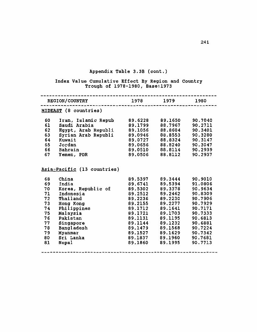
241

Appendix Table 3.3B (cont.)

Index Value Cumulative Effect By Region and CountryTrough of 1978-1980, Base:1973

REGION/COUNTRY

MIDEAST (8 countries)

60 Iran, Islamic Repub61 Saudi Arabia62 Egypt, Arab Republi63 Syrian Arab Republi64 Kuwait65 Jordan66 Bahrain67 Yemen, PDR

Asia-Pacific (13 countries)

68 China69 India70 Korea, Republic of71 Indonesia72 Thailand73 Hong Kong74 Philippines75 Malaysia76 Pakistan77 Singapore78 Bangladesh79 Myanmar80 Sri Lanka81 Nepal

1978

89.622889.179989.105689.094689.072789.065689.051089.0506

89.539789.674189.530289.251289.223689.215589.171289.172189.113189.114489.147989.152789.183789.1860

1979

89.165088.796788.860488.855388.832488.824088.811488.8112

89.344489.539489.337889.246289.223089.227789.164189.170389.119589.123289.156889.162989.196089.1995

1980

90.704090.271190.340190.328090.314790.304790.293990.2937

90.901091. 080690.963490.830990.790690.792990.717190.733390.681390.688190.722490.734290.768190.7713

242

Appendix Table 3.3B (cont.)

Index Value Cumulative Effect By Region and CountryTrough of 1978-1980, Base:1973

REGION/COUNTRY

Africa (31 countries)

82 Nigeria83 Algeria84 South Africa85 Morocco86 Cameroon87 Tunisia88 Cote d'Ivoire89 Tanzania90 Sudan91 Ghana92 Kenya93 Ethiopia94 Zimbabwe95 Zaire96 Gabon97 Uganda98 Senegal99 Madagascar

100 Zambia101 Somalia102 Congo, People's Rep103 Rwanda104 Niger105 Burundi106 Malawi107 Liberia108 Mauritius109 Burkina Faso110 Sierra Leone111 Botswana112 Chad113 Togo114 Mauritania115 Central African Rep116 Swaziland117 Lesotho118 Gambia, The119 Seychelles

1978

88.730088.698488.728188.719288.706088.710588.679488.668888.638788.436388.418688.404488.408588.306588.295688.176088.170988.170288.166888.162288.161188.157288.152288.151088.150388.149088.146988.145388.143688.144188.144388.141988.141888.139688.139688.139588.139288.1390

1979

88.659488.608888.616588.599188.582988.588588.546588.539788.511188.372088.353588.338588.340688.262588.249788.036388.029488.026388.023188.017288.015488.011188.005588.002588.002888.001587.999287.996787.994687.995087.994987.992787.992587.989787.989387.989087.988687.9883

1980

90.064890.022989.962589.952989.936989.944989.899489.885889.862889.632789.613389.602189.605989.544189.528089.205289.199189.193789.190889.172189.170689.166889.161289.158689.158189.156789.154589.152089.149789.149889.149989.147489.147689.144689.143489.142789.142389.1419

243

Appendix Table 3.3C

Index Value Cumulative Effect By Region and CountryPeak of 1984-1986, Base:1973

-------------------------------------------------------------REGION/COUNTRY 1984 1985 1986

-------------~----------------------------------------- - - - - - -Base Economy

1 United states 100.000 100.000 100.0000

Japan Area

2 Japan 99.507 99.725 94.7810

Europe (24 countries)

3 Germany, Federal Re 102.016 102.439 95.99704 France 103.925 104.408 96.70105 United Kingdom 104.511 105.045 96.70506 Italy 105.658 106.283 96.80207 Spain 106.045 106.671 96.78208 Netherlands 106.454 107.129 96.89109 Sweden 106.868 107.551 97.1060

10 Switzerland 106.960 107.677 96.946011 Belgium 107.328 108.013 97.065012 Austria 107.485 108.186 97.038013 Norway 107.605 108.322 97.056014 Denmark 107.788 108.517 97.087015 Finland 107.854 108.598 97.048016 Turkey 108.141 108.902 97.291017 Yugoslavia 108.567 109.362 97.628018 Czechoslovakia 108.694 109.506 97.733419 Greece 108.783 109.608 97.772320 Portugal 108.845 109.671 97.790721 Hungary 108.890 109.715 97.807922 Ireland 108.912 109.741 97.781823 Luxembourg 108.927 109.757 97.789124 Iceland 108.933 109.763 97.789625 Cyprus 108.944 109.776 97.798026 Malta 108.949 109.781 97.8007

Canada Area

27 Canada 109.505 110.497 98.3519-------------------------------------------------------------

244

Appendix Table 3.3C (cont.)

Index Value Cumulative Effect By Region and CountryPeak of 1984-1986, Base:1973

REGION/COUNTRY

ANZPAC (6 countries)

28 Australia29 New Zealand30 Papua New Guinea31 Fiji32 Solomon Islands33 Tonga

WESHEM (26 countries)

34 Mexico35 Venezuela36 Colombia37 Chile38 Ecuador39 Guatemala40 Trinidad and Tobago41 EI Salvador42 Uruguay43 Panama44 Paraguay45 Dominican Republic46 Costa Rica47 Honduras48 Bahamas, The49 Haiti50 Jamaica51 Barbados52 Suriname53 Guyana54 Antigua and Barbuda55 Belize56 Grenada57 st. Vincent and the58 Dominica59 st. Kitts and Nevis

1984

109.909109.989109.993109.995109.996109.996

109.990110.108110.104110.310110.295110.280110.245110.215110.145110.152110.143110.106110.132110.128110.129110.126110.135110.130110.128110.127110.127110.128110.127110.127110.127110.127

1985

111.168111.254111. 260111. 262111.263111.263

111. 254111. 373111.428111.636111. 601111. 568111. 532111. 487111. 423111.432111.435111.458111. 486111.481111.482111.477111.488111. 482111. 479111.479111.479111.479111. 479111. 479111. 479111. 479

1986

98.849598.894398.898398.900198.900798.9008

99.162599.246199.330499.498799.513299.516799.512299.500799.434499.442399.438599.454099.477999.473399.473599.469299.476699.471899.468899.468099.468099.468399.467999.468099.467999.4680

245

Appendix Table 3.3C (cont.)

Index Value Cumulative Effect By Region and CountryPeak of 1984-1986, Base:1973

REGION/COUNTRY

MIDEAST (8 countries)

60 Iran, Islamic Repub61 Saudi Arabia62 Egypt, Arab Republi63 Syrian Arab Republi64 Kuwait65 Jordan66 Bahrain67 Yemen, PDR

Asia-Pacific (13 countries)

68 China69 India70 Korea, Republic of71 Indonesia72 Thailand73 Hong Kong74 Philippines75 Malaysia76 Pakistan77 Singapore78 Bangladesh79 Myanmar80 Sri Lanka81 Nepal

1984

109.061108.916108.905108.841108.857108.854108.839108.838

111. 349112.061112.055112.169112.179112.277112.301112.361112.379112.407112.490112.526112.592112.601

1985

110.347110.308110.255110.159110.179110.178110.167110.166

113.026113.881113.960114.132114.197114.295114.295114.377114.426114.463114.555114.591114.662114.673

1986

97.874797.890697.766497.623997.633697.628597.622197.6221

99.9385100.568100.640100.815100.861100.943100.969101.036101.082101.112101.183101. 202101.257101. 265

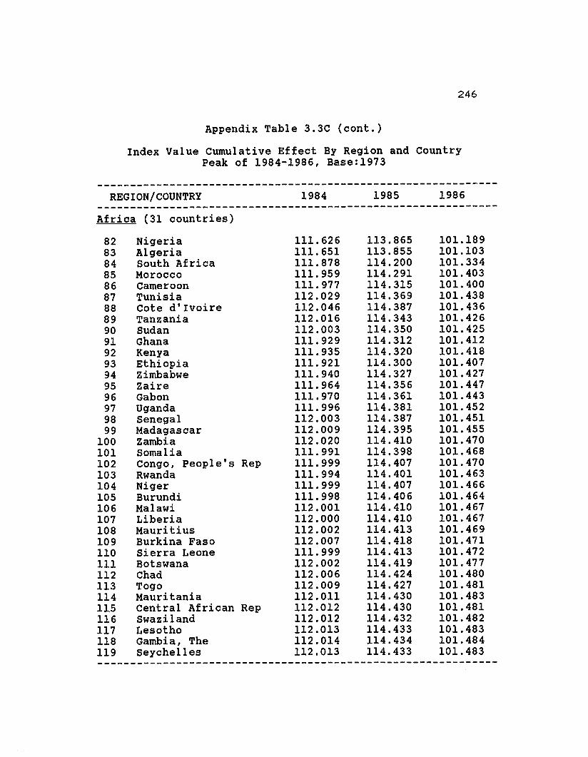
246

Appendix Table 3.3C (cont.)

Index Value Cumulative Effect By Region and CountryPeak of 1984-1986, Base:1973

------------------------------------------------------- - - ~ - - -

REGION/COUNTRY 1984 1985 1986-------------------------------------------------------------Africa (31 countries)

82 Nigeria83 Algeria84 South Africa85 Morocco86 Cameroon87 Tunisia88 Cote d'Ivoire89 Tanzania90 Sudan91 Ghana92 Kenya93 Ethiopia94 Zimbabwe95 Zaire96 Gabon97 Uganda98 Senegal99 Madagascar

100 Zambia101 Somalia102 Congo, People's Rep103 Rwanda104 Niger105 Burundi106 Malawi107 Liberia108 Mauritius109 Burkina Faso110 Sierra Leone111 Botswana112 Chad113 Togo114 Mauritania115 Central African Rep116 Swaziland117 Lesotho118 Gambia, The119 Seychelles

111.626111. 651111.878111.959111.977112.029112.046112.016112.003111.929111.935111.921111.940111.964111.970111.996112.003112.009112.020111. 991111.999111. 994111.999111.998112.001112.000112.002112.007111. 999112.002112.006112.009112.011112.012112.012112.013112.014112.013

113.865113.855114.200114.291114.315114.369114.387114.343114.350114.312114.320114.300114.327114.356114.361114.381114.387114.395114.410114.398114.407114.401114.407114.406114.410114.410114.413114.418114.413114.419114.424114.427114.430114.430114.432114.433114.434114.433

101.189101.103101.334101. 403101. 400101.438101. 436101. 426101. 425101. 412101. 418101. 407101.427101. 447101. 443101. 452101.451101. 455101. 470101. 468101. 470101. 463101.466101.464101.467101.467101.469101.471101. 472101.477101. 480101.481101.483101. 481101. 482101. 483101. 484101.483

-------------------------------------------------------------

247

Appendix Table 3.4A

Trade Shares in Billions of Current Dollars1950-1990

------------------------------------------------------------Year USTRD1 USTRADE G-5 G-10 WORLD-TRADE

w/o Ag & Pet------------------------------------------------------------

1950 19.624 45.897 46.378 121.4701951 25.889 62.752 64.388 159.0101952 24.910 61. 719 64.362 152.5001953 24.108 61. 914 65.442 148.2101954 23.994 64.399 69.104 153.820

1955 26.780 72.298 77.662 182.3801956 31. 320 81. 571 87.182 201.4801957 34.115 90.091 95.391 218.9901958 30.983 82.429 88.757 206.0001959 33.413 90.933 97.993 221.240

1960 36.007 102.926 112.933 246.1601961 36.142 107.554 120.852 255.6301962 38.775 114.158 128.517 267.9401963 41.067 123.938 141. 674 292.3101964 46.024 139.487 160.117 326.530

1965 39.550 49.932 152.410 175.731 355.3901966 46.003 57.170 168.974 193.160 390.3501967 49.474 59.753 177.253 204.380 409.1601968 58.595 69.501 201. 793 230.627 454.9401969 64.826 75.830 230.401 269.411 519.440

1970 72.645 85.048 265.714 312.888 595.8401971 78.051 91.891 297.435 352.400 667.3301972 91.109 108.061 353.163 421. 734 789.6101973 114.920 144.022 484.139 577.571 1093.1801974 155.228 210.312 678.451 792.006 1622.980

1975 160.319 214.736 697.635 817.828 1678.8901976 184.982 249.292 794.742 923.720 1888.8201977 207.554 283.593 910.236 1047.991 2149.9901978 250.514 331.892 1079.091 1241. 750 2492.1101979 301. 393 408.591 1345.875 1563.814 3178.340

------------------------------------------------------------

Appendix Table 3.4A (cont.)

Trade Shares in billions of current Dollars1950-1990

248

Year USTRD1 USTRADE G-5 G-10 WORLD-TRADEw/o Ag & Pet

-------------------------------------------------------------1980 351. 213 482.550 1611. 724 1857.013 3868.5001981 375.367 512.067 1578.745 1750.031 3819.8001982 360.076 471. 326 1481.995 1650.873 3544.2401983 370.592 475.517 1463.788 1624.410 3455.6401984 449.211 570.340 1601. 485 1705.433 3684.670

1985 480.156 571. 278 1641. 485 1766.718 3705.8601986 531.902 609.453 1869.837 2074.522 4070.2401987 589.905 678.564 2176.210 2462.649 4774.3301988 687.495 781.969 2489.142 2792.668 5461.8301989 745.998 856.734 2673.772 2971. 541 5911.030

1990 910.579 3048.728 3487.347 6760.050

w/o Ag & Pet - Without Agriculture and Petroleum Trade.Sources: Bureau of Economic Analysis, Bel Data.

lMF-lFS Tapes.

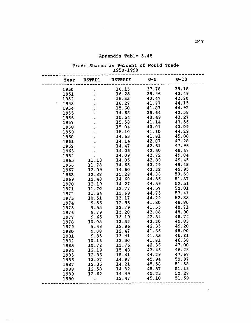
249

Appendix Table 3.4B

Trade Shares as Percent of World Trade1950-1990

----------------------------------------------------------Year USTRD1 USTRADE G-5 G-10

----------------------------------------------------------1950 16.15 37.78 38.181951 16.28 39.46 40.491952 16.33 40.47 42.201953 16.27 41. 77 44.151954 15.60 41.87 44.921955 14.68 39.64 42.581956 15.54 40.49 43.271957 15.58 41.14 43.561958 15.04 40.01 43.091959 15.10 41.10 44.291960 14.63 41.81 45.881961 14.14 42.07 47.281962 14.47 42.61 47.961963 14.05 42.40 48.471964 14.09 42.72 49.041965 11.13 14.05 42.89 49.451966 11. 78 14.65 43.29 49.481967 12.09 14.60 43.32 49.951968 12.88 15.28 44.36 50.691969 12.48 14.60 44.36 51.871970 12.19 14.27 44.59 52.511971 11.70 13.77 44.57 52.811972 11.54 13.69 44.73 53.411973 10.51 13.17 44.29 52.831974 9.56 12.96 41.80 48.801975 9.55 12.79 41.55 48.711976 9.79 13.20 42.08 48.901977 9.65 13.19 42.34 48.741978 10.05 13.32 43.30 49.831979 9.48 12.86 42.35 49.201980 9.08 12.47 41. 66 48.001981 9.83 13.41 41.33 45.811982 10.16 13.30 41.81 46.581983 10.72 13.76 42.36 47.001984 12.19 15.48 43.46 46.281985 12.96 15.41 44.29 47.671986 13.07 14.97 45.94 50.971987 12.36 14.21 45.58 51.581988 12.58 14.32 45.57 51.131989 12.62 14.49 45.23 50.271990 13.47 45.10 51.59

----------------------------------------------------------

250

Appendix Table 3.5

G-5 and G-10 Share of Gross World Productin Billions of Current US dollars

YEAR

195019511952195319541955195619571958195919601961196219631964196519661967196819691970197119721973197419751976197719781979198019811982198319841985198619871988

GD5SHR

54.610354.523054.374654.347853.994854.282353.715553.326559.981453.081853.549153.630153.879853.279452.986952.912852.994753.152652.955152.678852.050552.000551. 765951.124648.816848.245848.493848.599349.417248.401747.041947.604247.935248.935149.866450.738652.834753.301653.5369

G5GDP

388.64456.03488.42517.56527.61575.05613.71649.24750.17709.72754.63806.13874.21933.04

1014.721103.211206.951283.731394.981528.671662.771839.552120.002535.232760.973075.723352.273817.544637.795236.975760.365944.475893.566177.566525.296900.088343.099556.17

10667.67

GD10SHR

22.235322.632723.486823.523924.247024.409824.832024.958133.362924.713725.975227.135427.459827.756628.321128.370828.353628.830628.514228.930729.847630.833432.285134.062933.362233.814833.318933.579535.623035.655335.240132.887831.823831.511530.206530.202735.877738.619939.6497

G10GDP

158.24189.30210.97224.02236.93258.59283.71303.86417.26330.43366.05407.88445.54486.08542.36591. 52645.75696.31751.14839.53953.49

1090.751322.191689.151886.892155.732303.262637.713343.213857.844315.214106.793912.683978.003952.694107.355665.436923.967900.53

GWP

711. 66836.40898.25952.31977.15

1059.371142.521217.481250.671337.031409.231503.131622.521751.221915.042084.962277.492415.182634.272901. 873194.533537.564095.364958.925655.786375.116912.787855.139384.97

10819.8112245.1712487.2812294.8412623.9813085.5513599.2715790.9417928.4719925.84

G5GDP includes the US share and is larger than G10GDPwhich does not. Source: IMF-IFS Tapes.

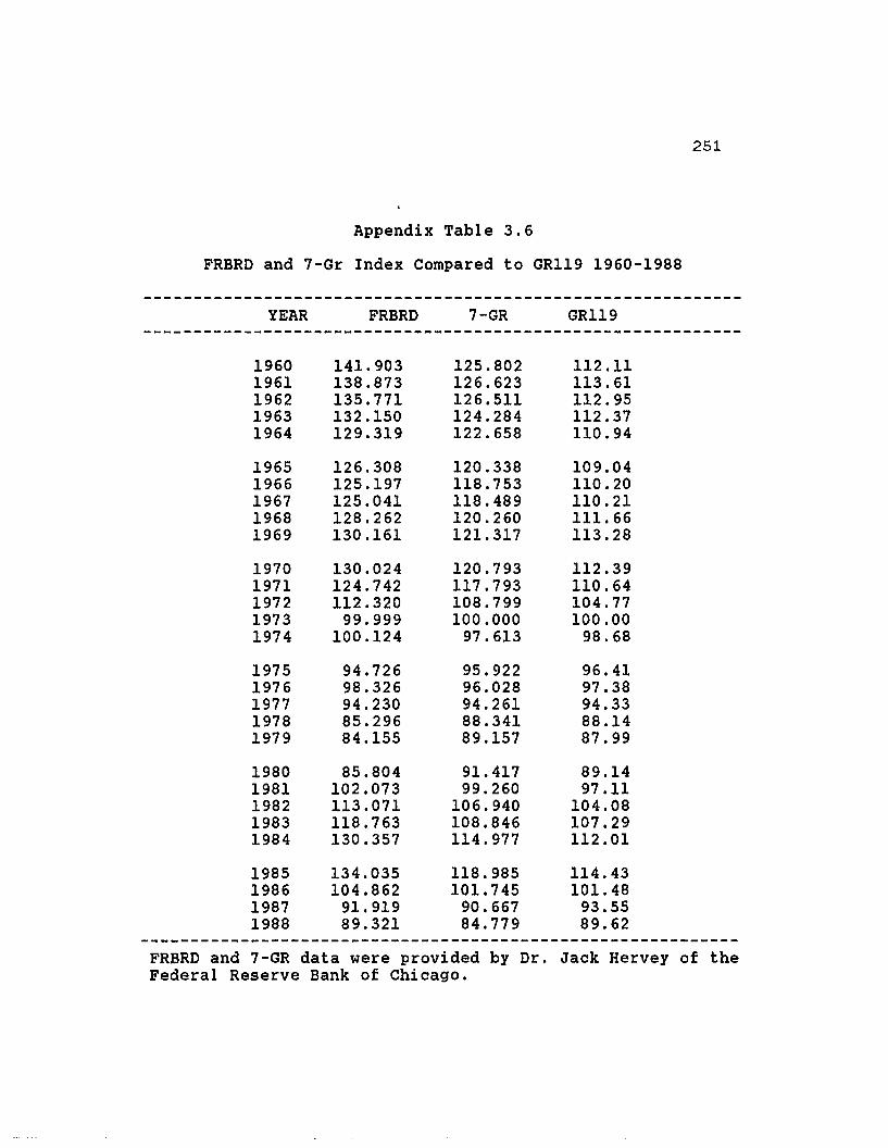
Appendix Table 3.6

FRBRD and 7-Gr Index Compared to GRl19 1960-1988

251

YEAR FRBRD 7-GR GRl19

1960 141.903 125.802 112.111961 138.873 126.623 113.611962 135.771 126.511 112.951963 132.150 124.284 112.371964 129.319 122.658 110.94

1965 126.308 120.338 109.041966 125.197 118.753 110.201967 125.041 118.489 110.211968 128.262 120.260 111.661969 130.161 121. 317 113.28

1970 130.024 120.793 112.391971 124.742 117.793 110.641972 112.320 108.799 104.771973 99.999 100.000 100.001974 100.124 97.613 98.68

1975 94.726 95.922 96.411976 98.326 96.028 97.381977 94.230 94.261 94.331978 85.296 88.341 88.141979 84.155 89.157 87.99

1980 85.804 91. 417 89.141981 102.073 99.260 97.111982 113.071 106.940 104.081983 118.763 108.846 107.291984 130.357 114.977 112.01

1985 134.035 118.985 114.431986 104.862 101. 745 101.481987 91. 919 90.667 93.551988 89.321 84.779 89.62

------------------------------------------------------------FRBRD and 7-GR data were provided by Dr. Jack Hervey of theFederal Reserve Bank of Chicago.

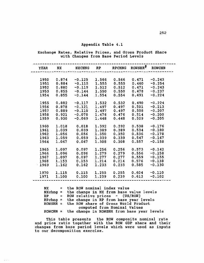
252

Appendix Table 4.1

Exchange Rates, Relative Prices, and Gross Product Sharewith Changes from Base Period Levels

YEAR NX NXCHNG RP RPCHNG ROWSHR# ROWCHN

19501951195219531954

19551956195719581959

19601961196219631964

1965196619671968

. 1969

19701971

0.8740.8840.8800.8550.855

0.8820.8780.8890.9210.930

1.0181.0391.0561.0591.067

1.0971.0961.0971.1531.162

1.1151.100

-0.125-0.115-0.119-0.144-0.144

-0.117-0.121-0.110-0.078-0.069

0.0180.0390.0560.0590.067

0.0970.0960.0970.1530.162

0.1150.100

1.5661.5551.5121.5501.554

1.5321. 4971. 4971. 4761.448

1. 3921. 3891.3501.3391. 308

1.2561. 2791. 2771. 2141. 233

1. 2551.239

0.5660.5550.5120.5500.554

0.5320.4970.4970.4760.448

0.3920.3890.3500.3390.308

0.2560.2790.2770.2140.233

0.2550.239

0.4710.4600.4710.4780.491

0.4900.5010.5080.5140.509

0.5380.5340.5360.5470.557

0.5730.5560.5590.5760.585

0.6040.613

-0.243-0.254-0.243-0.237-0.224

-0.224-0.213-0.207-0.200-0.205

-0.176-0.180-0.178-0.167-0.158

-0.142-0.158-0.155-0.138-0.130

-0.110-0.102

NX =NXchng =RP =RPchng =ROWSHR =ROWCHN =

the ROW nominal index valuethe change in NX from base value levelsROW relative prices (US/ROW)the change in RP from base year levelsthe ROW share of Gross World Product

computed from Nominal Valuesthe change in ROWSHR from base year levels

This table presents the ROW composite nominal rateand price ratio together with the ROW GDP share and theirchanges from base period levels which were used as inputsto our decomposition exercise.

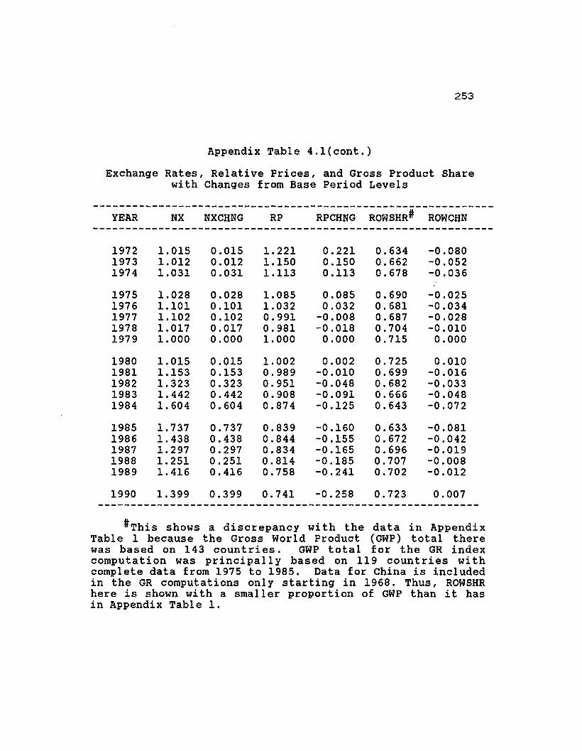
253

Appendix Table 4.1{cont.)

Exchange Rates, Relative Prices, and Gross Product Sharewith Changes from Base Period Levels

YEAR NX NXCHNG RP RPCHNG ROWSHR# ROWCHN

197219731974

19751976197719781979

19801981198219831984

19851986198719881989

1990

1.0151.0121.031

1.0281.1011.1021.0171.000

1.0151.1531.3231. 4421. 604

1. 7371. 4381.2971. 2511. 416

1.399

0.0150.0120.031

0.0280.1010.1020.0170.000

0.0150.1530.3230.4420.604

0.7370.4380.2970.2510.416

0.399

1.2211.1501.113

1.0851.0320.9910.9811.000

1.0020.9890.9510.9080.874

0.8390.8440.8340.8140.758

0.741

0.2210.1500.113

0.0850.032

-0.008-0.0180.000

0.002-0.010-0.048-0.091-0.125

-0.160-0.155-0.165-0.185-0.241

-0.258

0.6340.6620.678

0.6900.6810.6870.7040.715

0.7250.6990.6820.6660.643

0.6330.6720.6960.7070.702

0.723

-0.080-0.052-0.036

-0.025-0.034-0.028-0.0100.000

0.010-0.016-0.033-0.048-0.072

-0.081-0.042-0.019-0.008-0.012

0.007

#This shows a discrepancy with the data in AppendixTable 1 because the Gross World Product (GWP) total therewas based on 143 countries. GWP total for the GR indexcomputation was principally based on 119 countries withcomplete data from 1975 to 1985. Data for China is includedin the GR computations only starting in 1968. Thus, ROWSHRhere is shown with a smaller proportion of GWP than it hasin Appendix Table 1.

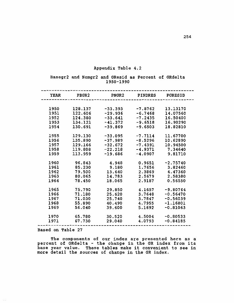
254

Appendix Table 4.2

Basegr2 and Nomgr2 and GResid as Percent of GRdelta1950-1990

----------------------------------------------------------YEAR PBGR2 PNGR2 PINDRES PGRESID

----------------------------------------------------------

1950 128.137 -33.393 -7.8762 13.131701951 122.606 -29.936 -6.7468 14.075601952 124.380 -33.641 -7.2435 16.504001953 134.121 -41.372 -9.6518 16.902901954 130.691 -39.869 -9.6503 18.82810

1955 129.130 -33.095 -7.7114 11.677001956 135.890 -37.989 -8.5296 10.628901957 129.166 -32.672 -7.4391 10.945001958 119.808 -22.218 -4.9371 7.346401959 113.959 -19.686 -4.0907 9.81710

1960 96.843 4.948 0.9651 -2.757401961 85.230 9.180 1. 7656 3.824601962 79.500 13.640 2.3869 4.473601963 80.065 14.783 2.5679 2.583801964 78.450 18.065 2.9187 0.56550

1965 75.790 29.850 4.1657 -9.807641966 71.180 25.620 3.7648 -0.564701967 71.030 25.740 3.7847 -0.560391968 55.890 40.490 4.7955 -1.168011969 56.040 39.600 5.1692 -0.81063

1970 65.780 30.520 4.5004 -0.805331971 67.730 29.040 4.0793 -0.84185

----------------------------------------------------------Based on Table 27

The components of our index are presented here as apercent of GRdelta - the change in the GR index from itsbase year value. These tables make it convenient to see inmore detail the sources of change in the GR index.

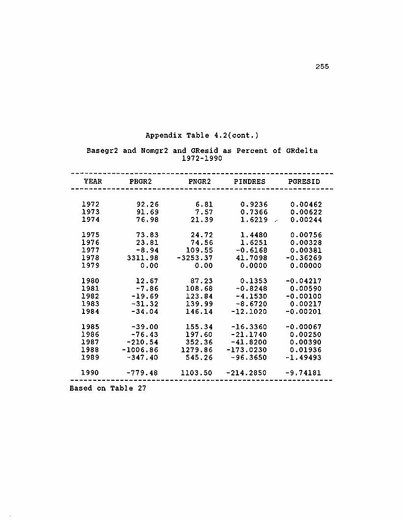
255

Appendix Table 4.2(cont.)

Basegr2 and Nomgr2 and GResid as Percent of GRdelta1972-1990

----------------------------------------------------------YEAR PBGR2 PNGR2 PINDRES PGRESID

----------------------------------------------------------

1972 92.26 6.81 0.9236 0.004621973 91. 69 7.57 0.7366 0.006221974 76.98 21.39 1. 6219 0.00244

1975 73.83 24.72 1.4480 0.007561976 23.81 74.56 1.6251 0.003281977 -8.94 109.55 -0.6168 0.003811978 3311. 98 -3253.37 41. 7098 -0.362691979 0.00 0.00 0.0000 0.00000

1980 12.67 87.23 0.1353 -0.042171981 -7.86 108.68 -0.8248 0.005901982 -19.69 123.84 -4.1530 -0.001001983 -31.32 139.99 -8.6720 0.002171984 -34.04 146.14 -12.1020 -0.00201

1985 -39.00 155.34 -16.3360 -0.000671986 -76.43 197.60 -21.1740 0.002501987 -210.54 352.36 -41. 8200 0.003901988 -1006.86 1279.86 -173.0230 0.019361989 -347.40 545.26 -96.3650 -1. 49493

1990 -779.48 1103.50 -214.2850 -9.74181----------------------------------------------------------Based on Table 27

Appendix Table 4.3

Delta4, Xresid, and GResid as Percent of GRdelta1950-1990

256

YEAR PDELTA4 PXRESID PGRESID

1950 117.690 -30.8220 13.131701951 115.644 -29.7200 14.075601952 111. 419 -27.9230 16.504001953 115.991 -32.8930 16.902901954 111. 730 -30.5580 18.82810

1955 115.512 -27.1890 11.677001956 116.097 -26.7260 10.628901957 112.844 -23.7890 10.945001958 111.113 -18.4600 7.346401959 106.866 -16.6830 9.81710

1960 109.330 -6.5730 -2.757401961 101. 286 -5.1110 3.824601962 99.009 -3.4820 4.473601963 100.177 -2.7610 2.583801964 101. 043 -1. 6090 0.56550

1965 109.207 0.6008 -9.807641966 100.851 -0.2866 -0.564701967 100.710 -0.1504 -0.560391968 99.225 1.9425 -1.168011969 98.465 2.3456 -0.81063

1970 98.705 2.1005 -0.805331971 98.821 2.0204 -0.84185

------------------------------------------------Based on Table 24

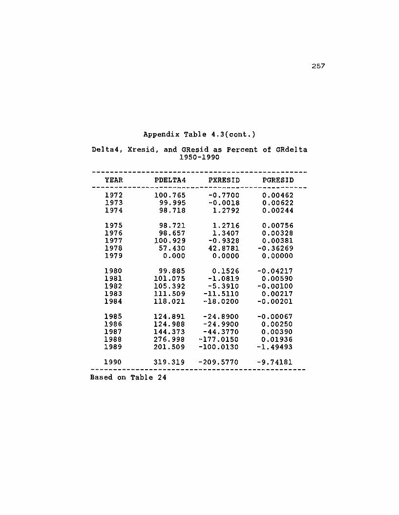
Appendix Table 4.3(cont.)

Delta4, Xresid, and GResid as Percent of GRdelta1950-1990

------------------------------------------------YEAR PDELTA4 PXRESID PGRESID

------------------------------------------------1972 100.765 -0.7700 0.004621973 99.995 -0.0018 0.006221974 98.718 1. 2792 0.00244

1975 98.721 1. 2716 0.007561976 98.657 1. 3407 0.003281977 100.929 -0.9328 0.003811978 57.430 42.8781 -0.362691979 0.000 0.0000 0.00000

1980 99.885 0.1526 -0.042171981 101.075 -1.0819 0.005901982 105.392 -5.3910 -0.001001983 111. 509 -11. 5110 0.002171984 118.021 -18.0200 -0.00201

1985 124.891 -24.8900 -0.000671986 124.988 -24.9900 0.002501987 144.373 -44.3770 0.003901988 276.998 -177.0150 0.019361989 201. 509 -100.0130 -1. 49493

1990 319.319 -209.5770 -9.74181------------------------------------------------Based on Table 24

257

Appendix Table 4.4

Bresid, Nresid, and INDresid as Percent of GRdelta1950-1990

258

----------------------------------------------------YEAR PBRESID PNRESID PINDRES

----------------------------------------------------1950 -21.28800 -1. 65700 -7.87621951 -21.51500 -1. 45900 -6.74681952 -19.09400 -1. 58600 -7.24351953 -20.94600 -2.29600 -9.65181954 -18.87500 -2.03300 -9.6503

1955 -18.11500 -1.36200 -7.71141956 -16.70500 -1. 49200 -8.52961957 -15.23800 -1.11200 -7.43911958 -13.01700 -0.50500 -4.93711959 -12.18600 -0.40700 -4.0907

1960 -7.51600 -0.02100 0.96511961 -6.79200 -0.08500 1. 76561962 -5.69000 -0.17900 2.38691963 -5.14100 -0.18700 2.56791964 -4.28700 -0.24100 2.9187

1965 -3.06996 -0.49532 4.16571966 -3.56894 -0.48241 3.76481967 -3.46056 -0.47448 3.78471968 -1. 86152 -0.99174 4.79551969 -1.87216 -0.95141 5.1692

1970 -1.96223 -0.43809 4.50041971 -1. 72906 -0.32974 4.0793

----------------------------------------------------Based on Tables 24 and 26

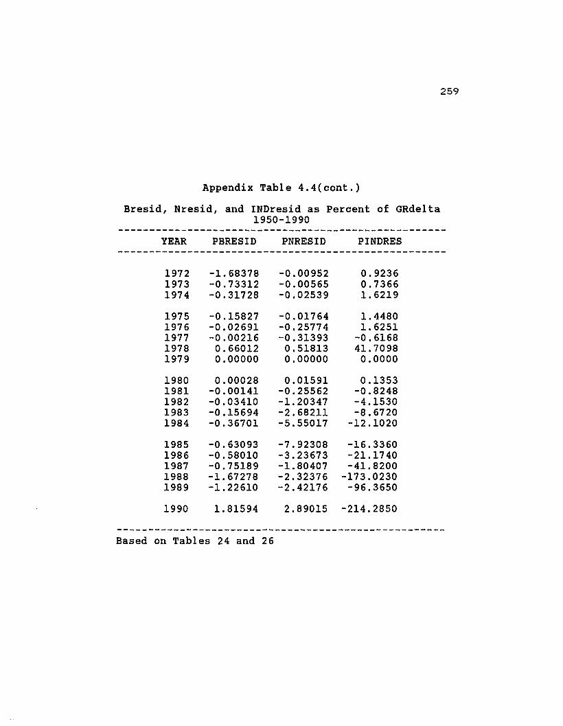
Appendix Table 4.4(cont.)

259

Bresid, Nresid, and INDresid as Percent of GRdelta1950-1990

YEAR PBRESID PNRESID PINDRES

1972 -1.68378 -0.00952 0.92361973 -0.73312 -0.00565 0.73661974 -0.31728 -0.02539 1. 6219

1975 -0.15827 -0.01764 1.44801976 -0.02691 -0.25774 1. 62511977 -0.00216 -0.31393 -0.61681978 0.66012 0.51813 41. 70981979 0.00000 0.00000 0.0000

1980 0.00028 0.01591 0.13531981 -0.00141 -0.25562 -0.82481982 -0.03410 -1. 20347 -4.15301983 -0.15694 -2.68211 -8.67201984 -0.36701 -5.55017 -12.1020

1985 -0.63093 -7.92308 -16.33601986 -0.58010 -3.23673 -21.17401987 -0.75189 -1. 80407 -41.82001988 -1. 67278 -2.32376 -173.02301989 -1.22610 -2.42176 -96.3650

1990 1.81594 2.89015 -214.2850

----------------------------------------------------Based on Tables 24 and 26

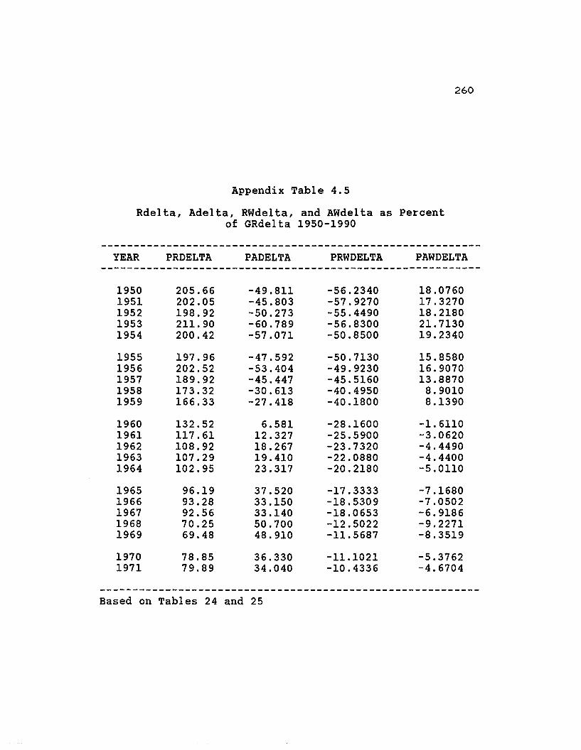
260

Appendix Table 4.5

Rdelta, Adelta, RWdelta, and AWdelta as Percentof GRdelta 1950-1990

YEAR PRDELTA PADELTA PRWDELTA PAWDELTA

1950 205.66 -49.811 -56.2340 18.07601951 202.05 -45.803 -57.9270 17.32701952 198.92 -50.273 -55.4490 18.21801953 211.90 -60.789 -56.8300 21. 71301954 200.42 -57.071 -50.8500 19.2340

1955 197.96 -47.592 -50.7130 15.85801956 202.52 -53.404 -49.9230 16.90701957 189.92 -45.447 -45.5160 13.88701958 173.32 -30.613 -40.4950 8.90101959 166.33 -27.418 -40.1800 8.1390

1960 132.52 6.581 -28.1600 -1.61101961 117.61 12.327 -25.5900 -3.06201962 108.92 18.267 -23.7320 -4.44901963 107.29 19.410 -22.0880 -4.44001964 102.95 23.317 -20.2180 -5.0110

1965 96.19 37.520 -17.3333 -7.16801966 93.28 33.150 -18.5309 -7.05021967 92.56 33.140 -18.0653 -6.91861968 70.25 50.700 -12.5022 -9.22711969 69.48 48.910 -11. 5687 -8.3519

1970 78.85 36.330 -11.1021 -5.37621971 79.89 34.040 -10.4336 -4.6704

----------------------------------------------------------Based on Tables 24 and 25

Appendix Table 4.5(cont.)

Rdelta, Adelta, RWdelta, and AWdelta as Percentof GRdelta, 1972-1990

261

----------------------------------------------------------YEAR PRDELTA PADELTA PRWDELTA PAWDELTA

----------------------------------------------------------1972 104.87 7.68 -10.9200 -0.86171973 99.37 8.17 -6.9491 -0.60101974 81. 27 22.55 -3.9651 -1.1324

1975 76.59 25.62 -2.6043 -0.88971976 25.01 78.41 -1.1748 -3.59311977 -9.30 114.21 0.3685 -4.34901978 3362.18 -3303.11 -50.8648 49.22281979 0.00 0.00 0.0000 0.0000

1980 12.49 85.98 0.1812 1. 24121981 -8.04 111.31 0.1814 -2.37411982 -20.62 130.46 0.9706 -5.41681983 -33.53 151.61 2.3665 -8.94421984 -37.68 165.48 4.0040 -13.7864

1985 -43.72 179.62 5.3517 -16.35831986 -80.96 211. 74 5.1108 -10.90351987 -215.97 362.98 6.1760 -8.81991988 -1017.44 1295.53 12.2453 -13.34671989 -353.00 556.25 6.8276 -8.5607

1990 -771. 85 1089.96 -9.4440 10.6494----------------------------------------------------------Based on Tables 24 and 25

Appendix Table 4.6

RAchng and Wchng as Percent of GRdelta1950-1990

262

'I' -,

YEAR PRACHNG PWCHNG PWRAJ PGRESID

1950 136.991 -40.0286 -10.09380 13.131701951 139.233 -42.4458 -10.86360 14.075601952 131. 338 -38.9802 -8.86240 16.504001953 128.703 -37.2635 -8.34190 16.902901954 122.162 -33.4275 -7.56300 18.82810

1955 133.366 -36.3060 -8.73720 11.677001956 131. 245 -34.4113 -7.46200 10.628901957 129.258 -32.7429 -7.46040 10.945001958 132.866 -32.2625 -7.95040 7.346401959 130.592 -32.6374 -7.77170 9.81710

1960 140.857 -29.6795 -8.42050 -2.757401961 133.210 -28.4753 -8.55940 3.824601962 131. 569 -27.9486 -8.09410 4.473601963 131. 223 -26.3151 -7.49140 2.583801964 131. 216 -25.0203 -6.76130 0.56550

1965 140.353 -24.2725 -6.27261 -9.807641966 132.817 -25.3114 -6.94084 -0.564701967 132.042 -24.7253 -6.75687 -0.560391968 128.504 -21.4848 -5.85175 -1.168011969 126.300 -19.6955 -5.79394 -0.81063

1970 121.605 -16.3445 -4.45528 -0.805331971 119.566 -15.0029 -3.72105 -0.84185

----------------------------------------------------------Based on Tables 24 and 28

Appendix Table 4.6{cont.}

RAchng and Wchng as Percent of GRdelta1950-1990

263

----------------------------------------------------------YEAR PRACHNG PWCHNG PWRAJ PGRESID

-----------------------------------------------------------

1972 113.731 -11.7678 -1. 96787 0.004621973 108.407 -7.5456 -0.86843 0.006221974 105.620 -5.0930 -0.52968 0.00244

1975 103.772 -3.4922 -0.28755 0.007561976 105.220 -4.7640 -0.45899 0.003281977 104.240 -3.9815 -0.26177 0.003811978 101.940 -1. 6324 0.00064 -0.362691979 0.000 0.0000 0.00000 0.00000

1980 98.597 1. 4224 0.01763 -0.042171981 102.404 -2.1931 -0.21700 0.005901982 105.255 -4.4551 -0.79877 -0.001001983 108.032 -6.6196 -1. 41447 0.002171984 112.636 -9.9167 -2.71749 -0.00201

1985 114.721 -11. 2427 -3.47795 -0.000671986 106.747 -5.8708 -0.87864 0.002501987 102.826 -2.6747 -0.15504 0.003901988 101.122 -1.1234 -0.01525 0.019361989 103.351 -1.7628 -0.09268 -1. 49493

1990 108.530 1.1803 0.03191 -9.74181

----------------------------------------------------------Based on Tables 24 and 28

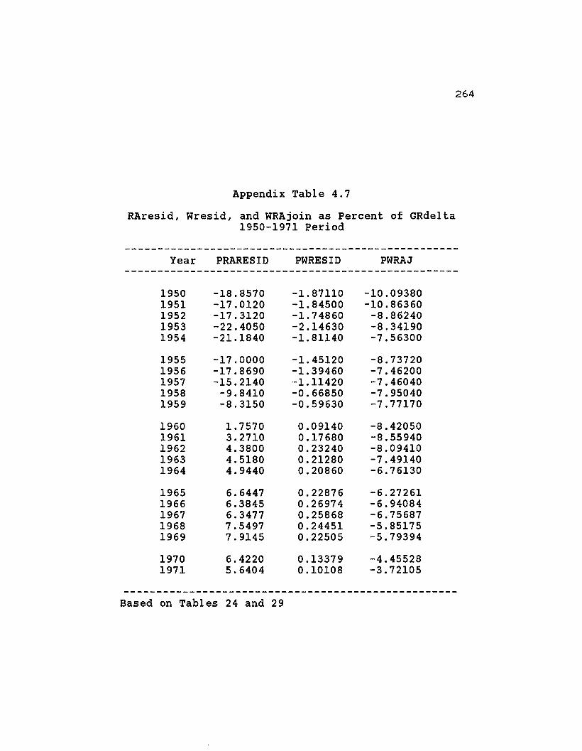
264

Appendix Table 4.7

RAresid, Wresid, and WRAjoin as Percent of GRdelta1950-1971 Period

---------------------------------------------------Year PRARESID PWRESID PWRAJ

--------------------------------------------~------

1950 -18.8570 -1. 87110 -10.093801951 -17.0120 -1. 84500 -10.863601952 -17.3120 -1.74860 -8.862401953 -22.4050 -2.14630 -8.341901954 -21.1840 -1. 81140 -7.56300

1955 -17.0000 -1. 45120 -8.737201956 -17.8690 -1.39460 -7.462001957 -15.2140 --1.11420 -7.460401958 -9.8410 -0.66850 -7.950401959 -8.3150 -0.59630 -7.77170

1960 1. 7570 0.09140 -8.420501961 3.2710 0.17680 -8.559401962 4.3800 0.23240 -8.094101963 4.5180 0.21280 -7.491401964 4.9440 0.20860 -6.76130

1965 6.6447 0.22876 -6.272611966 6.3845 0.26974 -6.940841967 6.3477 0.25868 -6.756871968 7.5497 0.24451 -5.851751969 7.9145 0.22505 -5.79394

1970 6.4220 0.13379 -4.455281971 5.6404 0.10108 -3.72105

---------------------------------------------------Based on Tables 24 and 29

265

Appendix Table 4.7(cont.)

RAresid, Wresid, and WRAjoin as Percent of GRdelta1972-1990

Year PRARESID PWRESID PWRAJ---------------------------------------------------

1972 1.1841 0.01384 -1. 967871973 0.8622 0.00443 -0.868431974 1.8045 0.00442 -0.52968

1975 1. 5573 0.00184 -0.287551976 1. 7958 0.00387 -0.458991977 -0.6701 -0.00101 -0.261771978 42.8678 0.00966 0.000641979 0.0000 0.00000 0.00000

1980 0.1349 0.00003 0.017631981 -0.8645 -0.00042 -0.217001982 -4.5830 -0.00896 -0.798771983 -10.0550 -0.04187 -1. 414471984 -15.1680 -0.13430 -2.71749

1985 -21.1760 -0.23607 -3.477951986 -24.0340 -0.07813 -0.878641987 -44.1910 -0.03071 -0.155041988 -176.9780 -0.02194 -0.015251989 -99.8910 -0.02973 -0.09268

1990 -209.5840 -0.02505 0.03191

---------------------------------------------------Based on Tables 24 and 29

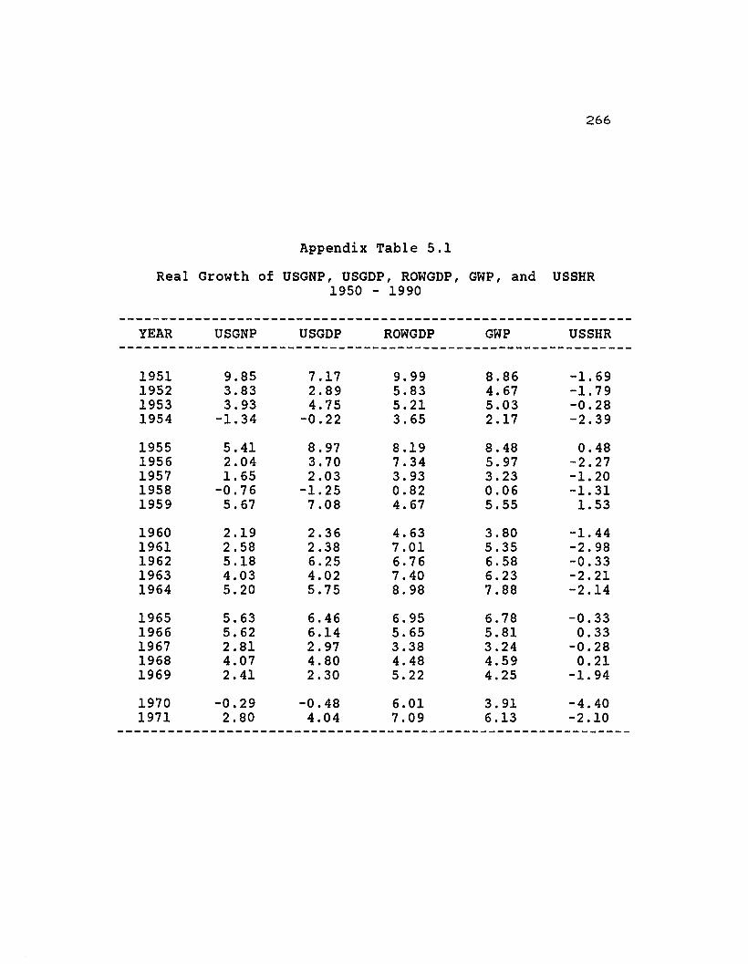
266

Appendix Table 5.1

Real Growth of USGNP, USGDP, ROWGDP, GWP, and USSHR1950 - 1990

YEAR

1951195219531954

19551956195719581959

19601961196219631964

19651966196719681969

19701971

USGNP

9.853.833.93

-1. 34

5.412.041. 65

-0.765.67

2.192.585.184.035.20

5.635.622.814.072.41

-0.292.80

USGDP

7.172.894.75

-0.22

8.973.702.03

-1. 257.08

2.362.386.254.025.75

6.466.142.974.802.30

-0.484.04

ROWGDP

9.995.835.213.65

8.197.343.930.824.67

4.637.016.767.408.98

6.955.653.384.485.22

6.017.09

GWP

8.864.675.032.17

8.485.973.230.065.55

3.805.356.586.237.88

6.785.813.244.594.25

3.916.13

USSHR

-1. 69-1. 79-0.28-2.39

0.48-2.27-1. 20-1. 311.53

-1. 44-2.98-0.33-2.21-2.14

-0.330.33

-0.280.21

-1. 94

-4.40-2.10

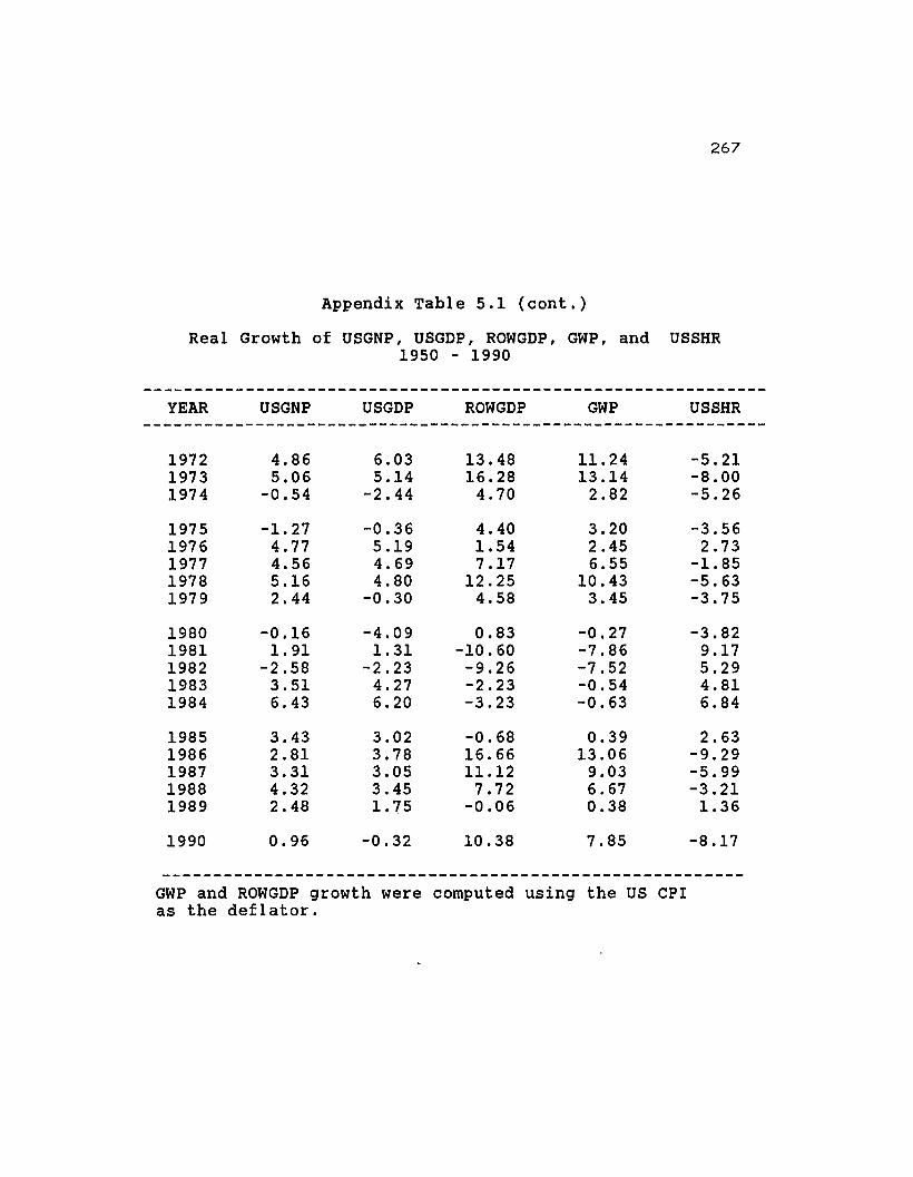
267

Appendix Table 5.1 (cont.)

Real Growth of USGNP, USGDP, ROWGDP, GWP, and USSHR1950 - 1990

-------------------------------------------------------------YEAR USGNP USGDP ROWGDP GWP USSHR

-------------------------------------------------------------

1972 4.86 6.03 13.48 11. 24 -5.211973 5.06 5.14 16.28 13.14 -8.001974 -0.54 -2.44 4.70 2.82 -5.26

1975 -1. 27 -0.36 4.40 3.20 -3.561976 4.77 5.19 1.54 2.45 2.731977 4.56 4.69 7.17 6.55 -1.851978 5.16 4.80 12.25 10.43 -5.631979 2.44 -0.30 4.58 3.45 -3.75

1980 -0.16 -4.09 0.83 -0.27 -3.821981 1. 91 1.31 -10.60 -7.86 9.171982 -2.58 -2.23 -9.26 -7.52 5.291983 3.51 4.27 -2.23 -0.54 4.811984 6.43 6.20 -3.23 -0.63 6.84

1985 3.43 3.02 -0.68 0.39 2.631986 2.81 3.78 16.66 13.06 -9.291987 3.31 3.05 11.12 9.03 -5.991988 4.32 3.45 7.72 6.67 -3.211989 2.48 1. 75 -0.06 0.38 1.36

1990 0.96 -0.32 10.38 7.85 -8.17

---------------------------------------------------------GWP and ROWGDP growth were computed using the us CPIas the deflator.

Appendix Table 5.2

Comparative Growth Rates of the G-5 Countries(based on constant local currency units)

--------------------------------------------YEAR USGNP GERGNP JAPGNP UKGD FRGD

--------------------------------------------

1951 9.85 2.24 5.861952 3.83 1.04 2.521953 3.93 6.04 4.35 2.911954 -1. 34 5.68 3.92 4.72

1955 5.41 8.47 3.37 5.451956 2.04 1.58 4.811957 1.65 7.22 1. 94 5.821958 -0.76 6.40 0.35 2.531959 5.67 8.70 4.04 8.16

1960 2.19 12.22 4.54 6.921961 2.58 4.17 10.96 3.22 5.371962 5.18 4.48 8.42 1.03 6.471963 4.03 2.71 8.03 4.12 5.191964 5.20 6.35 10.75 5.05 6.32

1965 5.63 5.12 5.66 2.25 4.671966 5.62 2.81 9.97 2.08 5.081967 2.81 -0.24 10.36 2.73 4.581968 4.07 5.58 11. 44 4.12 4.181969 2.41 7.22 11. 42 1. 35 6.75

1970 -0.29 4.88 9.84 2.38 5.571971 2.80 3.00 4.28 2.72 4.67

--------------------------------------------

268

269

Appendix Table 5.2 (cont.)

Comparative Growth Rates of the G-5 Countries(based on constant local currency units)

--------------------------------------------YEAR USGNP GERGNP JAPGNP UKGD FRGD

--------------------------------------------

1972 4.86 4.25 7.96 2.34 4.341973 5.06 4.73 7.42 7.63 5.291974 -0.54 0.05 -0.76 -1.01 3.06

1975 -1.27 -1. 27 2.88 -0.67 -0.281976 4.77 5.40 4.14 3.65 4.151977 4.56 2.52 4.65 1.04 3.171978 5.16 3.39 4.84 3.73 3.291979 2.44 3.96 5.42 2.31 3.19

1980 -0.16 1.04 3.43 -1. 96 1. 611981 1. 91 0.11 3.35 -1.06 1.171982 -2.58 -1.11 3.37 1. 34 2.521983 3.51 1.84 2.77 3.76 0.691984 6.43 3.02 4.22 1. 64 1.31

1985 3.43 1. 79 4.99 3.64 1.861986 2.81 2.15 2.65 3.88 2.501987 3.31 1. 48 4.19 4.53 2.231988 4.32 3.58 6.12 3.93 4.081989 2.48 3.73 4.57 2.00 3.86

1990 0.96 4.39 5.50 0.70 2.65

united states, Germany, Japan, United Kingdom, France

GNP and GDP data at constant prices from the IMF-IFStapes were used to derive the preceding growth rates.

270

Appendix Table 5.3How Real Interest Rates were derived.

Year USinf USbonds GERinf GERbonds JAPinf JAPbonds

1956195719581959196019611962196319641-9651966196719681969197019711972197319741975197619771978197919801981198219831984198519861987198819891990

1.503.422.730.931.511.081.121.211.311. 672.992.784.225.415.904.263.316.22

11.049.135.746.497.65

11. 2713.5110.32

6.163.214.323.561.863.744.014.835.40

3.183.1:.53.324.334.123.883.954.004.194.284.925.075.656.677.356.166.216.847.567.997.617.428.419.44

11. 4613.9113.0011.1112.5210.62

7.688.388.858.508.55

2.552.112.090.981.492.282.882.992.353.233.621. 611. 631.873.445.245.507.006.965.944.303.692.694.125.426.335.273.282.412.18

-0.130.241.272.782.69

6.907.506.805.806.405.905.906.106.207.108.107.006.506.808.308.007.909.30

10.408.507.806.205.807.408.50

10.388.957.897.786.875.925.845.927.098.88

5.083.985.375.247.676.344.90

11. 6123.1911. 75

9.388.164.213.737.744.952.741.892.262.040.620.030.752.283.11

6.866.917.037.097.197.286.707.269.269.208.727.336.097.699.228.668.067.426.816.344.944.214.275.057.36

USinf, GERinf, JAPinf, are the inflation rates in theUS, Germany, and Japan. USbonds, GERbonds, JAPbonds, arethe nominal interest rates in the respective countries.The real interest rate is the difference between thenominal interest rates and inf I ation in each country.Inflation data is the change in consumer prices series ofthe IMF-IFS tapes. Nominal interest rates are fromgovernment bond yields data from the same tapes.

Appendix Table 5.4

US Exports, Imports, and the us Trade Balance(in millions)

----------------------------------------YEAR EXP111 IMP111 TBAL

----------------------------------------

1948 12653 8081 45721949 12051 7544 4507

1950 9993 9631 3621951 13967 11922 20451952 13203 11707 14961953 12262 11846 4161954 12854 11140 1714

1955 14291 12489 18021956 17333 13987 33461957 19495 14620 48751958 16367 14616 17511959 16407 17006 -599

1960 19626 16381 32451961 20190 15952 42381962 20973 17802 31711963 22427 18640 37871964 25690 20334 5356

1965 26699 23233 34661966 29379 27791 15881967 30934 28819 21151968 34063 35438 -13751969 37332 38498 -1166

1970 42659 42389 2701971 43549 48342 -4793

----------------------------------------

271

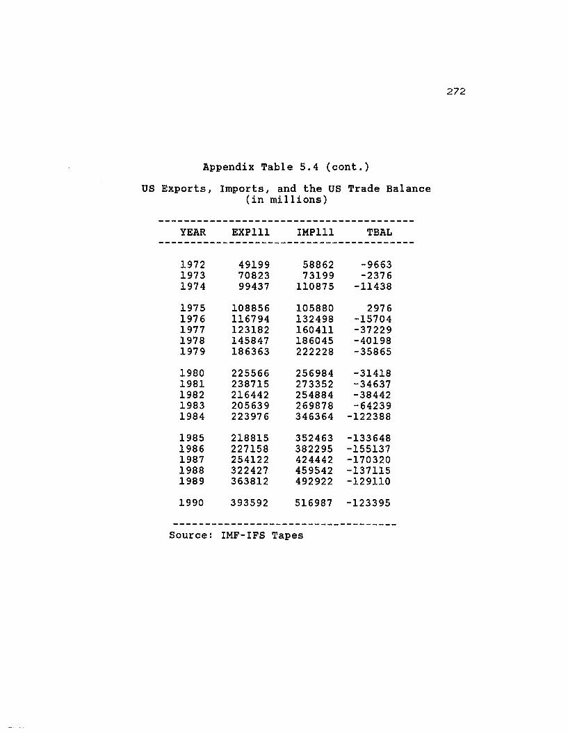
Appendix Table 5.4 (cont.)

US Exports, Imports, and the us Trade Balance(in mi 11ions)

----------------------------------------YEAR EXP111 IMP111 TBAL

----------------------------------------

1972 49199 58862 -96631973 70823 73199 -23761974 99437 110875 -11438

1975 108856 105880 29761976 116794 132498 -157041977 123182 160411 -372291978 145847 186045 -401981979 186363 222228 -35865

1980 225566 256984 -314181981 238715 273352 -346371982 216442 254884 -384421983 205639 269878 -642391984 223976 346364 -122388

1985 218815 352463 -1336481986 227158 382295 -1551371987 254122 424442 -1703201988 322427 459542 -1371151989 363812 492922 -129110

1990 393592 516987 -123395

-----------------------------------Source: IMF-IFS Tapes

272

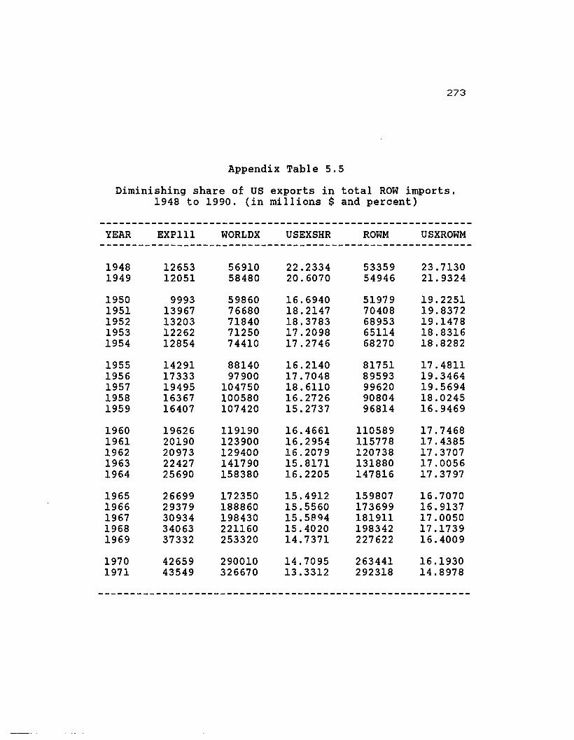
273

Appendix Table 5.5

Diminishing share of us exports in total ROW imports.1948 to 1990. (in millions $ and percent)

----------------------------------------------------------YEAR EXP111 WORLDX USEXSHR ROWM USXROWM

----------------------------------------------------------

1948 12653 56910 22.2334 53359 23.71301949 12051 58480 20.6070 54946 21.9324

1950 9993 59860 16.6940 51979 19.22511951 13967 76680 18.2147 70408 19.83721952 13203 71840 18.3783 68953 19.14781953 12262 71250 17.2098 65114 18.83161954 12854 74410 17.2746 68270 18.8282

1955 14291 88140 16.2140 81751 17.48111956 17333 97900 17.7048 89593 19.34641957 19495 104750 18.6110 99620 19.56941958 16367 100580 16.2726 90804 18.02451959 16407 107420 15.2737 96814 16.9469

1960 19626 119190 16.4661 110589 17.74681961 20190 123900 16.2954 115778 17.43851962 20973 129400 16.2079 120738 17.37071963 22427 141790 15.8171 131880 17.00561964 25690 158380 16.2205 147816 17.3797

1965 26699 172350 15.4912 159807 16.70701966 29379 188860 15.5560 173699 16.91371967 30934 198430 15.5894 181911 17.00501968 34063 221160 15.4020 198342 17.17391969 37332 253320 14.7371 227622 16.4009

1970 42659 290010 14.7095 263441 16.19301971 43549 326670 13.3312 292318 14.8978

----------------------------------------------------------

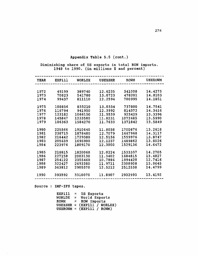
274

Appendix Table 5.5 (cont.)

Diminishing share of us exports in total ROW imports.1948 to 1990. (in millions $ and percent)

YEAR EXP111 WORLDX USEXSHR ROWM USXROWM

197219731974

19751976197719781979

19801981198219831984

19851986198719881989

1990

491997082399437

108856116794123182145847186363

225566238715216442205639223976

218815227158254122322427363812

393592

389740541780811110

835210941950

106615012335801584270

19106401878480172938016959001809170

18200602003130235546026933802905570

3310070

12.623513.072312.2594

13.033412.399211.553911.823111. 7633

11.805812.707912.515612.125712.3800

12.022411. 340210.788611. 971112.5212

11. 8907

341008478201700995

737800814372923429

10724851371842

17008761667968155997614898621529136

15333371684815199442823089082512538

2932993

14.427514.810314.1851

14.754114.341613.339613.599013.5849

13.261814.311713.874713.802614.6472

14.270513.482712.741613.964514.4799

13.4195

Source: IMF-IFS tapes.

=

EXP111 = US ExportsWORLDX = World ExportsROWM ROW ImportsUSEXSHR = (EXP111 / WORLDX)USXROWM = (EXP111 / ROWM)

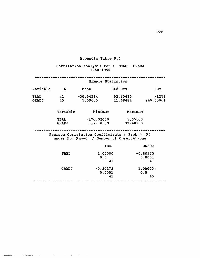
Appendix Table 5.6

Correlation Analysis for: TBAL GRADJ1950-1990

275

Simple Statistics

Variable N Mean std Dev Sum

TBAL 41 -30.54234 52.70435 -1252GRADJ 43 5.59653 11.68484 240.65061

Variable Minimum Maximum

TBAL -170.32000 5.35600GRADJ -17.18609 37.48203

Pearson Correlation Coefficients / Prob > IRIunder Ho: Rho=O / Number of Observations

TBAL

GRADJ

TBAL GRADJ

1.00000 -0.801730.0 0.0001

41 41

-0.80173 1.00000 .0.0001 0.0

41 43

276

Appendix Table 5.7

ROW Average Nominal Rates, Relative Prices,and the US Trade Balance, 1950-1990

---------------------------------------------------Year A R Tbalance

---------------------------------------------------

1950 0.874 1.566 3621951 0.884 1.555 20451952 0.880 1.512 14961953 0.855 1.550 4161954 0.855 1.554 1714

1955 0.882 1.532 18021956 0.878 1. 497 33461957 0.889 1. 497 48751958 0.921 1. 476 17511959 0.930 1. 448 -599

1960 1.018 1.392 32451961 1.039 1.389 42381962 1.056 1.350 31711963 1.059 1.339 37871964 1.067 1. 308 5356

1965 1.097 1.256 34661966 1.096 1. 279 15881967 1.097 1. 277 21151968 1.153 1. 214 -13751969 1.162 1. 233 -1166

1970 1.115 1.255 2701971 1.100 1.239 -47931972 1.015 1. 221 -96631973 1.012 1.150 -23761974 1.031 1.113 -11438

1975 1.028 1.085 29761976 1.101 1.032 -157041977 1.102 0.991 -372291978 1.017 0.981 -401981979 1.000 1.000 -35865

A = Nominal Rates, R = Relative Prices US/ROW; A andRare GDP-weighted geometric means for all ROW countries.

Appendix Table 5.7 cont.

Nominal Rates, Relative Prices,and the Trade Balance

277

Year A R Tbalance

1980 1.015 1.002 -314181981 1.153 0.989 -346371982 1. 323 0.951 -384421983 1. 442 0.908 -642391984 1. 604 0.874 -122388

1985 1. 737 0.839 -1336481986 1.438 0.844 -1551371987 1.297 0.834 -1703201988 1.251 0.814 -1371151989 1.416 0.758 -129110

1990 1.399 0.741 -123395

Source: IMF-IFS Tapes

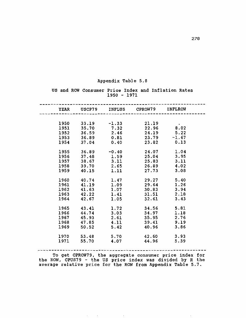
278

Appendix Table 5.8

us and ROW Consumer Price Index and Inflation Rates1950 - 1971

YEAR

19501951195219531954

19551956195719581959

19601961196219631964

19651966196719681969

19701971

USCP79

33.1935.7036.5936.8937.04

36.8937.4838.6739.7040.15

40.7441.1941. 6342.2242.67

43.4144.7445.9347.8550.52

53.4855.70

INFLUS

-1.337.322.460.810.40

-0.401. 593.112.651.11

1. 471.091.071. 411.05

1. 723.032.614.115.42

5.704.07

CPROW79

21.1922.9624.1923.7923.82

24.0725.0425.8326.8927.73

29.2729.6430.8331.5132.61

34.5634.9735.9539.4140.96

42.6044.96

INFLROW

8.025.22

-1. 670.13

1.043.953.114.023.08

5.401. 263.942.183.43

5.811.182.769.193.86

3.935.39

To get CPROW79, the aggregate consumer price index forthe ROW, CPUS79 - the us price index was divided by R theaverage relative price for the ROW from Appendix Table 5.7.

279

Appendix Table 5.8 (cont.)

US and ROW Consumer Price Index and Inflation Rates

------------------------------------------------------------YEAR USCP79 INFLUS CPROW79 INFLROW

------------------------------------------------------------

1972 57.63 3.40 47.16 4.781973 61.19 5.99 53.19 12.031974 67.85 10.34 60.93 13.59

1975 74.07 8.77 68.21 11. 291976 78.37 5.64 75.93 10.721977 83.41 6.23 84.10 10.221978 89.78 7.36 91.43 8.361979 100.00 10.78 100.00 8.96

1980 113.48 12.65 113.24 12.431981 125.19 9.82 126.57 11.131982 132.89 5.97 139.71 9.881983 137.19 3.18 151. 01 7.781984 143.11 4.23 163.70 8.07

1985 148.15 3.46 176.56 7.561986 150.96 1.88 178.67 1.191987 156.59 3.66 187.76 4.961988 162.81 3.90 199.94 6.291989 170.67 4.71 225.10 11.85

1990 179.85 5.24 242.42 7.41

Source: IMF-IFS Tapes.

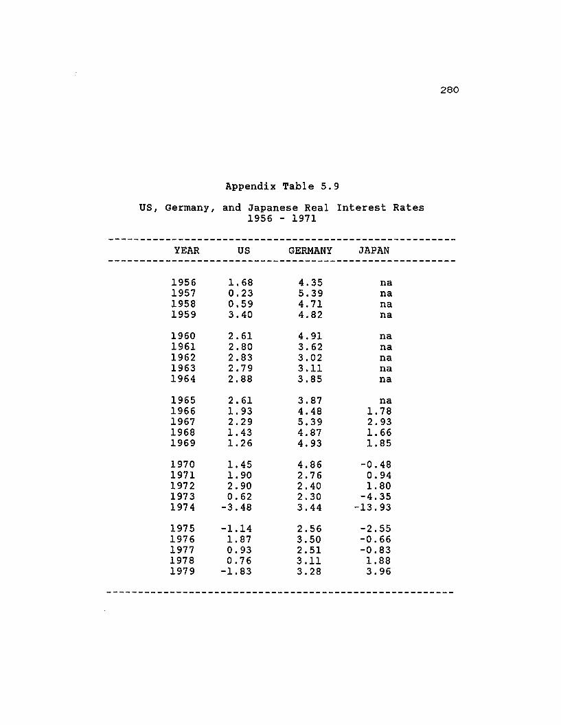
280

Appendix Table 5.9

US, Germany, and Japanese Real Interest Rates1956 - 1971

-------------------------------------------------------YEAR US GERMANY JAPAN

-------------------------------------------------------

1956 1. 68 4.35 na1957 0.23 5.39 na1958 0.59 4.71 na1959 3.40 4.82 na

1960 2.61 4.91 na1961 2.80 3.62 na1962 2.83 3.02 na1963 2.79 3.11 na1964 2.88 3.85 na

1965 2.61 3.87 na1966 1. 93 4.48 1. 781967 2.29 5.39 2.931968 1. 43 4.87 1. 661969 1. 26 4.93 1.85

1970 1. 45 4.86 -0.481971 1. 90 2.76 0.941972 2.90 2.40 1.801973 0.62 2.30 -4.351974 -3.48 3.44 -13.93

1975 -1.14 2.56 -2.551976 1. 87 3.50 -0.661977 0.93 2.51 -0.831978 0.76 3.11 1.881979 -1.83 3.28 3.96

Appendix Table 5.9 (cont.)

US, Germany, and Japanese Real Interest Rates1956 - 1971

281

YEAR US GERMANY JAPAN-------------------------------------------------------

1980 -2.05 3.08 1. 481981 3.59 4.05 3.711982 6.84 3.68 5.321983 7.90 4.61 5.531984 8.20 5.37 4.55

1985 7.06 4.69 4.301986 5.82 6.05 4.321987 4.64 5.60 4.181988 4.84 4.83 3.521989 3.67 4.31 2.77

1990 3.15 6.19 4.25

Source : IMF-IFS Tapes

282

Appendix Table 5.10

The us Balance of Payments in Billions1955 - 1990

---~--------------------------------------------------- - - - - - - - -

YEAR Current Account Capital AccountCA KA

Overall Bal anceOA

1955 -0.51 -0.54 -1.05

1956 1.57 -1. 67 -0.101957 3.41 -2.00 1. 411958 -0.13 -2.68 -2.811959 -2.28 -0.01 -2.291960 2.82 -6.22 -3.40

1961 3.82 -5.17 -1.351962 3.38 -6.03 -2.651963 4.40 -6.34 -1. 941964 6.82 -8.35 -1. 531965 5.41 -6.70 -1. 29

1966 3.03 -2.79 0.241967 2.59 -5.98 -3.391968 0.59 1.08 1. 671969 0.42 2.32 2.741970 2.33 -13.02 -10.69

1971 -1.45 -29.02 -30.471972 -5.78 -5.27 -11.05

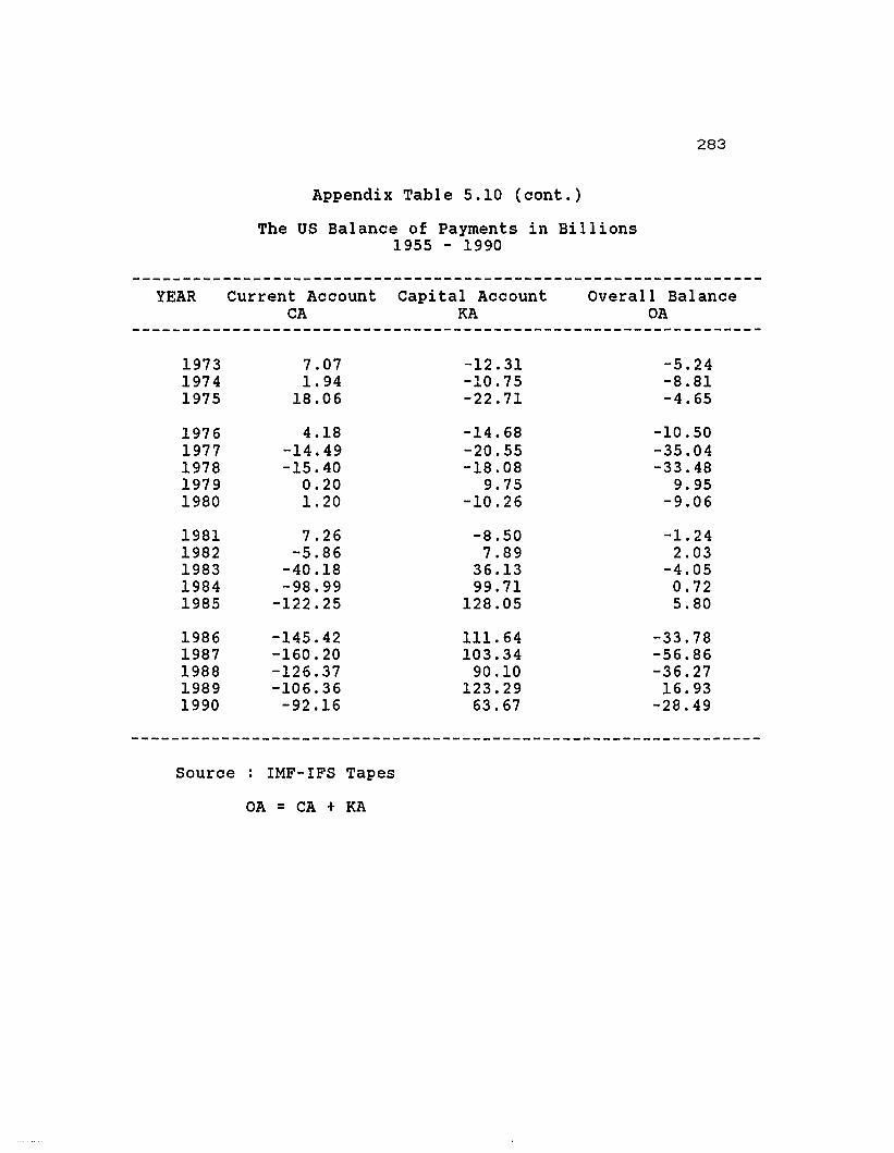
283

Appendix Table 5.10 (cont.)

The us Balance of Payments in Billions1955 - 1990

YEAR Current Account Capital AccountCA KA

Overall BalanceOA

1973 7.07 -12.31 -5.241974 1. 94 -10.75 -8.811975 18.06 -22.71 -4.65

1976 4.18 -14.68 -10.501977 -14.49 -20.55 -35.041978 -15.40 -18.08 -33.481979 0.20 9.75 9.951980 1. 20 -10.26 -9.06

1981 7.26 -8.50 -1.241982 -5.86 7.89 2.031983 -40.18 36.13 -4.051984 -98.99 99.71 0.721985 -122.25 128.05 5.80

1986 -145.42 111.64 -33.781987 -160.20 103.34 -56.861988 -126.37 90.10 -36.271989 -106.36 123.29 16.931990 -92.16 63.67 -28.49

Source : IMF-IFS Tapes

OA = CA + KA

284

Appendix Table 5.11

Components of the us Capital Account in Billions1953 - 1990

Year

195319541955

19561957195819591960

19611962196319641965

19661967196819691970

19711972

DirectFlows

(DF)

-0.58-0.54-0.63

-1. 72-2.24-1.08-1.13-2.63

-2.34-2.51-3.25-3.43-4.60

-5.00-4.11-4.48-4.70-6.13

-7.26-6.80

PortfolioFlows

(PF)

-0.06-0.030.26

0.08-0.17-0.90-0.06-0.38

-0.44-0.83-0.82-0.76-1.12

0.19-0.29

2.851.581. 20

1.203.93

Long TermFlows(NIE)

-0.16

0.450.07

-0.491.05

-1.43

-0.94-1. 20-1.81-2.78-1.56

-0.59-2.35-1. 46-1. 23-1. 46

-3.03-2.97

Short TermFlows(NIE)

0.13-0.78-0.53

-1.02-0.81-0.70-0.28-0.77

-0.45-0.39-0.11-0.451.00

1. 981.003.718.13

-6.47

-10.172.51

Net ErrorFlows(NEF)

-0.360.160.52

0.541.150.490.41

-1.01

-1.00-1.10-0.35-0.93-0.42

0.63-0.230.46

-1. 46-0.16

-9.76-1. 94

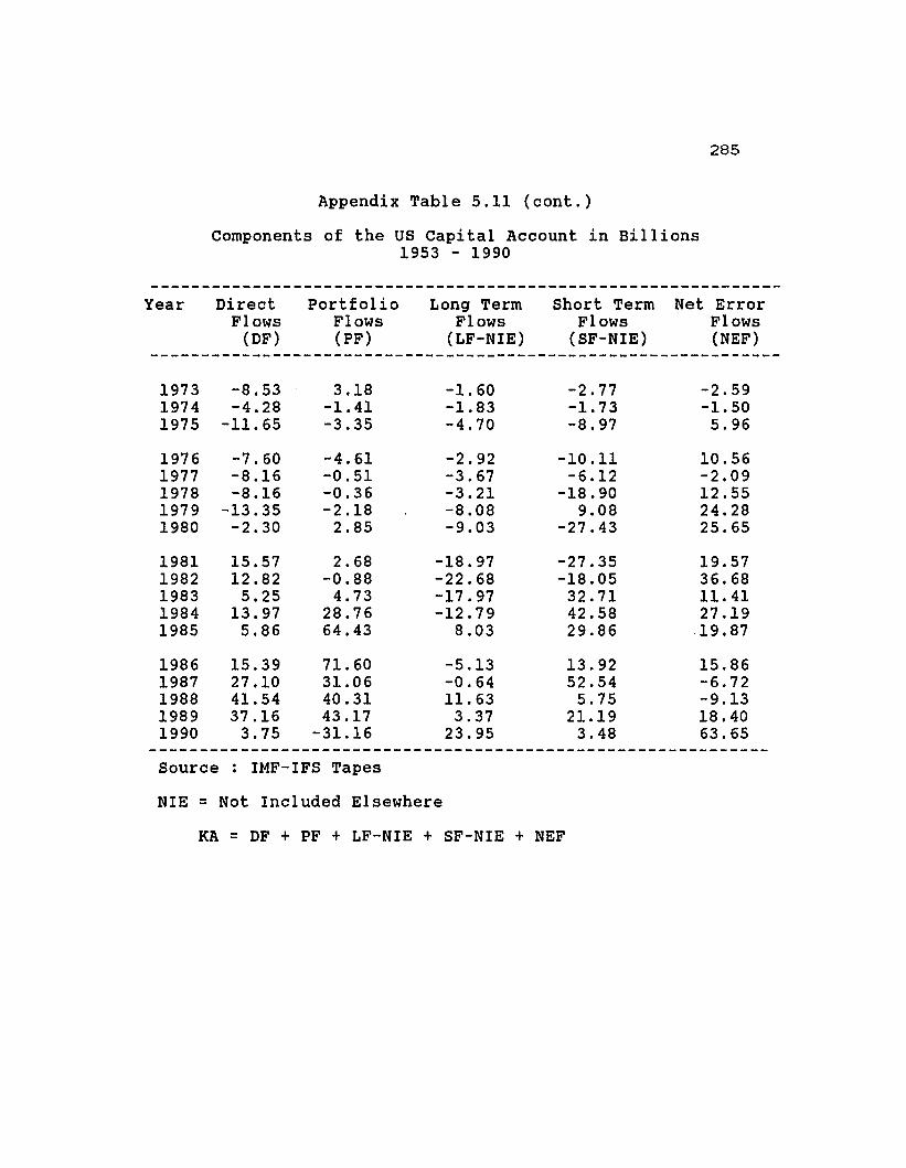
Appendix Table 5.11 (cont.)

Components of the us Capital Account in Billions1953 - 1990

285

--------------------------------------------------------------Year Direct Portfolio Long Term Short Term Net Error

Flows Flows Flows Flows Flows(DF) (PF) (LF-NIE) (SF-NIE) (NEF)

--------------------------------------------------------------

1973 -8.53 3.18 -1. 60 -2.77 -2.591974 -4.28 -1.41 -1.83 -1. 73 -1. 501975 -11. 65 -3.35 -4.70 -8.97 5.96

1976 -7.60 -4.61 -2.92 -10.11 10.561977 -8.16 -0.51 -3.67 -6.12 -2.091978 -8.16 -0.36 -3.21 -18.90 12.551979 -13.35 -2.18 -8.08 9.08 24.281980 -2.30 2.85 -9.03 -27.43 25.65

1981 15.57 2.68 -18.97 -27.35 19.571982 12.82 -0.88 -22.68 -18.05 36.681983 5.25 4.73 -17.97 32.71 11. 411984 13.97 28.76 -12.79 42.58 27.191985 5.86 64.43 8.03 29.86 19.87

1986 15.39 71.60 -5.13 13.92 15.861987 27.10 31.06 -0.64 52.54 -6.721988 41.54 40.31 11.63 5.75 -9.131989 37.16 43.17 3.37 21.19 18.401990 3.75 -31.16 23.95 3.48 63.65

-------------------------------------------------------------Source : IMF-IFS Tapes

NIE = Not Included Elsewhere

KA = DF + PF + LF-NIE + SF-NIE + NEF

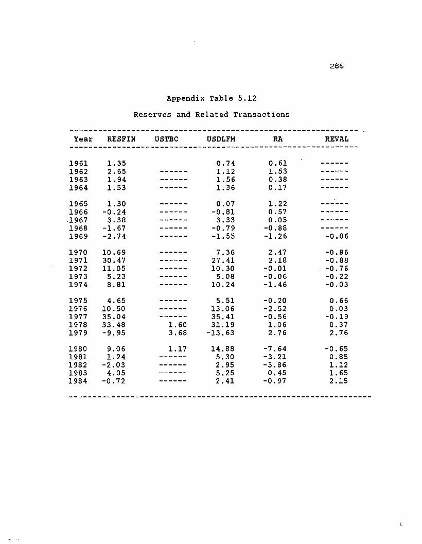
286

Appendix Table 5.12

Reserves and Related Transactions

-------------------------------------------------------------Year RESFIN USTBC USDLFM RA REVAL

-------------------------------------------------------------

1961 1.35 0.74 0.61 ------1962 2.65 ------ 1.12 1.53 ------1963 1. 94 ------ 1.56 0.38 ------1964 1.53 ------ 1. 36 0.17 ------

1965 1.30 ------ 0.07 1. 22 ------1966 -0.24 ------ -0.81 0.57 ------

.1967 3.38 ------ 3.33 0.05 ------1968 -1. 67 ------ -0.79 -0.88 ------1969 -2.74 ------ -1. 55 -1. 26 -0.06

1970 10.69 ------ 7.36 2.47 -0.861971 30.47 ------ 27.41 2.18 -0.881972 11.05 ------ 10.30 -0.01 . -0.761973 5.23 ------ 5.08 -0.06 -0.221974 8.81 ------ 10.24 -1. 46 -0.03

1975 4.65 ------ 5.51 -0.20 0.661976 10.50 ------ 13.06 -2.52 0.031977 35.04 ------ 35.41 -0.56 -0.191978 33.48 1. 60 31.19 1.06 0.371979 -9.95 3.68 -13.63 2.76 2.76

1980 9.06 1.17 14.88 -7.64 -0.651981 1. 24 ------ 5.30 -3.21 0.851982 -2.03 ------ 2.95 -3.86 1.121983 4.05 ------ 5.25 0.45 1. 651984 -0.72 ------ 2.41 -0.97 2.15

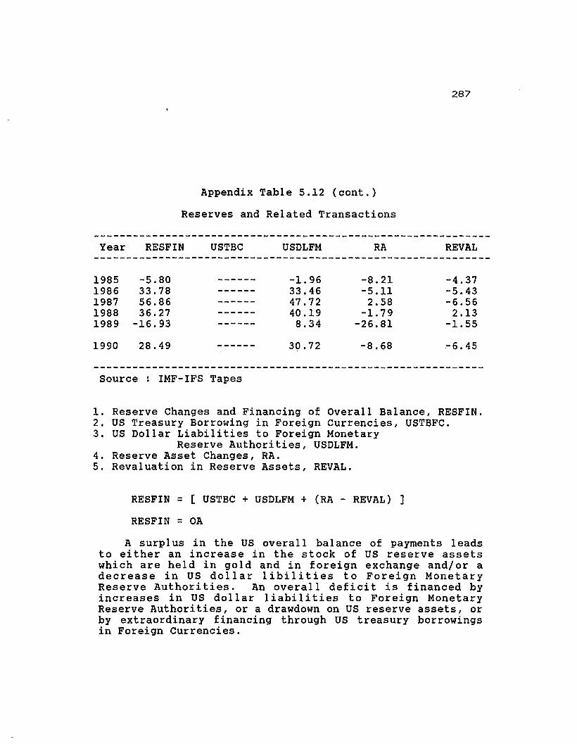
287

Appendix Table 5.12 (cont.)

Reserves and Related Transactions

Year RESFIN USTBC USDLFM RA REVAL

1985 -5.80 ------ -1.96 -8.21 -4.371986 33.78 ------ 33.46 -5.11 -5.431987 56.86 ------ 47.72 2.58 -6.561988 36.27 ------ 40.19 -1. 79 2.131989 -16.93 ------ 8.34 -26.81 -1. 55

1990 28.49 ------ 30.72 -8.68 -6.45

Source : IMF-IFS Tapes

1. Reserve Changes and Financing of Overall Balance, RESFIN.2. US Treasury Borrowing in Foreign Currencies, USTBFC.3. US Dollar Liabilities to Foreign Monetary

Reserve Authorities, USDLFM.4. Reserve Asset Changes, RA.5. Revaluation in Reserve Assets, REVAL.

RESFIN = [ USTBC + USDLFM + (RA - REVAL) ]

RESFIN = OA

A surplus in the US overall balance of payments leadsto either an increase in the stock of US reserve assetswhich are held in gold and in foreign exchange and/or adecrease in US dollar libilities to Foreign MonetaryReserve Authorities. An overall deficit is financed byincreases in US dollar liabilities to Foreign MonetaryReserve Authorities, or a drawdown on US reserve assets, orby extraordinary financing through US treasury borrowingsin Foreign Currencies.

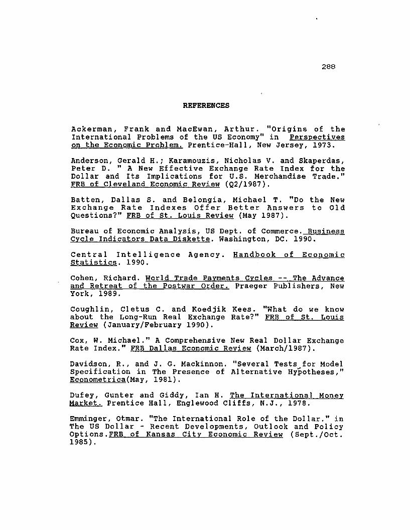
288

REFERENCES

Ackerman, Frank and MacEwan, Arthur. "Origins of theInternational Problems of the US Economy" in Perspectiveson the Economic Problem. Prentice-Hall, New Jersey, 1973.

Anderson, Gerald H.; Karamouzis, Nicholas V. and Skaperdas,Peter D. " A New Effective Exchange Rate Index for theDollar and Its Implications for U.S. Merchandise Trade."FRB of Cleveland Economic Review (Q2/1987).

Batten, Dallas S. and Belongia, Michael T. "Do the NewExchange Rate Indexes Offer Better Answers to oldQuestions?" FRB of st. Louis Review (May 1987).

Bureau of Economic Analysis, US Dept. of Commerce. BusinessCycle Indicators Data Diskette. Washington, DC. 1990.

Central Intelligence Agency. Handbook of EconomicStatistics. 1990.

Cohen, Richard. World Trade Payments Cycles -- The Advanceand Retreat of the Postwar Order. Praeger Publishers, NewYork, 1989.

Coughlin, Cletus C. and Koedjik Kees. "What do we knowabout the Long-Run Real Exchange Rate?" FRB of st. LouisReview (January/February 1990).

Cox, W. Michael." A Comprehensive New Real Dollar ExchangeRate Index." FRB Dallas Economic Review (March/1987).

Davidson, R., and J. G. Mackinnon. "Several Tests for ModelSpecification in The Presence of Al ternative Hypotheses,"Econometrica{May, 1981).

Dufey, Gunter and Giddy, Ian H. The International MoneyMarket. Prentice Hall, Englewood Cliffs, N.J., 1978.

Emminger, otmar. "The International Role of the Dollar." inThe US Dollar - Recent Developments, Outlook and PolicyOptions.FRB of Kansas City Economic Review (Sept./Oct.1985).

289

Fieleke, Norman S. ed. International Payments Imbalances inthe 1980's. Federal Reserve Bank of Boston. ConferenceProceedings, October 1988.

FRB Staff. 'Index of the Weighted-Average Exchange Value ofthe US Dollar: Revision.' Federal Reserve Bulletin.(August, 1978).

Frenkel, Jacob A. "Commentary on Causes of Appreciation andVolatility of the Dollar," in The US Dollar - RecentDevelopments, Outlook and Policy Options. FRB of KansasCity Economic Review (September/October 1985).

Fry, Earl H. Financial Invasion of the U.S.A. -- A Threatto American Society? McGraw Hi 11 Book Company, New York,1980.

Geiger, Theodore The Future of the International System:The US and the World Political Economy. Allen & Unwin,Inc., Winchester, MA, 1988.

Hervey, Jack L. and Strauss, William A. "The InternationalValue of the Dollar: An Inflation-Adjusted Index." FRBChicago Economic Perspectives XI (January/February1987) .

Hervey, Jack L. and Strauss, William A. " The New DollarIndices are no Different from the Old Ones." FRB ChicagoEconomic Perspectives. XI (July/August 1987).

Hirsch, Fred and Higgins, Ilse. "An Indicator of EffectiveExchange Rates". IMF STAFF PAPERS. (November 1970).

Hooper, Peter and Morton, John. "Summary Measures of theDollar's Foreign Exchange Value." Federal Reserve Bulletin(October/1978).

IBRD/World Bank. Socio Economic Indicators in computerdiskettes. 1990.

IBRD/World Bank. World Tables in computer diskettes. 1990.

International Monetary Fund, International FinancialStatistics Tapes. Washington, DC. 1991.

Koenig, Evan F. "Recent Trade and Exchange Rate Movements:Possible Explanations." FRB of Dallas EconomicReview. (September 1989).

290

Krueger, Anne. Exchange Rate Determination: CambridgeSurveys of Economic Literature. New York: CambridgeUniversity Press. 1983.

Maciejewski, Edouard B. "Real Effective Exchange RateIndices: A Re-examination of the Major Conceptual andMethodological Issues.' IMF STAFF PAPERS. 1984.

National Trade Data Bank. NTDB CD ROM Disk, 1990.

ott, Mack. "The Dollar's Effective Exchange Rate:Assessing the Impact of Alternative Weighting Schemes."Federal Reserve Bank of st. Louis (February, 1987).

Pauls, B. Dianne. "Measuring the Foreign Exchange Value ofthe Dollar." Federal Reserve Bulletin (June /1987).

Rosenweig, Jeffrey A. "Constructing and Using Exchange RateIndexes." FRB of Atlanta Economic Review LXXII(Summer/1987).

Schroder, Jurgen. "The Rol e of the SDR' s in theInternational Monetary System" in International andEuropean Monetary Systems. Claassen, Emil-Maria, ed.Praeger Publishers, New York, 1990.

Whitt, Joseph A., Jr. "Purchasing Power Parity and ExchangeRates in the Long Run." FRB Atlanta Economic Review LXXIV(July/August 1989).