
Ubc 2011 fall alrasheed mohammed
143
A MODIFIED PARTICLE SWARM OPTIMIZATION AND ITS APPLICATION IN THERMAL MANAGEMENT OF AN ELECTRONIC COOLING SYSTEM by Mohammed R.A Alrasheed B.Sc., King Saud University, 1997 M.Sc., Carnegie Mellon University, 2002 A THESIS SUBMITTED IN PARTIAL FULFILLMENT OF THE REQUIREMENTS FOR THE DEGREE OF DOCTOR OF PHILOSOPHY in THE FACULTY OF GRADUATE STUDIES (Mechanical Engineering) THE UNIVERSITY OF BRITISH COLUMBIA (Vancouver) October 2011 © Mohammed R.A. Alrasheed, 2011
-
Upload
independent -
Category
Documents
-
view
0 -
download
0
Transcript of Ubc 2011 fall alrasheed mohammed

A MODIFIED PARTICLE SWARM OPTIMIZATION AND ITS APPLICATION IN THERMAL MANAGEMENT OF AN
ELECTRONIC COOLING SYSTEM
by
Mohammed R.A Alrasheed
B.Sc., King Saud University, 1997
M.Sc., Carnegie Mellon University, 2002
A THESIS SUBMITTED IN PARTIAL FULFILLMENT OF THE REQUIREMENTS
FOR THE DEGREE OF
DOCTOR OF PHILOSOPHY
in
THE FACULTY OF GRADUATE STUDIES
(Mechanical Engineering)
THE UNIVERSITY OF BRITISH COLUMBIA
(Vancouver)
October 2011
© Mohammed R.A. Alrasheed, 2011
ii
Abstract
Particle Swarm Optimization (PSO) is an evolutionary computation technique, which
has been inspired by the group behavior of animals such as schools of fish and flocks of
birds. It has shown its effectiveness as an efficient, fast and simple method of optimization.
The applicability of PSO in the design optimization of heat sinks is studied in this thesis.
The results show that the PSO is an appropriate optimization tool for use in heat sink design.
PSO has common problems that other evolutionary methods suffer from. For example,
in some cases premature convergence can occur where particles tend to be trapped at local
optima and not able to escape in seeking the global optimum. To overcome these problems,
some modifications are suggested and evaluated in the present work. These modifications
are found to improve the convergence rate and to enhance the robustness of the method.
The specific modifications developed for PSO and evaluated in the thesis are:
Chaotic Acceleration Factor
Chaotic Inertia Factor
Global Best Mutation
The performance of these modifications is tested through benchmarks problems, which are
commonly found and used in the optimization literature. Detailed comparative analysis of
the modifications to the classical PSO approach is made, which demonstrates the potential
performance improvements.
In particular, the modified PSO algorithms are applied to problems with nonlinear
constraints. The non-stationary, multi-stage penalty method (PFM) is implemented to handle

iii
nonlinear constraints. Pressure vessel optimization and welded beam optimization
are two common engineering problems that are used for testing the performance of
optimization algorithms and are used here as benchmark testing examples. It is found that
the modified PSO algorithms, as developed in this work, outperform many classical and
evolutionary optimization algorithms in solving nonlinear constraint problems.
The modified PSO algorithm is applied in heat sink design and detailed results are
presented. The commercially available software package Ansys Icepak is used in the present
work to solve the heat and flow equations in implementing the optimal design variables
resulting from the modified PSO algorithms. The main contributions the work are
summarized and suggestions are made for possible future work.
iv
Preface
1. A version of Chapter 3 has been published:
Alrasheed, M.R., de Silva, C.W., and Gadala, M.S., "Evolutionary
optimization in the design of a heat sink," Editor: de Silva C.W.,
Mechatronic Systems: Devices, Design, Control, Operation and
Monitoring, pp. 55-78, CRC Press, Boca Raton, FL , 2007.
Alrasheed, M. R. , de Silva, C. W., and Gadala, M. S. ,“A new
extension of particle swarm optimization and its application in
electronic heat sink design,” in ASME Conference Proceeding (IMECE
2007), Seattle, Washington, pp.1221-1230, November 2007.
2. A version of Chapter 5 has been submitted for publication:
Alrasheed, M.R., de Silva, C.W., and Gadala, M.S., " Application of
PSO with Novel Chaotic Acceleration, Chaotic Inertia factors and Best
Global Mutation Algorithms to solve Constrained Nonlinear
Engineering Problems,” (Submitted).
3. A version of Chapter 6 has been submitted for publication:
Alrasheed, M.R., de Silva, C.W., and Gadala, M.S., "Applying
Modified Particle Swarm Optimization in Heat Sink Design by using
Chaotic Acceleration and Global Mutation," (Submitted).
v
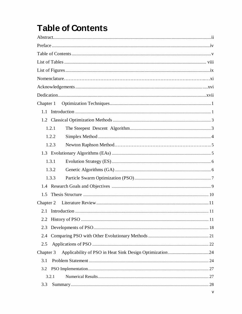
Table of Contents Abstract................................................................................................................................ ii
Preface ................................................................................................................................ iv
Table of Contents ................................................................................................................. v
List of Tables ................................................................................................................... viii
List of Figures ..................................................................................................................... ix
Nomenclature…………………………………………………………………….………..…xi
Acknowledgements ....................................................................................................... ....xvi
Dedication ........................................................................................................................ xvii
Chapter 1 Optimization Techniques .................................................................................. 1
1.1 Introduction ....................................................................................................................... 1
1.2 Classical Optimization Methods ...................................................................................... 3
1.2.1 The Steepest Descent Algorithm ....................................................................... 3
1.2.2 Simplex Method ................................................................................................... 4
1.2.3 Newton Raphson Method………………………………………………….. ... 5
1.3 Evolutionary Algorithms (EAs) ....................................................................................... 5
1.3.1 Evolution Strategy (ES) ....................................................................................... 6
1.3.2 Genetic Algorithms (GA) .................................................................................... 6
1.3.3 Particle Swarm Optimization (PSO) ................................................................... 7
1.4 Research Goals and Objectives ....................................................................................... 9
1.5 Thesis Structure .............................................................................................................. 10
Chapter 2 Literature Review ........................................................................................... 11
2.1 Introduction ..................................................................................................................... 11
2.2 History of PSO ................................................................................................................ 11
2.3 Developments of PSO ..................................................................................................... 18
2.4 Comparing PSO with Other Evolutionary Methods ..................................................... 21
2.5 Applications of PSO ...................................................................................................... 22
Chapter 3 Applicability of PSO in Heat Sink Design Optimization ................................. 24
3.1 Problem Statement ......................................................................................................... 24
3.2 PSO Implementation.......................................................................................................... 27
3.2.1 Numerical Results ................................................................................................. 27
3.3 Summary ......................................................................................................................... 28

vi
Chapter 4 New Extensions to PSO and Analysis ............................................................. 29
4.1 Introduction ....................................................................................................................... 29
4.2 Proposed Developments .................................................................................................... 30
4.2.1 Chaotic Acceleration Factor (Ca) ........................................................................... 30
4.2.2 Chaotic Inertia Weight Factor (ωc ) .................................................................. 31
4.2.3 Global Best Mutation ............................................................................................ 32
4.3 Parameter Sensitivity Analysis ........................................................................................... 36
4.3.1 Population Size ..................................................................................................... 37
4.3.2 Chaotic Acceleration Factor (Ca) ...................................................................... 37
4.3.3 Results of Parameter Sensitivity Analysis .............................................................. 37
4.4 Benchmarks .................................................................................................................... 46
4.4.1 Sphere Function .................................................................................................. 46
4.4.2 Griewank’s Function .......................................................................................... 46
4.4.3 Rosenbrock Function ......................................................................................... 47
4.4.4 Rastrigin Function .............................................................................................. 47
4.5 Results and Evaluation................................................................................................... 47
4.6 Summary ......................................................................................................................... 65
Chapter 5 Application of Modified PSO Algorithms to Solve Constrained Nonlinear Engineering Problems ........................................................................................................ 66
5.1 Introduction .................................................................................................................... 66
5.2 The Penalty Function Methods ..................................................................................... 67
5.3 Test Problems ................................................................................................................. 69
5.3.1 Pressure Vessel Optimization ............................................................................ 70
5.3.2 Weld Beam Optimization .................................................................................. 73
5.4 Summary .......................................................................................................................... 77
Chapter 6 Applying Modified PSO in Heat Sink Design by Using Chaotic Acceleration and Global Mutation .......................................................................................................... 78
6.1 Introduction .................................................................................................................... 78
6.2 Entropy Generation Minimization (EGM) of a Heat Sink .......................................... 79
6.3 Optimization Results ...................................................................................................... 88
6.4 CFD Solution .................................................................................................................. 92
6.5 Summary ......................................................................................................................... 93
Chapter 7 Conclusion ..................................................................................................... 94

vii
7.1 Contributions and Significances ................................................................................... 94
7.2 Possible Future Work ..................................................................................................... 95
Bibliography ...................................................................................................................... 97
Appendices ...................................................................................................................... 103
Appendix A: Rosenbrock Simulations ............................................................................... 103
Appendix B: Rastrigrin Simulation Results ........................................................................ 105
Appendix C: Griewank Simulation Results ........................................................................ 107
Appendix D: Pressure Vessel Optimization (Simulation Results) .................................... 109
Appendix E: Weld Beam Optimization (Simulation Results) ........................................... 111
Appendix F: Computer Codes ............................................................................................. 113
viii
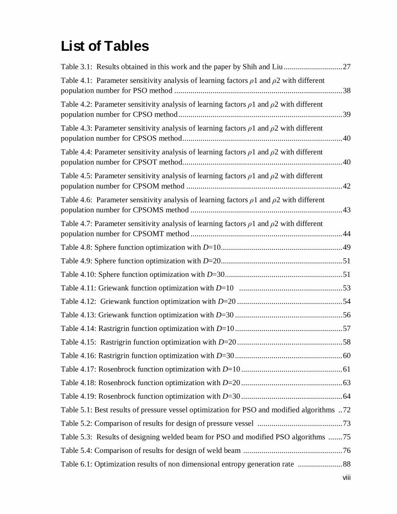
List of Tables Table 3.1: Results obtained in this work and the paper by Shih and Liu ............................. 27
Table 4.1: Parameter sensitivity analysis of learning factors ρ1 and ρ2 with different population number for PSO method ................................................................................... 38
Table 4.2: Parameter sensitivity analysis of learning factors ρ1 and ρ2 with different population number for CPSO method ................................................................................. 39
Table 4.3: Parameter sensitivity analysis of learning factors ρ1 and ρ2 with different population number for CPSOS method ............................................................................... 40
Table 4.4: Parameter sensitivity analysis of learning factors ρ1 and ρ2 with different population number for CPSOT method............................................................................... 40
Table 4.5: Parameter sensitivity analysis of learning factors ρ1 and ρ2 with different population number for CPSOM method ............................................................................. 42
Table 4.6: Parameter sensitivity analysis of learning factors ρ1 and ρ2 with different population number for CPSOMS method ........................................................................... 43
Table 4.7: Parameter sensitivity analysis of learning factors ρ1 and ρ2 with different population number for CPSOMT method ........................................................................... 44
Table 4.8: Sphere function optimization with D=10 ............................................................ 49
Table 4.9: Sphere function optimization with D=20 ............................................................ 51
Table 4.10: Sphere function optimization with D=30 .......................................................... 51
Table 4.11: Griewank function optimization with D=10 ................................................... 53
Table 4.12: Griewank function optimization with D=20 .................................................... 54
Table 4.13: Griewank function optimization with D=30 ..................................................... 56
Table 4.14: Rastrigrin function optimization with D=10 ..................................................... 57
Table 4.15: Rastrigrin function optimization with D=20 .................................................... 58
Table 4.16: Rastrigrin function optimization with D=30 ..................................................... 60
Table 4.17: Rosenbrock function optimization with D=10 .................................................. 61
Table 4.18: Rosenbrock function optimization with D=20 .................................................. 63
Table 4.19: Rosenbrock function optimization with D=30 .................................................. 64
Table 5.1: Best results of pressure vessel optimization for PSO and modified algorithms .. 72
Table 5.2: Comparison of results for design of pressure vessel .......................................... 73
Table 5.3: Results of designing welded beam for PSO and modified PSO algorithms ....... 75
Table 5.4: Comparison of results for design of weld beam ................................................. 76
Table 6.1: Optimization results of non dimensional entropy generation rate ...................... 88

ix
List of Figures
Figure 2.1 : Movement of a particle in search space ......................................................... 16
Figure 2.2 : Flow chart describes the search mechanism of particle swarm optimization algorithm (PSO) ................................................................................................................. 18
Figure 3.1: Schematic diagram of a plate-fin sink. .............................................................. 24
Figure 3.2: Optimum entropy generation rate with vary of N (PSO and GA) .................... 28
Figure 0.1: Parameter sensitivity analysis of learning factors ρ1 and ρ2 with different population number for PSO m ............................................................................................ 38
Figure 0.2: Parameter sensitivity analysis of learning factors ρ1 and ρ2 with different population number for CPSO method ................................................................................ 39
Figure 4.3: Parameter sensitivity analysis of learning factors ρ1 and ρ2 with different population number for CPSOS method .............................................................................. 40
Figure 4.4: Parameter sensitivity analysis of learning factors ρ1 and ρ2 with different population number for CPSOT method .............................................................................. 41
Figure 4.5: Parameter sensitivity analysis of learning factors ρ1 and ρ2 with different population number for CPSOM method ............................................................................ 43
Figure 4.6: Parameter sensitivity analysis of learning factors ρ1 and ρ2 with different population number for CPSOMS method .......................................................................... 44
Figure 4.7: Parameter sensitivity analysis of learning factors ρ1 and ρ2 with different population number for CPSOMT method .......................................................................... 45
Figure 4.8: Sphere function optimization with D=10 .......................................................... 49
Figure 4.9 : Sphere function optimization with D=20 ......................................................... 50
Figure 4.10: Sphere function optimization with D=30 ........................................................ 52
Figure 4.11: Griewank function optimization with D=10 .................................................... 53
Figure 4.12: Griewank function optimization with D=20 .................................................... 54
Figure 4.13: Griewank function optimization with D=30 .................................................... 55
Figure 4.14: Rastrigrin function optimization with D=10 .................................................... 57
Figure 4.15: Rastrigrin function optimization with D=20 .................................................... 58
Figure 4.16: Rastrigrin function optimization with D=30 .................................................... 59
Figure 4.17 : Rosenbrock function optimization with D=10 ................................................ 61
Figure 4.18: Rosenbrock function optimization with D=20 ................................................. 62
Figure 4.19: Rosenbrock function optimization with D=30 ................................................. 64
Figure 5.1: Schematic diagram of pressure vessel .............................................................. 71
x
Figure 5.2: Schematic diagram of welded beam ................................................................. 74
Figure 6.1: Schematic diagram of a general fin in convective heat transfer ........................ 82
Figure 6.2: Geometrical configuration of a plate-fin sink ................................................... 86
Figure 6.3: Optimization of non dimensional entropy generation rate ................................ 89
Figure 6.4: Optimum entropy generation rate with vary of N ............................................. 89
Figure 6.5: Optimum entropy generation rate and optimum flow velocity with different values of N ........................................................................................................................ 90
Figure 6.6: Optimum entropy generation rate and optimum thickness of fin with different
values of N ........................................................................................................................ 91
Figure 6.7: Optimum entropy generation rate and optimum height of fin with different values of N ........................................................................................................................ 91
Figure 6.8: Temperature distribution through cross section of the heat sink ....................... 92
Figure 6.9: Velocity profile through the heat sink .............................................................. 93

xi
Nomenclature List of Symbols
a Height of fin, m.
Ac Cross-sectional area of the fin, m2.
b Base thickness, mm.
Ca Chaotic acceleration factor.
d Thickness of the fin, m.
Dh Hydraulic diameter of the channel, m.
fapp Apparent friction factor.
퐹 Drag force, N.
fi Current solution that is achieved by a particle i.
fg Global solution that is achieved by all particles.
푓.푅푒 h Fully developed flow factor Reynolds number group.
푓(푥) Objective Function.
퐺(푥) Penalty factor.
푔 (푥) Inequality constraints.
h Heat transfer coefficient, W/m2 K.
ℎ (푥) Equality constraints.
ℎ(푡) Penalty value.
iterationcurrent Current iteration number.
iterationmax Total number of iteration.
k Thermal conductivity of the heat sink, W/m.K.
kf Thermal conductivity of air, W/m.K.
퐾 Contraction loss coefficient.
퐾 Expansion loss coefficient.
L Base length, mm.
퐿∗ Dimensionless fin length.
m Mass, kg.
xii
푚̇ Mass flow rate, kg/s.
N Total number of fins.
푁̇ Non-dimensional Entropy generation rate.
Nsize Swarm size.
푁 Nusselt number on heat sink in flow direction.
P Perimeter, m.
푃 Best solution of the objective function that has been discovered by a
particular particle.
푃 Best global solution of the objective function that has been discovered
by all the particles of the population.
푞 (푥) Violated function of the constraints.
Q Total heat dissipation , W.
R Overall heat sink resistance, K/W.
Rfin Thermal resistance of a single fin, K/W.
푟푎푛푑 Random number.
푟푎푛푑 Random number.
푅푒 ∗ Reynolds number.
s Spacing between the fins, m.
푆̇ Entropy generation rate, W/k.
Tb Base temperature, K.
Te Ambient air temperature, K.
Tw Wall temperature, K.
푣 Current velocity for particle i.
푣 New velocity for particle i.
Vch Channel velocity, m/s.
푉 Stream velocity, m/s.
푉 Maximum velocity, m/s.
W Heat sink width, m.
푥 Current location of the solution for each particle in the search space.
푥 New location of the solution for each particle in the search space.
푥 Lower bounds.

xiii
푥 Upper bounds.
List of Greek Symbols 휃( 푞 (푥) ) Assignment function.
휇 Control parameter.
Kinematical viscosity coefficient, m2/s.
Air density, kg/m.
ρ1 Cognitive parameter.
ρ2 Social parameter.
휓(푞 (푥)) Power of the penalty function.
τ Mutation operator.
휔 Inertia factor.
휔 Chaotic inertia weight factor.
휔 Minimum value of inertia factor.
휔 Maximum value of inertia factor.
List of Subscripts amb Ambient.
app Approach.
ch Channel.
d Dimension number
D Total number of dimensions
f Fluid.
fin Single fin.
i Particle number

xiv
List of Abbreviations CPSO Chaotic Particle Swarm Optimization.
CPSOM Chaotic Particle Swarm Optimization with Mutation.
CPSOMS Chaotic Particle Swarm Optimization with Mutation (Chaotic
Acceleration added to Second Term of Velocity equation).
CPSOMT Chaotic Particle Swarm Optimization (Chaotic Acceleration added to
Third Term of Velocity equation).
CPSOS Chaotic Particle Swarm Optimization (Chaotic Acceleration added to
Second Term of Velocity equation).
CPSOT Chaotic Particle Swarm Optimization (Chaotic Acceleration added to
Third Term of Velocity equation).
ES Evolution Strategy.
EAs Evolutionary Algorithms.
GA Genetic Algorithms.
LP Linear programming problems.
MAs Memetic Algorithms.
NLP Nonlinear programming problem.
PFM Non-stationary, Multi-stage Penalty Method.
PSO Particle Swarm Optimization.
QP Quadratic programming problems.
SFL Shuffled Frog Leaping algorithm.

xv
Acknowledgments
I would like to thank Dr. C.W. de Silva and Dr. M.S. Gadala, my supervisors, for
the opportunity they provided me to complete my doctoral studies under their
exceptional guidance. Without their unending patience, constant encouragement,
guidance and expertise, this work would not have been possible.
My colleagues in Dr. de Silva’s Industrial Automation Laboratory and Dr.
Gadala’s research group also deserve many thanks for their support.
Most of all, I want to thanks my parents and my wife for endless support and
encouragements throughout my various studies and life endeavors.

xvi
Dedication
To my parents

1
Chapter 1
Optimization Techniques
1.1. Introduction
Optimization may be defined as the art of obtaining the best ways or solutions to satisfy
a certain objective and at the same time satisfying fixed requirements or constraints [1]. The
practice of optimization is as old as the civilization. According to the Greek historian
Herodotus, the Egyptians applied an early version of optimization technique when they tried
to figure out farmland taxes taking into account any change in value of each land resulting
from annual flooding of Nile river [2].
Optimization is the branch of computational science that searches for the best
solution of problems that are encountered in mathematics, physics, chemistry, biology,
engineering, architecture, economics, management, and so on. The rapid advancement in the
digital computing power and the enormous practical need for solving optimization problems
have helped researchers in exploring different areas of science and in coming up with new
methods that have the capability to solve hard and complicated problems.
An optimization problem consists of the following basic components:
The quantity to be optimized (maximized or minimized) which is termed the
objective function (or, cost function or performance index or fitness function).
The parameters which may be changed in the search for the optimum, which are

2
called design variables (or, parameters of optimization).
The restrictions or limits placed on the parameter values (design variables) of
optimization, which are known as constraints.
The optimization scheme finds the values (design variables) that minimize or maximize
the objective function while satisfying the constraints. Thus, the standard form of an
optimization problem can be expressed as follows:
Minimize 푓(푥), 푥 = (푥 ,푥 , … … … … , 푥 ) 1-1
Subject to:
ℎ (푥) = 0, 푖 = 1, … . ,푚 1-2
푔 (푥) ≤ 0, 푖 = 1, … . , 푞 1-3
푥 ≤ 푥 ≤ 푥 1-4
where 푓(푥) is the objective function and x is the column vector of the n independent
variables. Constraint equations of the form ℎ (푥) = 0 are termed equality constraints, and
those of the from 푔 (푥) ≤ 0 are termed inequality constraints. The equations 푥 ≤ 푥 ≤
푥 are bounds on optimization variables. In summary, the formulation of an optimization
problem involves the following:
Selecting one or more design variables or parameters
Choosing an objective function
Identifying a set of constraints as applicable
The objective function(s) and the constraint(s) must be functions of one or more design
variables.
3
The optimization problems are mainly classified into these four types:
Unconstrained problems: these problems have an objective function with no
constraints. Problems with simple bounds can be treated as unconstrained problems.
Linear programming problems (LP): if the objective function and all the constraints
are linear functions, then the problem is called a linear programming problem.
Quadratic programming problems (QP): if the objective function is a quadratic
function and all the constraints are linear functions, then the problem is called a
quadratic programming problem.
Nonlinear programming problem (NLP): a general constrained optimization problem
where one or more functions are nonlinear is called a nonlinear programming
problem.
The majority of engineering applications are classified under these categories of problems.
In practice, there are many optimization algorithms and they may be classified into
classical and stochastic methods [2]. Classical methods converge toward the solution by
making deterministic decisions. They are considered to be less expensive in terms of the
computational time. In the next section, the steepest descent algorithm, the Simplex method,
and the Newton’s method will be described briefly as they are considered among the most
common classical algorithms.
1.2. Classic Optimization Methods
1.2.1 The Steepest Descent Algorithm
The steepest descent algorithm, which may be traced back to the French mathematician
Cauchy in 1847 [2], is a first-order optimization algorithm to find the minimum value of a

4
function. It uses the gradient of a function (or the scalar derivative, if the function is single-
valued) to determine the direction in which the function is increasing or decreasing most
rapidly. If the minimum points exist, the method is guaranteed to locate them after an
(infinite number, theoretically) of iterations. The method is a simple, stable, and easy to
implement but it has some major drawbacks as follows:
It guarantees the convergence to a local minimum but does not ensure finding the
global minimum.
It is good for unconstrained optimization problems only.
It is generally a slow algorithm.
It tends to have poor performance if it is used by itself, not in conjunction with other
optimizing methods.
1.2.2 Simplex Method
Simplex method is a conventional direct search algorithm for solving linear
programming problems, which was created by George Dantzig in 1947 [3]. In this method
the best solution lies on the vertices of a geometric figure in N-dimensional space made of a
set of N+1 points. The method compares the objective function values at the N+1 verteces
and moves towards the optimum point, iteratively. The simplex method is very efficient in
practice, generally taking 2m to 3m iterations at most (where m is the number of equality
constraints) [2], and converging in expected polynomial time for certain distributions of
random inputs. The movement of the simplex algorithm is achieved by reflection,
contraction, and expansion. It has drawbacks including the following:
it is costly in terms of computational time

5
it does not ensure convergence to global optimum and there exists the possibility
of cycling
1.2.3 Newton Raphson Method
In 1669, Isaac Newton found an algorithm to solve for the roots of a polynomial
equation. Later, in 1690, Joseph Raphson modified Newton's method by using the derivative
of a function to find its roots. That modified method is called the Newton-Raphson method
[4]. In mathematics, it is the most widely used one of all root-locating algorithms. It can also
be used to find local maxima and minima of functions, as theses extreme values are the roots
of the derivative function. As the Newton-Raphson method uses the first derivative of the
function to find the root, it is necessary that the function should be differentiable.
1.3. Evolutionary Algorithms (EAs)
In optimization problems where the functions do not satisfy convexity conditions or
when the solution space is discontinuous, the deterministic methods are not applicable.
However, stochastic methods, which make random decisions to converge to a solution, are
known to be suitable for these problems. Most stochastic methods are usually considered to
be computationally expensive but this may be offset by the advancements in computer
technology. For this reason many researchers have heavily investigated the applicability of
stochastic methods in different areas of science, engineering, economics, and so on.
Evolutionary algorithms (EAs) are considered one of stochastic methods that take their
inspiration from natural selection and survival of the fittest in the biological world [5]. EAs
differ from other optimization techniques in that they involve a search from a "population"
of solutions, not from a single point. Each iteration of an EA involves a competitive

6
selection, which wipes out poor solutions. Evolution Strategy (ES), Genetic Algorithms
(GA), and PSO are examples of EAs [6] and they will be described briefly in the
subsequent paragraphs.
1.3.1 Evolution Strategy (ES)
Evolution Strategy (ES) is a stochastic search method based on the ideas of adaptation
and evolution. The concept of ES was introduced by Ingo Rechenberg at Berlin Technical
University in 1973 but was not developed as an algorithm to be used in the optimization
field, but rather used as a method to find optimal parameter settings in laboratory
experiments. Later on, through the work of Schwefel [5], ES was introduced as a method to
solve optimization problems. ES merely concentrates on translating the fundamental
mechanisms of biological evolution for technical optimization problems [7]. In ES, the
individuals, which are the problem potential solutions, consist of the objective variables plus
some other parameters such as the step size to guide the search. Search steps are taken
through stochastic variation, called mutation [8]. The mutation is usually carried out by
adding a realization of a normally distributed random vector. The parameters that
parameterize the mutation distribution are called strategy parameters. The parameterization
of an ES is highly customizable [9].
1.3.2 Genetic Algorithms (GA)
Genetic Algorithms (GA), under the umbrella of evolutionary methods work by
mimicking natural evolution and selection in nature according to Darwin’s theory. GA was
proposed by John Holland and his colleagues in the early part of the 1970s [10]. Simply,
GA encodes a possible solution to a specific problem in the form of a simple chromosome
(encoded string) and applies recombination operators to these structures in such a way as to
7
keep and store critical information of the problem. A collection of such strings is called
a population. Associated with each chromosome is its fitness value. Those chromosomes
which represent a better solution to the target problem are given more opportunity to
reproduce than those that are poorer solutions [11]. If the processes of natural reproduction
combined with the biological principle of survival of the fittest are applied, then in each
generation progresses, good chromosomes with high values of fitness are predicted to be
achieved. GA is known to be a useful substitute to traditional search and optimization
methods, especially for problems with highly complex, non-analytic, or ill-behaved
objective functions. A key element in a GA is that it maintains a population of candidate
solutions that evolves over time [12]. The population allows the chromosomes to continue to
explore new areas of the search space that potentially appear to have optimum solutions.
1.3.3 Particle Swarm Optimization (PSO)
More recently, an evolutionary computation technique called particle swarm
optimization (PSO) has evolved as a population-based stochastic optimization technique. It
was developed by Kennedy and Eberhart [13] and has been inspired by the group behavior
of animals such as schools of fish and flocks of birds. Unlike other heuristic techniques of
optimization, PSO has a flexible and well-balanced mechanism to enhance and adapt to the
global and local exploration abilities. PSO has its roots primarily in two methodologies [14].
Perhaps more obvious are its ties to artificial life (A-life), and the behavior of flocks of
birds, schools of fish, and swarms in particular. It is also related to evolutionary
computation, and has ties to genetic algorithms and evolutionary strategies [15]. It exhibits
some evolutionary computation attributes such as its initialization with a population of
random solutions, searching for optima by updating generations, and updating based on the
previous generations.

8
In general, PSO is based on a relatively simple concept, and can be implemented in a
few lines of computer code. Furthermore, it requires only simple mathematical operators,
and is computationally inexpensive in terms of both memory requirement and speed. In test
functions of evolutionary algorithms PSO has been proved to perform well and has been
used to solve many of the same kinds of problems as for evolutionary algorithms. PSO was
initially used to handle continuous optimization problems. Subsequently, PSO has been
expanded to handle combinatorial optimization problems, with both discrete and continuous
variables. Early testing has found the implementation to be effective in complex practical
problems.
PSO does not suffer from some of the difficulties of EA. For example, a particle
swarm system has memory, which the genetic algorithm (GA) does not have. In PSO,
individuals who fly past the optima are pulled to return toward them, and knowledge of
good solutions is retained by all particles [16]. Unlike other evolutionary computing (EC)
techniques, PSO can be realized using a relatively simple program, which is an important
advantage when compared with other optimization techniques. In summary, compared with
other methods, PSO has the following advantages [17]:
Faster and more efficient: PSO may get results of the same quality in significantly
fewer fitness and constraint evaluations.
Better and more accurate: In demonstrations and various application results, PSO is
found to give better and more accurate results than other algorithms reported in the
literature by its ability to converge to a good solution and escape local optima.
Less expensive and easier to implement: The algorithm is intuitive and does not need
specific domain knowledge to solve the problem. There is no need for transformations
9
or other complex manipulations. Implementation in difficult optimization areas
requires relatively simple and short coding.
The PSO method and the EAs seem to be promising alternatives to deterministic
techniques. First, they do not rely on any assumptions such as differentiability or continuity.
Second, they are capable of handling problems with nonlinear constraints, multiple
objectives, and time-varying components. Third, they have shown superior performance in
numerous real-world applications.
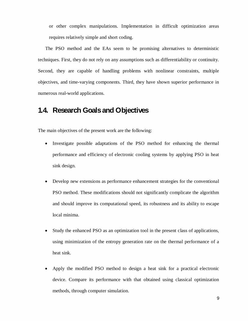
1.4. Research Goals and Objectives
The main objectives of the present work are the following:
Investigate possible adaptations of the PSO method for enhancing the thermal
performance and efficiency of electronic cooling systems by applying PSO in heat
sink design.
Develop new extensions as performance enhancement strategies for the conventional
PSO method. These modifications should not significantly complicate the algorithm
and should improve its computational speed, its robustness and its ability to escape
local minima.
Study the enhanced PSO as an optimization tool in the present class of applications,
using minimization of the entropy generation rate on the thermal performance of a
heat sink.
Apply the modified PSO method to design a heat sink for a practical electronic
device. Compare its performance with that obtained using classical optimization
methods, through computer simulation.
10
Utilize numerical procedures (e.g., FD) in solving the flow and heat transfer (HT)
equations of the heat sink problem.
1.5 Thesis Structure
A brief background of the optimization theory and the classical and non-classical
techniques of optimization were presented in the first part of the present chapter (Chapter 1).
In Chapter 2, a comprehensive literature review of PSO including its structure, how it works,
suggested developments to improve PSO, and its applications are highlighted. Chapter 3
shows the applicability of PSO in heat sink design optimization. Chapter 4 presents the
modifications (Chaotic Acceleration Factor, Chaotic Inertia Factor, and Best Global
Mutation) to the PSO algorithm, in the present work, to enhance its performance. In
Chapter 5, the performance of the modified PSO algorithms when they are applied to
nonlinear constraint problems is studied. Chapter 6 presents a detailed study of application
of the modified PSO algorithm in heat sink design. In Chapter 7 the main conclusions of the
present work are drawn and avenues for future research are suggested.

11
Chapter 2
Literature Review
2.1 Introduction The particle swarm optimization (PSO) is a relatively new generation of combinatorial
metaheuristic algorithms and is based on mimicking the group behavior of animals; for
example, flocks of birds or schools. In test functions of evolutionary algorithms, PSO has
proved to perform well and has been used to solve many of the same kinds of problems as
evolutionary algorithms. In this chapter PSO will be explained in detail in terms of its
history, how it works, modifications that have been added to improve its research ability, and
its applications.
2.2 History of PSO In 1995, two scientists introduced a new optimization technique and they named it
“Particle Swarm Optimization.” The technique was inspired by A-life, biological evaluation
and natural selection of species [6]. Simply, the method uses a population of individual
particles where each particle has a position, a velocity, and memory of the location of its
best fitness found during the search process. Each particle updates its velocity according to
its momentum, its memory, and the shared memory of the other particles in its
neighborhood. By adding the newly found velocity of the particle to its current position, the
particle will move to a new position in the search space. The PSO method appears to rely on
the five basic principles of swarm intelligence, as defined by [18]:
Proximity: the swarm should handle simple space and time computations

12
Quality: the swarm should be a able to respond to quality factors in the environment
Diverse response: the swarm should not commit its activities along excessively
narrow channels
Stability: the swarm should not change its behavior every time the environment
varies
Adaptability: the swarm must be able to change its behavior when the computational
cost is not prohibitive.
The PSO in its original form is defined by (see [14]):
Velocity Update Equation:
푣 = 푣 + 휌 . 푟푎푛푑 . (푃 − 푥 ) + 휌 . 푟푎푛푑 . 푃 − 푥 2-1
Position Update Equation:
푥 = 푥 + 푣 2-2
where
Particle position vector 풙풊풅: This vector contains the current location of the solution
for each particle in the search space.
Particle velocity vector 풗풊풅: This vector represents the degree to which vector 풙풊풅
(both vectors have consistent units) will change in magnitude and direction in the
next iteration. The velocity is the step size—the amount by which a change in the
풗풊풅 values changes the direction of motion in the search space; it causes the particle
to make a turn. The velocity vector is used to control the range and resolution of the
search.

13
Best solution Pi: This is the best solution of the objective function that has been
discovered by a particular particle.
Best Global Solution Pg : This is the best global solution of the objective function
that has been discovered by all the particles of the population.
ρ1 and ρ 2: Learning factors applied to influence the best position and the global
best position, respectively, of a particle.
rand1 and rand2 : are random numbers.
Kennedy and Eberhart [18] introduced their new method to researchers by highlighting
its potential as an effective optimization method while testing it in depth. They tested three
variations of PSO: GBEST, where all particles have knowledge about the group’s best
fitness, and two of the “LBEST” versions, one with a neighborhood of six particles and one
with a neighborhood of two particles. They tested PSO by using it to train the weights of a
neural network and showed that it is as effective as the usual error back-propagation method,
and compared the performance of PSO to published benchmarks results for genetic
algorithms (GAs). PSO outperformed GAs as it found the global optimum in each run, and
appears to have fairly similar results to that reported for GAs in [19] in terms of the number
of evaluations required to reach specified performance levels.
In 1997 Kennedy [20] studied the effect of both social and cognition components on the
performance of the algorithm by examining four models of PSO. These are “cognition-
only,” “social-only,” the full, and the “selfless” models. The first model was the “cognition-
only” model where he considered only the cognition component
푣 = 푣 + 휌 . 푟푎푛푑 . (푃 − 푥 ) 2-3

14
The second model was “social-only" where the only social component was considered.
푣 = 휌 . 푟푎푛푑 . 푃 − 푥 2-4
The “selfless” model was identical to the “social-only” model, with the exception that
the neighborhood did not contain the individual's own previous best performance, that is, i ≠
g. Therefore, none were attracted to their own successes, but rather only followed one
another through the hyperspace. Also, he introduced Vmax to control the particle’s velocity as
he realized that some particles tend to have an explosive growth in their velocities. Kennedy
compared the above-mentioned models with varying values of ρ1, ρ 2, and Vmax, by applying
these four models in finding the weights of a neural network. He found that:
In order to help particles avoid trapping at local minimum, Vmax should be
sufficiently high.
Both “social-only” and “selfless” models showed better performance when compared
to the full model. On other hand, the “cognition-only” model showed the worst
performance among the four models.
In 1998, Shi and Eberhart [21] introduced the inertia factor w which plays a very crucial
role in enhancing the search capability of the PSO algorithm. The inertia factor w is a
parameter that is used to control the impact of the previous velocities on the current velocity.
Hence, it influences the trade-off between the global and local exploration abilities of
particles. When w is small, the PSO is more like a local search algorithm. If there is an
acceptable solution within the initial search space, the PSO will find the global optimum
quickly; otherwise, it will not find the global optimum. When w is large ( >1.2), the PSO
tends to exploit new areas, which are beyond the search space limit. Consequently, the PSO
will take more iterations to find the global optimum and have more chances of failing to find

15
the global optimum. When 휔 is 0.8 < 휔 <1.2 , the PSO will have the best chance to find the
global optimum with a moderate number of iterations. According to Shi [21] it is
recommended to start with a large value 1.4 for 휔 and linearly decrease the value to 0.5 in
order to realize better convergence at reasonable speed. The inertia factor w can be
computed according to the following equation:
휔 = 휔 + ∗ 푖푡푒푟푎푡푖표푛 2-5
where
휔: the inertia factor
휔 and 휔 : the maximum and minimum values of inertia factor, which is
assigned according to the behavior of the problem
iterationmax = total number of iteration
iterationcurrent = current iteration number
The velocity equation after adding the inertia factor is as follows:
푣 = 휔. 푣 + 휌 . 푟푎푛푑 . (푃 − 푥 ) + 휌 . 푟푎푛푑 . 푃 − 푥 2-6
The heart of the PSO algorithm is the process by which vid is modified in equation (2-6),
forcing the particles to search through the most promising areas of the solution space again
and again adding the particle’s velocity vector vid to its location vector xid to obtain a new
location, as shown in Figure 2-1. Without modifying the values in vid, the particle would
simply take uniform steps in a straight line through the search space and beyond.
At each iteration, the previous values of vid constitute the momentum of a particle. This
momentum is essential, as it is this feature of PSO that allows the particles to escape local

16
optima. The velocities of the particles in each dimension are clamped to a maximum
velocity Vmax, as described before, which is an important parameter in determining the
optimum value of the objective function, with which the regions between the present
position and the best target position thus far are searched. If Vmax is too high, the particles
might fly past good solutions.
Figure 2.1: Movement of a particle in the search space.
휌 ∗ 푟푎푛푑 ∗ (푃 − 푥 )
푥
푥
푃
푃
휌 ∗ 푟푎푛푑 ∗ (푃 − 푥 )
푣
푣

17
On the other hand, if Vmax is too small, the particles might not explore sufficiently
beyond locally good regions. In fact, they could become trapped in local optima, unable to
move far enough to reach a better position in the problem space [22]. The acceleration
constants ρ1 and ρ2 in equation (2-6) represent the weightings of the stochastic acceleration
terms that direct each particle toward the pbest and gbest positions. They can be set to a
value of 2.0 in a typical optimization problem [19]. Population size is related to the search
space. If the population size is too small, is easy for the algorithm to converge to a local
optimum; if the size is too large, it will occupy a large computer memory and will need long
calculation time [18]. According to past work, 30–50 is a good population size, which will
ensure good search space convergence and a reasonable computational time [23]. Figure 2.2
presents a flow chart that describes the search mechanism of the PSO algorithm.
18
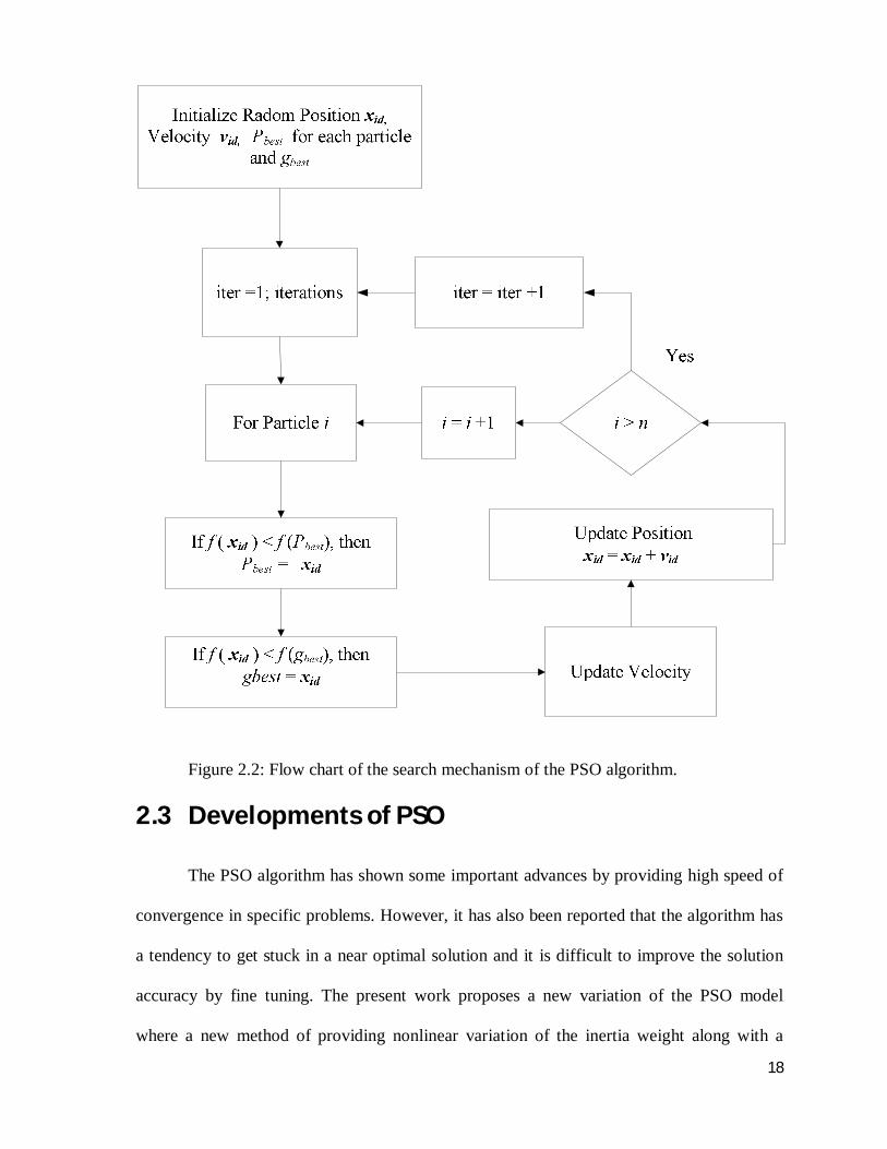
Figure 2.2: Flow chart of the search mechanism of the PSO algorithm.
2.3 Developments of PSO
The PSO algorithm has shown some important advances by providing high speed of
convergence in specific problems. However, it has also been reported that the algorithm has
a tendency to get stuck in a near optimal solution and it is difficult to improve the solution
accuracy by fine tuning. The present work proposes a new variation of the PSO model
where a new method of providing nonlinear variation of the inertia weight along with a
19
particle's old velocity are used to improve the speed of convergence as well as to fine tune
the search in the multidimensional space. Also a new method of determining and setting a
complete set of free parameters for any given problem is presented. This eliminates the
tedious trial and error-based approach to determine these parameters for a specific problem.
The performance of the proposed PSO model, along with the fixed set of free parameters, is
amply demonstrated by applying it to several benchmark problems and comparing with
several competing popular PSO and non-PSO combinatorial metaheuristic algorithms.
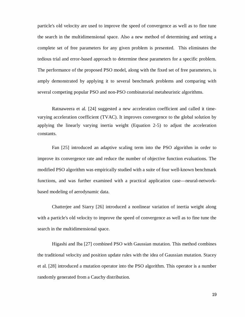
Ratnaweera et al. [24] suggested a new acceleration coefficient and called it time-
varying acceleration coefficient (TVAC). It improves convergence to the global solution by
applying the linearly varying inertia weight (Equation 2-5) to adjust the acceleration
constants.
Fan [25] introduced an adaptive scaling term into the PSO algorithm in order to
improve its convergence rate and reduce the number of objective function evaluations. The
modified PSO algorithm was empirically studied with a suite of four well-known benchmark
functions, and was further examined with a practical application case—neural-network-
based modeling of aerodynamic data.
Chatterjee and Siarry [26] introduced a nonlinear variation of inertia weight along
with a particle's old velocity to improve the speed of convergence as well as to fine tune the
search in the multidimensional space.
Higashi and Iba [27] combined PSO with Gaussian mutation. This method combines
the traditional velocity and position update rules with the idea of Gaussian mutation. Stacey
et al. [28] introduced a mutation operator into the PSO algorithm. This operator is a number
randomly generated from a Cauchy distribution.
20
Secrest and Lamond [29] presented a new visualization approach based on the
probability distribution of the swarm; thus the random nature of PSO is properly visualized.
They suggested a new algorithm based on moving the swarm a Gaussian distance from the
global and the local best.
Liu et al. [30] introduced a mutation mechanism into PSO to increase its global
search ability and to escape from local minima. The variable gbest mutated with Cauchy
distribution.
Xiang at al. [31] introduced a piecewise linear chaotic map (PWLCM) to perform the
chaotic search. An improved PSO algorithm combined with PWLCM (PWLCPSO) was
proposed subsequently, and experimental results were used to verify its superiority.
Selvakumar and Thanushkodi [32] proposed what was called a split-up in the
cognitive behavior. Making each particle remember its worst position helps the particles to
explore the search space very effectively. In order to exploit the promising solution region, a
simple local random search (LRS) procedure was integrated with PSO.
Angeline, a well known researcher in the evolutionary computation area, suggested a
hybrid version of the PSO algorithm [33]. The hybrid PSO incorporates a standard and
explicit tournament selection method from the evolutionary programming algorithm. A
comparison was performed between hybrid swarm and particle swarm, which showed that
the new development provided an advantage for some but not all complex functions. For
example, the hybrid PSO performed much worse than the standard PSO in evaluating the
Griewank function, which is a complex function with many local minima.
21
2.4 Comparison of PSO with Other Evolutionary Methods
Angeline in 1998 [34] did an early study to compare the particle swarm approach and
evolutionary computation in terms of their performance in solving four nonlinear functions,
which have been well-studied in the evolutionary optimization literature. He concluded that
the performance of the two methods was competitive. Particularly, PSO often locates the
near-optimum significantly faster than by evolutionary optimization but cannot dynamically
adjust its velocity step size to continue optimization.
Kennedy and Spears [35] compared the PSO algorithm with three versions of genetic
algorithm (GA), without mutation; without crossover; and the standard GA which has
crossover, mutation and selection, in a factorial time-series experiment. They found that all
algorithms improved over time, but the PSO found the global optimum on every trial, under
every condition. In short, PSO appears to be robust and shows superiority over all versions
of GA in almost every cases.
Hasen et al. [36] examined the effectiveness of PSO in finding the true global
optimal solution and made a comparison between PSO and GA in terms of their
effectiveness and their computational efficiency by implementing statistical analysis and
formal hypothesis testing. The performance comparison of the GA and PSO was
implemented using a set of benchmark test problems as well as two problems of space
system design optimization, namely, telescope array configuration and spacecraft reliability-
based design. They showed that the difference in the computational effort between PSO and
the GA was problem dependent. It appears that PSO outperforms GA by a large differential
in computational efficiency when used to solve unconstrained nonlinear problems with
22
continuous design variables and with low efficiency differential when applied to constrained
nonlinear problems with continuous or discrete design variables.
Lee et al. [37] implemented PSO and compared it with GA to find technical trading
rules in stock market. It was found that PSO could reach the global optimal value with less
iteration and kept equilibrium when compared to GA. Moreover, PSO showed the
possibility of solving complicated problems without using the crossover, mutation, and other
manipulations as in GA but using only basic equations.
Elbeltagi et al. [38] compared five evolutionary algorithms: GAs, Memetic
Algorithms (MAs), PSO, and Shuffled Frog Leaping algorithm (SFL) in solving two
benchmark continuous optimization test problems. The PSO method was generally found to
perform better than the other algorithms in terms of the success rate and the solution quality,
while being second best in terms of the processing time.
Allahverdi and Al-anzi [39] conducted extensive computational experiments to
compare the three methods: PSO, Tabu search, and Earliest Due Date (EDD) along with a
random solution in solving an assembly flow shop scheduling problem. The computational
analysis indicated that the PSO significantly outperformed the others for difficult problems.
2.5 Applications of PSO PSO, since its introduction in 1995, has been extensively applied to a wide range of
areas such engineering, science, medicine, and finance. Some examples of major areas of
applications are given below.
23
DNA reach: Chang et al. [40] successfully applied PSO to protein sequence motif
discovery problem. Their simulation results indicated that PSO could be used to obtain
the global optimum of protein sequence motifs.
Power and voltage control: Abido [41] applied PSO to solve the optimal power flow
(OPF) problem. The results were promising and showed the effectiveness and robustness
of the proposed approach.
Biomedical imaging: Wachowiak et al. [42] introduced a version of hybrid PSO to
biomedical image registration. The hybrid PSO technique produced more accurate
registrations than by the evolutionary strategies in many cases, with comparable
convergence. These results demonstrated the effectiveness of the PSO in image
registration, and emphasized the need for hybrid approaches for difficult registration
problems.
Heat sink design in electronic cooling: Alrasheed et al. [43] applied PSO in the area
of electronic cooling to heat sink design optimization. This work will be explained in
more detail later in the thesis.
Through a comparative evaluation using the results available in the literature, the
following comments may be made:
PSO uses objective function information to guide the search in the problem space.
Therefore, it can easily accommodate non-differentiable and non-convex objective
functions. Additionally, this property relieves PSO of analytical assumptions and
approximations that are often required for traditional optimization methods.
PSO uses probabilistic rules for particle movements, not deterministic rules. Hence,
it is a type of stochastic optimization algorithm that can search a complicated and
uncertain area, which makes PSO more flexible and robust than conventional method.

24
Chapter 3
Applicability of PSO in Heat Sink Design
Optimization1
In this chapter, the particle swarm optimization (PSO) is applied to design a heat sink
system. In the presented approach, a plate-fin heat sink design is realized for maximum
dissipation of the heat generated from electronic components, as represented by the entropy
generation rate.
3.1 Problem Statement
Figure 3.1: Schematic diagram of a plate-fin sink. 1 Alrasheed, M.R., de Silva, C.W., and Gadala, M.S., "Evolutionary optimization in the design of a heat sink," Editor: de Silva C.W., Mechatronic Systems: Devices, Design, Control, Operation and Monitoring, pp. 55-78, CRC Press, Boca Raton, FL, , 2007.
Alrasheed, M. R. , de Silva, C. W., and Gadala, M. S. ,“A new extension of particle swarm optimization and its application in
electronic heat sink design,” in ASME Conference Proceeding (IMECE 2007), Seattle, Washington, pp.1221-1230, November 2007.
L
a s
W
d
25
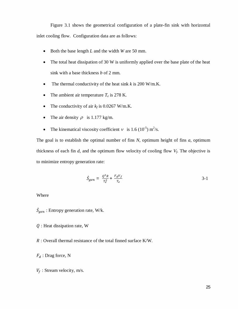
Figure 3.1 shows the geometrical configuration of a plate-fin sink with horizontal
inlet cooling flow. Configuration data are as follows:
Both the base length L and the width W are 50 mm.
The total heat dissipation of 30 W is uniformly applied over the base plate of the heat
sink with a base thickness b of 2 mm.
The thermal conductivity of the heat sink k is 200 W/m.K.
The ambient air temperature Te is 278 K.
The conductivity of air kf is 0.0267 W/m.K.
The air density is 1.177 kg/m.
The kinematical viscosity coefficient is 1.6 (10-5) m2/s.
The goal is to establish the optimal number of fins N, optimum height of fins a, optimum
thickness of each fin d, and the optimum flow velocity of cooling flow Vf. The objective is
to minimize entropy generation rate:
푆̇ = + 3-1
Where
푆̇ : Entropy generation rate, W/k.
푄 : Heat dissipation rate, W
푅 : Overall thermal resistance of the total finned surface K/W.
퐹 : Drag force, N
푉 : Stream velocity, m/s.
26
푇 : Ambient temperature, K.
N : Total number of fins
a : Height of fin, m.
d : Thickness of the fin, m.
s : The spacing between the fins, m.
W : Heat sink width, m.
and the design variables [x1, x2, x3, x4]T = [ N, a, d, Vf ].
The design boundaries corresponding to each design variable are
2 ≤ 푥 ≤ 40
25 mm ≤ 푥 ≤ 140 mm
0.2 mm ≤ 푥 ≤ 2.5 mm
0.5 m s⁄ ≤ 푥 ≤ 40 m s⁄
The number of fins must be an integer that can be restricted in the following domain:
2 ≤ 푁 ≤ 푖푛푡 1 + 3-2
The spacing s between two fins is given by:
푠 = − 푑 3-3
The first example in the paper of Shih and Liu [44, 44] is considered here, for a comparative
evaluation.
27
3.2 PSO Implementation
Initially, several runs were carried out with different values for the PSO key parameters
such as the initial inertia weight and the maximum allowable velocity. In the present
implementation, the initial inertia weight w is set to 0.9. Other parameters are set as: number
of particles n = 35, 휌 = 휌 = 2.0. The search is stopped if the number of iterations
reaches 300.
3.2.1 Numerical Results
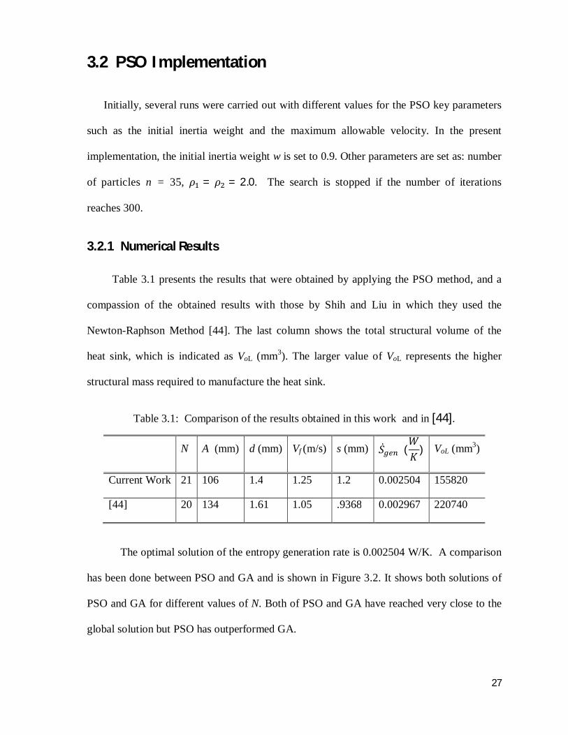
Table 3.1 presents the results that were obtained by applying the PSO method, and a
compassion of the obtained results with those by Shih and Liu in which they used the
Newton-Raphson Method [44]. The last column shows the total structural volume of the
heat sink, which is indicated as VoL (mm3). The larger value of VoL represents the higher
structural mass required to manufacture the heat sink.
Table 3.1: Comparison of the results obtained in this work and in [44].
N A (mm) d (mm) Vf (m/s) s (mm) 푆̇ (푊퐾 ) VoL (mm3)
Current Work 21 106 1.4 1.25 1.2 0.002504 155820
[44] 20 134 1.61 1.05 .9368 0.002967 220740
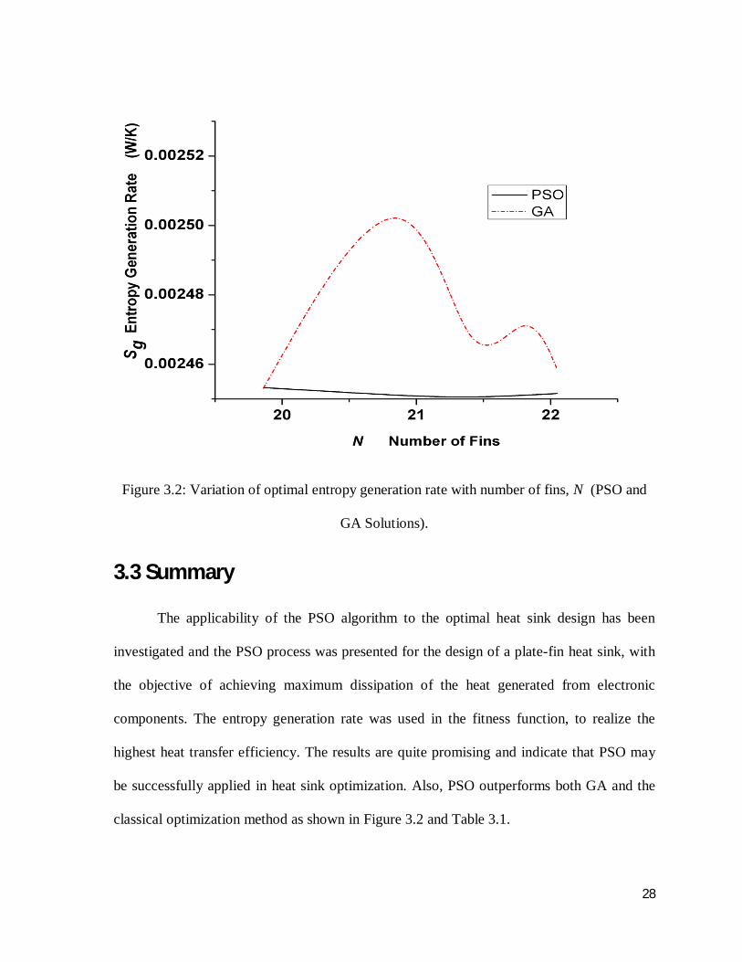
The optimal solution of the entropy generation rate is 0.002504 W/K. A comparison
has been done between PSO and GA and is shown in Figure 3.2. It shows both solutions of
PSO and GA for different values of N. Both of PSO and GA have reached very close to the
global solution but PSO has outperformed GA.
28
Figure 3.2: Variation of optimal entropy generation rate with number of fins, N (PSO and
GA Solutions).
3.3 Summary
The applicability of the PSO algorithm to the optimal heat sink design has been
investigated and the PSO process was presented for the design of a plate-fin heat sink, with
the objective of achieving maximum dissipation of the heat generated from electronic
components. The entropy generation rate was used in the fitness function, to realize the
highest heat transfer efficiency. The results are quite promising and indicate that PSO may
be successfully applied in heat sink optimization. Also, PSO outperforms both GA and the
classical optimization method as shown in Figure 3.2 and Table 3.1.
29
Chapter 4
New Extensions to PSO and Analysis
4.1 Introduction
In the previous chapters, the method of particle swarm optimization (PSO) was
introduced in detail and it was shown that it is an effective, efficient, fast and simple
method, which can outperform other available techniques of optimization. However, it
entails several problems that other evolutionary methods suffer from. For example, in some
cases, the particles tend to be trapped at local minima and are not able to escape them,
resulting in premature convergence. In this chapter some innovative modifications are
proposed to deal with these problems and to improve the robustness and convergence rate of
PSO. Specifically, the following modifications are introduced and investigated:
Chaotic Acceleration Factor
Chaotic Inertia Factor
Best Global Mutation
The performance of these enhancements will be tested through benchmark equations that are
commonly used in the optimization field.
30
4.2 Proposed Innovations
From numerical experiments it is observed that in the final stage of searching, PSO
suffers from a lack of diversity of the population. Because of premature convergence,
particles will not be able to adequately explore the feasible domain, and they may eventually
get trapped at local optima.
4.2.1 Chaotic Acceleration Factor (Ca)
Although there is no standard definition of chaos, it may be defined as a behavior
between perfect regularity and pure randomness [45]. There are typical features that a
system should possess for it to be described as chaotic system. These features include the
following:
(a) It is nonlinear.
(b) It has deterministic rules that every future state of the system must follow.
(c) It is sensitive to initial conditions.
Historically, the study of chaos began in mathematics and physics in 1963 when
Lorenz [46] introduced the canonical chaotic attractor. It then expanded into engineering,
and more recently into information and social sciences. Subsequently, the use of chaos as a
tool to enhance optimization algorithms has attracted many researchers due to its ease of
implementation and special ability to avoid trapping in local minima [47-54].
Due to the dynamic properties of the variables of chaos, the use of certain chaotic
sequences, rather than random numbers, may alter the characteristics of optimization
algorithms toward better solutions, by escaping from local optima.
31
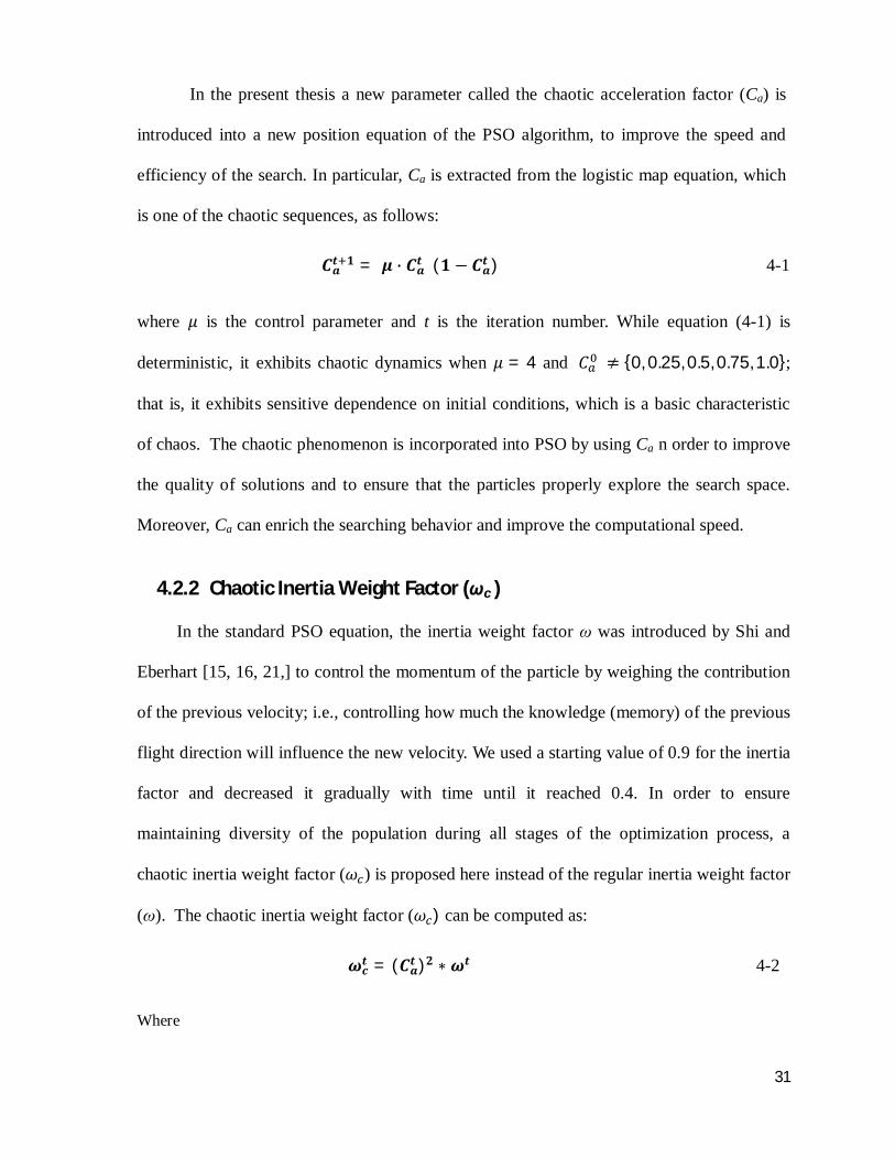
In the present thesis a new parameter called the chaotic acceleration factor (Ca) is
introduced into a new position equation of the PSO algorithm, to improve the speed and
efficiency of the search. In particular, Ca is extracted from the logistic map equation, which
is one of the chaotic sequences, as follows:
푪풂풕 ퟏ = 흁 ∙ 푪풂풕 (ퟏ − 푪풂풕 ) 4-1
where 휇 is the control parameter and t is the iteration number. While equation (4-1) is
deterministic, it exhibits chaotic dynamics when 휇 = 4 and 퐶 ≠ {0, 0.25, 0.5, 0.75, 1.0};
that is, it exhibits sensitive dependence on initial conditions, which is a basic characteristic
of chaos. The chaotic phenomenon is incorporated into PSO by using Ca n order to improve
the quality of solutions and to ensure that the particles properly explore the search space.
Moreover, Ca can enrich the searching behavior and improve the computational speed.
4.2.2 Chaotic Inertia Weight Factor (ωc )
In the standard PSO equation, the inertia weight factor ω was introduced by Shi and
Eberhart [15, 16, 21,] to control the momentum of the particle by weighing the contribution
of the previous velocity; i.e., controlling how much the knowledge (memory) of the previous
flight direction will influence the new velocity. We used a starting value of 0.9 for the inertia
factor and decreased it gradually with time until it reached 0.4. In order to ensure
maintaining diversity of the population during all stages of the optimization process, a
chaotic inertia weight factor (휔 ) is proposed here instead of the regular inertia weight factor
(ω). The chaotic inertia weight factor (휔 ) can be computed as:
흎풄풕 = (푪풂풕 )ퟐ ∗ 흎풕 4-2
Where

32
휔 ∶ the chaotic inertia weight factor
ω : the regular inertia weight factor
Ca : the chaotic acceleration factor
4.2.3 Global Best Mutation
It has been observed through simulations with numerical benchmarks that PSO
quickly finds a good local solution but it sometimes remains in a local optimum solution for
a considerable number of iterations (generations) without any improvement [43]; i.e.,
particles are trapped at one of the local optimum solutions. To get rid of this tendency, the
global search is improved by the introduction of a mutation process, which has some
conceptual similarity to the mutation in genetic algorithms (GAs). Under this new
modification, when the global optimum solution does not improve with the increasing
number of generation, the mutation operator (τ) is computed as follows:
휏 =∑
4-3
Where
fg = the global solution that is achieved by all particles
fi = the current solution that is achieved by a particle i
Nsize = swarm size
When τ is too small, it indicates that particles may be trapped at a local optimum solution.
So, if τ is less than a designated value σ, then the mutation process will start working by
changing the updated velocity equation to be of the form:
풗풊풅풕 ퟏ = 풗풊풅풕 + 풑품. 풆흎ퟐ푪풂
푵 4-5

33
The following pseudocode shows how mutation process takes place in the PSO scheme:
begin
initialize the population
for i=1 to number of particles
evaluate the fitness
update Pid and Pg
for d = 1 to number of dimensions
if 휏 ≤ 휎
푣 = 푣 + 푝 .
else
푣 = 휔 ∙ 푣 + 휌 ∙ 푟푎푛푑 ∙ (푝 − 푥 ) + 휌 ∙ 푟푎푛푑 ∙ (푝 − 푥 )
end if
update the position
increase d
increase i
end
end

34
The effect of incorporating these proposed modifications into the PSO method is
evaluated using the six versions of modified PSO listed below, in terms of both convergence
rate and performance of the modified PSO.
Version 1 (CPSO): 휔 replaces the regular inertia factor in the first right-hand term of
velocity- update equation so that the new velocity of the particle is given by:
풗풊풅풕 ퟏ = 흎풄ퟐ ∙ 풗풊풅풕 + 흆ퟏ ∙ 풓풂풏풅ퟏ ∙ (풑풊풅 − 풙풊풅풕 ) + 흆ퟐ ∙ 풓풂풏풅ퟐ ∙ (풑품 − 풙풊풅풕 ) 4-6
Ca is introduced to the second right-hand term in the position-update equation:
풙풊풅풕 ퟏ = 풙풊풅풕 + 푪풂풕 ퟏ ∙ 풗풊풅풕 ퟏ 4-7
Version 2 (CPSOS): 휔 replaces the regular inertia factor in the first right-hand term and Ca
is introduced to the second right-hand term of velocity- update equation so that the new
velocity of the particle is given by:
풗풊풅풕 ퟏ = 흎풄ퟐ ∙ 풗풊풅풕 + 푪풂 . 흆ퟏ ∙ 풓풂풏풅ퟏ ∙ (풑풊풅 − 풙풊풅풕 ) + 흆ퟐ ∙ 풓풂풏풅ퟐ ∙ 풑품 − 풙풊풅풕 4-8
Ca is introduced to the second right-hand term in the position-update equation:
풙풊풅풕 ퟏ = 풙풊풅풕 + 푪풂풕 ퟏ ∙ 풗풊풅풕 ퟏ 4-9
Version 3 (CPSOT): 휔 replaces the regular inertia factor in the first right-hand term and Ca
is introduced to the third right-hand term of the velocity-update equation so that the new
velocity of the particle is given by:
풗풊풅풕 ퟏ = 흎풄ퟐ ∙ 풗풊풅풕 + 흆ퟏ ∙ 풓풂풏풅ퟏ ∙ (풑풊풅 − 풙풊풅풕 ) + 푪풂 .흆ퟐ ∙ 풓풂풏풅ퟐ ∙ 풑품 − 풙풊풅풕 4-10
Ca is introduced to the second right-hand term in the position-update equation:
풙풊풅풕 ퟏ = 풙풊풅풕 + 푪풂풕 ퟏ ∙ 풗풊풅풕 ퟏ 4-11

35
Version 4 (CPSOM): 휔 replaces the regular inertia factor in the first right-hand term of
velocity-update equation so that the new velocity of the particle is given by:
풗풊풅풕 ퟏ = 흎풄ퟐ ∙ 풗풊풅풕 + 흆ퟏ ∙ 풓풂풏풅ퟏ ∙ (풑풊풅 − 풙풊풅풕 ) + 흆ퟐ ∙ 풓풂풏풅ퟐ ∙ (풑품 − 풙풊풅풕 ) 4-12
Note that if 휏 ≤ 휎 the update velocity equation given above will be replaced by what is
called the mutated velocity equation:
풗풊풅풕 ퟏ = 풗풊풅풕 + 풑품. 풆흎ퟐ푪풂
푵 4-13
Also, Ca is introduced to the second right-hand term in the position-update equation:
풙풊풅풕 ퟏ = 풙풊풅풕 + 푪풂풕 ퟏ ∙ 풗풊풅풕 ퟏ 4-14
Version 5 (CPSOMS): 휔 replaces the regular inertia factor in the first right-hand term and
Ca is introduced to the second right-hand term of the velocity-update equation so that the
new velocity of the particle is given by:
풗풊풅풕 ퟏ = 흎풄ퟐ ∙ 풗풊풅풕 + 푪풂 ∙ 흆ퟏ ∙ 풓풂풏풅ퟏ ∙ (풑풊풅 − 풙풊풅풕 ) + 흆ퟐ ∙ 풓풂풏풅ퟐ ∙ 풑품 − 풙풊풅풕 4-15
If 휏 ≤ 휎 the update velocity equation given above will be replaced by what is called the
mutated velocity equation:
풗풊풅풕 ퟏ = 풗풊풅풕 + 풑품. 풆흎ퟐ푪풂
푵 4-16
Aloso Ca is introduced to the second right-hand term in the position-update equation,
풙풊풅풕 ퟏ = 풙풊풅풕 + 푪풂풕 ퟏ ∙ 풗풊풅풕 ퟏ 4-17

36
Version 6 (CPSOMT): 휔 replaces the regular inertia factor in the first right-hand term and
Ca is introduced to the third right-hand term of the velocity-update equation so that the new
velocity of the particle is given as:
풗풊풅풕 ퟏ = 흎풄ퟐ ∙ 풗풊풅풕 + 흆ퟏ ∙ 풓풂풏풅ퟏ ∙ (풑풊풅 − 풙풊풅풕 ) + 푪풂 ∙ 흆ퟐ ∙ 풓풂풏풅ퟐ ∙ 풑품 − 풙풊풅풕 4-18
If 휏 ≤ 휎 the update velocity equation as given above will be replaced by what is called the
mutated velocity equation:
풗풊풅풕 ퟏ = 풗풊풅풕 + 풑품. 풆흎ퟐ푪풂
푵 4-19
Also, Ca is introduced to the second right-hand term in the position-update equation:
풙풊풅풕 ퟏ = 풙풊풅풕 + 푪풂풕 ퟏ ∙ 풗풊풅풕 ퟏ 4-20
The modified PSO method, as presented in this thesis, is termed mean PSO (or
MPSO). All modifications that are incorporated into PSO are validated next against the
original PSO using benchmark functions that are well known in the field of optimization.
4.3 Parameter Sensitivity Analysis
The PSO algorithm has several parameters that play a crucial role in the performance of
the algorithm in finding a good solution. These parameters are:
Number of particles in the population, Nsize
Inertia parameter, ω
Cognitive parameter, ρ1
Social parameter, ρ2

37
In order to find the best set of parameters, a sensitivity analysis for determining the
optimal values of the population size Nsize and the two learning factors ρ1 and ρ2 has been
done and will be presented in Section 4.3.2.
4.3.1 Population Size
Population size is related to the scale of the search space. If the population size is too
small, the algorithm can easily converge to a local optimum; if it is too large, it will require a
significant amount of computer memory and correspondingly increased computational time
[20, 56]. In fact, the selected population size is problem-dependent.
4.3.2. Learning Factors ( ρ1 ) and (ρ2 )
The two learning factors ρ1 and ρ2 in the velocity-update equation represent the
weighting of the stochastic acceleration terms that direct each particle toward the positions
Pi and Pg. Early experience with PSO led to setting each of the acceleration constants ρ1 and
ρ2 at 2.0 for typical applications [14]. However, for the newly modified versions of PSO the
parameter sensitivity analysis will be done to decide if the settings of the classical PSO
parameters are still adequate to achieve a good optimal solution.
4.3.3 Results of Parameter Sensitivity Analysis
In order to perform the parameter sensitivity analysis, the sphere function is used as
the fitness function with 20 dimensions, and each PSO version is run for 5 times. The
resulting average fitness values are listed in the following tables. Tables 4.1 through Table
4.7 present the experimental results of optimal values for both population size Nsize and two
learning factors ρ1 and ρ2.

38
Table 4-1: Sensitivity of learning factors ρ1 and ρ2 with different population number for PSO.
Nsize ρ1 = 0.5 ρ2 = 3.5
ρ1 = 1.0 ρ2 =3.0
ρ1 = 1.5 ρ2 =2.5
ρ1 = 2.0 ρ2 = 2.0
ρ1 = 2.5 ρ2 = 1.5
ρ1 = 3.0 ρ2 = 1.0
ρ1 = 3.5 ρ2 = 0.5
10 1.05E-01 4.60E-03 4.65E-04 1.54E-03 4.41E-03 1.00E-02 5.44E-01
20 2.00E-02 3.30E-04 2.79E-06 5.56E-09 2.21E-09 6.13E-05 7.19E-02
30 4.70E-02 1.19E-04 1.96E-06 2.13E-09 8.60E-11 4.54E-05 6.60E-02 40 5.00E-03 1.30E-04 1.53E-08 5.36E-12 9.55E-18 6.06E-07 4.80E-02
Figure 4.1: Sensitivity of learning factors ρ1 and ρ2 with different population number for PSO.

39
Table 4.2: Sensitivity of learning factors ρ1 and ρ2 with different population number for CPSO.
Nsize ρ1 = 0.5 ρ2 = 3.5
ρ1 = 1.0 ρ2 =3.0
ρ1 = 1.5 ρ2 =2.5
ρ1 = 2.0 ρ2 = 2.0
ρ1 = 2.5 ρ2 = 1.5
ρ1 = 3.0 ρ2 = 1.0
ρ1 = 3.5 ρ2 = 0.5
10 8.80E-05 2.8E-04 2.20E-03 6.70E-05 4.40E-03 6.70E-03 8.E-02 20 1.90E-08 2.6E-12 1.60E-12 1.00E-08 1.30E-07 2.50E-04 2.E-02 30 6.90E-16 1.9E-17 4.56E-23 6.70E-14 9.50E-10 1.20E-06 1.E-03 40 2.80E-17 2.7E-21 4.90E-30 9.60E-19 9.90E-12 7.50E-07 2.E-04
Figure 4.2: Sensitivity of learning factors ρ1 and ρ2 with different population number for CPSO.
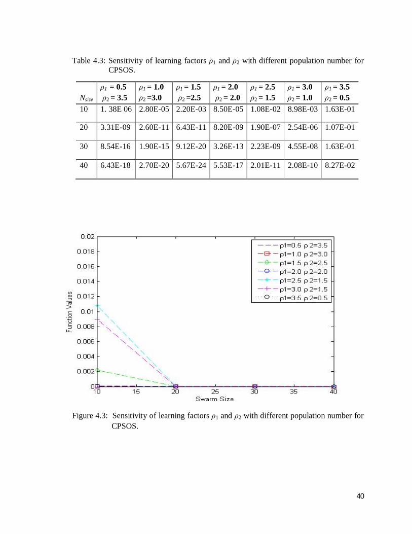
40
Table 4.3: Sensitivity of learning factors ρ1 and ρ2 with different population number for CPSOS.
Nsize ρ1 = 0.5 ρ2 = 3.5
ρ1 = 1.0 ρ2 =3.0
ρ1 = 1.5 ρ2 =2.5
ρ1 = 2.0 ρ2 = 2.0
ρ1 = 2.5 ρ2 = 1.5
ρ1 = 3.0 ρ2 = 1.0
ρ1 = 3.5 ρ2 = 0.5
10 1. 38E 06 2.80E-05 2.20E-03 8.50E-05 1.08E-02 8.98E-03 1.63E-01
20 3.31E-09 2.60E-11 6.43E-11 8.20E-09 1.90E-07 2.54E-06 1.07E-01
30 8.54E-16 1.90E-15 9.12E-20 3.26E-13 2.23E-09 4.55E-08 1.63E-01
40 6.43E-18 2.70E-20 5.67E-24 5.53E-17 2.01E-11 2.08E-10 8.27E-02
Figure 4.3: Sensitivity of learning factors ρ1 and ρ2 with different population number for CPSOS.
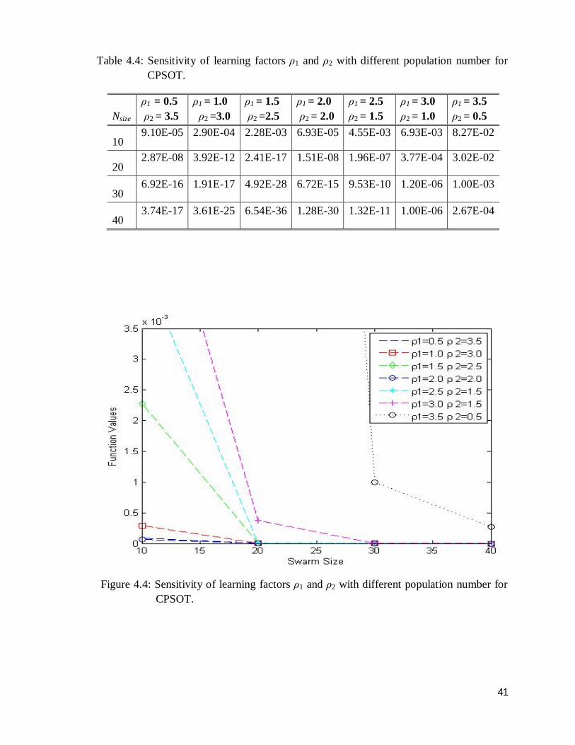
41
Table 4.4: Sensitivity of learning factors ρ1 and ρ2 with different population number for CPSOT.
Nsize ρ1 = 0.5 ρ2 = 3.5
ρ1 = 1.0 ρ2 =3.0
ρ1 = 1.5 ρ2 =2.5
ρ1 = 2.0 ρ2 = 2.0
ρ1 = 2.5 ρ2 = 1.5
ρ1 = 3.0 ρ2 = 1.0
ρ1 = 3.5 ρ2 = 0.5
10 9.10E-05 2.90E-04 2.28E-03 6.93E-05 4.55E-03 6.93E-03 8.27E-02
20 2.87E-08 3.92E-12 2.41E-17 1.51E-08 1.96E-07 3.77E-04 3.02E-02
30 6.92E-16 1.91E-17 4.92E-28 6.72E-15 9.53E-10 1.20E-06 1.00E-03
40 3.74E-17 3.61E-25 6.54E-36 1.28E-30 1.32E-11 1.00E-06 2.67E-04
Figure 4.4: Sensitivity of learning factors ρ1 and ρ2 with different population number for CPSOT.

42
Table 4.5: Sensitivity of learning factors ρ1 and ρ2 with different population number for CPSOM.
Nsize ρ1 = 0.5 ρ2 = 3.5
ρ1 = 1.0 ρ2 =3.0
ρ1 = 1.5 ρ2 =2.5
ρ1 = 2.0 ρ2 = 2.0
ρ1 = 2.5 ρ2 = 1.5
ρ1 = 3.0 ρ2 = 1.0
ρ1 = 3.5 ρ2 = 0.5
10 9.10E-05 2.90E-04 2.28E-03 6.93E-05 4.55E-03 6.93E-03 8.27E-02
20 2.87E-08 3.92E-12 2.41E-12 1.51E-08 1.96E-07 3.77E-04 3.02E-02
30 6.92E-16 1.91E-17 4.92E-21 6.72E-14 9.53E-10 1.20E-06 1.00E-03
40 3.74E-17 3.61E-21 6.54E-25 1.28E-18 1.32E-11 1.00E-06 2.67E-04

43
Figure 4.5: Sensitivity of learning factors ρ1 and ρ2 with different population number for CPSOM.
Table 4.6: Sensitivity of learning factors ρ1 and ρ2 with different population number for CPSOMS.
Nsize ρ1 = 0.5 ρ2 = 3.5
ρ1 = 1.0 ρ2 =3.0
ρ1 = 1.5 ρ2 =2.5
ρ1 = 2.0 ρ2 = 2.0
ρ1 = 2.5 ρ2 = 1.5
ρ1 = 3.0 ρ2 = 1.0
ρ1 = 3.5 ρ2 = 0.5
10 1.85E-04 5.90E-04 4.64E-03 1.41E-04 9.26E-03 1.41E-02 1.68E-01
20 7.20E-08 9.83E-12 6.05E-12 3.79E-08 4.92E-07 9.46E-04 7.58E-02
30 7.16E-16 1.98E-17 5.09E-21 6.95E-14 9.86E-10 1.24E-06 1.03E-03
40 4.99E-17 4.82E-21 8.73E-24 1.71E-18 1.76E-11 1.34E-06 3.57E-04
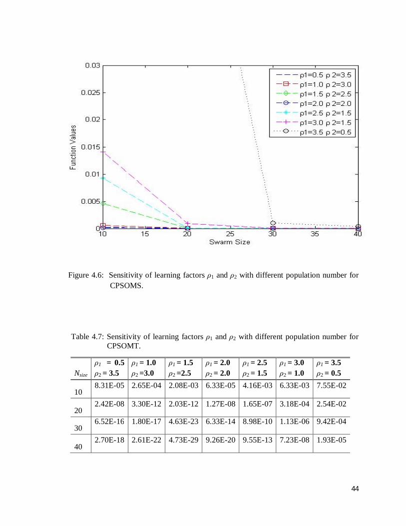
44
Figure 4.6: Sensitivity of learning factors ρ1 and ρ2 with different population number for CPSOMS.
Table 4.7: Sensitivity of learning factors ρ1 and ρ2 with different population number for CPSOMT.
Nsize ρ1 = 0.5 ρ2 = 3.5
ρ1 = 1.0 ρ2 =3.0
ρ1 = 1.5 ρ2 =2.5
ρ1 = 2.0 ρ2 = 2.0
ρ1 = 2.5 ρ2 = 1.5
ρ1 = 3.0 ρ2 = 1.0
ρ1 = 3.5 ρ2 = 0.5
10 8.31E-05 2.65E-04 2.08E-03 6.33E-05 4.16E-03 6.33E-03 7.55E-02
20 2.42E-08 3.30E-12 2.03E-12 1.27E-08 1.65E-07 3.18E-04 2.54E-02
30 6.52E-16 1.80E-17 4.63E-23 6.33E-14 8.98E-10 1.13E-06 9.42E-04
40 2.70E-18 2.61E-22 4.73E-29 9.26E-20 9.55E-13 7.23E-08 1.93E-05
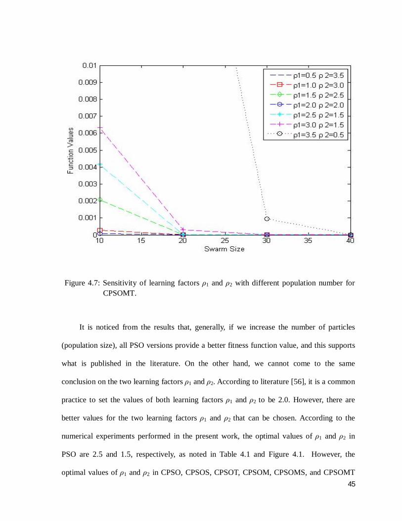
45
Figure 4.7: Sensitivity of learning factors ρ1 and ρ2 with different population number for CPSOMT.
It is noticed from the results that, generally, if we increase the number of particles
(population size), all PSO versions provide a better fitness function value, and this supports
what is published in the literature. On the other hand, we cannot come to the same
conclusion on the two learning factors ρ1 and ρ2. According to literature [56], it is a common
practice to set the values of both learning factors ρ1 and ρ2 to be 2.0. However, there are
better values for the two learning factors ρ1 and ρ2 that can be chosen. According to the
numerical experiments performed in the present work, the optimal values of ρ1 and ρ2 in
PSO are 2.5 and 1.5, respectively, as noted in Table 4.1 and Figure 4.1. However, the
optimal values of ρ1 and ρ2 in CPSO, CPSOS, CPSOT, CPSOM, CPSOMS, and CPSOMT
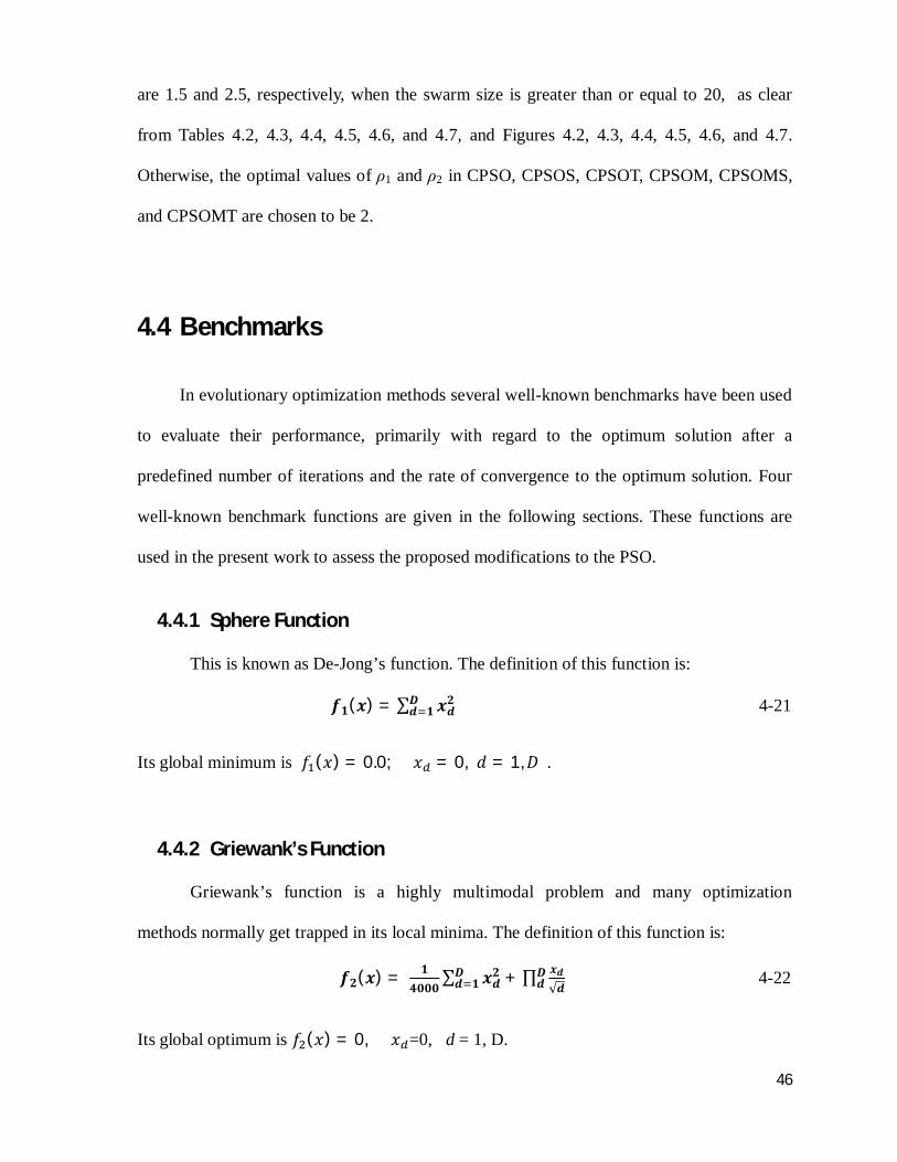
46
are 1.5 and 2.5, respectively, when the swarm size is greater than or equal to 20, as clear
from Tables 4.2, 4.3, 4.4, 4.5, 4.6, and 4.7, and Figures 4.2, 4.3, 4.4, 4.5, 4.6, and 4.7.
Otherwise, the optimal values of ρ1 and ρ2 in CPSO, CPSOS, CPSOT, CPSOM, CPSOMS,
and CPSOMT are chosen to be 2.
4.4 Benchmarks
In evolutionary optimization methods several well-known benchmarks have been used
to evaluate their performance, primarily with regard to the optimum solution after a
predefined number of iterations and the rate of convergence to the optimum solution. Four
well-known benchmark functions are given in the following sections. These functions are
used in the present work to assess the proposed modifications to the PSO.
4.4.1 Sphere Function
This is known as De-Jong’s function. The definition of this function is:
풇ퟏ(풙) = ∑ 풙풅ퟐ푫풅 ퟏ 4-21
Its global minimum is 푓 (푥) = 0.0; 푥 = 0, 푑 = 1,퐷 .
4.4.2 Griewank’s Function
Griewank’s function is a highly multimodal problem and many optimization
methods normally get trapped in its local minima. The definition of this function is:
풇ퟐ(풙) = ퟏퟒퟎퟎퟎ
∑ 풙풅ퟐ푫풅 ퟏ + ∏ 풙풅
√풅푫풅 4-22
Its global optimum is 푓 (푥) = 0, 푥 =0, d = 1, D.

47
4.4.3 Rosenbrock Function
Rosenbrock’s valley is also known as the Banana function. The global optimum is
inside a long, narrow and parabolic shaped flat valley with many local minima. Arriving at
the neighborhood of the valley is trivial, but converging to the global optimum is difficult.
The definition of this function is:
풇ퟑ(풙) = ∑ ퟏퟎퟎ 푫 ퟏ풅 ퟏ (풙풅 ퟏ − 풙풅ퟐ)ퟐ + (ퟏ − 풙풅)ퟐ 4-23
Its global optimum is 푓 (푥) = 0, 푥 =0, d = 1, D.
4.4.4 Rastrigin Function
This is a nonlinear multimodal function. This function is a fairly difficult problem
due to its large search space and its large number of local minima. The definition of this
function is:
풇ퟒ(풙) = ∑ (풙풅 ퟏ −ퟓퟏퟒ흅
ퟐ풙풅ퟐ + ퟓ
흅풙풅 − ퟔ)ퟐ푫 ퟏ
풅 ퟏ + ퟏퟎ ∗ ퟏ − ퟏퟖ흅
∗ 풄풐풔(풙풅) + ퟏퟎ 4-24
Its global optimum is 푓 (푥) = 0, 푥 =0, d = 1, D.
4.5 Results and Evaluation The original PSO and the newly modified CPSO, CPOS, CPSOT, and CPSOM,
CPSOMS and CPSOMT2 methods are applied to the four benchmark functions presented
above (Sphere, Rastrigin, Griewank, and Rosenbrock). All benchmarks are tested with 10,
20, and 30 dimensions and the search domain for all benchmark functions is {-5,5}. For
each function, 20 trials3 are carried out. The resulting average solution, best solution, worst
2 Computer codes of PSO and modified PSO algorithms are included on Appendix F. 3 Results of all trials for Rosenbrok, Rastrigin, and Griewank functions are listed on Appendix A, B, and C respectively .
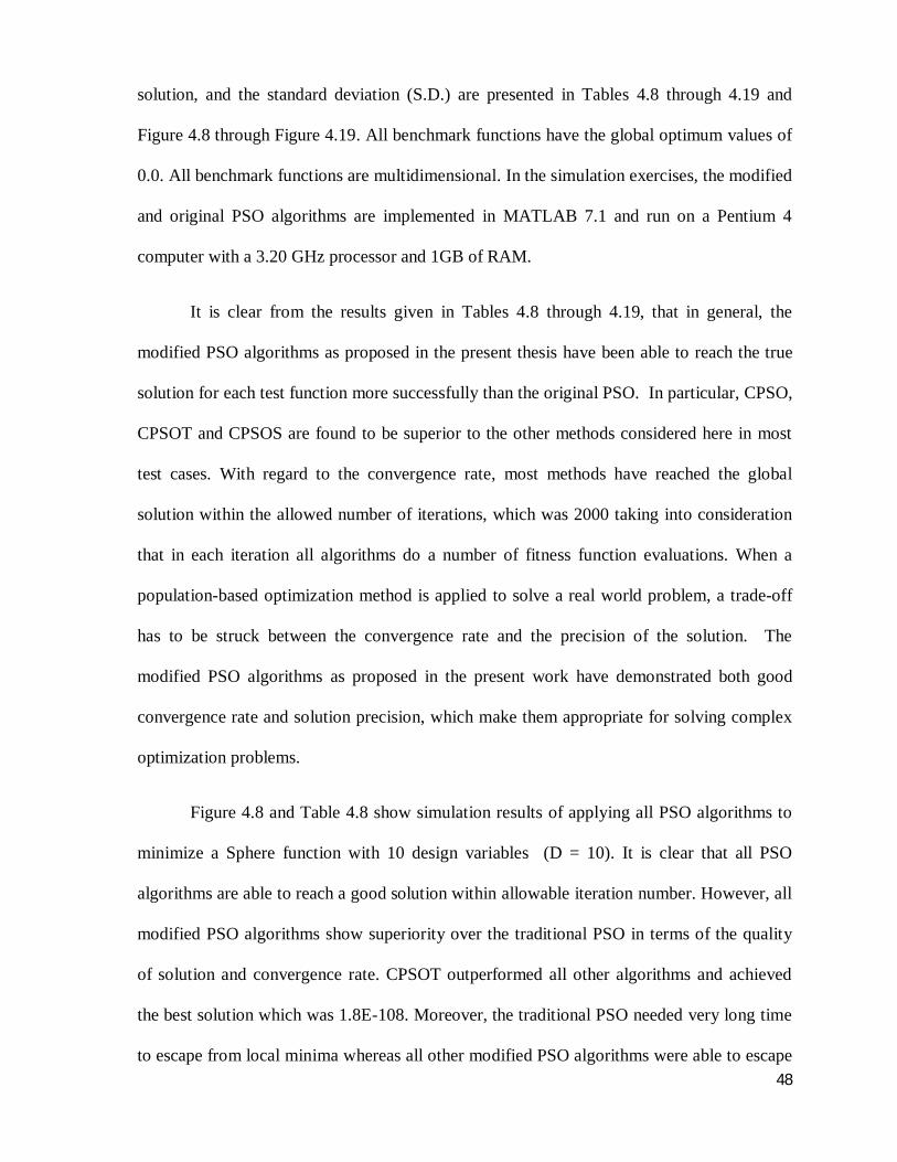
48
solution, and the standard deviation (S.D.) are presented in Tables 4.8 through 4.19 and
Figure 4.8 through Figure 4.19. All benchmark functions have the global optimum values of
0.0. All benchmark functions are multidimensional. In the simulation exercises, the modified
and original PSO algorithms are implemented in MATLAB 7.1 and run on a Pentium 4
computer with a 3.20 GHz processor and 1GB of RAM.
It is clear from the results given in Tables 4.8 through 4.19, that in general, the
modified PSO algorithms as proposed in the present thesis have been able to reach the true
solution for each test function more successfully than the original PSO. In particular, CPSO,
CPSOT and CPSOS are found to be superior to the other methods considered here in most
test cases. With regard to the convergence rate, most methods have reached the global
solution within the allowed number of iterations, which was 2000 taking into consideration
that in each iteration all algorithms do a number of fitness function evaluations. When a
population-based optimization method is applied to solve a real world problem, a trade-off
has to be struck between the convergence rate and the precision of the solution. The
modified PSO algorithms as proposed in the present work have demonstrated both good
convergence rate and solution precision, which make them appropriate for solving complex
optimization problems.
Figure 4.8 and Table 4.8 show simulation results of applying all PSO algorithms to
minimize a Sphere function with 10 design variables (D = 10). It is clear that all PSO
algorithms are able to reach a good solution within allowable iteration number. However, all
modified PSO algorithms show superiority over the traditional PSO in terms of the quality
of solution and convergence rate. CPSOT outperformed all other algorithms and achieved
the best solution which was 1.8E-108. Moreover, the traditional PSO needed very long time
to escape from local minima whereas all other modified PSO algorithms were able to escape
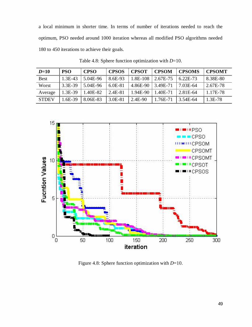
49
a local minimum in shorter time. In terms of number of iterations needed to reach the
optimum, PSO needed around 1000 iteration whereas all modified PSO algorithms needed
180 to 450 iterations to achieve their goals.
Table 4.8: Sphere function optimization with D=10.
D=10 PSO CPSO CPSOS CPSOT CPSOM CPSOMS CPSOMT Best 1.3E-43 5.04E-96 8.6E-93 1.8E-108 2.67E-75 6.22E-73 8.38E-80 Worst 3.3E-39 5.04E-96 6.0E-81 4.86E-90 3.49E-71 7.03E-64 2.67E-78 Average 1.3E-39 1.40E-82 2.4E-81 1.94E-90 1.40E-71 2.81E-64 1.17E-78 STDEV 1.6E-39 8.06E-83 3.0E-81 2.4E-90 1.76E-71 3.54E-64 1.3E-78
Figure 4.8: Sphere function optimization with D=10.
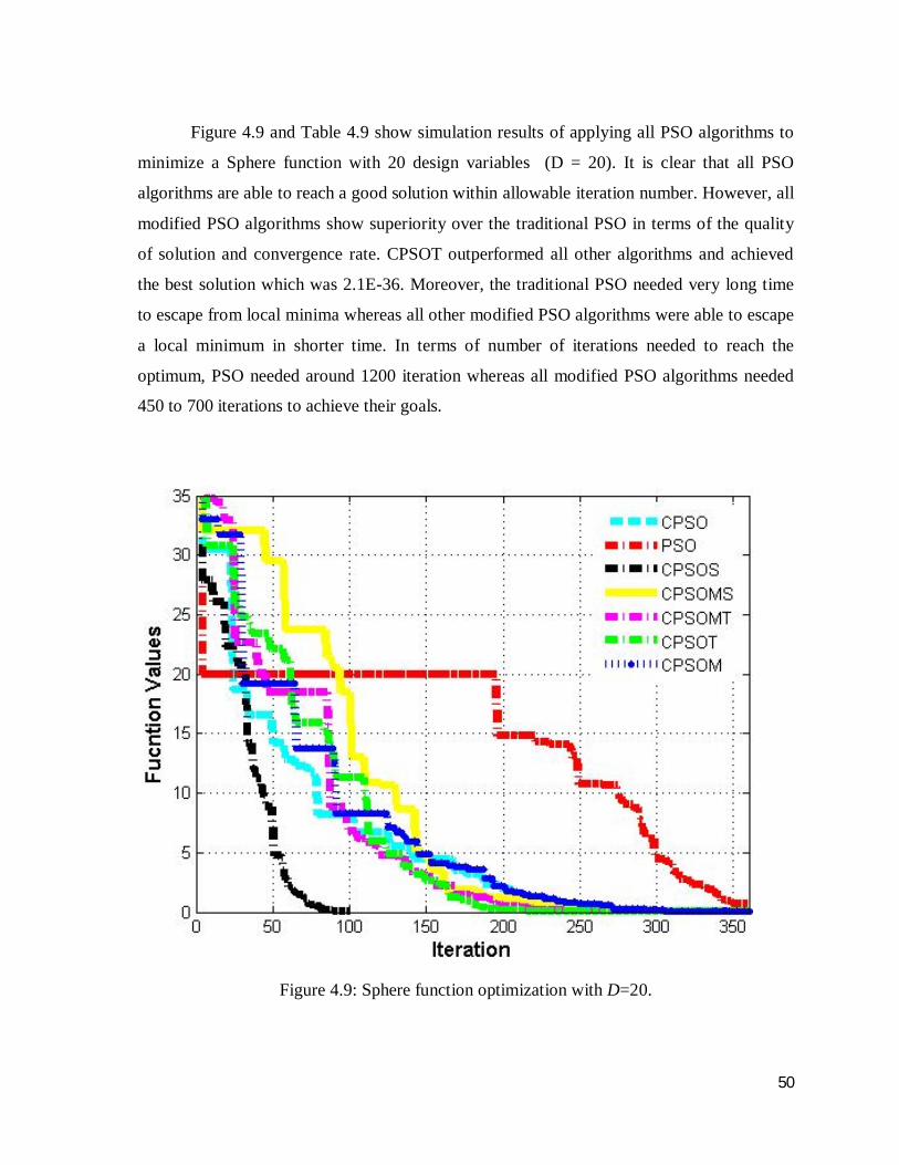
50
Figure 4.9 and Table 4.9 show simulation results of applying all PSO algorithms to
minimize a Sphere function with 20 design variables (D = 20). It is clear that all PSO
algorithms are able to reach a good solution within allowable iteration number. However, all
modified PSO algorithms show superiority over the traditional PSO in terms of the quality
of solution and convergence rate. CPSOT outperformed all other algorithms and achieved
the best solution which was 2.1E-36. Moreover, the traditional PSO needed very long time
to escape from local minima whereas all other modified PSO algorithms were able to escape
a local minimum in shorter time. In terms of number of iterations needed to reach the
optimum, PSO needed around 1200 iteration whereas all modified PSO algorithms needed
450 to 700 iterations to achieve their goals.
Figure 4.9: Sphere function optimization with D=20.
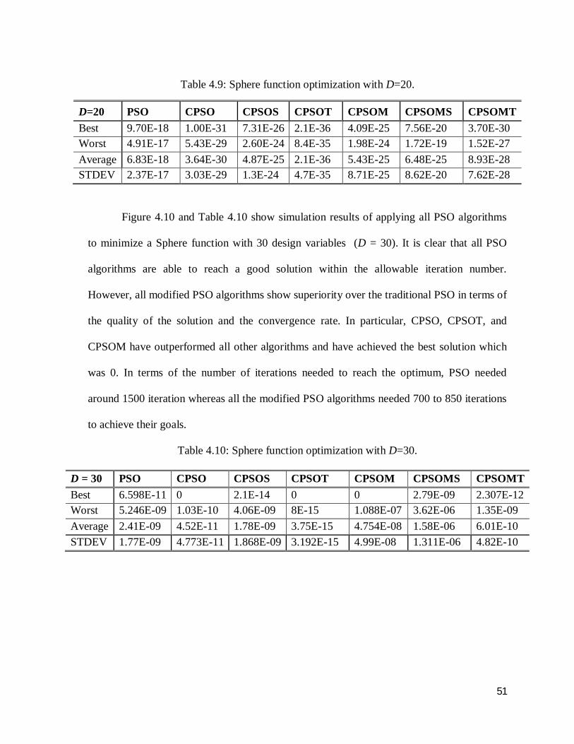
51
Table 4.9: Sphere function optimization with D=20.
D=20 PSO CPSO CPSOS CPSOT CPSOM CPSOMS CPSOMT Best 9.70E-18 1.00E-31 7.31E-26 2.1E-36 4.09E-25 7.56E-20 3.70E-30 Worst 4.91E-17 5.43E-29 2.60E-24 8.4E-35 1.98E-24 1.72E-19 1.52E-27 Average 6.83E-18 3.64E-30 4.87E-25 2.1E-36 5.43E-25 6.48E-25 8.93E-28 STDEV 2.37E-17 3.03E-29 1.3E-24 4.7E-35 8.71E-25 8.62E-20 7.62E-28
Figure 4.10 and Table 4.10 show simulation results of applying all PSO algorithms
to minimize a Sphere function with 30 design variables (D = 30). It is clear that all PSO
algorithms are able to reach a good solution within the allowable iteration number.
However, all modified PSO algorithms show superiority over the traditional PSO in terms of
the quality of the solution and the convergence rate. In particular, CPSO, CPSOT, and
CPSOM have outperformed all other algorithms and have achieved the best solution which
was 0. In terms of the number of iterations needed to reach the optimum, PSO needed
around 1500 iteration whereas all the modified PSO algorithms needed 700 to 850 iterations
to achieve their goals.
Table 4.10: Sphere function optimization with D=30.
D = 30 PSO CPSO CPSOS CPSOT CPSOM CPSOMS CPSOMT Best 6.598E-11 0 2.1E-14 0 0 2.79E-09 2.307E-12 Worst 5.246E-09 1.03E-10 4.06E-09 8E-15 1.088E-07 3.62E-06 1.35E-09 Average 2.41E-09 4.52E-11 1.78E-09 3.75E-15 4.754E-08 1.58E-06 6.01E-10 STDEV 1.77E-09 4.773E-11 1.868E-09 3.192E-15 4.99E-08 1.311E-06 4.82E-10

52
Figure 4.10: Sphere function optimization with D=30.
Figure 4.11 and Table 4.11 show simulation results of applying all PSO algorithms to
minimize a Griewank function with 10 design variables (D = 10). It is clear that all PSO
algorithms are able to reach a good solution within the allowable iteration number.
However, all modified PSO algorithms show superiority over the traditional PSO in terms of
the quality of solution and convergence rate. Specifically, CPSO, CPSOS, CPSOT, CPSOM
and CPSOMT have outperformed all other algorithms and achieved the average solution.
Moreover, the traditional PSO needed a very long time to escape from local minima whereas
all other modified PSO algorithms were able to escape a local minimum in a shorter time. In
terms of the number of iterations needed to reach the optimum, PSO needed around 1000
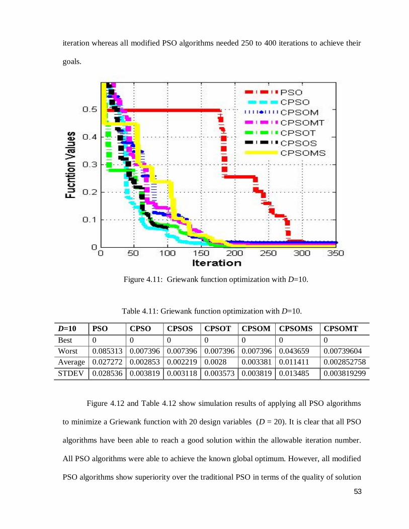
53
iteration whereas all modified PSO algorithms needed 250 to 400 iterations to achieve their
goals.
Figure 4.11: Griewank function optimization with D=10.
Table 4.11: Griewank function optimization with D=10.
D=10 PSO CPSO CPSOS CPSOT CPSOM CPSOMS CPSOMT Best 0 0 0 0 0 0 0 Worst 0.085313 0.007396 0.007396 0.007396 0.007396 0.043659 0.00739604 Average 0.027272 0.002853 0.002219 0.0028 0.003381 0.011411 0.002852758 STDEV 0.028536 0.003819 0.003118 0.003573 0.003819 0.013485 0.003819299
Figure 4.12 and Table 4.12 show simulation results of applying all PSO algorithms
to minimize a Griewank function with 20 design variables (D = 20). It is clear that all PSO
algorithms have been able to reach a good solution within the allowable iteration number.
All PSO algorithms were able to achieve the known global optimum. However, all modified
PSO algorithms show superiority over the traditional PSO in terms of the quality of solution

54
and the convergence rate. In particular, CPSO and CPSOM outperformed all other
algorithms and achieved the average solution. Moreover, the traditional PSO needed a very
long time to escape from local minima whereas all other modified PSO algorithms were able
to escape a local minimum in a shorter time. In terms of the number of iterations needed to
reach the optimum, PSO needed around 1200 iteration whereas all modified PSO algorithms
needed 550 to 620 iterations to achieve their goals.
Table 4.12: Griewank function optimization with D=20.
D=20 PSO CPSO CPSOS CPSOT CPSOM CPSOMS CPSOMT Best 0 0 0 0 0 0 0 Worst 0.009396 0.007396 0.007396 0.007396 0.007397 0.007405 0.007398195 Average 0.003415 0.001233 0.002193 0.00281 0.001233 0.002855 0.001849378 STDEV 0.004206 0.002465 0.003291 0.003609 0.002466 0.003638 0.003261846
Figure 4.12: Griewank function optimization with D=20.
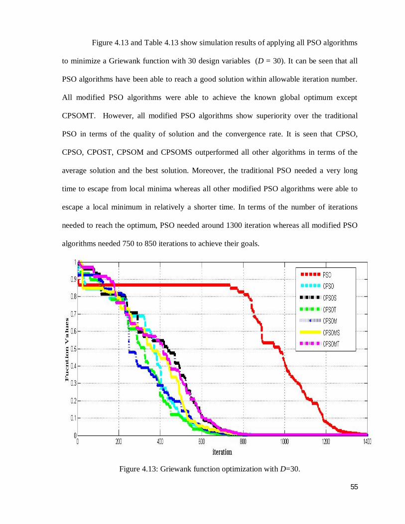
55
Figure 4.13 and Table 4.13 show simulation results of applying all PSO algorithms
to minimize a Griewank function with 30 design variables (D = 30). It can be seen that all
PSO algorithms have been able to reach a good solution within allowable iteration number.
All modified PSO algorithms were able to achieve the known global optimum except
CPSOMT. However, all modified PSO algorithms show superiority over the traditional
PSO in terms of the quality of solution and the convergence rate. It is seen that CPSO,
CPSO, CPOST, CPSOM and CPSOMS outperformed all other algorithms in terms of the
average solution and the best solution. Moreover, the traditional PSO needed a very long
time to escape from local minima whereas all other modified PSO algorithms were able to
escape a local minimum in relatively a shorter time. In terms of the number of iterations
needed to reach the optimum, PSO needed around 1300 iteration whereas all modified PSO
algorithms needed 750 to 850 iterations to achieve their goals.
Figure 4.13: Griewank function optimization with D=30.

56
Table 4.13: Griewank function optimization with D=30.
D=30 PSO CPSO CPSOS CPSOT CPSOM CPSOMS CPSOMT Best 1.06E-11 0 0 0 0 0 3E-15 Worst 0.007396 0.001396 0.002567 0.00604 0.008222 0.008026 0.007443829 Average 0.002602 0.000336 0.000903 0.001454 0.001979 0.004542 0.002686594 STDEV 0.003118 0.000589 0.001082 0.002547 0.0026 0.003957 0.003593766
Figure 4.14 and Table 4.14 show the simulation results of applying all PSO
algorithms to minimize a Rastrigrin function with 10 design variables (D = 10). Rastrigrin
function is one of the most difficult functions to be optimized as it has a large number of
local minima. It is seen that all PSO algorithms have been able to reach a good solution
within the allowable iteration number. In particular, CPSO, CPSOMS and CPSOMT
algorithms were able to achieve the known global optimum. However, all modified PSO
algorithms show superiority over the traditional PSO in terms of the quality of solution and
the convergence rate. In particular, CPSO, CPSOMS and CPSOMT outperformed all other
algorithms in terms of the average solution and the best solution. Moreover, the traditional
PSO needed a very long time to escape from local minima whereas all other modified PSO
algorithms were able to escape a local minimum in a relatively shorter time. In terms of the
number of iterations needed to reach the optimum, PSO needed around 1600 iteration
whereas all modified PSO algorithms needed 1100 to 1200 iterations to achieve their goals.
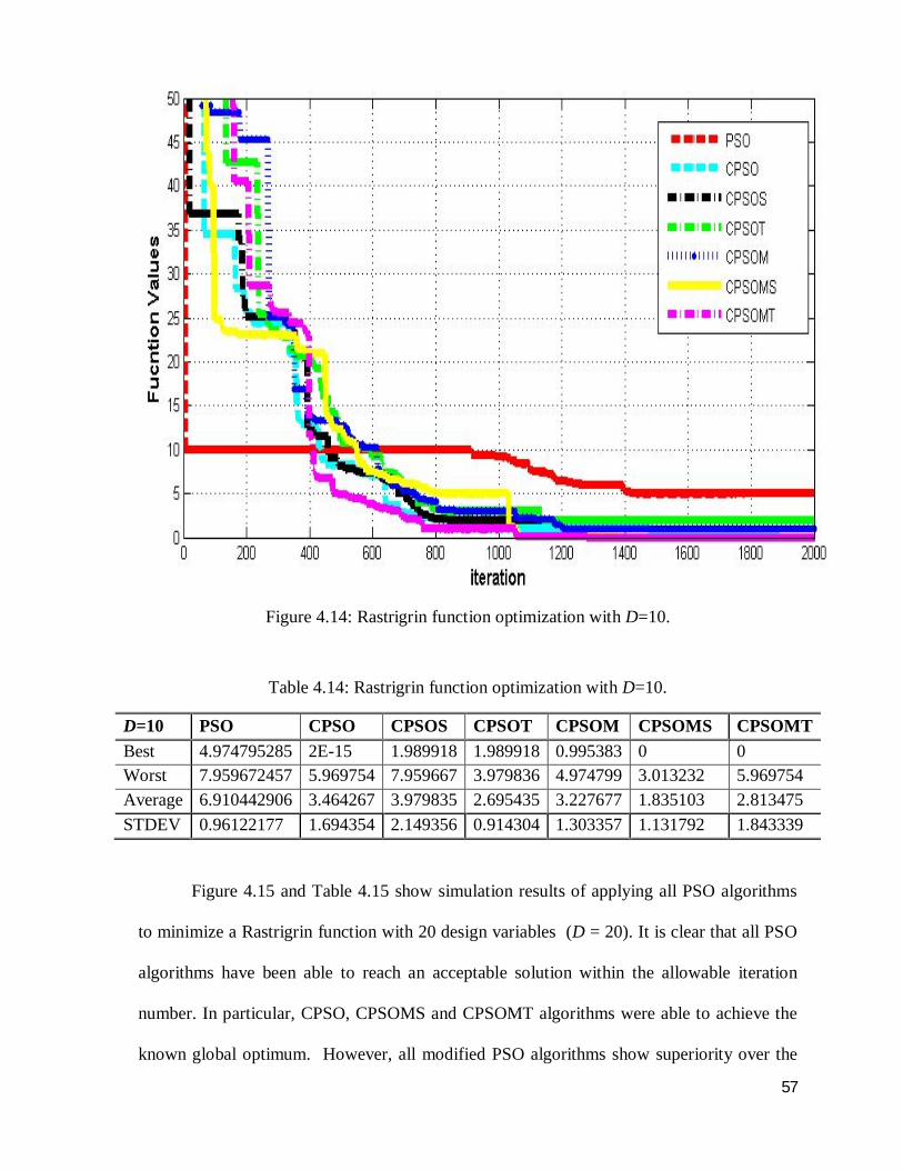
57
Figure 4.14: Rastrigrin function optimization with D=10.
Table 4.14: Rastrigrin function optimization with D=10.
D=10 PSO CPSO CPSOS CPSOT CPSOM CPSOMS CPSOMT Best 4.974795285 2E-15 1.989918 1.989918 0.995383 0 0 Worst 7.959672457 5.969754 7.959667 3.979836 4.974799 3.013232 5.969754 Average 6.910442906 3.464267 3.979835 2.695435 3.227677 1.835103 2.813475 STDEV 0.96122177 1.694354 2.149356 0.914304 1.303357 1.131792 1.843339
Figure 4.15 and Table 4.15 show simulation results of applying all PSO algorithms
to minimize a Rastrigrin function with 20 design variables (D = 20). It is clear that all PSO
algorithms have been able to reach an acceptable solution within the allowable iteration
number. In particular, CPSO, CPSOMS and CPSOMT algorithms were able to achieve the
known global optimum. However, all modified PSO algorithms show superiority over the
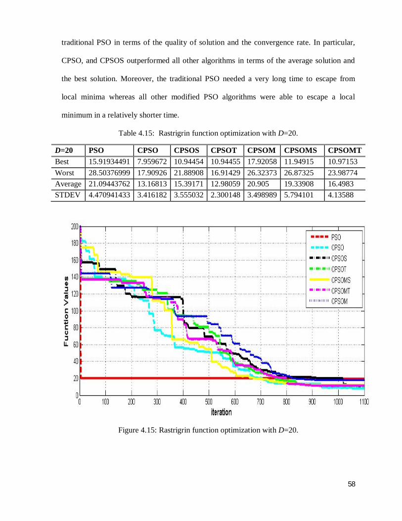
58
traditional PSO in terms of the quality of solution and the convergence rate. In particular,
CPSO, and CPSOS outperformed all other algorithms in terms of the average solution and
the best solution. Moreover, the traditional PSO needed a very long time to escape from
local minima whereas all other modified PSO algorithms were able to escape a local
minimum in a relatively shorter time.
Table 4.15: Rastrigrin function optimization with D=20.
D=20 PSO CPSO CPSOS CPSOT CPSOM CPSOMS CPSOMT Best 15.91934491 7.959672 10.94454 10.94455 17.92058 11.94915 10.97153 Worst 28.50376999 17.90926 21.88908 16.91429 26.32373 26.87325 23.98774 Average 21.09443762 13.16813 15.39171 12.98059 20.905 19.33908 16.4983 STDEV 4.470941433 3.416182 3.555032 2.300148 3.498989 5.794101 4.13588
Figure 4.15: Rastrigrin function optimization with D=20.

59
Figure 4.16 and Table 4.16 show simulation results of applying all PSO algorithms
to minimize a Rastrigrin function with 30 design variables (D = 30). It is seen that CPSO,
CPSOMS and CPSOMT algorithms have been able to achieve the known global optimum.
However, all modified PSO algorithms show superiority over the traditional PSO in terms of
the quality of solution and the convergence rate. In particular, CPSO outperformed all other
algorithms in terms of the average solution and the best solution. Moreover, the traditional
PSO needed a very long time to escape from local minima whereas all other modified PSO
algorithms were able to escape a local minimum in a relatively shorter time. In terms of the
number of iterations needed to reach the optimum, PSO needed around 1600 iteration
whereas all modified PSO algorithms needed 1100 to 1200 iterations to achieve their goals.
Figure 4.16: Rastrigrin function optimization with D=30.

60
Table 4.16: Rastrigrin function optimization with D=30.
D=30 PSO CPSO CPSOS CPSOT CPSOM CPSOMS CPSOMT Best 26.86389454 8.954632 17.90925 15.91934 18.17345 19.43948 13.17637 Worst 43.8588536 33.82858 36.81344 40.79325 40.78773 40.40168 36.20901 Average 33.65625578 22.70315 26.74327 24.27848 33.43253 33.38235 28.6357 STDEV 6.879109055 8.007193 6.137811 7.831487 6.222735 6.570589 6.494845
Figure 4.17 and Table 4.17 show simulation results of applying all PSO algorithms
to minimize a Rosenbrock function with 10 design variables (D = 10). Rosenbrock function
is one of the most difficult functions to be optimized as it has a large number of local
minima. It is clear that all PSO algorithms have been able to reach a good solution within
the allowable iteration number. In particular, CPSO and CPSOT were able to achieve the
known global optimum. However, all modified PSO algorithms show superiority over the
traditional PSO in terms of the quality of solution and the convergence rate. In particular,
CPSOT outperformed all other algorithms in terms of the average solution and the best
solution. Moreover, the traditional PSO needed a very long time to escape from local
minima whereas all other modified PSO algorithms were able to escape a local minimum in
a relatively shorter time. In terms of the number of iterations needed to reach the optimum,
PSO needed around 2000 iteration whereas all modified PSO algorithms needed 500 to 1000
iterations to achieve their goals.

61
Figure 4.17: Rosenbrock function optimization with D=10.
Table 4.17: Rosenbrock function optimization with D=10.
D=10 PSO CPSO CPSOS CPSOT CPSOM CPSOMS CPSOMT Best 0.090054 0.001282 0.001639 6.6E-06 0.090054 0.090054 0.020679 Worst 3.940706 1.840562 4.038685 2.451469 2.437366 3.327898 4.157364 Average 1.909339 0.955371 0.873332 0.50586 1.54684 1.584687 1.650556 STDEV 1.628303 0.742766 1.23413 0.868776 0.754985 1.227509 1.252528
Figure 4.18 and Table 4.18 show simulation results of applying all PSO algorithms
to minimize a Rosenbrock function with 20 design variables (D = 20). It is clear that all
PSO algorithms have been able to reach a good solution within the allowable iteration
number. CPSO, CPSOS and CPSOT algorithms were able to achieve the known global
optimum. However, all modified PSO algorithms show superiority over the traditional PSO
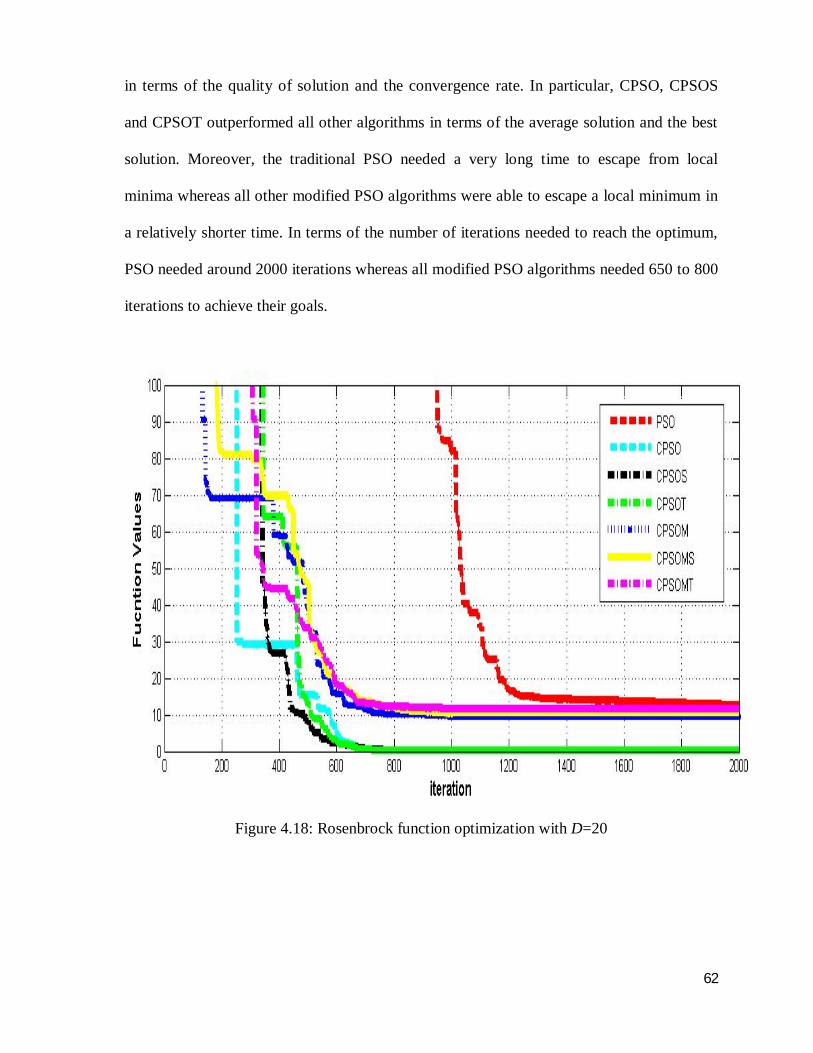
62
in terms of the quality of solution and the convergence rate. In particular, CPSO, CPSOS
and CPSOT outperformed all other algorithms in terms of the average solution and the best
solution. Moreover, the traditional PSO needed a very long time to escape from local
minima whereas all other modified PSO algorithms were able to escape a local minimum in
a relatively shorter time. In terms of the number of iterations needed to reach the optimum,
PSO needed around 2000 iterations whereas all modified PSO algorithms needed 650 to 800
iterations to achieve their goals.
Figure 4.18: Rosenbrock function optimization with D=20
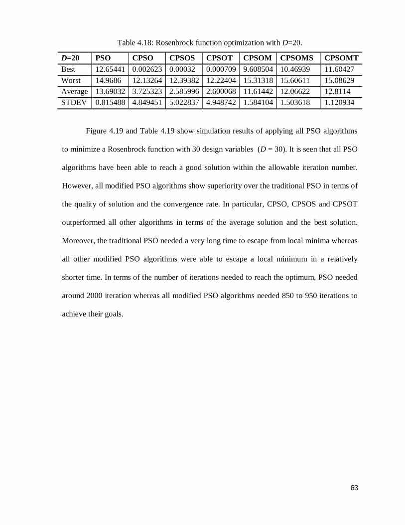
63
Table 4.18: Rosenbrock function optimization with D=20.
D=20 PSO CPSO CPSOS CPSOT CPSOM CPSOMS CPSOMT Best 12.65441 0.002623 0.00032 0.000709 9.608504 10.46939 11.60427 Worst 14.9686 12.13264 12.39382 12.22404 15.31318 15.60611 15.08629 Average 13.69032 3.725323 2.585996 2.600068 11.61442 12.06622 12.8114 STDEV 0.815488 4.849451 5.022837 4.948742 1.584104 1.503618 1.120934
Figure 4.19 and Table 4.19 show simulation results of applying all PSO algorithms
to minimize a Rosenbrock function with 30 design variables (D = 30). It is seen that all PSO
algorithms have been able to reach a good solution within the allowable iteration number.
However, all modified PSO algorithms show superiority over the traditional PSO in terms of
the quality of solution and the convergence rate. In particular, CPSO, CPSOS and CPSOT
outperformed all other algorithms in terms of the average solution and the best solution.
Moreover, the traditional PSO needed a very long time to escape from local minima whereas
all other modified PSO algorithms were able to escape a local minimum in a relatively
shorter time. In terms of the number of iterations needed to reach the optimum, PSO needed
around 2000 iteration whereas all modified PSO algorithms needed 850 to 950 iterations to
achieve their goals.

64
Figure 4.19: Rosenbrock function optimization with D=30.
Table 4.19: Rosenbrock function optimization with D=30.
D=30 PSO CPSO CPSOS CPSOT CPSOM CPSOMS CPSOMT Best 21.95872 0.131364 0.882529 0.24779 20.15327 20.32102 0.24779 Worst 25.52825 23.27029 24.16119 23.41681 24.96864 24.09354 25.01151 Average 23.49714 7.753474 8.680051 8.199372 22.68379 22.67154 9.550961 STDEV 1.26055 6.710197 6.399701 6.247195 1.652533 1.241008 7.182383
As it is easy to be figured out, the classical PSO is out performed by all modified PSO
algorithms suggested in this thesis. Because of velocity playing a crucial role in PSO’s
performance and the change in velocity in the classical PSO decreases especially when
particles reach a local optimum and makes particles not able to explore new area so that the
classical PSO reaches a stagnation period. Whereas in modified PSO Algorithms, this
problem has been avoided by incorporating chaos phenomena in PSO by introducing a

65
chaotic acceleration factor and modified inertia factor and velocity equation. By having such
modifications, population diversity is ensured and maintained through search process and
particles may travel over the whole search space.
In most cases, modified PSO algorithms without mutation factor generally performed better
than other modified PSO with mutation. The mutation factor should be reconsidered and
also velocity during mutation process.
4.6 Summary The PSO algorithm is known to have superior features compared with the traditional
optimization methods. The PSO algorithms use objective-function information to guide the
search in the problem space. Therefore, they can easily deal with non-differentiable and non-
convex objective functions. This property relieves PSO algorithms of numerous analytical
assumptions and approximations, which are often, required for traditional optimization
methods. The PSO algorithms use probabilistic rules for particle movements, not
deterministic rules. Hence, they are a type of stochastic optimization algorithm that can
search a complicated and uncertain area. This feature makes the PSO algorithms more
flexible and robust than the conventional methods. However, improving the convergence of
the PSO algorithm is an important objective when solving complex real-world problems. In
this chapter, novel modifications were incorporated into the original PSO method, in
different formats, to improve its convergence performance. The performance of the
proposed PSO methods were studied and compared with the original PSO method by using a
suite of four well-known test functions. All modified PSO methods proposed in this chapter
showed superior performance over the original PSO in terms of the quality of solution and
the convergence rate.

66
Chapter 5
Application of Modified PSO Algorithms to
Solve Constrained Nonlinear Engineering
Problems4
5.1 Introduction Constraint handling is a challenging problem in numerous applications such as
engineering design, finance, mathematics, economics, and structural engineering. A general
constrained optimization problem may be defined as:
Minimize 푓(풙), 풙 = (푥 ,푥 , … … … … , 푥 )
Subject to
푔 (푥) ≤ 0, 푖 = 1, … . ,푚
푥 ≤ 푥 ≤ 푥
where )(xf is the objective function, and x is the column vector of n independent variables.
푔 (푥) ≤ 0 are inequality constraints and 푥 ≤ 푥 ≤ 푥 are bounds on the optimization
4 Alrasheed, M.R. ,de Silva, C.W. and Gadala, M.S., " Application of PSO with Novel Chaotic Acceleration, Chaotic Inertia factors and Best Global Mutation Algorithms to solve Constrained Nonlinear Engineering Problems”, (Submitted)
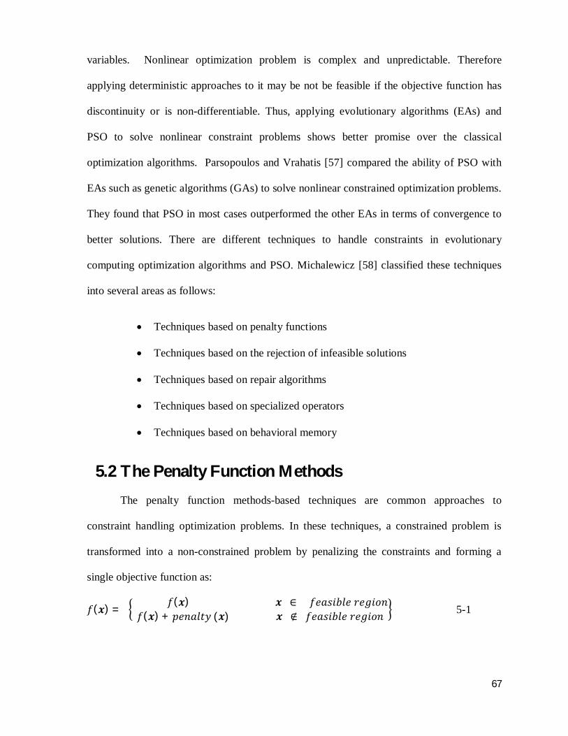
67
variables. Nonlinear optimization problem is complex and unpredictable. Therefore
applying deterministic approaches to it may be not be feasible if the objective function has
discontinuity or is non-differentiable. Thus, applying evolutionary algorithms (EAs) and
PSO to solve nonlinear constraint problems shows better promise over the classical
optimization algorithms. Parsopoulos and Vrahatis [57] compared the ability of PSO with
EAs such as genetic algorithms (GAs) to solve nonlinear constrained optimization problems.
They found that PSO in most cases outperformed the other EAs in terms of convergence to
better solutions. There are different techniques to handle constraints in evolutionary
computing optimization algorithms and PSO. Michalewicz [58] classified these techniques
into several areas as follows:
Techniques based on penalty functions
Techniques based on the rejection of infeasible solutions
Techniques based on repair algorithms
Techniques based on specialized operators
Techniques based on behavioral memory
5.2 The Penalty Function Methods The penalty function methods-based techniques are common approaches to
constraint handling optimization problems. In these techniques, a constrained problem is
transformed into a non-constrained problem by penalizing the constraints and forming a
single objective function as:
푓(풙) = 푓(풙) 풙 ∈ 푓푒푎푠푖푏푙푒 푟푒푔푖표푛푓(풙) + 푝푒푛푎푙푡푦 (풙) 풙 ∉ 푓푒푎푠푖푏푙푒 푟푒푔푖표푛 5-1

68
where 푝푒푛푎푙푡푦 (푥) is zero if no constraint is violated and is positive otherwise. The
feasible region is where 푥 satisfies all constraints and the unfeasible region is where at least
one of constraints has been violated.
푓(풙) = 푓(풙) + 푝푒푛푎푙푡푦 (풙) 5-2
The penalty functions are classified into two main types according the penalty values. If the
fixed penalty values have to be used, then the penalty function is called a stationary penalty
function. In contrast, if the penalty values are adjusted dynamically, then the penalty
function is called a non-stationary penalty function [57].
If the penalty values are high, the optimization algorithms usually get trapped in
local minima. However, if the penalty values are low, this may lead to slow and difficult
convergence in optimization algorithms. Non-stationary penalty functions generally show
superiority over the stationary penalty functions [57]. Consequently, the penalty function
methods require a fine tuning of both the penalty functions and the penalty values to avoid
premature convergence. In this chapter a non-stationary, multi-stage penalty method (PFM)
for constraint handling with PSO and modified PSO algorithms are implemented to solve
two engineering problems.
Non-stationary, Multi-stage Penalty Method (PFM):
The non-stationary, multi-stage penalty method (PFM) for constraint handling was first
introduced by Parsopoulos and Vrahatis in [57, 59]. The 푝푒푛푎푙푡푦 (푥) is the product of a
penalty value ℎ(푡) and a penalty factor 퐺(푥). So, the 푝푒푛푎푙푡푦 (푥) can be written as:
푝푒푛푎푙푡푦 (푥) = ℎ(푡) ∗ 퐺(푥) 5-3
where ℎ(푡) is a dynamically modified penalty value, t is the current iteration, and 퐺(푥) is a
penalty factor. So, an objective function may be defined as:
푓(푥) = 푓(푥) + ℎ(푡) ∗ 퐺(푥) 5-4

69
퐺(푥) , a penalty factor, is defined as follows:
퐺(푥) = ∑ 휃( 푞 (푥) ) ∗ 푞 (푥) ( ( )) 5-5
where
푞 (푥) = 푚푎푥 {0 ,푔 (푥)} , 푖 = 1, …푚 . And 푔 (푥) are the constraints.
So, 푞 (푥) is a violated function of the constraints
휃( 푞 (푥) ) is an assignment function
휓(푞 (푥)) is the power of the penalty function
For the problems that are optimized in this chapter, a violation tolerance is used for
constraints. Therefore, a constraint 푔 (푥) is considered to be violated if 푔 (푥) > 10 .
The following values (reported in Yang et al.[60] ) are used for the penalty function:
If 푞 (푥) < 1, then 휃( 푞 (푥) ) = 10, else if 휓 푞 (푥) = 2;
If 푞 (푥) < 0.001, then 휓 푞 (푥) = 1,
else if 푞 (푥) < 0.1, then 휃( 푞 (푥) ) = 20,
else if 푞 (푥) ≤ 1, then 휃( 푞 (푥) ) = 100,
otherwise 휃( 푞 (푥) ) = 100;
The penalty value ℎ(푡) is set to ℎ(푡) = 푡 ∗ √푡
5.3 Test Problems A non-stationary, multi-stage penalty function method (PFM) for constraint handling
with the original PSO and the proposed modified CPSO, CPOS, CPSOT, and CPSOM,
CPSOMS and CPSOMT methods are applied to two engineering problems with constraints:
Pressure vessel design optimization and Weld beam optimization. Both problems are tested

70
in 30 dimensions. For each problem, 50 trials5 are carried out. The resulting average
solution, best solution, worst solution, and the standard deviation (S.D.) are presented in
Tables 5.1 and Table 5.3. In the simulation, the modified and the original PSO algorithms
are implemented in MATLAB 7.1 and run on a Pentium 4 computer with a 3.20 GHz
processor and 1GB of RAM.
5.3.1 Pressure Vessel Optimization
Pressure vessel (see Figure 5-1) design is an important structural engineering
optimization problem. The objective is typically to find the lowest cost including the cost of
material, forming and welding. The problem involves discontinuous and non-differentiable
problems, so we have to consider stochastic optimization algorithms. Here we specifically
apply the PSO and Modified PSO algorithms. The objective of the problem of the pressure
vessel design is to minimize the total cost, including the cost of material, forming and
welding. There are four design variables: 푇 (thickness of the shell, 푥 ), 푇 (thickness of the
head, 푥 ), R (inner radius, 푥 ) and L (length of the cylindrical section of the vessel, not
including the head, 푥 ).
5 Results of all trials for Vessel design optimization and Weld beam optimization are listed on Appendix D, and E respectively
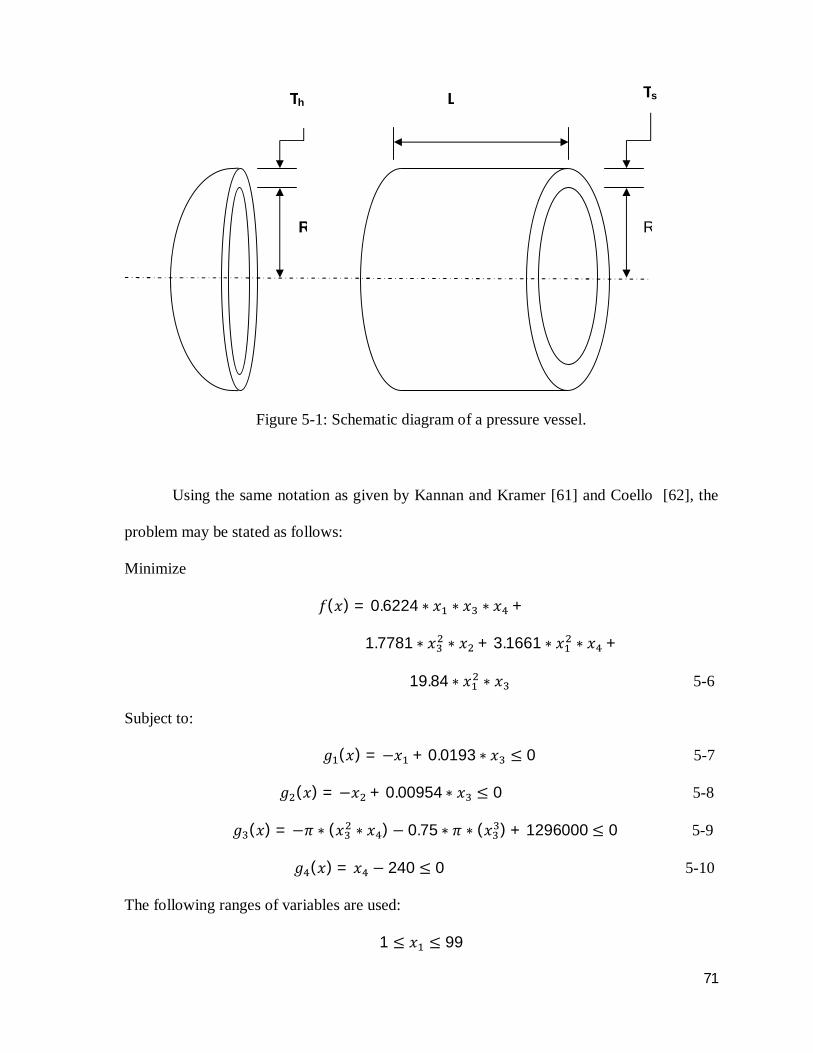
71
Figure 5-1: Schematic diagram of a pressure vessel.
Using the same notation as given by Kannan and Kramer [61] and Coello [62], the
problem may be stated as follows:
Minimize
푓(푥) = 0.6224 ∗ 푥 ∗ 푥 ∗ 푥 +
1.7781 ∗ 푥 ∗ 푥 + 3.1661 ∗ 푥 ∗ 푥 +
19.84 ∗ 푥 ∗ 푥 5-6
Subject to:
푔 (푥) = −푥 + 0.0193 ∗ 푥 ≤ 0 5-7
푔 (푥) = −푥 + 0.00954 ∗ 푥 ≤ 0 5-8
푔 (푥) = −휋 ∗ (푥 ∗ 푥 )− 0.75 ∗ 휋 ∗ (푥 ) + 1296000 ≤ 0 5-9
푔 (푥) = 푥 − 240 ≤ 0 5-10
The following ranges of variables are used:
1 ≤ 푥 ≤ 99
Th
R
L
R
Ts

72
1 ≤ 푥 ≤ 99
10 ≤ 푥 ≤ 200
Table 5.1 shows the simulations results of the PSO and suggested modified PSO algorithms
when they were applied to solve the pressure vessel design problem.
Table 5.1: Results of pressure vessel optimization with PSO and modified PSO.
PSO CPSO CPSOS CPSOT CPSOM CPSOMS CPSOMT
Best 8796.867 5835.759 5829.556 5864.28 5831.785 5878.712 5862.23
Worst 10176.55 7190.018 6376.388 6388.048 6399.267 6470.638 7209.17
Average 9075.586 6050.966 6044.642 6038.196 6087.259 6138.296 6121.879
S.D 315.3599 246.6402 132.3832 120.0518 128.0795 134.7369 217.2764
Some observations may be made from the results given in Table 5.1:
All modified PSO algorithms have converged to a solution much better than the
one achieved by the PSO algorithm and there are no big differences in the
solutions that were achieved by the modified PSO algorithms as proposed in the
present work.
CPSOS has outperformed all modified PSO algorithms in terms of achieving the
optimum result of 5829.5.
CPSOT has converged to the best average solution of 6038.19 among all the
algorithms
The pressure vessel design problem has been studied by many researchers. To make
a comparison between the modified PSO algorithms proposed in the present work and
other classical and evolutionary algorithms, the following results are selected from the
literature:
1. Deb and Gene [63] used Genetic Adaptive Search
2. Kannan and Kramer [61] used an augmented Lagrangian Multiplier approach

73
3. Coello [64] employed Genetic Algorithm (GA)
4. Parsopoulos and Varahatis [59] used a modified particle swarm approach, a unified
PSO algorithm.
A table of comparison is given below.
Table 5.2: Comparison of results for pressure vessel optimization.
Best Solution PSO 8796.867 CPSO 5835.759 CPSOS 5829.556 CPSOT 5864.28 CPSOM 5831.785 CPSOMS 5878.712 CPSOMT 5862.23 Deb 6410.3811 Kannan 7198.0428 Coello 6069.3267 Parsopoulos 6154.7
As indicated in the table, the modified PSO algorithms have generated better results over the
other methods, and the lowest cost is obtained by CPSOS, as 5829.556
5.3.2 Welded Beam Optimization
Now a welded beam is designed for minimum cost of weld subject to constraints on
shear stress(τ), bending stress in the beam (σ), buckling load on the bar (푃 ), end deflection
of the beam (δ), and side constraints. There are four design variables as shown in Figure 5.2:
ℎ (푥 ), 푙 (푥 ), 푡 (푥 ), 푏 (푥 ).
Using the same notation as given by Rao [65] , the problem is stated as follows:
푓(푥) = 1.10471 ∗ 푥 ∗ 푥 + 0.0481 ∗ 푥 ∗ 푥 ∗ (14.0 + 푥 ) 5-11
Subject to:
푔 (푥) = 휏(푥)− 휏 ≤ 0 5-12

74
푔 (푥) = 휎(푥)− 휎 ≤ 0 5-13
Figure 5-2: Schematic diagram of a welded beam.
푔 (푥) = 0.010471 ∗ 푥 + 0.0481 ∗ 푥 ∗ 푥 ∗ (14.0 + 푥 )− 5.0 ≤ 0 5-14
푔 (푥) = −푥 + 0.125 ≤ 0 5-15
푔 (푥) = 푥 − 푥 ≤ 0 5-16
푔 (푥) = 훿(푥)− 훿 ≤ 0 5-17
푔 (푥) = 푃 − 푃 (푥) ≤ 0 5-18
Where
휏(푥) = (휏 ′ ) + 2휏 ′휏 ′′ + (휏 ′′) 5-19
휏 ′ =√ ∗
5-20
휏 ′′ = ∗ 5-21
푀 = 푃 ∗ (퐿 + ) 5-22
푅 = + 5-23
h
b
l L
t
P
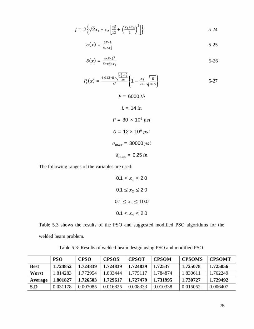
75
퐽 = 2 √2푥 ∗ 푥 + 5-24
휎(푥) = ∗∗
5-25
훿(푥) = ∗ ∗∗ ∗
5-26
푃 (푥) =. ∗ ∗
∗
1−∗ ∗
5-27
푃 = 6000 퐼푏
퐿 = 14 푖푛
푃 = 30 × 10 푝푠푖
퐺 = 12 × 10 푝푠푖
휎 = 30000 푝푠푖
훿 = 0.25 푖푛
The following ranges of the variables are used:
0.1 ≤ 푥 ≤ 2.0
0.1 ≤ 푥 ≤ 2.0
0.1 ≤ 푥 ≤ 10.0
0.1 ≤ 푥 ≤ 2.0
Table 5.3 shows the results of the PSO and suggested modified PSO algorithms for the
welded beam problem.
Table 5.3: Results of welded beam design using PSO and modified PSO.
PSO CPSO CPSOS CPSOT CPSOM CPSOMS CPSOMT Best 1.724852 1.724839 1.724839 1.724839 1.72537 1.725078 1.725056 Worst 1.814283 1.772954 1.833444 1.775117 1.784874 1.830611 1.762249 Average 1.801827 1.726503 1.729617 1.727479 1.731995 1.730727 1.729492 S.D 0.031178 0.007085 0.016825 0.008333 0.010338 0.015052 0.006407

76
Some observations may be made from the results given in Table 5.3:
All modified PSO algorithms have converged to a solution much better than the one
achieved by the conventional PSO algorithm, and there are no big differences of the
solutions that were achieved by the modified PSO algorithms.
CPSO, CPSOS, and CPSOT outperformed the other modified PSO algorithms in
terms of achieving the optimum result of 1.724839.
CPSO was able to converge to the best average solution of 1.726503 among all the
algorithms.
The weld beam problem has been studied by many researchers. The following work is
selected for comparison:
1. Deb [66] used Genetic algorithm to solve the problem;
2. Ragsdell and Phillips [66] used geometric programming
3. Parsopoulos and Varahatis [59] use a modified particle swarm technique, a unified
PSO algorithm.
As seen from Table 5.4, the modified PSO algorithms have achieved better results than from
other methods. The lowest cost, as obtained by CPSO, CPSOS, CPSOT is 1.72839.
Table 5.4: Comparison of the results for the weld beam design.
Best Solution PSO 1.724852 CPSO 1.724839 CPSOS 1.724839 CPSOT 1.724839 CPSOMT 1.72537 CPSOMS 1.725078 CPSOMT 1.725056 Deb 2.4331160 Ragsdell 2.38593732 Parsopoulos 1.7558
77
5.4 Summary In the present chapter, the optimization performance of the modified PSO
algorithms, as proposed in the proposed thesis, in solving constraints engineering problems
was investigated, by applying these algorithms for optimal design of a pressure vessel and a
welded beam. The modified PSO algorithms have been able to generate better solutions, in
comparison to the regular PSO and other approaches found in the literature, for both design
problems. It may be concluded that the proposed modifications to PSO show potential for
solving more complicated and real life engineering problems and in finding the global
optimum with fewer iterations.

78
Chapter 6
Heat Sink Design by Using Modified PSO6
6.1 Introduction The recent trend in the electronic device industry is toward denser and larger heat flux
densities. As a result, more powerful products require higher thermal performance through
efficient cooling. For example, some 900 million computers are in use in the world today,
with personal computers comprising approximately half the total. This growth is reasonable
in view of the projections taking into account that some 400 million computers were in use
by the end of 2001 [67]. These rapid advances in computer systems and other digital
hardware have led to the associated increase in the thermal dissipation from microelectronic
devices. This trend has fueled the interest of the engineers and researchers in controlling the
maximum operating temperature, and achieving long term reliability and efficient
performance of electronic components.
In electronic equipment, the temperature of each component must be maintained
within an allowable upper limit, specified for each component from the viewpoint of
operating performance and reliability. The power density in electronic systems is growing
due to the high speeds of operation that are attained and the miniaturization of the associated
components and devices. Generally, heat sinks are used to maintain the operating
temperature for reliable operation of the electronic device. Choosing a suitable heat sink has
become crucial to the overall performance of electronic packages. The forced-air cooling
6 Alrasheed, M.R. , de Silva, C.W., and Gadala, M.S., " Applying Modified Particle Swarm Optimization in Heat Sink Design by using Chaotic Acceleration and Global Mutation," (Submitted).

79
technique, which is one of the effective methods for thermal management of electronic
equipment cooling, is commonly used in the electronic cooling area [68]. The development
of a systematic and rather optimal design methodology for air-cooling heat sinks is
undoubtedly very important in satisfying the current thermal necessities and for successful
heat removal in the future generations of critical electronic components [69].
The performance of forced air convection heat sinks in electronic devices depends on
a number of parameters including the thermal resistance, dimensions of the cooling
channels, location and concentration of the heat sources, and the airflow bypass due to flow
resistance through the channel. In general, an important goal of the heat sink design is to
reduce the overall thermal resistance [70]. An alternative and related criterion for designing
a heat sink is to maximize the thermal efficiency. Both criteria would affect the maximum
heat dissipation. In a practical industrial design, different criteria are chosen depending on
whether the primary objective is to maximize the heat transfer, minimize the pumping
power, or achieve the minimum device volume or weight under the prescribed constraints
such as component size and heat transfer time [71].
6.2 Entropy Generation Minimization of a Heat Sink The idea of using the entropy generation rate to estimate the heat transfer
enhancement was first proposed by Bejan [72] as a performance assessment criterion for
thermal systems. A fin can generate the entropy associated with the external flow and
because the fin is non-isothermal it can also generate entropy internally. The entropy
generation rate that is associated with the heat transfer in a heat sink can serve as the
capability of transferring heat to the surrounding cooling medium. As in all thermodynamic
systems, the entropy in a heat sink is generated from the irreversibility of heat transfer with

80
finite temperature differences and the friction of fluid flow. The basic thermodynamic
equations for the stream channel as an open system in steady flow are:
푚̇ = 푚̇ = 푚̇ 6-1
푚̇ ℎ + ∬푞′′ 푑퐴 − 푚̇ ℎ 6-2
푆̇ = 푚̇ 푠 − 푚̇ 푠 −∬′′
6-3
The canonical form 푑ℎ = 푇 푑푠 + 1 휌 푑푃 may be written as:
ℎ − ℎ = 푇 (푠 − 푠 ) + 1 휌 (푃 − 푃 ) 6-4
where it is assumed that the temperature and density do not change significantly between the
inlet and the outlet. Combining equations (6-2) through (6-4), the entropy generation rate
can be written in this form:
푆̇ = ∬ 푞′′ − 푑퐴 − ̇ (푃 − 푃 ) 6-5
Knowing that:
푚̇ = 퐴 휌 푉 6-6
퐹 = 퐴(푃 − 푃 ) 6-7
We obtain:
푆̇ = ∬ 푞′′ (푇 − 푇 )푑퐴 − 퐹 푉 6-8
where Fd is the drag force.

81
Equation (6-8) represents the entropy generation rate associated with the fin heat
transfer in external flow. As shown in Figure 6.1, a fin also generates entropy internally
since the fin is nonisothermal:
푆̇ = ∬ 푞′′ 푑퐴 − 6-9
where wT and Tb represent the local temperature and the base temperature, respectively, and
Q is the heat dissipation rate of the heat sink.
Adding equations (6-8) and (6-9) the entropy generation rate for a single fine can be
written as:
푆̇ = Δ + 6-10
A uniform stream with velocity Vf and the absolute temperature Te passes through the fin as
shown in Figure 6.1. Fluid friction appears in the form of the drag force Fd along the
direction of Vf. Equation (6-10) shows that fluid friction and inadequate thermal
conductivity jointly contribute to degrading of the thermodynamic performance of the fin.
Thus, the optimal thermodynamic size of the fin can be computed by minimizing the entropy
generation rate given by equation (6-10) subjected to necessary design constraints.

82
Figure 6.1: Schematic diagram of a general fin in convective heat transfer.
The heat transfer rate between the fin and the stream is q and theoretically a heat sink is
required to satisfy an equation of the form
∬푞′′푑퐴 ≅푄 6-11
For a heat sink set, the temperature excess of ∆푇 is related to the overall heat sink thermal
resistance as
Δ푇 = 푄.푅 6-12
where Q is the heat dissipation rate of the heat sink and R is the overall heat sink thermal
resistance. The first term of the entropy generation in (6-10) can be written as (Q ∆푇 / Te2).
The temperature difference (∆푇) is represented as (Tb - Te). So, the entropy change rate of a
heat sink set can be written as
푆̇ = + 6-13
Tb
q
fV
eT
Q
Tw
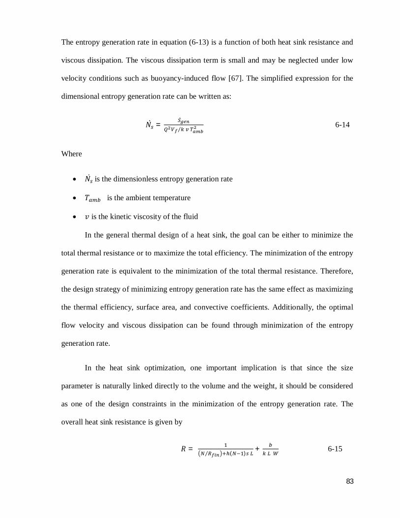
83
The entropy generation rate in equation (6-13) is a function of both heat sink resistance and
viscous dissipation. The viscous dissipation term is small and may be neglected under low
velocity conditions such as buoyancy-induced flow [67]. The simplified expression for the
dimensional entropy generation rate can be written as:
푁̇ =̇
⁄ 6-14
Where
푁̇ is the dimensionless entropy generation rate
푇 is the ambient temperature
푣 is the kinetic viscosity of the fluid
In the general thermal design of a heat sink, the goal can be either to minimize the
total thermal resistance or to maximize the total efficiency. The minimization of the entropy
generation rate is equivalent to the minimization of the total thermal resistance. Therefore,
the design strategy of minimizing entropy generation rate has the same effect as maximizing
the thermal efficiency, surface area, and convective coefficients. Additionally, the optimal
flow velocity and viscous dissipation can be found through minimization of the entropy
generation rate.
In the heat sink optimization, one important implication is that since the size
parameter is naturally linked directly to the volume and the weight, it should be considered
as one of the design constraints in the minimization of the entropy generation rate. The
overall heat sink resistance is given by
푅 = ⁄ ( )
+
6-15

84
where N is the number of fins and Rfin is the thermal resistance of a single fin given by:
푅 = ( ) ( )
6-16
with
푚 =
6-17
Also P is the perimeter of the fin and Ac is the cross-sectional area of the fin. The total drag
force on the heat sink may be obtained by considering a force balance on the heat sink.
Specifically,
( ⁄ )
= 푓 푁 (2 푎 퐿 + 푠 퐿) + 퐾 (푎 푊) + 퐾 (푎 푊) 6-18
where fapp is the apparent friction factor for hydrodynamically developing flow. The channel
velocity Vch is related to the free stream velocity by
푉 = 푉 ( 1 + ) 6-19
The apparent friction factor fapp for a rectangular channel may be computed using a form of
the model developed by Muzychka [73] for developing laminar flow:
푓 푅푒 = .√ ∗ + 푓 푅푒
. 6-20
where
퐿∗ =
6-21
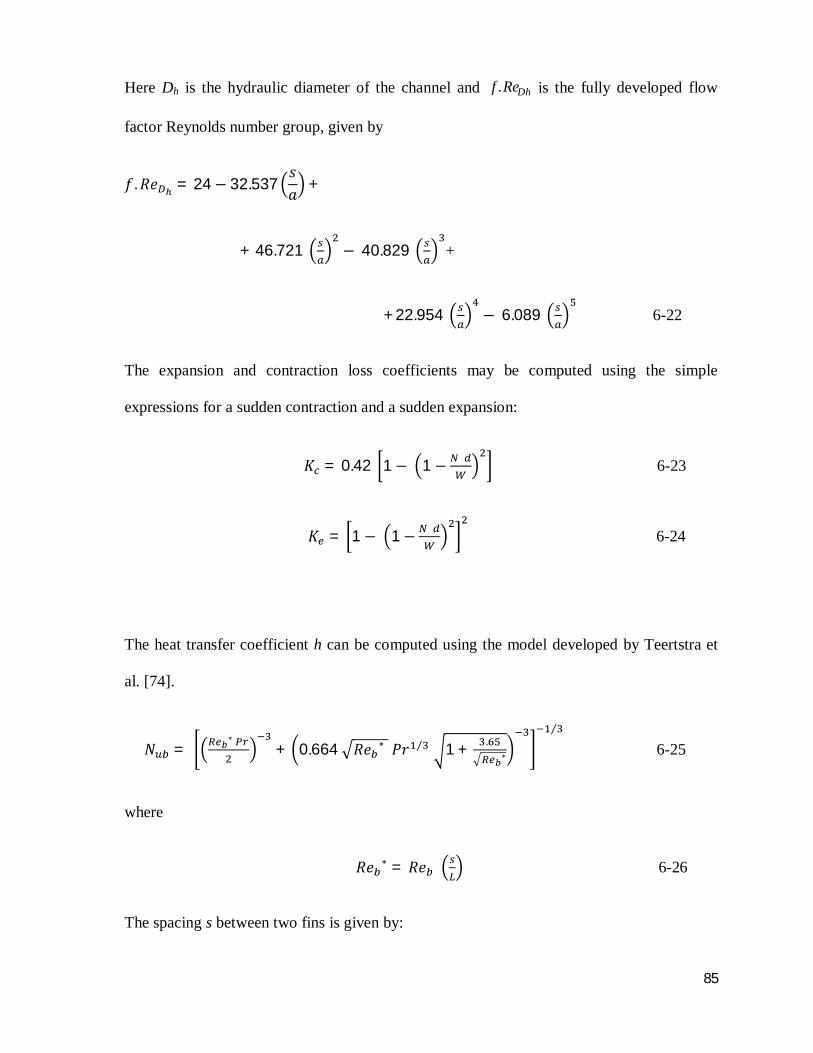
85
Here Dh is the hydraulic diameter of the channel and DhRe.f is the fully developed flow
factor Reynolds number group, given by
푓.푅푒 = 24 − 32.537푠푎 +
+ 46.721 − 40.829 +
+22.954 − 6.089 6-22
The expansion and contraction loss coefficients may be computed using the simple
expressions for a sudden contraction and a sudden expansion:
퐾 = 0.42 1 − 1 − 6-23
퐾 = 1 − 1− 6-24
The heat transfer coefficient h can be computed using the model developed by Teertstra et
al. [74].
푁 = ∗ + 0.664 푅푒 ∗ 푃푟 ⁄ 1 + .
∗
⁄
6-25
where
푅푒 ∗ = 푅푒 6-26
The spacing s between two fins is given by:

86
푠 = − 푑 6-27
푁 = 6-28
Figure 6.2: Geometrical configuration of a plate-fin sink.
Configuration data are as follows:
Both the base length L and the width W are 50 mm.
The total heat dissipation of 30 W is uniformly applied over the base plate of the heat
sink with a base thickness b of 2 mm.
The thermal conductivity of the heat sink k is 200 W/m.K.
L
a s
W
d
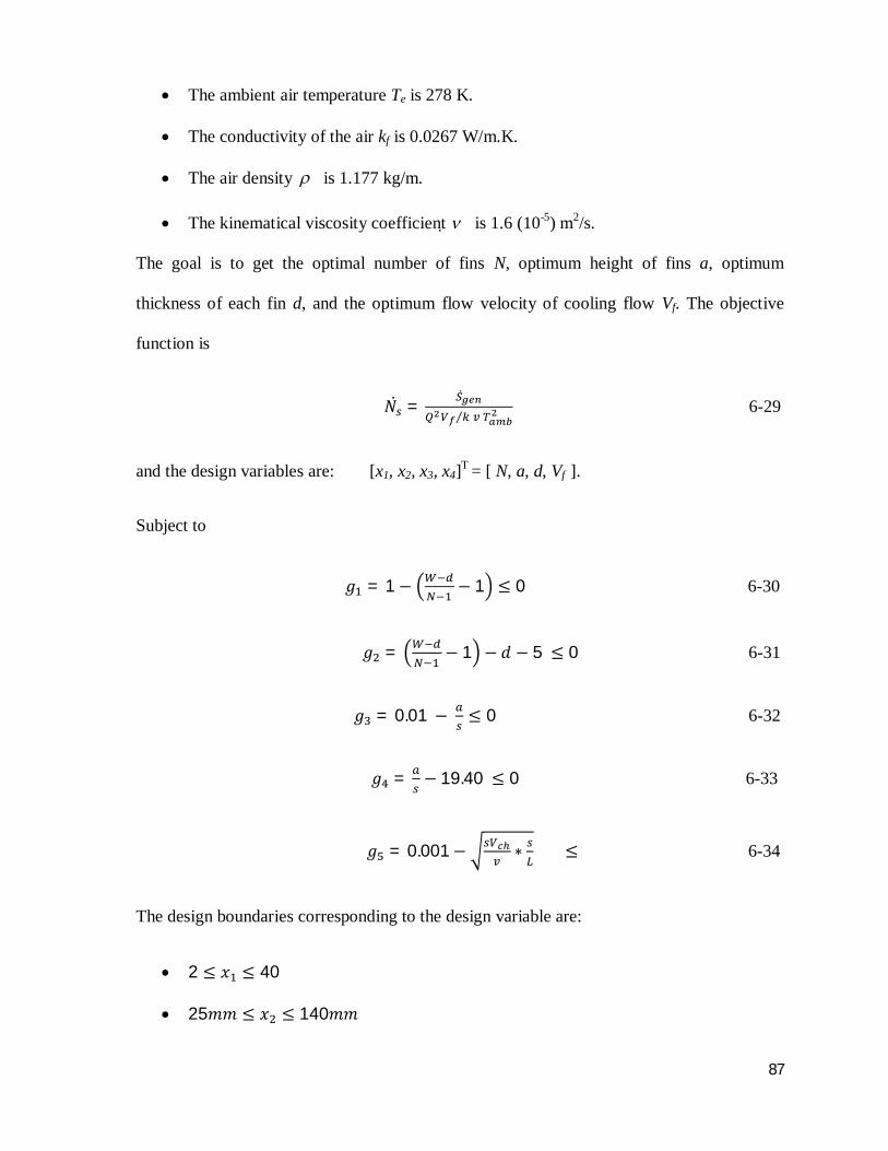
87
The ambient air temperature Te is 278 K.
The conductivity of the air kf is 0.0267 W/m.K.
The air density is 1.177 kg/m.
The kinematical viscosity coefficient is 1.6 (10-5) m2/s.
The goal is to get the optimal number of fins N, optimum height of fins a, optimum
thickness of each fin d, and the optimum flow velocity of cooling flow Vf. The objective
function is
푁̇ =̇
⁄ 6-29
and the design variables are: [x1, x2, x3, x4]T = [ N, a, d, Vf ].
Subject to
푔 = 1 − − 1 ≤ 0 6-30
푔 = − 1 − 푑 − 5 ≤ 0 6-31
푔 = 0.01 − ≤ 0 6-32
푔 = − 19.40 ≤ 0 6-33
푔 = 0.001− ∗ ≤ 6-34
The design boundaries corresponding to the design variable are:
2 ≤ 푥 ≤ 40
25푚푚 ≤ 푥 ≤ 140푚푚
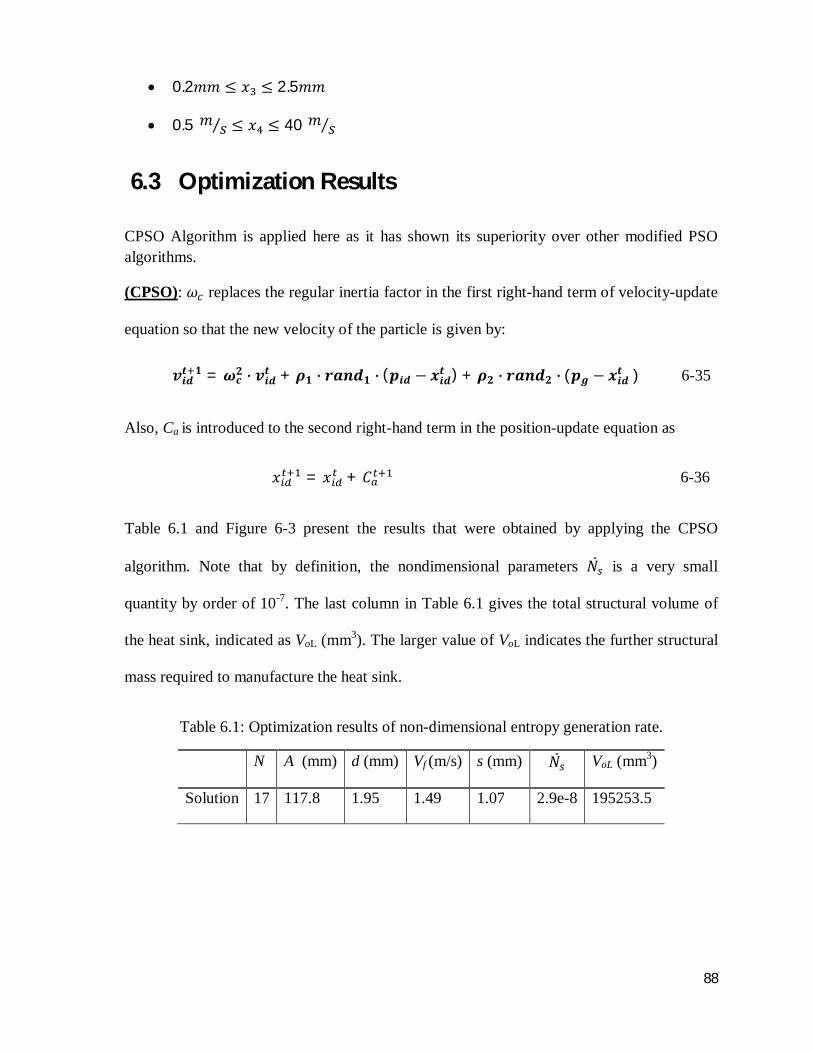
88
0.2푚푚 ≤ 푥 ≤ 2.5푚푚
0.5 푚 푠⁄ ≤ 푥 ≤ 40 푚 푠⁄
6.3 Optimization Results
CPSO Algorithm is applied here as it has shown its superiority over other modified PSO algorithms.
(CPSO): 휔 replaces the regular inertia factor in the first right-hand term of velocity-update
equation so that the new velocity of the particle is given by:
풗풊풅풕 ퟏ = 흎풄ퟐ ∙ 풗풊풅풕 + 흆ퟏ ∙ 풓풂풏풅ퟏ ∙ (풑풊풅 − 풙풊풅풕 ) + 흆ퟐ ∙ 풓풂풏풅ퟐ ∙ (풑품 − 풙풊풅풕 ) 6-35
Also, Ca is introduced to the second right-hand term in the position-update equation as
푥 = 푥 + 퐶 6-36
Table 6.1 and Figure 6-3 present the results that were obtained by applying the CPSO
algorithm. Note that by definition, the nondimensional parameters 푁̇ is a very small
quantity by order of 10-7. The last column in Table 6.1 gives the total structural volume of
the heat sink, indicated as VoL (mm3). The larger value of VoL indicates the further structural
mass required to manufacture the heat sink.
Table 6.1: Optimization results of non-dimensional entropy generation rate.
N A (mm) d (mm) Vf (m/s) s (mm) 푁̇ VoL (mm3)
Solution 17 117.8 1.95 1.49 1.07 2.9e-8 195253.5
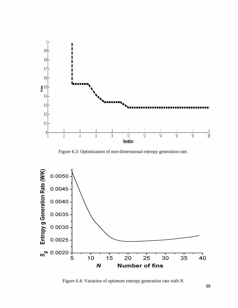
89
Figure 6.3: Optimization of non-dimensional entropy generation rate.
Figure 6.4: Variation of optimum entropy generation rate with N.

90
Figure 6.4 shows that as N the number of fins increases the entropy generation rate
will decrease dramatically due to increasing the surface area of the heat sink. When N
reaches 22 fins and up then the entropy generation rate will start increasing gradually and
the search will start go away from the optimal solution location. As it is clear from the figure
the optimal solution location is located N values vary between 15 and 20 fins. The optimal
solution of the entropy generation rate is 0.002679 W/K.
Figure 6.5: Variation optimum entropy generation rate and optimum flow velocity with N.

91
Figure 6.6: Variation of optimum entropy generation rate and optimum thickness of fin with N.
Figure 6.7: Variation of optimum entropy generation rate and optimum height of fin with
different values of N.

92
Figure 6.5, Figure 6.6, and Figure 6.7 show the behavior of the design variables (Vf = flow
velocity, a = height of fin, d = thickness of fin) in the optimization process of the entropy
generation rate for different values of N.
6.4 CFD Solution
The optimal values of N, a, d, and Vf are applied using Ansys IcePak, which uses the
finite volume method to solve computational fluid dynamic problems. Figures 6.8 and
6.9 show the temperature distribution through the cross-section of a heat sink and
velocity distribution through the heat sink as analyzed by Ansys Icepak. The results
show that the highest base temperature is approximately 43.2o.
Figure 6.8: Temperature distribution through the cross-section of heat sink.

93
Figure 6.9: Velocity profile through the heat sink.
6.5 Summary
The applicability of the modified PSO algorithm to the optimal heat sink design has
been investigated in this chapter. The modified PSO algorithm was presented for the design
of a plate-fin heat sink, with the objective of realizing the maximum dissipation of the heat
generated from electronic components. The entropy generation rate was used in the fitness
function, to realize the highest heat transfer efficiency. A practical application was presented
as an illustrative example.
94
Chapter 7
Conclusion
The particle swarm optimization (PSO) algorithm is known to have superior features
compared with the traditional optimization methods. The PSO algorithms use objective-
function information to guide the search in the problem space. Therefore, they can easily
deal with non-differentiable and non-convex objective functions. Additionally, this property
relieves PSO algorithms of various analytical assumptions and approximations, which are
often required by traditional optimization methods. PSO algorithms use probabilistic rather
than deterministic rules for particle movement. Hence, they are types of stochastic
optimization algorithm that can search a complicated and uncertain area. This feature makes
PSO algorithms more flexible and robust than conventional methods. However, improving
the convergence of a PSO algorithm is an important objective when solving complex real-
world problems. To the best knowledge of the author, the present thesis represents the first
study of the applicability of PSO in the optimization of the heat sink design Optimization.
7.1 Contributions and Significance In this thesis, a novel Chaotic Acceleration Factor, Chaotic Inertia Factor, and Global
Best Mutation have been incorporated into the original PSO method, in different formats, to
improve its convergence performance. The performance of the modified PSO methods are
studied in the present thesis and compared with the original PSO method by using well-
known test functions. All modified PSO methods proposed in this work show superior

95
performance over the classical PSO with regard to the quality of the solution and the
convergence rate.
The performance of the modified PSO algorithms when applied to nonlinear
constraints problems has been studied as well in the thesis. Non-stationary, multi-stage
penalty method (PFM) was implemented within the modified algorithms to handle nonlinear
constraints. Pressure vessel optimization and welded beam optimization are two common
engineering problems that are usually used for testing the performance of optimization
algorithms. These two examples have been used as benchmark testing examples in the
present work. The modified PSO algorithms, developed in this work, have outperformed
many classical and evolutionary optimization algorithms in solving nonlinear constraints
problems.
Finally in the present thesis, the modified PSO algorithm was applied in heat sink
design and detailed results were presented. Ansys Icepak was used to solve the heat and
flow equations by implementing the optimal design variables resulting from the application
of the modified PSO algorithms.
7.2 Possible Future Work Even though the work presented in this thesis is complete in its entirety, there are several
possibilities of further work in this area. Some suggestions in this regard are listed below.
It would be useful to study the performance of the modified PSO algorithms when
they are applied to high dimensional problems.
Although the incorporation of the proposed modifications has significantly improved
the performance of the PSO algorithm in most cases, the modified PSO algorithms
occasionally experienced premature convergence. Hybridization with other

96
optimization algorithms might be a possible solution to this problem provided that
the new hybridization technique retain the good features of PSO.
It is also of interest to develop parallel versions of the modified PSO algorithms, so
that they can be made more efficient when applied to highly constrained problems.

97
Bibliography
[1] Dantzig, G.B., Linear Programming and Extensions, Princeton University Press, Princeton, NJ, 1998.
[2] Nocedal, J., and Wright, S.J., Numerical Optimization, Springer Series in Operations Research, Springer, Berlin, Germany, 2000.
[3] Nelder, J., and Mead, R., "A Simplex Method for Function Minimization," The Computer Journal, Vol. 7, No.4, pp. 308-313, 1965.
[4] Tjalling J. Ypma, "Historical Development of the Newton-Raphson Method," SIAM Review, Vol.37, No.4, pp. 531-551, 1995. [5] Bäck, T., Hammel, U., and Schwefel, H. P., "Evolutionary Computation: Comments on the History and Current State," IEEE Transactions on Evolutionary Computation, Vol.1, No.1, pp. 3-17, 1997.
[6] Kennedy, J., And Eberhart, R. , "Particle swarm optimization," Proceedings of IEEE International Conference on Neural Networks, Piscataway, NJ. pp. 1942–1948, 1995. [7] Beyer, H.G., 2001, The theory of evolution strategies, Springer, Berlin, 2001. [8] Mezura-Montes, E., and Coello, C. A. C., "A Simple Evolution Strategy to Solve Constrained Optimization Problems," IEEE Transactions on Evolutionary Computation, Vol.9, No.1, pp. 1- 17, 2005.
[9] Hansen, N., and Ostermeier, A., "Completely Derandomized Self-Adaptation in Evolution Strategies," Evolutionary Computation, Vol.9, No.2, pp. 159-195, 2001
[10] Forrest, S., "Genetic Algorithms," ACM Computing Surveys (CSUR), Vol.28, No.1, pp. 77-80, 1996.
[11] Maulik, U., and Bandyopadhyay, S., "Genetic Algorithm-Based Clustering Technique," Pattern Recognition, Vol.33, No.9, pp. 1455-1465, 2000.
[12] Whitley, D., "A Genetic Algorithm Tutorial," Statistics and Computing, Vol.4, No.2, pp. 65-85, 1994.
[13] Kennedy, J., Eberhart, R., and Shi, Y., Swarm Intelligence, Springer, Berlin, Germany, 2001.
[14] Eberhart, R. C., and Kennedy, J., "A New Optimizer using Particle Swarm Theory," Proceedings of the Sixth International Symposium on Micro Machine and Human Science, New York, NY , 1995.

98
[15] Abido, M., "Optimal Power Flow using Particle Swarm Optimization," International Journal of Electrical Power and Energy Systems, Vol.24, No.7, pp. 563-571, 2002.
[16] Fukuyama, Y., "Fundamentals of Particle Swarm Techniques," Editors: Lee, K.Y., El-Sharkawi, M.A., Modern Heuristic Optimization Techniques with Applications to Power Systems, Vol.51, pp. 45-51, 2002.
[17] Hu, X., Eberhart, R. C., and Shi, Y., "Engineering Optimization with Particle Swarm," Proceedings of IEEE Swarm Intelligence Symposium, Indianapolis, Indiana, pp. 53–57, 2003.
[18] Eberhart, R. C., and Kennedy, J., "A New Optimizer using Particle Swarm Theory," Proceedings of the Sixth International Symposium on Micro Machine and Human Science, New York, NY, 1995 .
[19] Davis, L., Handbook of Genetic Algorithms, Van Nostrand Reinhold, New York, NY, 1991.
[20] Kennedy, J., "The Particle Swarm: Social Adaptation of Knowledge," IEEE International Conference on Evolutionary Computation, Indianapolis, IN, pp. 303-308, 1997.
[21] Shi, Y. and Eberhart, R.," Modified Particle Swarm Optimizer," Proceedings of the IEEE Congress on Evolutionary Computation, Piscataway, NJ, pp. 69-73, 1998
[22] Eberhart, R. C., and Shi, Y., "Particle Swarm Optimization: Developments, Applications and Resources," Proceedings of the Congress on Evolutionary Computation, Piscataway, NJ, pp. 81-86, 2001.
[23] Carlisle, A., Applying the Particle Swarm Optimizer to Non-Stationary Environments, PhD Thesis, Auburn University, Auburn, AL, 2002.
[24] Ratnaweera, A., Halgamuge, S. K., and Watson, H. C., "Self-Organizing Hierarchical Particle Swarm Optimizer with Time-Varying Acceleration Coefficients," Evolutionary Computation, Vol. 8, No.3, pp. 240-255, 2004.
[25] Fan, H., "A Modification to Particle Swarm Optimization Algorithm," Engineering Computations, Vol.19, No.8, pp. 970-989,2002.
[26] Chatterjee, A., and Siarry, P., "Nonlinear Inertia Weight Variation for Dynamic Adaptation in Particle Swarm Optimization," Computers & Operations Research, Vol.33, No.3, pp. 859-871, 2006.
[27] Higashi, N., and Iba, H., "Particle Swarm Optimization with Gaussian Mutation," Proceedings of IEEE Swarm Intelligence Symposium, Indianapolis, Indiana, pp. 72-79, 2003.

99
[28] Stacey, A., Jancic, M., and Grundy, I., "Particle Swarm Optimization with Mutation," Proceedings of the IEEE Congress on Evolutionary Computation, Canberra, Australia, pp. 1425-1430, 2003.
[29] Secrest, B. R., and Lamont, G. B., "Visualizing Particle Swarm Optimization-Gaussian Particle Swarm Optimization," Proceeding of IEEE Swarm Intelligence Symposium, Indianapolis, IN, , pp. 198-204, 2003. [30] Liu, J., Xu, W., and Sun, J., 2005, "Quantum-behaved Particle Swarm Optimization with Mutation Operator," Proceedings of 17th International Conference on Tools with Artificial Intelligence, Hong Kong (China), pp.230-240, 2005.
[31] Xiang, T., Liao, X., and Wong, K., "An Improved Particle Swarm Optimization Algorithm Combined with Piecewise Linear Chaotic Map," Applied Mathematics and Computation, Vol.190, No.2, pp. 1637-1645, 2007.
[32] Selvakumar, A. I., and Thanushkodi, K., "A New Particle Swarm Optimization Solution to Nonconvex Economic Dispatch Problems," IEEE Transactions on Power Systems, Vol. 22, No.1, pp. 42-51, 2007.
[33] Angeline, P. J., "Using selection to improve Particle Swarm Optimization," IEEE World Congress on Computational Intelligence, Anchorage, AK , pp. 84-89, 1998.
[34] Angeline, P. J., "Evolutionary Optimization Versus Particle Swarm Optimization: Philosophy and Performance Differences," Lecture Notes in Computer Science, pp. 601-610, 1998.
[35] Kennedy, J., and Spears, W. M., "Matching Algorithms to Problems: an Experimental Test of the Particle Swarm and some Genetic Algorithms on the Multimodal Problem generator," Proceedings of the IEEE International Conference on Evolutionary Computation, Anchorage, AK , pp. 78–83, 1998.
[36] Hassan, R., Cohanim, B., De Weck, O., "A Comparison of Particle Swarm Optimization and the Genetic Algorithm," Proceedings of the 1st AIAA Multidisciplinary Design Optimization Specialist Conference, Austin, TX , 2005.
[37] Lee, J., Lee, S., Chang, S., "A Comparison of GA and PSO for Excess Return Evaluation in Stock Markets," Artificial Intelligence and Knowledge Engineering Applications: A Bioinspired Approach, pp. 221-230,2005.
[38] Elbeltagi, E., Hegazy, T., and Grierson, D., "Comparison among Five Evolutionary-Based Optimization Algorithms," Advanced Engineering Informatics, Vol.19, No.1, pp. 43-53, 2005.

100
[39] Allahverdi, A., and Al-Anzi, F. S., "A PSO and a Tabu Search Heuristics for the Assembly Scheduling Problem of the Two-Stage Distributed Database Application," Computers & Operations Research, Vol.33, No.4, pp. 1056-1080, 2006.
[40] Chang, B. C. H., Ratnaweera, A., Halgamuge, S. K., "Particle Swarm Optimisation for Protein Motif Discovery," Genetic Programming and Evolvable Machines, Vol.5, No.2, pp. 203-214, 2004.
[41] Abido, M. A., "Optimal Power Flow using Particle Swarm Optimization," International Journal of Electrical Power and Energy Systems, Vol.24, No.12, pp. 563-571, 2002.
[42] Wachowiak, M. P., Smolíková, R., Zheng, Y., "An Approach to Multimodal Biomedical Image Registration Utilizing Particle Swarm Optimization," IEEE Transactions on Evolutionary Computation, Vol.8, No.3, pp. 289-301, 2004.
[43] Alrasheed, M.R., de Silva, C.W., and Gadala, M.S., "Evolutionary optimization in the design of a heat sink," Editor: de Silva C.W., Mechatronic Systems: Devices, Design, Control, Operation and Monitoring, pp. 55-78CRC Press, Boca Raton, FL, , 2007.
[44] Shih, C. J., and Liu, G. C., "Optimal Design Methodology of Plate-Fin Heat Sinks for Electronic Cooling using Entropy Generation Strategy," IEEE Transactions on Components and Packaging Technologies, Vol.27, No.3, pp. 551-559, 2004.
[45] Ditto, W., and Munakata, T., "Principles and Applications of Chaotic Systems," Communications of the ACM, Vol.38, No.11, pp. 96-102, 1995.
[46] Lorenz, E. N., "Deterministic Nonperiodic Flow," Journal of the Atmospheric Sciences, Vol.20, pp. 130-141, 1963.
[47] Elwakil, A., and Ozoguz, S., "Chaos in Pulse-Excited Resonator with Self Feedback," Electronics Letters, Vol.39, No.11, pp. 831-833, 2003.
[48] Li, B., and Jiang, W., "Optimizing Complex Functions by Chaos Search," Cybernetics and Systems, Vol.29, No.4, pp. 409-419, 1998.
[49] Liu, S., and Hou, Z., "Weighted gradient direction based chaos optimization algorithm for nonlinear programming problem," Proceedings of the 4th World Congress on Intelligent Control and Automation, Vol. 3, Shanghai, China, pp. 1779-1783, 2002.
[50] Lu, Z., Shieh, L. S., Chen, G., "Simplex Sliding Mode Control for Nonlinear Uncertain Systems Via Chaos Optimization," Chaos, Solutions & Fractals, Vol. 23, No.3, pp. 747-755, 2005.
[51] Wang, S., Jiang, Y., and Yang, H., "Chaos optimization strategy on fuzzy-immune-PID control of the turbine governing system," IEEE/RSJ International Conference on Intelligent Robots and Systems, Beijing, China, pp. 1594-1598, 2006.
101
[52] Yan, X. F., Chen, D. Z., and Hu, S. X., "Chaos-Genetic Algorithms for Optimizing the Operating Conditions Based on RBF-PLS Model," Computers & Chemical Engineering, Vol.27, No.10, pp. 1393-1404, 2003.
[53] Yang, D., Li, G., and Cheng, G., "On the Efficiency of Chaos Optimization Algorithms for Global Optimization," Chaos, Solutions & Fractals, Vol. 34, No.4, pp. 1366-1375, 2007.
[54] Zilong, G., Sun'an, W., and Jian, Z., "A Novel Immune Evolutionary Algorithm Incorporating Chaos Optimization," Pattern Recognition Letters, Vol. 27, No.1, pp. 2-8, 2006.
[55] Shi, Y., and Eberhart, R., "Parameter Selection in Particle Swarm Optimization," Proceedings of the 6th International Conference on Evolutionary Programming, Indianapolis, IN, pp. 591-600, 1997. [56] Kennedy, J., and Eberhart, R. C., "Particle Swarm Optimization," Proceedings of IEEE International Conference on Neural Networks, Perth, Australia, pp. 1942-1948, 1995.
[57] Parsopoulos, K. E., and Vrahatis, M. N., "Particle Swarm Optimization Method for Constrained Optimization Problems," Intelligent Technologies–Theory and Application: New Trends in Intelligent Technologies, pp. 214–220, 2002.
[58] Michalewicz, Z., "A Survey of Constraint Handling Techniques in Evolutionary Computation Methods," Evolutionary Programming, Vol.4, pp. 135, 1995.
[59] Parsopoulos, K., and Vrahatis, M., 2005, "Unified Particle Swarm Optimization for Solving Constrained Engineering Optimization Problems," Advances in Natural Computation, pp. 582-591.
[60] Yang, J. M., Chen, Y. P., Horng, J. T, "Applying Family Competition to Evolution Strategies for Constrained Optimization," Evolutionary Programming VI, Springer, pp. 201-211, 1997.
[61] Kannan, B., and Kramer, S. N., "An Augmented Lagrange Multiplier Based Method for Mixed Integer Discrete Continuous Optimization and its Applications to Mechanical Design," Journal of Mechanical Design, Vol.116, pp. 405-423, 1994.
[62] Coello, C., and Carlos, A., "Theoretical and Numerical Constraint-Handling Techniques used with Evolutionary Algorithms: A Survey of the State of the Art," Computer Methods in Applied Mechanics and Engineering, Vol. 191, No.11, pp. 1245-1287, 2002.
[63] K. Deb, A. S. Gene, Evolutionary Algorithms in Engineering Applications, Springer Verlag, Berlin, pp. 497-514, 1997.
[64] Coello, C. A. C., "Constraint-Handling using an Evolutionary Multiobjective Optimization Technique," Civil Engineering and Environmental Systems, Vol. 17, No.4, pp. 319-346, 2000.
102
[65] Rao, S.S., Engineering optimization: theory and practice, John Wiley and Sons, New York, NY, 1996.
[66] Regsdell. K.M., Phillips, D.,T., "Optimal Design of a Class of Welded Structures using Geometric Programming," ASME Journal of Engineering for Industries, Vol. 98, No.3, pp. 1021-1025, 1976.
[67] Bar-Cohen, A., and Iyengar, M., "Least-Energy Optimization of Air-Cooled Heat Sinks for Sustainable Development," IEEE Transactions on Components and Packaging Technologies, Vol. 26, No.1, pp. 16-25, 2003.
[68] Ogiso, K., "Assessment of overall Cooling Performance in Thermal Design of Electronics Based on Thermodynamics," Journal of Heat Transfer, Vol.123, pp. 999-1118, 2001.
[69] Shih, C., and Liu, G., "Optimal Design Methodology of Plate-Fin Heat Sinks for Electronic Cooling using Entropy Generation Strategy," IEEE Transactions on Components and Packaging Technologies, Vol. 27, No.3, pp. 551-559, 2004.
[70] Iyengar, M., and Bar-Cohen, A., 2003, "Least-Energy Optimization of Forced Convection Plate-Fin Heat Sinks," IEEE Transactions on Components and Packaging Technologies, Vol.26, No.1, pp. 62-70.
[71] Wei, X., and Joshi, Y., "Optimization Study of Stacked Micro-Channel Heat Sinks for Micro-Electronic Cooling," IEEE Transactions on Components and Packaging Technologies, Vol.26, No.1, pp. 55-61, 2003.
[72] Bejan, A., "Fundamentals of Exergy Analysis, Entropy Generation Minimization, and the Generation of Flow Architecture," International Journal of Energy Research, Vol.26, No.7, pp. 11-43, 2002.
[73] Muzychka, Y., and Yovanovich, M., "Modeling Friction Factors in Non-Circular Ducts for Developing Laminar Flow," AIAA Theoretical Fluid Mechanics Meeting, Albuquerque, NM, pp. 98-111, 1998.
[74] Teertstra, P., Yovanovich, M., and Culham, J., "Analytical Forced Convection Modeling of Plate Fin Heat Sinks," Journal of Electronics Manufacturing, Vol.10, No.4, pp. 253-262, 2000.

103
Appendix A: Rosenbrock Simulations
D=10 PSO CPSO CPSOS CPSOT CPSOM CPSOMS CPSOMT
3.640832 1.840562 0.884144 1.699185 1.16701 1.044121 0.020679 3.640832 0.318817 0.303438 2.451469 2.437366 3.327898 2.25528 3.940706 0.296693 0.877698 0.332115 1.108192 2.003032 0.650753 3.799521 0.023535 4.038685 0.058462 2.105517 0.506606 0.397768 3.546718 0.001282 0.748705 0.053166 1.84968 0.799626 0.62545 3.434511 0.219986 0.052233 0.003459 2.161527 0.090054 1.892486 2.72171 1.402038 0.003762 0.002182 2.37336 3.32764 0.95937 0.432756 1.103641 0.001639 6.6E-06 1.422613 1.35959 0.349325 0.173356 1.729728 0.023514 0.001191 2.356026 2.923288 0.622895 0.090054 1.522814 0.002521 0.128525 0.090054 0.506606 4.157364 0.090054 0.001282 0.001639 6.6E-06 0.090054 0.090054 0.020679 2.5421 0.84591 0.693634 0.472976 1.707134 1.588846 1.193137 3.940706 1.840562 4.038685 2.451469 2.437366 3.327898 4.157364 0.090054 0.001282 0.001639 6.6E-06 0.090054 0.090054 0.020679 3.940706 1.840562 4.038685 2.451469 2.437366 3.327898 4.157364 1.909339 0.955371 0.873332 0.50586 1.54684 1.584687 1.650556 1.628303 0.742766 1.23413 0.868776 0.754985 1.227509 1.252528
D=20
PSO CPSO CPSO1 CPSO2 CPSOM CPSOM1 CPSOM2 14.77538 12.13264 12.39382 12.22404 15.31318 15.60611 15.08629 14.9686 9.04781 9.127112 9.506127 14.14127 14.09401 14.2138 13.86907 5.087471 5.729692 6.045682 13.34389 13.61235 12.31349 13.83683 2.30223 1.70002 2.526545 11.85639 12.80462 11.98918 13.6464 0.305469 0.171469 0.456638 11.25901 12.81378 13.17808 14.34583 0.012199 0.015282 0.073817 11.65092 12.20007 13.76581 14.74087 0.002623 0.00032 0.021811 11.34093 10.84917 12.53197 13.23384 3.990205 0.002849 0.00418 11.46004 10.80718 11.91513 12.65441 3.990836 0.000939 0.000709 10.48114 10.91709 11.63848 12.84771 3.990278 0.005093 0.00345 9.608504 10.46939 11.60427 12.65441 0.002623 0.00032 0.000709 9.608504 10.46939 11.60427 14.9686 12.13264 12.39382 12.22404 15.31318 15.60611 15.08629 13.87849 4.416418 3.461728 3.590646 12.11475 12.52077 12.91059

104
D=20 PSO CPSO CPSO1 CPSO2 CPSOM CPSOM1 CPSOM2
12.65441 0.002623 0.00032 0.000709 9.608504 10.46939 11.60427 14.9686 12.13264 12.39382 12.22404 15.31318 15.60611 15.08629 13.69032 3.725323 2.585996 2.600068 11.61442 12.06622 12.8114 0.815488 4.849451 5.022837 4.948742 1.584104 1.503618 1.120934
D=30 PSO CPSO CPSO1 CPSO2 CPSOM CPSOM1 CPSOM2
25.44421 23.27029 24.16119 23.41681 22.3762 22.82363 25.01151 25.24805 20.78994 21.10782 20.00034 24.35923 20.32102 17.3837 24.38584 18.24011 17.55898 17.3837 22.11317 24.09354 13.8474 25.52825 15.03935 14.7054 13.8474 20.57749 23.54891 11.09909 24.69256 10.98845 12.37957 11.09909 20.90991 22.57798 9.044747 23.96387 7.786614 9.204992 9.044747 21.81795 23.64399 5.872516 23.43649 5.444626 6.200303 5.872516 24.96864 23.18691 4.153748 22.83932 2.68628 3.843773 4.153748 24.69238 22.85872 1.586254 21.95872 0.737856 1.499634 1.586254 24.13376 22.66534 0.24779 22.63532 0.131364 0.882529 0.24779 20.15327 22.87414 22.31824 21.95872 0.131364 0.882529 0.24779 20.15327 20.32102 0.24779 25.52825 23.27029 24.16119 23.41681 24.96864 24.09354 25.01151 23.9683 10.70971 11.38233 10.85975 22.60199 22.75073 11.31869 21.95872 0.131364 0.882529 0.24779 20.15327 20.32102 0.24779 25.52825 23.27029 24.16119 23.41681 24.96864 24.09354 25.01151 23.49714 7.753474 8.680051 8.199372 22.68379 22.67154 9.550961 1.26055 6.710197 6.399701 6.247195 1.652533 1.241008 7.182383

105
Appendix B: Rastrigrin Simulation Results
D=10 PSO CPSO CPSO1 CPSO2 CPSOM CPSOM1 CPSOM2
7.959672457 1.989918 5.969754 1.989918 3.979841 2.984896 0.994959 6.9647134 5.969754 3.979836 2.984877 0.995383 0.99521 4.974795 7.959672457 1.989918 1.989918 3.979836 3.979853 2.984877 2.984877 7.959672457 2E-15 7.959667 3.979836 2.98488 2.984879 5.969754 7.959672457 3.979836 1.989918 1.989918 2.985448 0.994984 0 7.959672457 4.974795 1.989918 1.989918 3.624665 3.013232 2.985722 6.9647134 2.984877 5.969754 2.984877 3.775655 2.984878 2.984877 4.974795285 2.984877 1.989918 1.989918 0.996019 0 1.99357 6.9647134 3.979836 4.974795 3.979836 4.974799 1.989918 4.974795 7.959672457 3.979836 2.984877 1.989918 3.979859 2.984881 2.984921 4.974795285 2E-15 1.989918 1.989918 0.995383 0 0 7.362697022 3.283365 3.979836 2.785885 3.22764 2.191775 3.084827 7.959672457 5.969754 7.959667 3.979836 4.974799 3.013232 5.969754 4.974795285 2E-15 1.989918 1.989918 0.995383 0 0 7.959672457 5.969754 7.959667 3.979836 4.974799 3.013232 5.969754 6.910442906 3.464267 3.979835 2.695435 3.227677 1.835103 2.813475 0.96122177 1.694354 2.149356 0.914304 1.303357 1.131792 1.843339 D=20
PSO CPSO CPSOS CPSOT CPSOM CPSOMS CPSOMT 16.91430397 14.92438 12.93446 17.90925 17.92058 13.0003 12.04297 15.91934491 15.91933 13.92942 11.9395 24.91385 23.08105 17.91471 18.90422208 17.90926 21.88908 16.91429 17.92058 25.87178 20.95621 16.91430397 7.959672 10.94454 11.9395 25.3492 23.88613 17.93904 15.91934492 17.90925 13.92942 11.9395 26.32373 13.99532 13.83725 26.32372571 10.94454 11.93951 10.94455 17.92058 11.94915 10.97153 16.91430397 9.949591 13.92942 11.9395 17.92058 25.42521 23.98774 28.50376999 11.9395 11.9395 12.93446 17.92058 20.8488 12.85887 16.91430397 15.91931 17.90925 12.93446 20.50377 16.01282 15.39511 18.90422208 12.93446 18.90421 12.93446 19.96834 26.87325 17.94496 15.91934491 7.959672 10.94454 10.94455 17.92058 11.94915 10.97153 28.50376999 17.90926 21.88908 17 26.32373 26.87325 23.98774 19.71291337 13.51485 15.0902 13.35617 20.90884 19.98052 16.56731 15.91934491 7.959672 10.94454 10.94455 17.92058 11.94915 10.97153 28.50376999 17.90926 21.88908 16.91429 26.32373 26.87325 23.98774 21.09443762 13.16813 15.39171 12.98059 20.905 19.33908 16.4983 4.470941433 3.416182 3.555032 2.300148 3.498989 5.794101 4.13588

106
D=30
PSO CPSO CPSOS CPSOT CPSOM CPSOMS CPSOMT 27.8588536 8.954632 17.90925 15.91934 32.22532 19.43948 13.17637 27.8588536 11.9395 23.879 31.83866 29.75289 29.4346 31.84311 28.85381266 27.85883 28.85379 40.79325 18.17345 40.40168 24.29034 26.86389454 28.85377 34.82354 29.84873 29.08372 29.17302 23.21942 26.86389455 33.82858 23.87901 16.9143 37.90482 38.51367 29.86681 26.86389454 27.85883 19.89918 22.88403 35.50147 34.47192 36.20901 43.8588536 23.879 24.87396 17.90926 36.04048 40.3305 32.02557 43.8588536 21.88909 29.84875 19.89917 34.6957 36.22407 32.37525 27.8588536 15.91936 22.88404 23.879 40.78773 36.25866 29.22827 27.8588536 18.90422 36.81344 26.86388 32.74896 28.96988 28.96801 26.86389454 8.954632 17.90925 15.91934 18.17345 19.43948 13.17637 43.8588536 33.82858 36.81344 40.79325 40.78773 40.40168 36.20901 31.61011384 21.88909 26.53222 25.28852 32.15631 32.75489 27.54896 26.86389454 8.954632 17.90925 15.91934 18.17345 19.43948 13.17637 43.8588536 33.82858 36.81344 40.79325 40.78773 40.40168 36.20901 33.65625578 22.70315 26.74327 24.27848 33.43253 33.38235 28.6357 6.879109055 8.007193 6.137811 7.831487 6.222735 6.570589 6.494845

107
Appendix C: Griewank Simulation Results
D=10 PSO CPSO CPSOS CPSOT CPSOM CPSOMS CPSOMT
0 0.007396 0 0 0 0 0.00739604 0 0.007396 0.007396 0.007396 0 0 0.00739604 0.043476 0 0 0 0 0 0 0.085313 0 0 0 0 0.007396 0 0.007396 0.007396 0 0.007396 0.007396 0.007396 0.00739604 1E-15 0 0 0 0.007396 0 0 0.041013 0 0.007396 0 0 0 0 0 0.007396 0 0.007396 0.007396 0.007396 0.00739604 0.007396 0 0 0 0 0.043659 0 0.007396 0 0 0 0.007396 0 0 0 0 0 0 0 0 0 0.019199 0.002958 0.001479 0.002219 0.002958 0.006585 0.002958416 0.085313 0.007396 0.007396 0.007396 0.007396 0.043659 0.00739604 0.085313 0.007396 0.007396 0.007396 0.007396 0.043659 0.00739604 0.027272 0.002853 0.002219 0.0028 0.003381 0.011411 0.002852758 0.028536 0.003819 0.003118 0.003573 0.003819 0.013485 0.003819299
D=20 PSO CPSO CPSOS CPSOT CPSOM CPSOMS CPSOMT
0 0 0.007396 0 0.007397 0.007402 0.007398195 0.009396 0 0 0 0 0 0 0 0.007396 0.004126 0.007396 0 0.007399 0 0.007396 0 2E-15 0.004134 0 0 0 0 0 0 0 0 0 0 0.007396 1E-15 0 0.007396 0 0 0 0 0 0 0 0 0.007405 0 0 0 0 0 0 0 0 0.007396 0 0.007396 0.007396 0 0.004653 0.007396148 0 0 0 0 1E-15 0 0 0 0 0 0 0 0 0 0.009396 0.007396 0.007396 0.007396 0.007397 0.007405 0.007398195 0.003415 0.001233 0.002193 0.00281 0.001233 0.002855 0.001849378 0.004206 0.002465 0.003291 0.003609 0.002466 0.003638 0.003261846
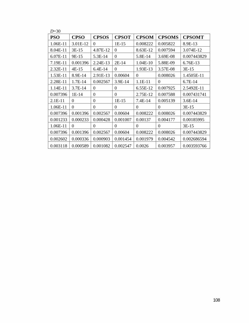
108
D=30 PSO CPSO CPSOS CPSOT CPSOM CPSOMS CPSOMT 1.06E-11 3.01E-12 0 1E-15 0.008222 0.005822 8.9E-13 8.04E-11 3E-15 4.87E-12 0 8.63E-12 0.007594 3.074E-12 6.07E-11 9E-15 5.3E-14 0 5.8E-14 3.69E-08 0.007443829 7.19E-11 0.001396 2.24E-13 2E-14 1.04E-10 5.88E-09 6.76E-13 2.32E-11 4E-15 6.4E-14 0 1.93E-13 3.57E-08 3E-15 1.53E-11 8.9E-14 2.91E-13 0.00604 0 0.008026 1.4505E-11 2.28E-11 1.7E-14 0.002567 3.9E-14 1.1E-11 0 6.7E-14 1.14E-11 3.7E-14 0 0 6.55E-12 0.007925 2.5492E-11 0.007396 1E-14 0 0 2.75E-12 0.007588 0.007431741 2.1E-11 0 0 1E-15 7.4E-14 0.005139 3.6E-14 1.06E-11 0 0 0 0 0 3E-15 0.007396 0.001396 0.002567 0.00604 0.008222 0.008026 0.007443829 0.001233 0.000233 0.000428 0.001007 0.00137 0.004177 0.00185995 1.06E-11 0 0 0 0 0 3E-15 0.007396 0.001396 0.002567 0.00604 0.008222 0.008026 0.007443829 0.002602 0.000336 0.000903 0.001454 0.001979 0.004542 0.002686594 0.003118 0.000589 0.001082 0.002547 0.0026 0.003957 0.003593766
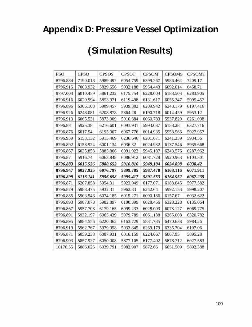
109
Appendix D: Pressure Vessel Optimization
(Simulation Results)
PSO CPSO CPSOS CPSOT CPSOM CPSOMS CPSOMT 8796.884 7190.018 5989.492 6054.759 6399.267 5986.464 7209.17 8796.915 7003.932 5829.556 5932.188 5954.443 6092.014 6458.71 8797.004 6010.459 5861.232 6175.754 6228.004 6183.503 6283.905 8796.916 6020.994 5853.971 6119.498 6131.617 6055.247 5995.457 8796.896 6305.108 5989.457 5939.382 6209.942 6248.179 6197.416 8796.926 6248.081 6208.878 5864.28 6190.718 6014.459 5953.12 8796.913 6065.531 5873.009 5916.384 6060.783 5937.829 6261.098 8796.88 5925.38 6216.601 6091.931 5993.087 6158.28 6327.716 8796.876 6017.54 6195.007 6067.776 6014.935 5958.566 5927.957 8796.959 6153.132 5915.469 6236.646 6201.671 6241.259 5934.56 8796.892 6158.924 6001.134 6036.32 6024.932 6137.546 5935.668 8796.867 6035.853 5885.866 6091.923 5945.187 6243.576 6287.962 8796.87 5916.74 6063.848 6086.912 6081.729 5920.963 6103.301 8796.883 6015.536 5880.652 5910.816 5949.104 6034.898 6038.42 8796.947 6027.925 6076.797 5899.785 5987.478 6168.116 6071.911 8796.899 6116.141 5956.658 5995.417 5891.553 6164.952 6067.235 8796.871 6207.858 5954.31 5923.049 6177.071 6188.045 5977.582 8796.879 5988.475 5932.31 5962.83 6242.64 5992.153 5998.207 8796.885 5903.546 6074.185 6015.271 6090.186 6157.67 6032.622 8796.893 5987.078 5982.897 6100.399 6028.456 6328.228 6135.064 8796.867 5957.708 6179.165 6099.233 6028.003 6073.127 6069.775 8796.891 5932.197 6065.439 5979.789 6061.138 6265.008 6320.782 8796.895 5884.556 6220.362 6163.729 5831.785 6470.638 5984.26 8796.919 5962.767 5979.058 5933.845 6269.179 6335.704 6107.06 8796.871 6059.238 6087.931 6016.159 6224.667 6067.95 5895.28 8796.903 5857.927 6050.008 5877.105 6177.402 5878.712 6027.583 10176.55 5886.025 6039.791 5982.907 5872.66 6051.509 5892.388

110
PSO CPSO CPSOS CPSOT CPSOM CPSOMS CPSOMT 9342.754 5934.718 6097.069 6064.499 6175.912 5926.959 6108.169 9342.754 5962.668 5966.112 6137.385 6026.005 6117.226 6118.399 9342.754 5940.455 6101.746 5945.35 5886.543 6137.593 6121.822 9342.754 5910.321 6325.312 5936.039 6325.642 6277.084 6005.888 9342.754 6126.18 6005.179 6045.959 6064.574 6133.279 6102.08 9342.754 6192.029 6095.219 6106.576 6249.599 6395.565 6103.644 9342.754 6059.53 6049.481 5938.562 6010.594 6320.367 6376.837 9342.754 5835.759 6376.388 6202.906 6094.165 6234.844 6231.615 9342.754 6048.66 6045.709 5981.825 6093.162 6178.271 6376.061 9342.754 5861.292 6075.187 5899.497 6129.368 6099.708 6107.417 9342.754 6043.429 5860.821 6016.819 6052.186 6233.715 5940.814 9342.754 5927.741 5990.364 6105.484 5931.346 6293.671 6055.253 9342.754 5968.521 5931.883 6324.294 6026.83 6066.763 6025.135 9342.754 5836.176 5847.605 5904.54 6171.415 6356.82 5880.311 9342.754 5971.621 6102.715 5942.242 6087.72 6039.884 5862.23 9342.754 5912.351 5948.469 5997.299 5902.177 6048.295 6402.254 9342.754 5939.627 5997.607 6009.198 5921.249 6101.446 6308.219 9342.754 6333.629 6096.572 5988.621 6070.329 6055.331 6205.76 9342.754 5934.336 6143.406 5937.637 6126.126 6139.207 6073.765 9342.754 5867.223 6189.761 6301.411 6297.317 6220.028 6180.54 9342.754 5937.88 6037.557 6058.344 6178.109 5986.954 6002.698 9342.754 6180.656 6266.767 6388.048 6066.641 5951.942 5913.174 9342.754 5984.83 6318.091 6203.16 6208.309 6245.236 6097.64

111
Appendix E: Welded Beam Optimization
(Simulation Results)
PSO CPSO CPSOS CPSOT CPSOM CPSOMS CPSOMT 1.81428 1.72484 1.725005 1.726163 1.726586 1.743457 1.725143 1.814279 1.72484 1.724839 1.724868 1.729601 1.725709 1.725965 1.814279 1.724839 1.724839 1.72531 1.72957 1.725536 1.737385 1.814279 1.72484 1.724839 1.724846 1.740152 1.727841 1.729866 1.81428 1.726325 1.724843 1.740583 1.726071 1.741822 1.728633 1.81428 1.731532 1.724918 1.725166 1.728371 1.738443 1.727109 1.81428 1.724898 1.755606 1.724839 1.726196 1.726774 1.725896 1.814279 1.729475 1.724839 1.726643 1.72652 1.726875 1.726273 1.81428 1.724849 1.724841 1.724839 1.727664 1.725511 1.762249 1.81428 1.72484 1.72484 1.72484 1.728795 1.726096 1.731086 1.81428 1.724844 1.734566 1.724859 1.732981 1.726919 1.731236 1.814279 1.726098 1.833444 1.724839 1.738247 1.72806 1.730059 1.814279 1.724849 1.724854 1.72484 1.725804 1.727204 1.729139 1.81428 1.72484 1.72485 1.738992 1.731919 1.728399 1.72852 1.814281 1.725079 1.727079 1.724843 1.727055 1.732553 1.728771 1.814279 1.724998 1.724839 1.724839 1.736438 1.728774 1.725056 1.81428 1.724894 1.725759 1.724848 1.726573 1.725757 1.731783 1.81428 1.724855 1.724855 1.729096 1.729529 1.727897 1.730413 1.81428 1.724839 1.724849 1.72513 1.72948 1.726885 1.727682 1.814279 1.724848 1.724882 1.724903 1.725975 1.726114 1.726617 1.814279 1.729492 1.725104 1.724839 1.726924 1.726837 1.725142 1.814279 1.724854 1.739738 1.724839 1.728194 1.727484 1.734987 1.814283 1.772954 1.725939 1.72484 1.729634 1.730017 1.728455 1.81428 1.724839 1.725228 1.72484 1.731365 1.725723 1.735446 1.81428 1.724839 1.751026 1.724839 1.736005 1.72936 1.736384 1.81428 1.724848 1.724872 1.724875 1.72537 1.728552 1.725134 1.81428 1.724839 1.724839 1.734895 1.725756 1.727168 1.725573 1.814279 1.725056 1.724839 1.724839 1.726782 1.830611 1.729475
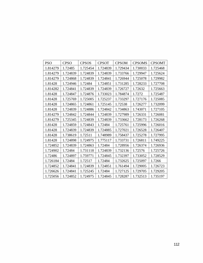
112
PSO CPSO CPSOS CPSOT CPSOM CPSOMS CPSOMT 1.814279 1.72485 1.725454 1.724839 1.729434 1.730033 1.725468 1.814279 1.724839 1.724839 1.724839 1.733766 1.729947 1.725624 1.814279 1.724868 1.724839 1.724841 1.726944 1.725078 1.729982 1.81428 1.724946 1.72484 1.724851 1.731285 1.728233 1.727708 1.814282 1.724841 1.724839 1.724839 1.726727 1.72632 1.725663 1.81428 1.724847 1.724876 1.733023 1.784874 1.7272 1.725487 1.81428 1.725769 1.725005 1.725237 1.733297 1.727176 1.725085 1.81428 1.724865 1.724861 1.725145 1.72538 1.726277 1.732099 1.81428 1.724839 1.724886 1.724842 1.734863 1.743071 1.727105 1.814279 1.724842 1.724844 1.724839 1.727989 1.726331 1.726081 1.814279 1.725345 1.724839 1.724839 1.733662 1.728173 1.726268 1.81428 1.724859 1.724843 1.72484 1.725761 1.725996 1.726016 1.81428 1.724839 1.724839 1.724885 1.727021 1.726528 1.726407 1.81428 1.738619 1.72511 1.748989 1.758437 1.725278 1.727995 1.81428 1.724898 1.724975 1.775117 1.733731 1.726811 1.749225 1.724852 1.724839 1.724863 1.72484 1.728956 1.726374 1.726936 1.724902 1.72484 1.731118 1.724839 1.732136 1.72576 1.725726 1.72486 1.724897 1.759771 1.724845 1.732397 1.733052 1.728529 1.726184 1.72484 1.72517 1.72484 1.732625 1.725097 1.7266 1.724852 1.724841 1.724839 1.724851 1.761494 1.729005 1.726723 1.726626 1.724841 1.725245 1.72484 1.727125 1.729705 1.729205 1.725056 1.724852 1.724975 1.724845 1.728287 1.732513 1.735197

113
Appendix F: Computer Codes
PSO%% Particle Swarm Optimization Simulation
% Simulates the movements of a swarm to minimize the objective function % The swarm matrix is % swarm(index, [location, velocity, best position, best % value], [x, y components or the value component]) %%%%%%%%%%%%%%%%%%%%%%%%%%%%%%%%%%%%%%%%%%%%%%%%%%%%%%%%%%%% %% %%%%%%%%%%%%%%Initialization%%%%%%%%%%%%%%%%%%%%%%%%%%%% % %%%%%%%%%%%%%%%Parameters%%%%%%%%%%%%%%%%%%%%%%%%%%%%%%%% clear clc correction_factor1 = 2; correction_factor2 = 2; wmax=1.2; wmin=0.2; iterations =100; swarm_size = 40; D=4; for NR =1:1 for d=1:D %%%%%%%%%%%Welding xmin=[0.1; 0.1; 0.1 ;0.1]; xmax=[2.0; 10.0; 10.0; 2.0]; %%%%%%%%%%%%%%%%%%%% %xmin=[0;0]; %xmax=[6;6]; xmin=[5 ;0.025; 0.0002; 0.5]; xmax=[40; 0.14; 0.002; 1.5]; %d1=0.0625; xmin = [1;1;10;10]; d2=d1*99; %xmax = [99; 99; 200; 200]; %xmin(d)=-5; %xmax(d)=+5; %xmin=[-5;0]; %xmax=[10;15]; end %------------------------------------------------------% %tic for iter=1:iterations W(iter)=wmax-((wmax-wmin)/iterations)*iter; end % ---- initial swarm position -------------------------% for d=1:D f2=0.3; Vmax(d)=f2*(xmax(d)-xmin(d)); end for i=1:swarm_size for d= 1 : D swarm(i, 1, d) =(xmax(d)-xmin(d)); end

114
end % Asumming of Global best value so far swarm(:, 4, 1) = 100; swarm(:, 3, 1) =200; %initial velocity swarm(:, 2, :) = 0; gbest=4; %%%%%%%%%%%%% PSO search strat%%%%%%%%%%%%%%%%%%%%%%%%%%%%% for iter = 1 : iterations %-- evaluating position & quality --- for i = 1 : swarm_size %----------------------------- %%%%%fitness evaluation val=moh(swarm,i,D,iter); % Stopping=abs(val-swarm(gbest,4,1)); if val < swarm(i, 4, 1) % local best valu swarm(i, 4, 1) = val; % if new position is better for d=1:D % update position of best solution of each particle swarm(i, 3, d) = swarm(i, 1, d); end end temp = global best position gbest= the particle that discoverd the best Solution [temp, gbest] = min(swarm(:, 4, 1)); temp1=gbest; bestLocation=swarm(gbest,1,:); Fittness(iter,1)=temp; %%%------------------------------ %--- updating velocity vectors for d=1:D swarm(i, 2, d) =(W(iter)*swarm(i, 2, d)... +correction_factor1*rand*(swarm(i, 3, d)- swarm(i, 1, d))... + correction_factor2*rand*(swarm(gbest, 1, d)- swarm(i, 1, d))); if (swarm(i,2,d)>Vmax(d)) swarm(i,2,d)=Vmax(d); if (swarm(i,2,d)<-Vmax(d)) swarm(i,2,d)=-Vmax(d); end %update particle's position

115
swarm(i, 1, d) =(swarm(i, 1, d) +swarm(i, 2, d)); if (swarm(i,1,d)>xmax(d)) swarm(i,1,d)=xmax(d); end if (swarm(i,1,d)<xmin(d)) swarm(i,1,d)=xmin(d); end end end Final(NR,1)=temp; if Stopping<0.0001 toc break end end AFinal(NR,1)=temp; Ploting A good Figures fh = figure(1); % returns the handle to the figure object set(fh, 'color', 'white'); % sets the color to white h=plot(Fittness); get(gcf); get(gca); get(h); o modify the line style. Possible options are ':' dotted, '-' solid, '--' dashed, '-.' dash-dotted set(h,'linestyle','--'); set(h,'color','r'); set(h,'linewidth',5); set(h,'marker','+'); set(h,'markersize',1); set(gca,'box','off'); xlabel('iteration','fontsize',12,... 'fontweight','bold'); ylabel('Fucntion Minimization','fontsize',12,... % 'fontweight','bold'); Legend('PSO','CSPO','CPSO1','CPSO2','CPSOM','CPSOM1','CPSOM2'); grid; fh = figure(1); % returns the handle to the figure object set(fh, 'color', 'white'); % sets the color to white hleg1 = legend('PSO','CPSOM','CPSO','CPSO1'); plot(Fittness,'k-') [glob,iterF]=min(Fittness(:,1)); FINAL=glob; FinalLocation=bestLocation(iterF,1,:); plot (bestLocation,'dg-.','DisplayName', 'Fittness', 'YDataSource', 'Fittnes' ); figure(gcf) Defines limits for x and y axes, and sets title, labels and legends axis([0 2*pi -1.5 1.5]) title('2D plots', 'fontsize', 12) xlabel('iteration') ylabel('Fucntion Minimization') legend('cos(x)', 'sin(x)') axis([0 1000 0 0.5]); hold on
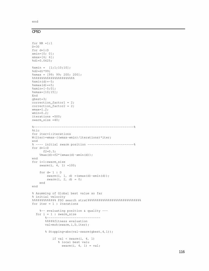
116
end CPSO
for NR =1:1 D=30 for d=1:D xmin=[0; 0]; xmax=[6; 6]; %d1=0.0625; %xmin = [1;1;10;10]; %d2=d1*99; %xmax = [99; 99; 200; 200]; %%%%%%%%%%%%%%%%%%%%%%% %xmin(d)=-5; %xmax(d)=+5; %xmin=[-5;0]; %xmax=[10;15]; End gbest=3; correction_factor1 = 2; correction_factor2 = 2; wmax=1.2; wmin=0.2; iterations =500; swarm_size =40; %------------------------------------------------------% %tic for iter=1:iterations W(iter)=wmax-((wmax-wmin)/iterations)*iter; end % ---- initial swarm position -------------------------% for d=1:D f2=0.3; Vmax(d)=f2*(xmax(d)-xmin(d)); end for i=1:swarm_size swarm(i, 4, 1) =100; for d= 1 : D swarm(i, 1, d) =(xmax(d)-xmin(d)); swarm(i, 2, d) = 0; end end % Asumming of Global best value so far % initial velocity %%%%%%%%%%%%% PSO search strat%%%%%%%%%%%%%%%%%%%%%%%%%%%%% for iter = 1 : iterations %-- evaluating position & quality --- for i = 1 : swarm_size %----------------------------- %%%%%fitness evaluation val=moh(swarm,i,D,iter); % Stopping=abs(val-swarm(gbest,4,1)); if val < swarm(i, 4, 1) % local best valu swarm(i, 4, 1) = val;
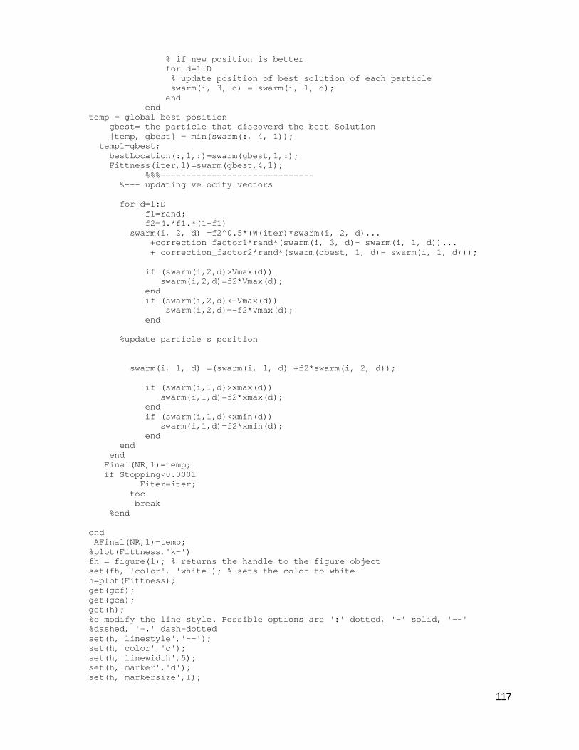
117
% if new position is better for d=1:D % update position of best solution of each particle swarm(i, 3, d) = swarm(i, 1, d); end end temp = global best position gbest= the particle that discoverd the best Solution [temp, gbest] = min(swarm(:, 4, 1)); temp1=gbest; bestLocation(:,1,:)=swarm(gbest,1,:); Fittness(iter,1)=swarm(gbest,4,1); %%%------------------------------ %--- updating velocity vectors for d=1:D f1=rand; f2=4.*f1.*(1-f1) swarm(i, 2, d) =f2^0.5*(W(iter)*swarm(i, 2, d)... +correction_factor1*rand*(swarm(i, 3, d)- swarm(i, 1, d))... + correction_factor2*rand*(swarm(gbest, 1, d)- swarm(i, 1, d))); if (swarm(i,2,d)>Vmax(d)) swarm(i,2,d)=f2*Vmax(d); end if (swarm(i,2,d)<-Vmax(d)) swarm(i,2,d)=-f2*Vmax(d); end %update particle's position swarm(i, 1, d) =(swarm(i, 1, d) +f2*swarm(i, 2, d)); if (swarm(i,1,d)>xmax(d)) swarm(i,1,d)=f2*xmax(d); end if (swarm(i,1,d)<xmin(d)) swarm(i,1,d)=f2*xmin(d); end end end Final(NR,1)=temp; if Stopping<0.0001 Fiter=iter; toc break %end end AFinal(NR,1)=temp; %plot(Fittness,'k-') fh = figure(1); % returns the handle to the figure object set(fh, 'color', 'white'); % sets the color to white h=plot(Fittness); get(gcf); get(gca); get(h); %o modify the line style. Possible options are ':' dotted, '-' solid, '--' %dashed, '-.' dash-dotted set(h,'linestyle','--'); set(h,'color','c'); set(h,'linewidth',5); set(h,'marker','d'); set(h,'markersize',1);

118
set(gca,'box','off'); xlabel('iteration','fontsize',12,... 'fontweight','bold'); ylabel('Fucntion Minimization','fontsize',12,... 'fontweight','bold'); Legend('PSO','CSPO','CPSO1','CPSO2','CPSOM','CPSOM1','CPSOM2'); grid; [glob,iterF]=min(Fittness(:,1)); FINAL=glob; FinalLocation=bestLocation(iterF,1,:); plot (bestLocation,'dg-.','DisplayName', 'Fittness', 'YDataSource', 'Fittnes' ); figure(gcf) % Defines limits for x and y axes, and sets title, labels and legends axis([0 2*pi -1.5 1.5]) title('2D plots', 'fontsize', 12) xlabel('iteration') ylabel('Fucntion Minimization') legend('cos(x)', 'sin(x)') axis([0 1000 0 0.5]); hold on end CPSOS %% Particle Swarm Optimization Simulation % Simulates the movements of a swarm to minimize the objective function % The swarm matrix is % swarm(index, [location, velocity, best position, best % value], [x, y components or the value component]) %%%%%%%%%%%%%%%%%%%%%%%%%%%%%%%%%%%%%%%%%%%%%%%%%%%%%%%%%%%% %% %%%%%%%%%%%%%%Initialization%%%%%%%%%%%%%%%%%%%%%%%%%%%% % %%%%%%%%%%%%%%%Parameters%%%%%%%%%%%%%%%%%%%%%%%%%%%%%%%% clear clc correction_factor1 = 2; correction_factor2 = 2; wmax=1.2; wmin=0.2; iterations =100; swarm_size = 40; for NR =1:1 for d=1:D xmax = [99; 99; 200; 200]; xmin=[2 ;0.025; 0.0002; 0.5]; xmax=[40; 0.14; 0.002; 1.5]; %xmin(d)=-5; %xmax(d)=+5; %xmin=[-5;0]; %xmax=[10;15]; end %------------------------------------------------------% %tic for iter=1:iterations W(iter)=wmax-((wmax-wmin)/iterations)*iter; end % ---- initial swarm position -------------------------% for d=1:D f2=0.3; Vmax(d)=f2*(xmax(d)-xmin(d)); end for i=1:swarm_size for d= 1 : D swarm(i, 1, d) =(xmax(d)-xmin(d)); end

119
end % Asumming of Global best value so far swarm(:, 4, 1) = 100; %swarm(:, 3, 1) =200; % initial velocity swarm(:, 2, :) = 0; %%%%%%%%%%%%% PSO search strat%%%%%%%%%%%%%%%%%%%%%%%%%%%%% for iter = 1 : iterations %-- evaluating position & quality --- for i = 1 : swarm_size %----------------------------- %%%%%fitness evaluation val=moh(swarm,i,D,iter); Stopping=abs(val-swarm(gbest,4,1)); if val < swarm(i, 4, 1) % local best valu swarm(i, 4, 1) = val; % if new position is better for d=1:D % update position of best solution of each particle swarm(i, 3, d) = swarm(i, 1, d); end end % temp = global best position gbest= the particle that discoverd the best Solution [temp, gbest] = min(swarm(:, 4, 1)); temp1=gbest; bestLocation(iter,1,:)=swarm(gbest,1,:); Fittness(iter,1)=temp; %%%------------------------------ %--- updating velocity vectors for d=1:D f1=rand; f2=4.*f1.*(1-f1); swarm(i, 2, d) =f2^0.5*(W(iter)*swarm(i, 2, d)... +f2*correction_factor1*rand*(swarm(i, 3, d)- swarm(i, 1, d))... + correction_factor2*rand*(swarm(gbest, 1, d)- swarm(i, 1, d))); if (swarm(i,2,d)>Vmax(d)) swarm(i,2,d)=f2*Vmax(d); end if (swarm(i,2,d)<-Vmax(d)) swarm(i,2,d)=-f2*Vmax(d); end %update particle's position swarm(i, 1, d) =(swarm(i, 1, d) +f2*swarm(i, 2, d)); if (swarm(i,1,d)>xmax(d)) swarm(i,1,d)=f2*xmax(d); end if (swarm(i,1,d)<xmin(d)) swarm(i,1,d)=f2*xmin(d); end end end Final(NR,1)=temp; if Stopping<0.0001 Fiter=iter; toc break %end end AFinal(NR,1)=temp; plot(Fittness,'k-') fh = figure(1); % returns the handle to the figure object set(fh, 'color', 'white'); % sets the color to white

120
h=plot(Fittness); get(gcf); get(gca); get(h); o modify the line style. Possible options are ':' dotted, '-' solid, '--' dashed, '-.' dash-dotted set(h,'linestyle','-.'); set(h,'color','k'); set(h,'linewidth',5); set(h,'marker','*'); set(h,'markersize',1); set(gca,'box','off'); xlabel('iteration','fontsize',12,... 'fontweight','bold'); ylabel('Fucntion Minimization','fontsize',12,... 'fontweight','bold'); Legend('PSO','CSPO','CPSO1','CPSO2','CPSOM','CPSOM1','CPSOM2'); grid; [glob,iterF]=min(Fittness(:,1)); FINAL=glob; FinalLocation=bestLocation(iterF,1,:); plot (bestLocation,'dg-.','DisplayName', 'Fittness', 'YDataSource', 'Fittnes' ); figure(gcf) % Defines limits for x and y axes, and sets title, labels and legends axis([0 2*pi -1.5 1.5]) title('2D plots', 'fontsize', 12) xlabel('iteration') ylabel('Fucntion Minimization') legend('cos(x)', 'sin(x)') axis([0 1000 0 0.5]); hold on end CPSOT gbest=3; correction_factor1 = 2; correction_factor2 = 2; wmax=1.2; wmin=0.2; iterations =500; swarm_size = 40 for NR =1:50 for d=1:D %xmax = [99; 99; 200; 200]; xmin(d)=-5; xmax(d)=+5; xmin=[-5;0]; xmax=[10;15]; end %------------------------------------------------------% %tic for iter=1:iterations W(iter)=wmax-((wmax-wmin)/iterations)*iter; end % ---- initial swarm position -------------------------% for d=1:D f2=0.3; Vmax(d)=f2*(xmax(d)-xmin(d)); end for i=1:swarm_size for d= 1 : D swarm(i, 1, d) =(xmax(d)-xmin(d)); end end

121
% Asumming of Global best value so far swarm(:, 4, 1) = 100; %swarm(:, 3, 1) =200; % initial velocity swarm(:, 2, :) = 0; %%%%%%%%%%%%% PSO search strat%%%%%%%%%%%%%%%%%%%%%%%%%%%%% for iter = 1 : iterations %-- evaluating position & quality --- for i = 1 : swarm_size %----------------------------- %%%%%fitness evaluation val=weld(swarm,i,D,iter); % Stopping=abs(val-swarm(gbest,4,1)); if val < swarm(i, 4, 1) % local best valu swarm(i, 4, 1) = val; % if new position is better for d=1:D % update position of best solution of each particle swarm(i, 3, d) = swarm(i, 1, d); end end % temp = global best position % gbest= the particle that discoverd the best Solution [temp, gbest] = min(swarm(:, 4, 1)); temp1=gbest; bestLocation(iter,1,:)=swarm(gbest,1,:); Fittness(iter,1)=temp; %%%------------------------------ %--- updating velocity vectors for d=1:D f1=rand; f2=4.*f1.*(1-f1); swarm(i, 2, d) =f2^0.5*(W(iter)*swarm(i, 2, d)... +correction_factor1*rand*(swarm(i, 3, d)- swarm(i, 1, d))... + f2*correction_factor2*rand*(swarm(gbest, 1, d)- swarm(i, 1, d))); if (swarm(i,2,d)>Vmax(d)) swarm(i,2,d)=f2*Vmax(d); end if (swarm(i,2,d)<-Vmax(d)) swarm(i,2,d)=-f2*Vmax(d); end %update particle's position swarm(i, 1, d) =(swarm(i, 1, d) +f2*swarm(i, 2, d)); if (swarm(i,1,d)>xmax(d)) swarm(i,1,d)=f2*xmax(d); end if (swarm(i,1,d)<xmin(d)) swarm(i,1,d)=f2*xmin(d); end end end % Final(NR,1)=temp; %if Stopping<0.0001 % Fiter=iter; % toc % break %end end AFinal(NR,1)=temp; fh = figure(1); % returns the handle to the figure object set(fh, 'color', 'white'); % sets the color to white

122
h=plot(Fittness); get(gcf); get(gca); get(h); %o modify the line style. Possible options are ':' dotted, '-' solid, '--' %dashed, '-.' dash-dotted set(h,'linestyle','-.'); set(h,'color','g'); set(h,'linewidth',5); set(h,'marker','x'); set(h,'markersize',1); set(gca,'box','off'); xlabel('iteration','fontsize',12,... 'fontweight','bold'); ylabel('Fucntion Minimization','fontsize',12,... 'fontweight','bold'); Legend('PSO','CSPO','CPSO1','CPSO2','CPSOM','CPSOM1','CPSOM2'); grid;
CPSOM
correction_factor1 = 1.5; correction_factor2 = 2.5; wmax=1.2; wmin=0.2; iterations =100; swarm_size = 40; D=4; for NR =1:1 for d=1:D %xmin=[-5;0]; %xmax=[10;15]; end %------------------------------------------------------% %tic for iter=1:iterations W(iter)=wmax-((wmax-wmin)/iterations)*iter; end % ---- initial swarm position -------------------------% for d=1:D f2=0.3; Vmax(d)=f2*(xmax(d)-xmin(d)); end for i=1:swarm_size for d= 1 : D swarm(i, 1, d) =(xmax(d)-xmin(d)); end end % Asumming of Global best value so far swarm(:, 4, 1) = 100; %swarm(:, 3, 1) =200; % initial velocity swarm(:, 2, :) = 0; %gbest=4; %%%%%%%%%%%%% PSO search strat%%%%%%%%%%%%%%%%%%%%%%%%%%%%% for iter = 1 : iterations %-- evaluating position & quality --- for i = 1 : swarm_size %----------------------------- %%%%%fitness evaluation swarm(i, 1, 1)=int8(swarm(i, 1, 1)); val=moh(swarm,i,D,iter);

123
Stopping=abs(val-swarm(gbest,4,1)); if val < swarm(i, 4, 1) % local best valu swarm(i, 4, 1) = val; AAAAAA(iter,1)=val; % if new position is better for d=1:D % update position of best solution of each particle swarm(i, 3, d) = swarm(i, 1, d); AQQ(iter,d)= swarm(i, 1, d); end end % temp = global best position % gbest= the particle that discoverd the best Solution [temp, gbest] = min(swarm(:, 4, 1)); temp1=gbest; bestLocation(1,:)=swarm(gbest,1,:); Fittness(iter,1)=temp; %%%------------------------------ %--- updating velocity vectors for d=1:D f1=rand; f2=4.*f1.*(1-f1); swarm(i, 2, d) =f2^0.5*(W(iter)*swarm(i, 2, d)... +correction_factor1*rand*(swarm(i, 3, d)- swarm(i, 1, d))... + correction_factor2*rand*(swarm(gbest, 1, d)- swarm(i, 1, d))); if iter >= iterations/2 swarm(i, 2, d)= swarm(i, 2, d)+swarm(gbest,3, d)/swarm_size*exp (W(iter)^2*f2); end if (swarm(i,2,d)>Vmax(d)) swarm(i,2,d)=f2*Vmax(d); end if (swarm(i,2,d)<-Vmax(d)) swarm(i,2,d)=-f2*Vmax(d); end %update particle's position swarm(i, 1, d) =(swarm(i, 1, d) +f2*swarm(i, 2, d)) if (swarm(i,1,d)>xmax(d)) swarm(i,1,d)=f2*xmax(d); end if (swarm(i,1,d)<xmin(d)) swarm(i,1,d)=f2*xmin(d); end end end Final(NR,1)=temp; if Stopping<0.0001 Fiter=iter; toc break end end AFinal(NR,1)=temp; %======Ploting Nice figure fh = figure(1); % returns the handle to the figure object set(fh, 'color', 'white'); % sets the color to white h=plot(Fittness); get(gcf); get(gca); get(h); %o modify the line style. Possible options are ':' dotted, '-' solid, '--' %dashed, '-.' dash-dotted set(h,'linestyle',':');

124
set(h,'linewidth',5); set(h,'marker','o'); set(h,'markersize',1); set(gca,'box','off'); xlabel('iteration','fontsize',12,... 'fontweight','bold'); ylabel('Fucntion Minimization','fontsize',12,... grid; %hleg1 = legend('CPSOM'); %plot(Fittness,'-bo') %[glob,iterF]=min(Fittness(:,1)); %FINAL=glob; %FinalLocation=bestLocation(iterF,1,:); %plot (bestLocation,'dg-.','DisplayName', 'Fittness', 'YDataSource', 'Fittnes' ); figure(gcf) % Defines limits for x and y axes, and sets title, labels and legends %axis([0 2*pi -1.5 1.5]) %title('2D plots', 'fontsize', 12) %legend('cos(x)', 'sin(x)') %axis([0 1000 0 0.5]); hold on end CPSOMS
%% Particle Swarm Optimization Simulation % Simulates the movements of a swarm to minimize the objective function % The swarm matrix is % swarm(index, [location, velocity, best position, best % value], [x, y components or the value component]) %%%%%%%%%%%%%%%%%%%%%%%%%%%%%%%%%%%%%%%%%%%%%%%%%%%%%%%%%%%% %% %%%%%%%%%%%%%%Initialization%%%%%%%%%%%%%%%%%%%%%%%%%%%% % %%%%%%%%%%%%%%%Parameters%%%%%%%%%%%%%%%%%%%%%%%%%%%%%%%% clear clc gbest=3; correction_factor1 = 1.5; correction_factor2 = 2.5; wmax=1.2; wmin=0.2; iterations =500; swarm_size = 40; D=4; for NR =1:50 for d=1:D %%%%%%%%%%%Welding xmin=[0.1; 0.1; 0.1 ;0.1]; xmax=[2.0; 10.0; 10.0; 2.0]; %%%%%%%%%%%%%%%%%%%% %d1=0.0625; %xmin = [1;1;10;10]; %d2=d1*99; %xmax = [99; 99; 200; 200];
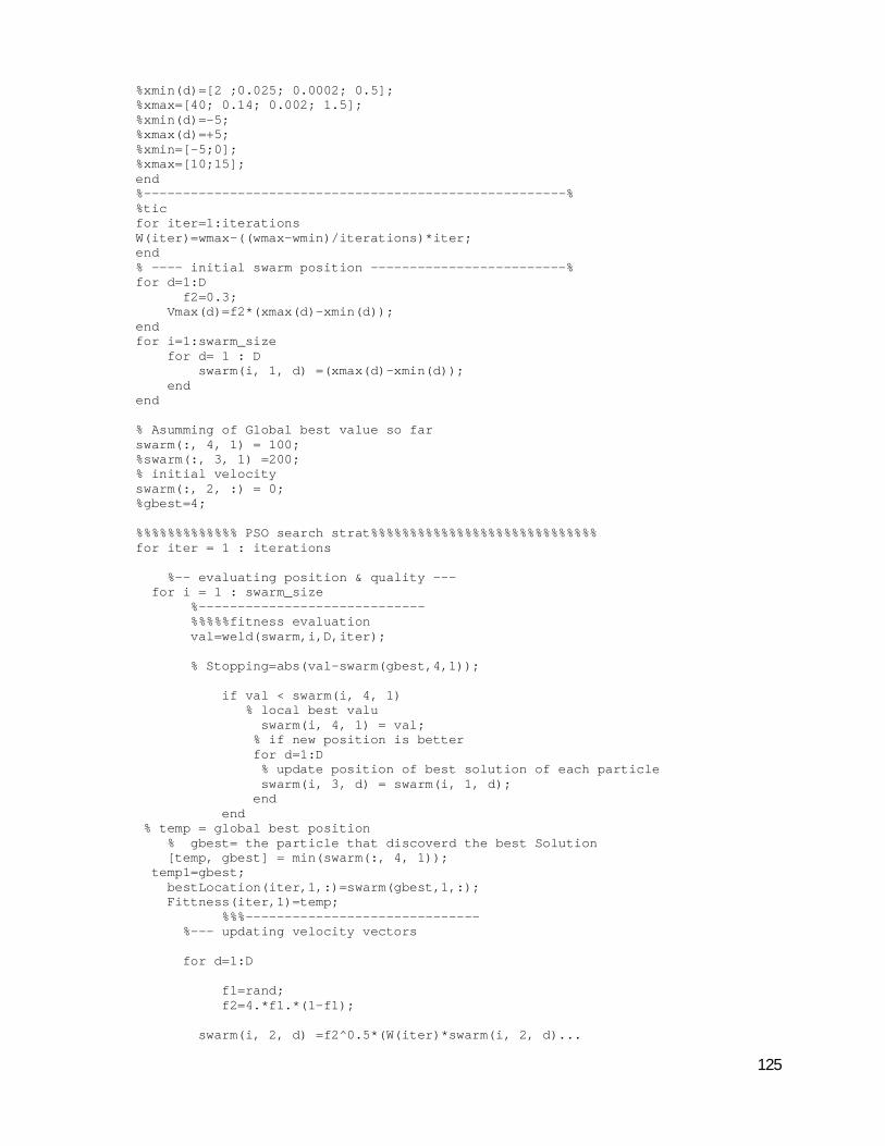
125
%xmin(d)=[2 ;0.025; 0.0002; 0.5]; %xmax=[40; 0.14; 0.002; 1.5]; %xmin(d)=-5; %xmax(d)=+5; %xmin=[-5;0]; %xmax=[10;15]; end %------------------------------------------------------% %tic for iter=1:iterations W(iter)=wmax-((wmax-wmin)/iterations)*iter; end % ---- initial swarm position -------------------------% for d=1:D f2=0.3; Vmax(d)=f2*(xmax(d)-xmin(d)); end for i=1:swarm_size for d= 1 : D swarm(i, 1, d) =(xmax(d)-xmin(d)); end end % Asumming of Global best value so far swarm(:, 4, 1) = 100; %swarm(:, 3, 1) =200; % initial velocity swarm(:, 2, :) = 0; %gbest=4; %%%%%%%%%%%%% PSO search strat%%%%%%%%%%%%%%%%%%%%%%%%%%%%% for iter = 1 : iterations %-- evaluating position & quality --- for i = 1 : swarm_size %----------------------------- %%%%%fitness evaluation val=weld(swarm,i,D,iter); % Stopping=abs(val-swarm(gbest,4,1)); if val < swarm(i, 4, 1) % local best valu swarm(i, 4, 1) = val; % if new position is better for d=1:D % update position of best solution of each particle swarm(i, 3, d) = swarm(i, 1, d); end end % temp = global best position % gbest= the particle that discoverd the best Solution [temp, gbest] = min(swarm(:, 4, 1)); temp1=gbest; bestLocation(iter,1,:)=swarm(gbest,1,:); Fittness(iter,1)=temp; %%%------------------------------ %--- updating velocity vectors for d=1:D f1=rand; f2=4.*f1.*(1-f1); swarm(i, 2, d) =f2^0.5*(W(iter)*swarm(i, 2, d)...

126
+f2*correction_factor1*rand*(swarm(i, 3, d)- swarm(i, 1, d))... + correction_factor2*rand*(swarm(gbest, 1, d)- swarm(i, 1, d))); if iter >= iterations/2 swarm(i, 2, d)= swarm(i, 2, d)+swarm(gbest,3, d)/swarm_size*exp (W(iter)^2*f2); end if (swarm(i,2,d)>Vmax(d)) swarm(i,2,d)=f2*Vmax(d); end if (swarm(i,2,d)<-Vmax(d)) swarm(i,2,d)=-f2*Vmax(d); end %update particle's position swarm(i, 1, d) =(swarm(i, 1, d) +f2*swarm(i, 2, d)); if (swarm(i,1,d)>xmax(d)) swarm(i,1,d)=f2*xmax(d); end if (swarm(i,1,d)<xmin(d)) swarm(i,1,d)=f2*xmin(d); end end end % Final(NR,1)=temp; %if Stopping<0.0001 % Fiter=iter; % toc % break %end end AFinal(NR,1)=temp; %plot(Fittness,'k-') fh = figure(1); % returns the handle to the figure object set(fh, 'color', 'white'); % sets the color to white h=plot(Fittness); get(gcf); get(gca); get(h); %o modify the line style. Possible options are ':' dotted, '-' solid, '--' %dashed, '-.' dash-dotted set(h,'linestyle','-'); set(h,'color','y'); set(h,'linewidth',5); set(h,'marker','s'); set(h,'markersize',1); set(gca,'box','off'); xlabel('iteration','fontsize',12,... 'fontweight','bold'); ylabel('Fucntion Minimization','fontsize',12,... 'fontweight','bold'); %Legend('PSO','CSPO','CPSO1','CPSO2','CPSOM','CPSOM1','CPSOM2'); grid; %[glob,iterF]=min(Fittness(:,1)); %FINAL=glob; %FinalLocation=bestLocation(iterF,1,:);

127
%plot (bestLocation,'dg-.','DisplayName', 'Fittness', 'YDataSource', 'Fittnes' ); figure(gcf) % Defines limits for x and y axes, and sets title, labels and legends %axis([0 2*pi -1.5 1.5]) %title('2D plots', 'fontsize', 12) %xlabel('iteration') %ylabel('Fucntion Minimization') %legend('cos(x)', 'sin(x)') %axis([0 1000 0 0.5]);
Benchmark Functions
function val= asd(swarm,i,D) for d=1:D x(d)=swarm(i,1,d); end val=0; %----------------------- Sphere for d=1:D val=val+x(d)^2;end %---------------------------------------------------------- %%Rosenbrock &&&&&&&x1&x2=[-5,5] for d=1:D-1 a1=x(d+1)-(x(d))^2; b1=1-x(d); val=val+((100*(a1)^2+(b1)^2)); end %-------------------------------------------------------------- % Brianin function x1=[-5,10]& x2=[0,15] val =(x(2)-(5.1/(4*pi^2))*x(1)^2+(5/pi)*x(1)-6)^2+(10*(1-(1/(pi*8)))*cos(x(1))+10); %----------------------------------------------------------------------- %Rastrigrin val=x(1)^2+x(2)^2-cos(18*x(1))-cos(18*x(2)); val=x(1)^2+x(2)^2-cos(18*x(1))-cos(18*x(2)); val=(4-(2.1*x(1)^2+x(1)^4/3))*x(1)^2+(x(1)*x(2))+(-4+4*x(2)^2)*x(2)^2; for d=1:D val=val+(x(d)^2-(10*cos(2*pi*x(d)))+10); end %=========================== % Griewank function n=D; fr = 4000; s = 0; p = 1; for d = 1:n; s = s+x(d)^2; end for d = 1:n; p = p*cos(x(d)/sqrt(d)); end val = s/fr-p+1; %========================