ikBîØe funs'kd % vuqiek flag

ikBîØe la;kstd % lqdkUr nk'k, vfuy dqekj

Cource Director : Anupama Singh Cource Coordinator : Sukanta Dash, Anil Kumar :

,u- ,s -b- ;kstuk& Hkk-—-vuq-i- ds rRok/kku es mRikn ,oa çlaLdj.k

fodklksUeq[k ijh{k.kksa gsrq vk/kqfud vfHkdYiukvksa ij vçR;{k çf'k{k.k

dk;ZØe

(16-17 ekpZ, 2021)

Virtual Training Programme On Advanced Designs for Product and Process Development

Oriented Experiments Under the aegis of NAE Scheme of ICAR

(16-17 March, 2021)

Hkk-—-vuq-i- & Hkkjrh; —f"k lkaf[;dh vuqla/kku laLFkku

Ykkbczsjh ,osU;w] iwlk] ubZ fnYyh & 110012

ICAR- INDIAN AGRICULTURAL STATISTICS RESEARCH INSTITUTE

LIBRARY AVENUE, PUSA, NEW DELHI – 110 012 (INDIA)

—f"k jlk;u laHkkx] Hkk-—-vuq-i- & Hkkjrh; Ñf"k vuqla/kku

laLFkku] ubZ fnYyh - 110012 DIVISON OF AGRICULTUAL CHEMICALS, ICAR-

INDIAN AGRICULTURAL RESEARCH INSTITUTE, NEW DELHI- 110012 (INDIA)

http://iasri.icar.gov.in

¼ Hkk-Ñ-vuq-i-& Hkkjrh; Ñf"k lkaf[;dh vuqla/kku laLFkku] ubZ fnYyh ,oa —f"k jlk;u laHkkx] Hkk-Ñ-vuq-i-&

Hkkjrh; Ñf"k vuqla/kku laLFkku] ubZ fnYyh ½

(Jointly organized by ICAR-IASRI and DIVISON OF AGRICULTURAL CHEMICALS,

ICAR- IARI, New Delhi)

lanHkZ iqfLrdk

Reference Manual

qFFREFT

ql?3t5q-qrstftq pft uif$1+51 erStlum qiqelri tqr,\ p{B urfu;ft Vei ra++ furrq u'-r

q- 31frft 11{aryr t r *o* d pfr- wfur+1 ii etq ord d qler-qT?l 3le{ir{ qq qRreTor

ordmrT rff qdN qrd B 3il{ g-s-n qfteiqrem erft-+emen, e-R-flq-{ d-f,fiqn, qTE.trq;tq

sr1oM, q-{rEI TqfXurq nq,ffi do-quw S* I"TT^ergu*'r.w^fr$ qre kqI qrdr

Bi qrerq frt EE qTtrqftt \.q vrrrur6'er=irui,r tl qjcifud qirqqffi t-qT d 6xul "€|.

eR u.grr*o Vu tlt* qoftft o <ttflu gB uil?<lfll"t"fl i qrsarm or nreqd. rem ! t

.ffi. tm "j*rq (q Rreri lrqr.fi .) ililft.i,) .n Ri\ sqrl)rft tnltrrihlq .5*=1qq td'.n

ffil-o oqi ii rft qr.{att.r 3{,J,1} B t

911B461 sq t Aq Frqt fi s"".ow pB cqrlurr o1 ffq qqr,i d r furq^ trq q" ?R

3T5qtrrq o\ qfultff qiri d ftq qst *- lfi Gfi-qd ot ql-fid{ vq ffiq"T sfua

"fu*dl, fr|fq\ gm farqr .ilq t qrserri gr{r 3ndFsfl qRreT"r 6Td-mq ttrfLql+Tq d-dtfui d

ft"* o) EB \.q r+d€ or5riur.r t oi&<t otqtfio qq\ftrrci o) qprriloftd o-{i d eEd

sqqYft ft-s gq t t

qfqrq qRreTur -orrimq "BFTTE \ti s-*iw-tq fffli+Tq q-{lH!il tg slgF.o elffi" q't

o**r, gfr ffiru-vn 1-q qTfur+1fr{ o) 1'fi qTed .an A .r*q t dl q-{ B nIfu q-6qrm

d enq{+ t qu qjqilq {r.,wi .} qrq erido c:l 3lfp)o l?-.rtd oT 3Tr{T;I ITET;I o\ nd r 5s)

frrilq t fr, ryg otrivnat t'6qrlili o) orltiur-r *J q',ilfr qr-{ r\ ord oqi t\ ,il {reTq

-*r\r, fi, q{rq fi tgrft-o qfler"ir d l?rf irf}-q;qqr3ii ot s€l uq{n'T oq'i gq '3-r-q')

Gilgft-o qifuot qqfrq\ dl qErqin qi ttr fl.Tvhd ltorai ii .ft qrtT{o *'rr I

lTRreTq orriri,,t {{t yct.,T( drlq f+qr rlqT t fA gql{ frqrFtro Ve uyut"'r ".t! q6g

rrfl*rhrr B t yl?rerir ,) .$Frila(r fiqq) $'s yotq B, (o) qoa mlto qfteroil d fa\ e#)'norqr

(sq) qg oT{o qfte{"il d f}{ 3lflf+-iq.il (q) 1g-1uf&ul. qfter'il ig 3rft-6nqTq (q)

i"it .it .rfta,il S tuq erftocqil \q (s) stros) d frAqq & qrffi nq ftqifrq I

w<.f gRror i fui rT\ .r-rrL{t;r, lilEq or l}qo fr"y lTil{ ori B t oirm t fu qRrer"r

ordmi d q)ql,r qord ,rd ilrrrr3r) q;) n,Er'} *\ {ii,',rrftd d feq ue ilera .rqd'lt $'n t

{ q1qd qi.Tilq {r.rgi +i $q{ .ntri +' laq E;l{o eI.lTcII( tor ql -d ofn cprft, qq-q1qq1

(or),"u-ftel"r etfroelqr dali 91{ yfueror ord*,q .} qrq},l.n Y g-'{, fltle, d. Sorf,- ErYr

G 3 3rfra q-qrq A gq q-g1el Er<niyt .ii 'rrrq * d-qrr qt{i d fuq q.rf, o-r5-qo t t

"\\sT^Lagftd (rr$q 6$ rrrd. zozt f{t{r-6, qr.?'3rg'q'-u'7'ui'ot'r{'

srgsqr.?.3rgq-qmfi-q EE infM er5uwt s{a{T;r, Eft rsrM vq q'fir ft-wn .nr qf, 3rqot {NqFrt t qa \4{qH qT.?.3I.q. d Rreir q',{rr d qrrq w*ntrq ft-om ordffq d asrqtrn d EE eiM vq€T'ro er]q"ilT ii v.q lrorq vRrerur d< d sc t fi ord oq w t t s"=q e-orq qRrsT"r d< d3ffi.fd 3ilZilfud frtd afi qrd vRreT"r oTffi d 3{frftfi -r{isnr .rrrftq ER q-jgqm qR'q-q d PrenfulTrrT grr qrq}fuf, tffic/effir EF f,Qrr fuft';{ vt*ir qs qft,qq wiermt ot3rlYso-drJy( sr-q qRlwr ord-s,-q rfr sndfuo oror t t qtqrq qflrepr ord-*-q qrp3tSq''*qR-frqPR qrfurr+t r5vun s{ell;r vs EE {sl{rl rrqrrr, qr.F.3rjq- qrrftq fR 3rjsqm $s"rn iln g1rtrq t eildfua fu-qr .rqr t r

sq5ffi triffiq nE fid ot erSndt, eE .f,ds.nfl o1 4'q t r gfr 3i-jqqg of 5"r-aaor qqd {si1.q {.6ri A ftf qd 3rer<I Tnd{d VE 3ilcr"rqo t fu 3ffi d dofi, Mq"r \q

-qMI of eqrqr

d fil\ sfuo et1Mq qqfrzri o) errcrqr -qr$ r ER lgrM + \.rqf*fl silq zmqt d stern iqrfuq-+t of gfisr { srq{r sEE {€IT;I qil {qr t t

PR YiTf,dfuil d qlilCqotq .Rrqpi qi'.ry ti ii nqqr'{ ogo er-5r.fr t t wqerc aN gr(}q pfi erww{r"lrfr d oTd-{d efr ftN o) {-rirqtf fu q<Tl .tr{ {6r t I ilfr uiss d ir{am n go fgw$cffi sfi (http://drs.icar.gov.inl oi fuors fuqT t I s{am i Nenps d ftf rtEftsoo znqErrfr&o (@)or fr fuf,rq fuqr t M em.r*3rf,q rrcirT otq 3tTfl+SsmqErrd wt fud W t rRerfr fAPrqd-e qqrqm.fr*iqedm n ffiaf}-d Wd 3il({+q{er1;r d tqy6 q{ H1rn;q rnc odfi, ii gTf,eT fu-qr .rqr t I s{srg o) gB ffir d f&\, EE3rjqqFT q sfud {nfuq.htq .ro;ftdi d erSrdrr .d -{dr.} d stcq d -d'+-s qRreTq ord-oq 3{rq}fu(ori or fi ft-qer srSro t r

cdqr.{ qPreT"r ordmq " \rarc gs ,Nfw-{"r ff{rd=5-s qftH"il ig silgfuo olftoenryseT qfierq qft=q-snreii \s q€le{orrcTo sfr,ild d ffiEur of qRq-ir qiMq ffiEur a-m-ffi qfuorq t r+'ro uqr+r t I qffi of qrcqr o{i vs qi1fusrwr w ffis q-a kqr qr}'lr t cfuerurord-f,q d rqr q-6"R i-qts fuqr rrqT t fo zrt fuGr< qs 3ryqqiT zry ft61-q-6r Fv * I gs cRreT"rord-q,q d +{H, 's-d.il.ft \sqgs/Vq\rs_q.q$f,Z3ni qfweArri {Grfq sfffiq Wi d 3qqdrrrm erio 3ffi d fut znr ffiqur oti r g{rs qRrnqrqoq, fs $csrr-r d aErrM 3il{ qtf 3r5q- .Trfiq pft erXew'r {Nsn{ d orfw qlB Mim) -.} fis wsq}'r qd.rrt

6q qrft sors werqi or uffio tr<rclrq q,ri d fiF€)-i wtrrdcndr o) s+rzlo vs srnd q.Tri i srcfl3rf,@ wrrq fuqT t t gs rcFf,r o) dqrq ttr{i t Zftd o'r oq .nri .Fr 6{ sr+rcr rlqrcl fuqr rTqT t, fu{fr oM re sf,fi t I qrrfi-q ER lsrM ergwun ws{Tr{ ur iluo, gq iift-dr ii fr .d qm.fr An*q am gi fd$ 'rft rox at flfr d fil\ vf,wrfr {S E}-n I 6q ?fr frre+r Eqnr gq fteelqr, qrF.3r3.q.- qri-fis pE q-$sqn s{affi znt 3ilqT( r+-e .nri t ftrdii {s ordqrf,r d fr\ qEqrmi o)qTqifud ftrqrtaq d. srGs qgr(, F-eyrzn,,Trq3r5.,{ qr.f \n3{q d 3rrrrrft t f}€ii -6qRr qrfEyf{fuqT 3il{ {fl odytrc'n fr e'$,r isft qnTq rrft q rfr *pft qm{qo Eft*lr( !qce{ o'{r$ r 6q d. {ftqrqrrft, vqr'naret (ot), qfter"r GIFTo-.or+ or fl$q s..iEs oril.[ir] fu*)? frftq.rffiffii d aqmqFHq vs sd*q fu-qr t rq sc !rq-d qfd .fr 3mrft t Hi-i ercri 3rqo e-qrq\ t rs r{R-or o1dqn 6-{i ii q6 of t r

q{ Fffi$ qd, 2021

I{*'\( e'

g6Tf, ERTrrkpED-rr TifrGr6

FOREWORD

The ICAR-lrrrlian Agricultural statistics llcscarch Institute is a premier Instirute in the discipline of

Agricultural Statistics ancl lnformatics in the country' 'I'he tnstitute has been engaged in conducting

research, teaching ancl organizing training prog.u*-"' in Agricultural statistics and lnformatics with

special emphasis o" "EXf"ri*Ental

Dlsigni Sampling "Techniques' Statistical Genetics' Crop

Forecasting Techniques, BioiniormaLi., uni Compuiet Applications' The Institute has been very

actively pursuing ac-lvisory services that have enabled the institute to make its presence felt both in

NationalAgriculturalResearch&F,t.lucationSystem(NARES)anclNatiorralAgriculturalStatisticsSystem (NASS). 'fhe l^stitute has take. a leacl in .l"reiopi^g Statistical Software Packages useful for

Agricultural Research.

statistically valicl inferences lay the fountlations of quality agricultural research' ln order to make

research globally competitive, it is esse.tiai that sountl statlst'i-*t methodologies be adopted for the

collection and analysis of clata. The training programn-res organizecl by the Institute a-re very useful in

appraising the advances in statisticut t".i,-riq,r""s to the uJtuul us"rs in the agricultural and allied

sciences.

Thepresentonlinetraining"Advanced?."-:iq"tlt:.Uld"tlandProcessf)evelopmentOrientedExperiments" jointly organizecl by ICAR-lASRi a,.',1 Division oi Agricultural Chemicals' ICAR- IARI'

New Delhi has bc.cn especially tlcsigrretl to Lrrir.rg facultv.n-rernl-rcrs int'l stut'lc'nts in NARI]s together so

as to tlerive the maximu,.,, aiu,.1,-.*i. a,.ivantagti through interaction with tht-' iaculty ancl among the

fellow participants. I am sure that the e*peri",-,"cc gai,rell frorrr this training will cnable the participants

to concluct their research more effectively u,i.1 dru* valitl concluiions by aclopting suitable

experimental designs for their scientific experimentation ancl using appropriate and modern statistical

methodologies foianalyzing clata generated from such experiments'

The training contents are intertwining of theory antl application- 'l'he topics arc covcrctl are as follows:

(a)Desig.s for Single Factor Ilxperiments, (L)Ocsigrrs for Multi-pactor Lrxperiments' (c)Rcsponse:

surface Designs antl Applications, (c-l)Designs for Bioassay ancl (e) web resources on clesignecl

experimcnts.

The lecture notes given in tl-re reference manual provide a detailecl exposition of the subiect' I hope

that the reference manual will 6c quite useful to ihc participants. I take this opportunity to thank the

entirefacultyforiloingawoncieriuliob.lwishtocomplementl)r'SecmaJaggi'HeadofDivision(A)'Design of Experimeits, pr. Sukanta Dash, Course Co-Coortlinators Dr' Anil Kumar' Course

Coorclinator, fo. U.i,-rgi,-,g out this valuable document on time' We look forwarr'-l to suggestions from

every corner in improving this manual'

New Delhi15 March,2021

aJRaien6r Parsad

DIRECTOR, ICAR-IASRI

PREFACEThe ICAR-lntlia. Agricultural statistics Rcsearch Institute has been ancl contilrues to be a premierInstitute in the discipline of Agricultural Statistics anti Informatics. 'l'he institute is also functioning asa Centre of Aclvanced Faculty I raining in Agricultural statistics ancl Conrputer Ap-rplications unclerthe aegis of Human Ilesource Deve'lopinent Programnre of the Education Division of ICAR. Besiclesorganizing the training programme uncler CentrJof Arlvancecl Faculty 'l'raining

1cnil.y, Institute alsotakes lead in conduct of summer/ winter school sponsored by Eclucation Division of ICAR ancl tailormade training programmes for clifferent national antl international organizations. The present onlinetraining proSramme is being organized jointly by by ICAR-lASIil antl Division of AgriculturalChemicals, ICAR- IAIil, New Delhl

Application of appropriatc statistical techr.riclues iornrs the backbor.re of ar.ry research encleavour inagriculture and alliecl sciences. In orcler to maintain ancl improve the quality oi agricultural research,it is of paramount importance that sounci and modern siatistical methodologies are usecl in theloll.e-ctio1

and analysis of clata ancl then in the interpretation of results. The lnstitute has establisheditself in the world of statistics so far as research in Agiicultural Statistics is concerned.

The Institute has also become a veteran in .rigorously undertaking the consultancy antl ac-lvisoryservices for the ag,ricultural rcsearch pc'rsonnL-l. i-nstitutc nu* plun, to start [:-arlvisory services for theresearch personnel in NAIttrs. with this air.n, l.stitute has taken a Ie.ar-l in thc cle-velop.rrent of a DesignResources server (http://c{qlealgq-v'in;.-l'hc'lrrstitute has also dcveloprecl Inc-lian NARES statisticalComputing Portal (http://stat.iairi.res.inl'qcll4-Igfortal) in which analysis oi clifferent events isprovided as a service orientet'l computing. sit rti";;r;fic web solutions have also been developedin the institute and macle availat-,te in puutic domain at instit.ute webpage. The Institute has a vastexperience of organizing several training programmes for the agriculfural scientists with a view toimprove the use of souncr statisticar technlques in agricultural research.

'rhe present online training "Advanced Designs for I'roduct and process Development rJrientedExperiments" is designed to acquaint the participrants with the atlvances in experimental cle-signs anclstatistical analytical techniques related to protiuci ancl process cieveloprnent oriented experiments. Theemphasis will also be laicl on interpretation and presentation of results. 'rhe training programme isplanned in such a way that it is blencl of theory and applications.'Ihe participants will be familiarizec.lwith experimental cleiigns for product ancl.process development oriented experiments. This trainingprogramme will also enable to build a briclge between thii Institute ancl the faculty ancl stuclents ofICAR-lARI, New Delhi.

we take this opportunity to thank all the faculty nrembers who have. clevoted their time ancl energy inmaking this training Programe r1reanirrgful ari.l successful. AIthoug,h every erlitorial care has beentaken in preparing the nranual, errors in.l omissions arc Iikely to occur. ICAII-lnciian AgriculturalStatistics Research lnstitute' or the' authors are, however,_ in no *uy ,"rponsible for any liability arisingout of the use of the contents of this referencc' rnanual. we are thaniful to Division of AgricultureEducation-' ICAR for provicling.aJl-necessary support to organize this training programme uncler NAEscheme of lCAIt. we are thankful to Director, ICAR-rAI{ for ailorganize this online workshop. we are also grateful t. Dr. najen.r"5;:t"X5:X.t#r'.:[-ii1,ffr::his guidance and continuous interest in this workshop ancl rnuting ail necessary facilities available tous we would like to make a special mention.of Dr. seema Jaggi, l-iead (A), t)esign of Experiments forher guit'lance antl support. we are also thankful to one ana"Jt for tlre.ir untiring elforts anri help inprcparing this nrarrual.

d.New Delhi1.5 March,2021

4*tSukanta Dash

Course CoordinatorAnil Kumar

Course Coordinator

CONTENTS

1. Planning and Designing of Agricultural Experiments - Seema Jaggi

1-8

2. Fundamentals of Design of Experiments - V.K. Gupta and Rajender Parsad

9-50

3. Designs for Factorial Experiments - V.K.Gupta, Rajender Parsad, Seema Jaggi and Sukanta Dash

51-81

4. Response Surface Designs - Rajender Parsad and Krishan Lal

82-96

5. Designs for Bioassays - Krishan Lal

97-109

6. Design Resource Server - Rajender Parsad , V.K. Gupta and Sukanta Dash

110-125

7. Computational Tools for Drug Design and Discovery - Abhishek Mandal

126-139

8. NAE- Capacity Building Program: An Overview - Sukanta Dash and Anil Kumar

140-151

Planning and Designing of Agricultural Experiments

SEEMA JAGGI

ICAR-IASRI, Library Avenue, Pusa, New Delhi – 110 012

Seema.jaggi@icar.gov.in

An experiment is usually associated with a scientific method for testing certain phenomena.

An experiment facilitates the study of such phenomena under controlled conditions and thus

creating controlled condition is an essential component. Scientists in the biological fields

who are involved in research constantly face problems associated with planning, designing

and conducting experiments. Basic familiarity and understanding of statistical methods that

deal with issues of concern would be helpful in many ways. Researchers who collect data

and then look for a statistical technique that would provide valid results will find that there

may not be solutions to the problem and that the problem could have been avoided first by

a properly designed experiment. Obviously it is important to keep in mind that we cannot

draw valid conclusions from poorly planned experiments. Second, the time and cost

involved in many experiments are enormous and a poorly designed experiment increases

such costs in time and resources. For example, an agronomist who carries out fertilizer

experiment knows the time limitation of the experiment. He knows that when seeds are to

be planted and harvested. The experimenter plot must include all components of a complete

design. Otherwise what is omitted from the experiment will have to be carried out in

subsequent trials in the next cropping season or next year. The additional time and

expenditure could be minimized by a properly planned experiment that will produce valid

results as efficiently as possible. Good experimental designs are products of the technical

knowledge of one's field, an understanding of statistical techniques and skill in designing

experiments.

Any research endeavor may entail the phases of Conception, Design, Data collection,

Analysis and Dissemination. Statistical methodologies can be used to conduct better

scientific experiments if they are incorporated into entire scientific process, i.e., From

inception of the problem to experimental design, data analysis and interpretation. When

planning experiments, we must keep in mind that large uncontrolled variations are common

occurrences. Experiments are generally undertaken by researchers to compare effects of

several conditions on some phenomena or in discovering an unknown effect of particular

process. An experiment facilitates the study of such phenomena under controlled

conditions. Therefore, the creation of controlled condition is the most essential

characteristic of experimentation. How we formulate our questions and hypotheses are

critical to the experimental procedure that will follow. For example, a crop scientist who

plants the same variety of a crop in a field may find variations in yield that are due to

periodic variations across a field or to some other factors that the experimenter has no

control over. The methodologies used in designing experiments will separate with

confidence and accuracy a varietal difference of crops from the uncontrolled variations.

The different concepts in planning of experiment can be well explained through chapati

tasting experiment.

Consider an experiment to detect the taste difference in chapati made of wheat flour of

2

c306 and pv 18 varieties. The null hypothesis we can assume here is that there is no taste

difference in chapatis made of c306 or pv18 wheat flours. After the null hypothesis is set,

we have to fix the level of significance at which we can operate. The pv18 is a much higher

yielding variety than c306. Hence a false rejection may not help the country to grow more

pv18 and the wheat production may decrease while a false acceptance may give more

production of pv18 wheat and the consumption may be less or practically nil. Thus the

false acceptance or false rejection are of practically equal consequence and we agree to

choose the level of significance at α = 0.05. Now to execute the experiment, a subject is to

be found with extrasensory powers who can detect the taste differences. The colors of c306

and pv18 are different and anyone, even without tasting the chapatis, can distinguish the

chapatis of either kind by a mere glance. Thus the taster of the chapatis has to be

blindfolded before the chapatis are given for tasting. Afterwards, the method is to be

decided in which the experiment will be conducted. The experiment can be conducted in

many ways and of them three methods are discussed here:

Give the taster equal number of chapatis of either kind informing the taster about it.

Give the taster pairs of chapatis of each kind informing the taster about it.

Give the taster chapatis of either kind without providing him with any information. Let

us use 6 chapatis in each of these methods.

Under first method of experimentation, if the null hypothesis is true, then the experimenter

cannot distinguish the two kinds of chapaties and he will randomly select 3 chapatiS out of

6 chapaties given to him, as made of pvl8 wheat. In that case, all correct guesses are made

if selection exactly coincides with the exactly used wheat variety and the probability for

such an occurrence is:

05.020

1163

Under second method,the pv18 wheat variety chapaties are selected from each pair given if

the null hypothesis is true. Furthermore, independent choices are made of pv18 variety

chapaties from each pair. Thus the probability of making all correct guesses is

1/(2)3 = 1/8 = 0.125.

In third method the experimenter has to make the choice for each chapati and the situation

is analogous at calling heads or tails in a coin tossing experiment. The probability of making

all correct guesses would then be:

1/26 = 1/64 = .016.

If the experimenter makes all correct guesses in third method as its probability is smaller

than the selected = 0.05, we can reject the null hypothesis and conclude that the two wheat

varieties give different tastes at chapaties. In other methods the probability of making all

correct guesses does not exceed = 0.05 and hence with either method, we cannot reject

the null hypothesis even if all correct guesses are made.

However, if 8 chapaties are used by first method and if the taster guesses all of them, we

can reject the null hypothesis, at 0.05 level of significance, as the probability of making all

3

correct guesses would then be

5611

83

which is smaller than 0.05. 8 chapaties will

not enable us to reject the null hypothesis even if all correct guesses are made by second

method as the probability of making all correct guesses is 06.016

1

4

14

it is easy to

see that if 10 chapaties are given by second method and if all correct guesses are made, then

we can reject the null hypothesis at 0.05 level of significance. Not to unduly influence the

taster in making guesses, we should also present the chapaties in a random order rather than

systematically presenting them for tasting.

The above discussed chapati tasting experiment brings home the following salient features of experimentation:

All the extraneous variations in the data should be eliminated or controlled excepting

the variations due to the treatments under study. One should not artificially provide

circumstances for one treatment to show better results than others.

Far a given size of the experiment, though the experiment can be done in many ways,

even the best results may not turn out to be significant with some designs, while some

other design can detect the treatment differences. Thus there is an imperative need the

choose the right type of design, before the commencement of the experiment, lest the

results may be useless.

If for some specific reasons related to the nature .of the experiment, a particular

method has to be used in experimentation, then adequate number of replications of

each treatment have to be provided in order to get valid inferences.

The treatments have to be randomly allocated to the experimental units.

The terminologies often used in planning and designing of experiments are listed below.

Treatment

Treatment refers to controllable quantitative or qualitative factors imposed at a certain level

by the experimenter. For an agronomist several fertilizer concentrations applied to a

particular crop or a variety of crop is a treatment. Similarly, an animal scientist looks upon

several concentrations of a drug given to animal species as a treatment. In agribusiness we

may look upon impact of advertising strategy on sales a treatment. To an agricultural

engineer, different levels of irrigation may constitute a treatment.

Experimental Unit

An experimental unit is an entity that receives a treatment e.g., for an agronomist or

horticulturist it may be a plot of a land or batch of seed, for an animal scientist it may be a

group of pigs or sheep, for a scientist engaged in forestry research it may be different tree

species occurring in an area, and for an agricultural engineer it may be manufactured item.

Thus, an experimental unit maybe looked upon as a small subdivision of the experimental

material, which receives the treatment.

4

Experimental Error

Differences in yields arising out of experimental units treated alike are called Experimental

Error.

Controllable conditions in an experiment or experimental variable are terms as a factor. For

example, a fertilizer, a new feed ration, and a fungicide are all considered as factors. Factors

may be qualitative or quantitative and may take a finite number of values or type.

Quantitative factors are those described by numerical values on some scale. The rates of

application of fertilizer, the quantity of seed sown are examples of quantitative factors.

Qualitative factors are those factors that can be distinguished from each other, but not on

numerical scale e.g., type of protein in a diet, sex of an animal, genetic make up of plant

etc. While choosing factors for any experiment researcher should ask the following

questions, like What treatments in the experiment should be related directly to the objectives

of the study? Does the experimental technique adopted require the use of additional factors?

Can the experimental unit be divided naturally into groups such that the main treatment

effects are different for the different groups? What additional factors should one include in

the experiment to interact with the main factors and shed light on the factors of direct

interest? How desirable is it to deliberately choose experimental units of different types?

Basic Principles of Design of Experiments

Given a set of treatments which can provide information regarding the objective of an

experiment, a design for the experiment, defines the size and number of experimental units,

the manner in which the treatments are allotted to the units and also appropriate type and

grouping of the experimental units. These requirements of a design ensure validity,

interpretability and accuracy of the results obtainable from an analysis of the observations.

These purposes are served by the principles of:

Randomization

Replication

Local (Error) control

Randomization

After the treatments and the experimental units are decided the treatments are allotted to the

experimental units at random to avoid any type of personal or subjective bias, which may

be conscious or unconscious. This ensures validity of the results. It helps to have an

objective comparison among the treatments. It also ensures independence of the

observations, which is necessary for drawing valid inference from the observations by

applying appropriate statistical techniques.

Depending on the nature of the experiment and the experimental units, there are various

experimental designs and each design has its own way of randomization. Various speakers

while discussing specific designs in the lectures to follow shall discuss the procedure of

random allocation separately.

Replication

If a treatment is allotted to r experimental units in an experiment, it is said to be replicated

r times. If in a design each of the treatments is replicated r times, the design is said to have

r replications. Replication is necessary to

5

Provide an estimate of the error variance which is a function of the differences among

observations from experimental units under identical treatments.

Increase the accuracy of estimates of the treatment effects.

Though, more the number of replications the better it is, so far as precision of estimates is

concerned, it cannot be increased infinitely as it increases the cost of experimentation.

Moreover, due to limited availability of experimental resources too many replications

cannot be taken.

The number of replications is, therefore, decided keeping in view the permissible

expenditure and the required degree of precision. Sensitivity of statistical methods for

drawing inference also depends on the number of replications. Sometimes this criterion is

used to decide the number of replications in specific experiments.

Error variance provides a measure of precision of an experiment, the less the error variance

the more precision. Once a measure of error variance is available for a set of experimental

units, the number of replications needed for a desired level of sensitivity can be obtained as

below.

Given a set of treatments an experimenter may not be interested to know if two treatment

differ in their effects by less than a certain quantity, say, d. In other words, he wants an

experiment that should be able to differentiate two treatments when they differ by d or more.

The significance of the difference between two treatments is tested by t-test where

,r/s2

yyt

2

ji

Here, ,y i and jy are the arithmetic means of two treatment effects each based on r

replications, s2 is measure of error variation.

Given a difference d, between two treatment effects such that any difference greater than d

should be brought out as significant by using a design with r replications, the following

equation provides a solution of r.

,r/s2

dt

2

2

2

2

0 s2xd

tr …(1)

where 0t is the critical value of the t-distribution at the desired level of significance, that is,

the value of t at 5 or 1 per cent level of significance read from the t-table. If s2 is known or

based on a very large number of observations, made available from some pilot pre-

experiment investigation, then t is taken as the normal variate. If s2 is estimated with n

6

degree of freedom (d.f.) then t0 corresponds to n d.f.

When the number of replication is r or more as obtained above, then all differences greater

than d are expected to be brought out as significant by an experiment when it is conducted

on a set of experimental units which has variability of the order of s2. For example, in an

experiment on wheat crop conducted in a seed farm in Bhopal, to study the effect of

application of nitrogen and phosphorous on yield a randomized block design with three

replications was adopted. There were 11 treatments two of which were (i) 60 Kg/ha of

nitrogen (ii) 120 Kg/ha of nitrogen. The average yield figures for these two application of

the fertilizer were 1438 and 1592 Kg/ha respectively and it is required that differences of

the order of 150 Kg/ha should be brought out significant. The error mean square (s2) was

12134.88. Assuming that the experimental error will be of the same order in future

experiments and t0 is of the order of 2.00, which is likely as the error d.f. is likely to be more

than 30 as there are 11 treatments; Substituting in (1), we get:

.)approx( 4150

88.2134x2x2

d

st2r

2

2

2

22

0

Thus, an experiment with 4 replications is likely to bring out differences of the order of 150

Kg/ha as significant.

Another criterion for determining r is to take a number of replications which ensures at least

10 d.f. for the estimate of error variance in the analysis of variance of the design concerned

since the sensitivity of the experiment will be very much low as the F test (which is used to

draw inference in such experiments) is very much unstable below 10 d.f.

Local Control

The consideration in regard to the choice of number of replications ensure reduction of

standard error of the estimates of the treatment effect because the standard error of the

estimate of a treatment effect is rs /2, but it cannot reduce the error variance itself. It is,

however, possible to devise methods for reducing the error variance. Such measures are

called error control or local control. One such measure is to make the experimental units

homogenous. Another method is to form the units into several homogenous groups, usually

called blocks, allowing variation between the groups.

A considerable amount of research work has been done to divide the treatments into suitable

groups of experimental units so that the treatment effect can be estimated more precisely

Extensive use of combinatorial mathematics has been made for formation of such group

treatments. This grouping of experiment units into different groups has led to the

development of various designs useful to the experimenter. We now briefly describe the

various term used in designing of an experiment

Blocking

It refers to methodologies that form the units into homogeneous or pre-experimental

subject-similarity groups. It is a method to reduce the effect of variation in the experimental

material on the Error of Treatment of Comparisons. For example, animal scientist may

7

decide to group animals on age, sex, breed or some other factors that he may believe has an

influence on characteristic being measured. Effective blocking removes considerable

measure of variation nom the experimental error. The selection of source of variability to

be used as basis of blocking, block size, block shape and orientation are crucial for blocking.

The blocking factor is introduced in the experiment to increase the power of design to detect

treatment effects.

The importance of good designing is inseparable from good research (results). The

following examples point out the necessity for a good design that will yield good research.

First, a nutrition specialist in developing country is interested in determining whether

mother's milk is better than powdered milk for children under age one. The nutritionist has

compared the growth of children in village A, who are all on mother's milk against the

children in village B, who use powdered milk. Obviously, such a comparison ignores the

health of the mothers, the sanitary-conditions of the villages, and other factors that may

have contributed to the differences observed without any connection to the advantages of

mother's milk or the powdered milk on the children. A proper design would require that

both mother's milk and the powdered milk be alternatively used in both villages, or some

other methodology to make certain that the differences observed are attributable to the type

of milk consumed and not to some uncontrollable factor. Second, a crop scientist who is

comparing 2 varieties of maize, for instance, would not assign one variety to a location

where such factors as sun, shade, unidirectional fertility gradient, and uneven distribution

of water would either favor or handicap it over the other. If such a design were to be adopted,

the researcher would have difficulty in determining whether the apparent difference in yield

was due to variety differences or resulted from such factors as sun, shade, soil fertility of

the field, or the distribution of water. These two examples illustrate the type of poorly

designed experiments that are to be avoided.

Analysis of Variance

Analysis of Variance (ANOVA) is a technique of partitioning the overall variation in the

responses into different assignable sources of variation, some of which are specifiable and

others unknown. Total variance in the sample data is partitioned and is expressed as the sum

of its non-negative components is a measure of the variation due to some specific

independent source or factor or cause. ANOVA consists in estimation of the amount of

variation due to each of the independent factors (causes) separately and then comparing

these estimates due to ascribable factors (causes) with the estimate due to chance factor the

latter being known as experimental error or simply the error.

Total variation present in a set of observable quantities may, under certain circumstances,

be partitioned into a number of components associated with the nature of classification of

the data. The systematic procedure for achieving this is called Analysis of Variance. The

initial techniques of the analysis of variance were developed by the statistician and

geneticist R. A. Fisher in the 1920s and 1930s, and is sometimes known as Fisher's analysis

of variance, due to the use of Fisher's F-distribution as part of the test of statistical

significance.

Thus, ANOVA is a statistical technique that can be used to evaluate whether there are

differences between the average value, or mean, across several population groups. With this

model, the response variable is continuous in nature, whereas the predictor variables are

8

categorical. For example, in a clinical trial of hypertensive patients, ANOVA methods

could be used to compare the effectiveness of three different drugs in lowering blood

pressure. Alternatively, ANOVA could be used to determine whether infant birth weight is

significantly different among mothers who smoked during pregnancy relative to those who

did not. In a particular case, where two population means are being compared, ANOVA is

equivalent to the independent two-sample t-test.

The fixed-effects model of ANOVA applies to situations in which the experimenter applies

several treatments to the subjects of the experiment to see if the response variable values

change. This allows the experimenter to estimate the ranges of response variable values that

the treatment would generate in the population as a whole. In it factors are fixed and are

attributable to a finite set of levels of factor eg. Sex, year, variety, fertilizer etc.

Consider for example a clinical trial where three drugs are administered on a group of men

and women some of whom are married and some are unmarried. The three classifications

of sex, drug and marital status that identify the source of each datum are known as factors.

The individual classification of each factor is known as levels of the factors. Thus, in this

example there are 3 levels of factor drug, 2 levels of factor sex and 2 levels of marital status.

Here all the effects are fixed. Random effects models are used when the treatments are not

fixed. This occurs when the various treatments (also known as factor levels) are sampled

from a larger population. When factors are random, these are generally attributable to

infinite set of levels of a factor of which a random sample are deemed to occur eg. research

stations, clinics in Delhi, sire, etc. Suppose new inject-able insulin is to be tested using 15

different clinics of Delhi state. It is reasonable to assume that these clinics are random

sample from a population of clinics from Delhi. It describes the situations where both fixed

and random effects are present.

In any ANOVA model, general mean is always taken as fixed effect and error is always

taken as random effect. Thus class of model can be classified on the basis of factors, other

than these two factors. ANOVA can be viewed as a generalization of t-tests: a comparison

of differences of means across more than two groups.

The ANOVA is valid under certain assumptions. These assumptions are:

Samples have been drawn from the populations that are normally distributed.

Observations are independent and are distributed normally with mean zero and variance

σ2.

Effects are additive in nature.

The ANOVA is performed as one-way, two-way, three-way, etc. ANOVA when the number

of factors is one, two or three respectively. In general, if the number of factors is more, it is

termed as multi-way ANOVA.

9

FUNDAMENTALS OF DESIGN OF EXPERIMENTS

V.K. Gupta and Rajender Parsad

ICAR-I.A.S.R.I., Library Avenue, New Delhi - 110 012

vkgupta@iasri.res.in; rajender.parsad@icar.gov.in

1. Introduction

Any scientific investigation involves formulation of certain assertions (or hypotheses)

whose validity is examined through the data generated from an experiment conducted for

the purpose. Thus experimentation becomes an indispensable part of every scientific

endeavour and designing an experiment is an integrated component of every research

programme. Three basic techniques fundamental to designing an experiment are

replication, local control (blocking), and randomization. Whereas the first two help to

increase precision in the experiment, the last one is used to decrease bias. These techniques

are discussed briefly below.

Replication is the repetition of the treatments under investigation to different experimental

units. Replication is essential for obtaining a valid estimate of the experimental error and to

some extent increasing the precision of estimating the pairwise differences among the

treatment effects. It is different from repeated measurements. Suppose that the four animals

are each assigned to a feed and a measurement is taken on each animal. The result is four

independent observations on the feed. This is replication. On the other hand, if one animal

is assigned to a feed and then measurements are taken four times on that animal, the

measurements are not independent. We call them repeated measurements. The variation

recorded in repeated measurements taken at the same time reflects the variation in the

measurement process, while variation recorded in repeated measurements taken over a time

interval reflects the variation in the single animal's responses to the feed over time. Neither

reflects the variation in independent animal's responses to feed. We need to know about the

latter variation in order to generalize any conclusion about the feed so that it is relevant to

all similar animals.

For inferences to be broad in scope, it is essential that the experimental conditions should

be rather varied and should be representative of those to which the conclusions of the

experiment are to be applied. However, an unfortunate consequence of increasing the scope

of the experiment is an increase in the variability of response. Local control is a technique

that can often be used to help deal with this problem.

Blocking is the simplest technique to take care of the variability in response because of the

variability in the experimental material. To block an experiment is to divide, or partition,

the observations into groups called blocks in such a way that the observations in each block

are collected under relatively similar experimental conditions. If blocking is done well, the

comparisons of two or more treatments are made more precisely than similar comparisons

from an unblocked design.

The purpose of randomization is to prevent systematic and personal biases from being

introduced into the experiment by the experimenter. A random assignment of subjects or

experimental material to treatments prior to the start of the experiment ensures that

observations that are favoured or adversely affected by unknown sources of variation are

observations “selected in the luck of the draw” and not systematically selected.

10

Lack of a random assignment of experimental material or subjects leaves the experimental

procedure open to experimenter bias. For example, a horticulturist may assign his or her

favourite variety of experimental crop to the parts of the field that look the most fertile, or

a medical practitioner may assign his or her preferred drug to the patients most likely to

respond well. The preferred variety or drug may then appear to give better results no matter

how good or bad it actually is.

Lack of random assignment can also leave the procedure open to systematic bias. Consider,

for example, an experiment conducted to study the effect of drugs in controlling the blood

pressure. There are three drugs available in the market that can be useful for controlling the

diastolic blood pressure. There are 12 patients available for experimentation. Each drug is

given to four patients. If the allotment of drugs to the patients is not random, then it is quite

likely that the experimenter takes four observations on drug 1 from the four patients on

whom the onset of the disease is recent; the four observations on drug 2 are taken on four

patients on whom the disease is 5-6 years old; and the four observations on drug 3 are taken

on four patients on whom the disease is chronic in nature. This arrangement of treatments

on patients is also likely if the assignment of drugs to the patients is made randomly.

However, deliberately choosing this arrangement could well be disastrous. Duration of

illness could be a source of variation and, therefore, response to drug 1 would be better as

compared to drug 2 and drug 3. This could naturally lead to the conclusion that drug 1 gives

a better response to control blood pressure as compared to drug 2 and drug 3.

There are also analytical reasons to support the use of a random assignment. The process of

randomization ensures independence of observations, which is necessary for drawing valid

inferences by applying suitable statistical techniques. It helps in making objective

comparison among the treatment effects. The interested reader is referred to Kempthorne

(1977) and Dean and Voss (1999).

To understand the meaning of randomization, consider an experiment to compare the effects

on blood pressure of three exercise programmes, where each programme is observed four

times, giving a total of 12 observations. Now, given 12 subjects, imagine making a list of

all possible assignments of the 12 subjects to the three exercise programs so that 4 subjects

are assigned to each program. (There are 12! / (4!4!4!), or 34,650 ways to do this). If the

assignment of subjects to programs is done in such a way that every possible assignment

has the same chance of occurring, then the assignment is said to be a completely random

assignment. Completely randomized designs discussed in section 3, are randomized in this

way. It is indeed possible that a random assignment itself could lead to the order 1,1,1,1,

2,2,2,2, 3,3,3,3. If the experimenter expressly wishes to avoid certain assignments, then a

different type of design should be used. An experimenter should not look at the resulting

assignment, decide that it does not look very random, and change it.

The data generated through designed experiments exhibit a lot of variability. Even

experimental units (plots) subjected to same treatment give rise to different observations

thus creating variability. The statistical methodologies, in particular the theory of linear

estimation, enables us to partition this variability into two major components. The first

major component comprises of that part of the total variability to which we can assign

causes or reasons while the second component comprises of that part of the total variability

to which we cannot assign any cause or reason. This variability arises because of some

factors unidentified as a source of variation. Howsoever careful planning is made for the

experimentation, this component is always present and is known as experimental error. The

11

observations obtained from experimental units identically treated are useful for the

estimation of this experimental error. Ideally one should select a design that will give

experimental error as small as possible. There is, though, no rule of thumb to describe what

amount of experimental error is small and what amount of it can be termed as large. A

popular measure of the experimental error is the Coefficient of Variation (CV). The other

major component of variability is the one for which the causes can be assigned or are known.

There is always a deliberate attempt on the part of the experimenter to create variability by

the application of several treatments. So treatment is one component in every designed

experiment that causes variability. If the experimental material is homogeneous and does

not exhibit any variability then the treatments are applied randomly to the experimental

units. Such designs are known as zero-way elimination of heterogeneity designs or

completely randomized designs (CRD). Besides the variability arising because of the

application of treatments, the variability present in the experimental material (plots) is the

other major known source of variability. Forming groups called blocks containing

homogeneous experimental units can account for this variability if the variability in the

experimental material is in one direction only. Contrary to the allotment of treatments

randomly to all the experimental units in a CRD, the treatments are allotted randomly to the

experimental units within each block. Such designs are termed as one-way elimination of

heterogeneity setting designs or the block designs. The most common block design is the

randomized complete block (RCB) design. In this design all the treatments are applied

randomly to the plots within each block. However, for large number of treatments the

blocks become large if one has to apply all the treatments in a block, as desired by the RCB

design. It may then not be possible to maintain homogeneity among experimental units

within blocks. As such the primary purpose of forming blocks to have homogeneous

experimental units within a block is defeated. A direct consequence of laying out an

experiment in RCB design with large number of treatments is that the coefficient of

variation (CV) of the design becomes large. This amounts to saying that the error sum of

squares is large as compared to the sum of squares attributable to the model and hence,

small treatment differences may not be detected as significant. It also leads to poor precision

of treatment comparisons or estimation of any normalized treatment contrast. High CV of

the experiments is a very serious problem in agricultural experimentation. Many

experiments conducted are rejected due to their high CV values. It causes a great loss of the

scarce experimental resources. It is hypothesized that the basic problem with high CV and

poor precision of estimation of treatment contrasts is that the block variations are not

significant (block mean square is small as compared to error mean square) in large number

of cases. In another research project entitled A Diagnostic Study of Design and Analysis

of Field Experiments, carried out at Indian Agricultural Statistics Research Institute

(IASRI), New Delhi, 5420 experiments were retrieved from Agricultural Field Experiments

Information System conducted using a RCB design and were analyzed. The replication

effects were found to be not significantly different at 5% level of significance in more than

75% of the cases. A close scrutiny of the results of 1186 experiments conducted in RCB

design by the PDCSR, Modipuram on Research Stations during 1990-2001, revealed that

the replication effect was not significant in 740 (62.39%) of the experiments. In the varietal

trials conducted under the aegis of All India Co-ordinated Research Project on Rapeseed

and Mustard, we analyzed the data from different initial varietal trials (IVT) and advanced

varietal trials conducted at different locations. Data from a total of 30 locations were

analyzed as per procedure of RCB design (design adopted). It was found that the replication

effects are not significantly different in 21 (70%) experiments. In any experimentation, non-

12

significant differences between block effects or a high value of CV may arise due to any of

the following causes:

1. Bad management of the controllable factors during experimentation (managerial

aspects).

2. Faulty formation of blocks (designing).

3. Lack of identification of ancillary information that could have been used as covariate

(Analysis of covariance).

The first point may be taken care of if the experimenter is very cautious and experienced.

Analysis of covariance is an analytical procedure and is very effective in controlling the

experimental error although it has nothing to do with the designing of the experiment. The

most important point which has to be taken care of during the allocation of treatments to

different experimental units is to adopt the proper blocking techniques. Therefore, there is

a strong need to effectively control the variation through blocking. This necessitates the use

of incomplete block designs. A block design is said to be an incomplete block design if the

design has at least one block that does not contain all the treatments. Some common

incomplete block designs are balanced incomplete block (BIB) design, partially balanced

incomplete block (PBIB) design including Lattice designs – square and rectangular, cyclic

designs, alpha designs, etc. One may, however, argue that in these designs the purpose of

demonstration of a variety effect in the field cannot be done as all the treatments are not

appearing in adjacent piece of land. To overcome this problem, it is recommended that

resolvable block designs with smaller block sizes may be used.

A resolvable block design is a design in which the blocks can be grouped in such a fashion

that each of the treatments occurs in each of the groups exactly once; in other words, each

group is a complete replication. One particular class of resolvable incomplete block designs

that has been recommended for varietal trials is the class of Lattice designs (square lattice

and rectangular lattice). The limitation of these designs is that the varieties is 2sv or

)1( ssv . Further, the block size in case of square lattice designs is s and in case of

rectangular lattice designs is s1. If the number of genotypes to be assessed does not satisfy

these conditions, then either some additional genotypes may be added or exiting genotypes

may be deleted. This limitation on the number of genotypes and the block size has been

overcome by the introduction of alpha designs in the literature. It is now possible to obtain

an alpha design for any composite number of genotypes and for any block size. Only

restriction is that the block size must be a factor of number of genotypes. In other words, it

is possible to obtain an alpha design in skv genotypes, where k denotes the block size

and s is a positive integer. A critical look at the experimentation in the NARS reveals that

-designs have not found much favour from the experimenters. It may possibly be due to

the fact that the experimenters find it difficult to lay their hands on -designs. The

construction of these designs is not easy. An experimenter has to get associated with a

statistician to get a randomized layout of this design. For the benefit of the experimenters,

a comprehensive catalogue of -designs for ,150)(6 skv 52 r , 103 k and

152 s has been prepared along with lower bounds to A- and D- efficiencies and

generating arrays. The layout of these designs along with block contents has also been

prepared.

13

In some experimental situations, the user may be interested in getting designs outside the

above parametric range. To circumvent such situations, a - version of user friendly

software module for the generation of -designs has been developed. This module

generates the alpha array along with lower bounds to A and D-efficiency. The -array and

the design is generated once the user enter the number of treatments (v), number of

replications (r) and the block size (k). The module generates the design for any v, k, r

provided v is a multiple of k. It also gives the block contents of the design generated.

Further, the variability in the experimental material may be in two directions and forming

rows and columns can control this variability and the treatments are assigned to the cells.

Each cell is assigned one treatment. For the randomization purpose, first the rows are

randomized and then the columns are randomized. There is no randomization possible

within rows and/or within columns. Such designs are termed as two-way elimination of

heterogeneity setting designs or the row-column designs. The most common row-column

design is the Latin square design (LSD). The other row-column designs are the Youden

square designs, Youden type designs, Generalized Youden designs, Pseudo Youden

designs, etc.

In the experimental settings just described, the interest of the experimenter is to make all

the possible pairwise comparisons among the treatments. There may, however, be

situations where some treatments are on a different footing than the others. The set of

treatments in the experiment can be divided into two disjoint groups. The first group

comprises of two or more treatments called the test treatments while the second group

comprises of a single or more than one treatment called the control treatments or the

controls. The single control situation is very common with the experimenters. The test

treatments are scarce and the experimenter cannot afford to replicate these treatments in the

design. Thus, the tests are singly replicated in the design. Such a design in tests is a

disconnected design and we cannot make all the possible pairwise comparisons among tests.

Secondly, we cannot estimate the experimental error from such a design. To circumvent

these problems, the control treatment(s) is (are) added in each block at least once. Such a

design is called an augmented design. There may, however, be experimental situations

when the tests can also be replicated. In such a situation the tests are laid out in a standard

design like BIB design, PBIB design including Lattice design – square and rectangular,

cyclic design, alpha designs, etc. and the control(s) is (are) added in each block once (or

may be more than once). In this type of experimental setting the interest of the experimenter

is not to make all the possible pairwise comparisons among the treatments, tests and controls

together. The experimenter is interested in making pairwise comparisons of the tests with

the controls only. The pairwise comparisons among the tests or the controls are of no

consequence to the experimenter. These experiments are very popular with the

experimenters, particularly the plant breeders.

Another very common experimental setting is the following: An experiment is laid out at

different locations/sites or is repeated over years. The repetition of the experiments over

locations or years becomes a necessity for observing the consistency of the results and

determining the range of geographical adaptability. In these experiments, besides analyzing

the data for the individual locations/sites or years, the experimenter is also interested in the

combined analysis of the data. For performing combined analysis of data, first the data for

each experiment at a given location/site or year is analyzed separately. It is then followed

14

by testing the homogeneity of error variances using Barttlett’s 2 -test. The details of the

Bartlett's 2 -test are given in Example 3. It is same procedure as given in the lecture notes

on Diagnostics and Remedial Measures with only difference that the estimated error

variances 2iS are to be replaced by mean square error and 1ir is to be replaced by

corresponding error degrees of freedom. If the errors are homogeneous, then the combined

analysis of data is carried out by treating the environments (locations/sites and/or years) as

additional factors. If, however, the error variances are heterogeneous, then the data needs

a transformation. A simple transformation is that the observations are divided by the root

mean square error. This transformation is similar to Aitken’s transformation. The

transformed data is then analyzed in the usual manner. In both these cases, first the

interaction between the treatments and environments is tested against the error. If the

interaction is significant i.e. the interaction is present, then the significance of treatments is

tested against the interaction mean square. If the interaction is non-significant i.e.

interaction is absent then the treatments are tested against the pooled mean squares of

treatments environment interaction and error. This is basically for the situations where the

experiment is conducted using a RCB design. However, in general if the interaction is

absent, then one may delete this term from the model and carry out the analysis using a

model without interaction term.

The group of experiments may be viewed as a nested design with locations/years as the

bigger blocks and the experiments nested within blocks. For doing the combined analysis,

the replication wise data of the treatments at each environment provide useful information.

The treatment site (or year) interactions can also be computed. However, if at each site,

only the average value of the observations pertaining to each treatment is given then it is

not possible to study the treatment site (or year) interaction. The different sites or the

years are natural environments. The natural environments are generally considered as a

random sample from the population. Therefore, the effect of environment (location or year)

is considered as random. All other effects in the model that involve the environment either

as nested or as crossed classification are considered as random. The assumption of these

random effects helps in identifying the proper error terms for testing the significance of

various effects.

Some other experimental situations that can be viewed as groups of experiments are those

in which it is difficult to change the levels of one of the factors. For example, consider an

experimental situation, where the experimenter is interested in studying the long-term effect

of irrigation and fertilizer treatments on a given crop sequence. There are 12 different

fertilizer treatments and three-irrigation treatments viz. continuous submergence, 1-day

drainage and 3-day drainage. It is very difficult to change the irrigation levels. Therefore,

the three irrigation levels may be taken as 3 artificially created environments and the

experiment may be conducted using a RCB design with 12 fertilizer treatments with suitable

number of replications in each of the 3 environments. The data from each of the three

experiments may be analyzed individually and the mean square errors so obtained may be

used for testing the homogeneity of error variances and combined analysis of data be

performed.

In case of artificially created environments, the environment effect also consists of the effect

of soil conditions in field experiments. Therefore, it’s suggested that the data on some

15

auxiliary variables may also be collected. These auxiliary variables may be taken as

covariate in the analysis.

Besides Aitken’s transformation described above, other commonly used transformations are

the arcsine transformation, square root transformation and the logarithmic transformation.

These transformations are particular cases of a general family of transformations, Box-Cox

transformation. The transformations other than Aitken’s transformation are basically useful

for the analysis of experimental data from individual experiments.

So far we have discussed about the experimental situations when the factors are cross-

classified, i.e., the levels of one factor are experimented at all the levels of the other factor.

In practical situations it may be possible that one factor is nested within another factor. The

variability in the experimental material enables us to form the blocks supposed to comprise

of experimental units that are homogeneous. But the experimental units within block may

also exhibit variability that can be further controlled by forming sub blocks within blocks.

For example, in hilly areas the long strips may form the big blocks while small strips within

the long strips may constitute the sub blocks. As another example, the trees are the big

blocks and position of the branches on the trees may form the sub blocks. Such designs are

called nested designs. The combined analysis of data can also be viewed as a nested design.

The sites (or years) may constitute the big blocks and the experiments are nested within

each block. The combined analysis of data can also be carried out as a nested design.

The experimental error can be controlled in two ways. As described above, one way of

controlling the error is through the choice of an appropriate design by controlling the

variability among the experimental units. The other way is through sound analytical

techniques. There is some variability present in the data that has not been taken care of or

could not be taken care of through the designing of an experiment. Such type of variability

can be controlled at the time of analysis of data. If some auxiliary information is available

on each experimental unit then this information can be used as a covariate in the analysis of

covariance. The covariance analysis results into further reduction in the experimental error.

But the auxiliary variable that is being used as a covariate should be such that it is not

affected by the application of the treatments. Otherwise a part of the variability will be

eliminated while making adjustments for the covariate. There may be more than one

covariate also.

The above discussion relates to the experimental situations in which the treatment structure

comprises of many levels of a single factor. There are, however, experimental settings in

which there are several factors studied together in an experiment. Each factor has several

levels. The treatments comprise of all the possible combinations of several levels of all the

factors. Such experiments where several factors with several levels are tried and the

treatments are the treatment combinations of all the levels of all the factors are known as

factorial experiments. Factorial experiments can be laid out in a CRD, RCB design, LSD

or any other design. Factorial experiments, in fact, correspond to the treatment structure

only. Consider a 322 experiment in which three levels of Nitrogen denoted as 210 n,n,n ,

two levels of Phosphorous denoted as 10 p,p and two levels of Potash denoted as 10 k ,k are

tried. The 12 treatment combinations are 000 kpn , 110010100 kpn,kpn,kpn ,

,kpn,kpn,kpn,kpn 111011101001 ,kpn 002 ,kpn 102 ,kpn 012 112 kpn . This experiment can be

laid out in any design. The advantage of factorial experiments is that several factors can be

16

studied in one experiment and, therefore, there is a considerable saving of resources. The

second advantage is that the precision of comparisons is improved because of the hidden

replication of the levels of the factors. In the 12 treatment combinations, each treatment

appears only once. But the levels of N appear three times each, the levels of P and K appear

six times each, respectively. These are hidden replications that help in improved precision.

The third advantage is that besides studying the main effects of factors we can also study

the interactions among factors. The interaction helps us in studying the effect of levels of

a factor at constant level of the other factors.

When the number of factors and/or levels of the factors increase, the number of treatment

combinations increase very rapidly and it is not possible to accommodate all these treatment

combinations in a single homogeneous block. For example, a 27 factorial would have 128

treatment combinations and blocks of 128 plots are quite big to ensure homogeneity within

them. In such a situation it is desirable to form blocks of size smaller than the total number

of treatment combinations (incomplete blocks) and, therefore, have more than one block

per replication. The treatment combinations are then allotted randomly to the blocks within

the replication and the total number of treatment combinations is grouped into as many

groups as the number of blocks per replication.

There are many ways of grouping the treatments into as many groups as the number of

blocks per replication. It is known that for obtaining the interaction contrast in a factorial

experiment where each factor is at two levels, the treatment combinations are divided into

two groups. Such two groups representing a suitable interaction can be taken to form the

contrasts of two blocks each containing half the total number of treatments. In such cases

the contrast of the interaction and the block contrast become identical. They are, therefore,

mixed up and cannot be separated. In other words, the interaction gets confounded with the

blocks. Evidently the interaction confounded has been lost but the other interactions and

main effects can now be estimated with better precision because of reduced block size. This

device of reducing the block size by taking one or more interactions contrasts identical with

block contrasts is known as confounding. Preferably only higher order interactions with

three or more factors are confounded, because these interactions are less important to the

experimenter. As an experimenter is generally interested in main effects and two factor

interactions, these should not be confounded as far as possible. The designs for such

confounded factorials are incomplete block designs. However, usual incomplete block

designs for single factor experiments cannot be adopted, as the contrasts of interest in two

kinds of experiments are different. The treatment groups are first allocated at random to

the different blocks. The treatments allotted to a block are then distributed at random to its

different units. When there are two or more replications in the design and if the same set of

interactions is confounded in all the replications, then confounding is called complete and

if different sets of interactions are confounded in different replications, confounding is

called partial. In complete confounding all the information on confounded interactions is

lost. However, in partial confounding, the information on confounded interactions can be

recovered from those replications in which these are not confounded. In some experimental

situations, some factors require large plot sizes and the effect of these factors is obvious,

the experimenter is interested in the main effects of other factor and interaction with high

precision. Split plot designs are used for such experimental situations. If the experimenter

is interested only in interaction of the two factors and both factors require large plot sizes,

the strip plot designs may be used.

17

In factorial experiments, sometimes, due to constraint on resources and/or time it is not

possible to have more than one replication of the treatment combinations. In these

situations, a single replicated factorial experiment with or without blocking is used and the

higher order interactions are taken as error. To make the exposition clear, consider an

experiment that was conducted to study the effect of irrigation (three levels), nitrogen (5

levels), depth (3-6 depths), classes of soil particle sizes (3-5) on organic carbon in rice–

wheat cropping system. For each factorial combination, there is only one observation, and

the experimenter was interested in studying the main effects and two factor interactions.

Therefore, the data was analyzed as per procedure of singly replicated factorial experiment

by considering the 3 –factor/4 factor interactions as the error term. In some of the

experimental situations, the number of treatment combinations becomes so large that even

a single replication becomes difficult. The fractional factorial plans are quite useful for these

experimental situations.

The above discussion relates to the experiments in which the levels or level combinations

of one or more factors are treatments and the data generated from these experiments are

normally analyzed to compare the level effects of the factors and also their interactions.

Though such investigations are useful to have objective assessment of the effects of the

levels actually tried in the experiment, this seems to be inadequate, especially when the

factors are quantitative in nature and cannot throw much light on the possible effect(s) of

the intervening levels or their combinations. In such situations, it is more realistic and

informative to carry out investigations with the twin purpose:

a) To determine and to quantify the relationship between the response and the settings of

a set of experimental factors.

b) To find the settings of the experimental factor(s) that produces the best value or the best

set of values of the response(s).

If all the factors are quantitative in nature, it is natural to think the response as a function of

the factor levels and data from quantitative factorial experiments can be used to fit the

response surface over the region of interest. The special class of designed experiments for

fitting response surfaces is called response surface designs.

Through response surface designs one can obtain the optimum combination of levels of

input factors. However, there do occur experimental situations where a fixed quantity of

inputs, may be same dose of fertilizer, same quantity of irrigation water or same dose of

insecticide or pesticide etc. are applied. The fixed quantity of input is a combination of two

or more ingredients. For example, fixed quantity of water may be a combination of different

qualities of water sources or fixed quantity of nitrogen may be obtained from different

sources. In a pesticide trial, a fixed quantity of pesticide may be obtained from four different

chemicals. In these experiments the response is a function of the proportion of the ingredient

in the mixture rather than the actual amount of the mixture. The experiments with mixture

methodology are quite useful for these experimental situations.

Besides controlling the variability in the experimental material by a process of forming

blocks, rows and columns, etc. termed as local control, there are other techniques. The

analysis of covariance technique is one very important way of reducing the experimental

error.

18

2. Contrasts and Analysis of Variance

The main technique adopted for the analysis and interpretation of the data collected from

an experiment is the analysis of variance technique that essentially consists of partitioning

the total variation in an experiment into components ascribable to different sources of

variation due to the controlled factors and error. Analysis of variance clearly indicates a

difference among the treatment means. The objective of an experiment is often much more

specific than merely determining whether or not all of the treatments give rise to similar

responses. For examples, a chemical experiment might be run primarily to determine

whether or not the yield of the chemical process increases as the amount of the catalyst is

increased. A medical experimenter might be concerned with the efficacy of each of several

new drugs as compared to a standard drug. A nutrition experiment may be run to compare

high fiber diets with low fiber diets. A plant breeder may be interested in comparing exotic

collections with indigenous cultivars. An agronomist may be interested in comparing the

effects of biofertilisers and chemical fertilisers. An water technologist may be interested in

studying the effect of nitrogen with Farm Yard Manure over the nitrogen levels without

farm yard manure in presence of irrigation.

The following discussion attempts to relate the technique of analysis of variance to provide

hypothesis tests and confidence intervals for the treatment comparisons among the

treatment effects.

2.1 Contrasts

Let y1, y2, …,yn denote n observations or any other quantities. The linear function

i

n

1i

i ylC

, where il 's are given number such that 0ln

1i

i

, is called a contrast of s'yi .

Let y1, y2, …,yn be independent random variables with a common mean and variance 2 .

The expected value of the random variable C is zero and its variance is .ln

1i

2i

2

In what

follows we shall not distinguish between a contrast and its corresponding random variable.

Sum of squares (s.s.) of contrasts. The sum of squares due to the contrast C is defined as

)C(Var/C 22 =

n

1i

2i

2 l/C . Here 2 is unknown and is replaced by its unbiased

estimate, i.e. mean square error. It is known that this square has a 22 distribution with

one degree of freedom when the s'yi are normally distributed. Thus the sum of squares

due to two or more contrasts has also a 22 distribution if the contrasts are independent.

Multiplication of any contrast by a constant does not change the contrast. The sum of

squares due to a contrast as defined above is not evidently changed by such multiplication.

19

Orthogonal contrasts. Two contrasts, i

n

1i

i1 ylC

and i

n

1i

i2 ylC

are said to be

orthogonal if and only if 0mln

1i

ii

. This condition ensures that the covariance between

1C and 2C is zero.

When there are more than two contrasts, they are said to be mutually orthogonal if they are

orthogonal pair wise. For example, with four observations 4321 y,y,y ,y , we may write

the following three mutually orthogonal contrasts:

(i) 4321 yyyy

(ii) 4321 yyyy

(iii) 4321 yyyy

The sum of squares due to a set of mutually orthogonal contrasts has a 22 distribution

with as many degrees of freedom as the number of contrasts in the set.

Maximum number of orthogonal contrasts. Given a set of n values n21 y,,y,y , the

maximum number of mutually orthogonal contrasts among them is n - 1. One way of

writing such contrasts is to progressively introduce the values as below:

(i) 21 yy

(ii) 321 y2yy

(n) n1n21 y1nyyy .

Another set of orthogonal contrasts for values of n is available in the Tables for Biological,

Agricultural and Medical Research prepared by Fisher and Yates (1963) under the name of

orthogonal polynomials.

To be specific about treatment effects let iitl denote a treatment contrast, 0l

i

i . The

BLUE of iitl is i

ii tl and its variance is denoted by )tl(Var i

i

i , where it is the

parameter pertaining to the treatment effect i. The sum of squares due to contrast i

iitl ˆ is

i

iii

ii tlraVtl ˆˆ/ˆ 2

2

where 2 is the error variance estimated by the error mean

squares, MSE. The significance of the contrast can be tested using the statistic

ii

i

iii

tlraV

tl

t

ˆˆ

ˆ

20

which follows the Student's t-distribution with degrees of freedom same as that of error.

The null hypothesis is rejected at % level of significance if the tabulated value of

)edf,2/1(t is greater than computed t-value. Here edf represents the error degrees of

freedom. F-test can be used instead of t-test using the relationship that 11

n,12n

Ft .

Contrasts of the type mi tt in which experimenters are often interested are obtainable from

i

i

itl by putting 1l ,1l mi and zero for the other l's. These contrasts are called as

elementary contrasts and are useful for pairwise comparisons.

Besides hypothesis testing, the experimenter may also be interested in obtaining a

confidence interval. In the sequel, we shall give a formula for a confidence interval for an

individual contrast. If confidence intervals for more than one contrast are required, then the

multiple comparison methods should be used instead. A-100 (1 - )% confidence interval

for the contrast iitl is

i

i

i2/,edfiiiii

i

i2/,edfii tlraVttltltlraVttl .

We can write this more succinctly as

iitl

i

i

i2/,edfii tlraVttl

where the symbol denotes that the upper limit of the interval is calculated using + and the

lower limit using - and edf is the number of degrees of freedom for error. The symbol

“ iitl ” mean that the interval includes the true value of contrast iitl with 100(1 -

)% confidence.

The outcome of a hypothesis test can be deduced from the corresponding confidence

interval in the following way. The null hypothesis

i

ii0 htl:H will be rejected at

significance level in favor of the two-sided alternative hypothesis

i

ii1 htl:H if the

corresponding confidence interval for i

iitl fails to contain h.

So far we have discussed experimental situations where one is interested in a single

treatment contrast. However, there may be situations when one is interested in a group of

treatment contrasts L t, where L is a p v matrix such that 01L , Rank (L) = p, and t

= ( ),,, 21 vttt is a v 1 vector of treatment effects. The sum of squares due to a set of

treatment contrasts L t is ( L t )’ LCL L t and the dispersion matrix of L t , the best

linear unbiased estimator of L t, is D( L t )= 2 LCL and C is the coefficient matrix of

reduced normal equations for estimating the linear functions of treatment effects. The null

hypothesis of interest say is L:0H t = 0 against L:1H t 0. The null hypothesis H0 is

21

tested using the statistic F=MSE

Contrasts)ofSS(set with p and edf (error degrees of freedom)

degrees of freedom. If L comprises of a complete set of (v-1) linearly independent

parametric functions, i.e., p = v-1, then we can get the treatment sum of squares as we get

in the ANOVA table. For more details on contrast analysis, a reference may be made to

Dean and Voss (1999).

In multi-factor experiments, the treatments are combinations of levels of several factors. In

these experimental situations, the treatment sum of squares is partitioned into sum of

squares due to main effects and interactions. These sums of squares can also be obtained

through contrast analysis. The procedure of obtaining sum of squares due to main effects

and interactions is discussed in the sequel.

2.2 Main Effects and Interactions

In general, let there be n-factors, say nFFF ...,,, 21 and thi factor has is levels, ni ,...,1 .

The )(

1

n

i

isv treatment combinations in the lexico-graphic order are given by

naaa ...21 where denotes the symbolic direct product and

nisii ,...,2,1;,...,1,0 1 a . Renumber the treatment combinations from 1 to v and

analyze the data as per procedure of general block designs for single factor experiments.

The treatment sum of squares obtained from the ANOVA is now to be partitioned into main

effects and interactions. This can easily be done through contrast analysis. One has to define

the set of contrasts for each of the main effects and interactions. Before describing the

procedure of defining contrasts for main effects and interactions, we give some

preliminaries. The total number of factorial effects (main effects and interactions) is 12n .

The set of main effects and interactions have a one-one correspondence with Ω , the set of

all n-component non-null binary vectors. For example a typical p-factor interaction,

npngggFFF pggg p 1,...1,...,, 2121

corresponds to the element

nxxx ,...,1 of Ω such that 1...21

pggg xxx and 0ux for pgggu ,...,, 21 .

The treatment contrasts belonging to different interactions Ω nx xxxF ,...,, 1 are

given by

tPx , where nx

nxxx

PPPP ...2121

where ixi

i PP if 1ix

is'1 if 0ix

where iP is a ii ss 1 matrix of complete set of linearly independent contrasts of order

is and is

1 is a 1is vector of ones. For example, if 4is , then

3111

0211

0011

iP .

For sum of squares of these contrasts and testing of hypothesis, a reference may be made to

section 2.1.

22

In the sequel we describe some basic designs.

3. Completely Randomized Design

Designs are usually characterized by the nature of grouping of experimental units and the

procedure of random allocation of treatments to the experimental units. In a completely

randomized design the units are taken in a single group. As far as possible the units forming

the group are homogeneous. This is a design in which only randomization and replication

are used. There is no use of local control here.

Let there be v treatments in an experiment and n homogeneous experimental units. Let the

ith treatment be replicated ir times (i = 1,2,…, v) such that nrv

1i

i

. The treatments are

allotted at random to the units.

Normally the number of replications for different treatments should be equal as it ensures

equal precision of estimates of the treatment effects. The actual number of replications is,

however, determined by the availability of experimental resources and the requirement of

precision and sensitivity of comparisons. If the experimental material for some treatments

is available in limited quantities, the numbers of their replication are reduced. If the

estimates of certain treatment effects are required with more precision, the numbers of their

replication are increased.

Randomization

There are several methods of random allocation of treatments to the experimental units.

The v treatments are first numbered in any order from 1 to v. The n experimental units are

also numbered suitably. One of the methods uses the random number tables. Any page of

a random number table is taken. If v is a one-digit number, then the table is consulted digit

by digit. If v is a two-digit number, then two-digit random numbers are consulted. All

numbers greater than v including zero are ignored.

Let the first number chosen be 1n ; then the treatment numbered 1n is allotted to the first

unit. If the second number is 2n which may or may not be equal to n1 then the treatment

numbered 2n is allotted to the second unit. This procedure is continued. When the ith

treatment number has occurred ir times, vi ,...,2,1 this treatment is ignored

subsequently. This process terminates when all the units are exhausted.

One drawback of the above procedure is that sometimes a very large number of random

numbers may have to be ignored because they are greater than v. It may even happen that

the random number table is exhausted before the allocation is complete. To avoid this

difficulty the following procedure is adopted. We have described the procedure by taking

v to be a two-digit number.

Let P be the highest two-digit number divisible by v. Then all numbers greater than P and

zero are ignored. If a selected random number is less than v, then it is used as such. If it is

greater than or equal to v, then it is divided by v and the remainder is taken to the random

number. When a number is completely divisible by v, then the random number is v. If v is

23

an n-digit number, then P is taken to be the highest n-digit number divisible by v. The rest

of the procedure is the same as above.

Alternative methods of random allocation If random number tables are not available, treatments can be allotted by drawing lots as

below. Let the number of the ith treatment be written on ir pieces of papers .,...,2,1 vi

The

v

1i

i nr pieces of papers are then folded individually so that the numbers written on

them are not visible. These papers are then drawn one by one at random. The treatment

that is drawn in the tth draw is allotted to the tth plot .,...,2,1 nt

Random allocation is also possible by using a fair coin. Let there be five treatments each

to be replicated four times. There are, therefore, 20 plots. Let these plots be numbered

from 1 to 20 conveniently.

When a coin is tossed, there are two events that is, either the head comes up, or the tail. We

denote the "head" by H and the "tail" by T. When the coin is tossed twice, there are four

events, that is, both times head HH; first head next tail HT: first tail next head TH and both

times tail TT. Similarly, when the coin is thrown three times, there are the following eight

possible events:

HHH, HHT, HTH, HTT, THH, THT, TTH, TTT.

Similar events can be written easily for four or more number of throws of the coin.

The five treatments are now labeled not by serial numbers as earlier but by any five of the

above eight events obtainable by tossing three coins. Let us use the first five events and

omit THT, TTH and TTT.

A coin is now thrown three times and the event happened noted. If the event is any of the

first five events described above, the treatment labeled by it is allotted to the first

experimental unit. If the event happened is any of the last three, it is ignored. The coin is

again tossed three times and this event is used to select a treatment for the second

experimental unit. If the same event occurs more than once, we are not to reject it until the

number of times it has occurred equals the number of replications of the treatment it

represents. This process is continued till all the experimental units are exhausted.

Analysis

This design provides a one-way classified data according to levels of a single factor. For

its analysis the following model is taken:

,iijiij r1,jv;,1,i ,ety

where ijy is the random variable corresponding to the observation ijy obtained from the jth

replicate of the ith treatment, is the general mean, it is the fixed effect of the ith treatment

and ije is the error component which is a random variable assumed to be normally and

independently distributed with zero means and a constant variance 2.

24

Let vi Ty i

j

ij ,...,2,1 be the total of observations from ith treatment. Let further

.GT

i

i Correction factor (C.F.) = G2/n.

Sum of squares due to treatments .F.Cr

Tv

1i i

2i

Total sum of squares = .F.Cyv

1i

r

1j

2ij

i

ANALYSIS OF VARIANCE

Sources of

variation

Degrees of

freedom (D.F.)

Sum of squares

(S.S.)

Mean squares

(M.S.)

F

Treatments v – 1 SST

.F.Cr

Tv

1i i

2i

MST = SST / (v - 1)

MST/MSE

Error n – v SSE = by

subtraction

MSE =

SSE / (n - v)

Total n – 1 .F.Cy

ij

2ij

The hypothesis that the treatments have equal effects is tested by F-test where F is the ratio

MST / MSE with (v - 1) and (n - v) degrees of freedom. We may then be interested to either

compare the treatments in pairs or evaluate special contrasts depending upon the objectives

of the experiment. This is done as follows:

For a completely randomized design, the BLUE of the treatment contrast iitl is i

ii tl

=i

ii yl , where iii r/Ty ,

i i

2i2

i

i

ir

l)tl(Var , where 2 is the error variance

estimated by the error mean squares, MSE. The sum of squares due to contrast i

ii tl is

i i

2i

2

i

i

ir

l/Yl .

The significance of the contrast can be tested by t test, where

i i

2i

i

ii

r

lMSE

yl

t

25

where )vn(,2/1t is the value of Student's t at the level of significance and degree of

freedom (n - v). Contrasts of the type mi tt in which experimenters are often interested

are obtainable from i

i

i tl by putting 1l ,1l mi and zero for the other l's. Such

comparisons are known as pairwise comparisons.

Sometimes the levels of the treatment factors divide naturally into two or more groups, and

the experimenter is interested in the difference of averages contrast that compares the

average effect of one group with the average effect of the other group(s). For example,

consider an experiment that is concerned with the effect of different colors of exam paper

(the treatments) on students’ exam performance (the response). Suppose that treatments 1

and 2 represent the pale colors, white and yellow, whereas treatments 3, 4 and 5 represent

the darker colors, blue, green and pink. The experimenter may wish to compare the effects

of light and dark colors on exam performance. One way of measuring this is to estimate

the contrast ,ttt3

1tt

2

154321 , which is the difference of the average effects of

the light and dark colors. The corresponding contrast coefficients are

3

1- ,

3

1- ,

3

1- ,

2

1 ,

2

1.

The BLUE of the above contrast would be 54321 y3

1y

3

1y

3

1y

2

1y

2

1 with

estimated standard error as .)9r

1

9r

1

9r

1

4r

1

4r

1(MSE

5 4321

A )%1(100 confidence interval for the contrast i

ii tl is

i

2i

2/,vniiiii

2i

2/,vniir

lMSEtyltl

r

lMSEtyl .

4. Randomized Complete Block Design

It has been seen that when the experimental units are homogeneous then a CRD should be

adopted. In any experiment, however, besides treatments the experimental material is a

major source of variability in the data. When experiments require a large number of

experimental units, the experimental units may not be homogeneous, and in such situations

CRD can not be recommended. When the experimental units are heterogeneous, a part of

the variability can be accounted for by grouping the experimental units in such a way that

experimental units within each group are as homogeneous as possible. The treatments are

then allotted randomly to the experimental units within each group (or blocks). The

principle of first forming homogeneous groups of the experimental units and then allotting

at random each treatment once in each group is known as local control. This results in an

increase in precision of estimates of the treatment contrasts, due to the fact that error

variance that is a function of comparisons within blocks, is smaller because of homogeneous

blocks. This type of allocation makes it possible to eliminate from error variance a portion

of variation attributable to block differences. If, however, variation between the blocks is

26

not significantly large, this type of grouping of the units does not lead to any advantage;

rather some degrees of freedom of the error variance is lost without any consequent decrease

in the error variance. In such situations it is not desirable to adopt randomized complete

block designs in preference to completely randomized designs.

If the number of experimental units within each group is same as the number of treatments

and if every treatment appears precisely once in each group then such an arrangement is

called a randomized complete block design.

Suppose the experimenter wants to study v treatments. Each of the treatments is replicated

r times (the number of blocks) in the design. The total number of experimental units is,

therefore, vr. These units are arranged into r groups of size v each. The error control

measure in this design consists of making the units in each of these groups homogeneous.

The number of blocks in the design is the same as the number of replications. The v

treatments are allotted at random to the v plots in each block. This type of homogeneous

grouping of the experimental units and the random allocation of the treatments separately

in each block are the two main characteristic features of randomized block designs. The

availability of resources and considerations of cost and precision determine actual number

of replications in the design.

Analysis The data collected from experiments with randomized block designs form a two-way

classification, that is, classified according to the levels of two factors, viz., blocks and

treatments. There are vr cells in the two-way table with one observation in each cell. The

data are orthogonal and therefore the design is called an orthogonal design. We take the

following model:

,r,...,2,1j

;v,...,2,1i ,ebty ijjiij

where ijy denotes the observation from ith treatment in jth block. The fixed effects ji b,t,

denote respectively the general mean, effect of the ith treatment and effect of the jth block.

The random variable ije is the error component associated with ijy . These are assumed to

be normally and independently distributed with zero means and a constant variance 2.

Following the method of analysis of variance for finding sums of squares due to blocks,

treatments and error for the two-way classification, the different sums of squares are

obtained as follows: Let v,...,2,1i Ty i

j

ij = total of observations from ith treatment

and By

j

jij r,,1j = total of observations from jth block. These are the marginal

totals of the two-way data table. Let further, .GBT

j

j

i

i

27

Correction factor (C.F.) = G2/rv, Sum of squares due to treatments .F.Cr

T

i

2i ,

Sum of squares due to blocks .F.Cv

B

j

2j , Total sum of squares = .F.Cy

ij

2ij

ANALYSIS OF VARIANCE

Sources of

variation

Degrees of

freedom (D.F.)

Sum of squares

(S.S.)

Mean squares

(M.S.)

F

Blocks r - 1

SSB .F.Cv

B

j

2j

MSB = SSB / (r - 1)

MSB/MSE

Treatments v - 1 SST .F.C

r

T

i

2i

MST = SST / (v - 1)

MST/MSE

Error (r - 1)(v - 1) SSE = by subtraction MSE =

SSE / (v - 1)(r - 1)

Total vr - 1 .F.Cy

ij

2ij

The hypothesis that the treatments have equal effects is tested by F-test, where F is the ratio

MST / MSE with (v - 1) and (v - 1)(r - 1) degrees of freedom. We may then be interested to

either compare the treatments in pairs or evaluate special contrasts depending upon the

objectives of the experiment. This is done as follows:

Let iitl denote a treatment contrast, 0l

i

i . The BLUE of iitl is i

ii tl =i

ii yl ,

where r/Ty ii ,

i

2i

2

i

i

i lr

)tl(Var

, where 2 is estimated by the error mean

squares, MSE. The sum of squares due to contrast i

ii tl is

r/l/yl

i

2i

2

i

i

i . The

significance of the contrast can be tested as per procedure described in sections 2 and 3.

The )%-(1 100 confidence interval for this contrast is

r/lMSEtyl

tlr/lMSEtyl

2i2/,v)1r)(1v(ii

ii2i2/),1r)(1v(ii

As we know that the outcome of a hypothesis test can be deduced from the corresponding

confidence interval in the following way. The null hypothesis

i

ii0 0tl:H will be

rejected at significance level in favor of the two-sided alternative hypothesis

i

ii1 0tl:H if the corresponding confidence interval for i

ii tl fails to contain 0. The

28

interval fails to contain 0 if the absolute value of ii yl is bigger than

i

2i2/),1r)(1v( r/lMSEt . Therefore, all possible paired comparisons between

treatment effects one may use the critical differences.

The critical difference for testing the significance of the difference of two treatment effects,

say ji tt is r/MSE2t.D.C 2/),1r)(1v( , where 2/),1r)(1v(t is the value of

Student's t at the level of significance and degree of freedom (v - 1)(r - 1). If the difference

of any two-treatment means is greater than the C.D. value, the corresponding treatment

effects are significantly different.

Example 4.1: An experiment was conducted to evaluate the efficacy of Londax 60 DF in

transplanted rice as pre-emergent application as stand alone and as tank mix with grass

partner against different weed flora. The weed counts were recorded. The details of the

experiment are given below:

The weed Count in Rice

Treatment Dose

(gai/ha)

Replications

1 2 3

Londax 60 DF 30 72 60 59

Londax 60 DF 45 81 56 71

Londax 60 DF 60 66 49 56

Londax+ Butachlor 30+938 8 9 4

Londax + Butachlor 45+938 10 17 6

Londax+ Butachlor 60+938 4 8 3

Butachlor 50 EC 938 22 10 11

Pretilachlor 50 EC 625 4 8 10

Pyrazo.Eth.10 WP 100 g/acre 20 46 33

Untreated Control - 79 68 84

Analyze the data and draw your conclusions.

Procedure and Calculations:

We compute the following totals:

Treatments totals ( .iy ) Treatment means ( b/yy .i.i )

.1y 72 + 60 + 59 = 191 .1y 191/3 = 63.6667

.2y 81 + 56 + 71 = 208 .2y 208/3 = 69.3333

.3y 66 + 49 + 56 = 171 .3y 171/3 = 57.0000

.4y 8 + 9+ 4 = 21 .4y 21/3 = 7.0000

.5y 10 + 17 + 6 = 33 .5y 33/3 = 11.0000

.6y 4 + 8 + 3 = 15 .6y 15/3 = 5.0000

.7y 22 + 10 + 11 = 43 .7y 43/3 = 14.3333

.8y 4 + 8 + 10 = 22 .8y 22/3 = 7.3333

.9y 20 + 46 + 33 = 99 .9y 99/3 = 33.0000

.10y 79 + 68 + 84 = 231 .10y 231/3 = 77.0000

29

Replication (or Blocks) Totals ( j.y ) Replication Means ( v/yy j.j. )

1.y 72 + … + 79 = 366 1.y 366/10 = 36.6

2.y 60 + … + 68 = 331 2.y 331/10 = 33.1

3.y 59 + … + 84 = 337 3.y 337/10 = 33.7

Grand Total (of all the observations) = 0000.1034.... j

ji

ii j

ij yyyy .

Correction Factor = vb/y2

.. = (1034)2/30 = 35638.5333

Sum of Squares due to Trees = .F.Cb/y

i

2.i

= 8.231063/231191 22 35638.5333

Sum of Squares due to Replications = .F.Cv/y

j

2j.

0667.705333.3563810/337331366 222 .

Total Sum of Squares = .F.Cy

i j

2ij

4667.24343..848172 222 FC .

Error Sum of Squares = Total Sum of Squares - Sum of Squares due to Trees - Sum of

Squares due to Replications = 24343.4667 – 70.0667 – 23106.8000 = 1166.6000.

We now form the following Analysis of Variance Table:

ANOVA

Source D.F. S.S. M.S. F Pr > F

Due to Treatments 9 23106.8000 2567.422 39.61 0.000

Due to Replications 2 70.0667 35.03335 0.54 0.592

Error 18 1166.6000 64.81111

Total 29 24343.4667

Critical Difference between any two tree means = b/MSE2xt .f.d error ,

= 3/81111.642101.2 = 13.810

On the basis of the critical difference we prepare the following table giving the significance

of the difference between two trees effects:

Mean Treatment No.

A 77.0000 10

B A 69.3330 2

B A 63.6670 1

30

B 57.0000 3

C 33.0000 9

D 14.3330 7

D 11.0000 5

D 7.3330 8

D 7.0000 4

D 5.0000 6

Suppose now that treatment numbers 1, 2, 3 and treatment numbers 4, 5, 6 form two groups

as the treatments in group 1 are with Londax only where as group2 comprises of treatments

in which Butachlor is added along with Londax. Our interest is in comparing the two groups.

We shall have the following contrast to be estimated and tested:

1. 654321 tttttt .

Similarly, suppose the other contrasts to be estimated and tested are:

7654

10987654321

3.3

9.2

tttt

tttttttttt

We have the following table:

Sl. No. D.F. Contrast S.S. M.S. F Pr > F

1 1 13944.5000 13944.5000 215.16 0.0001

2 1 6030.2815 6030.2815 93.04 0.0001

3 1 100.0000 100.0000 1.54 0.2301

Suppose now that the interest of the experimenter is to test certain hypothesis concerning

the three treatments in the Group 1. The sum of squares for testing the equality of tree

effects can be obtained by defining four mutually orthogonal contrasts as ;tt 21

.321 2t-tt

Using these sets of contrasts we get the following:

Sl. No. D.F. S.S. M.S. F Pr > F

1 2 228.6667 114.3333 1.76 0.1997

Example 4.2: An initial varietal trial (Late Sown, irrigated) was conducted to study the

performance of 20 new strains of mustard vis-a-vis four checks (Swarna Jyoti: ZC; Vardan:

NC; Varuna: NC; and Kranti: NC) using a Randomized complete Block Design (RCB)

design at Bhatinda with 3 replications. The seed yield in kg/ha was recorded. The details of

the experiment are given below:

Yield in kg/ha

Strain Code Replications

1 2 3

RK-04-3 MCN-04-110 1539.69 1412.35 1319.73

RK-04-4 MCN-04-111 1261.85 1065.05 1111.36

RGN-124 MCN-04-112 1389.19 1516.54 1203.97

HYT-27 MCN-04-113 1192.39 1215.55 1157.66

31

PBR-275 MCN-04-114 1250.27 1203.97 1366.04

HUJM-03-03 MCN-04-115 1296.58 1273.43 1308.16

RGN-123 MCN-04-116 1227.12 1018.74 937.71

BIO-13-01 MCN-04-117 1273.43 1157.66 1088.20

RH-0115 MCN-04-118 1180.82 1203.97 1041.90

RH-0213 MCN-04-119 1296.58 1458.65 1250.27

NRCDR-05 MCN-04-120 1122.93 1065.05 1018.74

NRC-323-1 MCN-04-121 1250.27 926.13 1030.32

RRN-596 MCN-04-122 1180.82 1053.47 717.75

RRN-597 MCN-04-123 1146.09 1180.82 856.67

CS-234-2 MCN-04-124 1574.42 1412.35 1597.57

RM-109 MCN-04-125 914.55 972.44 659.87

BAUSM-2000 MCN-04-126 891.40 937.71 798.79

NPJ-99 MCN-04-127 1227.12 1203.97 1389.19

SWAN JYOTI (ZC) MCN-04-128 1389.19 1180.82 1273.43

VARDAN (NC) MCN-04-129 1331.31 1157.66 1180.82

PR-2003-27 MCN-04-130 1250.27 1250.27 1296.58

VARUNA (NC) MCN-04-131 717.75 740.90 578.83

PR-2003-30 MCN-04-132 1169.24 1157.66 1111.36

KRANTI-(NC) MCN-04-133 1203.97 1296.58 1250.27

Analyze the data and draw your conclusions.

32

Procedure and Calculations: We compute the following totals:

Treatment

Total ( ).iy

Treatment Mean

( 3/.. ii yy )

Treatment Total

( ).iy

Treatment Mean

( 3/.. ii yy )

.1y 4271.77 .1y 1423.92 .13y 2952.04 .13y 984.01

.2y 3438.26 .2y 1146.09 .14y 3183.57 .14y 1061.19

.3y 4109.70 .3y 1369.90 .15y 4584.34 .15y 1528.11

.4y 3565.60 .4y 1188.53 .16y 2546.86 .16y 848.95

.5y 3820.28 .5y 1273.43 .17y 2627.89 .17y 875.96

.6y 3878.17 .6y 1292.72 .18y 3820.28 .18y 1273.43

.7y 3183.57 .7y 1061.19 .19y 3843.44 .19y 1281.15

.8y 3519.29 .8y 1173.10 .20y 3669.79 .20y 1223.26

.9y 3426.68 .9y 1142.23 .21y 3797.13 .21y 1265.71

.10y 4005.51 .10y 1335.17 .22y 2037.49 .22y 679.16

.11y 3206.72 .11y 1068.91 .23y 3438.26 .23y 1146.09

.12y 3206.72 .12y 1068.91 .24y 3750.82 .24y 1250.27

Replication (or Blocks) Totals ( jy. ) Replication Means ( vyy jj /.. )

1.y 29277.27 1.y 29277.27/24=1219.89

2.y 28061.73 2.y 28061.73/24=1169.24

3.y 26545.19 3.y 26545.19/24=1106.05

Grand Total (of all the observations) = 19.83884.... j

j

i

i

i j

ij yyyy .

Correction Factor = vby /2

.. = (83884.19)2/72 = 97730396.53

Sum of Squares due to treatments = ../2. FCby

i

i

= 05.251414353.977303963/82.375077.4271 22

Sum of Squares due to Replications = ../2. FCvy

j

j

3283.156139

53.9773039624/19.2654573.2806127.29277 222

.

Total Sum of Squares = ..2 FCyi j

ij

13.3133406..27.125069.1539 22 FC .

Error Sum of Squares = Total Sum of Squares - Sum of Squares due to treatments - Sum of

Squares due to Replications = 3133406.13-2514143.05-156139.33=463123.75.

33

We now form the following Analysis of Variance Table:

ANOVA (Yield: Bhatinda)

Source D.F. S.S. M.S. F Pr > F

Due to Treatments 23 2514143.05 109310.57 10.86 <0.0001

Due to Replications 2 156139.33 78069.66 7.75 0.0013

Error 46 463123.75 10067.91

Total 71 3133406.13

R-Square CV Root MSE Mean Yield

0.852198 8.612337 100.3390 1165.06

2. Critical Difference between any two tree means = b/MSE2xt .f.d error ,

= 3/91.10067210290.2 = 164.91

On the basis of the critical difference we prepare the following table giving the significance

of the difference between two treatment effects:

Mean Treatment No. Mean Treatment No.

1528.11 15 A 1173.10 8 D E F

1423.93 1 A B 1146.10 23 E F G

1369.90 3 A B C 1146.10 2 E F G

1335.18 10 B C D 1142.22 9 E F G

1292.73 6 B C D E 1068.90 12 F G

1281.14 19 B C D E 1068.90 11 F G

1273.43 18 B C D E 1061.19 7 F G

1273.43 5 B C D E 1061.19 14 F G

1265.72 21 B C D E 984.02 13 G H

1250.27 24 C D E 875.97 17 H

1223.27 20 C D E F 848.96 16 H

1188.55 4 D E F 679.15 22 I

Suppose now that treatment numbers 19, 20, 22 and 24 are the checks and rest of the

treatments are test entries. It is clear from the above Table that treatment 15 is significantly

different from highest performing check. The above Table gives Our interest is in

comparing the checks with new entries. We shall have the following contrast to be

estimated and tested:

1. 2422201923211821 2020202044444 ttttttttt .

We have the following table:

Sl. No. D.F. Contrast S.S. M.S. F Pr > F

Checks vs

Entries

1 46128.89 46128.89 4.58 0.0376

Suppose the experimenter can test any other hypothesis of interest.

Exercise 4.3: In order to select suitable tree species for Fuel, Fodder and Timber an

experiment was conducted in a randomized complete block design with ten different trees

34

and four replications. The plant height was recorded in cms. The details of the experiment

are given below:

Plant Height (Cms): Place – Kanpur

Name of Tree Spacing Replications

1 2 3 4

A. Indica 4x4 144.44 145.11 104.00 105.44

D. Sisso 4x2 113.50 118.61 118.61 123.00

A. Procer 4x2 60.88 90.94 80.33 92.00

A. Nilotic 4x2 163.44 158.55 158.88 153.11

T. Arjuna 4x2 110.11 116.00 119.66 103.22

L. Loucoc 4x1 260.05 102.27 256.22 217.80

M. Alba 4x2 114.00 115.16 114.88 106.33

C. Siamia 4x2 91.94 58.16 76.83 79.50

E. Hybrid 4x1 156.11 177.97 148.22 183.17

A. Catech 4x2 80.2 108.05 45.18 79.55

Analyze the data and draw your conclusions.

Procedure and Calculations: We compute the following totals:

Treatments totals ( .iy ) Treatment means ( b/yy .i.i )

.1y 144.44 +…+ 105.44 = 498.99 .1y 498.99/4 = 124.7475

.2y 112.50 + … + 123.00 = 473.72 .2y 473.72/4 = 118.4300

.3y 60.88 + … + 92.00 = 324.15 .3y 324.15/4 = 81.0375

.4y 163.44 + … + 153.11 = 633.98 .4y 633.98/4 = 158.4950

.5y 110.11 + … + 103.22 = 448.99 .5y 448.99/4 = 112.2475

.6y 260.05 + … +217.8 = 836.34 .6y 836.34/4 = 209.0850

.7y 114.00 + … + 106.33 = 450.37 .7y 450.37/4 = 112.5925

.8y 91.94 + … + 79.50 = 306.43 .8y 306.43/4 = 76.6075

.9y 156.11 + … + 183.17 = 665.47 .9y 665.47/4 = 166.3675

.10y 80.20 + … + 79.55 = 312.98 .10y 312.98/4 = 78.2450

Replication (or Blocks) Totals ( j.y ) Replication Means ( v/yy j.j. )

1.y 144.44 + … + 80.20 = 1294.67 1.y 1294.67/10 = 129.4670

2.y 145.11 + … + 108.05 = 1190.82 2.y 1190.82/10 = 119.0820

3.y 104.00 + … + 45.18 = 1222.81 3.y 1222.81/10 = 122.2810

4.y 105.44 + … + 79.55 = 1243.12 4.y 1243.12/10 = 124.3120

Grand Total (of all the observations) = 42.4951yyyy

j

j.

i

.i..

i j

ij .

Correction Factor = vb/y2

.. = (4951.42)2/40 = 612914.0004

Sum of Squares due to Trees = .F.Cb/y

i

2.i

35

= 35.6683600.6129144/98.31299.498 22

Sum of Squares due to Replications = .F.Cv/y

j

2j.

43.56900.612191410/12.124367.1294 22 .

Total Sum of Squares = .F.Cy

i j

2ij

42.89101.F.C55.7912.14544.144 222 .

Error Sum of Squares = Total Sum of Squares - Sum of Squares due to Trees - Sum of

Squares due to Replications = 89101.42 - 66836.35 - 569.43 = 21695.26.

We now form the following Analysis of Variance Table:

ANOVA

Source D.F. S.S. M.S. F Pr > F

Due to Trees 9 66836.35 7426.26 9.24 0.0001

Due to Replications 3 569.43 189.81 0.24 0.8703

Error 27 21695.26 803.53

Total 39 89101.04

Critical Difference between any two tree means = b/MSE2xt .f.d error ,

= 4/53.803x2x05.2 = 41.09

On the basis of the critical difference we prepare the following table giving the significance

of the difference between two trees effects:

Mean Tree No.

A 209.085 6

B 166.368 9

C B 158.500 4

D C 124.748 1

E D C 118.430 2

F E D 112.593 7

F E D 112.248 5

F E 81.038 3

F E 78.245 10

F 76.608 8

Suppose now that tree numbers 1, 2, 3, 4, 10 and trees numbers 5, 6, 7, 8, 9 form two groups

on the basis of some considerations. (The first group of trees is useful for fuel, fodder and

timber while the second group of trees is useful for fuel and fodder only). Our interest is in

comparing the two groups. We shall have the following contrast to be estimated and tested:

1. 10987654321 tttttttttt .

Similarly, suppose the other contrasts to be estimated and tested are:

36

109

108765

98765

104321

94321

10987654321

tt .7

t4tttt .6

t4tttt .5

t4tttt .4

t4tttt .3

tttttttttt9 .2

We have the following table:

Sl. No. D.F. Contrast S.S. M.S. F Pr > F

1 1 788.3285 788.3285 0.98 0.3307

2 1 4.1131 4.1131 0.01 0.9435

3 1 6680.2435 6680.2435 8.31 0.0076

4 1 5761.6546 5761.6546 7.17 0.0125

5 1 4801.1258 4801.1258 5.98 0.0213

6 1 7805.3981 7805.3981 9.71 0.0043

7 1 15531.1500 15531.1500 19.33 0.0002

Suppose now that the interest of the experimenter is to test certain hypothesis concerning

the five trees in the Group 1 (comprising of Trees Numbers 1, 2, 3, 4, and 10). The sum of

squares for testing the equality of tree effects can be obtained by defining four mutually

orthogonal contrasts as ;tt 21 ;2t-tt 321 ;3t-ttt 3321 104321 4t-tttt .

Using these sets of contrasts we get the following:

Sl. No. D.F. S.S. M.S. F Pr > F

1 4 17854.0908 4463.5227 5.55 0.0021

5. Latin Square Design

Latin square designs are normally used in experiments where it is required to remove the

heterogeneity of experimental material in two directions. These designs require that the

number of replications equal the number of treatments or varieties.

Definition 1. A Latin square arrangement is an arrangement of v symbols in v2 cells

arranged in v rows and v columns, such that every symbol occurs precisely once in each

row and precisely once in each column. The term v is known as the order of the Latin

square.

If the symbols are taken as A, B, C, D, a Latin square arrangement of order 4 is as follows:

A B C D

B C D A

C D A B

D A B C

A Latin square is said to be in the standard form if the symbols in the first row and first

column are in natural order, and it is said to be in the semi-standard form if the symbols of

37

the first row are in natural order. Some authors denote both of these concepts by the term

standard form. However, there is a need to distinguish between these two concepts. The

standard form is used for randomizing the Latin-square designs, and the semistandard form

is needed for studying the properties of the orthogonal Latin squares.

Definition 2. If in two Latin squares of the same order, when superimposed on one another,

every ordered pair of symbols occurs exactly once, the two Latin squares are said to be

orthogonal. If the symbols of one Latin square are denoted by Latin letters and the symbols

of the other are denoted by Greek letters, the pair of orthogonal Latin squares is also called

a graeco-latin square.

Definition 3. If in a set of Latin squares every pair is orthogonal, the set is called a set of

mutually orthogonal latin squares (MOLS). It is also called a hypergraeco latin square.

The following is an example of graeco latin square:

ABCD

BADC

CDAB

DCBA

ABCD

BADC

CDAB

DCBA

We can verify that in the above arrangement every pair of ordered Latin and Greek symbols

occurs exactly once, and hence the two latin squares under consideration constitute a

graecolatin square.

It is well known that the maximum number of MOLS possible of order v is v - 1. A set of

v - 1 MOLS is known as a complete set of MOLS. Complete sets of MOLS of order v exist

when v is a prime or prime power.

Randomization

According to the definition of a Latin square design, treatments can be allocated to the v2

experimental units (may be animal or plots) in a number of ways. There are, therefore, a

number of Latin squares of a given order. The purpose of randomization is to select one of

these squares at random. The following is one of the methods of random selection of Latin

squares.

Let a v v Latin square arrangement be first written by denoting treatments by Latin letters

A, B, C, etc. or by numbers 1, 2, 3, etc. Such arrangements are readily available in the

Tables for Statisticians and Biometricians (Fisher and Yates, 1974). One of these squares

of any order can be written systematically as shown below for a 55 Latin square:

DCBAE

CBAED

BAEDC

AEDCB

EDCBA

38

For the purpose of randomization rows and columns of the Latin square are rearranged

randomly. There is no randomization possible within the rows and/or columns. For

example, the following is a row randomized square of the above 55 Latin square;

BAEDC

CBAED

DCBAE

AEDCB

EDCBA

Next, the columns of the above row randomized square have been rearranged randomly to

give the following random square:

ACEDB

BDAEC

CEBAD

EBDCA

DACBE

As a result of row and column randomization, but not the randomization of the individual

units, the whole arrangement remains a Latin square.

Analysis of Latin Square Designs

In Latin square designs there are three factors. These are the factors P, Q, and treatments.

The data collected from this design are, therefore, analyzed as a three-way classified data.

Actually, there should have been 3v observations as there are three factors each at v levels.

But because of the particular allocation of treatments to the cells, there is only one

observation per cell instead of v in the usual three way classified orthogonal data. As a

result we can obtain only the sums of squares due to each of the three factors and error sum

of squares. None of the interaction sums of squares of the factors can be obtained.

Accordingly, we take the model

ijssjiijs etcrY

where ijsy denotes the observation in the ith row, jth column and under the sth treatment;

v,...,2,1s,j,it,c,r, sji are fixed effects denoting in order the general mean, the row,

the column and the treatment effects. The ijse is the error component, assumed to be

independently and normally distributed with zero mean and a constant variance, 2 .

The analysis is conducted by following a similar procedure as described for the analysis of

two-way classified data. The different sums of squares are obtained as below: Let the data

be arranged first in a row column table such that ijy denotes the observation of (i, j)th

cell of table.

Let ,v1,2,...,i total row iyR

j

thiji ,v1,2,...,j total column jyC th

i

ijj

sT sum of those observations which come from sth treatment (s= 1,2,…,v),

39

.total grandRG

i

i Correction factor, C.F.= .v

G

2

2

Treatment sum of squares =

.F.Cv

T

s

2s , Row sum of squares = .F.C

v

R

i

2i , Column sum of squares =

.F.Cv

C

j

2j

Analysis of Variance of v v Latin Square Design

Sources of Variation D.F. S.S. M.S. F

Rows v -1 .F.C

v

R

i

2i

Columns v - 1

.F.Cv

C

j

2j

Treatments v - 1 .F.C

v

T

s

2s

2ts 2

e2t s/s

Error (v - 1)(v - 2) By subtraction 2es

Total v2-1 .F.Cy

ij

2ij

The hypothesis of equal treatment effects is tested by F-test, where F is the ratio of treatment

mean squares to error mean squares. If F is not significant, treatment effects do not differ

significantly among themselves. If F is significant, further studies to test the significance

of any treatment contrast can be made in exactly the same way as discussed for randomized

block designs.

6. Illustrations for Combined Analysis of Data

Example 6.1: An initial varietal trial (Late Sown, irrigated) was conducted to study the

performance of 20 new strains of mustard vis-a-vis four checks (Swarna Jyoti: ZC; Vardan:

NC; Varuna: NC; and Kranti: NC) using a Randomized complete Block Design (RCB)

design at four locations (Sriganganagar, Navgaon, Bhatinda and Hissar) with 2 replications

at Sriganganagar and with 3 replications each at other 3 locations. The seed yield in kg/ha

was recorded. The data pertaining to Bhatinda is given in Example 4.2. The data from the

rest of 3 locations is given as below:

Yield in kg/ha

Strain

No.

Sriganganagar Navgaon Hissar

Replications Replications Replications

1 2 1 2 3 1 2 3 1

778.00 667.00 533.28 488.84 799.92 945.68

1040.2

5

1040.2

5 2 556.00 444.00 444.40 488.84 466.62 567.41 945.68 803.83 3

556.00 444.00 977.68 888.80 799.92

1134.8

2

1182.1

0

1040.2

5

40

4

778.00 778.00 888.80 799.92 799.92 969.33

1229.3

9

1134.8

2 5 556.00 556.00 666.60 666.60 444.40 898.40 851.11 969.33 6 444.00 444.00 799.92 533.28 577.72 851.11 756.55 969.33 7

556.00 333.00

1066.5

6

1022.1

2 933.24

1134.8

2

1323.9

6

1040.2

5 8

556.00 444.00

1111.0

0

1066.5

6

1066.5

6

1229.3

9

1134.8

2

1134.8

2 9

444.00 556.00 666.60 888.80 844.36

1087.5

4 898.40 992.97 10

778.00 556.00 533.28 622.16 844.36 851.11

1134.8

2 945.68 11

667.00 778.00

1022.1

2 666.60 755.48

1040.2

5

1276.6

7

1229.3

9 12 444.00 444.00 799.92 666.60 622.16 803.83 945.68 992.97 13

333.00 556.00 799.92 666.60 688.82 992.97

1182.1

0

1323.9

6 14

444.00 333.00 888.80 933.24 666.60

1040.2

5

1134.8

2

1276.6

7 15

556.00 333.00 844.36 688.82 577.72

1182.1

0

1418.5

2

1229.3

9 16

333.00 333.00 711.04 622.16 622.16

1087.5

4 945.68

1040.2

5 17

556.00 333.00 799.92 577.72 533.28 969.33

1040.2

5

1040.2

5 18

333.00 333.00

1066.5

6

1111.0

0 999.90 969.33

1087.5

4

1040.2

5 19

444.00 444.00 933.24 711.04 711.04

1418.5

2

1040.2

5 945.68

20

444.00 444.00 755.48 799.92 733.26

1182.1

0

1134.8

2

1087.5

4 21

333.00 444.00 844.36 755.48 666.60

1087.5

4

1323.9

6

1040.2

5 22 444.00 333.00 666.60 533.28 488.84 992.97 803.83 992.97 23

556.00 333.00 755.48 799.92

1022.1

2

1134.8

2 992.97

1229.3

9 24

333.00 333.00 488.84 577.72 666.60

1040.2

5 992.97

1182.1

0

The data from each of the centers were analyzed separately using PROC GLM of SAS. The

results for Bhatinda center are given in Example 1. The results of the other 3 locations are

given in the sequel.

ANOVA (Yield: Hissar)

Source D.F. S.S. M.S. F Pr > F

Due to Treatments 23 1007589.069 43808.220 3.06 0.0006

Due to Replications 2 37465.039 18732.519 1.31 0.2795

41

Error 46 657493.58 14293.33

Total 71 1702547.68

R-Square CV Root MSE Mean Yield

0.613818 11.30376 119.5548 1057.65

Treatments are significantly different at 5% level of significance, where as replications are

not significantly different. None of the entries gave significantly higher yield than best

performing check (Swarna Jyoti).

ANOVA (Yield: Navgaon)

Source D.F. S.S. M.S. F Pr > F

Due to Treatments 23 1685581.90 73286.19 6.51 <0.0001

Due to Replications 2 73332.38 36666.19 3.26 0.0476

Error 46 518154.24 11264.23

Total 71 2277068.52

R-Square CV Root MSE Mean Yield

0.772447 14.15831 106.1330 749.6164

Both treatments and replications are significantly different at 5% level of significance. New

entry at serial number 8 gave significantly higher yield than best performing check (Swarna

Jyoti).

ANOVA (Yield: Sriganganagar)

Source D.F. S.S. M.S. F Pr > F

Due to Treatments 23 699720.92 30422.65 4.03 0.0007

Due to Replications 1 31314.08 31314.08 4.15 0.0533

Error 23 173540.92 7545.26

Total 47 904575.92

R-Square CV Root MSE Mean Yield

0.808152 17.95781 86.86344 483.7083

Both treatments and replications are significantly different at 5% level of significance, New

entry at serial number 8 gave significantly higher yield than best performing check (Swarna

Jyoti). Error mean squares and error degrees of freedom of the 4 locations are:

Bhatinda Hissar Navgaon Sriganganagar

Error degrees of freedom 46 46 46 23

Error Mean Square 10067.91 14293.33 11264.23 7545.26

In order to perform the combined analysis of the data for 4 locations (group of experiments),

the mean square errors for the 4 locations were tested for the homogeneity of error variances

using Bartlett’s 2-test. The test is described in the sequel:

42

Let the experiment is conducted in k environments. The estimate of error variance for the

ith environment is 2is (MSE for ith environment) with if degrees of freedom (error degrees

of freedom).

We are interested to test the null hypothesis 222

210 ...: kH against the alternative

hypothesis :1H at least two of the si '2 are not equal, where 2i is the error variance for

treatment i. ( 2i is the error variance for the ith environment).

The procedure involves computing a statistic whose sampling distribution is closely

approximated by the 2 distribution with k - 1 degrees of freedom. The test statistic is

c

q3026.22

0

and null hypothesis is rejected when 21,

20 k , where 2

1, k is the upper

percentage point of 2 distribution with k - 1 degrees of freedom.

To compute 20 , follow the steps:

Step 1: Compute mean and variance of all v-samples.

Step 2: Obtain pooled variance

k

i

i

k

i

ii

p

f

sf

S

1

1

2

2

Step 3: Compute

k

i

iip

k

i

i SfSfq1

210

210

1

loglog

Step 4: Compute

k

i

k

i

ii ffk

c1

1

1

1

13

11

Step 5: Compute 20 .

For this example, the computed 20 was found to be 3.28. The tabulated value of

81.7205.0,3 . Therefore, the null hypothesis is not rejected. Therefore, the error variances

were found to be homogeneous. Now the combined analysis of data can be carried out using

the following statements of SAS.

Data comb;

Input loc $ rep var yield;

Cards;

.

.

43

.

;

proc glm;

class loc rep trt;

model yield = loc rep(loc) trt trt*loc;

random loc rep(loc) trt*loc/test;

run;

The results obtained are:

Combined Analysis of Data Over 4 Locations of Rapeseed-Mustard Initial Varietal

Trial

Source DF SS Mean Square F Value Pr>F

loc 3 16794186.86 5598062.29 497.31 <.0001

Replications(loc) 7 298250.83 42607.26 3.79 0.0008

Treatments 23 2153545.49 93632.41 8.32 <.0001

loc*Treatment 69 3495630.98 50661.32 4.50 <.0001

Error 161 1812312.49 11256.60

Total 263 24811785.12

R-square C.V. Root MSE Mean

0.93 11.81 106.10 898.59

Source Type III Expected Mean Square

loc Var(Error) + 2.7273 Var(loc*treatment) + 24 Var(rep(loc) + 65.455

Var(loc)

rep(loc) Var(Error) + 24 Var(rep(loc)

treatment Var(Error) + 2.6667 Var(loc*treatment) + Q(treatment)

loc*treatment Var(Error) + 2.7273 Var(loc*treatment)

Tests of Hypotheses for Mixed Model Analysis of Variance

Source DF SS MS F-Value Pr>F

loc 3 16794187 5598062 68.26 <.0001

Error: MS(rep(loc)) + MS(loc*treatment) - MS(Error)

rep(loc) 7 298251 42607 3.79 0.0008

loc*treatment 69 3495631 50661 4.50 <.0001

Error: MS(Error)

treatment 23 2153545 93632 1.88 0.0232

Error: 0.9778*MS(loc*treatment)+0.0222*MS(Error)

Example 6.2: An experimenter was interested in comparing 49 treatments. The experiment

was laid out in a lattice design with four replications. There were seven blocks per

replication and seven treatments were allotted within each block. Observations were

recorded on several characters but for illustration purposes only one data set (one character)

is analyzed. The same design was repeated over two years. The layout of the design is

given below:

44

Blocks Replication - I

1. 1 2 3 4 5 6 7

2. 8 9 10 11 12 13 14

3. 15 16 17 18 19 20 21

4. 22 23 24 25 26 27 28

5. 29 30 31 32 33 34 35

6. 36 37 38 39 40 41 42

7. 43 44 45 46 47 48 49

Blocks Replication - II

1. 1 8 15 22 29 36 43

2. 2 9 16 23 30 37 44

3. 3 10 17 24 31 38 45

4. 4 11 18 25 32 39 46

5. 5 12 19 26 33 40 47

6. 6 13 20 27 34 41 48

7. 7 14 21 28 35 42 49

Blocks Replication - III

1. 1 9 17 25 33 41 49

2. 43 2 10 18 26 34 42

3. 36 44 3 11 19 27 35

4. 29 37 45 4 12 20 28

5. 22 30 38 46 5 13 21

6. 15 23 31 39 47 6 14

7. 8 16 24 32 40 48 7

Blocks Replication - IV

1. 1 37 24 11 47 34 21

2. 15 2 38 25 12 48 35

3. 29 16 3 39 26 13 49

4. 43 30 17 4 40 27 14

5. 8 44 31 18 5 41 28

6. 22 9 45 32 19 6 42

7. 36 23 10 46 33 20 7

The analysis was carried out using PROC GLM of SAS and using the option of contrast

for carrying out the contrast analysis. The results of the analysis of data for the first year

are as given below:

RESULTS 1 (LATTICE DESIGN: FIRST YEAR)

Source DF SS Mean Square F Value Pr>F

Replications 3 186.04 62.01 7.53 0.0001

Block(replication) 24 358.94 14.95 1.82 0.0192

Treatments 48 3442.14 71.71 8.70 0.0001

Error 120 988.70 8.23

Total 195 6025.75

R-square C.V. Root MSE Mean

0.84 3.37 2.87 85.18

It may be noted that all sum of squares reported in the table are adjusted sums of squares

and that the adjustments have been made for all the other remaining effects. The CV is

45

very small and, therefore, the design adopted is appropriate. The interesting feature of the

design is that the blocks within replication sum of squares are significant and, therefore,

formation of blocks within replications has been fruitful. Thus, the formation of incomplete

blocks within replications has been very effective and the error mean square is quite small.

The treatment effects are also highly significant. The 49 treatments tried in the experiment

were formed into four groups on the basis of the nature of the treatments. The groups are -

Group 1: Treatments 1 - 15; Group 2: Treatments 16 - 30; Group 3: Treatments 31 - 46;

Group 4: Treatments 47 - 49. Contrast analysis was carried out to study the equality of the

treatment effects within groups and desired between group comparisons. The results are as

follows:

Contrast DF Contrast SS Mean Square F Value Pr > F

gr1 14 985.53 70.39 8.54 0.0001

gr2 14 1004.60 71.75 8.71 0.0001

gr3 15 1373.17 91.54 11.11 0.0001

gr4 2 60.27 30.13 3.66 0.0287

gr1 vs gr4 1 47.29 47.29 5.74 0.0181

gr2 vs gr4 1 92.69 92.69 11.25 0.0011

gr3 vs gr4 1 41.74 41.74 5.07 0.0262

gr1 vs gr2 1 18.86 18.86 2.29 0.1329

It may be seen that the group 1 vs group 2 comparisons are not significantly different

whereas all other comparisons are significantly different.

RESULT 2 (LATTICE DESIGN SECOND YEAR)

Source DF SS Mean Square F Value Pr>F

Replications 3 176.404 58.79 11.81 0.0001

Block(replication) 24 556.49 23.18 4.66 0.0001

Treatments 48 3353.21 69.85 14.03 0.0001

Error 120 597.30 4.97

Total 195 5413.92

R-square C.V. Root MSE Mean

0.89 2.50 2.23 89.31

It may be noted again that all sum of squares reported in the table are adjusted sums of

squares and that the adjustments have been made for all other remaining effects. The CV

is very small and therefore the design adopted is appropriate. The interesting feature of the

design is that the blocks within replication sum of squares are highly significant and,

therefore, formation of blocks within replications has been fruitful. Thus, the formation of

incomplete blocks within replications has been very effective and the error mean square is

quite small. The treatment effects are also highly significant.

In order to perform the combined analysis of the data for two years (group of experiments),

the mean square errors for the two years were tested for the homogeneity of error variances.

The value of F statistic was obtained as F = MSE1 / MSE2 = 8.23 / 4.97 = 1.6559

(significant at 5 % level of significance). Therefore, for performing the combined analysis

weighted least squares was done, the weight being the reciprocals of the root mean square

error. The weighted least squares analysis is carried out by defining a new variable newres

46

= res/root mean square error. The analysis of variance is then performed on the new

variable. The following analysis is usually carried out for these situations.

RESULT 3 (LATTICE DESIGN COMBINED ANALYSIS FOR YEARS 1 & 2)

Source DF SS Mean Square F Value Pr>F

Year 1 4911.42 4911.42 3672.45 0.0001

Replications 3 19.27 6.42 4.80 0.0028

Block(replication) 24 93.56 3.90 2.91 0.0001

Treatments 48 1142.94 23.81 17.80 0.0001

Year*Treatment 48 137.75 2.87 2.15 0.0001

Error 267 357.08 1.34

Total 391 6780.42

R-square C.V. Root MSE Mean

0.95 3.34 1.16 34.66

The year*treatment interaction is highly significant. Therefore, treatment is tested against

the year*treatment interaction mean square. The results obtained are given as:

Source DF Type III SS Mean Square F Value Pr > F

treatment 48 1142.94 23.81 8.30 <.0001

In the above analysis, the degrees of freedom for the replications and blocks (replications)

are 3 and 24 respectively and are same as that of individual year analyses. Therefore, no

distinction is made in the replications and blocks (replications) of the two years. Hence, this

procedure is inappropriate.

The appropriate procedure, therefore, is to view the groups of experiments as a nested

design with several factors nested within one another. The locations are treated as big

blocks, with the experiments nested within these. The combined analysis of data, therefore,

can be done as that of a nested design. An advantage of this analysis is that there is a further

reduction in the error sum of squares because one more source of variability is taken out

from the experimental error thus reducing the experimental error. This may also lead to the

reduction in the value of CV. If we take the data for two years together there will be 56

blocks and hence the blocks will account for 55 degrees of freedom. The analysis of

variance just described accounts for 28 degrees of freedom. The remaining 27 degrees of

freedom go into the error. However, if we analyze the data as a nested design, we get 55

degrees of freedom for the blocks that can be split into various components. In the sequel,

we present the appropriate analysis of groups of experiments. This enables us to further

reduce the experimental error thus reducing the CV. The results obtained are reproduced

below:

47

RESULT 4. (LATTICE DESIGN COMBINED ANALYSIS CONSIDERING

NESTED CLASSIFICATIONS - REPLICATIONS NESTED WITHIN YEARS AND

BLOCKS NESTED WITHIN REPLICATIONS AND YEARS ON THE

TRANSFORMED DATA)

Source DF SS Mean Square F Value Pr>F

Year 1 4911.42 4911.42 4344.23 <.0001

Replications(Year) 6 58.83 9.80 8.67 <.0001

Blocks(Year*replication) 48 139.74 2.91 2.58 <.0001

Treatments 48 968.42 20.18 17.85 <.0001

Year*Treatment 48 130.86 2.73 2.41 <.0001

Error 240 271.33 1.13

Total 391 6780.42

R-square C.V. Root MSE Mean

0.96 3.07 1.06 34.66

It may be seen that the error sum of squares has a reduction of 27 degrees of freedom. The

CV has also reduced from 3.34 to 3.07. The sums of squares due to various components in

the model are highly significant. The advantage of analyzing the data as a nested design is

quite visible thus. The year*treatment interaction is highly significant. Therefore, treatment

is tested against the year*treatment interaction mean square. The results obtained are given

as:

Source DF Type III SS Mean Square F Value Pr > F

treatment 48 968.42 20.18 7.40 <.0001

In the above analysis, the proper error terms can also be identified using PROC GLM of

SAS along with random statement with TEST option. Using PROC GLM, the expected

mean squares for different effects in the model are given as

Source Type III Expected Mean Square

Year Var(Error) + 4 Var(year*treatment) + 7 Var(block(year*rep)) + 49

Var(rep(year)) + 196 Var(year)

rep(year) Var(Error) + 7 Var(block(year*rep)) + 49 Var(rep(year))

block(year*rep) Var(Error) + 5.25 Var(block(year*rep))

treatment Var(Error) + 3.5 Var(year*treatment) + Q(treatment)

year*treatment Var(Error) + 3.5 Var(year*treatment)

Tests of Hypotheses for Mixed Model Analysis of Variance

Source DF SS MS F-Value Pr>F

Year 1 4911.42 4911.42 422.37 <.0001

Error: MS(rep(year)) + 1.1429*MS(year*treatment) - 1.1429*MS(Error)

rep(year) 6 58.83 9.80 2.80 0.0232

Error: 1.3333*MS(block(year*rep)) - 0.3333*MS(Error)

block(year*rep) 48 139.74 2.91 2.58 <.0001

year*treatment 48 130.86 2.73 2.41 <.0001

Error: MS(Error)

treatment 48 968.42 20.18 7.40 <.0001

Error: MS(year*treatment)

48

It is observed that the year*treatment interaction is highly significant and the proper error

term for testing the equality of treatment effects is year*treatment interaction mean square.

The above discussions refer to the combined analysis of experiments conducted at different

locations or different times at the same location in general block designs with same

treatments in each of the environments. There may arise situations where all the treatments

are not common to the whole set. Only subsets of the treatments are common to the whole

set. This may happen due to some location specific treatments that cannot be tried at all the

locations. Different treatments at different locations do not give any problem in the

combined analysis of data so long as there are some common treatments over all the

locations.

7. Factorial Experiments

Example 7.1: An experiment was conducted at Ludhiana Centre of AICRP on Cropping

Systems using a balanced confounded design for factorial experiments with three factors,

viz., Nitrogen (40, 80 and 120 kg/ha), Phosphorous (0, 40 and 80 kg/ha) and Potassium (0

and 40 kg/ha). These 18 treatment combinations were arranged in 3 blocks of size 6 each.

The analysis of the data was performed using PROC GLM of SAS. The SAS commands

and the output are given in the sequel.

Options linesize=72;

data ludh98k;

input rep block N P K trt yield;

cards;

1 1 40 0 0 1 7.79

1 1 120 80 0 17 10.30

1 1 40 80 40 6 10.08

1 1 120 40 40 16 11.66

1 1 80 0 40 8 9.13

1 1 80 40 0 9 10.56

1 2 40 0 40 2 6.12

1 2 120 0 0 13 8.44

1 2 120 80 40 18 11.44

1 2 80 40 40 10 9.13

1 2 80 80 0 11 9.40

1 2 40 40 0 3 6.85

1 3 80 0 0 7 6.25

1 3 120 0 40 14 7.78

1 3 40 40 40 4 6.66

1 3 80 80 40 12 9.42

1 3 40 80 0 5 6.50

1 3 120 40 0 15 11.82

2 1 120 0 0 13 7.86

2 1 120 40 40 16 10.15

2 1 40 80 40 6 7.50

2 1 80 0 40 8 7.89

2 1 80 80 0 11 8.00

2 1 40 40 0 3 6.40

2 2 120 0 40 14 8.50

49

2 2 80 80 40 12 9.86

2 2 40 40 40 4 7.70

2 2 120 80 0 17 10.79

2 2 80 40 0 9 7.87

2 2 40 0 0 1 6.30

2 3 80 0 0 7 7.00

2 3 40 80 0 5 8.00

2 3 120 80 40 18 10.90

2 3 40 0 40 2 6.62

2 3 80 40 40 10 9.62

2 3 120 40 0 15 9.50

3 1 80 80 0 11 10.00

3 1 120 80 40 18 10.86

3 1 40 40 40 4 7.58

3 1 80 0 40 8 6.35

3 1 120 40 0 15 9.40

3 1 40 0 0 1 5.94

3 2 120 0 40 14 9.00

3 2 40 80 40 6 8.80

3 2 80 40 40 10 9.53

3 2 120 80 0 17 10.56

3 2 40 40 0 3 7.07

3 2 80 0 0 7 6.00

3 3 80 40 0 9 7.20

3 3 120 0 0 13 8.36

3 3 40 0 40 2 6.05

3 3 80 80 40 12 10.45

3 3 120 40 40 16 10.10

3 3 40 80 0 5 7.50

4 1 80 80 0 11 7.97

4 1 80 40 40 10 7.18

4 1 40 80 40 6 6.16

4 1 40 0 0 1 4.95

4 1 120 40 0 15 10.12

4 1 120 0 40 14 7.15

4 2 80 0 0 7 6.65

4 2 40 40 0 3 6.66

4 2 80 80 40 12 7.90

4 2 120 40 40 16 10.10

4 2 40 0 40 2 6.49

4 2 120 80 0 17 10.30

4 3 80 0 40 8 6.12

4 3 40 40 40 4 5.80

4 3 120 80 40 18 10.06

4 3 120 0 0 13 7.37

4 3 80 40 0 9 7.24

4 3 40 80 0 5 7.70 ;

proc glm;

50

class rep block n p k;

model yield = rep block(rep) n p k n*p n*k p*k n*p*k;

run;

The output is given as: Dependent Variable: yield

Source DF Sum of Squares Mean Square F-Vlaue Pr>F

Model 28 185.8448 6.6373 13.56 <0.0001

Error 43 21.0427 0.4894

Corrected Total 71 206.8876

R-Square Coeff Var Root MSE Yield Mean 0.8983 8.4444 0.699547 8.284

Source DF Type III SS Mean Square F-Vlaue Pr>F

Rep 3 15.7187 5.2396 10.71 <.0001

Block(rep) 8 14.1946 1.7743 3.63 0.0027

N 2 89.1108 44.5554 91.05 <.0001

P 2 55.9270 27.9635 57.14 <.0001

K 1 3.2173 3.2173 6.57 0.0139

NP 4 4.2752 1.0688 2.18 0.0868

NK 2 0.7301 0.3650 0.75 0.4803

PK 2 0.1128 0.0564 0.12 0.8914

NPK 4 2.1958 0.5490 1.12 0.3588

From the above, it is clear that the blocks with in replication are significant indicating that

the incomplete blocks have help in reducing mean square error. All the three main effects

N, P and K are significant whereas none of the interaction is significant.

References

Kempthorne, O. (1977). Why randomize? Journal of Statistical Planning and Inference,

1, 1-25.

Dean, A. and Voss, D. (1999). Design and Analysis of Experiments. Springer Text in

Statistics, New York.

Fisher, R.A. and Yates, F. (1963). Statistical Tables For Biological, Agricultural and

Medical Research. Longman Group Ltd., England.

51

DESIGNS FOR FACTORIAL EXPERIMENTS

V.K.Gupta, Rajender Parsad, Seema Jaggi and Sukanta Dash

ICAR-I.A.S.R.I., Library Avenue, New Delhi – 110 012

vkgupta@iasri.res.in; rajender.parsad@icar.gov.in;

seema@iasri.res.in;sukanta.dash@icar.gov.in

1. Introduction Suppose that one wants to conduct an experiment to study the performance of a new crop or tree

species on the basis of yield in an area where it has never been grown before. A sample of pertinent

questions that arise for planning the experiment must be answered is given below:

1. What should be the best crop variety?

2. When should the crop be planted (Date of sowing)?

3. Should it be sown directly or transplanted? If sown directly, what would be the seeding

rate and if transplanted, what would be the age of the seedlings?

4. Should the seed be drilled or broadcast?

5. Must we use fertilizer? If yes, how much of the major elements are needed?

6. Have we to add minor elements?

7. Is irrigation necessary?

8. What should be the plant-to-plant and line-to-line spacing?

This problem may be investigated by varying a single factor at a time using designs for

single factor experiments (like completely randomized designs, randomized complete block

designs, incomplete block designs, row-column designs, etc.). For example, an experiment

may be conducted with varieties of the crop as treatments to pick the best variety. Using

the best variety, another experiment may be conducted to obtain the date of sowing. Then

using the best variety and the optimum date of sowing another experiment may be

conducted to find the optimum level for the other factors one at a time. The soundness of

this approach rests on the assumption that the response to different varieties is independent

of amount of nitrogen given i.e. the factors act independent of each other. But then this is

a big assumption and such situations are very rare.

To make the exposition simple, let us take two factors viz. irrigation and nitrogen fertilizer.

It is known that for most of the crops, higher level of irrigation up to certain limit is required

to secure an adequate response from a higher dose of manure. The two factors are not

independent but interact with each other. Thus, interaction is the failure of the differences

in response to changes in levels of one factor, to retain the same order and magnitude of

performance through out all the levels of other factors or the factors are said to interact

if the effect of one factor changes as the levels of the other factor(s) changes. In practice the experimenter deals with simultaneous variation in more than one factor. It

may be required to find the combination of most suitable level of irrigation and the optimum

dose of a nitrogenous fertilizer. Consider the results of a trial designed to measure the

effects of nitrogen and irrigation, both alone and in combinations when applied to rice crop.

The yield of rice crop in q/ha is given as

52

Rice yield in q/ha

Nitrogen

Irrigation

0 kg N/ha

(N0)

60 kg N/ha

(N1)

Mean

5 cm

irrigation (I0)

N0 I0 10.0 N1I0 30.0 20.0

10 cm

irrigation ( I1)

N0 I1 20.0 N1I1 40.0 30.0

Mean 15.0 35.0

Effect of nitrogen at I0 level of irrigation = 30.0 - 10.0 = 20.0 q/ha

Effect of nitrogen at I1 level of irrigation = 40.0 - 20.0 = 20.0 q/ha

Effect of irrigation at N0 level of nitrogen = 20.0 - 10.0 = 10.0 q/ha

Effect of irrigation at N1 level of nitrogen = 40.0 - 30.0 = 10.0 q/ha

As effect of nitrogen (irrigation) is same at all the levels of irrigation (nitrogen) hence, there

is no interaction between nitrogen and irrigation. Consider the results of another trial

designed to measure the effects of nitrogen and irrigation, both alone and in combinations

when applied to rice crop. The yield of rice crop in q/ha is given as

Rice yield in q/ha

Nitrogen

Irrigation

0 kg N/ha

(N0)

60 kg N/ha

(N1)

Mean

5 cm

irrigation (I0)

N0 I0 10.0 N1I0 30.0 20.0

10 cm

irrigation ( I1)

N0 I1 20.0 N1I1 50.0 35.0

Mean 15.0 40.0

Effect of nitrogen at I0 level of irrigation = 30.0 - 10.0 = 20.0 q/ha

Effect of nitrogen at I1 level of irrigation = 50.0 - 20.0 = 30.0 q/ha

Effect of irrigation at N0 level of nitrogen = 20.0 - 10.0 = 10.0 q/ha

Effect of irrigation at N1 level of nitrogen = 50.0 - 30.0 = 20.0 q/ha

As effect of nitrogen (irrigation) is not same at all the levels of irrigation (nitrogen) hence,

nitrogen and irrigation are interacting.

These effects as explained above are called as simple effects of the factors and average of

these simple effects is called main effect of the factor. Thus,

Main effect of Nitrogen = q/ha 0252

030020 ...

Main effect of Irrigation = q/ha 0152

020010 ...

Interaction of Irrigation and Nitrogen is the difference between simple effects, e.g., simple

effect of Irrigation at N1 level of Nitrogen minus the simple effect of Irrigation at N0 level

of Nitrogen = 20.0 - 10.0 = 10.0 q/ha. It may also be defined as the simple effect of Nitrogen

at I1 level of Irrigation minus the simple effect of Nitrogen at I0 level of Irrigation = 30.0 -

20.0 = 10.0 q/ha.

If interactions exist, which is generally true, the experiments should be planned in such a

way that these can be estimated and tested. It is now clear that it is not possible to estimate

53

interactions from the experiments in which levels of only one factor are studied at a time.

For this purpose, we must use multi-level, multi-factor experiments.

2. What are factorial experiments?

Definition: A treatment arrangement in which the treatments consist of all combination of

all levels of two or more factors. It is just an arrangement of treatments, not a design. One

can use this approach with a variety of designs.

Also factorial experiments can be defined as experiments in which the effects (main effects

and interactions) of more than one factor are studied together. In general if there are n

factors, say, F1, F2, ... , Fn and the ith factor has si levels, i=1,...,n , then the total number of

treatment combinations is

n

i

is1

. Factorial experiments are of two types.

1. Symmetrical Factorial Experiments: In these experiments the number of levels of all

factors is same i.e, n,1,i ssi .

2. Asymmetrical Factorial Experiments: In these experiments the number of levels of

all the factors are not same i.e. there are at least two factors for which the number of

levels ssi ' are different.

Factorial experiments have many advantages over single factor experiments.

Advantages:

More precision on each factor than with single factor experiments due to hidden

replications.

Provide an opportunity to study not only the individual effects of the factors but also

their interactions.

Good for exploratory work where we wish to find most important factor or the

optimal level of factor or combination of levels of more than one factor.

These experiments have the further advantage of economizing the experimental

resources. When the experiments are conducted factor by factor a large number of

experimental units are required for getting the same precision of estimation as one

would have got when all the factors are experimented together in the same

experiment, i.e., factorial experiment. There is thus a considerable amount of saving

of resources. Moreover, factorial experiments also enable us to study interactions

which the experiments conducted factor by factor do not allow us to study.

Disadvantages:

This approach is more complex than that of single factor experiments

With a number of factors each at several levels, the experiment can become very

large.

2.1 Symmetrical factorial experiments

The simplest symmetrical factorial experiments are n2 factorial experiments in which all the

n factors have 2 levels each. Consider the 22 factorial experiment with 2 factors say A and

54

B each at two levels, say 0 and 1. There will be 4 treatment combinations that can be written

as

00 = a0 b0 = (1); A and B both at first levels

10 = a1 b0 = a ; A at second level and B at first level

01 = a0 b1 = b ; A at first level and B at second level

11 = a1 b1 = ab; A and B both at second level.

We denote the treatment combinations by small letters (1), a, b, ab indicating the presence

of low or high level of the factor and treatment totals by [1], [a], [b], [ab]. The following

table gives the responses due to Factor A and Factor B.

FactorA

Factor B

a0 or

0

a1 or

1

Response

due to A

b0 or

0

[1] or

[a0 b0]

[a] or

[a1 b0]

[a] - [1] or

[a1 b0] - [a0 b0 ]

b1 or

1

[b] or

[a0 b1]

[ab] or

[a1b1]

[ab] - [b] or

[a1b1] - [a0 b1]

Response

Due to B

[b] - [1] or

[a0 b1] - [a0 b0]

[ab] - [a] or

[a1b1]- [a1 b0]

The responses [a] - [1] and [ab] - [b] are called simple effects of the factor A at 0 and 1

levels, respectively of the factor B. If the factors A and B are independent, the responses

[a] - [1] and [ab] - [b], both provide the estimate of the response due to A (except for the

experimental error). The average of these two simple effects is known as Main Effect of

factor A. Thus the main effect of factor A is

A =1

2{[a1b1] - [a0b1] +[a1b0 ]- [a0b0]} or A =

1

2 { [ab] - [b] + [a] - [1]} (1)

This is simplified by writing it in the form A = 1

2 (a - 1)(b + 1), where the right hand side

is to be expanded algebraically and then the treatment combinations are to be replaced by

corresponding treatment totals. From (1) we find that A is a linear function of the four

treatments totals with the sum of the coefficients of the linear function equal to zero (1

2-

1

2+

1

2-

1

2 = 0). Such a linear function among the treatment totals with sum of coefficients

equal to zero is called a contrast (or a comparison) of the treatment totals. Similarly the

main effect of factor B is

B =1

2{[a1b1] + [a0b1] -[a1b0]- [a0b0]} or B =

1

2 {[ab] + [b] - [a] - [1]} (2)

This is simplified by writing it in the form B = 1

2 (a + 1)(b - 1) where the right hand side

is to be expanded algebraically and then the treatment combinations are to be replaced by

corresponding treatment totals. From (2), we find that B is a linear function of the four

55

treatments totals with the sum of the coefficients of the linear function equal to zero (1

2 +

1

2-

1

2-

1

2 = 0), hence a contrast.

Consider now the difference of two simple effects of A

= { [ab] - [b] - [a] + [1] } (3)

Had the two factors been independent, then (3) would be zero. If not then this provides an

estimate of interdependence of the two factors and it is called the interaction between A and

B. The interaction between A and B is defined as

AB = 1

2 (a - 1)(b - 1)

where the expression on the right hand side is to be expanded algebraically and then the

treatment combinations are to be replaced by the corresponding treatment totals. It is easy

to verify that AB is a contrast of the treatment totals. The coefficients of the contrasts A and

AB are such that the sum of the products of the corresponding coefficients of the contrasts

A and AB is equal to zero i.e. (1

2) (

1

2) + ( -

2

1) ( -

1

2) + (

1

2) (-

1

2) + (-

1

2) (

1

2) = 0. Thus

the contrasts A and AB are orthogonal contrasts. It is easy to verify that the interaction of

the factor B with factor A, i.e., BA is the same as the interaction AB and hence the interaction

does not depend on the order of the factors. It is also easy to verify that the main effect B

is orthogonal to both A and AB.

The above three orthogonal contrasts defining the main effects and interaction can be easily

obtained from the following table, which gives the signs with which to combine the

treatment totals and also the divisor for obtaining the corresponding sum of squares. Main

effects and interactions are expressed in terms of individual treatment totals.

Treatment Totals

Factorial Effect

[1] [a] [b] [ab] Divisor

M + + + + 4r

A - + - + 4r

B - - + + 4r

AB + - - + 4r

Here r denotes the replication number. The rule to write down the signs of the main effect

is to give a plus sign to the treatment combinations containing the corresponding small letter

and a minus sign where the corresponding small letter is absent. The signs of interaction

are obtained by multiplying the corresponding signs of the two main effects. The first line

gives the general mean

M = 1

4 {[ab] + [a] + [b]+ [1]}

Consider now the 32 factorial experiment with 3 factors A, B, and C each at two levels, say

0 and 1. The 8 treatment combinations are written as

56

000 = a0 b0 c0 = (1); A, B and C, all three at first level

100 = a1 b0 c0 = a ; A at second level and B and C at first level

010 = a0 b1 c0 = b ; A and C both at first level and B at second level

110 = a1 b1 c0 = ab; A and B both at second level and C at first level

001 = a0 b0 c1 = c ; A and B both at first level and C at second level.

101 = a1 b0 c1 = ac; A and C both at second level and B at first level

011 = a0 b1 c1 = bc; A at first level and B and C both at second level

111 = a1 b1 c1 = abc; A, B and C, all three at second level

In a three factor experiment there are 3 main effects A, B, and C; 3 first order or two factor

interactions AB, AC, and BC; and one second order or three factor interaction ABC. The

main effects and interactions may be written as

)1)(1)(1( cba4

1A , ))()(( 1c1b1a

4

1B , ))()(( 1c1b1a

4

1C

))()(( 1c1b1a4

1AB , ))()(( 1c1b1a

4

1AC , ))()(( 1c1b1a

4

1BC

))()(( 1c1b1a4

1ABC .

These main effects and interactions are mutually orthogonal as may be verified from the

following table of signs:

Treatment

Totals

Factorial Effect

[1]

[a]

[b]

[ab]

[c]

[ac]

[bc]

[abc]

Divisor

M + + + + + + + + 8r

A - + - + - + - + 8r

B - - + + - - + + 8r

AB + - - + + - - + 8r

C - - - - + + + + 8r

AC + - + - - + - + 8r

BC + + - - - - + + 8r

ABC - + + - + - - + 8r

The rule for obtaining the signs of main effects and two factor interactions is the same as

that stated for a 22 experiment. The signs of ABC may be obtained by multiplying the signs

of AB and C or AC and B or BC and A or A, B and C.

Incidentally, it may be remarked that the method of representing the main effects and

interactions, which is due to Yates, is very useful and quite straightforward. For example,

if the design is 24 then

)1)(1)(1)(1(2

1

3 dcbaA , )1)(1)(1)(1(

2

1

3 dcbaAB ,

)1)(1)(1)(1(2

1

3 dcbaABC , and )1)(1)(1)(1(

2

1

3 dcbaABCD

By this rule the main effect or interaction of any design of the series 2n can be written out

directly without first obtaining the simple effects and then expressing the main effects or

interactions. For example,

57

...)1)(1)(1)(1)(1(1

edcba2

A1n

, ...)1)(1)(1)(1)(1(2

1

1 edcbaAB

n

,

...)1)(1)(1)(1)(1(1

edcba2

ABC1n

,

and ...)1)(1)(1)(1)(1(1

edcba2

ABCD1n

.

In case of a 2n factorial experiment, there will be 2n (=v) treatment combinations. We shall

have n main effects;

2

n first order or two factor interactions;

3

n second order or three

factor interactions;

4

n third order or four factor interactions and so on,

r

n, (r-1)th order

or r factor interactions and

n

n, (n-1)th order or n factor interaction. Using these v treatment

combinations, the experiment may be laid out using any of the suitable experimental designs

viz. completely randomized design or block designs or row-column designs, etc.

2.1.1 Steps of Analysis:

Step 1: Obtain the sum of squares (S.S.) due to treatments, S.S. due to replications (in case

randomized block design is used), S.S. due to rows and columns (in case a row-column

design is used), total S.S. and S.S. due to error as per established procedures. In case a

completely randomized design is used, there will be no S.S. due to replications.

Step 2: In order to study the main effects and interactions, the treatment sum of squares is

divided into different components viz. main effects and interactions each with single d.f.

We can obtain the S.S. due to these factorial effects by dividing the squares of the factorial

effect totals by r.2n.

Step 3: Obtain mean squares (M.S.) by dividing each S.S. by corresponding respective

degrees of freedom.

Step 4: After obtaining the different S.S., the usual ANOVA table is prepared and the

different effects are tested against error mean square and conclusions drawn.

Step 5: Obtain the standard errors (S.E.) for difference of means for all levels of single

factor averaged over levels of all other factors and means for all level combinations of two

factors averaged over levels of all other factors, using the following expressions.

S.E estimate of difference between means for all levels of single factor averaged over levels

of all other factors =1nr.2

2MSE

S.E estimate of difference between means for all level combinations of two factors averaged

over levels of all other factors = 2nr.2

2MSE

58

In general, S.E. estimate for testing the difference between means for all level combinations

of p- factors averaged over levels of all other factors

= pnr.2

2MSE

p=1,2,..,n.

The critical differences are obtained by multiplying the S.E. estimate by the student’s t value

at % level of significance and at error d.f.

Please note that when we say the critical difference for a factorial main effect, we actually

mean to say that the critical difference for testing the pairwise difference between levels of

that factor averaged over levels of other factors. Similarly, the critical difference for the

interaction effect involving p factors means that the critical difference for testing the

pairwise difference between the treatment combinations of levels of those factors averaged

over levels of other factors.

The ANOVA for a 2n factorial experiment with r replications conducted using a randomized

complete block design will be

ANOVA

Source of

variation

Degrees of

freedom

S.S. M.S. F-calculated

Replications r-1 SSR MSR = SSR/(r-1) MSR/MSE

Treatments 2n – 1 SST MST = SST/(2n – 1) MST/MSE

A 1 SSA = [A]2/r2n MSA = SSA MSA/MSE

B 1 SSB = [B]2/r2n MSB = SSB MSB/MSE

AB 1 SSAB=[AB]2/r2n MSAB = SSAB MSAB/MSE

C 1 SSC = [C]2/r2n MSC = SSC MSC/MSE

AC 1 SSAC=[AB]2/r2n MSAC = SSAC MSAC/MSE

Error (r-1)(2n-1) SSE MSE =

SSE/(r – 1)(2n – 1)

Total r.2n-1 TSS

Example 1: Analyze the data of a 23 Factorial Experiment conducted using a RCBD with

three replications. The three factors are the fertilizers viz, Nitrogen (N), Phosphorus (P) and

Potassium (K). The purpose of the experiment is to determine the effect of different kinds

of fertilizers on potato crop yield. The yields under 8 treatment combinations for each of

the three randomized blocks are given below:

Block-I

npk (1) K np p n nk Pk

450 101 265 373 312 106 291 391

Block-II

p nk K np (1) npk pk N

324 306 272 338 106 449 407 89

Block-III

p npk nk (1) n k pk Np

59

323 471 334 87 128 279 423 324

Analysis:

Step 1: To find the sum of squares due to blocks (replications), due to treatments and total

S.S., arrange the data in the following table

Blocks Treatment Combinations Total

(1) n p np k nk pk npk

B1 101 106 312 373 265 291 391 450 2289 (B1)

B2 106 89 324 338 272 306 407 449 2291 (B2)

B3 87 128 323 324 279 334 423 471 2369 (B3)

Total 294

(T1)

323

(T2)

959

(T3)

1035

(T4)

816

(T5)

931

(T6)

1221

(T7)

1370

(T8)

6949 (G)

Grand Total, G = 6949; Number of observations (n) =24 = (r.2n)

Correction Factor (C.F.) = 042201202524

6949

n

G 22

.)(

Total S.S. (TSS) = (1012+1062+...+4492+4712) - C.F.

= 352843.958

Block (Replication) S.S. (SSR) = C.F2

Br

j3

2j

1

=

C.F8

236922912289 222

)()()(

= 520.333

Treatment S.S. (SST) = C.Fr

Tv

1i

2i

2913 34865104220120253

7082029=

C.F3

137012219318161035959323294 22222222

..

)()()()()()()()(

Error S.S. (SSE) =Total S.S. - Block S.S. - Treatment S.S.

=352843.958 - 520.333 - 348651.2913 = 3672.3337

Step 2: Calculation of main effect totals and interactions totals is made by using the

following contrasts

N = [npk]- [pk] +[nk] - [k] +[np] - [p]+[n]- [1] = 369

P = [npk]+ [pk] - [nk] - [k] +[np] +[p] -[n]- [1] = 2221

K = [npk]+ [pk] +[nk] +[k] - [np] - [p] -[n]- [1] = 1727

NP = [npk] - [pk] - [nk] +[k] +[np] - [p] -[n]+[1] = 81

NK = [npk] - [pk] +[nk] - [k] - [np]+ [p] -[n]+[1] = 159

PK = [npk]+ [pk] - [nk] - [k] - [np]- [p]+[n]+[1] = -533

NPK = [npk] - [pk] - [nk] +[k] - [np]+ [p]+[n]- [1] =-13

60

We now obtain factorial effects (main effects and interactions) and S.S. due to factorial effects

Factorial effects = 12)(r.2

Total effect Factorial

1n .

Factorial effect SS =

)24(n

2

r.2

Total effect Factorial.

Factorial Effects:

N = 30.75, P = 185.083, K = 143.917, NP = 6.75, NK = 13.25, PK = -44.417, NPK = -

1.083

SS due to Factorial effects

SS due to N =5673.375; SS due to P = 205535.042

SS due to K =124272.0417; SS due to NP = 273.375

SS due to NK = 1053.375; SS due to PK = 11837.0417

SS due to NPK = 7.04166.

Step 3: We now obtain M.S. by dividing S.S.’s by respective d.f.

Step 4: Construct ANOVA table as given below:

ANOVA

Source of

Variation

Degrees of

Freedom (d.f)

Sum of Squares

(S.S)

Mean Squares

(M.S.)

Variance Ratio F

Replications r-1 = 2 520.333 260.167 0.9918

Treatments 23-1=7 348651.291 49807.3273 189.8797*

N (s-1)=1 5673.375 5673.375 21.6285*

P 1 205535.042 205535.042 783.5582*

K 1 124272.042 124272.042 473.7606*

NP 1 273.375 273.375 1.0422

NK 1 1053.375 1053.375 4.0158

PK 1 11837.041 11837.041 45.1262*

NPK 1 7.0412 7.0412 0.02684

Error (r-1) (2n-1)=14 3672.337 262.3098

Total r.2n-1=23 352843.958

(* indicates significance at 5% level of significance).

Step 5: S.E estimate of difference between means of levels of single factor averaged over

levels of all other factors =2nr.2

MSE

=6.612

S.E estimate of difference between means for all level combinations of two factors averaged

over levels of all other factors =3nr.2

MSE

= 9.351.

t0.05 at 14 d.f. =2.145. Accordingly critical differences (C.D.) can be calculated.

61

2.2 Experiments with factors each at three levels When factors are taken at three levels instead of two, the scope of an experiment increases.

It becomes more informative. A study to investigate if the change is linear or quadratic is

possible when the factors are at three levels. The more the number of levels the better, yet

the number of the levels of the factors cannot be increased too much as the size of the

experiment increases too rapidly with them. Let us begin with two factors A and B, each at

three levels say 0, 1 and 2 (32-factorial experiment). The treatment combinations are

00 = a0b0 = (1) ; A and B both at first levels

10 = a1b0 = a ; A is at second level and B is at first level

20 = a2b0 = a2 ; A is at third level and B is at first level

01 = a0b1 = b ; A is at first level and B is at second level

11 = a1b1 = ab ; A and B both at second level

21 = a2b1 = a2b ; A is at third level and B is at second level

02 = a0b2 = b2 ; A is at first level and B is at third level

12 = a1b2 = ab2 ; A is at second level and B is at third level

22 = a2b2 = a2b2 ; A and B both at third level

Any standard design can be adopted for the experiment. The main effects A, B can

respectively be divided into linear and quadratic components each with 1 d.f. as AL, AQ, BL

and BQ. Accordingly AB can be partitioned into four components as ALBL, ALBQ, AQBL,

AQBQ, each with one df. The coefficients of the treatment combinations to obtain the above

effects are given as

Treatment

totals

Factorial

effects

[1]

[a]

[a2]

[b]

[ab]

[a2b]

[b2]

[ab2]

[a2b2]

Divisor

M +1 +1 +1 +1 +1 +1 +1 +1 +1 9r=rx32

AL -1 0 +1 -1 0 +1 -1 0 +1 6r=rx2x 3

AQ +1 -2 +1 +1 -2 +1 +1 -2 +1 18r=6x3

BL -1 -1 -1 0 0 0 +1 +1 +1 6r=rx2x3

AL BL +1 0 -1 0 0 0 -1 0 +1 4r=rx2x2

AQ BL -1 +2 -1 0 0 0 +1 -2 +1 12r=rx6x2

BQ +1 +1 +1 -2 -2 -2 +1 +1 +1 18r=rx3x6

AL BQ -1 0 +1 +2 0 -2 -1 0 +1 12r=rx2x6

AQ BQ +1 -2 +1 -2 +4 -2 +1 -2 +1 36r=rx6x6

The rule to write down the coefficients of the linear (quadratic) main effects is to give a

coefficient as +1 (+1) to those treatment combinations containing the third level of the

corresponding factor, coefficient as 0(-2) to the treatment combinations containing the

second level of the corresponding factor and coefficient as -1(+1) to those treatment

combinations containing the first level of the corresponding factor. The coefficients of the

treatment combinations for two factor interactions are obtained by multiplying the

corresponding coefficients of two main effects. The various factorial effect totals are given

as

[AL] =+1[a2b2]+0[ab2] -1[b2]+1[a2b]+0[ab] -1[b]+1[a2]+0[a] -1[1]

[AQ] =+1[a2b2] -2[ab2]+1[b2]+1[a2b] -2[ab]+1[b]+1[a2] -2[a]+1[1]

[BL] =+1[a2b2]+1[ab2]+1[b2]+0[a2b]+0[ab]+0[b] -1[a2] -1[a] -1[1]

62

[ALBL] =+1[a2b2]+0[ab2] -1[b2]+0[a2b]+0[ab]+0[b] -1[a2]+0[a] -1[1]

[AQBL] =+1[a2b2] -2[ab2]+1[b2]+0[a2b]+0[ab]+0[b] -1[a2]+2[a] -1[1]

[BQ] =+1[a2b2]+1[ab2]+1[b2] -2[a2b] -2[ab] -2[b] -1[a2] -1[a] -1[1]

[ALBQ] =+1[a2b2]+0[ab2] -1[b2] -2[a2b]+0[ab]+2[b]+1[a2]+0[a] -1[1]

[AQBQ]=+1[a2b2] -2[ab2]+1[b2] -2[a2b]+4[ab] -2[b]+1[a2] -2[a]+1[1]

The sum of squares due to various factorial effects is given by

SSAL = r.2.3

AL2

; SSAq = r.6.3

AQ2

; SSBL = r.3.2

BL2

; SSALBL =

r.2.2

BA LL2

;

SSAQBL =

r.6.2

BA LQ2

; SSBQ= r.3.6

BQ2

; SSALBQ =

r.2.6

BA QL2

; SSAQBQ =

r.6.6

BA QQ2

;

If a randomized complete block design is used with r-replications then the outline of

analysis of variance is

ANOVA

Source of Variation D.F. S.S. M.S.

Replications r-1 SSR MSR=SSR/(r-1)

Treatments 32-1=8 SST MST=SST/8

A 2 SSA MSA=SSA/2

AL 1 SSAL MSAL= SSAL

AQ 1 SSAQ MSAQ=SSAQ

B 2 SSB MSB=SSB/2

BL 1 SSBL MSBL= SSBL

BQ 1 SSBQ MSBQ=SSBQ

AB 4 SSAB MSAB=SSAB/2

ALBL 1 SSALBL MSALBL=SSALBL

AQBL 1 SSAQBL MSAQBL=SSAQBL

ALBQ 1 SSALBQ MSALBQ=SSALBQ

AQBQ 1 SSAQBQ MSAQBQ=SSAQBQ

Error (r-1)(32-1)

=8(r-1)

SSE MSE=SSE/8(r-1)

Total r.32-1=9r-1 TSS

In general, for n factors each at 3 levels, the sum of squares due to any linear (quadratic)

main effect is obtained by dividing the square of the linear (quadratic) main effect total by

r.2.3n-1 (r.6.3n-1). Sum of squares due to a p-factor interaction is given by taking the square

of the total of the particular interaction component divided by r.(a1 a2 ...ap).3n-p, where a1,

a2, ... , ap are taken as 2 or 6 depending upon whether the effect of a particular factor is

linear or quadratic.

Example 2: A 32 experiment was conducted to study the effects of the two factors, viz.,

Nitrogen (N) and Phosphorus (P) each at three levels 0,1,2 on sugar beets. Two replications

of nine plots each were used. The table shows the plan and the percentage of sugar

(approximated to nearest whole number).

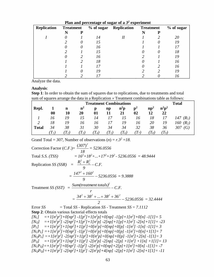
63

Plan and percentage of sugar of a 32 experiment

Replication Treatment % of sugar Replication Treatment % of sugar

N P N P

I 0 1 14 II 1 2 20

2 0 15 1 0 19

0 0 16 1 1 17

2 1 15 0 0 18

0 2 16 2 1 19

1 2 18 0 1 16

1 1 17 0 2 16

1 0 19 2 2 19

2 2 17 2 0 16

Analyze the data.

Analysis:

Step 1: In order to obtain the sum of squares due to replications, due to treatments and total

sum of squares arrange the data in a Replication Treatment combinations table as follows:

Repl.

Treatment Combinations

1 n n2 p np n2p p2 np2 n2p2

00 10 20 01 11 21 02 12 22

Total

1 16 19 15 14 17 15 16 18 17 147 (R1)

2 18 19 16 16 17 19 16 20 19 160 (R2)

Total 34

(T1)

38

(T2)

31

(T3)

30

(T4)

34

(T5)

34

(T6)

32

(T7)

38

(T8)

36

(T9)

307 (G)

Grand Total = 307, Number of observations (n) = r.32 =18.

Correction Factor (C.F.)= 18

307 2)(= 5236.0556

Total S.S. (TSS) = 162+182+...+172+192 - 5236.0556 = 48.9444

Replication SS (SSR) = C.F.9

RR 2

2

2

1

= 055652369

160147 22

.

= 9.3888

Treatment SS (SST) = C.F.r

totals) entSum(treatm 2

= 055652362

36383834 2222

....

= 32.4444

Error SS = Total SS - Replication SS - Treatment SS = 7.1112

Step 2: Obtain various factorial effects totals

[NL] =+1[n2p2]+0[np2] -1[p2]+1[n2p]+0[np] -1[p]+1[n2]+0[n] -1[1]= 5

[NQ] =+1[n2p2] -2[np2]+1[p2]+1[n2p] -2[np]+1[p]+1[n2] -2[n]+1[1]= -23

[PL] =+1[n2p2]+1[np2]+1[p2]+0[n2p]+0[np]+0[p] -1[n2] -1[n] -1[1]= 3

[NLPL] =+1[n2p2]+0[np2] -1[p2]+0[n2p]+0[np]+0[p] -1[n2]+0[n]+1[1]= 7

[NQPL] =+1[n2p2] -2[np2]+1[p2]+0[n2p]+0[np]+0[p] -1[n2]+2[n] -1[1]= 3

[PQ] =+1[n2p2]+1[np2]+1[p2] -2[n2p] -2[np] -2[p] +1[n2] +1[n] +1[1]= 13

[NLPQ]=+1[n2p2]+0[np2] -1[p2] -2[n2p]+0[np]+2[p]+1[n2]+0[n] -1[1]= -7

[NQPQ]=+1[n2p2] -2[np2]+1[p2] -2[n2p]+4[np] -2[p]+1[n2] -2[n]+1[1]= -11

64

Step 3: Obtain the sum of squares due to various factorial effects

SSNL =

0833.212

2

2

L 5=

r.2.3

N; SSNQ =

6944.14

36

)23( 22

r.6.3

NQ;

SSPL =

7500.012

322

r.3.2

PL ; SSNLPL =

1250.68

722

r.2.2

PN LL ;

SSNQPL =

375.024

322

r.6.2

PN LQ; SSPQ=

6944.4

36

1322

r.3.6

PQ;

SSNLPQ =

0417.224

)7( 22

r.2.6

PN QL; SSNQPQ =

6806.1

72

)11( 22

r.6.6

PN QQ;

Step 4: Construct the ANOVA table as given above and test the significance of the

various factorial effects:

ANOVA

Source of Variation D.F. S.S. M.S. F

Replications 1 9.3888 9.3888 10.5623*

Treatments 8 32.4444 4.0555 4.5624*

N 2 16.7774 8.3887 9.4371*

NL 1 2.0833 2.0833 2.3437

NQ 1 14.6944 14.6944 16.5310*

P 2 5.4444 2.7222 3.0624

PL 1 0.7500 0.7500 0.8437

PQ 1 4.6944 4.6944 5.2811

NP 4 10.2223 2.5556 2.875

NLPL 1 6.1250 6.1250 6.8905*

NQPL 1 0.3750 0.3750 0.4219

NLPQ 1 2.0417 2.0417 2.2968

NQPQ 1 1.6806 1.6806 1.8906

Error 8 7.1112 0.8889

Total 17 48.9444

(* indicates the significance at 5% level of significance)

2.3 Yates Algorithm

We now describe below a general procedure of computing the factorial effects:

Step 1: Write the treatment combinations in the lexicographic order, i.e., first vary the levels

of the first factor from 0 to s1 - 1 by keeping fixed the levels of other n – 1 factors at level

0. Then vary the levels of the second factor from 1 to s2 -1 levels in each of the first s1

treatment combinations by keeping the levels of factors 3 to n factors at 0 levels so as to get

s1xs2 treatment combinations; then vary the levels of the third factor from 1 to s3 - 1 by

keeping the levels of factors 4 to n at 0 levels in the earlier s1xs2 treatment combinations

and repeat the process till you get all the

n

1i

is treatment combinations. For example, if

65

there are three factors, first factor at 3 levels, second factor at 4 levels and third factor at 5

levels. Then 3x4x5 = 60 treatment combinations are:

000, 100, 200, 010, 110, 210, 020, 120, 220, 030, 130, 230, 001, 101, 201, 011, 111, 211,

021, 121, 221, 031, 131, 231, 002, 102, 202, 012, 112, 212, 022, 122, 222, 032, 132, 232,

003, 103, 203, 013, 113, 213, 023, 123, 223, 033, 133, 233, 004, 104, 204, 014, 114, 214,

024, 124, 224, 034, 134, 234.

Write all these treatment combinations in the first column and in the second column write

the corresponding treatment totals.

Step 2: Divide the observations in the second column in groups such that each group has s1

observations. Then we add the observations in each of these s1 groups in the third column,

then we repeat the process of linear component of the main effect of the first factor with

these groups and append the third column, repeat the process for quadratic effects and so

on till the polynomial upto the order of s1-1. For example, if the factor is at two levels, then

we make the groups of two observations each, and first half of the third column is filled

with sum of observations in these groups and second half with the differences of the second

observation and the first observation in each group. If the factor is at three levels, we make

the groups of three observations each, and one third column is filled with the sum of

observations in these groups, next one third by using the linear component, say -1, 0, 1, i.e.,

by taking the difference of the third observation and first observation in each group and rest

one third is filled by using the quadratic component 1, -2, 1, i.e., by adding the first and

third observation in each group and subtracting the twice of the second observation from

this sum. If the factor is at four levels, we make the groups of four observations each, the

first quarter of the next column is filled by sum of these observations in each of the groups,

next quarter is filled by using the linear component -3, -1, 1, 3, i.e., by adding the third

observation and 3 times the fourth observation from each group and then subtracting the

sum of second observation and three times the first observation from this sum. Next quarter

is filled using the quadratic component 1, -1, -1, 1, i.e. first observation minus second

observation minus third observation plus fourth observation of each of the groups and last

quarter is filled by using the cubic component say -1, 3, -3, 1, i.e. [–(first observation) + 3

(second observation) - 3(third observation) + fourth observation] from each group, and so

on.

In the third column, divide the observations into groups such that each group contains s2

observations and then use these groups to obtain the fourth column as in second column. In

the fourth column divide the observations into groups of s3 observations each and so on.

Repeat the process for all the n factors.

If all the factors are at same levels, then perform same operation on all the n columns.

For illustration, the various factorial effect totals in the Example 2, where each of the three

factors is at 2 levels each, can be obtained as follows:

Treatment

combinations

(1)

Treatment

totals

(2)

Operation as

per first factor

(3)

Operation as per

second factor

(4)

Operation as

per third

factor (5)

66

000 (1) 294 =I 617=I+II 2611 6949=G

100 n 323=II 1994=III+IV 4338 369=[N]

010 p 959=III 1747=V+VI 105 2221=[P]

110 np 1035=IV 2591=VII+VIII 264 81=[NP]

001 k 816=V 29=II-I 1377 1727=[K]

101 nk 931=VI 76=IV-III 844 159=[NK]

011 pk 1221=VII 115=VI-V 47 -533=[PK]

111 npk 1370=VII 149=VIII-VII 34 -13=[NPK]

For Example 2, the various factorial effects totals can be obtained as given in the

following table

Treatment

combinations

(1)

Treatment

totals

(2)

Operation as per

first factor

( 3)

Operation as per

second factor

( 4)

00 (1) 34=I 103=I+II+III 307=G

10 (n) 38=II 98=IV+V+VI 5=NL

20 (n2) 31=III 106=VII+VIII+IX -23=NQ

01 (p) 30=IV -3=III-I 3=PL

11 (np) 34=V 4=VI-IV 7=NLPL

21 (n2p) 34=VI 4=IX-VII 3=NQPL

02 (p2) 32=VII -11=III-2II+I 13=PQ

12 (np2) 38=VII -4=VI-2V+IV -7=NLPQ

22 (n2p2) 36=IX -8=IX-2VIII+VII -11=NQPQ

Remark: The analysis demonstrated so far is computationally feasible for the situation

when large number of factors is experimented with smaller number of levels. However,

usual tabular method of analysis can be employed for the situations when there are few

factors with more number of levels.

3. Confounding in Factorial Experiments When the number of factors and/or levels of the factors increase, the number of treatment

combinations increase very rapidly and it is not possible to accommodate all these treatment

combinations in a single homogeneous block. For example, a 25 factorial would have 32

treatment combinations and blocks of 32 plots are quite big to ensure homogeneity within

them. In such a situation it is desirable to form blocks of size smaller than the total number

of treatment combinations (incomplete blocks) and, therefore, have more than one block

per replication. The treatment combinations are then allotted randomly to the blocks within

the replication and the total number of treatment combinations is grouped into as many

groups as the number of blocks per replication.

A consequence of such an arrangement is that the block contrasts become identical to some

of the interaction component contrasts. For example, consider a 24 factorial experiment to

be conducted in two blocks of size 8 each per replication. The two blocks in a single

replication are the following:

Block – I Block - II

treatment combination treatment combination

A B C D A B C D

67

0 0 0 0 (1) 1 0 0 0 a

1 1 0 0 Ab 0 1 0 0 b

1 0 1 0 Ac 0 0 1 0 c

1 0 0 1 Ad 0 0 0 1 d

0 1 1 0 Bc 1 1 1 0 abc

0 1 0 1 Bd 1 1 0 1 abd

0 0 1 1 Cd 1 0 1 1 acd

1 1 1 1 Abcd 0 1 1 1 bcd

It may easily be verified that the block contrast is identical with the contrast for the

interaction ABCD, i.e., 0000+1100+1010+1001+0110+0101+0011+1111-1000-0100-

0010-0001-1110-1101-1011-0111. Thus, the interaction ABCD gets confounded with

block effects and it is not possible to separate out the two effects.

Evidently the interaction confounded has been lost but the other interactions and main

effects can now be estimated with better precision because of reduced block size. This

device of reducing the block size by taking one or more interactions contrasts identical with

block contrasts is known as confounding. Preferably only higher order interactions with

three or more factors are confounded, because these interactions are less important to the

experimenter. As an experimenter is generally interested in main effects and two factor

interactions, these should not be confounded as far as possible. The designs for such

confounded factorials are incomplete block designs. However usual incomplete block

designs for single factor experiments cannot be adopted, as the contrasts of interest in two

kinds of experiments are different. The treatment groups are first allocated at random to

the different blocks. The treatments allotted to a block are then distributed at random to its

different units.

When there are two or more replications in the design and if the same set of interaction

components is confounded in all the replications, then confounding is called complete and

if different sets of interactions are confounded in different replications, confounding is

called partial. In complete confounding all the information on confounded interactions is

lost. However, in partial confounding, the information on confounded interactions can be

recovered from those replications in which these are not confounded.

Advantages of Confounding

It reduces the experimental error considerably by stratifying the experimental material

into homogeneous subsets or subgroups. The removal of the variation among

incomplete blocks (freed from treatments) within replications results in smaller error

mean square as compared with a RCB design, thus making the comparisons among

some treatment effects more precise.

Disadvantages of Confounding

In the confounding scheme, the increased precision is obtained at the cost of sacrifice

of information (partial or complete) on certain relatively unimportant interactions.

The confounded contrasts are replicated fewer times than are the other contrasts and as

such there is loss of information on them and these can be estimated with a lower degree

of precision as the number of replications for them is reduced.

68

An indiscriminate use of confounding may result in complete or partial loss of

information on the contrasts or comparisons of greatest importance. As such the

experimenter should confound only those treatment combinations or contrasts that are

of relatively less or of no importance at all.

The algebraic calculations are usually more difficult and the statistical analysis is

complex, especially when some of the units (observations) are missing. In this package,

the attempt has been made to ease this problem.

3.1 Confounding in 23 Experiment

To make the exposition simple, we consider a small factorial experiment 23. Let the three

factors be A, B, C each at two levels.

Effects

Treat.

Combinations

A B C AB AC BC ABC

(1) - - - + + + -

(a) + - - - - + +

(b) - + - - + - -

(ab) + + - + - - -

(c) - - + + - - +

(ac) + - + - + - -

(bc) - + + - - + -

(abc) + + + + + + +

The various effects are given by

A = (abc) + (ac) + (ab) + (a) - (bc) - (c) - (b) - (1)

B = (abc) + (bc) + (ab) + (b) - (ac) - (c) - (a) - (1)

C = (abc) + (bc) + (ac) + (c) - (ab) - (b) - (a) - (1)

AB = (abc) + (c) + (ab) + (1) - (bc) - (ac) - (b) - (a)

AC = (abc) + (ac) + (b) + (1) - (bc) - (c) - (ab) - (a)

BC = (abc) + (bc) + (a) + (1) - (ac) - (c) - (ab) - (b)

ABC = (abc) + (c) + (b) + (a) - (bc) - (ac) - (ab) - (1)

Suppose that the experimenter decides to use two blocks of 4 units (plots) per replication

and that the highest order interaction ABC is confounded. Thus, in order to confound the

interaction ABC with blocks all the treatment combinations with positive sign are allocated

at random in one block and those with negative signs in the other block. Thus the following

arrangement gives ABC confounded with blocks and hence the entire information is lost on

ABC in this replication.

Replication I

Block 1: (1) (ab) (ac) (bc)

Block 2 : (a) (b) (c) (abc)

We observe that the contrast estimating ABC is identical to the contrast estimating block

effects. If the same interaction ABC is confounded in all the other replications, then the

interaction is said to be completely confounded and we cannot recover any information on

the interaction ABC through such a design. For the other six factorial effects viz. A, B, C,

AB, AC, BC there are two treatment combinations with a positive sign and two treatment

combinations with a negative sign in each of the two blocks and hence these differences are

not influenced among blocks and can thus be estimated and tested as usual without any

difficulty.

69

Similarly if we want to confound AB, then the two blocks will consists of

Block 1 (abc) (c) (ab) (1)

Block 2 (bc) (ac) (b) (a)

Here interaction AB is confounded with block effects whereas all other effects A, B, C, AC,

BC and ABC can be estimated orthogonally.

3.2 Partial confounding

When different interactions are confounded in different replications, the interactions are

said to be partially confounded. Consider again the 23 factorial experiment with each

replicate divided into two blocks of 4 units each. It is not necessary to confound the same

interaction in all the replications and several factorial effects may be confounded in one

single experiment. For example, the following plan confounds the interaction ABC, AB,

BC and AC in replications I, II, III and IV respectively.

Rep. I

Block 1 Block 2

Rep. II

Block 3 Block 4

Rep. III

Block 5 Block 6

Rep. IV

Block 7 Block 8

(abc) (ab) (abc) (ac) (abc) (ab) (abc) (ab)

(a) (ac) (c) (bc) (bc) (ac) (ac) (bc)

(b) (bc) (ab) (a) (a) (b) (b) (a)

(c) (1) (1) (b) (1) (c) (1) (c)

In the above arrangement, the main effects A, B and C are orthogonal to block contrasts.

The interaction ABC is completely confounded with blocks in replication I, but in the other

three replications the interaction ABC is orthogonal to blocks and consequently an estimate

of ABC may be obtained from replicates II, III and IV. Similarly it is possible to recover

information on the other confounded interactions AB (from replications I, III, IV), BC (from

replications I, II, IV) and AC (from replications I, II, III). Since the partially confounded

interactions are estimated from only a portion of the observations, they are determined with

a lower degree of precision than the other effects.

3.3 Construction of a Confounded Factorial

Given a set of interactions confounded, the blocks of the design can be constructed and

vice-versa i.e., if the design is given the interactions confounded can be identified.

3.4 Given a set of interactions confounded, how to obtain the blocks? The blocks of the design pertaining to the confounded interaction can be obtained by solving

the equations obtained from confounded interaction. We illustrate this through an example.

Example 3: Construct a design for 25 factorial experiment in 23 plots per block confounding

interactions ABD, ACE and BCDE.

Let x1, x2, x3, x4 and x5 denote the levels (0 or 1) of each of the 5 factors A, B, C, D and E.

Solving the following equations would result in different blocks of the design.

For interaction ABD: x1 + x2 + x4 = 0, 1

For interaction ACE : x1 + x3 + x5 = 0, 1

70

The interactions ABD and ACE are independent and BCDE is a generalized interaction. In

other words, a solution of the above two equations will also satisfy the equation

1,04321 xxxx . Treatment combinations satisfying the following solutions of above

equations will generate the required four blocks

(0, 0) (0, 1) (1, 0) (1, 1)

The solution (0, 0) will give the key block (A key block is one that contains one of the

treatment combination of factors, each at lower level).

There will be 3

5

2

2= 4 blocks per replication. The key block is as obtained below

A B C D E

1 1 1 0 0 abc

1 1 0 0 1 abe

1 0 1 1 0 acd

1 0 0 1 1 ade

0 1 1 1 1 bcde

0 1 0 1 0 bd

0 0 1 0 1 ce

0 0 0 0 0 (1)

Similarly we can write the other blocks by taking the solutions of above equations as (0, 1)

(1, 0) and (1, 1).

3.5 Given a block, how to find the interactions confounded?

The first step in detecting the interactions confounded in blocking is to select the key block.

If the key block is not given, it is not difficult to obtain it. Select any treatment combination

in the given block; multiply all the treatment combinations in the block by that treatment

combination and we get the key block. From the key block we know the number of factors

as well as the block size. Let it be n and k. We know then that the given design belongs to

the 2n factorial in 2r plots per block. The next step is to search out a unit matrix of order r.

From these we can find the interaction confounded. We illustrate this through an example.

Example 4: Given the following block, find out the interactions confounded.

(acde), (bcd), (e), (abec), (ad), (bde), (ab), (c)

Since the given block is not the key block we first obtain the key block by multiplying every

treatment combination of the given block by e. We get the following block:

(acd), (bcde), (1), (abc), (ade), (bd), (abe), (ce)

This is the key block as it includes (1). It is obvious that the factorial experiment involves

five factors and has 23 (=8) plots per block. Hence, the given design is (25, 23).

A B C D E

1 0 1 1 0

0 1 1 1 1

0 0 0 0 0

1 1 1 0 0

* 1 0 0 1 1

71

* 0 1 0 1 0

1 1 0 0 1

* 0 0 1 0 1

* indicates the rows of a unit matrix of order 3.

A B C D E

1 0 0 1(=1) 1(=1)

0 1 0 1(=2) 0(=2)

0 0 1 0(=3) 1(=3)

The interaction confounded is A B C D1 2 3 , A B C E1 2 3 . Here ABD and ACE are

independent interactions confounded and BCDE is obtained as the product of these two and

is known as generalized interaction.

3.6 General rule for confounding in 2n series

Let the design be (2n, 2r) i.e. 2n treatment combinations arranged in 2r plots per block.

Number of treatment combinations = 2n, Block size = 2r, Number of blocks per replication

=2n-r,

Total number of interactions confounded = 2n-r – 1, Number of independent interactions

confounded = n - r, Generalized interactions confounded = (2n-r - 1) - (n - r).

3.7 Analysis

For carrying out the statistical analysis of a (2n, 2r) factorial experiment in p replications,

the various factorial effects and their S.S. are estimated in the usual manner with the

modification that for completely confounded interactions neither the S.S due to

confounded interaction is computed nor it is included in the ANOVA table. The confounded

component is contained in the (p2n-r - 1) d.f. due to blocks. The splitting of the total degrees

of freedom is as follows:

Source of Variation Degrees of Freedom

Replication p - 1

Blocks within replication p(2n-r- 1)

Treatments (2n – 1) - (2n-r - 1)

Error By subtraction

Total p2n - 1

The d.f due to treatment has been reduced by 2n-r-1 as this is the total d.f confounded per

block.

3.8 Partial Confounding

In case of partial confounding, we can estimate the effects confounded in one replication

from the other replications in which it is not confounded. In (2n, 2r) factorial experiment

with p replications, following is the splitting of d.f’s.

Source of Variation Degrees of Freedom

Replication p- 1

Blocks within replication p(2n-r - 1)

Treatments 2n - 1

72

Error By subtraction

Total p2n - 1

The S.S. for confounded effects are obtained from only those replications where the given

effect is not confounded. From practical point of view, the S.S. for all the effects including

the confounded effects is obtained as usual and then some adjustment factor (A.F) is applied

to the confounded effects. The adjusting factor for any confounded effect is computed as

follows:

(i) Note the replication in which the given effect is confounded

(ii) Note the sign of (1) in the corresponding algebraic expression of the effect to the

confounded. If the sign is positive then

A.F = [Total of the block containing (1) of replicate in which the effect is confounded] -

[Total of the block not containing (1) of the replicate in which the effect is

confounded] =T1 -T2.

If the sign is negative, then A.F = T2 - T1.

This adjusting factor will be subtracted from the factorial effects totals of the confounded

effects obtained.

Example 5: Analyze the following 23 factorial-experiment conducted in two blocks of 4

plots per replication, involving three fertilizers N, P, K, each at two levels:

Replication I

Replication II

Replication III

Block 1 Block 2 Block 3 Block 4 Block 5 Block 6

(np)

101

(p)

88

(1)

125

(np)

115

(pk)

75

(n)

53

(npk)

111

(n)

90

(npk)

95

(k)

95

(nk)

100

(npk)

76

(1)

75

(pk)

115

(nk)

80

(pk)

90

(1)

55

(p)

65

(k)

55

(nk)

75

(p)

100

(n)

80

(np)

92

(k)

82

Step 1: Identify the interactions confounded in each replication. Here, each replication has

been divided into two blocks and one effect has been confounded in each replication. The

effects confounded are

Replication I NP; Replicate II NK; Replicate III NPK

Step 2: Obtain the blocks S.S. and Total S.S.

S.S. due to Blocks = Bi

i

2

1

6

4

- C.F = 2506

Total S.S. = Obs.2- C.F = 8658

Step 3: Obtain the sum of squares due to all the factorial effects other than the confounded

effects.

73

Treatment

Combinations

Total Yield Factorial Effects Sum of Squares (S.S)

= [Effect]2/ 23.r

(1) 255 G=0

n 223 [N]=48 96 =SN

2

p 253 [P]=158 1040.17 =SP

2

np 308 [NP]=66 -

k 232 [K]=10 4.17 =SK

2

nk 255 [NK]=2 -

pk 280 [PK]=-8 2.67 =SPK

2

npk 282 [NPK]=-108 -

Total for the interaction NP is given by

[NP] = [npk] - [pk] - [nk] + [k] + [np] - [p] - [n] + [1]

Here the sign of (1) is positive. Hence the adjusting factor (A.F) for NP, which is to be

obtained from replicate 1 is given by

A.F. for NP = (101 + 111 + 75 + 55) - (88 + 90 + 115 + 75) = -26

Adjusted effect total for NP becomes, [NP*] = [NP]- (-26) = 66 + 26 = 92.

It can easily be seen that the total of interaction NP using the above contrast from

replications II and III also gives the same total i.e. 92.

Similarly A.F. for NK =20, A.F. for NPK = -46

Hence adjusted effect totals for NK and NPK are respectively [NK*] =-18 and

[NPK*] = -62.

SNP

2 = S.S. due to NP = 1

16[NP*]2 = 529; SNK

2 = S.S. due to NK = 1

16 [NK*] = 20.25

SNPK

2 = S.S. due to NPK =1

16 [NPK*] = 240.25

Treatment S.S. = 2NS + 2

PS + 2KS + 2

NPS + 2NKS + 2

PKS + 2NPKS = 1932.7501

ANOVA

Source d.f. Sum of Squares M.S. F

Blocks 5 2506 501 1.31

Treatments 7 1932.75 276.107 -

N 1 96.00 96.00 -

P 1 1040.16 1040.16 2.71

NP 1 529.00 529.00 1.3

K 1 4.41 4.41 -

NK 1 20.25 20.25 -

PK 1 2.66 2.66 -

NPK 1 240.25 240.25 -

Error 11 4219.24 383.57

Total 23 8658

74

‘-’ indicates that these ratios are less than one and hence these effects are non-significant.

From the above table it is seen that effects due to blocks, main effects due to factor N, P,

and K or interactions are not significant.

4. Confounding in 3n Series

The concept of confounding here also is the same as in 2n series. We shall illustrate the

principles of confounding in 3n in 3r plots per block with the help of a 33 experiments laid

out in blocks of size 32(=9). Let the three factors be A, B and C and the confounded

interaction be ABC2. The three levels of each of the factor are denoted by 0, 1 and 2 and a

particular treatment combination be xi xj xk , i, j, k = 0, 1, 2.

Number of blocks per replication =3n-r = 3; Block size = 3r = 9; Degrees of freedom

confounded per replication = 3n-r – 1 = 2.

Number of interactions confounded per replicate = 3 1

3 1

n r

= 1.

The treatment combinations in 3 blocks are determined by solving the following equations

mod(3)

x1 + x2 + 2x3 = 0 ; x1 + x2 + 2x3 = 1 ; x1 + x2 + 2x3 = 2

Block I Block II Block III

A B C A B C A B C

1 0 1 1 0 0 1 0 2

0 1 1 0 1 0 0 1 2

1 1 2 1 1 1 1 1 0

2 0 2 2 0 1 2 0 0

0 2 2 0 2 1 0 2 0

2 1 0 2 1 2 2 1 1

1 2 0 1 2 2 1 2 1

2 2 1 2 2 0 2 2 2

0 0 0 0 0 2 0 0 1

5. Confounding in ns Factorial Experiments in rs experimental units per block

ns Factorial Experiments in rs experimental units per block are represented by rn ss ,( )

factorial experiments. For generation of rn ss ,( ), s should be a prime or prime power, i.e.,

mps , where p is prime and m is a positive integer. For the factorial experiments of the

type rn ss ,( ) there will be rns blocks per replication with ( )rs experimental units per

block. The total number of degrees of freedom confounded per replication is 1s rn ,

while the total number of interaction components confounded per replication is 1s

1s rn

as each interaction component has ( 1s ) degrees of freedom. The total number of

independent interaction components to be confounded is n-r and rest are generalized

interaction components. For the ( rn ) independent interaction components confounded,

we have the following set of )( rn equations as:

75

n

1j

j1j xp =0,1, ,, 32 …, 1s mod s

n

1j

j2j xp =0,1, ,, 32 …, 1s mod s

n

1j

jjk xp =0,1, ,, 32 …, 1s mod s

n

1j

jrnj xp )( =0,1, ,, 32 …, 1s mod s

where jkp ’s and 0,1, ,, 32 …, 1s are the elements of the Galois Field s and

n21 xxx ,,, are the variates corresponding to the n-factors and denote the levels of the

corresponding factors in the different treatment combinations. If 1m , then mod s in the

above equations should be replaced by mod {p, p(x)}, where p(x) is the minimal function

for GF( mp ) and x is the primitive root of the GF( mp ). These equations result into rns

different sets. Solution of each set gives one block. For example, if one wants to generate

a ),( 24 33 factorial experiment, then the number of independent interaction components to

be confounded are 4-2=2. These two independent interactions are represented by:

3210xpxpxpxp

3210xpxpxpxp

442332222112

441331221111

mod,,

mod,,

These sets of equations give rise to 9 combinations viz. the left hand sides satisfying (0,0);

(0,1); (0,2); (1,0); (1,1); (1,2); (2,0); (2,1) and (2,2). The treatment combinations in 9 blocks

in one replication are those satisfy the above combinations. The block containing the

treatment combinations satisfying

30xpxpxpxp 441331221111 mod and

30xpxpxpxp 442332222112 mod is the key block.

For the situations, where s is a prime power, we make use of the concept of minimal

functions. For example, if one wants to generate a ),( 442 -factorial experiment, then the

number of levels for each of the two factors is a prime power, i.e. 4 = 22 . The minimal

function for GF(4) is p(x) = 12 xx and the elements of the GF(4) are 0, 1, x , x+1. The

total number of treatment combinations is 16 and are given by

A 0 0 0 0 1 1 1 1 x x x x x+1 x+1 x+1 x+1

B 0 1 x x+1 0 1 x x+1 0 1 x x+1 0 1 x x+1

Here n = 2 and r = 1, therefore, the number of blocks per replication is 4 and number of

experimental units in each block is also 4. The number of independent interaction

components to be confounded is n - r = 1. Let the experimenter is interested in confounding

the interaction component AB. Therefore, the block contents can be obtained from the

solution of

76

),{mod,,, 1xx21xx10xx 221

The block contents obtained through the solution of the above equations are

Block - I Block - II Block - III Block - IV

A B A B A B A B

0 0 0 1 0 x 0 x+1

1 1 1 0 x 0 1 x

x x X x+1 1 x+1 x 1

x+1 x+1 x+1 x x+1 1 x+1 0

Similarly, we can get the block contents, if the other interaction components are

confounded.

The above discussion relates to the methods of construction of symmetrical factorial

experiments with confounding. The loss of information on the confounded interaction

components depends upon the number of replications in which these are confounded. The

designs in which the loss of information is equally distributed over the different components

of the interaction of given orders (order of an interaction is one less than the number of

factors involved in the interaction) may be desirable. A design with the above

characterization is a balanced confounded design. This design in case of symmetrical

factorials is defined as:

6. Balanced Confounded Design A partially confounded design is said to be balanced if all the interactions of a particular

order are confounded in equal number of replications.

How to construct a Balanced confounded Factorial Design?

Let us take the example of a (25, 23)- factorial experiment. The interest is in constructing a

design for a (25, 23)- factorial experiment achieving balance over three and four factor

interactions. In this case, s = 2, n = 5 and r = 3. Therefore, the total number of treatment

combinations is 32, the block size is 8 and the number of blocks per replicate is 32/8. The

number of degrees of freedom confounded is 312 35 . Each interaction component has 1

degree of freedom. Therefore, the number of interaction components to be confounded is 3.

The number of independent interactions to be confounded is 5-3 = 2 and one is the

generalized interaction component.

The number of 3 factor interactions = (5C3) = 10 viz. ABC, ABD, ABE, ACD, ACE, ADE,

BCD, BCE, BDE, and CDE and number of four factor interactions = (5C4) = 5 viz. ABCD,

ABCE, ABDE, ACDE, and BCDE. Therefore, to achieve balance total number f degrees

of freedom to be confounded is 10+5=15. As each interaction component has 1 d.f.,

therefore, number of degrees of freedom to be confounded are 15. The number of degrees

of freedom confounded in one replication is 3. Therefore, the number of replications

required is 15/3=5. The balance can be achieved by confounding the following interactions

in different replications:

Replication – I: ABD, ACE and BCDE

Replication – II: ACD, BCE and ABDE

Replication – III: ADE, BCD and ABCE

Replication – IV: ABE, CDE and ABCD

Replication – V: ABC, BDE and ACDE

77

The block contents may be obtained following the above procedure. The confounding in

asymmetrical factorials is somewhat different from symmetrical factorials. When an

interaction component is confounded in a replication in these designs, it is not necessary

that it is completely confounded with the blocks in the sense that the block contrasts and

the interaction contrasts become identical. These two sets of contrasts although not

identical, yet are dependent so that the contrasts for obtaining a confounded interaction from

the treatment totals are not free from block effects. Therefore, more than one replication is

needed in obtaining balanced confounded designs for asymmetrical factorial experiment. A

design is said to be Balanced confounded factorial experiment (BFE) if (i) any contrasts of

a confounded interaction component is estimable independently of any other contrasts

belonging to any other confounded interaction and (ii) the loss of information of each

degrees of freedom of any confounded interaction is same. To be more specific, BFE may

be defined as:

A factorial experiment will be called a balanced factorial experiment if

(i) Each treatment is replicated the same number of times.

(ii) Each of the blocks has the same number of plots.

(iii) Estimates of the contrasts belonging to different interactions are uncorrelated with

each other.

(iv) Complete balance is achieved over each of the interactions, i.e., all the normalized

contrasts belonging to the same interaction are estimated with the same variance.

Several methods of construction of designs for balanced factorial experiments are available

in literature based on pseudo factors or pairwise balanced block designs. We shall not be

presenting these methods here. The user may refer to standard textbooks for the same.

Further, it is known that an extended group divisible (EGD) design, if existent, has

orthogonal factorial structure with balance. In other words, an EGD design is a balanced

confounded factorial experiment. Therefore, the vast literature on the methods of

construction of extended group divisible designs may be used for the construction of BFE.

The conditions of equal replications and equal block sizes may now be relaxed.

Generation of a design for factorial experiments is easy. But when the number of factors

or the number of levels become large it becomes difficult to generate the layout of the

design. To circumvent this problem, IASRI has developed a statistical package SPFE

(Statistical Package for Factorial Experiments). This package is essentially for symmetrical

factorial experiments. There is a provision of generation of designs as well as the

randomized layout of the designs including totally and partially confounded designs. The

design is generated once the independent interactions to be confounded are listed. One can

give different number of independent interactions to be confounded in different replications

(The package is also capable of generating the design for factorial experiments by simply

giving the number of factors along with the number of levels and the block size. In this

case the package will itself determine the number of blocks per replication and the layout

by keeping the higher interactions confounded). Provision has also been made in this

package for analyzing the data generated from the experiments using these designs. The

data generated are analyzed as a general block design and the contrast analysis is carried

out to obtain the sum of squares due to main effects and interactions. Separate modules

have been developed for generating the probabilities using 2, F and t distributions for

testing the levels of significance.

78

This package deals with only symmetrical factorial experiments. However, in practice an

experimenter encounters situations where one has to use various factors with unequal

number of levels. The generation of the design for asymmetrical factorial experiments is,

however, a tedious job. We, therefore, give below a catalogue of designs commonly used.

In this catalogue A, B, C, etc. denote the factors and a, b, c, etc. denote the blocks within

replications.

Plan 1. Balanced group of sets for 3x22 factorial, blocks of 6 units each

BC, ABC confounded

Replication I Replication II Replication III

Block-1 Block-2 Block-1 Block-2 Block-1 Block-2

0 0 1 0 0 0 0 0 0 0 0 1 0 0 0 0 0 1

0 1 0 0 1 1 0 1 1 0 1 0 0 1 1 0 1 0

1 0 0 1 0 1 1 0 1 1 0 0 1 0 0 1 0 1

1 1 1 1 1 0 1 1 0 1 1 1 1 1 1 1 1 0

2 0 0 2 0 1 2 0 0 2 0 1 2 0 1 2 0 0

2 1 1 2 1 0 2 1 1 2 1 0 2 1 0 2 1 1

Plan 2. Balanced group of sets for 3x23 factorial, blocks of 6 units

BC, BD, CD

ABC, ABD, ACD confounded

Replication I

Block-1 Block-2 Block-3 Block-4

0 1 0 0 0 0 0 0 0 0 0 1 0 0 1 0

0 0 1 1 0 1 1 1 0 1 1 0 0 1 0 1

1 0 1 0 1 0 0 1 1 0 0 0 1 1 0 0

1 1 0 1 1 1 1 0 1 1 1 1 1 0 1 1

2 0 0 1 2 0 1 0 2 1 0 0 2 0 0 0

2 1 1 0 2 1 0 1 2 0 1 1 2 1 1 1

Replication II

Block-1 Block-2 Block-3 Block-4

0 0 1 0 0 0 0 1 0 0 0 0 0 1 0 0

0 1 0 1 0 1 1 0 0 1 1 1 0 0 1 1

1 0 0 1 1 0 1 0 1 1 0 0 1 0 0 0

1 1 1 0 1 1 0 1 1 0 1 1 1 1 1 1

2 1 0 0 2 0 0 0 2 0 0 1 2 0 1 0

2 0 1 1 2 1 1 1 2 1 1 0 2 1 0 1

Replication III

Block-1 Block-2 Block-3 Block-4

0 0 0 1 0 0 1 0 0 1 0 0 0 0 0 0

0 1 1 0 0 1 0 1 0 0 1 1 0 1 1 1

1 1 0 0 1 0 0 0 1 0 0 1 1 0 1 0

1 0 1 1 1 1 1 1 1 1 1 0 1 1 0 1

2 0 1 0 2 0 0 1 2 0 0 0 2 1 0 0

2 1 0 1 2 1 1 0 2 1 1 1 2 0 1 1

79

Plan 3. Balanced group of sets for 32 x2 factorial, blocks of 6 units

AB, ABC Confounded

Replication I Replication II

Block-1 Block-2 Block-3 Block-1 Block-2 Block-3

1 0 0 2 0 0 0 0 0 2 0 0 0 0 0 1 0 0

2 1 0 0 1 0 1 1 0 0 1 0 1 1 0 2 1 0

0 2 0 1 2 0 2 2 0 1 2 0 2 2 0 0 2 0

2 0 1 0 0 1 1 0 1 1 0 1 2 0 1 0 0 1

0 1 1 1 1 1 2 1 1 2 1 1 0 1 1 1 1 1

1 2 1 2 2 1 0 2 1 0 2 1 1 2 1 2 2 1

Replication III Replication IV

Block-1 Block-2 Block-3 Block-1 Block-2 Block-3

1 0 0 2 0 0 0 0 0 2 0 0 0 0 0 1 0 0

0 1 0 1 1 0 2 1 0 1 1 0 2 1 0 0 1 0

2 2 0 0 2 0 1 2 0 0 2 0 1 2 0 2 2 0

2 0 1 0 0 1 1 0 1 1 0 1 2 0 1 0 0 1

1 1 1 2 1 1 0 1 1 0 1 1 1 1 1 2 1 1

0 2 1 1 2 1 2 2 1 2 2 1 0 2 1 1 2 1

Plan 4. Balanced group of sets for 4x22 factorial, blocks of 8 units

ABC Confounded

Replication I Replication II Replication III

Block-1 Block-2 Block-1 Block-2 Block-1 Block-2

0 0 0 0 0 1 0 0 0 0 0 1 0 0 0 0 0 1

0 1 1 0 1 0 0 1 1 0 1 0 0 1 1 0 1 0

1 0 0 1 0 1 1 0 1 1 0 0 1 0 1 1 0 0

1 1 1 1 1 0 1 1 0 1 1 1 1 1 0 1 1 1

2 0 1 2 0 0 2 0 1 2 0 0 2 0 0 2 0 1

2 1 0 2 1 1 2 1 0 2 1 1 2 1 1 2 1 0

3 0 1 3 0 0 3 0 0 3 0 1 3 0 1 3 0 0

3 1 0 3 1 1 3 1 1 3 1 0 3 1 0 3 1 1

Plan 5. Balanced group of sets for 4 x 3x2 factorial, blocks of 12 units

AC, ABC confounded

Replication I Replication II Replication III

Block-1 Block-2 Block-1 Block-2 Block-1 Block-2 0 0 0 0 0 1 0 0 1 0 0 0 0 0 1 0 0 0

0 1 1 0 1 0 0 1 0 0 1 1 0 1 1 0 1 0

0 2 1 0 2 0 0 2 1 0 2 0 0 2 0 0 2 1

1 0 0 1 0 1 1 0 1 1 0 0 1 0 1 1 0 0

1 1 1 1 1 0 1 1 0 1 1 1 1 1 1 1 1 0

1 2 1 1 2 0 1 2 1 1 2 0 1 2 0 1 2 1

2 0 1 2 0 0 2 0 0 2 0 1 2 0 0 2 0 1

2 1 0 2 1 1 2 1 1 2 1 0 2 1 0 2 1 1

2 2 0 2 2 1 2 2 0 2 2 1 2 2 1 2 2 0

3 0 1 3 0 0 3 0 0 3 0 1 3 0 0 3 0 1

3 1 0 3 1 1 3 1 1 3 1 0 3 1 0 3 1 1

3 2 0 3 2 1 3 2 0 3 2 1 3 2 1 3 2 0

A2C, A2BC confounded

Replication IV Replication V Replication VI

Block-1 Block-2 Block-1 Block-2 Block-1 Block-2

80

0 0 1 0 0 0 0 0 0 0 0 1 0 0 0 0 0 1

0 1 0 0 1 1 0 1 1 0 1 0 0 1 0 0 1 1

0 2 0 0 2 1 0 2 0 0 2 1 0 2 1 0 2 0

1 0 0 1 0 1 1 0 1 1 0 0 1 0 1 1 0 0

1 1 1 1 1 0 1 1 0 1 1 1 1 1 1 1 1 0

1 2 1 1 2 0 1 2 1 1 2 0 1 2 0 1 2 1

2 0 0 2 0 1 2 0 1 2 0 0 2 0 1 2 0 0

2 1 1 2 1 0 2 1 0 2 1 1 2 1 1 2 1 0

2 2 1 2 2 0 2 2 1 2 2 0 2 2 0 2 2 1

3 0 1 3 0 0 3 0 0 3 0 1 3 0 0 3 0 1

3 1 0 3 1 1 3 1 1 3 1 0 3 1 0 3 1 1

3 2 0 3 2 1 3 2 0 3 2 1 3 2 1 3 2 0

A3C, A3BC confounded

Replication VII Replication VIII Replication IX

Block-1 Block-2 Block-1 Block-2 Block-1 Block-2 0 0 0 0 0 1 0 0 1 0 0 0 0 0 1 0 0 0

0 1 1 0 1 0 0 1 0 0 1 1 0 1 1 0 1 0

0 2 1 0 2 0 0 2 1 0 2 0 0 2 0 0 2 1

1 0 1 1 0 0 1 0 0 1 0 1 1 0 0 1 0 1

1 1 0 1 1 1 1 1 1 1 1 0 1 1 0 1 1 1

1 2 0 1 2 1 1 2 0 1 2 1 1 2 1 1 2 0

2 0 0 2 0 1 2 0 1 2 0 0 2 0 1 2 0 0

2 1 1 2 1 0 2 1 0 2 1 1 2 1 1 2 1 0

2 2 1 2 2 0 2 2 1 2 2 0 2 2 0 2 2 1

3 0 1 3 0 0 3 0 0 3 0 1 3 0 0 3 0 1

3 1 0 3 1 1 3 1 1 3 1 0 3 1 0 3 1 1

3 2 0 3 2 1 3 2 0 3 2 1 3 2 1 3 2 0

Plan 6. Balanced group of sets for 3x23 factorial, blocks of 12 units

ABC, ABCD confounded

Replication I Replication II

Block-1 Block-1 Block-1 Block-1

0 0 0 0 0 0 0 1 0 0 0 0 0 0 0 1

0 0 1 1 0 0 1 0 0 0 1 1 0 0 1 0

0 1 0 1 0 1 0 0 0 1 0 1 0 1 0 0

0 1 1 0 0 1 1 1 0 1 1 0 0 1 1 1

1 0 0 1 1 0 0 0 1 0 0 1 1 0 0 0

1 0 1 0 1 0 1 1 1 0 1 0 1 0 1 1

1 1 0 0 1 1 0 1 1 1 0 0 1 1 0 1

1 1 1 1 1 1 1 0 1 1 1 1 1 1 1 0

2 0 0 1 2 0 0 0 2 0 0 0 2 0 0 1

2 0 1 0 2 0 1 1 2 0 1 1 2 0 1 0

2 1 0 0 2 1 0 1 2 1 0 1 2 1 0 0

2 1 1 1 2 1 1 0 2 1 1 0 2 1 1 1

Replication III

Block-1 Block-2

0 0 0 0 0 0 0 1

81

0 0 1 1 0 0 1 0

0 1 0 1 0 1 0 0

0 1 1 0 0 1 1 1

1 0 0 0 1 0 0 1

1 0 1 1 1 0 1 0

1 1 0 1 1 1 0 0

1 1 1 0 1 1 1 1

2 0 0 1 2 0 0 0

2 0 1 0 2 0 1 1

2 1 0 0 2 1 0 1

2 1 1 1 2 1 1 0

82

RESPONSE SURFACE DESIGNS

Rajender Parsad and Krishan Lal

ICAR-I.A.S.R.I., Library Avenue, New Delhi-110 012

rajender.parsad@icar.gov.in; klkalra@iasri.res.in

1. Introduction

The subject of Design of Experiments deals with the statistical methodology needed for

making inferences about the treatment effects on the basis of responses (univariate or

multivariate) collected through the planned experiments. To deal with the evolution and

analysis of methods for probing into mechanism of a system of variables, the experiments

involving several factors simultaneously are being conducted in agricultural, horticultural

and allied sciences. Data from experiments with levels or level combinations of one or

more factors as treatments are normally investigated to compare level effects of the factors

and also their interactions. Though such investigations are useful to have objective

assessment of the effects of levels actually tried in the experiment, this seems to have

inadequate, especially when the factors are quantitative in nature. The above analysis

cannot give any information regarding the possible effects of the intervening levels of the

factors or their combinations, i.e., one is not able to interpolate the responses at the treatment

combinations not tried in the experiment. In such cases, it is more realistic and informative

to carry out investigations with the twin purposes:

a) To determine and to quantify the relationship between the response and the settings of

a group of experimental factors.

b) To find the settings of the experimental factors that produces the best value or the best

set of values of the response(s).

If all the factors are quantitative in nature, it is natural to think the response as a function of

the factor levels and data from quantitative factorial experiments can be used to fit the

response surfaces over the region of interest. Response surfaces besides inferring about the

twin purposes can provide information about the rate of change of a response variable. They

can also indicate the interactions between the quantitative treatment factors. The special

class of designed experiments for fitting response surfaces is called response surface

designs. A good response surface design should possess the properties viz., detectability of

lack of fit, the ability to sequentially build up designs of increasing order and the use of a

relatively modest, if not minimum, number of design points. Before formulating the

problem mathematically, we shall give examples of some experimental situations, where

response surface methodology can be usefully employed.

Example 1: The over-use of nitrogen (N) relative to Phosphorus (P) and Potassium (K)

concerns both the agronomic and environmental perspective. Phosphatic and Potassic

fertilizers have been in short supply and farmers have been more steadily adopting the use

of nitrogenous fertilizers because of the impressive virtual response. There is evidence that

soil P and K levels are declining. The technique of obtaining individual optimum doses for

the N, P and K through separate response curves may also be responsible for unbalanced

fertilizer use. Hence, determining the optimum and balanced dose of N, P and K for different

crops has been an important issue. This optimum and balanced dose should be

recommended to farmers in terms of doses from the different sources and not in terms of

the values of N, P and K alone, as the optimum combination may vary from source to source.

83

However, in actual practice the values of N, P and K are given in terms of kg/ha rather than

the combined doses alongwith the source of the fertilizers.

Example 2: For value addition to the agriculture produce, food-processing experiments are

being conducted. In these experiments, the major objective of the experimenter is to obtain

the optimum combination of levels of several factors that are required for the product. To

be specific, suppose that an experiment related to osmotic dehydration of the banana slices

is to be conducted to obtain the optimum combination of levels of concentration of sugar

solution, solution to sample ratio and temperature of osmosis. The levels of the various

factors are the following

Factors Levels

1. Concentration of sugar solution 40%, 50%, 60%, 70% and 80%

2. Solution to sample ratio 1:1, 3:1, 5:1, 7:1and 9:1

3. Temperature of osmosis 250C, 350C, 450C, 550C and 650C

In this situation, response surface designs for 3 factors each at five equispaced levels can be

used.

Example 3: Yardsticks (a measure of the average increase in production per unit input of a

given improvement measure) of many fertilizers, manures, irrigation, pesticides for various

crops are being obtained and used by planners and administrators in the formulation of

policies relating to manufacture/import/subsidy of fertilizers, pesticides, development of

irrigation projects etc.

The yardsticks have been obtained from the various factorial experiments. However, these

will be more reliable and satisfy more statistical properties, if response surface designs for

slope estimation are used.

In general response surface methodology is useful for all the factorial experiments in

agricultural experimental programme that are under taken so as to determine the level at

which each of these factors must be set in order to optimize the response in some sense and

factors are quantitative in nature. To achieve this we postulate that the response is a function

of input variables, i.e.

uvuuuu exxxy ,...,, 21

(1.1)

where Nu ,...,2,1 represents the N observations and iux is the level of the thi factor in

the thu observation. The function describes the form in which the response and the input

variables are related and ue is the experimental error associated with the thu observation

such that E (eu) = 0 and Var(eu) = 2. Knowledge of function gives a complete summary

of the results of the experiment and also enables us to predict the response for values of the

iux that are not included in the experiment. If the function is known then using methods

of calculus, one may obtain the values of vxxx ,...,, 21 which give the optimum (say,

maximum) response. In practice the mathematical form of is not known; we, therefore,

often approximate it, within the experimental region, by a polynomial of suitable degree in

variables iux . The adequacy of the fitted polynomial is tested through the usual analysis of

variance. Polynomials which adequately represent the true dose-response relationship are

84

called Response Surfaces and the designs that allow the fitting of response surfaces and

provide a measure for testing their adequacy are called response surface designs. If the

function in (1.1) is of degree one in sxiu ' i.e.

uvuvuuu exxxy ...22110

(1.2)

we call it a first-order response surface in vxxx ,...,, 21 . If (1.1) takes the form

uui

v

i

v

ii

iuii

v

i

iuii

v

i

iuiu exxxxy

1

1 11

2

1

0

(1.3)

We call it a second-order (quadratic) response surface. Henceforth, we shall concentrate on

the second order response surface which is more useful in agricultural experiments.

2. The Quadratic Response Surface The general form of a second-degree (quadratic) surface is

exxxxxx

xxxxxxy

uvuuvvvuuuu

vuvvuuvuvuuu

,1,131132112

22222

211122110

...

......

Let us assume that sxiu ' satisfy the following conditions:

(A) 0

1 1

N

u

v

uiu

ix

, if any i is odd, for 32,1,0 ori and .4i

(B)

N

u

iux

1

2 constant (for all i ) 2N (say)

(C)

N

u

iux

1

4 constant (for all i ) = 4CN (say) (2.1)

(D)

2

1

2ui

N

u

iuxx constant 4N (say), for all ii

We shall estimate the parameters si ' through the method of least squares. Let

sbsbsbb iiiii ',',',0 denote the best linear unbiased estimate of sss iiiii ',',',0

respectively. Under the above restrictions on sxiu ' , the normal equations are found to be:

v

i

ii

N

u

u bNNby

1

20

1

i

N

u

uiu bNyx 2

1

ii

N

u

uuiiu bNyxx

4

1

(2.2)

85

v

i

iiii

ii

iiii

N

u

uiu

bNbNCbN

bNbCNbNyx

1

4402

4402

1

2

1

Solving the above normal equations, we obtain the estimates bi‘s as

4

1

42

1 1

24

22

1

2

4

1

2

1

1 1

22

1

40

11

1

NCyCyxyxb

Nyxxb

Nyxb

NyxyvCb

N

u

uu

v

i

N

u

iuu

N

u

iuii

N

u

uuiiuii

N

u

uiui

v

i

N

u

uiu

N

u

u

(2.3)

where 2241 vvC .

The variances of and covariances between the estimated parameters are as follows:

42

422

220

4422

2

42

22

240

1(,

,

11

1

NCbbCov

NbbCov

NCbV

NbV

NbV

NvCbV

iiii

ii

ii

ii

i

(2.4)

Other covariances are zero. From the above expressions it is clear that a necessary condition

for the design to exist is that 0 . Thus, a necessary condition for a Second Order Design

to exist is that

(E) 1224 vCv (2.5)

If y is the estimated response at any given experimental point 02010 ,...,, vxxx , then the

variance of y is given by

1

1 11

20

20

1

200

1

1 1

20

20

1

40

1

200

,2,2

ˆ

v

i

v

iiiiiii

v

iiii

v

i

v

iiiiii

v

iiii

v

iii

xxbbCovxbbCov

xxbVxbVxbVbVyV

(2.6)

86

If 2

1

20

dx

v

ii

, where d is the distance of the point 02010 ,...,, vxxx from the origin, then

we may write

iiiiiiii

v

i

v

iiii

iiiii

bVbbCovbVxx

bVdbbCovbVdbVyV

2,2

,2ˆ

1

1 1

20

20

40

20

(2.7)

From the above expression, it is clear that if the coefficient of

1

1 1

20

20

v

i

v

iiii

xx is made equal

to zero, the variance of the estimated response at 02010 ,...,, vxxx will be a function of d ,

the distance of the point 02010 ,...,, vxxx from the origin. Now, the coefficient of

1

1 1

20

20

v

i

v

iiii

xx is

CN

CCN

bVbbCovbV iiiiiiii

1

21

11

2

1

21

2,2

4

2

4224

22

4

2

(2.8)

Obviously, this is zero, if and only if 3C . Thus, when 3C , the variance of the

estimated response at a given point, the response being estimated through a design satisfying

(A), (B), (C), (D), (E) becomes a function of the distance of that point from the origin. Such

designs are called as Second Order Rotatable Designs (SORD). We may now formally

define a SORD:

Let us consider N treatment combinations (points) Nuvixiu ,...,2,1,,...,2,1, to form a

design in v factors, through which a Second-degree surface can be fitted. This design is

said to be a SORD if the variance of the estimated response at any given point is a function

of the distance of that point from the origin. The necessary and sufficient conditions for a

set of points Nuvixiu ,...,2,1,,...,2,1, to form a SORD are

(A’) 0

1 1

N

u

v

uiu

ix

, if any i is odd, for 32,1,0 ori and .4i

(B’)

N

u

iux

1

22N

(C’) u

iux4 constant = 3 4N vi ,...,2,1

87

(D’) 22ui

u

iuxx 4N ; ii

(E’) 2224 vv

(2.9)

The conditions (A’), (B’) and (D’) are same as conditions (A), (B) and (D) in (2.1).

We now prove the following.

Lemma: If a set of points ,,...,2,1,,...,2,1, Nuvixiu satisfying (A’), (B’), (C’) and (D’)

are such that every point is equidistant from the origin, then

2224 vv

(2.10)

Proof: Let d be the distance of any point from the origin. Then, since all the points are

equidistant from the origin, we have

N

u

v

i

iu vxN

d

1

2

1

22 1

and

44

1 1 1

22

1

4

1

2

1

24

13

2

1

vvv

xxxN

1

xN

d

N

u

v

i

v

iiuiiu

v

i

iu

N

u

v

i

iu

Thus, 4422

2 13 vvvv

or, 02 224 vv

An arrangement of points satisfying (A’), (B’), (C’) and (D’) but not (E’) is called a Second

Order Rotatable Arrangement (SORA). A SORA can always be converted to an SORD by

adding at least one central point.

A near stationary region is defined as a region where the surface slopes along the v variable

axes are small compared to the estimate of experimental error. The stationary point of a near

stationary region is the point at which the slope of the response surface is zero when taken

in all the directions. The coordinates of the stationary point 02010 ,...,, vxxx0x are

obtained by differentiating the following estimated response equation with respect to each

ix and equating the derivatives to zero and solving the resulting equations

1

1 11

2

1

0ˆ

v

i

v

ii

iiii

v

i

iii

v

i

ii xxbxbxbbxY

(2.11)

88

In matrix notation (2.11) can be written as

Bxxbx 0ˆ bxY

(2.12)

where vv bbbxxx ,...,,,,...,, 2121 bx

and

vvvv

v

v

bbb

bbb

bbb

2/2/

2/2/

2/2/

21

22212

11211

B .

From equation (2.12)

Bxb 2

ˆ

x

xY

(2.13)

The stationary point 0x is obtained by equating (2.13) to zero and solving for x , i.e.

bBx01

2

1

(2.14)

To find the nature of the surface at the stationary point we examine the second derivative

of xY . From (2.13)

B2ˆ

2

2

x

xY (since B is symmetric).

The stationary point is a maximum, minimum or a saddle point according as B is negative

definite, positive definite or indefinite matrix. If v ,...,, 21 represent the v eigenvalues of

B. Then it is easy to see that if v ,...,, 21 are

(i) All negative, then at 0x the surface is a maximum

(ii) All positive, then at 0x the surface is a minimum

(iii) of mixed signs, i.e. some are positive and others are negative, then 0x is a saddle

point of the fitted surface.

Furthermore, if i is zero (or very close to zero), then the response does not change in

value in the direction of the axis associated with ix variable. The magnitude of i indicates

how quickly the response changes in the direction of axis associated with ix variable.

The conditions in (2.1) and (2.9) help in fitting of the response surfaces and define some

statistical properties of the design like rotatability. However, these conditions need not

necessary be satisfied before fitting a response surface. This can be achieved by using the

software packages like the Statistical Analysis System (SAS). PROC RSREG fits a second

order response surface design and locates the coordinates of the stationary point, predict the

response at the stationary point and give the eigenvalues v ,...,, 21 and the corresponding

89

eigen vectors. It also helps in determining whether the stationery point is a point of maxima,

minima or is a saddle point. The lack of fit of a second order response surface can also be

tested using LACKFIT option under model statement in PROC RSREG. The lack of fit is

tested using the statistic

F =)N'/(NSS

(N'-p) /SS

PE

LOF

(2.15)

where N is the total number of observations, N’ is the number of distinct treatments and p

is the number of terms included in the model. SSPE (sum of squares due to pure error) has

been calculated in the following manner: denote the lth observation at the uth design point

by ylu, where l =1,…, ru ( 1), u=1,…, N . Define uy to be average of ru observations at

the uth design point. Then, the sum of squares for pure error is

SSPE = 2

11

)ulu

r

l

N

u

y - (y u

(2.16)

Then sum of squares due to lack of fit (SSLOF) = sum of squares due to error - SSPE

The analysis of variance table for a second order response surface design is given below.

Table 1. Analysis of variance for second order response surface

Source d.f. S.S.

Due to regression

coefficients

22

vv

CFyxxb

yxbyxbyb

ii

N

u

uuiiuii

i

u

N

u

iuii

i

N

u

uiui

N

u

u

1

1

2

11

0

ˆ

ˆˆˆ

Error 1

22

vvN

By subtraction = SSE

Total 1N CFy

N

u

u 1

2

In the above table CF = correction factor =

N

Total Grand2

. For testing the lack of fit the

sum of squares is obtained using (2.16) and then sum of squares is obtained by subtracting

the sum of squares due to pure error from sum of squares due to error. The sum of squares

due to lack of fit and sum of squares due to pure error are based on 12

2'

vvN and

NN degrees of freedom respectively.

It is suggested that in the experiments conducted to find a optimum combination of levels

of several quantitative input factors, at least one level of each of the factors should be higher

than the expected optimum. It is also suggested that the optimum combination should be

determined from response surface fitting rather than response curve fitting, if the

experiment involves two or more than two factors.

90

3. Construction of Second Order Rotatable designs A second order response surface design is at least resolution V fractional factorial design. Here

3.1 Central Composite Rotatable Designs

Let there be v factors in the design. A class of SORD for v factors can be constructed in the

following manner. Construct a factorial v-factors with levels containing p2

combinations, where p2 is the smallest fraction of v2 without confounding any interaction

of third order or less. Next, another v2 points of the following type are considered:

00,000,000 . These vN p 22 points, give rise to a

SORD in v factors with levels 0,, . We have for this design,

.2

22

22

4

1

20

20

44

1

4

22

1

2

pN

uii

pN

u

iu

pN

u

iu

xx

x

x

On applying the condition of rotatability, we have

.2

2

222.3

222

44

444

p

p

pp

or

This equation gives a relationship between and . For determining and uniquely,

we either fix 1 or .12 For .2,1 2/p2

Example. Let 4v . Then the points of the SORD are

91

0 0 0

0 0 0

0 0 0

0 0 0

0 0 0

0 0 0

0 0 0

0 0 0

0 0 0 0

There are 25 points – a central point has been added because, all the non-central points are

equidistant from the origin, as 2 , here.

3.2 Construction of SORD using BIB Designs

If there exists a BIB design D with parameters **,*,*,*, krbv such that *3* r ,

then a SORD with each factor at 3 levels can be constructed.

Let *N be the ** bv incidence matrix of D. Then *N is a matrix of order ** vb ,

every row of which contains exactly *k unities and every column contains exactly *r

unities, rest positions being filled up by zeros. In *N , replace the unity by . Then, we

get *b combinations involving and zero. Next, each of these combinations are

‘multiplied’ with those of a *2k factorial with levels 1 where, the term ‘multiplication’

means the multiplication of the corresponding entries in the two combinations, zero entries

remaining unaltered. Thus, if 0 is multiplied by 11 we get 0 . The

procedure of multiplication gives rise to *b *2k points each of *v -dimension. These

points evidently satisfy all the conditions (A’), (B’), (C’) and (D’); however, since each

point in the arrangement is at the same distance from the origin, we have to take at least one

central point to get a SORD in *vv factors. The levels of the factors are 0, . The value

of can be determined by fixing 12 .

SORD’s can be constructed using BIB designs, even when *3*r . In the case, where

*3* r the set of *b *k2 points obtained using *N is to be augmented with further *v2

points of the type

00,000,000

For the N points (N = *b *k2 + *v2 ), we have

.2*

22*

4*22

44*4

k

uuiiu

k

u

iu

xx

rx

Thus 4*4*4 2*32*2 kkr

92

or, 2

1*

2122 2.**3

k

r

When *3* r , the points augmented are of type ...... and p2 in number,

where p2 is the smallest fraction of *2v factorial with levels , such that no interaction

of order three or less is confounded. In this case,

.22*

22*

44*22

44*4

pk

uuiiu

pk

u

iu

xx

rx

Thus, 44*44* 22*2.32*3 pkpk r

or, 4*41 2*3*2 kp r ,

which gives 21*2122 2.*3* pkr .

In both the cases, we get *v -factor SORD with each factor at five levels

4. Practical Exercise

Exercise 1: Consider an experiment that was conducted to investigate the effects of three

fertilizer ingredients on the yield of a crop under fields conditions using a second order

rotatable design. The fertilizer ingredients and actual amount applied were nitrogen (N),

from 0.89 to 2.83 kg/plot; phosphoric acid (P2O5) from 0.265 to 1.336 kg/plot; and potash

(K2O), from 0.27 to 1.89 kg/plot. The response of interest is the average yield in kg per plot.

The levels of nitrogen, phosphoric acid and potash are coded, and the coded variables are

defined as

X1=(N-1.629)/0.716, X2=(P2O5-0.796)/0.311, X3=(K2O -1.089)/0.482

The values 1.629, 0.796 and 1.089 kg/plot represent the centres of the values for nitrogen,

phosphoric acid and potash, respectively. Five levels of each variable are used in the

experimental design. The coded and measured levels for the variables are listed as

Levels of xI

-1.682 -1.000 0.000 +1.000 +1.682

N 0.425 0.913 1.629 2.345 2.833

P2O5 0.266 0.481 0.796 1.111 1.326

K2O 0.278 0.607 1.089 1.571 1.899

Six center point replications were run in order to obtain an estimate of the experimental

error variance. The complete second order model to be fitted to yield values is

2

1

3

2

3

1

23

10

i iiiii

iiii

iii xxxxY +e

The following table list the design settings of 1x , 2x and 3x and the observed values at 15

design points N, P2O5, K2O and yield are in kg.

93

Table 2: Central Composite Rotatable Design Settings in the Coded Variables 1x , 2x

and 3x , the original variables N, P2O5, K2O and the Average Yield of a Crop at Each

Setting

1x 2x 3x N P2O5 K2O Yield

-1 -1 -1 0.913 0.481 0.607 5.076

1 -1 -1 2.345 0.481 0.607 3.798

-1 1 -1 0.913 1.111 0.607 3.798

1 1 -1 2.345 1.111 0.607 3.469

-1 -1 1 0.913 0.481 1.571 4.023

1 -1 1 2.345 0.481 1.571 4.905

-1 1 1 0.913 1.111 1.571 5.287

1 1 1 2.345 1.111 1.571 4.963

-1.682 0 0 0.425 0.796 1.089 3.541

1.682 0 0 2.833 0.796 1.089 3.541

0 -1.682 0 1.629 0.266 1.089 5.436

0 1.682 0 1.629 1.326 1.089 4.977

0 0 -1.682 1.629 0.796 0.278 3.591

0 0 1.682 1.629 0.796 1.899 4.693

0 0 0 1.629 0.796 1.089 4.563

0 0 0 1.629 0.796 1.089 4.599

0 0 0 1.629 0.796 1.089 4.599

0 0 0 1.629 0.796 1.089 4.275

0 0 0 1.629 0.796 1.089 5.188

0 0 0 1.629 0.796 1.089 4.959

OPTIONS LINESIZE = 72;

DATA RP;

INPUT N P K YIELD;

CARDS;

….

….

….

;

PROC RSREG;

MODEL YIELD = N P K /LACKFIT NOCODE;

RUN;

Response Surface for Variable YIELD

Response Mean 4.464050

Root MSE 0.356424

R-Square 0.8440

Coef. of Variation 7.9843

Regression d.f. Sum of Squares R-Square F-Ratio Prob >

F

Linear 3 1.914067 0.2350 5.022 0.0223

Quadratic 3 3.293541 0.4044 8.642 0.0040

94

Crossproduct 3 1.666539 0.2046 4.373 0.0327

Total Regression 9 6.874147 0.8440 6.012 0.0049

Regression d.f. Sum of Squares R-Square F-Ratio Prob >

F

Lack of Fit 5 0.745407 0.149081 1.420 0.3549

Pure Error 5 0.524973 0.104995

Total Error 10 1.270380 0.127038

Parameter d.f Estimate Std Error T-ratio Prob > |T|

INTERCEPT 1 6.084180 1.543975 3.941 0.0028

N 1 1.558870 0.854546 1.824 0.0981

P 1 -6.009301 2.001253 -3.003 0.0133

K 1 -0.897830 1.266909 -0.709 0.4947

N*N 1 -0.738716 0.183184 -4.033 0.0024

P*N 1 -0.142436 0.558725 -0.255 0.8039

P*P 1 2.116594 0.945550 2.238 0.0491

K*N 1 0.784166 0.365142 2.148 0.0573

K*P 1 2.411414 0.829973 2.905 0.0157

K*K 1 -0.714584 0.404233 -1.768 0.1075

Factor d.f. Sum of Squares Mean Squares F-Ratio Prob >

F

N 4 2.740664 0.685166 5.393 0.0141

P 4 1.799019 0.449755 3.540 0.0477

K 4 3.807069 0.951767 7.492 0.0047

Canonical Analysis of Response Surface

Factor Critical Value

N 1.758160

P 0.656278

K 1.443790

Predicted value at stationary point 4.834526 kg

Eigenvectors

Eigenvalues N P K

2.561918 0.021051 0.937448 0.347487

-0.504592 0.857206 -0.195800 0.476298

-1.394032 -0.514543 -0.287842 0.807708

Stationary point is a saddle point.

The eigenvalues obtained are 321 and, as 2.561918, -0.504592, -1.394032. As

32 and are negative, therefore, take 032 WW . Let

M = {0.021051 0.857206 -0.514543,

0.937448 -0.195800 -0.287842,

0.34787 0.476298 0.807708};

95

denotes the matrix of eigenvectors. The estimated response at the stationary points be

4.834526 kg/plot. Let the desired response be desY =5.0 kg/plot. Therefore, let 1W , obtained

from the equation is sqrt (difference/2.561918)=AX1, say. To obtain various different sets

of many values of 1W , generate a random variable, u , which follows uniform distribution

and multiply this value with 1u2 such that 1W lies within the interval, (-AX1, AX1).

Now to get a combination of s'xi that produces the desired response obtain

0xW*Mx .

PROC IML;

W=J(3,1,0);

Ydes=5.0;

W2=0;

W3=0;

Dif=Ydes - 4.834526;

Ax1=Sqrt(dif/2.561918);

u= uniform(0);

W1= ax1*(2*u-1); print w1;

w[1,] = w1;

w[2,] = 0;

w[3,] = 0;

m = {0.021051 0.857206 -0.514543,

0.937448 -0.195800 -0.287842,

0.34787 0.476298 0.807708};

xest = {1.758160, 0.656278, 1.443790};

x = m*W+xest;

print x;

run;

Combinations of N, P, K estimated to produce 5.0 kg/plot of Beans.

Y N P K

5.0 1.760 0.730 1.471

1.762 0.815 1.503

1.754 0.460 1.371

One can select a practically feasible combination of N, P and K.

5. Response Surface Designs for Slope Estimation

The above discussion relates to the response surface designs for response optimization. In

many practical situations, however, the experimenter is interested in estimation of the rate

of change of response for given value of independent variable(s) rather than optimization

of response. This problem is frequently encountered e.g., in estimating rates of reaction in

chemical experiments; rates of growth of biological populations; rates of changes in

response of a human being or an animal to a drug dosage, rate of change of yield per unit

of fertilizer dose. Efforts have been made in the literature for obtaining efficient designs

for the estimation of differences in responses i.e., for estimating the slope of a response

surface.

96

Many researchers with different approaches have taken up the problem of designs for

estimating the slope of a response surface. We confine ourselves to two main approaches,

namely

Slope Rotatability

Minimax Designs

The designs possessing the property that the estimate of derivative is equal for all points

equidistant from the origin are known as slope rotatable designs. For a second order

response surface, the rate of change of response due to thi independent variable is given by

v

ii

iiiiiiii

xbxbbx

xy2

ˆ

For second order design satisfying (2.1) we have

),(),(),( iiiiijiiii bbCovbbCovbbCov

Thus variance of

ix

xy

ˆ is given by

iiiiiiiii

bVarbVarxbVarbVarx

xyVar

4

ˆ 22

Thus in order to obtain slope rotatable design, the design must satisfy

Conditions of symmetry (2.1)

122

4 vcv

iiii bVarbVar 4 .

It is important to note here that no rotatable design can be slope rotatable.

A minimax design is one that minimizes the variance of the estimated slope maximized over

all points in the design.

6. Web Resources on Response Surface designs

Response surface fitting can also be done using SAS and SPSS steps given on the link

Response Surface Designs at Design Resources Server using the link

http://www.iasri.res.in/design/Analysis%20of%20data/response_surface.html. Response

surface fitting can also be performed from IP Authenticated Indian NARS Statistical

Computing Portal (http://stat.iasri.res.in/sscnarsportal) using the link response surface

designs.

Some Useful References

Box, G.E.P. and Draper, N.R. (1987). Empirical model building and response surfaces.

New York, Wiley.

Das, M.N., Rajender Parsad and Manocha, V.P. (1999). Response Surface Designs.

Statistics and Applications. 1, 17-34.

Khuri, A.I. and Cornell, J.A. (1987). Response Surfaces: Designs and Analysis. New York:

Marcel Dekker.

Myers, R.H. and Montgomery, D.C. (1995). Response Surfaces Methodology: Process and

product optimization using designated experiments. John Wiley and Sons.

Parsad, R., Srivastava, R. and Batra, P.K. (2004). Designs for Fitting Response Surfaces

in Agricultural Experiments. IASRI, Publication.

97

DESIGNS FOR BIOASSAYS

Krishan Lal

Former Principal Scientist

I.A.S.R.I., Library Avenue, New Delhi – 110 012

klkalra@gmail.com

1. Introduction

Bioassay (commonly used for biological assay), or biological standardization is a type of

scientific experiment. Bioassays are typically conducted to measure the effects of a

substance on a living organism and are essential in the development of new drugs and in

monitoring environmental pollutants. Both are procedures by which the potency

(pharmacology) or the nature of a substance is estimated by studying its effects on living

matter. We are generally interested in the relative potency of a new drug to a standard drug.

Normally, two preparations of the stimulus-one of known strength (standard preparation)

and another of unknown strength (test preparation), both with quantitative doses, are applied

to a set of living organisms. The general objective of bioassay is to draw statistically valid

conclusions on the relative potency of the test preparation with respect to the standard

preparation. Bioassays are procedures that can determine the concentration of purity or

biological activity of a substance such as vitamin, hormone, and plant growth factor. While

measuring the effect on an organism, tissue cells, enzymes or the receptor is preparing to

be compared to a standard preparation. Bioassays may be qualitative or quantitative.

Qualitative bioassays are used for assessing the physical effects of a substance that may not

be quantified, such as abnormal development or deformity. Quantitative bioassays involve

estimation of the concentration or potency of a substance by measurement of the biological

response that it produces. Quantitative bioassays are typically analyzed using the methods

of biostatistics. Statistical methods have been effectively and gainfully employed in

problems relating to biological assays or bioassays. Bioassay is a method for the

quantitative estimation of the effects that result in a biological system after its exposure to

a substance. This is done by comparing the activity of living organisms and/or their parts

under standardized conditions versus the conditions under investigation. Bioassays allow

for a quantitative measurement of the effect of a substance on a biological system. The

biological material in which the effect is measured can range from sub cellular components

and microorganisms to groups of animals.

Definition of bioassay: To sum up a typical bioassay involves (i) stimulus, (ii) subject, and

(iii) response, the change produced on the subject due to application of stimulus (such as an

analytical value like blood sugar content or bone ash percentage, occurrence or non-

occurrence of a certain muscular contraction, recovery from symptoms of a dietary

deficiency, or death, etc).

Normally, two preparations of the stimulus, one of known strength (standard preparation)

and another of unknown strength (test preparation), both with quantitative doses, are

applied to a set of living organisms. The general objective of the bioassays is to draw

statistically valid conclusions on the relative potency of test preparation with respect to

standard one. If ds and dt denote the doses of the standard and the test preparations

respectively such that each of them produces a pre-assigned response in some living

organism, then the ratio ts dd / is called the relative potency of the test preparation. If

98

is greater than unity, it shows that a smaller dose of the test preparation produces as

much response as relatively larger dose of standard preparation and therefore the potency

of the test preparation is greater than that of standard preparation. Similarly, when less

than unity, the potency of the standard preparation is greater than that of the test

preparation. Naturally, such statistical procedures may depend on the nature of the stimulus

and response as well as on other extraneous experimental (biological or therapeutically)

considerations.

As is clear from the above discussion, the biological assay is an experiment in which the

interest lies in comparing the potencies of the treatments on an agreed scale. Biological

assays are therefore, different from traditional comparative experiments where the interest

lies in comparing the magnitude of effects of treatments. The experimental technique may

be same, but the difference in purpose affects the designing and the statistical analysis of

the experimental data. Thus, an investigation into the effects of different samples of insulin

on blood sugar of rabbits is not necessarily a biological assay; it becomes one if the interest

lies not simply in the change in blood sugar levels, but in their use for the estimation of the

samples on a scale of standard units of insulin. Another kind of bioassay is used to test the

effects of compounds being considered for use in drugs or skin care products. A field trial

of the responses of the potatoes to various phosphates fertilizers would not generally be

regarded as an assay; but if the yields of potatoes are to be used in assessing the potency of

a natural rock phosphate relative to a standard super phosphate, and perhaps even in

estimating the availability of phosphorus in the rock phosphate, then the experiment is an

assay.

2. Types of Bioassays

Bioassays can broadly be classified into direct and indirect assays. Finney (1978)

characterized bioassays as either direct or indirect.

Direct Assays are those assays where dose needed to produce a pre-assigned/ specified

response is directly measurable for both the preparations. In this case the response is certain

while the dose is a non-negative random variable that defines the tolerance distribution.

These assays are practical only when it is possible to administer the dose in such a manner

that the minimal amount of dose to produce a specified response can be measured directly.

In these assays, the potency of an unknown preparation is determined as the ratio of

exposure dose of the unknown and a standard preparation where each elicits the same

specified response (e. g. if 10μl of an unknown preparation produces the same biological

response as 1μl of a standard preparation then the potency of the unknown is 1/10 = 0.1 of

the standard). This methodology is mostly seen in the older pharmaceutical literature.

Following example given by Finney (1978) makes the ideas clear.

Example 1: (Burn, Finney and Goodwin 1950; Hatcher and Brody 1910). This is a typical

example of direct assay ‘the cat method’ for the assay of digitalis. The standard or test

preparation is infused at a fixed rate, into the blood stream of a cat until the heart stops

beating. The total time of infusion multiplied by rate is termed as dose. This is repeated on

several cats for each preparation and the mean doses are compared i.e., if xs and tx denote

average of tolerances for standard and test preparations respectively then an estimate of

relative potency is given by ts xxR . Three groups of cats were infused with two tinctures

of Strophantus using the procedure described above. The tinctures were having same

effective ingredients. The doses were recorded as quantities per kg body weight of cat.

99

Table 1 shows the fatal doses or tolerances of three groups of cats for two tinctures of

strophanthus. The doses were recorded as quantities per kg body weight of cat, and

unfortunately the total doses are not available: the tolerance is thus assumed to vary in

proportion to body weight, or at least to show an approximately proportion variation rather

than independence of body weight. Provided that the cats have been assigned at random to

the different preparations, either form of expression of dose gives a valid method of

estimating potency, but neither necessarily makes the best possible use of information on

body weight.

Table 1: Tolerances of cats for tinctures of strophanthus and ouabain

Preparation Strophanthus A

(In 0.01 c.c per kg.)

Strophanthus B

(In 0.01 c.c per kg.)

Tolerances ... 1.55 2.42

1.58 1.85

1.71 2.00

1.44 2.27

1.24 1.70

1.89 1.47

2.34 2.20

-- --

-- --

Mean … 1.68 1.99

Suppose that Strophanthus tincture B is to be regarded as the standard preparation, and A is

to be compared with it as a test preparation. From the means in Table 1, 0.0168 c.c. of A

is estimated to produce the same results as 0.0199 c.c. of B, either being just sufficient, on

an average, to kill a cat. Hence the relative potency is estimated to be

;18.10168.0

0199.0ˆ R

Thus, 1 c.c. of tincture A is estimated to be equivalent to 1.18 c.c. of tincture B.

Having obtained the estimate of relative potency ρ as above, a natural question is that of its

precision. We now work out the precision of estimate. Let AB xxR , then variance of R

is given by

AB

A

xRxx

R VV1

V 2

2

Now 0.6815 andA for 7587.02 xxi for B. It can be seen that both the sums of

squares are based on 6 degrees of freedom and, therefore, estimate of common variance is

given by

1200.012

6815.07587.02

s and 7

VV2s

xx BA (since both BA xx , are based on 7

observations) Here, 18.1R and therefore 0145.077

1V

2

2

2

R

x

sR

A

.

Hence, 120.00.0145 since 120.018.1 R .

100

An analysis in terms of log doses may be more satisfactory than one in the absolute units.

In direct assays, the assumption of a normal distribution of log tolerances, if admissible, has

many advantages. All variance estimates may be pooled in order to give the best possible

estimate of the population variance. The relative potency is estimated as the antilogarithm

of the difference of two means, instead of as a ratio of two means.

Indirect Assays: In most of the bioassays, response is not directly measurable and therefore

indirect methods are used to estimate the dose corresponding to a given response via a dose-

response relationship. These kinds of assays are known as indirect assays. In these assays

the dose is administered at some prefixed (usually non-stochastic) levels, and at each level

the response is observed for subjects included in the study. Thus, the dose is generally non-

stochastic and the responses are stochastic in nature. The stochastic response provides

information about the tolerance distribution of a particular preparation. If the response is a

quantitative variable (magnitude of some property like survival time, weight, etc.), then we

have quantitative assay. On the other hand if the response is quantal (i.e., all or nothing),

we have quantal assay. Both these assays are commonly adopted in statistical practice.

Within this framework, the nature of dose-response regression may call for suitable

transformation on the dose variable (called the dosage or dose-metameter) and/or response

variable called the response metameter. The objective of these transformations is to achieve

a linear dose-response regression that may induce simplification in statistical modeling and

analytical techniques. If z represents the dose in the original scale, then the two

transformations that have been found useful in bioassays are (i) zlogx e and (ii)zx ,

where >0 is a known constant. The first of these gives rise to parallel line assays and the

second to slope ratio assays. These assays generally fall in the category of quantitative

indirect assays. Transformation of response variable is generally not needed in such

bioassays.

3. Parallel Line Assays

In a bioassay, doses for both the standard and test preparations are considered as treatments,

i.e. there are the two groups of treatments, one for standard preparation and another for test

preparation. Often, within each group, the treatment effects are represented as a polynomial

in the logarithm of the doses. Particularly, when the polynomial is of degree one and both

the groups are sharing the same slope; the assay is known as parallel line assay. If the

number of doses of both the preparations are same, then the parallel line assay is called

symmetric, otherwise, asymmetric. In parallel line (PL) assay, there are three major contrast

of interest are (i) preparation contrasts p (ii) combined regression contrast 1 , and (iii)

parallelism contrast 1 . The first two provides an estimate of relative potency while the

third contrast is important for making validity tests i.e. to test whether the regression lines

for the two preparations are parallel. Hence it is desired that all of these contrasts are to be

estimated with full efficiency.

Consider an assay in which two stimuli A and B, each administered at )2(m prefixed

levels (doses) mddd ...,, ,21 . Let

itis YY be the response variable of standard (test)

preparations. It is not necessary to have the same number of doses for both the preparation,

but the modifications are straight forward and hence we assume this congruence. We first

101

assume that both isY

and itY

are continuous (and possibly non-negative) random variables.

Suppose that there exist some dosage ,...,m,dx iii 21i ,

and response metameter

XgY *

for some strictly monotone .g , such that the two dosage-response regressions

may be taken as linear, namely

isisssis

ititttit

exY

exY

*

*

(1)

where, for statistical inferential purposes, certain distributional assumptions are needed for

the error components ite

and ise

, mi ,,2,1 . For linearizing transformation,

)log(dosexi , mi ,,2,1 , let issisxYE )( *

(2)

denote the relation between the expected response and sx where )log( ss dx and sd

denotes the dose of the standard preparation. Denoting by td a dose equipotent to sd , we

have ts dd / , that is

tsts xxdd logloglog.

That is ts xx log . Substituting for sx in the relation of the standard preparation (2), we

get the relation for the test preparation as

itsis

xYE log*

that is, **

itittisYExYE

, (3)

where log st . Hence, the relationship for the test preparation is also linear like

that of the standard preparation for the same transformation. An examination of the two

equations for the two preparations shows that the lines have the same slope and are,

therefore, parallel.

In this setup we then have ts (unknown), while,

log st , where is the

relative potency of the test preparation with respect to the standard one. This leads to the

basic estimating function

st log

. (4)

So that if the natural parameters , s and t are estimated from the acquired bioassay

data set, statistical inferences on log (and hence) can be drawn in a standard fashion. If

in an assay m doses are taken for each of the two preparations and sx and tx denote the

averages of the dose metameters and sy and ty are the average responses for the

preparations, then it is known that

sss xy

and ttt xy .

(5)

102

Substituting these values in log /)( st , we get an estimate R of from

/}{log tsts yyxxR .

(6)

From equations (2) and (3) it is seen that the two lines for the two preparations should be

parallel when the dose metameter is log (dose). The assays corresponding to this

transformation are, therefore, called parallel line assays. Thus, in a parallel-line assay, the

two dose-response regression lines (1) are taken to be parallel and, further that the errors

ite and

ise have the same distribution (often taken as normal). For normally distributed

errors, the whole set of observations pertains to a conventional linear model with a

constraint on the two slopes, s and t , so that the classical maximum likelihood estimators

and allied likelihood ratio tests can be incorporated for drawing statistical conclusion on the

relative potency or the fundamental assumption of parallelism of the two regression lines.

The estimator of log involves the ratio of two normally distributed statistics, and,

therefore, it may be biased; moreover, generally the classical Fieller's theorem (see Finney,

1978) is incorporated for constructing a confidence interval for log (and hence,). Because

of this difference in setups (with that of the classical linear model), design aspects for such

parallel-line assays need a more careful appraisal. Gupta and Mukerjee (1996) gave a general introduction for the derivation of the contrasts

for symmetric and asymmetric parallel line assay. Considering an indirect assay with

quantitative responses, let s and t denote the typical doses of the standard and test

preparations and, with x = loges, z = loget. Let the quantitative doses of the standard and

test preparations included in the assay are m1 and m2 respectively, where m1, m2 2 and

11 ,, mss and 21 ,, mtt are prespecified doses for two preparations. These doses should

adequately cover the ranges of s and t. The v = m1 + m2 doses 11 ,, mss and

21 ,, mtt

represent the treatments in the present context. For ),1( 1mi let i be the effect of the

dose si of the standard preparation and for ),1( 2mi let 11m be the effect of the dose ti

of the test preparation. Then, using the notation introduced above, the contrasts are given

as

2

11

1

2

1

1

1

1

m

i

im

m

i

ip mm (7)

iim

m

imi

mmi

m

imi

mmh

2

1)12(

2

1

)122

(2

11

1)11(

2

1

)121

(1

1

log

61

(8)

iim

m

imi

mmi

m

imi

mmh

2

1)12(

2

1

)122

(2

11

1)11(

2

1

)121

(1

1

log

611

(9)

The above treatment contrasts have natural interpretation. p is the contrast between

preparations while p and 1

1 are combined regression and parallelism contrasts

respectively. The two straight lines are parallel if and only if 01

1 in which the common

103

slope is given by 1 . Put m1 = m2 = m in (7), (8), and (9) and we get the three major contrasts

of interest for symmetric parallel line assays.

4. Slope Ratio Assays

For linearizing transformation, doseix mi ,,2,1 , let

isssis

xYE *

(10)

denote the relation between the expected response and sx , where ss dx and sd denotes

the dose of the standard preparation. Denoting by td a dose equipotent to sd , we have

ts dd / , or ts dd that is t

s

x

x .

(11)

That is, ts xx . Substituting for sx in the relation of the standard preparation (11), we

get the relation for the test preparation as

tssisxYE *

or, **

itittsisYExYE ,

(12)

where st , i.e., st / and /1)/{ st .

(13)

Since the relative potency is estimated from the ratio of the slopes of the two preparations,

the assays, corresponding to the transformation z are called slope ratio assays.

The relative potency is typically a non-linear function of the two shapes t and s , and

presumes knowledge of. In such a case the two error components may not have the same

distribution even if they are normal. This results in heteroscedastic linear model (unless

=1), where the conventional linear estimators or allied tests may no longer possess validity

and efficiency properties.

Since is a ratio of two slopes, its conventional estimator based on the usual estimators

of the two slopes is of the ratio type. For such ratio-type estimators, again the well-known

Fieller theorem is usually adopted to attach a confidence set to or to test a suitable null

hypothesis. Again, the design aspects for such slope ratio assays need careful study and

Finney (1978) contains a detailed account of this study. Because of the common intercept,

usually a 2m+1 point design is advocated here. In slope ratio assay, it is assumed that the

two regression lines intersect at the same point on the response axis, i.e., the lines have the

same intercept. Since the dose takes value zero at response axis, it is logical to include a

blank dose in the assay for validity test. If there are m1 (m2) doses in standard (test)

preparation then a slope ratio assay contains 121 mm doses.

Inclusion of blank dose in the assay raises a question “does the linearity of the relation holds

up to zero doses?” It is therefore, necessary to test this relation and corresponding contrast

is known as blank contrast. The next question is “Whether the two lines intersect on the

104

response axis?” For this the two lines are fitted individually ignoring the blank dose and

then their intercepts on the response axis are compared. This provides another validity test.

The corresponding contrast is called intersection contrast. There are therefore, two major

contrasts of interest in slope ratio assays viz., blank contrast and intersection contrast.

For slope ratio assay with 121 mm doses, the blank and intersection contrasts are given

by

Blank contrast: ,,, 21 ταα gLB

Intersection Contrast: ,,,0 21 ταα IL

(14)

Where 2,1,1...,,25,22

immm iiiiα ,

2

12

1

i

ihg and ;)1( iii mmh i=1, 2.

5. Designs for Bio-assays

The main purpose of a bioassay is the estimation of the relative potency of test preparation

and standard preparation. It is desired that when a block design is used for the assay, these

contrasts of interest are estimated free from block effects and with full efficiency. If the

number of homogeneous experimental units is same as the number of doses, then the

experiment can be conducted using randomized complete block (RCB) design. All

treatment contrasts are estimated free from block effects in a RCB design. For large number

of doses, however, it may not generally be possible to get the same number of homogeneous

experimental units as the number of doses. In such situations recourse is made for using

incomplete block designs. In an incomplete block design, all treatment contrast cannot be

estimated free from block effects. Therefore, the problem is to choose an incomplete block

design that estimates the contrasts of interest free from block effects. Das and Kulkarni

(1966) obtained incomplete block designs for symmetric parallel line assays that estimate

preparation and combined regression contrasts free from block effects. Kyi Win and Dey

(1980) proposed block designs both for symmetric as well as asymmetric parallel line assays

and these designs estimate all the three contrasts free from block effects. Nigam and

Boopathy (1985) utilized the simple partially efficiency balanced block designs for

generating designs for parallel line assays and showed that these designs are capable of

estimating the three contrasts of interest free from block effects. They have presented two

series of block designs each for even and odd number of doses. Other notable contributions

in this area are by Puri and Gupta (1989) and Das and Saha (1986). The studies on

optimality aspects of block designs for parallel line assays were initiated by Mukerjee and

Gupta (1995). They presented A-optimal/efficient designs for the estimation of the three

contrasts of interest namely preparation, combined regression and parallelism in the

context of symmetric parallel line assays. Mukerjee (1997), however, studied the

optimality of block designs for parallel line assays relevant to D criterion. Chai, Das and

Dey (2001) considered the problem of obtaining A-optimal block designs for the estimation

of two major contrasts namely, preparation and combined regression, in the context of both

symmetric and asymmetric assays.

Das and Kulkarni (1966) obtained block designs for symmetric slope ratio assays using

similar method as they did for parallel line assays. Kulshrestha (1972) obtained block

designs for slope ratio assays by augmenting each block of a block design for parallel line

assays with a blank dose. Dey, Subramanian and Gupta (1999) proposed a general

technique for the construction of block designs for symmetrical slope ratio assays that

105

permit the estimation of ‘blank’ and ‘intersection’ contrasts free from block effects. The

work on optimality aspects of block designs for slope ratio assays was initiated by Das, Dey

and Gupta (2000).

6. Analysis of Bio-assays

6.1 Analysis of parallel line assays

The analysis of parallel line assays consists of two parts, (i) computation of the analysis of

variance, including sum of squares due to the various contrasts as defined above, providing

validity tests and the error mean squares, (ii) estimation of the relative potency and its

variance and limits. The sum of square for any contrast unaffected by block differences is

calculated by

k

i

i

k

i

ii

k

i

ii lrTlSl1

2

2

11

2

(15)

where l1, l2, . . . are coefficients of the contrast and r is the number of observations (or

replicates) on which Si or Ti is based.

Consider the model

mjmjmj ey ,

(16)

where ymj is the response to dose m in the jth block, μ is the general mean and βj the jth

block effect, δm denotes sm or tm , and the error emj is assumed to be normally distributed

with mean zero and variance 2 . The s.s. due to the other contrasts can be calculated from

the least squares estimates s1, s2, …, sk and t1, t2, …, tk of the effects of various doses of

standard and test preparations using the above model. The error s.s. is found in general as

the difference between the total s.s. and (unadjusted block s.s + adjusted dose s.s.). The

adjusted totals can be obtained by

)(ij

iiSi ySQ and

)(ij

iiTi yTQ (17)

where iy (j = 1, 2, …, b) is the jth block average, and summation is over all blocks

containing dose i of the preparations. All the required contrasts are functions of these Q’s.

Those unaffected by block differences are functions of the differences QSi - Q

Ti = (= Si - Ti):

sum of squares due to them are most conveniently obtained, as described earlier, directly

from the totals and remaining contrasts are functions of

Qi = QSi - Q

Ti. The s.s due to any affected contrast,

k

iiiQl

1, is then

k

i

i

k

i

ii lrEQl1

2

2

1

2 ,

(18)

where krrkrE /)( , k being the block size of the starting design and λ the

number of blocks in each of which any two given doses of the standard preparation occur

together.

The variance of the estimate of an affected contrast is ,)/2( 22

2k

i

i rEl where 22k , is the

error variance in the incomplete blocks of size k 2 . If a randomized (complete) block design

is used, the corresponding variance is 22

2 )/2( k

i

i rl and if a BIB with 2k doses, blocks of

106

size k1, and r replications is used, the variance is 21

2 )/2( k

i

i Erl , where E is the

efficiency factor of this BIB design. If the experiment is conducted using a block design

with

v

i

irn

1

experimental units arranged in b blocks with same or different sizes, then an

outline of analysis of variance table for a block design is

Table 2: Analysis of Variance in 21 mm point assays for validity tests: Block Design

Source of

Variation

d.f. SS MS F

Between Blocks b-1 SSB

Doses (adjusted) v-1 =

( )121 mm

SST

Preparation( p ) 1 SSLP

Combined

regression ( 1 )

1 SSCR

Parallelism ( 1 ) 1 SSP 1/2 SSPsb 22 / ssb

Deviation from

regression

v – 4 SSDR: by

subtraction )4/(2 vSSDRsd 22 / ssd

Within

doses(error) vrv

i

i 1

SSE

)/(

1

2 vrSSEsv

i

i

Total 1

1

v

i

ir TSS

For testing the linearity of regression, the mean squares for the deviations from regression is

tested by the F-test using the within squares as error. For testing parallelism, the “parallelism”

component is tested. If both these are not significant, then the relative potency can be

estimated.

Example 2: (Finney, 1978): This is an example related to the assay of a test preparation of

the testosterone propionate against a standard, using three doses of each. Each of the six doses

was injected into five capons, and the birds responded by showing a growth of comb. The

experiment was conducted using a completely randomized design. The response used for

bioassay is the increase in the sum of the length and height of the comb. The data obtained is

given below:

Doses→

Responses↓

Standard Preparation Test Preparation

20μg 40μg 80μg 20μg 40μg 80μg

20.20 20.21 20.22 20.20 20.21 20.22

1 6 12 19 6 12 16

2 6 11 14 6 11 18

3 5 12 14 6 12 19

4 6 10 15 7 12 16

5 7 7 14 4 10 15

107

For the 6-point assay, the contrasts are

Contrast 1s 2s 3s 1t 2t 3t Coefficient Divisor

20.20 20.21 20.22 20.20 20.21 20.22

Preparation

( p )

1 1 1 -1 -1 -1 3

Combined

Regression

( 1 )

-1 0 1 -1 0 1 6/ )log( h = 6/(3*(32-

1)* log102) =1.204

Parallelism

contrast

( 1 )

-1 0 1 1 0 -1 12/ )log( h =

12/(3*(32-1) * log102)

=0.602

The ANOVA table for the above is

Source of variation d.f. SS MS F Prob>F

Doses 5 519.067 103.813 43.86 0.0001

Preparation p 1 4.800 4.800 2.03 0.1673

Combined regression

1

1 510.050 510.050 215.51 0.0001

Parallelism 1 1 4.050 4.050 1.71 0.2032

Deviation from

regression

2 0.167 0.835 <1 NS

Within doses (error) 24 56.800 2.367

Total 29 575.867

We can see that both assumptions of linearity of regression and parallelism hold.

Therefore, one has to obtain the estimates of the preparation and combined regression

contrasts. The estimated values of these contrasts are

Contrast Estimate SE of estimate T for H0: Contrast

=0

Prob >T

Preparation -0.800 0.562 -1.42 0.1673

Combined

Regression

16.777 1.143 14.68 0.0001

Parallelism -2.990 2.286 -1.31 0.2032

Therefore, the estimate of relative potency is

048.1)777.16/800.0exp(20

20/expˆ

1 p .

Example 3:(Das and Giri, 1986): Here, the data obtained from a 6 point symmetrical

parallel line assay collected on a vitamin D assay by Coward and Kassner (1941) has been

used with some modifications. The design used is a randomized complete block designs

with liters as blocks (12 litters). To ensure comparability of the estimate of relative potency

all observation were used, but were fitted into an incomplete block design of the present

series by omitting two observations from each of the original block (litters), as shown by

blanks in Table 4, and forming 6 additional blocks (13-18) from the 24 observations

108

omitted, ignoring litter differences, but retaining the dose-observation relations. The design

assumed is that for 6 treatments in blocks of size 4. The data and the assumed design are

shown in the following table 2.4

Table 4: Data with the assumed design

Blocks Standard Preparation Test Preparation Block

Totals s1

2.5

s2

5

s3

10

t1

2.5

t2

5

t3

10

1 2 8 - - 9 7 26

2 6 - 9 3 - 8 26

3 - 6 12 4 6 - 28

4 9 11 - - 14 13 47

5 10 - 17 8 - 10 45

6 - 7 5 - 6 9 27

7 4 10 - 11 13 - 38

8 11 - 9 3 - 15 38

9 - 9 14 5 8 - 36

10 4 7 - 10 10 - 31

11 12 - 9 15 - 15 51

12 - 8 11 - 7 8 34

13 4 4 - - 5 9 22

14 7 - 8 3 - 9 27

15 - 15 10 6 8 - 39

16 2 4 - - 6 6 18

17 4 - 13 5 - 12 34

18 - 10 13 4 18 - 45

Dose

Total

75 99 130 69 112 127 612

The ANOVA table for this example is given by

Nature of Variation d.f. s.s m.s. F Prob.>F

Between Blocks

(unadjusted)

17 358.00 21.06 - -

Doses (adjusted) 5 302.333 60.47 8.83 <0.0001

Between Blocks

(adjusted)

17 382.333 22.49 3.28 0.0006

Preparation 1 0.222 0.22 0.03 0.8578

Regression 1 266.02 266.02 38.83 <0.0001

Parallelism 1 7.563 7.563 1.10 0.2986

Deviation from

regression

2 28.428 14.214 2.075 0.1370

Error (by subtraction) 49 335.667 6.850

Total 71 996.00

We can see that both assumptions of linearity of regression and parallelism hold.

109

One has to obtain the estimates of the preparation and combined regression contrasts. The

estimated values of these contrasts is

Contrast Estimate SE of

Estimate

T for H0:

Contrast=0

Prob.>T

Preparation -0.111 0.617 -0.18 0.8578

Combined regression 7.821 1.255 6.23 <0.0001

Parallelism -3.045 2.898 -1.05 0.2986

Therefore, the estimate of relative potency is

)821.7/111.0exp(5.2

5.2/expˆ

121 pcc .

REFERENCES

Bliss, C.I. (1940). Quantitative aspects of biological assay, J. Amer. Pharm. Ass,29, 465-

75.

Bliss, C.I. and Cattel, McK. (1943). Biological assay. Ann. Rev. Physiol,5, 479-539.

Chai,F.S., Das, A. and Dey, A. (2001). A-optimal block designs for parallel line assays. J.

Statist. Plann. Inf., 96, 403-414.

Das, A., Dey, A. and Gupta, S. (2000). A efficient block designs for slope ratio assays.

Cal. Statist. Assoc.Bull., 50, 255-263.

Das,A.D. and Saha,G.M. (1986). Incomplete block designs for asymmetrical parallel line

assays. Cal. Statist. Assoc. Bull., 35, 51-57. Das, M.N. and Giri, N.C. (1986). Design and Analysis of experiments. 2nd edition. Wiley

Eastern. New Delhi.

Das, M.N. and Kulkarni, G.A. (1966). Incomplete block designs for parallel line assays.

Biometrics, 22, 706-729.

Dey, A., Balasubramanian, K. and Gupta, S. (1999). Incomplete block designs for slope

ratio assays. J. Statist. Plann. Inf., 78, 369-383.

Finney, D.J. (1978). Statistical Methods in Biological Assays. 3rd edition. Charles Gfriffin.

London.

Gupta, S. and Mukerjee, R. (1996). Developments in incomplete block designs parallel line

bio-assays in Handbook of Statistics, vol. 13 (Eds. S. Ghosh and C. R. Rao). Elsevier

Science B.V., 875-901.

Kulshreshtha, A.C. (1972). A new incomplete block design for slope ratio assays.

Biometrics, 28, 585-587.

Kyi Win and Dey, A. (1980). Incomplete block designs for parallel line assays. Biometric,

36, 487-492.

Mukerjee, R. and Gupta, S. (1995). A efficient designs for bioassays. J.Statist. Plann. Inf.,

48, 247-259.

Mukerjee, R. (1997). D optimal design measures for parallel line assays with application to

exact designs. J. Ind. Soc. Agril. Statist., 49, 167-176.

Nigam,A.K. and Boopathy, G.M. (1985). Incomplete block designs for symmetrical parallel

line assays. J.Statist. Plann. Inf.,11, 111-117.

Puri, P.D. and Gupta, L.R. (1989). Supplemented designs for parallel; line bio-assay.

Shankhya, B/51, 339-347.

110

Design Resources Server

(http://drs.icar.gov.in)

Rajender Parsad, V.K. Gupta and Sukanta Dash

ICAR-IASRI, Library Avenue, New Delhi – 110 012

rajender.parsad@icar.gov.in; vkgupta@iasri.res.in ;Sukanta.Dash@icar.gov.in

1. Introduction

Design Resources Server is developed to popularize and disseminate the research in Design

of Experiments among the scientists of National Agricultural Research System (NARS) in

particular and researchers all over the globe in general and is hosted at

http://drs.icar.gov.in The home page of the server is

Design Resources Server is matter-of-factly a virtual, mobile library on design of

experiments created with an objective to advise and help the experimenters in agricultural

sciences, biological sciences, animal sciences, social sciences and industry in planning and

designing their experiments for making precise and valid inferences on the problems of their

interest. This also provides support for analysis of data generated so as to meet the

objectives of the study. The server also aims at providing a platform to the researchers in

design of experiments for disseminating research and also strengthening research in newer

emerging areas so as to meet the challenges of agricultural research. The purpose of this

server is to spread advances in theoretical, computational, and statistical aspects of Design

of Experiments among the mathematicians and statisticians in academia and among the

practicing statisticians involved in advisory and consultancy services.

This server works as an e-advisory resource for the experimenters. The actual layout of the

designs is available to the experimenters online and the experimenter can use these designs

for their experimentation. It is expected that the material provided at this server would help

the experimenters in general and agricultural scientists in particular in improving the quality

of research in their respective sciences and making their research globally competitive.

111

Design Server is open to everyone from all over the globe. Anyone can join this and add

information to the site to strengthen it further with the permission of the developers. The

Server contains a lot of useful information for scientists of NARS. The material available

on the server has been partitioned into 4 components:

- Useful for Experimenters: Electronic Books, online generation of randomized layout

of designs, online analysis of data, analysis of data using various softwares, statistical

genomics.

- Useful for Statisticians: Literature and catalogues of BBB designs, designs for making

test treatments-control treatment comparisons, designs for bioassays, designs for

factorial experiments (supersaturated designs, block designs with factorial treatment

structure), experiments with mixtures, Online generation of Hadamard matrices, MOLS

and orthogonal arrays.

- Other Useful Links: Discussion Board, Ask a Question, Who-is-where, important

links.

- Site Information: Feedback, How to Quote Design Resources Server, Copyright,

disclaimer, contact us and site map.

The major components are Useful for Experimenters and Research Statisticians. The

scientists, however, can use either of the parts or parts of their choice. A brief description

of all the above four components is given in the sequel.

2. Useful for Experimenters

This link has been designed essentially to meet the requirements of the experimenters whose

prime interest is in designing the experiment and then subsequently analyzing the data

generated so as to draw statistically valid inferences. To meet this end, the link contains the

following sub-links:

2.1 E-Learning

This is an important link that provides useful and important reading material on use of some

statistical software packages, designing experiments, statistical analysis of data and other

useful topics in statistics in the form of two electronic books viz.

1. Design and Analysis of Agricultural Experiments

www.iasri.res.in/design/Electronic-Book/index.htm

2. Advances in Data Analytical Techniques

www.iasri.res.in/design/ebook/EBADAT/index.htm

The screen shots of cover pages of these books are shown below:

112

The coverage of topics in these electronic books is very wide and almost all the aspects of

designing an experiment and analysis of data are covered. The chapters are decorated with

solved examples giving the steps of analysis. The users can have online access to these

electronic books. This provides good theoretical support and also reading material to the

users.

2.2 Online Design Generation-I

This link is very useful for experimenters because it helps in generation of randomized

layout of the following designs:

Basic Designs: Generates of randomized layout of completely randomized design and

randomized complete block design both for single factor and multifactor experiments and

Latin square designs for single factor experiments. The field book can be created as a .csv

file or a text file. This is available at

www.iasri.res.in/design/Basic Designs/generate_designs.htm.

Augmented Designs: A large number of germplasm evaluation trials are conducted using

augmented designs. The experimenters generally compromise with the randomization of

treatments in the design. Further, experimenters also need to know the optimum replication

number of controls in each block so as to maximize the efficiency per observation. Online

software for generation of randomized layout of an augmented randomized complete block

design for given number of test treatments, control treatments and number of blocks with

given block sizes, not necessarily equal, is developed and is available at

www.iasri.res.in/design/Augmented Designs/home.htm.

The design can be generated with optimum replication of control treatments in each block

so as to maximize efficiency per observation.

Resolvable Block Designs: Resolvable block designs are an important class of incomplete

block designs wherein the blocks can be formed together into sets with the blocks within

each set constituting a complete replication. In the class of resolvable block designs, square

lattice designs are very popular among experimenters. One can generate square lattice

designs with three replications using

www.iasri.res.in/WebHadamard/square lattice.htm.

Another important class of resolvable block designs is the alpha designs. These designs are

available when the number of treatments is a composite number. Literature on alpha designs

is available at

113

http://drs.icar.gov.in /Alpha/Home.htm.

This link also provides randomized layout of alpha designs for 6 ≤ v (=sk, the number of

treatments) ≤ 150, 2 ≤ r (number of replications) ≤ 5, 3≤ k (block size) ≤10 and 2 ≤ s ≤ 15

along with the lower bounds to A- and D- efficiencies of the designs.

The screen shots for generation of randomized layout of basic designs, augmented designs,

square lattice designs and alpha designs are

2.3 Online Analysis of Data

This link together with Analysis of Data forms the backbone of the Design Resources

Server. This particular link targets at providing online analysis of data generated to the

experimenter. At present an experimenter can perform online analysis of data generated

from augmented randomized block designs. This is available at http://drs.icar.gov.in

/spadweb/index.htm.

114

2.4 Analysis of Data

This is the most important link of the server because it targets at providing steps of analysis

of data generated from designed experiments using several statistical packages like SAS,

SPSS, GenStat, MINITAB, SYSTAT, SPAD, SPFE, SPAR 2.0, MS-Excel, etc. Some real

life examples of experiments are given and the questions to be answered are listed. Steps

for preparation of data files, the commands and macros to be used for analysis of data and

the treatment contrasts to be used for answering specific questions, etc. are given, which the

user can use without any difficulty. The data files and result files can also be downloaded.

This is available at

www.iasri.res.in/design/Analysis of data/Analysis of Data.html.

The following analysis can be performed using this link:

- Analysis of data generated from completely randomized designs, randomized complete

block design; incomplete block design; resolvable incomplete block design; Latin

square design; factorial experiments both without and with confounding; factorial

experiments with extra treatments; split and strip plot designs; cross over designs using

SAS and SPSS; steps of analysis of augmented design using SAS, SPSS and SPAD

- Response surface design using SAS and SPSS

- SAS code for analysis of groups of experiments conducted in different environments

(locations or season / year), each experiment conducted as a complete block or an

incomplete block design. Using this code, one can analyze the data for each of the

environments separately, test the homogeneity of error variances using Bartlett’s 2-

test, perform combined analysis of data considering both environment effects as fixed

and environment effects as random (both through PROC GLM and PROC MIXED) and

prepare site regression or GGE biplots

- SAS Macro for performing diagnostics (normality and homogeneity of errors) in

experimental data generated through randomized complete block designs and then

applying remedial measures such as Box-Cox transformation and applying the non-

parametric tests if the errors remain non-normal and / or heterogeneous even after

transformation

- SAS codes are also available for obtaining descriptive statistics, generating discrete

frequency distribution, grouped frequency distribution, histogram, testing the normality

of a given variable (overall groups or for each of the groups separately)

- correlation and regression using SAS and SPSS

115

- Tests of significance based on Student’s t-distribution using SAS, SPSS and MS-

EXCEL

- SAS and SPSS codes for performing principal component analysis, cluster analysis and

analysis of covariance

- SAS and SPSS codes for fitting non-linear models

The screens shots for analysis of data appear like

2.6 Statistical Genomics

A link on Statistical Genomics has been initiated essentially as an e-learning platform which

can be useful to the researchers particularly the geneticists, the biologists, the statisticians

and the computational biology experts. It contains the information on some public domain

software’s that can be downloaded free of cost. A bibliography on design and analysis of

microarray experiments is also given. These are hosted at

http://iasri.res.in/design/Statistical_Genomics/default.htm. A screen shot of this link is

116

3. Useful for Research Statisticians

This link is useful for researchers engaged in conducting research in design of experiments

and can be used for class room teaching also. The material on this link is divided into the

following sub-links:

3.1 Block Designs

This link provides some theoretical considerations of balanced incomplete block (BIB)

designs, binary variance balanced block (BBB) designs with 2 and 3 distinct block sizes,

partially balanced incomplete block (PBIB) designs, designs for test treatments-control

treatment(s) comparisons, etc. for research statisticians. The link also gives a catalogue of

designs and a bibliography on the subject for use of researchers. At present the following

material is available on this link:

- General method of construction of BBB designs; general methods of construction of

block designs for making test treatments - control treatment(s) comparisons;

bibliography

- Catalogue of BIB designs for number of replications r 30 for symmetric BIB designs

and r 20 for asymmetric BIB designs

- Catalogue of BBB designs with 2 and 3 distinct block sizes for number of replications

r 30. The catalogue also gives the resolvability status of the designs along with the

efficiency factor of the designs

- 6574 block designs for making all possible pair wise treatment comparisons for v 35

(number of treatments), b 64 (number of blocks), k 34 (block size)

Some screen shots on block designs are given below:

3.2 Designs for Bioassays

Designs for biological assays help in estimation of relative potency of the test preparation

with respect to the standard one. The material uploaded includes contrasts of interest in

parallel line assays and slope ratio assays. This link provides some theoretical

considerations of designs for bioassays along with a catalogue of designs and a bibliography

on the subject for use of researchers. Literature on bioassays is available at

http://drs.icar.gov.in /BioAssays/bioassay.html.

117

Some screen shots of this link are displayed below:

3.3 Designs for Factorial Experiments

Factorial experiments are most popular among agricultural scientists. To begin with,

material on block designs with factorial treatment structure and supersaturated designs is

available on this link.

Supersaturated Designs

Supersaturated designs are fractional factorial designs in which the degrees of freedom for

all its main effects and the intercept term exceed the total number of distinct factor level

combinations of the design. These designs are useful when the experimenter is interested in

identifying the active factors through the experiment and experimental resources are scarce.

Definition of supersaturated designs, experimental situations in which supersaturated

designs are useful, efficiency criteria for evaluation of supersaturated designs, catalogue of

supersaturated designs for 2-level factorial experiments and asymmetrical factorial

experiments and bibliography on supersaturated designs has been uploaded on the Server.

The complete details of the runs can be obtained by clicking on the required design in the

catalogue.

http://drs.icar.gov.in /Supersaturated_Design/Supersaturated.html.

Some screen shots of supersaturated designs are

118

Block Designs with Factorial Treatment Structure

Block designs with factorial treatment structure have useful applications in designs for crop

sequence experiments. Th link on block designs with factorial Treatment Structure provides

a bibliography with 232 references on the subject. Catalogues of block designs with factorial

treatment structure in 3-replications for number of levels for any factor at most 12

permitting estimation of main effects with full efficiency and controlling efficiency for

interaction effects are also given at this link. URL for this link is

www.iasri.res.in/design/factorial/factorial.htm.

Some screen shots for block designs with factorial treatment structure are

Mixed Orthogonal arrays

Definitions of Orthogonal arrays(OAs), mixed OA, Resolvable OA, -resolvable OA,

resolvable MOA, construction of OAs, blocking in OAs, generation of orthogonal arrays of

strength two, resolvable orthogonal arrays of strength two and the orthogonal blocking of

the resolvable orthogonal array for 4 ≤ n(# Runs) ≤ 144, and bibliography on OAs.

3.4 Experiments with Mixtures

Experiments with mixtures are quite useful for the experiments where a fixed quantity of

inputs (may be same dose of fertilizer, same quantity of irrigation water or same dose of

insecticide or pesticide etc.) are applied as a combination of two or more ingredients. In

these experiments the response is a function of the proportion of the ingredients in the

mixture rather than the actual amount of the mixture. A bibliography of experiments with

119

mixtures and online generation of simplex centroid designs are available on this page

http://drs.icar.gov.in/mixture/mixtures.aspx. Some screen shots of experiments with

mixtures are:

3.5 Online Design Generation- II

This link is helpful in generation of the following:

Hadamard matrix

Hadamard matrices have a tremendous potential for applications in many fields particularly

in fractional factorial plans, supersaturated designs, variance estimation from large scale

complex survey data, generation of incomplete block designs, coding theory, etc. One can

generate Hadamard matrices for all permissible orders up to 1000 except 668, 716, 876 and

892 using the URL www.iasri.res.in/WebHadamard/WebHadamard.htm. Methods

implemented produce Hadamard matrices in semi-normalized or normalized form. “None”

option is also available. Hadamard matrix can be generated in (0,1); (+1,-1); or (+,-) form.

The method of generation of Hadamard matrix is also given. The screen shots for generation

of Hadamard matrices are

Mutually Orthogonal Latin Squares and Orthogonal arrays

Using this link one can generate complete set of mutually orthogonal Latin squares of order

s, s being a prime or prime power less than 1000. One can also generate an orthogonal array

120

with parameters (ss+1, s2, s, 2) by choosing the output option as orthogonal arrays. The URL

of this link is http://drs.icar.gov.in/WebHadamard/mols.htm. Some screen shots of

mutually orthogonal Latin squares and orthogonal arrays are

3.6 Workshop Proceedings

Proceedings of 3 dissemination workshops are available for the stakeholders

1. Design and Analysis of On-Station and On-Farm Agricultural Experiments

2. Design and Analysis of Bioassays

3. Outliers in Designed Experiments

4. Other Useful Links

The purpose of this component is to develop a network of scientists in general and a network

of statisticians in particular around the globe so that interesting and useful information can

be shared among the peers. It also attempts to provide a sort of advisory to the scientists.

Some other useful and important links available on world wide web are also provided.

4.1 Discussion Board

The purpose of discussion board is to create a network of scientists and also to provide a

platform for sharing any useful piece of research or idea with scientists over the globe. The

user can use this board for learning and disseminating information after registering on the

discussion board. The information can be viewed by anybody over the globe. In case there

are some queries or some researchable issues, then other peers can also respond to these

queries. This helps in creating a network of scientists. Number of registered participants so

far is 78 (23: Agricultural Research Statisticians; 37: Experimenters; One Vice-Chancellor

and 17 ISS Officers). ( http://drs.icar.gov.in /MessageBoard/MessageBoard.asp).

121

4.2 Ask a Question

The ultimate objective of this server is to provide e-learning and e-advisory services. At

present this is being achieved through the link “Ask a Question”. Once a user submits a

question, a mail is automatically generated for Dr. Rajender Parsad, Dr. V.K. Gupta and

Mrs. Alka Arora, who answer the question on receiving the mail.

4.3 Who-is-where

Addresses of important contributors in Design of Experiments including their E-mail

addresses have been linked to Design Resources Server. The list includes experts from

USA, Canada, Australia, UK, China, Japan, Mexico, New Zealand, Oman, Syria, Taiwan,

Vietnam and India. This information is useful for all the researchers in Design of

Experiments in establishing linkages with their counterparts over the globe.

122

4.4 Important Links

This gives links to other important sites that provide useful material on statistical learning

in general and Design of Experiments in particular. Some links are as given below:

S No. Important Links

1. Design Resources: www.designtheory.org

2. Statistics Glossary http://www.cas.lancs.ac.uk/glossary_v1.1/main.html

3. Free Encyclopedia on Design of Experiments:

http://en.wikipedia.org/wiki/Design_of_experiments

4. Important Contributors to Statistics:

http://en.wikipedia.org/wiki/Statistics#Important_contributors_to_statistics

5. Electronic Statistics Text Book:

http://www.statsoft.com/textbook/stathome.html

6. On-line construction of Designs:

http://biometrics.hri.ac.uk/experimentaldesigns/website/hri.htm

7. GENDEX: http://www.designcomputing.net/gendex/

8. Hadamard Matrices

1. http://www.research.att.com/~njas/hadamard

2. http://www.uow.edu.au/~jennie/WILLIAMSON/williamson.html

9. Biplots :http://www.ggebiplot.com

10. Free Statistical Softwares: http://freestatistics.altervista.org/en/stat.php

11. Learning Statistics: http://freestatistics.altervista.org/en/learning.php

12. Statistical Calculators: http://www.graphpad.com/quickcalcs/index.cfm

13. SAS Online Doc 9.1.3:

http://support.sas.com/onlinedoc/913/docMainpage.jsp

14. University of South California: Courses in Statistics:

http://www.stat.sc.edu/curricula/courses/

123

15. Course on Introduction to Experimental Design:

http://www.stat.sc.edu/~grego/courses/stat506

16. Course on Experimental design:

http://www.stat.sc.edu/~grego/courses/stat706

5. Site Information

This link provides information about the site on the following aspects (i) Feedback from

stakeholders, (ii) How to Quote Design Resources Server, (iii) Copyright, (iv) Disclaimer,

(v) Contact us, and (vi) Sitemap.

5.1 Feedback/ Comments

The feedback / comments received from the users visiting the site have been put on the

server so that every user can benefit from the experience of other users. More importantly,

the feedback helps in improving the contents of the site and their presentation too. We have

received feedback from 19 researchers (6: Design Experts from India; 7: Experts from

abroad; 4: Experimenters and 2: Agricultural Research Statisticians). The first feedback was

received from Dr K Rameash, Entomologist working at ICAR Research Complex for NEH

Region, Sikkim Centre, Tadong, Gangtok.

5.2 How to quote Design Resources Server

To Quote Design Resources Server, use:

Design Resources Server. Indian Agricultural Statistics Research Institute (ICAR), New

Delhi 110 012, India. www.iasri.res.in/design (accessed last on <date>).

If referring to a particular page, then the site may be quoted as

Authors' name in 'Contact Us' list on that page. Title of page: Design Resources Server.

Indian Agricultural Statistics Research Institute (ICAR), New Delhi 110 012, India.

www.iasri.res.in/design (accessed last on <date>).

For example, page on alpha designs may be cited as

Parsad, R., Gupta, V.K. and Dhandapani, A. Alpha Designs: Design Resources Server.

Indian Agricultural Statistics Research Institute (ICAR), New Delhi 110 012, India.

www.iasri.res.in/design (accessed last on 21.03.2009).

5.3 Copyright

This website and its contents are copyright of "IASRI (ICAR)" - © "ICAR" 2008. All rights

reserved. Any redistribution or reproduction of part or all of the contents in any form, other

than the following, is prohibited:

print or download to a local hard disk extracts for personal and non-commercial use

only.

transmit it or store it in any other website or other form of electronic retrieval system.

except with express written permission of the authors, distribution or commercial

exploitation of the contents.

5.4 Disclaimer

The information contained in this website is for general information purposes only. The

information is provided by “IASRI” and whilst “IASRI” endeavours to keep the information

124

up-to-date and correct, no representations or warranties of any kind, express or implied,

about the completeness, accuracy, reliability, suitability or availability with respect to the

website or the information, products, services, or related graphics contained on the website

are made for any purpose. Any reliance placed on such information is, therefore, strictly at

user’s own risk.

In no event will “IASRI” be liable for any loss or damage including without limitation,

indirect or consequential loss or damage, or any loss or damage whatsoever arising from

loss of data or profits arising out of or in connection with the use of this website.

Through this website user are able to link to other websites which are not under the control

of “IASRI”. The inclusion of any links does not necessarily imply a recommendation or

endorsement the views expressed within them.

Every effort is made to keep the website running smoothly. However, “IASRI” takes no

responsibility for and will not be liable for the website being temporarily unavailable due

to technical issues beyond our control.

5.5 Site Map

This link gives a map of the various links available on the server. A user can access any of

the links through this map also. A snap shot of the site map is given below:

6. Some Information on the Usage of the Server

Design Resources Server is a copyright of IASRI (ICAR). The Server was registered

under Google Analytics on May 26, 2008. For the period May 26- October 31, 2011, it

has been used through 1102 cities in 113 countries spread over 6 continents. The average

time on the page is 2.59 minutes.

External links of the server are also available at:

- http://en.wikipedia.org/wiki/Design_of_experiments

- http://en.wikipedia.org/wiki/Hadamard_matrix

The server has been cited at:

- https://dspace.ist.utl.pt/bitstream/2295/145675/1/licao_21.pdf

for lecture presentation on Unitary operators.

125

- Chiarandini, Marco (2008). DM811-Heuristics for Combinatorial Optimization.

Laboratory Assignment, Fall 2008. Department of Mathematics and Computer

Science, University of Southern Denmark, Odense.

- http://support.sas.com/techsup/technote/ts723.html

- Warren F. Kuhfeld. Orthogonal Arrays. Analytics Division SAS, Document No.

273 (http:// support.sas.com/techsup/technote/ts723.html).

- Electronic text material in “New and Restructured Post-Graduate Curricula &

Syllabi on Statistical Sciences (Statistics/Agricultural Statistics; Bio-Statistics,

Computer Application) of Education Division, Indian Council of Agricultural

Research, New Delhi, 2008.

- Jingbo Gao, Xu Zhu, Nandi, A.K. (2009). Nonredundant precoding and PARR

reduction in MIMO OFDM systems with ICA based blind equalization. IEEE

transactions on Wireless Communications, 8(6), 3038-3049.

Server is also linked at

- ICARDA Intranet: Biometric Services

- CG Online learning resources- http://learning.cgiar.org/moodle/Experimental

Designs and Data Analysis

7. Future Directions

The Design Resources Server created and being strengthened at IASRI aims to culminate

into an expert system on design of experiments. To achieve this end, the materials available

on various links need to be strengthened dynamically. Besides this, the following additions

need to be made to the server in the near future:

- Online generation of

balanced incomplete block designs, binary balanced block designs and

partially balanced incomplete block designs

block designs with nested factors

designs for crop sequence experiments

efficient designs for correlated error structures

online generation of row-column designs

designs for factorial experiments; fractional factorial plans

- designs for microarray experiments

- designs for computer experiments

- designs for fitting response surfaces; designs for experiments with mixtures

- split and strip plot designs

- field book of all the designs generated

- labels generation for preparing seed packets

- online analysis of data

The success of the server lies in the hands of users. It is requested that the scientists in

NARS use this server rigorously and send their comments for further improvements to Dr.

Rajender Parsad (rajender@iasri.res.in) / Dr. V.K. Gupta (vkgupta@iasri.res.in). The

comments/ suggestions would be helpful in making this server more meaningful and useful.

126

Computational Tools for Drug Design And Discovery

Abhishek Mandal

Division of Agricultural Chemicals, ICAR-Indian Agricultural Research Institute, New

Delhi

1. Introduction

Computational approaches in drug design, discovery and development process gaining very

rapid exploration, implementation and admiration. Introducing a new drug in a market is a

very complex, risky and costly process in terms of time, money and manpower. Generally

it is found that drug discovery and development process takes around 10-14 years and more

than 1 billion dollars capital in total. So, for reducing time, cost and risk borne factors

computer aided drug design (CADD) method is widely used as a new drug design approach.

It has been seen that by the use of CADD approaches we canreduce the cost of drug

discovery and development up to 50%. CADD consist use of any software program-

based process for establishing a standard to relate activity to structure.

Figure 1. Trend followed in drug discovery

In silico: In silico is an expression meaning “performed on computer or via computer

simulation” in reference to biological experiments or the mimicking of biological processes

within computer hardware and software. The phrase was coined in 1989 as allusion to the

Latin phrases in vitro, in vivo, in situ which are commonly used in biology.

Lead compound: Chemical compound that shows promise as a treatment for a disease and

may lead to development of a new drug. Thousands of compounds are tested in the

laboratory to find a lead (leading) compound that may act on specific genes or proteins

involved in a disease. Once a lead compound found, the chemical structure is used as

starting point to make a drug that has the most benefits and the least harms.

In silico drug designing: It is commonly called as computer aided drug discovery (CADD).

The fundamental goal of CADD is to predict which molecules among many will bind to the

127

target and if so, how strongly they will, using knowledge and information on molecular

mechanics and dynamics. In a drug discovery project, CADD is typically used for three

main purposes:

(1) Filter large compound libraries into smaller sets of expected active compounds that

can be tested experimentally

(2) Direct the optimization of lead compounds, whether to increase its affinity or

improve drug metabolism and pharmacokinetics (DMPK) properties like absorption,

delivery, metabolism, excretion, and the potential for toxicity (ADMET)

(3) Model novel compounds, either by "increasing" starting molecules one functional

group at a time or by piecing together fragments into novel chemotypes.

2. Major types of approaches in CADD

There are mainly two types of approaches for drug design through CADD isthe following:

Structure based drug design / direct approach

Ligand based drug design / indirect approach

Figure 2. CADD in drug discovery/design pipeline. A therapeutic target is identified against

which a drug has to be developed. Depending on the availability of structure information, a

structure-based approach or a ligand-based approach is used. A successful CADD campaign

will allow identification of multiple lead compounds. Lead identification is often followed by

several cycles of lead optimization and subsequent lead identification using CADD. Lead

compounds are tested in vivo to identify drug candidates.

128

Table 1. Different type of approaches in CADD

Target

(receptor)

Ligand

Approach

Known Known Structure based drug design

Unknown Known Ligand based drug design

Known Unknown De novo Design

2.1 Structure Based Drug Design (SBDD)

Availability of 3D structure and prior knowledge on biological function(s) of target

protein are pre-requisites for SBDD approach. Based on the structure of the target protein,

SBDD allows design of candidate drugs that are predicted to bind to the target with high

affinity and selectivity. Assumption that underlies and justifies SBDD approach is that a

molecule’s potential to have desired biological effects for a specific protein relies on its

degree of ability to interact with binding sites on that protein.Computer-aided drug design

based on a structure (SBCADD) relies on the ability to determine and analyze biological

molecular 3D structures. This approach's central theory is that the ability of a molecule to

interact with a specific protein and induce a desired biological effect depends on its ability

to interact favorably on that protein with a particular binding site. Similar biological effects

will be exerted by molecules that share these favorable interactions. Thus, by careful

analysis of the binding site of a protein, novel compounds can be elucidated.Computational

methods in drug discovery allow the rapid screening of a large compound library and the

identification of potential binders through techniques of modeling / simulation and

visualization.

A. Preparation of a Target Structure

The ideal starting point for docking is a target structure experimentally determined

by X-ray crystallography or NMR techniques and deposited in the PDB.

Structural genomics has accelerated the rate of determination of target structures.

342 Sliwoski et al. was documented on the basis of comparative target protein models in

the absence of experimentally defined structures (Becker et al., 2006; Warner et al., 2006;

Budzik et al., 2010). Efforts were also made to incorporate information on binding

properties of known ligands back into the process of comparative modeling (Evers et al.,

2003; Evers and Klebe, 2004). Virtual screening success depends on the amount and quality

of structural information that is known about the target as well as the small molecules that

are docked. The first step is to determine the requirement for an appropriate binding pocket

to be present (Hajduk et al., 2005; Fauman et al., 2011). Typically this is achieved by

studying known target-ligand cocrystal structures or by using novel binding sites in silico

methods (Laurie and Jackson, 2006).

1. Modeling in comparison. Advances in methods for biophysics. Such as the techniques

of X-ray crystallography and NMR. The production of protein structures has increased. This

made it possible to use structural information to guide the discovery of drugs.

Computational methods are used to predict the 3D structure of target proteins in the absence

129

of experimental structures. Based on a template with a similar sequence, comparative

modeling is used to predict target structure, leveraging that protein structure is better

preserved than sequence, i.e. proteins with similar sequences have similar structures.

Homology modeling is a specific type of comparative modeling that shares the same

evolutionary origin in the template and target proteins. Comparative modeling involves: (1)

recognition of similar proteins to act as template structures, (2) sequence alignment of target

and template proteins, (3) copying co-ordinates for confidently matched regions, (4)

building missing target structure atom co-ordinates, and (5) design refinement and

assessment.

The steps involved in comparative modeling are shown in Figure 3. For example, PSIPRED

(Buchan et al., 2010) and MODELER (Marti-Renom et al., 2000) automate the comparative

modeling process.

a. Identification of template and alignment: The goal sequence is used as a request in the

PDB in the first step to define model structures. A straight forward PDB-BLAST search can

be used to determine templates with high sequence similarity (Altschul et al., 1990). If PDB-

BLAST does not produce any hits, more advanced fold recognition methods are available

(Kelley and Sternberg, 2009; Soding and Remmert, 2011). Methods such as ClustalW

(Thompson et al., 1994), which is a multiple sequence alignment tool, are followed by

sequence alignment. Structurally conserved regions are identified and used to build the

comparative model for closely related protein structures. Building and evaluating multiple

comparative models from multiple good-scoring sequence alignments improves the

comparative model's quality (Chivian and Baker, 2006; Misura et al., 2006). Combining

multiple templates has been shown to improve comparative models by using well-

determined, mutually exclusive regions (Rai and Fiser, 2006). Selection of templates is key

to successful modeling of homology. Alignment length, sequence identity, template

structure resolution, and secondary structure consistency between target and templates

should be carefully considered.

b. Model construction: Gaps and insertions in the original sequence alignment occur most

often outside of the secondary structure elements, resulting in chain breaks (gaps or

insertions) and incomplete residues (gaps) in the original target protein template. Modeling

these missing regions requires linking the anchor residues on either side of the missing

region, which are the N-and C-terminal residues of protein segments. There are two large

classes of methods of loop modeling: (1) methods based on knowledge and (2) methods

based on novo. Knowledge-based methods use protein structure loops with roughly the

same anchors as those found in target models.

Loops are added to the target structure from such structures. De novo methods generate a

large number of loops and use energy functions to assess the quality of predicted loops

(Hillisch et al., 2004). Nonetheless, both methods solve the problem of "loop closure," i.e.

detection of low-energy loop conformations from a large conformational sample space that

supports the structural constraint of connecting the two anchor points. Cyclic coordinate

descent (Canutescu and Dunbrack, 2003) and kinematic closure (KIC) algorithms (Mandell

130

et al., 2009) search for conformations that meet loop closure constraints in a target structure.

Cyclic descent co-ordinate iteratively changes dihedral angles one at a time to satisfy a

distance limit between anchor residues (Canutescu and Dunbrack, 2003). The KIC

algorithm derives from kinematic methods that allow geometric analysis of possible

configurations of a system of rigid objects connected by flexible joints. By analyzing bond

lengths and bond angle constraints, the KIC algorithm generates a Fourier polynomial in N

variables for N rotatable bond system (Coutsias and Seok, 2004). The loop's atomic

coordinates are then determined using the polynomial equation.

c. Refining and evaluation model: By introducing ideal bond geometries and removing

unfavorable contacts introduced by the initial modeling process, atomic models are refined.

Refining includes minimizing models that use techniques such as molecular dynamics

(Raval et al., 2012), minimizing Monte Carlo Metropolis (Misura and Baker, 2005), or

genetic algorithms (Xiang, 2006). For example, in an initial low-resolution step, the

ROSETTA refinement protocol fixes bond lengths and angles at ideal values and prevents

steric clashes. Using a Monte Carlo minimization technique (Misura and Baker, 2005),

ROSETTA then minimizes energy as a function of backbone torsional angles f, c, and v. In

drug design-oriented homology models, molecular dynamics-based optimization

techniques have been commonly used (Serrano et al., 2006; Li et al., 2008).

Figure 3. Structure based drug designing

Homology modelling: If there is no 3D structure information of the target, it may be

possible to create homology model (this is called homology modelling) based on primary

sequence similarity of the target to homologous proteins, of which 3D structure is

empirically known. The 3D structure, whether it is experimental or predicted structure, of

target protein provides information about chemical environment of the active site(s),

enabling researchers to identify ligand(s) (drug or agrochemicals) that can bind to the active

site with high affinity and selectivity. One thing that researchers should bear in mind is that,

since homology modelling builds the 3D structures of proteins based on template sequences,

the accuracy of the built model depends on the choice of template, alignment accuracy and

refinement of the model. Generally, the models built with the templates exhibiting over 70%

identities are considered to be accurate enough for drug discovery applications.

De novo design:

131

It is a process in which the 3D structure of receptor is used to design newer

molecules. Information available about target but no existing lead compounds that can

interact. This approach involves ligand optimization, it is done by analyzing the protein

active site properties that could be probable area of contact by the ligand.

Figure 4. Scheme of homology modelling

2.2 Ligand based drug designing

In many cases, 3D structure of target protein or its homolog is not available for

SBDD approach. This is true in particular for proteins that are present in cell surface or

membrane due to their inherent difficulties in protein crystallization. In some cases, the use

of unreliable homologous proteins (for example, low sequence identity) for homology

modelling can result in high rate of false positive hits. In such situations, researcher can take

LBDD. LBDD relies on knowledge of structural and chemical characteristics that molecules

must have for binding to the target of interest.

Pharmacophore modelling: Pharmacophore is an abstract description of minimum, steric

and electronic features that are required for interaction of target protein with ligand(s).

Inference of pharmacophore using knowledge on a set of ligands (training set) that can bind

to the target is called pharmacophore modelling. The process in the development of

pharmacophore model involves the alignment of multiple ligands (training set), which can

determine the essential chemical features that are responsible for their bioactivity. The

alignment of these multiple ligands can be achieved by superimposing a set of active

molecules. Such superimposed molecules are then transformed into abstract representation

of different features. Pharmacophore model explains why molecules of structural diversity

can bind to the common sites and have the same biological effects.

132

Figure 5. Features of Pharmacophore modelling

QSAR (Quantitative structure activity relationship): Quantitative structure–activity

relationship (QSAR) models are regression or classification models used to predict

activities of new chemical compounds based on their physio-chemical properties In general,

QSAR is a regression model where it relates a set of ‘predictor’ variables (X) such as

physio-chemical properties and molecular descriptors to the potency of the ‘response’

variable (Y) such as biological activity of the compound. Using this relationship, QSAR

model is used to predict the activity of new compounds. The predictive ability of the QSAR

model is dependent on the descriptors that were employed in the model generation.

Figure 6. Prediction of QSAR

3. Molecular Docking

Once the model providing chemical environment of active sites is built, protein-ligand

interactions can be explored through molecular docking, a method that predicts

energetically stable orientation of ligand when it is bound to target protein. Degree of

stability of interaction between molecules is the key factor to determining

biological consequences of the interaction. Molecular docking reports two important

133

information: 1) correct conformation of a ligand-target (or ligand-receptor) complex and 2)

its binding affinity which represents an approximation of the binding free energy

(mathematical methods called scoring functions are used to estimate binding interaction of

the protein-ligand complex). More than 30 molecular docking programs are currently

available.

Figure 7. Molecular docking

Types of Docking:There are mainly two types of docking

Rigid docking:The ligand and protein are treated as a rigid structure during docking. Only

translational and rotational degrees of freedom are considered. A large number

ofconformations of each ligand are generated in advance and each is docked separately.

Flexible docking: The most common form of docking in which conformations of each

molecule are generated by search algorithms during the docking process. The algorithms

can avoid considering conformation that do not fit.

Figure 8. Different types of docking

4. Scoring functions in docking In the fields of computational chemistry and molecular modelling, scoring functions are

mathematical functions used to approximately predict the binding affinity between two

molecules after they have been docked. Most commonly one of the molecules is a small

organic compound such as a drug and the second is the drug's biological target such as

a protein receptor. Scoring functions have also been developed to predict the strength

of intermolecular interactions between two proteins or between protein and DNA. Scoring

functions are normally parameterized (or trained) against a data set consisting of

experimentally determined binding affinities between molecular species similar to the

134

species that one wishes to predict. For currently used methods aiming to predict affinities

of ligands for proteins the following must first be known or predicted:

Protein tertiary structure – arrangement of the protein atoms in three-dimensional

space. Protein structures may be determined by experimental techniques such as X-ray

crystallography or solution phase NMR methods or predicted by homology modelling.

Ligand active conformation – three-dimensional shape of the ligand when bound to

the protein

Binding-mode – orientation of the two binding partners relative to each other in the

complex

Classes: There are four general classes of scoring functions:

Force field – affinities are estimated by summing the strength of intermolecular van der

Waals and electrostatic interactions between all atoms of the two molecules in the

complex using a force field. The intramolecular energies (also referred to as strain

energy) of the two binding partners are also frequently included. Finally since the

binding normally takes place in the presence of water, the desolation energies of the

ligand and of the protein are sometimes taken into account using implicit

solvation methods such as GBSA or PBSA.

Empirical – based on counting the number of various types of interactions between the

two binding partners. Counting may be based on the number of ligand and receptor

atoms in contact with each other or by calculating the change in solvent accessible

surface area (ΔSASA) in the complex compared to the uncomplexed ligand and protein.

The coefficients of the scoring function are usually fit using multiple linear

regression methods.

Knowledge-based (also known as statistical potentials) – based on statistical

observations of intermolecular close contacts in large 3D databases (such as

the Cambridge Structural Database or Protein Data Bank) which are used to derive

"potentials of mean force". This method is founded on the assumption that close

intermolecular interactions between certain types of atoms or functional groups that

occur more frequently than one would expect by a random distribution are likely to be

energetically favorable and therefore contribute favorably to binding affinity.

5. Search algorithms in molecular docking

It is used to find the best conformation of the ligand and protein system. Both rigid

and flexible dockings are used. There are different types of search algorithms are there and

are described below:

Matching algorithms (MA):

Molecular shape maps a ligand into an active site of a protein based on shape and

chemical information

Distance of the pharmacophore within the protein and ligand is calculated for match

Chemical properties, like H-bond donors and acceptors considered

Matching algorithms have the advantage of speed; used for the enrichment of active

compounds from large libraries

135

Matching algorithms for ligand docking are available in DOCK, FLOG, LibDock

and SANDOCK program.

Incremental construction (IC):

Put ligand into an active site in a fragmental and incremental fashion

Ligand is divided into several fragments by breaking its rotatable bonds

Largest fragment is considered first for docking having possible functional role

Remaining fragments can be added incrementally

Different orientations are generated to fit in the active site, realizes flexibility of the

ligand

IC method has been used in DOCK 4.0, FlexX, Hammerhead, SLIDE and eHiTS

Monte Carlo (MC): Generate poses of the ligand through bond rotation, rigid-body translation or rotation conformation,

tested with an energy-based selection criterion

Advantage of MC: change can be quite large allowing the ligand to cross the energy barriers on the

potential energy surface

Monte Carlo methods include an earlier version of AutoDock ICM , QXP

Genetic algorithm:

Idea stems from Darwin’s theory of evolution

Df of the ligand are encoded as binary strings called genes

Genes make up the ‘chromosome’ represents pose of the ligand

Mutation causes random changes in gene and cross over exchanges gene between

chromosomes

Structure assessed by scoring function

Genetic algorithms have used in AutoDock, GOLD, DIVALI and DARWIN

Table 2. List of molecular docking softwares

Molecular docking Service provider (INDIA)

Biomed Informatics, Hyderabad: www.biomedinfo.netfirms.com

Genomik Design Pharmaceuticals, Hyderabad:

Aurigene Discovery Technologies, Bangalore:

Software Year Organization

ADAM 1994 IMMD.lnc

Autodock 1990 The Scripps Research Institute

ICM Pro 1985 Molsoft L.L.C., La Jolla, California

Schrödinger Biologics Suite 1992 Schrödinger, LLC

Discovery Studio - Dassault Systèmes BIOVIA

AutoDockVina 2010 The Scripps Research Institute

BetaDock 2011 Hanyang University

1-Click Docking 2011 Mcule

AADS 2011 Indian Institute of Technology

Blaster 2019 University of California San

Francisco

LightDock 2018 Barcelona Supercomputing Center

MOLS 2.0 2016 University of Madras

136

6. Virtual Screening

Virtual screening (VS) is a computational technique used in drug discovery to

search libraries of small moleculesin order to identify those structures which are most likely

to bind to a drug target, typically a protein receptor or enzyme. It is defined

as "automatically evaluating very large libraries of compounds" using computer

programs. Virtual Screening can be used to select in house database compounds for

screening, choose compounds that can be purchased externally, and to choose which

compound should be synthesized next.

Figure 9. Virtual screening

Methods: There are two broad categories of screening techniques: ligand-based and

structure-based.

Ligand based virtual screening: Given a set of structurally diverse ligands that binds to

a receptor, a model of the receptor can be built by exploiting the collective information

contained in such set of ligands. These are known as pharmacophore models. A candidate

ligand can then be compared to the pharmacophore model to determine whether it is

compatible with it and therefore likely to bind. A popular approach to ligand-based virtual

screening is based on searching molecules with shape similar to that of known actives, as

such molecules will fit the target's binding site and hence will be likely to bind the target.

Structure based virtual screening: Structure-based virtual screening involves docking of

candidate ligands into a protein target followed by applying a scoring function to estimate

the likelihood that the ligand will bind to the protein with high affinity.

Figure 10. Types of virtual screening

In silico chemical library: Database of chemical compounds.

137

To screen large chemical databases and prioritize compounds for synthesis, Virtual

HTS uses high-performance computing. Using parallel processing clusters, current

hardware and algorithms allow structural screening of up to 100,000 molecules per day

(Agarwal and Fishwick, 2010). However, a virtual library must be available for screening

in order to perform a virtual screen. A variety of computational and combinatorial methods

can be used to construct general libraries. Some databases are listed as follows:

Zinc: Annotated commercially available compounds

Pubchem: Biologic activities of small molecules

ChEMBL: ChEMBL is a manually curated database of bioactive molecules with

drug-like properties, brings together chemical, bioactivity and genomic data to aid

the translation of genomic information into effective new drugs.

Chem DB: Annotated commercially available molecules

PDB eChem: Ligands and small molecules referred in PDB

DrugBank: Detailed drug data with comprehensive drug targetinformation

Maybridge: Individually designed compounds, produced by innovative synthetic

techniques

WOMBAT: Bioactivity data for compounds reported in medicinalchemistry

journals

3D MIND: Molecules with target interaction and tumor cell linescreen data

MDDR: Drugs under development or released; descriptions oftherapeutic

LIGAND: Chemical compounds with target and reactions data

Accelrys Available Chemicals Directory (ACD): Consolidated catalog from major

chemical suppliers

Table 4. Successful docking applications of some widely used docking software

Algorithm Target

SEED Plasmepsin (Friedman and Caflisch, 2009), target for malaria

Flavivirus Proteases (Ekonomiuk et al., 2009a,b), target for WNV and

Dengue virus

Tyrosine kinase erythropoietin-producing human hepatocellular carcinoma

receptor B4 (EphB4) (Lafleur et al., 2009) FlexX Plasmepsin II and IV inhibitors (Luksch et al., 2008), malaria

Anthrax edema factor (Chen et al., 2008)

Pneumococcal peptidoglycan deacetylase inhibitors (Bui et al., 2011) Glide Aurora kinases inhibitors (Warner et al., 2006)

Falcipain inhibitors (Shah et al., 2011)

Cytochrome P450 inhibitors (Caporuscioi et al., 2011)

Surflex Topoisomerase I, anticancer (optimization)

DOCK FK506 immunophilin (Zhao et al., 2006)

BCL6, oncogene in B-cell lymphomas (Cerchietti et al., 2010)

8. Challenges

CADD needs several basic data like three-dimensional structure of target, or its

homologues and also set of ligands.

Successful use of CADD tools naturally requires a great deal of expertise’

138

Significant efforts are needed in development of new and modifications of existing

tools are required for transformation of this are from art into the new advanced

technology.

Challenge to develop standardization for testing and validating the results and

accurate scoring functions.

Accurate prediction of ligand-receptor binding is still challenge.

The process of choosing an appropriate scoring function and algorithm for a specific

target and lead compound is tricky.

9. Conclusion

Computer-aided drug design accelerate synthesis the new compounds. However

experimental validation is mandatory for further confirmation.

With today’s computational resources, several million compounds can be screened

in a few days.

Pursuing a handful of promising leads for further development can save researchers

considerable time and expense.

The predictive power of CADD can help drug research programs to choose only the

most promising drug candidates.

Virtual screening, lead optimization and prediction of bioavailability and bioactivity

can help and guide experimental research

Terminology in CADD:

Drug (or) ligand: The small chemical compound that can bind to protein or enzyme and

can treat the disease or a small chemical compound that binds to macromolecules as signals

to start (catalyze) the reaction.

Receptor (or) Target: A biological molecule (mostly macromolecules such as protein and

DNA) that can receive a chemical signal (ligand) to catalyze a reaction or function.

Drug designing: A process of finding a small chemical compound that can bind to

macromolecules and works as a drug.

Chemo informatics: A branch of science that deals with the study of small chemical

compounds information such as properties, structures and functions.

Clefts/Cavities/Binding pockets: The space or gap regions in the protein structure. These

regions are essential for the binding of small chemical compounds that acts as signal or drug

molecule.

Homology modelling: Building the 3D structure of protein (target) based on the availability

of experimentally (X-ray or NMR) derived 3D structures of another related (template)

protein that shares the similarity.

Docking: This is a process of analyzing the binding interactions of ligand and receptor

molecules.

Ligand conformation: The orientation of the ligand molecule bound in the receptor

binding site.

Suggested Readings:

139

Lill, M. A., & Danielson, M. L. (2011). Computer-aided drug design platform using

PyMOL. Journal of Computer-Aided Molecular Design, 25(1), 13-19.

Shanmugam, G., &Jeon, J. (2017). Computer-aided drug discovery in plant pathology. The

Plant Pathology Journal, 33(6), 529.

Veselovsky, A. V. and Ivanov, A. S. (2003). Strategy of computer-aided drug

design. Current Drug Targets-Infectious Disorders, 3(1), 33-40.

Xue, Y., Shui, G. and Wenk, M. R. (2014). TPS1 drug design for rice blast disease in

Magnaporthe oryzae. Springer Plus, 3(1), 18.

Yadav, R. P., Ibrahim, K. S., Gurusubramanian, G., & Kumar, N. S. (2015). In silico

docking studies of non-azadirachtinlimonoids against ecdysone receptor of

Helicoverpa armigera (Hubner) (Lepidoptera: Noctuidae). Medicinal Chemistry

Research, 24(6), 2621-2631.

Zou, Y., Yu, S., Li, R., Zhao, Q., Li, X., Wu, M., Huang, T., Hu, H. and Wu, Q. (2014).

Synthesis, antifungal activities and molecular docking studies of novel 2-(2, 4-

difluorophenyl)-2-hydroxy-3-(1H-1, 2, 4-triazol-1-yl) propyl

dithiocarbamates. European Journal of Medicinal Chemistry, 74, 366-374.

Ooms, F. (2000). Molecular modeling and computer aided drug design. Examples of their

applications in medicinal chemistry. Current Medicinal Chemistry, 7(2), 141-158.

140

NAE-Website: An Overview http://naeagchem.icar.gov.in

Sukanta Dash and Anil Kumar

Sukanta.dash@icar.gov.in;anil.kumar@icar.gov.in

1. Introduction:

Need of information system

Maintain Information about phytochemicals at centralized place

Ability to carry out appropriate Statistical Analysis and Automate Uniform Reporting

Process

Provides Secure Access of Data for authorized users

Allow different users at different location to provide inputs in database.

We have provided two Access’s in this software (Information System): Restricted access and Open

access. Restricted access is for the Authorized users and they can input and modify the data into

the database. Open access is for Guest users who can only view the data. We have provided

different restriction level for different type of users. Initially there are four types of users i.e.

(admin, user-level(I), user-level(II),user-level(III)). Admin has all the rights to enter, delete,

update, change settings, authenticate new users etc. User-level(I) will have the login credentials

and can enter, delete and update data. User-level(II) can have the login credentials and they can

only input data. User-level(III)(guest users) don’t have login credentials so they cannot input

anything but they make queries and view data and reports . After gathering the entire requirement,

we had created a complete model of the software, which determines the complete working of it.

It has been finalized that the coding language and framework to be used in this project. We are

using Python programing language with Django framework with the Pycharm IDE for the backend

of the project. Currently we are using SQLlite for the Database as it is internally provided by

Django framework and it will be updated to MySQL Database once the server is installed. For the

141

frontend we are using html, css, bootstrap and jquery to create the layout of the different pages in

the system. The programming is going on in such a way, that both the backend and the frontend

are implemented simultaneously. Initially the GUI has been developed to a certain extent, and then

the functionalities will be added.

2. Information System: Brief report

An information system has been developed and deployed in the IASRI website with URL

http://naeagchem.icar.gov.in. The details and the screenshots of the information system has been

described below.

(Home page)

We have divided the Home page into four division. In first division we have title

of the project which is static and then in second division we have navigation bar

which contains six buttons (Home, About, Help, Contact and Login ) and it is

142

also static. Then we have side navigation bar which contains five tabs (Home,

Mandate, Achievements, Important Links , Team members and Query) and it is

dynamic and the number of tabs increase after login. The Fourth division is the

main section of the page, which contains all the information, and it is dynamic.

Registered and authenticated users have got login id and password with which

they can login themselves to access the data input rights. After login they can

access the form and input or retrieve information.

(Login page - Initially)

143

(After login)

After logging in users can see they user-id at the top right of the navigation bar.

144

(Team Members)

(Achievements)

145

(Mandate)

146

(About)

147

(Help)

(Important Links)

148

(Contact details)

All the contacts are made hyperlinks of the respected contact detail pages.

149

(Data entry Form layout)

The above layout show the form through which users can enter the information

into the database.

Data retrieval on the bases of type of pest, tested crop and year.

(User can query without login also)

(Types of queries)

Select type

of Query

150

(After querying output)

(After clicking download button-pdf )

Users can query data by accessing the query tab. Initially we have created three types of

queries i.e. Information related to (i) pest (ii) crop and (iii) year. After querying users can

download, the manuscript attached with the particular dataset.

3. Discussions:

This information system is made is create a database of the research’s done in the

field of plant source based environmentally safe crop protection and Production

technologies. This database will be very helpful for everyone as it will be a

Select pest and

click search

button

151

centralized information source for everyone who want’s any kind of information

related to the topic.

4. Future Scope:

This project has a very vast scope in future. When this project will be live many users

would be able to take benefit of the database created in this project. Different users at

different location would be able to access and share their experiments and would be able

to contribute to the database of this information system. They will be able to generate

reports and use them according to the requirement. Project can be updated in near future

as and when requirement for the same arises, as it is very flexible in terms of expansion.