Medical Image Analysis 4 (2000) 253–268www.elsevier.com/ locate /media

Two-dimensional spatial and temporal displacement and deformationqfield fitting from cardiac magnetic resonance tagging

*P. Clarysse , C. Basset, L. Khouas, P. Croisille, D. Friboulet, C. Odet, I.E. MagninˆCREATIS, UMR CNRS 5515, INSA Batiment 502, 69621 Villeurbanne Cedex, France

Received 17 December 1998; received in revised form 29 June 1999; accepted 10 January 2000

Abstract

Tagged magnetic resonance imaging is a specially developed technique to noninvasively assess contractile function of the heart. Severalmethods have been developed to estimate myocardial deformation from tagged image data. Most of these methods do not explicitlyimpose a continuity constraint through time although myocardial motion is a continuous physical phenomenon. In this paper, we proposeto model the spatio-temporal myocardial displacement field by a cosine series model fitted to the entire tagged dataset. The method hasbeen implemented in two dimensions (2D)1time. Its accuracy was successively evaluated on actual tagged data and on a simulatedtwo-dimensional (2D) moving heart model. The simulations show that an overall theoretical mean accuracy of 0.1 mm can be attainedwith adequate model orders. The influence of the tagging pattern was evaluated and computing time is provided as a function of the modelcomplexity and data size. This method provides an analytical and hierarchical model of the 2D1time deformation inside the myocardium.It was applied to actual tagged data from a healthy subject and from a patient with ischemia. The results demonstrate the adequacy of theproposed model for this evaluation. 2000 Elsevier Science B.V. All rights reserved.

Keywords: Two-dimensional spatial and temporal displacement; Displacement and deformation field fitting; Cardiac magnetic resonance tagging

1. Introduction resonance imaging (MRI), echographic ultrasound orSPECT images. In MRI, the contour of the endocardium

Myocardial ischemia is a frequently encountered and epicardium of the left ventricle (LV) are manuallypathological entity, which is caused by locally reduced traced on the images and the wall thickness changeblood flow due to the obstruction of arteries. The elastic between end-diastole and end-systole in the cardiac cyclemechanical properties of ischemic myocardium are altered can be estimated over the LV on a slice by slice basis.and, thus, the injured territory is less contractile. Therefore, More advanced approaches to the determination of con-noninvasive estimation of myocardial contractility is of tractile function are based on specific MR imaging tech-interest in order to detect regions with abnormal contrac- niques. Phase contrast MRI (Pelc et al., 1991; Wedeen,tion and suspected failing arteries. The degree of abnor- 1992, Meyer et al., 1996; Zhu et al., 1997) exploits themality is also of importance to determine the ability of the phase shift of moving spins to compute the velocity at ainjured region to recover satisfactory contractile function specific point in three-dimensional (3D) space. This tech-after reperfusion. nique is theoretically able to provide a dense velocity field.

In current clinical practice, physicians can obtain a crude However, measured velocity fields are often very noisy andestimate of the contractile function from cine magnetic need to be regularized. Also, in the existing methods,

usually only 2D velocity fields are considered. Magneticresonance (MR) tagging (Zerhouni et al., 1988; Axel andqElectronic Annexes available. See www.elsevier.com/ locate /media.Dougherty, 1989) consists of positioning a regular satura-*Corresponding author. Tel.: 133-4-7243-8148; fax: 133-4-7243-tion pattern onto the myocardial tissue by selective altera-8526.

E-mail address: patrick.clarysse@creatis.insa-lyon.fr (P. Clarysse). tion of the tissue magnetic characteristics. This pattern is

1361-8415/00/$ – see front matter 2000 Elsevier Science B.V. All rights reserved.PI I : S1361-8415( 00 )00018-9

254 P. Clarysse et al. / Medical Image Analysis 4 (2000) 253 –268

generated at the very beginning of an ECG-gated imaging image 3D motion, stripes are imposed in three orthogonalsequence (Fig. 1(a)). Changes in shape of the saturated directions in space. With this imaging method, the accura-stripes in the image sequence reflect changes in shape of cy of the estimated motion depends on the spatial res-the underlying myocardial tissue (Fig. 1(b–f)). In order to olution of the tagging pattern. The signal-to-noise ratio

Fig. 1. MRI SPAMM sequence of the heart (short axis views) from end-diastole (a) to end-systole (f). The initial tagging pattern (a) deforms to conform themyocardial motion. The tagging pattern is extracted and processed to compute the displacement field inside the myocardium.

P. Clarysse et al. / Medical Image Analysis 4 (2000) 253 –268 255

(SNR) limits the contrast of the tag lines. Atalar and been used to estimate the torsion and the circumferential-McVeigh (1994) derived optimal values for the tag width longitudinal shear (Buchalter et al., 1990), circumferentialand spacing. Due to T1 relaxation time, only a part of the shortening (Clark et al., 1991), and radial displacementscardiac cycle can be imaged. (Maier et al., 1992). However, these indices are generally

Several methods have been proposed to estimate the computed in the slice plane and do not take into accountmotion of the myocardium from tagged MR images (see the through-plane motion. In addition, only the deforma-Section 2). Most of them compute the motion field (or tion of the myocardium between end-diastole and end-displacement field) between one specific timepoint in the systole is considered. Later studies have tried to estimatecardiac cycle and the initial timepoint for which the tag deformation in 3D and compute more reliable deformationpattern is undeformed. It is necessary to repeat this task for descriptors. Moore et al. (1992) applied one set of radialeach image of the sequence to track the motion over time. tag planes parallel to the LV long axis, while five short axisOther methods provide a discrete estimate of the displace- image planes, orthogonal to the tag plane, are acquired. Ament field between two timepoints. To compute deforma- second set of long axis image planes is acquired radially intion parameters such as strains, the derivatives of the accord with the previous tag planes and with tags paralleldisplacement are, in such a case, numerically approxi- to the short axis image planes. Tag points are defined asmated. the intersections of tags in the image and the epicardial /

Myocardial contraction can be considered a continuous endocardial contours. The set of tag points defines aprocess through time and space. It is essential to integrate a decomposition of the LV myocardium into volume ele-spatio-temporal continuity assumption into the motion ments. Mechanical strains are computed at the node ofreconstruction algorithm. A continuous model can, more- each volume element. However, this approach is unable toover, provide easy access to various kinematic parameters highlight transmural changes of the deformation. Youngsuch as velocity and acceleration among others. In this and co-workers (Young and Axel, 1992; Young et al.,paper, we propose a new model-based approach for the 1995) have developed a finite element model for the 3Dspatio-temporal displacement field fitting from cardiac MR reconstruction of the heart wall motion. Their methodtagged sequences. The model provides a hierarchical includes a geometric fit of the inner and outer surfaces todescription of the motion and the accuracy of the recon- the endocardial contours within a prolate spheroidalstructed motion increases with the model order. The coordinate system. This allows registration of one heart toforward motion of the LV myocardium is modeled using a another. Then, tag grid intersections (SPAMM) are used tocosine series. From this model, it is possible to compute reconstruct the displacements of the nodes (typically 16) ofmyocardial point trajectories and several parameters of a 3D geometric model from the deformed state to theinterest, such as the Lagrangian deformation tensors, initial undeformed state. Each coordinate of the displace-velocities, and accelerations. Section 2 presents a short ment is fitted using the adequate tag point set. In the lastreview of the topic. The proposed method is detailed in step, deformation of the model from the initial configura-Section 3. The ability of the 2D1time implementation of tion at time t is estimated in order to reconstruct thethe method to accurately predict myocardial motion is deformation from end-diastole to end-systole. Deformationevaluated both on actual cardiac data at the tag points and inside the heart wall is linearly related to the one estimatedon a computer-generated model (Section 4). We deduce at the nodes of the model. The method proposed by O’Delloptimal time and space model orders as a function of tag and co-workers (O’Dell, 1995; O’Dell et al., 1995) followsspacing. The approach is applied to the MR tagged data of a similar idea to fit a 3D displacement field. This fit isa healthy subject and of one patient with severe ischemia. performed independently for the three coordinates of theSection 5 discusses the results and the properties of the displacement backward in time and once for each timemethod. frame. Three-dimensional displacements and deformations

are estimated at a set of material points (LV mesh) definedwithin the heart wall in the first time frame. The method

2. Related works based on MR tagging proposed by Park et al. (1996) is based on a deformablemodel in which parameters are piece-wise linear functions.

The noninvasive estimation of heart motion using These parameter functions have an intuitive meaning, suchstandard imaging techniques is a difficult problem due to as radial contraction or twisting about the long axis. Thethe lack of point correspondence between image in a forces needed for the dynamics of the deformable modelsequence and to the complex through-plane motion. The are computed from both LV boundary points (which areidea of MR tagging, originally introduced by Zerhouni et not always reliable) and 2D intersections of tag lines. Theyal. (1988) was to provide explicit point correspondences are computed on the vertices of prismatic volume elementsthrough the tags. A modification of the technique of the tag located on the inner and outer LV walls. The modelpattern generation was then proposed by Axel and parameters inside the LV wall are thus linear approxi-Dougherty (1989) known as spatial modulation of the mations of the ones on the LV boundaries. The deforma-magnetization (SPAMM). Since then, MR tagging has tion of the model is repeated once for each cardiac instant.

256 P. Clarysse et al. / Medical Image Analysis 4 (2000) 253 –268

Denney and Prince’s (1995) approach is based on a Erlangen, Germany) using a fast ECG-gated segmentedmultidimensional stochastic model for the estimation of a gradient echo sequence (TR570 ms with echo sharing,dense displacement field. The displacement field is esti- TE54 ms, Flip angle5158, matrix52563154, slicemated at points of a 3D grid enclosing the LV. The discrete thickness58 mm, FOV5280 mm, Acq51, oversampling5

displacement field is estimated within the Fisher estimation 27%). The tagging pattern is generated by a Dante pulseframework under smoothness and incompressibility as- sequence (Mosher and Smith, 1994) with two series ofsumptions. The variance of the various stochastic pro- tags oriented at 6458 and a tag spacing fixed to 8 mmcesses is chosen empirically. There is no underlying (Fig. 1). The images were then processed using FindTagsparametric model of the obtained displacement field. Thus, software (Guttman et al., 1994, 1997) to semi-automatical-the computation of strains involves discrete numerical ly extract the tag lines in both orientations within thedifferentiation (Denney and McVeigh, 1997). myocardium. The points of the tag lines are the input data

Declerck et al. (1998a,b) modeled the motion of the LV of the algorithm described hereafter. Endocardial andusing continuous spatio-temporal mapping. First, the LV epicardial contours were also extracted to circumscribe themyocardium is represented using a specially designed myocardium for the computation of the displacement andplanispheric coordinate system. Within this coordinate for display purposes. Note that due to T1 relaxation andsystem, the motion is modeled by affine functions whose the technical limitations of the MR scanner, only a portionparameter functions (dependent on space and time) are of the cardiac cycle (systole, |400 ms) can be acquireddetermined using a least mean square criterion and since the tagging tends to disappear. Two examinationssmoothing splines. The affine motion model is expected to have been considered in this study: one healthy case (9capture locally the main components of the heart motion. cardiac phases in a breath-hold) and one pathological caseThis results in three intuitive parameters, the radial con- with a severe postero-lateral ischemia (EF545%) at rest (9traction, the rotation about the long axis, and the longi- cardiac phases in a breath-hold) and under pharmaco-tudinal contraction. logical stress (using dobutamine, 6 cardiac phases in a

Radeva et al. (1997) proposed a 3D approach for the breath-hold).localization and tracking of SPAMM data. It is based on adeformable B-solid whose isoparametric curves are im- 3.2. Mathematical formulation and notationsplicit snakes tracking the tag lines in the images. Amini etal. (1998) represent and track the tag pattern by coupled Let us consider the 2D spatial and temporal displace-B-snake grids. Spline warps interpolate a dense vector field ment field, D, formally defined byusing displacement information at the intersections. Young

2 2(1998) also proposes a solution for the reconstruction of D: V 3 R, V , R → V9 , Rthe 3D heart wall motion directly from tagged MR images. ¢(P,t) ∞ D(x,y,t) 5 (D (x,y,t),D (x,y,t))x y

As already pointed out, the problem of the estimation of3. Materials and method the tag point P9 at time t, corresponding to the tag point, P,

in the initial undeformed state at time t (referred hereafter0

Our approach was to reconstruct the spatio-temporal as the forward displacement field fitting) is ill-posed anddisplacement field as a vector function of the spatial and can be related to the well-known aperture problem fortemporal coordinates. Each tag set is able to assess the optical flow estimation in computer vision (Fig. 2(a)). Tomotion along a direction perpendicular to the tag lines. alleviate this problem, one can consider only tag intersec-Therefore, we chose to reconstruct an accurate displace- tions. Displacement estimation using such a sparse in-ment field within a coordinate system relative to the tag formation is less accurate and, moreover, this approach isorientation. Note that it is always possible to adapt this to a not valid in 3D since intersections are out of the imagemore specific anatomical system if needed. The mathe- plane during motion. Therefore, an inverse approach ismatical expression of the reconstructed displacement field used as in (Young and Axel, 1992; O’Dell, 1995; Declerckallows for the direct analytical derivation and leads to the et al., 1998a,b), where an inverse displacement field iscomputation of the spatio-temporal deformation tensors estimated. Considering a tag from a deformed state at timeand other kinematic parameters such as velocities and t back to the initial undeformed tag at time t , it is possibleo

accelerations. The displacement field can theoretically be to exactly determine the displacement component ortho-reconstructed with increasing accuracy since the model is gonal to the axis of the initial tag (Fig. 2(b)). Thus, eachbased on cosine series. tag set is used to estimate one component of the motion.

In this paper, we have considered the displacement field Our approach consists of estimating the inverse displace-9 9fitting problem in two space dimensions and in time. ment field D9 5 D x,y,t ,D x,y,t and using the so-ob-s d s ds dx y

tained point correspondences to compute the direct dis-3.1. Imaging protocol placement field, D. In the sequel, all ‘9’ notations will refer

to variables relative to the so-called backward displace-Images were acquired on a 1.5T MR scanner (Siemens, ment field fit.

P. Clarysse et al. / Medical Image Analysis 4 (2000) 253 –268 257

Fig. 2. Principle of the direct and inverse displacement estimations using MR tagging. (a) The forward approach consists in looking for the correspondingpoint P9 at time t of each tag point P of the initial frame at time t . (b) The backward approach estimates the projection of the displacement in the direction0

orthogonal to the tags from time t to t .0

K21 L21 M213.3. Description of the model pkx]]9 9 S DD (x,y,t) 5O O O A cosy y,k,l,m Xk50 l50 m503.3.1. Reference coordinate system

ply pmtMost of the approaches mentioned in Section 2, except ] ]]S D3 cos cosS D. (2)Y Tthe ones in (Denney and McVeigh, 1997) and (Radeva etal., 1997), use a reference coordinate system more or less

The coefficients K and L are, respectively, the x and yadapted to the LV anatomy, such as the prolate-spheroidalspatial orders, and M is the temporal order. The X and Yor the planispheric coordinate system. The use of such aparameters are the maximum sizes of the LV in the x and yreference system allows the acquisition of motion parame-directions, and T is the amount of time between t , theoters related to the anatomy of the LV at classical circum-creation time of the tagging pattern, and the acquisitionferential, radial and longitudinal coordinates. This general-time of the last image frame of the sequence. Thely requires the definition of anatomical landmarks such as

9 9coefficients A and A are the model’s parametersx,k,l,m y,k,l,mthe LV long axis, the LV cavity center, and other specificto be estimated. Such a model is convenient for evenreference points. This is not an easy or error-free task. Onefunctions and requires that the system origin be outside theadvantage to use a coordinate system relative to the tagmyocardium region. In our case, this origin is located atpattern is to uncouple the estimation of the three com-one corner of the bounding box including the myocardium.ponents of the motion. In this way, the accuracy is not

The direct spatio-temporal displacement field, D, isdependent upon a specific anatomical system (see also themodeled using exactly the same mathematical expressions.Discussion section in (Denney and Prince, 1995)). It canIt is characterized by the parameters A and A , tox,k,l,m y,k,l,mbe used to estimate motion over the entire region ofbe determined.interest in the LV and also in the RV myocardium (Fayad et

Theoretically, the accuracy of the reconstructed dis-al., 1998). It is, however, possible to change the coordinateplacement field depends on the spatial and temporal orderssystem afterward.of the model. This allows control of the accuracy of thereconstruction as well as further analysis of the distribution

3.3.2. Spatio-temporal displacement field modeling of the parameters for different cases.The inverse spatio-temporal displacement field, D9, is

9modeled using cosine series. The component D of D9 hasx3.3.3. Estimation of the model’s parametersthe following mathematical expression:

In an (O,x,y) reference system, such that tag lines areK21 L21 M21

pkx either parallel or orthogonal to the system axes, the]]9 9 S DD (x,y,t) 5O O O A cosx x,k,l,m parameters of the inverse transform, D9(P9), with P9Xk50 l50 m50

belonging to the deformed (time t) tag lines, are estimatedply pmt] ]]S D3 cos cosS D. (1) through the minimization of the Euclidean distance be-Y T

tween the projection onto the coordinate axes of D9(P9)9The expression is similar for D with parameters and the abscissa of the undeformed initial tag lines (Fig.y

9A : 2(b)). The minimization of the two following error termsy,k,l,m

258 P. Clarysse et al. / Medical Image Analysis 4 (2000) 253 –268

leads to the separate computation of the estimated com- The parameters of the direct displacement field D(P) areˆ ˆ9 9ponents, D and D , of the inverse displacement field: computed according to the same scheme using the pointx y

correspondences given by D9(P9).tf

12 2ˆ 9]E 5 O O O ix(P,t ) 2 x(P9) 1 D (P9) i ,s dx 0 xN 3.4. Estimation of the initial location of the taggingt5tX XTags P9[XTagso

pattern(3)

tf Usually, the first image of the temporal sequence is12 2ˆ 9] acquired at t , a short time period after the creation of theE 5 O O O iy(P,t ) 2 y(P9) 1 D (P9) i ,s d 1y 0 yN t5tY YTags P9[YTagso tagging pattern (t |10 ms). Therefore, the tags have1

(4) already moved. The distance terms in the minimization of(3) and (4) require the initial tag abscissas at t which are0where N (respectively N ) is the total number of points forX Y not known a priori. The user could be asked for the tag

the set of tags orthogonal to the x (respectively y) spacing and initial abscissas but this is not very accurate.direction, and t is the timepoint of the last imagef We computed the optimal estimates of these parametersacquisition. Index XTags (respectively YTags) represents through the minimization of the following quadratic termthe set of the tags orthogonal to the x (respectively y) (given for tags orthogonal to the x direction) which is theˆ ˆ9 9direction. Replacing D and D by their expressions (1)x y sum of the differences between the estimated coordinatesand (2) in (3) and (4), we obtain the following system of of the tag points and the actual ones in the first frame at t :1two equations:

2ˆ ˆt E 5 O O X 1 (i 3 s ) 2 x P,t (8)max (t ) s dO(n)f f gox 0 XTags x 1x K21 L21 M21 0XTags P

C 5O O O O O OFxt5t o51 k50 l50 m50n5min (t )o x ˆwhere X is the estimated abscissa of the first left tag0

ˆ(index 0) at t , i is the index of the current tag and spkx9 ?s d 0 XTags x0]]]9 S D2 A cosx,k,l,m is the estimated tag spacing along x. This leads to a linearXˆ ˆsystem solved for X and s . A similar approach is used to2 0 x0ply9 ? pmts d ˆ ˆ]] ]] estimate Y and s for tags orthogonal to the y direction.S D G? cos ? cosS D2 x9 ? 1 x(n,t ) , (5)s d 0 y0 0Y T

t max (t ) O(n)f y K21 L21 M21 3.5. Deformation parametersC 5O O O O O OFy

t5t o51 k50 l50 m50n5min (t )o y The mathematical expression of the direct displacementfield allows the computation of spatio-temporal parameterspkx9 ?s d

]]]9 S D2 A cosy,k,l,m that characterize the motion and deformation of the LVXmyocardium. One can easily derive the velocity field given2ply9 ? pmts dby]] ]]S D G? cos ? cosS D2 y9 ? 1 y(n,t ) , (6)s d 0Y T

≠D≠D yxwhere P9 has x9,y9 coordinates and (?) stands for (o,n,t).s d ]] ]]V (x,y,t) 5 , V (x,y,t) 5 , (9)x y≠t ≠tThe indices min(t) and max(t) are, respectively, theminimum and the maximum indices of the tags at and the acceleration fieldtimepoint t. O(n) defines the number of points for tags with 2 ≠V≠V ≠ D yx xthe index, n. ] ]] ]g (x,y,t) 5 5 , g (x,y,t) 5 . (10)x 2 y≠t ≠t≠tTo obtain the coefficients A9 of the model, we solve

9 9≠C /≠A 5 0 and ≠C /≠A 5 0, ;i. The details of thex x,i y y,i The deformation field requires the computation of thecomputations are given in Appendix A. Finally, the result deformation tensor, ´, which is given byis a system of I linear equations for each component, x and

1 T Ty, of the form (see Appendix A) ]´ x,y,t 5 s=D 1 =D 1 =D =Dd, (11)s d 2I

where9O A B 2 C 5 0, i 5 1, . . . ,I, (7)j i, j ij50

≠D ≠Dx x]] ]]with I 5 KLM. The solution of (7) is obtained using the ≠x ≠y

=D 5singular value decomposition (Press et al., 1988), which is ≠D ≠Dy y1 2]] ]]a robust method for the estimation of least mean square≠x ≠y

problems with potentially singular matrices. The coeffi-9 9cients A and A of the backward model are now is the gradient of the displacement.x,k,l,m y,k,l,m

available. The principal deformations are obtained by the

P. Clarysse et al. / Medical Image Analysis 4 (2000) 253 –268 259

diagonalization of the ´ tensor. All these parameters are systematically computed to give an indication of thevery useful for analyzing the contractile function of the quality of the fit.myocardium.

4.2. Model of the moving LV

Young and Axel (1992) and O’Dell et al. (1995) have4. Simulation experimentsdesigned a 3D computer-generated model to check theaccuracy of their method. We restricted this model to 2DThe performance of the method were evaluated both onbut add a temporal variation of the model coefficients. Thethe tag points extracted from clinical data and on ainitial geometric model is a ring with two series ofcomputer-generated model of the moving LV myocardium.orthogonal tags described within a polar coordinate sys-tem. Let (R, u ) be the coordinates of points before motion

4.1. Error of fit on tag points and (R9, u 9), (x9, y9) be the polar and Cartesian coordi-nates, respectively, during motion. The motion model is

We quantitatively evaluated the ability of the model to defined by the following equations:fit the tag points extracted from one clinical data set. For

]]]]]]]2 2the inverse displacement field, D9, and for each point, P9, R 2 R int 2]]] 9R9 5 g(u ) 1 R u,t ,s dbelonging to tags in the successive frames, the Euclidean int (12)œ l ts d5distance between the actual corresponding point P of P9 u 9 5u 1 w t ? R 1 c t ,s d s dand the predicted corresponding point obtained by P9 1

k stdellx9 Tr t e 0 R9 cos u 9s dD9(P9) was computed. The mean magnitude, the maxi- x5 1 , (13)2k stdS D S D S DS Dellmum, and the standard deviation of the error were esti- y9 Tr t 0 e R9 sin u 9s dy

mated for the healthy case. Fig. 3 pictures the mean errorwithmagnitude as a decreasing function of the spatial and

temporal orders. The other statistical parameters varied in a 1 pt] ]]]f t 5 1 2 coss d S S DDsimilar fashion. The same computations were performed 2 t 1 N Dt1 im

for the direct displacement field, D. Then, the meanandmagnitude error was generally less than 0.2 mm. With a

spatial order equal to 5 and a temporal order greater than 5, 2p]w t 5 2 0.278 3 3 f(t). (14)s dthe error of fit is about 0.1 mm. This is comparable to 360

errors reported in previous studies (Denney and Prince,1995; O’Dell, 1995). The statistics of this error term are The coefficients N and Dt are the number of frames inim

Fig. 3. Mean error (in millimeters) of the estimated inverse displacement field fitting, measured at the tag points. The spatial orders for the x and ydirections are equal and range from 2 to 7. The temporal order varies from 1 to 7.

260 P. Clarysse et al. / Medical Image Analysis 4 (2000) 253 –268

the temporal sequence and the time between two frames,respectively. The term w(t) ? R represents a time varyingrotation which is also a function of radius, R. The rigidrotation is set by the time varying function c t 5 7.167 3s d(2p /360) 3 f t . The shortening of the interior contour iss ddescribed by the bivariate function

9R u,t 5 R 2 (R 2 15)g u f t ,s d s d s dint int int

3p]S S D Dwith g u 5 1 2 0.15 cos u 1 1 1 . (15)s d 4

The wall thickening variation is defined by l t 5 1 2s d0.2f t . The new Cartesian coordinates take into accounts dthe rigid translation through the time varying functionsTr t 5 0.5f t and Tr t 5 f t . An elliptization term is alsos d s d s d s dx y

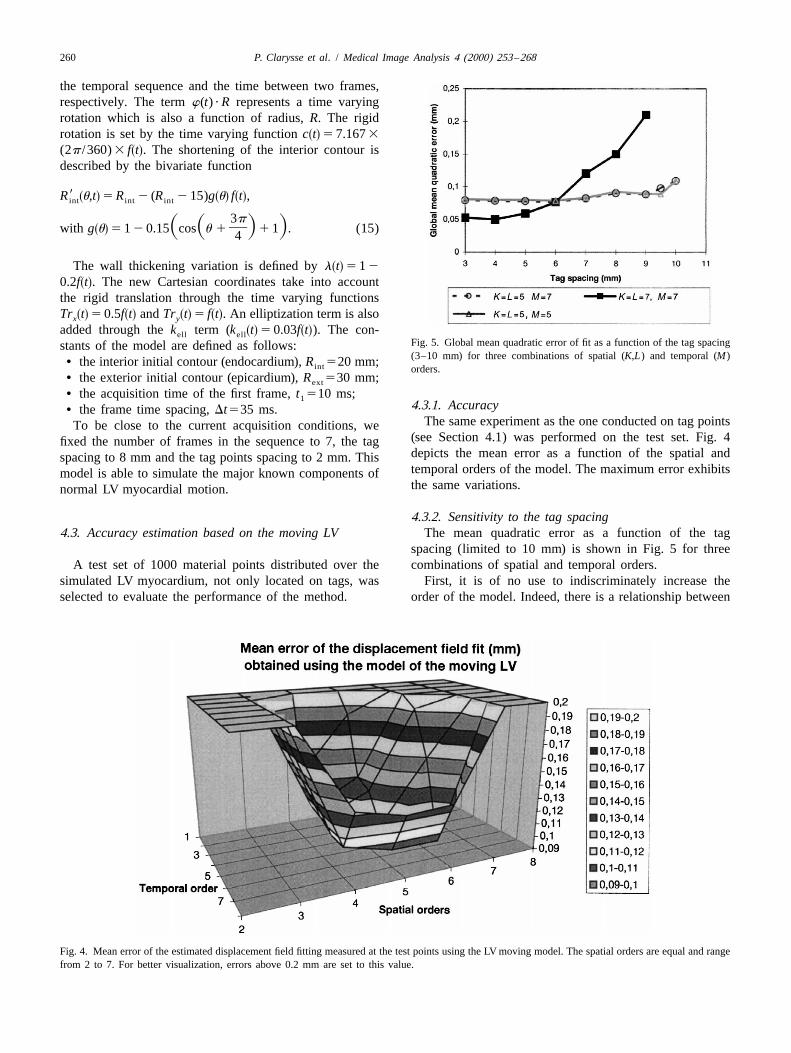
added through the k term (k t 5 0.03f t ). The con-s d s dell ellFig. 5. Global mean quadratic error of fit as a function of the tag spacingstants of the model are defined as follows:(3–10 mm) for three combinations of spatial (K,L) and temporal (M)• the interior initial contour (endocardium), R 520 mm;int orders.

• the exterior initial contour (epicardium), R 530 mm;ext

• the acquisition time of the first frame, t 510 ms;14.3.1. Accuracy• the frame time spacing, Dt535 ms.

The same experiment as the one conducted on tag pointsTo be close to the current acquisition conditions, we(see Section 4.1) was performed on the test set. Fig. 4fixed the number of frames in the sequence to 7, the tagdepicts the mean error as a function of the spatial andspacing to 8 mm and the tag points spacing to 2 mm. Thistemporal orders of the model. The maximum error exhibitsmodel is able to simulate the major known components ofthe same variations.normal LV myocardial motion.

4.3.2. Sensitivity to the tag spacing4.3. Accuracy estimation based on the moving LV The mean quadratic error as a function of the tag

spacing (limited to 10 mm) is shown in Fig. 5 for threeA test set of 1000 material points distributed over the combinations of spatial and temporal orders.

simulated LV myocardium, not only located on tags, was First, it is of no use to indiscriminately increase theselected to evaluate the performance of the method. order of the model. Indeed, there is a relationship between

Fig. 4. Mean error of the estimated displacement field fitting measured at the test points using the LV moving model. The spatial orders are equal and rangefrom 2 to 7. For better visualization, errors above 0.2 mm are set to this value.

P. Clarysse et al. / Medical Image Analysis 4 (2000) 253 –268 261

the model order and both the tag spacing and the temporal direction is randomly set. Fig. 6 shows the evolution of theresolution. For a conventional tag spacing value (8 mm), mean quadratic error measured on four test point sets as aone can deduce the optimal spatial (5) and temporal (7) function of the standard deviation of the perturbation. Thisorders (Fig. 4). The latter is directly related to the number is computed with spatial orders set to 5 and a temporalof image frames in the sequence (7 frames). The spatial order set to 7. The graph demonstrates the linear relation-orders are related to the tag spacing. Increasing the spatial ship between the quadratic error of the fit and the accuracyorder may affect the accuracy of the estimation by of the tag locations. Therefore, the accuracy of theintroducing spurious high order terms. An optimal cou- displacement field estimation is directly related to thepling between tag spacing and spatial orders provides good accuracy of the tag detection. This accuracy has not beenaccuracy within a reasonable computing time. Fig. 5 shows truly investigated. Typically, the first automatic extractiononly little improvement between spatial orders 5 and 7 for step is followed by user interventions to manually correcta tag spacing within 3 and 6 mm, but a spatial order 5 tag locations. Atalar and McVeigh (1994) have shown thatmodel is faster to compute (see Section 4.4). The effect of an accuracy on the order of 0.1 mm can theoretically bethe tag points spacing within a tag line has also been expected.investigated. This spacing is usually 1 mm; however, ouranalysis using the moving heart model shows that between1 and 3 mm the accuracy of the reconstructed field is 4.4. Computation timenearly constant for a tag spacing of 8 mm when theoptimal spatial and temporal orders are used. Fig. 7 illustrates the computing times obtained on a

Silicon Graphics Indigo 2 (MIPS R4400 CPU processor)with no special optimization of the code. The computing

4.3.3. Sensitivity to the accuracy of the tag location time is approximately a quadratic function of the parameter2The tags were extracted from the images by a previous number of the model (Space order 3Temporal order)

semi-automatic segmentation process. We observed the (Fig. 7(a)). It is also linearly dependent on the number ofdependency of the displacement estimation upon the tag points as shown in Fig. 7(b). In current practice andaccuracy of the tag location. A small perturbation was with the optimal orders, it takes less than 4 minutes toapplied to each tag point location generated by the model. compute the direct spatio-temporal displacement field.The magnitudes of the perturbations follow a Gaussian law Other parameters (deformation, velocities) are computed(zero mean with a varying standard deviation) while the immediately.

Fig. 6. Global mean quadratic error of fit as a function of the standard deviation of the noise perturbing the tag points locations. Four different sets ofpoints have been tested.

262 P. Clarysse et al. / Medical Image Analysis 4 (2000) 253 –268

Fig. 7. Computing times. (a) As a function of the spatial and temporal orders; (b) as a function of the tag points number.

5. Results on clinical cases cardiac contraction, i.e., at end-systole for mid-ventricularslices. Nine images were acquired for the healthy subject

Displacement and deformation fields are computed and and the patient at rest. Under pharmacological stress, onlyanalyzed on two clinical data sets. Fully informative six images were acquired for the patient.visualization of vector fields is not an easy task. We used aspecific visualization method developed by our group 5.1. Visualization of the displacement field(Khouas et al., 1998). Such a method represents, in asynthetic view, the direction, orientation and magnitude of Fig. 8(a) shows the displacement field for the healthya vector field using a 2D texture model. The comparison of case at end-systole. One can easily see that the displace-the results between cases was made at the maximum of the ment in the inferior, lateral and anterior regions is higher

P. Clarysse et al. / Medical Image Analysis 4 (2000) 253 –268 263

Fig. 8. Displacement field obtained at end-systole for the healthy subject. The direction of the displacement is given by the fibers while the magnitude iscolor-coded. The size of the region of interest which includes the myocardium is about 74374 mm. (a) Displacement field. (b) Displacement field withoutthe global rigid translation. Myocardial contours are displayed in white. (c) Definition of the myocardial regions.

than in the septal region, which is constrained by the right Fig. 9 illustrates the displacement field at end-systole forheart. The motion is mainly oriented toward the cavity’s the pathological case (severe postero-lateral ischemia) atcenter. For the purpose of contraction analysis, it is rest and under pharmacological stress using the same colorpreferable to eliminate the rigid translation that tends to map as for the healthy subject. Compared to the healthycomplicate the interpretation. Global translation compo- case, the magnitude of the displacement at rest is globallynents are provided by the spatial order 0 terms of our smaller and the orientation locally disorganized. Thismodel. This does not correspond to the true rigid transla- orientation, which is globally centripetal with the healthytion from a continuum mechanics point of view but rather subject, is clearly circumferential in the postero-lateralgives a mean value of the global displacement. Fig. 8(b) region (Fig. 9(a)). The pharmacological stress increases theillustrates the displacement field once this global transla- magnitude of the displacement and re-orientates the motiontion is removed. The motion is more homogeneous around toward the cavity’s center except for the postero-lateralthe myocardium. Differences between the regions is no region (Fig. 9(b)). This suggests a contractile defect in thismore significant, although the magnitude of the displace- region, which was confirmed by an angiographic study. Wement is still slightly smaller in the septum. Note the also observe reduced wall thickness in this region. Quick-existence of a gradient of the displacement magnitude time movies were also generated and are available asinside the myocardial wall. The magnitude is greater when Electronic Annexes (see www.elsevier.com/ locate /media).close to the endocardium. They depict the evolution of the displacement field through

Fig. 9. Displacement field obtained at end-systole for the ischemic patient. (a) At rest; (b) under pharmacological stress (dobutamine). Myocardial contoursare displayed in white.

264 P. Clarysse et al. / Medical Image Analysis 4 (2000) 253 –268

the cardiac systole for the healthy subject and the ischemic phenomenon. But the model, as stated, does not constrainpatient. One can visualize the progressive orientation of the initial strain values.the displacement towards the center and also the transmur-al gradient of the displacement magnitude for the healthysubject (End-systole corresponds to frame 6). Thepathological case exhibits quite a different behavior at rest 6. Discussion and conclusionand under pharmacological stress. In that case, the end-systole is at timepoint 6 and 5, respectively. The ability of the proposed spatio-temporal model to

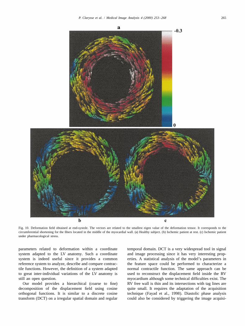
reconstruct a 2D time varying displacement field has beendemonstrated. Experiments using the moving LV model5.2. Visualization of the deformation fieldhave shown that a mean accuracy of 0.1 mm can beexpected. With actual experiments, the accuracy primarilyThe deformation field is computed as a function of thedepends on tag location accuracy. Only the orders of thecoordinates after deformation using the equations below:model are defined by the user. The analysis in Section 4.3121 T provides material to choose the optimal values for a given]F 5 (I 1 =D9(P9)) , ´ 5 (F F 2 I), (16)2 tagging pattern configuration (tag spacing and number of

where F is the deformation gradient tensor. The principal frames). The SVD decomposition algorithm introducesdeformations are obtained by diagonalizing the ´ matrix. another parameter (Press et al., 1988) that sets the maxi-Fig. 10(a) represents the principal deformation field associ- mum rate above which a singular value is zeroed. As aated with the smallest eigen values for the healthy case. consequence, equations which are corrupted by roundoffThe principal deformation is related to the circumferential errors are ignored. For small orders, this parameter has noshortening of the myocardial fibers located at the middle of influence. As the orders increase, a too small or a too highthe LV wall which are circumferentially oriented. The value of this parameter may degrade the accuracy. After

eorientation of the vectors is uniformly oriented along the several experiments, we set this value to 10 4, whichcircumferential direction and the magnitude significantly seems a good tradeoff. Another approach in order toincreases from the epicardium to the endocardium. reduce the effect of high order models is to use a

The deformation field for the pathological case at rest regularized approach for the displacement field estimation(Fig. 10(b)) is almost circumferentially oriented in the (Bogen and Rahdert, 1996).anteroseptal territories but the orientation is clearly toward It is theoretically possible to consider only one pointthe interior of the cavity in the posterolateral region. over two along each tag line to obtain the same accuracyMoreover, the magnitude is globally smaller compared to with half the computing time. Indeed, tag tracking algo-that for the healthy subject. The result under stress (Fig. rithms may incorporate some implicit smoothing so that10(c)) demonstrates an increase in magnitude over the reducing the density of points along the tags may not affectanteroseptal region but, again, no recovery is observed in the accuracy of the motion estimation. Note that the userthe posterolateral region. can control the overall accuracy of the computed displace-

ment field by observing the statistics of the error computed5.3. Pointwise tracking on the tags.

The main characteristic of the method, as opposed toThe identified model of the spatio-temporal displace- most of the previous studies (Denney and Prince, 1995;

ment field provides a Lagrangian description of motion O’Dell et al., 1995; Park et al., 1996), is that it integratesand, therefore, direct access to kinematic and deformation the temporal behavior of the displacement field. It is, inparameters of material points inside the LV myocardium. this sense, close to the method proposed by Declerck et al.The computation of velocities, accelerations and deforma- (1998a,b) in 3D, although their respective formulations aretions is analytical and benefits from the underlying smooth different. The principle of our method is directly applic-mathematical model to provide smooth temporal curves. able to 3D analysis. Considering a set of great axis imagesFig. 11(a) illustrates the variation of the two eigen values with tags parallel to the small axis image plane, one canfor three points belonging, respectively, to the anterior introduce similar equations to (1)–(4) for the estimation ofregion of the healthy case and to the ‘normal’ anterior the displacement field along the z direction. The evaluationregion of the pathological case at rest and under pharmaco- of the accuracy with a possible different distribution of taglogical stress. The two eigenvalues have almost the same points should necessitate a careful evaluation. Anotherevolution for the three regions although the magnitude is difference is that Declerck et al. (1998a,b) used a specificgreater with the healthy case. Fig. 11(b) clearly shows, LV anatomical coordinate system and computed threecompared to the normal case, the perturbed behavior of intuitive deformation parameters within that system. In ourthese parameters in an ischemic territory. The value system, we chose to reconstruct the displacement fieldobtained for the abnormal region at time t 5 0 is quite low. based on the geometry of the tag pattern. It is alwaysWe still do not have a satisfactory explanation of this possible to express the displacement and the numerous

P. Clarysse et al. / Medical Image Analysis 4 (2000) 253 –268 265

Fig. 10. Deformation field obtained at end-systole. The vectors are related to the smallest eigen value of the deformation tensor. It corresponds to thecircumferential shortening for the fibers located in the middle of the myocardial wall. (a) Healthy subject. (b) Ischemic patient at rest. (c) Ischemic patientunder pharmacological stress.

parameters related to deformation within a coordinate temporal domain. DCT is a very widespread tool in signalsystem adapted to the LV anatomy. Such a coordinate and image processing since it has very interesting prop-system is indeed useful since it provides a common erties. A statistical analysis of the model’s parameters inreference system to analyze, describe and compare contrac- the feature space could be performed to characterize atile functions. However, the definition of a system adapted normal contractile function. The same approach can beto great inter-individual variations of the LV anatomy is used to reconstruct the displacement field inside the RVstill an open question. myocardium although some technical difficulties exist. The

Our model provides a hierarchical (coarse to fine) RV free wall is thin and its intersections with tag lines aredecomposition of the displacement field using cosine quite small. It requires the adaptation of the acquisitionorthogonal functions. It is similar to a discrete cosine technique (Fayad et al., 1998). Diastolic phase analysistransform (DCT) on a irregular spatial domain and regular could also be considered by triggering the image acquisi-

266 P. Clarysse et al. / Medical Image Analysis 4 (2000) 253 –268

Fig. 11. Tracking the eigenvalues of myocardial points over time. (a) Within normal regions; (b) within ischemic regions as compared with the healthysubject.

tion on the end-systole. The proposed approach does not points, and the velocities or deformations over time. Theymake a priori assumptions such as incompressibility. The are computed in 2D and time in the current implementationdisplacement field estimation is based on the entire set of of the software. The accurate estimation of the truetag points and not only on the tag line intersections as with trajectories requires the extension of the method in 3D1

some other methods. time. We are currently working on the generalization of theThe proposed method, combined with a specific visuali- approach using long axis images. The large set of spatio-

zation tool, provides an innovative way to noninvasively temporal data must be carefully analyzed for populationsanalyze contractile function. Various spatio-temporal pa- of normal subjects and ischemic patients. Therefore, werameters can be accurately computed. These parameters are developing specific tools to aid in the exploration ofprovide a set of motion features not available before in the myocardial contractile function and to extract knowledgesame context: the 2D trajectories of material /myocardial from the proposed method.

P. Clarysse et al. / Medical Image Analysis 4 (2000) 253 –268 267

Fig. 11. (continued)

Acknowledgements leading to≠C 2]] 9 95 0 5 2A O b 2 2 O b c 2O A bi i,o i,o o k k,oThe FINDTAGS analysis software was used courtesy of S D9≠A o oi k±i

Dr. Elias A. Zerhouni of the Johns Hopkins University95 2 O b 2 c 1O A b .School of Medicine. This work is in the scope of the i,o o k k,oS D

o kscientific topics of the GDR-PRC ISIS research group ofExpanding the terms again, we obtain for each combina-the French National Center for Scientific Research

tion of k, l, m(CNRS). It was performed in the framework of the jointt max(t ) O(n)fK21 L21 M21Research Action ‘Beating Heart’ of the CNRS. This work pkx9 ?s d

]]]9 S D0 5 O O O A O O O cosˆ´is supported by the Region Rhone-Alpes under the grant x,k9,l 9,m9 Xt5t o51k950 l 950 m950 n5min(t )o´‘Sante et HPC’. The authors are grateful to the anonymousply9 ? pmt pk9x9 ?s d s dreviewers for their careful review of the manuscript and ]] ]] ]]]S D S D? cos ? cosS D ? cosY T Xthe pertinence of their comments.pl9y9 ? pm9ts d]]] ]]S D S D? cos ? cosY T

t max(t ) O(n)fpkx9 ?s dAppendix A ]]]S D2O O O cos Xt5t o51n5min(t )o

We provide the mathematical details of the computation ply9 ? pmts d]] ]]S D? cos ? cosS D ? x(n,t ) 2 x9 ?s ds d0of the model’s parameters for the x coordinate of the Y T

9inverse displacement field. Computing ≠C /≠A , ;i (seex x,i where (?) stands for (o,n,t). The matrix form is given byEqs. (5) and (6)), the indices t, n, o are grouped under the Eq. (7) with matrices B and C given byindex o, and the indices k, l, m under the index k. Let c beo t max(t ) O(n)fthe abscissa difference, we get pk(i)x9 ? pl(i)y9 ?s d s d

]]] ]]]S D S DB 5O O O cos ? cosi, j X Yt5t o51n5min(t )o≠C ≠ 2]] ]] 95 0 5 O O 2 A b 1 ck k,o oF S D G pm(i)t pk9( j)x9 ?s d9 9≠A ≠A oi i k ]] ]]]]S D S D? cos ? cosT X

≠ 2]] 9 95 O 2 A b 1 c 1O 2 A b , pl9( j)y9 ? pm9( j)ts di i,o o k k,oF S D G9≠A o ]]]] ]]]i S D S Dk±i ? cos ? cos ,Y T

268 P. Clarysse et al. / Medical Image Analysis 4 (2000) 253 –268

t Khouas, L., Clarysse, P., Friboulet, D., Odet, C., 1998. Fast 2D vectormax(t ) O(n)fpk(i)x9 ? pl(i)y9 ?s d s d field visualization using a 2D texture synthesis based on an auto-]]] ]]]S D S DC 5O O O cos ? cosi X Y regressive filter. Application to cardiac imaging. Machine Graphicst5t o51n5min(t )o

Vision 7 (4), 751–764.pm(i)t Maier, S.E., Fisher, S.E., McKinnon, G.C., Hess, O.M., Krayenbuehl,]]S D? cos ? x(n,t ) 2 x9 ? ,s ds d0T H.P., Boesiger, P., 1992. Evaluation of left ventricular segmental wall

motion in hypertrophic cardiomyopathy with myocardial tagging.where k i 5 int(i /LK), l i 5 int i 2 k i ML /M , m i 5s d s d ss s d d d s d Circulation 86, 1919–1928.i 2 k i ML 2 l i M.s d s d Meyer, F.G., Constable, R.T., Sinusas, A.J., Duncan, J.S., 1996. Tracking

myocardial deformation using phase contrast MR velocity fields: astochastic approach. IEEE Trans. Med. Imaging 15, 1–12.

Moore, C.C., O’Dell, W.G., McVeigh, E.R., Zerhouni, E.A., 1992.ReferencesCalculation of three-dimensional left ventricular strains from biplanartagged MR images. J. Magn. Reson. Imaging 2, 165–175.

Amini, A.A., Chen, Y., Curwen, R.W., Mani, V., Sun, J., 1998. Coupled Mosher, T.J., Smith, M.B., 1994. A DANTE tagging sequence for theB-snake grids and constrained thin-plate splines for analysis of 2D evaluation of translational sample motion. Magn. Reson. Med. 15,tissue deformations from tagged MRI. IEEE Trans. Med. Imaging 17 334–339.(3), 344–356. O’Dell, W.G., 1995. Myocardial deformation analysis in the passive dog

Atalar, E., McVeigh, E.R., 1994. Optimization of tag thickness for heart using high resolution MRI tagging. PhD Thesis, Johns Hopkinsmeasuring position with magnetic resonance imaging. IEEE Trans. University, Baltimore, 239 pp.Med. Imaging 13 (1), 152–160. O’Dell, W.G., Moore, C.C., Hunter, W.C., Zerhouni, E.A., McVeigh, E.R.,

Axel, L., Dougherty, L., 1989. Heart wall motion: improved method of 1995. Three-dimensional myocardial deformations: calculation withspatial modulation of magnetization for MR imaging. Radiology 183, displacement field fitting to tagged MR images. Radiology 195, 829–745–750. 835.

Bogen, D.K., Rahdert, D.A., 1996. A strain energy approach to regulari- Park, J., Metaxas, D., Axel, L., 1996. Analysis of left ventricular wallzation in displacement field fits of elastically deforming bodies. IEEE motion based on volumetric deformable models and MRI-SPAMM.Trans. Pattern Analysis Machine Intelligence 18 (6), 629–635. Medical Image Analysis 1 (1), 53–71.

Buchalter, M.B., Weiss, J.L., Rogers, W.L., Zerhouni, E.A., Weisfeldt, Pelc, N.J., Herfkens, R.J., Shimakawa, A., Enzmann, D.R., 1991. PhaseM.L., Beyar, R., Shapiro, E.P., 1990. Noninvasive quantification of left contrast cine magnetic resonance imaging. Magn. Reson. Q. 7, 229–ventricular rotational deformation in normal humans using magnetic 254.resonance imaging myocardial tagging. Circulation 81, 1236–1244. Press, W.H., Flannery, B.P., Teukolsky, S.A., Vetterling, W.T., 1988. In:

Clark, N.R., Reichek, N., Bergey, P., Hoffman, E.A., Brownson, D., Numerical Recipes in C, The Art of Scientific Computing. CambridgePalmon, L., Axel, L., 1991. Circumferential myocardial shortening in University Press, New York.the normal human left ventricle. Assessment by magnetic resonance Radeva, P., Amini, A.A., Huang, J., 1997. Deformable B-solids andimaging using spatial modulation of magnetization. Circulation 84, implicit snakes for 3D localization and tracking of SPAMM MRI data.67–74. Computer Vision Image Understanding 66 (2), 163–178.

Declerck, J., Ayache, N., McVeigh, E.R., 1998a. Use of a 4D planispheric Wedeen, V.J., 1992. Magnetic resonance imaging of myocardialtransformation for the tracking and the analysis of LV motion with kinematics. Technique to detect, localize, and quantify the strain ratestagged MR Images. INRIA, Sophia Antipolis, Technical Report No. of the active human myocardium. Magn. Reson. Med. 27, 52–67.RR-3535. Young, A.A., 1998. Model tags: direct 3D tracking of the heart wall

Declerck, J., Feldmar, J., Ayache, N., 1998b. Definition of a four motion from tagged MR Images. In: Wells, W.M., Colchester, A.,dimensional continuous planispheric transformation for the tracking Delp, S. (Eds.), Medical Image Computing and Computer-Assistedand the analysis of left-ventricle motion. Medical Image Analysis 2 Intervention-MICCAI’98. Cambridge, MA, USA, pp. 92–101.(2), 197–213. Young, A.A., Axel, L., 1992. Three-dimensional motion and deformation

Denney, T.S., McVeigh, E.R., 1997. Model-free reconstruction of the of the heart wall: estimation with spatial modulation of magnetizationthree-dimensional myocardial strain from planar tagged MR Images. J. – A model-based approach. Radiology 185, 241–247.Magn. Reson. Imaging 7, 799–810. Young, A.A., Kraitchman, D.L., Dougherty, L., Axel, L., 1995. Tracking

Denney, T.S., Prince, J.L., 1995. Reconstruction of 3D left-ventricular and finite element analysis of stripe deformation in magnetic resonancemotion from planar tagged cardiac MR images: an estimation theoretic tagging. IEEE Trans. Med. Imaging 14 (3), 413–421.approach. IEEE Trans. Med. Imaging 14 (4), 625–635. Zerhouni, E.A., Parish, D.M., Rogers, W.J., Yang, A., 1988. Human heart:

Fayad, Z.A., Ferrari, V.A., Kraitchman, D.L., Young, A.A., Palevsky, H.I., tagging with MR imaging – a method for noninvasive assessment ofBloomgarden, D.C., Axel, L., 1998. Right ventricular regional function myocardial motion. Radiology 169, 59–63.using MR tagging: normals versus chronic pulmonary hypertension. Zhu, Y., Drangova, M., Pelc, N.J., 1997. Estimation of deformationMagn. Reson. Med. 39, 116–123. gradient and strain from cine-PC velocity data. IEEE Trans. Med.

Guttman, M.A., Prince, J.L., McVeigh, E.R., 1994. Tag and contour Imaging 16 (6), 840–851.detection in tagged MR images of the left ventricle. IEEE Trans. Med.Imaging 13 (1), 74–88.

Guttman, M.A., Zerhouni, E.A., McVeigh, E.R., 1997. Analysis of cardiacfunction from MR Images. IEEE CG&A 17 (1), 30–38.