Prepared for submission to JHEP DESY 18-105, CERN-TH-2018-147

Two-current correlations in the pion on the lattice

Gunnar S. Balia,b Peter C. Brunsc Luca Castagninia Markus Diehld,e Jonathan R.

Gauntf Benjamin Glaßleg Andreas Schafera Andre Sternbeckh and Christian

Zimmermanna

aInstitute for Theoretical Physics, University of Regensburg, 93040 Regensburg, GermanybDepartment of Theoretical Physics, Tata Institute of Fundamental Research, Homi Bhabha Road,

Mumbai 400005, IndiacNuclear Physics Institute, 25069 Rez, Czech RepublicdFachbereich Physik, University of Hamburg, 22761 Hamburg, GermanyeDeutsches Elektronen-Synchroton DESY, 22607 Hamburg, GermanyfCERN Theory Division, 1211 Geneva 23, SwitzerlandgZentrum fur Datenverarbeitung, Universitat Tubingen, Wachterstr. 76, 72074 Tubingen, Ger-

manyhTheoretisch-Physikalisches Institut, Friedrich-Schiller-Universitat Jena, 07743 Jena, Germany

Abstract: We perform a systematic study of the correlation functions of two quark cur-

rents in a pion using lattice QCD. We obtain good signals for all but one of the relevant

Wick contractions of quark fields. We investigate the quark mass dependence of our results

and test the importance of correlations between the quark and the antiquark in the pion.

Our lattice data are compared with predictions from chiral perturbation theory.

arX

iv:1

807.

0307

3v2

[he

p-la

t] 2

8 N

ov 2

018

Contents

1 Introduction 1

2 Correlation functions of two currents 3

2.1 Isospin decomposition and constraints 4

2.2 Predictions from chiral perturbation theory 5

3 Lattice techniques 7

3.1 Lattice contractions and their symmetry properties 7

3.2 Physical matrix elements 9

3.3 Simulation Details 10

3.4 Renormalisation 17

4 Data quality and lattice artefacts 18

4.1 Plateaux and excited state contributions 18

4.2 Anisotropy effects 19

4.3 Finite volume effects 22

4.4 Finite momentum and boost invariance 23

5 Results for individual lattice contractions 23

5.1 Light quarks 23

5.2 Quark mass dependence 27

5.3 Test of factorisation 29

5.4 Root mean square radii 32

5.5 Subtraction term for the annihilation graph 37

6 Results for isospin amplitudes 38

6.1 Isospin amplitudes 38

6.2 Comparison with chiral perturbation theory 39

7 Summary 42

References 45

1 Introduction

The study of hadronic form factors has a long history in QCD and remains an active

field of study. Defined from the matrix elements of single currents, form factors contain

information about the spatial distribution of charge inside a hadron. Going beyond this,

the matrix elements of two currents at different points in space are sensitive to charge

– 1 –

correlations and thus yield qualitatively new information about QCD bound states and

their many-body structure.

Hadronic matrix elements of one or two currents can be calculated in lattice QCD. In

fact, it was realised long ago that two-current correlators on the lattice can be regarded

as gauge invariant probes of hadron wave functions. Following earlier work [1–8], detailed

computations for the vector, scalar and pseudoscalar currents were presented in [9, 10] and

extended studies for the vector current in [11]. These studies focused on a broad range of

physics and observables, such as confinement [1, 2], the size of hadrons [3–5, 8], comparison

with quark models [7], or the non-spherical shape of hadrons with spin 1 or larger [9–11].

The computation of two-current correlators on the lattice involves many different Wick

contractions of the quark fields, including disconnected graphs and graphs with all-to-all

propagators. This presents major challenges, for the sheer amount of calculations and for

obtaining statistically significant results. Whilst the work in [1–11] focused on the graph

denoted by C1 in figure 2, we study all relevant contractions for a meson here (leaving

the case of baryons for future work). We also extend the set of currents mentioned above

by the axial current. Last but not least, increased computing power has allowed us to use

larger lattices and a smaller pion mass than previous studies. Indeed, we will see that finite

volume effects can be appreciable for the quantities we are interested in.

At large distances between the two currents, the correlation functions we consider can

be evaluated in chiral perturbation theory, which describes the low-energy limit of QCD

in terms of mesons and their interactions. A leading-order calculation, supplemented by

an estimate of higher orders using resonance exchange graphs, has been performed in [12],

and we will compare our lattice results with these predictions.

An extension of the work presented here allows us to compute matrix elements that, as

explained in [13], can be connected with the Mellin moments of double parton distributions.

These distributions are necessary to compute coherent hard scattering on two spatially

separated partons inside a hadron. An additional challenge in this case is that one must

compute correlation functions for all vector or tensor components of the inserted currents

and then extract their twist-two part. Corresponding results for the pion will be presented

in a forthcoming paper. The ultimate goal is to extend such studies to double parton

distributions in the nucleon, which is of acute interest for the precise description of high-

multiplicity final states at the LHC and at possible future hadron colliders.

This paper is organised as follows. In section 2, we derive a number of general prop-

erties of two-current matrix elements of the pion and recall the predictions of chiral per-

turbation theory relevant to our study. Properties of the different Wick contractions and

their computation on the lattice are described in section 3. The general quality of our

data and the presence of lattice artefacts is investigated in section 4. Results for individual

lattice contractions are shown in section 5, including the quark mass dependence and the

relevance of correlations between the two currents. Physical matrix elements are presented

in section 6 and compared with chiral perturbation theory. A summary of our work is

given in section 7.

– 2 –

2 Correlation functions of two currents

The object of our study are correlation functions of two currents in a pion,

〈πk(p)| Oq1q2i (y)Oq3q4j (0) |πk′(p)〉 , (2.1)

where the pion charges k, k′ = +,−, 0 may differ between the bra and ket state, whereas

the four-momentum p is the same for both. The matrix elements (2.1) are understood

to be fully connected, with disconnected contributions like 〈π|π〉 · 〈0| Oi(y)Oj(0) |0〉 or

〈π| Oi(y) |0〉 · 〈0| Oj(0) |π〉 removed. The currents we consider are

Oqq′i (y) = q(y)Γiq′(y) , (2.2)

where q and q′ are u or d quark fields. The full set of Dirac matrices Γi corresponds to the

scalar, pseudoscalar, vector, axial and tensor currents:

Sqq′ = q q′ , Pqq′ = iqγ5q′ , V µ

qq′ = qγµq′ , Aµqq′ = qγµγ5q′ , Tµνqq′ = qσµν q′ . (2.3)

Note that for equal quark flavours all currents are hermitian.

In the present work, we investigate lattice data for correlation functions of two equal

currents V 0, A0, S or P . In a pion at rest, these currents are associated with the vector,

axial, scalar or pseudoscalar charges. We abbreviate the corresponding matrix elements

(2.1) as

〈V 0V 0〉, 〈A0A0〉, 〈SS〉, 〈PP 〉, (2.4)

respectively. For later use, we shall however consider the full set of currents (2.2) in the

theoretical exposition below.

The matrix elements 〈SS〉 and 〈PP 〉 are boost invariant and thus depend only on the

products y2 and yp of four-vectors, given that p2 = m2π is fixed. On the lattice, we can

compute the matrix elements for y0 = 0 and for different pion momenta. The rotation

to Euclidean time and the method to extract hadronic matrix elements from a lattice

calculation single out a particular reference frame. It is hence a valuable check for lattice

artefacts to verify that for a given ~y 2, the matrix elements with scalar and pseudoscalar

currents are independent of the pion momentum when ~y · ~p = 0, a condition that can be

achieved for both zero and nonzero ~p .

The operators (2.2) transform under charge conjugation (C) and under the combination

of parity and time reversal (PT ) as

Oqq′i (y) →CηiC Oq

′qi (y) , Oqq′i (y) →

PTηiPT Oq

′qi (−y) , (2.5)

with sign factors

ηiC = +1 for i = S, P,A, ηiC = −1 for i = V, T, (2.6)

and

ηiPT = +1 for i = S, P, V, ηiPT = −1 for i = A, T. (2.7)

We also define the products ηijC = ηiC ηjC and ηijPT = ηiPT η

jPT .

– 3 –

2.1 Isospin decomposition and constraints

The matrix elements (2.1) are not all independent due to constraints from isospin sym-

metry and from the discrete symmetries just discussed. To exploit isospin symmetry, it is

convenient to use linear combinations with isospin 0 and 1,

Osi = Ouui +Oddi , Ons

i = Ouui −Oddi , (2.8)

as well as the isotriplet current

Oai = QτaΓiQ , a = 1, 2, 3 (2.9)

with the Pauli matrices τa and the isodoublet Q = (u, d) of quark fields. One then has

Onsi = O3

i , Oudi =(O1i + iO2

i

)/2 , Odui =

(O1i − iO2

i

)/2 . (2.10)

Expressing the pion states in the isospin basis, we have

|π+〉 =(|π1〉+ i|π2〉

)/√

2 , |π−〉 =(|π1〉 − i|π2〉

)/√

2 , |π0〉 = |π3〉 . (2.11)

We can now decompose

〈πd| Osi(y)Os

j(0) |πc〉 = δcdF0(y) ,

〈πd| Oai (y)Obj(0) |πc〉 = δabδcdF1(y) +(δacδbd + δadδbc

)F2(y) +

(δacδbd − δadδbc

)iF3(y) ,

〈πd| Obi (y)Osj(0) |πc〉 = iεbcdG1(y) ,

〈πd| Osi(y)Obj(0) |πc〉 = iεbcdG2(y) , (2.12)

where for brevity we have suppressed the dependence of Fn, Gn on the pion momentum p

and on the indices i, j that specify the operators. Taking the complex conjugate of (2.12),

one readily finds that the isospin amplitudes Fn and Gn are real valued.

For the matrix elements in the quark flavor basis, we obtain

〈π+| Osi(y)Os

j(0) |π+〉 = 〈π0| Osi(y)Os

j(0) |π0〉 = F0 ,

〈π+| Onsi (y)Os

j(0) |π+〉 = −√

2 〈π0| Odui (y)Osj(0) |π+〉 = G1 ,

〈π0| Onsi (y)Os

j(0) |π0〉 = 0 (2.13)

and analogous relations for the matrix elements parameterised by G2, now also suppressing

the y-dependence of Fn and Gn. For matrix elements with two isotriplet operators, we have

〈π+| Onsi (y)Ons

j (0) |π+〉 = 2 〈π0| Oudi (y)Oduj (0) |π0〉 = 2 〈π0| Odui (y)Oudj (0) |π0〉 = F1 ,

〈π0| Onsi (y)Ons

j (0) |π0〉 = F1 + 2F2 ,

〈π−| Odui (y)Oduj (0) |π+〉 = F2 ,

〈π+| Oudi (y)Oduj (0) |π+〉 = (F1 + F2 − iF3)/2 ,

〈π+| Odui (y)Oudj (0) |π+〉 = (F1 + F2 + iF3)/2 ,

〈π0| Onsi (y)Oduj (0) |π+〉 = (F2 − iF3)/

√2 ,

〈π0| Odui (y)Onsj (0) |π+〉 = (F2 + iF3)/

√2 . (2.14)

– 4 –

From (2.12) one also finds that the matrix elements with two isosinglet or with two

isotriplet operators are even under the simultaneous exchange1

|π+〉 ↔ |π−〉 , Odui ↔ Oudi , (2.15)

whereas the matrix elements with one isosinglet and one isotriplet operator are odd under

that exchange. The charge conjugate of a matrix element is obtained by applying (2.15)

and multiplying with the product ηijC of intrinsic C parities of the two operators. One

readily sees that Gn = 0 if ηijC = +1 and that Fn = 0 if ηijC = −1. The charge conjugation

constraints give relations between matrix elements in the quark flavor basis. For ηijC = +1

the vanishing of G1 and G2 implies in particular

〈πk| Ouui (y)Ouuj (0) |πk〉 = 〈πk| Oddi (y)Oddj (0) |πk〉 ,〈πk| Ouui (y)Oddj (0) |πk〉 = 〈πk| Oddi (y)Ouuj (0) |πk〉 (2.16)

and thus

12 〈πk| Os

i(y)Osj(0) |πk〉 = 〈πk| Ouui (y)Ouuj (0) |πk〉+ 〈πk| Ouui (y)Oddj (0) |πk〉 ,

12 〈πk| Ons

i (y)Onsj (0) |πk〉 = 〈πk| Ouui (y)Ouuj (0) |πk〉 − 〈πk| Ouui (y)Oddj (0) |πk〉 (2.17)

for k = +,−, 0.

2.2 Predictions from chiral perturbation theory

Consider pions at rest and take the matrix elements 〈SS〉, 〈PP 〉, 〈V 0V 0〉 and 〈A0A0〉 at

y0 = 0 and large |~y |. These can then be computed in chiral perturbation theory. The

chiral expansion, on which this theory is based, requires the pion mass and momenta p

to be much smaller than 4πF ∼ 1 GeV, where F is the pion decay constant. In position

space, one should hence require |~y | � 0.2 fm. At leading order in the chiral expansion,

the matrix elements can be computed from the tree-level graphs in figure 1(a), (b) and

(c). The corresponding calculation is detailed in [12]. As an estimate for higher-order

contributions, the same work evaluated the resonance exchange graphs (d) and (e) from

the appropriate leading-order Lagrangian in the approximation of vanishing pion four-

momentum (thus setting mπ to zero). Resonance exchange graphs with the topology of

figure 1(c) would involve a vertex between pions and resonances, which vanishes in this

approximation. Considered were the lowest-lying resonances ρ, a1, a0, η and σ.

The corresponding results are given in sections II.A and III.B of [12]. For convenience,

we recast them into the notation used here, making use of the simplifications that arise

when setting y0 = 0. The isospin amplitudes Fi defined here are related to those in [12] as

F0 = C00, F1 = C1, F2 = C1 + C2 and iF3 = C3. We also note that the isospin currents

V aµ and Aaµ in [12] have an extra factor of 1/2 compared with our currents (2.9).

Vector and axial currents were only considered for the isovector case in [12], so that no

predictions are available for F0 in the 〈V 0V 0〉 and 〈A0A0〉 channels. Under the conditions

1According to (2.10) and (2.11) this corresponds to changing the sign of |πa〉 and Oai for a = 2 in the

isospin basis.

– 5 –

(a) (d) (e)(b) (c)

Figure 1. Graphs for the matrix elements 〈SS〉, 〈PP 〉, 〈V 0V 0〉, 〈A0A0〉 in chiral perturbation

theory. Single lines denote pions, double lines resonances, and crossed circles indicate current

insertions. The leading-order chiral Lagrangian gives rise to graph (a) for 〈SS〉, 〈V 0V 0〉 and to

graphs (b) and (c) for 〈PP 〉, 〈A0A0〉. The resonance exchange graphs (d) and (e) can contribute to

any of the four matrix elements, depending on the quantum numbers of the resonance.

stated above, the isotriplet amplitude F3 is found to vanish for all channels 〈SS〉, 〈PP 〉,〈V 0V 0〉, 〈A0A0〉.

For the remaining matrix elements, we obtain the following results from [12], writing

y = |~y | for simplicity. The leading order chiral Lagrangian gives rise to the amplitudes

FSS0(LO) =2B2mπ

π2yK1(mπ y) , FPP0(LO) = 0 ,

FSS1(LO) = 0 , FPP1(LO) = −B2m2

π

2π2K0(mπ y) ,

FSS2(LO) = 0 , FPP2(LO) =B2m2

π

2π2

[K0(mπy)− 2K1(mπ y)

mπ y

](2.18)

and

F V V1(LO) =2m3

π

π2y

[K1(mπ y)− K2(mπ y)

mπ y

],

FAA1(LO) =m3π

2π2y

[K1(mπ y) +

4K2(mπ y)

mπ y

],

F V V2(LO) = −1

2FVV1(LO) ,

FAA2(LO) = − m3π

2π2y

[K1(mπ y) +

2K2(mπ y)

mπ y

], (2.19)

where Kn denotes the Macdonald functions (modified Bessel functions of the second kind).

The pion decay constant F and the chiral symmetry breaking parameter B are defined

as usual in chiral perturbation theory, see section I.A in [12]. The resonance exchange

contributions read

FSS0(R) = −32B2(cσm)2mσ

π2F 2yK1(mσ y) ,

FPP0(R) =16B2

π2F 2y

[c2mma0 K1(ma0 y)− 2d2ηmηK1(mη y)

],

FSS1(R) = 0 , FPP1(R) = 0 , FSS2(R) = −1

2FPP0(R) , FPP2(R) = −1

2FSS0(R) ,

– 6 –

F V V1(R) = −FAA1(R) =∑

X=ρ,a1

sX2f2Xm

5X

π2F 2y

[K1(mX y) +

K2(mX y)

mX y

],

F V V2(R) = −FAA2(R) = −1

2F V V1(R) (2.20)

with signs sρ = 1, sa1 = −1. In the numerical evaluation of section 6.2, we will take the

resonance parameters estimated in [12]:

mρ = 0.8 GeV , fρ = 0.2 , ma1 = 1.25 GeV , fa1 = 0.1 ,

ma0 = 1 GeV , cm = 50 MeV , mη = 600 MeV , dη = 15 MeV ,

mσ = 0.5 GeV , cσm = 35 MeV . (2.21)

For the parameters in the chiral sector we will take mπ = 300 MeV, F = 100 MeV and

B = 2.4 GeV, which are rounded values of what we extract from our lattice simulations

with L = 40, see (5.20).

3 Lattice techniques

The lattice computation of the matrix elements (2.1) involves a considerable number of

different Wick contractions between the quark fields in the two currents and in the pion

source and sink. This is to be contrasted with, e.g., the computation of single-current

matrix elements, where there is only one connected and one disconnected graph. In the

present section, we give details about the lattice contractions for two-current correlators,

their relation with the physical pion matrix elements, and their implementation in the

lattice simulation.

3.1 Lattice contractions and their symmetry properties

The different lattice contractions are pictorially represented in figure 2. We have two fully

connected graphs C1 and C2, a graph A in which the pion in annihilated by one current and

created again by the second current, two graphs S1 and S2 with one disconnected quark

loop, and a doubly disconnected graph D with two quark loops.

The symbols Cij1 (y), Cij2 (y), etc. denote contributions to the physical matrix elements

(2.1), i.e. it is understood that

• the contractions shown are averaged over the gauge ensemble and divided by the

ensemble average of the pion two-point function,

• the two currents are inserted at the same time slice τ (i.e. y0 = 0), and the ratio

of four-point and two-point functions is evaluated at a plateau in τ . To use time

reversal invariance, the plateau must be symmetric between source and sink times,

• both source and sink are projected on definite momentum p. By translation invariance

one can thus shift their spatial positions by a common amount.

– 7 –

Oi(y)

Oi(y)

Oj(0)

C ij1 (y) =

= ηijC ×C ij2 (y) =

Oj(0)

Oi(y)

Aij(y) =

Oi(y)

Oj(0)

Oj(0)

Sij1 (y) = = ηijC ×

Sij2 (y) =

Oi(y)

Dij(y) =

Oi(y)

Oj(0)

Oi(y)

Oj(0)

Oj(0)

Oi(y)

Oj(0)

Figure 2. Lattice contractions for the two-current correlation function (2.1) in a pion. The

dependence on the pion momentum p is not indicated for brevity. The product ηijC of charge

conjugation parities of the two operators is defined below (2.7).

Details are given in section 3.3 below. For brevity, we do not indicate the dependence of

Cij1 (y) etc. on the pion momentum p.

From translation invariance one readily finds

M ij(y) = M ji(−y) for M = S2, D. (3.1)

– 8 –

Charge conjugation invariance gives

M ij(y) = ηijC Mji(−y) for M = C1. (3.2)

If ηijC = −1 one furthermore obtains M ij(y) = 0 for M = A,S2, D. From PT invariance

one gets

M ij(y) = ηijPTMij(−y) for M = C1, S1, S2, D, (3.3)

M ij(y) = ηijPTMji(y) for M = A,C2, (3.4)

where for the formulation of time reversal in the Euclidean path integral we refer to [14].

Finally, a useful relation for the contractions is obtained by taking the complex conju-

gate of the contraction, followed by a parity transformation and charge conjugation. This

gives [M ij(y)

]∗= ηPTM

ij(−y) for all contractions. (3.5)

Combining (3.3) with (3.5) we find that C1, S1, S2 and D are real valued, whereas combining

(3.4) with (3.5) gives

ReM ij(y) = 12

[M ij(y) +M ji(−y)

], i ImM ij(y) = 1

2

[M ij(y)−M ji(−y)

](3.6)

for M = A,C2.

3.2 Physical matrix elements

The form of the relation between pion matrix elements and lattice contractions depends

on the product of C parities. Using the shorthand notation

C1 = Cij1 (y) , C2 = 12

[Cij2 (y) + Cji2 (−y)

], A = 1

2

[Aij(y) +Aji(−y)

],

S1 = 12

[Sij1 (y) + Sji1 (−y)

], S2 = Sij2 (y) , D = Dij(y) , (3.7)

we have for ηijC = +1

〈π+| Ouui (y)Oddj (0) |π+〉 = C1 +[2S1 +D

],

〈π+| Ouui (y)Ouuj (0) |π+〉 =[2C2 + S2

]+[2S1 +D

],

〈π0| Ouui (y)Oddj (0) |π0〉 =[2S1 +D

]−A ,

〈π0| Ouui (y)Ouuj (0) |π0〉 = C1 +[2S1 +D

]+[2C2 + S2

]+A ,

〈π0| Odui (y)Oudj (0) |π0〉 = − C1 +[2C2 + S2

],

〈π−| Odui (y)Oduj (0) |π+〉 = 2C1 + 2A ,

〈π+| Odui (y)Oudj (0) |π+〉 = 2Cij2 (y) + S2 +Aij(y) ,√

2 〈π0| Odui (y)Ouuj (0) |π+〉 = C1 +[Cij2 (y)− Cji2 (−y)

]+Aij(y) . (3.8)

– 9 –

One can verify that this satisfies the isospin relations in section 2.1. We have three inde-

pendent real valued combinations, which can for instance be chosen as

12F0(y) = 〈π+| Ouui (y)Ouuj (0) |π+〉+ 〈π+| Ouui (y)Oddj (0) |π+〉

= C1 + 2[2S1 +D

]+ [2C2 + S2] ,

12F1(y) = 〈π+| Ouui (y)Ouuj (0) |π+〉 − 〈π+| Ouui (y)Oddj (0) |π+〉

= − C1 +[2C2 + S2

],

12F2(y) = 1

2 〈π−| Odui (y)Oduj (0) |π+〉= C1 +A , (3.9)

where F0, F1 and F2 are the isospin amplitudes defined in (2.12). These combinations are

real valued owing to (3.6), as the isospin amplitudes must be. The imaginary combination

iF3 of matrix elements can e.g. be isolated by

iF3(y) = 〈π+| Odui (y)Oudj (0) |π+〉 − 〈π+| Oudi (y)Oduj (0) |π+〉= 2[Cij2 (y)− Cji2 (−y)

]+[Aij(y)−Aji(−y)

]. (3.10)

In the present work, we only study the real valued combinations in (3.9).

For ηijC = −1 we have three nonzero lattice contractions, C1, C2 and S1, and two

independent matrix elements, which may be taken as

〈π+| Ouui (y)Oddj (0) |π+〉 = C1 + Sij1 (y)− Sji1 (y) ,

〈π+| Ouui (y)Ouuj (0) |π+〉 = 2C2 + Sij1 (y) + Sji1 (y) . (3.11)

Among all contractions, C1 has typically the smallest statistical uncertainties in the

lattice simulation and thus plays a special role. The above equations show that it does not

appear in isolation in any physical pion matrix element. However, C1 can be regarded as

“approximately physical” in the following sense. Consider QCD with nF = 4 (instead of

nF = 2) mass degenerate quarks, where SU(4) flavour symmetry is exact. It is easy to see

that in this theory

〈π+| Ouci (y)Osdj (0) |D+s 〉 = Cij1 (y) , (3.12)

where the quark content of the D+s meson is cs. The correlation function C1 computed in

our study does not exactly correspond to this matrix element, because our lattice action

has nF = 2 and not nF = 4 sea quark flavours. We therefore must interpret (3.12) within

the partially quenched approximation.

3.3 Simulation Details

Lattice action and quark mass values. We have performed Nf = 2 lattice simulations

with the Wilson gauge action and non-perturbatively improved Sheikholeslami-Wohlert

(NPI Wilson-clover) fermions. The gauge configurations were generated by the RQCD and

QCDSF collaborations. As is discussed for instance in [15, 16], there are eleven standard

– 10 –

ensemble β a [fm] κ L3 × T mπ [MeV] Lmπ Nfull Nused Nsm

IV 5.29 0.071 0.13632 323 × 64 294.6(14) 3.42 2023 960 400

V 5.29 0.071 0.13632 403 × 64 288.8(11) 4.19 2025 984 400

Table 1. Details of the ensembles used in this analysis. Nfull is the total number of available gauge

configurations and Nused the number of configurations used in the present study. Nsm indicates the

number of Wuppertal smearing iterations in the pion source. The error on the pion mass combines

statistical and systematic errors, see [15]. The time difference between pion source and sink is

t = 15a or t = 32a for both ensembles.

ensembles with pion masses down to 150 MeV. Two of these are used in the present study,

namely ensembles IV and V, with a reduced number of gauge configurations as indicated

in table 1.

We will also study the dependence of the pion matrix elements (2.1) on the quark

mass. To this end, we have performed simulations with ensemble V and different values of

κ in the quark propagator, namely

light quarks: κ = 0.13632 amq = 0.00291(3) ,

strange: κ = 0.135616 amq = 0.02195(3) ,

charm: κ = 0.125638 amq = 0.31475(3) , (3.13)

where we also give the values of the bare quark masses mq in lattice units. Here “light

quarks” refers to the κ value of ensemble V, whereas the other two values correspond to

the physical strange and charm quark masses, as determined in [17] and [18] by tuning the

pseudoscalar ground state mass to 685.8 MeV in the first case and the spin-averaged S-wave

charmonium mass to 3068.5 MeV in the second case. Since our simulations are performed

with an nF = 2 fermion action, the strange and charm quarks are partially quenched.

Correlation functions. To compute the pion matrix element in (2.1) on a lattice in

Euclidean space-time, we need the four-point correlators

Cij,~p4pt (~y , τ, t) = a6∑~x,~z

e−i~p ·(~x−~z ) 〈0|Π(~x, t)Oi(~y , τ)Oj(~0, τ) Π†(~z , 0) |0〉 , (3.14)

where Π(x) is a pion interpolator. We use interpolators with Dirac structure γ5. Pion

matrix elements are extracted by calculating the following ratio at time slices where excited

states should be suppressed:

〈π(p)| Oi(y)Oj(0) |π(p)〉 = R~pij(~y ) = 2E~p VCij,~p4pt (~y , τ, t)

C~p2pt(t)

∣∣∣∣0�τ�t

. (3.15)

Here V = L3a3 is the spatial volume and

C~p2pt(t) = a6∑~x,~z

e−i~p ·(~x−~z ) 〈0|Π(~x, t) Π†(~z , 0) |0〉 (3.16)

– 11 –

Figure 3. Lattice methods employed for computing the different graphs of the four-point function.

Colours are used to distinguish the different parts of a graph. Two stochastic sources within a pion

source or sink lead always to the application of the one-end trick or two-hand-trick, respectively.

the usual pion two-point function. In analogy to (3.14) and (3.15), we use an appropriate

ratio of the three-point function Ci,~p3pt(τ, t) and C~p2pt(t) to extract the matrix elements

〈π(p′)| Oi(0) |π(p)〉 of the vector and scalar currents. We thus obtain the vector and scalar

form factors for the pion, which are used in sections 3.4 and 5.3.

The pion energy in (3.15) is computed using the continuum dispersion relation E~p =√~p2 +m2

π, which is well satisfied for the momenta investigated here. The value of mπ is

obtained from an exponential fit of the two-point function, which gives

293 MeV (light, L = 40) , 299 MeV (light, L = 32) ,

691 MeV (strange, L = 40) , 3018 MeV (charm, L = 40) . (3.17)

The statistical errors of the fits are less than 1%, and since we do not aim at a high-precision

analysis, we do not attempt to quantify the uncertainty due to excited states. We observe

that the values in (3.17) agree reasonably well with the pion masses given in table 1 for

light quarks and quoted after (3.13) for strange quarks.

The source-sink distance is fixed to t = 15a ≈ 1.07 fm as a default. To investigate the

influence of excited states, we have also calculated graphs C1, C2 and S1 with t/a = 32.

To extract the desired matrix elements, we calculate the ratio (3.15) by fitting or averaging

over the plateau around τ = t/2. For the contractions C1 and A, we measure the τ

dependence of C4pt and fit to a plateau in the τ ranges specified in (4.1). For t/a = 15 we

have S2 data for τ/a = 7 and 8, which we average, whereas for the remaining contractions

C2, S2 and D we take τ/a = 7 or 8 for each gauge configuration on a statistical basis. We

recall that the plateau extraction must be symmetric around τ = t/2 in order to respect

the time reversal invariance relations of section 3.1. The data for C2 and S1 with t/a = 32

is restricted to τ/a = 16.

Details on the contractions. We now give details on the calculation of the different

lattice contractions for C4pt. Let us start with a broad overview, which is pictorially

represented in figure 3. Most graphs are calculated using the one-end trick [19] at the

source, which for A and C1 we are also able to use at the sink. C2 and S1 have a similar

structure, for which the sequential source technique [20] is suitable. In general, loops are

obtained using stochastic insertions, except for the double-insertion loop of S2, where usual

point-to-all propagators are used. The D graph is calculated using point sources only. For

the evaluation of the two-point graph G2 and the connected part G3 of the three-point

graph (see figure 3) we alternatively use point sources or the one-end trick.

We use stochastic Z2 ⊗ iZ2 wall sources, i.e. a set of complex random vectors η(`)t

carrying space-time, spin and colour indices (not explicitly written here). η(`)t is nonzero

– 12 –

only on the time slice t, where it has components (±1 ± i)/√

2 that are random for each

gauge configuration. Averaged over all realisations, one then has

1

N stsrc

Nstsrc∑`

η(`)t ⊗ η

†(`)t → 1t , (3.18)

where the matrix 1t is unity if both time indices are equal to t and zero otherwise. Using

this identity as an expression for the pion source represents the one-end trick.

The structure of graphs C1 and A allows us to perform a second one-end trick at the

sink, which we refer to as the “two-hand trick”. For C1 this trick was applied already

in [11]. In a different context it was used in [21], where it was dubbed the “stochastic

sandwich method”. Including the sign of the Wick contraction (easily obtained from the

number of fermion loops) we explicitly have2

Cij,~p1 (~y , τ, t) =a3

V N stsrc

Nstsrc∑`

∑~x

⟨[Ψ†(`),~0t (~x + ~y , τ)γ5ΓiΨ

(`),−~p0 (~x + ~y , τ)

]×[Ψ†(`),~00 (~x, τ)γ5ΓjΨ

(`),~pt (~x, τ)

]⟩,

Aij,~p(~y , τ, t) = −a3

V

∑~x

⟨Bi,−~p

0 (~x + ~y , τ)Bj,~pt (~x, τ)

⟩+a3

V

∑~x

⟨Bi,−~p

0 (~x + ~y , τ)⟩⟨

Bj,~pt (~x, τ)

⟩,

Bj,~pt (~x, τ) =

1

N stsrc

Nstsrc∑`

[Ψ†(`),~0t (~x, τ)γ5ΓjΨ

(`),~pt (~x, τ)

], (3.19)

where again V = L3a3 is the spatial volume. Here and in the following, the notation

〈. . .〉 denotes the average over the gauge ensemble and [. . .] indicates a closed spin-colour

structure. The vector Ψ(`),~pt is obtained from an inversion of the Wilson-clover Dirac

operator D on the random source,

DΨ(`),~pt = ΦE~p η(`)t , (3.20)

where (E~p)~x,~y

= e−i~p ·~x δ~x~y (3.21)

is a diagonal matrix in the spatial coordinates. For better legibility, the (~x, t)-component

of Ψ is written as Ψ(~x, t) rather than Ψ~xt in (3.19). We will use the same notation for

other quantities that are vectors in space-time.

Source smearing is implemented by Φ, which is a hermitian matrix acting on spatial

coordinates and colour indices and consists of 400 Wuppertal smearing iterations [22]. It

2Note that Cij,~p1 (~y , τ, t) is a contribution to the four-point correlator C4pt, whereas Cij1 (y) introduced in

section 3.1 is a contribution to the pion matrix element (3.15). The same holds for the other contractions.

– 13 –

turned out that taking ΦE~p instead of E~pΦ in (3.20) greatly improves the signal for nonzero

momenta. This observation contributed to introducing momentum smearing in [23]. The

contractions for which we have data with nonzero ~p are C1 and A on the lattice with

L = 40. Specifically, C1 was computed for all 24 nonzero momenta satisfying p2 ≤ 3 and

A for all 6 nonzero momenta with p2 = 1. Here p is given as a multiple of the smallest

non-trivial lattice momentum 2π/(La), which is equal to 437 MeV for L = 40.

As we see in (3.19), the calculation of A involves the subtraction of vacuum contri-

butions in order to give the fully connected pion matrix element. For symmetry reasons,

these subtractions are only nonzero for the currents A and P .

The connected part of graph S1 is obtained by applying the sequential source method

either to stochastic sources with the one-end trick (denoted by “oet”) or to point sources

(denoted by “pt”). The loop appearing in S1 is calculated by using a stochastic source η(`)τ

at time slice τ with the corresponding solution χ(`)τ of the Dirac equation,

Dχ(`)τ = η(`)τ . (3.22)

Specifically, we have

Sij,~p1 (~y , τ, t) = −a3

V

∑~x

⟨Gi,~p3 (~x + ~y , τ, t)Lj1(~x, τ)

⟩+a3

V

∑~x

⟨Gi,~p3 (~x, τ, t)

⟩⟨⟨Lj1(τ)

⟩⟩,

Lj1(~y , τ) =1

N stins

Nstins∑`

[η†(`)τ (~y , τ)Γjχ

(`)τ (~y , τ)

](3.23)

and ⟨⟨Lj1(τ)

⟩⟩=a3

V

∑~x

⟨Lj1(~x, τ)

⟩. (3.24)

Note that for symmetry reasons, the vacuum subtraction for S1 in (3.23) is only nonzero

for the scalar current S. If the one-end trick is used, then Gi,~p3 is given by

Gi,~p3,oet(~x, τ, t) =1

N stsrc

Nstsrc∑`

[X†(`),−~p0t,oet (~x, τ)γ5ΓiΨ

(`),~00 (~x, τ)

](3.25)

with the sequential propagator X(`),~p0t (~x, τ) obtained by inversion of(

DX(`),~p0t,oet

)(~x ′, t′) = δtt′

(Φ E~p Φγ5Ψ

(`),−~p0

)(~x ′, t′) . (3.26)

We refrain from writing out the corresponding expressions for G3,pt and X0t,pt with point

sources, given that they are identical to those used in standard computations of the pion

form factor, see e.g. [24]. We find very good agreement between S1 computed with the

one-end trick and with point sources, with slightly larger statistical errors for the latter. In

later sections, only the one-end trick results are used. By contrast, we take the point-source

version of G3 to evaluate the connected contributions to the vector and scalar form factors.

– 14 –

The contraction C2 has a similar structure as the connected part of S1, but it requires

the calculation of an additional propagator between the two current insertions. For its

evaluation we again use a stochastic source at the insertion time slice τ . To reduce statistical

noise, we make the following improvements. We consider the hopping parameter expansion

of the propagator [25–27], writing D = (1−H)/(2κ) with the hopping term H, and make

use of the geometric series:

M = D−1 = 2κ (1−H)−1 = 2κ∞∑n=0

Hn = 2κ

n(~y )−1∑n=0

Hn + 2κ∞∑

n=n(~y )

Hn . (3.27)

Since for the Wilson-clover action, H involves at most nearest neighbours on the lattice,

one needs at least

n(~y ) =

3∑i=1

min

( |yi|a, L− |yi|

a

)(3.28)

hopping terms to obtain a non-vanishing contribution to the propagator from a point ~x to

~x + ~y on a periodic lattice of spatial size La. Hence, the first sum on the r.h.s. of (3.27)

can be omitted, and we get

M = 2κ∞∑

n=n(~y )

Hn = Hn(~y ) 2κ∞∑n=0

Hn = Hn(~y )M for propagation from ~x to ~x + ~y ,

(3.29)

where in the last step we used (3.27) again. Taking Hn(~y )M instead of M itself, we

implicitly omit those terms that do not contribute to the propagation but may add to the

stochastic noise. The expression to be evaluated for the C2 graph is then given by

Cij,~p2 (~y , τ, t) =a3

V N stsrc

Nstsrc∑`

∑~x

⟨[X†(`),−~p0t,oet (~x, τ)γ5Γj ξ

(`),n(~y )τ (~x, τ)

]×[η†(`)τ (~x + ~y , τ)ΓiΨ

(`),~00 (~x + ~y , τ)

]⟩(3.30)

with

ξ(`),nτ = Hnχ(`)τ = HnD−1η(`)τ . (3.31)

For D and S2, one needs the pion two-point graph G2 and two single insertion loops L1

or one double insertion loop L2, respectively. For G2 we again use either one-end trick or

point sources. The double insertion loop is evaluated using a point source Sx at x = (~0, τ),

from which the point-to-all propagator Mx is obtained by inverting

DMx = Sx . (3.32)

Note that Sx and hence alsoMx is a vector in space-time but a matrix in spin and colour.

The space-time components of the point source are Sx(x′) = 1δxx′ . We then have

Lij2 (τ,~y ) = tr{γ5M†~0τ (~y , τ)γ5ΓiM~0τ (~y , τ) Γj

}(3.33)

– 15 –

L = 40 L = 32

graph N stsrc N st

ins,i N stins,j Nsrc Nins N st

src N stins,i N st

ins,j Nsrc Nins

C1 1 - - 1 L3 1 - - 1 L3

C2 1 10 - 5 L3 1 20 - 1 L3

A 1 - - 4 L3 1 - - 1 L3

S1 - - 120 4 L3 - - 120 3 L3

S2 1 - - 16 16 1 - - 1 2

D - 60 60 1 L3 - 60 60 1 L3

Table 2. Numbers N st of stochastic noise vectors and numbers of sources and current insertions

used for each graph in our simulations for the two lattice volumes. For most graphs, stochastic

propagators are connected to the insertion, which implies an average over the entire spatial lattice

volume. This is indicated by Nins = L3.

with the trace referring to spin and colour indices, and

Sij,~p2 (~y , τ, t) = −⟨G~p2,oet(t)L

ij2 (~y , τ)

⟩+⟨G~p2,oet(t)

⟩⟨Lij2 (~y , τ)

⟩,

Dij,~p(~y , τ, t) =a3

V

∑~x

{⟨G~p2,pt(t)L

i1(~x + ~y , τ)Lj1(~x, τ)

⟩−⟨G~p2,pt(t)

⟩⟨Li1(~x + ~y , τ)Lj1(~x, τ)

⟩−⟨G~p2,pt(t)L

j1(~x, τ)

⟩⟨⟨Li1(τ)

⟩⟩−⟨G~p2,pt(t)L

i1(~x, τ)

⟩⟨⟨Lj1(τ)

⟩⟩}+ 2

⟨G~p2,pt(t)

⟩⟨⟨Li1(τ)

⟩⟩⟨⟨Lj1(τ)

⟩⟩(3.34)

with 〈〈L1〉〉 defined in (3.24). When evaluated with the one-end trick, the two point graph

reads

G~p2,oet(t) =1

N stsrc

Nstsrc∑`

[Ψ†(`),~00 ΦE~pΦΨ

(`),−~p0

]. (3.35)

Note that 〈Lij2 〉 and 〈Li1 Lj1 〉 depend on the distance ~y between the currents and can be

nonzero for most combinations of Dirac matrices Γi and Γj . This makes vacuum subtrac-

tions necessary for S2 and D in most channels.

As indicated in (3.34), we use only stochastic sources for S2 and only point sources for

D. For the pion two-point function C2pt(t) = 〈G2(t)〉, we compare both methods and find

excellent agreement.

To increase statistics, we repeat the calculations at Nsrc time positions ts of the source

(keeping τ and t fixed relative to ts) and for several spatial insertion positions Nins of the

current. For most graphs, the latter is implicitly realised by using stochastic wall sources.

The corresponding numbers, as well as the size of the stochastic noise vector sets, are given

– 16 –

in table 2. Note that in some cases these numbers differ between the lattices with L = 40

and L = 32 (ensembles V and IV of table 1).

3.4 Renormalisation

We convert all lattice currents, which are defined in the lattice scheme at a lattice spacing

a, into the MS scheme at the renormalisation scale µ = 2 GeV. The corresponding renor-

malisation constants depend on the gauge coupling g2 = 6/β, where in our case β = 5.29.

For currents with nonzero anomalous dimension, such as in the scalar and pseudoscalar

cases, there is also a dependence on aµ. The conversion factors used for the correlator

(3.15) of currents i and j read

RMSij = Zi ZjR

latij with Zi = ZMS

i (1 + amq bi) , (3.36)

see e.g. [15]. Here we have included the coefficients bi for the mass-dependent order a

improvement. They become particularly relevant at the charm quark mass. In the vector

and axial vector cases, there are additional mass-independent order a improvement terms

(accompanied by cV and cA, respectively), which we ignore in the present work. Note that

some of the matrix elements listed in section 3.2 receive contributions from flavour singlet

current combinations. In these cases our renormalisation procedure should be regarded as

approximate, because we do not take into account operator mixing.

The renormalisation factors ZMSi have been obtained in [28] (updated in [15]) in a two-

step procedure: first the currents were matched non-perturbatively from the lattice scheme

to the RI’/MOM scheme and then from there to the MS scheme in continuum perturba-

tion theory. The coefficients bi = 1 + O(g2) have been computed in lattice perturbation

theory [29–31]. Furthermore, in [32] the coefficient bS was determined non-perturbatively

as

bnpS =(1 + 0.19246g2

) 1− 0.3737g10

1− 0.5181g4(3.37)

with an uncertainty of about 5%. We can determine bV non-perturbatively by evaluating

the vector form factor at zero momentum transfer with charm quarks (amq = 0.3147).

Multiplied by ZMSV (1 + amq bV ) this must give 1, owing to charge conservation. Using the

result FV (0) = 0.9068(2) from our L = 40 lattice and the value of ZMSV from [15], we extract

bnpV = 1.586(32) , (3.38)

where the uncertainty is dominated by the uncertainty on ZMSV .

Table 3 gives the values for ZMSi (2 GeV), as well as estimates bperti using one-loop

perturbation theory with an “improved” coupling constant (for details see (26) and (27)

in [15]). In the next row, we give the non-perturbative estimates bnpi from (3.37) and

(3.38). We see that the non-perturbative value for bV is 24% larger than the perturbative

estimate, while bS from [32] is about 19% smaller than the perturbative result. We remark

that different non-perturbative determinations of bi only need to agree up to order a effects.

Based on our result for bV , we make the naive assumption that all non-perturbative

coefficients are larger than the perturbative estimates and define rescaled coefficients

bresci = bperti

bnpVbpertV

, (3.39)

– 17 –

S P V A T

ZMS 0.6153(25) 0.476(13) 0.7356(48) 0.76487(64) 0.8530(25)

bpert 1.3453 1.2747 1.2750 1.2731 1.2497

bnp 1.091(55) 1.586(32)

bresc 1.673 1.586 1.586 1.584 1.555

Table 3. Renormalisation factors ZMSi from [15] for the different currents (2.3) in the MS scheme

at scale µ = 2 GeV. We also list the perturbative estimates of the coefficients bi from [15], the

non-perturbative determinations (3.37) and (3.38), and the rescaled values (3.39). For the latter,

we estimate an error of 34% as explained in the text.

which are also listed in the table. As is clear from the scalar channel, there is a huge

uncertainty in this procedure. We find |1−bnpS /brescS | = 34% and take this as our uncertainty

of the coefficients bresci with i 6= V . The results in the following chapters are obtained with

the coefficients bnpi for i = S, V and with bresci for all other currents.

4 Data quality and lattice artefacts

In this section we investigate the quality of our data and discuss a number of lattice

artefacts. We concentrate on the data for light quarks here, for which we have the largest

set of simulations. We verified that for heavy quarks, the lattice artefacts are not worse

than for light ones.

4.1 Plateaux and excited state contributions

For the contractions C1 and A, we have data for the ratio (3.15) of four-point and two-point

functions in a wide range of the current insertion time τ and can hence verify the existence

of a plateau. Figure 4 shows this ratio for two cases that are representative of channels

with a good signal. In the case of figure 4(a) we have data for sink-source separations of

t/a = 15 and 32, which we plot in such a way that the midpoints τ = t/2 coincide in

both cases. Throughout this paper, error bars are purely statistical and determined by the

jackknife method. To eliminate autocorrelations, we take the number of jackknife samples

as 1/8 times the number Nused of gauge configurations (see table 1).

The time separation t/a = 32 is half the temporal extent of our lattices, so that the pion

two-point function C2pt(t) at that point has equal contributions from pions that propagate

forward or backward from the source at time zero. To extract the pion matrix element, we

must hence multiply C4pt(~y , τ, t)/C2pt(t) in (3.15) with a normalisation factor N(32a) = 2,

which is also done in the figure. For t/a = 15, the contribution from backward propagating

pions in the two-point function is below 3%. We do not correct for this contamination and

take N(15a) = 1 in this case.

The data in figure 4 show a clear plateau around τ = t/2. In figure 4(a) the plateaux

for the two source-sink separations are in good agreement with each other, which indicates

that contributions from excited states are not very large. Based on the plots and their

– 18 –

0

0.2

0.4

0.6

0.8

1

1.2

1.4

−15 −10 −5 0 5 10 15

𝑁(𝑡

)𝐶

4pt(

𝑡,𝜏)

/𝐶2p

t(𝑡)

[arb

itr.u

nits

]

𝜏 − 𝑡/2 [𝑎]

𝐶1, ⟨𝐴0𝐴0⟩, 𝑦 = (0, 3, 1)𝑎, 𝑝2 = 0 , 𝐿 = 40

𝑡 = 32𝑎𝑡 = 32𝑎 (shifted 𝜏 → 64 − 𝜏)

𝑡 = 15𝑎

(a) C1, 〈A0A0〉, ~y/a = (0, 3, 1), p = 0, L = 40

00.5

11.5

22.5

33.5

44.5

5

−4 −2 0 2 4

𝐶4p

t(𝑡,

𝜏)/𝐶

2pt(

𝑡)[a

rbitr

.uni

ts]

𝜏 − 𝑡/2 [𝑎]

𝐴, ⟨𝑆𝑆⟩, 𝑡 = 15𝑎, 𝑦 = (0, 3, 1)𝑎, 𝑝2 = 0 , 𝐿 = 40

(b) A, 〈SS〉, ~y/a = (0, 3, 1), p = 0, L = 40, t = 15a

Figure 4. Dependence of the four-point function on the current insertion time τ at a fixed distance

~y between the two currents. Shown are the contributions of the contraction C1 to the correlator

〈A0A0〉 and of the contraction A to 〈SS〉. Here and in all following plots, errors are purely statistical.

The normalisation factor N(t) is specified in the text. p denotes the pion momentum and L the

spatial lattice extent. Unless mentioned otherwise, all data shown in this paper are for light quarks.

analogues for other channels, we extract plateau values by fitting to a constant in the

ranges

6 ≤ τ/a ≤ 9 for t/a = 15 ,

14 ≤ τ/a ≤ 18 and 46 ≤ τ/a ≤ 50 for t/a = 32 . (4.1)

For t/a = 32 we thus combine the two plateaux around τ/a = 16 and 48.

Examples for the extracted two-current matrix elements as a function of the distance

between the currents are shown in figure 5. Here and in the following, we write y = |~y |. We

see that the data for t/a = 15 and 32 are consistent within their statistical uncertainties.

In these plots and in their analogues for the other channels, we do not find any indication

for large excited state contamination.

4.2 Anisotropy effects

In the continuum, the correlation functions 〈V 0V 0〉, 〈A0A0〉, 〈SS〉 and 〈PP 〉 in a pion

at rest can only depend on the modulus y = |~y |. Lattice regularisation breaks rotational

invariance, so that an anisotropy in the ~y dependence of our correlators is a clear indication

of lattice artefacts.

At large distances y/a ∼ L/2 we see clear signs of anisotropy, as shown in figure 6(a)

to (c). As explained in detail in [8], this can be traced back to the use of a finite lattice with

periodic boundary conditions: the two currents are sensitive to the “images” of the pion

in lattice cells adjacent to the elementary cell of size L3. At a given distance y, this effect

is smallest for vectors ~y with directions close to space diagonals (±1,±1,±1) and largest

if ~y points along one of the coordinate axes. This gives rise to the distinct “sawtooth”

– 19 –

−0.4

−0.3

−0.3

−0.2

−0.2

−0.1

−0.1

0.0

0.4 0.6 0.8 1 1.2 1.4 1.6

5 10 15 20 25

corr

elato

r[G

eV⋅f

m−

3 ]

|𝑦|[fm]

Different sinks for 𝐶1, ⟨𝑉 0𝑉 0⟩, 𝑝2 = 0 , 𝐿 = 40

|𝑦|[𝑎]

t = 32at = 15a

(a) C1, 〈V 0V 0〉, p = 0, L = 40

−7.0

−6.0

−5.0

−4.0

−3.0

−2.0

−1.0

0.0

0.4 0.6 0.8 1 1.2 1.4 1.6

5 10 15 20 25

corr

elato

r[G

eV⋅f

m−

3 ]

|𝑦|[fm]

Different sinks for 𝐶1, ⟨𝑃 𝑃⟩, 𝑝2 = 0 , 𝐿 = 40

|𝑦|[𝑎]

t = 32at = 15a

(b) C1, 〈PP 〉, p = 0, L = 40

0.0

0.5

1.0

1.5

2.0

2.5

3.0

3.5

4.0

4.5

0.4 0.6 0.8 1 1.2 1.4 1.6

5 10 15 20 25

corr

elato

r[G

eV⋅f

m−

3 ]

|𝑦|[fm]

Different sinks for 𝐶2, ⟨𝑆𝑆⟩, 𝑝2 = 0 , 𝐿 = 32

|𝑦|[𝑎]

t = 32at = 15a

(c) C2, 〈SS〉, p = 0, L = 32

0.0

0.5

1.0

1.5

2.0

2.5

3.0

3.5

4.0

4.5

0.4 0.6 0.8 1 1.2 1.4 1.6

5 10 15 20 25co

rrela

tor[

GeV

⋅fm

−3 ]

|𝑦|[fm]

Different sinks for 𝑆1, ⟨𝑃𝑃⟩, 𝑝2 = 0 , 𝐿 = 32

|𝑦|[𝑎]

t = 32at = 15a

(d) S1, 〈PP 〉, p = 0, L = 32

Figure 5. Comparison between data with t/a = 15 and 32 for different contractions and different

lattice sizes. Shown are only data points satisfying the cut (4.2) discussed in the next section. The

correlation functions in this and all following figures have been converted to the MS scheme at the

scale µ = 2 GeV.

pattern seen in our plots, which was also observed in earlier studies [8, 11]. An analytic

investigation of the same phenomenon using a low-energy effective field theory can be found

in [33]. A method to correct for these periodic images was proposed in [8] and employed in

[11], where simulations were performed on L = 24 lattices with a ≈ 0.077 fm. The resulting

physical length La was thus 0.81 times the length of the smallest lattice used in our study.

Benefiting from the larger size of our lattices, we take a less sophisticated approach

here and consider only data for distances ~y close to the space diagonals. To this end, we use

exact lattice symmetries to map the vector ~y into the octant where all its components are

non-negative and define ϑ(~y ) as the angle between that vector and the diagonal (1, 1, 1).

– 20 –

−0.025

−0.020

−0.015

−0.010

−0.005

0.000

1.1 1.2 1.3 1.4 1.5 1.6

15 16 17 18 19 20 21 22 23

corr

elato

r[G

eV⋅f

m−

3 ]

|𝑦|[fm]

anisotropy effects for ⟨𝑉 0𝑉 0⟩, 𝑝2 = 0, 𝐿 = 40

|𝑦|[𝑎]

𝐶1 data𝐶1 data, averaged, filtered

(a) 〈V 0V 0〉, p = 0, L = 40

0.0

0.1

0.2

0.3

0.4

0.5

0.6

0.7

0.8

1.1 1.2 1.3 1.4 1.5 1.6

15 16 17 18 19 20 21 22 23

corr

elato

r[G

eV⋅f

m−

3 ]

|𝑦|[fm]

anisotropy effects for ⟨𝑆𝑆⟩, 𝑝2 = 0, 𝐿 = 40

|𝑦|[𝑎]

𝐶1 data𝐶1 data, averaged, filtered

(b) 〈SS〉, p = 0, L = 40

−1.0−0.9−0.8−0.7−0.6−0.5−0.4−0.3−0.2−0.1

0.0

1.1 1.2 1.3 1.4 1.5 1.6

15 16 17 18 19 20 21 22 23

corr

elato

r[G

eV⋅f

m−

3 ]

|𝑦|[fm]

anisotropy effects for ⟨𝑃 𝑃⟩, 𝑝2 = 0, 𝐿 = 40

|𝑦|[𝑎]

𝐶2 data𝐶2 data, averaged, filtered

(c) 〈PP 〉, p = 0, L = 40

0.0

0.2

0.4

0.6

0.8

1.0

1.2

1.4

0.8 0.9 1 1.1 1.2 1.3 1.4

10 12 14 16 18 20

corr

elato

r[G

eV⋅f

m−

3 ]

|𝑦|[fm]

anisotropy effects for ⟨𝑃𝑃 ⟩, 𝑝2 = 0, 𝐿 = 40

|𝑦|[𝑎]

𝑆2 data𝑆2 data, averaged, filtered

(d) 〈PP 〉, p = 0, L = 40

Figure 6. Anisotropy effects in our data at large and intermediate y (light points) and their

removal by the cut (4.2) (dark points).

We then retain only data points satisfying

cosϑ(~y ) ≥ 0.9 . (4.2)

After this cut, we statistically average the correlators over points ~y of the same length y,

which greatly decreases statistical errors. The points thus combined are not necessarily

related by an exact lattice symmetry operation, and we checked that restricting the data

combination to points that are equivalent on the lattice gives results consistent with those

of the more inclusive combination.

As seen in figure 6(a) to (c), the above procedure efficiently removes anisotropy effects

while retaining enough data points. It also removes a broad anisotropic structure that we

observe for 〈PP 〉 in the S2 graph, figure 6(d), for which we have no interpretation.

A different type of anisotropy effect appears at small y in our data for the contraction

C2: in channels with small statistical errors, we observe a huge dependence of the correlators

– 21 –

0

5

10

15

20

25

30

35

0.1 0.15 0.2 0.25 0.3 0.35

1.5 2 2.5 3 3.5 4 4.5 5

corr

elato

r[G

eV⋅f

m−

3 ]

|𝑦|[fm]

anisotropy effects for ⟨𝑆𝑆⟩, 𝑝2 = 0, 𝐿 = 40

|𝑦|[𝑎]

𝐶2 data𝐶2 data, averaged, filtered

(a) 〈SS〉, p = 0, L = 40

−30

−25

−20

−15

−10

−5

0

0.1 0.15 0.2 0.25 0.3 0.35

1.5 2 2.5 3 3.5 4 4.5 5

corr

elato

r[G

eV⋅f

m−

3 ]

|𝑦|[fm]

anisotropy effects for ⟨𝑃𝑃 ⟩, 𝑝2 = 0, 𝐿 = 40

|𝑦|[𝑎]

𝐶2 data𝐶2 data, averaged, filtered

(b) 〈PP 〉, p = 0, L = 40

Figure 7. Anisotropy effects for the contraction C2 at small y (light points) and their removal by

the cut (4.2) (dark points).

on the direction of ~y , as shown in figure 7. To understand this, we note that in C2 the two

current insertions are directly connected by a fermion propagator, which is hence evaluated

for a fixed space-time direction. The effect we see may thus directly reflect a discretisation

effect, namely the anisotropy of the fermion propagator on the lattice. This anisotropy

was studied in [34] (see figure 1 in that work), where it was shown that lattice artefacts

are smallest for distances y close to the diagonal n = (1, 1, 1, 1) in Euclidean space-time.

A cut on yn advocated in [34] is equivalent to our cut on cosϑ(~y ), given that we always

have y0 = 0. As seen in our figure 7, the cut (4.2) indeed removes the anisotropy effects

in C2 and yields points that can be connected by a reasonably smooth curve. One may

expect a similar situation for the contraction S2, where the two currents are connected by

two lattice propagators, but our statistical errors for S2 are too large to unambiguously

identify this effect.

To summarise, we apply the cut (4.2) and the averaging procedure described above

to all lattice data shown in the rest of this work. One must of course bear in mind that

the filtered data may still be affected by discretisation effects at small y and by finite size

effects at large y. Regarding the former, one should be most careful in the interpretation

of data with y/a below, say, 2 or 3. For the latter, we have an additional handle from the

comparison of our two lattice volumes, which we discuss next.

4.3 Finite volume effects

With lattices of two spatial volumes and otherwise identical parameters, we can investigate

finite volume effects on our observables. Figure 8 compares the results of the two lattices

with L = 32 and L = 40 for a representative selection of contractions and currents. Here

and in the rest of this paper, we show correlators on a linear scale, except in cases where

their values cover such a wide range that a logarithmic scale is more advantageous.

– 22 –

As is to be expected, finite size effects are more pronounced at larger distances y

between the two currents. However, we see that, depending on the contraction and on the

operator, volume effects may persist down to small y. Clearly, one needs to keep these

in mind when comparing our lattice data with predictions e.g. from chiral perturbation

theory in an infinite volume. We will come back to this aspect in section 6.1.

We notice in figure 8 that for the contractions A and S1, the statistical errors are

significantly larger for the L = 32 lattice. For A this is plausible from the number of source

time insertions, which is Nsrc = 4 for L = 40 but only Nsrc = 1 for L = 32 (see table 2).

For S1 the difference in Nsrc between the two lattices is less pronounced, and we conclude

that statistical fluctuations for this disconnected graph are particularly sensitive to the

simulation volume.

4.4 Finite momentum and boost invariance

The correlation functions we are studying in this work are matrix elements of two currents

at equal time in a pion at rest. As discussed after equation (2.4), we can test that our lattice

computation yields boost invariant results using the correlation functions 〈SS〉 and 〈PP 〉.These are Lorentz invariant and hence depend only on the invariant scalar products y2 and

py. Taking always y0 = 0, this means that the correlation functions in these channels must

coincide for equal ~y 2 if we select distance vectors with ~p ·~y = 0. This comparison is shown

for the contraction C1 in figure 9 with momenta satisfying ~p2 = 0, 1, 2, where ~p is given

in multiples of 2π/(La) ≈ 437 MeV. We see a good signal for the higher momenta and

full agreement between data for different momenta within statistical uncertainties. This

agreement persists for ~p2 = 3, which is not shown in the figure because the larger errors

would obscure the clarity of the plot.

We also have finite momentum data for the contraction A, restricted in this case to

~p2 = 1. We compare this with zero momentum data in figure 10 for the combination

F2 = 2(C1 + A) of contractions, which according to (3.9) represents a physical matrix

element in a definite isospin channel. Again, the data for different momenta are in good

agreement with each other.

5 Results for individual lattice contractions

In this section we present results for the individual lattice contractions shown in figure 2.

Having compared zero and finite pion momenta in section 4.4, we restrict our attention to

zero momentum data from now on.

5.1 Light quarks

An overview of the different contractions for each current combination is given in figure 11.

We show all contractions except for the doubly disconnected graph D, where we find huge

errors in all channels. Not only do these errors prevent us from seeing a signal for D, but

in addition they are large compared with the signal of all other contractions, so that even

the upper bounds on D that we could extract from our data would not be very useful.

The large statistical fluctuations of D can be traced back to the vacuum subtraction terms

– 23 –

10−3

10−2

10−1

100

0.4 0.6 0.8 1 1.2 1.4 1.6

5 10 15 20 25

corr

elato

r[G

eV⋅f

m−

3 ]

|𝑦|[fm]

Volume comparison for |𝐶1|, ⟨𝑉 0𝑉 0⟩, 𝑝2 = 0 (log scale)

|𝑦|[𝑎]

𝐿 = 32𝐿 = 40

(a) |C1|, 〈V 0V 0〉, p = 0

−0.08

−0.07

−0.06

−0.05

−0.04

−0.03

−0.02

−0.01

0.00

0.01

0.4 0.6 0.8 1 1.2 1.4 1.6

5 10 15 20 25

corr

elato

r[G

eV⋅f

m−

3 ]

|𝑦|[fm]

Volume comparison for A, ⟨𝐴0𝐴0⟩, 𝑝2 = 0

|𝑦|[𝑎]

𝐿 = 32𝐿 = 40

(b) A, 〈A0A0〉, p = 0

0.0

0.5

1.0

1.5

2.0

2.5

3.0

3.5

4.0

0.4 0.6 0.8 1 1.2 1.4 1.6

5 10 15 20 25

corr

elato

r[G

eV⋅f

m−

3 ]

|𝑦|[fm]

Volume comparison for 𝐶2, ⟨𝑆𝑆⟩, 𝑝2 = 0

|𝑦|[𝑎]

𝐿 = 32𝐿 = 40

(c) C2, 〈SS〉, p = 0

−7.0

−6.0

−5.0

−4.0

−3.0

−2.0

−1.0

0.0

0.4 0.6 0.8 1 1.2 1.4 1.6

5 10 15 20 25

corr

elato

r[G

eV⋅f

m−

3 ]

|𝑦|[fm]

Volume comparison for A, ⟨𝑆𝑆⟩, 𝑝2 = 0

|𝑦|[𝑎]

𝐿 = 32𝐿 = 40

(d) A, 〈SS〉, p = 0

−6.0

−5.0

−4.0

−3.0

−2.0

−1.0

0.0

0.4 0.6 0.8 1 1.2 1.4 1.6

5 10 15 20 25

corr

elato

r[G

eV⋅f

m−

3 ]

|𝑦|[fm]

Volume comparison for 𝐶1, ⟨𝑃 𝑃 ⟩, 𝑝2 = 0

|𝑦|[𝑎]

𝐿 = 32𝐿 = 40

(e) C1, 〈PP 〉, p = 0

0.0

0.5

1.0

1.5

2.0

2.5

3.0

3.5

4.0

4.5

0.4 0.6 0.8 1 1.2 1.4 1.6

5 10 15 20 25

corr

elato

r[G

eV⋅f

m−

3 ]

|𝑦|[fm]

Volume comparison for 𝑆1, ⟨𝑃𝑃⟩, 𝑝2 = 0

|𝑦|[𝑎]

𝐿 = 32𝐿 = 40

(f) S1, 〈PP 〉, p = 0

Figure 8. Comparison of correlators for the two spatial volumes used in our simulations.

in (3.34). For all currents, graph D has a fully connected contribution 〈G2 Li1L

j1 〉 and a

vacuum subtraction term 〈G2〉 〈Li1Lj1 〉 (plus additional subtractions involving 〈〈L1〉〉 in the

case of 〈SS〉). Whilst we see relatively good signals for the separate terms in some cases,

– 24 –

−2

0

2

4

6

8

10

12

14

0.4 0.6 0.8 1 1.2 1.4

4 6 8 10 12 14 16 18 20

corr

elato

r[G

eV⋅f

m−

3 ]

|𝑦|[fm]

𝐶1, ⟨𝑆𝑆⟩, several momenta, 𝐿 = 40

|𝑦|[𝑎]

𝑝2 = 2𝑝2 = 1𝑝2 = 0

(a) C1, 〈SS〉, L = 40

−14

−12

−10

−8

−6

−4

−2

0

2

0.4 0.6 0.8 1 1.2 1.4

4 6 8 10 12 14 16 18 20

corr

elato

r[G

eV⋅f

m−

3 ]

|𝑦|[fm]

𝐶1, ⟨𝑃 𝑃⟩, several momenta, 𝐿 = 40

|𝑦|[𝑎]

𝑝2 = 2𝑝2 = 1𝑝2 = 0

(b) C1, 〈PP 〉, L = 40

Figure 9. Comparison of the correlator C1 for 〈SS〉 and 〈PP 〉 with different pion momenta.

We select distances satisfying ~p · ~y = 0 and combine lattice data for all ~p with the same modulus

p = |~p |, which is given in multiples of 2π/(La) ≈ 437 MeV.

−0.500.000.501.001.502.002.503.003.504.004.50

0.4 0.6 0.8 1 1.2 1.4

4 6 8 10 12 14 16 18 20

corr

elato

r[G

eV⋅f

m−

3 ]

|𝑦|[fm]

𝐹2, ⟨𝑆𝑆⟩ (several momenta) , 𝐿 = 40

|𝑦|[𝑎]

𝑝2 = 1𝑝2 = 0

(a) F2, 〈SS〉, L = 40

−9.0

−8.0

−7.0

−6.0

−5.0

−4.0

−3.0

−2.0

−1.0

0.0

0.4 0.6 0.8 1 1.2 1.4

4 6 8 10 12 14 16 18 20

corr

elato

r[G

eV⋅f

m−

3 ]

|𝑦|[fm]

𝐹2, ⟨𝑃𝑃⟩ (several momenta) , 𝐿 = 40

|𝑦|[𝑎]

𝑝2 = 1𝑝2 = 0

(b) F2, 〈PP 〉, L = 40

Figure 10. As figure 9, but for the isospin amplitude F2 = 2(C1 +A).

at least for smaller distances y, the connected and subtraction terms turn out to be almost

equal in size and opposite in sign. Adding them, we lose any signal in the statistical noise.

We will discuss in section 6.1 how to deal with this situation for physical matrix elements

that receive contributions from D.

Let us return to figure 11. Given the strong decrease of most correlators with y, we

start the plots at y = 6a ≈ 0.43 fm to give a clearer picture of the situation at larger

distances. Compared with what is seen in the figure, no qualitative changes occur at

smaller y.

We observe a marked difference between the different currents as regards the relative

– 25 –

−0.25

−0.20

−0.15

−0.10

−0.05

0.00

0.05

0.10

0.15

0.6 0.8 1 1.2 1.4 1.6

6 8 10 12 14 16 18 20 22 24

corr

elato

r[G

eV⋅f

m−

3 ]

|𝑦|[fm]

⟨𝑉 0𝑉 0⟩, 𝑝2 = 0 , 𝐿 = 40

|𝑦|[𝑎]

𝑆2𝑆1𝐴

𝐶2𝐶1

(a) 〈V 0V 0〉, p = 0, L = 40

−0.10

−0.05

0.00

0.05

0.10

0.15

0.20

0.6 0.8 1 1.2 1.4 1.6

6 8 10 12 14 16 18 20 22 24

corr

elato

r[G

eV⋅f

m−

3 ]

|𝑦|[fm]

⟨𝐴0𝐴0⟩, 𝑝2 = 0, 𝐿 = 40

|𝑦|[𝑎]

𝑆2𝑆1𝐴

𝐶2𝐶1

(b) 〈A0A0〉, p = 0, L = 40

−5.0−4.0−3.0−2.0−1.0

0.01.02.03.04.05.06.0

0.6 0.8 1 1.2 1.4 1.6

6 8 10 12 14 16 18 20 22 24

corr

elato

r[G

eV⋅f

m−

3 ]

|𝑦|[fm]

⟨𝑆𝑆⟩, 𝑝2 = 0 , 𝐿 = 40

|𝑦|[𝑎]

𝑆2𝑆1𝐴

𝐶2𝐶1

(c) 〈SS〉, p = 0, L = 40

−5.0

−4.0

−3.0

−2.0

−1.0

0.0

1.0

2.0

3.0

0.6 0.8 1 1.2 1.4 1.6

6 8 10 12 14 16 18 20 22 24

corr

elato

r[G

eV⋅f

m−

3 ]

|𝑦|[fm]

⟨𝑃𝑃⟩, 𝑝2 = 0 , 𝐿 = 40

|𝑦|[𝑎]

𝑆2𝑆1𝐴

𝐶2𝐶1

(d) 〈PP 〉, p = 0, L = 40

Figure 11. Correlators of the four current combinations considered in this work. The contribu-

tions of all graphs are shown separately, except for D, which has huge statistical errors.

importance of different contractions. For the vector current, the connected graphs C1 and

C2 are clearly dominant, whilst the disconnected contributions S1, S2 and the annihilation

graph A are much smaller and in fact consistent with zero. In the axial current case, C1

is clearly dominating over all other contractions at smaller distances; for y above 1 fm the

errors on C2 and S2 become too large to draw strong conclusions. For both 〈SS〉 and 〈PP 〉we obtain a very clear signal for all contractions over a wide y range and see that apart

from C1 and C2 the annihilation graph A is of appreciable size, along with S1 and S2 in

the case of 〈PP 〉.We note that the graph C1 is only dominant in the case of 〈A0A0〉 and at relatively

small distances. This is among the most striking results of our study, given that one readily

associates this graph with the “valence content” of a pion and might have expected it to

be most prominent in general.

– 26 –

10−3

10−2

10−1

100

101

102

0.2 0.4 0.6 0.8 1 1.2 1.4

2 4 6 8 10 12 14 16 18 20

corr

elato

r[G

eV⋅f

m−

3 ]

|𝑦|[fm]

⟨𝑉 0𝑉 0⟩, |𝐶1|, 𝑝2 = 0 , 𝐿 = 40 (log scale)

|𝑦|[𝑎]

charmstrange

light

(a) 〈V 0V 0〉, |C1|, p = 0, L = 40

10−4

10−3

10−2

10−1

100

101

0.2 0.4 0.6 0.8 1 1.2 1.4

2 4 6 8 10 12 14 16 18 20

corr

elato

r[G

eV⋅f

m−

3 ]

|𝑦|[fm]

⟨𝐴0𝐴0⟩, |𝐶1|, 𝑝2 = 0 , 𝐿 = 40 (log scale)

|𝑦|[𝑎]

charmstrange

light

(b) 〈A0A0〉, |C1|, p = 0, L = 40

10−3

10−2

10−1

100

101

102

0.2 0.4 0.6 0.8 1 1.2 1.4

2 4 6 8 10 12 14 16 18 20

corr

elato

r[G

eV⋅f

m−

3 ]

|𝑦|[fm]

⟨𝑆𝑆⟩, |𝐶1|, 𝑝2 = 0 , 𝐿 = 40 (log scale)

|𝑦|[𝑎]

charmstrange

light

(c) 〈SS〉, |C1|, p = 0, L = 40

10−4

10−3

10−2

10−1

100

101

102

0.2 0.4 0.6 0.8 1 1.2 1.4

2 4 6 8 10 12 14 16 18 20

corr

elato

r[G

eV⋅f

m−

3 ]

|𝑦|[fm]

⟨𝑃𝑃⟩, |𝐶1|, 𝑝2 = 0 , 𝐿 = 40 (log scale)

|𝑦|[𝑎]

charmstrange

light

(d) 〈PP 〉, |C1|, p = 0, L = 40

Figure 12. Comparison of |C1| for the three different quark masses of our study. For clarity,

we have omitted data points for which the statistical error is too large compared with the central

value. The 〈PP 〉 correlator undergoes a sign change for strange and charm quarks.

5.2 Quark mass dependence

Let us see how the situation described in the previous subsection changes with increasing

quark mass. The quark and pion mass values of our study are given in (3.13) and (3.17).

With the strange quark mass, we have data only for the contractions C1 and A, whilst for

charm we have results for all contractions except S2. The errors on D are again huge in

this case, which we will discuss no further here.

We compare the correlator C1 for our three quark masses in figure 12. As is to be

expected, the behaviour for charm quarks differs more strongly from the two other cases

than light and strange quarks do from each other. The steeper decrease with y for charm

quarks is also expected and indicates that a “pion” made from heavy quarks is more

compact. We will return to this in section 5.4. In the case of 〈PP 〉, we observe that C1

crosses zero (seen as a sharp dip in the logarithmic plot). This happens around 0.95 fm for

– 27 –

−14.0−12.0−10.0−8.0−6.0−4.0−2.0

0.02.04.06.0

0.3 0.4 0.5 0.6 0.7 0.8 0.9 1 1.1

4 6 8 10 12 14 16

corr

elato

r[G

eV⋅f

m−

3 ]

|𝑦|[fm]

⟨𝑉 0𝑉 0⟩, 𝑝2 = 0 , 𝐿 = 40, charm mass

|𝑦|[𝑎]

𝑆1𝐴

𝐶2𝐶1

(a) 〈V 0V 0〉, p = 0, L = 40, charm mass

−2.50−2.00−1.50−1.00−0.50

0.000.501.001.502.002.50

0.3 0.4 0.5 0.6 0.7 0.8 0.9 1 1.1

4 6 8 10 12 14 16

corr

elato

r[G

eV⋅f

m−

3 ]

|𝑦|[fm]

⟨𝐴0𝐴0⟩, 𝑝2 = 0 , 𝐿 = 40, charm mass

|𝑦|[𝑎]

𝑆1𝐶2𝐶1

(b) 〈A0A0〉, p = 0, L = 40, charm mass

−1.00.01.02.03.04.05.06.07.08.09.0

10.0

0.3 0.4 0.5 0.6 0.7 0.8 0.9 1 1.1

4 6 8 10 12 14 16

corr

elato

r[G

eV⋅f

m−

3 ]

|𝑦|[fm]

⟨𝑆𝑆⟩, 𝑝2 = 0 , 𝐿 = 40, charm mass

|𝑦|[𝑎]

𝑆1𝐴

𝐶2𝐶1

(c) 〈SS〉, p = 0, L = 40, charm mass

−3.50

−3.00

−2.50

−2.00

−1.50

−1.00

−0.50

0.00

0.50

0.3 0.4 0.5 0.6 0.7 0.8 0.9 1 1.1

4 6 8 10 12 14 16

corr

elato

r[G

eV⋅f

m−

3 ]

|𝑦|[fm]

⟨𝑃 𝑃⟩, 𝑝2 = 0 , 𝐿 = 40, charm mass

|𝑦|[𝑎]

𝑆1𝐶2𝐶1

(d) 〈PP 〉, p = 0, L = 40, charm mass

Figure 13. As figure 11 but for charm quarks. The contribution from the annihilation graph A

is not shown for 〈A0A0〉 and 〈PP 〉, where its relatively large errors would obscure the plots.

strange quarks and around 0.35 fm for charm.

Not shown in our plots is the annihilation contribution for strange quarks. It is very

small compared with C1, except in the 〈SS〉 channel, where the ratio −A/C1 is about 40%

at y ∼ 0.5 fm and decreases with y. The annihilation mechanism thus significantly loses

importance when going from light to strange quark masses. With charm quarks, we find

A to be negligible in all channels.

In figure 13 we show different contractions for charm quarks. Compared with the case

of light quarks in figure 11, we see that not only the importance of A but also the one of

S1 is considerably reduced for charm. In turn, C2 remains important compared with C1

for both 〈A0A0〉 and 〈PP 〉. The expectation that C1 is the dominant contraction in each

channel is thus not even realised for charm quarks.

Looking at the largest contraction in each current combination, we observe that for

charm quarks 〈A0A0〉 is small compared to 〈V 0V 0〉 and 〈PP 〉 relatively small compared to

– 28 –

〈SS〉. By contrast, for light quarks 〈A0A0〉 is comparable in size to 〈V 0V 0〉, and 〈PP 〉 is

comparable in size to 〈SS〉. Our results for charm quarks confirm that in the heavy-quark

limit, matrix elements of the spin dependent currents Aµ and P are suppressed compared

with their spin independent counterparts V µ and S. Seen from this angle, the contraction

C1 is indeed dominant for charm because it is the most prominent contribution to 〈V 0V 0〉and 〈SS〉.

5.3 Test of factorisation

The two-current matrix elements 〈V 0V 0〉 and 〈SS〉 quantify the distribution of vector or

scalar charges at two separate points in the pion. By contrast, the corresponding single-

current matrix elements 〈π(p′)|V 0 |π(p)〉 and 〈π(p′)|S |π(p)〉 give the vector or scalar charge

distribution at one point in the pion if one performs a Fourier transform from the mo-

mentum transfer ~p − ~p ′ to three-dimensional space.3 In the absence of correlations, the

two-current distribution can be computed from the single-current one. A detailed analysis

of this has already been given in [8], with some focus on the non-relativistic limit. A way

to express the expectation for the two-current distribution in the absence of correlations is

to insert a complete set of intermediate states between the two currents and to keep only

the pion ground state [8, 13]. In momentum space, we have

Mii(~q2) =

∫d3y ei~q~y 〈π+(p)| Ouui (y)Oddi (0) |π+(p)〉

?=

∫d3y ei~q~y

∫d3p′

(2π)32p′0〈π+(p)| Ouui (y) |π+(p′)〉 〈π+(p′)| Oddi (0) |π+(p)〉

=ηiC2Eq

∣∣〈π+(Eq,−~q )| Ouui (0) |π+(p)〉∣∣2 , (5.1)

where E2q = m2

π + ~q 2 and it is understood that ~p = ~0. The question mark above the

equality sign indicates an assumption, which will be tested in the following. In the last

step of (5.1) we used the relation 〈π+| Oddi |π+〉 = ηiC 〈π+| Ouui |π+〉 with the C parity ηiCdefined in (2.6). Defining vector and scalar form factors as

〈π+(p′)|V µuu(0) |π+(p)〉 = (p′ + p)µFV (Q2) , 〈π+(p′)|Suu(0) |π+(p)〉 = FS(Q2) (5.2)

with Q2 = −(p− p′)2, we get

−MV 0V 0(~q 2)?=

(mπ + Eq)2

2Eq

[FV(2mπEq − 2m2

π

)]2,

MSS(~q 2)?=

1

2Eq

[FS(2mπEq − 2m2

π

)]2. (5.3)

In momentum space, the absence of correlations thus implies that the two-current matrix

element factorises into the product of two single-current form factors (and a kinematic

3As is well known and discussed e.g. in [35], this simple interpretation receives relativistic corrections,

which become relevant for distances of order 1/mπ or below. Our treatment here is fully relativistic and

not affected by this limitation.

– 29 –

prefactor). To compare the matrix elements in position space, we analytically Fourier

transform the r.h.s. of (5.3) using a parameterisation of the form factors. We note in

passing that in the limit ~q 2 � m2π the argument of the form factors in (5.3) becomes ~q 2,

as appropriate for a non-relativistic treatment. For our study with mπ ≈ 300 MeV, this

limit is however not relevant.

It follows from (3.8) that the two-current correlators in (5.1) receive contributions

from different contractions in the combination C1 +2S1 +D. Given the poor quality of our

data for D, we formulate a version of the factorisation hypothesis that requires only C1

for the two-current correlator and the connected three-point graph G3 for the elastic form

factors. To this end, we use the partially quenched scenario of nF = 4 mass-degenerate

quarks u, d, s and c, described at the end of section 3.2. In this case, one starts from the

matrix element 〈π+| Ouci (y)Osdi (0) |D+s 〉 and inserts a full set of intermediate states with

quark content cd. Retaining only the ground state term |D+〉 〈D+| and using SU(4) flavour

symmetry to relate the two single-current matrix elements to each other, one obtains the

analogue of (5.3). Disconnected contributions are in this case excluded by the quantum

numbers of the uc and sd currents. Our lattice computation can be understood as giving

the corresponding matrix elements, up to the effect of partial quenching due to the lattice

action with nF = 2.

Factorisation at q = 0. Let us first test the factorisation hypothesis (5.3) at ~q = ~0,

where it reads

− (2mπ)−1∫d3y 〈V 0V 0〉(~y )

?= 1 , 2mπ

∫d3y 〈SS〉(~y )

?=[FS(0)

]2. (5.4)

For the vector current we used the normalisation condition FV (0) = 1. We evaluate the

integrals on the l.h.s. of (5.4) as discrete sums over all lattice sites.4 The result for the

vector correlator is

− (2mπ)−1 a3∑~y

〈V 0V 0〉(~y ) = 0.975(33) (light quarks),

= 0.985(31) (strange),

= 1.053(36) (charm) (5.5)

for the three quark masses used in our study. In all cases, the agreement with factorisation

is excellent, despite the possibility of substantial lattice spacing effects for the charm quark.

In the scalar channel we obtain[2mπa

3∑~y

〈SS〉(~y )

]1/2= 3.14(4) GeV (5.6)

for light quarks, which is to be compared with the value FS(0) = 2.2 GeV we extract

from our scalar form factor data (see table 4 below). While this is of the same order of

magnitude, factorisation clearly fails in this case.

4In this case we do not use the cut in (4.2). As discussed in section 4.2, this leaves us with lattice

artefacts from images at large y, but this region is not important in the sum over ~y .

– 30 –

fit form factor F (0) M [GeV] n

1 FV 1 (fixed) 0.777(12) 1 (fixed)

2 1 (fixed) 0.872(16) 1.173(69)

1 FS 2.222(19) GeV 1.314(39) 1 (fixed)

2 2.212(19) GeV 2.023(50) 2 (fixed)

Table 4. Parameters obtained in fits of our form factor data to (5.8).

Let us give a heuristic argument why the factorisation hypothesis works so well in

the vector channel. V µqq(y) is a conserved current in QCD, so that the associated Noether

charge ρq =∫d3y V µ

qq(y) corresponds to a good quantum number. For a positive pion one

has 〈π+| ρu = 〈π+| and thus obtains∫d3y 〈π+|V 0

uu(y)V 0dd(0) |π+〉 = 〈π+| ρuV 0

dd(0) |π+〉 = 〈π+|V 0dd(0) |π+〉 = − 2mπ (5.7)

for zero pion momentum. To turn this argument into a theorem, one would need to discuss

possible short-distance singularities of the integrated two-current matrix element at ~y = ~0.

We shall not attempt this here. It is clear that the argument just given cannot be extended

to the scalar charge, which is not the Noether charge of a conserved current.

Factorisation as a function of y. We have extracted the vector form factor and the

connected part of the scalar form factor from our lattice simulations, using in this case the

full number of 2025 gauge configurations available for our lattice with L = 40. To Fourier

transform the r.h.s. of (5.3) to position space, we fit the form factor data to a power law

F (Q2) =F (0)(

1 +Q2/M2)n . (5.8)

For each form factor, we take two fit variants with different powers n, so as to have a handle

on the bias of the extrapolation to large Q2, where we have no data. Such an extrapolation

bias is inevitable when we Fourier transform to position space.

The extracted form factor data and the results of the fits are shown in figure 14, and

the fitted parameters are given in table 4. We see that the fits describe the FV data very

well. For FS , the quality of the data is less good, and so is the agreement between our fits

and the data points, but we consider this sufficient for our present study.

Having determined the form factors, we can evaluate the Fourier transforms of (5.3)

and compare the result with our lattice data for C1 as a function of y. We see in figure 15

that the Fourier transforms of the two form factor parameterisations agree very well in

the y range shown. For both currents, the factorisation hypothesis fails very clearly over a

wide range of y, indicating significant correlation effects for the distribution of both vector

and scalar charge in a pion of mass 300 MeV.

– 31 –

0.20

0.30

0.40

0.50

0.60

0.70

0.80

0.90

0.2 0.4 0.6 0.8 1 1.2

𝐹 𝑉

𝑄2[GeV2]

Form Factor Fit (Vector) , 𝐿 = 40

fit 2fit 1

lattice data

(a) fits of FV (Q2), L = 40

1.00

1.20

1.40

1.60

1.80

2.00

2.20

2.40

0 0.2 0.4 0.6 0.8 1 1.2

𝐹 𝑆[G

eV]

𝑄2[GeV2]

Form Factor Fit (Scalar) , 𝐿 = 40

fit 2fit 1

lattice data

(b) fits of FS(Q2), L = 40

Figure 14. Data for the vector and scalar pion form factors extracted from our simulations,

together with the fits specified in table 4. FS is given in the MS scheme at scale µ = 2 GeV.

10−3

10−2

10−1

100

101

0.2 0.4 0.6 0.8 1 1.2 1.4

5 10 15 20

corr

elato

r[G

eV⋅f

m−

3 ]

|𝑦|[fm]

factorization test for −⟨𝑉 0𝑉 0⟩, 𝐿 = 40 (log scale)

|𝑦|[𝑎]

𝐶1 dataform factor fit 1form factor fit 2

(a) factorisation test for − 〈V 0V 0〉, L = 40

10−1

100

101

102

0.2 0.4 0.6 0.8 1 1.2 1.4

5 10 15 20

corr

elato

r[G

eV⋅f

m−

3 ]

|𝑦|[fm]

factorization test for ⟨𝑆𝑆⟩, 𝐿 = 40 (log scale)

|𝑦|[𝑎]

𝐶1 dataform factor fit 1form factor fit 2

(b) factorisation test for 〈SS〉, L = 40

Figure 15. Test of the factorisation hypothesis for the two-current correlators 〈V 0V 0〉 and

〈SS〉. The lattice data corresponds to l.h.s. of (5.3) in position space, and the curves with error

bands are obtained by Fourier transforming the r.h.s. of (5.3) accordingly, using the form factor

parameterisations specified in (5.8) and table 4.

5.4 Root mean square radii

In figure 12 we noted a clear difference between the decrease of the two-current correlators

for light and heavy quarks, reflecting the different size of the pseudoscalar bound state in

the two cases. In the present section, we make this observation more quantitative. We

focus on the current combinations 〈V 0V 0〉 and 〈A0A0〉 and on graph C1, which can be

interpreted as a physical matrix element in the sense discussed at the end of section 3.2.

Following [3] and later work, we quantify the characteristic length scale of the two-current

– 32 –

correlators via root mean square (rms) radii rV V and rAA, defined by

r2V V =

∫d3y y2C V V

1 (~y )∫d3y C V V

1 (~y )(5.9)

for 〈V 0V 0〉 and in analogy for 〈A0A0〉. For the sake of legibility, we omit superscripts 0 in

the labels V V and AA in the remainder of this section.

One might think of evaluating (5.9) from the ratio∑~y∈E(~0)

y2C V V1 (~y )

/ ∑~y∈E(~0)

C V V1 (~y ) (5.10)

of lattice data, with the sum running over all ~y in the elementary lattice cell E(~0) defined

by −L/2 < yi/a ≤ L/2 for i = 1, 2, 3. However, the weight y2 in the numerator of (5.10)

enhances the importance of large distances to the extent that for our L = 40 lattice, the

contribution of points with y/a > L/2 to the sum over all ~y amounts to 39% for light and

to 16% for strange quarks. At such distances, the effect of periodic images discussed in

section 4.2 is considerable. Moreover, the slow decrease of y2C V V1 (~y ) with y implies that

the numerator of (5.10) misses important contributions from distances y/a >√

3L/2 that

are not included in the elementary cell.

In the following we present a method to deal with this situation. Let us assume that

the correlation function computed on the lattice has the form

C lat1 (~y ) =

∑~n∈Z3

C1(~y + ~nLa) , (5.11)

where C1(~y ) is the correlation function in the physical limit and the terms with ~n 6= ~0 are

due to the periodic boundary conditions on the lattice [8]. The rms radii can be computed

from the Fourier transform

C1(~q ) =

∫d3y ei~q~y C1(~y ) (5.12)

as

r2 = − 6[C1(~0)

]−1 dC1(~q )

dq2

∣∣∣∣q2=0

, (5.13)

where we used that C1 depends on ~q only via q = |~q |. On the lattice we can evaluate the

discrete Fourier transform

C lat1 (~q ) = a3

∑~y∈E(~0)

ei~q~y C lat1 (~y ) for ~q = ~kp0 (5.14)

with ~k ∈ Z3 and p0 = 2π/(La). We have

C lat1 (~q ) = a3

∑~n∈Z3

∑~y∈E(~0)

ei~q~y C1(~y + ~nLa) = a3∑~n∈Z3

∑~y∈E(~n)

ei~q~y−i~q~nLaC1(~y )

= a3∑

~y/a∈Z3

ei~q~y C1(~y ) , (5.15)

– 33 –

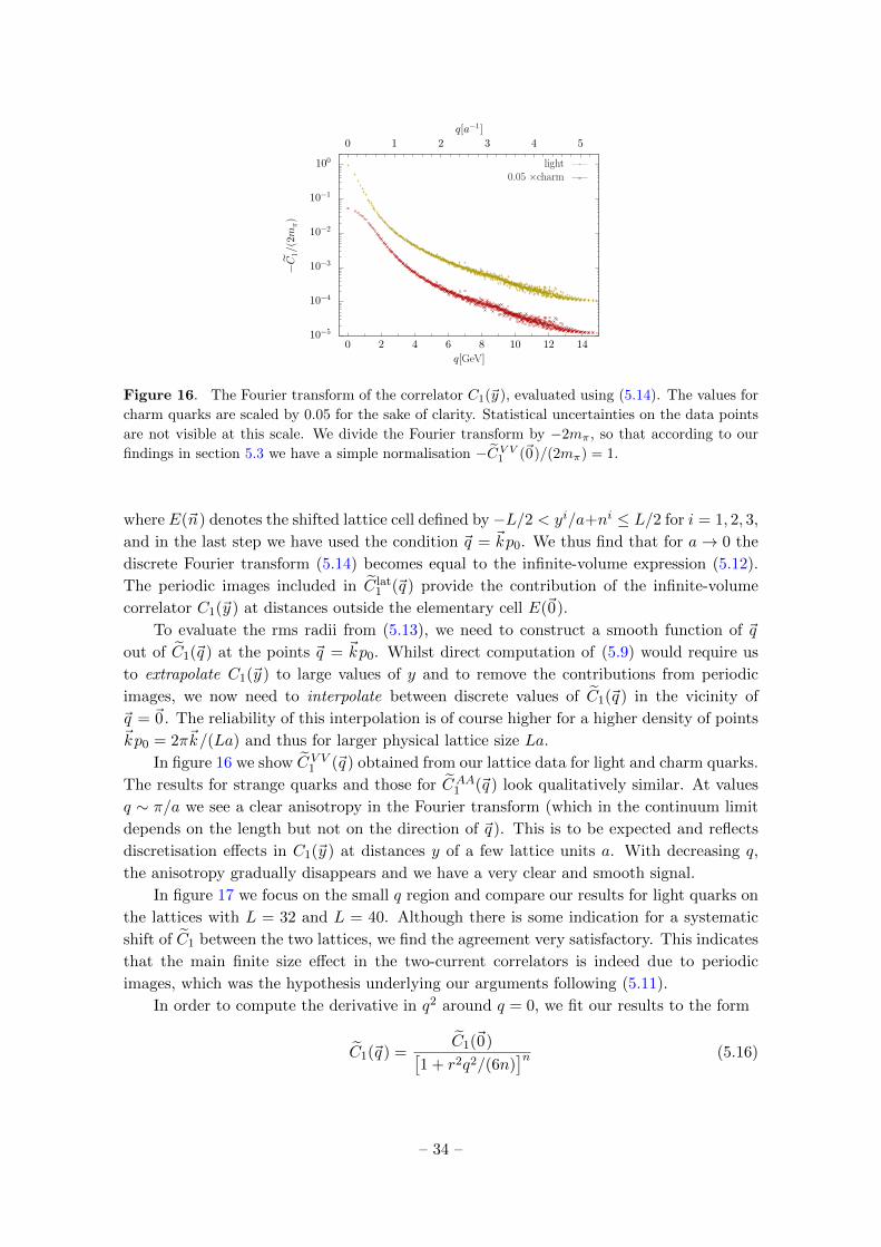
10−5

10−4

10−3

10−2

10−1

100

0 2 4 6 8 10 12 14

0 1 2 3 4 5

−𝐶

1/(2

𝑚𝜋)

𝑞[GeV]

𝑞[𝑎−1]

light0.05 ×charm

Figure 16. The Fourier transform of the correlator C1(~y ), evaluated using (5.14). The values for

charm quarks are scaled by 0.05 for the sake of clarity. Statistical uncertainties on the data points

are not visible at this scale. We divide the Fourier transform by −2mπ, so that according to our

findings in section 5.3 we have a simple normalisation −CV V1 (~0)/(2mπ) = 1.

where E(~n) denotes the shifted lattice cell defined by −L/2 < yi/a+ni ≤ L/2 for i = 1, 2, 3,

and in the last step we have used the condition ~q = ~kp0. We thus find that for a→ 0 the

discrete Fourier transform (5.14) becomes equal to the infinite-volume expression (5.12).

The periodic images included in C lat1 (~q ) provide the contribution of the infinite-volume

correlator C1(~y ) at distances outside the elementary cell E(~0).

To evaluate the rms radii from (5.13), we need to construct a smooth function of ~q

out of C1(~q ) at the points ~q = ~kp0. Whilst direct computation of (5.9) would require us

to extrapolate C1(~y ) to large values of y and to remove the contributions from periodic

images, we now need to interpolate between discrete values of C1(~q ) in the vicinity of

~q = ~0. The reliability of this interpolation is of course higher for a higher density of points~kp0 = 2π~k/(La) and thus for larger physical lattice size La.

In figure 16 we show C V V1 (~q ) obtained from our lattice data for light and charm quarks.

The results for strange quarks and those for CAA1 (~q ) look qualitatively similar. At values

q ∼ π/a we see a clear anisotropy in the Fourier transform (which in the continuum limit

depends on the length but not on the direction of ~q ). This is to be expected and reflects

discretisation effects in C1(~y ) at distances y of a few lattice units a. With decreasing q,

the anisotropy gradually disappears and we have a very clear and smooth signal.

In figure 17 we focus on the small q region and compare our results for light quarks on

the lattices with L = 32 and L = 40. Although there is some indication for a systematic

shift of C1 between the two lattices, we find the agreement very satisfactory. This indicates

that the main finite size effect in the two-current correlators is indeed due to periodic

images, which was the hypothesis underlying our arguments following (5.11).

In order to compute the derivative in q2 around q = 0, we fit our results to the form

C1(~q ) =C1(~0)[

1 + r2q2/(6n)]n (5.16)

– 34 –

0.0

0.2

0.4

0.6

0.8

1.0

1.2

0 0.5 1 1.5 2 2.5 3

0 0.05 0.1 0.15 0.2 0.25 0.3 0.35 0.4

−𝐶

1/(2

𝑚𝜋)

𝑞2[GeV2]

𝑞2[𝑎−2]

L=40L=32

(a) 〈V 0V 0〉, p = 0

0.0

0.1

0.2

0.3

0.4

0.5

0.6

0 0.5 1 1.5 2 2.5 3

0 0.05 0.1 0.15 0.2 0.25 0.3 0.35 0.4

𝐶1/

(2𝑚

𝜋)

𝑞2[GeV2]

𝑞2[𝑎−2]

L=40L=32

(b) 〈A0A0〉, p = 0

Figure 17. Volume comparison of the Fourier transform C1 for light quarks.

in the range 0 ≤ q2 ≤ q2max, varying the value of q2max between 2p20 and 6p20. For the lowest

value of q2max we have as many data points as parameters in (5.16), whereas the highest

value is motivated by the fact that there is no point with q2 = 7p20 because 7 cannot be

written as the sum of squares of three integers. Fits extending to even higher q2 put less

and less emphasis on the fit quality around q2 = 0 and are therefore less well suited for

determining the derivative at that point. Figure 18 shows the low q2 data together with

the different fit curves. The latter are in general very close to each other and can barely

be distinguished individually. In figure 19 we show the fitted values of r2V V and r2AA. The

dependence of r2 on q2max is in general mild, although for light or strange quarks there

seems to be a systematic increase of r2AA with q2max. We do not regard the fits with lower or

higher q2max as intrinsically more reliable around q2 = 0 and therefore determine an overall

value and error for each radius in the following way. The averaged value of r2 is obtained

as the arithmetic mean of the fitted values r2(q2max), and the root of the variance of these

values is used as systematic error on r2 due to our fitting procedure. The statistical error

on r2 is taken as the arithmetic mean of the jackknife errors on the fit results r2(q2max). The

outcome of this procedure is given in table 5, converted to values and errors for r instead

of r2.

radius [fm] light quarks strange charm

rV V 1.046(40)(09) 0.826(32)(09) 0.460(60)(25)

rAA 0.580(15)(09) 0.576(21)(08) 0.380(38)(12)

Table 5. Rms radii r for the correlator C1(y). The first error is statistical and the second one

due to the fitting procedure, as specified in the text.

We see that rV V decreases with increasing quark mass, as expected for a quantity that

– 35 –

0.0

0.2

0.4

0.6

0.8

1.0

1.2

0 0.5 1 1.5 2 2.5 3

0 0.05 0.1 0.15 0.2 0.25 0.3 0.35 0.4

scal

edco

rrela

tor

𝑞2[GeV2]

𝑞2[𝑎−2]

4pt FT light3pt light

(a) 〈V 0V 0〉, p = 0, L = 40, light quarks

0.0

0.2

0.4

0.6

0.8

1.0

1.2

0 0.5 1 1.5 2 2.5 3

0 0.05 0.1 0.15 0.2 0.25 0.3 0.35 0.4

−𝐶

1/(2

𝑚𝜋)

𝑞2[GeV2]

𝑞2[𝑎−2]

charmstrange

(b) 〈V 0V 0〉, p = 0, L = 40, strange and charm

0.0

0.1

0.2

0.3

0.4

0.5

0.6

0 0.5 1 1.5 2 2.5 3

0 0.05 0.1 0.15 0.2 0.25 0.3 0.35 0.4

𝐶1/

(2𝑚

𝜋)

𝑞2[GeV2]

𝑞2[𝑎−2]

lightstrangecharm

(c) 〈A0A0〉, p = 0, L = 40

Figure 18. The Fourier transform C1 at low values of q2. The curves (without error bands) show

the series of fits discussed in the text. In panel (a) the results for −C1/(2mπ) are labelled by “4pt

FT light”, whereas the points and curve labelled by “3pt light” show the r.h.s. of (5.17) evaluated

with our data for the vector form factor FV and fit 1 of table 4.

characterises the size of the pion. The ratio rAA/rV V increases with the quark mass, being

clearly below 1 for light and strange quarks and consistent with 1 for charm. A dynamical

interpretation of this interesting finding is beyond the scope of the present work.

The factorisation hypothesis for C V V1 discussed in section 5.3 gives the relation

− C1(~q )

2mπ

?=

(mπ + Eq)2

4mπEq

[FV(2mπEq − 2m2

π

)]2(5.17)

according to (5.3). We see in figure 18a that this is clearly ruled out, which confirms our

finding in position space in figure 15a.

For rms radii, the hypothesis (5.17) implies r2V V?= 2r2V , where rV is the radius asso-

ciated with the vector form factor FV , i.e. the conventional charge radius. Interestingly,

– 36 –

0.0

0.2

0.4

0.6

0.8

1.0

1.2

1.4

2 3 4 5 6 avg

𝑟2 𝑉𝑉

[fm2 ]

𝑞2max[𝑝2

0]

⟨𝑉 0𝑉 0⟩, |𝐶1|, 𝑝2 = 0 , 𝐿 = 40

charmstrange

light

(a) 〈V 0V 0〉, p = 0, L = 40

0.0

0.1

0.2

0.3

0.4

0.5

2 3 4 5 6 avg

𝑟2 𝐴𝐴

[fm2 ]

𝑞2max[𝑝2

0]

⟨𝐴0𝐴0⟩, |𝐶1|, 𝑝2 = 0 , 𝐿 = 40

charmstrange

light

(b) 〈A0A0〉, p = 0, L = 40

Figure 19. Squared rms radii r2 extracted from fitting C1 to the form (5.16) in the interval

0 ≤ q2 ≤ q2max, together with their jackknife errors. The entries labelled “avg” give the averaged

values corresponding to table 5, with statistical and systematic errors added in quadrature.

the kinematic prefactor on the r.h.s. of (5.17) does not contribute to d/dq2 at q2 = 0,

so that for the radii one obtains the same result as in the non-relativistic approxima-

tion, where the prefactor is 1. Quantitatively, we obtain√

2 rV = 0.878(14) fm with

fit 1 and√

2 rV = 0.849(12) fm with fit 2 of table 4, which is clearly below the value

rV V = 1.046(40)(09) fm for light quarks in table 5. A detailed discussion of the difference

between rV V and√

2 rV can be found in [8].

5.5 Subtraction term for the annihilation graph

The vacuum subtraction term for the annihilation graph A in (3.19) involves the same

three-point functions 〈Bt〉 that are necessary to compute the matrix elements of the axial

or pseudoscalar current between a pion state and the vacuum. As a by-product of our

simulations, we can thus extract these matrix elements. We can then compute the pion

decay constant from the relation∣∣〈π+|A0ud(0) |0〉

∣∣ =√

2mπFπ (5.18)

for a pion at rest. Using ∂µAµud(x) = 2mqPud(x), where mq is the average of u and d quark

masses, we have for a pion at rest∣∣∣∣ 〈π+|Pud(0) |0〉〈π+|A0

ud(0) |0〉

∣∣∣∣ =mπ

2mq=

B

mπ, (5.19)

where the last relation holds at leading order in chiral perturbation theory. The quark mass

mq and the chiral symmetry breaking parameter B are understood to be renormalised in

the MS scheme at the scale µ = 2 GeV, corresponding to the renormalisation constants

– 37 –

given in table 3. From the data of our two lattices, we obtain

Fπ = (100.2± 0.4) MeV , B = (2.41± 0.02) GeV for L = 40 (mπ = 293 MeV) ,

Fπ = (98.2± 1.0) MeV , B = (2.50± 0.05) GeV for L = 32 (mπ = 299 MeV) ,

(5.20)

where we also recall the pion masses fitted from our two-point correlation functions. The

quoted errors are purely statistical.

The above values of Fπ for mπ ≈ 300 MeV agree within a few percent with chiral

perturbation theory at NLO, see figure 10 in [36]. From equations (46), (65) and table 14

in the FLAG review [37], we obtain B = Σ/F 2 ≈ 2.6 to 2.7 GeV for nF = 2 quark flavours

in the chiral limit. This agrees reasonably well with our values in (5.20), given that we

use lowest-order chiral perturbation theory for their extraction and have not attempted to

correct our data for lattice artefacts.

6 Results for isospin amplitudes

In this section we present our results for the isospin amplitudes F0, F1 and F2 defined

in (2.12). We compare them with the predictions of chiral perturbation theory that were

computed in [12] and recalled in section 2.2 of the present paper. We consider the case of

light quarks throughout.

6.1 Isospin amplitudes

In figures 20 and 21, we show our results for the isospin amplitudes in all channels except

〈PP 〉 for F0 and 〈SS〉 for F1, where the statistical errors are too large to obtain a nonzero

signal. The y range shown is selected such that regions where we see no signal have been

omitted.

Comparison of the data for the L = 40 and L = 32 lattices shows a mixed situation

regarding finite-volume effects. These are significant for 〈PP 〉 in all three isospin com-

binations, for 〈A0A0〉 in F1 and for 〈SS〉 is F2. In the latter case, even the sign of the

signal changes when going from L = 32 to L = 40. For all other cases, volume effects are

moderate, except for 〈SS〉 in F0 at small y and for 〈V 0V 0〉 in F2 at large y.

We must now return to the doubly disconnected graph D, which contributes to F0 (but

not to F1 or F2). In all plots shown, the contribution from D is omitted since the result

would have too large errors to detect a signal. We must therefore ask whether there is any

reason to omit D in F0 = C1 + 2S1 +D. Given the structure of the corresponding graphs

in figure 2, it seems plausible to assume that the ratio D : S1 is similar in size to the ratio

S1 : C1. If one is willing to make this hypothesis, then one may justify the omission of

D in F0 for cases in which the data shows that |S1| � |C1|. In figure 22 we see that this

condition is satisfied for 〈SS〉 up to about y ∼ 1 fm, but not at all for 〈PP 〉. For 〈V 0V 0〉in the y region shown in figure 20(c), we find a very small ratio |S1/C1| < 0.035. The

correlator for 〈A0A0〉 is too noisy for F0 even if we only consider the sum C1 + 2S1.

– 38 –

10−3

10−2

10−1

100

101

102

0.4 0.6 0.8 1 1.2 1.4 1.6

5 10 15 20

corr

elato

r[G

eV⋅f

m−

3 ]

|𝑦|[fm]

𝐹1, ⟨𝑉 0𝑉 0⟩, 𝑝2 = 0

|𝑦|[𝑎]

𝐿 = 32𝐿 = 40

(a) F1, 〈V 0V 0〉, p = 0

−1.40

−1.20

−1.00

−0.80

−0.60

−0.40

−0.20

0.00

0.20

0.4 0.45 0.5 0.55 0.6 0.65 0.7 0.75 0.8 0.85

5 6 7 8 9 10 11 12

corr

elato

r[G

eV⋅f

m−

3 ]

|𝑦|[fm]

𝐹1, ⟨𝐴0𝐴0⟩, 𝑝2 = 0

|𝑦|[𝑎]

𝐿 = 32𝐿 = 40

(b) F1, 〈A0A0〉, p = 0

10−3

10−2

10−1

100

101

102

0.25 0.3 0.35 0.4 0.45

3 3.5 4 4.5 5 5.5 6 6.5

corr

elato

r[G

eV⋅f

m−

3 ]

|𝑦|[fm]

𝐹0, ⟨𝑉 0𝑉 0⟩, 𝑝2 = 0

|𝑦|[𝑎]

𝐿 = 32𝐿 = 40

(c) F0, 〈V 0V 0〉, p = 0

10−3

10−2

10−1

100

101

0.2 0.4 0.6 0.8 1 1.2 1.4 1.6

5 10 15 20 25

corr

elato

r[G

eV⋅f

m−

3 ]

|𝑦|[fm]

𝐹2, ⟨𝑉 0𝑉 0⟩, 𝑝2 = 0

|𝑦|[𝑎]

𝐿 = 32𝐿 = 40

(d) F2, 〈V 0V 0〉, p = 0

−0.20

0.00

0.20

0.40

0.60

0.80

1.00

1.20

1.40

0.2 0.3 0.4 0.5 0.6 0.7 0.8 0.9 1

2 4 6 8 10 12 14

corr

elato

r[G

eV⋅f

m−

3 ]

|𝑦|[fm]

𝐹2, ⟨𝐴0𝐴0⟩, 𝑝2 = 0

|𝑦|[𝑎]

𝐿 = 32𝐿 = 40

(e) F2, 〈A0A0〉, p = 0

−0.030

−0.020

−0.010

0.000

0.010

0.020

1.1 1.2 1.3 1.4 1.5 1.6 1.7

16 18 20 22 24

corr

elato

r[G

eV⋅f

m−

3 ]

|𝑦|[fm]

𝐹2, ⟨𝐴0𝐴0⟩, 𝑝2 = 0 , 𝐿 = 40

|𝑦|[𝑎]

𝐿 = 32𝐿 = 40

(f) F2, 〈A0A0〉, p = 0

Figure 20. Lattice results for isospin amplitudes of 〈V 0V 0〉 and 〈A0A0〉. The channel 〈A0A0〉 for

F0 has very large statistical errors and is not shown.

6.2 Comparison with chiral perturbation theory

In figures 23 and 24, we compare our lattice results with the predictions of chiral pertur-

bation theory discussed in section 2.2. We remind the reader that in leading-order chiral

– 39 –

−30

−20

−10

0

10

20

30

0.4 0.6 0.8 1 1.2 1.4 1.6

5 10 15 20 25

corr

elato

r[G

eV⋅f

m−

3 ]

|𝑦|[fm]

𝐹0, ⟨𝑆𝑆⟩, 𝑝2 = 0

|𝑦|[𝑎]

𝐿 = 32𝐿 = 40

(a) F0, 〈SS〉, p = 0

0.0

2.0

4.0

6.0

8.0

10.0

12.0

0.6 0.8 1 1.2 1.4 1.6

6 8 10 12 14 16 18 20 22 24

corr

elato

r[G

eV⋅f

m−

3 ]

|𝑦|[fm]

𝐹0, ⟨𝑃𝑃 ⟩, 𝑝2 = 0

|𝑦|[𝑎]

𝐿 = 32𝐿 = 40

(b) F0, 〈PP 〉, p = 0

−18.0

−16.0

−14.0

−12.0

−10.0

−8.0

−6.0

−4.0

−2.0

0.0

0.4 0.6 0.8 1 1.2 1.4 1.6

5 10 15 20 25

corr

elato

r[G

eV⋅f

m−

3 ]

|𝑦|[fm]

𝐹1, ⟨𝑃𝑃⟩, 𝑝2 = 0

|𝑦|[𝑎]

𝐿 = 32𝐿 = 40

(c) F1, 〈PP 〉, p = 0

−4.0

−3.0

−2.0

−1.0

0.0

1.0

2.0

3.0

4.0

5.0

0.2 0.4 0.6 0.8 1 1.2 1.4 1.6

5 10 15 20 25

corr

elato

r[G

eV⋅f

m−

3 ]

|𝑦|[fm]

𝐹2, ⟨𝑆𝑆⟩, 𝑝2 = 0

|𝑦|[𝑎]

𝐿 = 32𝐿 = 40

(d) F2, 〈SS〉, p = 0

−10.0−9.0−8.0−7.0−6.0−5.0−4.0−3.0−2.0−1.0

0.01.0

0.2 0.4 0.6 0.8 1 1.2 1.4 1.6

5 10 15 20 25

corr

elato

r[G

eV⋅f

m−

3 ]

|𝑦|[fm]

𝐹2, ⟨𝑃𝑃⟩, 𝑝2 = 0

|𝑦|[𝑎]

𝐿 = 32𝐿 = 40

(e) F2, 〈PP 〉, p = 0

Figure 21. Lattice results for isospin amplitudes of 〈SS〉 and 〈PP 〉. The channel 〈SS〉 for F1

has very large statistical errors and is not shown.

perturbation theory, it is admissible to replace the pion decay constant F in the chiral

limit with its value Fπ at the considered pion mass, which is the value we have extracted

in (5.20). Let us recall that predictions for the isospin amplitude F0 are not available for

– 40 –

−10

−5

0

5

10

15

20

25

30

0.4 0.6 0.8 1 1.2 1.4 1.6

5 10 15 20 25

corr

elato

r[G

eV⋅f

m−

3 ]

|𝑦|[fm]

⟨𝑆𝑆⟩, 𝑝2 = 0 , 𝐿 = 40

|𝑦|[𝑎]

𝐹0 without 𝐷𝐶1𝑆1

(a) 〈SS〉, p = 0, L = 40

−10.0

−8.0

−6.0

−4.0

−2.0

0.0

2.0

4.0

6.0

0.6 0.8 1 1.2 1.4 1.6

6 8 10 12 14 16 18 20 22 24

corr

elato

r[G

eV⋅f

m−

3 ]

|𝑦|[fm]

⟨𝑃𝑃⟩, 𝑝2 = 0 , 𝐿 = 40

|𝑦|[𝑎]

𝐹0 without 𝐷𝐶1𝑆1

(b) 〈PP 〉, p = 0, L = 40

Figure 22. Comparison of F0 with C1 and S1 for 〈SS〉 and 〈PP 〉. The contribution from D to

F0 is omitted, as explained in the text.

the channels 〈V 0V 0〉 and 〈A0A0〉 in [12]. Our lattice data in both channels is compatible

with zero within errors for y > 0.65 fm and not shown here.

Since chiral perturbation theory requires large distances to be valid, we start our plots

at y ≈ 0.65 fm ≈ 0.95m−1π ≈ 4.0/(4πFπ). Comparing the leading-order chiral result with

the resonance exchange contribution, we find three qualitatively different cases: for 〈SS〉and 〈PP 〉 in F1 the resonance terms are zero, for 〈PP 〉 in F0 and 〈SS〉 in F2 the leading-

order terms vanish, whereas in all other channels both contributions are nonzero and there

is a large difference between them in the y range under study. In the latter case, one may

doubt whether the chiral expansion is stable, given that the resonance terms are formally

subleading in the low-energy expansion. We also recall from the discussion in [12] that the

resonance terms are only meant to be an estimate of higher-order contributions, and that

the resonance parameters in the scalar and pseudoscalar channels are not well known.

With these caveats in mind, we now compare the chiral predictions with our lattice

data. As we see in figure 23, the agreement between lattice data and theoretical results is

quite good for 〈V 0V 0〉 in F1 and F2 and for 〈A0A0〉 in F2. These are the cases for which

the volume effects seen in figure 20 are moderate. The agreement for 〈A0A0〉 in F1 is still

fair, and we recall that in this channel the volume dependence is somewhat larger. For the

vector and axial currents, we thus obtain a rather satisfactory picture.

The situation is quite different for the scalar and pseudoscalar currents. For 〈SS〉in F0, we find no large volume effects on the lattice and have argued that the neglect of

graph D should not have dramatic effects, at least in the lower y range. The comparison

with the chiral prediction including resonance exchange is very bad in this case. For the

four channels shown in figure 24(b), (d), (e) and (f), there is also a strong disagreement

between lattice data and theory. We recall from figure 21 that in these cases the lattice

results for L = 40 and L = 32 point to significant finite volume effects. For 〈SS〉 in F1,

– 41 –

−0.30

−0.20

−0.10

0.00

0.10

0.20

0.30

0.40

0.50

0.8 1 1.2 1.4 1.6

10 12 14 16 18 20 22 24

corr

elato

r[G

eV⋅f

m−

3 ]

|𝑦|[fm]

𝐹1, ⟨𝑉 0𝑉 0⟩, 𝑝2 = 0 , 𝐿 = 40

|𝑦|[𝑎]

lattice data𝜒PT prediction (LO + Res)

𝜒PT prediction (LO)

(a) F1, 〈V 0V 0〉, p = 0, L = 40

−0.40

−0.30

−0.20

−0.10

0.00

0.10

0.20

0.30

0.40

0.50

0.8 1 1.2 1.4 1.6

10 12 14 16 18 20 22 24

corr

elato

r[G

eV⋅f

m−

3 ]

|𝑦|[fm]

𝐹1, ⟨𝐴0𝐴0⟩, 𝑝2 = 0 , 𝐿 = 40

|𝑦|[𝑎]

lattice data𝜒PT prediction (LO + Res)

𝜒PT prediction (LO)

(b) F1, 〈A0A0〉, p = 0, L = 40

−0.25

−0.20

−0.15

−0.10

−0.05

0.00

0.05

0.10

0.15

0.8 1 1.2 1.4 1.6

10 12 14 16 18 20 22 24

corr

elato

r[G

eV⋅f

m−

3 ]

|𝑦|[fm]

𝐹2, ⟨𝑉 0𝑉 0⟩, 𝑝2 = 0 , 𝐿 = 40

|𝑦|[𝑎]

lattice data𝜒PT prediction (LO + Res)

𝜒PT prediction (LO)

(c) F2, 〈V 0V 0〉, p = 0, L = 40

−0.25

−0.20

−0.15

−0.10

−0.05

0.00

0.05

0.10

0.15

0.8 1 1.2 1.4 1.6

10 12 14 16 18 20 22 24

corr

elato

r[G

eV⋅f

m−

3 ]

|𝑦|[fm]

𝐹2, ⟨𝐴0𝐴0⟩, 𝑝2 = 0 , 𝐿 = 40

|𝑦|[𝑎]

lattice data𝜒PT prediction (LO + Res)

𝜒PT prediction (LO)

(d) F2, 〈A0A0〉, p = 0, L = 40

Figure 23. Comparison of our lattice results for 〈V 0V 0〉 and 〈A0A0〉 with chiral perturbation

theory. The results obtained from the leading-order chiral Lagrangian are denoted by “LO” and

those including resonance exchange by “LO + Res”.

our lattice signal is consistent with zero within errors, and the chiral prediction is zero as

well at the order considered in [12]. In the sense that 〈SS〉 in F1 is small (compared for

instance with 〈PP 〉 in the same isospin amplitude) we can state agreement between our

lattice computation and chiral perturbation theory in this one case.

7 Summary

This paper contains a detailed study of two-current correlation functions in the pion in

lattice QCD. We use two gauge ensembles with a pion mass of mπ ≈ 300 MeV, a lattice

spacing of a ≈ 0.07 fm and spatial extensions of L = 32 and L = 40, respectively. Addi-

tional results for heavier quarks (strange or charm) are obtained in a partially quenched

setup.

We derive several general theoretical results concerning symmetry properties and the

connection between lattice graphs and physical amplitudes. In the remainder of our study,

– 42 –

−2.0

0.0

2.0

4.0

6.0

8.0

10.0

12.0

0.8 1 1.2 1.4 1.6

10 12 14 16 18 20 22 24

corr

elato

r[G

eV⋅f

m−

3 ]

|𝑦|[fm]

𝐹0, ⟨𝑆𝑆⟩, 𝑝2 = 0 , 𝐿 = 40

|𝑦|[𝑎]

lattice data without 𝐷𝜒PT prediction (LO + Res)

𝜒PT prediction (LO)

(a) F0, 〈SS〉, p = 0, L = 40

−0.5

0.0

0.5

1.0

1.5

2.0

2.5

3.0

3.5

0.8 1 1.2 1.4 1.6

10 12 14 16 18 20 22 24

corr

elato

r[G

eV⋅f

m−

3 ]

|𝑦|[fm]

𝐹0, ⟨𝑃𝑃⟩, 𝑝2 = 0 , 𝐿 = 40

|𝑦|[𝑎]

lattice data without 𝐷𝜒PT prediction (LO + Res)

𝜒PT prediction (LO)

(b) F0, 〈PP 〉, p = 0, L = 40

−0.20

−0.10

0.00

0.10

0.20

0.30

0.40

0.8 1 1.2 1.4 1.6

10 12 14 16 18 20 22 24

corr

elato

r[G

eV⋅f

m−

3 ]

|𝑦|[fm]

𝐹1, ⟨𝑆𝑆⟩, 𝑝2 = 0 , 𝐿 = 40

|𝑦|[𝑎]

lattice data𝜒PT prediction (LO)

(c) F1, 〈SS〉, p = 0, L = 40

−2.00−1.80−1.60−1.40−1.20−1.00−0.80−0.60−0.40−0.20

0.00

0.8 1 1.2 1.4 1.6

10 12 14 16 18 20 22 24

corr

elato

r[G

eV⋅f

m−

3 ]

|𝑦|[fm]

𝐹1, ⟨𝑃𝑃⟩, 𝑝2 = 0 , 𝐿 = 40

|𝑦|[𝑎]

lattice data𝜒PT prediction (LO)

(d) F1, 〈PP 〉, p = 0, L = 40

−0.80

−0.60

−0.40

−0.20

0.00

0.20

0.40

0.60

0.80

1.00

0.8 1 1.2 1.4 1.6

10 12 14 16 18 20 22 24

corr

elato

r[G

eV⋅f

m−

3 ]

|𝑦|[fm]

𝐹2, ⟨𝑆𝑆⟩, 𝑝2 = 0 , 𝐿 = 40

|𝑦|[𝑎]

lattice data𝜒PT prediction (LO + Res)

𝜒PT prediction (LO)

(e) F2, 〈SS〉, p = 0, L = 40

−4.0

−3.0

−2.0

−1.0

0.0

1.0

2.0

3.0

0.8 1 1.2 1.4 1.6

10 12 14 16 18 20 22 24

corr

elato

r[G

eV⋅f

m−

3 ]

|𝑦|[fm]

𝐹2, ⟨𝑃𝑃⟩, 𝑝2 = 0 , 𝐿 = 40

|𝑦|[𝑎]

lattice data𝜒PT prediction (LO + Res)

𝜒PT prediction (LO)

(f) F2, 〈PP 〉, p = 0, L = 40

Figure 24. As figure 23 but for the correlators 〈SS〉 and 〈PP 〉. The resonance exchange

contribution is zero for 〈SS〉 and 〈PP 〉 in F1.

we focus on correlation functions of two currents V 0, A0, S or P in a pion at rest. In our

lattice simulations, we make extensive use of stochastic sources, which allows us to obtain

satisfactory (and in many cases excellent) signals for all lattice contractions except for the

– 43 –

double disconnected graph D, where vacuum subtractions entail large cancellations and a

loss of the signal in statistical noise.

We study a number of lattice artefacts in our data. The comparison of results for two

different time differences between the pion source and sink gives no indication for large

contributions from excited states. Comparing the Lorentz invariant correlation functions

〈SS〉 and 〈PP 〉 for different pion momenta, we find that our lattice results are fully consis-

tent with boost invariance. We observe several types of anisotropic behaviour, indicating a

loss of rotational invariance due to either the periodic boundary conditions or to discreti-

sation effects. We find that these effects are significantly reduced by selecting distances ~y

between the two currents that are close to the spatial diagonals of the lattice. Finally, the

comparison of data for two lattices shows moderate volume effects in several channels, but

large ones in others.

In the connected graph C1, the “valence quark” and “valence antiquark” in the pion

are probed individually by the two currents. One might naively expect this contraction

to be dominant. An important result of our study is that this is not true: we find that

several lattice contractions are important for mπ ≈ 300 MeV. This concerns especially the

connected graph C2 with two current insertions on the same quark line, but in the case

of 〈SS〉 and 〈PP 〉 also the disconnected graph S1 and the annihilation contribution A.

For heavier quark masses, the importance of these graphs is reduced, although C2 remains

prominent in 〈A0A0〉 and 〈PP 〉 even for charm quarks. Of course, not every contraction

contributes to every physical matrix element, as shown in (3.8).

For the connected graph C1, we test the hypothesis that the two-current density can

be computed in terms of the single-current density, assuming the absence of correlation

effects between the quark and antiquark in the pion. We find that this hypothesis clearly

fails in a large range of current separations ~y , both for the vector and for the scalar current.

We also extract rms radii rV V and rAA of the correlator C1(~y ) for the vector and for

the axial current. We find that a Fourier transform w.r.t. ~y mitigates finite-size effects.

The radius rV V shows a clear decrease with the quark mass. Interestingly, it turns out

that rAA < rV V for light and strange quarks.

Combining the different lattice graphs to physical amplitudes in an isospin basis, we can

compare our lattice results with the computation in chiral perturbation theory performed

in [12], which includes the contributions from the leading-order chiral Lagrangian and an

estimate of higher-order contributions using resonance exchange graphs. We find rather

good agreement between the lattice data and the chiral calculation for vector and axial

currents, whereas the comparison for scalar and pseudoscalar currents is poor in five out

of six channels. Since the exchanged resonances are ρ and a1 in the former case and σ, a0,

η in the latter, our findings are consistent with the hypothesis that the exchange of the

lowest-mass vector and axial vector mesons often gives a good estimate of higher orders

in the chiral expansion, whereas the same does not necessarily hold for the exchange of

spin-zero mesons. This is in line with the conclusions drawn in [38, 39] and the general

success of models based on vector meson dominance.

The lattice methods presented in this work are suitable for the study of two-current

correlators that can be related to double parton distributions in the pion, thus providing

– 44 –

a connection with an active field of research in collider physics. This will be presented in

a forthcoming paper.

Acknowledgements

We gratefully acknowledge input from Sara Collins and Philipp Wein and discussions with

Michael Engelhardt. We used a modified version of the Chroma [40] software package, along

with the locally deflated domain decomposition solver implementation of openQCD [41].

The gauge ensembles have been generated by the QCDSF and RQCD collaborations on

the QPACE computer using BQCD [42, 43]. The discrete Fourier transforms in section 5.4

were computed using the package FFTW3 [44], and the graphs in figures 1 and 2 were

produced with JaxoDraw [45, 46]. The simulations used for this work were performed with

resources provided by the North-German Supercomputing Alliance (HLRN). This work

was supported by the Deutsche Forschungsgemeinschaft SFB/TRR 55.

References

[1] K. Barad, M. Ogilvie and C. Rebbi, Quark - Anti-quark Charge Distributions and

Confinement, Phys. Lett. 143B (1984) 222.

[2] K. Barad, M. Ogilvie and C. Rebbi, Quark-anti-quark charge distributions, Annals Phys. 168

(1986) 284.

[3] W. Wilcox and K.-F. Liu, Charge Radii From Lattice Relative Charge Distributions, Phys.

Lett. B172 (1986) 62.

[4] W. Wilcox, K.-F. Liu, B.-A. Li and Y.-l. Zhu, Relative Charge Distributions for Quarks in

Lattice Mesons, Phys. Rev. D34 (1986) 3882.

[5] W. Wilcox, Current overlap methods in lattice QCD, Phys. Rev. D43 (1991) 2443.

[6] M. C. Chu, M. Lissia and J. W. Negele, Hadron structure in lattice QCD. 1. Correlation

functions and wave functions, Nucl. Phys. B360 (1991) 31.

[7] M. Lissia, M. C. Chu, J. W. Negele and J. M. Grandy, Comparison of hadron quark

distributions from lattice QCD and the MIT bag model, Nucl. Phys. A555 (1993) 272.

[8] M. Burkardt, J. M. Grandy and J. W. Negele, Calculation and interpretation of hadron

correlation functions in lattice QCD, Annals Phys. 238 (1995) 441 [hep-lat/9406009].

[9] C. Alexandrou, P. de Forcrand and A. Tsapalis, Probing hadron wave functions in lattice

QCD, Phys. Rev. D66 (2002) 094503 [hep-lat/0206026].

[10] C. Alexandrou, P. de Forcrand and A. Tsapalis, The Matter and the pseudoscalar densities

in lattice QCD, Phys. Rev. D68 (2003) 074504 [hep-lat/0307009].

[11] C. Alexandrou and G. Koutsou, A Study of Hadron Deformation in Lattice QCD, Phys. Rev.

D78 (2008) 094506 [0809.2056].

[12] P. C. Bruns, Pion correlation functions in position space from chiral perturbation theory with

resonance exchange, 1512.06650.

[13] M. Diehl, D. Ostermeier and A. Schafer, Elements of a theory for multiparton interactions in

QCD, JHEP 03 (2012) 089 [1111.0910].

– 45 –

[14] P. Hasenfratz and M. Bissegger, CP, T and CPT in the non-perturbative formulation of

chiral gauge theories, Phys. Lett. B613 (2005) 57 [hep-lat/0501010].

[15] G. S. Bali, S. Collins, B. Glaßle, M. Gockeler, J. Najjar, R. H. Rodl et al., Nucleon isovector

couplings from Nf = 2 lattice QCD, Phys. Rev. D91 (2015) 054501 [1412.7336].

[16] G. S. Bali, S. Collins, B. Glaßle, M. Gockeler, J. Najjar, R. H. Rodl et al., The moment

〈x〉u−d of the nucleon from Nf = 2 lattice QCD down to nearly physical quark masses, Phys.

Rev. D90 (2014) 074510 [1408.6850].

[17] RQCD collaboration, G. S. Bali, S. Collins, D. Richtmann, A. Schafer, W. Soldner and

A. Sternbeck, Direct determinations of the nucleon and pion σ terms at nearly physical quark

masses, Phys. Rev. D93 (2016) 094504 [1603.00827].

[18] G. S. Bali, S. Collins, A. Cox and A. Schafer, Masses and decay constants of the D∗s0(2317)

and Ds1(2460) from Nf = 2 lattice QCD close to the physical point, Phys. Rev. D96 (2017)

074501 [1706.01247].

[19] UKQCD collaboration, M. Foster and C. Michael, Quark mass dependence of hadron masses

from lattice QCD, Phys. Rev. D59 (1999) 074503 [hep-lat/9810021].

[20] G. Martinelli and C. T. Sachrajda, A Lattice Study of Nucleon Structure, Nucl. Phys. B316

(1989) 355.

[21] Y.-B. Yang, A. Alexandru, T. Draper, M. Gong and K.-F. Liu, Stochastic method with low

mode substitution for nucleon isovector matrix elements, Phys. Rev. D93 (2016) 034503

[1509.04616].

[22] S. Gusken, A Study of smearing techniques for hadron correlation functions, Nucl. Phys.

Proc. Suppl. 17 (1990) 361.

[23] G. S. Bali, B. Lang, B. U. Musch and A. Schafer, Novel quark smearing for hadrons with

high momenta in lattice QCD, Phys. Rev. D93 (2016) 094515 [1602.05525].

[24] QCDSF/UKQCD collaboration, D. Brommel et al., The Pion form-factor from lattice QCD

with two dynamical flavours, Eur. Phys. J. C51 (2007) 335 [hep-lat/0608021].

[25] C. Thron, S. J. Dong, K. F. Liu and H. P. Ying, Pade - Z(2) estimator of determinants,

Phys. Rev. D57 (1998) 1642 [hep-lat/9707001].

[26] SESAM collaboration, G. S. Bali, H. Neff, T. Dussel, T. Lippert and K. Schilling,

Observation of string breaking in QCD, Phys. Rev. D71 (2005) 114513 [hep-lat/0505012].

[27] G. S. Bali, S. Collins and A. Schafer, Effective noise reduction techniques for disconnected

loops in Lattice QCD, Comput. Phys. Commun. 181 (2010) 1570 [0910.3970].

[28] M. Gockeler et al., Perturbative and Nonperturbative Renormalization in Lattice QCD, Phys.

Rev. D82 (2010) 114511 [1003.5756].

[29] S. Capitani, M. Gockeler, R. Horsley, H. Perlt, P. E. L. Rakow, G. Schierholz et al.,

Renormalization and off-shell improvement in lattice perturbation theory, Nucl. Phys. B593

(2001) 183 [hep-lat/0007004].

[30] S. Sint and P. Weisz, Further results on O(a) improved lattice QCD to one loop order of

perturbation theory, Nucl. Phys. B502 (1997) 251 [hep-lat/9704001].

[31] Y. Taniguchi and A. Ukawa, Perturbative calculation of improvement coefficients to O(g2a)

for bilinear quark operators in lattice QCD, Phys. Rev. D58 (1998) 114503

[hep-lat/9806015].

– 46 –

[32] P. Fritzsch, J. Heitger and N. Tantalo, Non-perturbative improvement of quark mass

renormalization in two-flavour lattice QCD, JHEP 08 (2010) 074 [1004.3978].

[33] R. A. Briceno, J. V. Guerrero, M. T. Hansen and C. J. Monahan, Finite-volume effects due

to spatially non-local operators, 1805.01034.

[34] K. Cichy, K. Jansen and P. Korcyl, Non-perturbative renormalization in coordinate space for

Nf = 2 maximally twisted mass fermions with tree-level Symanzik improved gauge action,

Nucl. Phys. B865 (2012) 268 [1207.0628].

[35] M. Burkardt, Impact parameter dependent parton distributions and off forward parton

distributions for ζ → 0, Phys. Rev. D62 (2000) 071503 [hep-ph/0005108].

[36] S. Durr, Validity of ChPT – is Mπ=135 MeV small enough?, PoS LATTICE2014 (2015)

006 [1412.6434].

[37] S. Aoki et al., Review of lattice results concerning low-energy particle physics, Eur. Phys. J.

C74 (2014) 2890 [1310.8555].

[38] J. F. Donoghue, C. Ramirez and G. Valencia, The Spectrum of QCD and Chiral Lagrangians

of the Strong and Weak Interactions, Phys. Rev. D39 (1989) 1947.

[39] G. Ecker, J. Gasser, A. Pich and E. de Rafael, The Role of Resonances in Chiral

Perturbation Theory, Nucl. Phys. B321 (1989) 311.

[40] SciDAC, LHPC, UKQCD collaboration, R. G. Edwards and B. Joo, The Chroma software

system for lattice QCD, Nucl. Phys. Proc. Suppl. 140 (2005) 832 [hep-lat/0409003].

[41] M. Luscher and S. Schaefer, Lattice QCD with open boundary conditions and twisted-mass

reweighting, Comput. Phys. Commun. 184 (2013) 519 [1206.2809].

[42] Y. Nakamura and H. Stuben, BQCD - Berlin quantum chromodynamics program, PoS

LATTICE2010 (2010) 040 [1011.0199].

[43] Y. Nakamura, A. Nobile, D. Pleiter, H. Simma, T. Streuer, T. Wettig et al., Lattice QCD

Applications on QPACE, 1103.1363.

[44] M. Matteo Frigo and S. G. Johnson, The design and implementation of FFTW3, Proc. IEEE

93 (2005) 216231.

[45] D. Binosi and L. Theussl, JaxoDraw: A Graphical user interface for drawing Feynman

diagrams, Comput. Phys. Commun. 161 (2004) 76 [hep-ph/0309015].

[46] D. Binosi, J. Collins, C. Kaufhold and L. Theussl, JaxoDraw: A Graphical user interface for

drawing Feynman diagrams. Version 2.0 release notes, Comput. Phys. Commun. 180 (2009)

1709 [0811.4113].

– 47 –