Turnaround strategies in financially distressed times
70
Turnaround strategies in financially distressed times An empirical investigation of European entities in distress Nicolaas Beute Enschede, February 2018
-
Upload
khangminh22 -
Category
Documents
-
view
0 -
download
0
Transcript of Turnaround strategies in financially distressed times

Turnaround strategies in financially distressed times
An empirical investigation of European entities in distress
Nicolaas Beute Enschede, February 2018

Nicolaas Beute University of Twente 2
Turnaround strategies in financially distressed times
An empirical investigation of European entities in distress
Master thesis research MSc Business Administration Financial management Author: Nicolaas Beute Student number: S1761366 Contact: [email protected] University: University of Twente Faculty: Behavioral, Management and Social Sciences Supervisor 1: dr. H.C. van Beusichem Supervisor 2: dr. X. Huang Company: Beaufort Consulting Supervisor 1: drs. M.W.K. Tempelman
Supervisor 2: mr. drs. J.M.C.M. Janssen

Nicolaas Beute University of Twente 3
Acknowledgements This master thesis assignment serves as the final assignment in the master Business Administration, where I attended the finance specialisation track with much joy and interest. Writing a master thesis is not an effortless activity and thus I would like to thank some people responsible for support and tips in writing my thesis, making sure my motivation stayed at an adequate level, as well as merely understanding the time and effort required for writing such an assignment. First of all I would like to thank my primary supervisor from the University of Twente, dr. Henry van Beusichem, for his tips, criticism and guidance through the process of writing this thesis. I would also like to thank my second supervisor dr. Xiaohong Huang for her feedback and tips. Additionally, I would like to thank all of the consultants at Beaufort Corporate Consulting for offering me a place to write my thesis as well as getting a feel of a work environment in a corporate finance related firm. I would especially like to thank mr. Tempelman and mr. Janssen, who have guided me through the thesis process whilst being an intern at Beaufort. Finally, a special thank you goes to my parents and my aunt, who never fail to motivate me and always try to get the best out of me.

Nicolaas Beute University of Twente 4
Abstract This study investigates the effect of turnaround strategies on the improvement in Altman’s Z”-score. Operational restructuring, asset restructuring and financial restructuring are found to be important clusters when conducting a research like this and underlying variables have been identified by conducting a literature review. In order to find this effect, several samples have been constructed. First, two samples with the main variables of interest are created, in which one sample incorporates all cases and the second only incorporates cases that experienced a change where the entity went from a distressed score to a non-distressed score, whereas the other two samples employ robust variables. Finally, a sample with restructuring thresholds is incorporated in the study. Firms in the sample are situated in the EU and realise at least €20 million turnover. This study finds that especially operational components of an entity entail a significant effect on improving the Z”-score. A reduction in both operational expenses and in the operational component of the working capital entail highly positive and significant results in achieving these improvements. This could have been expected as this is closely related to the true business of the firm, and what remains as the net income an entity achieves. Some robust regressions have also been run to find out what effects the broad balance sheet accounts have on the improvement in Z”-score. This also returns results that operational restructuring positively affects these improvements.

Nicolaas Beute University of Twente 5
Table of contents 1. Introduction 6 2. Literature review and hypotheses development 9 2.1 Financial distress 9 2.2 Turnaround following distress 15 3. Methodology 26 3.1 Research question 26 3.2 Hypotheses review 26 3.3 Variables and operationalisation 27 3.4 Sample and data collection 32 3.5 Method of analysis 34 3.6 Univariate statistics 36 4. Empirical results and descriptive statistics 41 4.1 Descriptive statistics 41 4.2 Assumptions of multiple regression analysis 45 4.3 Main OLS regression results 46 4.4 Robust OLS regression results 49 4.5 Main results with restructuring threshold 51 5. Conclusion 53 5.1 Main findings and hypothesis discussion 53 5.2 Limitations and recommendations 55 References 57

Nicolaas Beute University of Twente 6
1. Introduction Since the start of this millennium the world has experienced two large economic crises, the early 2000s recession, which included the dot-com bubble, and the 2007-2009 financial crisis originating from the subprime mortgage market. Two impactful crises in such a short span of time raises several questions for entrepreneurs. What strategy should I attain in order to not be affected by crises? Is it possible for my firm not to be affected by crises? How can I deflect financial problems after being affected by such crises? These are just three examples of questions an entrepreneur can ask himself. In times of crisis, however, there is an enormous amount of uncertainty an entrepreneur encounters, which increases the necessity of increasing knowledge with regards to proper actions an entrepreneur can employ during financially challenging periods. The circumstances an entity then enters, is primarily based upon financial failure, leading to an increasingly high chance of bankruptcy (Boyne, 2004). It is therefore not striking that, following these major economic crises, corporate turnaround has become an important subject of interest throughout both strategy as well as finance research. Early research by Hofer (1980) defines these corporate turnaround actions as a recovery of performance following financially challenging years (Schmitt & Raisch, 2013). While there is in an increasing amount of content available regarding corporate and financial distress in combination with turnaround strategies, it has been an important research subject for quite some time, with seminal works in the 70s and 80s, by for example Altman (1968) and Bibeault (1982). With time passing to a new millennium, so has the scope of research regarding turnaround. This has however, unfortunately, not yet led to uniform findings. Findings resulting from turnaround research, both strategically and financially, are mostly ambiguous in nature and remain largely fragmented, both on a theoretical as an empirical basis (Trahms et al., 2013). Trahms et al. (2013) also state that organisational decline is a persistent threat due to a weakening global economy, which increases the need for knowledge and research relating to turnaround strategies. Due to the widely varying problems an entity can encounter, it remains a challenging and complex subject. A decreasing availability of resources or decreasing performances of the entity are two examples that ultimately lead to such declines (e.g. Weitzel & Jonsson, 1989; Bruton et al., 1994). This suggests that both internal and external factors entail explanations of such an organisational decline. According to Sudarsanam and Lai (2001), responses an entity can employ, range from operational restructuring to financial restructuring, and basically cover all aspects of a business. It could be related to products, but also to employees. However, as stated by Trahms et al. (2013) empirical evidence regarding the effectiveness of these turnaround strategies remain extremely scarce. One important finding by Haugen and Senbet (1978, 1988) offers insights with regards to turnaround strategies. Broadly, there are two forms of turnaround, namely formal, which entails going concern following bankruptcy (it is frequently named as deliberate bankruptcy in finance research), and informal, which entails the turnaround strategies discussed in this study, such as operational restructuring and financial restructuring. The main difference is that informal restructuring techniques are far less costly than formal turnaround actions, which is important as it increases the necessity of this study. Since it is clear that private turnaround actions should cost less than formal

Nicolaas Beute University of Twente 7
turnaround actions, the choice for engaging in private turnaround strategies seems appropriate and obvious. This important conclusion by Haugen and Senbet (1978, 1988) does not give any insights in what private turnaround strategy would be an appropriate value-enhancer leading to successful turnaround from financial distress. Apart from these fragmented empirical findings, there is also a wide range of definitions relating to both financial distress and turnaround strategies. Throughout this study financial distress is measured with Altman’s Z”-score, which is an accounting-based measure, that is thoroughly explained in a later section. Additionally, the different turnaround strategies are clustered in operational restructuring, financial restructuring and asset restructuring, which are frequently named as important clusters in turnaround research. Apart from these three strategies, managerial restructuring is also an important and frequently named subject. More insights relating to these turnaround strategies are presented in a later section, which also presents the reason for choosing the three mentioned turnaround strategies as a subject of research. Acknowledging the fact that there is very little empirical evidence related to financial distress and turnaround strategies, it raises the question what value an entity can create through a certain turnaround strategy in light of becoming profitable, or at the very least, leaving financial distress. Which raises an important question that is central in this study, namely: To what extent do three turnaround strategies, namely operational restructuring, asset restructuring and financial restructuring, improve the Altman’s Z”-score? Due to the fact that there is an increasing amount of evidence that SMEs and large enterprises differ systematically in their choices of strategies to alleviate financial problems (e.g. Chowdhury & Lang, 1996), a certain scope has been given to this research, so that the results from statistical analyses are more suitable for generalisation. In light of this, the scope limits this research to enterprises that generate an annual turnover of at least €20 million to filter out smaller firms. Additionally, a limit is set to the amount of countries included in this study, which is set at the initial 15 EU countries. This scope of the study is further discussed in section three. In order to be able to make statements regarding the research question formulated, several hypotheses are formed and subsequently tested. As these hypotheses are derived from previous research, they are intertwined in the literature review in the next section. This study mainly finds that the operational restructuring methods entail the most significant results when relating turnaround strategies to improvements in Altman’s Z”-score. Important results are the change in operational expenses, which appear to be an important influencer. Also, optimising the working capital returns significant results which are mostly in line with the expectations. Some interesting findings are gathered that are related to the change in gross margin, which are contrasting with expectations. Results regarding both financial and asset restructuring remain largely inconclusive and it could be stated that the operational aspects of the business are the true influencers of an entities financial health. This is not surprising, as it entails the

Nicolaas Beute University of Twente 8
actual primary process that is employed in order to gain profits, these profits are not achieved through slicing the capital structure in a certain way. This study offers theoretical relevance. As stated, this study attempts to find relationships between the turnaround strategies and Altman’s Z”-score, so that an appropriate value can be given to a certain turnaround strategy. Apart from this, the study attempts to offer more insights regarding turnaround strategies and the underlying actions related to the strategies. Previously, turnaround strategies are frequently investigated individually, whereas this study attempts to combine multiple turnaround strategies in an attempt to find relations between turnaround strategies and the improvement on Altman’s Z”-score. Whilst turnaround strategies are investigated as a group, this study also offers insights for the individual turnaround strategies, presenting and combining available information, leading to up to date insights regarding operational, financial and asset restructuring. Apart from the theoretical relevance, this study also offers practical relevance. The practical relevance this study entails is related to what firms can expect after engaging in a turnaround strategy. After this study, it should be clear whether an entity should employ activities relating to operational restructuring, asset restructuring or financial restructuring. This leads to valuable information for both entrepreneurs that experience or have good reason to expect financial distress, as well as for consulting firms that assist entities in dire straits. Following this introduction the next section entails a literature review, which presents important insights regarding both financial distress and turnaround strategies. Section three introduces the methodology incorporated in this study. The empirical results are discussed in section four, which is followed by a conclusion in section five.
Nicolaas Beute University of Twente 9
2. Literature review and hypotheses development This section contains the literature review of this study. Its goal is to create a deeper understanding of the subject investigated. Financial distress, its causes and solutions and the methods of measurement are discussed. Additionally, turnaround strategies in the context of financial distress are elaborated upon through sketching the turnaround process and the different turnaround strategies, being operational restructuring, managerial restructuring, asset restructuring and financial restructuring. This literature review offers valuable insights necessary for understanding the following sections in this study. The hypotheses that are tested in this study are also formed in this section.
2.1 Financial distress Throughout previous research financial distress is a frequently investigated phenomenon. Studies solely focusing on financial distress are frequent in numbers, as are studies that use financial distress as an underlying construct. These studies incorporate many different definitions as well as forms of measurement, which increases the necessity of a thorough explanation of the wide range of definitions and measurements used throughout literature. Apart from creating a deeper understanding with regards to financial distress for the readers of this study, this is also important for the researcher, so that an appropriate form of measuring financial distress can be incorporated in this study. Therefore, the first part of this section discusses several definitions and forms of measurement. This enables the researcher of creating a uniform way of understanding and measuring financial distress, which is of importance throughout this study.
2.1.1 Defining distress A firm that experiences temporary lacks of liquidity, in combination with difficulties related to the payment of financial obligations, is globally defined as in financial distress. This is, however, just one of many definitions of financial distress. Andrade and Kaplan (1998), for example, classify two forms of financial distress: the first being defaulting on debt payments, and the second being the usage of debt restructuring, so that default is averted. The definition incorporated in their study has previously also been implemented by Brown et al. (1992) in their respective study. Early work by Wruck (1991) has set the tone regarding these definitions, as she defines financial distress as a circumstance in which the cash flow is not sufficient, in order to cover the obligations the firm currently has. Unpaid obligations to either suppliers or employees, damages from litigation, and failing to pay principal or interest payments are considered as such obligations. Violating debt covenants, like failure of principal or interest payments are important factors that could lead to financial distress being imminent. Negotiations with one or more creditors of the firm are inevitable following financial distress. In the study by Blazy et al. (2014), they state that financial distress is indeed inherent when the firm is unable to meet their current obligations. They argue that, in order to mitigate this financial distress, the firm can either opt for private or legal negotiations. Previous literature shows us that private renegotiations are generally less costly (e.g. Haugen & Senbet, 1978; Roe, 1983; Jensen, 1989, 1991). The definitions these researchers use with regards to financial distress are quite narrow, focusing solely on debt, the payment of debt, and restructuring of debt. The study by Opler and Titman (1994) apply a more broad definition, as they define it as a costly event

Nicolaas Beute University of Twente 10
that affects the relationship between debt holders and non-financial stakeholders. These problems lead to an increase in difficulty of gaining new capital as well as an increase in bearing the increasing costs of the difficult relationship between these debt holders and non-financial stakeholders, such as the customers, who could possibly choose for doing business with another firm, as they could expect the entity not to be able to deliver on their promises. The Gilbert et al. (1990) study presents insights that the characteristics of financial distress differ from bankruptcy characteristics. They state that financial distress is primarily characterised through losses and poor performance, as well as by negative cumulative earnings over several consecutive years. Bankruptcy is merely a consequence of financial distress. Financial ratios of an entity can show whether financial distress is inevitable. These accounting-based gauges are much used in empirical research to find out whether financial distress is currently experienced, expected or improbable. A limitation with regards to these accounting-based indicators is that it is an historical indicator; these indicators are however more than capable of predicting financial distress. Quite similar to the Gilbert et al. (1990) study, Denis and Denis (1995) adopt a definition where at least three negative net incomes are experienced. Another identification of financial distress through accounting-based measures is discussed by Asquith et al. (1994), who incorporate the interest coverage ratio and state that if in any of two consecutive years the EBITDA is lower than 80% of the actual interest expenses, the firm is experiencing financial distress. The definitions these researchers employ is similar to how they measure financial distress.
2.1.2 Causes and solutions Entering financial distress can be imminent through multiple reasons. First, a firm can experience insufficient cash amounts. This relates to the asset side on the balance sheet. Another reason would be a debt overhang problem on the liabilities side of the balance sheet, which means that debt amounts are too high to enable to firm to gain additional debt. The main consequence of these balance sheet issues relates to the cash flow, specifically, the cash flow is regularly insufficient to ascertain an entity can pay its outstanding obligations. This phenomenon leads to unavoidable negotiations with debt holders in order to alleviate current debt repayments by e.g. extending the period of repayment. Restructuring in order to turn this financial distress around requires funds; funds which are highly difficult to attain, due to the riskiness of the investment for investors. A great factor in complicating the obtainment of funds is a result of the fact that a financial boost does not necessarily imply a sustainable solution to the problem (Outecheva, 2007). As stated before, financial distress is a subject that has been investigated intensively. There is quite some empirical evidence on the causes of financial distress. First, it is found multiple times that financial distress occurs due to endogenous factors. These include mismanagement, inadequate capital structure layout through e.g. too much debt, and an inefficient operating structure. The capital market theory explains us that the correlation of these causes are unsystematic (e.g. Andrade & Kaplan, 1998; Asquith et al., 1994; Kaplan & Stein, 1993; Theodossiou et al., 1996; Whitaker, 1999). There is great diversity in the sources of financial distress and can be divided in exogenous or endogenous risks, as explained by financial theory. These signify risks respectively to market factors and internal firm factors. A figure below, drawn from

Nicolaas Beute University of Twente 11
research by Damodaran (2002), illustrates what risk factors exist and whether they are defined to be exogenous or endogenous. The below depicted figure primarily sketches factors that could lead to financial distress. Throughout these risks, a division can be made, with regards to whether a specific risk factor is an issue for just one firm, multiple firms or for the complete market. Single firm risk factors range from internal issues, such as the departure of an important manager and failure of completing and completed projects. Whereas local risk factors, that arise for firms in a similar region, could for example be attributed to natural disasters or increasing competition. Market-wide risks, which could lead to issues for many firms range from unfavourable exchange rates to all around economical weaknesses.
When a firm experiences financial distress, it does not mean that bankruptcy is imminent. A firm could very well reorganise in such a way that bankruptcy is alleviated. In order to do so, the managerial response to distress is of the utmost importance and requires distressed restructuring so that filing for bankruptcy is not a necessary, unwanted solution. Restructuring is a very broad construct that incorporates many forms of restructuring related to e.g. assets, creditors and shareholders. A simplified manner of classifying restructuring methods employed due to financial distress are related to the balance sheet of a firm. When looking at the asset side of the balance sheet, reorganisation related to asset sales, mergers, capital expenditures and layoffs are thinkable. On the other hand, the liabilities side, covers reorganisation in debt so that the fluctuation in liquidity is stabilised (Outecheva, 2007). Other insights are given by Wruck (1991), who states that the environment in which financial distress is generally resolved, consists of imperfect information and conflicts of interest. Financial distress, however, is definitely not synonymous with corporate death. Financial distress is regularly resolved through private negotiations or legal negotiations. These legal negotiations can be either Chapter 11 bankruptcy or Chapter 7 bankruptcy (which are US forms of bankruptcy, representing liquidation and continuation); due to the focus of this research, there is not an in-depth investigation with regards to these legal negotiations.

Nicolaas Beute University of Twente 12
Research conducted by previous authors allows us to find what turnaround strategies are used frequently by firms incorporated in their samples (e.g. Gilson, 1989, 1990; Gilson et al., 1990; Weiss, 1990; Morse & Shaw, 1988). Throughout the Gilson (1989, 1990) and Gilson et al. (1990) studies it is found that from the defaulted firms in their sample, 47% resolves the default or restructures the debt, which can both be seen as private turnaround strategies. Weiss (1990) shows that from his sample 95% of the firms engage in private turnaround strategies. The study by Morse and Shaw (1988) included a sample in which at least 67% of the firms use private turnaround strategies, whereas for 17% of the sample it is unclear whether they engaged in private or legal turnaround strategies. Knowing that a large amount of firms experiencing financial distress employ private activities in order to realise turnaround, it can be stated that the relevance of this study is clear, as private turnaround strategies are a frequently incorporated activity to become a fruitful entity once more.
2.1.3 Measuring financial distress As financial distress is a long-time research topic, so is the matter of how financial distress should be measured. Many approaches have been developed throughout the years, which range from forecasting financial distress to forecasting bankruptcy. Early research focused on static models that attempt to identify differing factors between distressed firms and firms that are not distressed (e.g. Altman, 1983; Zavgren, 1983; Foster, 1986; Jones, 1987), which is followed by newer research based upon dynamic models, that measure distress risk at each point in time (e.g. Mosmann et al., 1998; Cybinski, 2003; Altman & Hotchkiss, 2010). Apart from this static-dynamic division, a division in measurement can be made with regards to whether a model is accounting-based or market-based. The financial statements of an entity contain much information that can be tested by accounting-based models in order to measure whether a firm is experiencing financial distress risk. Financial ratios are employed to do so and are consequently compared to benchmark ratios. The results in this test show whether a firm experiences distress. Profitability and solvency ratios are just two examples of ratios employed to identify financial distress and all these measures are measured on an ex-post basis. Accounting-based models are very popular in empirical research due to the availability of the information necessary. Accounting-based models find their origination in an early study by Beaver (1966), who applied a univariate analysis, incorporating three criteria, namely: popularity of ratios employed in earlier research regarding distress, the performance of those ratios and the use of ratios that are within the cash flow framework. This cash flow framework presents some propositions, that logically result from this concept. These propositions are the following: the more liquid assets and amounts of cash generated through operations the smaller the chance of defaulting on obligations, and the higher the indebtedness and more cash outflow due to operations, increases the chance of default. The model by Beaver compares means of several financial ratios of defaulted entities with benchmarks of non-distressed entities. This model has performed well in the past, however this univariate approach has some considerable limitations, such as not being able to gauge time variation in financial ratios. Another limitation includes inconsistent results due to ratio classification. Also, multidimensionality of ratios is not always possible due to correlation between these financial ratios. This leads us to conclude that univariate techniques might not gauge financial distress as perfectly as aspired.

Nicolaas Beute University of Twente 13
Koh et al. (2015) present different insights related to financial distress. Throughout their study, they incorporate the distance-to-default, as Bharath and Shumway (2008) did in their study. The distance-to-default is calculated through decreasing the firm’s asset value by the amount of standard deviations it takes for a firm to go in default. The measure itself does not show financial distress, however, a firm is thought to be financially distressed when this distance-to-default drops in amount in two consecutive years, following previous literature (Asquith et al., 1994; Sudarsanam & Lai, 2001). In the Chen et al. (1995) study financial distress is defined as the liquidation value of the assets being lower than the total value of the creditors, which could eventually lead to forced bankruptcy or liquidation. Hendel (1996) therefore refers to financial distress as the chance of going bankrupt, which is directly linked to liquidity and credit. Recognition of possible financial distress requires immediate action, through enhancement of efficiency and controlling costs. Asquith et al. (1994) gauge financial distress by measuring a firm’s EBITDA. They argue that in case the EBITDA is lower than the reported expenses, the firm is in financial distress. Sudarsanam and Lai (2001) on the other hand, administer the Taffler’s Z-score to measure financial distress and state that a current negative Z-score following positive Z-scores in the two previous years, signals financial distress. Koh et al. (2015), however, argue that, due to the reliance on accounting data with the previously named measurement techniques of financial distress, that the metrics gathered through this data could be insufficient. In light of the early attempts by Beaver (1966) of creating a model that pinpoints whether a firm is in distress and could likely face default, Altman (1968, 1983, 2002, 2017) administered numerous studies endeavouring for new, stronger models. Questions such as what ratios are important in detecting distress and how they should be weighted as well as how the weights should be established, provided the foundation for these studies. In studying distress, Altman found weaknesses in the model Beaver developed and changed the essence of the model from univariate to multiple discriminant. This change is applied in order to find linear combinations in light of what ratios optimally discriminate between entities in financial distress and entities that are performing sound. The financial ratios Altman selected for his study, which were the same as the ratios Beaver selected, can be categorised in five groups, namely: profitability, solvency, liquidity, leverage and activity. Running statistical tests, Altman developed a model that generates an overall score that gauges whether a firm is in distress or not, the Altman Z-score. In this model, variable A is a ratio that tests corporate distress. Negative working capital for example, regularly leads to problems in satisfying short-term creditors, whereas a firm experiencing the contrary will have no problems in paying short-term creditors. The following variable, B, reflects the entities leverage through measuring how much of the earnings are reinvested. Low scores on this variable frequently means that debt is used in order to pay capital expenditures. Higher scores, on the other hand, reflect profitability, due to the capability of the firm to offset losses. Variable C is a version of ROA, which reflects whether a firm attains profits pre-interest and pre-tax. The fourth variable relates to market efficiency, by measuring how much the market value declines, before the liabilities are worth more on the financial statements than the entity’s assets. Finally, the assets are measured in their capability of generating sales, which reflects how the management copes with competition and whether their activities are

Nicolaas Beute University of Twente 14
employed efficiently. The outcome of this linear function determines the overall index of the Z-score of an entity. The first model developed by Altman had an accuracy rate of 72% for predicting corporate failure. This has been improved in later modelling by Altman. The initial model was tested by many researchers, who had several remarks regarding the Z-score model (e.g. Scott, 1981; Begley et al., 1996). The most recent remark on Altman’s Z-score model was made in a study by Grice and Ingram (2001). They show that the initial model does not have the aspired accuracy in recent periods, as it did in the late 60s and early 70s. Following their study, Altman administered changes to his model. By changing the grey area of the interpretation of the Z-score to a more conservative range, the accuracy rate improved to 84%. The primary reason for this is that firms have become more risky in general, leading to a declining accuracy. Due to the simplicity of the model developed by Altman, it is a frequently used model by e.g. financial analysts and accountants. Several studies have recently been dedicated to the Altman study. Balcaen and Ooghe (2006) found that the Z-score developed by Altman is very popular in distressed investing, M&A target analysis and turnaround strategies. Cortés et al. (2007) dedicated their research to the usefulness of the Z-score. For predicting bankruptcy it became clear that the Z-score is not a sufficing method. For predicting financial distress, on the other hand, it appeared to be extremely useful. However, it is important to denote that this model is administered for manufacturing firms in the United States. So while this model is appropriate for determining distress for firms in the manufacturing sector, Altman (1983) developed a revised model that is appropriate for all industrial firms and not solely firms in the manufacturing industry. This is mostly related to the exclusion of the sales to assets variable within the model, as the asset turnover is an industry-sensitive variable. Additionally, instead of implementing the market value of equity in the market efficiency variable, the book value of equity is incorporated. This leads to a new Z-score model, further denoted Z”, that can be implemented for firms in any industry (Altman, 1983). However, it is important to be critical with regards to this model, as it has not been tested worldwide. In 2017, Altman et al. (2017) proceeded the research on financial distress in cooperation with several other researchers. This study was purely based on the fact that they wanted to test the performance of the model in an international dataset. Throughout the study a large sample has been incorporated with firms from 31 European countries and three countries not located in Europe. In order to test the Z-score model by Altman, they implemented the Z”-score model, as it excludes the controversial asset turnover ratio. Also, it is seen as the model with the widest scope, since it does not exclude with regards to industry or privately or publicly held firms. The basis of this research is to assess whether the Z”-score model also performs in an international context, especially European countries. They re-estimate the model by employing large international datasets. This re-estimated model is consequently used as a benchmark for testing how and whether the model can attain improved accuracy by adding other variables then originally included in the model. In order to do so, they develop hypotheses and test for several factors, which are related to the re-estimation of the coefficients, the method of estimation, and several other factors such as size, age, industry and country of the firm. They test this both on a combined basis with regards to countries, as well as specifically for separate countries. The

Nicolaas Beute University of Twente 15
tests show that re-estimation of the coefficients only has little effect on the accuracy of the model, which leads to the conclusion that the coefficients within the original model are robust across time as well as country. The re-estimation of the coefficients only leads to an increase in accuracy of 1.2% from 74.3% to 74.5%. This suffices to say that the original model could indeed be employed in an international database. While it is true that several variables lead to an increase in accuracy of the Z”-score model, the increases are mostly marginal. Examples are the addition of country variables, leading to an increase in accuracy of 0.6% from 74.3% to 74.9%, the addition of industry variables to an increase of 0.8% from 74.3% to 75.1%, the addition of age variables to an increase in accuracy of 0.5% from 74.3% to 74.8%. Therefore, this Z”-score model is employed throughout this study with the coefficients as estimated by Altman (1983), since re-estimation of the coefficients and addition of other variables only leads to marginal increases in accuracy, leading to an appropriate method of predicting financial distress (Altman, 2017). This score is calculated as follows: Z” = 3.25 + 6.56A + 3.26B + 6.72C + 1.05D The variables are defined as follows: Z” = Overall index; A = Working capital to total assets; B = Retained earnings to total assets; C = EBIT to total assets, and D = Book value of equity to book value of total debt. The interpretation regarding the Z”-score model is as follows: Z” < 1.1 = Entity is distressed; 1.1 < Z” < 2.6 = Grey zone, and Z” > 2.6 = Entity is not distressed.
2.2 Turnaround following distress Due to the fact that no particular finance theory specifically fits with the subject of this study, a definitive theoretical lens is not included in this study. Throughout the remainder of this literature review, the different turnaround strategies are extensively investigated. By doing so, interesting variables are recognised that should be included throughout this study. Additionally, the remainder of this review also leads to the development of the hypotheses, which are linked to the variables that are found in previous research. Since financial distress has been a topic of research, so has research regarding turnaround strategies. Initial studies by e.g. Schendel et al. (1976) define turnaround as a decline from distress, as well as a recovery from distress. Throughout early research, turnaround strategies have been clustered in two groups, namely operational or strategic (e.g. Hambrick & Schecter, 1983; Ofek, 1993; Pearce & Robbins, 1993). Studies based

Nicolaas Beute University of Twente 16
on the organisational theory analyse the strategies and activities employed in order to realise a turnaround. Most findings argue that there are several classifications in order, so that turnaround can be properly investigated. Eichner (2010) classified turnaround in three forms, being asset restructuring, financial restructuring and operational restructuring. Apart from these three forms, managerial restructuring is also a frequently discussed strategy and relates to changes in the management of the firm (such as replacing either the CEO, CFO or COO). Asset restructuring is related to the asset structure of a firm and relates to major changes through divesting in e.g. financial or intangible non-current assets, on which Bowman and Singh (1993) elaborate. Modifications with regards to the capital structure are clustered under financial restructuring, which has been studied by e.g. Sudarsanam and Lai (2001). Operational restructuring has frequently been topic of research, Eichner (2010) and Sudarsanam and Lai (2001) argue that this form of restructuring is mostly targeted at improvements in efficiency. As in the study conducted by Sudarsanam and Lai (2001), Koh et al. (2015) confirm that there are indeed several forms of restructuring, with the most important being managerial, operational, asset and financial. Furthermore, they find results in previous literature that add to their research that there are several important factors that have great affect on the success of these turnaround strategies. The ability of a firm to change its strategy, structure and ideology is more relevant to short-term efficiency or slimming the costs. Additionally, they add that asset restructuring is most likely the most important factor in improving operating performance (e.g. Moulton & Thomas, 1993; Barker & Duhaime, 1997; Denis & Kruse, 2000). Research has frequently focused on timing related to the different stages incorporated in turnaround strategies. Robbins and Pearce (1993) adapt a four-step approach from Bibeault (1982) and made small changes to it, which is now a widely accepted framework. The steps within this framework are defined as follows: first, the turnaround situation, which is followed by retrenchment response, recovery response and finally turnaround success. Eichner (2010) argues that the second and third phase, respectively retrenchment response and recovery response, are the most important phases as they represent the actual implementation phases. Turnaround success is primarily based upon the actions a firm takes within these two phases. Studies have attempted to extend this framework or make slight changes to this framework. However, in all cases retrenchment and recovery are the primary drivers of turnaround success and these two constructs will thus be elaborated upon.
2.2.1 Process of turnaround Throughout a turnaround process, the stages frequently differ in terms of the process. In spite of this, the model of turnaround can always be divided in retrenchment and recovery. The activities within this process can also be divided. Findings by several researchers make a division in defensive activities, also named belt tightening, and strategic or stabilising activities (e.g. Hambrick & Schecter, 1983; DeWitt, 1993; Pearce & Robbins, 1993; Arogyaswamy et al., 1995; Domadenik et al., 2008). In his 1982 study, Bibeault enlightens us about retrenchment related activities and finds them to be a primary action in order to stop the bleeding of the firm, thus it means that the management must find activities that

Nicolaas Beute University of Twente 17
have the most impact on the cash flow and that these should be restructured. Finkin (1985) also elaborates upon this. Some researchers classify retrenchment as a separate function of the process, while others, such as Robbins and Pearce (1992) classify retrenchment as part of recovery. Barker and Mone (1994) and Castrogiovanni and Bruton (2000) state that turnaround success is determined by its retrenchment strategies and its contextual factors as well as the manner of implementation, whose arguments are strengthened by Morrow Jr. et al. (2004), who find that industry conditions significantly impact retrenchment. One of their main findings is that cost retrenchment is specifically successful in declining industries. Whatever findings are deemed most appropriate, it must be clear that corporate decline is inherently followed by the retrenchment phase. This is an intense phase, including severe cost cuts. However, results are ambiguous with regards to the activities in the retrenchment phase. The primary reason for this, as argued by Barker and Mone (1994), is that it is difficult to determine whether the retrenchment activities were an actual deployed turnaround strategy or whether it was a consequence of the decline the entity suffers. Sustainable growth should always be deemed necessary following successful retrenchment. In order to do so, liquidity is of the utmost importance, due to the nature of recovery activities, which consist of investments, refocus and growth (Pandit, 2000). Hofer (1980) argues that there are three strategies incorporated in the recovery phase, including refocusing of product, refocusing of market, and increases in market share. Eichner (2010) argues that innovations during recovery are immensely effective to ensure the firm of turnaround.
2.2.2 Operational turnaround strategies Early research regarding operational restructuring by Hofer (1980) states that organisational restructuring is primarily focused on improving the efficiency with which the firm currently operates. It can be defined as ‘doing the things right’ within an organisational decline, whereas the strategic moves incorporated in this strategy are defined as ‘doing the right things’. Many firms engaged in operational restructuring fail to become profitable after employing the related activities, which indicates that there is a bias that firms unable to generate profits are still continued (e.g. Acharya et al., 2007; Hotchkiss, 1995; Routledge & Gadenne, 2000). Bankruptcy law in the US offers insights related to this. It can be derived from Chapter 11 bankruptcy in the US, which allows an unprofitable or inefficient entity continuation of activities. Operational reorganisation enables a firm to deflect default, as investigated by e.g. White (1989), which is of preference for both equity and debt holders. Future returns are the sole driver for this, as they are mostly higher than liquidation returns (Routledge & Gadenne, 2000). This is also the reason that a study by Azoulay and Shane (2001) determine that the stakeholders are a large factor in continuation of the business. Sudarsanam and Lai (2001) define operational restructuring and classify several activities employed in this process. Operational restructuring is based upon the alteration of the processes the entity currently employs. Furthermore, it consists of adjusting the product or service offered in relation to their sales activities. It could also mean a decline in operating assets. Bowman and Singh (1993) found that operational restructuring incorporates staff reductions or cost reductions. Throughout these studies it is deemed possible to restructure through either declines or increases in e.g. products. Cottrell and Nault (2004) state that an increase in existing products is mostly counterproductive and may even hinder the performance of the firm.

Nicolaas Beute University of Twente 18
Taplin and Winterton (1995) demonstrate other operational restructuring strategies. They argue that default can be alleviated through workforce reduction. The sole purpose of this restructuring strategy is related to the income statement of the entity; the firm wants to increase its revenue per employee and through this strategy, the costs should also decrease. However, unambiguous empirical evidence is still missing with regards to layoffs. Several studies find that layoffs are indeed the primary contributor in cutting costs. On the other hand, these layoffs could result in not attaining the full potential of the human capital, whether the restructuring strategy is employed in order to increase efficiency or as an actual turnaround strategy is not of importance (e.g. John et al., 1992; Freeman & Cameron, 1993; Chowdhury & Lang, 1996). Nevertheless, multiple other studies present insights that downsizing in the form of layoffs is a frequently incorporated restructuring strategy, which results in immediate reduction of costs that positively affects the liquidity of the entity (e.g. Folger & Skarlicki, 1998; Budros, 1999; Norman et al., 2013). Numerous studies elaborate on downsizing and find that layoffs in the retrenchment phase of restructuring is mostly only effective in short-term, whereas this form of restructuring is very effective during the recovery phase (Love & Nohria, 2005). Obviously, there is a great human aspect related to layoffs, which leads several researchers to believe that, while there are many positive effects, there could also be numerous underlying negative effects. Several studies present insights in a phenomenon known as survivorship syndrome. This is a result of layoffs, that lead to decreasing creativity and decreasing commitment with the employees that remained at the entity. Another result is a negative effect related to the reputation of the firm. Finally, another negative effect is that the market returns are negatively affected through losing significant intellectual capital which the entity thrives upon (e.g. Amabile & Conti, 1999; Brockner et al., 2004; Nixon et al., 2004; Hannan et al., 2006; Flanagan & O’Shaughnessy, 2005; Love & Kraatz, 2009; Lin et al., 2008; Guthrie & Datta, 2008). On the other hand, several studies provide empirical evidence that the implementation process moderates these negative effects. Increases in employee commitment and ethical procedures during these employee layoffs are examples of constructs that positively affect financial performance following employee layoffs (e.g. Martin et al., 1995; DeWitt, 1998; DeWitt et al., 1998; Ludwig, 1993; Love & Nohria, 2005; Elliott & Smith, 2006; Chadwick et al., 2004; Reilly et al., 1993). As stated before, operational restructuring aims to reduce costs and generate revenues. Furthermore, this form of restructuring attempts to improve the efficiency of the firm by reducing their operating assets, which could possibly lead to slimming direct costs and corresponding overhead costs. These measures are generally administrated first by a firm following financial distress. The reason for this is that it is a measure that attempts to prevent short-term bankruptcy of the firm, and there is no reason to gauge the strategic health of a firm that is bankrupt; consequently, this is the following step after assuring that bankruptcy is deflected. While pressing the costs is an adequate measure when the firm is in financial distress, the efficiency of a firm can be improved through the before-named actions with regards to both output (revenues) and input (resources). Actions related to the improvement of revenues usually consist of focusing on existing products, the pricing of the product, and increasing marketing. Firms operating below their capacity generally incorporate asset reduction in order to enhance both the employment and productivity of the assets owned by the firm. Since these actions strengthen the firms’ cash flow, these actions are of the utmost importance, as augmentation of the cash flow is crucial for firms in financial distress. The next measure incorporated within operational restructuring is related to sales on a business-unit level, the closure or the integration of excess non-current assets, and the reduction

Nicolaas Beute University of Twente 19
in current assets. This operating-asset reduction measure attempts to enhance the efficiency of the operations currently administered by the firm (e.g. Bibeault, 1982; Hofer, 1980; Schendel et al., 1976). These operational restructuring methods are conducted so that both the cash flow and profit are augmented on a short term basis (Sudarsanam & Lai, 2001). Throughout this paragraph it can be seen that some of the measures which are related to operational restructuring, are employed in order to ensure efficiency in the operations of the firm. Therefore, the different techniques are clustered under changes in the operating costs of the firm, as these are inevitably related to both the slimming of operational costs, as well as employing the activities of the entity more efficient. The gross margin is therefore incorporated over revenue, as the gross margin is a reflection of efficiency, while revenue generation is not particularly related to increasing efficiency. Additionally, the operational part of the working capital is included as a variable, which relates to efficient employment of inventories as well as efficient implementation of debtor policies. Finally, as mentioned above, a reduction in tangible non-current assets is included, as this inhibits the sales of for example excess assets (this is mostly related to PP&E). The operationalisation of these constructs is elaborated upon in the following section, namely the methodology of this study. Research regarding operational restructuring gives several important insights in the development of the first hypotheses of this study. As named previously, operational restructuring is clustered in a variable measuring the change in operational costs and changes in the gross margin, which reflects a change in efficiency to the extent the firm is employing their activities following the reorganisation. Also, optimising of the operational part of working capital is included in operational restructuring, as is the change in tangible non-current assets, relating to e.g. PP&E. An increasingly investigated subject regarding cost retrenchment, relates to downsizing on employees. Early research finds that cost retrenchment is most certainly positively related to an increase in Altman’s Z”-score (e.g. Hambrick & Schecter, 1983; O’Neill, 1986; Schendel et al., 1976). These findings have been strengthened by many studies (e.g. DeWitt, 1998; Miles et al., 1993). Several studies find that employee layoffs are very important in order to cut costs (e.g. Cascio, 2002; Nixon et al., 2004; Morrow Jr. et al., 2004; Robbins & Pearce, 1992). Additionally, Norman et al. (2013) find that a reduction in workforce has immediate effect on operating expenses and even names it the most important first step towards turnaround. As did Robbins and Pearce (1992) in their study, in which their main findings relates to improvements through reductions in operational costs. A follow-up study by Robbins and Pearce (1993) found that retrenchment activities are important in order to realise turnaround and even named it the first step in turnaround processes, which is underpinned by research regarding the process of turnaround (Bibeault, 1982). Hambrick and Schecter (1983) add to existing research that successful turnaround is related to efficient employment of activities. John et al. (1992) and Finkin (1985) are two examples of studies that found the same results. Barker and Duhaime (1997) also find results indicating that both cost retrenchment as well as employing the activities more efficiently are positively related to Altman’s Z”-score. Similarly, several studies also find that decreases in ratios that indicate improved efficiency, are positively related to improvements in Z”-score (e.g. Schendel & Patton, 1976; Ramanujam, 1984; Thietart, 1988; Arogyaswamy, 1992). Additionally, Barker and Duhaime (1997) found that both optimisation of both the accounts receivables and inventories are positively related to the change in Altman’s Z”-score, which is underpinned by O’Neill (1986). Also, Robbins and Pearce (1992)

Nicolaas Beute University of Twente 20
state that working capital optimisation, through inventories and accounts receivable are of the utmost importance of realising a successful turnaround. Finally, changes in the tangible non-current assets owned by the entity are according to them primarily a good indicator of an entity’s chance of successful reorganisation (Moulton & Thomas, 1993). This is underpinned by Sudarsanam and Lai (2001), who find that restructuring through asset reduction is essential in realising turnaround. These findings are derived from previous studies, such as Hofer (1980) and Pearce and Robbins (1993). Furthermore, they find that this form of restructuring is frequently employed due to its successful nature, albeit on a lagged basis. Koh et al. (2015) find that this strategy is generally a value-adding strategy, as also found by Atanassov and Kim (2009). In addition, they find evidence that selling assets has a higher affiliation with recovery success than other strategies such as reducing debt; this difference, however, is found to be quite small. These insights lead to the first four hypotheses of this study: H1a: A reduction in operational expenses is positively related to improvements in Altman’s Z”-score; H1b: An increase in gross margin is positively related to improvements in Altman’s Z”-score; H1c: A reduction in the operational part of working capital is positively related to improvements in Altman’s Z”-score, and H1d: A reduction in tangible non-current assets is positively related to improvements in Altman’s Z”-score.
2.2.3 Managerial turnaround strategies While economic distress is frequently named as a cause for an entity entering financial distress, Whitaker (1999) argues that mismanagement of a firm is an even more frequent cause. However, due to very little systematic and significant evidence, constructs regarding managerial turnaround are omitted from this study; in order to be complete with regards to turnaround strategies, managerial restructuring is briefly mentioned. The Stopford and Baden-Fuller (1990) study determined that one factor that is of the utmost importance, namely the strategic innovation within a company, is found to be highly related to the beliefs of the chief executive officer (CEO). This could mean that for a firm to be able to realise a turnaround, a new management is vital. The replacement of management functions in relation to turnaround strategies is derived from agency theory. While replacement of for example the CEO is a remedy to drastically reduce agency costs, it is not a mandatory solution to declining these costs. Alignment of shareholder interests can also be done through reduction of CEO income and equity-based income (Gilson & Vetsuypens, 1993). Studies regarding managerial turnaround also find that departure of the current CEO is primarily not a determinant for guaranteed turnaround. They find that many more factors are important for managers, such as a good education, short tenure and management that have already experienced defaults in other entities (e.g. Boeker, 1997; Ling et al., 2007). Several studies show that turnaround is not essentially dependent on managerial turnaround (e.g. Clapham et al., 2005; Mackey, 2008). While numerous studies do argue that managerial turnaround strategies are important for successful turnaround, there are also many that argue the contrary (e.g. Barker et al., 2001; Chen & Hambrick, 2012; Daily & Dalton, 1995; Elloumi & Guevié, 2001).

Nicolaas Beute University of Twente 21
2.2.4 Asset turnaround strategies The third reorganisation strategy discussed in this study is asset restructuring. While operational restructuring is closely linked to asset restructuring, there are some vital differences that require elaboration. Operational restructuring aims to alter the asset portfolio a company possesses in light of strategic motivations. As stated before, this is done in order to improve efficiency, liquidity, or a combination of both. Asset restructuring on the other hand, relates to alteration of the actual business. This is named as an important feature for realising turnaround in many studies (e.g. O’Neill, 1986; Gibbs, 1993; Lasfer et al., 1996; Hoskisson et al., 2004). The agency theory also presents insights related to asset restructuring, as several studies relate asset restructuring to information asymmetry; this is an important factor resulting in possible agency conflicts. However, asset restructuring should reduce the asymmetry in information between agents and principals. This is done through the transfer of assets to the capital markets (e.g. Gibbs, 1993; Bergh et al., 2008; Li, 2013). The Hoskisson et al. (2004) study focused on asset restructuring and they found that this turnaround strategy is an appropriate approach for a firm to remodel the initial focus of the entity toward a group of peers. This should enable the firm to attain additional resources, while even mitigating e.g. intensive competition. A follow-up study by Brauer (2006) found that a firm should be very prudent in remodelling the business, since the breadth of the restructuring has major impact on performance; performance may even decline, if the restructuring activities are too broad. Earlier research regarding asset restructuring by Greening and Johnson (1996) finds that asset restructuring is a complex occupation and may lead to the management solely putting their efforts in successfully managing the reorganisation of the entity, which may lead to insufficient time to manage the daily activities of the firm. This obviously increases the chance of default for the entity. Through many studies empirical evidence has been provided that refocusing of business through asset restructuring is indeed linked to positive market reactions (e.g. Markides, 1992; Denis & Kruse, 2000). This is namely due to the interpretation of the refocusing by the market, which sees this as an adequate reaction to financial distress (Lasfer et al., 1996; Berger & Ofek, 1999). While operational restructuring is an important factor in cutting costs, it is mostly found to be insufficient as a sole measure to realise the turnaround. Actual asset retrenchment, on the other hand, significantly increases the probability of turnaround in combination with the initial cost retrenchment strategies employed through operational restructuring. The functionality of the asset retrenchment strategy is primarily strong due to diversification levels that are regularly too high. Numerous studies have been dedicated to this subject (e.g. Markides, 1992; Robbins & Pearce, 1992; Asquith et al., 1994; Denis & Rodgers, 2007; Li & Tallman, 2011). Markides (1995) also found that the positive effect results mostly through a reduction in leverage and more focus on the core competencies of the firm due to specialisation; this argument is strengthened by several studies (e.g. Denis & Kruse, 2000; Denis & Shome, 2005; Hakkala, 2006). There are plenty of studies that support the positive effects of asset restructuring through positive and abnormal returns, such as the Cusatis et al. (1993) study. However, one must most certainly not forget the pitfalls related to asset restructuring. A study by Winn (1997) demonstrates that asset restructuring in the form

Nicolaas Beute University of Twente 22
of asset reduction, frequently leads to divestments in extremely lucrative assets that are frequently very important in order to carry out their primary business. This is mostly done in order to increase liquidity through gaining cash (Andrade & Kaplan, 1998; Campello et al., 2010). Li (2013) argues that there could be a power shift following corporate distress, which could lead to negative reactions of the capital markets. The difference between creditors and equity holders is in the divestiture decisions. While equity holders presumably invest the gains back in the firm, the creditors will not do this, leading to a declining ROA (Brown et al., 1993). The reorganisation of firms to strategic business units, through divesting in units that do not fit within the core business, and acquiring businesses that strengthen their core, is, as stated above, inherently connected to asset restructuring. Strategic alliances, joint ventures and licensing deals are methods of succeeding in reorganising the business so that the core of the business is strengthened. Apart from these measures, a financially distressed firm could also merge with another firm, be taken over by a different firm through a hostile bid, or the management can be bought out in a management buy-out. Consequently, the two subjects asset divestment and asset investment are implemented in the asset restructuring method. Throughout previous literature it has been stated that firms experiencing significant financial distress, it is deemed vital that assets are reduced (e.g. Hofer, 1980; Pearce & Robbins, 1993). Divestments in either subsidiaries or divisions are considered as reductions at asset level. Through engaging in these divestments the firm attempts to release assets that do not generate profit, release assets that do not add value to the core business, or release assets, profitable or not, so that the liquidity of the firm can be augmented and, consequently, the financial distress can be alleviated. Asset divestment is an obvious consequence for firms experiencing financial distress, as it should improve the liquidity of the firm (Sudarsanam & Lai, 2001). Interestingly enough, Sudarsanam and Lai (2001) argue that asset investment is another much used form of asset restructuring. This regularly encompasses both internal expenditures and acquisitions. Apart from this, the firm could also increase its competitive advantage through, for example, economies of scale. As investments go hand-in-hand with cash outflow, this option is only available when the firm can both ascertain their survival and recovery. Apart from internal investments a firm may also decide to acquire a business that fits in their core competencies and core business, while aiming at long-term profit. Previous literature shows us that either an improper corporate strategy or maturing/declining products or markets are the most important factors leading to acquisitions (e.g. Hofer, 1980; Pearce & Robbins, 1993; Schendel et al., 1976). Other studies found that for firms that do not have severe financial problems yet, regularly conduct acquisitions in order to accelerate growth. They do however need to be managed carefully, so that the performance afterward can be sustained (Slatter, 1984; Grinyer et al., 1988). In order to be able to measure asset restructuring, underlying variables are required. Two variables that naturally arise from the literature as presented above are the financial non-current assets and the intangible non-current assets. These two subjects typically relate to the asset portfolio an entity possesses, with the exclusion of the tangible non-current assets, which are included as an operational component, as they are primarily included in the primary process an entity employs. Whereas with financial and intangible assets this is not naturally the case. The information presented above is of valuable importance when developing the hypotheses related to asset restructuring. First of all we can see that numerous studies state that asset restructuring can be performed
Nicolaas Beute University of Twente 23
through both investments and divestments in both financial and intangible assets (e.g. Hoskisson et al., 2004; Campello et al., 2010; Sudarsanam & Lai, 2001). However, it is clear that throughout previous research, both are frequently incorporated as restructuring strategies for firms experiencing distress. Several studies find that asset divestments in both financial and intangible assets are related to improvements in Altman’s Z”-score (e.g. O’Neill, 1986; Gibbs, 1993; Lasfer et al., 1996). Frequently, this is due to a reduction in agency conflicts, as mentioned previously, which should improve the actual business of the entity (e.g. Bergh et al., 2008; Li, 2013). Hofer (1980) and Pearce and Robbins (1993) state that financial distress can be solved through a reduction in both financial and intangible non-current assets, and even argue that it is vital for survival. This is also an important feature in the Sudarsanam and Lai (2001) study. These sales of assets should have positive impact due to the fact that they increase liquidity (Andrade & Kaplan, 1998; Campello et al., 2010). While for both asset investments and asset divestments there is empirical evidence that it has a significant impact on improving the financial well-being of the entity, this study focuses solely on divestments, as investments are frequently not possible due to already pressing liquidity problems as well as an increasing chance of default. This information leads to the next two hypotheses of this study: H2a: A reduction in financial non-current assets is positively related to improvements in Altman’s Z”-score, and H2b: A reduction in intangible non-current assets is positively related to improvements in Altman’s Z”-score.
2.2.5 Financial turnaround strategies The final turnaround strategy discussed in this literature review is financial restructuring. This form of reorganisation focuses on the capital structure of an entity. John (1993) argues that financial restructuring can broadly be clustered in two variables, namely debt restructuring and liquidity improvement. Both these reorganisation methods are related to the right side of the balance sheet and are thus related to the financing of the firm. Research by Opler (1993) and Eichner (2010) elaborate on these two variables and give valuable insights in the different components. First, liquidity improvements consist of three separate components, namely the optimisation of working capital, cutting or even omitting dividends and issuances of equity. Debt restructuring also consists of three components, which are debt provisions, reductions in debt and structural changes of debt. With regards to these separate components included in these two broad forms of financial restructuring, working capital optimisation is a tricky concept. This is due to its nature, that is also partly included in operational restructuring. Therefore, the focus of this component needs further elaboration. Three separate constructs are named in the study by Eichner (2010), which are inventory management, stretching payables and optimising receivables. While both inventory management and optimising of receivables are an operational component, stretching of the payables is a financing component and thus included as a financial turnaround strategy. Working capital optimisation requires a nuancing remark. While it is indeed true that this strategy can be used in order to alleviate financial distress, it could also present problems with regards to operational performance. Even though this is outside of the scope of the study, it should be noted that working capital optimisation shows positive results on a short-term basis, whereas longer term results, or lagged results, remain negative due to the stretching of payables and the optimising of receivables. Bowman et al. (1999) argue that financial restructuring is by far the most effective form of realising turnaround. This is nuanced by Yawson (2005) who finds that financial restructuring appears to be the most effective, due to
Nicolaas Beute University of Twente 24
immediate effects, while asset restructuring for example, has a lagged relation to performance. Modification of the capital structure, in order to assuage the firm of interest and debt payments, is the main objective of financial restructuring. Strategies related to financial restructuring can be, as stated above, divided in equity-based strategies and debt-based strategies. Studies by DeAngelo and DeAngelo (1990) and John et al. (1992) find that large firms in financial distress often reduce their dividends by large amounts. Furthermore, they found that firms attempt to raise equity through new issuances. While these equity-based strategies are regressive methods of reacting to financial distress, debt-based strategies are both preventive and regressive of nature. Throughout studies by Gilson (1989, 1990) he defines debt restructuring as the replacement of debt by new contracts that are subject to changes in interest/principal payments, extension of the maturity of the debt, and a swap of debt and equity. Regularly, over leverage, which can be understood as more debt than truly required, is argued to be an important factor contributing to financial distress by several finance theorists, such as Molina (2005). According to Gertler and Hubbard (1991) vulnerability relating to financial distress can be minimised by using equity, leading to a distribution of risk between both debt holders and equity holders. Wruck (1990) argues that a reduction in leverage can indeed help in bypassing financial distress, it does however not benefit the value of the entity. The positive effects realised by reducing leverage are indeed strengthened by numerous studies (e.g. Opler & Titman, 1994; Sheppard, 1994; Zingales, 1998; Kahl, 2002; Lin et al., 2008). Zingales (1998), for example, states that too much debt could lead to decreasing survival chances through decreasing investments. The empirical study by Giroud et al. (2012) finds that debt reduction does indeed lead to significant performance improvement. Debt ratios are found to be a determinant of operating performance improvement, as higher debt ratios lead to better performance (Kalay et al., 2007). This is underpinned by the Routlegde and Gadenne (2000) and George and Hwang (2010) studies, that find that successful turnarounds are frequently achieved by entities that are highly leveraged; these findings could however be conflicted due to contextual factors. Renegotiation of the credit lines is crucial to turnaround success according to Campello et al. (2011); achieving this is nevertheless dependent on macroeconomic factors, which are highly important in the willingness of the bank to actually start renegotiation. Studies by Asquith et al. (1994) and James (1996) demonstrate that the composition of debt within an entity is important for realising successful turnaround. Brown et al. (1993) relate debt composition to agency theory and state that the shift in power (from equity holders to debt holders) implies that equity is sold to private lenders and senior debt is offered to public debt holders. This should lead to positive market reactions. However, theory leads us to believe that both shareholders and management attempt to diminish the power increase of debt holders through making investments that have low value (while in financial distress). By doing this, they attempt to make debt holders agree to, for them, invaluable renegotiations regarding debt. This boosts the return shareholders retain after solvency is reached again (Bernardo & Talley, 1996). Due to the costly nature of bankruptcy/liquidation, the debt holders will most likely agree to concessions, which is empirically underpinned by several studies (e.g. Mella-Barral, 1999; Routledge & Gadenne, 2000; Noe & Wang, 2000). While reduction and reorganisation of debt is deemed extremely important for turnaround attempts, John (1993) states that the possession of sufficient liquidity is equally important. Chowdhury and Lang (1996) demonstrate that extending the accounts payable post in order to improve liquidity and relieve the firm of current obligations, is positively related to successful turnaround. Additionally, Eichner (2010) states that dividend cuts are a frequently observed

Nicolaas Beute University of Twente 25
measure, with the same goal as stretching the payables accounts. Yet empirical and conceptual underpinning is missing. However, it could also be thought to give negative signals toward the capital market. Similarly to operational restructuring, there are multiple underlying constructs. As stated previously, financial restructuring is measured through the leverage of the firm, as well as the working capital optimisation of the firm. While previously several other constructs have been named, such as dividend omissions and equity issuances, only these two constructs are incorporated within financial restructuring. This is due to the fact that leverage also measures dividend and equity. These constructs relate to debt restructuring as well as to some aspects of liquidity improvement. Working capital optimisation covers the remaining subjects of working capital not included in operational restructuring, which leaves the stretching of payables as a component of financial restructuring. Throughout financial restructuring the two underlying constructs leverage and working capital optimisation are important drivers for improving Altman’s Z”-score (e.g. Opler, 1993; Eichner, 2010). Wruck (1990) for example, sketches that reducing leverage should indeed lead to better financial circumstances. Since then many researchers have found leverage reductions to be positively related to changes in Altman’s Z”-score (e.g. Kahl, 2002; Lin et al., 2008; Opler & Titman, 1994; Sheppard, 1994). One of the more recent studies regarding turnaround and leverage finds that leverage reductions do indeed significantly improve performance. Campello et al. (2011) focus primarily on credit lines in their study, and find that renegotiation, which is reflected in leverage, is essential in reaching a turnaround. The research by Kahl (2002), as stated above, was focused on leverage and turnaround success. Specifically, he found that with reductions in leverage, in the form of creditors swapping debt for equity, should have enormous positive effects on Altman’s Z”-score. They state that this is due to the fact that reduced leverage leads to opportunities in investment policy. Other research by Winn (1997) found that at least two third of the firms that experience successful turnaround, decreased their leverage with large numbers and found a strong significantly positive relation between reductions in leverage and successfully improving the financial health of an entity. Schweizer and Nienhaus (2017) recently conducted a study regarding turnaround strategies and conclude that over leverage is one of the primary causes of distress, which has been stated in earlier research as well, such as the Outecheva (2007) and Molina (2005) studies. This leads us to believe that leverage reductions should indeed be positively associated with improvements in Altman’s Z”-score. Apart from their statements regarding leverage, Schweizer and Nienhaus (2017) also find that working capital optimisation, through for example stretching accounts payable, is positively related to improvements in Altman’s Z”-score. Research by Trahms et al. (2013) finds that firms able to stretch payables, indeed have better chances of turnaround. They deduct this from the Chowdhury and Lang (1996) study. Following the literature, the above named information leads the seventh and eighth hypotheses of this study: H3a: A reduction in leverage is positively related to improvements in Altman’s Z”-score, and H3b: An increase in the financial part of working capital is positively related to improvements in Altman’s Z”-score.

Nicolaas Beute University of Twente 26
3. Methodology This section presents the methodology incorporated throughout this study. Primarily, it sketches the research design as demonstrated in this study. Additionally, the sample is discussed, as is the form of data collection. Consequently, the variables incorporated in the research design are operationalised in this section.
3.1 Research question The research design presented in this paragraph is based upon the main objective of this study, which relates to the main research question as stated in the introduction. The research question is as follows: To what extent do three turnaround strategies, namely operational restructuring, asset restructuring and financial restructuring, improve the Altman’s Z”-score? Through the literature review there is now a clear understanding of the turnaround strategies. Through this review underlying variables are identified and can thus be operationalised, so that they can be employed as input for the statistical testing in this study. Consequently, hypotheses can be developed through the knowledge that is derived from studying the important articles which also served as input for the literature review. Through employing the variables identified in the literature review as well as statistically testing the influence of these variables, the research question can be answered.
3.2 Hypotheses review Throughout the literature review findings by several researchers have been transformed into hypotheses. Following each paragraph in the literature review the hypotheses are formed. These hypotheses are statistically tested throughout this study, in order to make inferences regarding the influence of particular variables of importance within the three turnaround strategies. Throughout this paragraph, a table is established, that shows the variables, the expected effect on Altman’s Z”-score, as well as the studies that have previously made inferences regarding the focus variables. All of the stated hypotheses are based upon linear effects.
Variables Expected effect Authors
Operational expenses (OPEX) A reduction in OPEX leads to an increase in Z”
Robbins and Pearce (1992), Miles et al. (1993), DeWitt (1998), Norman et al. (2013).
Gross Margin (GM) An increase in GM leads to an increase in Z”
Schendel & Patton (1976), Hambrick and Schecter (1983), Finkin (1985), John et al. (1992).
Working capital (operational) (WCOPER)
A reduction in WCOPER leads to an increase in Z”
O’Neill (1986), Robbins and Pearce (1992), Barker and Duhaime (1997).
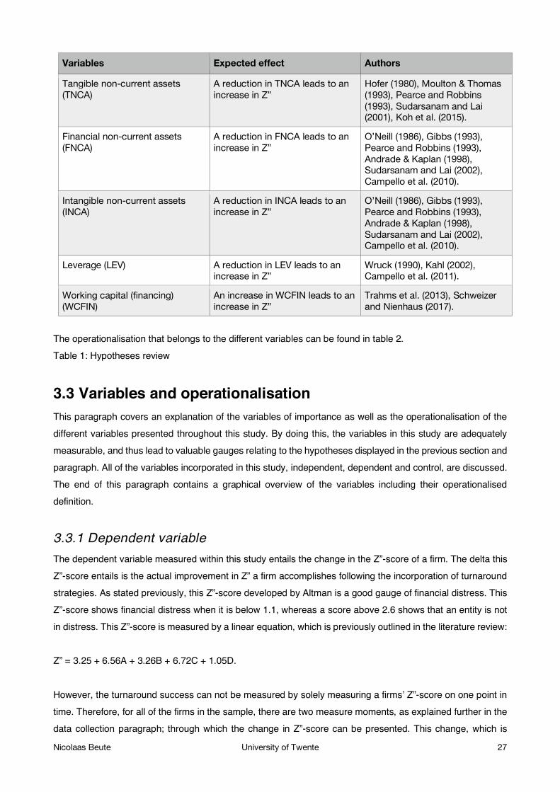
Nicolaas Beute University of Twente 27
Variables Expected effect Authors
Tangible non-current assets (TNCA)
A reduction in TNCA leads to an increase in Z”
Hofer (1980), Moulton & Thomas (1993), Pearce and Robbins (1993), Sudarsanam and Lai (2001), Koh et al. (2015).
Financial non-current assets (FNCA)
A reduction in FNCA leads to an increase in Z”
O’Neill (1986), Gibbs (1993), Pearce and Robbins (1993), Andrade & Kaplan (1998), Sudarsanam and Lai (2002), Campello et al. (2010).
Intangible non-current assets (INCA)
A reduction in INCA leads to an increase in Z”
O’Neill (1986), Gibbs (1993), Pearce and Robbins (1993), Andrade & Kaplan (1998), Sudarsanam and Lai (2002), Campello et al. (2010).
Leverage (LEV) A reduction in LEV leads to an increase in Z”
Wruck (1990), Kahl (2002), Campello et al. (2011).
Working capital (financing) (WCFIN)
An increase in WCFIN leads to an increase in Z”
Trahms et al. (2013), Schweizer and Nienhaus (2017).
The operationalisation that belongs to the different variables can be found in table 2. Table 1: Hypotheses review
3.3 Variables and operationalisation This paragraph covers an explanation of the variables of importance as well as the operationalisation of the different variables presented throughout this study. By doing this, the variables in this study are adequately measurable, and thus lead to valuable gauges relating to the hypotheses displayed in the previous section and paragraph. All of the variables incorporated in this study, independent, dependent and control, are discussed. The end of this paragraph contains a graphical overview of the variables including their operationalised definition.
3.3.1 Dependent variable The dependent variable measured within this study entails the change in the Z”-score of a firm. The delta this Z”-score entails is the actual improvement in Z” a firm accomplishes following the incorporation of turnaround strategies. As stated previously, this Z”-score developed by Altman is a good gauge of financial distress. This Z”-score shows financial distress when it is below 1.1, whereas a score above 2.6 shows that an entity is not in distress. This Z”-score is measured by a linear equation, which is previously outlined in the literature review: Z” = 3.25 + 6.56A + 3.26B + 6.72C + 1.05D. However, the turnaround success can not be measured by solely measuring a firms’ Z”-score on one point in time. Therefore, for all of the firms in the sample, there are two measure moments, as explained further in the data collection paragraph; through which the change in Z”-score can be presented. This change, which is

Nicolaas Beute University of Twente 28
shown as a percentage, offers insights to what extent turnaround strategies contribute to alleviating financial distress. Several researchers incorporate this Z”-score in restructuring focused studies, such as Balcaen and Ooghe (2006) and Cortés et al. (2007). Throughout this study the dependent variable is measured as a ratio. This is due to the fact that ratio variables as dependent variables are good input for an OLS regression, which is elaborated upon in a later paragraph.
3.3.2 Independent variables In order to find the effect to what extent the separate turnaround strategies contribute to improving Altman’s Z”-score, it is required to operationalise these turnaround strategies. Therefore, underlying constructs relating to turnaround strategies, which have been introduced in the previous section, are operationalised in this paragraph. In the literature review it became clear that the different turnaround strategies consist of actions that can be measured through financial data. Operational restructuring The first turnaround strategy that is operationalised is operational restructuring. Previous research shows us, as discussed in the literature review section, that operational restructuring mostly contains strategies that entail both cost-cutting, as well as measures that realise more efficient employment of activities. In line with previous research, operational restructuring is operationalised in the form of four variables namely, the change in operational costs, the change in gross margin, the change in the operational component of the working capital and the change in operational assets (such as PP&E) (e.g. Eichner, 2010; Sudarsanam & Lai, 2001; Hofer, 1980; Bowman & Singh, 1993; Taplin & Winterton, 1995). As for these variables the focus is on the change, it is measured by expressing the change in percentage from the first measurement moment to the second measurement moment. This means that when a firm starts with €2 million operational costs and at the second measurement moment the operational costs have a value of €1.5 million, it takes a value of 0.75 (decrease of 25%). As is the same case with the change in gross margin. Working capital, for which the asset component of the working capital is included in operational restructuring, is operationalised similarly: by measuring the change (in percentage) of the current assets minus cash & cash equivalents. Finally, the transfer of operational assets (e.g. Gibbs, 1993; Bergh et al., 2008; Li, 2013) is operationalised through measuring the change in tangible non-current assets. It is measured similarly as the other variables. An example would be where a firm owns €30 million non-current material assets and sells €7 million worth of these assets. The change from €30 million to €23 million, expressed in percentages, encompasses the gauge. Asset restructuring The second turnaround strategy entails asset restructuring, which is a strategy based upon changes in the asset portfolio. As this form of restructuring is mostly based upon large changes within the actual business of an entity, it is measured through two constructs, namely financial non-current assets, which could represent interests in other businesses or other forms of investments, as well as intangible non-current assets, such as trademarks or copyrights. These two constructs are frequently incorporated in restructuring studies (e.g. O’Neill, 1986; Gibbs, 1993; Lasfer et al., 1996) and are operationalised similarly as the other constructs in this

Nicolaas Beute University of Twente 29
study. Meaning that the change for both financial non-current assets and intangible non-current assets is expressed in percentages from 2010 to 2014. Financial restructuring Finally, the financial restructuring strategies are operationalised. Opler (1993) and Eichner (2010) show us that financial restructuring focuses mostly on the right-hand side of the balance sheet. Numerous studies focus on the components of financial restructuring. It entails debt measures, dividend measures as well as equity measures, but also contains liquidity improvement in the form of working capital management. Two underlying constructs are operationalised in order to measure financial restructuring. First, the change in leverage is measured similarly as the other operationalised variables previously mentioned. Leverage is a frequently incorporated component in turnaround research, as it combines the fundamental aspects of financial restructuring namely, the changes in debt and equity. The leverage a firm has, is measured through the formula non-current liabilities to equity. Whereas the liquidity improvement measures are gauged through the change in working capital, also in a similar way as the other variables incorporated. Working capital is, however split up in an operational and a financing component. The financing component is included in financial restructuring, which is measured through current liabilities. These variables are operationalised in line with previous research (e.g. Opler & Titman, 1994; Sheppard, 1994; Zingales, 1998; Kahl, 2002; Lin et al., 2008; Chowdhury & Lang, 1996).
3.3.3 Control variables Following the turnaround review by Schweizer and Nienhaus (2017), there are still some other variables that should be included in this study, which are control variables. These control variables, which are incorporated in the regression, are contextual factors that entail important determinants in the context of organisational change (e.g. Thomas & Ramaswamy, 1993; Coucke et al., 2007; Moulton et al., 1996; Indro et al., 1999). Throughout these studies it becomes clear that the context in which a firm is attempting to realise turnaround, is dependent on several factors. The most important contextual factors are added to the regression formula. These factors can be divided in microeconomic and macroeconomic factors. The microeconomic contextual factor added in this study contains the size of the firm (e.g. Greve, 2011; Moulton & Thomas, 1993; Robbins & Pearce, 1993). Whereas the macroeconomic contextual factors consist of industry (e.g. Chava & Jarrow, 2004; Rosenblatt & Mannheim, 1996; Routledge & Gadenne, 2000) and country (e.g. Bruton et al., 2003; Kang & Shivdasani, 1997; Hurry, 1993). Firm size Throughout previous research it is frequently stated that the size of a firm has tremendous impact on turnaround success. Several researchers have found positive correlation between the size of a firm and turnaround/survival (e.g. Agarwal et al., 2002; Kato, 2010; Stoeberl et al., 1998). Additionally, firm size is also found to be an important factor for managers relating to whether they are able to make the changes required in order to realise turnaround (Tushman et al., 1985). Boyne and Meier (2009) indeed state that the size of a firm has significant impact on the turnaround strategy that is chosen, whereas Bruton et al. (2003) prove that

Nicolaas Beute University of Twente 30
it is indeed a factor that affects turnaround success. In line with previous research the size of the firm is made measurable through incorporating the natural logarithm of the sales an entity realises in 2014. Industry Apart from the previously mentioned firm-specific contextual factor, there are macroeconomic contextual factors that also require implementation in this study. The first being the industry an entity is employing its activities in. It is found to be a significant factor relating to bankruptcy and turnaround (e.g. Chava & Jarrow, 2004; Mitchell & Mulherin, 1996; Rosenblatt & Mannheim, 1996). Routledge and Gadenne (2000) for example prove that retail companies have less chance of successful turnaround than entities in the manufacturing industry. Which is underpinned by Hancock et al. (2013). Furthermore, researchers have found that a specific industry an entity employs its activities in, has significant impact in determining what turnaround strategy is used (e.g. Morrow Jr et al., 2004; Ndofor et al., 2013). Controlling for the industry is done through creating dummies. These dummies contain level 1 codes as used by NACE classifications, where the dummy variable takes a value of 1 if the entity is employing its activities in that particular industry, whereas the value is 0 if not. Albeit true that through the database Orbis, which is used for data collection, the industry can not be found for the years 2010 and 2014, but solely for the most recent year. By using the level 1 codes industry changes within firms in the sample should be minimised. Country The other macroeconomic control variable encompasses the country an entity is positioned in. This is also found to impact the choice and success of a turnaround strategy (Bruton et al., 2003). Kang and Shivdasani (1997) and Hurry (1993) indeed find that there are differences in the turnaround strategies incorporated by firms. This raises awareness that the country a firm belongs to is controlled for. Therefore, country dummy variables are included in the regressions. These are incorporated so that heterogeneity is controlled for, as was the case in the Zingales (1998) study. There are dummy variables for every region included in the sample and they take a value of 1 if the entity is active in that region, and a value of 0 if they are not active in that region. As was this case with industry, the country of the firm is based upon the most recent country known by Orbis.
3.3.4 Graphical overview operationalisation Throughout this paragraph a graphical presentation of the operationalisation of the variables is shown. The information related to the variables is in all cases deducted from Orbis. First, the main variables of interest are operationalised, while also the variables employed in the robust analyses are operationalised.
Variables Operationalisation
Altman’s Z”-score Z” = 3.75 + 6.56A + 3.26B + 6.72C + 1.05D, where A is working capital to total assets, B is retained earnings to total assets, C is EBIT to total assets and D is book value of equity to book value of debt.

Nicolaas Beute University of Twente 31
Variables Operationalisation
Improvement in Altman’s Z”-score
The change in Altman’s Z”-score from 2010 to 2014. This change is expressed in percentages, through dividing the 2014 score by the 2010 score. Throughout the OLS regressions this variable is measured as a ratio.
Operational expenses The change in operational expenses from 2010 to 2014. This change is expressed in percentages, through dividing the 2014 value by the 2010 value.
Gross margin The change in gross margin (gross profit divided by sales) from 2010 to 2014. This change is expressed in percentages, through dividing the 2014 value by the 2010 value.
Working capital (operational component)
The change in current assets minus cash & cash equivalents from 2010 to 2014. This change is expressed in percentages, through dividing the 2014 value by the 2010 value.
Tangible non-current assets The change in tangible non-current assets from 2010 to 2014. This change is expressed in percentages, through dividing the 2014 value by the 2010 value.
Financial non-current assets The change in financial non-current assets from 2010 to 2014. This change is expressed in percentages, through dividing the 2014 value by the 2010 value.
Intangible non-current assets
The change in intangible non-current assets from 2010 to 2014. This change is expressed in percentages, through dividing the 2014 value by the 2010 value.
Leverage The change in leverage (non-current debt divided by equity) from 2010 to 2014. This change is expressed in percentages, through dividing the 2014 value by the 2010 value.
Working capital (financing component)
The change in current liabilities from 2010 to 2014. This change is expressed in percentages, through dividing the 2014 value by the 2010 value.
Firm size The natural logarithm of the amount of sales in 2014. The natural logarithm of this number is the input for the control variable.
Industry Dummy variable for each of the industries included in the study. The dummy takes a value of 1 if the firm is active in that industry and a value of 0 if the firm is not active in that industry.
Country Dummy variable for each of the countries included in the study. The dummy takes a value of 1 if the firm is located in that country and a value of 0 if the firm is not located in that country.
Non-current assets (NCA) The change in non-current assets from 2010 to 2014. This change is expressed in percentages, through dividing the 2014 value by the 2010 value.

Nicolaas Beute University of Twente 32
Variables Operationalisation
Current assets (CA) The change in current assets from 2010 to 2014. This change is expressed in percentages, through dividing the 2014 value by the 2010 value.
Equity (EQ) The change in shareholders’ equity from 2010 to 2014. This change is expressed in percentages, through dividing the 2014 value by the 2010 value.
Non-current liabilities (NCL) The change in non-current liabilities from 2010 to 2014. This change is expressed in percentages, through dividing the 2014 value by the 2010 value.
Current liabilities (CL) The change in current liabilities from 2010 to 2014. This change is expressed in percentages, through dividing the 2014 value by the 2010 value.
Table 2: Operationalisation of variables
3.4 Sample and data collection The sample used in this study as well as the data tested in this study is constructed through the financial database Orbis. Within Orbis a selection in firms is made. First, the research scope as presented in the introduction, is included as search filters within Orbis, leading to a large amount of firms. This means that first, firms are included in the sample that have their statutory seat in one of 15 EU countries, as selected by Orbis, which represent the initial fifteen member states of the EU prior to the addition of another 10 member states. Additionally, the scope for selecting firms within these countries is limited to firms generating a turnover of €20 million or more in the starting year (2010), which is frequently named as the minimum turnover for firms that are recognised as large firms. Furthermore, the scope for industries is based upon NACE sector codes developed in 2012. With the exclusion of sector K (finance and insurance) and sector O (public administration) all sectors are included in the sample. The reason for the exclusion of these two sectors originate from risk factors, which are different for financial and government firms. Moreover, all of the variables that are required in order to test the hypotheses, as well as variables that are required as input for the formulas, are gathered. This is done for both 2010 as well as 2014, as a change can solely be measured with at least two measure moments. The change between these years is consequently expressed in percentages. The change is expressed in percentages, so that there is a uniform manner of interpreting change that should lead to a minimum of extreme outlier values. This change entails the input for the research variables, as is elaborated upon in the previous paragraph. Merely firms that have all the available financial information are included in the sample, meaning that for both 2010 and 2014, information regarding the balance sheet of the firm has to be available, such as non-current material assets, equity and debt, current assets and current liabilities, as well as several income statement subjects, such as EBIT, operational expenses, gross margin, and sales. There is no particular reason for these years, however, the years 2006-2009 have been explicitly ignored, as the financial crisis during those years can have enormous impact on the statistical analyses, which makes it increasingly difficult to generalise the findings resulting from this study. While it is true that most studies incorporate lower sample ranges for similar studies, some restructuring content has also used a similar span,

Nicolaas Beute University of Twente 33
such as the Denis and Kruse (1999) and Gilson et al. (1990) studies. On average it seems that restructuring studies focus mostly on 2 to 5 year ranges. Following these actions the data is filtered and consequently, the data of firms that were in financial distress in 2010 are included as cases in the sample. In addition, firms with missing data are excluded from the sample. Due to the fact that previously mentioned extreme outliers can have enormous impact on a statistical analysis, especially a regression analysis, there is a need to eliminate these cases from the samples. These outliers are eliminated on the basis of Mahalanobis’ distance. When the statistical test shows a significant probability of less than 0.001, the data line of that entity is removed from the sample. The Mahalanobis’ distance is incorporated in this study, as it is a good method of eliminating outlier cases in a multivariate analysis. One of the reasons for this is a method that eliminates the effect of units as well as the effect of differing scales, which makes it a useful measure of outlying values. It is basically a multivariate way of determining the amounts of standard deviations that the value is away from the mean. Additionally, extreme outliers that had either enormous positive or enormous negative impact on the regression analysis have been removed from the sample. Primarily, the data gathered existed of 14,060 firms. Within this dataset, firms are filtered out when they did not have a distressed Z”-score in 2010, which led to the elimination of many firms. Following this action 219 entities remained in the dataset. The five samples employed throughout this study are deducted from these 219 firms. The first sample, employing the main variables of interest, contains all firms with all available information, whereas the second sample contains firms with all of the available information while also requiring the entity to move from a distressed to a non-distressed score. In the first sample 11 firms were removed from the initial 219 due to a significant probability of Mahalanobis’ distance, whereas additional case lines have been removed due to extreme outliers, leading to a final sample of 141 firms. The second sample removes 146 firms from the sample, due to them not reaching a non-distressed score leaving 73 firms. After removing cases on the basis of Mahalanobis’ distance as well as extreme outliers by hand, a sample consisting of 48 firms remains. The next two samples employ the robust variables and require all of the required information to be available. Employing Mahalanobis’ distance leads to the elimination of 11 outlier cases, leaving 208 firms. The remaining 19 case lines have been deleted on the basis of extreme values, which implies that the third sample consists of 189 firms. The fourth sample incorporates solely firms that went from a distressed to a non-distressed score. First, 146 firms are deleted due to them not reaching non-distressed scores. 12 firms are deleted on the basis of significant probability of Mahalanobis’ distance or extreme values, leaving 61 firms in the fourth sample. The final sample incorporates a different requirement for an entity to be included in this sample. Sometimes it is not clear whether a change in, for example operational expenses, is due to a changing business environment, or truly due to restructuring efforts. Research by Koh et al. (2015), deducted from other studies that a certain threshold can be established, implicating that a minimum change in percentage is recognised as actual turnaround efforts. Due to the fact that some of the variables included in their research are different than the variables in this research, a threshold for true restructuring in this study is made according to the turnaround

Nicolaas Beute University of Twente 34
clusters, rather than the separate underlying variables. As Kang and Shivdasani (1997) did in their study, which is followed by Koh et al. (2015) a change in fixed assets should entail at least a decrease of 15%. Denis and Kruse (2000) argue that actual operational decreases, such as layoffs, should be over 20%. Finally, they employ a 25% threshold with regards to financial restructuring techniques. Therefore, this sample incorporates firms which at least surpass one of these thresholds. This could mean a decrease of at least 20% in either OPEX or TNCA, a decrease of at least 25% in LEV and a minimum decrease of 15% in the FNCA and INCA variables. WCOPER, WCFIN and GM will not use such a threshold to determine restructuring, as it is difficult to gauge with a threshold, since the change is usually a result from altering the business of the firm. An example is that a firm can choose to sell an asset, or increase their debt, they can however not simply choose to increase their GM; that is a result from employing their activities. So incorporating these requirements for the final sample leads to a sample of 121 firms. This number of firms is reached through deleting firms from the first sample on the basis of outliers as well as firms not meeting the threshold requirement.
Table 3: Summarisation of samples
3.5 Method of analysis This study attempts to make inferences based upon quantitative data. In order to ascertain an understanding of the results of this study, the previous paragraphs have sketched the variables that resulted from the literature review as well as their operationalisation with regards to the actual statistical testing of hypotheses, which have also been summarised in this chapter. The remainder of this paragraph discusses through what method the analysis is performed. Hair et al. (2014) state that a multiple regression analysis is an adequate method of finding relations between multiple independent variables and a dependent variable. This manner of statistical testing is frequently incorporated in restructuring research (e.g. Sudarsanam & Lai, 2001; Koh et al., 2015) when the dependent
Sample Number of firms Requirement
1 141 Firms with all available information, no requirement with regard to change in Z”-score.
2 48 Firms with all available information, requirement where 2010 Z”-score is <1.1 and 2014 Z”-score is >2.6.
3 189 Firms with robust information, no requirement with regard to change in Z”-score.
4 61 Firms with robust information, requirement where 2010 Z”-score is <1.1 and 2014 Z”-score is >2.6.
5 121 Firms with all available information, requirement with regard to changes in variables of interest, where either the 20% (operational restructuring), 25% (financial restructuring) or 15% (asset restructuring) threshold must be met.

Nicolaas Beute University of Twente 35
variable is measured as a ratio; logistic regressions are incorporated when the dependent variable is dichotomous (e.g. Routledge & Gadenne, 2000; Denis & Kruse, 2000). As this study employs a ratio variable as dependent variable, the OLS regression is adopted. This OLS regression is adopted three times. Throughout all of the performed regressions there are ten models, the first model in the first regression attains solely the variables of interest, where in the second model the control variables are included. The first and second model in the first OLS regression include the firms in sample one. The third and fourth model are run solely for firms that went from a distressed score to a non-distressed score (sample two). Model three in the main OLS regression includes the predictor variables for the second sample, while in model four the control dummies are added. By doing this, it becomes clear whether filtering for firms that actually experienced turnaround success where the entity has left financial distress employ different strategies. By doing this, it should become clear what turnaround strategy leads to the best improvement in Z”-score. Throughout these two OLS regressions, the input variables are those as described in paragraph 3.3, which leads to the first linear equation presented at the end of the paragraph, as is in line with the research objective. The deltas entail the change, which is expressed in percentages, from 2010 to 2014. Additionally, two other robust OLS regressions are performed. It is thinkable that there are quite some entities that for example do not have either intangible or financial non-current assets. Therefore, the second OLS regressions does not employ the balance sheet accounts as in the previously outlined OLS regressions, but in addition to the income statement accounts GM and OPEX, the main accounts of the balance sheet are added to the regression. This means that the variables TNCA, WCOPER, WCFIN, LEV, FNCA and INCA, are changed to non-current assets, current assets, equity, non-current debt and current debt. As was the case with the previous OLS regressions, these robust OLS regressions also first incorporate all of the cases (sample three), whereas in the third and fourth model solely firms that have gone from a distressed score to a non-distressed score are incorporated (sample four). This leads to a new linear equation. Similarly as the variables in the primary OLS regressions, the deltas are expressed as percentages from 2010 to 2014. While the hypotheses are not formed with regards to these main accounts of the balance sheet, these robust regressions are incorporated in order to find interesting differences between the primary OLS regressions and the robust OLS regressions. Finally, an additional regression is performed. This regression is in line with the regression run with regard to the first two samples. This final regression, with two models (inclusion of industry and country dummies), requires a firm to meet the threshold of a decrease in the different turnaround strategies. This possibly filters out firms that did not knowingly conduct turnaround strategies. ΔZ” = α + β1ΔTNCA + β2ΔOPEX + β3ΔGM + β4ΔWCOPER + β5ΔWCFIN + β6ΔLEV + β7ΔFNCA + β8ΔINCA + β9Firmsize + β10Country + β11Industry + ε ΔZ” = α + β1ΔNCA + β2ΔOPEX + β3ΔGM + β4ΔCA + β5ΔEQ + β6ΔNCL + β7ΔCL + β8Firmsize + β9Country + β10Industry + ε

Nicolaas Beute University of Twente 36
3.6 Univariate statistics This final paragraph of chapter three offers several interesting descriptive statistics in the form of univariate statistics. First, univariate statistics for the underlying variables of Altman’s Z”-score are presented, followed by univariate statistics for the main variables and robust variables. These descriptive statistics are depicted for all of the samples. The first univariate analysis is performed on the underlying variables for the Z”-score. This is done for all of the samples. Table 4, panel A, shows the univariate statistics for the first sample, panel B for the second, etc.. Most values are not much of interest, for example the skewness and kurtosis are a non-issue due to the fact that the values are not incorporated in an actual regression to find coefficient estimates, but rather subject to a formula in order to find out what the financial health of an entity is. As can be seen the means of all the underlying variables in the first sample are negative, except for the A value in 2014 (M=0.001). This is expected, since part of the sample creation was finding firms in financial distress. These firms would most likely have lower scores on all values than their financially sound competitors. What is surprising though, is the fact that, apart from the A variable, the 2014 variables remain negative meaning that many firms in the sample failed to leave financial distress. However, most mean values of the variables did increase; variable A went from -0.028 to 0.001, variable C from -0.238 to -0.078 and variable D from -0.222 to -0.036. Table 4, panel B shows the univariate statistics for the second sample. As expected the means now show much more positive numbers in 2014. Variables C (2010: -0.287, 2014: 0.092) and D (2010: -0.224 2014: 2.759) show increases from a negative mean value to a positive mean value. This is mostly due to the fact that only entities that went from distressed to non-distressed are included in this sample. Table 4, panel C shows mostly negative means in the underlying variables of the Z”-score model. The mean of variable B even decreases from -1.488 in 2010 to -1.944 in 2014. Another interesting increase is the change in mean for the D variable, which went from -0.324 in 2010 to 0.561. Panel D shows the statistics for the fourth sample. Due to the sample consisting of success cases only, it is expected that the means would change from a negative to a positive value. Only the B variable mean remained negative (2010: -1.129, 2014: -0.114). Table 4, panel E shows the univariate statistics for the last sample. As was the case in most samples, most mean values did entail increases, but all of the values remained negative. Only the B variable decreased (2010: -1.521, 2014: -2.374). In order to check for multicollinearity the correlation matrices for the underlying variables of the Z”-score model have been checked. Correlation values that exceed 0.7 are a sign of multicollinearity. This is not the case and there is thus no appearance of multicollinearity. The correlation matrices can be found in appendix A. For all of the below tables, A is the working capital to total assets, B the retained earnings to total assets, C the EBIT to total assets, and D the book value of equity to book value of total debt.

Nicolaas Beute University of Twente 37
Table 4: descriptive statistics of the underlying variables of the Z"-score model Panel A Mean Median Std. Dev. Min Max N A 2010 -0.028 0.042 0.546 -4.964 0.853 141 A 2014 0.001 0.051 0.660 -5.743 0.970 141 B 2010 -1.565 -1.265 1.370 -7.121 0.499 141 B 2014 -2.321 -1,196 3.644 -25.079 0.620 141 C 2010 -0.238 -0.152 0.331 -1.483 0.358 141 C 2014 -0.078 0.004 0.694 -7,531 1.344 141 D 2010 -0.222 -0.326 0.436 -0.867 1.606 141 D 2014 -0.036 -0.204 0.837 -0.951 5.487 141 Panel B
A 2010 0.079 0.056 0.256 -0.487 0.853 48 A 2014 0.161 0.110 0.208 -0.096 0.970 48 B 2010 -1.115 -1.055 1.025 -4.888 0.496 48 B 2014 -0.113 -0.094 0.413 -1.295 0.871 48 C 2010 -0.287 -0.148 0.399 -1.425 0.217 48 C 2014 0.092 0.052 0.237 -0.199 1.344 48 D 2010 -0.224 -0.303 0.378 -0.736 1.204 48 D 2014 2.759 0.383 15.123 -0.564 105.105 48 Panel C
A 2010 -0.024 0.034 0.494 -4.964 0.853 189 A 2014 0.010 0.046 0.587 -5.743 0.970 189 B 2010 -1.488 -1.232 1.305 -7.121 0.578 189 B 2014 -1.944 -0.837 3.271 -25.079 0.871 189 C 2010 -0.262 -0.142 0.381 -1.893 0.358 189 C 2014 -0.055 0.006 0.606 -7.531 1.344 189 D 2010 -0.324 -0.332 1.332 -17.560 1.606 189 D 2014 0.561 -0.135 7.691 -0.950 105.105 189 Panel D
A 2010 0.064 0.042 0.305 -1.345 0.853 61 A 2014 0.163 0.103 0.207 -0.096 0.970 61 B 2010 -1.129 -1.053 1.049 -4.888 0.578 61 B 2014 -0.114 -0.011 0.425 -1.295 0.871 61 C 2010 -0.337 -0.188 0.432 -1.425 0.217 61 C 2014 0.102 0.052 0.225 -0.199 1.344 61 D 2010 -0.529 -0.307 2.247 -17.560 1.204 61 D 2014 2.330 0.322 13.423 -0.564 105.105 61 Panel E
A 2010 -0.031 0.051 0.581 -4.964 0.853 121 A 2014 -0.013 0.051 0.702 -5.743 0.970 121 B 2010 -1.521 -1.265 1.308 -7.120 0.499 121 B 2014 -2.374 -1.266 3.831 -25.079 0.620 121 C 2010 -0.236 -0.152 0.323 -1.483 0.358 121 C 2014 -0.081 0.006 0.727 -7.531 0.778 121 D 2010 -0.194 -0.315 0.449 -0.808 1.606 121 D 2014 -0.002 -0.158 0.881 -0.951 5.487 121
Table 4 legend: A is the working capital to total assets, B the retained earnings to total assets, C the EBIT to total assets, and D the book value of equity to book value of total debt.
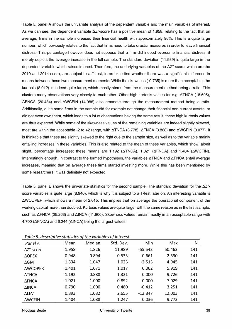
Nicolaas Beute University of Twente 38
Table 5, panel A shows the univariate analysis of the dependent variable and the main variables of interest. As we can see, the dependent variable ΔZ”-score has a positive mean of 1.958, relating to the fact that on average, firms in the sample increased their financial health with approximately 96%. This is a quite large number, which obviously relates to the fact that firms need to take drastic measures in order to leave financial distress. This percentage however does not suppose that a firm did indeed overcome financial distress, it merely depicts the average increase in the full sample. The standard deviation (11.989) is quite large in the dependent variable which raises interest. Therefore, the underlying variables of the ΔZ”-score, which are the 2010 and 2014 score, are subject to a T-test, in order to find whether there was a significant difference in means between these two measurement moments. While the skewness (-0.735) is more than acceptable, the kurtosis (8.912) is indeed quite large, which mostly stems from the measurement method being a ratio. This clusters many observations very closely to each other. Other high kurtosis values for e.g. ΔTNCA (18.695), ΔFNCA (20.434) and ΔWCFIN (14.986) also emanate through the measurement method being a ratio. Additionally, quite some firms in the sample did for example not change their financial non-current assets, or did not even own them, which leads to a lot of observations having the same result; these high kurtosis values are thus expected. While some of the skewness values of the remaining variables are indeed slightly skewed, most are within the acceptable -2 to +2 range, with ΔTNCA (3.778), ΔFNCA (3.868) and ΔWCFIN (3.077). It is thinkable that these are slightly skewed to the right due to the sample size, as well as to the variable mainly entailing increases in these variables. This is also related to the mean of these variables, which show, albeit slight, percentage increases: these means are 1.192 (ΔTNCA), 1.021 (ΔFNCA) and 1.404 (ΔWCFIN). Interestingly enough, in contrast to the formed hypotheses, the variables ΔTNCA and ΔFNCA entail average increases, meaning that on average these firms started investing more. While this has been mentioned by some researchers, it was definitely not expected. Table 5, panel B shows the univariate statistics for the second sample. The standard deviation for the ΔZ”-score variables is quite large (8.940), which is why it is subject to a T-test later on. An interesting variable is ΔWCOPER, which shows a mean of 2.015. This implies that on average the operational component of the working capital more than doubled. Kurtosis values are quite large, with the same reason as in the first sample, such as ΔFNCA (25.263) and ΔINCA (41.806). Skewness values remain mostly in an acceptable range with 4.700 (ΔFNCA) and 6.244 (ΔINCA) being the largest values.
Table 5: descriptive statistics of the variables of interest Panel A Mean Median Std. Dev. Min Max N ΔZ"-score 1.958 1.826 11.989 -55.543 50.463 141 ΔOPEX 0.948 0.894 0.533 -0.661 2.530 141 ΔGM 1.334 1.047 1.023 -2.513 4.945 141 ΔWCOPER 1.401 1.071 1.017 0.062 5.919 141 ΔTNCA 1.192 0.888 1.321 0.000 9.726 141 ΔFNCA 1.021 1.000 0.892 0.000 7.029 141 ΔINCA 0.790 1.000 0.480 -0.412 3.251 141 ΔLEV 0.893 1.082 2.655 -12.847 12.003 141 ΔWCFIN 1.404 1.088 1.247 0.036 9.773 141
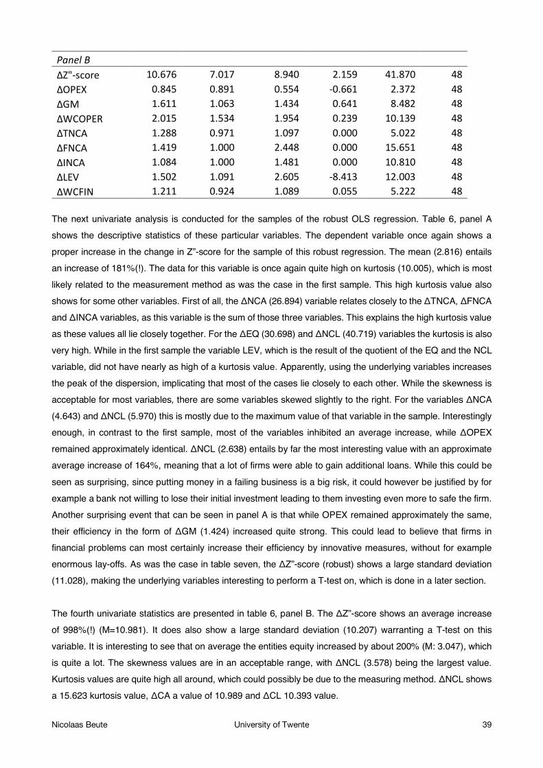
Nicolaas Beute University of Twente 39
Panel B
ΔZ"-score 10.676 7.017 8.940 2.159 41.870 48 ΔOPEX 0.845 0.891 0.554 -0.661 2.372 48 ΔGM 1.611 1.063 1.434 0.641 8.482 48 ΔWCOPER 2.015 1.534 1.954 0.239 10.139 48 ΔTNCA 1.288 0.971 1.097 0.000 5.022 48 ΔFNCA 1.419 1.000 2.448 0.000 15.651 48 ΔINCA 1.084 1.000 1.481 0.000 10.810 48 ΔLEV 1.502 1.091 2.605 -8.413 12.003 48 ΔWCFIN 1.211 0.924 1.089 0.055 5.222 48
The next univariate analysis is conducted for the samples of the robust OLS regression. Table 6, panel A shows the descriptive statistics of these particular variables. The dependent variable once again shows a proper increase in the change in Z”-score for the sample of this robust regression. The mean (2.816) entails an increase of 181%(!). The data for this variable is once again quite high on kurtosis (10.005), which is most likely related to the measurement method as was the case in the first sample. This high kurtosis value also shows for some other variables. First of all, the ΔNCA (26.894) variable relates closely to the ΔTNCA, ΔFNCA and ΔINCA variables, as this variable is the sum of those three variables. This explains the high kurtosis value as these values all lie closely together. For the ΔEQ (30.698) and ΔNCL (40.719) variables the kurtosis is also very high. While in the first sample the variable LEV, which is the result of the quotient of the EQ and the NCL variable, did not have nearly as high of a kurtosis value. Apparently, using the underlying variables increases the peak of the dispersion, implicating that most of the cases lie closely to each other. While the skewness is acceptable for most variables, there are some variables skewed slightly to the right. For the variables ΔNCA (4.643) and ΔNCL (5.970) this is mostly due to the maximum value of that variable in the sample. Interestingly enough, in contrast to the first sample, most of the variables inhibited an average increase, while ΔOPEX remained approximately identical. ΔNCL (2.638) entails by far the most interesting value with an approximate average increase of 164%, meaning that a lot of firms were able to gain additional loans. While this could be seen as surprising, since putting money in a failing business is a big risk, it could however be justified by for example a bank not willing to lose their initial investment leading to them investing even more to safe the firm. Another surprising event that can be seen in panel A is that while OPEX remained approximately the same, their efficiency in the form of ΔGM (1.424) increased quite strong. This could lead to believe that firms in financial problems can most certainly increase their efficiency by innovative measures, without for example enormous lay-offs. As was the case in table seven, the ΔZ”-score (robust) shows a large standard deviation (11.028), making the underlying variables interesting to perform a T-test on, which is done in a later section. The fourth univariate statistics are presented in table 6, panel B. The ΔZ”-score shows an average increase of 998%(!) (M=10.981). It does also show a large standard deviation (10.207) warranting a T-test on this variable. It is interesting to see that on average the entities equity increased by about 200% (M: 3.047), which is quite a lot. The skewness values are in an acceptable range, with ΔNCL (3.578) being the largest value. Kurtosis values are quite high all around, which could possibly be due to the measuring method. ΔNCL shows a 15.623 kurtosis value, ΔCA a value of 10.989 and ΔCL 10.393 value.

Nicolaas Beute University of Twente 40
Table 6: descriptive statistics of the robust variables Panel A Mean Median Std. Dev. Min Max N ΔZ"-score 2.816 2.159 11.028 -55.543 50.463 189 ΔOPEX 1.005 0.955 0.623 -0.661 4.603 189 ΔGM 1.424 1.070 1.158 -2.513 8.482 189 ΔNCA 1.474 0.914 2.132 0.000 17.746 189 ΔCA 1.552 1.196 1.255 0.058 8.745 189 ΔEQ 1.060 1.192 4.861 -38.443 30.470 189 ΔNCL 2.638 1.000 7.352 -2.305 63.674 189 ΔCL 1.500 1.098 1.528 0.036 9.773 189 Panel B
ΔZ"-score 10.981 7.105 10.207 2.159 50.463 61 ΔOPEX 0.816 0.841 0.568 -0.661 2.372 61 ΔGM 1.700 1.108 1.452 0.509 8.482 61 ΔNCA 1.343 0.914 1.299 0.017 7.800 61 ΔCA 1.919 1.665 1.312 0.146 8.745 61 ΔEQ 3.047 2.238 3.246 -1.827 18.180 61 ΔNCL 1.722 0.555 3.627 -2.305 21.683 61 ΔCL 1.367 0.920 1.535 0.055 8.903 61
The univariate statistics of the final sample are presented in table 7. As can be seen the mean increase in Z”-score in this sample is quite good (M=2.247). Other values are quite in line with other samples. Furthermore, the results are quite close to sample 1, as the requirements for addition in the sample are closely related. Kurtosis values for ΔTNCA (27.661), ΔFNCA (17.358) remain quite large. Skewness values are within the acceptable range, with ΔTNCA (4.226) having the largest value.
Table 7: descriptive statistics of the variables of interest for sample 5 Mean Median Std. Dev. Min Max N ΔZ"-score 2.247 1.807 11.819 -55.543 50.463 121 ΔOPEX 0.864 0.833 0.498 -0.661 2.367 121 ΔGM 1.303 1.050 1.000 -2.513 4.945 121 ΔWCOPER 1.331 1.028 0.946 0.062 5.220 121 ΔTNCA 1.064 0.785 1.140 0.000 9.726 121 ΔFNCA 1.017 1.000 0.963 0.000 7.029 121 ΔINCA 0.738 1.000 0.474 -0.412 3.251 121 ΔLEV 0.651 1.082 2.560 -12.847 7.223 121 ΔWCFIN 1.249 1.035 0.952 0.036 5.222 121

Nicolaas Beute University of Twente 41
4. Empirical results and descriptive statistics First, the T-tests as argued in the previous section are performed and discussed. Following these T-tests, the correlation between the independent variables and dependent variable is presented for all of the samples. Throughout the remainder of this paragraph the main results from the performed OLS regressions are presented and discussed. First, the regression models with the main variables are subject of discussion, while the robustness checks follow after. These regressions serve as the input for testing the hypotheses formed in section two.
4.1 Descriptive statistics As mentioned in the beginning of this section five T-tests are performed. The Z”-scores for both the main OLS regressions as well as the robust regressions had quite a large standard deviation. Therefore, the underlying values from 2010 and 2014 are subject to this test in order to find significant differences in the mean. The related table is found in appendix B. First, the Z”-score values of 2010 and 2014 from the primary OLS regression are tested. It appeared that there was no significant difference between the Z”-score in 2010 (M=-3.369, SD=6.474) and the Z”-score in 2014 (M=-4.372, SD=17.564) in mean. The test value incorporated is the average of the two means (-3.87) from which both variables did not significantly differ: 2010 value (p=0.360) and 2014 value (p=0.735). In sample two the means from the Z”-score values did significantly differ (2010: M=-1.532, SD=3.707, p=<0.001; 2014: M=7.955, SD=16.373, p=0.050). The next T-test is conducted on the variables from the Z”-scores in the robust model. The test value in this T-test is -2.68 which was the average between the 2010 and 2014 value. No significant difference was found between the 2010 value (M=-3.44, SD=6.21, p=0.198) and the 2014 value (M=-2.28, SD=17.87, p=0.656). Additionally, the T-test is conducted on the Z”-scores in sample 4. The 2010 mean (M=-2.329, SD=4.669, p=<0.001) and 2014 mean (M=7.581, SD=14.574, p=0.010) are found to significantly differ from each other. The final T-test resulted in no significant difference in mean between the 2010 (M=-3.197, SD=6.526, p=0.239) and 2014 (M=-4.611, SD=18.585, p=0.675) values. It is interesting to see that, while in the samples where all the cases are included there was no significant difference, a significant difference was found in the samples that included only success cases with firms going from a distressed to a non-distressed score. Now that the most interesting univariate statistics have been discussed, the next descriptive statistic frequently incorporated in multiple regression research is discussed. The correlation, which is frequently named as an important step before conducting the regression analysis, shows whether there are any significant relations between the dependent variable and the independent variables. Table 8 shows the Pearson correlation matrix of the first sample. While significant relations are indeed desirable, the correlation test merely returns one significant relation with the dependent variable, being the ΔWCOPER (0.278) variable. Apart from this significant relation not many interesting findings are deducted from the correlation matrix. It can however be stated that, due to correlation values not exceeding 0.7, there is no multicollinearity between the independent variables. This is also proven through the VIF values, which do not exceed 10. Appendix C contains the table in which the VIF values for these independent variables are depicted. While significant correlation is indeed an important factor in conducting multiple regression analysis, the fact that merely one variable correlates

Nicolaas Beute University of Twente 42
significantly should not be a problem, as previous literature (section 2) indeed finds that the variables of interest and dependent variable are related to one another. The reason of this small amount of significant correlations could very well be due to the sample size this study incorporates. Within the second sample, that employs the same variables, no significant correlations were found and the table is thus not included in this study. Table 9 shows the Pearson correlation matrix for the robust OLS regression. It shows two significant correlations at the 1% level. First, the ΔCA (0.261) variable is significantly correlated to the ΔZ”-score variable. This was expected, as it is very similar to the ΔWCOPER variable in the main OLS regression. The other variable that is significantly correlated is the ΔEQ (0.227) variable. Once again, we can see that there are no variables exceeding the 0,7 threshold, meaning that there is no multicollinearity and thus there are no variables that should be excluded. This also shows in the next table in appendix C, which shows the VIF values for the robust variables: these do not exceed 10. The fourth sample that incorporates similar variables did not return any significant correlations and is therefore not added. The fifth sample did return significant correlations and is thus added as table 10. ΔWCOPER (0.307) and ΔINCA (0.199) are found to correlate significantly with the change in Altmans Z”-score. As can be seen, the 0.7 threshold is not exceeded, relating to no multicollinearity. Additionally, the VIF values do not exceed 10, as can be seen in the next table in appendix C.

Table 8: Pearson correlation matrix for sample 1 1 2 3 4 5 6 7 8 9
ΔZ"-score (1) 1
ΔOPEX (2) -0.082 1
ΔGM (3) 0.106 -0.101 1
ΔWCOPER (4) 0.278 ** 0.153 -0.054 1
ΔTNCA (5) 0.093 0.353 ** -0.055 0.176 * 1 ΔFNCA (6) 0.030 0.011 -0.013 0.066 0.092 1 ΔINCA (7) 0.152 0.159 0.063 0.139 0.126 -0.134 1
ΔLEV (8) 0.114 -0.011 0.060 0.120 0.092 0.133 0.050 1 ΔWCFIN (9) -0.037 0.229 ** -0.123 0.321 ** 0.025 -0.102 0.127 0.104 1
**. Correlation is significant at the 0.01 level (2-tailed). *. Correlation is significant at the 0.05 level (2-tailed).
Table 9: Pearson correlation matrix for sample 3 1 2 3 4 5 6 7 8
ΔZ"-score (1) 1
ΔOPEX (2) -0.062 1
ΔGM (3) 0.097 -0.087 1
ΔNCA (4) 0.080 0.227 ** -0.047 1
ΔCA (5) 0.261 ** 0.156 * -0.081 0.174 * 1
ΔEQ (6) 0.227 ** -0.044 0.007 0.046 0.084 1 ΔNCL (7) -0.001 -0.042 0.055 -0.002 -0.023 -0.031 1
ΔCL (8) -0.015 0.124 -0.138 0.190 ** 0.489 ** -0.075 -0.130 1 **. Correlation is significant at the 0.01 level (2-tailed). *. Correlation is significant at the 0.05 level (2-tailed).

Nicolaas Beute University of Twente 44
Table 10: Pearson correlation matrix for sample 5 1 2 3 4 5 6 7 8 9
ΔZ"-score (1) 1
ΔOPEX (2) -0.106 1
ΔGM (3) 0.107 -0.147 1
ΔWCOPER (4) 0.307 ** 0.109 -0.062 1
ΔTNCA (5) 0.122 0.344 ** -0.029 0.153 1 ΔFNCA (6) 0.032 0.008 -0.012 0.074 0.112 1 ΔINCA (7) 0.199 * 0.089 0.053 0.140 0.075 -0.148 1
ΔLEV (8) 0.118 -0.174 0.050 0.028 0.061 0.150 0.007 1 ΔWCFIN (9) 0.064 0.265 ** -0.140 0.349 ** -0.035 -0.145 0.104 0.076 1
**. Correlation is significant at the 0.01 level (2-tailed). *. Correlation is significant at the 0.05 level (2-tailed).

4.2 Assumptions of multiple regression analysis Before conducting any regression analysis, it is of importance to test for the assumptions of regression analysis. This is first done for the two primary OLS regressions, after which also the assumptions are checked for the robust OLS regressions. The assumptions that are tested for are normality, homoscedasticity and linearity. In order to test for normality a histogram is incorporated, while the scatterplot offers insight in both the homoscedasticity and linearity of the data.
4.2.1 Main OLS regression The first sample, which includes the main variables of interest as well as all of the available cases without distinguishing actual success or not, is the first dataset that is checked for these assumptions. Within the histogram the normal curve offers good visual evidence of a normal distribution, meaning that the assumption of normality is passed. The scatterplot shows no pattern whatsoever, which relates to the data passing the assumption of homoscedasticity. When drawing a fit line through the scatterplot, it should more or less be a straight line in order for the data to be linear. This is indeed the case and thus for the first sample all assumptions of multiple regression analysis are passed. The second sample, which merely includes entities that went from a distressed score to a non-distressed score, is checked next. The normal curve through the histogram shows a proper clock-shaped pattern, relating to normality of the data. Additionally, the scatterplot shows no true pattern in the residual terms of the data meaning that the assumption of homoscedasticity is met. Drawing a fit line in this scatterplot leads to similar results as the previous sample; which means that the assumption of linearity is also met.
4.2.2 Robust OLS regression The robust samples in this study are structured similarly as the samples employed in the main OLS regression. The first robust sample inhibits all cases, both with turnaround success and no turnaround success. Whilst the second robust sample solely incorporates firms that went from a distressed to a non-distressed score. The normal curve that is drawn through the histogram of the first robust sample shows a nice clock shape, where it might be very slightly skewed to the left; this is however negligible. The scatterplot shows no pattern in the dispersion and drawing a fit line through the scatterplot leads to a fairly horizontal line. All assumptions have thus been tested for and met. The final sample shows a slightly left-skewed dispersion. This is however quite little and should not lead to difficulties in performing the regression analysis. The scatterplot shows a slight pattern where an increase in the predicted value leads to an increase in dispersion in the standardised residuals. Drawing a fit line through this scatterplot, however shows a straight line. Whether the assumption of homoscedasticity is met, is debatable. This is most likely due to the sample size this study incorporates. The data does however meet the assumption of linearity. While the data in the last sample could be seen as heteroscedastic, all samples are deemed functional to incorporate in a multiple regression analysis, which is the next step in this study.

Nicolaas Beute University of Twente 46
4.2.3 Main OLS regression with restructuring threshold The sample is structured as the first sample in this study. However, this sample, incorporates the restructuring threshold as introduced in section 3.4. All three assumptions have been checked for this sample. Normality can be read from the normal curve which is drawn through the histogram. The scatterplot of residuals to predicted values does not show any pattern and the fit line is quite straight. This tells us that the linearity assumption and assumption of homoscedasticity have been met.
4.3 Main OLS regression results Following the discussion regarding the assumptions, the results from the OLS regressions are now presented. Table 11 shows the results of the main OLS regression. Throughout all models the dependent variable is ΔZ”-score. Model 1 and 2 are based upon all cases, while model 3 and 4 are based upon cases that went from a distressed score to a non-distressed score. Throughout model 1 and 3 industry and country dummies have been excluded, while they are included in models 2 and 4, in order to control for those effects. Additionally, a control variable is included in order to extract the effects the size of a firm inhibits. Model 1 returns one significant variable, which is the change in the operational component of the working capital (ΔWCOPER) (β=3.543, t=3.423, p=<0.01). This variable is significant at the 1% level in model 1 and remains significant in model 2 at the 5% level (β=2.724, t=2.252, p=<0.05) and stays significant at the 5% level when looking at model 4 (β=-1.883, t=-2.180, p=<0.05). The third hypothesis is related to this particular variable, which states that a reduction of the operational component of working capital should positively affect the Z”-score. While model 1 and 2 do not support this hypothesis, as the beta coefficient is positive, meaning that an increase in the variable would positively affect the change in Altman’s Z”-score, model 4 does indeed support this hypothesis as the beta coefficient is negative. It should be noted that the fourth model offers a good view for the true effect of the change in the variable, as it solely incorporates entities that actually move from a distressed to a non-distressed score. So while the first and second model did not return any other significant results, the model with firms that did indeed experience an improvement in Altman’s Z”-score did return multiple significant results. Additionally, in contrast to the first model, two more variables are significant, albeit at the less strict 10% significance level. First, we can see that the change in operational expenses (ΔOPEX) does indeed significantly contribute to the change in Z”-score. The effect that ΔOPEX entails on ΔZ”-score is quite strong (β=-5.394, t=-1.753, p=<0.1). The first hypothesis that is stated in this study relates to the ΔOPEX variable. This hypothesis is supported through model 4, as it entails a large negative effect. While the effect did not appear to be significant in the first model, the fourth model that measures the effect on true turnaround success was significant and it could thus be stated that the first hypothesis is supported. The other variable that significantly affects the change in Z”-score is the change in the financial component of the working capital (β=2.627, t=1.829, p=<0.1). According to the previous literature regarding turnaround, which resulted in the final hypothesis of this study, the financing component of the working capital should

Nicolaas Beute University of Twente 47
increase in order to positively affect turnaround success. While model 1 offered no support for this hypothesis, the model with cases that entail pure turnaround success does offer support with the positive beta coefficient. The change in intangible non-current assets offers some interesting results. It is significant at the 5% level in model 3 and returns, in contrast to the hypothesis, a positive coefficient (β=2.702, t=2.302, p=<0.05). Supposing that investing in intangible non-current assets positively affects the Altman’s Z”-score. Hypotheses related to the remaining variables are not supported. This is due to the lack of significant results in the performed multiple regression. The results from the robust regression could however lead to partial support of these hypotheses, which follows in the next paragraph. In model one, the variables explained approximately 14% of the variance in the dependent variable (R2=0.143), while the coefficient of determination is considerably higher in the second model (R2=0.217) through adding industry and country dummies. Model three and four have respective R2 values of 0.231 and 0.668.

Nicolaas Beute University of Twente 48
Table 11: OLS regression Model 1 Model 2 Model 3 Model 4
ΔZ"-
score ΔZ"-score ΔZ"-score ΔZ"-score
ΔOPEX -3.116 -2.763 -4.674 -5.394 *
(-1.543) (-1.268) (-1.548) (-1.753)
ΔGM 0.978 1.002 0.056 -0.724
(-1.005) (0.915) (0.056) (-0.577)
ΔWCOPER 3.543 *** 2.724 ** -1.204 -1.883 **
(3.423) (2.252) (-1.457) (-2.180)
ΔTNCA 0.656 0.791 1.449 2.386
(0.815) (0.892) (1.001) (1.500)
ΔFNCA 0.009 0.449 -0.618 -0.056
(0.008) (0.335) (-1.144) (-0.034)
ΔINCA 3.203 2.829 2.702 ** -0.148
(1.521) (1.195) (2.302) (-0.029)
ΔLEV 0.307 0.122 0.499 0.811
(0.812) (0.300) (0.439) (1.154)
ΔWCFIN -1.114 -0.950 1.720 2.627 *
(-1.316) (-1.020) (1.178) (1.829)
Firm Size 0.439 -0.651 -5.601 * -4.327
(0.179) (-0.242) (-1.753) (-0.979)
Industry dummies No Yes No Yes
Country dummies No Yes No Yes
N 141 141 48 48
R² 0.143 0.217 0.231 0.668
Variable definitions are discussed in table 2. The corresponding t-statistics are presented below in parenthesis. Significance is denoted through * (10%), ** (5%) and ***(1%).

Nicolaas Beute University of Twente 49
4.4 Robust OLS regression results As discussed in section three, two additional OLS regressions are performed, with so-called robust variables. The variables within these robust regressions are very closely related to the main variables of interest, and through these robust regressions partial support could be found for hypotheses related to main variables of interest that returned insignificant results. Once again, model 1 and 2 contain all cases without making a distinction between actual turnaround success and no turnaround success, whereas model 3 and 4 solely incorporate cases where turnaround success in the form of a distressed Z”-score to a non-distressed Z”-score was achieved. Again, industry and country dummies have been added in model 2 and 4 in order to eliminate those effects, as well as a firm size variable to extract that effect out of the regression. In both models the firm size variable did not return any significant results. The first model returns a significant relation in the change in current assets (β=2.958, t=4.190, p=<0.01). The second model shows similar results in the change in current assets (ΔCA); it returns a significant beta at the 1% level (β=2.466, t=3.143, p=<0.01). This variable is no longer significant in the third and fourth model of the robust regression. While the ΔCA variable is not the same as the ΔWCOPER, the two variables are essentially very closely related. Therefore, we try to offer additional support for the third hypothesis of this study through the ΔCA variable. However, the beta coefficient is positive and does not offer additional support toward the hypothesis. It is quite thinkable that this results from the cash and cash equivalents that is included in the ΔCA variables, whereas it is not included in the ΔWCOPER variable. Additionally, the change in equity is significant at the 5% level in model 1 (β=0.391, t=2.453, p=<0.05). While in model 2 (β=0.421, t=2.292, p=<0.05) it is significant, it is not longer significant in the third and fourth model. The ΔEQ variable is closely related to the ΔLEV variable as the equity an entity owns is an underlying variable to the leverage variable. An increase in equity would mean that leverage reduces. The seventh hypothesis of this study states that a reduction in leverage should positively affect turnaround success. The beta coefficient is positive, meaning that an increase in equity relates to turnaround success. This does not truly support the hypothesis; it does partially support it as an increase in equity without a change in long-term debt relates to a reduction in leverage. Finally, the ΔCL variable is significant in model 1 (β=-1.152, t=-1.960, p=<0.1) and in model 2 (β=-1.050, t=-1.682, p=<0.1). This variable is very closely related to the variable consisting of the financing part of the working capital. The hypothesis related to the financing component of the working capital is already supported, additional support through the robust regression, however, is missing, as the returned beta coefficient is negative in this model. Model 4 does thus not contain any significant results regarding the variables that had significant effect on the change in Z”-score in models 1 and 2. It did return a significant effect for the change in gross margin. The ΔGM value has a negative effect on the change in Z”-score in model 2 (β=-2.162, t=-1.914, p=<0.1). The significance of the effect is at the least strict 10% level. The second hypothesis relates to the ΔGM variable, where it states

Nicolaas Beute University of Twente 50
that an increase in GM should positively affect turnaround success. However, this is not the case and thus (partial) support is not found for this hypothesis. The variance explained by the independent variables is approximately 15% in the first model (R2=0.154). The coefficient of determination in the third model entails 0.076, meaning that almost 8% of the variance is explained by the independent variables. Model 2 and 4 have respective coefficients of determination of 0.222 and 0.391.
Table 12: robust OLS regression Model 1 Model 2 Model 3 Model 4
ΔZ"-
score ΔZ"-score ΔZ"-score ΔZ"-score
ΔOPEX -1.901 -2.014 -1.838 -0.968 (-1.475) (-1.424) (-0.724) (-0.339) ΔGM 0.849 0.830 -1.330 -2.162 ***
(1.271) (1.151) (-1.363) (-1.914) ΔNCA 0.373 0.266 -0.138 -0.128 (1.003) (0.670) (-0.100) (-0.080) ΔCA 2.958 *** 2.466 *** 1.120 -0.035 (4.190) (3.143) (0.856) (-0.022) ΔEQ 0.391 ** 0.421 ** 0.215 0.098 (2.453) (2.292) (0.488) (0.195) ΔNCL -0.029 -0.017 -0.059 -0.372 (-0.279) (-0.156) (-0.137) (-0.787) ΔCL -1.152 * -1.050 * -0.214 0.410 (-1.960) (-1.682) (-0.195) (0.338) Firm Size 1.565 0.379 1.913 4.633
(0.861) (0.196) (0.570) (1.069) Industry dummies No Yes No Yes
Country dummies No Yes No Yes
N 189 189 61 61
R² 0.154 0.222 0.076 0.391 The corresponding t-statistics are presented below in parenthesis. Significance is denoted through * (10%), ** (5%) and ***(1%).

Nicolaas Beute University of Twente 51
4.5 Main results with restructuring threshold Table 13 shows the results of the final regression. Model 1 excludes industry and country dummies, while they are added in model 2. Throughout this sample no requirement with regard to moving from a distressed to a non-distressed score is included. However, there is a requirement with regards to the minimum change in the constructs. These thresholds have been discussed in paragraph 3.4. In both models the control variable for size appears to be insignificant. As we can see in model 1 there are three results that appear to be significant. The ΔWCOPER variable appears to be significant at the 1% level (β=3.533, t=2.968, p=<0.01). This variable is no longer significant when dummies are added in model two. Due to the fact that the coefficient returned is positive, this result does not offer additional support of hypothesis 3. Another variable that is significant in model 1 is ΔINCA (β=4.138, t=1.854, p=<0.10). Similarly to the ΔWCOPER variable it does not appear to be significant when industry and country dummies are added. As was the case in table 11, the coefficient is positive, meaning that contrasting results are returned when looking at the related hypothesis. The final variable that is significant in model 1 is ΔOPEX (β=-4.090, t=-1.721, p=<0.10). This strong negative coefficient is in line with previous research and thus offers additional support to the hypothesis related to OPEX. The variable remains significant in model two (β=-4.516, t=-1.746, p=<0.10) when industry and country dummies are included. No other variables returned significant results and thus no more additional support is found for the hypotheses. The coefficient of determination is 0.173 and 0.292 respectively.
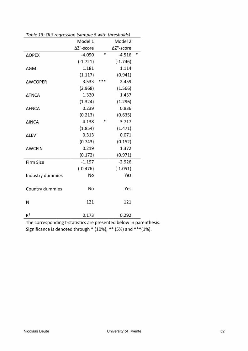
Nicolaas Beute University of Twente 52
Table 13: OLS regression (sample 5 with thresholds) Model 1 Model 2 ΔZ"-score ΔZ"-score ΔOPEX -4.090 * -4.516 * (-1.721) (-1.746)
ΔGM 1.181 1.114
(1.117) (0.941)
ΔWCOPER 3.533 *** 2.459
(2.968) (1.566)
ΔTNCA 1.320 1.437
(1.324) (1.296)
ΔFNCA 0.239 0.836
(0.213) (0.635)
ΔINCA 4.138 * 3.717
(1.854) (1.471)
ΔLEV 0.313 0.071
(0.743) (0.152)
ΔWCFIN 0.219 1.372
(0.172) (0.971)
Firm Size -1.197 -2.926 (-0.476) (-1.051)
Industry dummies No Yes
Country dummies No Yes
N 121 121
R² 0.173 0.292 The corresponding t-statistics are presented below in parenthesis. Significance is denoted through * (10%), ** (5%) and ***(1%).

Nicolaas Beute University of Twente 53
5. Conclusion This final section of the study summarises the findings of the performed regression and relates them to the hypotheses formed in section two. Furthermore, it discusses some limitations this study inhibits, as well as offering some recommendations for future research.
5.1 Main findings and hypothesis discussion The main objective of this thesis was to find out whether the three discussed turnaround strategies, namely operational restructuring, asset restructuring and financial restructuring had an effect on turnaround success. Through the extensive literature review, underlying variables have been connected with the particular turnaround strategies, whilst the literature review also offers a basis for the development of the hypotheses. The main objective is related to the main research question of this study, which is as follows: To what extent do three turnaround strategies, namely operational restructuring, asset restructuring and financial restructuring, improve the Altman’s Z”-score? In order to test for the hypotheses five samples were created with firms in financial distress between 2010 and 2014, of which two served as samples for robustness checks and one that includes a threshold to recognise true restructuring. These samples were subject to some OLS regressions of which the output served as the findings of this study. These findings offer insights in the effect of the variables on Altman’s Z”-score. What mainly culminates from the OLS regressions is that the underlying variables in operational restructuring offer results that are expected. The working capital, both the operational as the financing component, for example, shows strong significant results in relation to the effect on the Z”-score; these effects were expected. Additionally, operational expenses appear to be an important determinant in the quest for an entity to realise turnaround success. Decreases in OPEX seem to have significant positive result on the Z”-score. An interesting result from the OLS regression is the output related to the gross margin variable; it seems that a decrease in this efficiency ratio positively affects the Z”-score and thus exhibits an improvement on Altman’s Z”-score. This is especially interesting, since the result is derived from the robust sample in which all entities experienced actual turnaround success. The robust equity variable also returns significant results where an increase relates to better chances in turnaround success. Interestingly enough, the financing component of the working capital and its robust variable (ΔCL) seem to return contradicting results, where the main variable of interest returns a positive coefficient, while the robust variable shows a negative coefficient. Other predictions do not return conclusive results, as they were insignificant and thus based upon chance rather than actual effect. By linking the results from the OLS regressions to the hypotheses, theoretical implications can be deducted. It has frequently been argued by researchers that reductions in the operational expenses an entity has, is essential to improving a firms’ Z”-score. This could be in multiple ways, an example would be employee lay-

Nicolaas Beute University of Twente 54
offs (Cascio, 2002; Nixon et al., 2002). Employee lay-offs is a good example of a way to cut operational costs, due to its immediate effects (Norman et al. 2013). Empirical evidence is thus highly attainable regarding the positive relation of lay-offs and reducing operational expenses (Bibeault, 1982; Robbins and Pearce, 1993). Consequently, the findings resulting from this study do indeed confirm earlier findings regarding the relation between operational expenses and improving the Z”, as the first hypothesis of this study is supported by the results. This result seems quite logical, as a decrease in costs means a firm should attain more liquid funds, thus increasing the liquidity of the firm and decreasing the chance of bankruptcy. While the main regression did not result in any significant results regarding the gross margin variable, the robust regression did offer some insights in this variable. Although many researchers state that increased efficiency should indeed have a positive effect on turnaround success (Hambrick and Schecter, 1983). This does indeed sound logical, as better efficiency should lead to better financial results. Several researchers have indeed found corresponding results as to Hambrick and Schecter (1983) results (Finkin, 1985; John et al. 1992). The OLS regressions in this study, however, return negative coefficients, which is surprising. The second hypothesis of this study is therefore not supported nor in line with previous research. Many studies have acknowledged the importance of proper working capital optimisation in order to deflect bankruptcy (Robbins and Pearce, 1992; Barker and Duhaime, 1997). This study shows similar findings with regards to working capital optimisation. The operational component of the working capital, for example, shows significant results in relation to improving an entity’s Z”-score. However, it is interesting at the least, to see that in the sample where turnaround success was indeed achieved, the effect is negative, whereas in the first sample the effect of change in the operational component is positive. This means that in model 1 and 2 an increase of the operational component of the working capital is positively related, while in model 4 a decrease in that variable entails a positive effect on the change in Z”-score. This sounds logical, as a decrease in the WCOPER variable usually entails an increase in cash and cash equivalents, as the decrease in WCOPER is usually due to payment of debtors or sales of stocks, which should usually be a good thing for the liquidity of a firm. Therefore, through the fourth model, the third hypothesis of this study is supported, while the first and second model do not offer any support regarding this particular variable. In the regression that includes the threshold, the results are contrasting to the hypothesis, meaning that an increase in the WCOPER is positively related to an increase in Altman’s Z” The fourth hypothesis of this study relates to tangible non-current assets an entity owns. Moulton and Thomas (1993) argue that successful turnaround is most certainly affected by the changes in this balance sheet account. It is even named as an essential turnaround strategy by Sudarsanam and Lai (2001). Results regarding tangible non-current assets, however, remain inconclusive due to the fact that no significant results were returned following the regression. This means that no support is found for the fourth hypothesis. While previous research states that either investments or divestments in both financial- and intangible non-current assets could attain positive impact on improving the Z”-score (Sudarsanam and Lai, 2001; Hoskisson et al. 2004; Campello et al. 2010), results regarding these variables within this study remain largely

Nicolaas Beute University of Twente 55
inconclusive. Only in the main regression in model 3 and in the final regression in model 1 the intangible non-current assets returns a significant result. This is in contrast with the stated hypothesis, researchers have however mentioned that investing in intangible non-current assets could entail a positive effect on the financial health of a firm. The cluster variable in the robust regression is also insignificant and thus does not offer any partial support regarding the fifth and sixth hypotheses of this study. Apart from insignificance, the resulting coefficients have no consistency whatsoever, making any statement regarding these variables unreliable. Ground-setting work by Wruck (1990) set the tone for research relating leverage to turnaround success. Many more studies have since then found positive effects on the financial health of an entity when reducing leverage (Opler, 1993; Eichner, 2010). Capello et al. (2011) even go as far as stating that it is essential, while the main regression did not offer any significant results regarding the relation between leverage and turnaround success. The robust variable partly related to leverage did return significant results. This equity variable returns a positive coefficient meaning that an increase is positively related. This is broadly in line with previous research, as an increasing value of equity reflects in a decrease in leverage. Therefore, the seventh hypothesis of this study is partially supported and could be stated to be somewhat in line with previous studies, such as the Kahl (2002) and Lin et al. (2008) studies. Finally, some researchers find positive relations between stretching payments and a firms’ financial health. Trahms et al. (2013) for example find increasing chances for a firm to realise turnaround when they are successful in stretching their payments. Their findings are deducted from the Chowdhury and Lang (1996) research. The positive coefficient that resulted from the regression analysis is quite logic, as it is quite thinkable that an increase in this financing component is indeed positively related, as payments occur later in this instance than actual obtainment of products that can be further processed or sold. The findings in this study are therefore in line with their studies and thus the final hypothesis of this study is supported.
5.2 Limitations and recommendations While this study does offer support to some of the stated hypotheses and thus gives some valuable insights towards the effect the turnaround strategies entail on the financial health of a firm, this study also has its limitations. First of all, it is important to acknowledge that, while the scope of the study is focused on the initial 15 EU countries, many of the countries in the sample hold their statutory seat in the UK. This is not a problem due to the fact that there are control variables in the form of country dummies. However, it would be recommended that in future research a more broad sample is constructed with an approximate even dispersion of countries in the sample, or focus the study on one country. This would most likely lead to better interpretable results. Additionally, the sample size was quite low throughout this research, which is due to the fact that simply no more firms in financial distress within the scope of the study were identified. It would be highly recommended to increase the sample size in future similar research.

Nicolaas Beute University of Twente 56
As can be seen from tables 11 through 13 the coefficients of determination remain quite low. It is thinkable that a large amount of variance in the dependent variable is dependent on human factors. While managerial turnaround strategies were briefly discussed, they took no part in the actual regression analysis. The results regarding these managerial turnaround strategies could however be very interesting to research, as entities in financial distress do not always have room to think purely rational and a large human factor comes into play. It is therefore highly recommended to include managerial turnaround strategies in either a follow-up study, or a study related to turnaround from financial distress. While this study focuses on listed firms, due to availability of information, it would also be extremely interesting to study something similar as this research but then for smaller, less well-known firms. It is quite likely that in large firms which are the subject throughout this study are financially helped by large investors or banks, for whom it is very important that these firms do not go bankrupt. This could potentially bias the study, when these investors or banks invest additional money in the firm; not in order to gain profits, but in order to make sure the entity does not go bankrupt. Therefore, a similar study with smaller firms as a scope could be very insightful. Finally, the Z”-score model that is incorporated in this study is not without its caveats. The model is quite appropriate for identifying financial distress, both in an international context as well as in a multi-industry context. The model would potentially work even better with newly estimated coefficients for both countries as well as industries. Any research incorporating the Z”-score model will perform sound, it is however advisable that, especially when conducting research relating to just one country or one industry, the coefficients are estimated for that particular country or industry, to ascertain functionality.

Nicolaas Beute University of Twente 57
References Acharya, V. V., Franks, J., & Servaes, H. (2007). Private equity: Boom and bust?. Journal of Applied Corporate Finance, 19(4), 44-53. Agarwal, R., M.B. Sarkar, and R. Echambadi. 2002. The conditioning effect of time on firm survival: An industry life cycle approach. Academy of Management Journal, 45(5), 971–994. Altman, E. I. (1968). Financial ratios, discriminant analysis and the prediction of corporate bankruptcy. The Journal of Finance, 23(4), 589-609. Altman, E. I. (1983). Why businesses fail. Journal of Business Strategy, 3(4), 15-21. Altman, E. I. (2002). Revisiting credit scoring models in a Basel 2 environment. Working paper. Altman, E. I., & Hotchkiss, E. (2010). Corporate financial distress and bankruptcy: Predict and avoid bankruptcy, analyze and invest in distressed debt (Vol. 289). John Wiley & Sons. Altman, E. I., Iwanicz‐Drozdowska, M., Laitinen, E. K., & Suvas, A. (2017). Financial Distress Prediction in an International Context: A Review and Empirical Analysis of Altman's Z‐Score Model. Journal of International Financial Management & Accounting, 28(2), 131-171. Amabile, T. M., & Conti, R. (1999). Changes in the work environment for creativity during downsizing. Academy of Management Journal, 42(6), 630-640. Amburgey, T. L., & Miner, A. S. (1992). Strategic momentum: The effects of repetitive, positional, and contextual momentum on merger activity. Strategic Management Journal, 13(5), 335-348. Andrade, G., & Kaplan, S. N. (1998). How costly is financial (not economic) distress? Evidence from highly leveraged transactions that became distressed. The Journal of Finance, 53(5), 1443-1493. Arogyaswamy, K. (1992). Organizational turnaround: A two-stage strategy-contingency model (Doctoral dissertation, University of Wisconsin-Milwaukee). Arogyaswamy, K., Barker, V. L., & Yasai‐Ardekani, M. (1995). Firm turnarounds: an integrative two‐stage model. Journal of Management Studies, 32(4), 493-525. Asquith, P., Gertner, R., & Scharfstein, D. (1994). Anatomy of financial distress: An examination of junk-bond issuers. The Quarterly Journal of Economics, 109(3), 625-658. Atanassov, J., & Kim, E. (2009). Labor and corporate governance: International evidence from restructuring decisions. The Journal of Finance, 64(1), 341-374. Azoulay, P., & Shane, S. (2001). Entrepreneurs, contracts, and the failure of young firms. Management Science, 47(3), 337-358. Balcaen, S., & Ooghe, H. (2006). 35 years of studies on business failure: an overview of the classic statistical methodologies and their related problems. The British Accounting Review, 38(1), 63-93. Barker III, V. L., & Duhaime, I. M. (1997). Strategic change in the turnaround process: Theory and empirical evidence. Strategic management journal, 18(1), 13-38. Barker, V. L., & Mone, M. A. (1994). Retrenchment: Cause of turnaround or consequence of decline?. Strategic management journal, 15(5), 395-405. Barker III, V. L., Patterson Jr, P. W., & Mueller, G. C. (2001). Organizational causes and strategic consequences of the extent of top management team replacement during turnaround attempts. Journal of Management Studies, 38(2), 235-270.

Nicolaas Beute University of Twente 58
Beaver, W. H. (1966). Financial ratios as predictors of failure. Journal of Accounting Research, 4, 71-111. Begley, J., Ming, J., & Watts, S. (1996). Bankruptcy classification errors in the 1980s: An empirical analysis of Altman's and Ohlson's models. Review of Accounting Studies, 1(4), 267-284. Berger, P. G., & Ofek, E. (1999). Causes and effects of corporate refocusing programs. The Review of Financial Studies, 12(2), 311-345. Bergh, D. D., Johnson, R. A., & Dewitt, R. L. (2008). Restructuring through spin‐off or sell‐off: transforming information asymmetries into financial gain. Strategic Management Journal, 29(2), 133-148. Bernardo, A.E., and E.L. Talley. 1996. Investment policy and exit-exchange offers within financially distressed firms. Journal of Finance, 51(3), 871–888. Bharath, S. T., & Shumway, T. (2008). Forecasting default with the Merton distance to default model. The Review of Financial Studies, 21(3), 1339-1369. Bibeault, D. B. (1982). Management turnaround. New York: McGraw-Hill. Black, F., & Scholes, M. (1973). The pricing of options and corporate liabilities. Journal of political economy, 81(3), 637-654. Blazy, R., Martel, J., & Nigam, N. (2014). The choice between informal and formal restructuring: The case of French banks facing distressed SMEs. Journal of Banking & Finance, 44, 248-263. Boeker, W. (1997). Strategic change: The influence of managerial characteristics and organizational growth. Academy of management journal, 40(1), 152-170. Bowman, E. H., & Hurry, D. (1993). Strategy through the option lens: An integrated view of resource investments and the incremental-choice process. Academy of management review, 18(4), 760-782. Bowman, E. H., & Singh, H. (1993). Corporate restructuring: Reconfiguring the firm. Strategic Management Journal, 14(S1), 5-14. Bowman, E. H., Singh, H., Useem, M., & Bhadury, R. (1999). When does restructuring improve economic performance?. California Management Review, 41(2), 33-54. Boyne, G. A. (2004). A ‘3Rs’ strategy for public service turnaround: retrenchment, repositioning and reorganization. Public Money and Management, 24(2), 97-103. Boyne, G.A., and K.J. Meier. 2009. Environmental change, human resources and organizational turnaround. Journal of Management Studies, 46(5), 835–863. Brauer, M. (2006). What have we acquired and what should we acquire in divestiture research? A review and research agenda. Journal of Management, 32(6), 751-785. Brockner, J., Spreitzer, G., Mishra, A., Hochwarter, W., Pepper, L., & Weinberg, J. (2004). Perceived control as an antidote to the negative effects of layoffs on survivors' organizational commitment and job performance. Administrative Science Quarterly, 49(1), 76-100. Brown, S. J., Goetzmann, W., Ibbotson, R. G., & Ross, S. A. (1992). Survivorship bias in performance studies. The Review of Financial Studies, 5(4), 553-580. Brown, D. T., James, C. M., & Mooradian, R. M. (1993). The information content of distressed restructurings involving public and private debt claims. Journal of Financial Economics, 33(1), 93-118. Bruton, G.D., D. Ahlstrom, and J.C.C. Wan. 2003. Turnaround in East Asian firms: Evidence from ethnic overseas Chinese communities. Strategic Management Journal, 24(6), 519–540.
Nicolaas Beute University of Twente 59
Bruton, G. D., Oviatt, B. M., & White, M. A. (1994). Performance of acquisitions of distressed firms. Academy of Management Journal, 37(4), 972-989. Budros, A. (1999). A conceptual framework for analyzing why organizations downsize. Organization Science, 10(1), 69-82. Campello, M., E. Giambona, J.R. Graham, and C.R. Harvey. 2011. Liquidity management and corporate investment during a financial crisis. Review of Financial Studies, 24(6), 1944–1979. Campello, M., Graham, J. R., & Harvey, C. R. (2010). The real effects of financial constraints: Evidence from a financial crisis. Journal of financial Economics, 97(3), 470-487. Cascio, W. F. (2002). Responsible restructuring: Creative and profitable alternatives to layoffs. Berrett-Koehler Publishers. Castrogiovanni, G. J., & Bruton, G. D. (2000). Business turnaround processes following acquisitions: Reconsidering the role of retrenchment. Journal of Business Research, 48(1), 25-34. Chadwick, C., Hunter, L. W., & Walston, S. L. (2004). Effects of downsizing practices on the performance of hospitals. Strategic Management Journal, 25(5), 405-427. Chava, S., and R.A. Jarrow. 2004. Bankruptcy prediction with industry effects. Review of Finance, 8, 537–569. Chen, G., & Hambrick, D. C. (2012). CEO replacement in turnaround situations: Executive (mis) fit and its performance implications. Organization Science, 23(1), 225-243. Chen, Y., Weston, J. F., & Altman, E. I. (1995). Financial distress and restructuring models. Financial Management, 24(2), 57-75. Chowdhury, S. D. (2002). Turnarounds: A stage theory perspective. Canadian Journal of Administrative Sciences/Revue Canadienne des Sciences de l'Administration, 19(3), 249-266. Chowdhury, S. D., & Lang, J. R. (1996). Turnaround in small firms: An assessment of efficiency strategies. Journal of Business Research, 36(2), 169-178. Clapham, S. E., Schwenk, C. R., & Caldwell, C. (2005). CEO perceptions and corporate turnaround. Journal of Change Management, 5(4), 407-428. Cortes, E. A., Martinez, M. G., & Rubio, N. G. (2007). Multiclass corporate failure prediction by Adaboost. M1. International Advances in Economic Research, 13(3), 301-312. Cottrell, T., & Nault, B. R. (2004). Product variety and firm survival in the microcomputer software industry. Strategic Management Journal, 25(10), 1005-1025. Coucke, K., E. Pennings, and L. Sleuwaegen. 2007. Employee layoff under different modes of restructuring: exit, downsizing or relocation. Industrial and Corporate Change, 16:(2), 161–182. Cusatis, P. J., Miles, J. A., & Woolridge, J. R. (1993). Restructuring through spinoffs: The stock market evidence. Journal of Financial Economics, 33(3), 293-311. Cybinski, P. J. (2003). Doomed firms: an econometric analysis of the path to failure. Ashgate Publishing, Ltd.. Daily, C. M., & Dalton, D. R. (1995). CEO and director turnover in failing firms: An illusion of change?. Strategic Management Journal, 16(5), 393-400. Damodaran, A. (2002). Investment valuation, 2. Aufl., New York, 817.

Nicolaas Beute University of Twente 60
DeAngelo, H., & DeAngelo, L. (1990). Dividend policy and financial distress: An empirical investigation of troubled NYSE firms. The Journal of Finance, 45(5), 1415-1431. Denis, D. J., & Denis, D. K. (1995). Causes of financial distress following leveraged recapitalizations. Journal of Financial Economics, 37(2), 129-157. Denis, D. J., & Kruse, T. A. (2000). Managerial discipline and corporate restructuring following performance declines. Journal of Financial Economics, 55(3), 391-424. Denis, D. K., & Rodgers, K. J. (2007). Duration, outcome, and post-reorganization performance. Journal of Financial and Quantitative Analysis, 42(1), 101-118. Denis, D. K., & Shome, D. K. (2005). An empirical investigation of corporate asset downsizing. Journal of Corporate Finance, 11(3), 427-448. DeWitt, R. L. (1993). The structural consequences of downsizing. Organization Science, 4(1), 30-40. DeWitt, R. L. (1998). Firm, industry, and strategy influences on choice of downsizing approach. Strategic Management Journal, 59-79. DeWitt, R. L., Harrigan, K. R., & Newman, W. H. (1998). Downsizing strategically. Turnaround research: Past accomplishments and future challenges, 21-36. Dixit, A. K., & Pindyck, R. S. (1994). Investment under uncertainty. Princeton university press. Domadenik, P., Prašnikar, J., & Svejnar, J. (2008). Restructuring of firms in transition: ownership, institutions and openness to trade. Journal of International Business Studies, 39(4), 725-746. Eichner, T. (2010). Restructuring and turnaround of distressed manufacturing firms: An international empirical study. Peter Lang. Elliott, D., & Smith, D. (2006). Cultural readjustment after crisis: Regulation and learning from crisis within the UK soccer industry. Journal of Management Studies, 43(2), 289-317. Elloumi, F., & Gueyie, J. P. (2001). Financial distress and corporate governance: an empirical analysis. Corporate Governance: The international journal of business in society, 1(1), 15-23. Finkin, E. F. (1985). Company turnaround. Journal of Business Strategy, 5(4), 14-24. Flanagan, D. J., & O’shaughnessy, K. C. (2005). The effect of layoffs on firm reputation. Journal of management, 31(3), 445-463. Folger, R., & Skarlicki, D. P. (1998). When tough times make tough bosses: Managerial distancing as a function of layoff blame. Academy of Management Journal, 41(1), 79-87. Foster, G. (1986). Financial Statement Analysis, 2/e. Pearson Education India. Freeman, S. J., & Cameron, K. S. (1993). Organizational downsizing: A convergence and reorientation framework. Organization science, 4(1), 10-29. George, T. J., & Hwang, C. Y. (2010). A resolution of the distress risk and leverage puzzles in the cross section of stock returns. Journal of Financial Economics, 96(1), 56-79. Gertler, M., & Hubbard, R. G. (1991). Corporate financial policy, taxation, and macroeconomic risk (No. w3902). National Bureau of Economic Research. Gibbs, P. A. (1993). Determinants of corporate restructuring: The relative importance of corporate governance, takeover threat, and free cash flow. Strategic Management Journal, 14(S1), 51-68. Gilbert, L. R., Menon, K., & Schwartz, K. B. (1990). Predicting bankruptcy for firms in financial distress. Journal of Business Finance & Accounting, 17(1), 161-171.

Nicolaas Beute University of Twente 61
Gilson, S. C. (1989). Management turnover and financial distress. Journal of financial Economics, 25(2), 241-262. Gilson, S. C. (1990). Bankruptcy, boards, banks, and blockholders: Evidence on changes in corporate ownership and control when firms default. Journal of Financial Economics, 27(2), 355-387. Gilson, S. C., John, K., & Lang, L. H. (1990). Troubled debt restructurings: An empirical study of private reorganization of firms in default. Journal of financial economics, 27(2), 315-353. Gilson, S. C., & Vetsuypens, M. R. (1993). CEO compensation in financially distressed firms: An empirical analysis. The Journal of Finance, 48(2), 425-458. Giroud, X., H.M. Mueller, A. Stomper, and A. Westerkamp. 2012. Snow and leverage. Review of Financial Studies, 25(3), 680–710. Greening, D. W., & Johnson, R. A. (1996). Do managers and strategies matter? A study in crisis. Journal of Management Studies, 33(1), 25-51. Greve, H.R. 2011. Positional rigidity: Low performance and resource acquisition in large and small firms. Strategic Management Journal, 32(1), 103–114. Grice, J. S. & Ingram, R. W. (2001). Tests of the generalizability of Altman’s bankruptcy prediction model. Journal of Business Research, 54, 53– 61. Grinyer, P. H., Mayes, D. G., & McKiernan, P. (1988). Sharpbenders: The secrets of unleashing corporate potential. Basil Blackwell. Guthrie, J. P., & Datta, D. K. (2008). Dumb and dumber: The impact of downsizing on firm performance as moderated by industry conditions. Organization Science, 19(1), 108-123. Hair, J. F., Black, W. C., Babin, B. J., Anderson, R. E., & Tatham, R. L. (1998). Multivariate data analysis (Vol. 5, No. 3, pp. 207-219). Upper Saddle River, NJ: Prentice hall. Hakkala, K. (2006). Corporate restructuring and labor productivity growth. Industrial and Corporate Change, 15(4), 683-714. Hambrick, D. C., & Schecter, S. M. (1983). Turnaround strategies for mature industrial-product business units. Academy of management journal, 26(2), 231-248. Hannan, M. T., Baron, J. N., Hsu, G., & Koçak, Ö. (2006). Organizational identities and the hazard of change. Industrial and Corporate Change, 15(5), 755-784. Haugen, R. A., & Senbet, L. W. (1978). The insignificance of bankruptcy costs to the theory of optimal capital structure. The Journal of Finance, 33(2), 383-393. Haugen, R. A., & Senbet, L. W. (1988). Bankruptcy and agency costs: Their significance to the theory of optimal capital structure. Journal of Financial and Quantitative Analysis, 23(1), 27-38. Hendel, I. (1996). Competition under financial distress. The Journal of Industrial Economics, 309-324. Hofer, C. W. (1980). Turnaround strategies. Journal of Business Strategy, 1(1), 19-31. Hoskisson, R. E., Cannella, A. A., Tihanyi, L., & Faraci, R. (2004). Asset restructuring and business group affiliation in French civil law countries. Strategic Management Journal, 25(6), 525-539. Hotchkiss, E. S. (1995). Postbankruptcy performance and management turnover. The Journal of Finance, 50(1), 3-21. Hurry, D. (1993). Restructuring in the global economy: The consequences of strategic linkages between Japanese and US firms. Strategic Management Journal, 14(S1), 69-82.

Nicolaas Beute University of Twente 62
Indro, D.C., R.T. Leach, and W.Y. Lee. 1999. Sources of gains to shareholders from bankruptcy resolution. Journal of Banking & Finance, 23(1), 21–47. James, C. 1996. Bank debt restructurings and the composition of exchange offers in financial distress. Journal of Finance, 51(2), 711–727. Jensen, M. C. (1989). Eclipse of the public corporation. Jensen, M. C. (1991). Corporate control and the politics of finance. John, K. (1993). Managing financial distress and valuing distressed securities: A survey and a research agenda. Financial Management, 60-78. John, K., Lang, L. H., & Netter, J. (1992). The voluntary restructuring of large firms in response to performance decline. The Journal of Finance, 47(3), 891-917. Jones, F. L. (1987). Current techniques in bankruptcy prediction. Journal of accounting Literature, 6(1), 131-164. Kang, J.-K., and A. Shivdasani. 1997. Corporate restructuring during performance declines in Japan. Journal of Financial Economics, 46(1), 29–65. Kato, M. 2010. The role of investment efficiency in the industry life cycle. Industrial and Corporate Change, 19(1), 273–294. Kaplan, S. N., & Stein, J. C. (1993). The evolution of buyout pricing and financial structure in the 1980s. The Quarterly Journal of Economics, 108(2), 313-357. Kahl, M. (2002). Economic distress, financial distress, and dynamic liquidation. The Journal of Finance, 57(1), 135-168. Kalay, A., Singhal, R., & Tashjian, E. (2007). Is chapter 11 costly?. Journal of Financial Economics, 84(3), 772-796. Koh, S., Durand, R. B., Dai, L., & Chang, M. (2015). Financial distress: Lifecycle and corporate restructuring. Journal of Corporate Finance, 33, 19-33. Lasfer, M. A., Sudarsanam, P. S., & Taffler, R. J. (1996). Financial distress, asset sales, and lender monitoring. Financial Management, 57-66. Li, Y. (2013). A nonlinear wealth transfer from shareholders to creditors around Chapter 11 filing. Journal of Financial Economics, 107(1), 183-198. Li, S., & Tallman, S. (2011). MNC strategies, exogenous shocks, and performance outcomes. Strategic Management Journal, 32(10), 1119-1127. Lin, B., Lee, Z. H., & Gibbs, L. G. (2008). Operational restructuring: reviving an ailing business. Management Decision, 46(4), 539-552. Ling, Y., Zhao, H., & Baron, R. A. (2007). Influence of founder—CEOs' personal values on firm performance: Moderating effects of firm age and size. Journal of Management, 33(5), 673-696. Love, E. G., & Kraatz, M. (2009). Character, conformity, or the bottom line? How and why downsizing affected corporate reputation. Academy of Management Journal, 52(2), 314-335. Love, E. G., & Nohria, N. (2005). Reducing slack: The performance consequences of downsizing by large industrial firms, 1977–93. Strategic Management Journal, 26(12), 1087-1108. Ludwig, D. C. (1993). Adapting to a declining environment: Lessons from a religious order. Organization Science, 4(1), 41-56.

Nicolaas Beute University of Twente 63
Mackey, A. (2008). The effect of CEOs on firm performance. Strategic management journal, 29(12), 1357-1367. Markides, C. C. (1992). Consequences of corporate refocusing: Ex ante evidence. Academy of Management Journal, 35(2), 398-412. Markides, C. C. (1995). Diversification, restructuring and economic performance. Strategic Management Journal, 16(2), 101-118. Martin, C. L., Parsons, C. K., & Bennett, N. (1995). The influence of employee involvement program membership during downsizing: Attitudes toward the employer and the union. Journal of Management, 21(5), 879-890. Mella-Barral, P. 1999. The dynamics of default and debt reorganization. Review of Financial Studies, 12(1), 535–578. Miles, G., Snow, C. C., & Sharfman, M. P. (1993). Industry variety and performance. Strategic Management Journal, 14(3), 163-177. Mitchell, M.L., and J.H. Mulherin. 1996. The impact of industry shocks on takeover and restructuring activity. Journal of Financial Economics, 41(1), 193–229. Molina, C. A. (2005). Are firms underleveraged? An examination of the effect of leverage on default probabilities. The Journal of Finance, 60(3), 1427-1459. Morrow Jr, J. L., Johnson, R. A., & Busenitz, L. W. (2004). The effects of cost and asset retrenchment on firm performance: The overlooked role of a firm’s competitive environment. Journal of Management, 30(2), 189-208. Mossman, C. E., Bell, G. G., Swartz, L. M., & Turtle, H. (1998). An empirical comparison of bankruptcy models. Financial Review, 33(2), 35-54. Morse, D., & Shaw, W. (1988). Investing in bankrupt firms. The Journal of Finance, 43(5), 1193-1206. Moulton, W. N., & Thomas, H. (1993). Bankruptcy as a deliberate strategy: Theoretical considerations and empirical evidence. Strategic Management Journal, 14(2), 125-135. Moulton, W.N., H. Thomas, and M. Pruett. 1996. Business failure pathways: Environmental stress and organizational response. Journal of Management, 22(1), 571–595. Ndofor, H.A., J. VanEvenhoven, and V.L. Barker III. 2013. Software firm turnarounds in the 1990s: An analysis of reversing decline in a growing, dynamic industry. Strategic Management Journal, 34(1), 1123–1133. Nixon, R. D., Hitt, M. A., Lee, H. U., & Jeong, E. (2004). Market reactions to announcements of corporate downsizing actions and implementation strategies. Strategic Management Journal, 25(11), 1121-1129. Noe, T.H., and J. Wang. 2000. Strategic debt restructuring. Review of Financial Studies, 13(1), 985–1015. Norman, P. M., Butler, F. C., & Ranft, A. L. (2013). Resources matter: Examining the effects of resources on the state of firms following downsizing. Journal of Management, 39(7), 2009-2038. Ofek, E. (1993). Capital structure and firm response to poor performance: An empirical analysis. Journal of financial economics, 34(1), 3-30.

Nicolaas Beute University of Twente 64
O'Neill, H. M. (1986). Turnaround and recovery: What strategy do you need?. Long Range Planning, 19(1), 80-88. Opler, T. C. (1993). Controlling financial distress costs in leveraged buyouts with financial innovations. Financial Management, 79-90. Opler, T. C., & Titman, S. (1994). Financial distress and corporate performance. The Journal of Finance, 49(3), 1015-1040. Outecheva, N. (2007). Corporate financial distress: An empirical analysis of distress risk. Pandit, N. R. (2000). Some recommendations for improved research on corporate turnaround. M@n@gement, 3(2), 31. Ramanujam, V. (1984). Environmental context, organizational context, strategy, and corporate turnaround: an empirical investigation (Doctoral dissertation, University of Pittsburgh). Reilly, A. H., Brett, J. M., & Stroh, L. K. (1993). The impact of corporate turbulence on: Managers' attitudes. Strategic Management Journal, 14(S1), 167-179. Robbins, D. K., & Pearce, J. A. (1992). Turnaround: Retrenchment and recovery. Strategic management journal, 13(4), 287-309. Robbins, D. K., & Pearce, J. A. (1993). Entrepreneurial retrenchment among small manufacturing firms. Journal of business venturing, 8(4), 301-318. Roe, M. J. (1983). Bankruptcy and debt: A new model for corporate reorganization. Columbia Law Review, 83(3), 527-602. Rosenblatt, Z., and B. Mannheim. 1996. Organizational response to decline in the israeli electronics industry. Organization Studies, 17(1), 953–984. Routledge, J., & Gadenne, D. (2000). Financial distress, reorganization and corporate performance. Accounting & Finance, 40(3), 233-259. Pearce, J. A., & Robbins, K. (1993). Toward improved theory and research on business turnaround. Journal of Management, 19(3), 613-636. Schendel, D. E., & Patton, G. R. (1976). Corporate stagnation and turnaround. Journal of Economics and Business, 28(3), 236-241. Schendel, D., Patton, G. R., & Riggs, J. (1976). Corporate turnaround strategies: A study of profit decline and recovery. Journal of General Management, 3(3), 3-11. Schmitt, A., & Raisch, S. (2013). Corporate turnarounds: The duality of retrenchment and recovery. Journal of Management Studies, 50(7), 1216-1244. Schweizer, L., & Nienhaus, A. (2017). Corporate distress and turnaround: integrating the literature and directing future research. Business Research, 1-45. Scott, J. (1981). The probability of bankruptcy: a comparison of empirical predictions and theoretical models. Journal of Banking & Finance, 5(3), 317-344. Sheppard, J. P. (1994). Strategy and bankruptcy: An exploration into organizational death. Journal of Management, 20(4), 795-833. Slatter, S. S. P. (1984). Corporate recovery: A guide to turnaround management. Penguin books. Stoeberl, P.A., G.E. Parker, and S.-J. Joo. 1998. Relationship between organizational change and failure in the wine industry: An event history analysis. Journal of Management Studies, 35(4), 537–555.

Nicolaas Beute University of Twente 65
Stopford, J. M., & Baden‐Fuller, C. (1990). Corporate rejuvenation. Journal of Management Studies, 27(4), 399-415. Sudarsanam, S., & Lai, J. (2001). Corporate financial distress and turnaround strategies: An empirical analysis. British Journal of Management, 12(3), 183-199. Taplin, I. M., & Winterton, J. (1995). New clothes from old techniques: Restructuring and flexibility in the US and UK clothing industries. Industrial and Corporate Change, 4(3), 615-638. Theodossiou, P., Kahya, E., Saidi, R., & Philippatos, G. (1996). Financial distress and corporate acquisitions: Further empirical evidence. Journal of Business Finance & Accounting, 23(5‐6), 699-719. Thietart, R. A. (1988). Success strategies for businesses that perform poorly. Interfaces, 18(3), 32-45. Thomas, A. S., & Ramaswamy, K. (1993). Environmental change and management staffing: a comment. Journal of Management, 19(4), 877-887. Trahms, C. A., Ndofor, H. A., & Sirmon, D. G. (2013). Organizational decline and turnaround: A review and agenda for future research. Journal of Management, 39(5), 1277-1307. Trigeorgis, L., & Reuer, J. J. (2017). Real options theory in strategic management. Strategic Management Journal, 38(1), 42-63. Tushman, M. L., Virany, B., & Romanelli, E. (1985). Executive succession, strategic reorientations, and organization evolution: The minicomputer industry as a case in point. Technology in Society, 7(2-3), 297-313. Weitzel, W., & Jonsson, E. (1989). Decline in organizations: A literature integration and extension. Administrative Science Quarterly, 91-109. Weiss, L. A. (1990). Bankruptcy resolution: Direct costs and violation of priority of claims. Journal of Financial Economics, 27(2), 285-314. Whitaker, R. B. (1999). The early stages of financial distress. Journal of Economics and Finance, 23(2), 123-132. White, M. J. (1989). The corporate bankruptcy decision. The Journal of Economic Perspectives, 3(2), 129-151. Winn, J. (1997). Asset productivity turnaround: The growth/efficiency challenge. Journal of Management Studies, 34(4), 585-600. Wruck, K. H. (1990). Financial distress, reorganization, and organizational efficiency. Journal of financial economics, 27(2), 419-444. Yawson, A. (2005). Performance shocks, turnaround strategies, and corporate recoveries: The Australian experience. No. NSW, 2052. Zavgren, C. (1983). The prediction of corporate failure: the state of the art. Journal of Accounting Literature, 2(1), 1-38. Zingales, L. (1998). Survival of the Fittest or the Fattest? Exit and Financing in the Trucking Industry. The Journal of Finance, 53(3), 905-938.

Nicolaas Beute University of Twente 66
Appendix A Correlations underlying variables Z"-score model for sample 1 (2010) 1 2 3 4
A (1) 1
B (2) 0.044 1
C (3) 0.176 * -0.077 1
D (4) 0.141 0.135 0.146 1
**. Correlation is significant at the 0.01 level (2-tailed). *. Correlation is significant at the 0.05 level (2-tailed).
Correlations underlying variables Z"-score model for sample 1 (2014) 1 2 3 4
A (1) 1
B (2) 0.324 ** 1
C (3) 0.478 ** 0.564 ** 1
D (4) 0.145 0.395 ** 0.176 * 1
**. Correlation is significant at the 0.01 level (2-tailed). *. Correlation is significant at the 0.05 level (2-tailed).
Correlations underlying variables Z"-score model for sample 2 (2010) 1 2 3 4
A (1) 1
B (2) -0.327 * 1
C (3) -0.188 -0.175 1
D (4) -0.067 0.469 ** -0.104 1
**. Correlation is significant at the 0.01 level (2-tailed). *. Correlation is significant at the 0.05 level (2-tailed).
Correlations underlying variables Z"-score model for sample 2 (2014) 1 2 3 4
A (1) 1
B (2) -0.275 1
C (3) -0.181 0.126 1
D (4) -0.116 0.366 * 0.007 1
**. Correlation is significant at the 0.01 level (2-tailed). *. Correlation is significant at the 0.05 level (2-tailed).

Nicolaas Beute University of Twente 67
Correlations underlying variables Z"-score model for sample 3 (2010) 1 2 3 4
A (1) 1
B (2) -0.012 1
C (3) 0.108 -0.004 1
D (4) -0.033 -0.039 -0.013 1
**. Correlation is significant at the 0.01 level (2-tailed). *. Correlation is significant at the 0.05 level (2-tailed).
Correlations underlying variables Z"-score model for sample 3 (2014) 1 2 3 4
A (1) 1
B (2) 0.294 ** 1
C (3) 0.462 ** 0.560 ** 1
D (4) 0.013 0.105 0.038 1
**. Correlation is significant at the 0.01 level (2-tailed). *. Correlation is significant at the 0.05 level (2-tailed).
Correlations underlying variables Z"-score model for sample 4 (2010) 1 2 3 4
A (1) 1
B (2) -0.233 1
C (3) 0.088 -0.032 1
D (4) -0.154 -0.127 -0.114 1
**. Correlation is significant at the 0.01 level (2-tailed). *. Correlation is significant at the 0.05 level (2-tailed).
Correlations underlying variables Z"-score model for sample 4 (2014) 1 2 3 4
A (1) 1
B (2) -0.291 * 1
C (3) -0.130 0.077 1
D (4) -0.105 0.327 * 0.005 1
**. Correlation is significant at the 0.01 level (2-tailed). *. Correlation is significant at the 0.05 level (2-tailed).

Nicolaas Beute University of Twente 68
Correlations underlying variables Z"-score model for sample 5 (2010) 1 2 3 4
A (1) 1
B (2) 0.088 1
C (3) 0.212 * -0.137 1
D (4) 0.172 0.051 0.122 1
**. Correlation is significant at the 0.01 level (2-tailed). *. Correlation is significant at the 0.05 level (2-tailed).
Correlations underlying variables Z"-score model for sample 5 (2014) 1 2 3 4
A (1) 1
B (2) 0.345 ** 1
C (3) 0.494 ** 0.571 ** 1
D (4) 0.162 0.385 ** 0.163 1
**. Correlation is significant at the 0.01 level (2-tailed). *. Correlation is significant at the 0.05 level (2-tailed).

Nicolaas Beute University of Twente 69
Appendix B T-test results Sample 1 Mean Mean diff. T-statistic Significance Z"-score 2010 -3.369 0.501 0.918 0.360 Z"-score 2014 -4.372 -0.503 -0.340 0.735 Sample 2 Z"-score 2010 -1.532 -4.742 -8.862 <0.001 Z"-score 2014 7.955 4.745 2.008 0.050 Sample 3 Z"-score 2010 -3.443 -0.583 -1.290 0.198 Z"-score 2014 -2.280 0.580 0.446 0.656 Sample 4 Z"-score 2010 -2.329 -4.959 -8.297 <0.001 Z"-score 2014 7.581 4.951 2.653 0.010 Sample 5
Z"-score 2010 -3.197 0.703 1.184 0.239 Z"-score 2014 -4.611 -0.711 -0.421 0.675

Nicolaas Beute University of Twente 70
Appendix C VIF main regression Variable VIF model 1 VIF model 2 VIF model 3 VIF model 4 ΔOPEX 1.235 1.345 1.733 2.414 ΔGM 1.055 1.251 1.313 2.691 ΔWCOPER 1.179 1.509 1.613 2.363 ΔTNCA 1.205 1.368 1.560 2.525 ΔFNCA 1.076 1.424 1.082 13.595 ΔINCA 1.087 1.287 1.869 48.893 ΔLEV 1.068 1.165 1.713 2.782 ΔWCFIN 1.250 1.343 1.563 2.031
VIF robust regression Variable VIF model 1 VIF model 2 VIF model 3 VIF model 4 ΔOPEX 1.127 1.304 1.125 1.455 ΔGM 1.045 1.172 1.084 1.486 ΔNCA 1.098 1.209 1.730 2.420 ΔCA 1.374 1.631 1.590 2.410 ΔEQ 1.048 1.339 1.104 1.468 ΔNCL 1.026 1.123 1.318 1.621 ΔCL 1.412 1.531 1.538 1.913
VIF main regression sample 5 Variable VIF model 1 VIF model 2 ΔOPEX 1.347 1.544 ΔGM 1.074 1.306 ΔWCOPER 1.217 2.050 ΔTNCA 1.242 1.485 ΔFNCA 1.118 1.494 ΔINCA 1.076 1.335 ΔLEV 1.119 1.336 ΔWCFIN 1.401 1.684