1 23

MeccanicaAn International Journal of Theoreticaland Applied Mechanics AIMETA ISSN 0025-6455 MeccanicaDOI 10.1007/s11012-013-9821-9

TRT: thermo racing tyre a physical modelto predict the tyre temperature distribution

Flavio Farroni, Daniele Giordano,Michele Russo & Francesco Timpone

1 23

Your article is protected by copyright and all

rights are held exclusively by Springer Science

+Business Media Dordrecht. This e-offprint

is for personal use only and shall not be self-

archived in electronic repositories. If you wish

to self-archive your article, please use the

accepted manuscript version for posting on

your own website. You may further deposit

the accepted manuscript version in any

repository, provided it is only made publicly

available 12 months after official publication

or later and provided acknowledgement is

given to the original source of publication

and a link is inserted to the published article

on Springer's website. The link must be

accompanied by the following text: "The final

publication is available at link.springer.com”.

MeccanicaDOI 10.1007/s11012-013-9821-9

TRT: thermo racing tyre a physical model to predict the tyretemperature distribution

Flavio Farroni · Daniele Giordano ·Michele Russo · Francesco Timpone

Received: 7 February 2013 / Accepted: 9 October 2013© Springer Science+Business Media Dordrecht 2013

Abstract In the paper a new physical tyre thermalmodel is presented. The model, called Thermo RacingTyre (TRT) was developed in collaboration betweenthe Department of Industrial Engineering of the Uni-versity of Naples Federico II and a top ranking motor-sport team.

The model is three-dimensional and takes into ac-count all the heat flows and the generative terms occur-ring in a tyre. The cooling to the track and to externalair and the heat flows inside the system are modelled.Regarding the generative terms, in addition to the fric-tion energy developed in the contact patch, the strainenergy loss is evaluated. The model inputs come outfrom telemetry data, while its thermodynamic param-eters come either from literature or from dedicated ex-perimental tests.

The model gives in output the temperature circum-ferential distribution in the different tyre layers (sur-face, bulk, inner liner), as well as all the heat flows.These information have been used also in interactionmodels in order to estimate local grip value.

Keywords Tyre temperature · Real time thermalmodel · Strain energy loss · Friction power · Tyre heatflows

F. Farroni (B) · D. Giordano · M. Russo · F. TimponeDipartimento di Ingegneria Industriale, Università degliStudi di Napoli Federico II, Via Claudio 21, 80125 Naples,Italye-mail: flavio.farroni@unina.it

SymbolsT temperature [K]Tair air temperature [K]T∞ air temperature at an infinite

distance [K]Tr road surface temperature [K]t time [s]α = k

ρ·cvthermal diffusivity; αt tyre, αr

road [m2

s ]q̇G heat generated per unit of

volume and time [ Js·m3 ]

ρ density [ kgm3 ]

cv specific heat at constant volume[ J

kg·K ]cp specific heat at constant pressure

[ Jkg·K ]

kt , kr tyre and road thermalconductivity [ W

m·K ]Hc heat transfer coefficient [ W

m2·K ]h external air natural convection

coefficient [ Wm2·K ]

hf orc external air forced convectioncoefficient [ W

m2·K ]hint internal air natural convection

coefficient [ Wm2·K ]

x, y, z coordinatesFx , Fy longitudinal and lateral tyre-road

interaction forces [N]Fz normal load acting on the single

wheel [N]

Author's personal copy

Meccanica

vx , vy longitudinal and lateral slipvelocity [m

s ]A tyre-road contact area [m2]Atot total area of external surface

[m2]kair air thermal conductivity [ W

m·K ]V air velocity [m

s ]ν air kinematic viscosity [m2

s ]μ air dynamic viscosity [ kg

s·m ]L = 1

1De

+ 1W

characteristic length of the heatexchange surface [m]

W tread width [m]La contact patch length [m]De tyre external diameter [m]pi tyre inflating pressure [bar]g gravity acceleration [ m

s2 ]β coefficient of thermal air

expansion [1/T]

Gr = g·β·L3·(T −T∞)

ν2 Grashof number [–]

Pr = μ·cp

KairPrandtl number [–]

1 Introduction

In automobile racing world, where reaching the limitis the standard and the time advantage in an extremelyshort time period is a determining factor for the out-come, predicting in advance the behaviour of the ve-hicle system in different conditions is a pressing need.Moreover, new regulations limits to the track test ses-sions made the “virtual experimentation” fundamentalin the development of new solutions.

Through the wheels, the vehicle exchanges forceswith the track [1, 2] which depend on the structureof the tyres [3] and on their adherence, strongly in-fluenced by temperature [4, 5].

Theoretical and experimental studies, aimed topredict temperature distribution in steady state purerolling conditions, useful to evaluate its effects on en-ergetic dissipation phenomena, are quite diffused inliterature [6, 7]. Less widespread are analyses con-ducted in transient conditions involving tyre tempera-ture effects on vehicle dynamics. A thermal tyre modelfor racing vehicles, in addition to predict the temper-ature with a high degree of accuracy, must be able tosimulate the high-frequency dynamics characterizingthis kind of systems. Furthermore, the model has to beable to estimate the temperature distribution even of

the deepest tyre layers, usually not easily measurableon-line; it must predict the effects that fast temperaturevariations induce in visco-elastic materials behaviour,and it must take into account the dissipative phenom-ena related to the tyre deformations.

With the aim to understand the above phenomenaand to evaluate the influence of the physical variableson the thermal behaviour of the tyre, an analytical-physical model has been developed and called ThermoRacing Tyre (TRT).

At present time there are not physical models avail-able in literature able to describe the thermal be-haviour of the tyres in a sufficiently detailed way tomeet the needs of a racing company. The TRT modelmay be considered as an evolution of the Thermo-Tyre model [8] that allows to determine in a sim-plified way the surface temperature of such system,neglecting the heat produced by cyclic deformationsand not considering the structure of the different lay-ers.

The above mentioned limitations of ThermoTyrehave been removed in the implementation of TRT, thatresults in an accurate physical model useful for thethermal analysis of the tyre and characterized by pre-dictive attitudes since it is based on physical param-eters known from literature or measurable by specifictests [9].

2 Tyre modeling and base hypotheses

The tyre is considered as unrolled in the circumferen-tial direction (and then parallelepiped-shaped), lack-ing of sidewalls and grooves (so the tyre is modelledas slick), discretized by means of a grid, whose nodesrepresent the points in which the temperature will bedetermined instant by instant (Fig. 1).

The parallelepiped is constituted by three layers inthe radial direction z, which will be hereinafter indi-cated as surface (outer surface of the tyre), bulk (inter-mediate layer), and inner liner (inner surface).

The number of nodes of the grid is given by theproduct (numx · numy · numz) where numx representsthe number of nodes along the x direction, numy thenumber of nodes along the y direction and numz is thenumber of nodes along the z direction. Nodes enumer-ation has been carried out starting from the first layerin contact with the road, proceeding transversely. Eachlayer is subdivided in 15 elements in the longitudinal

Author's personal copy

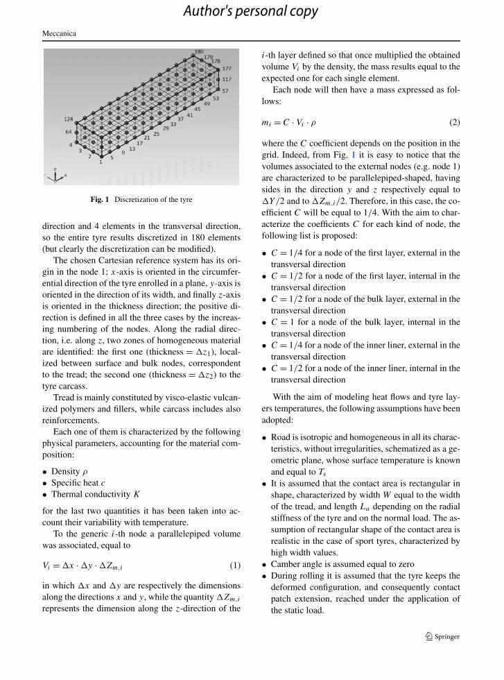
Meccanica

Fig. 1 Discretization of the tyre

direction and 4 elements in the transversal direction,so the entire tyre results discretized in 180 elements(but clearly the discretization can be modified).

The chosen Cartesian reference system has its ori-gin in the node 1; x-axis is oriented in the circumfer-ential direction of the tyre enrolled in a plane, y-axis isoriented in the direction of its width, and finally z-axisis oriented in the thickness direction; the positive di-rection is defined in all the three cases by the increas-ing numbering of the nodes. Along the radial direc-tion, i.e. along z, two zones of homogeneous materialare identified: the first one (thickness = �z1), local-ized between surface and bulk nodes, correspondentto the tread; the second one (thickness = �z2) to thetyre carcass.

Tread is mainly constituted by visco-elastic vulcan-ized polymers and fillers, while carcass includes alsoreinforcements.

Each one of them is characterized by the followingphysical parameters, accounting for the material com-position:

• Density ρ

• Specific heat c

• Thermal conductivity K

for the last two quantities it has been taken into ac-count their variability with temperature.

To the generic i-th node a parallelepiped volumewas associated, equal to

Vi = �x · �y · �Zm,i (1)

in which �x and �y are respectively the dimensionsalong the directions x and y, while the quantity �Zm,i

represents the dimension along the z-direction of the

i-th layer defined so that once multiplied the obtainedvolume Vi by the density, the mass results equal to theexpected one for each single element.

Each node will then have a mass expressed as fol-lows:

mi = C · Vi · ρ (2)

where the C coefficient depends on the position in thegrid. Indeed, from Fig. 1 it is easy to notice that thevolumes associated to the external nodes (e.g. node 1)are characterized to be parallelepiped-shaped, havingsides in the direction y and z respectively equal to�Y/2 and to �Zm,i/2. Therefore, in this case, the co-efficient C will be equal to 1/4. With the aim to char-acterize the coefficients C for each kind of node, thefollowing list is proposed:

• C = 1/4 for a node of the first layer, external in thetransversal direction

• C = 1/2 for a node of the first layer, internal in thetransversal direction

• C = 1/2 for a node of the bulk layer, external in thetransversal direction

• C = 1 for a node of the bulk layer, internal in thetransversal direction

• C = 1/4 for a node of the inner liner, external in thetransversal direction

• C = 1/2 for a node of the inner liner, internal in thetransversal direction

With the aim of modeling heat flows and tyre lay-ers temperatures, the following assumptions have beenadopted:

• Road is isotropic and homogeneous in all its charac-teristics, without irregularities, schematized as a ge-ometric plane, whose surface temperature is knownand equal to Ts

• It is assumed that the contact area is rectangular inshape, characterized by width W equal to the widthof the tread, and length La depending on the radialstiffness of the tyre and on the normal load. The as-sumption of rectangular shape of the contact area isrealistic in the case of sport tyres, characterized byhigh width values.

• Camber angle is assumed equal to zero• During rolling it is assumed that the tyre keeps the

deformed configuration, and consequently contactpatch extension, reached under the application ofthe static load.

Author's personal copy

Meccanica

• The tyre is also assumed motionless, in a La-grangian approach, with variable boundary condi-tions

• The radiation heat transfer mechanism is neglected.

3 Thermodynamic model

The developed thermodynamic tyre model is based onthe use of the diffusion equation of Fourier applied toa three-dimensional domain.

The complexity of the phenomena under study andthe degree of accuracy required have made that it be-comes necessary to take into account the dependenceof the thermodynamic quantities and in particular ofthe thermal conductivity on the temperature.

Furthermore, the non-homogeneity of the tyre hasmade it necessary to consider the variation of theabove parameters also along the thickness.

Therefore, the Fourier equation takes the followingformulation [10]:

∂T

∂t= q̇G

ρ · cv

+ 1

ρ · cv

·(

∂2k(z, T ) · T∂x2

+ ∂2k(z, T ) · T∂y2

+ ∂2k(z, T ) · T∂z2

)(3)

Writing the balance equations for each generic nodeneeds the modeling of heat generation and of heat ex-changes with the external environment.

For the tyre system, the heat is generated in twodifferent ways: for friction phenomena arising atthe interface with the asphalt and because of stress-deformation cycles to which the entire mass is sub-jected during the exercise.

3.1 Friction power

The first heat generation mechanism is connected withthe thermal power produced at tyre-road interface be-cause of interaction; in particular, it is due to the tan-gential stresses that, in the sliding zone of the contactpatch [11], do work dissipated in heat. This power iscalled “friction power” and will be indicated in the fol-lowing with FP. In the balance equations writing, FPcan be associated directly to the nodes involved in thecontact with the ground.

Since the lack in local variables availability, FP iscalculated as referred to global values of force and

sliding velocity, assumed to be equal in the whole con-tact patch:

FP = Fx · vx + Fy · vy

A

[W

m2

](4)

A part of this thermal power is transferred to the tyreand the remaining to the asphalt. This is taken into ac-count by means of a partition coefficient CR.

To determine the partition coefficient, the followingexpression can be used [12]:

CR = kt

kr

·√

αr

αt

(5)

in which thermal diffusivity α can be expressed as α =Kkρ·cv

.Considering the following road properties:

kr = 0.55

[W

m·K]

(6)

ρr = 2200

[kg

m3

](7)

cvr = 920

[J

kg·K]

(8)

and the properties of the SBR (Styrene and Butadienemixture used for the production of passenger tyres),available in literature [13, 14], the resulting calculatedvalue of CR is about 0.55, which means that the 55 %of the generated power is directed to the tyre.

Since the model takes into account the variabilityof the thermal conductivity of rubber with the temper-ature, also the CR coefficient will be a function of thecalculated temperature; this results in a variation be-tween 0.5 and 0.8.

Since Fx and Fy are global forces between tyre androad, and not known the contribution of each node tothese interaction forces, heat generated by means offriction power mechanism transferred to the tyre hasbeen equally distributed to all the nodes in contact withthe ground. The model allows not uniform local heatdistributions as soon as local stresses and velocitiesdistributions are known.

3.2 Strain energy loss (SEL)

The energy dissipated by the tyre as a result of cyclicdeformations is called Strain Energy Loss (SEL). This

Author's personal copy

Meccanica

Fig. 2 Hysteresis cycle for a front tyre

dissipation is due to a superposition of several phe-nomena: intra-plies friction, friction inside plies, non-linear visco-elastic behavior of all rubbery compo-nents.

The cyclic deformations to which the system is sub-ject occur with a frequency corresponding to the tyrerotational speed. During the rolling, in fact, portions oftyre, entering continuously in the contact area, are sub-mitted to deformations which cause energy loss andthen heat dissipation.

In the model the amount of heat generated by defor-mation (SEL) is estimated through experimental testscarried out deforming cyclically the tyre in three di-rections (radial, longitudinal and lateral) [15]. Thesetests are conducted on a proper test bench and a testplan, based on the range of interaction forces and fre-quencies at which tyre is usually stressed, has beendeveloped [16]. For each testing parameters combina-tion, the acquired and measured area of the hysteresiscycle is representative of the energy dissipated in thedeformation cycle (Fig. 2).

Estimated energies do not exactly coincide with theones dissipated in the actual operative conditions, asthe deformation mechanism is different; it is howeverpossible to identify a correlation between them on thebasis of coefficients estimated from real data teleme-try.

Interpolating all the results obtained by means ofthe test plan, an analytic function has been identi-fied [17]; it expresses the SEL as a function of theparameters (amplitude of the interaction force compo-nents and applying frequency) on which it depends.

3.3 Heat transfers modelling

As regards the heat exchange between the tyre and theexternal environment, it can be classified as follows:

• Heat exchange with the road (called “cooling to theground”);

• Heat exchange with the outside air;• Heat exchange with the inflating gas.

As said, the radiation mechanism of heat exchange isneglected. The same has to be said about the convec-tive heat exchange with the external air along the sur-face of the sidewalls because the air flow is directed al-most tangentially to them; for this reason the value ofconvective heat exchange coefficient is small. More-over, being the rubber characterized by very low ther-mal conductivity, belt thermal dynamics do not influ-ence significantly sidewall dynamics and vice versa

The phenomenon of thermal exchange with theasphalt has been modeled through Newton’s for-mula [18], schematizing the whole phenomenon bymeans of an appropriate coefficient of heat exchange.The term for such exchanges, for the generic i-th nodewill be equal to:

Hc · (Tr − Ti) · �X · �Y (9)

The heat exchange with the outside air is describedby the mechanism of forced convection, when thereis relative motion between the car and the air, and bynatural convection, when such motion is absent.

The determination of the convection coefficient h,both forced and natural, is based on the classical ap-proach of the dimensionless analysis [3].

Considering the tyre invested by the air similarly toa cylinder invested transversely from an air flux, theforced convection coefficient is provided by the fol-lowing formulation [10, 19]:

hf orc = kair

L·[

0.0239 ·(

V · Lν

)0.805](10)

in which, Kair is evaluated at an average temperaturebetween the effective air one and outer tyre surfaceone. V is considered to be coincident with the forwardspeed of the vehicle (air speed is supposed to be zero);the values of hforc calculated with the above approachare close to those obtained by means of CFD simula-tions [20, 21].

Author's personal copy

Meccanica

The natural convection coefficient h, also obtainedby the dimensionless analysis, can be expressed as:

h = Nu · kair

L(11)

in which, for this case:

Nu = 0.53 · Gr0.25 · Pr0.25 (12)

The last heat exchange, the convection with the inflat-ing gas, can be expressed my means of a mechanism ofnatural convection, as the indoor air is considered sta-tionary with respect to the tyre during rolling. In thiscase, by modeling the system as a horizontal cylindercoaxial with the inflating gas contained in a cavity, theheat exchange coefficient is:

hint = kair

δ·[

0.40 ·(

g · β · δ3 · (T − T∞)

ν2

)0.20

·(

μ · cp

k

)0.20](13)

with δ equal to the difference between effective rollingradius and the rim radius.

3.4 Contact area calculation

The size and the shape of the contact area are func-tion of the vertical load acting on each wheel, of theinflation pressure and of camber and toe angles.

In the T.R.T. model the contact area is assumed tobe rectangular in shape, as already said, with constantwidth W , equal to the tread width, and length La , vari-able with the above mentioned parameters, except thetoe angle.

The extension of the patch depends on the numberof nodes in contact with the road and it is calculatedas:

A0 = NEC · �x · �y (14)

NEC is given by (NECx) · (NECy).NECx is the number of nodes in contact along x mi-

nus one, calculated as explained in the following andNECy is the number of nodes in contact with the roadalong y minus one, identified by the ratio between thewidth W of the tread and the lateral dimension �y ofthe single element.

The area is indicated with A0 to emphasize that itis not variable during the simulation after having been

calculated in pre-processing. The real number of nodesin contact is calculated from the effective area of con-tact Aeff , which is obtained by means of diagrams asthe ones showed in Figs. 3 and 4, taking into accountactual vertical load and inflating pressure:

NECeff = Aeff

W · �x· NECy (15)

in which for the amountAeff

W ·�x, representing the num-

ber of nodes in contact with the road in the x directionminus one, it is considered the nearest integer.

The effective area of contact has been obtained onthe basis of the results provided by FEM simulations(Figs. 3 and 41), both for front and for rear tyre. Theused tyre FE model was validated on measured staticcontact patch and on measured static and dynamic tyreprofiles [22].

Below are shown the extensions of the effectivecontact area as a function of the vertical load and of thecamber angle for a value of the inflation pressure equalto the one employed in usual working conditions.

Effective contact area values have been adimen-sionalized respect to a reference value for confiden-tiality reasons.

In Fig. 4 it is possible to observe the influence ofinflating pressure variations on the contact area.

The obtained analytical expressions have been op-timized around the average value of camber angle as-sumed by each axle in typical working conditions andthey are of the type:

Aeff = [f (Fz, γ,pi)

] · groove factor (16)

in which groove factor is a coefficient taking into ac-count the presence or not of grooves on the tread andrepresents the ratio between the effective area of agrooved tyre and a of slick one with the same nomi-nal dimensions. By definition, then, this coefficient as-sumes unitary value in the case of a slick tyre.

Then, considering that in steady state conditions thevariations of the inflation pressure are small and thatcamber angle does not have a great influence on thesize of the contact area, for simplicity, these dependen-cies have been neglected. As a result, it is possible to

1In Figs. 3 and 4 camber values A, B , C, vertical load valuesFzA, FzB , FzC and inflating pressure values A, B , C are in-side typical working ranges of the considered tyres. Their rel-ative order is specified in figure captions and they are not ex-plicited for confidentiality reasons.

Author's personal copy

Meccanica

Fig. 3 (a) Contact area as a function of the vertical load fordifferent camber angles—front tyre (Camber C > Camber B >

Camber A). (b) Contact area as a function of the camber an-gle for different vertical loads—front tyre (FzA, FzB = 2FzA,FzC = 3FzA). (c) Contact area as a function of the verti-

cal load for different camber angles—rear tyre (Camber C >

Camber B > Camber A). (d) Contact area as a function ofthe camber angle for different vertical loads—rear tyre (FzA,FzB = 2FzA, FzC = 3FzA)

Fig. 4 (a) Contact area as a function of the vertical load for dif-ferent values of the inflation pressure—front tyre (Press. C >

Press. B > Press. A). (b) Contact area as a function of the verti-

cal load for different values of the inflation pressure—rear tyre(Press. C > Press. B > Press. A)

Author's personal copy

Meccanica

consider an expression, optimized on internal pressuretypical values at medium values of speed and camber,of the type:

Aeff = [f (Fz)

] · groove factor (17)

As said, in order to avoid excessive computationalloads, the number of nodes in contact has been con-sidered constant during a simulation. So for its deter-mination the average normal load acting on the sin-gle wheel has been considered. This average normalload is determined considering the dynamic behaviourof the car, taking into account longitudinal and lateralload transfers and aerodynamics downforces. There-fore, it results:

NECx = Aeff [f (Fz,average)] · groove factor

W · �x(18)

To take into account the variation of the contact areaextension as a function of the normal instantaneousload in the model, the values of the coefficients char-acterizing the heat exchanges, depending on the varia-tions of the size of the area (in particular Hc, for whatconcerns the conductive exchange with the asphalt andhf orc for the remaining area of the surface) have to bescaled, having decided not to act directly on NECx andNECy .

Since heat exchanges are expressed by relations ofthe type:

Q̇ = h · �T · A (19)

the effect of the contact patch variations can be trans-ferred to the heat transfer coefficients by means of fac-tors which are proportional to the ratio between the ex-tension of the effective area with respect to the staticone.

The equations of heat exchange become, therefore,the following:

Q̇ = C1 · Hc · (Tr − T ) · A0 (20)

Q̇ = C2 · hf orc · (T∞ − T ) · Aconv (21)

where:

C1 = Aeff

A0(22)

C2 = 1 + (1 − k1) · A0

Aconv

(23)

Aconv = Atot − A0 (24)

3.5 The constitutive equations

On the basis of the previous considerations it is pos-sible to write the power balance equations, based onheat transfers, for each elementary mass associated toeach node. These equations are different for each node,depending on its position in the grid.

The conductivity between the surface and the bulklayers is indicated with k1, while with k2 is indicatedthe conductivity associated to the exchange betweenthe bulk and the inner liner layers.

Image depicting the control volume associated withthe node 2 (surface layer) are reported in Figs. 5 and 6.The images show the thermal powers exchanged in alldirections respectively for the two cases: road contact(Fig. 5) and contact with the external air (Fig. 6).

As an example, the only heat balance equation fornode 2 along the x direction is reported, recalling that,for the performed discretization, the nodes adjacent to2 are 6 and 58:

k1

�X· (T6 − T2) · �Y · �Z1

2− k1

�X· (T2 − T58)

· �Y · �Z1

2= m2 · cv1 · �T2

�t(25)

Substituting the expression of the mass (2) (remindingthat in this case C = 1/2) leads to the equation:

�T2

�t= 1

ρ · cv1·[

k1

�X2·T6 − 2 · k1

�X2·T2 + k1

�X2·T58

]

(26)

Taking into account the exchanges along all directionsand all the possible heat generations, the equation ofnode 2 can be written (see Appendix):• in the case of contact with the road

�T2

�t= 1

ρ · cv1·[

2 · Q̇SEL

�X · �Y · �Z1

+(

−2 · k1

�X2− 2 · k1

�Y 2− 2 · k1

�Z21

− 2 · Hc

�Z1

)

· T2 + k1

�Y 2· T1 + k1

�Y 2· T3 + k1

�X2· T6

+ k1

�X2· T58 + 2 · k1

�Z21

· T62 + 2 · FP

�Z1

+ 2 · Hc

�Z1· Tr

](27)

Author's personal copy

Meccanica

Fig. 5 Control volume associated with the node 2, assumed incontact with the road

Fig. 6 Control volume associated with the node 2, assumed incontact with the external air

• in the case of contact with external air

�T2

�t= 1

ρ · cv1·[

2 · Q̇SEL

�X · �Y · �Z1

+(

−2 · k1

�X2− 2 · k1

�Y 2− 2 · k1

�Z21

− 2 · hf orc

�Z1

)

· T2 + k1

�Y 2· T1 + k1

�Y 2· T3 + k1

�X2· T6

+ k1

�X2· T58 + 2 · k1

�Z21

· T62

+ 2 · hf orc

�Z1· Tair

](28)

having denoted by Q̇SEL the power dissipated bycyclic deformation.

Note the presence, in Eq. (27), of the generativeterm identified by FP and of the term identifying thecooling with the road (characterized by the presence ofthe Hc coefficient). On the other hand, in (28) it is pos-sible to notice the absence of the generative term (FP)and the presence of the term identifying the exchangewith the outside air (characterized by the presence ofthe hf orc coefficient).

In the model the tyre has been considered motion-less and the boundary conditions rotating around it totake into account the fact that elements belonging tothe surface layer will be affected alternatively by theboundary conditions corresponding to the contact withthe road and to the forced convective exchange withthe external air.

The equations showed for node 2 are valid for allthe nodes belonging to the surface layer, localized in-ternally in lateral direction.

For a node still belonging to the surface layer, butexternal in lateral direction (C = 1/4), for examplenode 1, the equations are (see Appendix):• in the case of contact with the road

�T1

�t= 1

ρ · cv1·[

4 · Q̇SEL

�X · �Y · �Z1

+(

−2 · k1

�X2− 2 · k1

�Y 2− 2 · k1

�Z21

− 2 · Hc

�Z1

)

· T1 + 2 · k1

�Y 2· T2 + k1

�X2· T5 + k1

�X2· T57

+ 2 · k1

�Z21

· T61 + 2 · FP

�Z1+ 2 · Hc

�Z1· Tr

](29)

• in the case of contact with external air

�T1

�t= 1

ρ · cv1·[

4 · Q̇SEL

�X · �Y · �Z1

+(

−2 · k1

�X2− 2 · k1

�Y 2− 2 · k1

�Z21

− 2 · hf orz

�Z1

)

· T1 + 2 · k1

�Y 2· T2 + k1

�X2· T5 + k1

�X2

· T57 + 2 · k1

�Z21

· T61 + 2 · hf orc

�Z1· Tair

](30)

Author's personal copy

Meccanica

The equation relating to the bulk layer, for an internal

node in the lateral direction (C = 1), e.g. node 62, is

(see Appendix):

�T62

�t= 1

ρ · cv2·[

Q̇SEL

�X · �Y · (�Z12 + �Z2

2 )

+(

−2 · k2

�X2− 2 · k2

�Y 2− k2

�Z2 · (�Z12 + �Z2

2 )

− k1

�Z1 · (�Z12 + �Z2

2 )

)· T62 + k2

�Y 2

· T61 + k2

�Y 2· T63 + k2

�X2· T66 + k2

�X2

· T118 + k2

�Z2 · (�Z12 + �Z2

2 )· T122

+ k1

�Z1 · (�Z12 + �Z2

2 )· T2

](31)

Similarly, relatively to a bulk external node in the

transverse direction (C = 1/2), it results (see

Appendix):

�T61

�t= 1

ρ · cv2·[

2 · Q̇SEL

�X · �Y · (�Z12 + �Z2

2 )

+(

−2 · k2

�X2− 2 · k2

�Y 2− k2

�Z2 · (�Z12 + �Z2

2 )

− k1

�Z1 · (�Z12 + �Z2

2 )

)· T61 + 2 · k2

�Y 2

· T62 + k2

�X2· T65 + k2

�X2· T117

+ k2

�Z2 · (�Z12 + �Z2

2 )· T121

+ k1

�Z1 · (�Z12 + �Z2

2 )· T1

](32)

As concerns the innermost layer, the inner liner, the

equation of exchange for an internal node in the trans-

verse direction (C = 1/2), e.g. 122, is (see Appendix):

�T122

�t= 1

ρ · cv2·[

2 · Q̇SEL

�X · �Y · �Z2

+(

−2 · k2

�X2− 2 · k2

�Y 2− 2 · k2

�Z22

− 2 · hint

�Z2

)

· T122 + k2

�Y 2· T121 + k2

�Y 2· T123

+ k2

�X2· T126 + k2

�X2· T158 + 2 · k2

�Z22

· T62 + 2 · hint

�Z2· Tair_int

](33)

Finally, for an external node in the transverse direc-tion belonging to the Inner liner (C = 1/4), it is (seeAppendix):

�T121

�t= 1

ρ · cv2·[

4 · Q̇SEL

�X · �Y · �Z2

+(

−2 · k2

�X2− 2 · k2

�Y 2− 2 · k2

�Z22

− 2 · hint

�Z2

)

· T121 + 2 · k2

�Y 2· T122 + k2

�X2· T125

+ k2

�X2· T157 + 2 · k2

�Z22

· T61

+ 2 · hint

�Z2· Tair_int

](34)

In conclusion, the matrix equation at the basis of themodel is:

⎛⎜⎜⎜⎜⎜⎜⎜⎜⎜⎝

∂T1∂t

∂T2∂t

∂T3∂t· · ·· · ·∂Tn

∂t

⎞⎟⎟⎟⎟⎟⎟⎟⎟⎟⎠

=

⎛⎜⎜⎜⎜⎜⎜⎝

b1

b2

· · ·· · ·· · ·bn

⎞⎟⎟⎟⎟⎟⎟⎠

+ 1

ρ · cv

⎛⎜⎜⎜⎜⎜⎜⎜⎜⎝

a11 · · · a1n

a21 · · · a2n

· · · · · ·· · · · · ·· · · · · ·· · · · · ·an1 ann

⎞⎟⎟⎟⎟⎟⎟⎟⎟⎠

·

⎛⎜⎜⎜⎜⎜⎜⎝

T1

T2

· · ·· · ·· · ·Tn

⎞⎟⎟⎟⎟⎟⎟⎠

(35)

in which aij is the generic coefficient, relative to theenergy balance equation of the node i, that multipliesthe j th node temperature, while bi is the generic coef-ficient not multiplying nodes temperatures.

To properly operate in order to provide the tyre tem-perature distribution, the model requires the following

Author's personal copy

Meccanica

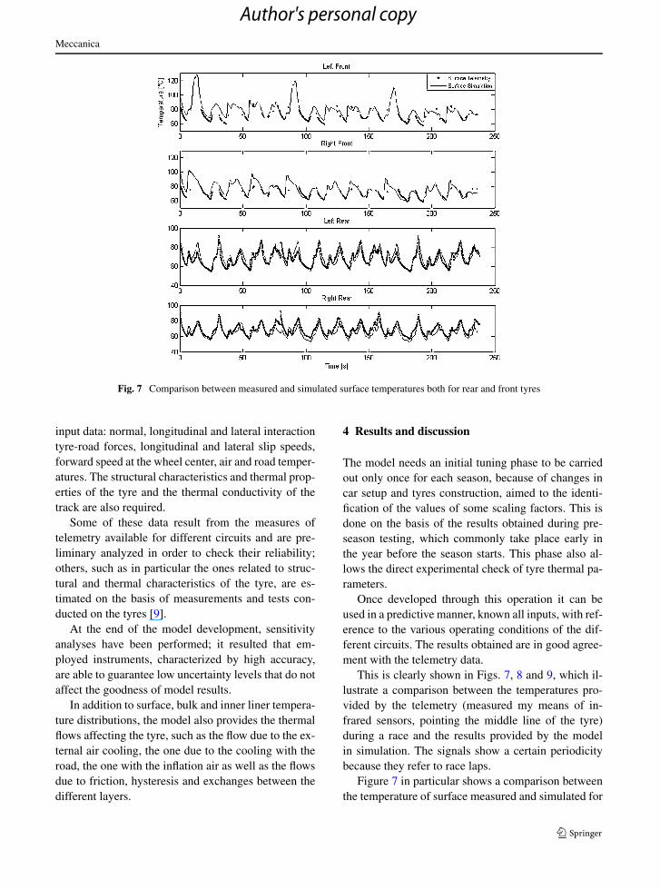
Fig. 7 Comparison between measured and simulated surface temperatures both for rear and front tyres

input data: normal, longitudinal and lateral interactiontyre-road forces, longitudinal and lateral slip speeds,forward speed at the wheel center, air and road temper-atures. The structural characteristics and thermal prop-erties of the tyre and the thermal conductivity of thetrack are also required.

Some of these data result from the measures oftelemetry available for different circuits and are pre-liminary analyzed in order to check their reliability;others, such as in particular the ones related to struc-tural and thermal characteristics of the tyre, are es-timated on the basis of measurements and tests con-ducted on the tyres [9].

At the end of the model development, sensitivityanalyses have been performed; it resulted that em-ployed instruments, characterized by high accuracy,are able to guarantee low uncertainty levels that do notaffect the goodness of model results.

In addition to surface, bulk and inner liner tempera-ture distributions, the model also provides the thermalflows affecting the tyre, such as the flow due to the ex-ternal air cooling, the one due to the cooling with theroad, the one with the inflation air as well as the flowsdue to friction, hysteresis and exchanges between thedifferent layers.

4 Results and discussion

The model needs an initial tuning phase to be carriedout only once for each season, because of changes incar setup and tyres construction, aimed to the identi-fication of the values of some scaling factors. This isdone on the basis of the results obtained during pre-season testing, which commonly take place early inthe year before the season starts. This phase also al-lows the direct experimental check of tyre thermal pa-rameters.

Once developed through this operation it can beused in a predictive manner, known all inputs, with ref-erence to the various operating conditions of the dif-ferent circuits. The results obtained are in good agree-ment with the telemetry data.

This is clearly shown in Figs. 7, 8 and 9, which il-lustrate a comparison between the temperatures pro-vided by the telemetry (measured my means of in-frared sensors, pointing the middle line of the tyre)during a race and the results provided by the modelin simulation. The signals show a certain periodicitybecause they refer to race laps.

Figure 7 in particular shows a comparison betweenthe temperature of surface measured and simulated for

Author's personal copy

Meccanica

Fig. 8 Bulk simulated temperature and comparison between measured and simulated inner liner temperatures both for rear and fronttyres

all the four wheels. As can be seen the agreement be-tween the model and telemetry is excellent.

With regard to the front wheels, the fragmentarytelemetry data is due to the fact that when the steer-ing angle exceeds a certain threshold, the temperaturemeasurement is not trusted because the sensor detectstemperature values corresponding to different zones ofthe tyre. Substantially when the steering wheel is overa certain value the reliability of the temperature signalis lost.

In Fig. 8, the temperatures of the inner liner mea-sured and those calculated with the model are reported.Also in this case, for all four wheels the agreement isexcellent. In the figure are also reported bulk temper-atures estimated by means of model simulations. Forbulk temperatures no data are available from teleme-try.

Proper time ranges have been selected to highlightthermal dynamics characteristic of each layer; in par-ticular, as concerns bulk and inner liner (Fig. 8), tem-perature decreasing trend is due to a vehicle slowdownbefore a pit stop.

Finally in Fig. 9, with reference to a different cir-cuit, the comparisons between the measured temper-

atures and those supplied by the model for all fourwheels of the vehicle are reported.

Even in this case, despite the fragmentary telemetrydata of the front tyres surface temperature, the agree-ment between the telemetry data and those evaluatedwith the model is good.

5 Conclusions

The Thermo Racing Tyre model presented in this pa-per is an indispensable instrument to optimize racingtyres performances since tyre surface temperatures aswell as bulk ones have great influence on the tyre-trackinteraction. The interaction forces reach their maxi-mum values only within a narrow temperature range,while decay significantly outside of it. The ability topredict the temperature distribution on the surface, andalso within the tyre in the different operating situationsduring the race, allows to identify the tyre conditionsduring the race, so it is possible to ensure the optimumtemperature to maximize the forces exchanged withthe track.

Moreover, having the model the possibility to turnin real time, it is suitable for applications on a driving

Author's personal copy

Meccanica

Fig. 9 Another example of bulk and inner liner simulated temperature and comparison between measured and simulated surfacetemperatures both for rear and front tyres

simulator where it is necessary to reproduce the realoperating conditions including the tyre temperatures.

The physical nature of the model, based on ana-lytic equations containing known or measurable phys-ical parameters, in addition to give to the model thepredictive ability, also allows an analysis of the influ-ence of different parameters including the constructivecharacteristics and chemical-physical properties of therubber. This is extremely useful in the design phaseof the tyres, but also for the choice of the tyres ac-cording to the various circuits characteristics and tothe methodology of their use.

Naturally, the model needs a preliminary tuningphase before it can be used and this stage is possible ifa sufficient wide and varied amount of data from mul-tiple circuits through the telemetry is available.

This phase is typically placed in the activities ofpre-season testing on the track. Once developed themodel, it will provide, on the basis of inputs fromtelemetry or from models if used on a driving simu-lator, the output temperature of the surface, bulk andinner liner as well as heat flows in input and in outputfrom the tyre. The knowledge of heat flows and hencetheir balance is another important instrument for the

identification of optimum operating conditions in or-der to maximize tyre performances.

Appendix

As an example, heat balance equation for node 2 alongthe x direction is reported, recalling that, for the per-formed discretization, the nodes adjacent to 2 are 6and 58:

k1

�X· (T6 − T2) · �Y · �Z1

2− k1

�X· (T2 − T58) · �Y

· �Z1

2= m2 · cv1 · �T2

�t(25)

Substituting the expression of the mass (2) (remindingthat in this case C = 1/2) leads to the equation:

�T2

�t= 1

ρ · cv1·[

k1

�X2·T6 − 2 · k1

�X2·T2 + k1

�X2·T58

]

(26)

Taking into account the exchanges along all direc-tions and all the possible heat generations, the equa-tion of node 2 can be written:

Author's personal copy

Meccanica

• in the case of contact with the road

Q̇SEL + k1

�X· (T6 − T2) · �Y · �Z1

2− k1

�X

· (T2 − T58) · �Y · �Z1

2+ k1

�Y· (T1 − T2) · �X

· �Z1

2− k1

�Y· (T2 − T3) · �X · �Z1

2+ k1

�Z1

· (T62 − T2) · �X · �Y + CR · Fx · vx + Fy · vy

A

· �X · �Y + Hc · (Tr − T2)

· �X · �Y = m2 · cv1 · �T2

�t(A)

• in the case of contact with external air

Q̇SEL + k1

�X· (T6 − T2) · �Y · �Z1

2− k1

�X

· (T2 − T58) · �Y · �Z1

2+ k1

�Y· (T1 − T2) · �X

· �Z1

2− k1

�Y· (T2 − T3) · �X · �Z1

2+ k1

�Z1

· (T62 − T2) · �X · �Y + hf orc · (Tair − T2)

· �X · �Y = m2 · cv1 · �T2

�t(B)

having denoted by Q̇SEL the power dissipated bycyclic deformation.

Once developed, the two expressions lead respec-tively to:• in the case of contact with the road

�T2

�t= 1

ρ · cv1·[

2 · Q̇SEL

�X · �Y · �Z1

+(

−2 · k1

�X2− 2 · k1

�Y 2− 2 · k1

�Z21

− 2 · Hc

�Z1

)

· T2 + k1

�Y 2· T1 + k1

�Y 2· T3 + k1

�X2· T6

+ k1

�X2· T58 + 2 · k1

�Z21

· T62

+ 2 · FP

�Z1+ 2 · Hc

�Z1· Tr

](27)

• in the case of contact with external air

�T2

�t= 1

ρ · cv1·[

2 · Q̇SEL

�X · �Y · �Z1

+(

−2 · k1

�X2− 2 · k1

�Y 2− 2 · k1

�Z21

− 2 · hf orc

�Z1

)

· T2 + k1

�Y 2· T1 + k1

�Y 2· T3 + k1

�X2· T6

+ k1

�X2· T58 + 2 · k1

�Z21

· T62

+ 2 · hf orc

�Z1· Tair

](28)

The equations showed for node 2 are valid for all thenodes belonging to the surface layer, localized inter-nally in lateral direction.

For a node still belonging to the surface layer, butexternal in lateral direction (C = 1/4), for examplenode 1, the complete equations are:• in the case of contact with the road

Q̇SEL + k1

�X· (T5 − T1) · �Y

2· �Z1

2− k1

�X

· (T1 − T57) · �Y

2· �Z1

2+ k1

�Y· (T2 − T1) · �X

· �Z1

2+ k1

�Z1· (T61 − T1) · �X · �Y

2+ CR

· Fx · vx + Fy · vy

A· �X · �Y

2+ Hc · (Tr − T1)

· �X · �Y

2= m1 · cv1 · �T1

�t(C)

• in the case of contact with external air

Q̇SEL + k1

�X· (T5 − T1) · �Y

2· �Z1

2− k1

�X

· (T1 − T57) · �Y

2· �Z1

2+ k1

�Y· (T2 − T1) · �X

· �Z1

2+ k1

�Z1· (T61 − T1) · �X · �Y

2+ hf orc

· (Tair − T1) · �X · �Y

2= m1 · cv1 · �T1

�t(D)

leading, respectively, to:• for the first case

�T1

�t= 1

ρ · cv1·[

4 · Q̇SEL

�X · �Y · �Z1

+(

−2 · k1

�X2− 2 · k1

�Y 2− 2 · k1

�Z21

− 2 · Hc

�Z1

)· T1

Author's personal copy

Meccanica

+ 2 · k1

�Y 2· T2 + k1

�X2· T5 + k1

�X2· T57

+ 2 · k1

�Z21

· T61 + 2 · FP

�Z1+ 2 · Hc

�Z1· Tr

](29)

• for the second case

�T1

�t= 1

ρ · cv1·[

4 · Q̇SEL

�X · �Y · �Z1

+(

−2 · k1

�X2− 2 · k1

�Y 2− 2 · k1

�Z21

− 2 · hf orz

�Z1

)

· T1 + 2 · k1

�Y 2· T2 + k1

�X2· T5 + k1

�X2

· T57 + 2 · k1

�Z21

· T61 + 2 · hf orc

�Z1· Tair

](30)

The equation relating to the bulk layer, for an internalnode in the lateral direction (C = 1), e.g. node 62, is:

Q̇SEL + k2

�X· (T66 − T62) · �Y ·

(�Z1

2+ �Z2

2

)

− k2

�X· (T62 − T118) · �Y ·

(�Z1

2+ �Z2

2

)

+ k2

�Y· (T61 − T62) · �X ·

(�Z1

2+ �Z2

2

)

− k2

�Y· (T62 − T63) · �X ·

(�Z1

2+ �Z2

2

)

+ k2

�Z2· (T122 − T62) · �X · �Y − k1

�Z1

· (T62 − T2) · �X · �Y = m62 · cv2 · �T62

�t(E)

Such expression, suitably developed, leads to:

�T62

�t= 1

ρ · cv2·[

Q̇SEL

�X · �Y · (�Z12 + �Z2

2 )

+(

−2 · k2

�X2− 2 · k2

�Y 2− k2

�Z2 · (�Z12 + �Z2

2 )

− k1

�Z1 · (�Z12 + �Z2

2 )

)· T62 + k2

�Y 2· T61

+ k2

�Y 2· T63 + k2

�X2· T66 + k2

�X2· T118

+ k2

�Z2 · (�Z12 + �Z2

2 )· T122

+ k1

�Z1 · (�Z12 + �Z2

2 )· T2

](31)

Similarly, relatively to a bulk external node in thetransverse direction (C = 1/2), it results:

Q̇SEL + k2

�X· (T65 − T61) · �Y

2·(

�Z1

2+ �Z2

2

)

− k2

�X· (T61 − T117) · �Y

2·(

�Z1

2+ �Z2

2

)

+ k2

�Y· (T62 − T61) · �X ·

(�Z1

2+ �Z2

2

)

+ k2

�Z2· (T121 − T61) · �X · �Y

2− k1

�Z1

· (T61 − T1) · �X · �Y

2= m61 · cv2 · �T61

�t(F)

that becomes:

�T61

�t= 1

ρ · cv2·[

2 · Q̇SEL

�X · �Y · (�Z12 + �Z2

2 )

+(

−2 · k2

�X2− 2 · k2

�Y 2− k2

�Z2 · (�Z12 + �Z2

2 )

− k1

�Z1 · (�Z12 + �Z2

2 )

)· T61 + 2 · k2

�Y 2· T62

+ k2

�X2· T65 + k2

�X2· T117

+ k2

�Z2 · (�Z12 + �Z2

2 )· T121

+ k1

�Z1 · (�Z12 + �Z2

2 )· T1

](32)

As concerns the innermost layer, the inner liner, theequation of exchange for an internal node in the trans-verse direction (C = 1/2), e.g. 122, is:

Q̇SEL + k2

�X· (T126 − T122) · �Y · �Z2

2− k2

�X

· (T122 − T158) · �Y · �Z2

2+ k2

�Y

· (T121 − T122) · �X · �Z2

2− k2

�Y

· (T122 − T123) · �X · �Z2

2+ k2

�Z2

· (T62 − T122) · �X · �Y + hint · (Tair_int − T122)

Author's personal copy

Meccanica

· �X · �Y = m122 · cv2 · �T122

�t(G)

that simplified returns:

�T122

�t= 1

ρ · cv2·[

2 · Q̇SEL

�X · �Y · �Z2

+(

−2 · k2

�X2− 2 · k2

�Y 2− 2 · k2

�Z22

− 2 · hint

�Z2

)

· T122 + k2

�Y 2· T121 + k2

�Y 2· T123

+ k2

�X2· T126 + k2

�X2· T158 + 2 · k2

�Z22

· T62 + 2 · hint

�Z2· Tair_int

](33)

Finally, for an external node in the transverse directionbelonging to the Inner liner (C = 1/4), it is:

Q̇SEL + k2

�X· (T125 − T121) · �Y

2· �Z2

2− k2

�X

· (T121 − T157) · �Y

2· �Z2

2+ k2

�Y

· (T122 − T121) · �X · �Z2

2+ k2

�Z2

· (T61 − T121) · �X · �Y

2

+ hint · (Tair_int − T121) · �X · �Y

2

= m121 · cv2 · �T121

�t(H)

which, simplified, provides:

�T121

�t= 1

ρ · cv2·[

4 · Q̇SEL

�X · �Y · �Z2

+(

−2 · k2

�X2− 2 · k2

�Y 2− 2 · k2

�Z22

− 2 · hint

�Z2

)

· T121 + 2 · k2

�Y 2· T122 + k2

�X2· T125

+ k2

�X2· T157 + 2 · k2

�Z22

· T61

+ 2 · hint

�Z2· Tair_int

](34)

References

1. Pacejka HB (2007) Tyre and vehicle dynamics.Butterworth-Heinemann, Stoneham

2. Capone G, Giordano D, Russo M, Terzo M, Timpone F(2008) Ph.An.Ty.M.H.A.: a physical analytical tyre modelfor handling analysis—the normal interaction. Veh SystDyn 47:15–27

3. Castagnetti D, Dragoni E, Scirè Mammano G (2008) Elas-tostatic contact model of rubber-coated truck wheels loadedto the ground. Proc Inst Mech Eng, Part L 222:245–257

4. Farroni F, Rocca E, Russo R, Savino S, Timpone F (2012)Experimental investigations about adhesion component offriction coefficient dependence on road roughness, contactpressure, slide velocity and dry/wet conditions. In: Pro-ceedings of the 14th mini conference on vehicle system dy-namics, identification and anomalies, VSDIA

5. Farroni F, Russo M, Russo R, Timpone F (2012) Tyre-roadinteraction: experimental investigations about the frictioncoefficient dependence on contact pressure, road rough-ness, slide velocity and temperature. In: Proceedings of theASME 11th biennial conference on engineering systemsdesign and analysis, ESDA2012

6. Park HC, Youn ISK, Song TS, Kim NJ (1997) Analysis oftemperature distribution in a rolling tire due to strain energydissipation. Tire Sci Technol 25:214–228

7. Lin YJ, Hwang SJ (2004) Temperature prediction of rollingtires by computer simulation. Math Comput Simul 67:235–249

8. De Rosa R, Di Stazio F, Giordano D, Russo M, TerzoM (2008) Thermo tyre: tyre temperature distribution dur-ing handling maneuvers. Veh Syst Dyn 46:831–844. ISSN:0042-3114

9. Allouis C, Amoresano A, Giordano D, Russo M, TimponeF (2012) Measurement of the thermal diffusivity of a tyrecompound by mean of infrared optical technique. Int RevMech Eng 6:1104–1108. ISSN: 1970-8734

10. Kreith F, Manglik RM, Bohn MS (2010) Principles of heattransfer, 6th edn. Brooks/Cole, New York

11. Gent AN, Walter JD (2005). The pneumatic tire. NHTSA,Washington

12. Johnson KL (1985) Contact mechanics. Cambridge Univer-sity Press, Cambridge

13. Agrawal R, Saxena NS, Mathew G, Thomas S, SharmaKB (2000) Effective thermal conductivity of three-phasestyrene butadiene composites. J Appl Polym Sci 76:1799–1803

14. Dashora P (1994) A study of variation of thermal conduc-tivity of elastomers with temperature. Phys Scr 49:611–614

15. Brancati R, Rocca E, Timpone F (2010) An experimentaltest rig for pneumatic tyre mechanical parameters measure-ment. In: Proceedings of the 12th mini conference on vehi-cle system dynamics, identification and anomalies, VSDIA

16. Giordano D (2009) Temperature prediction of high perfor-mance racing tyres. PhD thesis

17. Brancati R, Strano S, Timpone F (2011) An analyticalmodel of dissipated viscous and hysteretic energy due tointeraction forces in a pneumatic tire: theory and exper-iments. Mech Syst Signal Process 25:2785–2796. ISSN:0888-3270

Author's personal copy

Meccanica

18. Chadbourn BA, Luoma JA, Newcomb DE, Voller VR(1996) Consideration of hot-mix asphalt thermal proper-ties during compaction—quality management of hot-mixasphalt. In: ASTM STP 1299

19. Browne AL, Wickliffe LE (1980) Parametric study of con-vective heat transfer coefficients at the tire surface. Tire SciTechnol 8:37–67

20. Fluent 6.3 user’s guide (2006) Fluent Inc, Chap 3

21. Karniadakis GEM (1988) Numerical simulation of forcedconvection heat transfer from a cylinder in crossflow. Int JHeat Mass Transf 31:107–118

22. van der Steen R (2007) Tyre/road friction modeling.PhD thesis, Eindhoven University of Technology, Depart-ment of Mechanical Engineering

Author's personal copy