Journal of Ecology 2004

Tropical forest tree mortality, recruitment and turnover rates: calculation, interpretation and comparison when census intervals vary

SIMON L. LEWIS'^ OLIVER L. PHILLIPS', DOUGLAS SHEIL\ BARBARA VINCETI^ TIMOTHY R. BAKER'\ SANDRA BROWNE ANDREW W. GRAHAM^ NIRO HIGUCHL, DAVID W. HILBERTH WILLIAM F. LAURANCE^'', JEAN LEJOLY'", YADVINDER MALHP, ABEL MONTEAGUDO" '^ PERCY NÚÑEZ VARGAS", BONAVENTURE SONKÉ", NUR SUPARDI M.N.'^ JOHN W. TERBORGH'^ and RODOLFO VÁSQUEZ MARTÍNEZ'^ ^ Earth & Biosphere Institute, School of Geography, University of Leeds, Leeds LS2 9JT, UK, ^School of Geosciences, University of Edinburgh, Edinburgh EH9 3JU, UK, ^Centre for International Forestry Research, PO Box 6596 JKP WB, Jakarta 10065, Indonesia, '^Max-Planck-Institutfür Biogeochemie, Postfach 100164, 07701 Jena, Germany, ^ Winrock International, 1621 N. Kent Street, Suite 1200, Arlington, VA 22209, USA, "CSIRO Tropical Forest Research Centre and Cooperative Research Centre for Rainforest Ecology and Management, Atherton, Queensland, Australia, ^ Departamento Ecología, Instituto Nacional de Pesquisas Amazónicas, CP478, 69011-970, Manaus, AM, Brazil, ^Biological Dynamics of Forest Fragments Project, Instituto Nacional de Pesquisas Amazónicas, CP 478, 69011-970, Manaus, AM, Brazil, "^Smithsonian Tropical Research Institute, Apartado 2072, Balboa, Republic of Panama, ^''Laboratoire de Botanique Systématique at de Phytosociologie, Université Libre de Buxelles, 50 Avenue F. Roosevelt, Bruxelles, Belgium, ^^ Herbario Vargas, Universidad Nacional San Antonio Abad del Cusco, Cusco, Peru, ^^Proyecto Flora del Perú, Jardin Botánico de Missouri, Oxampampa, Peru, "Ecole Normale Supérieure de Yaounde, Université de Yaounde I, Yaounde, Cameroon, ^''Forest Ecology Unit, Forest Environment Division, Forest Research Institute Malaysia, Kepong, 52109 Kuala Lumpur, Malaysia, and "Center for Tropical Conservation, Duke University, Box 90381, Durham, NC27708, USA

Summary

1 Mathematical proofs show that rate estimates, for example of mortality and recruitment, will decrease with increasing census interval when obtained from censuses of non-homogeneous populations. This census interval effect could be confounding or perhaps even driving conclusions from comparative studies involving such rate estimates. 2 We quantify this artefact for tropical forest trees, develop correction methods and re-assess some previously published conclusions about forest dynamics. 3 Mortality rates of > 50 species at each of seven sites in Africa, Latin America, Asia and Australia were used as subpopulations to simulate stand-level mortality rates in a heterogeneous population when census intervals varied: all sites showed decreasing stand mortality rates with increasing census interval length. 4 Stand-level mortality rates from 14 multicensus long-term forest plots from Africa, Latin America, Asia and Australia also showed that, on average, mortality rates decreased with increasing census interval length. 5 Mortality, recruitment or turnover rates with differing census interval lengths can be compared using the mean rate of decline from the 14 long-term plots to standardize estimates to a common census length using X^••= '^ ^ ^°°^ where X is the rate and t is time between censuses in years. This simple general correction should reduce the bias associated with census interval variation, where it is unavoidable. 6 Re-analysis of published results shows that the pan-tropical increase in stem turnover rates over the late 20th century cannot be attributed to combining data with differing census intervals. In addition, after correction. Old World tropical forests do not have significantly

© 2004 British Ecological Society Correspondence: Simon L. Lewis (tel. +44 113 343 3361; fax+44 113 343 3308; e-mail slewis@pobox.com).

s. L. Lewis et al. lower turnover rates than New World sites, as previously reported. Our pan-tropical best estimate adjusted stem turnover rate is 1.81 + 0.16% a"' (mean + 95% CI, n = 65). 7 As differing census intervals affect comparisons of mortality, recruitment and turnover rates, and can lead to erroneous conclusions, standardized field methods, the calculation of local correction factors at sites where adequate data are available, or the use of our general standardizing formula to take account of sample intervals, are to be recommended.

Key-words: carbon dioxide, global environmental change, long-term monitoring, modelling, neotropics, palaeotropics, permanent sample plot, rain forest, tree, tropical forest dynamics

Journal of Ecology (2004) 10.1111/J.1365-2745.2004.00923.X

© 2004 British Ecological Society, Journal of Ecology

Introduction

Marking, counting and measuring individuals and periodically re-counting these individuals to infer population changes is common practice for ecological studies (Begon et al. 1996; Krebs 1999). For studies of tropical trees this has mostly taken the form of census- based permanent plot data: delineating an area, and permanently and uniquely marking each tree stem within that area that exceeds a given lower-size thresh- old, often > lOcmd.b.h. (diameter at breast height, 1.3 m, or above buttresses or other bole deformities). The plot is revisited periodically to note deaths and add the trees that reach the lower size limit, and these data are then used to calculate mortality and recruitment estimates (Sheil et al. 1995). Almost everything we know about tropical forest dynamics derives from this method (e.g. Connell et al. 1984; Swaine et al. 1987a; Carey et al. 1994; Phillips & Gentry 1994; Condit et al. 1999; Sheil et al. 2000; Vásquez & Phillips 2000; Lewis et al. 2004a; Phillips et al. 2004).

Mortality and recruitment estimates are funda- mental descriptors of tropical forest tree populations. Comparisons both between and among studies are important if we are to further understand tropical forest dynamics, both to make generalizations about patterns in time and space, and to infer their underlying causes (Swaine et al. 1987b; Hartshorn 1990; Phillips & Gentry 1994; Phillips et al. 1994; Phillips 1996; Lewis et al. 2004a; Phillips et al. 2004). However, these re- cruitment and mortality rate estimates are affected by a potentially serious artefact that may influence any conclusion based on permanent sample plots: these rate estimates are not independent of the time interval between censuses (Sheil & May 1996). Thus, conclu- sions based on comparing rates with differing census intervals are open to debate (for example see Phillips & Gentry 1994; responses by Phillips 1995; Sheil 1995; Phillips et al. 2004).

Mortality rate estimates are often based on models that assume a population is homogenous, with each member having an equal and constant probability of dying (Sheil et al. 1995). Sheil and May (1996) show

theoretically that when a population is made up of subpopulations with differing mortality rates, the population mortality rate, on average, will decrease with increasing time between censuses. This is because higher-mortality stems die faster, leaving increasing proportions of the original cohort represented by lower-mortality stems. Over time the lower-mortality stems dominate, leading to lower estimates of popula- tion mortality rates as the census interval increases.

It is unknown whether the theoretically demon- strated decline in mortality rate with increasing census interval is a serious problem or essentially trivial over the time-scales on which ecologists measure forest dynamics. Certainly, tropical forest stands are not homogeneous with respect to the mortality, recruit- ment or turnover of their component subpopulations. For example, individual species' mortality rates in three different forest stands each appear to vary by over an order of magnitude ( Vanclay 1991 ; Favrichon 1994; Condit et al. 1995). Further within-stand heterogene- ity may be generated if mortality rates change with stem size, as has been shown for stems > 10 cm d.b.h. in several localities (Mervart 1972; Hartshorn 1990; Hubbell & Foster 1990; Vanclay 1991; Clark & Clark 1992). Additionally, heterogeneity may arise from species-level mortality rates varying according to local variation in the physical environment. Thus we expect some impact of census interval length on mortality rate estimates, but neither a priori predictions of the magnitude or form of declines (linear, exponential, etc.), nor initial estimates of the declines in forest stands, are known.

Accurate mortality rate estimation presents several other problems, notably the large sample sizes and long time-periods required, due to intrinsically low mortality rates and the large stochastic component of tree mortal- ity in tropical forests. For example, in a study of 10 ha of forest in Ecuador, 20% of tree deaths > 10 cm d.b.h. were due to other trees knocking them over (Gale & Barfod 1999). Furthermore, very occasional deaths of very large trees accentuate this stochastic element by dramatically altering forest structure and hence local competition and recruitment (Sheil et al. 2000). A

3 stand of 1 ha with c. 600 trees > 10 cm d.b.h. and a Forest dynamics mortahty rate of c. 1.5% a"' translates to c. 9 trees dying when census ha"' a"', hence stochastic effects altering this by only a intervals vary few trees can have large effects on average mortality

rates. Thus long-term and/or large-scale studies are required.

Studies of tropical tree dynamics often consider mortality but not recruitment (Swaine et al. 1987b; Hartshorn 1990; Vanclay 1991; Condit et al. 1995; Lieberman et al. 1996); however, many studies report both (Carey et al. 1994; Favrichon 1994; Phillips & Gentry 1994; Phillips 1996; Condit et al. 1999; Shell et al. 2000). Shell and May (1996) show that the same effect of census interval applies to recruitment rates: a decline with increasing census interval. Of course, if recruitment rate estimates chosen are calculated as the number of recruited stems needed to maintain a population in equilibrium, as is commonly the case, then, by definition, declines with increasing census length are predicted to match those for mortality. Stem turnover {sensu Phillips & Gentry 1994), the mean of the mortal- ity and recruitment rates of a forest stand, would also, by definition, show the same decline with increasing census interval.

As more studies on forest dynamics are completed the scope for comparative studies and syntheses of tropical forest ecology increases, so there is an urgent need to understand and quantify the potential census- interval artefact. For example, one study of 65 sites from across the tropics showed that turnover rates have been increasing over the late 20th century, possibly as a result of increased productivity (Phillips & Gentry 1994; see Phillips 1996). However, the study included sites with a wide range of census intervals (2-38 years), and the central finding has hence been controversial (Phillips 1995; Shell 1995; Shell & May 1996; Condit 1997; Phillips & Shell 1997; Phillips et al. 2004).

We take two approaches to assess if the census inter- val effect on tropical forest tree mortality, recruitment and turnover rates is a serious problem. First, we use species-level mortality rates from seven sites from Latin America, Africa, Asia and Australia, using each species as a subpopulation to calculate the expected mortality rate for each stand for census intervals from 1 up to 50 years. This gives a first estimate of the magnitude of the artefact, and a clue as to the shape of the rela- tionship between mortality rates and census interval length. Secondly, we use 14 long-term multicensus plots from Latin America, Africa, Asia and Australia to test for a decline in mortality over time in permanent sample plot data. This gives a second estimate of the decline and its form, but will be more variable as stochastic effects and changes in mortality over time are included in the long-term data. Finally, we re-analyse Phillips's (1996) data set of 65 sites to test his conclu- sions about changes in forest dynamics over time and

© 2004 British regional differences in dynamics, taking into account Ecological Society, the differing census intervals used in each of the 65 Journal of Ecology sites.

Methods

SIMULATIONS WITH LARGE-SCALE DATA

SETS

Several forms of mortality rate estimate have been used (Shell et al. 1995). Here we consider the commonly used instantaneous rate measure, X, calculated as:

ln(«o) - Mn,) eqnl

where WQ and n, are the number of stems in the original population, and the number of stems surviving to time t, respectively. The time between the two stem censuses is t.

Shell and May (1996) provide the mathematical proofs that mortality and recruitment rate estimates decline with increasing census interval length if the population is heterogeneous. They show that the population mortality rate, \i¡¡(t), and its behaviour over lengthening census intervals, can be calculated from knowledge of each subpopulation, /', its original population of stems, K,O and mortality rate, X¡:

x••(o = -(i/oin S«,•e"'-7Z«,• eqn 2

For tropical forest sites where we know the original population of stems and the mortality rate for many species (the subpopulations) we can input these into the above equation and vary t to simulate the impact of varying the census interval on stand-level mortality rates when the stand is made up of many known subpopulations.

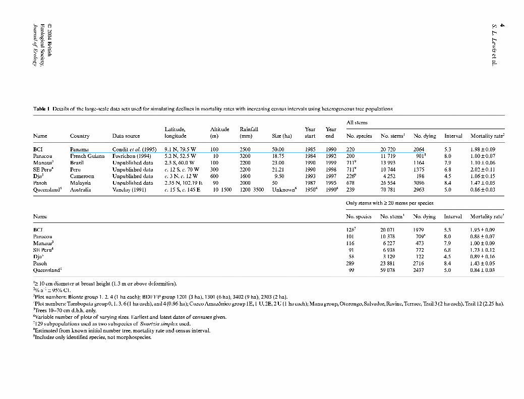
We used seven data sets from across the tropics that represent all the published and unpublished data that we are aware of, which report mortality rates for > 50 species at a given site for trees > 10 cm diameter at breast height (d.b.h., 1.3 m or above deformities; except at the Dja site, where only trees > 10 cm d.b.h. and < 70 cm d.b.h. were included). For each site, two censuses 5-8 years apart were chosen. Data from nearby permanent plots within a region were pooled, and only species with > 20 individuals were selected (or > 5 deaths for North Queensland, Vanclay 1991). We estimated declines in mortality rates by varying t from 1 to 50 years using 58-289 species mortality rates as subpopulations in equation 2 (Table 1). Species-level mortality rates, A.,, were calculated for all species selected in each region using the arithmetic mean of the census intervals for individual stems as t in the mortal- ity equation. The arithmetic mean was preferred as it is easy to compute, and the benefits of other procedures are unclear (cf Condit et al. 1999; Kubo et al. 2000). Each selected species was treated as a subpopulation in equation 2, with A.••(i) calculated for a census length of 1 year, and at 1-year intervals to a maximum of 50 years. However, the reader should note that not all

r 8 -s

m

^ r^ r/i '•í

ri)

x;

re

Table 1 Details of the large-scale data sets used for simulating declines in mortality rates with increasing census intervals using heterogeneous tree populations

All stems Latitude, Altitude Rainfall Year Year

Name Country Data source longitude (m) (mm) Size (ha) start end No. species No. stems' No. dying Interval Mortality rate^

BCI Panama Condit et al. (1995) 9.1 N, 79.5 W 100 2500 50.00 1985 1990 220 20 720 2064 5.3 1.98 ±0.09 Paracou French Guiana Favrichon (1994) 5.2 N, 52.5 W 10 3200 18.75 1984 1992 200 11719 901'* 8.0 1.00 ±0.07 Manaus' Brazil Unpublished data 2.3 S, 60.0 W 100 2200 23.00 1990 1999 711' 13 993 1164 7.9 1.10±0.06 SE Peru" Peru Unpublished data c. 12 S, c. 70 W 300 2200 21.21 1990 1998 711' 10 744 1375 6.8 2.02 ±0.11 Dja' Cameroon Unpublished data c. 3N,c. 12 W 600 1600 9.50 1993 1997 226' 4 252 198 4.5 1.06±0.15 Pasoh Malaysia Unpublished data 2.35 N, 102.19 E 90 2000 50 1987 1995 678 26 554 3096 8.4 1.47 ±0.05 Queensland' Australia Vanclay(1991) c. 15 S, c. 145 E 10-1500 1200-3500 Unknown' 1950' 1990' 239 70 781 2963 5.0 0.86 ±0.03

Only stems with > 20 stems per species

Name No. species No. stems' No. dying Interval Mortality rate^

BCI 128' 20 071 1979 5.3 1.95 ±0.09 Paracou 101 10 378 709* 8.0 0.88 ±0.07 Manaus^ 116 6 227 473 7.9 1.00 ±0.09 SE Peru" 91 6 938 772 6.8 1.73 ±0.12 Dja' 58 3 129 122 4.5 0.89 ±0.16 Pasoh 289 23 881 2716 8.4 1.43 ±0.05 Queensland' 99 59 078 2437 5.0 0.84 ±0.03

'> 10 cm diameter at breast height (1.3 m or above deformities). '% a-' ± 95% CI. ^Plot numbers: Bionte group 1, 2, 4 (1 ha each); BDFFP group 1201 (3 ha), 1301 (6 ha), 3402 (9 ha), 2303 (2 ha). "Plot numbers: Tambopata group 0,1, 3, 6(1 ha each), and 4 (0.96 ha); Cuzco Amazónico group IE, 1 U, 2E, 2U(1 haeach);Manugroup,Otorongo, Salvador, Ravine, Terrace, Trail 3 (2 ha each). Trail 12(2.25 ha). 'Trees 10-70 cm d.b.h. only. 'Variable number of plots of varying sizes. Earliest and latest dates of censuses given. '129 subpopulations used as two subspecies of Swartzia simplex used. ^Estimated from known initial number tree, mortality rate and census interval. 'Includes only identified species, not morphospecies.

Forest dynamics when census intervals vary

© 2004 British Ecological Society, Journal of Ecology

the variation in mortality rates is captured by using each species' mortality rate as a subpopulation.

The seven areas used were, with references about site conditions in parentheses: (i) Barro Colorado Island, Panama (BCI), a single 50-ha plot on an island created by the completion of the Panama Canal (Condit et al. 1995); (ii)Paracou, French Guiana, 3 x 6.25 ha plots in an area of continuous forest in the Guyanan shield (Favrichon 1994); (iii) north Manaus, seven plots, 1- 9 ha each, from a 1000 km^ area in central Amazonia, Brazil (Laurance et al. 1998); (iv) south-east Peru, 15 plots, 0.96-2.25 ha, in the Manu and Tambopata National parks (Gentry & Terborgh 1990; Phillips et al. 1994); (v) Dja Faunal Reserve, four plots, 2-2.5 ha, in south-east Cameroon (Sonké 1998); (vi) Pasoh, a sin- gle 50-ha plot in the centre of the Malay Peninsula, Malaysia (Kochummen et al. 1990; Condit et al. 1999); (vii) North Queensland, an unknown number of plots 0.04-0.5 ha from across North Queensland, Australia (Vanclay 1991). Note that some of the North Queens- land plots have been logged in the past or undergone silvicultural treatments, but the censuses used to gen- erate the mortality rates did not span any logging or silvicultural activity (Vanclay 1991). Further details of each site are given in Table 1.

The sites are geographically widespread, and span the range of rainfall regimes that tropical forests occupy, from aseasonal Pasoh (Kochummen et al. 1990) to the Dja Faunal Reserve site with a long dry season and low annual rainfall (Sonké 1998; see Table 1). The sites occur on a range of soil types from the poor oxisols of central Amazonia (Laurance et al. 1999; Lewis & Tanner 2000) to the more fertile ultisols and inceptisols of the south-east Peru plots (Phillips et al. 1994; Pitman et al. 2001). The sites span a range of stand-level mor- tality rates from less than 1% a"' to greater than 2% a"' (Table 1). The environmental and dynamic variation encompassed by these sites indicates that the results from these sites will be broadly applicable to tropical forests generally.

We chose 50 years as the limit of the simulation as few studies consider intervals longer than this. While Shell and May ( 1996) consider models that treat time as either discrete or continuous (m, and X, respectively, for mortality), we consider only the rate most commonly reported in the literature, X, because (i) both models behave similarly with respect to census interval (Shell & May 1996), (ii) differences are small when m, or X are small, and (iii) conversion is straightforward (Shell etal. 1995).

LONG-TERM DATA SETS

The impact of census interval length on mortality rates may be detectable by calculating stand-level mortality rates from long-term data sets that include a variety of census interval lengths. We selected 14 plots (again from Africa, Latin America, Asia and Australia) on the basis of a minimum plot size of 0.5 ha, a minimum of

10 years of monitoring, and at least six consecutive censuses (Table 2). These include the authors' data and summary data from plots that are included in Phillips's (1996) analysis that fit these criteria. Data for all trees > 10 cm d.b.h. are available for all plots, except Budongo, where only trees > 20 cm d.b.h. are included.

The 14 plots are geographically widespread, and span the range of environmental variation for tropical forests, e.g. from 1600 mm rainfall in Kade, Ghana, to 5000 mm in Katlekan, India, and from poor oxisols in the Brazilian plot to the more fertile soils of the Ghanaian and Peruvian plots (Table 2). The sites also span a wide range of stand-level mortality rates, from less than 1% a"' to nearly 3% a"' (Table 2).

The simplest method of detecting whether mortality rates decline with census interval is to take the original cohort of trees in a plot and calculate X for longer and longer census intervals (Shell 1995). However, if there has been a real systemic increase in mortality rates over the late 20th century (Phillips & Gentry 1994; Phillips 1996; Phillips et al. 2004) this increase would confound any census interval decline, leading to an underestima- tion of the problem. We therefore need to develop methods that control for potential systemic temporal changes in mortality. We use two distinct methods, taking the average of both methods to gain a better esti- mate of the changes.

Our first method is to include census intervals of differing length from both earlier and later in the period of monitoring of each plot. Firstly, we took the cohort of trees at the first census and calculated X for longer and longer census intervals from the first census. For example, for a plot measured in 1980, 1985, 1990 and 1995 we would take the 1980 cohort of trees and calculate X for 1980-85, 1980-90, 1980-95, giving A, for census intervals of 5, 10 and 15 years, respectively. Then, to remove any confounding systematic changes in X over the period of monitoring we performed the inverse of the above procedure, i.e. calculating A. for longer and longer census intervals backwards from the last census. For our example plot measured in 1980, 1985, 1990 and 1995, we would therefore take the 1990 cohort and calculate X from 1990 to 1995, then take the 1985 cohort and calculate?, from 1985 to 1995 and then take the 1980 cohort and calculate 1 from 1980 to 1995, again giving X for census intervals of 5,10 and 15 years. Finally, we ranked each sequence of A. for longer and longer census intervals ('forwards' from the first census and 'backwards' from the last census) by census interval. We then took the mean census interval and "k of each pair of measurements from the ranked lists. For our example plot this would be the mean of the 1980-85 and 1990-95 pair, and the mean of the 1980- 90 and 1985-95 pair of mortality rates (there is only one longest census interval from 1980 to 1995). Thus we generate estimates of "k that account for possible systematic trends in mortality over time, and keep sam- pling intensity equal across differing census interval lengths.

r 8 -s

m

^ r^ r/i '•í

ri)

x;

re

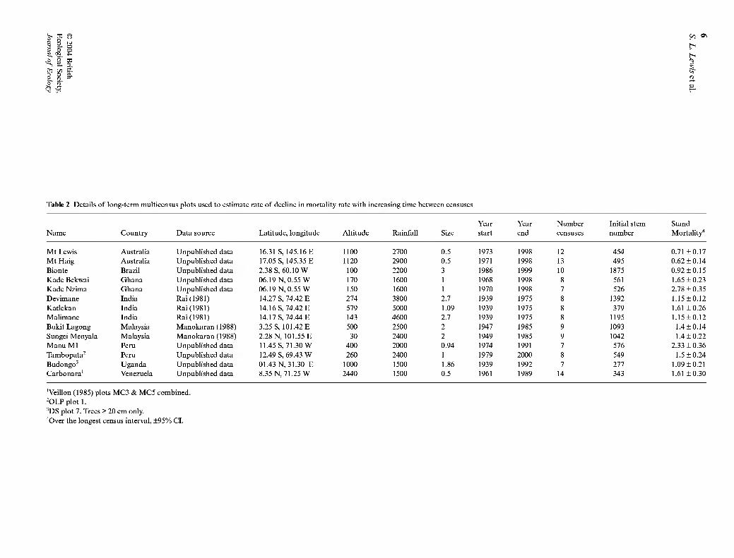
Table 2 Details of long-term multicensus plots used to estimate rate of decline in mortality rate with increasing time between censuses

Year Year Number Initial stem Stand Name Country Data source Latitude, longitude Altitude Rainfall Size start end censuses number Mortality"

Mt Lewis Australia Unpublished data 16.31 S, 145.16 E 1100 2700 0.5 1973 1998 12 454 0.71 ±0.17 Mt Haig Australia Unpublished data 17.05 S, 145.35 E 1120 2900 0.5 1971 1998 13 495 0.62 ±0.14 Bionte Brazil Unpublished data 2.38 S, 60.10 W 100 2200 3 1986 1999 10 1875 0.92 ±0.15 Kade Bekwai Ghana Unpublished data 06.19 N, 0.55 W 170 1600 1 1968 1998 8 561 1.65 ±0.23 Kade Nzima Ghana Unpublished data 06.19 N, 0.55 W 150 1600 1 1970 1998 7 526 2.78 ±0.35 Devimane India Rai(1981) 14.27 S, 74.42 E 274 3800 2.7 1939 1975 8 1392 1.15±0.12 Katlekan India Rai(1981) 14.16 S, 74.42 E 579 5000 1.09 1939 1975 8 379 1.61 ±0.26 Malimane India Rai(1981) 14.17 S, 74.44 E 143 4600 2.7 1939 1975 8 1195 1.15±0.12 Bukit Lagong Malaysia Manokaran (1988) 3.25 S, 101.42 E 500 2500 2 1947 1985 9 1093 1.4 ±0.14 Sungei Menyala Malaysia Manokaran (1988) 2.28 N, 101.55 E 30 2400 2 1949 1985 9 1042 1.4 ±0.22 Manu M1 Peru Unpublished data 11.45 S, 71.30 W 400 2000 0.94 1974 1991 7 576 2.33 ±0.36 Tambopata^ Peru Unpublished data 12.49 S, 69.43 W 260 2400 1 1979 2000 8 549 1.5 ±0.24 Budongo' Uganda Unpublished data 01.43 N, 31.30 E 1000 1500 1.86 1939 1992 7 277 1.09 ±0.21 Carbonara' Venezuela Unpublished data 8.35 N, 71.25 W 2440 1500 0.5 1961 1989 14 343 1.61 ±0.30

'Veillon (1985) plots MC3 & MC5 combined. 'OLP plot 1. 'DS plot 7. Trees > 20 cm only. "Over the longest census interval, ±95% CI.

7 For our second method we control for systemic Forest dynamics changes in X over time. We initially graph each consec- when census utive X against the mid-year of the census interval. This intervals vary shows the trend in mortality rates within a plot over time.

We then use linear regression to estimate the annual change in A. over time. We then use this annual rate of change of X to 'detrend' mortality rates calculated from the original cohort of trees over longer and longer cen- sus intervals. Finally, by ranking each sequence of A. for longer and longer census intervals, from both the 'forwards and backwards' (method 1) and 'detrending' (method 2) procedures, we then took the mean census interval and X of each pair of measurements from the ranked lists from the two methods to obtain our best estimate of X for census intervals of increasing length.

We combine the mortality-census interval data from the 14 long-term data sets to allow direct comparisons with the large-scale simulations so as to assess the functional form of the declines. When combining the mortality rates from our 14 long-term data sets to obtain average mortality rates we encounter a (generic) prob- lem when combining different data sets: what to do when all the data sets do not span the same minimum and maximum census lengths. For example, the short- est census interval at one site (Budongo) is 5.9 years (using the methods above), while the longest interval can be as low as 13 years (Bionte), thus we need to make assumptions about values outside these limits to obtain average mortality rates.

For each plot we used interpolation to obtain a mor- tality rate for each year of measurement. For intervals shorter than the shortest interval measured we used the mortality rate for the shortest interval for all shorter intervals, and likewise for longer intervals than we had data for. Finally, we report only the results where > 75% of plots (11 of 14) that were being monitored were measured, i.e. from 5 to 21 years. Thus we used repeated data for Budongo (5-year interval), Bionte (14-21 -year intervals) and Manu ( 17-21 -year intervals).

STATISTICAL ANALYSIS

The shape of the decline in mortality rates with increas- ing census interval depends upon the distribution of mortality rates of all the stems in the population. The shape of this distribution is unknown for any forest, thus we have no a priori prediction of the shape of the decline, and no indication whether all forest stands have similar distributions of mortality rates. Thus we opt for an empirical approach.

For both the large-scale and long-term data sets we limit analyses to fitting parameters requiring only two constants to be estimated. We fit three different func- tions to each data set: linear {y = a + bx), exponential {y = ae^'") and power (y = a.x"*), where x is the census interval and a and b are constants. Each of these is

© 2004 British fitted to minimize the sum of the squared differences Ecological Society, between the observed and predicted values of the depend- Journal of Ecology ent variable ('least squares regression'). We report

linear, exponential and power functions as each pro- vides a reasonable fit to at least one of the data sets.

We calculate 95% confidence interval values for mortality rates using the normal approximation to the binomial variance (Sokal & Rohlf 1995; as used in Condit et al. 1995). This method is recommended for use with populations of > 500 stems and/or > 5 deaths. Budongo, Carbonara, Malimane, Mt Haig and Mt Lewis all have initial populations of < 500 stems (Table 2); however, none of the intervals included is calculated from a population including < 5 deaths.

RE-ANALYSIS OF PUBLISHED TURNOVER

RATE SYTHESES

Phillips & Gentry (1994) analysed available turnover rate data and showed that turnover rates have been increasing across the tropics over the late 20th century. The turnover data set was later expanded to include 65 sites, which appeared to confirm the trend towards an increase in turnover over time (Phillips 1996). How- ever, Shell (1995) has suggested that this result may be explained by either (i) differing census intervals, as on average census intervals from later in the century were shorter than those earlier in the century, or (ii) the more recent censuses span severe El Niño Southern Oscilla- tion (ENSO) events, while the earlier censuses did not (but see Phillips 1995). We repeat Phillips's (1996) ana- lyses using turnover rates standardized to a common census interval length, to test if turnover still increases over the late 20th century once the census interval arte- fact is accounted for. First, we correlate the mid-year of the entire monitoring period with the turnover rate for all 65 sites (Phillips 1996, his Fig. 2). Secondly, we com- pare an early and a late census interval for the 27 plots that had three censuses (Phillips 1996, his Table 1). Assessment of the impacts of ENSO events on stem turnover rates is beyond the scope of this paper.

Phillips (1996) also showed that New World tropical forest sites had faster turnover than Old World tropical forest sites. However, the New World sites had much shorter average census intervals than the Old World sites. We repeated this analysis after standardizing all turnover rates to a common census interval. Also, Old World sites were monitored earlier in the 20th century than the New World sites: if turnover has been increas- ing over the late 20th century then turnover rates in Old World sites may be underestimated compared with New World sites. We therefore standardize the New and Old World plots to the average mid-year of monitor- ing for the entire data set.

We account for differing census intervals across the 65 sites in two ways: (i) using the generic correction factor developed and applied to all 65 sites; and (ii) for those plots with two or more census intervals, we calculated, as we did for our 14 long-term plots, a site- specific correction for each individual site (27 sites), while using the generic correction factor for the sites with only one interval.

8

S. L. Lewis et al. Results

SIMULATIONS WITH LARGE-SCALE

DATA SETS

Mean stand mortality rates ranged from 0.86% to 2.02%

for the seven stands, with all rates having a 95% CI

within 10% of their mean, except Dja, the Cameroonian

site, which had much lower sample sizes (initial popu-

lation of 4252 stems, whereas all other sites had > 10 000

stems; Table 1). Including only species with > 20 stems

reduced the stand mortality rate, compared with that

calculated using all stems, in all plots, although only

the SE Peru site showed a significant difference (non-

overlapping 95% CIs; Table 1). The reductions were, in

relative terms, between 1.3 and 16% lower when includ-

ing just the commoner species, and were less in sites

with > 20 000 stems monitored (1.3-2.6%), compared

with the sites with < 20 000 stems (9.0-16.0%).

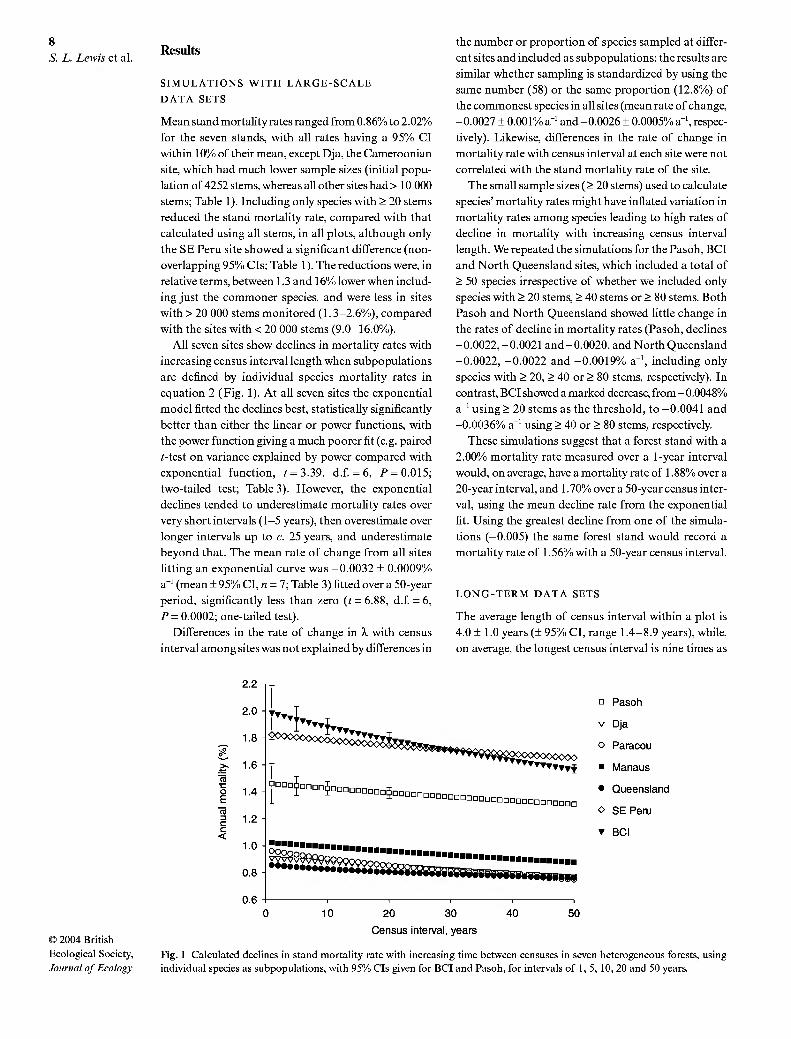
All seven sites show declines in mortality rates with

increasing census interval length when subpopulations

are defined by individual species mortality rates in

equation 2 (Fig. 1). At all seven sites the exponential

model fitted the declines best, statistically significantly

better than either the linear or power functions, with

the power function giving a much poorer fit (e.g. paired

i-test on variance explained by power compared with

exponential function, i=3.39, d.f = 6, P = 0.015;

two-tailed test; Table 3). However, the exponential

declines tended to underestimate mortality rates over

very short intervals (1-5 years), then overestimate over

longer intervals up to c. 25 years, and underestimate

beyond that. The mean rate of change from all sites

fitting an exponential curve was -0.0032 + 0.0009%

a"' (mean + 95% CI, K = 7; Table 3) fitted over a 50-year

period, significantly less than zero (t = 6.88, d.f = 6,

P = 0.0002; one-tailed test).

Differences in the rate of change in X with census

interval among sites was not explained by differences in

the number or proportion of species sampled at differ-

ent sites and included as subpopulations: the results are

similar whether sampling is standardized by using the

same number (58) or the same proportion (12.8%) of

the commonest species in all sites (mean rate of change,

-0.0027 + 0.001% a-' and-0.0026 + 0.0005% a"', respec-

tively). Likewise, differences in the rate of change in

mortality rate with census interval at each site were not

correlated with the stand mortality rate of the site.

The small sample sizes (> 20 stems) used to calculate

species' mortality rates might have inflated variation in

mortality rates among species leading to high rates of

decline in mortality with increasing census interval

length. We repeated the simulations for the Pasoh, BCI

and North Queensland sites, which included a total of

> 50 species irrespective of whether we included only

species with > 20 stems, > 40 stems or > 80 stems. Both

Pasoh and North Queensland showed little change in

the rates of decline in mortality rates (Pasoh, declines

-0.0022,-0.0021 and-0.0020, and North Queensland

-0.0022, -0.0022 and -0.0019% a"', including only

species with > 20, > 40 or > 80 stems, respectively). In

contrast, BCI showed a marked decrease, from - 0.0048%

a"' using > 20 stems as the threshold, to -0.0041 and

-0.0036% a"' using > 40 or > 80 stems, respectively.

These simulations suggest that a forest stand with a

2.00% mortality rate measured over a 1-year interval

would, on average, have a mortality rate of 1.88% over a

20-year interval, and 1.70% over a 50-year census inter-

val, using the mean decline rate from the exponential

fit. Using the greatest decline from one of the simula-

tions (-0.005) the same forest stand would record a

mortality rate of 1.56% with a 50-year census interval.

LONG-TERM DATA SETS

The average length of census interval within a plot is

4.0 + 1.0 years (+ 95% CI, range 1.4-8.9 years), while,

on average, the longest census interval is nine times as

© 2004 British Ecological Society, Journal of Ecology

2.2

2.0

1.8 ^ •>, 1 R w T" O 1 4 b m 3 C 1.2 C <

1.0

0.8

0.6

••"'i-H •••••. rr-""

^¿••DnSi °°°°°°°°°^nGannaGni

^••TTT^

°°°°°°°°°°nnGaGGnnnnnn

^^••••MS^

10 20 30

Census interval, years

40 50

n Pasoh

V Dja

o Paracou

• Manaus

• Queensland

O SE Peru

• BCI

Fig. 1 Calculated declines in stand mortality rate with increasing time between censuses in seven heterogeneous forests, using individual species as subpopulations, with 95% CIs given for BCI and Pasoh, for intervals of 1, 5, 10, 20 and 50 years.

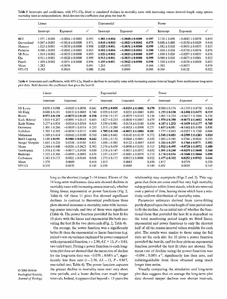
Table 3 Intercepts and coefficients, with 95% CIs, fitted to simulated declines in mortality rates with increasing census interval length using species mortality rates as subpopulations. Bold denotes the coefficient that gives the best fit

Linear Exponential Power

Intercept Exponent r^ Intercept Exponent r Intercept Exponent r^

BCI 1.971 ±0.006 -0.0084 ±0.0002 0.992 1.981 ±0.004 -0.0048 ±0.0000 0.997 2.150 ±0.050 -0.0685 ±0.0078 0.855 Queensland 0.847 ±0.003 -0.0018 ±0.0000 0.971 0.848 ± 0.003 -0.0023 ±0.0002 0.975 0.888 ±0.008 -0.0350 ±0.0029 0.916 Manaus 1.023 ±0.001 -0.0030 ±0.0000 0.998 1.025 ±0.001 -0.0031 ±0.0000 0.999 1.082 ±0.018 -0.0451 ±0.0055 0.835 Paracou 0.946 ±0.005 -0.0042 ±0.0002 0.983 0.952 ± 0.004 -0.0050 ±0.0002 0.990 1.034 ±0.024 -0.0730 ± 0.0074 0.876 SE Peru 1.819 ±0.002 -0.0035 ±0.0000 0.995 1.820 ±0.002 -0.0020 ±0.0000 0.997 1.890 ±0.020 -0.0297 ± 0.0033 0.858 Dja 0.911 ±0.001 -0.0028 ±0.0000 0.999 0.913 ± 0.001 -0.0033 ±0.0000 0.999 0.966 ±0.018 -0.0473 ± 0.0061 0.823 Pasoh 1.458 ±0.002 -0.0031 ±0.0000 0.996 1.459 ±0.001 -0.0022 ±0.0000 0.998 1.520 ±0.018 -0.0328 ±0.0038 0.852 Mean 1.282 -0.0038 0.991 1.285 -0.0032 0.994 1.362 -0.0473 0.859 95% CI 0.345 0.0016 0.008 0.346 0.0009 0.006 0.369 0.0128 0.022

Table 4 Intercepts and coefficients, with 95% CIs, fitted to declines in mortality rates with increasing census interval length from multicensus long-term plot data. Bold denotes the coefficient that gives the best fit

Linear Exponential Power

Intercept Exponent r' Intercept Exponent r^ Intercept Exponent r'

Mt Lewis 0.858 ±0.088 -0.0105 ±0.0056 0.641 0.875 ± 0.095 -0.0154 ±0.0081 0.670 0.980 ±0.174 -0.1319 ±0.0756 0.624 Mt Haig 0.888 ±0.101 -0.0153 ±0.0065 0.740 0.939 ±0.105 -0.0251 ±0.0085 0.801 1.193 ±0.130 -0.2408 ±0.0475 0.919 Bionte 0.972 ±0.120 -0.0072 ± 0.0149 0.158 0.974 ±0.125 -0.0079 ±0.0163 0.156 1.001 ±0.210 -0.0457 ±0.1086 0.126 Kade Bekwai 1.818 ±0.207 -0.0091 ±0.0113 0.465 1.827 ±0.213 -0.0056 ±0.0067 0.479 1.978 ±0.350 -0.0673 ±0.0692 0.548 Kade Nzima 3.277 ± 0.924 -0.0314 ±0.0516 0.415 3.359 ±0.981 -0.0124 ±0.0180 0.456 4.187 ±1.202 -0.1659 ±0.1177 0.769 Devimane 1.301 ±0.266 -0.0059 ±0.0116 0.255 1.313 ±0.280 -0.0053 ±0.0098 0.271 1.637 ±0.551 -0.1162 ±0.1190 0.531 Katlekan 1.703 ±0.302 -0.0034 ±0.0131 0.080 1.705 ±0.310 -0.0021 ±0.0080 0.081 1.777 ±0.665 -0.0297 ±0.1288 0.066 Melamane 1.569 ±0.414 -0.0162 ±0.0180 0.516 1.646 ±0.461 -0.0145 ±0.0139 0.572 2.546 ± 0.883 -0.2589 ±0.1283 0.824 Bukit Lagong 1.121 ±0.091 0.0060 ± 0.0044 0.642 1.226 ±0.152 0.0048 ±0.0061 0.632 1.003 ±0.188 0.0746 ± 0.0668 0.553 Sungei Menyala 1.663 ±0.226 0.0258 ±0.0108 0.851 1.690 ±0.585 0.0122 ±0.0067 0.810 1.326 ±0.297 0.1764 ±0.0771 0.852 Manu 2.364 ± 0.448 -0.0201 ±0.0425 0.302 2.376 ±0.459 -0.0096 ±0.0191 0.315 2.502 ±0.495 -0.0720 ±0.0972 0.498 Tambopata 1.518 ±0.146 -0.0017 ±0.0108 0.030 1.518±0.147 -0.0011 ±0.0072 0.032 1.591 ±0.248 -0.0259 ±0.0648 0.168 Budongo 1.522 ±0.306 -0.0095 ±0.0092 0.676 1.557 ±0.317 -0.0081 ±0.0079 0.715 2.174 ±0.534 -0.1848 ±0.0844 0.898 Carbonara 1.543 ±0.173 0.0021 ±0.0104 0.018 1.575 ±0.175 0.0015 ±0.0066 0.022 1.477 ±0.302 0.0252 ±0.0762 0.046 Mean 1.570 -0.0069 0.414 1.613 -0.0063 0.430 1.812 -0.0759 0.530 95% CI 0.333 0.0070 0.145 0.336 0.0049 0.149 0.451 0.0629 0.165

© 2004 British Ecological Society, Journal of Ecology

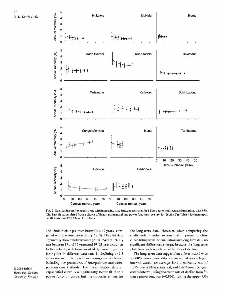
long as the shortest (range 5-14 times). Eleven of the 14 long-term multicensus data sets showed declines in mortality rates with increasing census intervals, whether fitting linear, exponential or power functions (Fig. 2, Table 4). Of these 11 plots five showed significant declines. In contrast to theoretical predictions three plots showed increases in mortality rates with increas- ing census intervals, and two of these were significant (Table 4). The power function provided the best fit for 10 plots, with the linear and exponential fits both pro- viding the best fit for two plots each (Fig. 2, Table 4).

On average, the power function was a significantly better fit than the exponential or linear functions (e.g. paired t-test on variance explained by power compared with exponential function, t = 2.99, d.£ = 13, P = 0.01; two tailed test). Fitting a power function to each long- term plot data set showed that the mean rate of decline for the long-term data was -0.076 + 0.06% a"', signi- ficantly less than zero (r = 2.36, d.f. = 13, P = 0.017, one-tailed test; Table 4). The power function captures the greater decline in mortality rates over very short time periods, and a lesser decline over much longer intervals. Indeed, it appears that beyond c. 15 years the

relationship may asymptote (Figs 2 and 3). This sug- gests that there are some small but very high mortality subpopulations within forest stands, which are removed over a period of time, leaving stems which have a rela- tively uniform distribution of mortality rates.

Parameter estimates derived from curve-fitting partly depend upon the total length of time period used to fit the decline. As an initial test of whether the func- tional form that provided the best fit is dependent on the total monitoring period length we fitted linear, exponential and power functions to only the shortest half of all the census interval values available for each plot. The results were similar to those using the full data set for each site: for 10 plots a power function provided the best fit, and for four plots an exponential function provided the best fit (data not shown). The mean rate of decline using the power function was -0.094 + 0.08% a"', significantly less than zero, and indistinguishable from those obtained using much longer time series.

Visually comparing the simulation and long-term plot data suggests that on average the long-term plot data showed steeper declines over shorter intervals,

10

s. L. Lewis et al. i * ^ 3 o E o

Mt Lewis

¡-feftH-H

Mt Haig

Hta+H-^

Bionte

(0

o E

Kade Bekwai

\^ i-H

Kade Nzima Devimane

_ 5

r 4 (0

o E

0

Melamane Katlekan

^H^^-M

Bukit Lagong

to •c o E

(0 •c o E

5

4

3

2

1 •

0

5 1

4

3

2

1 •

0

Sungei Mányala Manu

W Tambopata

#H4

Budongo

0 10 20 30 40 50

Census interval, years Carbonara

¡in^ 0 10 20 30 40 50 0 10 20 30 40 50

Census interval, years Census interval, years

Fig. 2 Declines in stand mortality rate with increasing time between censuses for 14 long-term multicensus forest plots, with 95% CIs. Best-fit curves fitted from a choice of linear, exponential and power functions, see text for details. See Table 4 for intercepts, coefficients and 95% CIs of fitted lines.

© 2004 British Ecological Society, Journal of Ecology

and similar changes over intervals > 12 years, com-

pared with the simulation data (Fig. 3). The plot data

apparently show small increases (< 0.01%) in mortality

rate between 13 and 15 years and 19-21 years, counter

to theoretical predictions, most likely caused by com-

bining the 14 different data sets, 11 declining and 3

increasing in mortality with increasing census interval,

including our procedures of interpolation and extra-

polation (see Methods). For the simulation data an

exponential curve is a significantly better fit than a

power function curve, but the opposite is true for

the long-term data. However, when comparing the

coefficients of either exponential or power function

curve-fitting from the simulation and long-term data no

significant differences emerge, because the long-term

plots have such widely variable rates of decline.

The long-term data suggest that a forest stand with

a 2.00% annual mortality rate measured over a 1-year

interval would, on average, have a mortality rate of

1.59% over a 20-year interval, and 1.49% over a 50-year

census interval, using the mean rate of decline from fit-

ting a power function (-0.076). Taking the upper 95%

11

Forest dynamics

when census

intervals vary

© 2004 British Ecological Society, Journal of Ecology

1.7

1.6

È- 1.5 (5 2 1.4

1.3

1.2

1.1

' o o o °°Oooo

10 15

Census interval

20 25

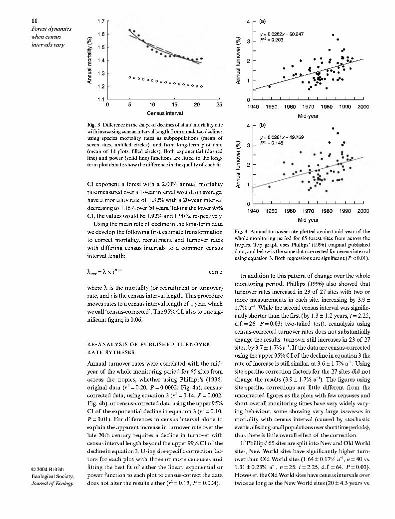
Fig. 3 Difference in the shape of declines of stand mortality rate with increasing census interval length from simulated declines using species mortality rates as subpopulations (mean of seven sites, unfilled circles), and from long-term plot data (mean of 14 plots, filled circles). Both exponential (dashed line) and power (solid line) functions are fitted to the long- term plot data to show the difference in the quality of each fit.

CI exponent a forest with a 2.00% annual mortality

rate measured over a 1-year interval would, on average,

have a mortality rate of 1.32% with a 20-year interval

decreasing to 1.16% over 50 years. Taking the lower 95%

CI, the values would be 1.92% and 1.90%, respectively.

Using the mean rate of decline in the long-term data

we develop the following first estimate transformation

to correct mortality, recruitment and turnover rates

with differing census intervals to a common census

interval length:

X• :Xxt° eqn 3

where X is the mortality (or recruitment or turnover)

rate, and t is the census interval length. This procedure

moves rates to a census interval length of 1 year, which

we call 'census-corrected'. The 95% CI, also to one sig-

nificant figure, is 0.06.

RE-ANALYSIS OF PUBLISHED TURNOVER

RATE SYTHESES

Annual turnover rates were correlated with the mid-

year of the whole monitoring period for 65 sites from

across the tropics, whether using Phillips's (1996)

original data (r' = 0.20, P = 0.0002; Fig. 4a), census-

corrected data, using equation 3 (r^ = 0.14, P = 0.002;

Fig. 4b), or census-corrected data using the upper 95%

CI of the exponential decline in equation 3 (r^ = 0.10,

P = 0.01). For differences in census interval alone to

explain the apparent increase in turnover rate over the

late 20th century requires a decline in turnover with

census interval length beyond the upper 99% CI of the

decline in equation 3. Using site-specific correction fac-

tors for each plot with three or more censuses and

fitting the best fit of either the linear, exponential or

power function to each plot to census-correct the data

does not alter the results either ((-- = 0.13, P = 0.004).

2 -

1 -

(a)

y=0.0262x-50.247 R2 = 0.203

*•

0 1940 1950 1960 1970 1980 1990 2000

Mid-year

4 r (b)

y =0.0261x-49.759 R2 = 0.145

1 -

1940 1950 1960 1970 1980 1990 2000

IVlid-year

Fig. 4 Annual turnover rate plotted against mid-year of the whole monitoring period for 65 forest sites from across the tropics. Top graph uses Phillips' (1996) original published data, and below is the same data corrected for census interval using equation 3. Both regressions are significant (P <0.01).

In addition to this pattern of change over the whole

monitoring period, Phillips (1996) also showed that

turnover rates increased in 23 of 27 sites with two or

more measurements in each site, increasing by 3.9 +

1.7% a"'. While the second census interval was signific-

antly shorter than the first (by 1.3+ 1.2 years, t = 2.25,

d.f. = 26, P = 0.03; two-tailed test), reanalysis using

census-corrected turnover rates does not substantially

change the results: turnover still increases in 23 of 27

sites, by 3.7 ± 1.7% a"'. If the data are census-corrected

using the upper 95% CI of the decline in equation 3 the

rate of increase is still similar, at 3.6 ± 1.7% a"'. Using

site-specific correction factors for the 27 sites did not

change the results (3.9 ± 1.7% a"'). The figures using

site-specific corrections are little different from the

uncorrected figures as the plots with few censuses and

short overall monitoring times have very widely vary-

ing behaviour, some showing very large increases in

mortality with census interval (caused by stochastic

events affecting small populations over short time periods),

thus there is little overall effect of the correction.

If Phillips' 65 sites are split into New and Old World

sites. New World sites have significantly higher turn-

over than Old World sites (1.64 ± 0.17% a"', « = 40 vs.

1.31+0.23% a-', w = 25; r = 2.25, d.f. = 64, P = 0.03).

However, the Old World sites have census intervals over

twice as long as the New World sites (20 ± 4.3 years vs.

12 S. L. Lewis et al.

© 2004 British Ecological Society, Journal of Ecology

8.8+ 1.4 years). When we census-corrected turnover rates for New and Old world sites, average turnover rates were not significantly different (1.92 + 0.21 vs. 1.63 + 0.27% a-'; r = 1.70, d.f = 64, P = NS). The non- significant difference narrows if we use the upper 95% CI for the decline in equation 3 (2.19 + 0.25 vs. 1.94 + 0.32% a-'; t = 1.70, d.f = 64, P = NS).

The Old World sites reported by Phillips (1996) were also, on average, measured over a decade earlier in the 20th century than the New World sites (mean of 1971 vs. 1982). Simply adjusting the turnover value for each site to the average mid-year of the data set (1978) using the equation in Fig. 4(b) ('time-corrected' data) sug- gests that the turnover rates of the New and Old World sites are very similar: 1.54±0.16%and 1.47±0.22%a"', respectively. When turnover values are corrected for both census-interval differences and when a study took place, this gives mean turnover rates for both New and Old World sites that are almost identical: 1.81+0.19% and 1.80 + 0.15% a"', respectively. The mean census- corrected and time-adjusted (to 1978) turnover rate for the 65 plots from across the tropics is 1.81 +0.16%a"'.

Discussion

DECLINES IN MORTALITY RATES OVER TIME

We have shown that stand-level mortality rates decline with increasing census interval length, as predicted from theory, whether rates are simulated using the mortality rates of many species in a stand as subpopu- lations, or derived from monitoring cohorts of trees in long-term multicensus plots (Figs 1, 2 and 3, Tables 3 and 4). Although declines are modest on an annual basis, correcting for census interval differences using our empirically derived equation 3 may result in the re-appraisal of differences in dynamics between differ- ent forests. For example, two sites from Phillips' (1996) analysis. Caño Rosalba (CRI), Venezuela, and Kade (Kl), Ghana, both have reported annual turnover rates of 1.49%, but these are obtained from census intervals of 2 and 25 years, respectively. Census-corrected turn- over rates suggest that Kade has higher annual turnover than Caño Rosalba (1.93% vs. 1.57%). More recently published studies further highlight how differing cen- sus interval lengths can impact on intersite compari- sons: the annual mortality rate for Budongo, Uganda, between 1939 and 1993 is 1.05% (Shell et al. 2000), while the reported rate at Pasoh, Malaysia, between 1987 and 1990 is 1.16% (Condit et al. 1999), 10% higher than Budongo. When the results are census-corrected Budongo has a higher mortality rate (1.42%) than Pasoh (1.26%).

The long-term plot data, while showing average declines in mortality rate with increasing census interval, are extremely variable. Of the 14 plots studied, 11 showed decreases, five of which were significant, while three, counter to our theoretical predictions, showed increases, of which two were significant (Sungei Menyala, Bukit

Lagong). We suggest that these increases may be caused by long-term non-linear temporal changes in mortality and recruitment rates. Our methods of accounting for potential increases in mortality rates over the late 20th century assume that any change, if present, is linear. This may not be the case, and some non-linear changes in forest dynamics may cause increases in mortality rates with increasing census intervals, as calculated using the methods described in this paper. For example, if the recruits to a plot have differing mortality rates, and mortality distribution, compared with the stems that died, and these temporal changes are systematic and non-linear, then this would affect the changes in mortality rates we detect with lengthening census inter- vals, including scenarios where an increase in mortality rate with lengthening census intervals is discoverable. However, the precise cause(s) of these increases in mortality rates with increasing census interval requires further research.

A power function provides the best fit for 10 of the 14 long-term plots, and on average this was a best fit across the 14 plots. However, as discussed, the data are highly variable. This may be caused by inherent sto- chastic variation, or measurement errors, ormay reñect different functional forms of decline in different forests. We do not know whether the distribution of mortality rates of stems in different forests are similar or quite different, thus at present it is unknown whether our empirical approach either identifies the correct func- tional form, or, indeed, that a single functional form is applicable to all forests. We firstly used a generic cor- rection factor derived from the mean decline from all 14 long-term plots to correct other data. This is better than ignoring the census interval problem, but if dif- ferent forests have different functional forms of decline, then a site-specific correction may be more appro- priate. However, site-specific corrections will often be based on very few data points from a single site, or from a single small plot, and thus will include large stochas- tic variation leading to a poor estimate of the rate of decline for a single site. Some of the site-specific esti- mates from plots with only two intervals actually show very large increases in mortality with increasing census interval, for which there is no obvious cause, and this is likely to be merely variability in the system. For these reasons, we suggest that corrections may be done on both a generic, and where possible, site-specific basis. Nevertheless, we recommend a generic correction at this stage, as (i) the variation in mortality rates over short time periods and small sample sizes is known to be very large, and (ii) the simulation data suggest that different forests may have similar functional forms of decline.

The most striking result is that the long-term forest plot data show a much steeper rate of decline in mor- tality over shorter census intervals than the simulations using species as subpopulations (Fig. 3). The steepness of the decline in mortality rate with increasing census interval is governed by the distribution of mortality

13 rates of all stems, with notably steep declines associated Forest dynamics with a fraction of the population having much higher when census mortality rates than the rest (Shell & May 1996). This intervals vary suggests that trees in the cohorts measured in the

long-term plots contained subpopulations with very high mortality rates, which once dead left trees with a relatively narrow distribution of mortality rates (hence the flattening of the curve in Fig. 3 beyond c. 15 years). These very high mortality subpopulations were not captured by the species mortality rates we included in equation 2. Three possible explanations for this are examined below, (i) The simulations sampled only commoner species and thereby may have under- represented rarer species, some of which may have very dynamic populations, (ii) The assumptions that mor- tality rates were equal for all individuals within a species and that the mortality rate of a given stem was constant and independent of other stems may be incor- rect, (iii) There may have been temporal fluctuations in mortality.

The simplest explanation of why the large-scale data sets did not include all the variation in mortality rates is that by including only species with > 20 stems, we only included commoner species. These stems repres- ent 35 + 13% of all species at a site (range 13-58%), and 77+ 13% of aU stems at a site (range 44-97%). Conceivably, rarer species will show wider variation in mortality rates than commoner species; for example, very 'early successional' species, which often have high mortality rates, tend to occur at low densities in old-growth forests (Swaine 1994; Condit et al. 1995). Although comparing simulated declines with only very common species (> 80 stems), rather than species with > 20 stems, did not show large differences at Pasoh and North Queensland, there was a large difference at BCL This may be because BCI is known to have a large and relatively common pioneer community that is largely absent at Pasoh and in North Queensland (Condit et al. 1999). Thus the simulations may have under- represented the distribution of mortality rates within a stand.

All individuals within a species were assumed to have the same probability of dying, but any within-species differences could further increase heterogeneity. Exam- ples include possible differences in mortality rate by size class, and differing mortality rates when stems of the same species occupy different microhabitats. Dif- ferences in the mortality rate of a given species by size class have been documented at several sites, thus these mechanisms could plausibly widen the distribution of mortality rates within a forest stand (Mervart 1972; HubbeU & Foster 1990; Vanclay 1991; Clark & Clark 1992).

The results from the simulations are constrained by the assumptions in equation 2, primarily that the probability of mortality of a given stem is constant and

© 2004 British independent of its neighbours (Sheü & May 1996). Obvious Ecological Society, violations of these assumptions include local com- Journal of Ecology petition for limiting resources, and the impact of other

stems dying nearby. With local competition two iden- tical individuals would have different probabilities of dying depending on the competitive interactions with their respective neighbours. This may explain why slow growing individuals have higher mortality rates than faster growing equivalent-sized individuals (Swaine et al. 1987a,b). Mortality events do impact on nearby trees, for example, increasing mortality through dam- age to the remaining trees or decreasing mortality through increasing levels of essential resources, such as light following canopy opening (Lewis 1998). The much steeper declines in mortality in the long-term plot data suggest these types of effects may be import- ant processes in real populations.

Finally, the simulations do not include possible changes in the distribution of mortality rates over time. This is likely, because the environmental noise that affects processes that in turn affect tree mortality rates (e.g. droughts, Condit et al. 1995, wind events. Nelson et al. 1994, or diseases) may become more variable as the study period is extended. This is because environ- mental noise is not random ('white noise'), but is char- acterized by strong correlations on many scales ('pink noise'; Halley 1996; Gisiger 2001). The longer plots are monitored, the more likely it is that environmental conditions will be such that the mortality rates of some subpopulations will be temporarily increased, so lead- ing to a longer 'tail' in the mortality rate distribution and increasing the steepness of decline in mortality with increasing census interval. The potential impact of temporal changes in mortality-rate distributions is considerable; for example, the Pasoh 50-ha plot showed highly significant differences in mortality rate between 1987 and 1990 (1.16%), and between 1990 and 1995 (1.60%) (Condit et al. 1999). Due to the large size of the Pasoh plot, these differences are very unlikely to be explained by very local mosaic/successional effects, which suggests that differing environmental conditions caused the differing stand mortality rates, and hence the distributions of mortality rates of the component subpopulations changed over time.

REANALYSIS OF PREVIOUS RESULTS

The conclusion that turnover rates have increased in tropical forests over the late 20th century is robust to the charge that this is an artefact due to the combina- tion of data that vary in census interval (cf Shell 1995). Two tests using Phillips's (1996) expanded turnover data set show that the census interval effect does not affect Phillips' conclusions about turnover increasing over time, whether using the generic census correction in equation 3 or site-specific corrections, where appli- cable (Fig. 4). To account for the increase in turnover, the declines in turnover with increasing census interval would have to be beyond the upper 99% CI of the decline parameter reported here, which is very unlikely.

Shell's (1995) original critique of the evidence for increasing turnover over the late 20th century also

14 S. L. Lewis et al.

© 2004 British Ecological Society, Journal of Ecology

suggests that the apparent increase could be explained by a single event, the 1982-83 El Niño Southern Oscil- lation (ENSO), as many of the recent data spanned this event. However, the rigorous assessment of the hypo- thesis that the apparent increase in turnover rates is due to a short-term response to an extreme synchronized global event, such as the 1982-83 ENSO, or more generally to a possible late 20th century increase in the frequency and intensity of ENSO events, is beyond the scope of this paper. Quantifying to what extent a forest is 'ENSO-affected' and quantifying whether ENSO events are more intense and frequent later in the 20th century, and then understanding whether individual ENSO events are driving local and global changes in turnover values, remains a challenge for ecologists (Lewis et al. 2004b; Malhi & Wright 2004). How- ever, recent analyses from Amazonia have shown that growth, recruitment and mortality rates have simultane- ously increased within the same plots over the 1980s and 1990s, as has net above-ground biomass, both in areas largely unaffected, and in those strongly affected, by ENSO events (Baker et al. 2004; Lewis et al. 2004a; Phillips et al. 2004). Factors that potentially explain such widespread and simultaneous changes should be the subject of detailed investigations.

If turnover rates have been increasing over time, as current evidence suggests, then it becomes important to know when the plots to be compared were measured. Comparing data from, say, the 1960s with data from the 1990s may lead to erroneous conclusions. Indeed, if forest dynamics have been accelerating over recent decades then standardizing for the year of monitoring will need to become standard practice. More generally, as evidence accumulates that ecosystems are responding to global change, particularly to increases in atmos- pheric carbon dioxide concentrations, nitrogen inputs, temperature increases and changes in rainfall patterns, much ecological data may become difficult to interpret without considering when studies took place.

The Old World forest plots compiled by Phillips (1996) were censused much earlier in the last century than the New World plots, with mean mid-years of 1971 and 1982, respectively. Adjusting turnover rates from the New and Old World plots to a common census interval length, using equation 3, and a common mid- year of monitoring gives almost identical turnover rates for the New and Old World tropics ( 1.81 vs. 1.80% a"'). This result seems sensible, as there is no a priori reason why many plots from many soil types and cli- mates from one continent should have higher turnover rates than many plots from many soil types and climates from three other continents combined. The current best estimate of the pan-tropical average annual turnover rate for tropical forests is therefore 1.81% (mode = 2.06, median =1.78, SD = 0.64, min = 0.60, max = 3.71), for an average census mid-year of 1978 and a census interval length of one (using equation 3). Forests can therefore be defined as less or more dynamic based on the number of standard deviations

standardized plot turnover data are from the mean, or in relation to the median or mode, due to the strong right skew (0.69) and lesser leptokurtosis (0.39) of the distribution.

RECOMMENDATIONS

Mortality, recruitment and turnover rates decline with increasing census interval, as previously shown theoretically, and now demonstrated empirically. This effect should be taken into account. In addition, stand dynamic rates are highly variable over short time-scales and small spatial scales. The frequency of measure- ment and plot size needed for any field study will clearly depend upon the questions being asked and resources available. For example, the most accurate stand level rates for comparisons with other plots will always come from monitoring many trees for many years, while trends over time are probably most accurately eluci- dated by annual measurements. However, common protocols are required for comparative studies. Cur- rently, probably the most common census interval length is the 5-year interval, which is becoming a de facto standard (seemingly due to resource constraints). In order to maximize intercensus and intersite com- parability we therefore recommend collecting and report- ing results in intervals as near to 5 years as possible, as well as reporting results for each interval and for the longest period possible. This combination of results reduces census interval problems, and provides the most accurate results. If adequate data are available, then the calculation of a site-specific correction factor using the methods described in this paper may be appropriate. For comparisons where census intervals do unavoidably vary, and robust local corrections are unavailable, then standardization to account for the census interval artefact, using equation 3, will be necessary.

Acknowledgements

This work on permanent sample plot methodologies and analyses is funded by the UK Natural Environ- ment Research Council (NER/A/S/2000/00532 and GR9/04635) and the EU Fifth Framework programme (CARBONSINK-LBA). Y. Malhi is funded by the Royal Society. We thank E. Losos and R. Condit for helping to access the CTFS data sets, and M. Swaine and the University of Ghana Botany Department for providing unpublished data (Kade). Mortality data analysed for the first time here were collected with the support of the following: J. Froment, J. Vautherin, P. Seme, J. Rössel of ECOFAC, and the 6th FED EU project (Dja Faunal Reserve site); Brazil's National Institute for Amazonian Research (INPA), MCT, the European Union and Department for International Development (UK), and CNPq, Brazil (BIONTE site); NASA-LBA, Andrew W Mellon Foundation, US Agency for International Development, Smithsonian

15

Forest dynamics

when census

intervals vary

© 2004 British Ecological Society, Journal of Ecology

Institute (Biological Dynamics of Forest Fragments

Project site); the late A.H. Gentry, F Ángulo, C. Díaz,

J. Janovec, N. Jaramillo, K. Johnson, S. Rose, M. Stern,

M. Sánchez, INRENA, Cuzco Amazónico, Peruvian

Safaris S.A., UNSAAC, American Philosophical Soci-

ety, NGS (5472-95), National Science Foundation,

WWF-US/Garden Club of America, Conservation

International, MacArthur and Mellon Foundations,

National University of San Antonio de Abad de

Cusco, and a NERC Research Fellowship to OP (SE

Peru site); Forest Research Institute of Malaysia, US

National Science Foundation, Smithsonian Tropical

Research Institute (Pasoh site); Professor J. P. Veillon

and colleagues of the Instituto de Silvicultura, Uni-

versidad de Los Andes, Merida, Venezuela, USDA

International Institute of Tropical Forestry and the

University of Illinois (Agreement no. 19-91-064)

(Carbonara); Uganda Forest Department, ODA (now

DFID) Forestry Research Programme (R4737), Mak-

erere University Herbarium, Budongo Forest Project

team, Kew Herbarium, Tony Katende, Olivia Maganyi,

Andy Plumptre, Chris Bakuneeta, Abel Musinguzi,

Silvano Muringeera, Rufino Tolit, Tim Synnott, Peter

Savill, Quentin Cronk, Jo Eggeling, Colyear Dawkins

and Howard Wright (Budongo); Dr Geoff Stocker and

colleagues at CSIRO (Mt Lewis, Mt Haig). We also

thank Jerome Chave and an anonymous referee for

valuable comments on the manuscript.

References

Baker, T.R., Phillips, O.L., Malhi, Y, Almeida, S., Arroyo, L., Di Fiore, A. et al. (2004) Increasing biomass in Amazon forest plots. Philosophical Transactions of the Royal Society of London Series B-Biology Sciences, 359, 353-365.

Begon, M., Harper, XL. & Townsend, C.R. (1996) Ecology: Individuals, Populations and Communities. Blackwell Scien- tific, Oxford.

Carey, E.V., Brown, S., Gillespie, A.J.R. & Lugo, A.E. (1994) Tree mortality in mature lowland tropical moist and trop- ical lower montane moist forests of Venezuela. Biotropica, 26, 255-265.

Clark, D.A. & Clark, D.B. (1992) Life-history diversity of canopy and emergent trees in a neotropical rain-forest. Ecological Monographs, 62, 315-344.

Condit, R. (1997) Forest turnover, density, and COj. Trends in Ecology and Evolution, 12, 249-250.

Condit, R., Ashton, RS., Manokaran, N., LaFrankie, J.V, Hubbell, S.R & Foster, R.B. (1999) Dynamics of the forest communities at Pasoh and Barro Colorado: comparing two 50-ha plots. Philosophical Transactions of the Royal Society of London Series B-Biology Sciences, 354, 1739- 1748.

Condit, R., Hubbell, S.R & Foster, R.B. (1995) Mortality- rates of 205 neotropical tree and shrub species and the impact of a severe drought. Ecological Monographs, 65, 419^39.

Connell, J.H., Tracey, J.G. &Webb, L.J. (1984) Compensatory recruitment, growth and mortality as factors maintaining rain-forest tree diversity. Ecological Monographs, 54, 141- 164.

Favrichon, V. (1994) Classification of Guiana tree species into functional-groups for a dynamic community matrix of vegetation. Revue D Ecologie-la Terre et la Vie, 49, 379- 403.

Gale, N. & Barfod, A.S. (1999) Canopy tree mode of death in a western Ecuadorian rain forest. Journal of Tropical Ecology, \5, 415^^6.

Gentry, A.H. & Terborgh, J. (1990) Composition and Dynamics of the Cocha Cashu 'Mature' Floodplain Foresta. Four Neotropical Rainforests (ed. A.H. Gentry), pp. 542-564. Yale University Press, New Haven, Connecticut.

Gisiger, T. (2001) Scale invariance in biology: coincidence or footprint of a universal mechanism? Biology Reviews, 76, 161-209.

Halley, J.M. (1996) Ecology, evolution and l//-noise. Trends in Ecology and Evolution, 11, 33-37.

Hartshorn, G.S. (1990) An overview of neotropical forest dynamics. Four Neotropical Rainforests (ed. A.H. Gentry), pp. 585-599. Yale University Press, New Have, Connecticut.

Hubbell, S.R & Foster, R.B. (1990) Structure, dynamics, and equilibrium status of old-growth forest on Barro Colorado Island. Four Neotropical Rainforests (ed. A.H. Gentry), pp. 522-541. Yale University Press, New Haven, Connecticut.

Kochummen, K.M., LaFrankie, J.V. & Manokaran, N (1990) Floristic composition of Pasoh Forest Reserve, a lowland rain forest in Peninsular Malaysia. Journal of Tropical Forest Science, 3, 1-13.

Krebs, C.J. (1999) Ecological Methodology. Benjamin/Cum- mings, Menlo Park, California.

Kubo, T., Kohyama, T., Potts, M.D. & Ashton, RS. (2000) Mortality rate estimation when inter-census intervals vary. Journal of Tropical Ecology, 16, 753-756.

Laurance, W.F., Fearnside, P.M., Laurance, S.G., Delamonica, P., Lovejoy, T.E., Rankin-de Merona, J. etal. (1999) Relation- ship between soils and Amazon forest biomass: a landscape- scale study. Foreí/£co/og)'a«a'A/a«ageme«¿, 118,127-138.

Laurance, W.F., Ferreira, L.V, Rankin-de Merona, J.M. & Laurance, S.G. (1998) Rain forest fragmentation and the dynamics of Amazonian tree communities. Ecology, 79, 2032-2040.

Lewis, S.L. (1998) Treefall Gaps and regeneration: a compar- ison of continuous andfragmentedforest in central Amazonia. PhD thesis, University of Cambridge, Cambridge.

Lewis, S.L., Malhi, Y & Phillips, O.L. (2004b) Fingerprinting the impacts of global change on tropical forests. Philosoph- ical Transactions of the Royal Society of London Series B- Biology Sciences, 359, 437^62.

Lewis, S.L., Phillips, O.L., Baker, T.R., Lloyd, J, Malhi, Y, Almeida, S. et al. (2004a) Concerted changes in tropical forest structure and dynamics: evidence from 50 South American long-term plots. Philosophical Transactions of the Royal Society of London Series B-Biology Sciences, 359, 421-436.

Lewis, S.L. & Tanner, E.V.J. (2000) Effects of above- and belowground competition on growth and survival of rain forest tree seedlings. Ecology, 81, 2525-2538.

Lieberman, D., Lieberman, M., Peralta, R. & Hartshorn, G.S. ( 1996) Tropical forest structure and composition on a large- scale altitudinal gradient in Costa Rica. Journal of Ecology, 84, 137-152.

Malhi, Y & Wright, X (2004) Spatial patterns and recent trends in the climate of tropical rainforest regions. Philo- sophical Transactions of the Royal Society of London Series B-Biology Sciences, 359, 311-329.

Manokaran, N. (1988) Population dynamics of tropical forest trees. PhD thesis. University of Aberdeen, Aberdeen.

Mervart, J. (1972) Growth and mortality rates in the natural high forest of Western Nigeria. Nigeria Forestry Information Bulletin (New Series), 22, 1-46.

Nelson, B.W., Kapos, V, Adams, JB., Oliveira, WJ, Braun, O.P.G. & Doamaral, I.E. (1994) Forest disturbance by large blowdowns in the Brazilian Amazon. Ecology, 75, 853-858.

Phillips, O.L. (1995) Evaluating turnover in tropical forests. Science, 268, 894-895.

16 Phillips, O.L. (1996) Long-term environmental change in S L Lewis et al tropical forests: increasing tree turnover. Environmental

Conservation, 23, 235-248. Phillips, O.L., Baker, T.R., Arroyo, L., Higuchi, N., Killeen, T. J.,

Laurance, W.F. etal. (2004) Pattern and process in Amazon tree turnover: 1976-2001. Pliilosophical Transactions of tlie Royal Society of London Series B-Biology Sciences, 359, 381-407.

Phillips, O.L. & Gentry, A.H. (1994) Increasing turnover through time in tropical forests. Science, 263, 954-958.

Phillips, O.L., Hall, R, Gentry, A.H., Sawyer, S.A., Vásquez, M. & R. (1994) Dynamics and species richness of tropical rain- forests. Proceedings of the National Academy of Sciences of the United States of America, 91, 2805-2809.

Phillips, O. & Shell, D. (1997) Forest turnover, diversity and CO,. Trends in Ecology and Evolution, 12, 404.

Pitman, N.C.A., Terborgh, J.W., Silman, M.R., Nunez, V.R, Neill, D.A., Cerón, CE. et ai (2001) Dominance and dis- tribution of tree species in upper Amazonian terra firme forests. Ecology, 82, 2101-2117.

Rai, S.N. (198l)Floristic composition and survival pattern of tropical rain forest tree species of Western Ghats, India. Myforest, June, 101-110.

Shell, D. (1995) Evaluating turnover in tropical forests. Science, 268, 894.

Shell, D., Burslem, D.F.R.P & Alder, D. (1995) The inter- pretation and misinterpretation of mortality-rate measures. Journal of Ecology, 83, 331-333.

Shell, D., Jennings, S. & Savill, P. (2000) Long-term perman- ent plot observations of vegetation dynamics in Budongo, a Ugandan rain forest. Journal of Tropical Ecology, 16, 765-800.

Shell, D. & May, R.M. (1996) Mortality and recruitment rate evaluations in heterogeneous tropical forests. Journal of ico/ogj, 84, 91-100.

Sokal, R.R. & Rohlf, F.J. (1995) Biometry. The Principles and Practice of Statistics in Biology Research, 2nd edn. W.H. Freeman, New York.

Sonké, B. ( 1998) Etudes Floristiques et Structurales Des Forets de la Reserve de Faune Du Dja ( Cameroun). PhD thesis, Universite Libre de Bruxelles, Belgium.

Swaine, M.D. (1994) Long-term studies of tropical forest dynamics. Long-Term Experiments in Agricultural and Ecological Sciences (eds R.A. Leigh & A.E. Johnston), pp. 305-316. CAB International, Wallingford.

Swaine, M.D., Hall, J.B. & Alexander, I.J. (1987a) Tree population-dynamics at Kade, Ghana (1968-82). Journal of Tropical Ecology, 3, 331-345.

Swaine, M.D., Lieberman, D. & Putz, F.F. (1987b) The dynamics of tree populations in tropical forest - a review. Journal of Tropical Ecology, 3, 359-366.

Vanclay, J.K. (1991) Mortality functions for North Queensland rain forests. Journal of Tropical Forest Science, 4, 15-36.

Vásquez, M.R. & Phillips, O.L. (2000) Allpahuayo: floristics, structure, and dynamics of a high-diversity forest in Amazonian Peru. Annals of the Missouri Botanical Garden, 87, 499-527.

Veillon, J.P (1985) El crecimento de algunos bosques nat- urales de Venezuela en relación con los parámetros del medio ambiente. Revista Forestal Venezolana, 29, 5-121.

Received 10 December 2003 revision accepted 5 May 2004 Handling Editor: Joseph Wright

© 2004 British Ecological Society, Journal of Ecology