Methods in Psychiatry

Finding Our Way: An Introduction to Path AnalysisDavid L Streiner, PhD'

Path analysis is an extension of multiple regression. It goes beyond regression in that itallows for the analysis of more complicated models. In particular, it can examine situationsin which there are several final dependent variables and those in which there are "chains"of influence, in that variable A influences variable B, which in tum affects variable C.Despite its previous name of "causal modelling." path analysis cannot be used to establishcausality or even to determine whether a specific model is correct; it can only determinewhether the data are consistent with the model. However, it is extremely powerfiil forexamining complex models and for comparing different models to determine which onebest fits the data. As with many techniques, path analysis has its own unique nomenclature,assumptions, and conventions, which are discussed in this paper.

(Can J Psychiatry 2005;50:115-122)Information on author affiliations appears at the end ofthe article.

Highlights

• Path analysis can be used to analyze models that are more complex (and realistic) thanmultiple regression.

• 11 can compare differeni models to delennine which one best tits the data.• Path analysis ean disprove a model that postulates causal relations among variables, but it

cannot prove causality.

Key Words: path analysis, structural equation modelling, multiple regression

One ofthe first things we leam in introductory statistics isthat there are 2 types of variables: independent variables

(IVs) and dependent variables (DVs). The distinctionbetween them is in most cases relatively clear and straight-forward: we want to see what effect the IVs {sometimes calledpredictor variables in multiple regression) have on the DV.For example, if we compare antidepressant medication withcognitive-behavioural therapy to see which leads to greaterremission in depressive symptoms, the IV is the type of treat-ment, and the DV is. perhaps, the score on a depression scale.In selecting candidates for medical school, the DV would besuccessful graduation, or not, and the IVs could be previousgrade point average, a numerical grade assigned to letters ofreference, qualifying examination scores, and so on.

Unfortunately, the real worid refuses to fall into just these 2 cat-egories of variables. Life insists on being more complicated,and there are situations in which, if we are asked whether a cer-tain variable is a DV or an IV, we would have to say, "Yes."Let's assume, for example, that we found that women withyoung children at home suffer more from depression thanwomen matched for age and marital status who do not have kids

at home. One hypothesis is that children at home cause womento suffer from depression, based on the well-known fact thatkids can drive us crazy. This is the model shown on the top ofFigure 1—children at home have a direct effect on depression.However, another hypothesis is that staying at home leads tosocial isolation and that the isolation leads to dysphoria. This isthe model on the bottom of Figure 1.

In both models, it is obvious that children at home is the IVand depression is the DV. But what do we call isolation? It is aDV with respect to children, but it is an IV as regards depres-sion. In fact, the problem goes beyond mere terminology; thedeeper problem is how we should analyze the lower model.The issue becomes more complicated as our models becomemore complex. For example, we can posit that other factorsmay influence depression directly, for example, honnonalchanges or past depression and family history of depression;that children at home cause other stresses that in tum affect thewoman's mood; and that there can be outcomes in addition todysphoria. If we want to look at all these variables simulta-neously, we need both new tenninology and a new analyticstrategy.

Can J Psychiatry, Vol 50, No 2, February 2005 • 115

The Canadian Journal of Psycbiatry—Research Methods in Psychiatry

Figure 1 Two possible models of the effects of childrenat home on depression

Childrenat Home

Childrenat Home

Isolation

Depression

Depression

The name for the strategy eomes from the pictorial representa-tion ofthe models themselves. In the bottom of Figure 1, weare describing a path from children to isolation to depression.More complicated models may have more paths, or paths thatlead through more variables. Not surprisingly, then, this tech-nique is called path analysis. Path analysis is an extension ofmultiple regression that allows us to examine more compli-cated relations among the variables than having several IVspredict one DV and to compare different models against oneanother to see which one best fits the data. Before we begin.,though, a disclaimer about both the statistics and the temiinol-ogy. In the past (and occasionally now. among the benighted),this technique was referred to as eausal modelling, because itwas believed that it could be used to uncover causal pathways

Figure 2 Some possible path models

among variables—which factors were responsible for whatoutcomes. As we'll see later, this is a laudable goal but onethat cannot be solved by statistical methods, no matter howpowerful. From a statistical vantage point, models that mapout totally bizarre routes that can never exist in reality maylook as good—or even better—than models that conformmore closely to reality. Causality can be proven only throughthe correct research design (for example, longitudinal studiesor experiments), and no amount of statistical legerdemain canpull cause and effect out of a eross-sectional or cohort study.

Some Terminology and Drawing ConventionsTo return to the naming ofthe variables. In path analysis (andin its more sophisticated counterpart, structural equation mod-elling, which will be discussed in a later paper), we com-pletely avoid the confusion about IVs and DVs by the simpleexpedient of not using those labels. Rather, we use the termsexogenous and endogenous variables:• Exogenous variables bave straight arrows emerging from

them and none pointing to them {except from errorterms). i

• Endogenous variables have at least one straight arrowpointing to them.

The rationale for these terms is that the causes of (or factorsthat influence) exogenous variables are determined outsidetbe model that we're examining; whereas the factors affectingendogenous variables exist within the model itself, in a

Children

Isolation

(a)

Depression

Children

Isolation

(d)- ^

Depression

Children

Isolation

(b)- ^

Depression

(e)Children Depression

\ 7Isototion

Children

Isolation

(c)Depression

Anxiety

Chiidren

Isolation

(t)Depression

Anxiety

116• Can J Psychiatry, Vol 50, No 2. February 2005

Fmding Our Way: An Introduction to Path Analysis

moment, we'll see why there is that restriction on the shape(not the moral fibre) ofthe arrow. Thus, in the bottom of Fig-ure I. having children is an exogenous variable, and bothsocial isolation and depression are endogenous ones. Let'stake a look at some other possible models.

In Figure 2a, we are hypothesizing that exogenous variablesof having children and being isolated independently influencedepression and that children and isolation are not correlatedwith each other. This would be called an independent model,reflecting the lack of correlation between the 2 exogenousvariables. If we believe that the variables are correlated, wedraw a curved, 2-headed arrow between them, as in Figure 2b,where a curved., double-headed arrow reflects a correlation{or eovariance, a term that will be defmed shortly) betweenvariables. This is the run-of-the-mill multiple regressionmodel, although we often have more than just 2 exogenous orpredictor variables. Also, because as Meehl said, "everythingcorrelates to some extent with everything else" (I, p 204), wecustomarily assume that tbe correlations are present—so Iwon't bother to draw the curved arrows (except when neces-sary). In Figure 2c, we are extending the model by looking at 2endogenous variables, depression and anxiety. We are sayingthat having children affects only depression but not anxiety,while isolation influences both depression and anxiety.

The models on the right side of Figure 2 are called mediated orindirect ones, because the exogenous variables act on anendogenous variable, at least in part, through their influenceon an intemiediary (endogenous) variable. Thus, in Figure 2d,having children influences depression directly, as does isola-tion, but having children also affects isolation, which then actson depression; in other words, being isolated would causewomen to suffer from depression even in the absence of chil-dren, but the presence of children exacerbates this effect. Thisis somewhat different from Figure 2e, which is the same as thebottom part of Figure 1 in that isolation is due solely to the rugrats and would not exist in women if not for them. Finally, inFigure 2f, we see that one final endogenous variable (depres-sion) can also affect another one (anxiety). This by no meansexhausts the possibilities. Paths can be much longer andinvolve more intennediate steps, and there could be (and oftenare) more variables brought into the picture—both literallyand figuratively.

Two more tenns need to be introduced. In Figure 3, note thatpointing toward the 2 endogenous variables are small circleswith d's in them. The d's are short for disturbance, which inpath analysis is analogous to the error tenn tacked at the end ofregression equations. As with the error term, the disturbanceterm captures 2 things: 1) imprecision in the measurement ofthe endogenous variable, beeause all our measurement toolsare subject to some degree of error: and 2) all the other factorsaffecting the endogenous variable that we didn't measure

Figure 3 Adding disturbance terms and making themodel nonrecursive

Chiidren

isolation

Depression

Anxiety

because of oversight, lack of time, ignorance of theirimportance, laziness, or whatever. Because every endogenousvariable must have a disturbance term associated with it, weoften don't bother to draw it, to keep the drawing simpler, butif it's not explicitly drawn, it's implicitly present.

Finally (yes!), Figure 3 differs from Figure 2f in one subtle butimportant way. In Figure 2f, one endogenous variable(depression) affects a second (anxiety), whieh is logical, butthe second does not affect the first. It likely makes more clini-cal sense for there to be a path in both directions; that is,depression affects anxiety, and anxiety in turn is depres-sogenic. This latter model, with a feedback loop, is callednonrecursive, whereas path models that lead inexorably in onedirection are referred to as recursive. (No, I didn't inadver-tently reverse the terms. They are, for some unfathomable rea-son, completely and utterly counterintuitive. You'll just haveto live with that.) There is one cardinal rule for attempting toanalyze nonrecursive models: Don't! Although they are of̂ ena more accurate reflection ofthe way things work in the realworld, the analytic problems they produce are horrendous,Even more troubling, these problems are not immediatelyapparent from most computer printouts, especially to neo-phytes, so they are not aware that they are getting into aquagmire.

As we go through some examples, 2 other terms will keepappearing—variances and covariances. (Because they wereprobably first mentioned in introductory statistics. I'm con-sidering them to be old terms, so 1 haven't violated my state-ment about the number of new ones I'm introducing.)Variance is simply the amount of variation in a variable fromone person to another and, fonnally, is the square ofthe stan-dard deviation (SD). A eovariance is the first eousin of a cor-relation. A correlation tells us whether, if variable A goes up,variable B also goes up (a positive correlation), goes down (anegative eorrelation), or changes in a way unrelated to vari-able A (a zero correlation). When we calculate a correlation,both variables are transformed into standard scores that have amean of 0 and an SD of 1. Covariance is exactly the same

Can J Psychiatry, Vol 50, No 2, February 2005 • 117

The Canadian Journai of Psychiatry—Research Methods in Psychiatry

thing, except that the variables aren't transformed but remainin their original units of measurement. For various arcane rea-sons, it is often better to calculate multivariable statistics byusing the covariances among variables rather than their eorre-lations. The reason for our obsession with them is that they areall we have to work with in determining how variables influ-ence each other. When we've done a study measuring severalvariables on each person, what we end up with is a matrix con-sisting ofthe variances of eaeh variable along the main diago-nal (the rows running from the upper left to tbe lower rightcomers) and the eovadanees in all the cells off the main diago-nal. The job of path analysis is to determine whether there areany meaningful pattems in these data.

A Multiple Regression ExampleLet's begin to see what path analysis can do by using a differ-ent example and framing it first in multiple regression terms.In previous articles in this series, you have been introduced toa disorder not yet found in the DSM—photonumerophobia,whieh is the fear that our fear of numbers will come to light.We may want to see whether a person's seore on a scale ofphotonumerophobia (the PNP scale, which ironically isscored using numbers) can be predicted from 3 factors: over-all level of anxiety (ANX), high school math grade (HSM),and the discrepancy between what the person estimated lastyear's taxes to be and what the tax people said it actually was(TAX). That is, we are hypothesizing that photo-numerophobia is related to a person's overall anxiety level(we would expect a positive correlation) as well as to doingpoorly in math class (a negative correlation) and to screwingup one's income tax returns (again a positive correlation: thegreater the mistake, the more severe the phobia). If we wrotethis out as a regression, it would look like

=6., + /j, ANX + bMSM + bJAX + Error

Figure 4 Hypothesized model (a) and results (b) ofthe regression equation

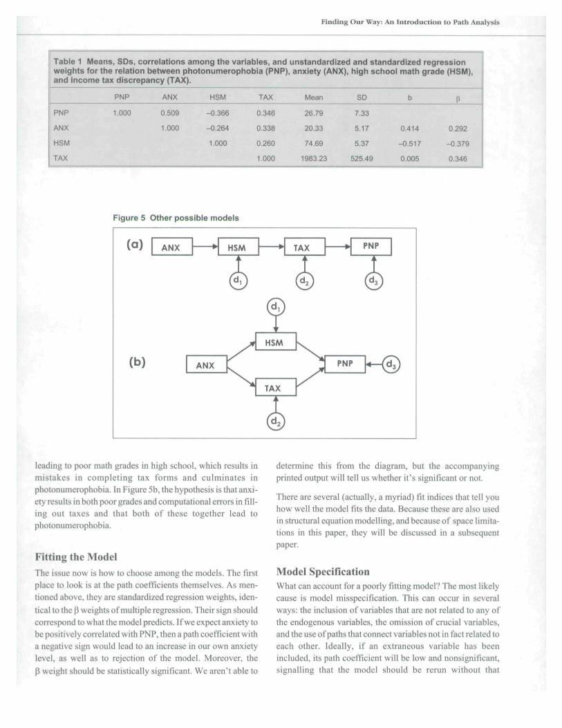
where bo is the intercept, and the other b^s are the slopes foreach IV. The means and SDs ofthe variables and the correla-tions among them are shown in Table I, as are the unstandard-ized regression weights {b) and the standardized ones (P).(Very briefly, the b weights are used with the data in their orig-inal units of measurement; tbe P weights after each variablehave been standardized to have a mean of 0 and an SD of 1.For a more complete description of the difference, see 2,3).The multiple correlation, R. is 0.638, and therefore R~ (thesquare of/?, reflecting the proportion of variance in the DVaccounted for by the equation) is 0.407. '

In the conventions of path analysis, each IV or predictor vari-able (now called an exogenous variable) would be shown as arectangle, with another rectangle for the DV, or endogenousvariable, as in the left side of Figure 4. Beeause computer pro-grams suffer from severe organic brain damage, it's necessaryto draw the curved arrows reflecting correlations among thevariables and the disturbance term. When we run the program,we'll get reams of paper, but most ofthe results can be sum-marized in a diagram, shown in the right side of Figure 4. Veryreassuringly, the correlations among the predictors (next tothe curved arrows) agree with the results from the regressionanalysis; as do the p weights, which are printed near the paths(the straight arrows). Finally, the number over the right side ofPNP is the value of/?", which again is identical to the resultsfrom the multiple regression. Also reassuring from a theoreti-cal standpoint is that the signs of tbe paths correspond to whatwe hypothesized.

Let's review what we've accomplished so far. We've taken aproblem that is easily bandied with inexpensive, well-known,and widely available computer programs (for multiple regres-sion) and shown how we ean get identical results by using anexpensive and areane one (for path analysis and structural

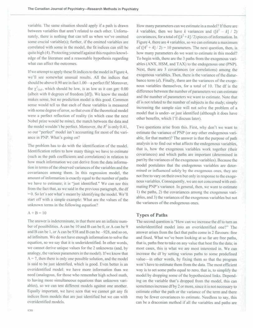
equation modelling). If this isall there is, it reflects progressthat we can easily live without.Fortunately, though (espe-cially for the purveyors ofthesoftware), path analysis can domuch more. For example, wecan postulate other hypothesesabout the relations among thevariables and see whether theyare better or worse in account-ing for the variance in the PNPseale. Two examples areshown in Figure 5. In Figure5a, it 's hypothesized that,rather than the variables actingseparately on PNP, there istruly a path, with anxiety

118• Can J Psychiatry, Vol 50, No 2, February 2005

Finding Our Way: An Introduction to Path Analysis

Table 1 Means, SDs, correlations among the variables, andweights for the relation between photonumerophobia (PNP;and income tax discrepancy (TAX).

PNP

ANX

HSM

TAX

PNP ANX HSM TAX

1.000 0.509 -0.366 0.346

1.000 -0.264 0.338

1.000 0.260

1.000

unstandardizec, anxiety (ANX),

Mean

26.7920.33

74.69

1983.23

andhigh

SD

7.33

5.17

5.37

standardized regressionschool math grade (HSM),

b

0.414-0.517

525.49 0.005

P

0.292

-0.379

0.346

Figure 5 Other possible models

leading to poor math grades in high school, which results inmistakes in completing tax forms and culminates inphotonumerophobia. In Figure 5b, the hypothesis is that anxi-ety resulls in both poor grades and computational errors in fill-ing out taxes and that both of these together lead tophotonumerophobia.

Fitting the ModelThe issue now is how to choose among the models. The firstplace to look is at the path coefficients themselves. As men-tioned above, they are standardized regression weights, iden-tical to the p weights of multiple regression. Their sign shouldcorrespond to what the model predicts. If we expect anxiety lobe positively correlated with PNP, then a path coefficient witha negative sign would lead to an increase in our own anxietylevel, as well as to rejection of the model. Moreover, the(J weight should be statistically significant. We aren't able to

determine this from the diagram, hut the accompanyingprinted output will tell us whether it's significant or not.

There are several {actually, a myriad) fit indices that tell youhow well the model fits the data. Because these are also usedin structural equation modelling, and because of space limita-tions in this paper, they will be discussed in a subsequentpaper.

Model SpecificationWhat ean account for a poorly fitting model? The most likelycause is model misspecification. This can occur in severalways: the inclusion of variables that are not related to any ofthe endogenous variables, the omission of crucial variables,and the use of paths that connect variables not in fact related toeach other. Ideally, if an extraneous variable has beenincluded, its path coefficient will be low and nonsignificant,signalling that the model should be rerun without that

Can J Psychiatry. Vol 50, No 2. February 2005 • 119

The Canadian Journal of Psychiatry—Research Methods in Psychiatry

variable. The same situation should apply if a path is drawnbetween variables that aren't related lo each other. Unfortu-nately, there is nothing that can tell us when we've omittedsome crucial variable{s); further, if the omitted variables arecorrelated with some in the model, the fit indices can still bequite high (4). Proteeting yourself against this requires knowl-edge ofthe literature and a reasonable hypothesis regardingwhat can affect the outcomes.

I f we attempt to apply these fit indices to the model in Figure 4,we'll see somewhat unusual results. AU the indices thatshould be above 0.90 are in fact 1.00—a perfect fit! Moreover,the x̂ GoF, which should be low, is as low as it can get: 0.00(albeit with 0 degrees of freedom [df|). We know the modelmakes sense, but no prediction model is this good. Commonsense would tell us that each of these variables is measuredwith some degree of error, so that even if the theoretical modelwere a perfect reflection of reality (in which case the nextNobel prize would be mine), the maleh between the data andthe model wouldn't be perfect. Moreover, the R^ is only 0.41,so our "perfect" model isn't accounting for most ofthe vari-ance in PNP. What's going on?

The problem has to do with the identification ofthe model.Identification refers to how many things we have to estimate(such as the path coefficients and correlations) in relation tohow much infonnation we can derive from the data informa-tion in terms ofthe observed variances ofthe variables and thecovariances among them. In this regression model, theamount of information is exactly equal to the number of pathswe have to estimate; it is "just identified." We can see thisfrom the faet that, as we said in the previous paragraph, the df^ 0. So let's see what's meant by identifying the model. We'llstart off with a simple example: What are the values of theunknown terms in the following equation?

A + B - 10

The answer is indeterminate, in that there are an infinite num-ber of possibilities. A can be 10 and Bean be 0, or A can be 9and B can be 1, or A can be 938 and B can be -928, and so on,ad infinitum. We do not have enough information to solve theequation, so we say that it is underidentified. In other words,we cannot derive unique values for the 2 unknowns (and, byanalogy, the various parameters in the model). If we know thatA ̂ 7, then there is only one possible solution, and the modelis said to be just identified, which is good. Even better is anoveridentified model: we have more information than weneed (analogous, for those who remember high school math,to having more simultaneous equations than unknown vari-ables), so we can test different models against one another.Equally important., we have seen that we cannot get any fitindices from models that are just identified but we can withoveridentified models.

120

How many parameters can we estimate in a model? If there arek variables, then we have k variances and ( [ ^ - k] I 2)eovadanees, for a total of ([A^ + k'\l2) pieees of information. InFigure 4, there are 4 variables, so we can estimate a maximumof ([4"̂ + 4] / 2) = 10 parameters. The next question, then, ishow many parameters do we want to estimate in this model?To begin with, there are the 3 paths from the exogenous vari-ables (ANX, HSM, and TAX) to the endogenous one (PNP).Next, there are 3 covarianees (or correlations) among theexogenous variables. Then, there is the variance ofthe distur-bance term {d). Finally, there are the variances ofthe exoge-nous variables themselves, for a total of 10. The df is thedifference between the number of parameters we can estimateand the number of parameters we want to estimate. Note thatdf is not related to the number of subjects in the study; simplyincreasing the sample size will not solve the problem of amodel that is under- or just identified (although it does haveother benefits, which I'll discuss later).

Two questions arise from this. First, why don't we want toestimate the variance of PNP (or any other endogenous vari-able, for that matter)? The answer is that the purpose of pathanalysis is to fmd out what affects the endogenous variables,that is, how the exogenous variables work together (theireovariances) and which paths are important (determined inpart by the variances ofthe exogenous variables). Because themodel postulates that the endogenous variables are deter-mined or influenced solely by the exogenous ones, they arenot free to vary on their own but only in response to the exoge-nous variables. Consequently, we are not concerned with esti-mating PNP's variance. In general, then., we want to estimate1) the paths, 2) the covariances among the exogenous vari-ables, and 3) the variances ofthe exogenous variables but notthe variances ofthe endogenous ones.

Types of PathsThe second question is "How can we increase the df to tum anunderidentified model into an overidentified one?" Theanswer arises from the faet that paths come in 2 flavours; freeand fixed. What we've been looking at so far are free paths,that is, paths free to take on any value that best fits the data; inmost cases, this is what we are most interested in. We canincrease the df by setting various paths to some predefinedvalue—in other words, by fixing them so that the programwon't have to estimate them from the data. The most efficientway is to set some paths equal to zero, that is, to simplify themodel by dropping some ofthe hypothesized links. Depend-ing on the variable that's dropped from the model, this eansometimes increase df by 2 or more, since it is not necessary toestimate either the path or the variance ofthe term and theremay be fewer covariances to estimate. Needless to say, thiscan be a draeonian method if all the variables and paths are

• Can J Psychiatry, Voi 50, No 2. February 2005

= .-A. _

Finding Our Way: An Introduction to Path Analysis

deemed essential to the model, but it may at times be neces-sary. For example, in the discussion about Figure 4,1 said thatwe should not have anxiety influencing depression anddepression affecting anxiety, logical as it may seem, becausethat would result in a nonrecursive model. Deciding whicharrow to eliminate may be based on our theories of anxiety anddepression or, perhaps, on research that may indicate whichcondition is generally present first or, in the absence of these,on just a guess—not an ideal situation by any means, but oneimposed by the technique.

This need for parsimony should also serve as a warning,which I'll return to later; path analysis is a model-testingapproach, not a model-building one. You should not throw inany variable that's available and draw every conceivable path,just to see what comes out. There should be a sound rationalefor the model, based on theory and research, or even on astrong hunch. Don't be scared off by the term "theory,"though. The rationale does not have to rival Einstein's theoryof genera! relativity in its complexity or degree of develop-ment. A postulate as simple as "isolation leads to dysphoria" isa theory, albeit not one that will immortalize its developer.

Another technique to reduce the df is to fix the value of a pathto be equal to I. For example, the paths from the disturbanceterms to the endogenous variables are automatically fixed bythe program to be I. (This is because we do not have enoughinformation to estimate both the variance and the path coeffi-cient ofthe d's, for the same reason, explained above, that wehad difficulty when trying to estimate the values of A and Bthat add up to 10. Because we are usually more interested inthe magnitude ofthe error, as reflected by its variance, than weare in the path coefficient, the latter is fixed, although we canoverrule the program if we wish.)

Sample SizeAs we just mentioned, the df depend solely on the number ofvariables and parameters in the model, not on the number ofsubjects. An underidentified model will remain under-identified even if we use 10 times the number of people. Thesample size beeomes important in accurately estimating thevalues ofthe paths, variances, and covariances. Because allthese are parameters, there is a standard error (SE) associatedwith each one, as well as a z test, which is the ratio of theparameter to the SE. If the sample size is too small, the esti-mates of the parameters are unstable, refiected in large SEsand nonsignificant z tests for their significance. Klein (5) rec-ommends a minimum of 10 cases for every parameter that'sestimated and 20 if you can find them; 5 are too few. Don'tforget that there are often 2 or 3 parameters for every variable,so path analysis is much hungrier for subjeets than are othermultivariable techniques such as multiple regression or factor

analysis, which usually require "only" 10 subjects pervariable.

AssumptionsBecause path analysis is an extension of multiple linearregression, many ofthe same assumptions hold for the 2 tech-niques. First, as the name implies, the relations among thevariables must be linear. Second, there should be no interac-tions among the variables (although we can add a new termthat reflects the interaction of 2 variables). Third, the endo-genous variables must be continuous (although you can getaway with a minimum of 5 categories if you have ordinal data)and relatively normally distributed, with skewness andkurtosis coefficients below 1. Fourth, it is assumed thai theeovariances among the disturbance terms are zero (equivalentto the assumption of uncorrelated errors among the predictorvariables in regression), although more advanced variants ofpath analysis can deal with violations of this assumption.Finally, as mentioned previously, path analysis is quite sensi-tive to the specification of the model; including irrelevantvariables, or more seriously, omitting relevant ones, candrastically affect the results.

Interpretation and Model BuildingAs I mentioned above (but cannot mention too often, althoughyou may dispute this), path analysis is a technique for testingmodels, not for building them. It does not make sense to drawall possible paths, close your eyes, and press the eompute but-ton. You may get results (assuming your model isn'tunderidentified), but it would be fatuous to believe them, oreven to hope that they will be replicated. Similarly, most com-puter programs for path analysis can print out modificationindices that tell you how the model can be improved, forexample, by including covarianees between variables or errorterms or by including paths between variables that weren'tspecified in the model. The major criterion for accepting orrejecting the suggestions is your theory. If the changes maketheoretical sense, try them out; if there is no theoretical justifi-cation for them, ignore them. Changing your modei simply toimprove the fit may result in a model that is neither sensiblenor reproducible.

Finally, having a model that fits the data doesn't prove that themodel is correct. There may be better models that you haven'ttested. More important, often changing the direction of anarrow, or even a series of arrows, may result in models that arestatistically equivalent. For example, if we ran the modelshown in Figure 5b, we would find that R' was 0.434 (admit-tedly, with not-too-impressive fit statistics). Changing thedirection of the arrow between ANX and TAX (and movingthe disturbance term as required) results in an identical valuefor Rr and all the fit statistics. Obviously, both can't he

Can J Psychiatry, Vol 50, No 2, Febmary 2005 • 121

The Canadian Journal of Psychiatry—Research Methods in Psychiatry

correct; they simply fit the data equally well. This fact alsoillustrates the point that path analysis cannot be used to estab-lish eausality: that is done through the design ofthe study, notits analysis.

Following in the Paths of OthersAssuming that the readers of this article will more likely beconsumers than doers of path analysis, the following arepoints to bear in mind, akin to the Convoluted Reasoning andAnti-Intellectual Pomposity (CRAP) deteetors in PDQStatistics (2).

1. Are the signs ofthe paths correct, and are they statisticallysignifieant? Don't be fooled by pretty diagrams and the bot-tom line; each element ofthe model has to make sense.

2. Does the final model presented in the paper make sense?That is, does it appear as if the mode! were derived from somecoherent theoretical and (or) empirical base, or couid the pathshave been drawn simply to improve the fit ofthe modei?

3. Was the sample size sufficient? Add up the number ofpaths, the number of curved arrows, the number of exogenousvariables, and the number of disturbance terms, and multiplyby 10. If the sample size is less than this, interpret the resultswith a considerable degree of scepticism.

SummaryPath analysis is a powerful statistical technique that allows formore complicated and realistic models than multiple regres-sion with its single dependent variable. However, theincreased sophistication places additional demands on users.Mastering a new computer program and new tenninology isperhaps the easiest part; the more demanding requirement is

that far greater attention must be paid to the underlying model,in terms of including as many relevant variables as possible,weeding out irrelevant ones, and specifying relations amongthe variables. This requires solid knowledge ofthe literatureand a model that makes clinical and theoretical sense.However, the rewards are being ahle to test these models andto compare different models against one another. Path analy-sis also provides a stepping stone to an even more sophisti-cated and useful t echn ique^s t ruc tu ra l equationmodelling—which will be diseussed in a subsequent artiele.

References1. Meehl P. Why summaries of research on p.sychological theories are often

uninterpretabie. Psychol Rep ! 990;66:195-244.2. Norman GR. Streiner DL. PIXJ statistics. 3rd ed. Toronto (ON): BC Decker;

2003.3. Norman GR, Streiner DL. Biostatistics: the bare essentials. 2nd ed. Toronto

(ON); BC Decker: 2000.4. Tomarken AJ. Waller NG. Potential problems with "well Rlting" models. J

Abnorm Psychol 2003;! 12:578-98.5. Klein RB. Principles and practice of structural equation modeling. New York:

Guilford; 1998.

Manuscript received April 2004 and accepted May 2004.This is the 24th article in the series on Research Methods in Psychiatry.For previous atlicles please see Can J Psychiatry 199O;35:616-2O,l991;36:357-62. I993;38:9-13. 1993;38:14O-8, 1994;39:135-40,1994;39:l91-6. 1995:40:60-6, l995;40:439-44. 1996;4l:I37-43.I996;41:491-7, 1996;41:498-502, 1997;42:388-94. 1998;43:l73-9,I998;43:4ll-5, I998;43:737^I, 1998;43:837^2. l999;44:i75-9,2000;45:833-6, 2001;46:72-6. 2O02;47:68-75, 2002;47:262-6.2002:47:552-6. 2003;48:756-61.Assistant Vice President, Research and Director, Baycrest Centre for

Geriatric Care; Professor, Departtnent of Psychiatry. University ofToronto. Toronto, Ontario.Address for correspondence: Dr DL Streiner. Director. Kunin*LunenfeldApplied Research Unit. Baycrest Centre for Geriatric Care. 3560 BathurstStreet, Toronto, ON M6A 2Eie-mail: dstreiner @ klaru-baycrest.on.ca

Resume : Trouver notre voie : une introduction a Tanalyse de dependanceL'analyse de dependance est une extension de la regression multiple. Elle va plus ioin que laregression en ce qu'elle permet Tanalyse de modeles plus compliques. En particulier. elle peutexaminer des situations ou se trouvent plusieurs variables dependantes finales et celles ou il y a des «chaines » d'influence. quand la variable A influence la variable B, qui a son tour intlue sur lavariable C. Malgre son ancien nom de « modelisation causale », Panalyse de dependance ne peut passervir a etablir la causalite, ou meme a determiner si un modele specifique est exact; elle peutseulement detenniner si les donnees sont conformes au modele. Toutefois, elle est tres efficace pourexaminer les modcies complexes et comparer differents modeles, afin de determiner lequelcorrespond le mieux aux donnees. Comme dans bien des techniques, l'analyse de dependance a sespropres nomenclature, hypotheses et conventions, que cet article decrit.

122* Can J Psychiatry, Vol 50, No 2. February 2005