Transportation Engineering

4th stage, Civil Engineering Transportation Engineering Lecture 4 2019-2020

25

Traffic Characteristics

Traffic stream parameters

Traffic stream parameters represent the engineer’s quantitative measure for understanding

and describing traffic flow. Three essential macroscopic parameters describe the traffic

stream: Speed, volume or rate of flow, and density.

1. Speed

The speed of vehicle is defined as the distance it travels per unit of time. It is in the inverse of

the time taken by a vehicle to traverse a given distance.

Speed (km/h) = 𝐷𝑖𝑠𝑡𝑎𝑛𝑐𝑒

𝑇𝑖𝑚𝑒

Spot speed—is the instantaneous speed of vehicle as it passes a specified point along a

street or highway.

Average travel speed—a traffic stream measure based on travel time observed on a known

length of highway. It is the length of the segment divided by the average travel time of

vehicles traversing the segment, including all stopped delay times. It is also a space mean

speed.

Space mean speed—A statistical term denoting an average speed based on the average

travel time of vehicles to traverse a segment of roadway.

SMS=nd/∑ti n= no. of observed vehicles d= distance traversed ti= time for the ith vehicle to traverse the section.

Time mean speed—the arithmetic average of speeds of vehicles observed passing a point on

a highway; also referred to as the average spot speed. The individual speeds of vehicles

passing a point are recorded and averaged arithmetically.


26

TMS= ∑ (d/ti)/n d= distance traversed ti= time for the ith vehicle to traverse the section. n= no. of observed vehicles TMS=951.1/10=95.1 (ft/sec) SMS= (10x500) / (5.0+5.6+5.6+4.8+6.1+5.3+5.9+5.2+4.5+5.0) = 94.3 ft/sec

Space mean speed is always less than time mean speed. Based on the statistical analysis of

observed data, this relationship is useful because time mean speeds often are easier to

measure in the field than space mean speeds.

Types of Speed:

a. Travel (Journey) speed: it is the length of highway section divided by the overall travel

time (including stopping time).

𝑇𝑟𝑎𝑣𝑒𝑙 (𝑗𝑜𝑢𝑟𝑛𝑒𝑦)𝑠𝑝𝑒𝑒𝑑 = 𝐷𝑖𝑠𝑡𝑎𝑛𝑐𝑒

𝑂𝑣𝑒𝑟𝑎𝑙𝑙 𝑡𝑟𝑎𝑣𝑒𝑙 𝑡𝑖𝑚𝑒

b. Running speed: it is the length of the highway section divided by running time required for

the vehicle to travel through the section.

𝑅𝑢𝑛𝑛𝑖𝑛𝑔 𝑠𝑝𝑒𝑒𝑑 = 𝐷𝑖𝑠𝑡𝑎𝑛𝑐𝑒

𝑂𝑣𝑒𝑟𝑎𝑙𝑙 𝑡𝑟𝑎𝑣𝑒𝑙 𝑡𝑖𝑚𝑒 − 𝑆𝑡𝑜𝑝𝑝𝑖𝑛𝑔 𝑡𝑖𝑚𝑒

Time (sec) d (ft) d/t (ft/sec)

5.0 500 100.0

5.6 500 89.3

5.6 500 89.3

4.8 500 104.2

6.1 500 82.0

5.3 500 94.3

5.9 500 84.7

5.2 500 96.2

4.5 500 111.1

5.0 500 100.0

Total =951.1

n= 10


27

c. Design speed: It is a selected speed used to determine various geometric design features

of the road (20 – 130) km/hr.

d. Operating speed: It is the speed at which drivers are observed operating their vehicles

during free flow condition (the 85th percentile of the distribution of observed speeds can be

used as a measure for operating speed) (56-88 km/hr) in Iraq.

2. Volume (vpd, vph): The total number of vehicles that pass over a given point or section of

a lane or roadway during specified time interval (usually one day or one hour).

Traffic Volume can be expressed in several terms such as flow rate, ADT, AADT, AAWT, and DHV

Multi-lane

highway

vphplane Vph (both dir)


28

Flow rate Flow rate is the equivalent hourly volume based on time interval less than one hour (15 min).

The traffic variation within the peak hour is called Subhourly volume

For example a volume of 200 vehicles observed over a 15-minute period may be expressed as

a rate of 200*4=800 vehicle/hour.

Actually, the 800 vehicles may not be observed if the full hour were counted.

The 800 vehicle/ hour becomes a rate of flow that exists for a 15-minute interval.

Example: the table below shows the volume per 15-minute for two sections of road.

Time Flow1 at section1 Flow2 at section 2

8.00-8.15 100 400

8.15-8.30 100 0

8.30-8.45 100 0

8.45-9.00 100 0

Volume/hour 400 400

Flow rate (v/h) (100*4)400 (400*4)=1600

The peak hour factor (PHF)

The peak hour factor is calculated to relate the peak flow rate to hourly volumes as follow:

𝑃𝐻𝐹 = 𝑉𝑜𝑙𝑢𝑚𝑒

ℎ𝑜𝑢𝑟𝑙𝑦 𝑓𝑙𝑜𝑤 𝑟𝑎𝑡𝑒 (4∗ 𝑉15) 0.25 ≤ 𝑃𝐻𝐹 ≤ 1

Where PHF =peak hour factor

V15=volume for peak 15-minute period

The peak hour factor is used to convert a peak hour volume to an estimated peak rate of

flow within an hour as below:

v=Peak hourly volume/PHV

v=peak rate of flow within hour (veh/hour)

The maximum possible value of the PHF is 1.0 which occurs when the volume in each interval

is constant. In the previous example, section1, the volume per each 15-minute was equal to


29

100. Then the PHF=400/4(100) = 1.0. This indicates a condition in which there is virtually no

variation of flow within the hour.

The minimum values occur when the entire hourly volume occurs in one interval as the flow 2 in

section 2 in the previous example. The PHF=400/4(400)=0.25. This indicates the most extreme case of

volume variation.

In practical terms, the PHF generally varies between 0.7 in rural roads and 0.98 in dense urban areas.

Example

1000 vehicles counted over 15-minute interval could be expressed as 1000

veh/0.25h=4000veh/h.

The rate of flow of 4000 veh/h is valid for the 15-minute period in which the volume of 1000

vehicles was observed.

The table below illustrates the difference between volumes and flow rate

Time interval Volume per time interval (veh) Flow rate for time interval (veh/h)

5:00-5:15 pm

5:15-5:30 pm

5:30-5:45 pm

5:45;6:00 pm

1000

1100

1200

900

1000/0.25=4000

1100/0.25=4400

1200/0.25=4800

900/0.25=3600

5:00-6:00 pm 4200

The full hourly volume is the sum of four 15-miumte volume observations = 4200veh/h

The flow rate for each 15-minute interval is the volume observed for the interval divided by

the 0.25 hours over which it is observed.

In the worst period of time, 5:30-5:45 pm, the flow rate is 4800 veh/h.

The PHF= 4200/4*1200= 0.875

The peak rate of flow= 4200/0.875=4800 veh/h, which is equal to the flow rate in the worst

interval.


30

Current and Future traffic

Current traffic (existing or attracted traffic), is the volume of the traffic that would use a

new or improved highway if it is opened to traffic. It is the traffic already using the highway

plus the traffic transferring to the new highway from less attracted routes.

Generated traffic, it represents the vehicle trips that would have been made if the new

facility had not been provided.

Current ADT: Current Average Daily Traffic

Average no. of vehicles per day during a specified time period

(More than one day and less than 1 year)

𝐶𝑢𝑟𝑟𝑒𝑛𝑡 𝐴𝐷𝑇 = 𝑇𝑜𝑡𝑎𝑙 𝑁𝑜.𝑜𝑓 𝑣𝑒ℎ𝑖𝑐𝑙𝑒𝑠 (𝑃𝑒𝑟𝑖𝑜𝑑 𝑚𝑜𝑟𝑒 𝑡ℎ𝑎𝑛 1 𝑑𝑎𝑦 𝑎𝑛𝑑 𝑙𝑒𝑠𝑠 𝑡ℎ𝑎𝑛 1 𝑦𝑒𝑎𝑟)

𝑇𝑖𝑚𝑒 𝑝𝑒𝑟𝑖𝑜𝑑 (𝑑𝑎𝑦𝑠)

𝑈𝑛𝑖𝑡𝑠 = 𝑣𝑝𝑑

𝑏𝑜𝑡ℎ 𝑑𝑖𝑟 Otherwise specified

= vpd

Ex. Volume of 5 days = 500000 vehicles

𝑐𝑢𝑟𝑟𝑒𝑛𝑡 𝐴𝐷𝑇 =500000

5= 100000

𝑣𝑝𝑑

𝑏𝑜𝑡ℎ 𝑑𝑖𝑟

Current AADT: Current Annual Average Daily Traffic

Average no. of vehicles per day during one year

𝑐𝑢𝑟𝑟𝑒𝑛𝑡 𝐴𝐴𝐷𝑇 =𝑉𝑜𝑙𝑢𝑚𝑒 𝑜𝑓 𝑜𝑛𝑒 𝑦𝑒𝑎𝑟

365

Units = vpd

vpd / both dir

V

V

Design capacity

Otherwise specified


31

Future (forecasted traffic)

The design of new highways or improvement of existing highways should not base on the

traffic volumes, but on the future traffic expected to use the facilities.

Future ADT (AADT): F. ADT (AADT) = Current ADT (AADT) + normal traffic growth

Normal traffic growth is the increase in the current traffic due to general increase in the

number and usage of vehicles.

Normal traffic growth = current traffic (existing traffic)*TPF

TPF: Traffic Projection Factor

𝑇𝑃𝐹 = (1 + 𝑟)𝑥+𝑛

Where:

r= Annual rate of traffic increase (0 – 10%)

n= design life in years (20 – 50 years)

x= construction period in years (2 – 4 years)

Example

r = 0.06

X = 2 years

n = 20 years

⸫ TPF = (1 + 0.06)20+2 = 3.6

Future ADT (AADT): suitable for pavement structural design- not suitable for geometric

design.


32

The average weekly traffic (AWT), is the average 24-hours traffic volume occurring on

weekdays at a given location for a period of time less than a year

hr/day

Average hr

vph

7

Morning

12 Night

3 Afternoon

12 Midnight

12 Noon

Peak hr

Peak day

vpd

2 1 3 31 Days/month

Average day


33

%Vph/vph

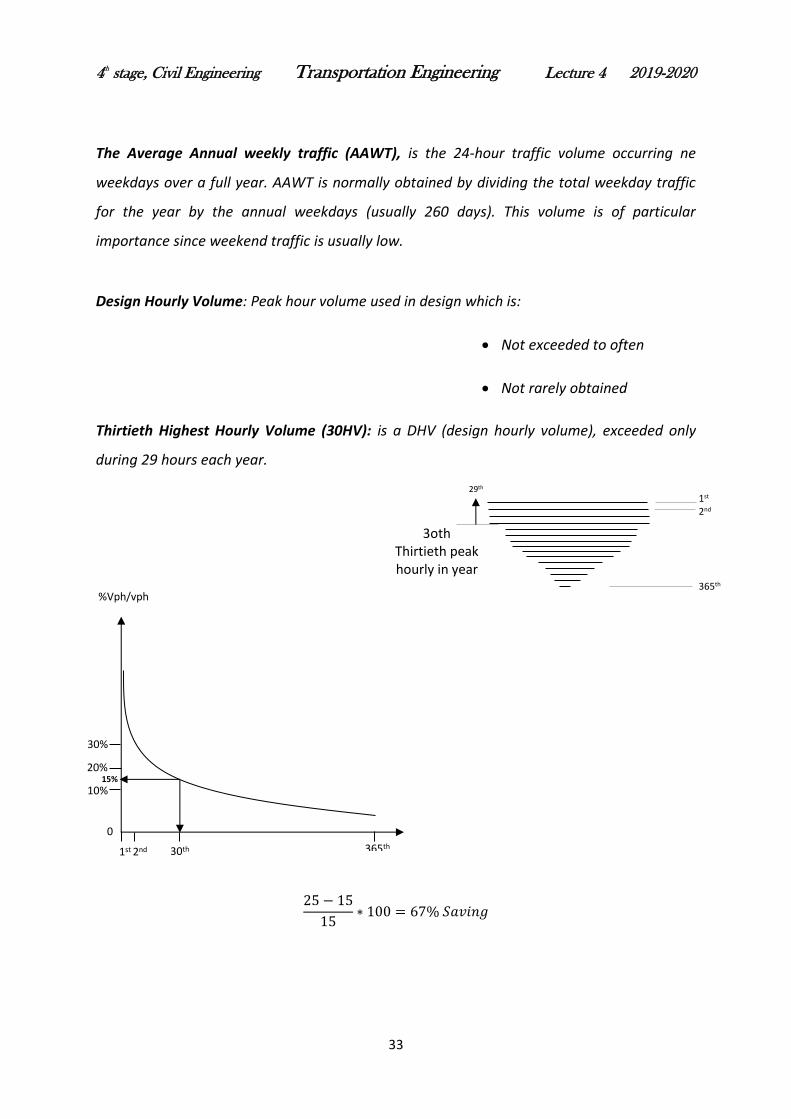
The Average Annual weekly traffic (AAWT), is the 24-hour traffic volume occurring ne

weekdays over a full year. AAWT is normally obtained by dividing the total weekday traffic

for the year by the annual weekdays (usually 260 days). This volume is of particular

importance since weekend traffic is usually low.

Design Hourly Volume: Peak hour volume used in design which is:

Not exceeded to often

Not rarely obtained

Thirtieth Highest Hourly Volume (30HV): is a DHV (design hourly volume), exceeded only

during 29 hours each year.

25 − 15

15∗ 100 = 67% 𝑆𝑎𝑣𝑖𝑛𝑔

365th 30th 1st 2nd

30%

20%

10% 15%

0

29th

1st 2nd

365th

3oth Thirtieth peak hourly in year


34

When the 365 peak hours volumes of a year at a given location are listed in descending order

(as shown in the figure above), the 30th peak hour is the 30th on the list and represents a

volume that is exceeded in only 29 hours of the year. For rural facilities, the 30th peak hour

may have a significantly lower volume than the worst hour of the year. This means that the

critical peaks may occur only infrequently.in such cases, it is not considered economically

feasible to invest large amounts of capital in providing additional capacity that will be used

only 29 hours of the year.

𝐷𝐻𝑉 (30𝑡ℎ) (𝑣𝑝ℎ

𝐵𝑜𝑡ℎ 𝐷𝑖𝑟) = 0.15 ∗ 𝐹. 𝐴𝐷𝑇 (𝐴𝐴𝐷𝑇)[𝑅𝑢𝑟𝑎𝑙 𝐴𝑟𝑒𝑎]

𝐷𝐻𝑉 (30𝑡ℎ) (𝑣𝑝ℎ

𝐵𝑜𝑡ℎ 𝐷𝑖𝑟) = 0.1 ∗ 𝐹. 𝐴𝐷𝑇 (𝐴𝐴𝐷𝑇)[𝑈𝑟𝑏𝑎𝑛 𝐴𝑟𝑒𝑎]

- Directional Distribution Factor (DDF): (50-80) %= the factor of proportion of traffic in peak direction

𝐷𝐷𝐹 = 𝑉𝑜𝑙𝑢𝑚𝑒 𝑜𝑓 𝑜𝑛𝑒 𝑑𝑖𝑟.

𝑉𝑜𝑙. 𝑜𝑓 𝐵𝑜𝑡ℎ 𝑑𝑖𝑟.∗ 100

DDHV= Directional design hourly traffic (vph/one dir) = DHV per one direction

𝐷𝐻𝑉 (𝑣𝑝ℎ

𝐵𝑜𝑡ℎ 𝑑𝑖𝑟) ∗ 𝐷𝐷𝐹 = 𝐷𝐻𝑉 (

𝑣𝑝ℎ

𝑂𝑛𝑒 𝑑𝑖𝑟 )

𝑁𝑜. 𝑜𝑓 𝑙𝑎𝑛𝑒𝑠 𝑓𝑜𝑟 𝑜𝑛𝑒 𝑑𝑖𝑟 = 𝐷𝐻𝑉 𝑓𝑜𝑟 𝑜𝑛𝑒 𝑑𝑖𝑟

𝐷𝑒𝑠𝑖𝑔𝑛 𝑐𝑎𝑝𝑎𝑐𝑖𝑡𝑦 𝑜𝑓 𝑙𝑎𝑛𝑒

No. of lanes for one dir ∗ 2 = 𝑁𝑜. 𝑜𝑓 𝑙𝑎𝑛𝑒𝑠 𝑓𝑜𝑟 𝑏𝑜𝑡ℎ 𝑑𝑖𝑟

As a result:

Current ADT * TPF = F. ADT (vpd/both dir)

F. ADT * 0.15 = DHV (vph/both dir) 0.1

(0.12 – 0.18)

(0.08 – 0.12)


35

DHV * DDF = DHV (vph/one dir)

𝐷𝐻𝑉 𝑓𝑜𝑟 𝑜𝑛𝑒 𝑑𝑖𝑟

𝐷𝑒𝑠𝑖𝑔𝑛 𝐶𝑎𝑝𝑎𝑐𝑖𝑡𝑦 𝑓𝑜𝑟 𝑙𝑎𝑛𝑒 (𝐿𝑂𝑆)= 𝑁𝑜. 𝑜𝑓 𝑙𝑎𝑛𝑒𝑠 𝑓𝑜𝑟 𝑜𝑛𝑒 𝑑𝑖𝑟

𝑁𝑜. 𝑜𝑓 𝑙𝑎𝑛𝑒𝑠 𝑓𝑜𝑟 𝑜𝑛𝑒 𝑑𝑖𝑟 ∗ 2 = 𝑇𝑜𝑡𝑎𝑙 𝑓𝑜𝑟 𝑏𝑜𝑡ℎ 𝑑𝑖𝑟

Capacity and Level of Service

Capacity: is a measure of the demand that a highway can potentially service

Level of Service (LOS): is a qualitative measurement describing the operational condition

within the traffic stream under a given demand. The parameters used to define the level of

service called the measure of effectiveness (MOE) and based on several criteria such as

travel time, speed, delay time and safety.

The highway capacity manuals defines six levels of service designated A through F. the level

A represents the highest level of service while F is the lowest and worst service.

The table below specifies the operational condition and operating speed for the level of

service categories.

LOS Description (operational Condition) Operating Speed (km/hr)

A Free flow 96

B Stable flow 88

C Stable flow with restriction 72

D Approaching unstable flow 56

E Unstable flow 48

F Forced flow (stop and go condition) < 48

Design Capacity (Design service flow rate): The maximum hourly rate at which vehicles can

be expected to pass a point or section of a lane or roadway during one hour under prevailing

roadway, traffic and control condition for a designated level of service.


36

The design capacity for different level of service is presented in the table below:

LOS Design Capacity (pcphpl)

A 660

B 1080

C 1550

D 1980

E 2200

This table specifies the desired LOS for varies terrain

Highway LOS

Level Rolling Mountain

Principal Arterial B B C

Minor Arterial B B C

Collector C C D

Local D D D

Example 1: It is proposed to design a minor arterial within an urban rolling area to serve an

anticipated current daily volume of 10000 pcpd. Find the required no. of lanes for this highway?

Sol. Minor arterial within rolling area Design LOS B

Design capacity = 1080 pcphpl

F. volume = current volume * TPF Assume TPF = 3.6

= 10000 * 3.6 = 36000 pcph/Both

DHV/Both = F. Volume * 0.1

= 0.1 * 36000 = 3600 pcph/Both

DHV/One dir = DHV/Both * DDF

= 3600 * 0.8 = 2880 pcph/One dir

No. of lanes / One dir = 2880/1080 = 2.6 use 3 lanes/ dir

⸫ Total no. of lanes = 3 * 2 = 6 lanes/ Both dir


37

Example 2: A multilane principal arterial is being designed through a rolling rural area. The

current daily volume = 8000 vpd in both dir. with 20% truck, peak hourly factor 90% and a

(60 – 40%) Directional Distribution factor. How many lanes are required? What if this

highway is in an urban area in a level terrain?

Sol.

Current volume = 8000 (0.2 * 2.5 + 0.8 * 1) = 10400 pcpd

F. volume = 10400 * TPF = 37440 pcpd/Both

DHV = 0.15 * 37440 = 5616 pcph/Both

Hourly flow rate = 5616/0.9= 6240 pcph/Both

Hourly flow rate = 6240 * 0.6 = 3744 pcph/ 1 dir

No. of lanes/ 1 dir = 3744/1080 = 3.46 use 4 lane/dir

Total = 4*2 = 8 lanes/both dir

3. Density

Density can be defined as the number of vehicles occupying a given length of road at a given

instant. Density is usually expressed as vehicles per kilometer (veh/km). High densities

indicate the vehicles are very close to each other, while low densities imply greater distances

between vehicles.

It is difficult to measure the density at the field. It can be measured through Ariel

photography which is an expensive method, or it can be estimated theoretically from the

density-flow-speed relationship.

𝑆𝑝𝑎𝑐𝑖𝑛𝑔 (𝑚) = 1 → 1000

𝐷𝑒𝑛𝑠𝑖𝑡𝑦 (𝑣𝑝𝑘𝑚)


38

Density (vpkm) = 1 (or 1000)/Spacing (m)

(Use 1 if the spacing in km, and use 1000 if the spacing in m)

4. Headway

Two types of headways describe the traffic characteristics, time headway and space

headway

1. Time Headway (ht): Time between the arrivals of successive vehicles at specified

time. It can be computed as the difference between the time of the front of a vehicle

arrives at a point on the highway (t1) and the time the front of the next vehicle

arrives at the same point (t2). It is usually expressed in seconds.

The average headway in a lane is directly related to the rate of flow:

ℎ𝑡 = 1 → 3600

𝑉𝑜𝑙𝑢𝑚𝑒 (𝑣𝑝ℎ) (1 𝑖𝑛 ℎ𝑜𝑢𝑟 𝑢𝑛𝑖𝑡, 3600 𝑖𝑛 𝑠𝑒𝑐𝑜𝑛𝑑 𝑢𝑛𝑖𝑡)

ℎ𝑡 = 𝑠𝑒𝑐


39

2. Space headways (hs), is the distance between the front of a vehicle and the front

of the following vehicle. It is usually expressed in meter. The average spacing in

the traffic lane can be directly related to the density of the lane

Hs=1000/D

Where:

D= the density of a lane, veh/km/ln

hs = the average space headway (m)

Gap: is the headway in a major stream which is evaluated by a vehicle driver in a

minor stream who wishes to merge into the minor stream. It is expressed in either

units of time (time gap) or units of distance (space gap)

Time lag: is the difference between the time a vehicle that merges into a main

traffic stream reaches a point on the highway in the area of merge and the time a

vehicle in the main stream reaches the same point.

Space lag, is the difference, at an instant time, between the distance a merging

vehicle is away from the a reference point in the area of merge and the distance

a vehicle in the main steam is away from the same point.


40

RELATIONSHIPS AMONG BASIC PARAMETERS

Flow- Density- Speed relationship

Speed, flow, and density are all related to each other and are fundamental for measuring the

operating performance and level of service of transportation facilities.

Under uninterrupted flow conditions, these three parameters are related by the following

equation: 𝐹𝑙𝑜𝑤 = 𝑆𝑝𝑒𝑒𝑑 ∗ 𝐷𝑒𝑛𝑠𝑖𝑡𝑦

This general relationship is shown in the following figure which is known as the fundamental

diagram of traffic flow.

The relationship between speed and density is consistently decreasing. As density increase,

speed decreases. This diagram shows that flow is zero under two different conditions:

- When density is zero, thus there is no vehicles on the road

- When speed is zero, vehicles are at complete stop because of the traffic congestion.


41

Example: A highway segment with a rate of flow of 1,000 veh/h and an average travel speed of 50 km/h would have a density of D = (1000 veh/h) / (50 km/h) = 20 veh/km

Free-flow speed: the average speed of vehicles on a given facility, measured under low-

volume conditions, when drivers tend to drive at their desired speed and are not constrained

by control delay.

Critical density: is the density of traffic when the volume is at capacity on a given roadway

or lane, critical density occurs when all vehicles are moving at or about the same speed.

96 Operating Speed

110

Density

110

A

Density (vpkm)

Flow vphpl

2000

B C D

E F

Flow

96

2000

B C D

E F

A

Speed


42

MCQ -The number of vehicles that pass a given point on the roadway or a given lane or direction of a highway in a specified period of time

a. Volume b. Density c. Speed d. Peak hour rate

-The most important vehicle features for highway design are:

a. Dimensions and

minimum turning radius

b. Weight and axle

loading

c. Passenger and heavy

truck

d. a and b

-Dimensions and minimum turning radius as a control for:

a. Pavement structural

design

b. Highway geometric

design

c. Vertical Alignment d. Horizontal

Alignment

-Weight and axle loading as a control for

a. Pavement

structural design

b. Highway geometric

design

c. Vertical Alignment d. Horizontal Alignment

-Vehicles that have four tires touching the pavement as

a. Passenger car (PC) b. Heavy Truck (HV) c. Truck combination (WB) d. Single unit truck

-Vehicles that have more than four tires touching the pavement as

a. Passenger car (PC) b. Heavy Truck (HV) c. Truck combination (WB) d. Single unit truck

-Minimum turn radius of vehicle is

a. 10m b. 15m c. 20m d. 25m

-Maximum limit of height vehicle in highway is

a. 5.6m b. 4.6m c. 6m d. 3.6m


43

-What is the gross weight of vehicle [Type 2-S-3]

a. 47 b. 20 c. 27 d. 66

-What is the gross weight of vehicle [Type 3-S-1-2]

a. 47 b. 20 c. 27 d. 66

-What is the gross weight of vehicle [Type 4-S-3]

a. 47 b. 20 c. 61 d. 66

-What is the equivalent passenger car for heavy vehicle in level area?

a. 1.5 b. 2.5 c. 3.5 d. 4.5

-What is the equivalent passenger car for heavy vehicle in rolling area?

a. 1.5 b. 2.5 c. 3.5 d. 4.5

-What is the equivalent passenger car for heavy vehicle in Mountain area?

a. 1.5 b. 2.5 c. 3.5 d. 4.5

-AADT is the number of vehicle count during

a. 365 day (each day in

year)

b. 260 day c. Workday and less 260 d. Workday less 365

-ADT is the number of vehicle count during

a. 365 day b. 260 day c. Workday and less 260 d. Daily and less 365


44

-AAWT is the number of vehicle count during

a. 365 day b. Workday in year 260

day

c. Workday and less 260 d. Workday less 365

-AWT is the number of vehicle count during

a. 365 day b. 260 day c. Workday and less 260 d. Workday less 365

-Why (30HV) is usually selected as a design hourly volume

a. It is not exceeded

to often and not

rarely obtain

b. It is truth volume

in highway

c. Save 67% from

cost and cause delay

29 hour in year

d. for lower value of

volume in highway

-The value of Peak hour factor (PHF) for volume 1600 veh/hr and quarter hour volume 400

veh is?

a. PHF = 0.8 b. PHF = 0.25 c. PHF = 1 d. PHF = 0.7

-Peak hour factor equal one meant that traffic stream is?

a. Non uniform and

stable flow

b. Uniform and

unstable flow

c. Non-uniform and

unstable flow

d. Uniform and

stable flow


45

-For design hourly volume 300veh/hr consists 10 percent of heavy vehicle. Determine the

hourly volume expressed by passenger car in level area

a. 315 b. 415 c. 270.15 d. 330

- Indicated what is the meant by PHF

a. Time mean speed b. Space mean speed c. Spot speed d. Peak hour factor

-What is the relationship of PHF?

∑ (d/t)/n D X N/∑ ti V/PHF V/(4 X V15)

-What is the relationship of flow rate?


-What is the relationship of SMS?


-What is the relationship of TMS?


-The number of vehicles present on a given length of roadway or lane called as?



46

-The difference between the time the front of a vehicle arrives at a point on the highway

and the time the front of the next vehicle arrives at the same point called as

a. Time Headway b. Space Headway c. Gap d. Time lag

-The distance between the front of a vehicle and the front of the following vehicle and is usually expressed in meter called as

a. Time Headway b. Space Headway c. Gap d. Time lag

- What is the unit measure volume?

a. Veh/day b. Veh/hr c. PC/hr d. All previous

- What is the unit measure density?

a. Veh/km b. Veh/hr c. PC/km d. A and C

- Future Traffic Rate (FTR) for highway with (5.5%) growth rate, (20 year) design life and (2 years) construction period is?

a. 3.6 b. 3.248 c. 2.982 d. 3.564

- Designer used flow rate in design because it is?

a. it is not exceeded to often and not rarely obtained

b. it is truth volume in highway

c. save 67% from cost and cause delay 29 hour in year

d. for lower value of volume in highway

-Measure of the demand that a highway can potentially service

a. capacity b. speed c. density d. level of service


47

- Equivalency between the Passenger Car Unit (PCU) and truck for rolling highway is?

a. 1.5 b. 2.5 c. 3.5 d. 4.5

-The number of vehicles that pass a given point on the roadway or a given lane or direction of a

highway in a specified period of time


-The average speed of all vehicles passing a point on a highway over a specified time period defined as?

a. Time mean speed b. Space mean speed c. Spot speed d. Density

-The average speed of all vehicles occupying a given section of a highway over a specified time period defined as?


- Indicated what is the meant by TMS


- Indicated what is the meant by SMS


-The average speed of all vehicles passing a point on a highway over a specified time period defined as?



48

-The average speed of all vehicles occupying a given section of a highway over a specified time period defined as?


- Indicated what is the meant by TMS


- Indicated what is the meant by SMS


Transportation Engineering

Documents

Transcript of Transportation Engineering