TRANSLATION STUDIES ON AN ANNULAR FIELD ...

TRANSLATION STUDIES ON AN ANNULAR FIELD REVERSEDCONFIGURATION DEVICE FOR SPACE PROPULSION

By

Carrie S. Hill

A DISSERTATION

Submitted in partial fulfillment of the requirements for the degree of

DOCTOR OF PHILOSOPHY

In Mechanical Engineering-Engineering Mechanics

MICHIGAN TECHNOLOGICAL UNIVERSITY

2012

c© 2012 Carrie S. Hill

Distribution A: Approved for public release; distribution unlimited.

This dissertation has been approved in partial fulfillment of the requirements for the Degreeof DOCTOR OF PHILOSOPHY in Mechanical Engineering-Engineering Mechanics.

Department of Mechanical Engineering-Engineering Mechanics

Dissertation Advisor: Dr. Lyon B. King

Committee Member: Dr. Brian Beal

Committee Member: Dr. Jeffrey Allen

Committee Member: Dr. David Kirtley

Department Chair: Dr. William Predebon

Contents

List of Figures . . . . . . . . . . . . . . . . . . . . . . . . . . . . . . . . . . . . . ix

List of Tables . . . . . . . . . . . . . . . . . . . . . . . . . . . . . . . . . . . . . . xix

Acknowledgments . . . . . . . . . . . . . . . . . . . . . . . . . . . . . . . . . . . xxi

Abstract . . . . . . . . . . . . . . . . . . . . . . . . . . . . . . . . . . . . . . . . . xxix

1 Introduction . . . . . . . . . . . . . . . . . . . . . . . . . . . . . . . . . . . . 11.1 Background . . . . . . . . . . . . . . . . . . . . . . . . . . . . . . . . . . 11.2 Aim and Scope . . . . . . . . . . . . . . . . . . . . . . . . . . . . . . . . 41.3 Structure of Dissertation . . . . . . . . . . . . . . . . . . . . . . . . . . . 6

2 Overview of Plasmoid Propulsion . . . . . . . . . . . . . . . . . . . . . . . . . 72.1 Principles of Pulsed Propulsion . . . . . . . . . . . . . . . . . . . . . . . . 72.2 Plasmoid Propulsion . . . . . . . . . . . . . . . . . . . . . . . . . . . . . 112.3 Plasmoid Thruster Technology . . . . . . . . . . . . . . . . . . . . . . . . 132.4 Summary . . . . . . . . . . . . . . . . . . . . . . . . . . . . . . . . . . . 21

3 Annular Field Reversed Configurations . . . . . . . . . . . . . . . . . . . . . 233.1 AFRC Basics . . . . . . . . . . . . . . . . . . . . . . . . . . . . . . . . . 233.2 AFRC Formation Techniques . . . . . . . . . . . . . . . . . . . . . . . . . 25

3.2.1 Parallel Coil Mode: Synchronous . . . . . . . . . . . . . . . . . . 273.2.2 Independent Coil Mode: Synchronous . . . . . . . . . . . . . . . . 283.2.3 Parallel Coil Mode: Asynchronous . . . . . . . . . . . . . . . . . . 293.2.4 Independent Coil Mode: Asynchronous . . . . . . . . . . . . . . . 32

3.3 AFRC Physics . . . . . . . . . . . . . . . . . . . . . . . . . . . . . . . . . 343.3.1 Radial Balance . . . . . . . . . . . . . . . . . . . . . . . . . . . . 353.3.2 Equilibrium Profiles . . . . . . . . . . . . . . . . . . . . . . . . . . 383.3.3 Magnetic Field Diffusion . . . . . . . . . . . . . . . . . . . . . . . 403.3.4 Plasma Drifts . . . . . . . . . . . . . . . . . . . . . . . . . . . . . 423.3.5 Termination . . . . . . . . . . . . . . . . . . . . . . . . . . . . . . 43

3.4 Literature Review of AFRCs . . . . . . . . . . . . . . . . . . . . . . . . . 453.5 Propulsion Considerations . . . . . . . . . . . . . . . . . . . . . . . . . . 55

v

4 Translation Model of an Annular Field Reversed Configuration . . . . . . . . 574.1 Annular Electromagnetic Launcher Model . . . . . . . . . . . . . . . . . . 58

4.1.1 Numerical Approach . . . . . . . . . . . . . . . . . . . . . . . . . 634.1.2 Model Validation . . . . . . . . . . . . . . . . . . . . . . . . . . . 67

4.2 Design Studies for the XOCOT-T3 Experiment . . . . . . . . . . . . . . . 704.2.1 Results for Nominal Case . . . . . . . . . . . . . . . . . . . . . . . 754.2.2 Cone Angle Study . . . . . . . . . . . . . . . . . . . . . . . . . . . 784.2.3 Inner Coil Radius Study . . . . . . . . . . . . . . . . . . . . . . . 814.2.4 Initial Energy Study . . . . . . . . . . . . . . . . . . . . . . . . . . 834.2.5 Coil Inductance Study . . . . . . . . . . . . . . . . . . . . . . . . 864.2.6 Parasitic Inductance and Resistance Study . . . . . . . . . . . . . . 884.2.7 Final XOCOT-T3 Experiment Design . . . . . . . . . . . . . . . . 924.2.8 Plasmoid Sensitivity Studies . . . . . . . . . . . . . . . . . . . . . 96

4.3 Magnetic Field Modeling of XOCOT-T3 . . . . . . . . . . . . . . . . . . . 1044.4 Summary and Discussion of Results . . . . . . . . . . . . . . . . . . . . . 112

5 Experiment, Facilities, and Diagnostics . . . . . . . . . . . . . . . . . . . . . 1175.1 Experimental Apparatus . . . . . . . . . . . . . . . . . . . . . . . . . . . . 118

5.1.1 Electromagnetic Coils . . . . . . . . . . . . . . . . . . . . . . . . 1195.1.2 Quartz Insulators . . . . . . . . . . . . . . . . . . . . . . . . . . . 1225.1.3 Main Bank Discharge Circuit . . . . . . . . . . . . . . . . . . . . . 1235.1.4 Pre-Ionization Source . . . . . . . . . . . . . . . . . . . . . . . . . 1275.1.5 Safety Considerations . . . . . . . . . . . . . . . . . . . . . . . . . 1295.1.6 Vacuum Facilities and Gas Injection . . . . . . . . . . . . . . . . . 1305.1.7 Experiment Operation . . . . . . . . . . . . . . . . . . . . . . . . 132

5.2 Diagnostics . . . . . . . . . . . . . . . . . . . . . . . . . . . . . . . . . . 1335.2.1 Current and Voltage Monitors . . . . . . . . . . . . . . . . . . . . 1355.2.2 Magnetic Field Probes . . . . . . . . . . . . . . . . . . . . . . . . 137

5.2.2.1 B-dot Probe Theory . . . . . . . . . . . . . . . . . . . . 1385.2.2.2 Differential B-dot Probe Theory . . . . . . . . . . . . . . 1475.2.2.3 Calibration of B-dot Probes . . . . . . . . . . . . . . . . 1495.2.2.4 Analysis of B-dot Data . . . . . . . . . . . . . . . . . . . 1535.2.2.5 Error Analysis for B-dot Probes . . . . . . . . . . . . . . 1565.2.2.6 XOCOT-T3 External B-dot Probes . . . . . . . . . . . . 1605.2.2.7 XOCOT-T3 Internal Magnetic Field Probes . . . . . . . . 1705.2.2.8 XOCOT-T3 TOF Magnetic Field Probes . . . . . . . . . 173

5.2.3 Plasma Probes . . . . . . . . . . . . . . . . . . . . . . . . . . . . . 1815.2.4 Single Frame Digital Camera . . . . . . . . . . . . . . . . . . . . . 194

5.3 Translation Measurements . . . . . . . . . . . . . . . . . . . . . . . . . . 1945.3.1 Velocity Measurements: Time-of-Flight Array . . . . . . . . . . . . 1955.3.2 Momentum Measurements . . . . . . . . . . . . . . . . . . . . . . 1975.3.3 Efficiency Estimates . . . . . . . . . . . . . . . . . . . . . . . . . 199

vi

5.3.4 Energy Analysis . . . . . . . . . . . . . . . . . . . . . . . . . . . . 200

6 Experimental Data: Translation Study . . . . . . . . . . . . . . . . . . . . . . 2036.1 Test Conditions . . . . . . . . . . . . . . . . . . . . . . . . . . . . . . . . 2046.2 Vacuum Characterization . . . . . . . . . . . . . . . . . . . . . . . . . . . 206

6.2.1 Vacuum Data: 10 kHz . . . . . . . . . . . . . . . . . . . . . . . . 2066.2.2 Vacuum Data: 20 kHz . . . . . . . . . . . . . . . . . . . . . . . . 213

6.3 Plasmoid Formation Characterization . . . . . . . . . . . . . . . . . . . . . 2196.3.1 Formation Results . . . . . . . . . . . . . . . . . . . . . . . . . . . 2196.3.2 Pre-Ionization . . . . . . . . . . . . . . . . . . . . . . . . . . . . . 2236.3.3 Main Bank Timing . . . . . . . . . . . . . . . . . . . . . . . . . . 226

6.3.3.1 Timing: 10 kHz . . . . . . . . . . . . . . . . . . . . . . 2266.3.3.2 Timing: 20 kHz . . . . . . . . . . . . . . . . . . . . . . 231

6.3.4 Repeatibility . . . . . . . . . . . . . . . . . . . . . . . . . . . . . 2326.3.4.1 Repeatibility: 10 kHz . . . . . . . . . . . . . . . . . . . 2336.3.4.2 Repeatibility: 20 kHz . . . . . . . . . . . . . . . . . . . 235

6.4 Translation Study Data . . . . . . . . . . . . . . . . . . . . . . . . . . . . 2416.4.1 Translation Data: 10 kHz . . . . . . . . . . . . . . . . . . . . . . . 2436.4.2 Translation Data: 20 kHz . . . . . . . . . . . . . . . . . . . . . . . 257

7 Translation Results . . . . . . . . . . . . . . . . . . . . . . . . . . . . . . . . 2637.1 Translation Data Reduction . . . . . . . . . . . . . . . . . . . . . . . . . . 2637.2 Velocity Results . . . . . . . . . . . . . . . . . . . . . . . . . . . . . . . . 264

7.2.1 Velocity Results: 10 kHz . . . . . . . . . . . . . . . . . . . . . . . 2677.2.2 Velocity Results: 20 kHz . . . . . . . . . . . . . . . . . . . . . . . 2887.2.3 Downstream Plasma Flux Measurements . . . . . . . . . . . . . . . 295

7.3 Discussion of Translation Results . . . . . . . . . . . . . . . . . . . . . . . 3037.4 Possible Failure Modes . . . . . . . . . . . . . . . . . . . . . . . . . . . . 305

7.4.1 Failure Mode: Current Induction Limit . . . . . . . . . . . . . . . . 3057.4.2 Failure Mode: Low Conductivity . . . . . . . . . . . . . . . . . . . 3067.4.3 Failure Mode: Instabilities and Imbalances . . . . . . . . . . . . . 308

7.5 Summary . . . . . . . . . . . . . . . . . . . . . . . . . . . . . . . . . . . 309

8 Instability Study Data and Results . . . . . . . . . . . . . . . . . . . . . . . . 3118.1 Instability Study Diagnostics . . . . . . . . . . . . . . . . . . . . . . . . . 3118.2 Instability Study Data . . . . . . . . . . . . . . . . . . . . . . . . . . . . . 312

8.2.1 Image Data . . . . . . . . . . . . . . . . . . . . . . . . . . . . . . 3138.2.2 Asymmetric Double Langmuir Probe Data . . . . . . . . . . . . . . 316

8.3 Discussion . . . . . . . . . . . . . . . . . . . . . . . . . . . . . . . . . . . 3218.4 Summary . . . . . . . . . . . . . . . . . . . . . . . . . . . . . . . . . . . 322

9 Radial Balance Study Data and Results . . . . . . . . . . . . . . . . . . . . . 3239.1 Radial Balance in AFRCs . . . . . . . . . . . . . . . . . . . . . . . . . . . 323

vii

9.2 Radial Balance Study Data . . . . . . . . . . . . . . . . . . . . . . . . . . 3289.3 Radial Balance Study Results . . . . . . . . . . . . . . . . . . . . . . . . . 3429.4 Discussion of Radial Balance Results . . . . . . . . . . . . . . . . . . . . . 344

10 Conclusion and Future Work . . . . . . . . . . . . . . . . . . . . . . . . . . . 34710.1 Contributions of This Work . . . . . . . . . . . . . . . . . . . . . . . . . . 34710.2 Future Work . . . . . . . . . . . . . . . . . . . . . . . . . . . . . . . . . . 350

References . . . . . . . . . . . . . . . . . . . . . . . . . . . . . . . . . . . . . . . 353

A XOCOT-T3 Supplemental Data . . . . . . . . . . . . . . . . . . . . . . . . . . 361

viii

List of Figures

1.1 Annular field reversed configuration schematic. The poloidal B-field issupported by a toroidal (azimuthal) plasma current. . . . . . . . . . . . . . 2

2.1 Family of pulsed indutive plasmoid thrusters, including (a) planar thruster,(b) conical θ -pinch FRC thruster, (c) RMF-FRC thruster, (d) AFRC thruster. 11

3.1 Principle dimensions of an (a) FRC and an (b) AFRC. . . . . . . . . . . . . 243.2 Force diagram for an AFRC translating from a conical coil. . . . . . . . . . 253.3 Formation schematic for an AFRC formed with the coils connected in

parallel, operating in phase. . . . . . . . . . . . . . . . . . . . . . . . . . . 303.4 Formation schematic for an AFRC formed with the coils connected in

parallel, operating asynchronously. . . . . . . . . . . . . . . . . . . . . . . 313.5 Formation schematic for an AFRC formed with the coils operating

indepedently and asynchronously. . . . . . . . . . . . . . . . . . . . . . . 333.6 Representative internal magnetic field structure of AFRCs showing a

reversed field on the inner coil as compared to the outer coil. . . . . . . . . 393.7 Representative internal electron density structure of AFRCs, showing a

peak density at B = 0. . . . . . . . . . . . . . . . . . . . . . . . . . . . . . 39

4.1 Schematic of the annular electromagnetic launcher model. The plasmoid isdepicted with circuit elements Lp and Rp, magnetically coupled to the coilsthrough Mop and Mip. . . . . . . . . . . . . . . . . . . . . . . . . . . . . . 59

4.2 Geometry and mesh used for the inductance calculations in COMSOL. Thecoil meshes were refined to resolve the skin depth of the current in the coils. 65

4.3 Results from the modified annular electromagnetic launcher model, usinga test case presented by Novac, et al [1]. . . . . . . . . . . . . . . . . . . . 69

4.4 Effective inductance of a slug-coil geometry calculated using COMSOL.Experimental data from Reference [2] are shown with the dotted line. . . . . 70

4.5 Definition of the plasmoid lifetime limit, as determined by the peak in thecoil-plasma coupling case where the plasmoid is not allowed to translate. . . 72

4.6 Results from the launcher model, including coil currents, plasma current,capacitor voltage, plasmoid velocity, and axial plasmoid position as afunction of time for nominal inputs. . . . . . . . . . . . . . . . . . . . . . 76

4.7 Positional dependence of the mutual inductance gradient for the inner andouter coil and the combined Lorentz force. . . . . . . . . . . . . . . . . . . 77

ix

4.8 Results from the cone angle study, including the final plasmoid position,final velocity, and energy efficiency. Results are shown for 2 differentcapacitor banks. . . . . . . . . . . . . . . . . . . . . . . . . . . . . . . . . 79

4.9 Mutual inductance gradient and Lorentz force as a function of slug position.Several different cone angles are shown, increasing in the arrow direction. . 80

4.10 Results from the inner coil radius study, including the final plasmoidposition, final velocity, and energy efficiency. Results are shown for 2different capacitor banks. . . . . . . . . . . . . . . . . . . . . . . . . . . . 82

4.11 Coupling coefficients and Lorentz force computations for several inner coilradii. . . . . . . . . . . . . . . . . . . . . . . . . . . . . . . . . . . . . . . 83

4.12 Results from the initial energy study, including the final plasmoid position,final velocity, and energy efficiency. Results are shown for 2 differentcapacitor banks. . . . . . . . . . . . . . . . . . . . . . . . . . . . . . . . . 85

4.13 Results from the coil inductance study, showing energy efficiency andminimum required input energy as a function of coil turns. . . . . . . . . . 87

4.14 Results from the stray inductance study, including the final plasmoidposition, final velocity, and energy efficiency as a function of stray inductance. 89

4.15 Results from the stray study, including the final plasmoid position, finalvelocity, and energy efficiency as a function of stray resistance. . . . . . . . 90

4.16 Plasmoid lifetime (related to rise time of circuit) as a function of strayinductance. . . . . . . . . . . . . . . . . . . . . . . . . . . . . . . . . . . 91

4.17 Lorentz force as a function of slug position for two stray outer coilinductances. The larger stray inductance results in a larger Lorentz force. . . 91

4.18 Results from the launcher model for the XOCOT-T3 design inputs,including coil currents, plasma current, capacitor voltage, plasmoidvelocity, and axial plasmoid position as a function of time for nominal inputs. 95

4.19 Results from the XOCOT-T3 design study on initial energy, including thefinal plasmoid position, final velocity, and energy efficiency. Results areshown for the primary bank (225 µF) and the alternate bank (43.5 µF). . . . 97

4.20 Sensitivity results from the XOCOT-T3 design study on plasmoid width,including the final plasmoid position, final velocity, and energy efficiency.Results are shown for the primary bank (225 µF) and the alternate bank(43.5 µF). . . . . . . . . . . . . . . . . . . . . . . . . . . . . . . . . . . . 99

4.21 Sensitivity results from the XOCOT-T3 design study on plasmoid length,including the final plasmoid position, final velocity, and energy efficiency.Results are shown for the primary bank (225 µF) and the alternate bank(43.5 µF). . . . . . . . . . . . . . . . . . . . . . . . . . . . . . . . . . . . 100

4.22 Sensitivity results from the XOCOT-T3 design study on plasmaconductivity, including the final plasmoid position, final velocity, andenergy efficiency. Results are shown for the primary bank (225 µF) andthe alternate bank (43.5 µF). . . . . . . . . . . . . . . . . . . . . . . . . . 102

x

4.23 Sensitivity results from the XOCOT-T3 design study on plasmoid radius,including the final plasmoid position, final velocity, and energy efficiency.Results are shown for the primary bank (225 µF) and the alternate bank(43.5 µF). . . . . . . . . . . . . . . . . . . . . . . . . . . . . . . . . . . . 103

4.24 Coil connections, circuit connections, and coil geometry used to calculatethe vacuum fields. The rectangles in (a) represent FEM objects inCOMSOL. The geometry used in COMSOL to represent the multi-turncoils is drawn in (b). . . . . . . . . . . . . . . . . . . . . . . . . . . . . . . 105

4.25 COMSOL results for the vacuum case using the XOCOT-T3 design,including (a) coil currents, (b) time history of midplane axial fields, (c)axial magnetic fields as the length of the coil, and (d) midplane axial fieldacross the radial cross section. . . . . . . . . . . . . . . . . . . . . . . . . 107

4.26 Magnetic field map from the XOCOT-T3 design, computed in COMSOL.Arrows denote field direction. Detail views of the magnetic field betweencoil turns is displayed in the smaller figures. . . . . . . . . . . . . . . . . . 108

4.27 COMSOL results for the plasmoid-coupling case using the XOCOT-T3design, including (a) coil currents, (b) time history of midplane axial fields,and (c) midplane axial field across the radial cross section. . . . . . . . . . 109

4.28 Coil connections, circuit connections, and coil geometry used to calculatethe translating plasmoid fields. The rectangles in (a) represent FEM objectsin COMSOL. The moving plasmoid in COMSOL is specified by the slidingregion of conductivity in (b). . . . . . . . . . . . . . . . . . . . . . . . . . 110

4.29 Coil currents and magnetic field predicted by COMSOL for a plasmoidtranslating at 50 km/s. . . . . . . . . . . . . . . . . . . . . . . . . . . . . . 111

5.1 The XOCOT-T3 experiment, connected to Chamber 5B. Image is along exposure photograph of a single pulse discharge in argon. Thepre-ionization antenna is shown as the thinner coil upstream (left) of themain 4-turn coils. . . . . . . . . . . . . . . . . . . . . . . . . . . . . . . . 118

5.2 A dimensional drawing of the XOCOT-T3 experiment from severalperspectives, connected to Chamber 5B. The coils were concentric,separating an annular space with quartz insulators. . . . . . . . . . . . . . . 119

5.3 A system view of the XOCOT-T3 experiment. . . . . . . . . . . . . . . . . 1205.4 XOCOT-T3 discharge coils, showing (a) a single turn of the inner coil and

(b) the outer coil assembly. . . . . . . . . . . . . . . . . . . . . . . . . . . 1215.5 Main Bank Discharge Circuit Schematic. . . . . . . . . . . . . . . . . . . . 1235.6 Photographs of the XOCOT-T3 main bank circuit. . . . . . . . . . . . . . . 1255.7 A schematic of the pre-ionization circuit. . . . . . . . . . . . . . . . . . . . 1285.8 Photographs of the pre-ionization circuit. The capacitor bank (far left) is

connected to the antenna (far right) through a thyristor stack (middle). Thecurrent in the circuit is measured with the Rogowski coil directly in frontof the capacitor bank. . . . . . . . . . . . . . . . . . . . . . . . . . . . . . 129

xi

5.9 A schematic of the vacuum facilities used in the XOCOT-T3 testing. Thisdiagram is not drawn to scale. . . . . . . . . . . . . . . . . . . . . . . . . . 131

5.10 Layout of the diagnostics used in the XOCOT-T3. The single frame camerais located outside the chamber, capturing images from an end-on view.Current and voltage monitors are not shown in this figure and are locatedon the external circuit. . . . . . . . . . . . . . . . . . . . . . . . . . . . . . 134

5.11 Capacitor Voltage Divider Circuit. The capacitor voltage is measuredacross the 10 kΩ resistor with an isolated Fluke multimeter. . . . . . . . . . 137

5.12 Magnetic field probe locations in the XOCOT-T3 experiment. Externalb-dot probes run the length of the discharge coils. The placement ofthe internal b-dot probes shown here is typical for most of the testing.Probe-to-probe spacing is 2.5 cm apart on the external and internal arrays. . 138

5.13 Illustration of a magnetic field probe. The probe head is connected to atransmission line and Vp is measured at the end of the transmission line. . . 139

5.14 The circuit schematic for a b-dot probe connected to transmission lines.The complete circuit (a) can be simplifed to equivalent lumped impedancesfor low frequency (b) as probe impedances ZP, line impedances Z0,termination impedance ZL, and high voltage capacitive coupling impedanceZc. . . . . . . . . . . . . . . . . . . . . . . . . . . . . . . . . . . . . . . . 141

5.15 The frequency response (gain and phase) of a simulated probe assemblywith negligible capacitance, 10 µH of inductance, and 10 Ω of resistancefrom 10 kHz to 1 MHz. . . . . . . . . . . . . . . . . . . . . . . . . . . . . 143

5.16 A SPICE circuit representation of a magnetic field probe used forexamining the effect of the high voltage capacitive coupling on the probe’stransfer function β (ω). . . . . . . . . . . . . . . . . . . . . . . . . . . . . 145

5.17 Gain and phase changes of a b-dot probes transfer function β (ω) due tohigh voltage capacitive coupling. The solid lines are from including Zc inthe transfer function and the dashed lines are from neglecting Zc. Resultsfrom a SPICE simulation are shown as hollow (gain) dots and solid (phase)dots. . . . . . . . . . . . . . . . . . . . . . . . . . . . . . . . . . . . . . . 146

5.18 Illustration of a differential magnetic field probe. Each probe head is woundin a separate direction. . . . . . . . . . . . . . . . . . . . . . . . . . . . . 148

5.19 Circuit diagram of a differential b-dot probe. Mutual inductance betweenprobe heads is indicated using the dot convention. . . . . . . . . . . . . . . 149

5.20 Integrated digital signals sampled from an analog waveform using an 8-bitdigitizer and a 12-bit digitizer. . . . . . . . . . . . . . . . . . . . . . . . . 156

5.21 External magnetic field probes and their calibration probes, secured to thequartz insulator. Two arrays of external probes and calibration probes spanthe length of the electromagnetic coils. . . . . . . . . . . . . . . . . . . . . 161

5.22 External magnetic field probe wiring diagram. . . . . . . . . . . . . . . . . 162

xii

5.23 The complex impedance of an external probe assembly (B007) from 1 kHzto 5MHz, measured with an impedance analyzer. An inset graph shows thedetail from 1 to 500 kHz. . . . . . . . . . . . . . . . . . . . . . . . . . . . 163

5.24 Sample calibration waveforms for external probe array, including (a) rawb-dot probe signals, (b) corresponding FFTs, (c) intervals of data used forcalibration, (d) NA waveform for three intervals, and (e) error in NA. . . . . 165

5.25 Measured phase delay at 9.1 kHz of external probes, compared to theirpredicted delay. . . . . . . . . . . . . . . . . . . . . . . . . . . . . . . . . 166

5.26 Photograph of internal magnetic field probes. . . . . . . . . . . . . . . . . 1715.27 Internal magnetic field probes wiring diagram. . . . . . . . . . . . . . . . . 1715.28 Photograph of TOF magnetic field probes. The downstream probe is the

larger probe (top) and the upstream probe is the smaller probe (bottom). . . 1745.29 TOF magnetic field probes wiring diagram. . . . . . . . . . . . . . . . . . 1755.30 TOF magnetic field probes’ impedance as a function of frequency for the

(a) upstream probe and (b) downstream probe. . . . . . . . . . . . . . . . . 1765.31 Measured frequency response of preamplifier #1 from 10 kHz to 1 MHz for

(a) 10x gain and (b) 100x gain. . . . . . . . . . . . . . . . . . . . . . . . . 1795.32 Measured frequency response of preamplifier #2 from 10 kHz to 1 MHz for

(a) 10x gain and (b) 100x gain. . . . . . . . . . . . . . . . . . . . . . . . . 1805.33 Sample I-V characteristic for single Langmuir probe. . . . . . . . . . . . . 1825.34 Ion flux probes, including (a) a photograph of the probes and (b) circuit

diagram . . . . . . . . . . . . . . . . . . . . . . . . . . . . . . . . . . . . 1855.35 Current density measured by the ion flux probes for a -6 V bias and -24 V

bias. . . . . . . . . . . . . . . . . . . . . . . . . . . . . . . . . . . . . . . 1865.36 Illustration of an asymmetric double Langmuir probe. . . . . . . . . . . . . 1885.37 Asymmetric double Langmuir probe I-V characteristics for several

different electron temperatures. . . . . . . . . . . . . . . . . . . . . . . . . 1915.38 Asymmetric double Langmuir probe, including (a) a photograph of the

probe and (b) circuit diagram. . . . . . . . . . . . . . . . . . . . . . . . . . 1935.39 Plasma probe data from a time-of-flight array in a PIPT experiment [3]. . . 196

6.1 Coil currents as a function of time for the vacuum shot using the 10 kHzbank. . . . . . . . . . . . . . . . . . . . . . . . . . . . . . . . . . . . . . . 207

6.2 Vacuum coil current data for the 10 kHz bank, including (a) averagewaveforms for the 500 J setting, (b) peak currents versus energy, and (c)peak currents versus discharge voltage. . . . . . . . . . . . . . . . . . . . . 208

6.3 XOCOT-T3 vacuum magnetic fields as a function of discharge energy forthe 10 kHz circuit. . . . . . . . . . . . . . . . . . . . . . . . . . . . . . . . 210

6.4 Downstream magnetic field signals measured with and without adifferential amplfier. . . . . . . . . . . . . . . . . . . . . . . . . . . . . . . 212

xiii

6.5 TOF peak-normalized vacuum magnetic field traces for the 10 kHz circuit,including average magnetic field waveforms for the (A) upstream probeand the (B) downstream probe. The coil current waveform is shown forcomparison. . . . . . . . . . . . . . . . . . . . . . . . . . . . . . . . . . . 214

6.6 Vacuum coil currents for the 20 kHz circuit, including (A) the timehistory of the coil currents, (B) peak coil currents compared to inputenergy, and (C) peak currents versus discharge voltage. Uncertainty forall measurements is 1%. . . . . . . . . . . . . . . . . . . . . . . . . . . . . 216

6.7 Vacuum magnetic fields for the 20 kHz circuit, including average magneticfield waveforms at the coil midplane on the outer wall (A), the inner wall(B), and the average magnetic field at peak coil current along the coil length(C). . . . . . . . . . . . . . . . . . . . . . . . . . . . . . . . . . . . . . . 217

6.8 TOF vacuum magnetic fields for the 20 kHz circuit, including averagemagnetic field waveforms for the (A) upstream probe and the (B)downstream probe. The coil current waveform is also shown. . . . . . . . . 218

6.9 Typical plasmoid formation data for the 10 kHz circuit at 500 J with a 4mTorr fill. A full time-history is shown with vacuum and plasma data forthe main bank current, midplane magnetic fields, and light output measuredby a photometer. . . . . . . . . . . . . . . . . . . . . . . . . . . . . . . . . 221

6.10 Typical plasmoid formation data for the 20 kHz circuit at 100 J with a 4mTorr fill. A full time-history is shown with vacuum and plasma data forthe (A) main bank current, (B), midplane magnetic fields, and (C) lightoutput measured by a photometer. . . . . . . . . . . . . . . . . . . . . . . 222

6.11 Pre-ionization study data, including current waveforms for the vacuum andplasma case, coil current compared to charge voltage, and energy absorbedby the plasma versus charge energy. . . . . . . . . . . . . . . . . . . . . . 225

6.12 Timing results for the 20 kHz, 100 J tests, showing energy absorbtion intothe plasma (top) and midplane magnetic fields for various delay intervals. . 228




6.16 Repeatibility study data for the 10 kHz circuit at 100 J, includingcoil currents and upstream magnetic field measurements. The standarddeviation of repeated data sets for each diagnostics is shown on the right. . . 234

6.17 Downstream results from the repeatibility study for the 10 kHz at 100J, including the measurements recorded from the TOF probes and thestandard deviations among repeated shots. . . . . . . . . . . . . . . . . . . 235

xiv







6.24 Average currents and magnetic fields at 7 µs compared to number ofsamples included in average. . . . . . . . . . . . . . . . . . . . . . . . . . 242

6.25 Total current and midplane magnetic field data at various fill pressures forthe 100 J, 10 kHz circuit. Vacuum traces are shown at each diagnostic bydotted lines. . . . . . . . . . . . . . . . . . . . . . . . . . . . . . . . . . . 245

6.26 Magnetic field data at various fill pressures and locations for the 100 J, 10kHz circuit. Vacuum traces are shown at each diagnostic by dotted lines. . . 246

6.27 Peak normalized downstream magnetic field data at various fill pressuresfor the 100 J, 10 kHz circuit. Vacuum traces are shown at each diagnosticby dotted lines. . . . . . . . . . . . . . . . . . . . . . . . . . . . . . . . . 247



6.30 TOF probe data at various fill pressures for the 500 J, 10 kHz circuit,including peak normalized downstream magnetic field data and plasma fluxmeasurements. Vacuum traces are shown at each diagnostic by dotted lines. 253



xv

6.33 Peak normalized downstream magnetic field data at various fill pressuresfor the 1000 J, 10 kHz circuit. Vacuum traces are shown at each diagnosticby dotted lines. . . . . . . . . . . . . . . . . . . . . . . . . . . . . . . . . 256

6.34 Total current and magnetic field data at various fill pressures for the 100 J,20 kHz circuit. Vacuum traces are shown at each diagnostic by dotted lines. 258

6.35 Magnetic field data at various fill pressures for the 100 J, 20 kHz circuit.Vacuum traces are shown for each diagnostic by a dotted line. . . . . . . . . 259

6.36 TOF probe data at various fill pressures for the 100 J, 20 kHz circuit,including peak normalized downstream magnetic field data and plasma fluxmeasurements. Vacuum traces are shown at each diagnostic by dotted lines. 260

7.1 Full data set from a single shot at 100 J with the 20 kHz bank and a 4 mTorrgas fill. . . . . . . . . . . . . . . . . . . . . . . . . . . . . . . . . . . . . . 265

7.2 Translation results for the 10 kHz circuit at 100 J, with a 1 mTorr fill pressure.2687.3 Translation results for the 10 kHz circuit at 100 J, with a 4 mTorr fill pressure.2697.4 Translation results for the 10 kHz circuit at 100 J, with a 10 mTorr fill

pressure. . . . . . . . . . . . . . . . . . . . . . . . . . . . . . . . . . . . . 2707.5 Translation results for the 10 kHz circuit at 100 J, with a 14 mTorr fill



pressure. . . . . . . . . . . . . . . . . . . . . . . . . . . . . . . . . . . . . 2737.8 Translation results for the 10 kHz circuit at 500 J, with a 1 mTorr fill pressure.2757.9 Translation results for the 10 kHz circuit at 500 J, with a 4 mTorr fill pressure.2767.10 Translation results for the 10 kHz circuit at 500 J, with a 10 mTorr fill









pressure. . . . . . . . . . . . . . . . . . . . . . . . . . . . . . . . . . . . . 286

xvi

7.19 Translation results for the 10 kHz circuit at 1000 J, with a 50 mTorr fillpressure. . . . . . . . . . . . . . . . . . . . . . . . . . . . . . . . . . . . . 287

7.20 Translation results for the 20 kHz circuit at 100 J, with a 1 mTorr fill pressure.2897.21 Translation results for the 20 kHz circuit at 100 J, with a 4 mTorr fill pressure.2907.22 Translation results for the 20 kHz circuit at 100 J, with a 10 mTorr fill




pressure. . . . . . . . . . . . . . . . . . . . . . . . . . . . . . . . . . . . . 2947.26 ADLP current measured 3.8 cm downstream of the coil exit plane for

several bias voltages. . . . . . . . . . . . . . . . . . . . . . . . . . . . . . 2967.27 Plasma density and electron temperature measured by an ADLP at z = 34.3

cm. Figure (c) shows that thin-sheath approximations are valid for thisprobe for the time-interval of interest. . . . . . . . . . . . . . . . . . . . . 297

7.28 Translation results for the 100 J, 20 kHz circuit including peak-normalizeddensity from an ADLP. . . . . . . . . . . . . . . . . . . . . . . . . . . . . 298

7.29 Collision cross sections for electron elastic scattering from argon and forelectron ionization from argon for various electron energies (a) and meanfree path for elastic and ionization scattering as a function of energy energyfor various neutral fill pressures (b). . . . . . . . . . . . . . . . . . . . . . 300

7.30 Estimated plasma density for ion saturation currents measured bydownstream plasma probes at several pressures. . . . . . . . . . . . . . . . 301

7.31 Time derivative of current compared to observed plasmoid current lifetimefor all XOCOT-T3 test conditions, showing the scaling for the outer coil(left) and inner coil (right). . . . . . . . . . . . . . . . . . . . . . . . . . . 306

8.1 Background images for the 10 kHz data (left) and 20 kHz data (right),showing the location of the insulator walls and tank entrance. . . . . . . . . 314

8.2 Images of the plasma from an end view for a 500 J, 4 mTorr plasma testwith the 10 kHz circuit. . . . . . . . . . . . . . . . . . . . . . . . . . . . . 315

8.3 Images of the plasma from an end view for a 100 J, 4 mTorr plasma testwith the 20 kHz circuit. . . . . . . . . . . . . . . . . . . . . . . . . . . . . 316

8.4 ADLP data at z = 33.8 cm, showing the temporal data at fixed bias voltagesand the reconstructed I-V characteristic. . . . . . . . . . . . . . . . . . . . 318

8.5 Theoretical I-V characteristics for a 4-mTorr backfill with 100% ionizationand various temperatures. . . . . . . . . . . . . . . . . . . . . . . . . . . . 319

8.6 ADLP measurements at the axial midplane, including (A) the temporalprobe current, (B) radial distribution of plasma current at various times,and (C) midplane magnetic fields. . . . . . . . . . . . . . . . . . . . . . . 320

xvii

9.1 Final plasmoid radius, calculated using Equation 9.11. The radial trajectoryusing XOCOT-T3 circuit parameters is shown in (a) for various plasmoidresistances. The final plasmoid position as a function of outer coil strayinductance is shown in (b). . . . . . . . . . . . . . . . . . . . . . . . . . . 327

9.2 Coil currents and midplane magnetic fields for Configuration #1. Theoriginal circuit data is shown with the faint dotted line. . . . . . . . . . . . 330

9.3 Magnetic field data for a 100 J, 4 mTorr shot with the circuit inConfiguration #1. The data using the original circuit is indicated by thefaint dotted lines. . . . . . . . . . . . . . . . . . . . . . . . . . . . . . . . 331

9.4 Magnetic pressure at the axial midplane for a 100 J, 4 mTorr dischargeusing the 20 kHz circuit in Configuration #1. . . . . . . . . . . . . . . . . . 332

9.5 Images of plasmoid formation for a 100 J, 4 mTorr discharge using the 20kHz circuit in Configuration #1. Midplane magnetic fields are shown forreference. . . . . . . . . . . . . . . . . . . . . . . . . . . . . . . . . . . . 334

9.6 Coil currents and midplane magnetic fields for Configuration #2. Theoriginal circuit data is shown with the faint dotted line. . . . . . . . . . . . 335

9.7 Magnetic field data for a 100 J, 4 mTorr shot with the circuit inConfiguration #2. The data using the original circuit is indicated by thefaint dotted lines. . . . . . . . . . . . . . . . . . . . . . . . . . . . . . . . 337

9.8 Magnetic pressure at the axial midplane for a 100 J, 4 mTorr dischargeusing the 20 kHz circuit in Configuration #2. . . . . . . . . . . . . . . . . . 338

9.9 Images of plasmoid formation for a 100 J, 4 mTorr discharge using the 20kHz circuit in Configuration #2. . . . . . . . . . . . . . . . . . . . . . . . 339

9.10 ADLP data at the axial midplane for Configuration #2. The data collectedby the probe is shown (A) along with the radial distribution along thechannel (B), and midplane mangetic fields (C). . . . . . . . . . . . . . . . . 341

A.1 Vacuum data from a shot at 500 J and 10 kHz. . . . . . . . . . . . . . . . . 362A.2 Vacuum data from a shot at 100 J and 20 kHz. . . . . . . . . . . . . . . . . 363A.3 Current, magnetic field, and photometer data from a shot at 500 J and 10

kHz, with a 4 mTorr fill of Argon. . . . . . . . . . . . . . . . . . . . . . . 364A.4 Current, magnetic field, and photometer data from a shot at 100 J and 20

kHz, with a 4 mTorr fill of Argon. . . . . . . . . . . . . . . . . . . . . . . 365A.5 Current and voltage traces from the ADLP at z = 34.3 cm. Curve fits to the

data were constructed from ADLP theory. . . . . . . . . . . . . . . . . . . 366

xviii

List of Tables

2.1 Pulsed inductive plasmoid thrusters. Asterisks denote projected numbers. . 14

3.1 History of AFRC devices . . . . . . . . . . . . . . . . . . . . . . . . . . . 46

4.1 Nominal inputs for design study . . . . . . . . . . . . . . . . . . . . . . . 744.2 XOCOT-T3 final design parameters . . . . . . . . . . . . . . . . . . . . . 94

5.1 XOCOT-T3 circuit impedances . . . . . . . . . . . . . . . . . . . . . . . . 1275.2 External magnetic field probes’ impedances, sensitivities, and

proportionality constants. Impedances were measured at 10 kHz. . . . . . . 1695.3 Internal magnetic field probes’ impedances, sensitivities, and

proportionality constants. Impedances were measured at 10 kHz. . . . . . . 172

6.1 XOCOT-T3 test conditions . . . . . . . . . . . . . . . . . . . . . . . . . . 2046.2 XOCOT-T3 vacuum coil currents as a function of energy for the 10 kHz bank.2076.3 XOCOT-T3 vacuum coil currents as a function of energy and charge

voltage for the 20 kHz circuit. . . . . . . . . . . . . . . . . . . . . . . . . 2146.4 XOCOT-T3 calculated circuit resitances for the 10 kHz circuit. . . . . . . . 227

xix

Acknowledgments

This research would not have been possible without the countless advice, technical input,and tireless support of many advisors, coworkers, friends, and family. Without yourinspiration, guidance, and encouragement, this work would be a shadow of itself.

First and foremost, I would like to thank my advisor Brad King. You’ve taught me themost useful skills I have learned in this research: approach concepts with nothing but apencil and paper. When things didn’t make sense, you encouraged me to look from a newdirection and follow the math. One of your greatest contributions to my career has been tomake sure that all ideas are properly motivated and have a purpose and place. Thank youalso for your patience and high standards, both which have shaped my future outlook onresearch.

I’d also like to thank the other members of my committee: David Kirtley, Brian Beal, andJeffrey Allen. After compiling this document, I can only imagine the hours of review thatmust go into it. Thank you for your ideas and inputs in the early phases of this researchwhen your creativity and realistic advice helped frame and ground the research. Thank you,David, for being a great mentor and sounding board for all things FRC-related. Withoutyour advice on every facet of this project, it would have been an (even bigger) monster ofmetal, glass, wires.

Thank you to the program support at AFRL-Edwards. Thank you especially to Dan Brown,who worked tirelessly to make sure this project received the proper support to see it through.Your patience as I sat for months glued to a computer screen is greatly appreciated. I’d alsolike to thank my coworkers in the EP Lab. You are a special blend of people I’m not sure Icould find anywhere else in this world. You were always willing to put down your tools towork on my problem.

Thank you to my many coworkers from the ISP Lab. My early days in the ISP Lab were aproduct of your input and advice on everything from coffee to leak-checking. Best of luckto the next generations of ISP’ers as you work toward that often elusive goal!

Finally, I’d like to thank my family and friends who cheered from the sidelines. Sasha,your refreshing fifth grade perspective reminded me that school can be fun. Emily, yourfriendship, advice, and humor were and still are a sanity-saver. And most of all Mike...thankyou for seeing this through with me. I know you didn’t bargain for my graduate studentcareer to stretch out quite this far, but you never complained. I look forward to manydissertation-less years with you!

xxi

Nomenclature

β Plasma beta; ratio of gas pressure to magnetic pressure

β (ω) B-dot probe’s sensitivity or transfer function

∆rm Separatrix width

ε0 Permittivity of free space

εB Electromotive force generated by a magnetic field

η System efficiency

η⊥ Resistivity perpendicular to B

ηB Beam efficiency

ηE Energy efficiency

ηP Propellant efficiency

λD Debye length

λM Mean free path

〈cosθ〉mv Momentum-weighted plume divergence

〈u〉m Mass-weighted velocity

T Thrust

µ0 Permeability of free space

∇p Pressure gradient

ΦB Magnetic flux

σP Plasmoid conductivity

xxiii

τB Magnetic field diffusion timescale

E Electric field

θ Azimuthal coordinate

Ap Area of probe

Bzi Inner field

Bzo Outer field

CMB Main bank capacitance

E0 Initial energy

ec Elementary charge

Eplasma Energy absorbed into plasma

g Acceleration due to gravity

h Time-step

H( f ) Transfer function

Isat+ Ion saturation current

Ii Inner coil current

Io Outer coil current

Ip Plasmoid current

Ibit Impulse bit

Ien Electron current

Isp Specific impulse

k Coupling coefficient, M12 ≡ k√

L1L2

kB Stefan-Boltzmann constant

kip Plasmoid-inner coil coupling coefficient

kop Plasmoid-outer coil coupling coefficient

l Coil length

Lc Coil inductance

xxiv

Le External circuit inductance

Li Inner coil inductance

Lo Outer coil inductance

Lp Plasmoid inductance

ls Separatrix length

Lei Inner coil circuit external inductance

Leo Outer coil circuit external inductance

ls Separatrix length

m Mass

m j Mass of the jth species

Mm Molar mass

mbit Mass bit

Mio Inner-outer coil mutual inductance

Mip Inner coil-plasmoid mutual inductance

Mop Outer coil-plasmoid mutual inductance

n Exponential power

n Number density

n0 Plasma density

NA Avogadro’s number

ne Electron density

Ni Inner coil turns

ni Plasma density

No Outer coil turns

nip Plasmoid-inner coil coupling exponent

nop Plasmoid-outer coil coupling exponent

NA B-dot probe’s proportionality constant

xxv

PB Magnetic pressure

Pk Gas internal pressure

q Charge

r Radial coordinate

Re External circuit resistance

rp Probe radius

rs Separatrix radius

Rei Inner coil circuit external resistance

Reo Outer coil circuit external resistance

ric Inner coil radius

rm,0 Zeroth order approximation to plasmoid magnetic null radius

rm Plasmoid magnetic null radius

roc Outer coil radius

Rp Plasma resistance

t Time

Te Electron temperature [K]

TeV Electron temperature [eV]

u Velocity

u f Final plasmoid slug velocity

u j Velocity of the jth species

uz Axial velocity

Vc Capacitor voltage

Vi Inner coil voltage

Vo Outer coil voltage

Vp Probe voltage

Z Charge number

xxvi

z Plasmoid slug position

Z0 Transmission line impedance

ZL Termination (load) impedance

Zp Probe impedance

zip Plasmoid-inner coil coupling scale length

zop Plasmoid-outer coil coupling scale length

zscale Coupling scale length or stroke length

zshi f t Positional offset of exponential profile

zsip Plasmoid-inner coil coupling positional offset

zsop Plasmoid-outer coil coupling positional offset

B Magnetic flux density or Magnetic field

J Current density

ADLP Asymmetric Double Langmuir Probe

AFRC Annular Field Reversed Configuration

AFRL Air Force Research Laboratory

B Magnetic flux density or Magnetic field

EP Electric Propulsion

FRC Field Reversed Configuration

ln Λ Coloumb logarithm

PI Pre-ionization

PIPT Pulsed Inductive Plasmoid Thruster

R Resistance

RMF Rotating Magnetic Field

TOF Time-of-flight

X Reactance

XOCOT-T3 Experiment on Coaxial Toroids for Translation

Z Complex impedance

xxvii

Abstract

This research investigated annular field reversed configuration (AFRC) devices for highpower electric propulsion by demonstrating the acceleration of these plasmoids usingan experimental prototype and measuring the plasmoid’s velocity, impulse, and energyefficiency.

The AFRC plasmoid translation experiment was design and constructed with the aid of adynamic circuit model. Two versions of the experiment were built, using underdampedRLC circuits at 10 kHz and 20 kHz. Input energies were varied from 100 J/pulse to 1000J/pulse for the 10 kHz bank and 100 J/pulse for the 20 kHz bank. The plasmoids wereformed in static gas fill of argon, from 1 mTorr to 50 mTorr. The translation of the plasmoidwas accomplished by incorporating a small taper into the outer coil, with a half angle of2. Magnetic field diagnostics, plasma probes, and single-frame imaging were used tomeasure the plasmoid’s velocity and to diagnose plasmoid behavior. Full details of thedevice design, construction, and diagnostics are provided in this dissertation.

The results from the experiment demonstrated that a repeatable AFRC plasmoid wasproduced between the coils, yet failed to translate for all tested conditions. The datarevealed the plasmoid was limited in lifetime to only a few (4-10) µs, too short fortranslation at low energy. A global stability study showed that the plasma suffered aradial collapse onto the inner wall early in its lifecycle. The radial collapse was tracedto a magnetic pressure imbalance. A correction made to the circuit was successful inrestoring an equilibrium pressure balance and prolonging radial stability by an additional2.5 µs. The equilibrium state was sufficient to confirm that the plasmoid current in anAFRC reaches a steady-state prior to the peak of the coil currents. This implies that theplasmoid will always be driven to the inner wall, unless it translates from the coils prior topeak coil currents. However, ejection of the plasmoid before the peak coil currents resultsin severe efficiency losses. These results demonstrate the difficulty in designing an AFRCexperiment for translation as balancing the different requirements for stability, balance, andefficient translation can have competing consequences.

xxix

Chapter 1

Introduction

1.1 Background

Electric space propulsion provides a fuel-efficient way to move objects around in space, at

the expense of inherently low thrust levels [4]. A branch of electric propulsion technology

referred to as pulsed inductive plasmoid thrusters (PIPT) promises higher thrust levels

than current technology with little change in efficiency. This class of thrusters form

dense plasmoids using magnetic induction and accelerate them to a high velocity using

electromagnetic forces. Plasmoids are magnetized structures of plasma, either in a toroid

or sheet form. Pulsed inductive plasmoid thrusters can be throttled for flexibility, are

compatible with a wide variety of propellants, and can be readily scaled to match power

demands.

Several types of pulsed inductive plasmoid thrusters have been investigated over the years

[5], [6], [7], [8], [9], [3]. These thrusters are at various stage of maturity, but have all

1

shown that a plasmoid can be ejected with significant velocity. Most of the thrusters have

a unique drawback, however. In some [8], the plasma initially touches the wall leading to

large energy losses [10]. In others [5], [6], the plasmoid can eject before being fully formed

[4] requiring large amounts of pulsed power for efficient operation [5]. While continued

engineering may minimize the impacts of these losses, it is worthwhile to investigate a new

thruster concept which promises to overcome some of the more traditional losses associated

with other thrusters. Annular field reversed configurations (AFRCs) are one such concept.

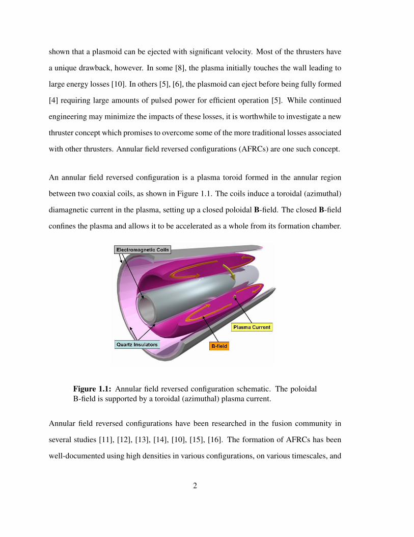
An annular field reversed configuration is a plasma toroid formed in the annular region

between two coaxial coils, as shown in Figure 1.1. The coils induce a toroidal (azimuthal)

diamagnetic current in the plasma, setting up a closed poloidal B-field. The closed B-field

confines the plasma and allows it to be accelerated as a whole from its formation chamber.

Figure 1.1: Annular field reversed configuration schematic. The poloidalB-field is supported by a toroidal (azimuthal) plasma current.

Annular field reversed configurations have been researched in the fusion community in

several studies [11], [12], [13], [14], [10], [15], [16]. The formation of AFRCs has been

well-documented using high densities in various configurations, on various timescales, and

2

with high energy levels. The research has shown that magnetically detached, long-lived,

and stable configurations can be formed using an annular source. The plasmoid forms off

both walls, does not require the fast switching requirements of similar sources, and allows

the plasmoid to form at low voltages (less than 1 kV). The presence of the inner coil allows

magnetic flux to be continuously added to the plasmoid after formation to aid in current

sustainment and to improve the lifetime of the AFRC plasmoid. The loss of magnetic flux

in similar sources leads to a diminished lifetime [17]. Additionally, the plasmoid forms in

a cylindrical geometry rather than with a planar coil suggesting that the plasmoid will only

emerge from the coils after it is fully formed.

The AFRC formation studies suggest that an AFRC plasmoid source would be suitable

for space propulsion technology, yet AFRC plasmoid translation (acceleration) has never

been thoroughly investigated. An early fusion experiment by Alideres, et al [18] used

an annular plasmoid source with permanent magnets to eject a deuterium plasmoid,

showing that translation of AFRCs is possible. This design is not appealing for a

space propulsion thruster due to its heavy mass. Furthermore, data published on this

experiment suggests poor propellant utilization efficiency and no information is provided

about the momentum and energy properties of the exhausting propellant. Both of these

are important considerations for a spacecraft thruster. This single experiment is the only

evidence of plasmoid motion in AFRC devices. Before AFRCs can be developed for

electric propulsion, plasmoid translation must be studied in a suitable framework for space

propulsion starting with a basic demonstration of plasmoid acceleration.

3

1.2 Aim and Scope

The objective of this research was to demonstrate AFRC plasmoid translation using an

experimental prototype, with design characteristics suitable for spacecraft propulsion.

Rather than build a complete thruster hardware package, the experiment was built around

the architecture of a spacecraft experiment using lightweight coils, long (20 µs) timescales,

heavy propellant, and plasmoid expansion into a field free region. If plasmoid translation

was successful, the plasmoid’s velocity and impulse were measured and the system’s

energy efficiency was estimated. If the plasmoid failed to translate, reasons for the failure

were investigated.

While past studies on AFRCs and FRCs were instrumental to the design of this experiment,

the design approach, constraints, and objectives for the prototype experiment differ from

past AFRC work in three major ways. The first difference was that the outer coil was

conical rather than using a cylindrical design with permanent magnets to accelerate the

plasmoid. The second difference is the energy and density requirements and design of the

experiment was based on the need to eject the plasmoid during its lifetime, compared with

heating the gas to fusion conditions. The final difference is that this experiment intends to

measure the directed momentum and energy efficiency of the accelerated plasmoid which

has not been addressed in previous research.

The translation of an AFRC plasmoid in a fusion study [18] was achieved with a cylindrical

geometry using permanent magnets to accelerate the plasmoid. Permanent magnets add

significant mass to a propulsion system, limiting its attractiveness. Conical coils have been

shown to accelerate a plasmoid in previous FRC literature [17] and these add no additional

4

mass to the system. Other PIPTs have successfully used them to accelerate a plasmoid as

well [8], [9], [3]. For AFRCs to be an attractive space propulsion technology, the translation

of the plasmoid must be accomplished using a conical coil.

Past research on AFRCs has focused on using energy levels and gas densities suitable

for fusion studies. While this information is not published in some sources, the energy

levels that are published are nominally over 10 kJ [11], [13], [14], [10], [15]. Neutral

fill densities are generally in excess of 50 mTorr, though formation studies are available

for lower densities from 10-50 mTorr [10], [15]. These energy budgets and densities are

sized to heat a gas for fusion reactions and are generally too high for a spacecraft thruster

design. In a thruster, the energy and density are scaled to match the energy and plasmoid

mass required to form and expel the plasmoid during a given time period. Therefore, it is

important to design a propulsion experiment with these considerations in mind.

The majority of previous research on AFRCs has focused on stationary plasmoid

experiments, where the plasmoid was not expelled from the coils. One AFRC study [18]

accelerated the plasmoid from the coils deliberately. While exit velocities of 100 - 200

km/s were recorded by downstream diagnostics, no data were available for the directed

momentum of the exhausting gas. This is one of the most important characteristics for a

spacecraft thruster, along with the system efficiency for converting the gas into directed

kinetic energy. As such, this research seeks to measure not only the directed velocity of the

accelerated plasma, but the impulse delivered by the gas and energy conversion efficiency

the AFRC prototype experiment attains.

This research is a critical step in directly evaluating AFRC thrusters for space propulsion.

If translation of the plasmoid can be demonstrated, the findings of this research can help

build a more realistic experiment for evaluating AFRC thruster technology. If translation of

5

the plasmoid cannot be detected, the results will highlight some of the technical challenges

in using AFRC devices for space propulsion.

1.3 Structure of Dissertation

This dissertation explores AFRCs as candidates for electric propulsion using an

experimental demonstration of plasmoid translation. The background information in

Chapter 2 provides an introduction to plasmoid propulsion as well as a review of other

PIPT devices. Chapter 3 discusses AFRC formation physics and presents a review of

AFRC formation studies. An engineering dynamic circuit model was developed to model

basic plasmoid translation behavior and to aid in experimental design. This model and

results from it are available in Chapter 4. The experimental setup constructed to test

AFRC translation is presented in Chapter 5. Diagnostic tools used in measuring the

plasmoid’s behavior are also included. The data collected from the translation experiment

are presented in Chapter 6, with full results following in Chapter 7. The translation study

discovered the plasmoid did not escape from the coils and suffered a shorter than expected

lifetime. An instability was the most likely reason for the abbreviated lifetime and a global

instability study was conducted. The results from this study in Chapter 8 uncovered a

radial motion of the plasmoid toward the inner wall. The nature of the radial imbalance is

discussed in Chapter 9, along with results from a study correcting for the radial imbalance

in this experiment. The impact of these corrections on future experiments is also discussed.

Conclusions are presented in Chapter 10, along with a discussion how the results from this

experiment impact future studies on AFRCs for propulsion.

6

Chapter 2

Overview of Plasmoid Propulsion

Annular field reversed configuration thrusters are a high power electric propulsion

technology, belonging to the class of pulsed inductive plasmoid thrusters (PIPT). Plasmoid

thrusters are inherently pulsed propulsion devices, where single plasmoids are formed using

an electromagnetic coil and ejected with a Lorentz force. A stream of plasmoids can be

ejected for continuous operation. Principles of pulsed propulsion are discussed in Section

2.1. An overview of plasmoid propulsion follows in Section 2.2. A comprehensive history

of past and present plasmoid propulsion research is presented in Section 2.3.

2.1 Principles of Pulsed Propulsion

Pulsed thrusters expel discrete slugs of propellant to create thrust, as opposed to steady state

thrusters which stream mass continuously. The repetition rate can be varied to match the

available power or desired thrust. This provides mission flexibility that steady-state devices

7

cannot achieve. A continuously pulsed thruster is the best candidate for testing the full

capability of many PIPT devices, however single-pulse behavior can be used as an initial

baseline for performance assessments. Performance measurements in a single-pulse system

include impulse-bit and energy efficiency of the plasmoid acceleration. Previously, these

have been defined for a single-pulse thruster assuming little divergence of the exhausting

plume and full utilization of the working gas [6]. An alternate derivation is presented here

to account for these non-ideal effects in a manner similar to previous efficiency architecture

for steady-state EP thrusters [19].

The impulse bit Ibit is the total momentum transfer per pulse the exhausting propellant

delivers to a spacecraft parallel to its direction of travel. It includes the mass m j of all

species, the average exhaust velocity of each species u j, and the off-axis divergence of

each species θ j. All of these quantities can vary with radial position r, leading to:

Ibit =n

∑j=0

∫ ∫m j(r)u j(r)cos

(θ j(r)

)rdθdr (2.1)

Mathematically, Ibit can be re-written as a product of the total mass of the propellant

or mass-bit mbit and weighted averages. The weighted averages are defined as

a mass-weighted average velocity 〈u〉m and momentum-weighted divergence relation

〈cosθ〉mv, where:

mbit =n

∑j=0

∫ ∫m j(r)rdθdr (2.2)

〈u〉m =∑

nj=0∫ ∫

m j(r)u j(r)rdθdr

∑nj=0∫ ∫

m j(r)rdθdr=

∑nj=0∫ ∫

m j(r)u j(r)rdθdr

mbit(2.3)

8

〈cosθ〉mv =∑

nj=0∫ ∫

m j(r)u j(r)cos(θ j(r)

)rdθdr

∑nj=0∫ ∫

m j(r)u j(r)rdθdr

=∑

nj=0∫ ∫

m j(r)u j(r)cos(θ j(r)

)rdθdr

〈u〉m mbit(2.4)

so that

Ibit = mbit 〈u〉m 〈cosθ〉mv (2.5)

The thrust is the time rate of change of the total impulse in the direction of travel, z:

T =dIbit

dtz (2.6)

Specific impulse Isp is defined as the thrust compared to the rate of propellant use at sea

level [4]. In single-pulse thrusters, this equates to the impulse by:

Isp =Ibit

mbitg(2.7)

The total system efficiency of a single-pulse thruster is a function of Ibit delivered by the

propellant, the mass of the propellant mbit , and the initial energy E0 required to operate the

thruster, related by:

η =I2bit

2mbitE0(2.8)

The total efficiency η can be distributed into various terms including the energy efficiency

ηE , propellant efficiency ηP, and beam efficiency ηB. These terms can be defined by

replacing Ibit in Equation 2.9 with Equation 2.5 and re-arranging terms:

η =12mbit 〈u〉2m 〈cosθ〉2mv

E0=

12

⟨mbitu2⟩

mE0

〈u〉2m〈u2〉m

〈cosθ〉2mv = ηEηPηB (2.9)

9

This research focuses on estimating the energy efficiency ηE of the plasmoid’s acceleration

using plume measurements rather than measuring the complete system efficiency η . Total

system efficiency measurements require direct impulse measurements using an isolated

thruster fixed to a thrust balance inside a vacuum tank. The engineering challenges

associated with developing a vacuum-compatible AFRC thruster and fast-response thrust

balance are beyond the scope of this basic investigative research. Energy efficiency

measurements in the plume provide an upper bound to system efficiency, when ηP, ηB

= 1.

Propellant efficiency ηP, though not an investigative topic of this research, is an important

consideration in pulsed gaseous thrusters because it includes the mass utilization of the

propellant [19]. Mass utilization is the ratio of ionized propellant to injected propellant. In

a pulsed gaseous thruster, propellant can stream out of the device while the coils are not

energized between pulses. Unionized propellant can also escape on the leading and trailing

edges of each pulse. If a large fraction of the propellant leaves the thruster without being

ionized, it cannot be accelerated by the coils and presents a large loss to the system. For

this reason, the system efficiency of any gaseous pulsed thruster must take into account the

total propellant efficiency.

Impulse, thrust, and efficiency can be extrapolated to multi-pulse operation, if it is assumed

that the pulses do not appreciably interfere and if the plasma slug maintains a coherent,

mass conserving structure. Single pulse operation only provides a baseline assessment;

characterization with multi-pulse operation is required to understand the full performance.

10

2.2 Plasmoid Propulsion

Pulsed inductive plasmoid thrusters form magnetized plasma toroids by inductively driving

large diamagnetic currents in a conductive plasma from an external coil. The magnetic

field structure arising from the current induction keeps the plasma fully contained and

detached from the coil’s magnetic field. This means the entire plasmoid can be ejected

(translated) from the formation coil as a complete entity using a Lorentz force (JxB). The

family of pulsed inductive plasmoid thrusters includes a diverse group of plasma sources;

a few are shown in Figure 2.1. A brief description of this group is given in the text by Jahn

[4].

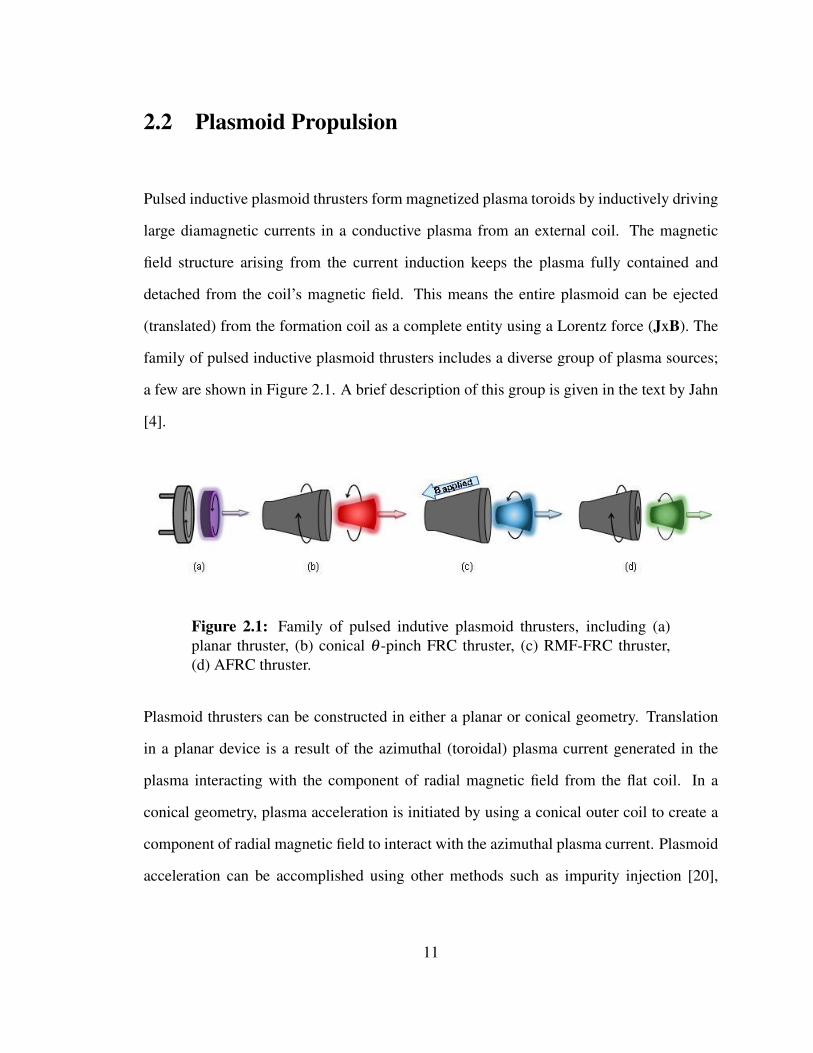
Figure 2.1: Family of pulsed indutive plasmoid thrusters, including (a)planar thruster, (b) conical θ -pinch FRC thruster, (c) RMF-FRC thruster,(d) AFRC thruster.

Plasmoid thrusters can be constructed in either a planar or conical geometry. Translation

in a planar device is a result of the azimuthal (toroidal) plasma current generated in the

plasma interacting with the component of radial magnetic field from the flat coil. In a

conical geometry, plasma acceleration is initiated by using a conical outer coil to create a

component of radial magnetic field to interact with the azimuthal plasma current. Plasmoid

acceleration can be accomplished using other methods such as impurity injection [20],

11

magnetic kicker coils to introduce an axial instability, or permanent magnets to create a

radial field component [18]. The conical outer coil is generally the easiest way to achieve

translation and it provides considerable mass savings for propulsion systems.

Pulsed inductive plasmoid thrusters are attractive for high power spacecraft propulsion for

several reasons. They create a high energy density plasmoid which can be accelerated

to high velocities. Their pulsed nature gives them throttling capability, allowing them to

cover a wide range of missions and power levels. By adjusting the pulse rate at a fixed

energy per pulse, they can match the desired thrust with little change in efficiency and

specific impulse. They operate on fast timescales, keeping non-conservative energy losses

to a minimum. The inductive plasmoid formation increases the lifetime of the device,

as it keeps hot plasma away from the walls, reducing erosion. Additionally, the inductive

formation allows for the use of any variety of propellants since material compatibility issues

are minimized.

The formation physics of the plasmoid is device dependant, though in each case the

plasma currents are generated inductively as a result of Faraday’s Law. Some devices

choose to start with a seed plasma, which is created in the pre-ionization (PI) stage. This

has been found in some devices to be critical to the formation [17], [21]. The level of

initial ionization varies as does the method for pre-ionization; pre-ionization remains an

empirical, device-dependant process.

12

2.3 Plasmoid Thruster Technology

Pulsed inductive plasmoid thrusters can be crafted from closed-field devices or from planar

current-sheet devices. Closed-field devices are generally referred to as compact toroids

and include the workhorses of fusion research: the Field Reversed Configuration (FRC)

[17], [21] and the Spheromak [22]. Several technologies have already been demonstrated

as propulsion devices, with impulse measurements on single or multi-pulse prototypes.

Others have only measured the velocity of the propellant downstream of the formation

coil. Several more are currently in development. A summary of all known PIPT devices

and studies is shown in Table 2.1.

The most notable pulsed inductive plasmoid device is the PIT, or pulsed inductive thruster.

A comprehensive review of this program and its variants is available in a review paper by

Polzin [6]. The PIT was developed in the 1960’s by TRW Space Systems. Early work

on basic physics in inductive plasma devices culminated in the early 1990’s development

of the PIT-MkVa propulsion system, currently the best performing thruster in PIPT [5].

The PIT-MkVa used a flat 1-m diameter coil, backed by 4.6 kJ/pulse, 1 µs rise-time

capacitor bank to ionize and accelerate a sheet of propellant. Single pulse testing with

ammonia at maximum energy was reported for mass bits between 3.1 mg to 0.69 mg.

Impulse-bit measurements were 121 mN-s to 56 mN-s, resulting in specific impulses

between 4000-9000 s. System efficiencies were constant across this range at 50%, deviating

by 5%. Testing at lower energies resulted in lower η and lower Isp. Results were also

shown for simulated hydrazine, but efficiencies were reduced from the ammonia tests. The

high pulse energies used in the PIT-MkVa were required for high efficiency. Lower energy

13

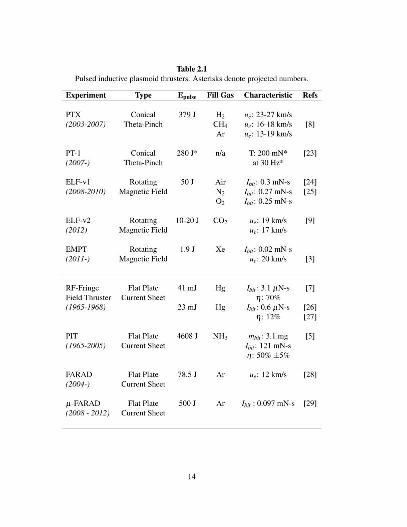
Table 2.1Pulsed inductive plasmoid thrusters. Asterisks denote projected numbers.

Experiment Type Epulse Fill Gas Characteristic Refs

PTX Conical 379 J H2 ue: 23-27 km/s(2003-2007) Theta-Pinch CH4 ue: 16-18 km/s [8]

Ar ue: 13-19 km/s

PT-1 Conical 280 J* n/a T: 200 mN* [23](2007-) Theta-Pinch at 30 Hz*

ELF-v1 Rotating 50 J Air Ibit : 0.3 mN-s [24](2008-2010) Magnetic Field N2 Ibit : 0.27 mN-s [25]

O2 Ibit : 0.25 mN-s

ELF-v2 Rotating 10-20 J CO2 ue: 19 km/s [9](2012) Magnetic Field ue: 17 km/s

EMPT Rotating 1.9 J Xe Ibit : 0.02 mN-s(2011-) Magnetic Field ue: 20 km/s [3]

RF-Fringe Flat Plate 41 mJ Hg Ibit : 3.1 µN-s [7]Field Thruster Current Sheet η : 70%(1965-1968) 23 mJ Hg Ibit : 0.6 µN-s [26]

η : 12% [27]

PIT Flat Plate 4608 J NH3 mbit : 3.1 mg [5](1965-2005) Current Sheet Ibit : 121 mN-s

η : 50% ±5%

FARAD Flat Plate 78.5 J Ar ue: 12 km/s [28](2004-) Current Sheet

µ-FARAD Flat Plate 500 J Ar Ibit : 0.097 mN-s [29](2008 - 2012) Current Sheet

14

testing at 2 kJ/pulse failed to exceed efficiencies above 30%. Future generations of the

PIT have not been able to match this performance; the PIT-MkVI and the 200 kWe NuPIT

suffered from switch failures and work has been discontinued.

The FARAD (Faraday accelerator with radio-frequency assisted discharge) is a device

similar to the PIT, developed in 2004 at Princeton University [28]. The FARAD used

an inductive RF pre-ionization (PI) source upstream of a 20 cm diameter flat coil. Using a

PI-stage, the FARAD demonstrated that it was possible to create and accelerate a current

sheet at 78.5 J/pulse. The resulting velocity using a 23 mTorr argon fill was 12 km/s.

After the original FARAD, four additional devices were created. The Conical Theta Pinch

FARAD (CTP-FARAD) used a conical coil instead of the flat coil to accelerate the plasmoid

[30]. Another used a pulsed PI and gas injection [31]. Princeton University is developing

a single-stage FARAD (SS-FARAD) which combines an RF pre-ionization circuit with the

main discharge circuit for a single-coil design [32]. Work on the SS-FARAD is currently

in progress. A steady-state microwave PI source FARAD (µ-FARAD) [33], [29] was

recently developed at NASA-Marshall. A conical discharge coil was substituted for the

planar version to provide mass containment of the streaming propellant. The microwave-PI

source was later discarded for a DC glow breakdown. Impulse measurements on the conical

µ-FARAD show impulse measurements of 0.097 mN-s at with input energy of 500 J and

mass flow rate of 120 mg/s. The poor performance on the µ-FARAD was attributed to

incomplete current sheet breakdown along the discharge coil.

Concurrent with the early years of PIT development, a similar device was also tested. The

RF-Fringe Field Thruster used a set of small diameter (15 cm) coaxial flat coils to ionize

and accelerate a mercury-vapor current sheet [7], [26], [27]. Permanent magnets behind the

coils increased the radial magnetic field in front of the coils. The coils were powered by an

15

external current supply at 240 kHz, with plasmoids ejected every half cycle. High power

testing was conducted with water-cooled coils at 30 kW steady state and up to 134 kW in

burst mode [7]. Thrust measurements of 1.5-2 N were recorded with a specific impulse of

2000-2500 seconds and an efficiency of 70%. This corresponds to an impulse-bit of 3.1

µN-s at 41 mJ/pulse. This performance could only be attained with water cooling through

the coil. Low energy testing on a radiation cooled design at 10 kW produced thrust levels

of 0.3 N, with a specific impulse of 900 seconds and an efficiency of 12% [26], [27]. This is

equivalent to a 0.6 µN-s impulse-bit at 23 mJ/pulse. It was suggested that these low ratings

were due to insufficient ionization and poor mass utilization; the thruster accelerated only

the ion mass fraction rather than the bulk propellant [7].

The PIT, FARAD, and RF-Fringe Field Thruster are current sheet accelerators. Breakdown

and acceleration must happen very quickly in a planar geometry, as the plasma begins to

push away from the coil as soon as it is formed. Without a pre-ionization, current sheet

devices require high voltages to breakdown and accelerate the propellant quickly. A coil

voltage on the PIT-MkVa of 32 kV was required for maximum performance. Additionally,

the current sheet must be impermeable to the neutral gas so that as it accelerates, it

can sweep up the surrounding neutrals for higher mass utilization [6]. The high degree

of ionization required implies that efficient, low-power and low-voltage operation is not

feasible for planar devices. This has been demonstrated in both the PIT development and

in the RF-Fringe Field thruster.

The closed-field PIPT devices allow the plasma to remain in contact with the coils for

a longer duration, reducing some of the strain on high voltage and energy requirements.

The closed-field structure is ideal for propulsion because the entire plasmoid mass can be

ejected as a bulk and can interact magnetically with the coils. A comprehensive review of

16

FRC technology for fusion research is available in the 2011 review paper by Steinhauer [21]

and in the 1988 paper by Tuszewski [17]. Three formation techniques for FRCs are listed

which would be compatible for propulsion: (1) θ -pinch formation, (2) rotating magnetic

field (RMF) formation, and (3) annular (coaxial) source formation. Propulsion concepts

using each formation method have been tested or are currently under development.

The Plasmoid Thruster Experiment (PTX) was investigated at NASA-Marshall in the

mid-2000s and used a θ -pinch coil to form and accelerate a small (1 cm) plasmoid [34],

[8]. The plasmoid’s velocity was measured using an interferometeric time-of-flight array

[8]. At coil energies of 9 J and coil voltages of 5.5 kV, plasmoids were ejected at 25

km/s using hydrogen, 17 km/s using methane, and 16 km/s with argon. Significant circuit

losses dissipated the remaining pulse energy of 370 J. Performance measurements (impulse,

efficiency) were speculated for this device at 1-100 mN with 0.1 to 49% of thrust efficiency,

but never directly measured. Thrust efficiency is defined as the ratio of final kinetic energy

compared to coil energy. System efficiencies are much lower. The next-generation PTX

(PT-1) was designed and constructed in 2007 to operate as a multi-pulse fully integrated

thruster, but funding was not provided for full testing [23].

Rotating magnetic fields are an alternative formation scheme for propulsion FRCs. With

RMF, electron current is driven by radio-frequency waves, keeping the instantaneous

current and voltages low enough for use with solid-state circuitry. The Electrodeless

Lorentz Force (ELF) thruster was developed by MSNW in 2008 [24]. The ELF

was a 50 J/pulse devices, 420 mm in length with an 8 degree cone and 26 cm exit

diameter. Nominal circuit voltages were 300 V, orders of magnitude below θ -pinch FRCs.

The first-generation ELF (ELF-v1) demonstrated single-pulse impulse measurements of

0.3mN-s at an estimated 30% efficiency on air [25]. The corresponding plasmoid velocity

17

was 15 km/s. Nitrogen and oxygen were also tested. A coherent plasmoid was measured

up to 1 m downstream. Data in the formation region demonstrated that the formation and

acceleration occur simultaneously.

Steady state operation of the next generation ELF (ELF-v2) was demonstrated in 2012

[9]. These experiments showcased steady-state operation of an FRC-thruster on Xenon

and complex propellants, including water and Martian air (95% CO2, 3% N2, 2% Ar). The

second generation ELF was slightly smaller than the original ELF, with a reduced length of

200 mm, cone angle of 12 degrees, and exit diameter of 20 cm. Bus voltages of 300 V were

used to drive the discharge capacitors at 2800 V using an MSNW-crafted power processing

unit. Steady-state operation (9 or more pulses) with Martian air demonstrated average

plasmoid velocities of 19 km/s. These numbers were based on a 4.8 kW power load, with a

mass flow of 250 sccm, and a 1500 Hz repetition rate. Increasing the power to 5.8 kW and

the flow rate to 500 sccm dropped the plasmoid velocity to 17 km/s. Steady-state operation

on water demonstrated that two populations emerged from the device. A fast population

was seen, traveling in excess of 50 km/s followed by a slower 17 km/s population. The dual

population was likely due to separation of the oxygen and hydrogen components, with the

hydrogen components leaving at much higher velocities. The discrepancy in velocity made

estimation of average plasmoid velocity using water propellant difficult. While the ELF-v2

was a 30 kW-nominal thruster, testing at power levels exceeding 5.8 kW was not feasible

at MSNW due to chamber and electronics limitations.

A small-scale RMF device has also been developed by MSNW for space propulsion [3].

The Electromagnetic Plasmoid Thruster (EMPT) is a nominal 1 J/pulse, 1 kW thruster,

with a footprint of 44 mm in diameter by 100 mm in length. Preliminary testing with

xenon demonstrated that 400 FRCs could be formed and ejected sequentially using a bus

18

voltage of 250 V and repetition rate of 2800 Hz. Average exit velocites under steady

state operation of 20 km/s were recorded at 1.9-2.1 J/pulse, corresponding to 5 kW of

input power. Impulse bits of 0.02 mN-s were also measured for single-pulse operation

with exit velocities of 10-40 km/s. Accurate impulse measurements under steady-state

operation were not possible due to interaction of the ballistic pendulum with background

gases, imperfect reflections, and other complications. Steady state operation of the EMPT

highlighted several important considerations for FRC-based PIPTs. The EMPT tests found

that with a high enough repetition rate (2800 Hz) only a single PI discharge was required

at the beginning of the pulse train. The seed plasma remaining in the channel after the

previous plasmoid departed was enough to initiate the next RMF-FRC. This required

matching the repetition rate for the thruster with the neutral refill time. If additional gas

was not added in time, there was not enough propellant left behind to form a second FRC.

This indicates a high level of propellant utilization. Additionally, some conditions resulted

in FRC formation on the first, third, and fourth pulses, but not on the second pulse. The

steady state operation also found that the first 2 FRCs created were different in behavior

from the remaining pulses. The first FRC appeared much faster and denser than the second

FRC, as indicated by an order of magnitude decrease in signal on downstream probes.

Steady state behavior of the thruster didn’t appear until the third pulse. These findings

underscore the importance of bringing thruster concepts past the single-pulse operation for

full performance mapping.

The Star Thrust Experiment (STX) is often mistakenly considered to be another RMF

thruster. The STX was a multi-megawatt concept was proposed in the late 1990’s [35].

The idea behind the STX was to use an RMF-FRC stage to heat propellant so that it could

be expelled from a gas nozzle at high velocity. The plasmoid itself was never intended

to be accelerated from the chamber, making it an electrothermal thruster rather than an

19

electromagnetic thruster. Thruster testing was never published, though formation results of

the RMF stage are available [36].

The final type of closed field thruster is the annular FRC (AFRC). The annular geometry

is intended to extend the formation timescales from less than 10 µs to over 100 µs and

eliminates the need for high voltage technology. The annular geometry prevents the plasma

from coming into contact with the walls at all times1, which can lead to severe energy losses

early in the formation. This is the only FRC device which has not been demonstrated for

propulsion. As discussed in Chapter 3, numerous formation studies have shown that stable

AFRC can be produced on slow timescales (10’s to 100’s of µs) suitable for ejecting a

plasmoid at low energy as well as fast (less than 10 µs) timescales. A translation study

in 1967 [18] demonstrated that a magnetized current sheet can be ejected at high velocity

(200 km/s) from an AFRC geometry using light gases, but that remains the only evidence

of AFRC translation in literature.

Two design concepts have been proposed to mate acceleration attachments to closed field

sources. Their purpose is to use a separate acceleration stage to boost the exit velocity of the

plasmoid and to increase device efficiency. The Propagating Magnetic Wave Accelerator

[37] proposed in 2000 projected a boost of efficiency from 50% to 90% at megawatt power

levels. A prototype PMWAC was built, but the device was never tested with a plasma

source. The Magnetically Accelerated Plasmoid (MAP) experiments were also intended

for use with an additional acceleration stage [38], [39], [40]. Plasma tests using a θ -pinch

source demonstrated exit velocities of 180 km/s at megawatt power levels.

1In the traditional theta-pinch FRC formation, the plasma comes in contact with the wall during the earlystages before reversal.

20

2.4 Summary

Pulsed inductive plasmoid thrusters form magnetized plasma toroids by inductively driving

large diamagnetic currents in a conductive plasma from an external coil. The currents in

the plasma react with the external coil magnetic field to drive the plasmoid out of the coils

under a directed Lorentz force. PIPTs offer many benefits to electric propulsion including

high thrust levels, mission flexibility, limited erosion, and a wide acceptance of various

propellants.

The PIPT family represents a diverse group of thruster concepts, in various stages of

development. Planar concepts include the PIT, the FARAD family, and the RF Fringe

Field thruster. The PIT and FARAD demonstrated single pulse performance, while the RF

Fringe Field thruster was operated at steady state. The PIT required massive amounts of

energy (4.6 kJ/pulse) for peak performance while the FARAD showed it was possible to

drop the energy to under 100 J/pulse with the addition of a pre-ionization stage. Closed

field concepts have also been tested including two version of FRC-based thrusters, conical

θ -pinch FRCs and RMF-FRCs. A conical θ -pinch thruster was developed and tested at

NASA-Marshall in two variations. The RMF-FRC thruster group, consisting of two scaled

versions, is currently under development by a small company. The first thruster, the ELF,

is a 30 kW thruster which has been operated on a wide variety of propellants. The second

thruster, the EMPT, has shown that coherant FRCs can be formed for as little as 1 J/pulse.

The RMF-FRC thrusters have both been operated in steady state and single pulse mode,

making them the most developed of all PIPTs.

An additional formation scheme has been demonstrated for FRC-based thrusters, using

21

coaxial coils to create a closed-field plasmoid. This formation method is referred to as the

Annular Field Reversed Configuration and has received considerable attention in plasmoid

formation studies. The formation studies have shown that it is possible to create a stable

plasma toroid with a fairly long lifespan using electromagnetic coils without permanent

magnets. While an AFRC-based thruster is possible, a thruster concept using AFRC

formation techniques has never been developed. This research explores the viability of

an AFRC thruster by demonstrating if an AFRC plasmoid can be translated from the

coils. If the plasmoid does translate, the plasmoid’s velocity, momentum, and acceleration

efficiency will be measured for a basic characterization.

22

Chapter 3

Annular Field Reversed Configurations

This chapter discusses annular field reversed configurations, including a basic description

of the AFRC in Section 3.1, descriptions of the different formation methods for AFRCs in

Section 3.2, and important AFRC physics in Section 3.3. A literature review on seven

past AFRC experiments is presented in Section 3.4. Section 3.5 discusses translation

considerations for AFRC devices.

3.1 AFRC Basics

AFRCs form an inductive, annular plasma toroid between an inner and outer coil. AFRCs

resemble traditional FRCs which are formed without the inner coil [21]. AFRCs and FRCs

get their name from the bi-directional magnetic field through their radial cross section; the

magnetic field is reversed on the plasmoid’s inner radius as compared to the outer radius.

The bi-directional field forms a separatrix (magnetic boundary) with a magnetic null at the

23

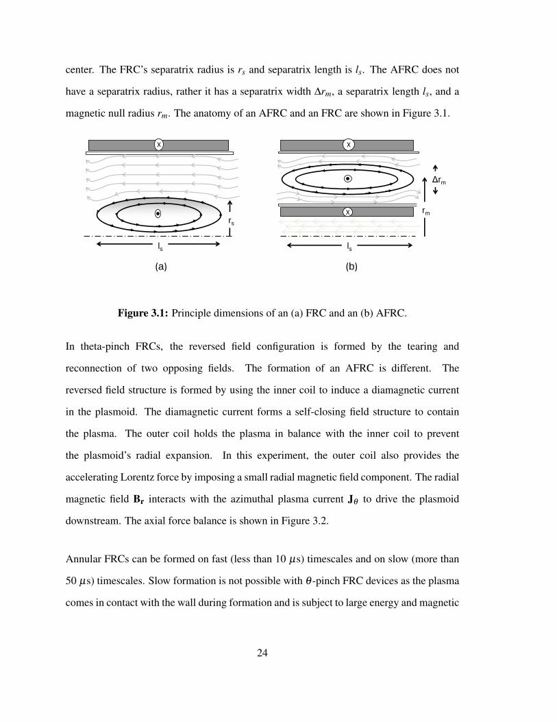
center. The FRC’s separatrix radius is rs and separatrix length is ls. The AFRC does not

have a separatrix radius, rather it has a separatrix width ∆rm, a separatrix length ls, and a

magnetic null radius rm. The anatomy of an AFRC and an FRC are shown in Figure 3.1.

X

rs

ls

X

X rm

Δrm

ls

(a) (b)

Figure 3.1: Principle dimensions of an (a) FRC and an (b) AFRC.

In theta-pinch FRCs, the reversed field configuration is formed by the tearing and

reconnection of two opposing fields. The formation of an AFRC is different. The

reversed field structure is formed by using the inner coil to induce a diamagnetic current

in the plasmoid. The diamagnetic current forms a self-closing field structure to contain

the plasma. The outer coil holds the plasma in balance with the inner coil to prevent

the plasmoid’s radial expansion. In this experiment, the outer coil also provides the

accelerating Lorentz force by imposing a small radial magnetic field component. The radial

magnetic field Br interacts with the azimuthal plasma current Jθ to drive the plasmoid

downstream. The axial force balance is shown in Figure 3.2.

Annular FRCs can be formed on fast (less than 10 µs) timescales and on slow (more than

50 µs) timescales. Slow formation is not possible with θ -pinch FRC devices as the plasma

comes in contact with the wall during formation and is subject to large energy and magnetic

24

FLorentz

Br

Jplasma

Figure 3.2: Force diagram for an AFRC translating from a conical coil.

flux losses. The reversal in a θ -pinch FRC must be done very quickly (less than 5 µs) to

prevent these energy and flux losses. As is shown in Section 3.2, the AFRC can form away

the wall to allow the configuration to build on slower timescales.

Annular FRCs have three stages of life: formation, equilibrium, and termination. The

formation stage begins with the start of the inner coil current. The equilibrium stage

takes over when the configuration is fully formed, with a bi-directional field in the

annulus. Equilibrium is eventually disturbed and the plasmoid configuration terminates

and disappears. A brief description of each stage and the important physics is explained in

Sections 3.2 and 3.3.

3.2 AFRC Formation Techniques

The formation of an AFRC plasmoid is a complex process. The plasma is subject to drifts,

collisions, shocks, instabilities, and rapidly changing magnetic topology. While these

effects are essential to the formation, the bulk behavior of the plasma can be simplified by

treating the plasmoid as a rigid conductor inductively driven between the coils. Formation

25

can then be explained with a magnetic transformer analogy, using a primary circuit and

secondary circuit. According to Faraday’s Law, magnetic fields created by currents in the

coils (primary circuits) induce currents in the plasmoid circuit (secondary circuit). The

currents in the plasmoid circuit develop to oppose changing magnetic fields or magnetic

flux created by the coil circuits. Magnetic flux ΦB is defined as the net magnetic field

passing through a surface or

ΦB =∫

AB ·dA (3.1)

An important consequence of Faraday’s Law in AFRCs is that the inner coil can actively

drive current in the plasmoid, adding magnetic flux to the configuration after the magnetic

fields close. This cannot be accomplished in traditional θ -pinch FRC devices.

Annular FRC plasmoids are generally created between coils resembling very long

solenoids, where the length of the coil is much greater than the radius of the coil. The

magnetic field inside a solenoid is directed along the axis, with the magnetic field constant

inside the solenoid and nearly zero outside. In the formation explanations provided here, it

is assumed that the aspect ratio of both coils and the plasma currents can be approximated

as semi-infinite solenoids. Magnetic fields are also super-imposable, meaning that the field

configuration of two coaxial coils is simply the vector sum of their vacuum magnetic fields.

The field generated by the plasma adds to this field, creating stronger fields outside the

configuration than in the vacuum case.

Four different formation schemes are used to create an AFRC. A brief description of each

formation method is provided in the following sections. Each method uses a pre-ionization

stage, during which the propellant is partially ionized using any variety of techniques. This

allows the propellant to respond to the currents in the coils. Though pre-ionization is a

critical part of the discharge [17], it has been investigated for AFRCs elsewhere [41] and

26

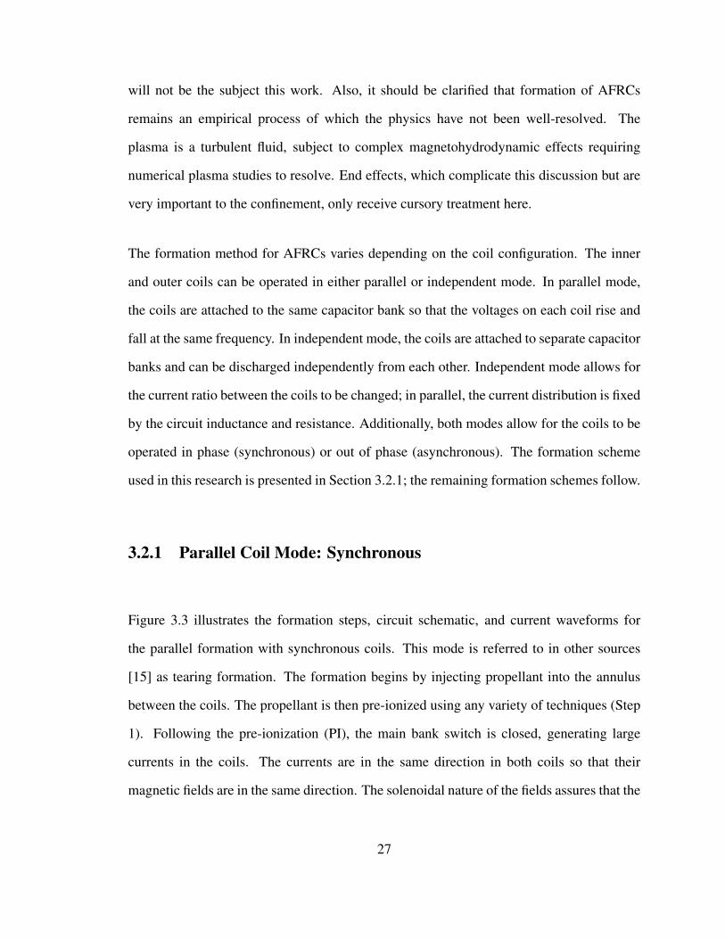
will not be the subject this work. Also, it should be clarified that formation of AFRCs

remains an empirical process of which the physics have not been well-resolved. The

plasma is a turbulent fluid, subject to complex magnetohydrodynamic effects requiring

numerical plasma studies to resolve. End effects, which complicate this discussion but are

very important to the confinement, only receive cursory treatment here.

The formation method for AFRCs varies depending on the coil configuration. The inner

and outer coils can be operated in either parallel or independent mode. In parallel mode,

the coils are attached to the same capacitor bank so that the voltages on each coil rise and

fall at the same frequency. In independent mode, the coils are attached to separate capacitor

banks and can be discharged independently from each other. Independent mode allows for

the current ratio between the coils to be changed; in parallel, the current distribution is fixed

by the circuit inductance and resistance. Additionally, both modes allow for the coils to be

operated in phase (synchronous) or out of phase (asynchronous). The formation scheme

used in this research is presented in Section 3.2.1; the remaining formation schemes follow.

3.2.1 Parallel Coil Mode: Synchronous

Figure 3.3 illustrates the formation steps, circuit schematic, and current waveforms for

the parallel formation with synchronous coils. This mode is referred to in other sources

[15] as tearing formation. The formation begins by injecting propellant into the annulus

between the coils. The propellant is then pre-ionized using any variety of techniques (Step

1). Following the pre-ionization (PI), the main bank switch is closed, generating large

currents in the coils. The currents are in the same direction in both coils so that their

magnetic fields are in the same direction. The solenoidal nature of the fields assures that the

27

magnetic field in the annulus is a result of the outer coil alone (Step 2). Current sheets are

generated in the plasma immediately following application of coil current. These current

sheets form close to the inner and outer coils. Each current sheet attempts to keep the

magnetic flux ΦB through its cross section constant. If the current sheets form immediately,

they will try to retain a ΦB = 0 condition through their cross section. The plasma current

close to the inner coil opposes the flux through the inner coil and the plasma current close to

the outer coil opposes the flux from the outer coil. Since the flux through the inner plasma

ring is generally much higher than the flux through the outer plasma ring, the current in the

inner ring will be much higher than the current in the outer ring. This means that the plasma

current is mostly due to the changing flux through the inner coil (Step 3). A radial Lorentz

force (Fr = Jθ Bz) implodes both current sheets toward the annular centerline. The current

sheets collide, resulting in single configuration with reversed fields on either side (Step 4).

Magnetic tearing and reconnection is thought to occur at the ends of the configuration to

improve confinement [15], yet evidence of this is unclear.

3.2.2 Independent Coil Mode: Synchronous

The inner and outer coils can be driven by different capacitor banks and different circuits.

If each circuit is designed with the proper phase, the currents in the outer coil and inner

coil can rise and fall in unison. The formation is identical that of the parallel synchronous

mode in Section 3.2.1. The only difference is that the inner and outer coil currents can now

be adjusted independently of each other by varying the circuit voltages.

28

3.2.3 Parallel Coil Mode: Asynchronous

Figure 3.4 shows the circuit configuration, typical current waveforms, and the formation

sequence for parallel coil operation with the coils operating out of phase. This mode is

referred to in other sources [15] as programmed formation. It is different from the parallel

formation circuit by the addition of a switch in the outer coil circuit. Before the start of the

discharge, the area between the coils is filled with gas. At t = 0, the inner coil circuit is

discharged and a magnetic field through the inner coil is generated (Step 1). As this field

reaches its maximum strength, the gas is pre-ionized (Step 2). The inner coil current and

field begin to decrease. The conducting plasma tries to oppose this decrease in magnetic

flux by developing a plasma current that is in the same direction as that of the inner coil.

The outer coil circuit switch is then closed, creating a current in the opposite direction of

the current in the inner coil and increasing the magnetic field inside the annulus. As a

result, the plasma becomes strongly attracted to the inner coil (Step 3). The direction of the

plasma current results in a magnetic field that reverses the field direction near the inner coil

and sets up the closed B-field structure in the plasma. The field lines from the inner coil

wrap around the outside of the plasma, such that the plasma separatrix is attached to the

inner coil (Step 4). When the inner coil current passes through zero and the direction of the

magnetic field from the inner coil changes, the plasma is forced off the wall by the current

repulsion. The plasmoid detaches from the inner wall and the separatrix moves towards the

center of the channel (Step 5).

29

t = 0

V0

1

+ + + +

-

- - -

-

1

X 2

X

X 3

X

X 4

X

2 3

4

Figure 3.3: Formation schematic for an AFRC formed with the coilsconnected in parallel, operating in phase.

30

3

X

X

1

X

2

X

+ + + +

+ -

-

-

-

- -

X X X X X X X X X X

4

X

X

5

1

2

3 4

5

t = 0

VO

t = t3

oute

r

inne

r

Figure 3.4: Formation schematic for an AFRC formed with the coilsconnected in parallel, operating asynchronously.

31

3.2.4 Independent Coil Mode: Asynchronous

Figure 3.5 shows the circuit configuration, typical current waveforms, and the formation

sequence for independent coil operation with the coils operating out of phase. The

formation sequence is nearly identical to that of the parallel coil mode with asynchronous

coils, with the difference arising from the two separate circuits for the outer and inner coils.

Before the start of the discharge, the area between the coils is filled with gas. At t = 0, the

inner coil circuit is discharged and a magnetic field through the inner coil is generated (Step

1). As this field reaches its maximum strength, the gas is pre-ionized (Step 2). The inner

coil current and field begin to decrease. The conducting plasma tries to oppose this decrease

in magnetic flux by developing a plasma current that is in the same direction as that of the

inner coil. The outer coil circuit is then discharged in the opposite direction as the current

in the inner coil, increasing the magnetic field inside the annulus. As a result, the plasma

becomes strongly attracted to the inner coil (Step 3). The direction of the plasma current

results in a magnetic field that reverses the field direction near the inner coil and sets up

the closed B-field structure in the plasma. The field lines from the inner coil wrap around

the outside of the plasma, such that the plasma separatrix is attached to the inner coil (Step

4). When the inner coil current passes through zero and the direction of the magnetic field

from the inner coil changes, the plasma is forced off the wall by the current repulsion. The

plasmoid detaches from the inner wall and the separatrix moves towards the center of the

channel (Step 5).

32

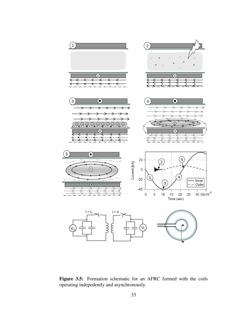
3

X

X

1

X

2

X

+ + + +

+ -

-

-

-

- -

X X X X X X X X X X

4

X

X

5

1

2

3 4

5

t = t3

VO

t = 0

Vi

Figure 3.5: Formation schematic for an AFRC formed with the coilsoperating indepedently and asynchronously.

33

3.3 AFRC Physics

While the formation physics of AFRCs and FRCs remain largely qualitative, the

equilibrium physics for them are easier to define. Several models exist to explain the

behavior of FRCs [21], but there is no single equilibrium solution in full agreement with

experimental data. Rather than digressing into the extensive topic of AFRC/FRC equilibria,

only a few salient topics will be covered in this section. These topics include deriving

the radial balance of AFRCs, presenting measured profiles of the equilibrium plasmoid,

discussing plasma heating through magnetic field diffusion, discussing plasma drifts and

instabilities. Termination of AFRCs is also covered, though this topic remains largely

device dependent.

Translation of the AFRC plasmoid in this research is accomplished by using a conical outer

coil. The conical outer coil introduces a small radial magnetic field component to interact

with the azimuthal plasmoid current and force the plasmoid out of the coils. This Lorentz

force is the primary acceleration mechanism in an AFRC thruster. Unlike other propulsion

technologies, a gas pressure gradient is not required for operation. The conical coil also

lessens the magnetic mirror intensity on the large end of the coil as shown by the asymmetry

in the axial magnetic field map in Figure 6.7 across the coil midplane (z = 15 cm). This

allows the plasmoid to escape from the coils. As the plasmoid passes by the mirror at the

large end of the coil, it experiences its peak acceleration as the strong radial magnetic fields

act on the plasmoid. In formation studies, the magnetic mirrors are symmetric on both ends

of the coil to confine the plasmoid to the annulus. A full discussion of translation physics

and predictions of an AFRC plasmoid’s trajectory is the topic of Chapter 4.

34

3.3.1 Radial Balance

The plasmoid must maintain a radial balance between the coils, dictated by the magnetic

pressure on either side of the magnetic separatrix. Magnetic pressure PB is related to the

square of the magnetic field B, according to:

PB =B2

2µ0(3.2)

The magnetic pressure on the inner radius of the plasmoid created by the reversed field

pushes the plasmoid toward the outer wall and the magnetic pressure from the outer coil

pushes the plasmoid toward the inner wall. The magnetic null radius rm corresponds to

where these forces are equal.

The magnetic null radius rm can be predicted by portraying the plasmoid to be a rigid

current sheet with forces acting on it. This treatment assumes the plasmoid is composed of

infinitely hot electrons and cold ions to form an impermeable barrier between the plasma

magnetic field and the coil magnetic field. The radial equation of motion for an annular

plasma is then

md2rm

dt2 = 2πrm

(B2

zi

2µ0−

B2zo

2µ0

)(3.3)

Bzi is the axial field on the inner radius of the plasmoid, Bzo is the axial field on the outer

side, and m is the plasmoid mass. The easiest approach to solve this differential equation is

to make the assumptions that the fields are generated by ideal solenoids with well defined

field distributions and inductances, as was done in References [42] and [43]. Additionally,

the length of the plasmoid is equal to the length of the coils l. In this instance, the inner

35

and outer fields are defined by:

Bzi =µ0 (NoIo− Ip)

l(3.4)

Bzo =µ0 (NoIo)

l(3.5)

No is the number of turns on the outer coil, Io is the current through the outer coil, and Ip is

the plasma current. The plasma current can be calculated by solving a circuit representation

of the plasmoid, with self inductance Lp, mutual inductances Mop, Mip and a resistance Rp:

ddt

(LpIp−MopIo−MipIi)+RpIp = 0 (3.6)

The inductances Lp, Mop, and Mip are defined according to solenoid approximations:

Lp =πµ0r2

ml

(3.7)

Mop =πµ0Nor2

ml

(3.8)

Mip =πµ0Nir2

icl

(3.9)

where ric is the inner coil radius. If the coil currents Ii and Io are independent of each other,

Equations 3.3 and 3.6 can be solved to find rm. Kondoh [42] used a linearization of Ip and

rm to find zeroth-order approximations. This assumes that d2rm/dt2 = 0. The linearization

approximates the zeroth-order plasma current Ip,0 and plasmoid radial position rm,0 to be

Ip,0 = 2N0I0 (3.10)

rm,0 =

√(NiIir2

icNoIo

− 2lµ0πIo

∫ t

t0RpIodt

)(3.11)

36

Equation 3.11 shows that plasma resistance causes the radial plasmoid position to decay

toward the inner wall. This was also seen in the experimental results [42]. Computer

simulations by Kondoh [42] on the full ODE equation set confirm this finding, with larger

resistances resulting in faster declines. A small radial oscillation is noted as well when the

resistance is very low. When Rp = 0, Equation 3.11 simplifies the radial position of the

plasmoid to a function of the coil current ratio. By increasing the inner coil current, it is

possible to drive the plasmoid toward the outer wall. Similarly, the plasmoid will move

toward the inner wall if the outer coil current is too large. This was verified in experiments

with independent coils [13].

The radial balance model for parallel coil operation was originally derived by Berger [43]

and a variation on his approach is taken here. If the coils are connected in parallel so that

Io and Ii can no longer be varied independently, additional constraints on the radial balance

model is required. The model must now include circuit equations for the outer and inner

coil to relate Ii and Io. Neglecting the resistance of each circuit (which will generally be

quite small) and any parasitic inductance, the circuit equations for the inner and outer coil

circuits are

Vo =ddt

(LoIo +MioIi−MopIp) (3.12)

Vi =ddt

(LiIi +MioIo−MipIp) (3.13)

The inductances can be represented by solenoid inductances, where Mip, Mop, have been

described in Equations 3.9 and 3.8 and the remaining inductances are defined as

Lo =πµ0N2

o r2oc

l(3.14)

Li =πµ0N2

i r2ic

l(3.15)

37

Mip =πµ0NiNor2

icl

(3.16)

Recognizing that parallel coil operation requires Vi = Vo, Equations 3.12 and 3.13 can

be used along with their inductances to find the radial position of the plasmoid rm. The

plasmoid current is the same as it was in the independent model with Ip = 2NoIo since the

radial equation of motion (Equation 3.3) does not change. With these constraints, the coil

current ratio becomesIi

Io=

N2o r2

oc +NiNOr2ic−2N2

o r2m

N2i r2

ic−NiNor2ic

(3.17)

If the turns on the inner coil and outer coil are equal (No = Ni), Equation 3.17 can be

simplified to find the plasmoid position

rm =

√r2

ic + r2oc

2(3.18)

In this case, the plasmoid splits the annulus into equal areas. Experimental parallel coil

operation [15] shows the plasmoid balanced between the coils at all times, though the exact

plasmoid position in relation to the coils is not provided.

3.3.2 Equilibrium Profiles

After the volatile formation stage, the magnetic field internal to an AFRC develops a

hyperbolic tangent profile to link the outer field with the inner field. The hyperbolic tangent

behavior of this field has been measured in several studies [12], [16], [10], [42], and [14].

The representative structure of these fields has been reproduced in Figure 3.6, showing a

change in field direction on the inner coil as compared to the outer coil. The width of the

profile and location of B = 0 varies between experiments.

38

B/B

wal

l [-]

r/roc [-]

1.0

-1.0

-0.5

0.5

0.0

1.00.2 0.80.60.4

Inne

r C

oil

Out

er C

oil

Figure 3.6: Representative internal magnetic field structure of AFRCsshowing a reversed field on the inner coil as compared to the outer coil.

The electron density profile was measured in two experiments [10], [14], using holographic

interferometry. The density profile follows a peaked structure, with the peak density along

the B = 0 centerline. Typical density profiles are displayed in Figure 3.7, scaled for peak

quantities.

n/n p

eak

[-]

r/roc [-]

T/T

peak [-]

-1.0

1.0

-0.5

0.0

0.5

1.0

-1.0

-0.5

0.0

0.5

1.0

0.80.60.40.2

Inne

r C

oil

Out

er C

oil

T

n

B

Figure 3.7: Representative internal electron density structure of AFRCs,showing a peak density at B = 0.

The temperature shown in Figure 3.7 was derived from a pressure balance in Reference

[14]. The pressure balance in AFRCs and FRCs equates the internal pressure of an FRC

to the external pressure from the coil fields PBe. The internal pressure is a sum of the

39

magnetic pressure PBi and the internal gas pressure from the hot plasma Pk. In equilibrium,

the pressure balance between internal and external pressures becomes:

Pk +PBi = PBe (3.19)

nkBTt +B2

zi

2µ0=

B2ze

2µ0(3.20)

In an AFRC, this assumes that the axial field on the outer side is equal to the pressure along

the inner side. If the plasma is highly collisional, the electron temperature and the ion

temperature will be approximately equal. Adequate temperature profiles for AFRCs are

not available in literature, but FRC experiments have shown the temperature profile across

the FRC is fairly flat [44].

The ratio of internal gas pressure to external field pressure is referred to as the plasma beta

β , defined as:

β =Pk

B2ze/2µ0

(3.21)

FRCs have a very high β from 0.8-0.95.

3.3.3 Magnetic Field Diffusion

AFRCs can be formed on slow timescales to deposit energy into the plasma after formation.

Magnetic field diffusion through the plasma provides ohmic heating by eddy currents

opposing the incoming field. This serves to increase the temperature and energy content of

the configuration. The 1/e timescale for a magnetic diffusion through a plasma thickness L

40

is related to the plasma resistivity η⊥ [45]:

τB =µ0Lη⊥

(3.22)

Another way to view τB is the total time it takes the magnetic field energy to be dissipated

into Ohmic heat.

The resistivity η⊥ perendicular to B in a fully ionized magnetized plasma is referred to as

Spitzer resistivity [46]:

η⊥ = 1.30×10−4 ZlnΛ

T 3/2ev

[Ω−m] (3.23)

where ln Λ is the Coulomb logarithm, Z is the ion charge, and TeV is the electron

temperature in eV. In FRCs, the resisitivity can be 10-100 times the Spitzer (or classical)

resistivity [47], [17]. However, for low temperature plasmas (less than 100 eV) as generated

in slow timescale AFRC devices, the collisionality of the plasma suggests that anomalous

effects are not important [48] and the resistivity is closer to Spitzer. For a 10 eV plasma

wtih a density of 1x1020 m−3, the Spitzer resistivity is about 4x10−5 Ω-m. The magnetic

field diffusion time for this plasma is 35 ns per mm. The ability of the field to quickly

diffuse through the plasma provides a rapid heating mechanism as the field energy is

converted into Ohmic heat. From this simple calculation, it’s apparent that creating a low

temperature plasma on a slow timescale could provide the significant Ohmic heating via

magnetic diffusion.

41

3.3.4 Plasma Drifts

Plasma drifts exist in FRCs and AFRCs plasmas as evidenced by the appearance of strong

rotational ion flows [21]. An AFRC experiment [16] recently measured an ion rotational

velocity of 5-7 km/s flowing with the current, though the origins of this drift were not

discussed. While the lack of consensus on equilibrium models makes it difficult to predict

the plasma drifts, the profiles of fields and gradients discussed in Section 3.3.2 can be used

to provide a qualitative understanding of possible drifts.

Ion movement in an AFRC is dominated by the gyromotion of ions around magnetic field

lines. The frequency at which ions orbit around a magnetic field line is known as the

gyrofrequency Ωi and is a function of the magnetic field strength B and the ion mass mi:

Ωi =qBmi

(3.24)

For an argon ion in a 20 mT field (as was measured in this research), the gyrofrequency (8

kHz) is on the order of the discharge frequency (10 kHz) indicating that motion of the ions

is likely. The gyrofrequency alone cannot lead to significant ion currents as the ions are

tied to a field line. However, the gyrofrequency gives rise to two plasma drifts including

the E×B drift and the diamagnetic drift.

A common drift in plasma fluids is the E ×B drift [45]. The E ×B drift is defined by

orthogonal electric and magnetic fields, according to Equation 3.25. Equilibrium models

[49] predict a radial electric field Er in an FRC and it is likely that it also appears in AFRCs.

The electric field points towards the coils, opposite the density gradient. With this field, the

drift direction will be in the same direction as the plasma current. The drift of the ions will

42

increase the current and the drift of the electrons will decrease the current.

vExB =E×B

B2 (3.25)

A diamagnetic drift is also likely in an AFRC [45]. The diamagnetic drift occurs when

a pressure gradient is orthogonal to a magnetic field, defined by Equation 3.26. The

equilibrium profiles in Section 3.3.2 show a density gradient, pointed toward the magnetic

null. This represents a pressure gradient ∇p in the radial direction. Combined with the axial

field, this will result in a diamagnetic drift for ions in the current direction. The diamagnetic

drift for electrons is in the counter current direction. The combination of the electron and

ion diamagnetic drifts add to the current.

vD =∇p×BqnB2 (3.26)

Another common drift in plasmas is the grad-B drift. It is not clear if these are important

in AFRCs as they do not appear in Maxwellian fluids [45].

3.3.5 Termination

An AFRC is sustained as long as a reversed field appears on the inner radius as compared

to the outer radius. The time duration of the field reversal is referred to as the configuration

lifetime. An AFRC’s configuration lifetime is device dependent, though it generally scales

with the rise-time (quarter cycle) of the inner coil current. Several experiments have shown

that it is possible to sustain an AFRC slightly past the quarter cycle or rise-time of the

43

coil currents [50], [42]. One AFRC experiment witnessed AFRC termination before the

quarter-cycle [16].

Several instabilities in FRCs are known to limit configuration lifetime. These instabilities

include rotational, tearing, and tilt instabilities. While these instabilities have been

witnessed in AFRC experiments [15], they generally do not appear to limit the lifetime

of an AFRC. In one instance [14], a tearing instability was blamed for the confinement

degradation but evidence for this was limited.

The most common mode of termination for an AFRC has been a radial collapse onto the

inner wall. This is not seen in traditional FRCs due to the lack of an inner boundary. A

radial collapse of the plasmoid has been seen in at least five separate experiments [42],

[50], [15], [16], [41]. In most cases [42], [50], [15], [16], the radial collapse was due to

a limit in current induction. The AFRC was unable to generate enough current to hold

itself off the inner coil indefinitely. In three of these experiments [42], [50], [15], the

configuration lifetime surpassed the time of peak coil currents, though the reversed field

began to decay shortly before the peak. In another experiment [16], the radial collapse

occurred shortly before the coil currents peaked. The data from this experiment suggest

that the plasmoid was driven into the inner wall by an unequal radial pressure balance. The

pressure on the outer radius appeared to be much higher than the pressure on the inner coil.

The mechanism for radial motion in the remaining experiment [41] is unclear as magnetic

field data to support a pressure imbalance or limit in current induction is not available.

The high occurrence of terminations due to radial plasmoid motion suggest that an AFRC

plasmoid can only be sustained as long as it is being driven. This observation has been

made in other sources as well [50], [16]. For a translation experiment, it is important to

eject the AFRC before the radial collapse, within the first quarter cycle.

44

An axial instability was also suspected in one instance [12]. The plasmoid was seen to

disappear when the density reached a critical value. The time it took for this critical density

to be reached was equal to the amount of time required for reducing the plasma density by

an axial flow. No diagnostic evidence of plasma flow was provided, so it is unclear if the

axial flow occurred.

3.4 Literature Review of AFRCs

Over seven different experiments and subsequent variants on AFRCs have been

investigated for fusion research since 1963. Although some of these experiments refer

to the annular plasmoid by a pseudonym (double theta pinch, flux-coil-generated FRC),

they all use an inductive, coaxial geometry to generate the annular plasmoid. Annular

FRC experiments, their years of operation, formation mode, and rise-time of the inner coil

current are shown in Table 3.1.

The earliest experiment on AFRCs was the ”Slingshot” experiment by Phillips, Mather,

and Wittman in 1963. Limited information is provided on the original Slingshot, but their

1981 proposal [11] provides details on a second version of the Slingshot tested in 1965.

The Slingshot used an outer coil diameter of 27.5 cm, inner coil diameter of 12.5 cm, and

coil length of 7.5 cm. The peak energy was 9 kJ, with a rise-time of 3 µs. Slingshot was

tested at high fill pressures between 100-600 mTorr on argon and helium. At 600 mTorr

and 300 mTorr, a radially centered plasma ring was noted to collapse to occupy 26% of the

radial width during the first 1-1.5 µs. The width remained constant during the remaining

current rise. At 100 mTorr, the plasma ring collapsed quickly (within 0.8 µs) and then

expanded steadily. At peak current, the ring occupied the entire width of the channel (4.5

45

Table 3.1History of AFRC devices

Experiment Year Mode RT References

Slingshot 1963-65 Parallel 3 µs [11]Synchronous

French AFRC 1967-68 Parallel 1-2 µs [18]Synchronous [12]

Double Theta-Pinch 1974-78 Independent 3.5-6.5 µs [13]Synchronous [51]

[42][52]

Garching Poloidal 1975 Parallel n/a [14]Field Belt-Pinch Synchronous

Coaxial 1985-87 Independent 21 µs [10]Slow Source Asynchronous

CSS-Upgrade (CSSU) 1987-89 Independent 66 µs [50]Asynchronous [53]

CSS-Parallel (CSSP) Parallel(tearing) 1989-93 Synchronous 39 µs [15](programmed) 1989-93 Asynchronous 46-140 µs

XOCOT 2003-08 Parallel 46-112 µs [41]Synchronous

Irvine FRC (IFRC) 2004- Independent 100 µs [16]Asynchronous (est) [54]

Flux-Coil-Generated FRC 2010- n/a n/a [55](FCG-FRC)

cm). Magnetic field measurements suggested that the plasma current was about half of the

total current. These measurements also noted a radial implosion of the plasma, followed

by an axial expansion. While translation was proposed in the proposal, no mention of

46

successful translation attempts were noted.

An experiment by a French group of researchers in 1967 demonstrated the first (and only)

translation of an AFRC [18]. This experiment injected approximately 10 µg of deuterium

into an annular channel 18 cm long with an inner and outer diameter of 9 cm and 15 cm.

The coils were connected in parallel, backed by a 2 µs pulse from a 1 J capacitor bank. The

total voltage drop across the coils was 10 kV. Two unconventional additions were added to

the design. The first was a permanent magnetic field in the azimuthal (toroidal) direction

of 0.65 T. The second was a 0.03 T radial magnetic field created by a soft iron circuit.

The radial field was added to provide the necessary Br for translation; the azimuthal field

was added for stability. The experiment demonstrated translation of the configuration to a

velocity of 200 km/s. A small translation delay of 0.8 µs was noted, where resistive heating

was noted to dissipate the magnetic energy into the sheet. A mass spectrometer located 110

cm downstream was used to measure the exhaust velocity of the particles. Two populations

were noted; a fast population traveling around 200 km/s and a slower population of 50 km/s.

Note that the kinetic energy of 10 µg of exhausted deuterium traveling at these velocities is

several orders of magnitude higher than the 1 J input energy. This indicates that only a small

fraction of the propellant was accelerated from the device to satisfy a basic energy balance.

Low levels of impurities (less than 5%) were observed. The French researchers noted that

not all conditions resulted in a successful ejection of a magnetically confined plasma. If the

gas fill was not uniform in the axial and azimuthal directions and was pre-ionized, only a

turbulent current layer formed. The plasma still appeared to translate, but at a lower speed

and with a high level of impurities, ingested from plasma-wall contact.

The French group did another AFRC experiment to test the prevailing theory of a

tearing instability in FRCs. The second experiment [12] was different from their original

47

translation experiment. The outer coil diameter was 16 cm with an inner coil diameter

of 8 cm and coil length of 7 cm. The coils were driven in parallel by a 2.0 kV capacitor

bank, with a quarter cycle of 1 µs. Deuterium and hydrogen were tested with fill pressures

ranging from 40-120 mTorr. A bias field of 0.15 G was used as well. An annular plasma

sheet was noted, with an estimated thickness of 3 mm and a reversed field on either side

of the sheet. The sheet was observed to last for about 2 µs. This lifetime exceeded

the tearing predictions. Instead of tearing, the sheet disappeared when a critical density

(6x1021 m−3) was reached. At low pressures (40-60 mTorr), the density would increase

until it reached this critical value. At higher pressures, the density would reach a maximum

before decaying to the critical density. The time required for the plasma sheet to reach the

critical density was close to that required to reduce the plasma density by axial flow to the

critical value, as predicted by a basic Lorentz force calculation. Axial flow measurements

to confirm this finding were never recorded.

The Double Theta-Pinch experiments were conducted in Japan from 1974-1978 [13], [51],

[42], [52]. The experiment was developed to create a high β toroidal plasma stabilized by

a toroidal magnetic field. The inner and outer coils were operated independently from each

other, but the circuits were designed to keep the coil currents in phase. The inner coil had

a diameter of 3 cm, 6 turns with a length of 30 cm. The outer coil was 14 cm in diameter,

40 turns, and 20 cm long. The experiments were conducted with various levels of energy

from 5 kJ to 12 kJ per pulse, with full periods of 14 µs to 26 µs (quarter cycle of 3.5 µs to

6.5 µs). All experiments were conducted using helium at 120 mTorr.

The first experiment on the Double Theta-Pinch [13] demonstrated that the radial location

of the plasmoid could be controlled by tuning the coil currents. Current sheets were

observed in streak photos to form on the inner and outer walls at early times and implode

48

towards each other. Their final radial position was dictated by a ratio of the inner coil to

outer coil currents. The next experiment on the Double Theta-Pinch was an experiment

with a toroidal field or hard-core [51]. A hard-core is a DC, linear current on the axis of

the device, which imposes a toroidal (azimuthal) field on the plasmoid. The toroidal field

was found to improve the axial stability of the configuration. Without the toroidal field,

the plasma was seen to tilt in the coils before the current peak. Once the issue of axial

stability was remedied, the Double Theta-Pinch team investigated the radial motion of the

AFRC between the coils [42]. Full results of this study are discussed in Section 3.3.1. The

plasmoid’s radial position was found to depend on the ratio of the coil currents, matching

well with their radial-balance model. Plasma resistance was predicted to affect the radial

motion as well. The plasmoid was noted to retain a reversed field for at least 5 µs, near the

time of the peak coil currents. Throughout the lifecycle of the configuration, the plasmoid

was observed to drift towards the inner wall. The plasmoid eventually terminated from

contact with the inner wall. The lifetime was extended by a couple µs by reducing the decay

of the coil currents with power crowbarring. The final Double Theta-Pinch experiment

[52] measured the internal magnetic field structure of the plasmoid. The magnetic field

measurements were used to estimate the plasma equilibria properties, including internal

plasma pressure, toroidal and poloidal currents, and the plasma β . The calculated β was

0.23-0.30, close to the predicted β from ideal MHD calculations.

Concurrent with the Double Theta-Pinch experiments, an experiment on understanding the

tearing instabilities of AFRC plasmas was being conducted [14]. The experiment, referred

to as a Poloidal-Field Belt Pinch, was larger than the previous devices. The outer coil was

42 cm in diameter, with a length of 75 cm. The inner coil was 17 cm in diameter, with a

length of 75 cm. The coils were driven in parallel by a 100 kJ capacitor bank, though no

rise-time or capacitance information was provided. A toroidal field was imposed on the

49

configuration for enhanced stability. Plasmoids were formed in a background fill between

10 mTorr and 70 mTorr; the type of gas is not mentioned. The configuration was noted

to last for 10-30 µs before an instability terminated the configuration. The instability was

thought to arise from resistive tearing since the lifetime trends matched well with tearing

predictions. This was never confirmed however, due to the uncertainties in the lifetime

evaluation and the tearing theory.

The Coaxial Slow Source (CSS) was a large project started in 1985 to study if AFRCs

could be formed on slow timescales for fusion applications. This was the first experiment

with slowly-formed AFRCs. Previous experiments on AFRCs were conducted with fast

rising currents (5 µs and under). The CSS demonstrated that it was possible to create a

plasma with rise-times in excess of 20 µs. The appeal of slowly building up the AFRC

allowed for plasma resistive heating using magnetic diffusion (see Section 3.3.3). The

CSS experiments intended to use this slow heating to achieve the plasma temperatures

and densities required for fusion, at much lower coil voltages and longer timescales than

traditional θ -pinch formation techniques would allow. They also intended to demonstrate

that flux could be continuously added to the formation, long after the formation phase

ceased. The CSS program consisted of three major experimental variations: the original

Coaxial Slow Source (CSS), the Coaxial Slow Source-Upgrade (CSSU), and the Coaxial

Slow Source-Parallel (CSSP). A program summary is provided in the 1993 final report

[56].

The original CSS [10] operated the inner coil and outer coil independently in an

asynchronous fashion. The inner coil was 11.5 cm in diameter, 1 m long with 4 turns.

(A 2-turn model was tested early on). The outer coil was 45 cm in diameter, 1 m long, and

only a single turn. The outer coil capacitor was charged to 2 kV and the inner coil was

50

charged to 5 kV. Coil voltages were much lower than this, between 1-2 kV. The capacitors

for each bank were 800 µF, meaning that 10 kJ was stored in the inner coil circuit and

1.6 kJ was stored in the outer circuit. The inner coil circuit was set to supply flux for 32

µs, with a quarter cycle rise of 18 µs. The early experiments noted lifetimes of 10-40 µs,

with flux lifetimes of 15-20 µs. The four-turn coil was found to produce longer lifetimes

than the 2-turn model. As was found in other studies with independent coils [13], the

CSS experiment discovered that it was possible to push the plasmoid to either wall by

changing the coil current ratios. A coil voltage ratio of 3 was required for keeping the

plasma centered.

The original CSS was upgraded to the CSSU in 1987 [50], [53]. The upgrade consisted

of increasing the flux delivery time (half-cycle) of the inner coil to 66 µs. The CSSU

experiment found that a reversed field plasmoid could be sustained as long as the coil

currents were changing. The configuration terminated when the circuit was crowbarred and

the plasma was forced to the inner wall. Configuration lifetime was also seen to increase

with pressure. Expected tilt instabilities were not observed. The overall energy content

of the plasmoid was found to be quite low. Thomson scattering during the equilibrium

phase of the discharge measured electron temperatures around 10 eV. An energy balance

analysis [50] discovered that the CSSU plasma was radiation dominated. Line radiation

losses from small impurities (carbon and oxygen) accounted for most of power originally

deposited into Ohmic heating. This prevented the CSSU plasma from reaching higher

temperatures. The troublesome impurities were introduced into the plasma through wall

contact. This occurred early in the formation stage, when the plasma was attracted to the

inner wall and during an axial contraction when the plasma expanded radially into the walls.

Radial bouncing of the plasma due to mismatched coil waveforms created turbulence and

enhanced transport of the impurities, worsening the global energy loss to the confinement.

51

The severe radiation losses of the CSSU prompted a major design change in the CSS

program. The design was reconfigured to connect the coils in parallel. The single turn

outer coil was exchanged for a 4-turn outer coil, to match the 4-turn inner coil. This was

done to ensure radial stability of the plasmoid (see Section 3.3.1). This new version of the

CSS is referred to as the Coaxial Slow Source Parallel (CSSP)[15]. The CSSP was operated

in both parallel modes, with the coils currents synchronized and asynchronized. These are

referred to in CSS literature as the tearing mode and programmed mode, respectively. In

tearing mode, a 3017 µF bank was used, with a quarter cycle of 39 µs. Capacitor banks

with 1520 to 7440 µF were used for the programmed operation, resulting in a quarter

cycle rise-times of 46-140 µs. The circuits were not crowbarred and were allowed to ring

down completely. Tearing formation was noted to form thin, sheet configurations with

efficient Ohmic heating while programmed mode was found to form short, fat plasmas

with low energy content. The parallel coil operation was observed to form radially stable

plasmoids at much lower pressures and lower coil voltages than with the CSSU. The low

pressure and low voltage formation (coil voltages below 100 V) were attainable because

the plasma remained off the walls at all times, eliminating energy losses due to quenching.

Confinement times of 10-40 µs were observed in the tearing formation. Temperatures were

measured between 10-20 eV, with an electron density of 2x1021 m−3. Halfway through

the lifetime, magnetic activity in the radial and azimuthal coordinates was seen. This

corresponded to an instability, as seen through streak photography. The instability was

not immediately disruptive, but the reversed field began to decay after its onset. Energy

transport was enhanced through wall contact among other mechanisms leading to a loss

of particles and loss of confinement. While a tearing instability was not seen in the

programmed mode, a tilting instability appeared shortly after formation. The tilt did not

appear to terminate the configuration but likely enhanced transport. Combined with the

short configuration length, the programmed mode plasmoid was quite low in energy. While

52

the parallel coil operation was successful in creating balanced plasmas with low radiation

losses, the internal energies of the configurations were insufficient for fusion application

and funding was discontinued.

The ability to form AFRCs at low coil voltages prompted a study into AFRCs for spacecraft

propulsion. The first part of this study was a joint effort between the Air Force Research

Laboratory and University of Michigan. It was a formation study into AFRCs with heavy

gases (argon and xenon). This experiment, the XOCOT-S [41], is a predecessor to the

experiment presented in this research, the XOCOT-T3. The XOCOT-S used parallel, single

turn outer and inner coils to form a plasma. The outer coil had an inner diameter of

43.5 cm and the inner coil had an inner diameter of 15.8 cm. Three timescales were

experimented with in the XOCOT-S, using quarter cycles of 112 µs, 62.5 µs, and 46.25

µs. The circuit was not crowbarred, allowing the circuit to ring through several reversals.

Coil voltages were kept low (less than 1 kV), with maximum discharge energies of 1.1 kJ.

In all discharges, plasma was observed through light emission and with a triple Langmuir

probe but it is unclear if this corresponded to a fully reversed AFRC as inner coil magnetic

field data were limited. The main conclusion from the XOCOT-S was that an insufficient

pre-ionization stage resulted in poor formation during the first current rise. The second

and third plasma formations (resulting from continued ringing of the capacitor) were much

higher in density and registered more magnetic field activity on external magnetic field

probes. Internal triple probe measurements for the shortest timescale experiments were

collected at the axial midplane on the annulus centerline. Peak densities during the first

formation cycle of 2x1018 m−3 were measured for argon (14 mTorr) and lower for xenon

(3 mTorr). During the second cycle, the plasma density increased to 3x1019 m−3 for argon

and 1x1020 m−3 for xenon. Peak temperatures at midplane were 6-8 eV for both argon and

xenon. Termination of the plasmoid occured 20 µs after the onset of plasma activity in the

53

annulus, appearing in images to collapse onto the inner wall.

The Irvine FRC (IFRC) experiment was conducted at University of California-Irvine

beginning in 2004 [16], [54]. The IFRC was a fusion-focused experiment exploring the

stability betatron orbits (large ion orbits) lend to an AFRC. The IFRC coils were operated

independently. The outer coil was 80 cm in diameter, with a length of 60 cm, and an initial

voltage of 1.4 kV. The inner coil was fashioned as a solenoid with 22 turns/m, a diameter

of 20 cm, a length of 130 cm, and a starting voltage of 5.4 kV. No information on the

discharge circuit is provided, including energy or capacitance. The waveforms published

from the experiment show a rise time of approximately 125 µs. The IFRC appears to be

a moderate-energy experiment (less than 5 kJ) based on the fairly low current through the

coils. Instead of the traditional deuterium gas fill, the IFRC used ethylene (C2H4) sputtered

from the surface of a coaxial cable. Slight impurities were introduced as well for diagnostic

purposes. No pressure information or neutral densities are provided. Field reversal on the

inner coil is seen almost immediately after the inner coil turn-on. The reversal lasts for

70 µs before disappearing. Internal magnetic probe measurements show the null radius

of the plasma moves toward the inner coil steadily throughout its lifetime. The plasmoid

terminates when it comes in contact with the inner wall. The authors [16] suggest a limit

in inner coil rise-time as the source of the termination, but no additional information is

provided. Electron temperatures, estimated by the line ratios of hydrogen, were between

2-4 eV for most of the discharge. Plasma current was measured with a small Rogowski coil

to be 12-16 kA during the stable part of the discharge. Drift calculations suggested that

the total plasmoid current was canceled by competing ion and electron motion around the

annulus, though the low fidelity of these estimates was unable to confirm this hypothesis.

The first task in the IFRC research was to determine how much of the plasma current

54

was attributed to ion motion [16]. Visible emission spectroscopy was used to estimate the

ion velocity by noting the Doppler shift of the impurities. Carbon and argon ions were

measured to flow in the direction of the plasma current at a velocity of 5-7 km/s for the

majority of the discharge. Krypton accelerated to 5-7 km/s but only after a delay of 50

µs. This was likely a result of the longer Coulomb collisional (ion-ion) relaxation time

for krypton than argon or carbon. The drift velocities of the ions was combined with a

Rigid-Rotor equilibrium model to estimate the total contribution of current due to ions. This

analysis estimated the ion current to be a full order of magnitude higher than the measured

plasma current. The authors suggest that electron motion due to drifts is responsible for

cancellation of some ion current. Their new estimate for plasma current, taking into account

the rotation frequency of electrons from drifts, was only a factor of 3 different from the

measured plasma current.

An experiment similar to the IFRC was conducted at the energy firm, Tri-Alpha. This

experiment was referred to as the Flux-Coil-Generated FRC. Limited information on the

experiment is available, however. Results in an interferometry paper [55] show slow rising

(100 µs) currents less than 100 kA. The plasma data show a reversed field on the inner wall

lasting about 80 µs with average electron densities of 1x1020 m−3.

3.5 Propulsion Considerations

AFRC experiments have demonstrated that a stable plasmoid can be sustained between two

coils, provided an inductive current in the plasma can be maintained. This plasmoid has

been noted to live until the rise-time of the coils for both slow (>10 µs) and fast (<10 µs)

timescales. For a propulsion experiment, it is desirable to lower the instantaneous energy

55

used to eject the plasmoid and to allow the plasmoid to fully form prior to expulsion from

the coils. This implies that the plasmoid should be formed with fast-rising pulse followed

by a slower pulse for translation. This arrangement, however, complicates the hardware.

Also, it is unclear how the plasmoid’s lifetime will be affected by this type of waveform.

Since translation and formation likely occur simultaneously, based on results from a similar

FRC experiment [24], slow timescales should allow the plasmoid to fully form prior to

ejection. Since slow timescales also lower the energy requirement for the circuit, they will

be used in this experiment.

Four operating modes are possible for an AFRC, but not all are suitable candidates for a

propulsion experiment. While asynchronous coils may provide an extra level of control

to accelerate the plamoid from the coils, it subjects the plasma to wall contact during a

significant portion of the discharge. The plasmoid is formed on the wall and lifts off only

after the configuration has been fully formed. Additionally, the plasmoid can bounce from

the inner wall to the outer wall. Wall contact cools the plasma and causes the plasma

to injest impurities which can radiate energy from the configuration. In a propulsion

device with a hot plasma such as a plasmoid thruster, wall contact must be minimzed or

eliminated; asynchronous formation modes are not a preferred method of formation for

propulsion devices. The parallel synchronous mode is an ideal choice for an AFRC device.

It eliminates wall contact and requires less hardware and tuning than the independent mode.

For these reasons, this mode was chosen as the formation method for this research.

56

Chapter 4

Translation Model of an Annular Field

Reversed Configuration

An annular electromagnetic launcher model was developed to aid in experimental design

of the AFRC translation experiment. The principle goal of this modeling effort was to

find an experimental design which would launch a plasmoid from the formation chamber

during the plasmoid’s expected lifetime. The secondary goal was to maximize the design’s

projected energy efficiency and the plasmoid’s velocity. This annular electromagnetic

launcher model simplifies the motion of the plasmoid using a circuit-based approach to

calculate the trajectory of the annular plasmoid. The annular electromagnetic launcher

model has been presented previously [57], with results on general scaling laws for AFRC

devices. The results presented here focus on experimental design, providing specific

dimensions for the required hardware.

The annular electromagnetic launcher model is presented in Section 4.1, including the

57

model equations, methodology, and model validation studies. Design studies for the

experiment using the model are presented in Section 4.2, along with expected trajectories

from the final design and a sensitivity study on plasma conditions. Magnetic field

predictions from the final design are presented in Section 4.3, showing the vacuum

fields of the coil design and the expected magnetic field profiles of the translating

plasmoid. A discussion of the results from the design study and conclusions about annular

electromagnetic launchers are provided in Section 4.4.

4.1 Annular Electromagnetic Launcher Model

Dynamic circuit models are a popular technique for analyzing pulsed inductive plasma

thrusters [4], [58], [2], [59], and electromagnetic launchers [1]. These models couple the

circuit equations with Newton’s law, producing a set of simultaneous equations to describe

the coupled electrical and dynamic behavior of the system. They simplify the device

down to a collection of circuit elements which can be solved using first order ordinary

differential equations rather than computationally intense particle codes. Dynamic circuit

models for plasma thrusters remain unverified with experimental measurements and their

treatment should be considered largely qualitative. Despite this limitation, their results

can be used to gain general insight into the governing physics and scaling requirements of

plasma thrusters.

Similar to other models, the annular electromagnetic launcher model developed for this

research treats the plasmoid as a rigid conducting slug accelerated by a Lorentz force.

This simplification masks the AFRC formation where the plasmoid is changing in shape as

external magnetic field pressure balances with internal plasma pressure. Instead, it assumes

58

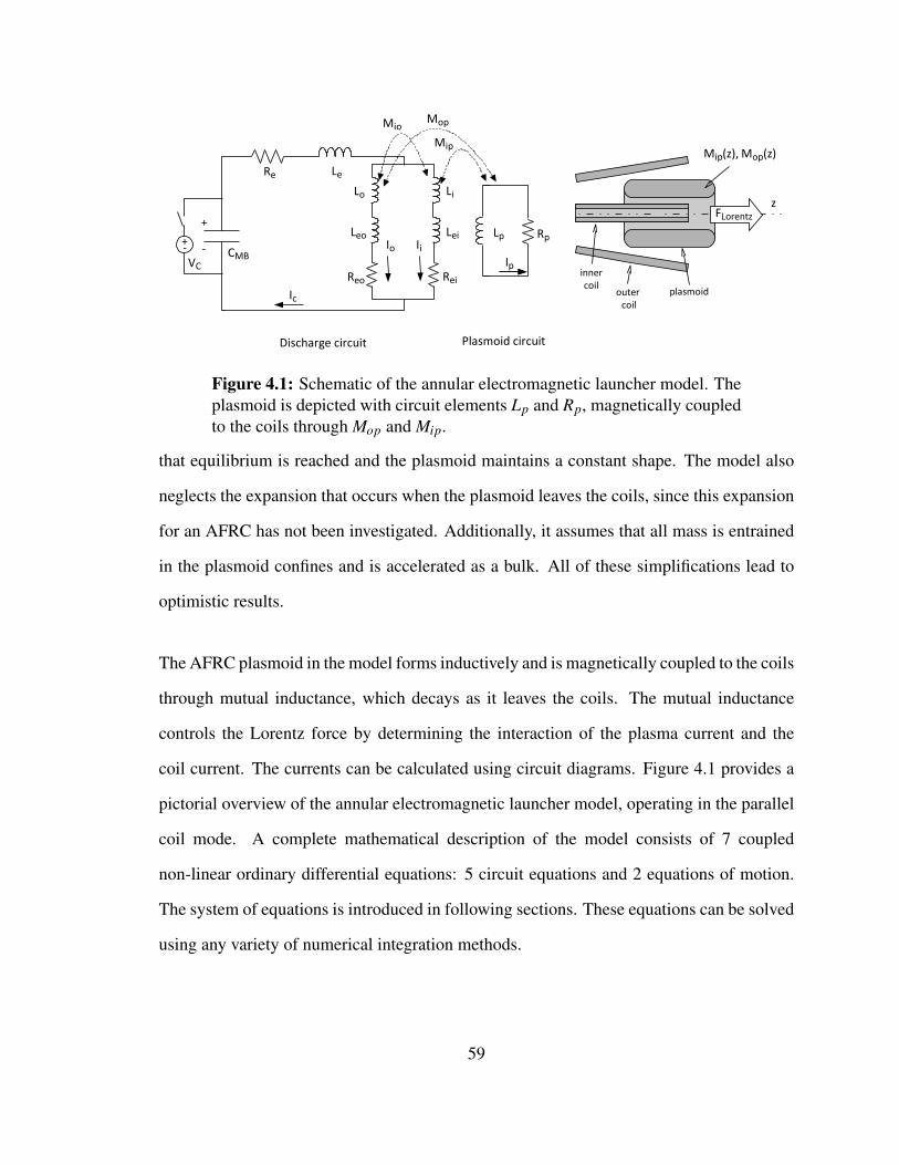
Discharge circuit

LeRe

Lo

Leo

Reo

Li

Lei

Rei

+

-

Mio

CMB

RpLp

Plasmoid circuit

IpIo Ii

Ic

Mip

Mop

FLorentzz

innercoil

outer coil

plasmoid

Mip(z), Mop(z)

VC

+-

Figure 4.1: Schematic of the annular electromagnetic launcher model. Theplasmoid is depicted with circuit elements Lp and Rp, magnetically coupledto the coils through Mop and Mip.

that equilibrium is reached and the plasmoid maintains a constant shape. The model also

neglects the expansion that occurs when the plasmoid leaves the coils, since this expansion

for an AFRC has not been investigated. Additionally, it assumes that all mass is entrained

in the plasmoid confines and is accelerated as a bulk. All of these simplifications lead to

optimistic results.

The AFRC plasmoid in the model forms inductively and is magnetically coupled to the coils

through mutual inductance, which decays as it leaves the coils. The mutual inductance

controls the Lorentz force by determining the interaction of the plasma current and the

coil current. The currents can be calculated using circuit diagrams. Figure 4.1 provides a

pictorial overview of the annular electromagnetic launcher model, operating in the parallel

coil mode. A complete mathematical description of the model consists of 7 coupled

non-linear ordinary differential equations: 5 circuit equations and 2 equations of motion.

The system of equations is introduced in following sections. These equations can be solved

using any variety of numerical integration methods.

59

The equations of motion for the plasmoid can be derived by calculating the Lorentz force

from JxB, but this requires solving several intense integrals. A much easier and equivalent

description can be found from conservation of energy, considering how the energy of the

system changes as the plasmoid travels out of the coils. Magnetic field energy will change

as the mutual inductance changes. This change in magnetic field energy can be related to

Newton’s 2nd Law through the work-kinetic energy theorem (Fz =−δU/δ z), giving:

mduz

dt=−

dMop

dzIoIo−

dMip

dzIiIp (4.1)

where

uz =dzdt

(4.2)

In this model, position of the plasmoid z is tracked with regard to the trailing edge and z

= 0 occurs at the small cone end of the coils. Computing the total circuit current Ic, and

the coil currents Io, and Ii requires a circuit analysis of the system, yielding the following

equations:

VC(t) = LedIc

dt+ReIc +(Lo +Leo)

dIo

dt+Mio

dIi

dt+ReoIo− Ip

dMop

dzuz−Mop

dIp

dt(4.3)

Ic = Io + Ii (4.4)

0 = (Lo +Leo)dIo

dt+Mio

dIi

dt+ReoIo +(Mip−Mop)

dIp

dt+

(dM23

dz− dM13

dz

)uzI3

−(Li +Lei)dIi

dt−Mio

dIi

dt−ReiIi (4.5)

0 = RpIp +LpdIp

dt−Mop

dIo

dt− Io

dMop

dzuz− Ii

dMip

dzuz−Mip

dIi

dt(4.6)

dVC

dt=− Ic

CMB(4.7)

60

The time derivatives of Mop and Mip in Equations 4.3, 4.16, and 4.6 have been separated

into a positional derivative and velocity using the chain rule. Their profiles Mop(z) and

Mip(z) as well as the coil and plasmoid inductances Lo, Li, and Lp are determined from

the coil and plasmoid geometry. Given the coil radii, lengths, cone angle, and plasmoid

geometry, the mutual inductance profiles Mop(z) and Mip(z) and Lo, Li, Lp can be calculated

using analytical equations, experimental methods, or electromagnetic field solvers. As

multiple authors have discovered [58], [2],[60], the M(z) profile satisfies an exponential

distribution, similar to:

M(z) = k0√

LpLc exp

(−

(∣∣z− zshi f t∣∣

zscale

)n)(4.8)

or

k(z) = k0 exp

(−

(∣∣z− zshi f t∣∣

zscale

)n)(4.9)

using

M(z) = k√

LpLc (4.10)

where Lc is the coil inductance and Lp is the slug inductance. In transformer nomenclature,

the coil is considered the primary inductor and the slug is the secondary inductor.

The difference in geometry between the outer coil-plasmoid combination and the inner

coil-plasmoid combination will result in different coupling for both systems, meaning that

for each geometry combination, the coefficients k0, zscale, zshi f t , n will have unique values

(kop, kip, zop, zip, zsop, zsip, nop, nip). It has been found that for large cone angles (greater

than 10), n approaches 1 and zshi f t is zero. For small cone angles, n and zshi f t increase

with decreasing cone angle.

The plasmoid’s mass m can be estimated by assuming a fully ionized plasma with uniform

61

density ni, constant volume V , and no mass crossing the plasmoid boundary. The plasmoid

mass is then estimated as: m = niV Mm/NA, where Mm is the molar mass of the plasmoid

gas, NA is Avogadro’s number. The density is assumed to be equal to the initial background

fill of gas, prior to the coil discharge. This profile underestimates the mass, since the density

profile measured in experiments peaks on centerline (as shown in Figure 3.7), but it will

sufficiently approximate the mass for this basic model.

The plasmoid’s resistance Rp can be estimated by assuming a uniform plasmoid

conductivity, σp, a constant cross-sectional area A, and an arc length 2πrm. The plasma

resistance is then R = 2πrm/Aσp. The plasma conductivity in FRC’s (and likely AFRCs)

is difficult to predict, though classical Spitzer conductivity is often used as a best-case

substitution. The temperature of an AFRC plasmoid formed with heavy gases is likely

between 10 eV and 50 eV. For the results presented here, an upper limit of 50 eV was

selected. A 50 eV plasma with a density of 1x1020 m−3 has a Spitzer conductivity of about

3x105 S/m. The actual value selected for the simulations was higher at 1x106 S/m. This

overestimate was unlikely to have a drastic impact on the final results, as a senstivity study

on plasma conductivity presented in Section 4.2.8 showed only minor differences in the

trajectory results between conductivities of 1x105 S/m and 1x106 S/m.

Since this model assumes a non-expanding plasmoid with a static mass, the impulse bit of

the transiting plasmoid is simply the product of the plasmoid mass and the terminal velocity

u f :

Ibit = mu f (4.11)

The energy efficiency of the plasmoid’s acceleration can be defined as the final plasmoid

kinetic energy compared to the energy initially stored in the capacitor bank. For the

62

non-expanding plasmoid, this is equivalent to the system efficiency.

ηE =12mu2

f

C1V 20

(4.12)

The launcher model is an initial value problem, requiring the values for Io, Ii, Ip, Vc, uz,

and z to be specified at t = 0. These 6 initial conditions, combined with the 7 independent

circuit elements (CMB, Le, Re, Leo, Lei, Reo, Rei), 5 coil geometry parameters (outer coil

radius, outer coil cone angle, inner coil radius, coil length, coil turns), 2 plasma geometry

parameters (height, width), and 2 plasma properties (ni, σp), require that 22 inputs be

specified for the model. This large parameter set can take up to 30 minutes to solve on a

single-core processor, with the bulk of the time consumed calculating Mop(z) and Mip(z).

4.1.1 Numerical Approach

The model equations (Equations 4.1 4.2 4.3 4.4 4.16 4.6 4.7)were integrated using a

Mathwork’s Matlab ode45 solver. It is an explicit 4th order Runge-Kutta solver, ideal

for medium-accuracy, non-stiff problems. The time-steps for the solver were determined

internally, using an adaptive technique to minimize errors.

The coil inductances, slug inductance, and mutual inductances were calculated from

the geometry of the coils and plasmoid using an electromagnetic field solver, as

was done in Reference [2]. The electromagnetic field solver used in this work was

COMSOL Multiphysics, with the AC/DC module. All simulations were completed with

a 2D-axisymmetric, time-harmonic solver using an estimated frequency from the circuit

parameters. The domain surrounding the coils was expanded to mimic a free-field

63

expansion. The coils and slug were modeled as single-turn entities, with multi-turn coils

accounted for by multiplying each quantity by the appropriate number of turns (L ∝ N2).

The slug was modeled with circular ends to approximate the expected profile for an AFRC

and an FRC. A sample geometry is displayed in Figure 4.2 a, with a typical mesh shown

in Figure 4.2 b. As is shown in Figure 4.2 b, the mesh for the solver was refined so that

at least 3 elements covered a single skin-depth. The number of elements was increased to

10 for important features such as corners. While this increased the computational time for

each simulation, resolving the skin-depth was important for accurate results.

COMSOL calculates the inductance directly for single, isolated coils. The inductance for

the inner and outer coil was calculated by simulating each coil in an isolated setting, with

no surrounding conductors. The inductance of the slug could not be calculated directly by

COMSOL, however. Modeling an isolated slug in COMSOL produced a current ring on

the inner surface alone, whereas the true inductance of the slug is dictated by current rings

on the inner and outer surfaces. To properly resolve these rings, both coils were modeled

as the primary inductors with the slug as a secondary inductor. The time-harmonic circuit

equations were used with the total simulated current in each coil to calculate Lp. The

time-harmonic equations for the system (neglecting resistance) are

Vo = jωLoIo + jωMioIi− jωkopIp (4.13)

Vi = jωLiIi + jωMioIo− jωkipIp (4.14)

0 = jωLpIp− jωMopIo− jωkipIi (4.15)

Equations 4.13-4.15 were re-arranged to find an expression for Lp, using math software

(Sage [61]) to expedite the process. The slug inductance Lp calculated from the

64

Skin Mesh withCurrent Density

(a)

(b)

(c)

r

z CL

inner coil

outer coil

slug

full domain

detailed domain

1.0

0.0

J/Jpeak

0.6

0.8

0.4

0.2

Figure 4.2: Geometry and mesh used for the inductance calculations inCOMSOL. The coil meshes were refined to resolve the skin depth of thecurrent in the coils.

65

time-harmonic circuit equations is

Lp =1

jωI2p

(jω2MioIoIi + jωLoI2

o + jωLiI2i −VoIo−ViIi

)(4.16)

This approach is only valid when the slug is inside the coils. Outside the coils, large

numerical errors develop and the slug inductance approaches infinity.

COMSOL also calculates the effective inductance of coupled conductors. The effective

inductance Le f f of two conductors can be shown to be [5]

Le f f = L1−M2

L2(4.17)

where L1 is the inductance of the primary coil, L2 is the inductance of the secondary coil,

and M is their mutual inductance. In transformer nomenclature, the primary coil is the

driving coil and the secondary coil is the non-driven coil. The effective inductance can be

re-written to express the mutual inductance in terms of the coupling coefficient k [2] so that

Le f f = L1(1− k2) (4.18)

The effective inductance of the inner and outer coil was calculated in COMSOL and

Equation 4.17 was used to calculate Mio. The effective inductance between each coil

and slug was also calculated in COMSOL, with each coil as the primary inductor. The

effective inductance as a function of position was calculated by moving the slug to several

axial locations. The coupling coefficients kop(z) and kip(z) were calculated from these data

using Equation 4.18.

The technique for calculating the coupling coefficients kop(z) and kip(z) was not ideal,

66

since it did not properly resolve the inner and outer current rings in the slug. A more

accurate technique might have been to calculate the coupling coefficients kip and kop from

the time-harmonic equations (Equations 4.13 - 4.15) for the full system. However, large

numerical errors produced when the slug is immediately outside the coils lead to gross

errors in the calculated trajectories using this method. This method calculated the mutual

inductances Mop and Mip increasing towards infinity, leading to rapidly increasing Lorentz

forces. In reality, the Lorentz force decays as the slug moves away from the coil since the

magnetic fields between the coils and slug no longer interact.

The coupling coefficient data kip(z) and kop(z) were used with a curve-fitting tool in

MatLab(R) to estimate coefficients for the empirical fits, described by Equation 4.9. These

coefficients were used with an analytical expression to calculate the positional derivatives

dMop/dz and dMip/dz as well.

4.1.2 Model Validation

Validation of the AELM model was limited, since experimental results for comparison

are not available for the annular launcher configuration. Despite this, an effort was made

to ensure the numerical techniques and model equations were comparable to results from

other single coil launcher studies. Two different studies were conducted to this end: a study

to check that the equations of motion agreed with results from a single-coil launcher study

and a study using COMSOL’s electromagnetic modeling to ensure that it could calculate a

reasonable coupling profile.

The first validation study compared the annular electromagnetic launcher model equations

67

against results from a numerical electromagnetic launcher study with a single flat coil

with a rigid flat armature by Novac, et al [1]. Novac’s flat coil launcher was modeled

using a similar circuit equation approach to the one presented here and compared it

against experimental results for terminal velocity. The annular electromagnetic launcher

model was tested with the experimental inputs provided in Table 1 by Novac, et al [1].

Current through the inner coil circuit for the annular launcher was minimized by setting

the resistance Rei to 100 Ω. The mutual inductance between the inner coil and slug was

turned off by setting the inner coil inductance L2 to zero. This reduced the dual coil model

to a single coil launcher. The mutual inductance profile was not provided in Reference

[1], but other authors [2] used kop = 0.98, zop = 0.005, nop = 1.0 in a separate validation

study with success. These values for the coupling profile were used in this study as

well. The results with the modified annular electromagnetic launcher using the circuit

parameters from [1] are shown in Figure 4.3. The current, velocity, and position history

shown in Figure 4.3 are in good agreement with the original results. Novac, et al report a

terminal velocity of 4.0 km/s for their experimental study. The terminal velocity predicted

with the modified annular model was 3.78 km/s, within 6% of the reported results. This

validation study ensures that the equations of motion and modified circuit equations from

the annular electromagnetic launcher are in agreement with published experimental data

from single-coil launcher studies.

The second validation study was completed to ensure that COMSOL software could be

used to predict a reasonable coupling profile for a single coil and projectile. The target

coupling profile was from an experimental demonstration of coil-slug coupling by Martin

and Eskridge [2]. In this experiment, a slug of aluminum was moved away from a conical

discharge coil and the resulting effective inductance of the coil was measured. Martin

and Eskridge’s geometry was duplicated in COMSOL and the effective inductance was

68

3000

2000

1000

0

Vel

ocity

[m/s

]

5x10-643210

Time [s]

16x10-3

14

12

10

8

6

4

2

0

Position [m

]

Velocity Position

600x103

500

400

300

200

100

0

-100

Cur

rent

[A]

5x10-643210

Time [s]

Coil Projectile

EOM VerificationNovac, et al.

(a) (b)

Figure 4.3: Results from the modified annular electromagnetic launchermodel, using a test case presented by Novac, et al [1].

computed. The slug dimensions were not provided, so a 2 mm offset was used to model the

slug. A comparison of the COMSOL results with Martin and Eskridge’s experimental

results are compared in Figure 4.4. A curve fit to the COMSOL data shows good

agreement with Martin and Eskridge’s experimental data, with a 12 % difference between

the experimental data and the profile predicted by COMSOL. The curve-fit produced the

coefficients for the fit to the exponential Le f f profile: Lc = 27 nH± 68 pH, ko = 89± 0.004,

z0 = 52 mm ± 1 mm. A sizeable difference between the COMSOL data and experimental

data published by Martin and Eskridge is likely due to a slight difference in the modeled

slug geometry, since this was not provided by the authors. However, the agreement between

the two results supports the use of COMSOL for computing coupling profiles for single-coil

geometries.

69

25x10-9

20

15

10

5

0

L eff [H

]

0.160.140.120.100.080.060.040.020.00Axial Position, z [m]

COMSOL data COMSOL fit Exp. Data

COMSOL Verification StudyMartin and Eskridge Exp. Data

Leff = Lc(1-k02exp(-2z/z0))

Figure 4.4: Effective inductance of a slug-coil geometry calculated usingCOMSOL. Experimental data from Reference [2] are shown with the dottedline.

4.2 Design Studies for the XOCOT-T3 Experiment

The annular electromagnetic launcher model was used to make design decisions for the

XOCOT-T3 AFRC translation experiment. Various input parameters were used with the

model to estimate the trajectory of a plasmoid and acceleration efficiency. Input parameters

favorable to plasmoid ejection from the coils were considered in the final design. The

design process was simplified by constraining several inputs to the model based on existing

hardware or hardware limitations. These inputs included outer coil dimensions, capacitance

values, and current limits. The remaining inputs for the external circuit, including the

half-angle of the outer coil, inner coil dimensions, charge voltages, coil inductances, stray

inductances, and resistances were varied across a limited range of feasible values to study

their effects. A final design was selected from the range of inputs tested. The primary goal

of this study was to find an experimental design which would expel the plasmoid from

70

the formation chamber during the plasmoid’s expected lifetime or before the magnetic

confinement of the plasmoid is expected to disappear. If the plasmoid configuration

terminates prior to expulsion from the coils, it will produce no directed impulse. Therefore,

it is critical to eject the plasmoid before the end of its lifecycle. The secondary goal was to

maximize the design’s projected energy efficiency and the plasmoid’s velocity. Sensitivity

studies on the plasmoid geometry and properties were conducted to estimate their impacts

to the plasmoid’s trajectory with the final design.

One of the most important considerations in the design process was that the final design

must result in plasmoid ejection from the coils prior to the expected lifetime of the

plasmoid. As stated previously, it is critical to eject the plasmoid prior to its termination

so it can impart impulse on the coils. If the plasmoid extinguishes inside the coils, it will

produce little thrust. Previous results on AFRC formation studies found that the lifetime of

an AFRC plasmoid was limited to the rise-time or quarter-cycle of the coil currents. This

is discussed in Section 3.3.5. The model therefore required that a plasmoid must leave the

coils within the first quarter cycle of the circuit discharge for a successful outcome. The

quarter cycle for each case was determined by simulating a stationary plasmoid coupled the

coils. This ensures the plasma-coil coupling determines the frequency rather than relying

on a vacuum (no plasma) waveform. The two cases can be very different. The lifetime

definition is displayed graphically in Figure 4.5. A vacuum waveform is shown along with

waveforms when the plasma is present in the coils (stationary and translating case). The

plasmoid inductively shorts the coils, leading to a higher frequency and larger current than

in the vacuum case. This lifetime limit assumes that the plasmoid maintains coherency

and stability after it ejects from the coils. Both assumptions are unlikely to hold in the

translation experiment where a free-field expansion is expected to alter the downstream

plasma dynamics considerably, though their effects must be determined experimentally.

71

12x103

10

8

6

4

2

0

Cur

rent

[A]

30x10-62520151050

Time [s]

With Translation Stationary Vacuum Condition

Outer Coil CurrentNominal Inputs

Lifetime Limit

Figure 4.5: Definition of the plasmoid lifetime limit, as determined by thepeak in the coil-plasma coupling case where the plasmoid is not allowed totranslate.

The expansive design space of the experiment was significantly narrowed by applying

design constraints to the problem. Most of these design constraints originated from limits

or dimensions of existing or readily available hardware. The design constraints were as

follows:

1. Capacitances should be either 225 µF or 43.5 µF.

2. The outer coil should be 30 cm in length and 24 cm in diameter to match insulator

and vacuum tank dimensions. The cone angle should not exceed 12.

3. The inner and outer coils must have the same number of turns for a radially balanced

plasmoid and should be equal in length.

4. Charge voltages cannot exceed 15 kV.

5. Total currents cannot exceed 30 kA (for the 225 µF capacitor) and 50 kA (for the

72

43.5 µF capacitor).

The design space was further reduced by applying limits to several parameters, based on

their expected ranges and what could be attained with realistic hardware. These limits were

as follows:

1. Le, Leo, Lei: 100 nH to 1 µH

2. Reo, Rei: 1 mΩ to 30 mΩ

3. Re: 10 mΩ to 50 mΩ

4. ri: 2.5 cm to 7.2 cm

The plasmoid dimensions for each case were scaled according to the coil dimensions. The

plasmoid length and thickness were specified as fractions of the coil length and annular

channel width, respectively. The plasmoid was assumed to start its trajectory at 10% of

the coil length (or 3 cm in from the small end of the coil). The plasmoid’s radial position

was centered between the coils. This is in contrast to the equilibrium position derived in

Section 3.3.1, which found that the radial position of the plasmoid splits the annulus into

equal areas. The assumptions required for this derivation, namely that the dimensions of

all inductors resemble ideal solenoids and the plasmoid is infinitesimally thin, are not valid

for the plasmoid description in the launcher model. The actual plasmoid position in the

experiment will be governed by the reversed field the plasmoid generates as well as the

thickness of the plasmoid. These are difficult to predict beforehand, so it was appropriate

to fix the plasmoid conditions arbitrarily. A sensitivity study was conducted to determine

how the plasmoid trajectory was affected by the plasmoid conditions (thickness, length,

conductivity).

73

Nominal input parameters were chosen to simplify the design studies. This allowed the

effects of one or two parameters to be studied individually. Nominal input parameters to

the model are displayed in Table 4.1

Table 4.1Nominal inputs for design study

Component Symbol Value

Capacitor CMB 225 µF43.5 µF

External inductance Le 200 nFOuter stray inductance Leo 100 nFInner stray inductance Lei 100 nFExternal resistance Re 10 mΩ

Outer stray resistance Reo 1 mΩ

Inner stray resistance Rei 1 mΩ

Outer coil radius ro 12 cmOuter coil length lo 30.5 cmOuter coil half-angle α 6

Coil turns Ni, No 4Inner coil radius ri 7.2 cmInner coil length li 30.5 cmOuter stray resistance Reo 1 mΩ


Plasma density ni 1.29x1020 m−3

Plasma conductivity σp 1x106 S/mPlasma length lp 80%lcPlasma width ∆rm 40%(ro− ri)Plasma radius rm (ro + ri)/2Charge voltage Vc 1.9 kV(225 µF) 400 JCharge voltage Vc 5.2 kV(43.5 µF) 600 J

74

4.2.1 Results for Nominal Case

The plasmoid trajectories and coil currents from the annular electromagnetic launcher

model were computed using the nominal inputs displayed in Table 4.1. This was done to

gain a basic understanding of the behavior of a translating plasmoid slug. The time history

of coil currents, plasma current, plasmoid velocity, capacitor voltage, and plasmoid axial

position is shown in Figure 4.6. Vacuum coil currents (no plasma in coils) are shown for

comparison. The plasmoid adds an inductive load to the circuit, indicated by the increased

frequency and increased coil currents compared to the vacuum case. The plasma current is

much higher than the coil currents due to its lower inductance. The plasmoid gains velocity

quickly, within 2 µs of the simulation start. The coil and plasma currents start to decay at

7 µs as the leading edge of the plasmoid passes the end of the coil. The inductive load

begins to decrease at this time, though the velocity continues to climb. The plasmoid slug

completely exits the coil (z = 0.3 m) at 10 µs and terminal velocity is reached 2 µs later.

The plasma current returns to zero and the coil currents return to their vacuum frequency.

The plasmoid slug is no longer able to inductively couple with the coils this far downstream,

leading to the decay in plasma current and loss of increased inductive loading on the coils.

The plasmoid slug reaches its lifetime limit at 15 µs, terminating at 0.8 m downstream.

The positional dependence of the the mutual inductance gradient (dM/dz) and the Lorentz

force for the nominal case is displayed in Figure 4.7. From this graph, it is apparent that the

inner coil is not responsible for the initial acceleration of the plasmoid; the initial plasmoid

acceleration is due to the outer coil alone. The mutual inductance gradient for the inner

coil is less than the mutual inductance gradient of the outer coil. The outer coil mutual

inductance gradient peaks before the inner coil and is greater in magnitude. This indicates

75

20x103

15

10

5

0

Cur

rent

[A]

30x10-62520151050

Time [s]

60x103

50

40

30

20

10

0

Cur

rent

[A]

100x103

80

60

40

20

0

Vel

ocity

[m/s

]

2.0

1.5

1.0

0.5

z [m]

1500

1000

500

0

Vol

tage

[V]

Life

time

Lim

it

OC Current IC Current Vac Currents Plasma Current Cap Voltage Velocity Position

Nominal Inputs225 uF; 400 J

Figure 4.6: Results from the launcher model, including coil currents,plasma current, capacitor voltage, plasmoid velocity, and axial plasmoidposition as a function of time for nominal inputs.

76

400

300

200

100

0

Lore

ntz

For

ce [N

]

1.00.80.60.40.2Axial Position [m]

Coi

l End

Nominal InputsCone Angle: 6 degrees

Total Outer Coil Inner Coil

-1.0x10-6

-0.8

-0.6

-0.4

-0.2

0.0

dM/d

z [H

/m]


Coi

l End

Outer Coil-Plasmoid Inner Coil-Plasmoid

Nominal InputsCone Angle: 6 degrees

(a) (b)

Figure 4.7: Positional dependence of the mutual inductance gradient for theinner and outer coil and the combined Lorentz force.

that both coils will push on the plasmoid slug at different times. Examining the plot of the

Lorentz force, this is readily apparent. The outer coil is responsible for the acceleration

during the first half of the coil and the inner coil largely accelerates the plasmoid through

the second half of the coil. The peak Lorentz force occurs somewhere between these zones.

This disparity in acceleration zones is likely a result of the cone angle from the outer coil.

The effects of cone angle on effective acceleration distance is discussed in Section 4.2.2.

The results in Figure 4.7 make it clear that the inner coil delivers a Lorentz force even

though it is not conical. While this is explained by the mutual inductance gradient displayed

in Figure 4.7, an alternate explanation is offered from a vector perspective. The inner coil

produces a radial magnetic field at the ends of the coil similar to magnetic mirror. As the

plasmoid travels past the end of the coil, the radial magnetic field and the azimuthal plasma

current exert an axial Lorentz force on the slug. The delayed acceleration is apparent in

Figure 4.7. When the plasmoid nears the end of the coil, the inner coil has a greater effect.

At the beginning of the coil, the inner coil exerts very little axial force on the plasmoid.

77

The momentum delivered by the exhausting plasmoid is 2.29 mN-s. The efficiency of

the system (calculated using Equation 4.12) for the nominal inputs was 27%. The low

efficiency can be explained by observing the coil current waveforms. After the plasmoid

slug leaves the coils, the coil currents continue to climb. They do not decay to zero like

the plasmoid current. The additional coil currents indicate that not all of the energy from

the capacitor was able to couple with the plasmoid before it exited the coils. Examining

the voltage history, it is apparent that the plasmoid slug left the coils while there was still

a significant voltage across the capacitor. The efficiency can be increased if the plasmoid

remains inside the coils for a longer duration, exiting when the coil currents are at their

peak to maximize the Lorentz force. This requires either increasing the plasmoid’s mass,

decreasing the charge voltage to decrease the coil currents, or reducing the cone angle to

lower the radial magnetic field. These effects slow the plasmoid’s trajectory for optimal

efficiency. However, if the plasmoid is allowed to remain in the coils for too long it can

terminate before ejecting. This discussion makes it clear that even in an ideal accelerator

like the one described by this model, fine tuning is required to maximize efficiency.

4.2.2 Cone Angle Study

The effect of cone angle was studied for the limited range of 2 to 12. The maximum cone

angle of 12 degrees was determined based on the dimensions of the mating vacuum port

for the experiment. The model was used with varying cone angles and nominal inputs to

compute the final position, velocity, and energy efficiency of the plasmoid as a function of

cone angle. This was done for 4 different inner coil radii. The results for both capacitor

banks are displayed in Figure 4.8. The smallest cone angle results in the longest trajectory,

highest velocity, and greatest efficiency. This is the case for several different inner coil

78

1.2

1.0

0.8

0.6

0.4

0.2

0.0

z fin

al [m

]

12108642

Cone Angle [deg]

Coil End

IC Radius 7.2 cm 6.0 cm 4.0 cm 2.8 cm

Cone Angle Study225 uF; 400 J

0.4

0.3

0.2

0.1

0.0

η E [-

]

12108642Cone Angle [deg]


0.6

0.5

0.4

0.3

0.2

0.1

0.0

η E [-

]

12108642Cone Angle [deg]

Cone Angle Study43.5 uF; 600 J

0.5

0.4

0.3

0.2

0.1

0.0

z fin

al [m

]

12108642

Cone Angle [deg]

Coil End


200x103

150

100

50

0

v fin

al [m

]

12108642

Cone Angle [deg]


160x103

140

120

100

80

60

40

v fin

al [m

]

12108642

Cone Angle [deg]


(a) (b)

(c) (d)

(e) (f)

Figure 4.8: Results from the cone angle study, including the final plasmoidposition, final velocity, and energy efficiency. Results are shown for 2different capacitor banks.

79

600

500

400

300

200

100

0

Lore

ntz

For

ce [N

]


cone angle

Coi

l End

Cone Angle Study225 uF; 2 kV

-1.2x10-6

-1.0

-0.8

-0.6

-0.4

-0.2

0.0

dM/d

z [H

/m]

0.60.40.20.0Axial Position [m]

coneangle

Coi

l End

Inner Coil

Outer Coil-Plasma

Coupling

Figure 4.9: Mutual inductance gradient and Lorentz force as a function ofslug position. Several different cone angles are shown, increasing in thearrow direction.

radii. This behavior holds only if the plasmoid has sufficient energy to escape the coils

completely. The results from the 43.5 µF case illustrate this for the largest inner coil radius

(7.2 cm). The 2 degree cone was not sufficient to accelerate the plasmoid far enough from

the coils in the allotted time and its final position fell short of the larger cone angle cases.

The 4 degree cone launched the plasmoid farther than the larger cone angles.

The increase in plasma position with decreased cone angle is not expected. Larger cone

angles exert greater Lorentz forces on the plasmoid slug due to the increased radial

magnetic field and this means they should expel it further. To understand why the results

for the coaxial geometry were different than expected, the dM/dz profiles and Lorentz

force profiles were displayed as a function of axial distance from the small end of the

coil (z = 0). The results are displayed in Figure 4.9. As is apparent in Figure 4.9a, a

larger cone angle exerts a larger Lorentz force on the slug for the far upstream regions (z

< 0.1 m). This is due to a greater dM/dz in the upstream regions of the coil. The greater

dM/dz means the larger cone angles will accelerate the plasmoid sooner than smaller cone

80

angles. However, maximizing the Lorentz force is about timing the peak coil currents with

the peak dM/dz for each coil. The peak dM/dz for smallest cone angle aligns with the

peak dM/dz for the inner coil. This means the combined Lorentz force (inner and outer)

will be greatest for the smallest cone angle, provided the plasmoid can accelerate to this

region within its lifetime. The greater Lorentz force results in greater terminal velocities,

greater acceleration efficiencies, and longer trajectories. For an annular FRC thruster, these

results suggest that small cone angles are better for maximizing performance than large

cone angles. Small cone angles allow the regions of peak dM/dz for the inner and outer

coil to overlap so that the maximum Lorentz force can be achieved.

4.2.3 Inner Coil Radius Study

The effect of the inner coil radius on the plasmoid trajectory was investigated for four

different coil radii: 2.8 cm, 4.0 cm, 6.0 cm, and 7.2 cm. The smallest radius was chosen

to match the aspect ratio of the CSS design[15]. The largest coil radius was selected as

the maximum radius that would allow clearance for quartz insulators and a 2.5 cm wide

channel. The model was used with these different inner coil radii to compute the final

position, velocity, and energy efficiency of the plasmoid as a function of cone angle.

The results for both capacitor banks are displayed in Figure 4.10. As was discovered in

Section 4.2.2, the largest inner coil radius creates the longest trajectory, highest velocity,

and greatest energy efficiency. The smallest radius fails to eject the plasmoid from the

coils for both capacitor banks indicating that more energy will be required for successful

translation with this radius. The inner coil radius improves the performance of the annular

launcher for two reasons: improved coupling and increased Lorentz forces. These are

illustrated in Figure 4.11. The larger radius increases the coupling k between the inner coil

81

140x103

120

100

80

60

40

v fin

al [m

]

2.52.01.5

Inner Coil Radius [cm]

IC Radius Study43.5 uF; 6 deg; 600 J

90x103

80

70

60

50

v fin

al [m

]

2.52.01.5


IC Radius Study225 uF; 6 deg; 400 J

0.3

0.2

0.1

η E [-

]

2.52.01.5



0.25

0.20

0.15

0.10

0.05

η E [-

]

2.52.01.5



0.40

0.35

0.30

0.25

0.20

0.15

0.10

z fin

al [m

]

2.52.01.5


Coil End


0.7

0.6

0.5

0.4

0.3

0.2

z fin

al [m

]

2.52.01.5


Coil End


(a) (b)(b)

(c) (d)

(e) (f)

Figure 4.10: Results from the inner coil radius study, including the finalplasmoid position, final velocity, and energy efficiency. Results are shownfor 2 different capacitor banks.

82

400

300

200

100

0

FLo

rent

z [N

]

0.60.50.40.30.20.1Axial Position [m]

IC Radius 7.2 cm 6.0 cm 4.0 cm 2.8 cm

IC Radius Study225 uF; 2 kV

0.75

0.70

0.65

0.60

0.55

0.50

0.45

k [-

]

2.52.01.5Inner Coil Radius [m]

OC-Plasmoid IC-Plasmoid

IC Radius Study225 uF; 2 kV

Figure 4.11: Coupling coefficients and Lorentz force computations forseveral inner coil radii.

and plasmoid and the outer coil and plasmoid, as the conductors are brought into closer

proximity. The Lorentz force also increases with increased inner coil radius. This is the

result of more effective coupling between the coils and plasmoid and the larger inner coil

inductance Li. An increased Li increases dMip/dz which is directly proportional to the

Lorentz force and also drives more current to the outer coil improving the outer coil’s

effectiveness. These findings conclude that an annular FRC thruster should maximize the

inner coil radius for improved performance.

4.2.4 Initial Energy Study

The initial energy for the system was studied to determine its effect on the plasmoid

trajectory, final velocity, and system efficiency. The range of energies studied was restricted

to a narrow range, based on maximum current ratings of each circuit. The maximum energy

for the 225 µF capacitor circuit was 500 J and the maximum energy for the 43.5 µF circuit

83

was 750 J. These ratings were based on current levels attained when a plasmoid was present

in the coils; the vacuum current levels were much lower. The results for final plasmoid

position, final velocity, and energy efficiency are shown in Figure 4.12.

The results from the initial energy study show the plasmoid travels a longer distance and

with a greater velocity when the initial energy stored in the capacitor is increased. If the

plasmoid travels past the end of the coils, the efficiency will be greatest for the lowest

energy settings. This is most apparent in the 225 µF data. The 100 J setting contains

too little energy to expel the plasmoid from the coils in the allotted time. When the

initial energy is increased to 200 J, the plasmoid is able to escape the coils and does so

with a greater efficiency than the 300 J and higher settings. The drop in efficiency with

increased energy can be understood by examining the Lorentz force equation, Equation

4.1. Maximizing the force and energy delivered to the plasmoid requires timing the peak

dM/dz with the peak currents. The peak dM/dz occurs at the far end of the coils, as shown in

Figure 4.7. Higher discharge energy settings cause the plasmoid to travel past the end of the

coils before the coil currents peak. This finding underscores the importance of optimizing

the timing for electromagnetic launchers to achieve peak efficiency. To maximize effiency

it is critical to time the plasmoid exit with the peak coil currents.

The results from the initial energy study also show that the minimum energy required

to eject the plasmoid from the coils is different for different size capacitor banks. The

225-µF bank requires a minimum of 200 J (under otherwise nominal conditions) to eject

the plasmoid and the 43.5-µF capacitor bank requires at least 600 J to eject the plasmoid.

The disparity in minimum energy for successful translation can be explained by noting that

the discharge frequency for the smaller bank is twice that of the larger bank. The quarter

cycle for the 43.5 µF bank is half of the quarter cycle for the 225 µF bank. This means the

84

0.4

0.3

0.2

0.1

η E [-

]

600400200

Initial Energy [J]

Energy Study43.5 uF; 6 deg

160x103

140

120

100

80

60

40v f

inal

[m/s

]

700600500400300200100

Initial Energy [J]


0.4

0.3

0.2

0.1

z fin

al [m

]

700600500400300200100

Initial Energy [J]

Coil End


0.34

0.32

0.30

0.28

0.26

0.24

η E [-

]

500400300200100

Initial Energy [J]

Energy Study225 uF; 6 deg

120x103

110

100

90

80

70

60

v fin

al [m

/s]

500400300200100

Initial Energy [J]

Energy Study225 uF; 6 deg

1.0

0.8

0.6

0.4

z fin

al [m

]

500400300200100

Initial Energy [J]

Coil EndEnergy Study225 uF; 6 deg

(a) (b)

(c) (d)

(e) (f)

Figure 4.12: Results from the initial energy study, including the finalplasmoid position, final velocity, and energy efficiency. Results are shownfor 2 different capacitor banks.

43.5 µF bank must use more instantaneous energy to expel the plasmoid in half the time of

the 225 µF bank. Additionally, the 225 µF bank is able to successfully launch a plasmoid

85

over a larger range of input energies than the 43.5 µF bank. The 225 µF bank can operate

between 200 J and 500 J while the smaller 43.5 µF bank may only work at 600 to 750

J. This finding indicates that plasmoid launchers with a low frequency should be used if

energy consumption is to be minimized.

4.2.5 Coil Inductance Study

The coil inductance should be maximized for peak efficiency. This ensures that most of

the initial energy from the capacitor bank is transferred to the coils from where it can

be transferred to the plasma. This lowers the energy budget for the system since the

initial energy stored in the capacitor can be used more efficiently. A basic study on the

effect of coil inductance was conducted using the nominal inputs in this design study.

The coil inductance was varied by changing the number of turns for the inner and outer

coil. Coil inductance is related to the number of turns N by N2. Since the results from

the initial energy study in Section 4.2.4 demonstrated that the efficiency was sensitive to

initial energy, the initial energy for each coil inductance case was optimized individually

for peak efficiency rather than using the nominal setting. The optimization was done using

the fmincon function, available in MatLab. The results from the coil inductance study

are shown in Figure 4.13 The results in Figure 4.13 show the expected trends. Energy

efficiency increases with coil inductance and the minimum initial energy decreases with

coil inductance. These results conclude that a large number of turns is optimal for reducing

the required input energy and increasing system efficiency.

The launcher model does not address how plasmoid formation is impacted by a multi-turn

coil. Multi-turn coils can create significant artifacts in the magnetic field, which may lead

86

1200

1000

800

600

400

200

Initi

al E

nerg

y [J

]

87654321

Coil Turns [-]

Coil Inductance Study225 uF; 6 deg 2000

1500

1000

500

Initi

al E

nerg

y [J

]

8765432

Coil Turns [-]

Coil Inductance Study43.5 uF; 6 deg

0.5

0.4

0.3

0.2

0.1η E

[-]

8765432

Coil Turns [-]

Coil Inductance Study43.5 uF; 6 deg

0.4

0.3

0.2

0.1

η E [-

]

87654321

Coil Turns [-]

Coil Inductance Study225 uF; 6 deg

(a) (b)

(c) (d)

Figure 4.13: Results from the coil inductance study, showing energyefficiency and minimum required input energy as a function of coil turns.

to plasma instabilities. For this reason, a modest number of turns should be used for both

coils. In this design study, four turns is a modest compromise. The data in Figure 4.13a and

c illustrate that four turns does not significantly alter the required input energy compared to

five or more turns and decreases the efficiency of an 8-turn coil by only 10%. A 4-turn coil

also allows the 30 cm long coil to be segmented into 7.5 cm wide strips, providing sufficient

spacing between junctions in the coil which may introduce deviations in the magnetic field.

87

4.2.6 Parasitic Inductance and Resistance Study

Reducing parasitic impedances in the discharge circuit is essential to maximizing energy

transfer from the capacitor into the coils and plasma load. However, parasitic inductance

and resistance are inherent to most experiments in non-negligible quantities so it is

important to understand how much of an effect they will have on the overall performance

of an electromagnetic launcher. The effect of parasitic elements was studies for the annular

electromagnetic launcher model in four separate studies. In the first study, the outer coil

stray inductance was varied from 100 nH to 1 µH to examine its effect. In the second study,

the inner coil stray inductance was varied across the same range. Both coil inductances

were varied across this range in the third study, with matching inductances. In the fourth

study, the stray resistance was varied for both coil circuits from 1 mΩ to 10 mΩ. All

other inputs were left at their nominal setting. The results from each study are displayed in

Figures 4.14-4.15, showing final plasmoid position, final velocity, and energy efficiency.

The results for the stray inductance show a surprising trend. Increasing the inner coil stray

inductance Lei increases the final plasmoid position and decreases the energy efficiency.

The same effect happens when both Leo and Lei are increased. The increase in plasmoid

position can be explained by observing that increased inductances decrease the frequency

and extend the lifetime. This is shown in Figure 4.16; increasing the stray inductance

increases the plasmoid lifetime (as defined in this model). The longer-lived plasmoid is

able to travel a greater distance. The efficiency and velocity decrease, however, since less

energy is available to the discharge coils and for the acceleration process. The results

in plasmoid position and energy efficiency are different when only the outer coil stray

inductance Leo is increased. The plasmoid position decreases and the energy efficiency

either stays constant or slightly increases. Increasing Leo diverts more current to the inner

88

165x103

160

155

150

145

v fin

al [m

]

1.0x10-60.80.60.40.2

Stray Inductance [H]

Stray Inductance Study 43.5 uF; 6 deg; 750 J

1.00

0.95

0.90

0.85

0.80

0.75

0.70

z fin

al [m

]

1.0x10-60.80.60.40.2


Variable Leo Variable Lei Lei = Leo

Stray Inductance Study 225 uF; 6 deg; 400 J

0.44

0.42

0.40

0.38

0.36

0.34

0.32

η E [-

]

1.0x10-60.80.60.40.2



0.30

0.28

0.26

0.24

0.22

η E [-

]

1.0x10-60.80.60.40.2



100x103

95

90

85

v fin

al [m

]

1.0x10-60.80.60.40.2



0.60

0.55

0.50

0.45

0.40

0.35

z fin

al [m

]

1.0x10-60.80.60.40.2



(a) (b)

(c) (d)

(e) (f)

Figure 4.14: Results from the stray inductance study, including the finalplasmoid position, final velocity, and energy efficiency as a function of strayinductance.

89

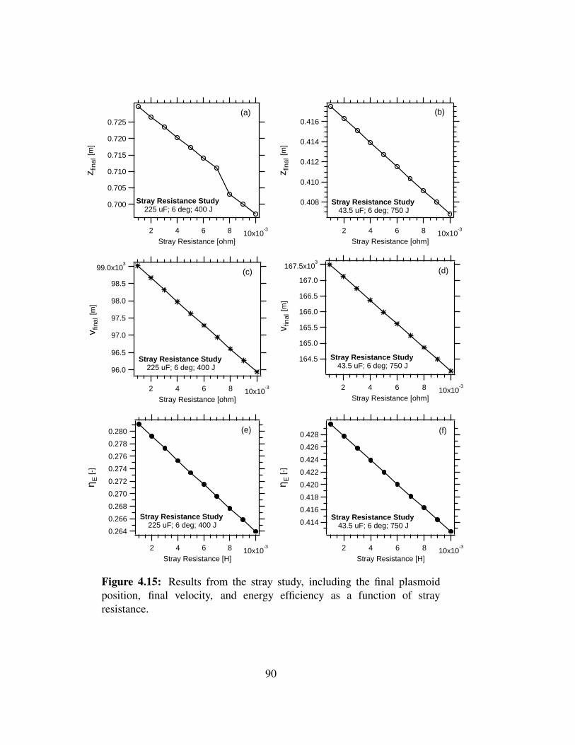
167.5x103

167.0

166.5

166.0

165.5

165.0

164.5

v fin

al [m

]

10x10-38642

Stray Resistance [ohm]

Stray Resistance Study 43.5 uF; 6 deg; 750 J

0.280

0.278

0.276

0.274

0.272

0.270

0.268

0.266

0.264

η E [-

]

10x10-38642

Stray Resistance [H]

Stray Resistance Study 225 uF; 6 deg; 400 J

0.428

0.426

0.424

0.422

0.420

0.418

0.416

0.414

η E [-

]

10x10-38642

Stray Resistance [H]


99.0x103

98.5

98.0

97.5

97.0

96.5

96.0

v fin

al [m

]

10x10-38642



0.725

0.720

0.715

0.710

0.705

0.700

z fin

al [m

]

10x10-38642



0.416

0.414

0.412

0.410

0.408

z fin

al [m

]

10x10-38642



(a) (b)

(c) (d)

(e) (f)

Figure 4.15: Results from the stray study, including the final plasmoidposition, final velocity, and energy efficiency as a function of strayresistance.

90

10x10-6

9

8

7

6

t lifet

ime

[s]

1.0x10-60.80.60.40.2



22x10-6

20

18

16

14

t lifet

ime

[s]

1.0x10-60.80.60.40.2



Variable Leo Variable Lei Lei = Leo

(a) (b)

Figure 4.16: Plasmoid lifetime (related to rise time of circuit) as a functionof stray inductance.

500

400

300

200

100

0

FLo

rent

z [N

]

0.60.50.40.30.20.10.0Slug Position [m]

Leo = 100 nH Leo = 1 uH

Stray Inductance Study225 uF; 6 deg; 400 J

Figure 4.17: Lorentz force as a function of slug position for two stray outercoil inductances. The larger stray inductance results in a larger Lorentzforce.

coil so that the outer coil is unable to provide as much initial acceleration to the plasmoid.

This shifts the maximum location of the Lorentz force closer to the edge of the coil, as

shown in Figure 4.17. This effect decreases the final plasmoid position since the plasmoid’s

initial acceleration is delayed. However, the delayed acceleration results in a more efficient

acceleration since the peak Lorentz force is now higher. The longer residence time inside

the coils allows the plasmoid to eject closer to the time of peak coil currents. The results

91

from the stray resistance study are displayed in Figure 4.15. The results from this study

are expected; larger resistances decrease the plasmoid position and decrease the system

efficiency since more energy is absorbed by Ohmic heating and unavailable for translation.

The effect for the range of parameters tested in this study does not show a large change in

results.

4.2.7 Final XOCOT-T3 Experiment Design

The results from the initial phase of the design study offered several insights into annular

electromagnetic launchers, including guidance on coil angles, inner coil radii, and coil

inductance. These findings were used to finalize a design for the XOCOT-T3 experiment.

The final design is presented in this section along with predicted trajectories of the resulting

plasmoid at various initial energy levels.

The cone angle study found that small cone angles are preferred for annular launchers; a

cone angle of 2 degrees was selected for the XOCOT-T3 experiment. The design study

on sizing the inner coil found that the inner coil should be as large as possible. The outer

coil radius of the XOCOT-T3 was fixed by available hardware to 12 cm so the maximum

inner coil radius must not exceed 7.2 cm. This provides clearance for the insulators and

allows 3 cm of channel width for plasmoid formation. The coil inductance study concluded

that multi-turn coils lower the minimum energy required to eject the plasmoid, though it

remains unclear what impact multi-turn coils will have on plasmoid formation. For this

reason, four turns for each coil was selected as a compromise between a high-inductance

coil design and lowered risk for detrimental plasma effects. The study on initial system

energy discovered that plasmoid launchers with a low frequency should be used if energy

92

consumption is to be minimized. Additionally, it found that the 225 µF capacitor bank has

a larger operating range than the 43.5 µF bank. The 225 µF bank can operate between

200 J and 500 J while the smaller 43.5 µF bank may only work at 600 to 750 J. For these

reasons, the 225 µF bank was used for most of the translation studies. The 43.5 µF bank

was used as an alternate to the 225 µF bank, in the event of capacitor failure.

The remaining design study investigated the effect of parasitic impedance. The results

from these design studies show that additional parasitic impedance on the outer coil circuit

only slightly decreases the trajectory of the plasmoid and impacts the terminal velocity

and energy efficiency only marginally. Additional impedance on both the inner and outer

coil circuit will increase the trajectory, but decrease the velocity and energy efficiency.

This means that parasitic impedance should be minimized, if possible. The design target

for the conceptual design studies was 100 nH, which is the minimum inductance for a

basic prototype experiment similar to the one developed in this research. The actual stray

inductance in the XOCOT-T3 experiment is likely to be higher than this figure, as longer

line lengths, bends, and gaps in the lines are required for diagnostic access. For this reason,

the target inductance in the XOCOT-T3 design projections was elevated to 500 nH per coil

circuit leg. The final design parameters for the XOCOT-T3 experiment are displayed in

Table 4.2.

The annular electromagnetic launcher model was used to predict the trajectories of the

plasmoid slug with the XOCOT-T3 design parameters. This was done to ensure the final

design would successfully eject the plasmoid from the coils and to predict the exit velocities

of the translating plasmoid. The predicted coil currents, plasma current, capacitor voltage,

velocity, and plasmoid position are displayed in Figure 4.18 for a 200 J discharge with the

225 µF capacitor. As indicated by the results, the 200 J discharge successfully ejects the

93

Table 4.2XOCOT-T3 final design parameters

Component Symbol Value

Capacitor CMB 225 µFAlternate 43.5 µFExternal inductance Le 200 nFOuter stray inductance Leo 500 nFInner stray inductance Lei 500 nFExternal resistance Re 10 mΩ

Outer stray resistance Reo 1 mΩ


Outer coil radius ro 12 cmOuter coil length lo 30.5 cmOuter coil half-angle α 2

Coil turns Ni, No 4Inner coil radius ri 7.2 cmInner coil length li 30.5 cmOuter stray resistance Reo 1 mΩ


Plasma density ni 1.29x1020 m−3

Plasma conductivity σp 1x106 S/mPlasma length lp 80%lcPlasma width ∆rm 40%(ro− ri)Plasma radius rm (ro + ri)/2Charge voltage Vc 1.3 kV(225 µF) 200 JCharge voltage Vc 5.3 kV(43.5 µF) 600 J

plasmoid before its allotted lifetime (18.6 µs). It reaches a terminal velocity of 110 km/s

during this time. The plasmoid’s mass of 1.1x10−8 kg, results in a directed impulse bit of

1.2 mN-s. The energy efficiency in this case is 33%. The effect of input energy on the

final velocity, momentum, and energy efficiency was examined for the XOCOT-T3 design.

The results from this study are shown in Figure 4.19. As expected, the plasmoid trajectory

is sensitive to the initial energy. Higher energies result in longer trajectories and faster

velocities, at the expense of energy efficiency. This effect was also noted in the results in

94

10x103

8

6

4

2

0

Cur

rent

[A]

30x10-62520151050

Time [s]

50x103

40

30

20

10

0

Cur

rent

[A]

100x103

80

60

40

20

0

Vel

ocity

[m/s

]

1.6

1.2

0.8

0.4

z [m]

1000

500

0

-500

Vol

tage

[V]

Life

time

Lim

it

OC Current IC Current Vac Currents Plasma Current Cap Voltage Velocity Position

XOCOT-T3 Design225 uF; 200 J

Figure 4.18: Results from the launcher model for the XOCOT-T3 designinputs, including coil currents, plasma current, capacitor voltage, plasmoidvelocity, and axial plasmoid position as a function of time for nominalinputs.

95

Section 4.2.4. The results in Figure 4.19 indicate that the plasmoid for the 225 µF bank

can be expected to translate from the coils at 200 J to 500 J of initial energy for the 225 µF

capacitor bank. The plasmoid should translate from the coils using the 43.5 µF bank from

600 J to 1 kJ of input energy. The upper energy limit is set by current ratings for circuit

components.

4.2.8 Plasmoid Sensitivity Studies

The design studies presented for the XOCOT-T3 design use fixed geometry and conditions

for the plasmoid. The sensitivity of these inputs was examined to see how alternate

plasmoid geometries would impact the results. Four sensitivity studies were conducted,

focusing on plasmoid dimensions (minor radius and length), plasmoid mean radius, and

plasmoid conductivity. All other inputs were set to the XOCOT-T3 design parameters,

outlined in Table 4.2.

The effect of the plasmoid width (radial direction) was studied by varying the width from

0.5 cm to 2.7 cm, at two intermediate values. The results from this study are displayed in

Figure 4.20. They show that the plasmoid is able to translate from the coils for all possible

widths with the 225 µF bank and for most possible widths with the 43.5 µF bank. The

thickest plasmoid in the higher frequency bank (43.5 µF) is too massive to translate from

the coils in the allotted time. The results also show the plasmoid position and velocity

decreases for thicker plasmoids. This effect is due to the larger plasmoid mass contained in

the thicker plasmoids. The efficiency generally improves with plasmoid thickness, provided

the plasmoid is able to exit the coils. Since efficiency is primarily a function of timing, the

slower velocity of the thicker plasmoids keeps the plasmoid contained in the coils for longer

96

0.4

0.3

0.2

0.1

η E [-

]

1000800600400200

Initial Energy [J]

XOCOT-T3 DesignC = 43.5 uF

0.34

0.32

0.30

0.28

0.26

0.24

0.22

η E [-

]

1000800600400200

Initial Energy [J]

XOCOT-T3 DesignC = 225 uF

250x103

200

150

100

50

v fin

al [m

]

1000800600400200

Initial Energy [J]


180x103

160

140

120

100

80

v fin

al [m

]

1000800600400200

Initial Energy [J]

XOCOT-T3 DesignC = 225 uF

0.6

0.5

0.4

0.3

0.2

0.1

z fin

al [m

]

1000800600400200

Initial Energy [J]

Coil End


1.2

1.0

0.8

0.6

0.4

z fin

al [m

]

500400300200100

Initial Energy [J]

Coil End XOCOT-T3 DesignC = 225 uF

(a) (b)

(c) (d)

(e) (f)

Figure 4.19: Results from the XOCOT-T3 design study on initial energy,including the final plasmoid position, final velocity, and energy efficiency.Results are shown for the primary bank (225 µF) and the alternate bank(43.5 µF).

97

duration so that its exit can be timed with higher coil currents.

The effect of plasmoid length was studied by varying the length of the plasmoid from 3 cm

to 25 cm (representing 10% to 80% of the coil length). The results are shown in Figure

4.21. The sensitivity of the plasmoid’s trajectory to plasmoid length is readily apparent in

these results. Shorter plasmoids are less likely to translate from the coils in their lifetime

compared to longer plasmoids. They do not couple as well to the coils as their longer

counterparts and they must travel a greater distance before encountering the region of peak

dM/dz at the end of the coils where they receive most of their kinetic energy. This means

that more energy will be required to translate the plasmoid if its length does not extend

more than half of the coil length. Provided a plasmoid is able to escape the coils during

its lifetime, shorter plasmoids can accumulate more kinetic energy than longer plasmoids.

Their lower mass allows them to be accelerated to higher velocities for the same amount

of transferred energy. The efficiency does not change appreciably with plasmoid length,

indicating that each plasmoid has the same final kinetic energy.

The plasma conductivity’s effect on the plasmoid’s trajectory was investigated for a range

of values from 103 S/m to 106 S/m. This spans the range of Spitzer conductivities for a

10 eV and 100 eV plasmoid. While temperatures of 100 eV are unlikely in an AFRC,

a Spitzer conductivity of 106 S/m represents an absolute upper bound. The results from

the conductivity study are displayed in Figure 4.22. These results show that plasma

conductivity (except for very low values) does not impact the translation of the plasmoid

out of the coils; the plasmoid is able to escape the coils with sufficient conductivity.

Conductivity does, however, impact the terminal velocity and system efficiency. In this

limited study, increased conductivity improves the energy efficiency and increases the final

velocity. Increased conductivity improves the coupling between the coils and plasmoid by

98

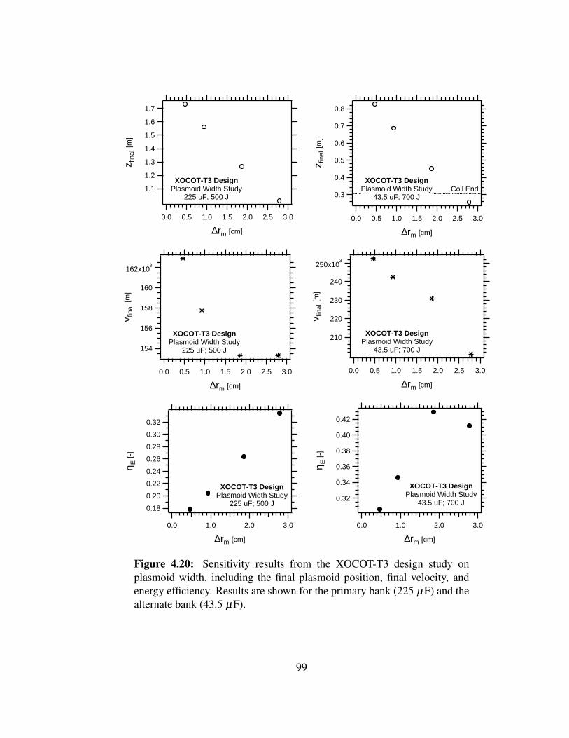
1.7

1.6

1.5

1.4

1.3

1.2

1.1

z fin

al [m

]

3.02.52.01.51.00.50.0

∆rm [cm]

XOCOT-T3 DesignPlasmoid Width Study

225 uF; 500 J

0.42

0.40

0.38

0.36

0.34

0.32

η E [-

]

3.02.01.00.0

∆rm [cm]


43.5 uF; 700 J

0.32

0.30

0.28

0.26

0.24

0.22

0.20

0.18

η E [-

]

3.02.01.00.0

∆rm [cm]


225 uF; 500 J

250x103

240

230

220

210

v fin

al [m

]

3.02.52.01.51.00.50.0

∆rm [cm]


43.5 uF; 700 J

162x103

160

158

156

154

v fin

al [m

]

3.02.52.01.51.00.50.0

∆rm [cm]


225 uF; 500 J

0.8

0.7

0.6

0.5

0.4

0.3

z fin

al [m

]

3.02.52.01.51.00.50.0

∆rm [cm]

Coil EndXOCOT-T3 Design

Plasmoid Width Study43.5 uF; 700 J

Figure 4.20: Sensitivity results from the XOCOT-T3 design study onplasmoid width, including the final plasmoid position, final velocity, andenergy efficiency. Results are shown for the primary bank (225 µF) and thealternate bank (43.5 µF).

99

1.2

1.0

0.8

0.6

0.4

0.2

z fin

al [m

]

2015105

lplasmoid [cm]


Plasmoid Length Study225 uF; 500 J

0.4

0.3

0.2

0.1

z fin

al [m

]

2015105

lplasmoid [cm]

Coil End

XOCOT-T3 DesignPlasmoid Length Study

43.5 uF; 700 J

200x103

150

100

50

0

v fin

al [m

]

2015105

lplasmoid [cm]


43.5 uF; 700 J

200x103

150

100

50

0

v fin

al [m

]

2015105

lplasmoid [cm]


225 uF; 500 J

0.4

0.3

0.2

0.1

0.0

η E [-

]

2015105

lplasmoid [cm]


43.5 uF; 700 J

0.25

0.20

0.15

0.10

0.05

0.00

η E [-

]

2015105

lplasmoid [cm]


225 uF; 500 J

(a) (b)

(c) (d)

(e) (f)

Figure 4.21: Sensitivity results from the XOCOT-T3 design study onplasmoid length, including the final plasmoid position, final velocity, andenergy efficiency. Results are shown for the primary bank (225 µF) and thealternate bank (43.5 µF).

100

generating thinner skin currents which couple more effectively to the coils. This results in

more efficient energy transfer between the plasmoid and coils, boosting the terminal kinetic

energy and system efficiency. These results are promising for the XOCOT-T3 design, as

low conductivities are unlikely due to the significant temperature (10 eV) and density (1020

m−3). The effect of the plasmoid’s radial position was studied in the final sensitivity study.

The radius of the plasmoid rm was moved to five radial locations between the inner and

outer coil. The results from this study are displayed in Figure 4.23. The effect of the

radial position does not appear to change the plasmoid’s trajectory and energy efficiency

appreciably, unless the plasmoid is located very close to the outer wall. In the 43.5 µF case,

the plasmoid does not translate from the coils if very close to the outer wall. Despite the

small change in results, it appears that plasmoids located closer to the inner wall attain a

greater velocity than those closer to the outer wall. The Lorentz force is higher for the inner

coil, due to its larger current. Improved coupling between the plasmoid and inner coil will

further increase the Lorentz force resulting in a larger velocity. Energy efficiency appears

to decrease as the plasmoid moves toward centerline. However, the change in efficiency

among all the results is small (less than 10%) so the effect of the plasmoid’s radial location

on energy efficiency is likely to be minimal.

The sensitivity studies conclude that the plasmoid’s trajectory and the energy efficiency

are highly sensitive to the plasmoid’s dimensions (length and width). If the plasmoid is too

wide or too short, it may not be able to translate from the coils during its lifetime. The initial

energy of the system will need to be increased to ensure the plasmoid can translate. The

plasmoid’s conductivity and initial radial position have less of an impact on the plasmoid’s

trajectory and energy efficiency. The extreme cases (very low conductivity and plasma very

close to outer wall) were the only cases which indicated issues with plasmoid ejection and

these extremes are unlikely in the XOCOT-T3.

101

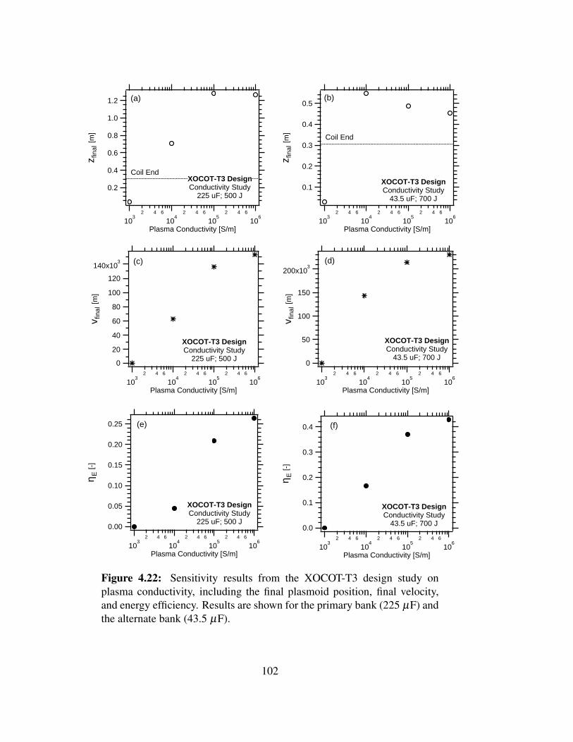
200x103

150

100

50

0

v fin

al [m

]

103

2 4 6

104

2 4 6

105

2 4 6

106

Plasma Conductivity [S/m]

XOCOT-T3 DesignConductivity Study

43.5 uF; 700 J

0.4

0.3

0.2

0.1

0.0

η E [-

]

103

2 4 6

104

2 4 6

105

2 4 6

106



43.5 uF; 700 J

0.25

0.20

0.15

0.10

0.05

0.00

η E [-

]

103

2 4 6

104

2 4 6

105

2 4 6

106



225 uF; 500 J

140x103

120

100

80

60

40

20

0

v fin

al [m

]

103

2 4 6

104

2 4 6

105

2 4 6

106



225 uF; 500 J

0.5

0.4

0.3

0.2

0.1

z fin

al [m

]

103

2 4 6

104

2 4 6

105

2 4 6

106


Coil End


43.5 uF; 700 J

1.2

1.0

0.8

0.6

0.4

0.2

z fin

al [m

]

103

2 4 6

104

2 4 6

105

2 4 6

106


Coil EndXOCOT-T3 DesignConductivity Study

225 uF; 500 J

(a) (b)

(c) (d)

(e) (f)

Figure 4.22: Sensitivity results from the XOCOT-T3 design study onplasma conductivity, including the final plasmoid position, final velocity,and energy efficiency. Results are shown for the primary bank (225 µF) andthe alternate bank (43.5 µF).

102

0.47

0.46

0.45

0.44

0.43

η E [-

]

0.1100.1050.1000.0950.0900.085

Plasma Radius [cm]

XOCOT-T3 DesignPlasma Radius Study

43.5 uF; 700 J

0.31

0.30

0.29

0.28

0.27

η E [-

]

0.1100.1050.1000.0950.0900.085

Plasma Radius [cm]


225 uF; 500 J

255x103

250

245

240

235

230

225

v fin

al [m

]

0.1100.1050.1000.0950.0900.085

Plasma Radius [cm]


43.5 uF; 700 J170x103

165

160

155

v fin

al [m

]

0.1100.1050.1000.0950.0900.085

Plasma Radius [cm]


225 uF; 500 J

1.25

1.20

1.15

1.10

z fin

al [m

]

0.1100.1050.1000.0950.0900.085

Plasma Radius [cm]


225 uF; 500 J

0.44

0.42

0.40

0.38

0.36

0.34

0.32

0.30

z fin

al [m

]

0.1100.1050.1000.0950.0900.085

Plasma Radius [cm]


Plasma Radius Study43.5 uF; 700 J

(a) (b)

(c) (d)

(e)(f)

Figure 4.23: Sensitivity results from the XOCOT-T3 design study onplasmoid radius, including the final plasmoid position, final velocity, andenergy efficiency. Results are shown for the primary bank (225 µF) and thealternate bank (43.5 µF).

103

The only sensitivity study not completed for this design was the effect of the starting

axial position of the plasmoid. The effect of the initial plasmoid axial position can be

qualitatively understood by examining the mutual inductance profiles shown in Figure 4.7.

These profiles show that if the plasmoid starts near z = 0, the transit time through the coils

will increase since the Lorentz force near the narrow end of the coil is small. If the plasmoid

is formed further downstream toward the wide end of the coil, the plasmoid can eject well

before the peak coil currents. This means the plasmoid will reach a lower terminal velocity

and the system’s efficiency will be lower. These arguments conclude that the plasmoid

trajectory is highly sensitive to the plasmoid’s initial axial position inside the coils.

4.3 Magnetic Field Modeling of XOCOT-T3

The magnetic field of the XOCOT-T3 design was calculated using COMSOL’s

electromagnetic field solver with the AC/DC module (version 4.2a). The magnetic field was

calculated for the vacuum case and for the plasmoid-coupling case with a stationary plasma.

The axial magnetic field profiles at several axial locations for a translating plasmoid were

also calculated. This section contains the magnetic field calculations and field profiles,

along with a brief discussion of the methods used in each case.

The vacuum magnetic fields were calculated using a time-dependent solver in COMSOL,

with a 2D axisymmetric geometry and circuit interface for current calculations. The final

geometry (see Table 4.2) was modeled with flat, four-turn coils for the inner and outer coils.

The coils were connected to an external circuit, with stray circuit elements defined by the

final design values. Modeling the problem in this fashion allowed the current through each

coil to be influenced by the external circuit and coil-coil coupling, as it would be in an

104

LeRe

Lo

Reo

Li

Lei

Rei

+

- CMB VC

Io Ii

Ic

Leo

zr centerline

(a) (b)

Figure 4.24: Coil connections, circuit connections, and coil geometry usedto calculate the vacuum fields. The rectangles in (a) represent FEM objectsin COMSOL. The geometry used in COMSOL to represent the multi-turncoils is drawn in (b).

experiment. Figure 4.24a shows the coil and circuit connections used in the COMSOL

model. Figure 4.24b depicts the geometry used to model the coils. The multi-turn coil is

modeled in a segmented design, with minimal spacing between the coil turns. The current

in each segment is entirely in the azimuthal direction. The rectangles in Figure 4.24a

represent the coils in COMSOL, connected the external circuit as shown. The vacuum

fields were calculated using the circuit parameters outlined in the XOCOT-T3 final design

(see Table 4.2). The calculated vacuum fields and coil currents are shown in Figure 4.25. As

expected, the vacuum fields are in phase with the coil currents. The magnetic field between

the coils is in the same direction as the magnetic field in the inner coil, though lower in

magnitude. The magnetic field along the length of the coils is not as uniform as expected.

A solenoidal coil (radius < length) has a uniform axial field through the center of the coil,

with curvature near the ends. The axial field distribution shown in Figure 4.25c is fairly

irregular with distortions seen every 7 cm or so. These distortions line up with the gaps

between the coils, suggesting the multi-turn coils are the source of the non-uniformities.

A topographical map of the magnetic field confirms this theory. This map is displayed in

105

Figure 4.26. Detail views of the area between the coils shows strong magnetic fields created

between subsequent turns of the multi-turn coil. These fields are created by interaction

between current repulsion in the nearby turns. These distortions extend away from the

coil, resulting in the non-uniform field distribution shown in Figure 4.25c. Following

computation of the vacuum fields, the magnetic fields created by a conductor (plasma)

between the coils were calculated by adding a conductive region between the coils. The

simulation was completed using the same methods and inputs as the vacuum magnetic field

studies. A plasmoid was draw between the coils, 1 cm wide and centered between the coils.

The conductivity of this region was fixed to 106 S/m. The resulting current and magnetic

fields are displayed in Figure 4.27. The plasmoid adds an inductive load to the circuit,

as noted by the change in frequency of the plasmoid-coupling case and greater currents

as compared to the vacuum case. The magnetic field between the coils also changes,

increasing in magnitude. The inner field is now in the opposite direction as the vacuum

field, creating a reversed field on either side of the plasmoid. The field changes directions

inside the plasmoid, as shown in Figure 4.27c. The appearance of a reversed field is

consistent with magnetic field measurements from previous AFRC experiments, as detailed

in Section 3.3.2. Magnetic field modeling was also completed in COMSOL to estimate

the magnetic field profiles of a translating plasmoid. The simulations were completed

using the same methods as the vacuum field calculations, 2D axisymmetric geometry with

coil currents specified using a circuit framework. The moving plasmoid was modeled as

a sliding rectangular region between the coils with a time-dependant conductivity σp(t).

The rectangular region of plasma conductivity, bound by z1 and z2, moved along z with a

constant velocity uz. Additionally, the plasmoid conductivity definition used a finite turn-on

delay τp to mimic the finite ionization time of a plasmoid. The plasmoid conductivity

relation is described by Equation 4.19. The geometry of the coils and plasmoid zone is

106

60x10-3

40

20

0

Bz

[ T ]

0.300.200.100.00

z [m]

Vacuum FieldsXOCOT-T3 Design

225 uF; 200 J

Outer Probes (r = 0.1143 m) Inner Probes (r = 0.084 m)

0.20

0.15

0.10

0.05

0.00

Bz

[ T ]

0.200.150.100.050.00

r [m]

inne

r co

il

oute

r co

il

Midplane Fields(z = 0.15 m)


30x10-3

20

10

0

-10

-20

-30

Bz

[ T ]

100x10-6806040200

Time [s]

Midplane Vacuum Fields (z = 0.15 m)


Outer Inner

15x103

10

5

0

-5

-10

-15

Cur

rent

[A]

100x10-6806040200

Time [s]

Vacuum CurrentsXOCOT-T3 Design

225 uF; 200 J

MBIC

OC

(a) (b)

(c)

(d)

Figure 4.25: COMSOL results for the vacuum case using the XOCOT-T3design, including (a) coil currents, (b) time history of midplane axial fields,(c) axial magnetic fields as the length of the coil, and (d) midplane axialfield across the radial cross section.

107

Figure 4.26: Magnetic field map from the XOCOT-T3 design, computedin COMSOL. Arrows denote field direction. Detail views of the magneticfield between coil turns is displayed in the smaller figures.

shown in Figure 4.28, along with the circuit connections.

σp(t) =

σp

(1− e−(t/τp)

)if z1 < z < z2

0 otherwise(4.19)

The moving plasmoid could have been modeled in COMSOL with a moving mesh instead

of the sliding conductivity region, but the moving mesh simulations were numerically

unstable and computationally expensive. The sliding conductivity simulations were found

to be slightly more stable, with total computation time around 12 hours. The simulation

was conducted with the following variables taup = 500 ns, uz = 50 km/s, σp = 106 S/m.

Magnetic field probes were position at several axial locations 5 cm apart on either side of

108

15x103

10

5

0

-5

-10

Cur

rent

[A]

100x10-6806040200

Time [s]

Vacuum Plasma Load

Coil CurrentsXOCOT-T3 Design

225 uF; 200 J

MB

OCIC

-0.10

-0.05

0.00

0.05

0.10

Bz

[ T ]

20x10-6151050

Time [s]

Midplane FieldsXOCOT-T3 Design

225 uF; 200 J

Vacuum Outer Probe Inner Probe

(a)

(b)

(c)

0.20

0.15

0.10

0.05

0.00

-0.05

-0.10

Bz

[ T ]

0.200.150.100.050.00r [m]

inne

r co

il

oute

r co

il

plas

ma

Midplane FieldXOCOT-T3 Design

225 uF; 200 J

Figure 4.27: COMSOL results for the plasmoid-coupling case using theXOCOT-T3 design, including (a) coil currents, (b) time history of midplaneaxial fields, and (c) midplane axial field across the radial cross section.

109

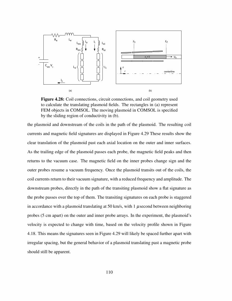
LeRe

Lo

Reo

Li

Lei

Rei

+

- CMB VC

Io Ii

Ic

Leo

zr centerline

(a) (b)

z1 z2

uzσp≠ 0

Figure 4.28: Coil connections, circuit connections, and coil geometry usedto calculate the translating plasmoid fields. The rectangles in (a) representFEM objects in COMSOL. The moving plasmoid in COMSOL is specifiedby the sliding region of conductivity in (b).

the plasmoid and downstream of the coils in the path of the plasmoid. The resulting coil

currents and magnetic field signatures are displayed in Figure 4.29 These results show the

clear translation of the plasmoid past each axial location on the outer and inner surfaces.

As the trailing edge of the plasmoid passes each probe, the magnetic field peaks and then

returns to the vacuum case. The magnetic field on the inner probes change sign and the

outer probes resume a vacuum frequency. Once the plasmoid transits out of the coils, the

coil currents return to their vacuum signature, with a reduced frequency and amplitude. The

downstream probes, directly in the path of the transiting plasmoid show a flat signature as

the probe passes over the top of them. The transiting signatures on each probe is staggered

in accordance with a plasmoid translating at 50 km/s, with 1 µsecond between neighboring

probes (5 cm apart) on the outer and inner probe arrays. In the experiment, the plasmoid’s

velocity is expected to change with time, based on the velocity profile shown in Figure

4.18. This means the signatures seen in Figure 4.29 will likely be spaced further apart with

irregular spacing, but the general behavior of a plasmoid translating past a magnetic probe

should still be apparent.

110

40x10-3

30

20

10

0

Bz

[ T ]

20x10-6151050

Time [s]

z = 5 cm z = 10 cm z = 15 cm z = 20 cm z = 25 cm z = 30 cm

Outer Probes (r = 11.4 cm)

-60x10-3

-40

-20

0

20

Bz

[ T ]

20x10-6151050

Time [s]

z = 5 cm z = 10 cm z = 15 cm z = 20 cm z = 25 cm z = 30 cm

Inner Probes (r = 8.4 cm)

14x103

12

10

8

6

4

2

0

Cur

rent

[A]

20x10-6151050

Time [s]

Translating Plasma Vacuum

Translation StudyXOCOT-T3 Design

225 uF; 200 J

Total

Outer Coil

Inner Coil (a)

(b)

(c)

6x10-3

4

2

0

Bz

[ T ]

20x10-6151050

Time [s]

Translating Plasmoid

z = 50 cm z = 60 cm

Downstream Probes (r = 9.7 cm)

(d)

Figure 4.29: Coil currents and magnetic field predicted by COMSOL for aplasmoid translating at 50 km/s.

111

4.4 Summary and Discussion of Results

An annular electromagnetic launcher model was developed to simplify the physics of a

translating plasmoid using a circuit-based approach. The plasmoid was approximated as

a rigid conducting slug, expelled from the coils by a Lorentz force. A series of design

studies was conducted to understand how inputs for the model such as cone angle and

inner coil radius affected the resulting plasmoid’s trajectory and the energy efficiency of

the translation process. Using the results from these studies, a design was selected for the

XOCOT-T3 and tested with the launcher model to ensure the plasmoid was able to translate

from the discharge coils during its lifetime. The final design selected the 225 µF capacitor

bank for a discharge frequency of 10 kHz, with the 43.5 µF, 20 kHz bank as the alternate.

The cone angle was minimized to 2 degrees and the inner coil radius was maximized at

7.2 cm. The minimum energy required for translation with the 225 µF bank was 200 J;

the minimum energy using the 43.5 µF bank was 600 J. The expected plasmoid velocity

and energy efficiency of the final design was estimated at 100 - 150 km/s with an energy

efficiency of 26 - 35%. The simulated plasmoid mass of 1.1x10−8 kg, resulted in a directed

impulse bit (momentum) of 1.1 mN-s to 1.7 mN-s.

The final XOCOT-T3 design selected four turns for the outer and inner coil. Magnetic

field simulations in COMSOL revealed that the coil introduced distortions in the field

from current interactions between nearby turns. Magnetic field simulations were conducted

with a conducting plasma between the coils, producing a reversed field magnetic field on

the inner wall compared to the vacuum field. The appearance of this reversed field in

the experiment will provide evidence that a conducting reversed-field plasmoid is present

in annulus. Further simulations with a moving conductive region between the coils,

112

mimicing a translating plasmoid, demonstrated typical magnetic field signatures expected

by a translating plasmoid. These signatures will aid in diagnosing plasmoid motion in the

experiment.

The design studies uncovered new insights into the design of annular launchers, including

the need for small cone angles on the outer coil. Shallow cone angles are required for

efficient annular launchers as they align the region of peak acceleration (dM/dz) of the

outer coil with the inner coil. Larger cone angles extended the region of peak acceleration

for the outer coil back towards the throat of the coil; while the region of peak acceleration

for the inner coil remains near the downstream end of the coil. Aligning the regions of peak

acceleration for the inner and outer coil maximizes the total dM/dz of the system, which is

directly proportional to the Lorentz force. This means that the maximum possible Lorentz

force can be achieved by timing the passage of the plasmoid through this region when the

coil currents and plasmoid current are at their peak. Maximizing the Lorentz force is a

direct payoff to energy efficiency, since it allows the plasmoid to exit with the maximum

velocity.

Maximum efficiency also arises when the inner coil is the largest possible diameter. This

brings the coil in closer contact with the plasmoid for improved coupling, increases the

inductance of the inner coil, and drives more current to the outer coil to improve its

effectiveness. All three effects work to maximize the Lorentz force and thus, energy

efficiency. The drawback to larger inner coil diameters is that it increases the chance of

wall contact with the plasma since finite thickness insulators must be placed over the coils

for electrical protection. Wall contact is to be avoided in pulsed inductive plasma systems

as it leads to massive cooling of the plasma and disruption of the current configuration.

The results from the design study also demonstrated the sensitivity of electromagnetic

113

launcher geometries to perfect timing. For maximum efficiency, the plasma must arrive

at the region of peak acceleration (peak dM/dz) when the coil currents and plasma current

peak. This was discovered in the energy study for the annular model, but can be expanded

to other geometries as well. The timing can be adjusted by changing the initial energy to

control the initial plasmoid acceleration. Unpredictable factors such as a variation in mass

of the plasmoid and a variation in plasmoid size can alter the optimal input energy from

model predictions. It is highly likely that empirical studies will be required to find the

optimal energy for each device to attain maximum efficiency.

The sensitivity of energy efficiency to timing of the plasmoid’s trajectory through the region

of peak acceleration is unfortunate for AFRCs. Experimental studies have demonstrated

that the lifetime of an AFRC is limited to the quarter-cycle of the discharge. This lifetime

definition is based on when magnetic field reversal is lost on the inner wall. In reality,

the reversed field begins to decay before this time implying that the plasma current begins

to degrade as well and the true lifetime is shorter than the quarter-cycle of the discharge.

This means that an AFRC must be ejected from the coils when the plasma currents peak,

sometime before the coil currents peak. This severely limits the energy efficiency of the

system, since all three currents must be at their peak together for maximum efficiency.

These observations are not limited to the annular geometry. Conical θ -pinch launchers

have similar acceleration physics and may be sensitive to a similar timing constraint. While

launcher-types studies have been previously conducted for conical θ -pinch designs [2],

lifetime considerations were not included in this analysis.

The exit velocity of the AFRC plasmoid predicted by these studies is much higher than

other PIPT devices. The range of exit velocities demonstrated in other experiments

discussed in Section 2.3 is between 10-20 km/s. The exit velocities predicted by the

114

launcher model were in excess of 100 km/s. These extreme exit velocities are the

consequence of a fairly high discharge frequency (10 kHz). The plasmoid must travel

the full length of the coil in less than 25 µs, accelerating from a standstill only when the

currents are high enough to result in a sufficient Lorentz force. Lengthening the quarter

cycle by reducing the frequency will likely lower the exit velocity, though the competing

effect of slower-building plasma currents may result in a longer initial translation delay.

Despite the numerous insights the annular electromagnetic launcher model results have

uncovered, many of these are based around the assumption of a rigid plasmoid-slug which

maintains its shape even as it travels downstream. This assumption is unlikely to hold in a

plasma experiment, as changing fluid properties will dominate the overall structure of the

plasmoid. Experimental hardware is required to fully test the capability of an AFRC-based

thruster. Data from the experiment can be compared to the model to understand how well

this model predicts plasmoid behavior.

115

Chapter 5

Experiment, Facilities, and Diagnostics

This chapter discusses the experimental setup, facilties, and diagnostics used in this

research. Section 5.1 describes the XOCOT-T3 experiment, including specific details

about the discharge circuit, the pre-ionization circuit, switching hardware, gas feed system,

vacuum systems, safety considerations, and experimental operating procedures. Detailed

information about the coil construction is provided, along with impedance measurements

of discharge circuit components. The diagnostics used in this work are discussed in Section

5.2. The diagnostic tools include current and voltage probes, magnetic field diagnostics,

plasma probes, and single frame photography. An indepth look at magnetic probe theory

is provided in Section 5.2.2 along with a discussion of probe calibration techniques and

probe construction. Plasma probes, or Langmuir probes, are discussed in Section 5.2.3.

The implementation of these diagnostics in measuring the plasmoid’s velocity, impulse-bit,

and energy efficiency is discussed in Section 5.3.

117

5.1 Experimental Apparatus

The XOCOT-T3 was a single pulse demonstration of AFRC formation and translation,

connected to Chamber 5B at the U.S. Air Force Research Laboratory-Edwards. A

photograph of the experiment and chamber is shown in Figure 5.1.

The experiment used two separate circuits for the pre-ionization and main bank discharge.

The inductive formation allowed all circuit components to remain at atmosphere. The

plasmoid was formed inside a pair of vacuum-sealed quartz liners. The current pulse

required to form the plasmoid was created by releasing the energy stored in a discharge

capacitor into main electromagnetic coils through a triggered ignitron switch. The

plasmoids were formed in a static backfill of gas, rather than using a puffed gas fill.

An antenna upstream of the main coils was used for pre-ionization. A cross-sectional

Figure 5.1: The XOCOT-T3 experiment, connected to Chamber 5B. Imageis a long exposure photograph of a single pulse discharge in argon. Thepre-ionization antenna is shown as the thinner coil upstream (left) of themain 4-turn coils.

118

Gas Inlets PI Coil

Inner Coil Outer Coil

Vacuum Tank

Orthogonal View Side View

Front View

Inner

Insulator

Outer

Insulator

30 cm

Figure 5.2: A dimensional drawing of the XOCOT-T3 experiment fromseveral perspectives, connected to Chamber 5B. The coils were concentric,separating an annular space with quartz insulators.

dimensional drawing of the experiment from several perspectives is shown in Figure 5.2.

A detailed circuit schematic in Figure 5.3 shows the layout of the entire experiment.

5.1.1 Electromagnetic Coils

The XOCOT-T3 main coils were concentric 4-turn coils, constructed from copper sheet.

The coils were designed based on the translation predictions from Section 4.2. The outer

coil had a nominal diameter of 24 cm, the inner coil diameter was 14 cm, and both coils

were 30.5 cm long. The outer coil was tapered to 2 to provide the Lorentz acceleration

force, while the inner coil remained cylindrical. Each turn on the outer coil was tapered to

provide a smooth magnetic field gradient. The thickness of the inner coil was 1.5 mm and

the outer coil thickness was 2 mm. Both coil thicknesses were sized to allow for 2-3 skin

depths of current penetration at 10 kHz.

119

Bleed Resistors

IgnitronSw

itch(N

E 7703)

Voltage M

easurement

Data Acquis ition System (DAQ

)

Building El ectrical (1 20 V, 60 H z)

Building El ectrical (1 20 V, 60 H z)

Main Bank P ow

er Suppl y(Glassm

an E R; 6 kV; 60 mA)

4-channel P ulse Genera tor (FG)(SRS DG535)

Main B

ank Circuit

GND

HV

GND

HV

DAQ

Thyristor Sw

itch

XOCOT-T3 Coils

DAQ

16 kΩ

Dump

Resistors

Pre-Ionizatio n Power Su pply

(Acopian; 25 kV; 3 mA)

TTL to FO(EA1217)

Ignitron Driv er(N

orthStar I G5F2-10)

Power Supply

120VAC to 12VDC

FG

PI Bank C

irc uit

225 uF 43.5 uF

TTL to FOFG

31 nF

Legend:HV relay

HV line

Fiber Optic lin e

< 120V line

10 kΩ

Vr

10 kΩ

1 MΩ

Figure 5.3: A system view of the XOCOT-T3 experiment.

120

Figure 5.4: XOCOT-T3 discharge coils, showing (a) a single turn of theinner coil and (b) the outer coil assembly.

The coils were hand wrapped from a flat copper sheet, annealed for workability. A mandrel

was machined for each coil and the coil turn cutouts were wrapped around it. The edges of

the coils were sanded to minimize high-voltage arcing. Connections to the coils were made

away from the walls to reduce local disturbances to the magnetic field. The connection

points were placed in the center of each coil, rather than at the corners to eliminate axial

coil currents. For the outer coil, connection plates were silver-soldered to the coil surface

and copper jumpers were bolted between coils. The inner coil turns were made from

a continuous sheet of copper, with the connection leads bent inwards. Custom copper

jumpers connected the turns in series. The inner coil was cantilevered from the back plate

with a plastic support structure to facilitate plasmoid translation. Drawings of the coils are

shown in Figure 5.4.

The coils were insulated to minimize arcing between the coils. Two layers of polymide

tape and PTFE spacers provided insulations between the outer coil turns. The inner coil

turns were insulated with polymide tape and 2 layers of clear, PVC heat shrink. The inner

coil was originally intended to be exposed to vacuum, but failures in the insulation at high

voltages required the custom inner insulator shown in Figure 5.2 to keep the inner coil at

121

atmosphere.

5.1.2 Quartz Insulators

Quartz insulators were used to protect the coils from the plasma for inductive formation.

The quartz insulators were custom fabricated to minimize the distance between the plasma

and the coils. The drawing in Figure 5.2 shows the arrangement of the insulators with

respect to the coils. The outer insulator had an inner diameter of 21.6 cm, wall thickness

of 6.35 mm, and a length of 61 cm. Rather than match the small angle taper on the outer

coil, it remained cylindrical. Since the cone angle on the outer coil was small (2), the

plasmoid was not expected to contact the cylindrical outer wall during its exit. Image

results in Chapter 8 confirm the plasma remained off the outer wall. A 6 mm gap between

its outer insulator surface and the small diameter of the outer coil was retained to provided

diagnostic access for the outer coil probes. The inner insulator sat directly on the inner coil

assembly. It was 16.2 cm on the outer diameter with a wall thickness of 4 mm. The inner

insulator extended 2.5 cm past the end of the coil.

The outer insulator was sealed against atmosphere using L-gaskets on the upstream and

downstream end. Small holes in the end plate of the inner insulator provided access for

the gas feed. Custom brass gas ports were epoxied to the inner insulator for gas hose

attachment. The gasket and gas feed seals were leak tested with a helium leak detector and

no detectable leaks were found.

122

5.1.3 Main Bank Discharge Circuit

The current pulse required to form the plasmoid was created by releasing the energy stored

in a discharge capacitor into the main coils, through an ignitron switch. The resulting

underdamped RLC circuit rang through 2-4 cycles, depending on the charge voltage. The

simplifed circuit schematic for the XOCOT-T3 main circuit is shown in Figure 5.5. The

coils are represented by Lo and Li, with parasitic elements indicated with the subscript e.

Photographs of the main bank circuit components are shown in Figure 5.6.

Two versions of the circuit were designed: a 10 kHz circuit and a 20 kHz circuit. The

10 kHz circuit was created first, using a single 225-µF (+15% -0%) discharge capacitor

(Maxwell p/n 32634). The actual frequency of the 10 kHz circuit was measured to be 9.4

kHz. The second version of the circuit was created by exchanging the 225-µF for a 43.5-µF

bank. This bank was constructed from three 14.5-µF (p/n CJE101) connected in parallel.

The second discharge circuit, designed for 20 kHz operation, rang at 19.4 kHz.

Low inductance transmission lines, connecting the capacitor bank to the coils, were

ignitron

Charging circuit Discharge circuit

LeRe

LeRe

Leo

Lo

Reo

Lei

Li

Rei

Vcharge

+

-

+ -

-

+

Firing unit

MioCMB

Rbleed

Figure 5.5: Main Bank Discharge Circuit Schematic.

123

constructed from 2 mm thick copper strips, 7 cm wide. The high voltage line and ground

line were sandwiched together to minimize their parasitic inductance and insulated with

polymide tape and PVC heat shrink. These are marked as Re and Le in Figure 5.5. The

inner coil and outer coil transmission lines connected to the main lines and were made

from 1.5 mm thick, 2.5 cm wide copper strap. These lines were sandwiched together as

much as possible to reduce stray inductance and still accomodate the Rogowski coils, used

for measuring the current. The inner and outer coil lines were insulated with 2 layers of

heat shrink insulation and 2 layers of polymide tape. The inner lines are noted in Figure

5.5 as Lei and Rei; the outer lines are marked as Leo and Reo.

The ignitron switch (National Electronics p/n 7703) closed when a column of mercury

plasma was created between the anode and cathode. The firing unit (Northstar p/n

IG5F2-10) provides the seed electrons required for the breakdown. Ignitron switches can be

extremely tempermental, but are robust solutions for switching high currents. They are not

intended to be used in ringing applications as they favor a positive voltage at the anode and

their operation around the zero-voltage point (current peak) creates significant EMI. They

are temperature sensitive and will not operate reliably at slightly elevated temperatures

(above 25 C) unless the cathode is actively cooled. The switch used in this experiment

produced a healthy dose of EMI, but did not seem to be severely affected by bi-polar

operation.

The main bank capacitor(s) were welded metal can capacitor(s) with a fairly high

inductance (100 nH or more). These capacitors use a dedicated terminal for the high voltage

connection and another (the casing for the 225 µF capacitor) as the ground connection. The

ground terminal of the capacitor was fixed to the ignitron cathode, connected to ground

through its firing unit. During a discharge, this was the only relative ground connection on

124

SwitchCap Terminal

Switch

MB TransmissionLines

IC TransmissionLines

DischargeCoils

CapManometer

CurrentMonitors

PICircuit

Figure 5.6: Photographs of the XOCOT-T3 main bank circuit.

125

the entire circuit. The capacitor was charged using a high voltage power supply (Glassman

p/n ER, 6kV, 60 mA). The power supply was connected to the capacitor terminals through a

normally-open high voltage relay to keep high voltage transients during circuit firing from

traveling back to the power supply. The power supply was also turned off during circuit

firing for additional protection.

The impedances of the transmission lines and coils were determined using a combination

of electromagnetic modeling, vacuum discharge tests, SPICE modeling, and an Agilent

4294A impedance analyzer. The coils were impossible to isolate from any parasitic

inductance, so their inductances Lo and Li were computed using COMSOL (see Section

4.2.7). The outer coil line inductance Leo was computed by measuring the total inductance

of the outer coil with the impedance analyzer and lines and subtracting Lo. The geometric

constraints of the experiment prevented any other impedance measurements from being

collected. Vacuum discharges were used to calculate the remaining inductances by

measuring the frequency f and using Equation 5.1 to solve for the system inductance. The

capacitance was assumed to be the nominal rating with no additional parasitics. Rather,

the parasitic elements associated with the capacitor bank were lumped together with the

impedances of the tranmission lines since they were difficult to isolate. The outer coil

circuit was tested alone to determine the external inductance Le. The inner coil circuit was

then tested alone to estimate Lei. The mutual inductance between the inner and outer coil

was determined by connecting both coils to the circuit and measuring the current ratios

between them. Equation 5.2 derived in Section 4.2 was used along with the current ratio to

calculate Mio. Finally, SPICE modeling was used to check the results and to determine the

total resistance using an interative approach. The current waveforms and SPICE waveforms

agreed within 1%. The impedence results are shown in Table 5.1.

126

f =1

2π√

LC(5.1)

Io

Ii=

Lei +Li−Mio

Leo +Lo−Mio(5.2)

Table 5.1XOCOT-T3 circuit impedances

Component Symbol R L C Remarks

Capacitor C1 – – 225 µF– – 43.5 µF

Main Re 13 mΩ – – (20 kHz)Lines Le – 112 nH – (20 kHz)

Inner Coil Rei 1 mΩ – –Lines Lei – 744 nH –

Outer Coil Leo – 600 nH –Lines Reo 1 mΩ – –

Outer Coil Lo – 2.282 µH –

Inner Coil Li – 857 nH –

5.1.4 Pre-Ionization Source

The pre-ionization (PI) plasma was created using a 2 Joule, 1 MHz ringing theta discharge

through a 2.5 cm wide antenna. The placement of the antenna is shown in Figure 5.2,

located 2.5 cm upstream of the main coils. The PI capacitor bank was six 5-nF ceramic

127

thyristor

Charging circuit PI circuit

LextRext

LextRext

La

RaVcharge

+

-

+-

-

+

FO Trigger

CPI

RHV

RGND

Figure 5.7: A schematic of the pre-ionization circuit.

capacitors connected in parallel to retain a high-Q pulse. The bank was switched through a

16 kV, 9 kA compact thyristor stack (Applied Pulsed Power p/n S33A-4), triggered by an

optical pulse. The feedlines were made from thin copper strips, tightly sandwiched together

to mimimize parastic inductance. The power supply for the PI circuit (Acopian; 25 kV; 3

mA) was connected through 20 1-kV diodes and high impedance resistors, including a 5

kΩ resistor between ground and the low voltage side of the capacitor to protect the power

supply. The PI power supply remained connected to the circuit and turned on during the

tests since the PI capacitor bank was unable to hold a constant voltage for more than a

couple seconds. The pre-ionization circuit diagram is shown in Figure 5.7. Photographs of

the PI circuit are shown in Figure 5.8.

An additional PI source was used to increase the effectiveness of the ringing PI. Seed

electrons were created using a simple 2-kV DC glow discharge into the main chamber. The

DC glow was required as the PI plasma and AFRC plasmoid would not form without it.

This secondary source is also referred to as the pre-pre-ionization or PPI. These methods

were selected based on earlier work with the XOCOT-S [41].

128

Figure 5.8: Photographs of the pre-ionization circuit. The capacitor bank(far left) is connected to the antenna (far right) through a thyristor stack(middle). The current in the circuit is measured with the Rogowski coildirectly in front of the capacitor bank.

5.1.5 Safety Considerations

The high voltages used in this experiment posed significant safety concerns for the operator.

Several engineering controls were implemented to minimize the risk of personnel or

equipment injury, including fiber optically isolated switches, two energy drain systems, and

restricted physical access to the experiment. These engineering controls are considered the

minimum required for safe operation; future experiments should consider stricter controls

such as door interlocks and fiber optically isolated power supplies.

The PI switch and main bank switch were triggered with a fiber optic signal. The signal

line responsible for triggering each switch was connected to a optical signal convertor and

then to a long fiber optical cable. The fiber optic cable then connected to the switch. These

fiber optic controls prevented any high voltage transients in the switches from traveling

back along the lines to the user.

129

High energy storage capacitors can build up charge over time, even when not connected to

a power source. In this experiment, excess charge was drained by attaching high impedance

resistors across the terminals. Two parallel high resistance resistors were connected across

the terminals for redunancy. The high impedance assured that they would not affect

experiment performance.

The energy stored in the capacitor also needs to be drained very quickly in the event of an

emergency. A load of three parallel 50 kΩ non-inductive resistors were connected across

the capacitor terminals through a normally-closed gravity activated switch. The switch

was opened during experiment firing and then closed again after the circuit discharge. The

resulting RC time constant of this circuit was 3.6 seconds (for the 10 kHz circuit).

The experiment was enclosed in a polycarbonate shroud on all sides to prevent physical

access to the experiment during operation. The shroud required several tools and about

5 minutes to open, giving plenty of time for the energy dump bank to dissipate all the

energy from the capacitor. Continuous high voltage cabling fed through the shroud before

connecting to the capacitors. The polycarbonate also functioned as a UV-blocker for the

plasma optical radiation.

5.1.6 Vacuum Facilities and Gas Injection

The XOCOT-T3 experiment is connected to Chamber 5B. Chamber 5B is a stainless steel

vacuum chamber 1 meter in diameter and 2 meters in length. It is nominally evacuated with

twin diffusion pumps, backed by a 10 hp, 300 cfm roughing pump and Roots blower. For

these tests, the vacuum facility was equipped with a 6-inch turbomolecular pump, backed

130

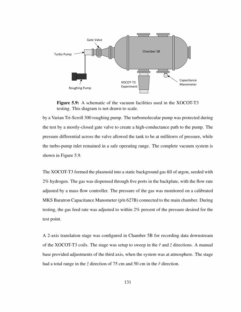
Capacitance Manometer

Gate Valve

Turbo Pump

Roughing Pump

Chamber 5B

XOCOT-T3Experiment

Figure 5.9: A schematic of the vacuum facilities used in the XOCOT-T3testing. This diagram is not drawn to scale.

by a Varian Tri-Scroll 300 roughing pump. The turbomolecular pump was protected during

the test by a mostly-closed gate valve to create a high-conductance path to the pump. The

pressure differential across the valve allowed the tank to be at millitorrs of pressure, while

the turbo-pump inlet remained in a safe operating range. The complete vacuum system is

shown in Figure 5.9.

The XOCOT-T3 formed the plasmoid into a static background gas fill of argon, seeded with

2% hydrogen. The gas was dispensed through five ports in the backplate, with the flow rate

adjusted by a mass flow controller. The pressure of the gas was monitored on a calibrated

MKS Baratron Capacitance Manometer (p/n 627B) connected to the main chamber. During

testing, the gas feed rate was adjusted to within 2% percent of the pressure desired for the

test point.

A 2-axis translation stage was configured in Chamber 5B for recording data downstream

of the XOCOT-T3 coils. The stage was setup to sweep in the r and z directions. A manual

base provided adjustments of the third axis, when the system was at atmosphere. The stage

had a total range in the z direction of 75 cm and 50 cm in the r direction.

131

5.1.7 Experiment Operation

Several hours before testing, the chamber was pumped to 2x10−5 Torr to remove impurities.

The low pressure measurement was recorded with a hot ion gauge and cold cathode gauge.

The capacitance manometer was turned on at least 4 hours before testing to ensure accurate

readings. The remaining instruments were powered on for at least 1 hour prior to testing.

A 4-channel pulse generator (Stanford Research System p/n DG535) was used to control

the experiment timing. The data acquisition system and pre-ionization circuit were

triggered concurrently. The main bank switch was triggered after the pre-ionization.

Timing between all channels on the function generator could be varied from shot-to-shot.

The testing sequence for a single test point consisted of twelve steps: (1) Turn on the

propellant, using the mass flow controller equipment. (2) Monitor the pressure on the

capacitance manometer read-out until the pressure stabilizes around the desired test point.

(3) Set the desired PI voltage and main bank voltage on the power supplies. (4) Turn on the

PI supply to charge PI bank. (5) Turn on the PPI supply. (6) Open the relay to disconnect

the dump resistors from the main bank charge supply. (7) Turn on the main bank supply

to charge the main bank. (8) When the capacitor is fully charged, open the charge relay,

and turn off the main bank power supply. (9) Wait for capacitor to drain to the desired test

voltage (typically 4-6 seconds). (10) Manually trigger the function generator to discharge

the experiment. (11) Turn off the PI supply and turn off the relay to reconnect the dump

resistors. (12) Collect the data on a central computer and reset the operating conditions.

The gas was left on for multiple tests, with the number of shots determined by maintaining

a safe temperature on the turbo-pump. The discharge circuit was not designed to dissipate

132

heat loads since it was meant to be a single-shot experiment. An overly-conservative five

minutes between shots was set as the minimum wait time.

5.2 Diagnostics

An objective of this research was to measure the velocity, momentum, and energy efficiency

of an AFRC plasmoid in the XOCOT-T3 experiment. The plasmoid velocity was measured

with a time-of-flight (TOF) array, consisting of two probes spaced apart a fixed distance.

Both magnetic field (b-dot) probes and Langmuir plasma probes were used in the TOF

array. Momentum was inferred by combining the velocity measurements with a mass

estimate from a density map of the plume. The density of the plume was measured with

Langmuir probes in the translation region of the experiment. Energy efficiency was then

estimated by comparing the kinetic energy of the plasmoid to the initial energy stored in

the capacitor.

Additional diagnostics were also incorporated, though they were not essential to the

performance characterization of the experiment. These diagnostics were still important for

monitoring the health of the experiment, the shot-to-shot repeatibility, and for diagnosing

plasmoid behavior. Coil current measurements were made on the inner and outer coil

circuits. External magnetic field probes adjacent to the outer coil provided non-intrusive

information about the magnetic field topology of the plasmoid. The external probes were

also a qualitative TOF array upstream of the main TOF array in the translation region. Fast

single-frame photography was used for mapping a qualitative radial plasma distribution

inside the formation chamber. An asymmmetric double Langmuir probe was used for

mapping the radial distribution of plasma inside the confinement region. The arrangement

133

30 cm

zr

18.2 cm

Outer Coil

Inner Coil

Internal ProbesTOF Probes

External ProbesB-dot Probes

Ion-Flux Probe

Single Frame Camera

Asymmetric Double Langmuir Probe

Figure 5.10: Layout of the diagnostics used in the XOCOT-T3. The singleframe camera is located outside the chamber, capturing images from anend-on view. Current and voltage monitors are not shown in this figureand are located on the external circuit.

of the diagnostics are shown in Figure 5.10.

For most of the tests, the XOCOT-T3 data acquisition (DAQ) system was a 16-channel,

high-speed oscillscope network, with two Tektronix 8-bit, 4-channel, 125 MS/s

oscilloscopes and one Nicolet Sigma 8-channel, 12-bit, 100 MS/s oscillscope. The

Tektronix oscilloscopes (p/n TDS 7104 and TDS 5104) were set to record 50,000 samples

at 125 MSamples per second (8 ns per point). The Nicolet Sigma (p/n LDS 100) recorded

50,000 points at 100 MS/s (10 ns per point). The sample rates were more than adequate

to capture phenomena well below the Nyquist frequency (50 MHz). The Nicolet and

Tektronix oscilloscopes recorded 10% of the data before the oscilloscope triggered. This

provided a clean DC response, used to correct for oscilloscope offsets. The oscilloscopes

were located inside a grounded screen room behind Chamber 5B. The screen room was

clad in solid sheet copper 0.6 mm thick. This corresponds to a single skin depth at 10 kHz,

effectively blocking all higher frequency radiated EMI. A secondary DAQ component was

added to the system during the 20 kHz tests. This was a 24 channel PXI system with 12-bit,

134

60 MS/s digitizers (NI-5105). The trigger on this system was also set to record a pre-trigger

record length of 10%. The sampling frequency was set to 60 MS/s, with a record length of

20,000 points.

5.2.1 Current and Voltage Monitors

The outer and inner coil currents were measured using wide band Rogowski coils (Pearson

Electronics p/n 301x) on the outer and inner transmission lines. Placement is shown

in Figure 5.3. The Pearson current monitors had a sensistivity of 0.01 V/A +1%, a

3 dB bandwidth from 5 Hz to 2 MHz, a useable risetime of 200 ns, a droop rate of

3.0%/millisecond, and peak current ratings of 50 kA. A bi-directional 20 dB attenuator

(Weinschel p/n 34-20-34) was added to the output of the current monitor to decrease the

sensitivity of the current monitor to 0.001 V/A. The attenuator had a deviation of ±0.6

dB and bandwidth of DC - 4 GHz. The current monitors and attenuators were used well

within recommended operating ranges; no significant errors were expected from these

measurements.

The PI current was measured with a small-profile Rogowski coil (Stangenes Industries p/n

2-0.1WA). The PI current monitor had an output sensitivity of 0.1 V/A± 0.5%, a droop rate

of 0.0008%/µs, an rise time of 20 ns, a 3dB bandwidth from 1 Hz to 20 MHz, and a peak

current of 5 kA. The rise time and bandwidth of the PI current monitor was insufficient to

capture the initial rise of plasma current at 1 MHz, though this information was not required

in this experiment. The PI circuit characteristics and waveforms were not a focus of this

research, so the significant errors introduced by using a non-ideal current monitor had little

impact on the results.

135

Initial capacitor voltage was recorded using a battery isolated multimeter, connected to

a voltage divider circuit between the terminals of the capacitor as shown in Figure 5.11.

This circuit used two high impedance resistors (bleed resistors) in parallel and a small 10

kΩ resistor in series with one high impedance resistor. The terminals of the small resistor

were connected to an isolated multimeter (Fluke p/n 189) for the voltage readout. The

voltage divider circuit was calibrated at DC from 30 volts to 250 volts using a high-voltage

Tektronix 6015A probe and a Fluke multimeter (p/n 189) at 47 voltage points. A linear

curve fit to the data resulted in the following relation: Vcap = CF*Vresistor. Each circuit

used different bleed resistors. The 10 kHz circuit used two parallel 2.66 MΩ (Caddock

p/n MS 313) bleed resistors and the 20 kHz circuit used two parallel 23 MΩ resistors.

The voltage divider calibration factor for the 10 kHz circuit was calculated to be 266.47 ±

0.90. The calibration factor for the 20 kHz circuit was 2466.93 ± 3.42. This includes the

measurement error and the standard deviation from the linear fit.

The circuit was triggered manually by waiting for the resistor voltage on the voltage divider

circuit to reach a certain level. Error analysis revealed that a tolerance of 10 mV on this

reading was allowed to maintain a 1% or less deviation in capacitor energy for the 10

kHz circuit. A tolerance of 1 mV was required for the 20 kHz circuit. Normal operation

came well within these bounds so the error in capacitor energy using a manual trigger was

expected to be small.

Time-dependent voltage measurements are difficult to record on pulsed high-frequency

experiments since an accurate and well-known ground reference must be known. High

ground potentials can develop during the discharge, resulting in an inconsistent voltage

offset that cannot be accounted for. Voltage measurements also require direct contact

to the circuit which presents a high voltage danger to the operator. For these

136

R B

R B

10 k

to Fluke Multimeter

+

-

VR

+

- CMB

Figure 5.11: Capacitor Voltage Divider Circuit. The capacitor voltage ismeasured across the 10 kΩ resistor with an isolated Fluke multimeter.

reasons, time-dependant voltages were not directly measured on the XOCOT-T3. The

time-depedendent voltage could be estimated by fitting the current measurements to an

RLC circuit description of the device.

5.2.2 Magnetic Field Probes

The principle diagnostics for this work were magnetic field probes (b-dot probes). The

XOCOT-T3 used 13 z-axis b-dot probes on the outer coil, 6 z-axis internal b-dot probes,

and 2 z-axis downstream TOF probes, as shown in Figure 5.12. The external b-dot probes

were placed between the outer coil and quartz insulator with a probe spacing of 2.5 cm.

The internal b-dot probes were also spaced 2.5 cm apart and were set on the inner insulator

for most of the tests. The TOF probes were located inside the translation region, spaced

18.2 cm apart. The near probe was at z = 49.5 cm and the far probe was at z = 67.7 cm.

137

B01 B02 B03 B04 B05 B06 B07 B08 B09 B10 B11 B12

B01 B02 B03 B04 B05 B06 B07

30 cm

zr

Internal ProbesTOF Probes

External Probes

18.2 cm

Figure 5.12: Magnetic field probe locations in the XOCOT-T3 experiment.External b-dot probes run the length of the discharge coils. The placementof the internal b-dot probes shown here is typical for most of the testing.Probe-to-probe spacing is 2.5 cm apart on the external and internal arrays.

5.2.2.1 B-dot Probe Theory

B-dot probes are loops of wire wrapped in a single plane. The loops enclose a

cross-sectional area A with a total number of turns N. When exposed to a time-changing

magnetic field, they detect an electromotive force εB (EMF) proportional to the rate of

change of magnetic flux ΦB normal to A as a result of Faraday’s Law:

εB =−NdΦB

dt=−N

dB ·Adt

=−NAdBdt

(5.3)

The proportionality constant NA relates the voltage produced by the EMF to the changing

magnetic field. The EMF is quite small, so large proportionality constants are used to

amplify the signal. The b-dot probe is generally connected to transmission lines and the

output voltage produced by the probe assembly Vp is measured at the end of the lines, shown

in Figure 5.13. Most elementary treatments equate the EMF generated by the fluctuating

magnetic field εB to the probe voltage Vp (i.e. εB = Vp). This relationship is only true for the

138

TransmissionLine

ProbeHead

+

-

A

XB

Vp

XX

X X X

N

ZL

Figure 5.13: Illustration of a magnetic field probe. The probe head isconnected to a transmission line and Vp is measured at the end of thetransmission line.

ideal case, which rarely exists. The transmission lines and the probe have non-negligible

impedance which become significant at high frequency. Additionally, the probe assembly

can interact with nearby ground planes and conductors, shunting capacitive current away

from or to the probe. These parasitic impedances distort εB by the time it arrives at the

measurement device, reducing the amplitude and shifting the phase.

The distortion of the signal can be regarded as a transfer function which transforms the field

fluctuations dB/dt into Vp [62]. The transfer function β (ω) includes the proportionality

constant NA as well as the impedance effects and external influences, resulting in the

following relation:

Vp =−β (ω)dBdt

=−β (ω)εB

NA(5.4)

Messer, et al introduced this notation in their broadband b-dot probe calibration paper [63],

referring to β (ω) as the sensitivity parameter. An expanded derivation of β (ω) is derived

here to include additional capacitive effects.

The probe assembly’s transfer function β (ω) can be modeled by considering the circuit

equivalent of a probe assembly, shown in Figure 5.14a. The probe head (circuit elements

139

with subscript p) is connected to a balanced transmission line such as a twisted, shielded

pair. The EMF from field fluctuations creates a source voltage εB. The probe and

transmission lines contain some resistance, inductance, capacitance, and conductance

which alter the source voltage by the time it is measured across a termination load ZL.

The finite resistivity of the lines and probe dissipate some of the source voltage as ohmic

loss. The inductance converts the voltage into magnetic field temporarily and releases it

a short time later. Capacitance behaves similar to inductance, but it converts the voltage

to an electric field instead of a magnetic field. Conductance shunts some of the current

into alternative paths. At frequencies below 1 MHz, capacitance effects can have very little

effect but if the probe is located close to a high-voltage source, the large potential difference

can cause the relatively small capacitance to have a significant coupling effect. This effect

is largely neglected in all treatments of b-dot probe behavior.

The probe assembly shown in Figure 5.14a represents a distributed impedance diagram

where the transmission line is treated as a collection of individual small impedances. If

the wavelength is much longer than the transmission line, the net effect of the individual

impedances can be lumped together into one common element Z. This approximation is

sufficient for the low frequencies considered in this work (10-500 kHz). The upper limit

of 500 kHz was based on the expected transit time between the probes for a 100 km/s

plasmoid velocity. Furthermore, at low frequency the effective impedace of the capacitive

elements between the lines is sufficiently high (Z = − jωC) so C and G in Figure 5.14

can be neglected. Then, the net impedance Z is a complex quantity with resistance R and

reactance X , equivalent to Z = R + jX . The equivalent circuit using lumped elements is

shown in Figure 5.14b.

Applying Kirchoff’s current and voltage laws to the equivalent probe circuit shown in

140

(a)

L R L R

2Z1

L R L R

CG CGZL

+

-

VP

2Z2 2Zn

2Z0

+

-

VPZL

Z0

Zp

(b)

L R

L R

CG

εBZ0

VC

Rp

CpLpẐC

Cc

+

-

+

-+

-εB

Figure 5.14: The circuit schematic for a b-dot probe connected totransmission lines. The complete circuit (a) can be simplifed to equivalentlumped impedances for low frequency (b) as probe impedances ZP, lineimpedances Z0, termination impedance ZL, and high voltage capacitivecoupling impedance Zc.

Figure 5.14b, Vp and εB are related by:

Vp

εB=

ZL

ZL +2Z0 +ZP + Zc−1 (ZLZp +Z0ZL +Z0Zp +Z2

0) (5.5)

Combining Equations 5.4 and 5.5, the probe’s transfer function β (ω) is:

Vp

B= β (ω) = NA

ZL

ZL +2Z0 +ZP + Zc−1 (ZLZp +Z0ZL +Z0Zp +Z2

0) (5.6)

The high voltage capacitive coupling impedance Zc is defined as the voltage at the probe

side of the capacitor Cc with respect to ground divided by the current through the capacitor:

Zc =ZcVc

(Vc−VHV )(5.7)

The voltage at the capacitor is equivalent to the combined voltage drop across Z0 and ZL.

141

This creates the following expression for Zc:

Zc =

Vp (Z0 +ZL)

ZL

Z−1c

Vp (Z0 +ZL)

ZL−VHV

=

Zc (Z0 +ZL)

(Z0 +ZL)−ZL

VHV

Vp

(5.8)

It should be stressed that Equation is only valid for low frequency, where inductive effects

in the transmission lines dominate the capacitive effects and the cable length is much,

much shorter than the frequency wavelength. If either condition does not hold, a different

formation of Equation 5.2.2.1 must be used.

In some cases, the high voltage capacitive coupling impedance Zc can be neglected. This

is true if the capacitance between the coil and probe is very, very small and the voltage

differential between the probe and nearby conductors are small. Removing this element

from the circuit leaves the probe head and transmission lines connected in series so their

equivalent impedances ZP and Z0 add. Their combined series impedances form a single

complex expression: R + jX . The probe’s transfer function for this case resembles that

found by other authors [63]:

VpdBdt

= β (ω) = NAZL

ZL +2Z0(ω)+ZP(ω)= NA

ZL

ZL +R(ω)+ jX(ω)(5.9)

The probe’s transfer function is frequency dependant, as noted by the functional form of

β (ω). The proportionality constant NA does not change with frequency, but the complex

impedance components R and X do. Resistance will increase with frequency as the skin

depth decreases. The reactance will also increase with frequency as X ≡ ωL for inductive

142

0.80

0.75

0.70

0.65

0.60

|β/N

A| [

-]

104

2 3 4 5 6 7 8 9

105

2 3 4 5 6 7 8 9

106

Frequency [Hz]

-40

-30

-20

-10

Phase [º]

Magnitude Phase

R = 10 ΩL = 10 µH

Figure 5.15: The frequency response (gain and phase) of a simulated probeassembly with negligible capacitance, 10 µH of inductance, and 10 Ω ofresistance from 10 kHz to 1 MHz.

circuits and X ≡ −1ωC for capacitive circuits. Combined, R and X dictate the phase shift and

attenuation of β (ω) over a range of frequencies. For illustration of this, a sample frequency

response of β is shown in Figure 5.15. The magnitude and phase of β (ω) shown in Figure

5.15 were computed using Equation 5.9 from 10 kHz to 1 MHz for a typical probe assembly

with neglibible capacitance, an inductance of 10 µH, and a resistance of 10 Ω, measured

across a 50 Ω load.

The results in Figure 5.15 show that the signal recorded at the end of the probe assembly is

only 85% of the signal produced by the field fluctuations εB, at 10 kHz. The values chosen

for this example are realistic representations of a b-dot probe used in plasma research, with

a high inductance (8 µH) probe head and 4 meters of twisted coax cable. The magnitude

and phase of β (ω) as shown in Figure 5.15 stays constant for 10 kHz to 100 kHz. After

100 kHz, the magnitude and phase shift drop substatially. This means that for the typical

case presented here, different frequency signals will arrive at the probe with different phase

delays and with different attenuation levels. This illustrates that for probes exposed to a

wide bandwidth, it is important to resolve β (ω) across the entire bandwidth and to account

143

for the significant attenuation caused even at a single frequency.

The effect of the high voltage capacitive coupling impedance can be illustrated by plotting

the transfer functions with and without Zc (Equations 5.6 and 5.9, respectively) and

comparing the output with a circuit model. A SPICE-based circuit simulation software

(LTspice IV v4.12a) was used to model a representative probe connected to 3.05 meters of

twisted-shielded pair transmission lines. The SPICE circuit is shown in Figure 5.16. The

probe’s EMF was modeled as 10 kHz sinusoidal voltage source Vs, using a 8.2 µH inductor

with 6.483 Ω of series resistance and 2.9 pF of parallel capacitance. The transmission lines

were modeled as circuit elements with a pair-to-pair inductance of 587 nH/m, capacitance

of 87.6 pF/m, and resistance of 0.427 Ω/m. The capacitance from one conductor to the

shield was set as 149 pF/m. A capacitor Cc was connected between the probe elements and

a high voltage voltage sinusoidal source Vc. Three different simulations were conducted.

The first simulation set the high voltage source to an amplitude of 1 kV at a frequency of

10 kHz and swept the capacitor Cc from 1 fF to 100 pF. The second simulation fixed the

capacitor Cc at 10 pF and varied the high voltage source from 100 V to 10 kV at 10 kHz.

The final simulation set the capacitor Cc to 10 pF and swept the high voltage source from

-100 V to -10 kV. The transfer function for each case was calculated using Equations 5.6

and 5.9. The gain and phase for each SPICE simulation is displayed with the calculated

phase and gain in Figure 5.17. The solid lines are from including Zc in the analysis and the

dashed lines are from neglecting Zc.

The effect of the high voltage capacitive coupling impedance is apparent from Figure 5.17.

For the limited range of parameters shown, Zc does not dramatically alter the gain of

the probe’s transfer function β (ω) but it can introduce significant phase changes if the

capacitance is sizeable or if the potential difference between the probe and high voltage

144

Figure 5.16: A SPICE circuit representation of a magnetic field probeused for examining the effect of the high voltage capacitive coupling onthe probe’s transfer function β (ω).

source is large. The sign of the phase shift indicates that the high voltage coupling can

either cause the probe signal to lead the field fluctuations (when the potential difference is

positive) or to lag them (when the potential difference is negative). The relatively constant

gain across the span of Vc and Cc shows that the magnitude of the signal should not change

due to the effect of Zc. This behavior is expected as pure capacitance does not remove

energy from a source, it merely displaces it in time. Note that the results shown in Figure

5.17 are for a single frequency.

The frequency dependance of the probe’s transfer function disappears if the load impedance

ZL is set to a large value (i.e. 1 MΩ). As tempting as it is to terminate the signal into 1

MΩ to greatly simplify the analysis, this should be avoided. Impedance matching requires

that the source impedance and the load impedance ZL are equivalent. This ensures that

all the power from the source is deposited into the load and is not reflected back to the

145

0.8650

0.8645

0.8640

0.8635

0.8630

Gai

n [-

]

10-12

2 3 4 5 6 7 8 9

10-11

2 3 4 5 6 7 8 9

10-10

Capacitance [F]

30x10-3

20

10

0

-10

Phase S

hift [rad] Gain Phase Gain (SPICE) Phase (SPICE)

Vc = 1000 V

0.869

0.868

0.867

0.866

Gai

n [-

]

102

2 3 4 5 6 7 8 9

103

2 3 4 5 6 7 8 9

104

| Vc | [V]

-50x10-3

-40

-30

-20

-10

Phase S

hift [rad]

Negative VcCc = 10 pF

0.8650

0.8645

0.8640

0.8635

0.8630

Gai

n [-

]

102

2 3 4 5 6 7 8 9

103

2 3 4 5 6 7 8 9

104

Vc [V]

30x10-3

20

10

0

-10

Phase S

hift [rad]

Positive Vc

Cc = 10 pF

Figure 5.17: Gain and phase changes of a b-dot probes transfer functionβ (ω) due to high voltage capacitive coupling. The solid lines are fromincluding Zc in the transfer function and the dashed lines are from neglectingZc. Results from a SPICE simulation are shown as hollow (gain) dots andsolid (phase) dots.

146

source. Failure to match impedances can result in inaccurate measurements especially at

of higher frequency. Multiple reflections of the same signal are recorded, leading to errors

during integration. Since the probe and transmission lines are low impedance, magnetic

field probes should always be terminated with a low impedance load, conventionally 50

ohms.

The theory presented in this section is considerably more involved that classical treatment

of b-dot probes, however it is essential in obtaining high accuracy measurements from

broadband probe signals. Failure to account for the frequency dependent behavior of the

probe assembly can result in significant errors. This is especially evident by examining

the sample probe response shown in Figure 5.15. In this example, failure to account

for impedance effects at low frequency can result in an field magnitude error of 15%.

Assuming a constant response for the probe from 10 kHz to 500 kHz results in an error

of over 40% for the high frequency portion of the signal. While the actual error will be

dependent on the probe design, this example illustrates the importance of resolving the

probe’s response across the entire frequency range of measured signal. A full error analysis

of b-dot probe methods is provided in Section 5.2.2.5.

5.2.2.2 Differential B-dot Probe Theory

A differential b-dot probe arrangement is commonly used to cancel capacitive effects

between the probe head and nearby conductors, including plasmas. Two probe heads are

wound over the same form, in opposite directions. A schematic of a differential probe

assembly is shown in Figure 5.18.

Each probe head records the same magnetic field, though the resulting EMF for each probe

147

TransmissionLinesProbe Heads

+

-

B

Vp,1

XX

X X

ZL

+

-ZL Vp,2

X

X

Winding direction

Figure 5.18: Illustration of a differential magnetic field probe. Each probehead is wound in a separate direction.

has the opposite sign. The capacitive effect measured by each probe is in the same direction

and has the same magnitude. The probe voltages Vp1 and Vp2 are subtracted from each other

so that the total voltage is twice the field, with the capacitive effects canceling, as shown in

Equation 5.10.

Vp =Vp1−Vp2 =(

V Bp1 +VC

p1

)−(

V Bp2 +VC

p2

)=(

V Bp1 +VC

p1

)−(−V B

p1 +VCp1

)= 2V B

p1

(5.10)

Differential b-dot probes behave much the same as their traditional single-winding

counterparts, with one exception. The windings on each differential probe couple to each

other with a mutual inductance. Each probe winding works to oppose the change of flux

through its probe-pair. An equivalent circuit diagram of the probe head, showing the mutual

inductance between the windings (using the dot-convention), is displayed in Figure 5.19.

The effect of the mutual inductance between the windings will add to the inductive

impedance of the probe assembly, increasing the phase delay and the attenuation. Including

the mutual inductance into the transfer function results in a modified expression for β (ω):

β (ω) = NAZL

ZL +R(ω)+ j (X(ω)+ωM)(5.11)

148

εB

Rp1

Cp1Lp1

+

-

εB

Rp2

Cp2Lp2

+

-

+

-Vp1ZL

+

-ZL Vp2

Figure 5.19: Circuit diagram of a differential b-dot probe. Mutualinductance between probe heads is indicated using the dot convention.

where R and X are the resistive and reactive impedance of a single probe in the differential

pair and M is their mutual coupling. This equation assumes both probes in the differential

pair are identical (as they should be).

5.2.2.3 Calibration of B-dot Probes

B-dot probes must be calibrated prior to use to determine their sensitivity. If the probe is to

be used across a range of frequencies, its sensitivity as a function of frequency must also

be calibrated. There are three ways to calibrate a b-dot probe:

1. Measure N and A directly, then measure the complex impedance as a function of

frequency.

2. Measure the output voltage of the probe when it is placed into a known AC field.

Change the frequency of the AC field to determine the frequency response of β (ω).

3. Measure the output voltage of the probe when it is placed into a known AC field.

Measure the complex impedance as a function of frequency independently.

149

The first method listed is suitable if N and A can be measured with a great deal of accuracy.

A ceramic core surface-mount (SM) inductor is the ideal candidate for this method [64].

The inductors are machine fabricated with very thin wire so that N and A can be known to

a high degree of certainty. Since inductance is related to NA, deviations from the target NA

can be easily detected by measuring the inductance. Most SM inductors have an inductance

tolerance of 5% or less; the deviation from the reported NA can be much lower. Once NA

is known, the probe assembly’s impedance can be measured across the probe’s required

bandwidth using an impedance analyzer, network analyzer, or similar tool.

The second method can be implemented by tuning the source frequency and measuring the

probe’s output [65]. Alternatively, one can use a network analyzer to measure the scattering

parameters of the source and the probe to calculate the transfer function [66] [63]. Tuning

the source frequency works well for limited bandwidth situations, but can get cumbersome

when the required bandwidth spans several orders of magnitude. Magnetic field sources

can have limited frequency responses and often several different sources are required to

cover the entire frequency range.

The third method requires calibration at a single frequency to determine NA. The remaining

variables in the transfer function β (ω) can be measured using an impedance analyzer.

These measurements are straight-forward and equipment to take these measurements is

readily available. This is the calibration method selected for this research.

The second and third method are similar in that they require that the magnetic field source

is well behaved and well known. Most calibration experiments measure the magnetic field

at DC with a Hall-probe for a given current level and then assume that it behaves identically

at higher frequencies. This assumption must be rigorously checked if small errors in the

measurement are required, as skin effect and the proximity effect can lead to magnetic field

150

deviations at elevated frequencies. Other experiments simply calculate the magnetic field

from the geometry and current, using formularies or electromagnetic field solvers. This is

sufficient if high accuracy (less than 10 %) measurements are not required.

The most popular source for the magnetic field in methods #2 and #3 is a Helmholtz coil

[67]. A Helmholtz coil consists of two identical loops of coils, connected in series with

their spacing equal to the coil radius. The magnetic field inside a Helmholtz coil is in

a single direction, extremely uniform in the center of the coil, and defined by a simple

formula:

Bz =

(45

)3/2µ0NI

a(5.12)

In equation 5.12, N is the number of turns per coil, I is the current through the coil, and a

is the coil radius. The magnetic field of a Helmholtz coil can be measured at DC using a

Hall-probe. It is often assumed to have the same current-to-field ratio at low frequency. The

AC current through the Helmholtz coil can be measured using a low impedance resistor or

a Rogowski coil. If the frequency characteristics of the Helmholtz coil are well-behaved

in the neighborhood of the measurements, it can provide an ideal magnetic field source for

probe calibration.

There are some pitfalls to using a Helmholtz coil as a magnetic field source at moderate (10

kHz - 100 kHz) frequencies. Since the probe voltage is proportional to dB/dt, the magnetic

field created by the Helmholtz coil must be high enough to produce a readable probe

voltage. Common laboratory function generators generally have maximum current rating

of 200 mA (10 V into 50 ohm), which is too low to create a significant magnetic field. This

current can be boosted by an external amplifier, but these can be expensive for frequencies

above 10 kHz. Higher current levels can also cause the coil to overheat. The number

of loops on the coil can be increased, but doing so also increases the inductance. The

151

inductance and resistance form a low-pass filter, with a cutoff frequency of fc = R/(2πL).

A Helmholtz coil generally has an inductance of several hundred µH and paired with a 50

ohm resistor for load balancing, this results in a cutoff frequency of 10-30 kHz. The area of

the coil can be made smaller to increase the magnetic field, but this limits the physical probe

size that can be placed in the coil. The uniform axial magnetic field shown in Equation 5.12

only applies to the very center of the coil and begins to drop off substantially at 20% of the

coil’s diameter. Balancing all of these restrictions requires special care when designing a

Helmholtz coil for moderate frequency use.

At higher frequencies (above 100 kHz), the current distribution through the Helmholtz coil

turns becomes affected by the skin depth and proximity effect as mentioned previously.

Detailed studies of these effects are necessary to determine if the magnetic field inside

the Helmholtz coil remains consistent with DC measurements. Above 1 MHz, a simple

Helmholtz coil calibration becomes difficult. Small details such as the connection of

wires to the magnetic field source can have a big impact on its frequency response [64].

Capacitive effects between the turns can also start to take effect, providing an alternative

path for current. The length of coil windings also becomes important as the wavelength

decreases. Some authors choose not to calibrate the probe at all at high frequencies, relying

instead on having probe with a well-known proportionality constant [64]. Other authors

attempt to correct for the high frequency effects by calculating the proportionality constant

from the scattering matrix of the probe-coil pair, obtained using a network analyzer [63].

The probes used in the XOCOT-T3 experiment were calibrated using a combination

of methods outlined above and were probe-dependant. High frequency calibration of

magnetic field probes was found to be unnecessary for this research, as the upper frequency

limit of the probes was determined to be 500 kHz (see Section 5.2.2.4). A full explanation

152

of the calibration methods used is provided in the probe-specific sections.

5.2.2.4 Analysis of B-dot Data

The signals from b-dot probes can be integrated digitally to calculate the time-dependant

magnetic field, B(t). If the phase delay created by the probe and line impedances is not

significant, a simple scaled, numerical integration method can be applied. The probe

voltage can be divided by the magnitude of |β (ω0)| at the principle frequency ω0 and

integrated:

B(t) =1

|β (ω0)|

∫Vp(t) dt (5.13)

This is referred to as the standard integration method.

Equation 5.13 is only valid for signals with constant attenuation and phase shift across their

applied bandwidth. If R and X vary over the frequency spectrum of the signal and contribute

to a significant frequency dependant phase shift and attenuation in the probe signal, their

variation with frequency should be considered. This can be done by converting the time

domain signal Vp(t) into the frequency-domain using a Fourier transform algorithm, such as

a fast Fourier transform (FFT). The frequency-domain signal Vp(ω) can then be multiplied

by β (ω) [62]. An inverse Fourier transform, such as an inverse Fast Fourier Transform

(IFFT) can be used to convert the scaled signal back to the time domain for the integration.

This sequence of operations is illustrated in Equation 5.14 through 5.17.

Vp(t)⇒ FFT ⇒Vp(ω) (5.14)

B(ω) =Vp(ω) ·β (ω) (5.15)

153

B(ω)⇒ IFFT ⇒ B(t) (5.16)

B(t) =∫

Bdt (5.17)

This method is referred to as the phase correction method in this work. It has been referred

to as the hybrid method in other sources [65].

Alternatively, the signal can be integrated in frequency space [62]. Singularities introduced

by the discrete Fourier transform at ω = 0 due to offsets, non-zero field components, and

other factors makes this approach less attractive [65].

If a b-dot probe is used with a filtering circuit or an amplifier, the transfer function H( f )

of the amplifier or circuit should be measured across the range of frequencies prior to use.

The effect of the amplifier can then be accounted for in the phase-correction method by

multiplying H( f ) by the probe’s transfer function β (ω) in Equation 5.15 in the method of

cascaded transfer functions.

In some cases, high frequency signals present in the data are unwanted or cannot be

properly characterized. Some filtering techniques suggest adding an analog filter in-line

with the probe to remove the high frequency components. Simple analog filters can

decrease the amplitude of a signal by 10x at the filter frequency, but they also introduce

a phase shift at frequencies an order of magnitude above and below the filter frequency.

This wide rolloff band is unattractive if the frequency to be filtered is close (within an order

of magnitude) to frequencies of interest.

Digital filters can also be used to attenuate high frequency signals. Digital filters are ideal

as they can be applied after the data has been collected so their effects on the raw data

can be reversed. They can also be designed to have much sharper rolloffs than analog

154

filters and introduce no phase shifts. In this research, the frequency of the EMI created by

the ignitron switch was within an order of magnitude of frequency components created by

plasma activity. For these reasons, digital filters were chosen to be used in this work instead

of their analog counterparts.

Oscilloscopes and other DAQ systems can introduce a small DC-offset to the signal. This

offset must be corrected for prior to the integration. The oscilloscopes in this research

recorded 50 µs of data prior to firing the PI circuit. The average voltage of the data in this

quiescent delay window was subtracted from all the data points to correct for the offset.

The digital integration used for calculating magnetic field requires that a high level of

digitization precision is used to collect the probe signals used for b-dot probes. Traditional

oscilloscopes normally use an 8-bit analog-to-digital convertor. This low resolution will

introduce significant uncertainty in the data. The small DC-offset error in the digitzer

causes some of the data to be discretized incorrectly. This error in discretization cannot

be recovered even by removing the offset. The error propagates in time through the

integration, leading to a positive or negative droop which worsens in time. If the data is

discretized with low resolution, it is readily apparent that this can lead to gross deviations.

To illustrate this effect, two ideal digitizers were simulated in Igor Pro to sample a clean

analog signal. One digitizer used a 8 bits of resolution, the other used 12 bits. A small

offset (10% of a bin level) was added to the data prior to sampling. The offset was removed

after sampling and prior to integration. The analog and digital signals were integrated

and plotted along with the integrated analog signal. The results are shown in Figure 5.20.

From these results, it is apparent that small offsets on a low resolution digitizer will lead to

trending errors in integrated data.

Random events, such as digitizer noise and periodic EMI, can also cause errors in the

155

400x10-63002001000

Time [s]

Analog 8-bit Digital 12-bit Digital

Figure 5.20: Integrated digital signals sampled from an analog waveformusing an 8-bit digitizer and a 12-bit digitizer.

probe signal. However, if the sampling rate is very high and the digitization of the signal

is also high, the average of the noise over a short time interval will be very small. When

the signal is integrated, the errors introduced by the noise will smooth out and have only

a small impact on the integrated signal. For these reasons, the data from the external

and internal b-dot probes was recorded at 100 MS/s using the 12-bit Nicolet Sigma 100

oscilloscope. The TOF probes were recorded on a 8-bit system to accomodate a commercial

pre-amplifier.

5.2.2.5 Error Analysis for B-dot Probes

Errors in b-dot probes come from several sources:

† Transfer function errors (σβ )

† Integration errors (σINT )

156

† Instrument errors (σinst)

† Electrostatic pickup errors (σcap)

† EMI error (σEMI)

† Statistical averaging errors (σstat)

† Probe alignment errors (σalign)

Errors accumulated during the calibration process to calculate the transfer function σβ are

process dependent, but generally due to several common sources. These include uncertainty

in the calibration magnetic field, instrument imperfections, and background interference.

Computation of calibration errors in the XOCOT-T3 research will be discussed in the

probe-dependent sections below.

Integration errors occur because the signal is approximated using finite timesteps during

digitization. Integrating across these timesteps h result in errors as the small local errors

amass into a global error. The local error (per timestep) is generally quite small, on the

order of h3 for trapezoid integration [68]. This error is shown in Equation 5.18. When

this error is summed across all points, it results in total integration error σINT shown in

Equation 5.20.

∆Ei =−h3

12d2Vp

dt2 (5.18)

σINT =t f − ti

12h2 d2Vp

dt2 (5.19)

The total error is generally O(∆t2) or slightly higher for noisy derivative signals. If the

timestep is kept small, the integration error can be neglected.

157

Errors can also arise from small uncertainties in the instrument used to digitize and record

the probe signal. Instrument errors in digitizers are random and Gaussian in nature and

small in amplitude. If the data is sampled at a much faster rate than changes in the signal

and a high resolution digitizer is used, their net effect in the total integrated signal will

cancel out so that σinst will be small.

Electrostatic pickup errors σcap arise from fluctuating plasma potentials near the probe or

from nearby high voltage sources. The capacitance this interaction is usually quite low (10

pF), but the rapid fluctuations of a plasma or high voltages in a nearby coil can result in

several mV of signal on the probe. If the probe is built with a high proportionality constant,

the magnetic field amplitude will be much higher than the electrostatic coupling. In this

case, the electrostatic pickup errors σcap can be neglected. If magnetic field contribution is

very low, then a differential probe arrangement [64] should be used to minimize the σcap.

Background interference with the probe, such as that from noisy circuit components can

create real errors in the integrated probe signal. This type of noise is typical in ringing

RLC circuits. Background noise or EMI cannot be predicted, measured, or corrected for

since there is not a completely clean signal to compare against. Using a probe with a high

proportionality constant can reduce the effect of integrated EMI into the signal, but σEMI

should be considered in the computation.

Repeatibility errors are common for pulsed experiments. These errors can be calculated by

measuring the statistical spread in repeated data sets. The standard devation of these data

sets provides a figure for σstat .

158

Probe alignment errors (σalign) occur when the probe is off axis from the measured field.

Trigonometric relations show that the alignment error is

σalign = Bmeasured

(1

cosθ−1)

(5.20)

where θ is the angle of incidence between the probe’s normal vector and the magnetic field.

Small angle approximations assure that this error will be less than 2% for angles smaller

than 10 degrees and less than 0.5% for angles less than 5 degrees. With properly placed

probes, orientation and alignment errors can be neglected.

Instrument errors, electrostatic pickup errors, and background EMI errors affect how the

probe signal is recorded by the digitizer. These errors can be combined with the integration

error per timestep to form a single error in the integrated voltage signal σVint . These errors

are small in comparison to the probe signal, gaussian, and random in nature, meaning their

effect on the integrated signal will be small as well. An error of 1-2% can be used for a

conservative estimate.

The error in voltage integration σVint and calibration error σβ compute magnetic field

together, combining into a single uncertainty in calculated field σBcalc. The error can be

computed considering how all the component errors propogate through the calculation for

B. This is done using the method of partial derivatives [69]. In the method of partial

derivatives for error computation, the partial derivative of the function f (x1,x2, ...xn) with

respect to each variable xn is used along with the uncertainty of each variable to compute

the total error. The partial derivatives are calculated as:

θn =∂ f∂xn

(x1,x2,x3) (5.21)

159

Their contribution to the total error in f or σ f is

σ f =√

θ 21 σ2

1 +θ 22 σ2

2 + ...+θ 2n σ2

n (5.22)

where σn is the error in xn. Using this method, it is apparent that the calculated error in B

due to β and Vint is

σBcalc =√

θ 2β

σ2β+θ 2

Vintσ2Vint (5.23)

The partial derivatives can be calculated using the slope method with a point 3σ away in all

directions. This will provide a conservative estimate. The calculated error σBcalc combines

with the other sources of error using the method of uncorrelated errors so that the total error

in B is σB is:

σB =√

σ2Bcalc +σ2

stat +σ2align (5.24)

5.2.2.6 XOCOT-T3 External B-dot Probes

The magnetic field in the XOCOT-T3 experiment is primarily in the axial direction. Axial

magnetic field probes were installed between the outer coil and outer insulator to measure

the time-history of this field with and without a plasmoid. The high levels of EMI from

this experiment combined with the low discharge frequency required maximizing the

proportionality constant NA of the probes for maximum resolution. The external probes

were selected to have an NA = 1x10−3 turns-m2. To match this number and maintain

physical clearance between the outer coil and the outer insulator, the external axial probes

were wound on flexible thin, 2.5 cm wide plastic forms with small gauge magnet wire. A

photograph of the probes is shown in Figure 5.21.

160

30 cmAxialExternal Probes

Calibration Probes

Figure 5.21: External magnetic field probes and their calibration probes,secured to the quartz insulator. Two arrays of external probes and calibrationprobes span the length of the electromagnetic coils.

Probe spacing between each probe was 2.5 cm and measured with a digital caliper. Six

probes were wound on a continuous form and the form was secured to the outer quartz

insulator with polymide tape. All probe ends were twisted tightly and connected to M27500

twisted-shielded pair (83 Ω) outside of the coils, extending to the data acquisition system

inside the screen room. A BNC-breakout box inside the screen room connected the twisted

pair to a BNC connector. The shield from the twisted pair was grounded to the BNC

breakout box, which was connected to the screen room ground. A coaxial RG58 cable

connected the breakout box to the desired oscilloscope channel. A 50-ohm terminator

(Pasternack p/n PE6008-50) was added to the end of the cable before connecting to the

oscilloscope. A schematic of the external b-dot probe assembly with cable lengths is shown

in Figure 5.22.

The external probes were calibrated in-situ since their long length and low calibration

frequency required an actively cooled Helmholtz coil. Commercial surface mount (SM)

inductors with a known proportionality constant NA were placed alongside the probes,

epoxied to a Mylar strip. The calibration probes were 8.2µH wire-wound, ceramic core

161

BNC BreakoutBox (0.3 m)

50 Ω

DAQ

BNC CableRG58-U (2 m)

Twisted -ShieldedPair (3.76 m)

ProbeHead

Screen Room

Twisted -MagnetWire (0.3+ m)

Figure 5.22: External magnetic field probe wiring diagram.

SM inductor (Coilcraft p/n 1008CS-822XJLC), chosen for their small physical dimension

(2 mm by 2 mm) and high inductance. Their NA was provided by the manufacturer

as 2.13x10−4turns-m2 and was the largest NA for the probe size. The tolerance on the

inductance is 5% and since inductance is directly proportional to N2A, this tolerance was

a very conservative estimate for NA as well. Twisted magnet wire leads were soldered to

the SM inductor solder pads and these were connected to 4.60 meters of M27500 twisted

shielded pair cable and a BNC breakout box in the same manner as the external probes (see

Figure 5.22).

The impedances of the probe assemblies were measured with an impedance analyzer to

provide the resistance R and reactance X for the probe’s transfer function β (ω). The

impedance analyzer was an Agilent 4294A Precision Impedance Analyzer with a total

bandwidth of 40 Hz to 100 MHz, capable of sweeping through 800 points across any

subrange of frequencies, with a base accuracy of 0.08%. For the probe characterization,

the 4294A was set to record R and X at 800 points for four frequency intervals of interest:

(1kHz-10kHz), (10kHz-100kHz), (100kHz-1MHz), and (1MHz-5MHz). The coaxial cable

of each probe assembly was connected to an Agilent test fixture (p/n 16047E) on the

162

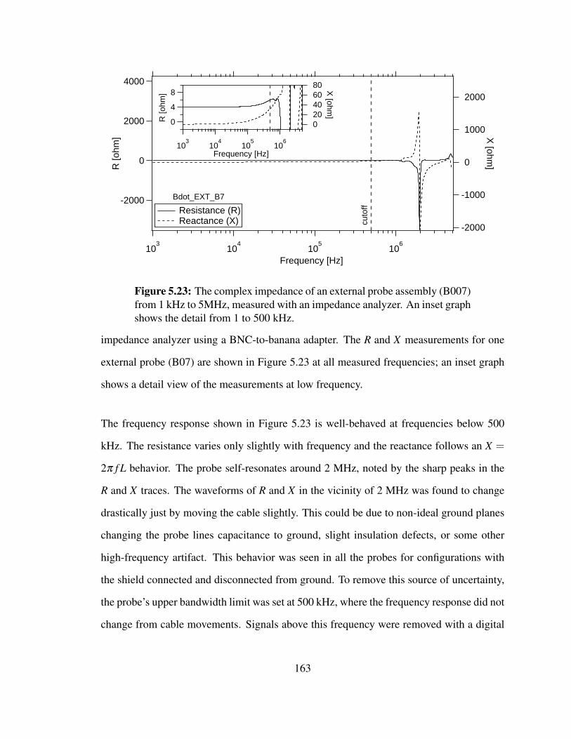
4000

2000

0

-2000

R [o

hm]

103

104

105

106

Frequency [Hz]

2000

1000

0

-1000

-2000

X [ohm

]8

4

0R [o

hm]

103

104

105

106

Frequency [Hz]

806040200

X [ohm

]

cuto

ff Resistance (R) Reactance (X)

Bdot_EXT_B7

Figure 5.23: The complex impedance of an external probe assembly (B007)from 1 kHz to 5MHz, measured with an impedance analyzer. An inset graphshows the detail from 1 to 500 kHz.

impedance analyzer using a BNC-to-banana adapter. The R and X measurements for one

external probe (B07) are shown in Figure 5.23 at all measured frequencies; an inset graph

shows a detail view of the measurements at low frequency.

The frequency response shown in Figure 5.23 is well-behaved at frequencies below 500

kHz. The resistance varies only slightly with frequency and the reactance follows an X =

2π f L behavior. The probe self-resonates around 2 MHz, noted by the sharp peaks in the

R and X traces. The waveforms of R and X in the vicinity of 2 MHz was found to change

drastically just by moving the cable slightly. This could be due to non-ideal ground planes

changing the probe lines capacitance to ground, slight insulation defects, or some other

high-frequency artifact. This behavior was seen in all the probes for configurations with

the shield connected and disconnected from ground. To remove this source of uncertainty,

the probe’s upper bandwidth limit was set at 500 kHz, where the frequency response did not

change from cable movements. Signals above this frequency were removed with a digital

163

filter prior to integration.

The impedance measurements recorded with the impedance analyzer were not capable

of isolating the high-voltage capacitance coupling Zc to the XOCOT-T3 outer coil. The

capacitance between each probe head and the coil was estimated to be very small (≈ 10 pF)

using theoretical calculations for a wire close to a wall. While the impedance analyzer was

able to take accurate measurements in this range, it required a very clean setup with short,

fixed leads and firm connections. Since the physical distances separating the probe head,

coil connection point, and analyzer were over 0.5 m apart it was impossible to record clean

measurements. Based on the findings in Section 5.2.2.1 and Figure 5.17, the high-voltage

capacitance is responsible only for an added phase shift. If the signal spans a narrow

bandwidth, a simple time-shift in the data can account for Zc and the simplifed transfer

function in Equation 5.9 can be applied to the signals.

The proportionality constant NA was determined for the external probes by discharging

the XOCOT-T3 main bank circuit through coils and recording the voltages generated by

the external probes and the calibration probes. These tests were performed at vacuum,

with no plasma present. A 12-bit, 100 MS/s oscilloscope was used to record the probe

voltages. The signals were terminated into 50 ohms prior to digitization. Twenty shots were

conducted at 500 J with the external probe and corresponding calibration probe recording

simultaneously. Ten shots were taken with midplane probe (B07) and its calibration probe

to establish repeatibility. For all shots, the current through the inner and outer coils was

also recorded. The probe voltages and their frequency spectra are shown in Figure 5.24a

and Figure 5.24b.

The probe signals were corrected for the frequency dependant impedance effects to find the

unscaled EMF produced by the magnetic field for each probe, using Equations 5.14 - 5.16

164

4

2

0

-2

Vpr

obe [V

]

120x10-680400

Time [s]

Midplane Probes(#006)

Calibration Probe

External Probe

10-2

10-1

100

101

102

103

104

|FF

T| [

V]

104

105

106

107

Frequency [Hz]

Calibration Probe

External Probe

Midplane Probes (#006)

(a) (b)

70x10-6

68

66

64

62

Err

or [t

urns

-m2]

300025002000150010005000

Point Number [-]


1.255x10-3

1.250

1.245

1.240

1.235

1.230

NA

[tur

ns-m

2]

300025002000150010005000

Point Number [-]


4

2

0

-2

(dB

/dt)

*nA

-1 [V

]

140x10-6120100806040200

Time [s]

Calibration Intervals


Calibration ProbeExternal Probe

(c)

(d) (e)

Figure 5.24: Sample calibration waveforms for external probe array,including (a) raw b-dot probe signals, (b) corresponding FFTs, (c) intervalsof data used for calibration, (d) NA waveform for three intervals, and (e)error in NA.

165

220x10-9

200

180

160

140

Pha

se D

elay

[s]

12108642Probe Index [-]

9.1 kHzFirst Crossing(26Jul2011) & (13Feb2012)

Transfer Function Results Calibration Array External Array

Impedance Predictions

Calibration Array External Array

Figure 5.25: Measured phase delay at 9.1 kHz of external probes, comparedto their predicted delay.

and setting the proportionality constant to unity. No filters were used in order to keep the

error estimates conservative. The resulting unscaled EMF signals from the midplane probes

are shown in Figure 5.24c. The phase correction method was checked by comparing the

original signals to the phase-corrected signals to determine if the expected phase shift from

the impedance measurements was accounted for in the data analysis. The comparison of

the corrected phase shift to the predicted phase shift at 9.1 kHz is shown in Figure 5.25. For

the external array data, the corrected phase shift lies within 1 sample period of the predicted

phase shift (marked with error bars). The calibration array shows the phase delay fits within

2 sample periods. This is due to the lower voltage signals and greater noise susceptibility.

These results indicate that the phase-correction data analysis is able to correct the phase of

the primary frequency component.

Despite the phase correction, the external probe’s signal did not have the same phase as

its corresponding calibration probe; the phase of the calibration probe lagged the phase of

the external probe. The phase difference was likely caused by a mismatched high voltage

coupling capacitance Zc due to the different capacitances and different voltage levels of

166

the signals. If left uncorrected, dividing the probe signals by the calibration signals would

result in large errors. Since Zc does not cause an attenuation of the signal and the frequency

spectrum of each signal illustrates that the 10 kHz frequency component is several orders

of magnitude higher than other frequencies, the calibration signals were shifted in time to

align with the probe signals.

After the phase corrections were applied, the external probes’ proportionality constants

were calculated by dividing the unscaled EMF signals from the external probes by the

corresponding calibration probe and multiplying by the calibration probe’s proportionality

constant NA, as illustrated in Equation 5.25. This was done for three time intervals in the

data, to prevent the portions of the signal with poor signal-to-noise ratios from artifically

inflating the error estimate. These time intervals are bracketed in Figure 5.24c. Figure 5.24d

shows the resulting trace from the calibration of the midplane probe. The proportionality

constants were calculated from the average of this trace (marked by a solid line) and the

standard deviation of the average NA (dotted lines) was recorded for the error estimate.

NA|ext = NA|cal

dBdt

∣∣ext

dBdt

∣∣cal

(5.25)

The experimental uncertainty in the calibration process were due to several sources,

including the uncertainty in the calibration probes NA, the uncertainty in the transfer

function, and he uncertainty in the measurement of the probe signals. The transfer functions

combined uncertainty was estimated using the uncertainty in the calibration probe’s NA,

the uncertainty in the impedance measurements, and the uncertainty in the termination

resistance. The calibration probes have a 5% uncertainty in their inductance. Inductance

is proportional to N2A so the specified uncertainty can be considered a very conservative

estimate for NA. The 4924A impedance analyzer specifies a tolerance of 0.08% on the

167

impedance measurements for the range of values measured. The 50 ohm terminators used

for ZL were assumed to have a 1% tolerance, as this information was not provided by the

manufacturer. The uncertainty in the probe signals was set by the accuracy of the digitizer,

specified as 0.25% ± 3 least significant bits.

Using the method of partial derivatives and transmission of error [69], the combined

experimental uncertainty across the calibration interval was computed for each probe. The

results for the midplane probe are shown in Figure 5.24e. The average experimental

calibration error σexp was combined with the statistical error from the data spread

calibration calculation σstat , shown in Figure 5.24d, to determine the total error in the

calibration process. This was done using the equation for uncorrelated errors:

σcal =√

σ2exp +σ2

stat (5.26)

The full results from the calibration are shown in Table 5.2, including the complex

impedance for each probe at 10 kHz, the magnitude of each probe assembly’s transfer

function at 10 kHz, and the proportionality constant for each probe assembly. From these

results, it is shown that the uncertainty in the calibration probes’ NA dominates the error

estimate, suggesting that for more accurate measurements using this calibration method an

inductor with tighter tolerances should be used.

The resulting proportionality constants were multiplied by the integrated EMFs to calculate

the magnetic field. The magnetic field at the midplane is shown in Figure 6.7.

The total error in the magnetic field measurement was calculated by combining the

uncertainty due to integration and the uncertainty in the transfer functions of the external

probes. While it was difficult to quantify the integration errors since there is no clean,

168

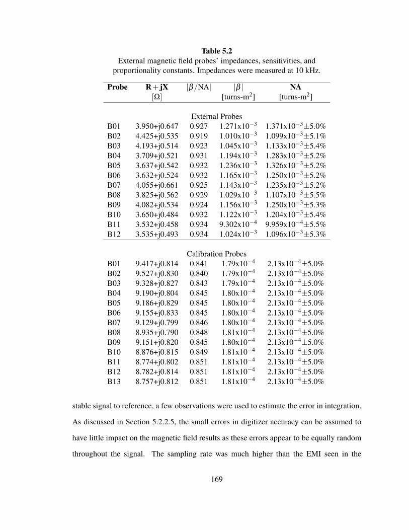
Table 5.2External magnetic field probes’ impedances, sensitivities, and

proportionality constants. Impedances were measured at 10 kHz.

Probe R+ jX |β/NA| |β | NA[Ω] [turns-m2] [turns-m2]

External ProbesB01 3.950+j0.647 0.927 1.271x10−3 1.371x10−3±5.0%B02 4.425+j0.535 0.919 1.010x10−3 1.099x10−3±5.1%B03 4.193+j0.514 0.923 1.045x10−3 1.133x10−3±5.4%B04 3.709+j0.521 0.931 1.194x10−3 1.283x10−3±5.2%B05 3.637+j0.542 0.932 1.236x10−3 1.326x10−3±5.2%B06 3.632+j0.524 0.932 1.165x10−3 1.250x10−3±5.2%B07 4.055+j0.661 0.925 1.143x10−3 1.235x10−3±5.2%B08 3.825+j0.562 0.929 1.029x10−3 1.107x10−3±5.5%B09 4.082+j0.534 0.924 1.156x10−3 1.250x10−3±5.3%B10 3.650+j0.484 0.932 1.122x10−3 1.204x10−3±5.4%B11 3.532+j0.458 0.934 9.302x10−4 9.959x10−4±5.5%B12 3.535+j0.493 0.934 1.024x10−3 1.096x10−3±5.3%

Calibration ProbesB01 9.417+j0.814 0.841 1.79x10−4 2.13x10−4±5.0%B02 9.527+j0.830 0.840 1.79x10−4 2.13x10−4±5.0%B03 9.328+j0.827 0.843 1.79x10−4 2.13x10−4±5.0%B04 9.190+j0.804 0.845 1.80x10−4 2.13x10−4±5.0%B05 9.186+j0.829 0.845 1.80x10−4 2.13x10−4±5.0%B06 9.155+j0.833 0.845 1.80x10−4 2.13x10−4±5.0%B07 9.129+j0.799 0.846 1.80x10−4 2.13x10−4±5.0%B08 8.935+j0.790 0.848 1.81x10−4 2.13x10−4±5.0%B09 9.151+j0.820 0.845 1.80x10−4 2.13x10−4±5.0%B10 8.876+j0.815 0.849 1.81x10−4 2.13x10−4±5.0%B11 8.774+j0.802 0.851 1.81x10−4 2.13x10−4±5.0%B12 8.782+j0.814 0.851 1.81x10−4 2.13x10−4±5.0%B13 8.757+j0.812 0.851 1.81x10−4 2.13x10−4±5.0%

stable signal to reference, a few observations were used to estimate the error in integration.

As discussed in Section 5.2.2.5, the small errors in digitizer accuracy can be assumed to

have little impact on the magnetic field results as these errors appear to be equally random

throughout the signal. The sampling rate was much higher than the EMI seen in the

169

frequency spectrum (consult Figure 5.24b) and a 12-bit digitizer was used to further reduce

the uncertainty from these effects. The midplane external probe signal is relatively free of

EMI; the noise level of the 1-10 MHz signal components shown in the FFT trace of Figure

5.24b is two orders of magnitude below the principle frequency. With the phase correction

method, the magnetic field matches the period and phase of the outer coil current to within

a few timesteps. When compared with significantly noisier calibration probe signal, the

difference in magnitude of the first and second magnetic field peaks is only 0.6%. All of

these clues suggest that the external magnetic field probes have a low level of integrated

error (less than 1%) for the first period of a vacuum shot, so a conservative error of 1% was

used. The error is expected to grow in time, but this is of little relevance as only the first

cycle of data from the experiment will be used in the analysis.

5.2.2.7 XOCOT-T3 Internal Magnetic Field Probes

Internal b-dot probes must be small to minimize perturbations to the plasmoid and retain

a large NA. Commercial surface mount (SM) inductors were chosen for the internal

b-dot probes since they use many turns around a very small area. The SM inductor

with the highest available NA was found to be the same inductor used for the external

calibration probes (in Section 5.2.2.6). This is a 8.2µH wire-wound, ceramic core SM

inductor (Coilcraft p/n 1008CS-822XJLC) with an NA provided by the manufacturer as

2.13x10−4turns-m2 ± 5%. The proportionality constant is well below the target NA of

1x10−3turns-m2, but a larger area probe would create larger plasma perturbations. It was

decided to accept the larger uncertainty at the expense of minimizing plasma perturbations.

An array of seven SM inductors were spaced 2.5 cm apart and sheathed inside a 7 mm

170

2.5 cm

Figure 5.26: Photograph of internal magnetic field probes.

Figure 5.27: Internal magnetic field probes wiring diagram.

diameter, 38 cm long quartz tube. Small diameter magnet wire was soldered to the

connection pads and these leads were twisted tightly until the end of the quartz tube. A

small diameter copper pipe was inserted into the quartz tube for EMI shielding. The twisted

leads and shield were connected to twisted-shielded cable (M27500) and fed through

the vacuum chamber using an isolated DB15 pin connector. The twisted-shielded pair

continued until it reached a BNC-breakout box inside the screen room. The shield was

grounded at the screen room. A photograph of the probes is shown in Figure 5.26. A

diagram of the probe construction is shown in Figure 5.27. For all of the data presented

in this research, the internal probes were placed directly outside the inner insulator at the

upstream end of the coils to check for magnetic field reversal. Figure 5.12 shows this

placement, with the first probe in the array located at z = 0.

171

The probes were not calibrated for NA since it was provided by the manufacturer. The

impedance of each probe assembly was measured using the Agilent 4294A Impedance

Analyzer, as was done for the external probes in Section 5.2.2.6. This was used to calculate

each probe’s transfer function β (ω). The results are shown in Table 5.3. Similar to what

was found with the external probes, the internal probes resonated at 1 MHz. The impedance

above 500 kHz was found to change drastically with probe position, movements of the

cable, and shielding attachment. To remove this source of uncertainty, the probe’s upper

bandwidth limit was set at 500 kHz, where the frequency response did not change from

cable movements. Signals above this frequency were removed with a digital filter prior to

integration.

Table 5.3Internal magnetic field probes’ impedances, sensitivities, and

proportionality constants. Impedances were measured at 10 kHz.

Probe R+ jX |β/NA| |β | NA[Ω] [turns-m2] [turns-m2]

Internal ProbesB01 9.356+j0.886 0.842 1.79x10−4 2.13x10−4±5.0%B02 9.370+j0.883 0.842 1.79x10−4 2.13x10−4±5.0%B03 9.283+j0.893 0.843 1.80x10−4 2.13x10−4±5.0%B04 9.276+j0.865 0.843 1.80x10−4 2.13x10−4±5.0%B05 9.255+j0.919 0.844 1.80x10−4 2.13x10−4±5.0%B06 9.134+j0.876 0.845 1.80x10−4 2.13x10−4±5.0%B07 9.154+j0.891 0.845 1.80x10−4 2.13x10−4±5.0%

The uncertainty in the probes’ transfer function σβ was calculated using the method of

partial derivatives [69]. The internal probes had a 5% uncertainty in their inductance,

according to the data sheet provided by the manufacturer. Since inductance is proportional

to N2A the uncertainty in inductance is a very conservative estimate for NA. The 4924A

impedance analyzer specified a tolerance of 0.08% on the impedance measurements for the

172

range of values measured. The 50 ohm terminators were assumed to have a 1% tolerance,

as this information was not provided by the manufacturer. The uncertainty in the probe

signals was set by the accuracy of the digitizer, specified as 0.25% ± 3 least significant

bits.

The error in the calculated field of the internal probes σBcalc was calculated using the

method of partial derivatives, combining the error in the transfer function σβ with the error

in the integrated probe signal σVint (see Equation 5.23). The probe’s smaller NA made them

more susceptible to noise pickup, so a 2% error was used for σVint . Orientation errors σalign

were considered trivial, since the probes’ normal axes were misaligned by no more than 5

degrees. Statistical errors σstat were taken into account by averaging several shot together

as warranted.

5.2.2.8 XOCOT-T3 TOF Magnetic Field Probes

The TOF b-dot probes required a very large NA since they were located far downstream

of the main discharge coils. The upstream probe in this array was selected to have an

NA of 1x10−3 turns-m2 and the downstream probe had an NA = 1x10−2 turns-m2. The

probes were wound on a notched, cylindrical Macor mandrel with small gauge magnet wire.

The upstream probe had mandrel dimensions of 2.48 mm by 17.73 mm and 50 winding

turns. The downstream probe had mandrel dimensions of 3.33 mm by 26.65 mm and

120 winding turns. Since the probes would be exposed directly to the plasma environment

with relatively small magnetic fields, the probes were wound in a differential configuration.

During construction, two lengths of wire were wrapped around the mandrel simultaneously

to provide nearly identical configurations for the two windings. The leads of each winding

173

Figure 5.28: Photograph of TOF magnetic field probes. The downstreamprobe is the larger probe (top) and the upstream probe is the smaller probe(bottom).

were twisted together and then the twisted leads were twisted with each other. The probe

head and twisted magnet wire leads were inserted into a 30 cm long quartz tube and a

copper tube was inserted between the leads and tube to provide a ground shield. The

twisted leads were connected to 2.36 meters of twisted-shielded cable (M27500). The

shields of the cables were soldered to the copper shields over the twisted magnet wire. The

twisted-shielded cable was connected to a vacuum feedthrough and joined to an additional

1.17 m of twisted-shielded cable (M27500) outside the vacuum tank. The twisted cable

connected to the screen room electrical panel with a BNC connector. An additional 2 m of

RG-58U cabling inside the screen room was required to attach the probe signals to a DAQ

unit. The probe cabling was terminated into 50 ohm in-line terminators prior to digitization

(or amplification). Photographs of both probes are shown in Figure 5.28. A wiring diagram

of the probe is shown in Figure 5.29.

The impedance of each probe assembly was measured using an Agilent 4294A impedance

174

Figure 5.29: TOF magnetic field probes wiring diagram.

analyzer. Each winding of each assembly was measured separately to check for deviations

between each differential probe winding. The impedances of each probe in the differential

assembly was found to agree by less than 2%, meaning that each probe for a differential

pair was nearly identical. The impedance across the range of frequencies is shown in

Figure 5.30 for both windings. One winding is indicated with a (+) and the other with a

(-). The TOF b-dot probes reached a resonance at a much lower frequency, due to the large

inductance of the probe heads. The upstream probe had a resonance around 900 kHz and

the downstream probe had a resonance at 600 kHz. The cutoff frequency for each probe

was calculated where the resistance of the assembly deviated by 3 dB from the resistance

at 10 kHz. For the upstream probe this was at 360 kHz and for the downstream probe this

was at 250 kHz. All frequencies above this point were removed with a digital filter prior to

integration.

The impedance of the differential assembly was considered from a single probe winding

only. This did not include the mutual inductance between the differential pairs. Since there

was no easy way to measure the mutual inductance, an estimate was made for how the

mutual inductance would affect the time-response of the probe. The transfer function for

175

101

102

103

104

Res

ista

nce

[ohm

]

103

104

105

106

Frequency [Hz]

-4000

-2000

0

2000

4000

Reactance [ohm

]3dB

cut

off (

250

kHz)

Resistance (R) Reactance (X)

R- = 11.3559

X+ = 5.27974 X+ = 54.2531X- = 53.5548

R- = 11.9216R+ = 11.901

X- = 5.21209

R+ = 11.3679

Downstream Probe

10

2

46

100

2

46

1000

2

46

Res

ista

nce

[ohm

]

103

104

105

106

Frequency [Hz]

-3000

-2000

-1000

0

1000

2000

Reactance [ohm

]3dB

cut

off (

360

kHz)

Resistance (R) Reactance (X)

R- = 7.86755

X+ = 2.36298 X+ = 23.8179X- = 23.612

R- = 8.12494R+ = 8.12719

X- = 2.3447

R+ = 7.87014

Upstream Probe

(a)

(b)

Figure 5.30: TOF magnetic field probes’ impedance as a function offrequency for the (a) upstream probe and (b) downstream probe.

the probe assembly was calculated using Equation 5.11, with R and X from a single probe

in the differential pair. The mutual inductance between the probe heads required for this

equation was estimated by calculating using the self-inductance of the probe head. This

is valid since both probes are co-wound for maximum coupling coefficient k = 1.0 and by

noting that M = k√

Lp1Lp2 = kLp. The upper limit on self-inductance of the probe head

was calculated by subtracting the cable impedance from the total probe assembly reactive

176

impedance (shown in Figure 5.30). The inductance of the upstream probe was calculated

to be 35 µH and the downstream probe was calculated to be 81.4 µH. The added mutual

inductance for the upstream probe would increase the phase-delay of the probe by 600 ns (at

10 kHz). The downstream probe’s estimated phase-delay due to mutual coupling between

probe heads would increase by 1.303 µs (at 10 kHz). The resulting phase delay between

the probes that would result by not factoring in the phase shift due to mutual coupling

in the differential assembly was 703 ns. For a plasmoid traveling at 100 km/s between

the probes, the measured velocity would be slower by 28% (28 km/s). The substantial

error accumulated by neglecting the mutual inductance of the probe heads required that the

velocity measurement must be cross-checked with a measurement from plasma probes, as

described in Section 5.3.1.

The TOF b-dot probes were not calibrated to find their proportionality constants for two

reasons. The first reason was that the TOF b-dot probes were used to record the time-history

of the magnetic field for measuring plasmoid velocity; the absolute magnetic field was of

little importance to this measurement. The second reason was that a calibration setup with

a traditional Helmholtz coil required a specialty high-current amplifier for accurate results.

A quick scaling study on sizing a Helmholtz coil for the upstream probe (17.73 mm long)

required that the diameter of the Helmholtz coil be 89 mm, so that the probe occupy no

more than 20% of the interior of the coil. (The field inside a Helmholtz coil is only uniform

across 20% of the coil diameter.) The minimum voltage that should be recorded by the

probe (NA of 1x10−3 turns-m2)is 100 mV, assuming a 1 mV noise floor. This dictates

that the minimum field at 10 kHz is 1.6 mT. This requires that product of the turns on the

Helmholtz coil and the current satisfy 79 turns-amps. The peak current available from an

available low-noise RF amplifier at 10 kHz was 800 mA (Kronheit 7500). The number

of turns required to match 800 mA was 100 turns. The total inductance of a Helmholtz

177

coil matching this description would be 3 mH. The cutoff frequency of the Helmholtz coil

with a 50 ohm series resistor is 2.7 kHz. At 10 kHz, the current would drop by 10 dB

(or more) meaning the actual current driven through the Helmholtz coil would be 70% of

the rated 800 mA. Increasing the turns on the Helmholtz coil would increase the field, but

it would also increase the inductance by N2. Increasing the current to reach 800 mA (or

above) would require a custom amplifier. For these reasons, it was decided not to calibrate

the TOF probes to find their proportionality constant and scale the resulting waveforms to

display B/NA.

A differential pre-amplifier (Tektronix p/n ADA400A) was sometimes used to measure the

differential signal between the probes prior to digitization. The amplifier was used when

the signal-to-noise ratio was too poor for adequate digitization. A 1-MHz commericial

preamplifier was chosen, with a variable gain of 100x or 10x. The transfer function for the

differential amplifiers was measured by applying two sinusoidal signals from a function

generator (Tektronix p/n AF3102) with opposite polarity to the inputs of the amplifier.

The frequency of the signals was changed to map the response of the amplifier to various

frequencies from 10 kHz to 1 MHz. The transfer function for the amplifier was H( f ) was

calculated by dividing the amplifier output by the input according to

H( f ) =Vout

Vin=|Vout ||Vin|

∠(θout−θin) (5.27)

Note that in Equation 5.27, Vout and Vin are phasors with an amplitude and phase. To

simplify the math, an FFT was performed on the input and output signals to calculate

their respective amplitudes and phases. A smoothing spline was used to interpolate the

transfer function at intermediate frequencies. The transfer function of each amplifier unit

is displayed in Figures 5.31 and 5.32. It should be noted that this method is not the

178

0.140

0.135

0.130

0.125

0.120

0.115

0.110

Gai

n [-

]

104

2 3 4 5 6 7 8

105

2 3 4 5 6 7 8

106

Frequency [Hz]

-1.5

-1.0

-0.5 Phase S

hift [rad]

Unit #1 (10x)DC CouplingNo offset

Gain Phase_Shift

1.00

0.95

0.90

0.85

0.80

0.75

Gai

n [-

]

104

2 3 4 5 6 7 8

105

2 3 4 5 6 7 8

106

Frequency [Hz]

-2.0

-1.5

-1.0

-0.5

Phase S

hift [rad]

Unit 1 (100x)DC couplingNo offset

Gain Phase_Shift

(a)

(b)

Figure 5.31: Measured frequency response of preamplifier #1 from 10 kHzto 1 MHz for (a) 10x gain and (b) 100x gain.

preferred method for measuring the transfer function of the differential amplifiers. Ideally,

chirp signals would be used as inputs for the amplifiers so that all frequencies of the desired

range could be tested at once. However, the signal generator used in this instance was not

179

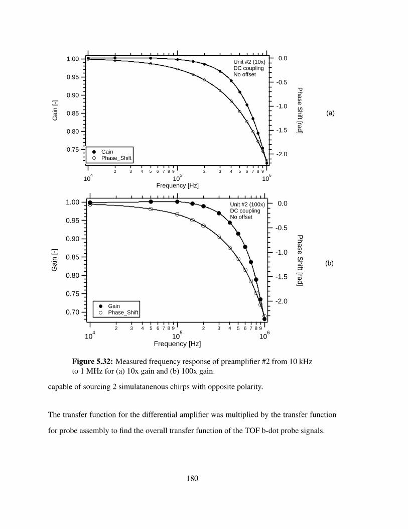
1.00

0.95

0.90

0.85

0.80

0.75

Gai

n [-

]

104

2 3 4 5 6 7 8 9

105

2 3 4 5 6 7 8 9

106

Frequency [Hz]

-2.0

-1.5

-1.0

-0.5

0.0

Phase S

hift [rad]

Unit #2 (10x)DC couplingNo offset

Gain Phase_Shift

1.00

0.95

0.90

0.85

0.80

0.75

0.70

Gai

n [-

]

104

2 3 4 5 6 7 8 9

105

2 3 4 5 6 7 8 9

106

Frequency [Hz]

-2.0

-1.5

-1.0

-0.5

0.0

Phase S

hift [rad]

Unit #2 (100x)DC couplingNo offset

Gain Phase_Shift

(a)

(b)

Figure 5.32: Measured frequency response of preamplifier #2 from 10 kHzto 1 MHz for (a) 10x gain and (b) 100x gain.

capable of sourcing 2 simulatanenous chirps with opposite polarity.

The transfer function for the differential amplifier was multiplied by the transfer function

for probe assembly to find the overall transfer function of the TOF b-dot probe signals.

180

5.2.3 Plasma Probes

Two different types of plasma probes were used in this research. The first type of plasma

probe was a single Langmuir probe fixed to a negative bias voltage. This is referred to in

this research as an ion flux probe. An asymmetric double Langmiur probe (ADLP) was

also used. This section explains how both probes were used in this research including basic

probe theory, probe construction and geometry, associated circuitry, and data analysis.

A single Langmuir probe is a conductive electrode emersed in a plasma, biased to a

potential [70], [71], [72]. The voltage applied to the probe is swept through a range of

voltages and the current collected to the probe is monitored as function of voltage. This

information can be used to infer plasma density, electron temperature, plasma potential,

and floating potential. The behavior of the probe current as a function of applied voltage is

referred to as an I-V characteristic. A illustration of a typical I-V characteristic is shown in

Figure 5.33. At low bias voltages (negative), the probe only collects ions. All electrons are

repelled. The current collected to the probe is constant in this region (Region I in Figure

5.33) as the ions surrounding the probe in the Debye layer shield out the probe’s potential

from the nearby plasma. This region is referred to as the ion saturation region. At high bias

voltages (positive), the probe only collects electrons. Ideally, the current here would be

constant as well, though in reality expanding electron sheaths cause an increase in current

with voltage. This region (Region III in Figure 5.33) is referred to as the electron saturation

region. The intermediate region (Region II in Figure 5.33) between the ion and electron

saturation regions is a transition region where the probe collects both ions and electrons.

Assumptions about the plasma can be applied to the data so that it can be used to infer

certain plasma properties. All three regions are required to build a complete picture, which

181

I II III

Voltage

Cur

rent

I = 0Sample I-V Characteristic

Single Langmuir Probe

Figure 5.33: Sample I-V characteristic for single Langmuir probe.

is why sweeping the probe through a range of voltages is necessary for measuring plasma

properties.

The fast timescales of the XOCOT-T3 experiment made sweeping the probe difficult. The

sweeping method would require novel, custom probe circuitry to satisfactorily sweep the

probe through a range of voltages on a timescale comparable to plasma fluctuations (greater

than 5 MHz). Instead of sweeping, the probe was fixed to a single bias in the ion saturation

region where repeatable data and repeatable probe behavior was most likely. Limited

information is available about a probe in ion saturation and generally only probe currents

can be reported with any accuracy. However, if certain assumptions can be made about the

plasma, density or temperature measurements can be inferred from the data.

If the kinetic energy of the plasma relative to the probe’s collection surface is much greater

than its thermal energy (1/2miu2i »kBT ), the ion saturation current is related to the local

plasma density n0, the velocity of the ions ui, the charge number of the ions Z, and the

182

probe area Ap by a simple flux relation [73]:

Isat+ = Apecn0Zui (5.28)

This relation is valid for planar probes normal to the velocity vector and for cylindrical

probes transverse to the flow vector. For a planar probe situated in a 10 eV, 100 km/s argon

plasma, the kinetic energy (3x10−16 J or 1900 eV) is two orders of magnitude higher than

the thermal energy (2x10−18 J or 10 eV). Since the AFRC plasma in the XOCOT-T3 was

expected to stream past the probes at 100 km/s with thermal temperatures less than 10 eV,

this means that Equation 5.28 can be used to estimate the plasmoid’s density if the velocity

is known.

The ion flux probes used in this research determined while plasma was measured at the

probe’s collection surface, it did not correspond to a flowing plasma (see Section 7.2.3).

Rather, it was due to background ionization of the neutral fill gas. In this case, the

density of the plasma was estimated by assuming an ion temperature Ti equivalent to the

electron temperature Te. Furthermore, the plasma was assumed to have no net drift velocity

impinging on the probe’s collecting surface, a Maxwellian energy distribution, and equal

number of ions and electrons (quasi-neutral). In this case, the ion saturation current related

to plasma density through [74]:

Isat+ = ecn0ApZ

√kBTe

2πmiii(X) (5.29)

where mi is the mass of the ions, ii(X) is a correction factor to account for collisional effects,

expanding collection areas, and probe potentials. Equation 5.2.3 is also valid when a

cylindrical probe is placed with its axis parallel to the flow vector [74]. In a stationary, fully

ionized (collisionless), and dense plasma, ii(X) is unity since these effects are negligible.

183

A thin ion sheath surrounds the probe, screening its potential from the rest of the plasma.

The thickness of this sheath, is given by the Debye length [45]

λD =

√ε0kBTe

n0e2c

(5.30)

When the sheath is much, much smaller than the probe radius, the area of the sheath is

approximately equal to the area of the probe. All ions with enough thermal energy to enter

the sheath are collected by the probe. This is commonly referred to as the thin-sheath

approximation. For the high density plasma created in the XOCOT-T3 (1018 - 1020 m−3

and 1-10 eV), λD is only a few microns. Using a probe radius rp of 1 mm or so will satisfy

the thin-sheath approximation. If the sheath grows to the limit of rp < 45λD, the sheath

expansion will need to be considered and a more elaborate form for ii(X) will be required

[75], [76].

Some sources [71] replace the ion thermal velocity (1/2π)(1/2) with a Bohm factor of

exp(-1/2) to tweak for presheath interactions. This changes the (1/2π)(1/2) coefficient in

Equation from 0.40 to 0.61. However, it has been shown elsewhere [77] that a coefficient

of 0.40 provides better agreement to classic analytical work on Langmuir probes [78].

The single Langmuir probes (or ion flux probes) in the XOCOT-T3 experiment were used

in the downstream region. Two probe assemblies were fixed 18.2 cm apart in the axial

direction at a 10 degree azimuthal spacing. The first probe assembly was located at z =

49.5 cm and the second assembly was located at z = 67.7 cm. Each assembly consisted

of two identical probes, with one insulated from the plasma for a EMI monitor. The

non-insulated (active) probe’s signal was compared to its insulated mate (the null probe)

to ensure the signal reading corresponded to a plasma flux rather than a noise event. The

probes were planar probes, with only a front face exposed. Each probe was machined

184

Figure 5.34: Ion flux probes, including (a) a photograph of the probes and(b) circuit diagram

from molybedenum and covered in by an alumina tube. The exposed area was 9.52 mm in

diameter, with a total area of 71.18 mm2. Short BNC cables (RG-188, 2 m long) connected

the probes to the tank feedthrough with an additional 0.5 meters of cabling (RG-58) outside

the tank for connection to the power supply. The probes were biased to a negative voltage

relative to ground to ensure electrons were repelled and ions were collection. Photographs

and drawings of the probes are shown in Figure 5.34a.

Two negative bias voltages were tested on the ion flux probes to determine the correct

voltage for ion saturation. Potentials of -6 V and -24 V relative to the chamber ground

were applied to the probe. The current density measured by the probes for each bias setting

is shown in Figure 5.35. It is noted that despite a large change in probe voltage, little

difference was seen in the current collected to the probe. This indicates that a bias voltages

of -6 V and -24 V both correspond to the ion saturation region. Since -24 V is farther into

the ion saturation region, this voltage was used for the ion flux probe bias.

Each probe assembly was connected to a 24 V (nominal) battery array, with the planar

electrode negatively biased to collect ions. The positive terminal of the battery was

185

5000

4000

3000

2000

1000

0

Ion

Cur

rent

Den

sity

[A/m

2 ]

25x10-620151050

Time [s]

Probe Bias -6 V -24 V

Upstream Probe (z = 49.5 cm)

Downstream Probe (z = 67.7cm)

Ion Flux Data21Mar2012

Figure 5.35: Current density measured by the ion flux probes for a -6 Vbias and -24 V bias.

connected to the vacuum tank. Current monitors (Pearson p/n 4100 and Stangenes p/n

0.5-1.0) were used to measure the current through each probe. The signal lines were

wrapped through the current monitors 10 times for a 10x amplification. The current

monitors were terminated into 50 Ω prior to digitization, dropping the amplification to

5x. The current monitors and wire wrappings were calibrated with a function generator

to measure the actual amplification, so it could be corrected for in data processing. The

orientation of each monitor was checked to ensure the current was an ion current and not

an electron current. Since batteries can have a slow rise-time, a small capacitor array

was connected across the terminals to improve the probe’s response. Two 10 µF tantalum

capacitors were connected in series, along with a 100 nF ceramic (X7R) capacitor. The

layout of the probe circuit is displayed in Figure 5.34b.

There was no accurate way to test the frequency response of the ion flux probes, due to

186

the uncertainty of the plasma’s ground path. This current path is necessary to resolve the

frequency response since it determines the resistance and inductance of the probe during

a measurement. The frequency response of the probe was made as high as possible by

keeping the lines to the ion flux probes short, with the circuitry connected directly outside

the tank. To minimize the uncertainty of the timing delays between probes, each probe was

made with identical line lengths and similar circuitry to ensure similar frequency responses.

The signals from each probe were scaled to calculate the ion current measured by each

probe. The null probe current was subtracted from the active probe current to remove

electrostatic pickup. A digital filter (500 kHz low pass) was then applied to remove

digitizer noise. The scaled signals from each probe assembly were compared to measure

the plasmoid’s velocity. For most tests in this research, this was the limit of the data analysis

for the ion flux probes.

The asymmetric double Langmuir probe was used primarily for comparative internal

plasma measurements of probe current across the plasma’s radius, though it was intended

to be used in the plume for density mapping. A double Langmuir probe [79] is a variation

on the single Langmuir probe, but uses two electrodes instead of one. A bias voltage is

applied between the electrodes so that neither electrode is tied to ground. This allows

the probe to float with the plasma floating potential (which can change rapidly in rf

plasmas), avoids the need for stable reference ground, and limits the current collected to

the probe. While most double Langmuir probes are used in a symmetric configuation with

both electrodes identical in size, the asymmetric probe uses two electrodes of different

sizes. The smaller electrode is biased positively to collect mostly electrons and the larger

electrode is negatively biased to collect mostly ions. The smaller electrode’s potential is

somewhere above the floating potential and the larger electrode’s potential is below the

187

+

-Vp

V2

V1

I+1

Ie1

I+2

Ie2

Ip

Figure 5.36: Illustration of an asymmetric double Langmuir probe.

floating potential. An illustration of the ADLP is displayed in Figure 5.36. The appeal of

using an asymmetric probe over a symmetric probe is that it samples more of the electron

energy distribution function providing a more accurate temperature [80] and is known

empirically to lower noise signals issues with the probe.

An asymmetric double probe can be used in a similar fashion to a symmetric double

probe, though the interpretation of the probe data between the two probes is different. An

asymmetric probe collects both ion and electron currents to its electrodes, as illustrated in

Figure 5.36. The current collected to the probe Ip is a sum of the electron current Ine and

ion currents I+n

Ip = I+1− Ie1 = Ie2− I+2 (5.31)

meaning

I+1− Ie1− Ie2 + I+2 = 0 (5.32)

The probe voltage Vp is the potential difference between V2 and V1

Vp =V2−V1 (5.33)

188

As in a single Langmuir probe, when the probe is placed in a Maxwellian, quasineutral

plasma with minimal flow relative to the collection area, the ion and electron currents for

singly charged species can be written as [74]

I = ecn0AnZ

√kBTe

2πmi(X) (5.34)

where An is the probe area of electrode n, m is the species mass, and i(X) a correction

factor, with X ≡ ecVn/kBTe. For electron currents, i(X) is the exponential function of X

from Boltzman’s law so that

Ien = ecn0An

√kBTe

2πmexp(X) = ecn0An

√kBTe

2πmexp(

ecVn

kBTe

)(5.35)

For ion currents, i(X) is more complicated as it depends on collisional effects, expanding

collection areas, and probe potentials. Generally, the ion current is given as

I+n = ecn0An

√kBTe

2πmii(X) (5.36)

Combining Equations 5.32 and 5.35 and dividing both sides by Ie1, the resulting equation

becomesI+1 + I+2

Ie1−1− A2

A1exp(

ecVp

kBTe

)= 0 (5.37)

Substituting in Ie1 = Ip + I+1 , Equation 5.37 transforms to

1+A2

A1

√kBTe

2πmexp(

ecVp

kBTe) =

I+1 + I+2

I+1− Ip(5.38)

Solving for Ip

Ip = I+1−I+1 + I+2

1+ A2A1

exp(

ecVpkBTe

) (5.39)

189

High density plasmas generally ensure that the I+n can be approximated to a thin-sheath

formulation so that ii(X) is unity. This is valid if the Debye length λD is much smaller

than the probe radius rp. If 3 < rp/λD < 50, thin-sheath behavior no longer applies and

ii(X) becomes a transition between thin-sheath and orbital-limited-motion (OML) theory.

Empirical fits for this region is defined elsewhere [81], [82]. For thin-sheath behavior

(rp/λD > 50), the ion current to each electrode is defined as

I+1 = ecn0A1

√kBTe

2πmi(5.40)

I+2 = ecn0A2

√kBTe

2πmi(5.41)

The I-V characteristic for an asymmetric double probe represents a shifted hyperbolic

tangent. A sample I-V characteristic for several temperatures is displayed in Figure 5.37.

At low temperatures, the characteristic saturates at low voltages. The saturation current and

voltage increase with temperature and density. The voltage required for saturation increases

with temperature. While most double probes only draw a few mA at most from the plasmas,

in the high-density plasmas of the XOCOT-T3, it is not unusual to see currents on the order

of a few amps. The electron temperatures in Figure 5.37 are expressed in electron-volts

(eV) which are non-SI units, as is common in plasma physics. An electron-volt is a unit of

energy. To convert electron temperatures in Kelvin Te to electron volts TeV , the following

relation is employed

TeV =kBTe

ec(5.42)

The relations presented in Equations 5.34 through 5.41 are only valid for negligible flow

velocity relative to the probe’s collection surface. They apply to cylindrical probes with a

length much greater than the radius and when the axis of the probe is oriented normal to

190

2.5

2.0

1.5

1.0

0.5

0.0

-0.5

Cur

rent

[A]

-40 -20 0 20 40Bias Voltage [V]

ADLP Characteristics

ne = 1.29e20 m-3;

A2/A1 = 0.17

Te 1 eV 5 eV 10 eV 15 eV 20 eV

Figure 5.37: Asymmetric double Langmuir probe I-V characteristics forseveral different electron temperatures.

the flow direction [74]. The ADLP data presented in this research did not always satisfy

this condition; internal measurements across the probe radius were collected with the flow

vector transverse to the probe’s collection surface. In this instance, the magnitude flow

vector of the plasmoid’s ion and electron currents were unknown. While the angular

velocity of the electrons was likely well in excess of 500 km/s (greater than 10 kA of

current), the ion velocity was only a few km/s if present at all. This means that the ion

kinetic energy is similar to the ion’s expected thermal energy (10 eV) and Equations 5.34

through 5.41 cannot be used to estimate the plasma’s density. A form of Equation 5.28 is

not valid, either. The probe current instead is a combination of the ion velocity and the

plasma density.

Langmuir probe theory and behavior are fraught with experimental uncertainty, leading

to over predictions of plasma density and electron temperature by 30% [82]. These

uncertainties include errors in fitting the data to Equation 5.39, errors in estimating the

191

collection area, thermal expansion of the probe, uncertainty in ion temperatures, end

effects, and the kinetic energy of the incoming ions in flowing plasmas. These uncertainties

are accounted for in the data analysis.

The ADLP in the XOCOT-T3 experiment was used in two locations. The probe was

first placed 3.8 cm (z = 34.28 cm) outside of the discharge coils. The probe was then

moved internally to the plasma to take measurements at the axial midplane (z = 15 cm). A

photograph of the ADLP is displayed in Figure 5.38a. The ion collection probe was made

from a tungsten rod with a diameter of 1.5 mm in diameter by 15 mm long, yielding an area

of 22 mm2. The electron collector was a thin tungsten wire 0.254 mm in diameter by 15

mm long. BNC cables (RG-188, 2 m long) connected the probes to the tank feedthrough

with an additional 2 meters of cabling (RG-58) outside the tank connecting the probes to the

power supply. The bias voltage between the probes was fixed by an isolated power supply

(Stanford Research System p/n SIM 928) or battery array. An array of capacitors was

used to hold the bias voltage steady throughout the discharge. Using three different types

of capacitors ensured that the slow, moderate, and fast risetimes could be resolved. The

voltage across the battery/capacitor array was monitored with a high frequency differential

voltage probe to ensure the voltage did not drop less than 10%.

The voltage applied between both electrodes of the double Langmuir probe is traditionally

swept by changing the bias voltage across the probe and measuring the current collected

to the probe. The fast timescales of the XOCOT-T3 experiment made it difficult to operate

the probe in this fashion, so the probe bias was fixed to a single level for each shot. Only

one measurement was taken at each voltage setting, necessitated by the largely qualitative

nature of the data collected from the diagnostics paired with the large number of tests

required to map a complete I-V characteristic. Repeating the trace 50 times would require

192

5 uF 100 nF

Vbias +

-

Electron

Ion

(b)

2 mF

(a)

A

V

Figure 5.38: Asymmetric double Langmuir probe, including (a) aphotograph of the probe and (b) circuit diagram.

several days of testing and produce excess wear on the experiment’s discharge circuit.

Repeated measurements were collected, though at a single probe voltage (Vp = 6 V) to

ensure the current collected to the probe did not fluctuate appreciably. Additionally, the

probe was only biased in one polarity, with the larger electrode collecting ions. This was

done to reduce the number of shots required to build the I-V characteristic and provide

better refinement of the characteristic.

Probe cleanliness was an issue in this experiment for the ADLP. It was noted that the current

collected to the probe would decay by 10% with every 10 shots. Dielectric contaminents

(likely quartz) would build up on the probe’s surface, leading to a drop in effective area. An

insitu cleaning technique was used to remove the contaminents. The probe was operated

in a glow-discharge mode by applying a high voltage (2 kV, 1 mA) across the probe for

1 minute using 50 mTorr of background gas. The bias was changed across the probe to

clean the other side. The bombardment of argon ions was generally sufficient to remove

the contaminents, though a 10% error in probe signal levels at a repeated condition was

still noted. Cleaning the probe more often might have lowered this uncertainty, but would

have resulted in longer test times and more stress on the vacuum equipment. Cleaning the

193

probe for longer would have damaged the probe. This 10% uncertainty in probe area was

accounted for in the error analysis of the probe data.

5.2.4 Single Frame Digital Camera

An intensified CCD single-frame digital camera was used to image the plasma formation.

The digital camera is a DiCAM-2, with a minimum exposure time of 5 ns. A 480 nm, 10

nm bandwidth filter was added to camera to isolate a set of Ar II emission lines. The camera

was pointed along a line parallel to the z-axis of the experiment so that an end-on view of

the plasmoid could be imaged. The camera had to be positioned to view only a portion

of the plasmoid; the perspective imposed by inner coil prevented the entire plasmoid from

being imaged.

5.3 Translation Measurements

One objective of this research was to measure the velocity, momentum, and energy

efficiency of the plasmoid as it traveled downstream from the coils. The measurements

were collected or designed to be collected using the diagnostics outlined in Section 5.2. The

velocity diagnostics are presented in Section 5.3.1. Using these techniques, the velocity

results in Chapter 7 show that the plasmoid failed to translate from the coils. Given

this observation, the design of the momentum and efficiency diagnostics are presented

in Sections 5.3.2 and 5.3.3 as they may have been implemented if plasmoid translated.

Section 5.3.4 describes the techniques used to estimate the global energy deposition into

the plasma.

194

5.3.1 Velocity Measurements: Time-of-Flight Array

The plasmoid velocity was measured using a time-of-flight (TOF) array. A TOF array uses

two or more probes spaced a fixed distance apart in the direct path of the plasmoid. The

time history of their signals is recorded as the plasmoid travels past. By comparing the

signals from the two probes, a mean velocity between the two probes can be measured.

The TOF array in the XOCOT-T3 consisted of both b-dot probes and plasma probes. The

plasmoid was a magnetically confined, dense plasma so that a translating plasmoid should

appear simultaneously on a plasma probe and a b-dot probe. If only one type of probe

is used, false readings can result. The magnetic field distortions from the formation of the

plasmoid can produce misleading signals on the b-dot probes. For example, an axial growth

in the AFRC can appear as a velocity on the downstream probes. Similarly, hot plasma

escaping the confinement can appear on the downstream plasma probes as a translating

plasma. Additionally, the phase error between the TOF b-dot probes as discussed in Section

5.2.2.8 results in a 30% measurement uncertainty on the b-dot probes. This means the

measurement on the b-dot probes must be cross-checked against the signals on the plasma

probes for accuracy. For these reasons, it was important to include both types of probes in

a TOF array.

In this research, the plasmoid’s velocity was measured with a TOF array for each operating

condition (fill pressure and energy). This information provided a characterization of the

experiment across its entire range. In the event of a translating plasmoid, the characteristic

magnetic signature should resemble a variant of Figure 4.29, with the magnetic field data on

the axially separated probes showing a distinct trend, staggered in time. The plasma probes

195

delay

Figure 5.39: Plasma probe data from a time-of-flight array in a PIPTexperiment [3].

should appear as sharp peaks, separated in time. Data from a similar plasmoid translation

experiment [3] shown in Figure 5.39 illustrates an expected delay.

The plasmoid was assumed to have reached a terminal velocity so no acceleration or

deceleration occured between the probes. Terminal velocity was demonstrated with the

annular electromagnetic launcher model to occur in the XOCOT-T3 design at z = 40

cm, about 10 cm downstream of the coils (see Section 4.2.7). This trajectory is likely

to be complicated with encounters with the cold background gas, recombination, and

thermal-to-kinetic energy conversions. All of these non-ideal effects lead to acceleration

or decceleration of the plasmoid. Additionally, the plasmoid was assumed to be

non-deforming along its direction of travel so that the velocity of the leading edge of the

plasma matched the tail end. Expansion of the plasmoid into a field free region would alter

this assumption. If the discharge is fairly repeatable, the validity of these assumptions can

be checked by repeating the test with the probes at new locations in the plume.

196

5.3.2 Momentum Measurements

Momentum measurements are ideally recorded with a measurement device such as a

ballistic pendulum or thrust stand. A ballistic pendulum captures the momentum of the

plasmoid downstream as it impacts the target, displacing the pendulum in accordance with

conservation of momentum. Thrust stands are directly attached to the thruster, measuring

the impulse the thruster produces during firing. Thrust stands require the entire system

to be mounted to the displacement sensor. The XOCOT-T3 is a benchtop demonstration

experiment and use of a thrust stand to take momentum measurements is not practical in

this instance. Ballistic pendulums are a better choice for impulse measurements in this

experiment, but development of such a diagnostic is prohibitively time-consuming for the

basic characterization this research is seeking.

The momentum of the plasmoid’s ejection was instead designed to be inferred from spatial

plume measurements, specifically density and velocity. Plasma density was to be measured

with an ADLP in ion saturation, as described in Section 5.2.3. Axial velocity measurements

were to be collected from a time-of-flight array of two axially separated ADLPs, outlined in

Section 5.3.1. Single point measurements were likely insufficient for resolving the density

of the plasmoid. The probe array was to be swept in the radial direction, across the entire

width of the plasmoid for a full density profile. Axisymmetry was to be assumed so the

momentum (Ibit) of the plasmoid could be calculated from a 2D integration of the velocity

and density measurements as shown in Equation 5.43. The number of measurement points

along the radial axis should be fine enough to resolve radial density gradients and were to

197

be determined after a baseline set of measurements is collected.

Ibit =∫ (Mm2π

NA

∫ni(r, t)uz(r)rdr

)dt (5.43)

Measuring the density with an ADLP in ion saturation would require an estimate for the

temperature of the plasma. While the temperature could be measured by changing the

probe voltage at repeated conditions, it is noted from Figure 5.37 that the ion saturation

current is less sensitive to temperature than density. Increasing the temperature by 5x only

doubles the calculated density. This means that small errors in temperature are unlikely to

add signficant error to the momentum measurement. A modest estimate for temperature

was to be made in this experiment by collecting two full I-V traces at different radii in the

plume, one on channel centerline and the other on the edge of the plume. The temperature

at intermediate points was to be estimated by fitting a line to the temperatures at the two

points.

Several assumptions factor into this momentum analysis. The momentum calculation

assumes that the velocity of the plasma is constant at the point of the measurement. It

neglects any momentum the neutrals deliver to the thuster. It also assumes that no additional

plasma is created downstream of the thruster. These assumptions, along with the large

uncertainties in densities calculated from Langmuir probe theory, are likely to result in

significant errors in the calculated momentum. Errors would exceed 50% with at least 30%

of the error due to uncertainty in the density measurement. The errors in the data were to

be estimated using the method of partial derivatives [69], at each data point. As momentum

measurements were never collected from the experiment (Chapter 7 shows the plasmoid

did not translate from the coils), actual error estimates were not completed.

198

5.3.3 Efficiency Estimates

The energy efficiency of the XOCOT-T3 was designed to be calculated by comparing

the final kinetic energy in the axial direction to the stored energy in the capacitor. This

estimate would include divergences losses or beam efficiency ηB by measuring only the

axial directed kinetic energy, but would not include propellant efficiency ηP

ηE =mbitu2

z

CMBV 2c

(5.44)

The mass of exhausted propellant mbit was to be calculated from the density map compiled

from momentum measurements, described in Section 5.3.2, where

mbit =∫ (Mm2π

NA

∫ni(r, t)rdr

)dt (5.45)

The velocity uz was also designed to be calculated from the momentum measurements,

using TOF array.

The error in estimated efficiency was predicted to be significant (at least 50 %), primarily

due to the uncertainty in plasma density inherent with Langmuir probe measurements

(30%). The total error was to be calculated using the method of partial derivatives [69]

to propagate the error due to each measured quantity.

199

5.3.4 Energy Analysis

Coil currents were used to estimate the energy deposition into the plasma by comparing

the difference between plasma and vacuum currents. Energy dissipated in the plasma was

calculated by a simple energy balance: E0 = Ecircuit +Eplasma. The input energy E0 is the

energy intially stored in the capacitor and the circuit energy Ecircuit is the energy dissipated

by the circuit’s ohmic heating∫

I2Rdt. The circuit resistance R was calculated from the

vacuum current (the current in the circuit without a plasma load). The energy into the

plasma was then calculated by:

Eplasma =12

CMBV (t0)2−R∫ t f

t0(Ii + Io)

2 dt− 12

CMBV (t f )2 (5.46)

In Equation 5.46, Iinner and Iouter are the currents through the coils with a plama load, V (t0)

is the initial charge voltage on the capacitor, CMB is the main bank circuit capacitance,

and V (t f ) is the voltage remaining on the capacitor after the desired time interval. The

energy dissipated by the plasma calculated by this method includes all losses (ionization,

radiation, inelastic collisions, etc) and estimates the global energy deposition and losses.

A more refined energy analysis requires more sophisticated measurement techniques and

models.

Equation 5.46 can be rearranged to estimate the circuit resitance for the vacuum case, where

Eplasma = 0. This is a quick way to estimate the resistance R, required to calculate the energy

into the plasma.

200

R =12CV (t0)2− 1

2CV (t f )2∫ t f

t0 (Iinner + Iouter)2 dt

(5.47)

The error in R and Eplasma are largely dependent on the uncertainty in the charge voltage

and integrated coil currents. The total error for each term was calculated using the method

of partial derivatives [69] and is presented alongside the data in Chapter 6.

201

Chapter 6

Experimental Data: Translation Study

This chapter discusses the experimental data collected in this research, used for the

translation analysis in Chapter 7. The full set of tested operating conditions is presented

in Section 6.1. Operating conditions refer to static gas pressure, discharge energy,

pre-ionization voltage, and timing between the pre-ionization and main bank trigger.

Vacuum results are presented in Section 6.2. These results include coil current and

magnetic field measurements without a plasma or gas fill. Results from plasma studies

begin in Section 6.3, starting with a detailed discussion of how plasmoid formation can

be inferred from current and magnetic field measurements. Section 6.3 also discusses the

results from basic device characterization studies, including a limited pre-ionization study,

optimal timing study, and the shot-to-shot repeatibility studies. Full data sets from all test

conditions are provided in Section 6.4. These data sets include measurements from the

external and internal magnetic field probes and downstream magnetic field probes. Results

from the plasma probes are also given, when available.

203

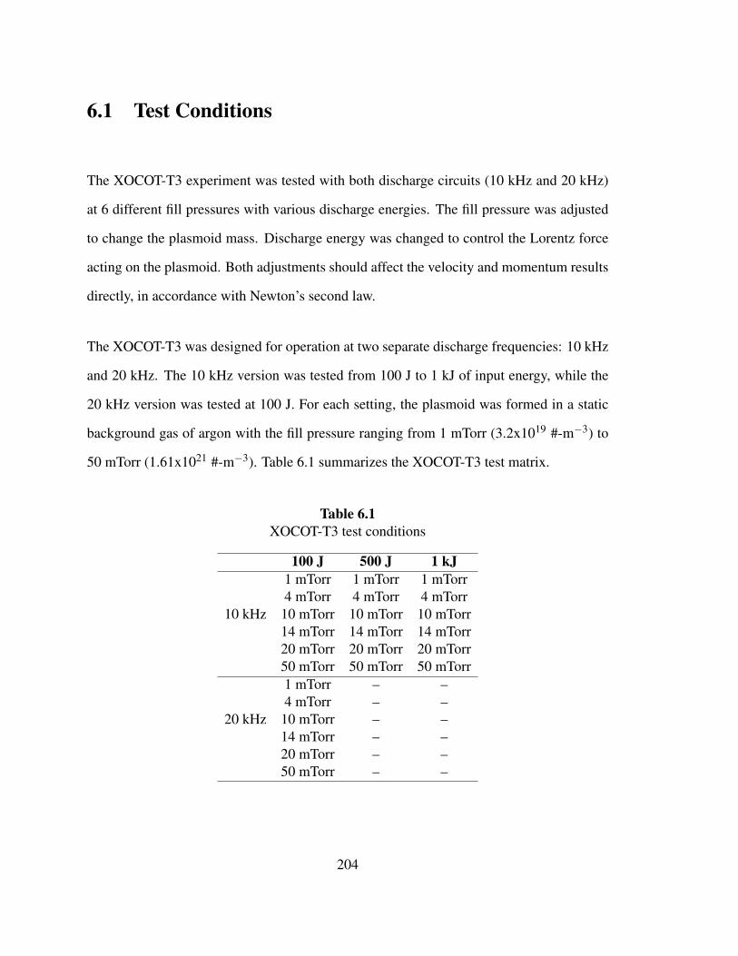
6.1 Test Conditions

The XOCOT-T3 experiment was tested with both discharge circuits (10 kHz and 20 kHz)

at 6 different fill pressures with various discharge energies. The fill pressure was adjusted

to change the plasmoid mass. Discharge energy was changed to control the Lorentz force

acting on the plasmoid. Both adjustments should affect the velocity and momentum results

directly, in accordance with Newton’s second law.

The XOCOT-T3 was designed for operation at two separate discharge frequencies: 10 kHz

and 20 kHz. The 10 kHz version was tested from 100 J to 1 kJ of input energy, while the

20 kHz version was tested at 100 J. For each setting, the plasmoid was formed in a static

background gas of argon with the fill pressure ranging from 1 mTorr (3.2x1019 #-m−3) to

50 mTorr (1.61x1021 #-m−3). Table 6.1 summarizes the XOCOT-T3 test matrix.

Table 6.1XOCOT-T3 test conditions

100 J 500 J 1 kJ1 mTorr 1 mTorr 1 mTorr4 mTorr 4 mTorr 4 mTorr

10 kHz 10 mTorr 10 mTorr 10 mTorr14 mTorr 14 mTorr 14 mTorr20 mTorr 20 mTorr 20 mTorr50 mTorr 50 mTorr 50 mTorr1 mTorr – –4 mTorr – –

20 kHz 10 mTorr – –14 mTorr – –20 mTorr – –50 mTorr – –

204

While the range of input energies for each circuit was largely chosen using the translation

predictions in Section 4.2.7, it was modified after experimental testing. The translation

predictions expected the plasmoid to translate out of the coils using 200 J to 500 J of input

energy with the 225 µF bank. However, during testing it was found that the maximum

current of 30 kA occurred at 1 kJ instead of 500 J. The coil-plasmoid coupling predicted by

the model was optimistic when compared with experimental results, leading to lower peak

currents. For this reason, the maximum energy for the 225 µF bank was elevated to 1 kJ.

The 43.5 µF bank was expected to translate a plasma starting at 600 J of initial energy from

model predictions. However, the circuit was only operated at 100 J of discharge energy to

increase the lifetime of the capacitor. The decision to decrease the minimum energy for the

43.5 µF circuit was based off of failures with the 225 µF capacitor. During high energy

testing, the 225 µF capacitor was damaged internally from the large voltage reversals at

peak current. Testing of the 43.5 µF capacitor at 600 J likely would have resulted in the

same internal damage as the current load was expected to be 30 kA with higher discharge

voltages of 5.25 kV. For this reason, the total energy for the circuit was derated. Operating

at reduced energy was unlikey to produce a translating plasmoid, however it was still

sufficient for studies of plasmoid behavior.

The range of fill pressures was selected to minimize the amount of mass the discharge

circuit would have to expel from the coils. Since plasmoid formation is likely dependent

on the initial neutral gas density, a range of parameters was selected across an order of

magnitude. The higher density fills were not expected to result in translation, but were

included in the test matrix in the event they resulted in a more stable plasmoid.

Additional settings for the XOCOT-T3 included the pre-ionization energy and the delay

between the pre-ionization bank trigger and the main bank trigger. The pre-ionization

205

energy was set to 2.4 J (12.5 kV charge voltage) following the study results detailed in

Section 6.3.2. The main bank delay was fixed to 10 µs, based on energy deposition into

the plasma and level of field reversal as seen by the inner coil probes. Further details on the

selection of the main bank timing delay are available in Section 6.3.3.

6.2 Vacuum Characterization

The XOCOT-T3 experiment was tested without plasma to determine the total coil currents

and vacuum magnetic fields as a function of discharge energy. At least 10 shots were

conducted at each nominal energy setting (consult Table 6.1) and the processed data for

each probe was averaged to compute an average waveform. The statistical spread between

shots was calculated and combined with the experimental error to determine the total error

in each result. Results for the 10 kHz circuit are provided in Section 6.2.1, and the 20 kHz

circuit results are in Section 6.2.2.

6.2.1 Vacuum Data: 10 kHz

A current waveform of the coil currents at 500 J for the 10 kHz circuit is shown in Figure

6.1. The waveform shows that the circuit rings at 9.5 kHz with 26% of the current passing

through the outer coil. The waveforms for the 100 J and 1 kJ cases are similar to the data

shown in Figure 6.1, with different amplitudes. Raw b-dot traces and processed magnetic

field data for the 500 J, 10 kHz vacuum circuit are available in Figure A.1 (in Appendix A).

The average coil currents as a function of discharge energy were compiled by averaging the

206

20x103

10

0

-10

Cur

rent

[A]

350x10-6300250200150100500

Time [s]

Outer Coil Inner Coil Total Current

500 J; 10 kHz; Vacuum23Aug2011 (#20)s: +1%, -0%

Figure 6.1: Coil currents as a function of time for the vacuum shot usingthe 10 kHz bank.

Table 6.2XOCOT-T3 vacuum coil currents as a function of energy for the 10 kHz

bank.

Energy Vcap Itotal Iouter Iinner[J] [V ] [A] [A] [A]100 J 942±4.2 V 10,575 +128 2,740 +33 7,835 +95

-72 -18 -53500 J 2108±7.6 V 24,507 +275 6,340 +73 18,167 +202

-124 -35 -891000 J 2981±10.4 V 33,736 +505 8,772 +132 24,964 +374

-376 -98 -279

current data at least 10 shots at each major energy setting (100 J, 500 J, 1 kJ). Five shots at

intermediate energy settings were also processed. The average waveform at 500 J is shown

in Figure 6.2a. The peak average coil currents as a function of discharge energy and coil

voltage follow in Figure 6.2b and Figure 6.2c. The average peak coil current at each energy

is tabulated in Table 6.2. Total errors for the average current are quite small (1%) and have

been omitted from Figure 6.2 for clarity.

Figure 6.2 shows that the current throughput is proportional to the square root of the

207

30x103

25

20

15

10

5

Cur

rent

[A]

1000800600400200

Discharge Energy [J]

10 kHzVacuum Peaks

30x103

25

20

15

10

5

Cur

rent

[A]

2500200015001000

Discharge Voltage [V]

10 kHzVacuum Peaks

20x103

10

0

-10

Cur

rent

[A]

140x10-6120100806040200

Time [s]


10 kHz; 500 JVacuum Averages

s : +1.1%, -0.5%

(a)

(b)

(c)

Figure 6.2: Vacuum coil current data for the 10 kHz bank, including (a)average waveforms for the 500 J setting, (b) peak currents versus energy,and (c) peak currents versus discharge voltage.

208

discharge energy, as expected. The spread in the data is small for the 100 J and 500 J case

(0.6%), indicating very repeatible coil currents despite manual triggering. The deviation

in the vacuum data for 1 kJ is moderately larger (1.5%), resulting from degradation of the

capacitor. The capacitor for the 10 kHz circuit was fault-limited to a voltage-reversal of

80% and 30 kA. Operating this bank at 1 kJ of input energy was at the maximum limit

for both ratings and likely damaged the capacitor. The data from these conditions is still

useable, at the expense of larger shot-to-shot deviations.

The average vacuum magnetic fields at each probe location were also calculated. The

resulting waveform averages for the magnetic field at the coil midplane at each energy

setting are shown in Figure 6.3a and b. The probe locations correspond to the outer and

inner surfaces of the annulus. The magnetic field along the discharge coil at 30.5 µs is

displayed in Figure 6.3c for the 500 J case. Magnetic fields calculated using COMSOL,

scaled from the results presented in Section 4.3, are displayed as well. The magnetic field

measured by the probes is within 10% of the fields predicted by COMSOL.

From these plots, it is readily apparent that the vacuum field inside the annulus is in a single

direction and magnitude of the magnetic field near the inner coil is only slightly lower than

near the outer coil. As expected, the vacuum magnetic field increases monotonically with

current and follows the time-behavior of the current. These plots also confirm that the axial

vacuum magnetic field is not uniform along the coil, as predicted by the electromagnetic

field simulations in Section 4.3. The non-uniformity was discovered in COMSOL to be an

artifact of the multi-turn coils and this finding is substantiated by the experimental data. The

shot-to-shot deviation in the magnetic field results is similar to the current data (1-2%). The

majority of the experimental error is due to the uncertainty in the probes’ proportionality

constants. The average vacuum traces are shown with the plasma shot data in the remaining

209

80x10-3

70

60

50

40

30

20

Bz

[ T ]

302520151050Probe Location [cm]

Outer Field Inner Field COMSOL (Outer Probes) COMSOL (Inner Probes)

Magnetic Fields(at t = 30.5 us)10 kHz; 500 J; Vac Avg

60x10-3

40

20

0

-20

-40

Bz

[ T ]

100x10-6806040200

Time [s]

Outer Midplane Field (r = 11.4 cm) (z = 15 cm)10 kHz; Vac Avg

100 J 500 J 1000 J

60x10-3

40

20

0

-20

-40

Bz

[ T ]

100x10-6806040200

Time [s]

Inner Midplane Field (r = 8.4 cm) (z = 15 cm)10 kHz; Vac Avg

100 J 500 J 1000 J

(A)

(B)

(C)

Figure 6.3: XOCOT-T3 vacuum magnetic fields as a function of dischargeenergy for the 10 kHz circuit.

210

sections of this Chapter for comparison.

The downstream magnetic fields were also measured during the vacuum shots. The data

was collected using a commerical 1-MHz differential amplifier (p/n Tektronix ADA400A),

as discussed in Section 5.2.2.8. The amplifier was required due to the poor signal-noise

resolution of the downstream probes. Several shots were also conducted without the

amplifier, connecting both probes to the oscilloscope directly with 50 Ω terminations. A

comparison of the data obtained from these techniques is shown in Figure 6.4, including

the raw signals and processed data. Figure 6.4 shows that the amplifier has difficulty

measuring the differential voltage correctly during the noise burst at t = 4 µs, leading

to an artificial sharp peak in the differential amplifier signal. This imperfection results in

errors in the calculated magnitude of the magnetic field, as it contributes a non-physical

offset. However, it does not affect the shape of the waveform several timesteps past the

glitch. Since the purpose of the downstream probes was to measure the time-history of the

translating plasma and not necessarily the magnetic field magnitude, the integrated signals

can be peak-normalized. This removes the magnitude error far from the glitch event and

retains the necessary time-history information required to resolve the plasmoid’s velocity.

While the normalization process may seem unnecessary for the relatively small errors in

the calculated vacuum field, the introduction of plasma noise into the signal worsens this

effect by over 20%.

The peak-normalized downstream magnetic field data was averaged across all available

shots to generate the typical waveform at each downstream probe location. The resulting

traces are displayed in Figure 6.5, with a sketch of the total current. It is apparent that the

downstream probes are not in phase with the current or with the upstream probes. The first

upstream probe peaks at 41.04 µs and the second probe peaks at 50.46 µs, while the current

211

-0.8

-0.6

-0.4

-0.2

0.0

0.2

0.4

0.6

0.8

B-d

ot S

igna

l [V

]

50x10-6403020100

Time [s]

60x10-3

40

20

0

-20

Diff

Am

pS

igna

l [V

]

600x10-9

500

400

300

200

100

0

Bz/

NA

[ T

/m2 ]

No Amplifier Amplifier

1000 J; 10 kHz; Vacuum25Aug2011 (#7)

26Aug2011 (#16)

Downstream Field

No Amplifier; 12 bit DAQ

ADA400A Differential Amplifier

Figure 6.4: Downstream magnetic field signals measured with and withouta differential amplfier.

212

peaks much sooner at 30.27 µs. This delay is likely due to finite magnetic-soakthrough

time of the vacuum facility; the magnetic diffusion time for a 1/4 inch plate of stainless

steel is around 70 µs. Since the downstream field is a superposition of the field from the

coils and the diffused field crossing the tank boundary, it can appear to lag from the coil

field. The difference in delay times can be explained by noting that the magnetic diffusion

time-constant is proportional to the square of the material thickness. An extra 1/8 inch of

metal would double the delay. The probes are located in different areas of the tank and

the variation in geometry may be enough to change the relative delay between the probes.

Regardless, this delay will not impact the measurements of the translating plasmoid, as

translation measurements occur local to the probe.

6.2.2 Vacuum Data: 20 kHz

The current data from the 20 kHz circuit was averaged over 10 or more vacumm shots to

calculate the mean current for each coil for the 100 J case. The resulting waveform at 100

J for the 20 kHz circuit is shown in Figure 6.6a. Peak coil currents as a function of input

energy is shown in Figure 6.6b, scaled in Figure 6.6c against discharge energy. Table 6.3

displays the peak average current for the 50 J and 100 J cases, along with the total error or

combined shot-to-shot deviation and exerimental error. Single-shot data for a 100 J test is

available in Appendix A, Figure A.2.

The current has start delay of 3 µs, resulting from a finite switch closing time. The circuit

rings through 2 complete cycles with a measured frequency of 19.5 kHz. The coil current

ratios remain identical to the 10 kHz bank, with 26% of the current passing though the outer

coil. The 100 J, 20 kHz bank produces similar current levels to the 100 J, 10 kHz bank, at

213

1.0

0.8

0.6

0.4

0.2

0.0

Bz/

Bpe

ak [

- ]

50x10-6403020100

Time [s]

Vacuum Average500 J; 10 kHz

Probe at 67.7 cm

Bz-probe Current

1.0

0.8

0.6

0.4

0.2

0.0

Bz/

Bpe

ak [

- ]

50x10-6403020100

Time [s]

Vacuum Average500 J; 10 kHz

Probe at 49.5 cm

Bz-probe Current

Figure 6.5: TOF peak-normalized vacuum magnetic field traces for the10 kHz circuit, including average magnetic field waveforms for the (A)upstream probe and the (B) downstream probe. The coil current waveformis shown for comparison.

Table 6.3XOCOT-T3 vacuum coil currents as a function of energy and charge

voltage for the 20 kHz circuit.

Energy Vcap Itotal Iouter Iinner[J] [V ] [A] [A] [A]100 J 2144 10751 +115 2816 +30 7936 +85

-41 -10 -31

214

the expense of higher coil and circuit voltages. The total experimental error for the peak

currents is very small for both energy settings and is comprised mostly of the experimental

uncertainty in the current measurement (+1%). Shot-to-shot deviations are less than 0.5%.

The magnetic fields across the entire coil length and the vacuum magnetic flux at coil

midplane were also measured at vacuum conditions, at every probe location. The average

magnetic field and flux at 100 J is shown in Figure 6.7. The midplane waveforms for the

first complete cycle near the outer coil are shown in Figure 6.7a. Figure 6.7b displays the

midplane magnetic field data near the inner coil. The magnetic fields along the coil at

peak current are shown in Figure 6.7c, with the predicted magnetic fields from COMSOL.

Uncertainty in each measurement is a combination of the statistical error between shots and

the experimental error in each measurement.

The vacuum magnetic field for the 20 kHz case is similar to the 10 kHz case, with the

magnetic field in the annulus in a single direction and following the time history of the coil

currents. Peak vacuum magnetic fields are approximately 20 mT for each midplane probe

at 100 J. From Figure 6.7c, it is apparent that the magnetic field along the coil length is not

uniform. This is an artifact of the segmented multi-turn coil design. As discussed in Section

4.3, this design increases the current density at the edges of each turn resulting in magnetic

field disturbances along the coil length. The shot-to-shot deviation in the magnetic fields

was calculated to be small, less than 0.5%. This means that the total uncertainty in each

measurement is primarily a result of the uncertainty in the measurement (5-6 %). The

COMSOL predictions agree with the experimental data within 10%, showing with more

clarity the axial distortions in the field caused by the multi-turn geometry.

The TOF vacuum magnetic field for the 20 kHz case is shown in Figure 6.8, for the probes

at z = 49.5 cm and z = 67.7 cm. The data is shown for the vacuum averages at 100 J,

215

10x103

8

6

4

2

Cur

rent

[A]

10080604020

Discharge Energy [J]

20 kHzVacuum Peaks

10x103

5

0

-5

Cur

rent

[A]

100x10-6806040200

Time [s]


20 kHz; 100 JVacuum Averages

s : +1.1% -0.4%

10x103

8

6

4

2

Cur

rent

[A]

200018001600140012001000800

Discharge Voltage [V]

20 kHzVacuum Peaks

(a)

(b)

(c)

Figure 6.6: Vacuum coil currents for the 20 kHz circuit, including (A) thetime history of the coil currents, (B) peak coil currents compared to inputenergy, and (C) peak currents versus discharge voltage. Uncertainty for allmeasurements is 1%.

216

50x10-3

40

30

20

10

0

Bz

[ T ]

302520151050

Axial Probe Position [cm]

Magnetic Fields (at t = 16.3 us)20 kHz; 100 J; Vac Avg

Data (r = 11.4 cm) Data (r = 8.4 cm) COMSOL (r = 11.4 cm) COMSOL (r = 8.4 cm)

20x10-3

10

0

-10

Bz [ T

]

50x10-6403020100

Time [s]

Midplane Outer Field r = 11.4 cm; z = 15 cm20 kHz; 100 J; Vac Avg

20x10-3

10

0

-10

Bz [ T

]

50x10-6403020100

Time [s]

Midplane Inner Field r = 8.4 cm; z = 15 cm20 kHz; 100 J; Vac Avg

(A)

(B)

(C)

Figure 6.7: Vacuum magnetic fields for the 20 kHz circuit, includingaverage magnetic field waveforms at the coil midplane on the outer wall(A), the inner wall (B), and the average magnetic field at peak coil currentalong the coil length (C).

217

160x10-9

140

120

100

80

60

40

20

0

Bz/

NA

[ T

/m2]

25x10-620151050

Time [s]

B-field Coil Current

Downstream Field (z = 67.7 cm)20 kHz; 100 JVacuum Average

700x10-9

600

500

400

300

200

100

0

Bz/

NA

[T/m

2]

25x10-620151050

Time [s]

Downstream Field (z = 49.5 cm)20 kHz; 100 JVacuum Average

B-field Coil Current

(A)

(B)

Figure 6.8: TOF vacuum magnetic fields for the 20 kHz circuit, includingaverage magnetic field waveforms for the (A) upstream probe and the (B)downstream probe. The coil current waveform is also shown.

scaled against each probe’s proportionality constant NA. The statistical spread in the TOF

magnetic field data is comparable to the data from inside the coils, with a 0.4% deviation in

the upstream TOF probe and a 1.7% spread for the downstream TOF probe. The magnetic

field measured by both TOF probes is significantly delayed from the coil currents. The

upstream TOF probe lags the coil current by 1.8 µs and the downstream TOF probe lags by

3.6 µs. As mentioned in Section 6.2.1, this is likely an artifact of the finite magnetic field

diffusion through the stainless steel tank boundary.

218

6.3 Plasmoid Formation Characterization

The first step towards plasmoid translation is to create a fully reversed plasmoid inside the

annulus. Plasmoid formation in the XOCOT-T3 experiment was tested by discharging the

coils into a gas fill to create the magnetized AFRC toroid. Results demonstrating plasmoid

formation are presented in Section 6.3.1.

Plasmoid formation can be enhanced by optimizing the pre-ionization settings, including

the pre-ionization input energy and the time interval between the PI and the main bank

trigger. Optimization of the PI pulse is discussed in Section 6.3.2. Timing results are

discussed in Section 6.3.3.

The XOCOT-T3 is a pulsed experiment and the data can vary from shot-to-shot.

Repeatibility results are presented in Section 6.3.4 to establish that while small deviations

between shots occur, the overall behavior of the XOCOT-T3 and AFRC experiment are

highly repeatable.

6.3.1 Formation Results

The XOCOT-T3 experiment was tested at 10 kHz and 20 kHz, across the range of energies

and fill pressures shown in Table 6.1. At each setting, AFRC plasmoids were formed

between the coils. A single data set from the 10 kHz circuit and the 20 kHz circuit are

presented in this subsection to discuss the key pieces of evidence indicating plasmoid

formation. Full results for each discharge energy at all background pressure are presented

219

in Section 6.4.

Coil current, midplane magnetic field, and photometer data is shown for a single shot

with the 10 kHz circuit in Figure 6.9 and with the 20 kHz circuit in Figure 6.10. A full

time-history is shown, through several discharge cycles. Vacuum traces are provided for

comparison. Raw data is included in Appendix A, Figures A.3 and A.4.

Evidence of plasmoid formation requires a magnetic field reversal on the inner wall and

inductive coupling in the coil currents. This indicates that current in the plasma is large

enough to reverse the magnetic field from the coils and to magnetically couple with the

coils. While some discharge circuits are constructed to only produce a single plasmoid,

the ringing of the XOCOT-T3 circuit produces several plasmoids through the duration of

the discharge. This occurs at each dI/dt event, where a reversed magnetic field is seen

on the inner wall along with a change in coil currents. This also corresponds to a peak

in light output measured from the downstream photometer, signifiying an intense burst of

ionization. In the data shown in Figure 6.9 and 6.10, it can be observed that 5 AFRCs

are formed with diminishing intensities. The actual number of AFRCs formed during any

given discharge is dependant on the input energy, pressure, and circuit frequency.

The data also shows that plasmoid formation sinks energy from the main bank circuit. This

is most readily seen in the current data for the 20 kHz circuit (top graph of Figure 6.10).

The vacuum circuit rings through 4 complete cycles, dropping to 2.5 during a plasma shot.

This behavior is expected and is a qualitative indication of the energy absorbed during

the formation process. Ideally the bulk of the energy should be deposited in the first

quarter cycle and should be carried downstream by the ejected plasmoid. Inefficiencies

in the circuit and a lossy or ineffective translation will leave some remaining energy in the

formation chamber for the subsequent pulses.

220

40x10-3

20

0

-20

-40

Bz

[T]

350x10-6300250200150100500

Time [s]

Midplane Fields500 J; 10 kHz; 4 mTorr

23Aug2012 (#25, #20)

2.5

2.0

1.5

1.0

0.5

0.0

[-]

350x10-6300250200150100500

Time [s]

Photometer Output500 J; 10 kHz; 4 mTorr

23Aug2012 (#25, #20)

20x103

10

0

-10

Cur

rent

[A]

350x10-6300250200150100500

Time [s]

Plasma Shot (#25)

Vacuum Shot (#20)

Total

Inner

Outer

Coil Currents500 J; 10 kHz; 4 mTorr

23Aug2012 (#25, #20)

(a)

(b)

(c)

Figure 6.9: Typical plasmoid formation data for the 10 kHz circuit at 500J with a 4 mTorr fill. A full time-history is shown with vacuum and plasmadata for the main bank current, midplane magnetic fields, and light outputmeasured by a photometer.

221

30x10-3

20

10

0

-10

-20

-30

Bz

[ T ]

300x10-6250200150100500

Time [s]

Midplane Fields100 J; 20 kHz; 4 mTorr

22May2012

Outer Field (#07) Inner Field (#07) Vacuum Field (#13)

10x103

5

0

-5

Cur

rent

[A]

300x10-6250200150100500

Time [s]

Plasma Shot (#07) Vacuum Shot (#13)

Total Current100 J; 20 kHz; 4 mTorr

22May2012

Total Inner

Outer

1.6

1.2

0.8

0.4

0.0

[-]

300x10-6250200150100500

Time [s]

Light Output100 J; 20 kHz; 4 mTorr

22May2012

(a)

(b)

(c)

Figure 6.10: Typical plasmoid formation data for the 20 kHz circuit at 100J with a 4 mTorr fill. A full time-history is shown with vacuum and plasmadata for the (A) main bank current, (B), midplane magnetic fields, and (C)light output measured by a photometer.

222

It is interesting to note that while the higher frequency bank is operated at 1/5 of the energy

of the 10 kHz bank, plasmoid formation occurs on the same timescale. The field reversal in

the 20 kHz, 100 J pulse occurs within 1.1 µs after the switch closes; the 500 J, 10 kHz pulse

reverses somewhere between 800 ns and 1.4 µs. Both circuits have nearly identical voltages

so these findings are somewhat expected. It is well known that coil voltage (proportional to

dI/dt) is responsible for ionization in pulsed devices. Therefore, one would expect matching

coil voltages would produce similar results. Additionally, the plasmoid formation sinks

much more energy in the 20 kHz bank than the 10 kHz bank. This finding is also not

surprising; ionization improves with increased frequency. The 20 kHz bank should be

more effective at ionization than the 10 kHz bank for matched coil voltages. While a full

study on the effects of frequency and coil voltage on AFRC formation are beyond the scope

of this research, these findings provide an interesting design note for future experiments.

The remaining data in this research will study only the first AFRC plasmoid. The focus of

this experiment is plasmoid translation, which is expected to happen with the first AFRC

when the fields and currents are at their peaks. Additionally, the secondary AFRCs are

often nonrepeatable as they depend on the leftovers from the first AFRC which may change

drastically from shot-to-shot.

6.3.2 Pre-Ionization

The pre-ionization circuit was first tested without a plasma from 5 kV to 15 kV to determine

the current waveform of the circuit. A typical trace using a 12 kV charge voltage is shown

by the dashed line in the top graph of Figure 6.11. The current monitor output as a function

of charge voltage is shown in the second graph of Figure 6.11. The PI circuit rang at

223

1.1 MHz through 18 cycles before the energy was dissipated into ohmic heat. The upper

limit of the current monitor used to measure the signal was 4 MHz. This presented two

problems: the rated sensitivity for the measured waveform was invalid and the full risetime

of the signal could not be accurately captured. For these reason, the current monitor data

was left unscaled.

Following the vacuum tests, the pre-ionization circuit was tested using a 4 mTorr gas fill

with a 5 kV to 15 kV charge voltage. A typical trace using a 12 kV charge voltage is

shown by the solid line in the top graph of Figure 6.11. The current monitor waveform

for the plasma trace shows that the plasma absorbs a significant portion of energy from the

discharge circuit, indicated by a severe damping. The PI plasma also seems to inductively

couple to the PI circuit, noting that the frequency increases from the vacuum case. The

vacuum and plasma shot current monitor data were integrated across their full ranges to

estimate the energy absorbed by the plasma. The results are shown as a function of charge

voltage in the bottom graph of Figure 6.11. The results were also scaled against the charge

voltage to represent the fraction of energy absorbed by the plasma. Uncertainty estimates

are from repeated tests at 12 kV, yielding a 10% spread in the data.

The results in Figure 6.11 show that the PI is ineffective at charge voltages below 8 kV,

when less than 10% of the energy is absorbed by the plasma. The pre-ionzation is most

effective at 15 kV when the plasma absorbs 1.1 J of energy from the circuit. Assuming an

ionization cost of 100 eV/ion, 1.1 J of energy is enough to ionize 6.86x1016 #-m−3 of the

fill gas. This is still several orders of magnitude below the neutral fill density (1.2x1020

#-m−3), indicating the PI only weakly ionizes the initial gas fill.

The PI circuit was designed with an absolute upper limit of 15 kV. While this seems to

produce the highest fraction of ions, operating consistently at 15 kV severely derates the

224

0.30

0.25

0.20

0.15

0.10

0.05

0.00

Epl

asm

a/E

char

ge [-

]

14121086PI Charge Voltage [V]

4 mTorr FillC = 33 pF

1.2

1.0

0.8

0.6

0.4

0.2

0.0

Ene

rgy

into

Pla

sma

[J]

14121086PI Charge Voltage [V]

4 mTorr FillC = 33 pF

-5

0

5C

urre

nt M

onito

r S

igna

l [V

]

15x10-61050

Time [s]

Plasma Shot Vacuum Shot

PI Characterization12 kV; 2.38 J

10

8

6

4

Cur

rent

Mon

itor

Sig

nal P

eak

[V]

14121086PI Charge Voltage [kV]

y = 0.762x-1.1954

PI CharacterizationVacuum Shots

C = 33 pF

Figure 6.11: Pre-ionization study data, including current waveforms forthe vacuum and plasma case, coil current compared to charge voltage, andenergy absorbed by the plasma versus charge energy.

225

lifetime of the capacitors and switch. A compromise was made to operate the circuit at a

12 kV, where the energy absorbed by the plasma was about 0.6 J and the resulting plasma

density was estimated at 3.82x1016 #-m−3. This is only half of the density produced at 15

kV, but it is still roughly the same ionization fraction (ions compared to initial neutral fill).

6.3.3 Main Bank Timing

The optimal timing between the pre-ionization and the main bank circuit trigger of the

experiment was tested by adjusting the time delay between the pre-ionization trigger and

the main bank trigger. The delay times tested include 10 µs, 20 µs, 30 µs, 50 µs, 100 µs,

150 µs, and 200 µs. This was done for all nominal discharge energies using a 4 mTorr

fill pressure. The energy absorbed by the plasma was calculated for each shot, using the

methods described in Section 5.3.4. The magnetic fields at the midplane were also analyzed

and compared for each delay interval. The results from the 10 kHz circuit and 20 kHz

circuit tests are discussed in Sections 6.3.3.1 and 6.3.3.2, respectively. From these results,

it was determined that a delay of 10 µs was sufficient for all test conditions. The results

also show that timing was not critical for the 20 kHz discharges or the 10 kHz discharges

at 500 J and above.

6.3.3.1 Timing: 10 kHz

The timing study for the 10 kHz circuit was conducted at 100 J, 500 J, and 1000 J using a 4

mTorr gas fill. Midplane magentic fields were examined from each shot to check for field

reversal and the coil currents were recorded to estimate the energy absorbed by the plasma.

226

Since the time-period of interest involves only the first 1/4 cycle, the energy absorbed

during the first 1/2 cycle was calculated. The first 1/2 cycle was chosen for comparison as it

is easier to calculate than the first 1/4 cycle when energy is stored in unknown inductances.

The energy absorbed by the plasma during the first 1/2 cycle was calculated for each data

set, using Equation 5.46. Circuit resistance is a required input for this equation and was

calculated by solving Equation 5.47, using the circuit current from the vacuum traces. The

calculated resistances and associated errors are shown in Table 6.4. The timing results for

each energy setting are shown in Figures 6.12, 6.13, and 6.14. Uncertainty estimates for

the energy calculations include calculated error as well as statistical error from repeated

shots with a 10 µs delay.

Table 6.4XOCOT-T3 calculated circuit resitances for the 10 kHz circuit.

Energy Rcircuit σtotal σsdev σmeas[J] [mΩ] [mΩ] [mΩ] [mΩ]100 J 14.0 1.3 0.6 1.2500 J 11.0 1.3 0.4 1.21000 J 12.6 1.2 0.7 1.7

The timing results for the 10 kHz circuit indicate that a 10 µs delay is acceptable for all

cases. At 100 J, the energy absorbed into the plasma is slightly higher than delays of 100

µs or more. The field reversal also is highest with a 10 µ delay. Larger discharge energy

settings (500 J and 1 kJ) results show that the timing delay is not essential to the onset of

reversal or to energy absorbtion. This suggests that the PI is more critical for low energy

than high energy settings. Testing without the PI at high energy demonstrated that it was

still possible to form an AFRC, though it did not appear until after the first 1/4 cycle and it

created weaker magnetic fields. AFRCs at 100 J and 10 kHz failed to form without the PI.

The uncertainty in the energy absorbed into the plasma is substantial. All significant errors

227

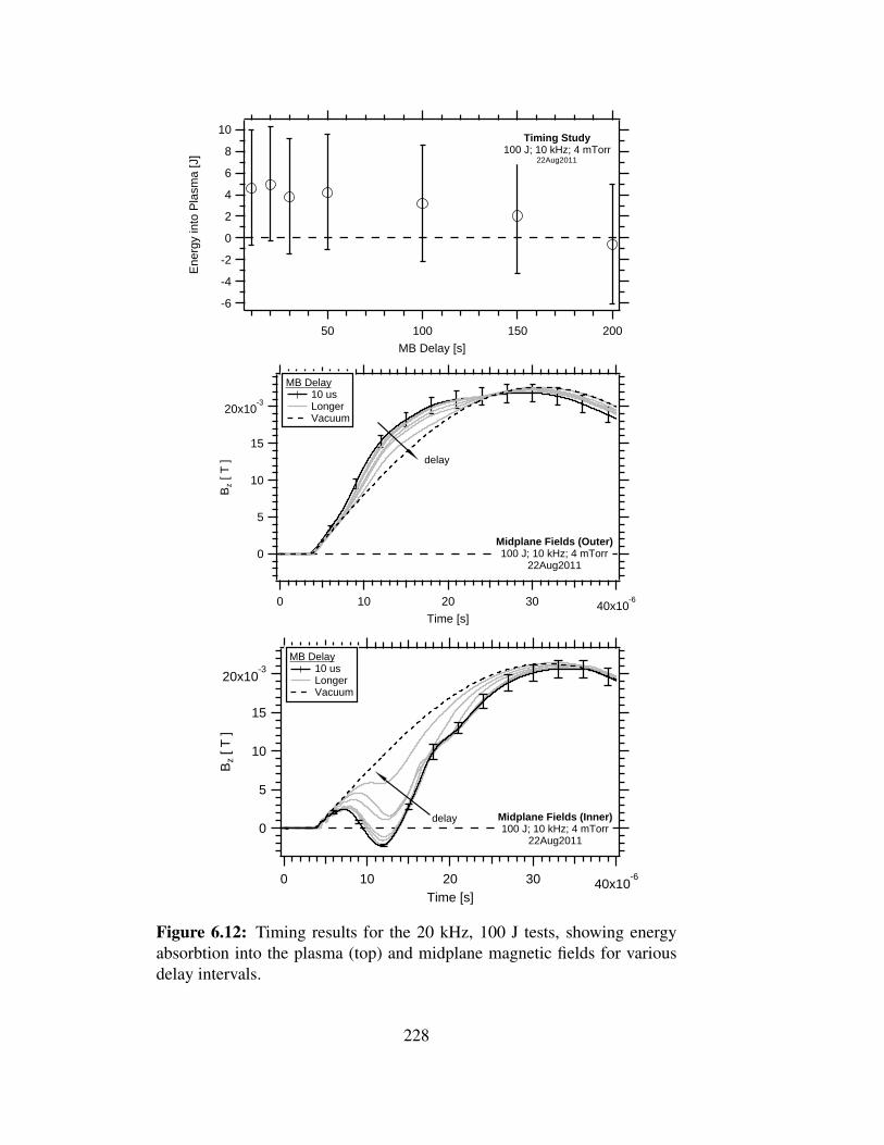
20x10-3

15

10

5

0

Bz

[ T ]

40x10-63020100

Time [s]

delay

Midplane Fields (Outer)100 J; 10 kHz; 4 mTorr

22Aug2011

MB Delay 10 us Longer Vacuum

20x10-3

15

10

5

0

Bz

[ T ]

40x10-63020100

Time [s]

delay Midplane Fields (Inner)100 J; 10 kHz; 4 mTorr

22Aug2011


10

8

6

4

2

0

-2

-4

-6

Ene

rgy

into

Pla

sma

[J]

20015010050

MB Delay [s]

Timing Study100 J; 10 kHz; 4 mTorr

22Aug2011

Figure 6.12: Timing results for the 20 kHz, 100 J tests, showing energyabsorbtion into the plasma (top) and midplane magnetic fields for variousdelay intervals.

228

40x10-3

20

0

-20

Bz

[ T ]

40x10-63020100

Time [s]

delay Midplane Fields (Inner)500 J; 10 kHz; 4 mTorr

23Aug2011


50x10-3

40

30

20

10

0

Bz

[ T ]

40x10-63020100

Time [s]

delay


26Aug2011


120

100

80

60

40

20

0

Ene

rgy

into

Pla

sma

[J]

20015010050

MB Delay [s]

Timing Study 500 J; 10 kHz; 4 mTorr

23Aug2011


229

60x10-3

40

20

0

-20

-40

Bz

[ T ]

40x10-63020100

Time [s]

delayMidplane Fields (Inner)1000 J; 10 kHz; 4 mTorr

24Aug2011


70x10-3

60

50

40

30

20

10

0

Bz

[ T ]

40x10-63020100

Time [s]

delay


24Aug2011


200

150

100

50

Ene

rgy

into

Pla

sma

[J]

200150100500

MB Delay [s]

Timing Study 1000 J; 10 kHz; 4 mTorr

24Aug2011


230

in this calculation point back to the 1% error in the current measurement. While this is a

fairly low uncertainty, the current measurement is used extenstively through the calculation

for Eplasma and is often squared and integrated which increases the error substantially. It

also appears in the calculation for the circuit resitance, contributing heavily to its 10% error.

The standard devation in absorbed energy among repeated shots only accounts for a small

portion of the error. In the 10 kHz, 100 J circuit, the standard devation between shots is

1.13 J.

6.3.3.2 Timing: 20 kHz

The timing study results for the 20 kHz circuit at 100 J are shown in Figure 6.15. The

midplane magnetic fields are displayed along with the energy absorbed by the plasma

during the first 1/2 cycle of the discharge. Uncertainty intervals show the combined error

due to the measurement and repeated data sets with a 10 µs delay.

The energy absorbed by the plasma does not change with respect to the main bank timing

delay. The energy absorbed for a 10 µs delay is 23.6 J ± 5.4 joules. Timing seems to

have a minor effect on the magnetic fields as well. Slightly stronger magnetic fields and a

somewhat faster reversal are seen for the 10 µs case compared to the longer delays. These

results indicate that timing of the main bank trigger is not vital to plasmoid formation, up

to 200 µs, and operating with a shorter delay yields only minor improvements. Using these

results as a guide, the timing delay between the pre-ionization trigger and main bank trigger

was set to 10 µs for the 20 kHz, 100 J tests.

231

20x10-3

10

0

-10

-20

Bz

[ T ]

20x10-6151050

Time [s]

delay

Midplane Fields (Inner)100 J; 20 kHz; 4 mTorr

23May2012

30x10-3

25

20

15

10

5

0

Bz

[ T ]

20x10-6151050

Time [s]

delay

MB Delay [us]10 Longer


23May2012

40

35

30

25

20

15

10

Ene

rgy

into

Pla

sma

[J]

200150100500

MB Delay [us]

Timing Study100 J; 20 kHz; 4 mTorr

23May2012


6.3.4 Repeatibility

The XOCOT-T3 experiment was tested repeatedly at single test condition for the 10 kHz

circuit and the 20 kHz circuit to establish shot-to-shot repeatibility. This was done for the

plasma discharges at one fill pressure (4 mTorr) with discharge energies of 100 J, 500 J,

and 1000 J for the 10 kHz circuit. The 20 kHz repeatibility study was performed at 100 J

and 4 mTorr. Repeatibility was established by averaging the data from each probe for 10

232

or more shots at each discharge energy.

6.3.4.1 Repeatibility: 10 kHz

The repeatibility study for the 10 kHz circuit was completed for each energy setting,

including 100 J, 500 J, and 1 kJ discharges. All tests were conducted using a 4 mTorr

background fill. At least 10 shots at each energy setting were recorded. The average

waveform for each diagnostic was computed along with the standard deviations from the

average. Figures 6.16, 6.18, and 6.20 show the results for the coil currents and upstream

magnetic fields. Figures 6.17, 6.19, 6.21 display the data for the downstream magnetic

fields and plasma probes. Average waveforms are shown, along with the corresponding

history of standard deviation. Error bars are a combination of the statistical deviation and

the measurement uncertainty.

Overall the XOCOT-T3 at 10 kHz creates fairly repeatible plasma discharges from the

reference of the magnetic probes. The first couple microseconds of the discharge show the

most deviation, as the plasma currents forms and ionizes the neutral fill. After this period,

the deviation on most probes drops to less than 10%. The coil currents and outer coil fields

show the highest repeatibility, with no more than 4% devation between shots.

The inner field probes are the best indicator of repeatable plasmoid behavior, as these are

the most direct measurement of plasmoid current. Using the inner probes as a guide, it can

be inferred that the high energy cases (500 J and 1 kJ) produce more repeatable plasmoids

than the low energy case. The deviation on the inner probe data for the high energy cases

does not exceed 10%. The plasmoid behavior is somewhat less predictable at 100 J, due

to low energy content. This is apparent in the longer reversal time and low reversed field.

233

1.2x10-3

1.0

0.8

0.6

0.4

0.2

0.0

Sta

ndar

d D

evia

tion

[ T ]

40x10-63020100

Time [s]

z = 5 cm z = 10 cm z = 15 cm

120

100

80

60

40

20

0

Sta

ndar

d D

evia

tion

[A]

40x10-63020100

Time [s]

Total Outer Inner

10x103

8

6

4

2

0

Cur

rent

[A]

40x10-63020100

Time [s]

10 shot average100 J; 10 kHz; 4mTorr

Coil Currents

25x10-3

20

15

10

5

0

Bz

[ T ]

40x10-63020100

Time [s]

Outer Fields

300x10-6

250

200

150

100

50

0

Sta

ndar

d D

evia

tion

[ T ]

40x10-63020100

Time [s]

z = 5 cm z = 10 cm z = 15 cm z = 25 cm

20x10-3

15

10

5

0

Bz

[ T ]

40x10-63020100

Time [s]

Inner Fields

Figure 6.16: Repeatibility study data for the 10 kHz circuit at 100 J,including coil currents and upstream magnetic field measurements. Thestandard deviation of repeated data sets for each diagnostics is shown on theright.

However, the repeated data sets even in the 100 J case do not differ in by more than 15-20%.

The downstream TOF probes show more shot-to-shot variation than the upstream probes.

The probe at z = 49.5 cm produces repeatable waveforms, with deviations between shots of

less than 6%. The probe at z = 67.7 cm is more susceptible to variation, showing deviations

234

1.0

0.8

0.6

0.4

0.2

0.0

Bz/

Bpe

ak [

- ]

50x10-6403020100

Time [s]

Probe at 49.5 cm

10 Shot Average100 J; 10 kHz; 4 mTorr

1.0

0.8

0.6

0.4

0.2

0.0

Bz/

Bpe

ak [

- ]

50x10-6403020100

Time [s]

Probe at 67.7 cm

70x10-3

60

50

40

30

20

10

0S

tand

ard

Dev

iatio

n [ -

]50x10

-6403020100

Time [s]

14x10-3

12

10

8

6

4

2Sta

ndar

d D

evia

tion

[ - ]

50x10-6403020100

Time [s]

Figure 6.17: Downstream results from the repeatibility study for the 10 kHzat 100 J, including the measurements recorded from the TOF probes and thestandard deviations among repeated shots.

of 15% at 100 J, 8% at 500 J, and 20% at 1 kJ. The magnetic fields at this probe location

are quite small so the variation is somewhat expected.

6.3.4.2 Repeatibility: 20 kHz

The repeatibility data for the 20 kHz circuit was conducted in 2 parts. First, 32 current

and magnetic field data sets were collected at 100 J of discharge energy and 4 mTorr of

background pressure. Downstream plasma probe data was collected during a second set

of testing using 10 shots of the same repeated conditions. The average waveform for each

diagnostic was computed along with the standard deviations of the each waveform from

235

5x10-3

4

3

2

1

0

Sta

ndar

d D

evia

tion

[ T ]

40x10-63020100

Time [s]

z = 5 cm z = 10 cm z = 15 cm

300

250

200

150

100

50

0

Sta

ndar

d D

evia

tion

[A]

40x10-63020100

Time [s]

Total Outer Inner

20x103

15

10

5

0

Cur

rent

[A]

40x10-63020100

Time [s]


Coil Currents

50x10-3

40

30

20

10

0

Bz

[ T ]

40x10-63020100

Time [s]

Outer Fields

1.0x10-3

0.8

0.6

0.4

0.2

0.0

Sta

ndar

d D

evia

tion

[ T ]

40x10-63020100

Time [s]

z = 5 cm z = 10 cm z = 15 cm z = 25 cm

40x10-3

20

0

-20

Bz

[ T ]

40x10-63020100

Time [s]

Inner Fields


the average. Figure 6.22 shows the results for the coil currents and upstream magnetic

fields. Figure 6.23 displays the data for the downstream magnetic fields and plasma probes.

Average waveforms are shown, along with the corresponding history of standard deviation.

Error bars are a combination of the statistical deviation and the measurement uncertainty.

236

1.0

0.8

0.6

0.4

0.2

0.0

Bz/

Bpe

ak [

- ]

50x10-6403020100

Time [s]

Probe at 49.5 cm

7 Shot Average500 J; 10 kHz; 4 mTorr

1.0

0.8

0.6

0.4

0.2

0.0

Bz/

Bpe

ak [

- ]

50x10-6403020100

Time [s]

Probe at 67.7 cm

12x10-3

10

8

6

4

2

0

Sta

ndar

d D

evia

tion

[-]

50x10-6403020100

Time [s]

50x10-3

40

30

20

10Sta

ndar

d D

evia

tion

[-]

50x10-6403020100

Time [s]


The repeatibility study data demonstrates that the XOCOT-T3 experiment operating at 100

J and 20 kHz produces repeatible data at each probe location. The current measurements

deviate between shots by less than 2% and the outer magnetic field measurements differ

by around 2.5%. The inner magnetic fields are somewhat more sporadic during the initial

ionization phase, differing by 12% during the first several µs, but leveling off to around 2%

around the local minimum. The downstream magnetic field data is similarily repeatable,

with only a few percent difference between shots. The plasma flux data is less repeatible

than the magnetic field measurements, differing between shots by 10-15 %.

237

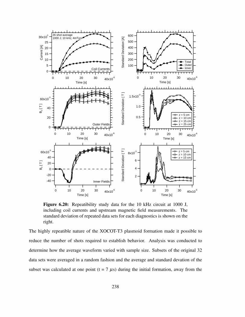
8x10-3

6

4

2

Sta

ndar

d D

evia

tion

[ T ]

40x10-63020100

Time [s]

z = 5 cm z = 10 cm z = 15 cm

600

500

400

300

200

100Sta

ndar

d D

evia

tion

[A]

40x10-63020100

Time [s]

Total Outer Inner

30x103

25

20

15

10

5

0

Cur

rent

[A]

40x10-63020100

Time [s]


Coil Currents

60x10-3

40

20

0

Bz

[ T ]

40x10-63020100

Time [s]

Outer Fields

1.5x10-3

1.0

0.5

Sta

ndar

d D

evia

tion

[ T ]

40x10-63020100

Time [s]

z = 5 cm z = 10 cm z = 15 cm z = 25 cm

60x10-3

40

20

0

-20

-40

Bz

[ T ]

40x10-63020100

Time [s]

Inner Fields


The highly repeatible nature of the XOCOT-T3 plasmoid formation made it possible to

reduce the number of shots required to establish behavior. Analysis was conducted to

determine how the average waveform varied with sample size. Subsets of the original 32

data sets were averaged in a random fashion and the average and standard devation of the

subset was calculated at one point (t = 7 µs) during the initial formation, away from the

238

0.10

0.08

0.06

0.04

0.02S

tand

ard

Dev

atio

n [ -

]

40x10-63020100

Time [s]

12x10-3

10

8

6

4

2

Sta

ndar

d D

evat

ion

[ - ]

40x10-63020100

Time [s]

1.0

0.8

0.6

0.4

0.2

0.0

Bz/

Bpe

ak [

- ]

50x10-6403020100

Time [s]

Probe at 67.7 cm

1.0

0.8

0.6

0.4

0.2

0.0

Bz/

Bpe

ak [

- ]

50x10-6403020100

Time [s]

Probe at 49.5 cm

18 shot average1000 J; 10 kHz; 4 mTorr

Figure 6.21: Downstream results from the repeatibility study for the 10 kHzat 1000 J, including the measurements recorded from the TOF probes andthe standard deviations among repeated shots.

startup transients. The results are displayed in Figure 6.24.

The results from this study shows that the averaged subset of current and midplane fields

fall within 2% of the set average, regardless of sample size. This suggests that only a

few shots are necessary to provide a characteristic of plasmoid behavior, assuming this

trend does not change appreciably with pressure and energy. A few shots at each setting

may not produce a statistically sound data set, they will be sufficient to determine under

what conditions the plasmoid translates. A larger sample set can then be collected at the

conditions where translation is evident. A reduced sample size for initial testing is also

warranted for ensuring the entire operating matrix can be explored before the discharge

239

500x10-6

400

300

200

100

0Sta

ndar

d D

evia

tion

[ T ]

20x10-6151050

Time [s]

z = 5 cm z = 10 cm z = 15 cm z = 28 cm

60

50

40

30

20

10

0

Sta

ndar

d D

evia

tion

[A]

20x10-6151050

Time [s]


10x103

8

6

4

2

0

Cur

rent

[A]

20x10-6151050

Time [s]

32 shot Average20 kHz; 100 J; 4 mTorr

Coil Currents

30x10-3

25

20

15

10

5

0

Bz

[ T ]

20x10-6151050

Time [s]

Outer Fields

1.0x10-3

0.8

0.6

0.4

0.2

0.0

Sta

ndar

d D

evia

tion

[ T ]

20x10-6151050

Time [s]

z = 5 cm z = 10 cm z = 15 cm

-20x10-3

-15

-10

-5

0

5

10

Bz

[ T ]

20x10-6151050

Time [s]

Inner Fields


circuit wears out. This was especially important in the XOCOT-T3 experiment, in which

the discharge capacitors were subject to severe wear during testing.

240

5x10-9

4

3

2

Sta

ndar

d D

evat

ion

[T/m

2]

30x10-62520151050

Time [s]

5x10-9

4

3

2

1

Sta

ndar

d D

evat

ion

[T/m

2]

30x10-62520151050

Time [s]

600x10-9

500

400

300

200

100

0B

z/N

A [

T/m

2 ]

30x10-62520151050

Time [s]

32 shot Average20 kHz; 100 J; 4 mTorr

Probe at 49.5 cm

160x10-9

140

120

100

80

60

40

20

0

Bz/

NA

[ T

/m2 ]

30x10-62520151050

Time [s]

Probe at 67.7 cm

Single Shot Average

1000

800

600

400

200

0

Ion

Flu

x [A

/m2 ]

20x10-6151050

Time [s]

Ion Flux Probes13 Shot Average

30

25

20

15

10

5Sta

ndar

d D

evat

ion

[A/m

2]

20x10-6151050

Time [s]

Near (49.5 cm) Far (67.7 cm)


6.4 Translation Study Data

The XOCOT-T3 experiment was tested in both circuit configurations at 6 different fill

pressures and various discharge energies. The fill pressure was adjusted to change the

plasmoid mass. Discharge energy was changed to control the Lorentz force acting on the

plasmoid. Both adjustments should affect the velocity and momentum results directly, in

241

-16.8x10-3

-16.6

-16.4

-16.2

-16.0

Bz

[ T ]

30252015105Samples [-]

+1%

-1%

Average

Average Inner Field at 7 us100J; 20 kHz; 4 mTorr

20.6x10-3

20.5

20.4

20.3

20.2

20.1

Bz

[ T ]

30252015105Samples [-]

+1%

-1%

Average

Average Outer Field at 7 us100 J; 20 kHz; 4 mTorr

6260

6240

6220

6200

Cur

rent

[A]

30252015105Samples [-]

+0.5%

-0.5%

Average

Average Current at 7 us100 J; 20 kHz; 4 mTorr

Figure 6.24: Average currents and magnetic fields at 7 µs compared tonumber of samples included in average.

242

accordance with Newton’s second law and the translation predictions in Chapter 4.

The pressure and energy setttings chosen for this research are presented in Table 6.1. The

fill pressure range varied from 1 mTorr to 50 mTorr, including 1 mTorr, 4 mTorr, 10 mTorr,

14 mTorr, 20 mTorr, and 50 mTorr. The energy for the 10 kHz circuit also covered a full

magnitude from 100 J to 1 kJ, with a stop at 500 J. The 20 kHz circuit was tested at each

fill pressure for the 100 J energy setting. Low energy testing of the 20 kHz circuit was

conducted at 50 J with 4 mTorr of background pressure. All tests were conducted using

an Argon fill, a 10 µs main bank trigger delay and the PI configuration outlined in Section

6.3.2.

The data collected from these experiments include magnetic field signatures, coil currents,

and downstream plasma flux measurements. Magnetic field data is collected from

three primary locations, including upstream measurements on the outer wall, upstream

measurements on the inner wall, and downstream measurements in the translation region.

Plasma flux probes were recorded at the same axial locations as the downstream magnetic

probe, spaced 180 degrees away.

The data from the 10 kHz circuit configuration is presented in Section 6.4.1 and the 20 kHz

data is presented in Section 6.4.2. Plasmoid translation measurements using these data sets

are discussed in Chapter 7.

6.4.1 Translation Data: 10 kHz

The XOCOT-T3 was tested with the 10 kHz circuit at 100 J, 500 J, and 1 kJ using a static

backfill of Argon. The coil currents and upstream magnetic field at all tested pressures at

243

100 J is displayed in Figures 6.25 - 6.27. This data was averaged from 3 to 6 shots at each

background pressure. Figure 6.25 displays the current data and the magnetic fields (inner

and outer) at the coil midplane (z = 15 cm). Figure 6.25 shows the magnetic field data

upstream of the midplane (at z = 5 cm and z = 10 cm) and at the far end of the coil (z =

25 cm). Downstream magnetic field signatures on the TOF probes are displayed in Figure

6.27. Confidence intervals for all traces is a combination of the experimental uncertainty

in each diagnostic and the statistical spread in the data among shots.

The 100 J, 10 kHz circuit produces a plasma current at all pressures, except for 50 mTorr.

This is noted by a reversed field on the inner wall, an excluded field on the outer probes,

and inductive coupling in the circuit current. The strength of the plasma current, evident

primarily by the inner field data, is strongly dependant on fill pressure. Low fill pressures

create a stronger current than the high pressure cases. The midplane inner field data (see

Figure 6.25) shows that the axial field crosses through zero only for the low pressure cases

of 1 mTorr and 4 mTorr. The field at higher pressures (other than 50 mTorr) attempts to

reverse, but the current is not strong enough to fully oppose the outer coil field. This trend is

also seen in the outer probes, where the excluded field increases with decreasing pressure.

The dependancy of plasma current on fill pressure can be understood by noting that plasma

resistance is proportional to density.

While the low pressure cases create a reversed field, the reversal is late and short lived. At

midplane, the field reversal takes 6 µs to develop and stops growing 2 µs later. The field

also fails to fully reverse, which would create the same field strengths on the inner coil

as the outer coil. This suggests that the AFRC in the 100 J, 10 kHz circuit is weak and

unlikely to translate.

The late reversal of the 100 J data makes it apparent that the field reversal begins at the

244

10x103

8

6

4

2

0

Cur

rent

[A]

40x10-63020100

Time [s]

1 mTorr 4 mTorr 10 mTorr 14 mTorr 20 mTorr 50 mTorr Vacuum

Total Current100 J; 10 kHz

22Aug2012

20x10-3

15

10

5

0

Bz

[ T ]

40x10-63020100

Time [s]

Inner Field at z = 15 cm

20x10-3

15

10

5

0

Bz

[ T ]

40x10-63020100

Time [s]

Outer Field at z = 15 cm

Figure 6.25: Total current and midplane magnetic field data at various fillpressures for the 100 J, 10 kHz circuit. Vacuum traces are shown at eachdiagnostic by dotted lines.

245

20x10-3

15

10

5

0

Bz

[ T ]

40x10-63020100

Time [s]


20x10-3

15

10

5

0

Bz

[ T ]

40x10-63020100

Time [s]



20x10-3

15

10

5

0

-5

Bz

[ T ]

40x10-63020100

Time [s]


20x10-3

15

10

5

0

Bz

[ T ]

40x10-63020100

Time [s]


25x10-3

20

15

10

5

0

Bz

[ T ]

40x10-63020100

Time [s]


Figure 6.26: Magnetic field data at various fill pressures and locations forthe 100 J, 10 kHz circuit. Vacuum traces are shown at each diagnostic bydotted lines.

246

1.0

0.8

0.6

0.4

0.2

0.0

Bz/

Bpe

ak [

- ]

50x10-6403020100

Time [s]

Probe at z = 67.7 cm

1.0

0.8

0.6

0.4

0.2

0.0

Bz/

Bpe

ak [

- ]

50x10-6403020100

Time [s]



Pressure Effects100 J; 10 kHz

22Aug2011

Figure 6.27: Peak normalized downstream magnetic field data at variousfill pressures for the 100 J, 10 kHz circuit. Vacuum traces are shown at eachdiagnostic by dotted lines.

247

narrow end of the coil initially. Reversal on the probes at z = 5 cm and z = 10 cm appears

before reversal on the midplane probe. This trend is seen in other conical FRC geometries

as well.

The downstream magnetic field signatures for the 100 J, 10 kHz data show no signficant

change from their vacuum pattern. The downstream signatures also show little noticeable

changes with pressure. The probe signatures measured closer to the coils (at z = 49.5

cm) appear to deflect very slightly with decreasing pressure, but this is likely due to the

changing field inside the coils.

The current and magnetic field signatures for the 500 J, 10 kHz circuit are shown in

Figures 6.28 - 6.30. Downstream plasma flux data is presented in Figure 6.30 for 1

mTorr, 4 mTorr, and 50 mTorr only. The 500 J data was collected from at least 3 shots

at each background pressure. Confidence intervals for all traces is a combination of the

experimental uncertainty in each diagnostic and the statistical spread in the data among

shots.

The large dI/dt in the 500 J circuit compared to the 100 J circuit produces a much stronger

plasma current at all pressures, even at 50 mTorr. The plasma current is only weakly

dependant on plasma pressure up to 20 mTorr, suggesting a fully ionized current with low

resistance from neutral collisions. The reversal also happens much faster in the 500 J case

than the 100 J case, within 600 ns of the switch closing. The 50 mTorr case shows a delayed

reversal of 3.5 µs.

Despite the fast development of the plasma current, the reversal only lasts 9.3 µs. This is

true for all pressures. Following the loss of reversal, the excluded field signature disappears

on the outer probes. The field returns to the vacuum cases. The disappearance of the

248

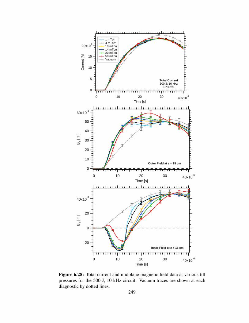
20x103

15

10

5

0

Cur

rent

[A]

40x10-63020100

Time [s]


Total Current500 J; 10 kHz

23Aug2011

40x10-3

20

0

-20

Bz

[ T ]

40x10-63020100

Time [s]


60x10-3

50

40

30

20

10

0

Bz

[ T ]

40x10-63020100

Time [s]



249

inductive load either indicates plasmoid termination or a translating plasmoid. This topic

will be discussed in more detail in Chapter 7.

The downstream magnetic field signatures for the 500 J, 10 kHz data show a slight change

when compared to their vacuum counterpart. The first probe shows a convex feature and the

second probe shows a concave nature. Neither feature changes drastically with pressure.

The downstream plasma flux data for 500 J is shown in the bottom graphs of Figure 6.30.

The plasma flux peaks on both probes at 12 µs for the low pressure case and at 17 µs for

the 50 mTorr case. The 1 mTorr fill creates a higher ion flux than the lower pressures, with

over 6 kA/m2 collected by the probe. This trend will be discussed in more detail in Chapter

7.

The current and magnetic field signatures for the 1 kJ, 10 kHz circuit are shown in Figures

6.31 - 6.33. The data was collected from at least 3 shots for the 1 mTorr through 14 mTorr

case. A circuit fault prevented more than 2 shots at 20 mTorr and 50 mTorr. Confidence

intervals for all traces is a combination of the experimental uncertainty in each diagnostic

and the statistical spread in the data among shots.

The results from the 1 kJ tests are similar in behavior to the 500 J circuit. The field reversal

happens quickly, within 200 ns of switch closing. Little change in field signatures is seen

with increasing pressure, except for the 50 mTorr fill. The reversal lasts 8.7 µs, 600 ns

shorter than the 500 J case. After reversal is lost, the field returns to the vacuum state. As

mentioned in the 500 J discussion, the disappearance of the inductive load either indicates

plasmoid termination or a translating plasmoid and will be discussed in more detail in

Chapter 7.

The downstream magnetic field signatures for the 1 kJ, 10 kHz data show a substantial

250

change from the vacuum traces. The first probe shows a flat profile in the magnetic field

rise at 12 µs, lasting 4 µs. This feature is most apparent in the low pressure data. The

severe noise in the probe at z = 67.7 cm makes it difficult to determine the corresponding

feature, but it appears to follow the same behavior. The comparison of these features with

the upstream probes will be analyzed in Chapter 7.

251

40x10-3

20

0

-20

Bz

[ T ]

40x10-63020100

Time [s]


40x10-3

20

0

-20

Bz

[ T ]

40x10-63020100

Time [s]


50x10-3

40

30

20

10

0

Bz

[ T ]

40x10-63020100

Time [s]


60x10-3

50

40

30

20

10

0

Bz

[ T ]

40x10-63020100

Time [s]


50x10-3

40

30

20

10

0

Bz

[ T ]

40x10-63020100

Time [s]



252

1.0

0.8

0.6

0.4

0.2

0.0

Bz/

Bpe

ak [

- ]

50x10-6403020100

Time [s]


TOF Array Results500 J; 10 kHz

23Aug2011

1.0

0.8

0.6

0.4

0.2

0.0

Bz/

Bpe

ak [

- ]

50x10-6403020100

Time [s]



1500

1000

500

0

Ion

Flu

x [A

/m2 ]

50x10-6403020100

Time [s]


6000

5000

4000

3000

2000

1000

0

Ion

Flu

x [A

/m2 ]

50x10-6403020100

Time [s]


Figure 6.30: TOF probe data at various fill pressures for the 500 J, 10kHz circuit, including peak normalized downstream magnetic field data andplasma flux measurements. Vacuum traces are shown at each diagnostic bydotted lines. 253

30x103

25

20

15

10

5

0

Cur

rent

[A]

40x10-63020100

Time [s]


Pressure Study1000 J; 10 kHz

24Aug2011

Total Current

60x10-3

40

20

0

-20

-40

Bz

[ T ]

40x10-63020100

Time [s]

Inner Field (z = 15 cm)

80x10-3

60

40

20

0

Bz

[ T ]

40x10-63020100

Time [s]

Outer Field (z = 15 cm)


254

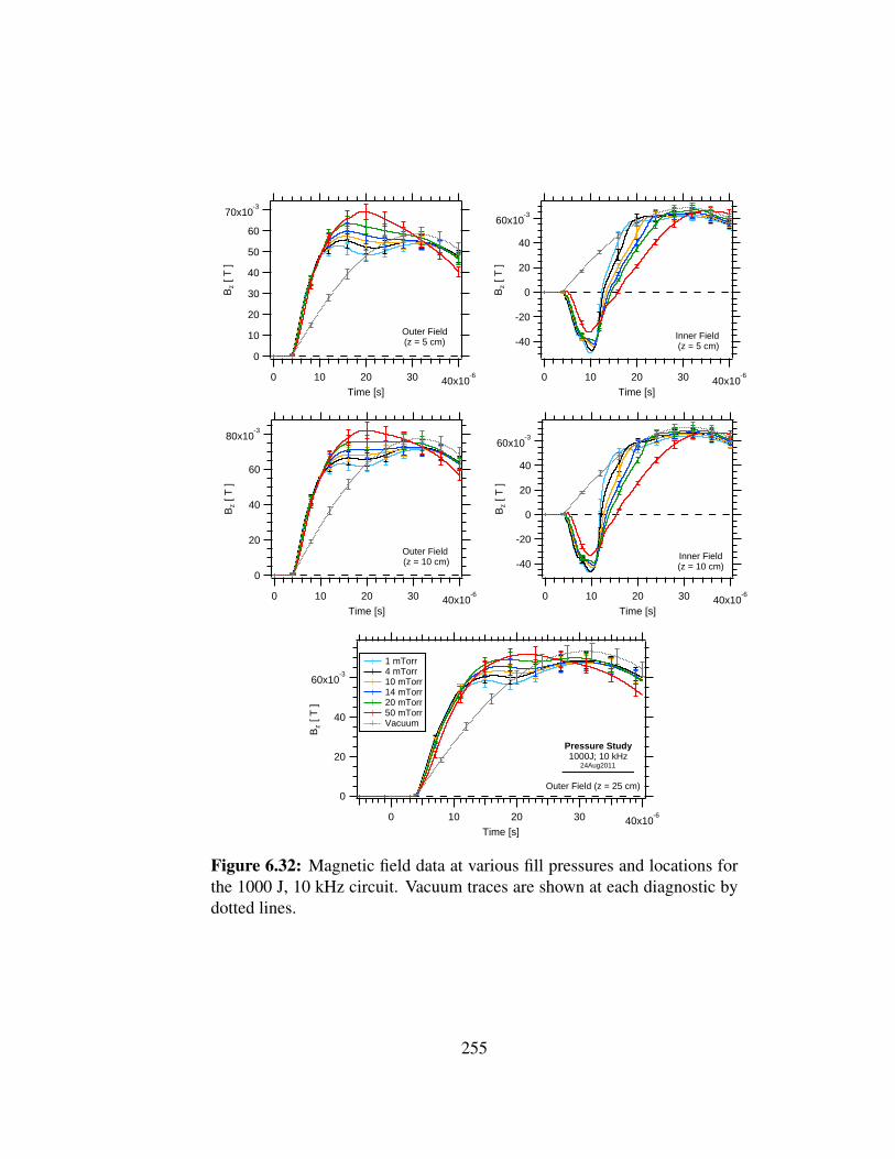
60x10-3

40

20

0

-20

-40

Bz

[ T ]

40x10-63020100

Time [s]

Inner Field(z = 10 cm)

60x10-3

40

20

0

-20

-40

Bz

[ T ]

40x10-63020100

Time [s]

Inner Field (z = 5 cm)

60x10-3

40

20

0

Bz

[ T ]

40x10-63020100

Time [s]



Pressure Study1000J; 10 kHz

24Aug2011

80x10-3

60

40

20

0

Bz

[ T ]

40x10-63020100

Time [s]


70x10-3

60

50

40

30

20

10

0

Bz

[ T ]

40x10-63020100

Time [s]

Outer Field(z = 5 cm)


255

1.0

0.8

0.6

0.4

0.2

0.0

-0.2

Bz/

Bpe

ak [

- ]

50x10-6403020100

Time [s]


1.0

0.8

0.6

0.4

0.2

0.0

Bz/

Bpe

ak [

- ]

50x10-6403020100

Time [s]


Pressure Study1000J; 10 kHz

24Aug2011

1 mTorr 4 mTorr10 mTorr14 mTorr 20 mTorr 50 mTorr Vacuum

Figure 6.33: Peak normalized downstream magnetic field data at variousfill pressures for the 1000 J, 10 kHz circuit. Vacuum traces are shown ateach diagnostic by dotted lines.

256

6.4.2 Translation Data: 20 kHz

The current and upstream magnetic field at all tested pressures for the 20 kHz circuit at

100 J is shown in Figures 6.34 and 6.35. This data was averaged from 5 shots at each

background pressure. Figure 6.34 displays the current data and the magnetic fields (inner

and outer) at the coil midplane (z = 15 cm). Figure 6.35 shows the magnetic field data

upstream of the midplane (at z = 5 cm and z = 10 cm) and at the far end of the coil (z = 25

cm). Confidence intervals for all traces is a combination of the experimental uncertainty

in each diagnostic and the statistical spread in the data among shots. The statistical spread

in the data is quite small (2-3%) with the uncertainty in magnetic field proportionality

constants comprising the largest source of error.

The effect of background pressure on plasmoid formation is especially evident in the inner

magnetic field data. With the exception of a fill pressure at 50 mTorr, the change in current

and outer magnetic field between pressures is only a few percent. The inner magnetic field

data shows more distinct plasmoid behavior at different pressures. At low pressures, higher

magnetic fields are generated on the inner wall signaling larger plasma currents. This trend

is somewhat expected; low fill pressures create less resistance for plasmoid current since

the current carriers have fewer interactions with the neutral gas. These results suggest that

plasmoid translation is more likely at low fill pressures (1-4 mTorr) due to the stronger

Lorentz force resulting from higher plasmoid currents and lower plasmoid mass.

The inner field for the 100 J, 10 kHz circuit reverses 1 µs after switch closing for the 4

mTorr case. The reversal lasts 10.3 µs, which is 1 µs longer than the 500 J and 1 kJ cases

for the 10 kHz circuit.

257

10x103

8

6

4

2

0

Cur

rent

[A]

20x10-6151050

Time [s]



23May2012

Total Current

20x10-3

10

0

-10

-20

Bz

[ T ]

20x10-6151050

Time [s]


30x10-3

25

20

15

10

5

0

Bz

[ T ]

20x10-6151050

Time [s]


Figure 6.34: Total current and magnetic field data at various fill pressuresfor the 100 J, 20 kHz circuit. Vacuum traces are shown at each diagnosticby dotted lines.

258

20x10-3

10

0

-10

-20

Bz

[ T ]

20x10-6151050

Time [s]


30x10-3

25

20

15

10

5

0

Bz

[ T ]

20x10-6151050

Time [s]


20x10-3

10

0

-10

-20

Bz

[ T ]

20x10-6151050

Time [s]


25x10-3

20

15

10

5

0

Bz

[ T ]

20x10-6151050

Time [s]


25x10-3

20

15

10

5

0

Bz

[ T ]

20x10-6151050

Time [s]


Figure 6.35: Magnetic field data at various fill pressures for the 100 J, 20kHz circuit. Vacuum traces are shown for each diagnostic by a dotted line.

A full set of downstream data was collected for the 100 J, 20 kHz study, shown in Figure

6.36. The downstream magnetic field data did not have to be normalized for amplifier

glitches, though a correction for the probes’ proportionality constants were not made. The

259

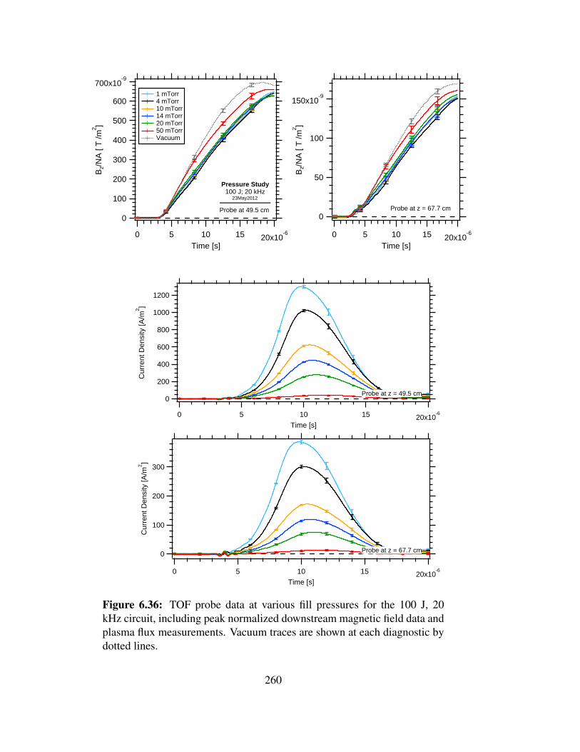
300

200

100

0

Cur

rent

Den

sity

[A/m

2]

20x10-6151050

Time [s]


1200

1000

800

600

400

200

0

Cur

rent

Den

sity

[A/m

2]

20x10-6151050

Time [s]


150x10-9

100

50

0

Bz/

NA

[ T

/m2 ]

20x10-6151050

Time [s]


700x10-9

600

500

400

300

200

100

0

Bz/

NA

[ T

/m2 ]

20x10-6151050

Time [s]



23May2012

Probe at 49.5 cm

Figure 6.36: TOF probe data at various fill pressures for the 100 J, 20kHz circuit, including peak normalized downstream magnetic field data andplasma flux measurements. Vacuum traces are shown at each diagnostic bydotted lines.

260

plasma flux at each location was also collected for each pressure. The magnetic field data

does not change appreciably with pressure, with the exception of the 50 mTorr case. The

plasma shot data for both probes show a lower peak field than the vacuum data. However,

no additional features are apparent deviating significantly from the vacuum traces.

The downstream plasma flux data shows that the current density measured by the probe

decreases with pressure, topping 1 kA/m2 with a 4 mTorr fill. The peaks also seem to lag

with increasing pressure. The plasma flux profiles follow a bell-shaped behavior without

any strong peaks visible. While this is more indicative of a thermal plasma spilling out

of the device than a translating plasmoid; full evidence of translation will be discussed in

Chapter 7.

261

Chapter 7

Translation Results

This chapter discusses the translation results from the experimental data presented in

Chapter 6. Section 7.1 describes the data reduction applied to the data to estimate plasmoid

translation velocities. Section 7.2 presents the plasmoid velocity results, demonstrating that

the plasmoid failed to translate from the formation region for all test conditions. Section 7.3

discusses possible causes for the failed translation, including a limit in inductive current,

insufficient conductivity, and gross instabilities.

7.1 Translation Data Reduction

The experimental data presented in Chapter 6 is sufficient to resolve the plasmoid’s velocity

at each operating point. The external probes are used as the first time-of-flight (TOF) array,

with the downstream probes forming the secondary array. Axial staggered signatures on

both arrays are a clear indicator of a translating magnetized plasmoid. Data from plasma

263

probes can be used to confirm that the magnetized structure contains a dense plasma. Small

switching delays between data sets can cause errors in velocity measurements. Velocity

data was collected from single shots when possible.

A single shot of data from the 20 kHz, 100 J circuit is shown in Figure 7.1. Uncertainty

estimates are omitted from this graph for clarity. This figure shows that each probe

recorded a different magnitude of field. The velocity measurements from this data

required comparing propagating features in axially-separated probes and the different field

magnitudes made it difficult to pick out features among different probes. The data was

peak-normalized to remove the differences in field magnitudes, making it easier to compare

features and trends in all probes.

The first step in processing the data for this research was to establish that the plasmoid

traveled out of the coils with a detectable velocity. Once the velocity was established,

plasma probe sweeps were to be used to estimate momentum and translation efficiency.

The results presented in Section 7.2 show that the plasmoid failed to translate under all

tested conditions. This means it was not necessary to estimate the plasmoid momentum

and translation efficiency.

7.2 Velocity Results

Plasmoid velocity can be measured by comparing when certain features appear at

different axial locations along the velocity vector. Several examples of this have been

provided previously in this dissertation. Characteristic magnetic probe signatures using

electromagnetic modeling for a constant-velocity plasmoid were computed in Section 4.3.

264

30x10-3

20

10

0

Bz

[ T ]

25x10-620151050

Time [s]

30x10-3

20

10

0

-10

Bz

[ T ]

600x10-9

500

400

300

200

100

0

Bz/

NA

[ T

/m2 ]

400

300

200

100

0

Ion

Flu

x [A

/m2 ]

z = 5 cm z = 10 cm z = 15 cm z = 25 cm z = 49.5 cm z = 67.7 cm Vacuum

Upstream-Outer Bz Probes

Upstream-Inner Bz Probes

TOF Bz Probes

TOF Plasma Probes100 J; 20 kHz; 4 mTorr

23May2012 (#18)

Figure 7.1: Full data set from a single shot at 100 J with the 20 kHz bankand a 4 mTorr gas fill.

265

Data from a TOF plasma probe array from a similar RMF-FRC translation experiment were

presented in Figure 5.39. The trends from these illustrations are discussed in detail here

so that this information can be used to decipher the translation data from the XOCOT-T3

experiments.

Magnetic field modeling in Section 4.3 was used to calculate the magnetic field from

a translating plasmoid. The results in Figure 4.28 show characteristic magnetic field

signatures for a plasmoid traveling at 50 km/s through the coils. The signatures were

measured using probes spaced 5 cm apart inside the coils and by probes placed in the

path of the plasmoid downstream of the coils. A peak field was recorded on the coil probes

as the trailing edge of the plasmoid passed by. The time delay between these peak fields

was 1 µs, corresponding to a velocity of 50 km/s. The peaks on the outer probes and inner

probes for the same axial location occurred at the same time, as well. The downstream

probes recorded a flat signature as the plasmoid traveled over it, lasting 5 µs for a plasmoid

25 cm in length.

The constant velocity in the magnetic field model was used for numerical stability, though

in reality the plasmoid should accelerate through the coil. This is apparent in the calculated

trajectory from the annular electromagnetic model shown in Figure 4.18. The plasmoid’s

acceleration through the coils will produce different delays than the uniform delay shown

in Figure 4.28, with shorter delays occurring with increasing distance from the beginning

of the coil. The peak velocity is not expected until the plasmoid is 10 cm outside the

coil, according to the trajectory shown in Figure 4.18. This means that TOF probes should

record a velocity comparable to the terminal velocity, but the coil probes should record a

lower velocity. The peak velocities for 500 J, 10 kHz circuit are expected to be 160 km/s,

according the predictions in Figure 4.19. This means that the time delay between features

266

on probes spaced 5 cm apart inside the coil should be greater than 300 ns. The time delay

between the probe located at z = 25 cm and the first probe in the TOF array is expected to

be around 1.25 µs and the delay between probes in the downstream TOF array should be 1

µs apart.

The plasma flux measurements appearing on the downstream plasma probes in a TOF array

appear as sharp peaks, spaced by a delay inversely proportional to the plasmoid velocity.

This was seen in an RMF-FRC translation experiment [3], with the data reproduced in

Figure 5.39. The first sharp peak in each signal corresponds to the arrival of the leading

edge of the plasmoid. The dense plasma front traveling at high velocity has only a brief

encounter with the probe, which is why it appears as a sharp peak. Additional signal follows

the initial peak as the remainder of the plasmoid passes by the probe.

Magnetic field data from single shot at each pressure and energy is presented in this Section

for the 10 kHz and 20 kHz discharge circuits. Plasma flux measurements are included,

when available. This data was used to estimate the plasmoid velocity. Each trace was

peak-normalized for the first quarter cycle. Error bars are omitted for clarity.

7.2.1 Velocity Results: 10 kHz

The results for the 10 kHz circuit at 100 J are presented in Figures 7.2 through Figure 7.7. A

single shot from each pressure and energy setting is shown, with all traces peak normalized

to show trends in the data.

The translation results at 100 J for each pressure do not show a translating plasmoid. The

switch closes at 4 µs and the inner field begins to reverse several µs later. If the reversal

267

1.0

0.8

0.6

0.4

0.2

0.0

Bz/

Bpe

ak [-

]

50x10-6403020100

Time [s]

1.0

0.8

0.6

0.4

0.2

0.0

Bz/

Bpe

ak [-

]

1.0

0.8

0.6

0.4

0.2

0.0

Bz/

Bpe

ak [-

] z = 5 cm z = 10 cm z = 15 cm z = 25 cm z = 49.5 cm z = 67.7 cm Vacuum



TOF Bz Probes100 J; 10 kHz; 1 mTorr

23Aug2012 (#05)

Figure 7.2: Translation results for the 10 kHz circuit at 100 J, with a 1mTorr fill pressure.

268

1.0

0.8

0.6

0.4

0.2

0.0

Bz/

Bpe

ak [-

]

50x10-6403020100

Time [s]

1.0

0.8

0.6

0.4

0.2

0.0

Bz/

Bpe

ak [-

]

1.0

0.8

0.6

0.4

0.2

0.0

Bz/

Bpe

ak [-

]





22Aug2012 (#26)


269

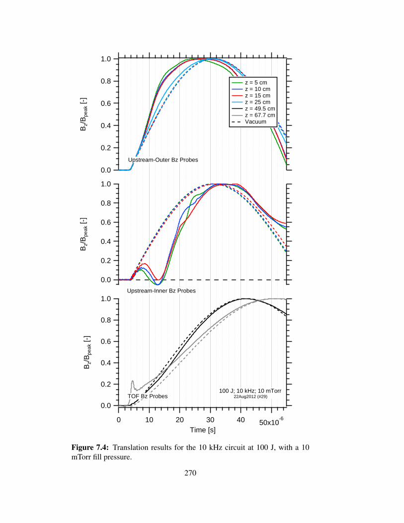
1.0

0.8

0.6

0.4

0.2

0.0

Bz/

Bpe

ak [-

]

50x10-6403020100

Time [s]

1.0

0.8

0.6

0.4

0.2

0.0

Bz/

Bpe

ak [-

]

1.0

0.8

0.6

0.4

0.2

0.0

Bz/

Bpe

ak [-





22Aug2012 (#29)


270

1.0

0.8

0.6

0.4

0.2

0.0

Bz/

Bpe

ak [-

]

50x10-6403020100

Time [s]

1.0

0.8

0.6

0.4

0.2

0.0

Bz/

Bpe

ak [-

]

1.0

0.8

0.6

0.4

0.2

0.0

Bz/

Bpe

ak [-

]





22Aug2012 (#31)


271

1.0

0.8

0.6

0.4

0.2

0.0

Bz/

Bpe

ak [-

]

50x10-6403020100

Time [s]

1.0

0.8

0.6

0.4

0.2

0.0

Bz/

Bpe

ak [-

]

1.0

0.8

0.6

0.4

0.2

0.0

Bz/

Bpe

ak [-





23Aug2012 (#10)


272

1.0

0.8

0.6

0.4

0.2

0.0

Bz/

Bpe

ak [-

]

50x10-6403020100

Time [s]

1.0

0.8

0.6

0.4

0.2

0.0

Bz/

Bpe

ak [-

]

1.0

0.8

0.6

0.4

0.2

0.0

Bz/

Bpe

ak [-

]





23Aug2012 (#18)


273

happens at all it is short lived, lasting at most 2 µs before changing back toward the vacuum

field. The peak reversed field on the inner probes does not correspond to any distinct peak

on the outer probe. The outer probes do not show any staggered features along their array;

they rise and fall in unison. Additionally, the downstream probes show no magnetic field

structure passing by. It’s clear from all these observations that even when a reversed field

plasmoid is formed, it never leaves the coils. The short-lived and relatively small reversal

suggests that the energy content of the plasmoid is too low form a sufficient current for the

Lorentz force.

The results for the 10 kHz circuit at 500 J are presented in Figures 7.8 through Figure

7.13. A single shot from each pressure and energy setting is shown, with all traces peak

normalized to show trends in the data. Data from the downstream plasma flux probes is

presented for the 1 mTorr, 4 mTorr, and 50 mTorr data sets.

The translation results at 500 J show that while the field reversal happens very quickly,

the plasmoid does not appear to translate from the coils. The field reversal peaks 6-7 µs

after the switch closes, but the upstream inner probe (z = 5 cm) peaks after the probes at

z = 10 cm and z = 15 cm. It also crosses through B = 0 a full µs after the downstream

probes. Furthermore, as the reversal peaks the field on the outer coil probes continue to

climb and don’t reach a peak until 5 µs later. The inner and outer probes at the same axial

location should show the same behavior in time with a translating plasmoid. The probe

at z = 25 cm reaches its peak 1 µs after the midplane probe and while this may also be

a translation indicator corresponding to the expected velocity (150 km/s), the downstream

magnetic field probes peak don’t agree. They appear to have an inflection several µs before

the outer probes peak and concurrent with the zero-crossing of the inner coil field.

The plasma flux measurements support this conclusion. The plasma flux (shown in Figures

274

1.0

0.8

0.6

0.4

0.2

0.0

Bz/

Bpe

ak [-

]

50x10-6403020100

Time [s]

0.8

0.4

0.0

-0.4

Bz/

Bpe

ak [-

]

1.0

0.8

0.6

0.4

0.2

0.0

Bz/

Bpe

ak [-

]

1.0

0.8

0.6

0.4

0.2

0.0

J ion

/Jpe

ak [-

]




TOF Bz Probes

500 J; 10 kHz; 1 mTorr 23Aug2011 (#43)21Mar2012 (#11)

TOF Ion Flux Probes


275

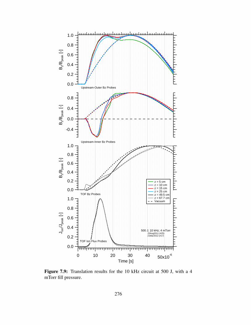
1.0

0.8

0.6

0.4

0.2

0.0

Bz/

Bpe

ak [-

]

50x10-6403020100

Time [s]

0.8

0.4

0.0

-0.4

Bz/

Bpe

ak [-

]

1.0

0.8

0.6

0.4

0.2

0.0

Bz/

Bpe

ak [-

]

1.0

0.8

0.6

0.4

0.2

0.0

J ion

/Jpe

ak [-

]




TOF Bz Probes


TOF Ion Flux Probes


276

1.0

0.8

0.6

0.4

0.2

0.0

Bz/

Bpe

ak [-

]

50x10-6403020100

Time [s]

1.0

0.8

0.6

0.4

0.2

0.0

-0.2

-0.4

-0.6

Bz/

Bpe

ak [-

]

1.0

0.8

0.6

0.4

0.2

0.0

Bz/

Bpe

ak [-

]




TOF Bz Probes 500 J; 10 kHz; 10 mTorr 23Aug2011 (#39)


277

1.0

0.8

0.6

0.4

0.2

0.0

Bz/

Bpe

ak [-

]

50x10-6403020100

Time [s]

1.0

0.8

0.6

0.4

0.2

0.0

-0.2

-0.4

-0.6

Bz/

Bpe

ak [-

]

1.0

0.8

0.6

0.4

0.2

0.0

Bz/

Bpe

ak [-

]




TOF Bz Probes 500 J; 10 kHz; 14 mTorr 23Aug2011 (#47)


278

1.0

0.8

0.6

0.4

0.2

0.0

Bz/

Bpe

ak [-

]

50x10-6403020100

Time [s]

1.0

0.8

0.6

0.4

0.2

0.0

-0.2

-0.4

Bz/

Bpe

ak [-

]

1.0

0.8

0.6

0.4

0.2

0.0

J ion

/Jpe

ak [-

]





23Aug2011 (#49)


279

1.0

0.8

0.6

0.4

0.2

0.0

-0.2

Bz/

Bpe

ak [-

]

50x10-6403020100

Time [s]

1.0

0.8

0.6

0.4

0.2

0.0

-0.2

Bz/

Bpe

ak [-

]

1.0

0.8

0.6

0.4

0.2

0.0

Bz/

Bpe

ak [-

]

1.0

0.8

0.6

0.4

0.2

0.0

J ion

/Jpe

ak [-

]




TOF Bz Probes


TOF Ion Flux Probes


280

7.8, 7.9, and 7.13) appears on both probes simultaenously. The peak flux to the probe

happens 2 µs after the inner fields peak and 1-2 µs before the outer coil probes peak. Even

if the plasmoid was traveling at a velocity around 160 km/s, a very sharp set of peaks spaced

1 µs apart should appear on the plasma probes. Assuming the plasma is 25 cm in length,

the signal should last on each probe for only 1.6 µs. The signature appears instead to be a

very elongated structure with FWHM of 8 µs. The source of the plasma on the downstream

probes is discussed in Section 7.2.3. The overwhelming verdict for the 500 J data is that

the plasmoid does not translate from the coils.

The results from the high energy tests at 1 kJ with the 10 kHz circuit are shown in Figures

7.14 through Figure 7.19. A single shot from each pressure and energy setting is presented,

with the data peak normalized for velocity measurements.

The results for the 1 kJ circuit are similar in nature to the 500 J circuit, with no clear

sign of translation seen in the magnetic field data. The field reverses quickly and peaks

6-7 µs after the switch closes. The point of maximum field reversal corresponds to an

insignificant inflection in the outer probe data; the full inflection occurs 5 µs later. The

probe at the far end of the coil reaches a peak after the probes further upstream and by

a single µs. However, the downstream magnetic probes show a strong inflection about 2

µs after the inner probes peak and 1 µs before the outer coil probes peak. The inflection

appears to be slightly staggered between the TOF probes, by a delay of less than 1 µs. This

would agree with the expected velocity of 200 km/s, but because it appears before the outer

coil probes peak it is likely just an artifact. As was also shown by the 500 J data, the 1 kJ

circuit fails to translate the plasmoid from the coils for each fill pressure tested.

281

1.0

0.8

0.6

0.4

0.2

0.0

Bz/

Bpe

ak [-

]

50x10-6403020100

Time [s]

1.0

0.5

0.0

-0.5

Bz/

Bpe

ak [-

]

1.0

0.8

0.6

0.4

0.2

0.0

Bz/

Bpe

ak [-




TOF Bz Probes

1000 J; 10 kHz; 1 mTorr 24Aug2011 (#48)


282

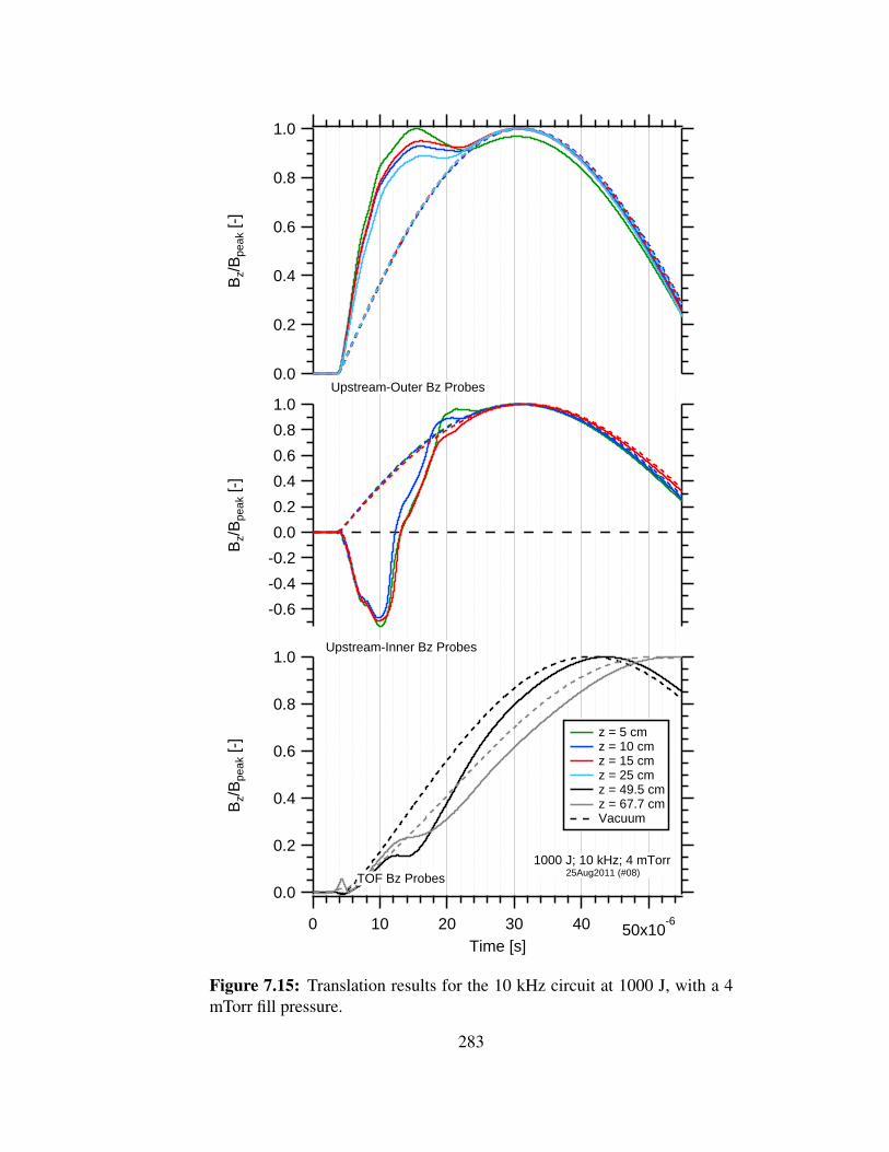
1.0

0.8

0.6

0.4

0.2

0.0

Bz/

Bpe

ak [-

]

50x10-6403020100

Time [s]

1.0

0.8

0.6

0.4

0.2

0.0

-0.2

-0.4

-0.6

Bz/

Bpe

ak [-

]

1.0

0.8

0.6

0.4

0.2

0.0

Bz/

Bpe

ak [-





25Aug2011 (#08)


283

1.0

0.8

0.6

0.4

0.2

0.0

Bz/

Bpe

ak [-

]

50x10-6403020100

Time [s]

1.0

0.8

0.6

0.4

0.2

0.0

-0.2

-0.4

-0.6

Bz/

Bpe

ak [-

]

1.0

0.8

0.6

0.4

0.2

0.0

Bz/

Bpe

ak [-




TOF Bz Probes

1000 J; 10 kHz; 10 mTorr 25Aug2011 (#17)


284

1.0

0.8

0.6

0.4

0.2

0.0

Bz/

Bpe

ak [-

]

50x10-6403020100

Time [s]

1.0

0.8

0.6

0.4

0.2

0.0

-0.2

-0.4

-0.6

Bz/

Bpe

ak [-

]

1.0

0.8

0.6

0.4

0.2

0.0

Bz/

Bpe

ak [-




TOF Bz Probes

1000 J; 10 kHz; 14 mTorr 25Aug2011 (#15)


285

1.0

0.8

0.6

0.4

0.2

0.0

Bz/

Bpe

ak [-

]

50x10-6403020100

Time [s]

1.0

0.8

0.6

0.4

0.2

0.0

-0.2

-0.4

-0.6

Bz/

Bpe

ak [-

]

1.0

0.8

0.6

0.4

0.2

0.0

Bz/

Bpe

ak [-




TOF Bz Probes

1000 J; 10 kHz; 20 mTorr 25Aug2011 (#12)


286

1.0

0.8

0.6

0.4

0.2

0.0

Bz/

Bpe

ak [-

]

50x10-6403020100

Time [s]

1.0

0.8

0.6

0.4

0.2

0.0

-0.2

-0.4

Bz/

Bpe

ak [-

]

1.0

0.8

0.6

0.4

0.2

0.0

Bz/

Bpe

ak [-




TOF Bz Probes

1000 J; 10 kHz; 50 mTorr 25Aug2011 (#21)


287

7.2.2 Velocity Results: 20 kHz

The 20 kHz circuit was operated at 100 J. The 100 J energy setting was unlikely to result in

translation due to an extremely low energy content, however the results are presented here

for completeness. These results are presented in a similar fashion to the results in Section

7.2.1, with a single shot from each pressure and energy setting. All traces have been peak

normalized to show transient trends in the data. Plasma flux data at each downstream

location is presented for each pressure setting.

The translation results at 100 J are similar in nature to the 500 J, 10 kHz results. The

switch closed at 3 µs and the inner field began to reverse 1 µs later. The reversal peaked at

9 µs, but no corresponding inflection was seen on the outer probes. These probes peaked

3 µs later. Again, the probe at z = 25 cm reached its peak after the midplane probe but

the delay did not necessarily indicate translation in light of the outer probe data. The

downstream magnetic probes witnessed no major inflection, though a deviation from their

vacuum pattern was noted. The peak plasma flux appeared on both downstream probes

simultaneously, less than 500 ns behind the peak field reversal, and about 1 µs before the

outer coil probes peaked. A significant signal on the plasma probes was recorded by both

probes as the plasmoid fields were still forming. As was discussed in the 10 kHz results,

the data recorded by all the probes does not represent a translating plasmoid as there were

no temporally related features among all the probes. The plasmoid fails to translate in the

100 J, 20 kHz circuit. The nature of the downstream plasma is discussed in Section 7.2.3.

288

1.0

0.8

0.6

0.4

0.2

0.0

-0.2

Bz/

Bpe

ak [-

]

25x10-620151050

Time [s]

0.8

0.4

0.0

-0.4

Bz/

Bpe

ak [-

]

1.0

0.8

0.6

0.4

0.2

0.0

Bz/

Bpe

ak [-

]

1.0

0.8

0.6

0.4

0.2

0.0

J ion

/Jpe

ak [-

]




TOF Bz Probes


23May2012 (#13)


289

1.0

0.8

0.6

0.4

0.2

0.0

-0.2

Bz/

Bpe

ak [-

]

25x10-620151050

Time [s]

0.8

0.4

0.0

-0.4

Bz/

Bpe

ak [-

]

1.0

0.8

0.6

0.4

0.2

0.0

Bz/

Bpe

ak [-

]

1.0

0.8

0.6

0.4

0.2

0.0

J ion

/Jpe

ak [-

]




TOF Bz Probes


23May2012 (#18)


290

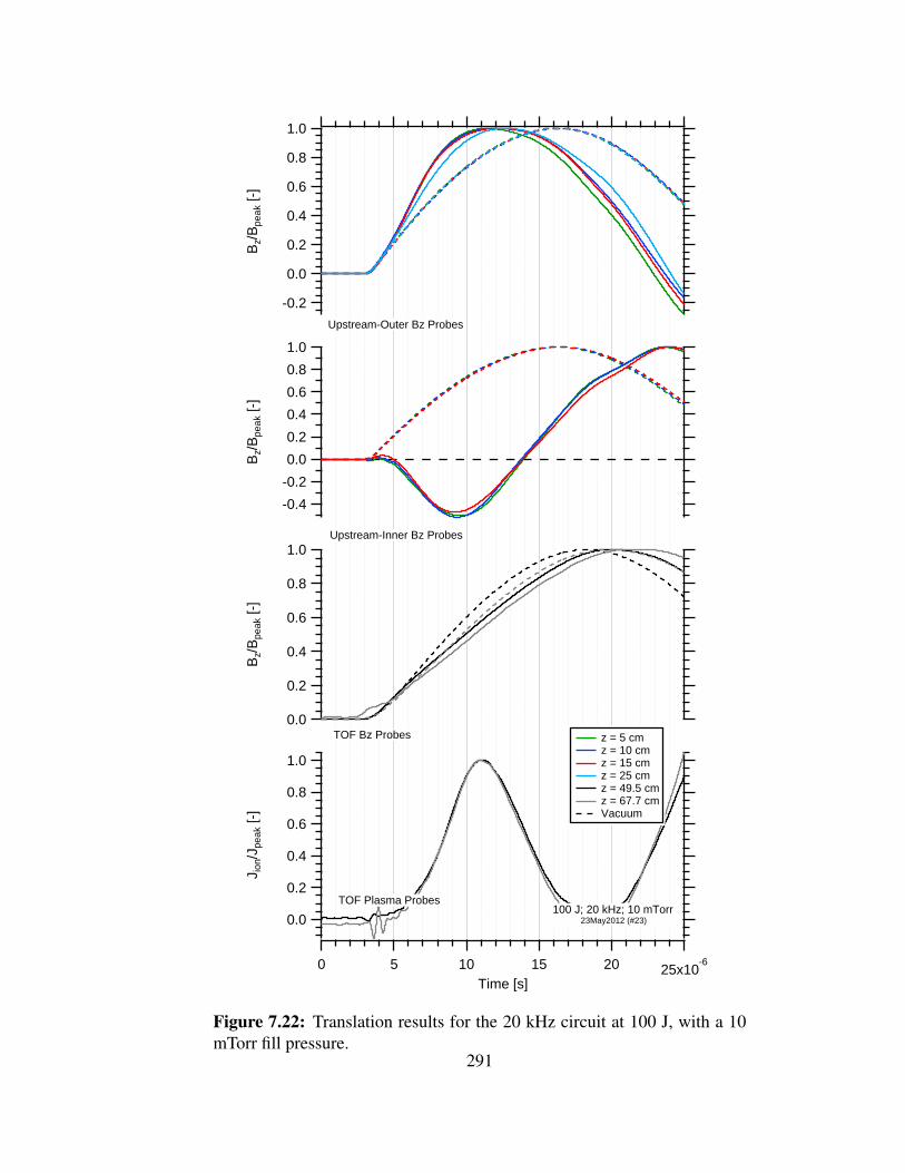
1.0

0.8

0.6

0.4

0.2

0.0

-0.2

Bz/

Bpe

ak [-

]

25x10-620151050

Time [s]

1.0

0.8

0.6

0.4

0.2

0.0

-0.2

-0.4

Bz/

Bpe

ak [-

]

1.0

0.8

0.6

0.4

0.2

0.0

Bz/

Bpe

ak [-

]

1.0

0.8

0.6

0.4

0.2

0.0

J ion

/Jpe

ak [-

]




TOF Bz Probes


23May2012 (#23)


291

1.0

0.8

0.6

0.4

0.2

0.0

-0.2

Bz/

Bpe

ak [-

]

25x10-620151050

Time [s]

1.0

0.8

0.6

0.4

0.2

0.0

Bz/

Bpe

ak [-

]

1.0

0.8

0.6

0.4

0.2

0.0

Bz/

Bpe

ak [-

]

1.0

0.8

0.6

0.4

0.2

0.0

-0.2

-0.4

J ion

/Jpe

ak [-

]




TOF Bz Probes


23May2012 (#28)


292

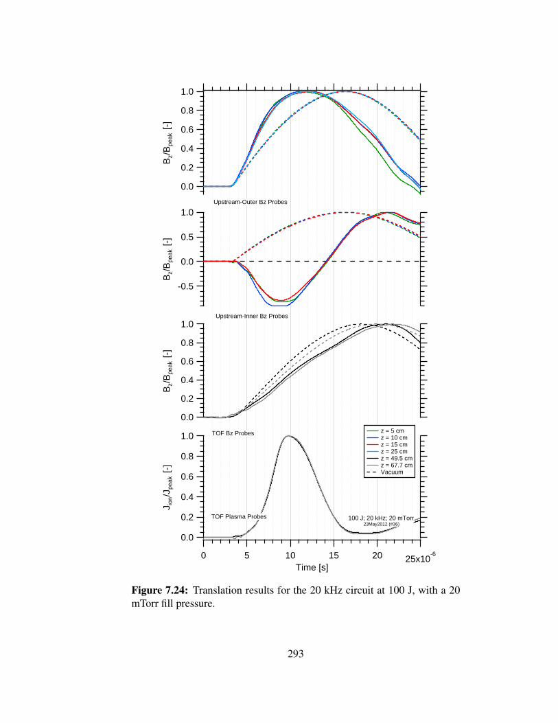
1.0

0.8

0.6

0.4

0.2

0.0

Bz/

Bpe

ak [-

]

25x10-620151050

Time [s]

1.0

0.5

0.0

-0.5

Bz/

Bpe

ak [-

]

1.0

0.8

0.6

0.4

0.2

0.0

Bz/

Bpe

ak [-

]

1.0

0.8

0.6

0.4

0.2

0.0

J ion

/Jpe

ak [-

]




TOF Bz Probes

TOF Plasma Probes 100 J; 20 kHz; 20 mTorr 23May2012 (#36)


293

1.0

0.8

0.6

0.4

0.2

0.0

Bz/

Bpe

ak [-

]

25x10-620151050

Time [s]

1.0

0.5

0.0

-0.5

Bz/

Bpe

ak [-

]

1.0

0.8

0.6

0.4

0.2

0.0

Bz/

Bpe

ak [-

]

1.0

0.8

0.6

0.4

0.2

0.0

J ion

/Jpe

ak [-

]




TOF Bz Probes


23May2012 (#48)


294

7.2.3 Downstream Plasma Flux Measurements

The appearance of plasma downstream of the channel on the ion flux probes was

unexpected when the plasmoid did not translate. The source of the plasma was investigated

by placing an ADLP 3.8 cm downstream of the coils’ end to determine the plasma

properties of plasma emerging directly downstream of the thruster. This information was

then compared to the signal measured by the downstream probes. Data was collected from

the probe for a 100 J, 20 kHz discharge at 4 mTorr. The probe’s bias voltage was varied

from 0 V - 32 V and the current through the probe was measured during each shot. The

resulting data is displayed in Figure 7.26a. The probe current at t = 20 µs is shown in

Figure 7.26b along with a curve-fit to the data from ADLP theory, used to estimate n0 and

TeV .

The ADLP results show that the probe current collected to the probe increased with bias

voltage, saturating between 15-20 V. The data was used to estimate the time-history of the

temperature and density of the plasma at this location from 12-30 µs by fitting theoretical

I-V traces to the data sets. The results are displayed in Figure 7.27a and Figure 7.27b.

Thin-sheath approximations were used to calculate the ion currents and proved to be valid

assumptions, indicated by rp/λD > 45 in Figure 7.27c. The curve-fit results to the data at

several points in time are displayed in Appendix A. Uncertainty estimates in the data are

shown as well, including errors in probe theory as well as in the error in measured current

due to probe contaminants.

The ADLP data shows a dense, cool plasma traveling out of the coils with a Gaussian-like

time history. Peak densities of 1.09x1020 m−3 were measured, with a constant temperature

295

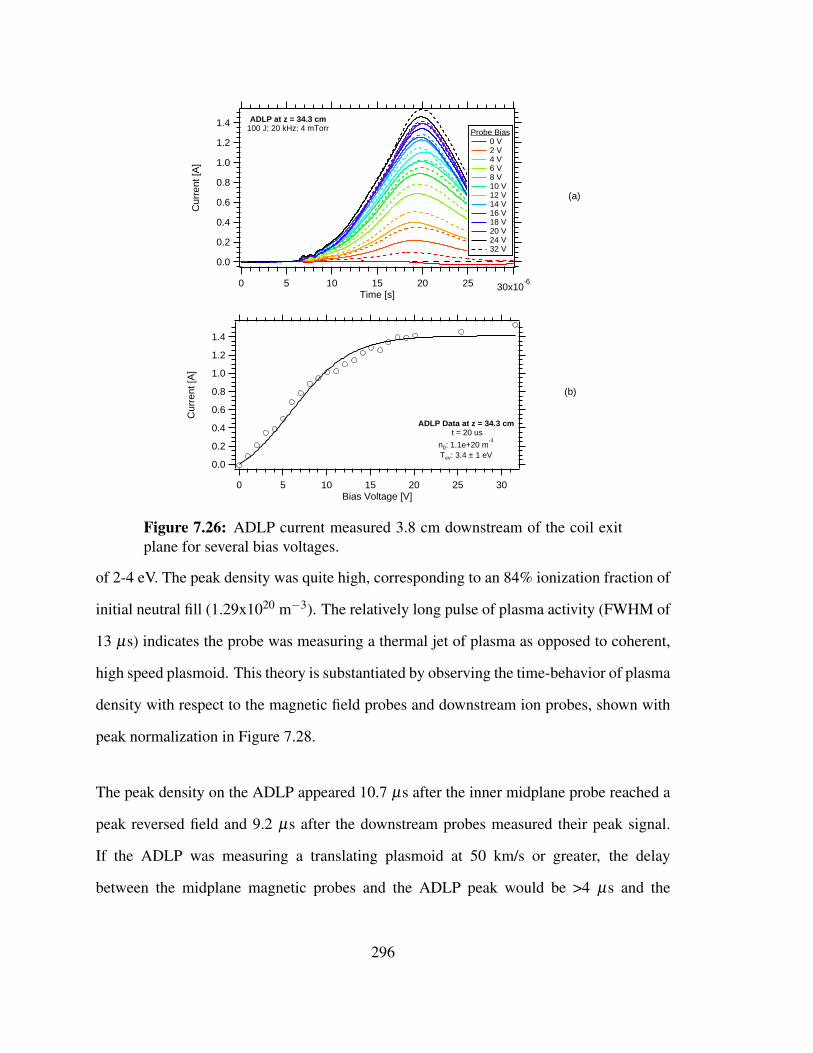
1.4

1.2

1.0

0.8

0.6

0.4

0.2

0.0

Cur

rent

[A]

30x10-62520151050

Time [s]

Probe Bias 0 V 2 V 4 V 6 V 8 V 10 V 12 V 14 V 16 V 18 V 20 V 24 V 32 V

ADLP at z = 34.3 cm100 J; 20 kHz; 4 mTorr

(a)

1.4

1.2

1.0

0.8

0.6

0.4

0.2

0.0

Cur

rent

[A]

302520151050Bias Voltage [V]

ADLP Data at z = 34.3 cm t = 20 us

n0: 1.1e+20 m-3

Tev: 3.4 ± 1 eV

(b)

Figure 7.26: ADLP current measured 3.8 cm downstream of the coil exitplane for several bias voltages.

of 2-4 eV. The peak density was quite high, corresponding to an 84% ionization fraction of

initial neutral fill (1.29x1020 m−3). The relatively long pulse of plasma activity (FWHM of

13 µs) indicates the probe was measuring a thermal jet of plasma as opposed to coherent,

high speed plasmoid. This theory is substantiated by observing the time-behavior of plasma

density with respect to the magnetic field probes and downstream ion probes, shown with

peak normalization in Figure 7.28.

The peak density on the ADLP appeared 10.7 µs after the inner midplane probe reached a

peak reversed field and 9.2 µs after the downstream probes measured their peak signal.

If the ADLP was measuring a translating plasmoid at 50 km/s or greater, the delay

between the midplane magnetic probes and the ADLP peak would be >4 µs and the

296

120x1018

100

80

60

40

20

Pla

sm

a D

en

sity [

#/m

3]

30x10-625201510

Time [s]

z = 34.3 cm 100 J; 20 kHz; 4 mTorr

4.0

3.5

3.0

2.5

2.0

Te

mp

era

ture

[e

V]

30x10-625201510

Time [s]

z = 34.3 cm 100 J; 20 kHz; 4 mTorr

(a)

(b)

500

400

300

200

100

r p/l

D [

-]

30x10-625201510

Time [s]

rp = 0.7 mm

rp = 0.124 mm

z = 34.3 cm100 J; 20 kHz; 4 mTorr

(b)

(c)

Figure 7.27: Plasma density and electron temperature measured by anADLP at z = 34.3 cm. Figure (c) shows that thin-sheath approximationsare valid for this probe for the time-interval of interest.

delay between the ADLP signal and the downstream probes would be >6.6 µs with the

downstream probes recording a peak after the ADLP. Since the ADLP signal does not

correspond to a translating plasmoid, it was likely the dense plasma originally created by

the AFRC released after magnetic confinement was lost. The high density of the plasma,

low temperature, and long delay time support this conclusion.

297

1.0

0.8

0.6

0.4

0.2

0.0

-0.2

Bz/

Bpe

ak [-

]

25x10-620151050

Time [s]

1.0

0.5

0.0

-0.5

Bz/

Bpe

ak [-

]

1.0

0.8

0.6

0.4

0.2

0.0

J ion

/Jpe

ak [-

]

1.0

0.8

0.6

0.4

0.2

0.0

n 0/n

peak

[-]

Upstream Outer Bz Probes

Upstream -Inner Bz Probes

ADLP

TOF Plasma Probes

z = 5 cm z = 10 cm z = 15 cm z = 25 cm z = 34.3 cm z = 49.5 cm z = 67.7 cm Vacuum

100 J; 20 kHz; 4 mTorr23May2012 (#18)

08Jun2012

Figure 7.28: Translation results for the 100 J, 20 kHz circuit includingpeak-normalized density from an ADLP.

298

The dense plasma created by the AFRC emerged from the channel after the first peak on the

downstream TOF plasma probes, meaning the plasma measured by the downstream probes

was not part of the bulk AFRC plasma. Instead, the plasma measured by the downstream

probes was likely created by one of three sources (1) hot electrons from the coil region

ionizing the background gas at the probe’s surface, (2) high energy plasma escaping the

plasmoid’s confinement, or (3) photoionization of the background gas by light emitted by

the plasmoid formation. The first and third source are the most likely. The second source

is highly unlikely; the delay between peaks on the downstream plasma probes are only 72

ns apart so the high energy plasma would have to be traveling in excess of 2000 km/s. This

velocity is unrealistic at 1% the speed of light or 827 keV (several orders of magntiude

higher than the expected energy of 10 eV).

To determine if background ionization was responsible for the plasma measured by the

probes, the mean free path for an ionization collision and an elastic collision between

an electron and neutral was calculated. The mean free path λM is the characteristic

length-scale for a collision, defined as:

λM =1

nnσ(7.1)

where σ is the collisional cross section and nn is the number density of the background

neutrals. The cross section as a function of electron energy is displayed in Figure 7.29a

for ionization of argon [83] and elastic collisions with argon [84]. From this graph, it is

apparent that low energy collisions (less than 15 eV) will simply scatter the participants

and produce no ionization. When the electron energy exceeds 20 eV, ionization and elastic

scattering are both just as likely. Above 100 eV, electrons are more likely to ionize the

argon neutral than to scatter off of it. These results imply that only the high energy tail

299

0.01

2

4

6

0.1

2

4

6

1

2

4

lM

[m

]

10080604020

Energy [eV]

Elastic Ionization

1 mTorr

10 mTorr

50 mTorr

2

4

6

10-21

2

4

6

10-20

2

4

6

10-19

s [

m2]

12 3 4 5 6 7 8

102 3 4 5 6 7 8

1002 3 4 5 6 7 8

1000

Energy [eV]

Elastic Ionization

(a)

(b)

Figure 7.29: Collision cross sections for electron elastic scattering fromargon and for electron ionization from argon for various electron energies(a) and mean free path for elastic and ionization scattering as a function ofenergy energy for various neutral fill pressures (b).

(20 eV and above) or a small fraction of the electron energy distribution function would be

responsible for ionization of the background gas. The mean free path for the elastic and

ionization collisions are displayed in Figure 7.29b for various fill pressures. The results in

this figure show that the mean free paths for the fill pressures in this experiment are between

1 cm and 1 m for both elastic and ionzation collisions. Since the probes are located 50

cm downstream from the narrow end of the coil, it is possible that high energy electrons

traveling from this region could ionize the background gas in front of the probes. The

electrons are also just as likely to scatter off without ionization, leading to lower ionization

fractions.

300

7x1018

6

5

4

3

2

1

0n 0

[m-3

]

20x10-6151050

Time [s]

Probe at z = 49.5 cm 1 mTorr

4 mTorr 10 mTorr 14 mTorr 20 mTorr 50 mTorr

2.0x1018

1.5

1.0

0.5

0.0

n 0 [m

-3]

20x10-6151050

Time [s]


(a)

(b)

Figure 7.30: Estimated plasma density for ion saturation currents measuredby downstream plasma probes at several pressures.

The mean free path decreases with density, therefore lower plasma densities should be

recorded by each probe for increased fill pressures. The electrons are more likely to

ionize a neutral upstream of the probes in a denser fill, leading to lower plasma densities

downstream. To investigate this trend in the ion flux data, the plasma density at each probe

was estimated using a fixed temperature of 1 eV (a slight reduction from the ADLP data)

and thin-sheath behavior. The results are displayed in Figure 7.30.

The data in Figure 7.30 shows that the plasma density measured by the TOF plasma probes

indeed decreases with increasing pressure. The mean free path decreases with density,

meaning an electron will experience more collisions before it reaches the probes in a

301

50 mTorr fill than in a 1 mTorr fill. This supports the theory that high energy electrons

traveling from the coil region are responsible for ionizing the plasma measured by the

downstream probes. It should be noted that the density measured by the downstream probes

(1x1018 m−3) is only a few percent of the neutral density (1x1020 m−3 or greater). This

is conclusive proof that the downstream plasma probes are not measuring the accelerated

AFRC plasmoid.

The high energy electrons (energies over 20 eV) which may have ionized the background

gas were likely created during initial ionization of the AFRC by the strong inductive fields

inside the coils and escaped the confinement region on open field lines. They had sufficient

energy to ionize the background gas downstream of the coils, resulting in simultaneous

signals on both downstream plasma probes. The density measured by the probes in the

denser neutral fills was less than the density measured by the probes in less dense neutral

fills because the electrons lost more energy due to more frequent collisions in the higher

pressure fills. This is also why the density measured by the upstream probe is higher than

the density measured by the downstream probe. These observations and the magnitude

of the plasma density measured by each probe are convincing evidence that the plasma

measured by the downstream probes was created by errant electrons from the discharge

coils.

Another possible source for the downstream plasma could be from photoionization of the

background gas. Photoionization occurs when a photon with an energy exceeding the

ionization potential of the gas strikes an atom and releases an electron. For argon, this

corresponds to 15.8 eV. This means that photons in the UV region of the electromagnetic

spectrum will be responsible for the bulk of the photoionization. Argon has several strong

emission lines in the UV spectrum from 49 nm to 75 nm [85]. These emission lines could

302

excite photons in the UV region, where the photoionization cross-sections of argon are the

highest [86]. However, the peak photoionization cross-sections (about 30x10−21 m−2) are

an order of magnitude smaller than the ionization cross sections shown in Figure 7.29. This

implies that they are less likely to create an ionization event than electron impact collisions.

Additionally, incoherant emission from the argon plasma in the discharge channel drops off

as 1/r2. This means that the probe signals measured by each probe should also decay as

1/r2, where r is their separation distance. The probes were spaced 18 cm apart, so the signal

on the downstream probe should decay by 30. The scaled data in Figure 6.36 show the

signal decay between probes is closer to 4. Both observations suggest that photoionization

is not a likely contributor to the bulk of the plasma downstream. Further analysis on this

phenomenon would require additional testing.

7.3 Discussion of Translation Results

The overwhelming conclusion from the translation data presented in Section 7.2 was

that the plasmoid failed to translate for all conditions tested. The delays in features

between probes spaced far apart appeared almost simultaneously. Additionally, signals on

downstream probes appeared before signals on upstream probes. These conflicting signals

do not agree with the expected profiles of a translating probe, shown in Figure 4.18 and

Figure 5.39.

While plasma activity was recorded by several plasma probes, the source of this plasma

was shown to be different than a translating plasmoid. Plasma activity was measured first

by the downstream probes with a peak in density observed 1 µs after the peak field reversal.

However, the density of this plasma was calculated to be at least two orders of magnitude

303

below the expected AFRC density and decreased with increasing pressure. The source

of this plasma was likely due to ionization of the downstream neutral gas by electrons

created during the initial firing of the main bank coils, as explained in Section 7.2.3 and

not a translating plasmoid. After plasma activity was seen on downstream probes, a dense

plasma was measured by a probe located 15 cm upstream of the downstream probes. While

the density of plasma measured at the probe was comparable to the expected density of the

AFRC, the plasma’s travel across the probe lasted longer than 13 µs, which was much too

slow for a 25 cm long plasmoid traveling at 100 km/s. Since plasma was seen to peak after

the loss of field reversal, it was most likely the remnants of the AFRC after confinement

was lost rather than a translating plasmoid.

Despite the lack of evidence supporting a translating plasmoid, an AFRC plasmoid was

observed for most conditions, indicated by a magnetic field reversal on the inner wall,

inductive coupling in the coil currents, and magnetic field exclusion on the outer wall. This

data was presented in Section 6.4. This data also showed that the maximum lifetime of the

AFRC plasmoid was much shorter than expected, with only 6-7 µs between the start of

reversal and the decay of the reversed field. The total lifetime for the plasmoid was 4-10

µs. The lifetime was expected to be closer to the quarter cycle of the discharge (25 µs for

the 10 kHz circuit; 12.5 µs for the 20 kHz circuit). The reason for the abbreviated lifetime

of the plasmoid is most likely related to its inability to translate. The source of lifetime

limitation will be explored in the remainder of this dissertation.

304

7.4 Possible Failure Modes

Several hypotheses can be made as to why the AFRC’s lifetime was much shorter than

expected and thus why it failed to translate. These hypotheses include a current induction

limit, insufficient conductivity, and a gross instability or imbalance. Each theory is briefly

explored in Sections 7.4.1, 7.4.2, and 7.4.3.

7.4.1 Failure Mode: Current Induction Limit

The AFRC requires an inductive drive for formation. A current is driven in the plasmoid

by changing current in the coils, analogous to a magnetic transformer. Plasmoid resistance

opposes this current drive through collisions. It is possible that when the rate of change

of current or coil voltage falls below a certain threshold, the inductive drive is insufficient

to stave off the loss of current from resistance. The plasmoid current can no longer be

sustained and the plasmoid disappears. The XOCOT-T3 data for all cases was examined

to see if there was some relationship between the plasmoid current lifetime and the dI/dt

of the coils (voltage). Plasmoid current lifetime is defined in this instance as the time span

between when the midplane probe initially crosses through B = 0 and when the reversed

field begins to decay. The decay of the reversed field indicates that the plasmoid current

is no longer working to generate a reversed field. Coil voltage is quantified by the time

derivative of the current, since the effective inductance (coils and plasmoid) is unknown.

To provide the best representative of each case, the average waveform from each data

set was used (see Section 6.4). Figure 7.31 shows the results from this scaling study,

considering the outer coil and inner coil independently. The results for a 50 mTorr fill

305

1.4x109

1.2

1.0

0.8

0.6

0.4

dI/d

t [A

/s]

6x10-6543210

Lifetime [s]

Inner Coil

600x106

500

400

300

200

100

dI/d

t [A

/s]

6x10-6543210

Lifetime [s]

100 J; 10 kHz 500 J; 10 kHz 1000 J; 10 kHz 100 J; 20 kHz

Outer Coil

Figure 7.31: Time derivative of current compared to observed plasmoidcurrent lifetime for all XOCOT-T3 test conditions, showing the scaling forthe outer coil (left) and inner coil (right).

have been removed since all tests with 50 mTorr show a delayed and incomplete reversal.

The results from this study show that the plasma current in higher energy plasmoids

disappears at a higher coil voltage (dI/dt) than their lower energy counterparts.

Additionally, the plasmoid current in the 500 J and 1000 J plasmoids disappears at the

same time (around 6 µs). A terminated lifetime from a current induction limit would show

that all discharges would disappear at the same coil voltage and the 1 kJ plasmoids would

be sustained several µs past the 500 J plasmoids. This study does not show these trends,

therefore it is likely the XOCOT-T3 plasmoid was not lifetime limited due to a drop in

current induction.

7.4.2 Failure Mode: Low Conductivity

An AFRC plasmoid creates a bi-directional field in the annulus which excludes the outer

coil field. If the conductivity is fairly low, the outer coil field can diffuse through the

306

plasmoid and annihilate the reversed field. The magnetic field diffusion time through the

plasmoid can be easily estimated using assumed plasma properties to determine if this is a

possibility.

The 1/e timescale for magnetic field diffusion is defined by Equation 7.2 from Chen[45]:

τd =µ0L2

η⊥(7.2)

where the plasma resistivity can be estimated using the Spitzer resistivity transverse to a

magnetic field [46]:

η⊥ = 1.29×104 ZlnΛ

T (3/2)(7.3)

In Equation 7.3, Z is the ionic charge, ln Λ is the Coulomb logarithm, and T is the electron

temperature in Kelvin. The Coulomb logarithm is a function of temperature and density

and it can be approximated to 10 for AFRC plasmas. The Spitzer resistivity drastically

under-predicts the resistivity as discussed in Section 4.1, but will be used in this instance

as a best-case scenario.

The internal temperature of an AFRC plasma can be anywhere between 10 eV and 50

eV. Using Equation 3.22, the magnetic soakthrough time for 1-cm thick, 10 eV plasma

is 3.49 µs. Increasing the temperature to 20 eV gives a soakthrough of 9.02 µs. A

50 eV plasma soaks through in 32 µs. These estimates suggest that the plasma lifetime

could be limited by soakthrough if the plasma is less than 20 eV. Internal measurements of

307

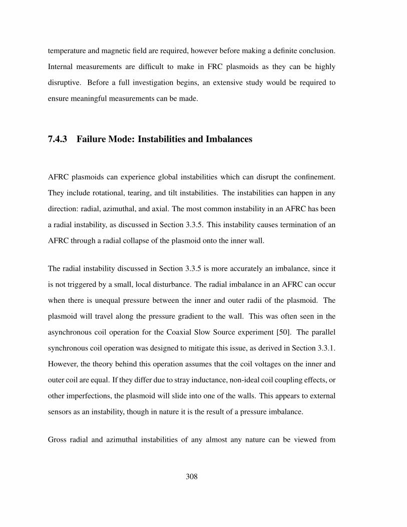
temperature and magnetic field are required, however before making a definite conclusion.

Internal measurements are difficult to make in FRC plasmoids as they can be highly

disruptive. Before a full investigation begins, an extensive study would be required to

ensure meaningful measurements can be made.

7.4.3 Failure Mode: Instabilities and Imbalances

AFRC plasmoids can experience global instabilities which can disrupt the confinement.

They include rotational, tearing, and tilt instabilities. The instabilities can happen in any

direction: radial, azimuthal, and axial. The most common instability in an AFRC has been

a radial instability, as discussed in Section 3.3.5. This instability causes termination of an

AFRC through a radial collapse of the plasmoid onto the inner wall.

The radial instability discussed in Section 3.3.5 is more accurately an imbalance, since it

is not triggered by a small, local disturbance. The radial imbalance in an AFRC can occur

when there is unequal pressure between the inner and outer radii of the plasmoid. The

plasmoid will travel along the pressure gradient to the wall. This was often seen in the

asynchronous coil operation for the Coaxial Slow Source experiment [50]. The parallel

synchronous coil operation was designed to mitigate this issue, as derived in Section 3.3.1.

However, the theory behind this operation assumes that the coil voltages on the inner and

outer coil are equal. If they differ due to stray inductance, non-ideal coil coupling effects, or

other imperfections, the plasmoid will slide into one of the walls. This appears to external

sensors as an instability, though in nature it is the result of a pressure imbalance.

Gross radial and azimuthal instabilities of any almost any nature can be viewed from

308

imaging the plasma end-on. A viewport on the far end of the XOCOT-T3 experiment

provided access for fast, single frame photography of the configuration to see if radial and

azimuthal instabilities are an issue. Axial instabilities are more difficult to see but may be

detected in the XOCOT-T3 experiment with axial probe arrays. Since radial and azimuthal

instabilities are easier to diagnose, these will be the topic of further investigation in Chapter

8 and 9.1.

7.5 Summary

The results from the XOCOT-T3 time-of-flight arrays demonstrated that despite the

presence of a reversed field, the plasmoid did not translate. The field reversal lasted 4-10 µs

before disappearing. The magnetic signatures on all probes have no staggered features that

would suggest a translation velocity. In some instances, signatures appear on downstream

probes before they appear on upstream probes. While plasma was measured downstream

of the thruster, it appeared simultaneously on probes spaced 18 cm apart and throughout

the formation sequence. These signals did not correspond to a translating AFRC plasmoid

and were likely due to ionization of the background gas by stray electrons.

Several hypotheses were suggested for why the plasmoid failed to translate. One hypothesis

was that the plasmoid current can only be driven when dI/dt is above a certain threashold.

This theory was ruled out for this experiment, by showing that the higher energy plasmoids

disappeared at a higher dI/dt than the lower energy plasmoids. Another theory was that the

plasma was lifetime limited due to magnetic soakthrough from the outer coil. This theory

was shown to be plausible as the soakthrough time for a 1 cm, 10 eV plasma is 3.49 µs.

Internal probing of the plasma is required to make any stronger connection between the

309

XOCOT-T3’s plasmoid lifetime and magnetic soakthrough. Instabilities could also be the

reason for a limited lifetime and translation failure. Radial and azimuthal instabilities will

be explored in Chapters 8 and 9.

310

Chapter 8

Instability Study Data and Results

The results from Chapter 7 concluded that the plasmoid failed to translate from the coils

and was limited in lifetime to 4-10 µs. One possible theory for the limited lifetime is

that the plasma experienced a disruptive instability or imbalance which terminated the

configuration. This chapter discusses the additional experimental data collected from the

XOCOT-T3 to explore this theory. Section 8.1 explains how Langmuir probes and fast,

single frame photography were implemented to look at radial and azimuthal instabilities

and imbalances. Section 8.2 presents the data from the instability and imbalance study.

The results from the study are discussed in Section 8.3.

8.1 Instability Study Diagnostics

Gross instabilities of a radial or azimuthal nature can be viewed by imaging the plasma

end-on (along the z-axis). A fast, single frame digital camera was installed at a viewport

311

opposite the discharge channel. The perspective view from the inner coil prevented the

entire plasmoid from being imaged properly. To see an accurate radial plasma distribution,

only an angular section of the channel could be viewed in a single frame. The camera,

described in Section 5.2.4, was an intensified CCD single-frame digital camera with a

minimum exposure time of 5 ns. A 480 nm, 10 nm bandwidth filter was added to camera

to isolate a set of Ar II emission lines.

The still images were recorded in 1 µs frame widths for the 10 kHz discharge and 500

ns frame widths for the 20 kHz discharge. Images were collected for the first 1/4 cycle

only and as long as enough visible light was detectable. The camera was unable to store

sequential images. Each image is from a separate shot at repeatable conditions.

The other diagnostic used in this section of research was an asymmetric double Langmuir

probe. The probe and circuit is described in Section 5.2.3. The ADLP was only used in the

20 kHz circuit, since the 10 kHz capacitor failed before data could be collected. The probe

was inserted directly into the discharge channel, at the axial midplane. The probe bias was

fixed to 24 V for all shots. Data was collected across the entire radial cross section of the

channel at one aziumuthal location, 2 mm apart.

8.2 Instability Study Data

The results from Chapter 6 show that all XOCOT-T3 discharges have the same gross

behavior. The reversed field disappears, followed by the loss of the inductive load and

excluded field on the outer probes. This means it was not necessary to rerun each operating

point; a single setting from each circuit was sufficient to resolve the overall plasma

312

behavior. Data from the 10 kHz circuit was collected for the 500 J, 4 mTorr discharge. Data

with the 20 kHz circuit was taken at 100 J with a 4 mTorr fill. Image data for both discharges

is presented in Section 8.2.1. Asymmetric double Langmuir probe data is provided for the

20 kHz circuit in Section 8.2.2.

8.2.1 Image Data

The XOCOT-T3 plasmoid was imaged for the first quarter cycle for two different

discharges. The 10 kHz tests used a 500 J/pulse energy setting with a 4 mTorr static fill.

The 20 kHz tests also used 4 mTorr of gas with 100 J of discharge energy. Background

images were captured prior to plasma shots. These images were used to establish insulator

boundaries for the plasma images. The background images for each discharge is displayed

in Figure 8.1. The insulator boundaries are drawn in the thick dotted lines. The thin dotted

line is the entrance to the translation chamber. The camera was pointed to look along

the length of the inner insulator. The red boxes indicate the areas where the edge of the

inner insulator is directly orthogonal to the camera lens. This is the only region in the

photographs where it will be possible to tell where the plasma is radially distributed.

Images for the 10 kHz discharge are compiled in Figure 8.2. The 20 kHz images are shown

in Figure 8.3. The outlines of the insulators have been drawn in each image as well as the

red boxes, corresponding to the region where the radial plasma distribution can be seen.

The midplane magnetic fields for each data set have been included for reference.

In the 10 kHz data, the plasma formed off of both walls, but quickly expanded in 4 µs to

touch the inner wall. Shortly after this, the loss of reversal was seen on the inner magnetic

313

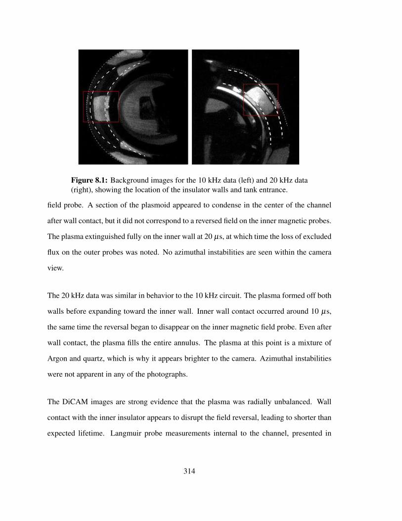
Figure 8.1: Background images for the 10 kHz data (left) and 20 kHz data(right), showing the location of the insulator walls and tank entrance.

field probe. A section of the plasmoid appeared to condense in the center of the channel

after wall contact, but it did not correspond to a reversed field on the inner magnetic probes.

The plasma extinguished fully on the inner wall at 20 µs, at which time the loss of excluded

flux on the outer probes was noted. No azimuthal instabilities are seen within the camera

view.

The 20 kHz data was similar in behavior to the 10 kHz circuit. The plasma formed off both

walls before expanding toward the inner wall. Inner wall contact occurred around 10 µs,

the same time the reversal began to disappear on the inner magnetic field probe. Even after

wall contact, the plasma fills the entire annulus. The plasma at this point is a mixture of

Argon and quartz, which is why it appears brighter to the camera. Azimuthal instabilities

were not apparent in any of the photographs.

The DiCAM images are strong evidence that the plasma was radially unbalanced. Wall

contact with the inner insulator appears to disrupt the field reversal, leading to shorter than

expected lifetime. Langmuir probe measurements internal to the channel, presented in

314

Figure 8.2: Images of the plasma from an end view for a 500 J, 4 mTorrplasma test with the 10 kHz circuit.

Section 8.2.2 confirm this finding.

315

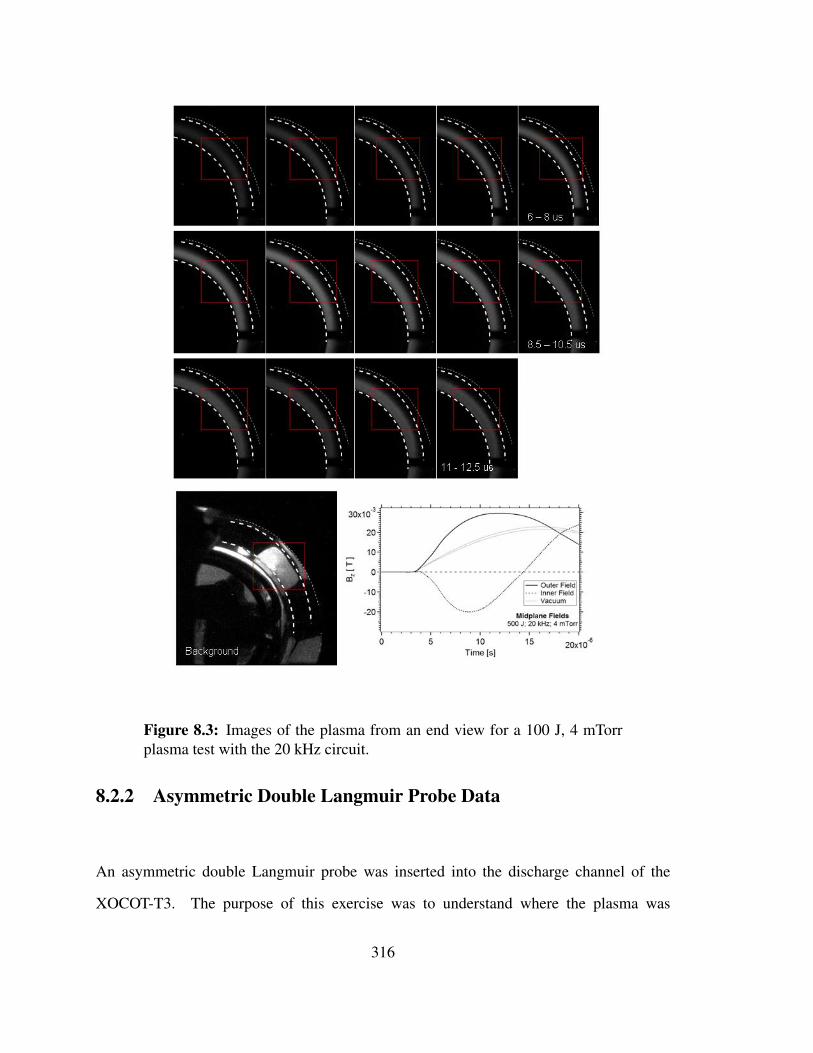
Figure 8.3: Images of the plasma from an end view for a 100 J, 4 mTorrplasma test with the 20 kHz circuit.

8.2.2 Asymmetric Double Langmuir Probe Data

An asymmetric double Langmuir probe was inserted into the discharge channel of the

XOCOT-T3. The purpose of this exercise was to understand where the plasma was

316

distributed spatially and temporally at the channel midplane. The probe and theory used to

interpret the probe is described in Section 5.2.3. Rather than using the traditional method

of sweeping the double probe to establish the I-V characteristic, the probe was fixed at a

single bias.

The bias voltage was selected by building a one-sided I-V characteristic 3.8 cm downstream

of the exit plane. The one-sided characteristic was chosen to limit the number of shots

required to construct the full trace. For the one-sided characteristic, the larger electrode was

biased negatively with respect to the smaller electrode to collect ions. While it would have

been preferred to collect the I-V characteristic at the midplane, this was decided against to

ensure the probe’s longevity. FRC plasmas tend to destroy probes very quickly. Using the

probe inside the channel for the 20+ shots required to establish the voltage for saturation

might have made the probe unusable for the full radial scan. The temporal data collected

for each bias voltage is displayed in Figure 8.4. Each trace represents a single shot at a

fixed bias voltage. The data at 20 µs was compiled to construct the I-V characteristic, also

shown in Figure 8.4. Additional I-V traces from this data set are presented in Appendix A.

The data in Figure 8.4 shows that the probe saturated around 15-18 V of applied bias

voltage. The plasma temperature and densities inside the channel were expected to be much

greater than the plasma downstream. Higher densities increase the saturation current, while

temperatures push the saturation voltage higher. Theoretical I-V characteristics are plotted

in Figure 8.5. These traces assume 100% ionization of the 4-mTorr gas fill. Figure 8.5

demonstrates that a bias voltage of 24 V is suitable for a 5-eV and 10-eV plasma case. If

the plasma is hotter than this, voltages in excess of 50 V are required. However, voltages

this high can cause the probe to emit electrons and disturb the surrounding plasma. For this

reason, it was decided that a conservative 24 V should be used for the bias. This bias will

317

1.4

1.2

1.0

0.8

0.6

0.4

0.2

0.0

Cur

rent

[A]

30x10-62520151050

Time [s]

Probe Bias 0 V 2 V 4 V 6 V 8 V 10 V 12 V 14 V 16 V 18 V 20 V 24 V 32 V

ADLP at z = 34.3 cm100 J; 20 kHz; 4 mTorr

(a)

1.4

1.2

1.0

0.8

0.6

0.4

0.2

0.0

Cur

rent

[A]


ADLP Data at z = 34.3 cm t = 20 us

n0: 1.1e+20 m-3

Tev: 3.4 ± 1 eV

(b)

Figure 8.4: ADLP data at z = 33.8 cm, showing the temporal data at fixedbias voltages and the reconstructed I-V characteristic.

still allow the probe to be used in the qualitative radial survey and limit the effect of the

probe on the plasma. Additionally, it will limit the current drawn to the probe and place

less strain on the circuit electronics and current transducers.

Following selection of the bias voltage, the ADLP was inserted into the channel at the axial

midplane. Data was collected at different radial locations between the insulators, shown in

Figure 8.6a. The data was analyzed to get the distribution of probe current along the radius

of the channel for several points in time (6-17 µs). These plots are displayed in Figure

8.6b. Midplane magnetic fields are also shown for comparison in Figure 8.6c.

318

5

4

3

2

1

0

Cur

rent

[A]


Theoretical ADLP Characteristics

ne = 1.29e20 m-3; Ap = 70 mm

2

Te 5 eV 10 eV 15 eV 20 eV

Figure 8.5: Theoretical I-V characteristics for a 4-mTorr backfill with 100%ionization and various temperatures.

The data and results in Figure 8.6 show that while plasma was detected along the entire

channel width, the peak of plasma occurred near the inner insulator. Over time, the plasma

near the inner wall grew and eventually the bulk of the plasma traveled to the inner wall.

This trend was also seen in the images in Section 8.2.1. Wall contact with the inner insulator

caused the plasmoid to lose field reversal so that the entire configuration quenched on the

inner wall. What the ADLP data makes more apparent than the images was that the plasma

seemed to form near the inner wall rather than at channel centerline (r = 93 mm). This

suggests that the inductive plasma current was insufficient to hold itself off the inner coil.

An additional note should be made about the seemingly high level of current collected by

the ADLP. The expected saturation current for this probe in a stationary, 100% ionized,

10 eV plasma is close to 4 A. The probe collects less than 4 A at the midplane, but the

current collected near the inner wall exceeds 6 A. While it is possible that the probe could

be perturbing the plasma, the high level of current may come from the fact that the probe is

located in a region of strong current. This increases the drift velocity of charged particles

relative to the probe and increases the probe current. The current is composed primarily

319

6

5

4

3

2

1

0

Pro

be C

urre

nt [A

]

20x10-6181614121086

Time [s]

Probe Position r = 84 mm (#21) r = 86 mm (#30) r = 88.5 mm (#26) r = 91 mm (#27) r = 93 (#19, #20) r = 98 mm (#25) r = 102 mm (#22)

ADLP at z = 15 cm100 J; 20 kHz; 4 mTorr

6

5

4

3

2

1

Ion

Cur

rent

[A]

120110100908070r-coordinate [mm]

time

17 us

6 us

inne

r co

il

inne

r in

sula

tor

oute

r in

sula

tor

oute

r co

il

ADLP at z = 15 cmOriginal Circuit

100 J; 20 kHz; 4 mTorr

30x10-3

20

10

0

-10

-20

Bz

[ T ]

20x10-6151050

Time [s]

Midplane Field Data100 J; 20 kHz; 4 mTorr

12Jun2012 (#003, #019)

Outer Field Inner Field Vacuum

Figure 8.6: ADLP measurements at the axial midplane, including (A) thetemporal probe current, (B) radial distribution of plasma current at varioustimes, and (C) midplane magnetic fields.

of electrons, but as discussed in Section 3.3.4 ions have been found to rotate as well.

The rotation of both species relative to the probe results in higher than expected current

levels. As discussed in Section 5.2.3, the presence of a plasma current makes it difficult

320

to determine plasma properties from the data. For this reason, the ADLP data at the axial

midplane is reported as probe current only.

8.3 Discussion

The internal ADLP data and the fast, single frame images provide independent,

overwhelming evidence that the plasmoid was radially unstable between the coils. Both

types of data show a plasmoid that formed near the inner wall and lost field reversal just

after wall contact. The plasmoid did not appear to be unstable azimuthally, up until wall

contact. The radial motion therefore limited the lifetime of the plasmoid and prevented the

configuration from translating out of the coils.

The most likely mechanism for the radial motion is uneven radial magnetic pressure on both

sides of the configuration. Ideally, the AFRC formed in the parallel mode with synchronous

coils should stay balanced between the coils. The magnetic pressure force pushing against

the outer surface should be equal to the magnetic pressure force pushing against the inner

surface. As was presented in Section 3.3.1, if the voltages on both coils are equal and the

plasma current is twice the product of the outer coil current and the number of turns on the

outer coil the pressure balance will hold. In the XOCOT-T3, it is likely that one of these

conditions was not met. In Chapter 9, data will be presented to determine what circuit

settings are required to maintain radial equilibrium.

321

8.4 Summary

This chapter investigated the limited lifetime of the XOCOT-T3’s annular plasmoid, using

the notion that the plasmoid experienced a fatal radial or azimuthal instability or imbalance.

Digital images from an intensified CCD camera were compiled from the 10 kHz and 20 kHz

circuits at 500 J and 100 J, respectively with a 4 mTorr gas fill. Using these images, it was

discovered that the plasmoid was not radially centered between the coils and traveled to

the inner wall about 4 µs after reversal. No azimuthal instabilities were observed. This

finding was further corroborated by double probe data collected at the axial midplane for

the 20 kHz circuit. An asymmetric double Langmuir probe was inserted into the discharge

channel at the axial midplane, scanning along the radius between the insulators. This data

showed that the bulk of the plasma traveled to the inner wall, coinciding with the loss of

the reversed field. The ADLP data also suggested that the plasma formed closest to the

inner wall, which was not expected. These data sets conclude that the lifetime of the AFRC

plasmoid was terminated due to a radial contact with the inner. Chapter 9 investigates the

mechanism for this radial wall contact, focusing on finding what conditions are required

for radial equilibrium.

322

Chapter 9

Radial Balance Study Data and Results

The results from Chapter 7 concluded that the plasmoid failed to translate from the coils

and was limited in lifetime to around 10 µs. An instability study presented in Chapter 8

determined that radial motion of the plasmoid was responsible for the short AFRC lifetime

in the XOCOT-T3. This chapter conducts a study to correct for the radial motion. A brief

overview on radial balance in AFRCs is given in Section 9.1. Data from circuit tuning

efforts used to control the radial motion are presented in Section 9.2. Section 9.3 covers the

results from this study. Section 9.4 discusses the results and how they impact future AFRC

translation experiments.

9.1 Radial Balance in AFRCs

A radial imbalance in AFRCs arises when an unequal pressure differential occurs on the

inner and outer radii of the plasmoid. The plasmoid is forced along the pressure gradient

323

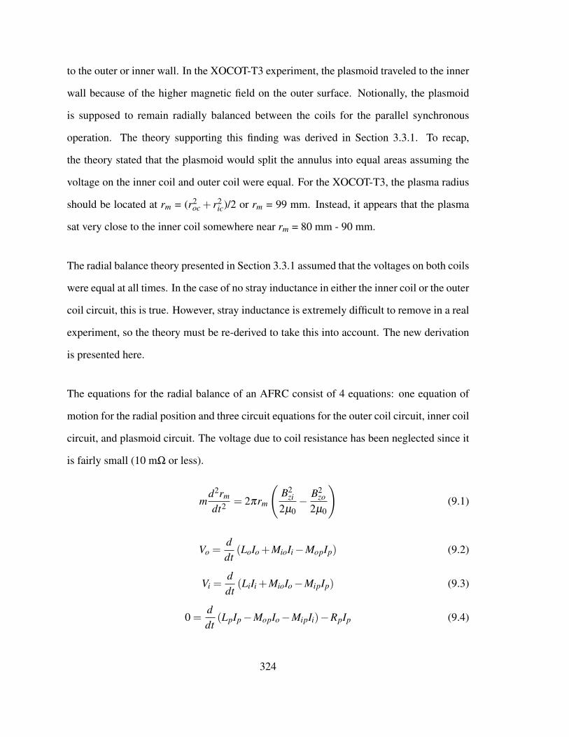
to the outer or inner wall. In the XOCOT-T3 experiment, the plasmoid traveled to the inner

wall because of the higher magnetic field on the outer surface. Notionally, the plasmoid

is supposed to remain radially balanced between the coils for the parallel synchronous

operation. The theory supporting this finding was derived in Section 3.3.1. To recap,

the theory stated that the plasmoid would split the annulus into equal areas assuming the

voltage on the inner coil and outer coil were equal. For the XOCOT-T3, the plasma radius

should be located at rm = (r2oc + r2

ic)/2 or rm = 99 mm. Instead, it appears that the plasma

sat very close to the inner coil somewhere near rm = 80 mm - 90 mm.

The radial balance theory presented in Section 3.3.1 assumed that the voltages on both coils

were equal at all times. In the case of no stray inductance in either the inner coil or the outer

coil circuit, this is true. However, stray inductance is extremely difficult to remove in a real

experiment, so the theory must be re-derived to take this into account. The new derivation

is presented here.

The equations for the radial balance of an AFRC consist of 4 equations: one equation of

motion for the radial position and three circuit equations for the outer coil circuit, inner coil

circuit, and plasmoid circuit. The voltage due to coil resistance has been neglected since it

is fairly small (10 mΩ or less).

md2rm

dt2 = 2πrm

(B2

zi

2µ0−

B2zo

2µ0

)(9.1)

Vo =ddt

(LoIo +MioIi−MopIp) (9.2)

Vi =ddt

(LiIi +MioIo−MipIp) (9.3)

0 =ddt

(LpIp−MopIo−MipIi)−RpIp (9.4)

324

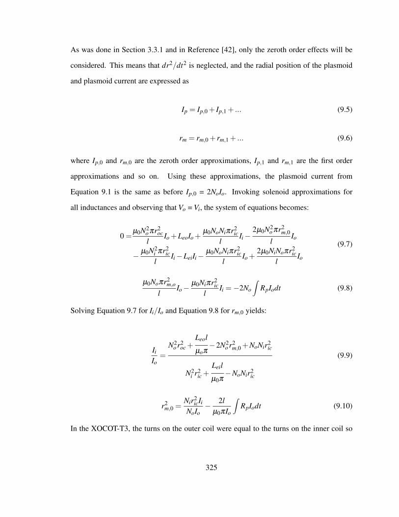
As was done in Section 3.3.1 and in Reference [42], only the zeroth order effects will be

considered. This means that dr2/dt2 is neglected, and the radial position of the plasmoid

and plasmoid current are expressed as

Ip = Ip,0 + Ip,1 + ... (9.5)

rm = rm,0 + rm,1 + ... (9.6)

where Ip,0 and rm,0 are the zeroth order approximations, Ip,1 and rm,1 are the first order

approximations and so on. Using these approximations, the plasmoid current from

Equation 9.1 is the same as before Ip,0 = 2NoIo. Invoking solenoid approximations for

all inductances and observing that Vo = Vi, the system of equations becomes:

0 =µ0N2

o πr2oc

lIo +LeoIo +

µ0NoNiπr2ic

lIi−

2µ0N2o πr2

m,0

lIo

− µ0N2i πr2

icl

Ii−LeiIi−µ0NoNiπr2

icl

Io +2µ0NiNoπr2

icl

Io

(9.7)

µ0Noπr2m,o

lIo−

µ0Niπr2ic

lIi =−2No

∫RpIodt (9.8)

Solving Equation 9.7 for Ii/Io and Equation 9.8 for rm,0 yields:

Ii

Io=

N2o r2

oc +Leol

µoπ−2N2

o r2m,0 +NoNir2

ic

N2i r2

ic +Leil

µ0π−NoNir2

ic

(9.9)

r2m,0 =

Nir2icIi

NoIo− 2l

µ0πIo

∫RpIodt (9.10)

In the XOCOT-T3, the turns on the outer coil were equal to the turns on the inner coil so

325

Ni = No = N. Combining Equations 9.9 and 9.10 with this information, the radius of the

plasmoid to a zeroth-order approximation is

r2m,0 =

µ0πr2ic

N2r2oc +

Leol

µ0π+N2r2

ic

− 2l2Lei

µ0πIo

∫RpIodt

Leil +2N2µ0πr2ic

(9.11)

It’s apparent from Equation 9.11 that with non-zero external parasitic inductances the

plasmoid radius is no longer a simple function of the outer and inner coil radii. To study the

effect of two different equation inputs, Equation 9.11 was used to predict the plasmoid’s

radial position in the XOCOT-T3 for the first 10 µs of the 20 kHz, 100 J condition. The

results for several different plasma resistance values are displayed in Figure 9.1a. These

results show that the plasmoid’s position is highly sensitive to the resistance of the plasma.

This matches the theory presented in Section 3.3.1 for independent coils. Resistance results

in a motion of the plasmoid toward the inner insulator. Since the plasmoid current is

responsible for generating the reversed field to hold the configuration off the inner wall,

this makes sense. Resistance decreases the ability to drive the inductive current and lowers

the plasma current. For Rp = 10 mΩ with the XOCOT-T3 predictions, the plasmoid comes

in contact with the inner insulator as the results in Figure 9.1a indicate.

Equation 9.11 was also used to study the effect of increasing the outer coil’s stray

inductance Leo. The final radial position of the plasmoid was calculated as a function

of Leo. Figure 9.1b displays the final radius (at 10 µs) of the plasmoid for Rp = 1 mΩ.

The results show that the plasmoid’s final position increases with increasing outer stray

inductance Leo. This is what is expected in experiments as well. Additional stray on the

outer circuit diverts more current to the inner coil and reduces the magnetic pressure from

the outer coil pushing the plasmoid toward the inner wall. It also helps minimize the voltage

326

94x10-3

92

90

88

86

r m,0

[m]

10-7

2 3 4 5 6 7 8 9

10-6

Leo [H]

Lei=744 nH; Rp = 1 mOhm

92x10-3

90

88

86

84

82

80

r m,0

[m]

10x10-686420

Time [s]

Inner Insulator

XOCOT-T3 PredictionsLeo = 600 nH; Lei = 744 nH

Rp = 1 mOhm Rp = 5 mOhm Rp = 10 mOhm

(a)

(b)

Figure 9.1: Final plasmoid radius, calculated using Equation 9.11. Theradial trajectory using XOCOT-T3 circuit parameters is shown in (a) forvarious plasmoid resistances. The final plasmoid position as a function ofouter coil stray inductance is shown in (b).

differential between the coils for increased radial balance.

327

9.2 Radial Balance Study Data

The plasmoid’s position in an AFRC experiment operating with parallel synchronous coils

is theoretically a function of stray inductance on the coil circuits and plasmoid resistance,

as discussed in Section 9.1. The easiest method to control the radial pressure balance in

the XOCOT-T3 experiment was to add additional stray inductance to the outer coil circuit.

This eased the magnetic pressure from the outer coil pushing the plasmoid toward the inner

wall by diverting more current to the inner coil.

Stray inductance was added to the outer coil by increasing the loop area between the

forward and return current paths. This was done for two tests. The first test added only a

modest amount of stray inductance, about 185 nH of extra inductance (or 785 nH total). The

second test increased the original amount by a factor of 1.78 from the original, using a total

stray inductance of 1.072 µH. These versions of the circuit are referred to as Configuration

#1 and Configuration #2, respectively. Stray inductance was added to the 20 kHz circuit

only. The capacitor for the 10 kHz circuit failed before similar tests could be conducted.

Since tests at all pressures using the 20 kHz circuit at 100 J had the same gross behavior

(loss of reversed field at 14 µs), Configuration #1 and Configuration #2 were only tested

at the 100 J, 4 mTorr settings. Full magnetic field profiles upstream and downstream were

collected from these configurations for vacuum and plasma discharges.

The vacuum data for Configuration #1 is shown in Figure 9.2, including the coil currents

and midplane fields. The data from the original version of the 20 kHz circuit at 100 J is

indicated in these plots by the faint dotted lines. The vacuum data from Configuration #1

328

was averaged over 6 shots. Error bars are a combination of the statistical devation (small)

and the measurement uncertainty.

The vacuum currents for Configuration #1 show the expected trends. The outer coil current

is lower than the original circuit (at 2600 A instead of 2800 A) and the inner coil current is

higher (8100 A compared to 8000 A). The total circuit current drops only marginally, down

67 A. This small drop is within the shot-to-shot variation. The current ratio between the

coils drops from 0.355 to 0.325. The current ratio is defined as outer coil current divided

by inner coil current. The vacuum magnetic fields change as well, when compared to the

original configuration. The midplane field in the annulus drops by 2 mT, or 10% of the

original field.

Following the vacuum circuit characterization with the new changes, plasma tests were

conducted. A fill pressure of 4 mTorr was used and 18 shots were discharged into the

neutral fill. The midplane magnetic fields from one of the shots is shown in Figure 9.3a.

The magnetic field data from the coil probes and TOF array is displayed in Figure 9.3b and

Figure 9.3c.

The magnetic field data showed that the additional stray inductance on the outer coil circuit

created a plasmoid with a higher plasmoid current. This was judged by the higher reversed

midplane field on the inner wall as compared to the original configuration (see Figure 9.3a).

The field reversal also happened faster. Instead of taking a full microsecond to reverse, the

field now reversed in 840 ns. The peak reversal with the new circuit occurred 5.7 µs

after the switch closed, lasting less than 1 µs at the peak. The reversed field decay was

much slower in the new circuit, lasting a full µs longer. The additional stray inductance

increased the configuration lifetime from 10 µ to 11 µs. While the inner field showed

marked changes, the outer field did not change appreciably for the first 3.5 µs, compared

329

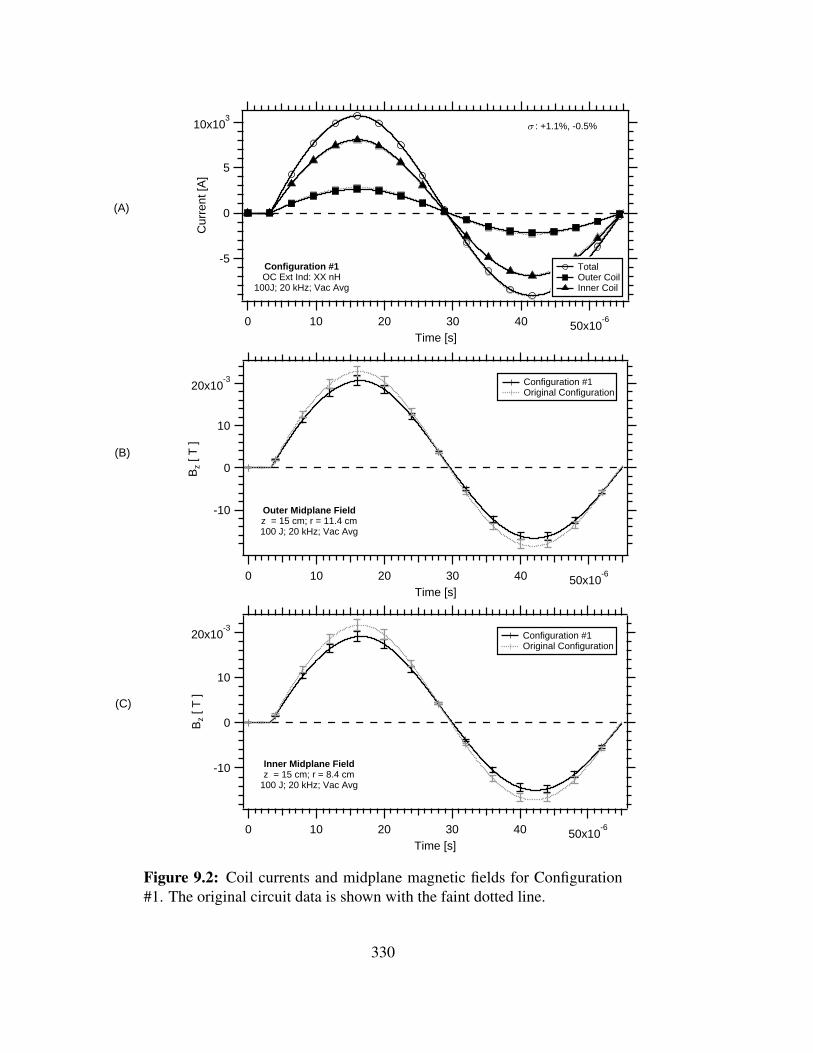
20x10-3

10

0

-10

Bz

[ T ]

50x10-6403020100

Time [s]

Inner Midplane Fieldz = 15 cm; r = 8.4 cm

100 J; 20 kHz; Vac Avg

Configuration #1 Original Configuration

20x10-3

10

0

-10

Bz

[ T ]

50x10-6403020100

Time [s]

Outer Midplane Fieldz = 15 cm; r = 11.4 cm100 J; 20 kHz; Vac Avg

Configuration #1 Original Configuration

10x103

5

0

-5

Cur

rent

[A]

50x10-6403020100

Time [s]


s : +1.1%, -0.5%

Configuration #1OC Ext Ind: XX nH

100J; 20 kHz; Vac Avg

(A)

(B)

(C)

Figure 9.2: Coil currents and midplane magnetic fields for Configuration#1. The original circuit data is shown with the faint dotted line.

330

30x10-3

20

10

0

-10

-20

Bz

[ T ]

20x10-6151050

Time [s]

Midplane FieldsConfiguration #1

100 J; 20 kHz; 4 mTorr24May2012 (#18)

Outer Field Inner Field Original Configuration

(A)

(B)

30x10-3

20

10

0

-10

-20

-30

Bz

[ T ]

20x10-6151050

Time [s]

z = 5 cm z = 10 cm z = 15 cm z = 25 cm Inner Fields

Axial FieldsUpstream TOF array

700x10-6

600

500

400

300

200

100

0

Bz/

NA

[ T

/m2]

25x10-620151050

Time [s]

16x10-6

14

12

10

8

6

4

2

0

Bz /N

A [ T

/m2]

z = 49.5 cm z = 67.7 cm

Axial FieldsDownstream TOF array

(C)

Figure 9.3: Magnetic field data for a 100 J, 4 mTorr shot with the circuitin Configuration #1. The data using the original circuit is indicated by thefaint dotted lines.

331

300

200

100

0

Pre

ssur

e [P

a]

20x10-6151050

Time [s]

Outer Pressure Inner Pressure Original Config

Midplane PressureConfiguration #1

100 J; 20 kHz; 4 mTorr24May2012 (#18)

Figure 9.4: Magnetic pressure at the axial midplane for a 100 J, 4 mTorrdischarge using the 20 kHz circuit in Configuration #1.

to the original configuration.

The axial fields recorded by other probes along the coil and TOF array were similar in

nature to the midplane probe and no evidence of translation was seen. An interesting

feature that appeared in the new inner field data when compared to the original data was

the extended pause near the maximum field reversal. In the original configuration, the

inner field reached the maximum field reversal and then quickly disappeared. The new

circuit created an extended pause, settling around the maximum for almost a full µs before

starting to disappear. This delay was too short to make considerable gains in translation,

but it showed a trend in improving the lifetime.

The magnetic pressure was calculated for the axial midplane, using the data shown in

Figure 9.3a. The pressure was calculated using Equation 3.2. The results are shown in

Figure 9.4. The magnetic pressure from the original circuit is shown for comparison.

The magnetic pressures data shows that a magnetic pressure differential across the plasmoid

332

was still apparent, with the inner pressure lower than the outer pressure. While the pressure

differential (30 Pa) was significantly less than in the original configuration, the stray

inductance did not correct for the pressure differential entirely.

Images from an end-on view were recorded of the plasmoid formation, created using

Configuration #1. Still frames using a fast-shutter camera were collected from 6-11.5 µs,

every 500 ns. This images are available in Figure 9.5. Midplane magnetic fields are also

shown in Figure 9.5 for reference.

The images for Configuration #1 show that the plasmoid came in contact with the inner

wall, but with a slight delay compared to the original circuit. The plasmoid appeared to

contact the wall in Figure 9.5 at 10-10.5 µs after the switch closes. In the original circuit

(consult Figure 8.3), the plasmoid hit the wall at 9-9.5 µs.

Since this small amount of stray inductance added to the circuit for Configuration #1 did

not have the desired effect, additional stray inductance was added to the discharge circuit

to further reduce the outer coil field. About 472 nH of extra inductance was added to the

outer coil circuit, providing a total stray inductance of 1.072 µH. This is referred to as

Configuration #2. This configuration was tested first at vacuum to determine how much the

coil currents and fields deviate from the original circuit. The vacuum data for Configuration

#2 is shown in Figure 9.6, including the coil currents and midplane fields. The data from

the original version of the 20 kHz circuit at 100 J is indicated in these plots with faint dotted

lines. The vacuum data from Configuration #2 was averaged over 6 shots. Error bars are a

combination of the statistical deviation (small) and the measurement uncertainty.

The vacuum currents for Configuration #2 exhibited a marked change from the original

configuration. The outer coil current was on average 454 A (or 16%) less than the original

333

Figure 9.5: Images of plasmoid formation for a 100 J, 4 mTorr dischargeusing the 20 kHz circuit in Configuration #1. Midplane magnetic fields areshown for reference.

334

20x10-3

10

0

-10

Bz

[ T ]

50x10-6403020100

Time [s]

Inner Midplane Fieldz = 15 cm; r = 8.4 cm


Configuration #2 Original Configuation

20x10-3

10

0

-10

Bz

[ T ]

50x10-6403020100

Time [s]

Outer Midplane Fieldz = 15 cm; r = 11.4 cm100 J; 20 kHz; Vac Avg

Configuration #2 Original Configuation

10x103

5

0

-5C

urre

nt [A

]

50x10-6403020100

Time [s]


Configuration #2OC Ext Ind: XX nH


s : +1.2%, -0.6%

(A)

(B)

(C)

Figure 9.6: Coil currents and midplane magnetic fields for Configuration#2. The original circuit data is shown with the faint dotted line.

335

circuit. The inner coil current increased by 280 A (3%) and the total current decreased by

173 A (1.6%). The current ratio between the coils changed to 0.287 (compared to 0.355 in

the original circuit). The outer vacuum field decreased by 22%, about 5 mT. The magnetic

field recorded by the inner probe dropped 5 mT as well.

Plasma tests were conducted on the circuit defined as Configuration #2, using a fill pressure

of 4 mTorr and discharge energy of 100 J. Twenty-eight test were performed with data

collected from all magnetic field probes, an asymmetric double Langmuir probe at the axial

midplane, and a fast-shutter, single frame camera. The midplane magnetic fields from one

of the shots is shown in Figure 9.7a. The data from the coil magnetic field probes and the

TOF magnetic field probes is displayed in Figure 9.7b and Figure 9.7c.

The reversed magnetic field generated by the plasmoid in Configuration #2 was much

greater than the reversed field seen in the original circuit, about 5 mT of additional field

during the initial reversal from 4-9 µs. By comparison, Configuration #1 had a field reversal

increase of about 4.4 mT. The reversal also happened sooner, in less than 630 ns from the

switch closing. The reversal also lasted considerably longer than the original circuit. Once

the peak reversed field was reached at 9.15 µs, the reversed field stayed constant for 2.5 µs

longer. The configuration lifetime with Configuration #2 increased to 13 µs, 3 µs longer

than the original circuit.

The outer field in Configuration #2 was less than the outer field in the original configuration.

This a consequence of the lower current through the outer coil. It also helped to reduce the

magnetic pressure pushing the plasmoid toward the inner wall. The axial probe signatures

upstream and downstream (shown in Figure 9.7b and c) show no sign of plasmoid motion,

even with the increased lifetime. This is unfortunate, but not entirely unexpected. In the 100

J case, there was likely little energy available for translation, especially when translation

336

600x10-6

500

400

300

200

100

0

Bz/

NA

[ T

/m2 ]

25x10-620151050

Time [s]

15x10-6

10

5

0

Bz /N

A [ T

/m2]

Axial FieldsDownstream TOF array

z = 49.5 cm z = 67.7 cm

30x10-3

20

10

0

-10

-20

Bz

[ T ]

20x10-6151050

Time [s]

z = 5 cm z = 10 cm z = 15 cm z = 25 cm Inner Fields

Axial FieldsUpstream TOF array

30x10-3

20

10

0

-10

-20

Bz

[ T ]

20x10-6151050

Time [s]

Outer Field Inner Field Original Configuration

Midplane FieldsConfiguration #2

100 J; 20 kHz; 4 mTorr21Jun2012 (#10)

(A)

(B)

(C)

Figure 9.7: Magnetic field data for a 100 J, 4 mTorr shot with the circuitin Configuration #2. The data using the original circuit is indicated by thefaint dotted lines.

337

300

200

100

0

Pre

ssur

e [P

a]

20x10-6151050

Time [s]

Outer Pressure Inner Pressure Original Configuration

Midplane PressureConfiguration #2

100 J; 20 kHz; 4 mTorr 21Jun2012 (#10)

Figure 9.8: Magnetic pressure at the axial midplane for a 100 J, 4 mTorrdischarge using the 20 kHz circuit in Configuration #2.

must be accomplished in under 10 µs.

The time-history of the magnetic pressure at the axial midplane for Configuration #2 was

calculated using Equation 3.2. The results are shown in Figure 9.8. The magnetic pressure

from the original circuit is also shown for comparison.

The magnetic pressures in Configuration #2 on the inner and outer surfaces of the plasmoid

were approximately equal, until 9 µs. The magnetic pressure on the inner wall leveled off,

dropping at 12 µs when the reversed field began to decay. The outer coil current continued

to climb after 9 µs, as the outer coil current continued to add magnetic field to the annulus.

To view the radial position of plasmoid in Configuration #2, end-on images were collected

from 6-14.5 µs with frame widths of 500 ns. This images are presented in Figure 9.9.

At the beginning of the image sequence, the plasmoid appeared fairly well centered

338

Figure 9.9: Images of plasmoid formation for a 100 J, 4 mTorr dischargeusing the 20 kHz circuit in Configuration #2.

339

between the insulators. Between 9 and 9.5 µs (when the inner field reached its peak),

the plasmoid began to expand radially in the channel. Inner wall contact was seen around

10.5 - 11 µs. After 11 µs, the plasma continued to expand though the perspective of these

images makes it difficult to see if it touched the outer wall as well. Since it did not overlap

the outer insulator line, it’s likely that it only contacted the inner wall.

The extended lifetime of the plasmoid in Configuration #2 warranted the use of an ADLP

to determine where the bulk of the plasmoid was radially located at the coil midplane. The

ADLP in Configuration #2 was used in the same manner as previously described in Section

8.2.2. A bias voltage of 24 V was applied across the probe, with the larger probe tip biased

to collect ions. The probe was scanned radially across the channel in 2 mm increments.

The current collected by the probe is shown in Figure 9.10a. The radial distribution of

plasma is plotted from 6-17 µs in Figure 9.10b. Midplane magnetic fields are shown for

comparison in Figure 9.10c.

Figure 9.10 shows expected AFRC behavior. The peak current (i.e. plasma density for

constant temperature and no flow velocity) was measured at the center of the channel

and then tapered toward the walls. This same profile was seen in other experiments as

well (consult Section 3.3.2). The plasma activity on channel centerline continues to climb

until 12 µs, when the field reversal started to decay. Between 10 and 11 µs, the plasma

activity near the wall starts to increase as more plasma came in contact with the wall. This

likely triggered the start of the plasmoid current decay a microsecond later and loss of field

reversal. The motion of the plasma appeared to be towards the inner wall, but the increase

in plasma current seen in this region may have to do with plasma bombardment of the inner

insulator.

While the plasmoid was more or less radially balanced in Configuration #2, the center

340

20x10-3

10

0

-10

-20

Bz

[ T ]

20x10-6151050

Time [s]

Midplane Field DataConfiguration #2


Outer Field Inner Field Vacuum

3.5

3.0

2.5

2.0

1.5

1.0

0.5

AD

LP C

urre

nt [A

]

120110100908070r-coordinate [mm]

time

17 us

6 us

inne

r co

il

inne

r in

sula

tor

oute

r in

sula

tor

oute

r co

il

ADLP at z = 15 cmConfiguration #2


3.5

3.0

2.5

2.0

1.5

1.0

0.5

0.0

AD

LP C

urre

nt [A

]

25x10-620151050

Time [s]

ADLP at z = 15 cmConfiguration #2

20 kHz; 100 J; 4 mTorr

Probe Position 84 mm 86 mm 88.5 mm 91 mm 93 mm 95 mm 97.5 mm 100 mm 102 mm

(A)

(B)

(C)

Figure 9.10: ADLP data at the axial midplane for Configuration #2. Thedata collected by the probe is shown (A) along with the radial distributionalong the channel (B), and midplane mangetic fields (C).

341

appeared to be located at the gas center of the channel (r = 93 mm) and not the magnetic

center (r = 99 mm). While this may be due to a preferential density gradient, it might also

have to do with the plasma current being insufficient to push off the coil further. Additional

testing with even more stray is required to find out if the equilibrium position is related to

a magnetic pressure balance or a preferential gas loading.

9.3 Radial Balance Study Results

The radial balance study data presented in Section 9.2 demonstrated that additional stray

inductance on the outer coil circuit reduced the magnetic pressure differential between the

outer and inner wall. The original circuit had a pressure difference between the inner and

outer wall of over 80 Pa. When 185 nH of stray was added to the outer coil circuit, the

pressure difference dropped to 30 Pa. The stray inductance on the outer coil was increased

to 1.072 µH and the pressure differential disappeared; the inner magnetic pressure was

equal to the outer magnetic pressure for the first 6 µs.

The additional stray inductance on the outer coil circuit increased the inner coil current

only slightly. An increase of 127 A (or 1.6%) was seen in Configuration #1. The inner coil

current increased by 280 A (3%) in Configuration #2. The slight current increase through

the inner coil did not appear to change the inner field rise-time significantly. The reversed

field in all configurations stopped increasing around 9 µs with only a 300 ns difference

between Configuration #2 and the original circuit.

The effect of reduced pressure on the outer wall allowed the plasmoid current to reach

an equilibrium state after the reversed field reached its maximum. For the case of 30%

342

additional inductance in the outer coil circuit, the reversed field was noted to linger around

-0.02 mT for 1 µs before decaying toward zero. When the amount of stray inductance on

the outer coil circuit was nearly doubled, an equilibrium time of 2.5 µs was seen before the

field decay.

Plasmoid termination was still attributed to wall contact with both modified versions of

the experiment. In Configuration #1 (less stray), the plasmoid could be seen in images to

touch the wall around 10 µs, at the same time the reversed field started to disappear. In

Configuration #2 (large amounts of stray), the images showed the plasma touched the wall

around 11 µs. This also coincided with the loss of reversed field.

The mechanism for wall contact in Configuration #1 was likely a radial imbalance, due

to a pressure differential. The pressure on the outer surface of the plasmoid was always

greater than the pressure on the inner surface. This drove the plasmoid into the inner wall,

extinguishing it. The stray inductance correction was insufficient to reduce the outer coil

field.

When this pressure differential was corrected for in Configuration #2, the plasmoid was

held off the wall after peak field reversal for a short duration of time, from 9-10 µs.

However, shortly after 10 µs, internal ADLP data showed the plasma activity near the

inner wall jumps between 10-11 µs. The peak of plasma activity stayed centered at 93 mm,

indicating that a growth in the plasmoid’s midsection was responsible for this initial wall

contact. It’s unclear what this expansion was due to since it came after the plasmoid current

(inner field) stopped climbing, but possible causes are an increase of gas pressure inside the

configuration due to joule heating, poor magnetic confinement, and a radial imbalance.

343

9.4 Discussion of Radial Balance Results

The primary purpose of the radial balance study was to determine the mechanism behind

the radial plasmoid motion in the original experiment. The radial motion mechanism was

traced to a pressure imbalance between the inner and outer field. When this pressure

differential was corrected for by reducing the current through the outer coil, the plasmoid

retained a radial balance between the insulators. The radial balance was short-lived, as an

expansion in the plasmoid’s minor radii resulted in wall contact with the inner insulator and

eventual decay of the configuration.

The detrimental effect of the radial expansion could be corrected for by widening the space

between the coils. However, this would decrease the efficiency and final position of the

plasmoid, as the results in Section 4.2.3 indicate. It would also increase the energy required

to accelerate the plasmoid.

The cause of radial expansion in the radially-balanced version of the XOCOT-T3 was

unclear. Two possibilities include an increase of gas pressure inside the configuration due

to joule heating, and lousy magnetic confinement. It also likely that the radial expansion

was caused by a magnetic pressure differential, as a magnetic differential was noted at the

time of wall contact. While most of the plasma appeared centered in the channel for an

additional 6 µs, it was unclear where the plasma current was. The plasma current could

have drifted through the plasmoid to the inner wall, leaving behind a dense region of plasma

it had previously heated.

While the radial expansion eventually led to termination of the plasmoid, a far more serious

344

concern for the plasmoid behavior is the asymptotic behavior of the plasma current. The

plasmoid current in the XOCOT-T3 reached steady state after 5 µs, as indicated by the

steady reversed field. This was approximately 1/2 of the coil current rise-time. While

the plasmoid current stopped increasing, the outer coil current continued to climb. If wall

contact did not occur at 10 µs, the plasmoid would have eventually been forced into the

inner wall. The asymptotic behavior in plasmoid current (or reversed field) was seen in

other longer-timescale experiments as well [50], [16], [15]. In each experiment, it was

seen to occur before the peak coil currents as well. The reversed-field data from CSS-U

experiments [50] indicated the plasmoid current reached steady-state at 50% of the coil

current rise. The reversed-field data from the CSS-P [15] also found the plasmoid current

reached a steady state at 50% of the coil current rise. In the IFRC experiment [16], the

plasmoid current increased for only the first 20% of the coil current’s risetime. While

the immediate effect of the radial stability of the plasmoid on was unclear in the CSS-U

and CSS-P due to the scale of the presented data and the effect of other instabilities, the

plasmoid in the IFRC was clearly seen to move radially inward after the plasmoid current

reached a steady state. The plasmoid drifted toward the inner wall, where it eventually

quenched. Clear explanations for the plasma current limit were not provided.

The asymptotic plasmoid current will likely always lead to a radial collapse of the plasmoid

when the coils are operated in synchronous mode. Even though the plasmoid current stops

increasing, the outer coil current continues to climb and forces the plasmoid toward the

inner wall. For propulsion, this means the plasmoid must be ejected at the time of peak

plasmoid current which occurs well before the coil currents peak. Studies with the annular

electromagnetic launcher model in Chapter 4 found that ejecting a plasmoid before the time

of peak coil currents results in an efficiency loss. Peak energy efficiencies in the annular

model were observed to be 55%, though nominal efficiencies were close to 30%. These

345

efficiencies were calculated based on ejecting the plasmoid at the full quarter-cycle. If

the plasmoid must be ejected well before the quarter cycle, it is unlikely that the energy

efficiency will surpass 10 %. This observation, coupled with the high sensitivity of the

plasmoid to radial imbalance, makes an AFRC-based thruster less attractive for space

propulsion.

346

Chapter 10

Conclusion and Future Work

10.1 Contributions of This Work

The objective of this research was to demonstrate AFRC translation for space propulsion

using an experimental prototype, with design characteristics suitable for space propulsion.

An experimental prototype was fabricated to accelerate the plasmoid using a lightweight,

conical outer coil and long timescales to match the needs of a typical propulsion system.

The experiment was operated at two different frequencies and tested from 100 J to 1 kJ of

input energy with a static background gas of argon.

The achievement of this work has been to demonstrate that while a reversed field AFRC was

formed in the experiment, it was unable to translate from the coils due to a radial collapse of

the plasmoid. This collapse was linked to a magnetic pressure imbalance which forced the

plasmoid toward the inner wall. Corrections made to the circuit restored the radial balance,

however a radial expansion of the plasmoid’s minor radius resulted in contact with the

347

inner insulator. The cause of the expansion remains unclear. Three possibilities include an

increase in the gas pressure inside the configuration due to joule heating, poor magnetic

confinement, and a motion of the plasma current toward the inner wall.

The plasmoid’s termination resulting from the radial collapse in this experiment was

exacerbated by the narrow channel width. The narrow channel width left little room for

plasmoid travel in the radial direction. Widening the channel would length the lifetime

of the plasmoid, however it would have another consequence for the total system. The

channel width used in this research was determined from numerical studies using an annular

electromagnetic launcher model developed specifically for this research. The studies

concluded that for the longest plasmoid trajectory at the highest efficiency, the inner coil

radii should be maximized. This improves coil-plasmoid coupling and diverts more current

to the outer coil to improve its effectiveness. Decreasing the radius of the inner coil would

decrease the net efficiency of the system, requiring more energy to accelerate the plasmoid

from the coils. Narrowing the channel width by decreasing the thickness of the insulators

may also increase the plasmoid lifetime. However, the plasma in an AFRC (and FRC) is

not tightly confined to the separatrix. A scrape-off layer of plasma exists just outside the

separatrix boundary. Even if the main separatrix is held off the plasma wall by current

repulsion, the scrape off layer can come into contact with the wall leading to massive

cooling and eventual extinction of the configuration.

While future experiments may be able to detect the cause of the plasmoid’s expansion, the

need for these tests is called into question by two findings of this research. The first finding

is that the plasmoid current’s rise-time with longer timescale experiments is less than the

rise-time of the coil currents. This finding was not limited to the parallel coil mode, either.

In this experiment, the plasma current’s rise-time was found to be half of the coil current

348

rise-time. This observation is not isolated incident; data from other experiments support

this finding as well. The limited rise-time of the current implies that the plasmoid will

always be forced to the inner wall as the outer coil current continues to rise. To avoid a

life-limiting radial collapse, the plasmoid must be ejected from the coils when the plasmoid

current peaks. This leads into the second finding of this research: for peak efficiency

in an AFRC thruster, the plasmoid must leave the coils at the time of the peak coil and

plasma currents. If the plasmoid exhausts from the coils too quickly, energy remains in the

capacitor and circuit that is unable to couple into the plasmoid. These findings combine

into a net result: AFRC plasmoid thrusters are unlikely to operate with significant system

efficiency.

The plasma current limit has received little attention in previous AFRC research. Some

speculation can be made as to why the plasmoid current reaches an asymptote in AFRCs.

Two of these theories include: plasmoid resistance and plasma drifts. Plasmoid resistance

could cause the current to reach a steady state as the additional current generated by a

weakening dI/dt becomes dissipated by ohmic heating. However, the sudden onset of the

plasmoid current plateau makes this theory questionable. If resistance was the source of

the current drop-off, it should occur gradually not abruptly as the data suggests. Plasma

drifts dominated by ions could also be a source for the current limit. Cocurrent motion

of the ions has been measured in previous AFRC work on the IFRC [16], with a delayed

start corresponding to when the limit in plasma current was reached. The delayed onset

was explained by the authors using a rough calculation of ion relaxation times for various

species. Order-of-magnitude estimates indicate that the ion plasma drifts in the IFRC

were sufficient to limit the electron contribution of the current. These findings support the

hypothesis that plasma drifts may be responsible for the current limit in AFRCs. Further

testing and tracking of the ion motion in AFRCs is required before definitive conclusions

349

can be made.

10.2 Future Work

While an AFRC thruster may not be an efficient source for plasmoid propulsion from an

energy standpoint, the design of an AFRC is conducive to efficient propellant utilization.

The narrow channel widths and relatively wide plasmoids seen in the XOCOT-T3 in end-on

imaging suggest that a high fraction of propellant injected into the channel is absorbed in

the plasma. The XOCOT-T3 plasmoids differ from the sheet-like configurations generated

in another AFRC study so these results were not entirely expected. High propellant

absorbtion into the plasma is promising for propellant efficiency as it indicates that a

majority of the injected propellant can be accelerated downstream, leading to increased

system efficiency.

For propellant efficiency to be an attractive benefit for AFRC propulsion, other PIPT

devices with higher energy efficiency must demonstrate extremely poor propellant

efficiency so that their system efficiency as a whole suffers. Recall from Section 2.1 that

system efficiency is a product of energy efficiency and propellant efficiency. A combination

of the low energy efficiency and high propellant efficiency in AFRCs could lead to similar

or increased efficiency when compared to other PIPT devices with high energy efficiency

and poor propellant efficiency. As propellant efficiency has not be studied in any of the

other closed-field sources, estimates of their complete system efficiency is not available.

Testing the theory of efficient propellant utilization in AFRC thruster requires that plasmoid

translation must be demonstrated at steady-state operation on an isolated thrust stand.

350

These are high reaching goals for AFRC technology as plasmoid translation has yet to

be demonstrated. Therefore, it is prudent to first evaluate other closed-field technologies

before moving forward with additional AFRC development.

The annular electromagnetic launcher model developed for this research illuminated the

sensitivity of annular electromagnetic launchers to input energy for peak efficiency. The

results demonstrated that the plasmoid must travel slowly through coils to reach the end of

the coils at the same time the coil and plasmoid currents peak for the highest efficiency.

The end of the coils corresponded to the region of maximum mutual inductance gradient

(dM/dz) which is directly proportional to the Lorentz force. These results are likely

not isolated to annular geometries. They may extend to similar designs which launch a

projectile through a conical inductive coil, such as the traditional conical theta-pinch. While

electromagnetic launcher modeling is available in the literature for conical theta-pinch

sources, lifetime considerations of the plasma were not taken into account in the work.

Therefore, it is of interest to see how susceptible a design like the conical theta-pinch

source is to input energy.

While electromagnetic launcher models seem to be a powerful design tool, their extension

to thruster designs should be applied with caution as these models remain unverified with

experimental studies. Model verification is essential before additional studies based on

these models are completed. Therefore, it is of interest to build an experiment to verify the

accuracy of these models. An excellent candidate for the experimental verification is the

conical theta-pinch source. While bench-top experiments with conical-theta pinch sources

have been completed, it is preferred to operate the thruster on an isolated thrust stand so

that the true efficiency can calculated.

The future of AFRCs for propulsion technology development is questionable, stemming

351

from the limit in toroidal plasma current. The current limit poses an interesting problem for

plasma physics, however. One hypothesis for why the current reaches an asymptotic limit in

AFRCs is that ion drifts in the plasmoid limit the electron current that can be driven by the

inner coil antenna. Measuring the ion drifts and electron current with significant accuracy

in a plasma is not a trivial task, especially in the dense plasma of an AFRC. However, an

experiment of this nature would support or refute this current limit hypothesis.

352

References

[1] B. M. Novac, I. R. Smith, M. C. Enache, and P. Senior, “Studies of a very highefficiency electromagnetic launcher,” Journal of Physics D-Applied Physics, vol. 35,no. 12, pp. PII S0022–3727(02)33567–8, 2002.

[2] A. Martin and R. Eskridge, “Electrical coupling efficiency of inductive plasmaaccelerators,” Journal of Physics D-Applied Physics, vol. 38, no. 23, pp. 4168–4179,2005.

[3] D. E. Kirtley, J. T. Slough, M. Pfaff, and C. Pihl, “Steady operation of anelectromagnetic plasmoid thruster,” in Proceedings of the 8th MSS/6th LPS/5thSPS Joint Subcommittee Meeting, (Huntsville, AL), JANNAF, December 2011.Distribution A.

[4] R. G. Jahn, Physics of Electric Propulsion. Mineola, NY: Dover Publications, 1968.

[5] C. L. Dailey and R. Lovberg, “The PIT MkV Pulsed Inductive Thruster,” 191155,1993. NASA Contractor Report 191155.

[6] K. A. Polzin, “Comprehensive review of planar pulsed inductive plasma thrusterresearch and technology,” Journal of Propulsion and Power, vol. 27, no. 3,pp. 513–531.

[7] G. Fonda-Bonardi, “The operating characteristics of an electromagnetic inductionplasma accelerator,” in AIAA Second Propulsion Joint Specialist Conference,no. AIAA-66-567.

[8] P. J. Fimognari III, A Magnetic and Interferometric Study of a Plasma Formed ina Conical-Theta-Pinch. Doctoral dissertation, University of Alabama-Huntsville,Huntsville, AL, 2007.

[9] D. E. Kirtley, A. Pancotti, J. T. Slough, and C. Pihl, “Steady operationof an FRC thruster on Martian atmosphere and liquid water propellants,”in 48th AIAA/ASME/SAE/ASEE Joint Propulsion Conference and Exhibit,no. AIAA-2012-4071, (Atlanta, GA), July 2012.

353

[10] Z. Pietrzyk, G. Vlases, R. Brooks, K. Hahn, and R. Raman, “Initial results from theCoaxial Slow Source FRC device,” Nuclear Fusion, vol. 27, no. 9, pp. 1478–89, 1987.

[11] J. Phillips, “Proposal to produce large compact toroids,” Report LA-8711-P, LosAlamos National Laboratory, March 1981.

[12] M. Alidieres, R. Aymar, P. Jourdan, and F. Koechlin, “Experimental study of a currentsheet,” Plasma Physics, vol. 10, pp. 841–850, 1968.

[13] Y. Kondoh, S. Nagao, N. Futawatari, and K. Itoh, “An experiment of doubletheta-pinch,” Japanese Journal of Applied Physics, vol. 13, no. 6, pp. 1037–1038,1974.

[14] G. Becker, A. Eberhagen, O. Gruber, H. Herold, J. Peiry, H. Rohr, R. Wilheim, andH. Zwicker, “The Garching belt-pinch experiments,” in 5th International Conferenceon Plasma Physics and Controlled Nuclear Fusion, pp. 47–55, 1975.

[15] W. Pierce, R. Maqueda, R. Brooks, and R. Farengo, “Initial results from parallel coiloperation of the Coaxial Slow Source field reversed configuration device,” NuclearFusion, vol. 33, pp. 117–132, 1993.

[16] W. Harris, E. Trask, T. Roche, E. Garate, W. Heidbrink, and R. McWilliams,“Ion flow measurements and plasma current analysis in the Irvine Field ReversedConfiguration,” Physics of Plasmas, vol. 16, p. 112509, 2009.

[17] M. Tuszewski, “Field reversed configurations,” Nuclear Fusion, vol. 28,pp. 2033–2092, 1988.

[18] M. Alidieres, R. Aymar, P. Jourdan, F. Koechlin, and S. A., “Acceleration d’un plasmadans une configuration de striction,” Plasma Physics, vol. 9, pp. 73–83, 1967.

[19] D. Brown, C. W. Larson, B. Beal, and A. D. Gallimore, “Methodology and historicalperspective of a hall thruster efficiency analsysis,” Journal of Propulsion and Power,vol. 25, pp. 1163–1176, 2009.

[20] P. Greve, J. Haumann, H. J. Kunze, and L. K. Ullrich, “Effects of an inhomogeneousimpurity distribution in a field-reversed theta-pinch,” Physics of Fluids, vol. 25, no. 3,pp. 452–456, 1982.

[21] L. C. Steinhauer, “Review of field-reversed configurations,” Physics of Plasmas,vol. 18, p. 07051, July 2011.

[22] T. R. Jarboe, “Review of spheromak research,” Plasma Physics and ControlledFusion, vol. 36, pp. 945–990, 1994.

[23] R. Eskridge and A. Martin, “Progress on the PT-1 prototype plasmoid thruster,” Tech.Rep. 200800006053, NASA Marshall Space Flight Center, October 17-19 2007.

354

[24] J. T. Slough, D. E. Kirtley, and T. Weber, “Pulsed plasmoid propulsion: The ELFthruster,” in 31st International Electric Propulsion Conference, no. IEPC-2007-265.

[25] D. E. Kirtley and J. T. Slough, “Preliminary performance measurements of theair-breathing ELF thruster,” in Proceedings of the 7th MSS/5th LPS/4th SPSJoint Subcommittee Meeting, no. TP-2008-489, (Colorado Springs, CO), JANNAF,December 2010. Distribution A.

[26] G. Fonda-Bonardi, “The experimental verification of performance of anelectromagnetic induction plasma thrustor,” in AIAA Electric Propulsion andPlasmadynamics Conference, (Colorado Springs, CO), 1967.

[27] G. Fonda-Bonardi, “Inductive plasma accelerator development,” AFAPL-TR-67-139,Air Force Propulsion Laboratory, 1968.

[28] E. Y. Choueiri and K. A. Polzin, “Faraday acceleration with radio-frequency assisteddischarge,” Journal of Propulsion and Power, vol. 22, no. 3, pp. 611–619, 2006.

[29] A. K. Hallock, Effect of Inductive Coil Geometry on the Operating Characteristics ofa Pulsed Inductive Plasma Accelerator. Doctoral dissertation, Princeton University,Princeton, New Jersey, 2012.

[30] A. K. Hallock, E. Y. Choueiri, and K. A. Polzin, “Current sheet formation in a conicaltheta pinch Faraday Accelerator with Radio-frequency Assisted Discharge,” in 30thInternational Electric Propulsion Conference, no. IEPC-2007-165.

[31] K. A. Polzin, M. F. Rose, and R. Miller, “Operational characteristics of a low-energyFARAD thruster,” in 44th AIAA/ASME/SAE/ASEE Joint Propulsion Conference andExhibit, no. AIAA-2008-5011.

[32] M. S. Feldman and E. Y. Choueiri, “Single Stage Faraday Accelerator withRadio-Frequency Assisted Discharge (SS-FARAD),” in 32nd International ElectricPropulsion Conference, no. IEPC-2011-220.

[33] A. K. Hallock and K. A. Polzin, “Design of a microwave assisted discharge inductiveplasma accelerator,” in 46th AIAA/ASME/SAE/ASEE Joint Propulsion Conference andExhibit, no. AIAA-2010-6527.

[34] S. J. Koelfgen, Magnetic Field and Quadruple Langmuir Probe Measurements in thePlume of the Plasmoid Thruster Experiment. Doctoral dissertation, University ofAlabama in Huntsville, Huntsville, AL, 2005.

[35] K. E. Miller, J. T. Slough, and A. L. Hoffman, “An overview of the Star ThrustExperiment,” in Space Technology and Applications International Forum, vol. 420,1998.

355

[36] J. T. Slough and K. E. Miller, “Flux generation and sustainment of a field reversedconfiguration with rotating magnetic field current drive,” Physics of Plasmas, vol. 7,no. 5, pp. 1945–1950, 2000.

[37] J. T. Slough, “Propagating magnetic wave plasma accelerator (PMWAC) for deepspace exploration,” phase 1 final report, NASA Institute of Advanced Concepts, 2000.

[38] J. T. Slough, “Multi-megawatt propulsion based on a compact toroid thruster,” in 29thInternational Electric Propulsion Conference, no. IEPC-2005-296.

[39] J. T. Slough and G. Votroubek, “Magnetically accelerated plasmoid (MAP)propulsion,” in 42nd AIAA/ASME/SAE/ASEE Joint Propulsion Conference andExhibit, no. AIAA-2006-4654.

[40] J. T. Slough, A. Blair, C. Pihl, and G. Votroubek, “Magnetically accelerated plasmoid(MAP) thruster - initial results and future plans,” in 30th International ElectricPropulsion Conference, no. IEPC-2007-16.

[41] D. E. Kirtley, Study of the Synchronous Operation of an Annular Field ReversedConfiguration Device. Doctoral dissertation, University of Michigan, Ann Arbor,MI, 2008.

[42] Y. Kondoh, K. Itoh, and S. Nagao, “Motion of the double theta-pinch plasma,” Journalof the Physical Society of Japan, vol. 41, no. 4, pp. 1356–1363, 1976.

[43] R. Berger, Analysis of Slow Formation of Plasmas in a Coaxial Double Theta Pinch.Doctoral dissertation, University of Washington, 1993.

[44] D. J. Rej and W. T. Armstrong, “Electron temperature measurements inthe field-reversed configuration experiment FRX-C,” Nuclear Fusion, vol. 24,pp. 177–182, Feb 1984.

[45] F. F. Chen, Introduction to Plasma Physics and Controlled Fusion. New York, NY:Springer, 2006.

[46] L. J. Spitzer, Physics of Fully Ionized Gases, vol. 3 of Interscience Tracts on Physicsand Astronomy. New York: Interscience Publishers, Inc., 1956.

[47] M. E. Kayama, “Resistivity in the dynamic current sheath of an field reversedconfiguration,” Physics of Plasmas, vol. 19, no. 3, pp. 032511–4, 2012.

[48] R. Farengo and R. D. Brooks, “Plasma heating and dynamics in the Coaxial SlowSource,” Nuclear Fusion, vol. 32, no. 1, pp. 67–80, 1992.

[49] N. Rostoker and A. Qerushi, “Equilibrium of field reversed configurations withrotation. i. one space dimension and one type of ion,” Physics of Plasmas, vol. 9,pp. 3057–3067, July 2002.

356

[50] R. Raman, G. Vlases, and T. Jarboe, “Energy balance in the CSSU device,” NuclearFusion, vol. 33, no. 11, pp. 1685–1694, 1993.

[51] Y. Kondoh, S. Okamura, S. Nagao, and M. Masuzaki, “Effects of the toroidalmagnetic field on an annular plasma,” Journal of the Physical Society of Japan,vol. 37, no. 1, pp. 200–205, 1974.

[52] K. Itoh, Y. Kondoh, and S. Nagao, “Toroidal plasma produced by the stabilizeddouble-theta pinch,” Nuclear Fusion, vol. 18, no. 6, pp. 769–774, 1978.

[53] R. J. Smith, Magnetic Equilibria of the Coaxial Slow Source. Doctoral dissertation,University of Washington, 1989.

[54] W. S. I. Harris, Ion Flow Measurements and Plasma Current Analysis in the IrvineField Reversed Configuration. Doctoral dissertation, University of California-Irvine,Irvine, California, 2009.

[55] H. Gota, N. Bolte, B. Deng, G. D., V. Kiyashko, K. Knapp, R. Mendozza,M. Morehouse, T. Roche, and F. Wessel, “Two-chord interferometry using 3.39 µmhe-ne laser on a flux-coil-generated FRC,” Review of Scientific Instruments, vol. 81,p. 10D512, 2010.

[56] R. D. Brooks and T. R. Jarboe, “Coaxial Slow Source,” Final Technical ReportDOE-ER-53243–5, November 1993.

[57] C. S. Niemela and L. B. King, “Numerical optimization of an annular field reversedconfiguration translation experiment,” in 31st International Electric PropulsionConference, no. IEPC-2009-008.

[58] C. L. Dailey and R. Lovberg, “The PIT MkV Pulsed Inductive Thruster,” NASAContractor Report 191155, July 1993.

[59] K. A. Polzin and E. Y. Choueiri, “Performance optimization criteria for pulsedinductive plasma acceleration,” IEEE Transactions on Plasma Science, vol. 34, no. 3,pp. 945–953, 2006.

[60] J. T. Cassibry, “Comparison of directly and inductively coupled pulsedelectromagnetic thrusters,” IEEE Transactions on Plasma Science, vol. 36, no. 5,pp. 2180–2188, 2008.

[61] http://www.sagemath.org.

[62] R. Shaw, J. Booske, and M. Mccarrick, “Broadband calibration for magnetic probesfor use in the Maryland spheromak,” Review of Scientific Instruments, vol. 58, no. 7,pp. 1204–1210, 1987.

357

[63] S. Messer, D. D. Blackwell, W. E. Amatucci, and D. N. Walker, “Broadbandcalibration of radio-frequency magnetic induction probes,” Review of ScientificInstruments, vol. 77, no. 115104, pp. 115104–1 – 115104–7, 2006.

[64] M. P. Reilly, W. Lewis, and G. H. Miley, “Magnetic field probes for use in radiofrequency plasmas,” Review of Scientific Instruments, vol. 80, no. 5, pp. 053508–5,2009.

[65] E. Everson, P. Pribyl, C. Constantin, A. Zylstra, D. Schaeffer, N. Kugland, andC. Niemann, “Design, construction, and calibration of three-axis, high-frequencymagnetic probe (b-dot probe) as a diagnostic for exploding plasmas,” Review ofScientific Instruments, vol. 80, no. 11, pp. 113505–8, 2009.

[66] J. Yang, J. Choi, B. Kim, N. Yoon, and S. Hwang, “A calibration method ofradio frequency magnetic probe,” Review of Scientific Instruments, vol. 70, no. 9,pp. 3774–3775, 1999.

[67] R. Phillips and E. Turner, “Construction and calibration techniques of highfrequency magnetic probes,” The Review of Scientfic Instruments, vol. 36, no. 12,pp. 1822–1825, 1965.

[68] R. L. Burden and J. D. Faires, Numerical Analysis. Belmont, CA: ThomsonBrooks/Cole, 2005.

[69] G. E. Box, J. S. Hunter, and W. G. Hunter, Statistics for Experimenters. Hoboken,NJ: Wiley-Interscience, 2005.

[70] L. Schott, Electrical Probes in Plasma Diagnostics. Amsterdam: North HollandPublishing Company, 1968.

[71] I. Hutchinson, Principles of Plasma Diagnostics. Cambridge: Cambridge UniversityPress, 2nd ed., 2002.

[72] V. Demidov, S. Ratynskaia, and K. Rypdal, “Electric probes for plasmas: The linkbetween theory and instrument,” Review of Scientific Instruments, vol. 73, no. 10,pp. 3409–3439, 2002.

[73] D. E. Koopman, “Langmuir probes and microwave measurements of the propertiesof streaming plasmas generated by focused laser pulses,” Physics of Fluids, vol. 14,no. 8, pp. 1707–1716, 1971.

[74] P. M. Chung, L. Talbot, and K. J. Touryan, Electric Probes in Stationary and FlowingPlasmas: Theory and Application. New York, NY: Springer-Verlang, 1975.

[75] T. Sheridan, “How big is a small Langmuir probe?,” Physics of Plasma, vol. 7, no. 7,pp. 3084–3088, 2000.

358

[76] D. Lee and Hershkowitz, “Ion collection by planar langmuir probes: Sheridan’s modeland verification,” Physics of Plasma, vol. 14, no. 3, pp. 033507–4, 2007.

[77] M. Tuszewski and J. A. Tobin, “The accuracy of Langmuir probe ion densitymeasurements in low-frequency RF discharges,” Plasma Sources and ScienceTechnology, vol. 5, pp. 640–647, 1996.

[78] J. G. Laframboise, “Theory of spherical and cylindrical langmuir probes in acollisionless, maxwellian plasma at rest,” University of Toronto Institute forAerospace Studies 100, Toronto, 1966.

[79] E. Johnson and L. Malter, “A flaoting double probe method for measurements in gasdischarges,” Physical Review, vol. 80, pp. 58–68, 1950.

[80] J. D. Swift and M. J. R. Schwar, Electrical Probes for Plasma Diagnostics. NewYork, NJ: American Elsevier, 2005.

[81] A. Karamcheti and C. Steinbruchel, “Parameterization of laframboise’s resultsfor spherical and cylindrical langmuir probes,” Journal of Vacuum Science andTechnology A, vol. 17, pp. 3051–3056, 1999.

[82] B. Beal, L. Johnson, D. Brown, J. Blakely, and D. Bromaghim, “Improvedanalysis techniques for cylindrical and spherical double probes,” Review of ScientificInstruments, vol. 83, pp. 073506–5, 2012.

[83] D. Rapp and P. Englander-Golden, “Total cross sections for ionizaiton and attachmentin gases by electron impact. i. positive ionization,” The Journal of Chemical Physics,vol. 43, no. 5, pp. 1464–1479, 1965.

[84] C. Yamabe, S. J. Buckman, and A. V. Phelps, “Measurement of free-free emissionfrom low-energy-electron collisions with Ar,” Physical Review A, vol. 27, no. 3,pp. 1345–1352, 1983.

[85] “Crc handbook of chemistry and physics.”

[86] G. Marr and J. West, “Absolute photoionization cross-section tables for Helium,Neon, Argon, and Krypton in the VUV spectral regions,” Atomic Data and NuclearData Tables, vol. 18, pp. 497–508, 1976.

[87] R. D. Milroy and J. T. Slough, “Poloidal flux loss and axial dynamics during theformation of a field-reversed configuration,” Physics of Fluids, vol. 30, no. 11,pp. 3566–3576, 1987.

359

Appendix A

XOCOT-T3 Supplemental Data

This section contains the additional XOCOT-T3 data used for analysis in Chapters 6, 7, 8,and 9.

Signals from a single vacuum shot at 500 J using the 10 kHz circuit is shown in Figure A.1.Unscaled coil current data and midplane b-dot signals are included. The b-dot signals havebeen processed to calculate the magnetic field, shown in the bottom plot of Figure A.1.

Signals from a single vacuum shot at 100 J using the 20 kHz circuit is shown in Figure A.2.Unscaled coil current data and midplane b-dot signals are included. The coil current datahas been scaled and filtered to calculate the total circuit current. The b-dot signals havebeen processed to calculate the vacuum magnetic field at the coil midplane. This plot isincluded at the bottom plot of Figure A.2.

Coil current, midplane magnetic field, and photometer data is shown for a single shotwith the 10 kHz circuit in Figure A.3 and with the 20 kHz circuit in Figure A.4. A fulltime-history is shown, through several discharge cycles. Vacuum traces are provided forcomparison.

Curve fits to ADLP data is displayed in Figure A.5 from data collected outside the coilsat z = 34.3 cm. This data was used to calculate the density and temperature of the plasmaemerging from the coils after magnetic confinement was lost.

361

15

10

5

0

-5

-10

Cur

rent

Mon

itor

Sig

nal [

V]

300x10-6250200150100500

Time [s]

4

3

2

1

0

-1

-2

-3

B-d

ot S

igna

l [V

]

1.0

0.8

0.6

0.4

0.2

0.0

-0.2

-0.4

-0.6

B-d

ot S

igna

l [V

]

40x10-3

20

0

-20

Bz

[ T ]

Inner Coil Outer Coil

Coil Currents

Outer Probe (z = 15 cm)

Inner Probe (z = 15 cm)

Inner

Outer Sample Vacuum Data500 J; 10 kHz23Aug2011 (#20)

Figure A.1: Vacuum data from a shot at 500 J and 10 kHz.

362

-10

-5

0

5

10

Cur

rent

Mon

itor

Out

put [

V]

250x10-6200150100500

Time [s]

-10x103

-5

0

5

10

Current [A

]

3

2

1

0

-1

-2

-3

B-d

ot S

igna

l [V

]

1.0

0.8

0.6

0.4

0.2

0.0

-0.2

-0.4

-0.6

B-d

ot S

igna

l [V

]

20x10-3

10

0

-10

Bz

[ T ]

Coil Currents

Outer B-probe (z = 15 cm)

Inner B-probe (z = 15 cm)

Outer Field Inner Field

Sample Vacuum Data100 J; 20 kHz22May2012 (#13)

Figure A.2: Vacuum data from a shot at 100 J and 20 kHz.

363

15

10

5

0

-5

-10

Cur

rent

Mon

itor

Sig

nal [

V]

300x10-6250200150100500

Time [s]

10

5

0

-5

B-d

ot S

igna

l [V

]

2.5

2.0

1.5

1.0

0.5

0.0

Pho

tom

eter

Sig

nal [

V]

-4

-2

0

2

B-d

ot S

igna

l [V

]



Coil Currents

Sample Formation Data500 J; 10 kHz; 4 mTorr

23Aug2011 (#25, #20)

Figure A.3: Current, magnetic field, and photometer data from a shot at500 J and 10 kHz, with a 4 mTorr fill of Argon.

364

8

6

4

2

0

-2

-4

-6

Cur

rent

Mon

itor

Sig

nal [

V]

140x10-6120100806040200

Time [s]

6

4

2

0

-2

-4

B-d

ot S

igna

l [V

]

1.5

1.0

0.5

0.0

Pho

tom

eter

S

igna

l [V

]

-1.0

-0.5

0.0

0.5

1.0

B-d

ot S

igna

l [V

]


Sample Formation Data100 J; 20 kHz; 4 mTorr

22May2012 (#07, #13)


Coil Currents

Figure A.4: Current, magnetic field, and photometer data from a shot at100 J and 20 kHz, with a 4 mTorr fill of Argon.

365

1.2

0.8

0.4

0.0

Cur

rent

[A]

302520151050

Bias Voltage [V]

22 usn: 9.6955e+19Tev: 3.2593

1.0

0.8

0.6

0.4

0.2

0.0

Cur

rent

[A]

302520151050

Bias Voltage [V]

24 usn: 7.552e+19Tev: 2.9311

0.6

0.4

0.2

0.0

Cur

rent

[A]

302520151050

Bias Voltage [V]

26 usn: 5.5635e+19Tev: 2.5214

1.0

0.8

0.6

0.4

0.2

0.0

Cur

rent

[A]

302520151050

Bias Voltage [V]

16 usn: 7.4953e+19Tev: 3.0631

0.50.40.30.20.10.0

Cur

rent

[A]

302520151050

Bias Voltage [V]

28 usn: 4.2399e+19Tev: 2.6593

1.2

0.8

0.4

0.0

Cur

rent

[A]

302520151050

Bias Voltage [V]

18 usn: 9.9424e+19Tev: 3.1136

0.4

0.3

0.2

0.1

0.0

Cur

rent

[A]

3020100

Bias Voltage [V]

30 usn: 3.4398e+19Tev: 2.8522

0.20

0.15

0.10

0.05

0.00

Cur

rent

[A]

3020100

Bias Voltage [V]

10 usn: 1.4785e+19Tev: 2.7759

0.4

0.3

0.2

0.1

0.0

Cur

rent

[A]

3020100

Bias Voltage [V]

12 usn: 2.8593e+19Tev: 3.185

0.6

0.4

0.2

0.0

Cur

rent

[A]

3020100

Bias Voltage [V]

14 usn: 4.9861e+19Tev: 3.264

1.2

0.8

0.4

0.0

Cur

rent

[A]

302520151050

Bias Voltage [V]

20 usn0: 1.0942e+20Tev: 3.3777

Figure A.5: Current and voltage traces from the ADLP at z = 34.3 cm.Curve fits to the data were constructed from ADLP theory.

366

TRANSLATION STUDIES ON AN ANNULAR FIELD ...

Documents

Transcript of TRANSLATION STUDIES ON AN ANNULAR FIELD ...