Electronic copy available at: http://ssrn.com/abstract=1521427

Translation-invariant andpositive-homogeneous risk measures and

optimal portfolio management

Zinoviy Landsman and Udi Makov,Department of Statistics,University of Haifa, Israel

Abstract

The problem of risk portfolio optimization with translation-invariantand positive-homogeneous risk measures, which includes value-at-risk(VaR) and tail conditional expectation (TCE), leads to the problemof minimizing a combination of a linear functional and a square rootof a quadratic functional for the case of elliptical multivariate under-lying distributions. In this paper we provide an explicit closed-formsolution of this minimization problem, and the condition under whichthis solution exists. The results are illustrated using data of 10 stocksfrom NASDAQ/Computers. The distance between the VaR and TCEoptimal portfolios is investigated.

Keywords: translation-invariant and positive-homogeneous risk mea-sure, value-at-risk, tail condition expectation, minimization of root ofquadratic functional, elliptical family.

1 Introduction

The success of the classical mean-variance (MV) optimal portfolio theory,initiated by Markowitz’s (1952) and further developed by many authors (for apartial list of references, see Boyle et al. (1998), Section 6; Steinbach (2001),McNeil, Frey, Embrechts (2005), Section 6.1.5), is mostly related to the factthat the corresponding model reduces to the problem of quadratic program-ming, which is convenient for practical implementation (Luenberger (1984)),and to the fact that analytical solution is provided for the case when short

1

Electronic copy available at: http://ssrn.com/abstract=1521427

selling is possible (Merton (1970)). Bearing in mind that the MV modeluses a variance premium principle as a risk measure, also known in financeliterature as expected quadratic utility, one of the important questions stillwidely discussed is how the risk of a diversified portfolio should be mea-sured. In this paper we consider the problem of optimal portfolio selectionwithin the class of translation-invariant and positive-homogeneous (TIPH)risk measures, popular in actuarial and financial theory. Important membersof this class are the value-at-risk (VaR) and the tail condition expectation(TCE) (also known as Tail VaR (TVaR), expected short fall (ES)), which aresuggested in BASEL II and Solvency II. Notice that the variance premiumrisk measure (expected quadratic utility) associated with the MV model isnot a member of the TIPH-class.

For the multivariate normal model that underlies the distribution of riskreturns, optimal portfolio management with the TIPH-class leads to the op-timization of a combination of linear and square root of quadratic functionalsof portfolio weights. This phenomenon is also preserved for the more gen-eral multivariate elliptical class of risk distributions, which is popular formodelling asset or loss returns in the multivariate set up (see Owen and Ra-binovitch (1983), Bingham and Kiesel (2002)). We note that distinct fromthe MV model, the optimal solution for the TIPH-class may not exist whenthe risk tolerance parameter takes large values. In this paper we provide asimple and feasible condition for the existence of the solution. Moreover, weobtain an analytical closed form expression for the optimal portfolio in theelliptical class of underlying distributions.

A risk measure, which may be denoted for instance by ρ, is technicallydefined to be a mapping from space of risks (random variables) X to the realline R. In effect, we have ρ : X ∋ X → ρ(X) ∈ R.

The TIPH-class of risk measures is defined as the class of risk measuresthat satisfies the following two conditions:

1. Measure ρ is translation invariant if for any constant α

ρ(X + α) = ρ(X) + α.

2. Measure ρ is positive homogeneous if for any positive constant γ > 0,

ρ(γX) = γρ(X).

2

The most commonly used risk measures

V aRq(X) = inf (x |FX (x) ≥ q ) ,

with FX (x) being the distribution function of X, and

TCEq (X) = E(X|X > V aRq(X))

are members of the TIPH-class.Furman and Landsman (2006) offered the Tail Standard Deviation risk

measure (TSD), defined as

TSDq (X) = TCEq (X) + λ√TVq (X), (1.1)

where TVq (X) = var (X|X > V aRq(X)) is the conditional variance of Xand λ is a positive constant, and pointed out its TIPH properties. Thewell-known standard deviation premium (SD)

SD (X) = E (X) + λ√var (X), (1.2)

used in property and casualty insurance (Bühlmann (1970), Chapter 4), is aparticular case of (1.1) when q → 0.

Distorted function-based risk measures (Wang (1995, 1996))

ρ(X) =

∫ 0

−∞

(g(F̄X)− 1)dx+

∫∞

0

g(F̄X)dx,

where g(x) is a nondecreasing function on the interval [0, 1] with g(0) = 0and g(1) = 1, and F̄X = 1 − FX (x) , are coherent risk measures (Artzner,Delbean, Eber, and Heath (1999) ), and as such are important subclass ofthe TIPH-class.

Let the vector of random variables XT = (X1, X2, ..., Xn) of asset returnsbe multivariate elliptically distributed, written as X ∽ En(µ,Σ,ψ). Thismeans that the characteristic function of vector X can be expressed as

ϕX (t) = exp(itTµ)ψ(12tTΣt

)(1.3)

for some column-vector µ, n× n positive-definite matrix Σ= ‖σij‖ni,j=1, andfor function ψ(t), called the characteristic generator (see details in (Fang et

3

al., 1990)). If the density of X exists (Fang et al., 1990, condition (2.19)), ithas the following form, for some function gn (·) , called the density generator:

fX (x) =cn√|Σ|gn

[1

2(x− µ)T Σ−1 (x− µ)

], (1.4)

which can be written as X ∼ En (µ,Σ, gn). From (1.3) it follows that, if A isan m× n matrix of rank m ≤ n, and b is an m dimensional column-vector,then

AX+ b ∼ Em(Aµ+ b,AΣAT , gm

), (1.5)

that is, any linear combination of elliptical distributions is another ellipticaldistribution with the same characteristic generator ψ or from the samesequence of density generators g1, ...gn, corresponding to ψ.

Let R be the portfolio return, R = wTX, where wT = (w1, ..., wn) is the

vector of real numbers. Let risk measure ρ, which is related to losses L = −Rand, therefore, to be minimized, belongs to the TIPH-class. Then we canwrite

ρ(−R) = −µTw+ρ(wTX− µTw

√var(wTX)

√var(wTX))

= −µTw + ρ(Z)√wTΣw, (1.6)

where Z = wT (X− µ)/

√wTΣw. The important property (1.5) of an el-

liptical family shows that Z is distributed as E1 (0,1, g1) , that is Z is astandard univariate elliptical random variable, whose distribution does notdepend on vectors µ, w, or matrix Σ, and consequently, nor does ρ(Z). If, forexample, X ∼ Nn (µ,Σ), Z has the standard normal distribution, N (0, 1) .

For a value-at-risk as a TIPH risk measure, ρ(·) = V aRq(·), representation(1.6) holds with

ρ(Z) = Zq = V aRq(Z) = F−1Z (q). (1.7)

If the mean vector exists, it coincides with vector µ, and then the tailcondition expectation TCEq (X) exists and is a TIPH risk measure. In thiscase (1.6) holds with

ρ(Z) = λq =c1∫∞

1

2(F−1Z(q))2

g1(u)du

1− q , (1.8)

see Landsman and Valdez (2003), Landsman (2006). Here g1(u) is the den-sity generator of the univariate marginal of the spherical distribution which

4

generates the elliptical family. If the elliptical family has a finite covariancematrix, Landsman and Valdez (2003) have shown that

ρ(Z) = λq =fZ∗(F

−1Z (q)))

1− q σ2Z ,

where σ2Z = var(Z) and fZ∗(z) is a density of some spherical random variableZ∗, whose distribution we call the distribution associate with the ellipticalfamily.

For a tail standard deviation risk measure, TSDq (X) , and a multivariatenormal model,

ρ(Z) = λq + λ√

(1− λqδq), (1.9)

where δq = λq−Zq. In the case of a more general multivariate elliptical setup,ρ(Z) in (1.9) looks slightly more complicated and can be found in Furmanand Landsman (2006). For the case of Student-t underlying distribution theλq and δq will be given explicitly in Section 3.

As for a standard deviation risk measure (1.2), ρ(Z) ≡ λ straightfor-wardly implies that (1.6) holds not only for elliptical, but for any underlayingdistribution of the portfolio risks X.

So, the problem of the minimization of risk measure from the TIPH classwhen w = (w1, ..., wn)

T are generalized weights is, in fact, equivalent to thatof the problem of the minimization of the functional

ρ(−R) = −µTw + λ√wTΣw, λ > 0, (1.10)

which is equivalent to the problem of maximization of functional

µTw− λ

√wTΣw,

where µ = EX and Σ = cov(X). This is a combination of the linear func-tional and square root of a quadratic functional with a balance parameterλ > 0, subject to the linear constraint

1Tw = 1, (1.11)

where 1 is the vector-column of n ones. This was considered in Landsman(2008a), where a lower boundary for the balance parameter λ that guaranteesthe existence of the solution of the optimization problem was found and the

5

analytical closed form of this solution was given. In Landsman (2008b) theproblem was solved under a system of linear constraints.

In this paper we exploit the analytical results obtained in Landsman(2008a,b) in order to investigate the VaR and TCE optimal portfolio solu-tions.

Section 2 is devoted to the problem of minimization of the root of thequadratic functional. The results of Section 2 can be directly applied for anyrisk measures of the TIPH-class. In Section 3 we use these results to find theVaR and TCE optimal portfolios and offer a numerical illustration using thedata of 10 stocks from NASDAQ/Computers.

Finally, in Section 4, we discuss the distance between the VaR and TCEoptimal portfolios by investigating the Euclidian distance between these so-lutions..

2 Minimization of the root of quadratic func-

tional

Let us recall, without proof, some of results established in Landsman (2008a,b).

First we notice that the goal functional

µTw + λ√wTΣw

is strictly convex for any vector µ. We give the explicit closed form solutionfor the problem of minimization of this functional, subject to a system oflinear restrictions presented in the matrix form as

Bw = c, c �= 0, (2.1)

with B = (bij)m,ni,j=1 a m× n, m < n rectangular matrix of the full rank, c is

some m× 1 vector and 0 is a vector-column of m zeros.Choosing the first n−m variables we form the partition wT= (wT

1,wT

2),

w1 = (w1, ..., wn−m)T ,w2 = (wn−m+1, ..., wn)

T and corresponding partitionsµT = (µT

1,µT

2), 1T = (1T

1, 1T2),

Σ =

(Σ11 Σ12Σ21 Σ22

), (2.2)

6

B =(B21 B22

),

where matrices B21 and B22 are of dimensions m × (m − n) and m × m,respectively. As matrix B is of full rank, suppose without loss of generalitythat matrix B22 is non singular. Definem×(n−m) and (n−m)×m matrices

D21 = B−122B21, D12 = DT

21(2.3)

and the (n−m)× (n−m) matrix

Q = Σ11 − Σ12D21 −D12Σ21 +D12Σ22D21 = (qij)n−mi,j=1. (2.4)

Denote by∆ = D12µ2 − µ1. (2.5)

We now introduce Lemma 1 and Theorem 1.

Lemma 1 As Σ is positive definite, Q is also positive definite.

Notice, that Lemma 2 guarantees that the value ∆TQ−1∆ > 0, ∆ �= 0.

Theorem 1 . Ifλ >

√∆TQ−1∆, (2.6)

the problem of the minimization of function (1.10) subject to (2.1) has thefinite solution

w∗ = Σ−1BT (BΣ−1BT )−1c

+

√cT (BΣ−1BT )−1c

(λ2 −∆TQ−1∆)(∆TQ−1,−∆TQ−1D12)

T . (2.7)

This theorem provides the optimal portfolio selection with risk measuresfrom the TIPH-class. In Landsman (2008b) it was also shown that if theexpected return is certain, that is among the linear constraints (2.1) there isalso the constraint

µTw = r,

one gets ∆ = 0 and

w∗ = Σ−1BT (BΣ−1BT )−1c.

7

This conforms with the mean-variance optimal portfolio. Notice that in thiscase condition (2.6) holds, and, therefore, an optimal portfolio exists.

For the important case of only one linear constraint, which was not men-tioned in the above cited papers,

bTw = c,

with b an n -dimensional vector and c constant, we have that m = 1, B =bT ,B21 = (b1, ..., bn−1) =bT

1, B22 = bn, c = c, µ

1= (µ1, ..., µn−1)

T ,µ2 = µn.Then for bn �= 0,

∆ =µnbnb1 − µ1.

The partition of matrix Σ is of the form

Σ =

(Σ11 σ

σT σnn

), (2.8)

with Σ11 of dimension (n− 1)× (n− 1), and

Q = Σ11 − 11σT − σ1T1 + σnn111T1.

Then from Theorem 1 it follows that

w∗ =

c

(bTΣ−1b)Σ−1b+

|c|√

(λ2 −∆TQ−1∆)(bTΣ−1b)(∆TQ−1,− 1

bnbT1Q−1∆)T .

(2.9)Note that in the case of constraint (1.11), we have b =1,b1 =D12 = 11, where11 is the vector-column of n−1 ones, c = 1 and∆ = (µn−µ1, ..., µn−µn−1)T .Then 2.9 reduces to

w∗ =

1

(1TΣ−11)Σ−11 +

1√

(λ2 −∆TQ−1∆)(1TΣ−11)(∆TQ−1,−1T1Q−1∆)T ,

(2.10)which agrees well with Theorem 1 of Landsman (2008a).

3 Value-at-Risk and Tail Value-at-Risk.

In this Section we apply the results of the previous section to VaR or TCErisk measures. Notice first that VaR-optimal and TCE-optimal portfolios

8

Table 1: Portfolio mean return

Stock ADBE TISA HAUP IMMR LOGIMean -0.0016 0.0092 0.0053 -0.0148 -0.0059

Stock NVDA OIIM PANL SCMM SSYSMean -0.0093 -0.0080 -0.0085 -0.0023 -0.0121

are defined as the solution of the problem of the minimization of functional(1.10) under constraint (1.11) with λ = Zq and λ = λq, respectively.

Secondly, observe that from condition (2.6) it follows that if the VaR-optimal portfolio exists, the TCE-optimal portfolio automatically exists. Infact, Z = (X1 − µ1)/

√σ11 is distributed E1(0, 1, g1), and we have (cf. (1.8))

TCEq(Z) = λq.

On the other hand, Lemma 1 of Landsman and Valdez (2005) gives

λq = Zq +

∫∞

ZqFZ (z) dz

FZ (Zq)≥ Zq = F−1Z (q), (3.1)

and condition (2.6) of Theorem 1 for λq holds if it holds for Zq.Further, we illustrate the results with the problem of optimal portfolio

selection. We consider a portfolio of 10 stocks from NASDAQ/Computers(ADOBE Sys. Inc., Top Image System (TISA), Hauppauge Digit (HAUP),Immerson Corp (IMMR), Logithch Int. Sa. (LOGI), NVIDIACorp., O2microIntl Lt (OIIM), Universal Displ (PANL), SCMMicrosystem (SCMM), Strata-sys Inc (SSYS) ) for the year 2007, and denote byX = (X1, ...,Xn)

T , n = 10,their weekly returns. The vector of means and covariance matrix of weeklyreturns are given in Table 1 and Table 2, respectively.

The return on the portfolio is R =∑n

j=1wjXj, where∑n

j=1wj = 1. Theloss, being −R, is given by

L = −n∑

j=1

wjXj,

and the VaR and TCE of −R are

V aRq(−R) = −µTw + Zq√wTΣw

9

Table 2: Portfolio covariance return

ADBE TISA HAUP IMMR LOGIADBE 0.0012088 0.0001915 0.0001390 0.0005170 0.0005389TISA 0.0001915 0.0030343 -0.0003295 0.0008143 0.0001490HAUP 0.0001390 -0.0003295 0.0050096 0.0005269 0.0005666IMMR 0.0005170 0.0008143 0.0005269 0.0053998 0.0003593LOGI 0.0005389 0.0001490 0.0005666 0.0003593 0.0018776

NVDA OIIM PANL SCMM SYSSADBE 0.0006330 0.0004924 0.0008320 -0.0002446 0.0008472TISA 0.0000345 -0.0001516 0.0004867 0.0000974 -0.0002585HAUP 0.0007979 0.0001053 0.0004440 0.0006469 0.0011251IMMR 0.0007018 0.0012359 -0.0000263 -0.0000338 0.0007976LOGI 0.0010585 0.0006486 0.0011565 0.0004212 0.0006734

NVDA OIIM PANL SCMM SSYSNVDA 0.0024724 0.0007340 0.0007735 0.0001867 0.0003532OIIM 0.0007340 0.0033428 0.0007140 -0.0006152 0.0007267PANL 0.0007735 0.0007140 0.0034164 -0.0004335 0.0016879SCMM 0.0001867 -0.0006152 -0.0004335 0.0034052 -0.0007061SSYS 0.0003532 0.0007267 0.0016879 -0.0007061 0.0045641

10

Table 3: Optimal portfolios

ADBE TISA HAUP IMMR LOGIminVaR 0.172 0.018 -0.045 0.098 0.0306minTCE 0.244 0.0871 0.0031 0.0496 0.0326

Stock NVDA OIIM PANL SCMM SSYSminVaR 0.1518 0.1262 0.084 0.2377 0.127minTCE 0.1004 0.1281 0.043 0.2175 0.0945

andTCEq(−R) = −µTw + λq

√wTΣw,

Respectively. By Theorem 1 we obtain the lower bound

U =√∆TQ−1∆ (3.2)

for the possible values of Zq and λq, guaranteeing the existence of the finitesolutions

argmin1Tw

V aRq(−R) = argmax1Tw

V aR1−q(R)

andargmin

1Tw

TCEq(−R) = argmax1Tw

TCE1−q(R).

For the data that were investigated U = 0.4307. This means (using (2.6))that if the portfolio of returns is considered to be multivariate normal, theVaR-optimal portfolio solution is finite for probability levels q ≥ 0.667, andthe TCE-optimal portfolio solution is finite for probability levels q ≥ 0.255.

Theorem 1 provides the explicit solution for VaR and TCE-optimal port-folios, which, for probability level q = 0.8, is reported in Table 3. For com-parison purposes, we calculate VaR, TCE, variance and mean characteristicsfor each of the portfolios and present them in Table 4.

Suppose the vector of returns X = (X1, ..., Xn)T has the multivariate

generalized Student-t distribution (GST), which is the natural generalizationof the multivariate normal family. GST has a density of the form

fX (x) =Γ(p)

Γ(p− n/2)√|Σ|

(2πkn,p)−n/2

[

1 +(x− µ)T Σ−1 (x− µ)

2kn,p

]−p

,

(3.3)

11

Table 4: Main characteristics for VaR and TCE optimal portfolios

VaR TCE Variance MeanminVaR 0.0155 0.0306 0.00073 0.0072minTCE 0.0161 0.0296 0.000595 0.0045

where the power parameter p > n/2 and the normalized constant

kn,p =

{p− (n+ 2)/2, p > (n+ 2)/21/2, n/2 < p ≤ (n+ 2)/2

. (3.4)

This we denote by X ∼ tn (µ,Σ;p, kn,p) (see details in Landsman and Valdez(2003), Landsman 2006)). Taking for example p = (n+m) /2, where nand m are integers, and kn,p = m/2, we get the traditional form of themultivariate Student t distribution with the density

fX (x) =Γ((n+m)/2)

(πm)n/2Γ(m/2)√|Σ|

[

1 +(x− µ)T Σ−1 (x− µ)

m

]−(n+m)/2

. (3.5)

It is known that for the classical Student-t distribution the covariance ofrandom vector is not equal to matrix Σ, but some scaled version of it. Thechoice of normalized constant kn,p as it was done in (3.4) guarantees thatthe covariance is equal to Σ for any degrees of freedom and any dimensionsof vector X. This is why in our numerical study we prefer to focus on theGST rather than on the classical Student-t distribution in order to maintaina constant variance equal to Σ. Notice, that in this case ρ(Z), (1.9), and itscomponents depend on the power parameter p and has a more complicatedform (Furman and Landsman (2006))

ρ(Z) = λq,p + λ

√

(1− FZ∗(Zq,p)

1− p − λq,pδq,p),

where FZ∗(x) is distribution function of Z∗∽ t1(0,

√k1,pk1,p−1

, p−1, k1,p−1), Zq,p

is the q-quantile of Z ∽ t1(0, 1, p, k1,p), λq,p =fZ∗(Zq,p )

1−q, δq,p = λq,p − Zq,p and

fZ∗(x) is the density of Z∗.The normal distribution is the limit case of the GST distribution for

p → ∞. Using Theorem 1, we can find the lower boundary of probabilitylevels for which the VaR-optimal and the TCE-optimal portfolios are finite.

12

p

q-bo

unda

ry

2 4 6 8 10

0.3

0.4

0.5

0.6

0.7

0.8

q-bound.TCE.norm

q-bound.VaR.norm

Figure 1: Lower boundary of VaR and TCE probability level for GeneralizedStudent-t distributions.

The graph of the variations of the lower boundary of VaR and TCE prob-ability levels, when the power parameter p of the underlying t-distribution isincreasing, is given in Figure 1.

4 Distance of the VaR and TCE optimal port-

folios

An important application of the explicit evaluation obtained for VaR andTCE optimal portfolio solutions is in the investigation of the distance ofthese two portfolios. In Figure 2 we give a the graphical illustration of theproblem.

13

Companies

Wei

ghts

2 4 6 8 10

-0.0

50.

00.

050.

100.

150.

200.

25

ADBE

TISA

HAUP

IMMR

LOGI

NVDA

OIIM

PANL

SCMM

SYSS

ooo -minVaR

−minTCE

Figure 2: Comparison between VaR and TCE optimal portfolios; q = 0.8.

14

As the optimal solutions

argmin1Tw

V aRq(−R) and argmin1Tw

TCEq(−R)

are points in Rn, we may naturally use the Euclidean distance to measurethe distance between the VaR and TCE optimal solutions,

d =√

(argmin1Tw

V aRq(−R)− argmin1Tw

TCEq(−R))T (argmin1Tw

V aRq(−R)− argmin1Tw

TCEq(−R)).

Theorem 1 makes it possible to calculate this distance explicitly. Further,it will be shown that as the probability level q increases to 1, the distancebetween these optimal portfolios vanishes. Let

δq = λq − Zq =∫∞

ZqFZ (z) dz

FZ (Zq)

be the difference between TCE and VaR for a standardized risk. Denote by

C = (1TΣ−11)−1/2√∆TQ−2∆+ (1T

1Q−1∆)2 (4.1)

the constant, which depends only on the mean and variance-covariance struc-ture of the underlying elliptical distribution of returns, but neither on q, noron its characteristic (or density) generator.

Theorem 2 Let X ∼ En (µ,Σ, gn) and a vector of expectations, µ,exists.

1. The distance between VaR and TCE optimal portfolio solutions is equalto

d = [(Z2q − U2)−1/2 − (λ2q − U2)−1/2]C, q > 1/2, (4.2)

where U is the lower bound for possible values Zq and λq (see (3.2))This distance decreases to 0 when q increases to 1.

2. Let the density generator of the corresponding univariate elliptical fam-ily, g1, be a differentiable function on [0,∞) and let for J(u) = − d

dulog g1(u)

1,

Z2qJ(1

2Z2q )→ l, q → 1. (4.3)

1The logarithm derivative of the density generator also plays an important role inelliptical tilting (see Landsman (2004), Theorem 3)

15

Then l > 2, and the distance can be asymptotically represented as

d =1

√Z2q − U2

[1

l − 1+1

2(αq−

2l − 3

(l − 2)2)+O((α− 2l − 3

(l − 2)2)2)]C, q → 1,

(4.4)where

αq =δq(2Zq + δq)

Z2q − U2→ 2l − 3

(l − 2)2, q → 1. (4.5)

3. If X ∼ tn (µ,Σ;p, kn,p) , then l = 2p1, p1 = p− (n− 1)/2, and

d =1

√Z2q − U2

[(1

2p1 − 1+1

2

(p1 − 1)3

(p1 − 1/2)3(αq−

p1 − 3/4

(p1 − 1)2)+O((αq−

p1 − 3/4

(p1 − 1)2)2)]C.

4. If X ∼ Nn (µ,Σ) , then l =∞, αq → 0, and

d =1

√Z2q − U2

[1

2αq +O(α

2q)]C.

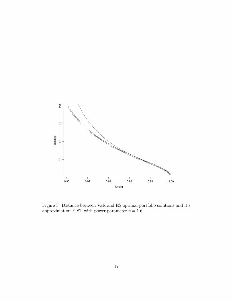
The proof is given in the appendixIn Figure 3 we give the graph of the distance between VaR and TCE

optimal portfolio solutions (up to the constant C) and its approximationobtained for the data considered in the previous section when the level q ↑ 1and power parameter p1 = 1.6.

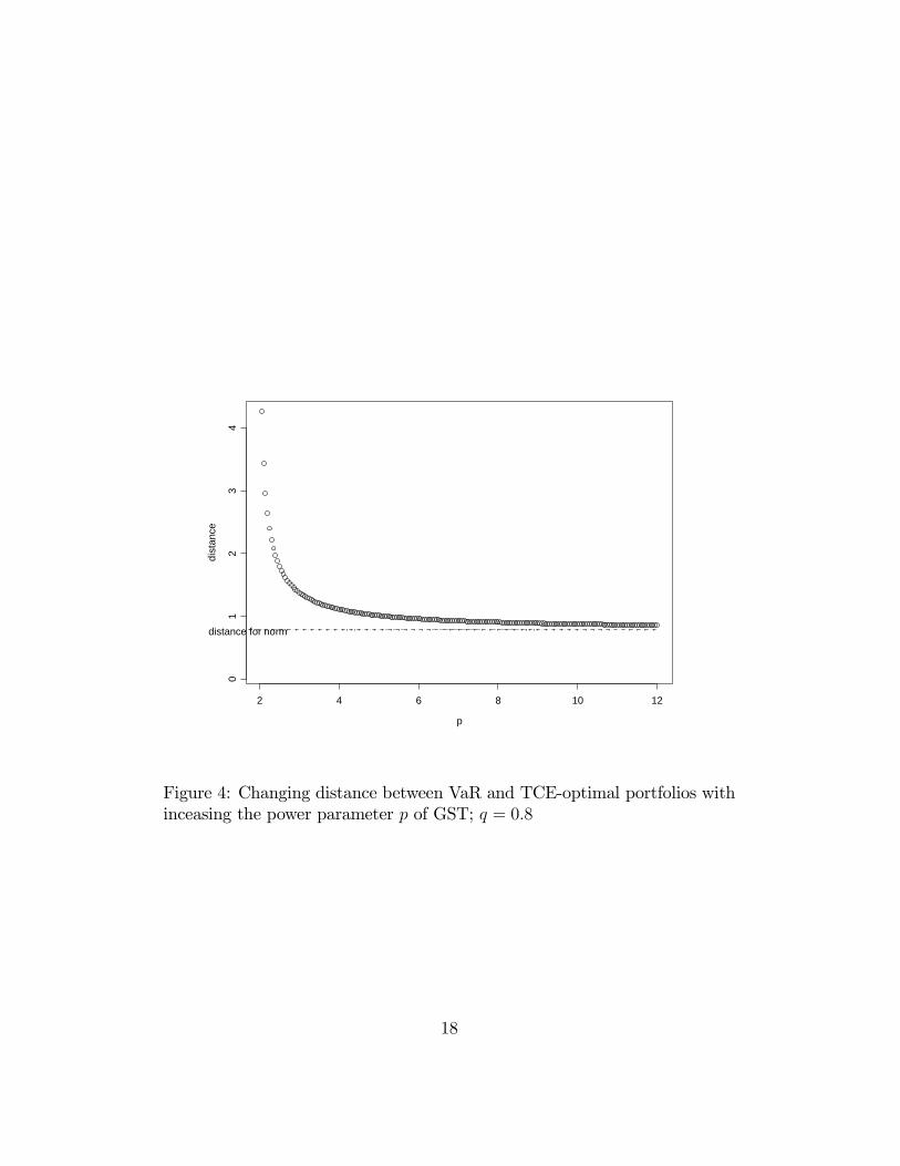
Figure 4 represents the graph of the distance between VaR and TCE-optimal portfolios when the power parameter p of the underlying GST dis-tribution increases. The probability level of the VaR and TCE risk measuresin the graph is equal to q = 0.8.

5 Conclusions

The problem of optimal portfolio selection with translation-invariant andpositive-homogeneous (TIPH) risk measures with a multivariate ellipticaldistribution of returns reduces to the minimization of a combination of alinear and a square root quadratic functionals. For the case when short sellingis possible we found the explicit closed-form solution of the problem, whichis different from that of mean-variance (MV) optimal portfolio selection.The analytical results we obtained were applied for the investigation of the

16

level q

dist

ance

0.90 0.92 0.94 0.96 0.98 1.00

0.5

1.0

1.5

2.0

Figure 3: Distance between VaR and ES optimal portfolio solutions and it’sapproximation; GST with power parameter p = 1.6

17

p

dist

ance

2 4 6 8 10 12

01

23

4

distance for norm

Figure 4: Changing distance between VaR and TCE-optimal portfolios withinceasing the power parameter p of GST; q = 0.8

18

distance between VaR and TCE -optimal solutions and illustrated with dataof weekly returns of 10 stocks from NASDAQ/Computers.

The importance of the results that were obtained is twofold: they give usnot only the analytical closed form for VaR, TCE, TSD (and other) optimalsolutions, but also the lower boundaries for q−levels guaranteeing the exis-tence of the solutions. Moreover, the advantages of an analytical solution tothe problem over numerical optimization algorithms include not only savingcomputer time (for optimal portfolio selection from some stock indexes suchas NASDAQ, having thousands of components, the numerical algorithmsmay consume a huge amount of computer time even with modern comput-ers), but also in the possibility of analyzing different aspects of the model;like the stability of the solution with respect to perturbation of the parame-ters of the system. As a direct application of the proposed explicit analyticresults we investigate how the lower boundary of VaR and TCE probabilitylevel changes when the power parameter of the generalized Student-t (GST)underlying distribution of the stock returns is increased.

6 Appendix

Proof Theorem 2:The exact expression for distance d, as written in (4.2), is obtained from

Theorem 1, formula (2.10), taking into account that 0 ≤ Zq < λq for q≥ 1/2. The constant C is equal to that given in (4.1). Further, from (4.2)one obtains straightforwardly

d =λ2q − Z2q

√Z2q − U2

√λ2q − U2(

√Z2q − U2 +

√λ2q − U2)

C → 0, q → 1,

because Zq, λq →∞, when q → 1. Further one can write

d =1

√Z2q − U2

(1− 1√

1 + αq)C,

where αq is defined in (4.5). If (4.3) holds, by L’Hospital’s rule we obtain

limq→1

Zqδq

= limq→1

Zq(1− q)∫∞

ZqFZ (z) dz

= limq→1

dZqdq

(1− q)− Zq−(1− q)dZq

dq

= limq→1

(−1 + Zq

(1− q)dZqdq

).

(6.6)

19

As FZ(Zq) = q, by the of implicit function theorem we have

dZqdq

= fZ(Zq)−1, (6.7)

recalling that

fZ(z) = c1g1(1

2z2) (6.8)

is the density of standardized univariate random variable Z.Using L’Hospital’srule again we obtain

limq→1

Zqc1g1(12Z2q )

(1− q) = − limq→1

dZqdq

[c1g1(1

2Z2q ) + Z

2q c1g

′

1(1

2Z2q )].

Then, taking into account (6.7), (6.8) and condition (4.3), we get

limq→1

Zqc1g1(12Z2q )

(1− q) = l − 1.

Substituting this into (6.6) and using again (6.7) yields

limq→1

δqZq

=1

l − 2,

and consequently (4.5). A Taylor expansion around the limit of αq, q → 1,which is equal to 2l−3

(l−2)2, provides (4.4). To prove item 3 we note that if

X ∼ tn (µ,Σ;p, kn,p) , the univariate marginal X1 ∼ t1(µ1, σ21, p1, k1,p1), p1 =p − (n − 1)/2 (see Landsman and Sherris (2007), Theorem 1). Then from(3.3) we obtain that

gn (u) = (1 + u/kn,p)−p , n = 1, 2, ...

and

J(u) = − d

dulog g1(u) =

p1(1 + u/k1,p1)

p1k1,p1.

Thus the limit l exists and l = 2p1. For a normal distribution, J(u) = u andthen l =∞ and αq → 0 when q → 1.

20

References

[1] Artzner, P., Delbaen, F., Eber, J.M., and Heath, D. (1999). "CoherentMeasures of Risk". Mathematical Finance ,9, 203-228.

[2] Avriel, M. (1976). Nonlinear Programming: Analysis and Methods.Prentice-Hall. Englewood Cliffs.

[3] Bingham, N.H. and Kiesel, R. (2002) ”Semi-Parametric Modelling inFinance: Theoretical Foundations,” Quantitative Finance,2, 241-250.

[4] Boyd, Stephen P, Vandenberghe, L. (2004). Convex optimization. Cam-bridge, UK.

[5] Boyle, P.P, Cox, S.H,...[et. al]. Financial Economics: With Applicationsto Investments, Insurance and Pensions, Actuarial Foundation, Schaum-burg, 1998

[6] Bühlmann, H. (1970). Mathematical Models in Risk Theory, Springer-Verlag, NY.

[7] Fang, K.T., Kotz, S. and Ng, K.W. (1990). Symmetric Multivariate andRelated Distributions London: Chapman & Hall.

[8] Furman, E. & Landsman, Z. (2006). Tail variance premium with appli-cations for elliptical portfolio of risks, ASTIN Bulletin 36, 2, 433-462.

[9] Landsman, Z. (2004). On the generalization of Esscher and variancepremiums modified for the elliptical family of distributions, Insurance:Mathematics and Economics, 35, 563-579.

[10] Landsman, Z. (2006). "On the generalization of Stein’s Lemma for el-liptical class of distributions". Statistics & Probability Letters. 76, 1012-1016.

[11] Landsman, Z. (2008a). "Minimization of the root of a quadratic func-tional under an affine equality constraint". Journal of Computationaland Applied Mathematics. 216, 319 — 327.

[12] Landsman, Z. (2008b). "Minimization of the root of a quadratic func-tional under a system of affine equality constraints with application to

21

portfolio management". Journal of Computational and Applied Mathe-matics, 220, 739 — 748

[13] Landsman, Z and Sherris, M. (2007). "An actuarial Premium PricingModel for Non-Normal Insurance and Financial Risks in IncompleteMarkets". North American Actuarial Journal , 11, 1, 119-135.

[14] Landsman, Z. and Valdez, E. (2003). "Tail Conditional Expectations forElliptical Distribution", North American Actuarial Journal, 7, 4, 55-71

[15] Landsman, Z. and Valdez, E. (2005) “Tail Conditional Expectation forExponential Dispersion Models,” ASTIN Bulletin, 35, 1, 189-209.

[16] Luenberger, D. G. (1984) The Linear and Nonlinear Programming,Addison-Wesley, CA

[17] Markowitz, H. M (1952). "Portfolio selection", Journal of Finance, 7,77—91.

[18] Merton, R. C. 1972. "An analytic derivation of the efficient portfoliofrontier". Journal of Financial Quantitative Analysis. 7, 1851-1872.

[19] McNeil, A.,J., Frey, R., Embrechts, P. (2005). Quantitative Risk Man-agement. Princeton University Press, Princeton.

[20] Muirhead, R.J. (1982).Aspects of Multivariate Statistical Theory, Wiley,NY

[21] Owen, J. and Rabinovitch, R. (1983), On the Class of Elliptical Distrib-utions and their Applications to the Theory of Portfolio Choice, Journalof Finance, 38, 3, 745-752.

[22] Roberts, A.W and Varberg, D.E.(1973). Convex Functions. AcademicPress, NY

[23] Steinbach, M.C. (2001). "Markowitz Revisited: Mean-Variance Modelsin Financial Portfolio Analysis". SIAM Review, 43, 1, 31-85.

[24] Wang, S. (1995). "Insurance pricing and increased limits ratemakingby proportional hazard transforms", Insurance: Mathematics and Eco-nomics, 17, 43-54.

22

[25] Wang, S. (1996). "Premium Calculation by Transforming the Layer Pre-mium Density", Astin Bulletin, 26, 71-92.

23