CLIMATE RESEARCHClim Res

Vol. 33: 27–41, 2006 Published December 21

1. INTRODUCTION

Forecasts of climate fluctuations with a seasonal(i.e. several months) lead-time are possible becausethe atmosphere responds to the more slowly varyingocean and land surfaces, an example being climatefluctuations associated with the El Niño-SouthernOscillation (ENSO) in the tropical Pacific. Severalclimate prediction centers routinely issue prob-abilistic seasonal forecasts based on dynamic general

circulation models (GCMs) that model the physicalprocesses and dynamic interactions of the global cli-mate system in response to sea and land surfaceboundary forcing. Probabilistic forecasts are obtainedfrom ensembles of GCM integrations initialized withdifferent atmospheric conditions. Periodic regionalclimate outlook forums in Africa and Latin Americahave issued seasonal climate forecasts targetingagriculture and other climate-sensitive sectors since1997.

© Inter-Research 2006 · www.int-res.com*Email: jhansen@iri.columbia.edu

Translating climate forecasts into agriculturalterms: advances and challenges

James W. Hansen1,*, Andrew Challinor2, Amor Ines3, Tim Wheeler4, Vincent Moron1

1International Research Institute for Climate and Society, 61 Route 9W, Palisades, New York 10964-8000, USA2Department of Meteorology, University of Reading, Reading RG6 6BB, UK

3Department of Biological and Agricultural Engineering, Texas A&M University, College Station, Texas 77843, USA4Department of Agriculture, University of Reading, PO Box 236, Reading RG6 6AR, UK

ABSTRACT: Seasonal climate prediction offers the potential to anticipate variations in crop productionearly enough to adjust critical decisions. Until recently, interest in exploiting seasonal forecasts fromdynamic climate models (e.g. general circulation models, GCMs) for applications that involve cropsimulation models has been hampered by the difference in spatial and temporal scale of GCMs andcrop models, and by the dynamic, nonlinear relationship between meteorological variables and cropresponse. Although GCMs simulate the atmosphere on a sub-daily time step, their coarse spatialresolution and resulting distortion of day-to-day variability limits the use of their daily output. Cropmodels have used daily GCM output with some success by either calibrating simulated yields orcorrecting the daily rainfall output of the GCM to approximate the statistical properties of historicobservations. Stochastic weather generators are used to disaggregate seasonal forecasts either byadjusting input parameters in a manner that captures the predictable components of climate, or byconstraining synthetic weather sequences to match predicted values. Predicting crop yields, simulatedwith historic weather data, as a statistical function of seasonal climatic predictors, eliminates the needfor daily weather data conditioned on the forecast, but must often address poor statistical properties ofthe crop–climate relationship. Most of the work on using crop simulation with seasonal climate fore-casts has employed historic analogs based on categorical ENSO indices. Other methods based on clas-sification of predictors or weather types can provide daily weather inputs to crop models conditionedon forecasts. Advances in climate-based crop forecasting in the coming decade are likely to includemore robust evaluation of the methods reviewed here, dynamically embedding crop models within cli-mate models to account for crop influence on regional climate, enhanced use of remote sensing, andresearch in the emerging area of ‘weather within climate.’

KEY WORDS: Yield forecasting · General circulation model · GCM · Crop simulation model ·Stochastic weather generator · Calibration · Probabilistic forecasting

Resale or republication not permitted without written consent of the publisher

OPENPEN ACCESSCCESS

Clim Res 33: 27–41, 2006

By providing advance information early enough toadjust critical agricultural decisions, seasonal climateprediction appears to offer significant potential to con-tribute to the efficiency of agricultural management,and to food and livelihood security. However, there is agap between the information that comes routinelyfrom climate prediction centers and regional climateoutlook forums, and the needs of farmers and otheragricultural decision makers. Applications of climateforecasts within agriculture are concerned with im-pacts on production and environmental and economicoutcomes, and not with climate fluctuations per se. Iffarmers are to benefit from seasonal climate forecasts,the information must be presented in terms of produc-tion outcomes at a scale relevant to their decisions,with uncertainties expressed in transparent, proba-bilistic terms. Market and food security early warningapplications also need to translate climate informationinto production outcomes, but generally at a differentspatial scale and lead time.

Stimulated in part by the socioeconomic conse-quences and widespread public awareness associatedwith the very strong 1997–1998 El Niño event, interestin agricultural application of seasonal climate predic-tion gained momentum in the late 1990s. Researchefforts have used dynamic, process-oriented cropsimulation models as a means of translating climateforecasts into crop yield prediction and as a basis forevaluating potential management responses. This workhas depended heavily on analog methods based oncategorical indicators of the ENSO (e.g. Jones et al.2000, Meinke & Hochman 2000, Podestá et al. 2002,Everingham et al. 2003, Meinke & Stone 2005). TropicalPacific sea surface temperatures (SSTs) or the SouthernOscillation Index (SOI) are classified into a small num-ber of categories or ‘phases.’ Weather data from pastyears, with the same predictor category as the forecastperiod, are used as input to crop models. The set ofsimulated outcomes provides a probabilistic forecast.Through the 1990s, this work seldom attempted to in-corporate operational dynamic climate forecasts, andborrowed little from the concurrent development ofmethodology for translating climate change scenarios(often based on the same GCMs used for seasonal fore-casting) into estimates of agricultural impacts. Despitestrong interest in using GCM-based seasonal forecastsfor agricultural applications, progress has—until re-cently—been slow, due in part to limited accessibility ofGCM results, methodological challenges related tothe spatio-temporal scale mismatch between GCMsand crop model requirements, and concerns aboutcharacterizing and interpreting forecast probabilities.

The 1997–1998 El Niño also stimulated debate aboutthe value of climate prediction to a range of societalproblems. One concern was that limited predictability

of crop yield response at the farm scale, early enoughto allow farmers to modify critical pre-planting deci-sions, might be a fundamental constraint to the use offorecasts by risk-averse farmers (Barrett 1998, Blench2003). The argument was based on 2 assumptions.(1) Variability of rainfall over small spatial scalesimplies that seasonal rainfall predictability is limited toregional spatial scales. (2) Because crop yield is not asimple function of seasonal total rainfall, the accumula-tion of errors going from seasonal climatic predictors(e.g. SSTs), to local seasonal means, to crop response,implies that predictions of effects such as crop re-sponse will be less accurate than predictions of climaticmeans. Recent research challenges these assumptions(Hansen 2005). Limited evidence suggests that muchof the skill of regional seasonal forecasts holds up at alocal scale (Gong et al. 2003), and that predictability ofcrop yield response can be as great or greater thanpredictability of seasonal climatic means (Cane et al.1994, Hansen et al. 2004).

Our objective here is to survey progress in translat-ing seasonal climate prediction into forecasts of agri-cultural production that are relevant to agriculturaldecision-making, through the integration of climatemodels with process-oriented agricultural simulationmodels. While most applications address crop or forageyields, relevant applications also include environmen-tal quality impacts (Mavromatis et al. 2002, Zhang2003). We highlight advances over the last decade, aswell as key challenges and emerging opportunities fac-ing us in the coming decade. Advances in the use ofseasonal climate forecasts with agricultural simulationmodels contribute to (1) translating climate forecastsinto more relevant information about impacts withinthe system being managed; (2) ex-ante assessment ofbenefit to motivate support and insights to target inter-ventions; and (3) guiding management responsesthrough the use of model-based systems that supportdiscussion and decision-making (Hansen 2005).

2. THE CLIMATE–CROP MODEL CONNECTIONPROBLEM

Operational seasonal climate forecasts are generallyissued as averages in time (≥ 3 mo) and space. Becauseof the effect of spatial and temporal averaging on therandom noise resulting from the chaotic nature of theatmosphere, the proportion of variability that is pre-dictable at a seasonal lead-time due to boundary forc-ing tends to increase with increasing spatial and tem-poral scale up to a point. Furthermore, computationalcapacity limits the spatial resolution of GCMs used forseasonal prediction to a fairly coarse grid scale, cur-rently on the order of 10 000 km2.

28

Hansen et al: Translating climate forecasts into agricultural terms

Crop production is a function of dynamic, nonlinearinteractions between weather, soil water and nutrientdynamics, management, and the physiology of thecrop. Relating predicted climatic variations, averagedin space and time, to crop response is not straightfor-ward. Crop response tends to be nonlinear and some-times non-monotonic over a realistic range of environ-mental variability. Furthermore, crops do not respondto conditions averaged through the growing season,but to dynamic interactions between weather, soilwater and nutrient dynamics, and the stage of cropdevelopment. In rainfed production systems, theinteraction between rainfall and the soil water balanceis particularly important. Crop characteristics, soilhydraulic and fertility properties, stresses, and man-agement mediate sensitivity to weather conditionswithin the growing season. Finally, a range of interact-ing weather variables mediates many aspects of cropgrowth and development. To capture the dynamic,nonlinear interactions between weather, soil water andnutrient dynamics, and physiology and phenology ofthe crop, process-oriented crop simulation modelstypically operate on a daily time step and a spatialscale of a homogeneous plot (although sampling theheterogeneity of soil, weather and management inputsallows simulated results to be interpreted at a rangeof scales).

Global and regional dynamic climate models operateon sub-daily time steps, but the spatial averaging thatoccurs within grid cells distorts the temporal variabilityof daily weather sequences (Osborn & Hulme 1997).Any distortion of daily weather variability can seri-ously bias crop model simulations (Semenov & Porter1995, Mearns et al. 1996, Riha et al. 1996, Mavromatis& Jones 1998a, Hansen & Jones 2000, Baron et al.2005). One of the most serious effects is a tendency toover-predict frequency of wet days and under-predicttheir mean intensity (Mearns et al. 1990, 1995, Mavro-matis & Jones 1998a, Goddard et al. 2001). The direc-tion of resulting crop model error cannot be easilyanticipated. On the one hand, when canopy cover isincomplete and evaporative demand is high, frequentlow-intensity showers do not recharge soil waterreserves in deeper layers, but favor increased evapora-tion from the soil surface, thereby increasing waterstress (de Wit & van Keulen 1987). On the other hand,increasing the frequency of rainfall events tends toreduce the duration of dry periods between rainevents, thereby reducing water stress (Carbone 1993,Mearns et al. 1996, Riha et al. 1996, Hansen & Jones2000). Baron et al. (2005) suggested that millet inSahelian West Africa can use only intermediate (10 to30 mm d–1) rainfall events efficiently, as smaller rainfallevents are largely lost to soil evaporation while moreintense rainfall is lost to runoff and drainage. Aggre-

gating daily rainfall from 17 stations to a scale typicalof GCMs resulted in the over-prediction of mean simu-lated yields by 28%, due to overestimation of rainfallefficiency associated with an increased proportion ofintermediate rainfall events in the aggregated series.

3. ADVANCES IN METHODS FOR LINKINGCLIMATE AND CROP MODELS

A range of methods for linking crop simulation mod-els to seasonal climate forecast models have beenadvanced. We survey recent advances in methodologyunder 4 categories (Hansen & Indeje 2004): (1) cropsimulation with daily climate model output, (2) use ofsynthetic daily weather conditioned on climate fore-casts, (3) statistical prediction of crop response simu-lated with historic weather, and (4) classification andanalog methods. The discussion includes some meth-ods that have been developed for simulating agricul-tural impacts of GCM-based climate change scenarios,but that appear to have potential for yield predictionbased on seasonal forecasts.

The applications include both field scales with afocus on farmer decisions, and regional scales that arerelevant to food security early warning and marketapplications. Simulating crop response to weather ataggregate scales has progressed in 2 parallel direc-tions. Process-oriented crop models that have beendeveloped for field-scale applications can be scaled upby (1) representing heterogeneity of environment andmanagement with spatial data sets, (2) probabilisticsampling of environmental variables, (3) calibration ofmodel input parameters or (4) model outputs againstreported crop data at the scale of interest (Hansen &Jones 2000). The alternative is to simulate aggregatecrop response with models that are simplified to oper-ate on a large spatial scale while maintaining enoughcomplexity to capture the major components of yieldresponses to climate variability. Examples rangefrom water-satisfaction indices based on simplifiedsoil water balance (Frere & Popov 1979), to process-oriented models such as the General Large-Area Model(GLAM) designed to simulate annual crop yields at aGCM grid scale (Challinor et al. 2004, 2005).

3.1. Crop simulation with daily climate model output

Despite the tendency of GCMs to seriously distort dailyvariability, daily GCM output has been used as input tocrop models with some success through either thecalibration of yields simulated with raw GCM output,simple rescaling to correct GCM mean bias, or theapplication of a more sophisticated simultaneous cor-

29

Clim Res 33: 27–41, 2006

rection of GCM rainfall frequency and intensity.Mavromatis & Jones (1998b) used uncorrected dailyoutput from runs of the HadCM2 GCM as input to theCERES-Wheat model for studying potential impacts ofclimate change on regional winter wheat production inFrance. Yields simulated with GCM weather dataapproximated mean yields simulated with observedweather during the past century, and captured a yieldtrend associated with the recent trend in observedtemperature, but under-represented year-to-year vari-ability. Challinor et al. (2005) used daily meteorologi-cal variables from 9 seasonal hindcast runs from eachof 7 GCMs as input to the GLAM crop model to predictgroundnut yields over western India. Historic districtgroundnut yields aggregated to the GCM grid scaleshowed lowest overall prediction error when simulatedyields were calibrated to observed district yields,regardless of whether mean bias in the GCM outputwas first corrected.Studies (Mavromatis & Jones 1998a, Hansen & Jones2000, Baron et al. 2005) have demonstrated the impacton day-to-day variability and crop simulation results,of aggregating daily weather data to a spatial scaletypical of GCM grid cells and operational seasonalforecasts. Several approaches have been proposed todisaggregate GCM output and other area-averageddaily data sources (e.g. satellite rainfall estimates) tothe scale of individual stations in a manner that cor-rects the biases. The simplest option for calibratingdaily GCM output to match observed mean localclimate is to apply a simple shift (e.g. Ines & Hansen2006). An additive shift is appropriate for temperatureand solar radiation. A multiplicative adjustment, e.g.

x ’i = xi,GCM xobs �xGCM (1)

is more appropriate for precipitation, as it preserves thesequence of zero values associated with dry days,where xi,GCM and x’i refer to raw and calibrated GCMrainfall on day i, respectively, and xobs and xGCM arelong-term mean observed and simulated rainfall, re-spectively, for a given time of year. However, becausethe multiplicative shift corrects total rainfall by adjust-ing intensity and not frequency, it cannot correct theobserved tendency of GCMs to over-predict frequencyand under-predict mean intensity (see Section 2).

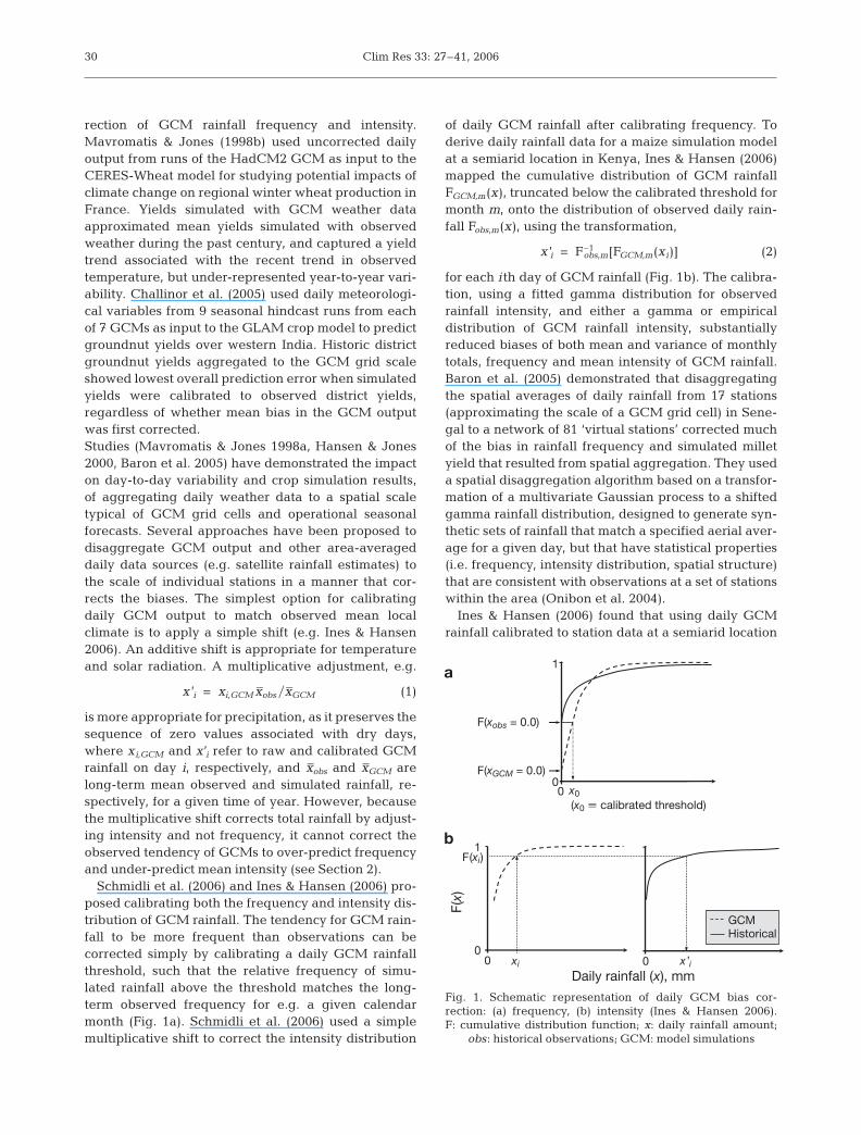
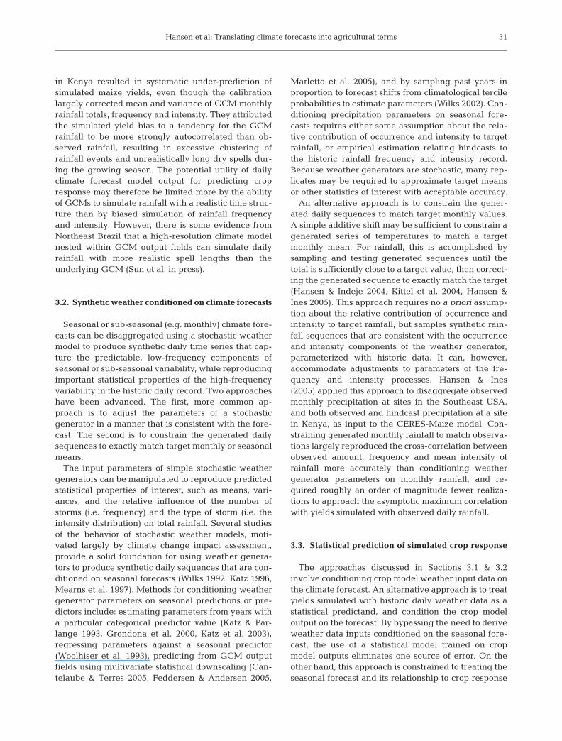
Schmidli et al. (2006) and Ines & Hansen (2006) pro-posed calibrating both the frequency and intensity dis-tribution of GCM rainfall. The tendency for GCM rain-fall to be more frequent than observations can becorrected simply by calibrating a daily GCM rainfallthreshold, such that the relative frequency of simu-lated rainfall above the threshold matches the long-term observed frequency for e.g. a given calendarmonth (Fig. 1a). Schmidli et al. (2006) used a simplemultiplicative shift to correct the intensity distribution

of daily GCM rainfall after calibrating frequency. Toderive daily rainfall data for a maize simulation modelat a semiarid location in Kenya, Ines & Hansen (2006)mapped the cumulative distribution of GCM rainfallFGCM,m(x), truncated below the calibrated threshold formonth m, onto the distribution of observed daily rain-fall Fobs,m(x), using the transformation,

x ’i = F–1obs,m[FGCM,m(xi)] (2)

for each i th day of GCM rainfall (Fig. 1b). The calibra-tion, using a fitted gamma distribution for observedrainfall intensity, and either a gamma or empiricaldistribution of GCM rainfall intensity, substantiallyreduced biases of both mean and variance of monthlytotals, frequency and mean intensity of GCM rainfall.Baron et al. (2005) demonstrated that disaggregatingthe spatial averages of daily rainfall from 17 stations(approximating the scale of a GCM grid cell) in Sene-gal to a network of 81 ‘virtual stations’ corrected muchof the bias in rainfall frequency and simulated milletyield that resulted from spatial aggregation. They useda spatial disaggregation algorithm based on a transfor-mation of a multivariate Gaussian process to a shiftedgamma rainfall distribution, designed to generate syn-thetic sets of rainfall that match a specified aerial aver-age for a given day, but that have statistical properties(i.e. frequency, intensity distribution, spatial structure)that are consistent with observations at a set of stationswithin the area (Onibon et al. 2004).

Ines & Hansen (2006) found that using daily GCMrainfall calibrated to station data at a semiarid location

30

GCMHistorical

0Daily rainfall (x), mm

1

00

F(x)

F(xi)

xi x ’i

1

F(xobs = 0.0)

F(xGCM = 0.0)

00

(x0 � calibrated threshold)x0

b

a

Fig. 1. Schematic representation of daily GCM bias cor-rection: (a) frequency, (b) intensity (Ines & Hansen 2006).F: cumulative distribution function; x: daily rainfall amount;

obs: historical observations; GCM: model simulations

Hansen et al: Translating climate forecasts into agricultural terms

in Kenya resulted in systematic under-prediction ofsimulated maize yields, even though the calibrationlargely corrected mean and variance of GCM monthlyrainfall totals, frequency and intensity. They attributedthe simulated yield bias to a tendency for the GCMrainfall to be more strongly autocorrelated than ob-served rainfall, resulting in excessive clustering ofrainfall events and unrealistically long dry spells dur-ing the growing season. The potential utility of dailyclimate forecast model output for predicting cropresponse may therefore be limited more by the abilityof GCMs to simulate rainfall with a realistic time struc-ture than by biased simulation of rainfall frequencyand intensity. However, there is some evidence fromNortheast Brazil that a high-resolution climate modelnested within GCM output fields can simulate dailyrainfall with more realistic spell lengths than theunderlying GCM (Sun et al. in press).

3.2. Synthetic weather conditioned on climate forecasts

Seasonal or sub-seasonal (e.g. monthly) climate fore-casts can be disaggregated using a stochastic weathermodel to produce synthetic daily time series that cap-ture the predictable, low-frequency components ofseasonal or sub-seasonal variability, while reproducingimportant statistical properties of the high-frequencyvariability in the historic daily record. Two approacheshave been advanced. The first, more common ap-proach is to adjust the parameters of a stochasticgenerator in a manner that is consistent with the fore-cast. The second is to constrain the generated dailysequences to exactly match target monthly or seasonalmeans.

The input parameters of simple stochastic weathergenerators can be manipulated to reproduce predictedstatistical properties of interest, such as means, vari-ances, and the relative influence of the number ofstorms (i.e. frequency) and the type of storm (i.e. theintensity distribution) on total rainfall. Several studiesof the behavior of stochastic weather models, moti-vated largely by climate change impact assessment,provide a solid foundation for using weather genera-tors to produce synthetic daily sequences that are con-ditioned on seasonal forecasts (Wilks 1992, Katz 1996,Mearns et al. 1997). Methods for conditioning weathergenerator parameters on seasonal predictions or pre-dictors include: estimating parameters from years witha particular categorical predictor value (Katz & Par-lange 1993, Grondona et al. 2000, Katz et al. 2003),regressing parameters against a seasonal predictor(Woolhiser et al. 1993), predicting from GCM outputfields using multivariate statistical downscaling (Can-telaube & Terres 2005, Feddersen & Andersen 2005,

Marletto et al. 2005), and by sampling past years inproportion to forecast shifts from climatological tercileprobabilities to estimate parameters (Wilks 2002). Con-ditioning precipitation parameters on seasonal fore-casts requires either some assumption about the rela-tive contribution of occurrence and intensity to targetrainfall, or empirical estimation relating hindcasts tothe historic rainfall frequency and intensity record.Because weather generators are stochastic, many rep-licates may be required to approximate target meansor other statistics of interest with acceptable accuracy.

An alternative approach is to constrain the gener-ated daily sequences to match target monthly values.A simple additive shift may be sufficient to constrain agenerated series of temperatures to match a targetmonthly mean. For rainfall, this is accomplished bysampling and testing generated sequences until thetotal is sufficiently close to a target value, then correct-ing the generated sequence to exactly match the target(Hansen & Indeje 2004, Kittel et al. 2004, Hansen &Ines 2005). This approach requires no a priori assump-tion about the relative contribution of occurrence andintensity to target rainfall, but samples synthetic rain-fall sequences that are consistent with the occurrenceand intensity components of the weather generator,parameterized with historic data. It can, however,accommodate adjustments to parameters of the fre-quency and intensity processes. Hansen & Ines(2005) applied this approach to disaggregate observedmonthly precipitation at sites in the Southeast USA,and both observed and hindcast precipitation at a sitein Kenya, as input to the CERES-Maize model. Con-straining generated monthly rainfall to match observa-tions largely reproduced the cross-correlation betweenobserved amount, frequency and mean intensity ofrainfall more accurately than conditioning weathergenerator parameters on monthly rainfall, and re-quired roughly an order of magnitude fewer realiza-tions to approach the asymptotic maximum correlationwith yields simulated with observed daily rainfall.

3.3. Statistical prediction of simulated crop response

The approaches discussed in Sections 3.1 & 3.2involve conditioning crop model weather input data onthe climate forecast. An alternative approach is to treatyields simulated with historic daily weather data as astatistical predictand, and condition the crop modeloutput on the forecast. By bypassing the need to deriveweather data inputs conditioned on the seasonal fore-cast, the use of a statistical model trained on cropmodel outputs eliminates one source of error. On theother hand, this approach is constrained to treating theseasonal forecast and its relationship to crop response

31

Clim Res 33: 27–41, 2006

as essentially static within a growing season. Whileour review focuses on forecasting using dynamic cropmodels, statistical prediction from GCM output fieldshas also been applied to remotely-sensed forage vege-tation indices (Indeje et al. 2006) and de-trended cropproduction statistics (G. Baigorria, pers. comm.).

Crops tend to show non-linear, non-monotonic rela-tionships with their environment over some range ofvariability, complicating direct statistical prediction.Other potential problems that violate assumptions ofordinary least-squares regression include residuals thatare non-normally distributed, and residual variancethat varies systematically with predictor. Approachesto dealing with these challenges include nonlinearregression, linear regression following normalizingtransformation, generalized linear models, and non-parametric models.

As an example of nonlinear regression, Hansen &Indeje (2004) predicted simulated maize yields at asite in southern Kenya as a cross-validated function ofthe first principal component of GCM rainfall overthe region. They chose a Mitscherlich function,

y = a + b (1 – e–cx) (3)

based on its widespread use for modeling plant re-sponse to water and other growth factors. Diagnosticsshowed some evidence that residual variance variedsystematically with the predictor—a mild violation ofthe assumptions of least-squares regression.

Where the relationship between predicted climatevariations and simulated crop response is only weaklynonlinear, transforming the predictand and potentiallythe predictor may correct nonlinearity, non-normalityof regression residuals and heterogeneity of residualvariance sufficiently to permit ordinary linear regres-sion. Hansen et al. (2004) used an optimal power series(Box & Cox 1964) transformation to normalize mildly-skewed simulated yield distributions before predictingdistrict and state wheat yields, simulated with ob-served antecedent rainfall and historic within-seasonrainfall, as a linear function of a regional GCM rainfallpredictor in northeastern Australia. Such data transfor-mations may not handle non-monotonic crop–climaterelationships or extreme departures from linearityand normality sufficiently to permit ordinary least-squares linear regression. Because aggregating inspace smoothes year-to-year variability of crop yieldsand, by the Central Limit Theorem, reduces depar-tures from normality, we hypothesize that linearregression, possibly with a normalizing transforma-tion, may be more suited for yield forecasts at anaggregate scale than at a field scale. Generalizedlinear models (McCullagh & Nelder 1989), designed toextend the benefits of linear regression where data arenot normally distributed, are a promising alternative

that to our knowledge has not yet been applied topredicting crop yields in response to forecast seasonalclimate variations.

3.4. Classification and analog methods

Several practical benefits account for the continueddominance of the historical analog approach for cropyield prediction described in Section 1 (Meinke &Stone 2005). The approach is easily adapted to anyspatial or temporal scale for which historic data areavailable. If the predictors used provide any predictiveinformation about higher-order variations beyond sea-sonal climatic means that influence crop response,analog years will incorporate that predictability intocrop simulations. Distributions derived from analogswill account for any differences in dispersion, in addi-tion to mean shifts associated with different statesof ENSO. Finally and perhaps most important, dis-tributions of outcomes simulated for the analog yearsassociated with a given category provide an intuitivemeans of estimating and communicating forecastuncertainty in probabilistic terms.

The analog method also has important limitations.Confidence, artificial forecast skill and biased estima-tion of uncertainty are concerns in those cases whenthe number of categories and limited record lengthlead to small sample sizes within each category (Sec-tion 4.3). More important, analogs based on ENSO orother empirical indices do not necessarily capture thebest that climate science or operational forecast sys-tems have to offer. While statistical climate predictionmodels have generally approached their predictivelimits, dynamic climate forecast models, which inte-grate global sea and land surface forcing, sometimesoutperform the best statistical models, and are expectedto improve with improvements in models, data assimi-lation, computer capacity and post-processing meth-ods. Stone et al. (2000) proposed using the analogapproach with GCM output fields classified into dis-crete categories by cluster analysis.

The analog method described above treats each pastyear falling within the given predictor category asequally probable. It is a special case of a more generalset of methods based on classification of predictors orweather types. If there is a basis for predicting that thecoming season is more likely to resemble some pastyears than others, we can use the predicted probabili-ties to derive a probability-weighted forecast distribu-tion, or calculate weighted mean or other distributionstatistics. The common method of issuing operationalseasonal climate forecasts as shifted probabilities ofeach of the climatological terciles, can be used directlyto assign weights to analog years or to resample past

32

Hansen et al: Translating climate forecasts into agricultural terms

years in proportion to the forecast probabilities. Forexample, Everingham et al. (2002) and Bezuidenhout& Singles (2006) sampled analog years in proportionto tercile forecasts from the South African WeatherService to forecast sugarcane production.

The k-nearest neighbor (KNN) method selects andassigns probability weights to a subset of k past yearsbased on their similarity, in predictor state space, to agiven predictor state (Lall & Sharma 1996). Weights wj

of the k nearest neighbors, ordered on the basis of theirsimilarity to the value of the current predictor vector,are calculated as:

wj = ( j Σ ki =1

i –1)–1 (4)

where j and i are indices of the given historic year andthe other k nearest neighbor years, sorted by distance(i.e. closest = 1) from the current predictor vector. Forall j > k, wi is set to 0. Using the KNN method to sam-ple past seasons showed comparable results to othermethods that Hansen & Indeje (2004) tested for GCM-based maize prediction in Kenya. It has also been usedsuccessfully for predicting reservoir inflow from sea-sonal rainfall predictors in Northeast Brazil (DeSouza& Lall 2003). The KNN analog approach can also beapplied on shorter time steps to probabilistically sam-ple subsets of past weather observations based on thedegree of similarity of current and historical values of agiven feature vector that may include atmosphericindicators from SST-forced GCM outputs (Clark et al.2004, Gangopadhyay et al. 2005). Appropriate selec-tion criteria can preserve moments of the historical dis-tribution, as well as observed spatial and temporal cor-relations and correlations among variables.

Weather classification works in the same way, exceptthat historic data are clustered into discrete circulationpatterns or ‘weather types’ identified e.g. by clusteranalysis, that explain a substantial portion of the vari-ability and spatial patterns of rainfall. The ability of aGCM, driven by SSTs, to produce daily regional circu-lation patterns with realistic frequency and seasonalityprovides a basis for re-sampling historic local rainfallobservations based on similarity of circulation patternssimulated by a GCM and from reanalysis data usedas a proxy for observed wind fields (V. Moron, pers.comm.). Moron proposed a 2-stage sampling proce-dure. To capture interannual variability, past seasonsare sampled in proportion to their similarity to the cur-rent year based on the distance between principalcomponents of GCM and reanalysis wind fields. Dailyrainfall is then sampled randomly from the pool of dayswithin the sampled past seasons with the sameweather type that the GCM simulates. The process isrepeated for the sequence of daily weather types thatthe GCM simulates through the season. The approachpredicted a substantial portion of the year-to-year vari-

ability of rainfall characteristics (i.e. frequency, distrib-ution of dry and wet spells, seasonal total) with encour-aging skill and realism (V. Moron, pers. comm.). Itappears to be a promising approach to conditioningdaily weather data inputs on aspects of sub-seasonalvariability that are predictable at a seasonal lead time,but it has not yet been tested for crop simulation.

Non-homogeneous hidden Markov models (NHMM)integrate weather classification with stochastic weathermodels (Section 3.2) (Hughes & Guttorp 1994, Charles etal. 1999, Hughes et al. 1999). Observed rainfall patternsare classified into discrete types. Transition betweenstates in a NHMM is a Markov process, with transitionprobabilities conditioned on a given set of predictors.The NHMM is parameterized using daily sequences ofspatial weather patterns, and is capable of representingthe historic spatial structure in the weather patterns thatit simulates. The NHMM has been applied to disaggre-gating seasonal rainfall predictions (Robertson et al.2004, 2006), and to disaggregate rainfall data in spaceand time as input to a maize simulation model over theSoutheast USA (Robertson et al. in press).

4. UNCERTAINTY IN CLIMATE-BASED CROPFORECASTING

Transparent presentation of uncertainty in proba-bilistic terms is crucial to appropriate application ofadvance information, particularly when risk aversioninfluences decisions. Underestimating the uncertaintyof a forecast can lead to excessive responses that areinconsistent with a decision makers’ risk tolerance,and can damage the credibility of the forecast pro-vider, while overestimating uncertainty leads to under-confidence and lost opportunity to prepare for adverseconditions and take advantage of favorable conditions.

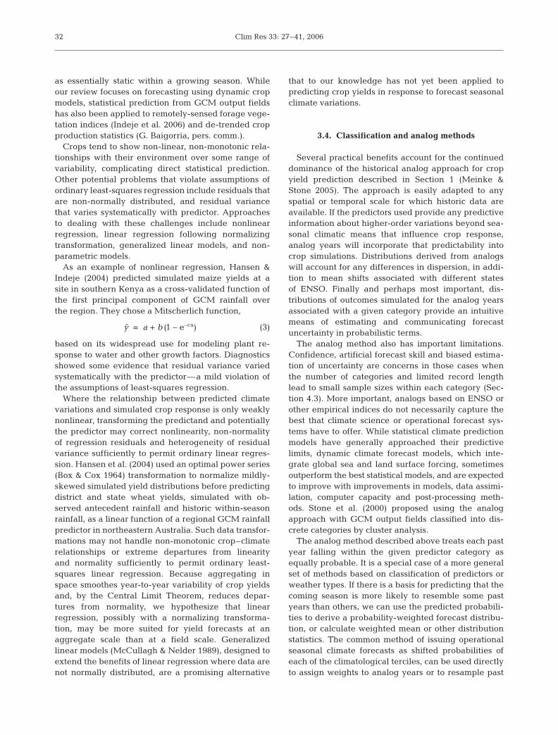
Climate variability and crop model (including input)error are the major sources of uncertainty in yield fore-casting. One way to characterize the uncertainty asso-ciated with climate variability is to simulate yields withantecedent weather observations up to a given forecastdate within the season for a current or hindcast year,and sample weather data for remainder of season fromall other years (Fig. 2). The resulting distribution ap-proximates the climatic component of uncertainty. In-formation about antecedent weather and its effect onstored soil moisture provides a degree of predictabilityof yields that increases as the forecast date advancesthrough the growing season, and an increasing propor-tion of weather data is observed, rather than sampled.Several proposed and operational crop-forecastingsystems integrate weather observations through thecurrent date with sampling from climatology for the re-mainder of the growing season (Thornton et al. 1997,

33

Clim Res 33: 27–41, 2006

Samba 1998, Bannayan et al. 2003, Lawless &Semenov 2005). Model error represents theremaining discrepancy between observedyields and yields simulated with observedweather.

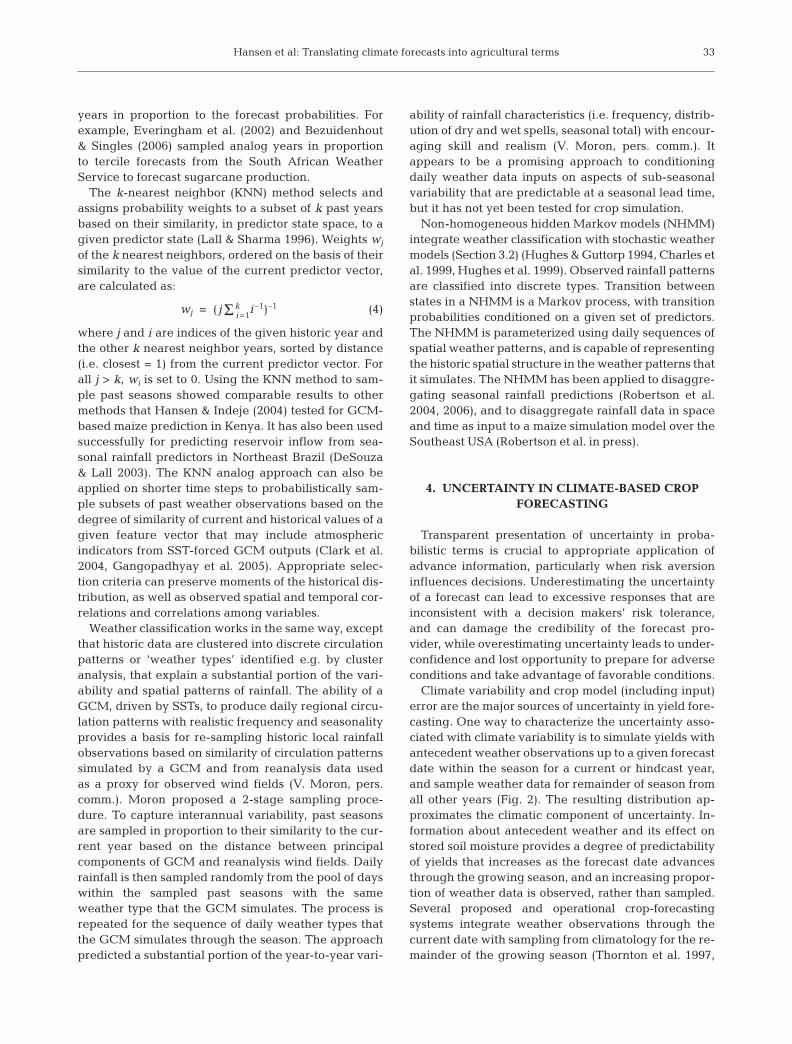
A skillful seasonal climate forecast reducesthe climatic component of uncertainty. Sincethe proportion of total uncertainty that is dueto climate decreases through the growingseason (Fig. 3a), the relative contribution ofseasonal forecasts to overall predictabilitytends to be greatest early in the season, andto decrease as the season progresses and anincreasing proportion of weather is observed,rather than predicted or sampled (Fig. 3b).On the other hand, reducing model errorthrough e.g. improved measurement or cali-bration of model inputs, updating crop statevariables based on remote sensing (see Sec-tion 5.2), or modeling additional yield-limit-ing factors, is likely to have a greater relativeimpact on overall uncertainty later in thegrowing season (Fig. 3c).

4.1. Deriving crop forecast distributions

Methods that have been developed forderiving and evaluating probabilistic cli-mate forecasts are generally relevant to fore-casts of agricultural impacts.

4.1.1. Forecast distributions from hindcast residuals

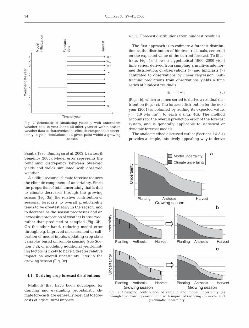
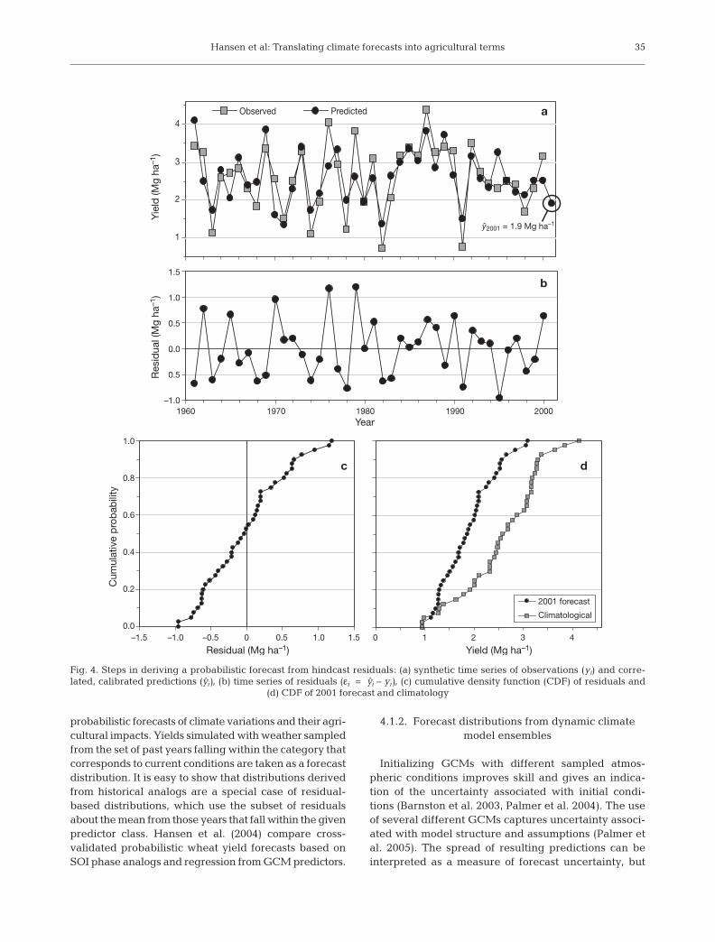
The first approach is to estimate a forecast distribu-tion as the distribution of hindcast residuals, centeredon the expected value of the current forecast. To illus-trate, Fig. 4a shows a hypothetical 1960–2000 yieldtime series, derived from sampling a multivariate nor-mal distribution, of observations (y) and hindcasts (y )calibrated to observations by linear regression. Sub-tracting predictions from observations yields a timeseries of hindcast residuals

εi = yi – yi (5)

(Fig. 4b), which are then sorted to derive a residual dis-tribution (Fig. 4c). The forecast distribution for the nextyear (2001) is obtained by adding its expected value,y = 1.9 Mg ha–1, to each ε (Fig. 4d). The methodaccounts for the overall prediction error of the forecastsystem, and is generally applicable to statistical ordynamic forecast models.

The analog method discussed earlier (Sections 1 & 3.4)provides a simple, intuitively appealing way to derive

34

Fore

cast

dat

e

Har

vest

Mod

elin

itial

izat

ion

Wea

ther

dat

a ye

ar

yk,1

yk,2

yk,3

...

yk,n

Time of year

123

...

k

...

n

Fig. 2. Schematic of simulating yields y with antecedentweather data in year k and all other years of within-seasonweather data to characterize the climatic component of uncer-tainty in yield simulations at a given point within a growing

season

Unc

erta

inty

Growing season

Growing season Growing season

Model uncertainty

Climate uncertainty

Unc

erta

inty

Unc

erta

inty

a

b

c

Planting Anthesis Harvest

Planting Anthesis Harvest Planting Anthesis Harvest

Planting Anthesis Harvest Planting Anthesis Harvest

Fig. 3. Changing contribution of climatic and model uncertainty (a)through the growing season; and with impact of reducing (b) model and

(c) climatic uncertainty

Hansen et al: Translating climate forecasts into agricultural terms

probabilistic forecasts of climate variations and their agri-cultural impacts. Yields simulated with weather sampledfrom the set of past years falling within the category thatcorresponds to current conditions are taken as a forecastdistribution. It is easy to show that distributions derivedfrom historical analogs are a special case of residual-based distributions, which use the subset of residualsabout the mean from those years that fall within the givenpredictor class. Hansen et al. (2004) compare cross-validated probabilistic wheat yield forecasts based onSOI phase analogs and regression from GCM predictors.

4.1.2. Forecast distributions from dynamic climatemodel ensembles

Initializing GCMs with different sampled atmos-pheric conditions improves skill and gives an indica-tion of the uncertainty associated with initial condi-tions (Barnston et al. 2003, Palmer et al. 2004). The useof several different GCMs captures uncertainty associ-ated with model structure and assumptions (Palmer etal. 2005). The spread of resulting predictions can beinterpreted as a measure of forecast uncertainty, but

35

1960 1970 1980 1990 2000Year

b

Cum

ulat

ive

pro

bab

ility

c

0

1.0

0.8

0.6

0.4

0.2

0.0

1.5

1.0

0.5

0.0

0.5

–1.0

–1.5 –1.0 –0.5 0 0.5 1.0 1.5 1 2 3 4

Yield (Mg ha–1)Residual (Mg ha–1)

Yie

ld (M

g ha

–1)

Res

idua

l (M

g ha

–1)

2001 forecast

Climatological

d

1

2

3

4Observed Predicted

y2001 = 1.9 Mg ha–1

a

Fig. 4. Steps in deriving a probabilistic forecast from hindcast residuals: (a) synthetic time series of observations (yi) and corre-lated, calibrated predictions (yi), (b) time series of residuals (εi = yi – yi), (c) cumulative density function (CDF) of residuals and

(d) CDF of 2001 forecast and climatology

Clim Res 33: 27–41, 2006

must be calibrated before forecasts can be expressedas probability distributions at a local scale (Doblas-Reyes et al. 2005, Palmer et al. 2005). However, there isnot yet a consensus about the most appropriate cali-bration method.

Probabilistic forecasting based on GCM ensemblescan be extended to crop yield prediction. For example,Challinor et al. (2005) used daily output from each mem-ber of both single- and multiple-GCM ensembles to as-sess probabilistic forecasts of observed district-levelgroundnut yields and crop failure in western India. Can-telaube & Terres (2005) used monthly climatic meanspredicted from each ensemble member, statisticallydownscaled and disaggregated to daily values, usinga stochastic weather generator (Feddersen & Andersen2005) to produce probability density estimates of griddedand national wheat yields across Europe.

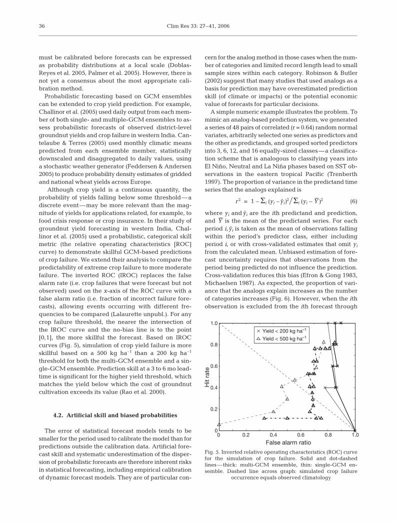
Although crop yield is a continuous quantity, theprobability of yields falling below some threshold—adiscrete event—may be more relevant than the mag-nitude of yields for applications related, for example, tofood crisis response or crop insurance. In their study ofgroundnut yield forecasting in western India, Chal-linor et al. (2005) used a probabilistic, categorical skillmetric (the relative operating characteristics [ROC]curve) to demonstrate skillful GCM-based predictionsof crop failure. We extend their analysis to compare thepredictability of extreme crop failure to more moderatefailure. The inverted ROC (IROC) replaces the falsealarm rate (i.e. crop failures that were forecast but notobserved) used on the x-axis of the ROC curve with afalse alarm ratio (i.e. fraction of incorrect failure fore-casts), allowing events occurring with different fre-quencies to be compared (Lalaurette unpubl.). For anycrop failure threshold, the nearer the intersection ofthe IROC curve and the no-bias line is to the point[0,1], the more skillful the forecast. Based on IROCcurves (Fig. 5), simulation of crop yield failure is moreskillful based on a 500 kg ha–1 than a 200 kg ha–1

threshold for both the multi-GCM ensemble and a sin-gle-GCM ensemble. Prediction skill at a 3 to 6 mo lead-time is significant for the higher yield threshold, whichmatches the yield below which the cost of groundnutcultivation exceeds its value (Rao et al. 2000).

4.2. Artificial skill and biased probabilities

The error of statistical forecast models tends to besmaller for the period used to calibrate the model than forpredictions outside the calibration data. Artificial fore-cast skill and systematic underestimation of the disper-sion of probabilistic forecasts are therefore inherent risksin statistical forecasting, including empirical calibrationof dynamic forecast models. They are of particular con-

cern for the analog method in those cases when the num-ber of categories and limited record length lead to smallsample sizes within each category. Robinson & Butler(2002) suggest that many studies that used analogs as abasis for prediction may have overestimated predictionskill (of climate or impacts) or the potential economicvalue of forecasts for particular decisions.

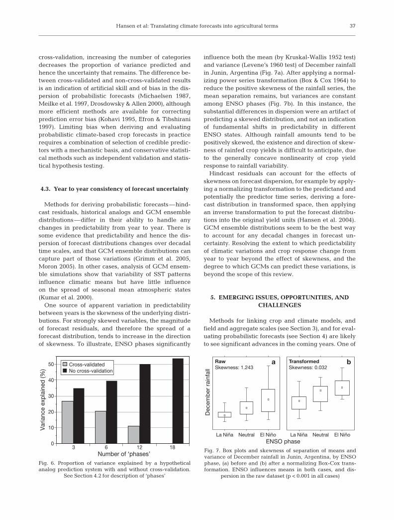
A simple numeric example illustrates the problem. Tomimic an analog-based prediction system, we generateda series of 48 pairs of correlated (r = 0.64) random normalvariates, arbitrarily selected one series as predictors andthe other as predictands, and grouped sorted predictorsinto 3, 6, 12, and 16 equally-sized classes—a classifica-tion scheme that is analogous to classifying years intoEl Niño, Neutral and La Niña phases based on SST ob-servations in the eastern tropical Pacific (Trenberth1997). The proportion of variance in the predictand timeseries that the analogs explained is

r2 = 1 – Σi (yi – yi)2�Σi (yi – Y––)2 (6)

where yi and yi are the ith predictand and prediction,and Y–– is the mean of the predictand series. For eachperiod i, yi is taken as the mean of observations fallingwithin the period’s predictor class, either includingperiod i, or with cross-validated estimates that omit yi

from the calculated mean. Unbiased estimation of fore-cast uncertainty requires that observations from theperiod being predicted do not influence the prediction.Cross-validation reduces this bias (Efron & Gong 1983,Michaelsen 1987). As expected, the proportion of vari-ance that the analogs explain increases as the numberof categories increases (Fig. 6). However, when the ithobservation is excluded from the ith forecast through

36

Hit

rate

1.0

0.8

0.6

0.4

0.2

00 0.2

Yield < 200 kg ha–1

Yield < 500 kg ha–1

0.4 0.6 0.8 1.0

False alarm ratio

Fig. 5. Inverted relative operating characteristics (ROC) curvefor the simulation of crop failure. Solid and dot-dashedlines—thick: multi-GCM ensemble, thin: single-GCM en-semble. Dashed line across graph: simulated crop failure

occurrence equals observed climatology

Hansen et al: Translating climate forecasts into agricultural terms

cross-validation, increasing the number of categoriesdecreases the proportion of variance predicted andhence the uncertainty that remains. The difference be-tween cross-validated and non-cross-validated resultsis an indication of artificial skill and of bias in the dis-persion of probabilistic forecasts (Michaelsen 1987,Meilke et al. 1997, Drosdowsky & Allen 2000), althoughmore efficient methods are available for correctingprediction error bias (Kohavi 1995, Efron & Tibshirani1997). Limiting bias when deriving and evaluatingprobabilistic climate-based crop forecasts in practicerequires a combination of selection of credible predic-tors with a mechanistic basis, and conservative statisti-cal methods such as independent validation and statis-tical hypothesis testing.

4.3. Year to year consistency of forecast uncertainty

Methods for deriving probabilistic forecasts—hind-cast residuals, historical analogs and GCM ensembledistributions—differ in their ability to handle anychanges in predictability from year to year. There issome evidence that predictability and hence the dis-persion of forecast distributions changes over decadaltime scales, and that GCM ensemble distributions cancapture part of those variations (Grimm et al. 2005,Moron 2005). In other cases, analysis of GCM ensem-ble simulations show that variability of SST patternsinfluence climatic means but have little influenceon the spread of seasonal mean atmospheric states(Kumar et al. 2000).

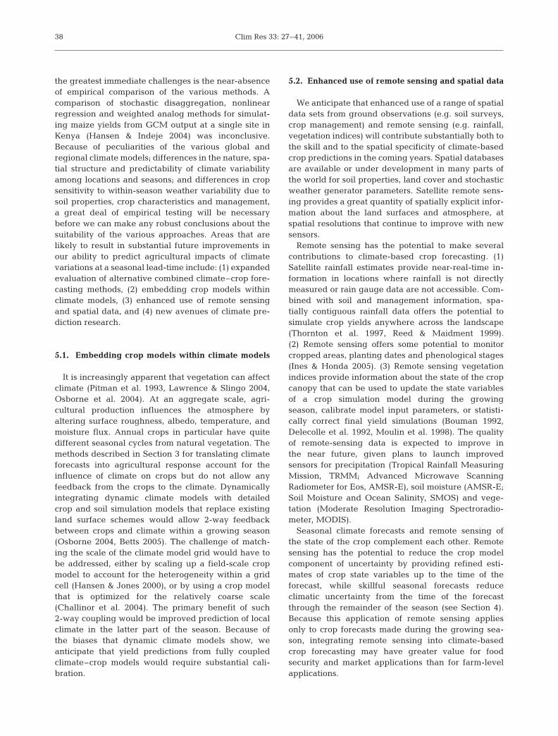
One source of apparent variation in predictabilitybetween years is the skewness of the underlying distri-butions. For strongly skewed variables, the magnitudeof forecast residuals, and therefore the spread of aforecast distribution, tends to increase in the directionof skewness. To illustrate, ENSO phases significantly

influence both the mean (by Kruskal-Wallis 1952 test)and variance (Levene’s 1960 test) of December rainfallin Junin, Argentina (Fig. 7a). After applying a normal-izing power series transformation (Box & Cox 1964) toreduce the positive skewness of the rainfall series, themean separation remains, but variances are constantamong ENSO phases (Fig. 7b). In this instance, thesubstantial differences in dispersion were an artifact ofpredicting a skewed distribution, and not an indicationof fundamental shifts in predictability in differentENSO states. Although rainfall amounts tend to bepositively skewed, the existence and direction of skew-ness of rainfed crop yields is difficult to anticipate, dueto the generally concave nonlinearity of crop yieldresponse to rainfall variability.

Hindcast residuals can account for the effects ofskewness on forecast dispersion, for example by apply-ing a normalizing transformation to the predictand andpotentially the predictor time series, deriving a fore-cast distribution in transformed space, then applyingan inverse transformation to put the forecast distribu-tions into the original yield units (Hansen et al. 2004).GCM ensemble distributions seem to be the best wayto account for any decadal changes in forecast un-certainty. Resolving the extent to which predictabilityof climatic variations and crop response change fromyear to year beyond the effect of skewness, and thedegree to which GCMs can predict these variations, isbeyond the scope of this review.

5. EMERGING ISSUES, OPPORTUNITIES, ANDCHALLENGES

Methods for linking crop and climate models, andfield and aggregate scales (see Section 3), and for eval-uating probabilistic forecasts (see Section 4) are likelyto see significant advances in the coming years. One of

37

50

40

30

20

10

03 6 12 18

Number of ‘phases’

Var

ianc

e ex

plai

ned

(%)

Cross-validatedNo cross-validation

Fig. 6. Proportion of variance explained by a hypotheticalanalog prediction system with and without cross-validation.

See Section 4.2 for description of ‘phases’

ENSO phase

Dec

emb

er r

ainf

all

La Niña Neutral El Niño La Niña Neutral El Niño

RawSkewness: 1.243

a bTransformedSkewness: 0.032

Fig. 7. Box plots and skewness of separation of means andvariance of December rainfall in Junin, Argentina, by ENSOphase, (a) before and (b) after a normalizing Box-Cox trans-formation. ENSO influences means in both cases, and dis-

persion in the raw dataset (p < 0.001 in all cases)

Clim Res 33: 27–41, 2006

the greatest immediate challenges is the near-absenceof empirical comparison of the various methods. Acomparison of stochastic disaggregation, nonlinearregression and weighted analog methods for simulat-ing maize yields from GCM output at a single site inKenya (Hansen & Indeje 2004) was inconclusive.Because of peculiarities of the various global andregional climate models; differences in the nature, spa-tial structure and predictability of climate variabilityamong locations and seasons; and differences in cropsensitivity to within-season weather variability due tosoil properties, crop characteristics and management,a great deal of empirical testing will be necessarybefore we can make any robust conclusions about thesuitability of the various approaches. Areas that arelikely to result in substantial future improvements inour ability to predict agricultural impacts of climatevariations at a seasonal lead-time include: (1) expandedevaluation of alternative combined climate–crop fore-casting methods, (2) embedding crop models withinclimate models, (3) enhanced use of remote sensingand spatial data, and (4) new avenues of climate pre-diction research.

5.1. Embedding crop models within climate models

It is increasingly apparent that vegetation can affectclimate (Pitman et al. 1993, Lawrence & Slingo 2004,Osborne et al. 2004). At an aggregate scale, agri-cultural production influences the atmosphere byaltering surface roughness, albedo, temperature, andmoisture flux. Annual crops in particular have quitedifferent seasonal cycles from natural vegetation. Themethods described in Section 3 for translating climateforecasts into agricultural response account for theinfluence of climate on crops but do not allow anyfeedback from the crops to the climate. Dynamicallyintegrating dynamic climate models with detailedcrop and soil simulation models that replace existingland surface schemes would allow 2-way feedbackbetween crops and climate within a growing season(Osborne 2004, Betts 2005). The challenge of match-ing the scale of the climate model grid would have tobe addressed, either by scaling up a field-scale cropmodel to account for the heterogeneity within a gridcell (Hansen & Jones 2000), or by using a crop modelthat is optimized for the relatively coarse scale(Challinor et al. 2004). The primary benefit of such 2-way coupling would be improved prediction of localclimate in the latter part of the season. Because ofthe biases that dynamic climate models show, weanticipate that yield predictions from fully coupledclimate–crop models would require substantial cali-bration.

5.2. Enhanced use of remote sensing and spatial data

We anticipate that enhanced use of a range of spatialdata sets from ground observations (e.g. soil surveys,crop management) and remote sensing (e.g. rainfall,vegetation indices) will contribute substantially both tothe skill and to the spatial specificity of climate-basedcrop predictions in the coming years. Spatial databasesare available or under development in many parts ofthe world for soil properties, land cover and stochasticweather generator parameters. Satellite remote sens-ing provides a great quantity of spatially explicit infor-mation about the land surfaces and atmosphere, atspatial resolutions that continue to improve with newsensors.

Remote sensing has the potential to make severalcontributions to climate-based crop forecasting. (1)Satellite rainfall estimates provide near-real-time in-formation in locations where rainfall is not directlymeasured or rain gauge data are not accessible. Com-bined with soil and management information, spa-tially contiguous rainfall data offers the potential tosimulate crop yields anywhere across the landscape(Thornton et al. 1997, Reed & Maidment 1999).(2) Remote sensing offers some potential to monitorcropped areas, planting dates and phenological stages(Ines & Honda 2005). (3) Remote sensing vegetationindices provide information about the state of the cropcanopy that can be used to update the state variablesof a crop simulation model during the growingseason, calibrate model input parameters, or statisti-cally correct final yield simulations (Bouman 1992,Delecolle et al. 1992, Moulin et al. 1998). The qualityof remote-sensing data is expected to improve inthe near future, given plans to launch improvedsensors for precipitation (Tropical Rainfall MeasuringMission, TRMM; Advanced Microwave ScanningRadiometer for Eos, AMSR-E), soil moisture (AMSR-E;Soil Moisture and Ocean Salinity, SMOS) and vege-tation (Moderate Resolution Imaging Spectroradio-meter, MODIS).

Seasonal climate forecasts and remote sensing ofthe state of the crop complement each other. Remotesensing has the potential to reduce the crop modelcomponent of uncertainty by providing refined esti-mates of crop state variables up to the time of theforecast, while skillful seasonal forecasts reduceclimatic uncertainty from the time of the forecastthrough the remainder of the season (see Section 4).Because this application of remote sensing appliesonly to crop forecasts made during the growing sea-son, integrating remote sensing into climate-basedcrop forecasting may have greater value for foodsecurity and market applications than for farm-levelapplications.

38

Hansen et al: Translating climate forecasts into agricultural terms

5.3. New avenues of climate research

Climate prediction research has tended to focus onclimatic means averaged in time over ≥ 3 mo periods,and over substantial spatial areas. Although this con-vention maximizes prediction skill by reducing non-covariant random variability, for agricultural appli-cations it does so at the expense of relevance. Withincreased attention to forecast applications, particu-larly in agriculture, and growing awareness of thetradeoffs between skill and value, climate predictionresearch is paying increasing attention to downscalingin space and time.

Seasonal forecasts can, in principle, be calibratedand evaluated at a local scale, although attemptsto quantify the effect on prediction skill have so farbeen few (e.g. Gong et al. 2003). Incorporating under-standing of fine-scale climatic influences—such asorography, land–water interfaces, or land cover—into either statistical downscaling models or high-resolution, regional dynamic climate modeling is likelyto further enhance prediction skill at the local scalethat is relevant to farm impacts and decisions.

Although it is impossible to predict the timing ofdaily weather events through a season, it is reasonableto assume that the large-scale ocean–atmosphereinteractions that give rise to predicable shifts in sea-sonal means may also influence higher-order statisticsof synoptic weather events that are important to agri-culture, such as the frequency and persistence of rain-fall events, the distribution of dry spell durations, thetiming of season onset and the probabilities of intenserainfall events or temperature extremes. For now, thepredictability of these higher-order statistics at a sea-sonal lead-time remains largely unquantified. Weanticipate that the emerging focus on what has beencoined ‘weather within climate’ will gain momentum;lead to improvements in prediction of the higher-orderweather statistics that determine agricultural impacts,and better characterization of predictability at finerspatial and temporal scales; and perhaps challenge theconvention of presenting operational forecasts only asseasonal climatic means at an aggregate spatial scale.

Acknowledgements. This work was supported by grant/coop-erative agreement number NA67GP0299 from the NationalOceanic and Atmospheric Administration (NOAA). The viewsexpressed herein are those of the authors, and do not neces-sarily reflect the views of NOAA or any of its sub-agencies.

LITERATURE CITED

Bannayan M, Crout NMJ, Hoogenboom G (2003) Applicationof the CERES-Wheat model for within-season prediction ofwinter wheat yield in the United Kingdom. Agron J95:114–125

Barnston AG, Mason SJ, Goddard L, DeWitt DG, Zebiak SE(2003) Multimodel ensembling in seasonal climate forecast-ing at IRI. Bull Am Meteorol Soc 84:1783–1796

Baron C, Sultan B, Balme M, Sarr B, Traore S, Lebel T, JanicotS, Dingkuhn M (2005) From GCM grid cell to agriculturalplot: scale issues affecting modelling of climate impact.Philos Trans R Soc B 360:2095–2108

Barrett CB (1998) The value of imperfect ENSO forecastinformation: discussion. Am J Agric Econ 80:1109–1112

Betts RA (2005) Integrated approaches to climate-crop mod-eling: needs and challenges. Philos Trans R Soc B 360:2049–2065

Bezuidenhout CN, Singels A (2006) Operational forecasting ofSouth African sugarcane production. I. System description.Agric Syst (in press), doi:10.1016/j.agsy.2006.02.001

Blench R (2003) Forecasts and farmers: exploring the limita-tions. In: O’Brien K, Vogel C (eds) Coping with climate vari-ability: the use of seasonal climate forecasts in southernAfrica. Ashgate, Aldershot, p 59–71

Bouman BAM (1992) Linking physical remote sensing modelswith crop growth simulation models, applied to sugarbeet.Int J Remote Sens 13:2565–2581

Box GEP, Cox DR (1964) An analysis of transformations. J RStat Soc B 26:211–243

Cane MA, Eshel G, Buckland RW (1994) Forecasting Zim-babwean maize yield using eastern equatorial Pacific seasurface temperature. Nature 16:3059–3071

Cantelaube P, Terres JM (2005) Seasonal weather forecasts forcrop yield modelling in Europe. Tellus 57A:476–487

Carbone GJ (1993) Considerations of meteorological timeseries in estimating regional-scale crop yield. J Clim 6:1607–1615

Challinor AJ, Wheeler TR, Slingo JM, Craufurd PQ, GrimesDIF (2004) Design and optimisation of a large-area process-based model for annual crops. Agric For Meteorol 124:99–120

Challinor AJ, Slingo JM, Wheeler TR, Doblas-Reyes FJ (2005)Probabilistic hindcasts of crop yield over western Indiausing the DEMETER seasonal hindcast ensembles. Tellus57A:498–512

Charles SP, Bates BC, Hughes JP (1999) A spatio-temporalmodel for downscaling precipitation occurrence andamounts. J Geophys Res 104(D24):31657–31669

Clark MP, Gangopadhyay S, Brandon D, Werner K, Hay L,Rajagopalan B, Yates D (2004) A resampling procedure forgenerating conditioned daily weather sequences. WaterResour Res W04304

Delecolle R, Maas SJ, Guerif M, Baret F (1992) Remote sensingand crop production models: present trends. ISPRS J Photo-grammetry Remote Sens 47:145–161

DeSouza FA, Lall U (2003) Seasonal to interannual ensemblestreamflow forecasts for Ceara, Brazil: applications of amultivariate, semi-parametric algorithm. Water Resour Res39:1307–1321

de Wit CT, van Keulen H (1987) Modelling production of fieldcrops and its requirements. Geoderma 40:253–265

Doblas-Reyes FJ, Hagedorn R, Palmer TN (2005) The rationalebehind the success of multi-model ensembles in seasonalforecasting. II. Calibration and combination. Tellus 57A:234–252

Drosdowsky W, Allen R (2000) The potential for improvedstatistical seasonal climate forecasts. In: Hammer GL,Nicholls N, Mitchell C (eds) Applications of seasonal cli-mate forecasting in agricultural and natural ecosystems.Kluwer, Dordrecht, p 77–87

Efron B, Gong G (1983) A leisurely look at the bootstrap, thejackknife, and cross-validation. Am Stat 37:36–48

39

Clim Res 33: 27–41, 2006

Efron B, Tibshirani R (1997) Improvements on cross-validation:the .632+ bootstrap method. J Am Stat Assoc 92(438):548–560

Everingham YL, Muchow RC, Stone RC, Inman-Bamber NG,Singels A, Bezuidenhout CN (2002) Enhanced risk man-agement and decision-making capability across the sugar-cane industry value chain based on seasonal climate fore-casts. Agric Syst 4459–477

Everingham YL, Muchow RC, Stone RC, Coomans DH (2003)Using Southern Oscillation Index phases to forecast sugar-cane yields: a case study for northeastern Australia. Int JClimatol 23:1211–1218

Feddersen H, Andersen U (2005) A method for statistical down-scaling of seasonal ensemble predictions. Tellus 57A:398–408

Frere M, Popov GF (1979) Agrometeorological crop monitoringand forecasting. FAO Plant Production and ProtectionPaper No. 17, FAO, Rome

Gangopadhyay S, Clark M, Rajagopalan B (2005) Statisticaldownscaling using k-nearest neighbors. Water Resour ResW02024, doi:10.1029/2004WR003444

Goddard L, Mason SJ, Zebiak SE, Ropelewski CF, Basher R,Cane MA (2001) Current approaches to seasonal-to-inter-annual climate predictions. Int J Climatol 21:1111–1152

Gong X, Barnston A, Ward M (2003) The effect of spatialaggregation on the skill of seasonal precipitation forecasts.J Clim 16:3059–3071

Grimm AAM, Sahai BAK, Ropelewski CCF (2005) Interdecadalvariability of atmospheric teleconnections and simulationskills of climate models. Geophys Res Abstr 7, 05733;available at: www.cosis.net/abstracts/EGU05/05733/EGU05-J-05733.pdf

Grondona MO, Podestá GP, Bidegain M, Marino M, Hordu H(2000) A stochastic precipitation generator conditioned onENSO phase: a case study in southeastern South America.J Clim 13:2973–2986

Hansen JW (2005) Integrating seasonal climate prediction andagricultural models for insights into agricultural practice.Philos Trans R Soc B 360:2037–2047

Hansen JW, Jones JW (2000) Scaling-up crop models forclimate variability applications. Agric Syst 65:43–72

Hansen JW, Indeje M (2004) Linking dynamic seasonal climateforecasts with crop simulation for maize yield prediction insemi-arid Kenya. Agric For Meteorol 125:143–157

Hansen JW, Ines AMV (2005) Stochastic disaggregation ofmonthly rainfall data for crop simulation studies. Agric ForMeteorol 131:233–246

Hansen JW, Potgieter A, Tippett M (2004) Using a generalcirculation model to forecast regional wheat yields inNortheast Australia. Agric For Meteorol 127:77–92

Hughes JP, Guttorp P (1994) A class of stochastic models forrelating synoptic atmospheric patterns to regional hydro-logic phenomena. Water Resour Res 30:1535–1546

Hughes JP, Guttorp P, Charles SP (1999) A non-homogeneoushidden Markov model for precipitation occurrence. J R StatSoc Ser C Appl Stats 48:15–30

Indeje M, Ward MN, Ogallo LJ, Davies G, Dilley M, AnyambaA (2006) Predictability of the normalized difference vegeta-tion index in Kenya and potential applications as an indica-tor of rift valley fever outbreaks in the Greater Horn ofAfrica. J Clim 19:1673–1687

Ines AVM, Honda K (2005) On quantifying agricultural andwater management practices from low spatial resolu-tion RS data using genetic algorithms: a numerical studyfor mixed-pixel environment. Adv Water Resour 28:856–870

Ines AVM, Hansen JW (2006) Bias correction of daily GCM

outputs for crop simulation studies. Agric For Meteorol138:44–53

Jones JW, Hansen JW, Royce FS, Messina CD (2000) Potentialbenefits of climate forecasting to agriculture. Agric EcosysEnviron 82:169–184

Katz RW (1996) Use of conditional stochastic models to gen-erate climate change scenarios. Clim Change 32:237–255

Katz RW, Parlange MB (1993) Effects of an index of atmo-spheric circulation on stochastic properties of precipitation.Water Resour Res 29:2335–2344

Katz RW, Parlange MB, Tebaldi C (2003) Stochastic modelingof the effects of large-scale circulation on daily weatherin the southeastern US. Clim Change 60:189–216

Kittel TGF, Rosenbloom NA, Royle JA Daly C and 9 others(2004) VEMAP Phase 2 Bioclimatic Database. I. Griddedhistorical (20th century) climate for modeling ecosystem dy-namics across the conterminous USA. Clim Res 27:151–170

Kohavi R (1995). A study of cross-validation and bootstrap foraccuracy estimation and model selection. In: MellishCS (ed) Proc 14th Int Joint Conf Artificial Intelligence.Morgan Kaufmann, San Francisco, p 1137–1143. Availableat: http://robotics.stanford.edu/~ronnyk

Kruskal WH, Wallis WA (1952) Use of ranks in one-criterionvariance analysis. J Am Stat Assoc 47:583–621

Kumar A, Barnston AG, Peng P, Hoerling MP, Goddard L(2000) Changes in the spread of the variability of theseasonal mean atmospheric states associated with ENSO.J Clim 13:3139–3151

Lall U, Sharma A (1996) A nearest neighbor bootstrap for timeseries resampling. Water Resour Res 32:679–693

Lawless C, Semenov MA (2005) Assessing lead-time for pre-dicting wheat growth using a crop simulation model. AgricFor Meteorol 135:302–313

Lawrence DM, Slingo JM (2004) An annual cycle of vegetationin a GCM. Part I. Implementation and impact on evapora-tion. Clim Dyn 22:87–105

Levene H (1960) Robust tests for equality of variance. In: OlkinI (ed) Contributions to probability and statistics: essays inhonor of Harold Hotelling. Stanford University Press, PaloAlto, CA, p 278–292

Marletto V, Zinoni F, Criscuolo L, Fontana G and 5 others(2005) Evaluation of downscaled DEMETER multi-modelensemble seasonal hindcasts in a northern Italy location bymeans of a model of wheat growth and soil water balance.Tellus 57A:488–497

Mavromatis T, Jones PD (1998a) Comparison of climate changescenario construction methodologies for impact assessmentstudies. Agric For Meteorol 91:51–67

Mavromatis T, Jones PD (1998b) Evaluation of HadCM2 anddirect use of daily GCM data in impact assessment studies.Clim Change 41:583–614

Mavromatis T, Jagtap S, Jones J (2002) El Niño SouthernOscillation effects on peanut yield and nitrogen leaching.Clim Res 22:129–140

McCullagh P, Nelder JA (1989) Generalized linear models(2nd edn). Chapman & Hall, London

Mearns LO, Schneider SH, Thompson SL, McDaniel LR (1990)Analysis of climate variability in general circulation models:comparison with observations and changes in variability indoubled CO2 experiments. J Geophys Res D95:20469–20490

Mearns LO, Giorgi F, McDaniel L, Shields C (1995) Analysis ofdaily variability of precipitation in a nested regional climatemodel: comparison with observations and doubled CO2

results. Global Planet Change 10:55–78Mearns LO, Rosenzweig C, Goldberg R (1996) The effects of

changes in daily and interannual climatic variability onCERES-Wheat: a sensitivity study. Clim Change 32:257–292

40

Hansen et al: Translating climate forecasts into agricultural terms

Mearns LO, Rosenzweig C, Goldberg R (1997) Mean and vari-ance change in climate scenarios: methods, agriculturalapplications, and measures of uncertainty. Clim Change37:367–396

Meilke PW Jr, Berry KJ, Landsea CW, Gray WM (1997) Asingle-sample estimate of shrinkage in meteorologicalforecasting. Weather Forecast 12:847–858

Meinke H, Hochman Z (2000) Using seasonal climate forecaststo manage dryland crops in northern Australia. In: HammerGL, Nicholls N, Mitchell C (eds) Applications of seasonalclimate forecasting in agricultural and natural ecosystems.Kluwer, Dordrecht, p 149–165

Meinke H, Stone RC (2005) Seasonal and inter-annual climateforecasting: the new tool for increasing preparedness toclimate variability and change in agricultural planning andoperations. Clim Change 70:221–253

Michaelsen J (1987) Cross-validation in statistical climate fore-cast models. J Appl Meteorol 26:1589–1600

Moron V (2005) Skill of Sahelian rainfall index in two atmo-spheric General Circulation model ensembles forced byprescribed sea surface temperatures. CLIVAR Exchanges10(14):19–22

Moulin S, Bondeau A, Dellecolle R (1998) Combining agricul-tural crop models and satellite observations: from field toregional scales. Int J Remote Sens 19:1021–1036

Onibun H, Lebel T, Afouda A, Guillot G (2004) Gibbs samplingfor conditional spatial disaggregation of rain fields. WaterResour Res W08401

Osborn TJ, Hulme M (1997) Development of a relationshipbetween station and grid-box rainday frequencies forclimate model evaluation. J Clim 10:1885–1908

Osborne TM (2004). Towards an integrated approach to simu-lating crop-climate interactions. PhD dissertation, Univer-sity of Reading

Osborne TM, Lawrence DM, Slingo JM, Chalinor AJ, WheelerTR (2004) Influence of vegetation on the local climate andhydrology in the tropics: sensitivity to soil parameters. ClimDyn 23:45–61

Palmer T, Alessandri A, Andersen U, Cantelaube P and 21others (2004) Development of a European multi-modelensemble system for seasonal to inter-annual prediction.Bull Am Meteorol Soc 85:853–872

Palmer TN, Doblas-Reyes FJ, Hagedorn R, Weisheimer A(2005) Probabilistic prediction of climate using multi-modelensembles: from basics to applications. Philos Trans R Soc B360:1991–1998

Pitman AJ, Durbridge TB, Henderson-Sellers A, McGuffe K(1993) Assessing climate model sensitivity to prescribeddeforested landscapes. Int J Climatol 13:879–898

Podestá G, Letson D, Messina C, Royce F and 6 others (2002)Use of ENSO-related climate information in agriculturaldecision making in Argentina: a pilot experience. AgricSyst 74:371–392

Rao KN, Gadgil S, Rao PRS, Savithri K (2000) Tailoring strate-gies to rainfall variability: the choice of the sowing window.Curr Sci 78:1216–1230

Reed SM, Maidment DR (1999) Coordinate transformations forusing NEXRAD data in GIS-based hydrologic modeling.J Hydrolog Eng 4:174–182

Riha SJ, Wilks DS, Simeons P (1996) Impacts of temperatureand precipitation variability on crop model predictions.Clim Change 32:293–311

Robertson AW, Kirshner S, Smyth P (2004) Downscaling ofdaily rainfall occurrence over Northeast Brazil using ahidden Markov model. J Clim 17:4407–4424

Robertson AW, Kirshner S, Smyth P, Charles SP, Bates BC(2006) Subseasonal to-interdecadal variability of the Aus-tralian monsoon over north Queensland. Q J R Meteor Soc132(615):519–542

Robertson AW, Ines AVM, Hansen JW (in press) Downscalingof seasonal precipitation for crop simulation. J Appl MeteorClimatol

Robinson JB, Butler DG (2002) An alternative method forassessing the value of the Southern Oscillation Index (SOI),including case studies of its value for crop management inthe northern grainbelt of Australia. Aust J Agric Res 53:423–428

Samba A (1998) Les logiciels Dhc de diagnostic hydriquedes cultures. Prévision des rendements du mil en zonessoudano-sahéliennes de l’Afrique de l’Ouest. Sécheresse 9:281–288

Schmidli J, Frei C, Vidale PL (2006) Downscaling from GCMprecipitation: a benchmark for dynamical and statisticaldownscaling methods. Int J Clim 26:679–689

Semenov MA, Porter JR (1995) Climatic variability and themodelling of crop yields. Agric For Meteorol 73:265–283

Stone R, Smith I, McIntosh P (2000) Statistical methods forderiving seasonal climate forecasts from GCMs. In:Hammer GL, Nicholls N, Mitchell C (eds) Applications ofseasonal climate forecasting in agricultural and naturalecosystems. Kluwer, Dordrecht, p 135–147

Sun L, Li H, Ward MN, Moncunill D (in press) Climate varia-bility and corn yields in semi-arid Ceará, Brazil. J ApplMeteorol Climatol

Thornton PK, Bowen WT, Ravelo AC, Wilkens PW, Farmer G,Brock J, Brink JE (1997) Estimating millet production forfamine early warning: an application of crop simulationmodelling using satellite and ground-based data in BurkinaFaso. Agric For Meteorol 83:95–112

Trenberth KE (1997) Short-term climate variations: recentaccomplishments and issues for future progress. Bull AmMeteorol Soc 78:1081–1096

Wilks DS (1992) Adapting stochastic weather generation algo-rithms for climate change studies. Clim Change 22:67–84

Wilks DS (2002) Realizations of daily weather in forecast sea-sonal climate. J Hydrometeorol 3:195–207

Woolhiser D, Keefer T, Redmond K (1993) Southern Oscillationeffects on daily precipitation in the southwestern UnitedStates. Water Resour Res 29:1287–1296

Zhang XC (2003) Assessing seasonal climate impact on waterresources and crop production using CLIGEN and WEPPmodels. Trans Am Soc Agric Eng 46:685–693

41

Submitted: September 19, 2005; Accepted: September 15, 2006 Proofs received from author(s): November 13, 2006