GEOPHYSICS, VOL. 60, NO. 4 (JULY-AUGUST 1995); P. 968-977,5 FIGS, 1 TABLE.

Transforming walk-away VSP data intoreverse VSP data

Rune Mittet* and Ketil Hokstad*

ABSTRACT

Marine walk-away vertical seismic profiling (VSP)data can be transformed into reverse VSP data usingan elastic reciprocity transformation. A reciprocitytransform is derived and tested using data generatedwith a 2-D high-order, finite-difference modelingscheme in a complex elastic model. First, 201 shots aregenerated with a walk-away VSP experimental config-uration. Both the x-component and the z-componentof the displacement are measured. These data arecollected in two common receiver data sets. Then twoshots are generated in a reverse VSP configuration.We demonstrate that subtraction of the reverse VSPdata from the walk-away VSP data gives very smallresiduals. The transformation of walk-away data intoreverse VSP data makes prestack shot-domain migra-tion feasible for walk-away data. Synthetic data from amultishot walk-away experiment can be obtained fromone or a few modeling operations with a RVSP exper-imental configuration. The required computer time isreduced by two orders of magnitude.

INTRODUCTION

Transforming walk-away vertical seismic profiling (VSP)data into reverse VSP data is of interest since wave-equationbased migration algorithms can process reverse VSP datamuch more efficiently than walk-away VSP data. The reasonwhy we want to use wave-equation based methods forprocessing walk-away VSP data is that such methods workin complex geological areas, and they can be adapted toprocess both P-wave and S-wave energy. In a walk-awayVSP (hereafter WVSP) experiment, geophones are locateddownhole while the source is moved along a line at, or nearthe earth’s surface (land WVSP and marine WVSP, respec-tively). There are typically 200 source positions along such awalk-away line. For wave-equation-based processing algo-

rithms, this high number of source positions poses a prob-lem. These are shot domain migration algorithms that de-pend on modeling each shot as part of the imagingprocedure. Depth migration and reverse-time migration al-gorithms that can be used in complex media are computerintensive, and to process a WVSP data set directly with suchmethods is too costly. However, WVSP data can be pro-cessed with a depth migration or reverse-time migrationscheme given that the measured data sets can be trans-formed into equivalent reverse VSP (hereafter RVSP) datasets. In a RVSP experiment the source is located downholewhile the receivers are located at the earth’s surface(Hardage, 1992). The key point is that in a RVSP experimentonly one or a few shots have to be processed. Three-dimensional reverse-time migration of RVSP data are de-scribed in Chen and McMechan (1992).

The simplest approach to the problem of obtaining RVSPdata from WVSP data is to approximate the wave propaga-tion with the acoustic wave equation. The transformationfrom WVSP data to RVSP data is straightforward in theacoustic approximation since the acoustic Green’s function,

t’), has the property that source and receivercoordinates can be interchanged without changing theGreen’s function, that is

= (1)

where is the source position, is the receiver position, t’is the start time for the signal, and t is the observation timefor the signal. Equation (1) implies that the recorded pres-sure for one experiment is the same as for the reciprocalexperiment where source and receiver coordinates are inter-changed. However, the acoustic wave equation is inade-quate for a WVSP experiment since the recorded datacontain a considerable amount of shear energy, thus areciprocity transform valid in an elastic medium must beused.

The transform is more complicated in the elastic casesince the Green’s tensor for displacement must include thevector properties of the body-force density and the observed

Manuscript received by the Editor December 17, 1993; revised manuscript received October 13, 1994.*IKU Petroleum Research, N-7034, Trondheim, Norway.© 1995 Society of Exploration Geophysicists. All rights reserved.

Transforming WVSP Data into RVSP Data 969

displacement field. For the Green’s tensor for displacement, The stress field can also be expressed, using the constitu- t’), we have (Aki and Richards, 1980) tive relation,

(2)

when we assume homogeneous boundary conditions for , t’). Here is the direction of the body-force

density exciting the signal, and is the vector component ofthe received signal.

t+ j

Idt’

0

For land data, the nine elements of this Green’s tensor canbe found. Three components of the displacement field mustbe measured for each shot. At each source location threeexperiments must be performed, and the direction of theforce exciting the wavefield must be changed for each ofthese three experiments to have linearly independent mea-surements. This procedure gives nine measurements (nine-component data) that are sufficient to determine the nineunknowns of the Green’s tensor. If, however, the source islocated in water, then this method cannot be used since thedirection of the body force cannot be controlled in the samemanner as for land data. In this paper, we solve the problemof transforming marine WVSP data into RVSP data byapplication of a relation between the Green’s tensor fordisplacement and the Green’s tensor for stress. The deriva-tion is valid for a 3-D medium, but our numerical examplewill be for a 2-D medium.

XI

t’) t’). (7)

Combining equations (3) and (5) andobtain

integratingby parts, we

t)

(8)

Combining equations (7) and (8), interchanging x and andusing the reciprocity properties of the Green’s tensors, wefind the relation,

THEORY

Displacement and stress are not independent fields, theyare linked through the equation of motion and the constitu-tive relation. Hence, the Green’s tensors for displacementand stress are not independent, and we will use this relationto obtain the desired reciprocity transform for marine WVSPdata into RVSP data.

which can be used to transform a marine WSP experimentinto a RVSP experiment. Let be the true source positionand be the true receiver position for a WSP experiment.We perform the substitutions x = and = and assumethat the medium under consideration is isotropic at the truesource position Thus,

In the Appendix, we show that the stress, (x, t), canbe expressed as a function of a Green’s tensor for stress,G t’), and a source tensor, t’),

t+ t) =

I Idt’

0(3)

and that the displacement, t), can be expressed as

+ (10)

We multiply both sides of equation (10) with a term and obtaina function of a Green’s tensor for displacement,

t’), and a body force t’),

t+ dt’

I (x, t’) (x’, t’). (4)

0

The source tensor is related to the body force density by

+ (5)

We note here that if the source is of the explosive type, then

t) =

and the resulting recorded displacement can be expressed

t+ (6)

0

where the superscript in denotes awith respect to the source coordinate

partial derivative

2 +

nn 1

(11)

where is a component of a unit vector that serves here asa projection operator. Integrating both sides of equation (11)with respect to t’ we identify asthe measured displacement resulting from an explosive sourceas given in equation (6).

The bulk modulus M(x) is defined by

= + (12)

The pressure t) is defined as proportional to the trace ofthe stress tensor and using equation (A-12) we have

970 Mittet and Hokstad

We write equation (11) as

(13)

(14)

Comparing with the definition of the pressure field inequation (13), we may define a pseudo-pressure field t)proportional to the trace of the Green’s tensor for stress as

(15)

where the fictitious source, at is

(16)

We now have the reciprocity relation

(17)

and hence, we have transformed the measured displacementfrom a marine WVSP experiment into a RVSP experimentswith the resulting pseudo pressure field

The interpretation of equation (17) is that the resultingpressure field at position using the expression t)(containing the projection operator as the source, isequivalent to a linear sum of the measured displacementfields at scaled with the bulk modulus in the water layer.

NUMERICAL EXAMPLE

We tested the marine WVSP reciprocity transformationusing 2-D synthetic data. The data were generated with ahigh-order, elastic, finite-difference algorithm (Holberg,1987; Mittet et al., 1988). The model is shown in Figure 1,with parameters given in Table 1. A WVSP was simulated bymodeling 201 shots with a shot interval of 25 m starting inposition A in Figure 1 and ending in position B. The sourcewas of the explosive type, t) withg(t) being a Gaussian with a maximum frequency of 50 Hz.The data were recorded in the well at position C. Therecording time was 4 seconds. The total CPU time for these201 simulations on a Cray Y-MP was slightly less thanseventeen hours. Common geophone gathers for both thex-component and the z-component of the displacement wereformed. These are shown in Figure 2, where the sections arescaled with

Next, we modeled an RVSP experiment with the source asgiven in equation (16) with = 1 and = 0. Thisprojection operator will ideally give a resulting pseudopressure (x, t) equivalent to thex-component of displace-ment. A similar reverse VSP experiment, but with theprojection operator = 0 and = 1, was performedgiving the pseudo pressure (x, t), equivalent to thez-component of displacement. The source was located atposition C, and data were recorded between position A andposition with a distance of 25 m between each hydro-phone. The total CPU time for these two simulations on a

FIG. 1. Model used for the test of the walk-away VSP reciprocity transformation.

Transforming WVSP Data into RVSP Data 971

Cray Y-MP was 10 minutes. The recorded sections arescaled with t and shown in Figure 3.

We have calculated the relative error energy to measurethe quality of the reciprocity transform. This quantity isformed by integrating the squared residual field (the WVSPfield minus the RVSP field squared) over time and spacecoordinates and normalize with the squared WVSP fieldintegrated over time and space coordinates. The relativeerror energy for the x-component equals 0.0026 and therelative error energy for the z-component equals 0.0027. InFigure 4 we show the difference between the WVSP data-sets and the RVSP data sets. The residual fields are small forall times. We show the residual data scaled with inFigure 5, to find the wave phenomena that contribute to therelative error energy. We observe that the residual fieldshave contributions for late arrivals only. The residual error isprobably a result of neglecting the contributions from thefinal state in equations (A-10) and (A-11). The assumption ofzero field in the final state is only partly true in this numericalexample since energy still is received at the receivers at thefinal time. Comparing Figure 2 and Figure 3 we observe that

Table 1. Physical parameters for the model used in the test ofthe walk-away VSP reciprocity transformation.

the residual error is a result of different events on the WVSPsection and the corresponding RVSP section and not be-cause of delay of the same event. This indicates that most ofthe residual error is a result of neglecting the contributionsfrom the final state and not because of dispersion effects orother numerically induced errors in our wave propagationscheme. Different numerical dispersion effects for the twotypes of data will mainly delay or advance waves that existin both data sets and thereby generate a residual field.

The contribution to the residual fields from the final statecan be shifted toward later times by increasing the recordlength of the WVSP data and by simultaneously increasingthe modeling time for the RVSP data.

CONCLUSIONS

An elastic reciprocity transform for marine WVSP datahas been developed. We have tested the proposed reciproc-ity transformation using data generated with a -2-D order finite-difference modeling scheme in a complex elasticmodel. The accuracy of the reciprocity transform was dem-onstrated by subtraction of the RVSP data from the WVSPdata, with very small residuals as the result. The relativeerror energy for the x-component equals 0.0026 and therelative error energy for the z-component equals 0.0027. Theremaining residuals are probably caused by the assumptionthat the final state is zero for both displacement and stressfields.

The proposed reciprocity transform makes it possible toprocess WVSP data efficiently with reverse-time migrationor depth-migration algorithms, since a multishot WVSPexperiment is transformed into a single-shot RVSP experi-

An important result using the proposed reciprocity trans-form is that synthetic data from a multishot walk-away VSPexperiment can be obtained from one or a few modelingoperations with a reverse VSP experimental configuration.The required computer time is reduced by two orders ofmagnitude.

REFERENCES

Aki, K., and Richards, P. G., 1980, Quantitative seismology: W. H.Freeman and Co.

Chen, H.-W., and G. A., 1992, 3D depthmigration for salt and structures using reverse-vsp data: J.

Expl., 1, 281-291. B. A., 1992, Crosswell seismology and reverse VSP:

Geophys. Press Ltd.Holberg, O., 1987, Computational aspects of the choice of operator

and sampling interval for numerical differentiation in large-scalesimulation of wave phenomena: Geophys. Prosp., 35, 629-655.

Mittet, R., Holberg, O., Amtsen, B., and Amundsen, L., 1988, Fastfinite-difference modeling of 3-D elastic wave propagation: 58thAnn. Intemat. Mtg., Expl. Geophys., Expanded Abstracts,1308-1311.

972 Mittet and Hokstad

FIG. 2. Particledisplacements for the walk-away VSP. The data are scaled with t (a) and (b)

FIG. 3. Pseudo

Transforming WVSP Data into RVSP Data 973

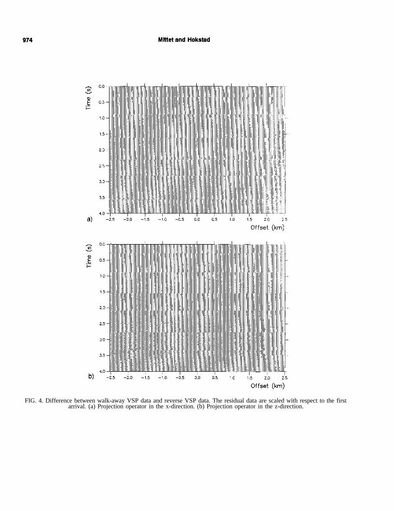
FIG. 4. Difference between walk-away VSP data and reverse VSP data. The residual data are scaled with respect to the firstarrival. (a) Projection operator in the x-direction. (b) Projection operator in the z-direction.

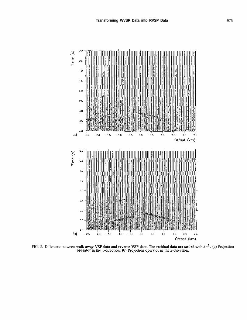
FIG. 5. Differencebetween (a) Projection

Transforming WVSP Data into RVSP Data 975

976 Mittet and Hokstad

APPENDIX AREPRESENTATION THEOREMS

First we develop an expression for the stress in terms ofthe stress Green’s tensor. Similar expression for the dis-placement field are well known and given in Aki andRichards (1980). We use Einstein’s summation conventionand for the partial derivatives we write = and =

We define the following quantities; p(x) is density, (x, t) is a component of the displacement vector, (x, t)

is a component of the stress tensor, t) is a componentof the body-force density vector, (x) is a component ofthe Hooke’s tensor, (x) is a component of the compli-ance tensor, and t) is a component of the straintensor. The equation of motion is,

(A-8)

where t means t + and is arbitrarily small. This limitprevents the time integration from ending at the peak of adelta function. The first integral gives the contribution frominternal body forces, the second integral gives the contribu-tion from spatial boundary conditions, and the third integralgives the contribution from initial and final conditions. FromAki and Richards (1980), we have for the displacement field,

(A-1)

and the constitutive relation is,

(A-2)

where the strain is: t) = t) + The wave equation for the stress field is then

(A-3)

where (x, t) is given in equation (5).We define the Green’s tensor for the stress field by

+

(A-4)

where we have the following relationstensor and the compliance tensor,

between theHooke’s

(A-5)

The Green’s tensor for stress, obeys thespatial reciprocity relation

(A-9)

if we include the contribution from the initial and finalconditions.

We assume that the surface integral terms in equa-tions (A-8) and (A-9) vanish, either because of homogeneousboundary conditions (the fields or the normal derivative ofthe fields vanish) or because of the Sommerfeld radiationcondition. The representations for stress and displacementreduce to,

(A-6)

and we haveof indices,

the following symmetryproperties for each pair

(A-7)

t) = t’)The representation theorem for thefrom equations (A-3) and (A-4) as

field is obtained

(A-10)

0 S

Transforming VWSP Data into RVSP Data 977

t’)

t+ l (A-11)

The contribution from the lower integration limit, t’ = 0, inequations (A-10) and (A-11) vanishes if the field componentsand their temporal derivatives are zero in the initial state,i.e., before the source is fired. The contribution from theupper integration limit, t’ = t , in equations (A-10) and(A-11) vanishes if the field components and their temporalderivatives are zero in the final state. This is usually true ina real seismic experiment if the shot intervalis of order10 seconds. When generating synthetic data, thevanishing of

the contribution from the upper integration limit will requirethat the modeling is continued until all field components areapproximately zero. This criterion may require much CPUtime, however we assume that the field components andtheir derivatives are negligible in the medium at the finalrecording time = t Hence, we neglect the contributionsto equation (A-10) and equation (A-11) from both the lowerand upper integration limits. We are then left with

t) =

(A-12)

t) (A-13)