Transfer in Deep Reinforcement Learning Using Successor ...

Transfer in Deep Reinforcement Learning UsingSuccessor Features and Generalised Policy Improvement

Andre Barreto 1 Diana Borsa 1 John Quan 1 Tom Schaul 1 David Silver 1

Matteo Hessel 1 Daniel Mankowitz 1 Augustin Zıdek 1 Remi Munos 1

AbstractThe ability to transfer skills across tasks has thepotential to scale up reinforcement learning (RL)agents to environments currently out of reach. Re-cently, a framework based on two ideas, successorfeatures (SFs) and generalised policy improve-ment (GPI), has been introduced as a principledway of transferring skills. In this paper we extendthe SF&GPI framework in two ways. One of thebasic assumptions underlying the original formu-lation of SF&GPI is that rewards for all tasks ofinterest can be computed as linear combinationsof a fixed set of features. We relax this constraintand show that the theoretical guarantees support-ing the framework can be extended to any set oftasks that only differ in the reward function. Oursecond contribution is to show that one can usethe reward functions themselves as features forfuture tasks, without any loss of expressiveness,thus removing the need to specify a set of featuresbeforehand. This makes it possible to combineSF&GPI with deep learning in a more stable way.We empirically verify this claim on a complex3D environment where observations are imagesfrom a first-person perspective. We show that thetransfer promoted by SF&GPI leads to very goodpolicies on unseen tasks almost instantaneously.We also describe how to learn policies specialisedto the new tasks in a way that allows them tobe added to the agent’s set of skills, and thus bereused in the future.

1. IntroductionIn recent years reinforcement learning (RL) has undergone amajor change in terms of the scale of its applications: from

1DeepMind. Correspondence to: Andre Barreto <[email protected]>.

Proceedings of the 35 th International Conference on MachineLearning, Stockholm, Sweden, PMLR 80, 2018. Copyright 2018by the author(s).

relatively small and well-controlled benchmarks to problemsdesigned to challenge humans—who are now consistentlyoutperformed by artificial agents in domains considered outof reach only a few years ago (Mnih et al., 2015; Bowlinget al., 2015; Silver et al., 2016; 2017).

At the core of this shift has been deep learning, a ma-chine learning paradigm that recently attracted a lot of at-tention due to impressive accomplishments across manyareas (Goodfellow et al., 2016). Despite the successesachieved by the combination of deep learning and RL,dubbed “deep RL”, the agents’s basic mechanics have re-mained essentially the same, with each problem tackledas an isolated monolithic challenge. An alternative wouldbe for our agents to decompose a problem into smallersub-problems, or “tasks”, whose solutions can be reusedmultiple times, in different scenarios. This ability of explic-itly transferring skills to quickly adapt to new tasks couldlead to another leap in the scale of RL applications.

Recently, Barreto et al. (2017) proposed a framework fortransfer based on two ideas: generalised policy improvement(GPI), a generalisation of the classic dynamic-programmingoperation, and successor features (SFs), a representationscheme that makes it possible to quickly evaluate a policyacross many tasks. The SF&GPI approach is appealingbecause it allows transfer to take place between any twotasks, regardless of their temporal order, and it integratesalmost seamlessly into the RL framework.

In this paper we extend Barreto et al.’s (2017) frameworkin two ways. First, we argue that its applicability is broaderthan initially shown. SF&GPI was designed for the scenariowhere each task corresponds to a different reward function;one of the basic assumptions in the original formulation wasthat the rewards of all tasks can be computed as a linearcombination of a fixed set of features. We show that such anassumption is not strictly necessary, and in fact it is possibleto have guarantees on the performance of the transferredpolicy even on tasks that are not in the span of the features.

The realisation above adds some flexibility to the problemof computing features that are useful for transfer. Our sec-ond contribution is to show a simple way of addressing this

arX

iv:1

901.

1096

4v1

[cs

.LG

] 3

0 Ja

n 20

19

Transfer in Deep Reinforcement Learning Using Successor Features and Generalised Policy Improvement

problem that can be easily combined with deep learning.Specifically, by looking at the associated approximationfrom a slightly different angle, we show that one can replacethe features with actual rewards. This makes it possibleto apply SF&GPI online at scale. In order to verify thisclaim, we revisit one of Barreto et al.’s (2017) experimentsin a much more challenging format, replacing a fully ob-servable 2-dimensional environment with a 3-dimensionaldomain where observations are images from a first-personperspective. We show that the transfer promoted by SF&GPI leads to good policies on unseen tasks almost instanta-neously. Furthermore, we show how to learn policies thatare specialised to the new tasks in a way that allows them tobe added to the agent’s ever-growing set of skills, a crucialability for continual learning (Thrun, 1996).

2. BackgroundIn this section we present the background material that willserve as a foundation for the rest of the paper.

2.1. Reinforcement learning

In RL an agent interacts with an environment and selects ac-tions in order to maximise the expected amount of reward re-ceived (Sutton & Barto, 1998). We model this scenario usingthe formalism of Markov decision processes (MDPs, Puter-man, 1994). An MDP is a tupleM ≡ (S,A, p, R, γ) whosecomponents are defined as follows. The sets S andA are thestate and action spaces, respectively. The function p definesthe dynamics of the MDP: specifically, p(·|s, a) gives thenext-state distribution upon taking action a in state s. Therandom variable R(s, a, s′) determines the reward receivedin the transition s a−→ s′; it is often convenient to considerthe expected value of this variable, r(s, a, s′). Finally, thediscount factor γ ∈ [0, 1) gives smaller weights to future re-wards. Given an MDP, the goal is to maximise the expectedreturn Gt =

∑∞i=0 γ

iRt+i, where Rt = R(St, At, St+1).In order to do so the agent computes a policy π : S 7→ A.

A principled way to address the RL problem is to use meth-ods derived from dynamic programming (DP) (Puterman,1994). RL methods based on DP usually compute the action-value function of a policy π, defined as:

Qπ(s, a) ≡ Eπ [Gt |St = s,At = a] , (1)

where Eπ[·] denotes expectation over the sequences of tran-sitions induced by π. The computation of Qπ(s, a) is calledpolicy evaluation. Once a policy π has been evaluated, wecan compute a greedy policy π′(s) ∈ argmaxaQ

π(s, a)that is guaranteed to perform at least as well as π, that is:Qπ′(s, a) ≥ Qπ(s, a) for any (s, a) ∈ S × A. The com-

putation of π′ is referred to as policy improvement. Thealternation between policy evaluation and policy improve-ment is at the core of many DP-based RL algorithms, which

usually carry out these steps only approximately.

As a convention, we will add a tilde to a symbol to indicatethat the associated quantity is an approximation; we willthen refer to the respective tunable parameters as θ. Forexample, the agent computes an approximation Qπ ≈ Qπby tuning θQ. In deep RL some of the approximationscomputed by the agent, like Qπ , are represented by complexnonlinear approximators composed of many levels of nestedtunable functions; among these, the most popular modelsare by far deep neural networks (Goodfellow et al., 2016).

In this paper we are interested in the problem of transferin RL (Taylor & Stone, 2009; Lazaric, 2012). Specifically,we ask the question: given a set of MDPs that only differin their reward function, how can we leverage knowledgegained in some MDPs to speed up the solution of others?

2.2. SF&GPI

Barreto et al. (2017) propose a framework to solve a re-stricted version of the problem above. Specifically, theyrestrict the scenario of interest to MDPs whose expectedone-step reward can be written as

r(s, a, s′) = φ(s, a, s′)>w, (2)

whereφ(s, a, s′) ∈ Rd are features of (s, a, s′) and w ∈ Rdare weights. In order to build some intuition, it helps tothink of φ(s, a, s′) as salient events that may be desirableor undesirable to the agent. Based on (2) one can define anenvironmentMφ(S,A, p, γ) as

Mφ ≡ {M(S,A, p, r, γ)|r(s, a, s′) = φ(s, a, s′)>w}, (3)

that is,Mφ is the set of MDPs induced by φ through allpossible instantiations of w. We call each M ∈Mφ a task.Given a task Mi ∈ Mφ defined by wi ∈ Rd, we will useQπi to refer to the value function of π on Mi.

Barreto et al. (2017) propose SF&GPI as a way to pro-mote transfer between tasks inMφ. As the name suggests,GPI is a generalisation of the policy improvement step de-scribed in Section 2.1. The difference is that in GPI theimproved policy is computed based on a set of value func-tions rather than on a single one. Let Qπ1 , Qπ2 , ...Qπn

be the action-value functions of n policies defined ona given MDP, and let Qmax = maxiQ

πi . If we de-fine π(s) ← argmaxaQ

max(s, a) for all s ∈ S, thenQπ(s, a) ≥ Qmax(s, a) for all (s, a) ∈ S × A. The re-sult also extends to the scenario where we replace Qπi withapproximations Qπi , in which case the lower bound onQπ(s, a) gets looser with the approximation error, as inapproximate DP (Bertsekas & Tsitsiklis, 1996).

In the context of transfer, GPI makes it possible to leverageknowledge accumulated over time, across multiple tasks, tolearn a new task faster. Suppose that the agent has access


to n policies π1, π2, ..., πn. These can be arbitrary policies,but for the sake of the argument let us assume they are so-lutions for tasks M1, M2, ..., Mn. Suppose also that whenexposed to a new task Mn+1 ∈ Mφ the agent computesQπin+1—the value functions of the policies πi under the re-

ward function induced by wn+1. In this case, applying GPIto the set {Qπ1

n+1, Qπ2n+1, ..., Q

πnn+1} will result in a policy

that performs at least as well as any of the policies πi.

Clearly, the approach above is appealing only if we have away to quickly compute the value functions of the policiesπi on the task Mn+1. This is where SFs come in handy. SFsmake it possible to compute the value of a policy π on anytask Mi ∈Mφ by simply plugging in the representation thevector wi defining the task. Specifically, if we substitute (2)in (1) we have

Qπi (s, a) = Eπ[∑∞

i=tγi−tφi+1 |St = s,At = a

]>wi

≡ ψπ(s, a)>wi, (4)

where φt = φ(st, at, st+1) and ψπ(s, a) are the SFs of(s, a) under policy π. As one can see, SFs decouple thedynamics of the MDP Mi from its rewards (Dayan, 1993).One benefit of doing so is that if we replace wi with wj in(4) we immediately obtain the evaluation of π on task Mj .It is also easy to show that

ψπ(s, a) = Eπ[φt+1 + γψπ(St+1, π(St+1)) |St = s,At = a],(5)

that is, SFs satisfy a Bellman equation in which φi play therole of rewards. Therefore, SFs can be learned using anyconventional RL method (Szepesvari, 2010).

The combination of SFs and GPI provides a general frame-work for transfer in environments of the form (3). Sup-pose that we have learned the functions Qπi

i using therepresentation scheme (4). When exposed to the task de-fined by rn+1(s, a, s′) = φ(s, a, s′)>wn+1, as long as wehave wn+1 we can immediately compute Qπi

n+1(s, a) =ψπi (s, a)>wn+1. This reduces the computation of allQπin+1 to the problem of determining wn+1, which can be

posed as a supervised learning problem whose objective isto minimise some loss derived from (2). Once Qπi

n+1 havebeen computed, we can apply GPI to derive a policy π that isno worse, and possibly better, than π1, ..., πn on task Mn+1.

3. Extending the notion of environmentBarreto et al. (2017) focus on environments of the form (3).In this paper we propose a more general notion of environ-ment:

M(S,A, p, γ) ≡ {M(S,A, p, ·, γ)}. (6)

M contains all MDPs that share the same S, A, p, and γ,regardless of whether their rewards can be computed as alinear combination of the features φ. Clearly,M⊃Mφ.

We want to devise a transfer framework for environmentM.Ideally this framework should have two properties. First, itshould be principled, in the sense that we should be able toprovide theoretical guarantees regarding the performanceof the transferred policies. Second, it should give rise tosimple methods that are applicable in practice, preferably incombination with deep learning. Surprisingly, we can haveboth of these properties by simply looking at SF&GPI froma slightly different point of view, as we show next.

3.1. Guarantees on the extended environment

Barreto et al. (2017) provide theoretical guarantees on theperformance of SF&GPI applied to any task M ∈ Mφ.In this section we show that it is in fact possible to deriveguarantees for any task inM. Our main result is below:

Proposition 1. Let M ∈ M and let Qπ∗ji be the

action-value function of an optimal policy of Mj ∈ Mwhen executed in Mi ∈ M. Given approximations{Qπ1

i , Qπ2i , ..., Q

πni } such that

∣∣∣Qπ∗ji (s, a)− Qπji (s, a)∣∣∣ ≤

ε for all s ∈ S, a ∈ A, and j ∈ {1, 2, ..., n}, let

π(s) ∈ argmaxamaxjQπji (s, a). (7)

Then,

‖Q∗ −Qπ‖∞ ≤2

1− γ

(‖r − ri‖∞ + min

j‖ri − rj‖∞ + ε

),

(8)whereQ∗ is the optimal value function ofM ,Qπ is the valuefunction of π in M , and ‖f − g‖∞ = maxs,a |f(s, a) −g(s, a)|.

The proof of Proposition 1 is in the supplementary material.Our result provides guarantees on the performance of theGPI policy (7) applied to an MDP M with arbitrary rewardfunction r(s, a). Note that, although the proposition doesnot restrict any of the tasks to be inMφ, in order to computethe GPI policy (7) we still need an efficient way of evaluat-ing the policies πj on task Mi. As explained in Section 2,one way to accomplish this is to assume that Mi and all Mj

appearing in the statement of the proposition belong toMφ;this allows the use of SFs to quickly compute Qπji (s, a).

Let us thus take a closer look at Proposition 1 under theassumption that all MDPs belong toMφ, except perhapsfor M . The proposition is based on a reference MDP Mi ∈Mφ. If Mi = Mj for some j, the second term of (8) disap-pears, and we end up with a lower bound on the performanceof a policy computed for Mi when executed in M . Moregenerally, one should think of Mi as the MDP inMφ that is“closest” toM in some sense (so it may be thatMi 6= Mj forall j). Specifically, if ri(s, a, s′) = φ(s, a, s′)>wi, we canthink of wi as the vector that provides the best approxima-tion φ(s, a, s′)>wi ≈ r(s, a, s′) under some well-definedcriterion. The first term of (8) can thus be seen as the


“distance” between M and Mφ, which suggests that theperformance of SF&GPI should degrade gracefully as wemove away from the original environmentMφ. In the par-ticular case where M ∈Mφ the first term of (8) vanishes,and we recover Barreto et al.’s (2017) Theorem 2.

3.2. Uncovering the structure of the environment

We want to solve a subset of the tasks inM and use GPIto promote transfer between these tasks. In order to do soefficiently, we need a function φ that covers the tasks ofinterest as much as possible. If we were to rely on Barretoet al.’s (2017) original results, we would have guaranteeson the performance of the GPI policy only if φ spanned allthe tasks of interest. Proposition 1 allows us to remove thisrequirement, since now we have theoretical guarantees forany choice of φ. In practice, though, we want features φsuch that the first term of (8) is small for all tasks of interest.

There might be contexts in which we have direct access tofeatures φ(s, a, s′) that satisfy (2), either exactly or approx-imately. Here though we are interested in the more generalscenario where this structure is not available, nor given tothe agent in any form. In this case the use of SFs requires away of unveiling such a structure.

Barreto et al. (2017) assume the existence of a φ ∈ Rdthat satisfy (2) exactly and formulate the problem of com-puting an approximate φ as a multi-task learning problem.The problem is decomposed into D regressions, each oneassociated with a task. For reasons that will become clearshortly we will call these tasks base tasks and denote themby M ≡ {M1,M2, ...,MD} ⊂ Mφ. The multi-task prob-lem thus consists in solving the approximations

φ(s, a, s′)>wi ≈ ri(s, a, s′), for i = 1, 2, ..., D, (9)

where ri is the reward of Mi (Caruana, 1997; Baxter, 2000).

In this section we argue that (9) can be replaced by a muchsimpler approximation problem. Suppose for a moment thatwe know a function φ and D vectors wi that satisfy (9)exactly. If we then stack the vectors wi to obtain a ma-trix W ∈ RD×d, we can write r(s, a, s′) = Wφ(s, a, s′),where the ith element of r(s, a, s′) ∈ RD is ri(s, a, s′).Now, as long as we have d linearly independent tasks wi,we can write φ(s, a, s′) = (W>W)−1W>r(s, a, s′) =W†r(s, a, s′). Since φ is given by a linear transformationof r, any task representable by the former can also be rep-resented by the latter. To see why this is so, note that forany task in Mφ we have r(s, a, s′) = w>φ(s, a, s′) =w>W†r(s, a, s′) = (w′)>r(s, a, s′). Therefore, we canuse the rewards r themselves as features, which means thatwe can replace (9) with the much simpler approximation

φ(s, a, s′) = r(s, a, s′) ≈ r(s, a, s′). (10)

One potential drawback of directly approximating r(s, a, s′)

is that we no longer have the flexibility of distinguishingbetween d, the dimension of the environmentMφ, and D,the number of base tasks in M. Since in general we willsolve (9) or (10) based on data, having D > d may lead to abetter approximation. On the other hand, using r(s, a, s′) asfeatures has a number of advantages that in many scenariosof interest should largely outweigh the loss in flexibility.

One such advantage becomes clear when we look at thescenario above from a different perspective. Instead ofassuming we know aφ and a W that satisfy (9), we can notethat, given any set of D tasks ri(s, a, s′), k ≤ D of themwill be linearly independent. Thus, the reasoning aboveapplies without modification. Specifically, if we use thetasks’s rewards as features, as in (10), we can think of themas inducing a φ(s, a, s′) ∈ Rk—and, as a consequence, anenvironmentMφ. This highlights a benefit of replacing (9)with (10): the fact that we can work directly in the space oftasks, which in many cases may be more intuitive. Whenwe think of φ as a non-observable, abstract, quantity, it canbe difficult to define what exactly the base tasks should be.In contrast, when we look at r directly the question we aretrying to answer is: is it possible to approximate the rewardfunction of all tasks of interest as a linear combination ofthe functions ri? As one can see, the set M works exactlyas a basis, and thus the name “base tasks”.

Another interesting consequence of using an approximationφ(s, a, s′) ≈ r(s, a, s′) as features is that the resulting SFsare nothing but ordinary action-value functions. Specifically,the jth component of ψ

πi(s, a) is simply Qπij (s, a). Next

we discuss how this gives rise to a simple approach that canbe combined with deep learning in a stable way.

4. Transfer in deep reinforcement learningAs described in the introduction, we are interested in usingSF&GPI to build scalable agents that can be combinedwith deep learning in a stable way. Since deep learninggenerally involves vast amounts of data whose storage isimpractical, we will be mostly focusing on methods thatwork online. As a motivating example for this section weshow in Algorithm 1 how SFs and GPI can be combinedwith Watkins & Dayan’s (1992) Q-learning.1

Algorithm 1 differs from standard Q-learning in two mainways. First, instead of selecting actions based on the valuefunction being learned, the behaviour of the agent is deter-mined by GPI (line 7). Depending on the set of SFs Ψ usedby the algorithm, this can be a significant improvement overthe greedy policy induced by Qπn+1 , which usually is themain determinant of a Q-learning agent’s behaviour.

1We use x α←− y meaning x← x+ αy. We also use∇θf(x)to denote the gradient of f(x) with respect to the parameters θ.


Algorithm 1 SF&GPI with ε-greedy Q-learning

Require:

φ, Ψ ≡ {ψπ1, ..., ψ

πn} features, SFsextend basis learn a new SF?αψ, αw, ε,ns hyper-parameters

1: if extend basis then2: create ψ

πn+1 parametrised by θψ3: Ψ← Ψ ∪ {ψ

πn+1}4: select initial state s ∈ S5: for ns steps do6: if Bernoulli(ε)=1 then a← Uniform(A) // exploration7: else a← argmaxb maxi ψ

πi(s, b)>w // GPI

8: Execute action a and observe r and s′

9: wαw←−−

[r − φ(s, a, s′)>w

]φ(s, a, s′) // learn w

10: if extend basis then // will learn new SFs11: a′ ← argmaxbψ

πn+1(s, b)>w

12: for i← 1, 2, ..., d do13: δ ← φi(s, a, s

′) + γψπn+1

i (s′, a′)− ψπn+1

i (s, a)

14: θψαψ←−− δ∇θψ ψ

πn+1

i (s, a) // learn ψπn+1

15: if s′ is not terminal then s← s′

16: else select initial state s ∈ S

Algorithm 1 also deviates from conventional Q-learning inthe way a policy is learned. There are two possibilities here.One of them is for the agent to rely exclusively on the GPIpolicy computed over Ψ (when the variable extend basisis set to false). In this case no specialised policy is learnedfor the current task, which reduces the RL problem to thesupervised problem of determining w (solved in line 9 as aleast-squares regression).

Another possibility is to use data collected by the GPIpolicy to learn a policy πn+1 specifically tailored for thetask. As shown in lines 13 and 14, this comes down tosolving equation (5). When πn+1 is learned the functionQπn+1(s, a) = ψ

πn+1(s, a)>w also takes part in GPI. This

means that, if the approximations Qπi(s, a) are reasonablyaccurate, the policy computed by Algorithm 1 should bestrictly better thanQ-learning’s counterpart. The SFs ψ

πn+1

can then be added to the set Ψ, and therefore a subsequentexecution of Algorithm 1 will result in an even strongeragent. The ability to build and continually refine a set ofskills is widely regarded as a desirable feature for continual(or lifelong) learning (Thrun, 1996).

4.1. Challenges involved in building features

In order to use Algorithm 1, or any variant of the SF&GPIframework, we need the features φ(s, a, s′). A natural wayof addressing the computation of φ(s, a, s′) is to see it as amulti-task problem, as in (9). We now discuss the difficultiesinvolved in solving this problem online at scale.

The solution of (9) requires data coming from D base tasks.In principle, we could look at the collection of sample tran-

sitions as a completely separate process. However, herewe are assuming that the base tasks M are part of the RLproblem, that is, we want to collect data using policies thatare competent in M. In order to maximise the potential fortransfer, while learning the policies πi for the base tasksMi we should also learn the associated SFs ψ

πi ; this cor-responds to building the initial set Ψ used by Algorithm 1.Unfortunately, learning value functions in the form (4) whilesolving (9) can be problematic. Since the SFs ψ

πi dependon φ, learning the former while refining the latter can clearlylead to undesirable solutions (this is akin to having a non-stationary reward function). On top of that, the computationof φ itself depends on the SFs ψ

πi , for they ultimately de-fine the data distribution used to solve (9). This circulardependency can make the process of concurrently learningφ and ψ

πi unstable—something we observed in practice.

One possible solution is to use a conventional value func-tion representation while solving (9) and only learn SFs forthe subsequent tasks (Barreto et al., 2017). This has thedisadvantage of not reusing the policies learned in M fortransfer. Alternatively, one can store all the data and learnthe SFs associated with the base tasks only after φ has beenlearned, but this may be difficult in scenarios involving largeamounts of data. Besides, any approximation errors in φwill already be reflected in the initial Ψ computed in M.

4.2. Learning features online while retainingtransferable knowledge

To recapitulate, we are interested in solving D base tasksMi and, while doing so, build φ and the initial set Ψ tobe used by Algorithm 1. We want φ and Ψ to be learnedconcurrently, so we do not have to store transitions, andpreferably Ψ should not reflect approximation errors in φ.

We argue that one can accomplish all of the above by re-placing (9) with (10), that is, by directly approximatingr(s, a, s′), which is observable, and adopting the resultingapproximation as the features φ required by Algorithm 1.

As discussed in Section 3.2, when using rewards as fea-tures the resulting SFs are collections of value functions:ψπi

= Qπi ≡ [Qπi1 , Q

πi2 , ..., Q

πiD ]. This leads to a particu-

larly simple way of building the features φ while retainingtransferable knowledge in Ψ. Given a set of D base tasksMi, while solving them we only need to carry out two extraoperations: compute approximations ri(s, a, s′) of the func-tions ri(s, a, s′), to be used as φ, and evaluate the resultingpolicies on all tasks—i.e., compute Qπij —to build Ψ.

Before providing a practical method to compute φ and Ψ,we note that, although the approximations ri(s, a, s′) canbe learned independently from each other, the computationof Q

πi requires policy πi to be evaluated under different


reward signals. This can be accomplished in different ways;here we assume that the agent is able to interact with thetasks Mi in parallel. We can consider that at each transitionthe agent observes rewards from all the base tasks, r ∈ RD,or a single scalar ri associated with one of them. We willassume the latter, but our solution readily extends to thescenario where the agent simultaneously observes D tasks.

Algorithm 2 shows a possible way of implementing oursolution, again using Q-learning as the basic RL method.We highlight the fact that GPI can already be used in thisphase, as shown in line 4, which means that the policies πican “cooperate” to solve each task Mi.

Algorithm 2 Build SF&GPI basis with ε-greedyQ-learning

Require:{M1,M2, ...,MD base tasksαQ, αr, ε,ns hyper-parameters

1: for ns steps do2: select a task t ∈ {1, 2, ..., D} and a state s ∈ S3: if Bernoulli(ε)=1 then a← Uniform(A) // exploration4: else a← argmaxb maxi Q

πit (s, b) // GPI

5: Execute action a in Mt and observe r and s′

6: θrαr←−− [r − rt(s, a, s′)]∇θr rt(s, a, s

′)7: for i← 1, 2, ..., D do8: a′ ← argmaxbQ

πii (s, b) // a′ ≡ πi(s)

9: θQαQ←−−

[r + γQπit (s′, a′)− Qπit (s, a)

]∇θQQ

πit (s, a)

10: return φ ≡ [r1, ..., rD] and Ψ ≡ {Qπ1, ..., Q

πD}

Note that if we were to learn general ψπi

(s, a) andφ(s, a, s′) in parallel we would necessarily have to usethe latter to update the former, which means computingan approximation on top of another (see (5)). In contrast,when learning Qπij (s, a) we can use the actual rewardsrj(s, a, s

′), as opposed to the approximations rj(s, a, s′)(line 9 of Algorithm 2). This means that φ and Ψ can belearned concurrently without the accumulation of approxi-mation errors in ψ

πi , as promised.

5. ExperimentsIn this section we use experiments to assess whether theproposed approach can indeed promote transfer on large-scale domains. Here we focus on what we consider the mostrelevant aspects of our experiments; for further details andadditional results please see the supplementary material.

5.1. Environment

The environment we consider is conceptually similar to oneof the problems used by Barreto et al. (2017) to evaluatetheir framework: the agent has to navigate in a room pickingup desirable objects while avoiding undesirable ones. Here

(a) Screenshot of environment

M1 1 0 0 0M2 0 1 0 0M3 0 0 1 0M4 0 0 0 1

(b) Base tasks M

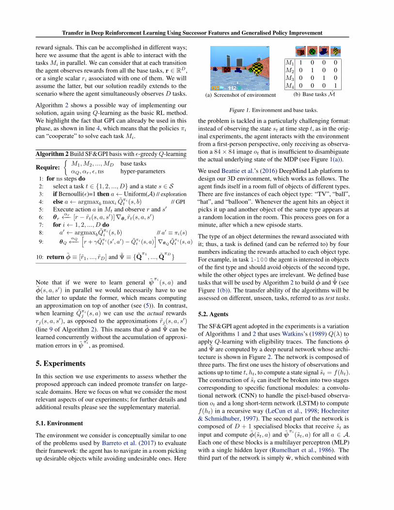
Figure 1. Environment and base tasks.

the problem is tackled in a particularly challenging format:instead of observing the state st at time step t, as in the orig-inal experiments, the agent interacts with the environmentfrom a first-person perspective, only receiving as observa-tion a 84× 84 image ot that is insufficient to disambiguatethe actual underlying state of the MDP (see Figure 1(a)).

We used Beattie et al.’s (2016) DeepMind Lab platform todesign our 3D environment, which works as follows. Theagent finds itself in a room full of objects of different types.There are five instances of each object type: “TV”, “ball”,“hat”, and “balloon”. Whenever the agent hits an object itpicks it up and another object of the same type appears ata random location in the room. This process goes on for aminute, after which a new episode starts.

The type of an object determines the reward associated withit; thus, a task is defined (and can be referred to) by fournumbers indicating the rewards attached to each object type.For example, in task 1-100 the agent is interested in objectsof the first type and should avoid objects of the second type,while the other object types are irrelevant. We defined basetasks that will be used by Algorithm 2 to build φ and Ψ (seeFigure 1(b)). The transfer ability of the algorithms will beassessed on different, unseen, tasks, referred to as test tasks.

5.2. Agents

The SF&GPI agent adopted in the experiments is a variationof Algorithms 1 and 2 that uses Watkins’s (1989) Q(λ) toapply Q-learning with eligibility traces. The functions φand Ψ are computed by a deep neural network whose archi-tecture is shown in Figure 2. The network is composed ofthree parts. The first one uses the history of observations andactions up to time t, ht, to compute a state signal st = f(ht).The construction of st can itself be broken into two stagescorresponding to specific functional modules: a convolu-tional network (CNN) to handle the pixel-based observa-tion ot and a long short-term network (LSTM) to computef(ht) in a recursive way (LeCun et al., 1998; Hochreiter& Schmidhuber, 1997). The second part of the network iscomposed of D + 1 specialised blocks that receive st asinput and compute φ(st, a) and ψ

πi(st, a) for all a ∈ A.

Each one of these blocks is a multilayer perceptron (MLP)with a single hidden layer (Rumelhart et al., 1986). Thethird part of the network is simply w, which combined with


Figure 2. Deep architecture used. Rectangles represent MLPs.

φ and ψπi will provide the final approximations.

The entire architecture was trained end-to-end through Algo-rithm 2 using the base tasks shown in Figure 1(b). After theSF&GPI agent had been trained it was tested on a test task,now using Algorithm 1 with the newly-learned φ and Ψ.In order to handle the large number of sample trajectoriesneeded in our environment both Algorithms 1 and 2 usedthe IMPALA distributed architecture (Espeholt et al., 2018).

Algorithm 1 was run with and without the learning of a spe-cialised policy (controlled via the variable extend basis).We call the corresponding versions of the algorithm “SF&GPI-continual” and “SF&GPI-transfer”, respectively. Wecompare SF&GPI with baseline agents that use the samenetwork architecture, learning algorithm, and distributeddata processing. The only difference is in the way the net-work shown in Figure 2 is updated and used during the testphase. Specifically, we ignore the MLPs used to compute φand ψ

πi and instead add another MLP, with the exact samearchitecture, to be jointly trained with w through Q(λ). Wethen distinguish three baselines. The first one uses the statesignal st = f(ht) learned in the base tasks to computean approximation Q(s, a)—that is, both the CNN and theLSTM are fixed. We will refer to this method simply asQ(λ). The second baseline is allowed to modify f(ht) dur-ing test, so we call it “DQ(λ) fine tuning” as a referenceto its deep architecture. Finally, the third baseline, “DQ(λ)from scratch”, learns its own representation f(ht).

5.3. Results and discussion

Figure 3 shows the results of SF&GPI and the baselines ona selection of test tasks. The first thing that stands out in thefigures is the fact that SF&GPI-transfer learns very goodpolicies for the test tasks almost instantaneously. In fact, asthis version of the algorithm is solving a simple supervisedlearning problem, its learning progress is almost impercepti-ble at the scale the RL problem unfolds. Since the baselines

are solving the full RL problem, in some tasks their per-formance eventually reaches, or even surpasses, that of thetransferred policies. SF&GPI-continual combines the desir-able properties of both SF&GPI-transfer and the baselines.On one hand, it still benefits from the instantaneous transferpromoted by SF&GPI. On the other hand, its performancekeeps improving, since in this case the transferred policy isused to learn a policy specialised to the current task. As aresult, SF&GPI-continual outperforms the other methods inalmost all of the tasks.2

Another interesting trend shown in Figures 3 is the factthat SF&GPI performs well on test tasks with negativerewards—in some cases considerably better than the alter-native methods—, even though the agent only experiencedpositive rewards in the base tasks. This is an indication thatthe transferred GPI policy is combining the policies πi forthe base tasks in a non-trivial way (line 7 of Algorithm 1).

In this paper we argue that SF&GPI can be applied evenif assumption (2) is not strictly satisfied. In order to il-lustrate this point, we reran the experiments with SF&GPI-transfer using a set of linearly-depend base tasks,M′ ≡ {1000, 0100, 0011, 1100}. Clearly, M′ can onlyrepresent tasks in which the rewards associated with thethird and fourth object types are the same. We thus fixedthe rewards associated with the first two object types andcompared the results of SF&GPI-transfer using M and M′on several tasks where this is not the case. The comparisonis shown in Figure 4. As shown in the figure, although usinga linearly-dependent set of base tasks does hinder transferin some cases, in general it does not have a strong impacton the results. This smooth degradation of the performanceis in accordance with Proposition 1.

The result above also illustrates an interesting distinctionbetween the space of reward functions and the associatedspace of policies. Although we want to be able to representthe reward functions of all tasks of interest, this does notguarantee that the resulting GPI policy will perform well.To see this, suppose we replace the positive rewards in Mwith negative ones. Clearly, in this case we would still havea basis spanning the same space of rewards; however, sincenow a policy that stands still is optimal in all tasks Mi,we should not expect GPI to give rise to good policies intasks with positive rewards. One can ask how to define a“behavioural basis” that leads to good policies acrossMthrough GPI. We leave this as an interesting open question.

6. Related workRecently, there has been a resurgence of the subject of trans-fer in the deep RL literature. Teh et al. (2017) propose an

2A video of SF&GPI-transfer is included as a supplement, andcan also be found on this link: https://youtu.be/-dTnqfwTRMI.

https://youtu.be/-dTnqfwTRMI


0 50 100 150 200 250

Environment step (millions)

0

5

10

15

20

25

Epis

ode r

ew

ard

Task1000

0100

0010

0001

(a) Base tasks

0 20 40 60 80 100


0

5

10

15

20

25

30

35

40

Epis

ode r

ew

ard

Q(¸)

DQ(¸) fine-tuned

DQ(¸) from scratch

SF & GPI transfer

SF & GPI continual

(b) Task 1100

0 20 40 60 80 100


−6

−5

−4

−3

−2

−1

0

Epis

ode r

ew

ard

(c) Task -1-100

0 20 40 60 80 100


−5

0

5

10

15

20

25

Epis

ode r

ew

ard

(d) Task -11-10

0 20 40 60 80 100


0

5

10

15

20

25

30

35

Epis

ode r

ew

ard

(e) Task -1101

0 20 40 60 80 100


−5

0

5

10

15

20

25

30

35

Epis

ode r

ew

ard

(f) Task -11-11

Figure 3. Average reward per episode on the base tasks and a selection of test tasks. The x axes have different scales because the amountof reward available changes across tasks. Shaded regions are one standard deviation over 10 runs.

-11-10 -1101 -11-11 -1101 -111-1 -1110

Task description

−5

0

5

10

15

20

25

30

35

40

Epis

ode r

ew

ard

Canonical base tasks

Linearly-dependent base tasks

Figure 4. Performance of SF&GPI-transfer using base tasks Mand M′. The box plots summarise the distribution of the rewardsreceived per episode between 50 and 100 million steps of learning.

approach for the multi-task problem—which in our case isthe learning of base tasks—that uses a shared policy as a reg-ulariser for specialised policies. Finn et al. (2017) proposeto achieve fast transfer, which is akin to SF&GPI-transfer,by focusing on adaptability, rather than performance, duringlearning. Rusu et al. (2016) and Kirkpatrick et al. (2016)introduce neural-network architectures well-suited for con-tinual learning. There have also been previous attempts tocombine SFs and deep learning for transfer, but none ofthem used GPI (Kulkarni et al., 2016; Zhang et al., 2016).

Many works on the combination of deep RL and transferpropose modular network architectures that naturally inducea decomposition of the problem (Devin et al., 2016; Heesset al., 2017; Clavera et al., 2017). Among these, a recurrenttheme is the existence of sub-networks specialised in differ-

ent skills that are managed by another network (Heess et al.,2016; Frans et al., 2017; Oh et al., 2017). This highlights aninteresting connection between transfer learning and hierar-chical RL, which has also recently re-emerged in the deepRL literature (Vezhnevets et al., 2017; Bacon et al., 2017).

7. ConclusionIn this paper we extended the SF&GPI transfer frameworkin two ways. First, we showed that the theoretical guaran-tees supporting the framework can be extended to any set ofMDPs that only differ in the reward function, regardless ofwhether their rewards can be computed as a linear combi-nation of a set of features or not. In order to use SF&GPIin practice we still need the reward features, though; oursecond contribution is to show that these features can be thereward functions of a set of MDPs. This reinterpretationof the problem makes it possible to combine SF&GPI withdeep learning in a stable way. We empirically verified thisclaim on a complex 3D environment that requires hundredsof millions of transitions to be solved. We showed that, byturning an RL task into a supervised learning problem, SF&GPI-transfer is able to provide skilful, non-trivial, poli-cies almost instantaneously. We also showed how thesepolicies can be used by SF&GPI-continual to learn spe-cialised policies, which can then be added to the agent’s setof skills. Together, these concepts can help endow an agentwith the ability to build, refine, and use a set of skills whileinteracting with the environment.


AcknowledgementsThe authors would like to thank Will Dabney and Hado vanHasselt for the invaluable discussions during the develop-ment of this paper. We also thank the anonymous reviewers,whose comments and suggestions helped to improve thepaper considerably.

ReferencesBacon, P., Harb, J., and Precup, D. The option-critic ar-

chitecture. In Proceedings of the AAAI Conference onArtificial Intelligence, pp. 1726–1734, 2017.

Barreto, A., Dabney, W., Munos, R., Hunt, J., Schaul, T.,van Hasselt, H., and Silver, D. Successor features fortransfer in reinforcement learning. In Advances in NeuralInformation Processing Systems (NIPS), 2017.

Baxter, J. A model of inductive bias learning. Journal ofArtificial Intelligence Research, 12:149–198, 2000.

Beattie, C., Leibo, J. Z., Teplyashin, D., Ward, T., Wain-wright, M., Kuttler, H., Lefrancq, A., Green, S., Valdes,V., Sadik, A., et al. Deepmind lab. arXiv preprintarXiv:1612.03801, 2016.

Bertsekas, D. P. and Tsitsiklis, J. N. Neuro-Dynamic Pro-gramming. Athena Scientific, 1996.

Bowling, M., Burch, N., Johanson, M., and Tammelin, O.Heads-up limit hold’em poker is solved. Science, 347(6218):145–149, January 2015.

Caruana, R. Multitask learning. Machine Learning, 28(1):41–75, 1997.

Clavera, I., Held, D., and Abbeel, P. Policy transfer via mod-ularity and reward guiding. In International Conferenceon Intelligent Robots and Systems (IROS), 2017.

Dayan, P. Improving generalization for temporal differencelearning: The successor representation. Neural Computa-tion, 5(4):613–624, 1993.

Devin, C., Gupta, A., Darrell, T., Abbeel, P., and Levine, S.Learning modular neural network policies for multi-taskand multi-robot transfer. CoRR, abs/1609.07088, 2016.URL http://arxiv.org/abs/1609.07088.

Espeholt, L., Soyer, H., Munos, R., Simonyan, K., Mnih, V.,Ward, T., Doron, Y., Firoiu, V., Harley, T., Dunning, I.,Legg, S., and Kavukcuoglu, K. IMPALA: Scalable dis-tributed deep-RL with importance weighted actor-learnerarchitectures. arXiv preprint arXiv:1802.01561, 2018.

Finn, C., Abbeel, P., and Levine, S. Model-agnostic meta-learning for fast adaptation of deep networks. CoRR,abs/1703.03400, 2017. URL http://arxiv.org/abs/1703.03400.

Frans, K., Ho, J., Chen, X., Abbeel, P., and Schul-man, J. Meta learning shared hierarchies. CoRR,abs/1710.09767, 2017. URL http://arxiv.org/abs/1710.09767.

Goodfellow, I., Bengio, Y., and Courville, A. DeepLearning. MIT Press, 2016. http://www.deeplearningbook.org.

Heess, N., Wayne, G., Tassa, Y., Lillicrap, T. P., Riedmiller,M. A., and Silver, D. Learning and transfer of modu-lated locomotor controllers. CoRR, abs/1610.05182, 2016.URL http://arxiv.org/abs/1610.05182.

Heess, N., TB, D., Sriram, S., Lemmon, J., Merel, J.,Wayne, G., Tassa, Y., Erez, T., Wang, Z., Eslami, S.M. A., Riedmiller, M. A., and Silver, D. Emergenceof locomotion behaviours in rich environments. CoRR,abs/1707.02286, 2017. URL http://arxiv.org/abs/1707.02286.

Hochreiter, S. and Schmidhuber, J. Long short-term memory.Neural computation, 9(8):1735–1780, 1997.

Kirkpatrick, J., Pascanu, R., Rabinowitz, N. C., Veness,J., Desjardins, G., Rusu, A. A., Milan, K., Quan, J.,Ramalho, T., Grabska-Barwinska, A., Hassabis, D.,Clopath, C., Kumaran, D., and Hadsell, R. Overcom-ing catastrophic forgetting in neural networks. CoRR,abs/1612.00796, 2016. URL http://arxiv.org/abs/1612.00796.

Kulkarni, T. D., Saeedi, A., Gautam, S., and Gershman, S. J.Deep successor reinforcement learning. arXiv preprintarXiv:1606.02396, 2016.

Lazaric, A. Transfer in Reinforcement Learning: A Frame-work and a Survey, pp. 143–173. 2012.

LeCun, Y., Bottou, L., Bengio, Y., and Haffner, P. Gradient-based learning applied to document recognition. Proceed-ings of the IEEE, 86(11):2278–2324, 1998.

Mnih, V., Kavukcuoglu, K., Silver, D., Rusu, A. A., Ve-ness, J., Bellemare, M. G., Graves, A., Riedmiller, M.,Fidjeland, A. K., Ostrovski, G., Petersen, S., Beattie, C.,Sadik, A., Antonoglou, I., King, H., Kumaran, D., Wier-stra, D., Legg, S., and Hassabis, D. Human-level controlthrough deep reinforcement learning. Nature, 518(7540):529–533, 2015.

Oh, J., Singh, S. P., Lee, H., and Kohli, P. Zero-shottask generalization with multi-task deep reinforcementlearning. CoRR, abs/1706.05064, 2017. URL http://arxiv.org/abs/1706.05064.

Puterman, M. L. Markov Decision Processes—DiscreteStochastic Dynamic Programming. John Wiley & Sons,Inc., 1994.

http://arxiv.org/abs/1612.03801







http://www.deeplearningbook.org

http://www.deeplearningbook.org










Rumelhart, D. E., Hinton, G. E., and Williams, R. J. Paralleldistributed processing: Explorations in the microstructureof cognition. chapter Learning Internal Representationsby Error Propagation, pp. 318–362. MIT Press, Cam-bridge, MA, USA, 1986.

Rusu, A. A., Rabinowitz, N. C., Desjardins, G., Soyer,H., Kirkpatrick, J., Kavukcuoglu, K., Pascanu, R.,and Hadsell, R. Progressive neural networks. CoRR,abs/1606.04671, 2016. URL http://arxiv.org/abs/1606.04671.

Silver, D., Huang, A., Maddison, C. J., Guez, A., Sifre, L.,van den Driessche, G., Schrittwieser, J., Antonoglou, I.,Panneershelvam, V., Lanctot, M., Dieleman, S., Grewe,D., Nham, J., Kalchbrenner, N., Sutskever, I., Lillicrap, T.,Leach, M., Kavukcuoglu, K., Graepel, T., and Hassabis,D. Mastering the game of go with deep neural networksand tree search. Nature, 529:484–503, 2016.

Silver, D., Schrittwieser, J., Simonyan, K., Antonoglou,I., Huang, A., Guez, A., Hubert, T., Baker, L., Lai, M.,Bolton, A., Chen, Y., Lillicrap, T., Hui, F., Sifre, L.,van den Driessche, G., Graepel, T., and Hassabis, D.Mastering the game of Go without human knowledge.Nature, 550, 2017.

Sutton, R. S. and Barto, A. G. ReinforcementLearning: An Introduction. MIT Press, 1998.URL http://www-anw.cs.umass.edu/˜rich/book/the-book.html.

Szepesvari, C. Algorithms for Reinforcement Learning.Synthesis Lectures on Artificial Intelligence and MachineLearning. Morgan & Claypool Publishers, 2010.

Taylor, M. E. and Stone, P. Transfer learning for reinforce-ment learning domains: A survey. Journal of MachineLearning Research, 10(1):1633–1685, 2009.

Teh, Y. W., Bapst, V., Czarnecki, W. M., Quan, J., Kirk-patrick, J., Hadsell, R., Heess, N., and Pascanu, R. Distral:Robust multitask reinforcement learning. In Advancesin Neural Information Processing Systems (NIPS), pp.4499–4509, 2017.

Thrun, S. Is learning the N-th thing any easier than learningthe first? In Advances in Neural Information ProcessingSystems (NIPS), pp. 640–646, 1996.

Vezhnevets, A. S., Osindero, S., Schaul, T., Heess, N.,Jaderberg, M., Silver, D., and Kavukcuoglu, K. FeU-dal networks for hierarchical reinforcement learning. InProceedings of the International Conference on MachineLearning (ICML), pp. 3540–3549, 2017.

Watkins, C. Learning from Delayed Rewards. PhD thesis,University of Cambridge, England, 1989.

Watkins, C. and Dayan, P. Q-learning. Machine Learning,8:279–292, 1992.

Zhang, J., Springenberg, J. T., Boedecker, J., and Burgard,W. Deep reinforcement learning with successor fea-tures for navigation across similar environments. CoRR,abs/1612.05533, 2016.



http://www-anw.cs.umass.edu/~rich/book/the-book.html

http://www-anw.cs.umass.edu/~rich/book/the-book.html

Transfer in Deep Reinforcement Learning Using SuccessorFeatures and Generalised Policy Improvement

Supplementary Material

Andre Barreto, Diana Borsa, John Quan, Tom Schaul, David Silver,Matteo Hessel, Daniel Mankowitz Augustin Zıdek, Remi Munos,{andrebarreto,borsa,johnquan,schaul,davidsilver,mtthss,dmankowitz,augustinzidek,munos}@google.com

DeepMind

AbstractIn this supplement we give details of the theory and experiments that had to be left out of the main paper due tothe space limit. For the convenience of the reader the statements of the theoretical results are reproduced beforethe respective proofs. We also report additional empirical analysis that could not be included in the paper. Thecitations in this supplement refer to the references listed in the main paper.

A. Proof of theoretical resultsWe restate Barreto et al.’s (2017) GPI theorem to be used as a reference in the derivations that follow.

Theorem 1. (Generalized Policy Improvement) Let π1, π2, ..., πn be n decision policies and let Qπ1 , Qπ2 , ..., Qπn beapproximations of their respective action-value functions such that

|Qπi(s, a)− Qπi(s, a)| ≤ ε for all s ∈ S, a ∈ A, and i ∈ {1, 2, ..., n}.

Defineπ(s) ∈ argmax

amaxiQπi(s, a).

Then,

Qπ(s, a) ≥ maxiQπi(s, a)− 2

1− γε

for any s ∈ S and any a ∈ A, where Qπ is the action-value function of π.

Lemma 1. Let δij = maxs,a |ri(s, a)− rj(s, a)| and let π be an arbitrary policy. Then,

|Qπi (s, a)−Qπj (s, a)| ≤ δij1− γ

.

Proof. Define ∆ij = maxs,a |Qπi (s, a)−Qπj (s, a)|. Then,

|Qπi (s, a)−Qπj (s, a)| =

∣∣∣∣∣ri(s, a) + γ∑s′

p(s′|s, a)Qπi (s′, π(s′))− rj(s, a)− γ∑s′

p(s′|s, a)Qπj (s′, π(s′))

∣∣∣∣∣=

∣∣∣∣∣ri(s, a)− rj(s, a) + γ∑s′

p(s′|s, a)(Qπi (s′, π(s′))−Qπj (s′, π(s′))

)∣∣∣∣∣≤ |ri(s, a)− rj(s, a)|+ γ

∑s′

p(s′|s, a)∣∣Qπi (s′, π(s′))−Qπj (s′, π(s′))

∣∣≤ δij + γ∆ij . (11)


Since (11) is valid for any s, a ∈ S ×A, we have shown that ∆ij ≤ δij + γ∆ij . Solving for ∆ij we get

∆ij ≤1

1− γδij .

Lemma 2. Let δij = maxs,a |ri(s, a)− rj(s, a)|. Then,

|Qπ∗ii (s, a)−Qπ

∗j

j (s, a)| ≤ δij1− γ

.

Proof. To simplify the notation, letQii(s, a) ≡ Qπ∗ii (s, a). Note that |Qii(s, a)−Qjj(s, a)| is the difference between the value

functions of two MDPs with the same transition function but potentially different rewards. Let ∆ij = maxs,a |Qii(s, a)−Qjj(s, a)|. Then,

|Qii(s, a)−Qjj(s, a)| =

∣∣∣∣∣ri(s, a) + γ∑s′

p(s′|s, a) maxbQii(s

′, b)− rj(s, a)− γ∑s′

p(s′|s, a) maxbQjj(s

′, b)

∣∣∣∣∣=

∣∣∣∣∣ri(s, a)− rj(s, a) + γ∑s′

p(s′|s, a)(

maxbQii(s

′, b)−maxbQjj(s

′, b))∣∣∣∣∣

≤ |ri(s, a)− rj(s, a)|+ γ∑s′

p(s′|s, a)∣∣∣max

bQii(s

′, b)−maxbQjj(s

′, b)∣∣∣

≤ |ri(s, a)− rj(s, a)|+ γ∑s′

p(s′|s, a) maxb

∣∣∣Qii(s′, b)−Qjj(s′, b)∣∣∣≤ δij + γ∆ij . (12)

Since (12) is valid for any s, a ∈ S ×A, we have shown that ∆ij ≤ δij + γ∆ij . Solving for ∆ij we get

∆ij ≤1

1− γδij .

Proposition 1. Let M ∈M and let Qπ∗ji be the action-value function of an optimal policy of Mj ∈M when executed in

Mi ∈ M. Given approximations {Qπ1i , Q

π2i , ..., Q

πni } such that

∣∣∣Qπ∗ji (s, a)− Qπji (s, a)∣∣∣ ≤ ε for all s ∈ S, a ∈ A, and

j ∈ {1, 2, ..., n}, letπ(s) ∈ argmaxamaxjQ

πji (s, a).

Then,

‖Q∗ −Qπ‖∞ ≤2

1− γ

(‖r − ri‖∞ + min

j‖ri − rj‖∞ + ε

),

whereQ∗ is the optimal value function ofM ,Qπ is the value function of π inM , and ‖f−g‖∞ = maxs,a |f(s, a)−g(s, a)|.

Proof. The result is a direct application of Theorem 1 and Lemmas 1 and 2. Let π∗ be an optimal value function of M .Then,

Q∗(s, a)−Qπ(s, a) = Qπ∗(s, a)−Qπ(s, a)

= Qπ∗(s, a)−Qπ

∗ii +Q

π∗ii −Qπ(s, a)

= Qπ∗(s, a)−Qπ

∗ii +Q

π∗ii −Qπi +Qπi −Qπ(s, a)

≤ |Qπ∗(s, a)−Qπ∗ii |+Q

π∗ii −Qπi + |Qπi −Qπ(s, a)|

From Lemma 2, we know that

|Qπ∗(s, a)−Qπ

∗ii | ≤

maxs,a |r(s, a)− ri(s, a)|1− γ

.


From Theorem 1 we know that, for any j ∈ {1, 2, ..., n}, we have

Qπ∗ii (s, a)−Qπi (s, a) ≤ Qπ

∗ii (s, a)−Qπ

∗j

i (s, a) +2

1− γε (Theorem 1)

= Qπ∗ii (s, a)−Qπ

∗j

j (s, a) +Qπ∗jj (s, a)−Qπ

∗j

i (s, a) +2

1− γε

≤ |Qπ∗ii (s, a)−Qπ

∗j

j (s, a)|+ |Qπ∗j

j (s, a)−Qπ∗j

i (s, a)|+ 2

1− γε

≤ 2

1− γmaxs,a |ri(s, a)− rj(s, a)|+ 2

1− γε (Lemmas 1 and 2).

(13)

Finally, from Lemma 1, we know that

|Qπi −Qπ(s, a)| ≤ maxs,a |r(s, a)− ri(s, a)|1− γ

.

B. Details of the experimentsIn this section we give details of the experiments that had to be left out of the main paper due to the space limit.

B.1. Agents’s architecture

The CNN used in Figure 2 is identical to that used by Mnih et al.’s (2015) DQN. The CNN outputs a 256-dimensionalvector that serves as the LSTM state. As shown in Figure 2, the LSTM also receives the previous action of the agent as aninput. The output of the LSTM is a vector of dimension 256, which in the paper we call the state signal s. The vector sis the input of the D + 1 MLPs used to compute φ and ψ

πi . These MLPs have 100 tanh hidden units and an output ofdimension D× |A|—that is, for each action a ∈ A the MLP outputs a D-dimensional vector representing either φ or one ofthe ψ

πi . These D-dimensional vectors are then multiplied by w, leading to a (D + 1)× |A| output representing r and Qπi .

B.2. Agents’s training

The losses shown in lines 9 and 13 of Algorithm 1 and in lines 6 and 9 of Algorithm 2 were minimised using the RMSPropmethod, a variation of the well-known back-propagation algorithm. As parameters of RMSProp we adopted a fixed decayrate of 0.99 and ε = 0.01. For all algorithms we tried at least two values for the learning rate: 0.01 and 0.001. For thebaselines “DQ(λ) fine tuning” and “DQ(λ) from scratch” we also tried a learning rate of 0.005. The results shown in thepaper are those associated with the best final performance of each algorithm.

As mentioned in the paper, the agents’s training was carried out using the IMPALA architecture (Espeholt et al., 2018).In IMPALA the agent is conceptually divided in two groups: “actors”, which interact with the environment in parallelcollecting trajectories and adding them to a queue, and a “learner”, which pulls trajectories from the queue and uses them toapply the updates. On the learner side, we adopted a simplified version of IMPALA that uses Q(λ) as the RL algorithm (i.e.,no parametric representation of policies nor off-policy corrections). For the distributed collection of data we used 50 actorsper task. Each actor gathered trajectories of length 20 that were then added to the common queue. The collection of datafollowed an ε-greedy policy with a decaying ε. Specifically, the value of ε started at 0.5 and decayed linearly to 0.05 in 106

steps. The results shown in the paper correspond to the performance of the ε-greedy policy (that is, they include exploratoryactions of the agents).

For the results with SF&GPI-continual, in addition to the loss induced by equation (5), minimised in line 14 of Algorithm 1,we also used a standard Q(λ) loss—that is, the gradients associated with both losses were combined through a weightedsum and then used to update θψ. The weights for the standard Q(λ) loss and the loss computed in line 13 of Algorithm 1were 1 and 0.1, respectively. Using the standard Q(λ) loss seems to stabilise the learning of ψ

πn+1 ; in this case (5) can beseen as a constraint for the standard RL optimisation. Obviously, if we want to add ψ

πn+1 to Ψ, we have to make sure thatthe SF semantics is preserved—that is, the result of the combined updates approximately satisfies (5). We confirmed thisfact by monitoring the loss computed in line 13 of Algorithm 1. Figure 5 shows the average of this loss computed over 10runs of SF&GPI-continual on all test tasks; as shown in the figure, the loss is indeed minimised, which implies that theresulting ψ

πn+1 are valid SFs that can be safely added to Ψ.


0 20 40 60 80 100


0.00

0.05

0.10

0.15

0.20

0.25

Psi

loss

Figure 5. Loss in the approximation of ψπn+1 (line 13 of Algorithm 1). Shaded region represents one standard deviation over 10 runs on

all test tasks.

B.3. Environment

The room used in the environment and illustrated in Figure 1(a) was of size 13× 13 (Beattie et al., 2016). The observationsot were an 84× 84 image with pixels re-scaled to the interval [0, 1]. The action space A contains 8 actions: move forward,move backwards, strafe left, strafe right, look left, look right, look left and move forward, and look right and move forward.Each action was repeated for 4 frames, that is, the agent was allowed to choose an action at every 4 observations (we notethat the “environment steps” shown in the plots refer to actual observations, not the number of decisions made by the agent).

C. Additional resultsIn our experiments we defined a set of 9 test tasks in order to cover reasonably well three qualitatively distinct combinationsof rewards: only positive rewards, only negative rewards, and mixed rewards. Figure 6 shows the results of SF&GPI-transferand the baselines on the test tasks that could not be included in the paper due to the space limit.

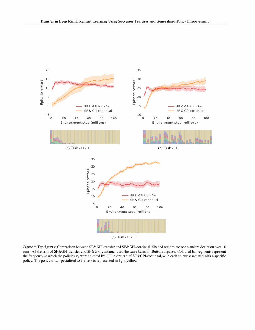
As discussed in the paper, ideally our agent should rely on the GPI policy when useful but also be able to learn and use aspecialised policy otherwise. Figures 7, 8 and 9 show that this is possible with SF&GPI-continual. Looking at Figure 7we see that when the test task only has positive rewards the performances of SF&GPI-transfer and SF&GPI-continualare virtually the same. This makes sense, since in this case alternating between the policies πi learned on M should leadto good performance. Although initially the specialised policy πtest does get selected by GPI a few times, eventually thepolicies πi largely dominate. The figure also corroborates the hypothesis that GPI is in general not computing a trivial policy,since even after settling on the policies πi it keeps alternating between them.

Interestingly, when we look at the test tasks with negative rewards this pattern is no longer observed. As shown in Figures 8and 9, in this case SF&GPI-continual eventually outperforms SF&GPI-transfer—which is not surprising. Looking at thefrequency at which policies are selected by GPI, we observe the opposite trend as before: now the policy πtest steadilybecomes the preferred one. The fact that a specialised policy is learned and eventually dominates is reassuring, as it indicatesthat πtest will contribute to the repository of skills available to the agent when added to Ψ.

As discussed in the main paper, one of the highlights of the proposed algorithm is the fact that it can use any set of base tasksand enable transfer to related, unseen, tasks. To empirically verify this claim, we tested several sets of base tasks. We used as areference our “canonical” set of base tasks M that spans the environmentM. We further validated our approach on a linearly-depend set of base tasks M′ that does not span the set of (test) tasks we are interested in—these results are shown in Figure 4.In addition to these, we now present experiments with a third set of base tasks that does span the set of tasks but does not in-clude any of the canonical tasks: M′′ = {(1, -0.1, -0.1, -0.1), (-0.1, 1, -0.1, -0.1), (-0.1, -0.1, 1, -0.1), (-0.1, -0.1, -0.1, 1)}.In Figure 10 we report results obtained by SF&GPI-transfer, using the three sets of base tasks described, on the 9 previously-introduced test tasks. We can see that all sets of base tasks lead to satisfactory transfer, but the performance of the transferredpolicy can vary significantly depending on the relation between the base tasks used and the test task. This is again anillustration of the distinction between the “reward basis” and the “behaviour basis” discussed in Section 5.3.


0 20 40 60 80 100


0

10

20

30

40

50

60

Epis

ode r

ew

ard

(a) Task 0111

0 20 40 60 80 100


0

10

20

30

40

50

60

70

Epis

ode r

ew

ard

Q(¸)

DQ(¸) fine-tuned

DQ(¸) from scratch

SF & GPI transfer

SF & GPI continual

(b) Task 1111

0 20 40 60 80 100


−3.0

−2.5

−2.0

−1.5

−1.0

−0.5

0.0

Epis

ode r

ew

ard

(c) Task -1000

0 20 40 60 80 100


−5

0

5

10

15

20

Epis

ode r

ew

ard

(d) Task -11-10

Figure 6. Average reward per episode on test tasks not shown in the main paper. The x axes have different scales because the amount ofreward available changes across tasks. Shaded regions are one standard deviation over 10 runs.


0 20 40 60 80 100


16

18

20

22

24

26

28

30

32

Epis

ode r

ew

ard

SF & GPI transfer

SF & GPI continual

(a) Task 1100

0 20 40 60 80 100


20

25

30

35

40

45

Epis

ode r

ew

ard

SF & GPI transfer

SF & GPI continual

(b) Task 0111

0 20 40 60 80 100


20

25

30

35

40

45

50

55

Epis

ode r

ew

ard

SF & GPI transfer

SF & GPI continual

(c) Task 1111

Figure 7. Top figures: Comparison between SF&GPI-transfer and SF&GPI-continual. Shaded regions are one standard deviation over 10runs. All the runs of SF&GPI-transfer and SF&GPI-continual used the same basis Ψ. Bottom figures: Coloured bar segments representthe frequency at which the policies πi were selected by GPI in one run of SF&GPI-continual, with each colour associated with a specificpolicy. The policy πtest specialised to the task is represented in light yellow.


0 20 40 60 80 100


−2.5

−2.0

−1.5

−1.0

−0.5

0.0

Epis

ode r

ew

ard

SF & GPI transfer

SF & GPI continual

(a) Task -1000

0 20 40 60 80 100


−4.5

−4.0

−3.5

−3.0

−2.5

−2.0

−1.5

−1.0

−0.5

0.0

Epis

ode r

ew

ard

SF & GPI transfer

SF & GPI continual

(b) Task -1-100

0 20 40 60 80 100


8

10

12

14

16

18

20

22

Epis

ode r

ew

ard

SF & GPI transfer

SF & GPI continual

(c) Task -1100



0 20 40 60 80 100


−5

0

5

10

15

20

Epis

ode r

ew

ard

SF & GPI transfer

SF & GPI continual

(a) Task -11-10

0 20 40 60 80 100


10

15

20

25

30

35

Epis

ode r

ew

ard

SF & GPI transfer

SF & GPI continual

(b) Task -1101

0 20 40 60 80 100


5

10

15

20

25

30

35

Epis

ode r

ew

ard

SF & GPI transfer

SF & GPI continual

(c) Task -11-11



1100 0111 1111 -1000 -1-100 -1100 -11-10 -1101 -11-11

Task description

−10

0

10

20

30

40

50

60

70

80

Epis

ode r

ew

ard

Canonical base tasks

Non-canonical base tasks

Linearly-dependent base tasks

Figure 10. Performance of SF&GPI-transfer using base tasks M, M′ and M′′, on the 9 test tasks. The box plots summarise thedistribution of the rewards received per episode between 50 and 100 million steps of learning.

Transfer in Deep Reinforcement Learning Using Successor ...

Documents

Transcript of Transfer in Deep Reinforcement Learning Using Successor ...