
Trading Volume and Market Efficiency: An Agent Based Model ...
37
HAL Id: halshs-00997573 https://halshs.archives-ouvertes.fr/halshs-00997573 Preprint submitted on 28 May 2014 HAL is a multi-disciplinary open access archive for the deposit and dissemination of sci- entific research documents, whether they are pub- lished or not. The documents may come from teaching and research institutions in France or abroad, or from public or private research centers. L’archive ouverte pluridisciplinaire HAL, est destinée au dépôt et à la diffusion de documents scientifiques de niveau recherche, publiés ou non, émanant des établissements d’enseignement et de recherche français ou étrangers, des laboratoires publics ou privés. Trading Volume and Market Effciency: An Agent Based Model with Heterogenous Knowledge about Fundamentals Vivien Lespagnol, Juliette Rouchier To cite this version: Vivien Lespagnol, Juliette Rouchier. Trading Volume and Market Effciency: An Agent Based Model with Heterogenous Knowledge about Fundamentals. 2014. halshs-00997573
-
Upload
khangminh22 -
Category
Documents
-
view
1 -
download
0
Transcript of Trading Volume and Market Efficiency: An Agent Based Model ...
HAL Id: halshs-00997573https://halshs.archives-ouvertes.fr/halshs-00997573
Preprint submitted on 28 May 2014
HAL is a multi-disciplinary open accessarchive for the deposit and dissemination of sci-entific research documents, whether they are pub-lished or not. The documents may come fromteaching and research institutions in France orabroad, or from public or private research centers.
L’archive ouverte pluridisciplinaire HAL, estdestinée au dépôt et à la diffusion de documentsscientifiques de niveau recherche, publiés ou non,émanant des établissements d’enseignement et derecherche français ou étrangers, des laboratoirespublics ou privés.
Trading Volume and Market Efficiency: An Agent BasedModel with Heterogenous Knowledge about
FundamentalsVivien Lespagnol, Juliette Rouchier
To cite this version:Vivien Lespagnol, Juliette Rouchier. Trading Volume and Market Efficiency: An Agent Based Modelwith Heterogenous Knowledge about Fundamentals. 2014. �halshs-00997573�
Working Papers / Documents de travail
WP 2014 - Nr 19
Trading Volume and Market Efficiency: An Agent Based Model with Heterogenous Knowledge about Fundamentals
Vivien LespagnolJuliette Rouchier
Noname manuscript No.(will be inserted by the editor)
Trading volume and market efficiency: an Agent Based Model withheterogenous knowledge about fundamentals
Vivien LESPAGNOL · Juliette ROUCHIER
May 2014
Abstract This paper studies the effect of investor’s bounded rationality on market dynamics. In anorder driven market, we consider a few-types model where two risky assets are exchanged. Agentsdiffer by their behavior, knowledge, risk aversion and investment horizon. The investor’s demand isdefined by a utility maximization under constant absolute risk aversion. Relaxing the assumptionof perfect knowledge of the fundamentals enables to identify two components in a bubble. The firstone comes from the unperceived fundamental changes due to trader’s belief perseverance. The secondone is generated by chartist behavior. In all simulations, speculators make the market less efficientand more volatile. They also increase the maximum amount of assets exchanged in the most liquidtime step. However, our model is not showing raising average volatility on long term. Concerning thefundamentalists, the unknown fundamental has a stabilization impact on the trading price. The closerthe anchor is to the true fundamental value, the more efficient the market is, because the prices changesmoothly.
Keywords Agent-based modeling · market microstructure · fundamental value · trading volume ·efficient market
JEL classification C63 · D44 · G12 · G14
Aix-Marseille University (Aix-Marseille School of Economics), CNRS & EHESS.Marseille, FRANCECorresponding author. E-mail: [email protected]
2 Vivien LESPAGNOL, Juliette ROUCHIER
1 Introduction
The main goal of financial markets is to guarantee an optimal transfer of resources from supplyto demand. This aim can be attained only if exchanges do actually occur in a considered period, i.e.the market is liquid. Amihud et al. (2005) write that "liquidity is a complex concept. Stated simply,liquidity is the ease of trading a security ". Hence liquidity is a property of the system, which cannot beattained by just one agent with not enough influence on the market to create a context of easy trade.It is, however, an important feature which assures the functioning of the financial market through thebehavior of the agents. It impacts the price, the volatility, and the amount of quoted orders.
During the last crisis, there was no way analysts could anticipate the liquidity and price falls thattook place. And, to the best of our knowledge, there is no known mean to impact on the marketliquidity and we are just faced with ex post observations and attempts to understand the data. Asan example: Air France -KLM was valued under 5e on the CAC40, even if a consensus of analystsestimates that the book value was at least 6 times higher. However, nobody wanted to hold this assetso it was undervalued from the start! This is neither predictable nor rational. Actually, it has beenshown that agent’s behavior is drastically driven by asset exposure to liquidity risk (Amihud, 2002).For example, a fly to quality is observed, traders prefer to hold less risky and more liquid assets evenif their returns is lower. Liquidity is studied by micro structure theory, but it is usually taken as anexogenous parameter which influences the agents’ behaviors. However, it has been little studied inagent-based computational economics, where it could be endogeneized as the emerging result of actualtransactions, then taken into account by the agents.
The contribution of agent based economics is to produce models that integrate agents’ boundedrationality, as well as their heterogeneity in terms of information and cognition. Several authors havealready proven that this assumption of heterogeneity is necessary to reproduce, with models, dynamicsof actual behaviors (like experimental data) (Bao et al., 2012).
The main goal of this paper is to focus on heterogeneous knowledge about fundamentals and itimpact on liquidity dynamics in a financial market. We build an agent-based model, for which wemake choices to produce the modeling structure and the rationality of agents. The comparison amongdifferent simulations show that the information that is available to different agents has an impacton price dynamics and market liquidity. Different stylized facts are thus produced. The introductionof an idiosyncratic perceived fundamental value enables to identify different bubble types: some thatcan be attributed to anchoring (Lord et al., 1979; Westerhoff, 2004), and some that are generated bychartists behavior, based on trend extrapolation (Hommes, 2006). As seen in other models (Giardinaand Bouchaud, 2003; Hommes et al., 2005; Lux and Marchesi, 1998), we observe a destabilizationpower of chartists. We also witness the stabilization impact of the anchor on the price variance, sincethe trading price evolves more slowly than in the case of perfect knowledge of fundamentals. Finally,we test the agent’s aggressiveness (Parlour, 1998) on the price efficiency. As expected, if agents takeinto account the market liquidity as a parameter of price valuation, we observe a rise in liquidity and afall in efficiency. It would be possible to evaluate, with this mean, the price of liquidity in the system,but at this stage, we do not perform econometric tests, just observe stylized facts.
This paper is organized as follows : Section 2 reports our model assumptions and their literature,describes the functioning of the model in English. Section 3 discusses results and Section 4 concludes.
2 Model and results
2.1 Choosing a suitable model to study liquidity
The field of microstructure focuses on the concept of liquidity, impact of traders type or informationrevealed. Without doubt, one of the most studied is the Kyle model (Kyle, 1985) where the authorfocuses on the optimal behavior of discretionary traders and their effect on patterns of trade. Another example is Grossman and Miller (1988), who point out the importance of liquidity for behavior,prices and the viability of the market. In their paper, they study how agents submit orders in moreor less liquid market so as to avoid disclosing their private information. Chu et al. (2009) highlight astrong preference of investors for liquid assets amid heightened price volatility during the last financialcrisis. In their study, extended asset guarantee is a way to improve asset liquidity. The liquidity theorypredicts that the level of liquidity and liquidity risk are priced (Amihud et al., 2005; Karolyi et al.,2012). Empirical studies find the effect of liquidity on asset prices to be statistically significant and
Trading volume and market efficiency 3
economically important, controlling for traditional risk measures and asset characteristics. This resultcould be generated by high transaction cost, demand pressure and inventory risk or private information.
The branch of finance in ABM aims at replicating some market stylized facts. The most famousexample is the Santa Fe Institute (SFI) market (LeBaron, 2002), the first agent-based financial marketplatform, which was used to study the impact of agent interactions and group learning dynamicsin a financial setting. It is made of learning agents who trade two assets, a risky and a non riskyone. The asset price is defined under a simple market clearing mechanism. Indeed, starting fromthe evidence that agents are boundly rational, Chiarella et al. (2013) point out the importance oflearning (which they model using genetic algorithms) to capture many realistic features of limit ordermarkets. In an other context, Lux and Marchesi (1998) model the agent’s mood (optimist or pessimistfeeling) to reproduce bubbles. An interesting stylized fact of this paper is that bubbles grow and burstexogeneously and cyclically. Hommes et al. (2005) highlight that with adaptive agents, the fundamentalsteady state becomes unstable and multiple steady states may arise. Pouget (2000), in her paperon market efficiency, highlights that agents type, investor’s market power and motivation drive themain market price oscillations. For her, the time horizon of each investor is the main explanation toinefficiency in markets.
These already quite complex results rely on market dynamics where agents are assumed to haveperfect knowledge of the fundamental and a special agent, the market maker, deals with market liq-uidity; most of the time there are only two assets, one risky and one non risky. We build our modelrelaxing these three assumptions, which are usually not abandoned all at once.
First, we relax the strong assumption of perfect knowledge of the fundamentals. According to theworks of Tversky and Kahneman (1974) on agent’s decision in unexpected context, traders are reluctantto change their beliefs and keep an influence of original belief for long. They process information withmisunderstanding and update their expectation very slowly, while using the market as a source of newinformation. Fundamental value, hence, is neither unique nor exogenous to the market (Orléan, 2011).We use this idea to build a learning model that is adapted to heterogeneous initial beliefs of agents.
For practical advantage and mathematical simplicity, the market maker is usually used as marketstructure. Lux (1995), Iori (2002), Hommes et al. (2005) or Harras and Sornette (2011) have developedthe same kind of market maker to provide liquidity. Hommes et al. (2005) argue "an advantage ofthe simple price adjustment rule is that the model remains analytically tractable". Beja and Goldman(1980) invoke a market maker mechanism in order to justify sluggish Walrassian price adjustment.Howewer, Foucault et al. (2005) has written that "a trader who monitors the market and occasionallycompetes with the patient traders by submitting limit orders, can significantly alter the equilibrium.His intervention forces patient traders to submit aggressive limit orders and hence narrows the spreads.This feature may provide important guidance for market design". LeBaron (2006) writes in his surveythat the most realistic mechanism to replicate a financial market in ABM would be to use an orderbook. In this market structure, there is no counter part as market maker who impacts on the marketprice or provides liquidity. The liquidity is endogenous to the model, generated only by the execution ofquoted orders. While working on liquidity, we decided to produce a more demanding model structure,and hence run an order book.
The model we base our market upon is Yamamoto’s model (2011), which we extend by adding asecond risky asset. The reason to use two risky and one non-risky assets to deal with liquidity canbe explained : if one risky asset only is modeled, in case of a shock on this asset, all risk aversetraders leave the market to invest in the risk free one. In a multi-risky assets, traders reallocate theirportfolio without leaving the market, which as a result does not become illiquid. An other advantage ofmulti-assets markets is the possibility to manage the risk. According to the portfolio theory, the mean-variance criteria highlights that it is possible to minimize the portfolio risk in case of multi-risky assets(if cov < 1, the correlation coefficient between the assets). As Chowdry and Nanda (1991) state, multiassets enable to study liquidity that is essential for both viability and dynamics of market. Finally, atwo risky assets model seems more realistic than a unique risky asset and can be extended to a n-riskyone. To the best of our knowledge, the main Agent-based Computational Economics (ACE) in financeare build with a unique risky asset and a risk free. We can mentioned a paper from Westerhoff (2004)and one from Chiarella et al. (2007) in which two risky assets are traded but with the intervention ofa specialist (the market maker).
As a summary, the novelty of our model stays in the aggregation of an order book structure wheretwo risky assets are traded and where fundamentalists don’t have access to the true fundamental value.In the following subsections we describe the models we use to build upon as well as the choices wespecifically added to the structure and rationality of our agents.
4 Vivien LESPAGNOL, Juliette ROUCHIER
2.2 Market structure
Gode and Sunder (1993) has proven with their Zero-Intelligence traders that computational marketstructure plays an important role in the market efficiency and price convergence. They argue that itis very important to fix a structure once, to be able to compare while testing different elements ofrationality.
Domowitz (1993) has shown that in the early 90’s over thirty important financial markets in theworld had some of order-driven market features in their design. Whereas some markets were driven byprices in the recent past (the NASDAQ until 2002), today, most stock exchanges operate on an orderbook. The more realistic modeling choice is thus an order driven market. As said before, this marketstructure is the most difficult to compute, but necessary when focusing on liquidity (LeBaron, 2006).
Our model is based on an order driven market where two stocks are traded. At any time t, anagent is randomly chosen to enter the market or not. She can invest her wealth in the two risky assets(Stocks) and in a risk free one (Bond). An order driven market is characterized by an order bookwhich contains the list of interested buyers and sellers. For each entry it keeps the number of sharesand the price that the buyers (sellers) are bidding (asking) for each asset and its limit execution date.The submitted prices are not continuous, they are defined as a multiple of a "tick" size. Orders areexecuted according to time submission and quoted price.
The market price is defined by a matching process between buy and sell orders quoted in the book.When the best quoted buy order meets a counter part, an exchange occurs. The market price of theasset is defined by the price at which this exchange is realized. If the best bid (or ask) meets no counterpart, no trade occurs. A mid point (bbestt +abestt )/2 is defined as market price. If (at least) a part of theorder book is empty, we assume that the new market price is equal to the previous one (pt = pt−1).For order book examples, see the papers of Chiarella et al. (2009), Foucault et al. (2005), Tedeschiet al. (2012) or Yamamoto (2011).
Note that bid, ask and market price need to be positive. Agents are heterogeneous in their initialendowment. Traders’ portfolios differ by their weight affected to each component, the assets and bond.In this model, agents are not allowed to engage in short selling and are not monetary constrained. Forsimplicity no quoted orders can be modify or cancelled. Indeed, the trader who has submitted ordershas to wait for its execution or for its limit execution date before submit a new one. Finally, the riskyassets are assumed to be independent (cov = 0), and this fact is common knowledge.
In this context, the order type is decided according to the submission price and the bid-ask spread.Agents face two types of orders : the market order (MO) and the limit order (LO). The first one enablesto exchange a defined quantity of assets very quickly, since agents agree to deal at any price. On theopposite, the second one is characterized by an amount of assets and a limit execution price. The limitorder insures the trading price but not its execution. Here, a market order is chosen when the agent’sbid (ask) is higher (lower) than the best quoted ask (bid). Otherwise, the agent submits at a limitprice. The type of order is a parameter that defines a simulation: it is set at the beginning and is usedas a functioning rule at each time-step.
When the length of the market order is larger than the best counter part, the remaining volume isexecuted against other quoted limit orders. If there is not enough quoted counter part, the remainingvolume is executed as new orders are submitted. Hence, the order type influences greatly the marketliquidity. As an example, in the case of two limit orders, if the best bid is lower than the best ask,no change occurs. The market stays illiquid until either a higher bid (lower ask) than the quoted ask(bid) or a market order is submitted.
2.3 Trader’s model
We make several assumptions about our agents in the system, some that are very usual in ACEfinancial models, and others that are related to our present issue regarding the impact of informationon liquidity and prices. Within a typology of agents that is rather usual, fundamentalists and chartistswho have different risk aversion, we add several features of bounded rationality that are relevant tothis type of modeling.
Trading volume and market efficiency 5
2.3.1 Agents with types and risk-aversion
In 1980, Beja and Goldman highlight that agents types affect the quality of the price signal. Ingeneral, modelers distinguish two (Chiarella et al., 2007; Jacob-Leal, 2012) or three (Chiarella et al.,2009; Hommes, 2006) types of agents that are fundamentalists, chartists and noise traders.
Following the financial theory, the first ones trade in order to make the market converge to itsfundamental value and are considered as informed traders. They trade in order to minimize the gapbetween the fundamental value and the trading price. Their goal is to bring money to the liquiditydemander and guarantee an optimal allocation of resources. They are assumed to be the most riskaverse agents and have long term investment horizons. According to this features, a pure fundamentalistmarket should be efficient in the sense of Fama (trading price close to fundamental price - Fama, 1970).Graphically, the trading price should oscillate strongly in a small path around its fundamental value. Itshould look like a with noise. However, this market should be relatively less liquid than an heterogeneousone (fundamentalists and chartists). Indeed, an efficient market populated by pure fundamentalists isilliquid until a new information arise. In this paper the liquidity is measured by the volume of exchange.
At the opposite, chartists are describe as speculators and have a destabilizing impact. They tryto predict price evolution so as to surf on the bubbles and hence exploit the market trends to makeprofit. As a consequence they revise their expectation frequently and prefer short time investments.Chartists don’t care about fundamental changes. They increase the market depth thanks to theirshort term horizon. A pure chartists market or an heterogeneous one should be more liquid but lessefficient. Graphically, the market price should oscillate around short trends that are independent ofthe fundamental value. We also expect that the spread between fundamental price and trading priceis wider in the case of chartists (or heterogeneous) market than in the case of fundamentalists one.
The more a trader is risk averse, the less she trades. The longer the investment horizon, the longerthe agent holds her assets and hence the less she trades as well. Amihud and Mendelson (1986) dis-tinguish different types of traders for each liquidity degree. At the equilibrium, in a market populatedby risk neutral agents, the long term investors – fundamentalists – buy assets relatively illiquid andwith a high trading cost because they expect to hold it for a long time. Whereas short term investors– chartists – prefer liquid asset with less trading cost in order to surf on the trend.
We choose here to model each individual agent as a mix of the two most usual components: fun-damentalists and chartists, as can be found in Yamamoto (2011). This formulation is motivated byHarras and Sornette (2011) who mention that "agent forms her opinion based on a combination ofdifferent sources". The fundamentalist’s source of an agent expects that the forward price converges toits fundamental, while the chartist’s one assumes that the future price follows the past trend (Hommes,2006). The key parameters of this agent model are g1 and g2, which are generated at initialization, foreach trader, following an exponential law of variance σ2
1 and σ22 , respectively. A pure fundamentalist
strategy has gi2 = 0, whereas a pure chartist strategy has gi1 = 0. When both values are higher than 0,the agent is a mixed of both, which implies that she takes into account the chartist and fundamentalistexpectations and make an average according to the g1 and g2 weight (following Eq. (5) in appendix5.1). From the two parameters values, the time horizon of investment and the risk aversion of eachagent is also calculated (Eq. (11) and (12)). The more the agent tends to be fundamentalist, the morerisk averse and long term investor she is. The converse is true : the higher the tendency to be chartist,the lower risk aversion and the longer the investment horizon.
2.3.2 Bounded rationality and market depth as information
The choice we make is to define our agents as boundedly rational. We try to replicate some real-life choices rather than optimal decision. Lord and al. (1979) focus on the belief perseverance oftraders: when an agent has formed an opinion, it is hard for her to change her mind. People arereluctant to search for evidences contradicting their beliefs. Even if they find such an evidence, theytreat it with excessive skepticism. Sometimes, people miss-interpret evidence that goes against theirhypothesis as actually being in their favor. As example, belief perseverance predicts that when peopleformulate expectation on fundamental value, they may continue to believe in it long time after theproof of fundamentals misunderstanding has emerged. In our paper, we distinguish two cases : a perfectknowledge of the true fundamental value and a belief perseverance one. We treat in more details thispoint in section 2.4.
According to their preferences, traders try to maximize their utility function under Constant Abso-lute Risk Aversion (CARA). The parameter of aversion toward risk is function of the trader components
6 Vivien LESPAGNOL, Juliette ROUCHIER
(Eq. (12)) and has a direct impact on the optimal demand of assets (Eq. (8) and (9)). The order size(si,jt ) an agent is willing to trade is assumed to be equal to the absolute difference in the optimal de-mand for asset j at time t and t−1. The sign of this difference gives us the agent’s position (Eq. (13)).When the difference is positive, the trader buys, if it’s null, she doesn’t enter the market, otherwise shesells. Remark that this type of utility is independent of wealth, as Chiarella et al. (2009) mentioned.This is not consistent with the intuition and some empirical results about aversion toward risk. Usuallywealthier people bear more easily risk than poorer ones (Prospect theory - Kahneman and Tversky,1979). The risk premium is decreasing with wealth. A possible evolution is to rewrite the model withan Harmonic Absolute Risk Aversion (HARA) function or at least a Decreasing Absolute Risk Aversion(DARA).
The submitted bid (or ask) is different of the expected forward price (p) according to the agent’smood. In an optimistic mood (Mt > 0), the agent accepts to buy (bt > pt) or sell (at > pt) at higherprice. She believes that the market will continue to raise. The buyer expects to make profit on thefuture sell and the seller expects to perceive an additional premium (at − pt). On the contrary, ifMt < 0, the trader is in a pessimist way, she expects a fall. Sellers and buyers accept to exchange butat a lower price than they predicted. They try to diminish their loss in case of a fall.
After defining the price (at or bt) and the quantity (st) at which the agent is willing to trade,she adapts her order according to the market depth. With an order book – where at least a part ofthe book is observable – Parlour (1998) shows how the order placement decision is influenced by thestate of the book. Particularly the depth available at the inside quotes. Empirical researches pointout that investors place more aggressive orders when the same side of the order book is thicker, andless aggressive orders when it is thinner (Handa et al., 2003). In concrete terms, with a probabilityProbit, the trader adapt her behavior according to the order imbalance (xobt ) which is defined by thelog difference between the depth of the five best bids and asks (as Yamamoto, 2011).
Probit = tanh(βi ∗ abs(xobt )) (1)
xbidt = log(depth of the 5 best bids
depth of the 5 best asks) or xaskt = log(
depth of the 5 best asks
depth of the 5 best bids) (2)
where ob = bid or ask respectively for a buy order or a sell order. βi reflects the sensitivity of theprobability of switching in response to the depth of the order book. The β parameter follows a uniformlaw on the interval [0;βmax]. It is constant over time but differs for each asset and agent. Accordingto the order imbalance, the agent submits more or less aggressive orders. She faces five specific cases :
1. Submit a bid knowing that the depth of the buy side is thicker than the other (xbidt > 0). In thiscontext, the risk of non execution of the order is high. There is a bigger demand of asset thansupply, therefore, only the more expensive orders have a chance to be executed. With a probabilityProbit – which is function of market depth and the sensitivity of agent to adapt, Eq. (1) – the agentsubmits at a more aggressive price. If she had decided to submit a limit order out of the bid-askspread, then she would have changed it for an order at the best bid price plus a tick size. The orderwould have taken the first place in the order book. If she had decided to submit a limit order inthe bid-ask spread, then she would have preferred to submit a market order. She takes more riskon price fluctuation but she is confidant in her probability of execution.
2. Submit an ask knowing that the depth of the buy side is thicker than the other (xaskt < 0). Thedemand is strong and the consider agent is a supplier. The probability of execution is high. With aprobability Probit, she submits a less aggressive order. She expects to earn more. If she had chosento submit a market order, then she would have preferred to submit a limit order at the best bidplus a tick size. If she had decided to submit a limit order in the bid-ask spread, then she wouldhave decreases her price submission to the best ask.
3. Submit a bid knowing that the depth of the buy side is thinner than the other (xbidt < 0). Thebuyer faces the same advantage as the seller in the previous case. With a probability Probit, theagent submits a less aggressive order, to buy at a lower price. If she had previously decided tosubmit a market order, then she would have preferred to trade at the ask minus a tick size. If herlimit order had been in the bid-ask spread, then she would have submitted at the best bid.
4. Submit a sell knowing that the depth of the buy side is thinner than the other (xaskt > 0). With aprobability Probit, the agent trades more aggressively. She prefers to loose a bit (the bid-ask spread)than to take a non-execution risk! If her original choice had been to submit a limit order in thespread, then she would have preferred to submit a market order. No control on the order price, but
Trading volume and market efficiency 7
she knows that she would have been the first in the order priority. If she had decided to submit outof the bid-ask spread, then she would have submitted at the best ask minus a tick size to be sureto be the first in the ask book.
5. In any other cases, the agent doesn’t update her order, she submits at the normal price (at or bt)defined by the Eq. (14) for a buy order and (15) for a sell order.
To sum up, the traders are heterogeneous in their fundamentalist and chartist components, theirinvestment horizon and their risk aversion. Moreover, they are bounded rational. Their mood and theiraggressiveness influence the price at which they are willing to trade. In the case of belief perseverance,we also assume that traders are reluctant to change their minds about fundamental value estimation,even if they have evidence of misunderstanding (Fischoff, Slovic and Lichtenstein, 1977 and Lord, Rossand Lepper, 1979 mentioned by Barberis and Thaler, 2003). Concerning the submission process, ateach period one agent is randomly chosen and follows the four next steps:
1. for each asset available on the market, she formulates expectations on the forward price accordingto her features (gi1 and gi2).
2. she defines the amount of assets she wants to trade according to a CARA utility function.3. she adapts her expectation according to her personal mood (simple rule of thumb). It is assumed
to be time and asset dependent.4. after having formulated an order, she corrects it according to the market depth and submits.
Her order is quoted in the order book and can’t be modified or removed. The complete mathematicalmodel is developed in the appendix (see appendix 5.1).
2.4 Fundamental value
The fundamental value is usually defined as: the expected dividend of the firm (Et[yt+k]) correctedby the risk premium required for risky asset (ασ2Z) divided by the actualization rate (R). This valueis assumed to be unique and equal to:
f =
∞∑k=1
Et(yt+k)− ασ2Z
Rk
There are lots of criticism about the definition of the fundamental value. The first problem comesfrom the heterogeneity of actualization rates, which one to select? A constant or a time evolutive?How to fixe it? The second problem is in the forward dividend. On which economic variable do webase our dividend expectation? Moreover the dividend expectations come from the market, and so,the fundamental value becomes intrinsic to the market whereas it must be intrinsic to the firm butexogenous to the market! With heterogeneous bounded rational agents and unpredictable future, thefundamental value becomes idiosyncratic.
In this paper, we distinguish two cases: a perfect knowledge one and an imperfect knowledge one,also namely "belief perseverance". In both settings, we assume that the true fundamental value (f)follows a random walk and agents have access to the entire history of asset prices.
In the case of perfect knowledge of the fundamental value, all fundamentalists have access tothe good information. Because everybody has the same information and processes it correctly, theestimation of the fundamental value (f) is assumed to be unique and right. For each fundamentalist i,it is mathematically expressed as:
f it = ft = ft ,∀i (3)
In the case of belief perseverance (imperfect knowledge of the fundamental value with adaptivelearning), the forward fundamental value becomes idiosyncratic. It is a well known fact that tradersmake errors in their expectations and are overconfident (Barberis and Thaler, 2003). Tversky andKahneman (1974) highlight that people make estimation of prices by starting from an initial valuethat is insufficiently adjusted across time. This is why we produce heterogeneity in our agents bygiving them different initial believes: even if they get the same piece of information in time, they donot necessarily deduce the same fundamental value for the asset. Our formulation of the estimated
8 Vivien LESPAGNOL, Juliette ROUCHIER
fundamental value is inspired by Westerhoff (2004), so as to fit the anchoring assumption that is oneaspect of bounded rationality. The fundamental value (f it ) of agent (i) in the case of belief perseveranceis designed as:
f it = γ1 pt−1 + γ2 fit−1 + γ3 f
iorigin
+ Nt + a(f it−1 − f it−2 −Nt)+ b (ft−1 − f it−1) (4)
f it 6= f jt ,∀i 6= j
The first line represents the anchor. It is defined by the last observed price (pt−1), her previous (f it−1)and her original (f i0) estimation of the fundamental value. γ1, γ2 and γ3 represent the weight given toeach component and add up to 1. The second line describes the anchor correction. The first componentreflects the arrival of new information (Nt), common knowledge. The second component highlightsthe faith related to it. As an example, if the recent update of the estimated fundamental value hasbeen above the news impact (f it−1 − f it−2 > Nt), the fundamentalist tends to overreact to news. Thea parameter is the degree of misperception, which represents the time needed to process information.The third line (ft−1 − f it−1) – which is the spread between the last true fundamental value and theestimated one – is the one that represents learning. The b parameter affected to this learning is assumedto be close to zero, agents are reluctant to change their mind. All parameters (a, b, γ1, γ2, γ3) are fixedand equal among traders.
3 Simulations analysis
This section describes the dynamics of two types of market that can be produced within our frame:in the first sub-section the market is made of traders that are pure fundamentalists ("one-type model")than in the second one is made of traders that are a mix of fundamentalist and chartist components("two-type model"). It has to be remembered that even agents who are all 100% fundamentalists arenot necessarily homogenous, since they differ in time horizon and aversion to risk. Within these twosub-frames, we study specifically the influence of the type of information agents get on the marketdynamics – more precisely we study volatility and liquidity when agents have perfect knowledge of thefundamental value of the assets, and when the agents have limited information. We hence face fourdifferent cases: OTP (One-Type model – Perfect knowledge), OTB (One-Type model – Belief persever-ance), TTP (Two-Types model – Perfect knowledge) TTB (Two-Types model – Belief perseverance).We change diverse parameters within each set of simulations to be able to establish 1/ the relevanceof our model which produces certain stylized facts which are usually recognized as relevant 2/ theinfluence of our main assumption: the disparition of perfect knowledge and the idiosyncratic learningof agents.
We ran 200 simulations for each trading round, each simulation being a succession of 8,000 time-steps, which we observe after 1000 steps have already been run (so that agents have time to learn andin order to exclude impacts of computer initialization). The model setup is summarized in the table 3of appendix 5.2.
3.1 Dynamics in one-type markets
3.1.1 Benchmark: perfect information
As said before, fundamentalists trade according the fundamental value of assets, of which theyare here perfectly aware: they submit orders to make the market efficient – current price equals thefundamental price. Even when all agents follow this rule, strong market efficiency is never verified, andwe observe an oscillation of the trading price around its fundamental. This inefficiency is linked to theheterogeneity of our population, which directly impacts the market dynamics. Thus, to model agentsheterogeneity, we focus on the the variance distribution of the fundamentalist component (σ2
g1), whichis the key parameter of our one-type markets. Increasing σ2
g1 makes the traders "more fundamentalists"in the sense that on average they become more risk averse and more long time investors (see Eq. (11)and Eq. (12)). We simulated trading rounds for increasing value of σ2
g1 , and identified a decreasingvolume of exchange (table 1). This is consistent with what can be expected from the variation of
Trading volume and market efficiency 9
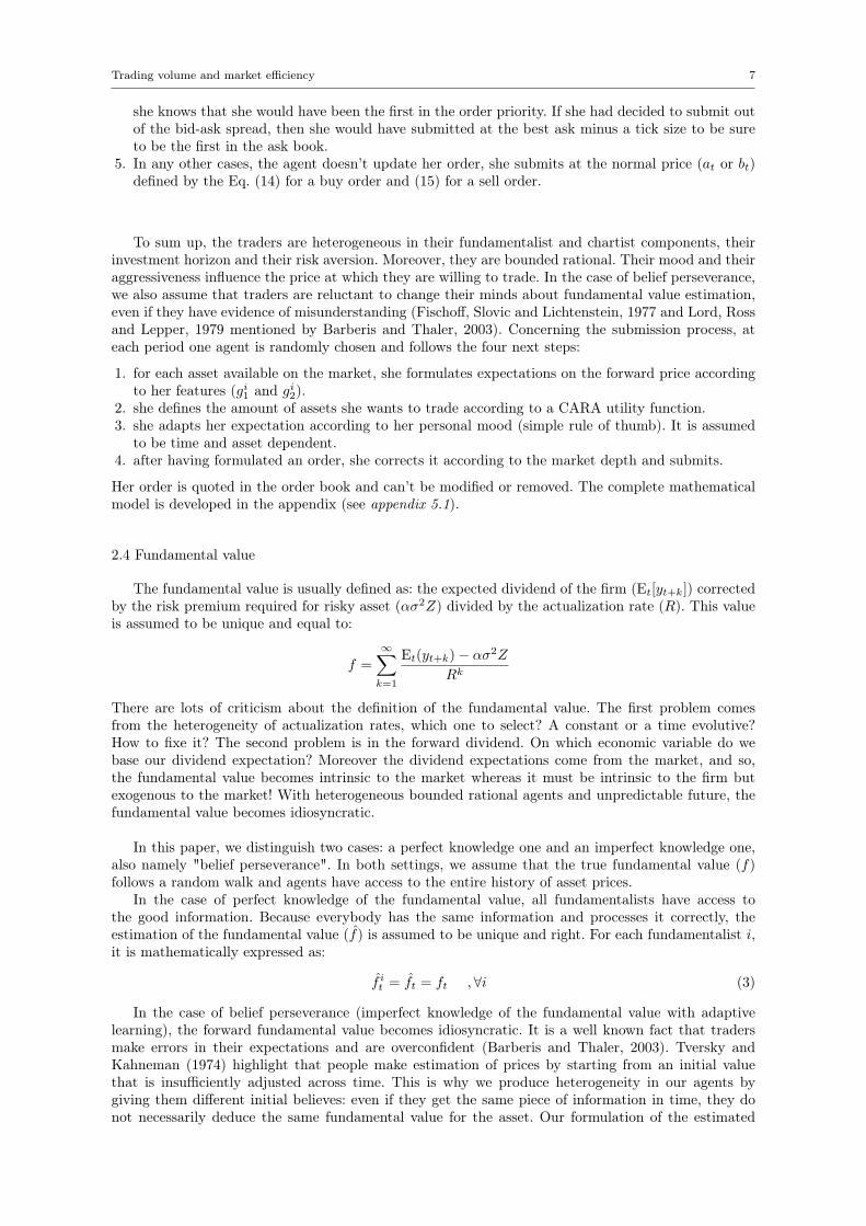
(a) Asset 1: Trading price (b) Asset 2: Trading price
(c) Asset 1 : Spread between trading price and fundamentalprice on a shorter period, 0-2000
(d) Asset 2 : Spread between trading price and fundamentalprice on a shorter period, 0-2000
Fig. 1: Price dynamics in OTP case (σ2g1 = 0.6, σ2
f1= 0.2, σ2
f2= 1)
Asset 1 σ2g1
= 0.1 σ2g1
= 0.6 σ2g1
= 1 σ2g1
= 10
Mean Std. Dev Mean Std. Dev Mean Std. Dev Mean Std. Devvol. per simu. 710 56 592 92 554 70 359 46max. vol./time step 11.3604 6.23 11.02806 9.17 10.94757 6.25 9.628196 6.98price variance 669 205 695 227 710 245 754 245
Table 1: Market liquidity in OTP case, σ2f = 0.2
risk aversion: the more risk averse the agents, the less they trade. The average trading volume persimulation falls from 710 to 359. This values are similar for each traded asset. Surprisingly, on averagethe most liquid time-step is not strongly affected by the variance distribution of the fundamentalistcomponent. For σ2
g1 = 0.1, the most liquid time-step is 11.36. It decreases slowly until 9.63 for σ2g1 = 10.
When considering Eq. (8) and (9), one could assume that the volume of exchange is correlated to priceoscillations rather than agents expectations. Indeed the amount an agent agrees to deal is defined bythe absolute difference of assets demand between time t and t− 1.
According to empirical data (Elyasiani et al. 2000), a decreasing trading volume implies an increasein the volatility of the market price: less assets are quoted and traded on the market, so the pricemovements are larger. In our model, a 50% liquidity fall implies an increasing price variance of 15%.The probability not to find any counter part (no quoted bid or ask) increases also from 2.6% to4%. When fundamentalists’ investment horizon is larger and their risk-aversion increases, the marketliquidity falls. So, this model is able to replicate the finding of Beja and Goldman (1980): increasingthe fundamentalist power in a previous stable system makes it less stable.
The variance of the trading price is high and linked to the variance of the fundamental value.When the true fundamental value changes, the fundamentalists perceive this movement and updatetheir expectations according to news. In our simulations, whatever the original fundamental value is,the trading price oscillates of ±26%. This value falls to ±20% and to ±13% if we exclude respectivelythe 10% and the 20% extreme data. So, usually the price oscillates strongly in a small path andsometimes, peaks appear and destabilize the market for a short period. As an example, for an initialtrue fundamental value of 300 ECU and σ2
g1 = 0.6, all prices are contained in the interval [−80; +80]around its fundamental, which is a wide trading price fluctuation around the fundamental, already
10 Vivien LESPAGNOL, Juliette ROUCHIER
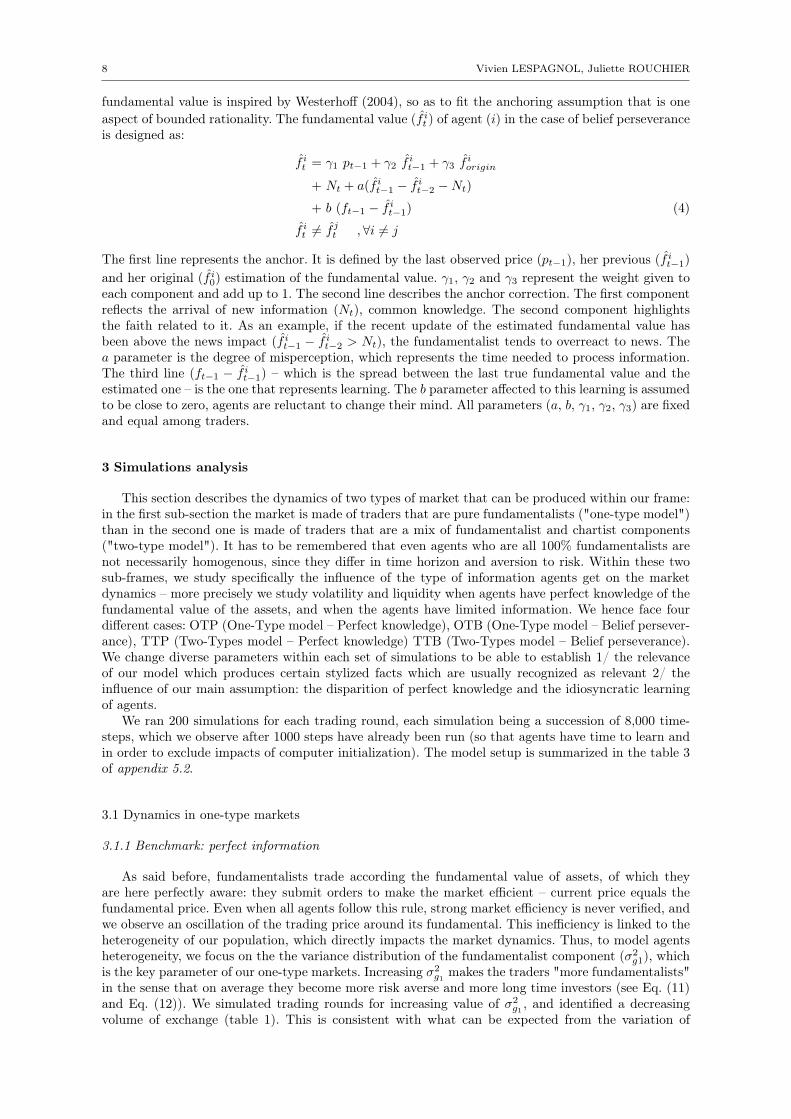
σ2f1
= 0.2 & σ2f2
= 0.2 Benchmak Belief perseveranceAsset 1 Mean Std. Dev Mean Std. Devprice 308.1574 12.32511 306.6011 3.695452mean spread 7.789 4.584102 6.931 11.74591variance 698 216 552 113Asset 2 Mean Std. Dev Mean Std. Devprice 310.4384 14.41455 308.0654 4.270272mean spread 9.645 6.012068 7.979 11.80833variance 723 240 546 142
Table 2: Perfect vs. imperfect knowledge of the fundamentals in one-type market
pointed out by Iori and Porter (2012). In a 95% confidence interval, the trading prices are containedin [−38; +58]. The spread asymmetry seems to mean that the market is overvalued, which is the case63% of the time. The mean spread – difference between the trading price and the true fundamentalvalue – is such that asset 1 is overvalued by 8 ECU, and asset 2 by 10 ECU. The average trading pricesare 308.157 and 310.438 ECU.
In addition, fundamentalists submit on average 20% of market orders so as to buy and 26% so asto sell: they are more impatient to sell than to buy, which is consistent with the literature.
Fig. 1 is a typical example of the OTP case. The trading price oscillates in a large spread around itsfundamental value, and never diverges. The executed orders are above as much as below the fundamen-tal price. If we focus on a smallest time interval, we distinguish two main dynamics that seem cyclical.Fig. 1c and Fig. 1d reflect them. We distinguish a short period of high price variation and a longerperiod of low variation. The periods of low variation appear mainly in the interval [-30;+30] aroundthe fundamental. This spread is equivalent to the one in which the 20% extreme data are excluded. Inthis interval, fundamentalist seems to estimate that the market is relatively efficient – which explainthe low variance of the trading price – until a bullish or bearish shock appears and destabilizes themarket – which becomes very volatile. After a short time, the price variance goes back to a low level,and the trading price converges to its true fundamental value. This is consistent with Eq. (8). The lessthe price varies, the more fundamentalists exchange and the faster the price converges.
Even in OTP case, we highlights that trading prices may differ from their fundamental value.
3.1.2 Belief perseverance
In this sub-section, we focus on changes in the dynamics of a one-type market where the assumptionof perfect knowledge of the fundamental value is relaxed : OTB case. Traders base their own predictionson their previous expectations (anchor) and a learning element (see Eq. (5)), and each agent is givena personal initial anchor.
If the original anchor is chosen close to the initial true fundamental value, the introduction ofpersonal believes about fundamental value will not change the market dynamics significantly. All valuesbeing the same, we found trading prices around 306 ECU for asset 1 and 308 ECU for asset 2, whichare respectively 0.858 ECU and 1.666 ECU less overvalued than in the OTP case (see Table 2). Thetrading price oscillates about ±26%. The 95% confidence interval makes the path thinner [-14%;+18%].And the market is overvalued 60% of the time, which means that the price seems to have a smootheroscillation and a lower variance. Moreover, when the variance of the true fundamental increases, thevariance of the market price is not really affected. The true fundamental value is perceived by thefundamentalists as being more stable than it really is.
The trading price is directly impacted, becoming more stable and the market liquidity is weaklydecreasing. All these results are what was expected. Fundamentalists thus integrate the news theyperceive in the trading price. If the fundamental value is perceived as stable, there will be no "non-integrated" news, and so no more trade. Finally, the belief perseverance makes runs more similar, thestandard deviation of the average price is at least twice lower compare to the OTP case.
If the anchor is not consistent with the fundamental value, the market price will not reflect thefundamental at all. Indeed, agents have a tendency to give less importance to news than to the originalfundamental expectation (f i0) because of the anchor. In this case, the trading price is stable and evolvesaround the original fundamental expectation. This is due to the fact that the anchoring is strong andlearning is slow, hence re-ajustment is slow. The result is an inefficient market: the market price neverreflects its fundamental.
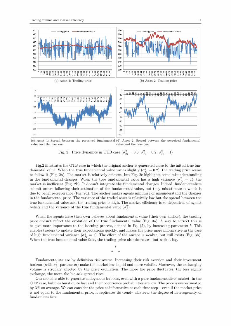
Trading volume and market efficiency 11
(a) Asset 1: Trading price (b) Asset 2: Trading price
(c) Asset 1: Spread between the perceived fundamentalvalue and the true one
(d) Asset 2: Spread between the perceived fundamentalvalue and the true one
Fig. 2: Price dynamics in OTB case (σ2g1 = 0.6, σ2
f1= 0.2, σ2
f2= 1)
Fig.2 illustrates the OTB case in which the original anchor is generated close to the initial true fun-damental value. When the true fundamental value varies slightly (σ2
f1= 0.2), the trading price seems
to follow it (Fig. 2a). The market is relatively efficient, but Fig. 2c highlights some misunderstandingin the fundamental changes. When the true fundamental value has a high variance (σ2
f2= 1), the
market is inefficient (Fig. 2b). It doesn’t integrate the fundamental changes. Indeed, fundamentalistssubmit orders following their estimation of the fundamental value, but they misestimate it which isdue to belief perseverance (Fig. 2d). The anchor makes agents minimize or misunderstand the changesin the fundamental price. The variance of the traded asset is relatively low but the spread between thetrue fundamental value and the trading price is high. The market efficiency is so dependent of agentsbeliefs and the variance of the true fundamental value (σ2
f ).
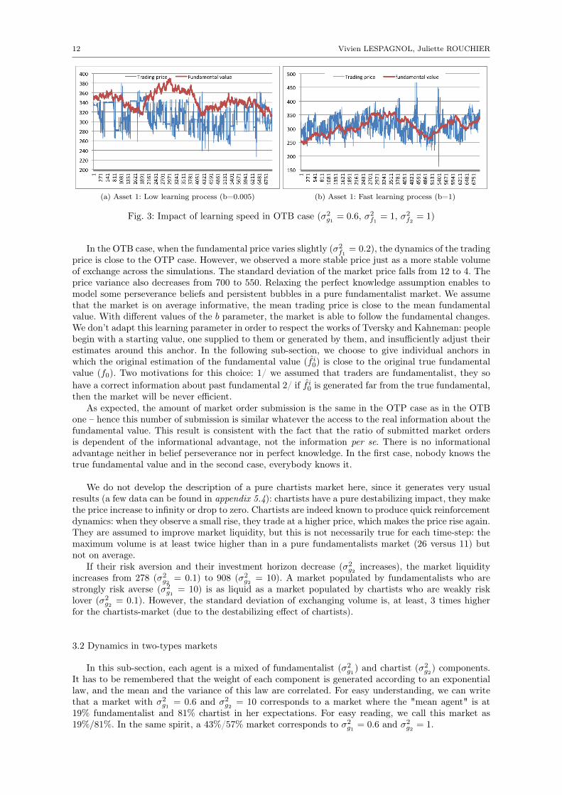
When the agents have their own believes about fundamental value (their own anchor), the tradingprice doesn’t reflect the evolution of the true fundamental value (Fig. 3a). A way to correct this isto give more importance to the learning process, defined in Eq. (5), by increasing parameter b. Thisenables traders to update their expectations quickly, and makes the price more informative in the caseof high fundamental variance (σ2
f2= 1). The effect of the anchor is weaker, but still exists (Fig. 3b).
When the true fundamental value falls, the trading price also decreases, but with a lag.
** *
Fundamentalists are by definition risk averse. Increasing their risk aversion and their investmenthorizon (with σ2
g1 parameter) make the market less liquid and more volatile. Moreover, the exchangingvolume is strongly affected by the price oscillation. The more the price fluctuates, the less agentsexchange, the more the bid-ask spread rises.
Our model is able to generate endogenous bubbles, even with a pure fundamentalists-market. In theOTP case, bubbles burst quite fast and their occurrence probabilities are low. The price is overestimatedby 3% on average. We can consider the price as informative at each time step – even if the market priceis not equal to the fundamental price, it replicates its trend– whatever the degree of heterogeneity offundamentalists.
12 Vivien LESPAGNOL, Juliette ROUCHIER
(a) Asset 1: Low learning process (b=0.005) (b) Asset 1: Fast learning process (b=1)
Fig. 3: Impact of learning speed in OTB case (σ2g1 = 0.6, σ2
f1= 1, σ2
f2= 1)
In the OTB case, when the fundamental price varies slightly (σ2f1
= 0.2), the dynamics of the tradingprice is close to the OTP case. However, we observed a more stable price just as a more stable volumeof exchange across the simulations. The standard deviation of the market price falls from 12 to 4. Theprice variance also decreases from 700 to 550. Relaxing the perfect knowledge assumption enables tomodel some perseverance beliefs and persistent bubbles in a pure fundamentalist market. We assumethat the market is on average informative, the mean trading price is close to the mean fundamentalvalue. With different values of the b parameter, the market is able to follow the fundamental changes.We don’t adapt this learning parameter in order to respect the works of Tversky and Kahneman: peoplebegin with a starting value, one supplied to them or generated by them, and insufficiently adjust theirestimates around this anchor. In the following sub-section, we choose to give individual anchors inwhich the original estimation of the fundamental value (f i0) is close to the original true fundamentalvalue (f0). Two motivations for this choice: 1/ we assumed that traders are fundamentalist, they sohave a correct information about past fundamental 2/ if f i0 is generated far from the true fundamental,then the market will be never efficient.
As expected, the amount of market order submission is the same in the OTP case as in the OTBone – hence this number of submission is similar whatever the access to the real information about thefundamental value. This result is consistent with the fact that the ratio of submitted market ordersis dependent of the informational advantage, not the information per se. There is no informationaladvantage neither in belief perseverance nor in perfect knowledge. In the first case, nobody knows thetrue fundamental value and in the second case, everybody knows it.
We do not develop the description of a pure chartists market here, since it generates very usualresults (a few data can be found in appendix 5.4): chartists have a pure destabilizing impact, they makethe price increase to infinity or drop to zero. Chartists are indeed known to produce quick reinforcementdynamics: when they observe a small rise, they trade at a higher price, which makes the price rise again.They are assumed to improve market liquidity, but this is not necessarily true for each time-step: themaximum volume is at least twice higher than in a pure fundamentalists market (26 versus 11) butnot on average.
If their risk aversion and their investment horizon decrease (σ2g2 increases), the market liquidity
increases from 278 (σ2g2 = 0.1) to 908 (σ2
g2 = 10). A market populated by fundamentalists who arestrongly risk averse (σ2
g1 = 10) is as liquid as a market populated by chartists who are weakly risklover (σ2
g2 = 0.1). However, the standard deviation of exchanging volume is, at least, 3 times higherfor the chartists-market (due to the destabilizing effect of chartists).
3.2 Dynamics in two-types markets
In this sub-section, each agent is a mixed of fundamentalist (σ2g1) and chartist (σ2
g2) components.It has to be remembered that the weight of each component is generated according to an exponentiallaw, and the mean and the variance of this law are correlated. For easy understanding, we can writethat a market with σ2
g1 = 0.6 and σ2g2 = 10 corresponds to a market where the "mean agent" is at
19% fundamentalist and 81% chartist in her expectations. For easy reading, we call this market as19%/81%. In the same spirit, a 43%/57% market corresponds to σ2
g1 = 0.6 and σ2g2 = 1.
Trading volume and market efficiency 13
In addition of the belief perseverance, because traders are not myopic, they are able to adapttheir orders before submitting (see Eq. (1)). More specifically, according to the market depth, theparticipants resolve the trade-off between accepting the non-execution risk and paying the bid-askspread. This choice, which is made according to the individual ability to adapt to the visible part ofthe order book (βit), has a direct impact on the market efficiency.
Different parameters that drive the market dynamics are treated in the following sub-frames as theratios of agents types, the agents’ aggressiveness and the knowledge of fundamentals.
3.2.1 Benchmark: perfect information
As we can expect, even if chartists have a destabilizing impact on the market, when a fundamen-talists trend exists, the market never diverges. In our simulations, the trading price never exceeds 100times the fundamental value even if fundamentalists are in minority. Indeed, in a 19%/81% market,the trading price evolves in a large spread around its fundamental value [−150; +250] but stays in thispath. Minimizing the chartist component (43%/57% market) doesn’t impact drastically the averagetrading price but makes its volatility significantly lower (849 vs. 200). In the same way, the limits andthe variance of the spread between the trading price and the true fundamental value are lower. Thisis coherent with the chartist destabilizing impact.
To compare this data to the previous case: in the OTP case, the market price is above the funda-mental price 63% of time. The trend induces by the fundamentalists is a kind of white noise around thefundamental. So the trading price tends to be as above as below the fundamental price, the positive andnegative spread counter-balance each other and the market is relatively efficient. Hence when chartiststrade, because of their backward looking, they just amplify fundamentalists’ trends: in the TTP case,the trading price is above the fundamental value 62% of time in the 43%/57% market, and 57% oftime in the 19%/81%market. Increasing the weight of chartist’s component makes the trading priceabove as much as below the fundamental value. However, it also makes the price more volatile, andmore overvalued on average. So, the market price is less frequently over the fundamental value, but itis on average more overvalued! This result is justified by the positive spreads which are much biggerthan the negative one and the extreme cases which do not counter-balance each other. It is also worthnoticing that simulations display different qualitative emerging patterns, with much less predictabilitythan in case of one-type market. This is in accordance with the reinforcement dynamics of chartists.
Concerning the traders’ choice between market and limit order, in the 43%/57% market, traders useMO to buy in 20.5% of cases and to sell in 24%. In the 19%/81% market – where agents are essentiallychartist in their behavior –, the ratios of submitted MO decrease and converge to 20% to buy and 22%to sell. Thus "impatience" to sell is still present in our two-types markets. The decreasing amount ofsubmitted MO is consistent with O’Hara and Easley (1995) who points out that the chartists are theliquidity suppliers, they submit LO and the fundamentalists because of their informational advantagecapture this liquidity by submitting MO. Our model is able to reproduce this stylized fact.
Unfortunately, the trading volumes of our two-types markets are unexpectedly low. In the chartists-market (see appendix 5.4), the liquidity is around 300 for σ2
g2 = 0.6 and increases to 900 for σ2g2 = 10.
In the OTP case (σ2g1 = 0.6), it is around 600. In the TTP case (σ2
g1 = 0.6 and σ2g2 = 1), it is as low
as 391. Chartists should at least couner-balance the decreasing part of fundamentalists submissions,since we know they are liquidity suppliers! As an example, an increase in the ratio of chartist (from57% to 81%) makes the price variance twice higher and the trading volume 10% lower. This result isin opposition with empirical study and logically incoherent: adding chartists or noise traders permitsto increase the market liquidity usually.
However, the result can be explained by our structure: the asset demand defined by Eq. (14) andEq. (15). The first and second differentials in the case of two independent assets are :
∂πt∂pt+τ
=1
α pt pt+τV ar> 0 and
∂πt∂V ar
= −ln
(pt+τpt
)α pt V ar2
< 0
∂πt∂2pt+τ
=−1
α p2t pt+τV ar< 0 and
∂πt∂2V ar
=
2 ln
(pt+τpt
)α ptV ar3
> 0
The positive impact of the expected price and the negative impact of the variance on the asset demandare verified. The second differential enables to highlight a stronger effect of the price variance. So, due tothe increasing price variance, the fundamentalists trade less. However, the decrease of fundamentalist
14 Vivien LESPAGNOL, Juliette ROUCHIER
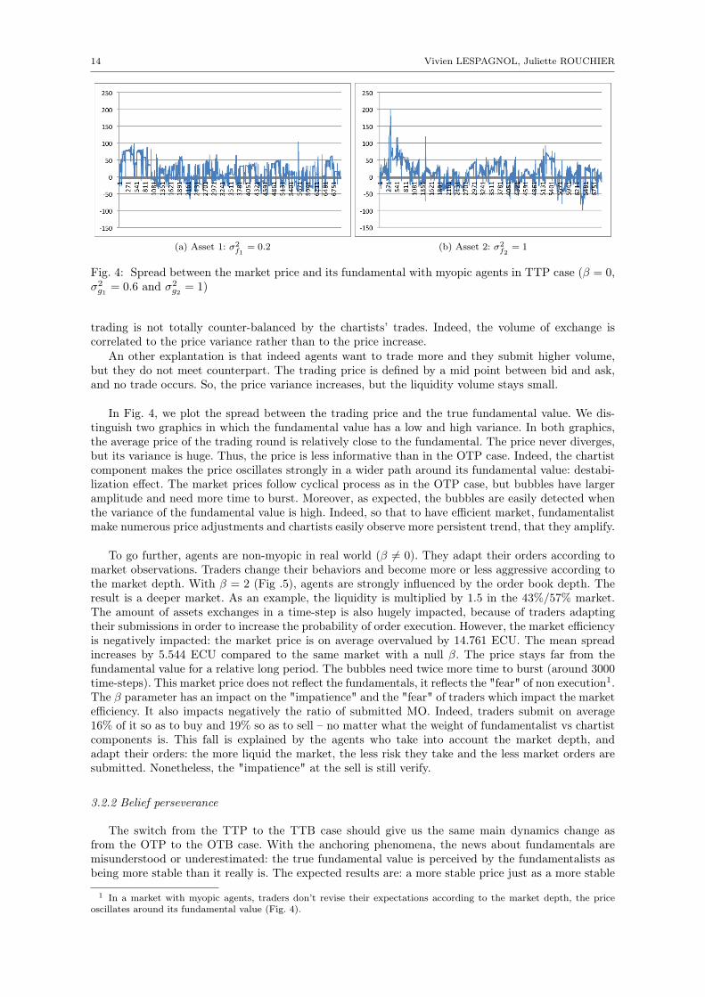
(a) Asset 1: σ2f1
= 0.2 (b) Asset 2: σ2f2
= 1
Fig. 4: Spread between the market price and its fundamental with myopic agents in TTP case (β = 0,σ2g1 = 0.6 and σ2
g2 = 1)
trading is not totally counter-balanced by the chartists’ trades. Indeed, the volume of exchange iscorrelated to the price variance rather than to the price increase.
An other explantation is that indeed agents want to trade more and they submit higher volume,but they do not meet counterpart. The trading price is defined by a mid point between bid and ask,and no trade occurs. So, the price variance increases, but the liquidity volume stays small.
In Fig. 4, we plot the spread between the trading price and the true fundamental value. We dis-tinguish two graphics in which the fundamental value has a low and high variance. In both graphics,the average price of the trading round is relatively close to the fundamental. The price never diverges,but its variance is huge. Thus, the price is less informative than in the OTP case. Indeed, the chartistcomponent makes the price oscillates strongly in a wider path around its fundamental value: destabi-lization effect. The market prices follow cyclical process as in the OTP case, but bubbles have largeramplitude and need more time to burst. Moreover, as expected, the bubbles are easily detected whenthe variance of the fundamental value is high. Indeed, so that to have efficient market, fundamentalistmake numerous price adjustments and chartists easily observe more persistent trend, that they amplify.
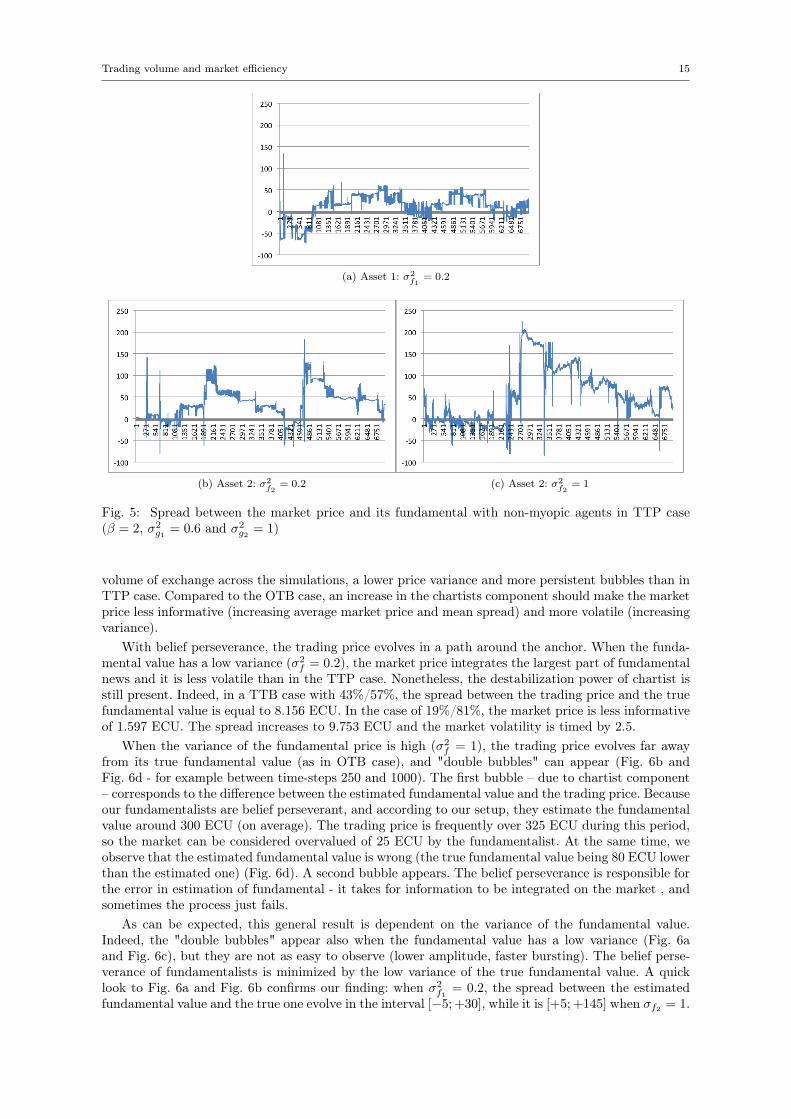
To go further, agents are non-myopic in real world (β 6= 0). They adapt their orders according tomarket observations. Traders change their behaviors and become more or less aggressive according tothe market depth. With β = 2 (Fig .5), agents are strongly influenced by the order book depth. Theresult is a deeper market. As an example, the liquidity is multiplied by 1.5 in the 43%/57% market.The amount of assets exchanges in a time-step is also hugely impacted, because of traders adaptingtheir submissions in order to increase the probability of order execution. However, the market efficiencyis negatively impacted: the market price is on average overvalued by 14.761 ECU. The mean spreadincreases by 5.544 ECU compared to the same market with a null β. The price stays far from thefundamental value for a relative long period. The bubbles need twice more time to burst (around 3000time-steps). This market price does not reflect the fundamentals, it reflects the "fear" of non execution1.The β parameter has an impact on the "impatience" and the "fear" of traders which impact the marketefficiency. It also impacts negatively the ratio of submitted MO. Indeed, traders submit on average16% of it so as to buy and 19% so as to sell – no matter what the weight of fundamentalist vs chartistcomponents is. This fall is explained by the agents who take into account the market depth, andadapt their orders: the more liquid the market, the less risk they take and the less market orders aresubmitted. Nonetheless, the "impatience" at the sell is still verify.
3.2.2 Belief perseverance
The switch from the TTP to the TTB case should give us the same main dynamics change asfrom the OTP to the OTB case. With the anchoring phenomena, the news about fundamentals aremisunderstood or underestimated: the true fundamental value is perceived by the fundamentalists asbeing more stable than it really is. The expected results are: a more stable price just as a more stable
1 In a market with myopic agents, traders don’t revise their expectations according to the market depth, the priceoscillates around its fundamental value (Fig. 4).
Trading volume and market efficiency 15
(a) Asset 1: σ2f1
= 0.2
(b) Asset 2: σ2f2
= 0.2 (c) Asset 2: σ2f2
= 1
Fig. 5: Spread between the market price and its fundamental with non-myopic agents in TTP case(β = 2, σ2
g1 = 0.6 and σ2g2 = 1)
volume of exchange across the simulations, a lower price variance and more persistent bubbles than inTTP case. Compared to the OTB case, an increase in the chartists component should make the marketprice less informative (increasing average market price and mean spread) and more volatile (increasingvariance).
With belief perseverance, the trading price evolves in a path around the anchor. When the funda-mental value has a low variance (σ2
f = 0.2), the market price integrates the largest part of fundamentalnews and it is less volatile than in the TTP case. Nonetheless, the destabilization power of chartist isstill present. Indeed, in a TTB case with 43%/57%, the spread between the trading price and the truefundamental value is equal to 8.156 ECU. In the case of 19%/81%, the market price is less informativeof 1.597 ECU. The spread increases to 9.753 ECU and the market volatility is timed by 2.5.
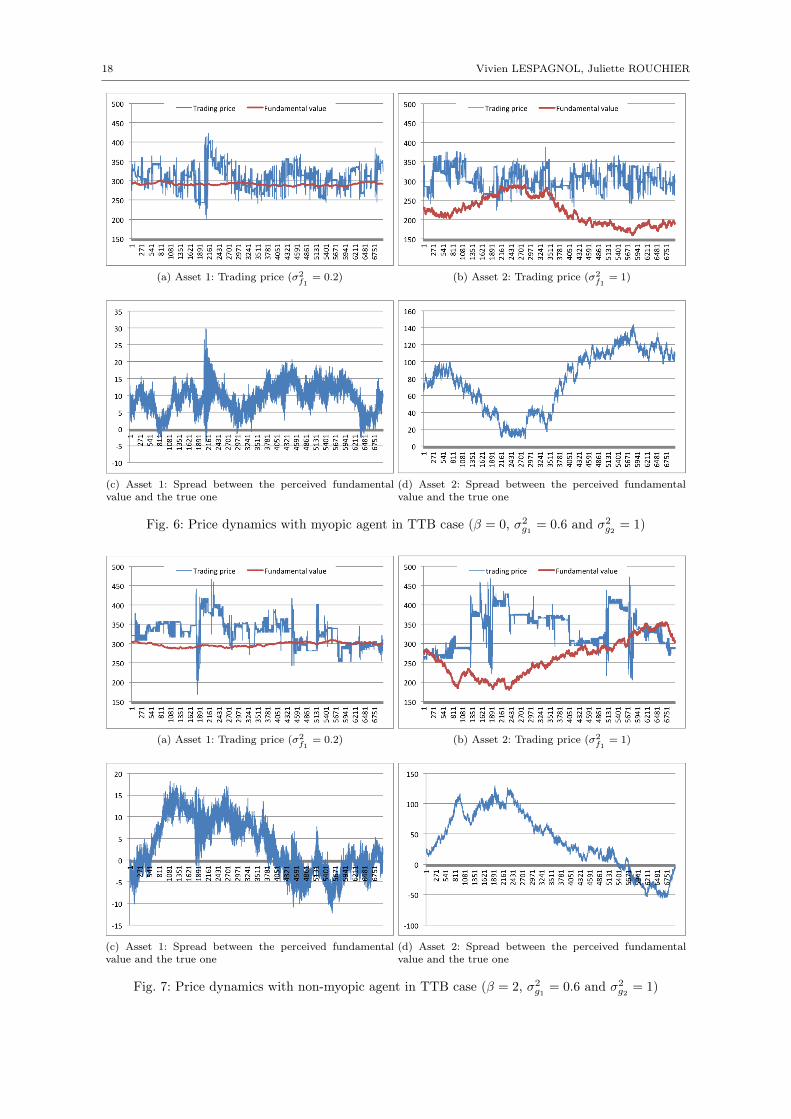
When the variance of the fundamental price is high (σ2f = 1), the trading price evolves far away
from its true fundamental value (as in OTB case), and "double bubbles" can appear (Fig. 6b andFig. 6d - for example between time-steps 250 and 1000). The first bubble – due to chartist component– corresponds to the difference between the estimated fundamental value and the trading price. Becauseour fundamentalists are belief perseverant, and according to our setup, they estimate the fundamentalvalue around 300 ECU (on average). The trading price is frequently over 325 ECU during this period,so the market can be considered overvalued of 25 ECU by the fundamentalist. At the same time, weobserve that the estimated fundamental value is wrong (the true fundamental value being 80 ECU lowerthan the estimated one) (Fig. 6d). A second bubble appears. The belief perseverance is responsible forthe error in estimation of fundamental - it takes for information to be integrated on the market , andsometimes the process just fails.
As can be expected, this general result is dependent on the variance of the fundamental value.Indeed, the "double bubbles" appear also when the fundamental value has a low variance (Fig. 6aand Fig. 6c), but they are not as easy to observe (lower amplitude, faster bursting). The belief perse-verance of fundamentalists is minimized by the low variance of the true fundamental value. A quicklook to Fig. 6a and Fig. 6b confirms our finding: when σ2
f1= 0.2, the spread between the estimated
fundamental value and the true one evolve in the interval [−5; +30], while it is [+5; +145] when σf2 = 1.
16 Vivien LESPAGNOL, Juliette ROUCHIER
When agents are non-myopic (β 6= 0), and hence take into account the depth of the order book,the price rises. The destabilization power of chartist in the case of belief perseverance and non-myopiais less obvious. Indeed, the average market price are around 314.6 ECU for asset 1 and 325 for asset2 – whatever the weight of fundamentalist vs chartist. The destabilization power of chartist stays inthe price volatility: an increase of chartist ratio from 57% to 81% makes the variances 3 times higher2.Moreover, the standard error is also positively impacted (times by 3), noticing that simulations displaydifferent emerging patterns. This is surely du to the impact of the market depth in the price valuation,which evolve at each time-step, and which is increased by chartist behavior. So, the market price reflectsthe "fear" of no order execution and the chartist’s herding. This is why the runs are less similar amongtrading round. Finally and non surprisingly, the volume of exchange is hugely increase by non-myopicagent. However, as mentioned previously, we observe a fall in liquidity when the weight of chartistscomponent is heavy. The amount of exchange decreases form 632 to 486 for the first asset and from 760to 618 for the second one3. Our assumption – the price variance is mainly responsible of the liquidityfall – seems to be confirmed.
In Fig. 7b and Fig.7d, we focus on the high variance case of the true fundamental value, that is themost caricatural one. Between time-steps 800 and 2500, the market is clearly inefficient. The marketprice seems to be driven by an excess of optimism, due to chartist behavior (Fig. 7b). But, Fig. 7dhighlights a fundamental value overvalued by 100 ECU. So the spread between the true fundamentalvalue and the trading price is driven by non-myopia, chartist behavior and belief perseverance offundamentalist. After that, between the time-steps 2500 and 4000, the trading price stays relativelyconstant and the true fundamental value converges to the estimated one. The spread difference tends tozero (Fig. 7d). The bubble bursts partially, even if fundamentalists don’t revise their expectations. Thetrue fundamental value rises and goes back to a value close to the anchor. Thus, this price convergenceis independent of agents expectations. After the time-step 4000, the trading price falls to the truefundamental value. This part of the price convergence is due to agents’ trade and to their slow learningprocess. The anchor has a strong impact on the market dynamics, when the variance of the fundamentalprice increases, the trading price does not follow it, or with a delay.
** *
Fundamentalists and chartists are heterogeneous in their investment horizons, risk aversion, aggres-siveness, moods and knowledge of the fundamentals. They also differ by their roles, liquidity suppliersor demanders. A pur chartist strategy (σ2
g1 = 0) makes the market inefficient until it disappears.Chartists base their forward expectations on the past trend. They submit essentially limit orders. Afundamentalist strategy (σ2
g2 = 0) makes the trading price evolves around its fundamental value withmore or less fluctuations. So, in the OTP case, the marker is considered as relatively efficient. In ourtwo-types market, agents are an aggregation of fundamentalist and chartist components. The morechartists are, the less market is efficient. Indeed, increasing chartist component makes the marketprice overvalued on average. The market price oscillates more frequently and in a wide spread. In theTTP case (43%/57%), we have observed at least an increase of the average price by 2 ECU and avariance increase of 22% compared to the OTP case. The chartist component makes also decreasingthe amount of submitted market orders (relative low impact) and increasing the maximum amountof asset exchange in a time-step. This is coherent with the chartist’s destabilization power. However,an unexpected results, already mentioned is the market liquidity fall. The volume of exchange is morecorrelated to the price variance than to the expectation of rising price, but the amount of exchangebecomes more stable across simulations (decreasing standard error).
In the spirit of the bounded rationality, we have tried to relax the strong assumption of perfectknowledge of the fundamentals. To do that, we propose an adaptive learning of the fundamental valuewith belief perseverance. The main results of this essay are a decreasing price variance, smallest extremevalues and the market efficiency function of the fundamental variance and the anchor. Indeed, if thefundamental value has a high variance, the market will be inefficient because of the belief perseverance.But, if the anchor is closed to the true fundamental value and that fundamental value has a lowvariance, the TTB case is more efficient than the TTP one – in the sense that the market price is onaverage closed to the true fundamental value. However, the spread between the trading price and the
2 It has to be remembered that the market volatility was multiplied by 2.5 with myopic agents.3 As point of comparaison, the trading volume in a 43%/57% market with myopic agents is 392 for the first asset and
420 for the other one.
Trading volume and market efficiency 17
true fundamental value has a higher mean and variance. The market price does not integrate all thefundamental changes in the case of belief perseverance.
Finally, this model deals with agents’ behavior according to market depth. The β parameter, becauseof arbitrage between higher price and no execution risk, makes long term trend easily identified bychartists, and more persistent bubbles (higher amplitude and duration). The result is a non efficientmarket in any way. However, the β parameter permits also to improve the market liquidity. A quickcomparison between Fig. 6 and Fig. 7 permits to understand the main dynamics imply by the βparameter. When agents are myopic (β = 0), the trading price oscillates frequently around its truefundamental value. Some trends appear but they have low amplitude and the duration is short (betweentime-steps 250 and 1000 as an example). As previously mentioned, the price evolves in an horizontalwide path. In the TTB case with myopic agent, the main reason of bubbles is a non perceived change inthe fundamental (belief perseverance). When agents are receptive to the order book statement (β 6= 0),the market price can stay over- or under-valued for a longer period. Long periods of rise (or fall) areobservable and the market liquidity increases by 35% at least. In addition of unperceived change in thefundamental, the bubbles are self-sustained by a "fear" of order non execution. Traders care less aboutfundamentals, the market efficiency is negatively impact. The amount of submitted market ordersdecreases. It falls from 20% to 16% for the buy and from 23% to 19% for the sell. The market isdeeper, traders can be more patient. They don’t need to take too much risk and so prefer to submitlimit orders. From a certain point of view the difference between β = 0 and β 6= 0 is the liquiditypricing. This idea will be quantitatively investigating in a future work.
18 Vivien LESPAGNOL, Juliette ROUCHIER
(a) Asset 1: Trading price (σ2f1
= 0.2) (b) Asset 2: Trading price (σ2f1
= 1)
(c) Asset 1: Spread between the perceived fundamentalvalue and the true one
(d) Asset 2: Spread between the perceived fundamentalvalue and the true one
Fig. 6: Price dynamics with myopic agent in TTB case (β = 0, σ2g1 = 0.6 and σ2
g2 = 1)
(a) Asset 1: Trading price (σ2f1
= 0.2) (b) Asset 2: Trading price (σ2f1
= 1)
(c) Asset 1: Spread between the perceived fundamentalvalue and the true one
(d) Asset 2: Spread between the perceived fundamentalvalue and the true one
Fig. 7: Price dynamics with non-myopic agent in TTB case (β = 2, σ2g1 = 0.6 and σ2
g2 = 1)
Trading volume and market efficiency 19
4 Conclusion
In this paper we present an order driven market, where two assets are traded, in order to study theliquidity dynamics. We show that agent types influence the market dynamics. Indeed, fundamentalistsmake the market oscillates around its fundamental price, while chartists make it diverge. Moreover,according to Beja et Goldman (1980), increasing the fundamentalist power in a previous stable systemor adding chartists make the price oscillates in a higher spread and varies more but never diverges.In fact, chartists – due to their reinforcement dynamics – amplify fundamentalists trend and marketinefficiency. They also impact negatively the amount of submitted market order per run, but tradersare still more impatient at the sell than at the buy.
In any cases, this model is able to generate endogenous bubbles bloom and burst, which is the basicqualitative feature that is interesting in an artificial market. As usual in financial ABM, our model isalso able to reproduce long term memory.
Concerning the liquidity, as we can expect, chartists increase the maximum amount of assets ex-change in a time-step. Unexpectedly, they make the market less liquid on average than fundamentalists.This is counter-intuitive when comparing to Shiller (2000) and Odeon et Barber (2000), but has a strongexplanation within the logic of our model. Nonetheless, with this liquidity fall due to chartist compo-nent, we observe an increasing price variance as an increasing bid-ask spread. That is consistent withthe literature.
Relaxing the assumption of perfect knowledge of the fundamentals permit to identify interestingchange in price dynamics. Our model is able to generate bubbles in a pur fundamentalist market.Indeed, when agents do not have perfect knowledge of fundamentals (belief perseverance), the tradingprices may evolve independently of the true fundamental values. This is due to the fact that theanchoring is strong and learning is slow, hence re-adjustment is slow. A possible way to correct thismisunderstanding is to give more importance to the learning process. Notice that our model is notcalibrated on real world, thus we have to improve this parameter. However, we know that a high valueis not consistent with the behavioral research.
The belief perseverance permits to identify to main components in a bubble. The bubbles can bedue to chartist following trend and (/or) to the misunderstanding of the fundamental’s change.
Finally, it also may have positive impacts. Indeed, when the fundamental value has a low variance,the fact that agents do not know it perfectly has a stabilizing impact on the market dynamics. Thesmall shocks in the fundamental value are unperceived, so the trading price oscillates less and in asmaller spread. In fact, the trading price reflects the main fundamental trends.
About the myopia, the fact that traders’ choices are influenced by the quoted order book makesthe market inefficient on long periods. The arbitrage between bid-ask spread and risk of no-executionmakes bubbles take more time to burst. Trends are identified easily by chartists, and fundamentalistscare less about fundamentals. In this case, the market price is driven by the "fear" of non execution.Because of this strategy of order submission, we observe, as with increasing chartists’ power, a de-creasing amount of submitting market orders. The result is a huge improve of the market liquidity anda loss in market efficiency. From a certain point of view, this inefficiency corresponds to the liquiditycost that is not taking into account in our definition of the fundamental value.
Hence, our model realizes many interesting features that allow us to explore liquidity in an artificialmarket, although we have added several complex elements to the usually used framework. The influenceof a bad perception of the fundamental value, in particular, seems to produce rather expected dynamics,which means that we can carry on using this framework.
We still have one problem that is not consistent with the literature : there is a large liquidity fallwhen chartists are more present, the liquidity can fall on average of one third, because of the rise in theprice variance. This is due to the asset demand equation, which is based on price and asset variationduring the two last time-steps, see Eq. (13). We will have to explore a way to minimize this fall byadding noise traders agents (NTA), think about the asset demand equation and permits to more thanone agent to submit at each time step.
From now, we wish to explore the importance of belief and its impact on self-fulfilling prophecy.As example, how two independent assets in their fundamentals may have a correlation in their price

20 Vivien LESPAGNOL, Juliette ROUCHIER
fluctuation. We also wish to explore new ways of getting information for the agents, and in particularto see the impact of a spread of information through diverse shapes of social network.
An other project, more econometric, is to focus on the co-movement in moments of assets re-turns. When fundamentals are correlated, we search the long run common dynamics between the assetvolatility
Trading volume and market efficiency 21
5 Appendix
5.1 Mathematical Model
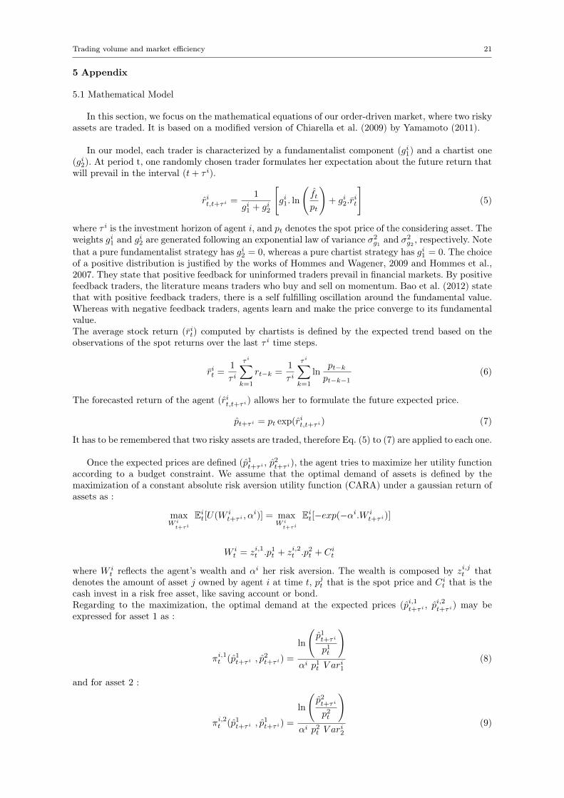
In this section, we focus on the mathematical equations of our order-driven market, where two riskyassets are traded. It is based on a modified version of Chiarella et al. (2009) by Yamamoto (2011).
In our model, each trader is characterized by a fundamentalist component (gi1) and a chartist one(gi2). At period t, one randomly chosen trader formulates her expectation about the future return thatwill prevail in the interval (t+ τ i).
rit,t+τ i =1
gi1 + gi2
[gi1. ln
(ftpt
)+ gi2.r
it
](5)
where τ i is the investment horizon of agent i, and pt denotes the spot price of the considering asset. Theweights gi1 and gi2 are generated following an exponential law of variance σ2
g1 and σ2g2 , respectively. Note
that a pure fundamentalist strategy has gi2 = 0, whereas a pure chartist strategy has gi1 = 0. The choiceof a positive distribution is justified by the works of Hommes and Wagener, 2009 and Hommes et al.,2007. They state that positive feedback for uninformed traders prevail in financial markets. By positivefeedback traders, the literature means traders who buy and sell on momentum. Bao et al. (2012) statethat with positive feedback traders, there is a self fulfilling oscillation around the fundamental value.Whereas with negative feedback traders, agents learn and make the price converge to its fundamentalvalue.The average stock return (rit) computed by chartists is defined by the expected trend based on theobservations of the spot returns over the last τ i time steps.
rit =1
τ i
τ i∑k=1
rt−k =1
τ i
τ i∑k=1
lnpt−kpt−k−1
(6)
The forecasted return of the agent (rit,t+τ i) allows her to formulate the future expected price.
pt+τ i = pt exp(rit,t+τ i) (7)
It has to be remembered that two risky assets are traded, therefore Eq. (5) to (7) are applied to each one.
Once the expected prices are defined (p1t+τ i , p2t+τ i), the agent tries to maximize her utility function
according to a budget constraint. We assume that the optimal demand of assets is defined by themaximization of a constant absolute risk aversion utility function (CARA) under a gaussian return ofassets as :
maxW it+τi
Eit[U(W it+τ i , α
i)] = maxW it+τi
Eit[−exp(−αi.W it+τ i)]
W it = zi,1t .p1t + zi,2t .p2t + Cit
where W it reflects the agent’s wealth and αi her risk aversion. The wealth is composed by zi,jt that
denotes the amount of asset j owned by agent i at time t, pjt that is the spot price and Cit that is thecash invest in a risk free asset, like saving account or bond.Regarding to the maximization, the optimal demand at the expected prices (pi,1t+τ i , p
i,2t+τ i) may be
expressed for asset 1 as :
πi,1t (p1t+τ i , p2t+τ i) =
ln
(p1t+τ i
p1t
)αi p1t V ar
i1
(8)
and for asset 2 :
πi,2t (p1t+τ i , p1t+τ i) =
ln
(p2t+τ i
p2t
)αi p2t V ar
i2
(9)

22 Vivien LESPAGNOL, Juliette ROUCHIER
The two assets are assumed to be independent (Cov = 0). In this case, πi,1t is equal to the optimaldemand of Yamamoto’s paper (2011). The variance (V arij) reflects the risk investment of asset jevaluated by agent i. It is assumed to be equal to the variance of the logarithmic of the return rate.
V arij =1
τ i
τ i∑k=1
[rjt−k − ri,jt ]2 (10)
where ri,jt is the average spot return of asset j. A general writing is given by Eq. (6). The investmenthorizon (τ i) and the risk aversion (αi) are dependent of agent’s features. We define them as Yamamoto(2011):
τ i = τ1 + gi11 + gi2
(11)
αi = α1 + gi11 + gi2
(12)
where τ and α are respectively a reference time horizon and a reference degree of aversion toward risk.
Finally, the agent has to define and submit her order. The amont of assets (sj,it ) the agent is willingto trade is determined by the absolute difference in the optimal demand for asset j at time t and t− 1as:
si,jt = abs(πi,jt − πi,jt−1) (13)
The sign of this difference (πi,jt − πi,jt−1), gives the agent’s position. Notice that the submission price
may differ of the expected one (pi,jt+τ i , Eq. (7)) according to the agent’s mood (M i,jt ). The buy price is
defined as :
bi,jt = pi,jt+τ i(1 +M i,jt ) (14)
The sell price is:
ai,jt = pi,jt+τ i(1 +M i,jt ) (15)
where M i,jt is randomly assigned from a uniform distribution of mean zero.

Trading volume and market efficiency 23
5.2 Parameters setup
For the perceived fundamental value, the parameters are arbitrary fixed and are justified by theinterpretation of the Kannehman’s evidences. We tried to reflect the difficulty of agents to estimatethe probability of occurrence, their excess of optimism, their wishful thinking, and their believes per-severances.
Description Parameter ValueMarket variables
Traders amount Nb_agents 1000Share amount - ∞Tick size - 10−3
Original fundamental value asset 1 : f10 f10 = 300asset 2 : f20 f20 = 300
Original market price p10 p10 = f10 = 300p20 p20 = f20 = 300
Fundamental value (Random Walk) f1t f1t−1 +N (0, σ2f1
)
f2t f2t−1 +N (0, σ2f2
)
Assets covariance Cov1,2 0Agent components
Weight fundamentalist : g1 exponential law of variance σ2g1
chartist : g2 exponential law of variance σ2g2
Original endowment
wealth : W i0 12.000 ECU
asset 1 : zi,10 U(0; 20)asset 2 : zi,20 U(0; 20)bond : Ci
0 W i0 − z
i,10 .p10 − z
i,2t .p20
Time horizon reference τ 300Risk aversion reference α 0.1Agent mood M i,j
t U(−0.25;+0.25)
Propensity of adaptation βi U(0;βmax)βmax 2
Perfect knowledge case
Fundamental value of agent i f it ft
Belief perseverance case
Fundamental value of agent iγ1 pt−1 + γ2 f it−1 + γ3 f i0
f it +Nt + a(f it−1 − f it−2 −Nt)
+b (ft−1 − f it−1)
Anchor componentγ1 0.02γ2 0.4γ3 0.58
Information confidence a 0.98Learning b 0.005Original expectation (idiosyncratic) f i0 f0 +N (0, σ2
f )
New information Nt N (0, 1)
Table 3: Parameters setup
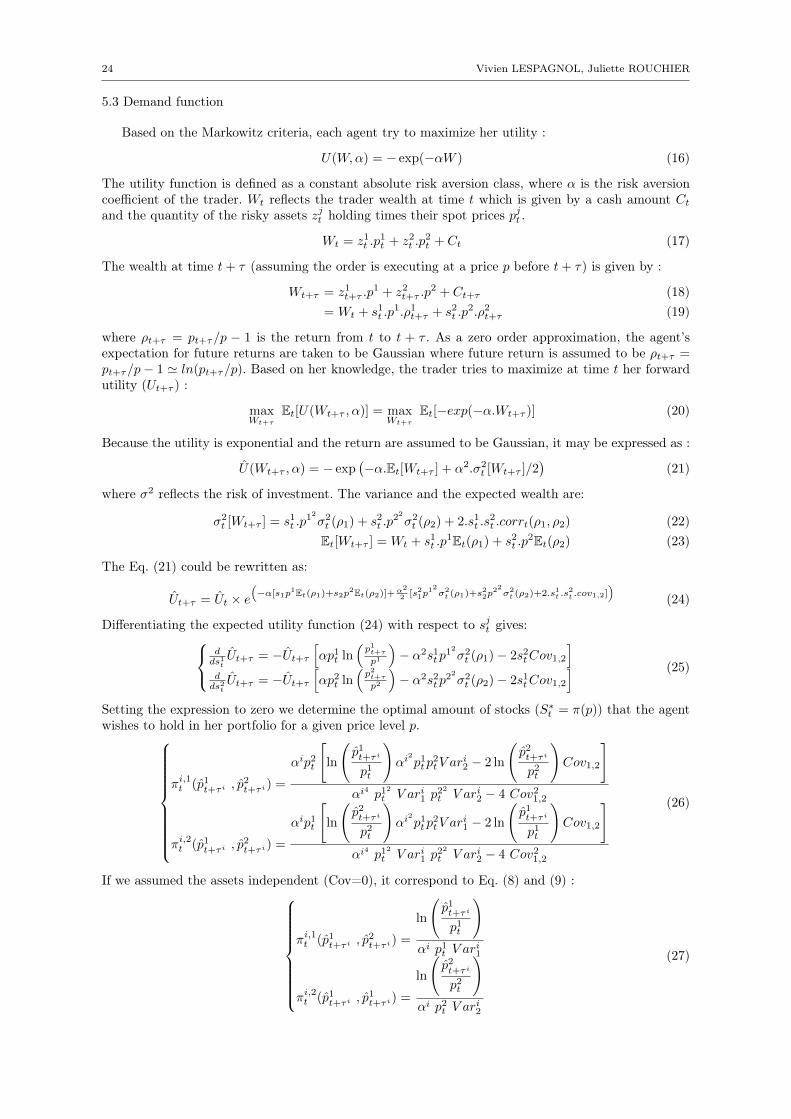
24 Vivien LESPAGNOL, Juliette ROUCHIER
5.3 Demand function
Based on the Markowitz criteria, each agent try to maximize her utility :
U(W,α) = − exp(−αW ) (16)
The utility function is defined as a constant absolute risk aversion class, where α is the risk aversioncoefficient of the trader. Wt reflects the trader wealth at time t which is given by a cash amount Ctand the quantity of the risky assets zjt holding times their spot prices pjt .
Wt = z1t .p1t + z2t .p
2t + Ct (17)
The wealth at time t+ τ (assuming the order is executing at a price p before t+ τ) is given by :
Wt+τ = z1t+τ .p1 + z2t+τ .p
2 + Ct+τ (18)= Wt + s1t .p
1.ρ1t+τ + s2t .p2.ρ2t+τ (19)
where ρt+τ = pt+τ/p − 1 is the return from t to t + τ . As a zero order approximation, the agent’sexpectation for future returns are taken to be Gaussian where future return is assumed to be ρt+τ =pt+τ/p− 1 ' ln(pt+τ/p). Based on her knowledge, the trader tries to maximize at time t her forwardutility (Ut+τ ) :
maxWt+τ
Et[U(Wt+τ , α)] = maxWt+τ
Et[−exp(−α.Wt+τ )] (20)
Because the utility is exponential and the return are assumed to be Gaussian, it may be expressed as :
U(Wt+τ , α) = − exp(−α.Et[Wt+τ ] + α2.σ2
t [Wt+τ ]/2)
(21)
where σ2 reflects the risk of investment. The variance and the expected wealth are:
σ2t [Wt+τ ] = s1t .p
12σ2t (ρ1) + s2t .p
22σ2t (ρ2) + 2.s1t .s
2t .corrt(ρ1, ρ2) (22)
Et[Wt+τ ] = Wt + s1t .p1Et(ρ1) + s2t .p
2Et(ρ2) (23)
The Eq. (21) could be rewritten as:
Ut+τ = Ut × e(−α[s1p1Et(ρ1)+s2p2Et(ρ2)]+α2
2 [s21p12σ2
t (ρ1)+s22p
22σ2t (ρ2)+2.s1t .s
2t .cov1,2]
)(24)
Differentiating the expected utility function (24) with respect to sjt gives:dds1t
Ut+τ = −Ut+τ[αp1t ln
(p1t+τp1
)− α2s1tp
12σ2t (ρ1)− 2s2tCov1,2
]dds2t
Ut+τ = −Ut+τ[αp2t ln
(p2t+τp2
)− α2s2tp
22σ2t (ρ2)− 2s1tCov1,2
] (25)
Setting the expression to zero we determine the optimal amount of stocks (S∗t = π(p)) that the agentwishes to hold in her portfolio for a given price level p.
πi,1t (p1t+τ i , p2t+τ i) =
αip2t
[ln
(p1t+τ i
p1t
)αi
2
p1tp2tV ar
i2 − 2 ln
(p2t+τ i
p2t
)Cov1,2
]αi4 p1
2
t V ari1 p22t V ari2 − 4 Cov21,2
πi,2t (p1t+τ i , p2t+τ i) =
αip1t
[ln
(p2t+τ i
p2t
)αi
2
p1tp2tV ar
i1 − 2 ln
(p1t+τ i
p1t
)Cov1,2
]αi4 p1
2
t V ari1 p22t V ari2 − 4 Cov21,2
(26)
If we assumed the assets independent (Cov=0), it correspond to Eq. (8) and (9) :πi,1t (p1t+τ i , p
2t+τ i) =
ln
(p1t+τ i
p1t
)αi p1t V ar
i1
πi,2t (p1t+τ i , p1t+τ i) =
ln
(p2t+τ i
p2t
)αi p2t V ar
i2
(27)
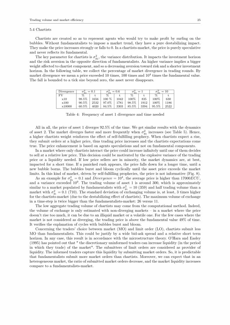
Trading volume and market efficiency 25
5.4 Chartists
Chartists are created so as to represent agents who would try to make profit by surfing on thebubbles. Without fundamentalists to impose a market trend, they have a pure destabilizing impact.They make the price increases strongly or falls to 0. In a chartists-market, the price is purely speculativeand never reflects its fundamental.
The key parameter for chartists is σ2g2 , the variance distribution. It impacts the investment horizon
and the risk aversion in the opposite direction of fundamentalists. An higher variance implies a biggerweight affected to chartist component, and so a decreasing aversion toward risk and a shorter investmenthorizon. In the following table, we collect the percentage of market divergence in trading rounds. Bymarket divergence we mean a price exceeded 10 times, 100 times and 104 times the fundamental value.The fall is bounded to a tick size beyond zero, the asset never disappears.
Divergence σ2g2
= 0.1 σ2g2
= 0.6 σ2g2
= 1 σ2g2
= 10
FV % t % t % t % tx10 98.5% 1656 100 % 1042 100% 835 100% 630x100 90.5% 2532 97.0% 1781 98.5% 1912 100% 1186x10000 60.5% 4020 84.5% 3303 85.5% 3394 95.5% 2522
Table 4: Frequency of asset 1 divergence and time needed
All in all, the price of asset 1 diverges 92.5% of the time. We get similar results with the dynamicsof asset 2. The market diverges faster and more frequently when σ2
g2 increases (see Table 5). Hence,a higher chartists weight reinforces the effect of self-fulfilling prophecy. When chartists expect a rise,they submit orders at a higher price, thus trading price increases and the chartists expectations cometrue. The price enhancement is based on agents speculations and not on fundamental components.
In a market where only chartists interact the price could increase infinitely until one of them decidesto sell at a relative low price. This decision could be motivated by the explosive variance of the tradingprice or a liquidity needed. If low price sellers are in minority, the market dynamics are, at best,impacted for a short time. If a panicked rush appears, the price falls down for a longer time, until anew bubble borns. The bubbles burst and bloom cyclically until the asset price exceeds the marketlimits. In this kind of market, driven by self-fulfilling prophecies, the price is not informative (Fig. 8).
As an example for σ2g2 = 0.1 and Divergence = 104, the average price is higher than 17000ECU ,
and a variance exceeded 109. The trading volume of asset 1 is around 300, which is approximatelysimilar to a market populated by fundamentalists with σ2
g1 = 10 (359) and half trading volume than amarket with σ2
g1 = 0.1 (710). The standard deviation of exchanging volume is, at least, 3 times higherfor the chartists-market (due to the destabilizing effect of chartists). The maximum volume of exchangein a time-step is twice bigger than the fundamentalists-market: 26 versus 11.
The low aggregate trading volume of chartists may come from the computational method. Indeed,the volume of exchange is only estimated with non-diverging markets – in a market where the pricedoesn’t rise too much, it can be due to an illiquid market or a volatile one. For the few cases where themarket is not considered as diverging, the trading price is above the fundamental value 49% of time.It verifies the explanation of cycles with bubbles burst and bloom.
Concerning the traders’ choice between market (MO) and limit order (LO), chartists submit lessMO than fundamentalists. This could be justify by a wide bid-ask spread and a relative short termhorizon. In any case, this result is in accordance with the microstructure theory. O’Hara and Easley(1995) has pointed out that " the discretionary uninformed traders can increase liquidity (in the periodin which they trade) of the market". The submitters of limit orders are considered as provider ofliquidity. The informed traders capture this liquidity by submitting market orders. So, it is predictablethat fundamentalists submit more market orders than chartists. Moreover, we can expect that in anheterogeneous market, the ratio of submitted market orders decrease, and the market liquidity increasescompare to a fundamentalists-market.
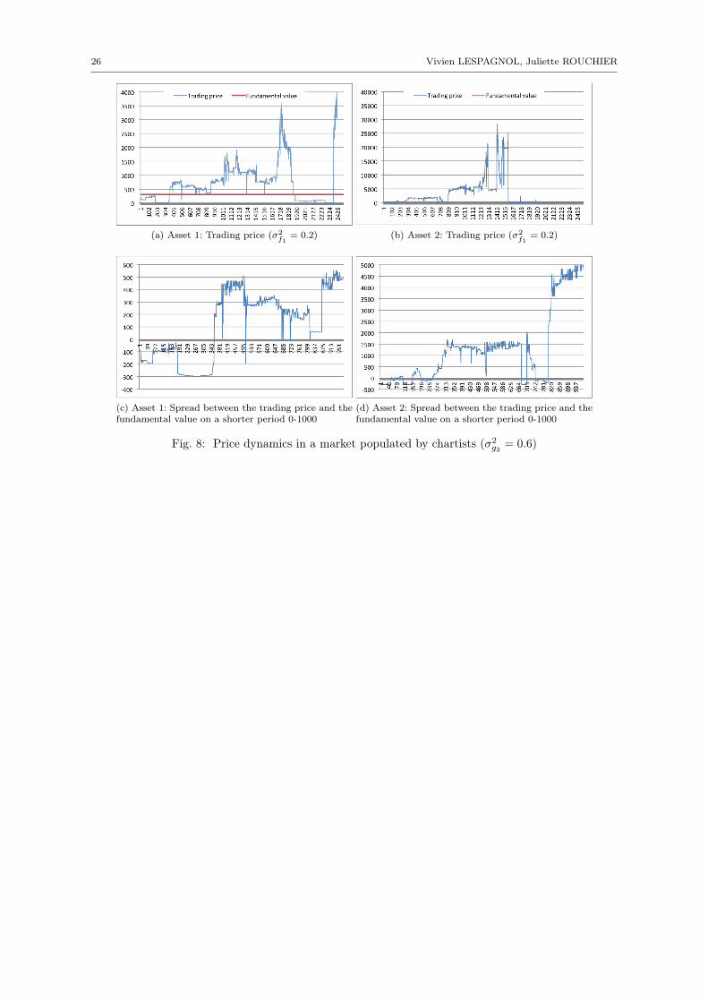
26 Vivien LESPAGNOL, Juliette ROUCHIER
(a) Asset 1: Trading price (σ2f1
= 0.2) (b) Asset 2: Trading price (σ2f1
= 0.2)
(c) Asset 1: Spread between the trading price and thefundamental value on a shorter period 0-1000
(d) Asset 2: Spread between the trading price and thefundamental value on a shorter period 0-1000
Fig. 8: Price dynamics in a market populated by chartists (σ2g2 = 0.6)
Trading volume and market efficiency 27
5.5 Tables and graphics
Table 5: Frequency of asset 1 divergence and time needed
Divergence σ2g2
= 0.1 σ2g2
= 0.6 σ2g2
= 1 σ2g2
= 10
FV % t % t % t % tx10 98.5% 1656 100 % 1042 100% 835 100% 630x100 90.5% 2532 97.0% 1781 98.5% 1912 100% 1186x10000 60.5% 4020 84.5% 3303 85.5% 3394 95.5% 2522
Divergence=10 means that the trading price exceed 10 times the fundamental value at least once in the simulationst = the average time needed for divergence
Table 6: Divergence table, when asset-1 diverges
σ2f1
= 0.01
Divergence σ2g2
= 0.6 σ2g2
= 1 σ2g2
= 10
10 99.5% 99.5% 100%100 96% 97.5% 99%10000 73.5% 83% 94%
σ2f1
= 0.2
Divergence σ2g2
= 0.6 σ2g2
= 1 σ2g2
= 10
10 99.5% 100% 100%100 96% 98.5% 99.5%10000 77% 83% 94.5%
σ2f1
= 1
Divergence σ2g2
= 0.6 σ2g2
= 1 σ2g2
= 10
10 100% 100% 100%100 97% 98.5% 99%10000 76% 81% 94%
For each σ2g2, 9 pools of trading rounds are simulated with different variance for the white noise of the fundamental
value (ft = ft−1 +N (0, σ2f ) with σ
2f = 0.01, 0.2, 1)
Table 7: Impact of components (σ2f = 0.2)
Parameter σ2g1
= 0.6 + fi σ2g1
= 0.6, σ2g2
= 1 + fi + β = 2
Average price 308.157 306.601 309.623 307.580 314.148(Std. Err) (12.33) (3.70) (13.34) (6.04) (9.11)Price variance 695.665 552.525 849.258 726.803 801.683
(227.26) (112.85) (223.35) (155.92) (334.26)Mean spread 7.79 6.93 9.21 8.16 14.70
(4.58) (11.74) (6.09) (12.30) (15.80)Spread interval [-72;+77] [-68; +77] [-98; +132] [-90; +115] [-93; +141]Overvalued 61.44% 59.84% 62.15% 60.39% 66.83%Liquidity 592.8899 573.1003 391.1416 392.1275 632.5406
(92.22) (33.32) (26.55) (21.38) (76.86)MO (buy) 20.17% 20.64% 20.55% 20.77% 16.62%MO (sell) 26.13% 25.06% 23.73% 23.22% 19.32%

28 Vivien LESPAGNOL, Juliette ROUCHIER
Table 8: OTP with σ2f = 0.2
σ2g1
= .6 σ2g1
= 1 σ2g1
= 10
Asset 1 Mean Std. Dev. Mean Std. Dev. Mean Std. Dev.price 308.1574 12.32511 308.5255 12.43877 308.7847 12.14842variance 695.6651 227.2629 710.3875 245.5468 754.0125 245.0574mean fv 300.3684 11.89047 300.6404 11.02654 300.6333 10.57084volume 592.8899 92.22462 554.1616 70.9133 359.2986 46.13003mean volume 0.0846986 0.0131749 0.0791659 0.0101305 0.0513284 0.00659max volume 11.02806 9.170719 10.94757 6.253219 9.628196 6.97539empty 0.0307221 0.0439115 0.0348336 0.0460844 0.0348007 0.0443637overvalued 61.44% 0.0753254 61.44% 0.0738832 61.85% 0.0855326mean spread 7.788996 4.584102 7.885097 5.147205 8.151459 6.281391min spread -72.33428 8.516987 -72.69171 8.482047 -72.95131 8.329592max spread 77.45177 6.372596 78.35316 6.433966 78.23292 8.157135variance spread 648.9922 207.5843 666.5788 230.6979 702.8659 223.1803means95 7.869221 4.670239 7.956016 5.264398 8.326653 6.382589mins95 -40.52318 9.37619 -40.9088 10.46586 -44.06135 11.27737maxs951 56.98935 12.31665 58.10474 12.68831 57.43411 13.31851variances95 518.0513 176.0479 531.5191 192.232 564.9372 187.6149Asset 2 Mean Std. Dev. Mean Std. Dev. Mean Std. Dev.price 310.4384 14.41455 309.6829 12.31885 309.1788 13.56409variance 695.5531 267.0946 714.1698 237.3936 776.5419 271.0681mean fv 300.9104 13.22514 299.6201 10.7646 299.1682 12.00967volume 613.6832 156.6822 579.0842 143.0713 370.6732 105.7914mean volume 0.087669 0.0223832 0.0827263 0.0204388 0.0529533 0.0151131max volume 14.4399 10.52302 14.77144 9.396637 12.61206 6.8184empty 0.0300579 0.0442258 0.0370929 0.0456139 0.0406014 0.047353overvalued 64.04% 0.0873622 64.94% 0.0843774 64.08% 0.0894455mean spread 9.528054 5.892816 10.06278 5.886229 10.01056 6.95305min spread -73.41645 8.496879 -74.2861 7.131068 -74.22578 8.279589max spread 78.76266 5.920565 78.93036 5.644677 80.62684 6.275525variance spread 663.3532 241.2208 672.9731 212.7183 742.3849 260.2845means95 9.644843 6.012068 10.231 6.012701 10.2157 7.098899mins95 -39.22203 10.75663 -39.87547 10.63538 -42.48869 12.32808maxs951 57.90253 12.26719 58.19551 13.06891 59.31074 12.56349variances95 533.1659 208.8357 536.8655 180.1373 601.8252 228.8337MO buy-1 20.17% 0.0188271 20.12% 0.0214991 20.19% 0.0242499MO sell-1 26.13% 0.0193556 26.20% 0.0212283 26.21% 0.0248144MO buy-2 19.70% 0.0230664 19.56% 0.0244686 19.60% 0.0267621MO sell-2 26.81% 0.0231043 27.00% 0.0237113 27.11% 0.0272122
Trading volume and market efficiency 29
Table 9: OTB with σ2f1
= 0.2 and σ2f2
= 1
σ2g1
= .6 σ2g1
= 1 σ2g1
= 10
Asset 1 Mean Std. Dev. Mean Std. Dev. Mean Std. Dev.price 306.1534 3.463512 306.3909 4.428084 306.6645 4.943354variance 557.3468 131.1669 567.7487 128.1391 618.8802 186.5933volume 578.2245 31.8367 536.9683 33.07209 350.9792 25.6745max volume 7.205507 4.983599 7.271991 4.155743 6.43139 3.839755empty 0.0097464 0.0213598 0.0100921 0.0211485 0.0134243 0.0280378overvalued 59.74% 0.1677892 60.10% 0.1824225 57.49% 0.1557758mean spread 6.911655 12.32845 7.322211 13.05146 5.173439 11.53773min spread -69.69829 13.87851 -68.97779 15.19092 -71.71536 13.62496max spread 77.33325 14.94849 77.48692 14.6541 75.0051 13.00802variance spread 604.4926 142.0178 615.7138 139.9558 663.056 191.6678mean spreadEFV 0.9585063 11.68905 1.137591 12.01733 -1.263458 10.33704min spreadEFV -16.12562 11.66179 -16.06191 12.56467 -18.0219 11.39867max spreadEFV 18.04531 12.37507 18.28009 12.12234 15.47089 10.54068variance spreadEFV 48.20557 33.40747 51.33188 38.64856 47.13037 42.22906Asset 2 Mean Std. Dev. Mean Std. Dev. Mean Std. Dev.price 306.9574 4.857592 307.3198 4.740281 307.6364 6.105452variance 554.5131 124.6286 546.4546 148.3676 610.1107 165.1104volume 591.5599 104.284 545.064 98.79757 362.3642 78.3615max volume 9.448241 6.288714 9.1585 5.0728 9.462259 7.067709empty 0.0084321 0.0185964 0.0099371 0.0189447 0.0154214 0.0247669overvalued 57.24% 0.337121 57.42% 0.334296 53.53% 0.3484412mean spread 10.51849 58.13192 11.59553 60.38223 5.454497 56.81206min spread -104.4057 60.1539 -103.0915 62.62739 -107.7331 58.155max spread 117.198 61.72648 118.8464 61.65015 111.0119 59.30671variance spread 1760.692 1047.526 1823.554 1307.714 1642.148 920.5805mean spreadEFV 3.766442 58.18193 4.482041 60.67168 -1.915285 57.38136min spreadEFV -65.32578 60.14335 -64.62811 62.65806 -66.80576 57.027max spreadEFV 72.74141 59.81421 72.84327 60.14862 63.62937 58.75076variance spreadEFV 1211.545 996.9575 1279.267 1242.215 1023.606 855.6559MO buy-1 20.72% 0.0127661 20.73% 0.0156313 20.77% 0.0182882MO sell-1 24.94% 0.0130618 25.05% 0.0165479 25.17% 0.0184851MO buy-2 20.66% 0.0171273 20.54% 0.0162071 20.46% 0.0211096MO sell-2 25.33% 0.0169755 25.44% 0.0169223 25.63% 0.0213242
30 Vivien LESPAGNOL, Juliette ROUCHIER
Table 10: Two-types market with myopic agent. σ2g1 = 0.6 and σ2
g2 = 1
β = 0, σ2f1
= σ2f2
= 0.2
TTP TTBAsset 1 Mean Std. Er. Mean Std. Er.price 309.623 13.33735 307.580 6.040267variance 849.258 223.3471 726.8023 155.9246volume 391.1416 26.55105 392.1275 21.38328max volume 8.123096 5.535868 6.525318 4.079126empty 0.0118771 0.0111059 0.0068514 0.0087016overvalued 62.15% 0.0817064 60.39% 0.152901mean spread 9.217 6.093379 8.156 12.2993min spread -98.574 25.37524 -90.252 27.31835max spread 132.057 44.44724 115.275 41.7988variance spread 804.3789 190.9701 767.7095 172.077mean spreadEFV XXX XXX 0.825 10.62857min spreadEFV XXX XXX -16.574 10.69423max spreadEFV XXX XXX 18.169 12.00475variance spreadEFV XXX XXX 50.32136 42.07813Asset 2 Mean Std. Er. Mean Std. Er.price 310.860 12.16608 309.691 7.112836variance 947.3698 285.6258 778.3532 201.7131volume 420.4131 75.1874 415.8279 65.98666max volume 12.38223 6.11285 9.802436 5.959227empty 0.0187443 0.0155055 0.0098757 0.0093289overvalued 63.67% 0.0956571 61.59% 0.1764587mean spread 10.548 7.088149 9.332 14.26773min spread -110.418 24.05953 -95.646 25.73981max spread 145.036 44.72508 128.776 41.6798variance spread 913.5817 269.3361 815.5288 216.4183mean spreadEFV XXX XXX -0.034 12.61678min spreadEFV XXX XXX -17.304 13.32003max spreadEFV XXX XXX 17.020 12.26027variance spreadEFV XXX XXX 44.1114 34.73074MO buy-1 20.55% 0.0106554 20.77% 0.0093301MO sell-1 23.73% 0.0110661 23.22% 0.0095739MO buy-2 20.51% 0.012634 20.56% 0.0118371MO sell-2 24.27% 0.0125587 23.72% 0.0122481

Trading volume and market efficiency 31
Table 11: Two-types market with myopic agent. σ2g1 = 0.6 and σ2
g2 = 10
β = 0, σ2f1
= σ2f2
= 0.2
TTP TTBAsset 1 Mean Std. Er. Mean Std. Er.price 309.645 15.22974 309.288 10.85575variance 1956.68 591.2399 1771.537 505.3346volume 353.1909 31.70824 359.5172 25.59655max volume 7.523469 3.864274 7.465332 4.121011empty 0.0356364 0.0350324 0.0249586 0.0138739overvalued 57.86% 0.0987944 58.02% 0.1550106mean spread 9.580 10.39823 9.753 16.83569min spread -142.921 25.00724 -138.842 29.81492max spread 243.640 78.684 230.3917 74.51019variance spread 1910.569 582.1038 1813.58 515.8413mean spreadEFV XXX XXX 0.768 12.62883min spreadEFV XXX XXX -19.384 13.306max spreadEFV XXX XXX 21.280 12.97876variance spreadEFV XXX XXX 56.97127 45.44262Asset 2 Mean Std. Er. Mean Std. Er.price 309.436 16.16384 308.833 10.64477variance 2311.15 877.6242 1808.425 585.7817volume 378.5888 62.57369 424.1773 51.19907max volume 11.76656 5.955194 9.868778 4.701071empty 0.0381564 0.0161272 0.0229529 0.0119421overvalued 57.00% 0.1161541 56.94% 0.1359406mean spread 8.390 13.24927 9.082 14.8614min spread -149.588 22.47362 -139.976 25.73726max spread 251.085 89.33567 223.124 71.53082variance spread 2272.728 835.8982 1867.683 612.2452mean spreadEFV XXX XXX 0.539 11.09187min spreadEFV XXX XXX -19.180 11.22918max spreadEFV XXX XXX 21.270 12.4479variance spreadEFV XXX XXX 57.38593 42.02272MO buy-1 19.91% 0.01346 20.10% 0.0104076MO sell-1 22.39% 0.011808 22.13% 0.0103705MO buy-2 20.51% 0.0136254 20.17% 0.0106023MO sell-2 22.53% 0.0138985 22.17% 0.0103072
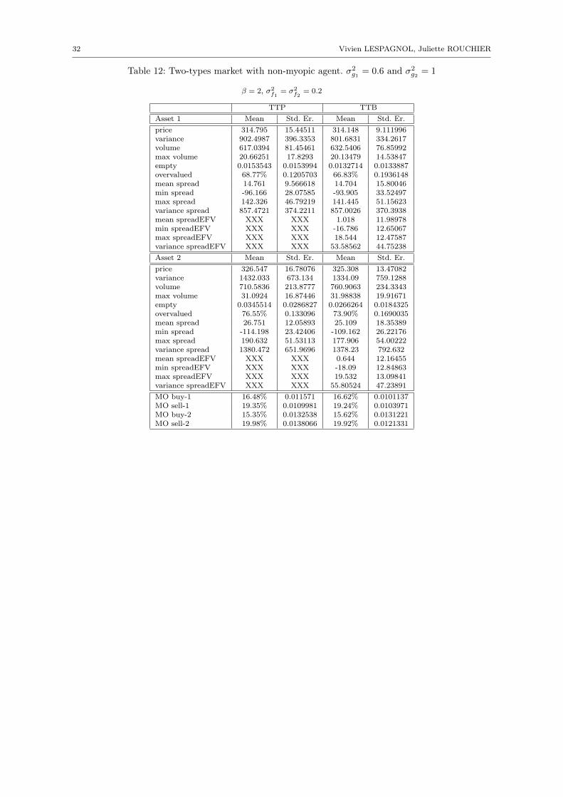
32 Vivien LESPAGNOL, Juliette ROUCHIER
Table 12: Two-types market with non-myopic agent. σ2g1 = 0.6 and σ2
g2 = 1
β = 2, σ2f1
= σ2f2
= 0.2
TTP TTBAsset 1 Mean Std. Er. Mean Std. Er.price 314.795 15.44511 314.148 9.111996variance 902.4987 396.3353 801.6831 334.2617volume 617.0394 81.45461 632.5406 76.85992max volume 20.66251 17.8293 20.13479 14.53847empty 0.0153543 0.0153994 0.0132714 0.0133887overvalued 68.77% 0.1205703 66.83% 0.1936148mean spread 14.761 9.566618 14.704 15.80046min spread -96.166 28.07585 -93.905 33.52497max spread 142.326 46.79219 141.445 51.15623variance spread 857.4721 374.2211 857.0026 370.3938mean spreadEFV XXX XXX 1.018 11.98978min spreadEFV XXX XXX -16.786 12.65067max spreadEFV XXX XXX 18.544 12.47587variance spreadEFV XXX XXX 53.58562 44.75238Asset 2 Mean Std. Er. Mean Std. Er.price 326.547 16.78076 325.308 13.47082variance 1432.033 673.134 1334.09 759.1288volume 710.5836 213.8777 760.9063 234.3343max volume 31.0924 16.87446 31.98838 19.91671empty 0.0345514 0.0286827 0.0266264 0.0184325overvalued 76.55% 0.133096 73.90% 0.1690035mean spread 26.751 12.05893 25.109 18.35389min spread -114.198 23.42406 -109.162 26.22176max spread 190.632 51.53113 177.906 54.00222variance spread 1380.472 651.9696 1378.23 792.632mean spreadEFV XXX XXX 0.644 12.16455min spreadEFV XXX XXX -18.09 12.84863max spreadEFV XXX XXX 19.532 13.09841variance spreadEFV XXX XXX 55.80524 47.23891MO buy-1 16.48% 0.011571 16.62% 0.0101137MO sell-1 19.35% 0.0109981 19.24% 0.0103971MO buy-2 15.35% 0.0132538 15.62% 0.0131221MO sell-2 19.98% 0.0138066 19.92% 0.0121331
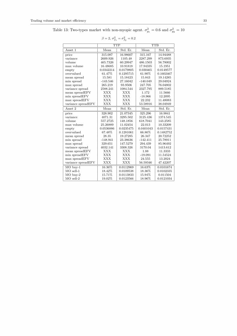
Trading volume and market efficiency 33
Table 13: Two-types market with non-myopic agent. σ2g1 = 0.6 and σ2
g2 = 10
β = 2, σ2f1
= σ2f2
= 0.2
TTP TTBAsset 1 Mean Std. Er. Mean Std. Er.price 315.087 16.98607 315.167 14.94488variance 2609.926 1105.48 2287.299 873.6935volume 465.7326 60.29947 486.1503 56.78002max volume 16.48685 10.91818 17.94335 15.1951empty 0.0342214 0.0179805 0.030465 0.0149577overvalued 61.47% 0.1295715 61.90% 0.1602467mean spread 15.581 15.18423 15.843 19.14285min spread -143.546 27.16042 -140.049 29.04924max spread 265.219 93.9506 247.705 76.04802variance spread 2588.241 1084.544 2327.795 889.5185mean spreadEFV XXX XXX 1.172 11.5666min spreadEFV XXX XXX -18.966 12.2095max spreadEFV XXX XXX 22.232 11.48083variance spreadEFV XXX XXX 53.58916 38.04949Asset 2 Mean Std. Er. Mean Std. Er.price 328.902 21.07345 325.296 16.9841variance 4071.31 3295.502 3125.436 1374.545volume 557.2725 148.1856 618.7041 143.2585max volume 25.26889 11.02454 22.013 10.33209empty 0.0536886 0.0235475 0.0401043 0.0157431overvalued 67.48% 0.1281061 66.86% 0.1482752mean spread 28.35 19.27285 26.347 20.72252min spread -148.941 23.38636 -142.411 25.78911max spread 329.651 147.5279 294.439 85.96492variance spread 4032.141 3308.326 3170.04 1413.612mean spreadEFV XXX XXX 1.88 11.3333min spreadEFV XXX XXX -19.091 11.54524max spreadEFV XXX XXX 24.555 13.2024variance spreadEFV XXX XXX 56.59346 47.42207MO buy-1 16.36% 0.0112969 16.63% 0.0101674MO sell-1 18.42% 0.0109538 18.36% 0.0102335MO buy-2 15.71% 0.0113833 15.94% 0.011504MO sell-2 19.02% 0.0123566 18.96% 0.0121034
Cohen et al. (1980) Duffy and Ochs (1999) Orléan (1995)
34 Vivien LESPAGNOL, Juliette ROUCHIER
References
Yakov Amihud, Haim Mendelson, and Lasse Heje Perdersen. Liquidity and asset prices. Foundationsand trends in finance, 1(4):269–364, 2005.
Te Bao, Cars Hommes, Joep Sonnemans, and Jan Tuinstra. Individual expectations, limited rationalityand aggregate outcomes. Journal of Economic Dynamics and Control, 36:1101–1120, 2012.
Nicholas Barberis and Richard Thaler. A survey of behavioral finance. Handbook of economics offinance, 1(B):1053–1128, 2003.
Avraham Beja and M. Barry Goldman. On the dynamic behavior of prices in disequilibrium. TheJournal of Finance, 35(2):235–248, May 1980.
Carl Chiarella, Roberto Dieci, and Xue-Zhong He. Heterogeneous expectations and speculative be-havior in a dynamic multi-asset framework. Journal of Economic Behavior and Organization, 62:408–427, 2007.
Carl Chiarella, Giulia Iori, and Josep Perello. The impact of heterogeneous trading rules on the limitorder book and order flows. Journal of Economic Dynamics and Control, 33:525–537, 2009.
Carl Chiarella, Xue-Zhong He, and Lijian Wei. Learning and evolution of trading stategies in limitorder markets. Working paper, July 2013.
Chenghuan Sean Chu, Andreas Lehnert, and Wayne Passmore. Strategic trading in multiple assets andthe effects on market volatility. International Journal of Central Banking, 5(4):143–172, december2009.
Kalman J. Cohen, Gabriel A. Hawawini, Steven F. Maier, Robert A. Schwartz, and David K. Whitcomb.Implications of microstructure theory for empirical research on stock price behavior. The Journalof Finance, 35(2):249–257, May 1980.
John Duffy and Jack Ochs. Emergence of money as a medium of exchange: An exeprimental study.The American Economic Review, 89(4):847–877, september 1999.
Eugene F. Fama. Efficient capital markets: A review of theory and empirical work. Journal of Finance,25(2):383–417, May 1970.
Thierry Foucault, Ohad Kadan, and Eugene Kandel. Limit order book as a market for liquidity. TheReview of Financial Studies, 18(4):1171–1217, winter 2005.
Irene Giardina and Jean-Philippe Bouchaud. Bubbles, crashes and intermittency in agent based marketmodels. The European Physical Journal B, 31:421–437, 2003.
Dhananjay K. Gode and Shyam Sunder. Allocative efficiency of markets with zero-intelligence traders:Market as a partial substitute for individual rationality. The Journal of Political Economy, 101:119–137, February 1993.
Sanford J. Grossman and Merton H. Miller. Liquidity and market structure. The Journal of Finance,43(3):617–633, July 1988.
Puneet Handa, Robert A. Schwartz, and Ashish Tiwari. Quote setting and price formation in an orderdrivern market. Journal of financial markets, 6:461–489, 2003.
Georges Harras and Didier Sornette. How to grow a bubble: A model of myopic adapting agents.Journal of Economic Behavior and Organization, 80:137–154, 2011.
C. Hommes, H. Huang, and D. Wang. A robust rational route to randomness in a simple asset pricingmodel. Journal of Economic Dynamics and Control, 29:1043–1072, 2005.
Cars Hommes. Heterogeneous agent models in economics and finance. Handbook of computationaleconomics, 2:1109–1186, 2006.
Cars Hommes and Florian Wagener. Complex evolutionary systems in behavioral finance. HandbookOf Financial Markets: Dynamics and Evolution, pages 217–276, 2009.
Cars Hommes, Peter Boswijk, and Sebastiano Manzan. Behavioral heterogneity in stock prices. Journalof Economic Dynamics and Control, 31:1938–1970, 2007.
G. Iori and J. Porter. Agent-based modelling for financial markets. Chapter prepared for the Handbookon Computational Economics and Finance, 2012.
Giulia Iori. A microsimulation of traders activity in the stock market : the role of heterogeneity, agents’interactions and trade frictions. Journal of Economic Behavior and Organization, 49:269–285, 2002.
Sandrine Jacob-Leal. Fundamentalists, chartists and asset pricing anomalies. October 2012.Daniel Kahneman and Amos Tversky. Prospect theory : An analysis of decision under risk. Econo-metrica, 47(2):263–292, 1979.
G. Andrew Karolyi, Kuan-Hui Lee, and Mathijs A. van Dijk. Understanding commonality in liquidityaround the world. journal of financial economics, 105:82–112, 2012.
Albert S. Kyle. Continuous auctions and insider trading. Econometrica, 53(6):1315–1335, 1985.
Trading volume and market efficiency 35
Blake LeBaron. Building the santa fe artificial stock market. Working paper, June 2002.Blake LeBaron. Agent-based computational finance. Handbook of computational economics, 2(B):1187–1227, 2006.
Thomas Lux. Herd behaviour, bubbles and crashes. The Economic Journal, 105(431):881–896, jul1995.
Thomas Lux and Michele Marchesi. Volatility clustering in financial markets: A micro-simulation ofinteractive agents. January 1998.
Maureen O’Hara and David Easley. Market microstructure. Handbooks in Operations Research andManagement Science, 9:357–383, 1995.
André Orléan. Bayesian interactions and collective dynamics of opinion: Herd behavior and mimeticcontagion. Journal of Economic Behavior and Organization, 28:257–274, 1995.
André Orléan. L’Empire de la valeur. La couleur des idées, October 2011.Christine A. Parlour. Price dynamics in limit order markets. The Review of Financial Studies, 11(4):789–816, winter 1998.
Cecile Pouget. L’efficience informationnelle revisitée sous l’angle de l’efficience allocative. In ColloqueGDR. GDR, 2000.
Gabriele Tedeschi, Giulia Iori, and Mauro Gallegati. Herding effects in order driven markets: The riseand fall of gurus. Journal of Economic Behavior and Organization, 81:82–96, 2012.
Amos Tversky and Daniel Kahneman. Judgment under uncertainty: Heuritics and biases. Science, 185(4157):1124–1131, september 1974.
Frank H. Westerhoff. Multi-asset market dynamics. Macroeconomic Dynamics, 8:596–616, 2004.Ryuichi Yamamoto. Order aggressiveness, pre-trade transparency, and long memory in an order-drivenmarket. Journal of Economic Dynamics and Control, 35:1938–1963, 2011.