This article was downloaded by: [Monash University Library]On: 16 August 2014, At: 15:48Publisher: RoutledgeInforma Ltd Registered in England and Wales Registered Number: 1072954 Registered office: MortimerHouse, 37-41 Mortimer Street, London W1T 3JH, UK

Journal of the Asia Pacific EconomyPublication details, including instructions for authors and subscription information:http://www.tandfonline.com/loi/rjap20

Trade Liberalization and Economic Growth in Fiji. AnEmpirical Assessment Using the ARDL ApproachParesh Narayan a & Russell Smyth ba Department of Accounting , Finance and Economics, Griffith University , Australiab Department of Economics , Monash University , AustraliaPublished online: 13 Dec 2010.

To cite this article: Paresh Narayan & Russell Smyth (2005) Trade Liberalization and Economic Growth in Fiji.An Empirical Assessment Using the ARDL Approach, Journal of the Asia Pacific Economy, 10:1, 96-115, DOI:10.1080/1354786042000309099

To link to this article: http://dx.doi.org/10.1080/1354786042000309099

PLEASE SCROLL DOWN FOR ARTICLE

Taylor & Francis makes every effort to ensure the accuracy of all the information (the “Content”) containedin the publications on our platform. However, Taylor & Francis, our agents, and our licensors make norepresentations or warranties whatsoever as to the accuracy, completeness, or suitability for any purpose ofthe Content. Any opinions and views expressed in this publication are the opinions and views of the authors,and are not the views of or endorsed by Taylor & Francis. The accuracy of the Content should not be reliedupon and should be independently verified with primary sources of information. Taylor and Francis shallnot be liable for any losses, actions, claims, proceedings, demands, costs, expenses, damages, and otherliabilities whatsoever or howsoever caused arising directly or indirectly in connection with, in relation to orarising out of the use of the Content.

This article may be used for research, teaching, and private study purposes. Any substantial or systematicreproduction, redistribution, reselling, loan, sub-licensing, systematic supply, or distribution in anyform to anyone is expressly forbidden. Terms & Conditions of access and use can be found at http://www.tandfonline.com/page/terms-and-conditions

Journal of the Asia Pacific EconomyVol. 10, No. 1, 96–115, February 2005

Trade Liberalization and EconomicGrowth in Fiji. An Empirical AssessmentUsing the ARDL Approach

PARESH KUMAR NARAYAN∗ & RUSSELL SMYTH∗∗∗Department of Accounting, Finance and Economics, Griffith University, Australia∗∗Department of Economics, Monash University, Australia

ABSTRACT This study investigates the effect of trade liberalization on economic performancein Fiji using a Cobb–Douglas production function, which is expanded to take into accountpolitical instability and trade liberalization. The long run results conform to theoretical expec-tations, except for the contribution of labour force, which is negatively related to real GrossDomestic Product. We attribute this to the rapid and consistent emigration of skilled labourfollowing the 1987 coups. While human capital was found to be the most influential variable,exports and investment were found to be weakly related to Gross Domestic Product. The keyfinding is that the dummy variable for signing the IMF agreement in 1984 had a statisticallysignificant positive effect on real Gross Domestic Product in the long run, but the short runeffects of signing the agreement as well as the short run and long run effects of implementingthe agreement in 1986 were statistically insignificant.

KEY WORDS: Fiji, trade liberalization, cointegration, coups, IMF, GDP

JEL CLASSIFICATIONS: C22, F1

Introduction

Trade liberalization can refer to one of at least three things (Greenaway & Sapsford,1994, p. 158). These are a reduction in import barriers with no change in exportincentives; a movement in relative prices towards neutrality via a reduction in im-port barriers and/or an improvement in export incentives; and the substitution of lesscostly for more costly forms of protection. The standard neoclassical model suggeststhat trade liberalization should unequivocally promote growth (Krueger, 1997, 1998).However, Ocampo & Taylor (1998), among others, argue that the standard microe-conomic conditions that underpin the proposition that liberalization leads to growth

Correspondence Address: Department of Accounting, Finance and Economics, Griffith University, PMB50Gold Coast Mail Centre, Queensland 9276, Australia. Email: p.narayan@griffith.edu.au

1354–7860 Print/1469–9648 Online /05/01000096–20 C© 2005 Taylor & Francis LtdDOI: 10.1080/1354786042000309099

Dow

nloa

ded

by [

Mon

ash

Uni

vers

ity L

ibra

ry]

at 1

5:48

16

Aug

ust 2

014

Trade Liberalization and Economic Growth in Fiji 97

rarely hold in practice and that once we allow for increasing returns and productivityenhancing investment the standard neoclassical policy prescription falls down. Arange of econometric methodologies have been used to examine the effects of tradeliberalization on economic performance in developing countries with cross-sectional,panel and time series data, but the empirical evidence is inconclusive.

This article examines the effect of trade liberalization on economic performance inFiji using the bounds testing approach to cointegration. Fiji is a small island countrywith a population of 0.824 million in 2001 and population growth of 1.4 percentbetween 1975 and 1999 (World Bank, 2002). It is classified by the World Bank(2002) as a lower-middle income country with GDP per capita (PPP$US) in 2001of US$2130. However, compared with other South Pacific Island economies, Fiji’ssocial development indicators are quite high. In 1999, life expectancy was 68.8 yearsand the overall literacy rate was 92.6 percent (UNDP, 2001). From the time at which itobtained independence in 1970 until the mid-1980s, Fiji pursued import substitutionpolicies. Since the mid-1980s Fiji has followed export promotion policies. Generally,Fiji’s growth performance has been quite poor with real Gross Domestic Product(GDP) per capita growing at a meagre 2.2 percent per annum between 1970 and 2001.Following the introduction of trade liberalization measures, Fiji’s average growth rateshowed some improvement between 1986 and 1990, but growth over the last decadehas been disappointing. This is usually attributed to a mixture of poor economicpolicies and political instability, with coups occurring in 1987 and 2000.

The rest of the article is set out as follows. The next section reviews the literature onthe relationship between trade liberalization and economic performance in developingcountries. Fiji’s experience with trade liberalization is discussed in the section after.The fourth section sets out the empirical specifications and the subsequent sectiondiscusses the econometric methodology. The results are presented and discussed in thefinal section. We use alternative dummy variables for denoting the beginning of tradeliberalization in Fiji as well as tax on international trade as a more objective measure.Foreshadowing the main conclusions, the dummy variables provide little support forthe suggestion that trade liberalization has had a positive effect on performance, butthe results for tax on international trade are not clear-cut. Some of the short run resultssuggest that while reducing tax on international trade has no statistically significanteffect on GDP in the current period, it increases GDP with a one period lag.

Literature Review on Trade Liberalization

Existing studies investigating the effect of trade liberalization on performance fall intothree main categories.1 First, one set of studies uses cross-sectional data on a numberof countries. These studies typically either use ‘with-without’ or ‘before-after’scenarios. The ‘with-without’ approach involves comparing countries that have beensubject to trade liberalization with countries that have not undertaken trade reform,and attributing any difference in performance to the reform programme. Studies

Dow

nloa

ded

by [

Mon

ash

Uni

vers

ity L

ibra

ry]

at 1

5:48

16

Aug

ust 2

014

98 P. K. Narayan & R. Smyth

using the ‘with-without’ approach include the World Bank (1990) and Mosley et al.(1991a). The ‘before-after’ approach is similar to the ‘with-without’ approach, butit adds a time series dimension, which compares the ‘with-withouts’ for a few yearsbefore and after the introduction of trade liberalization. Studies which have used the‘before-after’ approach include the World Bank (1990) and Mosley et al. (1991b).

A second set of studies uses time series analysis to examine the effect of tradeliberalization, normally focusing on a single country (see for example Harrigan &Mosely, 1991; Papageorgiou et al., 1991; Greenaway & Sapsford, 1994; Onafoworaet al., 1996; Greenaway et al., 1997). These studies use a wide variety of fairly so-phisticated econometric techniques. For example, Greenaway & Sapsford (1994) usea structural break model to investigate the effect of trade liberalization on economicgrowth. Meanwhile, more recently, Onafowora et al. (1996) use Vector Autoregres-sion (VAR) methods to examine trade liberalization for a group of countries in Sub-Saharan Africa, and Greenaway et al. (1997) model growth as a smooth transitionprocess then search for evidence of coincidence of trade liberalization and take-offin growth.

Most of the cross-sectional and time series studies have found, at best, mixed sup-port for the hypothesis that trade liberalization promotes growth. One clear exceptionis Papageorgiou et al. (1991), which concludes unequivocally that trade liberalizationboosts both exports and growth. This study is often cited by the World Bank andother supporters of trade liberalization as conclusive evidence of the efficacy of tradeliberalization. However, the Papageorgiou et al. (1991) study has been widely criti-cized on methodological grounds (see for example Collier, 1993; Greenaway, 1993).More recent studies which have subjected the data (or a subset of the data) used byPapageorgiou et al. (1991) to more rigorous statistical testing have failed to replicatetheir results (see Greenaway & Sapsford, 1994; Greenaway et al., 1997).

A third set of studies has applied panel data methods (Greenaway et al., 1998,2002). Through modelling the dynamics, these studies have distinguished betweenimmediate and medium-run effects of liberalization. Greenaway et al. (1998, 2002)find that the output effect of trade liberalization is a ‘J curve’ response where theinitial effect on growth is minimal or even negative, but there are modest increases inoutput with one and two period lags. Therefore, these studies suggest, in contrast tomuch of the cross-sectional and time series literature, that liberalization might havea positive effect on growth in real GDP. However, the effect of trade liberalization ongrowth is lagged one or two periods and even then is relatively modest.

Trade Liberalization in Fiji

From 1970, the date at which it obtained independence, up until the mid-1980s, Fijiprimarily relied on tourism and resource-based industries, the most important of whichwas sugar. In this period, Fiji maintained a regulatory regime consisting of relativelyhigh tariffs and various non-tariff barriers such as licensing and import quotas. Elek

Dow

nloa

ded

by [

Mon

ash

Uni

vers

ity L

ibra

ry]

at 1

5:48

16

Aug

ust 2

014

Trade Liberalization and Economic Growth in Fiji 99

et al. (1993, p. 752) go as far as to suggest that Fiji pursued ‘a comprehensive. . . .program of import substitution’. This is disputed by Akram-Lodhi (1996, p. 262)who notes that the level of industrialization was still quite limited up until the 1990s.However, as Akram-Lodhi (1996, p. 262) acknowledges, while the manufacturingsector was small, the limited industrial development that did occur in this period wasstill largely based on import substitution policies.

In 1984, Fiji first signed an International Monetary Fund (IMF) structural adjust-ment package. This date is often regarded as ‘the beginning of the move towards anexport oriented economy’ (Prasad, 1998, p. 1084). The real shift in industrial policytowards trade liberalization occurred in 1986 with the announcement of the creationof in-bond manufacturing sites. These offered both local and foreign investors cus-toms exemptions and tax concessions in exchange for a commitment to export at least95 percent of output (Akram-Lodhi, 1992). Akram-Lodhi (1996, p. 263) states: ‘Thispolicy initiative was meant to be the first decisive step in a shift in industrial policyaway from import substitution and toward export promotion’. It is usually consideredthat in announcing this initiative Fiji was ‘responding both to the international trendtowards economic liberalization and export-oriented industrialization and to specificadvice from its consultants and international agencies’ (Chandra, 1989, p. 170).

The policy-switch from import substitution to export promotion intensified fol-lowing the two political coups in 1987 (Akram-Lodhi, 1996; Sturton & McGregor,1991). The coups had immediate and drastic adverse economic consequences forFiji and the military-backed interim government saw greater industrialization and anexport-oriented model of development as central to Fiji’s future economic develop-ment (Chandra, 1989, p. 170). In addition to setting up in-bond manufacturing sites,since the mid-to-late 1980s Fiji has also simplified the approval process for foreigndirect investment, largely scrapped import licensing and progressively reduced tarifflevels. The change in attitude of the Fiji government is reflected in the tone of a majorspeech in 1991 by Ratu Sir Kamisese Mara, the then Prime minister of Fiji who stated:

[O]ur economic policies indicate that we have woken up to the challenges ofcompeting in the international environment. We are no longer content to hidebehind high tariff barriers. . . . Growth will be hampered unless steps are taken toencourage efficiency and . . . encouraging competition from abroad is one wayof doing just that. . . . Government has . . . a strong and practical commitmentto making our economy efficient and outward oriented. (Mara, 1991, pp. 6–10,cited in Akram-Lodhi, 1996, p. 265)

While there is no consensus on the effects trade liberalization has had on Fiji’s econ-omy, a common view is that trade liberalization has not delivered. Kumar & Prasad(2002, pp. 3–4) sum up the views of many writers when they state: ‘The policyswitch from import substitution to export-oriented strategy pursued vigorously af-ter the coups of 1987 led to modest economic recovery in the periods 1991–1996

Dow

nloa

ded

by [

Mon

ash

Uni

vers

ity L

ibra

ry]

at 1

5:48

16

Aug

ust 2

014

100 P. K. Narayan & R. Smyth

and 1996–2000. However, this policy shift has not as yet delivered a higher averageannual growth’. An important consideration here is that trade liberalization has oc-curred against a backdrop of political instability, with coups in 1987 and 2000 andongoing uncertainty about property rights in land leases, which has deterred invest-ment (Prasad & Tisdell, 1996; Chand, 1998). In Fiji, 83 percent of the land is ownedby indigenous Fijians who constitute only 50 percent of the population. While thisland cannot be bought or sold, following independence it was made available in theform of 30-year agricultural leases. Most of these leases have recently expired or willexpire in the near future, leading to rural–urban migration as displaced tenants seekalternative employment in urban areas (Prasad, 2002, p. 18).

Given these rural–urban push factors, there is now wide recognition that the agri-cultural sector was downgraded too early in the structural reform programme (Akram-Lodhi, 1997; Prasad, 2002). The problems confronting agriculture are reflected mostdrastically in the situation facing the sugar industry, which, together with tourism,has long been one of Fiji’s two principal industries and still employs 45 percent ofFiji’s workforce. Since the mid-1990s it has been in perpetual decline due to fallingproductivity and expiring land leases. The sugar industry’s share of GDP fell from11.3 percent in 1996 to 7 percent in 2001. Over the same period its share of agricul-tural output fell from 41.2 percent to 29.6 percent with a further projected decline to25.6 percent in 2002 (Kumar & Prasad, 2002, p. 5).

The introduction of in-bond manufacturing sites and the creation of tax-free zoneshas generally stimulated manufacturing exports – in particular, garment exports. Thecurrent value of garment exports increased from F$8.8 million in 1987 to F$141million in 1994 and to F$333 million by 2000 (Reserve Bank of Fiji, 2002, p. A42). Asearly as 1990, garment export production made up over 55 percent of manufacturingproduction, over 22 percent of exports and 37 percent of employment in manufacturing(Akram-Lodhi, 1992; Elek et al., 1993). The growth in garment exports was facilitatedby a significant devaluation of the Fiji dollar following the 1987 coups and again in1998. However, over the last few years exports of garments have also been declining.An important reason for this has been the reduction in import duties under the WorldTrade Organization, which has reduced preferential access to markets in Australia,New Zealand and the United States, forcing several large factories to close (Kumar& Prasad, 2002).

Empirical Specification

The core model which we employ to investigate the effects of trade liberalization is aCobb–Douglas production function, which is consistent with the specification used inseveral previous studies (see for example Abhayaratne, 1996; Chuang, 2000; Hossain& Chung, 1999; and Ramirez, 2000). We estimate three versions of the model toinvestigate the impact of trade liberalization on national income in Fiji, using annualtime series data for the period 1962 to 2000. The three models are as follows:

Dow

nloa

ded

by [

Mon

ash

Uni

vers

ity L

ibra

ry]

at 1

5:48

16

Aug

ust 2

014

Trade Liberalization and Economic Growth in Fiji 101

Model 1:

ln GDPt = α0 + α1 ln Labt + α2 ln Expt + α3 ln Edut + α4 ln Invt

+ α5 ln Taxt + α6Coupt + ε1t (1)

Model 2:

ln GDPt = β0 + β1 ln Labt + β2 ln Expt + β3 ln Edut + β4 ln Invt

+ β5 ln Taxt + β6 D84t + β7Coupt + ε2t (2)

Model 3:

ln GDPt = η0 + η1 ln Labt + η2 ln Expt + η3 ln Edut + η4 ln Invt

+ η5 ln Taxt + η6 D86 + η7Couptε3t (3)

Here, ln GDP is the natural log of real gross domestic income. ln Lab is the naturallog of the labour force. ln Exp is the natural log of real exports. ln Edu is the naturallog of the secondary school enrolment rate. ln Inv is the natural log of the ratio oftotal investment to GDP. ln Tax is the natural log of tax on international trade. D84is a dummy variable representing the date on which Fiji officially signed the IMFstructural adjustment policies. It takes the value of one from 1984 onwards and zerootherwise. D86 is a dummy variable representing the date on which Fiji implementedthe IMF structural adjustment policies. It takes the value of one from 1986 onwardsand zero otherwise. Coup is a dummy variable taking the value of one in 1987 and2000 – the years in which there were coups and ε is an error term. The sourcesof the data were the International Financial Statistics published by the InternationalMonetary Fund; the World Tables published by the World Bank; the Reserve Bankof Fiji Quarterly Review published by the Reserve Bank of Fiji; and the CurrentEconomic Statistics published by the Fiji Bureau of Statistics.

Existing studies have used a myriad of proxies for trade liberalization. Two of theproxies for trade liberalization, which we use are D84 and D86. A dummy vari-able, which is activated on the date on which the structural adjustment agreementis signed, which in Fiji’s case was 1984, is used by Greenaway et al. (1998, 2002)to proxy trade liberalization. However, as they note, the trade liberalization processneed not occur instantaneously when the IMF or World Bank agreement is signed.As discussed above, in Fiji’s case, it is generally accepted that the IMF structuraladjustment package was not implemented until 1986. Thus, we use this date as analternative proxy for liberalization. While policy accounts have the advantage thatthey are intuitively comprehensible and relatively straightforward to document, it isalso important to complement these with objective measures (Greenaway et al., 1998,p. 1549). Thus, we use tax on international trade as a complementary third measure

Dow

nloa

ded

by [

Mon

ash

Uni

vers

ity L

ibra

ry]

at 1

5:48

16

Aug

ust 2

014

102 P. K. Narayan & R. Smyth

of trade liberalization. If trade liberalization has had a positive effect on GDP inFiji, ln Tax will have a negative sign and D84 and D86 denoting the signing andintroduction of IMF structural adjustment policies will have a positive sign.

We expect the coefficients on ln Lab, ln Inv, ln Exp and ln Edu to be positive.Endogenous growth theory suggests that either human capital or trade is the mainengine of growth (Lucas, 1988; Grossman & Helpman, 1991; Young, 1991). Empiricalstudies that support the view that human capital contributes to economic growthinclude Barro (1991), Barro & Lee (1993) and Chuang (2000). The extant literatureon whether exports cause growth is ambiguous. A broad generalization is that cross-sectional studies are quite supportive of such a relationship, but the results of timeseries studies are much more mixed (Greenaway & Sapsford, 1994). Studies thathave found that exports have a positive and significant effect on economic growthinclude Dollar (1992), Harrison (1996) and Chuang (2000). However, other studieshave found little or no evidence of causality between exports and growth. Thesestudies include Jung & Marshall (1985), Ahmad & Kwan (1991), Oxley (1993) andAbhayaratne (1996). Previous studies for Fiji using time series data for 1968 to 1996to examine the effect of the 1987 coups (Gounder, 1999) and foreign aid (Gounder,2001) on economic growth, found that the coefficient on exports had a positive sign,but in most cases it was generally statistically insignificant.

We expect the coefficient on Coup to be negative. Studies for African, Asian andLatin American countries suggest that political instability has a negative effect oneconomic growth (see for example Fosu, 1992; Barro & Sala-i-Martin, 1995; DiAd-darrio, 1997). Previous studies for Fiji have also found that political instability hashad a negative effect on economic growth (Gounder, 1999, 2001, 2002, Chand, 2000).

Econometric Methodology

We employ the bounds testing approach to cointegration within an AutoregressiveDistributed Lag (ARDL) framework (hereafter the ARDL approach) recently devel-oped by Pesaran, Shin and Smith (see Pesaran & Pesaran, 1997; Pesaran & Shin,1999; Pesaran et al., 2001). The statistic underlying the ARDL procedure is the Waldor F-statistic in a generalized Dickey–Fuller type regression, which is used to testthe significance of lagged levels of the variables under consideration in a conditionalunrestricted equilibrium correction model (UECM). This procedure has several ad-vantages over alternatives such as the Engle & Granger (1987) two-step residual-basedprocedure for testing the null of no cointegration and the system-based reduced rankregression approach pioneered by Johansen (1988, 1995) and Johansen & Juselius(1990).

The first main advantage is that the ARDL approach is applicable irrespective ofwhether the underlying regressors are purely I (0), purely I (1) or mutually coin-tegrated. Thus, because the ARDL approach does not depend on pre-testing theorder of integration of the variables, it eliminates the uncertainty associated with

Dow

nloa

ded

by [

Mon

ash

Uni

vers

ity L

ibra

ry]

at 1

5:48

16

Aug

ust 2

014

Trade Liberalization and Economic Growth in Fiji 103

pre-testing the order of integration. Pre-testing is particularly problematic in the unit-root-cointegration literature where the power of unit root tests are typically low, andthere is a switch in the distribution function of the test statistics as one or more roots ofthe xt process approach unity (Pesaran & Pesaran, 1997, p. 184). Second, the UECMis likely to have better statistical properties than the two-step Engle–Granger methodbecause, unlike the Engle–Granger method, the UECM does not push the short-rundynamics into the residual terms (Pattichis, 1999; Banerjee et al., 1993, 1998).

The other major advantage of the ARDL approach is that it can be applied tostudies that have a small sample size. It is well known that the Engle & Granger(1987) and Johansen (1988, 1995) methods of cointegration are not reliable forsmall sample sizes, such as that in the present study. Several previous studies, how-ever, have applied the ARDL approach to relatively small sample sizes. Gounder(1999, 2002) has used the ARDL methodology to test empirically various growthhypotheses for Fiji using similar sample sizes to that in this study. Pattichis (1999)uses the ARDL approach to estimate a disaggregated import demand function forCyprus employing annual data for 1975–1994 (20 observations). Tang (2001) usesthe ARDL approach to model inflation in Malaysia employing annual data for1973–1997 (25 observations). Tang (2002) employs the ARDL approach to esti-mate a money demand function for Malaysia using annual data for 1973–1998(26 observations), while Tang & Nair (2002) use the ARDL approach to esti-mate an import demand function for Malaysia using annual data for 1970–1998(29 observations).

The ARDL procedure involves two stages. The first stage is to establish the exis-tence of a long-run relationship. Once a long-run relationship has been established,a two-step procedure is used in estimating the long-run relationship. An initial in-vestigation of the existence of a long-run relationship predicted by theory amongthe variables in question is preceded by an estimation of the short-run and long-runparameters using models (1), (2) and (3), respectively. Suppose that with respect tomodel 1, theory predicts that there is a long-run relationship among ln GDPt , ln Labt ,ln Expt , ln Edut , ln Invt and ln Taxt . Without having any prior information about thedirection of the long-run relationship among the variables, unrestricted error correc-tion regressions are estimated for model 1 taking each of the variables in turn as adependent variable (see the Appendix).

Similarly, unrestricted error correction regressions are derived for models 2 and3. The F tests are used for testing the existence of long-run relationships. When along-run relationship exists, the F test indicates which variable should be normal-ized. The null hypothesis for no cointegration amongst the variables in equation(A1) (see the Appendix) is (H0 : λ1GDP = λ2GDP = λ3GDP = λ4GDP = λ5GDP =λ6GDP = 0) against the alternative (H1 : λ1GDP �= λ2GDP �= λ3GDP �= λ4GDP �=λ5GDP �= λ6GDP �=0).

The F test has a non-standard distribution which depends upon; (i) whether vari-ables included in the ARDL model are I (0) or I (1); (ii) the number of regressors; and

Dow

nloa

ded

by [

Mon

ash

Uni

vers

ity L

ibra

ry]

at 1

5:48

16

Aug

ust 2

014

104 P. K. Narayan & R. Smyth

(iii) whether the ARDL model contains an intercept and/or a trend. Two sets of criticalvalues are reported in Pesaran & Pesaran (1997) (see also Pesaran et al., 2001). Thetwo sets of critical values provide critical value bounds for all classification of theregressors into purely I (1), purely I (0) or mutually cointegrated.

If the computed F statistics fall outside the critical bounds, a conclusive decisioncan be made regarding cointegration without knowing the order of integration of theregressors. For instance, if the empirical analysis shows that the estimated FGDP(·)is higher than the upper bound of the critical values then the null hypothesis of nocointegration is rejected. Once a long-run relationship has been established, in thesecond stage, a further two-step procedure to estimate the model is carried out. First,the orders of the lags in the ARDL model are selected using an appropriate lagselection criteria such as the Schwartz Bayesian Criteria and in the second step theselected model is estimated by the ordinary least squares technique.

Empirical Results

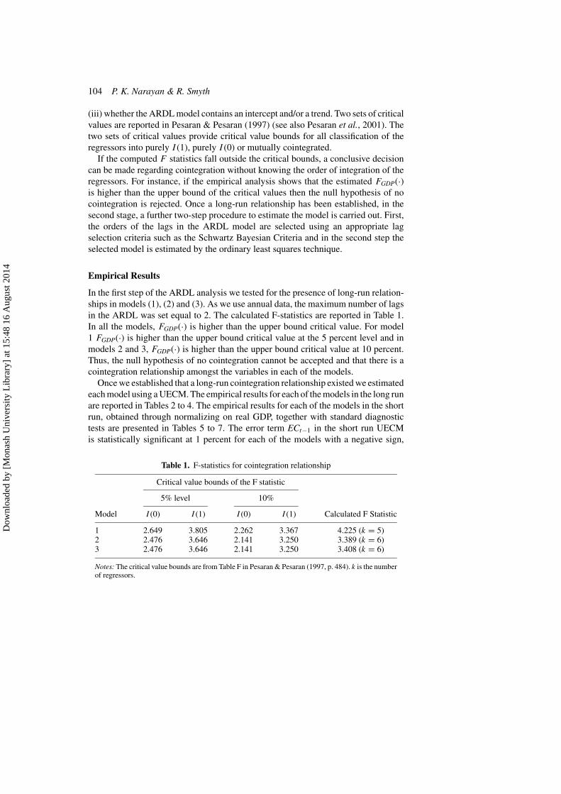
In the first step of the ARDL analysis we tested for the presence of long-run relation-ships in models (1), (2) and (3). As we use annual data, the maximum number of lagsin the ARDL was set equal to 2. The calculated F-statistics are reported in Table 1.In all the models, FGDP(·) is higher than the upper bound critical value. For model1 FGDP(·) is higher than the upper bound critical value at the 5 percent level and inmodels 2 and 3, FGDP(·) is higher than the upper bound critical value at 10 percent.Thus, the null hypothesis of no cointegration cannot be accepted and that there is acointegration relationship amongst the variables in each of the models.

Once we established that a long-run cointegration relationship existed we estimatedeach model using a UECM. The empirical results for each of the models in the long runare reported in Tables 2 to 4. The empirical results for each of the models in the shortrun, obtained through normalizing on real GDP, together with standard diagnostictests are presented in Tables 5 to 7. The error term ECt−1 in the short run UECMis statistically significant at 1 percent for each of the models with a negative sign,

Table 1. F-statistics for cointegration relationship

Critical value bounds of the F statistic

5% level 10%

Model I (0) I (1) I (0) I (1) Calculated F Statistic

1 2.649 3.805 2.262 3.367 4.225 (k = 5)2 2.476 3.646 2.141 3.250 3.389 (k = 6)3 2.476 3.646 2.141 3.250 3.408 (k = 6)

Notes: The critical value bounds are from Table F in Pesaran & Pesaran (1997, p. 484). k is the numberof regressors.

Dow

nloa

ded

by [

Mon

ash

Uni

vers

ity L

ibra

ry]

at 1

5:48

16

Aug

ust 2

014

Trade Liberalization and Economic Growth in Fiji 105

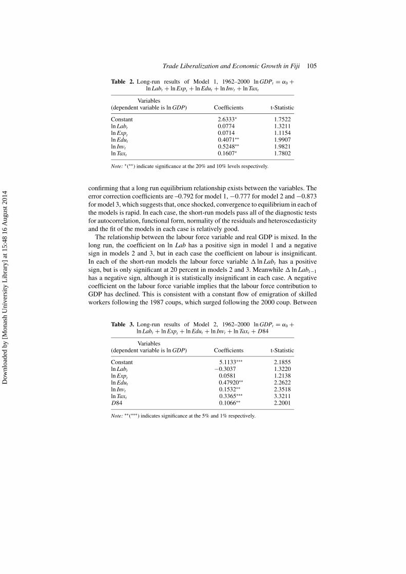
Table 2. Long-run results of Model 1, 1962–2000 ln GDPt = α0 +ln Labt + ln Expt + ln Edut + ln Invt + ln Taxt

Variables(dependent variable is ln GDP) Coefficients t-Statistic

Constant 2.6333∗ 1.7522ln Labt 0.0774 1.3211ln Expt 0.0714 1.1154ln Edut 0.4071∗∗ 1.9907ln Invt 0.5248∗∗ 1.9821ln Taxt 0.1607∗ 1.7802

Note: ∗(∗∗) indicate significance at the 20% and 10% levels respectively.

confirming that a long run equilibrium relationship exists between the variables. Theerror correction coefficients are –0.792 for model 1, −0.777 for model 2 and −0.873for model 3, which suggests that, once shocked, convergence to equilibrium in each ofthe models is rapid. In each case, the short-run models pass all of the diagnostic testsfor autocorrelation, functional form, normality of the residuals and heteroscedasticityand the fit of the models in each case is relatively good.

The relationship between the labour force variable and real GDP is mixed. In thelong run, the coefficient on ln Lab has a positive sign in model 1 and a negativesign in models 2 and 3, but in each case the coefficient on labour is insignificant.In each of the short-run models the labour force variable � ln Labt has a positivesign, but is only significant at 20 percent in models 2 and 3. Meanwhile � ln Labt−1

has a negative sign, although it is statistically insignificant in each case. A negativecoefficient on the labour force variable implies that the labour force contribution toGDP has declined. This is consistent with a constant flow of emigration of skilledworkers following the 1987 coups, which surged following the 2000 coup. Between

Table 3. Long-run results of Model 2, 1962–2000 ln GDPt = α0 +ln Labt + ln Expt + ln Edut + ln Invt + ln Taxt + D84

Variables(dependent variable is ln GDP) Coefficients t-Statistic

Constant 5.1133∗∗∗ 2.1855ln Labt −0.3037 1.3220ln Expt 0.0581 1.2138ln Edut 0.47920∗∗ 2.2622ln Invt 0.1532∗∗ 2.3518ln Taxt 0.3365∗∗∗ 3.3211D84 0.1066∗∗ 2.2001

Note: ∗∗(∗∗∗) indicates significance at the 5% and 1% respectively.

Dow

nloa

ded

by [

Mon

ash

Uni

vers

ity L

ibra

ry]

at 1

5:48

16

Aug

ust 2

014

106 P. K. Narayan & R. Smyth

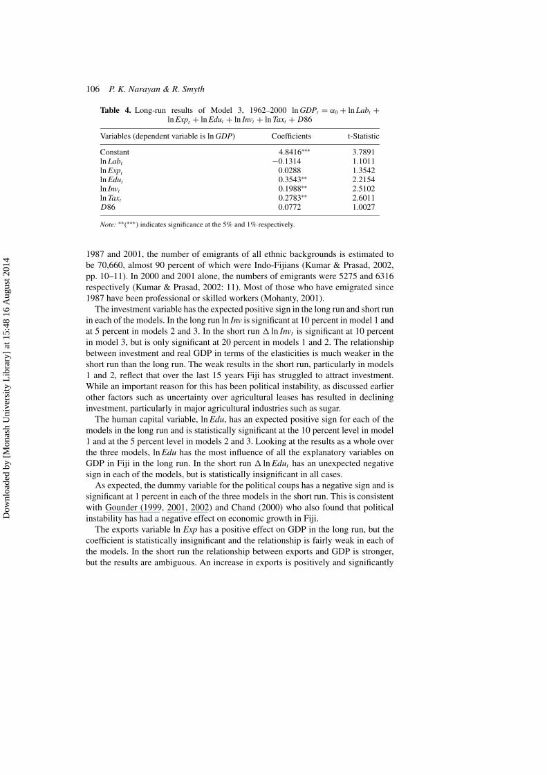
Table 4. Long-run results of Model 3, 1962–2000 ln GDPt = α0 + ln Labt +ln Expt + ln Edut + ln Invt + ln Taxt + D86

Variables (dependent variable is ln GDP) Coefficients t-Statistic

Constant 4.8416∗∗∗ 3.7891ln Labt −0.1314 1.1011ln Expt 0.0288 1.3542ln Edut 0.3543∗∗ 2.2154ln Invt 0.1988∗∗ 2.5102ln Taxt 0.2783∗∗ 2.6011D86 0.0772 1.0027

Note: ∗∗(∗∗∗) indicates significance at the 5% and 1% respectively.

1987 and 2001, the number of emigrants of all ethnic backgrounds is estimated tobe 70,660, almost 90 percent of which were Indo-Fijians (Kumar & Prasad, 2002,pp. 10–11). In 2000 and 2001 alone, the numbers of emigrants were 5275 and 6316respectively (Kumar & Prasad, 2002: 11). Most of those who have emigrated since1987 have been professional or skilled workers (Mohanty, 2001).

The investment variable has the expected positive sign in the long run and short runin each of the models. In the long run ln Inv is significant at 10 percent in model 1 andat 5 percent in models 2 and 3. In the short run � ln Invt is significant at 10 percentin model 3, but is only significant at 20 percent in models 1 and 2. The relationshipbetween investment and real GDP in terms of the elasticities is much weaker in theshort run than the long run. The weak results in the short run, particularly in models1 and 2, reflect that over the last 15 years Fiji has struggled to attract investment.While an important reason for this has been political instability, as discussed earlierother factors such as uncertainty over agricultural leases has resulted in declininginvestment, particularly in major agricultural industries such as sugar.

The human capital variable, ln Edu, has an expected positive sign for each of themodels in the long run and is statistically significant at the 10 percent level in model1 and at the 5 percent level in models 2 and 3. Looking at the results as a whole overthe three models, ln Edu has the most influence of all the explanatory variables onGDP in Fiji in the long run. In the short run � ln Edut has an unexpected negativesign in each of the models, but is statistically insignificant in all cases.

As expected, the dummy variable for the political coups has a negative sign and issignificant at 1 percent in each of the three models in the short run. This is consistentwith Gounder (1999, 2001, 2002) and Chand (2000) who also found that politicalinstability has had a negative effect on economic growth in Fiji.

The exports variable ln Exp has a positive effect on GDP in the long run, but thecoefficient is statistically insignificant and the relationship is fairly weak in each ofthe models. In the short run the relationship between exports and GDP is stronger,but the results are ambiguous. An increase in exports is positively and significantly

Dow

nloa

ded

by [

Mon

ash

Uni

vers

ity L

ibra

ry]

at 1

5:48

16

Aug

ust 2

014

Trade Liberalization and Economic Growth in Fiji 107

Table 5. Short-run results of Model 1, 1962–2000

Variable Coefficient t-Statistic

C 0.0005 0.0145� ln GDPt−1 0.0143 0.0884� ln Labt 1.6350 0.8944� ln Labt−1 −1.3052 −0.7600� ln Expt 0.1933∗∗∗ 3.3468� ln Expt−1 −0.1022∗ −1.8509� ln Edut −0.0484 −0.2777� ln Invt 0.0528# 1.3512� ln Taxt 0.1673# 1.4898� ln Taxt−1 −0.2391∗∗ −2.1195ECt−1 −0.7918∗∗∗ −4.9805COUPt −0.1185∗∗∗ −3.2839

Diagnostic testsR2 0.7609R̄2 0.6557σ 0.0437χ 2

Auto(2) 5.1708χ 2

Norm(2) 1.6123χ 2

WHITE(21) 25.0196χ 2

RESET(2) 5.7713FForecast(1990) 2.5157χ2

ARCH(2) 1.1886

Note: where σ is the standard error of the regression; χ2Auto (2) is the Breusch–

Godfrey LM test for autocorrelation; χ2Norm (2) is the Jarque–Bera normality test;

χ2RESET (2) is the Ramsey test for omitted variables/functional form; χ2

White (2) isthe White test for heteroscedasticity; X2

ARCH (2) is the autoregressive conditionalheteroscedasticity test for the problem of heteroscedasticity under serially correlatedresiduals. FForecast is the Chow predictive failure test (when calculating this test,1990 was chosen as the starting point for forecasting). Critical values for χ2 (2) =9.210 and χ2 (21) = 38.932. ∗∗∗(∗∗)∗indicates significance at the 1%, 5% and 10%respectively; #is significance at the 20% level.

related to GDP at 1 percent in the same year, but changes in exports lagged one yearare negatively and weakly significantly related to GDP the following year.

The dummy variables depicting alternative dates of trade liberalization providelittle evidence that trade liberalization has had a positive effect on real GDP in Fiji. Inthe long run D84 and D86 have a positive sign in models 2 and 3 respectively, but onlyD84 is statistically significant. Both dummy variables are statistically insignificantin the short run models and the relationship with GDP is fairly weak in each case.In model 2, signing the IMF structural adjustment agreement in 1984 resulted ina statistically significant 0.1066 percent increase in GDP in the long run, but is

Dow

nloa

ded

by [

Mon

ash

Uni

vers

ity L

ibra

ry]

at 1

5:48

16

Aug

ust 2

014

108 P. K. Narayan & R. Smyth

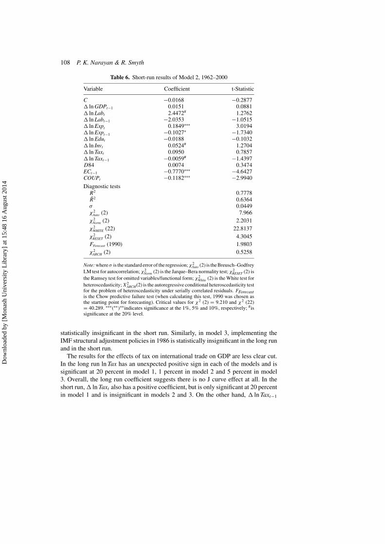
Table 6. Short-run results of Model 2, 1962–2000

Variable Coefficient t-Statistic

C −0.0168 −0.2877� ln GDPt−1 0.0151 0.0881� ln Labt 2.4472# 1.2762� ln Labt−1 −2.0353 −1.0515� ln Expt 0.1849∗∗∗ 3.0194� ln Expt−1 −0.1027∗ −1.7340� ln Edut −0.0188 −0.1032� ln Invt 0.0524# 1.2704� ln Taxt 0.0950 0.7857� ln Taxt−1 −0.0059# −1.4397D84 0.0074 0.3474ECt−1 −0.7770∗∗∗ −4.6427COUPt −0.1182∗∗∗ −2.9940

Diagnostic testsR2 0.7778R̄2 0.6364σ 0.0449χ 2

Auto (2) 7.966χ 2

Norm (2) 2.2031χ 2

WHITE (22) 22.8137χ 2

RESET (2) 4.3045FForecast (1990) 1.9803χ2

ARCH (2) 0.5258

Note: whereσ is the standard error of the regression;χ2Auto (2) is the Breusch–Godfrey

LM test for autocorrelation; χ2Norm (2) is the Jarque–Bera normality test; χ2

RESET (2) isthe Ramsey test for omitted variables/functional form; χ2

White (2) is the White test forheteroscedasticity; X2

ARCH(2) is the autoregressive conditional heteroscedasticity testfor the problem of heteroscedasticity under serially correlated residuals. FForecastis the Chow predictive failure test (when calculating this test, 1990 was chosen asthe starting point for forecasting). Critical values for χ2 (2) = 9.210 and χ2 (22)= 40.289. ∗∗∗(∗∗)∗∗indicates significance at the 1%, 5% and 10%, respectively; #issignificance at the 20% level.

statistically insignificant in the short run. Similarly, in model 3, implementing theIMF structural adjustment policies in 1986 is statistically insignificant in the long runand in the short run.

The results for the effects of tax on international trade on GDP are less clear cut.In the long run ln Tax has an unexpected positive sign in each of the models and issignificant at 20 percent in model 1, 1 percent in model 2 and 5 percent in model3. Overall, the long run coefficient suggests there is no J curve effect at all. In theshort run, � ln Taxt also has a positive coefficient, but is only significant at 20 percentin model 1 and is insignificant in models 2 and 3. On the other hand, � ln Taxt−1

Dow

nloa

ded

by [

Mon

ash

Uni

vers

ity L

ibra

ry]

at 1

5:48

16

Aug

ust 2

014

Trade Liberalization and Economic Growth in Fiji 109

Table 7. Short-run results of Model 3, 1962–2000

Variable Coefficient t-Statistic

C −0.0300 −0.5011� ln GDPt−1 0.0923 0.5173� ln Labt 2.4396# 1.2865� ln Labt−1 −2.0771 −1.0014� ln Expt 0.1562∗∗∗ 2.5554� ln Expt−1 −0.0863# −1.4789� ln Edut −0.0547 −0.2976� ln Invt 0.0740* 1.7462� ln Taxt 0.0875 0.7061� ln Taxt−1 −0.0041 −1.0454D86 0.0144 0.6450ECt−1 −0.8725∗∗∗ −4.6289COUPt −0.1339∗∗∗ −3.2491

Diagnostic testsR2 0.7497R̄2 0.6245σ 0.0456χ 2

Auto (2) 2.4739χ2

Norm (2) 2.1573χ2

WHITE (22) 25.8680χ2

RESET (2) 4.9257FForecast (1990) 2.5891χ 2

ARCH (2) 0.3068

Note: where σ is the standard error of the regression; χ2Auto (2) is the Breusch–

Godfrey LM test for autocorrelation; χ2Norm (2) is the Jarque–Bera normality test;

χ2RESET (2) is the Ramsey test for omitted variables/functional form; χ2

White (2) isthe White test for heteroscedasticity; X2

ARCH (2) is the autoregressive conditionalheteroscedasticity test for the problem of heteroscedasticity under serially correlatedresiduals. FForecast is the Chow predictive failure test (when calculating this test, 1990was chosen as the starting point for forecasting). Critical values for χ2 (2) = 9.210and χ2 (22) = 40.289. ∗∗∗(∗∗)∗indicates significance at the 1%, 5% and 10% levels,respectively; #is significance at the 20% level.

has a negative sign and is statistically significant in model 1 at 5 percent. The shortrun results for model 1 suggest that while reducing tax on international trade has nostatistically significant effect on GDP in the current period, it increases GDP with aone period lag. This suggests at least the beginning of a Jcurve effect of liberalizationon real GDP, which is similar to the findings of Greenaway et al. (1998, 2002), whomodel the dynamics using panel data. However, it is not very conclusive when thedummy variables for the IMF structural adjustment programme enter the equationsin models 1 and 2. � ln Taxt−1 is only significant at 20 percent in model 2 and isstatistically insignificant in model 3.

Dow

nloa

ded

by [

Mon

ash

Uni

vers

ity L

ibra

ry]

at 1

5:48

16

Aug

ust 2

014

110 P. K. Narayan & R. Smyth

Conclusion

This article uses the ARDL approach to cointegration to examine the relationshipbetween economic performance and trade liberalization. The core model that weemploy is a Cobb–Douglas production function, which is expanded to take into ac-count political instability and trade liberalization. Our findings suggest that politicalinstability is consistently a statistically significant influence on economic perfor-mance in the short-run. The dummy variable for signing the IMF agreement in 1984had a statistically significant positive effect on real GDP in the long run, but theshort run effects of signing the agreement as well as the short run and long runeffects of implementing the agreement in 1986 were statistically insignificant. Inthe long run, tax on international trade has an unexpected positive sign in each ofthe models. The short run results for model 1 suggest that while reducing tax oninternational trade has no statistically significant effect on GDP in the current pe-riod, it increases GDP with a one period lag. This is suggestive of the beginningof a Jcurve effect of trade liberalization, which has been observed in some recentcross-country studies of trade liberalization that have used panel data. However, it isnot conclusive given that the Jcurve effect is not robust across all of the short runmodels.

On the whole, the extant literature on trade liberalization and economic growthhas found that trade liberalization has not contributed to economic growth. While ourresults are generally consistent with the existing literature it is important to see thereasons for this. In Fiji’s case there are several domestic issues that are constrainingFiji’s bid to benefit from trade liberalization. Of these, political instability has beenone of the biggest hurdles. The period since 1987 has been a volatile one in termsof the political and economic climate. In this period, Fiji has not only experiencedcoups, but has undergone 14 changes in government. The ensuing economic policieshave, as a result, become a function of the rapid turnover in government.

Some policy implications can be drawn directly from our empirical results. Thefinding that education has the most important impact on GDP in Fiji is important.The rapid rate of skilled labour emigration, due mainly to political instability andracial discrimination, is having a deleterious effect on Fiji’s human resources. Theexodus of educated and skilled labour is also sending the wrong signals to investors.In this respect, our finding that there is a weak relationship between investment andGDP and between exports and GDP is particularly alarming. The Reserve Bank ofFiji aims for a 5 percent growth rate, which requires private investment between 20percent and 25 percent. However, between 1987 and 2000, average private invest-ment was a mere 5 percent. One of the most obvious implications of our results isthat if Fiji is to realize its target growth rate it needs to create a stable political andeconomic climate conducive to investment. It follows from this that political stabil-ity and policies designed to raise investment are a precondition for Fiji’s economicsuccess.

Dow

nloa

ded

by [

Mon

ash

Uni

vers

ity L

ibra

ry]

at 1

5:48

16

Aug

ust 2

014

Trade Liberalization and Economic Growth in Fiji 111

Note

1. For an extensive overview of the literature see Greenaway (1998, pp. 501–505); Greenaway et al. (1998,pp. 1551–1553) and Greenaway et al. (2002, pp. 231–234).

References

Abhayaratne, A. (1996) Foreign trade and economic growth: evidence from Sri Lanka, 1960–1992, AppliedEconomics Letters, 3, pp. 567–570.

Ahmad, J. & Kwan, A. C. C. (1991) Causality between exports and economic growth, Economic Letters,37, pp. 243–248.

Akram-Lodhi, A. H. (1992) Tax-free manufacturing in Fiji: an evaluation, Journal of Contemporary Asia,22, pp. 373–393.

Akram-Lodhi, A. H. (1996) Structural adjustment in Fiji under the interim government, 1987–1992,Contemporary Pacific, 8, pp. 259–290.

Akram-Lodhi, A. H. (1997) Structural adjustment and the agrarian question in Fiji, Journal of Contempo-rary Asia, 27, pp. 37–57.

Banerjee, A., Dolado, J., Galbraith, J. W. & Hendry, D. F. (1993) Co-integration, Error Correction andthe Econometric Analysis of Non-Stationary Data (Oxford: Oxford University Press).

Banerjee, A., Dolado, J. & Mestre, R. (1998) Error-correction mechanism tests for cointegration in a singleequation framework, Journal of Time Series Analysis, 19, pp. 267–283.

Barro, R. (1991) Economic growth in a cross section of countries, Quarterly Journal of Economics, 106,pp. 407–443.

Barro, R. & Lee, J. W. (1993) International comparisons of educational attainment, Journal of MonetaryEconomics, 32, pp. 363–394.

Barro, R. J. & Sala-i-Martin, X. (1995) Economic Growth (New York: McGraw Hill).Chand, S. (1998) Current events in Fiji: an economy adrift in the Pacific, Pacific Economic Bulletin, 13,

pp. 1–17.Chand, S. (2000) Coups, cyclones and recovery: the Fiji experience, Pacific Economic Bulletin, 15, pp.

15–23.Chandra, R. (1989) The political crisis and the manufacturing sector in Fiji, Pacific Viewpoint, 30.Chuang, Y. C. (2000) Human capital, exports and economic growth: a causality analysis for Taiwan,

1952–1995, Review of International Economics, 8, pp. 712–720.Collier, P. (1993) Higgledy-piggledy liberalisation, World Economy, 16, pp. 503–512.DiAddarrio, S. (1997) Estimation of the economic costs of conflict: an examination of the two-gap esti-

mation model for the case of Nicaragua, Oxford Development Studies, 25, pp. 123–141.Dollar, D. (1992) Outward oriented developing economies really do grow more rapidly: evidence from 95

LDCs, 1976–1985, Economic Development and Cultural Change, 40, pp. 523–544.Elek, A., Hill, H. & Tabor, S. (1993) Liberalization and diversification in a small island economy: Fiji

since the 1997 coups, World Development, 21, pp. 749–769.Engle, R. F. & Granger, C. W. J. (1987) Cointegration and error correction representation: estimation and

testing, Econometrica, 55, pp. 251–276.Fosu, A. K. (1992) Political instability, freedom and economic growth: evidence from sub Saharan Africa,

Economic Development and Cultural Change, 40, pp. 829–841.Gounder, R. (1999) The political economy of development: empirical results from Fiji, Economic Analysis

and Policy, 29, pp. 133–150.Gounder, R. (2001) Aid-growth nexus: empirical evidence from Fiji, Applied Economics, 33, pp. 1008–

1019.Gounder, R. (2002) Political and economic freedom, fiscal policy and growth nexus: some empirical results

for Fiji, Contemporary Economic Policy, 20, pp. 234–245.

Dow

nloa

ded

by [

Mon

ash

Uni

vers

ity L

ibra

ry]

at 1

5:48

16

Aug

ust 2

014

112 P. K. Narayan & R. Smyth

Greenaway, D. (1993) Liberalising foreign trade through rose tinted glasses, Economic Journal, 103, pp.208–223.

Greenaway, D. (1998) Does trade liberalisation promote economic development? Scottish Journal ofPolitical Economy, 45, pp. 491–511.

Greenaway, D. & Sapsford, D. (1994) What does liberalisation do for exports and growth?,Weltwirtschaftliches Archiv, 130, pp. 152–174.

Greenaway, D, Leybourne, S. & Sapsford, D. (1997) Modelling growth (and liberalisation) using smoothtransitions analysis, Economic Inquiry, 35, pp. 798–814.

Greenaway, D., Morgan, W. & Wright, P. (1998) Trade reform, adjustment and growth: what does theevidence tell us?, Economic Journal, 108, pp. 1547–1561.

Greenaway, D., Morgan, W. & Wright, P. (2002) Trade liberalisation and growth in developing countries,Journal of Development Economics, 67, pp. 229–244.

Grossman, G. & Helpman, E. (1991) Innovation and Growth in the Global Economy (Cambridge, Mass:MIT Press).

Harrigan, J. & Mosley, P. (1991) Evaluating the impact of world bank structural adjustment lending:1980–1987, Journal of Development Studies, 27, pp. 63–94.

Harrison, A. (1996) Openness and growth: a time-series cross-country analysis for developing countries,Journal of Development Economics, 48, pp. 419–447.

Hossain, F. & Chung, P. J. (1999) Long-run implications of neoclassical growth models: empirical evi-dence from Australia, New Zealand, South Korea and Taiwan, Applied Economics, 31, pp. 1073–1082.

Johansen, S. (1988) Statistical analysis of cointegrating vectors, Journal of Economic Dynamics andControl, 12, pp. 231–254.

Johansen, S. (1995) Likelihood-based Inference in Cointegrated Vector Autoregressive Models (Oxford:Oxford University Press).

Johansen, S. & Juselius, K. (1990) Maximum likelihood estimation and inference on cointegration withapplications to the demand for money, Oxford Bulletin of Economics and Statistics, 52, pp. 169–210.

Jung, W. S. & Marshall, P. J. (1985) Exports, growth and causality in developing countries, Journal ofDevelopment Economics, 18, pp. 1–12.

Krueger, A. (1997) Trade policy and economic development: how we learn, American Economic Review,87, pp. 1–22.

Krueger, A. (1998) Why trade liberalisation is good for growth, Economic Journal, 108, pp. 1513–1522.

Kumar, S. & Prasad, B. (2002) Fiji’s economic woes: a nation in search of development progress, PacificEconomic Bulletin, 17, pp. 1–23.

Lucas, R. (1988) On the mechanics of economic development, Journal of Monetary Economics, 22, pp.3–42.

Mara, K. (1991) Opening address to networking South Pacific 91, Fiji and Investment Trade Forum, MimeoNadi, Fiji.

Mohanty, M. (2001) Contemporary emigration from Fiji: some trends and issues in the post-independenceera, Current Trends in South Pacific Migration, Asia-Pacific Migration Research Network, Wollon-gong: University of Wollongong, pp. 54–73.

Mosley, P., Harrigan, J. & Toye, J. (Eds) (1991a) Aid and Power: The World Bank and Policy-basedLending, Volume 1: Analysis and Policy Proposals (London: Routledge).

Mosley, P., Harrigan, J. & Toye, J. (Eds) (1991b) Aid and Power: The World Bank and Policy-basedLending, Volume 2: Case Studies (London: Routledge).

Ocampo, J. A. & Taylor, L. (1998) Trade liberalisation in developing countries: modest benefits, butproblems with productivity growth, macro prices and income distribution, Economic Journal, 108,pp. 1523–1546.

Dow

nloa

ded

by [

Mon

ash

Uni

vers

ity L

ibra

ry]

at 1

5:48

16

Aug

ust 2

014

Trade Liberalization and Economic Growth in Fiji 113

Onafowora, O. A., Owoye, A. & Nyatepe-Coo, A. (1996) Trade policy, export performance and eco-nomic growth: evidence from sub Saharan Africa, Journal of International Trade and EconomicDevelopment, 5, pp. 341–360.

Oxley, L. (1993) Cointegration, causality and export-led growth in Portugal 1865–1985, Economic Letters,43, pp. 163–166.

Papageorgiou, D., Michaely, M. & Choski, A. (Eds) (1991) Liberalising Foreign Trade (Oxford: Blackwell).Pattichis, C. A. (1999) Price and income elasticities of disaggregated import demands: results from UECMs

and an application, Applied Economics, 31, pp. 1061–1071.Pesaran, M. H. & Pesaran, B. (1997) Working with Microfit 4.0: Interactive Econometric Analysis (Oxford:

Oxford University Press).Pesaran, M. H. & Shin, Y. (1999) An autoregressive distributed lag modelling approach to cointegration

analysis, in: S. Strom (Ed.), Econometrics and Economic Theory in the 20th Century: The RagnarFrisch Centennial Symposium (Cambridge: Cambridge University Press).

Pesaran, M. H., Shin, Y. & Smith, R. (2001) Bounds testing approaches to the analysis of level relationships,Journal of Applied Econometrics, 16, pp. 289–326.

Prasad, B. (1998) The woes of economic reform: poverty and income inequality in Fiji, InternationalJournal of Social Economics, 25, pp. 1073–1093.

Prasad, B. (2002) Trade liberalisation in the South Pacific Forum island countries: a panacea for economicand social ills? Working Paper No. 2002.3, Department of Economics, University of the South Pacific,Suva, Fiji.

Prasad, B. & Tisdell, C. (1996) Getting property rights ‘right’: land tenure in Fiji, Pacific Economic Bulletin,1, pp. 31–46.

Ramirez, M. (2000) Foreign direct investment in Mexico: a cointegration analysis, Journal of DevelopmentStudies, 37, pp. 138–162.

Reserve Bank of Fiji (2002) Reserve Bank of Fiji Quarterly Review (March) (Suva: The Reserve Bank ofFiji).

Sturton, M. & McGregor, A. (1991) Fiji economic adjustment 1987-91, Pacific Islands DevelopmentProgram, East-West Center, Honolulu, Hawaii.

Tang, T. C. (2001) Bank lending and inflation in Malaysia: assessment from unrestricted error-correctionmodels, Asian Economic Journal, 15, pp. 275–289.

Tang, T. C. (2002) Demand for M3 and expenditure components in Malaysia: assessment from boundstesting approach, Applied Economics Letters, 9, pp. 721–725.

Tang, T. C. & Nair, M. (2002) A cointegration analysis of Malaysian import demand function: reassessmentfrom the bounds test, Applied Economics Letters, 9, pp. 293–296.

United Nations Development Programme (UNDP) (2001) Human Development Report 2001 (New York:Oxford University Press).

World Bank (1990) Report on Adjustment Lending II: Policies for the Recovery of Growth, DocumentR90-99 (Washington, DC: World Bank).

World Bank (2002) World Development Indicators Database (Washington DC: The World Bank).Young, A. (1991) Learning by doing and the dynamic effects of international trade, Quarterly Journal of

Economics, 106, pp. 369–405.

Appendix. Error correction models

� ln GDPt = a0GDP +n∑

i=1

biGDP� ln GDPt−i +n∑

i=0

ciGDP� ln Labt−i

+n∑

i=0

diGDP� ln Expt−i +n∑

i=0

eiGDP� ln Edut−i +n∑

i=0

fiGDP� ln Invt−i

Dow

nloa

ded

by [

Mon

ash

Uni

vers

ity L

ibra

ry]

at 1

5:48

16

Aug

ust 2

014

114 P. K. Narayan & R. Smyth

+n∑

i=0

�iGDP� ln Taxt−i+λ1GDP ln GDPt−i + λ2GDP ln Labt−i

+ λ3GDP ln Expt−i + λ4GDP ln Edut−i + λ5GDP ln Invt−i

+ λ6GDP ln Taxt−i + ε1t (A1)

� ln Labt = a0Lab +n∑

i=1

biLab� ln Labt−i +n∑

i=0

ciLab�GDPt−i

+n∑

i=0

diLab� ln Expt−i +n∑

i=0

eiLab� ln Edut−i +n∑

i=0

fiLab� ln Invt−i

+n∑

i=0

giLab� ln Taxt−i+λ1Lab ln GDPt−i + λ2Lab ln Labt−i

+ λ3Lab ln Expt−i + λ4Lab ln Edut−i + λ5Lab ln Invt−i

+ λ6Lab ln Taxt−i + ε2t (A2)

� ln Expt = a0Exp +n∑

i=1

bi Exp� ln Expt−i +n∑

i=0

ciExp� ln Labt−i

+n∑

i=0

diExp� ln GDPt−i +n∑

i=0

eiExp� ln Edut−i +n∑

i=0

fiExp� ln Invt−i

+n∑

i=0

giExp� ln Taxt−i+λ1Exp ln GDPt−i + λ2Exp ln Labt−i

+ λ3Exp ln Expt−i + λ4Exp ln Edut−i + λ5Exp ln Invt−i

+ λ6Exp ln Taxt−i + ε3t (A3)

� ln Edut = a0Edu +n∑

i=1

biEdu� ln Edut−i +n∑

i=0

ciEdu� ln Labt−i

+n∑

i=0

diEdu� ln GDPt−i +n∑

i=0

eiEdu� ln Expt−i +n∑

i=0

fiEdu� ln Invt−i

+n∑

i=0

giEdu� ln Taxt−i + λ1Edu ln GDPt−i + λ2Edu ln Labt−i

+ λ3Edu ln Expt−i + λ4Edu ln Edut−i + λ5Edu ln Invt−i

+ λ6Edu ln Taxt−i + ε4t (A4)

Dow

nloa

ded

by [

Mon

ash

Uni

vers

ity L

ibra

ry]

at 1

5:48

16

Aug

ust 2

014

Trade Liberalization and Economic Growth in Fiji 115

� ln Invt = a0Inv +n∑

i=1

biInv� ln Invt−i +n∑

i=0

ciInv� ln Labt−i

+n∑

i=0

diInv� ln GDPt−i +n∑

i=0

eiInv� ln Expt−i +n∑

i=0

fiInv� ln Edut−i

+n∑

i=0

giInv� ln Taxt−i+λ1Inv ln GDPt−i + λ2Inv ln Labt−i

+ λ3Inv ln Expt−i + λ4Inv ln Edut−i + λ5Inv ln Invt−i

+ λ6Inv ln Taxt−i + ε5t (A5)

� ln Taxt = a0Tax +n∑

i=1

biTax� ln Taxt−i +n∑

i=0

ciTax� ln Labt−i

+n∑

i=0

diTax� ln GDPt−i +n∑

i=0

eiTax� ln Expt−i +n∑

i=0

fiTax� ln Edut−i

+n∑

i=0

giTax� ln Invt−i + λ1Tax ln GDPt−i + λ2Tax ln Labt−i

+ λ3Tax ln Expt−i + λ4Tax ln Edut−i + λ5Tax ln Invt−i

+ λ6Tax ln Taxt−i + ε6t (A6)

Dow

nloa

ded

by [

Mon

ash

Uni

vers

ity L

ibra

ry]

at 1

5:48

16

Aug

ust 2

014