Systems & Control Letters 55 (2006) 396–406www.elsevier.com/locate/sysconle

Tracking control with prescribed transient behaviour for systemsof known relative degree�

Achim Ilchmanna,∗, Eugene P. Ryanb, Philip Townsendb

aInstitute of Mathematics, Technical University Ilmenau, Weimarer Straße 25, 98693 Ilmenau, GermanybDepartment of Mathematical Sciences, University of Bath, Claverton Down, Bath BA2 7AY, UK

Received 22 February 2005; received in revised form 23 August 2005; accepted 12 September 2005Available online 14 November 2005

Abstract

Tracking of a reference signal (assumed bounded with essentially bounded derivative) is considered for multi-input, multi-output linearsystems satisfying the following structural assumptions: (i) arbitrary—but known—relative degree, (ii) the “high-frequency gain” matrix issign definite—but of unknown sign, (iii) exponentially stable zero dynamics. The first control objective is tracking, by the output y, withprescribed accuracy: given � > 0 (arbitrarily small), determine a feedback strategy which ensures that, for every reference signal r, the trackingerror e = y − r is ultimately bounded by � (that is, ‖e(t)‖ < � for all t sufficiently large). The second objective is guaranteed output transientperformance: the evolution of the tracking error should be contained in a prescribed performance funnel F� (determined by a function �). Bothobjectives are achieved by a filter in conjunction with a feedback function of the filter states, the tracking error and a gain parameter. The latteris generated via a feedback function of the tracking error and the funnel parameter �. Moreover, the feedback system is robust to nonlinearperturbations bounded by some continuous function of the output. The feedback structure essentially exploits an intrinsic high-gain propertyof the system/filter interconnection by ensuring that, if (t, e(t)) approaches the funnel boundary, then the gain attains values sufficiently largeto preclude boundary contact.© 2005 Elsevier B.V. All rights reserved.

Keywords: Output feedback; Transient behaviour; Tracking; Relative degree

1. Introduction

1.1. Class of systems

We consider the class of nonlinearly-perturbed (perturbationp), m-input (u(t) ∈ Rm), m-output (y(t) ∈ Rm) linear systemsof the form

x(t) = Ax(t) + Bu(t) + p(t, x(t)), x(0) = x0 ∈ Rn,

y(t) = Cx(t) ∈ Rm,

}(1)

where A ∈ Rn×n, B ∈ Rn×m, C ∈ Rm×n and p: R+ × Rn →Rn are such that the following hold.

� Based on work supported in part by the UK Engineering & PhysicalSciences Research Council (GR/S94582/01) and the Deutsche Forschungsge-meinschaft (IL 25/3-1).

∗ Corresponding author. Tel.: +4936 7769 3623; fax: +4936 7769 3270.E-mail addresses: achim.ilchmann@tu-ilmenau.de (A. Ilchmann),

epr@maths.bath.ac.uk (E.P. Ryan), p.townsend@bath.ac.uk (P. Townsend).

0167-6911/$ - see front matter © 2005 Elsevier B.V. All rights reserved.doi:10.1016/j.sysconle.2005.09.002

Assumption A1 (strict relative degree and sign-definite high-frequency gain). For some known � ∈ N, CAiB = 0 for i =1, . . . , �− 2, and CA�−1B is either strictly positive definite orstrictly negative definite.

Assumption A2 (minimum-phase).

det

[sI − A B

C 0

]�= 0 for all s ∈ C with Re s�0.

Assumption A3 (nonlinear perturbation). The perturbationp: R+×Rn → Rn is a Carathéodory function with the propertythat, for some continuous �: Rm → R+,

‖p(t, x)‖��(Cx) ∀(t, x) ∈ R+ × Rn.

Remark 1.

(i) If the transfer function s �→ C(sI − A)−1B =∑∞i=0 CAiBs−i+1 is non-trivial (not identically zero),

A. Ilchmann et al. / Systems & Control Letters 55 (2006) 396–406 397

then there exists � ∈ N such that CAiB = 0 for i =1, . . . , � − 2 and CA�−1B �= 0. Assumption A1 requiresthat � be known, and CA�−1B to be not only invertible(i.e. strict relative degree) but also either strictly positivedefinite or strictly negative definite.In the single-input single-output (SISO) case, the hypoth-esis of sign definiteness is redundant and A1 is simplyequivalent to positing that the transfer function is ofknown relative degree ��1. In the multi-input, multi-output (MIMO) context, A1 is highly restrictive: never-theless we include the restricted MIMO case here as thiscan be done with little extra analytical effort vis a vis theSISO case. The general vector relative degree MIMO caseis considerably more subtle and is the subject of ongoinginvestigations.

(ii) Coppel ([2, Theorem 10]) has shown (see also [3, Propo-sition 2.1.2]) that Assumption A2 is equivalent to: (A, B)

is stabilizable, (C, A) is detectable, and the transfer func-tion s �→ C(sI − A)−1B has no zeros in the closed righthalf complex plane {� ∈ C | Re(�)�0}.Note that the minimum phase assumption implies that theunperturbed (p ≡ 0) system has exponentially stable zerodynamics, see, for example [5, Section 5.1].

(iii) Even in the absence of a nonlinear perturbation p, the re-sults of the paper are new. We encompass perturbationsfor added generality and remark that perturbations satis-fying A3 can be incorporated with relative ease in theanalysis.

Linear systems satisfying Assumptions A1 and A2 are,at least in the SISO case, typical of the class of systemsunderlying the area of high-gain adaptive control, as stud-ied in Morse [10], Byrnes and Willems [1] and Mareels [8]for example. Most early results pertain to systems of rela-tive degree one. More recently, systems of higher relativedegree have been investigated: in Section 3.2, we com-pare some of these investigations with the approach adoptedhere.

1.2. Control objectives and the performance funnel

The first control objective is approximate tracking, by theoutput y, of reference signals r of class R := W 1,∞(R+, Rm),i.e. the space of locally absolutely continuous boundedfunctions with bounded derivative, endowed with norm‖r‖1,∞ := ‖r‖∞ + ‖r‖∞. In particular, for arbitrary � > 0,we seek an output feedback strategy which ensures that,for every r ∈ R, the closed-loop system has a boundedsolution and the tracking error e(t) = y(t) − r(t) is ul-timately bounded by � (that is, ‖e(t)‖�� for all t suffi-ciently large). The second control objective is prescribedtransient behaviour of the tracking error signal. We cap-ture both objectives in the concept of a performance funnel(Fig. 1)

F� := {(t, e) ∈ R+ × Rm |�(t)‖e‖ < 1}

Error evolution

Ball of radius 1/�(t)

t

F�

Fig. 1. Prescribed performance funnel F�.

associated with a function � (the reciprocal of which determinesthe funnel boundary) belonging to

B :={� ∈ W 1,∞(R+, R)

∣∣∣∣�(0) = 0, �(s) > 0 ∀s > 0,

lim infs→∞ �(s) > 0

}.

The aim is an output feedback strategy ensuring that, for everyreference signal r ∈ R, the tracking error e = y − r evolveswithin the funnel F�. For example, if lim inf t→∞ �(t) > 1/�,then evolution within the funnel ensures that the first con-trol objective is achieved. If � is chosen as the function t �→min{t/T , 1}/�, then evolution within the funnel ensures thatthe prescribed tracking accuracy � > 0 is achieved within theprescribed time T > 0.

The paper is structured as follows. In Section 2, we describethe control strategy and present the main result in Theorem2. A discussion, including intuition and literature review, ispresented in Section 3. An example is given in Section 4, whichillustrates the control strategy by numerical simulations. Forpurposes of exposition, all proofs are deferred to Section 5.

2. The control

Let Assumptions A1 and A2 hold, with relative degree ��2;the relative degree 1 case will be treated separately.

2.1. Filter

Introduce the filter

�i (t) = −�i (t) + �i+1, �i (0) = �0i ∈ Rm,

i = 1, . . . , � − 2,

��−1(t) = −��−1(t) + u(t), ��−1(0) = �0�−1 ∈ Rm,

398 A. Ilchmann et al. / Systems & Control Letters 55 (2006) 396–406

which, on writing

�(t) =

⎛⎜⎜⎜⎜⎜⎜⎝

�1(t)

�2(t)

�3(t)...

��−2(t)

��−1(t)

⎞⎟⎟⎟⎟⎟⎟⎠

,

F =

⎡⎢⎢⎢⎢⎢⎢⎣

−I I 0 · · · 0 00 −I I · · · 0 00 0 −I · · · 0 0...

......

. . ....

...

0 0 0 · · · −I I

0 0 0 · · · 0 −I

⎤⎥⎥⎥⎥⎥⎥⎦

, G =

⎡⎢⎢⎢⎢⎢⎢⎣

000...

0Im

⎤⎥⎥⎥⎥⎥⎥⎦

,

may be expressed as

�(t) = F�(t) + Gu(t), �(0) = �0 ∈ R(�−1)m,

�1(t) = H�(t), H := [Im

... 0... · · · ... 0].

}(2)

2.2. Feedback

Let �: R → R be any C∞ function with the properties

lim supk→∞

�(k) = +∞ and lim infk→∞ �(k) = −∞. (3)

Introduce the projections

�i : R(�−1)m → Rim,

� = (�1, . . . , ��−1) �→ (�1, . . . , �i ), i = 1, . . . , � − 1

and define the C∞ function

�1: R × Rm → Rm, (k, e) �→ �1(k, e) := −�(k)e, (4)

with derivative (Jacobian matrix function) D�1. Next, for i =2, . . . , �, define the C∞ function �i : R×Rm ×R(i−1)m → Rm

by the recursion

�i (k, e, �i−1�)

:= �i−1(k, e, �i−2�) + ‖D�i−1(k, e, �i−2�)‖2k4

× (1 + ‖�i−1�‖2)(�i−1 + �i−1(k, e, �i−2�)), (5)

wherein we adopt the notational convention �1(k, e, �0�) :=�1(k, e).

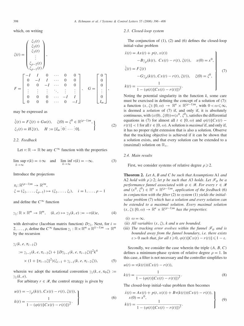
For arbitrary r ∈ R, the control strategy is given by

u(t) = −��(k(t), Cx(t) − r(t), �(t)),

k(t) = 1

1 − (�(t)‖Cx(t) − r(t)‖)2 .

⎫⎬⎭ (6)

2.3. Closed-loop system

The conjunction of (1), (2) and (6) defines the closed-loopinitial-value problem

x(t) = Ax(t) + p(t, x(t))

−B��(k(t), Cx(t) − r(t), �(t)), x(0) = x0,

�(t) = F�(t)

−G��(k(t), Cx(t) − r(t), �(t)), �(0) = �0,

k(t) = 1

1 − (�(t)‖Cx(t) − r(t)‖)2 .

⎫⎪⎪⎪⎪⎪⎪⎪⎪⎪⎪⎬⎪⎪⎪⎪⎪⎪⎪⎪⎪⎪⎭

(7)

Noting the potential singularity in the function k, some caremust be exercised in defining the concept of a solution of (7):a function (x, �): [0, ) → Rn × R(�−1)m, with 0 < �∞,is deemed a solution of (7) if, and only if, it is absolutelycontinuous, with (x(0), �(0))=(x0, �0), satisfies the differentialequations in (7) for almost all t ∈ [0, ) and �(t)‖Cx(t) −r(t)‖ < 1 for all t ∈ [0, ). A solution is maximal if, and only if,it has no proper right extension that is also a solution. Observethat the tracking objective is achieved if it can be shown thata solution exists, and that every solution can be extended to a(maximal) solution on R+.

2.4. Main results

First, we consider systems of relative degree ��2.

Theorem 2. Let A, B and C be such that Assumptions A1 andA2 hold with ��2; let p be such that A3 holds. Let F� be aperformance funnel associated with � ∈ B. For every r ∈ Rand (x0, �0) ∈ Rn × R(�−1)m, application of the feedback (6)in conjunction with the filter (2) to system (1) yields the initial-value problem (7) which has a solution and every solution canbe extended to a maximal solution. Every maximal solution(x, �): [0, ) → Rn × R(�−1)m has the properties:

(i) = ∞.(ii) All variables (x, �), k and u are bounded.

(iii) The tracking error evolves within the funnel F� and isbounded away from the funnel boundary, i.e. there exists > 0 such that, for all t �0, �(t)‖Cx(t) − r(t)‖�1 − .

Secondly, we consider the case wherein the triple (A, B, C)

defines a minimum-phase system of relative degree � = 1. Inthis case, a filter is not necessary and the controller simplifies to

u(t) = �(k(t))(Cx(t) − r(t)),

k(t) = 1

1 − (�(t)‖Cx(t) − r(t)‖)2 . (8)

The closed-loop initial-value problem then becomes

x(t) = Ax(t) + p(t, x(t)) + B�(k(t))(Cx(t) − r(t)),

x(0) = x0,

k(t) = 1

1 − (�(t)‖Cx(t) − r(t)‖)2 .

⎫⎪⎬⎪⎭ (9)

A. Ilchmann et al. / Systems & Control Letters 55 (2006) 396–406 399

Theorem 3. Let A, B and C be such that Assumptions A1 andA2 hold with � = 1; let p be such that A3 holds. Let F� be aperformance funnel associated with � ∈ B. For every r ∈ Rand x0 ∈ Rn, the initial-value problem (9) has a solution andevery solution can be extended to a maximal solution. Everymaximal solution x: [0, ) → Rn has the properties:

(i) = ∞.(ii) x, k and u are bounded.

(iii) There exists > 0 such that, for all t �0,�(t)‖Cx(t) − r(t)‖�1 − .

Remark 4.

(i) A simple example of a function satisfying (3) is � : k �→k cos k. The rôle of the function � is similar to the con-cept of a “Nussbaum” function in adaptive control. Note,however, that the requisite properties (3) are less restric-tive than (a) the “Nussbaum property”

lim supk→∞

1

k

∫ k

0�(�) d� = ∞,

lim infk→∞

1

k

∫ k

0�(�) d� = −∞,

as required in Ye [11], for example, or (b) the stronger“scaling invariant Nussbaum property”, as required inJiang et al. [6], for example.

(ii) In the specific case of a system of relative degree � = 2in Theorem 2, writing e(t) = Cx(t) − r(t) and omittingthe argument t for simplicity, the control strategy takes theexplicit form

u = �(k)e − [(�′(k)‖e‖)2 + (�(k))2]k4[1 + ‖�‖2]�,

k = [1 − �2‖e‖2]−1, � = � − �(k)e,

� = − � + u, �(0) = �0.

(iii) If CA�−1B is known to be positive (respectively, negative)definite, the need for the function �, with properties (3),in (4) or (8) is obviated and it may be replaced by k �→�(k) = −k, (k �→ �(k) = k), respectively. The proofs ofTheorem 2 and 3 are readily modified to confirm this claim.In the case of sign-definite CA�−1B of known sign, theresult of Theorem 3 is proved in Ilchmann et al. [4]:the general case of Theorem 3, wherein CA�−1B is ofunknown sign, is new.

3. Discussion

3.1. Intuition

The intuition behind the filter (2) and feedback control strat-egy (6) is as follows. With �0 = 0, the transfer function from uto �1 is given by

H(sI − F)−1G = (s + 1)1−�I .

(A,[I+A]�−1B,C)

u (F,G,H)�1

(s+1)�−1Iu

(A,B,C) y

Fig. 2.

Therefore, with reference to Fig. 2, the transfer function fromthe signal �1 to the output y is given by

(s + 1)�−1C(sI − A)−1B = C[I + A]�−1(sI − A)−1B

= C(sI − A)−1[I + A]�−1B,

which has the minimum phase property and is of relative degreeone (see Lemma 5 below): thus, the triple (A, [I +A]�−1B, C)

defines a minimum-phase system of strict relative degree onewith high-frequency gain CA�−1B.

Lemma 5. Let (1) be such that Assumptions A1 and A2 holdwith ��2 and assume p = 0. Then the following hold.

(i) The triple (A, [I + A]�−1B, C) has the minimum phaseproperty.

(ii) There exist K ∈ Rn×m(�−1) and invertible U ∈ Rn×n suchthat, under the coordinate change

(y(t)

z(t)

�(t)

)= L

(x(t)

�(t)

),

(y0

z0

�0

)= L

(x0

�0

),

L :=(

U −UK

0 I

), (10)

the conjunction of system (1) and filter (2) is represented by

y(t) = A1y(t) + A2z(t) + CA�−1B�1(t),

y(0) = y0 ∈ Rm,

z(t) = A3y(t) + A4z(t), z(0) = z0 ∈ Rn−m,

�(t) = F�(t) + Gu(t), �(0) = �0 ∈ R(�−1)m,

⎫⎪⎪⎪⎪⎬⎪⎪⎪⎪⎭

(11)

where A4 ∈ R(n−m)×(n−m) has spectrum in open left halfcomplex plane.

If (x, �) : [0, ) → Rn × Rm(�−1) is a maximal solution ofthe nonlinearly-perturbed closed-loop system (7), then, in viewof Lemma 5 and writing

y(t) = Cx(t), e(t) = y(t) − r(t), e0 = y0 − r(0), (12)

there exists an invertible linear coordinate transformation L(with associated invertible submatrix U) which takes (7) into

400 A. Ilchmann et al. / Systems & Control Letters 55 (2006) 396–406

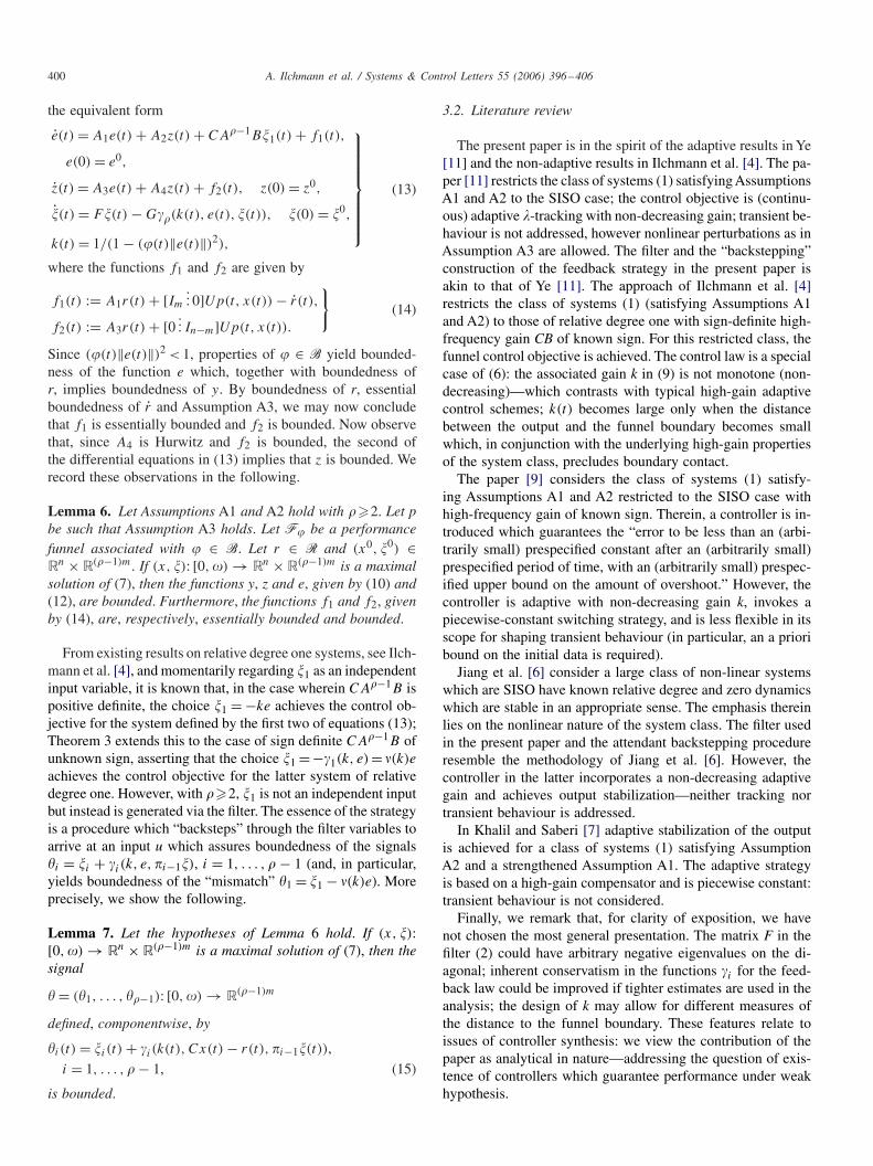
the equivalent form

e(t) = A1e(t) + A2z(t) + CA�−1B�1(t) + f1(t),

e(0) = e0,

z(t) = A3e(t) + A4z(t) + f2(t), z(0) = z0,

�(t) = F�(t) − G��(k(t), e(t), �(t)), �(0) = �0,

k(t) = 1/(1 − (�(t)‖e(t)‖)2),

⎫⎪⎪⎪⎪⎪⎪⎪⎬⎪⎪⎪⎪⎪⎪⎪⎭

(13)

where the functions f1 and f2 are given by

f1(t) := A1r(t) + [Im

... 0]Up(t, x(t)) − r(t),

f2(t) := A3r(t) + [0 ... In−m]Up(t, x(t)).

}(14)

Since (�(t)‖e(t)‖)2 < 1, properties of � ∈ B yield bounded-ness of the function e which, together with boundedness ofr, implies boundedness of y. By boundedness of r, essentialboundedness of r and Assumption A3, we may now concludethat f1 is essentially bounded and f2 is bounded. Now observethat, since A4 is Hurwitz and f2 is bounded, the second ofthe differential equations in (13) implies that z is bounded. Werecord these observations in the following.

Lemma 6. Let Assumptions A1 and A2 hold with ��2. Let pbe such that Assumption A3 holds. Let F� be a performancefunnel associated with � ∈ B. Let r ∈ R and (x0, �0) ∈Rn × R(�−1)m. If (x, �): [0, ) → Rn × R(�−1)m is a maximalsolution of (7), then the functions y, z and e, given by (10) and(12), are bounded. Furthermore, the functions f1 and f2, givenby (14), are, respectively, essentially bounded and bounded.

From existing results on relative degree one systems, see Ilch-mann et al. [4], and momentarily regarding �1 as an independentinput variable, it is known that, in the case wherein CA�−1B ispositive definite, the choice �1 = −ke achieves the control ob-jective for the system defined by the first two of equations (13);Theorem 3 extends this to the case of sign definite CA�−1B ofunknown sign, asserting that the choice �1 =−�1(k, e)= �(k)e

achieves the control objective for the latter system of relativedegree one. However, with ��2, �1 is not an independent inputbut instead is generated via the filter. The essence of the strategyis a procedure which “backsteps” through the filter variables toarrive at an input u which assures boundedness of the signals�i = �i + �i (k, e, �i−1�), i = 1, . . . , � − 1 (and, in particular,yields boundedness of the “mismatch” �1 = �1 − �(k)e). Moreprecisely, we show the following.

Lemma 7. Let the hypotheses of Lemma 6 hold. If (x, �):[0, ) → Rn × R(�−1)m is a maximal solution of (7), then thesignal

� = (�1, . . . , ��−1): [0, ) → R(�−1)m

defined, componentwise, by

�i (t) = �i (t) + �i (k(t), Cx(t) − r(t), �i−1�(t)),

i = 1, . . . , � − 1, (15)

is bounded.

3.2. Literature review

The present paper is in the spirit of the adaptive results in Ye[11] and the non-adaptive results in Ilchmann et al. [4]. The pa-per [11] restricts the class of systems (1) satisfying AssumptionsA1 and A2 to the SISO case; the control objective is (continu-ous) adaptive �-tracking with non-decreasing gain; transient be-haviour is not addressed, however nonlinear perturbations as inAssumption A3 are allowed. The filter and the “backstepping”construction of the feedback strategy in the present paper isakin to that of Ye [11]. The approach of Ilchmann et al. [4]restricts the class of systems (1) (satisfying Assumptions A1and A2) to those of relative degree one with sign-definite high-frequency gain CB of known sign. For this restricted class, thefunnel control objective is achieved. The control law is a specialcase of (6): the associated gain k in (9) is not monotone (non-decreasing)—which contrasts with typical high-gain adaptivecontrol schemes; k(t) becomes large only when the distancebetween the output and the funnel boundary becomes smallwhich, in conjunction with the underlying high-gain propertiesof the system class, precludes boundary contact.

The paper [9] considers the class of systems (1) satisfy-ing Assumptions A1 and A2 restricted to the SISO case withhigh-frequency gain of known sign. Therein, a controller is in-troduced which guarantees the “error to be less than an (arbi-trarily small) prespecified constant after an (arbitrarily small)prespecified period of time, with an (arbitrarily small) prespec-ified upper bound on the amount of overshoot.” However, thecontroller is adaptive with non-decreasing gain k, invokes apiecewise-constant switching strategy, and is less flexible in itsscope for shaping transient behaviour (in particular, an a prioribound on the initial data is required).

Jiang et al. [6] consider a large class of non-linear systemswhich are SISO have known relative degree and zero dynamicswhich are stable in an appropriate sense. The emphasis thereinlies on the nonlinear nature of the system class. The filter usedin the present paper and the attendant backstepping procedureresemble the methodology of Jiang et al. [6]. However, thecontroller in the latter incorporates a non-decreasing adaptivegain and achieves output stabilization—neither tracking nortransient behaviour is addressed.

In Khalil and Saberi [7] adaptive stabilization of the outputis achieved for a class of systems (1) satisfying AssumptionA2 and a strengthened Assumption A1. The adaptive strategyis based on a high-gain compensator and is piecewise constant:transient behaviour is not considered.

Finally, we remark that, for clarity of exposition, we havenot chosen the most general presentation. The matrix F in thefilter (2) could have arbitrary negative eigenvalues on the di-agonal; inherent conservatism in the functions �i for the feed-back law could be improved if tighter estimates are used in theanalysis; the design of k may allow for different measures ofthe distance to the funnel boundary. These features relate toissues of controller synthesis: we view the contribution of thepaper as analytical in nature—addressing the question of exis-tence of controllers which guarantee performance under weakhypothesis.

A. Ilchmann et al. / Systems & Control Letters 55 (2006) 396–406 401

4. Example

We illustrate the controller strategy (6) for the SISO relativedegree two system with nonlinear perturbations modelling apendulum (with input force u):

y(t) + a sin y(t) = bu(t), (16)

with unknown real parameters a and b �= 0. Eq. (16) is equiv-alent to (1) with x(t) = (y(t), y(t))T,

A =[

0 10 0

], B =

[0b

], C = [1 ... 0],

p(t, x(t)) = a sin y(t), t �0.

The funnel is specified by the smooth function

t �→ �(t) ={

10(1 − (0.1 t − 1)2), 0� t < 10,

10, t �10(17)

which assures a tracking accuracy |e(t)| < 0.1 for all t �10. Ifnon-zero b is of unknown sign, then, choosing � : k �→ k cos k,writing e(t) = y(t) − r(t) and suppressing the argument t forsimplicity, the control strategy is

u = (k cos k)e − [� − (k cos k)e]×[(cos k − k sin k)2e2 + k2cos2k]k4[1 + �2],

k = [1 − �2e2]−1,

� = −� + u, �(0) = 0.

⎫⎪⎪⎪⎬⎪⎪⎪⎭

(18)

Adopting the values a=1/2, b=1, initial data (y(0), y(0))=(0, 0) and reference signal t �→ r(t) = (1/2) cos t , the be-haviour of the closed-loop system (16)–(18) over the time in-terval [0, 20] is depicted in Fig. 3. The “peaks” in the controlaction occur whenever the tracking error is close to the bound-ary of the funnel. However, if b �= 0 is known a priori to bepositive, then the peaking behaviour is considerably mollifiedby choosing the function �: k �→ −k in place of k �→ k cos k

in which case the strategy is

u = −ke − [� + ke][e2 + k2]k4[1 + �2],k = [1 − �2e2]−1,

� = −� + u, �(0) = 0.

⎫⎪⎬⎪⎭ (19)

For the same parameter values and initial data as above, thebehaviour (16), under control (19), is shown in Fig. 4.

5. Proofs

5.1. Proof of Lemma 5

Note that

K := [[I + A]�−2B... [I + A]�−3B

... . . .... [I + A]

× B... B] ∈ Rn×(�−1)m

is such that

AK − KF = [[I + A]�−1B... 0

... . . .... 0],

KG = B and CK = 0.

The coordinate transformation

(t) = x(t) − K�(t),

together with (1) (with p = 0) and (2), yields

(t) = A (t) + [I + A]�−1B�1(t),

y(t) = C (t).

}(20)

Since C[I + A]�−1B = CA�−1B is invertible by AssumptionA1, we have Rn = im [I + A]�−1B ⊕ ker C, and thus thereexists an invertible U ∈ Rn×n so that, under the change ofcoordinates(

y(t)

z(t)

)= U (t),

we may express (20) as

y(t) = A1y(t) + A2z(t) + CA�−1B�1(t),

z(t) = A3y(t) + A4z(t).

}(21)

Therefore, the coordinate transformation matrix

L =[U −UK

0 I

]

takes (1) and (2) into form (11). It remains to show that A4 hasspectrum in open left half complex plane. Writing

M1(s) =[sI − A B

C 0

]and

M2(s) =[

sI − A 0 B

0 sI − F −G

C 0 0

],

we have

M3(s) :=[

I K 00 I 00 0 I

]M2(s)

[I K 00 I 00 0 I

]−1

=[

sI − A AK − KF 00 sI − F −G

C 0 0

].

In view of the particular structure of F, G and AK − KF , it isreadily verified that

| det M3(s)| = | det M4(s)|, where

M4(s) =[sI − A [I + A]�−1B

C 0

].

Moreover,

M5(s) :=[U 00 I

]M4(s)

[U−1 0

0 I

]

=[

sI − A1 −A2 CA�−1B

−A3 sI − A4 0I 0 0

].

402 A. Ilchmann et al. / Systems & Control Letters 55 (2006) 396–406

20-1

0

0

1

1/�(·)

e(·)

The funnel and tracking error e

20-1

0

0

1

r(·)

y(·)

The reference r and output y

200

0

4

k(·)

The function k

20-15

0

0

15

u(·)

The control u

(a)

(b)

(c)

(d)

Fig. 3. Unknown sign b �= 0: control (18) applied to the nonlinear pendulum (16). (a) The funnel and tracking error e. (b) The reference r and output y.(c) The function k. (d) The control u.

A. Ilchmann et al. / Systems & Control Letters 55 (2006) 396–406 403

The funnel and tracking error e

The reference r and output y

The function k

The control u

(a)

(b)

(c)

(d)

-1

0

1

-1

0

1

0

4

-5

0

5

200

200

200

200

1/�(·)

e(·)

r(·)

y(·)

k(·)

u(·)

Fig. 4. Known sign b > 0: control (19) applied to the nonlinear pendulum (16). (a) The funnel and tracking error e. (b) The reference r and output y. (c) Thefunction k. (d) The control u.

404 A. Ilchmann et al. / Systems & Control Letters 55 (2006) 396–406

We may now conclude that, for all s ∈ C with Re(s)�0,

| det(CA�−1B) det(sI − A4)|= | det M5(s)| = | det M4(s)|= | det M3(s)| = | det M2(s)|= | det(sI − F) det M1(s)| �= 0,

whence Assertions (i) and (ii). �

5.2. Proof of Lemma 7

Assume that (x, �): [0, ) → Rn × R(�−1)m is a maximalsolution of (7). Write y(t) = Cx(t) and e(t) = y(t) − r(t) forall t ∈ [0, ). By Lemma 5, there exists an invertible lineartransformation L under which the closed-loop system (7) maybe expressed in the form (13), wherein, by Lemma 6, e and z

are bounded and the functions f1 and f2, given by (14), are,respectively, essentially bounded and bounded. By the first ofEq. (13), we may infer the existence of c1 > 0 such that

‖e(t)‖�c1(1 + ‖�1(t)‖) for a.a. t ∈ [0, ).

By boundedness of �, e and essential boundedness of �, thereexists c2 > 0 such that

|k(t)| = 2k2(t)|�2(t)〈e(t), e(t)〉 + �(t)�(t)‖e(t)‖2|�c2k

2(t)(1 + ‖�1(t)‖) for a.a. t ∈ [0, ).

Since k(t)�1 for all t ∈ [0, ), we may now conclude theexistence of c3 > 0 such that

‖(k(t), e(t))‖2 �c3k4(t)(1 + ‖�1(t)‖2) for a.a. t ∈ [0, ).

Then, for some constant c4,1 > 0, we have, by invoking (5),

〈�1(t), �1(t)〉�〈�1(t), (−�1(t) + �2(t))〉

+ ‖�1(t)‖‖D�1(k(t), e(t))‖‖(k(t), e(t))‖� − ‖�1(t)‖2 + 〈�1(t), (�2(t) + �1(k(t), e(t)))〉

+ ‖�1(t)‖ ‖D�1(k(t), e(t))‖√c3 k2(t)

√1 + ‖�1(t)‖2

�c4,1 − ‖�1(t)‖2 + 〈�1(t), �2(t)〉+ 〈�1(t), �1(k(t), e(t))〉+ ‖�1(t)‖2 ‖D�1(k(t), e(t))‖2k4(t)(1 + ‖�1(t)‖2)

= c4,1 − ‖�1(t)‖2 + 〈�1(t), �2(t) + �2(k(t), e(t), �1(t))〉= c4,1 − ‖�1(t)‖2 + 〈�1(t), �2(t)〉for a.a. t ∈ [0, ).

Analogous calculations yield the existence of constantsc4,2, . . . , c4,�−1 > 0, such that

〈�i (t), �i (t)〉�c4,i − ‖�i (t)‖2 + 〈�i (t), �i+1(t)〉for a.a. t ∈ [0, ), i = 2, . . . , � − 2

and

〈��−1(t), ��−1(t)〉�c4,�−1 − ‖��−1(t)‖2 for a.a. t ∈ [0, ).

Writing c4 = c4,1 + · · · + c4,�−1, we have

1

2

d

dt‖�(t)‖2 �c4 − ‖�(t)‖2 + 〈�1(t), �2(t)〉

+ · · · + 〈��−2(t), ��−1(t)〉= c4 − 〈�(t), P�(t)〉 for a.a. t ∈ [0, ),

where P is a positive-definite, symmetric, tridiagonal matrixwith all diagonal entries equal to 1 and all sub- and superdiag-onal entries equal to −1/2 (in fact, P is the symmetric part ofF). By positivity of P, it follows that � is bounded. This com-pletes the proof of the lemma. �

5.3. Proof of Theorem 2

Introducing the open set

D := {(x, �, �)∈Rn×R(�−1)m×R|(�(|�|)‖Cx−r(|�|)‖)2 < 1}and defining, on D,

�∗�: (x,�,�)�→��(1/(1−(�(|�|)‖Cx−r(|�|)‖)2),Cx−r(|�|), �),

the initial-value problem (7) may be recast on D as

x(t) = Ax(t) + p(t, x(t)) − B�∗�(x(t), �(t), �(t)),

�(t) = F�(t) − G�∗�(x(t), �(t), �(t)),

�(t) = 1,

(x(0), �(0), �(0)) = (x0, �0, 0) ∈ D.

⎫⎪⎪⎪⎪⎪⎬⎪⎪⎪⎪⎪⎭

(22)

The standard theory of ordinary differential equationsnow applies to conclude the existence of a solution t �→(x(t), �(t), �(t)) ∈ D to (22) and, moreover, every solutioncan be extended to a maximal solution (x, �, �): [0, ) → D.We will make use of the following fact in due course: if thereexists a compact set C ⊂ D such that (x(t), �(t), �(t)) ∈ Cfor all t ∈ [0, ), then = ∞. To see this, assume that such aset C exists and, seeking a contradiction, suppose that < ∞.By Assumption A3 of p, continuity of �∗

� and boundednessof (x, �, �), it follows from (22) that (x, �, �) is uniformlycontinuous on the bounded interval [0, ). Therefore, the limit(x∗, �∗, ) = limt↗(x(t), �(t), �(t)) exists and, by compact-ness, lies in C ⊂ D. By the existence theory, the initial-valueproblem (22), with initial data (x∗, �∗, ) replacing (x0, �0, 0)

has a solution: concatenation of this solution with (x, �, �)

yields a proper right extension of the latter, contradicting itsmaximality.

A. Ilchmann et al. / Systems & Control Letters 55 (2006) 396–406 405

Clearly, if (x, �, �): [0, ) → D is a solution of (22), then(x, �): [0, ) → Rn × R(�−1)m is a solution of (7); conversely,if (x, �) : [0, ) → Rn × R(�−1)m is a solution of (7), then(x, �, �) : [0, ) → Rn × R(�−1)m × R, with component �given by �(t) = t , is a solution of (22). We may now concludethat, for each (x0, �0) ∈ Rn × R(�−1)m, (7) has a solution andevery solution can be maximally extended.

Let (x0, �0) ∈ Rn × R(�−1)m be arbitrary and let (x, �) be amaximal solution of (7) with interval of existence [0, ). Writ-ing y(t)=Cx(t), e(t)=y(t)−r(t) for all t ∈ [0, ) and invok-ing Lemma 5, there exists an invertible linear transformation Lwhich takes (7) into the equivalent form (13)–(14). Introducing�1 : [0, ) → Rm given by (15), viz.

�1(t) = �1(t) − �(k(t))e(t),

then, by the first of equations (13), we have

e(t) = f3(t) + �(k(t))CA�−1Be(t) for a.a. t ∈ [0, ), (23)

with

f3(t) := A1e(t) + A2z(t) + CA�−1B�1(t) + f1(t).

By Lemmas 6 and 7, the functions y, z, e, and � =(�1, . . . , ��−1), given by (15), are bounded which, togetherwith essential boundedness of f1, implies essential bounded-ness of f3. Therefore, there exists c5 > 0 such that

〈e(t), e(t)〉�c5 + �(k(t))〈e(t), CA�−1Be(t)〉for a.a. t ∈ [0, ). (24)

We are now in a position to prove boundedness of k. Writing

�0 := 12‖((CA�−1B)T + CA�−1B)−1‖−1 and

�1 := ‖CA�−1B‖

and recalling that CA�−1B is either positive or negative defi-nite, we have

�0‖e‖2 � |〈e, CA�−1Be〉|��1‖e‖2 ∀e ∈ Rm.

Define the continuous function �: R → R as follows.Case (a): If CA�−1B is positive definite, then set

�(k) :={−�1�(k), �(k)�0,

−�0�(k), �(k) < 0.

Case (b): If CA�−1B is negative definite, then set

�(k) :={

�0�(k), �(k)�0,

�1�(k), �(k) < 0.

Therefore,

�(k)〈e, CA�−1Be〉� − �(k)‖e‖2, ∀e ∈ Rm, ∀k�0,

which, together with boundedness of e, �, essential bounded-ness of � and (24), implies the existence of c6 > 0 such that

d

dt(�(t)‖e(t)‖)2

= 2�(t)�(t)‖e(t)‖2 + 2�2(t)〈e(t), e(t)〉�c6 − 2�2(t)�(k(t))‖e(t)‖2 for a.a. t ∈ [0, ).

By properties (3) of �, there exists a strictly increasing un-bounded sequence (kj ) in (1, ∞) such that �(kj ) → ∞ asj → ∞. Seeking a contradiction, suppose that k is unbounded.For each j ∈ N, define

�j := inf{t ∈ [0, )| k(t) = kj+1},�j := sup{t ∈ [0, �j ]| �(k(t)) = �(kj )},�j := sup{t ∈ [0, �j ]| k(t) = kj }��j .

Then, for all j ∈ N and all t ∈ [�j , �j ], we have k(t)�kj and�(k(t))� �(kj ). Therefore,

(�(t)‖e(t)‖)2 �1 − 1

kj

�1 − 1

k1=: c7 > 0,

∀t ∈ [�j , �j ], ∀j ∈ N

and so

d

dt(�(t)‖e(t)‖)2 �c6 − 2c7�(k(t)),

∀t ∈ [�j , �j ], ∀j ∈ N.

Let j∗ ∈ N be sufficiently large so that c6 − 2c7�(kj∗) < 0.Then,

(�(�j∗)‖e(�j∗)‖)2 − (�(�j∗)‖e(�j∗)‖)2 < 0,

whence the contradiction

0 >1

1 − (�(�j∗)‖e(�j∗)‖)2 − 1

1 − (�(�j∗)‖e(�j∗)‖)2

= k(�j∗) − k(�j∗)�0.

This proves boundedness of k.Next we show boundedness of �, x and u.Since k is bounded, there exists > 0 such that �(t)‖e(t)‖�

1 − for all t ∈ [0, ). By boundedness of y, z, � and k, itfollows from the recursive construction in (15) that, for i =1, . . . , �−1, �i and �i are bounded. Consequently x is boundedand, by (4) and (5), boundedness of �� (and hence of u) follows.

Finally, it remains to prove that = ∞. Suppose that isfinite. Let c8 > 0 be such that ‖(x(t), �(t))‖�c8 for all t ∈[0, ). Let

C :={(x, �, �) ∈ D

∣∣∣∣�(|�|)‖Cx − r(|�|)‖�1 − ,

‖(x, �)‖�c8, � ∈ [0, ]}

.

Then C is a compact subset of D and contains the trajectory ofthe maximal solution t �→ (x(t), �(t), t) of (22). Therefore, thesupposition that is finite is false. This completes the proof ofthe theorem. �

406 A. Ilchmann et al. / Systems & Control Letters 55 (2006) 396–406

5.4. Proof of Theorem 3

This is a straightforward modification of the proof ofTheorem 2, essentially excising all vestiges of the filterequations. �

Acknowledgements

The authors are indebted to the anonymous reviewer fordrawing their attention to an error in the original manuscript.

References

[1] C.I. Byrnes, J.C. Willems, Adaptive stabilization of multivariable linearsystems, Proceedings of the 23rd Conference on Decision and Control,Las Vegas, Nevada, 1984, pp. 1574–1577.

[2] W.A. Coppel, Matrices of rational functions, Bull. Austral. Math. Soc.11 (1974) 89–113.

[3] A. Ilchmann, Non-Identifier-Based High-Gain Adaptive Control,Springer, Berlin, London, 1993.

[4] A. Ilchmann, E.P. Ryan, C.J. Sangwin, Tracking with prescribedtransient behaviour, ESAIM Control Opt. Calculus Variations 7 (2002)471–493.

[5] A. Isidori, Nonlinear Control Systems, third ed., Springer, Berlin,1995.

[6] Z.-P. Jiang, I. Mareels, D.J. Hill, J. Huang, A unifying framework forglobal regulation via nonlinear output feedback: from ISS to iISS, IEEETrans. Automat. Control 49 (4) (2004) 549–562.

[7] H.K. Khalil, A. Saberi, Adaptive stabilization of a class of nonlinearsystems using high-gain feedback, IEEE Trans. Automat. Control 32(11) (1987) 1031–1035.

[8] I.M.Y. Mareels, A simple selftuning controller for stably invertiblesystems, Syst. Control Lett. 4 (1984) 5–16.

[9] D.E. Miller, E.J. Davison, An adaptive controller which providesan arbitrarily good transient and steady-state response, IEEE Trans.Automat. Control 36 (1) (1991) 68–81.

[10] A.S. Morse, Recent problems in parameter adaptive control, in: I.D.Landau (Ed.), Outils et Modèles Mathématiques pour l’Automatiquel’Analyse de Systèmes et le Traitment du Signal, Birkhäuser, Basel,1983, pp. 733–740.

[11] X. Ye, Universal �-tracking for nonlinearly-perturbed systems,Automatica 35 (1999) 109–119.