Towards Probabilistic Generative Models for Socially ...
142
HAL Id: tel-03192456 https://hal.inria.fr/tel-03192456 Submitted on 8 Apr 2021 HAL is a multi-disciplinary open access archive for the deposit and dissemination of sci- entific research documents, whether they are pub- lished or not. The documents may come from teaching and research institutions in France or abroad, or from public or private research centers. L’archive ouverte pluridisciplinaire HAL, est destinée au dépôt et à la diffusion de documents scientifiques de niveau recherche, publiés ou non, émanant des établissements d’enseignement et de recherche français ou étrangers, des laboratoires publics ou privés. Towards Probabilistic Generative Models for Socially Intelligent Robots Xavier Alameda-Pineda To cite this version: Xavier Alameda-Pineda. Towards Probabilistic Generative Models for Socially Intelligent Robots. Computer Vision and Pattern Recognition [cs.CV]. Université Grenoble - Alpes, 2020. tel-03192456
-
Upload
khangminh22 -
Category
Documents
-
view
0 -
download
0
Transcript of Towards Probabilistic Generative Models for Socially ...

HAL Id: tel-03192456https://hal.inria.fr/tel-03192456
Submitted on 8 Apr 2021
HAL is a multi-disciplinary open accessarchive for the deposit and dissemination of sci-entific research documents, whether they are pub-lished or not. The documents may come fromteaching and research institutions in France orabroad, or from public or private research centers.
L’archive ouverte pluridisciplinaire HAL, estdestinée au dépôt et à la diffusion de documentsscientifiques de niveau recherche, publiés ou non,émanant des établissements d’enseignement et derecherche français ou étrangers, des laboratoirespublics ou privés.
Towards Probabilistic Generative Models for SociallyIntelligent RobotsXavier Alameda-Pineda
To cite this version:Xavier Alameda-Pineda. Towards Probabilistic Generative Models for Socially Intelligent Robots.Computer Vision and Pattern Recognition [cs.CV]. Université Grenoble - Alpes, 2020. tel-03192456

Habilitation a Diriger des Recherches
Towards Probabilistic Generative Modelsfor Socially Intelligent Robots
Learning Multi-Person Robot Interactions from Audio-Visual Data
Xavier Alameda-Pineda, PhD
Inria Grenoble Rhone-AlpesLaboratoire Jean-KuntzmannMultidisciplinary Institute of Artificial IntelligenceUniversite Grenoble Alpes
Defended before the following committee:
Prof. Ramesh Jain University of California, Irvine RapporteurDr. Emmanuel Vincent Inria Nancy Grand-Est RapporteurProf. Christian Wolf Institut National de Sciences Appliquees, Lyon RapporteurProf. Rita Cucchiara Universita degli Studi di Modena e Reggio Emilia ExaminatriceProf. Kristen Grauman University of Texas at Austin ExaminatriceDr. Edmond Boyer Inria Grenoble Rhone-Alpes Examinateur


Abstract
Socially intelligent robots represent a scientific and technological challengethat needs significant contributions at the cross-roads of machine learning,computer vision, audio processing and robotics to be addressed. Naturally,given that the communication modalities most commonly used in human in-teraction are audio and video, audio-visual fusion plays is a skill to be mas-tered for robots to exhibit social intelligence. The scenarios and tasks to beaddressed in social robotics, require learning methods operating in unsuper-vised settings and handling the uncertainty in perception and in action. In ad-dition, the developed tools cannot disregard the recent advances and break-through in representation learning brought by deep neural architectures. Con-sequently, combinations of probabilistic models – able to account for uncer-tainty – and deep neural networks – learning powerful data representations –seem the most appropriate methodological framework to develop social intel-ligence for robotic platforms. In this manuscript, we motivate the interest ofdeveloping machine learning methods exploiting audio-visual data to endowrobots with social intelligence. We present the foundations of probabilisticgenerative models and discuss in detail seven recent contributions. Each ofthem addresses a different task, useful to acquire social intelligence, and aredeveloped under the large framework of deep probabilistic models – combi-nations of deep neural networks and probabilistic models. Several future re-search opportunities as well as my personal scientific ambition for the nextyears conclude the manuscript.


Contents
Contents v
I. Introduction 1I.1 Socially Intelligent Robots . . . . . . . . . . . . . . . . . . . . . . . . . . . . . . . . . . . . . . . . . . . . 1I.2 Probabilistic Generative Models . . . . . . . . . . . . . . . . . . . . . . . . . . . . . . . . . . . . . . . . 2I.3 Models with Computationally Tractable p(x) . . . . . . . . . . . . . . . . . . . . . . . . . . . . . . . . . 4I.4 Models with Computationally Intractable p(x) . . . . . . . . . . . . . . . . . . . . . . . . . . . . . . . . 5I.5 Learning with Audio-Visual Data . . . . . . . . . . . . . . . . . . . . . . . . . . . . . . . . . . . . . . . . 8I.6 Document Structure . . . . . . . . . . . . . . . . . . . . . . . . . . . . . . . . . . . . . . . . . . . . . . . 10
A Computationally Tractable p(x) 11
II. Robust Clustering for Audio-Visual Speaker Detection 13II.1 Introduction . . . . . . . . . . . . . . . . . . . . . . . . . . . . . . . . . . . . . . . . . . . . . . . . . . . . 14II.2 Gaussian Mixtures with Weighted Data . . . . . . . . . . . . . . . . . . . . . . . . . . . . . . . . . . . . 15II.3 EM with Fixed Weights . . . . . . . . . . . . . . . . . . . . . . . . . . . . . . . . . . . . . . . . . . . . . 16II.4 Modeling the Weights . . . . . . . . . . . . . . . . . . . . . . . . . . . . . . . . . . . . . . . . . . . . . . 17II.5 EM with Random Weights . . . . . . . . . . . . . . . . . . . . . . . . . . . . . . . . . . . . . . . . . . . . 17II.6 Estimating the Number of Components . . . . . . . . . . . . . . . . . . . . . . . . . . . . . . . . . . . . 19II.7 Algorithm Initialization . . . . . . . . . . . . . . . . . . . . . . . . . . . . . . . . . . . . . . . . . . . . . 21II.8 Experiments . . . . . . . . . . . . . . . . . . . . . . . . . . . . . . . . . . . . . . . . . . . . . . . . . . . 22II.9 Audio-Visual Clustering . . . . . . . . . . . . . . . . . . . . . . . . . . . . . . . . . . . . . . . . . . . . . 25II.10 Conclusions . . . . . . . . . . . . . . . . . . . . . . . . . . . . . . . . . . . . . . . . . . . . . . . . . . . 28III. Non-linear Regression for Acoustico-Articulatory Speaker Adaptation 29III.1 Introduction . . . . . . . . . . . . . . . . . . . . . . . . . . . . . . . . . . . . . . . . . . . . . . . . . . . . 30III.2 Gaussian Mixture Regression . . . . . . . . . . . . . . . . . . . . . . . . . . . . . . . . . . . . . . . . . . 31III.3 Integrated Cascaded GMR . . . . . . . . . . . . . . . . . . . . . . . . . . . . . . . . . . . . . . . . . . . 32III.4 EM algorithm for IC-GMR . . . . . . . . . . . . . . . . . . . . . . . . . . . . . . . . . . . . . . . . . . . . 33III.5 Joint GMR . . . . . . . . . . . . . . . . . . . . . . . . . . . . . . . . . . . . . . . . . . . . . . . . . . . . 36III.6 EM algorithm for J-GMR (with missing data) . . . . . . . . . . . . . . . . . . . . . . . . . . . . . . . . . 37III.7 Discussion . . . . . . . . . . . . . . . . . . . . . . . . . . . . . . . . . . . . . . . . . . . . . . . . . . . . 39III.8 Experiments . . . . . . . . . . . . . . . . . . . . . . . . . . . . . . . . . . . . . . . . . . . . . . . . . . . 40III.9 Conclusions . . . . . . . . . . . . . . . . . . . . . . . . . . . . . . . . . . . . . . . . . . . . . . . . . . . 44III.10 Appendix: Derivation of Q for IC-GMR . . . . . . . . . . . . . . . . . . . . . . . . . . . . . . . . . . . . . 44III.11 Appendix: Maximization of Q for IC-GMR . . . . . . . . . . . . . . . . . . . . . . . . . . . . . . . . . . . 45III.12 Appendix: Calculation of Q for the Joint GMR model . . . . . . . . . . . . . . . . . . . . . . . . . . . . 46IV. Robust Deep Regression for Computer Vision 49IV.1 Introduction . . . . . . . . . . . . . . . . . . . . . . . . . . . . . . . . . . . . . . . . . . . . . . . . . . . . 50IV.2 Related Work . . . . . . . . . . . . . . . . . . . . . . . . . . . . . . . . . . . . . . . . . . . . . . . . . . . 50IV.3 Deep Regression with a Robust Mixture Model . . . . . . . . . . . . . . . . . . . . . . . . . . . . . . . . 51IV.4 Experiments . . . . . . . . . . . . . . . . . . . . . . . . . . . . . . . . . . . . . . . . . . . . . . . . . . . 53IV.5 Conclusions . . . . . . . . . . . . . . . . . . . . . . . . . . . . . . . . . . . . . . . . . . . . . . . . . . . 57
v

vi Contents
B Computationally Intractable p(x) 59
V. Variational Expectation-Maximisation for Audio-Visual Multi-Speaker Tracking 61V.1 Introduction . . . . . . . . . . . . . . . . . . . . . . . . . . . . . . . . . . . . . . . . . . . . . . . . . . . . 62V.2 Related Work . . . . . . . . . . . . . . . . . . . . . . . . . . . . . . . . . . . . . . . . . . . . . . . . . . . 63V.3 Proposed Model . . . . . . . . . . . . . . . . . . . . . . . . . . . . . . . . . . . . . . . . . . . . . . . . . 64V.4 Variational Approximation . . . . . . . . . . . . . . . . . . . . . . . . . . . . . . . . . . . . . . . . . . . . 66V.5 Variational Expectation Maximization . . . . . . . . . . . . . . . . . . . . . . . . . . . . . . . . . . . . . 67V.6 Algorithm Implementation . . . . . . . . . . . . . . . . . . . . . . . . . . . . . . . . . . . . . . . . . . . 69V.7 Experiments . . . . . . . . . . . . . . . . . . . . . . . . . . . . . . . . . . . . . . . . . . . . . . . . . . . 70V.8 Conclusions . . . . . . . . . . . . . . . . . . . . . . . . . . . . . . . . . . . . . . . . . . . . . . . . . . . 78V.9 Appendix: Learning the parameters of the linear transformations . . . . . . . . . . . . . . . . . . . . . 79VI. Conditional Random Fields for Deep Pixel-Level Inference 81VI.1 Introduction . . . . . . . . . . . . . . . . . . . . . . . . . . . . . . . . . . . . . . . . . . . . . . . . . . . . 82VI.2 Related work . . . . . . . . . . . . . . . . . . . . . . . . . . . . . . . . . . . . . . . . . . . . . . . . . . . 82VI.3 Attention-Gated CRFs for Deep Structured Multi-Scale Feature Learning . . . . . . . . . . . . . . . . . 83VI.4 Exploiting AG-CRFs with a Multi-scale Hierarchical Network . . . . . . . . . . . . . . . . . . . . . . . . 85VI.5 Experiments . . . . . . . . . . . . . . . . . . . . . . . . . . . . . . . . . . . . . . . . . . . . . . . . . . . 86VI.6 Conclusions . . . . . . . . . . . . . . . . . . . . . . . . . . . . . . . . . . . . . . . . . . . . . . . . . . . 89VII. Variational Auto-Encoders for Audio-Visual Speech Enhancement 91VII.1 Introduction . . . . . . . . . . . . . . . . . . . . . . . . . . . . . . . . . . . . . . . . . . . . . . . . . . . . 92VII.2 Related Work . . . . . . . . . . . . . . . . . . . . . . . . . . . . . . . . . . . . . . . . . . . . . . . . . . . 93VII.3 Audio VAE . . . . . . . . . . . . . . . . . . . . . . . . . . . . . . . . . . . . . . . . . . . . . . . . . . . . . 94VII.4 Visual VAE . . . . . . . . . . . . . . . . . . . . . . . . . . . . . . . . . . . . . . . . . . . . . . . . . . . . 95VII.5 Audio-visual VAE . . . . . . . . . . . . . . . . . . . . . . . . . . . . . . . . . . . . . . . . . . . . . . . . . 95VII.6 AV-VAE for Speech Enhancement . . . . . . . . . . . . . . . . . . . . . . . . . . . . . . . . . . . . . . . 97VII.7 The Mixture of Inference Networks VAE . . . . . . . . . . . . . . . . . . . . . . . . . . . . . . . . . . . . 99VII.8 MIN-VAE for Speech enhancement . . . . . . . . . . . . . . . . . . . . . . . . . . . . . . . . . . . . . . . 102VII.9 Experiments . . . . . . . . . . . . . . . . . . . . . . . . . . . . . . . . . . . . . . . . . . . . . . . . . . . 104VII.10 Conclusions . . . . . . . . . . . . . . . . . . . . . . . . . . . . . . . . . . . . . . . . . . . . . . . . . . . 106VIII. Conditional Adversarial Networks for Unsupervised Person Re-Identification 107VIII.1 Introduction . . . . . . . . . . . . . . . . . . . . . . . . . . . . . . . . . . . . . . . . . . . . . . . . . . . . 108VIII.2 Related work . . . . . . . . . . . . . . . . . . . . . . . . . . . . . . . . . . . . . . . . . . . . . . . . . . . 108VIII.3 Clustering based Unsupervised Person Re-ID . . . . . . . . . . . . . . . . . . . . . . . . . . . . . . . . . 109VIII.4 Beyond Unsupervised Person Re-ID with Adversarial Networks . . . . . . . . . . . . . . . . . . . . . . . 110VIII.5 Experimental Validation . . . . . . . . . . . . . . . . . . . . . . . . . . . . . . . . . . . . . . . . . . . . . 111VIII.6 Conclusions . . . . . . . . . . . . . . . . . . . . . . . . . . . . . . . . . . . . . . . . . . . . . . . . . . . 116IX. Conclusion and Future Research Opportunities 117IX.1 Summary . . . . . . . . . . . . . . . . . . . . . . . . . . . . . . . . . . . . . . . . . . . . . . . . . . . . . 117IX.2 Conclusions . . . . . . . . . . . . . . . . . . . . . . . . . . . . . . . . . . . . . . . . . . . . . . . . . . . 118IX.3 Future Research Opportunities . . . . . . . . . . . . . . . . . . . . . . . . . . . . . . . . . . . . . . . . . 118Bibliography 123

Chapter I
Introduction
I.1 Socially Intelligent Robots
Robots sharing our daily lives is both a societal mirage and a scientific Ithaca. A societal mirage because of all thescience-fiction stories about companions robot and the recent advances in artificial intelligence; a scientific Ithacabecause the interaction skills of current robotic platforms are limited to a handful of tasks and environments. My long-term research goal is to contribute to the development of socially intelligent robots. Social intelligence, as defined byEdward Lee Thorndike in 1920, is the ability to understand and manage our relationship with other people and toengage in adaptive social interactions, see [1]. In other words, social intelligence is the competence to understand theenvironment optimally and react appropriately for socially successful conduct, see [2]. At the light of this definition,it becomes quite clear that we are very far from developing robots that exhibit social intelligence. The amount andvariety of scientific skills required to implement social intelligence in robotic platforms are vast, and it would be overlyambitious and unrealistic to pretend to address it with the expertise of a single researcher or research group. I amparticularly interested in developing low-level robotic social intelligence, meaning “close to the raw sensor signal:”in the lower abstraction layers. High-performance tools and methods able to process raw robotic data (perceptionand action signals) are necessary before connections with more abstract representations (semantics, knowledge)are possible. The rest of the manuscript should be understood in this scientific and technological context.There are three important aspects to be taken into account to develop socially intelligent robots (or systems) atany level of abstraction. First, environments populated by humans are inherently multi-modal, and we give priorityto auditory and visual sensors because they are (i) the primary perception modalities for social interaction, and (ii)technologically mature. Second, these environments are populated by persons, in plural, and one must develop toolsto handle the complexity of multi-person interactions. Third, the robot must perceive and act, thus inducing changesin the environment with its presence and actions. These three aspects hide a common challenge: the phenomenalinking the sources of information and the raw signals are very complex, and it is very difficult to establish rules onhow the information is mixed and transformed from the sources to the sensors. Examples of such complex relation-ships are between the images of a speaker’s lips and the corresponding sound waveform, between the raw audio andthe dynamics of a multi-person conversation or between the robot motion commands needed to join an ongoing in-teraction and the reaction of its participants. Current advances in machine learning and deep learning demonstratedthat these phenomena can be learned to a certain extent. This motivates the subtitle of this manuscript: “LearningMulti-Person Robot Interactions from Audio-Visual Data.”The information processing community at large (computer vision, audio processing, multimedia, natural languageprocessing, to name a few) has been significantly impacted by the development of deep neural networks capableto digest large amounts of observations and to solve certain specific tasks close to or beyond human performance.This has changed the way we tackle information processing and how we address and conceive machine learningmethods. Despite the undeniable advances made thanks to deep neural networks, it is unclear how to efficiently dealwith the uncertainty proper to the scenarios of our interest. For instance, when combining observations from differentmodalities, or through time, or when retrieving the source that generated an observation, it is important to accountfor uncertainty while learning. Simply because most of these tasks are solved in an unsupervised way, i.e. withoutground truth. Probabilistic generative models (PGM) are very well tailored for this kind of setup, since they are able tomodel the data generation process without requiring access to labels. Indeed, PGM learn the probability distributionof the observations, often depending on hidden or latent variables. Since PGMs deal with the full distribution ofthe latent/observed variables (or a good approximation of it), they can take into account uncertainty in processinginformation for both perception and action.Naturally, one would like to combine the representation power of deep neural networks, with the flexibility and theinterpretability of probabilistic generative models. There are different possible ways to do that, depending on the level
1

2 Chapter I. Introduction
of fusion between these two big methodological families. Firstly, one can simply extract observations with deep neuralnetworks, e.g., person detections and sound directions of arrival, and then fuse the observations together and throughtime with a PGM for instance to track multiple speakers. In this case, deep neural networks are trained before hand,and then used to provide information to the unsupervised PGM. Examples of PGMs able to integrate deeply extractedfeatures are shown in Chapters II, III and V. A more integrated learning scheme would consist in using a deep neuralnetwork as a back-bone to extract features, and then implementing probabilistic inference within the network, as ifit was part of the feed-forward pass. In this case, the parameters of the probabilistic model become parameters ofthe network, and the PGM is used to train also the back-bone. However, by design, the parameters of this back-boneare not seen as parameters of the PGM. Examples of this way of combining deep and probabilistic models can befound in Chapters IV and VI. Finally, a fully integrated option consists in including all the parameters of the networkas parameters of the PGM, and then training the entire model within the probabilistic formulation. Examples of thisfamily can be found in Chapters VII and VIII. The difference between the second and third familis is due to historicalreasons rather than to a key methodological aspect. For instance, both a CNN backbone toped with a mixture modeland a variational autoencoder are trained by maximising a lower bound of the observed log-likelihood. However, thetools used to optimise the respective lower bounds are very different. It is not clear if one of this methodologies issystematically better than the others. At a first glance, one may think that integrating all parameters of the modelwithin the probabilistic formulation is the optimal choice, but this may lead to computationally very heavy training andinference algorithms. Splitting the work in two parts, first extracting key information from the raw data using a DNNand then fusing the extracted information by means of a PGM will simplify the probabilistic inference algorithms, butthe deep representations will be learned to minimise a different objective than the likelihood of the PGM. This is why,even if I am firmly convinced that combining probabilistic graphical models and deep networks is the key to developsocial robotic abilities, I also believe that we are only at the beginning of this gold mine. I consequently chose the titleof this manuscript to be: “Towards Probabilistic Generative Models for Socially Intelligent Robots.”The remaining of the Chapter is structured as follows. First, in Section I.2 the foundations of PGMs, the linear-Gaussian model and the problem of modeling with latent variables are introduced. Then, two big families of PGMs,those with computationally tractable and intractable likelihood, are discussed, in Sections I.3 and I.4 respectively.Given the role auditory and visual sensing played in my research, some generalities on learning with audio-visual dataare presented in Section I.5. Finally the structure of the document is depicted.
I.2 Probabilistic Generative Models
Traditionally, generative models have been considered in contrast to discriminative models, for classification. Indeed,generative models learn p(x|c), where x is the observation and c is the class, and then compute p(c|x) using the Bayestheorem, while discriminative models learn p(c|x) directly. The advantage of generative models is that a new classcan be simply added by learning p(x|c′), while discriminative models have to relearn from scratch when a new classis added. The drawback of generative models is the underlying assumption that the conditional probability p(x|c) fitsthe chosen distribution, which is not always the case. Moreover, generative models possess a prominent advantage:one can sample from them and generate data. However, generating data by random sampling of probabilistic modelsdoes not always provide satisfactory results.With the development of deep architectures the generation of new sample points became not only a feasible op-tion, but it actually open new lines of research since the generated samples can be too real – the so-called deepfakes.Additionally, the data generated from the probabilistic model, specially if some of their properties can be controlled,can be used to train robust recognition models. This may be useful when the collection, annotation and curation oflarge datasets is costly or very hard (e.g. privacy or ethical issues).In this section we will describe the foundations of probabilistic generative models. More precisely, we will discusstwo basic concepts in probabilistic generative models. First, the linear-Gaussian model, which is the building blockof many widely popular PGMs, including probabilistic principal component analysis and variational auto-encoders.Second, we will discuss the problem of learning with latent variables, which is the most common formulation forunsupervised learning with probabilistic generative models.
I.2.1 The Linear Gaussian Model
The linear-Gaussian model is an extremly popular model in the literature. This is due to a key intrinsic property of themultivariate Gaussian distribution, which is defined on a generic Euclidean (real) space of finite dimension X , RX .The probability density function (PDF) of a multivariate Gaussian distribution writes:p(x;µ,Σ) = N (x;µ,Σ)
1
|2πΣ|1/2 exp
(−1
2(x− µ)>Σ−1(x− µ)
), (I.1)

Towards Probabilistic Generative Models for Socially Intelligent Robots 3where µ ∈ RX is the mean vector and Σ ∈ RX×X is the covariance matrix, and must be symmetric and positivedefinite. The term in the exponential if often named the Mahalanobis distance [3], and is denoted as:
M(x;µ,Σ) = ‖x− µ‖Σ = (x− µ)>Σ−1(x− µ). (I.2)The level-curves of the probability density function are the same of the Mahalanobis distance: the shorter the dis-tance the higher the value of the PDF. For any unit vector v, the quantity v>Σv denotes the variance of the distributionin the direction v, see [4]. Moreover, since the covariance matrix is symmetric and positive definite, all its eigenvaluesare real and strictly positive. We can therefore write the eigendecomposition as Σ = UΛU>, where Λ is a diagonalmatrix with the (strictly positive) eigenvalues and U is a matrix with the eigenvectors as columns. Therefore, theinverse of the covariance matrix – the precision matrix – writes Σ−1 = UΛ−1U>. Combining these two properties,one can see that the level-curves ofM(x;µ,Σ) are further away from µ in the direction(s) or larger variance (i.e. inthe direction of the eigenvector corresponding to the largest eigenvalue(s)). From the fact that Σ (and Σ−1) are sym-metric and positive define (and therefore have strictly positive eigenvalues), one can understand that the level curvesof (I.1) and (I.2) are ellipsoids.The Gaussian distribution has many other interesting properties, but we will focus in the relationship of this dis-tribution with affine transformations. Indeed, a very well known result is the so-called linear-Gaussian model, heavilyexploited in the literature, see for instance [5]. The main result states that, if we apply an affine transformation to aGaussian random variable Y = AX + b, with A ∈ RY×X and b ∈ RY , of a certain finite dimension Y , the resultingrandom variable is also Gaussian:
X ∼ N (x;µ,Σ), Y = AX + b ⇒ Y ∼ N (y; Aµ+ b,AΣA>). (I.3)If there is additional Gaussian randomness on Y independent of the one in X, then we have the construct nec-essary to interpret a bivariate (joint) Gaussian distribution on (X,Y) as a prior distribution on X plus a conditionaldistribution on Y|X which consists of an affine transformation of X with some Gaussian random additive noise in-dependent of X. See further explanations in [4]. This property is one of the main reasons of the popularity of theGaussian distribution when applied to pattern recognition, since it is the main element for probabilistic linear regres-sion, probabilistic PCA (see next Section) and linear dynamical systems.
I.2.2 Learning with latent variables
Generally speaking, we are interested in unsupervised problems,I.1 where we have access to a dataset of samplesD = xnNn=1. This dataset is used to estimate the parameters of the model, θ, through a maximum log-likelihoodformulation:
maxθL(θ;D) = max
θ
N∑n=1
log p(xn;θ). (I.4)This principle, when applied to a multivariate Gaussian distribution, provides the very classical estimates for themean and covariance matrix (obtained taking the vector and matrix derivatives and equating them to zero):
µ =1
N
N∑n=1
xn and Σ =1
N
N∑n=1
(xn − µ)(xn − µ)>. (I.5)
The principle of maximum likelihood in (I.4) builds on two very common assumptions. First, the samples in Dare statistically independent of each other. Second, the samples in D are identically distributed. While the first holdsfor the reamining of the manuscript, the second holds everywhere except for Chapter II, where the samples are notidentically distributed.One drawback of the standard definition of the Gaussian distribution is that it does not allow to consider hidden orlatent variables. An extremely large body of literature deals with the use of the Gaussian distribution in the scenariowhere there are hidden or latent variables. Typically, one assumes that for each sample inD, xn, there is an associatedhidden random variable Zn.I.2 This variable can be continuous or discrete and may have or not have more complexstructure. Different models arise for different choices, but all of them share the fact that the realisations of zn thatallowed to generate xn are unknown during learning.
I.1Some of the contributions detailed later on cannot be strictly considered within the unsupervised learning framework, but we keep this line ofpresentation for the sake of simplicity.I.2In this section, the hidden variable will always be denoted by Z and the observed variable by X. Unfortunately, the complexity of the modelsdescribed later on make very hard to uniform the notations through the manuscript, and each chapter will present its own particular notations.

4 Chapter I. Introduction
The sentence above is confusing since we have not explained yet what do we mean by generate. In probabilisticgenerative models, we define the model in the order in which the generation – or random sampling – is supposedto happen. Typically, the hidden variable Zn is generated (sampled) first using the parameters θZ, thus obtaining the(unknown) realisation zn, and the observed variable Xn|zn is sampled using the conditional distribution using theparameters θX and obtaining xn. In one way or another, the generation of Xn depends on the value zn.I.3The fact that zn is hidden or latent is problematic in practice, because for many models the log-likelihood can onlybe obtained by marginalizing the hidden variable:
L(θ;D) =
N∑n=1
log
∫Zp(xn, zn;θ)dzn, (I.6)
where θ = θX ∪ θZ.Since the direct optimisation of the above expression is often computationally or numerically intractable, it isa widely accepted common practice to consider a computationally tractable lower bound of the log-likelihood tobe maximized instead. This strategy leads to the well known expectation-maximization algorithm [6], its variationalversion [7] as well as the variational auto-encoders [8]. These are the kind of models explored in this manuscript andtheir associated algorithms. In the following we will give a short overview of various models and provide interestinginsights of each one, without providing all the details necessary to implement the learning algorithms. For thesereasons we will drop the sample index n when presenting the models.
I.3 Models with Computationally Tractable p(x)
In this section we discuss three models for which the marginal distribution p(x) is computationally tractable, even ifits optimisation w.r.t. the parameters, i.e. (I.6), is not. The advantage of these models, as we will see after presentingthem, is that we can learn their parameters with an exact expectation-maximization algorithm [6]. Their drawback isthat they are somewhat simple. In other words, if we want to model more complex phenomena, we will certainly stepout of the exact EM reduce circle, as we will see in the next Section.I.3.1 Probabilistic PCA
This is the simplest model one can build, as it considers a multivariate Gaussian vector which is partly hidden. Asdiscussed above, this can easily be mapped into two multivariate Gaussian vectors with an affine relationship betweenthem. More precisely, we assume that the hidden variable is a continuous random vector of dimension Z , z ∈ RZ :p(z) = N (z; 0, I), p(x|z) = N (x; Wz + µ, σ2I). (I.7)
where I is the identity matrix of the appropriate dimension, W ∈ RX×Z , µ ∈ RX and σ2 > 0 is a positive scalar.I.3.2 Linear Dynamical Systems
This model can be understood as the extension of Probabilistic PCA to sequences. Indeed, we will now assume thatour observations consist on T vectors x = x1:T , where 1 : T collects the entire sequence, and therefore of T hiddenvectors z = z1:T . The dimensions of the hidden and observed spaces remain the same as in Probabilistic PCA. Lineardynamical systems assume a “dynamic” model linking the hidden variable through time in a sequential manner withfirst order Markovian dependecies, and an “observation” model linking the observation at each time step xt with itscorresponding hidden variable zt. More formally:p(z1) = N (z1;µ,V), p(zt|zt−1) = N (zt; Azt−1,Γ), p(xt|zt) = N (xt; Czt,Σ), (I.8)
where µ ∈ RZ , A ∈ RZ×Z , C ∈ RX×Z and V, Γ and Σ are covariance matrices of dimension Z × Z , Z × Z andX × X respectively. Besides the temporal aspect, there are a few differences between the definition of PPCA andthe linear dynamical systems, regarding how the linear-Gaussian model is used. First, the affine transformations inPPCA, became linear transformations in LDS. Second, the spherical covariance matrices in PPCA (i.e. σ2I) becamefull covariance matrices in LDS. Of course, both PPCA and LDS can be defined in the most general case, but we choseto follow the seminal presentation in [4].
I.3Until now, we made a clear distinction between the random variables in upper capital letters, and their realisations in lower capital letters.Unless this distinction is required for the understanding of certain parts of the manuscript, it will not be used anymore.

Towards Probabilistic Generative Models for Socially Intelligent Robots 5I.3.3 Gaussian Mixture Models
This is the simplest model that considers discrete hidden variables. GMM assume that the hidden variable z repre-sents a finite choice z ∈ 1, . . . ,K. The sampling of z is done with probabilities π1, . . . , πK that are normalised to 1and that need to be estimated. Once the choice of z, x is sampled from a Gaussian with parameters indexed by z. Wewrite:p(z = k) = πk, p(x|z = k) = N (x;µk,Σk), (I.9)
where µk and Σk are respectively the mean vector and covariance matrix of the k-th component of the GMM.In the same way that PPCA can be extended to sequences leading to LDS, GMM can be extended to sequencesas well. This means that the discrete hidden variable z is now a sequence of random variables with a temporal link.This model is very well known and usually referred to as hidden Markov model (HMM). It has been widely exploitedin many applications requiring the analysis of sequential data. For the sake of concision, we will not discuss HMMs.
I.3.4 The expectation-maximization algorithm
All four models (PPCA, LDS, GMM and HMM) have very different underlying assumptions on the hidden variable, butshare one very important property: the marginal p(x) is computationally tractable. Indeed, for all the models describedin this section, one can compute:p(x) =
∫Zp(x, z)dz and p(z|x) =
p(x|z)p(z)
p(x). (I.10)
The so-called posterior distribution of the latent variable p(z|x) is very important, as we will explain in the following.First, one can notice that, for any distribution q over the hidden variable, the following holds (see [4]):log p(x;θ) =
∫Zq(z) log
p(x, z;θ)
q(z)dz︸ ︷︷ ︸
F(q,θ)
+DKL(q(z)‖p(z|x;θ)). (I.11)
Since the Kullback-Leibler divergence is non-negative, we can immediately see that F is a lower bound of the log-likelihood we would like to maximise. Moreover, the KL divergence is zero, if and only if the two distributions are thesame. So, if p(z|x) can be computed, then we can set q(z) = p(z|x), and now we obtain a tight bound, since thesecond term of the previous equation is zero. In that case, if we now optimise the first term w.r.t. θ, and because Fis tight to the log-likelihood, we are directly optimising the desired quantity. Notice that we are only interested in thepart of the first term that depends on θ:F(q,θ)
θ=
∫Zp(z|x) log p(x, z;θ)dz := Q(θ). (I.12)
where θ= indicates equality up to an additive constant that does not depend on θ.
The functionQ defined in (I.12) is referred to as the expected complete-data log-likelihood and it a very importantmathematical object in EM-based learning models. Indeed, the function Q can be understood as an expectation ofthe complete log-likelihood over the a posteriori distribution:Q(θ) = Ep(z|x)
[log p(x, z;θ)
]. (I.13)
EM algorithms [4], [6] alternate between computing the Q function through the expectation above – the E step –and maximising the function Q w.r.t. the parameters θ – the M step. Importantly, in addition to be computationallytractable, p(z|x) needs to allow for an exact computation of the Q function. If, on top of these two properties, thefunction Q can be optimised in closed-form, we refer to the associated EM to as an exact EM: the procedure willconverge to a local maxima of the log-likelihood. Otherwise, some further approximations need to be done.We are interested in the particular case when p(x) is not computationally tractable. At its turn, this implies that
p(z|x) is not computationally tractable either, and thatQ cannot be computed in closed form, let alone optimised. Nextsection describes a few common models that suffer from this problem, and their associated learning algorithms.I.4 Models with Computationally Intractable p(x)
In this section we discuss three models for which the marginal, p(x), is not tractable, and their associated algorithms.This must not be seen as an exhaustive list, but rather as a set of simple examples that quickly step out of the exactEM learning framework described in the previous section.

6 Chapter I. Introduction
I.4.1 Markov Random Fields
(MRF), also known as conditional random fields, are a class of probabilistic generative models that assume a set ofobservations x = x1:V , indexed by the V vertices of a graph G = (V, E), where V and E denote the set of vertices andedges of G respectively. A set of hidden random variables associated to x, is also indexed by the vertices z = z1:V .The definition of a MRF is done through potentials instead of probability distributions. Typically, these potentialsdescribe the relation between the observations and the hidden variables, as well as between hidden variables. Whilethe former are referred to as unary potentials the later are referred to as binary potentials. Generally speaking onewrites the following energy potential:
E(x, z) =∑v∈V
ψu(xv, zv) +∑v,v′∈V
evv′ψb(zv, zv′), (I.14)where evv′ is the weight associated to the edge from v to v′, and ψu and ψb are the unary and binary potentials re-spectively. Once these potentials are defined, to fix ideas one can think of the Euclidean distance if both xv andzv are real-valued vectors of the same dimension, the energy is cast into a probability formulation by means of theexponential function. Indeed, we are interested in the a posteriori distribution of the latent variables:
p(z|x)z∝ exp
(− E(x, z)
), (I.15)
where z∝ denotes equality up to a multiplicative constant that does not depend on z.This multiplicative constant is precisely what poses a computational challenge. Even in the simplest case, i.e.using the Euclidean distance as potentials, the exact computation of the posterior is challenging. Indeed, if onewrites down the posterior probability defined above, one quickly realises that it boils down to a Gaussian distributionof dimension V Z , whereZ is the dimension of z. Roughly speaking, the part of the precision matrix associating zv and
zv′ will be a diagonal matrix filled with evv′ . In order to obtain the mean of the posterior distribution, one must inversethe precision matrix, which is an extremely costly operation. Overall, the posterior distribution is very well defined, butcomputationally intractable.One possible solution is to exploit the mean-field approximation, which proposes to use an alternative to the trueposterior distribution. In general, the mean-field approximation assumes that the set of hidden variables z splits into
H non-intersecting subsets: hh, h = 1, . . . ,H . Formally we write:p(z|x) ≈
H∏h=1
qh(hh). (I.16)
In this case, when runing the E-step, and minimising the KL divergence in (I.11), one obtains:qh(hh) ∝ exp
(E∏
j 6=h qj(hj)
[log p(z,x)
]), (I.17)
meaning that one must know use all other qj ’s to obtain qh. While this can lead to a computationally tractable solution,it has the main drawback that all qh’s except for one need to be initialised (in addition to the model parameters).In the case of MRF, the initialisation problem could be easily solved by initialising all latent variables to the asso-ciated observation (or to the most probable value given that observation). Moreover, the most common assumptionis to enforce that all hidden variables are independent of each other:
p(z|x) ≈∏v
qv(zv), qv(zv) ∝ exp(E∏
v′ 6=v qv′ (zv′ )
[log p(z,x)
]). (I.18)
Generally speaking, there is not reason whatsoever for the KL divergence to reduce to zero, when the function q isimposed to belong to a class of distributions (e.g. to factorize). As a consequence, F(q,θ) is not a tight lower boundof log p(x;θ) in (I.11) anymore: variational techniques do not necessarily converge to a local optimum. The reader isreferred to [7] for a more complete discussion on the topic.I.4.2 Variational Auto-Encoders
In this section, we rapidly present the variational auto-encoder [9] and associated variational methodology for modeltraining and inference. In a nutshell, VAEs can be seen as the non-linear extension of PPCA. The generative model ofVAE follows:pθ(x, z) = p(x|z)p(z), (I.19)

Towards Probabilistic Generative Models for Socially Intelligent Robots 7with
pθ(x|z) = N(x;µθ(z),diagσ2
θ(z)), p(z) = N (z; 0, IL), (I.20)
where diag· is the operator that forms a diagonal matrix from a vector by putting the vector entries on the diagonal,and µθ : RZ 7→ RX and σθ : RZ 7→ RX+ are non-linear functions of z modeled by a DNN. This DNN is called thedecoder network or the generation network, and is parametrized by a set of weights and biases denoted θ. Note thatthe marginal distribution of x, pθ(x), is given by:
pθ(x) =
∫pθ(x|z)p(z)dz. (I.21)
Since any conditional distribution pθ(x|z) can provide a mode, pθ(x) can be highly multi-modal (in addition to beingpotentially highly dimensional). With this in mind it makes sense to set a diagonal covariance matrix in (I.20) sincemarginal distributions of arbitrary complexity can be obtained by designing and tuning the decoder network. Settingdiagonal covariance matrices often makes the mathematical derivations easier.However, (I.21) is not computationally tractable due to the non-linearity induced by the DNN. As a consequence,the posterior distribution pθ(z|x) is not tractable either and an exact EM cannot be derived. Instead, standard practiceapproximates the posterior distribution by means of another DNN often referred to as the encoder. We write:
pθ(z|x) ≈ qφ(z|x) = N(z;µφ(x),diagσ2
φ(x)), (I.22)
where µφ : RF 7→ RL and σφ : RF 7→ RL+ are non-linear functions of x modeled by the encoder network. Due to thisapproximation, as it was the case in the MRF model, the KL divergence in (I.11) is not null, and the bound is not tight.In order to train VAE, a further step is taken, and the KL term in (I.11) is droped (ignored):log p(x;θ) ≥ Eqφ(z|x)
[log pθ(x|z)
]−DKL
(qφ(z|x) ‖ p(z)
)=: L(θ,φ; x). (I.23)
The aim now is to find both the best parameters of the generative model θ (the ones we are interested in originally)and the best parameters of the variational posterior distribution φ. The optimisation problem to solve is:maxθ,φL(θ,φ; x). (I.24)
However, due to the non-linearities of the generative model, one cannot take the expectation in (I.23). Instead, onemust approximate it by sampling from the posterior distribution qφ(z|x):L(θ,φ; x) ≈ 1
R
R∑r=1
[log pθ(x|z(r))
]−DKL
(qφ(z|x) ‖ p(z)
), z(r) ∼ qφ(z|x). (I.25)
This would be enough if we only needed to train the generative (decoder) parameters θ. However, we must alsotrain the inference (encoder) parameters φ. This poses a problem since the sampling operation z(r) ∼ qφ(z|x) isnot differentiable w.r.t. φ. To overcome this issue, the reparametrization trick was proposed in [9]. The idea is quitesimple, instead of sampling from a Gaussian distribution with parameters µφ(x) and diagσ2φ(x), we sample from
a standard multivariate Gaussian distribution z(r) ∼ N (0, I), and then compute the posterior sample as: z(r) =µφ(x) + diagσφ(x)z(r) in a way that now the sampling operation becomes differentiable w.r.t. φ.I.4.3 Generative Adversarial Networks
A third, and extremely popular, model where approximate inference is required are generative adversarial networks(GAN) [10]. The reason – and the interest – of their approximate inference is the same as in VAE. As in VAE, GANs buildupon deep neural networks, and therefore their construction in based on non-linear mappings. However, they differin principle and in practice from VAE. Indeed, GANs are conceived to approximate complex marginal distributions onthe observed variable p(x), without requiring the a posterior distribution over a latent variable p(z|x).However, GANs work with the latent variable z on top of the observed variable x. While z is assumed to followa standard multivariate Gaussian distribution, the conditional relationship between x and z is not stochastic, butdeterministic. Indeed:
x = fθ(z), z ∼ N (0, I). (I.26)Therefore the probability on x is defined as follows:
p(x ∈ X ) =
∫Z(X )
|∇zfθ(z)|−1N (z; 0, I)dz, Z(X ) = z|fθ(z) ∈ X, (I.27)

8 Chapter I. Introduction
where we measure the set of z’s that fall into X when passed through fθ. In other words, fθ is transforming thestandard multivariate Gaussian distribution of z into a more complex distribution, parametrized by θ and the definitionof fθ. The question now is how to find the optimal parameters θ.As previously announced, the aim of GANs is to approximate complex distributions of x. To do so, GANs use a“discriminator” who’s aim is to learn to make the difference between generated samples and real samples. Indeed,this discriminator – usually another neural network – is trained so as to recognize which samples come from thegenerator fθ and therefore are fake, and which ones are real. Therefore, the discriminator is trained to solve a binaryclassification task; and the generator is trained to make things difficult for the discriminator.More formally, we assume that our discriminator is a function dλ with parameters λ, the learning of a GAN is castinto a min-max problem:
maxθ
minλ
EpT (x)[1− dλ(x)] + Ep(z)[dλ(fθ(z))], (I.28)where pT (x) is the true posterior distribution of the data x. Needless to say, these expectations cannot be computedanalytically, and they need to be sampled from the training set and from a standard Gaussian respectively.
In order to interpret the previous equation, let us discuss what happens when one of the two networks, the genera-tor or the discriminator, is frozen. Let us start by freezing the generator, fθ. In that case, the parameters λ are trainedto minimise the cross-entropy loss with label “1” for real data (i.e. sampled from the true distribution pT (x)) and withlabel “0” for those samples generated by (the frozen) fθ. If we now freeze the discriminator, the generator is clearlytrained to maximize the output of concatenating discriminator and generator. In other words, the generator is trainedto make Ep(z)[dλ(fθ(z)) close to 1, and not to 0. The generator and the discriminator play an adversarial game. Finally,another possible interpretation is that the discriminator acts as a parametric loss for the generator, and this loss ismodified depending on the generated samples.GANs quickly became a machine learning revolution, and since their debut in 2014, there have been many appli-cations and surprising results in terms of data (image) quality. However, training GANs requires a lot of know-howdue to various problems. The most common problem is the fact that the discriminator can easily become too strong,making the task for the generator too hard. In practice, the gradient back-propagated to the generator is too small andthe generator does not learn. In our practical application of Chapter VIII, due to the small capacity of the discriminator,we observed the opposite effect: the discriminator was often lost. Another recurrent difficulty is the so-called mode
collapse. This happens when the generator produces very low-variance samples, resulting in a generated data setthat lack of diversity. Various strategies have been proposed to overcome different problems, but this discussion isnot in the scope of this manuscript.I.5 Learning with Audio-Visual Data
Auditory and visual data are of very different physical, semantic and statistical nature. Indeed, while auditory datameasures the air pressure of a membrane, and translate its variations into an electronic signal, visual data measuresthe amount of light a photosensor receives. For common objects, this has a major implication when in comes tosource overlap: in audio, sources overlap by addition, in video sources overlap by occlusion. As an example, we willhave trouble seeing a speaker hid behind another person, but we will clearly hear the spoken words.The sensors used to record auditory and visual data (microphones and cameras) have also interesting conse-quences for computational approaches. While common microphones are (quasi) omnidirectional, i.e. they recordsound from almost all directions, cameras have a limited field-of-view.I.4 If we think of a robotic platform, this meansthat the robot can hear what happens all around, but can only see the part of the scene towards where its camera ispointing.Another interesting problem is the source activity and presence in the raw data. As long as there is light, a personwill always be reflecting this light, and therefore be perceivable with a camera if within its field of view. However, silentpersons are unperceivable from and auditory point of view. Furthermore, when perceiving multiple sources, one mustbe careful to extract the information associated to each source from the raw data. In the visual modality this presenceis binary: either the source is visible or it is not (occluded or out of the field of view). However, in the auditory modality,the sources are present only when active, but independently of the orientation of the device. In addition the perceivedsound is usually modeled as a linear combination of the source sounds, meaning that the sounds are mixed in theenvironment before being perceived.This raises the question of which representation should be used for each of the two modalities. While raw imagesappear to be an appropriate representation because (i) they are already spatialised and (ii) by nature cannot contain
I.4This claim refers to the a vast amount of cameras and microphones. Of course there exist specific devices such directional microphonesand omnidirectional cameras, but they are not used everywhere. In other words, the vast majority of auditory and visual sensors used in consumerelectronics are omnidirectional microphones and standard cameras with limited field-of-view.

Towards Probabilistic Generative Models for Socially Intelligent Robots 9one than more sources per pixel, the raw audio data (digital waveform) does not possess these interesting charac-teristics. This is why, very often, the raw audio signal is transformed into a different representation for which theseproperties partially hold. One of the most common representations used to this aim is the short-time Fourier trans-form (STFT). This representation operates on a sliding-window basis, and transforms chunks of the original signalinto the Fourier domain, creating a time-frequency representation. The advantage of such a time-frequency is thatone can make reasonable assumptions, such that there is only one predominant source per time-frequency point,thus getting closer to the visual spirit. This is called W-disjoint orthogonality, see [11].
Auditory and visual data differ also in the way they are contaminated with unwanted effects. Auditory data is usu-ally contaminated with a variety of auditory events such as other people speaking or a door closing, with backgroundnoise and with reverberations. Visual data is usually contaminated by variations in the lighting conditions, backgroundclutter and blur due to fast motion. All these pollute the raw data and make it challenging to extract information insome situations. Despite the difference between auditory and visual data, there is a large body of literature providingexperimental evidence that, when correctly fused, the joint processing of auditory and visual data can provide hugebenefits, see for instance [12]–[14]. This is certainly due to the complementarity of auditory and visual data. For in-stance, in the event of a door closing, this could be easily localised if seen, and denoised appropriately. For all this tobe possible, there must be a way to relate the information extracted from the auditory and visual modalities.The correspondence should be achieved at three different levels: temporal, geometric and semantic. The simplestform of temporal correspondence is synchrony. For many applications synchronising the video frames with the cor-responding chunck of audio signal suffices to success in jointly processing auditory and visual data. However, thereare tasks for which the events of interest may not be completely synchronised. For instance, in speech production,some phonemes exhibit desynchrony between the auditory and visual data. The geometric correspondence – oftenreferred to as calibration – is usually addressed by establishing a mapping between the positions in the image andcertain characteristics in the sound space representation. While this is possible for one microphone (if there are re-verberations), it is far easier for microphone arrays. Roughly speaking, this is due to the fact that the sound does notarrive at the same time at all microphones, and this delay depends on the position of the sound source. Depending onthe complexity of the sound representation this map can be purely geometric or learned. Finally, we desire to achievea certain level of semantic correspondence. Differently from the geometric and temporal correspondences, semanticcorrespondence has a wide range of interpretations. At a very low level, we may want to guess which auditory andvisual observations correspond to the same source. At a much higher level, we could think of inferring emotionalstates, interpersonal relationships or understanding humour. To do so, we must learn semantic correspondences notonly between auditory and visual data, but also up to the recognition level, aiming to extract semantic cues.The fact that the auditory and visual modalities are complementary, together with the challenges associated toproperly fusing them, lead to a large body of literature on fusing multi-modal (audio-visual) data, see [15]. From earlystudies discussing the cocktail party problem, up to very recent works aiming to detect, localise and track audio-visualevents, or to enhance classically mono-modal tasks with the aid of the other modality (e.g. audio-visual speech en-hancement). One of the standard questions when addressing audio-visual fusion was where to fuse the data: meaningat which point of the processing pipeline. Before the raise of deep architectures, i.e. when recognition and represen-tation where to separate processes, there were two main fusion strategies. Early fusion referred to the strategy ofmixing the auditory and visual representations before the recognition step. By contrast, late fusion referred to asfusing the information after the recognition step took place independently for each modality. Both strategies haveadvantages and drawbacks highly depending on the addressed task. With the raise of deep learning, where there isno clear separation anymore between representation and recognition, the fusion strategies can happen at variousstages of the pipeline at the same time. More importantly, for the processing pipelines learned end-to-end, the fusionhelps shaping both the representation and the recognition directly for the tackled task.I.5 Therefore, the key ques-tion is then at which level of the representation is appropriate to fuse the auditory and visual features. This is a verygeneric question, which answer depends on the type of network used to represent auditory and visual data, and theirarchitectures, as well as on the task. Luckily for us (researchers on learning for audio-visual processing), up to knowthere is no generic recipe allowing to answer this very important question.Correctly fusing audio-visual data is not decoupled from properly representing each of the data streams. Even ifaudio-visual tasks can be very different from mono-modal (auditory and visual) tasks, it is important to inspire fromexisting works in computer vision and audio-processing to successfully propose new contributions on audio-visualfusion. In addition, given the overall motivation tied to robotic platforms, the tools and methods proposed to endowrobots with social intelligence, have to be adapted to the data streamed from the robotic sensors and to the com-putational power. Therefore, the contributions presented in this manuscript must be understood at the cross-roadsof: computer vision, audio processing, machine learning and robotics. Consequently, some of the contributions willeffectively deal with audio-visual fusion, some others with mono-modal processing, and some others with challengesthat are associated to robotic platforms. For each of the contributed chapters, there is a chapter pitch right below theabstract, providing a quick idea of the contribution. I hope you will enjoy reading the rest of the manuscript.
I.5This is not particular to audio-visual fusion, but a general property of all end-to-end architectures.

10 Chapter I. Introduction
I.6 Document Structure
The rest of the manuscript is divided into two parts: Exact Inference and Approximate Inference. While the threechapters of the first part will follow the methodology described in Section I.3, the second part will present four contri-butions based on the methodologies discussed in Section I.4. This seven contributions are presented in a coherentformat: the first page of each chapter provides an abstract, often an illustration, and a “chapter pitch” with the keyinformation of the chapter. Then, the application and/or methodology are motivated in the introduction, positionedwith respect to the state-of-the-art, described in detail from a methodological and algorithmic perspective, and finallyevaluated with a series of experiments. After describing these contributions, one can find the overall Conclusions,and the References.

Part A
Computationally Tractable p(x)
11


Chapter II
Robust Clustering for Audio-Visual Speaker Detection
Ground Truth Abstract In the clustering literature, parametric finite-mixture mod-els play a central role due to their interesting mathematical proper-ties and to the existence of maximum-likelihood estimators basedon expectation-maximization (EM). In this chapter we propose a newmixturemodel that associates a weight with each observed point. Weintroduce the weighted-data Gaussian mixture and we derive two EMalgorithms. The first one considers a fixed weight for each observa-tion. The second one treats each weight as a random variable fol-lowing a gamma distribution. We propose a model selection methodbased on a minimum message length criterion, provide a weight ini-tialization strategy, and validate the proposed algorithms by compar-ing them with several state of the art parametric and non-parametricclustering techniques. We also demonstrate the robustness of theproposed method in the presence of data captured from differentmodalities, namely audio-visual speaker detection.
Chapter Pitch
Methodological contribution A new mixture model robust to outliers, where each observation x has an associatedhidden Gamma-distributed weight w.p(x) =
K∑k=1
πk
∫R+
N(
x;µk,1
wΣk
)G(w;α, β)dw.
Applicative task Robust clustering in general, and audio-visual speaker detection in particular.Interesting insight In this model each sample sees a mixture model with the same proportions and mean vectors,but with the covariance matrices scaled with a sample-dependent weight. Therefore the sampling is independent butnot identically distributed.Dissemination This work was first published IEEE Workshop on Machine Learning for Signal Processing, and thenat IEEE Transactions on Pattern Analysis and Machine Learning in 2016, see [16], [17]
13

14 Chapter II. Robust Clustering for Audio-Visual Speaker Detection
II.1 Introduction
Finding significant groups in a set of data points is a central problem in many fields. Consequently, clustering hasreceived a lot of attention, and many methods, algorithms and software packages are available today. Among thesetechniques, parametric finite mixture models play a paramount role, due to their interesting mathematical propertiesas well as to the existence of maximum likelihood estimators based on expectation-maximization (EM) algorithms.While the finite Gaussian mixture (GMM) [18] is the model of choice, it is extremely sensitive to the presence of out-liers. Alternative robust models have been proposed in the statistical literature, such as mixtures of t-distributions[19] and their numerous variants, e.g. [20]–[25]. In contrast to the Gaussian case, no closed-form solution existsfor the t-distribution and tractability is maintained via the use of EM and a Gaussian scale mixture representation,T (x|µ,Σ, α) =
∫∞0N (x|µ,Σ/w)G(w,α/2, α/2)dw, where x is an observed vector, N is the multivariate Gaussiandistribution with mean µ and covariance Σ/w, and G is the gamma distribution of a univariate positive variable wparameterized by α. In the case of mixtures of t-distributions, with mixing coefficients πk ,∑K
k=1 πkT (x|µk,Σk, αk), alatent variable w can also be introduced. Its distribution is a mixture of K gamma distributions that accounts for thecomponent-dependent αk [19]. Clustering is then usually performed associating a positive variable wi, distributed asw, with each observed point xi. The distributions of both wi and xi do not depend on i. The observed data are drawnfrom i.i.d. variables, distributed according to the t-mixture, or one of its variants [19]–[25].
In this chapter we propose a finite mixture model in which variable wi is used as a weight to account for thereliability of the observed xi and this independently on its assigned cluster. The distribution of wi is not a gammamixture anymore but has to depend on i to allow each data point to be potentially treated differently. In contrast tomixtures of t-distributions, it follows that the observed data are independent but not identically distributed.We introduce the weighted-data Gaussian mixture model (WD-GMM). We distinguish two cases, namely (i) theweights are known a priori and hence they are fixed, and (ii) the weights are modeled as variables and hence theyare iteratively updated, given initial estimates. We show that in the case of fixed weights, the GMM parameters canbe estimated via an extension of the standard EM which will be referred to as the fixed weighted-data EM algorithm(FWD-EM). Then we consider the more general case of weights that are treated as random variables. We modelthese variables with gamma distributions (one distribution for each variable) and we formally derive a closed-form EMalgorithm which will be referred to as the weighted-data EM algorithm (WD-EM). While the M-step of the latter is similarto the M-step of FWD-EM, the E-step is considerably different as both the posterior probabilities (responsibilities) andthe parameters of the posterior gamma distributions (the weights) are updated (E-Z-step and E-W-step).The responsibilities are computed using the Pearson type VII distribution (the reader is referred to [22] for a dis-cussion regarding this distribution), also called the Arellano-Valle and Bolfarine generalized t-distribution [26], andthe parameters of the posterior gamma distributions are computed from the prior gamma parameters and from theMahalanobis distance between the data and the mixture means. Note that the weights play a different role than theresponsibilities. Unlike the responsibilities, which are probabilities, the weights are random variables that can takearbitrary positive values. Their posterior means can be used as an absolute measure of the relevance of the data.Typically, an outlying data point which is far from any cluster center will have a small weight while it may still be as-signed with a significant responsibility value to the closest cluster. Responsibilities indicate which cluster center isthe closest but not if any of them is close at all.The idea of weighted-data clustering has already been proposed in the framework of non-parametric clusteringmethods such as K-means and spectral clustering, e.g. [27]–[30]. These methods generally propose to incorporateprior information in the clustering process in order to prohibit atypical data (outliers) to contaminate the clusters.The idea of modeling data weights as random variables and to estimate them via EM was proposed in [31] in theparticular framework of Markovian brain image segmentation. In [31] it is shown that specific expert knowledge isnot needed and that the data-weight distribution guide the model towards a satisfactory segmentation. A variationalEM is proposed in [31] as their formulation has no closed form. In this chapter we build on the idea that, instead ofrelying on prior information about atypical data, e.g. [27]–[30], we devise a novel EM algorithm that updates the weightdistributions. The proposed method belongs to the robust clustering category of mixture models because observeddata that are far away from the cluster centers have little influence on the estimation of the means and covariances.An important feature of mixture based clustering methods is to perform model selection on the premise thatthe number of components K in the mixture corresponds to the number of clusters in the data. Traditionally, modelselection is performed by obtaining a set of candidate models for a range of values ofK (assuming that the true valueis in this range). The number of components is selected by minimizing a model selection criteria, such as the Bayesianinference criterion (BIC), minimum message length (MML), Akaike’s information criteria (AIC) to cite just a few [18],[32]. The disadvantage of these methods is twofold. Firstly, a whole set of candidates has to be obtained and problemsassociated with running EM many times may emerge. Secondly, they provide a number of components that optimallyapproximate the density and not the true number of clusters present in the data. More recently, there seems to bea consensus among mixture model practitioners that a well-founded and computationally efficient model selection

Towards Probabilistic Generative Models for Socially Intelligent Robots 15strategy is to start with a large number of components and to merge them [33]. [32] proposes a practical algorithmthat starts with a very large number of components (thus making the algorithm robust to initialization), iterativelyannihilates components, redistributes the observations to the other components, and terminates based on the MMLcriterion. [34] starts with an overestimated number of components using BIC, and then merges them hierarchicallyaccording to an entropy criterion. More recently [35] proposes a similar method that merges components based onmeasuring their pair-wise overlap.
Another trend in handling the issue of finding the proper number of components is to consider Bayesian non-parametric mixture models. This allows the implementation of mixture models with an infinite number of componentsvia the use of Dirichlet process mixture models. In [36], [37] an infinite Gaussian mixture (IGMM) is presented witha computationally intensive Markov Chain Monte Carlo implementation. At first glance, IGMM may appear similarto FWD-EM. However, these two algorithms are quite different. While IGMM is fully Bayesian the proposed FWD-EMis not, in the sense that no priors are assumed on the parameters, typically the means and covariance matrices.IGMM implies Student predictive distributions while FWD-EM involves only Gaussian distributions. More flexibilityin the cluster shapes has been allowed by considering infinite mixture of infinite Gaussian mixtures (I2GMM) [38].The flexibility is however limited to a cluster composed of sub-clusters of identical shapes and orientations, whichmay alter the performance of this approach. Altogether, IGMM and I2GMM are not designed to handle outliers, asillustrated in Section II.8, Figs. II.2-f and II.2-g. Infinite Student mixture models have also been considered [39], butinference requires a variational Bayes approximation which generates additional computational complexity.Bayesian non-parametrics, although promising techniques, require a fully Bayesian setting. The latter, however,induces additional complexity for handling priors and hyper-priors, especially in a multi-variate context. In contrast,our latent variable approach allows exact inference. With respect to model selection, we therefore propose to extendthe method of [32] to weighted-data mixtures. We formally derive an MML criterion for the weighted-data mixturemodel and we plug this criterion into an efficient algorithm which, starting with a large number of components, si-multaneously estimates the model parameters, the posterior probabilities of the weights and the optimal number ofcomponents.We also propose to apply the proposed weighted-data robust clustering method to the problem of fusing auditoryand visual information. This problem arises when the task is, e.g. to detect a person that is both seen and heard,such as an active speaker. Single-modality signals – vision-only or audio-only – are often either weak or ambiguous,and it may be useful to combine information from different sensors, e.g. cameras and microphones. There are severaldifficulties associated with audio-visual fusion from a data clustering perspective: the two sensorial modalities (i) livein different spaces, (ii) are contaminated by different types of noise with different distributions, (iii) have differentspatiotemporal distributions, and (iv) are perturbed by different physical phenomena, e.g. acoustic reverberations,lighting conditions, etc. For example, a speaker may face the camera while he/she is silent and may emit speechwhile he/she turns his/her face away from the camera. Speech signals have sparse spectro-temporal structure andthey are mixed with other sound sources, such as music or background noise. Speaker faces may be totally or partiallyoccluded, in which case face detection and localization is extremely unreliable. We show that the proposed methodis well suited to find audio-visual clusters and to discriminate between speaking and silent people.The remainder of this chapter is organized as follows. Section II.2 outlines the weighted-data mixture model;Section II.3 sketches the FWD-EM algorithm. Weights modeled with random variables are introduced in Section II.4and the WD-EM is described in detail in Section II.5. Section II.6 details how to deal with an unknown number of clustersand Section II.7 addresses the issue of algorithm initialization. In Section II.8 the proposed algorithms are tested andcompared with several other parametric and non-parametric clustering methods. Section II.9 addresses clustering ofaudio-visual data. Section II.10 concludes the chapter. Additional results and videos are available online.II.1
II.2 Gaussian Mixtures with Weighted Data
In this Section, we present the intuition and the formal definition of the proposed weighted-data model. Let x ∈ Rdbe a random vector following a multivariate Gaussian distribution with mean µ ∈ Rd and covariance Σ ∈ Rd×d,namely p(x|θ) = N (x;µ,Σ), with the notation θ = µ,Σ. Let w > 0 be a weight indicating the relevance of theobservation x. Intuitively, higher the weight w, stronger the impact of x. The weight can therefore be incorporatedinto the model by “observing x w times”. In terms of the likelihood function, this is equivalent to raise p(x;θ) to thepower w, i.e. N (x;µ,Σ)w. However, the latter is not a probability distribution since it does not integrate to one. Itis straightforward to notice that N (x;µ,Σ)w ∝ N (x;µ,Σ/w). Therefore, w plays the role of the precision and isdifferent for each datum x. Subsequently, we write:p(x;θ, w) = N
(x;µ,
1
wΣ
), (II.1)
II.1https://team.inria.fr/perception/research/wdgmm/

16 Chapter II. Robust Clustering for Audio-Visual Speaker Detection
from which we derive a mixture model with K components:p(x;Θ , w) =
K∑k=1
πkN(x;µk,
1
wΣk
), (II.2)
where Θ = π1, . . . , πK ,θ1, . . . ,θK are the mixture parameters, π1, . . . , πK are the mixture coefficients satisfy-ing πk ≥ 0 and ∑Kk=1 πk = 1, θk = µk,Σk are the parameters of the k-th component and K is the numberof components. We will refer to the model in (II.2) as the weighted-data Gaussian mixture model (WD-GMM). Let
X = x1, . . . ,xn be the observed data andW = w1, . . . , wn be the weights associated withX. We assume eachxi is independently drawn from (II.2) with w = wi. The observed-data log-likelihood is:
log p(X;Θ ,W )=
n∑i=1
log
(K∑k=1
πkN(xi;µk,
1
wiΣk
)). (II.3)
It is well known that direct maximization of the log-likelihood function is problematic in case of mixtures and that theexpected complete-data log-likelihood must be considered instead. Hence, we introduce a set of n hidden (assign-ment) variablesZ = z1, . . . , zn associated with the observed variablesX and such that zi = k, k ∈ 1, . . . ,K if andonly if xi is generated by the k-th component of the mixture. In the following we first consider a fixed (given) numberof mixture components K , we then extend the model to an unknown K , thus estimating the number of componentsfrom the data.
II.3 EM with Fixed Weights
The simplest case is when the weight values are provided at algorithm initialization, either using some prior knowledgeor estimated from the observations (e.g.Section II.7), and are then kept fixed while alternating between the expectationand maximization steps. In this case, the expected complete-data log-likelihood is:Qc(Θ ,Θ(r)
)= Ep(Z|X;W ,Θ(r)) [log p (X,Z;W ,Θ)] , (II.4)
where Ep[·] denotes the expectation with respect to the distribution p. The (r + 1)-th EM iteration consists of twosteps namely, the evaluation of the posterior distribution given the current model parameters Θ(r) and the weightsW (E-step), and the maximization of (II.4) with respect to Θ (M-step):
Θ(r+1) = arg maxΘQc(Θ ,Θ(r)
). (II.5)
It is straightforward to show that this yields the following FWD-EM algorithm:
II.3.1 The E-Step of FWD-GMM
The posteriors η(r+1)ik = p(zi = k|xi;wi,Θ(r)) are updated with:
η(r+1)ik =
π(r)k p(xi;θ
(r)k , wi)
p(xi;Θ(r), wi)
, (II.6)where p and p are defined in (II.1) and (II.2).
II.3.2 The M-Step of FWD-GMM
Expanding (II.4) we get:Qc(Θ ,Θ(r)
)=
n∑i=1
K∑k=1
η(r+1)ik log πkN
(xi;µk;
1
wiΣk
)Θ=
n∑i=1
K∑k=1
η(r+1)ik
(log πk − log |Σk|1/2 −
wi2
(xi − µk)>Σ−1k (xi − µk)), (II.7)

Towards Probabilistic Generative Models for Socially Intelligent Robots 17where Θ
= denotes equality up to a constant that does not depend on Θ . By canceling out the derivatives with respect tothe model parameters, we obtain the following update formulae for the mixture proportions, means, and covariancesmatrices:π(r+1)k =
1
n
n∑i=1
η(r+1)ik , (II.8)
µ(r+1)k =
n∑i=1
wiη(r+1)ik xi
n∑i=1
wiη(r+1)ik
, (II.9)
Σ(r+1)k =
n∑i=1
wiη(r+1)ik
(xi − µ(r+1)
k
)(xi − µ(r+1)
k
)>n∑i=1
η(r+1)ik
. (II.10)
II.4 Modeling the Weights
As we already remarked, the weights play the role of precisions. The notable difference between standard finitemixture models and the proposed model is that there is a different weight wi, hence a different precision, associatedwith each observation xi. Within a Bayesian formalism, the weights W may be treated as random variables, ratherthan being fixed in advance, as in the previous case. Since (II.1) is a Gaussian, a convenient choice for the prior on w,p(w) is the conjugate prior of the precision with known mean, i.e. a gamma distribution. This ensures that the weightposteriors are gamma distributions as well. Summarizing we have:
p(w;φ) = G (w;α, β) = Γ (α)−1βαwα−1e−βw, (II.11)
where G (w;α, β) is the gamma distribution, Γ(α) =∫∞0tα−1e−tdt is the gamma function, and φ = α, β are theparameters of the prior distribution of w. The mean and variance of the random variable w are given by:
E[w] =α
β, and E[(w − E(w))2] =
α
β2. (II.12)
II.5 EM with Random Weights
In this section we derive the WD-EM algorithm associated to a model in which the weights are treated as randomvariables following (II.11). The gamma distribution of each wi is assumed to be parameterized by φi = αi, βi.Within this framework, the expectation of the complete-data log-likelihood is computed over both the assignmentand weight variables:QR(Θ ,Θ(r)
)= Ep(Z,W |X;Θ(r),Φ)[log p(Z,W ,X;Θ ,Φ)], (II.13)
where we used the notation Φ = φ1, . . . ,φn. We notice that the posterior distribution factorizes on i:p(Z,W |X;Θ(r),Φ
)=
n∏i=1
p(zi, wi|xi;Θ(r),φi
)and each one of these factors can be be decomposed as:
p(zi, wi|xi;Θ(r),φi
)= p(wi|zi,xi;Θ(r),φi)p(zi|xi;Θ(r),φi), (II.14)
where the two quantities on the right-hand side of this equation have closed-form expressions. The computation ofeach one of these two expressions leads to two sequential steps, the E-W-step and the E-Z-step, of the expectationstep of the proposed algorithm.

18 Chapter II. Robust Clustering for Audio-Visual Speaker Detection
II.5.1 The E-Z Step of WD-GMM
The marginal posterior distribution of zi is obtained by integrating (II.14) overwi. As previously, we denote the respon-sibilities with η(r+1)
ik = p(zi = k|xi;Θ(r),φi). The integration computes:η(r+1)ik =
∫p(zi = k,wi|xi;Θ(r),φi
)dwi
k∝∫π(r)k p
(xi|zi = k,wi;Θ
(r))p(wi;φi)dwi
=
∫π(r)k p
(xi;θ
(r)k , wi
)G(wi;αi, βi)dwi
k∝ π(r)k P(xi;µ
(r)k ,Σ
(r)k , αi, βi), (II.15)
where P(xi;µk,Σk, αi, βi) denotes the Pearson type VII probability distribution function, which can be seen as ageneralization of the t-distribution:P(x;µ,Σ, α, β) =
Γ(α+ d/2)
|Σ|1/2Γ(α)(2πβ)d/2
(1 +||x− µ||2Σ
2β
)(II.16)
II.5.2 The E-W Step of WD-GMM
The posterior distribution of wi, namely p(wi|zi = k,xi;Θ(r),φi) is a gamma distribution, because it is the conjugateprior of the precision of the Gaussian distribution. Therefore, we only need to compute the parameters of the posteriorgamma distribution:
p(wi|zi = k,xi;Θ(r),φi)
wi∝ p(xi|zi = k,wi;Θ(r))p(wi;φi)
= N (xi;µ(r)k ,Σ
(r)k /wi)G(wi;αi, βi) = G(wi; a
(r+1)i , b
(r+1)ik ), (II.17)
where the parameters of the posterior gamma distribution are evaluated with:a(r+1)i = αi +
d
2, and b
(r+1)ik = βi +
1
2||xi − µ(r)
k ||2Σ(r)k
(II.18)The conditional mean of wi, namely w(r+1)
ik , can then be evaluated with:w
(r+1)ik = Ep(wi|zi=k,xi;Θ(r),φi)
[wi] =a(r+1)i
b(r+1)ik
. (II.19)
While estimating the weights themselves is not needed by the algorithm, it is useful to evaluate them in order tofully characterize the observations and to discriminate between inliers and outliers. First notice that the marginalposterior distribution of wi is a mixture of gamma distributions:p(wi|xi;Θ(r),φi)
K∑k=1
p(wi|zi = k,xi;Θ(r),φi)p(zi = k|xi;Θ(r),φi)
=
K∑k=1
G(wi; a(r+1)i , b
(r+1)ik )η
(r+1)ik , (II.20)
and therefore the posterior mean of wi is evaluated with:w
(r+1)i = Ep(wi|xi;Θ(r),φi)
[wi] =
K∑k=i
η(r+1)ik w
(r+1)ik . (II.21)
By inspection of (II.18) and (II.19) it is easily seen that the value of wi decreases as the distance between the clustercenters and observation xi increases. Importantly, the evaluation of wi enables outlier detection. Indeed, an outlieris expected to be far from all the clusters, and therefore all wik will be small, leading to a small value of wi. It isworth noticing that this is not possible using only the responsibilities ηik , since they are normalized by definition, andtherefore their value is not an absolute measure of the datum’s relevance, but only a relative measure of it.

Towards Probabilistic Generative Models for Socially Intelligent Robots 19II.5.3 The M-Step of WD-GMM
This step maximizes the expected complete-data log-likelihood over the mixture parameters. By expanding (II.13), wehave:QR(Θ ,Θ(r)
) Θ=
n∑i=1
K∑k=1
∫wi
η(r+1)ik log πkN
(xi;µk,
1
wiΣk
)p(wi|xi, zi = k,Θ(r),φi)dwi
=
n∑i=1
K∑k=1
η(r+1)ik
(log πk − log |Σk|1/2 −
w(r+1)ik
2(xi − µk)>Σ−1k (xi − µk)
). (II.22)
The parameter updates are obtained from canceling out the derivatives of the expected complete-data log-likelihood (II.22).As with standard Gaussian mixtures, all the updates are closed-form expressions:π(r+1)k =
1
n
n∑i=1
η(r+1)ik , (II.23)
µ(r+1)k =
n∑i=1
w(r+1)ik η
(r+1)ik xi
n∑i=1
w(r+1)ik η
(r+1)ik
, (II.24)
Σ(r+1)k =
n∑i=1
η(r+1)ik w
(r+1)ik
(xi − µ(r+1)
k
)(xi − µ(r+1)
k
)>n∑i=1
η(r+1)ik
. (II.25)
It is worth noticing that the M-step of the WD-EM algorithm is very similar to the M-step of the FWD-EM algorithm(section II.3). Indeed, the above iterative formulas, (II.23), (II.24), (II.25) are identical to the formulas (II.8), (II.9),(II.10), except that the fixed weights wi are here replaced with the posterior means of the random weights, w(r+1)
ik .II.6 Estimating the Number of Components
So far it has been assumed that the number of mixture components K is provided in advance. This assumption isunrealistic for most real-world applications. In this Section we propose to extend the method and algorithm proposedin [32] to the weighted-data clustering model. An interesting feature of this model selection method is that it does notrequire parameter estimation for many different values of K , as it would be the case with the Bayesian informationcriterion (BIC) [40]. Instead, the algorithm starts with a large number of components and iteratively deletes compo-nents as they become irrelevant. Starting with a large number of components has the additional advantage of makingthe algorithm robust to initialization. Formally, the parameter estimation problem is cast into a transmission encodingproblem and the criterion is to minimize the expected length of the message to be transmitted:length(X,Θ) = length(Θ) + length(X|Θ). (II.26)
In this context, the observations and the parameters have to be quantized to finite precision before the transmission.This quantization sets a trade off between the two terms of the previous equation. Indeed, when truncating to highprecision, length(Θ) may be long, but length(X|Θ) will be short, since the parameters fit well the data. Conversely,if the quantization is coarse, length(Θ) may be short, but length(X|Θ) will be long. The optimal quantization stepcan be found by means of the Taylor approximation [32]. In that case, the optimization problem corresponding to theminimum message length (MML) criterion, is:
ΘMML = argminΘ
− log p(Θ)− log p(X|Θ,Φ) +
1
2log|I(Θ)|+ D(Θ)
2
(1 + log
1
12
), (II.27)
where I(Θ) = −ED2Θ log p(X|Θ) is the expected Fisher information matrix (FIM) andD(Θ) denotes the dimension-ality of the model, namely the dimension of the parameter vector Θ. Since the minimization (II.27) does not dependon the weight parameters, Φ will be omitted for simplicity.
In our particular case, as in the general case of mixtures, the Fisher information matrix cannot be obtained analyti-cally. Indeed, the direct optimization of the log-likelihood does not lead to closed-form solutions. Nevertheless, it was

20 Chapter II. Robust Clustering for Audio-Visual Speaker Detection
noticed that the complete FIM upper bounds the FIM [32], and that the expected complete-data log-likelihood lowerbounds the log-likelihood. This allows us to write the following equivalent optimization problem:ΘMML = argmin
Θ
− log p(Θ)− logQR
(Θ ,Θ(r)
)+
1
2log|Ic(Θ)|+ D(Θ)
2
(1 + log
1
12
), (II.28)
where Ic denotes the expected complete-FIM and QR is evaluated with (II.22).As already mentioned, because there is a different weight wi for each observation i, the observed data are notidentically distributed and our model cannot be considered a classical mixture model. For this reason, the algorithmproposed in [32] cannot be applied directly to our model. Indeed, in the proposed WD-GMM setting, the complete-FIMis:
Ic(Θ) = diag(π1
n∑i=1
Ii(θ1), . . . , πK
n∑i=1
Ii(θK), nM) (II.29)
where Ii(θk) = −ED2θk
logP(xi|θk, αi, βi) is the Fisher information matrix for the i-th observation with respect tothe parameter vector θk (mean and the covariance) of the k-th component, P is defined in (II.16), and M is the Fisherinformation matrix of the multinomial distribution, namely the diagonal matrix diag(π−11 , . . . , π−1K ). We can evaluate|Ic(Θ)| from (II.29):
|Ic(Θ)| = nK(M+1)|M|K∏k=1
πMk
∣∣∣∣∣ 1nn∑i=1
Ii(θk)
∣∣∣∣∣ , (II.30)where M denotes the number of free parameters of each component. For example, M = 2d when using diagonalcovariance matrices or M = d(d+ 3)/2 when using full covariance matrices.
Importantly, one of the main advantages of the methodology proposed in [32] is that one has complete freedomto choose a prior distribution on the parameters, p(Θ). In our case, inspired by (II.30), we select the following priordistributions for the parameters:p(θk) ∝
∣∣∣∣∣ 1nn∑i=1
Ii(θk)
∣∣∣∣∣− 1
2
, (II.31)p(π1, . . . , πK) ∝ |M|− 1
2 . (II.32)By substitution of (II.30)–(II.32) into (II.28) we obtain the following optimization problem:
ΘMML = argminΘ
M2
K∑k=1
log πk − logQR(Θ ,Θ(r)
)+K(M + 1)
2
(1 + log
n
12
), (II.33)
where we used D(Θ) = K(M + 1).One may notice that (II.33) does not make sense (diverges) if any of the πk ’s is allowed to be null. However, in thecurrent length coding framework, there is no point in transmitting the parameters of an empty component. Therefore,we only focus on the non-empty components, namely those components for which πk > 0. Let K+ denote the indexset of non-empty components and let K+ = |K+| be its cardinality. We can rewrite (II.33) as:
ΘMML = argminΘ
M2
∑k∈K+
log πk − logQR(Θ ,Θ(r)
)+K+(M + 1)
2
(1 + log
n
12
). (II.34)
The above minimization problem can be solved by modifying the EM algorithm described in Section II.5 (noticethat there is an equivalent derivation for the fixed-weigth EM algorithm described in Section II.3). Indeed, we remarkthat the minimization (II.34) is equivalent to using a symmetric improper Dirichlet prior for the proportions with expo-nent −M/2. Moreover, since the optimization function for the parameters of the Gaussian components is the same(equivalently, we used a flat prior for the mean vector and covariance matrix), their estimation formulas (II.24) and(II.25) still hold. Therefore, we only need to modify the estimation of the mixture proportions, namely:πk =
max
0,∑ni=1 ηik − M
2
∑Kk′=1 max
0,∑ni=1 ηik′ − M
2
. (II.35)The max operator in (II.35) verifies whether the k-th component is supported by the data. When one of the componentsbecomes too weak, i.e. the required minimum support M/2 cannot be obtained from the data, this component isannihilated. In other words, its parameters will not be estimated, since there is no need in transmitting them. One hasto be careful in this context, since starting with a large value of K may lead to several empty components. In order

Towards Probabilistic Generative Models for Socially Intelligent Robots 21
Algorithm 1: WD-EM with model selection based on the MML criterion.input :X = xini=1,Ky,Khigh,Θ
(0) = π(0)k ,µ
(0)k ,Σ
(0)k
Khigh
K=1 ,Φ(0) = α(0)
i , β(0)i ni=1
output: The minimum length mixture model: Θmin and the final data weights: Wmin
Set: r = 0,K+ = kKhigh
k=1 ,LENmin = +∞ while |K+| ≥ Ky dorepeat
for k = 1 toKhigh do
E-Z step using (II.15): η(r+1)ik =
π(r)k P
(xi;µ
(r)k ,Σ
(r)k ,α
(r)i ,β
(r)ik
)∑Khigh
l=1 π(r)l P
(xi;µ
(r)l ,Σ
(r)l ,α
(r)i ,β
(r)il
)E-W step using (II.18): α
(r+1)i = α
(0)i + d
2 β(r+1)ik = β
(0)i + 1
2 ||xi −µ(r)k ||2Σ(r)
k
wik =α
(r+1)i
β(r+1)ik
M-step π(r+1)k =
max0,∑n
i=1 η(r+1)ik −M
2
∑Khigh
l=1 max0,∑n
i=1 η(r+1)il −M
2
if π(r+1)k > 0 then
Evaluate θ(r+1)k : mean µ(r+1)
k using (II.24) and covariance Σ(r+1)k using (II.25).
elseK+ = K+ − 1
endend
Θ(r+1) =π(r+1)k ,θ
(r+1)k
Khigh
k=1Compute optimal length LEN
(r+1)MML with (II.34). r ← r + 1
until |∆LEN(r)MML| < ε
if LEN(r)MML < LENmin then
LENmin = LEN(r)MML Θmin = Θ(r) Wmin = wini=1 with wi =
Khigh∑k=1
ηikwik
endk∗ = argmink′∈K+
(π(r)k′
), K+ = K+/k∗
end
to avoid this singular situation, we adopt the component-wise EM procedure (CEM) [41], as proposed in [32] as well.Intuitively, we run both E and M steps for one component, before moving to the next component. More precisely, afterrunning the E-Z and E-W steps for the component k, its parameters are updated if k ∈ K+, otherwise the componentis annihilated if k 6∈ K+. The rationale behind this procedure is that, when a component is annihilated its probabilitymass is immediately redistributed among the remaining components. Summarizing, CEM updates the componentsone by one, whereas the classical EM simultaneously updates all the components.The proposed algorithm is outlined in Algorithm 1. In practice, an upper and a lower number of components, Khighand Ky , are provided. Each iteration r of the algorithm consists of component-wise E and M steps. If needed, someof the components are annihilated, and the parameters are updated accordingly, until the relative length differenceis below a threshold, |∆LEN
(r)MML| < ε. In that case, if the message length, i.e. (II.34) is lower than the currentoptimum, the parameters, weights, and length are saved in Θmin, Wmin and LENmin respectively. In order to explorethe full range of K , the less populated component is artificially annihilated, and CEM is run again. The complexity ofAlgorithm 1 is similar to the complexity of the algorithm in [32], with the exception of the E-W step. However, the mostcomputationally intensive part of this step (matrix inversion and matrix-vector multiplications in (II.18)) is alreadyachieved in the E-Z step.
II.7 Algorithm Initialization
The EM algorithms proposed in Section II.3, Section II.5, and Section II.6 require proper initialization of both the weights(one for each observation and either a fixed valuewi or parametersαi, βi) and of the model parameters. TheK-meansalgorithm is used for an initial clustering, from which values for the model parameters are computed. In this sectionwe concentrate onto the issue of weight initialization. An interesting feature of our method is that the only constrainton the weights is that they must be positive. Initial wi values may depend on expert or prior knowledge and may beexperiment- or goal-dependent. This model flexibility allows the incorporation of such prior knowledge. In the absenceof any prior information/knowledge, we propose a data-driven initialization scheme and make the assumption thatdensely sampled regions are more important that sparsely sampled ones. We note that a similar strategy could be

22 Chapter II. Robust Clustering for Audio-Visual Speaker Detection
used if one wants to reduce the importance of dense data and to give more importance to small groups of data or tosparse data.We adopt a well known data similarity measure based on the Gaussian kernel, and it follows that the weight wiassociated with the data point i is evaluated with:
wi =∑j∈Sq
i
exp
(−d
2(xi,xj)
σ
), (II.36)
where d(xi,xj) is the Euclidean distance, Sqi denotes the set containing the q nearest neighbors of xi, and σ is apositive scalar. In all the experiments we used q = 20 for the simulated datasets and q = 50 for the real datasets. Inboth cases, we used σ = 100. In the case of the FWD-EM algorithm, the weightswi thus initialized remain unchanged.However, in the case of the WD-EM algorithm, the weights are modeled as latent random variables drawn from agamma distribution, hence one needs to set initial values for the parameters of this distribution, namely αi and βiin (II.11). Using (II.12) one can choose to initialize these parameters such as αi = w2i and βi = wi, such that the meanand variance of the prior distribution are wi and 1 respectively.
II.8 Experiments
−20 −15 −10 −5 0 5 10 15 20−20
−15
−10
−5
0
5
10
15
20
GT
−20 −15 −10 −5 0 5 10 15 20−20
−15
−10
−5
0
5
10
15
20
GT
−20 −15 −10 −5 0 5 10 15 20−20
−15
−10
−5
0
5
10
15
20
GT
−20 −15 −10 −5 0 5 10 15 20−20
−15
−10
−5
0
5
10
15
20
GT
−20 −15 −10 −5 0 5 10 15 20−20
−15
−10
−5
0
5
10
15
20
GT
−20 −15 −10 −5 0 5 10 15 20−20
−15
−10
−5
0
5
10
15
20
GT
−20 −15 −10 −5 0 5 10 15 20−20
−15
−10
−5
0
5
10
15
20
GT
−20 −15 −10 −5 0 5 10 15 20−20
−15
−10
−5
0
5
10
15
20
GT
Figure II.1: Samples of the SIM dataset with no outliers (top row) and contaminated with 50% outliers (bottom row). The 600 inliersare generated from Gaussian mixtures while the 300 outliers are generated from a uniform distribution.
The proposed algorithms were tested and evaluated using eight datasets: four simulated datasets and four pub-licly available datasets that are widely used for benchmarking clustering methods. The main characteristics of thesedatasets are summarized in Table II.1. The simulated datasets (SIM) are designed to evaluate the robustness of theproposed method with respect to outliers. The simulated inliers are drawn from Gaussian mixtures while the simulatedoutliers are drawn from a uniform distribution, e.g. Figure II.1. The SIM datasets have different cluster configurationsin terms of separability, shape and compactness. The eight datasets that we used are the following:• SIM-Easy: Five clusters that are well separated and compact.
Table II.1: wgmm/images/Datasets used for benchmarking and their characteristics: n is the number of data points, d is the dimen-sion of the data space, andK is number of clusters.
Data Set n d K
SIM-Easy 600 2 5SIM-Unbalanced 600 2 4SIM-Overlapped 600 2 4SIM-Mixed 600 2 6MNIST [42] 10, 000 141 10Wav [43] 5, 000 21 3BCW [44] 569 30 2Letter Recognition [45] 20, 000 16 26

Towards Probabilistic Generative Models for Socially Intelligent Robots 23• SIM-Unbalanced: Four clusters of different size and density.• SIM-Overlapped: Four clusters, two of them overlap.• SIM-Mixed: Six clusters of different size, compactness and shape.• MNISTcontains instances of handwritten digit images normalized to the same size [42]. We preprocessed thesedata with PCA to reduce the dimension from 784 to 141, by keeping 95% of the variance.• Wav is the Waveform Database Generator [43].• BCW refers to the Breast Cancer Wisconsin data set [44], in which each instance represents a digitized imageof a fine needle aspirate (FNA) of breast mass.• Letter Recognition contains 20, 000 single-letter images that were generated by randomly distorting the imagesof the 26 uppercase letters from 20 different commercial fonts [45]. Each letter/image is described by 16 fea-tures. This dataset is available through the UCI machine learning repository.
Table II.2: Results obtained with the MNIST, WAV, BCW, and Letter Recognition datasets. The clustering scores correspond to theDavies-Bouldin (DB) index. The best results are shown in underlined bold, and the second best results are shown in bold. Theproposed method yields the best results for the WAV and BCW datasets, while I2GMM yields the best results for the MNIST dataset.Interestingly, the non-parametric methods (K-means, HAC and Ncut) yield excellent results for Letter Recognition.
Dataset WD-EM FWD-EM GMM GMM+U FM-uMST IGMM I2GMM K-Means KK-Means Ncut HACMNIST 2.965(0.15) 3.104(0.21) 3.291(0.14) 3.245(0.09) 2.443(0.00) 3.555(0.06) 2.430(0.14) 2.986(0.01) 2.980(0.02) 4.760(0.08) 3.178(0.00)
WAV 0.975(0.00) 1.019(0.00) 1.448(0.03) 1.026(0.04) 1.094(0.10) 1.028(0.02) 2.537(0.35) 1.020(0.00) 0.975(0.05) 2.781(0.06) 1.089(0.00)
BCW 0.622(0.00) 0.687(0.00) 0.714(0.00) 0.689(0.00) 0.727(0.00) 0.719(0.00) 0.736(0.09) 0.659(0.00) 0.655(0.00) 0.838(0.00) 0.685(0.00)
Letter Recognition 1.690(0.00) 1.767(0.01) 2.064(0.06) 2.064(0.06) 1.837(0.00) 2.341(0.11) 1.724(0.03) 1.450(0.02) 1.504(0.03) 1.626(0.00) 1.626(0.00)
Table II.3: Micro F1 scores obtained on the real data sets (MNIST, WAV, BCW and Letter Recognition). The number in parenthesisindicates the standard deviation of 20 repetitions. Based on this classification score, I2GMM yields the best result.
Data set WD-EM FWD-EM GMM GMM+U FM-uMST IGMM I2GMM K-Means KK-Means Ncut HACMNIST 0.524(0.01) 0.455(0.01) 0.573(0.00) 0.549(0.01) 0.519(0.00) 0.689(0.02) 0.545(0.06) 0.497(0.02) 0.507(0.02) 0.402(0.00) 0.532(0.00)
WAV 0.774(0.00) 0.534(0.00) 0.535(0.00) 0.552(0.00) 0.632(0.08) 0.543(0.01) 0.493(0.00) 0.521(0.00) 0.522(0.00) 0.387(0.00) 0.597(0.00)
BCW 0.965(0.00) 0.907(0.00) 0.885(0.00) 0.915(0.00) 0.927(0.00) 0.914(0.00) 0.682(0.00) 0.907(0.00) 0.910(0.00) 0.859(0.00) 0.879(0.00)
Letter Recognition 0.315(0.01) 0.323(0.00) 0.423(0.00) 0.423(0.00) 0.379(0.00) 0.306(0.02) 0.466(0.01) 0.340(0.00) 0.343(0.01) 0.347(0.00) 0.347(0.00)
In addition to the two proposed methods (FWD-EM and WD-EM) we tested the following algorithms:• GMM uses EM with the standard Gaussian mixture model, implemented as described in [46];• GMM+U uses EM with a GMM and with an additional uniform component, [47];• FM-uMST stands for the finite mixture of unrestricted multivariate skew t-distribution algorithm of [25];• IGMM stands for the infinite Gaussian mixture model [36];• I2GMM stands for the infinite mixture of infinite Gaussian mixtures [38];• K-Means is the standard K-means algorithm;• KK-Means is the kernel K-means algorithm of [48];• NCUT is the spectral clustering algorithm of [49].• HAC is the hierarchical agglomerative clustering algorithm of [50].
All the above algorithms need proper initialization. All the mixture-based algorithms, WD-EM, FWD-EM, GMM, GMM+U,FM-uMST, IGMM and I2GMM start from the same proportions, means, and covariances which are estimated fromthe set of clusters provided by K-means. The latter is randomly initialized several times to find a good initialization.Furthermore, algorithms WD-EM, FWD-EM, GMM, GMM+U and FM-uMST are iterated until convergence, i.e, the log-likelihood difference between two consecutive iterations is less than 1%, or are stopped after 400 iterations.

24 Chapter II. Robust Clustering for Audio-Visual Speaker Detection
Table II.4: DB scores obtained on the SIM-X dataset (best and second best).
Outliers WD-EM FWD-EM GMM GMM+U FM-uMST IGMM I2GMM K-Means KK-Means Ncut HAC
SIM-Ea
sy
10% 0.229(0.01) 0.295(0.01) 0.295(0.01) 0.222(0.02) 0.307(0.02) 1.974(0.12) 0.500(0.16) 0.291(0.01) 0.330(0.07) 0.283(0.01) 0.266(0.00)
20% 0.266(0.02) 0.338(0.01) 0.342(0.01) 0.233(0.01) 0.349(0.02) 1.564(0.43) 0.626(0.28) 0.344(0.01) 0.420(0.10) 0.335(0.01) 0.330(0.01)
30% 0.330(0.01) 0.385(0.01) 0.384(0.02) 0.227(0.02) 0.501(0.04) 1.296(0.12) 0.570(0.27) 0.372(0.01) 0.381(0.03) 0.366(0.02) 0.376(0.01)
40% 0.358(0.01) 0.445(0.04) 0.453(0.05) 0.211(0.02) 0.585(0.06) 1.259(0.16) 0.534(0.21) 0.417(0.01) 0.411(0.01) 0.409(0.01) 0.401(0.01)
50% 0.380(0.01) 0.455(0.02) 0.459(0.02) 0.195(0.01) 0.568(0.05) 1.107(0.06) 0.626(0.21) 0.422(0.01) 0.439(0.03) 0.422(0.01) 0.438(0.01)
SIM-Un
balance
d 10% 0.270(0.01) 0.954(0.72) 1.354(1.02) 0.277(0.01) 1.104(0.76) 1.844(0.29) 0.491(0.17) 0.405(0.02) 0.433(0.05) 0.402(0.02) 0.427(0.02)
20% 0.329(0.03) 4.503(4.33) 3.003(1.85) 0.269(0.01) 1.181(0.44) 1.278(0.45) 0.591(0.13) 0.512(0.02) 0.515(0.03) 0.477(0.03) 0.529(0.02)
30% 0.399(0.03) 3.502(3.09) 2.034(1.22) 0.252(0.03) 1.414(0.88) 1.272(0.35) 0.601(0.10) 0.548(0.03) 0.540(0.03) 0.531(0.02) 0.570(0.03)
40% 0.534(0.13) 2.756(2.33) 2.097(1.15) 0.251(0.02) 1.650(0.94) 1.239(0.36) 0.615(0.05) 0.557(0.03) 0.567(0.02) 0.563(0.02) 0.597(0.02)
50% 0.557(0.10) 2.400(1.44) 1.520(0.38) 0.268(0.01) 1.612(0.69) 1.144(0.36) 0.665(0.10) 0.580(0.03) 0.585(0.03) 0.583(0.03) 0.636(0.02)
SIM-Ov
erlappe
d 10% 0.305(0.02) 0.693(0.31) 1.510(0.97) 0.307(0.02) 1.373(0.63) 2.168(0.20) 0.554(0.14) 0.395(0.03) 0.428(0.06) 0.385(0.01) 0.427(0.01)
20% 0.368(0.03) 1.562(0.45) 1.881(0.50) 0.293(0.01) 2.702(1.28) 1.837(0.37) 0.608(0.08) 0.467(0.02) 0.532(0.07) 0.440(0.02) 0.502(0.01)
30% 0.472(0.04) 1.825(0.55) 2.209(0.64) 0.294(0.03) 5.101(1.99) 1.568(0.61) 0.586(0.15) 0.532(0.02) 0.521(0.03) 0.508(0.01) 0.557(0.01)
40% 0.549(0.04) 2.372(0.54) 2.597(0.73) 0.322(0.01) 4.569(1.72) 1.320(0.40) 0.687(0.11) 0.546(0.02) 0.556(0.03) 0.541(0.03) 0.593(0.02)
50% 0.641(0.06) 2.269(0.44) 2.247(0.60) 0.298(0.02) 5.762(3.34) 1.174(0.25) 0.815(0.12) 0.563(0.03) 0.576(0.02) 0.560(0.03) 0.618(0.02)
SIM-Mi
xed
10% 0.282(0.01) 0.443(0.11) 0.448(0.11) 0.290(0.01) 0.951(0.35) 2.032(0.46) 0.414(0.12) 0.358(0.01) 0.418(0.06) 0.359(0.01) 0.355(0.01)
20% 0.351(0.02) 0.857(0.52) 1.325(0.79) 0.286(0.01) 1.062(0.38) 1.782(0.44) 0.462(0.08) 0.413(0.02) 0.476(0.06) 0.409(0.01) 0.428(0.01)
30% 0.396(0.02) 1.368(0.74) 1.524(0.64) 0.278(0.01) 1.693(0.56) 1.627(0.54) 0.483(0.07) 0.454(0.02) 0.464(0.04) 0.449(0.01) 0.468(0.01)
40% 0.449(0.03) 1.100(0.61) 1.188(0.59) 0.277(0.02) 1.609(0.43) 1.456(0.34) 0.483(0.05) 0.478(0.02) 0.504(0.04) 0.478(0.01) 0.508(0.02)
50% 0.492(0.03) 1.364(0.59) 1.513(0.67) 0.265(0.01) 1.972(0.86) 1.366(0.29) 0.562(0.04) 0.501(0.01) 0.515(0.02) 0.499(0.02) 0.546(0.02)
EM-WD FWD-EM GMM EM-WD
GMM+UFM-uMST
GMM Ground Truth
Figure II.2: Results obtained by fitting mixture models to the SIM-Mixed data in the presence of 50% outliers (see Table II.4). Firstrow (left to right): WD-EM, FWD-EM, GMM, GMM+U. Second row (left to right):: FM-uMST, IGMM, I2GMM, Ground truth.
To quantitatively evaluate all the tested methods, we chose to use the Davies-Bouldin (DB) index [51]:DB =
1
K
K∑k=1
Rk, (II.37)where Rk = maxk,k 6=l(Sk + Sl)/dkl, Sk = n−1k
∑x∈Ck
‖x − µk‖ is the cluster scatter, nk is the number of samplesin cluster k, µk is the cluster center, and dkl = ‖µk − µl‖. A low value of the DB index means that the clusters are farfrom each other with respect to their scatter, and therefore the discriminative power is higher. Since the algorithmsare randomly initialized, we repeat each experiment 20 times and compute the mean and standard deviation of theDB index for each experiment. Table II.2 summarizes the results obtained with the MNIST, WAV, BCW, and LetterRecognition datasets. The proposed WD-EM method yields the best results for the WAV and BCW data, while theI2GMM method yields the best results for the MNIST data. It is interesting to notice that the non-parametric methodsK-means, NCUT and HAC yield the best and second best results for the Letter Recognition data.For completeness we also provide the micro F1 scores (also used in [38]) obtained with the MNIST, WAV, BCW andLetter Recognition datasets in Table II.3. Based on this classification score, the proposed WD-EM method yields thebest results for the WAV and BCW data, while the I2GMM yields the best results for the Letter Recognition data, and

Towards Probabilistic Generative Models for Socially Intelligent Robots 25the IGMM method yields the best results for the MNIST data. This comparison also shows that I2GMM, GMM andGMM+U yield similar scores.
An interesting feature of the proposed weighted-data clustering algorithms is their robustness in finding goodclusters in the presence of outliers. To illustrate this ability we ran a large number of experiments by adding outliers,drawn from a uniform distribution, to the four simulated datasets, e.g. Table II.4 and Figure II.2. A comparison betweenWD-EM, FWD-EM, and the state-of-art clustering techniques mentioned above, with different percentages of outliers,is provided. As it can be easily observed in these tables, GMM+U performs extremely well in the presence of outliers,which is not surprising since the simulated outliers are drawn from a uniform distribution. Overall, the proposedWD-EM method is the second best performing method. Notice the very good performance of the Ncut method forthe SIM-overlapped data. Among all these methods, only GMM+U and WD-EM offer the possibility to characterizethe outliers using two very different strategies.The GMM+U model simply pulls them in an outlier class based onthe posterior probabilities. The WD-EM algorithm iteratively updates the posterior probabilities of the weights, andthe final posteriors, (II.17), allow to implement a simple outlier detection mechanism. Another important remark isthat WD-EM systematically outperforms FWD-EM, which fully justifies the proposed weighted-data model. Figure II.2shows results of fitting the mixture models to SIM-mixed data drawn from a Gaussian mixture and contaminated with50% outliers drawn from a uniform distribution. These plots show that GMM, IGMM, and I2GMM find five componentscorresponding to data clusters while they also fit a component onto the outliers, roughly centered on the data set.II.9 Audio-Visual Clustering
In this section we illustrate the effectiveness of our method to deal with audio-visual data which belong to the het-erogenous type of data, i.e. gathered with different sensors, having different noise statistics, and different sourcesof errors. Prior to clustering one needs to represent audio and visual observations in the same Euclidean space, e.g.Figure II.3. Without loss of generality we adopt the sound-source localization method of [52] that performs 2D direc-tion of arrival (DOA) estimation followed by mapping the estimated sound-source direction onto the image plane: aDOA estimate therefore corresponds to a pixel location in the image plane. To find visual features, we use an upper-body detector [53] that provides an approximate localization of human heads, followed by lip localization using faciallandmark detection [54]. The rationale of combining upper-body detection with facial landmark localization is that,altogether this yields a detection and localization algorithm that is much more robust to head pose than the vastmajority of face detection methods.Let A = ajna
j=1 ∈ R2 and V = vjnvj=1 ∈ R2 denote the set of auditory and visual observations respectively.To initialize the weight variables, we use (II.36) in the following way. An auditory sample is given a high initial weightif it has many visual samples as neighbors, or wai =
∑vj∈V exp(−d2(ai,vj)/σ). Visual weights are initialized in an
analogous way, wvi =∑aj∈A exp(−d2(vi,aj)/σ). As illustrated below, this cross-modal weighting scheme favorsclusters composed of both auditory and visual observations. We recorded three sequences:
• The fake speaker (FS) sequence, e.g. first and second rows of Figure II.4, consists of two persons facing thecamera and the microphones. While the person onto the right emits speech signals (counting from “one” to“ten”) the person onto the left performs fake lip, facial, and head movements as he would speak.• The moving speakers (MS) sequence, e.g. third and fourth rows of Figure II.4, consists of two persons that movearound while they are always facing the cameras and microphones. The persons take speech turns but there isa short overlap between the two auditory signals.• The cocktail party (CP) sequence, e.g. fifth and sixth rows of Figure II.4, consists of four persons engaged inan informal dialog. The persons wander around and turn their heads towards the active speaker; occasionallytwo persons speak simultaneously. Moreover the speakers do not always face the camera, hence face and lipdetection/localization are unreliable.The visual data are gathered with a single camera and the auditory data are gathered with two microphonesplugged into the ears of an acoustic dummy head, referred to as binaural audition. The visual data are recordedat 25 video frames per second (FPS). The auditory data are gathered and processed in the following way. First, theshort-time Fourier transform (STFT) is applied to the left- and right-microphone signals which are sampled at 48 KHz.Second, the left and right spectrograms thus obtained are combined to yield a binaural spectrogram from which asound-source DOA is estimated. A spectrogram composed of 512 frequency bins is obtained by applying the STFTover a sliding window of width 0.064 s and shifted along the signal with 0.008 s hops. An audio frame, or 512 frequencybins, is associated with each window, hence there are 125 audio frames per second (with 0.056 ms overlap betweenconsecutive frames). Both the visual and audio frames are further grouped into temporal segments of width 0.4 s,hence there are 10 visual frames and 50 audio frames in each segment.

26 Chapter II. Robust Clustering for Audio-Visual Speaker Detection
Figure II.3: Audio-visual data acquisition and alignment. Top: left- and right-microphone signals. A temporal segment of 0.4 sis outlined in red. Middle: Binaural spectrogram that corresponds to the outlined segment. This spectrogram is composed of 50binaural vectors, each one being associated with an audio frame (shown as a vertical rectangle). Bottom: video frames associatedwith a segment. A sound-source direction of arrival (DOA) is extracted from each binaural vector and mapped onto the image plane,hence each green dot in the image plane corresponds to a DOA.
As already mentioned, we follow the method of [52] to extract a sound-source DOA from each audio frame. Inorder to increase the robustness of audio localization, a voice activity detector (VAD) [55] is first applied to eachframe, such that not all the frames have DOA estimates associated with them. On an average there are 40 audio DOAobservations per segment. The FS sequence contains 28 segments, the MS sequence contains 43 segments, whilethe CP sequence contains 115 segments. The left hand sides of Figure II.4 show the central frame of a segment withall the visual features (blue) and auditory features (green) available within that segment.We tested the proposed WD-EM algorithm on these audio-visual data as well as the GMM+U [47] and FM-uMST[25] algorithms. We chose to compare our method with these two methods for the following reasons. Firstly, all threemethods are based on finite mixtures and hence they can use a model selection criterion to estimate the number ofcomponents in the mixture that best approximates clusters in the data. This is important since the number of personsand of active speakers among these persons are not known in advance. Secondly, as demonstrated in the previoussection, these three methods yield robust clustering in the presence of outliers.WD-EM uses the MML criterion for model selection as described in Section II.6. We implemented a model selectioncriterion based on BIC to optimally select the number of components with GMM+U and FM-uMST. While each algo-rithm yields an optimal number of components for each audio-visual segment, not all them contain a sufficient numberof audio and visual observations, such that the component can be associated with an active speaker. Therefore, weapply a simple two-step strategy, firstly to decide whether a component is audio-visual, audio-only, or visual-only, andsecondly to select the best audio-visual components. Let nv and na be the total number of visual and audio observa-tions in a segment. We start by assigning each observation to a component: let nka and nkv be the number of audio andvisual observations associated with component k. Let rk = minnka, nkv/(na+nv) measure the audio-visual relevanceof a component. If rk ≥ s then component k corresponds to an active speaker, with s being a fixed threshold.Figure II.4 shows examples of applying the WD-EM, GMM+U and FM-uMST algorithms to the three sequences.One may notice that, while the visual observations (blue) are very accurate and form small lumps around the movinglips of a speaker (or of a fake speaker), audio observations (green) are very noisy and have different statistics; thisis due to the presence of reverberations (the ceiling in particular) and of other sound sources, such as computerfans. The ground-truth active speaker is shown with a yellow frame. The data clusters obtained by the three methods

Towards Probabilistic Generative Models for Socially Intelligent Robots 27
Data & Active speaker WD-EM GMM+U FM-uMST
FS-A Correct Correct Correct
FS-B Correct Correct Incorrect
MS-A Correct Correct Correct
MS-B Correct Incorrect Incorrect
CP-A Correct Correct Incorrect
CP-B Correct Incorrect CorrectFigure II.4: Results obtained on the fake speaker (FS), moving speaker (MS) and cocktail party (CP) sequences. The first columnshows the audio (green) and visual (blue) observations, as well as a yellow bounding box that shows the ground-truth active speaker.The second, third and fourth columns show the mixture components obtained with the WD-EM, GMM+U and FM-uMST methods,respectively. The blue disks mark components that correspond to correct detections of active speakers, namely whenever there isan overlap between a component and the ground-truth bounding box.

28 Chapter II. Robust Clustering for Audio-Visual Speaker Detection
Table II.5: The correct detection rates (CDR) obtainedwith the threemethods for three scenarios: fake speaker (FS), moving speakers(MS), and cocktail party (CP).
Scenario # Segments WD-EM GMM-U [47] FM-uMST [25]FS 28 100.00% 100.00% 71.43%
MS 43 83.87% 61.90% 72.22%
CP 115 65.66% 52.48% 49.57%
are shown with red ellipses. A blue disk around a cluster center designates an audio-visual cluster. Altogether, onemay notice that the proposed method outperforms the two other methods. An interesting feature of WD-EM is thatthe weights give more importance to the accurate visual data (because of the low-variance groups of observationsavailable with these data) and hence the audio-visual cluster centers are pulled towards the visual data (lip locationsin these examples).To further quantify the performance of the three methods, we carefully annotated the data. For each segment, weidentified the active speaker and we precisely located the speaker’s lips. Let xg be the ground-truth lip location. Weassign xg to a component by computing the maximum responsibility (II.15) of xg. When xg is assigned to an audio-visual cluster, an active speaker is said to be correctly detected if the posterior probability of xg is equal or greaterthan 1/K , whereK is the number of components. Table II.5 summarizes the results obtained with the three methods.
II.10 Conclusions
We presented a weighted-data Gaussian mixture model. We derived a maximum-likelihood formulation and we de-vised two EM algorithms, one that uses fixed weights (FWD-EM) and another one with weights modeled as randomvariables (WD-EM). While the first algorithm appears to be a straightforward generalization of standard EM for Gaus-sian mixtures, the second one has a more complex structure. We showed that the expectation and maximizationsteps of the proposed WD-EM admit closed-form solutions and hence the algorithm is extremely efficient. Moreover,WD-EM performs much better than FWD-EM which fully justifies the proposed generative probabilistic model for theweights. We extended the MML-based model selection criterion proposed in [32] to the weighted-data Gaussian mix-ture model and we proposed an algorithm that finds an optimal number of components in the data. Interestingly, theWD-EM algorithm compares favorably with several state-of-the-art parametric and non-parametric clustering meth-ods: it performs particularly well in the presence of a large number of outliers, e.g. up to 50% of outliers. Hence, theproposed formulation belongs to the robust category of clustering methods.We also applied WD-EM to the problem of clustering heterogenous/multimodal data sets, such as audio-visualdata. We briefly described the audio-visual fusion problem and how it may be cast into a challenging audio-visualclustering problem, e.g. how to associate human faces with speech signals and how to detect and localize activespeakers in complex audio-visual scenes. We showed that the proposed algorithm yields better audio-visual clusteringresults than two other finite-mixture models, and this for two reasons: (i) it is very robust to noise and to outliersand (ii) it allows a cross-modal weighting scheme. Although not implemented, the proposed model has many otherinteresting features when dealing with multimodal data: it enables to balance the importance of the modalities, toemphasize one modality, or to use any prior information that might be available, for example by giving high weightpriors to visual data corresponding to face/lip localization.

Chapter III
Non-linear Regression for Acoustico-Articulatory Speaker Adaptation
Abstract This chapter addresses the adaptation of an acoustic-articulatory inversion model of a reference speaker tothe voice of another source speaker, using a limited amount of audio-only data. In this study, the articulatory-acousticrelationship of the reference speaker is modeled by a Gaussian mixture model and inference of articulatory data fromacoustic data is made by the associated Gaussian mixture regression (GMR). To address speaker adaptation, we pro-pose two different models based on GMR: the integrated-cascaded or IC-GMR and the joint or J-GMR. We present thetwo models, derive the respective EM algorithms for learning the parameters, and discuss the similarities and differ-ences between the models and algorithms. We provide an extensive evaluation of the IC-GMR and J-GMR on bothsynthetic acoustic-articulatory data and on the multi-speaker MOCHA EMA database. We compare various GMR-basedadaptation models, and discuss their respective merits.
Figure III.1: Graphical representation of the generative models associated to the D-, SC-, IC-, and J-GMR. In the present applicativeframework, Y is a reference articulatory feature vector, X is a reference acoustic feature vector, and Z is a source acoustic featurevector.
Chapter Pitch
Methodological contribution Two tri-variate mixture models working with missing data. The models differ in theway they consider a link between the first and third random subvectors of the joint random vector (see IC-GMR andJ-GMR on Figure III.1), represented in orange in the following:p(x,y, z) =
M∑m=1
p(m)p(y|m)p(x|y,m)p(z|x,y,m). (III.1)
Applicative task Regression adaptation in general, acoustic-articulatory inversion in particular.Interesting insight While the two models are strongly related to each other, the corresponding learning algorithmsare not. Indeed, in order to keep low computational cost, the EM for IC-GMM must be constructed from the Gaussian-linear model, and not as a particular case of the EM for J-GMM.Dissemination Both the IC-GMM and the J-GMM were published at IEEE Transactions on Audio, Speech and Lan-guage Processing, see [56], [57].
29

30 Chapter III. Non-linear Regression for Acoustico-Articulatory Speaker Adaptation
III.1 Introduction
Gaussian Mixture Regression (GMR) is an efficient regression technique derived from the well-known Gaussian Mix-ture Model (GMM) [18]. The GMR is widely used in different areas of speech processing, e.g. voice conversion [58],[59], in image processing, e.g. head pose estimation from depth data [60], generation of hand writing [61], and inrobotics [17], [62], [63]. In the present chapter, we consider the application of GMR to the speech acoustic-articulatoryinversion problem, i.e. estimating trajectories of speech articulators (jaws, lips, tongue, palate) from speech acousticdata [64]–[66]. Such model can be used in the context of pronunciation training to automatically animate a virtualtalking head displaying the internal speech articulators, using only the speaker’s voice. Such acoustic-articulatoryGMR is generally trained on a large dataset of input-output joint observations recorded on a single speaker, later onreferred to as the reference speaker. Using this reference GMR with the speech signal produced by a new speaker(hereafter referred to as the source speaker) can lead to poorly estimated articulatory trajectories. Indeed, becauseof the differences in the voice characteristics and in the speech production strategies across speakers, the new inputdata does not follow the statistical distribution of the reference acoustic data. Therefore, we address the problem ofGMR speaker adaptation: We consider a GMR adaptation process that can be used to easily adapt a virtual talkinghead to any new speaker. Moreover, the adaptation process must be designed to work with a tiny set of input-only,i.e. acoustic, observations from the source speaker (in practice using a few sentences), in order to guarantee a user-friendly non-invasive system. Indeed, in real-world applications collecting data from a new user comes at high cost,especially for articulatory data.
The general speaker adaptation and normalization problem has been considered in, e.g., [67], [68]. In order toaddress this problem in the specific GMR framework, [69] proposed to adapt the model parameters related to inputobservations using two state-of-the-art adaptation techniques for GMM, namely: maximum a posteriori (MAP) [70]and maximum likelihood linear regression (MLLR) [71]. Then, we proposed a general framework called cascadedGMR (C-GMR) and derived two implementations [56]. The first one, referred to as Split-C-GMR (SC-GMR), is a simplechaining of two separate GMRs: a first GMR maps the source acoustic feature vector, denoted Z, into a referenceacoustic feature vector, denoted X, and then a second GMR maps X into the output articulatory feature vector, de-noted Y, lying in the reference speaker articulatory space (see Fig. III.1-(b)). The second implementation, referred toas Integrated-C-GMR (IC-GMR) combines the two successive pings in a single probabilistic model (see Fig. III.1-(c)).Indeed, the Z-to-X and X-to-Y mappings are integrated at the mixture component level, sharing the X space. Impor-tantly, the EM algorithm associated to the IC-GMR model [56] uses the general methodology of missing data [4], [72],explicitly taking into account the tiny amount of adaptation data from the source speaker. Specifically, the sourcedata consisted in a small subset of the sentences of the reference training set, and the complement of this subsetwas considered missing. The IC-GMR was shown to provide superior performance to the SC-GMR and also to a directGMR between Z and Y that disregards the X data (D-GMR, see Fig. III.1-(a)).As seen in Fig. III.1-(c), the IC-GMR does not explicitly model any direct statistical dependency between Z and Y(i.e. in the graphical model, there is no arrow between Z and Y). In other words, the cascade is “forced” to passthrough X, the reference speaker’s acoustic space. In a general manner, adding such link would enable the output
Y to be jointly inferred from Z and X. In the above-mentioned limited parallel dataset strategy [56] (the source dataconsist in a small subset of the sentences of the reference training set) the acoustics of the source and the referencespeaker are not physically linked, but they share the same phonetic content. Therefore, adding the Z-Y link to theIC-GMR model enables to exploit the correlation associated to the shared phonetic content. Even if the direct ZYcorrelation happened to be weaker than the other cross-correlations (ZX and XY), the impact of exploiting this directlink and thus estimating Y jointly from X and Z cannot be assessed with the IC-GMR. We also propose to use a jointmulti-variate GMM on Z,X,Y, and we can thus refer to this model as Joint GMM (J-GMM), and to the associatedregressor as J-GMR.The research question addressed: “Is there any benefit of explicitly modeling a direct link between the sourcespeaker’s acoustics (Z) and the reference speaker’s articulation (Y), with special emphasis on the case of very limitedamount of adaptation data?” To this aim:• We present two GMM-based regression models: a “cascaded” GMR which disables the link between Z and Yand a “joint” (standard) GMR which enables this link. Both models are presented in the case of missing data,since the adaptation dataset is much smaller.• We then provide the inference and learning procedures for both models, meaning the inference equation as wellas the EM algorithm. These are then used to provide an comprehensive theoretical comparison between the“cascaded” IC-GMR and “joint” J-GMR models.• Finally, wee provide an extensive evaluation of both GMR-based models on synthetic acoustic-articulatory dataas well as on the multi-speaker MOCHA EMA database.

Towards Probabilistic Generative Models for Socially Intelligent Robots 31The remaining of this chapter is organized as follows. Section III.2 gives a brief technical presentation of the GMRspeaker adaptation problem in the present acoustic-articulatory inversion contextm and presents two straightforwardmodels: D-GMR and SC-GMR. Section III.3 presents the IC-GMR models, which integrates the link-less “cascacded”strategy within the mixture model, rather than having two different mixture models as in SC-GMR. The EM correspond-ing to the IC-GMR is presented in Section III.4. Section III.5 presents and discusses the J-GMM and the associatedJ-GMR inference equation. The complete derivation of the corresponding EM algorithm is presented in Section III.6.The theoretical differences between the IC-GMR and J-GMR models are discussed in Section III.7. In Section III.8, weevaluate the practical performance of the proposed J-GMR under the task of speech acoustic-to-articulatory inversionwith two different datasets, one synthetic and one of real data, and compare it to the performance of the D-GMR, SC-GMR, and IC-GMR. We discuss the research question risen above in the light of the experimental results. Section III.9concludes the chapter.
III.2 Gaussian Mixture Regression
III.2.1 Definitions, notations and working hypothesis
Let us consider a GMM and the associated GMR between realizations of input X and output Y random (column)vectors, of arbitrary finite dimension. In the present speech acoustic-to-articulatory inversion framework, Y is anarticulatory feature vector and X is a corresponding acoustic feature vector, both from the reference speaker. Let usdefine J = [X>,Y>]> where > denotes the transpose operator. Let p(X = x; ΘX) denote the probability densityfunction (PDF) of X.III.1 Let N (x;µX,ΣXX) denote the Gaussian distribution evaluated at x with mean vector µXand covariance matrix ΣXX. Let ΣXY denote the cross-covariance matrix between X and Y and ΛXX the precisionmatrix of X (similarly for cross-terms). With these notations, the PDF of a GMM on J writes:p(j; ΘJ ) =
M∑m=1
p(m)N (j;µJ,m,ΣJJ,m), (III.2)where M is the number of components, p(m) = πm ≥ 0 and ∑M
m=1 πm = 1. Let Dxy = xn,ynNn=1 denote alarge training dataset of N i.i.d. vector pairs drawn from the (X,Y) distribution. In practice, these data are featurevectors extracted from synchronized articulatory and acoustic recordings of the reference speaker. The parametersof the above GMM reference model are estimated fromDxy , using an EM algorithm. Then, inference of y given a newobserved value x can be performed by the minimum mean squared error (MMSE) estimator, which is the posteriormean y = E[Y|x]:y =
M∑m=1
p(m|x)(µY,m + ΣYX,mΣ−1XX,m(x− µX,m)
), (III.3)
with p(m|x) =πmN (x;µX,m,ΣXX,m)∑Mk=1 πkN (x;µX,k,ΣXX,k)
. Alternatively, one may consider maximum a posteriori (MAP) inference usingy = arg maxy p(y|x).
Let us now consider a new input vector Z following a different statistical distribution that the one of X. Here, Zis an acoustic feature vector from the source speaker, to which the reference GMR has to be adapted. We assumethat a tiny dataset Dz of new input vectors z is available for the adaptation. As in [56], we assume that Dz can bealigned with a subset of the reference input dataset: This requires that the new speaker pronounces a subset of thesentences contained inDxy and that these new recordings are time-aligned with the corresponding recordings of thereference speaker (e.g. using dynamic time warping (DTW) techniques). Since the working hypothesis is that the datatuples are i.i.d., we can reorder the dataset and write without loss of generality Dz = znN0n=1, with N0 N .
III.2.2 D-GMR and SC-GMR
In this section, we briefly recall the two basic approaches for GMR adaptation, namely D-GMR and SC-GMR in Fig. III.1.The first one is a direct Z-to-Y GMR (D-GMR). Inference of y given an observed value z is done using (III.3), replac-ing x and X with z and Z:
y =
M∑m=1
p(m|z)(µY,m + ΣYZ,mΣ−1ZZ,m(z− µZ,m)
), (III.4)
with p(m|z) =πmN (z;µZ,m,ΣZZ,m)∑Mk=1 πkN (z;µZ,k,ΣZZ,k)
. The parameters are trained with Dzy = zn,ynN0n=1.
III.1In the following, for concision we omit X and we may omit ΘX , depending on the context.

32 Chapter III. Non-linear Regression for Acoustico-Articulatory Speaker Adaptation
The second model is an instance of the cascaded GMR. As mentioned in the introduction, the Split-CascadedGMR (SC-GMR) consists of chaining two distinct GMRs: a Z-to-X GMR followed by the reference X-to-Y GMR. Theinference equation thus consists in chaining x = E[X|z] and y = E[Y|x], where both expectations follow (III.3) withtheir respective parameters. Note that the two GMRs may have a different number of mixture components. Note alsothat the first GMR is trained with the N0 samples of Dzx = zn,xnN0n=1, while the second GMR is the reference GMRtrained with the N samples of Dxy.
III.3 Integrated Cascaded GMR
We now present the integrated cascaded GMR (IC-GMR) model, see Figure III.1 that we propose to address the presentspeaker adaptation problem. Then, we discuss the specific way the EM algorithm is to be used in this context. Thetechnical derivation of this algorithm is given in the next section.
III.3.1 Definition of the mixture model
The core idea of the IC-GMR model is to combine spectral conversion and acoustic-articulatory inversion into a singleGMR-based mapping process. Very importantly, this is made at the component level of the GMR, i.e. within themixture,as opposed to the SC-GMR of Section III.2. In other words, the plugged “conversion + inversion” components sharethe same component assignment variablem, as illustrated by the graphical model shown in Fig. III.1 (c). The goal is tobenefit from the partitioning of the acoustic-articulatory space of the reference speaker (i.e. X-Y ) which is assumedto be well estimated, when proceeding to the source speaker adaptation. Contrary to the SC-GMR, the structure of theZ-to-X conversion process is thus here constrained by the structure of theX-to-Y GMR.
The statistical dependencies betweenX , Y and Z are here defined as:p(x,y, z|Θ) =
M∑m=1
p(m)p(y|m,ΘY ,m)p(x|y,m,ΘX|Y ,m)p(z|x,m,ΘZ|X,m), (III.5)with
p(m) = πm, (III.6)p(y|m,ΘY ,m) = N (y|em,Rm) , (III.7)p(x|y,m,ΘX|Y ,m) = N (x|Amy + bm,Um) , (III.8)p(z|x,m,ΘZ|X,m) = N (z|Cmx+ dm,Vm) . (III.9)
For each component, πm still represents the prior distribution, em and Rm are respectively the mean vector and covari-ance matrix of the marginal Gaussian distribution ofY , Am, bm and Um are respectively the transition matrix, constantvector and covariance matrix of the linear-Gaussian conditional pdf model in (X,Y ), and the same for Cm, dm andVm with (Z,X).
III.3.2 Inference equation
Similarly to Section III.2, the minimum MSE estimation y of y given z is given by its posterior mean:III.2y =E[Y |z] =
∫RDY
yp(y|z)dy, (III.10)with
p(y|z) =
∫RDX
M∑m=1
p(x,y,m|z)dx. (III.11)In the IC-GMR case we have:
p(x,y,m|z) = p(m|z)p(y|x, z,m)p(x|z,m) = p(m|z)p(y|x,m)p(x|z,m), (III.12)III.2In this subsection we omit the parameter set in PDF notation for clarity of presentation.

Towards Probabilistic Generative Models for Socially Intelligent Robots 33since Y is independent of Z conditionally onX and m [4]–(Section 8.2). Therefore, we have:
p(y|z) =
M∑m=1
p(m|z)
∫RDX
p(y|x,m)p(x|z,m)dx. (III.13)At this point, we can insert (III.13) into (III.10). But to go further, we face a problem: the model is expressed in termsof the distributions p(y|m), p(x|y,m), p(z|x,m) and not the “inverse” distributions p(z|m), p(x|z,m), p(y|x,m) asrequired in (III.13).III.3 Fortunately, a linear-Gaussian model is “invertible”: knowing the Gaussian PDFs p(y) and p(x|y),the PDFs p(x) and p(y|x) are derived easily and form a linear-Gaussian model [4] (p. 93). In the present case, we canchain the inversion across Y ,X and Z to obtain:
p(y|x,m,ΘY |X,m) = N (y|A∗mx+ b∗m,U∗m) , (III.14)p(x|m,ΘX,m) = N (x|e∗m,R∗m) , (III.15)p(x|z,m,ΘX|Z,m) = N (x|C∗mz + d∗m,V∗m) , (III.16)p(z|m,ΘZ,m) = N (z|f∗m,P∗m) , (III.17)
withU∗m = (R−1m + A>mU−1m Am)−1,
A∗m = U∗mA>mU−1m , b∗m = U∗m(R−1m em − A>mU−1m bm),
R∗m = Um + AmRmA>m, e∗m = Amem + bm,
V∗m = (R∗−1m + C>mV−1m Cm)−1,
C∗m = V∗mC>mV−1m , d∗m = V∗m(R∗−1m e∗m − C>mV−1m dm),
P∗m = Vm + CmR∗mC>m, f∗m = Cme∗m + dm.
Now we can calculate (III.10) as:y =
M∑m=1
p(m|z)
∫RDX
(∫RDY
yp(y|x,m)dy
)p(x|z,m)dx =
M∑m=1
p(m|z)
∫RDX
(A∗mx+ b∗m)p(x|z,m)dx
=
M∑m=1
p(m|z)(A∗m(C∗mz + d∗m) + b∗m), (III.18)and finally:
y =
M∑m=1
p(m|z)(A∗mC∗mz + A∗md∗m + b∗m). (III.19)It can be shown that C∗m = ΣXZ,mΣ−1ZZ,m, d∗m = µX,m − C∗mµZ,m. Therefore, (III.19) is equivalent to :
y =
M∑m=1
p(m|z)(µY ,m + ΣY X,mΣ−1XX,mΣXZ,mΣ−1ZZ,m(z − µZ,m)). (III.20)The component weights p(m|z) are obtained by applying the classical formula (III.3) with distribution (III.17).
Equation (III.20) exhibits the chaining of Z-to-X and X-to-Y linear regressions at the mixture component level.This results into a Z-to-Y GMR with a specific form of the covariance matrixΣY Z,m = ΣY X,mΣ−1XX,mΣXZ,m. (III.21)
Note that these parameters depend on the joint distribution of (X,Y ,Z), and in practice they are estimated from allavailable (x,y, z) data (as we will see below). Even if their inference equation has the same general form, this makesthe IC-GMR quite different from the D-GMR, since this latter was obtained from a limited set of N0 (z,y) data only.III.4 EM algorithm for IC-GMR
In the following, we derive the exact EM algorithm associated to the IC-GMR model presented in the previous section.The aim of the EM algorithm is to maximize the expected complete-data log-likelihood, denoted byQ. At each iteration,the E-step computes Q and the M-step maximizes Q with respect to the parameters Θ . The EM algorithm alternatesbetween the E and M steps until convergence.III.3p(m|z) can be deduced from p(z|m) using the Bayes formula.

34 Chapter III. Non-linear Regression for Acoustico-Articulatory Speaker Adaptation
III.4.1 E-step
At iteration i+ 1, Q(Θ ,Θ(i)) is defined as the expected value of the complete data log-likelihood with parameter setΘ . The expectation is taken accordingly to the posterior distribution of latent variables given the observed data andthe parameter set at the previous iteration, Θ(i). In order to derive the Q function we follow the general methodologygiven in, e.g., [4]–(Section 9.4) and [73]. This leads to:Q(Θ ,Θ(i)
)=
N0∑n=1
M∑m=1
γ(i+1)m (on) log p(on,m|Θm) +
N∑n=N0+1
M∑m=1
1
p(jn|Θ(i)
J
) ∫RDZ
p(on,m|Θ(i)
m
)log p(on,m|Θm)dzn
(III.22)where all pdfs are defined in Section III.3.1, jn = [x>n y>n ]> and on = [x>n y
>n z>n ]> (see the details in Appendix III.10).For n ∈ [1, N0],
γ(i+1)m (on) =
p(on,m|Θ(i)m )
p(on|Θ(i))(III.23)
are the so-called responsibilities (of component m explaining observation on) [4]. Note that (III.22) is valid for anytrivariate mixture model on (X,Y ,Z) (or any bivariate mixture model on (J,Z)) with partially missing z data andi.i.d. observations. If we now extend the definition of responsibilities for n ∈ [N0 + 1, N ] with:γ(i+1)m (jn) =
p(jn,m|Θ(i)J,m)
p(jn|Θ(i)J )
, (III.24)and we use the IC-GMR definition (III.5)–(III.9), (III.22) becomes (see Appendix III.10 for details):Q(Θ ,Θ(i)) =
1
2
N0∑n=1
M∑m=1
γ(i+1)m (on) (2 log πm − log |Rm| − log |Um| − log |Vm| −M(yn − em;Rm)− Tr[V−1m V(i)
m ])
−M(xn − Amyn − bm;Um)−M(zn − Cmxn − dm;Vm)) +1
2
N∑n=N0+1
M∑m=1
γ(i+1)m (jn) (2 log πm − log |Rm| − log |Um|
− log |Vm| −M(yn − em;Rm)−M(xn − Amyn − bm;Um)−M(C(i)m xn + d(i)m − Cmxn − dm;Vm), (III.25)
whereM(x;R) = x>R−1x denotes the Mahalanobis distance of x with matrix R and Tr stands for the trace operator.The sum in the range [1, N0] is a direct match of [4]–(9.40), i.e. the classical EM for GMM, while the sum in [N0 + 1, N ]results from the expectation over the missing data zn.For n ∈ [N0 + 1, N ], let us denote the expected value of Zn given xn for the m-th model component by z′nm =
C(i)m xn+d(i)m = µ
(i+1)Z|xn,m
. This amounts to replace the missing data with their conditional mean givenxn and the currentmodel parameters. For convenience, let us extend the notation z′nm to the interval n ∈ [1, N0] with z′nm = zn (whichdoes not depend on m here). If, in addition, we denote γ(i+1)
nm = γ(i+1)m (on) for n ∈ [1, N0] and γ(i+1)
nm = γ(i+1)m (jn) for
n ∈ [N0 + 1, N ], then Q(Θ ,Θ(i)) can be rewritten as:Q(Θ ,Θ(i)) =
1
2
N∑n=1
M∑m=1
γ(i+1)nm (2 log πm − log |Rm| −M(yn − em;Rm)− log |Um| −M(xn − Amyn − bm;Um)
− log |Vm| −M(z′nm − Cmxn − dm;Vm))−M∑m=1
(N∑
n=N0+1
γ(i+1)nm
)Tr[V−1m V(i)
m ]. (III.26)
III.4.2 M-step
In this subsection, we provide the M-step updates for the IC-GMR parameters. The details of the derivations are givenin Appendix III.11. Three important properties of the update rules appear. First, they are all closed-form expressions,thus yielding to an intrisically efficient EM algorithm. Second, the dependencies between the update rules do notform a loop. In other words, we first update the parameters that are independent, to later on estimate the rest ofthem. Third, several auxiliary quantities are shared between different updates, so that calculating these quantitiesonce for all saves computational power. Additionally, this allows to present the update rules more clearly, as follows.

Towards Probabilistic Generative Models for Socially Intelligent Robots 35Auxiliary variables are weighted sums of the observations and their outer-products:
S(i+1)m =
N∑n=1
γ(i+1)nm , S
(i+1)X,m =
N∑n=1
γ(i+1)nm xn, and S
(i+1)XX,m =
N∑n=1
γ(i+1)nm xnx
>n . (III.27)
The definition of the variables S(i+1)Y ,m , S(i+1)
Z′,m , S(i+1)XY ,m, S(i+1)
Y Y ,m, S(i+1)Z′X,m and S(i+1)
Z′Z′,m follows the same principle.
Priors Maximization of Q(Θ ,Θ(i)) with respect to the priors is trivial, since it is identical to the GMM case [4] (withof course the responsibilities being calculated from the IC-GMR’s PDF). For m ∈ [1,M ], we have:π(i+1)m =
1
NS(i+1)m . (III.28)
Constant vectors and transition matrices For m ∈ [1,M ], we have:e(i+1)m =
1
S(i+1)m
S(i+1)Y ,m , (III.29)
and Am, bm, Cm and dm are updated with:
A(i+1)m =
(S(i+1)XY ,m−
1
S(i+1)m
S(i+1)X,m S
(i+1)>Y ,m
)(S(i+1)Y Y ,m−
1
S(i+1)m
S(i+1)Y ,m S
(i+1)>Y ,m
)−1, b(i+1)m =
1
S(i+1)m
(S(i+1)X,m−A(i+1)
m S(i+1)Y ,m
)(III.30)
C(i+1)m =
(S(i+1)Z′X,m−
1
S(i+1)m
S(i+1)Z′,mS
(i+1)>X,m
)(S(i+1)XX,m−
1
S(i+1)m
S(i+1)X,m S
(i+1)>X,m
)−1,d(i+1)m =
1
S(i+1)m
(S(i+1)Z′,m−C(i+1)
m S(i+1)X,m
).
(III.31)Note that A(i+1)
m and b(i+1)m have the form of the standard weighted-MSE estimates of Am and bm given the (x, y)dataset and using the responsibilities as weights. C(i+1)
m and d(i+1)m have a similar form but take into account partiallymissing z data.
Covariance matrices For m ∈ [1,M ], we have:
R(i+1)m = e(i+1)
m e(i+1)>m +
(S(i+1)Y Y ,m − S
(i+1)Y ,m ∗ e
(i+1)m
)S(i+1)m
, (III.32)
U(i+1)m =b(i+1)
m b(i+1)>m + 1
S(i+1)m
(S(i+1)XX,m+A(i+1)
m S(i+1)Y Y ,mA(i+1)>
m − S(i+1)XY ,m ∗ A(i+1)
m −(S(i+1)X,m− A(i+1)
m S(i+1)Y ,m
)∗ b(i+1)
m
),
(III.33)V(i+1)m =d(i+1)
m d(i+1)>m + 1
S(i+1)m
(S(i+1)Z′Z′,m+C(i+1)
m S(i+1)XX,mC(i+1)>
m
−S(i+1)Z′X,m ∗ C
(i+1)m −
(S(i+1)Z′,m− C(i+1)
m S(i+1)X,m
)∗ d(i+1)
m
)+ V(i)
m
∑Nn=N0+1 γ
(i+1)nm , (III.34)
where P∗Q = PQ>+QP> denotes the symmetrized outer product of P and Q. Interestingly, (III.29), (III.32), (III.30) and(III.33) correspond to the classical two-variable GMM, whereas (III.31) and (III.34) encode the effect of the missingdata. Indeed, all statistics related to Z are computed using the actually observed zn for n ∈ [1, N0] and the expectedvalue µ(i+1)
Z|xn,mfor n ∈ [N0 + 1, N ].
III.4.3 EM Initialization
In order to infer the articulatory trajectory y from the acoustic features of the source speaker z by means of (III.19),the parameters of the joint model (III.5) need to be estimated from the data. Since (III.5) is a mixture model, thisnaturally leads to an EM algorithm [4], [6], whose derivation is given in the next section. In general, the initialization ofEM algorithms is known to be a crucial phase. In the present study, we propose the following strategy:

36 Chapter III. Non-linear Regression for Acoustico-Articulatory Speaker Adaptation
• First, the reference GMR is obtained from an extensive set of (x,y) data, using the EM algorithm for GMMs.• Second, we note that the joint marginal distribution of (X,Y ) obtained by integrating (III.5) over z is given by:
p(j|ΘJ) =
M∑m=1
πmp(y|m,ΘY ,m)p(x|y,m,ΘX|Y ,m). (III.35)Since for each m, both the marginal distribution of Y and the conditional distribution of X|y are Gaussian,(III.35) is equivalent to the standard GMM on (X,Y ) given in (III.2). Therefore, the parameters of (III.35), i.e.πm, em,Rm,Am, bm,UmMm=1 are computed from the parameters of the reference GMR.
• Third, Cm,dm,VmMm=1, i.e., the parameters involving Z , are initialized using the N0 aligned (z,x) data. Basi-cally, this is done by evaluating (III.31) with the auxiliary variables involving Z being calculated using observedz data only, i.e. z1:N0
, corresponding x data, i.e. x1:N0, and responsibilities for n ∈ [1, N0] given by (III.23).
• Finally, after the initialization is done, both theN0 aligned (z,x,y) data and the remainingN−N0 (x,y) data areused to train the IC-GMR. Most importantly, all data are used to jointly update all IC-GMR parameters, as opposedto the SC-GMR adaptation, where the reference model remains unchanged, i.e. its parameters are not influencedby the adaptation data z1:N0 .The complete EM algorithm for the IC-GMR, including the initialization step, is schematized in Algorithm 2. TheE-step boils down to the calculation of the responsibilities (III.23) and (III.24). The M-step computes the auxiliaryquantities defined in (III.27) that speed up the update of the parameters (III.28)–(III.34).
III.5 Joint GMR
In this section we present the proposed Joint GMM generative model (J-GMM) and the associated inference equation.We also discuss the relationship with previous works, i.e. [74] and [56]. The Joint GMM on (X,Y,Z) is defined as:p(o) =
M∑m=1
p(m)p(o|m; Θm) =
M∑m=1
πmN (o;µm,Σm), (III.36)where Θm = µm,Σm are the parameters of the m-th Gaussian component, and thus Θ = ∪Mm=1πm,Θm. In orderto derive the associated inference equation we first compute:
p(y|z) =
∫X
M∑m=1
p(x,y,m|z)dx =
M∑m=1
p(m|z)p(y|z,m). (III.37)Since the conditional and marginal distributions of a Gaussian are Gaussian as well, (III.37) is a GMM. Therefore,the J-GMR inference equation under the MMSE criterion turns out to be identical to the usual expression for a directZ-to-Y GMR, i.e. (III.4).III.4 At first sight, this may look a bit strange since this gives the impression of by-passing theinformation contained in X. However, this is not the case: although its inference equation is identical, the complete“joint” process for GMR adaptation is not equivalent to a GMR build directly from (z,y) training data, i.e. the D-GMR.Indeed, as shown in the next section, the estimation of the J-GMR parameters with the EM algorithm uses all theavailable data, i.e.Dxy andDz, hence including all x data. In summary, the D-GMR and the J-GMR inference equationsare identical but these two models differ by their underlying generative model and associated training procedure,leading to different parameter values (even when using the same adaptation dataset).
A J-GMM-based model has already been considered in [74] as the underlying generative model of O in the presentspeaker adaptation problem. However, [74] performs MAP inference instead of MMSE inference. More importantly,even if the underlying generative model is a J-GMM, the inference equation in [74] corresponds to the IC-GMR. Indetails, p(o) in (1-2) of [74] corresponds to (III.36), while p(y|z) in (6) of [74] corresponds to (III.20). Indeed, thisposterior PDF p(y|z) assumes no direct link between Z and Y, which is correct for the IC-GMM but incorrect for theJ-GMM. Thus the inference in [74] is not consistent with the J-GMM.III.5III.4Alternately a MAP estimator can be used by taking the argmax of (III.37).III.5Note that in [74], the details of the derivation of the intermediate form (6) into the GMR form (7) are not provided. In contrast, we provideddetailed derivation in [56], where (19) is shown to result into two equivalent forms of a GMR expression (25) and (26). Also, to be fully precise, (7)
in [74] corresponds to (26) in [56] up to two differences that we interpret as typos: First, the term Σ(x,x)m in (9) of [74] should be Σ
(x,x)m
−1 , see e.g.,(5) in [56]; and second, a right-sided term Σ
(x,x)m
−1 is missing in (10) in [74], i.e. Σ(a,s)m Σ
(y,y)m
−1Σ
(y,x)m should be Σ
(a,s)m Σ
(y,y)m
−1Σ
(y,x)m Σ
(x,x)m
−1
(see (26) in [56]). Without this matrix, “unnormalized” input data are propagated into the mapping process.

Towards Probabilistic Generative Models for Socially Intelligent Robots 37
Algorithm 2: EM algorithm for integrated cascaded-GMR (IC-GMR) with partially missing data Z.InitializationUse EM for GMM over xn,ynNn=1 to compute Θ in
J :πinm, e
inm,Rin
m,Ainm, b
inm,Uin
m
Mm=1
.for n := 1 : N0 do
z′nm = zn, ∀m.endform := 1 : M do
for n := 1 : N0 doSet γinnm using (III.24) with Θ inJ .
endSinZ′,m =
∑N0
n=1 γinnmz
′nm Sin
Z′X,m =∑N0
n=1 γinnmz
′nmx
>n S
inZ′Z′,m =
∑N0
n=1 γinnmz
′nm(z′nm)>
end
Use (III.31), (III.34) with the previous auxiliary variables to compute Cinm,d
inm,Vin
m
Mm=1
.Set Θ(0) = Θ in and i = 1.while Not convergence do
E-stepfor n := 1 : N0 do
p(on|Θ(i)) =∑Mm=1 p(on,m|Θ(i)
m ), using (III.5).form := 1 : M do
γ(i)nm =
p(on,m|Θ(i)m )
p(on|Θ(i)).
endendfor n := N0 + 1 : N do
p(jn|Θ(i)) =∑Mm=1 p(jn,m|Θ
(i)J,m), using (III.35).
form := 1 : M doγ(i)nm =
p(jn,m|Θ(i)J,m)
p(jn|Θ(i)J )
.z′nm = C(i)
m xn + d(i)m .end
endM-stepform := 1 : M computeAuxiliary variables using (III.27)
π(i+1)m and e(i+1)
m using (III.28) and (III.29)A(i+1)m and b(i+1)
m using (III.30)C(i+1)m and d(i+1)
m using (III.31)R(i+1)m ,U(i+1)
m and V(i+1)m using (III.32), (III.33) and (III.34)
endi++
end
Remarkably, (III.5) characterizes the IC-GMR as a particular case of the J-GMR. In Section III.7, we show that thisis also true at the mixture model level, i.e. the IC-GMM (III.5) is a particular case of the J-GMM (III.36) with (III.21). Thematrix product ΣXZ,mΣ−1ZZ,m enables to go from z to x, and then ΣYX,mΣ−1XX,m enables to go from x to y, so that theIC-GMR goes from z to y “passing through x”. In contrast, the J-GMR enables to go directly from z to y, though again,it is not equivalent to the Z-Y D-GMR since x data are used at training time, as is shown in the next section.
III.6 EM algorithm for J-GMR (with missing data)
This section introduces the exact EM algorithm associated to the J-GMM, explicitly handling an incomplete adaptationdataset using the general methodology of missing data. The EM iteratively maximizes the expected complete-datalog-likelihood. At iteration i+ 1, the E-step computes the auxiliary function Q(Θ,Θ(i)), where Θ(i) are the parameters

38 Chapter III. Non-linear Regression for Acoustico-Articulatory Speaker Adaptation
computed at iteration i. The M-step maximizesQwith respect to Θ, obtaining Θ(i+1). In the following we first describethe E and M steps, then we detail the initialization process. Finally we comment the link between the EM algorithmsof the IC-GMM and J-GMM, and the differences between the proposed EM and the EM for J-GMM given in [74]. Theassociated source code is available at: https://git.gipsa-lab.grenoble-inp.fr/cgmr.git.III.6.1 E-step
In order to derive the auxiliary function Q(Θ,Θ(i)), we follow the general methodology given in [4]–(Section 9.4)and [73]. In [56], we have shown that this leads to the general expression:Q(Θ,Θ(i)) =
N0∑n=1
M∑m=1
γ(i+1)nm log p(on,m; Θm)+
N∑n=N0+1
M∑m=1
1
p(jn; Θ(i)J )
∫p(on,m; Θ(i)
m ) log p(on,m; Θm)dzn, (III.38)where
γ(i+1)nm =
p(on,m; Θ(i))
p(on; Θ(i)), n ∈ [1, N0], (III.39)
are the so-called responsibilities (of component m explaining observation on) [4]. Eq. (III.38) is valid for any mixturemodel on i.i.d. vectors (J ,Z) with partly missing z data. Here we study the particular case of the J-GMM. For thisaim, we denote µ(i)
Z|jn,m the posterior mean of Z given jn and given that the data were generated by them-th Gaussiancomponent with parameters Θ
(i)m :µ(i)Z|jn,m = µ
(i)Z,m + Σ
(i)ZJ,m
(Σ
(i)JJ,m
)−1(jn − µ(i)
J,m). (III.40)Let us define o′nm = [j>n , µ
(i)>Z|jn,m]> if n ∈ [N0 + 1, N ], i.e. o′nm is an “augmented” observation vector in which for
n ∈ [N0 + 1, N ] the missing data vector zn is replaced with (III.40). Let us arbitrarily extend o′nm with o′nm = on forn ∈ [1, N0], and let us extend the definition of the responsibilities to the incomplete data vectors jn:
γ(i+1)nm =
p(jn,m; Θ(i)J )
p(jn; Θ(i)J )
, n ∈ [N0 + 1, N ]. (III.41)Then,Q(Θ,Θ(i)) is given by (III.43). The proof is given in Appendix III.12. The first double sum in (III.43) is similar to theone found in the usual EM for GMM (without missing data), except that for n ∈ [N0+1, N ] missing z data are replacedwith their estimate using the corresponding x and y data and the current parameter values, and responsibilities arecalculated using available data only. The second term is a correction term that, as seen below, modifies the estimationof the covariance matrices Σm in the M-step to take into account the missing data.
Q(Θ,Θ(i)) =
N∑n=1
M∑m=1
γ(i+1)nm
(log πm −
log |Σm|+ (o′nm − µm)>Σ−1m (o′nm − µm)
2
)(III.42)
− 1
2
M∑m=1
(N∑
n=N0+1
γ(i+1)nm
)Tr [ΛZZ,m(Λ
(i)ZZ,m)−1
]. (III.43)
III.6.2 M-step
Priors: Maximization of Q(Θ,Θ(i)) with respect to the priors πm is identical to the classical case of GMM withoutmissing data [4]. For m ∈ [1,M ], we have:π(i+1)m =
1
N
N∑n=1
γ(i+1)nm . (III.44)
Mean vectors: For m ∈ [1,M ], derivating Q(Θ,Θ(i)) with respect to µm and setting the result to zero leads to:µ(i+1)m =
∑Nn=1 γ
(i+1)nm o′nm∑N
n=1 γ(i+1)nm
. (III.45)This expression is the empirical mean, similar to the classical GMM case, except for the specific definition of obser-vation vectors and responsibilities for n ∈ [N0 + 1, N ].

Towards Probabilistic Generative Models for Socially Intelligent Robots 39Covariance matrices: Let us first express the trace in (III.43) as a function of Σ−1m by completing (Λ
(i)ZZ,m)−1 with
zeros to obtain the matrix (Λ0 (i)ZZ,m)−1:
(Λ0 (i)ZZ,m)−1 =
[0 0
0 (Λ(i)ZZ,m)−1
]. (III.46)
Thus, Tr [ΛZZ,m(Λ(i)ZZ,m)−1
]= Tr [Σ−1m (Λ
0 (i)ZZ,m)−1
], and by canceling the derivative ofQ(Θ,Θ(i)) with respect to Σ−1mwe get:Σ(i+1)m =
1∑Nn=1 γ
(i+1)nm
[N∑n=1
γ(i+1)nm (o′nm − µm)(o′nm − µm)> +
(N∑
n=N0+1
γ(i+1)nm
)(Λ
0(i)ZZ,m)−1
]. (III.47)
The first term is the empirical covariance matrix and is similar to the classical GMM without missing data, except againfor the specific definition of observation vectors and responsibilities for n ∈ [N0+1, N ]. The second term can be seenas an additional correction term that deals with the absence of observed z data vectors for n ∈ [N0+1, N ]. We remarkthat Σ
(i+1)m depends on all the terms of Σ
(i)m obtained at previous iteration, since Λ
(i)ZZ,m =
[(Σ
(i)m )−1
]ZZ6= (Σ
(i)ZZ,m)−1.
III.6.3 EM Initialization
The initialization of the proposed EM algorithm takes a very peculiar aspect. Indeed, as a result of the nature of theadaptation process, the reference X-Y GMM model is used to initialize the marginal parameters in (X,Y). As for theZ parameters, we adopt the two possible following strategies. Strategy 1 is data-driven: The marginal parameters in Zare initialized using the adaptation dataDz = znN0
n=1. The cross-term parameters in (Z,X) and (Z,Y) are initializedby constructing the sufficient statistics using zn,xn,ynN0n=1. Since the number of adaptation data is limited, andthe related statistics may be poorly reliable, we also propose Strategy 2 which is a “blind” strategy: The ZX cross-covariance matrix is set to the identity matrix, the ZY cross-covariance matrix is set to zero and the covariance of
Z is set to the covariance of X. As shown in Section III.8, this simple blind initialization exhibited significantly betterperformance than the one exploiting the statistics of the adaptation set in our experiments, for small adaptation sets.Finally, remember that, whatever the initialization, all model parameters are jointly updated by alternating the E and Msteps, using both reference data Dxy and aligned adaptation data Dz.
III.7 Discussion
We have seen in Section III.5 that the IC-GMM is a particular (constrained) version of the J-GMM. However, the EM forthe IC-GMM presented in Section III.4 is not derivable as a particular case of the EM for J-GMM provided in the previoussection. More precisely, if one attempts to estimate the IC-GMR parameters with the EM algorithm introduced in theprevious section, one should constrain the M-step by (III.21). Naturally, the complexity of the resulting constrainedalgorithm would be much higher than the complexity of the (unconstrained) EM of Section III.4. Consequently, evenif the IC-GMR and the J-GMR models are closely related, the two learning algorithms are intrinsically different. Thisdifference arises from the fact that the IC-GMM deals with constrained covariance matrices, whereas the J-GMM usesfully free covariance matrices.We show here that the IC-GMM (III.5) is a particular case of the J-GMM (III.36) with (III.21). Without loss of gener-ality, the density components of the J-GMM can be rewritten as:
p(o|m) = πmp(y|m)p(x|y,m)p(z|x,y,m), (III.48)where all pdfs are Gaussian. Here the conditional pdf of Z depends on both x and y, whereas in the IC-GMM it dependsonly on x (see Fig. III.1). Setting p(z|x,y,m) = p(z|x,m) is equivalent to say that Z and Y are conditionally independentgiven x, which can be expressed equivalently as p(y, z|x,m) = p(y|x,m)p(z|x,m) [4]–Section 8.2. Let us denoteU = [Y>,Z>]>. p(u|x,m) is a Gaussian pdf with covariance matrix ΣUU|x,m = ΣUU,m −ΣUX,mΣ−1XX,mΣXU,m [4]–Section 2.3. It is easy to show that the block diagonal term of this matrix is ΣYZ,m−ΣYX,mΣ−1XX,mΣXZ,m. Therefore,the conditional independence holds if and only if this block-diagonal term is null, i.e. (III.21). Alternately, we can writep(o|m) as a multivariate Gaussian and decompose the argument of the exponential function: it is then easy to showthat p(z|x,y,m) = p(z|x,m) for all values of x, y, and z (and m), if and only if all entries of ΛZY,m(= Λ>YZ,m) arezero, for all m ∈ [1,M ]. Of course the two conditions are equivalent: Since ΛUU,m = Σ−1UU|x,m [4]–(2.79) and (2.82),ΛUU,m is block-diagonal if and only if ΣUU|x,m is block-diagonal.

40 Chapter III. Non-linear Regression for Acoustico-Articulatory Speaker Adaptation
Figure III.2: Power spectra generated by VLAM for the same articulatory configuration but for two different vocal tract lengths.
III.8 Experiments
The performance of the J-GMR was evaluated on the speech acoustic-to-articulatory inversion task (i.e. recoveringmovement of the tongue, lips, jaw and velum from speech acoustics), and compared to the D-GMR, SC-GMR andIC-GMR. Two series of experiments were conducted: the first one on synthetic data, the second one on real data.III.8.1 Experimental Set Up
Synthetic Data Experiments on synthetic data were conducted using a so-called articulatory synthesizer. This al-lowed us to carry out a first investigation of the J-GMR behavior by controlling finely the structure of the adaptationdataset (as opposed to the real data of Section III.8.1). A synthetic dataset of vowels was thus generated using theVariable Linear Articulatory Model (VLAM) [75]. VLAM consists of a vocal tract model driven by seven control param-eters (lips aperture and protrusion; jaw; tongue body, dorsum and apex; velum). For a given articulatory configuration,VLAM calculates the corresponding area function using 29 tubes of variable length and then deduces the correspond-ing spectrum using acoustic simulation [76]. Among other articulatory synthesizers, VLAM is of particular interestin our study. Indeed, it integrates a model of the vocal tract growth and enables to generate two different spectrafrom the same articulatory configuration but different vocal tract length. We used this feature to simulate a parallelacoustic-articulatory dataset for two speakers (reference and source) with different vocal tract length correspond-ing to speaker age of 25 years and 17 years respectively. The difference in vocal tract length induces a shift of theformants along the frequency axis as illustrated in Fig. III.2. Moreover, this shift is non-linear, justifying the use of anon-linear (or locally linear) mapping model such as the GMR.We generated a dataset of (z,x,y) triplets structured into four clusters simulating the 4 following vowels: /a/, /i/,/u/, /@/. In these experiments, the spectrum is described by the position and the amplitude of the 4 first formants,which are easily captured on such synthetic data, hence 8-dimensional x and z observations. We generated 20, 000triplets (5, 000 for each of the 4 vowels). These data are displayed in Fig. III.3 (red points) along with a selection of
467 adaptation vectors (green points), in the two first formant frequencies (F1-F2) plane.MOCHA EMA Data Experiments on real data were conducted using electromagnetic articulatory (EMA) recordings.We used the publicly available Multichannel Articulatory Database (MOCHA) [77] provided by the Center for SpeechTechnology Research (University of Edinburgh). It includes acoustic-articulatory data of two speakers: fsew0 (fe-male) and msak0 (male). Both speakers uttered 460 sentences extracted from the British TIMIT corpus, representing20.6 min of speech for fsew0, and 17.4 min of speech for msak0.
Mel-frequency cepstral coefficients (MFCC) were used here to represent the acoustic content of the speech signal.Each audio observation (x and z) was a 26-dimensional vector composed of 13 MFCC coefficients and their firstderivatives. These vectors were extracted from the 16-kHz speech waveform every 10 ms, leading to a total of about123, 800 vectors for fsew0 and of about 104, 600 vectors for msak0.

Towards Probabilistic Generative Models for Socially Intelligent Robots 41
Figure III.3: Synthetic data generated using VLAM in the F2-F1 acoustic space.
Regarding the articulatory data, each observation y was a 14-dimensional vector gathering the 2D coordinatesof 7 electromagnetic actuation coils describing the lips, tongue, jaw and velum positions in the midsagittal plane ofthe reference speaker’s vocal tract, every 10 ms. These articulatory data were normalized following the proceduredescribed in [78]. This normalization consists in centering and whitening the data (i.e. subtracting the mean value ofeach feature and dividing by its standard deviation) on a per-file basis. The mean (resp. standard deviation) of eachfeature was then low-pass filtered to alleviate the DC drift observed in the raw MOCHA database (see Fig. 3.6, p. 71in [78]). Note that this has become a de-facto standard procedure, see [64] and [65].We conducted two series of experiments: adaptation of reference speaker fsew0 to source speaker msak0 (de-noted msak0→fsew0) and adaptation of reference speaker mask0 to source speaker fsew0 (denoted fsew0→msak0).
Experimental Protocol For the synthetic data, the complete set of (z,x,y) triplets, are naturally aligned. For theMOCHA data, dynamic time warping (DTW) was used to time-align each of the sentences pronounced by the sourcespeaker with the corresponding sentence pronounced by the reference speaker. The source speaker’s acoustics waswarped onto the reference speaker’s acoustics (and by synchronicity onto the reference speaker’s articulatory data).For the experiments on the synthetic dataset, the EM algorithm for training the reference X-Y model (and also the
Z-X model for the SC-GMR) was initialized using the k-means algorithm, repeated 5 times (only the best initial modelwas kept for training). For all EMs, the number of iterations was empirically set to 50. All methods were evaluatedunder a 30-fold cross-validation protocol: The data was divided in 30 subsets of approximate equal size, 29 subsetswere used for training and 1 subset for test, considering all permutations. In each of the 30 folds, k/30 of the sizeof the training set was used for adaptation, with k ∈ [1, 10]. For a given value of k, we conducted 10 experimentswith a different adaptation dataset. For each experiment, the optimal number of mixture components (within M =2, 4, 8, 12, 16, 20) was determined using cross-validation during the training of the reference X-Y model.III.6 In themajority of these experiments, the optimal value of M was found to be 16. Similarly, the number K of components ofthe Z-X model of the SC-GMR was set by cross-validation within the set 2, 4, 8, 12, 16.
For the experiments with MOCHA, a similar procedure was used, though with different settings to adapt to thedifference in dataset size and dimension. Here, all methods were evaluated under a 5-fold cross-validation protocol(four subsets for training and one subset for test, all of approximate equal size). In each of the five folds, k/20 of thesize of the training set was used for adaptation, with k ∈ [1, 10]. This results in 50 experiments for each of the twoaforementioned configurations (msak0→fsew0 and fsew0→msak0). As for M , the number of mixture components,cross-validation on the reference model for the MOCHA dataset let to an optimal value M = 128. However, theresults for M = 128, 64, and 32 were found to be quite close, which is consistent with the results reported in previousliterature [64]. Given that the J-GMR and IC-GMR models have more parameters than the reference model, and arethus more prone to overfitting, we chose to setM = 32. As forK , it was set using the same cross-validation procedureas for the synthetic data case.For both synthetic and real data experiments, the performance was assessed by calculating the average RootMean Squared Error (RMSE) between the articulatory trajectories estimated from the source speaker’s acoustics, andthe ones generated by the reference speaker (for the real data experiments, the reference speaker’s acoustics and
III.6Remember that, in nature, the number of mixture components M of the J-GMR and IC-GMR is imposed by the reference model.

42 Chapter III. Non-linear Regression for Acoustico-Articulatory Speaker Adaptation
Figure III.4: RMSE (unitless) of the Z-to-Y mapping as a function of the size of the adaptation data (in number of vectors), for D-GMR,SC-GMR, IC-GMR and J-GMR (lower and upper bounds are given by the X-Y mapping in magenta and the Z-to-Y mapping with noadaptation in yellow; error bars represent 95% confidence intervals.)
articulatory test data were aligned on the source speaker’s acoustics using DTW). 95% confidence interval of RMSEmeasures were obtained using paired t-tests. For the synthetic data, the vectors were generated independently (i.e.with no temporal structure), hence each vector provides an independent RMSE measure. As for the MOCHA dataset,independence between samples was assumed by considering the average RMSE on 5 consecutive frames, i.e. 50 ms.Note that the RMSE values for the synthetic data are unitless, since the VLAM articulatory data are arbitrary controlparameters.In order to discuss complexity and accuracy issues for the different models, we define the data-to-parameters ratio(DPR) as the total number of (scalar) data divided by the total number of (scalar) parameters to estimate. This simplemeasure provides prior information on how much the model is prone to overfit: The lower the DPR is (meaning lesstraining data or more complex models) the more the model is prone to overfitting. Table III.1 presents the DPR valuesfor the synthetic dataset and for MOCHA, for each model, and for the two extreme values ofN0 in the reported figures(see below). Note that the DPR is not a performance measure per se; it rather provides a potential explanation for thebehavior of the models under evaluation. Indeed, in practice we observed that training models with DPR below 20 isrisky, since the overfitting phenomenon may be predominant, impairing the generalization capabilities of the trainedmodel. We can see in Table III.1 that all values are significantly larger than 20, except for the D-GMR with small N0, aswill be discussed later.
Table III.1: Data-to-parameters ratio for the synthetic dataset and for MOCHA (for both speakers), for all models and for the twoextreme values ofN0 reported in Fig. 4 and Fig. 5.
Data Synthetic fsew0→msak0 msak0→fsew0N0 Low High Low High Low High
Reference 137 137 121 121 144 144D-GMR 3 34 6 61 7 71SC-GMR 89 100 69 88 81 104IC-GMR 77 87 56 72 67 86J-GMR 63 70 47 61 56 72
III.8.2 Results and Discussion
Synthetic Data The RMSE for the J-GMR, as well as for the D-GMR, SC-GMR and IC-GMR are plotted in Fig. III.4, asa function of N0, the size of the adaptation set. The performance of the J-GMR, SC-GMR and IC-GMR are relativelyclose, and are clearly better than without adaptation and than the D-GMR, especially for low values of N0. This latterresult comes from the fact that the D-GMR exploits only the limited amount of reference speaker’s articulatory datathat can be associated with the source speaker’s audio data, i.e. Dzy = zn,ynN0n=1. As illustrated by the DPRvalues in Table III.1, this is a quite limited dataset compared to the dataset exploited by the C-GMR family, i.e. Dz ∪

Towards Probabilistic Generative Models for Socially Intelligent Robots 43
Figure III.5: RMSE (in mm) with 95% confidence intervals for source speaker fsew0 (left) and msak0 (right) as a function of theamount of adaptation data, for D-, SC-, IC- and J-GMR, and their respective oracle in dotted lines.
Dxy = znN0n=1 ∪ xn,ynNn=1. For low N0 values, this results in poor performance of the D-GMR, with possiblesevere overfitting. This tends to validate the benefit of exploiting all available (x,y) observations during the adaptationprocess, as done in the C-GMR framework.
As in [56], the IC-GMR performs better than the SC-GMR, except for the lower N0 value. Importantly, we observe asystematic and statistically significant improvement of the proposed J-GMR over the IC-GMR, for all N0 values. Thegain of J-GMR over IC-GMR is within the approximate range 1.5%–2.5% of RMSE depending on N0. Subsequently, theJ-GMR also clearly outperforms the SC-GMR, except for the lowerN0 for which the difference between J-GMR and SC-GMR is not significant. These results illustrate that the J-GMR is able to better exploit the statistical relations betweenz, x and y data compared to the other C-GMR models. Indeed, while the Z-X and X-Y statistical relationships areexploited by the SC-, IC- and J-GMR, only the latter directly exploits the Z-Y statistical relationship. Therefore, only inthe J-GMR the mapping is not forced to pass through X, which is shown to be beneficial in this set of experiments.
Regarding the initialization strategy of the J-GMR, we notice that for the lower range of N0 values the blind ini-tialization strategy clearly outperforms the one based on the statistics of the adaptation set (denoted with the suffix“(STAT)” in Fig. III.4). This shows that in that case, the amount of adaptation data is not sufficient to calculate reli-able statistics to be exploited in model parameter estimation. When the adaptation set grows in size (over approx.3, 000 vectors), the difference in performance between the two initialization strategies becomes not significant, if any.Therefore, in the following, we will favor the blind initialization strategy.MOCHA EMA The results of the experiments fsew0→msak0 and msak0→fsew0 on the MOCHA EMA dataset areshown in Figure III.5 respectively. Here also, the curves plot the RMSE against the amount of adaptation data. Similarlyto [56] and similarly to the synthetic data experiments, for small adaptation sets, the IC-GMR clearly outperforms theD-GMR model. This is observed for the two source speakers msak0 and fsew0. The same tendency is observed withthe proposed J-GMR model since the J-GMR performance is close to the IC-GMR performance (see below). SC-GMRalso outperforms D-GMR, but only for the lowestN0 value, since the difference between SC-GMR and IC-GMR is higherthan in the synthetic data case. Altogether, these first general results confirm the results obtained on synthetic dataand, again, they can be explained by the fact that the D-GMR exploits only the reference speaker’s articulatory data thatcan be associated with the source speaker’s audio data (see the small corresponding DPR values in Table III.1). Thiscorroborates the benefit of (i) relying on an intermediate representation space, for instance the reference acousticspace X, and (ii) exploiting all available (x,y) observations during the adaptation process. The fact that both J-GMRand IC-GMR clearly outperform SC-GMR everywhere seems to support the interest of a model structure where X is asingle common representation space tied to both input Z and output Y at the mixture component level (as alreadyobserved for the IC-GMR in [56]).
As for the comparison between J-GMR and IC-GMR, these results also confirm the potential interest of using theJ-GMR method over the IC-GMR. Indeed, while the two methods perform closely for tiny amounts of adaptation data,the J-GMR exhibits better results than the IC-GMR for larger amounts of adaptation data. More precisely, we canidentify three different zones in the RMSE plots of both source speakers. First the data scarcity zone (below 3 min ofadaptation data), where the IC-GMR shows equivalent performance than the J-GMR (for fsew0→mska0 conversion)or slightly better performance but not in a statistically significant manner (for the msak0→fsew0).Second, the data abundance zone (above 7 min and more than 9 min of adaptation data for fsew0→msak0 andmsak0→fsew0 respectively), where the D-GMR has enough data to show competitive performance compared to theJ-GMR (see the correct DPR values for the D-GMR for highN0 in Table III.1). At the same time, the RMSE of the IC-GMR

44 Chapter III. Non-linear Regression for Acoustico-Articulatory Speaker Adaptation
is here higher than the RMSE of D-GMR and J-GMR in a statistically significant manner. Therefore, it would appear thatthe constraint associated to the IC-GMR model penalizes its performance when enough adaptation data is available.This would suggest that more data implies more complex underlying links, some of which cannot be captured wellby the IC-GMR model. This explanation is reinforced by the results under the so-called “oracle” settings, when all datais used at adaptation time, i.e. N0 = N , which can be seen as the right limit of the plots. The result of the oraclesettings for the four models are represented with dotted lines in Figure III.5. We can see that the J-GMR is able tobetter exploit the overall statistical correlations than the IC-GMR. Interestingly, the J-GMR oracle RMSE is below theD-GMR oracle RMSE, whereas the IC-GMR oracle RMSE is above. Hence, even for large adaptation data, it appears tobe a good thing to exploit x at the mixture component level, but it is not such a good thing to do it in a too constrainedmanner.This behavior is also observed, in a somewhat less intense manner, in the third zone (between 3 min and 7/9 minof adaptation data). Here the IC-GMR starts exhibiting worse performance than J-GMR (the difference is statisticallysignificant from 5 min and 7 min of adaptation data for fsew0→msak0 and msak0→fsew0, respectively). At thesame time, the D-GMR does not have enough data yet to approach the performance of the J-GMR. Our understandingis that, within this range, the complexity of the adaptation data overwhelms the IC-GMR, while not yet containingenough information to optimally exploit the Z-Y link.Overall, the privileged choice for cross-speaker acoustic-articulatory inversion appears to be the J-GMR. Indeed,if not enough adaptation data is available, the J-GMR has equivalent or close performance to the IC-GMR. In case alarge amount of adaptation data is available, the J-GMR and the D-GMR perform closely, with a small advantage forthe J-GMR, and this is further confirmed by the oracle results. Finally, the J-GMR has proven to be the most effectivemodel in half-way situations between adaptation data scarcity and abundance.
III.9 Conclusions
We presented two models for acoustic-articulatory inversion adaptation. The first model does not consider a linkbetween Z and Y, and we denote it as IC-GMR. The second models exploits this link, and we refer to is as J-GMR (it isnothing but a tri-variate GMM with missing data). We provided the exact EM training algorithm for both the IC-GMR andthe J-GMR, explicitly considering missing input data. We further discussed the theoretical links between these twomodels, both at the mixture level and at the EM algorithm level. We then applied these models to the cross-speakeracoustic-articulatory inversion task.The reported experiments on both synthetic and real data show that the J-GMR and IC-GMR outperform the D-GMR, especially for small adaptation datasets. Moreover, we can provide an answer to the question stated in theintroduction: Including an explicit link to the probabilistic model between the reference speaker’s articulatory spaceand the source speaker’s auditory space is beneficial for the present adaptation task. On the synthetic dataset, the J-GMR outperforms systematically the IC-GMR. On the real data, the J-GMR performs similarly to the IC-GMR for limitedadaptation datasets but outperforms the IC-GMR for larger ones. The data-to-parameters ratio of the J-GMR is slightlyinferior to the one of the IC-GMR, reflecting a slightly higher complexity of the J-GMR over the IC-GMR. However, inour experimental set-up this difference did not have a negative effect on the performance of the J-GMR.
III.10 Appendix: Derivation of Q for IC-GMR
Q is classically computed by taking the expectation of the complete-data log-likelihood with respect to the posteriordistribution of the hidden variables given the observations (and the parameters at previous iteration):Q(Θ ,Θ(i)
)=
N0∑n=1
M∑m=1
p(m|on,Θ(i)
)log p(on,m|Θm) +
N∑n=N0+1
M∑m=1
∫RDZ
p(zn,m|jn,Θ(i)
)log p(on,m|Θm)dzn.
(III.49)With definition (III.23) and multiplying and dividing the terms of the second double sum by p(jn,Θ(i)), (III.22) followsimmediately. Injecting (III.5)–(III.9) into the first double sum of (III.22) leads to the first double sum of (III.25). As forthe second double sum, we remark that:∫
RDZ
p(on,m|Θ(i)
m
)log p(on,m|Θm)dzn
= p(jn,m|Θ(i)
m
)[log p (jn,m|Θm) + +
∫RDZ
p(zn,m|jn,Θ(i)
m
)log p (zn,m|jn,Θm) dzn
].

Towards Probabilistic Generative Models for Socially Intelligent Robots 45Factor p(jn|Θ(i)) together with p(jn,m|Θ(i)
m ) form the responsibilities (III.24), and the integral term is responsible forthe term −M(C(i)m xn + d(i)m − Cmxn − dm;Vm) −Tr[V−1m V(i)
m ] of (III.25), that is equivalent in the case of missing datato the term −M(zn − Cmxn − dm;Vm) present in the first double sum of (III.25).III.11 Appendix: Maximization of Q for IC-GMR
In this appendix we present the derivations for the M-step. All formulas start by taking the derivative ofQ as expressedin (III.26).Constant vectors and transition matrices For m ∈ [1,M ], we have:
∂Q(Θ ,Θ(i))
∂em= R−1m
N∑n=1
γ(i+1)nm (yn − em).
Setting this expression to zero leads to:em =
∑Nn=1 γ
(i+1)nm yn∑N
n=1 γ(i+1)nm
, (III.50)from which we obtain (III.29). This expression is very similar to the classical GMM case (see [4]), except for thespecific definition of the responsibilities for n ∈ [N0 + 1, N ]. In the same line, taking the derivative of Q(Θ ,Θ(i)) withrespect to bm and setting the result to zero leads to:
bm =
∑Nn=1 γ
(i+1)nm (xn − Amyn)∑Nn=1 γ
(i+1)nm
. (III.51)Besides, for m ∈ [1,M ], we have:
∂Q(Θ ,Θ(i))
∂Am= U−1m
N∑n=1
γ(i+1)nm (xn − Amyn − bm)y>n .
Setting this expression to zero leads to:Am=
(N∑n=1
γ(i+1)nm (xn − bm)y>n
)(N∑n=1
γ(i+1)nm yny
>n
)−1. (III.52)
With the notation introduced in (III.27), Equ. (III.51) and (III.52) write:bm =
1
S(i+1)m
(S(i+1)X,m − AmS(i+1)
Y ,m
) (III.53)and
Am =(S(i+1)XY ,m − bmS
(i+1)>Y ,m
)S(i+1)−1Y Y ,m . (III.54)
Replacing (III.53) into (III.54) we can deduce the final result for Am and bm given by (III.30)III.7. The optimal expressionfor Cm and dm in (III.31) are obtained in the same manner.Covariance matrices For m ∈ [1,M ], we have:
∂Q(Θ ,Θ(i))
∂R−1m=
1
2
N∑n=1
γ(i+1)nm
(Rm−(yn−em)(yn−em)>
).
Setting this expression to zero leads to:Rm =
1∑Nn=1 γ
(i+1)nm
N∑n=1
γ(i+1)nm (yn−em)(yn−em)> =
1
S(i+1)m
(S(i+1)Y Y ,m − S
(i+1)Y ,m ∗ em + eme
>m
).
III.7Alternately one can solve for Am first and place the result in (III.53) to obtain bm. The two solutions are equivalent, including in terms ofcomputational cost.

46 Chapter III. Non-linear Regression for Acoustico-Articulatory Speaker Adaptation
We recall that P∗Q = PQ>+QP> denotes the symmetrized outer product of P and Q. From these equations the resultin (III.32) follows immediately. In the same line, taking the derivative of Q(Θ ,Θ(i)) with respect to U−1m and settingthe result to zero leads to:Um =
1
S(i+1)m
N∑n=1
γ(i+1)nm (xn−Amyn−bm)(xn−Amyn−bm)>,
which drives us to (III.33). These expressions are of course empirical covariance matrices weighted by specific re-sponsibilities. As for the maximization of Q(Θ ,Θ(i)) with respect to Vm, we have the additional contribution of theTrace term due to the missing data. Setting the corresponding derivative to zero yields:Vm =
1
S(i+1)m
((N∑
n=N0+1
γ(i+1)nm
)V(i)m +
N∑n=1
γ(i+1)nm (z′nm−Cmxn−dm)(z′nm−Cmxn−dm)>
).
The second term on the right side is an empirical covariance matrix and, again, it is similar to the classical GMM case[4] except for the specific definition of observation vectors and responsibilities for n ∈ [N0 + 1, N ]. The first termaccounts for the missing data, i.e. zn for n ∈ [N0 + 1, N ]. From this last equation (III.34) follows easily.III.12 Appendix: Calculation of Q for the Joint GMR model
In [56], we provided the general expression (III.38) of Q which is valid for any mixture model of the form p(o; Θ) =∑Mm=1 p(m)p(o|m; Θm) parameterized by Θ, and applied on a i.i.d. random vector O = [J>,Z>]> with missing z datafor n ∈ [N0 + 1, N ]. We now further calculate this expression for the J-GMM model defined in (III.36). Injecting (III.36)into (III.22) leads to:
Q(Θ,Θ(i)) =
N0∑n=1
M∑m=1
γ(i+1)nm
(log
πm|Σm|1/2
− 1
2||on − µm||Σ
)(III.55)
+
N∑n=N0+1
M∑m=1
1
p(jn; Θ(i)J )
((log
πm|Σm|1/2
)∫p(on,m; Θ(i))dzn −
∫1
2||on − µm||Σm
p(on,m; Θ(i))dzn
), (III.56)
where ‖x‖Σ = x>Σ−1x stands for the Mahalanobis distance, (i) denotes the i-th iteration, and γ(i+1)nm are definedin (III.39).
To further develop (III.56), we first notice that for Gaussian vectors we have:∫Z
p(on,m; Θ(i))dzn = p(jn,m; Θ(i)J ) = πmN (j;µ
(i)J,m,Σ
(i)JJ,m). (III.57)
More importantly, we need to calculate:f(jn) =
∫Z
−1
2||on − µm||Σm
p(on,m; Θ(i))dzn =
∫Z
−1
2||on − µm||Σm
πme− 1
2 ||on−µm||Σm√(2π)D|Σ(i)
m |dzn
The literature on matrix calculus provides a formula to integrate a quadratic term multiplied by another exponentialquadratic term over the complete vector, but not over a subvector. Therefore, we need to separate the terms in jn andthe terms in zn. Using the precision matrix Λm = Σ−1m , we can first develop the quadratic term as:||on − µm||Σm = −(on − µm)>Λm(on − µm) = −(jn − µJ,m)>ΛJJ,m(jn − µJ,m)
− 2(jn − µJ,m)>ΛJZ,m(zn − µZ,m)− (zn − µZ,m)>ΛZZ,m(zn − µZ,m), (III.58)then reorganize it into (see [79]–Section 8.1.6):
||on − µm||Σm = −(on − µm)>Λm(on − µm) = −∣∣∣|zn − µZ,m + Λ−1ZZ,mΛZJ,m(jn − µJ,m)
∣∣∣ |Λ−1ZZ,m
+ (jn − µJ,m)>ΛJZ,mΛ−1ZZ,mΛZJ,m(jn − µJ,m) − (jn − µJ,m)>ΛJJ,m(jn − µJ,m). (III.59)In the first term on the right hand side, we can recognize the posterior mean vector of Z given jn, i.e.:
µZ|jn,m = µZ,m −Λ−1ZZ,mΛZJ,m(jn − µJ,m) = µZ,m + ΣZJ,mΣ−1JJ,m(jn − µJ,m). (III.60)

Towards Probabilistic Generative Models for Socially Intelligent Robots 47Besides, the two last terms of (III.59) can be factorized. We can recognize the inverse covariance matrix of J forcomponent m, Σ−1JJ,m = ΛJJ,m −ΛJZ,mΛ−1ZZ,mΛZJ,m [4]–(2.91), and thus we have:
||on − µm||Σm = ||zn − µZ|jn,m||Λ−1ZZ,m
+ ||jn − µJ,m||ΣJJ,m. (III.61)
Of course, the same result holds at iteration i+ 1:||on − µ(i)
m ||Σ(i)m
= ||zn − µ(i)Z|jn,m||Λ(i)−1
ZZ,m
+ ||jn − µ(i)J,m||Σ(i)
JJ,m
. (III.62)Reinjecting (III.58) and (III.62) into (III.58) leads to:
f(jn) =
∫Z
(−||jn − µJ,m||Λ−1
JJ,m− ||zn − µZ,m||Λ−1
ZZ,m− 2(jn − µJ,m)>ΛJZ,m(zn − µZ,m)
)
× πme− 1
2 ||zn−µ(i)
Z|jn,m||
Λ(i)−1ZZ,m e
− 12 ||jn−µ
(i)J,m||Σ(i)
JJ,m
2
√(2π)D|Σ(i)
m |dzn. (III.63)
Separating jn and zn, the calculation of |Σ(i)m | can be done by noting that:
|Σ(i)m | = |Σ(i)
JJ,m||Σ(i)ZZ,m −Σ
(i)ZJ,mΣ
(i)−1JJ,m Σ
(i)JZ,m| = |Σ
(i)JJ,m||Λ
(i)−1ZZ,m|, (III.64)
and thus:πme
− 12 ||zn−µ(i)
Z|jn,m||
Λ(i)−1ZZ,m e
− 12 ||jn−µ
(i)J,m)||
Σ(i)JJ,m√
(2π)D|Σ(i)m |
=e− 1
2 ||zn−µ(i)
Z|jn,m||
Λ(i)−1ZZ,m√
(2π)DZ |Λ(i)−1ZZ,m|
× πme− 1
2 ||jn−µ(i)J,m)||
Σ(i)JJ,m√
(2π)DJ |Σ(i)JJ,m|
=e− 1
2 ||zn−µ(i)
Z|jn,m||
Λ(i)−1ZZ,m√
(2π)DZ |Λ(i)−1ZZ,m|
× p(jn,m; Θ(i)J,m). (III.65)
Therefore, we have:f(jn) = p(jn,m; Θ
(i)J )
∫Z
(−‖jn − µJ,m‖Λ−1
JJ,m−||zn − µZ,m||Λ−1
ZZ,m− 2(jn − µJ,m)>ΛJZ,m(zn − µZ,m)
)
× e− 1
2 ||zn−µ(i)
Z|jn,m||
Λ(i)−1ZZ,m
2√
(2π)DZ |Λ(i)−1ZZ,m|
dzn. (III.66)
After [79]–(351) and (357), we obtain:f(jn) = p(jn,m|Θ(i)
J )(− 1
2||jn − µJ,m||Λ−1
JJ,m− (jn − µJ,m)>ΛJZ,m(µ
(i)Z|jn,m − µZ,m)
−1
2||µ(i)
Z|jn,m − µZ,m||Λ−1ZZ,m
− 1
2Tr [ΛZZ,mΛ
(i)−1ZZ,m
]),
which can be reorganized into:f(jn) = −1
2p(jn,m; Θ
(i)J )(||o′nm − µm||Λ−1
m+ Tr [ΛZZ,mΛ
(i)−1ZZ,m
]). (III.67)
Using (III.57), (III.67) and the extended definition of responsibilities for n ∈ [N0 + 1, N ], (III.56) can be rewritten into(III.43).


Chapter IV
Robust Deep Regression for Computer Vision
Abstract We address the problem of how to robustly train a ConvNet for regression, or deep robust regression. Tradi-tionally, deep regression employ the L2 loss, known to be sensitive to outliers, i.e. samples that either lie at an abnormaldistance away from the majority of the training samples, or that correspond to wrongly annotated targets. This meansthat, during backpropagation, outliers may bias the training process due to the high magnitude of their gradient. In thischapter, we propose DeepGUM: a deep regression model that is robust to outliers thanks to the use of a Gaussian-uniform mixture model. We derive an optimization algorithm that alternates between the unsupervised detection ofoutliers using expectation-maximization, and the supervised training with cleaned samples using stochastic gradientdescent. DeepGUM is able to adapt to a continuously evolving outlier distribution, avoiding to manually impose anythreshold on the proportion of outliers in the training set. Extensive experimental evaluations on four different tasks (fa-cial and fashion landmark detection, age and head pose estimation) lead us to conclude that our novel robust techniqueprovides reliability in the presence of various types of noise and protection against a high percentage of outliers.
21 52 62 29 0
Figure IV.1: A Gaussian-uniform mixture model is combined with a ConvNet architecture to downgrade the influence of wronglyannotated targets (outliers) on the learning process.
Chapter Pitch
Methodological contribution A two-component mixture model on top of a pre-trained deep regressor can detectoutliers in an unsupervised manner, allowing to automatically clean the training set.L =
N∑n=1
rn(θ(c))||yn − φ(in;w)||22, rn(θ(c)) ∼ inlier responsibility.
Applicative task Robust deep regression in compute vision.Interesting insight The responsibilities help back-propagating the gradient of the relevant samples. However, onemust use the Euclidean distance and not the Mahalanobis distance in the loss. Otherwise, the most common errors(directions of higher variance) are mitigated and the network does not learn from them.Dissemination DeepGUM was published at the European Conference on Computer Vision in 2018, see [80].
49

50 Chapter IV. Robust Deep Regression for Computer Vision
IV.1 Introduction
For the last decade, deep learning architectures have undoubtably established the state of the art in computer visiontasks such as image classification [81], [82] or object detection [83], [84]. These architectures, e.g. ConvNets, con-sist of several convolutional layers, followed by a few fully connected layers and by a classification softmax layerwith, for instance, a cross-entropy loss. ConvNets have also been used for regression, i.e. predict continuous asopposed to categorical output values. Classical regression-based computer vision methods have addressed humanpose estimation [85], age estimation [86], head-pose estimation [87], or facial landmark detection [88], to cite a few.Whenever ConvNets are used for learning a regression network, the softmax layer is replaced with a fully connectedlayer, with linear or sigmoid activations, and L2 is often used to measure the discrepancy between prediction andtarget variables. It is well known that L2-loss is strongly sensitive to outliers, potentially leading to poor generalizationperformance [89]. While robust regression is extremely well investigated in statistics, there has only been a handfulof methods that combine robust regression with deep architectures.We propose to mitigate the influence of outliers when deep neural architectures are used to learn a regressionfunction, ConvNets in particular. More precisely, we investigate a methodology specifically designed to cope with twotypes of outliers that are often encountered: (i) samples that lie at an abnormal distance away from the other trainingsamples, and (ii) wrongly annotated training samples. On the one hand, abnormal samples are present in almostany measurement system and they are known to bias the regression parameters. On the other hand, deep learningrequires very large amounts of data and the annotation process, be it either automatic or manual, is inherently proneto errors. These unavoidable issues fully justify the development of robust deep regression.The proposed method combines the representation power of ConvNets with the principled probabilistic mixtureframework for outlier detection and rejection, e.g. Figure IV.1. We propose to use a Gaussian-uniform mixture (GUM)as the last layer of a ConvNet, and we refer to this combination as DeepGUM. The mixture model hypothesizes a Gaus-sian distribution for inliers and a uniform distribution for outliers. We interleave an EM procedure within stochasticgradient descent (SGD) to downgrade the influence of outliers in order to robustly estimate the network parameters.We empirically validate the effectiveness of the proposed method with four computer vision problems and associateddatasets: facial and fashion landmark detection, age estimation, and head pose estimation. The standard regressionmeasures are accompanied by statistical tests that discern between random differences and systematic improve-ments.The remainder of the chapter is organized as follows. Section IV.2 describes the related work. Section IV.3 de-scribes in detail the proposed method and the associated algorithm. Section IV.4 describes extensive experimentswith several applications and associated datasets. Section IV.5 draws conclusions and discusses the potential ofrobust deep regression in computer vision.
IV.2 Related Work
Robust regression has long been studied in statistics [89]–[91] and in computer vision [92]–[94]. Robust regressionmethods have a high breakdown point, which is the smallest amount of outlier contamination that an estimator canhandle before yielding poor results. Prominent examples are the least trimmed squares, the Theil-Sen estimator orheavy-tailed distributions [95]. Several robust training strategies for artificial neural networks are also available [96],[97].M-estimators, sampling methods, trimming methods and robust clustering are among the most used robust sta-tistical methods. M-estimators [89] minimize the sum of a positive-definite function of the residuals and attempt toreduce the influence of large residual values. The minimization is carried our with weighted least squares techniques,with no proof of convergence for most M-estimators. Sampling methods [93], such as least-median-of-squares orrandom sample consensus (RANSAC), estimate the model parameters by solving a system of equations defined for arandomly chosen data subset. The main drawback of sampling methods is that they require complex data-samplingprocedures and it is tedious to use them for estimating a large number of parameters. Trimming methods [91] rankthe residuals and down-weight the data points associated with large residuals. They are typically cast into a (non-linear) weighted least squares optimization problem, where the weights are modified at each iteration, leading toiteratively re-weighted least squares problems. Robust statistics have also been addressed in the framework of mix-ture models and a number of robust mixture models were proposed, such as Gaussian mixtures with a uniform noisecomponent [47], [98], heavy-tailed distributions [24], trimmed likelihood estimators [99], [100], or weighted-data mix-tures [17]. Importantly, it has been recently reported that modeling outliers with an uniform component yields verygood performance [17], [98].Deep robust classification was recently addressed, e.g. [101] assumes that observed labels are generated from truelabels with unknown noise parameters: a probabilistic model that maps true labels onto observed labels is proposed

Towards Probabilistic Generative Models for Socially Intelligent Robots 51and an EM algorithm is derived. In [102] is proposed a probabilistic model that exploits the relationships betweenclasses, images and noisy labels for large-scale image classification. This framework requires a dataset with explicitclean- and noisy-label annotations as well as an additional dataset annotated with a noise type for each sample, thusmaking the method difficult to use in practice. Classification algorithms based on a distillation process to learn fromnoisy data was recently proposed [103].
Recently, deep regression methods were proposed, e.g. [85], [88], [104]–[106]. Despite the vast robust statisticsliterature and the importance of regression in computer vision, at the best of our knowledge there has been onlyone attempt to combine robust regression with deep networks [107], where robustness is achieved by minimizing theTukey’s bi-weight loss function, i.e. an M-estimator. We take a radical different approach and propose to use robustmixture modeling within a ConvNet. We conjecture that while inlier noise follows a Gaussian distribution, outlier errorsare uniformly distributed over the volume occupied by the data. Mixture modeling provides a principled way to char-acterize data points individually, based on posterior probabilities. We propose an algorithm that interleaves a robustmixture model with network training, i.e. alternates between EM and SGD. EM evaluates data-posterior probabilitieswhich are then used to weight the residuals used by the network loss function and hence to downgrade the influenceof samples drawn from the uniform distribution. Then, the network parameters are updated which in turn are usedby EM. A prominent feature of the algorithm is that it requires neither annotated outlier samples nor prior informationabout their percentage in the data. This is in contrast with [102] that requires explicit inlier/outlier annotations and with[107] which uses a fixed hyperparameter (c = 4.6851) that allows to exclude from SGD samples with high residuals.IV.3 Deep Regression with a Robust Mixture Model
We assume that the inlier noise follows a Gaussian distribution while the outlier error follows a uniform distribution.Let i ∈ RM and y ∈ RD be the input image and the output vector with dimensionsM andD, respectively, withD M .Let φ denote a ConvNet with parameters w such that y = φ(i,w). We aim to train a model that detects outliers anddowngrades their role in the prediction of a network output, while there is no prior information about the percentageand spread of outliers. The probability of y conditioned by i follows a Gaussian-uniform mixture model (GUM):p(y|i;θ,w) = π N (y;φ(i;w),Σ) + (1− π) U(y; γ), (IV.1)
where π is the prior probability of an inlier sample, γ is the normalization parameter of the uniform distribution andΣ ∈ RD×D is the covariance matrix of the multivariate Gaussian distribution. Let θ = π, γ,Σ be the parameter setof GUM. At training we estimate the parameters of the mixture model, θ, and of the network, w. An EM algorithm isused to estimate the former together with the responsibilities rn, which are plugged into the network’s loss, minimizedusing SGD so as to estimate the later.IV.3.1 EM Algorithm
Let a training dataset consist of N image-vector pairs in,ynNn=1. At each iteration, EM alternates between evaluat-ing the expected complete-data log-likelihood (E-step) and updating the parameter set θ conditioned by the networkparameters (M-step). In practice, the E-step evaluates the posterior probability (responsibility) of an image-vector pairn to be an inlier:
rn(θ(i)) =π(i)N (yn;φ(in,w
(c)),Σ(i))
π(i)N (yn;φ(in,w(c)),Σ(i)) + (1− π(i))γ(i), (IV.2)
where (i) denotes the EM iteration index andw(c) denotes the currently estimated network parameters. The posteriorprobability of the n-th data pair to be an outlier is 1− rn(θ(i)). The M-step updates the mixture parameters θ with:Σ(i+1) =
N∑n=1
rn(θ(i))δ(i)n δ(i)>n , (IV.3)
π(i+1) =
N∑n=1
rn(θ(i))/N, (IV.4)1
γ(i+1)=
D∏d=1
2
√3
(C
(i+1)2d −
(C
(i+1)1d
)2), (IV.5)
where δ(i)n = yn−φ(in;w(c)), and C1 and C2 are the first- and second-order centered data moments computed using(δ(i)nd denotes the d-th entry of δ(i)n ):
C(i+1)1d =
1
N
N∑n=1
(1− rn(θ(i)))
1− π(i+1)δ(i)nd , C
(i+1)2d =
1
N
N∑n=1
(1− rn(θ(i)))
1− π(i+1)
(δ(i)nd
)2. (IV.6)

52 Chapter IV. Robust Deep Regression for Computer Vision
Figure IV.2: Loss gradients for Biweight (black), Huber (cyan),L2 (magenta), and DeepGUM (remaining colors). Huber andL2 overlapup to δ = 4.6851 (the plots are truncated along the vertical coordinate). DeepGUM is shown for different values of π and γ, althoughin practice they are estimated via EM. The gradients of DeepGUM and Biweight vanish for large residuals. DeepGUM offers someflexibility over Biweight thanks to π and γ.
The iterative estimation of γ as just proposed has an advantage over using a constant value based on the volume ofthe data, as done in robust mixture models [98]. Indeed, γ is updated using the actual volume occupied by the outliers,which increases the ability of the algorithm to discriminate between inliers and outliers.Another prominent advantage of DeepGUM for robustly predicting multidimensional outputs is its flexibility forhandling the granularity of outliers. Consider for example to problem of locating landmarks in an image. One maywant to devise a method that disregards outlying landmarks and not the whole image. In this case, one may use a GUMmodel for each landmark category. In the case of two-dimensional landmarks, this induces D/2 covariance matricesof size 2 (D is the dimensionality of the target space). Similarly one may use an coordinate-wise outlier model, namely
D scalar variances. Finally, one may use an image-wise outlier model, i.e. the model detailed above. This flexibility isan attractive property of the proposed model as opposed to [107] which uses a coordinate-wise outlier model.IV.3.2 Network Loss Function
As already mentioned we use SGD to estimate the network parameters w. Given the updated GUM parameters esti-mated with EM, θ(c), the regression loss function is weighted with the responsibility of each data pair:LDEEPGUM =
N∑n=1
rn(θ(c))||yn − φ(in;w)||22. (IV.7)With this formulation, the contribution of a training pair to the loss gradient vanishes (i) if the sample is an inlier withsmall error (||δn||2 → 0, rn → 1) or (ii) if the sample is an outlier (rn → 0). In both cases, the network will not backpropagate any error. Consequently, the parameters w are updated only with inliers. This is graphically shown in Fig-ure IV.2, where we plot the loss gradient as a function of a one-dimensional residual δ, for DeepGUM, Biweight, Huberand L2. For fair comparison with Biweight and Huber, the plots correspond to a unit variance (i.e. standard normal,see discussion following eq. (3) in [107]). We plot the DeepGUM loss gradient for different values of π and γ to discussdifferent situations, although in practice all the parameters are estimated with EM. We observe that the gradient of theHuber loss increases linearly with δ, until reaching a stable point (corresponding to c = 4.6851 in [107]). Conversely,the gradient of both DeepGUM and Biweight vanishes for large residuals (i.e. δ > c). Importantly, DeepGUM offerssome flexibility as compared to Biweight. Indeed, we observe that when the amount of inliers increases (large π) orthe spread of outliers increases (small γ), the importance given to inliers is higher, which is a desirable property. Theopposite effect takes place for lower amounts of inliers and/or reduced outlier spread.IV.3.3 Training Algorithm
In order to train the proposed model, we assume the existence of a training and validation datasets, denoted T =iTn,yT
nNTn=1 and V = iVn,yV
nNVn=1, respectively. The training alternates between the unsupervised EM algorithm ofSection IV.3.1 and the supervised SGD algorithm of Section IV.3.2, i.e. Algorithm 3. EM takes as input the training set,

Towards Probabilistic Generative Models for Socially Intelligent Robots 53
Algorithm 3: DeepGUM training.input : T = (iTn,yT
n)NTn=1, V = iVn,yV
nNVn=1, and ε > 0 (convergence threshold).
Initialization: Run SGD on T to minimize (IV.7). repeatEM algorithm: Unsupervised outlier detection. repeatUpdate the rn’s with (IV.2). Update the mixture parameters with (IV.3), (IV.4), (IV.5).until The parameters θ are stable.repeatRun SGD to minimize LDEEPGUM in (IV.7).until Early stop with a patience ofK epochs.
until LDEEPGUM grows on V .
alternates between responsibility evaluation, (IV.2) and mixture parameter update, (IV.3), (IV.4), (IV.5), and iterates untilconvergence, namely until the mixture parameters do not evolve anymore. The current mixture parameters are usedto evaluate the responsibilities of the validation set. The SGD algorithm takes as input the training and validation setsas well as the associated responsibilities. In order to prevent over-fitting, we perform early stopping on the validationset with a patience of K epochs.Notice that the training procedure requires neither specific annotation of outliers nor the ratio of outliers presentin the data. The procedure is initialized by executing SGD, as just described, with all the samples being supposed tobe inliers, i.e. rn = 1,∀n. Algorithm 3 is stopped when LDEEPGUM does not decrease anymore. It is important to noticethat we do not need to constrain the model to avoid the trivial solution, namely all the samples are considered asoutliers. This is because after the first SGD execution, the network can discriminate between the two categories. Inthe extreme case when DeepGUM would consider all the samples as outliers, the algorithm would stop after the firstSGD run and would output the initial model.Since EM provides the data covariance matrix Σ, it may be tempting to use the Mahalanobis norm instead of the
L2 norm in (IV.7). The covariance matrix is narrow along output dimensions with low-amplitude noise and wide alongdimensions with high-amplitude noise. The Mahalanobis distance would give equal importance to low- and high-amplitude noise dimensions which is not desired. Another interesting feature of the proposed algorithm is that theposterior rn weights the learning rate of sample n as its gradient is simply multiplied by rn. Therefore, the proposedalgorithm automatically selects a learning rate for each individual training sample.IV.4 Experiments
The purpose of the experimental validation is two-fold. First, we empirically validate DeepGUM with three datasets thatare naturally corrupted with outliers. The validations are carried out with the following applications: fashion landmarkdetection (Section IV.4.1), age estimation (Section IV.4.2) and head pose estimation (Section IV.4.3). Second, wedelve into the robustness of DeepGUM and analyse its behavior in comparison with existing robust deep regressiontechniques by corrupting the annotations with an increasing percentage of outliers on the facial landmark detectiontask (Section IV.4.4).We systematically compare DeepGUM with the standard L2 loss, the Huber loss and the Biweight loss (usedin [107]). In all these cases, we use the VGG-16 architecture [108] pre-trained on ImageNet [109]. We also tried to usethe architecture proposed in [107], but we were unable to reproduce the results reported in [107] on the LSP and Parsedatasets, using the code provided by the authors. Therefore, for the sake of reproducibility and for a fair compari-son between different robust loss functions, we used VGG-16 in all our experiments. In detail, we fine-tune the lastconvolutional block and both fully connected layers with a mini-batch of size 128 and learning rate set to 10−4. Thefine-tuning starts with 3 epochs of L2 loss, before exploiting either the Biweight, Huber of DeepGUM loss. When usingany of these three losses, the network output is normalized with the median absolute deviation (as in [107]), computedon the entire dataset after each epoch. Early stopping with a patience of K = 5 epochs is employed and the data isaugmented using mirroring.In order to evaluate the methods, we report the mean absolute error (MAE) between the regression target andthe network output over the test set. In addition, we complete the evaluation with statistical tests that allow to pointout when the differences between methods are systematic and statistically significant or due to chance. Statisticaltests are run per-image regression errors and therefore can only be applied to the methods for which the code isavailable, and not to average errors reported in the literature; in the latter case, only MAE are made available. Inpractice, we use the non-parametric Wilcoxon signed-rank test [110] to assess whether the null hypothesis (the mediandifference between pairs of observations is zero) is true or false. We denote the statistical significance with ∗, ∗∗ or
∗∗∗, corresponding to a p-value (the probability of the null hypothesis being true) smaller than p = 0.05, p = 0.01 or

54 Chapter IV. Robust Deep Regression for Computer Vision
Table IV.1: Mean absolute error on the upper-body subset of FLD, per landmark and in average. The landmarks are left (L) and right(R) collar (C), sleeve (S) and hem (H). The results of DFA are from [112] and therefore do not take part in the statistical comparison.
Method Upper-body landmarksLC RC LS RS LH RH Avg.
DFA [112] (L2) 15.90 15.90 30.02 29.12 23.07 22.85 22.85DFA [112] (5 VGG) 10.75 10.75 20.38 19.93 15.90 16.12 15.23L2 12.08 12.08 18.87 18.91 16.47 16.40 15.80Huber [113] 14.32 13.71 20.85 19.57 20.06 19.99 18.08Biweight [107] 13.32 13.29 21.88 21.84 18.49 18.44 17.88DeepGUM 11.97∗∗∗ 11.99∗∗∗ 18.59∗∗∗ 18.50∗∗∗ 16.44∗∗∗ 16.29∗∗∗ 15.63∗∗∗
Figure IV.3: Sample fashion landmarks detected by DeepGUM.
p = 0.001, respectively. We only report the statistical significance of the methods with the lowest MAE. For instance,A∗∗∗ means that the probability that method A is equivalent to any other method is less than p = 0.001.IV.4.1 Fashion Landmark Detection
Visual fashion analysis presents a wide spectrum of applications such as cloth recognition, retrieval, and recommen-dation. We employ the fashion landmark dataset (FLD) [111] that includes more than 120K images, where each imageis labeled with eight landmarks. The dataset is equally divided in three subsets: upper-body clothes (6 landmarks),full-body clothes (8 landmarks) and lower-body clothes (4 landmarks). We randomly split each subset of the datasetinto test (5K), validation (5K) and training (∼30K). Two metrics are used: the mean absolute error (MAE) of thelandmark localization and the percentage of failures (landmarks detected further from the ground truth than a giventhreshold). We employ landmark-wise rn.Table IV.1 reports the results obtained on the upper-body subset of the fashion landmark dataset (additional resultson full-body and lower-body subsets are included in the supplementary material). We report the mean average error (inpixels) for each landmark individually, and the overall average (last column). While for the first subset we can comparewith the very recent results reported in [112], for the other there are no previously reported results. Generally speaking,we outperform all other baselines in average, but also in each of the individual landmarks. The only exception is thecomparison against the method utilizing five VGG pipelines to estimate the position of the landmarks. Although thismethod reports slightly better performance than DeepGUM for some columns of Table IV.1, we recall that we are usingone single VGG as front-end, and therefore the representation power cannot be the same as the one associated to apipeline employing five VGG’s trained for tasks such as pose estimation and cloth classification that clearly aid thefashion landmark estimation task.Interestingly, DeepGUM yields better results than L2 regression and a major improvement over Biweight [107] andHuber [113]. This behavior is systematic for all fashion landmarks and statistically significant (with p < 0.001). Inorder to better understand this behavior, we computed the percentage of outliers detected by DeepGUM and Biweight,which are 3% and 10% respectively (after convergence). We believe that within this difference (7% corresponds to
2.1K images) there are mostly “difficult” inliers, from which the network could learn a lot (and does it in DeepGUM)if they were not discarded as happens with Biweight. This illustrates the importance of rejecting the outliers whilekeeping the inliers in the learning loop, and exhibits the robustness of DeepGUM in doing so. Figure IV.3 displays afew landmarks estimated by DeepGUM.IV.4.2 Age Estimation
Age estimation from a single face image is an important task in computer vision with applications in access controland human-computer interaction. This task is closely related to the prediction of other biometric and facial attributes,

Towards Probabilistic Generative Models for Socially Intelligent Robots 55
Method MAEL2 5.75Huber [113] 5.59Biweight [107] 5.55Dex [86] 5.25DexGUM∗∗∗ 5.14DeepGUM∗∗∗ 5.08
Figure IV.4: Results on the CACD dataset: (left) mean absolute error and (right) images considered as outliers by DeepGUM, thecorresponding annotation is (left to right): 14, 14, 14, 16, 20, 23 (top row) and 49, 51, 60, 60, 60, 62 (bottom row).
such as gender, ethnicity, and hair color. We use the cross-age celebrity dataset (CACD) [114] that contains 163, 446images from 2, 000 celebrities. The images are collected from search engines using the celebrity’s name and desiredyear (from 2004 to 2013). The dataset splits into 3 parts, 1, 800 celebrities are used for training, 80 for validation and120 for testing. The validation and test sets are manually cleaned whereas the training set is noisy. In our experiments,we report results using image-wise rn.
Apart from DeepGUM, L2, Biweight and Huber, we also compare to the age estimation method based on deepexpectation (Dex) [86], which was the winner of the Looking at People 2015 challenge. This method uses the VGG-16architecture and poses the age estimation problem as a classification problem followed by a softmax expected valuerefinement. We report results with two different approaches using Dex. First, our implementation of the original Dexmodel. Second, we add the GUM model on top the the Dex architecture; we termed this architecture DexGUM.The table in Figure IV.4 reports the results obtained on the CACD test set for age estimation. We report the meanabsolute error (in years) for size different methods. We can easily observe that DeepGUM exhibits the best results: 5.08years of MAE (0.7 years better than L2). Importantly, the architectures using GUM (DeepGUM followed by DexGUM)are the ones offering the best performance. This claim is supported by the results of the statistical tests, which saythat DexGUM and DeepGUM are statistically better than the rest (with p < 0.001), and that there are no statisticaldifferences between them. This is further supported by the histogram of the error included in the supplementarymaterial. DeepGUM considered that 7% of images were outliers and thus these images were undervalued duringtraining. The images in Figure IV.4 correspond to outliers detected by DeepGUM during training, and illustrate the abilityof DeepGUM to detect outliers. Since the dataset was automatically annotated, it is prone to corrupted annotations.Indeed, the age of each celebrity is automatically annotated by subtracting the date of birth from the picture time-stamp. Intuitively, this procedure is problematic since it assumes that the automatically collected and annotatedimages show the right celebrity and that the times-tamp and date of birth are correct. Our experimental evaluationclearly demonstrates the benefit of a robust regression technique to operate on datasets populated with outliers.
IV.4.3 Head Pose Estimation
The McGill real-world face video dataset [87] consists of 60 videos (a single participant per video, 31 women and 29men) recorded with the goal of studying unconstrained face classification. The videos were recorded in both indoorand outdoor environments under different illumination conditions and participants move freely. Consequently, someframes suffer from important occlusions. The yaw angle (ranging from −90 to 90) is annotated using a two-steplabeling procedure that, first, automatically provides the most probable angle as well as a degree of confidence, andthen the final label is chosen by a human annotator among the plausible angle values. Since the resulting annotationsare not perfect it makes this dataset suitable to benchmark robust regression models. As the training and test setsare not separated in the original dataset, we perform a 7-fold cross-validation. We report the fold-wise MAE averageand standard deviation as well as the statistical significance corresponding to the concatenation of the test resultsof the 7 folds. Importantly, only a subset of the dataset is publicly available (35 videos over 60).In Table IV.2, we report the results obtained with different methods and employ a dagger to indicate when a particu-lar method uses the entire dataset (60 videos) for training. We can easily notice that DeepGUM exhibits the best resultscompared to the other ConvNets methods (respectively 0.99, 0.50 and 0.20 lower than L2, Huber and Biweight inMAE). The last three approaches, all using deep architectures, significantly outperform the current state-of-the-artapproach [115]. Among them, DeepGUM is significantly better than the rest with p < 0.001.

56 Chapter IV. Robust Deep Regression for Computer Vision
Table IV.2: Mean average error on the McGill dataset. The results of the first half of the table are directly taken from the respectivepapers and therefore no statistical comparison is possible. †Uses extra training data.
Method MAE RMSEXiong et al. [116]† - 29.81± 7.73Zhu and Ramanan [54]† - 35.70± 7.48Demirkus et al. [87]† - 12.41± 1.60Drouard et al. [115] 12.22± 6.42 23.00± 9.42
L2 8.60± 1.18 12.03± 1.66Huber [113] 8.11± 1.08 11.79± 1.59Biweight [107] 7.81± 1.31 11.56± 1.95DeepGUM∗∗∗ 7.61± 1.00 11.37± 1.34
IV.4.4 Facial Landmark Detection
We perform experiments on the LFW and NET facial landmark detection datasets [88] that consist of 5590 and 7876face images, respectively. We combined both datasets and employed the same data partition as in [88]. Each face islabeled with the positions of five key-points in Cartesian coordinates, namely left and right eye, nose, and left and rightcorners of the mouth. The detection error is measured with the Euclidean distance between the estimated and theground truth position of the landmark, divided by the width of the face image, as in [88]. The performance is measuredwith the failure rate of each landmark, where errors larger than 5% are counted as failures. The two aforementioneddatasets can be considered as outlier-free since the average failure rate reported in the literature falls below 1%.Therefore, we artificially modify the annotations of the datasets for facial landmark detection to find the breakdownpoint of DeepGUM. Our purpose is to study the robustness of the proposed deep mixture model to outliers generatedin controlled conditions. We use three different types of outliers:• Normally Generated Outliers (NGO): A percentage of landmarks is selected, regardless of whether they belong tothe same image or not, and shifted a distance of d pixels in a uniformly chosen random direction. The distanced follows a Gaussian distribution, N (25, 2). NGO simulates errors produced by human annotators that made amistake when clicking, thus annotating in a slightly wrong location.
• Local - Uniformly Generated Outliers (l-UGO): It follows the same philosophy as NGO, sampling the distance dfrom a uniform distribution over the image, instead of a Gaussian. Such errors simulate human errors that arenot related to the human precision, such as not selecting the point or misunderstanding the image.• Global - Uniformly Generated Outliers (g-UGO): As in the previous case, the landmarks are corrupted with uniformnoise. However, in g-UGO the landmarks to be corrupted are grouped by image. In other words, we do not corrupta subset of all landmarks regardless of the image they belong to, but rather corrupt all landmarks of a subset ofthe images. This strategy simulates problems with the annotation files or in the sensors in case of automaticannotation.
The first and the second types of outlier contamination employ landmark-wise rn, while the third uses image-wise rn.the plots in Figure IV.5 report the failure rate of DeepGUM, Biweight, Huber and L2 (top) and the outlier detectionprecision and recall of all except for L2 (bottom) for the three types of synthetic noise. The precision correspondsto the percentage of training samples classified as outliers that are true outliers; and the recall corresponds to thepercentage of outliers that are classified as such. The first conclusion that can be drawn directly from this figureare that, on the one hand, Biweight and Huber systematically present a lower recall than DeepGUM. In other words,DeepGUM exhibits the highest reliability at identifying and, therefore, ignoring outliers during training. And, on theother hand, DeepGUM tends to present a lower failure rate than Biweight, Huber and L2 in most of the scenarioscontemplated.Regarding the four most-left plots, l-UGO and g-UGO, we can clearly observe that, while for limited amounts ofoutliers (i.e. < 10%) all methods report comparable performance, DeepGUM is clearly superior to L2, Biweight andHuber for larger amounts of outliers. We can also safely identify a breakdown point of DeepGUM on l-UGO at ∼ 40%.This is inline with the reported precision and recall for the outlier detection task. While for Biweight and Huber, bothdecrease when increasing the number of outliers, these measures are constantly around 99% for DeepGUM (before
40% for l-UGO). The fact that the breakdown point of DeepGUM under g-UGO is higher than 50% is due to fact that thea priori model of the outliers (i.e. uniform distribution) corresponds to the way the data is corrupted.For NGO, the corrupted annotation is always around the ground truth, leading to a failure rate smaller than 7%for all methods. We can see that all four methods exhibit comparable performance up to 30% of outliers. Beyond

Towards Probabilistic Generative Models for Socially Intelligent Robots 57
10 20 30 40 50 600
20
40
60
80
100
10 20 30 40 50 600
20
40
60
80
100
10 20 30 40 50 600
2
4
6
8
10
10 20 30 40 50 600
20
40
60
80
100
10 20 30 40 50 600
20
40
60
80
100
10 20 30 40 50 600
20
40
60
80
100
Figure IV.5: Evolution of the failure rate (top) when augmenting the noise for the 3 types of outliers considered (from left to right:l-UGO, g-UGO and NGO). We also display the corresponding precisions and recalls in percentage (bottom) for the outlier class. Bestseen in color.
that threshold, Biweight outperforms the other methods in spite of presenting a progressively lower recall and a highprecision (i.e. Biweight identifies very few outliers, but the ones identified are true outliers). This behavior is alsoexhibited by Huber. Regarding DeepGUM, we observe that in this particular setting the results are aligned with L2.This is because the SGD procedure is not able to find a better optimum after the first epoch and therefore the earlystopping mechanism is triggeres and SFD output the initial network, which corresponds to L2. We can concludethat the strategy of DeepGUM, consisting in removing all points detected as outliers, is not effective in this particularexperiment. In other words, having more noisy data is better than having only few clean data in this particular caseof 0-mean highly correlated noise. Nevertheless, we consider an attractive property of DeepGUM the fact that it canautomatically identify these particular cases and return an acceptable solution.IV.5 Conclusions
This chapter introduced a deep robust regression learning method that uses a Gaussian-uniform mixture model. Thenovelty resides in combining a probabilistic robust mixture model with deep learning in a jointly trainable fashion.In this context, previous studies only dealt with the classical L2 loss function or Tukey’s Biweight function, an M-estimator robust to outliers [107]. Our proposal yields better performance than previous deep regression approachesby proposing a novel technique, and the derived optimization procedure, that alternates between the unsupervisedtask of outlier detection and the supervised task of learning network parameters. The experimental validation ad-dresses four different tasks: facial and fashion landmark detection, age estimation, and head pose estimation. Wehave empirically shown that DeepGUM (i) is a robust deep regression approach that does not need to rigidly specifya priori the distribution (number and spread) of outliers, (ii) exhibits a higher breakdown point than existing methodswhen the outliers are sampled from a uniform distribution (being able to deal with more than 50% of outlier contami-nation without providing incorrect results), and (iii) is capable of providing comparable or better results than currentstate-of-the-art approaches in the four aforementioned tasks. Finally, DeepGUM could be easily used to remove un-desired samples that arise from tedious manual annotation. It could also deal with highly unusual training samplesinherently present in automatically collected huge datasets, a problem that is currently addressed using error-proneand time-consuming human supervision.


Part B
Computationally Intractable p(x)
59


Chapter V
Variational Expectation-Maximisation for Audio-Visual Multi-Speaker Tracking
Abstract In this chapter we address the problem oftracking multiple speakers via the fusion of visual andauditory information. We propose to exploit the com-plementary nature and roles of these two modalitiesin order to accurately estimate smooth trajectories ofthe tracked persons, to deal with the partial or totalabsence of one of the modalities over short periodsof time, and to estimate the acoustic status – eitherspeaking or silent – of each tracked person over time.We propose to cast the problem at hand into a gen-erative audio-visual fusion (or association) model for-mulated as a latent-variable temporal graphical model.This may well be viewed as the problem of maximiz-ing the posterior joint distribution of a set of contin-uous and discrete latent variables given the past andcurrent observations, which is intractable. We pro-pose a variational inference model which amounts ap-proximating the joint distribution with a factorized dis-tribution. The solution takes the form of a closed-form expectation maximization procedure. We de-scribe in detail the inference algorithm, we evaluateits performance and we compare it with several base-line methods. These experiments show that the pro-posed audio-visual tracker performs well in informalmeetings involving a time-varying number of people.
Chapter Pitch
Methodological contribution An audio-visual multi-observation multi-source linear dynamical system is proposed,and a variational EM is derived to exploit this model in a computationally efficient manner.Applicative task Audio-visual multi-person tracking.Interesting insight Thanks to the variational approximation, the inference is performed by alternating N – the num-ber of sources – Kalman filters/smoothers with T – the number of frames – GMM E-steps. In short, alternatingtracking and clustering.Dissemination The multi-source AV tracker was published in IEEE Transactions on Pattern Analysis and MachineIntelligence [117].
61

62 Chapter V. Variational Expectation-Maximisation for Audio-Visual Multi-Speaker Tracking
V.1 Introduction
We address the problem of tracking multiple speakers via the fusion of visual and auditory information [118]–[124].We propose to exploit the complementary nature of these two modalities in order to accurately estimate the positionof each person at each time step, to deal with the partial or total absence of one of the modalities over short periodsof time, and to estimate the acoustic status, either speaking or silent, of each tracked person. We propose to cast theproblem at hand into a generative audio-visual fusion (or association) model formulated as a latent-variable temporalgraphical model. We propose a tractable solver via a variational approximation.We are particularly interested in tracking people involved in informal meetings and social gatherings.In this typeof scenarios, participants wander around, cross each other, move in and out the camera field of view, take speechturns, etc. Acoustic room conditions, e.g. reverberation, and overlapping audio sources of various kinds drasticallydeteriorate or modify the microphone signals. Likewise, occluded persons, lighting conditions and mid-range cameradistance complicate the task of visual processing. It is therefore impossible to gather reliable and continuous flowsof visual and audio observations. Hence one must design a fusion and tracking method that is able to deal withintermittent visual and audio data.We propose a multi-speaker tracking method based on a dynamic Bayesian model that fuses audio and visual in-formation over time from their respective observation spaces. This may well be viewed as a generalization of single-observation and single-target Kalman filtering – which yields an exact recursive solution – to multiple observationsand multiple targets, which makes the exact recursive solution computationally intractable. We propose a variationalapproximation of the joint posterior distribution over the continuous variables (positions and velocities of tracked per-sons) and discrete variables (observation-to-person associations) at each time step, given all the past and presentaudio and visual observations. The proposed approximation consists on factorizing the joint distribution. We ob-tain a variational expectation maximisation (VEM) algorithm that is not only computationally tractable, but also veryefficient.In general, multiple object tracking consists of the temporal estimation of the kinematic state of each object,i.e. position and velocity. In computer vision, local descriptors are used to better discriminate between objects, e.g.person detectors/descriptors based on hand-crafted features [125] or on deep neural networks [126]. If the trackedobjects emit sounds, their states can be inferred as well using sound-source localization techniques combined withtracking, e.g. [127]. These techniques are often based on the estimation of the sound’s direction of arrival (DOA)using a microphone array, e.g. [128], or on a steered beamformer [127]. DOA estimation can be carried out eitherin the temporal domain [129], or in the spectral (Fourier) domain [130]. However, spectral-domain DOA estimationmethods are more robust than temporal-domain methods, in particular in the presence of background noise andreverberation [131], [132]. The multiple sound-source localization and tracking method of [127] combines a steeredbeamformer with a particle filter. The loudest sound source is detected first, the second loudest one is next detected,etc., and up to four sources. This leads to many false detections. Particle filtering is combined with source-to-trackassignment probabilities in order to determine whether a newly detected source is a false detection, a source that iscurrently being tracked, or a new source. In practice, this method requires several empirically defined thresholds.Via proper camera-microphone calibration, audio and visual observations can be aligned such that a DOA corre-sponds to a 2D location in the image plane. We adopt the audio-visual alignment method of [133], which learns amapping from the space spanned by inter-channel spectral features (audio features) to the space of source locations,which in our case corresponds to the image plane. Interestingly, the method of [133] estimates both this mapping andits inverse via a closed-form EM algorithm. Moreover, this allows us to exploit the richness of representing acousticsignals in the short-time Fourier domain [134] and to extract noise- and reverberation-free audio features [131].We propose to represent the audio-visual fusion problem via two sets of independent variables, i.e. visual-feature-to-person and audio-feature-to-person sets of assignment variables. An interesting characteristic of this way of doingis that the proposed tracking algorithm can choose to use visual features, audio features, or a combination of both, andthis choice can be made independently for every person and for every time step. Indeed, audio and visual informationare rarely available simultaneously and continuously. Visual information suffers from limited camera field-of-view,occlusions, false positives, missed detections, etc. Audio information is often corrupted by room acoustics, envi-ronmental noise and overlapping acoustic signals. In particular speech signals are sparse, non-stationary and areemitted intermittently, with silence intervals between speech utterances. Hence a robust audio-visual tracking mustexplicitly take into account the temporal sparsity of the two modalities and this is exactly what we propose.We use the AV16.3 [135] and the AVDIAR [136] datasets to evaluate the performance of the proposed audio-visualtracker. We use the Multiple Object Tracking (MOT) metrics and the Optimal Sub Pattern Assignment fo Tracks (OSPA-T) metrics to quantitatively assess method performance. MOT and in particular MOTA (tracking accuracy), whichcombines false positives, false negatives, identity switches, by comparing the estimated tracks with the ground-truthtrajectories, is a commonly used score to assess the quality of a multiple person tracker.V.1 OSPA-T measures the
V.1https://motchallenge.net/

Towards Probabilistic Generative Models for Socially Intelligent Robots 63distance between two point sets and hence it is also useful to compare ground-truth tracks with estimated tracks inthe context of multi-target tracking [137]. We use MOT and OSPA-T metrics to compare our method with two recentlyproposed audio-visual tracking methods [121], [124] and with a visual tracker [125]. An interesting outcome of theproposed method is that speaker diarization, i.e. who speaks when, can be coarsely inferred from the tracking output,thanks to the audio-feature-to-person assignment variables. The speaker diarization results obtained with our methodare compared with two other methods [136], [138] based on the Diarization Error Rate (DER) score.
The remainder of the chapter is organized as follows. Section V.2 describes the related work. Section V.3 describesin detail the proposed formulation. Section V.4 describes the proposed variational approximation and Section V.5details the variational expectation-maximization procedure. The algorithm implementation is described in Section V.6.Tracking results and comparisons with other methods are reported in Section V.7. Finally, Section V.8 draws a fewconclusions.V.2
V.2 Related Work
In computer vision, there is a long history of multiple object tracking methods. While these methods provide interestinginsights concerning the problem at hand, a detailed account of existing visual trackers is beyond our scope. Severalaudio-visual tracking methods were proposed in the recent past, e.g. [118]–[120], [139]. These papers proposed to useapproximate inference of the filtering distribution using Markov chain Monte Carlo particle filter sampling (MCMC-PF).These methods cannot provide estimates of the accuracy and merit of each modality with respect to each trackedperson.More recently, audio-visual trackers based on particle filtering and probability hypothesis density (PHD) filters wereproposed, e.g. [121]–[124], [140]–[142]. [123] used DOAs of audio sources to guide the propagation of particles, andcombined the filter with a mean-shift algorithm to reduce the computational complexity. Some PHD filter variants wereproposed to improve the tracking performance [140], [141]. The method of [121] also used DOAs of active audio sourcesto give more importance to particles located around DOAs. Along the same line of thought, [124] proposed a mean-shift sequential Monte Carlo PHD (SMC-PHD) algorithm that used audio information to improve the performance of avisual tracker. This implies that the persons being tracked must emit acoustic signals continuously and that multiple-source audio localization is reliable enough for proper audio-visual alignment.PHD-based tracking methods are computationally efficient but their inherent limitation is that they are unable toassociate observations to tracks. Hence they require an external post-processing mechanism that provides associ-ations. Also, in the case of PF-based audio-visual filtering, the number of tracked persons must be set in advanceand sampling can be a computational burden. In contrast, the proposed variational formulation embeds associationvariables within the model, uses a birth process to estimate the initial number of persons and to add new ones alongtime, and an explicit dynamic model yields smooth trajectories.Another limitation of the methods proposed in [118], [120], [123], [140]–[142] is that they need as input a contin-uous flow of audio and visual observations. To some extent, this is also the case with [121], [124], where only theaudio observations are supposed to be continuous. All these methods showed good performance in the case of theAV16.3 dataset [135] in which the participants spoke simultaneously and continuously – which is somehow artificial.The AV16.3 dataset was recorded in a specially equipped meeting room using three cameras that generally guaran-tee that frontal views of the participants were always available. This contrasts with the AVDIAR dataset which wasrecorded with one sensor unit composed of two cameras and six microphones. The AVDIAR scenarios are composedof participants that take speech turns while they look at each other, hence they speak intermittently and they do notalways face the cameras.Recently, we proposed an audio-visual clustering method [17] and an audio-visual speaker diarization method [136].The weighted-data clustering method of [17] analyzed a short time window composed of several audio and visualframes and hence it was assumed that the speakers were static within such temporal windows. Binaural audio fea-tures were mapped onto the image plane and were clustered with nearby visual features. There was no dynamicmodel that allowed to track speakers. The audio-visual diarization method [136] used an external multi-object visualtracker that provided trajectories for each tracked person. The audio-feature-space to image-plane mapping [133]was used to assign audio information to each tracked person at each time step. Diarization itself was modeled witha binary state variable (speaking or silent) associated with each person. The diarization transition probabilities (statedynamics) were hand crafted, with the assumption that the speaking status of a person was independent of all theother persons. Because of the small number of state configurations, i.e. 0, 1N (where N is the maximum numberof tracked persons), the MAP solution could be found by exhaustively searching the state space. In Section V.7.2 weuse the AVDIAR recordings to compare our diarization results with the results obtained with [136].
V.2Supplemental materials are available at https://team.inria.fr/perception/research/var-av-track/

64 Chapter V. Variational Expectation-Maximisation for Audio-Visual Multi-Speaker Tracking
The variational Bayesian inference method proposed we propose may well be viewed as a multimodal generaliza-tion of variational expectation maximization algorithms for multiple object tracking using either visual-only informa-tion [125] or audio-only information [143], [144]. We show that these models can be extended to deal with observationsliving in completely different mathematical spaces. Indeed, we show that two (or several) different data-processingpipelines can be embedded and treated on an equal footing in the proposed formulation. Special attention is given toaudio-visual alignment and to audio-to-person assignments: (i) we learn a mapping from the space of audio featuresto the image plane, as well as the inverse of this mapping, which are integrated in the proposed generative approach,and (ii) we show that the an increase in the number of assignment variables, due to the use of two modalities, do notaffect the complexity of the algorithm. Absence of observed data of any kind or erroneous data are carefully modeled:this enables the algorithm to deal with intermittent observations, whether audio, visual, or both. This is probably oneof the most prominent features of the method, in contrast with most existing audio-visual tracking methods whichrequire continuous and simultaneous flows of visual and audio data. Moreover, we show that our tracker can be usedfor audio-visual speaker diarization [136].V.3 Proposed Model
V.3.1 Mathematical Definitions and Notations
Unless otherwise specified, uppercase letters denote random variables while lowercase letters denote their realiza-tions, e.g. p(X = x), where p(·) denotes either a probability density function (pdf) or a probability mass function (pmf).For the sake of conciseness we generally write p(x). Vectors are written in slanted bold, e.g.X,x, whereas matricesare written in bold, e.g.Y, y. Video and audio data are assumed to be synchronized, and let t denote the common frameindex. Let N be the upper bound of the number of persons that can simultaneously be tracked at any time t, and letn ∈ 1 . . . N be the person index. Let n = 0 denote nobody. A t subscript denotes variable concatenation at time t,e.g. Xt = (Xt1, . . . ,Xtn, . . . ,XtN ), and the subscript 1 : t denotes concatenation from 1 to t, e.g. X1:t = (X1, . . . ,Xt).
LetXtn ∈ X ⊂ R2, Y tn ∈ Y ⊂ R2 andW tn ∈ W ⊂ R2 be three latent variables that correspond to the 2D position,2D velocity and 2D size (width and height) of person n at t, respectively. Typically, Xtn and W tn are the center andsize of a bounding box of a person while Y tn is the velocity of Xtn. Let St = (X>tn,W>tn,Y
>tn)>Nn=1 ⊂ R6 be thecomplete set of continuous latent variables at t, where > denotes the transpose operator. Without loss of generality,we assume that a person is characterized with the bounding box of her/his head and the center of this bounding boxis assumed to be the location of the corresponding speech source.
We now define the observations.At each time t there are Mt visual observations and Kt audio observations. Let ft = f tmMt
m=1 and gt = gtkKt
k=1be realizations of the visual and audio observed random variables F tmMtm=1 and GtkKt
k=1, respectively. Visualobservations, f tm = (v>tm,u>tm)>, correspond to the bounding boxes of detected faces, namely the concatenation ofthe bounding-box center, width and height, vtm ∈ V ⊂ R4, and of a feature vector utm ∈ H ⊂ Rd that describes thephotometric content of that bounding box, i.e. a d-dimensional face descriptor. Audio observations, gtk , correspondto inter-channel spectral features, where k is a frequency sub-band index. Let’s assume that there are K sub-bands,thatKt ≤ K sub-bands are active at t, i.e. sub-bands with sufficient signal energy, and that there are J frequencies persub-band. Hence, gtk ∈ R2J corresponds to the real and imaginary parts of J complex-valued Fourier coefficients. Itis well established that inter-channel spectral features gtkKt
k=1 contain audio-source localization information, whichis what is needed for tracking. These audio features are obtained by applying the multi-channel audio processingmethod described below. Note that both the number of visual and of audio observations at t, Mt and Kt, vary overtime. Let o1:t = (o1, . . . ,ot) denote the set of observations from 1 to t, where ot = (ft,gt).Finally, we define the assignment variables of the proposed latent variable model. There is an assignment variable(a discrete random variable) associated with each observed variable. Namely, letAtm andBtk be associated with f tmand with gtk , respectively, e.g. p(Atm = n) denotes the probability of assigning visual observation m at t to person n.Note that p(Atm = 0) and p(Btk = 0) are the probabilities of assigning visual observation m and audio observation kto none of the persons, or to nobody. In the visual domain, this may correspond to a false detection while in the audiodomain this may correspond to an audio signal that is not uttered by a person. There is an additional assignmentvariable, Ctk that is associated with the audio generative model described in Section V.3.4. The assignment variablesare jointly denoted with Zt = (At,Bt,Ct).
V.3.2 The Filtering Distribution
We remind that the objective is to estimate the positions and velocities of participants (multiple person tracking) and,possibly, to estimate their speaking status (speaker diarization). The audio-visual multiple-person tracking problem

Towards Probabilistic Generative Models for Socially Intelligent Robots 65is cast into the problems of estimating the filtering distribution p(st, zt|o1:t) and of inferring the state variable St.Subsequently, speaker diarization can be obtained from audio-feature-to-person information via the estimation of theassignment variablesBtk (Section V.6.3).
We reasonably assume that the state variable St follows a first-order Markov model, and that the visual and audioobservations only depend on St and Zt. By applying Bayes rule, one can then write the filtering distribution of (st, zt)as:p(st, zt|o1:t) ∝ p(ot|st, zt)p(zt|st)p(st|o1:t−1), (V.1)
with:p(ot|st, zt) = p(ft|st,at)p(gt|st, bt, ct), (V.2)
p(zt|st) = p(at)p(bt)p(ct|st, bt), (V.3)p(st|o1:t−1) =
∫p(st|st−1)p(st−1|o1:t−1)dst−1. (V.4)
Eq. (V.2) is the joint (audio-visual) observed-data likelihood. Visual and audio observations are assumed independentconditionally to St, and their distributions will be detailed in Sections V.3.3 and V.3.4, respectively.V.3 Eq. (V.3) isthe prior distribution of the assignment variable. The observation-to-person assignments are assumed to be a prioriindependent so that the probabilities in (V.3) factorize as:p(at) =
Mt∏m=1
p(atm), (V.5)
p(bt) =
Kt∏k=1
p(btk), (V.6)
p(ct|st, bt) =
Kt∏k=1
p(ctk|stn, Btk = n). (V.7)It makes sense to assume that these distributions do not depend on t and that they are uniform. The followingnotations are introduced: ηmn = p(Atm = n) = 1/(N + 1) and ρkn = p(Btk = n) = 1/(N + 1). The probabilityp(ctk|stn, Btk = n) is discussed below (Section V.3.4).
Eq. (V.4) is the predictive distribution of st given the past observations, i.e. from 1 to t− 1. The state dynamics in(V.4) are modeled with a linear-Gaussian first-order Markov process. Moreover, it is assumed that the dynamics areindependent over speakers:p(st|st−1) =
N∏n=1
N (stn;Dst−1 n,Λtn), (V.8)where Λtn is the dynamics’ covariance matrix and D is the state transition matrix, given by:
D =
I4×4I2×202×2
02×4 I2×2
.
As described in Section V.4 below, an important feature of the proposed model is that the predictive distribution(V.4) at frame t is computed from the state dynamics model (V.8) and an approximation of the filtering distributionp(st−1|o1:t−1) at frame t − 1, which also factorizes across speaker. As a result, the computation of (V.4) factorizesacross speakers as well.
V.3.3 The Visual Observation Model
As already mentioned above (Section V.3.1), a visual observation f tm consists of the center, width and height of abounding box, namely vtm ∈ V ⊂ R4, as well as of a feature vector utm ∈ H ⊂ Rd describing the region inside thebounding box. Since the velocity is not observed, a 4 × 6 projection matrix Pf = (I4×4 04×2) is used to project stnonto V . Assuming that the Mt visual observations f tmMtm=1 available at t are independent, and that the appearance
V.3We will see that Gt depends on Xt but depends neither on Wt nor on Yt , and Ft depends on Xt and Wt but not on Yt.

66 Chapter V. Variational Expectation-Maximisation for Audio-Visual Multi-Speaker Tracking
representation of a person is independent of his/her position in the image, e.g. CNN-based embedding, the visuallikelihood in (V.2) is defined as:p(ft|st,at) =
Mt∏m=1
p(vtm|st, atm)p(utm|h, atm), (V.9)where the observed bounding-box centers, widths, heights, and feature vectors are drawn from the following distribu-tions:
p(vtm|st, Atm = n) =
N (vtm;Pfstn,Φtm) if 1 ≤ n ≤ NU(vtm; vol(V)) if n = 0,
(V.10)
p(utm|h, Atm = n) =
B(utm;hn) if 1 ≤ n ≤ NU(utm; vol(H)) if n = 0,
(V.11)where Φtm ∈ R4×4 is a covariance matrix quantifying the measurement error in the bounding-box center and size,U(·; vol(·)) is the uniform distribution with vol(·) being the volume of the support of the variable, B(·;h) is the Bhat-tacharya distribution [145], and h = (h1, . . . ,hN ) ∈ Rd×N is a set of prototype feature vectors that model the appear-ances of the N persons.V.3.4 The Audio Observation Model
It is well established in the recent audio signal processing literature that inter-channel spectral features encode sound-source localization information [130], [131], [133]. Therefore, observed audio features, gt = gtkKt
k=1 are obtainedby considering all the pairs of a microphone array. Audio observations depend neither on the size of the boundingbox wt, nor on the velocity yt. Indeed, we note that the velocity of a sound source (a moving person) is of about 1meter/second, which is negligible compared to the speed of sound. Moreover, the inter-microphone distance is smallcompared to the source-to-microphone distance, hence the Doppler effect, if any, is similar across microphones.Hence one can replace s with x = Pgs in the equations below, with Pg = (I2×2 02×4). By assuming independenceacross frequency sub-bands (indexed by k), the audio likelihood in (V.2) can be factorized as:p(gt|st, bt, ct) =
Kt∏k=1
p(gtk|xtbtk , btk, ctk). (V.12)While the inter-channel spectral features gtk contain localization information, in complex acoustic environments thereis no explicit transformation that maps a source location onto an inter-channel spectral feature. We therefore makerecourse to modeling this mapping via learning a non-linear regression. We use the method of [131] to extract audiofeatures and the piecewise-linear regression model of [133] to learn a mapping between the space of audio-sourcelocations and the space of audio features. The method of [133] belongs to the mixture of experts (MOE) class ofmodels and hence it embeds well in our latent-variable mixture model. Let hkrr=Rr=1 be a set of linear regressions,such that the r-th linear transformation hkr maps x ∈ R2 onto gk ∈ R2J for the frequency sub-band k. It follows that(V.12) writes:
p(gtk|xtn, Btk = n,Ctk = r) =
N (gtk;hkr(xtn),Σkr) if 1 ≤ n ≤ NU(gtk; vol(G)) if n = 0,
(V.13)where Σkr ∈ R2J×2J is a covariance matrix that captures the linear-mapping error and Ctk is a discrete randomvariable, such that Ctk = r means that the audio feature gtk is generated through the r-th linear transformation.
Please consult Appendix V.9 for details on how the parameters of the linear transformations hkr are learned froma training dataset.V.4 Variational Approximation
Direct estimation of the filtering distribution p(st, zt|o1:t) is computationally intractable. Consequently, evaluatingexpectations over this distribution is intractable as well. We overcome this problem via variational inference andassociated EM closed-form solver [4], [7]. More precisely p(st, zt|o1:t) is approximated with the following factorizedform:p(st, zt|o1:t) ≈ q(st, zt) = q(st)q(zt), (V.14)

Towards Probabilistic Generative Models for Socially Intelligent Robots 67which implies
q(st) =
N∏n=1
q(stn), q(zt) =
Mt∏m=1
q(atm)
K∏k=1
q(btk, ctk), (V.15)where q(Atm = n) and q(Btk = n,Ctk = r) are the variational posterior probabilities of assigning visual observationmto person n and audio observation k to person n, respectively. The proposed variational approximation (V.14) amountsto break the conditional dependence of S and Z with respect to o1:t which causes the computational intractability.Note that the visual, At, and audio, Bt, Ct, assignment variables are independent, that the assignment variables foreach observation are also independent, and that Btk and Ctk are conditionally dependent on the audio observation.This factorized approximation makes the calculation of p(st, zt|o1:t) tractable. The optimal solution is given by aninstance of the variational expectation maximization (VEM) algorithm [4], [7], which alternates between two steps:
• Variational E-step: the approximate log-posterior distribution of each one of the latent variables is estimated bytaking the expectation of the complete-data log-likelihood over the remaining latent variables, i.e. (V.16), (V.17),and (V.18) below, and• M-step: model parameters are estimated by maximizing the variational expected complete-data log-likelihood.V.4
In the case of the proposed model the latent variable log-posteriors write:log q(stn) = Eq(zt)
∏` 6=n q(st`)
[log p(st, zt|o1:t)] + const, (V.16)log q(atm) = Eq(st)∏` 6=m q(at`)
∏k q(btk,ctk)
[log p(st, zt|o1:t)] + const, (V.17)log q(btk, ctk) = Eq(st)∏m q(atm)
∏` 6=k q(bt`,ct`)
[log p(st, zt|o1:t)] + const. (V.18)A remarkable consequence of the factorization (V.14) is that p(st−1|o1:t−1) is replaced with q(st−1) =
∏Nn=1 q(st−1 n),consequently (V.4) becomes:
p(st|o1:t−1) ≈∫p(st|st−1)
N∏n=1
q(st−1 n)dst−1. (V.19)It is now assumed that the variational posterior distribution q(st−1 n) is Gaussian with mean µt−1 n and covarianceΓt−1 n:
q(st−1 n) = N (st−1 n;µt−1 n,Γt−1 n). (V.20)By substituting (V.20) into (V.19) and combining it with (V.8), the predictive distribution (V.19) becomes:
p(st|o1:t−1) ≈N∏n=1
N (stn;Dµt−1 n,DΓt−1 nD> + Λtn). (V.21)Note that the above distribution factorizes across persons. Now that all the factors in (V.1) have tractable expressions,a VEM algorithm can be derived.
V.5 Variational Expectation Maximization
The proposed VEM algorithm iterates between an E-S-step, an E-Z-step, and an M-step on the following grounds.
V.5.1 E-S-step
the per-person variational posterior distribution of the state vector q(stn) is evaluated by developing (V.16). The jointposterior p(st, zt|o1:t) in (V.16) is the product of (V.2), (V.3) and (V.21). We thus first sum the logarithms of (V.2), of(V.3) and of (V.21). Then we ignore the terms that do not involve stn. Evaluation of the expectation over all the latentvariables except stn yields the following Gaussian distribution:q(stn) = N (stn;µtn,Γtn), (V.22)
V.4Even if the M-step is in closed-form, the inference is based on the variational posterior distributions. Therefore, the M-step could also beregarded as variational.

68 Chapter V. Variational Expectation-Maximisation for Audio-Visual Multi-Speaker Tracking
with:Γtn =
(K∑k=1
R∑r=1
βtknrP>g L>krΣ−1kr LkrPg︸ ︷︷ ︸#1
+
Mt∑m=1
αtmnP>f Φ−1tmPf︸ ︷︷ ︸#2
+(Λtn + DΓt−1 nD>
)−1︸ ︷︷ ︸
#3
)−1, (V.23)
and with:µtn = Γtn
(K∑k=1
R∑r=1
βtknrP>g L>krΣ−1kr (gkr − lkr)︸ ︷︷ ︸#1
+
Mt∑m=1
αtmnP>f Φ−1tmvtm︸ ︷︷ ︸#2
+(Λtn + DΓt−1 nD>
)−1Dµt−1 n︸ ︷︷ ︸
#3
), (V.24)
where αtmn = q(Atm = n) and βtknr = q(Btk = n,Ctk = r) are computed in the E-Z-step below. A key point is that,because of the recursive nature of the formulas above, it is sufficient to make the Gaussian assumption at t = 1,i.e. q(s1n) = N (s1n;µ1n,Γ1n), whose parameters may be easily initialized. It follows that q(stn) is Gaussian at everyframe.We note that both (V.23) and (V.24) are composed of three terms: the first (#1), second (#2) and third terms (#3)of (V.23) and of (V.24) correspond to the audio, visual, and past cumulated information contributions to the precisionmatrix and the mean vector, respectively. Remind that the covariance Φtm is associated with the visual observedvariable in (V.10). Matrices Lkr and vectors lkr characterize the piecewise affine mappings from the space of personlocations to the space of audio features, i.e. Appendix V.9, and covariances Σkr capture the errors that are associatedwith both audio measurements and the piecewise affine approximation in (V.13). A similar interpretation holds for thethree terms of (V.24).
V.5.2 E-Z-step
by developing (V.17), along the same reasoning as above, we obtain the following closed-form expression for thevariational posterior distribution of the visual assignment variable:αtmn = q(Atm = n) =
τtmnηmn∑Ni=0 τtmiηmi
, (V.25)where τtmn is given by:
τtmn =
N (vtm;Pfµtn,Φtm)e
− 12 tr(P>f Φ−1
tmPfΓtn
)B(utm;hn) if 1 ≤ n ≤ N
U(vtm; vol(V))U(utm; vol(H)) if n = 0.
Similarly, for the variational posterior distribution of the audio assignment variables, developing (V.18) leads to:βtknr = q(Btk = n,Ctk = r) =
κtknrρknπr∑Ni=0
∑Rj=1 κtkijρkiπj
, (V.26)where κtknr is given by:
κtknr =
N (gtk; LkrPgµtn + lkr,Σkr)e
− 12 tr(P>g L>krΣ−1
kr LkrPgΓtn
)N (xtn;νr,Ωr) if 1 ≤ n ≤ N
U(gtk; vol(G)) if n = 0.(V.27)
To obtain (V.27), an additional approximation is made. Indeed, the logarithm of (39) in Appendix V.9 is part of thecomplete-data log-likelihood and the denominator of this formula contains a weighted sum of Gaussian distributions.Taking the expectation of this term is not tractable because of the denominator. Based on the dynamical model (V.8),we replace the state variable xtn in (39) with a “naive” estimate xtn predicted from the position and velocity inferredat t− 1: xtn = xt−1 n + yt−1 n.V.5.3 M-step
The entries of the covariance matrix of the state dynamics, Λtn, are the only parameters that need be estimated. Tothis aim, we develop Eq(st)q(zt)[log p(st, zt|o1:t)] and ignore the terms that do not depend on Λtn. We obtain:J(Λtn) = Eq(stn)
[logN (stn;Dµt−1 n,DΓt−1 nD> + Λtn)
],
which can be further developed as:J(Λtn) = log |DΓt−1 nD> + Λtn|+ Tr
((DΓt−1 nD> + Λtn)−1
((µtn − Dµt−1 n)(µtn − Dµt−1 n)> + Γtn
) ). (V.28)
Hence, by differentiating (V.28) with respect to Λtn and equating to zero, we obtain:Λtn = Γtn − DΓt−1 nD> + (µtn − Dµt−1 n)(µtn − Dµt−1 n)>. (V.29)

Towards Probabilistic Generative Models for Socially Intelligent Robots 69
Algorithm 4: Variational audio-visual tracking (VAVIT).Input: visual observations f1:t = v1:t, ξ1:t;audio observations g1:t;Output: Parameters of q(s1:t): µ1:t,n,Γ1:t,nNn=0 (the estimated position of each person n is given by the twofirst entries of µ1:t,n);Person speaking status for 1 : tInitialization;for t = 1 to end doGather visual and audio observations at frame t;Perform voice activity detection;Initialization of E-Z step;
for iter = 1 to Niter doE-Z-step (vision):form ∈ 1, ...,Mt do
for n ∈ 0, ..., Nt doEvaluate q(Atm = n) with (V.25);end
endE-Z-step (audio):for k ∈ 1, ...,Kt do
for n ∈ 0, ..., Nt and r ∈ 1, ..., R doEvaluate q(Btk = n,Ctk = r) with (V.26) and (V.27);end
endE-S-step:for n ∈ 1, ..., Nt doEvaluate Γtn and µtn with (V.23) and (V.24);endM-step: Evaluate Λtn with (V.29);
endPerform birth (see Section V.6.2);Output the results;end
V.6 Algorithm Implementation
The VEM procedure above will be referred to as VAVIT which stands for variational audio-visual tracking, and pseudo-code is shown in Algorithm 4. In theory, the order in which the two expectation steps are executed is not important.In practice, the issue of initialization is crucial. In our case, it is more convenient to start with the E-Z step rather thanwith the E-S step because the former is easier to initialize than the latter (see below). We start by explaining how thealgorithm is initialized at t = 1 and then how the E-Z-step is initialized at each iteration. Next, we explain in detailthe birth process. An interesting feature of the proposed method is that it allows to estimate who speaks when (i.e.perform speaker diarization) which is explained in detail at the end of the section.
V.6.1 Initialization
At t = 1 one must provide initial values for the parameters of the distributions (V.22), namely µ1n and Γ1n for alln ∈ 1 . . . N. These parameters are initialized as follows. The means are initialized at the image center and thecovariances are given very large values, such that the variational distributions q(s1n) are non-informative. Once theseparameters are initialized, they remain constant for a few frames, i.e. until the birth process is activated (see Sec-tion V.6.2 below).
As already mentioned, it is preferable to start with the E-Z-step than with the E-S-step because the initialization ofthe former is straightforward. Indeed, the E-S-step (Section V.5) requires current values for the posterior probabilities(V.25) and (V.27) which are estimated during the E-Z-step and which are both difficult to initialize. Conversely, theE-Z-step only requires current mean values, µtn, which can be easily initialized by using the model dynamics (V.8),namely µtn = Dµt−1n.

70 Chapter V. Variational Expectation-Maximisation for Audio-Visual Multi-Speaker Tracking
V.6.2 Birth Process
We now explain in detail the birth process, which is executed at the start of the tracking to initialize a latent variablefor each detected person, as well as at any time t to detect new persons. The birth process considers B consecutivevisual frames. At t, with t > B, we consider the set of visual observations assigned to n = 0 from t − B to t, namelyobservations whose posteriors (V.25) are maximized for n = 0 (at initialization all the observations are in this case).We then build observation sequences from this set, namely sequences of the form (vmt−B, . . . , vmt
)n ∈ B, where mtindexes the set of observations at t assigned to n = 0 and n indexes the set B of all such sequences. Notice thatthe birth process only uses the bounding-box center, width and size, v, and that the descriptor u is not used. Hencethe birth process is only based on the smoothness of an observed sequence of bounding boxes. Let’s consider themarginal likelihood of a sequence n, namely:Ln = p((vmt−B
, . . . , vmt)n) (V.30)=
∫· · ·∫p(vmt−B
|st−B n) . . . p(vmt |st n)p(st n|st−1 n) . . . p(st−B+1 n|st−B n)p(st−B n)dst−B:t n,
where st,n is the latent variable already defined and n indexes the set B. All the probability distributions in (V.30) werealready defined, namely (V.8) and (V.10), with the exception of p(st−B,n). Without loss of generality, we can assumethat the latter is a normal distribution centered at vmtand with a large covariance. Therefore, the evaluation of (V.30)yields a closed-form expression for Ln. A sequence n generated by a person is likely to be smooth and hence Ln ishigh, while for a non-smooth sequence the marginal likelihood is low. A newborn person is therefore created from asequence of observations n if Ln > τ , where τ is a user-defined parameter. As just mentioned, the birth process isexecuted to initialize persons as well as along time to add new persons. In practice, in (V.30) we setB = 3 and hence,from t = 1 to t = 4 all the observations are initially assigned to n = 0.
V.6.3 Speaker Diarization
Speaker diarization consists of assigning temporal segment of speech to persons [146]. We introduce a binary variableχtn such that χtn = 1 if person n speaks at time t and χtn = 0 otherwise. Traditionally, speaker diarization is based onthe following assumptions. First, it is assumed that speech signals are sparse in the time-frequency domain. Second,it is assumed that each time-frequency point in such a spectrogram corresponds to a single speech source. Therefore,the proposed speaker diarization method is based on assigning time-frequency points to persons.
In the case of the proposed model, speaker diarization can be coarsely inferred from frequency sub-bands in thefollowing way. The posterior probability that the speech signal available in the frequency sub-band k at frame t wasuttered by person n, given the audio observation gtk , is:p(Btk = n|gtk) =
R∑r=1
p(Btk = n,Ctk = r|gtk), (V.31)whereBtk is the audio assignment variable andCtk is the affine-mapping assignment variable defined in Section V.3.4and in Appendix V.9. Using the variational approximation (V.26), this probability becomes:
p(Btk = n|gtk) ≈R∑r=1
q(Btk = n,Ctk = r) =
R∑r=1
βtknr, (V.32)and by accumulating probabilities over all the frequency sub-bands, we obtain the following formula:
χtn =
1 if 1
Kt
∑Kt
k=1
∑Rr=1 βtknr ≥ γ
0 otherwise,(V.33)
where γ is a user-defined threshold. Note that there is no dynamic model associated with diarization: χtn is estimatedindependently at each frame and for each person. More sophisticated diarization models can be found in [136], [147].V.7 Experiments
V.7.1 Experimental Protocol
The AVDIAR Dataset We used the AVDIARV.5 dataset [136] to evaluate the performance of the proposed audio-visualtracking method. This dataset is challenging in terms of audio-visual analysis. There are several participants involvedV.5https://team.inria.fr/perception/avdiar/

Towards Probabilistic Generative Models for Socially Intelligent Robots 71in informal conversations while wandering around. They are in between two and four meters away from the audio-visual recording device. They take speech turns and often there are speech overlaps. They turn their faces away fromthe camera. The dataset is annotated as follows: The visual annotations comprise the centers, widths and heights oftwo bounding boxes for each person and in each video frame, a face bounding box and an upper-body bounding box.An identity (a number) is associated with each person through the entire dataset. The audio annotations comprisethe speech status of each person over time (speaking or silent), with a minimum speech duration of 0.2 s. The audiosource locations correspond to the centers of the face bounding boxes.
The dataset was recorded with a sensor composed of two cameras and six microphones, but only one camera isused in the experiments described below. The videos were recorded at 25 FPS. The frame resolution is of 1920× 1200pixels corresponding to a field of view of 97 × 80. The microphone signals are sampled at 16 kHz. The datasetwas recorded into two different rooms, living-room and meeting-room, e.g. Fig. V.2 and Fig. V.3. These two roomshave quite different lighting conditions and acoustic properties (size, presence of furniture, background noise, etc.).Altogether there are 18 sequences associated with living-room (26927 video frames) and 6 sequences with meeting-room (6031 video frames). Additionally, there are two training datasets, T1 and T2 (one for each room) that containinput-output pairs of multichannel audio features and audio-source locations that allow to estimate the parametersof (V.13) using the method of [133]. This yields a mapping between source locations in the image plane, x, and audiofeatures, g. Audio feature extraction is described in detail below.One interesting characteristic of the proposed tracking is its flexibility in dealing only with visual data, only withaudio data, or with visual and audio data. Moreover, the algorithm is able to automatically switch from unimodal(audio or visual) to multimodal (audio and visual). In order to quantitatively assess the performance and merits ofeach one of these variants we used two configurations:• Full camera field of view (FFOV): The entire horizontal field of view of the camera, i.e. 1920 pixels, or 97, is beingused, such that visual and audio observations, if any, are simultaneously available, and• Partial camera field of view (PFOV): The horizontal field of view is restricted to 768 pixels (or 49) and there aretwo blind strips (576 pixels each) on its left- and right-hand sides; the audio field of view remains unchanged,1920 pixels, or 97.
The PFOV configuration allows us to test scenarios in which a participant may leave the camera field of view and stillbe heard. Notice that since ground-truth annotations are available for the full field of view, it is possible to assess theperformance of the tracker using audio observations only, as well as to analyse the behavior of the tracker when itswitches from audio-only tracking to audio-visual tracking.
TheAV16.3 Dataset We also used the twelve recordings of the AV16.3 dataset [135] to evaluate the proposed methodand to compare it with [121] and with [124]. The dataset was recorded in a meeting room. The videos were recordedat 25 FPS with three cameras fixed on the room ceiling. The image resolution is of 288×360 pixels. The audio signalswere recorded with two eight-microphone circular arrays, both placed onto a table top, and sampled at 16 kHz. In addi-tion, the dataset comes with internal camera calibration parameters, as well as with external calibration parameters,namely camera-to-camera and microphone-array-to-camera calibration parameters. We note that the scenarios as-sociated with AV16.3 are somehow artificial in the sense that the participants speak simultaneously and continuously.This stays in contrast with the AVDIAR recordings where people take speech turns in informal conversations.
Audio Features In the case of AVDIAR, the STFT (short-time Fourier transform) [134] is applied to each microphonesignal using a 16 ms Hann window (256 audio samples per window) and with an 8 ms shift between successive win-dows (50% overlap), leading to 128 frequency bins and to 125 audio FPS. Inter-microphone spectral features are thencomputed using [132]. These features – referred to in [132] as direct-path relative transfer function (DP-RTF) features– are robust against background noise and against reverberations, hence they do not depend on the acoustic proper-ties of the recording room, as they encode the direct path from the audio source to the microphones. Nevertheless,they may depend on the orientation of the speaker’s face. If the microphones are positioned behind a speaker, thedirect-path sound wave (from the speaker to the microphones) propagates through the speaker’s head, hence it isattenuated. This may have a negative impact on the direct-to-reverberation ratio. Here we assume that, altogether,this has a limited effect.The audio features are averaged over five audio frames in order to be properly aligned with the video frames. Thefeature vector is then split into K = 16 sub-bands, each sub-band being composed of J = 8 frequencies; sub-bandswith low energy are disregarded. This yields the set of audio observations at t, gtkKt
k=1, Kt ≤ K (see Section V.3.4and Appendix V.9).

72 Chapter V. Variational Expectation-Maximisation for Audio-Visual Multi-Speaker Tracking
Figure V.1: This figure displays two DOAs, associated with one microphone array (bottom left), projected onto the image plane, andillustrates the geometric relationship between a DOA and the current location of a speaker.
Interestingly, the computed inter-microphone DP-RTF features can be mapped onto the image plane and hencethey can be used to estimate directions of arrival (DOAs). Please consult [133] for more details. Alternatively, one cancompute DOAs explicitly from time differences of arrival (TDOAs) between the microphones of a microphone array,provided that the inter-microphone geometry is known. The disadvantage is that DOAs based on TDOAs assume free-field acoustic-wave propagation and hence they don’t have a built-in reverberation model. Moreover, if the cameraparameters are known and if the camera location (extrinsic parameters) is known in the coordinate frame of themicrophone array, as is the case with the AV16.3 dataset, it is possible to project DOAs onto the image plane. We usethe multiple-speaker DOA estimator of [148] as it provides accurate results for the AV16.3 sensor setup [135]. Let dtkbe the line corresponding to the projection of a DOA onto the image plane and let xtn be the location of person n attime t. It is straightforward to determine the point xtk ∈ dtk the closest to xtn, e.g. Fig. V.1. Hence the inter-channelspectral features gtkKt
k=1 are replaced with xtkKt
k=1 and (V.13) is replaced with:p(xtk|xtn, Btk = n) =
N (xtk;xtn, σI) if 1 ≤ n ≤ NU(xtk; vol(X )) if n = 0,
(V.34)where σI is an isotropic covariance that models the uncertainty of the DOA, e.g. Fig. V.4, third row.
Visual Features In both AVDIAR and AV16.3 datasets participants do not always face the cameras and hence facedetection is not robust. Instead we use the person detector of [149] from which we infer a body bounding-box anda head bounding-box. We use the person re-identification CNN-based method [150] to extract an embedding (i.e. aperson descriptor) from the body bounding-box. This yields the feature vectors utmMtm=1 ⊂ R2048 (Section V.3.3).Similarly, the center, width and height of the head bounding-box yield the observations vtmMt
m=1 ⊂ R4 at each framet.
EvaluationMetrics We used standard multi-object tracking (MOT) metrics [151] to quantitatively evaluate the perfor-mance of the proposed tracking algorithm. The multi-object tracking accuracy (MOTA) is the most commonly usedmetric for MOT. It is a combination of false positives (FP), false negatives (FN; i.e. missed persons), and identityswitches (IDs), and is defined as:MOTA = 100
(1−
∑t(FPt + FNt + IDst)∑
t GTt
), (V.35)
where GT stands for the ground-truth person trajectories. After comparison with GT trajectories, each estimatedtrajectory can be classified as mostly tracked (MT) and mostly lost (ML) depending on whether a trajectory is coveredby correct estimates more than 80% of the time (MT) or less than 20% of the time (ML). In the tables below, MT andML indicated the percentage of ground-truth tracks under each situation.In addition to MOT, we also used the OSPA-T metric [137]. OSPA-T is based on a distance between two pointsets and combines various aspects of tracking performance, such as timeliness, track accuracy, continuity, dataassociations and false tracks. It should be noted that OSPA-T involves a number of parameters whose values mustbe provided in advance. We used the publicly available code provided by one of the authors of [137] for computing theOSPA-T scores in all the experimental evaluations reported below.V.6
V.6http://ba-tuong.vo-au.com/codes.html

Towards Probabilistic Generative Models for Socially Intelligent Robots 73Table V.1: OSPA-T and MOT scores for the living-room sequences (full camera field of view)
Method OSPA-T(↓) MOTA(↑) FP(↓) FN(↓) IDs(↓) MT(↑) ML(↓)[121] 28.12 10.37 44.64 % 43.95% 732 20% 7.5 %[124] 30.03 18.96 8.13 % 72.09% 581 17.5% 52.5%[125] 14.79 96.32 1.77% 1.79% 80 92.5% 0%
VAVIT 17.05 96.03 1.85% 2.0% 86 92.5% 0%
Table V.2: OSPA-T and MOT scores for the meeting-room sequences (full camera field of view).
Method OSPA-T (↓) MOTA(↑) FP(↓) FN(↓) IDs(↓) MT(↑) ML(↓)[121] 5.76 62.43 18.63% 17.19% 297 70.59 % 0%[124] 7.83 28.48 0.93% 69.68% 155 0 % 52.94%[125] 3.02 98.50 0.25% 1.11% 25 100.00% 0%
VAVIT 3.57 98.16 0.38% 1.27% 32 100.00% 0%
Table V.3: OSPA-T and MOT scores for the living-room sequences (partial camera field of view).
Method OSPA-T(↓) MOTA(↑) FP(↓) FN(↓) IDs(↓) MT(↑) ML(↓)[121] 28.14 17.82 36.86% 42.88% 1722 32.50% 7.5%[124] 29.73 20.61 5.54% 72.45% 989 12.5% 40%[125] 22.25 66.39 0.48% 32.95% 129 45% 7.5%
VAVIT 21.77 69.62 8.97% 21.18% 152 70% 5%
Table V.4: OSPA-T and MOT scores for the meeting-room sequences (partial camera field of view).
Method OSPA-T(↓) MOTA(↑) FP(↓) FN(↓) IDs(↓) MT(↑) ML(↓)[121] 7.23 29.04 23.05% 45.19 % 461 29.41% 17.65%[124] 8.17 26.95 1.05% 70.62% 234 5.88% 52.94%[125] 5.80 64.24 0.43% 35.18% 24 36.84% 15.79%
VAVIT 5.81 65.27 5.07% 29.5% 26 47.37% 10.53%
Table V.5: OSPA-T and MOT scores obtained with the AV16.3 dataset.
Method OSPA-T (↓) MOTA(↑) FP(↓) FN(↓) IDs(↓) MT(↑) ML(↓)[124] 17.28 36.4 16.72% 42.22% 765 11.11% 0%[125] 13.32 82.9 5.29% 11.5 % 51 85.2% 0%
VAVIT 10.88 84.1 6.51% 9.18% 29 92.6% 0%
In our experiments, the threshold of overlap to consider that a ground truth is covered by an estimation is set to 0.1intersection over union (IoU). In the PFOV configuration, we need to evaluate the audio-only tracking, i.e. the speakersare in the blind areas. As mentioned before, audio localization is less accurate than visual localization. Therefore, forevaluating the audio-only tracker we relax by a factor of two the expected localization accuracy with respect to theaudio-visual localization accuracy.
V.7.2 Results and Discussion
Benchmarking with Baseline Methods To quantitatively evaluate its performance, we benchmarked the proposedmethod with two state-of-the-art audio-visual tracking methods. The first one is the audio-assisted video adaptive

74 Chapter V. Variational Expectation-Maximisation for Audio-Visual Multi-Speaker Tracking
particle filtering (AS-VA-PF) method of [121], and the second one is the sparse audio-visual mean-shift sequentialMonte-Carlo probability hypothesis density (AV-MSSMC-PHD) method of [124].Notice that both these methods do not make recourse to a person detector as they use a tracking-by-detectionparadigm. This stays in contrast with our method which uses a person detector and probabilistically assigns eachdetection to each person. In principle, the baseline methods can be modified to accept person detection as visualinformation. However, we did not modify the baseline methods and used the software provided by the authors of [121]and [124].Sound locations are used to reshape the typical Gaussian noise distribution of particles in a propagation step,then [121] uses the particles to weight the observation model. [124] uses audio information to improve the performanceand robustness of a visual SMC-PHD filter. Both [121] and [124] require input from a multiple sound-source localization(SSL) algorithm. In the case of AVDIAR recordings, the multi-speaker localization method proposed in [132] is usedto provide input to [121] and [124].V.7 In the case of AV16.3 recordings the method of [135] is used to provide DOAsto [121], [124] and to our method, as explained above.We also compare the proposed method with a visual multiple-person tracker, more specifically the online Bayesian
variational tracker (OBVT) of [125], which is based on a similar variational inference as the one presented here. In [125]visual observations were provided by color histograms. In our benchmark, for the sake of fairness, the proposedtracker and [125] share the same visual observations.The OSPA-T and MOT scores obtained with these methods as well as the proposed method are reported in Ta-ble V.1, Table V.2, Table V.3, Table V.4, and Table V.5. The symbols ↑ and ↓ indicate higher the better and lower thebetter, respectively. In the case of AVDIAR, we report results with both meeting-room and living-room in the two con-figurations: FFOV, Table V.1 and Table V.2 and PFOV, Table V.3 and Table V.4. In the case of AV16.3 we report resultswith the twelve recordings commonly used by audio-visual tracking algorithms, Table V.5.The most informative metrics are OSPA-T and MOTA (MOT accuracy) and one can easily see that both [125] andthe proposed method outperform the other two methods. The poorer performance of both [121] and [124] for all theconfigurations is generally explained by the fact that these two methods expect audio and visual observations to besimultaneously available. In particular, [121] is not robust against visual occlusions, which leads to poor IDs (identityswitches) scores.The AV-MSSMC-PHD method [124] uses audio information in order to count the number of speakers. In practice,we noticed that the algorithm behaves differently with the two datasets. In the case of AVDIAR, we noticed that thealgorithm assigns several visible participants to the same audio source, since in most of the cases there is only oneactive audio source at a time. In the case of AV16.3 the algorithm performs much better, since participants speaksimultaneously and continuously. This explains why both FN (false negatives) and IDs (identity switches) scores arehigh in the case of AVDIAR, i.e. Tables V.1, V.2, and V.3.One can notice that in the case of FFOV, [125] and the proposed method yield similar results in terms of OSPA-Tand MOT scores: both methods exhibit low OSPA-T, FP, FN and IDs scores and, consequently, high MOTA scores.Moreover, they have very good MT and ML scores (out of 40 sequences 37 are mostly tracked, 3 are partially tracked,and none is mostly lost). As expected, the inferred trajectories are more accurate for visual tracking (whenever visualobservations are available) than for audio-visual tracking: indeed, the latter fuses visual and audio observations whichslightly degrades the accuracy because audio localization is less accurate than visual localization.As for the PFOV configuration (Table V.3 and Table V.4), the proposed algorithm yields the best MOTA scores bothfor meeting-room and for living-room. Both [121] and [124] have difficulties when visual information is not available:both these algorithms fail to track speakers when they walk outside the visual field of view. While [124] can detect aspeaker when it re-enters the visual field of view, [121] cannot. Obviously, the visual-only tracker [125] fails outside thecamera field of view.
Audio-Visual Tracking Examples We now provide and discuss results obtained with three AVDIAR recordings andone AV16.3 recording, namely the FFOV recording Seq13-4P-S2-M1 (Fig. V.2), the PFOV recordings Seq19-2P-S1M1(Fig. V.3) and Seq22-1P-S0M1 (Fig. V.5), and the seq45-3p-1111 recording of AV16.3 (Fig. V.4).V.8 All these recordingsare challenging in terms of audio-visual tracking: participants are seated, then they stand up or they wander around.In the case of AVDIAR, some participants take speech turns and interrupt each other, while others remain silent.The first rows of Fig. V.2, Fig. V.3 and Fig. V.4 show four frames sampled from two AVDIAR recordings and oneAV16.3 recording, respectively. The second rows show ellipses of constant density that correspond to visual uncer-tainty (covariances). The third rows show the audio uncertainty. The audio uncertainties (covariances) are much
V.7The authors of [121] and [124] kindly provided their software packages.V.8https://team.inria.fr/perception/research/variational_av_tracking/

Towards Probabilistic Generative Models for Socially Intelligent Robots 75
Figure V.2: Four frames sampled from Seq13-4P-S2M1 (living room). First row: green digits denote speakers while red digits denotesilent participants. Second, third and fourth rows: the ellipses visualize the visual, audio, and dynamic covariances, respectively, ofeach tracked person. The tracked persons are color-coded: green, yellow, blue, and red.
Figure V.3: Four frames sampled from Seq19-2P-S1M1 (living room). The camera field of view is limited to the central strip. Wheneverthe participants are outside the central strip, the tracker entirely relies on audio observations and on the model’s dynamics.

76 Chapter V. Variational Expectation-Maximisation for Audio-Visual Multi-Speaker Tracking
Figure V.4: Four frames sampled from seq45-3p-1111 of AV16.3. In this dataset, the participants speak simultaneously and continu-ously.
(a) Ground-truth trajectory (b) AS-VA-PF [121] (c) OBVT [125] (d) VAVIT (proposed)
Figure V.5: Trajectories associated with a tracked person under the PFOV configuration (sequence Seq22-1P-S0M1 recorded in meet-ing room). The ground-truth trajectory (a) corresponds to the center of the bounding-box of the head. The trajectory (b) obtainedwith [121] is non-smooth. Both [121] and [125] fail to track outside the camera field of view. In the case of the OBVT trajectory (c), thereis an identity switch, from “red” (before the person leaves the visual field of view) to “blue” (after the person re-enters in the visualfield of view).
larger than the visual ones since audio localization is less accurate than visual localization. The fourth rows showsthe contribution of the dynamic model to the uncertainty, i.e. the inverse of the precision (#3) in eq. (V.23). Noticethat these “dynamic” covariances are small, in comparison with the “observation” covariances. This ensures trackingcontinuity (smooth tracjectories) when audio or visual observations are either weak or totally absent. Fig. V.3 shows atracking example with a partial camera field of view (PFOV) configuration. In this case, audio and visual observationsare barely available simultaneously. The independence of the visual and audio observation models and their fusionwithin the same dynamic model guarantees robust tracking in this case.Fig. V.5 shows the ground-truth trajectory of a person and the trajectories estimated with the audio-visual tracker [121],with the visual tracker [125], and with the proposed method. The ground-truth trajectory corresponds to a sequence

Towards Probabilistic Generative Models for Socially Intelligent Robots 77Table V.6: DER (diarization error rate) scores obtained with the AVDIAR dataset.
Sequence DiarTK [138] [136] Proposed (FFOV) Proposed (PFOV)Seq01-1P-S0M1 43.19 3.32 1.64 1.86Seq02-1P-S0M1 49.9 - 2.38 2.09Seq03-1P-S0M1 47.25 - 6.59 14.65Seq04-1P-S0M1 32.62 9.44 4.96 10.45Seq05-2P-S1M0 37.76 - 29.76 30.78Seq06-2P-S1M0 56.12 - 14.72 15.83Seq07-2P-S1M0 41.43 - 42.36 37.56Seq08-3P-S1M1 31.5 - 38.4 48.86Seq09-3P-S1M1 52.74 - 38.26 68.81Seq10-3P-S1M1 56.95 - 54.26 54.04Seq12-3P-S1M1 63.67 17.32 44.67 47.25Seq13-4P-S2M1 47.56 29.62 43.45 43.17Seq15-4P-S2M1 62.53 - 41.49 64.38Seq17-2P-S1M1 17.24 - 16.53 15.63Seq18-2P-S1M1 35.05 - 19.55 20.58Seq19-2P-S1M1 38.96 - 26.47 27.84Seq20-2P-S1M1 43.58 35.46 38.24 44.3Seq21-2P-S1M1 32.22 20.93 25.87 25.9Seq22-1P-S0M1 23.53 4.93 2.79 3.32Seq27-3P-S1M1 46.05 18.72 47.07 54.75Seq28-3P-S1M1 30.68 - 23.54 31.77Seq29-3P-S1M0 38.68 - 30.74 35.92Seq30-3P-S1M1 51.15 - 49.71 57.94Seq32-4P-S1M1 41.51 30.20 46.25 43.03Overall 42.58 18.88 28.73 33.36
of bounding-box centers. Both [121] and [125] failed to estimate a correct trajectory. Indeed, [121] requires simultane-ous availability of audio-visual data while [125] cannot track outside the visual field of view. Notice the non-smoothtrajectory obtained with [121] in comparison with the smooth trajectories obtained with variational inference, i.e. [125]and proposed.
Speaker Diarization Results As already mentioned in Section V.6.3, speaker diarization information can be extractedfrom the output of the proposed VAVIT algorithm. Notice that, while audio diarization is an extremely well investigatedtopic, audio-visual diarization has received much less attention. In [147] it is proposed an audio-visual diarizationmethod based on a dynamic Bayesian network that is applied to video conferencing. Their method assumes that par-ticipants take speech turns with a small silent interval between turns, which is an unrealistic hypothesis in the generalcase. The diarization method of [152] requires audio, depth and RGB data. More recently, [136] proposed a Bayesiandynamic model for audio-visual diarization that takes as input fused audio-visual information. Since diarization is notour main objective, we only compared our diarization results with [136], which achieves state of the art results, andwith the diarization toolkit of [138] which only considers audio information.The diarization error rate (DER) is generally used as a quantitative measure. As is the case with MOT, DER combinesfalse positives (FP), false negatives (FN) and identity swithches (IDs) scores within a single metric. The NIST-RTevaluation toolboxV.9 is used. The results obtained with [136], [138] and with the proposed method are reported inTable V.6, for both the full field-of-view and partial field-of-view configurations (FFOV and PFOV). The proposed methodperforms better than the audio-only baseline method [138]. In comparison with [136], the proposed method performsslightly less well despite the lack of a special-purpose diarization model. Indeed, [136] implements diarization withina hidden Markov model (HMM) that takes into account both diarization dynamics and the audio activity observed ateach time step, whereas our method is only based on observing the audio activity over time.The ability of the proposed audio-visual tracker to perform diarization is illustrated in Fig. V.6 and in Fig. V.7 witha FFOV sequence (Seq13-4P-S2-M1, Fig. V.2) and with a PFOV sequence (Seq19-2P-S1M1, Fig. V.3), respectively.
V.9https://www.nist.gov/itl/iad/mig/rich-transcription-evaluation
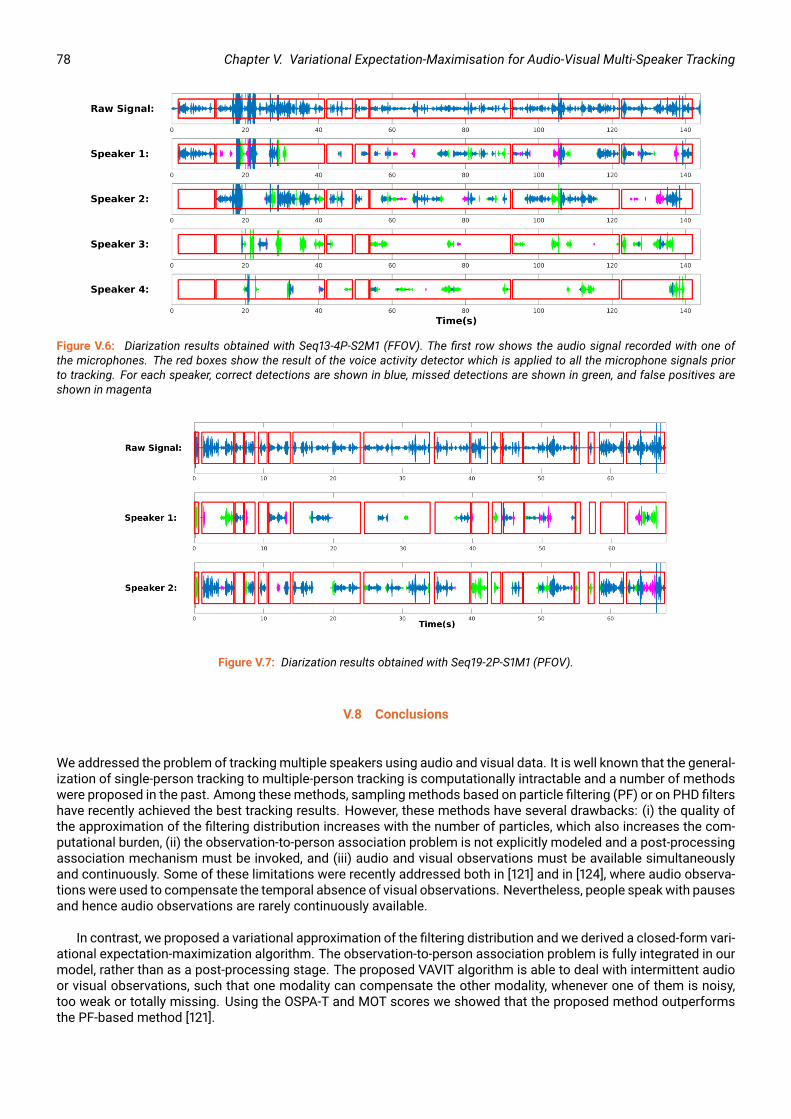
78 Chapter V. Variational Expectation-Maximisation for Audio-Visual Multi-Speaker Tracking
Figure V.6: Diarization results obtained with Seq13-4P-S2M1 (FFOV). The first row shows the audio signal recorded with one ofthe microphones. The red boxes show the result of the voice activity detector which is applied to all the microphone signals priorto tracking. For each speaker, correct detections are shown in blue, missed detections are shown in green, and false positives areshown in magenta
Figure V.7: Diarization results obtained with Seq19-2P-S1M1 (PFOV).
V.8 Conclusions
We addressed the problem of tracking multiple speakers using audio and visual data. It is well known that the general-ization of single-person tracking to multiple-person tracking is computationally intractable and a number of methodswere proposed in the past. Among these methods, sampling methods based on particle filtering (PF) or on PHD filtershave recently achieved the best tracking results. However, these methods have several drawbacks: (i) the quality ofthe approximation of the filtering distribution increases with the number of particles, which also increases the com-putational burden, (ii) the observation-to-person association problem is not explicitly modeled and a post-processingassociation mechanism must be invoked, and (iii) audio and visual observations must be available simultaneouslyand continuously. Some of these limitations were recently addressed both in [121] and in [124], where audio observa-tions were used to compensate the temporal absence of visual observations. Nevertheless, people speak with pausesand hence audio observations are rarely continuously available.In contrast, we proposed a variational approximation of the filtering distribution and we derived a closed-form vari-ational expectation-maximization algorithm. The observation-to-person association problem is fully integrated in ourmodel, rather than as a post-processing stage. The proposed VAVIT algorithm is able to deal with intermittent audioor visual observations, such that one modality can compensate the other modality, whenever one of them is noisy,too weak or totally missing. Using the OSPA-T and MOT scores we showed that the proposed method outperformsthe PF-based method [121].

Towards Probabilistic Generative Models for Socially Intelligent Robots 79V.9 Appendix: Learning the parameters of the linear transformations
In this appendix we describe the audio observation model we use. More precisely, we make explicit the generativemodel introduced in (V.13). For that purpose we consider a training set of audio features, or inter-channel spectralfeatures (which in practice correspond to the real and imaginary parts of complex-valued Fourier coefficients) andtheir associated source locations, T = (gi,xi)Ii=1 and let (g,x) ∈ T . The vector g is the concatenation ofK vectorsg = [g1| . . . gk| . . . gK ] where [·|·] denotes vertical vector concatenation. We recall that for all sub-bands k; 1 ≤ k ≤ K ,gk ∈ R2J where J is the number of frequencies in each sub-band. Without loss of generality we consider the sub-bandk. The joint probability of (gk,x) can be marginalized as:
p(gk,x) =
R∑r=1
p(gk|x, Ck = r)p(xk|Ck = r)p(Ck = r). (V.36)Assuming Gaussian variables, we have p(gk|x, Ck = r) = N (gk|hkr(x),Σkr), p(x|Ck = r) = N (x|νkr,Ωkr), andp(Ck = r) = πkr , where hkr(x) = Lkrx + lkr with Lkr ∈ R2J×2 and lkr ∈ R2J , Σr ∈ R2J×2J is the associatedcovariance matrix, and x is drawn from a Gaussian mixture model with R components, each component r beingcharacterized by a prior πkr , a mean νkr ∈ R2 and a covariance Ωkr ∈ R2×2. The parameter set of this model forsub-band k is:
Θk = Lkr, lkr,Σkr,νkr,Ωkr, πkrr=Rr=1 . (V.37)These parameters can be estimated via a closed-form EM procedure from a training dataset, e.g. T (please consult[133]).
One should notice that there is a parameter set for each sub-band k, 1 ≤ k ≤ K , hence there are K models thatneed be trained in our case. It follows that (12) writes:p(gtk|xtn, Btk = n,Ctk = r) = (V.38)
N (gtk; Lkrxtn + lkr,Σkr) if 1 ≤ n ≤ NU(gtk; vol(G)) if n = 0.
The right-hand side of (7) can now be written as:p(Ctk = r|xtn, Btk = n) =
πrN (xtn;νr,Ωr)∑Ri=1 πiN (xtn;νi,Ωi)
. (V.39)


Chapter VI
Conditional Random Fields for Deep Pixel-Level Inference
Abstract Recent works have shown that exploiting multi-scale rep-resentations deeply learned via convolutional neural networks (CNN)is of tremendous importance for accurate contour detection. Thischapter presents a novel approach for predicting contours which ad-vances the state of the art in two fundamental aspects, i.e. multi-scalefeature generation and fusion. Different from previous works directlyconsidering multi-scale feature maps obtained from the inner layersof a primary CNNarchitecture, we introduce a hierarchical deepmodelwhich produces more rich and complementary representations. Fur-thermore, to refine and robustly fuse the representations learned atdifferent scales, the novel Attention-Gated Conditional RandomFields(AG-CRFs) are proposed. The experiments ran on two publicly avail-able datasets (BSDS500 and NYUDv2) demonstrate the effectivenessof the latent AG-CRF model and of the overall hierarchical framework.
Chapter Pitch
Methodological contribution A probabilistic model based on conditional random fields, that incorporates attentionunder the form of binary gates. The posterior probability of these gates is computed using the sigmoid function σ onthe a posteriori expectation of the binary potential.E =
∑s
∑i
φh(his, fis) +
∑s′,s
∑i,j
gis′,sψh(his,hjs′)︸ ︷︷ ︸
Gated pairwise potential
⇒ Egis′,s = σ
−Eq(his)
∑j
Eq(hj
s′ )
ψh(his,h
js′) .
Applicative task Pixel-level inference tasks, in particular contour detection.Interesting insight The gating formalism allows to model when the information from a certain random variable hasto be used when inferring a neighboring variable, which conceptually corresponds to the attention mechanism in deepnetworks. The probabilistic formulation allows to formally interpret the a posteriori distribution of the gating variablesas attention tensors and implement the whole inference procedure within the deep neural network framework.Dissemination The attention-gated CRF was published in Advances in Neural Information Processing Systems [153].
81

82 Chapter VI. Conditional Random Fields for Deep Pixel-Level Inference
VI.1 Introduction
Considered as one of the fundamental tasks in low-level vision, contour detection has been deeply studied in the pastdecades. While early works mostly focused on low-level cues (e.g. colors, gradients, textures) and hand-crafted fea-tures [154]–[156], more recent methods benefit from the representational power of deep learning models [157]–[161].The ability to effectively exploit multi-scale feature representations is considered a crucial factor for achieving accu-rate predictions of contours in both traditional [162] and CNN-based [159]–[161] approaches. Restricting the attentionon deep learning-based solutions, existing methods [159], [161] typically derive multi-scale representations by adopt-ing standard CNN architectures and considering directly the feature maps associated to different inner layers. Thesemaps are highly complementary: while the features from the first layers are responsible for predicting fine details, theones from the higher layers are devoted to encode the basic structure of the objects. Traditionally, concatenation andweighted averaging are very popular strategies to combine multi-scale representations (see Fig. VI.1.a). While thesestrategies typically lead to an increased detection accuracy with respect to single-scale models, they severly simplifythe complex relationship between multi-scale feature maps.The motivational cornerstone of this study is the following research question: is it worth modeling and exploitingcomplex relationships between multiple scales of a deep representation for contour detection? In order to provide ananswer and inspired by recent works exploiting graphical models within deep learning architectures [163], [164], weintroduce Attention-Gated Conditional Random Fields (AG-CRFs), which allow to learn robust feature map represen-tations at each scale by exploiting the information available from other scales. This is achieved by incorporating anattention mechanism [165] seamlessly integrated into the multi-scale learning process under the form of gates [166].Intuitively, the attention mechanism will further enhance the quality of the learned multi-scale representation, thusimproving the overall performance of the model.We integrated the proposed AG-CRFs into a two-level hierarchical CNN model, defining a novel Attention-guidedMulti-scale Hierarchical deepNet (AMH-Net) for contour detection. The hierarchical network is able to learn richermulti-scale features than conventional CNNs, the representational power of which is further enhanced by the proposedAG-CRF model. We evaluate the effectiveness of the overall model on two publicly available datasets for the contourdetection task, i.e. BSDS500 [167] and NYU Depth v2 [168]. The results demonstrate that our approach is able to learnrich and complementary features, thus outperforming state-of-the-art contour detection methods.
VI.2 Related work
In the last few years several deep learning models have been proposed for detecting contours [157]–[159], [161], [169],[170]. Among these, some works explicitly focused on devising multi-scale CNN models in order to boost performance.For instance, the Holistically-Nested Edge Detection method [159] employed multiple side outputs derived from theinner layers of a primary CNN and combine them for the final prediction. Liu et. al. [170] introduced a framework tolearn rich deep representations by concatenating features derived from all convolutional layers of VGG16. Bertasiuset. al. [158] considered skip-layer CNNs to jointly combine feature maps from multiple layers. Maninis et. al. [161]proposed Convolutional Oriented Boundaries (COB), where features from different layers are fused to compute ori-ented contours and region hierarchies. However, these works combine the multi-scale representations from differentlayers adopting concatenation and weighted averaging schemes while not considering the dependency between thefeatures. Furthermore, these works do not focus on generating more rich and diverse representations at each CNNlayer.
The combination of multi-scale representations has been also widely investigated for other pixel-level predictiontasks, such as semantic segmentation [171], visual saliency detection [172] and monocular depth estimation [164],pedestrian detection [153] and different deep architectures have been designed. For instance, to effectively aggregatethe multi-scale information, Yu et. al. [171] introduced dilated convolutions. Yang et. al. [173] proposed DAG-CNNswhere multi-scale feature outputs from different ReLU layers are combined through element-wise addition operator.However, none of these works incorporate an attention mechanism into a multi-scale structured feature learningframework.Attention models have been successfully exploited in deep learning for various tasks such as image classifica-tion [174], speech recognition [175] and image caption generation [176]. However, to our knowledge, this work is thefirst to introduce an attention model for estimating contours. Furthermore, we are not aware of previous studiesintegrating the attention mechanism into a probabilistic (CRF) framework to control the message passing betweenhidden variables. We model the attention as gates [166], which have been used in previous deep models such as re-stricted Boltzman machine for unsupervised feature learning [177], LSTM for sequence learning [178], [179] and CNNfor image classification [180]. However, none of these works explore the possibility of jointly learning multi-scale deeprepresentations and an attention model within a unified probabilistic graphical model.

Towards Probabilistic Generative Models for Socially Intelligent Robots 83
fs+1 fs+1
(a) Multi-Scale Neural Network (b) Multi-Scale CRFs
fsfs1 fs1 fs
I I
hs1 hs1hs hs hs+1hs+1
fs+1 · · ·
· · ·(c) Attention-Gated CRFs
fs1 fs
I
gs1,s gs,s+1
hs1 hs hs+1
· · ·
· · ·
· · ·
· · ·
Figure VI.1: An illustration of different schemes for multi-scale deep feature learning and fusion. (a) the traditional approach (e.g.concatenation, weighted average), (b) CRF implementing multi-scale feature fusion (c) the proposed AG-CRF-based approach.
VI.3 Attention-Gated CRFs for Deep Structured Multi-Scale Feature Learning
VI.3.1 Problem Definition and Notation
Given an input image I and a generic front-end CNN model with parameters Wc, we consider a set of S multi-scalefeature maps F = fsSs=1. Being a generic framework, these feature maps can be the output of S intermediateCNN layers or of another representation, thus s is a virtual scale. The feature map at scale s, fs can be interpretedas a set of feature vectors, fs = f isNi=1, where N is the number of pixels. Opposite to previous works adoptingsimple concatenation or weighted averaging schemes [159], [181], we propose to combine the multi-scale featuremaps by learning a set of latent feature maps hs = hisNi=1 with a novel Attention-Gated CRF model sketched inFig.VI.1. Intuitively, this allows a joint refinement of the features by flowing information between different scales.Moreover, since the information from one scale may or may not be relevant for the pixels at another scale, we utilisethe concept of gate, previously introduced in the literature in the case of graphical models [182], in our CRF formulation.These gates are binary random hidden variables that permit or block the flow of information between scales at everypixel. Formally, gise,sr ∈ 0, 1 is the gate at pixel i of scale sr (receiver) from scale se (emitter), and we also writegse,sr = gise,srNi=1. Precisely, when gise,sr = 1 then the hidden variable hisr is updated taking (also) into accountthe information from the se-th layer, i.e. hse . As shown in the following, the joint inference of the hidden features andthe gates leads to estimating the optimal features as well as the corresponding attention model, hence the nameAttention-Gated CRFs.
VI.3.2 Attention-Gated CRFs
Given the observed multi-scale feature maps F of image I, the objective is to estimate the hidden multi-scale rep-resentation H = hsSs=1 and, accessorily the attention gate variables G = gse,srSse,sr=1. To do that, we formal-ize the problem within a conditional random field framework and write the Gibbs distribution as P (H,G|I,Θ) =exp (−E(H,G, I,Θ)) /Z (I,Θ), where Θ is the set of parameters and E is the energy function. As usual, we exploitboth unary and binary potentials to couple the hidden variables between them and to the observations. Importantly,the proposed binary potential is gated, and thus only active when the gate is open. More formally the general formVI.1of the energy function writes:
E(H,G, I,Θ) =∑s
∑i
φh(his, fis)︸ ︷︷ ︸
Unary potential
+∑se,sr
∑i,j
gise,srψh(hisr ,hjse)︸ ︷︷ ︸
Gated pairwise potential
. (VI.1)
The first term of the energy function is a classical unary term that relates the hidden features to the observed multi-scale CNN representations. The second term synthesizes the theoretical contribution of the present study becauseit conditions the effect of the pair-wise potential ψh(hise ,hjsr ) upon the gate hidden variable gise,sr . Fig. VI.1c depictsthe model formulated in Equ.(VI.1). If we remove the attention gate variables, it becomes a general multi-scale CRFsas shown in Fig. VI.1b.
Given that formulation, and as it is typically the case in conditional random fields, we exploit the mean-field approx-imation in order to derive a tractable inference procedure. Under this generic form, the mean-field inference procedureVI.1One could certainly include a unary potential for the gate variables as well. However this would imply that there is a way to set/learn the apriori distribution of opening/closing a gate. In practice we did not observe any notable difference between using or skipping the unary potentialon g.

84 Chapter VI. Conditional Random Fields for Deep Pixel-Level Inference
writes:q(his) ∝ exp
(φh(his, f
is) +
∑s′ 6=s
∑j
Eq(gis′,s)gis′,sEq(hj
s′ )ψh(his,h
js′)
), (VI.2)
q(gis′,s) ∝ exp(gis′,sEq(hi
s)
∑j
Eq(hj
s′ )
ψh(his,h
js′))
, (VI.3)where Eq stands for the expectation with respect to the distribution q.
Before deriving these formulae for our precise choice of potentials, we remark that, since the gate is a binary vari-able, the expectation of its value is the same as q(gis′,s = 1). By defining:Mi
s′,s = Eq(his)
∑j Eq(hj
s′ )
ψh(his,h
js′),
the expected value of the gate writes:αis,s′ = Eq(gi
s′,s)gis′,s =
q(gis′,s = 1)
q(gis′,s = 0) + q(gis′,s = 1)= σ
(−Mi
s′,s
), (VI.4)
where σ() denotes the sigmoid function. This finding is specially relevant in the framework of CNN since many ofthe attention models are typically obtained after applying the sigmoid function to the features derived from a feed-forward network. Importantly, since the quantityMis′,s depends on the expected values of the hidden features his, theAG-CRF framework extends the unidirectional connection from the features to the attention model, to a bidirectionalconnection in which the expected value of the gate allows to refine the distribution of the hidden features as well.
VI.3.3 AG-CRF Inference
In order to construct an operative model we need to define the unary and gated potentials φh and ψh. In our case, theunary potential corresponds to an isotropic Gaussian:φh(his, f
is) = −a
is
2‖his − f is‖2, (VI.5)
where ais > 0 is a weighting factor.The gated binary potential is specifically designed for a two-fold objective. On the one hand, we would like tolearn and further exploit the relationships between hidden vectors at the same, as well as at different scales. On theother hand, we would like to exploit previous knowledge on attention models and include linear terms in the potential.Indeed, this would implicitly shape the gate variable to include a linear operator on the features. Therefore, we chosea bilinear potential:
ψh(his,hjs′) = hisK
i,js,s′ h
js′ , (VI.6)
where his = (hi>s , 1)> and Ki,js,s′ ∈ R(Cs+1)×(Cs′+1) beingCs the size, i.e. the number of channels, of the representation
at scale s. If we write this matrix as Ki,js,s′ = (Li,js,s′ , l
i,js,s′ ; l
j,i>s′,s , 1), then Li,js,s′ exploits the relationships between hidden
variables, while li,js,s′ and lj,is′,s implement the classically used linear relationships of the attention models. In orderwords, ψh models the pair-wise relationships between features with the upper-left block of the matrix. Furthemore,ψh takes into account the linear relationships by completing the hidden vectors with the unity. In all, the energy functionwrites:
E(H,G, I,Θ) = −∑s
∑i
ais2‖his − f is‖2 +
∑se,sr
∑i,j
gise,sr hisrK
i,jsr,se h
jse . (VI.7)
Under these potentials, we can consequently update the mean-field inference equations to:q(his) ∝ exp
(− ais
2(‖his‖ − 2hi>s f is) +
∑s′ 6=s
αis,s′hi>s
∑j
(Li,js,s′ hjs′ + li,js,s′)
), (VI.8)
where hjs′ is the expected a posteriori value of hjs′ .The previous expression implies that the a posteriori distribution for his is a Gaussian. The mean vector of theGaussian and the functionM write:
his =1
ais
(aisf
is +
∑s′ 6=s
αis,s′∑j
(Li,js,s′ hjs′ + li,js,s′)
)Mi
s′,s =∑j
(hisL
i,js,s′ h
js′ + hi>s li,js,s′ + hj>s′ lj,is′,s
)which concludes the inference procedure. Furthermore, the proposed framework can be simplified to obtain thetraditional attention models. In most of the previous studies, the attention variables are computed directly from themulti-scale features instead of computing them from the hidden variables. Indeed, since many of these studies do not

Towards Probabilistic Generative Models for Socially Intelligent Robots 85propose a probabilistic formulation, there are no hidden variables and the attention is computed sequentially throughthe scales. We can emulate the same behavior within the AG-CRF framework by modifying the gated potential asfollows:
ψh(his,hjs′ , f
is, f
js′) = hisL
i,js,s′h
js′ + f i>s li,js,s′ + f j>s′ lj,is′,s. (VI.9)
This means that we keep the pair-wise relationships between hidden variables (as in any CRF) and let the attentionmodel be generated by a linear combination of the observed features from the CNN, as it is traditionally done. Thechanges in the inference procedure are straightforward and reported in the supplementary material due to spaceconstraints. We refer to this model as partially-latent AG-CRFs (PLAG-CRFs), whereas the more general one is denotedas fully-latent AG-CRFs (FLAG-CRFs).VI.3.4 Implementation with neural network for joint learning
In order to infer the hidden variables and learn the parameters of the AG-CRFs together with those of the front-endCNN, we implement the AG-CRFs updates in neural network with several steps: (i) message passing from the se-th scale to the current sr-th scale is performed with hse→sr ← Lse→sr ⊗ hse , where ⊗ denotes the convolutionaloperation and Lse→sr denotes the corresponding convolution kernel, (ii) attention map estimation q(gse,sr = 1) ←σ(hsr (Lse→sr ⊗hse) + lse→sr ⊗hse + lsr→se ⊗hsr ), where Lse→sr , lse→sr and lsr→se are convolution kernels andrepresents element-wise product operation, and (iii) attention-gated message passing from other scales and addingunary term: hsr = fsr ⊕ asr
∑se 6=sr (q(gse,sr = 1) hse→sr ), where asr encodes the effect of the aisr for weightingthe message and can be implemented as a 1 × 1 convolution. The symbol ⊕ denotes element-wise addition. Inorder to simplify the overall inference procedure, and because the magnitude of the linear term of ψh is in practicenegligible compared to the quadratic term, we discard the message associated to the linear term. When the inferenceis complete, the final estimate is obtained by convolving all the scales.
VI.4 Exploiting AG-CRFs with a Multi-scale Hierarchical Network
VI.4.1 AMH-Net Architecture.
The proposed Attention-guided Multi-scale Hierarchical Network (AMH-Net), as sketched in Figure VI.2, consists ofa multi-scale hierarchical network (MH-Net) together with the AG-CRF model described above. The MH-Net is con-structed from a front-end CNN architecture such as the widely used AlexNet [81], VGG [183] and ResNet [184]. Oneprominent feature of MH-Net is its ability to generate richer multi-scale representations. In order to do that, we per-form distinct non-linear mappings (deconvolution D, convolution C and max-pooling M) upon fl, the CNN featurerepresentation from an intermediate layer l of the front-end CNN. This leads to a three-way representation: fDl , fC
l andfMl . Remarkably, while D upsamples the feature map, C maintains its original size and M reduces it, and differentkernel size is utilized for them to have different receptive fields, then naturally obtaining complementary inter- andmulti-scale representations. The fC
l and fMl are further aligned to the dimensions of the feature map fD
l by the de-convolutional operation. The hierarchy is implemented in two levels. The first level uses an AG-CRF model to fuse thethree representations of each layer l, thus refining the CNN features within the same scale. The second level of thehierarchy uses an AG-CRF model to fuse the information coming from multiple CNN layers. The proposed hierarchi-cal multi-scale structure is general purpose and able to involve an arbitrary number of layers and of diverse intra-layerrepresentations.VI.4.2 End-to-End Network Optimization.
The parameters of the model consist of the front-end CNN parameters, Wc, the parameters to produce the richerdecomposition from each layer l, Wl, the parameters of the AG-CRFs of the first level of the hierarchy, WIlLl=1, andthe parameters of the AG-CRFs of the second level of the hierarchy, WII. L is the number of intermediate layers usedfrom the front-end CNN. In order to jointly optimize all these parameters we adopt deep supervision [159] and we addan optimization loss associated to each AG-CRF module. In addition, since the contour detection problem is highlyunbalanced, i.e. contour pixels are significantly less than non-contour pixels, we employ the modified cross-entropyloss function of [159]. Given a training data set D = (Ip,Ep)Pp=1 consisting of P RGB-contour groundtruth pairs, theloss function ` writes:
`(W)
=∑p
β∑
ekp∈E+p
log P(ekp = 1|Ip; W
)+(1− β
) ∑ekp∈E−p
log P(ekp = 0|Ip; W
), (VI.10)
where β = |E+p |/(|E+
p | + |E−p |), E+p is the set of contour pixels of image p and W is the set of all parameters. Theoptimization is performed via the back-propagation algorithm with standard stochastic gradient descent.

86 Chapter VI. Conditional Random Fields for Deep Pixel-Level Inference
AG-CRF
AG-CRF
AG-CRF AG-CRF
C
D
M
D D
C M
D D
D
C M
D D
D
C C C C C C
DL
C
DL
Front-End CNN
C
. . . . . .
. . .. . .
. . . . . . . . .. . .
. . .. . .
D DD
DL
DL
C Convolution
M Max-pooling
D Deconvolution
L Loss
HIERARCHY 1
HIERARCHY 2
fl
fCl fMl
fDl fM0
lfC0
l
Figure VI.2: An overview of the proposed AMH-Net for contour detection.
VI.4.3 AMH-Net for contour detection.
After training of the whole AMH-Net, the optimized network parameters W are used for the contour detection task.Given a new test image I, the L+ 1 classifiers produce a set of contour prediction maps ElL+1l=1 = AMH-Net(I; W).The El are obtained from the AG-CRFs with elementary operations as detailed in the supplementary material. Weinspire from [159] to fuse the multiple scale predictions thus obtaining an average prediction E =
∑l El/(L+ 1).
VI.5 Experiments
VI.5.1 Experimental Setup
Datasets To evaluate the proposed approach we employ two different benchmarks: the BSDS500 and the NYUDv2datasets. The BSDS500 dataset is an extended dataset based on BSDS300 [167]. It consists of 200 training, 100validation and 200 testing images. The groundtruth pixel-level labels for each sample are derived considering multipleannotators. Following [159], [169], we use all the training and validation images for learning the proposed model andperform data augmentation as described in [159]. The NYUDv2 [168] contains 1449 RGB-D images and it is split intothree subsets, comprising 381 training, 414 validation and 654 testing images. Following [159] in our experiments weemploy images at full resolution (i.e. 560× 425 pixels) both in the training and in the testing phases.
EvaluationMetrics During the test phase standard non-maximum suppression (NMS) [185] is first applied to producethinned contour maps. We then evaluate the detection performance of our approach according to different metrics,including the F-measure at Optimal Dataset Scale (ODS) and Optimal Image Scale (OIS) and the Average Precision(AP). The maximum tolerance allowed for correct matches of edge predictions to the ground truth is set to 0.0075for the BSDS500 dataset, and to .011 for the NYUDv2 dataset as in previous works [159], [185], [186].
Implementation Details The proposed AMH-Net is implemented under the deep learning framework Caffe [187]. Theimplementation code is available on GithubVI.2. The training and testing phase are carried out on an Nvidia Titan XGPU with 12GB memory. The ResNet50 network pretrained on ImageNet [188] is used to initialize the front-end CNN ofAMH-Net. Due to memory constraints, our implementation only considers three scales, i.e. we generate multi-scalefeatures from three different layers of the front-end CNN (i.e. res3d, res4f, res5c). In our CRF model we considerdependencies between all scales. Within the AG-CRFs, the kernel size for all convolutional operations is set to 3 × 3with stride 1 and padding 1. To simplify the model optimization, the parameters aisr are set as 0.1 for all scales duringtraining. We choose this value as it corresponds to the best performance after cross-validation in the range [0, 1].The initial learning rate is set to 1e-7 in all our experiments, and decreases 10 times after every 10k iterations. Thetotal number of iterations for BSDS500 and NYUD v2 is 40k and 30k, respectively. The momentum and weight decayparameters are set to 0.9 and 0.0002, as in [159]. As the training images have different resolution, we need to set thebatch size to 1, and for the sake of smooth convergence we updated the parameters only every 10 iterations.VI.2https://github.com/danxuhk/AttentionGatedMulti-ScaleFeatureLearning

Towards Probabilistic Generative Models for Socially Intelligent Robots 87
Figure VI.3: Qualitative results on the BSDS500 (left) and the NYUDv2 (right) test samples. The 2nd (4th) and 3rd (6th) columns arethe ground-truth and estimated contour maps respectively.
Table VI.1: BSDS500 dataset: quantitative results.
Method ODS OIS APHuman .800 .800 -Felz-Hutt[189] .610 .640 .560Mean Shift[190] .640 .680 .560Normalized Cuts[49] .641 .674 .447ISCRA[191] .724 .752 .783gPb-ucm[167] .726 .760 .727Sketch Tokens[156] .727 .746 .780MCG[192] .747 .779 .759DeepEdge[158] .753 .772 .807DeepContour[157] .756 .773 .797LEP[193] .757 .793 .828HED[159] .788 .808 .840CEDN[169] .788 .804 .834COB [161] .793 .820 .859RCF [170] (not comp.) .811 .830 –AMH-Net (fusion) .798 .829 .869
Table VI.2: NYUDv2 dataset: quantitative results.
Method ODS OIS APgPb-ucm [167] .632 .661 .562OEF [194] .651 .667 –Silberman et. al. [168] .658 .661 –SemiContour [195] .680 .700 .690SE [196] .685 .699 .679gPb+NG [197] .687 .716 .629SE+NG+ [186] .710 .723 .738HED (RGB) [159] .720 .734 .734HED (HHA) [159] .682 .695 .702HED (RGB + HHA) [159] .746 .761 .786RCF (RGB) + HHA) [170] .757 .771 –AMH-Net (RGB) .744 .758 .765AMH-Net (HHA) .716 .729 .734AMH-Net (RGB+HHA) .771 .786 .802
VI.5.2 Experimental Results
In this section, we present the results of our evaluation, comparing our approach with several state of the art methods.We further conduct an in-depth analysis of our method, to show the impact of different components on the detectionperformance.Comparison with state of the art methods. We first consider the BSDS500 dataset and compare the performance ofour approach with several traditional contour detection methods, including Felz-Hut [189], MeanShift [190], NormalizedCuts [49], ISCRA [191], gPb-ucm [167], SketchTokens [156], MCG [192], LEP [193], and more recent CNN-based methods,including DeepEdge [158], DeepContour [157], HED [159], CEDN [169], COB [161]. We also report results of the RCFmethod [170], although they are not comparable because in [170] an extra dataset (Pascal Context) was used duringRCF training to improve the results on BSDS500. In this series of experiments we consider AMH-Net with FLAG-CRFs.The results of this comparison are shown in Table VI.1 and Fig. VI.4a. AMH-Net obtains an F-measure (ODS) of 0.798,thus outperforms all previous methods. The improvement over the second and third best approaches, i.e. COB andHED, is 0.5% and 1.0%, respectively, which is not trivial to achieve on this challenging dataset. Furthermore, whenconsidering the OIS and AP metrics, our approach is also better, with a clear performance gap.
To perform experiments on NYUDv2, following previous works [159] we consider three different types of inputrepresentations, i.e. RGB, HHA [186] and RGB-HHA data. The results corresponding to the use of both RGB and HHAdata (i.e. RGB+HHA) are obtained by performing a weighted average of the estimates obtained from two AMH-Netmodels trained separately on RGB and HHA representations. As baselines we consider gPb-ucm [167], OEF [194], the

88 Chapter VI. Conditional Random Fields for Deep Pixel-Level Inference
Recall0 0.1 0.2 0.3 0.4 0.5 0.6 0.7 0.8 0.9 1
Prec
isio
n
0
0.1
0.2
0.3
0.4
0.5
0.6
0.7
0.8
0.9
1
[F=0.800] Human[F=0.798] AMH-Net[F=0.793] COB[F=0.788] CEDN[F=0.788] HED[F=0.757] LEP[F=0.756] DeepContour[F=0.753] DeepEdge[F=0.747] MCG[F=0.727] SketchTokens[F=0.726] UCM[F=0.724] ISCRA[F=0.641] Normalized Cuts[F=0.640] MeanShift[F=0.610] Felz-Hut
(a) BSDS500 Data SetRecall
0 0.1 0.2 0.3 0.4 0.5 0.6 0.7 0.8 0.9 1
Prec
isio
n
0
0.1
0.2
0.3
0.4
0.5
0.6
0.7
0.8
0.9
1
[F=0.800] Human[F=0.771] AMH-Net[F=0.746] HED[F=0.706] SE+NG+[F=0.695] SE[F=0.685] gPb+NG[F=0.680] SemiContour[F=0.658] Silberman[F=0.651] OEF[F=0.632] gPb-ucm
(b) NYUDv2 Data Set
Figure VI.4: Precision-Recall Curves of different methods on two data sets.
Table VI.3: Performance analysis on NYUDv2 RGB data.
Method ODS OIS APHypercolumn [181] .718 .729 .731HED [159] .720 .734 .734AMH-Net (baseline) .711 .720 .724AMH-Net (w/o AG-CRFs) .722 .732 .739AMH-Net (w/ CRFs) .732 .742 .750AMH-Net (w/o deep supervision) .725 .738 .747AMH-Net (w/ PLAG-CRFs) .737 .749 .746AMH-Net (w/ FLAG-CRFs) .744 .758 .765
method in [168], SemiContour [195], SE [196], gPb+NG [197], SE+NG+ [186], HED [159] and RCF [170]. In this case theresults are comparable to the RCF [170] since the experimental protocol is exactly the same. All of them are reportedin Table VI.2 and Fig. VI.4b. Again, our approach outperforms all previous methods. In particular, the increasedperformance with respect to HED [159] and RCF [170] confirms the benefit of the proposed multi-scale feature learningand fusion scheme. Examples of qualitative results on the BSDS500 and the NYUDv2 datasets are shown in Fig. VI.3.We show more examples of predictions from different multi-scale features on the BSDS500 dataset VI.5.Ablation Study. To further demonstrate the effectiveness of the proposed model and analyze the impact of the dif-ferent components of AMH-Net on the countour detection task, we conduct an ablation study considering the NYUDv2dataset (RGB data). We tested the following models: (i) AMH-Net (baseline), which removes the first-level hierarchyand directly concatenates the feature maps for prediction, (ii) AMH-Net (w/o AG-CRFs), which employs the proposedmulti-scale hierarchical structure but discards the AG-CRFs, (iii) AMH-Net (w/ CRFs), obtained by replacing our AG-CRFs with a multi-scale CRF model without attention gating, (iv) AMH-Net (w/o deep supervision) obtained removingintermediate loss functions in AMH-Net and (v) AMH-Net with the proposed two versions of the AG-CRFs model, i.e.PLAG-CRFs and FLAG-CRFs. The results of our comparison are shown in Table VI.3, where we also consider as refer-ence traditional multi-scale deep learning models employing multi-scale representations, i.e. Hypercolumn [181] andHED [159].
These results clearly show the advantages of our contributions. The ODS F-measure of AMH-Net (w/o AG-CRFs)is 1.1% higher than AMH-Net (baseline), clearly demonstrating the effectiveness of the proposed hierarchical networkand confirming our intuition that exploiting more richer and diverse multi-scale representations is beneficial. Table VI.3also shows that our AG-CRFs plays a fundamental role for accurate detection, as AMH-Net (w/ FLAG-CRFs) leads toan improvement of 1.9% over AMH-Net (w/o AG-CRFs) in terms of OSD. Finally, AMH-Net (w/ FLAG-CRFs) is 1.2% and1.5% better than AMH-Net (w/ CRFs) in ODS and AP metrics respectively, confirming the effectiveness of embedding

Towards Probabilistic Generative Models for Socially Intelligent Robots 89
Figure VI.5: Examples of predictions from different multi-scale features on BSDS500. The first column is the input test images. The2nd to the 5nd columns show the predictions from different multi-scale features. The last column shows the final contour map afterstandard NMS.
an attention mechanism in the multi-scale CRF model. AMH-Net (w/o deep supervision) decreases the overall perfor-mance of our method by 1.9% in ODS, showing the crucial importance of deep supervision for better optimization ofthe whole AMH-Net. Comparing the performance of the proposed two versions of the AG-CRF model, i.e. PLAG-CRFsand FLAG-CRFs, we can see that AMH-Net (FLAG-CRFs) slightly outperforms AMH-Net (PLAG-CRFs) in both ODS andOIS, while bringing a significant improvement (around 2%) in AP. Finally, considering HED [159] and Hypercolumn [181],it is clear that our AMH-Net (FLAG-CRFs) is significantly better than these methods. Importantly, our approach utilizesonly three scales while for HED [159] and Hypercolumn [181] we consider five scales. We believe that our accuracycould be further boosted by involving more scales.
VI.6 Conclusions
We presented a novel multi-scale hierarchical convolutional neural network for contour detection. The proposedmodel introduces two main components, i.e. a hierarchical architecture for generating more rich and complemen-tary multi-scale feature representations, and an Attention-Gated CRF model for robust feature refinement and fusion.The effectiveness of our approach is demonstrated through extensive experiments on two public available datasetsand state of the art detection performance is achieved. The proposed approach addresses a general problem, i.e.

90 Chapter VI. Conditional Random Fields for Deep Pixel-Level Inference
how to generate rich multi-scale representations and optimally fuse them. Therefore, we believe it may be also usefulfor other pixel-level tasks.

Chapter VII
Variational Auto-Encoders for Audio-Visual Speech Enhancement
Abstract We are interested in unsupervised (unknown noise) speech enhancement using latent variable generativemodels. We propose to learn generativemodels for clean speech spectrogrambased on a variational autoencoder (VAE)where both auditory and visual information are used to infer the posterior of the latent variables. This is motivated by thefact that visual data, i.e. lips images of the speaker, provide helpful and complementary information about speech. Assuch, they can help train a richer inference network, where the audio and visual information are fused. We propose twodifferent strategies, one systematically using audio and video, and a second one inferring the best combination of audioand video. Moreover, during speech enhancement, visual data are used to initialize the latent variables, thus providing amore robust initialization than using the noisy speech spectrogram. A variational inference approach is derived to trainthe proposed VAE. Thanks to the novel inference procedure and the robust initialization, the proposed audio-visual VAEsexhibit superior performance on speech enhancement than using the standard audio-only counterpart.
Chapter Pitch
Methodological contribution Two audio-visual speech generative models based on variational autoencoders. Onesystematically employing both auditory and visual data, and a second one automatically infering the optimal balancebetween the two modalities.Applicative task Audio-visual speech enhancement.Interesting insight The non-linearity associated to the variational autoencoders is attractive because it leads tohigh representation power, but one must be careful about the additional computational burden. When dealing withadditional hidden variables (i.e. mixing variables), one must rederive appropriate learning and inference algorithms,since the standard procedures for learning VAE are not sufficient anymore.Dissemination The first method was published in IEEE Transactions on Audio, Speech and Language Process-ing [198] and the second is Submitted to IEEE Transactions on Signal Processing [199].
91

92 Chapter VII. Variational Auto-Encoders for Audio-Visual Speech Enhancement
VII.1 Introduction
Speech enhancement, or removing background noise from noisy speech [200], [201], is a classic yet very importantproblem in signal processing and machine learning. Traditional solutions to this problem are based on spectral sub-traction [202] and Wiener filtering [203], targeting noise and/or speech power spectral density (PSD) estimation in theshort-time Fourier transform (STFT) domain. The recent impressive performance of deep neural networks (DNNs) incomputer vision and machine learning has paved the way to revisit the speech enhancement problem. DNNs havebeen widely utilized in this regard, where a neural network is trained to map a noisy speech spectrogram to its cleanversion, or to a time frequency (TF) mask [204]–[206]. This is usually done in a supervised way, using a huge datasetof noise and clean speech signals for training. As such, the performance of a supervised speech enhancement tech-nique often degrades when dealing with an unknown type of noise.Unsupervised techniques offer another procedure for speech enhancement that does not use noise signals fortraining. A popular unsupervised method is based on nonnegative matrix factorization (NMF) [207]–[209] for model-ing the PSD of speech signals [210], which decomposes PSD as a product of two non-negative low-rank matrices (adictionary of basis spectra and the corresponding activations). An NMF-based speech enhancement method consistsof first learning a set of basis spectra for clean speech spectrograms at training phase, prior to speech enhancement[208], [211], [212]. Then, by decomposing the noisy spectrogram as the sum of clean speech and noise spectrograms,the corresponding clean speech activations as well as the NMF parameters of noise are estimated. While being com-putationally efficient, this modeling and enhancement framework cannot properly explain complicated structure ofspeech spectrogram due to the limited representational power dictated by the two low-rank matrices. A deep au-toencoder (DAE) has been employed in [213] to model clean speech and noise spectrograms. A DAE is pre-trainedfor clean speech spectrograms, while an extra DAE for noise spectrogram is trained at the enhancement stage us-ing the noisy spectrogram. The corresponding inference problem is under-determined, and the authors proposed toconstrain the unknown speech using a pre-trained NMF model. As such, this DAE-based method might encounter thesame shortcomings as those of the NMF-based speech enhancement [214].Deep latent variable models offer a more sophisticated and efficient modeling framework than NMF and DAE,gaining much interest over the past few years [214]–[219]. The first and main step is to train a generative model forclean speech spectrogram using a variational auto-encoder (VAE) [9], [220]. VAE provides an efficient way to estimatethe parameters of a non-linear generative model, also called the decoder. This is done by approximating the intractableposterior distribution of the latent variables using a Gaussian distribution parametrized by a neural network, called theinference (encoder) network. The encoder and decoder are jointly trained to maximize a variational lower bound on themarginal data log-likelihood. At test time, the trained generative model is combined with a noise model, e.g. NMF. Theunknown noise parameters and clean speech are then estimated from the observed noisy speech. Being independentof the noise type at training, these methods show better generalization than the supervised approaches [214], [215].Although it has been shown that the fusion of visual and audio information is beneficial for various speech per-ception tasks, e.g. [221]–[223], audio-visual speech enhancement (AVSE) has been far less investigated than audiospeech enhancement (ASE). AVSE methods can be traced back to [224] and subsequent work, e.g. [225]–[230]. Notsurprisingly, AVSE has been recently addressed in the framework of deep neural networks (DNNs) and a number ofinteresting architectures and well-performing algorithms were developed, e.g. [231]–[235]. In this chapter, we pro-pose to fuse single-channel audio and single-camera visual information for speech enhancement in the frameworkof VAEs. This may well be viewed as a multimodal extension of VAE-based methods of [214]–[218], [236] which, upto our knowledge, yield state-of-the-art ASE performance in an unsupervised learning setting. In order to incorporatevisual observations into the VAE speech enhancement framework, we propose to investigate two strategies. First,to systematically combine both streams, formulating the problem via a conditional VAE – we name this strategy AV-VAE. Second, to automatically estimate the optimal balance between auditory and visual information, formulating theproblem via a mixture of interence networks – we name this strategy MIN-VAE.For both strategies, as in [215] we proceed in three steps. First, the parameters of the generative architecturesare learned using synchronized clean audio-speech and visual-speech data. This yields an audio-visual speech priormodel. The training is totally unsupervised, in the sense that speech signals mixed with various types of noise signalare not required. This stays in contrast with supervised DNN methods that need to be trained in the presence of manynoise types and noise levels in order to ensure generalization and good performance, e.g. [231]–[233]. Second, thelearned speech prior is used in conjunction with a mixture model and with a NMF noise variance model, to infer thenoise NMF parameters. Third, the clean speech is reconstructed using the speech prior (VAE parameters) as wellas the estimated noise variance model. The latter may well be viewed as a probabilistic Wiener filter. The learnedVAE architecture and the proposed speech reconstruction methods are thoroughly tested and compared with thestate-of-the-art method, using the NTCD-TIMIT dataset [237].The rest of the chapter is structured as follows. Section VII.2 discusses the related work. Sections VII.3 and VII.4discuss the audio-only VAE and the visual-only VAE, respectively. The AV-VAE is then discussed in Section VII.5,

Towards Probabilistic Generative Models for Socially Intelligent Robots 93and the associated speech enhancement is presented in Section VII.6. We then introduce the MIN-VAE model inSection VII.7, and the associated speech enhancement procedure in Section VII.8. The conducted experiments arepresented in Section VII.9, and Section VII.10 concludes the chapter.
VII.2 Related Work
Speech enhancement has been an extremely investigated topic for the last decades and a complete state-of-the-artis beyond the scope of this chapter. We briefly review the literature on single-channel speech enhancement (SE) andthen we discuss the most significant work in AVSE. Classical methods use spectral subtraction [202] and Wienerfiltering [203] based on noise and/or speech PSD estimation in the STFT domain. Another popular family of methodsis the short-term spectral amplitude estimator [238], initially based on a local complex-valued Gaussian model of thespeech STFT coefficients and then extended to other density models [239], [240], and to a log-spectral amplitudeestimator [241], [242]. A popular technique for modeling the PSD of speech signals [210] is NMF, e.g. [207], [208],[243].More recently, SE has been addressed in the framework of DNNs [204]. Supervised methods learn mappingsbetween noisy-speech and clean-speech spectrograms, which are then used to reconstruct a speech waveform [205],[244], [245]. Alternatively, the noisy input is mapped onto a TF mask, which is then applied to the input to removenoise and to preserve speech information as much as possible [246]–[248]. In order for these supervised learningmethods to generalize well and to yield state-of-the-art results, the training data must contain a large variability interms of speakers and, even more critically, in terms of noise types and noise levels [205], [246]; in practice this leadsto cumbersome learning processes.Alternatively, generative (or unsupervised) DNNs do not use any kind of noise information for training, and for thisreason they are very interesting because they have very good generalization capabilities. An interesting generativeformulation is provided by VAEs [8]. Combined with NMF, VAE-based methods yield state-of-the-art SE performance[214]–[218], [236] for an unsupervised learning setting. VAEs conditioned on the speaker identity have also been usedfor speaker-dependent multi-microphone speech separation [219], [249] and dereverberation [250].The use of visual cues to complement audio, whenever the latter is noisy, ambiguous or incomplete, has been thor-oughly studied in psychophysics [221]–[223]. Indeed, speech production implies simultaneous air circulation throughthe vocal tract and tongue and lip movements, and hence speech perception is multimodal. Several computationalmodels were proposed to exploit the correlation between audio and visual information for the perception of speech,e.g. [226], [229]. A multi-layer perceptron architecture was proposed in [225] to map noisy-speech linear predictionfeatures concatenated with visual features onto clean-speech linear prediction features. Then Wiener filters were builtfor denoising. Audio-visual Wiener filtering was later extended using phoneme-specific Gaussian mixture regressionand filterbank audio features [251]. Other AVSE methods exploit noise-free visual information [227], [228] or make useof twin hidden Markov models (HMMs) [230].State-of-the-art supervised AVSE methods are based on DNNs. The rationale of [231], [233] is to use visual informa-tion to predict a TF soft mask in the STFT domain and to apply this mask to the audio input in order to remove noise. In[233] a video-to-speech architecture is trained for each speaker in the dataset, which yields a speaker-dependent AVSEmethod. The architecture of [231] is composed of a magnitude subnetwork that takes both visual and audio data asinputs, and a phase subnetwork that only takes audio as input. Both subnetworks are trained using ground-truth cleanspeech. Then, the magnitude subnetwork predicts a binary mask which is then applied to both the magnitude andphase spectrograms of the input signal, thus predicting a filtered speech spectrogram. The architectures of [234] and[232] are quite similar: they are composed of two subnetworks, one for processing noisy speech and one for process-ing visual speech. The two encodings are then concatenated and processed to eventually obtain an enhanced speechspectrogram. The main difference between [234] and [232] is that the former predicts both enhanced visual and au-dio speech, while the latter predicts only audio speech. The idea of obtaining a binary mask for separating speechof an unseen speaker from an unknown noise was exploited in [235]: a hybrid DNN model integrates a stacked longshort-term memory (LSTM) and convolutional LSTM for audio-visual (AV) mask estimation.In the supervised deep learning methods just mentioned, generalization to unseen data is a critical issue. Themajor issues are noise and speaker variability. Therefore, training these methods requires noisy mixtures with a largenumber of noise types and speakers, in order to guarantee generalization. In comparison, the proposed method istotally unsupervised: its training is based on VAEs and it only requires clean audio speech and visual speech. The gainand the noise variance are estimated at test time using a Monte Carlo expectation-maximization (MCEM) algorithm[252]. The clean speech is then reconstructed from the audio and visual inputs using the learned parameters. Thelatter may well be viewed as a probabilistic Wiener filter. This stays in contrast with the vast majority of supervisedDNN-based AVSE methods that predict a TF mask which is applied to the noisy input.

94 Chapter VII. Variational Auto-Encoders for Audio-Visual Speech Enhancement
VII.3 Audio VAE
In this section, we briefly review the deep generative speech model that was first proposed in [214] along with itsparameters estimation procedure using VAEs [8]. Let sfn denote the complex-valued speech STFT coefficient atfrequency index f ∈ 0, ..., F − 1 and at frame index n. At each TF bin, we have the following model which will bereferred to as audio VAE (A-VAE):sfn|zn ∼ Nc(0, σf (zn)), (VII.1)
zn ∼ N (0, I) (VII.2)where zn ∈ RL, with L F , is a latent random variable describing a speech generative process, N (0, I) is a zero-mean multivariate Gaussian distribution with identity covariance matrix, and Nc(0, σ) is a univariate complex properGaussian distribution with zero mean and variance σ. Let sn ∈ CF be the vector whose components are the speechSTFT coefficients at frame n. The set of non-linear functions σf : RL 7→ R+F−1f=0 are modeled as neural networkssharing the input zn ∈ RL. The parameters of these neural networks are collectively denoted by θ. This variance canbe interpreted as a model for the short-term PSD of the speech signal.
Figure VII.1: The A-VAE network used for learning a speech prior using audio data. The encoder network (left) takes as inputthe squared magnitude vector sn, associated with the STFT frame sn (outlined in green), and outputs the mean and variance ofthe posterior distribution q (zn|sn;ψ). The decoder network (right) takes zn as input (sampled from the posterior distribution) andoutputs the variance of p(sn|zn;θ).
An important property of VAEs is to provide an efficient way of learning the parameters θ of such generative models[8], taking ideas from variational inference [253], [254]. Let s = sn ∈ CF Ntr−1n=0 be a training dataset of clean-speechSTFT frames and let z = zn ∈ RLNtr−1
n=0 be the associated latent variables. In the VAE framework, the parametersθ are estimated by maximizing a lower bound of the log-likelihood, ln p(s;θ), called evidence lower bound (ELBO),defined by:
L (s;θ,ψ)=Eq(z|s;ψ) [ln p (s|z;θ)]−DKL (q (z|s;ψ) ‖ p(z)) , (VII.3)where q (z|s;ψ) denotes an approximation of the intractable true posterior distribution p(z|s;θ), p(z) is the prior dis-tribution of z, and DKL(q ‖ p) = Eq[ln(q/p)] is the Kullback-Leibler divergence. Independently, for all l ∈ 0, ..., L − 1and all n ∈ 0, ..., Ntr − 1, q(z|s;ψ) is defined by:
zln|sn ∼ N (µl (sn) , σl (sn)) , (VII.4)where sn , (|s0n|2 . . . |sF−1 n|2)>. The non-linear functions µl : RF+ 7→ RL−1l=0 and σl : RF+ 7→ R+L−1l=0 are modeledas neural networks, sharing as input the speech power spectrum frame sn, and collectively parameterized by ψ. Theparameter setψ is also estimated by maximizing the variational lower bound defined in (VII.3), which is actually equiv-alent to minimizing the Kullback-Leibler divergence between q (z|s;ψ) and the intractable true posterior distributionp(z|s;θ) [253]. Using (VII.1), (VII.2) and (VII.4) we can develop this objective function as follows:
L (s;θ,ψ)c=−
F−1∑f=0
Ntr−1∑n=0
Eq(zn|sn;ψ)
[dIS(|sfn|2 ;σf (zn)
)]
+1
2
L−1∑l=0
Ntr−1∑n=0
[ln σl (sn)− µ2
l (sn)− σl (sn)], (VII.5)
where dIS(x; y) = x/y− ln(x/y)−1 is the Itakura-Saito divergence [210]. Finally, using sampling techniques combinedwith the so-called “reparametrization trick” [8] to approximate the intractable expectation in (VII.5), one obtains anobjective function which is differentiable with respect to both θ and ψ and can be optimized using gradient-ascentalgorithms [8]. The encoder-decoder architecture of the A-VAE speech prior is summarized in Figure VII.1.

Towards Probabilistic Generative Models for Socially Intelligent Robots 95VII.4 Visual VAE
We now introduce two VAE network variants for learning the speech prior from visual data, that will be referred toas base visual VAE (V-VAE) and augmented V-VAE, and which are summarized in Figure VII.2. As it can be seen,this architecture is similar to A-VAE, with the notable difference that it takes as input visual observations, namely lipimages. In more detail, standard computer vision algorithms are used to extract a fixed-sized bounding-box from theimage of a speaking face, with the lips in its center, i.e. a lip region of interest (ROI). This ROI is embedded into a visualfeature vector vn ∈ RM using a two-layer fully-connected network, referred below as the base network, whereM is thedimension of the visual embedding. Optionally, one can use an additional pre-trained front-end network (dashed box)composed of a 3D convolution layer followed by a ResNet with 34 layers, as part of a network specifically trained forthe task of supervised audio-visual speech recognition [255]. This second option is referred to as augmented V-VAE.In variational inference [253], [254], any distribution over the latent variables z can be considered for approximatingthe intractable posterior p(z|s;θ) and for defining the ELBO. For the V-VAE model, we explore the use of an approximateposterior distribution q(z|v;γ) defined by:
zln|vn ∼ N (µl(vn), σl(vn)) , (VII.6)where v = vnNtr−1
n=1 is the training set of visual features, and where the non-linear functions µl : RM 7→ RL−1l=0and σl : RM 7→ R+L−1l=0 are collectively modeled with a neural network parameterized by γ which takes vn as input.Notice that V-VAE and A-VAE share the same decoder architecture, i.e. (VII.1). Eventually, the objective function ofV-VAE has the same structure as (VII.5) and hence one can use the same gradient-ascent algorithm as above toestimate the parameters of the V-VAE network.
Figure VII.2: The two V-VAE network variants (base and augmented) for learning speech prior from visual features. A lip ROI isembedded into a visual feature vector, denoted by vn, which is encoded and decoded using the same architecture and the samelearning method as A-VAE. Optionally, one can also use a pre-trained network (dashed box) composed of a 3D convolution layerfollowed by a ResNet with 34 layers.
VII.5 Audio-visual VAE
We now investigate an audio-visual VAE model, namely a model that combines audio speech with visual speech. Therationale behind this multimodal approach is that audio data are often corrupted by noise while visual data are not.Without loss of generality, it will be assumed that audio and visual data are synchronized, i.e. there is a video frameassociated with each audio frame.In order to combine the above A-VAE and V-VAE formulations, we consider the conditional variational auto-encoder(CVAE) framework to learn structured-output representations [256]. At training, a CVAE is provided with data as wellas with associated class labels, such that the network is able to learn a structured data distribution. At test time,the trained network is provided with a class label to generate samples from the corresponding class. CVAEs havebeen proven to be very effective for missing-value inference problems, e.g. computer vision problems with partiallyavailable input-output pairs [256].
VII.5.1 The Generative Model
In the case of AV speech enhancement we consider a training set of Ntr synchronized frames of AV features, namely(s,v) = sn,vnNtr−1
n=1 where, as above, vn ∈ RM is a lip ROI embedding. The clean audio speech, which is onlyavailable at training, is conditioned on the observed visual speech. The visual information is however available bothat training and at testing, therefore it serves as a deterministic prior on the desired clean audio speech. Interestingly, it

96 Chapter VII. Variational Auto-Encoders for Audio-Visual Speech Enhancement
also affects the prior distribution of zn. To summarize, the following latent space model is considered, independentlyfor all l ∈ 0, ..., L− 1 and all TF bins (f, n):sfn|zn,vn ∼ Nc(0, σf (zn,vn)), (VII.7)
zln|vn ∼ N (µl(vn), σl(vn)) , (VII.8)where the non-linear functions σf : RL × RM 7→ R+F−1f=0 are modeled as a neural network parameterized by θand taking zn and vn as input, and where (VII.8) is identical to (VII.6) but the corresponding parameter set γ willhave different estimates, as explained below. Also, notice that σf in (VII.1) and in (VII.7) are different, but they bothcorrespond to the PSD of the generative speech model. This motivates the abuse of notation that holds through thechapter. The proposed architecture is referred to as audio-visual VAE (AV-VAE) and is shown in Fig. VII.3. Comparedto A-VAE of Section VII.3 and Figure VII.1, and with V-VAE of Section VII.4 and Figure VII.2, the mean and variance ofthe zn prior distribution, are conditioned by visual inputs.
Figure VII.3: Pipeline of the proposed AV-VAE architecture for learning an audio-visual speech prior for speech enhancement. Theencoder takes a single frame of squared magnitude of speech’s STFT, denoted by sn, as well as the corresponding visual featurevector vn, and outputs the parameters of the posterior distribution q (zn|sn,vn;ψ). The decoder network takes zn, sampled fromthe posterior distribution, together with vn as input and outputs the variance of p(sn|zn,vn;θ).
VII.5.2 The Posterior Distribution
We now introduce the distribution q (z|s,v;ψ), which approximates the intractable posterior distribution p(z|s,v;θ),defined, as above, independently for all l ∈ 0, ..., L− 1 and all frames:zln|sn,vn ∼ N (µl (sn,vn) , σl (sn,vn)) , (VII.9)
where the non-linear functions µl : RF+×RM 7→ RL−1l=0 and σl : RF+×RM 7→ R+L−1l=0 are collectively modeled as anencoder neural network, parameterized byψ, that takes as input the speech power spectrum and its associated visualfeature vector, at each frame. The complete set of model parameters, i.e. γ , θ andψ, can be estimated by maximizinga lower bound of the conditional log-likelihood ln p(s|v;θ,γ) over the training dataset, defined by:Lav-cvae (s,v;θ,ψ,γ) = Eq(z|s,v;ψ) [ln p (s|z,v;θ)]−DKL (q (z|s,v;ψ) ‖ p(z|v;γ)) . (VII.10)
This network architecture appears to be very effective for the task at hand. In fact, if one looks at the cost functionin (VII.10), it can be seen that the KL term achieves its optimal value for q (z|s,v;ψ) = p(z|v;γ). By looking at theencoder of Fig. VII.3, this can happen by ignoring the contribution of the audio input. Moreover, the first term in thecost function (VII.10) attempts to reconstruct as well as possible the audio speech vector at the output of the decoder.This can be done by using the audio vector in the input of the encoder as much as possible. This stays in contrastwith the optimal behavior of the second term which tries to ignore the audio input. By minimizing the overall cost, thevisual and audio information can be fused in the encoder.VII.5.3 Training of the AV-VAE
During the training of AV-VAE, the variable zn is sampled from the approximate posterior modeled by the encoder,and it is then passed to the decoder. However, at test time only the decoder and prior networks are used while theencoder is discarded. Hence, zn is sampled from the prior network, which is basically different from the encoder

Towards Probabilistic Generative Models for Socially Intelligent Robots 97network. The KL-divergence term in the cost function (VII.10) is responsible for reducing as much as possible thediscrepancy between the recognition and prior networks. One can even control this by weighting the KL-divergenceterm with β > 1:
Lβ-av-cvae (s,v;θ,ψ,γ) = Eq(z|s,v;ψ) [ln p (s|z,v;θ)]− βDKL (q (z|s,v;ψ) ‖ p(z|v;γ)) . (VII.11)This was introduced in [257], namely β-VAE, and was shown to facilitate the automated discovery of interpretablefactorized latent representations. However, in the case of the proposed AV-VAE architecture, we follow a differentstragety, proposed in [256], in order to decrease the gap between the recognition and prior networks. As a conse-quence, the ELBO defined in (VII.10) is modified as follows:
Lav-cvae (s,v;θ,ψ,γ) = αLav-cvae (s,v;θ,ψ,γ) + (1− α)Ep(z|v;γ) [ln p (s|z,v;θ)] , (VII.12)where 0 ≤ α ≤ 1 is a trade-off parameter. Note that the original ELBO is obtained by setting α = 1. The new termin the right-hand side of the above cost function is actually the original reconstruction cost in (VII.10) but with eachzn being sampled from the prior distribution, i.e. p (zn|vn;γ). In this way the prior network is forced to learn latentvectors that are suitable for reconstructing the corresponding speech frames. As it will be shown below, this methodsignificantly improves the overall speech enhancement performance.
To develop the cost function in (VII.12), we note that the KL-divergence term admits a closed-form solution, be-cause the involved distributions are Gaussian. Furthermore, since the expectations with respect to the approximateposterior and prior of zn are not tractable, we approximate them using Monte-Carlo estimations, as usually done inpractice. After some mathematical manipulations, one obtains the following cost function:Lav-cvae
(s,v;θ,ψ,γ
)=
1
R
R∑r=1
Ntr−1∑n=0
(α ln p(sn|z(r)n,1,vn;θ) + (1− α) ln p(sn|z(r)n,2,vn;θ)
) (VII.13)
+α
2
L−1∑l=0
Ntr−1∑n=0
(lnσl (sn,vn)
σl(vn)− ln σl (sn,vn) + (µl (sn,vn)− µl(vn))
2
σl(vn)
),
where z(r)n,1 ∼ q(zn|sn,vn;ψ) and z
(r)n,2 ∼ p(zn|vn;γ). This cost function can be optimized in a similar way as withclassical VAEs, namely by using the reparametrization trick together with a stochastic gradient-ascent algorithm.Notice that the reparameterization trick must be used twice, for z
(r)n,1 and for z
(r)n,2.
VII.6 AV-VAE for Speech Enhancement
This section describes the speech enhancement algorithm based on the proposed AV-VAE speech model. It is verysimilar to the algorithm that was proposed in [215] for audio-only speech enhancement with VAE. The unsupervisednoise model is first presented, followed by the mixture model, and by the proposed algorithm to estimate the param-eters of the noise model. Finally, clean-speech inference procedure is described. Through this section, v = vnN−1n=0 ,s = snN−1n=0 and z = znN−1n=0 denote the test sets of visual features, clean-speech STFT features and latent vectors,respectively. These variables are associated with a noisy-speech test sequence of N frames. One should notice thatthe test data are different than the training data used in the previous sections. The observed microphone (mixture)frames are denoted by x = xnN−1n=0 .VII.6.1 Unsupervised Noise Modeling
As in [214], [215], we use an unsupervised NMF-based Gaussian noise model that assumes independence across TFbins:bfn ∼ Nc
(0, (WbHb)fn
), (VII.14)
where Wb ∈ RF×K+ is a nonnegative matrix of spectral power patterns and Hb ∈ RK×N+ is a nonnegative matrix oftemporal activations, with K being chosen such that K(F +N) FN [210]. We remind that Wb and Hb need to beestimated from the observed microphone signal.The observed mixture (microphone) signal is modeled as follows:
xfn =√gnsfn + bfn, (VII.15)
for all TF bins (f, n), where gn ∈ R+ represents a frame-dependent and frequency-independent gain, as suggestedin [215]. This gain provides robustness of the AV-VAE model with respect to the possibly highly varying loudness ofthe speech signal across frames. Let us denote by g = (g0 . . . gN−1)> the vector of gain parameters that must beestimated. The speech and noise signals are further assumed to be mutually independent, such that by combining(VII.7), (VII.14) and (VII.15), we obtain, for all TF bins (f, n):xfn|zn,vn ∼ Nc
(0, gnσf (zn,vn) + (WbHb)f,n
). (VII.16)

98 Chapter VII. Variational Auto-Encoders for Audio-Visual Speech Enhancement
VII.6.2 Parameter Estimation
Having defined the speech generative model (VII.7), (VII.8), and the observed mixture model (VII.16), the inferenceprocess requires to estimate the set of model parameters φ = Wb,Hb,g from the set of observed STFT coeffi-cients x and of observed visual features v. Then, these parameters will be used to estimate the clean-speech STFTcoefficients. Since integration with respect to the latent variables is intractable, straightforward maximum likelihoodestimation of φ is not possible. Alternatively, the latent-variable structure of the model can be exploited to derive anexpectation-maximization (EM) algorithm [6]. Starting from an initial set of model parameters φ?, EM consists ofiterating until convergence between:- E-step: Evaluate Q(φ;φ?)=Ep(z|x,v;φ?)[ln p(x, z,v;φ)];- M-step: Update φ? ← argmaxφ Q(φ;φ?).
E-Step Because of the non-linear relation between the observations and the latent variables in (VII.16), we cannotcompute the posterior distribution p(z|x,v;φ?), and hence we cannot evaluate Q(φ;φ?) analytically. As in [215], wethus rely on the following Monte Carlo approximation:Q(φ;φ?) ≈ Q(φ;φ?) (VII.17)c= − 1
R
R∑r=1
∑(f,n)
(ln(gnσf (z(r)n ,vn) + (WbHb)f,n
)+
|xfn|2
gnσf (z(r)n ,vn) + (WbHb)f,n
),
where c= denotes equality up to additive terms that do not depend on φ and φ?, and where z(r)n Rr=1 is a sequence ofsamples drawn from the posterior p(zn|xn,vn;φ?) using Markov Chain Monte Carlo (MCMC) sampling. In practicewe use the Metropolis-Hastings algorithm [258], which forms the basis of the MCEM algorithm [252]. At the m-thiteration of the Metropolis-Hastings algorithm and independently for all n ∈ 0, ..., N − 1, a sample zn is first drawnfrom a proposal random walk distribution:
zn|z(m−1)n ; ε2 ∼ N (z(m−1)n , ε2I). (VII.18)Using the fact that this is a symmetric proposal distribution [258], the acceptance probability η is computed by:
η = min
(1,
p(xn|zn,vn;φ?)p(zn|vn;γ?)
p(xn|z(m−1)n ,vn;φ?)p(z(m−1)n |vn;γ?)
),
wherep (xn|zn,vn;φ?) =
F−1∏f=0
p(xfn|zn,vn;θ?u), (VII.19)with p(xfn|zn,vn;θ?u) defined in (VII.16) and p (zn|vn;γ?) defined in (VII.8). Next, u is drawn from a uniform distributionU([0, 1]). If u < η, the sample is accepted and we set z
(m)n = zn, otherwise the sample is rejected and we set z
(m)n =
z(m−1)n . Only the lastR samples are kept for computing Q(φ;φ?) in (VII.17), i.e. the samples drawn during the so-calledburn-in period are discarded.
M-Step Q(φ;φ?) in (VII.17) is maximized with respect to the new model parameters φ. As usual in the NMF litera-ture [259], we adopt a block-coordinate approach by successively and individually updating Hb, Wb and g, using theauxiliary function technique as done in [215]. Following the same methodology, we obtain the following formula forupdating the NMF model parameters:
Hb ← Hb
W>b
(|X|2
R∑r=1
(V
(r)x
)−2)W>
b
R∑r=1
(V
(r)x
)−11/2
, (VII.20)
Wb ←Wb
(|X|2
R∑r=1
(V
(r)x
)−2)H>b
R∑r=1
(V
(r)x
)−1H>b
1/2
, (VII.21)

Towards Probabilistic Generative Models for Socially Intelligent Robots 99where (·)(·) denotes element-wise exponentiation, (·) (·) denotes element-wise multiplication, and (·)
(·) denoteselement-wise division. Moreover, V(r)
x ∈ RF×N+ is the matrix with entries gnσf (z(r)n ,vn) + (WbHb)f,n, and X ∈ CF×Nis the matrix with entries (X)f,n = xfn. The gains are updated as follows:
g> ← g>
1>(|X|2
R∑r=1
(V
(r)s
(V
(r)x
)−2))1>[R∑r=1
(V
(r)s
(V
(r)x
)−1)]1/2
, (VII.22)
where 1 is a vector of ones with dimensionF and V(r)s ∈ RF×N+ is the matrix with entries σf (z
(r)n ,vn). The nonnegativeproperty of Hb, Wb, and of g is ensured, provided that their entries are initialized with nonnegative values. In practice,only one iteration of updates (VII.20), (VII.21) and (VII.22) is performed at each M-step.
VII.6.3 Speech Reconstruction with AV-VAE
Let φ∗ = W∗b ,H
∗b ,g∗ denote the set of parameters estimated by the above MCEM algorithm. Let sfn =
√g∗nsfnbe the scaled version of the speech STFT coefficients as introduced in (VII.15), with g∗n = (g∗)n. The final step is toestimate these coefficients according to their posterior mean [215]:
ˆsfn = Ep(sfn|xfn,vn;φ∗)[sfn] = Ep(zn|xn,vn;φ∗)
[Ep(sfn|zn,vn,xn;φ∗)[sfn]
] (VII.23)= Ep(zn|xn,vn;φ∗)
[g∗nσf (zn,vn)
g∗nσf (zn,vn) + (W∗bH∗b)f,n
]xfn.
This estimation corresponds to a “probabilistic” version of Wiener filtering, with an averaging of the filter over theposterior distribution of the latent variables. As above, this expectation cannot be computed analytically, but insteadit can be approximated using the same Metropolis-Hastings algorithm of Section VII.6.2. The time-domain estimateof the speech signal is finally obtained from the inverse STFT with overlap-add.
VII.7 The Mixture of Inference Networks VAE
In this section, we aim to devise a framework able to choose the best combination between the auditory and visualencodings, as opposed to systematically using both encodings like in AV-VAE. To achieve this goal, we propose aprobabilistic mixture of the audio and visual encoders, and name it mixture of inference networks VAE (MIN-VAE).In a nutshell, the model learns to select if the posterior of zn should be audio- or video-based.. In the following weintroduce the mathematical formulation associated with the proposed MIN-VAE. The overall architecture is depictedin the Figure VII.4.
Figure VII.4: Architecture of the proposed mixture of inference networks VAE (MIN-VAE). A mixture of an audio- and a video-basedencoder is used to approximate the intractable posterior distribution of the latent variables.

100 Chapter VII. Variational Auto-Encoders for Audio-Visual Speech Enhancement
VII.7.1 The Generative Model
We assume that each latent code is generated either from an audio or from a video prior. We model this with a mixingvariable αn ∈ 0, 1 describing whether the latent code zn corresponds to the audio or to the visual prior. Once thelatent code is generated from the corresponding prior, the speech frame sn follows a complex Gaussian with thevariance computed by the decoder. We recall that the variance is a non-linear transformation of the latent code.Formally, each STFT time frame sn is modeled as:
sn|zn,vn ∼ Nc(0,diag(σs(zn,vn)
)), (VII.24)
zn|αn ∼[N (µa, σaI)
]αn
·[N (µv, σvI)
]1−αn
, (VII.25)αn ∼ παn × (1− π)1−αn , (VII.26)
where the audio and video priors are parametrized by (µa, σa) and (µv, σv) respectively, and αn is assumed to follow aBernoulli distribution with parameter π. We propose two versions of this architecture, namely: MIN-VAE-v1 where thedecoder (VII.24) takes the same form as (VII.7) and uses explicitly visual information (see Fig. VII.4), and MIN-VAE-v2where the decoder (VII.24) takes the same form as (VII.1) and does not use explicitly visual information. In both casesthe parameters of the decoder are denoted by θ. The derivations will be done for the general case, that is MIN-VAE-v1.VII.7.2 The Posterior Distribution
In order to estimate the parameters of the generative model described above, i.e. ψ = µa,µv, σa, σv, θ, and π, wefollow a maximum likelihood procedure. To derive it, we need to compute the posterior of the latent variables:p(zn, αn|sn,vn) = p(zn|sn,vn, αn) · p(αn|sn,vn). (VII.27)
The individual factors in the right-hand side of the above equation cannot be computed in closed-form, due to thenon-linear generative model. As similarly done in VAE, we pursue an amortized inference approach to approximatep(zn|sn,vn, αn) with a parametric Gaussian distribution defined as follows:
q(zn|sn,vn, αn;φ) =
q(zn|sn;φa) αn = 1,
q(zn|vn;φv) αn = 0,(VII.28)
in which, φ = φa,φv, and φa and φv denote the parameters of the associated audio and visual inference neu-ral networks, taking the same architectures as those in (VII.4) and (VII.6), respectively. For the posterior of αn, i.e.p(αn|sn,vn), we resort to a variational approximation, denoted r(αn). Put it all together, we have the following approx-imate posterior:
q(zn|sn,vn, αn;φ) · r(αn) ≈ p(zn, αn|sn,vn). (VII.29)VII.7.3 Training the MIN-VAE
In order to train the MIN-VAE, we devise an optimization procedure alternating between estimating Θ = φ,θ,ψ, πand updating the variational posterior r. We recall the definition s = snNtr
n=1, and z, and define α and v analogously.The full posterior of the latent variables can be written as:p(z,α|s,v) =
p(s,v, z,α)
p(s,v)=p(s|z,v;θ)p(z|α)p(α)
p(s,v;θ). (VII.30)
We then target the KL-divergence between the approximate posterior and the true posterior which reads:DKL
(q(z|s,v,α;φ)r(α)‖p(z,α|s,v)
)=
=
∫Z,A
q(z|s,v,α;φ)r(α) logq(z|s,v,α;φ)r(α)p(s,v;θ)
p(s|z,v;θ)p(z|α)p(α)dzdα
= −L(Θ, r) + log p(s,v;θ) ≥ 0, (VII.31)where
L(Θ, r) =
∫Z,A
q(z|s,v,α;φ)r(α) logp(s|z,v;θ)p(z|α)p(α)
q(z|s,v,α;φ)r(α)dzdα. (VII.32)

Towards Probabilistic Generative Models for Socially Intelligent Robots 101From (VII.31) we can see that log p(s,v;θ) ≥ L(Θ, r). Therefore, instead of maximizing the intractable data log-likelihood log p(s,v;θ), we maximize its lower-bound, i.e. L(Θ, r), or equivalently:
Θ∗, r∗ = argminΘ,r
−L(Θ, r) (VII.33)subject to the constraint that r integrates to one. We solve this problem by alternately optimizing the cost over r andΘ. In the following, the two optimization steps are discussed.Optimizing w.r.t. r(α) With Θ being fixed to its current estimate, solving (VII.33) boils down to:
minrn(αn)
∫Arn(αn)
[log
rn(αn)
p(αn)+ Jn(αn)
]dαn,∀n, (VII.34)
meaning that the optimal r is separable on n, where,Jn(αn) =
∫Zq(zn|sn,vn, αn;φ) log
q(zn|sn,vn, αn;φ)
p(sn|zn,vn;θ)p(zn|αn)dzn
= DKL
(q(zn|sn,vn, αn;φ)‖p(zn|αn)
)− Eq(zn|sn,vn,αn;φ)
[log p(sn|zn,vn;θ)
]. (VII.35)
Using calculus of variations, we find that rn(αn) ∝ p(αn) exp(− Jn(αn)
), which is a Bernoulli distribution. To findthe associated parameter, we need to compute Jn(αn). Since the expectation involved in (VII.35) is intractable tocompute, we approximate it using a single sample denoted zαnn drawn from q(zn|sn,vn, αn;φ), obtaining:
Jn(αn) = DKL
(q(zn|sn,vn, αn;φ)‖p(zn|αn)
)− log p(sn|zαn
n ,vn;θ), (VII.36)The parameter of the Bernoulli distribution then takes the following form:
πn = g(Jn(αn = 0)− Jn(αn = 1) + log
π
1− π), (VII.37)
where g(x) = 1/(1 + exp(−x)) is the sigmoid function. To compute the KL divergence terms, we use the followinglemma:Lemma Let p1(x;µ1,Σ1) and p2(x;µ2,Σ2) be two multivariate Gaussian distributions in Rn. Then, the KL diver-gence between p1 and p2 reads:
DKL(p1‖p2) =1
2
(log|Σ|2|Σ|1
− n+ trace (Σ−12 Σ1) + (µ2 − µ1)TΣ−12 (µ2 − µ1)). (VII.38)
Utilizing the above lemma, we can write (for αn = 1):
DKL
(q(zn|sn;φa) ‖ p(zn|αn)
)=
1
2log
σLa∣∣∣diag(σaz(sn))∣∣∣ −+
>(diag(σaz(sn)
))+ ‖µaz(sn)− µa‖2
2σa− L
2, (VII.39)
and analogously for the vision-based term (αn = 0).Optimizing w.r.t. Θ With r being fixed to its current estimate, from (VII.33), we can write the optimization over Θ as:
minΘ
∫Z,A
q(z|s,v,α;φ)r(α) logq(z|s,v,α;φ)r(α)
p(s|z,v;θ)p(z|α)p(α)dzdα
= minΘ
Er(α)
[ ∫Zq(z|s,v,α;φ) log
q(z|s,v,α;φ)
p(s|z,v;θ)p(z|α)dz]
+DKL
(r (α) ‖ p(α)
)= min
Θ
Ntr∑n=0
Er(αn)
[Jn(αn)
]+DKL
(r (αn) ‖ p(αn)
)= min
Θ
Ntr∑n=0
πn
(DKL
(q(zn|sn;φa)‖p(zn|αn = 1)
)− Eq(zn|sn;φa)
[log p(sn|zn,vn;θ)
])+
(1− πn)(DKL
(q(zn|vn;φv)‖p(zn|αn = 0)
)− Eq(zn|vn;φv)
[log p(sn|zn,vn;θ)
])+DKL
(r (αn) ‖ p(αn)
). (VII.40)

102 Chapter VII. Variational Auto-Encoders for Audio-Visual Speech Enhancement
As before, the expectations involved in the above equation are approximated with a single sample drawn from theassociated posteriors, resulting in:Ntr∑n=1
−πn ln p (sn|zan;θ)− (1− πn) ln p (sn|zvn;θ) +DKL
(r (αn) ‖ p(αn)
)+ (VII.41)
πnDKL
(q(zn|sn;φa) ‖ p(zn|αn = 1)
)+ (1− πn)DKL
(q(zn|vn;φv) ‖ p(zn|αn = 0)
),
where, zan ∼ q(zn|sn;φa) and zvn ∼ q(zn|vn;φv). After computing the cost function, the parameters are updatedusing a re-parametrization trick along with a stochastic gradient descent algorithm, e.g. the Adam optimizer. Finally,optimizing (VII.41) over π leads to minimizing the following KL-divergence:DKL
(q (αn) ‖ p(αn)
)= πn log
πnπ
+ (1− πn) log1− πnπ
, (VII.42)yielding
π =1
Ntr
Ntr∑n=1
πn. (VII.43)Now, with the derived variational inference formulas, we obtain the inference mixture for the MIN-VAE:
p(zn|sn,vn) = πnN(µaz(sn),diag(σaz(sn)
))+ (1− πn)N
(µvz(vn),diag(σvz(vn)
)). (VII.44)
The overall training algorithm then consists of alternating the variational distribution update of αn via (VII.37), theupdate of φ, θ, and ψ via stochastic gradient descent of (VII.41), and the update of π using (VII.43).VII.8 MIN-VAE for Speech enhancement
VII.8.1 Unsupervised Noise Modeling
At test time, once the MIN-VAE is trained, the STFT time frames of the observed noisy speech are modeled as xn =sn + bn, for n = 0, . . . , N − 1, with bn denoting noise STFT time frame. For the probabilistic modeling of sn, weuse the generative model trained on clean data (i.e. the previous section). For bn, the following NMF based model isconsidered [215]:VII.1
bn ∼ N(0,diag(Whn
)), (VII.45)
where, W ∈ RF×K+ , and hn denotes the n-th column of H ∈ RK×N+ . The parameters, i.e. W,H, as well as theunknown speech are then estimated following a Monte-Carlo Expectation-Maximization (MCEM) method [260]. Thisstrategy is inspired by the recent literature [215], [261].The generative model consists of (VII.24), (VII.25), and (VII.26), where all the parameters except π have alreadybeen trained on clean audio and visual data. The observations are noisy STFT frames x = xnN−1n=0 , as well as the
visual data v = vnN−1n=0 . The latent variables of the model are s = snN−1n=0 , z = znN−1n=0 , and α = αnN−1n=0 .Furthermore, the parameters of the model are Θ = W,H, π.VII.8.2 Parameter Estimation
The full posterior is written as:p(sn, zn, αn|xn,vn; Θ) ∝ p(xn, sn, zn,vn, αn; Θ) = p(xn|sn; Θ)× p(sn|zn,vn)× p(zn|αn)× p(αn) (VII.46)
To estimate the parameter set, we use variational expectation-maximization (VEM) [260], where in the variationalexpectation step (VE-step), the above intractable posterior is approximated by a variational distribution r(sn, zn, αn),as similarly done in [261]. The maximization step (M-step) performs parameters update using the obtained variationaldistributions. We assume that r factorizes as follows:r(sn, zn, αn) = r(sn)× r(zn)× r(αn). (VII.47)
Denoting the current estimate of the parameters as Θold, the VEM approach consists of iterating between the VE-stepsand the M-step, which are detailed below.VII.1Compared to the noise model used with AV-VAE, we discard here the gain term. Both models, AV-VAE and MIN-VAE can be used with or withoutthe gain term. In the experiments we conducted, we did not see any advantage of using the gain, so we discarded it to reduce te computationalcomplexity. We believe that this phenomenon is due to the fact that the dataset we use is well balanced across samples, and therefore the gainterm does not play an important role. When using an imbalanced dataset, this term could have an important impact.

Towards Probabilistic Generative Models for Socially Intelligent Robots 103VE-r(sn) step The variational distribution of sn is computed as [260]:
r(sn) ∝ exp(Er(zn)·r(αn)
[log p(xn, sn, zn, αn,vn; Θold)
])∝ exp
(Er(zn)
[log p(xn|sn; Θold) + log p(sn|zn,vn)
])= exp
(−∑f
[ |xfn − sfn|2(WH)fn
+|sfn|2γfn
]), (VII.48)
where,γ−1fn = Er(zn)
[1
σs,f (z(d)n ,vn)
]≈ 1
D
D∑d=1
1
σs,f (z(d)n ,vn)
, (VII.49)and z
(d)n
Dd=1
is a sequence sampled from r(zn). From (VII.48), we can see that r(sfn) = Nc(mfn, νfn), where:mfn =
γfnγfn + (WH)fn
· xfn and νfn =γfn · (WH)fnγfn + (WH)fn
(VII.50)
VE-r(zn) step The variational distribution of zn can be computed by the following standard formula:r(zn) ∝ exp
(Er(sn)·r(αn)
[log p(xn, sn, zn, αn,vn; Θold)
])∝ exp
(Er(sn)·r(αn)
[log p(sn|zn,vn) + log p(zn|αn)
])∝ exp
(∑f
− log(σs,f (zn,vn)
)− |mfn|2 + νfn
σs,f (zn,vn)+
∑αn∈0,1
r(αn) ·[
log p(zn|αn)]), r(zn) (VII.51)
This gives us an unnormalized distribution r(zn) whose normalization constant cannot be computed in closed-from,due to the non-linear terms. However, we use the Metropolis-Hastings algorithm [260] to sample from it. To that end,we need to start with an initialization, z(0). At the beginning of the inference, z(0) is set to be the posterior mean in theoutput of the visual-encoder, i.e. the bottom-left network in Fig. VII.4, where vn is given as the input. Then, a candidatesample denoted z(c) is obtained by sampling from a proposal distribution, usually chosen to be a Gaussian:z(c)|z(0) ∼ N (z(0), εI), (VII.52)
where, ε > 0 controls the speed of convergence. Then, z(c) is set to be the next sample z(1) with the followingprobability:p = min
(1,r(z(c))
r(z(0))
). (VII.53)
That means, some u is drawn from a uniform distribution between 0 and 1. Then, if u < p, the sample is accepted andz(1) = z(c). Otherwise, it is rejected and z(1) = z(0). This procedure is repeated until the required number of samplesis achieved. The first few samples are usually discarded, as they are not so reliable.VE-r(αn) step The variational distribution of αn is computed as:
r(αn) ∝ exp(Er(sn)·r(zn)
[log p(xn, sn, zn, αn,vn; Θold)
])∝ p(αn)× exp
(Er(zn)
[αn · log p(zn|αn = 1) + (1− αn) · log p(zn|αn = 0)
]) (VII.54)which is a Bernoulli distribution with the following parameter:
πn = g(Er(zn)
[log
p(zn|αn = 1)
p(zn|αn = 0)
]+ log
π
1− π), (VII.55)
with g(.) being the sigmoid function.M-step After updating all the variational distributions, the next step is to update the set of parameters, i.e. Θ =W,H, π. To do so, we need to optimize the complete-data log-likelihood which reads:
Q(Θ; Θold) = Er(s)·r(z)·r(α)
[log p(x, s, z,α,v; Θ)
]cte.= Er(s)
[log p(x|s; Θ)
]+ Er(α)
[log p(α)
]cte.=∑f,n
−|xfn −mfn|2 + νfn(WH)fn
− log(WH)fn + πn log π + (1− πn) log(1− π) (VII.56)

104 Chapter VII. Variational Auto-Encoders for Audio-Visual Speech Enhancement
15 10 5 0 5 10 15SNR (dB)
0
2
4
6
8
10
12
Impr
ovem
ent
A-VAEV-VAEAV-VAE
MIN-VAE-v1MIN-VAE-v2A\V-AVE
15 10 5 0 5 10 15SNR (dB)
0.6
0.4
0.2
0.0
0.2
0.4
Impr
ovem
ent
A-VAEV-VAEAV-VAE
MIN-VAE-v1MIN-VAE-v2A\V-AVE
15 10 5 0 5 10 15SNR (dB)
0.25
0.20
0.15
0.10
0.05
0.00
0.05
0.10
Impr
ovem
ent
A-VAEV-VAEAV-VAE
MIN-VAE-v1MIN-VAE-v2A\V-AVE
LR Babble White Street Car CafeNoise type
0
5
10
15
20
Impr
ovem
ent
A-VAEV-VAEAV-VAE
MIN-VAE-v1MIN-VAE-v2A\V-VAE
LR Babble White Street Car CafeNoise type
0.4
0.2
0.0
0.2
0.4
0.6
Impr
ovem
ent
A-VAEV-VAEAV-VAE
MIN-VAE-v1MIN-VAE-v2A\V-VAE
LR Babble White Street Car CafeNoise type
0.20
0.15
0.10
0.05
0.00
0.05
Impr
ovem
ent
A-VAEV-VAEAV-VAE
MIN-VAE-v1MIN-VAE-v2A\V-VAE
Figure VII.5: Performance comparison of different VAE architectures for speech enhancement (left SDR, middle PESQ, right STOI).Top row shows the averaged results in terms of input noise levels, whereas the bottom row reports the averaged results versusdifferent noise types. Here, no noise was added to the input of the audio-encoders of MIN-VAE-v1 and MIN-VAE-v2 during training.
The update formulas for W and H can be obtained by using standard multiplicative updates [262]:H← H
W>(V (WH)
−2)
W> (WH)−1 , (VII.57)
W←W
(V (WH)
−2)
H>
(WH)−1
H>, (VII.58)
where V =[|xfn −mfn|2 + νfn
](f,n)
. Optimizing over π leads to a similar update formula as in (VII.43):
π =1
N
N∑n=1
πn. (VII.59)
VII.8.3 Speech Reconstruction with MIN-VAE
Let Θ∗ = W∗,H∗, π∗ denote the optimal set of parameters found by the above VEM procedure. An estimation ofthe clean speech is then obtained as the variational posterior mean (∀f, n):sfn = Er(sfn)[sfn] =
γ∗fnγ∗fn + (W∗H∗)fn
· xfn, (VII.60)where, γ∗fn, defined in (VII.49), is computed using the optimal parameters.
VII.9 Experiments
In this section, we aim to evaluate the speech enhancement performance of different VAE architectures, includingA-VAE [215], V-VAE [263], AV-VAE [263], and the proposed MIN-VAE. We consider two versions of our proposed net-work. The first one, named MIN-VAE-v1, is shown in Fig. VII.4. The second version, referred to as MIN-VAE-v2, sharesthe same architecture as MIN-VAE-v1 except that the visual features are not used in the decoder. To measure theperformance, we use standard scores, including the signal-to-distortion ratio (SDR) [264], the perceptual evaluationof speech quality (PESQ) [265], and the short-time objective intelligibility (STOI) [266]. SDR is measured in decibels(dB), while PESQ and STOI values lie in the intervals [−0.5, 4.5] and [0, 1], respectively (the higher the better). For eachmeasure, we report the averaged difference between the output value (evaluated on the enhanced speech signal) andthe input value (evaluated on the noisy/unprocessed mixture signal).

Towards Probabilistic Generative Models for Socially Intelligent Robots 105
15 10 5 0 5 10 15SNR (dB)
0
2
4
6
8
10
12
Impr
ovem
ent
A-VAEV-VAEAV-VAE
MIN-VAE-v1MIN-VAE-v2A\V-AVE
15 10 5 0 5 10 15SNR (dB)
0.6
0.4
0.2
0.0
0.2
0.4
Impr
ovem
ent
A-VAEV-VAEAV-VAE
MIN-VAE-v1MIN-VAE-v2A\V-AVE
15 10 5 0 5 10 15SNR (dB)
0.25
0.20
0.15
0.10
0.05
0.00
0.05
0.10
Impr
ovem
ent
A-VAEV-VAEAV-VAE
MIN-VAE-v1MIN-VAE-v2A\V-AVE
LR Babble White Street Car CafeNoise type
0
5
10
15
20
Impr
ovem
ent
A-VAEV-VAEAV-VAE
MIN-VAE-v1MIN-VAE-v2A\V-VAE
LR Babble White Street Car CafeNoise type
0.4
0.2
0.0
0.2
0.4
0.6
Impr
ovem
ent
A-VAEV-VAEAV-VAE
MIN-VAE-v1MIN-VAE-v2A\V-VAE
LR Babble White Street Car CafeNoise type
0.20
0.15
0.10
0.05
0.00
0.05
0.10
Impr
ovem
ent
A-VAEV-VAEAV-VAE
MIN-VAE-v1MIN-VAE-v2A\V-VAE
Figure VII.6: Performance comparison of different VAE architectures for speech enhancement (left SDR, middle PESQ, right STOI).Top row shows the averaged results in terms of input noise levels, whereas the bottom row reports the averaged results versusdifferent noise types. Here, some uniform noise was added to the input of the audio-encoders in MIN-VAE-v1 and MIN-VAE-v2 duringtraining.
VII.9.1 Experimental Set-up
Dataset We use the NTCD-TIMIT dataset [237], which contains AV recordings from 56 English speakers with an Irishaccent, uttering 5488 different TIMIT sentences [267]. The visual data consists of 30 FPS videos of lips ROIs. Eachframe (ROI) is of size 67×67 pixels. The speech signal is sampled at 16 kHz, and the audio spectral features arecomputed using an STFT window of 64 ms (1024 samples per frame) with 47.9% overlap, hence F = 513. The datasetis divided into 39 speakers for training, 8 speakers for validation, and 9 speakers for testing, as proposed in [237]. Thetest set includes about 1 hour noisy speech, along with their corresponding lips ROIs, with six different noise types,including Living Room (LR), White, Cafe, Car, Babble, and Street, with noise levels: −15,−10,−5, 0, 5, 10, 15 dB.Architecture and training details The generative networks (decoders) of A-VAE and V-VAE consist of a single hiddenlayer with 128 nodes and hyperbolic tangent activations. The dimension of the latent space is L = 32. The A-VAEencoder has a single hidden layer with 128 nodes and hyperbolic tangent activations. The V-VAE encoder is similar tothat, except for extracting visual features embedding lip ROIs into a feature vector vn ∈ RM , with M = 128. This iscomposed of two fully-connected layers with 512 and 128 nodes, respectively. The dimension of the input correspondsto a single vectorized frame, namely 4489 = 67 × 67. AV-VAE combines the architectures of A-VAE and V-VAE asillustrated in Fig.VII.2 and VII.2. The audio and the video encoders in Fig. VII.4 share also the same architectures asthose of A-VAE and V-VAE encoders, respectively.
To have a fair comparison, we fine-tunned the A-VAE and V-VAE of [263], which have been trained with a standardGaussian prior for the latent variables, by using a parametric Gaussian prior, as the ones in (VII.25). The decoderparameters of MIN-VAE-v1 and MIN-VAE-v2 are initialized with those of the pretrained AV-VAE and A-VAE, respectively.The parameters of the audio and the video encoders are also initialized with the corresponding parameters in thepretrained A-VAE and V-VAE encoders. Then, all the parameters are fine-tuned using the Adam optimizer [268] with astep size of 10−4, for 100 epochs, and with a batch-size of 128.We also considered another way to combine A-VAE with V-VAE, in which these two VAE architectures share thesame decoder, and they are trained alternately. That is, at each epoch, the shared decoder is trained using latentsamples coming from either the encoder of A-VAE or that of V-VAE. As a result, at each epoch, only the encoderparameters of the corresponding VAE, i.e. A-VAE or V-VAE, are updated while those of the other encoder are keptfixed. We refer to the resulting VAE as A\V-VAE.
Speech enhancement parameters For all the methods, the rank of W and H in the noise model (VII.45) is set toK = 10, and these matrices are randomly initialized with non-negative entries. At the first iteration of the inferencealgorithms, the Markov chain of the Metropolis-Hastings algorithm (see Section VII.8.2) is initialized by using the noisy

106 Chapter VII. Variational Auto-Encoders for Audio-Visual Speech Enhancement
observed speech and the visual features as input to the associated encoders, and taking the posterior mean as theinitialization of the latent codes. For the proposed VAE architectures, i.e. MIN-VAE-v1, MIN-VAE-v2, and A\V-VAE, thevisual-encoders were used.VII.9.2 Results and Discussion
Figure VII.5 summarizes the results of all the VAE architectures, in terms of SDR, PESQ, and STOI. The top row ofthis figure reports the averaged results versus different noise levels, whereas the bottom row shows the averagedresults in terms of noise type. From this figure we can see that V-VAE performs pretty well at high noise levels.However, the intelligibility improvements in terms of STOI are not as good as those of the other algorithms. A\V-VAEoutperforms other methods in terms of SDR and PESQ. Nevertheless, its intelligibility improvement is not satisfactory.The proposed MIN-VAE methods also outperform A-VAE, especially at high noise levels. As explained earlier, thismight be due to the facts that the proposed networks efficiently make use of the robust initialization provided by thevisual data, and also by the richer generative models (decoders) which are trained using both audio and visual latentcodes. At high noise levels, MIN-VAE-v1 outperforms MIN-VAE-v2, implying the importance of using visual modalityin the decoder when the input speech is very noisy. A related observation is that, MIN-VAE-v2 outperforms both MIN-VAE-v1 and AV-VAE when the level of noise is low, implying that the visual features in the generative model contributemainly in high noise regimes. Part of the worse performance of AV-VAE could be explained by the way the latentcodes are initialized, which is based on concatenation of noisy audio and clean visual data. It is worth mentioningthat in the low noise regime, the amount of performance improvement is decreasing for all the methods. In fact, it isdifficult to enhance a less noisy speech signal.Regarding noise type, we see that the algorithms perform very differently. The Babble noise is the most difficultnoise environment according to the bottom row of Fig. VII.5. In terms of SDR, all the methods show their best per-formance for the Car noise, with a very large improvement achieved by the audio-visual based methods. In terms ofPESQ, the White noise is the easiest one for all the methods, especially A\V-VAE that shows the best performance.Finally, in terms of STOI, MIN-VAE-v1 achieves the best performance for the Car noise.To encourage the proposed MIN-VAE networks to make use of the visual data in the encoder more efficiently, weadded some uniform noise to about one-third of speech spectrogram time frames that are fed to the audio encoderof the proposed VAE architectures. Figure VII.6 presents the results of this experiment. A clear performance improve-ment is observed compared to Fig. VII.5, especially for ME-AVE-v2. With this new training, the proposed algorithmsoutperform AV-VAE in all noise levels. The SDR improvements for high noise levels, however, are very close. As a con-clusion, the best performing algorithm turns out to be MIN-VAE-v2, outperforming A\V-VAE, especially at low levelsof noise. Some audio examples are available at https://team.inria.fr/perception/research/av-vae-se/ and
https://team.inria.fr/perception/research/min-vae-se/.VII.10 Conclusions
Inspired by the importance of latent variable initialization for VAE-based speech enhancement, and as another waythan simple concatenation to effectively fuse audio and visual modalities in the encoder of VAE, we proposed two VAE-based audio-visual speech enhancement methods. First, AV-VAE which systematically uses both audio and visualinformation. Second, MIN-VAE which uses a mixture of inference (audio and visual encoder) networks, which arejointly trained with a shared generative network. The respective training algorithms are also provided. After training,we propose to enhance the speech contaminated with an unknown noise type. Therefore, the noise model mustbe estimate at test time, and two inference procedures (one for each generative speech model) are proposed. TheMCEM inference method of MIN-VAE is initialised on the visual modality, which is assumed to be clean in contrastto audio data, as opposed to AV-VAE, which requires to be initialised with audio-visual data. Extensive experimentsallowed us to compare various VAE-based speech enhancement models. Some future works include making theproposed algorithms robust to noisy visual data, e.g. by using the mixture idea suggested in [261], incorporating thetime dependency between audio and visual time frames by utilizing recurrent layers, and reducing the computationalcomplexity of the inference.

Chapter VIII
Conditional Adversarial Networks for Unsupervised Person Re-Identification
Abstract Unsupervised person re-ID is the task of identifying people on a target data set for which the ID labels areunavailable during training. In this chapter, we propose to unify two trends in unsupervised person re-ID: clustering &fine-tuning and adversarial learning. On one side, clustering groups training images into pseudo-ID labels, and uses themto fine-tune the feature extractor. On the other side, adversarial learning is used, inspired by domain adaptation, tomatchdistributions from different domains. Since target data is distributed across different camera viewpoints, we proposeto model each camera as an independent domain, and aim to learn domain-independent features. Straightforwardadversarial learning yields negative transfer, we thus introduce a conditioning vector to mitigate this undesirable effect.In our framework, the centroid of the cluster to which the visual sample belongs is used as conditioning vector of ourconditional adversarial network, where the vector is permutation invariant (clusters ordering does not matter) and itssize is independent of the number of clusters. To our knowledge, we are the first to propose the use of conditionaladversarial networks for unsupervised person re-ID. We evaluate the proposed architecture on top of two state-of-the-art clustering-based unsupervised person re-identification (re-ID) methods on four different experimental settings withthree different data sets and set the new state-of-the-art performance on all four of them.
Figure VIII.1: Pipeline of our method: alternatively (1) clustering target’s training data set using φ representation, producing noisypseudo-label ID pn alongside centroids φp, and (2) conditional adversarial training, using a Camera-DiscriminatorDCAM conditionedby φp to enforce camera invariance on a per identity basis to avoid negative transfer. Pseudo-label ID are used to train an ID classifierCPS−ID alongside the discriminator.
Chapter Pitch
Methodological contribution A camera-conditional adversarial training framework for robust feature learning.
Applicative task Unsupervised person re-identification.
Interesting insight Setting an adversarial loss based on the cameras directly leads to a negative transfer effect, sincethe distribution of identities is not uniforn w.r.t. the camera. We exploit clustering unsupervised re-id techniques, andcondition the camera adversarial network to the “pseudo-label” provided by the clustering algorithm.
Dissemination CANUREID will appear at the International Conference on Pattern Recognition [269].107

108 Chapter VIII. Conditional Adversarial Networks for Unsupervised Person Re-Identification
VIII.1 Introduction
Person re-identification (re-ID) is a well-studied retrieval task [270]–[272] that consists in associating images of thesame person across cameras, places and time. Given a query image of a person, we aim to recover his/her identity(ID) from a set of identity-labeled gallery images. The person re-ID task is particularly challenging for two reasons.First, query and gallery images contain only IDs which have never been seen during training. Second, gallery and queryimages are captured under a variety of background, illumination, viewpoints and occlusions.Most re-ID models assume the availability of heavily labeled datasets and focus on improving their performanceon the very same data sets, see for instance [273], [274]. The limited generalization capabilities of such methods werepointed out in previous literature [275], [276]. In the recent past, researchers attempted to overcome this limitationby investigating a new person re-ID task, where there is a source dataset annotated with person IDs and anotherunlabeled target dataset. This is called unsupervised person re-ID. Roughly speaking, the current trend is to use a pre-trained base architecture to extract visual features, cluster them, and use the cluster assignments as pseudo-labelsto re-train the base architecture using standard supervised re-ID loss functions [277], [278].In parallel, since generative adversarial networks were proposed, adversarial learning has gained popularity inthe domain adaptation field [279]–[281]. The underlying intuition is that learning a feature generator robust to thedomain shift between source and target would improve the target performance. The adversarial learning paradigmhas been successfully used for person re-ID in both the supervised [282], [283], and the unsupervised [276], [284]learning paradigms.We propose to unify these two trends in unsupervised person re-ID: hence using conditional adversarial networksfor unsupervised person re-ID. Our intuition is that good person re-ID visual features should be independent of thecamera/viewpoint, see Fig. 1. Naturally, one would expect that an adversarial game between a generator (featureextractor) and a discriminator (camera classifier) should suffice. However, because the ID presence is not uniform inall cameras, such simple strategy implies some negative transfer and limits – often decreases – the representationalpower of the visual feature extractor. To overcome this issue, we propose to use conditional adversarial networks,thus providing an additional identity representation to the camera discriminator. Since in the target dataset, the IDlabels are unavailable, we exploit the pseudo-labels. More precisely, we provide, as conditioning vector, the centroidof the cluster to which the image belongs. Our contributions are the following:• We investigate the impact of a camera-adversarial strategy in the unsupervised person re-ID task.• We realize the negative transfer effect, and propose to use conditional adversarial networks.• The proposed method can be easily plugged into any unsupervised clustering-based person re-ID methods. Weexperimentally combine CANU with two clustering-based unsupervised person re-ID methods, and propose touse their cluster centroids as conditioning labels.• Finally, we perform an extensive experimental validation on four different unsupervised re-ID experimental set-tings and outperform current state-of-the-art methods by a large margin on all settings.The rest of the chapter is organized as follows. Section VIII.2 describes the state-of-the-art. Section VIII.3 dis-cusses the basics of clustering-based unsupervised person re-ID and sets the notations. The proposed conditionaladversarial strategy is presented in Section VIII.4. The extensive experimental validation is discussed in Section VIII.5before drawing the conclusions in Section VIII.6.
VIII.2 Related work
Unsupervised person re-identification (re-ID) has drawn growing attention in the last few years, taking advantage ofthe recent achievements of supervised person re-ID models, without requiring an expansive and tedious labeling pro-cess of the target data set. A very important line of research starts from a pre-trained model on the source data set andis based on clustering and fine-tuning [276]–[278], [284], [285]. It alternates between a clustering step generating noisypseudo-labels, and a fine-tuning step adapting the network to the target data set distribution, leading to a progressivelabel refinement. Thus, these methods do not use the source data set during adaptation. A lot of effort has beeninvested in improving the quality of the pseudo-labels. Sampling from reliable clusters during adaptation [276], gradu-ally reducing the number of clusters and merging by exploiting intrinsic inter-ID diversity and intra-ID similarity [284], orperforming multiple clustering on visual sub-domains and enforcing consistency [277] have been investigated. Morerecently, [278] investigated the interaction of two different models to assess and incorporate pseudo-label reliabilitywithin a teacher-student framework.

Towards Probabilistic Generative Models for Socially Intelligent Robots 109A different approach is directly inspired by Unsupervised Domain Adaptation (UDA) [275], [286]–[290]: using boththe source and target data sets during adaptation. These methods aim to match the distributions on the two datasets while keeping its discriminative ability leveraging source ground truth ID labels. A first strategy learns to mapsource’s detections to target’s style detections, and train a re-ID model in a supervised setting using those only thosetransferred detections [275], or in combination with the original target detections [286]. More standard UDA strategiesuse adversarial learning to match the source and target distributions [280], [288].
Negative transfer has been investigated in unsupervised domain adaptation [291], especially for Partial DomainAdaptation (PDA) [292]–[294], where target labels are only a subset of the source’s. Negative transfer is defined asthe inability of an adaptation method to find underlying common representation between data sets and is generallycaused by the gap between the distributions of the two data sets being too wide [295] for the algorithm to transferknowledge. Weighting mechanisms are generally employed to remove the impact of source’s outliers class on theadaptation process, either for the matching part [293], [294], [296], the classification part [295], or both [292]. Inter-estingly, [295] uses a domain discriminator conditioned by source label to perform conditional distribution matching.Investigating negative transfer is not limited to UDA settings. For example, a similar method has been proposed fordomain generalization [297], implementing a conditional discriminator to match conditioned domain distributions. Bydoing so, the impact of the difference between prior label distributions on the discriminative ability of the model isalleviated.Within the task of unsupervised person re-ID, different cameras could be considered as different domains, andstandard matching strategies could be used. However, they would inevitably induce negative transfer as describedbefore for generic domain adaptation. Direct application of PDA methods into the person re-ID tasks is neither simplenor expected to be successful. The main reason is that, while PDA methods handle a few dozens of classes, standardre-ID data sets contain a few thousands of IDs. This change of scale requires a different strategy, and we proposeto use conditional adversarial networks, with a conditioning label that describes the average sample in the cluster,rather than representing the cluster index. In conclusion, different from clustering and fine-tuning unsupervised per-son re-ID methods, we propose to exploit (conditional) adversarial networks to learn visual features that are cameraindependent and thus more robust to appear changes. Different from previous domain adaptation methods, we pro-pose to match domains (cameras) with a conditioning label that evolves during training, since it is the centroid of thecluster to which the visual sample is assigned, allowing us having a representation that is independent of the numberof clusters and the cluster index.
VIII.3 Clustering based Unsupervised Person Re-ID
We propose to combine conditional adversarial networks with clustering-based unsupervised person Re-ID. To detailour contributions, we first set up the basics and notations of existing methods for unsupervised person re-ID.Let S denote a source ID-annotated person re-ID dataset, containing NS images corresponding to MS differentperson identities captured by KS cameras. We write S = (xSn ,pSn , cSn)NSn=1, where each three-tuple consists of adetection image, xSn , a person ID one-hot vector, pSn ∈ 0, 1M
S and a camera index one-hot vector, cSn ∈ 0, 1KS .Similarly, we define T = (xTn , cTn )NTn=1 a target person re-ID dataset, with KT cameras and NT element, without IDlabels.
Source pre-training Let φ be a convolutional neural network backbone (e.g. ResNet-50 [298]) served as a trainablefeature extractor. The goal of person re-ID is to be able to discriminate person identities, and therefore an identityclassifier CID is required. The output of CID is a MS -dimensional stochastic vector, encoding the probability of theinput to belong to each of the identities. The cross-entropy and triplet losses are usually employed:
LSCE(φ,CID) = −E(xS ,pS)∼S
log⟨CID(φ(xS)),pS
⟩, (VIII.1)
LSTRI(φ) =E(xS ,xSp ,xSn)∼PSmax(0, ‖φ(xS)− φ(xSp )‖+m− ‖φ(xS)− φ(xSn)‖), (VIII.2)
where E denotes the expectation, 〈·, ·〉 the scalar product, ‖·‖ theL2-norm distance, xSp and xSn are the hardest positiveand negative example for xS in PS the set of all triplets in S , and m = 0.5. We similarly denote LTCE and LSTRI the cross-entropy and triplet losses evaluated on the target dataset. However, in unsupervised reID settings, target ID labels areunavailable, and therefore we will need to use alternative pseudo-ID labels. The re-ID feature extractor φ is typicallytrained using:LSID(φ,CID) = LSCE(φ,CID) + λLSTRI(φ), (VIII.3)
for a fixed balancing value λ, achieving competitive performance on the source test set [299]. However, they notori-ously lack generalization power and perform badly on datasets unseen during training [275], thus requiring adaptation.

110 Chapter VIII. Conditional Adversarial Networks for Unsupervised Person Re-Identification
Target fine-tuning As discussed above, target ID labels are unavailable. To overcome this while leveraging thediscriminative power of widely-used losses described in Eq. VIII.3, methods like [277], [278] use pseudo-labels. Thehypothesis of these methods is that the features learned during the pre-training stage are exploitable for the inferenceof target’s ID labels to a certain extent. Starting from the pre-trained model, these methods alternate between (i)pseudo ID label generation pTn NTn=1 using a standard clustering algorithm (k-means or DBSCAN [300]) on the targettraining set φ(xTn )NTn=1 and (ii) the update of φ using losses similar to Eq. VIII.3 supervised by pTn NTn=1. Since ourapproach is agnostic to the ID loss used at this step, we choose to denote it by LPS-ID(φ,CPS-ID), CPS-ID being an optionalclassifier layer for the pseudo-labels, and develop it further in the experimental section.VIII.4 Beyond Unsupervised Person Re-ID with Adversarial Networks
In this section we discuss the main limitation of clustering-based unsupervised re-ID methods: we hypothesize thatviewpoint variability can make things difficult for clustering methods and propose two alternatives. First, an adversar-ial network architecture targeting re-ID features that are camera-independent. This strategy could, however, inducesome negative transfer when the correlation between cameras and IDs is strong. Second, a conditional adversarialnetwork architecture specifically designed to overcome this negative transfer.Camera adversarial-guided clustering We hypothesize that camera (viewpoint) variability is one of the major limit-ing factors for clustering-based unsupervised re-ID methods. In plain, if the embedding space variance explained bycamera changes is high, the clustering method could be clustering images from the same camera, rather than im-ages from the same ID. Therefore, φ will produce features that can very well discriminate the camera at the expenseof the ID. To alleviate this problem, we propose to directly enforce camera invariance in φ’s representation by usingan adversarial strategy, where the discriminator is trained to recognize the camera used to capture the image. Conse-quently, the generator, in our case φ, is trained to remove any trace from the camera index (denoted by c). Intuitively,this should reduce the viewpoint variance in the embedding space, improve pseudo-labels quality and increase thegeneralization ability of φ to unseen IDs.
To do so, we require a camera discriminator DCAM (see Fig. VIII.1 for a complete overview of the architecture). Thegenerator φ and the discriminator DCAM will be trained through a min-max formulation:minφ,CPS-ID
maxDCAMLTPS-ID(φ,CPS-ID)− µLTCAM(φ,DCAM), (VIII.4)
where µ > 0 is a balance hyper-parameter that can be interpreted as a regularization parameter [280], and LTCAM isdefined via the cross-entropy loss:LTCAM(φ,DCAM) = −E(xT ,cT )∼T
log⟨DCAM(φ(xT )), cT
⟩ (VIII.5)On one side, the feature extractor φ must minimize the person re-ID loss LPS-ID at the same time as making theproblem more challenging for the camera discriminator. On the other side, the camera discriminator tries to learn torecognize the camera corresponding to the input image.
Adversarial negative transfer It has been shown [297] that minimizing (VIII.4) is equivalent to the following problem:minφ,CPS-ID
LTPS-ID(φ,CPS-ID) (VIII.6)s.t. JSDT (p(φ(x)|c = 1), . . . , p(φ(x)|c = K)) = 0,
where JSDT stands for the multi-distribution Jensen-Shanon divergence [301] on the target set T , and we droppedthe superscript T in the variables to ease the reading.Since the distribution of ID labels may strongly depend on the camera, the plain adversarial strategy in (VIII.6) canintroduce negative transfer [295]. Formally, since we have:
p(p|c = i) 6= p(p|c = j), i 6= j
then solving (VIII.6) is not equivalent (see [297]) to:minφ,CPS-ID
LTPS-ID(φ,CPS-ID) (VIII.7)s.t. JSDT (p(φ(x)|p, c = 1), . . . , p(φ(x)|p, c = K)) = 0,
which is the problem we would implicitly want to solve. Intuitively, negative transfer means that the camera discrim-inator learns p(c|p) instead of p(c|x,p), exploiting ID to infer camera information and decreasing the representationpower of φ due to the adversarial loss.

Towards Probabilistic Generative Models for Socially Intelligent Robots 111Conditional adversarial networks We propose to directly solve the optimization problem in Eq. VIII.7 to alleviate thenegative transfer. Similar to the original conditional GAN formulation [302], we condition the adversarial discriminatorwith the input ID p. Given that ID labels are unavailable on the target set, we replace them by the pseudo-labelsobtained during the clustering phase.
However, since we are handling a large number of IDs (700 to 1500 in standard re-ID datasets), using a one-hotrepresentation turned out to be very ineffective. Indeed, such representation is not permutation-invariant, meaning thatif the clusters are re-ordered, the associated conditional vector changes, which does not make sense. We, therefore,need a permutation-invariant conditioning label.To do so, we propose to use the cluster centroids φp which are provided by the clustering algorithms at no extracost. This conditioning vectors are permutation invariant. Importantly, we do not back-propagate the adversarial lossthrough the ID-branch, to avoid using an ID-dependant gradient from the adversarial loss. This boils down to defining
LC-CAM as:LTC-CAM(φ,DC-CAM) = −E(x,p,c)∼T log 〈DC-CAM(φ(x), φp), c〉 (VIII.8)
and then solving:minφ,CPS-ID
maxDC-CAM
LTPS-ID(φ,CPS-ID)− µLTC-CAM(φ,DC-CAM). (VIII.9)
VIII.5 Experimental Validation
In this section, we provide implementation details and an in-depth evaluation of the proposed methodology, settingthe new state-of-the-art in four different unsupervised person re-ID experimental settings. We also provide an ablationstudy and insights on why conditional adversarial networks outperform existing approaches.
VIII.5.1 Evaluation Protocol
We first describe here the baselines, on which our proposed CANU is built and tested. The used datasets and theevaluation metrics are then introduced.
Baselines The proposed CANU can be easily plugged into any clustering-based unsupervised person re-ID meth-ods. Here, we experimentally test it on two state-of-the-art clustering-based unsupervised person re-ID methods, asbaselines.First, self-similarity grouping [277] (SSG) performs independent clustering on the upper-, lower- and full-body fea-tures, denoted as φU, φL and φF. They are extracted from three global average pooling layers of the convolutionalfeature map of ResNet-50 [298]. The underlying hypothesis is that noisy global pseudo-label generation can be im-proved by using multiple, but related clustering results, and enforcing consistency between them. The triplet loss isused to train the overall architecture.To implement CANU-SSG, we define three different camera discriminators, one for each embedding,DUC-CAM,DLC-CAMand DFC-CAM respectively, each fed with samples from the related representation and conditioned by the global embed-ding φF. In the particular case of CANU-SSG, the generic optimisation problem in Eq. VIII.9 instantiates as:
minφ
maxDU,L,FC-CAM
LTSSG(φ)− µLTC-CAM(φU, DUC-CAM)− µLTC-CAM(φL, DLC-CAM)− µLTC-CAM(φF, DFC-CAM). (VIII.10)
Second, Mutual Mean-Teaching [278] (MMT) reduces pseudo-label noise by using a combination of hard and softassignment: using hard labeling reduces the amount of information given to the model, and using soft labeling allowsthe cluster’s confidence to be taken into account. MMT defines two different models (φ1, C1PS-ID) and (φ2, C2PS-ID), bothimplemented with a IBN-ResNet-50 [303] backbone, initialized with two different pre-trainings on the source dataset.They are then jointly trained using pseudo labels as hard assignments, and inspired by teacher-student methods, usingtheir own pseudo ID predictions as soft pseudo-labels to supervise each other. Soft versions of cross-entropy andtriplet loss are used.To implement CANU-MMT, similar to CANU-SSG, we define two camera discriminators D1C-CAM and D2C-CAM, eachdedicated to one embedding, and train it using the following instantiation of the generic optimisation problem inEq. VIII.9:

112 Chapter VIII. Conditional Adversarial Networks for Unsupervised Person Re-Identification
minφ1,2,C1,2PS-ID
maxD1,2C-CAM
LTMMT(φ1, C1PS-ID) + LTMMT(φ2, C2PS-ID)− µLTC-CAM(φ1, D1C-CAM)− µLTC-CAM(φ2, D2C-CAM). (VIII.11)
While the clustering strategy used in SSG is DBSCAN [300], the one used in MMT is standard k-means. For a faircomparison, we implemented CANU with DBSCAN, which has the advantage of automatically selecting the number ofclusters. We also evaluate the performance of MMT using the DBSCAN clustering strategy without CANU, to evaluatethe impact of our method on a fair basis.
Datasets The proposed adversarial strategies are evaluated using three datasets: Market-1501 (Mkt) [274], DukeMTMC-reID (Duke) [273] and MSMT17 (MSMT) [304]. In all three cases, the dataset is divided into three parts: training, gallery,and query. The query and the gallery are never available during training and only used for testing.Mkt is composed of M = 1, 501 (half for training and half for testing) different identities, observed through K = 6different cameras (viewpoints). The deformable parts model [305] is used for person detection. As a consequence,there are N = 12, 936 training images and 19, 732 gallery images. In addition, there are 3, 368 hand-drawn boundingbox queries.Duke is composed of M = 1, 404 (half for training and half for testing) identities captured from K = 8 cameras.In addition, 408 other ID, called “distractors”, are added to the gallery. Detections are manually selected, leading to
N = 16, 522 images for train, 17, 661 for the gallery and 2, 228 queries.MSMT is the largest and most competitive dataset available, with M = 4, 101 identities (1, 041 for training, and
3, 060 for test), K = 15 cameras, with N = 32, 621 images for training, 82, 161 for the Gallery and 11, 659 queries.The unsupervised person re-ID experimental setting using dataset A as source and dataset B as the target isdenoted by A I B. We compare the proposed methodology in four different settings: Mkt I Duke, Duke IMkt, Mkt IMSMT and Duke IMSMT.
Evaluation metrics In order to provide an objective evaluation of the performance, we employ two standard metricsin person re-ID [274]: Rank-1 (R1) and mean average-precision (mAP). Precisely, for each query image, we extract visualfeatures employing φ, and we compare them to the features extracted from the gallery using the cosine distance.Importantly, the gallery images captured with the same camera as the query image are not considered. For R1, aquery is well identified if the closest gallery feature vector corresponds to the same identity. In the case of mAP,the whole list of gallery images is considered, and precision at different ranking positions is averaged. See [274] fordetails. For both metrics, the mean over the query set is reported.
Implementation details For both MMT and SSG, we use the models pre-trained on the source datasets (e.g. ForMkt IDuke, we use the model pre-trained on the Market dataset and provided by [277] and [278]). DBSCAN is used atthe beginning of each training epoch, the parameters for DBSCAN are the same described as in [277]. The weight for(conditional) adversarial losses µ is set to 0.1 for MMT and to 0.05 for SSG, chosen according to a grid search withvalues between [0.01, 1.8] (see below). The used conditional discriminator has two input branches, one as the (condi-tional) ID branch and the other is the camera branch, both consist of four fully-connected layers, of size [2048, 1024],[2048, 1024], [1024, 1024], [1024, number of cameras], respectively. Batch normalization [306] and ReLU activation areused. For MMT, during the unsupervised learning, we train the IBN-ResNet-50 [303] feature extractor with Adam [307]optimizer using a learning rate of 0.00035. As default in [278], the network is trained for 40 epochs but with feweriterations per epoch (400 v.s. 800 iterations) while keeping a similar or better performance. For SSG, we train theResNet-50 [298] with SGD optimizer using a learning rate of 6e-5. At each epoch, unlike MMT, we iterate through thewhole training set instead of training with a fix number of iterations.
After training, the discriminator is discarded and only the feature extractor is kept for evaluations. For SSG, first, itcombines the features extracted from the original image and the horizontally flipped image with a simple sum. Second,the summed features are normalized by their L2 norm. Finally, The full-, upper- and, lower-body normalized featuresare concatenated to form the final features. For MMT, the features extracted from the feature extractor are directlyused for evaluations. Our code and model will be made publicly available at https://team.inria.fr/perception/canu-reid/.
In the following, we first compare the proposed methodology with the state-of-the-art (see Sec. VIII.5.2). Secondly,we discuss the benefit of using conditional camera-adversarial training in the ablation study (see Sec. VIII.5.3), andinclude several insights on the performance of CANU.

Towards Probabilistic Generative Models for Socially Intelligent Robots 113Table VIII.1: Comparison of the proposedCANUmethodology on theMkt IDuke and Duke IMkt unsupervised person re-ID settings.CANU-MMT establishes a new state-of-the-art in both settings, and CANU-SGG outperforms SSG.
Method Mkt I Duke Duke IMktR1 mAP R1 mAP
PUL [276] 30.0 16.4 45.5 20.5TJ-AIDL [308] 44.3 23.0 58.2 26.5SPGAN [275] 41.1 22.3 51.5 22.8HHL[286] 46.9 27.2 62.2 31.4CFSM [287] 49.8 27.3 61.2 28.3BUC [284] 47.4 27.5 66.2 38.3ARN [309] 60.2 33.4 70.3 39.4UDAP [289] 68.4 49.0 75.8 53.7ENC [290] 63.3 40.4 75.1 43.0UCDA-CCE [288] 47.7 31.0 60.4 30.9PDA-Net [310] 63.2 45.1 75.2 47.6PCB-PAST [285] 72.4 54.3 78.4 54.6Co-teaching [311] 77.6 61.7 87.8 71.7SSG [277] 73.0 53.4 80.0 58.3CANU-SSG (ours) 76.1 57.0 83.3 61.9MMT [278] 81.8 68.7 91.1 74.5MMT (DBSCAN) 80.2 67.2 91.7 79.3CANU-MMT (ours) 83.3 70.3 94.2 83.0
Table VIII.2: Comparison of the proposed CANU methodology on the Mkt I MSMT and Duke I MSMT unsupervised person re-IDsettings. CANU-MMT establishes a new state-of-the-art in both settings, and CANU-SGG outperforms SSG.
Method Mkt IMSMT Duke IMSMTR1 mAP R1 mAP
PTGAN [312] 10.2 2.9 11.8 3.3ENC [290] 25.3 8.5 30.2 10.2SSG [277] 31.6 13.2 32.2 13.3CANU-SSG (ours) 45.5 19.1 43.3 17.9MMT [278] 54.4 26.6 58.2 29.3MMT (DBSCAN) 51.6 26.6 59.0 32.0CANU-MMT (ours) 61.7 34.6 66.9 38.3
VIII.5.2 Comparison with the State-of-the-Art
We compare CANU-SSG and CANU-MMT to the state-of-the-art methods and we demonstrate in Tables VIII.1 and VIII.2that CANU-MMT sets a new state-of-the-art result compared to the existing unsupervised person re-ID methods by alarge margin. In addition, CANU-SSG outperforms SSG in all settings. Since the MSMT dataset is more recent, fewercomparisons are available in the experiments involving this dataset, hence the two different tables.More precisely, the proposedCANU significantly improves the performance of the baselines, SSG [277] and MMT [278].In Mkt IDuke and Duke IMkt (Table VIII.1), CANU-SSG improves SSG by ↑3.1%/↑3.6% (R1/mAP, same in the follow-ing.) and ↑3.3%/↑3.6% respectively, and CANU-MMT significantly outperforms MMT by ↑1.5%/↑1.6% and ↑3.1%/↑8.5%respectively. Moreover, for the more challenging setting (Table VIII.2), the improvement brought by CANU is evenmore evident. For SSG, for example, we increase the R1/mAP by ↑13.9%/↑5.9% in Mkt IMSMT, and by ↑11.1%/↑4.6% inDuke IMSMT. For MMT, CANU-MMT outperforms MMT by ↑7.3%/↑8.0% in Mkt IMSMT, and by ↑8.7%/↑9.0% in Duke IMSMT. Finally, the consistent improvement in the four settings of CANU-MMT over MMT (DBSCAN) and the inconsis-tent improvement of MMT (DBSCAN) over standard MMT proves that the increase of the performance is due to theproposed methodology. To summarize, we greatly improve the baselines using the proposed CANU. More importantly,to our best knowledge, we outperform the existing methods by a large margin and establish a new state-of-the-artresult.

114 Chapter VIII. Conditional Adversarial Networks for Unsupervised Person Re-Identification
Table VIII.3: Impact of µ in the performance of CANU. When the mAP values are equal, we highlight the one corresponding to higherR1.
Method µMkt I Duke Duke IMktR1 mAP R1 mAP
CANU
-SSG
0.01 72.8 53.3 79.7 57.20.05 76.1 57.0 83.3 61.90.1 74.7 56.2 82.7 61.10.2 75.3 56.5 81.8 60.30.4 73.3 53.5 80.4 59.21.8 7.1 2.9 39.1 17.1CA
NU-M
MT 0.01 81.3 68.9 92.6 79.20.05 82.4 70.3 93.0 81.30.1 83.3 70.3 94.2 83.00.2 82.7 70.3 93.4 82.50.4 82.5 70.3 93.8 82.01.8 82.8 69.9 93.1 81.3
Table VIII.4: Evaluation of the impact of the conditional strategy on SGG [277] and MMT [278] (using DSCAN). When the mAP valuesare equal, we highlight the one corresponding to higher R1.
Method Mkt I Duke Duke IMktR1 mAP R1 mAP
SSG [277] 73.0 53.4 80.0 58.3SSG+Adv. 75.4 56.4 83.8 62.7CANU-SSG 76.1 57.0 83.3 61.9
MMT (DBSCAN) 80.2 67.2 91.7 79.3MMT+Adv. 82.6 70.3 93.6 82.2CANU-MMT 83.3 70.3 94.2 83.0
VIII.5.3 Ablation Study
In this section, we first perform a study to evaluate the impact of the value of µ. Secondly, we demonstrate theinterest of the conditional strategy, versus its non-conditional counterpart. Thirdly, we study the evolution of themutual information between ground-truth camera indexes and pseudo-labels using MTT (DBSCAN), thus providingsome insights on the quality of the pseudo-labels and the impact of the conditional strategy on it. Finally, we visualizethe evolution of the number of lost person identities at each training epoch, to assess the impact of the variability ofthe training set.Selection of µ We ablate the value µ by comparing the performance (R1 and mAP) of models trained within the range[0.01, 1.8]. From Tab. VIII.3, µ = 0.1 (CANU-MMT) and µ = 0.05 (CANU-SSG) yield the best person re-ID performance.Is conditional necessary? From Table VIII.4, we show that the camera adversarial network can help the person re-IDnetworks trained with clustering-based unsupervised methods better capture the person identity features: CANU andadding a simple adversarial discriminator (+Adv.) significantly outperform the baseline methods in all settings. Thisis due to the combination of the camera adversarial network with unsupervised clustering-based methods. By doingso, the camera dependency is removed from the features of each person thus increasing the quality of the overallclustering. However, because of the negative transfer effect, the camera adversarial network cannot fully exploit thecamera information while discarding the person ID information. For this reason, the proposed method CANU improvesthe capacity of the camera adversarial network over the simple adversarial strategy. In summary, we demonstrate thatthe camera adversarial network can help improve the results of unsupervised clustering-based person re-ID. Moreover,the proposed CANU further improves the results by removing the link between camera and IDs.Removing camera information Table VIII.4 demonstrates that removing camera information is globally positive,but that can also be harmful if it is not done with care. In this section, we further demonstrate that the proposed

Towards Probabilistic Generative Models for Socially Intelligent Robots 115
Figure VIII.2: Mutual information between pseudo labels and camera index evolution for the MMT setting. Ground-truth ID compar-ison is displayed in dashed lines for both datasets: Mkt I Duke (left) and Duke IMkt (right).
Figure VIII.3: Evolution of the number of lost person IDs during training using MMT on Duke IMkt.
adversarial strategies actually reduce the camera dependency in clustering results and present some insights onwhy the conditional strategy is better than the plain adversarial network. To do so, we plot the mutual informationbetween the pseudo-labels provided by DBSCAN, and the fixed camera index information, at each clustering stage(i.e. training epoch) in Fig. VIII.2. Intuitively, the mutual information between two variables is a measure of mutualdependence between them: the higher it is, the more predictable one is from knowing the other. We report the resultsfor MMT on Duke IMkt and Mkt IDuke, CANU-MMT and the simple adversarial strategy. We observe that the mutualinformation is systematically decreasing with the training, even for plain MMT. Both adversarial strategies significantlyoutperform plain MMT at reducing the camera-pseudo-ID dependency, CANU-MMT being slightly less effective thanMMT+Adv. This is consistent with our theoretical framework, since matching ID-conditioned camera distribution inφ does not account for the ID-Camera dependency, and thus is less effective in terms of camera dependency, butpreserves identity information, see Table VIII.4. We also observe that there is a significant gap between the targetmutual information (i.e. measured between ground truth ID and camera index) for all methods, which exhibits theperformance gap between supervised and unsupervised person re-ID methods.
Evolution of the number of lost IDs Since we train the target dataset using unsupervised techniques, we do notuse the ground-truth labels in the target dataset during training. Instead, we make use of the pseudo labels providedby DBSCAN. DBSCAN discards the outliers i.e. features that are not closed to others. It is natural to wonder howmany identities are “lost” at every iteration. We here visualize the number of lost ID (all those that are not present ina training epoch) after each clustering step. We plot the evolution of this number with the training epoch for MMT,MMT+Adv. and CANU-MMT on Duke IMkt in Fig. VIII.3. The dual experiment, i.e. on Mkt I Duke revealed that no IDwas lost by any method. In Fig. VIII.3, we first observe that the loss of person identities decreases with the clusteringsteps. It means that the feature extractor provides more and more precise features representing person identities.Secondly, the use of camera adversarial training can reduce the loss of person identities in the clustering algorithm,

116 Chapter VIII. Conditional Adversarial Networks for Unsupervised Person Re-Identification
which reflects the benefit of camera adversarial networks to the clustering algorithm and thus to the unsupervisedperson re-ID task.VIII.6 Conclusions
We demonstrate the benefit of unifying adversarial learning with current unsupervised clustering-based person re-identification methods. We propose to condition the adversarial learning with the cluster centroids, being these repre-sentations independent of the number of clusters and invariant to cluster index permutations. The proposed strategyboosts existing clustering-based unsupervised person re-ID baselines and sets the new state-of-the-art performancein four different unsupervised person re-ID experimental settings. We believe that the proposed method CANU wasa missing component in training unsupervised person re-identification networks and we hope that our work can giveinsight to this direction in the person re-identification domain.

Chapter IX
Conclusion and Future Research Opportunities
IX.1 Summary
In this manuscript we discussed several approaches allowing to endow a robot – or an autonomous system – withsocial intelligence. As presented in the introduction, we priviledge probabilistic generative models processing audi-tory and visual data. However, when required, we focus on developing mono-modal approaches. Very importantly, allthese tasks have an underlying common motivation: they are building blocks useful to provide social intelligence torobotic platforms. Chapter I describes the motivation of this global research direction, as well as the main method-ological tools and the phylosophy behind. Inthere, we discussed probabilistic generative models, those with exactand approximate inference, as well as the interest of learning from audio-visual data. After, we presented severalcontributions that are here summarised.Robust clustering for audio-visual speaker detection is discussed in Chapter II. To that aim, a weighted-data Gaus-sian mixture model is proposed with two variants. The first one deals with fixed weights, while the second one modelsthe weights as random variables. In both cases, we present an exact expectation-maximisation algorithm. A mini-mum message length criterion is derived to automatically infer the number of clusters – or speakers. Experiments onstandard clustering datasets as well as on audio-visual speakers data are presented and discussed. The detection ofspeakers in the scene, together with their speaking status, is one of the most basic tasks to build social intelligence.Chapter III introduces a generic framework to adapt a regression model between two modalities to a new distribu-tion of one of the modalities. Gaussian mixture models are selected to address this problem, and are experimentallyvalidated with the acoustico-articulatory task. Even if this task does not directly apply to social robotics, it is interest-ing to be able to adapt a map between two modalities when there are changes in the data distribution of one modality.For instance, one can imagine to adapt a previously learned audio-visual mapping, to the accoustic conditions of adifferent room. Two version of the regression adaptation method are presented, differing on a probabilistic link be-tween two of the random variables. The respective EM-algorithms are discussed, together with the relationship withbetween the two GMM-based models.A probabilistic model for robust deep regresion is introduced in Chapter IV. Classical deep regression methodsare typically trained with the Eucliean (distance) loss. For carefully annotated datasets, this is an appropriate lossfunction to train a neural network for regression. However, curating large-scale datasets is very costly, and sometimes a chimeric task. As a consequence, the community often relies in automatic annotation procedures and thefinal dataset is prone to annotation errors. Ideally, one would like an automatic method to clean the training set at thesame time as (or prior to) training the deep neural network. We propose a mixture model consisting on a zero-centeredGaussian plus a uniform distribution. While the Gaussian models the variance of the correctly annotated samples,the uniform distribution allows to model large regression errors due to the annotation mistakes. The mixture modelis trained together with the network. The responsibilities computed with the E-step of the EM algorithm are thenexploited to weight the Euclidean loss used to train the neural network. In this way, the identification of outliers isunsupervised, and the neural network is supervised only with clean data.After three chapters using probabilistic models with exact inference procedures, the second part of the manuscriptdiscusses models with approximate inference algorithms. Firstly, we discuss a variational EM algorithm for trackingmultiple speakers with audio-visual data in Chapter V. We model the dynamics with a Gaussian distribution, andpropose a model able to automatically assign the many auditory and visual observations to the sources (persons).To that aim, observation-to-source latent variables are defined, and together with the position of the persons form theset of hidden random variables. The posterior distribution of these latent variables is computationally intractable, andwe propose to approximate it with a separable distribution. The associated VEM consists on alternating a frame-wiseE-step of a GMM with several Kalman filters in parallel and the M-step. Additionally we managed to assess when eachof the speakers is active thanks to the audio-to-person assingment variables.
117

118 Chapter IX. Conclusion and Future Research Opportunities
After, in Chapter VI, we discuss the use of conditional random fields for deep pixel-level inference. We re-introducethe concept of gates within a probabilistic model on the top of a deep neural network. After proposing and derivingthe associated variational inference procedure, we can reinterpret the gates as attention variables. In addition, theinference procedure is implemented within the neural network, allowing a fine merge between the probabilistic modeland the computational flow of a deep net.Chapter VII discusses the use of variational autoencoders for speech enhancement through the exploitation ofaudio-visual data. Two models are presented: one systematically using auditory and visual data, and the second, au-tomatically finding the optimal mix between the two modalitis to enhance the trained model. For each of the models,an associated EM-like training procedure is discussed at enhancement time. Indeed, the models we proposed are in-spired from the unsupervised speech enhancement literature, meaning that the noise type is not known during trainingtime. Therefore, we use a noise model that can be estimated at the same time as the speech signal is enhanced.Finally, an adversarial strategy for unsupervised person re-identification is discussed in Chapter VIII. The intuitionbehind the method introduced in this chapter is to develop a visual representation for person re-id that is camera-independent. Simply applying an adversarial game between a feature generator and a discriminator trying to recognisewhich camera was the image taken with, is not a successful strategy. This is because there is a negative transfer effectbetween the ID label and the camera label. We therefore provide the ID label to the network so as to palliate with thisnegative transfer effect. In addition, since we aim to propose a method working in the unsupervised settings, wecannot have access to any ID labels in the target dataset/task. The direct application of a conditional adversarialnetwork is not possible. We exploit recent advances in culstering-based person re-id, allowing us to use the clustermembership as ID pseudo-labels.
IX.2 Conclusions
Overall, the work presented in this manuscript leads to several conslusions. First, even if the raise of deep neuralnetworks allowed great advances in several tasks, there are many others for which the combination of deep networkswith other frameworks – probabilistic models in particular – provides a good balance between representation powerand robustness to clutter. Importantly, probabilistic models also allow to exploit and account for uncertainty. There-fore, combinations of probabilistic models and deep networks seem to be a good methodological framework whendealing with realistic environments, for instance then ones derived from robotic applications. Another advantage ofprobabilistic models is that they allow for a certain level of interpretability when, for instance, fusing information fromdifferent modalities or discarding data points corrupted by noise.Secondly, the fusion of auditory and visual data is a challenging research field, in which one tries to successfullyexploit the complementary nature of the two modalities. On the one hand, auditory data perceives sources standingeverywhere, and merges them by summing their corresponding signals. On the other hand, video data perceivesonly within the camera(s) field of view, and merges the sources by superposition. Subsequently, beyond noise andclutter, one of the main differences between audio and video is that while the audio signal within a time interval isthe combination of all active sound sources, the video signal will mostly contain sources on the foreground, since theones in the background will be occluded. The differences between the audio and video modalities provide the rightframe for scientific research: their fusion is as interesting as it is challenging.Thirdly, developing learning models for robotic platforms is also motivating and not straightforward. While onemay perform computationally expensive tasks off-line, we must also be sure that the inference algorithms at test(runtime) are light enough to fit the computational resources of the robotic platform. This constraint is difficult torespect, since many of the high performance models used to process auditory and/or visual data are computationallyvery costly. Therefore, the path towards socially intelligent robots does not only require the design of smart strategiesfor audio-visual fusion, but also the derivation of light-weight algorithms for inference and on-line model update.Finally, in this manuscript we have only discussed models, tools and algorithms for robotic perception. However,a robot cannot be socially intelligent without taking socially pertinent actions. How to learn action policies that aresocially pertinent is out of the scope of my previous research, while it will be one of my future research guidelines.
IX.3 Future Research Opportunities
In the future we will investigate several directions of research. First a purely methodological direction based on deepprobabilistic models, then how to exploit these kind of methods to continue our research on robot perception, as wellas take the risk and investigate learning optimal action policies for socially pertinent robots.

Towards Probabilistic Generative Models for Socially Intelligent Robots 119IX.3.1 Deep probabilistic models
Among the most common tools for processing sequences of data, there are probabilistic state-space models andrecurrent networks. While the later can effective learn complex temporal patterns, the former can exploit uncertaintythrough time. VAE are a third class of methods able to model uncertainty through the use of deep architectures.To overcome the limitations of this three classes of methods, a few recent studies were published at the cross-roads of deep recurrent networks and of probabilistic models, and we reviewed them in a recent preprint [313]. Inthis monograph, we have also proposed a new class of models, that is an umbrella of the recent literature on thetopic, unified the notation, and proposed several interesting future research lines. We termed this class of modelsDynamical Variational Autoencoders, or DVAE. In a sentence, this means that we aim to model a recurrent processand its uncertainty by means of deep neural networks and probabilistic models. We name the big family of all thesemethods as “Deep Probabilistic Models.”Learning deep probabilistic models is challenging from the theoretical, methodological and computational pointsof view. Indeed, the problem of learning, for instance, deep generative filters in the framework of nonlinear and non-Gaussian SSMs remains intractable and approximate solutions, that are both optimal from a theoretical point of viewand efficient from a computational point of view, remain to be proposed. We plan to investigate both discriminativeand generative deep recurrent networks and to apply them to audio, visual and audio-visual processing tasks.• Discriminative deep filters. We plan to address challenging problems associated with the temporal modeling ofhuman-behavior recognition. In particular we plan to devise novel algorithms to robustly track visual focus ofattention, eye-gaze, head-gaze, facial expressions, lip movements, as well as hand and body gestures. Thesetasks require end-to-end learning, from the detection of facial and body landmarks to the prediction of theirtrajectories and activity recognition. In particular, we will address the task of characterizing temporal patterns ofbehavior in flexible settings, e.g. users not facing the camera. For example, lip reading for speech enhancementand speech recognition must be performed in unconstrained settings, e.g. in the presence of rigid head motionsor when the user’s face is partially occluded.• Generative recurrent deep networks. Most of the VAE-based methods in the literature are tailored to use uni-modal data. VAE models for multimodal data are merely available and we are among the first to propose anaudio-visual VAE model for speech enhancement [261]. Nevertheless, the proposed framework treats the twomodalities unevenly. We started to investigate the use of mixture models in an attempt to put the two modalitieson an equal footing [198], [199]. However, this is a long term endeavor since it raises many difficult questionsfrom both theoretical and algorithmic points of view. Indeed, while the concept of noisy speech is well for-malized in the audio signal processing domain, it is not understood in the computer vision domain. We planto thoroughly address the combination of generative deep networks with robust mixture modeling. We plan toaddress the added complexity in the framework of variational approximation, possibly using robust probabilitydistributions. Eventually, we would like to combine VAEs with RNNs. As already mentioned, we started to inves-tigate this problem in the framework of our work on speech enhancement [314], which may be viewed either asa recurrent VAE or, more generally, as a non-linear DNN-based formulation of SSMs. We will apply this kind ofdeep generative/recurrent architectures to other problems that are encountered in audio-visual perception andwe will propose case-by-case tractable and efficient solvers.
IX.3.2 Human behavior understanding
Interactions between a robot and a group of people require human behavior understanding (HBU) methods. Considerfor example the tasks of detecting eye-gaze and head-gaze and of tracking the gaze directions associated with a groupof participants. This means that, in addition to gaze detection and gaze tracking, it is important to detect persons andto track them as well. Additionally, it is important to extract segments of speech, to associate these segments withpersons and hence to be able to determine over time who looks to whom and who is the speaker and who are thelisteners. The temporal and spatial fusion of visual and audio cues stands at the basis of understanding social rolesand of building a multimodal conversational model.We propose to perform audio-visual HBU by taking explicitly into account the complementary nature of the audioand video modalities. Indeed, in face-to-face communication, the robot must choose with whom it should engage dia-log, e.g. based on proximity, eye gaze, head movements, lip movements, facial expressions, etc., in addition to speech.Unlike in the single-user human-robot interaction case, it is crucial to associate temporal segments of speech withparticipants and hence to combine speech diarization with spoken dialog. Under such scenarios, speech signals areperturbed by noise, reverberation and competing audio sources, hence speech localization and speech enhancementmethods must be used in conjunction with speech recognition and with spoken dialog.

120 Chapter IX. Conclusion and Future Research Opportunities
• Deep visual descriptors. One of the most important ingredients of HBU is to learn visual representations of hu-mans using deep discriminative networks. This process comprises detecting people and body parts in imagesand then extracting 2D or 3D landmarks. We plan to combine body landmark detectors and facial landmarkdetectors, based on feedforward architectures, with landmark tracking based on recurrent neural networks. Theadvantage is twofold: to eliminate noise, outliers and artefacts, which are inherent to any imaging process,and to build spatio-temporal representations for higher-level processes such as action and gesture recognition.While the task of noise filtering can be carried out using existing techniques, the task of removing outliers andartefacts is more difficult. Based on our recent work on robust deep regression, we plan to develop robust deeplearning methods to extract body and facial landmarks. In addition to the Gaussian-uniform mixture used in[80], we plan to investigate the Student t-distribution and its variants as it has interesting statistical properties.Moreover, we plan to combine deep learning methods with robust rigid registration methods in order to distin-guish between rigid and non-rigid motion and to separate them. This research will combine robust probabilitydistributions functions with deep learning and hence will lead to novel algorithms for robustly detecting land-marks and tracking them over time. Simultaneously, we will address the problem of assessing the quality of thelandmarks without systematic recourse to annotated datasets.• Deep audio descriptors. We will also investigate methods for extracting descriptors from audio signals. Thesedescriptors must be free of noise and reverberation. While there are many noise filtering and dereverberationmethods available, they are not necessarily well adapted to the tasks involved in live interaction between a robotand a group of people. In particular, they often treat the case of a static acoustic scene: both the sources and themicrophones remain fixed. This represents a strong limitation and the existing methods must be extended todeal with dynamic acoustic scenes, e.g. [315]. We plan to develop deep audio descriptors that are robust againstnoise and reverberation. In particular we plan to address speech enhancement and speech dereverbereration inorder to facilitate the tasks of speech-source localization and speech recognition. Moreover, we plan to developa speaker recognition method that can operate in a complex acoustic environment. Recent work and recentlyreleased datasets provide a solid starting point for the task of in-the-wild speaker recognition.
IX.3.3 Learning robot actions
Whenever a robot acts in a populated space, it must perform social actions. Such robot social actions are typicallyassociated with the need to perceive a person or a group of persons in an optimal way as well as to take appropri-ate decisions such as to safely move towards a selected group, to pop into a conversation or to answer a question.Therefore, one can distinguish between two types of robot social actions: (i) physical actions which correspond tosynthesizing appropriate motions using the robot actuators (motors), possibly within a sensorimotor loop, so as toenhance perception and maintain a natural interaction and (ii) spoken actions which correspond to synthesizing ap-propriate speech utterances needed by a spoken dialog system. We will focus on the former, and integrate the lattervia collaborations with research groups having with established expertise in speech technologies.In this context, we face three problems. First, given the complexity of the environment and the inherent limitationsof the robot’s perception capabilities, e.g. limited camera field of view, cluttered spaces, complex acoustic conditions,etc., the robot will only have access to a partial representation of the environment, and up to a certain degree ofaccuracy. Second, for learning purposes, there is no easy way to annotate which are the best actions the robot mustchoose given a situation: supervised methods are therefore not an option. Finally, given that the robot moves withina populated environment, it is desirable to have the capability to enforce certain constrains, thus limiting the range ofpossible robot actions. There are mainly two methodologies for robot action. On the one hand we have sensor-basedrobot control techniques, such as model predictive control (MPC), that require a faithful representation of the transitionfunction so as to compute the optimal action trajectory. On the other hand we have learning-based techniques, suchas deep Q networks, that allow to learn the transition function together with the optimal policy function, but theycannot be coupled with hard-constraints. Our scenario is complex enough to require learning (part of) the transitionfunction, and at the same time we would like to enforce constraints when controling the robot.• Constrained RL. Naturally one may be tempted to combine MPC and DQN, but this is unfortunately not possible.Indeed, DQN cannot disentangle the policy π from the environment f , and MPC requires an explicit expressionfor f to solve the associated optimisation problem, their direct combination is not possible. We will investigatetwo directions. First, to devise methodologies able to efficiently learn the transition function f , to later on use itwithin the MPC framework. Second, to design learning methodologies that are combined with MPC, so that theactions taken within the learning process satisfy the required constraints. A few combinations of RL and MPCfor robot navigation in human-free scenarios [316]–[318] as well as MPC variants driven by data [319], [320] haverecently appeared in the literature. How to adapt this recent trend to dynamic complex environments such as amulti-party conversational situation is still to be investigated.

Towards Probabilistic Generative Models for Socially Intelligent Robots 121• Meta RL. An additional challenge, independent to the learning and control combination foreseen, is the data dis-tribution gap between the simulations and the real-world. Meta-learning, or the ability to learn how to learn, canprovide partial answers to this problem. Indeed, developing machine learning methods able to understand howthe learning is achieved can be used to extend this learning to a new task and speed up the learning process onthe new task. Recent developments proposed meta-learning strategies specifically conceived for reinforcementlearning, leading to Meta-RL methods [321]. One promising trend in Meta-RL is to have a probabilistic formula-tion involving SSMs and VAEs, i.e. hence sharing the methodology based on dynamical variational autoencodersdescribed before [322]. Very importantly, we are not aware of any studies able to combine Meta-RL with MPC tohandle the constraints, and within a unified formulation. From a methodological perspective, this is an importantchallenge we face in the next few years.
IX.3.4 Statement of Scientific Ambition
In the near future, I would like to develop machine learning methods that enable social skills in robotic platforms. To doso, I will continue deriving models, training and inference algorithms, and associated implementations, at the cross-roads of probabilistic models and deep neural networks. In addition, I will do my best in contributing fundamentallyto the understanding of how to properly fuse auditory and visual information. Importantly, and this is a scientific riskthat I would like to embrace, I will invest significant efforts in developing learning methods for social robot actions,thus endowing robotic platforms with action policies for social interaction. I hope that in a few years from now, I willbe able to present to the scientific community a consistent sequence of impactful contributions in these directions.


Bibliography
[1] R. J. Sternberg, Handbook of intelligence. Cambridge University Press, 2000.[2] M. Ganaie and H. Mudasir, “A study of social intelligence & academic achievement of college students ofdistrict srinagar, j&k, india,” Journal of American Science, vol. 11, no. 3, pp. 23–27, 2015.[3] P. C. Mahalanobis, “On the generalized distance in statistics,” National Institute of Science of India, 1936.[4] C. Bishop, Pattern Recognition and Machine Learning. Springer, 2006.[5] R. E. Kalman, “A New Approach to Linear Filtering and Prediction Problems,” Journal of Basic Engineering,vol. 82, no. 1, pp. 35–45, Mar. 1960.[6] A. P. Dempster, N. M. Laird, and D. B. Rubin, “Maximum likelihood from incomplete data via the EM algorithm,”
J. Royal Stat. Soc., Series B (methodological), pp. 1–38, 1977.[7] V. Smidl and A. Quinn, The Variational Bayes Method in Signal Processing. Springer, 2006.[8] D. P. Kingma, D. J. Rezende, S. Mohamed, and M. Welling, “Semi-supervised learning with deep generativemodels,” in Adv. Neural Information Processing Systems (NIPS), 2014, pp. 3581–3589.[9] D. P. Kingma and M. Welling, “Auto-encoding variational bayes,” in International Conference on Learning Repre-
sentations (ICLR), 2014.[10] I. Goodfellow, J. Pouget-Abadie, M. Mirza, B. Xu, D. Warde-Farley, S. Ozair, A. Courville, and Y. Bengio, “Gener-ative adversarial nets,” in Advances in neural information processing systems, 2014, pp. 2672–2680.[11] S. Gannot, E. Vincent, S. Markovich-Golan, and A. Ozerov, “A consolidated perspective on multimicrophonespeech enhancement and source separation,” IEEE/ACM Transactions on Audio, Speech, and Language Pro-
cessing, vol. 25, no. 4, pp. 692–730, 2017.[12] N. Neverova, C. Wolf, G. Taylor, and F. Nebout, “Moddrop: Adaptive multi-modal gesture recognition,” IEEE Trans-
actions on Pattern Analysis and Machine Intelligence, vol. 38, no. 8, pp. 1692–1706, 2015.[13] C. Chen, S. Majumder, Z. Al-Halah, R. Gao, S. K. Ramakrishnan, and K. Grauman, “Audio-visual waypoints fornavigation,” arXiv preprint arXiv:2008.09622, 2020.[14] R. Gao, T.-H. Oh, K. Grauman, and L. Torresani, “Listen to look: Action recognition by previewing audio,” in
Proceedings of the IEEE/CVF Conference on Computer Vision and Pattern Recognition, 2020, pp. 10 457–10 467.[15] T. Baltrusaitis, C. Ahuja, and L.-P. Morency, “Multimodal machine learning: A survey and taxonomy,” IEEE trans-
actions on pattern analysis and machine intelligence, vol. 41, no. 2, pp. 423–443, 2018.[16] I. D. Gebru, X. Alameda-Pineda, R. Horaud, and F. Forbes, “Audio-visual speaker localization via weighted clus-tering,” in IEEE Workshop on Machine Learning for Signal Processing, 2014.[17] I.-D. Gebru, X. Alameda-Pineda, F. Forbes, and R. Horaud, “EM algorithms for weighted-data clustering withapplication to audio-visual scene analysis,” IEEE Transactions on Pattern Analysis and Machine Intelligence,vol. 38, no. 12, pp. 2402–2415, 2016.[18] G. McLachlan and D. Peel, Finite Mixture Models. Wiley, 2000.[19] ——, “Robust mixture modelling using the t distribution,” Statistics and Computing, vol. 10, no. 4, pp. 339–348,2000.[20] C. M. Bishop and M. Svensen, “Robust bayesian mixture modelling,” Neurocomputing, vol. 64, pp. 235–252,2005.[21] C. Archambeau and M. Verleysen, “Robust Bayesian clustering,” Neural Networks, vol. 20, no. 1, pp. 129–138,2007.
123

124 Bibliography
[22] J. Sun, A. Kaban, and J. M. Garibaldi, “Robust mixture clustering using pearson type VII distribution,” PatternRecognition Letters, vol. 31, no. 16, pp. 2447–2454, 2010.
[23] J. L. Andrews and P. D. McNicholas, “Model-based clustering, classification, and discriminant analysis viamixtures of multivariate t-distributions,” Statistics and Computing, vol. 22, no. 5, pp. 1021–1029, 2012.[24] F. Forbes and D. Wraith, “A new family of multivariate heavy-tailed distributions with variable marginal amountsof tailweight: Application to robust clustering,” Statistics and Computing, vol. 24, no. 6, pp. 971–984, Nov. 2014.[25] S. Lee and G. McLachlan, “Finite mixtures of multivariate skew t-distributions: Some recent and new results,”
Statistics and Computing, vol. 24, no. 2, pp. 181–202, 2014.[26] S. Kotz and S. Nadarajah, Multivariate t Distributions and their Applications. Cambridge, 2004.[27] B. Long, Z. M. Zhang, X. Wu, and P. S. Yu, “Spectral clustering for multi-type relational data,” in Proceedings of
the 23rd International Conference on Machine learning, ACM, 2006, pp. 585–592.[28] G. Tseng, “Penalized and weighted k-means for clustering with scattered objects and prior information in high-throughput biological data,” Bioinformatics, vol. 23, no. 17, pp. 2247–2255, 2007.[29] M. Ackerman, S. Ben-David, S. Branzei, and D. Loker, “Weighted clustering,” in Proceedings of AAAI, 2012.[30] D. Feldman and L. Schulman, “Data reduction for weighted and outlier-resistant clustering,” in Proceedings of
the Twenty-Third Annual ACM-SIAM Symposium on Discrete Algorithms, SIAM, 2012, pp. 1343–1354.[31] F. Forbes, S. Doyle, D. Garcia-Lorenzo, C. Barillot, and M. Dojat, “A weighted multi-sequence Markov model forbrain lesion segmentation,” in Proceedings of the International Conference on Artificial Intelligence and Statis-
tics, vol. 9, Sardinia, Italy, 2010, pp. 225–232.[32] M. A. T. Figueiredo and A. K. Jain, “Unsupervised learning of finite mixture models,” IEEE Transactions onPattern
Analysis and Machine Intelligence, vol. 24, no. 3, pp. 381–396, 2002.[33] C. Hennig, “Methods for merging gaussian mixture components,” Advances in Data Analysis and Classification,vol. 4, no. 1, pp. 3–34, 2010.[34] J. P. Baudry, E. A. Raftery, G. Celeux, K. Lo, and R. Gottardo, “Combining mixture components for clustering,”
Journal of Computational and Graphical Statistics, vol. 19, no. 2, 2010.[35] V. Melnykov, “Merging mixture components for clustering through pairwise overlap,” Journal of Computational
and Graphical Statistics, 2014.[36] C. E. Rasmussen, “The infinite gaussian mixture model.,” in NIPS, vol. 12, 1999, pp. 554–560.[37] D. Gorur and C. Rasmussen, “Dirichlet process gaussian mixture models: Choice of the base distribution,”
Journal of Computer Science and Technology, vol. 25, no. 4, pp. 653–664, 2010.[38] H. Z. Yerebakan, B. Rajwa, and M. Dundar, “The infinite mixture of infinite gaussian mixtures,” in Advances in
Neural Information Processing Systems, 2014, pp. 28–36.[39] X. Wei and C. Li, “The infinite student t-mixture for robust modeling,” Signal Processing, vol. 92, no. 1, pp. 224–234, 2012.[40] G. Schwarz et al., “Estimating the dimension of a model,” The Annals of Statistics, vol. 6, no. 2, pp. 461–464,1978.[41] G. Celeux, S. Chretien, F. Forbes, and A. Mkhadri, “A component-wise EM algorithm for mixtures,” Journal of
Computational and Graphical Statistics, vol. 10, no. 4, 2001.[42] Y. LeCun, L. Bottou, Y. Bengio, and P. Haffner, “Gradient-based learning applied to document recognition,” Pro-
ceedings of the IEEE, vol. 86, no. 11, pp. 2278–2324, 1998.[43] L. Breiman, J. Friedman, C. J. Stone, and R. A. Olshen, Classification and Regression Trees. CRC Press, 1984.[44] W. Street, W. Wolberg, and O. Mangasarian, “Nuclear feature extraction for breast tumor diagnosis,” in IS&T/SPIE’s
Symposium on Electronic Imaging: Science and Technology, International Society for Optics and Photonics,1993, pp. 861–870.[45] P. W. Frey and D. J. Slate, “Letter recognition using holland-style adaptive classifiers,” Machine Learning, vol. 6,no. 2, pp. 161–182, 1991.[46] C. M. Bishop, Pattern Recognition and Machine Learning (Information Science and Statistics). Secaucus, NJ,USA: Springer-Verlag New York, Inc., 2006, ISBN: 0387310738.[47] J. D. Banfield and A. E. Raftery, “Model-based gaussian and non-gaussian clustering,” Biometrics, pp. 803–821,1993.[48] I. S. Dhillon, Y. Guan, and B. Kulis, “Kernel K-means: spectral clustering and normalized cuts,” in Proceedings of
the Tenth International Conference on Knowledge Discovery and Data Mining, ACM, 2004, pp. 551–556.

Towards Probabilistic Generative Models for Socially Intelligent Robots 125[49] J. Shi and J. Malik, “Normalized cuts and image segmentation,” IEEE Transactions on Pattern Analysis and
Machine Intelligence, vol. 22, no. 8, pp. 888–905, 2000.[50] Y. Zhao and G. Karypis, “Evaluation of hierarchical clustering algorithms for document datasets,” inProceedings
of the Eleventh International Conference on Information and KnowledgeManagement, ACM, 2002, pp. 515–524.[51] D. Davies and D. Bouldin, “A cluster separation measure,” IEEE Transactions on Pattern Analysis and Machine
Intelligence, no. 2, pp. 224–227, 1979.[52] A. Deleforge, R. Horaud, Y. Y. Schechner, and L. Girin, “Co-localization of audio sources in images using binauralfeatures and locally-linear regression,” IEEE Transactions on Audio, Speech and Language Processing, vol. 23,no. 4, pp. 718–731, Apr. 2015.[53] V. Ferrari, M.-J. Marin-Jimenez, and A. Zisserman, “Progressive search space reduction for human pose esti-mation,” in Proceedings of the IEEE Conference on Computer Vision and Pattern Recognition, 2008.[54] X. Zhu and D. Ramanan, “Face detection, pose estimation, and landmark localization in the wild,” in Proceedings
of IEEE Conference on Computer Vision and Pattern Recognition, 2012.[55] J. Sohn, N. S. Kim, and W. Sung, “A statistical model-based voice activity detection,” IEEE Signal Processing
Letters, vol. 6, no. 1, pp. 1–3, 1999.[56] T. Hueber, L. Girin, X. Alameda-Pineda, and G. Bailly, “Speaker-adaptive acoustic-articulatory inversion usingcascaded gaussian mixture regression,” IEEE Trans. Audio, Speech, Lang. Process., vol. 23, no. 12, pp. 2246–2259, 2015.[57] L. Girin, T. Hueber, and X. Alameda-Pineda, “Extending the cascaded gaussian mixture regression frameworkfor cross-speaker acoustic-articulatory mapping,” IEEE/ACMTransactions on Audio, Speech, and Language Pro-
cessing, vol. 25, no. 3, pp. 662–673, 2017.[58] Y. Stylianou, O. Cappe, and E. Moulines, “Continuous probabilistic transform for voice conversion,” IEEE Trans.
Speech Audio Process., vol. 6, no. 2, pp. 131–142, 1998.[59] T. Toda, A. W. Black, and K. Tokuda, “Voice conversion based on maximum-likelihood estimation of spectralparameter trajectory,” IEEE Trans. Audio, Speech, Lang. Process., vol. 15, no. 8, pp. 2222–2235, 2007, ISSN:1558-7916.[60] Y. Tian, L. Sigal, H. Badino, F. de la Torre, and Y. Liu, “Latent gaussian mixture regression for human poseestimation,” in Asian Conf. Comp. Vision, Queenstown, New Zealand, 2010, pp. 679–690.[61] A. Chowriappa, R. Rodrigues, T. Kesavadas, V. Govindaraju, and A. Bisantz, “Generation of handwriting by ac-tive shape modeling and global local approximation (GLA) adaptation,” in Int. Conf. Frontiers in Handwriting
Recognition, Kolkata, India, 2010, pp. 206–211. DOI: 10.1109/ICFHR.2010.40.[62] S. Calinon, F. D’halluin, E. L. Sauser, D. G. Caldwell, and A. G. Billard, “Learning and reproduction of gestures byimitation: An approach based on hidden markov model and gaussian mixture regression,” IEEE Robotics and
Automation Magazine, vol. 17, no. 2, pp. 44–54, 2010.[63] X. Alameda-Pineda and R. Horaud, “Vision-guided robot hearing,” Int. J. Rob. Res., vol. 34, no. 4-5, pp. 437–456,2015, ISSN: 0278-3649.[64] T. Toda, A. W. Black, and K. Tokuda, “Statistical mapping between articulatory movements and acoustic spec-trum using a gaussian mixture model,” Speech Communication, vol. 50, no. 3, pp. 215–227, 2008.[65] H. Zen, Y. Nankaku, and K. Tokuda, “Continuous stochastic feature mapping based on trajectory HMMs,” IEEE
Trans. Audio, Speech, Lang. Process., vol. 19, no. 2, pp. 417–430, 2011.[66] G. Ananthakrishnan and O. Engwall, “Mapping between acoustic and articulatory gestures,” Speech Communi-
cation, vol. 53, no. 4, pp. 567–589, 2011.[67] S. Dusan and L. Deng, “Vocal-tract length normalization for acoustic-to-articulatory mapping using neural net-works,” Proc. Acoust. Soc. Am., vol. 106, no. 4, p. 2181, 1999.[68] G. Sivaraman, V. Mitra, H. Nam, M. Tiede, and C. Espy-Wilson, “Vocal tract length normalization for speakerindependent acoustic-to-articulatory speech inversion,” Proc. Interspeech, pp. 455–459, 2016.[69] T. Hueber, G. Bailly, P. Badin, and F. Elisei, “Speaker adaptation of an acoustic-articulatory inversion modelusing cascaded gaussian mixture regressions,” in Proc. Interspeech, Lyon, France, 2013, pp. 2753–2757.[70] J.-L. Gauvain and C.-H. Lee, “Maximum a posteriori estimation for multivariate gaussian mixture observationsof markov chains,” IEEE Trans. Speech, Audio Process., vol. 2, no. 2, pp. 291–298, 1994, ISSN: 1063-6676.[71] M. J. Gales and P. C. Woodland, “Mean and variance adaptation within the MLLR framework,” Computer Speech
& Language, vol. 10, no. 4, pp. 249–264, 1996.[72] G. McLachlan and K. Thriyambakam, The EM algorithm and extensions. New-York, USA: John Wiley and sons,1997.

126 Bibliography
[73] Z. Ghahramani and M. I. Jordan, “Learning from incomplete data,” Cambridge, MA, USA, Tech. Rep., 1994.[74] H. Uchida, D. Saito, N. Minematsu, and K. Hirose, “Statistical acoustic-to-articulatory mapping unified withspeaker normalization based on voice conversion,” in Proc. Interspeech, Dresden, Germany, 2015, pp. 588–592.[75] L. Menard, J.-L. Schwartz, L.-J. Boe, and J. Aubin, “Articulatory–acoustic relationships during vocal tract growthfor french vowels: Analysis of real data and simulations with an articulatory model,” Journal of Phonetics,vol. 35, no. 1, pp. 1–19, 2007.[76] P. Badin and G. Fant, “Notes on vocal tract computation,” Quarterly Progress and Status Report, Dept for Speech,
Music and Hearing, KTH, Stockholm, pp. 53–108, 1984.[77] A. A. Wrench, “A multi-channel/multi-speaker articulatory database for continuous speech recognition re-search.,” Phonus., vol. 5, pp. 1–13, 2000.[78] K. Richmond, “Estimating articulatory parameters from the acoustic speech signal,” PhD thesis, University ofEdinburgh, 2002.[79] K. B. Petersen, M. S. Pedersen, et al., The matrix cookbook, 2012.[80] S. Lathuiliere, P. Mesejo, X. Alameda-Pineda, and R. Horaud, “Deepgum: Learning deep robust regression witha gaussian-uniform mixture model,” in Proceedings of the European Conference on Computer Vision (ECCV),2018, pp. 202–217.[81] A. Krizhevsky, I. Sutskever, and G. E. Hinton, “Imagenet classification with deep convolutional neural networks,”in NIPS, 2012.[82] C. Szegedy, W. Liu, Y. Jia, P. Sermanet, S. Reed, D. Anguelov, D. Erhan, V. Vanhoucke, and A. Rabinovich, “Goingdeeper with convolutions,” in CVPR, 2015.[83] R. Girshick, J. Donahue, T. Darrell, and J. Malik, “Rich Feature Hierarchies for Accurate Object Detection andSemantic Segmentation,” in CVPR, 2014.[84] P. Sermanet, D. Eigen, X. Zhang, M. Mathieu, R. Fergus, and Y. Lecun, “Overfeat: Integrated recognition, local-ization and detection using convolutional networks,” in ICLR, 2014.[85] A. Toshev and C. Szegedy, “DeepPose: Human Pose Estimation via Deep Neural Networks,” in CVPR, 2014.[86] R. Rothe, R. Timofte, and L. Van Gool, “Deep expectation of real and apparent age from a single image withoutfacial landmarks,” IJCV, 2016.[87] M. Demirkus, D. Precup, J. J. Clark, and T. Arbel, “Hierarchical temporal graphical model for head pose estima-tion and subsequent attribute classification in real-world videos,” CVIU, pp. 128–145, 2015.[88] Y. Sun, X. Wang, and X. Tang, “Deep convolutional network cascade for facial point detection,” in CVPR, 2013.[89] P. Huber, Robust Statistics. Wiley, 2004.[90] R. A. Maronna, D. R. Martin, and V. J. Yohai, Robust statistics. John Wiley & Sons, 2006.[91] P. J. Rousseeuw and A. M. Leroy, Robust regression and outlier detection. John Wiley & sons, 2005, vol. 589.[92] M. J. Black and A. Rangarajan, “On the unification of line processes, outlier rejection, and robust statistics withapplications in early vision,” IJCV, vol. 19, no. 1, pp. 57–91, 1996.[93] P. Meer, D. Mintz, A. Rosenfeld, and D. Y. Kim, “Robust regression methods for computer vision: A review,” IJCV,vol. 6, no. 1, pp. 59–70, 1991.[94] C. V. Stewart, “Robust parameter estimation in computer vision,” SIAMReview, vol. 41, no. 3, pp. 513–537, 1999.[95] A. Gelman, J. Carlin, H. Stern, and D. Rubin,BayesianData Analysis, ser. Chapman & Hall/CRC Texts in StatisticalScience. Taylor & Francis, 2003.[96] G. Beliakov, A. V. Kelarev, and J. Yearwood, “Robust artificial neural networks and outlier detection. Technicalreport,” CoRR, vol. abs/1110.0169, 2011.[97] R. Neuneier and H. G. Zimmermann, “How to train neural networks,” in Neural Networks: Tricks of the Trade,Springer Berlin Heidelberg, 1998, pp. 373–423.[98] P. Coretto and C. Hennig, “Robust improper maximum likelihood: tuning, computation, and a comparison withother methods for robust Gaussian clustering,” JASA, vol. 111, pp. 1648–1659, 2016.[99] A. Galimzianova, F. Pernus, B. Likar, and Z. Spiclin, “Robust estimation of unbalanced mixture models on sam-ples with outliers,” TPAMI, vol. 37, no. 11, pp. 2273–2285, 2015.
[100] N. Neykov, P. Filzmoser, R. Dimova, and P. Neytchev, “Robust fitting of mixtures using the trimmed likelihoodestimator,” CSDA, vol. 52, no. 1, pp. 299–308, 2007.

Towards Probabilistic Generative Models for Socially Intelligent Robots 127[101] A. J. Bekker and J. Goldberger, “Training deep neural-networks based on unreliable labels,” in ICASSP, 2016,pp. 2682–2686.[102] T. Xiao, T. Xia, Y. Yang, C. Huang, and X. Wang, “Learning from massive noisy labeled data for image classifi-cation,” in CVPR, 2015.[103] Y. Li, J. Yang, Y. Song, L. Cao, J. Luo, and J. Li, “Learning from Noisy Labels with Distillation,” arXiv preprint
arXiv:1703.02391, 2017.[104] S. Mukherjee and N. Robertson, “Deep Head Pose: Gaze-Direction Estimation in Multimodal Video,” TMM,vol. 17, no. 11, pp. 2094–2107, 2015.[105] R. Ranjan, V. M. Patel, and R. Chellappa, “Hyperface: A deep multi-task learning framework for face detection,landmark localization, pose estimation, and gender recognition,” CoRR, vol. abs/1603.01249, 2016.[106] S. Lathuiliere, R. Juge, P. Mesejo, R. Munoz-Salinas, and R. Horaud, “Deep Mixture of Linear Inverse RegressionsApplied to Head-Pose Estimation,” in CVPR, 2017.[107] V. Belagiannis, C. Rupprecht, G. Carneiro, and N. Navab, “Robust optimization for deep regression,” in ICCV,2015.[108] K. Simonyan and A. Zisserman, “Very deep convolutional networks for large-scale image recognition,” CoRR,vol. abs/1409.1556, 2014.[109] O. Russakovsky, J. Deng, H. Su, J. Krause, S. Satheesh, S. Ma, Z. Huang, A. Karpathy, A. Khosla, M. Bernstein,A. C. Berg, and L. Fei-Fei, “ImageNet Large Scale Visual Recognition Challenge,” IJCV, vol. 115, no. 3, pp. 211–252, 2015.[110] F. Wilcoxon, “Individual comparisons by ranking methods,” Biometrics Bulletin, pp. 80–83, 6 1945.[111] Z. Liu, P. Luo, S. Qiu, X. Wang, and X. Tang, “Deepfashion: Powering robust clothes recognition and retrievalwith rich annotations,” in CVPR, 2016.[112] Z. Liu, S. Yan, P. Luo, X. Wang, and X. Tang, “Fashion Landmark Detection in the Wild,” in ECCV, 2016.[113] P. J. Huber, “Robust estimation of a location parameter,” The annals of mathematical statistics, pp. 73–101,1964.[114] B.-C. Chen, C.-S. Chen, and W. H. Hsu, “Cross-age reference coding for age-invariant face recognition andretrieval,” in ECCV, 2014.[115] V. Drouard, R. Horaud, A. Deleforge, S. Ba, and G. Evangelidis, “Robust head-pose estimation based on partially-latent mixture of linear regressions,” TIP, vol. 26, pp. 1428–1440, 2017.[116] X. Xiong and F. De la Torre, “Supervised descent method and its applications to face alignment,” in CVPR, Jun.2013, pp. 532–539.[117] Y. Ban, X. Alameda-Pineda, L. Girin, and R. Horaud, “Variational bayesian inference for audio-visual tracking ofmultiple speakers,” IEEE Transactions on Pattern Analysis and Machine Intelligence, 2019.[118] D. Gatica-Perez, G. Lathoud, J.-M. Odobez, and I. McCowan, “Audiovisual probabilistic tracking of multiplespeakers in meetings,” IEEE Transactions on Audio, Speech and Language Processing, vol. 15, no. 2, pp. 601–616, 2007.[119] T. Hospedales and S. Vijayakumar, “Structure inference for bayesian multisensory scene understanding,” IEEE
Transactions on Pattern Analysis and Machine Intelligence, vol. 30, no. 12, pp. 2140–2157, 2008.[120] S. Naqvi, M. Yu, and J. Chambers, “A multimodal approach to blind source separation of moving sources,” IEEE
Journal of Selected Topics in Signal Processing, vol. 4, no. 5, pp. 895–910, 2010.[121] V. Kılıc, M. Barnard, W. Wang, and J. Kittler, “Audio assisted robust visual tracking with adaptive particle filter-ing,” IEEE Transactions on Multimedia, vol. 17, no. 2, pp. 186–200, 2015.[122] N. Schult, T. Reineking, T. Kluss, and C. Zetzsche, “Information-driven active audio-visual source localization,”
PloS one, vol. 10, no. 9, 2015.[123] M. Barnard, W. Wang, A. Hilton, J. Kittler, et al., “Mean-shift and sparse sampling-based SMC-PHD filtering foraudio informed visual speaker tracking,” IEEE Transactions on Multimedia, vol. 18, no. 12, pp. 2417–2431, 2016.[124] V. Kılıc, M. Barnard, W. Wang, A. Hilton, and J. Kittler, “Mean-shift and sparse sampling-based SMC-PHD filteringfor audio informed visual speaker tracking,” IEEE Transactions on Multimedia, vol. 18, no. 12, pp. 2417–2431,2016.[125] S. Ba, X. Alameda-Pineda, A. Xompero, and R. Horaud, “An on-line variational Bayesian model for multi-persontracking from cluttered scenes,” Computer Vision and Image Understanding, vol. 153, pp. 64–76, 2016.

128 Bibliography
[126] S. Bae and K. Yoon, “Confidence-based data association and discriminative deep appearance learning forrobust online multi-object tracking,” IEEE Transactions on Pattern Analysis and Machine Intelligence, vol. 40,no. 3, pp. 595–610, Mar. 2018.[127] J.-M. Valin, F. Michaud, and J. Rouat, “Robust localization and tracking of simultaneous moving sound sourcesusing beamforming and particle filtering,” Robotics and Autonomous Systems, vol. 55, no. 3, pp. 216–228, 2007.[128] A. Lombard, Y. Zheng, H. Buchner, and W. Kellermann, “TDOA estimation for multiple sound sources in noisyand reverberant environments using broadband independent component analysis,” IEEE Transactions onAudio,
Speech, and Language Processing, vol. 19, no. 6, pp. 1490–1503, 2011.[129] X. Alameda-Pineda and R. Horaud, “A geometric approach to sound source localization from time-delay es-timates,” IEEE/ACM Transactions on Audio, Speech, and Language Processing, vol. 22, no. 6, pp. 1082–1095,2014.[130] Y. Dorfan and S. Gannot, “Tree-based recursive expectation-maximization algorithm for localization of acousticsources,” IEEE/ACMTransactions onAudio, Speech and Language Processing (TASLP), vol. 23, no. 10, pp. 1692–1703, 2015.[131] X. Li, L. Girin, R. Horaud, and S. Gannot, “Estimation of the direct-path relative transfer function for supervisedsound-source localization,” IEEE/ACM Transactions on Audio, Speech, and Language Processing, vol. 24, no. 11,pp. 2171–2186, 2016.[132] X. Li, L. Girin, R. Horaud, S. Gannot, X. Li, L. Girin, R. Horaud, and S. Gannot, “Multiple-speaker localization basedon direct-path features and likelihood maximization with spatial sparsity regularization,” IEEE/ACM Transac-
tions on Audio, Speech and Language Processing, vol. 25, no. 10, pp. 1997–2012, 2017.[133] A. Deleforge, R. Horaud, Y. Y. Schechner, and L. Girin, “Co-localization of audio sources in images using binauralfeatures and locally-linear regression,” IEEE/ACM Transactions on Audio, Speech and Language Processing,vol. 23, no. 4, pp. 718–731, 2015.[134] B. Gold, N. Morgan, and D. Ellis, Speech and audio signal processing: processing and perception of speech and
music. John Wiley & Sons, 2011.[135] G. Lathoud, J.-M. Odobez, and D. Gatica-Perez, “AV16.3: An audio-visual corpus for speaker localization andtracking,” in Machine Learning for Multimodal Interaction, Springer, 2004, pp. 182–195.[136] I. D. Gebru, S. Ba, X. Li, and R. Horaud, “Audio-visual speaker diarization based on spatiotemporal Bayesianfusion,” IEEE Transactions on Pattern Analysis and Machine Intelligence, vol. 40, no. 5, pp. 1086–1099, 2018.DOI: 10.1109/TPAMI.2017.2648793.[137] B. Ristic, B.-N. Vo, D. Clark, and B.-T. Vo, “A metric for performance evaluation of multi-target tracking algo-rithms,” IEEE Transactions on Signal Processing, vol. 59, no. 7, pp. 3452–3457, 2011.[138] D. Vijayasenan and F. Valente, “DiarTk: an open source toolkit for research in multistream speaker diarizationand its application to meeting recordings,” in INTERSPEECH, Portland, OR, USA, 2012, pp. 2170–2173.[139] N. Checka, K. Wilson, M. Siracusa, and T. Darrell, “Multiple person and speaker activity tracking with a particlefilter,” in IEEE International Conference on Acoustics, Speech, and Signal Processing, Montreal, Canada, 2004,pp. 881–884.[140] Y. Liu, W. Wang, J. Chambers, V. Kilic, and A. Hilton, “Particle flow SMC-PHD filter for audio-visual multi-speakertracking,” in International Conference on Latent Variable Analysis and Signal Separation, 2017, pp. 344–353.[141] Y. Liu, A. Hilton, J. Chambers, Y. Zhao, and W. Wang, “Non-zero diffusion particle flow SMC-PHD filter foraudio-visual multi-speaker tracking,” IEEE International Conference on Acoustics, Speech, and Signal Process-
ing, pp. 4304–4308, Apr. 2018.[142] X. Qian, A. Brutti, M. Omologo, and A. Cavallaro, “3d audio-visual speaker tracking with an adaptive particlefilter,” in IEEE International Conference on Acoustics, Speech and Signal Processing, New-Orleans, Louisiana,2017, pp. 2896–2900.[143] X. Li, Y. Ban, L. Girin, X. Alameda-Pineda, and R. Horaud, “Online Localization and Tracking of Multiple MovingSpeakers in Reverberant Environments,” IEEE Journal of Selected Topics in Signal Processing, vol. 13, no. 1,pp. 88–103, Mar. 2019.[144] Y. Ban, X. Alameda-Pineda, C. Evers, and R. Horaud, “Tracking Multiple Audio Sources with the Von MisesDistribution and Variational EM,” IEEE Signal Processing Letters, vol. 26, no. 6, pp. 798–802, Jun. 2019.[145] A. Bhattacharyya, “On a measure of divergence between two statistical populations defined by their probabilitydistributions,” Bull. Calcutta Math. Soc., vol. 35, pp. 99–109, 1943.[146] X. Anguera Miro, S. Bozonnet, N. Evans, C. Fredouille, G. Friedland, and O. Vinyals, “Speaker diarization: A reviewof recent research,” IEEE Transactions on Audio, Speech, and Language Processing, vol. 20, no. 2, pp. 356–370,2012.

Towards Probabilistic Generative Models for Socially Intelligent Robots 129[147] A. Noulas, G. Englebienne, and B. Krose, “Multimodal speaker diarization,” IEEE TPAMI, vol. 34, no. 1, pp. 79–93,2012.[148] G. Lathoud and M. Magimai-Doss, “A sector-based, frequency-domain approach to detection and localizationof multiple speakers,” in IEEE International Conference on Acoustics, Speech, and Signal Processing, IEEE, vol. 3,2005, pp. 265–268.[149] Z. Cao, T. Simon, S.-E. Wei, and Y. Sheikh, “Realtime multi-person 2d pose estimation using part affinity fields,”in IEEE Conference on Computer Vision and Pattern Recognition, Hawaii, USA, 2017, pp. 7291–7299.[150] L. Zheng, H. Zhang, S. Sun, M. Chandraker, Y. Yang, and Q. Tian, “Person re-identification in the wild,” in IEEE
Conference on Computer Vision and Pattern Recognition, Hawaii, USA, 2017, pp. 1367–1376.[151] A. Milan, L. Leal-Taixe, I. Reid, S. Roth, and K. Schindler, “Mot16: A benchmark for multi-object tracking,” arXiv
preprint arXiv:1603.00831, 2016.[152] V. P. Minotto, C. R. Jung, and B. Lee, “Multimodal multi-channel on-line speaker diarization using sensor fusionthrough SVM,” IEEE Transactions on Multimedia, vol. 17, no. 10, pp. 1694–1705, 2015.[153] D. Xu, W. Ouyang, E. Ricci, X. Wang, and N. Sebe, “Learning cross-modal deep representations for robust pedes-trian detection,” 2017.[154] J. Canny, “A computational approach to edge detection,” TPAMI, no. 6, pp. 679–698, 1986.[155] D. R. Martin, C. C. Fowlkes, and J. Malik, “Learning to detect natural image boundaries using local brightness,color, and texture cues,” TPAMI, vol. 26, no. 5, pp. 530–549, 2004.[156] J. J. Lim, C. L. Zitnick, and P. Dollar, “Sketch tokens: A learned mid-level representation for contour and objectdetection,” in CVPR, 2013.[157] W. Shen, X. Wang, Y. Wang, X. Bai, and Z. Zhang, “Deepcontour: A deep convolutional feature learned by positive-sharing loss for contour detection,” in CVPR, 2015.[158] G. Bertasius, J. Shi, and L. Torresani, “Deepedge: A multi-scale bifurcated deep network for top-down contourdetection,” in CVPR, 2015.[159] S. Xie and Z. Tu, “Holistically-nested edge detection,” in ICCV, 2015.[160] I. Kokkinos, “Pushing the boundaries of boundary detection using deep learning,” arXiv preprint arXiv:1511.07386,2015.[161] K.-K. Maninis, J. Pont-Tuset, P. Arbelaez, and L. Van Gool, “Convolutional oriented boundaries,” in ECCV, 2016.[162] X. Ren, “Multi-scale improves boundary detection in natural images,” in ECCV, 2008.[163] X. Chu, W. Ouyang, X. Wang, et al., “Crf-cnn: Modeling structured information in human pose estimation,” in
NIPS, 2016.[164] D. Xu, E. Ricci, W. Ouyang, X. Wang, and N. Sebe, “Multi-scale continuous crfs as sequential deep networks formonocular depth estimation,” CVPR, 2017.[165] V. Mnih, N. Heess, A. Graves, et al., “Recurrent models of visual attention,” in NIPS, 2014, pp. 2204–2212.[166] T. Minka and J. Winn, “Gates,” in NIPS, 2009.[167] P. Arbelaez, M. Maire, C. Fowlkes, and J. Malik, “Contour detection and hierarchical image segmentation,”
TPAMI, vol. 33, no. 5, 2011.[168] N. Silberman, D. Hoiem, P. Kohli, and R. Fergus, “Indoor segmentation and support inference from rgbd images,”in ECCV, 2012.[169] J. Yang, B. Price, S. Cohen, H. Lee, and M.-H. Yang, “Object contour detection with a fully convolutional encoder-decoder network,” 2016.[170] Y. Liu, M.-M. Cheng, X. Hu, K. Wang, and X. Bai, “Richer convolutional features for edge detection,” arXiv preprint
arXiv:1612.02103, 2016.[171] F. Yu and V. Koltun, “Multi-scale context aggregation by dilated convolutions,” arXiv preprint arXiv:1511.07122,2015.[172] G. Li and Y. Yu, “Visual saliency based on multiscale deep features,” in CVPR, 2015.[173] S. Yang and D. Ramanan, “Multi-scale recognition with dag-cnns,” in ICCV, 2015.[174] T. Xiao, Y. Xu, K. Yang, J. Zhang, Y. Peng, and Z. Zhang, “The application of two-level attention models in deepconvolutional neural network for fine-grained image classification,” in CVPR, 2015.[175] J. K. Chorowski, D. Bahdanau, D. Serdyuk, K. Cho, and Y. Bengio, “Attention-based models for speech recogni-tion,” in NIPS, 2015.

130 Bibliography
[176] K. Xu, J. Ba, R. Kiros, K. Cho, A. C. Courville, R. Salakhutdinov, R. S. Zemel, and Y. Bengio, “Show, attend andtell: Neural image caption generation with visual attention.,” in ICML, 2015.[177] Y. Tang, “Gated boltzmann machine for recognition under occlusion,” in NIPS Workshop on Transfer Learning
by Learning Rich Generative Models, 2010.[178] F. A. Gers, N. N. Schraudolph, and J. Schmidhuber, “Learning precise timing with lstm recurrent networks,”
Journal of machine learning research, vol. 3, no. Aug, pp. 115–143, 2002.[179] J. Chung, C. Gulcehre, K. Cho, and Y. Bengio, “Empirical evaluation of gated recurrent neural networks on se-quence modeling,” arXiv preprint arXiv:1412.3555, 2014.[180] X. Zeng, W. Ouyang, J. Yan, H. Li, T. Xiao, K. Wang, Y. Liu, Y. Zhou, B. Yang, Z. Wang, et al., “Crafting gbd-net forobject detection,” arXiv preprint arXiv:1610.02579, 2016.[181] B. Hariharan, P. Arbelaez, R. Girshick, and J. Malik, “Hypercolumns for object segmentation and fine-grainedlocalization,” in CVPR, 2015.[182] J. Winn, “Causality with gates,” in AISTATS, 2012.[183] K. Simonyan and A. Zisserman, “Very deep convolutional networks for large-scale image recognition,” arXiv
preprint arXiv:1409.1556, 2014.[184] K. He, X. Zhang, S. Ren, and J. Sun, “Deep residual learning for image recognition,” arXiv preprint arXiv:1512.03385,2015.[185] P. Dollar and C. L. Zitnick, “Structured forests for fast edge detection,” in ICCV, 2013.[186] S. Gupta, R. Girshick, P. Arbelaez, and J. Malik, “Learning rich features from rgb-d images for object detectionand segmentation,” in ECCV, 2014.[187] Y. Jia, E. Shelhamer, J. Donahue, S. Karayev, J. Long, R. Girshick, S. Guadarrama, and T. Darrell, “Caffe: Convo-lutional architecture for fast feature embedding,” in ACM MM, 2014.[188] J. Deng, W. Dong, R. Socher, L.-J. Li, K. Li, and L. Fei-Fei, “Imagenet: A large-scale hierarchical image database,”in CVPR, 2009.[189] P. F. Felzenszwalb and D. P. Huttenlocher, “Efficient graph-based image segmentation,” IJCV, vol. 59, no. 2,2004.[190] D. Comaniciu and P. Meer, “Mean shift: A robust approach toward feature space analysis,” IEEE Transactions
on Pattern Analysis and Machine Intelligence, vol. 24, no. 5, pp. 603–619, 2002.[191] Z. Ren and G. Shakhnarovich, “Image segmentation by cascaded region agglomeration,” in CVPR, 2013.[192] J. Pont-Tuset, P. Arbelaez, J. Barron, F. Marques, and J. Malik, “Multiscale combinatorial grouping for imagesegmentation and object proposal generation,” TPAMI, 2016.[193] Q. Zhao, “Segmenting natural images with the least effort as humans,” in BMVC, 2015.[194] S. Hallman and C. C. Fowlkes, “Oriented edge forests for boundary detection,” in CVPR, 2015.[195] Z. Zhang, F. Xing, X. Shi, and L. Yang, “Semicontour: A semi-supervised learning approach for contour detec-tion,” in CVPR, 2016.[196] P. Dollar and C. L. Zitnick, “Fast edge detection using structured forests,” TPAMI, vol. 37, no. 8, pp. 1558–1570,2015.[197] S. Gupta, P. Arbelaez, and J. Malik, “Perceptual organization and recognition of indoor scenes from rgb-d im-ages,” in CVPR, 2013.[198] M. Sadeghi, S. Leglaive, X. Alameda-Pineda, L. Girin, and R. Horaud, “Audio-visual speech enhancement usingconditional variational auto-encoders,” IEEE/ACM Transactions on Audio, Speech, and Language Processing,vol. 28, pp. 1788–1800, 2020.[199] M. Sadeghi and X. Alameda-Pineda, “Mixture of inference networks for vae-based audio-visual speech en-hancement,” Submitted to IEEE Transactions on Signal Processing, 2020.[200] E. Vincent, T. Virtanen, and S. Gannot, Audio Source Separation and Speech Enhancement. Wiley, 2018.[201] P. C. Loizou, Speech enhancement: theory and practice. CRC press, 2007.[202] S. Boll, “Suppression of acoustic noise in speech using spectral subtraction,” IEEE Transactions on Acoustics,
Speech, and Signal Processing, vol. 27, no. 2, pp. 113–120, 1979.[203] J. S. Lim and A. V. Oppenheim, “Enhancement and bandwidth compression of noisy speech,” Proceedings of
the IEEE, vol. 67, no. 12, pp. 1586–1604, 1979.[204] W. DeLiang and J. Chen, “Supervised speech separation based on deep learning: An overview,” IEEE Transac-
tions on Audio, Speech, and Language Processing, vol. 26, no. 10, pp. 1702–1726, 2018.

Towards Probabilistic Generative Models for Socially Intelligent Robots 131[205] Y. Xu, J. Du, L.-R. Dai, and C.-H. Lee, “A regression approach to speech enhancement based on deep neuralnetworks,” IEEE Transactions on Audio, Speech, and Language Processing, vol. 23, no. 1, pp. 7–19, 2015.[206] X. Li and R. Horaud, “Multichannel speech enhancement based on time-frequency masking using subbandlong short-term memory,” in IEEE Workshop on Applications of Signal Processing to Audio and Acoustics, 2019,pp. 1–5.[207] K. Wilson, B. Raj, P. Smaragdis, and A. Divakaran, “Speech denoising using nonnegative matrix factorizationwith priors,” in Proc. IEEE International Conference on Acoustics, Speech and Signal Processing (ICASSP), LasVegas, USA, 2008, pp. 4029–4032.[208] N. Mohammadiha, P. Smaragdis, and A. Leijon, “Supervised and unsupervised speech enhancement usingnonnegative matrix factorization,” IEEE Transactions on Audio, Speech, and Language Processing, vol. 21, no. 10,pp. 2140–2151, 2013.[209] F. Sedighin, M. Babaie-Zadeh, B. Rivet, and C. Jutten, “Multimodal soft nonnegative matrix co-factorization forconvolutive source separation,” IEEE Transactions on Signal Processing, vol. 65, no. 12, pp. 3179–3190, 2017.[210] C. Fevotte, N. Bertin, and J.-L. Durrieu, “Nonnegative matrix factorization with the Itakura-Saito divergence:With application to music analysis,” Neural computation, vol. 21, no. 3, pp. 793–830, 2009.[211] F. Smaragdis, B. Raj, and M. Shashanka, “Supervised and semi-supervised separation of sounds from single-channel mixtures,” in Proc. Int. Conf. Indep. Component Analysis and Signal Separation, 2007, pp. 414–421.[212] G. J. Mysore and P. Smaragdis, “A non-negative approach to semi-supervised separation of speech from noisewith the use of temporal dynamics,” in 2011 IEEE International Conference on Acoustics, Speech and Signal
Processing (ICASSP), 2011.[213] M. Sun, X. Zhang, and T. F. Zheng, “Unseen noise estimation using separable deep auto encoder for speechenhancement,” IEEE/ACM Transactions on Audio, Speech, and Language Processing, vol. 24, no. 1, pp. 93–104,2016.[214] Y. Bando, M. Mimura, K. Itoyama, K. Yoshii, and T. Kawahara, “Statistical speech enhancement based on proba-bilistic integration of variational autoencoder and non-negative matrix factorization,” in Proc. IEEE International
Conference on Acoustics, Speech, and Signal Processing (ICASSP), 2018, pp. 716–720.[215] S. Leglaive, L. Girin, and R. Horaud, “A variance modeling framework based on variational autoencoders forspeech enhancement,” in Proc. IEEE International Workshop onMachine Learning for Signal Processing (MLSP),2018, pp. 1–6.[216] K. Sekiguchi, Y. Bando, K. Yoshii, and T. Kawahara, “Bayesian multichannel speech enhancement with a deepspeech prior,” in Proc. Asia-Pacific Signal and Information Processing Association Annual Summit and Confer-
ence (APSIPA ASC), 2018, pp. 1233–1239.[217] M. Pariente, A. Deleforge, and E. Vincent, “A statistically principled and computationally efficient approach tospeech enhancement using variational autoencoders,” in Proc. Conference of the International Speech Com-
munication Association (INTERSPEECH), 2019.[218] S. Leglaive, U. Simsekli, A. Liutkus, L. Girin, and R. Horaud, “Speech enhancement with variational autoen-coders and alpha-stable distributions,” in Proc. IEEE International Conference on Acoustics, Speech, and Signal
Processing (ICASSP), 2019, pp. 541–545.[219] H. Kameoka, L. Li, S. Inoue, and S. Makino, “Supervised determined source separation with multichannel vari-ational autoencoder,” Neural Computation, vol. 31, no. 9, pp. 1–24, 2019.[220] D. J. Rezende, S. Mohamed, and D. Wierstra, “Stochastic backpropagation and approximate inference in deepgenerative models,” in Proceedings of the 31st International Conference on Machine Learning (ICML), 2014.[221] W. Sumby and I. Pollack, “Visual contribution to speech intelligibility in noise,” The Journal of the Acoustical
Society of America, vol. 26, no. 2, pp. 212–215, 1954.[222] N. Erber, “Auditory-visual perception of speech,” Journal of Speech andHearingDisorders, vol. 40, no. 4, pp. 481–492, 1975.[223] A. MacLeod and Q. Summerfield, “Quantifying the contribution of vision to speech perception in noise,” British
Journal of Audiology, vol. 21, no. 2, pp. 131–141, 1987.[224] L. Girin, G. Feng, and J.-L. Schwartz, “Noisy speech enhancement with filters estimated from the speaker’slips,” in Proc. European Conference on Speech Communication and Technology (EUROSPEECH), Madrid, Spain,1995, pp. 1559–1562.[225] L. Girin, J.-L. Schwartz, and G. Feng, “Audio-visual enhancement of speech in noise,” The Journal of the Acous-
tical Society of America, vol. 109, no. 6, pp. 3007–3020, 2001.

132 Bibliography
[226] J. W. Fisher III, T. Darrell, W. T. Freeman, and P. A. Viola, “Learning joint statistical models for audio-visual fusionand segregation,” in Proc. Advances in Neural Information Processing Systems (NIPS), 2001, pp. 772–778.[227] S. Deligne, G. Potamianos, and C. Neti, “Audio-visual speech enhancement with AVCDCN (audio-visual code-book dependent cepstral normalization),” in Proc. IEEE International Workshop on Sensor Array and Multichan-
nel Signal Processing, 2002, pp. 68–71.[228] R. Goecke, G. Potamianos, and C. Neti, “Noisy audio feature enhancement using audio-visual speech data,” in
Proc. IEEE International Conference on Acoustics, Speech, and Signal Processing (ICASSP), 2002, pp. 2025–2028.[229] J. R. Hershey and M. Casey, “Audio-visual sound separation via hidden markov models,” in Proc. Advances in
Neural Information Processing Systems (NIPS), 2002, pp. 1173–1180.[230] A. H. Abdelaziz, S. Zeiler, and D. Kolossa, “Twin-HMM-based audio-visual speech enhancement,” in Proc. IEEE
International Conference on Acoustics, Speech and Signal Processing (ICASSP), 2013, pp. 3726–3730.[231] T. Afouras, J. S. Chung, and A. Zisserman, “The conversation: Deep audio-visual speech enhancement,” in Proc.
Conference of the International Speech Communication Association (INTERSPEECH), 2018, pp. 3244–3248.[232] A. Gabbay, A. Shamir, and S. Peleg, “Visual speech enhancement,” in Proc. Conference of the International
Speech Communication Association (INTERSPEECH), 2018, pp. 1170–1174.[233] A. Gabbay, A. Ephart, T. Halperin, and S. Peleg, “Seeing through noise: Speaker separation and enhancement us-ing visually-derived speech,” in Proc. IEEE International Conference on Acoustics, Speech, and Signal Processing
(ICASSP), 2018, pp. 3051–3055.[234] J.-C. Hou, S.-S. Wang, Y.-H. Lai, Y. Tsao, H.-W. Chang, and H.-M. Wang, “Audio-visual speech enhancementusing multimodal deep convolutional neural networks,” IEEE Transactions on Emerging Topics in Computational
Intelligence, vol. 2, no. 2, pp. 117–128, 2018.[235] M. Gogate, A. Adeel, R. Marxer, J. Barker, and A. Hussain, “DNN driven speaker independent audio-visual maskestimation for speech separation,” in Proc. Conference of the International Speech Communication Association
(INTERSPEECH), 2018, pp. 2723–2727.[236] S. Leglaive, L. Girin, and R. Horaud, “Semi-supervised multichannel speech enhancement with variational au-toencoders and non-negative matrix factorization,” in Proc. IEEE International Conference on Acoustics, Speech,
and Signal Processing (ICASSP), 2019, pp. 101–105.[237] A.-H. Abdelaziz, “NTCD-TIMIT: A new database and baseline for noise-robust audio-visual speech recognition,”in Proc. Conference of the International Speech Communication Association (INTERSPEECH), 2017, pp. 3752–3756.[238] Y. Ephraim and D. Malah, “Speech enhancement using a minimum-mean square error short-time spectral am-plitude estimator,” IEEE Transactions on Acoustics, Speech, and Signal Processing, vol. 32, no. 6, pp. 1109–1121,1984.[239] R. Martin, “Speech enhancement based on minimum mean-square error estimation and supergaussian priors,”
IEEE Transactions on Speech and Audio Processing, vol. 13, no. 5, pp. 845–856, 2005.[240] J. Erkelens, R. Hendriks, R. Heusdens, and J. Jensen, “Minimum mean-square error estimation of discretefourier coefficients with generalized gamma priors,” IEEE Transactions on Audio, Speech, and Language Pro-
cessing, vol. 15, no. 6, pp. 1741–1752, 2007.[241] Y. Ephraim and D. Malah, “Speech enhancement using a minimum mean-square error log-spectral amplitudeestimator,” IEEE Transactions on Acoustics, Speech, and Signal Processing, vol. 33, no. 2, pp. 443–445, 1985.[242] I. Cohen and B. Berdugo, “Speech enhancement for non-stationary noise environments,” Signal processing,vol. 81, no. 11, pp. 2403–2418, 2001.[243] B. Raj, R. Singh, and T. Virtanen, “Phoneme-dependent NMF for speech enhancement in monaural mixtures,”in Proc. Conference of the International Speech Communication Association (INTERSPEECH), 2011, pp. 1217–1220.[244] X. Lu, Y. Tsao, S. Matsuda, and C. Hori, “Speech enhancement based on deep denoising autoencoder.,” in Proc.
Conference of the International Speech Communication Association (INTERSPEECH), 2013, pp. 436–440.[245] S.-W. Fu, Y. Tsao, and X. Lu, “SNR-aware convolutional neural network modeling for speech enhancement.,”in Proc. Conference of the International Speech Communication Association (INTERSPEECH), 2016, pp. 3768–3772.[246] Y. Wang and D. Wang, “Towards scaling up classification-based speech separation,” IEEE Transactions on Au-
dio, Speech, and Language Processing, vol. 21, no. 7, pp. 1381–1390, 2013.

Towards Probabilistic Generative Models for Socially Intelligent Robots 133[247] Y. Wang, A. Narayanan, and D. Wang, “On training targets for supervised speech separation,” IEEE/ACM trans-
actions on audio, speech, and language processing, vol. 22, no. 12, pp. 1849–1858, 2014.[248] F. Weninger, H. Erdogan, S. Watanabe, E. Vincent, J. Le Roux, J. R. Hershey, and B. Schuller, “Speech enhance-ment with LSTM recurrent neural networks and its application to noise-robust ASR,” in Proc. International Con-
ference on Latent Variable Analysis and Signal Separation (LVA/ICA), 2015, pp. 91–99.[249] L. Li, H. Kameoka, and S. Makino, “Fast MVAE: Joint separation and classification of mixed sources basedon multichannel variational autoencoder with auxiliary classifier,” in Proc. IEEE International Conference on
Acoustics, Speech, and Signal Processing (ICASSP), 2019, pp. 546–550.[250] S. Inoue, H. Kameoka, L. Li, S. Seki, and S. Makino, “Joint separation and dereverberation of reverberant mix-tures with multichannel variational autoencoder,” in Proc. IEEE International Conference on Acoustics, Speech,
and Signal Processing (ICASSP), 2019, pp. 96–100.[251] I. Almajai and B. Milner, “Visually derived wiener filters for speech enhancement,” IEEE Transactions on Audio,
Speech, and Language Processing, vol. 19, no. 6, pp. 1642–1651, 2010.[252] G. C. Wei and M. A. Tanner, “A Monte Carlo implementation of the EM algorithm and the poor man’s dataaugmentation algorithms,” Journal of the American statistical Association, vol. 85, no. 411, pp. 699–704, 1990.[253] M. I. Jordan, Z. Ghahramani, T. S. Jaakkola, and L. K. Saul, “An introduction to variational methods for graphicalmodels,” Machine learning, vol. 37, no. 2, pp. 183–233, 1999.[254] D. M. Blei, A. Kucukelbir, and J. D. McAuliffe, “Variational inference: A review for statisticians,” Journal of the
American Statistical Association, vol. 112, no. 518, pp. 859–877, 2017.[255] S. Petridis, T. Stafylakis, P. Ma, F. Cai, G. Tzimiropoulos, and M. Pantic, “End-to-end audiovisual speech recog-nition,” in Proc. IEEE International Conference on Acoustics, Speech, and Signal Processing (ICASSP), 2018,pp. 6548–6552.[256] K. Sohn, H. Lee, and X. Yan, “Learning structured output representation using deep conditional generativemodels,” in Proc. Advances in Neural Information Processing Systems (NIPS), 2015, pp. 3483–3491.[257] I. Higgins, L. Matthey, A. Pal, C. Burgess, X. Glorot, M. Botvinick, S. Mohamed, and A. Lerchner, “β-vae: Learn-ing basic visual concepts with a constrained variational framework,” in International Conference on Learning
Representations (ICLR), 2017.[258] C. P. Robert and G. Casella, Monte Carlo Statistical Methods. Secaucus, NJ, USA: Springer-Verlag New York,Inc., 2005, ISBN: 0387212396.[259] C. Fevotte and J. Idier, “Algorithms for nonnegative matrix factorization with the β-divergence,” Neural compu-
tation, vol. 23, no. 9, pp. 2421–2456, 2011.[260] C. Bishop, Pattern Recognition and Machine Learning. Springer-Verlag Berlin, Heidelberg, 2006.[261] M. Sadeghi and X. Alameda-Pineda, “Robust unsupervised audio-visual speech enhancement using a mixtureof variational autoencoders,” inProc. IEEE International Conference onAcoustics, Speech, andSignal Processing
(ICASSP), 2020.[262] C. Fevotte, N. Bertin, and J.-L. Durrieu, “Nonnegative matrix factorization with the Itakura-Saito divergence:With application to music analysis,” Neural computation, vol. 21, no. 3, pp. 793–830, 2009.[263] M. Sadeghi, S. Leglaive, X. Alameda-Pineda, L. Girin, and R. Horaud, “Audio-visual speech enhancement usingconditional variational auto-encoder,” arXiv preprint arxiv.org/abs/1908.02590, 2019.[264] E. Vincent, R. Gribonval, and C. Fevotte, “Performance measurement in blind audio source separation,” IEEE
Transactions on Audio, Speech, and Language Processing, vol. 14, no. 4, pp. 1462–1469, 2006.[265] A. W. Rix, J. G. Beerends, M. P. Hollier, and A. P. Hekstra, “Perceptual evaluation of speech quality (PESQ)-anew method for speech quality assessment of telephone networks and codecs,” in Proc. IEEE International
Conference on Acoustics, Speech, and Signal Processing (ICASSP), 2001, pp. 749–752.[266] C. H. Taal, R. C. Hendriks, R. Heusdens, and J. Jensen, “An algorithm for intelligibility prediction of time–frequency weighted noisy speech,” IEEE Trans. Audio, Speech, Language Process., vol. 19, no. 7, pp. 2125–2136,2011.[267] M. S. Garofolo, L. F. Lamel, W. M. Fisher, J. G. Fiscus, D. S. Pallett, N. L. Dahlgren, and V. Zue, “TIMIT acousticphonetic continuous speech corpus,” in Linguistic data consortium, 1993.[268] D. P. Kingma and J. Ba, “Adam: A method for stochastic optimization,” in International Conference on Learning
Representations (ICLR), 2015.[269] G. Delorme, Y. Xu, S. Lathuiliere, R. Horaud, and X. Alameda-Pineda, “Canu-reid: A conditional adversarial net-work for unsupervised person re-identification,” in International Conference on Pattern Recognition, 2020.

134 Bibliography
[270] D. Yi, Z. Lei, S. Liao, and S. Z. Li, “Deep metric learning for person re-identification,” in ICPR, 2014.[271] T. Matsukawa and E. Suzuki, “Person re-identification using cnn features learned from combination of at-tributes,” in ICPR, 2017.[272] N. Jiang, J. Liu, C. Sun, Y. Wang, Z. Zhou, and W. Wu, “Orientation-guided similarity learning for person re-identification,” in ICPR, 2018.[273] E. Ristani, F. Solera, R. Zou, R. Cucchiara, and C. Tomasi, “Performance measures and a data set for multi-target,multi-camera tracking,” in ECCV Workshops, 2016.[274] L. Zheng, L. Shen, L. Tian, S. Wang, J. Wang, and Q. Tian, “Scalable person re-identification: A benchmark,” in
IEEE ICCV, 2015.[275] W. Deng, L. Zheng, Q. Ye, G. Kang, Y. Yang, and J. Jiao, “Image-image domain adaptation with preserved self-similarity and domain-dissimilarity for person re-identification,” in IEEE CVPR, 2018.[276] H. Fan, L. Zheng, C. Yan, and Y. Yang, “Unsupervised person re-identification: Clustering and fine-tuning,” ACM
Trans. Multimedia Comput. Commun. Appl., 2018.[277] Y. Fu, Y. Wei, G. Wang, Y. Zhou, H. Shi, and T. S. Huang, “Self-similarity grouping: A simple unsupervised crossdomain adaptation approach for person re-identification,” in IEEE ICCV, 2019.[278] Y. Ge, D. Chen, and H. Li, “Mutual mean-teaching: Pseudo label refinery for unsupervised domain adaptationon person re-identification,” ICLR, 2020.[279] E. Tzeng, J. Hoffman, K. Saenko, and T. Darrell, “Adversarial discriminative domain adaptation,” in IEEE CVPR,2017.[280] Y. Ganin, E. Ustinova, H. Ajakan, P. Germain, H. Larochelle, F. Laviolette, M. Marchand, and V. Lempitsky, “Domain-adversarial training of neural networks,” JMLR, 2016.[281] K. Bousmalis, G. Trigeorgis, N. Silberman, D. Krishnan, and D. Erhan, “Domain separation networks,” in NIPS,2016.[282] Z. Zhong, L. Zheng, Z. Zheng, S. Li, and Y. Yang, “Camera style adaptation for person re-identification,” in IEEE
CVPR, 2018.[283] Z. Zheng, L. Zheng, and Y. Yang, “Unlabeled samples generated by gan improve the person re-identificationbaseline in vitro,” in IEEE ICCV, 2017.[284] Y. Lin, X. Dong, L. Zheng, Y. Yan, and Y. Yang, “A bottom-up clustering approach to unsupervised person re-identification,” in AAAI, 2019.[285] X. Zhang, J. Cao, C. Shen, and M. You, “Self-training with progressive augmentation for unsupervised cross-domain person re-identification,” in IEEE CVPR, 2019.[286] Z. Zhong, L. Zheng, S. Li, and Y. Yang, “Generalizing a person retrieval model hetero-and homogeneously,” in
ECCV, 2018.[287] X. Chang, Y. Yang, T. Xiang, and T. M. Hospedales, “Disjoint label space transfer learning with common fac-torised space,” in AAAI, 2019.[288] L. Qi, L. Wang, J. Huo, L. Zhou, Y. Shi, and Y. Gao, “A novel unsupervised camera-aware domain adaptationframework for person re-identification,” in IEEE CVPR, 2019.[289] L. Song, C. Wang, L. Zhang, B. Du, Q. Zhang, C. Huang, and X. Wang, “Unsupervised domain adaptive re-identification: Theory and practice,” Pattern Recognition, 2020.[290] Z. Zhong, L. Zheng, Z. Luo, S. Li, and Y. Yang, “Invariance matters: Exemplar memory for domain adaptiveperson re-identification,” in IEEE CVPR, 2019.[291] L. Torrey and J. Shavlik, “Transfer learning,” in Handbook of Research on Machine Learning Applications, E.Soria, J. Martin, R. Magdalena, M. Martinez, and A. Serrano, Eds., 2009.[292] Z. Cao, K. You, M. Long, J. Wang, and Q. Yang, “Learning to transfer examples for partial domain adaptation,”in IEEE CVPR, Jun. 2019.[293] Z. Cao, M. Long, J. Wang, and M. I. Jordan, “Partial transfer learning with selective adversarial networks,” in
IEEE CVPR, 2018.[294] J. Zhang, Z. Ding, W. Li, and P. Ogunbona, “Importance weighted adversarial nets for partial domain adaptation,”
IEEE CVPR, 2018.[295] Z. Wang, Z. Dai, B. Poczos, and J. Carbonell, “Characterizing and avoiding negative transfer,” in IEEE CVPR,2019, pp. 11 293–11 302.[296] Y. Yao, Y. Zhang, X. Li, and Y. Ye, “Heterogeneous domain adaptation via soft transfer network,” in ACM MM,2019.

Towards Probabilistic Generative Models for Socially Intelligent Robots 135[297] Y. Li, X. Tian, M. Gong, Y. Liu, T. Liu, K. Zhang, and D. Tao, “Deep domain generalization via conditional invariantadversarial networks,” in ECCV, 2018.[298] K. He, X. Zhang, S. Ren, and J. Sun, “Deep residual learning for image recognition,” in IEEE CVPR, 2016.[299] A. Hermans, L. Beyer, and B. Leibe, “In defense of the triplet loss for person re-identification,” ArXiv preprint,2017.[300] M. Ester, H.-P. Kriegel, J. Sander, X. Xu, et al., “A density-based algorithm for discovering clusters in large spatialdatabases with noise.,” in Kdd, vol. 96, 1996, pp. 226–231.[301] J. Lin, “Divergence measures based on the shannon entropy,” IEEE Transactions on Information Theory, 1991.[302] M. Mirza and S. Osindero, “Conditional generative adversarial nets,” arXiv preprint arXiv:1411.1784, 2014.[303] X. Pan, P. Luo, J. Shi, and X. Tang, “Two at once: Enhancing learning and generalization capacities via ibn-net,”in ECCV, 2018.[304] L. Wei, S. Zhang, W. Gao, and Q. Tian, “Person transfer gan to bridge domain gap for person re-identification,”in IEEE CVPR, 2018.[305] P. F. Felzenszwalb, R. B. Girshick, D. McAllester, and D. Ramanan, “Object detection with discriminatively trainedpart-based models,” IEEE Trans. Pattern Anal. Mach. Intell., 2010.[306] S. Ioffe and C. Szegedy, “Batch normalization: Accelerating deep network training by reducing internal covariateshift,” arXiv preprint arXiv:1502.03167, 2015.[307] D. P. Kingma and J. Ba, “Adam: A method for stochastic optimization,” arXiv preprint arXiv:1412.6980, 2014.[308] J. Wang, X. Zhu, S. Gong, and W. Li, “Transferable joint attribute-identity deep learning for unsupervised personre-identification,” in IEEE CVPR, 2018, pp. 2275–2284.[309] Y.-J. Li, F.-E. Yang, Y.-C. Liu, Y.-Y. Yeh, X. Du, and Y.-C. Frank Wang, “Adaptation and re-identification network:An unsupervised deep transfer learning approach to person re-identification,” in IEEE CVPR Workshops, 2018,pp. 172–178.[310] Y.-J. Li, C.-S. Lin, Y.-B. Lin, and Y.-C. F. Wang, “Cross-dataset person re-identification via unsupervised posedisentanglement and adaptation,” in IEEE ICCV, 2019.[311] B. Han, Q. Yao, X. Yu, G. Niu, M. Xu, W. Hu, I. Tsang, and M. Sugiyama, “Co-teaching: Robust training of deepneural networks with extremely noisy labels,” in NeurIPS, 2018.[312] L. Wei, S. Zhang, W. Gao, and Q. Tian, “Person transfer gan to bridge domain gap for person re-identification,”in IEEE CVPR, 2018.[313] L. Girin, S. Leglaive, X. Bie, J. Diard, T. Hueber, and X. Alameda-Pineda, “Dynamical variational autoencoders:A comprehensive review,” arXiv preprint arXiv:2008.12595, 2020.[314] S. Leglaive, X. Alameda-Pineda, L. Girin, and R. Horaud, “A recurrent variational autoencoder for speech en-hancement,” in ICASSP 2020-2020 IEEE International Conference on Acoustics, Speech and Signal Processing
(ICASSP), IEEE, 2020, pp. 371–375.[315] D. Kounades-Bastian, L. Girin, X. Alameda-Pineda, S. Gannot, and R. Horaud, “A variational EM algorithm forthe separation of time-varying convolutive audio mixtures,” IEEE Transactions on Audio, Speech, and Language
Processing, vol. 24, no. 8, pp. 1408–1423, 2016.[316] A. Nagabandi, G. Kahn, R. S. Fearing, and S. Levine, “Neural network dynamics for model-based deep reinforce-ment learning with model-free fine-tuning,” in 2018 IEEE International Conference on Robotics and Automation
(ICRA), IEEE, 2018, pp. 7559–7566.[317] K. Napat, M. I. Valls, D. Hoeller, and M. Hutter, “Practical reinforcement learning for mpc: Learning from sparseobjectives in under an hour on a real robot,” in 2nd Annual Conference on Learning for Dynamics and Control
(L4DC 2020), 2020.[318] D. Hoeller, F. Farshidian, and M. Hutter, “Deep value model predictive control,” in Conference on Robot Learning,2020, pp. 990–1004.[319] D. Piga, M. Forgione, S. Formentin, and A. Bemporad, “Performance-oriented model learning for data-drivenmpc design,” IEEE control systems letters, vol. 3, no. 3, pp. 577–582, 2019.[320] J. Berberich, J. Kohler, M. A. Muller, and F. Allgower, “Data-driven model predictive control with stability androbustness guarantees,” IEEE Transactions on Automatic Control, 2020.[321] A. Gupta, R. Mendonca, Y. Liu, P. Abbeel, and S. Levine, “Meta-reinforcement learning of structured explorationstrategies,” in Advances in Neural Information Processing Systems, 2018, pp. 5302–5311.[322] K. Rakelly, A. Zhou, C. Finn, S. Levine, and D. Quillen, “Efficient off-policy meta-reinforcement learning via prob-abilistic context variables,” in International conference on machine learning, 2019, pp. 5331–5340.