�����������������

Citation: Li, C.; Wan, T.; Han, J.;

Jiang, W. Towards Distributed

Lexicographically Fair Resource

Allocation with an Indivisible

Constraint. Mathematics 2022, 10, 324.

https://doi.org/10.3390/

math10030324

Academic Editors: Seifedine Kadry

and Frank Werner

Received: 3 November 2021

Accepted: 17 January 2022

Published: 20 January 2022

Publisher’s Note: MDPI stays neutral

with regard to jurisdictional claims in

published maps and institutional affil-

iations.

Copyright: © 2022 by the authors.

Licensee MDPI, Basel, Switzerland.

This article is an open access article

distributed under the terms and

conditions of the Creative Commons

Attribution (CC BY) license (https://

creativecommons.org/licenses/by/

4.0/).

mathematics

Article

Towards Distributed Lexicographically Fair ResourceAllocation with an Indivisible ConstraintChuanyou Li 1,2,3,*, Tianwei Wan 1,2, Junmei Han 4 and Wei Jiang 4,5

1 School of Computer Science and Engineering, Southeast University, Nanjing 210096, China;220201883@seu.edu.cn

2 MOE Key Laboratory of Computer Network and Information Integration, Southeast University,Nanjing 210096, China

3 State Key Laboratory of Mathematical Engineering and Advanced Computing, Wuxi 214000, China4 National Key Laboratory for Complex Systems Simulation, Department of Systems General Design,

Institute of Systems Engineering, AMS, Beijing 100083, China; hjm.han@163.com (J.H.);jiangwei_cetc15@163.com (W.J.)

5 North China Institute of Computing Technology, Beijing 100083, China* Correspondence: chuanyou.li@gmail.com

Abstract: In the cloud computing and big data era, data analysis jobs are usually executed overgeo-distributed data centers to make use of data locality. When there are not enough resources tofully meet the demands of all the jobs, allocating resources fairly becomes critical. Meanwhile, it isworth noting that in many practical scenarios, resources waiting to be allocated are not infinitelydivisible. In this paper, we focus on fair resource allocation for distributed job execution over multiplesites, where resources allocated each time have a minimum requirement. Aiming at the problem,we propose a novel scheme named Distributed Lexicographical Fairness (DLF) targeting to wellspecify the meaning of fairness in the new scenario considered. To well study DLF, we follow acommon research approach that first analyzes its economic properties and then proposes algorithmsto output concrete DLF allocations. In our study, we leverage a creative idea that transforms DLFequivalently to a special max flow problem in the integral field. The transformation facilitates ourstudy in that by generalizing basic properties of DLF from the view of network flow, we prove that DLFsatisfies Pareto efficiency, envy-freeness, strategy-proofness, relaxed sharing incentive and 1

2 -maximinshare. After that, we propose two algorithms. One is a basic algorithm that stimulates a water-fillingprocess. However, our analysis shows that the time complexity is not strongly polynomial. Aimingat such inefficiency, we then propose a new iterative algorithm that comprehensively leveragesparametric flow and push-relabel maximal flow techniques. By analyzing the steps of the iterativealgorithm, we show that the time complexity is strongly polynomial.

Keywords: distributed settings; fair resource allocation; network flow; indivisibility

1. Introduction

In this paper we study fair resource allocation for distributed job execution overmultiple sites, where resources are not infinitely divisible. This problem arises from cloudcomputing and big data analytics, where we notice two significant features. One is thatrunning data analysis jobs often requires a large amount of data that is usually stored atgeo-distributed sites. Collecting all data needed from different sites and then executing jobsat a central location would involve unacceptable time costs in data transmission. Hence,distributed data analysis jobs that could execute close to the input data receive attentionrecently [1,2]. Job execution requires system resources. If multiple jobs need to executeat the same site but there are not enough system resources to meet their demands, fairresource allocation becomes a critical problem. On the other hand, in cloud computing,resources are usually allocated as a virtual machine. Although the amount of resources of a

Mathematics 2022, 10, 324. https://doi.org/10.3390/math10030324 https://www.mdpi.com/journal/mathematics

Mathematics 2022, 10, 324 2 of 23

virtual machine is usually configurable, cloud providers often use a basic service to requirethe minimum amount of resources that a virtual machine must have. Thus, when studyingfair resource allocation, we consider the constraint that resources are not infinitely divisible.

Resource allocation is a classical combinatorial optimization problem in many fieldslike computer science, manufacturing, and economics. In the past decades, fair resourceallocation receives a lot of attention [3–5]. To study fair allocation, providing a reasonablescheme to define fairness is critical. In the literature, max-min fairness is a popular schemeto define fair allocation when meeting competing demands [6]. B. Radunovic et al. [7]proved that in a compact and convex sets max-min fairness is always achievable. Mean-while, the authors studied algorithms to achieve max-min fairness whenever it exists.However, they do not consider distributed job execution which is different from our work.

Max-min fairness has been generalized aiming at fair allocation of multiple types ofresources. A. Ghodsi et al. [8] proposed Dominant Resource Fairness (DRF). By definingdominant share for each user, they proposed an algorithm to maximize the minimumdominant share across all users. As a different option of DRF, D. Dolev et al. [9] proposed“no justified complaints” which focuses on the bottleneck resource type. DRF could sacrificethe efficiency of job execution. In order to achieve a better tradeoff between fairness andefficiency, T. Bonald et al. [10] proposed Bottleneck Max Fairness. By considering differentmachines could have different configurations, W. Wang et al. [11] extended DRF to handleheterogeneous machines. All the above studies are interested in multi-resource allocation.Different from them, our problem arises from a distributed scenario where data cannot bemigrated and resources allocated to jobs are not infinitely divisible. Hence, none of theschemes on fairness defined by them can be applied to handle our problem.

Y. Guan et al. [12] considered fair resource allocation in distributed job executions.By considering fairness towards aggregate resources allocated, they defined max-minfairness under distributed settings. This work is close to our work. The key difference isthat resources are assumed to be infinitely divisible. Nevertheless, we consider that theassumption does not make sense in many practical scenarios. Furthermore, it is worthnoting that their fair scheme cannot be applied in our scenario, due to max-min fairnesseven may not exist under our settings. Hence, aiming at the new problem addressed in thispaper, it is still necessary to study a new reasonable scheme on fairness.

To handle fair resource allocation in distributed setting with a minimum indivisibleresource unit, we set up the model in the integral field and propose a novel fair resourceallocation scheme named Distributed Lexicographical Fairness (DLF) to specify the mean-ing of fairness. If an allocation satisfies DLF, the aggregate resource allocation across allsites (machines or datacenters) of each job should be lexicographical optimal. To ver-ify a new defined fair scheme is self-consistent or not, a usual way [8,9,12] is to studywhether it well satisfies critical economic properties such as Pareto efficiency, envy-freeness,strategy-proofness, maximin share and sharing incentive, and whether there exist efficientalgorithms to achieve a fair allocation.

To conduct our study, we leverage a creative idea that transforms DLF equivalentlyinto a network flow model. Such transformation facilitates us to not only study economicproperties but also to design new algorithms based on efficient max flow algorithms.More precisely, we first generalize basic properties of DLF based on network flow theoriesand then use them to further prove that DLF satisfies Pareto efficiency, envy-freeness,strategy-proofness, 1

2 -maximin share, and relaxed sharing incentive. On the other hand,to get a DLF allocation, we proposed two algorithms based on max flow theory. One isnamed Basic Algorithm, which simulates a water-filling procedure. However, the timecomplexity is not strongly polynomial as it is affected by of the capacity of sites. To furtherimprove the efficiency, we proposed a novel iterative algorithm leveraging parametricflow techniques [13] and the push-relabel maximal flow algorithm. The complexity of theiterative algorithm decreases to O(|V|2|E| log (|V|2/|E|)) where |V| is the number of jobsand sites, and |E| is the number of edges in the flow network graph.

The contribution of this paper is summarized as follows.

Mathematics 2022, 10, 324 3 of 23

1. We address a new distributed fair resource allocation problem, where resources arecomposed of indivisible units. To handle the problem, we propose a new schemenamed Distributed Lexicographical Fairness (DLF).

2. We creatively transform DLF into a model based on network flow and generalize itsbasic properties.

3. By proving DLF satisfies critical economic properties and proposing efficient algo-rithms to get a DLF allocation, we confirm that DLF is self-consistent and is reasonableto define fairness in the scenario considered.

The rest of this paper is organized as follows. Section 2 introduces the system modeland gives a formal definition of distributed lexicographical fairness. Section 3 remodelsdistributed lexicographical fairness by using network flow theories. Section 4 provesbasic properties, based on which proofs in Section 5 show that distributed lexicographicalfairness satisfies five critical economic properties. Section 6 presents two algorithms andanalyzes their time complexities. Finally, Section 7 brings our concluding remarks anddiscusses future work.

2. System Model & Problem Definition2.1. System Model

We consider a set of distributed sitesM = {M1, M2, . . . , Mm}, where each site Micould be a cluster of servers or a data center depending on the scale of the system modeled.Each site Mj has a computing capability Cj that is measured by the number of computingslots. Note that we consider each computing slot is no more divisible.

Suppose there is a set of n distributed execution jobs J = {J1, J2, . . . , Jn}. A job iscomposed of multiple tasks. Note that we assume each task has independent data inputsand thus different tasks can run in parallel. We do not permit data migration between sitesdue to unacceptable overheads. By considering data locality, each task can only be executedat a designated site. For any job Ji in J , it could require resource at each site. Thus, for theset of jobs J , we model their resource demands by a n×m matrix Dn×m, where each entrydij is the job Ji’s resource demand at site Mj. We assume each task execution occupies onecomputing slot and thus resource demand is modeled by the number of tasks. If Ji has notask to run at a site Mj, we let dij = 0.

For the set of jobs J , we leverage a n × m matrix An×m to represent the resourceallocation. In An×m, each entry aij means the amount of resources that job Ji can receivefrom site Mj. Note that resources are not considered infinitely divisible. We require thatthe value of each aij can only be a non-negative integer, i.e., we use integer 1 to model theminimum resource unit.

Each site Mj has a finite capacity. We claim a capacity constraint by Formula (1) thatrequires the total amount of resources allocated at each site cannot exceed the capacity.On the other hand, it is not reasonable to allocate more resources than what a job demands.Thus, we claim a rational constraint by Formula (2):

∀Mj ∈ M,n

∑i=1

aij ≤ Cj, (1)

∀Ji ∈ J , Mj ∈ M, 0 ≤ aij ≤ dij. (2)

In this paper, whenever a resource allocation An×m is claimed feasible, each entry aijmust be a non-negative integer and the above constraints (1) and (2) are satisfied.

2.2. Problem Definition2.2.1. Single Site

We are interested in fair allocation for the set of jobs. The key is to specify the meaningof fairness in our model. We start the discussion from a single site. Before giving aformal definition, let us consider an example: there are four jobs J1, J2, J3 and J4 runningon a single site M1 whose computing ability is modeled by 20 time slots. Suppose J1

Mathematics 2022, 10, 324 4 of 23

requires 8 time slots, J2 requires 4 time slots, J3 requires 10 time slots and J4 needs 40 timeslots to execute their tasks. The demands of J1, J2, J3 and J4 are formulated by a vector〈8, 4, 10, 40〉. The site M1 cannot meet the resource requirements at the same time such thathow to allocation resource among the four jobs becomes critical. Let us consider a feasibleallocation 〈6, 2, 6, 6〉. Intuitively, it is not fair enough as we can increase J2’s allocation bydecreasing J1’s allocation to obtain 〈5, 3, 6, 6〉. Similar adjustment can also be made betweenJ2 and J3 which increases J2’s allocation by decreasing J3’s allocation to get 〈5, 4, 5, 6〉. Notethat we cannot continue to increase J2’s allocation by decreasing J4’s allocation as J2’sdemand is 4 such that 〈5, 5, 5, 5〉 is not rational (i.e., not feasible).

From the above example, we can see that different allocations have different fairlevels that need to be specified. Our idea is to make different fair levels be comparable.Let us consider again the allocation vectors 〈6, 2, 6, 6〉, 〈5, 3, 6, 6〉 and 〈5, 4, 5, 6〉. If werearrange them into a monotone nondecreasing order, then we have 〈2, 6, 6, 6〉, 〈3, 5, 6, 6〉and 〈4, 5, 5, 6〉. Now we shall consider that 〈4, 5, 5, 6〉 is the greatest one of the three. Suchcomparison arises from lexicographical order whose definition is given below.

Definition 1. ~X and ~Y are two n dimensional vectors under monotone nondecreasing order. If ∃tsuch that Xt < Yt and ∀i < t, Xi = Yi, then ~X < ~Y, otherwise ~X = ~Y.

Note that lexicographical order is a total order such that any two vectors are compa-rable. Accordingly, for all feasible allocations, we shall take the one who has the greatestlexicographical order as the fairest allocation. Indeed, the fairness allocation problem ina single site becomes a lexicographical order optimization: finding the allocation whohas the greatest lexicographical order. Suppose ~A is a n dimensional vector. We adopt afunction φ(~A) to get the monotone nondecreasing order of ~A. Lexicographical fairness isdefined below.

Definition 2. Suppose X is a finite set of vectors of n-dimension. We claim ~A ∈ X is lexicograph-ical fairness if and only if ∀~B ∈ X , there is φ(~B) ≤ φ(~A).

Lexicographical fairness always exists as X is finite. Definition 2 can be well appliedto fair allocation problem on a single site if we consider that X is the set of all feasibleallocations. Note that allocations satisfying lexicographical fair may not be unique. In theabove example, the following three allocations 〈5, 4, 5, 6〉, 〈6, 4, 5, 5〉 and 〈5, 4, 6, 5〉 all satisfylexicographical fair.

2.2.2. Multiple Sites

In the following, we shall extend Definition 2 to adapt the distributed settings: fromone site to multiple sites. One intuitive way is to fairly allocate the resource by Definition 2in each site independently. However, this way could lead to an unfair allocation from asystem-wide view: the aggregate resource allocated to different jobs could be far from fair.In distributed resource allocation, the system-wide processing rate of each job is normallydecided by its aggregate resource received. Thus, to handle the distributed setting froma system-wide view, we consider all the sites as a united resource pool. Equation (3) isa job-wise allocation vector ~A derived from allocation matrix An×m. ~A means the totalamount of resources allocated to each job from all the sites:

~A = 〈m

∑j=1

a1j,m

∑j=1

a2j, ...,m

∑j=1

anj〉, (3)

where the ith entry ~Ai of ~A is the aggregate resource allocated to the job Ji. Distributed Lexi-cographical Fairness (DLF) requires that the job-wise vector ~A satisfy lexicographical fairness.

Let X be the set of all feasible allocations and let X = {~A|A ∈ X}, i.e., the set of alljob-wise allocations of the allocation matrices in X . We have the following definition of DLF.

Mathematics 2022, 10, 324 5 of 23

Definition 3. An allocation An×m satisfies Distributed Lexicographical Fairness, if and only if, itsjob-wise allocation vector ~A satisfies lexicographical fairness over the set X.

Distributed Lexicographical Fairness is always achievable for resource allocation ona set of sites. To verify whether the definition on DLF is reasonable and self-consistent,we need to confirm that it not only satisfies common economic properties of fairnessincluding Pareto efficiency, envy-freeness, strategy-proofness, maximin share and sharingincentive but also has efficient algorithm to out a DLF allocation. These two tasks are nottrivial. To facilitate our further study, we shall transform DLF equivalently to a networkflow problem.

3. Problem Transformation

Network flow is a well-known topic in Combinatorial Optimization. TransformingDLF equivalently to a network flow problem gives us good opportunity to apply knowledgein network flow, i.e., based on the existing network flow theories, we shall not only provethat DLF has good economic properties but also propose efficient algorithms to output aDLF allocation.

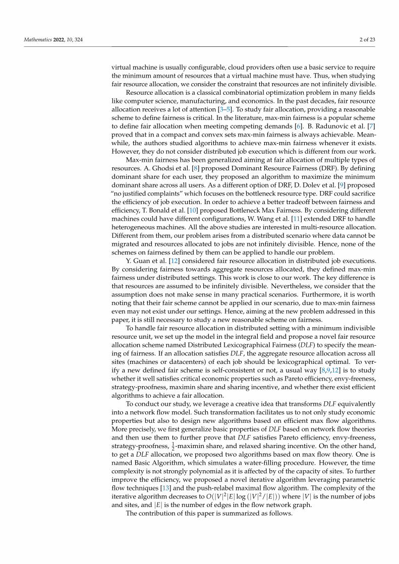
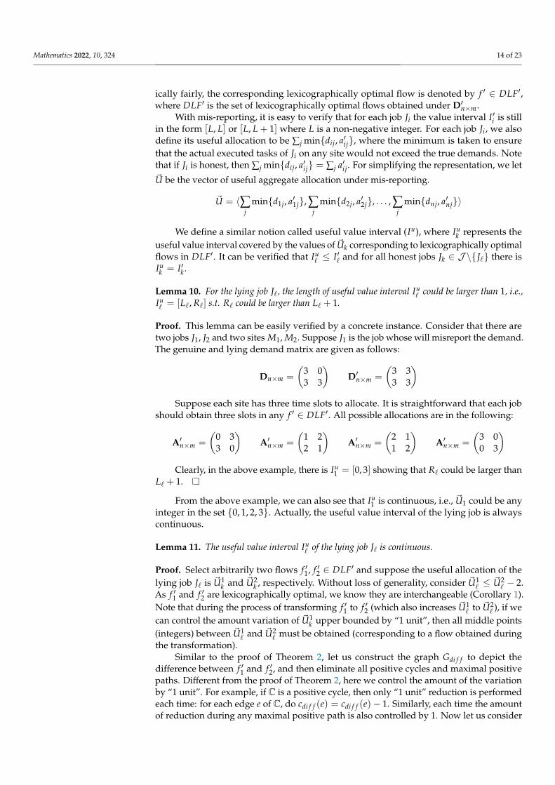
Transforming DLF means that we should build a flow network that could well modeljobs, sites, capacity constraint, rational constraint, and the integral requirements. Beforegiving a formal description, we perform a concrete case study first. Consider there are twojobs J1, J2 executed over two sites M1, M2. The demands of the two jobs are respectively〈3, 1〉 and 〈0, 2〉, while the capacity of M1 is 4 and the capacity of M2 is 3. Figure 1 depictsthe flow network built for the case. We can see that J1, J2 and M1, M2 all appear as nodesin the graph. We use directly edges between jobs and sites to express the demands (byedge capacity). s and t in the graph represent respectively the source and sink node whichare essential for any flow network. We add directed edges between s and the two jobs,where the capacity has no special constraint (expressed by +∞). We also add directededges from every site to t, where the capacity of edge is set to the corresponding capacityof site. Our general idea is to use the amount of flow passing by J1 and J2 to model thecorresponding allocations. It is well-known that a feasible flow never breaks the capacityof any edge in the flow network. With the above settings, any feasible flow satisfies thecapacity and rational constraints. If we further require that the flow is in integral field (i.e.,for any feasible flow, the amount of flow on any edge is an integer), a feasible allocationactually corresponds to a feasible flow and vice versa.

dij

…

…

J1

J2

M1

M2

s t

3

1

2

4

3

s

M1

t M2

Mm

Jobs Sites

J1

J3

J2

Jn

C1

C2

C3

Figure 1. The flow network graph built for case study.

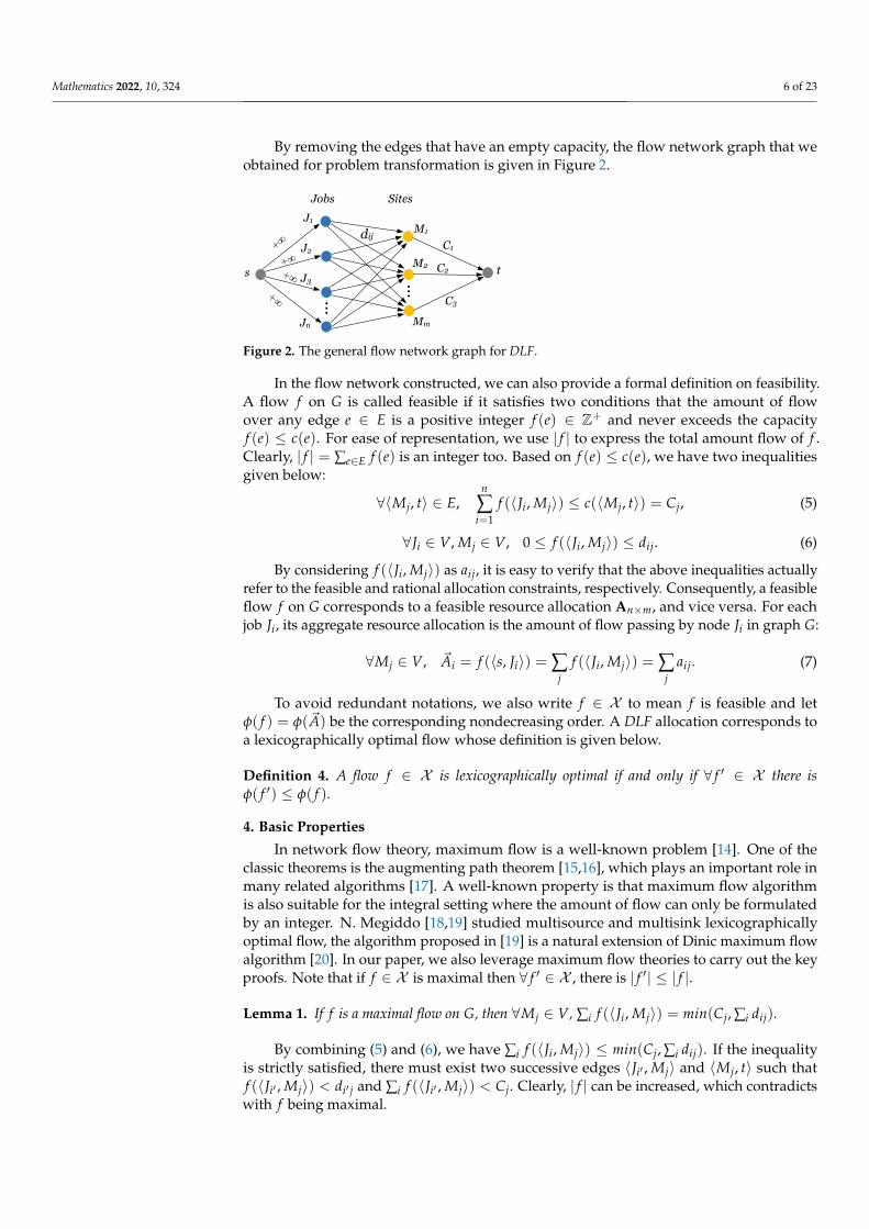
Now let us give a formal description on problem transformation. Necessary notationsare introduced first. We consider graph G = (V, E) with a capacity function c : E → Z+,where V = {s} ∪ J ∪M ∪ {t}. s and t represent the source node and the sink node,respectively, in a flow network. J is the set of nodes representing jobs andM is the set ofnodes corresponding to sites. Each edge e ∈ E is denoted as a pair of ordered nodes, i.e.,e = 〈vp, vq〉. The capacity function c is defined in the following.

c(e) =

dij if vp = Ji and vq = Mj ;+∞ if vp = s and vq = Ji;Cj if vp = Mj and vq = t ;0 otherwise.

(4)

Mathematics 2022, 10, 324 6 of 23

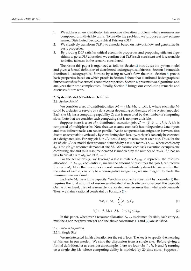
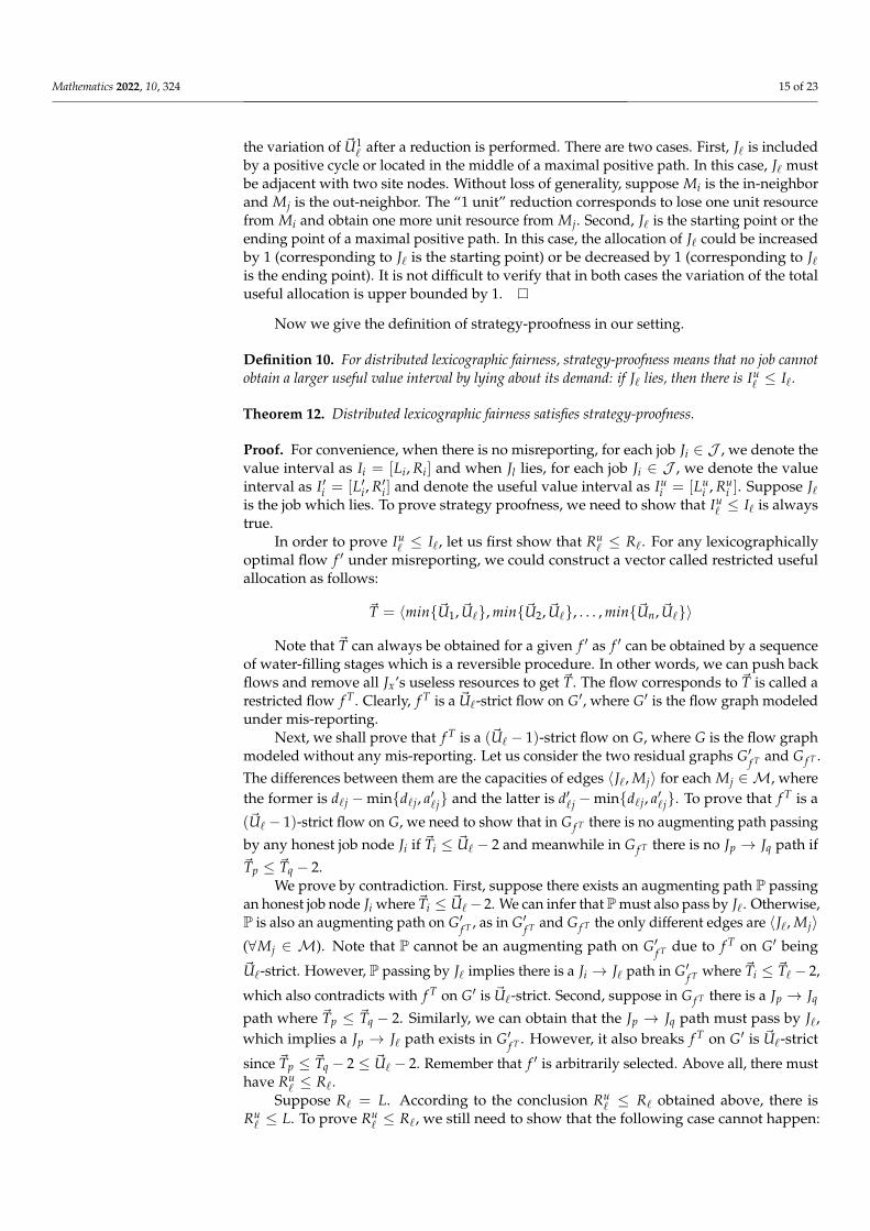
By removing the edges that have an empty capacity, the flow network graph that weobtained for problem transformation is given in Figure 2.

dij

…

…

J1

J2

M1

M2

s t

5

2

2

6

3

s

M1

t M2

Mm

Jobs Sites

J1

J3

J2

Jn

C1

C2

C3

Figure 2. The general flow network graph for DLF.

In the flow network constructed, we can also provide a formal definition on feasibility.A flow f on G is called feasible if it satisfies two conditions that the amount of flowover any edge e ∈ E is a positive integer f (e) ∈ Z+ and never exceeds the capacityf (e) ≤ c(e). For ease of representation, we use | f | to express the total amount flow of f .Clearly, | f | = ∑e∈E f (e) is an integer too. Based on f (e) ≤ c(e), we have two inequalitiesgiven below:

∀〈Mj, t〉 ∈ E,n

∑i=1

f (〈Ji, Mj〉) ≤ c(〈Mj, t〉) = Cj, (5)

∀Ji ∈ V, Mj ∈ V, 0 ≤ f (〈Ji, Mj〉) ≤ dij. (6)

By considering f (〈Ji, Mj〉) as aij, it is easy to verify that the above inequalities actuallyrefer to the feasible and rational allocation constraints, respectively. Consequently, a feasibleflow f on G corresponds to a feasible resource allocation An×m, and vice versa. For eachjob Ji, its aggregate resource allocation is the amount of flow passing by node Ji in graph G:

∀Mj ∈ V, ~Ai = f (〈s, Ji〉) = ∑j

f (〈Ji, Mj〉) = ∑j

aij. (7)

To avoid redundant notations, we also write f ∈ X to mean f is feasible and letφ( f ) = φ(~A) be the corresponding nondecreasing order. A DLF allocation corresponds toa lexicographically optimal flow whose definition is given below.

Definition 4. A flow f ∈ X is lexicographically optimal if and only if ∀ f ′ ∈ X there isφ( f ′) ≤ φ( f ).

4. Basic Properties

In network flow theory, maximum flow is a well-known problem [14]. One of theclassic theorems is the augmenting path theorem [15,16], which plays an important role inmany related algorithms [17]. A well-known property is that maximum flow algorithmis also suitable for the integral setting where the amount of flow can only be formulatedby an integer. N. Megiddo [18,19] studied multisource and multisink lexicographicallyoptimal flow, the algorithm proposed in [19] is a natural extension of Dinic maximum flowalgorithm [20]. In our paper, we also leverage maximum flow theories to carry out the keyproofs. Note that if f ∈ X is maximal then ∀ f ′ ∈ X , there is | f ′| ≤ | f |.

Lemma 1. If f is a maximal flow on G, then ∀Mj ∈ V, ∑i f (〈Ji, Mj〉) = min(Cj, ∑i dij).

By combining (5) and (6), we have ∑i f (〈Ji, Mj〉) ≤ min(Cj, ∑i dij). If the inequalityis strictly satisfied, there must exist two successive edges 〈Ji′ , Mj〉 and 〈Mj, t〉 such thatf (〈Ji′ , Mj〉) < di′ j and ∑i f (〈Ji′ , Mj〉) < Cj. Clearly, | f | can be increased, which contradictswith f being maximal.

Mathematics 2022, 10, 324 7 of 23

In our model, if a flow f ∈ X is lexicographically optimal, it is easy to verify thatf is also a maximal flow but not vice versa, i.e., a lexicographically optimal flow is aspecial maximal flow. Given a feasible flow f on G, an augmenting path is a directedsimple path from s to t (e.g., P = {s, v1, v2, ..., vi, vi+1, ..., t}) on the residual graph G f .Similarly, an adjusting cycle C on G f is a directed simple cycle from s to s (does not passby t). The capacity of a given path (or a given cycle) is defined to be the capacity of thecorresponding bottleneck edge, e.g., for a path P, c(P) = mine=〈vi ,vi+1〉∈P c(e) and for acycle C, c(C) = mine=〈vi ,vi+1〉∈C c(e). For ease of representation, we consider augmentingpath or adjusting cycle to only contain edges with positive capacity, i.e., c(P) > 0 andc(C) > 0.

In our context, performing an augmentation means increasing the original flow fby δ (δ ∈ Z+ and 1 ≤ δ ≤ c(P)) along an augmenting path P in G f and performing anadjustment means adjusting the original flow f by δ (δ ∈ Z+ and 1 ≤ δ ≤ c(C)) along anadjusting cycle C in G f . By performing an augmentation or an adjustment on a flow f , wecan get a new feasible flow. The difference is that only the augmentation increases | f |.

Claim 1. For a given feasible flow f on G, if there does not exist any augmenting path passing byJk in G f , then for any feasible f ′ augmented from f , there is also no augmenting path passing by Jkin G f ′ .

Proof. We prove by contradiction: assume there exists a feasible flow f ′ augmented from fand in the residual graph G f ′ , however, there is an augmenting path passing by Jk (denotedby P∗ in the following). In our model, c(〈s, Jk〉) = +∞, which implies 〈s, Jk〉 is an edgeexisting in any residual graph. Therefore, we only need to consider P∗ where the first twonodes are s and Jk.

As f ′ is augmented from f , we can perform successive augmentations on f to getf ′. Note that each augmentation is performed along an augmenting path. Hence, as-sume the successive augmentations are performed on a sequence of augmenting pathsP = {P1,P2, ...,Pr}which are respectively in the intermediate residual graphs {G1, G2, ..., Gr}obtained by augmentations. Here G1 is exactly G f , G2 is obtained by perform an augmenta-tion along P1 on G1, et al. Next, we perform a recursive analysis to gradually reduce P andfinally prove that in G f there also exists an augmenting path passing by Jk, which leads toa contradiction.

Finding P` the last path in P which has common nodes (except s, Jk and t) withP∗: P` ∩ P∗/{s, Jk, t} 6= ∅. A special case is that we cannot find such P`. It means thatstarting from G f by performing augmentations along all the augmenting paths in P , thereis no influence on the existence of P∗, i.e., P∗ is already an augmenting path in G f .

If such P` exists, it implies that after the augmentation is performed along P` in G`,the follow-up augmentations along P`+1, P`+2, ..., Pr do not affect the existence of P∗ anymore, i.e., P∗ exists in G`+1, G`+2, ..., Gr. Now let us focus on finding an augmentationpath passing by Jk which appears in G` (before the augmentation along P` is performed).Assume vx is the first node not only passing by P` but also appearing in P∗. We know thatthe augmentation along P` does not affect the existence of the first part of P∗: {s, Jk, ..., vx}.The remaining part of P∗ may not exist in G`. However, we can replace it with the part{vx, ..., t} that appears in P`. By concatenating the above two parts together, we actuallyfind another augmentation path in G` passing by Jk. If P` is exactly P1 of P , we alreadyfind an augmentation path passing by Jk in G f . Otherwise, let us denote the new foundaugmentation path by P∗ too, reduce P to {P1,P2, ...,P`} and restart the whole process.As P is not infinite, the process will be stopped after finite times, which implies G f mustinclude an augmentation path passing by Jk.

In our model, if a maximal flow is also lexicographically optimal, it must satisfy aspecial condition. In a residual graph G f , we name a simple path is a Jp → Jq path if it startsat Jp, ends at Jq, and does not pass by s and t. Note that any Jp → Jq path only containsedges with positive capacity.

Mathematics 2022, 10, 324 8 of 23

Theorem 2. A maximal flow f on G is lexicographically optimal if and only if for all Jp and Jq, if~Ap ≤ ~Aq − 2, then there is no Jp → Jq path on the residual graph G f .

Proof. First, proving the “only if” side. Assume there exist Jp and Jq, where ~Ap ≤ ~Aq − 2and a Jp → Jq path exists in G f . As the existence of 〈s, Jp〉 and 〈Jq, s〉, we can perform anadjustment by 1-unit from s to Jp, then along the Jp → Jq path and along the edge 〈Jq, s〉to reach s again. Note that by the above adjustment, we obtain a new maximal flow f ′

where ~A′p = ~Ap + 1 ≤ ~Aq − 1 = ~A′q. Therefore, f ′ is lexicographically larger than f , i.e.,φ( f ′) > φ( f ), which contradicts with f is lexicographically optimal.

Second, proving the “if” side by contradiction. Suppose that flow f is maximalon G and satisfies the condition. However, it is not lexicographically optimal. As-sume fopt is a lexicographically optimal flow such that φ( fopt) > φ( f ) and | f | = | fopt|.By comparing f with fopt, the set of jobs J can be naturally divided into three partsJ < = {Ji ∈ J | f (〈s, Ji〉) < fopt(〈s, Ji〉)}, J = = {Ji ∈ J | f (〈s, Ji〉) = fopt(〈s, Ji〉)} andJ > = {Ji ∈ J | f (s, Ji) > fopt(〈s, Ji〉)}. Next, we construct a special graph Gdi f f [21]to differentiate fopt and f .

Let us denote Gdi f f = (Vdi f f , Edi f f ), where Vdi f f = J ∪M. We also define a capacityfunction cdi f f for the edges of Edi f f :

1. if f (〈Ji, Mj〉) ≤ fopt(〈Ji, Mj〉), then cdi f f (〈Ji, Mj〉) = fopt(〈Ji, Mj〉)− f (〈Ji, Mj〉) andcdi f f (〈Mj, Ji〉) = 0;

2. otherwise, cdi f f (〈Mj, Ji〉) = f (〈Ji, Mj〉)− fopt(〈Ji, Mj〉) and cdi f f (〈Ji, Mj〉) = 0.

According to Lemma 1, we know for any site Mj there is fopt(〈Mj, t〉) = f (〈Mj, t〉).Therefore, in the graph Gdi f f , for each Mj, we have ∑i cdi f f (〈Mj, Ji〉) = ∑i cdi f f (〈Ji, Mj〉).

In Gdi f f , there could exist “positive cycles” (denoted by C): for each edge e of C, thereis cdi f f (e) > 0. For a positive cycle C, we let cap be the minimum capacity of all the edgescontained in C. We shall eliminate all these cycles by capacity reductions. For each edgee of C, we perform cdi f f (e) = cdi f f (e)− cap. Clearly, after the reduction, C is no more apositive cycle. Note that once we eliminate a positive cycle C on Gdi f f , it is equivalent toperform an adjustment by cap on G f . For example, assume Ji is a node included in the cycleC. The adjustment is starting from s, along the edge 〈s, Ji〉, then along the cycle C back toJi, and finally along the edge 〈Ji, s〉 back to s. We can eliminate all the positive cycles to geta new G′di f f by performing a sequence of capacity reduction operations. Compared withGdi f f , G′di f f corresponds to another maximal flow f ′, where ∀Ji, there is f (s, Ji) = f ′(s, Ji).Hence, f ′ is not lexicographically optimal either. Moreover, J <, J = and J > are alwayskept during the capacity reductions. In the following, we turn to focus on G′di f f .

In G′di f f , there must exist positive paths (for each edge in the path, the capacity isa positive integer), otherwise the flow f ′ is exactly fopt, which implies both f and f ′ arealso lexicographically optimal. As there are no positive cycles in G′di f f , we can extendany positive paths to be a maximal positive path, where there are no edges with positivecapacity entering the starting point and no edges with positive capacity leaving the endingpoint. The minimum capacity of edges in a maximal positive path is also denoted bycap ≥ 1. Next, we shall demonstrate that for any maximal positive path in G′di f f , thestarting point Jp must belong to J < and the ending point Jq must belong to J >. Clearly,Jp cannot belong to J > due to every node in J > having positive entering edges. On theother hand, Jp cannot belong to J = norM, since for each node in J = or inM, the totalcapacity of the positive entering edges is equal to the total capacity of the positive leavingedges. Consequently, Jp can only belong to J <. Similarly, we can infer that the endingpoint Jq can only belong to J >. Now we show that the maximal positive path in G′di f fcorresponds to a Jp → Jq path in G f . First, note that from Gdi f f to G′di f f , we only decreasethe capacity of some edges, such that if a maximal positive path appears in G′di f f , it is alsoa path in Gdi f f (not necessarily maximal).

Mathematics 2022, 10, 324 9 of 23

Suppose 〈Ji, Mj〉 is a directed edge in the maximal positive path. 〈Ji, Mj〉 is also anedge having positive capacity in Gdi f f . Then, c f (〈Ji, Mj〉) the capacity of the edge 〈Ji, Mj〉inside G f satisfies:

c f (〈Ji, Mj〉) = c(〈Ji, Mj〉)− f (〈Ji, Mj〉) ≥ max ( fopt(〈Ji, Mj〉)− f (〈Ji, Mj〉), 0) = cdi f f (〈Ji, Mj〉)

Similarly, assume 〈Mj, Ji〉 is a directed edge in the maximal positive path. 〈Mj, Ji〉 isalso an edge with positive capacity in Gdi f f . c f (〈Mj, Ji〉) the capacity of the edge 〈Mj, Ji〉inside G f satisfies:

c f (〈Mj, Ji〉) = f (〈Ji, Mj〉) ≥ max ( f (〈Ji, Mj〉)− fopt(〈Ji, Mj〉), 0) = cdi f f (〈Mj, Ji〉)

The above two formulas together indicate that for each edge of a maximal positivepath in Gdi f f , the capacity of the corresponding edge in G f is also positive. Without lossof generality, assume a maximal positive path that starts at Jp and ends at Jq. Then we getthe corresponding Jp → Jq path in G f . According to the assumption on f , we can easilyinfer that ~Ap ≥ ~Aq − 1 as the existence of the Jp → Jq path. Next, we show that f must belexicographically optimal.

First, let us assume ~Ap ≥ ~Aq. Together with the existence of the maximal positive pathfrom Jp to Jq, we can infer that ~Aopt

p > ~Ap ≥ ~Aq > ~Aoptq . By considering that the problem

is defined in integral field, we can obtain ~Aoptp ≥ ~Ap + 1 ≥ ~Aq + 1 ≥ ~Aopt

q + 2. Note thatas the maximal path exists, there is a Jq → Jp path (a reversed path from Jq to Jp) in theresidual graph Gopt. As the sufficiency of this theorem is already proven, we can get that~Aopt

q ≥ ~Aoptp − 1. Above all, we can obtain ~Aopt

p ≥ ~Aoptq + 2 ≥ ~Aopt

p + 1. A contradiction isidentified, which means only ~Ap = ~Aq − 1 can happen.

Consider ~Ap = ~Aq − 1. Note that in this case we still have the Jp → Jq path in G f

and such that ~Aoptq ≥ ~Aopt

p − 1. Next, we focus on the maximal positive path from Jpto Jq in G′di f f and do capacity reductions by cap along such maximal path. Rememberthat the capacity reductions correspond to do an adjustment in G f ′ , which results in anew maximal flow f ′′ that satisfies | f ′′| = | f ′| = | f |, ~A′′p = ~A′p + cap = ~Ap + cap and~A′′q = ~A′q − cap = ~Aq − cap. Together with ~Ap = ~Aq − 1, we have ~A′′p = ~A′′q + 2cap− 1.The new difference graph G′′di f f is obtained by capacity reductions. Hence, in G′′di f f , fornode Jp there are no positive edges entering in and for node Jq there are no positive edgesleaving out. Therefore, we have ~Aopt

p ≥ ~A′′p and ~Aoptq ≤ ~A′′q . Above all, we have

~Aoptp ≥ ~A′′p = ~A′′q + 2cap− 1 ≥ ~Aopt

q + 2cap− 1 ≥ ~Aoptp + 2cap− 2.

Let us assume cap ≥ 2. According to the above inequality, we have ~Aoptp ≥ ~Aopt

p + 2,which also results in a contraction.

Now we can conclude that for any maximal path existing in G′di f f (w.l.o.g, Jp and Jq

represents respectively the starting point and the ending point), we must have ~Ap = ~Aq − 1and cap = 1. We perform capacity reductions by cap = 1 along such maximal positivepath. The adjustment corresponding to such capacity reductions is to increase ~Ap by 1and meanwhile to decrease ~Aq by 1. Note that for the flow f ′′ got after the adjustment,there is φ( f ′′) = φ( f ′) = φ( f ). It means that the adjustment cannot make f be better interms of lexicographical order. Finally, we continue to perform capacity reductions alongmaximal positive paths one by one until no positive edges remains in the difference graph(i.e., fopt is obtained). As no adjustment can make f be better, f is already lexicographicallyoptimal.

Corollary 1. If both f and f ′ are lexicographically optimal, they are interchangeable.

Mathematics 2022, 10, 324 10 of 23

The above corollary is straightforward by the proof of Theorem 2. One can constructthe different graph between f and f ′. Then, capacity reductions can be performed toeliminate all positive cycles and maximal positive paths, which is indeed a process oftransformation between the two optimal flows.

Lexicographically optimal flow is not unique. Let LOF be the set including all lexico-graphically optimal flows. Next, we study the variation of aggregate resource obtained bya job among different optimal flows.

Definition 5. For any Ji ∈ J , the value interval Ii is defined as the value range of the aggregateresource ~Ai in all f ∈ LOF.

Remember that our problem is discussed in Z+ such that each value interval wedefined only includes integers. The following theorem shows that the length of any valueinterval is at most 1.

Theorem 3. ∀ f , f ′ ∈ LOF, ∀Ji ∈ J , there is |~Ai − ~A′i| ≤ 1.

Proof. We prove by contradiction. Assume there exists a pair of flows f , f ′ ∈ LOF andthere exists a job Jp ∈ J which satisfies ~A′p − ~Ap ≥ 2. Based on the proof of Theorem 2, weconstruct the difference graph Gdi f f between f and f ′ and target to transform f to f ′. As~Ap needs to be increased, we have Jp ∈ J <. Moreover, during the transformation, theremust exist a time that Jp becomes a starting point of a maximal positive path. Suppose theending point of such path is Jq. We have Jq ∈ J > (such that ~Aq > ~A′q) and ~Ap = ~Aq − 1.On the other hand, the reverse of such maximal path is a Jq → Jp path on the residualgraph G f ′ . According to Theorem 2, there is ~A′q ≥ ~A′p − 1. Above all, we can showthat ~A′p ≥ ~Ap + 2 = ~Aq + 1 > ~A′q + 1 ≥ ~A′p, which is a contradiction as ~A′p > ~A′p isobtained.

Based on the Theorem 3, we provide a more specified definition of value interval.

Definition 6. A job Ji’s value interval Ii is [L, L] if and only if ~Ai = L for all f ∈ LOF. A job Ji’svalue interval Ii is [L, L + 1] if and only if there exist a pair of flows f , f ′ ∈ LOF such that ~Ai = Land ~A′i = L + 1.

Theorem 4. For a job Jp ∈ J , suppose ~Ap = L of a given flow f ∈ LOF. Jp’s value interval is[L, L + 1] if and only if there exists a Jp → Jq path in the residual graph G f where ~Ap = ~Aq − 1.

Proof. For the “if” side, since one could obtain a new flow f ′ ∈ LOF by performing anadjustment along the edge 〈s, Jp〉, then along the Jp → Jq path and along the edge 〈Jq, s〉back to s. In the new flow f ′, there is ~A′p = L + 1, which implies Ip = [L, L + 1].

For the “only if” side, there exists a flow f ′ ∈ LOF with ~A′p = L + 1. Based on the proofof Theorem 2, we transform f to f ′. We first eliminate all positive cycles and then eliminatemaximal positive path one by one. During the transformation process, we can find a maximalpositive path which starts at Jp and ends at another node Jq satisfying ~Ap = ~Aq − 1. By suchmaximal path, we can identify the corresponding Jp → Jq path on G f .

By Theorem 4, we directly have the following two corollaries.

Corollary 2. For a job Jp ∈ J , suppose ~Ap = L under a given flow f ∈ LOF. Jp’s value intervalis [L− 1, L] if and only if there exists a Jq → Jp path in the residual graph G f where ~Aq = ~Ap − 1.

Corollary 3. For a job Jp ∈ J , suppose ~Ap = L under a given flow f ∈ LOF. Jp’s valueinterval is [L, L] if and only if in the residual graph G f there neither exists a Jp → Jq path where~Ap = ~Aq − 1 nor exists a Jq → Jp path where ~Aq = ~Ap − 1.

Mathematics 2022, 10, 324 11 of 23

We define binary relations on value intervals in order to make the comparison. LetIp = [Lp, Rp] and Iq = [Lq, Rq] be the two value intervals of Jp and Jq respectively. Ip < Iqif and only if Lp < Lq or Rp < Rq. Symmetrically, Ip > Iq if and only if Lp > Lq or Rp > Rq.Finally, Ip = Iq if and only if Lp = Lq and Rp = Rq.

Theorem 5. Suppose f ∈ LOF and in the residual graph G f there exists a Jp → Jq path where~Ap = ~Aq − 1 = L. Let P denote the set of jobs passed by the Jp → Jq path, then ∀Jk ∈ P, there isIk = [L, L + 1].

Proof. The value intervals of Jp and Jq can be obtained directly by Theorem 4 and Corollary 2,respectively. Both of them are equal to [L, L + 1]. Suppose Jk ∈ P and Jk is not Jp nor Jq.Clearly, we have a Jp → Jk path and a Jk → Jq path in the residual graph G f . AssumeJk’s value interval Ik ≤ [L − 1, L], i.e., ~Ak ≤ L − 1 under the current flow f . Then wecan perform an adjustment by 1 along the edge 〈s, Jk〉, then along the Jk → Jq path andalong the edge 〈Jk, s〉 back to s. After the adjustment, we obtain a new flow f ′, where~Ak′= L and ~Aq

′= L. However, it implies that f ′ satisfies φ( f ′) > φ( f ) which contradicts

with f is lexicographically optimal. Symmetrically, we can prove that Ik ≥ [L, L + 1] isnot true too due to the existence of the Jp → Jk path in G f . Above all, we can concludeIk = [L, L + 1].

Definition 7. A feasible flow f on G is lexicographically feasible if and only if ∀Jp, Jq ∈ J , if~Ap ≤ ~Aq − 2, then no Jp → Jq path exists in the residual graph G f .

Definition 8. A lexicographically feasible flow f on G is called v-strict if and only if ∀Ji ∈ J ,there is ~Ai ≤ v and if ~Ai ≤ v− 1, then in G f there is no augmenting path passing by Ji.

For any given lexicographically optimal flow, we can get one unique value:

vmax = max{~A1, ~A2, ..., ~An}.

From Definitions 7 and 8, we can easily see that a lexicographically optimal flow isvmax-strict. Additionally, we consider the empty flow (| f | = 0) as 0-strict. Starting fromthe empty flow, a lexicographically optimal flow could be obtained after a sequence ofwater-filling stages are carried out.

Definition 9. A water-filling stage is performed on any v-strict (0 ≤ v < vmax) flow: performingaugmentation by 1 for each job node in the set J v = {Ji ∈ J |~Ai = v}.

Note that by a water-filling stage, it is not necessarily that ∀Ji ∈ J v, ~Ai is increasedby 1, as there may already be no augmentation path passing by Ji in G f . According toClaim 1, we know that if ~Ai fails to be increased, then it will no more be increased during thefollowing water-filling stages. That is also the reason that for a v-strict flow a water-fillingstage only needs to focus on nodes in J v.

Lemma 6. A lexicographically optimal flow is obtained after vmax water-filling stages.

Proof. This lemma is true if during all water-filling stages there is no flow obtained breakslexicographic feasibility (Definition 7).

Without loss of generality, let us focus on one water-filling stage which will be per-formed on a v-strict flow, where 0 ≤ v < vmax. In such stage, we know there are a sequenceof augmentations that will be performed for each node in the set J v. Clearly, before anyaugmentations are performed, the v-strict flow is lexicographically feasible. We need toprove that after any augmentation is successfully performed, the new flow obtained is stilllexicographically feasible.

Mathematics 2022, 10, 324 12 of 23

Suppose after a sequence augmentations the flow f obtained is still lexicographicallyfeasible. In the current state, we can divide jobs into three parts: S1 = {Ji ∈ J |~Ai ≤ L− 1},S2 = {Ji ∈ J |~Ai = L} and S3 = {Ji ∈ J |~Ai = L+ 1}. Consider that the next augmentationwill be executed along an augmenting path (denoted by P) that passes by node Jk andassume that after the augmentation the new flow f ′ is not lexicographically feasible, i.e.,in G′f , there exists a Jp → Jq path where ~Ap ≤ ~Aq − 2. Since L + 1 = max{~A1, ~A2, ..., ~An},we have Jp ∈ S1 which implies ~Ap will not be increased during the current water-fillingstage. There are two cases. First, in G′f , P and the Jp → Jq path have no intersections (sharecommon nodes in the path). In this case, we can infer that the Jp → Jq path also exists in G f ,as the augmentation does not affect the existence of the Jp → Jq path. On the other hand,we can infer that under the flow f there is also ~Ap ≤ ~Aq − 2. The reason is that from f to f ′

both ~Ap and ~Aq are kept. However, it violates the assumption that f is lexicographicallyfeasible. Second, in G′f , P and the Jp → Jq path have intersections. Along the two paths, letus assume node x is the first common node where the two paths intersect. Note that thesub-path (from Jp to x) of Jp → Jq is not affected by the augmentation such that it also existsin G f . On the other hand, P has a sub-path from x to t in G f . Therefore, we can find anaugmenting path from s to Jp, then from Jp to x and finally from x to t. However, it violatesf is v-strict. Above all, we get the proof.

Theorem 7. Suppose Jp’s value interval is Ip = [L− 1, L]. Under any L-strict flow f , if~Ap = L− 1, then there exists a Jp → Jq path on G f where ~Aq = L. Symmetrically, if ~Ap = L,then there exists a Jq → Jp path on G f where ~Aq = L− 1.

Proof. Since f is L-strict, we can perform a sequence of water-filling stages on f to get alexicographically optimal flow f ′. Clearly, ~Ap is no more increased during the followingwater-filling stages such that ~A′p = ~Ap. First, consider currently ~Ap = L− 1. Accordingto Corollary 2, we know in G f ′ there exists a Jp → Jq path where ~Aq = ~Ap + 1 = L. Next,we prove that the Jp → Jq path existing in G f ′ also appears in G f . From f to f ′, successivewater-filling stages on f are performed. Every water-filling stage is composed of a sequenceof augmentations each of which corresponds to an augmenting path. Thus, we could use anordered set S = {P1,P2, . . . ,Pr} to include all augmenting paths (of all water-filling stages)used for augmenting f to f ′. Suppose Pi ∈ S is the last element in S which shares commonnodes with the Jp → Jq path and suppose the first common node of the two paths is Jk.Let f i−1 denote the flow before the augmentation along Pi is processed. Note that f i−1 islexicographically feasible according to the proof of Lemma 6. We can infer that the Jp → Jkpath (sub-path of Jp → Jq) already appears in G f i−1 . On the other hand, there is a pathfrom Jk to t in G f i−1 , which is the sub-path of Pi. Together with the edge 〈s, Jp〉, we find anaugmenting path passing by Jp in G f i−1 . Remember that f is L-strict such that in G f thereis no augmenting path passing by Jp. By Claim 1, we know that in G f i−1 there should alsobe no augmenting path passing by Jp, i.e., a contradiction is identified. Therefore, for anypath Pi ∈ S , it shares no common nodes with the Jp → Jq path, which implies the Jp → Jq

path also exists in G f . The proof for the second case ~Ap = L is symmetric where we canfind an augmenting path passing by Jq (with ~Aq = L− 1) in an intermediately obtainedresidual graph, which also concludes a contradiction.

Corollary 4. For any L-strict flow f on G, if there exists a Jp → Jq path in G f where~Ap = ~Aq − 1 = L − 1, then the same path also exists in any lexicographically optimal flowf ′ that could be augmented from f .

Corollary 4 is actually the inverse proposition of Theorem 7. The proof can be obtainedby applying the proof of Theorem 7 in a reversed direction.

Mathematics 2022, 10, 324 13 of 23

5. Economic Properties

In this section, we investigate whether or not a DLF allocation (or, equivalently, alexicographically optimal flow) satisfies economic properties which is critical to verifyingwhether DLF is reasonable to define fairness in our scenario.

5.1. Pareto Efficiency and Envy-Freeness

Pareto efficiency: Increasing the allocation of a job must decrease the allocation ofanother job.

If Pareto efficiency is satisfied, all the available resources must be allocated or the totalresource requirements are already fully met, i.e., resource utilization is maximized. Notethat fairness is only necessary when resources cannot meet all the demands. Therefore, anyreasonable scheme on fairness should be Pareto efficiency.

Theorem 8. Distributed lexicographical fairness satisfies Pareto efficiency.

Proof. The proof is straightforward. Suppose DLF does not satisfy Pareto efficiency. Weknow that a DLF allocation corresponds to a lexicographically optimal flow. DLF does notsatisfy Pareto efficiency which directly implies that lexicographically optimal flow is notmaximal. This is a contradiction.

Envy-freeness: no job would expect to get the allocation of any other job.Envy-freeness is also a usual requirement of any fair scheme. Under a fair allocation,

we can easily imagine that no job prefers the allocation of another job. In our setting,envy-freeness could be represented by the following inequality.

∀Jq ∈ J , ∑j

min (aqj, dpj) ≤∑j

apj. (8)

At first glance, DLF allocation does not always satisfy envy-freeness. For example,there are two jobs, J1 and J2, each of which has one task to be executed on the same site M1whose time slots is 1. No matter which job gets the time slot, the other one would envy itsallocation. This happens due to our discussion area being in Z+. Indeed in our setting, Jp

never envies Jq’s allocation if ~Ap ≤ ~Aq − 2.

Theorem 9. ∀Jp, Jq ∈ J , if ~Ap ≤ ~Aq − 2, then Jp does not envy Jq’s allocation.

Proof. Proof by contradiction. Suppose f is lexicographically optimal. However, thereexists a pair of jobs—Jp and Jq, where ~Ap ≤ ~Aq − 2 and ∑j min (aqj, dpj) > ∑j apj. We caninfer that ∃Mj ∈ M such that min (aqj, dpj) > apj. Note that in G f the two edges 〈Jp, Mj〉and 〈Mj, Jq〉 together form a Jp → Jq path. Combining with ~Ap ≤ ~Aq − 2, we find that acontradiction with f is lexicographically optimal.

5.2. Strategy-Proofness

Strategy-proofness: No job can get more allocation by lying about its demands.Strategy-proofness ensures incentive compatibility. This property is important for a

fairness scheme. With strategy-proofness, no participant can break the fairness schemewith its own information. In our setting, strategy-proofness is used to ensure that a jobshould not get profits by misreporting its demands. Suppose J` lies about its demands.The demand matrix is denoted by D′n×m. Note that under D′n×m we could still computelexicographically optimal allocation and model the problem under another flow graphdenoted by G′.

Since only J` lies, ∀Mj ∈ M, if Jk ∈ J \{J`}, then d′kj = dkj. For J`, we consider d′`jcould be any non-negative integer, i.e., we do not assume d′`j ≥ d`j. Under the setting withmisreporting, the allocation matrix is denoted by A′. When A′ is distributed lexicograph-

Mathematics 2022, 10, 324 14 of 23

ically fairly, the corresponding lexicographically optimal flow is denoted by f ′ ∈ DLF′,where DLF′ is the set of lexicographically optimal flows obtained under D′n×m.

With mis-reporting, it is easy to verify that for each job Ji the value interval I′i is stillin the form [L, L] or [L, L + 1] where L is a non-negative integer. For each job Ji, we alsodefine its useful allocation to be ∑j min{dij, a′ij}, where the minimum is taken to ensurethat the actual executed tasks of Ji on any site would not exceed the true demands. Notethat if Ji is honest, then ∑j min{dij, a′ij} = ∑j a′ij. For simplifying the representation, we let~U be the vector of useful aggregate allocation under mis-reporting.

~U = 〈∑j

min{d1j, a′1j}, ∑j

min{d2j, a′2j}, . . . , ∑j

min{dnj, a′nj}〉

We define a similar notion called useful value interval (Iu), where Iuk represents the

useful value interval covered by the values of ~Uk corresponding to lexicographically optimalflows in DLF′. It can be verified that Iu

` ≤ I′` and for all honest jobs Jk ∈ J \{J`} there isIuk = I′k.

Lemma 10. For the lying job J`, the length of useful value interval Iu` could be larger than 1, i.e.,

Iu` = [L`, R`] s.t. R` could be larger than L` + 1.

Proof. This lemma can be easily verified by a concrete instance. Consider that there aretwo jobs J1, J2 and two sites M1, M2. Suppose J1 is the job whose will misreport the demand.The genuine and lying demand matrix are given as follows:

Dn×m =

(3 03 3

)D′n×m =

(3 33 3

)Suppose each site has three time slots to allocate. It is straightforward that each job

should obtain three slots in any f ′ ∈ DLF′. All possible allocations are in the following:

A′n×m =

(0 33 0

)A′n×m =

(1 22 1

)A′n×m =

(2 11 2

)A′n×m =

(3 00 3

)Clearly, in the above example, there is Iu

1 = [0, 3] showing that R` could be larger thanL` + 1.

From the above example, we can also see that Iu1 is continuous, i.e., ~U1 could be any

integer in the set {0, 1, 2, 3}. Actually, the useful value interval of the lying job is alwayscontinuous.

Lemma 11. The useful value interval Iu` of the lying job J` is continuous.

Proof. Select arbitrarily two flows f ′1, f ′2 ∈ DLF′ and suppose the useful allocation of thelying job J` is ~U1

k and ~U2k , respectively. Without loss of generality, consider ~U1

` ≤ ~U2` − 2.

As f ′1 and f ′2 are lexicographically optimal, we know they are interchangeable (Corollary 1).Note that during the process of transforming f ′1 to f ′2 (which also increases ~U1

` to ~U2` ), if we

can control the amount variation of ~U1k upper bounded by “1 unit”, then all middle points

(integers) between ~U1` and ~U2

` must be obtained (corresponding to a flow obtained duringthe transformation).

Similar to the proof of Theorem 2, let us construct the graph Gdi f f to depict thedifference between f ′1 and f ′2, and then eliminate all positive cycles and maximal positivepaths. Different from the proof of Theorem 2, here we control the amount of the variationby “1 unit”. For example, if C is a positive cycle, then only “1 unit” reduction is performedeach time: for each edge e of C, do cdi f f (e) = cdi f f (e)− 1. Similarly, each time the amountof reduction during any maximal positive path is also controlled by 1. Now let us consider

Mathematics 2022, 10, 324 15 of 23

the variation of ~U1` after a reduction is performed. There are two cases. First, J` is included

by a positive cycle or located in the middle of a maximal positive path. In this case, J` mustbe adjacent with two site nodes. Without loss of generality, suppose Mi is the in-neighborand Mj is the out-neighbor. The “1 unit” reduction corresponds to lose one unit resourcefrom Mi and obtain one more unit resource from Mj. Second, J` is the starting point or theending point of a maximal positive path. In this case, the allocation of J` could be increasedby 1 (corresponding to J` is the starting point) or be decreased by 1 (corresponding to J`is the ending point). It is not difficult to verify that in both cases the variation of the totaluseful allocation is upper bounded by 1.

Now we give the definition of strategy-proofness in our setting.

Definition 10. For distributed lexicographic fairness, strategy-proofness means that no job cannotobtain a larger useful value interval by lying about its demand: if J` lies, then there is Iu

` ≤ I`.

Theorem 12. Distributed lexicographic fairness satisfies strategy-proofness.

Proof. For convenience, when there is no misreporting, for each job Ji ∈ J , we denote thevalue interval as Ii = [Li, Ri] and when Jl lies, for each job Ji ∈ J , we denote the valueinterval as I′i = [L′i, R′i] and denote the useful value interval as Iu

i = [Lui , Ru

i ]. Suppose J`is the job which lies. To prove strategy proofness, we need to show that Iu

` ≤ I` is alwaystrue.

In order to prove Iu` ≤ I`, let us first show that Ru

` ≤ R`. For any lexicographicallyoptimal flow f ′ under misreporting, we could construct a vector called restricted usefulallocation as follows:

~T = 〈min{~U1, ~U`}, min{~U2, ~U`}, . . . , min{~Un, ~U`}〉

Note that ~T can always be obtained for a given f ′ as f ′ can be obtained by a sequenceof water-filling stages which is a reversible procedure. In other words, we can push backflows and remove all Jx’s useless resources to get ~T. The flow corresponds to ~T is called arestricted flow f T . Clearly, f T is a ~U`-strict flow on G′, where G′ is the flow graph modeledunder mis-reporting.

Next, we shall prove that f T is a (~U` − 1)-strict flow on G, where G is the flow graphmodeled without any mis-reporting. Let us consider the two residual graphs G′f T and G f T .The differences between them are the capacities of edges 〈J`, Mj〉 for each Mj ∈ M, wherethe former is d`j −min{d`j, a′`j} and the latter is d′`j −min{d`j, a′`j}. To prove that f T is a

(~U` − 1)-strict flow on G, we need to show that in G f T there is no augmenting path passing

by any honest job node Ji if ~Ti ≤ ~U` − 2 and meanwhile in G f T there is no Jp → Jq path if~Tp ≤ ~Tq − 2.

We prove by contradiction. First, suppose there exists an augmenting path P passingan honest job node Ji where ~Ti ≤ ~U`− 2. We can infer that P must also pass by J`. Otherwise,P is also an augmenting path on G′f T , as in G′f T and G f T the only different edges are 〈J`, Mj〉(∀Mj ∈ M). Note that P cannot be an augmenting path on G′f T due to f T on G′ being~U`-strict. However, P passing by J` implies there is a Ji → J` path in G′f T where ~Ti ≤ ~T` − 2,

which also contradicts with f T on G′ is ~U`-strict. Second, suppose in G f T there is a Jp → Jq

path where ~Tp ≤ ~Tq − 2. Similarly, we can obtain that the Jp → Jq path must pass by J`,which implies a Jp → J` path exists in G′f T . However, it also breaks f T on G′ is ~U`-strict

since ~Tp ≤ ~Tq − 2 ≤ ~U` − 2. Remember that f ′ is arbitrarily selected. Above all, there musthave Ru

` ≤ R`.Suppose R` = L. According to the conclusion Ru

` ≤ R` obtained above, there isRu` ≤ L. To prove Ru

` ≤ R`, we still need to show that the following case cannot happen:

Mathematics 2022, 10, 324 16 of 23

Iu` = [L, L] while I` = [L − 1, L]. We prove by contradiction: assume the above case

happens such that ~U` = L, f T defined above is a L-strict flow on G′ and (L− 1)-strict flowon G. The (L− 1)-strict flow on G let us know that jobs which are possible to performthe next water-filling stage belong to the set {Ji ∈ J |~Ti = ~U` − 1 = L − 1}. AssumeJp ∈ {Ji ∈ J |~Ti = L − 1}. Note that in the residual graph G f T the augmentation pathpassing by Jp must also pass by J`, otherwise, the path also exists in G′f T which violates

that f Tis a L-strict flow on G′. Such augmentation path also passing by J` means that inG′f T there exists a Jp → J` path. Considering the flow f T on G′, we continue to perform

water-filling stages until the lexicographically optimal flow f ′ is obtained. Note that asJp ∈ {Ji ∈ J |~Ti = L− 1}, its allocation is more increased during the water-filling stages.Therefore, we have:

~A′p = ~Up = L− 1 < L = ~U` ≤ ~A′`.

Note that according to Corollary 4 the Jp → J` path still exists in G′f ′ . There are

two cases. First, ~U` < ~A′`, which implies ~A′p ≤ ~A′` − 2. It contradict with that f ′ islexicographically optimal. Second, consider ~U` = ~A′`. The existing Jp → J` path in G′f ′implies Iu

` = [L− 1, L] contradicting with the assumption Iu` = [L, L].

Finally, if no job in the set {Ji ∈ J |~Ti = L− 1} is successful to perform augmentation,f T is also a L-strict flow on G. Since I` = [L− 1, L], by Theorem 7, we know there is aJp → J` path on G f T where ~Ap = L− 1 under the flow f T on G. Similarly, we can infer thatthe Jp → J` path also appears in G′f T . Again, by Corollary 4, the Jp → J` path exists in G′f ′that Iu

` cannot be [L, L].

5.3. Maximin Share

Maximin share [22]: Each job is required to divide a set of m indivisible resources inton bundles and it will receive the minimum valuable bundle.

Maximin share (MMS) is a well-defined notion in fair indivisible resources allocation.If a fair scheme satisfies MMS, the allocation for any participant is at least to be the averagecase. In our setting, the maximin share defined for each job Ji is given in the following.

MMSi =

⌊1n

m

∑j=1

min (Cj, n · dij)

⌋(9)

Theorem 13. Distributed lexicographically fairness satisfies 12 -maximin share.

Proof. Select a job Jk ∈ J arbitrarily. We know that Jk’s value interval Ik is [L− 1, L] orIk = [L, L]. We consider a L-strict flow f on a new flow graph GL = (V, E), where the nodeset V and the edge set E are the same with the flow graph G and the difference is that forany edge 〈s, Ji〉 (Ji ∈ J ), we define c(〈s, Ji〉) = L. Clearly, any L-strict flow on such a graphGL is a maximal flow.

It is well known that maximal flow corresponds to minimum cut. Suppose (VL, VL)is a minimum cut in GL, where VL, VL ⊆ V, V = VL ∪ VL and ∅ = VL ∩ VL. Minimumcut of GL is not necessarily unique. In the following, we consider the minimum cut whereJk ∈ VL is satisfied. Note that such minimum cut must exist, otherwise it contradicts withthat Jk’s value interval is [L− 1, L] or [L, L].

Denote VL = {s} ∪ J1 ∪M1 and VL = J2 ∪M2 ∪ {t} where J = J1 ∪ J2 andM =M1 ∪M2. By considering f on GL, we have:

∑Ji∈J1

~Ai = ∑Mj∈M1

Cj + ∑Ji∈J1

∑Mj∈M2

dij (10)

Mathematics 2022, 10, 324 17 of 23

Equation (10) is computed by the minimum cut: edges from VL to VL should be fullyfilled, while edges from VL to VL should not contain any flow (otherwise contradictingwith that f on GL is maximal). Let r = |J1| ≤ n, we have:

∑Mj∈M1

min (Cj, ndkj) ≤ ∑Mj∈M1

Cj ≤ ∑Ji∈J1

~Ai ≤ rL (11)

The second inequality is from Equation (10) and dij ≥ 0, and the last inequality is by fis L-strict. Note that if ~Ak = L− 1 the last inequality is strict. Furthermore, we have: 1

n ∑Mj∈M1

min (Cj, ndkj)

≤1

r ∑Mj∈M1

min (Cj, ndkj)

≤ ⌊1r ∑

Ji∈J1

~Ai

⌋≤ ~Ak (12)

The second inequality is from (11). The last inequality is due to the round-downaverage allocation of jobs in J1 being unable to reach L if there exists one job in J1 whoseallocation is less than L and, on the other hand, if for each job in J1 the allocation is equalto L, the inequality is still true as ~Ak = L.

For the setM2 we have:

1n ∑

Mj∈M2

min (Cj, ndkj) ≤1n ∑

Mj∈M2

ndkj = ∑Mj∈M2

dkj ≤ ~Ak (13)

The last inequality in (13) is based on the property of the minimum cut (VL, VL).Combining (12) and (13) together, we have: 1

n ∑Mj∈M

min (Cj, ndkj)

=

1n ∑

Mj∈M1

min (Cj, ndkj) +1n ∑

Mj∈M2

min (Cj, ndkj)

≤

1n ∑

Mj∈M1

min (Cj, ndkj) + ∑Mj∈M2

dkj

=

1n ∑

Mj∈M1

min (Cj, ndkj)

+ ∑Mj∈M2

dkj (14)

≤ 2~Ak

In other words, ~Ak ≥ 12 MMSk. Thus, the bound 1

2 is obtained.

We now provide a simple instance to show that the above bound 12 is tight. Consid-

ering an instance composed of two jobs and two sites, each site has two slots to allocate.The demand matrix is given on the left and a possible distributed lexicographically fairallocation is given on the right.

D2×2 =

(1 12 0

)A2×2 =

(0 12 0

)(15)

We have ~A1 = 1 and the value interval is I1 = [1, 2]. The maximin share of J1 isMMS1 = 2, thus ~A1 = 1

2 MMS1.

5.4. Sharing Incentive

Sharing incentive: Each job should be better off sharing the total resources thanexclusively using its own partition of the total resources.

In our scenario, sharing incentive means that each job Ji should be allocated with atleast a 1

n fraction of resources. It is similar to Maximin share and can often be used when

Mathematics 2022, 10, 324 18 of 23

resources are infinitely divisible. Although we are interested in a different scenario, weshall show that DLF satisfies a relaxed sharing incentive. Specifically, when considering thewhole system as a single resource pool, the following formula is true.

∀Mj ∈ M, ∑j

aij ≥⌊

1n ∑

jmin (Cj, dij)

⌋(16)

Theorem 14. Distributed lexicographical fairness satisfies relaxed sharing incentive.

Proof. Suppose there is job Jk ∈ J whose value interval Ik is [L − 1, L] or [L, L]. Weconsider a L-strict flow f on a new flow graph GL = (V, E), where the node set V andthe edge set E are the same with the flow graph G and the difference is that for any edge〈s, Ji〉 (Ji ∈ J ), we define c(〈s, Ji〉) = L. Clearly, any L-strict flow on such a graph GL is amaximal flow.

It is well known that maximal flow corresponds to minimum cut. Suppose (VL, VL) isa minimum cut in GL, where VL, VL ⊆ V, V = VL ∪ VL and ∅ = VL ∩ VL. Minimum cut ofGL is not necessarily unique. In the following, we consider the minimum cut where Jk ∈ VL

is satisfied. Note that such minimum cut must exist, otherwise it contradicts with Jk’s valueinterval being [L− 1, L] or [L, L]. Denote VL = {s} ∪ J1 ∪M1 and VL = {t} ∪ J1 ∪M2such that J = J1 ∪ J2 andM =M1 ∪M2. Then we have:

∑Ji∈J1

~Ai = ∑Mj∈M1

Cj + ∑Ji∈J1

∑Mj∈M2

dij (17)

Equation (17) is computed by the minimum cut, edges from VL to VL should be fullyfilled while the reversed arcs should be zero (otherwise contradicting with f is maximal onGL). Let r = |J1|. Since r ≤ n, we have:

nr ∑

Ji∈J1

~Ai ≥ ∑Ji∈J1

~Ai ≥ ∑Mj∈M1

min (Cj, dkj) + ∑Mj∈M2

dkj ≥ ∑Mj∈M

min (Cj, dkj) (18)

Equation (18) can be rewritten as:

1r ∑

Ji∈J1

~Ai ≥1n ∑

Mj∈Mmin (Cj, dkj) (19)

If Ik = [L− 1, L] and ~Ak = L− 1 then the average value is smaller than L. Otherwise,the average value is not larger than L. Combining them together, we have:

~Ak ≥⌊

1r ∑

Ji∈J1

~Ai

⌋≥

1n ∑

Mj∈Mmin (Cj, dkj)

(20)

6. Algorithms

In this section, we shall propose two network flow-based algorithms to achieve adistributed lexicographically fair allocation (or equivalently get a lexicographically optimalflow). We use the techniques of parametric flow which is a flow network where the edgecapacities could be functions of a real-valued parameter. A special case of parametricflow was studied by G. Gallo et al. [13], who extended their push-relabel maximum flowalgorithm [23] to the parametric setting. In this paper, the techniques used are based on thework of [13,23].

Mathematics 2022, 10, 324 19 of 23

Generally, the capacity of each edge in a parametric flow network is a function ofparameter λ where λ belongs to the real value set R. The capacity function is representedby cλ and the following three conditions hold:

1. cλ(〈s, v〉) is a non-decreasing function of λ for all v 6= t;2. cλ(〈v, t〉) is a non-increasing function of λ for all v 6= s;3. cλ(〈v, w〉) is constant for all v 6= s and w 6= t.

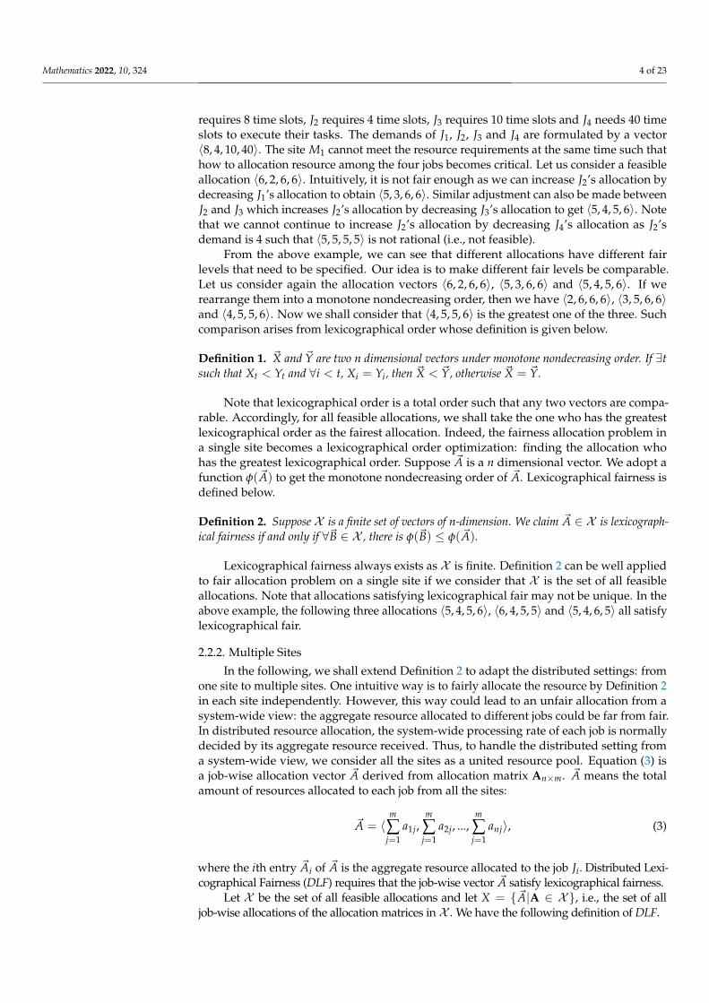
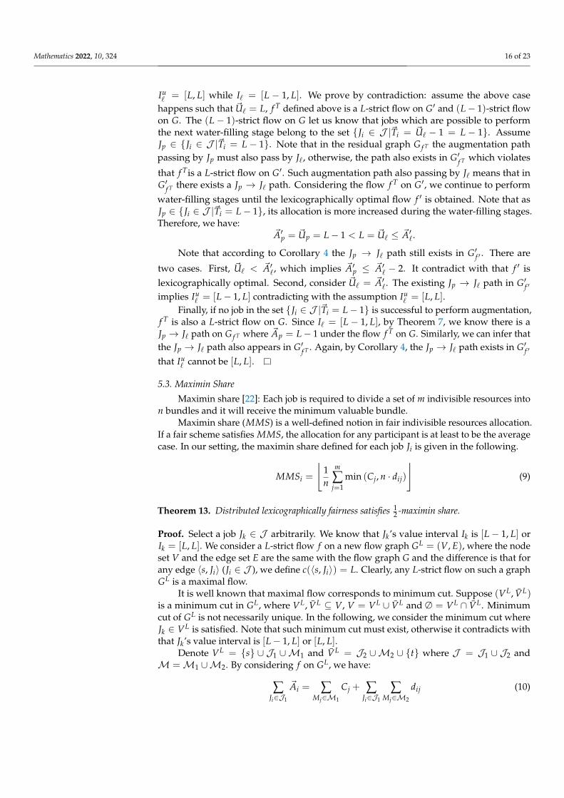
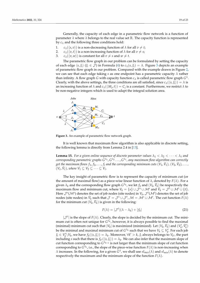
The parametric flow graph in our problem can be formulated by setting the capacityof each edge 〈s, Ji〉 (Ji ∈ J ) in Formula (4) to cλ(s, Ji) = λ. Figure 3 depicts an exampleof parametric flow graph in our problem. Compared with the example drawn in Figure 2,we can see that each edge taking s as one endpoint has a parametric capacity λ ratherthan infinity. A flow graph G with capacity function cλ is called parametric flow graph Gλ.Clearly, with the above settings, the three conditions are all satisfied, since cλ(〈s, Ji〉) = λ isan increasing function of λ and cλ(〈Mj, t〉) = Cj is a constant. Furthermore, we restrict λ tobe non-negative integers which is used to adapt the integral solution area.

dij

…

…

λ

λ λ λ

s

M1

t M2

Mm

Jobs Sites J1

J3

J2

Jn

C1

C2

C3

Figure 3. An example of parametric flow network graph.

It is well known that maximum flow algorithm is also applicable in discrete setting,the following lemma is directly from Lemma 2.4 in [13].

Lemma 15. For a given online sequence of discrete parameter values λ1 < λ2 < · · · < λ` andcorresponding parametric graphs Gλ1 , Gλ2 . . . , Gλ` , any maximum flow algorithm can correctlyget the maximum flows f1, f2, . . . , fl and the corresponding minimum cuts (V1, V1), (V2, V2), . . . ,(V`, V`), where V1 ⊆ V2 ⊆ · · · ⊆ V`.

The key insight of parametric flow is to represent the capacity of minimum cut (orthe amount of maximal flow) as a piece-wise linear function of λ, denoted by F(λ). For agiven λk and the corresponding flow graph Gλk , we let fk and (Vk, Vk) be respectively themaximum flow and minimum cut, where Vk = {s} ∪ J s ∪Ms and Vk = J t ∪Mt ∪ {t}.Here J s(Ms) denotes the set of job nodes (site nodes) in Vk, J t(Mt) denotes the set of jobnodes (site nodes) in Vk such that J = J s ∪ J t,M =Ms ∪Mt. The cut function F(λ)for the minimum cut (Vk, Vk) is given in the following:

F(λ) = |J t|(λ− λk) + | fk| (21)

|J t| is the slope of F(λ). Clearly, the slope is decided by the minimum cut. The mini-mum cut is often not unique for Gλk , however, it is always possible to find the maximal(minimal) minimum cut such that |Vk| is maximized (minimized). Let (Vk, Vk) and (V′k , V′k)be the minimal and maximal minimum cut of Gλk such that we have Vk ⊆ V′k . For each jobJi ∈ V′k\Vk, we have fk(〈s, Ji〉) = λk. Moreover, ∀k′ > k, Ji always belongs to Vk′ , the partincluding s such that there is fk′(〈s, Ji〉) = λk. We can also infer that the maximum slope ofcut function corresponding to Gλk+1 is not larger than the minimum slope of cut functioncorresponding to Gλk , i.e., the slope of the piece-wise function F(λ) is non-increasing whenλ increases. In the following, for a given Gλ, we shall use slmax(λ) and slmin(λ) to denoterespectively the maximum and the minimum slope of the function F(λ).

Mathematics 2022, 10, 324 20 of 23

6.1. Basic Algorithm

Based on the water-filling stages introduced in Section 4, we first propose a basicalgorithm which implements a sequence of water-filling stage until a lexicographicallyoptimal flow is obtained.

Theorem 16. A L-strict flow f on graph G is also a maximum flow on the parametric graph GL,where λ = L.

The feasibility of f on GL is straightforward. As L-strict ensures that there is noaugmenting path on GL

f , f is maximal on GL.The basic algorithm aims to solve a sequence of parametric flows where λ = 0, 1, . . . , vmax.

Although vmax cannot be foreknown, the process will be stopped until no job can get moreaggregate allocation by continuing to increase λ. The complexity of the basic algorithmdepends on the concrete maximum flow algorithm selected. If augmentation used inFord–Fulkerson is directly taken, the complexity of implementing each water-filling isO(|V|3). Overall, the complexity is O(vmax · |V|3) as there are vmax water-filling stages. Ifthe push-relabel algorithm (implemented with queue [13]) is take for implementing eachwater-filling stage, then the overall complexity decreases to O(|V|3 + vmax · |V|2) as onlythe first water-filling stage costs |V|3 operations. However, no matter which way is selectedfor implementing water-filling stage, the overall complexity is not strongly polynomial of|V|, since vmax is related to the input capacities which are upper-bounded by O(∑m

j=1 Cj).

6.2. Iterative Algorithm

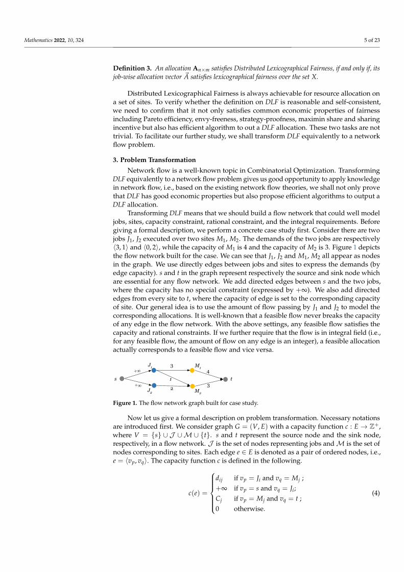
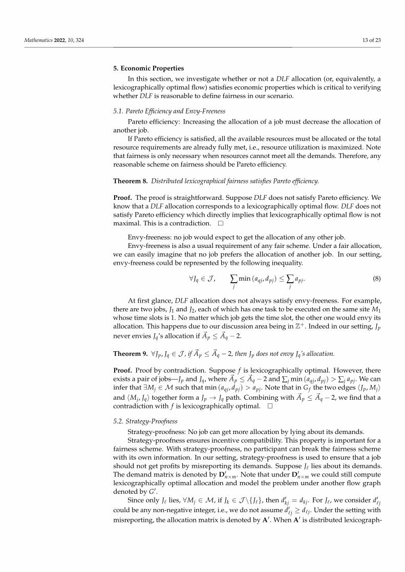
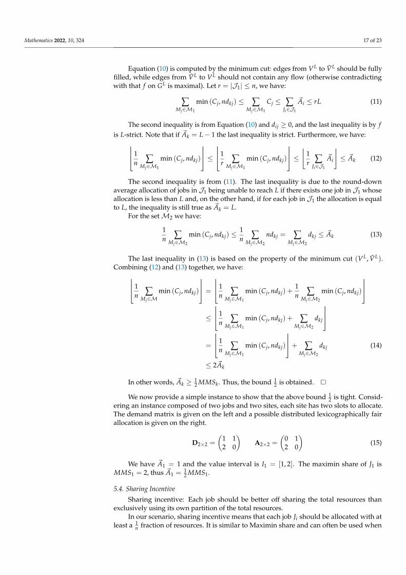
The basic algorithm is time-costly due to the algorithm being performed each timethe parameter λ is increased. However, increasing λ by one does not necessarily meanthe slope of F(λ) decreases immediately. Indeed, the slope of the piece-wise function F(λ)only decreases at a few special points (called breakpoints in the following). To understandbreakpoints, let us consider the first example where J1 and J2 execute over two sites M1and M2. The flow network is built in Figure 1. Let us explain the breakpoints by calculatinga DLF allocation for this example. The capacity of 〈s, J1〉 and 〈s, J2〉 is now expressed by avariable λ. Figure 4 depicts what happens when λ increases, and the dash line denotes theminimum cut. When 0 ≤ λ ≤ 2 (Figure 4a), the slope of F(λ) is equal to 2, i.e., for both〈s, J1〉 and 〈s, J2〉, their capacity expansion contributes to the increasing of F(λ). Note thatλ = 2 is the first breakpoint. When 2 < λ ≤ 4 (Figure 4b), only the capacity expansion of〈s, J1〉 contributes to the increasing of F(λ) such that the slope of F(λ) decreases to 1. λ = 4is the second breakpoint. When λ > 4 (Figure 4c), the increasing of λ will no more increaseF(λ) such that the slope decreases to 0. In Figure 4d, we depict the two breakpoints andshow the curve of F(λ).

Generally once the slope decreases, it means there exist some jobs whose aggregateallocation stops increasing. Consequently, we only need to focus on every breakpoint:we first set the parameter λ, then perform push-relabel maximum flow algorithm to geta λ-strict flow and finally compute a new slope for F(λ). When the computation of allbreakpoints is finished, we obtain a lexicographically optimal flow which corresponds to aDLF allocation.

Mathematics 2022, 10, 324 21 of 23

Source

2

2

5 6

3

6

2 Sink

（d）De_parameter

Source

2

2

5 6

3

2λ

λ Sink

（a）0≤λ≤2

Source

2

2

5 6

3

2λ

λ Sink

（b）2<λ≤3

Source

2

2

5 6

3

2λ

λ Sink

（c）λ>3

λ

1

J2 2

4

3

1

3

2

3

λ

λ λ

s

4

3

t

（a）0≤λ≤2

t

J1 M1

M2

J1

J2

M1

M2

J2

1

3

3 4

λ

λ s

2

（b）2<λ≤4

J1 M1

M2

s t

（c）λ>4

F (λ)

2 4

4

6

λ

breakpoints

0 （d）F (λ)

J1

J1

J1

J1

J2

J2

J2

J2

Two breakpoints: (2, 6) and (3, 8)

s1 s1

s1 s1

s2

s2

s2

s2

Figure 4. Example of piece-wise function F(λ) and breakpoints.

Based on the above idea, we propose a more efficient iterative algorithm. The pseudo-code is presented in Algorithm 1. The general idea is to maintain a parametric flowwith λ in an increasing order and identify each breakpoint sequentially. For a given λk,if slmax(λk) > slmin(λk) (which means there at least exists one job Ji whose aggregateallocation ~Ai = λk cannot be further increased), (λk, F(λk)) is a breakpoint. Remember thatour problem is considered in Z+. When a breakpoint identified is not an integer, we needto perform necessary rounding operations.

Algorithm 1: Iterative Algorithm

1 begin2 λ1 ← 1;3 Compute f1 on Gλ1 ;4 while slmin(λ1) > 0 do5 λ2 ← ∑m

j=1 Cj + 1; % set to the maximum value;6 Compute f2 on the reversed graph Gλ2 ;7 while True do8 fλ1(λ) = slmin(λ1)(λ− λ1) + | f1|;9 fλ2(λ) = slmax(λ2)(λ− λ2) + | f2|;

10 if slmin(λ1) = slmax(λ2) then11 if λ2 is not an integer then12 λ2 ← bλ2c;13 Update f1 to a maximum flow on Gλ2 ;14 λ2 ← λ2 + 1;15 Update f1 to a maximum flow on Gλ2 ;

16 else17 Update f1 to a maximum flow on Gλ2 ;

18 λ1 ← λ2;19 break;

20 λ2 ← | f2|−| f1|−λ2slmax(λ2)+λ1slmin(λ1)slmin(λ1)−slmax(λ2)

;

21 Update f2 to a maximum flow on the reversed graph Gλ2 ;

22 return f1;

In the first two lines of Algorithm 1, we set the parameter λ = 1 and run a push-labelalgorithm to get a 1-strict flow. Lines (4–11) contain the main iterative procedure wherethe key idea is using the Newton method to identify every breakpoint. More specifically,we first set a big enough value for λ2 ensuring that the slope of F(λ) at λ2 is 0. At line 8and line 9 we have two line functions which are all part of F(λ) but have difference slopes.

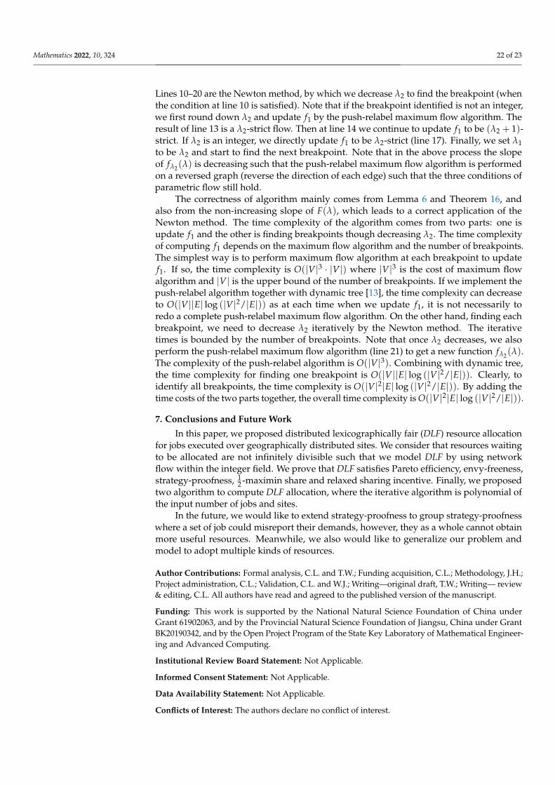
Mathematics 2022, 10, 324 22 of 23

Lines 10–20 are the Newton method, by which we decrease λ2 to find the breakpoint (whenthe condition at line 10 is satisfied). Note that if the breakpoint identified is not an integer,we first round down λ2 and update f1 by the push-relabel maximum flow algorithm. Theresult of line 13 is a λ2-strict flow. Then at line 14 we continue to update f1 to be (λ2 + 1)-strict. If λ2 is an integer, we directly update f1 to be λ2-strict (line 17). Finally, we set λ1to be λ2 and start to find the next breakpoint. Note that in the above process the slopeof fλ2(λ) is decreasing such that the push-relabel maximum flow algorithm is performedon a reversed graph (reverse the direction of each edge) such that the three conditions ofparametric flow still hold.

The correctness of algorithm mainly comes from Lemma 6 and Theorem 16, andalso from the non-increasing slope of F(λ), which leads to a correct application of theNewton method. The time complexity of the algorithm comes from two parts: one isupdate f1 and the other is finding breakpoints though decreasing λ2. The time complexityof computing f1 depends on the maximum flow algorithm and the number of breakpoints.The simplest way is to perform maximum flow algorithm at each breakpoint to updatef1. If so, the time complexity is O(|V|3 · |V|) where |V|3 is the cost of maximum flowalgorithm and |V| is the upper bound of the number of breakpoints. If we implement thepush-relabel algorithm together with dynamic tree [13], the time complexity can decreaseto O(|V||E| log (|V|2/|E|)) as at each time when we update f1, it is not necessarily toredo a complete push-relabel maximum flow algorithm. On the other hand, finding eachbreakpoint, we need to decrease λ2 iteratively by the Newton method. The iterativetimes is bounded by the number of breakpoints. Note that once λ2 decreases, we alsoperform the push-relabel maximum flow algorithm (line 21) to get a new function fλ2(λ).The complexity of the push-relabel algorithm is O(|V|3). Combining with dynamic tree,the time complexity for finding one breakpoint is O(|V||E| log (|V|2/|E|)). Clearly, toidentify all breakpoints, the time complexity is O(|V|2|E| log (|V|2/|E|)). By adding thetime costs of the two parts together, the overall time complexity is O(|V|2|E| log (|V|2/|E|)).

7. Conclusions and Future Work

In this paper, we proposed distributed lexicographically fair (DLF) resource allocationfor jobs executed over geographically distributed sites. We consider that resources waitingto be allocated are not infinitely divisible such that we model DLF by using networkflow within the integer field. We prove that DLF satisfies Pareto efficiency, envy-freeness,strategy-proofness, 1

2 -maximin share and relaxed sharing incentive. Finally, we proposedtwo algorithm to compute DLF allocation, where the iterative algorithm is polynomial ofthe input number of jobs and sites.

In the future, we would like to extend strategy-proofness to group strategy-proofnesswhere a set of job could misreport their demands, however, they as a whole cannot obtainmore useful resources. Meanwhile, we also would like to generalize our problem andmodel to adopt multiple kinds of resources.

Author Contributions: Formal analysis, C.L. and T.W.; Funding acquisition, C.L.; Methodology, J.H.;Project administration, C.L.; Validation, C.L. and W.J.; Writing—original draft, T.W.; Writing— review& editing, C.L. All authors have read and agreed to the published version of the manuscript.

Funding: This work is supported by the National Natural Science Foundation of China underGrant 61902063, and by the Provincial Natural Science Foundation of Jiangsu, China under GrantBK20190342, and by the Open Project Program of the State Key Laboratory of Mathematical Engineer-ing and Advanced Computing.

Institutional Review Board Statement: Not Applicable.

Informed Consent Statement: Not Applicable.

Data Availability Statement: Not Applicable.

Conflicts of Interest: The authors declare no conflict of interest.

Mathematics 2022, 10, 324 23 of 23

References1. Pu, Q.; Ananthanarayanan, G.; Bodik, P.; Kandula, S.; Akella, A.; Bahl, P.; Stoica, I. Low latency geo-distributed data analytics.

ACM SIGCOMM Comput. Commun. Rev. 2015, 45, 421–434. [CrossRef]2. Vulimiri, A.; Curino, C.; Godfrey, P.B.; Jungblut, T.; Padhye, J.; Varghese, G. Global Analytics in the Face of Bandwidth and

Regulatory Constraints. NSDI 2015, 7, 7–8.3. Brams, S.J.; Taylor, A.D. Fair Division- from Cake-Cutting to Dispute Resolution; Cambridge University Press: Cambridge, UK , 1996.4. Moulin, H. Fair Division and Collective Welfare; MIT Press: Cambridge, MA, USA, 2003.5. Brandt, F.; Conitzer, V.; Endriss, U.; Lang, J.; Procaccia, A.D. (Eds.) Handbook of Computational Social Choice; Cambridge University

Press: Cambridge, UK, 2016.6. Bertsekas, D.P.; Gallager, R.G.; Humblet, P. Data Networks; Prentice-Hall International: Hoboken, NJ, USA , 1992; Volume 2.7. Radunovic, B.; Boudec, J.Y.L. A unified framework for max-min and min-max fairness with applications. IEEE/ACM Trans. Netw.

(TON) 2007, 15, 1073–1083. [CrossRef]8. Ghodsi, A.; Zaharia, M.; Hindman, B.; Konwinski, A.; Shenker, S.; Stoica, I. Dominant Resource Fairness: Fair Allocation of

Multiple Resource Types. In Proceedings of the 8th USENIX Symposium on Networked Systems Design and Implementation,NSDI, Boston, MA, USA, 30 March–1 April 2011.

9. Dolev, D.; Feitelson, D.G.; Halpern, J.Y.; Kupferman, R.; Linial, N. No justified complaints: On fair sharing of multiple resources.In Proceedings of the 3rd Innovations in Theoretical Computer Science Conference, Cambridge, MA, USA, 8–10 August 2012.

10. Bonald, T.; Roberts, J. Multi-resource fairness: Objectives, algorithms and performance. In Proceedings of the ACM SIGMETRICSPerformance Evaluation Review; ACM: New York, NY, USA, 2015; Volume 43, pp. 31–42.

11. Wang, W.; Li, B.; Liang, B. Dominant resource fairness in cloud computing systems with heterogeneous servers. In Proceedingsof the IEEE INFOCOM 2014—IEEE Conference on Computer Communications, Toronto, ON, Canada, 27 April–2 May 2014;pp. 583–591.

12. Guan, Y.; Li, C.; Tang, X. On Max-min Fair Resource Allocation for Distributed Job Execution. In Proceedings of the 48thInternational Conference on Parallel Processing, ICPP, Kyoto, Japan, 5–8 August 2019; pp. 55:1–55:10.

13. Gallo, G.; Grigoriadis, M.D.; Tarjan, R.E. A Fast Parametric Maximum Flow Algorithm and Applications. SIAM J. Comput. 1989,18, 30–55. [CrossRef]

14. Schrijver, A. Combinatorial Optimization: Polyhedra and Efficiency; Springer Science & Business Media: Berlin/Heidelberg, Germany,2003; Volume 24.

15. Berge, C. Two theorems in graph theory. Proc. Natl. Acad. Sci. USA 1957, 43, 842. [CrossRef] [PubMed]16. Norman, R.Z.; Rabin, M.O. An algorithm for a minimum cover of a graph. Proc. Am. Math. Soc. 1959, 10, 315–319. [CrossRef]17. Fulkerson, D.; Ford, L. Flows in Networks; Princeton University Press Princeton: Princeton, NJ, USA, 1962.18. Megiddo, N. Optimal flows in networks with multiple sources and sinks. Math. Program. 1974, 7, 97–107. [CrossRef]19. Megiddo, N. A good algorithm for lexicographically optimal flows in multi-terminal networks. Bull. Am. Math. Soc. 1977,

83, 407–409. [CrossRef]20. Dinic, E.A. Algorithm for solution of a problem of maximum flow in networks with power estimation. Sov. Math. Dokl. 1970, 11,

1277–1280.21. Bernstein, A.; Kopelowitz, T.; Pettie, S.; Porat, E.; Stein, C. Simultaneously Load Balancing for Every p-norm, with Reassignments.

In Proceedings of the 8th Innovations in Theoretical Computer Science Conference, ITCS 2017, Berkeley, CA, USA, 9–11 January2017; pp. 51:1–51:14.

22. Kurokawa, D.; Procaccia, A.D.; Wang, J. Fair Enough: Guaranteeing Approximate Maximin Shares. J. ACM 2018, 65, 8:1–8:27.[CrossRef]

23. Goldberg, A.V.; Tarjan, R.E. A New Approach to the Maximum Flow Problem. In Proceedings of the 18th Annual ACMSymposium on Theory of Computing, Berkeley, CA, USA, 28–30 May 1986; pp. 136–146. [CrossRef]