Towards a query optimizer for text-centric tasks

Towards a Query Optimizer for Text-Centric Tasks

Panagiotis G. IpeirotisNew York University

Eugene AgichteinEmory University

Pranay JainColumbia University

Luis GravanoColumbia University

October 28, 2006

Abstract

Text is ubiquitous and, not surprisingly, many important applications rely on textual data fora variety of tasks. As a notable example, information extraction applications derive structuredrelations from unstructured text; as another example, focused crawlers explore the web to locatepages about specific topics. Execution plans for text-centric tasks follow two general paradigmsfor processing a text database: either we can scan, or “crawl,” the text database or, alternatively,we can exploit search engine indexes and retrieve the documents of interest via carefully craftedqueries constructed in task-specific ways. The choice between crawl- and query-based executionplans can have a substantial impact on both execution time and output “completeness” (e.g.,in terms of recall). Nevertheless, this choice is typically ad-hoc and based on heuristics or plainintuition. In this article, we present fundamental building blocks to make the choice of executionplans for text-centric tasks in an informed, cost-based way. Towards this goal, we show how toanalyze query- and crawl-based plans in terms of both execution time and output completeness.We adapt results from random-graph theory and statistics to develop a rigorous cost model forthe execution plans. Our cost model reflects the fact that the performance of the plans dependson fundamental task-specific properties of the underlying text databases. We identify theseproperties and present efficient techniques for estimating the associated parameters of the costmodel. We also present two optimization approaches for text-centric tasks that rely on the cost-model parameters and select efficient execution plans. Overall, our optimization approacheshelp build efficient execution plans for a task, resulting in significant efficiency and outputcompleteness benefits. We complement our results with a large-scale experimental evaluationfor three important text-centric tasks and over multiple real-life data sets.

1 Introduction

Text is ubiquitous and, not surprisingly, many applications rely on textual data for a variety oftasks. For example, information extraction applications retrieve documents and extract structuredrelations from the unstructured text in the documents. Reputation management systems downloadweb pages to track the “buzz” around companies and products. Comparative shopping agentslocate e-commerce web sites and add the products offered in the pages to their own index.

To process a text-centric task over a text database (or the web), we can retrieve the relevantdatabase documents in different ways. One approach is to scan or crawl the database to retrieve itsdocuments and process them as required by the task. While such an approach guarantees that wecover all documents that are potentially relevant for the task, this method might be unnecessarilyexpensive in terms of execution time. For example, consider the task of extracting information ondisease outbreaks (e.g., the name of the disease, the location and date of the outbreak, and the

1

number of affected people) as reported in news articles. This task does not require that we scanand process, say, the articles about sports in a newspaper archive. In fact, only a small fractionof the archive is of relevance to the task. For tasks such as this one, a natural alternative tocrawling is to exploit a search engine index on the database to retrieve –via careful querying– theuseful documents. In our example, we can use keywords that are strongly associated with diseaseoutbreaks (e.g., “World Health Organization,” “case fatality rate”) and turn these keywords intoqueries to find news articles that are appropriate for the task.

The choice between a crawl- and a query-based execution strategy for a text-centric task isanalogous to the choice between a scan- and an index-based execution plan for a selection queryover a relation. Just as in the relational model, the choice of execution strategy can substantiallyaffect the execution time of the task. In contrast to the relational world, however, this choicemight also affect the quality of the output that is produced: while a crawl-based execution of atext-centric task guarantees that all documents are processed, a query-based execution might misssome relevant documents, hence producing potentially incomplete output, with less-than-perfectrecall. The choice between crawl- and query-based execution plans can then have a substantialimpact on both execution time and output recall. Nevertheless, this important choice is typicallyleft to simplistic heuristics or plain intuition.

In this article, we introduce fundamental building blocks for the optimization of text-centrictasks. Towards this goal, we show how to rigorously analyze query- and crawl-based plans for atask in terms of both execution time and output recall. To analyze crawl-based plans, we applytechniques from statistics to model crawling as a document sampling process; to analyze query-based plans, we first abstract the querying process as a random walk on a querying graph, andthen apply results for the theory of random graphs to discover relevant properties of the queryingprocess. Our cost model reflects the fact that the performance of the execution plans depends onfundamental task-specific properties of the underlying text databases. We identify these propertiesand present efficient techniques for estimating the associated parameters of the cost model.

In brief, the contributions and content of the article are as follows:

• A novel framework for analyzing crawl- and query-based execution plans for text-centric tasksin terms of execution time and output recall (Section 3).

• A description of four crawl- and query-based execution plans, which underlie the implemen-tation of many existing text-centric tasks (Section 4).

• A rigorous analysis of each execution plan alternative in terms of execution time and re-call; this analysis relies on fundamental task-specific properties of the underlying databases(Section 5).

• Two optimization approaches that estimate “on-the-fly” the database properties that affectthe execution time and recall of each plan. The first alternative follows a “global” optimizationapproach, to identify a single execution plan that is capable of reaching the target recall forthe task. The second alternative partitions the optimization task into “local” chunks; thisapproach potentially switches between execution strategies by picking the best strategy forretrieving the “next-k” tokens at each execution stage (Section 6).

• An extensive experimental evaluation showing that our optimization strategy is accurate andresults in significant performance gains. Our experiments include three important text-centrictasks and multiple real-life data sets (Sections 7 and 8).

2

… … …Cholera 1999 NigeriaYellow fever 2005 MaliDiseaseName Date Country

From what we know, 28 fatal cases of yellow fever were reported toMali’s national health authorities

within 2005…

The New York TimesArchive

...from what we know, 28 fatal cases of yellow fever were reported toMali’s national health authorities

within 2005….


within 2005….


within 2005….

Cholera outbreaks occurred in May 1999 in Nigeria (176 cases, 56 deaths). The outbreak is now


within 2005….

Cholera outbreaks occurred in May 1999 in Nigeria (176 cases, 56

deaths). The outbreak is now under control…

DiseaseOutbreaks in The New York Times Archive

Figure 1: Extracting DiseaseOutbreaks tuples

Finally, Section 9 discusses related work, while Section 10 provides further discussion and concludesthe article. This article expands on earlier work by the same authors [IAJG06,AIG03], as discussedin Section 9.

Note to Referees

This article contains material from an earlier conference publication [IAJG06] (which, in turn, builton an even earlier workshop publication [AIG03]). The current submission substantially extendsthe published material. More specifically:

• In this article, we present a detailed description of our methodology for estimating the pa-rameter values required by our cost model (Sections 6.1.1 through 6.1.4). In [IAJG06], dueto space restrictions, we only gave a high-level overview of our techniques.

Another substantial new contribution with respect to [IAJG06] is that now our optimizers donot rely on knowledge of the |Tokens| statistics, but instead estimate this parameter “on-the-fly” as well, during execution of the task.

• In this article, we present a new, “local” optimizer that potentially builds “multi-strategy”executions by picking the best strategy for each batch of k tokens (Section 6.2). In contrast,the “global” optimizer in [IAJG06] only attempts to identify a single execution plan that iscapable of reaching the full target recall.

We implemented the new local optimization approach and compared it experimentally againstthe global approach of [IAJG06]; the results of the comparison are presented in Figures 26,27, 28, and 29, in Section 8. The results show the superiority of the local optimizer over theglobal optimizer.

2 Examples of Text-Centric Tasks

In this section, we briefly review three important text-centric tasks that we will use throughout thearticle as running examples, to illustrate our framework and techniques.

3

….

Microsoft 145Word Frequency

….…. ….….

….

Retailers prepare for launch day of

Microsoft’s Xbox 360

Best Buy takes to the desert to

celebrate Xbox launchSony BMG offers

MP3 files and disks for unsafe CDs

Sony 96Xbox 124

...

.........

Content Summary of Forbes.comForbes.com

Figure 2: Content summary of Forbes.com

2.1 Task 1: Information Extraction

Unstructured text (e.g., in newspaper articles) often embeds structured information that can beused for answering relational queries or for data mining. The first task that we consider is theextraction of structured information from text databases. An example of an information extractiontask is the construction of a table DiseaseOutbreaks(DiseaseName, Date, Country) of reporteddisease outbreaks from a newspaper archive (see Figure 1). A tuple 〈yellow fever, 2005, Mali〉might then be extracted from the news articles in Figure 1.

Information extraction systems typically rely on patterns —either manually created or learnedfrom training examples— to extract the structured information from the documents in a database.The extraction process is usually time consuming, since information extraction systems might relyon a range of expensive text analysis functions, such as parsing or named-entity tagging (e.g., toidentify all person names in a document). See [Gri97] for an introductory survey on informationextraction.

A straightforward execution strategy for an information extraction task is to retrieve and pro-cess every document in a database exhaustively. As a refinement, an alternative strategy might usefilters and do the expensive processing of only “promising” documents; for example, the Proteus sys-tem [GHY02] ignores database documents that do not include words such as “virus” and “vaccine”when extracting the DiseaseOutbreaks relation. As an alternative, query-based approaches such asQXtract [AG03] have been proposed to avoid retrieving all documents in a database; instead, theseapproaches retrieve appropriate documents via carefully crafted queries.

2.2 Task 2: Content Summary Construction

Many text databases have valuable contents “hidden” behind search interfaces and are hence ig-nored by search engines such as Google. Metasearchers are helpful tools for searching over manydatabases at once through a unified query interface. A critical step for a metasearcher to process aquery efficiently and effectively is the selection of the most promising databases for the query. Thisstep typically relies on statistical summaries of the database contents [CLC95, GGMT99]. Thesecond task that we consider is the construction of a content summary of a text database. Thecontent summary of a database generally lists each word that appears in the database, togetherwith its frequency. For example, Figure 2 shows that the word “xbox” appears in 124 documentsin the Forbes.com database. If we have access to the full contents of a database (e.g., via crawl-ing), it is straightforward to derive these simple content summaries. If, in contrast, we only haveaccess to the database contents via a limited search interface (e.g., as is the case for “hidden-web” databases [Ber01]), then we need to resort to query-based approaches for content summaryconstruction [CC01, IG02].

4

London Hotels

Encyclopedia of Plants

Plant Physiology

Weather Information Hepaticophytawww.plantphysiol.orgwaynesword.palomar.edu/...www.botanyworld.comURL

Botany Documents on the WebWeb

...

Figure 3: Focused resource discovery for Botany pages

2.3 Task 3: Focused Resource Discovery

Text databases often contain documents on a variety of topics. Over the years, a number ofspecialized search engines (as well as directories) that focus on a specific topic of interest have beenproposed (e.g., FindLaw). The third task that we consider is the identification of the databasedocuments that are about the topic of a specialized search engine, or focused resource discovery.

As an example of focused resource discovery, consider building a search engine that specializesin documents on botany from the web at large (see Figure 3). For this, an expensive strategy wouldcrawl all documents on the web and apply a document classifier [Seb02] to each crawled page todecide whether it is about botany (and hence should be indexed) or not (and hence should beignored). As an alternative execution strategy, focused crawlers (e.g., [CvdBD99,CPS02,MPS04])concentrate their effort on documents and hyperlinks that are on-topic, or likely to lead to on-topicdocuments, as determined by a number of heuristics. Focused crawlers can then address the focusedresource discovery task efficiently at the expense of potentially missing relevant documents. As yetanother alternative, Cohen and Singer [CS96] propose a query-based approach for this task, wherethey exploit search engine indexes and use queries derived from a document classifier to quicklyidentify pages that are relevant to a given topic.

3 Describing Text-Centric Tasks

While the text-centric examples of Section 2 might appear substantially different on the surface,they all operate over a database of text documents and also share other important underlyingsimilarities.

Each task in Section 2 can be regarded as deriving “tokens” from a database, where a token isa unit of information that we define in a task-specific way. For Task 1, the tokens are the relationtuples that are extracted from the documents. For Task 2, the tokens are the words in the database(accompanied by the associated word frequencies). For Task 3, the tokens are the documents (orweb pages) in the database that are about the topic of focus.

The execution strategies for the tasks in Section 2 rely on task-specific document processors toderive the tokens associated with the task. For Task 1, the document processor is the informationextraction system of choice (e.g., Proteus [GHY02], DIPRE [Bri98], Snowball [AG00]): given adocument, the information extraction system extracts the tokens (i.e., the tuples) that are presentin the document. For Task 2, the document processor extracts the tokens (i.e., the words) that arepresent in a given document, and the associated document frequencies are updated accordingly inthe content summary. For Task 3, the document processor decides (e.g., via a document classifiersuch as Naive Bayes [DH73] or Support Vector Machines [Vap98]) whether a given document is

5

about the topic of focus; if the classifier deems the document relevant, the document is added as atoken to the output and is discarded otherwise.

The alternate execution strategies for the Section 2 tasks differ in how they retrieve the inputdocuments for the document processors, as we will discuss in Section 4. Some execution strategiesfully process every available database document, thus guaranteeing the extraction of all the tokensthat the underlying document processor can derive from the database. In contrast, other executionstrategies focus, for efficiency, on a strict subset of the database documents, hence potentiallymissing tokens that would have been derived from unexplored documents. One subcategory appliesa filter (e.g., derived in a training stage) to each document to decide whether to fully process it ornot. Other strategies retrieve via querying the documents to be processed, where the queries canbe derived in a number of ways that we will discuss. All these alternate execution strategies thusexhibit different tradeoffs between execution time and output recall.

Definition 3.1 [Execution Time] Consider a text-centric task, a database of text documentsD, and an execution strategy S for the task, with an underlying document processor P . Then, wedefine the execution time of S over D, Time(S, D), as

Time(S, D) = tT (S) +∑

q∈Qsent

tQ(q) +∑

d∈Dretr

(tR(d) + tF (d)

)+

∑d∈Dproc

tP (d) (1)

where

• Qsent is the set of queries sent by S,

• Dretr is the set of documents retrieved by S (Dretr ⊆ D),

• Dproc is the set of documents that S processes with document processor P (Dproc ⊆ D),

• tT (S) is the time for training the execution strategy S,

• tQ(q) is the time for evaluating a query q,

• tR(d) is the time for retrieving a document d,

• tF (d) is the time for filtering a retrieved document d, and

• tP (d) is the time for processing a document d with P .

Assuming that the time to evaluate a query is constant across queries (i.e., tQ = tQ(q), for everyq ∈ Qsent) and that the time to retrieve, filter, or process a single document is constant acrossdocuments (i.e., tR = tR(d), tF = tF (d), tP = tP (d), for every d ∈ D), we have:

Time(S, D) = tT (S) + tQ · |Qsent |+(tR + tF

)· |Dretr |+ tP · |Dproc | (2)

2

Definition 3.2 [Recall] Consider a text-centric task, a database of text documents D, and anexecution strategy S for the task, with an underlying document processor P . Let Dproc be the setof documents from D that S processes with P . Then, we define the recall of S over D, Recall(S, D),as

Recall(S, D) =|Tokens(P,Dproc)||Tokens(P,D)|

(3)

where Tokens(P,D) is the set of tokens that the document processor P extracts from the set ofdocuments D. 2

6

Input: database D, recall threshold τ , document processor POutput: tokens Tokensretr

Tokensretr = ∅, Dretr = ∅, recall = 0while recall < τ do

Retrieve an unprocessed document d and add d to Dretr

Process d using P and add extracted tokens to Tokensretr

recall = |Tokensretr |/|Tokens|endreturn Tokensretr

Figure 4: The Scan strategy

Our problem formulation is close, conceptually, to the evaluation of a selection predicate in anRDBMS. In relational databases, the query optimizer selects an access path (i.e., a sequential scanor a set of indexes) that is expected to lead to an efficient execution. We follow a similar structurein our work. In the next section, we describe the alternate evaluation methods that are at the coreof the execution strategies for text-centric tasks that have been discussed in the literature.1 Then,in subsequent sections, we analyze these strategies to see how their performance depends on thetask and database characteristics.

4 Execution Strategies

In this section, we review the alternate execution plans that can be used for the text-centric tasksdescribed above, and discuss how we can “instantiate” each generic plan for each task of Section 2.Our discussion assumes that each task has a target recall value τ , 0 < τ ≤ 1, that needs to beachieved (see Definition 3.2), and that the execution can stop as soon as the target recall is reached.

4.1 Scan

The Scan (SC) strategy is a crawl-based strategy that processes each document in a database Dexhaustively until the number of tokens extracted satisfies the target recall τ (see Figure 4).

The Scan execution strategy does not need training and does not send any queries to thedatabase. Hence, tT (SC) = 0 and |Qsent | = 0. Furthermore, Scan does not apply any filtering,hence tF = 0 and |Dproc | = |Dretr |. Therefore, the execution time of Scan is:

Time(SC, D) = |Dretr | · (tR + tP ) (4)

The Scan strategy is the basic evaluation strategy that many text-centric algorithms use whenthere are no efficiency issues, or when recall, which is guaranteed to be perfect according to Def-inition 3.2, is important. We should stress, though, that |Dretr | for Scan is not necessarily equalto |D|: when the target recall τ is low, or when tokens appear redundantly in multiple documents,Scan may reach the target recall without processing all the documents in D. In Section 5, we showhow to estimate the value of |Dretr | that is needed by Scan to reach a target recall τ .

1While it is impossible to analyze all existing techniques within a single article, we believe that we offer valuableinsight on how to formally analyze many query- and crawl-based strategies, hence offering the ability to predicta-priori the expected performance of an algorithm.

7

Input: database D, recall threshold τ , classifier C, document processor POutput: tokens Tokensretr

Tokensretr = ∅ , Dretr = ∅, recall = 0while recall < τ and |Dretr | < |D| do

Retrieve an unprocessed document d and add d to Dretr

Use C to classify d as useful for the task or notif d is useful then


endrecall = |Tokensretr |/|Tokens|

endreturn Tokensretr

Figure 5: The Filtered Scan strategy

A basic version of Scan accesses documents in random order. Variations of Scan might imposea specific processing order and prioritize, say, “promising” documents that are estimated to con-tribute many new tokens. Another natural improvement of Scan is to avoid processing altogetherdocuments expected not to contribute any tokens; this is the basic idea behind Filtered Scan, whichwe discuss next.

4.2 Filtered Scan

The Filtered Scan (FS) strategy is a variation of the basic Scan strategy. While Scan indistin-guishably processes all documents retrieved, Filtered Scan first uses a classifier C to decide whethera document d is useful, i.e., whether d contributes at least one token (see Figure 5). Given thepotentially high cost of processing a document with the document processor P , a quick rejectionof useless documents can speed up the overall execution considerably.

The training time tT (FS) for Filtered Scan is equal to the time required to build the classifierC for a specific task. Training represents a one-time cost for a task, so in a repeated execution ofthe task (i.e., over a new database) the classifier will be available with tT (FS) = 0. This is thecase that we assume in the rest of the analysis. Since Filtered Scan does not send any queries,|Qsent | = 0. While Filtered Scan retrieves and classifies |Dretr | documents, it actually processesonly Cσ · |Dretr | documents, where Cσ is the “selectivity” of the classifier C, defined as the fractionof database documents that C judges as useful. Therefore, according to Definition 2, the executiontime of Filtered Scan is:

Time(FS, D) = |Dretr | ·(tR + tF + Cσ · tP

)(5)

In Section 5, we show how to estimate the value of |Dretr | that is needed for Filtered Scan to reachthe target recall τ .

Filtered Scan is used when tP is high and there are many database documents that do notcontribute any tokens to the task at hand. For Task 1, Filtered Scan is used by Proteus [GHY02],which uses a hand-built set of inexpensive rules to discard useless documents. For Task 2, theFiltered Scan strategy is typically not applicable, since all the documents are useful. For Task 3,the Filtered Scan strategy corresponds to a “hard” focused crawler [CvdBD99] that prunes thesearch space by only considering documents that are pointed to by useful documents.

8

Input: database D, recall threshold τ , tokens Tokensseed , document processor POutput: tokens Tokensretr

Tokensretr = ∅, Dretr = ∅, recall = 0while Tokensseed 6= ∅ do

Remove a token t from Tokensseed

Transform t into a query q and issue q to DRetrieve up to maxD documents matching qforeach newly retrieved document d do

Add d to Dretr

Process d using P and add newly extracted tokens to Tokensretr and Tokensseed

recall = |Tokensretr |/|Tokens|if recall ≥ τ then

return Tokensretr

endend


Figure 6: The Iterative Set Expansion strategy

Both Scan and Filtered Scan are crawl-based strategies. Next, we describe two query-basedstrategies, Iterative Set Expansion, which emulates query-based strategies that rely on “bootstrap-ping” techniques, and Automatic Query Generation, which generates queries automatically, withoutusing the database results.

4.3 Iterative Set Expansion

Iterative Set Expansion (ISE) is a query-based strategy that queries a database with tokens as theyare discovered, starting with a typically small number of user-provided seed tokens Tokensseed . Theintuition behind this strategy is that known tokens might lead to unseen tokens via documents thathave both seen and unseen tokens (see Figure 6). Queries are derived from the tokens in a task-specific way. For example, a Task 1 tuple 〈Cholera, 1999,Nigeria〉 for DiseaseOutbreaks might beturned into query [Cholera AND Nigeria]; this query, in turn, might help retrieve documents thatreport other disease outbreaks, such as 〈Cholera, 2005,Senegal〉 and 〈Measles, 2004,Nigeria〉.

Iterative Set Expansion has no training phase, hence tT (ISE) = 0. We assume that IterativeSet Expansion has to send |Qsent | queries to reach the target recall. In Section 5, we show how toestimate this value of |Qsent |. Also, since Iterative Set Expansion processes all the documents thatit retrieves, tF = 0 and |Dproc | = |Dretr |. Then, according to Definition 3.1:

Time(ISE ,D) = |Qsent | · tQ + |Dretr | ·(tR + tP

)(6)

Informally, we expect Iterative Set Expansion to be efficient when tokens tend to co-occur in thedatabase documents. In this case, we can start from a few tokens and “reach” the remaining ones.(We define reachability formally in Section 5.4.) In contrast, this strategy might “stall” and leadto poor recall for scenarios when tokens occur in isolation, as was analyzed in [AIG03].

Iterative Set Expansion has been successfully applied in many tasks. For Task 1, Iterative SetExpansion corresponds to the Tuples algorithm for information extraction [AG03], which was shownto outperform crawl-based strategies when |Duseful | � |D|, where Duseful is the set of documents in

9

Input: database D, recall threshold τ , document processor P , queries QOutput: tokens Tokensretr

Tokensretr = ∅, Dretr = ∅, recall = 0foreach query q ∈ Q do

Retrieve up to maxD documents matching qforeach newly retrieved document d do

Add d to Dretr


recall = |Tokensretr |/|Tokens|if recall ≥ τ then

return Tokensretr

endend


Figure 7: The Automatic Query Generation strategy

D that “contribute” at least one token for the task. For Task 2, Iterative Set Expansion correspondsto the query-based sampling algorithm by Callan et al. [CCD99], which creates a content summaryof a database from a document sample obtained via query words derived (randomly) from thealready retrieved documents. For Task 3, Iterative Set Expansion is not directly applicable, sincethere is no notion of “co-occurrence.” Instead, strategies that start with a set of topic-specificqueries are preferable. Next, we describe such a query-based strategy.

4.4 Automatic Query Generation

Automatic Query Generation (AQG) is a query-based strategy for retrieving useful documents fora task. Automatic Query Generation works in two stages: query generation and execution. In thefirst stage, Automatic Query Generation trains a classifier to categorize documents as useful or notfor the task; then, rule-extraction algorithms derive queries from the classifier. In the executionstage, Automatic Query Generation searches a database using queries that are expected to retrieveuseful documents. For example, for Task 3 with botany as the topic, Automatic Query Generationgenerates queries such as [plant AND phylogeny ] and [phycology ]. (See Figure 7.)

The training time for Automatic Query Generation involves downloading a training set Dtrain

of documents and processing them with P , incurring a cost of |Dtrain | · (tR + tP ). Training timealso includes the time for the actual training of the classifier. This time depends on the learningalgorithm and is, typically, at least linear in the size of Dtrain . Training represents a one-time costfor a task, so in a repeated execution of the task (i.e., over a new database) the classifier will beavailable with tT (AQG) = 0. This is the case that we assume in the rest of the analysis. Duringexecution, the Automatic Query Generation strategy sends |Qsent | queries and retrieves |Dretr |documents, which are then all processed by P , without any filtering2 (i.e., |Dproc | = |Dretr |). InSection 5, we show how to estimate the values of |Qsent | and |Dretr | that are needed for Automatic

2Note that we could also consider “filtered” versions of Iterative Set Expansion and Automatic Query Generation,just as we do for Scan. For brevity, we do not study such variations: filtering is less critical for the query-basedstrategies than for Scan, because queries generally retrieve a reasonably small fraction of the database documents.

10

Query Generation to reach a target recall τ . Then, according to Definition 3.1:

Time(AQG, D)= |Qsent | · tQ + |Dretr | ·(tR + tP

)(7)

The Automatic Query Generation strategy was proposed under the name QXtract for Task1 [AG03]; it was also used for Task 2 in [IG02] and for Task 3 in [CS96].

The description of the execution time has so far relied on parameters (e.g., |Dretr |) that arenot known before executing the strategies. In the next section, we focus on the central issue ofestimating these parameters. In the process, we show that the performance of each strategy dependsheavily on task-specific properties of the underlying database; then, in Section 6 we show how tocharacterize the required database properties and select the best execution strategy for a task.

5 Estimating Execution Plan Costs

In the previous section, we presented four alternative execution plans and described the executioncost for each plan. Our description focused on describing the main factors of the actual executiontime of each plan and did not provide any insight on how to estimate these costs: many of theparameters that appear in the cost equations are outcomes of the execution and cannot be used toestimate or predict the execution cost. In this section, we show that the cost equations described inSection 4 depend on a few fundamental task-specific properties of the underlying databases, suchas the distribution of tokens across documents. Our analysis reveals the strengths and weaknessesof the execution plans and (most importantly) provides an easy way to estimate the cost of eachtechnique for reaching a target recall τ . The rest of the section is structured as follows. First,Section 5.1 describes the notation and gives the necessary background. Then, Sections 5.2 and 5.3analyze the two crawl-based techniques, Scan and Filtered Scan, respectively. Finally, Sections 5.4and 5.5 analyze the two query-based techniques, Iterative Set Expansion and Automatic QueryGeneration, respectively.

5.1 Preliminaries

In our analysis, we use some task-specific properties of the underlying databases, such as thedistribution of tokens across documents. We use g(d) to represent the “degree” of a document dfor a document processor P , which is defined as the number of distinct tokens extracted from dusing P . Similarly, we use g(t) to represent the “degree” of a token t in a database D, which isdefined as the number of distinct documents that contain t in D. Finally, we use g(q) to representthe “degree” of a query q in a database D, which is defined as the number of documents from Dretrieved by query q.

In general, we do not know a-priori the exact distribution of the token, document, and querydegrees for a given task and database. However, we typically know the distribution family forthese degrees, and we just need to estimate a few parameters to identify the actual distribution forthe task and database. For Task 1, the document and token degrees tend to follow a power-lawdistribution [AIG03], as we will see in Section 7. For Task 2, token degrees follow a power-lawdistribution [Zip49] and document degrees follow roughly a lognormal distribution [Mit04]; weprovide further evidence in Section 7. For Task 3, the document and token distributions are, bydefinition, uniform over Duseful with g(t) = g(d) = 1. In Section 6, we describe how to estimate theparameters of each distribution.

11

t1 t2 tM

d1

d2

d3

dN

...

...

D

Tok ens

Samplingfor t1

Samplingfor t2

Samplingfor tM

Figure 8: Modeling Scan as multiple sampling processes, one per token, running in parallel over D

5.2 Cost of Scan

According to Equation 4, the cost of Scan is determined by the size of the set Dretr , which isthe number of documents retrieved to achieve a target recall τ .3 To compute |Dretr |, we base ouranalysis on the fact that Scan retrieves documents in no particular order and does not retrievethe same document twice. This process is equivalent to sampling from a finite population [Ros02].Conceptually, Scan samples for multiple tokens during execution. Therefore, we treat Scan asperforming multiple “sampling from a finite population” processes, running in parallel over D (seeFigure 8). Each sampling process corresponds to a token t ∈ Tokens. According to probabilitytheory [Ros02, page 56], the probability of observing a token t k times in a sample of size S followsthe hypergeometric distribution. For k = 0, we get the probability that t does not appear in thesample, which is

(|D|−g(t)S

)/(|D|

S

). The complement of this value is the probability that t appears in

at least one document in the set of S retrieved documents. So, after processing S documents, theexpected number of retrieved tokens for Scan is:

E[|Tokensretr |] =∑

t∈Tokens

1− (|D| − g(t))! (|D| − S)!(|D| − g(t)− S)!|D|!

(8)

Hence, we estimate4 the number of documents that Scan should retrieve to achieve a target recallτ as: |Dretr | = min{S : E[|Tokensretr |] ≥ τ |Tokens|} (9)

The number of documents |Dretr | retrieved by Scan depends on the token degree distribution. InFigure 9, we show the expected recall of Scan as a function of the number of retrieved documents,

3We assume that the values of tR and tP are known or that we can easily estimate them by repeatedly retrievingand processing a few sample documents.

4To avoid numeric overflows during the computation of the factorials, we first take the logarithm of the ratio(|D|−g(t))!(|D|−S)!(|D|−g(t)−S)!|D|! and then use the Stirling approximation ln x! ≈ x ln x − x + ln x

2+ 1

2ln 2π to efficiently compute

the logarithm of each factorial. After computing the value of the logarithm of the ratio, we simply compute theexponential of the logarithm to estimate the original value of the ratio.

12

g(t)=1g(t)=2g(t)=4.4

0

0.2

0.4

0.6

0.8

1

Reca

ll

20 40 60 80 100100% |Dretr| / |D|

Figure 9: Recall of the Scan strategy as a function of the fraction of retrieved documents, forg(t) = 1, g(t) = 2, and g(t) = 4.4

when g(t) is uniform for all tuples. For many databases, the distribution of g(t) is highly skewedand follows a power-law distribution: a few tokens appear in many documents, while the majorityof tokens can only be extracted from only a few documents. For example, the Task 1 tuple 〈SARS ,2003, China〉 can be extracted from hundreds of documents in the New York Times archive, whilethe tuple 〈Diphtheria, 2003, Afghanistan〉 appears only in a handful of documents. The recall ofScan for a given sample size S is lower over a database with a power-law token degree distributioncompared to the recall over a database with uniform token degree distribution, when the tokendegree distributions have the same mean value (see Figure 10). This is expected: while it is easyto discover the few very frequent tokens, it is hard to discover the majority of tokens, with lowfrequency. By estimating the parameters of the power-law distribution, we can then compute theexpected values of g(t) for the (unknown) tokens in D and use Equations 8 and 9 to derive theexpected cost of Scan. In Section 6, we show how to perform such estimations on-the-fly.

The analysis above assumes a random retrieval of documents. If the documents are retrievedin a special order, which is unlikely for the task scenarios that we consider, then we should modelScan as “stratified” sampling without replacement: instead of assuming a single sampling pass, wedecompose the analysis into multiple “strata” (i.e., into multiple sampling phases), each one withits own g(·) distribution. A simple instance of such technique is Filtered Scan, which (conceptually)samples useful documents first, as discussed next.

5.3 Cost of Filtered Scan

Filtered Scan is a variation of the basic Scan strategy, therefore the analysis of both strategies issimilar. The key difference between these strategies is that Filtered Scan uses a classifier to filterdocuments, which Scan does not. The Filtered Scan classifier thus limits the number of documentsprocessed by the document processor P . Two properties of the classifier C are of interest for ouranalysis:

• The classifier’s selectivity Cσ: if Dproc is the set of documents in D deemed useful by theclassifier (and then processed by P ), then Cσ = |Dproc |

|D| .

13

Power Law (beta=1.75)

Uniform

0.2

0.4

0.6

0.8

1

Reca

ll

20 40 60 80 100100% |Dretr| / |D|

Figure 10: Recall of the Scan strategy as a function of the fraction of retrieved documents, compar-ing the cases when g(t) is constant for each token t and when g(t) follows a power-law distribution(the mean value of g(t) is the same in both cases, E[g(t)] = 4.4)

• The classifier’s recall Cr: this is the fraction of useful documents in D that are also classifiedas useful by the classifier. The value of Cr affects the effective token degree for each tuple t:now each token appears, on average, Cr · g(t) times5 in Dproc , the set of documents actuallyprocessed by P .

Using these observations and following the methodology that we used for Scan, we have:


t∈Tokens

1− (Cσ ·|D| − Cr ·g(t))! (Cσ ·|D| − S)!(Cσ ·|D| − Cr ·g(t)− S)! (Cσ ·|D|)!

(10)

Again, similar to Scan, we have:

|Dretr | =|Dproc |Cσ

=min{S : E[|Tokensretr |] ≥ τ |Tokens|}

Cσ(11)

Equations 10 and 11 show the dependence of Filtered Scan on the performance of the classifier.When Cσ is high, almost all documents in D are processed by P , and the savings compared to Scanare minimal, if any. When a classifier has low recall Cr, then many useful documents are rejectedand the effective token degree decreases, in turn increasing |Dretr |. We should also emphasize thatif the recall of the classifier is low, then Filtered Scan is not guaranteed to reach the target recallτ . In this case, the maximum achievable recall might be less than one and |Dretr | = |D|.

5.4 Cost of Iterative Set Expansion

So far, we have analyzed two crawling-based strategies. Before moving to the analysis of the IterativeSet Expansion query-based strategy, we define “queries” more formally as well as a graph-basedrepresentation of the querying process, originally introduced in [AIG03].

5We assume uniform recall across tokens, i.e., that the classifier’s errors are not biased towards a specific set oftokens. This is a reasonable assumption for most classifiers. Nevertheless, we can easily extend the analysis andmodel any classifier bias by using a different classifier recall Cr(t) for each token t.

14

T D

t1

t3

t2

t4

d1

d3

d2

d4

t2

t1

t5

t3

t4

t5 d5

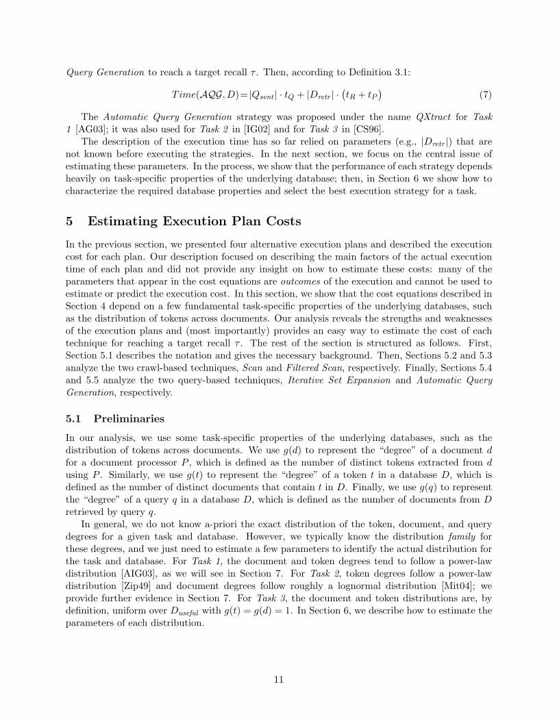
Figure 11: Portion of the querying and reachability graphs of a database

Definition 5.1 [Querying Graph] Consider a database D and a document processor P . Wedefine the querying graph QG(D,P ) of D with respect to P as a bipartite graph containing theelements of Tokens and D as nodes, where Tokens is the set of tokens that P derives from D. Adirected edge from a document node d to a token node t means that P extracts t from d. An edgefrom a token node t to document node d means that d is returned from D as a result to a queryderived from the token t. 2

For example, suppose that token t1, after being suitably converted into a query, retrieves a documentd1 and, in turn, that processor P extracts the token t2 from d1. Then, we insert an edge into QGfrom t1 to d1, and also an edge from d1 to t2. We consider an edge d → t, originating froma document node d and pointing to a token node t, as a “contains” edge, and an edge t → d,originating from a token node t and pointing to a document node d, as a “retrieves” edge.

Using the querying graph, we analyze the cost and recall of Iterative Set Expansion. As a simpleexample, consider the case where the initial Tokensseed set contains a single token, tseed . We startby querying the database using the query derived by tseed . The cost at this stage is a function ofthe number of documents retrieved by tseed : this is the number of neighbors at distance one fromtseed in the querying graph QG. The recall of Iterative Set Expansion, at this stage, is determinedby the number of tokens derived from the retrieved documents, which is equal to the number ofneighbors at distance two from tseed . Following the same principle, the cost in the next stage (afterquerying with the tokens at distance two) depends on the number of neighbors at distance threeand recall is determined by the number of neighbors at distance four, and so on.

The previous example illustrates that the recall of Iterative Set Expansion is bounded by thenumber of tokens “reachable” from the Tokensseed tokens; the execution time is also bounded by thenumber of documents and tokens that are “reachable” from the Tokensseed tokens. The structureof the querying graph thus defines the performance of Iterative Set Expansion. To compute theinteresting properties of the querying graph, we resort to the theory of random graphs: our approachis based on the methodology suggested by Newman et al. [NSW01] and uses generating functions todescribe the properties of the querying graph QG. We define the generating functions Gd0(x) and

15

Gt0(x) to describe the degree distribution6 of a randomly chosen document and token, respectively:

Gd0(x) =∑

k

pdk · xk, Gt0(x) =∑

k

ptk · xk (12)

where pdk is the probability that a randomly chosen document d contains k tokens (i.e., pdk =Pr{g(d) = k}) and ptk is the probability that a randomly chosen token t retrieves k documents(i.e., ptk = Pr{g(t) = k}) when used as a query.

In our setting, we are also interested in the degree distribution for a document (or token,respectively) chosen by following a random edge. Using the methodology of Newman et al. [NSW01],we define the functions Gd1(x) and Gt1(x) that describe the degree distribution for a documentand token, respectively, chosen by following a random edge:

Gd1(x) = xGd′0(x)Gd′0(1)

, Gt1(x) = xGt′0(x)Gt′0(1)

(13)

where Gd′0(x) is the first derivative of Gd0(x) and Gt′0(x) is the first derivative of Gt0(x), respec-tively. (See [NSW01] for the proof.)

For the rest of the analysis, we use the following useful properties of generating functions [Wil90]:

• Moments: The i-th moment of the probability distribution generated by a function G(x) isgiven by the i-th derivative of the generating function G(x), evaluated at x = 1. We mainlyuse this property to compute efficiently the mean of the distribution described by G(x).

• Power : If X1, . . . , Xm are independent, identically distributed random variables generated bythe generating function G(x), then the sum of these variables, Sm =

∑mi=1 Xi, has generating

function [G(x)]m.

• Composition: If X1, . . . , Xm are independent, identically distributed random variables gener-ated by the generating function G(x), and m is also an independent random variable generatedby the function F (x), then the sum Sm =

∑mi=1 Xi has generating function F (G(x)).

Using these properties and Equations 12 and 13, we can proceed to analyze the cost of IterativeSet Expansion. Assume that we are in the stage where Iterative Set Expansion has sent a set Q oftokens as queries. These tokens were discovered by following random edges on the graph; therefore,the degree distribution of these tokens is described by Gt1(x) (Equation 13). Then, by the Powerproperty, the distribution of the total number of retrieved documents (which are pointed to bythese tokens) is given by the generating function:7

Gd2(x) = [Gt1(x)]|Q| (14)

Now, we know that Dretr in Equation 6 is a random variable and its distribution is givenby Gd2(x). We also know that we retrieve documents by following random edges on the graph;therefore, the degree distribution of these documents is described by Gd1(x) (Equation 13). Then,

6We use undirected graph theory despite the fact that our querying graph is directed. Using directed graph resultswould of course be preferable, but it would require knowledge of the joint distribution of incoming and outgoingdegrees for all nodes of the querying graph, which would be challenging to estimate. So we rely on undirected graphtheory, which requires only knowledge of the two marginal degree distributions, namely the token and documentdegree distributions.

7This is the number of non-distinct documents. To compute the number of distinct documents, we use the sievemethod. For details, see [Wil90, page 110].

16

by the Composition property8, the distribution of the total number of tokens |Tokensretr | retrievedby the Dretr documents is given by the generating function:9

Gt2(x) = Gd2(Gd1(x)) = [Gt1(Gd1(x))]|Q| (15)

Finally, we use the Moments property to compute the expected values for |Dretr | and |Tokensretr |,after Iterative Set Expansion sends Q queries.

E[|Dretr |] =[

d

dx[Gt1(x)]|Q|

]x=1

(16)

E[|Tokensretr |] =[

d

dx[Gt1(Gd1(x))]|Q|

]x=1

(17)

Hence, the number of queries |Qsent | sent by Iterative Set Expansion to reach the target recall τ is:

|Qsent | = min{Q : E[|Tokensretr |] ≥ τ |Tokens|} (18)

Our analysis, so far, did not account for the fact that the tokens in a database are not always“reachable” in the querying graph from the tokens in Tokensseed . As we have briefly discussed,though, the ability to reach all the tokens is necessary for Iterative Set Expansion to achieve goodrecall. Before elaborating further on the subject, we describe the concept of the reachability graph,which we originally introduced in [AIG03] and is fundamental for our analysis.

Definition 5.2 [Reachability Graph] Consider a database D, and an execution strategy Sfor a task with an underlying document processor P and querying strategy R. We define thereachability graph RG(D,S) of D with respect to S as a graph whose nodes are the tokens that Pderives from D, and whose edge set E is such that a directed edge ti → tj means that P derives tjfrom a document that R retrieves using ti. 2

Figure 11 shows the reachability graph derived from an underlying querying graph, illustratinghow edges are added to the reachability graph. Since token t2 retrieves document d3 and d3 containstoken t3, the reachability graph contains the edge t2 → t3. Intuitively, a path in the reachabilitygraph from a token ti to a token tj means that there is a set of queries that start with ti and leadto the retrieval of a document that contains the token tj . In the example in Figure 11, there is apath from t2 to t4, through t3. This means that query t2 can help discover token t3, which in turnhelps discover token t4. The absence of a path from a token ti to a token tj in the reachabilitygraph means that we cannot discover tj starting from ti. This is the case for the tokens t2 and t5in Figure 11.

The reachability graph is a directed graph and its connectivity defines the maximum achievablerecall of Iterative Set Expansion: the upper limit for the recall of Iterative Set Expansion is equalto the total size of the connected components that include tokens in Tokensseed . In random graphs,typically we observe two scenarios: either the graph is disconnected and has a large number ofdisconnected components, or we observe a giant component and a set of small connected compo-nents. Chung and Lu [CL02] proved this for graphs with a power-law degree distribution, and alsoprovided the formulas for the composition of the size of the components. Newman et al. [NSW01]

8We use the Composition property and not the Power property because |Dretr | is a random variable.9Again, this is the number of non-distinct tokens. To compute the number of distinct tokens, we use the sieve

method. For details, see [Wil90, page 110].

17

provide similar results for graphs with arbitrary degree distributions. Interestingly for our problem,the size of the connected components can be estimated for many degree distributions using only asmall number of parameters (e.g., for power-law graphs we only need an estimate of the averagenode out-degree [CL02] to compute the size of the connected component; in Section 6 we explainhow we obtain such estimates). By estimating only a small number of parameters, we can thuscharacterize the performance limits of the Iterative Set Expansion strategy.

As discussed, Iterative Set Expansion relies on the discovery of new tokens to derive new que-ries. Therefore, in sparse and “disconnected” databases, Iterative Set Expansion can exhaust theavailable queries and still miss a significant part of the database, leading to low recall. In suchcases, if high recall is a requirement, different strategies are preferable. The alternative query-basedstrategy that we examine next, Automatic Query Generation, showcases a different querying ap-proach: instead of deriving new queries during execution, Automatic Query Generation generatesa set of queries offline and then queries the database without using query results as feedback.

5.5 Cost of Automatic Query Generation

Section 4.4 showed that the cost of Automatic Query Generation consists of two main components:the training cost and the querying cost. Training represents a one-time cost for a task, as discussedin Section 4.4, so we ignore it in our analysis. Therefore, the main component that remains to beanalyzed is the querying cost.

To estimate the querying cost of Automatic Query Generation, we need to estimate recall aftersending a set Q of queries and the number of retrieved documents |Dretr | at that point. Each queryq retrieves g(q) documents, and a fraction p(q) of these documents is useful for the task at hand.Assuming that the queries are biased only towards retrieving useful documents and not towardsany other particular set of documents, the queries are conditionally independent10 within the set ofdocuments Duseful and within the rest of the documents, Duseless . Therefore, the probability that auseful document is retrieved by a query q is p(q)·g(q)

|Duseful | . Hence, the probability that a useful documentd is retrieved by at least one query is:

1− Pr{d not retrieved by any query}=1−|Q|∏i=1

(1− p(qi) · g(qi)

|Duseful |

)So, given the values of p(qi) and g(qi), the expected number of useful documents that are retrievedis:

E[|Dusefulretr |] = |Duseful | ·

1−|Q|∏i=1

(1− p(qi) · g(qi)

|Duseful |

) (19)

and the number of useless documents retrieved is:

E[|Duselessretr |]= |Duseless | ·

1− |Q|∏i=1

(1− (1− p(qi)) · g(qi)

|Duseless |

) (20)

Assuming that the “precision” of a query q is independent of the number of documents that qretrieves,11 we get simpler expressions:

E[|Dusefulretr |]= |Duseful | ·

(1−

(1− E[p(q)] · E[g(q)]

|Duseful |

)|Q|)

(21)

10The conditional independence assumption implies that the queries are only biased towards retrieving usefuldocuments, and not towards any subset of useful documents.

11We observed this assumption to be true in practice.

18

E[|Duselessretr |]= |Duseless | ·

(1−

(1− (1− E[p(q)]) · E[g(q)]

|Duseless |

)|Q|)

(22)

where E[p(q)] is the average precision of the queries and E[g(q)] is the average number of retrieveddocuments per query. The expected number of retrieved documents is then:

E[|Dretr |] = E[|Dusefulretr |] + E[|Duseless

retr |] (23)

To compute the recall of Automatic Query Generation after issuing Q queries, we use thesame methodology that we used for Filtered Scan. Specifically, Equation 21 reveals the totalnumber of useful documents retrieved, and these are the documents that contribute to recall.These documents belong to Duseful . Hence, similarly to Scan and Filtered Scan, we model AutomaticQuery Generation as sampling without replacement ; the essential difference now is that the samplingis over the Duseful set. Therefore, we have an effective database size |Duseful | and a sample sizeequal to |Duseful

retr |.12 By modifying Equation 8 appropriately, we have:


t∈Tokens

1−(|Duseful | − g(t))!

(|Duseful | − |Duseful

retr |)!(

|Duseful | − g(t)− |Dusefulretr |

)!|Duseful |!

(24)

A good approximation of the average value of |Tokensretr | can be derived by setting S to be themean value of the |Duseful

retr | distribution (Equation 21). Similarly to the analysis for Iterative SetExpansion, we have: |Qsent | = min{Q : E[|Tokensretr |] ≥ τ |Tokens|} (25)

In this section, we analyzed four alternate execution plans and we showed how their executiontime and recall depend on fundamental task-specific properties of the underlying text databases.Next, we show how to exploit the parameter estimation and our cost model to significantly speedup the execution of text-centric tasks.

6 Putting it All Together

In Section 5, we examined how we can estimate the execution time and the recall of each executionplan by using the values of a few parameters, including the target recall τ and the token, document,and query degree distributions. In this section, we present two different optimization schemes. InSection 6.1, we present a “global” optimizer, which tries to pick the best execution strategy forreaching the target recall. Then, in Section 6.2 we present a “local” optimizer, which partitionsthe execution in multiple stages, and selects the best execution strategy for each stage. As we willshow in our experimental evaluation in Section 8, our optimization approaches leads to efficientexecutions of the text-centric tasks.

6.1 Global Optimization Approach

The goal of our global optimizer is to select an execution plan that will reach the target recall inminimum amount of time. The optimizer starts by choosing one of the execution plans describedin Section 4, using the cost model that we presented in Section 5.

12The documents Duselessretr increase the execution time but do not contribute towards recall and we ignore them for

recall computation.

19

Our cost model relies on a number of parameters, which are generally unknown before executinga task. Some of these parameters, such as classifier selectivity and recall (Section 5.3), can beestimated efficiently before the execution of the task. For example, the classifier characteristicsfor Filtered Scan and query degree and precision for Automatic Query Generation can be easilyestimated during classifier training using cross-validation [CMN98].

Other parameters of our cost model, namely the token and document distributions, are challeng-ing to estimate. Rather than attempting to estimate these distributions without prior information,we rely on the fact that for many text-centric tasks we know the general family of these distri-butions, as we discussed in Section 5.1. Hence, our estimation task reduces to estimating a fewparameters of well-known distribution families,13 which we discuss below.

To estimate the parameters of a distribution family for a concrete text-centric task and database,we could resort to a “preprocessing” estimation phase before we start executing the actual task. Forthis, we could follow —once again— Chaudhuri et al. [CMN98], and continue to sample databasedocuments until cross-validation indicates that the estimates are accurate enough. An interestingobservation is that having a separate preprocessing estimation phase is not necessary in our scenario,since we can piggyback such estimation phase into the initial steps of an actual execution of the task.In other words, instead of having a preprocessing estimation phase, we can start processing the taskand exploit the retrieved documents for “on-the-fly” parameter estimation. The basic challenge inthis scenario is to guarantee that the parameter estimates that we obtain during execution areaccurate. Below, we discuss how to perform the parameter estimation for each of the executionstrategies of Section 4.

6.1.1 Scan

Our analysis in Section 5.2 relies on the characteristics of the token and document degree dis-tributions. After retrieving and processing a few documents, we can estimate the distributionparameters based on the frequency of the initially extracted tokens and documents. Specifically,we can use a maximum likelihood fit to estimate the parameters of the document degree distribu-tion. For example, the document degrees for Task 1 tend to follow a power-law distribution, witha probability mass function Pr{g(d) = x} = x−β/ζ(β), where ζ(β) is the Riemman zeta functionζ(β) =

∑+∞n=1 n−β that serves as a normalizing factor. Our goal is to estimate the most likely

value of β, for a given sample of document degrees g(d1), . . . , g(ds). Using a maximum likelihoodestimation (MLE) approach, we identify the value of β that maximizes the likelihood function:

l(β|g(d1), . . . , g(ds)) =s∏

i=1

g(di)−β

ζ(β)

Taking the logarithm, we have the log-likelihood function:13Our current optimization framework follows a parametric approach, by assuming that we know the form of

the document and token degree distributions but not their exact parameters. Our framework can also be used ina completely non-parametric setting, in which we make no assumptions on the degree distributions; however, theestimation phase would be more expensive in such a setting. The development of an efficient, completely non-parametric framework is a topic for interesting future research.

20

L(β|g(d1), . . . , g(ds)) = log l(β|g(d1), . . . , g(ds))

=s∑

i=1

(−β log g(di)− log ζ(β))

= −s · log ζ(β)− β

s∑i=1

log g(di) (26)

To find the maximum of the log-likelihood function, we identify the value of β that makes the firstderivative of L be equal to zero:

d

dβL(β|g(d1), . . . , g(ds)) = 0

−s · ζ ′(β)ζ(β)

−s∑

i=1

log g(di) = 0

ζ ′(β)ζ(β)

= −1s

s∑i=1

log g(di) (27)

where ζ ′(β) is the first derivative of the Riemman zeta function. Then, we can estimate the valueof β using numeric approximation. Similar approaches can be used for other distribution families.

The estimation of the token degree distribution is typically more challenging than the estimationof the document degree distribution. While we can observe the degree g(d) of each document dretrieved in a document sample, we cannot directly determine the actual degree g(t) of each tokent extracted from sample documents. In general, the degree g(t) of a token t in a database is largerthan the degree of t in a document sample extracted from the database. Hence, before using themaximum likelihood approach described above, we should estimate, for each extracted token t, thetoken degree g(t) in the database.

We denote the sample degree of a token t as s(t), defined over a given document sample. Using,again, a maximum likelihood approach, we find the most likely token frequency g(t) that maximizesthe probability of observing the token frequency s(t) in the sample:

Pr{g(t)|s(t)} =Pr{s(t)|g(t)} · Pr{g(t)}

Pr{s(t)}(28)

Since Pr{s(t)} is constant across all possible values of g(t), we can ignore this factor for thismaximization problem. From Section 5.2, we know that the probability of retrieving s(t) times atoken t when it appears g(t) times in the database follows a hypergeometric distribution, and then:

Pr{s(t)|g(t)} =

(g(t)s(t)

)(|D|−g(t)S−s(t)

)(|D|S

)To estimate Pr{g(t)}, we rely on our knowledge of the distribution family of the token degrees.For example, the token degrees for Task 1 follow a power-law distribution, with Pr{g(t)} =g(t)−β/ζ(β). Then, for Task 1, we find the value of g(t) that maximizes the following:

Pr{s(t)|g(t)} · Pr{g(t)} =

(g(t)s(t)

)(|D|−g(t)S−s(t)

)(|D|S

) · g(t)−β

ζ(β)(29)

21

For this, we take the logarithm of the expression above and use the Stirling approximation14 toeliminate the factorials. We then find the value of g(t) for which the derivative of the logarithm ofthe expression above with respect to g(t) is equal to zero. Given the database size |D|, the samplesize S, and the sample degree s(t) of the token, we can estimate efficiently the maximum likelihoodestimate of g(t), for different values of the parameter(s) of the token degree distribution. Then,using these estimates of the database token degrees, we can proceed as in the document distributioncase and estimate the token distribution parameters.

The final step in the token distribution estimation is the estimation of the value of |Tokens|,which we need, as we will see, to evaluate Equation 8. Unfortunately, the Tokens set is, of course,unknown and so are the g(t) degrees on which Equation 8 relies. But during execution, we know thenumber of tokens that we extract from the documents that we retrieve, and this actual number ofextracted tokens should match the E[|Tokensretr |] prediction of Equation 8 for the correspondingvalues of the sample size S. Furthermore, we know the values of |D|, S, and the probabilitiesPr{g(t) = k}. Therefore, the value |Tokens| ·Pr{g(t) = k} is an estimate of how many tokens havedegree k in the database. Hence, the only unknown value in Equation 8 is the value of |Tokens|,and E[|Tokensretr |] is monotonically increasing with |Tokens|. We can then estimate the value of|Tokens| that solves Equation 8 by observing which value of |Tokens| is most likely to result inexecutions that extract E[|Tokensretr |] tokens for the given sample size S.

6.1.2 Filtered Scan

The analysis for Filtered Scan is analogous to the analysis of Scan. Assuming that the only classifierbias is towards useful documents (see Section 5.3), we use the document degree distribution in theretrieved sample to estimate the database degree distribution. To estimate the token distribution,the only difference with the analysis for Scan is that the probability of retrieving a token s(t) timeswhen it appears g(t) times in the database is now:

Pr{s(t)|g(t)} =

(Cr·g(t)s(t)

)(Cσ ·|D|−Cr·g(t)S−s(t)

)(Cσ ·|D|S

) (30)

where Cr is the classifier’s recall and Cσ is the classifier’s selectivity (see Section 5.3).

6.1.3 Iterative Set Expansion

The crucial observation in this case is that, during querying, we actually sample from the distribu-tions generated by the Gt1(x) and Gd1(x) functions, rather than from the distributions generatedby Gt0(x) and Gd0(x) (see Section 5.4). Still, we can use our estimation procedure that we appliedfor Scan to return the parameters for the distributions generated by Gt1(x) and Gd1(x), based onthe sample document and token degrees observed during querying. However, these estimates arenot the actual parameters of the token and document degree distributions, which are generated bythe Gt0(x) and Gd0(x) functions, respectively, not by Gt1(x) and Gd1(x). Hence, our goal is toestimate the parameters for the distributions generated by the Gt0(x) and Gd0(x) functions, giventhe parameter estimates for the distributions generated by the Gt1(x) and Gd1(x) functions.

For this, we can use Equations 12 and 13, together with the distributions generated by Gt1(x)and Gd1(x), to estimate the Gt0(x) and Gd0(x) distributions. Intuitively, Gt1(x) and Gd1(x)overestimate Pr{g(t) = k} and Pr{g(d) = k} by a factor of k, since tokens and documents with

14The Stirling approximation is ln x! ≈ x ln x− x + ln x2

+ 12

ln 2π.

22

degree k are k times more likely to be discovered during querying than during random sampling.Therefore,

Pr{g(t) = k} = Kt ·PrISE{g(t) = k}

k

Pr{g(d) = k} = Kd ·PrISE{g(d) = k}

k

where PrISE{g(t) = k} and PrISE{g(d) = k} are the probability estimates that we get for thedistributions generated by Gt1(x) and Gd1(x), and Kt and Kd are normalizing constants thatensure that the sum across all probabilities is one.

6.1.4 Automatic Query Generation

For the document degree distribution, we can proceed analogously as for Scan. The crucial differenceis that Automatic Query Generation underestimates Pr{g(d) = 0}, the probability that a documentd is useless, while it overestimates Pr{g(d) = k}, for k ≥ 1. The correct estimate for Pr{g(d) = 0}is:

Pr{g(d) = 0} =|Duseless ||D|

=|Duseless |

|Duseful |+ |Duseless |(31)

To estimate the correct values of |Duseful | and |Duseless |, we use Equations 19 and 20. For eachsubmitted query qi, we know its precision p(qi) and its degree g(qi). We also know the numberof useful documents retrieved |Duseful

retr | and the number of useless documents retrieved |Duselessretr |.

Hence, the only unknown variable in Equation 19 is |Duseful |, while the only unknown variablein Equation 20 is |Duseless |. It is difficult to solve these equations analytically for |Duseful | and|Duseless |. However, Equations 19 and 20 are monotonic with respect to |Duseful | and |Duseless |,respectively, so it is easy to estimate numerically the values of |Duseful | and |Duseless | that solve theequations. Then, we can estimate Pr{g(d) = 0} using Equation 31. After correcting the estimatefor Pr{g(d) = 0}, we proportionally adjust the estimates for the remaining values Pr{g(d) = k},for k ≥ 1, to ensure that

∑+∞i=0 Pr{g(d) = i} = 1.

To estimate the parameters of the token distribution, we assume that, given sufficiently manyqueries, Automatic Query Generation will have perfect recall. In this case, we assume that Auto-matic Query Generation performs random sampling over the Duseful documents, rather than overthe complete database. We then set:

Pr{s(t)|g(t)} =

(g(t)s(t)

)(|Duseful |−g(t)S−s(t)

)(|Duseful |

S

) (32)

where S = |Dusefulretr |. Then, we proceed with the estimation analogously as for Scan.

6.1.5 Choosing an Execution Strategy

Using the estimation techniques from Sections 6.1.1 through 6.1.4, we can now describe our overallglobal optimization approach. Initially, our optimizer is informed of the general token and docu-ment degree distribution (e.g., the optimizer knows that the token and document degrees follow apower-law distribution for Task 1 ). As discussed, the actual parameters of these distributions areunknown, so the optimizer assumes some rough constant values for these parameters (e.g., β = 2 for

23

Input: database D, recall threshold τ , alternate strategies S1, . . . ,Sn

Output: tokens Tokensretr , documents Dretr

statistics = ∅, Dretr = ∅, Tokensretr = ∅, recall = 0while recall < τ and |Dretr | < |D| do

/* Locate best possible strategy */foreach Si ∈ {S1, . . . ,Sn} do

Use available statistics to estimate Time(Si, D), the time for Si to reach target recallτ

endstrategy = arg min

Si

{Time(Si, D)}, where Si ∈ {S1, . . . ,Sn}

/* Execute strategy */Execute strategy over N unprocessed documents and update Dretr and Tokensretr

accordinglyRefine statistics using Dretr and Tokensretr

endreturn Tokensretr , Dretr

Figure 12: The “global” optimization approach, which chooses an execution strategy that is ableto reach a target recall τ

power-law distributions) —which will be later refined— to decide which of the execution strategiesfrom Section 4 is most promising.15

Our optimizer’s initial choice of execution strategy for a task may of course be far from opti-mal, since this choice is made without accurate parameter estimates for the token and documentdegree distributions. Therefore, as documents are retrieved and tokens are extracted using thisinitial execution strategy, the optimizer updates the distribution parameters using the techniquesof Sections 6.1.1 through 6.1.4, checking the robustness of the new estimates using cross-validation.

At any point in time, if the estimated execution time for reaching the target recall, Time(S, D),of a competing strategy S is smaller than that of the current strategy, then the optimizer switches toexecuting the less expensive strategy, continuing from the execution point reached by the currentstrategy. In practice, we refine the statistics and reoptimize only after the chosen strategy hasprocessed N documents.16 (In our experiments, we set N = 100.) Figure 12 summarizes thisalgorithm.

6.2 Local Optimization Approach

The global optimization approach (Section 6.1) attempts to pick an execution plan to reach atarget recall τ for a given task. The optimizer only revisits its decisions as a result of changes inthe token and document statistics on which it relies, as we discussed. In fact, if the optimizer wereprovided with perfect statistics, it would pick a single plan (out of Scan, Filtered Scan, IterativeSet Expansion, and Automatic Query Generation) from the very beginning and continue with this

15Incidentally, this general approach is also followed by relational query processors [SAC+79], where rough constantvalues are used in the absence of reliable statistics for query optimization (e.g., the selectivity of certain selectionconditions might be arbitrarily assumed to be, say, 1

10).

16An interesting direction for future research is to use confidence bounds for the statistics estimates, which dictatehow often to reoptimize. Intuitively, the estimates become more accurate as we process more documents. Hence, theneed to reconsider the optimization choice decreases as the execution progresses.

24

Input: database D, recall threshold τ , alternate strategies S1, . . . ,Sn, optimization intervalk

Output: tokens Tokensretr

statistics = ∅, Dretr = ∅, Tokensretr = ∅while recall < τ and |Dretr | < |D| do

/* Optimize for the next-k tokens */{Tokens ′retr , D

′retr} = GlobalOptimizer(D −Dretr , k

|Tokens|−|Tokensretr | , S1, . . . ,Sn)Tokensretr = Tokensretr ∪ Tokens ′retrDretr = Dretr ∪D′

retr

Refine statistics for D −Dretr , using Dretr and Tokensretr


Figure 13: The “local” optimization approach, which chooses a potentially different executionstrategy for each batch of k tokens

plan until reaching the target recall.Interestingly, often the best execution plans for a text-centric task might use different execution

strategies at different stages of the token extraction process. For example, consider Task 1 with atarget recall τ = 0.6. For a given text database, the Iterative Set Expansion strategy (Section 4.3)might stall and not reach the target recall τ = 0.6, as discussed in Section 5.4. So our globaloptimizer might not pick this strategy when following the algorithm in Figure 12. However, IterativeSet Expansion might be the most efficient strategy for retrieving, say, 50% of the tokens in thedatabase. So a good execution plan in this case might then start by running Iterative Set Expansionto reach a recall value of 0.5, and then switch to another strategy, say Filtered Scan, to finally achievethe target recall, namely, τ = 0.6. We now introduce a local optimization approach that explicitlyconsiders such combination executions that might include a variety of execution strategies.

Rather than choosing the best strategy —according to the available statistics— for reaching atarget recall τ , our local optimization approach partitions the execution into “recall stages” andsuccessively identifies the best strategy for each stage. So initially, the local optimization approachchooses the best execution strategy for extracting the first k tokens, for some predefined value ofk, then identifies the best execution strategy for extracting the next k tokens, and so on, untilthe target recall τ is reached. Hence, the local optimization approach can be regarded as invokingthe global optimization approach repeatedly, each time to find the best strategy for extracting thenext k tokens (see Figure 13). As a result, the local optimization approach can generate flexiblecombination executions, with different execution choices for different recall stages.

At each optimization point for a task over a database, the local optimization approach choosesthe execution strategy for extracting the next batch of k tokens. The new tokens will be extractedfrom the unseen documents in the database, so the optimizer adjusts the statistics on which itrelies accordingly, to ignore the documents that have already been processed in the task execution.Typically, the most frequent tokens are extracted early in the execution; the document and tokendegree distributions in the unseen portion of the database are thus generally different from thecorresponding distributions in the complete database. To account for these differences, at each op-timization point the local optimization approach follows the estimation procedures of Sections 6.1.1through 6.1.4 to characterize the distributions over the complete database; then, the optimizer usesthe distribution statistics for the complete database —as well as the statistics for the retrieved doc-uments and tokens— to estimate the distribution statistics over the unseen portion of the database:

25

Token Degree Distribution

y = 5492.2x-2.0254

R2 = 0.8934

1

10

100

1000

10000

1 10 100 1000

Token Degree

Num

ber

of T

oken

s

Figure 14: Token distribution for Task 1 ’s DiseaseOutbreaks

we can easily compute the degree distribution for the unseen tokens and documents by subtractingthe distribution for the retrieved documents from the distribution for the complete database.

Next, we report the results of our experimental evaluation of our optimization approaches, tohighlight their strengths and weaknesses for choosing execution strategies that reach the targetrecall τ efficiently.

7 Experimental Setting

We now describe the experimental setting for each text-centric task of Section 2, including the real-world data sets for the experiments. We also present interesting statistics about the task-specificdistribution of tokens in the data sets.

7.1 Information Extraction

Document Processor: For this task, we use the Snowball information extraction system [AG00]as the document processor (see Section 3). We use two instantiations of Snowball: one for extractinga DiseaseOutbreaks relation (Task 1a) and one for extracting a Headquarters relation (Task 1b). ForTask 1a, the goal is to extract all the tuples of the target relation DiseaseOutbreaks (DiseaseName,Country), which we discussed throughout the article. For Task 1b, the goal is to extract all the tuplesof the target relation Headquarters (Organization,Location), where a tuple 〈o, l〉 in Headquartersindicates that organization o has headquarters in location l. A token for these tasks is a singletuple of the target relation, and a document is a news article from the New York Times archive,which we describe next.Data Set: We use a collection of newspaper articles from The New York Times, published in1995 (NYT95) and 1996 (NYT96). We use the NYT95 documents for training and the NYT96documents for evaluation of the alternative execution strategies. The NYT96 database contains182,531 documents, with 16,921 tokens for Task 1a and 605 tokens for Task 1b. Figures 14 and 15show the token and document degree distribution (Section 5) for Task 1a: both distributions followa power-law, a common distribution for information extraction tasks. The distributions are similar

26

Document Degree Distribution

y = 43060x-3.3863

R2 = 0.9406

1

10

100

1000

10000

100000

1 10 100Document Degree

Num

ber

of D

ocum

ents

Figure 15: Document distribution for Task 1 ’s DiseaseOutbreaks

for Task 1b.Execution Plan Instantiation: For Filtered Scan we use a rule-based classifier, created usingRIPPER [Coh96]. We train RIPPER using a set of 500 useful documents and 1,500 not usefuldocuments from the NYT95 data set. We also use 2,000 documents from the NYT95 data set asa training set to create the queries required by Automatic Query Generation. Finally, for IterativeSet Expansion, we construct the queries using the conjunction of the attributes of each tuple (e.g.,tuple 〈typhus,Belize〉 results in query [typhus AND Belize]).

7.2 Content Summary Construction

Document Processor: For this task, the document processor is a simple tokenizer that extractsthe words that appear in the eligible documents, defined as a sequence of one or more alphanumericcharacters and ignoring capitalization.Data Set: We use the 20 Newsgroups data set from the UCI KDD Archive [BM98]. This data setcontains 20,000 messages from 20 Usenet newsgroups. We also randomly retrieve additional Usenetarticles to create queries for Automatic Query Generation. Figures 16 and 17 show the token anddocument degree distribution (Section 5) for this task. The document degree follows a lognormaldistribution [Mit04] and the token degree follows, as expected [Zip49], a power-law distribution.Execution Plan Instantiation: For this task, Filtered Scan is not directly applicable, sinceall documents are “useful.” For Iterative Set Expansion, the queries are constructed using wordsthat appear in previously retrieved documents; this technique corresponds to the Learned ResourceDescription strategy for vocabulary extraction presented by Callan et al. [CCD99]. Finally, forAutomatic Query Generation, we constructed the queries as follows: first, we separate the docu-ments into topics according to the high-level name of the newsgroup (e.g., “comp”, “sci”, and soon); then, we train a rule-based classifier using RIPPER, which creates rules to assign documentsinto categories (e.g., cpu AND ram → comp means that a document containing the words “cpu”and “ram” is assigned to the “comp” category). The final queries for Automatic Query Genera-tion contain the antecedents of the rules, across all categories. This technique corresponds to theFocused Probing strategy for vocabulary extraction presented by Ipeirotis and Gravano [IG02].

27

Token Degree Distribution

1

10

100

1000

10000

100000

1 10 100 1000 10000 100000Token Degree

Num

ber

of T

oken

s

Figure 16: Token distribution for Task 2

7.3 Focused Resource Discovery

Document Processor: For this task, the document processor is a multinomial Naive Bayesclassifier, which detects the topic of a given web page [CvdBD99]. The topic of choice for ourexperiments is “Botany.”Data Set: We retrieved 8,000 web pages listed in Open Directory17 under the category “Top→ Science → Biology → Botany.” We selected 1,000 out of the 8,000 documents as trainingdocuments, and created a multinomial Naive Bayes classifier that decides whether a web page isabout Botany. Then, for each of the downloaded Botany pages, we used Google to retrieve allits “backlinks” (i.e., all the web pages that point to that page); again, we classified the retrievedpages and for each page classified as “Botany” we repeated the process of retrieving the backlinks,until none of the backlinks was classified under Botany. This process results in a data set withapproximately 12,000 pages about Botany, pointed to by approximately 32,000 useless documentsdeemed irrelevant to the Botany topic. To augment the data set with additional useless documents,we picked 10 more random topics from the third level of the Open Directory hierarchy and wedownloaded all the web pages listed under these topics, for a total of approximately 100,000 pages.After downloading the backlinks for these pages, our data set contained a total of approximately800,000 pages, out of which 12,000 are relevant to Botany.Execution Plan Instantiation: For this task, the Scan plan corresponds to an unfocused crawl,with a classifier deciding whether each of the retrieved pages belongs to the category of choice.As an instantiation of Filtered Scan, we use the “hard” version of the focused crawler describedin [CvdBD99]. The focused crawler starts from a few Botany web pages, and then visits a webpage only when at least one of the documents that points to it is useful. Finally, to create queriesfor Automatic Query Generation, we train a RIPPER classifier using the training set, and create aset of rules that assign documents into the Botany category. We use these rules to query the dataset and retrieve documents.

17http://www.dmoz.org

28

Document Degree Distribution

0

20

40

60

80

100

120

140

160

180

1 10 100 1000 10000Document Degree

Num

ber

of D

ocum

ents

Figure 17: Document distribution for Task 2

8 Experimental Evaluation

In this section, we present our experimental results. Our experiments focus on the execution timesof each alternate execution strategy (Section 4) for the tasks and settings described in Section 7.We compute the actual execution times and compare them against our estimates from Section 5.First, we compute our estimates with exact values for the various parameters on which they rely(e.g., token degree distribution). Then, we measure the execution time using our optimizationstrategies, which rely on approximate estimates of these parameters, as described in Section 6.

Accuracy of Cost Model with Correct Information: The goal of the first set of ex-periments is to examine whether our cost model of Section 5 captures the real behavior of thealternate execution strategies of Section 4, when all the parameters of the cost model (e.g., tokenand document degrees, classifier characteristics) are known a-priori. For this, we first measure theactual execution time of the strategies, for varying values of the target recall τ . The lines SC time,FS time, ISE time, AQG time in Figures 18, 19, 20, and 21 show the actual execution time ofthe respective strategies for the tasks described in Section 7. Then, to predict the execution timeof each strategy, we used our equations from Section 5. The lines SC pred, FS pred, ISE pred,AQG pred in Figures 18, 19, 20, and 21 show our execution time estimates for varying values ofthe target recall τ . The results were exceptionally accurate, confirming the accuracy of our theo-retical modeling. The prediction error is typically less than 10% for all values of target recall τ .Furthermore, our modeling captures the characteristics and the limitations of each execution plan.For example, Automatic Query Generation is the fastest execution plan for Task 1a (Figure 18)when the target recall τ is under 0.15. However, due to the limited number of queries generatedduring the training phase, Automatic Query Generation does not reach higher recall values in ourscenario and implementation. (We generated 72 queries for this task.) Our analysis correctly cap-tures this limitation and shows that, for higher recall targets, other strategies are preferable. Thislimitation also appears for the Iterative Set Expansion strategy, confirming previously reportedresults [AIG03]. The results are similar for Task 2 and Task 3 : our analysis correctly predicts theexecution time and the recall limitations of each strategy.

Quality of Choice of Execution Strategies: After confirming that our cost models accu-

29

10

100

1,000

10,000

100,000

0.00 0.10 0.20 0.30 0.40 0.50 0.60 0.70 0.80 0.90 1.00Recall

Exec

utio

n Ti

me

(sec

s)SC_time SC_pred

FS_time FS_pred

ISE_time ISE_pred

AQG_time AQG_pred

Figure 18: Actual vs. estimated execution times for Task 1a, as a function of the target recall τ

rately capture the actual execution time of the alternate execution strategies, we examine whetherour optimization strategies lead to the choice of the fastest plan for each value of target recall τ .We start executing each task by using the strategy that is deemed best for the target recall and theavailable statistics. These statistics are the expected distribution family of the token and documentdegrees for the task, with some “default” parameters, such as β = 2 for power-law distributions(see Section 7). As we retrieve documents and extract tokens during the actual execution, theavailable statistics are refined and progressively lead to better estimates of the document and tokendegree distributions for the complete database. The global optimization approach reconsiders itschoice of execution plan every N documents (see Figure 12). For our experiments, we use N = 100,which allows the statistics to change sufficiently between reoptimizations, but —at the same time—without allowing a suboptimal algorithm to run for too long. The local optimization approach de-fines “combination” executions by picking the best strategy for selecting k tokens at a time (seeFigure 13). For our experiments, we set k = 0.05 · |Tokens|.

The Global line in Figures 22, 23, 24, and 25 shows the actual execution time, for different recallthresholds, using our global optimization approach. Typically, our global optimizer finishes the taskin the same time as the best possible strategy, resulting in execution times that can be up to 10 timesfaster than alternative plans that we might have picked based on plain intuition or heuristics. Forexample, consider Task 1b with recall target τ = 0.35 (Figure 23): without our cost modeling, wemight select Iterative Set Expansion or Automatic Query Generation, both reasonable choices giventhe relatively low target recall τ = 0.35. However, Automatic Query Generation cannot achievea recall of 0.35 and Iterative Set Expansion is more expensive than Filtered Scan for that task.Our optimizer, on the other hand, correctly predicts that Filtered Scan should be the algorithm ofchoice. In this example, our optimizer initially picked Iterative Set Expansion, but quickly revisedits decision and switched to Filtered Scan after gathering statistics from only 1-2% of the database.

We should note here that our optimizer’s actual time estimates are often far from the actualexecution times, especially at the beginning of the execution when parameter estimates are roughand usually inaccurate. Fortunately, these time estimates are only used to pick the best availablestrategy, therefore even coarse estimates are sufficient. We observed high time estimation errorsfrequently in our experiments but, due to the large differences in execution time between the

30

10

100

1,000

10,000

100,000

0.00 0.10 0.20 0.30 0.40 0.50 0.60 0.70 0.80 0.90 1.00Recall

Exec

utio

n Ti

me

(sec

s)SC_time SC_predFS_time FS_predISE_time ISE_predAQG_time AQG_pred

Figure 19: Actual vs. estimated execution times for Task 1b, as a function of the target recall τ

strategies, our optimizer still managed to pick good execution plans. As the execution progresses,the estimates become increasingly accurate and the optimizer not only identifies the best executionplans but also provides accurate time estimates as well.

As another interesting observation derived from out experiments, our prediction algorithm some-times overestimates the achievable recall of a strategy (e.g., for Automatic Query Generation). Insuch cases, our (incorrectly picked) strategy runs to completion; then, naturally, our technique picksthe “next best” strategy and continues the execution from the point reached by the (incorrectlypicked) strategy. In such cases, we sometimes observed a small performance gain derived fromthis initial mistake, since the “incorrect” strategy outperforms the “correct” strategy for the firstpart of the execution. This result shows that a multi-strategy execution can often perform betterthan an optimization strategy that attempts to pick a single execution plan, which is precisely therationale behind our local optimization approach.

The Local line in Figures 26, 27, 28, and 29 shows the actual execution time, for different recallthresholds, using our local optimization approach. Not surprisingly, the local optimizer behavessimilarly to the global optimizer for low recall targets, where both optimization approaches proceedsimilarly. However, the local optimizer becomes noticeably preferable for higher target recall valuesthat are beyond the reach of the fastest execution strategies: the global optimizer, by design, ignoresan execution plan if this plan cannot reach the target recall. In contrast, the local optimizer canchoose a fast execution strategy for extracting the initial batches of tokens, even if such strategycould not reach the overall target recall; then the local optimizer can pick a slower strategy tocontinue from the point where the fastest plan has stopped. Interestingly, the advantage of thelocal optimizer diminishes over time, and its execution times slowly converge towards the executiontimes of the global optimizer: the local optimizer targets the most promising parts of the databaseearly on, through fast early executions, and the associated speed-ups in the execution diminish asthe distribution of tokens over the unseen documents becomes sparser and sparser.

Conclusions: We demonstrated how our modeling approach can be used to create an optimizerfor text-centric tasks. The presented approach allows for a better understanding of the behaviorof query- and crawl-based strategies, in terms of both execution time and recall. Furthermore,our modeling works well even with on-the-fly estimation of the required statistics, and results in

31

0.1

1.0

10.0

100.0

1,000.0

0.00 0.10 0.20 0.30 0.40 0.50 0.60 0.70 0.80 0.90 1.00Recall

Exec

utio

n Ti

me

(sec

s)

SC_pred SC_timeISE_pred ISE_timeAQG_pred AQG_time

Figure 20: Actual vs. estimated execution times for Task 2, as a function of the target recall τ

close-to-optimal execution times. Our work provides fundamental building blocks towards a fullquery optimizer for text-centric tasks: given a specific target recall (e.g., “find 40% of all diseaseoutbreaks mentioned in the news”), the query optimizer can automatically select the (combinationof) best execution strategies to achieve this recall.

9 Related Work

In this article, we analyzed and estimated the computational costs of text-centric tasks. We concen-trated on three important tasks: information extraction (Task 1 ), text database content summaryconstruction (Task 2 ), and focused resource discovery (Task 3 ).

Implementations of Task 1 (Section 2.1) traditionally use the Scan strategy of Section 4.1,where every document is processed by the information extraction system (e.g., [Gri97, YG98]).Some systems use the Filtered Scan strategy of Section 4.2, where only the documents that matchspecific URL patterns (e.g., [Bri98]) or regular expressions (e.g., [GHY02]) are processed further.Agichtein and Gravano [AG03] presented query-based execution strategies for Task 1, correspondingto the Iterative Set Expansion strategy of Section 4.3 and Automatic Query Generation strategyof Section 4.4. More recently, Etzioni et al. [ECD+04] used what could be viewed as an instance ofAutomatic Query Generation to query generic search engines for extracting information from theweb. Cafarella and Etzioni [CE05] presented a complementary approach of constructing a special-purpose index for efficiently retrieving promising text passages for information extraction. Suchdocument (and passage) retrieval improvements can be naturally integrated into our framework.

For Task 2, the execution strategy in [CCD99] can be cast as an instance of Iterative Set Ex-pansion, as discussed in Section 4.3. Another strategy for the same task [IG02] can be consideredan instance of Automatic Query Generation (Section 4.4). Interestingly, over large crawlable data-bases, where both query- and crawl-based strategies are possible, query-based strategies have beenshown to outperform crawl-based approaches for a related database classification task [GIS02], sincesmall document samples can result in good categorization decisions at a fraction of the processingtime required by full database crawls.

For Task 3, focused resource discovery systems typically use a variation of Filtered Scan [CvdBD99,

32

10

100

1,000

10,000

100,000

1,000,000

0.00 0.10 0.20 0.30 0.40 0.50 0.60 0.70 0.80 0.90 1.00Recall

Exec

utio

n Ti

me

(sec

s)

SC_time SC_predFS_time FS_predAQG_time AQG_pred

Figure 21: Actual vs. estimated execution times for Task 3, as a function of the target recall τ

CPS02,DCL+00,MPS04], where a classifier determines which links to follow for subsequent compu-tationally expensive steps of retrieval and processing. Other strategies, which we model as variantsof Automatic Query Generation, may also be effective for some scenarios [CS96].

Other important text-centric tasks can be modeled in our framework. One such task is textfiltering (i.e., selecting documents in a text database on a particular topic) [Oar97], which canbe executed following either Filtered Scan, or, if appropriate, Automatic Query Generation. An-other task is the construction of comparative web shopping agents [DEW97]. This task requiresidentifying appropriate web sites (e.g., by using an instance of Automatic Query Generation) andsubsequently extracting product information from a subset of the retrieved pages (e.g., by usingan implementation of Filtered Scan). For the task of training named entity recognition systems,Jones [Jon05] showed that named-entity co-occurrence graphs (e.g., involving person and locationnames) follow a power-law degree distribution, which suggests that the execution of this task mightalso be modeled in our framework. As another example, web question answering systems [BBDL02]usually translate a natural language question into a set of web search queries to retrieve documentsfor a subsequent answer extraction step over a subset of the retrieved documents. This processcan thus be viewed as a combination of Automatic Query Generation and Filtered Scan. Recently,Ntoulas et al. [NZC05] presented query-based strategies for exhaustively “crawling” a hidden webdatabase while issuing as few queries as possible.

Estimating the cost of a query execution plan requires estimating parameters of the cost model.We adapted effective database sampling techniques (e.g., [CMN98, LS95]) for our problem, as wediscussed in Section 6. Our work is similar in spirit to query optimization over structured relationaldatabases, adapted to the intrinsic differences of executing text-centric tasks; our work is alsorelated to previous research on optimizing query plans with user-defined predicates [CS99], inthat we provide a robust way of estimating costs of complex text-centric “predicates.” Our workcan then be regarded as developing specialized, efficient techniques for important special-purpose“operators” (e.g., as was done for fuzzy matching [CGGM03]).

Our optimization approach is conceptually related to adaptive query execution techniques de-veloped for relational data. In particular, Ives et al. [IFF+99] describe the Tukwila system fordistributed processing of joins over autonomous data sources, with no information about table

33

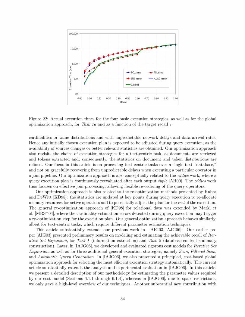
10

100

1,000

10,000

100,000

0.00 0.10 0.20 0.30 0.40 0.50 0.60 0.70 0.80 0.90 1.00Recall

Exec

utio

n Ti

me

(sec

s)SC_time FS_time

ISE_time AQG_time

Global

Figure 22: Actual execution times for the four basic execution strategies, as well as for the globaloptimization approach, for Task 1a and as a function of the target recall τ

cardinalities or value distributions and with unpredictable network delays and data arrival rates.Hence any initially chosen execution plan is expected to be adjusted during query execution, as theavailability of sources changes or better relevant statistics are obtained. Our optimization approachalso revisits the choice of execution strategies for a text-centric task, as documents are retrievedand tokens extracted and, consequently, the statistics on document and token distributions arerefined. Our focus in this article is on processing text-centric tasks over a single text “database,”and not on gracefully recovering from unpredictable delays when executing a particular operator ina join pipeline. Our optimization approach is also conceptually related to the eddies work, where aquery execution plan is continuously reevaluated after each output tuple [AH00]. The eddies workthus focuses on effective join processing, allowing flexible re-ordering of the query operators.

Our optimization approach is also related to the re-optimization methods presented by Kabraand DeWitt [KD98]: the statistics are updated at key points during query execution to re-allocatememory resources for active operators and to potentially adjust the plan for the rest of the execution.The general re-optimization approach of [KD98] for relational data was extended by Markl etal. [MRS+04], where the cardinality estimation errors detected during query execution may triggera re-optimization step for the execution plan. Our general optimization approach behaves similarly,albeit for text-centric tasks, which require different parameter estimation techniques.

This article substantially extends our previous work in [AIG03, IAJG06]. Our earlier pa-per [AIG03] presented preliminary results on modeling and estimating the achievable recall of Iter-ative Set Expansion, for Task 1 (information extraction) and Task 2 (database content summaryconstruction). Later, in [IAJG06], we developed and evaluated rigorous cost models for Iterative SetExpansion, as well as for three additional general execution strategies, namely Scan, Filtered Scan,and Automatic Query Generation. In [IAJG06], we also presented a principled, cost-based globaloptimization approach for selecting the most efficient execution strategy automatically. The currentarticle substantially extends the analysis and experimental evaluation in [IAJG06]. In this article,we present a detailed description of our methodology for estimating the parameter values requiredby our cost model (Sections 6.1.1 through 6.1.4), whereas in [IAJG06], due to space restrictions,we only gave a high-level overview of our techniques. Another substantial new contribution with

34

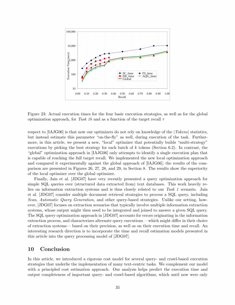
10

100

1,000

10,000

100,000

0.00 0.10 0.20 0.30 0.40 0.50 0.60 0.70 0.80 0.90 1.00Recall

Exec

utio

n Ti

me

(sec

s)

SC_time FS_timeISE_time AQG_timeGlobal

Figure 23: Actual execution times for the four basic execution strategies, as well as for the globaloptimization approach, for Task 1b and as a function of the target recall τ

respect to [IAJG06] is that now our optimizers do not rely on knowledge of the |Tokens| statistics,but instead estimate this parameter “on-the-fly” as well, during execution of the task. Further-more, in this article, we present a new, “local” optimizer that potentially builds “multi-strategy”executions by picking the best strategy for each batch of k tokens (Section 6.2). In contrast, the“global” optimization approach in [IAJG06] only attempts to identify a single execution plan thatis capable of reaching the full target recall. We implemented the new local optimization approachand compared it experimentally against the global approach of [IAJG06]; the results of the com-parison are presented in Figures 26, 27, 28, and 29, in Section 8. The results show the superiorityof the local optimizer over the global optimizer.

Finally, Jain et al. [JDG07] have very recently presented a query optimization approach forsimple SQL queries over (structured data extracted from) text databases. This work heavily re-lies on information extraction systems and is thus closely related to our Task 1 scenario. Jainet al. [JDG07] consider multiple document retrieval strategies to process a SQL query, includingScan, Automatic Query Generation, and other query-based strategies. Unlike our setting, how-ever, [JDG07] focuses on extraction scenarios that typically involve multiple information extractionsystems, whose output might then need to be integrated and joined to answer a given SQL query.The SQL query optimization approach in [JDG07] accounts for errors originating in the informationextraction process, and characterizes alternate query executions —which might differ in their choiceof extraction systems— based on their precision, as well as on their execution time and recall. Aninteresting research direction is to incorporate the time and recall estimation models presented inthis article into the query processing model of [JDG07].

10 Conclusion

In this article, we introduced a rigorous cost model for several query- and crawl-based executionstrategies that underlie the implementation of many text-centric tasks. We complement our modelwith a principled cost estimation approach. Our analysis helps predict the execution time andoutput completeness of important query- and crawl-based algorithms, which until now were only

35

0.1

1.0

10.0

100.0

1,000.0

0.00 0.10 0.20 0.30 0.40 0.50 0.60 0.70 0.80 0.90 1.00Recall

Exec

utio

n Ti

me

(sec

s)SC_time ISE_time

AQG_time Global

Figure 24: Actual execution times for the three basic execution strategies, as well as for the globaloptimization approach, for Task 2 and as a function of the target recall τ

empirically evaluated, with limited theoretical justification. We demonstrated that our modelingcan be successfully used to create optimizers for text-centric tasks, and showed that our optimizershelp build efficient execution plans to achieve a target recall, resulting in executions that can beorders of magnitude faster than alternate choices.

Our work can be extended in multiple directions. For example, the current framework assumesthat the document processors have perfect “precision,” in that they always produce accurate results.Relaxing this assumption and, correspondingly, predicting the precision of the output produced bydifferent strategies is a natural next step. Another interesting direction is to apply our model toother text-centric tasks and also study how to minimize our reliance on task-specific prior knowledgeof the token and document distributions for our analysis.

References

[AG00] Eugene Agichtein and Luis Gravano. Snowball: Extracting relations from large plain-text collections. In Proceedings of the Fifth ACM Conference on Digital Libraries (DL2000), 2000.

[AG03] Eugene Agichtein and Luis Gravano. Querying text databases for efficient informa-tion extraction. In Proceedings of the 19th IEEE International Conference on DataEngineering (ICDE 2003), 2003.

[AH00] Ron Avnur and Joseph M. Hellerstein. Eddies: Continuously adaptive query processing.In Proceedings of the 2000 ACM SIGMOD International Conference on Managementof Data (SIGMOD 2000), pages 261–272, 2000.

[AIG03] Eugene Agichtein, Panagiotis G. Ipeirotis, and Luis Gravano. Modeling query-basedaccess to text databases. In Proceedings of the Sixth International Workshop on theWeb and Databases, WebDB 2003, pages 87–92, 2003.

36

https://www.researchgate.net/publication/200031515_Eddies_Continuously_Adaptive_Query_Processing?el=1_x_8&enrichId=rgreq-c16b4f7d78394926ca4067183fb34710-XXX&enrichSource=Y292ZXJQYWdlOzIyMDIyNTIyMDtBUzoxMDQ0NTY4NzYxOTk5NDBAMTQwMTkxNTg2ODI0NA==



https://www.researchgate.net/publication/2482149_Snowball_Extracting_Relations_from_Large_Plain-Text_Collections?el=1_x_8&enrichId=rgreq-c16b4f7d78394926ca4067183fb34710-XXX&enrichSource=Y292ZXJQYWdlOzIyMDIyNTIyMDtBUzoxMDQ0NTY4NzYxOTk5NDBAMTQwMTkxNTg2ODI0NA==



https://www.researchgate.net/publication/2479444_Modeling_Query-Based_Access_to_Text_Databases?el=1_x_8&enrichId=rgreq-c16b4f7d78394926ca4067183fb34710-XXX&enrichSource=Y292ZXJQYWdlOzIyMDIyNTIyMDtBUzoxMDQ0NTY4NzYxOTk5NDBAMTQwMTkxNTg2ODI0NA==



https://www.researchgate.net/publication/4053370_Querying_text_databases_for_efficient_information_extraction?el=1_x_8&enrichId=rgreq-c16b4f7d78394926ca4067183fb34710-XXX&enrichSource=Y292ZXJQYWdlOzIyMDIyNTIyMDtBUzoxMDQ0NTY4NzYxOTk5NDBAMTQwMTkxNTg2ODI0NA==



10

100

1,000

10,000

100,000

1,000,000

0.00 0.10 0.20 0.30 0.40 0.50 0.60 0.70 0.80 0.90 1.00Recall

Exec

utio

n Ti

me

(sec

s)

SC_time FS_time

AQG_time Global

Figure 25: Actual execution times for the three basic execution strategies, as well as for the globaloptimization approach, for Task 3 and as a function of the target recall τ

[BBDL02] Michele Banko, Eric Brill, Susan Dumais, and Jimmy Lin. AskMSR: Question answer-ing using the World Wide Web. In Proceedings of the 2002 AAAI Spring Symposiumon Mining Answers from Texts and Knowledge Bases, 2002.

[Ber01] Michael K. Bergman. The Deep Web: Surfacing hidden value. Journal of ElectronicPublishing, 7(1), August 2001.

[BM98] Catherine L. Blake and Christopher John Merz. UCI repository of machine learningdatabases. http://www.ics.uci.edu/~mlearn/MLRepository.html, 1998.

[Bri98] Sergey Brin. Extracting patterns and relations from the world wide web. In Proceedingsof the First International Workshop on the Web and Databases, WebDB 1998, pages172–183, 1998.

[CC01] James P. Callan and Margaret Connell. Query-based sampling of text databases. ACMTransactions on Information Systems, 19(2):97–130, 2001.

[CCD99] James P. Callan, Margaret Connell, and Aiqun Du. Automatic discovery of languagemodels for text databases. In Proceedings of the 1999 ACM SIGMOD InternationalConference on Management of Data (SIGMOD’99), pages 479–490, 1999.

[CE05] Michael J. Cafarella and Oren Etzioni. A search engine for natural language applica-tions. In Proceedings of the 14th International World Wide Web Conference (WWW2005), pages 442–452, 2005.

[CGGM03] Surajit Chaudhuri, Kris Ganjam, Venkatesh Ganti, and Rajeev Motwani. Robustand efficient fuzzy match for online data cleaning. In Proceedings of the 2003 ACMSIGMOD International Conference on Management of Data (SIGMOD 2003), pages313–324, 2003.

[CL02] Fan Chung and Linyuan Lu. Connected components in random graphs with givendegree sequences. Annals of Combinatorics, 6:125–145, 2002.

37

https://www.researchgate.net/publication/221213232_Robust_and_Efficient_Fuzzy_Match_for_Online_Data_Cleaning?el=1_x_8&enrichId=rgreq-c16b4f7d78394926ca4067183fb34710-XXX&enrichSource=Y292ZXJQYWdlOzIyMDIyNTIyMDtBUzoxMDQ0NTY4NzYxOTk5NDBAMTQwMTkxNTg2ODI0NA==




https://www.researchgate.net/publication/239440978_White_Paper_The_Deep_Web_Surfacing_Hidden_Value?el=1_x_8&enrichId=rgreq-c16b4f7d78394926ca4067183fb34710-XXX&enrichSource=Y292ZXJQYWdlOzIyMDIyNTIyMDtBUzoxMDQ0NTY4NzYxOTk5NDBAMTQwMTkxNTg2ODI0NA==

https://www.researchgate.net/publication/239440978_White_Paper_The_Deep_Web_Surfacing_Hidden_Value?el=1_x_8&enrichId=rgreq-c16b4f7d78394926ca4067183fb34710-XXX&enrichSource=Y292ZXJQYWdlOzIyMDIyNTIyMDtBUzoxMDQ0NTY4NzYxOTk5NDBAMTQwMTkxNTg2ODI0NA==

https://www.researchgate.net/publication/221214968_Automatic_Discovery_of_Language_Models_for_Text_Databases?el=1_x_8&enrichId=rgreq-c16b4f7d78394926ca4067183fb34710-XXX&enrichSource=Y292ZXJQYWdlOzIyMDIyNTIyMDtBUzoxMDQ0NTY4NzYxOTk5NDBAMTQwMTkxNTg2ODI0NA==



https://www.researchgate.net/publication/2555104_AskMSR_Question_answering_using_the_Worldwide_Web?el=1_x_8&enrichId=rgreq-c16b4f7d78394926ca4067183fb34710-XXX&enrichSource=Y292ZXJQYWdlOzIyMDIyNTIyMDtBUzoxMDQ0NTY4NzYxOTk5NDBAMTQwMTkxNTg2ODI0NA==



https://www.researchgate.net/publication/220515613_Query-Based_Sampling_of_Text_Databases?el=1_x_8&enrichId=rgreq-c16b4f7d78394926ca4067183fb34710-XXX&enrichSource=Y292ZXJQYWdlOzIyMDIyNTIyMDtBUzoxMDQ0NTY4NzYxOTk5NDBAMTQwMTkxNTg2ODI0NA==

https://www.researchgate.net/publication/220515613_Query-Based_Sampling_of_Text_Databases?el=1_x_8&enrichId=rgreq-c16b4f7d78394926ca4067183fb34710-XXX&enrichSource=Y292ZXJQYWdlOzIyMDIyNTIyMDtBUzoxMDQ0NTY4NzYxOTk5NDBAMTQwMTkxNTg2ODI0NA==

https://www.researchgate.net/publication/2788606_Extracting_Patterns_and_Relations_from_the_World_Wide_Web?el=1_x_8&enrichId=rgreq-c16b4f7d78394926ca4067183fb34710-XXX&enrichSource=Y292ZXJQYWdlOzIyMDIyNTIyMDtBUzoxMDQ0NTY4NzYxOTk5NDBAMTQwMTkxNTg2ODI0NA==



https://www.researchgate.net/publication/221023410_A_search_engine_for_natural_language_applications?el=1_x_8&enrichId=rgreq-c16b4f7d78394926ca4067183fb34710-XXX&enrichSource=Y292ZXJQYWdlOzIyMDIyNTIyMDtBUzoxMDQ0NTY4NzYxOTk5NDBAMTQwMTkxNTg2ODI0NA==



https://www.researchgate.net/publication/244521691_UCI_Repository_of_Machine_Learning_Databases?el=1_x_8&enrichId=rgreq-c16b4f7d78394926ca4067183fb34710-XXX&enrichSource=Y292ZXJQYWdlOzIyMDIyNTIyMDtBUzoxMDQ0NTY4NzYxOTk5NDBAMTQwMTkxNTg2ODI0NA==

https://www.researchgate.net/publication/244521691_UCI_Repository_of_Machine_Learning_Databases?el=1_x_8&enrichId=rgreq-c16b4f7d78394926ca4067183fb34710-XXX&enrichSource=Y292ZXJQYWdlOzIyMDIyNTIyMDtBUzoxMDQ0NTY4NzYxOTk5NDBAMTQwMTkxNTg2ODI0NA==

10

100

1,000

10,000

100,000

0.00 0.10 0.20 0.30 0.40 0.50 0.60 0.70 0.80 0.90 1.00Recall

Exec

utio

n Ti

me

(sec

s) Global

Local

Figure 26: Actual execution times for the global and local optimization approaches, for Task 1aand as a function of the target recall τ

[CLC95] James P. Callan, Zhihong Lu, and William Bruce Croft. Searching distributed collec-tions with inference networks. In Proceedings of the 18th Annual International ACMSIGIR Conference on Research and Development in Information Retrieval, SIGIR’95,pages 21–28, 1995.

[CMN98] Surajit Chaudhuri, Rajeev Motwani, and Vivek R. Narasayya. Random samplingfor histogram construction: How much is enough? In Proceedings of the 1998 ACMSIGMOD International Conference on Management of Data (SIGMOD’98), pages 436–447, 1998.

[Coh96] William Weston Cohen. Learning trees and rules with set-valued features. In Pro-ceedings of the 13th National Conference on Artificial Intelligence (AAAI-96), EighthConference on Innovative Applications of Artificial Intelligence (IAAI-96), pages 709–716, 1996.

[CPS02] Soumen Chakrabarti, Kunal Punera, and Mallela Subramanyam. Accelerated focusedcrawling through online relevance feedback. In Proceedings of the 11th InternationalWorld Wide Web Conference (WWW11), pages 148–159, 2002.

[CS96] William Weston Cohen and Yoram Singer. Learning to query the web. In AAAIWorkshop on Internet-Based Information Systems, pages 16–25, 1996.

[CS99] Surajit Chaudhuri and Kyuseok Shim. Optimization of queries with user-defined pred-icates. ACM Transactions on Database Systems, 24(2):177–228, 1999.

[CvdBD99] Soumen Chakrabarti, Martin van den Berg, and Byron Dom. Focused crawling: A newapproach to topic-specific web resource discovery. Computer Networks, 31(11-16):1623–1640, May 1999.

38

https://www.researchgate.net/publication/2323046_Searching_Distributed_Collections_With_Inference_Networks?el=1_x_8&enrichId=rgreq-c16b4f7d78394926ca4067183fb34710-XXX&enrichSource=Y292ZXJQYWdlOzIyMDIyNTIyMDtBUzoxMDQ0NTY4NzYxOTk5NDBAMTQwMTkxNTg2ODI0NA==




https://www.researchgate.net/publication/222486802_Focused_crawling_A_new_approach_to_topic-specific_Web_resource_discovery?el=1_x_8&enrichId=rgreq-c16b4f7d78394926ca4067183fb34710-XXX&enrichSource=Y292ZXJQYWdlOzIyMDIyNTIyMDtBUzoxMDQ0NTY4NzYxOTk5NDBAMTQwMTkxNTg2ODI0NA==



https://www.researchgate.net/publication/2458229_Learning_to_Query_the_Web?el=1_x_8&enrichId=rgreq-c16b4f7d78394926ca4067183fb34710-XXX&enrichSource=Y292ZXJQYWdlOzIyMDIyNTIyMDtBUzoxMDQ0NTY4NzYxOTk5NDBAMTQwMTkxNTg2ODI0NA==

https://www.researchgate.net/publication/2458229_Learning_to_Query_the_Web?el=1_x_8&enrichId=rgreq-c16b4f7d78394926ca4067183fb34710-XXX&enrichSource=Y292ZXJQYWdlOzIyMDIyNTIyMDtBUzoxMDQ0NTY4NzYxOTk5NDBAMTQwMTkxNTg2ODI0NA==

https://www.researchgate.net/publication/2679420_Random_sampling_for_histogram_construction_How_much_is_enough_In_SIGMOD_1998?el=1_x_8&enrichId=rgreq-c16b4f7d78394926ca4067183fb34710-XXX&enrichSource=Y292ZXJQYWdlOzIyMDIyNTIyMDtBUzoxMDQ0NTY4NzYxOTk5NDBAMTQwMTkxNTg2ODI0NA==




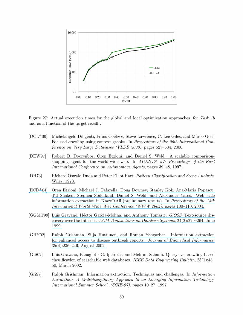
10

100

1,000

10,000

0.00 0.10 0.20 0.30 0.40 0.50 0.60 0.70 0.80 0.90 1.00Recall

Exec

utio

n Ti

me

(sec

s)Global

Local

Figure 27: Actual execution times for the global and local optimization approaches, for Task 1band as a function of the target recall τ

[DCL+00] Michelangelo Diligenti, Frans Coetzee, Steve Lawrence, C. Lee Giles, and Marco Gori.Focused crawling using context graphs. In Proceedings of the 26th International Con-ference on Very Large Databases (VLDB 2000), pages 527–534, 2000.

[DEW97] Robert B. Doorenbos, Oren Etzioni, and Daniel S. Weld. A scalable comparison-shopping agent for the world-wide web. In AGENTS ’97: Proceedings of the FirstInternational Conference on Autonomous Agents, pages 39–48, 1997.

[DH73] Richard Oswald Duda and Peter Elliot Hart. Pattern Classification and Scene Analysis.Wiley, 1973.

[ECD+04] Oren Etzioni, Michael J. Cafarella, Doug Downey, Stanley Kok, Ana-Maria Popescu,Tal Shaked, Stephen Soderland, Daniel S. Weld, and Alexander Yates. Web-scaleinformation extraction in KnowItAll (preliminary results). In Proceedings of the 13thInternational World Wide Web Conference (WWW 2004), pages 100–110, 2004.

[GGMT99] Luis Gravano, Hector Garcıa-Molina, and Anthony Tomasic. GlOSS: Text-source dis-covery over the Internet. ACM Transactions on Database Systems, 24(2):229–264, June1999.

[GHY02] Ralph Grishman, Silja Huttunen, and Roman Yangarber. Information extractionfor enhanced access to disease outbreak reports. Journal of Biomedical Informatics,35(4):236–246, August 2002.

[GIS02] Luis Gravano, Panagiotis G. Ipeirotis, and Mehran Sahami. Query- vs. crawling-basedclassification of searchable web databases. IEEE Data Engineering Bulletin, 25(1):43–50, March 2002.

[Gri97] Ralph Grishman. Information extraction: Techniques and challenges. In InformationExtraction: A Multidisciplinary Approach to an Emerging Information Technology,International Summer School, (SCIE-97), pages 10–27, 1997.

39

https://www.researchgate.net/publication/10751756_Information_extraction_for_enhanced_access_to_disease_outbreak_reports?el=1_x_8&enrichId=rgreq-c16b4f7d78394926ca4067183fb34710-XXX&enrichSource=Y292ZXJQYWdlOzIyMDIyNTIyMDtBUzoxMDQ0NTY4NzYxOTk5NDBAMTQwMTkxNTg2ODI0NA==



https://www.researchgate.net/publication/221022357_Web-scale_information_extraction_in_knowltAll_preliminary_results?el=1_x_8&enrichId=rgreq-c16b4f7d78394926ca4067183fb34710-XXX&enrichSource=Y292ZXJQYWdlOzIyMDIyNTIyMDtBUzoxMDQ0NTY4NzYxOTk5NDBAMTQwMTkxNTg2ODI0NA==






https://www.researchgate.net/publication/2809006_A_Scalable_Comparison-Shopping_Agent_for_the_World-Wide_Web?el=1_x_8&enrichId=rgreq-c16b4f7d78394926ca4067183fb34710-XXX&enrichSource=Y292ZXJQYWdlOzIyMDIyNTIyMDtBUzoxMDQ0NTY4NzYxOTk5NDBAMTQwMTkxNTg2ODI0NA==



https://www.researchgate.net/publication/249627779_GIOSS_Text-source_discovery_over_the_Internet?el=1_x_8&enrichId=rgreq-c16b4f7d78394926ca4067183fb34710-XXX&enrichSource=Y292ZXJQYWdlOzIyMDIyNTIyMDtBUzoxMDQ0NTY4NzYxOTk5NDBAMTQwMTkxNTg2ODI0NA==



https://www.researchgate.net/publication/216721999_Pattern_Classification_and_Scene_Analysis?el=1_x_8&enrichId=rgreq-c16b4f7d78394926ca4067183fb34710-XXX&enrichSource=Y292ZXJQYWdlOzIyMDIyNTIyMDtBUzoxMDQ0NTY4NzYxOTk5NDBAMTQwMTkxNTg2ODI0NA==

https://www.researchgate.net/publication/216721999_Pattern_Classification_and_Scene_Analysis?el=1_x_8&enrichId=rgreq-c16b4f7d78394926ca4067183fb34710-XXX&enrichSource=Y292ZXJQYWdlOzIyMDIyNTIyMDtBUzoxMDQ0NTY4NzYxOTk5NDBAMTQwMTkxNTg2ODI0NA==

0.1

1.0

10.0

100.0

1,000.0

0.00 0.10 0.20 0.30 0.40 0.50 0.60 0.70 0.80 0.90 1.00Recall

Exec

utio

n Ti

me

(sec

s)

Global

Local

Figure 28: Actual execution times for the global and local optimization approaches, for Task 2 andas a function of the target recall τ

[IAJG06] Panagiotis G. Ipeirotis, Eugene Agichtein, Pranay Jain, and Luis Gravano. To search orto crawl? Towards a query optimizer for text-centric tasks. In Proceedings of the 2006ACM SIGMOD International Conference on Management of Data (SIGMOD 2006),pages 265–276, 2006.

[IFF+99] Zachary G. Ives, Daniela Florescu, Marc Friedman, Alon Y. Levy, and Daniel S.Weld. An adaptive query execution system for data integration. In Proceedings of the1999 ACM SIGMOD International Conference on Management of Data (SIGMOD’99),pages 299–310, 1999.

[IG02] Panagiotis G. Ipeirotis and Luis Gravano. Distributed search over the hidden web:Hierarchical database sampling and selection. In Proceedings of the 28th InternationalConference on Very Large Databases (VLDB 2002), pages 394–405, 2002.

[JDG07] Alpa Jain, AnHai Doan, and Luis Gravano. SQL queries over unstructured text da-tabases (poster paper). In Proceedings of the 23rd IEEE International Conference onData Engineering (ICDE 2007), 2007. To appear.

[Jon05] Rosie Jones. Learning to Extract Entities from Labeled and Unlabeled Text. PhD thesis,Carnegie Mellon University, School of Computer Science, 2005.

[KD98] Navin Kabra and David J. DeWitt. Efficient mid-query re-optimization of sub-optimalquery execution plans. In Proceedings of the 1998 ACM SIGMOD International Con-ference on Management of Data (SIGMOD’98), pages 106–117, 1998.

[LS95] Yibei Ling and Wei Sun. An evaluation of sampling-based size estimation methodsfor selections in database systems. In Proceedings of the 11th IEEE InternationalConference on Data Engineering (ICDE 1995), pages 532–539, 1995.

[Mit04] Michael Mitzenmacher. Dynamic models for file sizes and double pareto distributions.Internet Mathematics, 1(3):305–334, 2004.

40

https://www.researchgate.net/publication/221213884_An_Adaptive_Query_Execution_System_for_Data_Integration?el=1_x_8&enrichId=rgreq-c16b4f7d78394926ca4067183fb34710-XXX&enrichSource=Y292ZXJQYWdlOzIyMDIyNTIyMDtBUzoxMDQ0NTY4NzYxOTk5NDBAMTQwMTkxNTg2ODI0NA==







https://www.researchgate.net/publication/2537726_Distributed_Search_over_the_Hidden_Web_Hierarchical_Database_Sampling_and_Selection?el=1_x_8&enrichId=rgreq-c16b4f7d78394926ca4067183fb34710-XXX&enrichSource=Y292ZXJQYWdlOzIyMDIyNTIyMDtBUzoxMDQ0NTY4NzYxOTk5NDBAMTQwMTkxNTg2ODI0NA==




https://www.researchgate.net/publication/3597726_An_evaluation_of_sampling-based_size_estimation_methods_forselections_in_database_systems?el=1_x_8&enrichId=rgreq-c16b4f7d78394926ca4067183fb34710-XXX&enrichSource=Y292ZXJQYWdlOzIyMDIyNTIyMDtBUzoxMDQ0NTY4NzYxOTk5NDBAMTQwMTkxNTg2ODI0NA==



https://www.researchgate.net/publication/35452481_Learning_to_extract_entities_from_labeled_and_unlabeled_text?el=1_x_8&enrichId=rgreq-c16b4f7d78394926ca4067183fb34710-XXX&enrichSource=Y292ZXJQYWdlOzIyMDIyNTIyMDtBUzoxMDQ0NTY4NzYxOTk5NDBAMTQwMTkxNTg2ODI0NA==

https://www.researchgate.net/publication/35452481_Learning_to_extract_entities_from_labeled_and_unlabeled_text?el=1_x_8&enrichId=rgreq-c16b4f7d78394926ca4067183fb34710-XXX&enrichSource=Y292ZXJQYWdlOzIyMDIyNTIyMDtBUzoxMDQ0NTY4NzYxOTk5NDBAMTQwMTkxNTg2ODI0NA==

https://www.researchgate.net/publication/2379750_Dynamic_Models_for_File_Sizes_and_Double_Pareto_Distributions?el=1_x_8&enrichId=rgreq-c16b4f7d78394926ca4067183fb34710-XXX&enrichSource=Y292ZXJQYWdlOzIyMDIyNTIyMDtBUzoxMDQ0NTY4NzYxOTk5NDBAMTQwMTkxNTg2ODI0NA==

https://www.researchgate.net/publication/2379750_Dynamic_Models_for_File_Sizes_and_Double_Pareto_Distributions?el=1_x_8&enrichId=rgreq-c16b4f7d78394926ca4067183fb34710-XXX&enrichSource=Y292ZXJQYWdlOzIyMDIyNTIyMDtBUzoxMDQ0NTY4NzYxOTk5NDBAMTQwMTkxNTg2ODI0NA==

https://www.researchgate.net/publication/4250969_SQL_Queries_Over_Unstructured_Text_Databases?el=1_x_8&enrichId=rgreq-c16b4f7d78394926ca4067183fb34710-XXX&enrichSource=Y292ZXJQYWdlOzIyMDIyNTIyMDtBUzoxMDQ0NTY4NzYxOTk5NDBAMTQwMTkxNTg2ODI0NA==



10

100

1,000

10,000

100,000

1,000,000

0.00 0.10 0.20 0.30 0.40 0.50 0.60 0.70 0.80 0.90 1.00Recall

Exec

utio

n Ti

me

(sec

s)

Global

Local

Figure 29: Actual execution times for the global and local optimization approaches, for Task 3 andas a function of the target recall τ

[MPS04] Filippo Menczer, Gautam Pant, and Padmini Srinivasan. Topical web crawlers: Eval-uating adaptive algorithms. ACM Transactions on Internet Technology, 4(4):378–419,November 2004.

[MRS+04] Volker Markl, Vijayshankar Raman, David Simmen, Guy Lohman, Hamid Pirahesh,and Miso Cilimdzic. Robust query processing through progressive optimization. InProceedings of the 2004 ACM SIGMOD International Conference on Management ofData (SIGMOD 2004), pages 659–670, 2004.

[NSW01] Mark E. J. Newman, Steven H. Strogatz, and Duncan J. Watts. Random graphs witharbitrary degree distributions and their applications. Physical Review E (Statistical,Nonlinear, and Soft Matter Physics), 64(2):026118 (1–17), August 2001.

[NZC05] Alexandros Ntoulas, Petros Zerfos, and Junghoo Cho. Downloading textual hidden webcontent by keyword queries. In Proceedings of the Fifth ACM+IEEE Joint Conferenceon Digital Libraries (JCDL 2005), 2005.

[Oar97] Douglas W. Oard. The state of the art in text filtering. User Modeling and User-Adapted Interaction, 7(3):141–178, 1997.

[Ros02] Sheldon M. Ross. Introduction to Probability Models. Academic Press, 8th edition,December 2002.

[SAC+79] Patricia G. Selinger, Morton M. Astrahan, Donald D. Chamberlin, Raymond A. Lo-rie, and Thomas G. Price. Access path selection in a relational database managementsystem. In Proceedings of the 1979 ACM SIGMOD International Conference on Man-agement of Data (SIGMOD’79), pages 23–34, 1979.

[Seb02] Fabrizio Sebastiani. Machine learning in automated text categorization. ACM Com-puting Surveys, 34(1):1–47, March 2002.

41

https://www.researchgate.net/publication/221214594_Robust_Query_Processing_through_Progressive_Optimization?el=1_x_8&enrichId=rgreq-c16b4f7d78394926ca4067183fb34710-XXX&enrichSource=Y292ZXJQYWdlOzIyMDIyNTIyMDtBUzoxMDQ0NTY4NzYxOTk5NDBAMTQwMTkxNTg2ODI0NA==






https://www.researchgate.net/publication/200034311_Access_Path_Selection_in_a_Relational_Database_Management_System?el=1_x_8&enrichId=rgreq-c16b4f7d78394926ca4067183fb34710-XXX&enrichSource=Y292ZXJQYWdlOzIyMDIyNTIyMDtBUzoxMDQ0NTY4NzYxOTk5NDBAMTQwMTkxNTg2ODI0NA==






https://www.researchgate.net/publication/220116422_The_State_of_the_Art_in_Text_Filtering?el=1_x_8&enrichId=rgreq-c16b4f7d78394926ca4067183fb34710-XXX&enrichSource=Y292ZXJQYWdlOzIyMDIyNTIyMDtBUzoxMDQ0NTY4NzYxOTk5NDBAMTQwMTkxNTg2ODI0NA==

https://www.researchgate.net/publication/220116422_The_State_of_the_Art_in_Text_Filtering?el=1_x_8&enrichId=rgreq-c16b4f7d78394926ca4067183fb34710-XXX&enrichSource=Y292ZXJQYWdlOzIyMDIyNTIyMDtBUzoxMDQ0NTY4NzYxOTk5NDBAMTQwMTkxNTg2ODI0NA==

https://www.researchgate.net/publication/11846504_Random_Graphs_with_Arbitrary_Degree_Distributions_and_their_Applications?el=1_x_8&enrichId=rgreq-c16b4f7d78394926ca4067183fb34710-XXX&enrichSource=Y292ZXJQYWdlOzIyMDIyNTIyMDtBUzoxMDQ0NTY4NzYxOTk5NDBAMTQwMTkxNTg2ODI0NA==



https://www.researchgate.net/publication/274339921_Introduction_to_Probability_Models?el=1_x_8&enrichId=rgreq-c16b4f7d78394926ca4067183fb34710-XXX&enrichSource=Y292ZXJQYWdlOzIyMDIyNTIyMDtBUzoxMDQ0NTY4NzYxOTk5NDBAMTQwMTkxNTg2ODI0NA==

https://www.researchgate.net/publication/274339921_Introduction_to_Probability_Models?el=1_x_8&enrichId=rgreq-c16b4f7d78394926ca4067183fb34710-XXX&enrichSource=Y292ZXJQYWdlOzIyMDIyNTIyMDtBUzoxMDQ0NTY4NzYxOTk5NDBAMTQwMTkxNTg2ODI0NA==

[Vap98] Vladimir Naumovich Vapnik. Statistical Learning Theory. Wiley-Interscience, Septem-ber 1998.

[Wil90] Herbert S. Wilf. Generatingfunctionology. Academic Press Professional, Inc., 1990.

[YG98] Roman Yangarber and Ralph Grishman. NYU: Description of the Proteus/PET systemas used for MUC-7. In Proceedings of the Seventh Message Understanding Conference(MUC-7), 1998.

[Zip49] George Kingsley Zipf. Human Behavior and the Principle of Least Effort. Addison-Wesley, 1949.

42

https://www.researchgate.net/publication/44417592_Human_Behavior_and_the_Principle_of_Least_Effort?el=1_x_8&enrichId=rgreq-c16b4f7d78394926ca4067183fb34710-XXX&enrichSource=Y292ZXJQYWdlOzIyMDIyNTIyMDtBUzoxMDQ0NTY4NzYxOTk5NDBAMTQwMTkxNTg2ODI0NA==

https://www.researchgate.net/publication/44417592_Human_Behavior_and_the_Principle_of_Least_Effort?el=1_x_8&enrichId=rgreq-c16b4f7d78394926ca4067183fb34710-XXX&enrichSource=Y292ZXJQYWdlOzIyMDIyNTIyMDtBUzoxMDQ0NTY4NzYxOTk5NDBAMTQwMTkxNTg2ODI0NA==

https://www.researchgate.net/publication/220694713_Statistical_Learning_Theory?el=1_x_8&enrichId=rgreq-c16b4f7d78394926ca4067183fb34710-XXX&enrichSource=Y292ZXJQYWdlOzIyMDIyNTIyMDtBUzoxMDQ0NTY4NzYxOTk5NDBAMTQwMTkxNTg2ODI0NA==

https://www.researchgate.net/publication/220694713_Statistical_Learning_Theory?el=1_x_8&enrichId=rgreq-c16b4f7d78394926ca4067183fb34710-XXX&enrichSource=Y292ZXJQYWdlOzIyMDIyNTIyMDtBUzoxMDQ0NTY4NzYxOTk5NDBAMTQwMTkxNTg2ODI0NA==

Towards a query optimizer for text-centric tasks

Documents

Transcript of Towards a query optimizer for text-centric tasks