Towards a Mathematical Model of Within-Session Operant Responding

Towards a Mathematical Model of Within-Session Operant Responding

Estêvão G. Bittar and Kleber Del-ClaroUniversidade Federal de Juiz de Fora

Lucas G. Bittar and Michelle C. P. da SilvaUniversidade Federal de Uberlândia

Operant response rate changes within the course of a typical free-operant experimental session. Thesechanges are orderly, and reliably demonstrated with subjects from different species, responding underdifferent experimental conditions. Killeen (1995) postulated that the response rate changes are a functionof the interplay between arousal and satiation and offered a mathematical model for this hypothesis. Herewe analyze Killeen’s model, demonstrating that, although solid in its principles, it presents some flawsin its implementation. Then, based on the same principles, we build and test a new model of within-session motivation dynamics. We also demonstrate that, by representing arousal as a variable that rangesbetween 0 and 1, we can obtain a surprisingly simple model of free-operant response rate.

Keywords: response rate, motivation, arousal, satiation, models

Supplemental materials: http://dx.doi.org/10.1037/a0029086.supp

What are the processes that underlie operant responding? Ac-cording to Killeen (1994), they are three: arousal, coupling, andtime constraints. Behavior is fueled by arousal, constrained bytime, and directed by coupling. In an impressive effort, Killeenoffered formal models for each of these factors and combined themin an integrative theory called mathematical principles of rein-forcement (MPR; Killeen, 1994; Killeen & Sitomer, 2003).

In 1995, Killeen made an attempt to use MPR to account forwithin-session changes in operant responding. At that time, Mc-Sweeney and her colleagues had already demonstrated that, within thecourse of a typical free-operant experimental session, response ratesshow changes that sometimes exceed 450% (McSweeney, Hatfield, &Allen, 1990). Moreover, they demonstrated that these within-sessionchanges in response rates are orderly, generally increasing, decreas-ing, or increasing up to a peak and then decreasing (McSweeney,Hatfield, & Allen, 1990; McSweeney & Hinson, 1992; McSweeney,Roll, & Weatherly, 1994). These variations are reliably demonstratedwith subjects from different species, responding for different reinforc-ers, operating different operanda, under different rates of reinforce-ment and under different schedules of reinforcement (McSweeney &Hinson, 1992; McSweeney, Roll, & Weatherly, 1994; McSweeney,Weatherly, & Swindell, 1995b; Roll & McSweeney, 1997).

Because coupling (the association of response and incentives in ananimal’s short-term memory [STM]) and time constraints remainrelatively constant throughout the course of an experimental session,

Killeen (1995) began applying MPR to within-session responding byassuming that the observed changes in response rate must be relatedto variations in the subject’s arousal as time elapses and more rein-forcers are presented and consumed. Next, he expanded his arousalmodel to present a full description of how arousal first accumulatesand then dissipates as the session progresses toward its end. In thisarticle, we revise Killeen’s (1995) model of arousal as applied towithin-session responding and discuss how it can be possibly improved.Then, we suggest a new model and test it using behavioral data from ourown laboratory as well as data from different researchers.

Modeling Arousal

The model of arousal built into MPR preceded MPR’s elabora-tion by several years (Killeen, Hanson, & Osborne, 1978). It wasfirst presented to account for adjunctive behavior that generallyarises when subjects respond under an intermittent schedule ofreinforcement (Falk, 1961; Falk, 1972; Wallace & Singer, 1976).Killeen hypothesized that “adjunctive behaviors are normally oc-curring parts of an organism’s repertoire, but that their rate ofoccurrence is excited to supernormal levels by a heightened levelof arousal” (Killeen et al., 1978).

As a first step to the construction of his arousal model, Killeen etal. (1978) showed that the presentation of a reinforcer to an organismelicits a state of arousal that decays exponentially over time. If a newreinforcer is presented during this decay, the arousal elicited by thesecond reinforcer adds to what’s left of the arousal elicited by the first,promoting an accumulation of effects. In a session where variousreinforcers are successively presented, the average arousal A at time tis given by the following equation (Killeen et al., 1978):

At�� aR(1 � e

�t� )

a � Q�,(1)

where R is reinforcement rate, Q is the jolt of arousal engenderedby each reinforcer, � is the time constant that controls decay of

Estêvão G. Bittar and Kleber Del-Claro, Department of Zoology, Uni-versidade Federal de Juiz de Fora, Juiz de Fora, Brazil; Lucas G. Bittar,Medical School, Universidade Federal de Uberlândia, Uberlândia, Braziland Michelle C. P. da Silva, Institute of Psychology, Universidade Federalde Uberlândia, Uberlândia, Brazil.

We thank Peter Killeen, Anthony Dickinson, and the reviewers for theiruseful comments in a previous version of this paper.

Correspondence concerning this article should be addressed to EstêvãoG. Bittar, Rua Eduardo Marquez, 931, Uberlândia/MG, Brazil, CEP 38400-442. E-mail: [email protected]

Journal of Experimental Psychology: Animal Behavior Processes © 2012 American Psychological Association2012, Vol. 38, No. 3, 292–302 0097-7403/12/$12.00 DOI: 10.1037/a0029086

292

arousal, and a represents the total time of activation elicited byeach reinforcer.

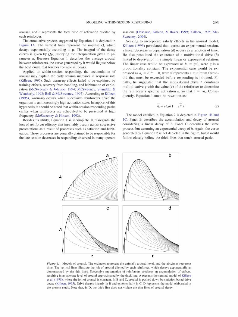
The cumulative process suggested by Equation 1 is depicted inFigure 1A. The vertical lines represent the impulse Q, whichdecays exponentially according to �. The integral of the decaycurves is given by Q�, justifying the interpretation given to pa-rameter a. Because Equation 1 describes the average arousalbetween reinforcers, the curve generated by it would lie just belowthe bold curve that touches the arousal peaks.

Applied to within-session responding, the accumulation ofarousal may explain the early session increases in response rate(Killeen, 1995). Such warm-up effects failed to be explained bytraining effects, recovery from handling, and habituation of explo-ration (McSweeney & Johnson, 1994; McSweeney, Swindell, &Weatherly, 1998; Roll & McSweeney, 1997). According to Killeen(1995), warm-up occurs when successive reinforcers drive theorganism to an increasingly high activation state. In support of thishypothesis, it should be noted that within-session responding peaksearlier when reinforcers are scheduled to be presented at highfrequency (McSweeney & Hinson, 1992).

Besides its utility, Equation 1 is incomplete. It disregards theloss of reinforcer efficacy that inevitably occurs across successivepresentations as a result of processes such as satiation and habit-uation. Those processes are generally claimed to be responsible forthe late session decreases in responding observed in many operant

sessions (DeMarse, Killeen, & Baker, 1999; Killeen, 1995; Mc-Sweeney, 2004).

Seeking to incorporate satiety effects in his arousal model,Killeen (1995) postulated that, across an experimental session,a linear decrease in deprivation (d) occurs as a function of time.He also postulated the existence of a motivational drive (h)linked to deprivation in a simple linear or exponential relation.The linear case would be expressed as ht � �dt, were � is aproportionality constant. The exponential case would be ex-pressed as ht � e�dt � �, were � represents a minimum thresh-old that must be exceeded before responding is initiated. Fi-nally, he suggested that the motivational drive h combinesmultiplicatively with the value (v) of the reinforcer to determinethe reinforcer’s specific activation a, so that a � vht. Conse-quently, Equation 1 must be rewritten as:

At�� vhtR(1 � e

�t� ). (2)

The model entailed in Equation 2 is depicted in Figure 1B and1C. Panel B describes the accumulation and decay of arousalconsidering a linear decay of h. Panel C describes the sameprocess, but assuming an exponential decay of h. Again, the curvegenerated by Equation 2 is not depicted in the figure, but it wouldfollow closely bellow the thick lines that touch arousal peaks.

Figure 1. Models of arousal. The ordinates represent the animal’s arousal level, and the abscissas representtime. The vertical lines illustrate the jolt of arousal elicited by each reinforcer, which decays exponentially asdemonstrated by the thin lines. Successive presentation of reinforcers produces an accumulation of effects,resulting in an average level of arousal approximated by the thick line. A presents the seminal model of Killeenet al. (1978), where the jolt of arousal is constant. In B and C, arousal is pushed down by satiation-based drivedecay (Killeen, 1995). Drive decays linearly in B and exponentially in C. D represents the model elaborated inthe present study. Note that, in D, the thick line does not violate the thin lines of arousal decay.

293MODELING WITHIN-SESSION RESPONDING

The Modeling Mistake

Although capable of drawing a bitonic function of arousal alongsuccessive reinforcers, Equation 2 presents a modeling mistake.After the peak, the arousal curve is pulled down by the increas-ingly smaller motivational drive (h). As it can be seen from PanelsB and C of Figure 1, the general arousal A assumes a null valuewhen drive h comes to 0. However, because arousal elicited byeach reinforcer decays exponentially, and because exponentialdecay curves never reach 0, the general arousal A could never becompletely extinguished.

The reason why Equation 2 produces such a distortion is be-cause all the terms in it are multiplied by the motivational drive h.Drive h is a direct function of deprivation d. Therefore, it decaysas deprivation does. However, as we can see from Figure 1B and1C, at some point each new reinforcer will begin to reduce thegeneral arousal, producing some sort of “negative arousal.” Thismoment is represented in Figure 1 as the point where the thick line(which illustrates the general level of arousal) crosses the thin lines(which illustrate the course of the arousal elicited by each rein-forcer). After this point, the vertical lines that illustrate the jolts Qof arousal and that always depart from the remaining arousal fromthe previous reinforcer would be representing a subtraction ofarousal. It could be argued that, after satiation, the reinforcingstimulus becomes aversive, inhibiting instrumental behavior. Butthis argument would be invalid for two reasons. First, the subtrac-tion of arousal occurs significantly before drive h reaches a nullvalue. Second, in the context of a free-operant session wheresubjects work to produce reinforcers, after the crossing point theywould be working to produce aversive stimuli—if we assumearousal to be related to operant responding, as Killeen (1994) does.Given the problems entailed in Equation 2, we propose a newmodel of the dynamics of arousal.

Fixing the Bug

To offer a new model of arousal, we first return to Killeen’smodel of arousal as originally presented (Killeen et al., 1978).Immediately after the presentation of a reinforcer, the animal’slevel of arousal A1 will be given by:

A1 � Q, (3)

where Q is the jolt of arousal engendered by the reinforcer. Thequantity A1 will decay exponentially over time, according to thefunction

At � A1e�t� , (4)

where � is the exponential time constant.If we assume that satiation decreases the arousing effect of

reinforcers, we must consider that, when the next reinforcer ispresented, quantity Q will be slightly smaller. If we assume that Qalso decays exponentially, then

Qn � Qe�n� , (5)

where n is the number of reinforcers previously consumed and �is a constant that dictates how fast satiation proceeds. When n �

�, Q is attenuated to approximately 36.8% of its initial value. Forn � 0, Q0 � Q.

Considering Equations 4 and 5, at the time a second reinforceris presented, the arousal level of the subject will be given by:

A2 � A1e�T� � Qe

�1� , (6)

where T is the time elapsed since the last reinforcer. Equation6 simply states that the animal’s arousal at the presentation ofthe second reinforcer (A2) will be the remaining arousal

from the first presentation (A1e�T� ) plus the new jolt attenuated by

a small satiation (Qe�1� ). Following the same process, arousal at

the third presentation will be:

A3 � A2e�T� � Qe

�2� , (7)

And arousal at the nth reinforcer will be:

An � An�1e�T� � Qe

1�n� . (8)

Equation 8 is a recursive function. solving it for n, and assumingA0 � 0, we can write it as:

An �Qe

T�

�1�n

� ��1 � en��e

�T� �n�

�eT� � e

1�

. (9)

If we want to know arousal A at moment t into session, insteadof after a number n of reinforcers, we can assume that reinforcersare presented at an average rate R, which equals 1/T. We can alsoassume that n � Rt. Then,

At �Qe

1R�

�1�Rt

� ��1 � e�t�

�Rt� �

�e1

R� � e1�

. (10)

The arousal model of Equation 10 is illustrated in Figure 1D.The major difference between Equation 10 and Equation 2 is that,here, the only effect of satiation is that the quantity Q (verticallines in Figure 1) becomes increasingly smaller with successivereinforcers. Eventually, new reinforcers will add almost nothing tothe general state of arousal. When this happens, the animal’sarousal will decay respecting the natural decay of the reinforcerspreviously presented. The thin lines in Figure 1D are not violated.It should also be noted that, even when the animal reaches totalsatiation, Equation 10 predicts it will continue to respond until allthe previously elicited arousal dissipates. The effect of satiation issimply to decrease the arousing effect of each new reinforcer—itcannot affect the general arousal level engendered by the reinforc-ers presented earlier in the session. This is a very importantdifference from Equation 2, and may help explain at least oneinstance of what Morgan (1974) termed “resistance to satiation.”As he noticed,

It sometimes happens that an experimenter is careless enough to leavea rat in automated testing apparatus for much longer than the usualsession length. When the rat is finally removed, the food cup is oftenfound to be full of reward pellets, that the rat has evidently obtainedby lever pressing, but not consumed. (Morgan, 1974, pp. 451–452)

294 BITTAR, DEL-CLARO, BITTAR, AND SILVA

The lever pressing under satiation is sustained by what is left ofthe arousal that was previously elicited. The animal continues torespond, but his arousal level is not being augmented anymore.Residual arousal rapidly fades, carrying the response rate alongwith it. This hypothesis is supported by Myers (1960), who re-ported that “during the accumulation of pellets . . ., the rats’response rates decline rapidly until responding ceases entirely.”

A Word on a Controversy

Before we proceed to the next step in constructing our model, itis important to clarify that we use the term satiation within a broaddefinition that includes postingestive factors (e.g., level of sugar inthe blood, stomach distension, tissue hydration etc.) as well aspreingestive factors (i.e., habituation to the sensory properties ofthe reinforcer). The relative contribution of post- and preingestivefactors to the decrement in responding is still under dispute. WhileKilleen and his colleagues emphasize the importance of postinges-tive factors (Killeen, 1995; DeMarse, Killeen, & Baker, 1999),McSweeney and her colleagues have demonstrated that the pre-ingestive factors may overcome the effects of postingestive factorsin conditions where these two components of satiation are variedin opposite directions (Aoyama & McSweeney, 2001; Mc-Sweeney, 2004). The equations above are silent about this contro-versy. They simply state that the arousal elicited by each reinforcer(Q) decreases as more reinforcers are presented and consumed.They do not try to answer whether the factors promoting the decayof Q are mainly post- or preingestive.

Constraining Arousal

In MPR, arousal is directed by coupling to produce operantresponding (Killeen, 1994; Killeen & Bizo, 1998). Operant re-sponding, in its turn, is constrained by time. This point is impor-tant: time constrains responding, not arousal. MPR takes arousal asa linear function of reinforcement rate (Killeen & Bizo, 1998;Killeen & Sitomer, 2003). As such, arousal is free to reach unlim-itedly high values as the rate of reinforcement increases.

Here, we maintain the assumption that organisms behave underconstraints. However, we consider that arousal itself is also con-strained, because the hypothesis that organisms can be unlimitedlyexcited seems unreasonable from a biological point of view. Tolimit the increase of arousal, we may consider it as a variable thatvaries in the range of 0 to 1. Then, we multiply its value by itsdistance to the ceiling. In this way, when arousal is low, its growthis not significantly restrained, because the distance to the ceiling isclose to 1. As arousal rises, the distance to the ceiling comes closeto 0, and growth is heavily restrained. Mathematically, adding thisceiling effect means multiplying Equation 10 by 1 � A and solvingfor A, which yields:

At �Qe

1R�

�1��1 � e

�t�

�Rt� �

�Qe1

R��

1� � e

Rt��e

1� � e

1R��1 � Qe

�t�

�1��

. (11)

Equation 11 is clearly not as simple as Equation 2, but it isconceptually consistent. It models a process where reinforcers addarousal and satiation subtracts the arousal adding effect of rein-forcers, up to a point where it begins to dissipate according to itsnatural course. Moreover, arousal is presented here as a dimen-

sionless variable with range between 0 (no arousal at all) and 1(maximum arousal supported by the organism’s biology).

From Arousal to Responding

Equation 11 describes how arousal accumulates and dissipatesin the course of an experimental session, but unless it is placedinside a general model of response rate, it will say much about ahypothetical construct but nothing about objective behavioral datawe want to model and predict.

Following MPR’s basic assumptions, we now need to considerhow coupling directs arousal, producing operant responding(Killeen, 1994; Killeen & Bizo, 1998). To do this, we simplemultiply Equation 11 by C, a coupling coefficient that variesbetween 0 and 1 and represents the degree to which target re-sponses and reinforcers are associated in the subjects’ STM(Killeen, 1994). The product of A and C represents the amount ofarousal directed to emission of target responses.

Considering a hypothetical situation where the animal is totallyaroused (A � 1), and where there is perfect coupling (C � 1), wewould expect to obtain the maximum response rate attainable. Thismaximum response rate can be represented as 1/�, where � is thetime required for the emission of a single response. Otherwise, ina situation where directed arousal (AC) is 0.5 we would expect aresponse rate B � 0.5/�. So, as a general law, response rate isgiven by:

B �

AC

� . (12)

Equation 12 is the simplest possible formalization of Killeen’stheory of operant behavior (Killeen, 1994). Here, his three princi-ples are present: arousal (A), coupling (C) and time constraints (�).The relations between these processes and responding are imme-diately clear: response rate (B) is directly proportional to arousaland coupling, and inversely proportional to the time required torespond. The only reason why Killeen did not come to such asimple solution is because, in his model (Killeen, 1994), arousal isan unconstrained parameter. By assuming A and C as parametersthat vary in the range of 0 to 1, we naturally establish a ceiling of1/� to response rate.

Application to Variable Interval (VI) Schedules

Killeen (1994) demonstrated that the coupling coefficient for VIschedules is given by:

C ��B

�B � R , (13)

where � is the memory-decay rate and is the coupling constant—related to the proportion of target responses in the overall streamof behavior. For VI schedules, the coupling constant is around 1/3(Killeen, 1994). Inserting Equation 13 into Equation 12 and solv-ing for B yields:

B �

�A

� �

R

� . (14)

The subtrahend plays a significant role only at very high rates ofreinforcement, where the reinforcer effects extend back to the prior


consummatory response, decreasing coupling and reducing re-sponse rates. Omitting it incurs only a small decrease in goodnessof fit (Killeen, 1995). For the sake of simplicity, our final modelfor within-session responding under variable interval scheduleswill be given by the following:

B �

�A

� . (15)

Next we assess the predictive power of Equation 15 with datafrom our own laboratory, as well as data from different research-ers. But first we refer the reader to Table 1 for a summary ofparameters and variables, their interpretations, and dimensions.

Experimental Support

Equation 15 postulates that response rate B is a function of �,, Q, �, �, and R. The time constant �, which dictates how fastarousal decays, is a variable probably related to the organism’sbiology, and therefore should remain constant across a largevariety of experimental operations. For most VI schedules isestimated to remain close to 1/3 (Killeen, 1994). On the otherhand, parameters Q, �, and � can be indirectly manipulated. Weshould alter Q and � by changing the reinforcers’ properties,such as its quality and size, as well as the deprivation state. Weshould alter parameter � through operations that affect responseduration. Finally, the rate of reinforcement R can be directlycontrolled. Now we present empirical data from experimentswhere within-session response rates were affected by the oper-ations listed above. By fitting Equation 15 to these data we canverify whether its parameters change in the expected directions.In all experiments the model was fitted to data by nonlinearleast-squares method. The Excel sheet used for parameter esti-mates is available to the reader as supplementary material tothis article.

Varying the Rate of Reinforcement (R)

In an unpublished experiment from our laboratory (Bittar,2010), six rats (Group 1) pressed levers under VI schedules ofreinforcement with the average interval ranging from 15 to 120 s

in different conditions. The order of the conditions was randomlydetermined for each subject, and each condition was maintained ineffect during 15 daily sessions. The reinforcers consisted of 0.1 ccof water, and the rats were 20-hr water-deprived at the beginningof each session. Figure 2 shows the within-session response ratesduring successive 3-min bins, averaged through the last five ses-sions during which each condition was in effect. Response ratesconformed to the patterns typically reported in literature (Mc-Sweeney & Hinson, 1992), increasing under VI 60-s and VI 120-sschedules and increasing up to a peak and then decreasing underVI 15-s and VI 30-s schedules. The curves through the data pointswere drawn by Equation 15, with parameter estimates provided inTable 2.

Equation 15 was capable of providing an adequate descrip-tion of response rates while maintaining parameter estimates attheoretically consistent values. Because the reinforcer stimulusand the deprivation level was the same across different condi-tions, we set parameter Q at 0.15. Parameter � was set at aconstant 6-min value. Parameter � suffered small variations atdifferent VI schedules, floating around 0.5 s per response.Parameter �, in its turn, behaved in the most interesting way. Itwas estimated at 23.6 and 65.2 at VI 15-s and VI 30-s sched-ules, respectively. Because the reinforcer used in the experi-ment was a very small amount of water (0.1 cc), it is possiblethat the minimum satiation provided by each reinforcer dissi-pated between presentations. At the higher rate of reinforce-ment provided by the VI 15-s schedule, there was little dissi-pation, and satiation was faster (smaller value of �). At thelower reinforcement rate, however, dissipation of satiation wassignificant, leading � to a higher value on the VI 30-s schedule.For the VI 60-s and VI 120-s schedules, � took an infinityvalue, meaning that all satiation dissipated between reinforce-ments (i.e., deprivation level remained constant throughout thesession).

Figure 2 also presents data from a different group of five rats(Group 2) responding under a VI 20-s schedule and yet anothergroup of three rats (Group 3) responding under a VI 45-s schedule.Rats on both groups received 30 daily experimental sessions, andthe data points represent the response rate averaged over the lastfive sessions during which each schedule was in effect. Apparatus

Table 1Parameters and Variables of Equation 15, Their Interpretations, and Dimensions

Parameter Name Interpretation Dimension

B Response rate The number of responses in a time intervaldivided by the interval’s duration.

1/T

Q Arousal impulse The jolt of arousal engendered by the firstreinforcer in the session.

1

R Rate of reinforcement The number of reinforcers presented in a timeinterval divided by the interval’s duration.

1/T

� Mu The time constant of arousal decay T� Beta Constant of satiation. 1C Coupling coefficient The degree to which responses and

reinforcers are associated in the animal’sshort-term memory.

1

� Delta The time required for the emission of a singleresponse.

T

Rho (coupling constant) The proportion of target responses in theoverall stream of behavior.

1


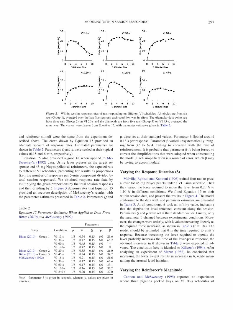
and reinforcer stimuli were the same from the experiment de-scribed above. The curve drawn by Equation 15 provided anadequate account of response rates. Estimated parameters areshown in Table 2. Parameters Q and � were settled at their typicalvalues (0.15 and 6-min, respectively).

Equation 15 also provided a good fit when applied to Mc-Sweeney’s (1992) data. Using lever presses as the target re-sponse and 45-mg Noyes pellets as reinforcers, she exposed ratsto different VI schedules, presenting her results as proportions(i.e., the number of responses per 5-min component divided bytotal session responses). We obtained response rate data bymultiplying the given proportions by the total session responsesand then dividing by 5. Figure 3 demonstrates that Equation 15provided an accurate description of McSweeney’s results, withthe parameter estimates presented in Table 2. Parameters Q and

� were set at their standard values. Parameter � floated around0.18 s per response. Parameter � varied unsystematically, rang-ing from 32 to 67.4, failing to correlate with the rate ofreinforcement. It is probable that parameter � is being forced tocorrect the simplifications that were adopted when constructingthe model. Each simplification is a source of error, which � maybe trying to accommodate.

Varying the Response Duration (�)

Melville, Rybiski and Kamrani (1996) trained four rats to pressa lever for 45-mg Noyes pellets under a VI 1-min schedule. Thenthey varied the force required to move the lever from 0.25 N to1.10 N in different conditions. We fitted Equation 15 to theirwithin-session data, and present the results in Figure 4. The modelconformed to the data well, and parameter estimates are presentedin Table 3. At all conditions, � took an infinity value, indicatingthat the deprivation level remained constant along the session.Parameters Q and � were set at their standard values. Finally, onlythe parameter � changed between experimental conditions. More-over, the changes were orderly, with � values increasing linearly asthe required force increased, as shown in Table 3 (r � .94). Thereader should be reminded that � is the time required to emit aresponse. Because increasing the force required to operate thelever probably increases the time of the lever-press response, theobtained increases in � shown in Table 3 were expected in ad-vance. The conclusion here is identical to Killeen’s (1994). Afteranalyzing an experiment of Mazur (1982), he concluded thatincreasing the lever weight results in increases in �, while main-taining the arousal level invariant.

Varying the Reinforcer’s Magnitude

Cannon and McSweeney (1995) reported an experimentwhere three pigeons pecked keys on VI 30-s schedules of

Figure 2. Within-session response rates of rats responding on different VI schedules. All circles are from sixrats (Group 1), averaged over the last five sessions each condition was in effect. The triangular data points arefrom three rats (Group 2) on VI 20-s and the diamonds are from five rats (Group 3) on VI 45-s, averaged thesame way. The curves were drawn from Equation 15, with parameter estimates given in Table 2.

Table 2Equation 15 Parameter Estimates When Applied to Data FromBittar (2010) and McSweeney (1992)

Parameters

Study Condition � Q � �

Bittar (2010) – Group 1 VI 15-s 1/3 0.54 0.15 6.0 23.6VI 30-s 1/3 0.47 0.15 6.0 65.2VI 60-s 1/3 0.45 0.15 6.0 VI 120-s 1/3 0.47 0.15 6.0

Bittar (2010) – Group 2 VI 20-s 1/3 0.55 0.15 6.0 21.0Bittar (2010) – Group 3 VI 45-s 1/3 0.74 0.15 6.0 34.2McSweeney (1992) VI 15-s 1/3 0.21 0.15 6.0 51.6

VI 30-s 1/3 0.17 0.15 6.0 67.4VI 60-s 1/3 0.17 0.15 6.0 33.1VI 120-s 1/3 0.16 0.15 6.0 37.2VI 240-s 1/3 0.20 0.15 6.0 32.0

Note. Parameter � is given in seconds, whereas � values are given inminutes.


reinforcement. The duration of reinforcers (access to mixedgrain) varied from 2 s to 20 s in different conditions. Theypresented their results as the number of responses per 5-mincomponent divided by total session responses, from which wecalculated response rate data. The experimental results and thefitted curves from Equation 15 are depicted in Figure 5. Param-eter estimates are presented in Table 4. Response duration �was settled at 0.25 s and � at its standard value 6 min.Parameters Q and �, on the other hand, were strongly correlatedwith the reinforcer magnitude, but in opposite directions. As thereinforcer magnitude increased, the jolt of arousal elicited byeach reinforcer (Q) increased (r � .96) while the number ofreinforcers needed to produce 63.2% of satiation (�) decreased(r � �0.88). In short, we conclude that increasing the rein-forcer magnitude affects response rate through a double effectmechanism: Q is increased and � is decreased.

Varying the Organism’s Capacity

DeMarse, Killeen and Baker (1999) measured the weight of 20food-deprived pigeons before and after providing 1-hr of access toa food cup. The difference in weight was defined as the pigeons’eating capacity. The four subjects with greater capacity(M � 47.5 g) were grouped to form the Group LC while the foursubjects with smaller capacity (M � 19.2 g) formed the Group SC.Then, all pigeons responded under VI 30-s schedules. In differentconditions, reinforcers consisted of 2 s or 5 s of access to a hoppercontaining milo grain. The experimenters also delivered one rein-forcer just before the beginning of each session to attenuatewarm-up effects (DeMarse et al., 1999). This procedural detailresults in the pigeons’ arousal being significantly greater than 0 atthe start of the sessions, thus requiring a small adjustment of

Equation 15. To account for their data, we added Qe�t� to the

arousal model of Equation 11, which is embedded in Equation 15.This term represents the arousal elicited by the presession rein-

forcer, which decays exponentially throughout the session accord-ing to the decay rate �.1

Results for both groups, averaged from the last five sessionsduring which each condition was in effect, are presented in Figure6, with the curves drawn from the adjusted Equation 15.

As can be seen from the parameter estimates presented inTable 5, the most significant changes occurred in the satiationparameter �, as could be predicted. This parameter took smallervalues (indicating faster satiation) in Group SC than in GroupLC. Within groups, satiation proceeded faster at the 5-s hopperaccess than at the 2-s hopper access condition. When LCsubjects responded for 2-s hopper access, no satiation occurredat all (� � ). Parameters Q and � were settled at 0.3 and6-min, respectively. Parameter � varied around 0.24-s forGroup SC and around 0.31-s for Group LC, indicating that SCsubjects responded slightly faster.

Alternative Models

Visual inspection of Figures 2 to 6 leaves us with the impressionthat Equation 15 provides an adequate description of the experi-ments cited above. However, does Equation 15 describe data betterthan alternative models?

To answer this question we fitted two other models of within-session responding to the results from the aforementioned ex-periments. The first model is from Killeen (1995) and thesecond from McSweeney, Hinson and Cannon (1996). There’salso a linear model from Aoyama (1998), but as Aoyama and

1The right thing to do would be to add the initial arousal term (Qe�

t�)

to Equation 10 and then correct it for ceiling effects to obtain the adjustedmodel of arousal for this experiment. By adding the term directly toEquation 11 we make it free from ceiling effects, thus allowing arousal to

exceed 1. However, because adding Qe�t� to Equation 10 and then cor-

recting it results in a very complex equation, we choose to privilegesimplicity at the cost of a small loss in precision.

Figure 3. Within-session response rates of rats responding on different VI schedules in McSweeney’s (1992)experiment. The curves were drawn from Equation 15, with parameter estimates given in Table 2.


McSweeney (2001) acknowledged, it cannot account for thebitonic pattern of response rates observed in the behavioral datapresented here. Therefore, it was excluded from the analysisbelow. Before we go on to compare the performance of each ofthese models, we provide a brief description of these alternativeformulations.

Killeen’s (1995) Model

We have seen before that Killeen calculates the within-sessionarousal level as follows:

A�t � vhtR(1 � e�t� ).

This is Equation 2, and we have already discussed its limita-tions. The motivational drive ht, in its turn, is given by ht � �dt,where

dt � d � (M � mR)t. (16)

M represents the metabolic rate and m represents the size of thereinforcers. Equation 16 simply states that deprivation at time tinto session (dt) depends on the initial deprivation level (d0)attenuated by the balance between the resources that have beenspent (M) and the resources that have been consumed (mR).

To obtain a prediction of operant response rates, Killeen statesthe following:

B �

kA�t

A�t � 1(17)

This equation postulates that response rate is a hyperbolicfunction of arousal level, scaled by parameter k—the maximumresponse rate attainable at a specific experimental context,given by C/�. The entire model has seven parameters (k, v, �,d0, M, m, and �). Because parameter � is redundant withparameter v, it may be fixed at 1. It is also possible to fixmetabolic rate M at 0, assuming that metabolic processes areinsignificant in the course of a typical experimental session(Killeen, 1995). Parameter m may be set at 1, leaving deficit d0

to be measured in number of reinforcers. We are finally leftwith four parameters free to vary: k, v, d0, and �.

McSweeney, Hinson, and Cannon’s (1996) Model

McSweeney et al. (1996) also provided a model of within-session operant responding. After examining the fit of severalfunctions to within-session responding data, they arrived at a threeparameter equation given by the following:

P �

b

eaT �

c

c � T. (18)

where P is the proportion of the total-session responses thatoccur during successive time bins, and a, b and c are free

Table 3Equation 15 Parameter Estimates When Applied to Data FromMelville, Rybiski, and Kamrani (1996)

Parameters

Condition � Q � �

0.15N 1/3 0.52 0.15 6.0 0.25N 1/3 0.44 0.15 6.0 0.50N 1/3 0.56 0.15 6.0 0.75N 1/3 0.72 0.15 6.0 1.10N 1/3 0.96 0.15 6.0


Figure 4. Within-session response rates of rats, from Melville et al. (1996) experiment. The numbers on theupper-right side of panels represent the force required to move the lever under each condition. The curves weredrawn from Equation 15, with parameter estimates given in Table 3.


parameters. The first term promotes an exponential decay ofresponse rate attributed to habituation. The second term pro-motes a hyperbolic increase of response rate attributed to sen-sitization. These two processes combine to draw a bitonicpattern of response rate along the course of an experimentalsession. Contrary to Equation 15 and to Killeen’s (1995) model,Equation 18 is an empirical model. Therefore, its parametershave no theoretical meaning.

Comparing the Fits

We used the least-squares method to fit Equation 17 (Killeen,1995) and Equation 18 (McSweeney et al., 1996) to data fromall the experiments mentioned above. Then we compared therelative goodness of fit of these models and Equation 15 usingthe bias-corrected Akaike Information Criteria (AICc), which ispreferred over traditional AIC when working with small samplesizes (Spiess, & Neumeyer, 2010). The Akaike weights for allmodels for all conditions of all experiments are presented inTable 6. At each condition these weights can be interpreted as

the probability of a specific model being the best model amongits competitors (therefore, Akaike weights in a row must alwaysadd up to 1). Equation 15 performed better than the alternativemodels in 19 of 25 comparisons (76%). McSweeney’s modelperformed better in 5 comparisons (20%) and Killeen’s modelin one (4%).

Besides often providing a better fit to data, Equation 15 alsoprovides a better fit to theory. While McSweeney’s model isadmittedly empirical, Killeen’s model has some flaws in its con-struction. The model outlined here, on the other hand, is solidlygrounded in MPR’s core principles (Killeen, 1994). As a conse-quence, its parameters have clear theoretical meanings, assumingvalues that are immediately interpretable and easy to compare andunderstand.

Table 4Equation 15 Parameter Estimates When Applied to Data FromCannon & McSweeney (1995)

Parameters


2-s 1/3 0.25 0.03 6.0 53.75-s 1/3 0.25 0.05 6.0 63.78-s 1/3 0.25 0.04 6.0 33.915-s 1/3 0.25 0.09 6.0 10.720-s 1/3 0.25 0.10 6.0 16.9


Figure 5. Within-session response rates of pigeons responding for reinforcers with varied duration betweenconditions. The curves were drawn from Equation 15, with parameter estimates given in Table 4. The data arefrom Cannon & McSweeney (1995).

Figure 6. Within-session response rates of large capacity (LC) and smallcapacity (SC) rats responding for reinforcers with varied duration betweenconditions. The curves were drawn from Equation 15, with parameterestimates given in Table 5. The data are from DeMarse, Killeen, & Baker(1999).


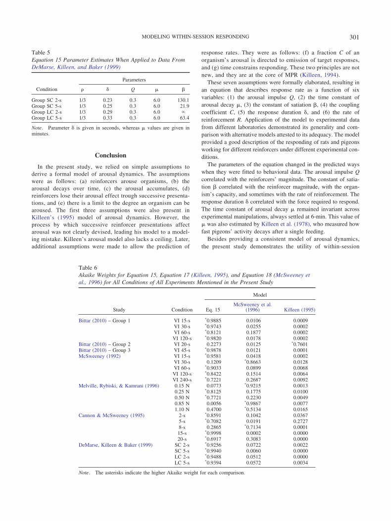
Conclusion

In the present study, we relied on simple assumptions toderive a formal model of arousal dynamics. The assumptionswere as follows: (a) reinforcers arouse organisms, (b) thearousal decays over time, (c) the arousal accumulates, (d)reinforcers lose their arousal effect trough successive presenta-tions, and (e) there is a limit to the degree an organism can bearoused. The first three assumptions were also present inKilleen’s (1995) model of arousal dynamics. However, theprocess by which successive reinforcer presentations affectarousal was not clearly devised, leading his model to a model-ing mistake. Killeen’s arousal model also lacks a ceiling. Later,additional assumptions were made to allow the prediction of

response rates. They were as follows: (f) a fraction C of anorganism’s arousal is directed to emission of target responses,and (g) time constrains responding. These two principles are notnew, and they are at the core of MPR (Killeen, 1994).

These seven assumptions were formally elaborated, resulting inan equation that describes response rate as a function of sixvariables: (1) the arousal impulse Q, (2) the time constant ofarousal decay �, (3) the constant of satiation �, (4) the couplingcoefficient C, (5) the response duration �, and (6) the rate ofreinforcement R. Application of the model to experimental datafrom different laboratories demonstrated its generality and com-parison with alternative models attested to its adequacy. The modelprovided a good description of the responding of rats and pigeonsworking for different reinforcers under different experimental con-ditions.

The parameters of the equation changed in the predicted wayswhen they were fitted to behavioral data. The arousal impulse Qcorrelated with the reinforcers’ magnitude. The constant of satia-tion � correlated with the reinforcer magnitude, with the organ-ism’s capacity, and sometimes with the rate of reinforcement. Theresponse duration � correlated with the force required to respond.The time constant of arousal decay � remained invariant acrossexperimental manipulations, always settled at 6-min. This value of� was also estimated by Killeen et al. (1978), who measured howfast pigeons’ activity decays after a single feeding.

Besides providing a consistent model of arousal dynamics,the present study demonstrates the utility of within-session

Table 5Equation 15 Parameter Estimates When Applied to Data FromDeMarse, Killeen, and Baker (1999)

Parameters


Group SC 2-s 1/3 0.23 0.3 6.0 130.1Group SC 5-s 1/3 0.25 0.3 6.0 21.9Group LC 2-s 1/3 0.29 0.3 6.0 Group LC 5-s 1/3 0.33 0.3 6.0 63.4


Table 6Akaike Weights for Equation 15, Equation 17 (Killeen, 1995), and Equation 18 (McSweeney etal., 1996) for All Conditions of All Experiments Mentioned in the Present Study

Model

Study Condition Eq. 15McSweeney et al.

(1996) Killeen (1995)

Bittar (2010) – Group 1 VI 15-s *0.9885 0.0106 0.0009VI 30-s *0.9743 0.0255 0.0002VI 60-s *0.8121 0.1877 0.0002VI 120-s *0.9820 0.0178 0.0002

Bittar (2010) – Group 2 VI 20-s 0.2273 0.0125 *0.7601Bittar (2010) – Group 3 VI 45-s *0.9878 0.0121 0.0001McSweeney (1992) VI 15-s *0.9581 0.0418 0.0002

VI 30-s 0.1209 *0.8663 0.0128VI 60-s *0.9033 0.0899 0.0068

VI 120-s *0.8422 0.1514 0.0064VI 240-s *0.7221 0.2687 0.0092

Melville, Rybiski, & Kamrani (1996) 0.15 N 0.0773 *0.9215 0.00130.25 N *0.8125 0.1775 0.01000.50 N *0.7721 0.2230 0.00490.85 N 0.0056 *0.9867 0.00771.10 N 0.4700 *0.5134 0.0165

Cannon & McSweeney (1995) 2-s *0.8591 0.1042 0.03675-s *0.7082 0.0191 0.27278-s 0.2865 *0.7134 0.0001

15-s *0.9998 0.0002 0.000020-s *0.6917 0.3083 0.0000

DeMarse, Killeen & Baker (1999) SC 2-s *0.9256 0.0722 0.0022SC 5-s *0.9940 0.0060 0.0000LC 2-s *0.9488 0.0512 0.0000LC 5-s *0.9394 0.0572 0.0034

Note. The asterisks indicate the higher Akaike weight for each comparison.


operant responding data. Because schedules of reinforcementare generally held constant throughout the session, observedvariations in response rate must be primarily attributed tochanges in processes such as arousal, satiation, and habituation.As a consequence, within-session data provide a valuablemeans to clarify the relation between performance and impor-tant motivational variables.

Finally we demonstrated that, by representing arousal as aparameter in the range of 0 to 1, we can formalize MPR (Killeen,1994) in the simplest and most intuitive form of Equation 12.

References

Aoyama, K., & McSweeney, F. K. (2001). Habituation may contribute towithin-session decreases in responding under high-rate schedules ofreinforcement. Animal Learning & Behavior, 29, 79–91. doi:10.3758/BF03192817

Aoyama, K. (1998). Within-session response rate in rats decreases as afunction of amount eaten. Physiology & Behavior, 64, 765–769. doi:10.1016/S0031-9384(98)00118-8

Bittar, E. G. (2010). Within-session responding under several variableinterval schedules of reinforcement. Unpublished manuscript.

Cannon, C. B., & McSweeney, F. K. (1995). Within-session changes inresponding when rate and duration of reinforcement vary. BehaviouralProcesses, 34, 285–292. doi:10.1016/0376-6357(95)00009-J

DeMarse, T. B., Killeen, P. R., & Baker, D. (1999). Satiation, capacity, andwithin-session responding. Journal of the Experimental Analysis ofBehavior, 72, 407–423. doi:10.1901/jeab.1999.72-407

Falk, J. L. (1961). Production of polydipsia in normal rats by an intermit-tent food schedule. Science, 133, 195–196. doi:10.1126/science.133.3447.195

Falk, J. L. (1972). The nature and determinants of adjunctive behavior.R. M. Gilbert & J. D. Keehn (Eds.), Schedule effects: Drugs, drinking,and aggression. Toronto, Canada: University of Toronto Press.

Killeen, P. R., & Bizo, L. A. (1998). The mechanics of reinforcement.Psychonomic Bulletin & Review, 5, 221–238. doi:10.3758/BF03212945

Killeen, P. R., Hanson, S. J., & Osborne, S. R. (1978). Arousal: Its genesisand manifestation as response rate. Psychological Review, 85, 571–581.doi:10.1037/0033-295X.85.6.571

Killeen, P. R., & Sitomer, M. T. (2003). MPR. Behavioural Processes, 62,49–64. doi:10.1016/S0376-6357(03)00017-2

Killeen, P. R. (1994). Mathematical principles of reinforcement. Behav-ioral and Brain Sciences, 17, 105–172. doi:10.1017/S0140525X00033628

Killeen, P. R. (1995). Economics, ecologics, and mechanics: The dynamicsof responding under conditions of varying motivation. Journal of theExperimental Analysis of Behavior, 64, 405–431. doi:10.1901/jeab.1995.64-405

Mazur, J. E. (1982). A molecular approach to ratio schedule performance.M. L. Commons, R. J. Herrnstein & H. Rachlin (Eds.), Quantitativeanalyses of behavior. Vol. 2: Matching and maximizing accounts. Pen-sacola, FL: Ballinger.

McSweeney, F. K., Hatfield, J., & Allen, T. M. (1990). Within-sessionresponding as a function of post-session feedings. Behavioural Pro-cesses, 22, 177–186. doi:10.1016/0376-6357(91)90092-E

McSweeney, F. K., Hinson, J. M., & Cannon, C. B. (1996). Sensitization-habituation may occur during operant conditioning. Psychological Bul-letin, 120, 256–271. doi:10.1037/0033-2909.120.2.256

McSweeney, F. K., & Hinson, J. M. (1992). Patterns of responding withinsessions. Journal of the Experimental Analysis of Behavior, 58, 19–36.doi:10.1901/jeab.1992.58-19

McSweeney, F. K., & Johnson, K. S. (1994). The effect of time betweensessions on within-session patterns of responding. Behavioural Pro-cesses, 31, 207–217. doi:10.1016/0376-6357(94)90007-8

McSweeney, F. K., Roll, J. M., & Weatherly, J. N. (1994). Within-sessionchanges in responding during several simple schedules. Journal of theExperimental Analysis of Behavior, 62, 109–132. doi:10.1901/jeab.1994.62-109

McSweeney, F. K., Swindell, S., & Weatherly, J. N. (1998). Exposure tocontext may contribute to within-session changes in responding. Behav-ioural Processes, 43, 315–328. doi:10.1016/S0376-6357(98)00026-6

McSweeney, F. K., Weatherly, J. N., & Swindell, S. (1995b). Within-session changes in key and lever pressing for water during severalmultiple variable-interval schedules. Journal of the Experimental Anal-ysis of Behavior, 64, 75–94. doi:10.1901/jeab.1995.64-75

McSweeney, F. K. (1992). Rate of reinforcement and session duration asdeterminants of within-session patterns of responding. Animal Learning& Behavior, 20, 160–169. doi:10.3758/BF03200413

McSweeney, F. K. (2004). Dynamic changes in reinforcer effectiveness:Satiation and habituation have different implications for theory andpractice. The Behavior Analyst, 27, 177–188.

Melville, C. L., Rybiski, L. R., & Kamrani, B. (1996). Within-sessionresponding as a function of force required for lever press. BehaviouralProcesses, 37, 217–224. doi:10.1016/0376-6357(96)00008-3

Morgan, M. J. (1974). Resistance to satiation. Animal Behaviour, 22,449–466. doi:10.1016/S0003-3472(74)80044-8

Myers, R. D. (1960). Spontaneous hoarding during operant conditioning.Journal of the Experimental Analysis of Behavior, 3, 154.

Roll, J. M., & McSweeney, F. K. (1997). Within-session changes inoperant responding when gerbils (Meriones unguiculatus) serve as sub-jects. Current Psychology: A Journal for Diverse Perspectives on Di-verse Psychological Issues, 15, 340 –345. doi:10.1007/s12144-997-1011-2

Spiess, A. N., & Neumeyer, N. (2010). An evaluation of R2 as an inade-quate measure for nonlinear models in pharmacological and biochemicalresearch: A Monte Carlo approach. BMC pharmacology, 10, 6. doi:10.1186/1471-2210-10-6

Wallace, M. & Singer, G. (1976). Schedule induced behavior: A review ofits generality, determinants, and pharmacological data. Pharmacology,Biochemistry and Behavior, 5, 483– 490. doi:10.1016/0091-3057(76)90114-3

Received December 12, 2011Revision received April 10, 2012

Accepted May 3, 2012 �


Towards a Mathematical Model of Within-Session Operant Responding

Documents

Transcript of Towards a Mathematical Model of Within-Session Operant Responding