TIPs for the Analysis of Poverty in Mexico, 1992-2005

TIPs for the Analysis of Poverty in Mexico, 1992-2005

Carlos M. Urzúa* Alejandra Macías

and Héctor H. Sandoval

Documento de Trabajo Working Paper

EGAP-2007-08

Tecnológico de Monterrey, Campus Ciudad de México

*EGAP, Calle del Puente 222, Col. Ejidos de Huipulco, 14380 Tlalpan, México, DF, MÉXICO E-mail: [email protected]

TIPs for the Analysis of Poverty in Mexico, 1992-2005*

Carlos M. Urzúa Tecnológico de Monterrey, Campus Ciudad de México

Alejandra Macías

Secretaría de Desarrollo Social

and

Héctor H. Sandoval Consejo Nacional de Evaluación de la Política de Desarrollo Social

This version: April 2007

Resumen

Este trabajo propone varios cambios a la metodología oficial que se utiliza actualmente para medir el estado de pobreza en México. Entre otras sugerencias, se recomienda el uso de métodos de remuestreo para estimar los intervalos de confianza de los estadísticos de pobreza, así como el empleo del análisis de dominancia cuando se hacen comparaciones intertemporales. De manera particular, dado que las líneas de pobreza cambian a lo largo del tiempo, se propone para ese fin el uso de las curvas TIP. Usando las ocho encuestas que fueron levantadas durante el periodo 1992-2005, se presentan un gran número de índices de pobreza absoluta y de curvas TIP, así como comparaciones entre sí. Uno de los hallazgos es que las condiciones en que vive el medio millón de mexicanos más paupérrimo podrían inclusive haber empeorado respecto a las que tenían antes de la crisis de 1994.

Abstract This paper proposes some changes to the official methodology that is currently in use to measure the state of poverty in Mexico. Among other suggestions, it is recommended the use of bootstrapping to estimate confidence intervals for the poverty statistics, as well as the use of dominance analysis when making intertemporal comparisons. In particular, since poverty lines change over time, the paper proposes the use of TIP curves for that end. Using the eight surveys that were made during the period 1992-2005, the paper presents a large number of absolute poverty statistics and TIP curves, as well as comparisons among them. One of the findings is the deterioration of the living conditions of the poorest among the poor, about a half million people, with respect to the conditions they endured before the 1994 economic crisis. Keywords: Poverty, confidence intervals, standard error, bootstrap, resampling, FGT measures, TIP curves, dominance, Mexico JEL classification: I32, D63 *We are grateful to James Foster for his criticism to an earlier draft. We are also grateful to Silvio Rendón for sharing with us an unpublished technical report by Javier Ruiz-Castillo (2005a) on poverty in Mexico. Among several suggestions made by Ruiz-Castillo in that report, he advocates, as we do here, the use of TIP curves.

2

1. Introduction

Since there was not a widely accepted methodology to measure poverty in Mexico in 2001, the

authorities decided to constitute an ad-hoc committee of experts on the subject. The Comité

Técnico para la Medición de la Pobreza (CTMP) was then asked to provide a single

methodology that could be employed by the government to produce official poverty statistics. In

2006 that ad-hoc committee was replaced by the legally constituted Consejo Nacional de

Evaluación de la Política de Desarrollo Social (CONEVAL), which, starting that year, has the

mandate of defining, identifying and measuring poverty in Mexico. As will be briefly reviewed

later, CTMP and CONEVAL have made substantial advances to that end. Although the official

methodology for measuring poverty may be subject to criticisms, some of which will be noted

below, the fact that all economic and political actors are willing to take it as a reference certainly

helps to articulate better policies to attack poverty.

The main purpose of this paper is to suggest some changes in that official methodology

in order to have more robust conclusions on the state of poverty in Mexico. To start with, it is

suggested that all poverty measures should be always accompanied with an estimate of their

precision. Somewhat surprisingly, it is only until very recently that studies on Mexican poverty

have started to incorporate information about the standard errors of their poverty estimates. The

widely circulated report on Mexican poverty by CONEVAL (2006) is a good example. On the

other hand, bad examples are numerous, including a recent book by the World Bank (2004) in

which increases or decreases of poverty estimates are viewed invariably as meaningful, without

ever reporting the corresponding standard errors.

Regarding that issue, and in contrast with an alternative methodological proposal made

by CTMP (2005), we suggest in this paper the routinely use of bootstrapping to calculate

3

confidence intervals for the poverty statistics. We also stress that such a resampling procedure

should take into account the statistical design of the income and expenditure surveys on which

poverty estimates are generated.

A second suggestion to make more robust the official statistics on poverty relates to the

aggregate measures to be employed. For reasons of simplicity, both CTMP and CONEVAL

decided to report in official documents only headcount ratios. But it is known since Sen (1976)

that such an index, although very easy to understand by the public, is fraught with conceptual

difficulties. This point is implicitly acknowledged by CTMP (2002) in an appendix to its first

methodological document, where the committee recommended a further examination of the data

using some of the aggregate poverty measures introduced by Foster, Greer and Thorbecke

(1984). In this paper we advocate just the same, and present those poverty statistics for the eight

latest income and expenditure surveys.

Finally, this paper also proposes the use of dominance analysis when making

intertemporal comparisons about the state of poverty in Mexico. In particular we advocate the

use of TIP curves, as presented by Jenkins and Lambert (1997). Although there are other

possible ways to do that analysis, we believe that TIP curves are easier to understand by the

general public. The paper presents the curves corresponding to each of the surveys, and also

comments on possible poverty dominances over different years. In particular, our analysis casts

some doubts about the commonly-held belief that the current state of poverty in Mexico is less

worrisome than the one that prevailed before the 1994 economic crisis.

The content of the paper is as follows: The next section presents information on the

surveys that are employed in this paper to calculate the poverty measures, as well as on two

important data adjustments that had to be made prior to the computation of the statistics. It also

4

presents the methodology for poverty measurement suggested by CTMP and CONEVAL. Section

three presents a detailed description of the bootstrap method, which is then applied to compute

robust confidence intervals for several poverty indexes. The results are quite comprehensive, since

they make use of the eight different income and expenditure surveys. Section four goes one step

further and makes a dominance analysis by means of TIP curves. Finally, section 5 draws the

conclusions.

2. Surveys and methodology

The information used to measure poverty in Mexico comes from the ENIGH (Encuesta

Nacional de Ingresos y Gastos de los Hogares), a household income and expenditure survey

made by INEGI (Instituto Nacional de Estadística, Geografía e Informática) every two years.

This paper uses the eight different surveys corresponding to the years 1992, 1994, 1996, 1998,

2000, 2002, 2004 and 2005 (this last year is an exception to the rule that surveys are taken in

even years). Although the way in which those surveys are designed have changed over the

years, the eight most recent ones can be safely compared with each other (except for a minor

difference to be mentioned later). Furthermore, those particular years are quite interesting, since

during that single span the Mexican economy went through sharp economic downturns and

upturns: After coming from a period of stability and relatively low growth rates from 1992 to

1994, the economy suffered at the end of 1994 a financial crisis that sent it to a very deep

recession that lasted two years. A strong recovery ensued in the years 1998-2000, partially

fueled by the strong performance showed by the US economy in that period. From the year 2001

to 2003, though, the Mexican economy stagnated, and had an even more disappointing record

5

than the US economy. Finally, in the last two years covered by the surveys, 2004-2005, the

economy enjoyed a mild but sustained recovery.

Before starting our study, it is important to note that the data reported in the surveys

mentioned above were adjusted in two ways: First, we deleted all duplicated income entries that

were found in each of the surveys. The first three ENIGHs were free of error in that respect,

while the rest had duplicated responses in varying degrees.1 It is interesting to note that the same

cleaning procedure was followed by the authorities in their document on poverty circulated at

the end of 2006 (CONEVAL, 2006). Our second adjustment had to do with the cases of

households that reported negative net incomes. For reasons that will be given later on, in those

instances the net incomes were changed to zero.

There are two other comments, more technical, that we would like to make regarding the

surveys: First, all the ENIGHs were designed to be representative not only at national level, but

also at urban (localities with 2,500 inhabitants or more) and rural (i.e., non-urban) levels.

Although the most recent surveys are also representative at other levels, for purposes of

comparison our results are only reported on the first three. The second comment to be made is

about the sampling design of the ENIGHs. This is an important issue if one wants to make

poverty comparisons over the years, since the estimation of standard errors for poverty measures

should take into account such a sampling design (see, e.g., Howes and Lanjow, 1998). For that

end, in this paper we make use of the information on the corresponding strata and primary

sampling units reported by INEGI for each ENIGH.2

1 The number of duplicated entries for the years 1998, 2000, 2002, 2004 and 2005 were, respectively, 1, 4, 9, 92 and 1. Except for the year 2004, whose duplicated entries accounted for .12% of the total, the errors found in the rest of the years can be regarded as insignificant. 2 We also follow this institution in disregarding, in the case of the calculation of standard errors, the instances in which there are also secondary, and even tertiary, sampling units.

6

Regarding the official methodology to measure poverty, as first established by CTMP

(2002 and 2005) and later adopted by CONEVAL, we can state its two main elements as

follows: First, as is the case in most of the other developing countries, the official poverty

statistics are based on absolute poverty lines, while the household welfare is identified with its

income. Since we don’t want to take issue on those two choices here, we refer the reader to the

thoughtful papers by Ruiz-Castillo (2005a,b) in which both of those directives are challenged

for the case of Mexico. In particular, Ruiz-Castillo advocates the simultaneous estimation of

absolute and relative poverty, while he sides in favor of consumption-based measures.

The other main point is that the official methodology also establishes that the headcount

ratio should be used to report poverty incidence, and this according to three different poverty

definitions: “food poverty”, when income is too low to cover basic food necessities;

“capabilities poverty”, when income is insufficient to buy basic food, education and health

necessities; and “assets poverty”, when income is too low to cover basic food, education, health,

dressing, housing and public transportation necessities. The reader may consult CTMP (2002)

for the way in which the corresponding three poverty lines are derived. Here it suffices to note

that by “income” is meant per capita income, since individuals, rather than households are

typically considered in the official statistics.

Furthermore, the actual variable that is employed is net income, which is the result of

subtracting from total current income all transfers to other households. This is important to keep

in mind, since, as shown by Sandoval and Urzúa (2007), in all the ENIGHs that are examined in

this paper there are some households that actually report negative net incomes, a fact that may

have in turn some consequences. In such a case, that paper shows that if the poverty measures

go beyond a mere headcount they could behave in rather anomalous ways. Thus, it is important

7

to decide from the onset what to do with the negative net incomes. As pointed out earlier, in our

exercise we decided to set them equal to zero. Although Sandoval and Urzúa (2007) suggest

better ways to deal with that problem, by setting them equal to zero we continue to get the same

official poverty incidence statistics while avoiding anomalous behaviors.

Regarding the poverty indices to be computed in this paper, we will use particular

members of the following FGT class introduced by Foster, Greer and Thorbecke (1984):

(1) 0, ,1)(1

≥⎟⎠⎞

⎜⎝⎛ −

= ∑=

αα

α

q

i

i

zyz

nzP

where q is the number of poor people in a population of size n , and where the i-th member has

an income yi which is less or equal than the poverty line z. The headcount ratio used by CTMP

and CONEVAL is obtained when ,0=α which gives poverty incidence (the proportion of the

population whose welfare falls below the poverty line). On the other hand, the relative poverty-

gap measure is found when :1=α

.1)(1

1 ∑=

⎟⎠⎞

⎜⎝⎛ −

=q

i

i

zyz

nzP

This index measures poverty intensity, the shortfall in the welfare of the poor relative to the

poverty line. Finally, the squared poverty-gap index is obtained when :2=α

,1)(1

2

2 ∑=

⎟⎠⎞

⎜⎝⎛ −

=q

i

i

zyz

nzP

which, by giving more weight to the poorest individuals, provides a measure of the severity of

poverty. It may be noted that if one were to accept Sen’s (1976) monotonicity and transfer

axioms, of the three indexes considered here it is only the squared poverty-gap which would be

considered to be a bona fide poverty measure.

8

3. Testing for Changes in Poverty

As noted in the introduction, one of the purposes of this paper is to calculate confidence

intervals for the FGT poverty statistics in the case of Mexico. An approach that might be used

for that end is to apply the delta method (which boils down to a simple Taylor expansion). This

is in fact the procedure implicitly recommended by CTMP (2005), and later implemented by

CONEVAL (2006) in its study of poverty incidence in Mexico during the years 1992-2005.

Actually, assuming that a poverty line is fixed, it is easy to find the asymptotic sampling

variances when the estimators are means of simple functions of random variables. In fact,

Kakwani (1993) has presented explicitly the approximate sampling variance for the class of

FGT poverty indices given in (1); namely,

.)var(2

2

nPPP αα

α−

≈

Note that, as we stressed earlier, that type of approximation cannot be applied directly,

since it presumes that the survey was taken using a simple design. However, after making use of

the fact that the FGT measures are additively decomposable, Jolliffe and Semykina (2000) show

how to include the possibility of a complex design that includes stratification and clustering.3 A

methodological note that is broadly similar is also made by CTMP (2005).

It is worth noting, however, that the Taylor approximation given above is derived

assuming an asymptotic normal distribution for the estimators, which is obviously incorrect in

the case of poverty measures. This is so because those indexes oscillate between 0 and 1 (0%

and 100%). As a consequence, if one uses a normal approximation for the confidence intervals,

these could end up containing values less than zero or greater than one (see, e.g., Sandoval and

3 Those authors have actually written a STATA program, whose command name is sepov, that accomplishes automatically that task.

9

Urzúa, 2007, for an example with real data). Furthermore, a normal approximation would lead

to symmetric confidence intervals, which seems unwarranted on a priori grounds.

But then, how can one construct more robust confidence intervals for poverty statistics?

The answer is well known: By using resampling methods, the most versatile of which is Efron’s

bootstrap. Even though since the mid-eighties there have been numerous applications of

bootstrapping in Economics, it is interesting to note that it took some time for this simulation

procedure to be recognized as a valuable tool among researchers interested on poverty and

income distribution. To our knowledge, it was Deaton (1997) who first used it in the context of

poverty, while Mills and Zandvakili (1997) were the pioneers in the case of inequality

measurement.

The idea of bootstrapping is simple. Given a dataset, such as the one coming from an

income and expenditure survey, one creates a large number of independent bootstrap samples

(in our case “bootstrap surveys”) by sampling with replacement from the dataset. One then

computes the statistic of interest for each of those samples, and estimates the standard error of

the original statistic by the empirical standard deviation of those replications.

To be more precise, and following the presentation in Efron and Tibshiriani (1993), if n

is the sample size, then the bootstrap algorithm for the (nonparametric) estimation of the

standard error of the FGT statistic αP can be described as follows: First, select B independent

bootstrap samples, each with size n and drawn with replacement. In our case B was selected to

be equal to 500.4 The second step involves the computation of the poverty measure for each

4 Efron and Tibshiriani (1993) suggest that in the case of standard error estimation an upper bound that works well is 250 replications. However, since the interest in this paper is on robust confidence intervals, that lead us to choose 500 replications for all cases.

10

bootstrap sample: ),(ˆ bPα . ,...,2 ,1 Bb = The last step involves the estimation of the standard

error of the original poverty statistic using the standard deviation of the B replications given by:

[ ] ∑∑==

=⎭⎬⎫

⎩⎨⎧

−−B

b

B

b

BbPPBPbP1

2/1

1

2 ./)(ˆ where,)1/()(ˆααα

In the case of the estimation of confidence intervals for the poverty measures, which is

important in the case of this paper, there are several procedures available. We choose here to

work with Efron’s bias-corrected and accelerated (BCa) method, which is more time demanding

than most of the others, but it is also one of the best. Since the formulae required to present the

method is a little bit cumbersome we refer the reader to Efron and Tibshiriani (1993, chap. 14)

for the details. Finally, there is an important reminder to be made before presenting the

empirical results: The bootstrapping computation of the confidence intervals have to take into

account the complex design of the ENIGHs.5

Table 1 presents the values of the FGT poverty indices and their confidence intervals

thus obtained. The estimates are given for eight different years, as well as for the three official

definitions of poverty. As noted there, the figures correspond to the population at large

(individuals, not households), and also to the national level. To complement this last case, tables

A1 and A2 in the Appendix present the FGT indices for the case of urban and rural Mexico.

Before making intertemporal comparisons, it is worth commenting about how our results

compare to the ones calculated by the government. Since the current methodology dictates that

only the head-count ratio (poverty incidence) be reported, the official documents typically

5 This is not a difficult task to accomplish in most statistical packages. For instance, in STATA one has to declare first the survey design using the command svyset, and then use the command bootstrap leaving the “size” option unspecified (in such a way that the bootstrap samples are in agreement with the total number of clusters in each stratum). The BCa confidence intervals are also available in that package.

11

Table 1 FGT Poverty Indices for Mexico, 1992-2005

(Population at large, national level)

Year P(0) P(1) P(2)

Food Poverty1992 22.4% 19.4% 25.7% 7.5% 6.1% 8.8% 3.5% 2.9% 4.2%1994 21.3% 19.0% 23.6% 7.2% 6.2% 8.1% 3.3% 2.9% 3.8%1996 36.9% 36.1% 38.4% 13.8% 13.3% 14.4% 7.0% 6.6% 7.5%1998 34.3% 33.0% 35.6% 13.5% 12.9% 14.2% 7.2% 6.7% 7.6%2000 24.1% 22.7% 25.7% 8.4% 7.9% 9.1% 4.1% 3.9% 4.8%2002 20.0% 19.0% 21.4% 6.2% 5.8% 6.6% 2.8% 2.7% 3.8%2004 17.4% 16.4% 18.4% 5.8% 5.6% 6.5% 3.0% 2.5% 3.4%2005 18.2% 17.2% 19.0% 6.1% 5.9% 6.7% 3.0% 2.3% 3.7%

Capabilities Poverty1992 30.7% 27.4% 34.1% 10.7% 9.3% 12.2% 5.2% 4.3% 6.1%1994 30.1% 27.0% 32.6% 10.2% 9.2% 11.7% 4.9% 4.3% 5.6%1996 46.1% 45.1% 47.4% 18.5% 17.9% 19.4% 9.8% 9.5% 10.3%1998 42.6% 41.4% 43.9% 17.7% 17.0% 18.4% 9.7% 9.2% 10.3%2000 31.8% 30.3% 33.2% 11.6% 11.1% 12.4% 5.9% 5.7% 6.7%2002 26.9% 25.7% 28.1% 9.1% 8.6% 9.6% 4.3% 4.1% 5.1%2004 24.7% 23.7% 25.8% 8.4% 8.1% 9.1% 4.2% 3.7% 4.8%2005 24.7% 23.7% 25.7% 8.7% 8.3% 9.2% 4.4% 3.5% 5.2%

Assets Poverty1992 54.0% 50.8% 57.3% 22.5% 20.3% 24.6% 12.3% 10.9% 13.7%1994 52.7% 49.5% 55.4% 21.8% 20.1% 23.5% 11.8% 10.9% 13.1%1996 68.7% 67.7% 70.0% 33.2% 32.7% 34.1% 20.0% 19.5% 20.7%1998 64.5% 63.3% 65.9% 31.4% 30.5% 32.4% 19.1% 18.6% 19.9%2000 53.6% 51.9% 55.2% 23.3% 22.4% 24.2% 13.1% 12.5% 13.9%2002 50.0% 48.7% 51.2% 20.0% 19.4% 20.8% 10.6% 10.3% 11.2%2004 47.2% 45.4% 48.4% 18.6% 18.1% 19.4% 10.0% 9.2% 10.8%2005 47.0% 45.9% 48.1% 19.0% 18.4% 19.6% 10.2% 8.8% 11.6%

[95% Conf. Int.] [95% Conf. Int.] [95% Conf. Int.]

Source: Own estimates based on the corresponding ENIGHs.

12

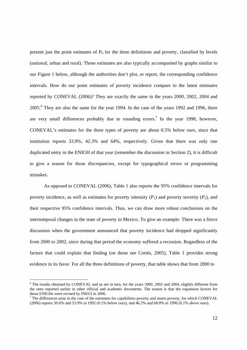
present just the point estimates of P0 for the three definitions and poverty, classified by levels

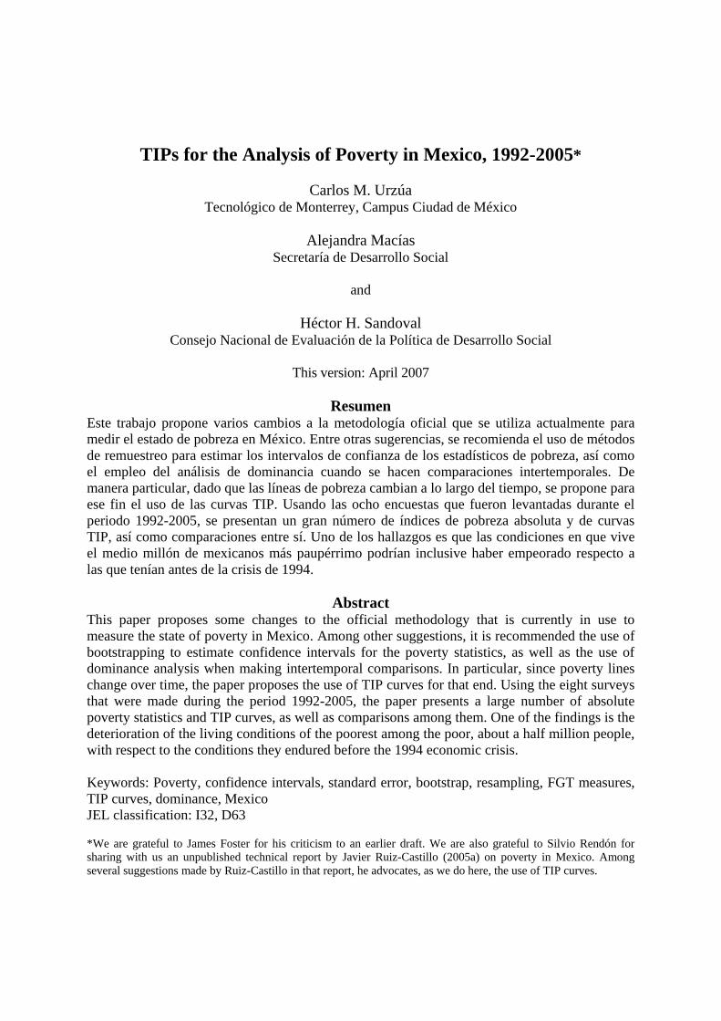
(national, urban and rural). Those estimates are also typically accompanied by graphs similar to

our Figure 1 below, although the authorities don’t plot, or report, the corresponding confidence

intervals. How do our point estimates of poverty incidence compare to the latest estimates

reported by CONEVAL (2006)? They are exactly the same in the years 2000, 2002, 2004 and

2005.6 They are also the same for the year 1994. In the case of the years 1992 and 1996, there

are very small differences probably due to rounding errors.7 In the year 1998, however,

CONEVAL’s estimates for the three types of poverty are about 0.5% below ours, since that

institution reports 33.9%, 42.3% and 64%, respectively. Given that there was only one

duplicated entry in the ENIGH of that year (remember the discussion in Section 2), it is difficult

to give a reason for those discrepancies, except for typographical errors or programming

mistakes.

As opposed to CONEVAL (2006), Table 1 also reports the 95% confidence intervals for

poverty incidence, as well as estimates for poverty intensity (P1) and poverty severity (P2), and

their respective 95% confidence intervals. Thus, we can draw more robust conclusions on the

intertemporal changes in the state of poverty in Mexico. To give an example: There was a fierce

discussion when the government announced that poverty incidence had dropped significantly

from 2000 to 2002, since during that period the economy suffered a recession. Regardless of the

factors that could explain that finding (on those see Cortés, 2005), Table 1 provides strong

evidence in its favor. For all the three definitions of poverty, that table shows that from 2000 to

6 The results obtained by CONEVAL and us are in turn, for the years 2000, 2002 and 2004, slightly different from the ones reported earlier in other official and academic documents. The reason is that the expansion factors for those ENIGHs were revised by INEGI in 2006. 7 The differences arise in the case of the estimates for capabilities poverty and assets poverty, for which CONEVAL (2006) reports 30.6% and 53.9% in 1992 (0.1% below ours), and 46.2% and 68.8% in 1996 (0.1% above ours).

13

Figure 1 Poverty Incidence in Mexico for the Population at Large, 1992-2005

0.00

0.10

0.20

0.30

0.40

0.50

0.60

0.70

0.80

1992 1994 1996 1998 2000 2002 2004 2005

Food Poverty

Capabilities Poverty

Assets Poverty


14

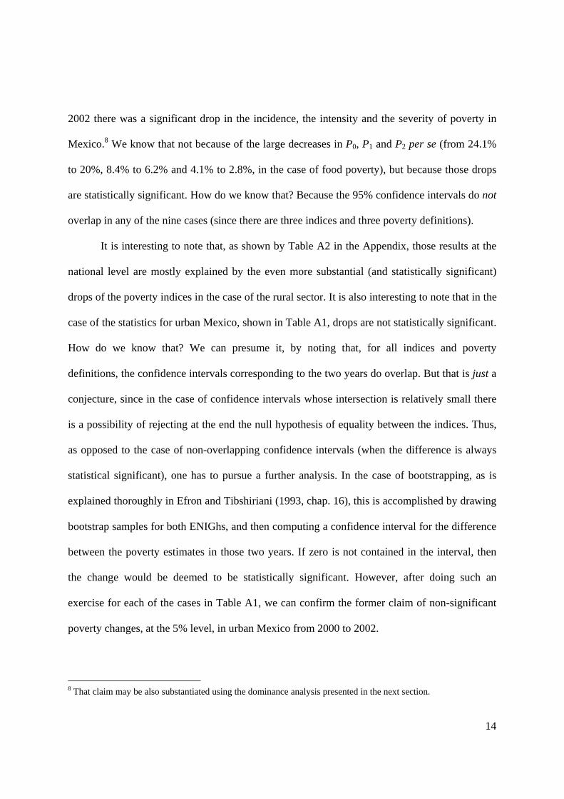
2002 there was a significant drop in the incidence, the intensity and the severity of poverty in

Mexico.8 We know that not because of the large decreases in P0, P1 and P2 per se (from 24.1%

to 20%, 8.4% to 6.2% and 4.1% to 2.8%, in the case of food poverty), but because those drops

are statistically significant. How do we know that? Because the 95% confidence intervals do not

overlap in any of the nine cases (since there are three indices and three poverty definitions).

It is interesting to note that, as shown by Table A2 in the Appendix, those results at the

national level are mostly explained by the even more substantial (and statistically significant)

drops of the poverty indices in the case of the rural sector. It is also interesting to note that in the

case of the statistics for urban Mexico, shown in Table A1, drops are not statistically significant.

How do we know that? We can presume it, by noting that, for all indices and poverty

definitions, the confidence intervals corresponding to the two years do overlap. But that is just a

conjecture, since in the case of confidence intervals whose intersection is relatively small there

is a possibility of rejecting at the end the null hypothesis of equality between the indices. Thus,

as opposed to the case of non-overlapping confidence intervals (when the difference is always

statistical significant), one has to pursue a further analysis. In the case of bootstrapping, as is

explained thoroughly in Efron and Tibshiriani (1993, chap. 16), this is accomplished by drawing

bootstrap samples for both ENIGhs, and then computing a confidence interval for the difference

between the poverty estimates in those two years. If zero is not contained in the interval, then

the change would be deemed to be statistically significant. However, after doing such an

exercise for each of the cases in Table A1, we can confirm the former claim of non-significant

poverty changes, at the 5% level, in urban Mexico from 2000 to 2002.

8 That claim may be also substantiated using the dominance analysis presented in the next section.

15

We invite the reader to peruse the tables to compare the poverty indices over the rest of

the years. Here we just draw three noticeable conclusions: First, after the economic crisis that

erupted at the end of 1994, the state of poverty in Mexico deteriorated very sharply. This can be

seen by comparing the figures in Table 1 for 1994 (the corresponding ENIGH was made several

months before the beginning of the crisis) with the ones for 1996-1998. Second, poverty

conditions improved from 2000 to 2004. And third, even though the government made for

electoral reasons an untypical ENIGH in the year 2005, the poverty conditions did not turn out

to have improved over the ones prevailing in 2004.

As a final point, note that all of our conclusions above are based on the indices that

measure poverty incidence, intensity or severity. Not less, but also not more. We invite the

reader to try to answer, by just looking at the tables, the important question of whether or not the

state of poverty in Mexico that prevailed in 1994, right before the crisis, was definitely worse

than the current conditions, as represented by the 2004 indices (better, in terms of simple point

estimates, than the 2005 indices). At the end of the next section will try to give an unambiguous

answer to that question.

4. TIP curves

Since all the comparisons made in the last section depend on particular indices, a natural

question to ask is if by using other poverty measures we would end up with the same rankings as

the ones obtained before. There is an important literature that tries to establish criteria for

unambiguous poverty rankings, the general framework to which that question belongs. Although

there are several possible ways to face that problem (e.g., through the use of generalized Lorenz

curves), we believe that the methodology introduced by Jenkins and Lambert (1997) is, aside

16

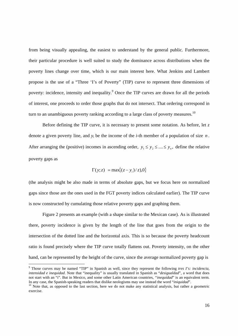
from being visually appealing, the easiest to understand by the general public. Furthermore,

their particular procedure is well suited to study the dominance across distributions when the

poverty lines change over time, which is our main interest here. What Jenkins and Lambert

propose is the use of a “Three ‘I’s of Poverty” (TIP) curve to represent three dimensions of

poverty: incidence, intensity and inequality.9 Once the TIP curves are drawn for all the periods

of interest, one proceeds to order those graphs that do not intersect. That ordering correspond in

turn to an unambiguous poverty ranking according to a large class of poverty measures.10

Before defining the TIP curve, it is necessary to present some notation. As before, let z

denote a given poverty line, and yi be the income of the i-th member of a population of size n .

After arranging the (positive) incomes in ascending order, ,....21 nyyy ≤≤≤ define the relative

poverty gaps as

{ }0),/)(max);( zyzzy i−=Γ

(the analysis might be also made in terms of absolute gaps, but we focus here on normalized

gaps since those are the ones used in the FGT poverty indices calculated earlier). The TIP curve

is now constructed by cumulating those relative poverty gaps and graphing them.

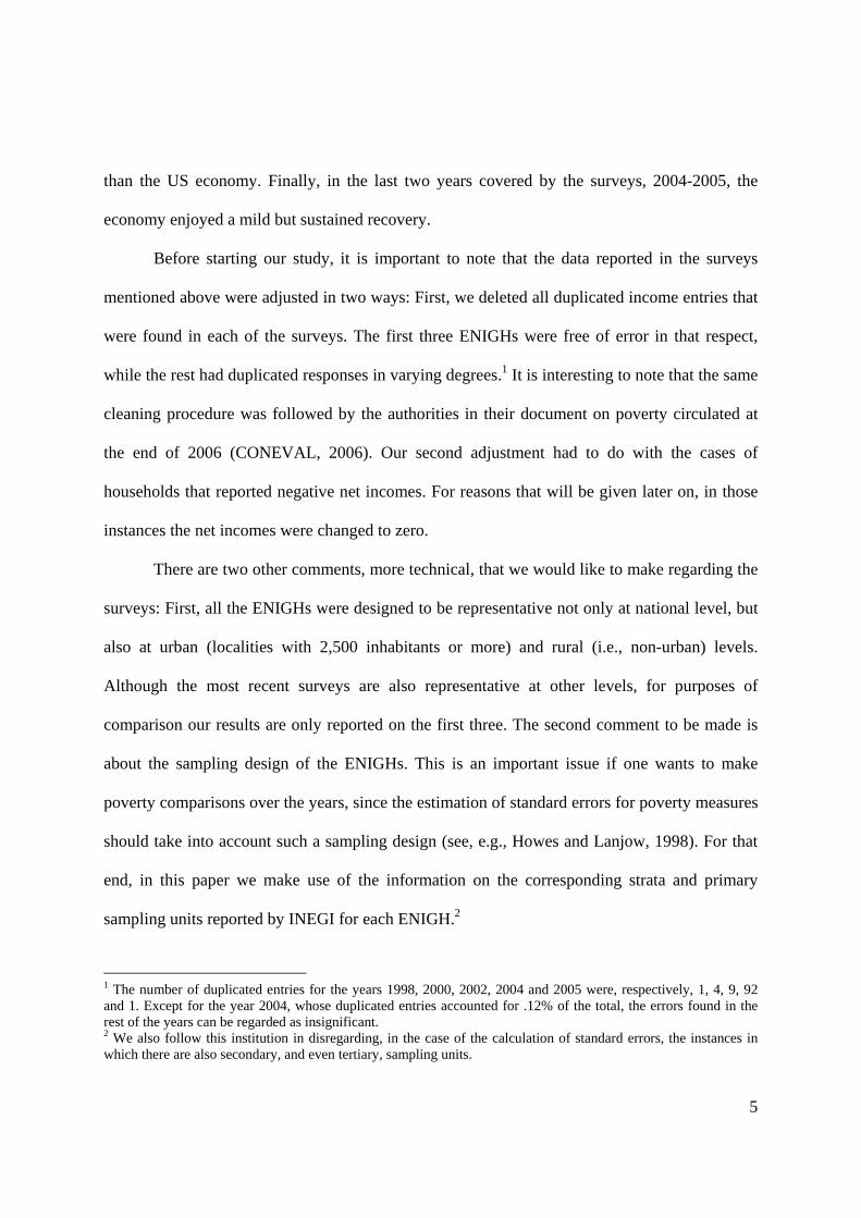
Figure 2 presents an example (with a shape similar to the Mexican case). As is illustrated

there, poverty incidence is given by the length of the line that goes from the origin to the

intersection of the dotted line and the horizontal axis. This is so because the poverty headcount

ratio is found precisely where the TIP curve totally flattens out. Poverty intensity, on the other

hand, can be represented by the height of the curve, since the average normalized poverty gap is 9 Those curves may be named “TIP” in Spanish as well, since they represent the following tres I’s: incidencia, intensidad e inequidad. Note that “inequality” is usually translated in Spanish as “desigualdad”, a word that does not start with an “i”. But in Mexico, and some other Latin American countries, “inequidad” is an equivalent term. In any case, the Spanish-speaking readers that dislike neologisms may use instead the word “iniquidad”. 10 Note that, as opposed to the last section, here we do not make any statistical analysis, but rather a geometric exercise.

17

Figure 2 The TIP Curve and Its Three I’s

18

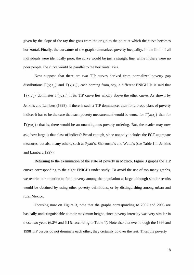
given by the slope of the ray that goes from the origin to the point at which the curve becomes

horizontal. Finally, the curvature of the graph summarizes poverty inequality. In the limit, if all

individuals were identically poor, the curve would be just a straight line, while if there were no

poor people, the curve would be parallel to the horizontal axis.

Now suppose that there are two TIP curves derived from normalized poverty gap

distributions );( yzyΓ and );( xzxΓ , each coming from, say, a different ENIGH. It is said that

);( xzxΓ dominates );( yzyΓ if its TIP curve lies wholly above the other curve. As shown by

Jenkins and Lambert (1998), if there is such a TIP dominance, then for a broad class of poverty

indices it has to be the case that each poverty measurement would be worse for );( xzxΓ than for

);( yzyΓ ; that is, there would be an unambiguous poverty ordering. But, the reader may now

ask, how large is that class of indices? Broad enough, since not only includes the FGT aggregate

measures, but also many others, such as Pyatt’s, Shorrocks’s and Watts’s (see Table 1 in Jenkins

and Lambert, 1997).

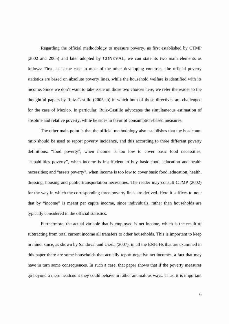
Returning to the examination of the state of poverty in Mexico, Figure 3 graphs the TIP

curves corresponding to the eight ENIGHs under study. To avoid the use of too many graphs,

we restrict our attention to food poverty among the population at large, although similar results

would be obtained by using other poverty definitions, or by distinguishing among urban and

rural Mexico.

Focusing now on Figure 3, note that the graphs corresponding to 2002 and 2005 are

basically undistinguishable at their maximum height, since poverty intensity was very similar in

those two years (6.2% and 6.1%, according to Table 1). Note also that even though the 1996 and

1998 TIP curves do not dominate each other, they certainly do over the rest. Thus, the poverty

19

Figure 3 TIPs Curves for Mexico, 1992-2005

(Food poverty, population at large)


20

conditions in 1996-1998 were considerably worse than the ones prevailing before the economic

crisis, as represented by the 1992-1994 TIP curves, and also worse than the poverty conditions

that took place after the end of that crisis, as given by the 2000-2005 TIP curves.

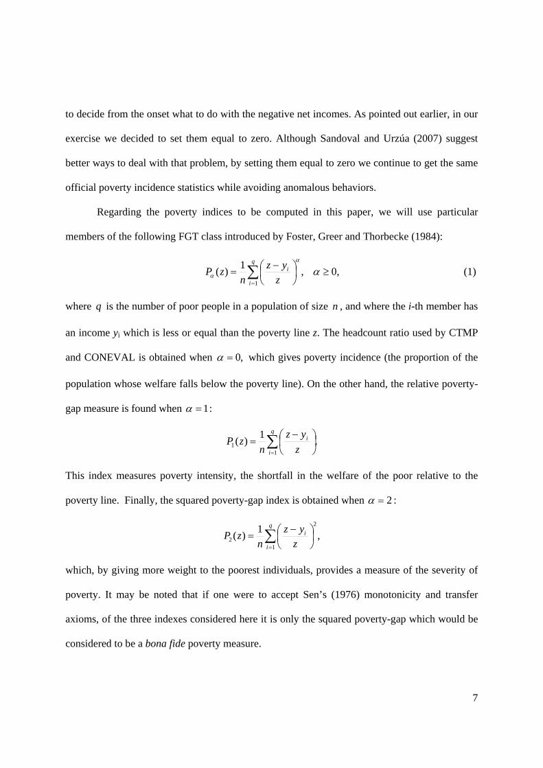
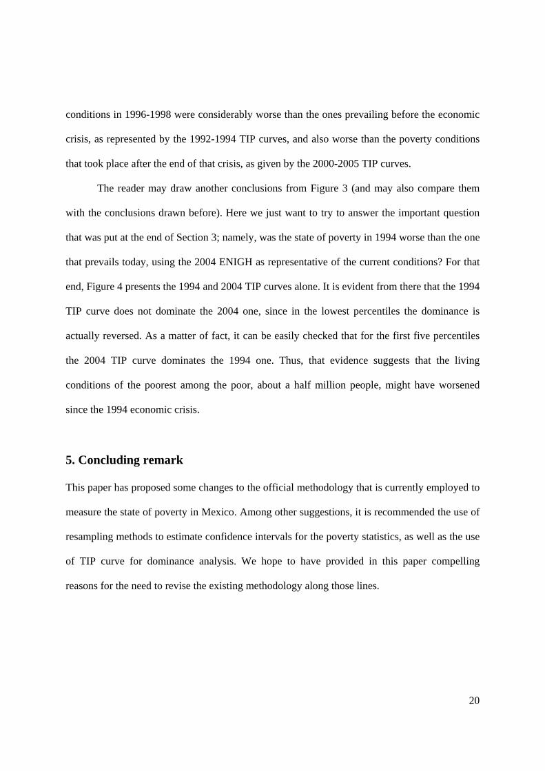
The reader may draw another conclusions from Figure 3 (and may also compare them

with the conclusions drawn before). Here we just want to try to answer the important question

that was put at the end of Section 3; namely, was the state of poverty in 1994 worse than the one

that prevails today, using the 2004 ENIGH as representative of the current conditions? For that

end, Figure 4 presents the 1994 and 2004 TIP curves alone. It is evident from there that the 1994

TIP curve does not dominate the 2004 one, since in the lowest percentiles the dominance is

actually reversed. As a matter of fact, it can be easily checked that for the first five percentiles

the 2004 TIP curve dominates the 1994 one. Thus, that evidence suggests that the living

conditions of the poorest among the poor, about a half million people, might have worsened

since the 1994 economic crisis.

5. Concluding remark

This paper has proposed some changes to the official methodology that is currently employed to

measure the state of poverty in Mexico. Among other suggestions, it is recommended the use of

resampling methods to estimate confidence intervals for the poverty statistics, as well as the use

of TIP curve for dominance analysis. We hope to have provided in this paper compelling

reasons for the need to revise the existing methodology along those lines.

21

Figure 4 TIPs Curves for 1994 and 2004 (Food poverty, population at large)


22

References

Comité Técnico para la Medición de la Pobreza (2002). Medición de la pobreza: Variantes metodológicas y estimación preliminar, México, Secretaría de Desarrollo Social. Reprinted in M. Székely, ed. (2005).

Comité Técnico para la Medición de la Pobreza (2005). Recomendaciones metodológicas para

la evaluación intertemporal de niveles de pobreza en México (2000-2002), in M. Székely, ed. (2005).

Consejo Nacional de Evaluación de la Política de Desarrollo Social (2006). El CONEVAL

reporta cifras sobre la evolución de la pobreza en México, comunicado número 001/2006, México.

Cortés, F. (2005), ¿Disminuyó la pobreza? México 2000-2002, in M. Székely, ed. (2005). Deaton, A. (1997). The Analysis of Household Surveys: A Microeconometric Approach to

Development Policy, Baltimore, Johns Hopkins. Efron, B., and R. J. Tibshirani (1993). An Introduction to the Bootstrap, London, Chapman &

Hall. Foster, J., J. Greer, and E. Thorbecke (1984). A Class of Decomposable Poverty Measures,

Econometrica, 52, 761-765. Howes, S., and J. O. Lanjow (1998). Does Sample Design Matter for Poverty Rate

Comparisons?, Review of Income and Wealth, 44, 99-109. Jenkins, S. P., and P. J. Lambert (1997). Three ‘I’s of Poverty Curves, with an Analysis of UK

Poverty Trends, Oxford Economic Papers, 49, 317-327. Jenkins, S. P., and P. J. Lambert (1998). Three ‘I’s of Poverty Curves and Poverty Dominance:

Tips for Poverty Analysis, Research on Economic Inequality, 8, 39-56. Jolliffe, D., and A. Semykina (2000). Robust Standard Errors for the Foster-Greer-Thorbecke

Class of Poverty Indices, Stata Technical Bulletin Reprints, 8, 274-278. Kakwani, N. (1993). Statistical Inference in the Measurement of Poverty, Review of Economics

and Statistics, 75, 632-639. Mills, J. A., and S. Zandvakili (1997). Statistical Inference via Bootstrapping for Measures of

Inequality, Journal of Applied Econometrics, 12, 133-150.

23

Ruiz-Castillo, J. (2005a). An Evaluation of ‘El Ingreso Rural y la Producción Agropecuaria en México’, technical report, Servicio de Información Alimentaria y Pesquera, México, SAGARPA.

Ruiz-Castillo, J. (2005b). Relative and Absolute Poverty: The Case of Mexico, 1992-2004,

Working Paper 06-11, Departamento de Economía, Universidad Carlos III de Madrid. Sandoval, H. H., and C. M. Urzúa (2007). Negative Net Incomes and the Measurement of

Poverty: A Note, submitted to Estudios Económicos. Sen, A. (1976). Poverty: An Ordinal Approach to Measurement, Econometrica, 52, 219-231. Székely, M., ed. (2005). Números que mueven al mundo: La medición de la pobreza en México,

México, ANUIES, CIDE, SEDESOL, Miguel Ángel Porrúa. World Bank (2004). Poverty in Mexico: An Assessment of Conditions, Trends, and Government

Strategy, Washington, World Bank.

24

Table A1 FGT Poverty Indices for Urban Mexico, 1992-2005

(Population at large)

Year P(0) P(1) P(2)

Food Poverty1992 13.3% 10.9% 16.6% 3.6% 2.9% 4.4% 1.4% 1.1% 1.8%1994 9.9% 8.2% 11.4% 2.6% 2.1% 3.1% 1.0% 0.8% 1.2%1996 26.7% 25.2% 28.2% 8.4% 7.9% 9.1% 3.7% 3.4% 4.0%1998 21.8% 20.2% 23.1% 6.6% 6.0% 7.1% 2.9% 2.6% 3.2%2000 12.5% 10.7% 14.7% 3.3% 2.6% 4.1% 1.4% 1.1% 1.9%2002 11.3% 9.0% 14.1% 2.8% 2.1% 3.5% 1.1% 0.8% 1.4%2004 11.0% 8.3% 13.1% 3.0% 2.1% 3.7% 1.4% 1.0% 1.7%2005 9.9% 8.0% 11.7% 2.6% 2.0% 3.2% 1.1% 0.8% 1.3%


Assets Poverty1992 44.5% 40.3% 48.6% 16.5% 14.6% 18.9% 8.2% 7.0% 9.4%1994 40.6% 37.1% 44.9% 14.1% 12.4% 15.8% 6.8% 6.0% 7.7%1996 60.9% 59.2% 62.2% 27.0% 26.0% 27.8% 15.2% 14.5% 15.8%1998 56.3% 54.6% 57.8% 23.6% 22.7% 24.7% 12.7% 12.2% 13.5%2000 43.7% 40.6% 46.4% 16.0% 14.6% 17.4% 7.9% 7.0% 9.0%2002 41.2% 37.7% 45.7% 14.4% 12.3% 16.3% 6.9% 5.7% 8.2%2004 41.1% 37.5% 44.1% 14.5% 12.4% 16.4% 7.1% 5.8% 8.3%2005 38.3% 35.4% 41.5% 13.4% 12.0% 15.0% 6.4% 5.5% 7.4%



25

Table A2 FGT Poverty Indices for Rural Mexico, 1992-2005

(Population at large)

Year P(0) P(1) P(2)

Food Poverty1992 35.6% 30.7% 41.4% 13.1% 10.8% 15.4% 6.4% 5.0% 7.7%1994 37.0% 32.7% 40.8% 13.4% 11.7% 15.4% 6.6% 5.6% 7.6%1996 52.1% 50.0% 54.0% 21.8% 20.7% 23.1% 11.8% 11.1% 12.7%1998 52.3% 50.3% 54.6% 23.5% 22.3% 24.7% 13.3% 12.4% 14.1%2000 42.3% 37.3% 47.7% 16.4% 13.8% 19.5% 8.4% 6.7% 11.5%2002 34.0% 28.3% 38.0% 11.8% 10.1% 13.5% 5.6% 4.7% 6.5%2004 28.0% 22.0% 37.8% 10.5% 6.9% 15.2% 5.6% 3.7% 8.6%2005 32.3% 26.2% 41.7% 12.2% 9.5% 16.7% 6.4% 4.8% 8.6%


Assets Poverty1992 67.7% 63.5% 71.4% 31.1% 28.0% 34.6% 18.2% 15.9% 21.0%1994 69.5% 66.0% 72.9% 32.3% 29.5% 34.9% 18.8% 17.1% 20.7%1996 80.6% 79.2% 82.0% 42.7% 41.5% 43.8% 27.2% 26.2% 28.3%1998 76.3% 74.4% 78.1% 42.6% 41.2% 43.9% 28.2% 27.0% 29.4%2000 69.2% 65.1% 73.6% 34.7% 31.1% 38.8% 21.3% 18.3% 24.4%2002 64.3% 58.9% 68.5% 29.2% 26.4% 32.7% 16.7% 14.7% 18.7%2004 57.3% 52.1% 64.7% 25.5% 21.0% 32.5% 14.8% 11.0% 20.2%2005 61.8% 55.8% 71.0% 28.3% 24.1% 35.0% 16.7% 13.9% 21.7%



TIPs for the Analysis of Poverty in Mexico, 1992-2005

Documents

Transcript of TIPs for the Analysis of Poverty in Mexico, 1992-2005