Thresholding of cryo-EM density maps by false discovery rate ...

research papers

IUCrJ (2019). 6 https://doi.org/10.1107/S2052252518014434 1 of 16

IUCrJISSN 2052-2525

CRYOjEM

Received 20 July 2018

Accepted 12 October 2018

Edited by L. A. Passmore, MRC Laboratory of

Molecular Biology, UK

‡ Candidate for a joint PhD degree from EMBL

and Heidelberg University.

§ Current address: Kavli Institute of

Nanoscience, Department of Bionanoscience,

Delft University of Technology, Van der

Maasweg 9, 2629 HZ Delft, The Netherlands

Keywords: electron cryo-microscopy; signal

detection; false discovery rate; cryo-EM density;

subtomogram averaging; local resolution; ligand

binding.

Supporting information: this article has

supporting information at www.iucrj.org

Thresholding of cryo-EM density maps byfalse discovery rate control

Maximilian Beckers,a,b‡ Arjen J. Jakobia,c,d§ and Carsten Sachsea,e*

aStructural and Computational Biology Unit, European Molecular Biology Laboratory (EMBL), Meyerhofstrasse 1,

69117 Heidelberg, Germany, bFaculty of Biosciences, European Molecular Biology Laboratory (EMBL),

Meyerhofstrasse 1, 69117 Heidelberg, Germany, cHamburg Unit c/o DESY, Notkestrasse 85, 22607 Hamburg, Germany,dThe Hamburg Centre for Ultrafast Imaging (CUI), Luruper Chaussee 149, 22761 Hamburg, Germany, and eErnst

Ruska-Centre for Microscopy and Spectroscopy with Electrons (ER-C-3/Structural Biology), Forschungszentrum Julich,

52425 Julich, Germany. *Correspondence e-mail: [email protected]

Cryo-EM now commonly generates close-to-atomic resolution as well as

intermediate resolution maps from macromolecules observed in isolation and in

situ. Interpreting these maps remains a challenging task owing to poor signal in

the highest resolution shells and the necessity to select a threshold for density

analysis. In order to facilitate this process, a statistical framework for the

generation of confidence maps by multiple hypothesis testing and false

discovery rate (FDR) control has been developed. In this way, three-

dimensional confidence maps contain signal separated from background noise

in the form of local detection rates of EM density values. It is demonstrated that

confidence maps and FDR-based thresholding can be used for the interpretation

of near-atomic resolution single-particle structures as well as lower resolution

maps determined by subtomogram averaging. Confidence maps represent a

conservative way of interpreting molecular structures owing to minimized noise.

At the same time they provide a detection error with respect to background

noise, which is associated with the density and is particularly beneficial for the

interpretation of weaker cryo-EM densities in cases of conformational flexibility

and lower occupancy of bound molecules and ions in the structure.

1. Introduction

Cryo-EM-based structure determination has undergone

remarkable technological advances over the past few years,

leading to a sudden multiplication of near-atomic resolution

structures (Patwardhan, 2017). Before these transformative

changes, only highly regular specimens such as helical or

icosahedral viruses could be resolved in such detail (Unwin,

2005; Sachse et al., 2007; Zhang et al., 2008; Yonekura et al.,

2003; Yu et al., 2008; Ge & Zhou, 2011). With the advent of

direct electron detectors (McMullan et al., 2016) and simul-

taneous improvements in image-processing software (Scheres,

2012b; Lyumkis et al., 2013; Punjani et al., 2017), smaller, less

regular and more heterogeneous single-particle specimens

became amenable to routine imaging below 4 A resolution

(Bai et al., 2013; Li et al., 2013; Liao et al., 2013). Recently, the

highest resolution structures have become available at �2 A

resolution (Merk et al., 2016; Bartesaghi et al., 2018, 2015) and

sub-4 A resolution structures of molecules below 100 kDa

have been resolved from images obtained with and without an

optical phase plate (Merk et al., 2016; Khoshouei et al., 2017).

These studies established technical routines for the determi-

nation of atomic models of structures that it was previously

thought to be impossible to resolve by cryo-EM or any other

technique (Bai et al., 2015; Galej et al., 2016; Fitzpatrick et al.,

2017; Gremer et al., 2017). Electron tomography is the

http://crossmark.crossref.org/dialog/?doi=10.1107/S2052252518014434&domain=pdf&date_stamp=2019-01-01

visualization technique of choice for more complex samples,

including the cellular environment. Owing to the poor signal-

to-noise ratio (SNR), individual tomograms suffer from

substantial noise artifacts. In the case where tomograms

contain identical molecular units, they can be averaged by

orientationally aligning particle volumes (Briggs, 2013).

Recently, with the increase in data quality and improved

image-processing routines, this approach also yielded near-

atomic resolution maps from the HIV capsid (Schur et al.,

2016).

Regardless of whether they originate from single-particle

analysis or subtomogram averaging, the resulting reconstruc-

tions are inherently limited in resolution and suffer from

contrast loss at high resolution (Rosenthal & Henderson,

2003). In the raw reconstructions, the high-resolution features

are barely visible as the amplitudes follow an exponential

decay described by the B-factor quantity that combines the

effects of radiation damage, imperfect detectors, computa-

tional inaccuracies and molecular flexibility. The Fourier shell

correlation (FSC) is the accepted procedure to estimate

resolution (Saxton & Baumeister, 1982; van Heel et al., 1982;

Rosenthal & Henderson, 2003) and can be compared with a

given spectral signal-to-noise ratio (SSNR; Penczek, 2002).

Consequently, B-factor compensation by sharpening is

essential and is common practice. Sharpening is combined

with signal-to-noise weighting to limit the enhancement of

noise features (Rosenthal & Henderson, 2003). Based on

sharpened maps, atomic models are built and are further

improved by real-space or Fourier-space coordinate refine-

ment (Adams et al., 2010; Murshudov, 2016). This process is

particularly challenging at the resolutions between 3 and 5 A

that are commonly achieved in cryo-EM. Recently, we

proposed a method to sharpen maps by using local radial

amplitude profiles computed from refined atomic models

(Jakobi et al., 2017). This method facilitates the interpretation

of densities with resolution variation, but also requires the

prior knowledge of a starting atomic model with correctly

refined atomic B factors. Despite this advance, a more general

approach is needed at the initial stages of density interpreta-

tion, in particular in the absence of prior model information.

Tracing of amino acids derived from the primary structure as

well as the placement of nonprotein components into density

maps remains a laborious and time-consuming task. In parti-

cular, the EM density contains a large dynamic range of gray

values for which only a small percentage of voxels are relevant

for interpretation using isosurface-rendered thresholded

representations. In practice, the process of choosing a

threshold is helped by the empirical recognition of binary

density features matching those of expected protein features

at the given resolution. Therefore, it would be desirable to

have more robust density-thresholding methods at hand to

reduce subjectivity and provide statistical guidance in deciding

which map features are considered to be significant with

respect to background noise.

Extracting significant information from noisy data is a

common problem in many fields of science. The simplest

approach is based on thresholding corresponding to multiples

of a standard deviation � from an expected mean value. The

experimental values are only considered to be significant when

above this threshold and are rejected as noise when below this

threshold. In X-ray crystallography and cryo-EM, this �approach is commonly applied to the determined maps and �thresholds are often reported when isosurface renderings of

the density are displayed. In EM maps in particular, the �levels reported for interpretation are not universal and will be

chosen by the interpreter, as they vary from structure to

structure between 1� and 5� and often to a smaller extent

within the structure. The reason for the observed variation is

that the high-resolution amplitudes of density peaks are very

weak and can be compromised by noise after sharpening. In

statistical theory, it has been recognized that the simple �method tends to increase the probability of declaring signifi-

cance erroneously with larger numbers of tests (Miller et al.,

2001), which is referred to as the multiple testing problem. To

account for this effect, the probability of correct detection

could be increased by controlling the false discovery rate

(FDR; Benjamini & Hochberg, 1995). This statistical proce-

dure has been applied to noisy images in astronomy (Miller et

al., 2001) and to time recordings of brain magnetic resonance

images (Genovese et al., 2002) to better discriminate signal

from noise.

Owing to the low SNRs of cryo-EM maps at high resolution,

separating signal from noise remains a daunting task. At

present, the visualization and interpretation of the density

requires experience of the operator and thus relies on

subjectively chosen isosurface thresholds. As sharpening

procedures also amplify noise alongside the high-resolution

signal, a more robust assessment of the statistical significance

of these features by a particular detection error is desirable.

Here, we propose to apply the statistical framework of

multiple hypothesis testing by controlling the FDR of cryo-

EM maps. The resulting maps, which we refer to as confidence

maps, represent the FDR on a per-voxel basis and allow the

separation of signal from noise background. Confidence maps

provide complementary information to EM densities from

single-particle reconstructions and subtomogram averaging as

they allow the detection of particularly weak features based

on statistical significance measures.

2. Methods

2.1. Statistical framework

In order to overcome limitations in interpreting density

features with respect to significance, we applied multiple

hypothesis testing using FDR control to cryo-EM maps. In this

workflow, we estimate the noise distribution from the back-

ground of a sharpened cryo-EM map, apply subsequent

statistical hypothesis testing for each voxel and control the

FDR (Fig. 1a). For the background noise, we assume a

Gaussian distribution or, if required, an empirical density

distribution where the mean and variance of the noise are

estimated from four independent density cubes outside the

particle density along the central x, y and z axes (Fig. 1b).

research papers

2 of 16 Maximilian Beckers et al. � Thresholding of cryo-EM density maps IUCrJ (2019). 6

Subsequently, these estimates are used to obtain upper bounds

to assess signal from the particle with respect to background

noise (see Appendix A). In addition, we assume that the cryo-

EM density to be interpreted consists of positive signal (see

Section 3). Therefore, statistical hypothesis tests are carried

out by one-sided testing. To account for the total number of

voxels and the dependency between voxels, p-values are

further corrected by means of an FDR control procedure

according to Benjamini & Yekutieli (2001), which has been

designed to control the FDR under arbitrary dependencies.

The FDR-adjusted p-values (or q-values) of each voxel are

directly interpretable as the maximum fraction of voxels that

have been mistakenly assigned to signal over the background.

As the q-values of the respective voxels provide a well

established detection measure, we further explored their use

for density presentation and thresholding. Based on the FDR,

we inverted the map values to the positive predictive value

(PPV) by PPV = 1 � FDR. When the map is thresholded at a

PPV of 0.99, at least 99% of the binarized voxels are truly

positive density signal within the map, corresponding to an

FDR of 1%. We term these maps confidence maps, referring to

the fact that PPVs serve as a measure of the confidence with

which we can discriminate the signal from the noise. These

confidence maps can then be visualized in the same way as

usual cryo-EM maps with common visualization software, the

difference being that the threshold for visualization is now

given by 1 � FDR rather than the density potential.

2.2. Simulations

The simulated images were 400 � 400 pixels in size. The

scaled grid was generated by adding two orthogonal

research papers

IUCrJ (2019). 6 Maximilian Beckers et al. � Thresholding of cryo-EM density maps 3 of 16

Figure 1False discovery rate (FDR) analysis of cryo-EM maps. (a) Left: flowchart of confidence-map generation. The cryo-EM map is converted to p-values andfinally FDR-controlled. Right: slice views through a cryo-EM map of 20S proteasome (EMD-6287) depicted at the respective stages of the algorithm(blue boxes) on the left. Note the strong increase in contrast when the sharpened map is converted to the confidence map. (b) Left: estimation of thebackground noise from windows (red) outside the particle. Right: histograms (top, probability on a linear scale; bottom, probability on a log scale) of thebackground window together with the probability density function of the estimated Gaussian distribution. (c) Evaluation of the algorithm on a simulatedtwo-dimensional density grid. The upper right quadrant of images in real space (left column) together with the corresponding power spectrum in theFourier domain (right column) are displayed. A density grid with added normally distributed noise at a signal-to-noise ratio of 1.2 leads to a loss ofcontrast at high resolution. Confidence maps recapitulate these high-resolution features (arrows), showing that high-resolution signal is detected withhigh sensitivity. FDR thresholding at 1% recovers a similar binary grid in comparison with 3� thresholding while minimizing noise contributions andminimizing detected noise (enlarged insets).

two-dimensional cosine waves with a period of five pixels,

where all values smaller than 0 were set to 0, and multiplying

the sum by a factor of 0.5 in order to scale the maximum to 1.

The scaled grid was 200� 200 in size and was embedded in the

center of the 400� 400 image. Gaussian-distributed noise with

a mean of 0 and a given variance of 0.01 (Fig. 1c), 0.1

(Supplementary Fig. S1a) or 1.33 (Supplementary Fig. S1b),

respectively, was added to the grid image. The mean and

variance for the multiple testing procedure were estimated

outside the scaled grid and the FDR procedure was carried

out as described. Simulations were implemented in MATLAB

(MathWorks).

2.3. Software

The algorithm is implemented in Python, based on NumPy

(Walt et al., 2011) and the mrcfile I/O library (Burnley et al.,

2017). Local resolutions were calculated using ResMap

(Kucukelbir et al., 2014). The software is available at

https://git.embl.de/mbeckers/FDRthresholding. Figures were

prepared with UCSF Chimera (Pettersen et al., 2004).

3. Results

3.1. FDR-based hypothesis testing yields improved signaldetection in simulations

In order to evaluate the principal performance of the

proposed method on simulated data, we prepared a two-

dimensional grid of continuous density waves (Fig. 1c, left).

We added white noise to a series of test images containing

SNRs of between 3.9 and 0.3 as occur in the high-resolution

shells of three-dimensional reconstructions when the FSC

curve decreases from 0.67 to 0.143, often reported as the

resolution cutoff. Firstly, we generated a test image with an

SNR of 1.2 and noted that signal from high-resolution features

cannot be detected in the power spectrum computed from the

simulated noise images, although it is present in the noise-free

power spectrum (Fig. 1c, right). The detection of these high-

resolution features, however, can be recovered from the

corresponding confidence images that were generated as

described above, even at SNRs ranging between 3.9 and 0.3

(Supplementary Figs. S1a and S1b). When comparing images

thresholded at conventional 3.0� levels with confidence

images thresholded at a PPV of 0.99 or an FDR of 0.01

(referred to in the following as 1% FDR), we note that FDR-

controlled thresholding allows more faithful detection of weak

density features closer to noise levels. In this way, the density

transformation to confidence images minimizes false-positive

detection of pixels and improves the peak precision as

adjacent noise peaks are suppressed (Supplementary Fig. S2).

3.2. Confidence maps from near-atomic resolution mapsseparate signal from background suitable for molecularstructure interpretation

In order to assess the potential of confidence maps for the

interpretation of cryo-EM densities, we applied the algorithm

to the near-atomic resolution map of Tobacco mosaic virus

(TMV) determined at a resolution of 3.35 A (EMD-2842;

Fromm et al., 2015). Variances could be estimated reliably

outside the helical rod for a range of different window sizes

from 10 to 30 voxels using the cryo-EM density (Supple-

mentary Fig. S3). To generate the confidence map, we trans-

formed the cryo-EM density to p-values and subsequently to

confidence maps in an equivalent manner to the simulated

confidence images above. Next, we inspected a longitudinal

TMV section through the four-helical bundle of the coat

protein and compared the confidence map with the cryo-EM

density (Figs. 2a and 2b). The confidence map revealed

backbone traces that contain values close to 1 corresponding

to the helical pitch of the LR helix. They clearly stand out with

respect to background noise, which is suppressed towards

values of 0. The associated histogram of the confidence map

revealed a strong peak beyond 0.99 PPV or below 1% FDR,

separating signal from background and thresholding 5.7% of

voxels within the density. In the case of the deposited cryo-EM

map, the subjectively fine-tuned and recommended 1.2�threshold also yielded a recognizable outline of helical pitch

contours while detecting only 3.7% of voxels from the density.

In analogy to isosurface-rendered cryo-EM densities, the

confidence map exhibits recognizable structural details, such

as the �-helical pitch and many side chains of the central

helices (Fig. 2c). When applying a lower FDR of 0.01%, the

polypeptide density becomes discontinuous and smaller

density features disappear. When using higher FDR thresh-

olds such as 10%, noise starts to be included in the density. At

the recommended 1% FDR threshold, the appearance of

noise is minimal and well controlled in the confidence maps.

This is in contrast to cryo-EM densities, where the appearance

of noise is very sensitive to small changes in the threshold

level, in particular at lower �. In fact, the recommended 1.2�contour includes only 52% of the atoms of the model, whereas

the 1% FDR threshold contour already contains 73% of atoms

with minimized noise. In order to include the same amount of

atoms in a contour, a threshold of 0.7� would be required,

which will at the same time lead to a noticeable increase in

obstructing noise. Furthermore, we also examined two addi-

tional confidence maps from EMDB model challenge targets

determined at near-atomic resolution: 20S proteasome

(Campbell et al., 2015) and �-secretase (Bai et al., 2015)

(Supplementary Figs. S4a and S4b). These confidence maps

confirm the previous observation that when displayed at FDR

levels of 1% they provide structural details at near-atomic

resolution while effectively separating signal from noise.

3.3. Confidence maps provide a map-detection error withrespect to background noise

When confidence maps are generated from cryo-EM

densities, we determine a voxel-based confidence measure of

molecular density signal with respect to background noise. In

principle, the confidence measure could also be interpreted as

a broader error estimate of the EM map referring to the rate

of falsely discovered voxels. However, the error that arises

from a cryo-EM experiment is a comprehensive quantity

research papers


which results from multiple contributions in the form of the

solvent scattering and detector noise, as well as computational

sources from alignment and reconstruction algorithms in

addition to variation of the signal by multiple molecular

conformations and radiation-damage effects (Frank & Liu,

1995; Penczek et al., 2006). Estimating the complete series of

error contributions to signal variation is currently not possible

in the context of common cryo-EM collection schemes. In

order to separate signal from background, however, it is

sufficient to consider background noise from the solvent area.

Rather than exact quantification of the experimental error, we

aim to detect those voxels where the deviation is large enough

to declare them statistically significant. Owing to the binary

separation of signal from background, protein density varia-

tions are flattened in confidence maps. This property of

confidence maps is particularly beneficial in the recognition of

weak density features with intensities close to the background

noise (see Section 3.5). Therefore, the most straightforward

way of estimating noise is to measure the variance of the map

solvent area. This variance mainly captures errors that arise

from detector noise and solvent scattering, while neglecting

the contributions of computation and local molecular varia-

tions. Detector noise can be considered to be distributed

uniformly over the three-dimensional reconstruction, whereas

the solvent-scattering distribution will not be uniform as the

pure solvent noise next to the particle will be higher when

compared with solvent noise projected through the particle

owing to solvent displacement and variations of water thick-

ness in the particle view (Penczek, 2010). Consequently,

measuring noise in the solvent area of cryo-EM maps will lead

to an effective overestimation of the background noise and

therefore to an underestimation of the confidence (see

Proposition 1 in Appendix A). Although these deviations from

a uniform Gaussian noise model do not allow absolute error

determination, in practice an estimation of solvent variance

can be used as a conservative upper bound for error rates

without including errors arising from computation and mole-

cular variation. Uncertainty from overfitting noise during the

iterative refinement procedure is neglected in confidence

maps and can therefore lead to underestimated FDRs.

However, we do not consider noise overfitting to be a major

problem with mature refinement algorithms (regularization of

the likelihood) and the stable methods for initial model

generation that have emerged in recent years. In conclusion,

the error that arises from confidence maps should be consid-

ered to be a map-detection error with respect to background

research papers


Figure 2Confidence maps separate signal from noise for molecular-density interpretation. (a) Left: confidence map with a longitudinal section through the TMVcoat protein displayed, indicating the �-helical pitch of the LR helix. The lower half shows the chosen contour at 1% FDR in blue with 5.7% of voxelsdetected. Right, the corresponding histogram of the confidence map with signal separated above 0.99 PPV (1% FDR). (b) Left: the same section as in (a)from cryo-EM density and the recommended threshold contoured at 1.2� in gray with 3.7% of voxels detected. Right: the corresponding histogram ofthe cryo-EM density with thresholded values displayed in gray. (c) Isosurface-rendered thresholded confidence maps at 0.01%, 1% and 10% FDR (left,center left and center right, respectively) shown in blue and sharpened cryo-EM density with a 1.2� threshold (right) in gray from TMV (EMD-2842).Shown are helix Ala86–Asp77 (top), a quarter cross-section (bottom left) and a side view (bottom right) of the TMV map.

noise that deviates systematically from the absolute experi-

mental error of the map intensities. Yet, the quantity remains

beneficial in the process of interpreting cryo-EM densities.

3.4. Robustness of FDR-controlled density transformation

In order to test the robustness of the approach, we

systematically assessed the effects of the required input on the

resulting confidence map. Firstly, we tested the influence of

severely underestimating noise in confidence-map generation

by using half or three quarters of the determined variance of

the 20S proteasome densities (Supplementary Fig. S4c). The

resulting confidence maps displayed at 1% FDR revealed an

excessive declaration of background as signal, which poses a

principal risk of overinterpretation. This principal risk,

however, is less relevant when the variance measurements

outside the particle proposed here are used, as we tend to

overestimate noise (see above and Proposition 1 in Appendix

A). Therefore, we tested the effect of overestimating the

variance by 1.25-fold, twofold and eightfold and generated

confidence maps according to the defined procedure. The

resulting confidence maps show the disappearance of map

features at the 1% FDR threshold only when the variance is

severely overestimated by a factor of 8; for small over-

estimations the effect is hardly noticeable in the appearance of

the map. Another important noise-related parameter prior to

the proposed procedure is the level of sharpening applied.

Therefore, we applied a series of B factors from 0 to �250 A2

to the 20S proteasome maps and converted them to confidence

maps. Firstly, with increasingly negative B factors the corre-

sponding confidence maps displayed at 1% FDR showed a loss

of features owing to the decrease in relative significance. This

is in contrast to cryo-EM densities, which become severely

over-sharpened and the density features are dominated by

noise (Supplementary Fig. S4d). Secondly, when under-

sharpened maps are used for noise estimation, the maps will

contain only low-resolution features lacking high-resolution

detail at the respective significance level, in analogy to cryo-

EM densities. Therefore, when over-sharpened maps are used

for noise estimation, confidence maps inherently avoid the

enhancement of noise features that could be mistakenly

interpreted as signal. Although noise estimation is important

for the procedure, tests show that smaller variance over-

estimation does not have a noticeable effect on the map

interpretation of 1% FDR confidence maps. In conclusion,

confidence maps represent a conservative way of displaying

maps at defined significance while avoiding the problem of

over-sharpening, which represents a principal benefit over the

visualization of �-thresholded sharpened EM densities.

3.5. Confidence maps facilitate the detection of weak densityfeatures

In order to evaluate further molecular details of the confi-

dence map, we inspected more ambiguous density features of

the TMV map. Peripheral density at lower and higher radii of

the virus was notoriously difficult to interpret in previous work

(Fromm et al., 2015; Sachse et al., 2007; Namba & Stubbs,

1986). For these regions, we found that well defined features

are present in the 1% FDR confidence maps. The densities of

the coat protein for the loops Gln97–Thr103 located at the

inner radius and Thr153–Gly155 at the outer radius are not

research papers


Figure 3Confidence maps facilitate the detection of weak density features. Detailed comparison of TMV density and the corresponding confidence map. A sliceview through the TMV rod with enlarged insets for inner and outer radii density (top). Lys53 side-chain density (left) and the molecular environment ofArg61 side chains (right) are shown at 0.7� and 1.2� thresholds and in a 1% FDR confidence map.

present in the respective EM map, but are clearly traceable in

the 1% FDR confidence map (Fig. 3, center). In addition, side-

chain density for Lys53 contacting the adjacent subunit was

found to be clearly significant, while being discontinuous in

the original map (Fig. 3, bottom left). Based on confidence

maps, the readjustment of side-chain rotamers was possible, as

illustrated for example by significant density for Arg61, which

suggests a realignment of Arg61 to form stabilizing inter-

actions with the aromatic Trp152 (Fig. 3, bottom right). The

presented examples of TMV illustrate that confidence maps

represent an alternative for density display, which can help in

the process of molecular-feature detection. Although

threshold adjustments in cryo-EM maps can also help model

interpretation in ambiguous regions and enhance weak

density features, they also amplify noise features and increase

the risk of noise fitting.

We also tested the utility of the FDR-thresholding approach

for conformationally heterogeneous densities and for three-

dimensional classes of the V-ATPase–SidK complex (EMD-

8724), which were determined at 6.8 A resolution (Zhao et al.,

2017). Firstly, the deposited EM map contains very weak EM

density for the bacterial effector SidK owing to low occupancy

and flexible motion. The corresponding confidence map of the

V-ATPase–SidK complex reveals that the SidK density is not

significant as continuous density when thresholded at 1%

FDR as it is too noisy for further analysis (Supplementary Fig.

S5a). In Section 3.7, we will deal with cases of local resolution

and SNR variation that can be accommodated by a locally

adjusted FDR procedure. Secondly, we analyzed confidence

maps from three conformational states generated by three-

dimensional classification (EMD-8724, EMD-8725 and EMD-

8726). The generated confidence maps thresholded at 1%

FDR of states 1, 2 and 3 confirm previous observations about

the rotational states of SidK using EM maps (Supplementary

Fig. S5b) and show that computationally separated three-

dimensional classes can be equally well visualized using this

approach. Taken together, confidence maps provide an

inherent significance level associated with the density and

minimize false-positive noise detection. In this way, confidence

maps can guide atomic model interpretation of cryo-EM

density maps, in particular in density regions of ambiguous

quality.

3.6. Confidence maps from subtomogram averages

We further explored whether structures determined at

lower resolution may also benefit from this approach. For this

purpose, we examined the in situ-determined subtomogram

average of the HeLa nuclear pore complex computed from

eight pore particles at 90 A resolution (Mahamid et al., 2016).

The deposited map clearly shows continuous densities for the

cytoplasmatic and inner ring molecules, whereas density below

and above the pore is noisy when visualized at a threshold of

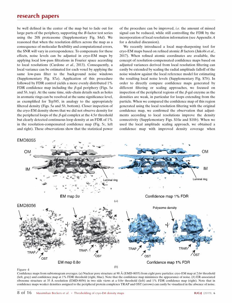
2.0� (Fig. 4a). The corresponding 1% FDR confidence map

shows continuous features for the ring structure with minim-

ized noise, which makes interpretation straightforward. In

order to generate a confidence map for a subtomogram

average structure, care must be taken to identify areas of noise

devoid of any signal in order to estimate the noise variance

reliably (Supplementary Fig. S6a). The same tomograms

recorded from lamella of HeLa cells also yielded a subtomo-

gram average of ER-associated ribosomes. The ribosome

structure itself could be determined at 35 A at the membrane,

with the weak density below the membrane ascribed to a

translocon-associated protein complex and an oligosaccharyl-

transferase (Mahamid et al., 2016). The corresponding densi-

ties can only be visualized at low thresholds corresponding to

0.8�, while increasing the amount of background noise and

hampering molecular interpretation (Fig. 4b). The 1% FDR

confidence maps, however, display the additional protein

complexes in the absence of noise. In this case, the confidence

map discriminates between specific association of the TRAP

complex and the looser association of ribosomes within the

polysome assembly. Further, we examined the deposited and

confidence maps of the 23 A resolution nuclear pore structure

determined by subtomogram averaging (Appen et al., 2015;

Supplementary Fig. S6d). While the overall densities look very

similar, we focused our comparison on the ambiguous density

assignment of the linker region of Nup133. The presence of

density in the 1% FDR confidence maps confirms the conti-

nuity of this density stretch and the author’s interpretation of

placing the Nup133 linker region connecting the N-terminal

�-propeller and C-terminal �-helical domain (Supplementary

Fig. S6d, upper right). In addition, we identified additional

densities in the connecting densities between the inner and

nuclear ring as well as between the inner and the cytoplasmic

ring (Supplementary Fig. S6d, bottom). Both densities are not

visible at the recommended threshold of 2.1�, but they are

reliably displayed in the 1% FDR confidence map. In contrast

to clearly defined features in high-resolution protein struc-

tures (for example secondary structure or side chains), we

generally do not know what the density features of such

subtomogram averages should look like, which makes manual

thresholding as well as the validation of additional densities

difficult. Taken together, confidence maps generated from

lower resolution subtomogram averages assist in the density

interpretation by separating the signal with respect to back-

ground noise.

3.7. Confidence maps benefit from local SNR adjustment incases of resolution variation

After establishing their usefulness for maps covering a

range of resolutions, we wanted to further explore how FDR-

controlled confidence maps cope with large resolution differ-

ences within a single map. For this purpose, we analyzed the

very high-resolution map (2.2 A resolution) of �-galactosidase

(�-gal; EMD-2984; Bartesaghi et al., 2015) in more detail as it

covers resolution ranges from 2.1 to 3.8 A. In order to reveal

high-resolution details in the center of the map high shar-

pening levels were required, and consequently less well

resolved parts in the periphery of the map resulted in over-

sharpened densities. When we applied our method to the

cryo-EM density volume, we found the 1% FDR confidence to

research papers


be well defined in the center of the map but to fade out for

large parts of the periphery, supporting the B-factor test series

using the 20S proteasome (Supplementary Fig. S4d). We

reasoned that when the resolution differs across the map as a

consequence of molecular flexibility and computational errors,

the SNR will vary in correspondence. To compensate for these

effects, noise levels can be adjusted in cryo-EM maps by

applying local low-pass filtrations in Fourier space according

to local resolutions (Cardone et al., 2013). Consequently, a

local variance can be estimated for each voxel by applying the

same low-pass filter to the background noise windows

(Supplementary Fig. S7a). Application of this procedure

followed by FDR control yields a more evenly distributed 1%

FDR confidence map including the �-gal periphery (Figs. 5a

and 5b, top). At the same time, side-chain details such as holes

in aromatic rings can be resolved at the same significance level,

as exemplified for Trp585, in analogy to the appropriately

filtered density (Figs. 5a and 5b, bottom). Closer inspection of

the cryo-EM density shows that we did not observe density for

the peripheral loops of the �-gal complex at the 4.5� threshold

but clearly detected continuous loop density at an FDR of 1%

in the resolution-compensated confidence map (Fig. 5c, left

and right). These observations show that the statistical power

of the procedure can be improved, i.e. the amount of missed

signal can be reduced, while still controlling the FDR by the

incorporation of local resolution information (see Appendix A

for a detailed discussion).

We recently introduced a local map-sharpening tool for

cryo-EM maps based on refined atomic B factors (Jakobi et al.,

2017). When refined atomic coordinates are available, the

concept of resolution-compensated confidence maps based on

adjusted variances derived from local resolution filtering can

easily be extended by scaling the radial amplitude falloff of the

noise window against the local reference model for estimating

the resulting local noise levels (Supplementary Fig. S7b). In

order to directly compare confidence maps generated by

different filtering or scaling approaches, we focused on

inspection of the peripheral regions of the �-gal enzyme as the

densities are weak, in particular for loops extending from the

particle. When we compared the confidence map of this region

generated using the local resolution filtering with the original

confidence map, we confirmed the observation that adjust-

ments according to local resolutions improve the density

connectivity (Supplementary Figs. S10a and S10b). When we

used the local amplitude scaling approach, we obtained a

confidence map with improved density coverage when

research papers


Figure 4Confidence maps from subtomogram averages. (a) Nuclear pore structure at 90 A (EMD-8055) from eight pore particles: cryo-EM map at 2.0� threshold(left, gray) and confidence map at 1% FDR threshold (right, blue). Note that the confidence map minimizes the appearance of noise. (b) ER-associatedribosome structure at 35 A resolution (EMD-8056) in two side views at a 0.8� threshold (left) and 1% FDR confidence map (right). Note that inconfidence maps weaker densities assigned to the peripheral protein complexes TRAP and OST (arrows) can easily be visualized in the absence of noise.

compared with the original confidence map but less coverage

when using local resolution filtering (Supplementary Figs.

S10b and S10c). In combination, when local variance is esti-

mated based on local amplitude scaling and filtering, we find

optimal coverage of the density and the atomic model

(Supplementary Fig. S10d). Another example from the

EMDB model challenge is the TRPV1 channel determined at

3.4 A resolution (EMD-5578; Liao et al., 2013). The structure

contains a well defined transmembrane region and a more

flexible cytoplasmic domain that is less well resolved. The

application of locally adjusted SNRs to the confidence map

yields a map with well interpretable density including mole-

cular details (Supplementary Figs. S7c and S7d). In analogy to

the examples above, the cytoplasmic domain is only visible at

lower thresholds than the core of the protein. The 1% FDR

confidence map captures all density occupied by the protein,

including the more flexible regions in the cytoplasmic domain.

The example of the TRPV1 channel confirms the observation

for �-gal that local resolution differences need to be taken into

account for the correct generation of confidence maps. When

maps exhibit a strong local variation of noise owing to mole-

cular flexibility and computational errors, local variances can

be estimated based on local resolution measurements or on

local sharpening procedures and yield well interpretable

confidence maps at a single FDR threshold.

3.8. Confidence maps confirm the detection of boundmolecules

The majority of near-atomic resolution maps obtained by

cryo-EM are in the resolution range between 3 and 4.5 A.

research papers


Figure 5Confidence maps benefit from local SNR adjustment based on local resolution. (a) Locally filtered �-galactosidase (EMD-2984) cryo-EM map (gray)displayed at a 4.5� threshold (left) and (b) confidence map (blue) including signal-to-noise adjustment based on local resolution at a 1% FDR threshold(right) in side view and cross-section. High-resolution features such as Glu304–Glu398 and holes in the aromatic rings of Trp585 in the 3.5/4.5�-thresholded cryo-EM map (a) in comparison with the 1% FDR confidence map (b). (c) Comparison of density features from peripheral loop regions notcovered by density in the locally filtered cryo-EM map (left) compared with the 1% FDR confidence map that shows densities for the respective loops.

Although main-chain and large side-chain densities can often

be modeled reliably, smaller side chains and ordered non-

protein components such as water molecules and ions are

inherently difficult to model at these resolutions and pose the

risk of noise fitting. Therefore, we investigated whether

confidence maps can help to mitigate this problem and

inspected a putative Mg2+ site coordinated by Glu416, Glu461,

His418 and three additional H2O molecules inside the �-gal

enzyme. We rigidly placed the Mg2+ ion and coordinated water

molecules based on the 1.6 A resolution X-ray crystal struc-

ture (Wheatley et al., 2015; PDB entry 4ttg) and superposed

them onto the deposited EM density map. The map at the

lower 3.5� threshold shows convincing density for only two of

the three water molecules (Fig. 6a, top left). In contrast, the

1% FDR confidence map based on local variance estimation

reveals distinct density peaks for all three suspected H2O

molecules (Fig. 6a, top right). Furthermore, �-gal had been

imaged in the presence of the small-molecule inhibitor PETG.

Location and conformational modeling of the ligand remains

challenging owing to flexibility and lower occupancy (Fig. 6a,

bottom left). Ligand placement is facilitated using confidence

maps, with density being well resolved for the complete small-

molecule inhibitor (Fig. 6a, bottom right). The confidence

density confirms the previous re-refinement of the inhibitor

position and conformation (Jakobi et al., 2017). In addition, we

also tested whether the detection of smaller ions can be

facilitated by confidence maps. For this purpose, we turned

again to the TRPV1 channel and inspected the density

surrounding Gly643, known as the selectivity filter for the ions

passing the channel. The deposited map reveals a density peak

in the symmetry center that is compatible with a small ion. In

support, the confidence map also shows a density peak at the

same position, supporting the presence of an ion with a

confidence of 1% FDR (Fig. 6b, bottom right). In corre-

spondence, there are multiple cryo-EM structures reporting

putative ion densities along an array of carbonyls forming an

inner cavity of the channel (Lee & MacKinnon, 2017;

McGoldrick et al., 2018). Closer inspection of the �-secretase

complex reveals significant density for a membrane-embedded

phosphatidylcholine (PC) lipid molecule. In order to detect

the two PC acyl chains, the deposited EM map requires

thresholding at two different � levels of 4 and 5, presumably

owimg to differences in chain mobility (Fig. 6c). In contrast,

the corresponding 1% FDR confidence map encompasses

most of the density of the two acyl chains without the need for

threshold adjustments. In conclusion, confidence maps from

cryo-EM structures possess minimized noise and can be

directly used to evaluate the significance of density features

that are present by providing a map-detection error that, for

example, 1% of the peaks are expected to be falsely discov-

ered. Using complementary information for the interpretation

of cryo-EM structures will help to reduce the subjectivity

involved in the process of density interpretation.

4. Discussion

In the current manuscript, we introduced FDR-based statis-

tical thresholding of cryo-EM densities as a complementary

research papers


Figure 6Confidence maps confirm the localization of nonprotein components. (a)�-Galactosidase (EMD-2984) with 3.5/4.5�-thresholded cryo-EM maps(left and center, gray) and a 1% FDR-thresholded confidence map (right,blue). Top: the Mg2+ ion is coordinated by Glu461, Glu416, His418 andthree H2O molecules. Bottom: density of bound PETG ligand in 3.5/4.5�-thresholded cryo-EM maps and the 1% FDR confidence map. (b) TRPV1channel (EMD-5778) with a 5�-thresholded cryo-EM map (left) and a1% FDR-thresholded confidence map (right): the selectivity filter formedby the carbonyls of symmetry-related Gly643 residues. The presence of aputative ion is supported by the confidence map. (c) �-Secretase (EMD-3061) with 4�- and 5�-thresholded cryo-EM maps (left) and a 1% FDR-thresholded confidence map (right). The confidence map reveals densityfor both acyl chains of phosphatidylcholine at a single threshold.

tool for map interpretation. This approach has been used

successfully in other fields of image-processing sciences

(Genovese et al., 2002). Based on a total of five near-atomic

resolution EM maps from the EMDB model challenge (http://

challenges.emdatabank.org), one intermediate resolution

(6.8 A) structure and three subtomogram averages in the

resolution range 90–23 A, we showed that the use of 1% FDR

confidence maps is well suited for detailed molecular-feature

detection and results in better confidence, in particular for the

assignment of weak structural features. Although different �levels ranging between 1 and 5 could be used for the inter-

pretation of relevant cryo-EM map features for all maps,

confidence maps thresholded at a common 1% FDR level

show a consistent interpretability of molecular features for

these maps. The advantage of confidence maps is that they

effectively separate signal from a background noise estimate

by assigning a confidence scale from 0 to 1 and at 1% FDR. In

this way, they show a consistent inclusion of signal while

minimizing noise. In contrast, for cryo-EM densities small

changes of the isosurface � threshold can have severe conse-

quences for the interpretability of molecular features and bear

the risk of mistakenly including noise. Therefore, confidence

maps and associated FDR thresholds provide a common and

conservative thresholding criterion for the interpretation of

cryo-EM maps.

Included in the algorithm is a direct assessment of the signal

significance with respect to background noise associated with

particular density features visible in cryo-EM maps, which

adds an additional objectivity to the reporting of ambiguous

density features. Based on these properties, high-resolution

confidence maps will be helpful in initial atomic model

building when no or few atomic reference structures are

available and for the assessment of critical details such as side-

chain conformations and nonprotein molecules in the density.

The use of these maps will improve the quality of initial atomic

models before launching real-space or reciprocal-space atomic

coordinate refinement (Murshudov, 2016; Adams et al., 2010),

which should proceed with sharpened or alternatively model-

based sharpened maps as refinement targets (Jakobi et al.,

2017). Molecular interpretation based on confidence maps is

not limited to maps of close-to-atomic resolution, as we have

demonstrated its benefit for cases of intermediate-resolution

single-particle and subtomogram averaging with three maps

ranging in resolution from 7 to 90 A. In these cases, the

interpretation of an unassigned density using a confidence

level is a beneficial property, in particular in the absence of

atomic model information.

We also showed that the generation of confidence maps is a

robust procedure. From the sharpened cryo-EM density, we

compute the CDF from the solvent background, which in most

cases can be approximated by a Gaussian distribution. In

addition, we assume protein density to be positive, as the

overwhelming majority of density for determined atoms

resides in positive density. Moreover, we find that the region

selected for noise estimation is critical as it has to contain pure

noise devoid of signal. We found this particularly important

for generating confidence maps from subtomogram averages

with particle boundaries that are less well defined. Generally,

when estimating background noise outside the particle we

tend to overestimate noise owing to a lower ice thickness in

the particle regions. Smaller deviations from noise estimation

show little effect on the conversion to confidence maps

(Supplementary Fig. S4b). We show that when suboptimally

sharpened input maps are used to generate confidence maps,

the operator avoids the common risk of mistakenly inter-

preting noise as signal in over-sharpened cryo-EM densities. In

contrast, confidence maps generated from over-sharpened

input maps will only result in an insufficient declaration of the

density signal, which is an important safety feature. Once

noise has been estimated, the procedure of generating confi-

dence maps is statistically clearly defined (Benjamini &

Hochberg, 1995; Benjamini & Yekutieli, 2001) and does not

contain any free parameters to optimize. Only in cases of

substantial resolution variation owing to molecular flexibility

and computational errors may it be required to locally adjust

SNRs by including prior information through local resolution

filtering. More sophisticated approaches such as amplitude

scaling can also be used in cases where atomic reference

structures are available. Adjusting FDR control based on

prior information is routinely implemented in other applica-

tions of statistical hypothesis testing (Chong et al., 2015;

Ploner et al., 2006). With this manuscript, we provide a

program that requires a three-dimensional volume as input

and allows specification of the location of the density windows

used for noise estimation. The presented implementation

including local resolution filtration is computationally fast,

taking from 30 s to 2 min on a Xeon Intel CPU for the maps

produced in this manuscript.

We presented several cases in our simulation and EMDB

maps where confidence maps displayed weak structural

features more clearly while minimizing the occurrence of

false-positive pixels (Figs. 1–6). This is a particularly useful

property of confidence maps. Weak densities close to inherent

noise levels are present in most cryo-EM maps and they result

as a consequence of the molecular specimen as well as from

the applied computational procedures. For example, they can

originate from side-chain mobility in the form of multiple

rotamers or side-chain-specific radiation damage (Fromm et

al., 2015; Allegretti et al., 2014; Bartesaghi et al., 2014). In

addition, ligands, including small organic compounds or larger

protein complex components, may have lower occupancy or

partial flexibility (Zhao et al., 2017). In many complexes,

peripheral loops exposed to the solvent tend to have larger

molecular flexibility than the core of the protein (Hoffmann et

al., 2015). We showed that thresholding confidence maps

yields higher voxel-detection rates than thresholding in

common cryo-EM densities. We believe that is a result of the

fact that the human operator prefers to recommend a more

conservative � threshold to avoid the excessive inclusion of

noise, while as a consequence one misses out on signal. Using

confidence maps, this type of noise can be suppressed and as a

result more reliable signal can be interpreted.

With the increasing number of near-atomic resolution

cryo-EM structures, the process of building atomic models has

research papers


become increasingly important, but remains time-consuming

and labor-intense. Confidence maps can assist the user

throughout this process. In X-ray crystallography, multiple

complementary maps are used routinely in the process of

model building. Real-space model building and optimization is

typically performed using maximum-likelihood-weighted

2mFo � DFc maps, assisted by mFo � DFc difference maps to

highlight errors in the model. Various forms of OMIT maps

computed from phases of models in which a selection of atoms

(for example a ligand) has been omitted are used to confirm

the presence of ligands and ambiguous density. Similarly,

confidence maps display a complementary aspect of cryo-EM

maps in helping to reduce ambiguity in density interpretation

of, for example, weakly bound ligands, alternative side-chain

rotamers and conformationally heterogeneous structures,

including incomplete or flexible parts of the complex. It is

evident that confidence maps would not be suitable for model

refinement, as they do not discriminate the scattering masses

of different atoms or the relative uncertainties of atomic

positions. These properties are usually modeled by atomic

electron form factors and atomic displacement factors (atomic

B factors). However, owing to the increased precision of

density peaks and noise suppression, it is perceivable that

confidence maps could be used to guide positional coordinate

refinement if implemented as a peak-searching procedure. In

addition, defined confidence values for density stretches

should also be useful and potentially beneficial for automated

model-building approaches. Interpreting cryo-EM densities by

means of an atomic model is often the final step of a cryo-EM

experiment. In practice, atomic models can even be used as a

validation tool to examine density features for side chains at

expected positions. One of the key advantages of the confi-

dence maps proposed here is that they can be generated

without prior knowledge of an atomic model. As the conver-

sion of cryo-EM densities to FDR controlled maps is

conceptually simple and computationally straightforward,

confidence maps could be routinely consulted to provide

complementary information of statistical significance during

the intricate process of interpreting ambiguous densities in

cryo-EM structures resulting from molecular flexibility or

partial occupancy.

APPENDIX AA1. Statistical model

For each voxel in the reconstructed three-dimensional

volume, where the voxels are indexed i, j, k, the intensity Xi,j,k

is modeled as

Xi;j;k ¼ �i;j;k þ "i;j;k; ð1Þ

where "i,j,k is a real-valued random variable representing the

background noise with mean �0,i,j,k 2 R and variance �2i,j,k 2

R>0, and where �i,j,k 2 R is the true intensity as observed

without background noise.

We developed an algorithm by means of multiple

hypothesis testing, which controls the maximum amount of

false-positive signal in the map, i.e. the FDR with respect to

background noise. Firstly, we limit the tested voxels to the

reconstruction sphere, and voxels located outside a diameter

larger than the box size are disregarded as they arise from a

smaller subset of averaged images than the voxels inside.

Secondly, we focus on the detection of voxels with positive

deviations from background noise (see Section A3). In addi-

tion, voxels that contain significant signal are affected by

further sources of noise such as flexibility, incomplete binding

of ligands and structural heterogeneity, leading to intensity

variations of the signal. Consequently, these sources lead to an

increase of the variance for these voxels as part of the inco-

herent signal, which we do not consider here as it is going

beyond the scope of detecting signal beyond background.

Background noise of experimental cryo-EM data, however,

poses principal challenges to the statistician, as it can result in

non-uniform distributions across the map: although back-

ground noise variances from images of uniform noise over the

pixels can be assumed to be uniform over the central sphere

(Supplementary Fig. S8c right), background noise outside the

particle is higher when compared with background noise

affecting the particle itself owing to solvent displacement and

variations of the relative ice thickness at the particle (Penczek

et al., 2006). Therefore, estimating noise in the solvent region

outside the particle could lead to an overestimation of the

actual influence of the background noise on the particle (see

Section 3.3). Although this may cause several problems for

comprehensive probabilistic modeling, these estimates can be

interpreted as conservative bounds for the signal significance

of the particle over background noise. For this reason, we use

multiple hypothesis testing in order to calculate these upper

bounds for detection errors of false-positive rates, as we prove

in Proposition 1. In cases when alternative noise estimates are

available, they can be supplied as additional input to the

procedure in order to generate confidence maps.

For each voxel a z-test is carried out, which identifies

significant deviations from background noise. The value of the

test statistic Z at each voxel is then given as

zi;j;k ¼xi;j;k � �0;i;j;k

�i;j;k

; ð2Þ

where xi,j,k 2 R is the reconstructed mean intensity at the

respective voxel. We are testing for true intensity �i,j,k higher

than 0; thus, the null and alternative hypotheses for each voxel

become

H0 : �i;j;k ¼ 0

H1 : �i;j;k > 0: ð3Þ

The null hypothesis H0 states that the true intensity �i,j,k at the

respective voxel is 0, i.e. no signal beyond background noise,

while the second hypothesis H1 states the deviation towards

higher values. Testing for deviations towards negative values,

i.e. negative densities, is easily accomplished in this setting by

multiplying the normalized map intensities zi,j,k by �1, leading

to a left-sided test procedure. Both options can be chosen by

the user.

research papers


Under the null hypothesis H0 and by approximating the

background noise with a Gaussian distribution (Kucukelbir et

al., 2014; Vilas et al., 2018), the test statistic Z follows a stan-

dard Gaussian distribution. The p-values in our procedure are

then calculated as

pi;j;k ¼PðZi;j;k � zi;j;kjH0Þ ¼ 1��ðzi;j;kÞ if xi;j;k � e��1 if xi;j;k <e��

�;

ð4Þ

where Zi,j,k is a random variable representing the test statistic

at voxel i,j,k, zi,j,k is the particular realization and e�� is the

background noise as estimated from the solvent area and the

cumulative distribution function �() of the standard Gaussian

distribution. Alternatively, p-values can also be calculated in a

nonparametric way without any assumptions about the

underlying background noise distribution by simply replacing

the cumulative distribution function �() of the standard

Gaussian distribution with the empirical cumulative distribu-

tion function bFFðÞ estimated from the sample of background

noise, given as

bFFðtÞ ¼ number of elements in the sample � t

total number of elements in the sample; t 2 R: ð5Þ

This allows the complete procedure to be carried out without

any distribution assumptions. However, comparisons show

that the background noise can be well approximated with a

Gaussian distribution even in the tail areas, which are most

important for the calculation of p-values (see Section A3,

Fig. 1b and Supplementary Fig. S8a). The respective method

for p-value calculation, i.e. nonparametric or with Gaussian

assumption, can be chosen by the user. All cases presented in

the manuscript, if not stated otherwise, were calculated with

the assumption of Gaussian-distributed background noise.

Note that the p-values defined here differ only marginally

from the p-values commonly used for one-sided testing in a

way that for all voxels with intensities smaller than the esti-

mated mean noise level e�� their value is set to 1. This definition

allows the control of the FDR in the more general setting of

allowed overestimated mean and variance (see Proposition 1).

A2. Multiple testing correction

The respective hypothesis tests are applied to each voxel in

the three-dimensional volume. To account for the multiple

testing problem with up to more than a million tests, we

choose to control the FDR. Control in this context means

giving upper bounds for the error that occurs. The FDR is

defined as the expected amount of false rejections, i.e.

FDR :¼ EV

V þ R

� �if V þ R 6¼ 0

0 if V þ R ¼ 0

(; ð6Þ

where V 2 N0 is the number of false rejections, R 2 N0 is the

number of true rejections and EðÞ denotes the expectation

value. Owing to dependencies between hypotheses at voxels

close to each other, we choose the Benjamini–Yekutieli

procedure (Benjamini & Yekutieli, 2001), giving an FDR-

adjusted p-value for each voxel; these are often referred to as

q-values. To describe the adjustment of p-values according to

Benjamini and Yekutieli in more detail and for ease of nota-

tion, we will now use a sequence of voxels from the map and

denote the number of hypotheses, i.e. tested voxels, by m. The

p-values pi, i = 1, . . . , m are then sorted, from small to large,

resulting in sorted p-values p(i), i = 1, . . . , m. q-values are then

calculated as

qðiÞ ¼ mini�k�m

pðkÞm

k�

h i; ð7Þ

where m is the number of hypotheses, k is a running index and

� ¼Pm

l¼1ð1=lÞ. By recognizing the correct index in the

sequence of voxels for each index (i), i = 1, . . . , m in the sorted

array and subsequent conversion into the three-dimensional

volume, we can assign each voxel position i, j, k its corre-

sponding q-value. In order to interpret the resulting map, the

q-value for each voxel then gives the minimal FDR that has to

be imposed at the thresholding in order to call the respective

voxel a significant deviation from the background. The final

value associated with voxel i, j, k, q0i,j,k, is then calculated as

q0i;j;k ¼ 1� qi;j;k; ð8Þ

where qi,j,k is the q-value at the voxel indexed with i,j,k. Thus,

visualization of the map at a value of 0.99 corresponds to a

maximal FDR of 1%, or a minimal PPV of 99%, and therefore

means that of all the visible voxels at this threshold, a

maximum of 1% are expected to be background noise.

Next, we show that the presented procedure with p-values

as defined above controls the FDR even in the case of over-

estimated background noise, i.e. by using the possibly over-

estimated background-noise estimates from the solvent area

in (2) for all voxels.

Proposition 1. Consider Gaussian-distributed random vari-

ables representing the background noise at all voxels i, j, k in

the three-dimensional map with true mean �0,i,j,k 2 R and

variance �2i;j;k 2 R>0. Moreover, let e�� 0;i;j;k and e�2�2 � �2

i;j;k,e�� 2 R, e�2�2 2 R>0 for all i, j, k, the overestimated background-

noise parameters. Then, gqi;j;kqi;j;k � qi;j;k, where gqi;j;kqi;j;k corresponds

to the q-value as defined in (7) and calculated with our

procedure with parameters e��; e�2�2 and qi;j;k corresponds to the

q-value as obtained with the true parameters �0;i;j;k and �2i;j;k.

Proof. In order to prove the statement, we will now re-

capitulate the algorithm and prove the inequality at all

necessary steps. We start by showing that the true p-value at

voxel position i, j, k, pi,j,k, is smaller when compared with the p-

value gpi;j;kpi;j;k calculated from the overestimated background-

noise parameters using (4). In other words, we want to show

that pi;j;k �gpi;j;kpi;j;k or, equivalent to this, gpi;j;kpi;j;k � pi;j;k � 0. If

xi;j;k <e�� then the statement is trivial, because gpi;j;kpi;j;k ¼ 1 and

pi,j,k � 1, which is a general property of p-values.

For xi;j;k � e��, considering (2) and (4), it follows that

research papers


gpi;j;kpi;j;k � pi;j;k ¼ 1�1

21þ erf

xi;j;k � e��21=2e��

� �� 1þ

1

21þ erf

xi;j;k � �0;i;j;k

21=2�i;j;k

� �� ¼ �

1

2erf

xi;j;k � e��21=2e��

� �þ

1

2erf


21=2�i;j;k

� �: ð9Þ

As the error function erf() is monotonically increasing, it is

sufficient to show that


21=2�i;j;k

�xi;j;k � e��

21=2e�� :

Because xi;j;k � e�� 0 and thus also xi,j,k � �0,i,j,k � 0, as well

as e�� i;j;k, we have


21=2�i;j;k

�xi;j;k � e��

21=2e�� ¼ðxi;j;k � �0;i;j;kÞe�� ðxi;j;k � e��Þ�

21=2e��i;j;k

�ðxi;j;k � �0;i;j;kÞ� � ðxi;j;k � e��Þ�

21=2e��i;j;k

¼ð��0;i;j;k þ e��Þ�

21=2e��i;j;k

� 0; ð10Þ

where in the last inequality it was used that e�� 0;i;j;k ande�� i;j;k > 0. This gives the desired result of gpi;j;kpi;j;k � pi;j;k.

Recapitulating the calculation of q-values in (7) together

with the conversion of the three-dimensional volume to a

sequence, it follows that

qðaÞ ¼ mina�k�m

pðkÞm

k�

h i� min

a�k�mfpðkÞpðkÞ

m

k�

h i¼ fqðaÞqðaÞ; a ¼ 1; . . . ;m;

ð11Þ

where m is the number of hypotheses, k is a running index and

� ¼Pm

l¼1ð1=lÞ. This gives the desired result:gqi;j;kqi;j;k � qi;j;k: ð12Þ

&

As the Benjamini–Yekutieli procedure controls the FDR

when using true parameters, our procedure (i.e. the

Benjamini–Yekutieli procedure applied to the modified p-

values) will give a more conservative estimate of the FDR (as

shown in Proposition 1). Therefore, our algorithm controls the

FDR sufficiently well by giving an upper conservative bound

for the FDR. Thus, Proposition 1 states that even in the setting

of non-uniform background noise with higher noise levels in

the region of background-noise estimation, the FDR is

controlled and thus robust in the sense that the maximum

FDR is still guaranteed. Furthermore, it must be mentioned

that estimates of the background-noise levels are not the only

factor that contributes to FDR estimation. Both the number of

voxels as well as their dependencies within the map have an

important influence and are considered in the FDR adjust-

ment. This makes the generation of confidence maps even with

severely overestimated background-noise parameters a

powerful procedure (Supplementary Fig. S4), where powerful

is used here in its statistical sense of decreasing the error of

missing true signal. However, the power of the procedure can

be further increased, i.e. the amount of true missed signal

reduced while controlling the FDR, by including information

about local resolutions, the cutoffs in reciprocal space beyond

which no signal is expected, while at the same time controlling

the FDR.

A3. Choice of positive-density model with Gaussianbackground noise

Although the model of Gaussian noise is often used to

approximate background noise in cryo-EM images and maps

(Sigworth, 1998; Scheres, 2012a; Kucukelbir et al., 2014; Vilas

et al., 2018), it is important to analyze actual maps to better

understand deviations from this assumption. For this purpose,

we analyzed a total of 32 deposited cryo-EM densities from 2

to 8 A resolution and compared the empirical cumulative

density function (CDF) with the ideal Gaussian CDF

(Supplementary Fig. S8a). It is apparent that all of them follow

the ideal Gaussian CDF closely. For each map, we assessed

normality by Anderson–Darling hypothesis testing (Anderson

& Darling, 1954) and found that 75% and 87.5% of the maps

do not significantly deviate from normality when conservative

thresholds corresponding to 1% and 0.1% family-wise error

rates (FWER) are chosen (Supplementary Fig. S8b). One of

the reasons for the observed deviations from an idealized

Gaussian distribution is a result of the three-dimensional

reconstruction procedure. In principle, when truly aligned

images containing white Gaussian noise are combined by

linear inversion, the obtained three-dimensional volume will

also have a Gaussian distribution. In practice, in cases when

uncertainties reside on the five orientation parameters, back-

ground noise is not necessarily Gaussian-distributed. More-

over, the resulting three-dimensional reconstructions will

contain local correlations, i.e. ‘colored noise’. Therefore, we

analyzed the resulting noise of three-dimensional recon-

structions generated from pure noise images with even

angular sampling. The resulting amplitude spectrum shows

that it differs from pure white noise owing to correlations

between adjacent pixels (Supplementary Fig. S8c, left).

Furthermore, the variances estimated for each voxel from 900

reconstructions show that they can be approximated as

uniform over the central sphere (Supplementary Fig. S8c,

right).

For the map EMD-6287, which deviates strongly from

normality according to the Anderson–Darling test, we

generated a confidence map using the Gaussian and the

empirical CDF. We inspected these confidence maps

(Supplementary Fig. S8d) and found that the visual agreement

between the two maps is very high. To highlight potential

differences, we computed a difference map between the two

confidence maps created by the two approaches and observed

no systematic variation when deviation from normality was

assumed. Therefore, when interpreting confidence maps, small

deviations from normality do not appear to have practical

limitations. In order to rule out any potential unforeseen

effects when maps deviate more strongly, we routinely

implemented monitoring of the degree of deviation from the

research papers


ideal Gaussian CDF. For instance, when the deviation of the

empirical CDF from the Gaussian CDF exceeds 0.01, referring

to the fact that the p-values deviate by more than 1%, we can

optionally use the empirical CDF for the generation of

confidence maps.

The second assumption of the proposed confidence map is

that the protein gives rise to positive density in cryo-EM maps.

When inspecting EM density maps, it is evident that not all

signal present in the map is positive, which might be important

to consider for atomic coordinate refinement. Therefore, we

analyzed whether significant negative densities can be

detected in confidence maps generated from inverted densi-

ties. Indeed, the confidence maps from negative densities

reveal significant signal in regions between protein density,

often in a spatially complementary way (Supplementary Fig.

S9a, left). Using the independently determined X-ray struc-

ture of the 20S proteasome (PDB entry 1pma; Lowe et al.,

1995), we tested whether negative density coincides with the

atomic model. Overall, negative density has only a very small

2.5% overlap with atoms, which is close to the predicted false-

discovery rate of 1% (Supplementary Fig. S9b). When using

positive density, however, we find that a large fraction of 60%

of the PDB atoms are found in the 1% FDR-contoured

confidence map and that 10% of this volume is occupied by

modeled atoms. In conclusion, we show that negative density

presents significant signal in cryo-EM maps, but that only a

very small fraction is occupied by atoms. The largest fraction

of negative densities are found next to positive protein density,

most likely owing to the fact that the molecular density is

lower than in the particle-surrounding solvent area. Based on

this analysis and our objective to identify those voxels that

arise from protein density, we include the restraint of testing

for positive signal into the generation of confidence maps and

include an additional option to test for negative signal, which

could be used for further investigation of negative densities.

A4. Testing with local filtering

In the presence of extreme resolution variation, using

uniformly sharpened and filtered maps will lead to confidence

maps with insufficient representation of features in both areas

with B factors either lower than the average or higher than the

average. Therefore, in the next two sections, we will show how

noise levels can be locally adjusted and subsequently esti-

mated by the inclusion of local resolution information as well

as atomic B factors and how this can be used to increase the

power to detect weaker features while controlling the FDR.

Local filtration of EM maps according to the local resolution

(Cardone et al., 2013) has been shown to be a powerful

approach as it leads to local reductions in background noise.

These variations of noise levels between different voxels at

different resolutions from local filtering can be also accounted

for in the generation of confidence maps. For each voxel, a

map duplicate volume is filtered at the corresponding reso-

lution and the noise distribution is estimated from the solvent

area outside the particle. This procedure results in three three-

dimensional maps, the estimates of local variances of the

background noise at each voxel after local filtration, the

estimates of local means of the background noise at each voxel

after local filtration and the locally filtered map. These three

maps are subsequently used for the testing procedure. Thus,

the value of the test statistic (2) is calculated by

zi;j;k ¼xi;j;k � e��i;j;ke��i;j;k

; ð13Þ

where xi,j,k 2 R is the intensity of the locally filtered map at

voxel i, j, k, and e��i;j;k 2 R and e��i;j;k 2 R>0 are the local mean

and standard deviation estimate of the background noise at

the respective voxel. All subsequent steps of the algorithm

remain identical, as well as the validity of Proposition 1.

A5. Testing with local amplitude scaling

As for the local filtration, local amplitude scaling gives rise

to varying noise levels at different voxels. In order to obtain

both mean and variance estimates for each voxel after local

amplitude scaling, a duplicate window outside the particle

containing pure noise is scaled according to the rolling window

used in local amplitude scaling for each voxel, i.e. the ampli-

tudes of the Fourier transform of the box containing pure

noise at frequency s, denoted as Fnoise(s), are multiplied by a

frequency-dependent sharpening factor kðsÞ 2 R�0, which is

consequently given as

kðsÞ ¼

FsharpenedðsÞ

FobservedðsÞif FobservedðsÞ 6¼ 0

0 if FobservedðsÞ ¼ 0

8<: ; ð14Þ

where FsharpenedðsÞ 2 R�0 and FobservedðsÞ 2 R�0 are rotationally

averaged amplitudes of the Fourier transform at frequency s

given at the respective rolling window for the sharpened and

the observed experimental map, respectively. The noise

distribution is then estimated from the scaled noise sample. In

analogy to the case of locally filtered maps, this procedure

again results in three three-dimensional maps of estimated

means, variances and intensities of the locally sharpened map

for each voxel that can be incorporated with (13) in the testing

procedure. Proposition 1 remains valid.

Acknowledgements

We thank Martin Beck (EMBL) for critical reading of the

manuscript and the thesis advisory committee members

Wolfgang Huber and Rob Russel (Heidelberg University) for

stimulating discussions. We are grateful to Thomas Hoffmann

and Jurij Pecar (IT Services) for the setting up and main-

tenance of the high-performance computational environment

at EMBL. Author contributions were as follows. MB and CS

initiated the project. MB developed and implemented the

code for the algorithm. AJJ helped with structure comparison

and implementation including LocScale integration. CS

supervised the project. MB and CS wrote the manuscript with

input from AJJ. The authors declare that no competing

financial interests exist.

research papers


Funding information

MB was supported by the EMBL International PhD

Programme.

References

Adams, P. D., Afonine, P. V., Bunkoczi, G., Chen, V. B., Davis, I. W.,Echols, N., Headd, J. J., Hung, L.-W., Kapral, G. J., Grosse-Kunstleve, R. W., McCoy, A. J., Moriarty, N. W., Oeffner, R., Read,R. J., Richardson, D. C., Richardson, J. S., Terwilliger, T. C. &Zwart, P. H. (2010). Acta Cryst. D66, 213–221.

Allegretti, M., Mills, D. J., McMullan, G., Kuhlbrandt, W. & Vonck, J.(2014). Elife, 3, e01963.

Anderson, T. W. & Darling, D. A. (1954). J. Am. Stat. Assoc. 49, 765–769.

Appen, A. von, Kosinski, J., Sparks, L., Ori, A., DiGuilio, A. L.,Vollmer, B., Mackmull, M.-T., Banterle, N., Parca, L., Kastritis, P.,Buczak, K., Mosalaganti, S., Hagen, W., Andres-Pons, A., Lemke,E. A., Bork, P., Antonin, W., Glavy, J. S., Bui, K. H. & Beck, M.(2015). Nature (London), 526, 140–143.

Bai, X.-C., Fernandez, I. S., McMullan, G. & Scheres, S. H. W. (2013).Elife, 2, e00461.

Bai, X.-C., Yan, C., Yang, G., Lu, P., Ma, D., Sun, L., Zhou, R.,Scheres, S. H. W. & Shi, Y. (2015). Nature (London), 525, 212–217.

Bartesaghi, A., Aguerrebere, C., Falconieri, V., Banerjee, S., Earl,L. A., Zhu, X., Grigorieff, N., Milne, J. L. S., Sapiro, G., Wu, X. &Subramaniam, S. (2018). Structure, 26, 848–856.

Bartesaghi, A., Matthies, D., Banerjee, S., Merk, A. & Subramaniam,S. (2014). Proc. Natl Acad. Sci. USA, 111, 11709–11714.

Bartesaghi, A., Merk, A., Banerjee, S., Matthies, D., Wu, X., Milne,J. L. S. & Subramaniam, S. (2015). Science, 348, 1147–1151.

Benjamini, Y. & Hochberg, Y. (1995). J. R. Stat. Soc. B, 57, 289–300.Benjamini, Y. & Yekutieli, D. (2001). Ann. Stat. 29, 1165–1188.Briggs, J. A. (2013). Curr. Opin. Struct. Biol. 23, 261–267.Burnley, T., Palmer, C. M. & Winn, M. (2017). Acta Cryst. D73, 469–

477.Campbell, M. G., Veesler, D., Cheng, A., Potter, C. S. & Carragher, B.

(2015). Elife, 4, e06380.Cardone, G., Heymann, J. B. & Steven, A. C. (2013). J. Struct. Biol.

184, 226–236.Chong, E. Y., Huang, Y., Wu, H., Ghasemzadeh, N., Uppal, K.,

Quyyumi, A. A., Jones, D. P. & Yu, T. (2015). Sci. Rep. 5, 17221.Fitzpatrick, A. W. P., Falcon, B., He, S., Murzin, A. G., Murshudov, G.,

Garringer, H. J., Crowther, R. A., Ghetti, B., Goedert, M. &Scheres, S. H. W. (2017). Nature (London), 547, 185–190.

Frank, J. & Liu, W. (1995). J. Opt. Soc. Am. A Opt. Image Sci. Vis. 12,2615–2627.

Fromm, S. A., Bharat, T. A. M., Jakobi, A. J., Hagen, W. J. H. &Sachse, C. (2015). J. Struct. Biol. 189, 87–97.

Galej, W. P., Wilkinson, M. E., Fica, S. M., Oubridge, C., Newman,A. J. & Nagai, K. (2016). Nature (London), 537, 197–201.

Ge, P. & Zhou, Z. H. (2011). Proc. Natl Acad. Sci. USA, 108, 9637–9642.

Genovese, C. R., Lazar, N. A. & Nichols, T. (2002). Neuroimage, 15,870–878.

Gremer, L., Scholzel, D., Schenk, C., Reinartz, E., Labahn, J., Ravelli,R. B. G., Tusche, M., Lopez-Iglesias, C., Hoyer, W., Heise, H.,Willbold, D. & Schroder, G. F. (2017). Science, 358, 116–119.

Heel, M. van, Keegstra, W., Schutter, W. & Van Bruggen, E. (1982).Life Chemistry Reports, edited by E. J. Wood, Suppl. 1, pp. 69–73.London: Harwood.

Hoffmann, N. A., Jakobi, A. J., Moreno-Morcillo, M., Glatt, S.,Kosinski, J., Hagen, W. J. H., Sachse, C. & Muller, C. W. (2015).Nature (London), 528, 231–236.

Jakobi, A. J., Wilmanns, M. & Sachse, C. (2017). Elife, 6, 213.Khoshouei, M., Radjainia, M., Baumeister, W. & Danev, R. (2017).

Nat. Commun. 8, 16099.

Kucukelbir, A., Sigworth, F. J. & Tagare, H. D. (2014). Nat. Methods,11, 63–65.

Lee, C.-H. & MacKinnon, R. (2017). Cell, 168, 111–120.Li, X., Mooney, P., Zheng, S., Booth, C. R., Braunfeld, M. B.,

Gubbens, S., Agard, D. A. & Cheng, Y. (2013). Nat. Methods, 10,584–590.

Liao, M., Cao, E., Julius, D. & Cheng, Y. (2013). Nature (London),504, 107–112.

Lowe, J., Stock, D., Jap, B., Zwickl, P., Baumeister, W. & Huber, R.(1995). Science, 268, 533–539.

Lyumkis, D., Brilot, A. F., Theobald, D. L. & Grigorieff, N. (2013). J.Struct. Biol. 183, 377–388.

Mahamid, J., Pfeffer, S., Schaffer, M., Villa, E., Danev, R., KuhnCuellar, L., Forster, F., Hyman, A. A., Plitzko, J. M. & Baumeister,W. (2016). Science, 351, 969–972.

McGoldrick, L. L., Singh, A. K., Saotome, K., Yelshanskaya, M. V.,Twomey, E. C., Grassucci, R. A. & Sobolevsky, A. I. (2018). Nature(London), 553, 233–237.

McMullan, G., Faruqi, A. R. & Henderson, R. (2016). MethodsEnzymol. 579, 1–17.

Merk, A., Bartesaghi, A., Banerjee, S., Falconieri, V., Rao, P., Davis,M. I., Pragani, R., Boxer, M. B., Earl, L. A., Milne, J. L. S. &Subramaniam, S. (2016). Cell, 165, 1698–1707.

Miller, C. J., Genovese, C., Nichol, R. C., Wasserman, L., Connolly,A., Reichart, D., Hopkins, A., Schneider, J. & Moore, A. (2001).Astron. J. 122, 3492–3505.

Murshudov, G. N. (2016). Methods Enzymol. 579, 277–305.Namba, K. & Stubbs, G. (1986). Science, 231, 1401–1406.Patwardhan, A. (2017). Acta Cryst. D73, 503–508.Penczek, P. A. (2002). J. Struct. Biol. 138, 34–46.Penczek, P. A. (2010). Methods Enzymol. 482, 1–33.Penczek, P. A., Yang, C., Frank, J. & Spahn, C. M. T. (2006). J. Struct.

Biol. 154, 168–183.Pettersen, E. F., Goddard, T. D., Huang, C. C., Couch, G. S.,

Greenblatt, D. M., Meng, E. C. & Ferrin, T. E. (2004). J. Comput.Chem. 25, 1605–1612.

Ploner, A., Calza, S., Gusnanto, A. & Pawitan, Y. (2006). Bioinfor-matics, 22, 556–565.

Punjani, A., Rubinstein, J. L., Fleet, D. J. & Brubaker, M. A. (2017).Nat. Methods, 14, 290–296.

Rosenthal, P. B. & Henderson, R. (2003). J. Mol. Biol. 333, 721–745.

Sachse, C., Chen, J. Z., Coureux, P.-D., Stroupe, M. E., Fandrich, M. &Grigorieff, N. (2007). J. Mol. Biol. 371, 812–835.

Saxton, W. O. & Baumeister, W. (1982). J. Microsc. 127, 127–138.Scheres, S. H. W. (2012a). J. Mol. Biol. 415, 406–418.Scheres, S. H. W. (2012b). J. Struct. Biol. 180, 519–530.Schur, F. K. M., Obr, M., Hagen, W. J. H., Wan, W., Jakobi, A. J.,

Kirkpatrick, J. M., Sachse, C., Krausslich, H.-G. & Briggs, J. A. G.(2016). Science, 353, 506–508.

Sigworth, F. J. (1998). J. Struct. Biol. 122, 328–339.Unwin, N. (2005). J. Mol. Biol. 346, 967–989.Vilas, J. L., Gomez-Blanco, J., Conesa, P., Melero, R., Miguel de la

Rosa-Trevın, J., Oton, J., Cuenca, J., Marabini, R., Carazo, J. M.,Vargas, J. & Sorzano, C. O. S. (2018). Structure, 26, 337–344.

Walt, S., Colbert, S. C. & Varoquaux, G. (2011). Comput. Sci. Eng. 13,22–30.

Wheatley, R. W., Juers, D. H., Lev, B. B., Huber, R. E. & Noskov, S. Y.(2015). Phys. Chem. Chem. Phys. 17, 10899–10909.

Yonekura, K., Maki-Yonekura, S. & Namba, K. (2003). Nature(London), 424, 643–650.

Yu, X., Jin, L. & Zhou, Z. H. (2008). Nature (London), 453, 415–419.Zhang, X., Settembre, E., Xu, C., Dormitzer, P. R., Bellamy, R.,

Harrison, S. C. & Grigorieff, N. (2008). Proc. Natl Acad. Sci. USA,105, 1867–1872.

Zhao, J., Beyrakhova, K., Liu, Y., Alvarez, C. P., Bueler, S. A., Xu, L.,Xu, C., Boniecki, M. T., Kanelis, V., Luo, Z.-Q., Cygler, M. &Rubinstein, J. L. (2017). PLoS Pathog. 13, e1006394.

research papers


http://scripts.iucr.org/cgi-bin/cr.cgi?rm=pdfbb&cnor=pw5002&bbid=BB1

































































































































Thresholding of cryo-EM density maps by false discovery rate ...

Documents

Transcript of Thresholding of cryo-EM density maps by false discovery rate ...