THE ASTROPHYSICAL JOURNAL, 515 :842È867, 1999 April 201999. The American Astronomical Society. All rights reserved. Printed in U.S.A.(

THREE-DIMENSIONAL STEREOSCOPIC ANALYSIS OF SOLAR ACTIVE REGION LOOPS. I. SOHO/EITOBSERVATIONS AT TEMPERATURES OF (1.0È1.5) ] 106 K

MARKUS J. ASCHWANDEN1Department of Astronomy, University of Maryland, College Park, MD 20742 ; markus=astro.umd.edu

JEFFREY S. NEWMARK

Space Applications Corporation, Vienna, VA 22180

JEAN-PIERRE DELABOUDINIERE

Institute dÏAstrophysique Spatiale, Paris XI, 91405 Orsay Cedex, FranceUniversite�

WERNER M. NEUPERT

Hughes SXT Corporation, Lanham, MD 20706

J. A. KLIMCHUK

Space Science Division, Code 7675, Naval Research Laboratory, Washington, DC 20375-5352

G. ALLEN GARY

ES82-Solar Physics Branch, Space Science Laboratory, NASA/MSFC, Huntsville, AL 35812

FABRICE PORTIER-FOZZANI

Laboratoire dÏAstronomie Spatiale, CNRS, BP 8, 13376 Marseille Cedex 12, France

AND

ARIK ZUCKER

ETH, Institute Astronomy, 15, CH-8092 Zurich, SwitzerlandHa� ldeliwegReceived 1998 May 13; accepted 1998 November 23

ABSTRACTThe three-dimensional structure of solar active region NOAA 7986 observed on 1996 August 30 with

the Extreme-Ultraviolet Imaging Telescope (EIT) on board the Solar and Heliospheric Observatory(SOHO) is analyzed. We develop a new method of dynamic stereoscopy to reconstruct the three-dimensional geometry of dynamically changing loops, which allows us to determine the orientation ofthe mean loop plane with respect to the line of sight, a prerequisite to correct properly for projectione†ects in three-dimensional loop models. With this method and the Ðlter-ratio technique applied to EIT171 and 195 images we determine the three-dimensional coordinates [x(s), y(s), z(s)], the loop widthA�w(s), the electron density and the electron temperature as a function of the loop length s forn

e(s), T

e(s)

30 loop segments. Fitting the loop densities with an exponential density model we Ðnd that thene(h)

mean of inferred scale height temperatures, MK, matches closely that of EIT Ðlter-ratioTej \ 1.22 ^ 0.23

temperatures, MK. We conclude that these cool and rather large-scale loops (withTeEIT \ 1.21 ^ 0.06

heights of h B 30È225 Mm) are in hydrostatic equilibrium. Most of the loops show no signiÐcant thick-ness variation w(s), but we measure for most of them a positive temperature gradient (dT /ds [ 0) acrossthe Ðrst scale height above the footpoint. Based on these temperature gradients we Ðnd that the conduc-tive loss rate is about 2 orders of magnitude smaller than the radiative loss rate, which is in strongcontrast to hot active region loops seen in soft X-rays. We infer a mean radiative loss time of qrad B 40minutes at the loop base. Because thermal conduction is negligible in these cool EUV loops, they are notin steady state, and radiative loss has entirely to be balanced by the heating function. A statisticalheating model with recurrent heating events distributed along the entire loop can explain the observedtemperature gradients if the mean recurrence time is minutes. We computed also a potential Ðeld[10model (from SOHO/MDI magnetograms) and found a reasonable match with the traced EIT loops. Withthe magnetic Ðeld model we determined also the height dependence of the magnetic Ðeld B(h), theplasma parameter b(h), and the velocity No correlation was found between the heating rateAlfve� n vA(h).requirement and the magnetic Ðeld at the loop footpoints.E

H0 BfootSubject headings : Sun: activity È Sun: corona È Sun: UV radiation È techniques : image processing

1. INTRODUCTION

The evolution of coronal plasma loops, beginning fromthe well-kept secret of the elusive heating mechanism, to thesomewhat better understood conductive and radiativecooling processes, and the various transitions from steadystate to nonequilibrium states, still represents a keyproblem of coronal plasma physics. Because the average

1 Current address : Lockheed-Martin ATC, Solar and AstrophysicsLaboratory, Department H1-12, Building 252, 3251 Hanover Street, PaloAlto, CA 94304 ; aschwanden=sag.lmsal.com.

temperature of the solar corona ranges around TeB 1.5

MK, this temperature seems to reÑect the most likely steadystate condition of coronal structures, demarcating at thesame time a watershed where cooling and heating processesstart to lose equilibrium. It is therefore a physically mean-ingful choice to distinguish between cool2 and hot loops

2 The temperature range of MK that we denote as cool here isTe[ 1.5

sometimes also termed intermediate temperatures (e.g., Brown 1996),whereas loops with temperatures of K are referred to as coolT

e[ 105

loops (e.g., Martens & Kuin 1982).

842

THREE-DIMENSIONAL ANALYSIS OF SOLAR ACTIVE REGIONS 843

with respect to this maximum likelihood temperature TeB

1.5 MK, which also separates roughly the line-formationtemperatures in the EUV/XUV and soft X-ray (SXR) wave-length regimes. Coronal loops in EUV/XUV wavelengthscould only be studied with few instruments, mainly from thespacecraft missions Skylab, SOHO, T ransition Region AndCoronal Explorer (T RACE), and from a few short-durationrocket Ñights (e.g., American Science and Engineering[AS&E], High-Resolution Telescope and Spectrograph[HRTS], or Solar EUV Rocket Telescope and Spectro-graph [SERTS]). The scarce EUV observations before thelaunch of SOHO provided little systematic information onthe physical structure of cooler active region loops in thetemperature regime of MK, as opposed to theT

e[ 1.5

much more frequently studied hotter loops MK)(TeZ 1.5

in SXR (with OSO 8, P78-1, Hinotori, SMM/XRP, Y ohkoh/SXT, Coronas, etc.). A number of statistical studies exist onhot active region loops observed in SXRs (e.g., Pallavicini,Serio, & Vaiana 1977 ; Rosner, Tucker, & Vaiana 1978 ;Cheng 1980 ; Porter & Klimchuk 1995 ; Klimchuk & Gary1995 ; Kano & Tsuneta 1995, 1996), but there are no compa-rable statistics available on cooler active region loopsobserved at temperatures of MK in EUV.T

e\ 1.0È1.5

Moreover, not much e†ort has been invested in the three-dimensional reconstruction of coronal loops at any wave-length so far (although the technology is ready ; see, e.g.,Gary 1997). This work represents a Ðrst comprehensive sta-tistical study on physical parameters of cool active regionloops in the MK temperature range, measuredT

e\ 1.0È1.5

with unprecedented accuracy using a newly developedthree-dimensional reconstruction method called dynamicstereoscopy.

Let us quickly review some highlights of earlier work onEUV loops in the MK temperature range. AT

eB 1.0È1.5

comprehensive account on literature before 1991 can befound in Bray et al. (1991). The Skylab XUV spectrohelio-graph provided images with 2AÈ3A resolution at wave-lengths of 180È630 including the Mg IX line with aA� ,formation temperature of MK. Dere (1982)T

e\ 0.9

analyzed such XUV loops and found (1) that they are closeto hydrostatic equilibrium (within the uncertainties of theunknown three-dimensional geometry) and (2) that hot

MK) loops do not have a cool core structure as(Te[ 1

suggested by Foukal (1975). Sheeley (1980) studied the tem-poral variability of EUV loops and found lifetimes of B1.5hr for 1 MK loops, somewhat longer than those of 0.5 MKloops. This lifetime of 1 MK loops, estimated by Sheeleyfrom time-lapse movies, is actually close to the value weinfer for the radiative cooling time from SOHO/EIT data.Observations with SERTS revealed that the brightest struc-tures seen in Mg IX are not spatially coincident with hottercoronal loops seen in SXR but are rooted in chromosphericHe II features and thus seem to trace out cooler coronalloops with apex temperatures of MK (Brosius et al.T

e[ 1

1997). The existence of numerous cooler loops has also beenpostulated from the observed discrepancy between SXR-inferred temperatures of active regions and simultaneousradio brightness temperature measurements because theformer include only the contributions from hot loops,whereas the latter are sensitive to the combined free-freeopacity of both hot and cool loops (Webb et al. 1987 ; Nittaet al. 1991 ; Schmelz et al. 1992, 1994 ; Brosius et al. 1992 ;Klimchuk & Gary 1995 ; Vourlidas & Bastian 1996). Themost recent work on EUV loops comes from SOHO/EIT

(Neupert et al. 1998 ; Aschwanden et al. 1998a, 1998b) andSOHO/CDS (Fludra et al. 1997 ; Brekke et al. 1997).Neupert et al. (1998) analyzed a long-lived loop structureand an open-Ðeld radial feature and found (1) that they areclose to hydrostatic equilibrium (within the uncertainties ofthe unknown three-dimensional geometry), and (2) thatradiative energy loss strongly dominates conductive energyloss at these loop temperatures of MK,T

e\ 1.0È1.5

requiring a heating function that scales with the squareddensity, The temporal variability and lifetime ofE

HP n

e2.

EUV loops can now best be studied from SOHO/EITmovies (Newmark et al. 1997).

What progress can we expect from a new analysis ofactive region loops, using the most recent EUV data avail-able from SOHO/EIT? To accomplish sensible tests of theo-retical models on heating and cooling processes, accuratephysical parameters from resolved single loops are needed.However, most of the previous literature deals with line-of-sight averaged quantities without discriminating betweensingle loops. For a proper determination of physical param-eters from single active region loops, a number of analysisproblems have to be overcome.

1. Geometric loop deÐnition2. IdentiÐcation and tracing of loops in images3. Disentangling of nested loops4. Separation of overlying or closely spaced loops5. Discrimination of multiple loops along the line of sight6. Three-dimensional reconstruction of loop geometry

and deprojection7. Temperature discrimination along the line of sight8. Reliable temperature and emission measure determi-

nation.

Most of these problems have not been treated in a sys-tematic way in previous studies. Here we present the resultsof a new approach, making use of the principle of dynamicstereoscopy to reconstruct the three-dimensional orienta-tion of loops, which provides a reliable method to obtainmore accurate physical parameters as a function of the looplength, properly corrected for line-of-sight related projec-tion e†ects. The enhanced accuracy is expected to allow formore rigorous tests of theoretical loop models.

In ° 2 we describe the stereoscopic data analysis of 30loops observed with SOHO/EIT at a wavelength band cen-tered around Fe IX, Fe X at 171 In ° 3 we apply physicalA� .loop models to the data and investigate loop scaling laws. Asummary and conclusions are given in ° 4.

2. STEREOSCOPIC DATA ANALYSIS

2.1. Data SetThe investigated active region is a long-lived coronal

structure that was present during several solar rotations,from its apparition in 1996 July until its disappearance in1996 September (Hudson et al. 1998 ; Harvey & Hudson1998), numbered as NOAA 7978, 7981, 7986 during con-secutive rotations. We concentrate here on the central meri-dian transit on 1996 August 30, when the dipolar magneticÐeld structure o†ered the most favorable perspective to dis-entangle the ““ jungle ÏÏ of nested loops.

An Fe IX/Fe X image recorded with SOHO/EITet al. 1995) at a wavelength of 171 on(Delaboudiniere A�

1996 August 30, 0020 :14 UT is shown in Figure 1 (top). Forstereoscopic correlations we will also use EIT images from

-0.05 0.00 0.05

-0.16

-0.14

-0.12

-0.10

-0.08

-0.06

-0.04

deg

96/ 8/30 0:20:14.881

-0.05 0.00 0.05deg

-0.16

-0.14

-0.12

-0.10

-0.08

-0.06

-0.04

deg

96/ 8/30 0:20:14.881

EIT 171 A

EIT 171 A filtered

FIG. 1.ÈSOHO/EIT Fe IX/Fe X image of active region AR 7986, recorded on 1996 August 30, 0020 :14 UT, at a wavelength of 171 sensitive in theA� ,temperature range of MK (top). The gray scales of the image is scaled logarithmically in Ñux, the contours correspond to increments of 100 DNT

e\ 1.0È1.5

(data numbers). The heliographic grid has a spacing of 5¡. The Ðltered image (bottom) was created by subtracting a smoothed image (using a boxcar of 3 ] 3pixels) from the original image, in order to enhance the loop Ðne structure.

0.00 0.05 0.10 0.15 0.20 0.25 0.30East-West distance from Sun center x-x0 [deg]

0.00

0.05

0.10

0.15

0.20

0.25

0.30

Nor

th-S

outh

dis

tanc

e fr

om S

un c

ente

r y

-y0

[deg

]

(x1,y1)(x2,y2)

(x3,y3)

h1=hfoot

(xn,yn)

Azimuth angle α

Inclination angle θ

Footpoint baseline

Vertic

al

Definition of Loop Parameters

THREE-DIMENSIONAL ANALYSIS OF SOLAR ACTIVE REGIONS 845

the previous (1996 August 29, 0015 :15 UT) and followingday (1996 August 31, 0010 :14 UT). The multiloop structureof this active region is clearly visible in the high-pass Ðlteredrendering shown in Figure 1 (bottom). The Ðltered image issimply created by subtracting a smoothed image (with aboxcar average over 3 ] 3 pixels) from the original image.The original (full disk) image has a pixel size of and2A.616was recorded with an exposure time of 3.5 s. The absolutecoordinate system of the full-disk image was established byÐtting a circle to the solar limb (at 30 limb positions). Theaccuracy of the so-deÐned Sun center position is estimatedto be pixel/301@2 B 0.2 pixel. The o†set of the Sunp

xB 1

center position provided (by an automatic limb-(x0@ , y0@ )Ðtting routine) in the FITS header of the archive EIT imagewith respect to our value is found to be(x0, y0) (x0@ [ x0) \]0.5 and pixels. For the solar radius we(y0@ [ y0) \ [3.9Ðnd a di†erence of pixels. Part of the dis-(r0@ [ r0) \ [1.2crepancy probably results from the automatic limb-Ðttingroutine that can fail in the presence of active regions nearthe limb. The discrepancy in the solar radius has a morefundamental reason related to the problem of deÐning theradius of a fuzzy EUV limb, which is moreover found to beasymmetric in equator and polar direction (Zhang, White,& Kundu 1998). The EIT pixel size of is derived*x \ 2A.616for a spacecraft distance of d \ 0.01 AU from Earth andbased on the assumption that the solar limb seen in EIT

corresponds to the top of the chromosphere (h \171 A�2500 km).

2.2. Dynamic Stereoscopy MethodIn order to analyze the three-dimensional structure of

coronal loops we develop a new technique we might calldynamic stereoscopy, as opposed to static stereoscopy,where the solar rotation is used to vary the aspect angle ofotherwise static structures (e.g., Loughhead, Chen, & Wang1984 ; Berton & Sakurai 1985 ; Aschwanden & Bastian1994a, 1994b ; Davila 1994 ; Aschwanden et al. 1995 ; Asch-wanden 1995). The innovative feature of this new techniqueis that spatial structures, e.g., coronal loops, are allowed toevolve dynamically during the time interval over which thestereoscopic correlation is performed.

In the dynamic stereoscopy method we take advantage ofthe fact that the global magnetic Ðeld is slowly evolving (sayduring a day) compared with heating and cooling processesin coronal loops. Consequently, the coronal magnetic ÐeldB(x, t) can be considered as invariant over short timescales,whereas the conÐned plasma can Ñow through ““ magneticconduits ÏÏ in a highly dynamic manner. If a speciÐc coronalÑux tube following a Ðeld line B(x, is loaded with brightt1)plasma at time the same Ñux tube may be cooled downt1,at time (say a few hours later) and invisible at the samet2observed wavelength, whereas heating may occur in anadjacent Ñux tube B(x ] *x, which was dark at timet2), t1and appears now bright at time For adjacent Ñux tubes,t2.the two Ðeld lines B(x) and B(x ] *x) will run almost paral-lel, a property we will exploit in our dynamic stereoscopymethod. Our method is applicable to coronal structuresthat meet the following two conditions.

1. The global magnetic vector Ðeld B(x, t) is static (orslowly varying) during the time interval over which stereo-scopic correlations are performed (typically 1 day). Themagnetic Ðeld can be traced out by optically thin emission(e.g., in SXR or EUV wavelengths).

2. At least one footpoint of an observed coronal loop is

identiÐable, which can be used as a reference level of thealtitude. For EUV emission we assume that the altitude of aloop footpoint is located in the lower corona above thechromosphere, at an altitude of km above thehfoot B 2500photosphere.

We outline brieÑy the numerical procedure of our imple-mentation of the dynamic stereoscopy method, and themathematical coordinate transformations are given inAppendix A. The projected geometry of a loop segment inan image at time is traced out by a series of image coordi-t1nates i \ 1, . . . , n, starting at footpoint position(x

i, y

i),

assumed to be anchored at height (Fig. 2). Two(x1, y1), hfootadditional variables to characterize the three-dimensionalgeometry of the loop segment are the azimuth angle a of thefootpoint baseline and the inclination angle Ë of the meanloop plane (intersecting the footpoint baseline ; see Fig. 2).The procedure of stereoscopic correlation (illustrated inFig. 3) includes the following steps.

1. Measuring of positions i \ 1, by tracing(xi, y

i), . . . , n

ja loop segment in an image recorded at time startingt1,with the primary footpoint at (x1, y1).

2. Estimating the position of the secondary footpointto obtain the azimuth angle a of the footpoint(x

F2, y

F2)

baseline. If the full length of the loop can be traced, thesecondary footpoint is just given by the last point x

n, y

n,

and the tangent of the azimuth angle a corresponds to theratio of the latitude and longitude di†erence(b

F2[ b

F1)

of the two footpoints, i.e.,(lF2

[ lF1

)

tan a \ (bF2

[ bF1

)(lF2

[ lF1

). (1)

However, most of the loops analyzed here can only be reli-ably traced over 1 density scale height, whereas the apexsegment is generally so weak that some uncertainty resultsin the localization of the secondary, magnetically conjugate,

FIG. 2.ÈDeÐnition of loop parameters : loop point positions (xi, y

i),

i \ 1, . . . , n starting at the primary footpoint at height theh1 \ hfoot,azimuth angle a between the loop footpoint baseline and heliographiceast-west direction, and the inclination angle Ë between the loop plane andthe vertical to the solar surface.

B(x,t1)B(x+∆x,t2)

Previous day

-0.14 -0.12 -0.10 -0.08 -0.06 -0.04EW distance [deg]

-0.14

-0.12

-0.10

-0.08

-0.06

-0.04

NS

dis

tanc

e [d

eg]

Previous day

-0.14 -0.12 -0.10 -0.08 -0.06 -0.04EW distance [deg]

-0.14

-0.12

-0.10

-0.08

-0.06

-0.04

NS

dis

tanc

e [d

eg]

θ=-100 100 200 900

Reference day

-0.06 -0.04 -0.02 0.00 0.02EW distance [deg]

-0.14

-0.12

-0.10

-0.08

-0.06

-0.04Reference day

-0.06 -0.04 -0.02 0.00 0.02EW distance [deg]

-0.14

-0.12

-0.10

-0.08

-0.06

-0.04

(x1,y1)(xn,yn)

Following day

-0.00 0.02 0.04 0.06 0.08 0.10EW distance [deg]

-0.14

-0.12

-0.10

-0.08

-0.06

-0.04Following day

-0.00 0.02 0.04 0.06 0.08 0.10EW distance [deg]

-0.14

-0.12

-0.10

-0.08

-0.06

-0.04

θ=900 200 100 -100

Stripe aligned with projection θ=100

Stripe aligned with projection θ=200

Stripe aligned with projection θ=300

Stripe aligned with observed projection

Stripe aligned with projection θ=100

Stripe aligned with projection θ=200

Stripe aligned with projection θ=300

846 ASCHWANDEN ET AL. Vol. 515

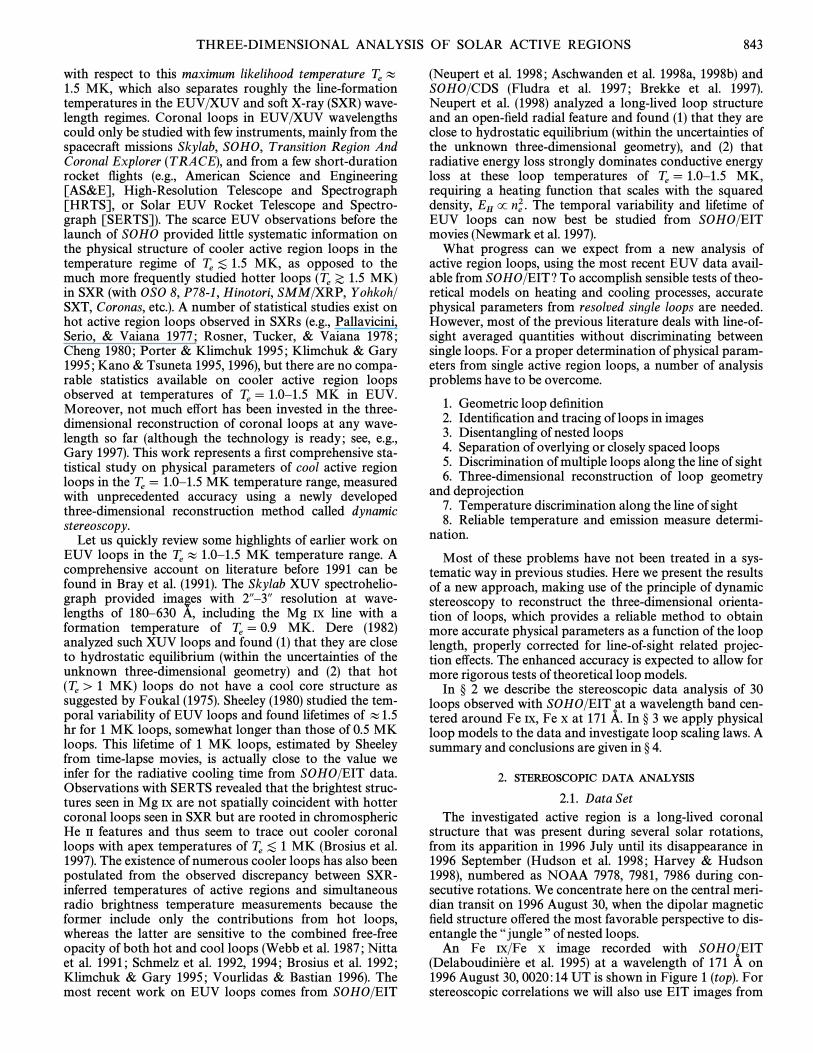
FIG. 3.ÈPrinciple of dynamic stereoscopy is illustrated here with an example of two adjacent loops, where a thicker loop is bright at time whereas at1,thinner loop is brightest at time From the loop positions measured at an intermediate reference time t, i.e., (middle panel in middle row),t2. (x

i, y

i) t1 \ t \ t2projections are calculated for the previous and following days for di†erent inclination angles Ë of the loop plane (left and right panel in middle row). By

extracting stripes parallel to the calculated projections Ë \ 10¡, 20¡, 30¡ (bottom) it can be seen that both loops appear only co-aligned with the stripe axis forthe correct projection angle Ë \ 20¡, regardless of the footpoint displacement *x between the two loops. The co-alignment criterion can therefore be used toconstrain the correct inclination angle Ë, even for dynamically changing loops.

footpoint. However, the general dipole characteristic of themagnetic Ðeld in this active region provides sufficient guid-ance to localize the secondary footpoint with an accuracy of

of the loop length. In order to obtain an error esti-[10%mate of the location of the secondary footpoint, we repeatthe loop tracing procedure Ðve times for each loop andobtain from the measured azimuth angles j \ 1, . . . , 5 aa

j,

mean and standard deviation a ^ da.3. The loop positions measured in the image at(x

i, y

i)

time are then transformed into heliographic longitudet1and latitude coordinates and altitudes based on(lij, b

ij) (h

ij),

the azimuth angle a of the footpoint baseline and the vari-able inclination angle which is varied over a range ofË

j,

in increments of *Ë \ 1¡.[90¡ \ Ëj\ ]90¡

4. The heliographic coordinate is then transformedlij(t1)

to the time of the second stereoscopic pair image,t2 lij@ (t2),

using the solar di†erential rotation rate applied to the time

interval We use the di†erential rotation rate speci-(t2 [ t1).Ðed by Allen (1973),

l@(t2) \ l(t1) ] [13¡.45 [ 3¡ sin2 b](t2 [ t1)1 day

. (2)

The heliographic latitude and altitude are assumed tobij

hijbe constant during the considered time interval.

5. In the stereoscopic pair image at time we calculatet2the image coordinates of the projected loop struc-(xij@ , y

ij@ )

ture. Parallel to these loop curves (with typical lengths ofpixels) we extract image stripes of some widthn

s\ 50È200

pixels) by interpolating the image brightness(nw

\ 16F(x, y) at the positions of the curved coordinate grid.

6. The stretched two-dimensional image stripes (ns] n

wpixels) are then scanned for parallel brightness ridges,caused by ““ dynamic ÏÏ structures that are co-aligned (orparallel-displaced) to the loop projection in image (fort2

-0.12 -0.10 -0.08 -0.06 -0.04 -0.02

-0.14

-0.12

-0.10

-0.08

-0.06

-0.04

deg

96/ 8/29 0:15:15.006-0.06 -0.04 -0.02 0.00 0.02

-0.14

-0.12

-0.10

-0.08

-0.06

-0.04

96/ 8/30 0:20:14.8810.00 0.02 0.04 0.06 0.08

-0.14

-0.12

-0.10

-0.08

-0.06

-0.04

96/ 8/31 0:10:14.130

-0.12 -0.10 -0.08 -0.06 -0.04 -0.02deg

-0.14

-0.12

-0.10

-0.08

-0.06

-0.04

deg

96/ 8/29 0:15:15.006-0.06 -0.04 -0.02 0.00 0.02

deg

-0.14

-0.12

-0.10

-0.08

-0.06

-0.04

96/ 8/30 0:20:14.8810.00 0.02 0.04 0.06 0.08

deg

-0.14

-0.12

-0.10

-0.08

-0.06

-0.04

96/ 8/31 0:10:14.130

-0.12 -0.10 -0.08 -0.06 -0.04 -0.02

-0.14

-0.12

-0.10

-0.08

-0.06

-0.04

-0.12 -0.10 -0.08 -0.06 -0.04 -0.02

-0.14

-0.12

-0.10

-0.08

-0.06

-0.04

-0.06 -0.04 -0.02 0.00 0.02

-0.14

-0.12

-0.10

-0.08

-0.06

-0.04

1

1

2

2

3

3

4

4

5

5

6

6

7

7

8

8

9

910

10

11

11

1212

131314141515 16

1617

1718

18

19

19

20

20

21

21

22

22

23

2324

2425

25

26

26

27

27

28

28

29

29

30

30

-0.06 -0.04 -0.02 0.00 0.02

-0.14

-0.12

-0.10

-0.08

-0.06

-0.04

1

1

2

2

3

3

4

4

5

5

6

6

7

7

8

8

9

910

10

11

11

1212

131314141515 16

1617

1718

18

19

19

20

20

21

21

22

22

23

2324

2425

25

26

26

27

27

28

28

29

29

30

30

0.00 0.02 0.04 0.06 0.08

-0.14

-0.12

-0.10

-0.08

-0.06

-0.04

0.00 0.02 0.04 0.06 0.08

-0.14

-0.12

-0.10

-0.08

-0.06

-0.04

g g g

No. 2, 1999 THREE-DIMENSIONAL ANALYSIS OF SOLAR ACTIVE REGIONS 847

illustration see examples shown in Fig. 3, bottom). Thisscanning process is numerically performed by measuringthe total lengths of parallel contiguous brightnessL (Ë

k)

ridges detected in each image stripe k for a given angle Ëk.

As the examples in Figure 3 (bottom) show, loop projectionsin stripes with angles Ë (e.g., Ë \ 10¡ or 30¡) that deviatefrom the mean loop plane Ë \ 20¡) appear as curved fea-tures and thus have shorter parallel segments than thoseprojections in stripes with inclination angles that coincidewith the mean loop plane (Ë \ 20¡). The numerical detec-tion of the length of parallel segments is therefore a reliableindicator of whether the inclination angle used in theË

kcoordinate transformation matches the e†ective loop planeË. We evaluate this criterion in our algorithm by maximiz-ing the sum of all detected contiguous parallel brightnessridges, i.e., by maximizing the quantity (max [; asL (Ë

k)])

a function of the variable inclination angle used in theËkcoordinate transformation. This way we infer the most

likely value of the inclination angle Ë of the mean loopplane.

7. The same procedure is repeated in forward and back-ward directions in time. The mean and standard deviationof Ë ^ dË is determined by averaging the two stereoscopicsolutions (^1 day).

The independent stereoscopic correlation in forward (]1day) and backward ([1 day) direction provides a usefulredundancy of the solution. The time di†erence of ^1 day

corresponds to an aspect angle change of Except for^13¡.5.steps 1È2, which constitute the deÐnition of a selected loopfeature, all other steps (3È7) of the stereoscopic correlationare performed automatically by a numeric code withouthuman interaction. The determination of the loop inclina-tion angle Ë is therefore achieved in a most objective way,within the principle of dynamic stereoscopy.

2.3. L oop GeometryWith the dynamic stereoscopy method described above

we analyzed the three-dimensional coordinates of 30 loopsfrom the EIT 171 image on 1996 August 30 (Fig. 4, middleA�column). The true three-dimensional geometry of (thecentral axis of) a coronal loop can be characterized withthree orthogonal spatial coordinates i \ 1,[x(s

i), y(s

i), z(s

i)],

. . . , n, parametrized by the loop length parameter Whensi.

we trace a loop structure in an image (see Fig. 4, middlecolumn), we can accurately measure the two coordinates

without imposing any geometric constraint on[x(si), y(s

i)],

its shape, as opposed to a method that Ðts a predeÐnedgeometric model (e.g., a circular geometry or its ellipticprojection). We impose only some constraints on the thirdcoordinate namely, assuming that the loop segment isz(s

i),

mathematically described in a plane, whose orientation wequantify with two free parameters (Fig. 2) : with the azimuthangle a (of the loop footpoint baseline) and the stereo-scopically measured inclination angle Ë (with respect to the

FIG. 4.ÈProjections of 30 stereoscopically reconstructed loop segments (numbered white curves) are shown overlaid on the SOHO/EIT 171 imagesA�(top) and the Ðltered images (bottom) of 1998 August 29 (left), 30 (center), and 31 (right). The 30 loop segments were traced from the Ðlter image of August 30(bottom middle), whereas the projections on the previous and following day were calculated from the inclination angles Ë obtained from the dynamicstereoscopy method. Note that the overall magnetic Ðeld structure is almost invariant during the 3 days, but dynamic changes of the loops produce slightdisplacements between the calculated projections forward and backward in time and the actually observed Ðne structure.

848 ASCHWANDEN ET AL. Vol. 515

vertical). However, the planar approximation serves onlyfor mathematical convenience and deÐnes a mean loopplane but does not require that the actual loop is exactlyconÐned in a plane because our dynamic stereoscopymethod allows for near-parallel displacements in time andspace within some range. One additional constraint is alsointroduced by the reference level of the Ðrst footpointh(s1)position, assumed to be located at a Ðxed height of h(s1) \

Mm.hfoot B 2.5Some geometric elements of the analyzed 30 loops are

listed in Table 1 : the heliographic longitude and latitude(l1)position of the primary footpoint(b1) [x(s1), y(s1), h(s1) \

the azimuth angle a of the footpoint baseline mea-hfoot],sured at the primary footpoint, and the inclination angle Ëof the loop plane. The average heliographic position of the30 loop footpoints is whichSl

F1T \ 251¡.0, Sb

F1T \ [11¡.8,

is slightly southward of the Sun center position at this time,l0 \ 255¡.8, b0 \ 7¡.2.

The average azimuth angle (modulo 180¡) of the 30 loopfootpoint baselines is a \ [3¡ ^ 10¡, which represents theglobal orientation of the large-scale dipolar magnetic Ðeldthat dominates the active region, which was used as a guideto estimate the azimuth angle of the footpoint baseline forindividual loop segments. The only complete loop thatcould be traced out (without gaps between the footpoints) isloop 1, which has an azimuth angle of a \ 15¡ ^ 1¡.

The inclination angles Ë of the loop planes cover a largerange from Ë \ [56¡ to Ë \ ]69¡, having an average of

SËT \ 7¡ ^ 37¡. The southern loops (loops 1È11, 23È30) allshow an inclination toward south (with Ë negative if theprimary footpoint is to the east), whereas the northern loops(loops 12È22) show a systematic inclination toward north(with Ë positive if the primary footpoint is to the east). Thisfan-shaped divergence of loop planes is consistent with theoverall magnetic dipolar Ðeld, having the dipole axisaligned to the east-west direction.

We visualize the three-dimensional structure of the ste-reoscopically reconstructed 30 loops in Figure 5, where dif-ferent perspectives and viewing angles are displayed. Thetraced segments (Fig. 4) of the reconstructed loops aremarked with thick lines in Figure 5, whereas the thin linesrepresent circular segments in the loop plane, constrainedby the two footpoints and the endpoint of the tracedsegment. We rotated these reconstructed 30 loops by [7.2days to the east (Fig. 5, bottom left), in order to illustrate thedistribution of inclination angles. The group of loops thatare inclined to the south in our EIT image of 1996 August30 are also found to have a similar conÐguration (withsimilar loop heights and loop plane inclinations) in an EITimage observed 7.2 days earlier, when this active regioncrossed the east limb (Fig. 5, top left).

2.4. L oop Background SubtractionWe parametrize the positions of the traced loop segments

from the image coordinates as a function of the[x(si), y(s

i)]

(projected) loop length parameter by interpolating thesi,

TABLE 1

GEOMETRIC PARAMETERS OF 30 CORONAL LOOPS (1996 AUGUST 29, EIT 171 A� )

Heliographic Azimuth Inclination Loop Center Loop Loop Scale LoopLoop Coordinates l1, b1 Angle a Angle Ë Radius R0 O†set Z0 Trace L 1 Length L Height j Width w

Number (deg) (deg) (deg) (Mm) (Mm) (Mm) (Mm) (Mm) (Mm)

1 . . . . . . . . . . . . . 247.9, [15.4 15 ^ 1 [42 ^ 1 56 [14 149 149 49 6.82 . . . . . . . . . . . . . 247.7, [15.5 13 ^ 1 [49 ^ 5 62 18 91 234 50 6.13 . . . . . . . . . . . . . 247.4, [15.6 12 ^ 1 [34 ^ 1 68 31 89 282 57 7.44 . . . . . . . . . . . . . 247.3, [15.0 8 ^ 2 [26 ^ 1 77 45 104 338 57 6.95 . . . . . . . . . . . . . 247.1, [14.9 8 ^ 3 [49 ^ 1 73 37 121 309 56 6.36 . . . . . . . . . . . . . 247.0, [13.9 2 ^ 2 [56 ^ 1 84 53 80 381 42 7.07 . . . . . . . . . . . . . 246.1, [14.7 4 ^ 2 [36 ^ 1 89 51 125 389 62 7.18 . . . . . . . . . . . . . 245.2, [14.7 9 ^ 2 [33 ^ 2 113 80 124 534 57 7.19 . . . . . . . . . . . . . 247.0, [12.2 [3 ^ 3 [12 ^ 1 86 44 41 366 60 8.110 . . . . . . . . . . . . 245.8, [13.3 1 ^ 2 [23 ^ 1 124 95 90 609 53 7.911 . . . . . . . . . . . . 244.9, [12.2 1 ^ 3 [31 ^ 2 144 116 56 725 66 6.812 . . . . . . . . . . . . 247.3, [10.7 [6 ^ 2 10 ^ 1 116 94 153 585 60 7.813 . . . . . . . . . . . . 250.6, [10.1 [9 ^ 7 11 ^ 1 73 60 62 373 60 6.414 . . . . . . . . . . . . 247.1, [9.8 [8 ^ 3 10 ^ 1 113 87 70 554 33 6.415 . . . . . . . . . . . . 247.5, [9.0 [8 ^ 1 12 ^ 1 125 105 103 643 47 6.816 . . . . . . . . . . . . 248.1, [8.5 [11 ^ 3 25 ^ 1 85 59 63 400 53 6.717 . . . . . . . . . . . . 248.5, [8.0 [14 ^ 4 32 ^ 1 93 71 52 455 47 7.418 . . . . . . . . . . . . 249.0, [7.4 [9 ^ 4 40 ^ 3 92 79 109 483 93 5.619 . . . . . . . . . . . . 249.6, [6.9 [18 ^ 3 39 ^ 1 116 95 130 590 65 7.920 . . . . . . . . . . . . 250.7, [6.6 [24 ^ 6 52 ^ 6 78 64 103 399 56 7.721 . . . . . . . . . . . . 251.5, [6.1 [21 ^ 6 58 ^ 3 67 47 85 318 45 7.622 . . . . . . . . . . . . 251.9, [5.7 [25 ^ 5 58 ^ 3 49 29 53 217 58 7.223 . . . . . . . . . . . . 259.1, [10.7 [4 ^ 4 0 ^ 1 102 71 69 479 60 8.024 . . . . . . . . . . . . 258.6, [11.4 [1 ^ 4 14 ^ 6 114 90 106 568 64 8.725 . . . . . . . . . . . . 263.2, [16.6 [1 ^ 5 43 ^ 1 138 70 59 582 42 8.126 . . . . . . . . . . . . 259.9, [13.8 [8 ^ 4 13 ^ 2 100 60 39 446 59 5.127 . . . . . . . . . . . . 259.1, [13.4 [2 ^ 3 50 ^ 2 101 68 72 471 58 7.128 . . . . . . . . . . . . 258.0, [13.4 0 ^ 2 27 ^ 2 90 63 86 423 57 7.529 . . . . . . . . . . . . 257.9, [13.7 5 ^ 2 36 ^ 1 78 45 88 344 60 6.030 . . . . . . . . . . . . 257.5, [13.8 [2 ^ 3 69 ^ 1 76 44 86 336 38 7.4

Average . . . 251.0 (^5.4), [11.8 (^3.3) [3 (^10) 7 (^37) 93 (^23) 62 (^27) 89 (^29) 433 (^136) 55 (^10) 7.1 (^0.8)

OBSERVED 7.2 DAYS EARLIER

-0.35 -0.30 -0.25

-0.10

-0.05

0.00

deg

96/ 8/22 20:10:13.008

VIEW FROM EARTH

-0.10 -0.08 -0.06 -0.04 -0.02 0.00 0.02 0.04EW [deg]

-0.16

-0.14

-0.12

-0.10

-0.08

-0.06

-0.04

-0.02

1

1

2

2

3

3

4

4

5

5

6

6

7

7

8

8

9

910

10

11

11

1212

131314141515 16

1617

1718

18

19

19

20

20

21

21

22

22

23

2324

2425

25

26

26

27

27

28

28

29

29

30

30

ROTATED TO NORTH

-0.10 -0.08 -0.06 -0.04 -0.02 0.00 0.02 0.040.24

0.26

0.28

0.30

0.32

0.34

0.36

0.38

1

1

2

2

3

3

4

4

5

5

6

6

7

7

8

8

9

9

10

10

11

11

12

12

13

13

14

14

15

15

16

16

17

17

18

18

19

19

20

20

21

21

22

22

23

23

24

24

25

25

26

26

27

27

28

28

29

29

3030

ROTATED TO EAST (-7.2 DAYS)

-0.35 -0.30 -0.25EW [deg]

-0.10

-0.05

0.00

NS

[deg

]

1

1

2

2

3

3

4

4

5

5

6

6

7

7

8

8

9 9 10

10

11

11

1212

1313 14

14 15

15

16

16

17

17

18

18

19

19

20

20

21

21

22

22

23

2324

24

25

25

26

26

27

27

28

28

29

29

30

30

No. 2, 1999 THREE-DIMENSIONAL ANALYSIS OF SOLAR ACTIVE REGIONS 849

FIG. 5.ÈThree di†erent projections of the stereoscopically reconstructed 30 loops of AR 7986 are shown. The loop segments that were traced from the1996 August 30, 171 image are marked with thick solid lines, whereas the extrapolated segments (thin solid lines) represent circular geometries extrapolatedA�from the traced segments. The three views are (1) as observed from Earth with (bottom right), (2) rotated to north by (top right), and (3)l0, b0 b0@ \ b0 [ 100¡rotated to east by (corresponding to [7.2 days of solar rotation, bottom left). An EIT 171 image observed at the same time ([7.2 daysl0@ \ l0 ] 97¡.2 A�earlier) is shown for comparison (top left), illustrating a similar range of inclination angles and loop heights as found from stereoscopic correlations a weeklater. The heliographic grid has a spacing of 5¡ degrees or 60 Mm.

coordinates with a constant resolution of *si\ s

i`1 [ si\

1 pixel in the image plane. These positions mark the centralaxes of the analyzed loops. For single-loop analysis it isconvenient to introduce a coordinate grid that is co-[s

i, t

j]

aligned with the loop axis and is the coordinate ortho-sj, t

jgonal to the loop axis. The projections [x(si, t

j), y(s

i, t

j)]

of these curved coordinate grids are shown in Figure 6 (topright). We parametrized both coordinates with a[s

i, t

j]

uniform resolution of 1 pixel and have chosen a width of 16pixels for the width of the stripes symmetrically bracket-(t

j),

ing the central loop axis. We show the radiative Ñux asF(tj)

a function of the loop cross section for each loop (1È30)tjand for each position along the central loop axis with ans

iincremental step of pixel in Figure 6, measured from*si\ 1

the EIT 171 image of 1996 August 30.A�In a next step we attempt to separate the loop-associated

Ñuxes from the loop-unrelated background. This is a very

crucial step to determine the correct emission measure andelectron density in a given loop. This task is difficultbecause most of the loops are very closely spaced andseparated only by a few pixels at their primary footpoint(see Fig. 6). Very few loops occur in an isolated environment(e.g., such as loop 25 ; see Figs. 4È6). For many cross sec-tions there is not enough separation between adjacent loopsto model the loop-unrelated background properly. The factthat the Ñux-unrelated background makes up typically50%È90% of the total EUV Ñux measured at a given lineof sight (see Fig. 7) indicates that we can separate out onlya fraction of superposed and nested loops, like the top-most elements on the topological surface of a ““ strand ofspaghetti. ÏÏ

We tested various methods and found the following to beleast susceptible to confusion by adjacent loops. We calcu-lated the background proÐle to the observed ÑuxF

B(t

j) F(t

j)

AR 7986, Loop Stripe Projections #1-30

1

1

2

2

3

3

4

4

5

5

6

6

7

7

8

8

9

910

10

11

11

12

12

1313

1414

151516

1617

17

18

18

19

19

20

20

21

21

22

22

23

23

24

2425

25

26

26

27

27

28

28

29

29

30

30

Loop #1#2 #3 #4 #5 #6 #7 #8 #9 #10

#11 #12 #13 #14 #15 #16 #17 #18 #19 #20 #21 #22 #23 #24 #25 #26 #27 #28 #29 #30

FIG. 6.ÈPositions of the curved coordinate grids of the 30 analyzed loop segments are shown in the top right panel, which has the same orientation as the1996 August 30 map shown in Fig. 4 (middle). The coordinate grid of loop 1 is represented with 1 pixel resolution, whereas only the outer borders and centralaxes are indicated for the other loop segments. The vertically oriented panels represent the coordinate grids of the analyzed 30 loops, stretched out along theloop axis. The top of the panels corresponds to the primary footpoint (see positions in Table 1). In each panel we show the EIT 171 Ñux loop crossl1, b1 A�sections measured perpendicularly to the loop axes. Successive cross sections are separated by a distance of 1 pixel along the loop axis. The Ñux associatedwith each loop is marked with a gray area, obtained by background subtraction with a cubic spline interpolation between both sides of the loop cross section.

0 20 40 60 80 100Loop length [pixels]

0

200

400

600

800

1000

Flu

x [D

N]

Total flux

Background

Background-subtracted

Flux ratio Floop/Ftotal=0.29

0.0 0.2 0.4 0.6 0.8 1.0Flux ratio Floop/Ftotal

0

2

4

6

8

Num

ber

of lo

ops

THREE-DIMENSIONAL ANALYSIS OF SOLAR ACTIVE REGIONS 851

FIG. 7.ÈLoop-associated EUV Ñux thick line], the total EUV Ñux thin line], and the background dotted line][Floop(s), [Ftotal(s), [Ftotal(s) [ Fflux(s),measured along the loop is shown for loop 1 (left). A histogram of the relative fractions (integrated over the traced loop lengths) is shown from allFloop/Ftotal30 analyzed loops (right).

by cubic spline interpolation between various cross sectionboundaries which were varied over a range of 1, . . . ,[t1, t2],4 pixels (or 2È7 Mm for the half-width of the loop crosssection) on both sides of the central loop axis. From thevaried loop boundaries those were used for the[t1, t2]background envelope that maximize the Ñux integratedover loop cross section, i.e., the maximum of / [F(t

j)

because this quantity is invariant to lateral[ FB(t

j)]dt

jdisplacements (in transverse direction t) and is least suscep-tible to changes of the functional form F(t) along the loopcoordinate s. This method has the advantage of adjustingfor loop thickness variations, for o†sets in tracing of thecentral axis, and for co-alignment errors between the 171and 195 image in the use of the Ðlter-ratio technique. TheA�so-determined loop-associated Ñuxes are shown with grayareas for each cross section in Figure 6. The resultsF(t

j) o

s/sishow that the allowed loop half-width range of ^1, . . . , 4pixels separates most of the loops reasonably, except foroccasional double loop detections (e.g., 22 or 26 in Fig. 6)near the primary footpoint. Such loop segments where theloop separation fails will be excluded in further analysis.

2.5. L oop Cross SectionsWe measured the loop width w(s) as a function of the

loop length parameter s, using the deÐnition of the equiva-lent width w(s),

w(s) \ / F(s, tj) [ F

B(s, t

j) dt

jmax [F(s, t

j) [ F

B(s, t

j)]

. (3)

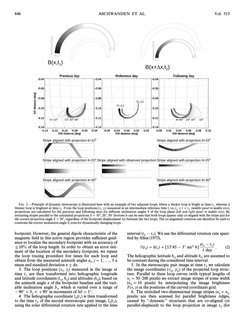
These loop widths w(s) are shown as a function of the looplength s in Figure 8 for the 10 loops that are least confusedby adjacent loops, as can be judged from the cross sections

shown in Figure 6 (loop 1, 8, 11, 14, 15, 19, 20, 21,F(tj) o

s/si25, 28). Performing a linear regression Ðtted to the observedvalues w(s), we Ðnd a signiÐcant variation of the loop thick-ness only for two of them (loop 20 and 28). To quantify thevariation of the loop thickness we calculated a loop diver-gence factor, deÐned by the average width in the upper part

to the lower part of the(smax/2 \ s \ smax) (0 \ s \ smax/2)traced loop segment. We remind the reader that the tracedloop segments generally extend over about 1 density scaleheight but often do not reach the loop top (except for thesmallest loop, 1). The loop divergence factors and theiruncertainties are shown in Figure 8 (bottom right) for eachloop. We caution that some of the loop thickness variationnear the footpoints is due to separation problems of closelyspaced adjacent loops (as can be judged from Fig. 6). A

histogram of average loop widths is shown in Figure 8 (topright), whereas the individual values w and their mean andstandard deviation (w \ 7100 ^ 800 km) are also listed inTable 1. The preference for such a narrow range of loopdiameters is perhaps an instrumental resolution biasbecause the Ðnest recognizable structures are most likely tobe seen at a scale corresponding to the size of a few pixels.

2.6. L oop Densities and Scale HeightsFor electron density and temperature diagnostics we are

using a Ðlter-ratio technique applied to the EIT 171 and 195wavelength images, based on the most recent EIT stan-A�

dard software (status of 1998 February, Newmark et al.1996 ; SOHO EIT UserÏs Guide). The resulting emissionmeasures EM and temperatures are based on the cal-T

eEIT

culation of synthetic spectra using the CHIANTI database,containing some 1400 emission lines in the 150È400 A�wavelength range (Dere et al. 1997). For details of the EITcalibration and error analysis, the reader is referred to

et al. (1995), Moses et al. (1997), andDelaboudiniereNeupert et al. (1998). Further cross calibrations of the EITinstrument with NRL rocket Ñights carrying an EIT dupli-cate instrument are in progress (led by D. Moses). In brief,we note that the main errors at this stage are systematic anddue to calibration questions. This has a larger e†ect on theemission measure than on the temperature because thelatter is determined from a ratio, in which systematic errorscancel out to some extent. Our estimate of the absoluteerror in the temperature determination is about 0.2 MK,whereas the emission measure has a systematic error of upto a factor of 4. The abundances in the above calculationsare those given by Meyer (1985) for the corona. As iron is alowÈÐrst ionization potential (FIP) element, abundancequestions play a minor role in the uncertainties.

To determine the electron density along individualne(s)

loops, we use the background-subtracted EIT Ñuxesin the Ðlter ratios and the loop widthsFloop(s) \ F(s) [ F

B(s)

w(s). An additional important loop parameter is the line-of-sight angle t(s), which provides a correction factor of thee†ective column depth for a loop with circular cross sectionspeciÐed by a diameter w(s), i.e., (seew

z(s) \ w(s)/cos [t(s)]

Appendix B). With this parametrization we deÐne thedensity along a loop (normalized to a Ðlling factor ofn

e(s)

unity) by

ne(s) \

SEM(s)w

z(s)

\SEM(s) cos [t(s)]

w(s), (4)

0 50 100 150 200

468

1012

Loop # 1: w= 6.8 Mm

0 20 40 60 80 100 120

468

1012

Loop # 8: w= 7.2 Mm

0 10 20 30 40 50 60

468

1012

Loop #11: w= 6.7 Mm

0 10 20 30 40 50

468

1012

Loop #14: w= 6.3 Mm

0 20 40 60 80

468

1012

Loop #15: w= 6.8 Mm

0 20 40 60 80

468

1012

Loop #19: w= 8.1 Mm

0 20 40 60 80

468

1012

Loop #20: w= 7.7 Mm

0 10 20 30 40 50 60

468

1012

Loop #21: w= 7.6 Mm

0 10 20 30 40 50 60

468

1012

Loop #25: w= 8.1 Mm

0 20 40 60 80Loop length [Mm]

468

1012

Loop #28: w= 7.6 Mm

Loop

wid

th w

[Mm

]

Loops #1-30

0 2 4 6 8 10Loop width w[Mm]

0

2

4

6

8

Num

ber

of lo

ops

Loops #1-30

0 10 20 30 40Loop number #

0.0

0.5

1.0

1.5

2.0

Loop

div

erge

nce

fact

or

852 ASCHWANDEN ET AL. Vol. 515

FIG. 8.ÈVariation of the loop thickness is shown for the 10 loops with the least confusion by adjacent loops (see cross sections in Fig. 6) as a function ofthe loop length s (left). A linear regression Ðt is indicated (solid line in left panels). The average (equivalent) width w is histogrammed for all 30 analyzed loops(top right). A loop divergence factor is calculated from the ratio of the average width in the upper half and lower half (traced) loop segments (right bottom).Note that most of the loops show no signiÐcant loop thickness variation.

with the loop length s(x, y) parametrized as a function of theimage position (x, y), from which the EIT emission measureEM(x, y) is measured. Because the line-of-sight angle t(s) isvery sensitive to the loop orientation, correct values of theelectron density can only be obtained from an appro-n

e(s)

priate three-dimensional model of the loop (constrained bystereoscopic correlations here). The projection e†ect of theloop curvature on the e†ective column depth and thew

z(s),

e†ect of the inclination angle Ë of the loop plane on theinferred density scale height j(Ë) are illustrated in Figure 9(see also discussion in Alexander & Katsev 1996).

The electron density calculated from equation (4) isne(s)

shown graphically for the 10 least-confused loops (1, 8, 11,14, 15, 19, 20, 21, 25, 28) in Figure 10 (left). Because theheight dependence s(h) of the loop length is known from ourstereoscopic reconstruction (displayed in Fig. 5), we candirectly obtain the parametrization and Ðtn

e[s(h)] # n

e(h)

an exponential density model,

ne(h) \ n

e0 expC

[ hj(T

e)D

(5)

to obtain a scale height temperature which is deÐned byTej,

(e.g., Lang 1980, p. 285)

j(Te) \ kB T

ekmH g

B 46A T

e1 MK

B[Mm] , (6)

with the Boltzmann constant, k the mean molecularkBweight (k B 1.4 for the solar corona), the mass of themH

hydrogen atom, and g the acceleration of gravity at thesolar surface. The so obtained scale height j, with a mean ofj \ 55 ^ 10 Mm, and the inferred scale height temperature

with a mean of are listed in Tables 1Tej, T

ej \ 1.22 ^ 0.23,

and 2 for each of the analyzed 30 loops. Loop segmentranges that are obviously confused by adjacent or crossingloops (as can be judged from Fig. 6), have been excluded inthe Ðtting of the scale height model. We Ðnd that most ofthe analyzed loop segments Ðt closely an exponentialdensity model (see Fig. 10, left). Deviations from an expo-nential density model can often be explained by uncer-tainties in the background subtraction or by confusion fromadjacent or overlying loops. A correction to the local scaleheight temperature would also result from temperature gra-dients (° 2.8), which are of the order (dT /ds)/(T /j) B0.05 ^ 0.20 and are neglected here.

2.7. L oop TemperaturesIndependently of the scale height temperature we canT

ej,

also determine the temperature directly from the EIT Ðlterratio (as described in ° 2.6), which moreover provides atemperature di†erentiation along the loop, SinceT

eEIT(s).

our loop deÐnitions are based on tracing of an EIT 171 A�image, we use only the Ðlter ratio of EIT 171 (Fe IX, Fe X)A�and 195 (Fe XII), which is sensitive in the temperatureA�regime of MK. We are using the spatial loopT

e\ 1.0È1.5

deÐnition [x(s), y(s)] based on the 171 image and applyA�the same background-subtraction technique to the 195 A�

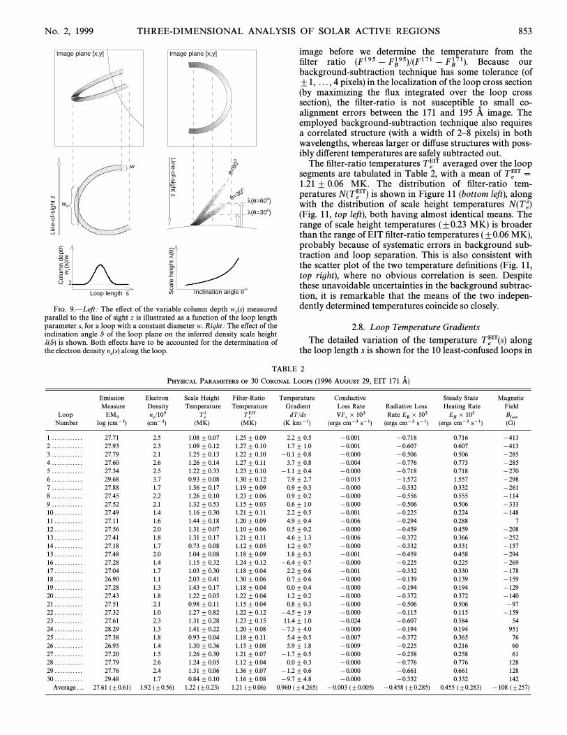
Image plane [x,y]

Line

-of-

sigh

t z

wz

w

Loop length s

Col

umn

dept

hw

z(s)

/w

1

Image plane [x,y]

θ=60

0

θ=300

Line-of-sight z

λ(θ=600)

λ(θ=300)

Inclination angle θSca

le h

eigh

t λ(θ

)

No. 2, 1999 THREE-DIMENSIONAL ANALYSIS OF SOLAR ACTIVE REGIONS 853

FIG. 9.ÈL eft : The e†ect of the variable column depth measuredwz(s)

parallel to the line of sight z is illustrated as a function of the loop lengthparameter s, for a loop with a constant diameter w. Right : The e†ect of theinclination angle Ë of the loop plane on the inferred density scale heightj(Ë) is shown. Both e†ects have to be accounted for the determination ofthe electron density along the loop.n

e(s)

image before we determine the temperature from theÐlter ratio Because our(F195 [ F

B195)/(F171 [ F

B171).

background-subtraction technique has some tolerance (of^1, . . . , 4 pixels) in the localization of the loop cross section(by maximizing the Ñux integrated over the loop crosssection), the Ðlter-ratio is not susceptible to small co-alignment errors between the 171 and 195 image. TheA�employed background-subtraction technique also requiresa correlated structure (with a width of 2È8 pixels) in bothwavelengths, whereas larger or di†use structures with poss-ibly di†erent temperatures are safely subtracted out.

The Ðlter-ratio temperatures averaged over the loopTeEIT

segments are tabulated in Table 2, with a mean of TeEIT \

1.21 ^ 0.06 MK. The distribution of Ðlter-ratio tem-peratures is shown in Figure 11 (bottom left), alongN(T

eEIT)

with the distribution of scale height temperatures N(Tej)

(Fig. 11, top left), both having almost identical means. Therange of scale height temperatures (^0.23 MK) is broaderthan the range of EIT Ðlter-ratio temperatures (^0.06 MK),probably because of systematic errors in background sub-traction and loop separation. This is also consistent withthe scatter plot of the two temperature deÐnitions (Fig. 11,top right), where no obvious correlation is seen. Despitethese unavoidable uncertainties in the background subtrac-tion, it is remarkable that the means of the two indepen-dently determined temperatures coincide so closely.

2.8. L oop Temperature GradientsThe detailed variation of the temperature alongT

eEIT(s)

the loop length s is shown for the 10 least-confused loops in

TABLE 2

PHYSICAL PARAMETERS OF 30 CORONAL LOOPS (1996 AUGUST 29, EIT 171 A� )

Emission Electron Scale Height Filter-Ratio Temperature Conductive Steady State MagneticMeasure Density Temperature Temperature Gradient Loss Rate Radiative Loss Heating Rate Field

Loop EM0 ne/109 T

ej T

eEIT dT /ds +F

c] 103 Rate E

R] 103 E

H] 103 Bfoot

Number log (cm~5) (cm~3) (MK) (MK) (K km~1) (ergs cm~3 s~1) (ergs cm~3 s~1) (ergs cm~3 s~1) (G)

1 . . . . . . . . . . . . 27.71 2.5 1.08 ^ 0.07 1.25 ^ 0.09 2.2 ^ 0.5 [0.001 [0.718 0.716 [4132 . . . . . . . . . . . . 27.93 2.3 1.09 ^ 0.12 1.27 ^ 0.10 1.7 ^ 1.0 [0.001 [0.607 0.607 [4133 . . . . . . . . . . . . 27.79 2.1 1.25 ^ 0.13 1.22 ^ 0.10 [0.1 ^ 0.8 [0.000 [0.506 0.506 [2854 . . . . . . . . . . . . 27.60 2.6 1.26 ^ 0.14 1.27 ^ 0.11 3.7 ^ 0.8 [0.004 [0.776 0.773 [2855 . . . . . . . . . . . . 27.34 2.5 1.22 ^ 0.33 1.23 ^ 0.10 [1.1 ^ 0.4 [0.000 [0.718 0.718 [2706 . . . . . . . . . . . . 29.68 3.7 0.93 ^ 0.08 1.30 ^ 0.12 7.9 ^ 2.7 [0.015 [1.572 1.557 [2987 . . . . . . . . . . . . 27.88 1.7 1.36 ^ 0.17 1.19 ^ 0.09 0.9 ^ 0.3 [0.000 [0.332 0.332 [2618 . . . . . . . . . . . . 27.45 2.2 1.26 ^ 0.10 1.23 ^ 0.06 0.9 ^ 0.2 [0.000 [0.556 0.555 [1149 . . . . . . . . . . . . 27.52 2.1 1.32 ^ 0.53 1.15 ^ 0.03 0.6 ^ 1.0 [0.000 [0.506 0.506 [33310 . . . . . . . . . . . 27.49 1.4 1.16 ^ 0.30 1.21 ^ 0.11 2.2 ^ 0.5 [0.001 [0.225 0.224 [14811 . . . . . . . . . . . 27.11 1.6 1.44 ^ 0.18 1.20 ^ 0.09 4.9 ^ 0.4 [0.006 [0.294 0.288 712 . . . . . . . . . . . 27.56 2.0 1.31 ^ 0.07 1.10 ^ 0.06 0.5 ^ 0.2 [0.000 [0.459 0.459 [20813 . . . . . . . . . . . 27.41 1.8 1.31 ^ 0.17 1.21 ^ 0.11 4.6 ^ 1.3 [0.006 [0.372 0.366 [25214 . . . . . . . . . . . 27.18 1.7 0.73 ^ 0.08 1.12 ^ 0.05 1.2 ^ 0.7 [0.000 [0.332 0.331 [15715 . . . . . . . . . . . 27.48 2.0 1.04 ^ 0.08 1.18 ^ 0.09 1.8 ^ 0.3 [0.001 [0.459 0.458 [29416 . . . . . . . . . . . 27.28 1.4 1.15 ^ 0.32 1.24 ^ 0.12 [6.4 ^ 0.7 [0.000 [0.225 0.225 [26917 . . . . . . . . . . . 27.04 1.7 1.03 ^ 0.30 1.18 ^ 0.04 2.2 ^ 0.6 [0.001 [0.332 0.330 [17818 . . . . . . . . . . . 26.90 1.1 2.03 ^ 0.41 1.30 ^ 0.06 0.7 ^ 0.6 [0.000 [0.139 0.139 [15919 . . . . . . . . . . . 27.28 1.3 1.43 ^ 0.17 1.18 ^ 0.04 0.0 ^ 0.4 [0.000 [0.194 0.194 [12920 . . . . . . . . . . . 27.43 1.8 1.22 ^ 0.05 1.22 ^ 0.04 1.2 ^ 0.2 [0.000 [0.372 0.372 [14021 . . . . . . . . . . . 27.51 2.1 0.98 ^ 0.11 1.15 ^ 0.04 0.8 ^ 0.3 [0.000 [0.506 0.506 [9722 . . . . . . . . . . . 27.32 1.0 1.27 ^ 0.82 1.22 ^ 0.12 [4.5 ^ 1.9 [0.000 [0.115 0.115 [15923 . . . . . . . . . . . 27.61 2.3 1.31 ^ 0.28 1.23 ^ 0.15 11.4 ^ 1.0 [0.024 [0.607 0.584 5424 . . . . . . . . . . . 28.29 1.3 1.41 ^ 0.22 1.20 ^ 0.08 [7.3 ^ 4.0 [0.000 [0.194 0.194 95125 . . . . . . . . . . . 27.38 1.8 0.93 ^ 0.04 1.18 ^ 0.11 5.4 ^ 0.5 [0.007 [0.372 0.365 7626 . . . . . . . . . . . 26.95 1.4 1.30 ^ 0.36 1.15 ^ 0.08 5.9 ^ 1.8 [0.009 [0.225 0.216 6027 . . . . . . . . . . . 27.20 1.5 1.26 ^ 0.30 1.21 ^ 0.07 [1.7 ^ 0.5 [0.000 [0.258 0.258 6128 . . . . . . . . . . . 27.79 2.6 1.24 ^ 0.05 1.12 ^ 0.04 0.0 ^ 0.3 [0.000 [0.776 0.776 12829 . . . . . . . . . . . 27.76 2.4 1.31 ^ 0.06 1.36 ^ 0.07 [1.2 ^ 0.6 [0.000 [0.661 0.661 12830 . . . . . . . . . . . 29.48 1.7 0.84 ^ 0.10 1.16 ^ 0.08 [9.7 ^ 4.8 [0.000 [0.332 0.332 142

Average . . . 27.61 (^0.61) 1.92 (^0.56) 1.22 (^0.23) 1.21 (^0.06) 0.960 (^4.265) [0.003 (^0.005) [0.458 (^0.285) 0.455 (^0.283) [108 (^257)

0 50 100 150 20001234

n [1

09 cm

-3] Loop # 1 λ = 49.5 Mm

Teλ = 1.08 _+0.07 MK

0 50 100 150 2001.001.101.201.301.401.50

Te

[MK

] Loop # 1 TeEIT = 1.25_+0.09 MK

dTe/ds=0.0022 MK/Mm

0 20 40 60 80 100 120 14001234

n [1

09 cm

-3] Loop # 8 λ = 57.8 Mm

Teλ = 1.26 _+0.10 MK

0 20 40 60 80 100 120 1401.001.101.201.301.401.50

Te

[MK

] Loop # 8 TeEIT = 1.23_+0.06 MK

dTe/ds=0.0009 MK/Mm

0 10 20 30 40 50 6001234

n [1

09 cm

-3] Loop #11 λ = 66.1 Mm

Teλ = 1.44 _+0.18 MK

0 10 20 30 40 50 601.001.101.201.301.401.50

Te

[MK

] Loop #11 TeEIT = 1.20_+0.09 MK

dTe/ds=0.0049 MK/Mm

0 20 40 60 8001234

n [1

09 cm

-3] Loop #14 λ = 33.6 Mm

Teλ = 0.73 _+0.08 MK

0 20 40 60 801.001.101.201.301.401.50

Te

[MK

] Loop #14 TeEIT = 1.12_+0.05 MK

dTe/ds=0.0012 MK/Mm

0 20 40 60 80 100 12001234

n [1

09 cm

-3] Loop #15 λ = 47.7 Mm

Teλ = 1.04 _+0.08 MK

0 20 40 60 80 100 1201.001.101.201.301.401.50

Te

[MK

] Loop #15 TeEIT = 1.18_+0.09 MK

dTe/ds=0.0018 MK/Mm

0 20 40 60 80 100 120 14001234

n [1

09 cm

-3] Loop #19 λ = 65.7 Mm

Teλ = 1.43 _+0.17 MK

0 20 40 60 80 100 120 1401.001.101.201.301.401.50

Te

[MK

] Loop #19 TeEIT = 1.18_+0.04 MK

0 20 40 60 80 10001234

n [1

09 cm

-3] Loop #20 λ = 56.3 Mm

Teλ = 1.22 _+0.05 MK

0 20 40 60 80 1001.001.101.201.301.401.50

Te

[MK

] Loop #20 TeEIT = 1.22_+0.04 MK

dTe/ds=0.0012 MK/Mm

0 20 40 60 80 10001234

n [1

09 cm

-3] Loop #21 λ = 45.1 Mm

Teλ = 0.98 _+0.11 MK

0 20 40 60 80 1001.001.101.201.301.401.50

Te

[MK

] Loop #21 TeEIT = 1.15_+0.04 MK

dTe/ds=0.0008 MK/Mm

0 20 40 6001234

n [1

09 cm

-3] Loop #25 λ = 42.6 Mm

Teλ = 0.93 _+0.04 MK

0 20 40 601.001.101.201.301.401.50

Te

[MK

] Loop #25 TeEIT = 1.18_+0.11 MK

dTe/ds=0.0054 MK/Mm

0 20 40 60 80 100Loop length s[Mm]

01234

n [1

09 cm

-3] Loop #28 λ = 57.1 Mm

Teλ = 1.24 _+0.05 MK

0 20 40 60 80 100Loop length s[Mm]

1.001.101.201.301.401.50

Te

[MK

] Loop #28 TeEIT = 1.12_+0.04 MK

Ele

ctro

n de

nsity

ne(

s)

Ele

ctro

n te

mpe

ratu

re T

eEIT(s

)

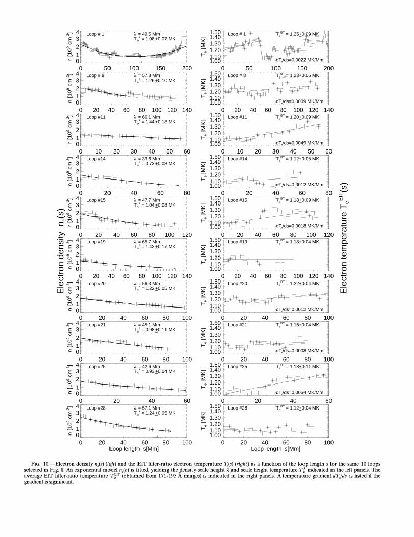
FIG. 10.ÈElectron density (left) and the EIT Ðlter-ratio electron temperature (right) as a function of the loop length s for the same 10 loopsne(s) T

e(s)

selected in Fig. 8. An exponential model is Ðtted, yielding the density scale height j and scale height temperature indicated in the left panels. Thene(h) T

ej

average EIT Ðlter-ratio temperature (obtained from 171/195 images) is indicated in the right panels. A temperature gradient is listed if theTeEIT A� dT

e/ds

gradient is signiÐcant.

0.5 1.0 1.5 2.0Scale height temperature Te

λ [MK]

0

2

4

6

8

10

Num

ber

of lo

ops

N=30 Teλ = 1.22 _+ 0.23 MK

0.5 1.0 1.5 2.0EIT filter ratio temperature Te

EIT [MK]

0

5

10

15

20

Num

ber

of lo

ops

N=30 TeEIT = 1.21 _+ 0.06 MK

0.5 1.0 1.5 2.0EIT filter ratio temperature Te

EIT [MK]

0.5

1.0

1.5

2.0

Sca

le h

eigh

t tem

pera

ture

Teλ [M

K]

-0.020 -0.010 0.000 0.010 0.020EIT temperature gradient dT/ds [K/m]

0

2

4

6

8

10

Num

ber

of lo

ops

N=30

THREE-DIMENSIONAL ANALYSIS OF SOLAR ACTIVE REGIONS 855

FIG. 11.ÈStatistics of scale height temperatures (left top), EIT Ðlter-ratio temperatures (left bottom), scatter plot of these two temperatures (rightTej T

eEIT

top), and EIT temperature gradients dT /ds (right bottom) for all analyzed 30 loops.

Figure 10 (right). We note that the Ðlter-ratio temperaturevaries sometimes discontinuously along the loop, e.g., thereis a jump from MK to MK at s \ 70 MmT

e\ 1.35 T

e\ 1.1

in loop 1 (Fig. 10, top right), which may be caused by con-tamination from a hotter loop that is located almost paral-lel to loop 1 at s \ 70 Mm (see cross sections in Fig. 6). Suchconfusion problems can only be identiÐed in hindsight.Despite such confusion problems, there seems to be a trendof a positive temperature gradient dT /ds [ 0 above thefootpoint for most of the loops (Table 2). To estimate theseaverage temperature gradients (without correcting formultiloop confusion) we performed a linear regression T

e(s)

for all loops. The most signiÐcant temperature gradients arefound for loop 11 (dT /ds \ ]0.0049 K m~1), for loop 20(dT /ds \ ]0.0012 K m~1), and for loop 25 (dT /ds \] 0.0054 K m~1) ; see examples in Figure 10 and Table 1.The distribution of temperature gradients N(dT /ds) isshown in Figure 11 (bottom right), revealing that B75% ofthe loops have a positive temperature gradient dT /ds [ 0across the Ðrst scale height above their footpoints. Higherparts of these loops are not detectable in EIT(h Z 1j)images due to insufficient density contrast (1 scale heightcorresponds to a factor of B3 in density or a factor of B10in emission measure or EIT Ñux).

2.9. Magnetic Field, Plasma-b Parameter, andVelocityAlfve� n

There is no accurate method available yet to determinethe height dependence of the coronal magnetic Ðeld, nor to

trace the magnetic Ðeld along a particular active regionloop. Some attempts are in progress to match loop geome-tries observed in SXR or EUV with potential Ðeld models(constrained by the photospheric boundary and projectionsof coronal loops ; Gary 1997 ; Gary & Alexander 1999). As aÐrst approximation to investigate the magnetic Ðeld alongthe observed EUV loops, we calculate here a potential Ðeldmodel of AR 7986, using the code of Sakurai (1982) appliedto a SOHO/Michelson-Doppler Imager (MDI) magneto-gram, recorded on the same day as the EIT image (with atime di†erence of 20 hr). The potential Ðeld model is shownin Figure 12, overlaid on the MDI magnetogram, and co-aligned with the traced EIT loops (by transforming thethree-dimensional Ðeld lines according to the solar rotationrate during the time di†erence). Note that the EUV loopsrepresent independent tracers of the plasma along magneticÐeld lines and thus convey an important test of how well thecoronal magnetic Ðeld is represented with a potential Ðeldmodel. The match of the traced EUV loops with the poten-tial Ðeld shown in Figure 12 is remarkably good, given thetime di†erence of 20 hr and the nonpotential structureimplied by currents that are likely to be present in thisactive region, imposed by the observed Ðlament along theneutral line. Detailed modeling with potential and force-freemagnetic Ðelds and investigating the best match with indi-vidual loops traced from EIT and SXT images will bepursued in a subsequent study.

To estimate the magnetic Ðeld along the traced EIT loopswe localize those potential Ðeld lines that have the closest

-0.10 -0.08 -0.06 -0.04 -0.02 0.00 0.02 0.04EW [deg]

-0.16

-0.14

-0.12

-0.10

-0.08

-0.06

-0.04

-0.02

NS

[deg

]

1

1

2

2

3

3

4

4

5

5

6

6

7

7

8

8

9

9

10

10

11

11

12

12

1313

1414

151516

16

17

17

18

18

19

19

20

20

21

21

22

22

23

23

24

24

25

25

26

26

27

27

28

28

29

29

30

30

960830 002014 UT: SOHO/EIT 171 A loops + MDI/Potential field

-0.10 -0.08 -0.06 -0.04 -0.02 0.00 0.02 0.04EW [deg]

-0.16

-0.14

-0.12

-0.10

-0.08

-0.06

-0.04

-0.02

NS

[deg

]

856 ASCHWANDEN ET AL. Vol. 515

FIG. 12.ÈSOHO/MDI magnetogram recorded on 1996 August 30, 2048 UT, rotated to the time of the analyzed EIT image (1996 August 30, 0020 :14 UT),with contour levels at B \ [350, [250, . . . , ]1150 G (in steps of 100 G). Magnetic Ðeld lines calculated from a potential Ðeld model are overlaid (thin lines)onto the 30 loops (thick lines) traced from the SOHO/EIT image.

footpoints to the EIT loop footpoints and take the heightdependence of their magnetic Ðeld strength B(h) as a proxyfor the EIT loops. The height dependence of the magneticÐeld B(h) of the 30 potential Ðeld lines closest to theanalyzed EIT loops is shown in Figure 13 (top). It can beapproximated with a dipole model,

B(h) \ BfootA

1 ] hhD

B~3, (7)

with a mean dipole depth of Mm and a range ofhD

\ 75footpoint Ðeld strengths . . . , 230 G (dashed linesBfoot B 20,in Fig. 13, top), or a mean of G.Bfoot B 100

With the potential Ðeld B(h) and the measured densityand temperature proÐles we can now determinen

e(h) T

e(h)

the height dependence of the plasma-b parameter for eachof the 30 analyzed loops,

b(h) \ n(h)kTe(h)

[B(h)2/8n]B 3.47 ] 10~15 n

e(h)T

e(h)

B(h)2 , (8)

which quantiÐes the ratio of the thermal to the magneticpressure and thus provides a crucial criterion for magneticconÐnement. The plasma-b parameter is shown in Figure 13(middle), ranging typically at in the entire coronalb [ 0.1range Mm) of the EUV loops. We Ðnd only 2 (out(h [ 200

of 30 loops) that exceed the critical limit of b º 1, possiblyimplying currents and nonpotential magnetic Ðelds alongthe loops. Gary & Alexander (1999) found such regimeswith in the upper corona at from analysisb Z 1 h Z 0.2 R

_of SXR loops, in contrast to the common belief that thecoronal value is always b > 1 (Dulk & McLean 1978 ; Priest1981 ; Sakurai 1989 ; Gary 1990 ; McClymont, Jiao, & Mikic�1997). Reliable measurements of the plasma-b parameterrequire fully resolved structures, such as single loopsanalyzed here (save for unknown Ðlling factors), whereasline-of-sight averaged densities are expected to underesti-mate the density in loop structures and thus are biasedtoward too low b values.

A further plasma parameter that is of interest for coronalloop dynamics is the velocity, which can be com-Alfve� nputed along individual loops thanks to the knowledge ofthe magnetic Ðeld B(h) and density n

e(h),

vA(h) \ B(h)

J4nni(h)m

i

B 2.18]1011 B(h)

Jne(h)

cm s~1 . (9)

This quantity is shown in Figure 13 (bottom). The Alfve� nvelocity is found to be highest near the footpoints of theanalyzed EUV loops, ranging from tovA(h \ 0) B 20006000 km s~1, and is dropping o† steadily with larger height

0 50 100 150 200Vertical height h[Mm]

1

10

100

1000

Mag

netic

fiel

d B

[G]

0 50 100 150 200Vertical height h[Mm]

0.001

0.010

0.100

1.000

10.000

The

rmal

/Mag

netic

pre

ssur

e β

Magnetic confinement

0 50 100 150 200Vertical height h[Mm]

100

1000

10000

Alfv

en v

eloc

ity v

A[k

m/s

]

No. 2, 1999 THREE-DIMENSIONAL ANALYSIS OF SOLAR ACTIVE REGIONS 857

FIG. 13.ÈMagnetic Ðeld B(h) (top), the plasma-b parameter or ratio ofthermal to magnetic pressure, b(h) (middle), and the velocityAlfve� n vA(h)(bottom) determined as a function of height h for the 30 analyzed EITloops. The magnetic Ðeld B(h) is taken from the nearest potential Ðeld line(see Fig. 12). The vertical density scale height j \ 55 Mm is marked with adotted line. A potential Ðeld model is indicated with dashed curves (top).

to a characteristic value of Mm) B 500È1000 kmvA(h Z 100s~1.

3. PHYSICAL MODELS AND DISCUSSION

The density and temperature diagnostics obtained asfunctions of three-dimensional space coordinates allow usto investigate the physical conditions in the analyzed loopsand to test some theoretical loop models and scaling laws.The major beneÐt of this study is that the loop geometry iswell determined by the data, so that no geometric assump-tions have to be made in the application of theoretical loopmodels.

3.1. L oop L ength ParametrizationBecause the thermal energy is generally much smaller

than the magnetic energy in the corona [plasma parameterenergy transport in coronal loopsb \ n

ekB T

e/(B2/8n) > 1],

can be reduced to one dimension, as a function of the looplength parameter s. In our analysis we detected, except forone complete loop, only segments of loops that extendabout 1 scale height above the primary footpoint. We willdenote the start of the traced loop segments at the primaryfootpoint with s \ 0, the end of the traced loop segmentwith and the full loop length extending all the ways \ L 1,to the secondary footpoint with s \ L . By localizing thesecondary footpoint of traced loops from the global dipolarmagnetic Ðeld of the active region, we obtained the approx-imate azimuth angle and length of the footpoint baseline.Using the stereoscopically determined inclination angle Ëand the azimuth angle a of the footpoint baseline (Fig. 2), wewere able to project the three-dimensional loop coordinatesinto the loop plane X-Z (eq. [A5]). In this loop plane wecan approximate the loop geometry with a circular func-tion, by interpolating the three loop positions (s \ 0, L )L 1,with the circle parametrization [X(r), Y (r)],

X \ R0 cos r , (10)

Z \ R0 sin r ] Z0 , (11)

yielding the circular loop radius and the o†set of theR0 Z0circle center from the footpoint baseline. The loop lengths(r) can now be parametrized as a function of the circularangle r,

s(r) \ R0(r ] r0) , [r0 ¹ r ¹ (n ] r0) , (12)

where the starting angle is deÐned by the loop radiusr0 R0and center o†set Z0,

r0 \ arcsinZ0R0

. (13)

The full loop length L is then

L \ R0(n ] 2r0) . (14)

The geometric elements and L are listed inR0, Z0, L 1,Table 1 for all 30 loops. The same circular geometry wasalso used to visualize the extrapolated loop segments inFigure 5.

For the application of the hydrostatic equilibrium equa-tion we need also to quantify the height dependence h(s) ofthe loop length, which is determined by the loop planeinclination angle Ë and equations (11)È(12),

h(s) \ Z cos Ë \C

Z0 ] R0 sinA s

R0[ r0

BDcos Ë .

(15)

The apexes or loop tops, have ahtop \ (Z0 ] R0) cos Ë,range of Mm in our sample of 30 loops andhtop \ 30È225thus extend up to 4 scale heights (with j \ 55 ^ 10 Mm).

3.2. Static L oop ModelIn static loop models it is assumed that mass Ñows can be

neglected, leading to the basic steady state energy balanceequation, e.g., derived by Rosner et al. (1978),

EH(s) ] E

R(s) [ +F

C(s) \ 0 , (16)

858 ASCHWANDEN ET AL. Vol. 515

where denotes the rate of heat deposition, the energyEH

ERradiated from the loop, and is the thermal conductiveF

CÑux, to be balanced at each location s of the loop in a staticmodel.

The conductive Ñux term can be expressed in one-dimensional form (with the Spitzer thermal conductivityi \ 0.92 ] 10~6 ergs s~1 cm~1 K~7@2 ; Spitzer 1962, p. 144)by

+FC(s) \ d

dsC

[iT 5@2(s)dT (s)

dsD

B[52

iT 3@2(s)CdT (s)

dsD2

ergs cm~3 s~1 , (17)

where the approximation on the right-hand side includesonly the linearized temperature dependence T (s). The lin-earized temperature dependence can be written in terms ofour measured temperature gradients (dT /ds) and mean tem-peratures listed in Table 2 byT

eEIT

T (s) \ TeEIT ]

AdTdsBA

s [ L 12B

. (18)

The conductive Ñux term in the energy balance equa-+FC(s)

tion (17) is calculated for s \ 0 in Table 2, having a mean ofergs cm~3 s~1.S+(F

c)T \ ([0.003 ^ 0.005) ] 10~3

The radiative loss term can be written in terms ofER(s)

the electron density and the radiative loss functionne(s)

"(T ),

ER(s) \ [n

e(s)2"[T (s)] ergs cm~3 s~1 , (19)

which can be approximated with a constant value in ourrelatively narrow temperature range of interest (T

e\

0.5È2.0 MK),

"[T ] \ 10~21.94 ergs cm~3 s~1 (105.75 \ T \ 106.3) ,

(20)

as calculated by Raymond, Cox, & Smith (1976) for solarabundances (Rosner et al. 1978 ; Fig. 10 ; and eq. [A1]). Theradiative loss rate is calculated for s \ 0 in Table 2,E

R(s)

having a mean of ergsSERT \ ( [ 0.46 ^ 0.29) ] 10~3

cm~3 s~1 for our 30 analyzed loops, surpassing the conduc-tive loss rate by about 2 orders of magnitude (under theassumption of a Ðlling factor of unity).

Static hydrodynamic loop models assume steady stateconditions, i.e., the heating rate has to balance the energylosses by conduction and radiation according to equation(16). Because we Ðnd here that the conductive loss rate ismuch smaller than the radiative loss for this set of analyzedEUV loops, the required steady state heating rate has tobalance essentially the radiative loss rate, i.e., E

HB [E

R.

This steady state heating rate requirement (deÐned byEHeq. [16]) is listed in Table 2, having a mean of SE

HT \

(]0.46 ^ 0.28) ] 10~3 ergs cm~3 s~1. Because the radi-ative loss rate is proportional to the squared density (eq.[19]), for which we found an exponential decrease withheight (eq. [5]), the steady state heating rate requirementfollows a similar exponential relation,

EH(s) B [E

R(s) B n

e02 "(T ) expC

[ 2hj(T )

D, (21)

with an exponential scale height that equals half the densityscale height. Such an exponential heating scale height ors

H,

heat-deposition length, has been introduced, for instance inloop models of Serio et al. (1981),

EH(s) \ E

H0 expA

[ ssH

B, (22)

which has a mean value of Mm)/2 \sH

\ j/2 \ (55 ^ 1028 ^ 5 Mm (see Table 1) for our group of EUV loops. Thisis a very stringent requirement for the spatial distribution ofthe heating function. It is very unlikely that the heatingfunction always adjusts to the gravitational stratiÐcationwithout thermal conduction. However, because we foundthat conductive loss is 2 orders of magnitude smaller thanradiative loss, the observed temperature and density struc-ture of EUV loops can only be controlled by a combinationof heating and radiative loss. Because these two termscannot be balanced in a natural way, we conclude that theobserved EUV loops are not in steady state and thus cannotbe explained with static models.

Coronal loops in steady state conditions have also beensimulated numerically, where solutions of the static energyequation yield the result that the conductive energy loss isabout equivalent to twice the radiative loss (e.g., Vesecky,Antiochos, & Underwood 1979). Consequently, for loops insteady state condition, the heating rate, the conductive loss,and the radiative loss are all of about the same order. Thefact that we Ðnd the conductive loss to be 2 orders of magni-tude smaller than radiative loss violates this rule of thumbfor steady state condition. Therefore, we conclude that theobserved EUV loops are not in steady state condition butrather in a cooling phase, far o† the equilibrium.

3.3. L oop L ifetimeTo investigate the lifetime of loops we have to consider

the fastest of the energy loss timescales. The conductive losstime,

qcond \ EthdE

C/dt

\ 3nekbTe

+FC

B 1.1 ] 10~9neT ~5@2L 02 [s] ,

(23)

is found to be s (or 10 days), using theqcond B 9 ] 105average parameters from Table 1, cm~3,n

e\ 1.92 ] 109

K, and cm. TheTeEIT \ 1.22 ] 106 L 0 \ L /2 \ 2.2 ] 1010

conductive loss time of EUV loops is therefore substantiallylonger than for SXR loops, for two reasons (1) the tem-perature is cooler, and (2) the loop length is somewhatlarger. If we compare typical SXR loops as observed withY ohkoh/SXT, where typical temperatures of MK,T

eSXR \ 5

densities of cm~3, and loop lengths ofne\ 3 ] 109

LSXR \ 1010 cm were measured (Kano & Tsuneta 1995), weÐnd conductive loss times of s (or 2.4 hr).qcondSXR B 8 ] 103The huge di†erence in the conductive loss times of EUVand SXR loops comes mainly from the temperature factor,(T SXR/T EUV) B 5, which raised to the T ~5@2 power yields aratio of

qcondEUVqcondSXR B

AT EUVT SXR

B~5@2B 55 , (24)

i.e., the conductive loss time is about 55 times longer forEUV loops than for SXR loops.

Let us now estimate the radiative loss time of EUV loops(under the assumption of a Ðlling factor of unity). The radi-

No. 2, 1999 THREE-DIMENSIONAL ANALYSIS OF SOLAR ACTIVE REGIONS 859

ative lifetime is

qrad \ EthdE

R/dt

\ 3nekbTe

ne2 "(T

e)

, (25)

yielding a mean lifetime of s or about 40qrad B 2.3 ] 103minutes, based on our mean values Sn

eT \ 1.92 ] 109

cm~3, MK, and "(T ) \ 10~21.94 ergs cm~3STeT \ 1.22

s~1. Comparing the radiative lifetime of EUV loops withSXR loops, there is less of a di†erence than for the conduc-tive loss time. This similarity is because the mean electrondensities are comparable, i.e., cm~3 versusn

eEUV B 2 ] 109

cm~3 (Kano & Tsuneta 1995), and the radi-neSXR B 3 ] 109

ative loss function has only a slightly smaller value at SXRtemperatures, i.e., "(T EUV) B 10~21.94 ergs cm~3 s~1 (eq.[17]) versus "(T SXR) B 10~22.18 ergs cm~3 s~1 (Kano &Tsuneta 1995), whereas the temperatures di†er by a linearfactor T SXR/T EUV B 5. The ratio of radiative loss timesbetween EUV and SXR loops is therefore mainly deter-mined by the temperature ratio,

qradEUVqradSXR B

AT EUVT SXR

BB 0.2 , (26)

yielding a radiative cooling time of s (or about 3qradSXR B 104hr) for SXR loops. The mean physical loop parameters ofEUV and SXR loops and the resulting timescales are alsosummarized in Table 3 for convenience.

From these average physical parameters of our 30analyzed EIT loops we Ðnd therefore that the conductivecooling time is at least 2 orders of magnitude larger than theradiative cooling time, a result that we have already noticedby comparing conductive loss rates versus the radiative lossrates in Table 2. This extreme ratio for EUV loops is inmarked contrast to SXR loops, where the ratio qcondSXR /qradSXR \8 ] 103/104 B 1 is close to unity if we use the mean loopparameters of Kano & Tsuneta (1995). An even greater dif-ference was found by Porter & Klimchuk (1995) and Priestet al. (1998), who measured ratios >1 for individual SXRloops. Note that, for many of these loops, the ratio mayactually be near unity if we allow for the possibility of smallÐlling factors (see ° 3.5). It is therefore possible that a major-ity of SXR loops are in quasi-static equilibrium. This isdeÐnitely not the case for the EUV loops, since small Ðllingfactors make the discrepancy between the radiative andconductive loss rates even larger. The ratio of conductive toradiative cooling times of EUV loops is even more di†erentwith respect to large-scale SXR loops, where the oppositeratio was found, i.e., the conductive loss being 2 orders ofmagnitude stronger than radiative loss (Priest et al. 1998).

We have only limited information on the real lifetime ofthe analyzed loops. A lower limit is constrained by the radi-ative cooling time, amounting to 40 minutes at the loopbase. The real lifetime can be a few times longer, if radiativecooling is partially balanced by heating. However, the reallifetime cannot be much longer than the radiative coolingtime because the required heating function would then haveto be extremely Ðne tuned close to the steady state condi-tion, which is implausible without the e†ect of thermal con-duction. Based on this argument we conclude that the reallifetime cannot exceed a few radiative cooling times, say afew hours. This conclusion is somewhat supported by thelocalization capability of our dynamic stereoscopy method.The stereoscopic correlation over time intervals of ^24 hrclearly shows spatial displacements of loops. It is thereforeconceivable that the heating function is not cospatial over24 hr, but rather spreads over multiple neighbored Ðeldlines, where individual loop strands cool o† on timescales asshort as the radiative cooling time (B40 minutes). Short-term Ñuctuations in MK on the order of 5È10T

e[ 1.0

minutes were also reported by Habbal, Ronan, & Withbroe(1985). A conceivable scenario is quasi-periodic microÑareheating as simulated by Peres (1997).

3.4. L oop Scaling L awsScaling laws have been derived among physical loop

parameters (such as the temperature the loop pressure p,Te,

the loop length L , the steady state heating rate requirement[in a steady state model], and the magnetic Ðeld B), toE

Htest the internal self-consistency of the energy balance equa-tion for a given set of observed loops. We show the relation-ships between these parameters in the form of correlationplots for our sample of 30 EUV loops in Figure 14, includ-ing the loop length L , the loop base pressure p0 \ p(h \ 0),the steady state heating rate at the footpoint E

H0 \ EH(h \

0), and the magnetic Ðeld at the footpoint. The foot-Bfootpoint Ðeld strengths have been measured from theBfootMDI magnetogram by taking the maximum Ðeld valuesamong the nearest MDI pixels to the EIT loop footpoints(see values of listed in Table 2).3 We omit correlationsBfootwith the temperature because this parameter is almost con-stant for our data set. Linear regres-(T

eEIT \ 1.21 ^ 0.06)

3 The cautious reader may make a distinction between a photosphericand coronal footpoint deÐnition, which can be related using Ñux conserva-tion as in case of a canopy-like divergence fromSBcorTrcor2 \ SBphotTrphot2 ,photospheric Ñux tube radius to coronal footpoint radius Thisrphot rcor.e†ect is not considered here.

TABLE 3

COMPARISON OF MEAN PHYSICAL LOOP PARAMETERS IN EUV AND SXR

EUV SXRParameter (This Work) (Kano & Tsuneta 1995, 1996)

Objects . . . . . . . . . . . . . . . . . . . . . . . . . . . . . . . . Cool loops Hot loopsObservations . . . . . . . . . . . . . . . . . . . . . . . . . SOHO/EIT 171 A� Y ohkoh/SXTElectron temperature T

e(MK) . . . . . . 1.2 5

Electron density ne0 (cm~3) . . . . . . . . . 2 ] 109 3 ] 109

Loop half-length L (cm) . . . . . . . . . . . . . 2 ] 1010 1 ] 1010Loop pressure p0 (dyne cm~2) . . . . . . 0.6 4Conductive loss time qcond (s) . . . . . . . 9 ] 105 8 ] 103Radiative loss time qrad (s) . . . . . . . . . . . 2 ] 103 1 ] 104Ratio qcond/qrad . . . . . . . . . . . . . . . . . . . . . . . 450 1

100 1000Loop length L [Mm]

0.1

1.0

10.0

Loop

pre

ssur

e p

[dyn

e cm

-2]

p ~ L-0.41+0.12

100 1000Loop length L [Mm]

0.0001

0.0010

0.0100

Hea

ting

rate

E_H

[erg

cm

-3 s

-1]

EH ~ L-0.73+0.23

0.1 1.0 10.0Loop pressure p [dyne cm-2]

0.0001

0.0010

0.0100

Hea

ting

rate

E_H

[erg

cm

-3 s

-1]

EH ~ p 1.89+0.07

100 1000Loop length L [Mm]

1

10

100

1000

Mag

netic

fiel

d B

foot[G

]

Bfoot ~ L-1.02+0.43

1 10 100 1000Magnetic field Bfoot[G]

0.1

1.0

10.0

Loop

pre

ssur

e p

[dyn

e cm

-2]

p ~ Bfoot 0.06+0.06

1 10 100 1000Magnetic field Bfoot[G]

0.0001

0.0010

0.0100

Hea

ting

rate

E_H

[erg

cm

-3 s

-1]

EH ~ Bfoot 0.11+0.12

860 ASCHWANDEN ET AL. Vol. 515

FIG. 14.ÈScaling laws between the steady state heating rate requirement loop base pressure loop length L , and magnetic Ðeld strength forEH0, p0, Bfootour sample of 30 EUV loops. Linear regression Ðts are indicated with solid lines, the standard deviations of the slopes are marked with dashed lines.

sion Ðts reveal the following correlations

p0 P L~0.41B0.12 , (27)

B P L~1.02B0.43 , (28)

EH0 P L~0.73B0.23 , (29)

EH0 P p01.89B0.07 . (30)

We do not Ðnd a signiÐcant correlation between the looppressure and the magnetic Ðeld (Fig. 14, middlep0 Bfootright), or between the heating rate and the magneticE

H0Ðeld (Fig. 14, bottom right).BfootFirst, let us discuss the scaling between loop pressure andloop length. From the analysis of SXR loops (Porter &Klimchuk 1995 ; Klimchuk & Porter 1995), a power-law

index of [ 1.82 ¹ b ¹ [0.22 (90% conÐdence range) wasfound for the correlation This result is consistentp0 P Lb.with our Ðndings from EUV loops, with b \ [0.41 ^ 0.12(1 p standard deviation, eq. [27]). The theoretical interpre-tation of this value b depends on the heating depositionlength in the context of a speciÐc heating model. In thesimplest case where the heating source is localized in a pointsource and does not depend on any other physical param-eters, i.e., the same amount of thermal energy is deposited inloops of di†erent lengths, the volumetric heating rate wouldscale as If we additionally assume that theE

HP L~1.

heating rate has to balance the radiative loss, asEH

P p2,supported by the observed correlation (eq. [30]), then thepressure is expected to scale with loop length by p0 P L~0.5,

No. 2, 1999 THREE-DIMENSIONAL ANALYSIS OF SOLAR ACTIVE REGIONS 861

or b \ [0.5, for one-dimensional loops. This is consistentwith our observed relation (eq. [27]).p0 P L~0.41B0.21

Second, we discuss the physical interpretation of corre-lations with the heating rate Inserting the deÐnition ofE

H0.the loop base pressure p0,

p0 \ p(h \ 0) \ 2ne0 kB T

eEIT , (31)

into the steady state heating rate that is required toEHbalance the dominant radiative loss (eq. [21]), we Ðnd[E

Rimmediately

EH0 P n

e02 B p02 , (32)

since the temperature as well as the radiative lossTeEIT,

function "(T ), can be approximated by a constant for thegiven data set. This explains, by deÐnition, the correlationfound for EUV loops (eq. [30]). Such a dependence (E

H0 Pp2) was also inferred for soft X-ray bright points(Kankelborg, Walker, & Hoover 1997). Note that thisscaling law is distinctly di†erent from that derived byRosner et al. (1978), or Galeev et al. (1981),

EH0 B 105p07@6L 0~5@6 , (33)

which was derived under the assumption of quasi-staticequilibrium, in which radiative and conductive losses arenecessarily comparable (e.g., Vesecky et al. 1979). The sameapplies to the generalized scaling law of Serio et al. (1981),who account for a nonconstant pressure p(h), parametrizedby a pressure scale height and a heading deposition scales

pheight sH

,

EH0 B 105p07@6L 0~5@6 exp

C0.5L

A 1sH

[ 1sp

BD. (34)

Also Kano & Tsuneta (1996) derived an energy scaling lawby equating radiative and conductive energy loss, for thespecial case of the heating source is located at the loop top,

EH0 \ 4.0 ] 103(p0 T

m1@2)L 0 ergs cm~3 s~1 (35)

with the maximum temperature at the loop top. Simi-Tmlarly, Ofman, Klimchuk, & Davila (1998) derive a heating

rate scaling law for resonant absorption of wavesAlfve� nunder the assumption of quasi steady state equilibrium.Consequently, because all these energy scaling laws arebased on the assumption of quasi-static equilibrium, inwhich radiative and conductive losses are necessarily com-parable, they are not applicable to our set of EIT loops,where conductive loss is completely negligible comparedwith the radiative loss.

Third, we discuss the physical meaning of correlationswith the magnetic Ðeld. For models where loop heating isaccomplished by dissipation of magnetic energy (e.g., nano-Ñare heating model of Parker 1988), one would expect arelation which is not consistent with our ÐndingsE

HP B2,

because we did not Ðnd any signiÐcant correlation betweenand (Fig. 14, bottom right). In many coronal heatingE

HBfootmodels, the dissipated energy depends also on the loopE

Hlength L . It is then useful to investigate the speciÐc depen-dence of the magnetic Ðeld B on the loop length L fromobservations, e.g., speciÐed by a power law (Porter & Klim-chuk 1995),

B P Ld . (36)

Theoretically, a power-law index of d \ [3 is expected fora point dipole, or d \ [2 for a line dipole, in the far-Ðeldapproximation. In the near Ðeld, i.e., for Ðeld lines compara-

ble with the dipole separation, these relations are stronglymodiÐed (approaching a regime of d B 0). The distinctionbetween the near-Ðeld and far-Ðeld approximations shouldtherefore be taken into account in the application of a B(L )relation. Klimchuk & Porter (1995) inferred that d B [0.7by combining their P P L~1 result for SXR loops with theSkylab result of Golub et al. (1980) that wherePAR P BAR1.6,the subscripts refer to averages over entire active regions.Recent work with more detailed magnetic Ðeld modelingyields a value of d \ [0.97 ^ 0.25 (Mandrini, Demoulin, &Klimchuk 1999). This recent value obtained from magneticÐeld extrapolations of many active regions agrees verywell with the value found here from EUV loops,d B [1.02 ^ 0.42 (eq. [28]). The value of d B [1 for bothSXR and EUV loops indicates that the observed loopsbelong to the near-Ðeld regime rather than to the far-Ðeldcase. Interestingly, no correlation was found between Bfootand L for large-scale magnetic Ðelds of the global corona,which extends out to the heliosphere (Wang et al. 1997).

3.5. L oop Filling FactorsSo far we assumed a Ðlling factor of unity in our deriva-

tion of physical loop parameters. However, there is someindirect evidence that coronal loops may consist of manyunresolved thin strands (Golub et al. 1990), which suggestsa higher electron density inside the strands than obtainedfrom the volume-averaged emission measure across amacroscopic loop diameter. If we denote the true densityinside the strands with and the volume Ðlling factor ofn

e*

strands by f, the two densities relate by

ne*(s) \

SEM(s)w

z(s)

1f\ n

e(s)

Jf. (37)

This Ðlling factor a†ects the radiative loss rate (eq. [19]),but not the conductive loss rate (eq. [17]). Numerical solu-tions of the static energy equation in coronal loops haveshown that the conductive energy loss to the chromosphereis about twice as much as the radiative loss in the corona(Vesecky et al. 1979). Based on this argument, the Ðllingfactor can be derived by equating twice the conductive lossrate with the radiative loss rate, Porter &2+F

C(s) B E

R(s).

Klimchuk (1995) used this approach to infer Ðlling factors>1 for most of the 47 SXR loops they analyzed. Several hadÐlling factors greater than 1, an unphysical situation thatled them to conclude that those particular loops cannot bein quasi-static equilibrium. We Ðnd a similar situation forour EUV loops. Introducing a Ðlling factor less than 1would increase the radiative loss rate, but not the conduc-tive loss rate, and so the 2 order of magnitude discrepancythat already exists would become even larger. Thus, ourconclusion that the loops are not in equilibrium seems ines-capable. It is interesting to note that the nonequilibriumloops of the Porter and Klimchuk study are relatively coolat T B 2 MK. They may belong to a separate class of loops(Cargill & Klimchuk 1997) that includes the EIT loops pre-sented here.

3.6. Hydrostatic EquilibriumThe exponential density proÐles of our analyzedn

e(h)

sample of EUV loops together with the Ðnding that theresulting scale height temperature (T j \ 1.22 ^ 0.23 MK)matches exactly the Ðlter-ratio temperature (T EIT \1.21 ^ 0.06 MK) in the statistical average, clearly provesthat these EUV loops are in hydrostatic equilibrium. On the

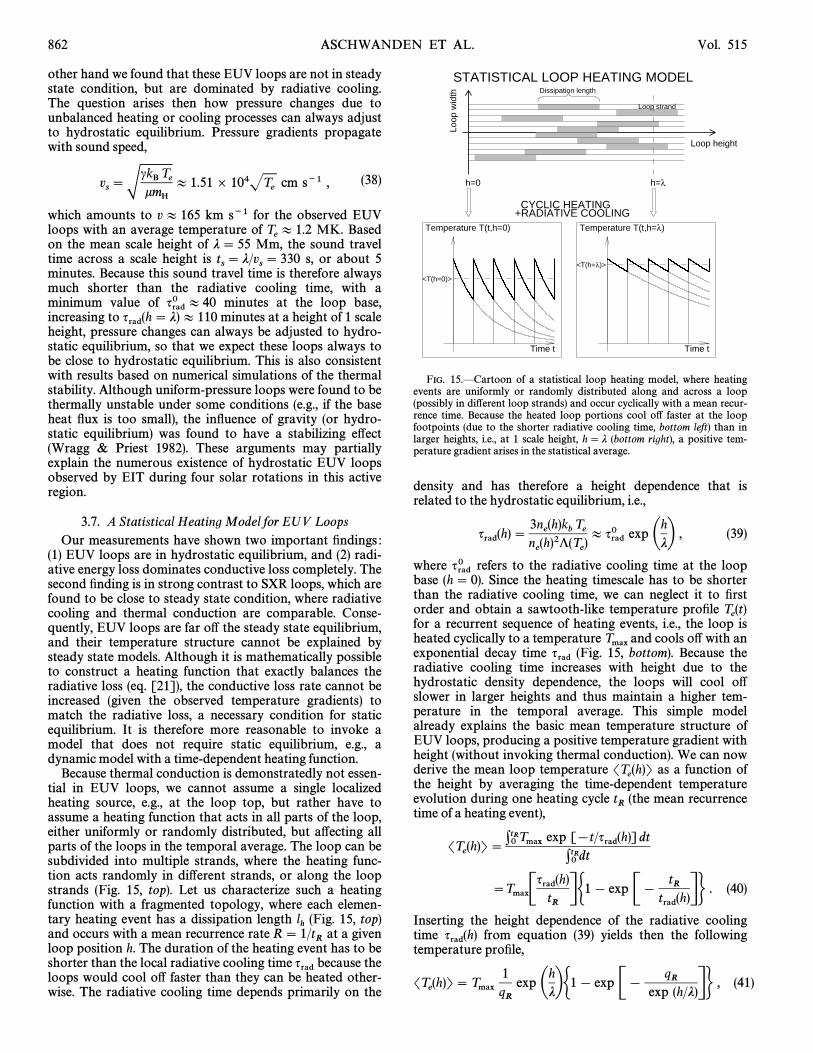
Loop

wid

th

Loop height

h=0 h=λ

Dissipation length

Loop strand

STATISTICAL LOOP HEATING MODEL

CYCLIC HEATING+RADIATIVE COOLING

Temperature T(t,h=0) Temperature T(t,h=λ)

<T(h=0)>

<T(h=λ)>

Time t Time t

862 ASCHWANDEN ET AL. Vol. 515

other hand we found that these EUV loops are not in steadystate condition, but are dominated by radiative cooling.The question arises then how pressure changes due tounbalanced heating or cooling processes can always adjustto hydrostatic equilibrium. Pressure gradients propagatewith sound speed,

vs\SckB T

ekmH

B 1.51 ] 104JTe

cm s~1 , (38)

which amounts to v B 165 km s~1 for the observed EUVloops with an average temperature of MK. BasedT

eB 1.2

on the mean scale height of j \ 55 Mm, the sound traveltime across a scale height is s, or about 5t

s\ j/v

s\ 330

minutes. Because this sound travel time is therefore alwaysmuch shorter than the radiative cooling time, with aminimum value of minutes at the loop base,qrad0 B 40increasing to minutes at a height of 1 scaleqrad(h \ j) B 110height, pressure changes can always be adjusted to hydro-static equilibrium, so that we expect these loops always tobe close to hydrostatic equilibrium. This is also consistentwith results based on numerical simulations of the thermalstability. Although uniform-pressure loops were found to bethermally unstable under some conditions (e.g., if the baseheat Ñux is too small), the inÑuence of gravity (or hydro-static equilibrium) was found to have a stabilizing e†ect(Wragg & Priest 1982). These arguments may partiallyexplain the numerous existence of hydrostatic EUV loopsobserved by EIT during four solar rotations in this activeregion.

3.7. A Statistical Heating Model for EUV L oopsOur measurements have shown two important Ðndings :

(1) EUV loops are in hydrostatic equilibrium, and (2) radi-ative energy loss dominates conductive loss completely. Thesecond Ðnding is in strong contrast to SXR loops, which arefound to be close to steady state condition, where radiativecooling and thermal conduction are comparable. Conse-quently, EUV loops are far o† the steady state equilibrium,and their temperature structure cannot be explained bysteady state models. Although it is mathematically possibleto construct a heating function that exactly balances theradiative loss (eq. [21]), the conductive loss rate cannot beincreased (given the observed temperature gradients) tomatch the radiative loss, a necessary condition for staticequilibrium. It is therefore more reasonable to invoke amodel that does not require static equilibrium, e.g., adynamic model with a time-dependent heating function.

Because thermal conduction is demonstratedly not essen-tial in EUV loops, we cannot assume a single localizedheating source, e.g., at the loop top, but rather have toassume a heating function that acts in all parts of the loop,either uniformly or randomly distributed, but a†ecting allparts of the loops in the temporal average. The loop can besubdivided into multiple strands, where the heating func-tion acts randomly in di†erent strands, or along the loopstrands (Fig. 15, top). Let us characterize such a heatingfunction with a fragmented topology, where each elemen-tary heating event has a dissipation length (Fig. 15, top)l

hand occurs with a mean recurrence rate at a givenR \ 1/tRloop position h. The duration of the heating event has to be

shorter than the local radiative cooling time because theqradloops would cool o† faster than they can be heated other-wise. The radiative cooling time depends primarily on the

FIG. 15.ÈCartoon of a statistical loop heating model, where heatingevents are uniformly or randomly distributed along and across a loop(possibly in di†erent loop strands) and occur cyclically with a mean recur-rence time. Because the heated loop portions cool o† faster at the loopfootpoints (due to the shorter radiative cooling time, bottom left) than inlarger heights, i.e., at 1 scale height, h \ j (bottom right), a positive tem-perature gradient arises in the statistical average.

density and has therefore a height dependence that isrelated to the hydrostatic equilibrium, i.e.,

qrad(h) \ 3ne(h)k

bTe

ne(h)2"(T

e)B qrad0 exp

AhjB

, (39)

where refers to the radiative cooling time at the loopqrad0base (h \ 0). Since the heating timescale has to be shorterthan the radiative cooling time, we can neglect it to Ðrstorder and obtain a sawtooth-like temperature proÐle T

e(t)

for a recurrent sequence of heating events, i.e., the loop isheated cyclically to a temperature and cools o† with anTmaxexponential decay time (Fig. 15, bottom). Because theqradradiative cooling time increases with height due to thehydrostatic density dependence, the loops will cool o†slower in larger heights and thus maintain a higher tem-perature in the temporal average. This simple modelalready explains the basic mean temperature structure ofEUV loops, producing a positive temperature gradient withheight (without invoking thermal conduction). We can nowderive the mean loop temperature as a function ofST

e(h)T

the height by averaging the time-dependent temperatureevolution during one heating cycle (the mean recurrencet

Rtime of a heating event),

STe(h)T \ /0tRTmax exp [[t/qrad(h)] dt

/0tRdt

\TmaxCqrad(h)

tR

DG1 [ exp

C[ t

Rtrad(h)

DH. (40)

Inserting the height dependence of the radiative coolingtime from equation (39) yields then the followingqrad(h)temperature proÐle,

STe(h)T \ Tmax

1qR

expAh

jBG

1 [ expC

[ qR

exp (h/j)DH

, (41)

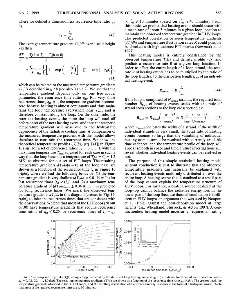
0 50 100 150 200Height h[Mm]

1.0

1.2

1.4

1.6

1.8

2.0

Tem

pera

ture

Te[

MK

]

h=λ

q R=1

.0 (I

nfre

quen

t hea

ting)

qR=0.0 (Frequent heating)

0.1 1.0 10.0 100.0Recurrence time ratio qR=tR/τrad

0

0.000

0.010

0.020

0.030

0.040

dT/d

h=[T

(λ)-

T(0

)]/λ

[K

/m]

Tem

pera

ture

gra

dien

t

0 10 20 30 40 50 60Recurrence time tR [min]

0

5

10

15

20

25

Num

ber

of lo

ops

No. 2, 1999 THREE-DIMENSIONAL ANALYSIS OF SOLAR ACTIVE REGIONS 863

where we deÐned a dimensionless recurrence time ratio qRby

qR

\ tR

qrad0 . (42)

The average temperature gradient dT /dh over a scale heightj is then

dTdh

BTe(h \ j) [ T

e(h \ 0)

j

\Tmaxj

1qR

GeC

1 [ expA

[ qReBD

[ [1 [ exp ([qR)]H

,

(43)

which can be related to the measured temperature gradientsdT /ds described in ° 2.8 (see also Table 2). We see that thetemperature gradient depends only on one free modelparameter, the recurrence time ratio For very shortq

R.

recurrence times, the temperature gradient becomesqR

> 1,zero because heating is almost continuous and thus main-tains the loop temperature everywhere near and isT maxtherefore constant along the loop. On the other side, therarer the heating events, the more the loop will cool o†before onset of the next heating event, and thus the steeper atemperature gradient will arise due to the hydrostaticdependence of the radiative cooling time. A comparison ofthe measured temperature gradient with this model allowstherefore to constrain the recurrence time. We show thetheoretical temperature proÐles (eq. [41]) in FigureST

e(h)T

16 (left), for a set of recurrence ratios . . . , 1, with theqR

\ 0,maximum temperature adjusted for each case in such aTmaxway that the loop base has a temperature of T

e(h \ 0) \ 1.2

MK, as observed for our set of EIT loops. The resultingtemperature gradients dT /dh(h \ 0) at the loop base areshown as a function of the recurrence time in Figure 16t

R(right), where we Ðnd the following behavior : (1) the tem-perature gradient is very shallow (dT /dh \ 0.01 K m~1) forfast recurrence times and (2) a maximum tem-(t

R\ trad0 ),

perature gradient of K m~1 is predicted(dT /dh)max [ 0.04for long recurrence times. We mark the observed tem-perature gradients dT /ds in this diagram (crosses in Fig. 16,right), to infer the recurrence times that are consistent withthe observations. We Ðnd that most of the EIT loops (20 outof 30) have temperature gradients that require recurrencetime ratios of or recurrence times ofq

R[ 0.25, t

R\ q

R

minutes (based on minutes). From] qrad0 [ 10 qrad0 B 40this model we predict that heating events should occur witha mean rate of about 5 minutes in a given loop location tomaintain the observed temperature gradient in EUV loops.The predicted correlation between temperature gradients(dT /dh) and temperature Ñuctuation rates R could possiblybe checked with high-cadence EIT movies (Newmark et al.1997).

This heating model is entirely constrained by theobserved temperature and density proÐle andT

e(s) n

e(s)

predicts a recurrence rate R at a given loop location. Inorder to a†ect the entire length of a loop strand, the totalrate R of heating events has to be multiplied by the ratio ofthe loop length L to the dissipation length of an individ-lheatual heating event,

Rstrand \ RL

lheat. (44)

If the loop is composed of strands, the required totalNstrandnumber of heating events scales with the ratio ofRloopstrand cross sections to the loop cross section, i.e.,

Rloop \ RstrandA w

wstrand

B2 \ RL

lheat

A wwstrand

B2, (45)

where indicates the width of a strand. If the width ofwstrandindividual strands is very small, the total rate of heatingevents becomes so large that the variability of individualheating events cannot be resolved with currently availabletime cadences, and the temperature proÐle of the loop willappear smooth in space and time. Future investigations willreveal whether individual heating events can be resolved ornot.

The purpose of this simple statistical heating modelwithout conduction is just to illustrate that the observedtemperature gradients can naturally be explained withrecurrent heating events uniformly distributed all over theentire loop. A heating source that is conÐned to a small partof the loop cannot explain the temperature structure ofEUV loops. For instance, a heating source localized at theloop-top cannot balance the radiative energy loss in thelower part of the loop (because thermal conduction is ineffi-cient in EUV loops), an argument that was used by Neupertet al. (1998) against the heat-deposition model at largeheights (e.g., Wheatland, Sturrock, & Acton 1997). A con-ductionless heating model necessarily requires a heating

FIG. 16.ÈTemperature proÐles along a loop predicted by the statistical loop heating model (Fig. 15) are shown for di†erent recurrence time ratiosTe(h)

0.1, 0.2, . . . , 1.0 (left). The resulting temperature gradients dT /dh are shown as a function of the recurrence time ratio (right). The crosses mark theqR

\ 0, qRtemperature gradients observed in the 30 EIT loops, and the resulting distribution of recurrence times is shown in the form of a histogram (insert). Notet

Rthat most of the required recurrence times are minutes.[10

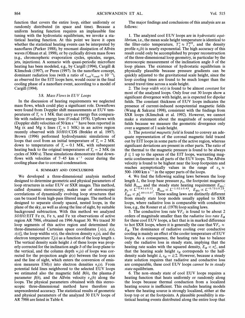
864 ASCHWANDEN ET AL. Vol. 515

function that covers the entire loop, either uniformly orrandomly distributed (in space and time). Because auniform heating function requires an implausible Ðnetuning with the hydrostatic equilibrium, we invoke a sta-tistical heating function. At this point we leave it openwhether the statistical heating events can be interpreted bynanoÑares (Parker 1988), by resonant dissipation of Alfve� nwaves (Ofman et al. 1998), or by cyclically driven mass Ñows(e.g., chromospheric evaporation cycles, spicules, surges,jets, injections). A scenario with quasi-periodic microÑareheating has been modeled, e.g., by Cargill (1994), Cargill &Klimchuk (1997), or Peres (1997). In the nanoÑare concept,dominant radiation loss (with a ratio of qrad/qcond B 10~2),as observed for the EIT loops here, would occur in the Ðnalcooling phase of a nanoÑare event, according to a model ofCargill (1994).

3.8. Mass Flows in EUV L oopsIn the discussion of heating requirements we neglected

mass Ñows, which could play a signiÐcant role. DownÑowswere found from Doppler shift measurements at EUV tem-peratures of MK that carry an energy Ñux compara-T

eB 1

ble with radiative energy loss (Foukal 1978). UpÑows with(Doppler shift) velocities of 50 km s~1 have been reported inMg IX and Mg X lines MK) in an active region(T

eB 1

recently observed with SOHO/CDS (Brekke et al. 1997).Brown (1996) performed hydrodynamic simulations ofloops that cool from an initial temperature of MKT

e\ 2

down to temperatures of MK, with subsequentTe\ 0.1

heating back to the original temperatures of MK (inTe\ 2

cycles of 3000 s). These simulations demonstrate that down-Ñows with velocities of 7È45 km s~1 occur during thecooling phase due to coronal condensation.

4. SUMMARY AND CONCLUSIONS

We developed a three-dimensional analysis methoddesigned to determine geometric and physical parameters ofloop structures in solar EUV or SXR images. This method,called dynamic stereoscopy, makes use of stereoscopiccorrelations of dynamically evolving loop structures thatcan be traced from high-pass Ðltered images. The method isdesigned to separate closely spaced, nested loops, in theplane of the sky, as well as along the line of sight, by suitablebackground subtraction. With this method we analyzedSOHO/EIT Fe IX, Fe X, and Fe XII observations of activeregion AR 7986, obtained on 1996 August 30. We traced 30loop segments of this active region and determined thethree-dimensional Cartesian space coordinates [x(s), y(s),z(s)], the loop widths w(s), the electron density and then

e(s),

electron temperature as a function of the loop length s.Te(s)

The vertical density scale height j of these loops was prop-erly corrected for the inclination angle Ë of the loop plane tothe vertical, and the column depth of loops was cor-w

z(s)

rected for the projection angle t(s) between the loop axisand the line of sight, which enters the conversion of emis-sion measures EM(s) into electron densities Fromn

e(s).

potential Ðeld lines neighbored to the selected EUV loopswe estimated also the magnetic Ðeld B(h), the plasma-bparameter b(h), and the velocity along theAlfve� n vA(h)loops. The physical parameters obtained with this stereo-scopic three-dimensional method have therefore anunprecedented accuracy. The statistical results of geometricand physical parameters of the analyzed 30 EUV loops ofAR 7986 are listed in Table 4.

The major Ðndings and conclusions of this analysis are asfollows :

1. The analyzed cool EUV loops are in hydrostatic equi-librium, i.e., the mean scale height temperature is identical tothe Ðlter-ratio temperature, and the densityT

ej B T

eEIT,

proÐle is nearly exponential. The high accuracy of thisne(h)

result could only be accomplished by proper reconstructionof the three-dimensional loop geometry, in particular by thestereoscopic measurement of the inclination angle Ë of theloop planes. The existence of hydrostatic equilibrium isphysically plausible because pressure gradients can bequickly adjusted to the gravitational scale height, since theloop cooling times are found to be much longer than thesound travel time across a scale height.

2. The loop width w(s) is found to be almost constant formost of the analyzed loops. Only four out 30 loops show asigniÐcant divergence with height, as is expected for dipolarÐelds. The constant thickness of EUV loops indicates thepresence of current-induced nonpotential magnetic Ðelds(Wang & Sakurai 1998), consistent with the Ðndings fromSXR loops (Klimchuk et al. 1992). However, we cannotmake a statement about the magnitude of nonpotentialÐelds because we measure the geometric divergence onlyover a segment of 1 scale height.

3. The potential magnetic Ðeld is found to convey an ade-quate representation of the coronal magnetic Ðeld tracedout by EIT loops in some parts of the active region, whereassigniÐcant deviations are present in other parts. The ratio ofthe thermal to the magnetic pressure is found to be always

up to the apexes of the EIT loops, warranting mag-b [ 1netic conÐnement in all parts of the EUV loops. The Alfve� nvelocity is found to be highest near the loop footpoints andreaches asymptotically values in the range of vA B500È1000 km s~1 in the upper parts of the loops.

4. We Ðnd the following scaling laws between the looplength L , the loop base pressure the footpoint magneticp0,Ðeld and the steady state heating requirementBfoot, E

H0 :p0 P L~0.41B0.12, Bfoot P L~1.02B0.43, E

H0 P L~0.73B0.23,These scaling laws are distinctly di†erentE

H0 P p01.89B0.07.from steady state loop models usually applied to SXRloops, where radiative loss is comparable with conductiveloss, e.g., the Rosner et al. (1978) loop scaling laws.

5. The conductive loss rate is found to be about 2+FCorders of magnitude smaller than the radiative loss rate E

Rfor these cool EUV loops, a fact that is in marked di†erenceto hot SXR loops, where it is generally the case that +F

CB

The dominance of radiative cooling over conductiveER.

cooling is mainly an e†ect of the cooler temperature of EUVloops. As a consequence, the heating rate has to balanceonly the radiative loss in steady state, implying that theheating rate scales with the squared density, andE

HP n

e2,

that the heating scale height corresponds to the half-sHdensity scale height j, However, because a steadys

H\ j/2.

state solution requires that radiative and conductive lossare comparable, these cool EUV loops cannot be in steadystate equilibrium.

6. The nonÈsteady state of cool EUV loops requires aheating function that heats uniformly or randomly alongthe loops because thermal conduction from a localizedheating source is inefficient. This excludes heating modelswhere the heating source is strongly localized, either at theloop top or at the footpoints. A plausible possibility is sta-tistical heating events distributed along the entire loop that

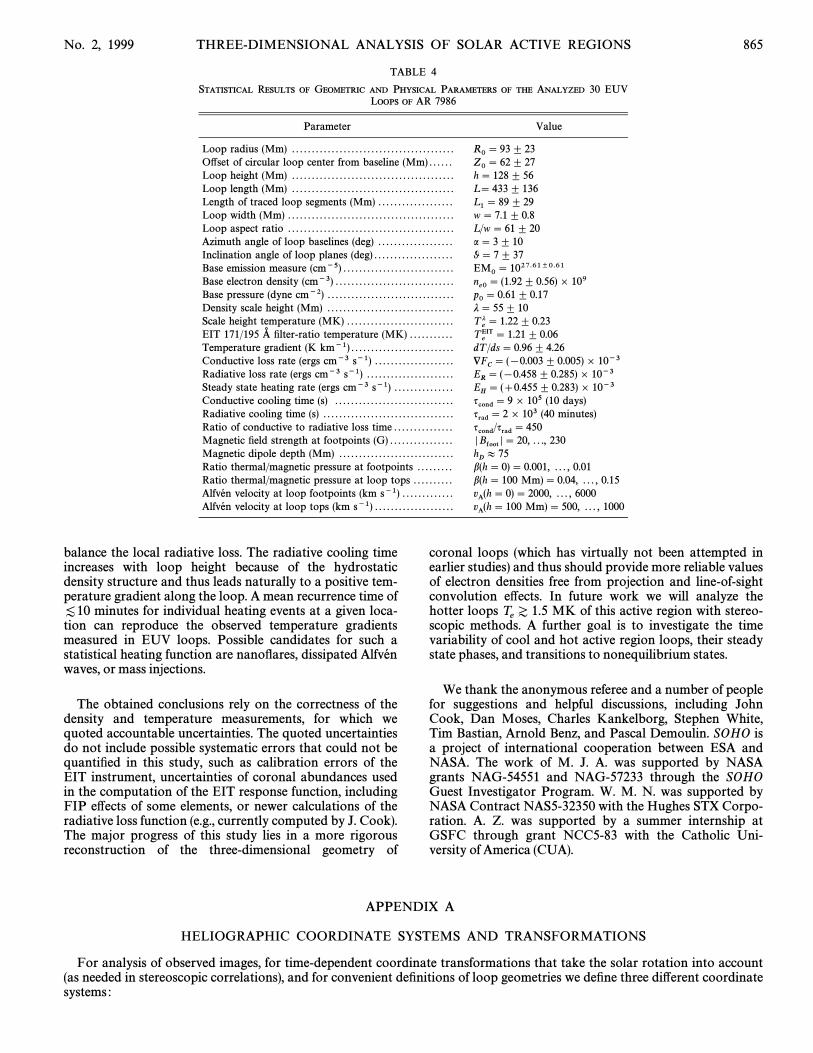
No. 2, 1999 THREE-DIMENSIONAL ANALYSIS OF SOLAR ACTIVE REGIONS 865

TABLE 4

STATISTICAL RESULTS OF GEOMETRIC AND PHYSICAL PARAMETERS OF THE ANALYZED 30 EUVLOOPS OF AR 7986

Parameter Value

Loop radius (Mm) . . . . . . . . . . . . . . . . . . . . . . . . . . . . . . . . . . . . . . . . . R0 \ 93 ^ 23O†set of circular loop center from baseline (Mm) . . . . . . Z0 \ 62 ^ 27Loop height (Mm) . . . . . . . . . . . . . . . . . . . . . . . . . . . . . . . . . . . . . . . . . h \ 128 ^ 56Loop length (Mm) . . . . . . . . . . . . . . . . . . . . . . . . . . . . . . . . . . . . . . . . . L \ 433 ^ 136Length of traced loop segments (Mm) . . . . . . . . . . . . . . . . . . . L 1 \ 89 ^ 29Loop width (Mm) . . . . . . . . . . . . . . . . . . . . . . . . . . . . . . . . . . . . . . . . . . w \ 7.1 ^ 0.8Loop aspect ratio . . . . . . . . . . . . . . . . . . . . . . . . . . . . . . . . . . . . . . . . . . L /w \ 61 ^ 20Azimuth angle of loop baselines (deg) . . . . . . . . . . . . . . . . . . . a \ 3 ^ 10Inclination angle of loop planes (deg) . . . . . . . . . . . . . . . . . . . . Ë \ 7 ^ 37Base emission measure (cm~5) . . . . . . . . . . . . . . . . . . . . . . . . . . . . EM0 \ 1027.61B0.61Base electron density (cm~3) . . . . . . . . . . . . . . . . . . . . . . . . . . . . . . n

e0 \ (1.92 ^ 0.56) ] 109Base pressure (dyne cm~2) . . . . . . . . . . . . . . . . . . . . . . . . . . . . . . . . p0 \ 0.61 ^ 0.17Density scale height (Mm) . . . . . . . . . . . . . . . . . . . . . . . . . . . . . . . . j \ 55 ^ 10Scale height temperature (MK) . . . . . . . . . . . . . . . . . . . . . . . . . . . T

ej \ 1.22 ^ 0.23

EIT 171/195 A� Ðlter-ratio temperature (MK) . . . . . . . . . . . TeEIT \ 1.21 ^ 0.06

Temperature gradient (K km~1) . . . . . . . . . . . . . . . . . . . . . . . . . . dT /ds \ 0.96 ^ 4.26Conductive loss rate (ergs cm~3 s~1) . . . . . . . . . . . . . . . . . . . . +F

C\ ([0.003 ^ 0.005) ] 10~3

Radiative loss rate (ergs cm~3 s~1) . . . . . . . . . . . . . . . . . . . . . . ER

\ ([0.458 ^ 0.285) ] 10~3Steady state heating rate (ergs cm~3 s~1) . . . . . . . . . . . . . . . E

H\ (]0.455 ^ 0.283) ] 10~3

Conductive cooling time (s) . . . . . . . . . . . . . . . . . . . . . . . . . . . . . . qcond \ 9 ] 105 (10 days)Radiative cooling time (s) . . . . . . . . . . . . . . . . . . . . . . . . . . . . . . . . . qrad \ 2 ] 103 (40 minutes)Ratio of conductive to radiative loss time . . . . . . . . . . . . . . . qcond/qrad \ 450Magnetic Ðeld strength at footpoints (G) . . . . . . . . . . . . . . . . o Bfoot o \ 20, . . ., 230Magnetic dipole depth (Mm) . . . . . . . . . . . . . . . . . . . . . . . . . . . . . h

DB 75

Ratio thermal/magnetic pressure at footpoints . . . . . . . . . b(h \ 0) \ 0.001, . . . , 0.01Ratio thermal/magnetic pressure at loop tops . . . . . . . . . . b(h \ 100 Mm) \ 0.04, . . . , 0.15Alfve� n velocity at loop footpoints (km s~1) . . . . . . . . . . . . . vA(h \ 0) \ 2000, . . . , 6000Alfve� n velocity at loop tops (km s~1) . . . . . . . . . . . . . . . . . . . . vA(h \ 100 Mm) \ 500, . . . , 1000

balance the local radiative loss. The radiative cooling timeincreases with loop height because of the hydrostaticdensity structure and thus leads naturally to a positive tem-perature gradient along the loop. A mean recurrence time of

minutes for individual heating events at a given loca-[10tion can reproduce the observed temperature gradientsmeasured in EUV loops. Possible candidates for such astatistical heating function are nanoÑares, dissipated Alfve� nwaves, or mass injections.

The obtained conclusions rely on the correctness of thedensity and temperature measurements, for which wequoted accountable uncertainties. The quoted uncertaintiesdo not include possible systematic errors that could not bequantiÐed in this study, such as calibration errors of theEIT instrument, uncertainties of coronal abundances usedin the computation of the EIT response function, includingFIP e†ects of some elements, or newer calculations of theradiative loss function (e.g., currently computed by J. Cook).The major progress of this study lies in a more rigorousreconstruction of the three-dimensional geometry of

coronal loops (which has virtually not been attempted inearlier studies) and thus should provide more reliable valuesof electron densities free from projection and line-of-sightconvolution e†ects. In future work we will analyze thehotter loops MK of this active region with stereo-T

eZ 1.5

scopic methods. A further goal is to investigate the timevariability of cool and hot active region loops, their steadystate phases, and transitions to nonequilibrium states.

We thank the anonymous referee and a number of peoplefor suggestions and helpful discussions, including JohnCook, Dan Moses, Charles Kankelborg, Stephen White,Tim Bastian, Arnold Benz, and Pascal Demoulin. SOHO isa project of international cooperation between ESA andNASA. The work of M. J. A. was supported by NASAgrants NAG-54551 and NAG-57233 through the SOHOGuest Investigator Program. W. M. N. was supported byNASA Contract NAS5-32350 with the Hughes STX Corpo-ration. A. Z. was supported by a summer internship atGSFC through grant NCC5-83 with the Catholic Uni-versity of America (CUA).

APPENDIX A

HELIOGRAPHIC COORDINATE SYSTEMS AND TRANSFORMATIONS

For analysis of observed images, for time-dependent coordinate transformations that take the solar rotation into account(as needed in stereoscopic correlations), and for convenient deÐnitions of loop geometries we deÐne three di†erent coordinatesystems :

866 ASCHWANDEN ET AL. Vol. 515

Image coordinate system (x, y, z).ÈThe (x, y) coordinates refer to the x-axis and y-axis of an observed image, whereas thecoordinate (z) is orthogonal to the image, or parallel to the line-of-sight direction, deÐned positive toward the observer. Theorigin (x, y, z) \ (0, 0, 0) of this coordinate system is most conveniently assumed at the Sun center position. A solar FITSimage should contain the position of the Sun center in pixel units (in FITS header CRPIX1, CRPIX2 or E–XCEN,(i

x0, jy0)

E–Y CEN), the pixel size (*x, *y) in units or arcseconds (in FITS header CDEL T 1, CDEL T 2), and the solar radius in pixelir0units (in FITS header SOL AR–R, or E–XSMD, E–Y SMD if the semidiameters of an ellipse are Ðtted). With this information,

a pixel position (i, j) can then be converted into the coordinate system (x, y) by

xi\ *x(i [ i

x0) , (A1)

yi\ *y( j [ j

y0) , (A2)

where *x \ arcseconds pixel~1 for (x, y) in units of arcseconds, or with km, if physical length*x \ R_

/ir0, R

_\ 696,000

units (km) are preferred.Heliographic coordinate system (l, b, r).ÈThe heliographic coordinate system is corotating with the solar surface. A position

on the solar surface is generally speciÐed by heliographic longitude and latitude coordinates (l, b) (in units of heliographicdegrees), with reference to the Carrington rotation grid. The heliographic longitude and latitude of the Sun center[l0(t), b0(t)]and the position angle P(t) of the solar rotation axis for a given time t are published in The Astronomical Almanac (NauticalAlmanac Office, NRL, Washington DC). The two-dimensional spherical coordinate system (l, b) can be generalized into athree-dimensional coordinate system by incorporating the height h above the solar surface, which can be expressed as adimensionless distance to the Sun center (in units of solar radii),

r \A

1 ] hR

_

B. (A3)

The transformation from the three-dimensional heliographic coordinate system (l, b, r) into image coordinates (x, y, z) can beaccomplished by applying a series of four rotations to the (normalized) vector (0, 0, r) (see also Loughhead, Wang, & Blows1983),

(t:tt

x/R_

y/R_

z/R_

)t;tt\

(t:tt

cos (P ] P0) [sin (P ] P0) 0sin (P ] P0) cos (P ] P0) 0

0 0 1

)t;tt(t:

1 0 00 cos b0 [sin b00 sin b0 cos b0

)t;tt

(t:cos (l0 [ l) 0 [sin (l0 [ l)

0 1 0sin (l0 [ l) 0 cos (l0 [ l)

)t;tt(t:

1 0 00 cos[b [sin[b0 sin[b cos[b

)t;tt(t:

00r

)t;tt , (A4)

where are the heliographic longitude and latitude of the Sun center, P is the position angle of the solar rotation axis(l0, b0)with respect to the north-south direction (deÐned positive toward east), and is the image rotation (roll) angle with respectP0to the north-south direction for images rotated to solar north). In stereoscopic correlations, only the longitude of(P ] P0 \ 0the Sun center, is time-dependent in Ðrst order (according to the solar rotation rate), whereas and P(t) are slowlyl0(t), b0(t)varying and thus almost constant for short time intervals.

L oop plane coordinate system (X, Y , Z).ÈTo parametrize coronal loops it is also convenient to introduce a Cartesiansystem that is aligned with the loop footpoint baseline (X-axis) and coincides with the loop plane (X-Z plane, Y \ 0). Forinstance, a circular loop model deÐned in the X-Z plane is speciÐed in equations (10)È(11). The transformation of loopcoordinates (X, Y \ 0, Z) into Cartesian coordinate system (X@, Y @, Z@) that is aligned with the heliographic coordinate system(l, b, r) can simply be accomplished with help of two rotations,

(t:tt

X@Y @Z@

)t;tt\

(t:tt

cos a [sin a 0sin a cos a 0

0 0 1

)t;tt(t:

1 0 00 cos Ë sin Ë0 [sin Ë cos Ë

)t;tt(t:

XYZ

)t;tt , (A5)

where the azimuth angle a denotes the angle between the loop footpoint baseline and the east-west direction and Ë representsthe inclination or tilt angle between the loop plane and the vertical to the solar surface (Fig. 2). Placing the origin of the loopcoordinate system [X \ 0, Y \ 0, Z \ 0] (which is also the origin of the rotated coordinate system [X@ \ 0, Y @ \ 0, Z@ \ 0]at heliographic position at an altitude above the solar surface, the transformation into heliographic coordinates is(l1, b1) hFootthen given by

(t:tt

lbr

)t;tt\

(t:tt

l1 ] arctan [X@/(Z@ ] hfoot ] R_

)]b1 ] arctan [Y @/(Z@ ] hfoot ] R

_)]

J[X@2 ] Y @2 ] (Z@ ] hfoot ] R_

)2]/R_

)t;tt . (A6)

No. 2, 1999 THREE-DIMENSIONAL ANALYSIS OF SOLAR ACTIVE REGIONS 867

APPENDIX B

LINE-OF-SIGHT CORRECTION ON LOOP COLUMN DEPTH

Column depth of loops with constant cross section.ÈIn order to convert observed emission measures EM(x, y) \y, z) dz into local electron densities y, z) we need information on the column depth / dz. An approximation that is/ n

e2(x, n

e(x,

often useful is coronal loops with a constant cross section w, which can be measured from the FWHM as it appearsperpendicular to the line of sight in the plane of the sky. For three-dimensional models of loops parametrized by coordinates

the angle t between the line of sight and a loop segment can then directly be derived by the ratio of the projected to(xi, y

i, z

i),

the e†ective length of a loop segment [i, i ] 1].

cos (t[xi, y

i, z

i]) \ J(x

i`1 [ xi)2 ] (y

i`1 [ yi)2

J(xi`1 [ x

i)2 ] (y

i`1 [ yi)2 ] (z

i`1 [ zi)2

(B1)

yielding the column depth along the line-of-sight axis z,wz

wz[x

i, y

i, z

i] \ w

cos (t[xi, y

i, z

i])

. (B2)

REFERENCESAlexander, D., & Katsev, S. 1996, Sol. Phys., 167, 153Allen, C. W. 1973, Astrophysical Quantities (London: Athlone)Aschwanden, M. J. 1995, Lect. Notes Phys., 444, 13Aschwanden, M. J., & Bastian, T. S. 1994a, ApJ, 426, 425ÈÈÈ. 1994b, ApJ, 426, 434Aschwanden, M. J., Bastian, T. S., Nitta, N., Newmark, J., Thompson, B. J.,

& Harrison, R. A. 1998a, in ASP Conf. Ser. 155, Second Advances inSolar Physics Euroconference : Three-Dimensional Structure of SolarActive Regions, ed. C. Alissandrakis & B. Schmieder (San Francisco :ASP), 311

Aschwanden, M. J., Lim, J., Gary, D. E., & Klimchuk, J. A. 1995, ApJ, 454,412

Aschwanden, M. J., et al. 1998b, in ASP Conf. Ser. 155, Second Advancesin Solar Physics Euroconference : Three-Dimensional Structure of SolarActive Regions, ed. C. Alissandrakis & B. Schmieder (San Francisco :ASP), 145

Berton, R., & Sakurai, T. 1985, Sol. Phys., 96, 93Bray, R. J., Cram, L. E., Durrant, C. J., & Loughhead, R. E. 1991, Plasma

Loops in the Solar Corona (Cambridge : Cambridge Univ. Press)Brekke, P., Kjeldseth-Moe, O., Brynildsen, N., Maltby, P., Haugan,

S. V. H., Harrison, R. A., Thompson, W. T., & Pike, C. D. 1997, Sol.Phys., 170, 163

Brosius, J. W., Davila, J. M., Thomas, R. J., Saba, J. L. R., Hara, H., &Monsignori-Fossi, B. C. 1997, ApJ, 477, 969

Brosius, J. W., Willson, R. F., Holman, G. D., & Schmelz, J. T. 1992, ApJ,386, 347

Brown, S. F. 1996, A&A, 305, 649Cargill, P. J. 1994, ApJ, 422, 381Cargill, P. J., & Klimchuk, J. A. 1997, ApJ, 478, 799Cheng, C. C. 1980, ApJ, 238, 743Davila, J. M. 1994, ApJ, 423, 871

J. P., et al. 1995, Sol. Phys., 162, 291Delaboudiniere,Dere, K. P. 1982, Sol. Phys., 75, 189Dere, K. P., Landi, E., Mason, H. E., Monsignori-Fossi, B. F., & Young,

P. R. 1997, A&AS, 125, 149Dulk, G. A., & McLean, D. J. 1978, Sol. Phys., 57, 279Fludra, A., Brekke, P., Harrison, R. A., Mason, H. E., Pike, C. D., Thomp-

son, W. T., & Young, P. R. 1997, Sol. Phys., 175, 487Foukal, P. 1975, Sol. Phys., 43, 327ÈÈÈ. 1978, ApJ, 223, 1046Galeev, A. A., Rosner, R., Serio, S., & Vaiana, G. S. 1981, ApJ, 243, 301Gary, G. A. 1990, Mem. Soc. Astron. Italiana, 61, 457ÈÈÈ. 1997, Sol. Phys., 174, 241Gary, G. A., & Alexander, D. 1999, Sol. Phys., in pressGolub, L., Herant, M., Kalata, K., Lovas, I., Nystrom, G., Pardo, F.,

Spiller, E., & Wilczynski, J. 1990, Nature, 344, 842Golub, L., Maxson, C., Rosner, R., Serio, S., & Vaiana, G. S. 1980, ApJ,

238, 343Habbal, S. R., Ronan, R., & Withbroe, G. L. 1985, Sol. Phys., 98, 323Harvey, K. L., & Hudson, H. S. 1998, in Proc. Y ohkoh Workshop, Obser-

vational Plasma Astrophysics : Five Years of Y ohkoh and Beyond, ed. T.Watanabe, T. Kosugi, & A. C. Sterling (Astrophys. and Space ScienceLibrary ; Dordrecht : Kluwer), 229, 315

Hudson, H. S., LaBonte, B. J., Sterling, A. C., & Watanabe, T. 1998, inProc. Y ohkoh Workshop, Observational Plasma Astrophysics : FiveYears of Y ohkoh and Beyond, ed. T. Watanabe, T. Kosugi, & A. C.Sterling (Astrophys. and Space Science Library ; Dordrecht : Kluwer),229, 237

Kankelborg, C. C., Walker, A. B. C., II, & Hoover, R. B. 1997, ApJ, 491,952

Kano, R., & Tsuneta, S. 1995, ApJ, 454, 934ÈÈÈ. 1996, Publ. Astron. Soc. Japan, 48, 535Klimchuk, J. A., & Gary, D. E. 1995, ApJ, 448, 925Klimchuk, J. A., Lemen, J. R., Feldman, U., Tsuneta, S., & Uchida, Y. 1992,

PASJ, 44, L181Klimchuk, J. A., & Porter, L. J. 1995, Nature, 377, 131Lang, K. R. 1980, Astrophysical Formulae (Berlin : Springer)Loughhead, R. E., Chen, C. L., & Wang, J. L. 1984, Sol. Phys., 92, 53Loughhead, R. E., Wang, J. L., & Blows, G. 1983, ApJ, 274, 883Mandrini, C. H., Demoulin, P., & Klimchuk, J. A. 1999, ApJ, submittedMartens, P. C. H., & Kuin, N. P. M. 1982, A&A, 112, 366McClymont, A. N., Jiao, L., & Z. 1997, Sol. Phys., 174, 191Mikic� ,Meyer, J. P. 1985, APJS, 57, 173Moses, D., et al. 1997, Sol. Phys., 175, 571Neupert, W. M., et al. 1998, Sol. Phys., 183, 305Newmark, J. S., J. P., Dere, K. P., Gurman, J. B., Lemen,Delaboudiniere,

J. R., & Thompson, B. J. 1996, EOS, Vol. 77, 46, 557Newmark, J. S., Thompson, B., Gurman, J. B., J. P., Asch-Delaboudiniere,

wanden, M. J., & Mason, H. 1997, BAAS, 29/5, 1321, 73.07Nitta, N., et al. 1991, ApJ, 374, 374Ofman, L., Klimchuk, J. A., & Davila, J. M. 1998, ApJ, 493, 474Pallavicini, R., Serio, S., & Vaiana, G. S. 1977, ApJ, 216, 108Parker, E. N. 1988, ApJ, 330, 474Peres, G. 1997, in Proc. 5th SOHO Workshop on The Corona and Solar

Wind Near Minimum Activity (Nordwiijk : ESA SP-404), 55Porter, L. J., & Klimchuk, J. A. 1995, ApJ, 454, 499Priest, E. R. 1981, Solar Flare Magnetohydrodynamics (New York :

Gordon & Breach)Priest, E. R., Foley, C. R., Heyvaerts, J., Arber, T. D., Culhane, J. L., &

Acton, L. W. 1998, Nature, 393, 545Raymond, J. C., Cox, D. P., & Smith, B. W. 1976, ApJ, 204, 290Rosner, R., Tucker, W. H., & Vaiana, G. S. 1978, ApJ, 220, 643Sakurai, T. 1982, Sol. Phys., 76, 301ÈÈÈ. 1989, Space Sci. Rev., 51, 11Schmelz, J. T., Holman, G. D, Brosius, J. W., & Gonzalez, R. D. 1992, ApJ,

399, 733Schmelz, J. T., Holman, G. D., Brosius, J. W., & Willson, R. F. 1994, ApJ,

434, 786Serio, S., Peres, G., Vaiana, G. S., Golub, L., & Rosner, R. 1981, ApJ, 243,

288Sheeley, N. 1980, Sol. Phys., 66, 79SOHO EIT UserÏs Guide. 1998, http ://umbra.nascom.nasa.gov/eit/

eit–guide/guide.htmlSpitzer, L. 1962, Physics of Fully Ionized Gases (New York : Interscience)Vesecky, J. F., Antiochos, S. K., & Underwood, J. H. 1979, ApJ, 233, 987Vourlidas, A., & Bastian, T. S. 1996, ApJ, 466, 1039Wang, H., & Sakurai, T. 1998, PASJ, 50, 111Wang, Y. M., et al. 1997, ApJ, 485, 419Webb, D. F., Holman, G. D., Davis, J. M., Kundu, M. R., & Shevgaonkar,

R. K. 1987, ApJ, 315, 716Wheatland, M. S., Sturrock, P. A., & Acton, L. W. 1997, ApJ, 482, 510Wragg, M. A., & Priest, E. R. 1982, A&A, 113, 269Zhang, J., White, S. M., & Kundu, M. R. 1998, ApJ, 504, L127