Threats to agriculture at the extensive and

intensive margins

Economic analyses of selected land-use issues in the U.S. West and British Columbia

Alison J. Eagle

Thesis committee

Thesis supervisor: Prof. dr. ir. A.J. Oskam Professor of Agricultural Economics and Rural Policy, Wageningen University Thesis Co-supervisor: Prof. dr. G.C. van Kooten Professor and Canada Research Chair, Department of Economics, University of Victoria, Canada and Associate Professor, Agricultural Economics and Rural Policy Group, Wageningen University Other members: Prof. dr. ir. R. Brouwer, VU University Amsterdam Prof. dr. E.C. van Ierland, Wageningen University Prof. dr. P. Nijkamp, VU University Amsterdam Dr. ir. J.J. Stoorvogel, Wageningen University This research has been conducted under the auspices of the Mansholt Graduate School of Social Sciences

Threats to agriculture at the extensive and

intensive margins

Economic analyses of selected land-use issues in the U.S. West and British Columbia

Alison J. Eagle

Thesis

submitted in partial fulfillment of the requirements for the degree of doctor at Wageningen University

by the authority of the Rector Magnificus Prof. dr. M.J. Kropff, in the presence of the

Thesis Committee appointed by the Doctorate Board to be defended in public

on Monday 29 June 2009 at 11 AM in the Aula.

Alison J. Eagle Threats to agriculture at the extensive and intensive margins – Economic analyses of selected land-use issues in the U.S. West and British Columbia, 165 pages. Ph.D. Thesis, Wageningen University, Wageningen, NL (2009) With references, with summaries in English and Dutch ISBN: 978-90-8585-394-7

i

Abstract Agricultural land uses are frequently challenged by competing land demands for urban uses and for nature. Decisions made by private operators at the natural (extensive) and urban (intensive) margins of land use may not be socially desirable due to the externalities and public goods associated with agricultural land use and production. The objective of this research is to inform and determine the economic implications of land use policies and decisions in two agricultural systems – (1) rangeland of the arid U.S. west, and (2) the urban fringe of British Columbia, Canada – where competition for land use and associated spillovers threaten long-term agricultural sustainability. This research uses econometric methods and Geographic Information Systems (GIS) to accomplish this goal.

At the extensive margin, we address an issue where wildlife conservation interests challenge agricultural range uses in Nevada and another where invasive weeds reduce grazing productivity in California. We investigate the factors influencing the decline of greater sage grouse (Centrocercus urophasianus) populations and, using regression analysis, find that annual weather variations are dominant. Still there is some evidence that cattle grazing negatively affects sage grouse populations. We assess agricultural losses and damages due to yellow starthistle (Centaurea solstitialis L.) by using a survey administered to ranchers. Data collected included infestation rates, loss of forage quality and control efforts. Total state-wide losses of livestock forage value are calculated at 6-7% of the annual harvested pasture value.

Further, at the intensive margin, this research explores the economic implications of the Agricultural Land Reserve (ALR) in southwestern British Columbia. GIS technology is used to assemble spatial data of farmland near the city of Victoria. Hedonic models determine spatial, farm type and ALR protection impacts on farmland prices from 1974 through 2008, incorporating a total of 2211 parcel sales into the analysis. We find that ALR zoning reduced protected land prices over time, even though prices were impacted more by urban than agricultural production factors. Next, we analyze ALR exclusion applications from 1974 through 2006 using a logit regression model of re-zoning decisions, and find that, although approvals became more likely over time, agricultural capability is a key determinant in exclusion decisions. Finally, we explore the impact of niche- and direct-marketing on farm economic sustainability. Among farms surveyed, the majority (>80%) of farm area was devoted to vegetable and berry production, and more than 50% of total sales took place on-farm. Production intensity (gross revenue per unit of land) is positively related to recent farm investments, crop diversity, and greenhouse or nursery operations; and negatively related to university education, female operators, farm area and agri-tourism. Results suggest that direct marketing could improve long-term agricultural sustainability in this region.

Key Words Agriculture-environment interactions, economic modelling, sage grouse, yellow starthistle, urban-rural fringe, Geographic Information Systems (GIS), farmland conservation, direct marketing

ii

Preface and Acknowledgments Although I moved to Victoria, British Columbia as a soil scientist, seven years – and much research – later, I am now able to (somewhat tentatively still) assume the title of “agricultural economist”. This academic and career transformation began when my search for research work led me to Kees van Kooten at the University of Victoria, who was seeking someone to manage research accounts and perform administrative duties, one day per week. I agreed to the task while continuing to seek long-term employment that fit with my training. However, this very part-time position soon morphed into full-time research, as I was drawn into data collection, literature reviews, data analysis and modeling in various research projects addressing forest and agricultural economics. Because of my interests in agricultural sustainability, I was soon able to direct my attention to research projects that focused on farm interactions with the environment and society, the basis for this PhD dissertation.

I owe much thanks to administrators, research assistants and other graduate students in our research group for their encouragement and collaboration during this process. These include Tom Hobby, Kurt Niquidet, Lili Sun, Geerte Cotteleer, Rachel Jantzen, Karen Crawford, Linda Voss, Robin Tunnicliffe and Tracy Stobbe. Tracy Stobbe deserves special mention as office-mate, sounding board and close friend during our most recent projects. I count it a special privilege to share friendship with such a colleague. There are numerous others in the Department of Economics at UVic with whom I shared many enjoyable coffee times, welcome breaks during days of sitting in front of a computer. Thanks also to Mark Eiswerth at the University of Wisconsin, who readily accepted me as a colleague in the work on sage grouse and yellow starthistle.

In the course of the research related to British Columbia agriculture, two contacts deserve special mention for their efforts in connecting me with the local agricultural community and the provincial government Ministry of Agriculture and Lands. Robert Maxwell welcomed me to meet with and explore research options with members of the Peninsula Agricultural Commission, and subsequently introduced me to Robin Tunnicliffe, a local farmer and student who played a key role in the survey of direct-marketing farmers. Rob Kline, district agrologist in the BC government, set up meetings in the ministry, encouraged my progress and provided insights and comments along the way.

I have received much from Kees van Kooten in terms of support, patience, guidance and teaching. He has directed me toward many helpful resources as I learned much about applied resource economics, encouraged me to use my strengths and work on my weaknesses, and introduced me to many interesting and resourceful people, including Arie Oskam, my promoter for this degree. Kees’ encouragement in directing me toward this PhD programme at Wageningen University was significant and much appreciated. He was also willing to accommodate my (more complicated than anticipated) leaves of absence associated with the arrival of my two children, in 2004 and 2006, and welcomed me back to participation in research when and how it was possible for me. Thank you.

iii

Other friends and my family have provided listening ears and continued support throughout this whole process. Thanks especially go to my husband of nearly 14 years, David Eagle, who has always encouraged me to explore my academic leanings and interests, and with whom many of the ideas in this dissertation and other research have been fine-tuned and pondered. Finally, I trust that this work will in some way make the world a better place for my children, Joshua and Anastasia, who light up my life with their curiosity and energy.

Thank You!

Alison Eagle

Durham, NC, April 2009

v

Table of Contents

Abstract ...................................................................................................................................... i

Preface and Acknowledgments ............................................................................................... ii

Table of Contents ..................................................................................................................... v

List of Figures .......................................................................................................................... ix

List of Tables ............................................................................................................................ x

1. Introduction ....................................................................................................................... 1

1.1 Public Goods and Externalities .................................................................................... 1

1.2 The Extensive Margin .................................................................................................. 2

1.3 The Intensive Margin ................................................................................................... 4

1.4 Research Objective and Research Questions ............................................................... 7

1.5 Research Methods ........................................................................................................ 8

1.5.1 GIS Modelling of Farmland ............................................................................. 10

1.6 Research Outline ........................................................................................................ 10

2. Determinants of Threatened Sage Grouse in Northeastern Nevada .......................... 13

Abstract ............................................................................................................................. 13

2.1 Introduction ................................................................................................................ 13

2.2 Potential Human Factors Affecting Sage Grouse Populations .................................. 15

2.2.1 Habitat Modification and Loss ......................................................................... 15

2.2.2 Predation ........................................................................................................... 17

2.2.3 Harvests/Hunting .............................................................................................. 17

2.3 Source and Analysis of Data for Northeastern Nevada ............................................. 17

2.3.1 Population Data ................................................................................................ 17

2.3.2 Harvests and Hunting Data .............................................................................. 19

2.3.3 Miscellaneous Data .......................................................................................... 21

2.4 Determinants of Enumerated Sage Grouse: Empirical Analysis ............................... 22

2.4.1 Regression Model ............................................................................................. 22

2.4.2 Regression Results ........................................................................................... 24

2.4.3 Sage Grouse Harvests and Hunter Success ...................................................... 27

2.5 Concluding Remarks ................................................................................................. 29

Appendix 2-A – Comments on Population Model Development ..................................... 31

vi

3. Costs and Losses Imposed on California Ranchers by Yellow Starthistle ................ 35

Abstract ............................................................................................................................. 35

3.1 Introduction ................................................................................................................ 35

3.2 Methods ..................................................................................................................... 37

3.2.1 Survey Design and Administration .................................................................. 37

3.2.2 Estimating Aggregate Economic Losses .......................................................... 39

3.3 Results ........................................................................................................................ 42

3.3.1 Key Survey Findings ........................................................................................ 43

3.3.2 Estimates of Aggregate Economic Losses From YST ..................................... 46

3.4 Discussion .................................................................................................................. 48

4. GIS Methods and Data for BC Agricultural Land Research ..................................... 52

4.1 Introduction ................................................................................................................ 52

4.2 Data Sources .............................................................................................................. 52

4.3 Data Compilation and GIS Analysis .......................................................................... 55

4.3.1 Fragmentation ................................................................................................... 56

4.3.2 Distance and Elevation Measures .................................................................... 59

4.3.3 Incorporation of Sales Data .............................................................................. 60

4.3.4 Problem Solving and Database Cleaning ......................................................... 60

4.4 GIS Data in Economic Models .................................................................................. 61

4.4.1 Hedonic Farmland Pricing Model .................................................................... 61

4.4.2 ALR Exclusion Applications ........................................................................... 61

4.4.3 Direct Marketing Agriculture ........................................................................... 62

5. Farmland Protection and Agricultural Land Values at the Urban-Rural Fringe in British Columbia ............................................................................................................. 63

Abstract ............................................................................................................................. 63

5.1 Introduction ................................................................................................................ 63

5.1.1 Farmland Conservation Approaches ................................................................ 65

5.1.2 British Columbia and the Agricultural Land Reserve ...................................... 66

5.1.3 Hedonic Pricing Models of Farmland .............................................................. 68

5.2 Data and Methods ...................................................................................................... 70

5.2.1 Model Specifications and Validation ............................................................... 79

5.3 Results and Discussion .............................................................................................. 80

5.4 Implications and Conclusions .................................................................................... 88

vii

6. Farmland Preservation Verdicts – Rezoning Agricultural Land in British Columbia .......................................................................................................................................... 91

Abstract ............................................................................................................................. 91

6.1 Introduction ................................................................................................................ 91

6.2 Study Area and Background ...................................................................................... 94

6.3 Data and Methods ...................................................................................................... 96

6.4 Empirical Results ..................................................................................................... 100

6.4.1 Marginal Effects ............................................................................................. 103

6.5 Policy Implications and Conclusions ....................................................................... 106

7. Farming on the Urban Fringe – The Economic Impacts of Niche and Direct Marketing Strategies .................................................................................................... 107

Abstract ........................................................................................................................... 107

7.1 Introduction .............................................................................................................. 107

7.2 Sustainability and Urban Fringe Agriculture ........................................................... 109

7.2.1 Non-market Values ........................................................................................ 109

7.2.2 The Market for Local and Organic ................................................................. 111

7.3 Study Region ........................................................................................................... 112

7.4 Research Methods .................................................................................................... 114

7.4.1 Data Collection ............................................................................................... 114

7.4.2 Data Analysis and Model Development ......................................................... 115

7.5 Results ...................................................................................................................... 116

7.5.1 Farm and Farmer Characteristics ................................................................... 116

7.5.2 Production and Marketing .............................................................................. 119

7.5.3 Farm Income and Investments ....................................................................... 120

7.5.4 Production Intensity ....................................................................................... 122

7.5.5 Success and Sustainability ............................................................................. 125

7.5.6 Ecological Sustainability ................................................................................ 126

7.6 Discussion ................................................................................................................ 127

7.7 Conclusions .............................................................................................................. 128

Appendix 7-A – Agricultural Investment Calculations .................................................. 130

Appendix 7-B – Building Replacement Values .............................................................. 131

8. Discussion and Conclusions ......................................................................................... 133

8.1 Introduction .............................................................................................................. 133

8.2 Economic Theory and Methods ............................................................................... 134

viii

8.3 Sage Grouse Population Dynamics in Nevada ........................................................ 135

8.4 Yellow Starthistle Infestation in California ............................................................. 135

8.5 Urban-Fringe Agriculture in British Columbia ....................................................... 136

8.5.1 The ALR as a Farmland Conservation Technique ......................................... 137

8.5.2 Urban and Residential Influences .................................................................. 137

8.5.3 Durability of the Agricultural Land Reserve .................................................. 138

8.5.4 Farm Adaptations at the Urban Fringe ........................................................... 139

8.6 Final Remarks .......................................................................................................... 139

References ............................................................................................................................. 141

Summary ............................................................................................................................... 151

Samenvatting (Summary in Dutch) .................................................................................... 155

Related Publications ............................................................................................................ 161

Curriculum Vitae ................................................................................................................. 165

ix

List of Figures Figure 2-1. Effort to measure population in leks and along transects, Elko County, Nevada,

1951–2001. ..................................................................................................................... 18

Figure 2-2. Annual sage grouse population per unit of effort in leks and transects, Elko County, Nevada, 1951–2001 .......................................................................................... 19

Figure 2-3. Sage grouse populations counted in leks and transects and total population, and annual harvests by hunters, Elko County, Nevada, 1951–2001. .................................... 20

Figure 2-4. Hunting success: Annual harvests of sage grouse per hunter and per day spent hunting, Elko County, Nevada, 1958–2000. .................................................................. 21

Figure 3-1. Map of yellow starthistle infestations in California, showing the three counties targeted in the mail-out survey of ranchers .................................................................... 38

Figure 3-2. Estimated ground area covered by YST, as a proportion of total vegetation, on infested private land. ...................................................................................................... 44

Figure 4-1. Portion of North Saanich showing individual farm parcels (A), each associated with individual spatial and meta data, and the same area combined into larger farmland blocks (B), with property lines and separating roads removed ...................................... 57

Figure 4-2. Map of Saanich peninsula showing all farmland blocks ....................................... 58

Figure 5-1. Location of parcels included in hedonic models ................................................... 71

Figure 5-2. Farmland value in relation to parcel size, inclusion in the ALR and the presence of buildings, Saanich peninsula, 2008 ............................................................................ 82

Figure 5-3. Saanich peninsula farmland prices for average size lot (2 ha), 1974–2008, moving 5-year average, based on model of all farm property sales. Faded trend lines show annual BC population growth rate and Canadian 5-yr mortgage rate ............................ 83

Figure 6-1. Timeline of key events affecting the Agricultural Land Reserve in British Columbia ........................................................................................................................ 95

Figure 6-2. Population growth for Abbotsford and Saanich peninsula, 1966–2006, with provincial population for comparison ............................................................................ 97

Figure 6-3. South-western British Columbia with highlighted study areas (A), the City of Abbotsford (B) and the Saanich peninsula (C). The Agricultural Land Reserve (ALR) is indicated by the shaded area on regional maps and ALR exclusion applications are shown as dots. ................................................................................................................. 98

Figure 7-1. Average (median) distribution of capital investments by farm size category ..... 125

x

List of Tables Table 2-1. Factors identified by respondents to the 2002 Nevada Ranch Survey as likely

causes for declines in sage grouse populations .............................................................. 14

Table 2-2. Summary Description of Available Variables ........................................................ 22

Table 2-3. Heckman regression with sample selection, results for sage grouse populations in Elko County, Nevada, 1951–2001 ................................................................................. 25

Table 2-4. Seemingly Unrelated Regression Results for Sage Grouse Hunting Success and Harvests in Elko County, Nevada, 1951-2001 ............................................................... 28

Table 3-1. Selected Ranch Characteristics, California Yellow Starthistle Survey, 2003. ........ 43

Table 3-2. Land area managed by survey respondents. ........................................................... 44

Table 3-3. Baseline grazing productivity and impacts of YST ................................................ 45

Table 3-4. Actions taken by ranchers in response to YST-related forage losses on private land. ................................................................................................................................ 45

Table 3-5. Actions taken by ranchers to control YST on private land. ................................... 46

Table 3-6. YST annual loss and cost estimates for Calaveras, Mariposa and Tehama counties added together, 2003 ...................................................................................................... 47

Table 3-7. California YST annual loss and cost estimates (Year 2003) .................................. 48

Table 4-1. Data and sources for GIS analysis and modelling .................................................. 54

Table 5-1. Selected human population and farm statistics over 35 years, Canada, British Columbia, and the Saanich peninsula. ............................................................................ 67

Table 5-2. Example studies using hedonic pricing models to evaluate farmland values ........ 69

Table 5-3. Summary statistics for farmland sales model ......................................................... 74

Table 5-4. Summary statistics for potential farmland sales model, properties in ALR or otherwise having farm potential, but with no active agriculture observed in 2004 Land Use Inventory ................................................................................................................. 76

Table 5-5. Significant factors affecting active farmland prices on the Saanich peninsula, 1974–2008 ...................................................................................................................... 81

Table 5-6. Significant factors affecting potential farmland prices on the Saanich peninsula, 1974–2008 ...................................................................................................................... 86

Table 5-7. Farmland value on Saanich peninsula from hedonic models, 2004-08, $/ha for parcel of two ha in size ................................................................................................... 87

Table 6-1. Explanatory Variables and Summary Statistics ..................................................... 99

Table 6-2. Logit model estimation results for ALR exclusion decisions .............................. 101

Table 6-3. Marginal effects from Model 1 (full model) of factors that were significant in at least two of the four estimated logit models ................................................................. 105

Table 7-1. Farm characteristics on Saanich Peninsula – 2006, contrast direct-marketing farms with all farms ................................................................................................................ 117

Table 7-2. Crop types grown by direct marketing farms on the Saanich peninsula .............. 119

Table 7-3. Marketing channels utilized by direct-marketing farmers on Saanich Peninsula 120

Table 7-4. Selected income and investment characteristics of direct marketing farms and farmers on the Saanich peninsula, by farm size ........................................................... 121

Table 7-5. Regression models of production intensity .......................................................... 124

1

1. Introduction Productive agriculture is essential to human survival, wellbeing and freedom. Agriculture’s interaction with the natural environment and with society is intensified by human population growth and increased global movement of people, plants and animals. Reliable and consistent agricultural production is threatened globally by environmental degradation, the loss of productive land to development, political instability and other forces. These threats can be primarily social (e.g., population growth, urban development), primarily environmental (e.g., salinization, water availability, climate), or a combination thereof.

When agriculture competes with other land uses, such as those with natural or urban functions, public and private land-use decisions can significantly impact environmental quality and other publicly valued goods and services (Hardie et al., 2004). Spillover effects, or externalities, at these land-use points of interaction have major impacts on social wellbeing and on survival of the existing agricultural system. In this research, attention is drawn to interactions between agriculture and nature – also called the extensive margin of land use – and between agriculture and urban-development uses – here denoted the intensive margin of land use or the urban fringe. With these unions of land-use options, threats to agriculture at the extensive and intensive margins tend to include a greater set of social and environmental values than other contemporary farm dilemmas. Therefore, effective analysis and design of related agricultural and land-use policy are crucial to the achievement of socially optimal management strategies.

How can economic models of contemporary threats to agriculture assist in reducing negative impacts and achieving land-use decisions that are in the best interests of society? This research proposes to investigate, first, the economic impacts of selected threats to agricultural production at the extensive and intensive margins of land use; second, how these issues interact with societal values and the potential for market failure; and, third, the effectiveness of policy and individual farmers’ responses. Invasive species, competition for natural resources, and urban development are three discernable threats in the agricultural systems considered here. Western North America forms the geographic focus of this research.

1.1 Public Goods and Externalities Socio-economic analyses of agricultural interactions between society and the environment provide the background for the formation of responsive policy. Ecosystem resilience is challenged when the policy focus is primarily regulatory or controlling, complexities are ill considered and system interactions are simplified (Holling and Meffe, 1996). Management for sustainability therefore requires an understanding of complex systems that are subject to change. Since the concept of sustainability itself is multifaceted and dynamic, the objectives are often difficult to comprehend and attain (Oskam and Feng, 2008). Aids to decision-making that endeavour to explain economic and natural system interactions help to make the most efficient use of limited public time and money. Government intervention is justified

Chapter 1

2

when public goods and externalities cause the outcomes of private decisions to be less than socially optimal.

Externalities occur when the decisions of some impose a cost (or a benefit) on others, whether an individual or group of individuals, but the former does not take these external costs (benefits) into account when making decisions. In addition, no agent has an incentive to provide a public good because, once it is provided, no one can be excluded. It is non-rival in consumption; the consumption by one individual does not impact the ability of another to also consume it. There is also no restriction as to who can benefit, as it is accessible to all. Economic theory suggests that public goods and goods with positive externalities will be under-provided in a free market, while goods producing negative externalities will be over-provided. These are market failures. Examples in agriculture include the provision of public goods, such as flood control, wildlife habitat and other ecological services, and negative externalities that result in groundwater pollution (from over-fertilization) or ecosystem damage from overstocking of public rangeland. Positive externalities include efforts to reduce weed infestations on one’s own land, which result in reduced proliferation of weeds on neighbouring lands; typical negative externalities related to agriculture at the urban fringe include traffic congestion and complaints about adverse smells or air pollution from farming activities.

At both the extensive and intensive margins of land use, private landowners make decisions with respect to agricultural land that can result in large spillovers and environmental externalities (Hardie et al., 2004). Because many people are affected in addition to those directly involved, the decisions and their impacts are in the public interest and government intervention plays a principal role in correcting the market failures. Policy makers are asked to resolve the divergence between social and private costs (benefits) by bringing private land uses closer to the level considered optimal from society’s perspective (which is generally different from what is privately optimal). Policies can take the form of regulations (e.g., zoning restrictions), direct measures (e.g., tax breaks to reward specific practices, cost sharing for pollution control, public purchase or promotion of a product or practice) or market-based incentives (e.g., taxes on fertilizer use, subsidies to produce more environmentally sensitive cropping practices, markets for development rights).

1.2 The Extensive Margin The relatively short time-frame of North American agricultural practice and policy was initially focused on extensification, expanding onto seemingly unlimited land resources. Environmental impacts of this expansion – habitat destruction, soil erosion, reduced water quality, endangered native species and introduction of invasive weeds – have serious impacts on the long-term sustainability of agriculture and human society, both of which depend on a healthy natural environment. As a result, a majority of U.S. agri-environmental policies (AEPs) have focused on relieving the damages (negative externalities) caused by unsustainable farming practices, which have often been connected with expansion of agriculture onto increasingly marginal, environmentally sensitive land (Baylis et al., 2008). Canadian efforts for increased agricultural sustainability have also included significant

Introduction

3

research efforts and promotion of conservation tillage and windbreaks, as well as wildlife habitat in and around active agriculture.

In this research, the spillovers to society resulting from agricultural land use decisions at the extensive margin are related to wildlife conservation and to damages from invasive weeds. Both studies addressing these issues are positioned in the context of livestock grazing on the environmentally sensitive and marginal western rangelands, which are a significant component of American lore and culture. Rangeland cattle production in the forest, brush and open grassland habitats of the western United States relies on the continued health and resilience of the interconnected natural ecosystem. With a substantial amount of cattle grazing taking place on public land, much management of the range resources is allocated to government agencies. Public land ownership accentuates the relationship between agriculture and nature, and range production must exist in harmony with recreation and conservation interests. The health of this ecosystem therefore has bearing on many facets of human life.

Although biologists have noted the coexistence of agricultural activities on the western range with the decline of certain wildlife populations, it is difficult to determine whether these are cause and effect relationships or whether other factors play more important roles. Regulatory action that restricts the agricultural activity might in some cases have little of the desired impact. For example, since the late 1960s, biologists have observed declining populations of sage grouse species, including the Greater Sage Grouse (Centrocercus urophasianus) (Aldridge and Brigham, 2003; Beck et al., 2003). While it has been suggested that cattle-grazing negatively affects sage grouse populations, long range empirical evidence for sage grouse population fluctuations is difficult to obtain, and the relationship between population dynamics and cattle grazing has not been proven (Beck and Mitchell, 2000; Connelly et al., 2004). The problem plaguing decision-makers is one of determining appropriate levels of public forage. A reduction in grazing rights, especially in the spring during nesting season, would have significant economic impacts on cattle ranchers who rely on public forage (Torell et al., 2002). Some grazing permits have already been reduced in recent years, stemming partly from forage losses due to fires. Many of the affected ranchers are members of small and declining, very isolated communities, and Nevada state legislators have commissioned a number of studies to explore the range socio-economic-ecosystem. This research seeks to answer the specific policy-derived questions about interactions between sage grouse populations and allocation of public grazing rights in eastern Nevada.

Just as cattle-grazing – or perhaps overgrazing – has possibly decreased the resilience of the natural rangeland system to withstand potential crises, the accidental introduction of noxious weeds has caused similar damage, further increasing the susceptibility to “surprise” as described by Holling and Meffe (1996). With some exceptions (Leistritz et al., 1992), few studies have investigated the economic impacts of specific weed species on rangeland. Most previous research has been based on expert best estimates and has covered large regions (e.g., Pimentel et al., 2000). A recent extensive literature review into the environmental and economic impacts of 16 significant invasive weeds in the U.S. determined that comprehensive regional economic data were not available for most weeds examined, including yellow starthistle (Centaurea solstitialis L., hereafter YST) (Duncan et al., 2004).

Chapter 1

4

The most widespread non-crop weed in California, YST infestation on rangeland and in natural ecosystems has prompted significant biological research efforts, including searches for optimal control methods specific to California conditions (Jetter et al., 2003; Kyser and DiTomaso, 2002). Invasive weeds such as YST have an ability to spread quickly, and private control efforts have the potential for significant public benefits, preventing further spreading and improving water availability in watersheds (Jetter et al., 2003). As a result, ecologists and agricultural scientists have argued for publicly funded YST control. However, with no reliable estimates of economic impacts due to YST, public resource managers have little basis for such monetary allocation decisions. For significant public funds to be effectively allocated to weed control, the private and public economic implications need to be better understood. Using data from expert and rancher surveys to form economic models, this research assesses the economic impacts of YST infestations on rangeland in California.

1.3 The Intensive Margin At the intensive margin of land use, where agriculture competes with residential, commercial and industrial demands, private land-use decisions and the resulting externalities and public impacts look quite different from those at the extensive margin (Hardie et al., 2004). While extensive agriculture has access to large tracts of land, agriculture at the intensive margin attempts to make better use of (the more costly) land resources by utilizing non-land capital. As a result, negative spillovers such as traffic congestion or ground- and surface-water pollution from manure and high-value horticultural crops, for example, pose problems for both farmers and the general public. Where urban-development pressures compete with agricultural land uses, reductions in parcel size (with associated farmland and wildlife habitat fragmentation) have serious negative impacts on ecosystem services such as biodiversity and hydrology (Kjelland et al., 2007). Positive spillovers from agricultural land include landscape views, environmental services (e.g., wildlife habitat, flood protection), and open space.

Since the 1970s, support for local agricultural preservation in North America has spawned food networks that advocate various levels of “ideological localism”. There is a strong connection between environmental sustainability and social justice (Curtis, 2003; DuPuis and Goodman, 2005), even though localism (defined as prioritizing the local) can be pursued at the expense of efficiency and thus real economic costs, and cannot be assumed superior purely on the basis of scale (Born and Purcell, 2006). While the idealism of eco-local and ecological economics can be attained in certain towns and regions by people who are willing and able to pay for it in terms of money or lifestyle changes, not all members of the community have the luxury of such choices. In some of these cases the positive externalities provided by farmland and agricultural activity are extended from open space, prevention of urban sprawl, attractive landscapes and environmental amenities to (much less measurable) symbolic or sacred values of preserving traditional agricultural heritage (Baylis et al., 2008). Although not necessarily an externality, tourism potential (e.g., restaurants able to serve local fare) is another recently recognized benefit.

Existence values and concerns about risk management are also expressed by many supporters of local agriculture. Transportation cost increases, recent animal health problems (e.g., BSE –

Introduction

5

mad cow disease, avian influenza) requiring large-scale slaughter for disease containment, and produce contaminated with disease-causing bacteria, have raised public worries about local food security in the case of border closures, environmental disasters and energy crises. Many people also attach importance to preserving genetic material of and knowledge about locally adapted crop varieties. Genetic diversity serves an important role in adaptation to climate change, diseases and insect pests. Additionally, local crop varieties with their unique characteristics contribute to cultural heritage and richness. However, these issues complicated by their long-term nature, and, aside from the actions of some private supporters who are willing to sacrifice other resources for these causes, the public interest must be maintained by political decisions. In many cases, appropriate discount rates and future valuation are difficult to determine.

In recent years, European agricultural support programs have moved away from directly supporting production towards ones that de-coupled production and support, to prevent adverse environmental impacts as well as overproduction. In addition, programs increasingly attempt to compensate farmers for their provision of socially valuable environmental services and landscape value (Baylis et al., 2008). Farmers also receive support for organic production (especially during transition periods), sustainable nutrient management, and other ecologically positive practices (Lohr and Salomonsson, 2000). As North American populations have likewise increasingly moved into urban settings, the values of these urban residents have a greater impact on agri-environmental policy. The social significance of local agricultural landscape and sustainable agricultural production has been more clearly and commonly expressed. Since the 1970s, the response has been a series of farmland protection strategies near urban areas, with the goal of preventing urban sprawl and preserving traditional agricultural landscapes (Kline and Wichelns, 1996; Nelson, 1999; Vaillancourt and Monty, 1985). Farmland preservation programs have been widely embraced throughout North America, even though rarely associated with assisting in farm economic stability.

Farmland conservation techniques have been categorized into four general types: regulatory, incentive-based, participatory and hybrid (Duke and Lynch, 2006). Regulatory techniques tend to remove some individual property rights – including rights to develop land, to complain about farm practices, or to use land for certain purposes. Zoning, right-to-farm laws and growth boundaries are common, especially in Canada, where individual property rights are not a constitutional entitlement as in the USA. Incentive-based techniques include taxation increases or relief, depending on the desired outcome. Participatory techniques tend to be voluntary, at least in part, and include the well-known purchase of development rights (by government or private parties). Hybrid techniques, as fitting with the name, combine aspects of the other three types, often with some government regulation and voluntary participation included. Examples include transferable development rights (TDRs), where property rights can only be sold to landowners in designated districts, thus granting public control over the location of new development, but also compensating those who cannot develop their land for the lost option value.

Wide-reaching state and provincial policies have been implemented to protect agricultural land from encroaching urban development (Hanna, 1997; Nelson, 1992). Farmland

Chapter 1

6

conservation programs, especially when costly to the public, prioritize the protection of land based on the costs and expected public benefits. Where resources are limited and only some farmland can be protected because large-scale taking of development rights is not constitutionally permissible (as in much of the USA), farms are ranked based on multiple social and economic objectives (Machado et al., 2006). In various jurisdictions, even with these efforts, farmland near urban centres continues to be lost to development; both as urban areas expand and as land is converted to rural estates with trivial agricultural production. While under current market conditions these land uses are the most efficient, critics assert that the loss of public value in these transformations exceeds the benefits.

Established in 1974, the Agricultural Land Reserve (ALR) in British Columbia is one of the longest-standing and possibly most extensive and restrictive farmland protection scheme in North America. BC’s ALR contains more than 4.7 million ha of land spread throughout the agricultural regions of the province, with some of the best quality farmland near large and developing cities. Agricultural and forestry land protection implemented by Oregon in 1973 similarly contained no provisions to compensate land-owners for the “taking” of property rights, although 27 years later Oregon voters changed their minds about compensation for government zoning decisions in the adoption of Measure 7 (Abbott et al., 2003). The lack of compensation and considerable potential for economic gain from development of ALR land has led some landowners to spend considerable effort in obtaining variances to the restrictive zoning legislation. Applications for ALR exclusion are often met with significant public disapproval and the decision process has been accused of being biased and not in the public interest (Campbell, 2006; Green, 2006).

Agricultural production at the urban-rural fringe faces challenges related to development pressure, non-farming neighbours’ concerns about nuisance issues, and declining available farm services due to fragmentation. Nearby farms also have a negative price effect on residential property, most significantly in the presence of farm animals (Cotteleer, 2008). Increasing prices for contiguous farmland that is further removed from non-agricultural properties indicate that the externality costs to farmers related to urban proximity become embedded in land prices. A recent study of 30+-year old farm use districts in Portland, Oregon found that negative externalities related to urban activities had stronger impacts on farming than the agricultural tax savings and land protection mechanisms (Marin, 2007).

Innovative farmers at the urban fringe are exploring alternatives to commodity production and marketing systems. In many cases this involves direct-marketing or niche production. For example, an increasing number of farmers are embracing organic production methods, with 2.3% of BC farms certified organic as of 2006 (Statistics Canada, 2006). Close proximity to markets gives farmers at the urban fringe a relative advantage that may compensate for the negative externalities related to location. Communication and contact at the market or farm gate increases consumer confidence in food safety and sustainability. Local farmers have high demand for their products and consumer demand for variety also necessitates greater diversity at the farm market and in the field.

Introduction

7

If agriculture contributes significant public goods and positive externalities in terms of environmental services, social sustainability, diet-related health, and public education about food and the environment, effective government policy is vital in order to obtain the socially optimum level of farmland and agricultural production. Decisions about the allocation of public funds and energy require rational decision-making tools and models, such as those explored in this research.

1.4 Research Objective and Research Questions The objective of this research is to inform and determine the economic implications of land use policies and decisions in two agricultural systems in western North America where competition for land use and associated spillovers threaten long-term agricultural sustainability. When facing extant challenges to agriculture systems at the extensive and intensive margins of land use, how can economic models and analysis assist in the development and assessment of socially optimal policy? Given the broad research objective, specific research questions are outlined below.

1. What are the most significant factors affecting greater sage grouse (Centrocercus urophasianus) population decline on rangeland in Nevada? In particular, given ongoing conflicts over cattle grazing on public rangeland in the western USA (as characterized, for example, by the so-called Sagebrush Rebellion of the 1980s), one needs to determine whether limits on ranchers’ access to public forage are an appropriate and effective means for restoring this important wildlife species. That is, does livestock grazing have a detrimental effect on grouse populations? These questions are addressed in Chapter 2.

2. What are the economic consequences of yellow starthistle (YST) infestation on rangeland in California? How do losses in grazing value compare with out-of-pocket control costs spent by land-owners and lessees? These are the research questions for Chapter 3.

These first two questions address issues at the extensive margin, where agricultural land uses interact with nature. Rangeland in Nevada is primarily publicly owned and serves multiple purposes in addition to grazing, including recreation, forestry and wildlife habitat. Similarly in California, rangeland is multi-purpose, and YST control has significant effects on water availability and on native species populations in the natural ecosystem.

The remaining research questions are applied to the intensive margin of land-use, where urban and agricultural interests intersect. Increasing urban population in south-western British Columbia creates divergent demands for urban land uses and for local agricultural landscapes. Non-market values, environmental spillovers, and externalities that are provided by or experienced by farmers can result in non-optimal provision of active agriculture.

3. How does current local and provincial agricultural policy in British Columbia impact farmland value and long-term sustainability of agricultural production? That is, how effective is the Agricultural Land Reserve (ALR) in protecting farmland?

Chapter 1

8

What are the economic impacts of externalities directed toward agriculture at the urban fringe? Chapter 5 examines these questions.

4. What factors influence the success of applications to remove farmland from protected zoning status? Do spatial impacts or political climate play a larger role? These questions are addressed in Chapter 6.

5. How have niche and direct-marketing activities impacted the economic sustainability of farmers on the urban fringe? What farm actions and characteristics are associated with improved economic performance and success? How do current agricultural policies play a role and are they sufficient to encourage long-term agricultural production? These questions are the focus in Chapter 7.

1.5 Research Methods Applied econometric models, survey data collection tools and Geographic Information System (GIS)-based hedonic pricing models are used to answer the research questions. In the studies comprising this research, the chief econometric methods are built on multiple linear regression models. While each empirical chapter deals with the specifics of its research methods, a brief synopsis is presented here.

The theoretical basis for the regression models lies in the assumption that changes in observed levels of a dependent variable (e.g., sage grouse population, land prices, probability of ALR exclusion application acceptance) can be partially explained by changes in multiple independent or explanatory variables. The basic equation for multiple regression takes the following form (see Greene, 2000): yi = β1xi1 + β2xi2 + … + βKxiK + εi (1) where:

y is the regressand, i.e., the dependent variable

i indexes the n sample observations; i = 1 , . . . , n

k = 1 , . . . , K are the regressors or covariates, i.e., the explanatory variables

β = the coefficient explaining the effect of each regressor

and

ε = a random disturbance, i.e., the error term or constant

The signs, magnitudes, and probability values of coefficients associated with various factors provide information as to the statistical and economic significance of these factors in empirical situations.

A multiple regression model provides a basis for understanding relationships between factors, and in the pertinent research studies the model was adapted to fit specific statistical requirements of the data. With respect to sage grouse populations in Chapter 2, the data were

Introduction

9

first corrected for variability in counting effort, and a Heckman sample selectivity model accounted for missing data in some years. This includes a regression equation and a sample selection equation, both of which are assumed to have normal distribution (Greene, 2000). Different models were estimated to compare population counting methods, allowing the study to provide information regarding the effectiveness of these wildlife management tools.

While no different in application from other multiple regression models, the hedonic (implicit) price model is a tool for valuing the various characteristics of which an entity (such as a parcel of land) is composed (Rosen, 1974). The theory is that prices can be parsed out into constituent parts, to determine the value of, for example, a land-use zone designation, a certain farm type, or proximity to an urban area. The resulting determinations are then called shadow prices of these characteristics – what landowners are willing to pay for such characteristics, even though they have not expressly indicated such willingness. Using a multiple regression model and spatial data from the GIS, we estimate hedonic land price models for both active and potential farmland, to determine factor impacts on agricultural land values. The resulting models utilize 35 years of land sales on the Saanich Peninsula of Vancouver Island to investigate effects over the timeframe of the ALR policy inception until 2008. The GIS methodology is described in more detail in the next section.

Another adaptation to the classical regression model is necessary when faced with discrete choices, which in the case of ALR zoning applications for removal is actually a binary choice, either approved or denied (Chapter 6). This cannot be modelled by linear regression because the independent variable is not normally distributed. Therefore, a binary logit model is applied, where the probability of the choice is the dependent variable, that this, the probability of observing y as conditional on x (Baum, 2006, p. 249). Using a logit regression model, we assess the outcomes of ALR removal applications over 34 years in two near-urban regions of BC. The data include proposed uses, spatial information and results of the application.

Other variants to the general regression model included 1) the estimation of robust standard errors, to address observed heteroskedasticity in the model variances and 2) the estimation of a fixed effects model, to correct for autocorrelation in one data set. As well, in a number of cases (e.g., farmland price model in Chapter 5), some dependent and independent variables were log transformed (natural logarithm of value used) to achieve better linear fit in the resulting model. This enables the modelling of non-linear relationships between factors.

Data collection involved the development and administration of farmer/rancher surveys in two of the research studies, first, in the estimation of damages due to YST on rangeland, and, second, in the study of niche production and direct farm marketing at the urban fringe. In the case of YST infestation, previous damage estimates had been speculative guesses based on information from real estate agents, employing the opportunity costs of funds associated with the increased length of time that land infested with YST was on the market (Jetter et al., 2003). Because the survey used in this study elicited responses from 302 ranchers, this enabled the determination of actual measures of damage from ranchers who have direct experience with YST infestation of their lands. Calculations included the determination of

Chapter 1

10

economic impact at a county level for three key counties and further extending the results to the state level. Policy decision-makers had requested more information for guiding state-led control efforts. In this case, state-level information was needed to inform decisions regarding weed control spending relative to other budget demands. With regard to local and direct farm marketing on the urban fringe, an intensive, in-person survey of 25 farmers enabled the capture of farm-level decision and management data that would otherwise be impossible to gather. The survey captured variables such as farm characteristics, economic status and agricultural policy impacts.

1.5.1 GIS Modelling of Farmland Spatial factors are integral to effective policy that seeks to address farm-level economic sustainability and the impacts of agricultural and other land-use activity on the urban fringe. As intensive computing power has become more widely available and inexpensive, Geographic Information Systems (GIS) are proving to be valuable for compiling and analyzing large amounts of spatial data (Anselin, 2001). Although theoretical advances have been significant, the focus of this thesis is along empirical lines, utilizing GIS tools to address real-world problems.

In this research, a GIS model was essential for organizing data, providing spatially explicit variables and developing spatially oriented indices that impact land value (Chapter 5) and zoning decisions (Chapter 6). Agricultural land use at the intensive margin is greatly impacted by spatial factors and indices that inform agricultural production practices, various urban influences, farmland conservation efforts and overall sustainability of local agriculture. While a variety of data are available in appropriate formats, these targeted studies of the spatial dynamics of land use and associated economic interactions required significant data searches, cleaning and manipulation. Spatially oriented data, such as land use and distances to transportation corridors, was then linked to economic information for inclusion in the applicable models.

1.6 Research Outline Using the described methods, succeeding chapters of this dissertation will explore and discuss the answers to the research questions posed above. By applying econometric methods to new and unexplored datasets, these studies seek answers to specific questions that currently perturb policy decision makers and agricultural producers. Thus we gain insight into issues regarding rural land use that are often complex and involve trade-offs among multiple social, economic and environmental objectives.

Beginning with agricultural success and survival issues at the extensive margin of land use, Chapters 2 and 3, respectively, examine sage grouse population dynamics as related to cattle grazing and the economic damages and costs associated with YST infestation. By utilizing previously unavailable data from a 50-year time period, this research provides a useful empirical counterpoint to the more common speculative assumptions about sage grouse populations. Even though ecosystem damages from invasive weeds are well described in the

Introduction

11

literature, the current research into YST infestation damages and costs presents the first known documentation of economic consequences drawn from the perspective of range users.

The remaining research focuses on the intensive margin. Because of the complexity involved in setting up the GIS for south-western BC, a separate chapter (Chapter 4) is devoted to the GIS model development from which is extracted data for economic analysis. Chapters 5 through 7 address threats to agricultural production at the urban fringe, the intensive margin, in British Columbia. By applying a hedonic pricing model to farmland, this research provides the first known assessment of the ALR’s impact on the farmland market, the development value of farmland at the urban fringe in BC, and thus indirectly an assessment of the ALR’s strength in conserving farmland. The exploration of factors impacting the success of applications for removal from farmland conservation zoning provides the first known study of the political economy of removals of land from an agricultural reserve. The survey of niche and direct marketing farmers at the urban fringe presents a unique picture of the economic circumstances and social capital that are characteristic of such farmers who have adapted somewhat to the pressures of agriculture at the intensive margin. Farmland conservation policy (the ALR) and farm-level decisions that adapt to the potential of urban fringe markets are thus examined for their potential to impact agricultural survival in the face of current challenges. All three of these studies provide useful information to the public policy processes in various jurisdictions that seek to find optimal management strategies for farmland conservation. Final conclusions pertaining to all research findings will follow in Chapter 8.

13

2. Determinants of Threatened Sage Grouse in Northeastern Nevada1 Abstract We examined potential human determinants of observed declines in greater sage grouse (Centrocercus urophasianus) populations in Elko County, Nevada. Although monitoring of sage grouse has occurred for decades, monitoring levels have not been consistent. This article contributes to the literature by normalizing grouse counts by the annual effort to count them, performing regression analyses to explain the resulting normalized data, and correcting for sample selectivity bias that arises from years when counts were not taken. Our findings provide some evidence that cattle-grazing contributes to a reduction in sage grouse populations, but this result should be interpreted with caution because our data do not include indications about the timing and precise nature of grazing practices. Annual variations in weather appear to be a major determinant after statistically controlling for human interactions with the landscape, suggesting that climate change is a key potential long-run threat to this species.

Keywords population viability analysis, endangered species, sage grouse

2.1 Introduction Biologists and game bird hunters have been concerned with the plight of the greater sage grouse (Centrocercus urophasianus) in western North America since the early 1900s. Biologists estimate that populations have declined by 69 to 99% from pre-European settlement to today (Deibert, 2004). Declines in the western States have averaged some 30% over the past decades (Bureau of Land Management (BLM), 2000). These estimates are based primarily on observations of habitat loss, with habitat fragmentation also having reduced the distribution of the species over time (Connelly et al., 2004).

After receiving petitions calling for sage grouse to be listed as threatened or endangered across its entire range, the U.S. Fish and Wildlife Service initiated a status review of the species in April 2004 (Deibert, 2004). Although Washington State declared it a threatened species in 1998 (Washington Department of Fish and Wildlife, 2000) and the State BLM office in Nevada designated it as “Sensitive” (Nevada Natural Heritage Program, 2004), the Fish and Wildlife Service determined that listing the sage grouse under the Endangered

1 This chapter has been published as: van Kooten, G. Cornelis, Alison J. Eagle and Mark E. Eiswerth. 2007. Determinants of threatened sage grouse in northeastern Nevada. Human Dimensions of Wildlife 12:53-70.

Chapter 2

14

Species Act was not warranted at this time.2 Federal listing would likely have resulted in significant restrictions on ranchers’ use of public forage.

In Nevada, the governor formed a Sage Grouse Task Force to take a proactive approach to identifying range management options that might forestall a future listing or, at least, reduce the impact of a listing on the rural economy (Neel, 2001). During hearings in late 2000, views were expressed concerning factors that might negatively impact sage grouse in the State. These could be categorized as “pro-ranching” or “pro-conservation”—for or against grazing of domestic livestock on public lands. The debate was and continues to be political, mainly because there is little evidence concerning sage grouse populations in the State and the factors that affect them. The most definitive study to date, for example, concludes that, although sage grouse populations in Nevada are declining (at an annual rate of 1.41% over the period 1974–1985 and 2.53% thereafter), “current data sets are somewhat ambiguous and likely reflect erratic monitoring efforts … [so results] should be viewed cautiously” (Connelly et al., 2004, pp. 6–37). Reasons for the reported declines in Nevada are somewhat speculative, based primarily on evidence from field studies in other states.

Ranchers have their own views about sage grouse decline and its causes that are not easily ignored by politicians. Consider the 2002 results of a survey administered to all Nevada ranchers with public grazing allotments (see van Kooten et al., 2006a; van Kooten et al., 2006b, for details). Responses to the following question are of particular relevance: “Do you think sage grouse populations are in decline?” (103 responded “yes,” 97 “no,” and 44 declared that they were uncertain whether population had declined). Those responding “yes” identified predation as the most important factor for declining sage grouse, followed by hunting and wildfire (Table 2-1). Most identified predation by ravens and coyotes as a particular problem. Of respondents who did not think grouse populations declined or did not know, 28 still indicated that predation was a major threat.

Table 2-1. Factors identified by respondents to the 2002 Nevada Ranch Survey as likely causes for declines in sage grouse populations (n=103)

Factor Respondents indicating this as a contributing factora

Hunting 49 (8) Wildfire 41 (16) Loss of habitat due to invasive weeds 15 (2) Over grazing 3 (0) Range management policies 26 (4) Increased number of predators of sage grouse &

their eggs 97 (28)

Other 21 (1) a Figures in parentheses indicate numbers of respondents who cited these reasons as

contributing to decline in sage grouse even though they had indicated that they did not think grouse populations had declined or know if they had declined.

2 In a January 7, 2005 press release available at http://news.fws.gov/NewsReleases./R9/

Determinants of threatened sage grouse in northeastern Nevada

15

Ranchers were also asked whether “Wildlife species that are considered threatened or endangered are unaffected by livestock grazing.” On average, most ranchers did not consider livestock grazing to be detrimental to sage grouse habitat. Under-utilization of range by domestic livestock, fire suppression and poor range management practices were considered by 12 respondents to contribute to reduced sage grouse numbers.

Policymakers must balance the views of ranchers against conservationists in designing appropriate range management strategies for the sage grouse’s recovery. According to the conclusions from a sage grouse workshop in 2005, although evidence may suggest that sage grouse populations are declining, the hypothesis that numbers are non-declining cannot be rejected outright.3 The implication for policy is that detractors of sage grouse conservation can with some legitimacy claim that there may be more birds than enumerated. The workshop concluded that greater effort is required to archive and analyze grouse data of all kinds as there is insufficient data available at this time.

The current article contributes to this debate and investigates the role that humans have on sage grouse populations in Nevada. We specifically consider whether there is evidence to indicate that ranchers’ perceptions are correct. We use population data from northeastern Nevada for the period 1951 to 2001 to examine human factors that potentially affect sage grouse populations, while controlling for biological and climate factors. We estimate relationships between sage grouse numbers and factors that may impact grouse populations, focusing on the potential effects of hunting, grazing, re-vegetation and predator control and efforts to measure grouse numbers—human factors that policy can impact. Because hunting success will decline in concert with declines in grouse numbers, we also investigate factors that contribute to hunting success and harvests to determine if this provides information about grouse populations and their determinants.

2.2 Potential Human Factors Affecting Sage Grouse Populations Humans affect sage grouse populations through habitat manipulation (e.g., fire suppression, grazing of domestic livestock and range re-vegetation), predator control programs and hunting. In addition, there are extraneous factors that affect grouse numbers, most of which are climate or weather related. Our empirical analysis controls for these weather/ climate variables; thus in this section we discuss only the human factors that might affect sage grouse. A more in-depth review of studies of factors affecting sage grouse is found in Connelly et al. (2004).

2.2.1 Habitat Modification and Loss Sage grouse engage in a lek mating system. Birds congregate at a central location (known as a lek), where males seek to draw the attention of females for mating purposes. Counting birds at leks is considered the best means of estimating populations. Lekking occurs in open areas

3 The statements in this paragraph are based on an e-mail summarizing the workshop outcome and sent May 25, 2005 to various stakeholders by Dr. J. Christopher Haney, Director of Conservation Science, Defenders of Wildlife in Washington, DC.

Chapter 2

16

of 0.1 to 5 hectares in size, surrounded by sagebrush (Artemisia spp.). Nesting habitat is characterized by big sagebrush with 15% to 38% canopy cover and a grass and forb understory (Connelly et al., 1991; Gregg et al., 1994; Sveum et al., 1998; Terres, 1991). The presence and quality of the sagebrush/grasses/forbs mosaic is critical to success of the sage grouse, with loss of good habitat thought to be a major contributor to reduced grouse numbers (Aldridge and Brigham, 2003). Grouse habitat is impacted by humans through their decisions concerning livestock grazing, fire suppression and habitat modification (e.g., investments in range improvements) (Beck et al., 2003).

The effects of cattle grazing on sage grouse are controversial. Some level of grazing may be acceptable or even beneficial, but, although there “is little direct experimental evidence linking grazing practices to sage grouse population levels, … indirect evidence suggests grazing by livestock or wild herbivores … may have negative impacts on sage grouse populations” (Beck and Mitchell, 2000; Connelly et al., 2000, p. 974). Although “historic grazing practices had strong negative impacts on sage-grouse habitat, … research directly addressing the population-level impact of current livestock grazing practices on sage-grouse is lacking” (Crawford et al., 2004, p. 11). The presumption is that livestock grazing on public lands is detrimental to sage grouse, and conservation organizations have lobbied public land agencies to curtail domestic livestock grazing on key sage grouse habitat (Clifford, 2002). The BLM and Forest Service in Nevada have reduced grazing by nearly 540,000 AUMs, or by 33%, between 1981 and 2002. The timing, intensity and location of grazing, however, can be used as a range management tool for good or bad (Beck and Mitchell, 2000; Crawford et al., 2004; Pedersen et al., 2003), although no data relating to these factors are available. We use data on cattle numbers and AUMs of grazing to determine if livestock are a contributing factor to habitat modification that results in reduced sage grouse numbers.

Humans also have some control over wildfire. If fires occur too infrequently and/or are too intense (D'Antonio and Vitousek, 1992; Pyne, 1997), land may be converted from perennial range (suitable habitat) to annual grassland, primarily cheatgrass (Bromus tectorum), that is considered detrimental to sage grouse. Intense infrequent fires can lead to more frequent occurrence of fire even with fire suppression if the range ecology has changed. Throughout the Intermountain West, the number of fires doubled and average fire size increased by 400% between 1988 and 1999 (Pyke et al., 2003). Although fire may rejuvenate and invigorate sagebrush, making it more palatable for grouse, it might also reduce habitat by controlling the sagebrush and favoring annual grasses. Lacking data on fire suppression expenses, we use annual area affected by fire as a proxy for human influence. We assume that sage grouse and their habitat are negatively correlated with wildfire area.

Lastly, human investments in range improvements can impact the sagebrush ecosystem. Habitat conversion was pronounced during the 1950s and 1960s as sagebrush areas were converted to crested wheatgrass (Agropyron cristatum). Land converted in the BLM’s Elko District amounted to 158,000 acres (ac) in the 1950s, 227,000 ac in the 1960s, 51,000 ac during the 1970s through 1990s and a cumulative 512,000 ac by 2001. Planting of crested wheatgrass is thought to be detrimental to grouse survival (Braun and Beck, 1996; Connelly

Determinants of threatened sage grouse in northeastern Nevada

17

et al., 2000). We examine this proposition using data on area planted to crested wheatgrass as an explanatory variable in our regression analysis.

2.2.2 Predation Predation is the largest source of mortality for sage grouse and occurs at every life stage. The major nest predators are the common raven (Corvus corax), ground squirrel (Spermophilus spp.), badger (Taxidea taxus) and coyote (Canis latrans), whereas the primary predators of adult grouse include golden eagle (Aquila chrysaetos), various types of hawk, weasel (Mustela spp.), coyote and common raven (Schroeder and Baydack, 2001, p. 25). Humans can potentially affect grouse numbers by controlling predators. There is little information about the effects of predator control on sage grouse populations, but the data that do exist suggest it is a very effective management tool (Schroeder and Baydack, 2001). Predator control in Nevada occurred at intensive levels through the first half of the 20th century, but bait poisons and similar forms of predator control were prohibited from the mid-1970s on. Strychnine was used prior to 1973, primarily to target large mammals such as coyote, although the common raven, which was identified by ranchers as having a major negative impact on sage grouse, also fell victim to this method of control. We used a strychnine dummy variable and expenditures on predator control to test whether predators might contribute to declining sage grouse populations.

2.2.3 Harvests/Hunting Hunting appears to have a negative effect on overall grouse populations, which suggests that it adds to mortality (Connelly et al., 2003; Johnson and Braun, 1999). However, because sage grouse are recognized as a game species, this might indicate that hunting simply shifts the cause of mortality—that hunting is compensatory. Compensatory mortality occurs when adult deaths are density dependent and not source dependent, so that perhaps only habitat loss, predation of nests and weather are sources of population decline. Connelly et al. (2000) suggested that harvests are additive and therefore recommend that, where hunting does occur, takes be limited to 10% of the population and that hunting cease when a particular population is below 300 breeding birds (p. 976). Using regression analysis, we tested whether hunting leads to additive or compensatory mortality.

2.3 Source and Analysis of Data for Northeastern Nevada

2.3.1 Population Data The Nevada Department of Wildlife (NDOW) identifies some 1,362 leks statewide (although not all are active), and estimates that there are some 60,000 breeding birds (Neel, 2001, pp. 10-11).4 However, the only population data that we could find consisted of lek data and

4 Connelly et al. (2004) indicate that only 1,077 leks have been identified in Nevada and they do not provide estimates of sage grouse numbers, basing evidence of population decline only on limited lek data. Braun (1998) estimates there are 20,000 breeding sage grouse in Nevada.

Chapter 2

18

reports of sightings by biologists (transect data).5 Our data were compiled from handwritten forms found in filing cabinets in NDOW offices in Reno and entered in Excel spreadsheets by an NDOW biologist.6 Compared to populations enumerated at leks, those enumerated along transects form a much more consistent set of observations over time. Population data for counties other than Elko County were considered to be too sparse and inconsistent to be of any use. We focused our analysis only on Elko County, although the lessons learned are applicable to other regions.

Lek data were only available from 1954 to 1985, with one additional observation from 1988 (Figure 2-1). For the 32 years, the average number of leks enumerated per year was 52.25 (=32.15 if missing years are treated as zeros) and the median was 9.5. Transect data were from 1951 through 2001, but “counts” varied from 0 (1992, 1993, 1996, 1997, 1998) to almost 300 (1968) (Figure 2-1).7 Ignoring the 5 years when no effort was made to count (or collected data were not recorded/saved), the average number of transects counted per period was 51.78 (=45.81 if missing years are treated as zeros), and the median was 15.5. Clearly, population estimates in a given year depend on the effort expended to count birds.

Figure 2-1. Effort to measure population in leks and along transects, Elko County, Nevada, 1951–2001.

The effort to count grouse populations fluctuated substantially over time due to budget constraints and priorities (Connelly et al., 2004). We divided (normalized) the lek (transect) populations enumerated in each year by the number of leks (transects) counted in that year to 5 Given the paucity of information on age and gender of observed birds, we employ only data of all enumerated birds, ignoring chicks. 6 Excel data were provided by Nanci Fowler of NDOW and are available from the authors. 7 The lek data used by Connelly et al. (2004) are likely similar to ours. However, it may be that they interpreted the transect data as having come from leks. Because we accessed the Excel spreadsheets before anyone else (including NDOW), it is possible that what we interpret to be data from transects was later judged to have come from leks. Further, unlike Connelly et al. (2004), we focus only on Elko County and do not include observations beyond 2001.

0

50

100

150

200

250

300

1950 1960 1970 1980 1990 2000

Year

Cou

nts

Leks Transects

Determinants of threatened sage grouse in northeastern Nevada

19

identify trends in bird populations. Without normalizing, the raw estimates of population are misleading as they would be sensitive to the actual number of leks and transects enumerated—sensitive to the effort made to count grouse. If normalized population trends downward, it would be evidence of declining bird numbers. We plotted annual population per unit of effort expended to count birds (Figure 2-2). The largest average number of grouse enumerated at any one time occurred in 1951, the first year for which data were available.8 Five transects were enumerated in 1951 with an average of 56.4 birds per transect. Average population per count for 1951–2001 was 15.8, with the average higher for leks (20.99 birds per unit effort) than for transects (11.59).

Figure 2-2. Annual sage grouse population per unit of effort in leks and transects, Elko County, Nevada, 1951–2001

Annual sage grouse populations obtained from lek and transect measurements were plotted (Figure 2-3). The respective mean annual populations for transects and leks were 510.6 (SD = 629.46) and 1141.0 (SD = 1045.24), while the mean of the annual populations counted by all methods was 1313.6 (SD = 1541.13).

Based on these data (Figure 2-2 and Figure 2-3), but with particular reference to the per-effort counts (Figure 2-2), there does not appear to be a discernible decline in the sage grouse population. It appears that enumerated grouse numbers are simply a function of the effort made to count them, and any population decline can be attributed to a reduction in counting effort.

2.3.2 Harvests and Hunting Data We obtained harvests by hunters from annual NDOW reports. Hunting data were available for the period from 1958 to 2000, except for 1963 (no reason given) and 1985 (when there 8 It is important to note, however, that the high average for 1951 might have been due simply to the small number of counts or the fact that biologists targeted areas where grouse were already known to be more plentiful (given this was the first year a census was reported).

0.0

10.0

20.0

30.0

40.0

50.0

1950 1960 1970 1980 1990 2000

Year

Popu

latio

n pe

r Cou

nt

Leks Transects

Chapter 2

20

was no hunting season). The average annual harvest over the period was 5,069 (SD = 2,683), substantially greater than the enumerated population of grouse. With rare exceptions (e.g., 1960), harvests exceeded enumerated populations (Figure 2-3).9 This was not unexpected as information provided by hunters constituted a near total of all harvested birds, with maybe a few grouse taken illegally and some legal harvests not reported. In contrast, enumerated population constituted a sample that depends on counting effort. This underscores the importance of analyzing normalized count data.

Figure 2-3. Sage grouse populations counted in leks and transects and total population (left scale), and annual harvests by hunters (right scale), Elko County, Nevada, 1951–2001.

Also available from NDOW annual reports were data on number of hunters and days spent hunting. Average annual take per hunter and per day spent hunting (replacing 1963 and 1985 with mean values) are plotted in Figure 2-4. There was a clearly discernible downward trend in harvests per day, and take per hunter appeared to be trending downward, with the exception of 1978–1979 when there were fewer hunters.

Although our normalized population data do not enable us to discern a trend in grouse populations, the decline in hunter success serves as one indicator that sage grouse numbers might be falling over time. However, although hunter success may be a better indicator because hunting data are likely more reliable (although we cannot be entirely sure), such data may simply reflect declining returns to hunting effort for reasons unrelated to sage grouse population.

9 In Figure 2-3, but not in the regression analyses, the average harvest level is used for years when no hunting occurred.

0

2000

4000

6000

8000

1950 1960 1970 1980 1990 2000

Year

Popu

latio

n

0

3000

6000

9000

12000

Har

vests

Leks Transects TOTAL Harvest

Determinants of threatened sage grouse in northeastern Nevada

21

Annual real expenditures on predator control and use of strychnine in Nevada were obtained from files at the State Department of Agriculture’s Predator Control Division in Reno. The former variable was deflated by the U.S. CPI (with 2000 = 100), whereas the latter was converted to a dummy variable that takes on a value of one in years when strychnine was used (otherwise zero).

Figure 2-4. Hunting success: Annual harvests of sage grouse per hunter and per day spent hunting, Elko County, Nevada, 1958–2000.

2.3.3 Miscellaneous Data Lacking basic annual data on key aspects of range management in Nevada, we used cattle numbers, AUMs of grazing made available by public land agencies, area affected by wildfire and annual area planted predominantly to crested wheatgrass as proxy variables for the true effects that fire and range management have on habitat loss. State-level data on area affected by fire and AUMs of grazing on BLM land (accounting for the majority of public range land) were obtained from yearly BLM reports. Area planted (primarily) to crested wheatgrass for the Elko BLM District, which includes Elko County and some of the surrounding area, was obtained from the Elko BLM office. Total number of cattle in Elko County was available from the U.S. Department of Agriculture’s website (www.usda.gov), whereas average monthly weather data on temperatures, snowfall and precipitation were available for Elko Airport for the entire study period, with the exception of a gap in some of the data for the period 1952–1954. Summary information for all of the variables considered in the regression analyses is provided in Table 2-2.

1.50

3.00

4.50

1955 1960 1965 1970 1975 1980 1985 1990 1995 2000

Year

Har

vest

per

hun

ter

0.25

0.50

0.75

Har

vest

per

day

per hunter

per day

Chapter 2

22

Table 2-2. Summary Description of Available Variables

Item Obs(Yrs) Mean Std. Dev. Min MaxTransects counted 46 51.8 71.3 1 293Population in transects 46 502.0 644.2 8 2466Population per transect 46 11.6 8.9 4 56.4 Number of leks counted 32 52.3 45.7 1 182Poulation in leks 32 1166.6 1113.0 5 4708Population per lek 32 21.0 8.6 2.5 43.9 Area affected by fire, Elko Co (‘000s

acres) 49 114.6 233.2 3.0 1383.1

Area revegetated (‘000s acres) 51 9.9 20.1 0 121.2Number of cattle, Elko Co (‘000s) 51 179.5 17.3 147 220AUMs of grazing permitted in NV

(millions) 51 2.0 0.6 1.14 3.20

Strychnine dummy (=1 in years poison

bait used) 51 0.4 0.5 0 1

Expenditure on predator control, NV ($2000 mil) 48 1.6 0.3 0.65 2.17

May precipitation, Elko (inches) 51 100.9 86.0 0 409Annual snowfall, Elko (inches) 46 398.3 191.5 83 1008Total annual precipitation, Elko (inches) 47 965.2 295.3 477 1834Average monthly temperature, Elko

(deg F × 10) 47 461.6 17.2 418.1 506.9

Minimum average monthly winter temperature, Elko (deg F × 10) 49 271.4 40.2 177.3 347.7

Harvest of sage grouse 42 5069.3 2715.7 0 11859Number of hunters 42 1845.7 672.9 0 3296Number of days of hunting 42 3938.2 1737.1 0 7660Harvest per hunter 42 2.5 0.8 0 4.4Harvest per hunter-day 42 1.3 0.5 0 2.5% of harvest 42 38.0 13.2 0 58.98% of hunters 42 32.2 10.6 0 47.36

2.4 Determinants of Enumerated Sage Grouse: Empirical Analysis

2.4.1 Regression Model We determined the effect of human factors on the sage grouse population in Elko County, Nevada, while controlling for weather and other habitat factors.10 If we consider only enumerated population, it would seem that, because the effort to count sage grouse varied

10 For purposes of tractability and because sage grouse do not migrate large distances, it is assumed that “replenishment” of grouse from outside the study area does not occur.

Determinants of threatened sage grouse in northeastern Nevada

23

from one year to the next (Figure 2-1), a Poisson count model with varying effort would be appropriate (Ramsey and Schafer, 2002, pp. 661–62). The count model was rejected because the number of counts in some years was substantial; the only variable that affected the enumerated population in a statistically significant fashion was effort. This was true whether separate equations for lek and transect populations were estimated, or whether we used a total population model with lek and transect effort included separately.11 Instead, we regressed normalized populations—population per lek and population per transect—on potential explanatory variables.

Two problems arose. First, there were a number of years for which there were no observations because they were not recorded or no effort was made to monitor leks or “walk” transects, or both. In that case, it was appropriate to use a Heckman sample selectivity model in which there is a regression equation that is of primary interest and a selection equation (Greene, 2000, pp. 905–926). Let the equation that determines the sample selection be

z *j = γ′j wjt + ujt, j∈[lek, transect, combined], (1)

and the equation of primary interest be

yjt = β′j xjt+ ejt, j∈[lek, transect, combined]. (2)

The dependent variable yj refers to normalized population (population per count) for j (=leks, transects, combined), and is only observed when z *

j > 0 (effort is made to count sage grouse);

xj are population-specific regressors (factors); wj are regressors determining whether an effort is made to count grouse; and ej ∼ N(0, σ), uj ∼ N(0,1) and corr(ej, uj) = ρ. The marginal effect of the regressors on normalized population consists of the direct effect on the mean of yj (namely β) plus an indirect effect that makes its presence felt through the estimated Mill’s inverse ratio (λ) derived from the sample selection equation (1). Failure to take into consideration years when grouse were not enumerated but information about the independent variables is nonetheless available results in sample selectivity bias, or a specification error from omitting λ in regression (2). We tested whether ρ is statistically different from zero; if not, OLS regression is adequate, but the coefficient estimates are more likely to be consistent if selectivity is taken into account.

The second problem was that the error terms in the two population equations were likely correlated. To take this into account and keep the statistical analysis simple, we combined the lek and transect data into a single regression, using a dummy variable to account for the difference between lek and transect counts.

11 All statistical analyses were conducted using routines available in Stata, Release 8 (Stata Corporation, 2003). To take into account the high number of zero observations, we used a zero-inflated count model that also adjusted for observed over-dispersion.

Chapter 2

24

2.4.2 Regression Results In all cases, the results of a restricted version of a full model are presented, with a Wald χ2 test used to determine if the restricted model is statistically different from the full model (Table 2-3). Because our interest was only on human factors, the only variables included in the full models but eliminated from the restricted regressions were weather variables (e.g., snowfall squared, snowfall multiplied by average monthly minimum temperature) and precipitation multiplied by re-vegetation area. All of the human factor variables were included in the final restricted regressions. The z-statistics on the estimated coefficients of dropped variables were all below 1.0. In addition, the lag of population was not included as an explanatory variable as it turned out to be statistically insignificant in all regression models and its use in the lek and transect (and combined) regression equations did not make sense since the lek- and transect-derived population series were highly irregular, with bird populations dependent on the effort to count them.

Likelihood ratio tests indicated that the selection and regression equations were independent (Table 2-3). Further evidence of this was provided by the high standard error on Mill’s inverse ratio (λ). The results for both the regression and selection equations were valid. The selection equation results provided support for the trends observed in Figure 2-1. Over time there has been a statistically significant downward trend in effort to enumerate sage grouse, and this trend is greatest for leks. There was also weak evidence suggesting that the decision to count sage grouse was positively related to cattle numbers in the region, at least with respect to transects. Because NDOW relies on hunting data to model grouse populations, one expects effort to count grouse in the field (at leks or transects) to be inversely related to the number of hunters. The estimated coefficient on hunters in the selection model was negative in all three regressions (Table 2-3), but they were statistically insignificant.

For the “regression equation,” we found that normalized population was higher for leks than for transects (i.e., on average more sage grouse were counted at a lek than along a transect, although this was not an unexpected result given that birds congregate at leks). There was some evidence that population per lek was higher if more effort was spent counting leks. However, this result did not carry over to the combined model (probably because effort is negatively correlated with population per unit of counting in the transect model, although the estimated coefficient is insignificant).

Determinants of threatened sage grouse in northeastern Nevada

25

Table 2-3. Heckman regression with sample selection, results for sage grouse populations in Elko County, Nevada, 1951–2001

Tab

le 2

-3. H

eckm

an R

egre

ssio

n w

ith S

ampl

e Se

lect

ion,

Res

ults

for

Sage

Gro

use

Popu

latio

ns in

Elk

o C

ount

y,

Nev

ada,

195

1-20

01 (D

epen

dent

var

iabl

e: P

opul

atio

n pe

r C

ount

)

Expl

anat

ory

varia

ble

Tran

sect

Mod

el

Lek

Mod

el

Com

bine

d M

odel

Est.

coef

f.a z-

stat

. Es

t. co

eff.a

z-st

at.

Est.

coef

f.a z-

stat

. R

egre

ssio

n Eq

uatio

n

In

terc

ept

-258

.161

3**

-2.1

5 -4

1.28

63

-0.4

5 -1

53.8

399*

-1.7

9 Ef

fort

coun

ting

sage

gro

use

-0.0

090

-0.5

0 0.

0407

* 1.

84

-0.0

001

-0.0

1 Le

k du

mm

y (=

1 if

lek,

els

e 0)

13

.071

8***

10.4

7 A

rea

affe

cted

by

fire

0.00

01

0.02

-0

.002

6 -0

.33

0.00

12

0.33

A

rea

re-v

eget

ated

-0

.008

8 -0

.16

0.05

00

1.30

0.

0098

0.

25

Num

ber o

f cat

tle

-0.1

515**

-2

.31

0.05

61

0.88

-0

.082

1 -1

.68

Yea

r stry

chni

ne u

sed

-0

.333

4 -0

.11

-4.0

228

-1.3

7 -1

.551

8 -0

.74

Sage

gro

use

harv

este

d 0.

0005

1.

17

0.00

07**

2.

43

0.00

06**

2.

19

May

pre

cipi

tatio

n 0.

0196

1.

80

0.03

58**

*5.

19

0.02

95**

* 3.

98

Ann

ual s

now

fall

-0.0

093

-1.1

8 -0

.015

2**

-2.4

5 -0

.014

1**

-2.4

6 To

tal a

nnua

l pre

cipi

tatio

n 0.

6357

**

2.35

0.

1009

0.

52

0.38

10**

1.

99

Ave

rage

mon

thly

tem

pera

ture

0.

2431

**

2.11

-0

.027

2 -0

.35

0.11

90

1.47

M

inim

um a

vera

ge m

onth

ly w

inte

r te

mpe

ratu

re

-0.0

326

-0.9

7 -0

.009

4 -0

.34

-0.0

290

-1.1

7

Ave

rage

mon

thly

tem

pera

ture

×

annu

al p

reci

pita

tion

-0.0

005**

-2

.08

0.00

01

0.47

-0

.000

2 -1

.38

Sele

ctio

n Eq

uatio

n

In

terc

ept

37.2

330

0.93

29

.005

2 0.

99

11.1

596

1.05

Y

ear s

ince

195

0 -1

.178

4 -1

.36

-0.4

756

-1.5

2 -0

.275

9**

-2.0

4 Le

k du

mm

y (=

1 if

lek,

els

e 0)

-3

.668

4**

-2.0

9 N

umbe

r of c

attle

0.

1879

* 1.

67

-0.0

599

-0.5

8 0.

0226

0.

56

Num

ber o

f hun

ters

-0

.008

0 -1

.30

-0.0

009

-1.1

1 -0

.001

2 -1

.35

(T

able

con

tinue

d on

nex

t pag

e)

Chapter 2

26

(Tab

le c

ontin

ued)

Stat

istic

s Tr

anse

ct M

odel

Le

k M

odel

C

ombi

ned

Mod

el

Es

t. co

eff.a

z-st

at.

Est.

coef

f.a z-

stat

. Es

t. co

eff.a

z-st

at.

ρ 0.

1768

0.

57b

0.18

92

0.95

b 0.

0188

0.

29b

σ 4.

7073

***

0.56

b 2.

8756

***

0.41

b 4.

5736

***

0.42

b λ

0.83

22

2.69

b 0.

5440

2.

75b

0.08

62

1.31

b LR

χ2(

1) te

st o

f ind

epen

dent

equ

atio

ns

(ρ =

0)

0.00

1 0.

03

0.00

1 N

umbe

r of o

bser

vatio

ns

40

40

79

Cen

sore

d ob

serv

atio

ns

5 15

19

U

ncen

sore

d ob

s 35

25

60

W

ald

χ2

(df)

26

.04*

** (1

2)

122.

9***

(12)

16

9.95

***

(13)

Lo

g lik

elih

ood

-109

.056

6 -6

7.25

414

-188

.582

3 a **

* den

otes

stat

istic

al si

gnifi

canc

e at

the

1% le

vel o

r bet

ter,

** si

gnifi

canc

e at

the

5% le

vel o

r bet

ter,

and

* sign

ifica

nce

at th

e 10

% le

vel o

r bet

ter.

b Sta

ndar

d er

rors

rath

er th

an z

-sta

tistic

s.

Determinants of threatened sage grouse in northeastern Nevada

27

Of the factors under direct human control, there was weak evidence (from the transect model) suggesting that cattle grazing may have a negative impact on grouse populations, although the result did not appear in the lek regression or combined regression. Rather than postulating an inverse relationship between cattle and grouse numbers, it might simply be that biologists do not count transects where cattle are present.12 Finally, the estimated coefficient on harvests was positive and statistically significant in the lek and combined regression models; but the estimated coefficient was so small that it can be considered negligible, suggesting that mortality is likely to be compensatory, contrary to recent thinking (Connelly et al., 2000, p. 976).

It is interesting that fire suppression, re-vegetation and predator control (as measured by use of strychnine) were all statistically insignificant in explaining grouse populations. There was no evidence to support ranchers’ contentions that predators are a major contributor to loss of sage grouse. Even actual expenditures on predator control were not correlated with grouse numbers (this variable was removed in the restricted version of the model). This result does not imply that the ranchers are wrong (because actual predator numbers were not used in the regressions as these were not available) (Table 2-1), but only that our particular analyses provided no support for the ranchers’ position (see also Discussion section). Further investigation of the effect of predators certainly appears to be warranted, even if only for political reasons.

Remaining explanatory factors were weather-related. Sage grouse numbers increase with higher May precipitation, higher annual precipitation, lower annual snowfall, higher average monthly temperatures and higher minimum temperatures in the winter months, although the latter result was statistically insignificant. The results for average monthly temperature and annual precipitation were moderated somewhat, as indicated by the coefficient on the cross product of these variables. These results were expected from the literature (Neel, 2001).

Although humans clearly have some impact on sage grouse, it is difficult to identify and appears to be swamped by weather factors (Table 2-3). Humans do impact sage grouse indirectly through, for example, activities that cause climate change. But climate change is a global issue beyond the control of range management policy.

2.4.3 Sage Grouse Harvests and Hunter Success Sage grouse continue to be a hunted species in Nevada. If grouse are truly in decline one would expect harvests to decline, controlling for number of hunters and length of season. One would also expect hunting success as measured by harvests per hunter and per hunter-day to be falling over time. It is difficult to determine if there is a discernable trend in harvests (Figure 2-3), while it appears that hunting success declines over time (Figure 2-4).

We examined whether there was a statistically significant decline in sage grouse harvests and hunter success over time. Further, what effect did rangeland policy decisions have on

12A reviewer pointed to anecdotal evidence of young sage grouse finding meals of insects in or near cow dung. The analysis provided in this article neither supports nor refutes this claim.

Chapter 2

28

harvests and hunter success? In particular, our interest was to determine if re-vegetation, cattle grazing, effort to control predators, number of hunters and number of days of hunting affect hunting success and harvests of grouse. We employed seemingly unrelated regression (SUR) because the error terms in the equations for total harvests, harvests per hunter and harvests per hunter-day were likely correlated; by taking this into account, estimated coefficients were more efficient. The SUR regression results are reported in Table 2-4.

We only used regressors that come under the direct control of policymakers—number of hunters, length of season (measured by hunter-days),13 area re-vegetated, cattle grazed and predator control effort. Enumerated (lek plus transect) grouse population and population lagged one period were left out of the regressions because it is unlikely that wildlife managers access these data in deciding how many permits to issue and length of season.14

Table 2-4. Seemingly Unrelated Regression Results for Sage Grouse Hunting Success and Harvests in Elko County, Nevada, 1951-2001a

Explanatory Variable Harvest per

Hunter Harvest per Day

of Hunting Harvest Intercept 5.9096*** 3.9571*** 4019.71 (5.17) (5.83) (1.43) Year since 1950 -0.0342** -0.0270*** -79.5347**

(-2.53) (-3.36) (-2.40) Number of hunter-days -0.0002 -0.0003*** 0.4149

(-1.15) (-2.88) (0.93) Number of hunters 0.0016*** 0.0011*** 2.7751**

(3.20) (3.84) (2.29) Area re-vegetated 0.0114*** 0.0053** 6.0377

(2.73) (2.15) (0.59) Number of cattle -0.0237*** -0.0148*** -17.1311

(-4.46) (-4.79) (-1.31) Year strychnine used (=1, else 0) -0.7368*** -0.3067* -966.0973

(-2.56) (-1.79) (-1.37) Number of observations 42 42 42 χ2 (6) 83.51*** 106.87*** 226.10***

R2 0.665 0.718 0.843 a Estimated regression coefficients with z-statistics provided in parentheses. *** denotes statistical significance at the 1% level or better, ** significance at the 5% level or better,

and * significance at the 10% level or better.

All regressors were statistically significant at the 10% level or better in all three regression equations, except for hunter-days in the harvest per hunter and harvest equations and the re-

13 The authority determines both season length and number of hunting permits. Although it may not be the case, we use hunter-days as a proxy for changes in season length from one year to the next given the number of hunters. 14 This observation is based on discussions with NDOW staff. If hunting decisions are based on population estimates, it would necessarily be based on the population in the previous period. However, population lagged one period turned out to be statistically insignificant.

Determinants of threatened sage grouse in northeastern Nevada

29

vegetation, cattle and strychnine variables in the harvest equation. Goodness- of-fit tests indicated that our regressors explained a high degree of the variation in all dependent variables.

The most important result was that harvests and hunting success declined over time. This is perhaps the strongest statistical evidence available for the view that sage grouse numbers are indeed declining. Further, the evidence suggested that, upon controlling for other variables including time, cattle grazing reduces hunting success. This provides indirect evidence that cattle grazing may negatively impact sage grouse, supporting the result found for the transect model (Table 2-3). However, further research is required to establish this causal link as hunters may simply avoid cattle-grazed habitats, and this shows up in lower success rates.

Hunter success was also lower during years that strychnine was used to control predators. This provides some evidence against the hypothesis that a decrease in the control of predators contributed to declining sage grouse populations. This accords with the finding that the strychnine dummy variable (as well as expenditures on predator control) was a statistically insignificant factor in explaining enumerated sage grouse.

Hunter success was positively correlated with re-vegetation efforts. Re-vegetation did not seem to affect grouse populations (Table 2-3), so its role is unclear. Perhaps more grouse congregate on areas that have been re-vegetated (at least during hunting season), making it easier for hunters to find them. This warrants further investigation.

Finally, an increase in the number of hunters increased harvests as expected. However, an increase in hunters also increased the success rate, contrary to expectation. One explanation is that, if grouse are difficult to locate because they are spread evenly across the landscape, more hunters (if grouped together) may have a better chance of harvesting a grouse. An increase in season length (as measured by hunter-days), on the other hand, reduces hunting success (at least as measured by harvests per day), because more days are available to reach one’s bag limit and/or grouse are more difficult to find as time goes on (as best hunting sites are visited first). Season length has a positive albeit statistically insignificant impact on harvests.

If hunting mortality is compensatory (Table 2-3), changes in the number of permits issued and/or season length are unlikely to affect grouse numbers. But if hunting mortality is additive, the results suggest that one should target the number of hunters more than season length if the desire is to reduce hunting impacts on sage grouse populations.

2.5 Concluding Remarks Protection of sage grouse and their habitat poses a challenge for public land managers and politicians. The options available to decision-makers include: do nothing, reduce domestic grazing on public range, perhaps by purchasing grazing privileges from ranchers (van Kooten et al., 2006a), or manipulate range and wildlife resources until desired outcomes are achieved (if at all possible). None of these strategies is particularly straightforward from a scientific or political standpoint. Politically, there still remains sufficient doubt about the effect that

Chapter 2

30

various human activities have on sage grouse. We provided some insights into the issue using empirical results from models of sage grouse numbers for Elko County, Nevada. Because sage grouse migrate within an area of not more than about 3,000 km2 (Connelly et al., 2000, p. 969), the sage grouse in Elko County can be considered a single population. Hence, our conclusions might be applicable to other sage grouse populations occupying similar environments in the western United States.

In Nevada, reported sage grouse numbers appear to be largely a function of the effort spent enumerating them—the more effort devoted to counting sage grouse, the more one finds. It is not possible to state definitively that populations are in decline, but that stated declines in population may simply be the result of a failure to count grouse. Irregularity in data collection thus poses a challenge for analyzing grouse population trends and their underlying determinants. More effort is required to count (and archive) sage grouse populations.

Our findings are relevant to ongoing policy discussions regarding the conservation of sage grouse and the likely economic impacts of (and human responses to) actions to protect the bird. Currently there is substantial debate regarding the magnitude and causes of population decline, and a variety of opinions regarding whether changes in land management practices (e.g., grazing) would, in fact, lead to appreciable benefits in terms of enhancing populations. Our findings provide limited evidence that cattle grazing could contribute to reductions in sage grouse populations. Increases in cattle numbers were associated with lower grouse counts per unit of counting effort in the case of transects, ceteris paribus, but not for leks. The presence of cattle appears to reduce hunting success and harvests by hunters. Although changes in grazing management techniques (for a given cattle stocking rate) may be beneficial to the sage grouse, the data necessary to test this hypothesis were not available for our study. We can only conclude that more information and better data on forage consumed by domestic livestock (our data consisted only of AUMs allocated and cattle numbers) and wildlife ungulates are required to establish a definitive link between grazing on public range and sage grouse populations.

Our findings provide no support for the hypothesis that predators are a major driver of declining sage grouse populations. This is not to suggest that predators can be excluded as an important factor, only that we found no evidence of this impact in our data, which may have been a poor surrogate for actual predation pressure.

Finally, weather factors appear to be the most important drivers of sage grouse populations. We conclude that, if sage grouse are being driven to imperilment, climate change will probably be a significant factor in bringing this about. In that case, efforts should be devoted to identifying regions where sage grouse have the greatest chance of survival in the future and ensuring that grouse in those regions are adequately protected.

Determinants of threatened sage grouse in northeastern Nevada

31

Appendix 2-A – Comments on Population Model Development A correctly specified model requires that all pertinent factors be included, and significant attempts were made to obtain data for all theorized factors impacting sage grouse population dynamics. The regression model was chosen as a first order approximation of the relationship between sage grouse population and other factors – a Taylor series (see Greene, 2000). While the main regressor of policy interest was the agriculturally influenced factor of cattle grazing, other factors were included in the model to correct for their possible effect. Predators are expected to have an impact on grouse populations, and, in fact, 94% of ranchers surveyed indicated that increased numbers of predators were likely causes for sage grouse population decline (see Table 2-1). Some ranchers argued that predator poisoning (including ravens) should be reinstated in order to benefit the sage grouse populations. Complicating this issue is the fact that ravens are now a protected species (a mythical animal in some Native American cultures).

Predator-prey models have proved useful in other population studies. However, with multiple predators and with these predators impacting each other and prey in ways that are not fully understood, the relationships are too complex to model in a satisfying fashion. For instance, even though coyotes (Canis latrans) are controlled in some regions for purposes of protecting sage grouse, recent research has generated greater knowledge of the intricacies present in the biological interactions (Mezquida et al., 2006). A decrease in coyote numbers may in fact be associated with decreasing sage grouse populations, since the coyotes also prey on other sage grouse predators, such as foxes (Vupes vulpes), badgers (Taxidea taxus) and common ravens (Corvus corax).

As well, the only predator-related information available was that of some predator control (strychnine poisoning) that was implemented prior to 1973 (when poisoning was banned) and state-wide public expenditures to control predation, including predation by mice on crops. Therefore, such expenditures and control efforts are only a weak indication of sage grouse predator control.

The model presented in this chapter didn’t find any significant population impacts related to the predator data that were included as instruments in the analysis (strychnine use and public pest control expenditures). The complexity of the relationships discussed by Mezquida et al. (2006) helps to explain why this is not as surprising as one might think. In previous models developed over the course of this research, some evidence for predator impacts on population did appear to be statistically significant. Although these models were later discarded because the Heckman sample selectivity specification used in Chapter 2 was deemed superior (due to a correction for effort and inclusion of some additional weather factors), we will present some of the other results below for comparison purposes.

First, we used a censored (tobit) regression model to take into account the years where sage grouse were not enumerated, but information about the independent variables was available (Greene, 2000, pp.905-26).

yit = β′i xit+ eit, i = leks, transects, yit = *ity if *

ity >0 and yit = 0 if *ity ≤ 0 (1)

Chapter 2

32

where xi (i = lek, transect) are population-specific regressors. For a randomly drawn observation, which may or may not be censored,

⎟⎟⎠

⎞⎜⎜⎝

⎛Φ

+⎟⎠⎞

⎜⎝⎛Φ=

)/()/(

]|[σσϕσ

σ iti

itiiti

itiitityE

x'βx'β

x'βx'β

x , i = leks, transects (2)

where Φ is the normal cumulative distribution function and φ refers the normal density function. The results from this restricted model are shown in Table 2-A-1. In this model, cattle numbers were actually positively related to sage grouse populations (while the Heckman model found negative impacts in one of the specifications), and predator control with strychnine was also positively influential (even though it had no impact in any of the Heckman models). Since the model shown in Table 2-A-1 did not correct for year of observation (a trend over time), it is likely missing something important that was subsequently included in the Heckman model.

Exploring another alternative, we also estimated a three-stage least squares regression model (Stata Corporation, 2003, pp.306–25), that included information on sage grouse harvests:

thtot

ttransttranstransttranstransttrans

tlektleklektleklektlek

hhyhy

,

,,'

1,0,,

,,'

1,0,,

' εγεαα

εαα

++=+++=

+++=

zδxβ

xβ (3)

where h refers to harvests of grouse by hunters, xi (i = lek, transect) are population-specific regressors (as before), z are harvest-specific regressors, α, β, γ and δ are coefficients to be estimated, and εj (j = 1, 2, 3) are correlated disturbance terms. Notice that we do not first find the reduced form equations, but, rather, include the endogenous variable, harvests, in the lek and transect equations.

The model results are shown in Table 2-A-2. Again, predator control and cattle numbers seemed to both have positive impacts on sage grouse populations, but only in the lek model. The final combination of lek and transect data (in the Heckman model) allowed for inclusion of more population information within one model than presented in Table 2-A-2. For these reasons, the alternative models were deemed inferior to the ones adopted for publication (and thus the main body of this chapter).

Determinants of threatened sage grouse in northeastern Nevada

33

Table 2-A-1. SUR and Censored (Tobit) Regression Results for Sage Grouse Populations in Elko County, Nevada, 1951-2001 (Dependent variable: Population per Count)

SUR Regression Modela Censored Regression Modelb Explanatory variable Lek Data Transect Data Lek Data Transect Data

Intercept -56.931*** (-4.23)

16.639 (1.07)

-103.579*** (-4.41)

6.812 (0.39)

Sage grouse harvested 0.00049 (0.89)

0.00056 (0.88)

-0.0000005 (-0.00)

0.00049 (0.70)

Number of cattle 0.00034*** (4.37)

-0.000035 (-0.38)

0.00059*** (4.40)

0.000023 (0.23)

Area affected by fire -0.0000002 (-0.04)

-0.0000004 (-0.07)

-0.0000007 (-0.07)

0.0000008 (0.12)

Area re-vegetated 0.00002 (1.14)

0.00002 (0.20)

0.00012 (1.13)

0.000029 (0.31)

Year strychnine used (=1, 0 otherwise)

7.198*** (2.58)

2.684 (0.83)

13.874** (3.10)

4.273 (1.19)

May precipitation 0.017803 (1.18)

0.013608 (0.78)

0.022742 (1.05)

0.018063 (0.93)

Annual precipitation -0.111127*** (-3.19)

-0.05890 (-1.47)

-0.168786*** (-3.19)

-0.07971* (-1.77)

Average monthly temperature × annual precipitation

0.000244*** (3.31)

0.000116 (1.36)

0.000365*** (3.27)

0.000155 (1.63)

Number of observations 45 45 45 45 OLS: R2 Tobit: Pseudo R2 0.578 0.087 0.146 0.019 LR χ2 (8 df) 61.65*** 4.28 40.69*** 5.79 a Seemingly unrelated regression, with z-statistics provided in parentheses. *** denotes statistical significance at the 1% level or better, ** significance at the 5% level or better, and *

significance at the 10% level or better. b Tobit regressions with t-statistics provided in parentheses. Statistical significance denoted in the same manner

as for SUR model.

Chapter 2

34

Table 2-A-2: Three-Stage Least Squares Regression Results for Sage Grouse Populations and Harvests in Elko County, Nevada, 1951-2001a

Explanatory Variable Population per count from leks

Population per count from transect sightings

Harvest Equation

Intercept -54.7222***

(-3.81) 17.0970 (1.11)

2131.917*** (3.09)

Sage grouse harvested 0.0014 (1.20)

-0.0014 (-1.03)

Number of cattle 0.0003*** (3.28)

0.000004 (0.12)

Year strychnine used (=1, else 0) 7.2404*** (2.79)

4.8185 (1.63)

May precipitation 0.0135 (0.88)

0.0221 (1.33)

Annual precipitation -0.0941*** (-2.77)

-0.0789** (-2.16)

Average monthly temperature × annual precipitation

0.0002*** (2.83)

0.0002** (2.02)

One-year lag in total population 0.402** (2.13)

Number of hunters 1.437*** (3.85)

Number of observations 47 47 47 LR χ2 (df) 60.95*** (6) 9.18 (6) 24.38*** (2)

a Estimated regression coefficients with z-statistics provided in parentheses. *** denotes statistical significance at the 1% level or better, ** significance at the 5% level or better, and *

significance at the 10% level or better.

35

3. Costs and Losses Imposed on California Ranchers by Yellow Starthistle1 Abstract While the significant ecosystem damage caused by invasive weeds has been well documented, the economic consequences of specific invasive weed species are poorly understood. Yellow starthistle (Centaurea solstitialis L., hereafter YST) is the most widespread noncrop weed in California, resulting in serious damage to forage on natural range and improved pasture. A survey was administered to California cattle ranchers to investigate YST infestation rates, loss of forage quantity and value and control or eradication efforts. The results were used to estimate countywide losses and costs for three focus counties, as well as statewide losses/costs, due to YST in California. Total losses of livestock forage value due to YST on private land for the state of California are estimated at $7.65 million per year, with ranchers’ out-of-pocket expenditures on YST control amounting to $9.45 million per year. Together, these amount to the equivalent of 6%–7% of the total annual harvested pasture value for the state. Therefore, while the impacts are relatively small within the statewide total agricultural production system, losses and costs due to YST infestation do constrain California’s livestock grazing sector.

Key Words forage values, invasive weed economics, invasive weeds, nonnative species

3.1 Introduction Nonindigenous invasive weed species can have substantial impacts on forage quantity and quality, increasing management costs, imposing land use changes and thereby reducing ranch profitability. Environmental damage and losses due to the approximately 50 000 nonindigenous species in the United States have been estimated at more than $136 billion per year, with $6 billion due to weeds in pastures (Pimentel et al., 2000).

1 This chapter has been published as: Eagle, Alison J., Mark E. Eiswerth, Wayne S. Johnson, Steve E. Schoenig and G. Cornelis van Kooten. 2007. Costs and losses imposed on California ranchers by yellow starthistle. Rangeland Ecology and Management 60: 369-77. This research was funded in part by the Weed Management Area Program at CDFA. The authors would like to thank Joseph DiTomaso of the University of California–Davis for suggestions and comments in the survey design phase of this project and Michael Pitcairn of CDFA for discussions regarding the initial findings and implications of the survey. We are also indebted to Susan LaGrande of the California Cattlemen’s Association, Sue Strom of the University of Nevada, Carrie Bartzen of the University of Wisconsin and Colleen Murphy-Vierra at CDFA.

Chapter 3

36

Although the impacts of invasive weeds on livestock grazing are significant, relatively few studies have estimated the economic effects of specific weed species on the ranching sector. Notable exceptions include studies of leafy spurge (Euphorbia esula L.) (Leistritz et al., 1992; Leitch et al., 1996) and various species of knapweed (Centaurea diffusa Lam., C. maculosa Lam. and Acroptilon repens L.) (Hirsch and Leitch, 1996).

Yellow starthistle (Centaurea solstitialis L., hereafter YST), a Eurasian native believed to have been introduced in the mid- 19th century in imported contaminated alfalfa seed (DiTomaso and Gerlach, 2000), is the most widely distributed noncrop weed in California (DiTomaso et al., 2000). It may now be found in much of the United States, although by far the heaviest infestations, in addition to California, are in other western states, including Idaho, Oregon and Washington (USDA 2006; USGS 2005). Surveys of county agricultural commissioners reveal that the area in California infested by YST has increased significantly over the past five decades, from 1.2 million acres in 1958 to 1.9 million acres in 1965, 7.9 million acres in 1985 and 14.3 million acres in 2002 (Maddox and Mayfield, 1985; Pitcairn et al., 2004).

YST spreads via high rates of seed production, with dispersion aided by birds and, more commonly, human activities such as road building, construction, and the movement of contaminated vehicles, equipment and horticultural soils. Each plant is capable of producing up to 100 000 seeds (DiTomaso, 2007) of which approximately 95% are viable (Lass et al., 1999). A study conducted on YST in Idaho indicated the mean longevity of its pappus-bearing achenes in the soil was 10 years (Callihan et al., 1993); such longevity can pose challenges to YST control and/or eradication efforts.

Although YST provides some forage value in early growth stages, the spiny nature of the weed means that livestock and wildlife avoid grazing in heavily infested areas, as the spines cause damage and discomfort to grazing animals. A study conducted in the Sacramento Valley of California indicated that dry annual range infested with YST contains less crude protein and total digestible nutrients relative to dry annual range not infested with YST (Barry, 1995). Prolonged ingestion of YST by horses causes a mostly fatal neurological disease called equine nigropallidal encephalomalacia (ENE) or ‘‘chewing disease’’ (Cordy, 1978).

Burning, cultivation, mowing, timed grazing, application of chemical herbicides and biological controls have been utilized in attempts to control YST. Regular prescribed burns and controlled grazing reduce YST seedbank stocks, seedling density and mature vegetative cover, but, because seeds can remain viable for many years, new plants can establish in subsequent years (Kyser and DiTomaso, 2002; Thomsen et al., 1993). One prescribed burning study conducted in California found that, following the cessation of the burning, the ecosystem transitioned back toward ‘‘conditions that favor the growth of yellow starthistle over that of the native forbs. This is indicated by rapid declines in vegetative cover, species richness and diversity after burn cessation’’ (Kyser and DiTomaso, 2002). The study therefore indicated that, ‘‘by most indices,’’ burned grassland was not significantly different from unburned grassland after three years (Kyser and DiTomaso, 2002).

Costs and losses imposed on California ranchers by yellow starthistle

37

As a result of the ineffectiveness of individual control methods and the persistence of the YST seed bank, effective management may require a combination of methods on a long-term basis. The principal objective of this article is to report the results of a survey that collects primary data on the damages that YST imposes on California ranchers. The survey data comprise baseline grazing revenues, grazing losses caused by YST, out-of-pocket YST management costs and other factors related to YST infestations as reported by ranchers. As such, they comprise the first comprehensive attempt to obtain such information.

The second objective is to combine the direct reports of surveyed ranchers with county-level data on YST infestation and land use, as well as other survey data, to estimate forage losses and mitigation costs 1) for the counties targeted by our survey and 2) statewide for California. Several assumptions, as well as supplemental sources of data, are necessary in order to extrapolate the results of the survey to the statewide level. To reflect appreciable uncertainty in the resulting estimates, we use standard errors of several key parameters to generate not only central point estimates of forage losses and mitigation costs but also the likely range of these values. Notwithstanding the uncertainty inherent in the estimates, we believe that the extrapolation exercise is informative and provides quite useful information given that such an exercise has so rarely been performed for any nonnative invasive weed species. Policymakers and land managers rarely have access to data on aggregate forage losses and mitigation costs of invasive species; the overall purpose of this article is to make such estimates available.

3.2 Methods

3.2.1 Survey Design and Administration We designed and administered the California Yellow Starthistle Survey: Economic Impacts on Agriculture (hereafter the Long Survey) to ranchers in California. The survey was reviewed by specialists at the California Department of Food and Agriculture and the California Cattlemen’s Association and, after inclusion of their comments, was endorsed by both institutions.

The process of survey administration began with pretesting in the spring of 2003 and continued with full implementation through the summer and early fall of 2003. Respondents were able to complete surveys either by mail or via the Internet. To support implementation of the survey by mail, the California Cattlemen’s Association provided lists of ranchers in the three counties of primary interest (Calaveras, Mariposa and Tehama). Mail survey implementation then involved mail-outs to all cattle ranchers in these three counties (1 076 in all). These counties were chosen because of the importance of livestock ranching and grazing to the agricultural economy of those counties and the expressed interest of ranchers in the YST problem as evidenced by their attendance and comments at focus meetings. The locations of the three counties are indicated in Figure 3-1, which also shows the extent of YST infestations in California. As is evident, our three priority targeted counties are among several in California that are experiencing substantial infestations of YST.

Chapter 3

38

Figure 3-1. Map of yellow starthistle infestations in California, showing the three counties targeted in the mail-out survey of ranchers

In addition, to reach ranchers thought to be most knowledgeable about invasive weeds, a second mode of implementation was employed. It involved, first of all, distributing information on how to participate in either hard copy or Internet versions of the survey to stakeholder groups in counties with significant levels of YST and livestock grazing. In particular, ‘‘survey notification cards’’ were sent to County Cooperative Extension, County Farm Bureau and other offices in several counties so that these agencies could inform ranchers about how to complete the survey. Second, we attended two working group sessions at two meetings of the California Cattlemen’s Association, where we were invited to distribute hard copies of the survey as well as information on how to complete the survey online. The completed surveys received from outside of the three targeted mail-out counties resulted from these efforts. This allowed for a broader, more diverse spectrum of statewide responses for comparison while targeting ranchers knowledgeable about YST.

With a nonrandom survey, the possibility for selection bias is always present. In particular, one might expect a tendency for those ranchers with the worst YST problems to be the most likely to complete the survey. With an eye toward this possibility, we assessed the

Tehama County

Calavaras County

Mariposa County

None Low High

Yellow Starthistle by Township

Map Produced by Colleen Murphy-Vierra

Costs and losses imposed on California ranchers by yellow starthistle

39

relationship between ranchers’ self-reported YST prevalence (in a particular county) and independent estimates of YST prevalence by county. As described in the ‘‘Results’’ section, we find no evidence of overrepresentation of those ranchers with the heaviest YST infestations.

In terms of content, the survey gathered detailed information from ranchers on topics related to livestock grazing and YST infestation and control. First, general information was collected with respect to grazing practices, number of animals grazed, basic ranch characteristics and demographic attributes of the ranchers. Second, a question was included to determine what the average per-acre grazing net revenues (i.e., without YST baseline) would typically be for each rancher on various types of rangeland/pastureland. Third, the survey posed questions specific to YST infestation on each rancher’s rented and owned lands. On this point, the survey first asked ranchers to estimate the number of acres they manage that was infested to any extent with YST. Then the ranchers were asked to estimate the average percent cover of YST on those infested acres. This sequence of questioning is intended to reduce the guesswork that respondents might otherwise face in determining what is meant by the term ‘‘infestation.’’ Fourth, a question was included that asked ranchers for their best estimates of the percent decline in forage (grazing) yield caused by the presence of YST on their lands.

Fifth, questions were included to ascertain rancher out-of-pocket expenses for YST control, types of YST control strategies utilized and other actions taken in response to YST infestation (e.g., purchasing additional feed for livestock or shifting livestock to another grazing area). Finally, the survey requested ranchers’ opinions on recreation and wildlife impacts of YST and the potential for different weed management programs.

The survey contained separate modules for eliciting data for private and public lands. However, since the majority of respondents managed private lands (294 respondents vs. 33 for public land), the focus here is on YST impacts on private grazing lands.

3.2.2 Estimating Aggregate Economic Losses The survey results were combined with county-level data on forage production area (CASS 2001) to estimate aggregate economic losses and costs due to YST for Calaveras, Mariposa and Tehama counties and also for the state of California as a whole. These calculations include only economic losses related to grazing land, thereby excluding other economic losses imposed by YST, such as those associated with increased water uptake by YST plants, damages to native plant habitat and impaired outdoor recreation activities (e.g., hiking and trail riding). That is, the economic losses estimated here are limited strictly to reductions in grazing opportunities for domestic livestock and related weed control expenses.

Aggregate losses in ranchers’ net revenues due to YST were developed as follows. First, the survey directly asked ranchers what the average per-acre grazing net revenues (without YST) would be on their lands, differentiated by type of range/pasture. Second, the survey also asked ranchers for their best estimates of the decrease in forage (grazing) yield caused by the presence of YST on their lands in the most recent year. Combining these data elements allowed for the estimation of the mean YST-induced reduction in net revenue per acre from

Chapter 3

40

livestock operations. Third, data on the total production area of rangeland and pastureland, by county, are available from the California Agricultural Statistics Service (CASS 2001). Combining all these data enabled the estimation of annual losses in net grazing revenues due to YST in the three focus counties as

Li = Ynr ηnr Ainr + Yip ηip Ai

ip (1)

where Li = annual loss in net revenues from grazing in county i, in dollars per year;

Ynr = baseline net revenue on native range in the absence of YST and other weeds, in dollars per acre per year (as reported in responses to the Long Survey);

ηnr = reduction in forage (grazing) yield caused by YST on native range, as a proportion of total yield (as reported in responses to the Long Survey);

Ainr = harvested area of ‘‘pasture, range’’ in county i, in acres (from CASS 2001);2

Yip = baseline net revenue on improved pasture in the absence of YST and other weeds, in dollars per acre per year (as reported in responses to the Long Survey);

ηip = reduction in forage (grazing) yield caused by YST on improved pasture, as a proportion of total yield (as reported in responses to the Long Survey); and

Aiip = harvested area of ‘‘pasture, irrigated’’ land in county i, in acres (from CASS 2001).

Losses in grazing net revenues for Calaveras, Mariposa and Tehama counties were computed using survey data and Equation [1] because the survey provides the best available picture to date of YST infestation rates and yield losses. Both baseline net grazing revenue (Ynr and Yip) and reduction in forage yield due to YST (ηnr and ηip) were derived directly from the survey responses provided by the ranchers.

While the survey collected information on individual experiences in non-target counties, the area represented by respondents from those counties was insufficient to give a clear picture of the YST infestation rates statewide. Therefore, to extrapolate to all of California, we integrated the survey and county grazing acreage data with estimates of the extent of YST infestation throughout the state, as explained next.

First, the average losses in grazing net revenues per acre due to YST (as reported by the respondents) provided the best estimates to date of the ranch-level reductions in forage caused by YST. One might think that scientists would have conducted field studies at the

2 Ai

nr and Aiip come from CASS (2001). Since the CASS data separates grazing land into range and irrigated

components, we used irrigated area as a proxy for improved pasture. This underestimates the losses on improved pasture and on irrigated pasture for two reasons. The losses on improved pasture are underestimated because much of the actual improved pasture area is likely included in the CASS “pasture, range” area, which in this analysis has the lowest grazing value ($6.11/acre). The losses on irrigated land are underestimated because the value from the survey for improved land is $16.75/acre, while the reported value from CASS (2001) for irrigated pasture averages $96.60/acre. Losses specific to irrigated pasture were not calculated because YST infestation is not as major an issue on irrigated land as elsewhere.

Costs and losses imposed on California ranchers by yellow starthistle

41

ranch level to measure forage losses, but that is not the case, at least to date. Second, estimates of YST infestation area by county were drawn from Pitcairn et al. (2004), based on information reported by California county agricultural commissioners and their staff. Third, the proportion of YST infested area that has historically been used as grazing land was estimated through a second survey (administered in 2004 and again in 2006)—the Short Survey on Yellow Starthistle and Grazing Lands in California. This survey collected information from county agricultural commission experts and weed management area representatives in 35 California counties, targeting those with the largest YST infestations and the largest amounts of rangeland. The survey asked each respondent to estimate the fraction of YST-infested area in their county that has historically been used as grazing land as opposed to forestland or steep terrain unsuitable for grazing. Since uncertainty is involved in estimating this proportion, the survey allowed respondents to indicate ranges of percentages (0%–10%, 11%–20% and so on) in which they believe the true proportion lies. While it would be preferable to have more exact estimates (e.g., from satellite imaging or GPS data), such data are currently not available.

Data for the statewide analysis was thus collected from: 1) the California Yellow Starthistle Survey: Economic Impacts on Agriculture (Long Survey), 2) the Short Survey on Yellow Starthistle and Grazing Lands in California (Short Survey), 3) grazing production area from CASS (2001) and 4) YST infestation area by county from Pitcairn et al. (2004). Annual losses in net grazing revenues due to YST were estimated for California counties as follows and then summed for the state as a whole:

Li = (gnr Ainr + gip Ai

ip ) δi Wi (2)

where Li = annual loss in net revenues from grazing in county i, in dollars per year;

gnr = mean losses in grazing net revenues due to YST on native range (estimated from Long Survey results), in dollars per acre per year;

gip = mean losses in grazing net revenues due to YST on improved pasture (estimated from the Long Survey results), in dollars per acre per year;

δi = amount of YST-infested land in county i historically used for grazing (estimated from the Short Survey results), as a proportion; and

Wi = area in county i that is estimated to be infested with YST (from Pitcairn et al., 2004), in acres.

All other variables are as previously defined.

Next, we extrapolated the results of the survey to estimate the amount of money that ranchers are spending out of their own pockets to control YST. This is estimated for both the target counties and the entire state as

ei = c(Ainr + Ai

ip) (3)

Chapter 3

42

where ei = out-of-pocket expenditures by ranchers to control YST in county i, in dollars per year;

c = mean out-of-pocket expenditures by ranchers to control YST (statewide estimate from Long Survey results), in dollars per acre per year; and

Ainr and Ai

ip are as previously defined.

Note that the rancher expenditures in Equation (3) include only explicit outlays of money and exclude ranchers’ cost of time spent managing YST, a potentially significant cost.

Extrapolation to the state level of both the annual losses in grazing revenue and out-of-pocket YST control expenses involves only 49 out of the 58 total California counties. This is because nine counties—Alpine, Del Norte, Imperial, Inyo, Mono, Orange, San Bernardino, San Diego and San Francisco— satisfy one or more of the following conditions: 1) no current infestations of YST, 2) extremely small YST infestations at present, or 3) lack of data on the acreage of grazed rangeland or pastureland. The estimation of impacts for the remaining 49 counties represents an analysis that pertains to those regions where YST invasion is a bona fide issue for livestock grazing operations.

3.3 Results Since survey effort was concentrated in Calaveras, Mariposa and Tehama counties, these counties comprised 71% of the responses. In addition, ranchers in 30 other California counties completed and returned surveys, yielding a total of 302 surveys returned, 243 in hard copy and 59 from the Internet-based version.3 The response rates for the three priority targeted counties were as follows: 21% for Calaveras County, 19% for Mariposa County and 20% for Tehama County. Since surveys were sent to all ranchers in those counties, these percentages also represent the proportions of all ranchers in the tri-county target area that responded.

With any survey such as this, the possibility for selection bias is always present. In particular, one might expect a tendency for those ranchers with the worst YST problems to be the most likely to return the survey. This could lead to an overstatement of the average costs and losses incurred by ranchers. To investigate this possibility, we examined the relationship between ranchers’ self-reported YST prevalence (in a particular county) and independent countywide estimates of YST prevalence (from Pitcairn et al., 2004). The question is, Were ranchers with the worst YST problems overrepresented in the survey compared to those with lesser YST problems? A comparison of the self-reported ranch YST infestation data with the best available estimates of countywide infestation rates suggests that this was not the case. For example, for Tehama County, which accounted for the largest number of returned surveys

3 When pasture land managed by survey respondents was compared with CASS (2001) harvested pasture (range plus improved), we found that the survey covered approximately 42%, 10%, and 25% of the pasture in Calaveras, Mariposa, and Tehama counties, respectively.

Costs and losses imposed on California ranchers by yellow starthistle

43

(116 out of 302), the weighted mean infestation rate self-reported by the ranchers was 35%.4 This is actually lower, not higher, than the best external estimate of the proportion of grazing land in Tehama County that is infested with YST, which is 41% (Pitcairn et al., 2004). Similarly, for Calaveras and Mariposa counties, the ranchers’ self-reported infestation rates are lower than the current countywide YST infestation estimates, but the divergences are even larger. Finally, for the other 30 ‘‘nontarget’’ counties from which surveys were received, the weighted mean self-reported infestation rate was 11%. Again, the best available data on countywide infestation rates indicates that the aggregate infestation rate in these 30 counties is larger, at about 25% (Pitcairn et al., 2004). In other words, we find no evidence that ranchers with the worst YST problems were overrepresented in the sample.

3.3.1 Key Survey Findings The first component of the survey collected basic information about the ranching operation. Seventy-one percent of survey respondents graze cattle on rangeland or forestland, while 48% graze cattle on pastureland (Table 3-1). About 13% of the ranchers grow alfalfa or meadow hay for their own use. Most of these ranches lie at relatively low elevations, with more than 57% of operations below 1 500 feet of elevation and 81% below 2 500 feet of elevation. Of those respondents reporting management of private land, the average owned area was 1 296 acres and leased area was 2 667 acres (Table 3-2). By and large, the ranchers manage mostly un-irrigated land for both owned and leased private property, with the average respondent reporting that only about 15% of their land is irrigated (n=264).

Table 3-1. Selected Ranch Characteristics, California Yellow Starthistle Survey, 2003.

Ranch Characteristics % of Respondentsa Maximum elevation < 1 500 ft 57.7% (n=279) Maximum elevation < 2 500 ft 81.0% (n=279) Cattle grazing on range or forest land 70.8% (n=298) Cattle grazing on pastureland 48.3% (n=298) Other grazing stock 57.0% (n=298) Grow crops (other than pasture) 29.9% (n=284) Alfalfa/meadow hay for own use 13.0% (n=284) Own private land 95.0% (n=298) Lease private land 39.5% (n=296) a In this column, n denotes the number of survey respondents who answered the

question.

4 Note that when we say weighted mean infestation rate, this is computed as the sum of self-reported infested acres on the respondent ranches in that county divided by the sum of the ranch acres managed by the respondents in that county. Thus, the mean is weighted by acres rather than a simple mean of the calculated infestation rates across all ranches.

Chapter 3

44

Table 3-2. Land area managed by survey respondents, California Yellow Starthistle Survey, 2003.

Type of land Number of respondents

Mean area per respondent, acres (std error in brackets)

Private land – owned 283 1,296 (175) Private land – leased 117 2,667 (627) Public land – leased 31 14,820 (3,726)

Next, the survey focused on the incidence of YST. Of the 294 respondents who manage private lands, 93% reported that there currently is, or at some point had been, YST on their land. (Unless otherwise noted, the statistics reported henceforth are for privately managed lands.) While 18% of respondents were unsure about the timing of YST appearance on their land, 63% of those who did know indicated that the weed had first appeared after 1970. When asked to estimate YST cover (YST as a proportion of total vegetation) for 2000 and 2003, the majority of respondents (62% in 2000, 64% in 2003) indicated YST cover on infested land area to be less than 30% (Figure 3-2), with no consistent or identifiable shift in cover categories over the 3-year period.

Figure 3-2. Estimated ground area covered by YST, as a proportion of total vegetation, on infested private land (n=223 [2000] and 212 [2003]).

As described in the ‘‘Methods’’ section, numbers for baseline (without YST) forage productivity and YST impacts on forage yields were obtained directly from the ranchers’ responses to the Long Survey; the results are summarized in Table 3-3. Estimated pasture yield declines due to YST varied between respondents from ‘‘minimal’’ to more than 50%, with mean losses of 15.3% and 12.7% on native range and improved pasture, respectively. On native rangeland where the mean net revenue on grazing land not infested with YST (baseline net revenue) was approximately $6 ac-1 y-1, the estimated mean drop in net revenue due to YST infestation approached $1 ac-1 y-1. Because of higher baseline forage productivity on improved pasture ($16.75 ac-1 y-1), absolute dollar losses per acre were more than double that of native range. For target counties, the county-specific calculations of baseline net

0

5

10 15 20 25 30 35 40

< 10% 10–20% 21–30% 31–40% 41–50% > 50%

20002004

Costs and losses imposed on California ranchers by yellow starthistle

45

revenue and estimated yield losses due to YST were similar to survey-aggregate results, but survey-aggregate results for these parameters were utilized for all calculations.

In addition to calculating the forage yield losses, we report the percentage of ranchers who took certain actions in response to YST. These included efforts expended to compensate for decreased forage yield, such as purchasing additional hay, leasing additional grazing land (public and private), or selling livestock (Table 3-4). Even though we did not attempt to estimate quantitatively the costs associated with these changes, it is clear that many ranchers are incurring such adjustment costs. Some 55% of respondents reacted to YST-induced forage losses by selling animals and/or purchasing additional forage, with these responses much more likely (P < 0.001) from ranchers who reported higher yield losses. The most common response to YST was to take action to control weeds, and almost 60% of these respondents reported using chemical applications (Table 3-5), most often Roundup (glyphosate) and Transline (clopyralid). Mowing and timed grazing were also common practices for weed control, with methods such as biological control, burning and cultivation also utilized.

Table 3-3. Baseline grazing productivity and impacts of YST (std errors in brackets), California Yellow Starthistle Survey, 2003.

Characteristic/parameter Type of grazing land Native range Improved pasture

Mean net revenue of grazing land not infested with YST or other invasive weeds

$6.11 ac–1yr–1

($0.38) $16.75 ac–1yr–1

($1.75) Mean decrease in forage yield attributable to

YST 15.3% (1.0%)

12.8% (1.4%)

Mean decrease in net revenue attributable to YST $0.93 ac–1yr–1 $2.14 ac–1yr–1

Direct costs incurred by ranchers for YST control (exclusive of compensation for decreased forage yield and rancher’s labor) were reported in the survey as out-of-pocket expenses. Among the 168 ranchers who reported monetary expenditures on YST management, the mean reported annual expenditure was $1 247. This was greater than the average of $374 spent on YST control using federal and/or state funds, as reported by the survey respondents.

Table 3-4. Actions taken by ranchers in response to YST-related forage losses on private land (n=246), California Yellow Starthistle Survey, 2003.

Action % of Respondents Purchase additional hay for feeding 46.8% Increase public grazing allotment 0.0% Lease additional private land for grazing 12.2% Sell livestock to reduce herd size 21.5% Take action to control weeds 83.3%

Chapter 3

46

Of considerably greater meaning than average cost across ranches is the estimate of mean out-of-pocket control costs per grazing acre since it is that estimate (plus its standard error) that we use to generate ‘‘Low,’’ ‘‘Central,’’ and ‘‘High’’ estimates of control costs at the county and statewide levels. From the survey responses on costs, plus responses on the acreages of the individual ranches, we calculate that the mean out-of-pocket control cost per grazing acre managed is $0.55 ac-1 y-1. The weighted standard error of cost per managed acre (used to generate the 95% confidence interval for this parameter) is $0.13 ac-1 y-1.

Table 3-5. Actions taken by ranchers to control YST on private land (n=198), California Yellow Starthistle Survey, 2003.

Action % of Respondents Chemical application 59.6% Roundup (glyphosate) 32.3% Transline (clopyralid) 23.7% Mowing 46.5% Timed grazing 34.9% Cultivation 20.2% Prescribed burning 19.2% Biological Control 16.2%

Finally, given the already considerable length of the survey, we did not ask ranchers specifically about whether they thought control efforts were cost effective or whether YST infestations were manageable over the longer run. Nonetheless, some insight to these issues may be gleaned by responses to an open-ended question that allowed ranchers to provide various comments. From the responses, it seems clear that most ranchers feel that they have little choice but to continue managing for YST, otherwise the productivity of rangelands would deteriorate even further. Some ranchers also expressed concern that further YST infestation could jeopardize nonmarket values of land, indicating that the land has value to them not only as forage for livestock. This suggests that management efforts are somehow worth undertaking if both market and nonmarket values are taken into account. Not surprisingly, some ranchers mentioned that it would be useful if management costs were lower (e.g., lower price of herbicide treatments) or subsidized. Some ranchers also felt that various levels of government should do more, such as spraying along public rights of way.

3.3.2 Estimates of Aggregate Economic Losses From YST Since two of the target counties, Tehama and Calaveras, had sufficient responses to calculate dependable county-specific values of mean grazing revenue and grazing yield losses due to YST, total losses were calculated first using these county-specific parameter values and then compared to the losses calculated using survey-aggregate (multiple county) values for the two parameters. Forage losses were calculated to be $367 000 (Calaveras) and $916 000 (Tehama) using survey-aggregate values and $289 000 (Calaveras) and $1 062 000 (Tehama) using county-specific data. The sum of the two county grazing loss estimates using the survey-aggregate values for the parameters is thus about 5% lower than the sum of the

Costs and losses imposed on California ranchers by yellow starthistle

47

estimates derived using the county-specific parameters. The reasonably similar range of results confirms the appropriateness of using survey-aggregate data for these counties and the rest of the state.

Calculations of total financial losses due to reduced forage and YST control expenditures in the targeted tri-counties are provided in Table 3-6. Annual losses due to reduced forage for livestock were estimated at between $1 million and $1.7 million, although the true value is most likely closer to the higher estimate because of the larger number of respondents (answers from > 200 ranchers used for Equation [1] versus estimates from a smaller number of professionals contributing to one of the parameters in Equation [2]) and the fact that the ranchers work more closely with the land in question. However, the similarity of the tricounty estimates derived from the two equations provides positive validation of our use of Equation [2] to develop statewide loss estimates. Out-of-pocket rancher expenditures on YST control in Tehama, Calaveras and Mariposa counties are estimated to be about $1 million annually, about the same as the estimated losses due to reduced forage availability.

Table 3-6. YST annual loss and cost estimates for Calaveras, Mariposa and Tehama counties added together, 2003.a

Category of loss/cost Estimated YST Losses and Costs Losses due to reduced forage for livestock As per Equation (1) $1.72 million As per Equation (2) $1.00 million Rancher out-of-pocket expenditures for YST

control (excluding time cost of labor) $0.98 million Subtotal losses/costs $1.98 to $2.70 million yr–1 a The estimates of lost forage in this table are based in part on extrapolations using data for harvested

pasture acreage by county. The area of pasture that would be harvested if YST did not exist is not observable, but would presumably be higher than the current level as the extensive margin would be expanded. Therefore, estimates of losses would also be higher. In addition, the estimated ‘subtotal’ losses and costs only include the loss/cost components included in the table and exclude other lost economic values (e.g., water losses, losses in outdoor recreation activity, lost ecosystem service flows such as soil retention, nutrient cycling, biodiversity and so on), public expenditures on YST management and several components of private expenditure on YST control.

Table 3-7 presents estimates of the statewide forage losses and rancher costs. The central estimate of statewide YST-caused losses due solely to reduced forage for livestock is $7.65 million per year. The central estimate of statewide rancher out-of-pocket costs for YST control (excluding time cost of labor) is $9.45 million annually. The sum of these estimates is $17.1 million per year. ‘‘Low’’ and ‘‘High’’ estimates of both forage losses and out-of-pocket control costs are derived using 95% confidence intervals (i.e., ± 2 standard errors) for the estimates of several key parameters in the equations: mean net grazing revenues per acre in the absence of YST, mean decrease in forage yield attributable to YST and mean per acre YST control expenditures by ranchers. The resulting estimates range from $10.65 million (Low) to $23.86 million (High) per year. The central estimate of losses plus costs induced by

Chapter 3

48

YST on grazing lands ($17.1 million) amounts to 6.3% of the total harvested pasture grazing value of $272 million for the state of California (CASS 2001).

Table 3-7. California YST annual loss and cost estimates (Year 2003).a

Category of loss/cost Estimated Annual YST Losses and Costs, 2003 Lower estimate Central estimate Higher estimate

Losses due to reduced forage for livestock $5.70 million $7.65 million $9.91 million

Rancher out-of-pocket expenditures for YST control (excluding time cost of labor)

$4.95 million $9.45 million $13.95 million

Subtotal losses/costs statewide $10.65 million $17.10 million $23.86 million a The estimates in this table pertain to 49 of the 58 counties in California. Since the number of acres of pasture

that would be harvested if YST did not exist is unobservable, but presumably higher than current harvest, the estimates of losses would be higher if the baseline were known. In addition, the estimated ‘subtotal’ losses and costs exclude many other categories of lost economic values and thus are not reflective of the comprehensive impacts of YST. (See also footnote to Table 3-6).

Total costs to grazing agriculture due to YST (forage loss plus control costs) in the three focus counties (Calaveras, Mariposa and Tehama) range between 7% and 16% of the total pasture revenue in those three counties (depending on the equation used) as compared to losses that run at about 6% of total pasture revenue statewide. Because of the greater prevalence and damage in the target counties (most notably Tehama County, where survey respondents indicated that 35% of private grazing land was infested), losses and control efforts understandably would have the highest relative (percentage) effects on ranching in such counties.

Although the statewide estimates exclude 9 of 58 California counties, these are unlikely to exhibit large rangeland damages due to YST infestation; therefore, the forage loss and mitigation cost estimates presented here are likely to increase only slightly by including impacts in these counties, and then only as YST continues to spread. More important, our estimates do not include the opportunity cost of time that ranchers spend controlling YST, which might well be substantial. Finally, we provide no estimates of secondary impacts on regional economies of reduced grazing activity due to YST, and these can be important in some rural counties. For these and other reasons, the estimates should not be construed as representing the total economic impacts of YST caused by its negative effects on grazing.

3.4 Discussion Compared to Hartmans et al. (1997), who assumed a more than 80% reduction in range productivity due to YST in Idaho on the basis of one expert’s opinion, our survey results indicated much lower reductions of about 15% and 13% on infested native range and improved pasture, respectively. Our survey results are more comparable, however, to those of more recent research by Eiswerth and van Kooten (2002) that uses the best professional judgments of weed scientists, county farm advisers, public land managers and other specialists familiar with YST and its spread in California specifically. That study found, for

Costs and losses imposed on California ranchers by yellow starthistle

49

example, that experts predicted forage losses of 6%–10% for minimal infestations and 22%–28% for moderate infestations, with moderate infestation defined by most experts to be around 30% cover. Since the majority of the ranchers in our survey indicated that YST cover on their infested lands was less than 30%, their self-reported estimates of forage losses of 10%–15% (on average) do not appear out of line with the best judgments of weed scientists and land managers as reported in Eiswerth and van Kooten (2002).

The economic value of grazing land from the survey results is somewhat lower than the average value reported by the CASS (CASS 2001). For example, where our survey found the average net revenue for native rangeland to be $6.11 ac-1, the CASS statewide average value for rangeland was $9.32 ac-1. By using the former rather than the latter values, this would tend to underestimate losses due to YST infestation.

Pimentel et al. (2000) calculated total U.S. annual costs due to invasive weeds in pasture to be approximately $6.0 billion, with the majority (83%) of the costs a result of control efforts (as opposed to actual losses and damages). In our analysis, reported out-of-pocket costs due to YST control efforts for the three target counties were approximately 36%–49% of total annual forage losses plus mitigation costs, much less on a percentage basis than the Pimentel et al. estimate (although our estimates pertain only to one particular weed). In the statewide calculations, about 54% of the total annual losses/costs were related to control costs rather than losses and damages. If control costs incurred by public agencies and damages experienced by other sectors were included, the ratios of costs to forage losses would be different.

While the losses and costs estimated in this article amount to between 6% and 7% of the total harvested pasture grazing value for the state of California, the estimates are not large relative to the $26 billion contributed annually by the state’s total agricultural sector. The absolute cost of YST may also seem less than one might expect given the pervasiveness of the weed in California. In light of our findings, it is important to note two factors. First, YST tends to invade and occupy ecological niches that typically offer relatively low per-acre values in agriculture, namely, semiarid grasslands. Therefore, though the relative impacts on those individual ranchers affected by YST are large, the aggregate monetary losses (e.g., due to reduced forage) may be lower than those associated with other nonnative weeds invading more productive agricultural lands. Second, it is important to remember that our analysis focuses only on livestock forage losses and out-of-pocket expenditures.

Importantly, it is useful to be aware that the monetary values of other negative impacts of YST may likely be greater than those examined here. For example, Gerlach (2004) provides a ‘‘rough preliminary estimate’’ indicating that the value of water lost to the Sacramento River watershed alone (due to higher rates of plant water uptake by YST relative to other vegetation) may range in the tens of millions of dollars annually. The monetary values of a suite of other ecological impacts (increased soil erosion, runoff of nutrients, losses in biodiversity and so on), as well as depressed recreational activities (e.g., hiking, hunting), may also be substantial. However, these have not been documented to date for YST, and that represents a useful next step in research.

Chapter 3

50

The results of this analysis lead to some policy implications for YST management. Many ranchers are spending appreciable amounts of money out of pocket to control YST. Along with the value of lost forage, the out-of-pocket costs amount to between 7% and 16% of the total pasture revenue in our three targeted counties, which is substantial relative to total grazing. Still, it is clear that the effort to control YST is a difficult and long-term battle, given the way in which YST spreads easily across the landscape and the substantial life span of the typical YST seedbank. Ranchers’ attempts to control YST with their own resources can be financially draining, especially given that YST control efforts need to be expended over a number of years before the full benefits of control accrue. A way to stabilize or lessen the aggregate statewide out-of-pocket costs is to focus on keeping YST-free regions uninfested and to promote yearly aggressive control of rebounding spot infestations within parcels that have undergone intensive 2–3-year control programs.

There remains a role for public intervention to control YST. First and foremost, control or eradication of invasive weeds is often a public good because such efforts reduce the negative spatial externalities—control of YST reduces the transboundary spillovers as one landowner’s efforts to reduce YST lowers the potential magnitude of the problem on neighbors’ fields. Relatedly, as discussed previously, the suite of costs/losses from YST outside the grazing sector (e.g., on recreational activities) are thought to be appreciable. Therefore, public expenditures/incentives for YST control on ranchers’ lands are expected to yield public benefits for a diverse array of other natural resource service flows negatively impacted by YST. Finally, it is well known that a private landowner has a higher discount rate than that of society more broadly. Therefore, since spending on YST mitigation yields benefits that might not be realized for long periods, the private landowner has less incentive than the public authority to undertake the investment in weed control or, from a social perspective, underinvests in mitigation efforts. Taken together, the case for public intervention is stronger, especially in projects such as biocontrol technology that do not target specific parcels of land.

Given the pervasiveness of YST in some areas of California, the question arises as to whether to ‘‘give up’’ on control in such areas. It is possible that this is optimal for relatively small areas of low productivity with already heavy infestations, but we doubt that this is the case for larger areas of rangeland. In our conversations with ranchers and in the open-ended responses they have provided to the survey, we do not find much support for ‘‘doing nothing’’ (which may not be surprising). Rather, many ranchers feel strongly that control efforts must be strong and sustained. Our study results do not shed much light on this question, except to the extent that we have shown the range of probable costs/losses in one agricultural sector at a given point in time. However, given that YST control has public goods benefits and that losses (and future control costs) increase with time if control efforts are ignored, we find little justification at present for the notion that it is optimal to abandon control efforts on a large scale. It turns out that investments to control YST are optimal (Eiswerth et al., 2006), although an optimal response involves adaptive management that is flexible over time, treats YST on a repeated and sustained basis, chooses the response based

Costs and losses imposed on California ranchers by yellow starthistle

51

on site-specific conditions and is comprised of an ever-changing mix of control options rather than any one technology.

52

4. GIS Methods and Data for BC Agricultural Land Research 4.1 Introduction The final three studies reported in this research consider the impacts of urban proximity and farmland conservation policy on agricultural production in south-western British Columbia. These include a hedonic price model of farmland, an investigation of factors impacting zoning changes, and results from survey of direct marketing farmers. Geographic Information System (GIS) models were compiled and the data used for preparing the econometric analyses and determining farmland value for survey participants. Therefore, as a preamble to these chapters, the GIS methods and data are explained in detail.

With the expansion of computer data processing capabilities, there have been corresponding increases in opportunities to view, manipulate, search and display geographic data. GIS allows research objects (e.g., cities, conservation areas, neighbourhoods, countries and buildings) to be analyzed with respect to location in reference to other similar objects or other spatially located data. Within GIS software, a “layer” is a digitally coded map of a specific type of object. Within a layer are individual observations (e.g., individual cities), each with a location that is visualized in the map and most often containing other associated explanatory data. These meta data can be viewed in attribute tables. Every layer can be overlaid on the others as they are each located according to set geographic points, typically longitude and latitude grids. GIS software allows for selection of observations by attributes (spatial or other) and by relationship to other items on a map. Observations can be merged with one another, split into additional segments, and given many different display options. Distances between observations (on the same or different layers) and many other summary statistics can be calculated within the GIS.

The potential achieved through the use of spatial data and their analysis allows for the exploration of patterns and relationships that would otherwise be difficult. GIS is effectively used by many public and private agencies to locate utilities and public services, site shopping centres, assess ecosystem health and communicate ideas. Spatial factors can have major impacts on economic relationships and decisions, and GIS is an important (relatively) new tool in economic analysis. The field of spatial econometrics has grown in recent years because of increased interest in spatial interactions and relationships and due to the continually increasing availability of affordable computer processing capabilities (Anselin, 2001).

4.2 Data Sources At least fourteen different datasets were assembled to create the hedonic price model for active and potential farmland on the Saanich peninsula, located directly north of Victoria. Data for the Saanich peninsula were used in all three research studies. With respect to ALR

Farmland protection and agricultural land values at the urban fringe in British Columbia

53

exclusion applications, additional data were incorporated for Abbotsford, a region in the Fraser Valley near the city of Vancouver. While the focus of the following descriptions and analysis is on the Saanich peninsula, activities that pertain to the general GIS set-up are also applicable to Abbotsford. ArcGIS version 9.1 was used as the main GIS programming platform.

The majority of the data utilized in this research were initially gathered by the Government of British Columbia through individual government ministries or public agencies (Table 4-1). Municipal governments and the regional district also provided spatial data that pertained to their respective regions. For the base geographic cadastral layer of the Saanich Peninsula, we started with that provided by the Capital Regional District (CRD), in ArcGIS format. The CRD is composed of 16 member municipalities and electoral districts surrounding and including Victoria. Three of the CRD municipalities – Saanich, Central Saanich and North Saanich – comprise the agricultural area of interest that is the focus of this research. The cadastral layer included individual observations for each parcel of land, each with unique identifying roll numbers that corresponded to descriptive and sales data sources. Each parcel is illustrated in the GIS as a polygon, a two-dimensional figure with a place in space and an area and perimeter that can be calculated in the program.

Elevation layers for the three municipalities were obtained from their respective government offices. Topographical lines were in 1 m, 5 m and 2 m increments for North Saanich, Saanich and Central Saanich, respectively, leading to differences in precision for properties located in different municipalities. Because of overlap at municipal borders, elevations associated with some properties were duplicated when land parcels were joined to elevation data, necessitating careful editing to remove the duplicates. North Saanich also contributed Canada Land Inventory (CLI) soil classification data, but since this was not available from the other two regions, CLI class could not be utilized in the analysis.

The Agricultural Land Reserve (ALR) is the primary public policy instrument of farmland preservation in the province. While maintained and controlled by the Agricultural Land Commission (ALC), the ALR also serves as the backdrop for almost all agricultural land issues tackled by the British Columbia Ministry of Agriculture and Lands (BC MAL). Spatial data with the current ALR boundary were obtained from BC MAL (with permission from the ALC). The Land Use Inventory (LUI) data set also from BC MAL served as an important source of current land use information, and included ALR status at the parcel-level. The LUIs for the Saanich Peninsula and Abbotsford were two of many performed by BC MAL from 2003 through 2006, with the interest of improving agricultural land management and relevant public policy at the urban-rural fringe.

Each LUI dataset was in spatial format, and presented land use details for all land within the ALR or that having farm-class status as designated by the assessment authority. The LUI obtained parcel-level data collection of farm activities and practices as perceived from the nearest public road-ways (eliminating the need to obtain right of access). Data included all observed land uses, types of agriculture observed and the scale of such agricultural activity. The records included geographic coordinates, enabling importation into the ArcGIS database.

Chapter 5

54

Table 4-1. Data and sources for GIS analysis and modelling T

able

4-1

. Dat

a an

d so

urce

s for

GIS

ana

lysi

s and

mod

ellin

g

Sour

ce

Dat

a D

escr

iptio

n Sp

atia

l Ti

me

Fram

e B

asic

GIS

laye

rs

CR

D

Cad

astre

– a

ll pa

rcel

s in

Saan

ich,

Cen

tral S

aani

ch a

nd N

orth

Saa

nich

Y

es

As o

f 200

5

Saan

ich

Elev

atio

n co

ntou

rs fo

r Saa

nich

, 5 m

incr

emen

ts

Yes

C

entra

l Saa

nich

El

evat

ion

cont

ours

for C

entra

l Saa

nich

, 2 m

incr

emen

ts

Yes

N

orth

Saa

nich

El

evat

ion

cont

ours

for N

orth

Saa

nich

, 1 m

incr

emen

ts

Yes

Spec

ific

to A

gric

ultu

ral L

and

BC

MA

L A

gric

ultu

ral L

and

Res

erve

(ALR

) bou

ndar

y la

yer

Yes

A

s of 2

005

B

C M

AL

Land

Use

Inve

ntor

y (L

UI)

, Saa

nich

Pen

insu

la; d

one

for a

ll la

nd p

arce

ls

with

in th

e A

LR o

r with

farm

cla

ss st

atus

(BC

A),

desi

gnat

es A

LR

stat

us a

nd ty

pe a

nd le

vel o

f agr

icul

tura

l act

ivity

Yes

20

04

La

ndC

or –

from

BC

A

Ass

essm

ent d

ata

for S

aani

ch, C

entra

l Saa

nich

and

Nor

th S

aani

ch –

as

sess

ed v

alue

s for

land

and

bui

ldin

gs; i

nclu

des B

C A

sses

smen

t act

ual

use

code

s, so

me

of w

hich

are

agr

icul

tura

l

No

2000

– 2

006

La

ndC

or

Prop

erty

des

crip

tions

– n

eigh

bour

hood

, vie

w, w

ater

fron

t, dw

ellin

g ty

pe a

nd si

ze, d

wel

ling

bedr

oom

s/ba

ths/

gara

ge

No

As o

f 200

6

La

ndC

or

Land

sale

s his

tory

for t

he S

aani

ch P

enin

sula

, tab

ulat

ed b

y ro

ll nu

mbe

r, in

clud

es sa

le d

etai

ls

No

19

74 –

Oct

200

8

A

LC

App

licat

ions

for e

xclu

sion

from

ALR

in S

aani

ch a

nd A

bbot

sfor

d N

o 19

74 –

200

6

Spat

ial a

nd E

cono

mic

Fac

tors

C

ity o

f Vic

toria

V

icto

ria C

ity H

all l

ocat

ion

No

2008

City

of A

bbot

sfor

d A

bbot

sfor

d C

ity H

all l

ocat

ion

No

2008

Stat

istic

s Can

ada

Roa

d ne

twor

k la

yer,

to lo

cate

Hig

hway

#17

(Pat

ricia

Bay

Hig

hway

on

Saan

ich

Peni

nsul

a) a

nd H

ighw

ay #

1 (in

Abb

otsf

ord)

Y

es

2005

St

atis

tics C

anad

a C

onsu

mer

Pric

e In

dex

(CPI

) N

o 19

74 –

200

7

Stat

istic

s Can

ada

BC

Pop

ulat

ion

Dat

a N

o 19

74 –

200

7

CM

HC

A

vera

ge re

side

ntia

l mor

tgag

e le

ndin

g ra

te –

5 y

ear

No

1974

– 2

007

A

bbre

viat

ions

: ALC

(Agr

icul

tura

l Lan

d C

omm

issi

on),

BCA

(BC

Ass

essm

ent),

BC

MA

L (B

ritis

h C

olum

bia

Min

istry

of A

gric

ultu

re a

nd L

ands

), C

MH

C (C

anad

a M

ortg

age

and

Hou

sing

Cor

pora

tion)

, CR

D (C

apita

l Reg

iona

l Dis

trict

), La

ndC

or (L

andC

or D

ata

Cor

pora

tion)

Farmland protection and agricultural land values at the urban fringe in British Columbia

55

BC Assessment serves as the provincial property assessment authority, determining land and improvement values for taxation purposes. Assessments are performed annually and, for residential properties, they closely reflect market sales (Cotteleer, 2008). For assessment purposes BC Assessment maintains a database of property characteristics, including residential characteristics and actual use codes. Actual use codes indicate the current land use of each property, including various codes for different agricultural uses. However, this is not regularly or meticulously updated, by admission of BC Assessment staff, so was not used in any analyses.

While BC Assessment is the owner of the property datasets, they make them available to realtors, the public and for research purposes through a private company, LandCor Data Corporation. For a reduced (research purposes) rate, LandCor supplied all data on property assessments, residential characteristics, neighbourhoods and all property sales on the Saanich Peninsula. Assessment values were for the years 2000 through 2006, property characteristics as determined in 2006, and sales covered the period from 1974 through October 2008.

Other spatial and economic factors that were used in model development were collected from publicly accessible sources through Statistics Canada and the Canada Mortgage and Housing Corporation. These included macroeconomic data (mortgage rates, consumer price index and GDP) and the locations of major roads and city centres.

The Agricultural Land Commission provided information on applications for exclusion from the ALR from its inception through 2006, both on the Saanich Peninsula and in Abbotsford. The information was not available in electronic form, nor could original copies leave ALC offices, so data collection required trips to Burnaby, where the ALC has its offices. Relevant files were located and copied, with clarifications of notations provided by ALC staff, if possible. All useful information was coded and entered into datasheet format. Locations were determined by roll number and/or address and associated maps used to confirm placement of each application within the new GIS layer. A discussion of the data compilation and spatial analysis continues in the following section.

4.3 Data Compilation and GIS Analysis Spatial analysis permits two main categories of data processing tasks that were utilized in this project. First, data from different sources can be linked together on the basis of spatial relationships, complete with calculations of distance, intersections of parts and transfer of characteristics. For example, the distance from each land parcel to the main highway and the city of Victoria was calculated. The intersection of elevation contour lines with the land parcel layer also enabled calculation of maximum and minimum elevation above sea level for each unit. The second category of spatial analysis permitted by GIS takes place within data from a single source. Based on common characteristics, entirely new data sets can be extracted, unified, merged and displayed. For example, this is how an index of farmland connectivity was developed (the inverse of fragmentation). From this data manipulation, we could gain a better understanding of farmland distribution in the region.

Chapter 5

56

Within the GIS map, the first layers added were the CRD cadastre (which includes all parcels of land, n=52 282) and the spatial LUI data set (which only includes land parcels with farm status and/or in the ALR, n=3 104). The regional map with all land included was primarily utilized to visualize surrounding areas and coastline, while subsequent analyses were performed with the LUI data set alone. Residential parcels within the GIS map were used in the analysis completed by Cotteleer (2008). The geographic coordinate system (GCS) and projected coordinate system (PCS) associated with different layers was not consistent between the CRD cadastre and the LUI. The GCS and PCS for the CRD layer were “GCS_North_American_1983” and “NAD_1983_UTM_Zone_10N” while the LUI coordinate system was in decimal degrees. To ensure that any additional spatial data would be written correctly, both layers needed to be in the same system. Using a personal geodatabase for all data addressed this issue, since the geodatabase governs all projections, and both layers (and any newly created ones) were then in the “NAD_1983_UTM_Zone_10N” system.

The ALR area and its perimeter were then added in another layer that was obtained from the Agricultural Land Commission (ALC). Connecting this layer with the farmland parcels determined which land was within the ALR and which was not. Because the data came directly from the zoning determination board, this was deemed to be more reliable than ALR designation fields in either the LUI or the assessment files, which did not always agree with one another, and at times were inconsistent with the ALR area/perimeter layer as supplied by the ALC. A number of parcels were only partially within the ALR, and land that was >50% ALR was designated as ALR, while that <50% was designated non-ALR. This required a significant amount of manual observation at the perimeter of the ALR zone within the GIS.

From the LUI layer, selections were made to separate active farmland from potential farmland based on the activity recorded. Activities included agricultural (agriculture, hobby farm) and non-agricultural (residential, commercial, water management), even though all land in the LUI was either within the Agricultural Land Reserve or held agricultural status for assessment purposes. From this point on, the two types of land were treated as separate units.

4.3.1 Fragmentation To calculate an index of farmland connectivity, the inverse of fragmentation in this case, we first examined possible physical and spatial characteristics that could impact fragmentation. In an agricultural region this is affected by many factors, including the total amount of farmland within a certain distance, the proportion of a land parcel’s perimeter connected to other farms, the number of non-farming neighbours within a certain distance, or the traffic load impacting farm transportation corridors. Since the study area is on a peninsula, calculating the amount of farmland within a certain distance (e.g., 1 or 5 km), could result in some inappropriate values for farmland that is nearer the ocean. As well, calculation of such relationships for such a large dataset would require more processing power than was available at this time.

Because of the technical limitations (computer processing power), we determined that the most appropriate fragmentation index would be composed of measures of (1) the proportion

Farmland protection and agricultural land values at the urban fringe in British Columbia

57

of the parcel perimeter connected to other farmland, and (2) the total size of the farmland block that contained the farmland parcel. The GIS was used to calculate both of these parameters for each farmland parcel, after which various combinations of the two parameters were examined for possible inclusion in the hedonic model. The initial index was calculated as the proportion of the perimeter connected with other farms multiplied by the size of the farmland block. Since this resulted in a non-normal distribution weighted toward large farmland block sizes, this was corrected by a revision that used the natural log of farmland block size. The index increases in value with greater connectivity between farms. The next few paragraphs detail the process within the GIS that was used to create the farmland blocks and calculate the proportion of parcel perimeter connected to other farmland.

Figure 4-1. Portion of North Saanich showing individual farm parcels (A), each associated with individual spatial and meta data, and the same area combined into larger farmland blocks (B), with property lines and separating roads removed. The only data associated with farm land blocks are of a spatial nature (area, perimeter, location) plus identifying labels.

Previous creations of farmland blocks used buffers around all parcels to cover roads and other gaps, but this artificially moved the outside boundaries of farmland blocks (Cotteleer, 2008; Cotteleer et al., 2009). These techniques were now revised, serving to maintain outside boundaries and achieve a more accurate measure of farmland block area. The active farmland layer was first copied to make a new layer (now called FarmlandBlocks). Using the Editor within ArcGIS, polygons within the layer that were adjacent to one another were merged manually to group them into contiguous farmland blocks. New polygons were added (using

Chapter 5

58

the “drawing” crayon) to cover roads and other such gaps between lots (Figure 4-1). These new polygons were then also merged to the created farmland block. Because this was all done within a personal geodatabase, the GIS automatically calculates the length and area of the new polygon. These characteristics were needed for each merged shape (farmland block) in order to calculate the fragmentation index.

When this task was complete, there were 20, 21 and 97 farmland blocks in North Saanich, Central Saanich and Saanich, respectively (see Figure 4-2). By joining (spatial join) the farmland blocks with each constituent parcel, the data file for each parcel was given characteristics (including block size and perimeter) of the farmland block.

Figure 4-2. Map of Saanich peninsula showing all farmland blocks

Visual assessment indicated that the highest levels of farmland fragmentation occurred in the municipality of Saanich, comprising approximately the southern third of the peninsula. This

Farmland protection and agricultural land values at the urban fringe in British Columbia

59

is the municipality with the greatest urban influence, being adjacent to Victoria. As can be seen in Figure 4-2, there are some very small farmland blocks in this southern region, including a number of active farms that are completely isolated from other farmland. Indices of fragmentation were calculated to test for possible price impacts. The size of the farmland block and the proportion of each parcel’s perimeter bordering other farmland were the two main components of these indices.

To calculate parcel perimeter bordering other farmland, the ArcGIS command “split line at vertices” was performed on the farmland parcel database. This returned a layer with all outside lines for all parcels. The parcel edge lines that coincided with farmland block edge lines were then selected from this layer the features that touch the boundary of the farmland blocks (using “select by location” and a negative buffer of 5m). The result was saved as a new layer, called “boundary lines”.

Some of the “boundary lines” in the resulting layer included more than just the boundary of a farmland block, as it was part of a parcel edge line that went past an inside corner of the block. Therefore, vertices were inserted in these lines, the lines split again at vertices, and the process repeated until only true outside boundary lines remained. These outside boundary lines were all associated with land parcels (each with identifying jurol number), and the distances were summed by jurol to obtain the perimeter distance that did not connect with other farmland.

4.3.2 Distance and Elevation Measures Distance and elevation (and thus slope) measures of land parcels to the ALR boundary and the main highway were calculated using Analysis tools within ArcGIS. Spatial join (an analysis tool in ArcGIS) was used to join the elevation contour line layer to the individual farmland and potential farmland layers, with the resulting table displaying all elevation lines that intersected each land parcel. This table was then summarized by jurol to obtain maximum and minimum elevation. As this had to be done for each individual municipality (three different elevation layers), the resulting tables were joined together to obtain elevations for the entire peninsula in one dataset. Some data cleaning was necessary on boundaries between municipalities because of overlapped parcels and contour lines.

Distances from parcels to the highway and to the ALR boundary were calculated using the spatial join tool as well, with the resulting join table displaying the nearest distance between the parcel and the nearest point on the line. This distance measure was therefore calculated from the edge of the parcel, rather than a mid-point (both options within ArcGIS). This is important especially for a larger parcel that may be adjacent to the highway while a mid-point calculation would indicate that it is farther away the highway than a smaller farm that is actually 0.5 km away from the highway. Before distance to either line could be calculated, the lines needed to be dissolved from many segments into one (a data management tool in ArcGIS). Since distances from Victoria were significantly larger than from the highway, and all farmland was at least 4.8 km away, the mid-point versus edge of parcel would have little impact in these relationships. Therefore, distance to Victoria was calculated using point distance, from the mid-point of each parcel polygon. This required conversion from polygon

Chapter 5

60

to point for each parcel (a data management tool in ArcGIS), followed by the distance calculation (a proximity analysis tool in ArcGIS).

4.3.3 Incorporation of Sales Data All applicable variables, including those from the LUI and those calculated through spatial analysis, were incorporated into one attribute table in ArcGIS by joining tables together by jurol. This resulting dataset (only the attribute table, not the spatial components) was exported from ArcGIS as a text file (*.csv) for importation into MS Access. The sales data were also imported into the same MS Access database. Jurol fields were created from component parts in the sales data, and then linked to the parcel characteristics. Property descriptions from BC Assessment were included as another table. Queries were then used to select for fields and observations of interest. This excluded sales that were indicated in the database as “multiple parcels” or “reject – not suitable for analysis”. Within MS Access queries, calculations for slope, fragmentation index and numerous dummy variables associated with parcel characteristics were performed. The final dataset, with over 1250 farmland observations and over 950 potential farmland observations, was then exported as a text file (with field names in the first row) for importation into STATA.

Within STATA, further data manipulations included conversion of all dollar values into 2006 values using the Canadian Consumer Price Index (CPI), calculation of dummy variables for year, farm activities and various land uses. Stata data management tools were also used to search for errors in the database (e.g., duplicate sales, outlier sales that were obvious decimal point errors in data entry). Yearly data such as BC population growth, mortgage rates and regional population were also linked to the sales data within Stata. The hedonic model (Chapter 5) describes all relevant factors used in the analysis.

4.3.4 Problem Solving and Database Cleaning Each individual parcel of land in the province has been given a unique identifier number by BC Assessment, the jurol number. This is composed of, first, the jurisdiction code, and then a roll number within that jurisdiction. Municipalities and other entities used these jurol numbers in identification of all land parcels. However, some issues remain in practice. When putting jurisdiction code and roll number together to make a “jurol”, some government organizations used different numbers of “zero” digits in between. Therefore, direct links were not immediately possible between some of the spatial data and the sales or assessment information. Once a pattern was noticed, this was addressed by changing the necessary roll numbers in the sales and assessment data using MS Access, and then re-attempting to link the data sets in ArcGIS.

Challenges also came up when it was noted that some parcels of land were not assigned a jurol number, others were associated with multiple jurol numbers, and still others had neighbouring parcels of land sharing the same jurol number. Sorting through these issues with thousands of land parcels was a lengthy task. Parcels with multiple jurol numbers and no jurol number needed to be eliminated from further analysis, as they could not be accurately linked to land sales. Parcels with neighbouring polygons sharing the same jurol tended to be separated by a road, so these were merged together within the GIS to take on the joint spatial

Farmland protection and agricultural land values at the urban fringe in British Columbia

61

characteristics. Some others, with up to 31 parcels associated with one jurol, were more recent subdivisions into residential lots, with little likelihood of having agricultural significance.

When trying to link the BC Assessment data with the GIS, there were numerous occasions when large swaths of the data did not link properly. Within the GIS, these data were designated on the map to investigate potential spatial patterns. At one point, all the BC Assessment data from the north part of the region were missing, as well as another centrally located area. This enabled us to determine that we did not actually have all the data needed, even though the database had appeared correct, with over 50,000 observations. Therefore, we went back to the data source to remedy the problem.

Once sales and spatial data were confirmed as having been successfully linked (with some data transfers back and forth between MS Access and ArcGIS to assess patterns etc.), all data were imported into ArcGIS for mapping. Other spatial layers – including roads, elevation contour lines and the city centre – were added at this time. Some data manipulation was then necessary before distances and indices could be calculated within the GIS. Those parcels of land within the LUI that indicated “agriculture”, “hobby farm”, or “un-used farmland” in any of the four activity fields (n=1038) were selected and labeled as farmland. These were included in the farmland sales model, with the remaining LUI parcels included in the “potential farmland” sales model.1 The latter had been given agricultural importance at some point since 1974 by being included in the ALR or granted farm class tax status and thus being included in the 2004 LUI.

4.4 GIS Data in Economic Models

4.4.1 Hedonic Farmland Pricing Model The study of farmland price responses to time, policy and other factors makes extensive use of the GIS data compiled and collated from the various databases. The LUI data for individual parcels were generally incorporated as dummy explanatory variables in the hedonic model. Distances, the fragmentation index and inclusion in the ALR were key factors in determining farmland prices. In addition, certain observations were examined on the GIS map in order to visualize determinants of suspected outliers in price. In this process, we were also able to recognize the facts that many key city and municipal parks in the region are within the ALR, and therefore have few immediate prospects for agricultural production. Such observations would have been much more difficult without the assistance of GIS.

4.4.2 ALR Exclusion Applications The ALR exclusion applications model utilized the base GIS model for both the Saanich peninsula as well as additional data for Abbotsford. This dataset contained individual parcels of land, the ALR boundary, highways and other relevant features. New layers, both polygon

1 Potential farmland refers to land that is not currently producing agricultural outputs but is classified as farmland or included in the Agricultural Land Reserve and could potentially be used for agricultural purposes.

Chapter 5

62

and point, were then created for each exclusion application. Spatial analysis included distance measurements from various boundaries, and land use characteristics were also obtained from the LUI, if available. After compilation within the GIS, data were exported for incorporation into the econometric models that examined factor impacts on exclusion application success.

4.4.3 Direct Marketing Agriculture The main data gathering instrument in the direct-marketing agriculture research was an in-person survey of 25 farmers. However, the hedonic model developed from 35 years of land sales in the region was utilized to calculate the current value of farmland owned by these farmers. This was especially useful since farmers would not likely be able to assess market value of their land and assessed values for BC farmland are also not accurate predictors. Therefore, these land values could be incorporated into models that examined production intensity and total capital investments. With more than one research study utilizing much of the same base data in the GIS, a certain degree of research efficiency was also attained.

63

5. Farmland Protection and Agricultural Land Values at the Urban-Rural Fringe in British Columbia1 Abstract Farmland conservation policies protect agricultural land from development and urban sprawl, and endeavour to provide more open space, environmental services and agricultural heritage than would be observed when all related costs are borne by landowners. Zoning and taxation policies attempt to pass these costs on to the public, thus reducing the conversion rate of farmland to urban uses. Containing more than 4.7 million hectares of farmland, the Agricultural Land Reserve (ALR) in British Columbia is a provincial zoning system that severely restricts sub-division and non-agricultural uses. The objective of this research is to determine the extent to which the ALR succeeds in preserving farmland. Does land pricing demonstrate an expected permanency of agricultural uses by reducing or removing option values for development? How do fragmentation, spatial and farm characteristics impact land values?

Using hedonic pricing models and Geographic Information Systems (GIS), we estimate the impacts of spatial and farm characteristics on the values of actively farmed and potentially farmable lands near the city of Victoria, British Columbia. With sales data from 1974 through 2008, model results find that landowners pay less for land within the ALR and that which is actively farmed, but they pay a premium for actively farmed land that is located further from the edges of protected tracts of agricultural land. Development option value comprises at least 17% to 33% of the price of unprotected land, depending on land use, lot size and other factors. Urban-rural edge effects negatively impact farmland value, and residential demand seems to be greater than farm demand, as evidenced by the high market value for smaller properties. While farmland protection in the form of the ALR is a positive factor, further action may be needed in order to sustain long-term productive agriculture in these zones.

Key Words Farmland conservation, Zoning, Hedonic price model, Urban-rural fringe, Geographic Information System (GIS)

5.1 Introduction Many countries, states, provinces and municipalities are concerned with the preservation of agricultural land. Agricultural land-use changes can create large spillover and environmental externalities that involve significant social costs, especially since the conversion of 1 This research was funded by Agriculture and Agri-Food Canada through the Farm Level Policy Network.

Chapter 5

64

agricultural land to a residential, commercial or industrial use is generally irreversible. Concerns about urban sprawl and permanent conversion of land from agriculture to other uses have prompted the adoption of farmland conservation policies in nearly all U.S. states and Canadian provinces.

Market failure with respect to land use occurs when individual decision-makers face incentives that do not recognize all social costs and benefits, leading to a divergence between what is privately and what is socially optimum. In the case of urban sprawl, three market failures are commonly observed (Brueckner, 2000) – the failure to account for (1) the social value of open space, (2) the social costs of traffic congestion, and (3) the full public infrastructure costs of development. In addition to providing open space and associated aesthetic values, agricultural land also provides other public benefits, which include, but are not limited to agrarian values, such as agricultural heritage and local food production, and environmental values such as wildlife habitat and flood protection (Hardie et al., 2004; Kline and Wichelns, 1996). While excessive urban growth can seriously erode social values, a certain level of land conversion may be desirable, with land uses directed to their highest and best use (Brueckner, 2000). This necessitates flexibility and adaptability as time progresses and social needs change.

Two other issues also need to be considered in a seemingly well-functioning land and land-use market at the urban-rural fringe. Hardie, et al. (2004) suggest that perfect foresight or equivalent discount rates for all land-owners may not be appropriate assumptions. For example, with regard to foresight, someone may purchase a house without being aware of the nuisance spillovers from nearby livestock operations, and thus be willing to lobby for removal of those spillovers. This increases operating expenses for farmers who are located near (new) urban neighbours, generates unforeseen costs for non-farming residents, and often requires government or court involvement with associated public costs. Buffer establishment and right-to-farm laws attempt to address such problems (Lisansky and Clark, 1987; Sullivan et al., 2004). Different members of the public also demonstrate a variety of discount rates, making it difficult to determine the social optimum (Baumol, 1968). For example, older farmers are more likely to sell land for development than younger ones (Hardie et al., 2004), and people with greater long-term concern about the environment call for low social discount rates, including no discounting (Groom et al., 2005). Therefore, government programs that impact land-use and land-use change at the urban-rural fringe are complicated by these issues.

Using a hedonic regression model (Rosen, 1974) applied to farmland prices, the current research examines the effectiveness of a long-term farmland conservation policy – the Agricultural Land Reserve (ALR) of British Columbia (BC) – in preventing urban development and preserving active farmland near the city of Victoria. By comparing farmland zoned as ALR with that outside the land reserve, we assess the existence and scope of development option values and the costs of urban-to-rural externalities, with consideration given to the impacts of spatial and land-use factors.

Farmland protection and agricultural land values at the urban fringe in British Columbia

65

5.1.1 Farmland Conservation Approaches While farmland conservation programs have succeeded in slowing urban sprawl, without sufficient or appropriate public policy the amount and/or type of land conserved may fall below the social optimum (Lynch and Musser, 2001). Disparate values among different members of society make such determinations difficult, and private (mostly non-profit) organizations have implemented some agricultural land conservation schemes to address the demands by certain segments of society. In addition, renewed awareness and heightened public concerns about climate change and dietary impacts on human health have increased market demand for local farm products. However, even though non-governmental programs and increased public demand impact farmland conservation, the focus of this research is on government policy that addresses the non-market externalities.

Farmland conservation policies are intentionally designed to correct the failures of the market and provide socially optimal levels of agricultural land, with the most attention and application at the urban-rural margin, referred to as the intensive margin of land use (Hardie et al., 2004). The public values provided by farmland conservation at the intensive margin range from agricultural value, such as the preservation of viable farms and productive soils, to environmental, aesthetic and anti-growth objectives (Kline and Wichelns, 1996). Even though many programs began with the intention preventing urban sprawl (and protecting the values of current residential owners), there has also been a demand for open space and attractive landscapes, a desire to ensure current and future opportunities for local food production, and a demand for environmental services such as protection of wildlife habitat and water quality (Kline and Wichelns, 1996). Therefore, even though economic theory suggests that protection of farmland in order to maintain future agricultural output is not a problem, and that the value of farmland would rise to the extent that development would no longer be a viable option if access to food was threatened (Brueckner, 2000), concern about food production is still used in public discourse to express public values for the existence of farmland and open space.

Policy techniques for farmland retention have been classified into four broad types: regulatory, incentive-based, participatory and hybrid, with various levels of associated or expected permanency (Duke and Lynch, 2006). Regulatory techniques include zoning and establishing urban growth boundaries, and can involve the removal or “taking” of certain property rights. Incentive-based techniques penalize or reward different land uses, such as agricultural property tax relief that tries to encourage farming where development may otherwise pay higher returns. Unless combined with other policies, however, tax relief risks encouraging minimal farm production characterized by low levels of capital investments (e.g., hobby farms), because it reduces the costs of land speculation (Hardie et al., 2004). Participatory techniques are voluntary for land-owners who may sell property or certain development rights associated with property. These include out-right sales of property to state or non-governmental bodies with the purpose of management for agriculture, rights of first refusal to the same institutions, and placement of easements on property. Hybrid techniques tend to combine regulatory and participatory techniques and may include sales of property

Chapter 5

66

rights that are only available to landowners in designated districts, as is the case with transferable development rights (TDRs).

Separation of development rights from ownership, with or without landowner compensation, has been implemented in numerous jurisdictions using zoning, purchase of development rights, a system of TDRs, conservation easements, and/or a combination of these instruments (see Barichello et al., 1995). Jurisdictions that decide to purchase development rights from farmland owners as a means of proecting farmland may find costs to be prohibitive. This is especially the case in the United States, where some zoning and “taking” of assumed rights have led to judicial challenges and review. With somewhat less power accorded to individual property rights in Canada, regulatory techniques like agricultural protection zoning and growth boundaries are more commonly utilized than purchase of development rights and other publicly costly programs (Hanna, 1997). In these cases, the costs of farmland preservation are borne primarily by the landowner-farmer.

Agricultural representatives emphasize that farmland conservation at the urban-rural fringe is only an effective long-term solution if agricultural activity is economically viable in the midst of development pressure and negative externalities associated with the location. Since agriculturally productive land is the largest capital investment for most farms in BC (and elsewhere), land prices are a key determinant of farm survival and profitability. If land prices exceed the agriculturally viable level and new or expanding farmers cannot justify purchases, farmland conservation programs run the risk of preventing development while at the same time hindering the continuation of active agriculture. Agriculture near urban areas is affected by traffic congestion, farmland fragmentation, vandalism and trespass that increase the cost of farming and reduce agricultural output below socially desired levels. For example, in Portland, Oregon, negative externalities related to urban activities have a bigger impact on farming than the more than thirty-year-old agricultural tax savings and land protection mechanisms (Marin, 2007). Therefore, effective farmland conservation must have a positive economic impact on agriculture if the goal is to maintain productive agriculture as a feasible alternative to development.

5.1.2 British Columbia and the Agricultural Land Reserve In December of 1972, the largely mountainous province of British Columbia became one of the first jurisdictions in North America to implement strict agricultural land zoning on a large scale with a short-term moratorium on farmland subdivision or development. Concern about urban sprawl and loss of prime farmland to development led to the formation of BC’s Agricultural Land Reserve (ALR) in 1974, establishing limits on subdivisions and non-farm activities for agriculturally zoned land. Less than 3% of BC’s land area is capable of growing a reasonable range of crops and only 0.6% is classed as prime agricultural soil (Runka, 2006). This land area is concentrated near the large population centres of metro-Vancouver, Victoria and Kelowna. Over 4.7 million ha of agricultural land is now protected within the ALR (Agricultural Land Commission, 2005), significantly more than the 2.8 million ha included in BC’s active farms as of 2006 (Statistics Canada, 2006).

Farmland protection and agricultural land values at the urban fringe in British Columbia

67

Most residents of BC want to protect the province’s agricultural land. Surveys report that 90% of British Columbians believe that government should limit urban development to protect farmers and farmland (Quayle, 1998), and 81% of Central Saanich residents feel that farmland preservation is beneficial (Walker, 2005). This public sentiment stems from strong values for open space retention and historical agricultural activities, recognition of agriculture’s significant role in ecosystem biodiversity and conservation, and concern for the local agricultural economy and community interests. Conservation groups expend significant effort encouraging the government and the general public to increase protection of agricultural land (Campbell, 2006; SmartGrowthBC, 2005).

Table 5-1. Selected human population and farm statistics over 35 years, Canada, British Columbia, and the Saanich peninsula.

1971 2006 % Change Canada Population 21 568 311 31 612 897 + 46.6% Total # of Farms 366 110 229 373 - 37.3 % Total Farm Area (‘000 ha) 68 661 67 587 - 1.6% Area per farm (ha) 188 295 + 56.9% Land in Crops (‘000 ha) 27 828 35 912 + 29.0% Farm Receipts (2006 $million) 24 290 36 950 + 52.1% British Columbia Population 2 184 621 4 113 487 + 88.3% Total # of Farms 18 400 19 844 + 7.8% Total Farm Area (‘000 ha) 2 357 2 835 + 20.3% Area per farm (ha) 128 143 + 11.7% Land in Crops (‘000 ha) 442 586 + 32.6% Farm Receipts (2006 $million) 1 159 2 289 + 97.4% Saanich peninsula (North Saanich, Central Saanich and Saanich) Population 73 777 134 833 + 82.8% Total # of Farms 425 510 + 20.0% Total Farm Area (ha) 4 821 5 169 + 7.2% Area per farm (ha) 11 10 - 10.6% Land in Crops (ha) 2110 2 505 + 18.7% Farm Receipts (2006 $million)a 36.69 54.26 + 47.9% Source: Statistics Canada, Census of Population, Agricultural Census and CANSIM Table 002-0001 a Farm receipts are shown for the entire Capital Regional District (683 farms in 1971, 991 farms in 2006),

since 1971 data are only available at the census division level, not census subdivision. In 2006, farm receipts for Saanich peninsula were $41.65 million (77% of the total for the CRD).

Agricultural census data suggest that, in the period from 1971 to 2006, even with higher population growth than the rest of Canada, BC succeeded in preserving productive farmland. Whether due to the ALR or effective farmer adaptation to changing markets, both number of farms and farmland area have experienced growth, a reverse of the trend elsewhere in the country (Table 5-1). With similar changes in crop area, productivity also increased to a greater extent in British Columbia, with a near doubling of farm receipts over 35 years,

Chapter 5

68

compared to an increase of only one and a half times for the country as a whole. While livestock receipts have gone up in BC since 1971, the largest expansion has been in crops, with vegetables (mostly greenhouse), small fruits, floriculture, nursery and grass sod for lawns increasing from 38% to 81% of total crop receipts. The biggest decreases were in tree fruits (from 23% to 8% of total crops) and wheat (from 7% to 0.3% of total crops). Direct payments from the government account for 13% of farm receipts for all of Canada, but only 4% in British Columbia (average of 2002–2006).

While BC (including the Saanich peninsula) is not losing farms and farmers in the same way as the rest of Canada, there are concerns that the long-term sustainability of productive agriculture is threatened by high land prices and associated development pressure. In the past 35 years, population growth in BC has been stronger than in Canada as a whole (Table 5-1). Market pressures and increasing land prices – especially acute near urban centres – combine with other factors to challenge the continuation of agriculture as we know it. Even though agricultural productivity has increased over time with cropping changes, local newspapers report that young prospective farmers cannot afford to buy land (Penner, 2008). Urban development, environmental threats (pollution, salinity) and increasing numbers of rural estates or hobby farms continue to reduce farmland productivity near urban areas. Farm product prices, marketing and labour and input availability also pose challenges to agricultural viability at the urban-rural fringe.

5.1.3 Hedonic Pricing Models of Farmland Significantly enhanced data processing capability provided by Geographic Information Systems (GIS) has made geocoded data (containing locations of individual observations) available for econometric analysis and modelling. With growing potential for exploring spatial factors and their interactions, including neighbourhood effects, spatial econometrics is a growing field of study (Anselin, 2001). Often utilizing aspects of spatial econometrics, most notably spatial structure (heterogeneity), hedonic pricing models can be used to evaluate real estate properties and their specific attributes, and applications to farmland sales can be found for various jurisdictions (see Table 5-2). Such research has shown, for example, that urban influences and potential for land-use conversion have significant positive land value impacts in Ohio and Maryland (Isgin and Forster, 2006; Nickerson and Lynch, 2001).

If a farmland conservation program is effective, and the option value of development is removed, protected land should be valued below unprotected land, thus making farmland more affordable for agricultural purposes. The relative impacts of urban influences and zoning or other protection mechanisms also demonstrate the extent to which urban-to-rural externalities impact agriculture. Almost 20 years after implementation, Nickerson and Lynch (2001) found no significant price impact of a permanent farmland preservation program in Maryland. This program was entirely voluntary, included less than 11% of farmland parcel sales in the study period, and allowed removal of land from protection after 25 years if agriculture was not demonstrably profitable. All of these factors likely contributed to the lack of a price impact.

Farmland protection and agricultural land values at the urban fringe in British Columbia

69

Table 5-2. Example studies using hedonic pricing models to evaluate farmland values

Reference Location Land use or other specifications

# of observations

Time Frame

(Cotteleer et al., 2009)

British Columbia Farmland 932 1974 – 2006 (33 yrs)

(Cotteleer et al., 2008)

The Netherlands farmland 947 2003 (1 yr)

(Drozd and Johnson, 2004)

Nebraska acreages 48 1996 – 1999 (3 yrs)

(Drozd and Johnson, 2004)

Nebraska agricultural land 101 1996 – 1999 (3 yrs)

(Elad et al., 1994) Georgia farmland 1 375 1986 – 1989 (4 yrs)

(Huang et al., 2006) Illinois farmland in 101 of 102 counties in state

> 64 000 sales, aggregated by county to 2 121 county-years

1979-1999 (20 yrs)

(Isgin and Forster, 2006)

Ohio farmland rental rates and estimated market values

252 1999 (single point in time)

(Kennedy et al., 1997)

Louisiana 948 1.5 yrs

(Marin, 2007) Portland, Oregon only Christmas trees and horticultural crops, assessed values

349 2002 (single point in time)

(Nickerson and Lynch, 2001)

Maryland farmland, 11% of parcels in farmland preservation program

224 1994-1997 (3.5 yrs)

In BC, ALR land near areas with high development pressure should be priced lower than similarly located non-ALR land, if the zoning regulations are credible and reduce the likelihood of non-agricultural development and utilization. The price difference effectively transfers the cost of maintaining land in agriculture from the farmer (who now pays less for land) to the public (which pays for enforcement and regulation). Within the ALR zone, protected farmland adjacent to the urban edges should be priced lower than that further from the urban area because of the reduced productivity associated with negative urban externalities (Nelson, 1992). Alternatively, if landowners do not believe agricultural protection is permanent, these lands will have higher values than land further from the urban edge in expectation that it will be sold to developers in the future. In an earlier hedonic model, Cotteleer, et al. (2009) determined a negative price impact of the ALR for actively farmed land near Victoria, BC. This research expands on the previous work by including potential farmland (land not currently farmed but with farming potential) and other additional observations, adding interactions with time, and calculating relative price impacts in current dollars.

We utilize data on land uses and values to explore the impacts of BC’s strict agricultural zoning policy on development option values, urban-to-rural externalities and the economic

Chapter 5

70

viability of productive agriculture in a near-urban region of Vancouver Island. Modelling at the parcel-level within a Geographic Information System (GIS) enabled spatial analysis. Sales data encompass a 35-year time frame following implementation of the ALR as a conservation measure. Few jurisdictions have such a long history of public control over development and subdivision of agricultural land. With a significant portion of ALR land protected for future agricultural use but not currently farmed, the models permit the evaluation of zoning impacts alone versus zoning in concert with current farming activity. We can then determine the extent to which zoning protection of “potentially but not currently farmed land” impacts current land prices and the ability for farmers to access affordable land.

5.2 Data and Methods All spatial data were combined within a geo-database using ArcGIS 9. MS Access and STATA 10 were used for further linking with non-spatial data and index calculations. All statistical analyses were performed using STATA 10.

Various data sets contributed spatial, land use and land value information for all agricultural and neighbouring parcels of land on the Saanich Peninsula on Vancouver Island (see Table 4-1). Cadastral and recent assessment data were obtained from local municipalities, the Capital Regional District and the BC Assessment Authority. Farm classification and inclusion within the ALR were indicated at parcel-level in the assessment data set and ALR boundaries were confirmed with cadastral data obtained from the Agricultural Land Commission. The BC Ministry of Agriculture and Lands (BC MAL) conducted a Land Use Inventory (LUI) in 2004, contributing farmland use and water management data for all ALR or farm classed properties.2 The LUI consisted of visual examinations of all properties from roadside and other access. Farms were inventoried for agricultural activities, water management, presence of buildings, scale of operation and direct marketing (sale of output directly to the public). A designation of “hobby farm” was given if agricultural activity appeared to be for amenity use only (e.g., residential property with one horse) (BC Ministry of Agriculture, 2004). The prices, vacancy status and other property characteristics in the region for all properties and for sales from 1974 through October 2008 were obtained from LandCor Data Corporation, a company that compiles data from various government sources.

Working with much of the same data, previous hedonic models investigated the impacts of hobby farms and other factors on farmland values in the Saanich peninsula region (Cotteleer et al., 2009; Stobbe et al., 2008). In this research, we revise and augment the data set of properties and sales, extending the time frame by more than two years, and we include all property in the ALR and with farm-class status. Previously, only those with agricultural use codes in the BC Assessment database had been included.3 This also allows an additional 2 Farm-class status in BC is designated by the provincial assessment authority, BC Assessment. This is separate from municipal land-use zoning. 3 Actual use codes (AUCs) in the BC Assessment database, which included agricultural uses and a vacant land status, were used to select land parcels for previous models. We have since learned that these are not kept current (by admission of BC Assessment). The model now includes all parcels with farm class assessment status plus all those in the ALR , some of which are not currently used for farming and do not have farm class status.

Farmland protection and agricultural land values at the urban fringe in British Columbia

71

contrast of active and potential agricultural land. All of these changes resulted in observations on 1231 farmland sales plus 980 potential farmland sales, compared to 893 observations in the earlier models. Figure 5-1 illustrates the location of active and potential farmland on the peninsula, which is located just north of the city of Victoria. For the purposes of this research, “active farmland” is defined as that designated agriculture, hobby farm, or unused farm land in the 2004 land use inventory (LUI), and “potential farmland” consists of all other properties in the ALR or with farm-class tax status, but with no agriculture designation in the LUI.4

Figure 5-1. Location of parcels included in hedonic models

Original data sets were also examined carefully, resulting in the removal of duplicate observations and the merging of multiple polygons in the GIS that comprised one parcel of land. Model modifications and the calculation of real dollar impacts make the current research accessible to decision-makers and others, permitting effective evaluation of the

4 This separation into “active farmland” and “potential farmland” assumes that actual uses of land have not changed significantly in the 35 years of sales included in the models. Although this assumption could be contested (some of the “potential” may have been “actual” in years past and vice versa), the models indicate that there is a price difference between these land use types throughout the study period.

Chapter 5

72

relative economic impacts of policy, geographic and other factors. With farmland sales covering 35 years following implementation of the ALR, we are also able to examine responses over time.

Besides adding observations, the Cotteleer et al. (2008; 2009) data have been modified and the model updated. This included changing the definition of vacant land to “at time of sale”, which was recorded for each sale incident, as opposed to the earlier definition that used vacancy as the land use in the 2004 LUI. Non-cash sales (8% of the total) were also added to the model, resulting in more observations. While cash versus non-cash sales did not affect land prices, it was retained in the regression models because cash sales affected other variable; notably cash played a more significant role in some years and was related to parcel size. All sale prices were adjusted for inflation using the Canadian consumer price index (CPI); in the fixed effects (FE) model macroeconomic variables were removed as the FE was equal to time. This also allowed for evaluation of interactions with time, that is, how the influence of different factors changed over time. Because of the large number of variables involved, other interaction terms were also examined for possible inclusion.

Properties in the study region that had farm-class status had a median 2006 assessed land value of less than $3700/ha. This is much lower than 2006 sale prices (modelled five-year average) of vacant farmland (no buildings), which were $165,000/ha for a 2 ha parcel (prices for 0.8 and 4.0 ha parcels were $311,000/ha and $104,000/ha, respectively). Assessed values are deliberately kept substantially below market values for farm-class property to keep property taxes low, as assessed values are used by municipalities to calculate taxes.

Tax savings due to farm-class status can be significant. Residential tax rates on the peninsula range from 4.0% to 6.1% (of full market-assessed value) and agricultural tax rates range from 12.9% to 16.0% (of the much lower agricultural assessed value). Assuming 2007 tax rates and that the five-year average sale price is similar to assessed land value for non-farm-class properties, farm-class status tax savings for a 2 ha parcel of land are estimated in the range of $1220 to $1910, depending on the municipality. Some BC municipalities that wish to circumvent this benefit to farm-class status have raised property tax mill rates for farm-class land far above residential rates.5

Because assessed values do not accurately reflect market values in this land use type, a hedonic land pricing model cannot feasibly incorporate all properties in the region. Therefore, we utilize only actual sales to study price impacts of the ALR, land use, spatial and other factors. The 1201 observations of active farmland parcel sales, and 955 sales of potential farmland, in the period 1974 to 2007 represent a total of 1130 individual parcels of land (some parcels were sold more than once). These account for 36% of all ALR and farm-class status properties that were included in the 2004 LUI. Sales that incorporated more than one parcel were excluded, and parcels were selected for the farmland sales model only if they could be linked to all twelve datasets.

5 For example, the respective 2007 farm tax rates in the municipalities of View Royal, Colwood, and Oak Bay are 31.4%, 70.2% and 3 020% (yes, three thousand and twenty) versus residential rates of 2.1%, 2.5% and 2.8%.

Farmland protection and agricultural land values at the urban fringe in British Columbia

73

Parcel-level spatial characteristics, elevation and slope were calculated in the GIS model, with point-to-point and point-to-feature distance measures for distances to Victoria and Highway #17, respectively. Using spatial information, farmland fragmentation – which applies to active farmland only – is a function of (a) the proportion of parcel boundaries that border other farmland, (b) the total amount of farmland within a certain distance of a parcel and (c) the total size of the constituent farmland block. Processor and time intensity proved to be excessive for calculation of proportions of farmland within various distances of all farmland parcels in the GIS. Therefore, the fragmentation index for each parcel was calculated as follows:6

I = Pb / Pt x lnS (1)

where Pb is the parcel perimeter that borders other farmland, Pt is the total parcel perimeter and S is the size of the farmland block (m2). Beginning with values of zero for entirely fragmented land parcels, the index increases as farmland is surrounded by more of the same and in larger contiguous blocks. A parcel of farmland that is surrounded by other farms is expected to experience fewer conflicts with urban neighbours, and one within a larger farmblock is expected to be able to draw on more farm resources or assistance from neighbouring farmers. Therefore, we expect that land with a higher fragmentation index (i.e., more connected with other farms) would have greater agricultural value, while the residential value would be unlikely to be much affected.

Summary data for the active farmland sales and potential farmland sales models are provided in Table 5-3 and Table 5-4, respectively. In the farmland sales data, more than half the transactions were primary sales of an individual property. Within this set of properties, horses and forage were the most commonly observed farm types, with vineyards and cattle the least common. More than 22% of farmland parcels sales were not within the ALR. Many land parcels were located near the edge of the ALR boundary, with 61% of properties having at least a portion within 50 m of the boundary. Being on the ALR boundary increases the likelihood of having non-farming neighbours, and a significant amount of farmland fragmentation was also noted. For example, the average fragmentation index for Saanich (6.0) was lower (indicating more fragmentation) than for Central Saanich (11.4), where there were larger blocks of farmland and more contiguous ALR land.

6 This fragmentation differs from previous versions by using the natural logarithm of S instead of S, normalizing the data and giving greater weight to edge factors of individual properties.

Chapter 5

74

Table 5-3. Summary statistics for farmland sales model

Tab

le 5

-3. S

umm

ary

stat

istic

s for

farm

land

sale

s mod

el

A

ll sa

les (

n=12

31)

Onl

y pr

imar

y sa

les (

n=65

4)

V

aria

ble

Mea

n M

edia

n St

. Dev

. M

in

Max

M

ean

Med

ian

St. D

ev.

Turn

over

a Ph

ysic

al c

hara

cter

istic

s

Lo

t siz

e, h

a 3.

42

2.03

4.

45

0.17

40

.7

3.78

2.

05

4.92

(-)

***

D

ista

nce

to A

LR b

ound

ary

for

parc

els w

ithin

ALR

, km

b 0.

22

0.06

0.

33

0.00

1.

70

0.22

0.

04

0.33

Fr

agm

enta

tion

Inde

xc 8.

4 8.

4 5.

3 0.

0 16

.9

8.4

8.4

5.2

Dis

tanc

e to

Vic

toria

, km

16

.0

15.1

6.

0 4.

8 30

.3

15.6

14

.9

6.0

(+)*

**

D

ista

nce

to H

ighw

ay #

17, k

m

1.9

1.8

1.1

0.0

5.2

2.0

1.9

1.1

Max

imum

Ele

vatio

n, m

63

60

33

0

180

62

58

32

(+)*

Slop

e fa

ctor

, ∆ m

/ha

5.9

3.8

7.0

0.2

49.4

5.

4 3.

7 6.

1 (+

)***

Sale

s cha

ract

eris

tics

Sale

Pric

e pe

r ha,

$’0

00sd

227.

7 17

5.7

215.

8 9.

7 2

890

189.

6 13

7.3

211.

6

C

ash

sale

0.

92

0 1

(+

)***

Extra

sale

(lat

er sa

le o

f sam

e pr

oper

ty)

0.47

0

1

Farm

type

s (fr

om L

and

Use

In

vent

ory)

e -

- -

- -

- -

- -

- -

- -

(bin

omia

l var

iabl

es, %

of o

bser

vatio

ns) -

- -

- -

- -

- -

- -

- -

-

C

ows (

beef

or d

airy

)

3.3

4.0

Hor

ses (

hors

e fa

rm o

r sta

bles

)

33.1

28

.6

(+)*

**

Po

ultry

7.

5

7.

0

O

ther

Liv

esto

ck

15.1

13

.9

Fora

ge

24.3

27

.5

(-)**

*

Tree

frui

t and

/or B

errie

s 7.

8

8.

6

N

urse

ry a

nd/o

r Gre

enho

use

7.1

6.6

Veg

etab

le

8.4

10.1

(-)

**

V

iney

ard

2.

8

2.

3

D

irect

Mar

ket (

farm

-sta

nds,

agri-

tour

ism

, B&

B)

6.7

6.7

H

obby

Far

m

31.1

27

.7

(+)*

**

(T

able

con

tinue

d on

nex

t pag

e)

Farmland protection and agricultural land values at the urban fringe in British Columbia

75

(T

able

con

tinue

d)

A

ll sa

les (

n=12

31)

Onl

y pr

imar

y sa

les (

n=65

4)

V

aria

ble

Mea

n

M

ean

Turn

over

O

ther

Pro

perty

Cha

ract

eris

tics

ALR

(par

cel i

n A

gric

ultu

ral L

and

Res

erve

) 77

.7

78.1

Pa

rtial

ALR

(par

cel o

nly

partl

y in

A

LR)

3.

8

3.

4

V

acan

t (no

bui

ldin

gs)

12.5

15

.3

(-)**

*

Res

iden

tial

55.6

54

.1

Com

mer

cial

2.

9

3.

2

Fo

rest

ed

0.4

0.5

Wat

erfr

ont o

r Prim

e V

iew

2.

1

1.

7

Su

b-st

anda

rd, P

oor o

r Fai

r R

esid

ence

9.

0

9.

9

Sour

ces:

200

4 M

AL

Land

Use

Inve

ntor

y, A

LC m

ap o

f ALR

, Lan

dCor

Pro

perty

Cha

ract

eris

tics

a Tu

rnov

er ra

te is

pos

itive

whe

n th

e fa

ctor

is a

ssoc

iate

d w

ith m

ultip

le sa

les o

f a p

rope

rty in

the

stud

y pe

riod

(neg

ativ

e w

hen

less

like

ly to

hav

e m

ultip

le

sale

s); s

tatis

tical

sign

ifica

nce

is c

alcu

late

d us

ing

a te

st o

f mea

ns o

f prim

ary

sale

s onl

y ve

rsus

subs

eque

nt sa

les;

*, *

* an

d **

* in

dica

ting

stat

istic

al

sign

ifica

nce

at th

e 0.

10, 0

.05

and

0.01

leve

ls, r

espe

ctiv

ely.

b D

ista

nce

data

are

onl

y fo

r par

cels

with

in th

e A

LR, n

=957

and

511

c Fr

agm

enta

tion

inde

x =

Prop

ortio

n of

par

cel p

erim

eter

bor

derin

g no

n-fa

rmla

nd X

ln(f

arm

blo

ck a

rea,

m2 )

d All

mon

etar

y va

lues

are

in 2

006

dolla

rs

e Not

e th

at a

ny o

ne p

rope

rty c

an h

ave

mul

tiple

farm

type

s so

the

tota

l may

not

add

up

to 1

00%

Chapter 5

76

Table 5-4. Summary statistics for potential farmland sales model, properties in ALR or otherwise having farm potential, but with no active agriculture observed in 2004 Land Use Inventory

Tab

le 5

-4. S

umm

ary

stat

istic

s for

pot

entia

l far

mla

nd sa

les m

odel

, pro

pert

ies i

n A

LR

or

othe

rwis

e ha

ving

farm

pot

entia

l, bu

t with

no

activ

e ag

ricu

lture

obs

erve

d in

200

4 L

and

Use

Inve

ntor

y, sh

own

for

all p

arce

l siz

es a

nd fo

r pa

rcel

s > 0

.2 h

a (n

umbe

rs in

bol

d-ita

lics a

re fo

r pa

rcel

s >0

.2 h

a)

A

ll sa

les

all s

izes

(n=9

80) a

nd >

0.2

ha (n

=876

) b

Prim

ary

sale

s onl

y al

l siz

es (n

=486

) and

>0.

2 ha

(n=4

43)

Var

iabl

e M

ean

Med

ian

St. D

ev.

Min

M

ax

Mea

n M

edia

n St

. Dev

. Tu

rnov

era

Phys

ical

cha

ract

eris

tics

Lot s

ize,

ha

1.42

0.

93

2.38

0.

06

37.8

1.

62

1.01

3.

03

(-)*

*

Lot s

ize

1.58

1.

07

2.48

0.

20

37.8

1.

76

1.10

3.

14

(-)**

Dis

tanc

e to

ALR

bou

ndar

y fo

r par

cels

w

ithin

ALR

, km

c 0.

24

0.02

0.

40

0.00

1.

67

0.23

0.

01

0.40

D

istan

ce to

ALR

bou

ndar

y 0.

24

0.02

0.

40

0.00

1.

67

0.23

0.

02

0.40

D

ista

nce

to V

icto

ria, k

m

16.9

16

.5

7.0

3.7

30.5

16

.4

16.0

6.

9 (+

)**

D

istan

ce to

Vic

toria

17

.5

16.7

6.

9 3.

7 30

.5

16.9

16

.4

6.8

(+)*

**

D

ista

nce

to H

ighw

ay #

17, k

m

1.9

1.9

1.1

0.0

4.9

1.9

1.9

1.1

Dist

ance

to H

wy #

17

1.9

1.9

1.1

0.0

4.9

1.9

1.9

1.1

Max

imum

Ele

vatio

n, m

60

55

32

7

185

60

55

32

Max

imum

Ele

vatio

n 62

55

32

7

185

62

56

32

Slop

e fa

ctor

, ∆ m

/ha

7.3

4.4

9.4

0 56

.6

7.4

4.8

9.3

Slop

e fa

ctor

7.

4 4.

9 8.

6 0

54.0

7.

5 5.

0 8.

6

Sale

s cha

ract

eris

tics

Sale

Pric

e pe

r ha,

$’0

00sd

664.

3 34

1.5

982.

9 7.

1 9

828

497.

2 27

9.2

600.

7 (+

)***

Sale

Pric

e pe

r ha

462.

7 30

5.0

456.

5 7.

1 3

185

376.

1 26

1.1

387.

9 (+

)***

Cas

h sa

le

0.92

0

1 0.

89

(+)*

**

Ca

sh sa

le

0.92

0

1 0.

89

(+)*

**

Ex

tra sa

le (l

ater

sale

of s

ame

prop

erty

) 0.

50

0 1

Ex

tra sa

le

0.49

0

1

(T

able

con

tinue

d on

nex

t pag

e)

Farmland protection and agricultural land values at the urban fringe in British Columbia

77

(T

able

con

tinue

d)

A

ll sa

les

all s

izes

(n=9

80) a

nd >

0.2

ha (n

=876

) b

Prim

ary

sale

s onl

y al

l siz

es (n

=486

) and

>0.

2 ha

(n=4

43)

Var

iabl

e M

ean

Mea

n

Tu

rnov

era

Oth

er P

rope

rty C

hara

cter

istic

s -

- -

- -

- -

- -

- -

- -

(bin

omia

l var

iabl

es, %

of o

bser

vatio

ns) -

- -

- -

- -

- -

- -

- -

-

A

LR (p

arce

l in

Agr

ic. L

and

Res

erve

)

96.8

97

.7

ALR

96

.5

97.5

(-)

*

Parti

al A

LR (p

arce

l onl

y pa

rtly

in A

LR)

3.

4

4.

1

Pa

rtia

l ALR

3.

8

4.

5

V

acan

t (no

bui

ldin

gs)

15.1

21

.4

(-)*

**

Va

cant

14

.7

19.6

(-)

***

R

esid

entia

l 85

.5

84.1

R

esid

entia

l 86

.0

84.7

C

omm

erci

al

4.2

4.1

Com

mer

cial

4.

5

4.

3

Fo

rest

ed

3.4

3.9

Fore

sted

3.4

4.1

Wat

erfr

ont o

r Prim

e V

iew

7.

0

6.

2

W

ater

fron

t or P

rime

6.

3

5.

6

Su

b-st

anda

rd, P

oor o

r Fai

r Con

ditio

n

13.4

13

.2

Sub-

stan

dard

11

.8

12.4

Sour

ces:

200

4 M

AL

Land

Use

Inve

ntor

y, A

LC m

ap o

f ALR

, Lan

dCor

Pro

perty

Cha

ract

eris

tics

a Tu

rnov

er ra

te is

pos

itive

whe

n th

e fa

ctor

is a

ssoc

iate

d w

ith m

ultip

le sa

les o

f a p

rope

rty in

the

stud

y pe

riod

(neg

ativ

e w

hen

less

like

ly to

hav

e m

ultip

le sa

les)

; st

atis

tical

sign

ifica

nce

is c

alcu

late

d us

ing

a te

st o

f mea

ns o

f prim

ary

sale

s onl

y ve

rsus

subs

eque

nt sa

les;

*, *

* an

d **

* in

dica

ting

stat

istic

al si

gnifi

canc

e at

the

0.10

, 0.0

5 an

d 0.

01 le

vels

, res

pect

ivel

y.

b El

imin

atio

n of

par

cels

less

than

0.2

ha

in si

ze a

llow

s thi

s mod

el to

be

mor

e co

mpa

rabl

e to

the

farm

land

mod

el, w

here

all

but t

wo

parc

els o

f lan

d w

ere

larg

er th

an

0.2

ha (a

nd th

ese

two

wer

e 0.

167

and

0.19

7 ha

). B

elow

this

size

, it i

s diff

icul

t and

unl

ikel

y to

ach

ieve

sign

ifica

nt a

gric

ultu

ral a

ctiv

ity.

c Dis

tanc

e da

ta a

re o

nly

for p

arce

ls w

ithin

the

ALR

, n=9

49 (8

45) a

nd 4

75 (4

32).

d All

mon

etar

y va

lues

are

in 2

006

dolla

rs.

Chapter 5

78

Tests of means between primary sales and subsequent sales of properties were used to examine factor impacts on property turnover rates. Turnover in this case refers to the tendency to be sold more than once in the study period. Higher turnover rates are associated with horses, hobby farms and cash sales, all of which are associated with properties of a residential nature. Forage and vegetable farms, vacant parcels and larger properties, likely with strong relationships to established agriculture and managed as longer-term productive farms, have lower turnover rates. The higher turnover rates associated with greater distance from Victoria, higher elevation and greater slope of a property are likely related to residential properties on hillsides toward the north end of the peninsula.

Sales of potential farmland likewise involved some multiple sales of the same property, with just over 50% of the total number of observations associated with primary sales (Table 5-4). When compared with active farmland, potential farmland properties tend to be smaller in size, have greater slope and are further away from Victoria. The potential farmland is also more likely to be in the ALR (since that is what designates it as having agricultural potential, by definition), more likely to be residential or vacant in nature, more likely to be waterfront and less likely to be in poor condition. Because of the significant number of properties in this dataset that were smaller than any in the active farmland category, the smallest segment (<0.2 ha) was eliminated for some analyses in order to permit a better comparison of active and potential agricultural land.

Initial comparisons of active and potential farmland also suggest that active farmland is of lower value, although removing the smallest properties reduces this difference. Hedonic models of both data sets were constructed to determine the relative price impacts of spatial and other characteristic factors, including farmland conservation efforts (i.e., the ALR). Following that analysis, the model results were used to determine how agricultural activity affects the pattern of land prices over equivalent size ranges for each land type.

The hedonic function takes the following form:

ln P = s1X1 + s2X2 + … snXn + C (2)

where P is the market price, s is the shadow price for a total of n characteristics X, and C is a constant. Where characteristic Xi can be affected by policy decisions, the resulting impact on land prices could increase or decrease the supply of productive agricultural land and its public benefits. While we use a linear functional form, explanatory variables that are non-normal in nature are log-transformed (natural logarithm) to improve model fit.

The regression models use the per hectare market value of land (CAD) as the dependent variable; all prices are corrected for inflation to 2006 values using the Canadian CPI. The covariates include parcel size, farm type, topographical features, a fragmentation index, distance to Victoria, and whether or not the parcel is within the ALR. Vacant land (the absence of residential or farm buildings) was determined at time of sale, with this characteristic coded with sale information. Improved model fit was also achieved by incorporating variables relating to cash/non-cash sales, multiple sales of the same property and interaction between time and the ALR. Time interactions with spatial characteristics were

Farmland protection and agricultural land values at the urban fringe in British Columbia

79

also tested. The “potential” farmland sales model excluded farm land uses or the fragmentation index, the latter of which required parcels to be component in a farmland block.

5.2.1 Model Specifications and Validation Cotteleer (2008) used Bayesian Model averaging with the initial data set to address multi-collinearity. Using the significant factors determined by that method, further modifications were made to allow for prediction of real dollar impacts and some additional factors added or re-calculated. For this research, Cotteleer’s hedonic regression model was adapted and then simplified as much as possible to reduce multi-collinearity. An examination of residuals over time indicated significant autocorrelation, even when macroeconomic variables were included. The FE model corrected these issues. A simulation model was then created using MS Excel to test the relative price impacts of varying levels of all the significant factors within their observed ranges.

Before presenting results from the hedonic models, we provide some additional details. Yearly BC population growth rate and five-year mortgage rates were initially incorporated into the farmland price model to correct for variation by year, both of which had significant negative land price effects. However, these were not sufficient to explain the trend over time, which was then corrected by adding a variable that counted the number of years since ALR inception. A test of residuals in this model, however, showed that there was a significant amount of autocorrelation with regard to time. This is why we used a fixed effects model, with time as the fixed effect and the macroeconomic variables removed as they were correlated with time. Real (inflation-adjusted) farmland sales values were retained as the dependent variable, however. Although reducing the degrees of freedom, which was not a serious problem with such a large data set, this adaptation increased the predicted data variability from 73.0% to 78.0% in the farmland model and from 79.0% to 82.4% in the potential farmland model.

To increase prediction, we also estimated a two-way fixed effects (FE) model, with time and neighbourhood as the fixed effects, both of which had significant price impacts. However, neighbourhood was correlated with distance, ALR, elevation and other variables. Within the resulting model, these effects could only vary within and not across neighbourhoods, distorting the true impact measurement. Therefore, neighbourhood was removed from the model, with the other spatial factors combined acting as a proxy.

Previous model estimates (Cotteleer, 2008) tested weighting matrices that considered different numbers (1 to 10) of nearest neighbours, and concluded that the spatial error and spatial lag dependence were best described by the distance-based matrices. Therefore, the model presented here utilizes distance measures alone for spatial analysis.

Because of observed heteroskedasticity in the model variances, robust standard errors are used. Multicollinearity of the explanatory variables was tested following model specification by calculating variance inflation factors (VIF). The mean VIF of the farmland pricing model

Chapter 5

80

was 2.59, with the largest factor (7.68) associated with the interaction term of “year x ALR”; that is, below the generally accepted maximum of 10 (Baum, 2006).

Parcel sizes were clustered below two hectares for the farmland data and below one hectare for the potential farmland data. This skewed both size and price per unit area away from a normal distribution. A number of high value estate-type residences further weighted the dataset toward smaller properties with very high prices, although the inclusion of dummy variables representing waterfront and substandard properties provided some correction. The model fit was significantly improved with logarithmic conversion of both price and lot sizes. The skewed data also guided the choice of the typical lot size chosen for reporting purposes, which for the farmland model is the median of 2.0 ha rather than the mean of 3.6 ha. Where lot size variation is indicated in the results that follow, they range from 0.7 ha to 10.5 ha, inclusive of 90% of the property in the active farmland dataset (5% were smaller and 5% were larger). This avoids the need to display results for parcel sizes that fall outside appropriate prediction limits.

5.3 Results and Discussion In an agricultural land market, active farmland is more important than potential farmland, as it constitutes little to no change in land use, with few land-use change costs. Hedonic land price model results are therefore presented first with respect to current active farmland (Table 5-5). A comparison with potential farmland follows. All real dollar prices are in 2006 CAD, to allow comparison with 2006 assessment values and potential comparison with census data. A real-estate boom starting in 2006 resulted in very high price increases, so effects are also indicated as a percentage of the average price.

Apart from time effects, lot size was the most significant factor contributing to farmland prices, with smaller lots worth far more per unit area than larger ones, even when controlling for the presence of buildings (Figure 5-2). This is as expected in a market with high demand for residential properties and has been observed in other studies (Nickerson and Lynch, 2001). With restrictions on number of residences per parcel of land and subdivision significantly restrained within the ALR zone, parcel size has little impact on the residential value of a property. For properties in the 0.8 to 4 ha size range, vacancy – the lack of buildings – reduced total land value by between $300,000 and $430,000, equivalent to the costs of building, landscaping and other activities associated with establishing a residence or farm operations.

At inception, ALR land was more valuable than that outside the reserve, with an average ALR parcel worth 16% more in the mid-1970s. However, this relationship was reversed by 2004–2008, and land in the ALR was worth 17% less than non-ALR farmland (Figure 5-3). Agricultural potential may have driven initial prices, as the best quality agricultural land was included within the ALR boundary. As time and population growth progressed in the region, residential and development potential increased to become a stronger influence. Although ALR properties tended to be larger in size than non-ALR ones (in the farmland model), there

Farmland protection and agricultural land values at the urban fringe in British Columbia

81

was no evidence of an interaction between ALR and parcel size. Therefore, we can assume that the model accurately predicts the ALR impact throughout the modelled size ranges.

Table 5-5. Significant factors affecting active farmland prices on the Saanich peninsula, 1974–2008 (n=1231), dependent variable is natural logarithm of inflation-adjusted price per ha (2006 CAD), R2=0.7790

Factor Coefficient t-statistic p-value Comments and descriptiona ln lot size (ha) -0.70814 -27.11 0.000 an increase in lot size from 2 ha to 4 ha

decreased the value by $143,000/ha (37%); see Figure 5-2 for detailed impact

lot size (ha) 0.01252 2.64 0.008

ALR 0.18080 3.15 0.002 see Figure 5-2 and Figure 5-3 for impact of the ALR and its modification over time

ALR X year (since 1973)

-0.01135 -3.84 0.000

distance to ALR boundary (km)

0.07926 2.05 0.041 parcels 1.0 km from ALR boundary were worth $30,900/ha (8%) more than those on the boundary

ln distance from Victoria (m)

-0.09141 -2.66 0.008 increase in distance from 7 km to 28 km reduced value by $47,100/ha (12%)

distance from highway (km)

-0.03215 -2.83 0.005 increase in distance between highway and land parcel from 0.1 km to 3.9 km reduced value by $46,500/ha (11%)

maximum elevation (m)

0.00083 2.24 0.025 Elevation change from 15 m to 124 m increased value by $35,000/ha (9%)

fragmentation index -0.00429 -1.65 0.099 isolated parcels were worth $27,900/ha (7%) more than those contained within a large block of farmland

horses 0.04048 1.76 0.079 increased value by $15,700/ha (4%) vegetable -0.17910 -3.93 0.000 reduced value by $63,900/ha (16%) direct market 0.11606 2.47 0.014 increased value by $46,900/ha (12%) vacant -0.61266 -8.76 0.000 vacancy (no buildings) decreased value

by $158,000/ha (39%), see Figure 5-2 for impact over different lot sizes

vacant X sqrt (lot size) 0.08547 2.36 0.018

residential 0.05286 1.89 0.059 increased value by $20,200/ha (5%) waterfront or prime

view 0.43291 3.27 0.001 increased value by $217,900/ha (54%)

sub-standard, poor or fair

-0.14066 -3.12 0.002 decreased value by $51,000/ha (13%)

extra sale 0.14759 6.28 0.000 secondary, tertiary, etc. sale of property in time period increased value by $60,300/ha (16%)

cash sale -0.06063 -1.35 0.177 not significant, but affected other key variables, so retained in model

time (0 or 1 for each year from 1974-2007, basis of 2008)

coefficients ranged from -1.4875 to 0.1515

corrected for inflation, values increased by 187% from 1974-78 to 2004-08

a Factor impacts are described as of 2008 for a 2.0 ha lot, all other factors held at the mean, unless otherwise indicated. For those that contain dollar values, comparisons are made between the 5th and the 95th percentile of the factor within the data set (with the exception of lot size).

Chapter 5

82

Figure 5-2. Farmland value in relation to parcel size, inclusion in the ALR and the presence of buildings, Saanich peninsula, 2008

The significant negative price impact of the ALR by 2007 indicates an expectation of permanency, or at least high costs entailed in removal from the reserve to facilitate development. By reducing the costs for ALR-zoned farmland, the continuance of the farmland preservation policy transfers the costs of the public land management system for protecting farmland onto long-time landowners (who “lost” an opportunity to sell at a higher price), and away from current and prospective farmers who now need to invest less in the necessary land capital. However, the long-term nature of this trend suggests that landowners in the region had a significant amount of time in which to understand the potential costs before actually facing them. Since model testing indicated no interaction effects between ALR and distance to Victoria, farmland protection zoning exerts a similar negative impact on price at all distances on the peninsula. Such interactions might be expected in a farming

0

200

400

600

800

1000

1200

0 2 4 6 8 10

2008

land

val

ue (

$'00

0s/h

a)

parcel size (ha)

vacant

with buildings

0

200

400

600

800

1000

0 2 4 6 8 10

2008

land

val

ue (

$'00

0s/h

a)

parcel size (ha)

ALR

non-ALR

Farmland protection and agricultural land values at the urban fringe in British Columbia

83

region that is not as constrained in area by ocean on all sides, since commuting value generally decreases at a certain point from the city.

Applying to all active farmland, the fragmentation index measures a somewhat different aspect of farmland connectivity than the ALR and distance within the ALR. However, the estimated regression coefficient was small. It was also negative, implying that more connected farmland has lower value, or that unconnected farmland is of higher value. This suggests increased development pressure and real estate speculation with disconnected farmland. Even without the ALR, greater connectivity within a farm block provides some protection from development, and reduces land costs. It should be noted that the ALR layout alone connects farm properties with one another, so ALR properties have a higher fragmentation index (more connectivity) compared to those outside the ALR (respective means of 9.8 and 4.0, t-test p<0.000). Therefore, in the absence of the ALR, the impact of fragmentation would be boosted.

Figure 5-3. Saanich peninsula farmland prices for average size lot (2 ha), 1974–2008, moving 5-year average, based on model of all farm property sales. Faded trend lines show annual BC population growth rate (solid line, range from 0.7 to 3.2%) and Canadian 5-yr mortgage rate (dotted line, range from 5.3 to 19.1%)

With respect to property located in the protected farmland zone, distance to the ALR boundary had a significant positive impact on land values. This confirms the (non-statistically significant) trend observed by Cotteleer (2008), and is most likely a result of being further removed from urban pressures and negative spillovers. This positive impact is tempered somewhat by negative coefficients for distances to Victoria and Highway #17, the main commuting corridor, as movement further into the ALR could include movement away from city and highway. The negative coefficients for these two variables provide further proof of the presence of real estate speculation or demand for rural residential properties. A similar negative coefficient for distance to the city was also observed in the state of Maryland (Nickerson and Lynch, 2001).

$50,000

$100,000

$150,000

$200,000

$250,000

$300,000

$350,000

$400,000

$450,000

$500,000

1970 1980 1990 2000 2010

Land

Val

ue ($

/ha)

ALR

non-ALR

population growth

mortgage rate

5

4

3

2

1

25

20

15

10

5 Can

adia

n 5-

yr m

ortg

age

rate

(%)

BC p

opul

atio

n gr

owth

rate

(%)

Chapter 5

84

From an agricultural perspective, the positive price impact of depth into the ALR, combined with the negative city and highway distance coefficients, may be related to a desire by farmers to locate further from noise and traffic and deeper within the rural area (peace and quiet atmosphere), but still maintain the convenience of close proximity to the city and highway for commuting to a second job or for agricultural marketing reasons. It should be noted that, while the coefficient for distance within the ALR was consistent, neither distance from the city nor the highway remained statistically significant when properties within 16 km of the city were removed from the model. In contrast to farmland, residential property sales on the Saanich peninsula (from 2000–2006) demonstrated a negative price response to proximity to Victoria, where property farther from the city tended to be of higher value (Cotteleer, 2008). While this may have been related to some high value estate properties in North Saanich, the results suggest that agricultural land prices may respond differently than residential property values.

For the average (2 ha) sized lot, a 1 km increase in distance within the ALR – associated with greater distance from the city or the highway – results in a farmland price increase of $18,400 to $29,100/ha (5% – 8%).77Therefore, the positive price impact of greater distance from non-farms is modified somewhat, but not removed entirely, by the negative price impact of distance from the city or the highway. These land price impacts are greater than those found in the Netherlands, where farmland prices in rural locations increased by €910/ha (0.6%) with each 1 km further increase in distance from nearby residential areas, while distance to highways was less important (Cotteleer et al., 2008). The price impact magnitude accentuates the importance of urban-rural fringe management, including the establishment of buffer zones, and good community relationships. The protection of agricultural land within larger blocks is also important.

Of the ten farm types – as specified by the Land Use Inventory (LUI) – that were initially included in the model, only two had a significant impact on farmland prices and horse operations were marginally significant. Vegetable farms were priced lower, perhaps due to low investments in non-mobile capital, while direct farm marketing increased land prices. The increased value of direct farm marketing properties is likely related to additional capital investments in farm-stands, on-farm markets or bed-and-breakfast facilities. We expect that the small positive impact of both horses and higher elevation (the latter of which tended to be associated with greater slope) are in relation to the demand for rural estate/residential properties with horse boarding facilities and pleasant hill-top views.

An extra sale (second, third or more) of the same property in the 35-year time period resulted in price increases of 16% in the model. Increased levels of housing turnover tend to be associated with greater amounts of home improvements and renovations, so the significance of this factor may be a result of property improvements prior to re-sale. The cash sale factor had no apparently significant impact on prices, but since t-tests showed non-cash sales were

77Evaluated for property within the ALR, in 2008, starting at median values for distance from Victoria (16.0km) and distance from Hwy#17 (1.6km), with all other factors set at their mean.

Farmland protection and agricultural land values at the urban fringe in British Columbia

85

related to parcel size (+), ALR designation (+), distance to Victoria (+) and year (-), the variable was included to correct for these possible effects.

Testing for fixed-effects over time found that 58% of the variation in sales prices was related to inter-year differences, largely because property values increased at a greater rate than the consumer price index. For an average sized lot (median of 2.0 ha),88farmland price increased from $124,700/ha in 1974–78 to $357,900/ha in 2004–08 (see Figure 5-3). Because of significant year-to-year variability, a five-year moving average is used in display and reporting, allowing real trends to be more easily recognized. Price increases in the early 1980s and early 1990s coincide with significantly higher population growth rates in the province. Both the 5-yr mortgage rates and provincial population growth are included to highlight the year-by-year differences. Until the late 1990s, land prices tended to be positively related to population growth and negatively related to mortgage rates, although the sharp rise in real-estate values in 2006–07 did not appear to be associated with similar population pressure.99Therefore, other factors, perhaps global in nature, are major forces during the latter part of the time period.

More than 80% of the variability in the price of potential farmland was explained in the hedonic models (Table 5-6). Two models are presented, the second one incorporating a parcel size restriction. More than 10% of the observations were land parcels smaller than 0.2 ha, which are quite unlikely to be of much agricultural significance. In the active farmland model, the vast majority were above this size threshold (with two exceptions of 0.17 and 0.20 ha). Therefore, the size restriction enables better comparison with the farmland sales model, while eliminating some high value residential-oriented properties from the “potential farmland” model. The size restriction had little impact on the significant factors in the model, although distance from ALR boundary became insignificant and maximum elevation and forested became significant. Also, distance from Victoria has a lesser impact (smaller coefficient) when the smallest parcels are removed. Descriptions of the model impacts in Table 5-6 have been calculated based on the restricted model (Model 2).

Many of the variables tested in the potential farmland model exhibited similar impacts as for active farmland. Notations in the comments column of Table 5-6 indicate where the impact of a factor was had more than a 5% price impact difference from that for active farmland. Waterfront and additional sales of the same property maintained positive price impacts, although to a lesser extent than for active farmland. The ALR impact and that of commercial and forested land uses were more pronounced for the potential farmland.

88Properties in the ALR account for nearly 80% of farmland sales. As the largest properties are within the ALR, one may suspect that parcel size was a driving factor in differences between ALR and non-ALR values. However, parcel size was included in the model, and median parcel sizes for both zones were similar, 2.1 ha for ALR and 1.9 ha for non-ALR. 99Sales for the first 10 months of 2008 indicate a reversal from this sharp price increase, as farm property values (per ha) decreased by 15% from the 2007 average.

Chapter 5

86

Table 5-6. Significant factors affecting potential farmland prices on the Saanich peninsula, 1974–2008

Tab

le 5

-6. S

igni

fican

t fac

tors

aff

ectin

g po

tent

ial f

arm

land

pri

ces o

n th

e Sa

anic

h pe

nins

ula,

197

4–20

08, d

epen

dent

var

iabl

e is

nat

ural

lo

gari

thm

of i

nfla

tion-

adju

sted

pri

ce p

er h

a (2

006

CA

D)

M

odel

1:

Mod

el 2

:

A

ll pa

rcel

size

s n=

980,

R2 =0

.869

6 O

nly

parc

els >

0.2

ha

n=87

6, R

2 =0.8

286

Com

men

ts a

nd d

escr

iptio

na

Fact

or

Coe

ffic

ient

p-

valu

e C

oeff

icie

nt

p-va

lue

ln

lot s

ize

(ha)

-0

.773

62

0.00

0 -0

.772

66

0.00

0 an

incr

ease

in lo

t siz

e fr

om 2

ha

to 4

ha

decr

ease

d la

nd

valu

e by

$16

0,90

0/ha

(39%

) lo

t siz

e (h

a)

0.01

828

0.07

6 0.

0166

8 0.

133

ALR

0.

4790

0 0.

087

0.48

327

0.07

2 A

LR la

nd w

as in

itial

ly h

ighe

r pric

ed (4

9% m

ore)

, but

this

w

as re

vers

ed in

ear

ly 1

990s

, so

that

non

-ALR

land

was

w

orth

$22

7,00

0/ha

(33%

) mor

e by

200

8 (+

+)b

ALR

X y

ear (

sinc

e 19

73)

-0.0

2697

0.

030

-0.0

2663

0.

026

dist

ance

to A

LR b

ound

ary

(km

) 0.

0611

3 0.

042

0.03

406

0.27

1 no

t sig

nific

ant w

hen

smal

lest

pro

perti

es re

mov

ed

ln d

ista

nce

from

Vic

toria

(km

) -0

.087

03

0.00

3 -0

.061

90

0.06

9 in

crea

se in

dis

tanc

e fr

om 7

km

to 2

8 km

redu

ced

valu

e by

$3

4,00

0 (8

%)

max

imum

ele

vatio

n (m

) 0.

0005

9 0.

127

0.00

076

0.08

7 el

evat

ion

chan

ge fr

om 1

5 m

to 1

24 m

incr

ease

d va

lue

by

$34,

000/

ha (9

%)

vaca

nt

-0.5

9221

0.

000

-0.5

8566

0.

000

vaca

ncy

decr

ease

d la

nd v

alue

by

$196

,900

/ha

(44%

), no

in

tera

ctio

n w

ith lo

t siz

e as

in a

ctiv

e fa

rmla

nd

com

mer

cial

0.

1340

6 0.

031

0.11

598

0.07

4 in

crea

sed

valu

e by

$49

,900

(11%

) (++

) fo

rest

ed

-0.1

5633

0.

133

-0.2

3157

0.

027

decr

ease

d va

lue

by $

84,9

00 (2

6%) (

++)

wat

erfr

ont o

r prim

e vi

ew

0.35

649

0.00

0 0.

3647

7 0.

000

incr

ease

d va

lue

by $

175,

300

(31%

) (- -

) su

b-st

anda

rd, p

oor o

r fai

r -0

.165

08

0.00

0 -0

.143

68

0.00

3 de

crea

sed

valu

e by

$55

,500

(15%

) ex

tra sa

le

0.10

290

0.00

0 0.

0933

3 0.

001

incr

ease

d va

lue

by $

38,1

00 (9

%) (

- -)

cash

sale

0.

0553

3 0.

287

0.07

311

0.19

9 no

t sig

nific

ant,

but a

ffec

ted

othe

r key

var

iabl

es, s

o re

tain

ed

in m

odel

tim

e tre

nd (0

or 1

for e

ach

year

fr

om 1

974-

2007

, bas

is o

f 200

8)

coef

ficie

nts r

ange

d

from

-2.3

0 to

0.1

0 co

effic

ient

s ran

ged

from

-2.2

6 to

0.1

1

a Fac

tor i

mpa

cts a

re d

escr

ibed

usi

ng M

odel

2, a

s of 2

008

for a

2.0

ha

lot,

all o

ther

fact

ors h

eld

at th

e m

ean,

unl

ess o

ther

wis

e in

dica

ted.

For

thos

e th

at c

onta

in

dolla

r val

ues,

com

paris

ons a

re m

ade

at th

e sa

me

leve

ls a

s the

farm

land

pric

e m

odel

, to

allo

w e

ffec

tive

cont

rast

s bet

wee

n th

e tw

o m

odel

s. b N

otat

ions

afte

r des

crip

tions

indi

cate

if p

rice

impa

cts d

iffer

by

mor

e th

an 5

% fr

om th

e ac

tive

farm

land

mod

el; t

hese

are

show

n as

mor

e pr

onou

nced

(++)

or l

ess

pron

ounc

ed (-

-).

Farmland protection and agricultural land values at the urban fringe in British Columbia

87

When adjusted for inflation, real estate values increased substantially in the period from 1974 through 2008. For a two-hectare parcel of potential farmland, the five-year average price increased from $121,700/ha to $363,700/ha from 1974-78 to 2004-08. The ALR reduced land prices significantly for all land, whether or not it is actively farmed, although it seemed to have less impact for land with a current agricultural use (see Table 5-7). While agricultural activity had little impact on land value within the ALR, land outside the ALR was much more influenced by land use. Therefore, the agricultural land use itself suggests a resistance to land use change, with less evidence of real-estate speculation or development pressure.

As with active farmland, lot size had a major impact on value of potential farmland, with smaller lots worth much more per hectare than larger ones. Each unit of land is valued first for its ability to hold a house or other residence, and additional area is not given much value. For a rural resident without agricultural interests, more land can often mean more lawn to mow and more trees and fences to maintain, with few relative benefits. The ALR and its modification over time had similar impacts as in the previous model, with higher values initially switching to lower values by the end of the study period. Where land within the ALR was initially worth 49% more than outside the ALR, after 35 years it was of 33% lower value. Therefore, the option value for development is likely higher than that suggested by the current difference that results from the zoning regulation.

Table 5-7. Farmland value on Saanich peninsula from hedonic models, 2004-08, $/ha for parcel of two ha in size

ALR Non-ALR Difference Active Farmland $ 342,566 $ 417,012 $ 74,446 Potential Farmland $ 358,543 $ 535,763 $ 177,220 Difference $ 15,977 $ 118,751

Distance from the ALR boundary was not important, likely because there are few advantages to non-farmers in being situated farther within the protected area. Also, the price impact of distance to Victoria suggests a preference for increased proximity to the city, although the impact was not quite as strong as with active farmland. The lack of significance of distance to the highway supports the hypothesis that proximity to the highway is valued by farmers because it is more useful for direct farm marketing. For non-farmers, there is no preference. Since the maximum distance from the main highway was only 4.9 km, there is little relative difference in commuting time due to this spatial factor.

Three other factors in the model demonstrate the importance of residential interests in this land market. Both maximum elevation and waterfront or prime views resulted in higher prices, attributes that are valued for residential purposes, but not necessarily for productive agriculture. Maximum elevation became more strongly significant when neighbourhoods were added as a fixed effect in the model, meaning that elevation was an important factor within neighbourhoods. Therefore, within a neighbourhood, a better ocean (or valley) view is of greater value. However, this fixed effect could not be included in the final model, because of serious correlation with distance to city and highway and other factors. Poor quality or

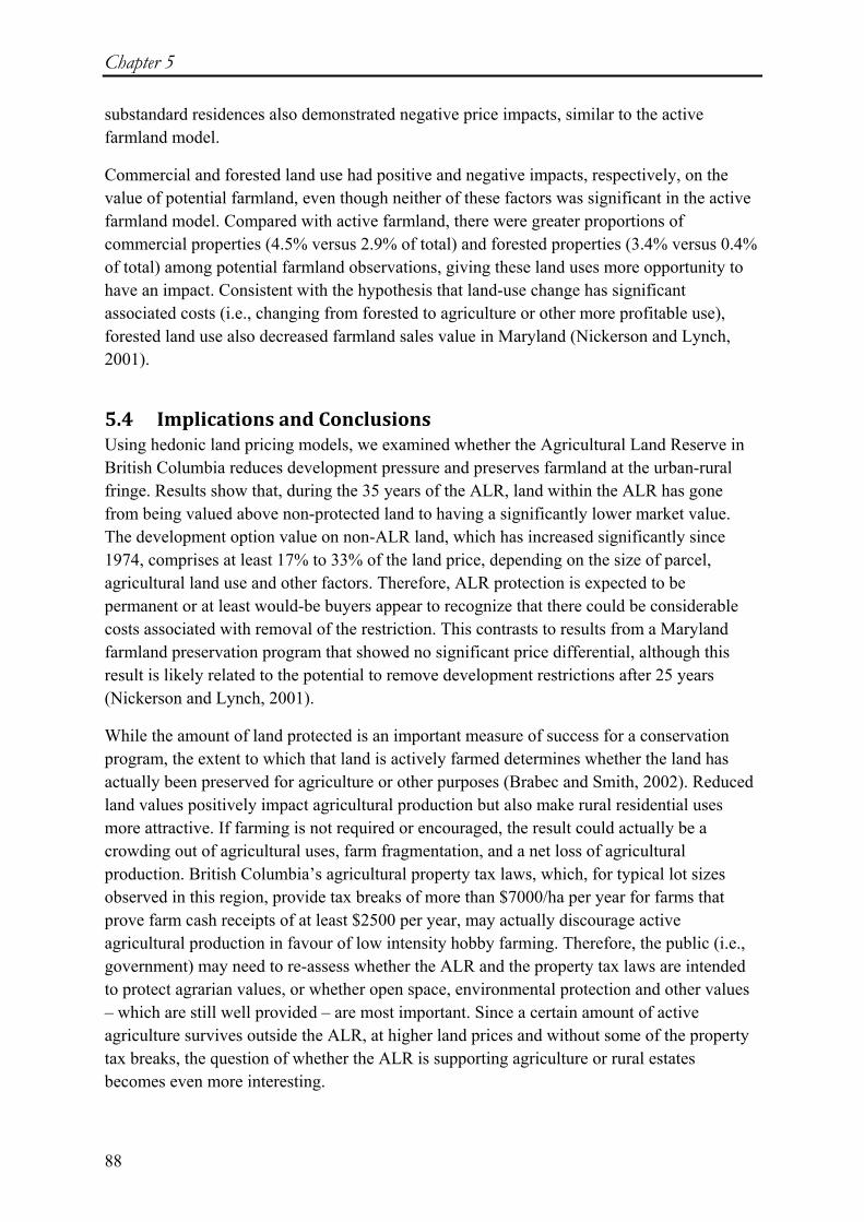
Chapter 5

88

substandard residences also demonstrated negative price impacts, similar to the active farmland model.

Commercial and forested land use had positive and negative impacts, respectively, on the value of potential farmland, even though neither of these factors was significant in the active farmland model. Compared with active farmland, there were greater proportions of commercial properties (4.5% versus 2.9% of total) and forested properties (3.4% versus 0.4% of total) among potential farmland observations, giving these land uses more opportunity to have an impact. Consistent with the hypothesis that land-use change has significant associated costs (i.e., changing from forested to agriculture or other more profitable use), forested land use also decreased farmland sales value in Maryland (Nickerson and Lynch, 2001).

5.4 Implications and Conclusions Using hedonic land pricing models, we examined whether the Agricultural Land Reserve in British Columbia reduces development pressure and preserves farmland at the urban-rural fringe. Results show that, during the 35 years of the ALR, land within the ALR has gone from being valued above non-protected land to having a significantly lower market value. The development option value on non-ALR land, which has increased significantly since 1974, comprises at least 17% to 33% of the land price, depending on the size of parcel, agricultural land use and other factors. Therefore, ALR protection is expected to be permanent or at least would-be buyers appear to recognize that there could be considerable costs associated with removal of the restriction. This contrasts to results from a Maryland farmland preservation program that showed no significant price differential, although this result is likely related to the potential to remove development restrictions after 25 years (Nickerson and Lynch, 2001).

While the amount of land protected is an important measure of success for a conservation program, the extent to which that land is actively farmed determines whether the land has actually been preserved for agriculture or other purposes (Brabec and Smith, 2002). Reduced land values positively impact agricultural production but also make rural residential uses more attractive. If farming is not required or encouraged, the result could actually be a crowding out of agricultural uses, farm fragmentation, and a net loss of agricultural production. British Columbia’s agricultural property tax laws, which, for typical lot sizes observed in this region, provide tax breaks of more than $7000/ha per year for farms that prove farm cash receipts of at least $2500 per year, may actually discourage active agricultural production in favour of low intensity hobby farming. Therefore, the public (i.e., government) may need to re-assess whether the ALR and the property tax laws are intended to protect agrarian values, or whether open space, environmental protection and other values – which are still well provided – are most important. Since a certain amount of active agriculture survives outside the ALR, at higher land prices and without some of the property tax breaks, the question of whether the ALR is supporting agriculture or rural estates becomes even more interesting.

Farmland protection and agricultural land values at the urban fringe in British Columbia

89

In the current study, a number of factors, including land price relationship to parcel size, signify that residential demand has a large impact on the rural land market on the Saanich peninsula. A preference for being closer to the city (reduced commuting costs) and at higher elevations with greater slope (nicer views) are all value by residential markets. The higher land value with the presence of horses also indicates that recreational horse-owners are a significant force in this region. Also, land that has a higher turnover rate (has been sold more than once in the study period) tends to be associated with residential values: smaller lot sizes, hobby farms, horses and cash sales. Those with lower turnover rates were more associated with productive agriculture: vegetable and forage production and vacant properties.

For farmers, the real and anticipated costs of dealing with urban neighbours are capitalized in farmland prices. This is evident from the strong price impact of location within the ALR, with price increases in the range of 5–8% for land that is only one kilometer further removed from urban influences, assuming the assurance of continued separation is guaranteed by the ALR. Such expenses result from needing to adjust farm practices, deal with conflict or complaints, and handle traffic congestion or trespass. In regions such as the near-urban area on the Saanich peninsula, policies that concentrate active and protected farmland within specific areas can therefore have a major impact on reducing these real economic costs to agriculture, improving the economic viability of agriculture in the region.

The presence of active agriculture alone, location within a farmland block and vegetable production also decreased land prices, making it more affordable for farmers. This may be because residential property seekers are less interested in land that is currently actively farmed or because farmers try to sell their land to others who will continue farming (and thus absorb the cost for retaining the land in agriculture). This evidence indicates that policies that encourage agricultural activity on land could have some of the same land price impacts as the ALR farmland zoning regulation. However, for land not currently farmed, the ALR serves as an important price regulator and development deterrent, making land potentially more affordable for agriculture. Therefore, regulatory protection and positive reinforcement of farming activity are likely necessary partners.

91

6. Farmland Preservation Verdicts – Rezoning Agricultural Land in British Columbia1 Abstract The Agricultural Land Reserve (ALR) in British Columbia, Canada, is a provincial zoning scheme designed to protect agricultural land from development. Since 1973, landowners have not had the right to develop or use ALR land for non-agricultural purposes. This has prompted a number of landowners to seek recovery of some option value by applying for exclusion from the ALR. Using Geographic Information System (GIS) technology and a binary choice (logit) model, this study examines factors that impact the acceptance of ALR exclusion applications. We find that distance to the major highway is a highly significant factor, with land closer to the highway more likely to be excluded. Exclusions are more likely to be approved when pertaining to smaller land parcels, smaller portions of the total parcel area, or poorer quality soils. These factors suggest that, as intended by public policy, agricultural capability is a key determinant in exclusion decisions, and properties of greater agricultural value tend to be retained in the ALR. In addition, industrial intended uses are more likely than others to be approved, with a 39% increased chance of approval for industrial uses in one region studied. The political party in power at the time of the decision also proved significant, with approvals more likely under Social Credit leadership and, in some model specifications, the current Liberal government. However, these impacts may be moderated by time and population growth measures.

Key Words Zoning, agricultural land, urban fringe, GIS, land use

6.1 Introduction Continued urbanization and encroaching development threatens the integrity of productive agricultural land near many urban areas in North America, causing public concern and generating significant media attention. As a result, many local and provincial/state jurisdictions have adopted the protection of farmland as a major policy goal. Market-based approaches are common, including taxes and subsidies, transferable development rights (TDR), purchase of development rights (PDR) and purchase of conservation easements. However, land-use regulation and zoning are also frequently utilized, particularly in Canada (Barichello et al., 1995; Hardie et al., 2004). 1 This chapter is a paper by Eagle, A.J., T.E. Stobbe, G. Cotteleer and G.C. van Kooten, submitted for publication to the Canadian Journal of Agricultural Economics. This research was funded by Agriculture and Agri-Food Canada through the Farm Level Policy Network.

Chapter 6

92

In jurisdictions with recurring fluctuations in political opinion and power, zoning and regulation can create expectations of impermanency, leading to lobbying and other pressure to change the status of affected tracts of land. This has been the case for more than 30 years in British Columbia, Canada, which has a province-wide farmland zoning system, the Agricultural Land Reserve (ALR), regulated by a politically-appointed Agricultural Land Commission (ALC). While the ALR mandate is to protect the public interest and future option value through farmland conservation, some exclusions may optimize public value by providing needed land for development.

What factors impact the success of an application for removal of land out of the ALR? Are such decisions biased by the political party in power at the time, by the proposed use of the land, or by the backing or opposition of the local municipal government? An improved understanding of factors impacting the fate of exclusion applications could determine the validity of concerns about the integrity of the ALR and the political process that protects the public interest. Accordingly, in this study we examine over 30 years of zoning decisions for two municipalities with significant farmland and tremendous development pressures, and the factors that impact decisions to change land zoning from agriculture to other uses. With the assistance of a Geographic Information System (GIS), this study uses logistical regression models to test the impacts of spatial, political and other factors on outcomes for 81 exclusion applications near large urban centres.

Providing preferential land tax is one of the most common agricultural land protection strategies across North America. The goal of preferential land taxes is to make agricultural use of the land relatively more attractive in the hopes of preventing or delaying development. But research indicates that taxation alone is not an effective method of preserving agricultural land (Anderson, 1993; Conklin and Lesher, 1977). Taxation distorts property values and subsidizes speculation on farmland (Blewett and Lane, 1988; Nelson, 1992), allowing farmers to hold out for the highest price (Blewett and Lane, 1988; Nelson, 1992). Although tax policies might increase net farm revenue, they do not encourage farmers to make their land more productive. Indeed, Plantinga and Miller (2001) conclude that the only way to fully deter farmland loss is to compensate landowners for foregone development returns.

To this end, TDR and PDR programs have been applied successfully in some areas to protect agricultural land (Brabec and Smith, 2002). However, Nickerson and Lynch (2001) found no impact on farmland prices from a PDR program in Maryland. This was likely because land could be removed from the program after 25 years, if it can be shown to be unprofitable for agriculture at that time. Therefore, buyers may speculate on future value, and be willing to pay more than would be justified by agricultural returns alone. Nelson (1992) argues that, while PDR and TDR programs may preserve open space, they do not necessarily protect an active farming economy, due to voluntary nature of the programs, speculation on the land, and attractiveness of the land to rural-estate holders. Exclusive farm-use districts were established in Oregon in 1973, where all development must be proven to improve agricultural production. Not surprisingly, building density twenty years later was significantly reduced inside the farmland zone (Kline, 2005).

Farmland preservation verdicts – Rezoning agricultural land in British Columbia

93

Zoning for exclusive agricultural use should, in theory, reduce land values so that they reflect the agricultural potential of land rather than its development potential. In general, when land use is restricted near cities, land values are lower than for similar parcels without restrictions. By restricting permissible land uses, these zoning rules then get capitalized in land prices (Henneberry and Barrows, 1990). A drawback of zoning is that it creates an incentive to lobby for exclusions and variances to the zoning regulations (Blewett and Lane, 1988). Speculation on land that developers believe has a high probability of being excluded can increase farmland values well beyond the agricultural returns from the land, thus undermining one of the main reasons for zoning – to keep agricultural land prices low for farmers. In the urban-rural fringe of southwestern BC, ALR zoning has reduced land prices, but these prices are still above likely agricultural value (Stobbe, 2008).

Some researchers have looked at factors that predict conversion of farmland to residential and other non-farm uses to provide more insight into the effectiveness of different conservation methods. If farm characteristics are shown to be the most important factors, farm profitability must necessarily play a large role in land-use and land-use change. Drozd and Johnson (2004) found that higher soil quality and other agronomic characteristics corresponded with lower rates of land conversion into acreages for large lot development near cities in Nebraska. Using country-wide data, Tweeten (1998) found that U.S. farm income and farm population were more significant factors than urban population in predicting changes in cropland area from 1949 to 1992. These studies show that there is some backing for the hypothesis that farm income and characteristics drive agricultural conversion in some areas.

Using a probit model, Isgin and Forster (2006) identified several factors that were significantly correlated with rural-to-urban land conversion in Ohio. Farmland conversion was more likely when a greater proportion of the population is living in urban areas, the size (area) of the county is larger, there is higher median family income, and observed per-acre land prices are higher; but the likelihood of conversion declined when a higher proportion of the county was classified as farmland. These and other studies (e.g. Shi et al., 1997) confirm the intuition that there are also strong effects of the local urban economy on the rural land market and that population pressure partly drives farmland conversion in some areas.

As detailed, there are many studies that examine farmland conversion to urban uses but the literature is sparse when it comes to pure agricultural zoning schemes. Since most North American agricultural zoning has been in place for less than 35 years (those in Oregon and BC were among the first in 1973), the removal of land from exclusive agricultural zones as local conditions change has not yet been studied to any extent. Yet, the need on occasion to remove land from agricultural protection has been acknowledged by Libby and Sharp (2003), for example, who consider the value of social capital in maintaining a sense of fairness in rezoning decisions.

British Columbia’s province-wide implementation of the ALR played a pioneering role in farmland conservation, and currently includes 4.7 million hectares of land for which subdivision and non-agricultural uses are severely restricted. However, there has been very little if any statistical and academic analysis related to zoning systems such as BC’s

Chapter 6

94

Agricultural Land Reserve. Most of the literature pertaining to the ALR is of a legal, political or advocacy nature (Campbell, 2006; Curran, 2005; Green, 2006); statistical and academic analyses of the economic and social impacts of the ALR and other related zoning systems are negligible. The academic work that is available effectively outlines the historical context for the ALR, exploring compensation issues and the continued viability of the farm economy (Garrish, 2003; Hanna, 1997). Hanna (1997) also discussed the way that applications for exclusion attempted to regain land value lost by the ALR classification, and determined that public applications for exclusion from 1974 to 1993 were approved at a much higher rate (88%) than private ones (30%). However, the primary focus was on economic incentives and compensation issues rather than statistical analysis.

Concerned citizens and environmental groups contend that land has been disproportionately excluded from the ALR under the Liberal government that came into power in May 2001. Requesting more accountability and public input, some have claimed that the decision-making structure is flawed (Campbell, 2006; Green, 2006). To our knowledge, however, no one has yet examined the factors that are associated with the outcomes of proposed exclusion applications.

The current study constitutes the only known statistical analysis of agricultural zoning in British Columbia, and thereby makes an essential empirical contribution to contrast the politics, lobbying and rhetoric that have occupied center stage in the debate over agricultural land preservation. It also helps fill a gap in the larger literature on agricultural land protection programs by illuminating the roles that spatial and non-spatial characteristics play in land zoning exclusion decisions. Although landowners can also apply for permission to subdivide or change land use while retaining ALR status, such applications cover much less area than whole-scale exclusion,2 making exclusions an appropriate measure of zoning change activity.

The next section provides a brief history and outline of the study area and the ALR. This is followed by a description of the data employed and the methods applied, including a summary of the spatial model used in the research. In the fourth section, we present the empirical results, with estimated logistical regression models and marginal effects. Armed with enhanced knowledge of factors that impact land zoning decisions, we conclude with a discussion of the implications as they apply to zoning modifications and exclusion from conservation zones.

6.2 Study Area and Background British Columbia’s ALR was established in 1973 under the New Democratic Party that then governed the province. The main impetus for its conception was the growing concern over urban sprawl and the associated loss of farmland near cities. It was estimated that BC was losing 4,000 to 6,000 hectares of farmland annually (Garrish, 2003). Assuming that all of this land was in crops, the loss accounted for 0.9 to 1.4% of BC’s total cropland (1971 Census of

2 For the entire province from 1974 through 1993, the total area affected by exclusion applications was 174,758 ha and the area covered by applications for subdivision or land-use change was 532 ha (Hanna 1997).

Farmland preservation verdicts – Rezoning agricultural land in British Columbia

95

Agriculture), similar to estimated losses in the Northeast region of the U.S. (0.98% annual loss), but higher than country-wide U.S. estimates of losses to urbanization (0.16% annual loss) (Dideriksen, 1976).

The ALR originally comprised all land two acres (0.8 ha) and larger with soils rated in quality classes one through four in the Canadian Land Inventory (CLI), land that already possessed farm class status under BC Assessment, and land zoned as agriculture by a local municipality. The landowner retains ownership but faces restrictions on land use that include prohibitions on subdivision, non-agricultural uses and development. One dwelling is allowed per parcel (for a farmhouse) and the Agricultural Land Commission must approve any exceptions to these rules. In its early years, the ALC’s main function was that of fine-tuning the set of parcels included in the ALR. Since then the administration of the ALR has changed, as has the size and composition of some of the lands in the ALR (see Figure 6-1 for a timeline of events). The most profound administrative change was the move in 2002 (under the Liberals) from a single province-wide commission composed of at least seven members to an ALC consisting of six regional panels of three members each.

Figure 6-1. Timeline of key events affecting the Agricultural Land Reserve in British Columbia

At the time of its formation, the ALR constituted 4,716,516 hectares, but it had grown to 4,759,249 ha by 2007, a net increase of 42,733 ha (Agricultural Land Commission, 2009). However, additions have primarily been in the colder, more arid and less productive northwest and exclusions concentrated in the fertile south. Accounting for almost half of the total provincial excluded area from 1973 to 2008, Vancouver Island, the lower Fraser River

province-wide ban on farmland subdivision

ALR initiated by Land Commission Act (18Apr1973)

First applications for removal received by Land Commission

Socred gov't replaces NDP

LC Act amended to remove jurisdiction over greenbelts, parks, and land

reserves - changes name to Agricultural Land Commission

Golf courses permitted on ALR

land

NDP gov't replaces Socred

Moratorium on golf course uses, then

removed as permitted use

Appeals to provincial cabinet no longer

allowed

ALC Act amended to strengthen role of local governments

Liberal gov't replaces NDP

ALC Act revised, replaces provincial

board with six regional ALC panels

ALC rescinds 1977 order that allowed

subdivisions into 1/4 sections without ALC

application

1971 1976 1981 1986 1991 1996 2001 2006

Selected events of BC's Agricultural Land Reserve

Chapter 6

96

Valley (lower mainland), and the Okanagan Valley have lost 11.0%, 10.3% and 7.4%, of their respective total ALR area since its inception.3 These three key agricultural regions generate more than 75% of the province’s farm receipts (Statistics Canada, 2006). Critics have accused the current ALC of allowing the removal of too much high quality land from the ALR in recent years (Green, 2006). However, there are also those who argue that not enough land is being let out and that housing prices in Vancouver and other urban areas are inflated due to the lack of land for new housing (Lazaruk, 2008).

A typical ALR exclusion application is a lengthy process involving detailed land use proposals, an agrologist’s report, public hearings, and frequently local government support or opposition. The application is decided by ALC commissioners who work in conjunction with ALC staff members and who often visit the site in question before deciding the fate of the application. Applications can be rejected outright, approved outright, or receive partial approval (for either some of the land or for some of the intended uses).

In this paper, we examine ALR exclusion applications from two agricultural regions near major urban centres – Greater Vancouver and Victoria. Both regions (Abbotsford, in the Fraser Valley, and the Saanich peninsula, on Vancouver Island) enjoy some of Canada’s mildest temperatures and most fertile soils. Farmers in the Abbotsford region grow a variety of field crops and there is intensive livestock production, but the region is perhaps best known for its berry production, particularly raspberries, blueberries and cranberries. The Saanich peninsula hosts many market garden, floriculture and nursery businesses as well as livestock, field crops and specialty crops such as wine grapes. Both face mounting development pressures from the nearby expanding urban centers of Vancouver and Victoria, respectively.

Since ALR inception, the population of British Columbia has been steadily growing, from 2.2 million in 1971 to 4.3 million in 2006. Population pressure leads to increased demands for land to expand housing, school, industry and other urban development. Since 1971, Abbotsford has experienced significantly more population growth than the Saanich peninsula (299% versus 66% increase; see Figure 6-2). Therefore, we hypothesize that applications for ALR exclusion in Abbotsford during this period were more common and more likely to be approved, since the public need for land was significantly greater.

6.3 Data and Methods Data for this inquiry were obtained from the Agricultural Land Commission’s files and entered manually into a GIS database. The data comprise all applications for exclusion from the ALR on the Saanich peninsula and in the Abbotsford municipality from 1973 to 2006. The Saanich peninsula data include applications from three municipalities (Saanich, Central Saanich and North Saanich). There were 65 applications for exclusions in Abbotsford and 16 for the Saanich peninsula (see Figure 6-3). While most applications were treated as individual observations, three applications (one from the Saanich peninsula and two from Abbotsford) 3 Authors’ calculations based on ALC Statistics (www.alc.gov.bc.ca/alr/stats/Statistics_TOC.htm)

Farmland preservation verdicts – Rezoning agricultural land in British Columbia

97

were split into 12 separate observations for this study, because they consisted of spatially distinct blocks that were ruled on separately by the ALC. Hence, we have a total of 90 observations.

Figure 6-2. Population growth for Abbotsford and Saanich peninsula, 1966–2006, with provincial population for comparison. (Source: Statistics Canada, census)

A list of variables included in the dataset is provided in Table 6-1, along with summary statistics. Half of the requests for exclusion involved land area that was less than 5.6 ha, and 76% of requests pertained to an entire parcel. Because a smaller parcel of land is more likely to be fragmented from other farmland and its exclusion would have a smaller impact on regional agriculture, we hypothesize that applications concerning these smaller parcels of land are more likely to be approved. In addition, an application that requests exclusion for only a portion of the entire parcel suggests a willingness on the part of the applicant to continue to contribute to local agriculture on the remainder of the land, and therefore would be more likely to gain ALC approval.

Applications are indicated by the ALC as public or private depending on whether they come from an individual or from a local government, the latter often as part of a long-term planning exercise. Because of the extensive planning and project development associated with public applications, the average area requested for exclusion in public applications was much larger than for private applications (see Table 6-1). Applications intending industrial use were also more likely to come from government rather than private sources (t-test, p=0.0253), and all those with a commercial intended use were private applications. However, residential applications were evenly distributed between private and public sources.

The distance variables examined in this study were constructed with ArcGIS using data provided by the BC Ministry of Agriculture and Lands in their Land Use Inventory for Abbotsford and the Saanich peninsula. This parcel-level dataset was overlaid with additional GIS dataset layers from the Federal Government showing the road and highway networks. The main commuting corridor for each jurisdiction was used to calculate distance to the

0.0

1.0

2.0

3.0

4.0

5.0

BC P

opul

atio

n (m

illio

ns)

British Columbia

0

40

80

120

160

200

1966 1971 1976 1981 1986 1991 1996 2001 2006

Regi

onal

Pop

ulat

ion

(tho

usan

ds)

AbbotsfordSaanich

Chapter 6

98

highway; in Abbotsford, this was the TransCanada Highway (#1), and on the Saanich Peninsula, this was the Patricia Bay Highway (#17). Following common practice (Cho et al., 2006), distances were transformed to natural logarithm to reduce potential distortion from significant outliers. Accordingly, requested area was also converted to natural logarithms.

Figure 6-3. South-western British Columbia with highlighted study areas (A), the City of Abbotsford (B) and the Saanich peninsula (C). The Agricultural Land Reserve (ALR) is indicated by the shaded area on regional maps and ALR exclusion applications are shown as dots. (Source: Ministry of Agriculture and Lands and the Agricultural Land Commission, edited map)

The potential agricultural value of land is affected by soil capability, in Canada denoted by Canada Land Inventory class. Upon establishment, the ALR included all land with prime agricultural soil classes (CLI classes 1 through 3), as well as all land currently zoned agricultural or receiving tax breaks from being categorized as “farm class”. Since the ALC considers soil class in deliberations regarding exclusion applications, we endeavoured to include soil class in the logit model for each observation. However, soil quality information was rarely provided in earlier applications (pre-1983). It was not possible to impute the classification from available soil maps, as their scale was not sufficiently detailed. Therefore, a weighted average of available data was calculated, specific to each region, and these values were used where information was missing.

Farmland preservation verdicts – Rezoning agricultural land in British Columbia

99

Table 6-1. Explanatory Variables and Summary Statistics

Continuous Variables Mean Std. Dev. Median Min Max Requested area (ha) 19.5 31.5 5.6 0.2 182.2 Requested area as percent of total (%) 86.3 27.4 100 4.6 100 Total parcel size (ha) 31.4 80.2 6.5 0.2 519 Soil (Classes 1 to 7) 2.76 1.07 2.70 1 6.35 Year 1989 11.1 1990 1974 2006 Distance to highway (m) 1,835 1,576 1,466 59 6,759 Distance to (relevant) City Hall (m) 6,368 5,465 4,777 2,040 28,791 Annual population growth (%)

Abbotsford 4.5 1.6 5.3 1.5 6.0 Saanich peninsula 1.3 0.9 0.8 0.5 2.9

Count Area Requested (ha) Other Variables (n=90) Mean Median Public applications 28 48.7 40.7 Private applications 62 6.3 3.9 Support of local government 68 16.0 4.2 Opposition of local government 9 10.6 10.2 Intended Uses

Industrial 33 23.1 7.7 Residential 41 21.2 5.8 Commercial 6 2.1 2.0 Other 10 11.4 4.1

Political Party in Power New Democratic (NDP) 39 17.9 4.2 Social Credit 33 19.1 5.7 Liberal 18 23.8 9.1

Abbotsford applications 73 21.0 5.8 Saanich peninsula applications 17 13.4 2.9 Source: Authors’ compilations The data for the variables that indicates support of the local government (and presumably the majority of the people living in the area) were also not complete. The ALC recorded local government support in 68 of the applications and opposition in 9 cases, leaving 13 applications with no information on this variable. Opposition was associated with residential intended-use applications (7 of the 9 cases of opposition were for residential applications.) Two dummy variables were included to explore the effect that support or non-support of the local government had on the probability of exclusion.

Political party was included to test whether the government in power at the time had any impact on approval rates (as suggested by numerous pundits). The New Democratic Party (NDP) founded the ALR in 1973, but soon thereafter lost power to the Social Credit (Socred) party, which governed the province between 1975 and 1986. The NDP again formed the government from 1986 to 2001 at which time the Liberals came to power.

A time dimension was included to determine if the approval rate of applications changes over time. Lag of excluded hectares records the number of hectares excluded in the previous two

Chapter 6

100

years – the historical memory. It was hypothesized that, because of the nature of ALC board membership, a succession of successful applications might lead to more success because the ALC may be more inclined to favour development. Lastly, regional population growth rate is included, measured as a five-year moving average, as an indicator of demand for new housing and increased development pressure.

A logistical binary (logit) model is utilized in the analysis, with the dependent variable taking on a value of 0 if the application was refused and 1 if the application was fully or partially approved. Using the logistical distributional function, we can write the probability of an application’s success as:

(1)

where β1 represents the coefficient on an intercept term and β2 represents a vector of coefficients on the vector of regressors, X. Using maximum likelihood procedures, the coefficients can be estimated and probabilities calculated for the significance of the explanatory variables on the acceptance rates of the dependent variable (Gujarati, 1995).

6.4 Empirical Results A total of 1,758 ha of land were included in the ALR exclusion applications for Abbotsford and the Saanich peninsula. The ALC permitted partial or total exclusion of farmland from the ALR for 60 of the 90 observations, although this accounted for only 38.7% (680 ha) of the area included in the applications. The average requested area for exclusion was significantly lower for approved applications than for those that were denied, with respective means (medians) of 14.0 (4.1) ha and 30.6 (13.4) ha.

The final logit regression models were selected on the basis of both theoretical considerations and statistical fit. Four model specifications are presented in Table 6-2. The full model includes all significant factors and those that have significant impacts on other relevant factors. Several restricted models were estimated by removing macro-variables.

The impact of parcel size is significant or nearly significant for all models, as smaller parcels of land are associated with more exclusion approvals. However, the proportion of a parcel requested for exclusion has a much stronger impact. Applications comprising less than the entire parcel area are more likely to be approved for exclusion, possibly because they come from landowners who accordingly present plans to enhance agricultural activity on the remaining portion of the land. For example, partial exclusions may be accompanied by plans for park development, concessions to agriculture or other “land swap” deals to strengthen the likelihood of approval. These applications could also be related to adjustments in the ALR boundary, where a portion of a parcel of land is of little agricultural value, and perhaps should not have been included in the ALR in the first place.

)( 2111)|1(

iXii eXYEP ββ +−+

===

Farmland preservation verdicts – Rezoning agricultural land in British Columbia

101

Table 6-2. Logit model estimation results for ALR exclusion decisions

Tab

le 6

-2. L

ogit

mod

el e

stim

atio

n re

sults

for

AL

R e

xclu

sion

dec

isio

ns (n

=90)

, dep

ende

nt v

aria

ble

is a

ppro

val o

f ap

plic

atio

n; c

oeff

icie

nt sh

own

(with

p-v

alue

in p

aren

thes

es).

Var

iabl

es

Mod

el 1

Fu

ll m

odel

M

odel

2

No

lags

M

odel

3

Tim

e tre

nd, n

o la

gs

Mod

el 4

N

o tim

e tre

nd

Log

requ

este

d ar

ea, h

a -0

.626

(0.

119)

-0

.622

(0.

120)

-0

.654

(0.

094)

-0

.806

(0.

027)

Pe

rcen

tage

of p

arce

l in

appl

icat

ion

-0.0

43 (

0.01

5)

-0.0

43 (

0.01

4)

-0.0

41 (

0.01

6)

-0.0

40 (

0.01

6)

Saan

ich

peni

nsul

a

2.76

2 (0

.185

) 2.

805

(0.1

68)

0.36

1 (0

.731

) 0.

334

(0.7

53)

Priv

ate

appl

ican

t 0.

765

(0.5

75)

0.76

6 (0

.575

) 1.

218

(0.3

46)

0.84

5 (0

.484

) Lo

g di

stan

ce to

hig

hway

-1

.360

(0.

008)

-1

.364

(0.

008)

-1

.418

(0.

004)

-1

.394

(0.

004)

So

cial

Cre

dit p

arty

1.

698

(0.1

13)

1.72

6 (0

.096

) 2.

005

(0.0

51)

1.61

9 (0

.072

) Li

bera

l par

ty

1.85

4 (0

.250

) 1.

932

(0.1

71)

1.24

3 (0

.321

) 1.

888

(0.0

65)

Loca

l gov

ernm

ent s

uppo

rt

-0.3

09 (

0.75

1)

-0.3

07 (

0.75

1)

-0.3

91 (

0.67

0)

-0.5

57 (

0.52

9)

Loca

l gov

ernm

ent o

ppos

ed

-2.1

38 (

0.19

5)

-2.1

65 (

0.18

4)

-2.3

77 (

0.13

7)

-2.6

23 (

0.08

7)

Inte

nded

land

use

C

omm

erci

al

-1.5

47 (

0.37

0)

-1.5

53 (

0.36

9)

-2.2

03 (

0.16

8)

-2.6

23 (

0.08

7)

Res

iden

tial

1.37

3 (0

.271

) 1.

383

(0.2

65)

1.08

4 (0

.354

) 0.

736

(0.5

07)

Indu

stria

l 2.

591

(0.0

61)

2.58

2 (0

.060

) 2.

340

(0.0

74)

2.01

8 (0

.107

) So

il cl

ass

0.71

7 (0

.074

) 0.

725

(0.0

66)

0.71

4 (0

.063

) 0.

647

(0.0

85)

Yea

r sin

ce A

LR in

cept

ion

0.14

7 (0

.099

) 0.

148

(0.0

98)

0.04

3 (0

.385

) –

– –

–

Popu

latio

n gr

owth

rate

a 0.

942

(0.1

60)

0.95

5 (0

.148

) –

– –

–

– –

– –

Ex

clud

ed a

rea

(sum

of p

revi

ous t

wo

year

s)

0.00

1 (0

.920

) –

– –

–

– –

– –

–

– –

–

Con

stan

t 5.

020

(0.4

24)

4.99

3 (0

.426

) 11

.097

(0.

018)

12

.720

(0.

004)

Ps

eudo

R2

0.43

21

0.43

20

0.41

14

0.40

47

a Pop

ulat

ion

grow

th ra

tes a

re re

gion

al (d

iffer

ent f

or S

aani

ch p

enin

sula

and

Abb

otsf

ord)

, spe

cifie

d as

the

five-

year

mov

ing

aver

age

Chapter 6

102

Although the approval rates appear to be somewhat higher for private applications – 69.4% acceptance rate (43.6% of area requested) versus 60.7% for public applications (37.3% of area requested) – there is no statistically significant difference between applicant type, ceteris paribus. These results contradict those of Hanna (1997) who, using summary statistics for the entire province from 1973 to 1993, determined that public applications were more readily approved. If the current models are restricted to exclude observations after 1993, applicant type continues to have no impact on approval.

Distance to the highway had the strongest significant impact on exclusion approvals, with land closer to the main commuting corridor in each region more likely to be removed from the ALR. This is most likely a result of negative traffic and urban development externalities decreasing agricultural viability, at least in the opinion of the decision panel. Land parcels farther from the highway are also more likely to be connected with other farmland, and their exclusion could have a more significant fragmentation impact on the agricultural land in the region.

Another significant finding relates to the political party in power. The Social Credit party significantly increased the likelihood of application acceptance in three of the four models, and Liberal party increased likelihood in Model 4. However, when time trend variables (population growth, previous excluded area and year since ALR inception) are taken into account, the significance of party variables is reduced. Therefore, the greater likelihood for permitted exclusions when the Socreds and Liberals were in power could be less a result of political activity and instead related to changes over time as well as elevated demand for residential development caused by high rates of population growth. A further anomaly in regard to political party pertains to the two years (1975 and 2005) when atypically high numbers of applications were experienced. When those years are excluded, both political parties become statistically insignificant.

Whether or not an application had the support of the local government appears to have only marginal impact on the likelihood of the application receiving approval. Since application for exclusion must be processed by the local municipality, applications likely encounter a rigorous selection process before they are forwarded to the ALC. Thus, only 10% of applications submitted to the ALC were opposed by the local government, while 76% were supported. Although local government support was not significant in any of the models, the factor was retained because it impacted land use intent: 87% of industrial applications versus 68% of non-industrial applications (t-test, p=0.0388) were associated with local government support.

Local government opposition was marginally significant in only one model (Model 4) – in that case, it reduced the probability of acceptance by 55%. The lack of statistical significance in other models may be related to the small number of applications to which this factor applied. Also, local government opposition was only recorded for applications submitted between 1975 and 1983, suggesting that, after this point in time, exclusion applications with local opposition either did not proceed past the local council or were adapted sufficiently to eliminate opposition.

Farmland preservation verdicts – Rezoning agricultural land in British Columbia

103

Intended use forms another category of variables analyzed. To avoid perfect multicollinearity in the data, the dummy on the ‘other’ category was integrated into the intercept term. (The ‘other’ category contained several applications from a university-college wishing to expand and applications for transportation infrastructure expansion.) Commercial use has a somewhat negative impact on approvals, although this variable is only significant in one model. Industrial uses are positively associated with ALR exclusion approvals in all models. Residential uses do not appear to impact application success.

Soil class was positively associated with exclusion approvals, consistent with the premise that more agriculturally valuable land will be kept within the ALR. A higher soil class (CLI class 4 through 7) indicates lower soil or site quality for agriculture (e.g., steep slopes, poor drainage). This proves that the ALC does consider agricultural capability in decision processes.

Although location and type of applicant (private versus public) were not significant in any model specification, their impact on other factors necessitates their retention in the models. For example, applications on the Saanich peninsula had a greater association with residential intended use (88% versus 36% for Abbotsford), while industrial intended uses only occurred in Abbotsford. Additionally, a greater number of the Socred era applications were in Abbotsford (41% of total versus 18% in Saanich). Public applications tended to be larger in size and had a greater association with industrial uses (54% versus 29% of private applications), so correcting for application type is also necessary to determine accurate size and industrial use impacts.

Correction for regional population growth strongly impacted the coefficients on location and the time trend. Because of the large difference in population growth characteristics between the two regions, this factor is likely important as a determinant of development pressure on agricultural and other land. However, its correlation with time (see Figure 6-2) means that it is difficult to separate the effect of time from that of population growth.

Several other variables were eliminated from the final models for a variety of reasons. Total parcel size was highly correlated with hectares requested for removal and showed no statistical significance. As well, distance to city hall was statistically insignificant in all cases. This is perhaps related to the fact that modern Abbotsford is a conglomeration of three historically separate entities (Abbotsford, Matsqui and Clearbrook), each with its own town center. Hence, distance to the current city hall may not be a good measure of the distance to the commercial centre.

Factor interactions between applicant type (public or private) and certain other variables were tested where those variables were significantly different between applicant types. However, none of these interactions exhibited any statistical significance in all model specifications, and so were not included in the final models.

6.4.1 Marginal Effects Marginal effects, evaluated at the mean, were calculated for the variables that were statistically significant in at least three of the four models (Table 6-3). A marginal effect can

Chapter 6

104

be interpreted as the change in the probability of an application being accepted when a variable increases decreases by one unit or a dummy variable changes from zero to one. With the noted differences between locations and applicant type, the marginal effects were calculated where applicant was equal to public or private, and where location was equal to Abbotsford or Saanich.

Acceptance rates for public applications were more sensitive than private applications with respect to location, distance to highway, political party, year and population growth rate. Similarly, the marginal effects separated into the two locations show that Abbotsford applications reacted more to the significant variables. In Abbotsford, changes in the significant factors have an approximately 10-fold greater impact on the likelihood of acceptance than on the Saanich peninsula.

Consider only the most important effects. When evaluated at the mean for all observations, the probability of application approval increases by 29% if the intended use switches from non-industrial to industrial. In this case, since industrial uses were only observed in Abbotsford, a more appropriate measure would be the marginal effect for Abbotsford only, which indicates that there is a 39% increased chance of acceptance for industrial applications. This reflects a high value for industrial land uses, at least in the view of the ALC, perhaps because new industrial developments require large units of land generally only available from agriculture.

The distance to the highway also has a major impact on the chance of exclusion. Evaluated at the mean, there is an 18% reduced likelihood of acceptance by increasing the distance one unit. Since this variable is a log of distance, this means that increasing distance from the highway from 1,149 metres (the mean of the log) to 3,123 metres is associated with 18% less chance of the application being approved. This result indicates that land that is further from major transportation arteries is more valuable for agriculture (or perhaps experiences lower levels of negative urban-source externalities), favouring retention within the ALR.

At the mean, where 86% of the parcel was included in the application, a 1% decrease of this proportion increased the probability of approval by 0.57%. Overall, an application’s chances fared better under the Socreds (20% more likely to be accepted). Time also played a role, as each year that passed increased an application’s chances of approval by 2%. Finally, a one-point increase in CLI soil class (reducing the land’s agricultural capability) increased the likelihood that an application would be accepted by an average of 10%, again with a greater impact for public applications and those in Abbotsford.

Farmland preservation verdicts – Rezoning agricultural land in British Columbia

105

Table 6-3. Marginal effects from Model 1 (full model) of factors that were significant in at least two of the four estimated logit models

Tab

le 6

-3. M

argi

nal e

ffec

ts fr

om M

odel

1 (f

ull m

odel

) of f

acto

rs th

at w

ere

sign

ifica

nt in

at l

east

two

of th

e fo

ur e

stim

ated

logi

t mod

els

Var

iabl

e A

ll ap

plic

atio

ns

Publ

ic

only

Pr

ivat

e on

ly

Abb

otsf

ord

only

Sa

anic

h on

ly

Log

requ

este

d ar

ea (h

a)

-0.0

836

-0.1

149

-0.0

706

-0.1

146

-0.0

121

Perc

enta

ge o

f par

cel i

nclu

ded

in a

pplic

atio

n -0

.005

7 -0

.007

9 -0

.004

8 -0

.007

8 -0

.000

8 Lo

g of

dis

tanc

e to

hig

hway

(m)

-0.1

816

-0.2

496

-0.1

533

-0.2

489

-0.0

263

Soci

al c

redi

t par

ty

0.19

98

0.27

51

0.16

88

0.27

43

0.02

93

Indu

stria

l use

inte

nded

(dum

my

varia

ble)

0.

2928

0.

3943

0.

2498

0.

3933

–

– –

So

il cl

ass (

1 to

7)

0.09

58

0.13

16

0.08

08

0.13

12

0.01

38

Yea

r sin

ce A

LR in

cept

ion

0.01

97

0.02

71

0.01

66

0.02

70

0.00

28

Sour

ce: A

utho

rs’ c

ompi

latio

ns

Chapter 6

106

6.5 Policy Implications and Conclusions These findings elucidate the underlying values that are seen in public decisions with respect to re-zoning from agricultural land to non-farm uses in British Columbia. The econometric models provide an empirical perspective on many popular opinions (often expressed in newspapers) regarding the Agricultural Land Reserve and exclusions from it, proving some opinions to be mistaken. When considering the high value of accessible land for non-farm uses, it is not surprising that land near a major commuting corridor is more likely to be excluded from the ALR. This correlates with the finding by Stobbe, Cotteleer and van Kooten (2008) that distance to a highway is a significant factor in distinguishing whether a farm is used for hobby purposes or for commercial agricultural production. Location near a major highway carries many externalities with it and some hobby farmers (who are also frequent commuters to jobs in the city) take advantage of the close proximity for commuting access. Commercial farms seem to experience more of the negative and less of the positive externalities of being near a highway. Establishing or expanding major highways near and in the midst of agricultural regions therefore has the potential to reduce the agricultural value of land relative to non-farm values. Additionally, a greater amount of effort is likely needed to conserve a land parcel for agriculture that is located closer to a major highway than one that is farther away. This information can assist those in government and the public who wish to determine how best to allocate farmland conservation resources.

An application for exclusion is more likely to succeed if it is intended for industrial use and/or pertains to only a portion of the parcel. In the full model, time is a significant factor, with applications more likely to succeed in later years. Even though the coefficient is not large in relation to other factors, the cumulative effect over time could be an indication of gradual weakening of the zoning system due to increased chances for exclusion.

Even when time factors were included in the model, the Social Credit political party was found to have a positive impact on the exclusion application success rate. Contrariwise, we find no evidence that exclusions were more readily granted under the Liberal government (and under the revised regionalized ALC structure), as certain vocal critics have suggested (Campbell, 2006; Green, 2006). Rather, we find that the changes noticed in the past decade are more likely the result of a general trend captured by our time variable, rather than something attributable to a particular political party. While these findings pertain to key agricultural regions in British Columbia, they do not necessarily apply to other jurisdictions. Indeed, one cannot even say that they apply to other areas of the province, and further research would be required to determine the province-wide effect and effects elsewhere.

107

7. Farming on the Urban Fringe – The Economic Impacts of Niche and Direct Marketing Strategies1 Abstract Agricultural production near large and thriving cities faces survival challenges related to development pressure (high land prices), farmland fragmentation and nuisance complaints. Yet common public opinion supports farm and farmland protection for the provision of open space, rural landscape and ambience, environmental services, local food and health promotion, and the basic existence value of agriculture – often associated with tradition or local history. These positive externalities indicate a necessity for government intervention to ensure the optimal social level of farmland and many jurisdictions have implemented farmland conservation and other related policies. Farmers also respond to changing economic and social climates by adapting production and marketing practices or increasing production intensity.

This research examines the economic impacts of niche and direct-marketing strategies on farmer survival and success near Victoria, British Columbia. While direct-marketing farms are similar to the average farm in the region in terms of size and gross farm income, they have significantly more operators and employees and a higher proportion of female operators. Most (74%) of the crop area was field vegetables, and 54% of the total product was sold directly at farm stands or on-farm markets. As one measure of economic success, production intensity – earnings per unit of land – was positively related to crop diversity, greenhouse production and recent farm investments, while negatively related to total farm area, higher education and female operators. The results suggest that idealism and non-economic values play a role in some decisions to adopt an agricultural lifestyle, with a trade-off of job and life satisfaction for income. However, land competition for non-farm uses, low availability of suitable labour, conflict with non-farming neighbours and sometimes overwhelming bureaucracy continue to make long-term survival and success tentative.

Key Words Direct marketing, local agriculture, organic farming, economic sustainability, farm survival, farm success, production intensity

7.1 Introduction Agricultural production near large and thriving cities faces survival challenges related to development pressure (rapidly rising land prices), traffic congestion, farmland fragmentation 1 This research was funded by Agriculture and Agri-Food Canada through the Farm Level Policy Network.

Chapter 7

108

and nuisance complaints. The negative externalities increase production costs for farmers, and expanding cities and rural residential demands compete with agriculture for productive land. The shifting boundary between urban and rural also brings new neighbours near active farms along with potential conflict regarding farm practices. On the other hand, increasing consumer demand for organic or locally produced food, for knowing where one’s food originates and for encouraging sustainable land management has changed or enhanced markets for some near-urban farmers (Jarosz, 2008). Farmers near urban centres may also have improved access to markets and non-farming income opportunities.

In addition to experiencing negative spillovers, landowners near urban areas provide positive externalities that are not reimbursed, another example of market failure. The conservation of agricultural land benefits society through the provision and retention of agricultural potential, open space, landscape views, urban sprawl control, and environmental services (i.e., flood control, wildlife habitat) (Kline and Wichelns, 1996). Other positive provisions include preservation value (i.e., existence, option and bequest values) and the symbolic values of traditional agriculture (Baylis et al., 2008). Preservation values often suggest very low or negative public discount rates. In other words, something (e.g., a piece of farmland) in the future is more highly valued when that item is for the good of all citizens, rather than an individual. However, farmers bear the costs and are seldom compensated for this provision, resulting in a supply of farmland that is lower than the social optimum. In response, farmland preservation policies tend to receive significant public support, and many jurisdictions in Canada (Hanna, 1997) and the USA (Duke and Lynch, 2006; Geoghegan, 2002; Machado et al., 2006) have implemented zoning and tax policies to protect farmland from development pressures and correct the market failure caused by externalities and public goods. Right-to-farm legislation also plays an important role in moderating conflict between farmers and other residents, and edge planning at the urban-rural fringe also commands significant attention of some municipalities (Lisansky and Clark, 1987; Sullivan et al., 2004).

However, conserving land for agricultural use does not necessarily equate with the economic survival of the farmers who remain on the “preserved” land. Farmland values tend to increase near major cities, as is explained theoretically by the von Thünen location rent model (see Hardie et al., 2004) and demonstrated by hedonic farmland price models (Cotteleer et al., 2009; Huang et al., 2006). With increased residential demand for rural estates or hobby farms, values also decline with parcel size (Cotteleer et al., 2009; Huang et al., 2006). Any conversion of agricultural land to urban uses is associated with further expectations for development, precipitating further price increases. These expectations often result in disinvestment in the agricultural sector – the idling of farmland or switching to activities that use more mobile capital (Berry, 1978). Alternatively, agricultural producers near cities adapt and maintain economic viability by intensifying land use or modifying production to take advantage of new and unique opportunities provided by the urban market. These adaptations include more greenhouse, market vegetable and organic production (Beauchesne and Bryant, 1999; Frederiksen and Langer, 2004; Purdy, 2005), direct sales, agricultural tourism and sales to high-end restaurants.

Farming on the urban fringe – The economic impacts of niche and direct marketing strategies

109

Does farm adaptation to niche- and direct-marketing enhance long-term agricultural survival in a region facing significant urban pressures? What farm actions and characteristics are associated with improved economic performance and success? How do current agricultural policies (e.g., farmland conservation, differential assessment of agricultural land) play a role and are they sufficient to encourage long-term agricultural production? Using a survey of direct-marketing and organic farmers near the city of Victoria, British Columbia, we explore economic and farm-level decision factors that contribute to farm productivity, farm success and environmental sustainability.

The remaining sections of the paper are structured as follows: First, we discuss aspects of sustainability and economic policy that are relevant to agricultural production at the urban fringe. Then, we give some background of the agricultural environment in the study region. This is followed by descriptions of data collection, analysis and model development, including limitations and tests for model fitness. Next we present results from the survey and econometric models along with discussion of these results. Implications for economic and environmental sustainability are discussed in the final section, as well as the impacts of current and potential policy interventions at the local, provincial and national levels.

7.2 Sustainability and Urban Fringe Agriculture Highly visible examples of unsustainability in agriculture (e.g., soil erosion, groundwater pollution, and rural social decline) accentuate the need for long-term sustainability in all agriculture, including that at the urban fringe. Defined by the Brundtland report (1987) as “the ability…to ensure that...the needs of the present generation [are met] without compromising the ability of future generations to meet their own needs”, sustainability has three facets – ecological, social and economic – that cannot be considered independent of one another (Oskam and Feng, 2008). The three aspects become interrelated when economic standards are used to evaluate ecological and social capital, thus providing a decision-making matrix.

If a social goal is to protect active local agricultural production at the urban fringe, sustainability in the larger sense must be considered. For example, a degree of ecological integrity could potentially be achieved without economic survival of farmers, and the result would be degradation of the entire system (or at least agricultural production in the region comes to an end). As well, local does not necessarily equate to social and ecological sustainability. For example, wineries and restaurants may use organic and locally produced food to collect market premiums from wealthy customers, but still treat employees poorly or create excessive waste (Eaton, 2008). Again, the whole system is important if the potential public values of the organic or locally produced food are to be fully realized.

7.2.1 Non-market Values Local and short-path food chains improve ecological sustainability by increasing consumer awareness of food origins and consequences, fostering more direct relationships between producers and consumers and encouraging organic or pesticide-free production. With larger markets, such systems tend to be more prevalent near and within larger urban centres. Local

Chapter 7

110

agricultural production has also generated significant public interest because of concerns about global warming and energy use much. “Food miles” are one common measure of the amount of energy and negative environmental impacts that result from long-distance transportation of food, although the most simplified measures often ignore production efficiency and other life cycle events that impact energy use and greenhouse gas emissions (Edwards-Jones et al., 2008). Pretty et al. (2005) calculated the external (hidden) environmental costs of the UK weekly food basket to be 11.8% more than the price paid, with significant improvements possible by changing to locally sourced food. Enhanced market availability and urban influence also explains why organic agriculture tends to be concentrated at the urban fringe (Beauchesne and Bryant, 1999; Frederiksen and Langer, 2004). These farming methods can provide significant environmental benefits by eliminating chemical pesticides and paying greater attention to soil/plant/animal system dynamics than do many conventional practices. In addition to using fewer external inputs (viz., energy) than typical conventional farming (Hoeppner et al., 2005; Stockdale et al., 2001), organic and agro-ecological methods have been shown to reduce soil erosion and nutrient losses by leaching (Poudel et al., 2002; Reganold et al., 1987), and to increase biodiversity of both crops and native species on farms (Bengtsson et al., 2005). While these benefits can be significant, they are not assured through organic certification alone, due to the complexity of the agricultural system. For example, organic agricultural practices have improved soil quality in some cases (Glover et al., 2000), but in others have reduced amounts of available nutrients (Gosling and Shepherd, 2005).

It has been consistently shown that people of low socioeconomic status in Europe and North America experience negative health impacts due to lower consumption of fresh fruit and vegetables, the prime constituents of minimally processed locally-marketed farm products (Darmon and Drewnowski, 2008). For reasons of health promotion and community economic development, local sustainable food projects have been utilized as key components of local policy, providing healthy food to populations with insecure food access and effectively increasing consumption of fresh fruit and vegetables (Eaton, 2008; Herman et al., 2008). Such programs increase demand for local products directly (through the program) and indirectly (by impacting consumer preferences). The related reductions in healthcare costs may not be easy to quantify, and the social nature of these programs tends to make them reliant on continuing government or donation funding. Therefore, with changes in government and political priorities, the long term impact on local producers and populations at risk may be ambiguous (Eaton, 2008).

In British Columbia, agricultural zoning through the Agricultural Land Reserve (ALR), agricultural property tax policies and the Farm Practices Protection (Right to Farm) Act soften the land price impacts of development pressure and other costs related to urban proximity. Such policies also transfer some of the costs for preservation of agricultural land from landowner-farmers to the public. Although the protection of farm practices through effective dispute resolution and buffer establishment is guided by provincial legislation in BC, implementation is most often the responsibility of developers and local governments. Conscious development of social capital – comprised of relationship networks, trust,

Farming on the urban fringe – The economic impacts of niche and direct marketing strategies

111

reciprocity and positive emotions – can have significant benefits to governments and individuals, by reducing conflict between non-farming and farming neighbours (Libby and Sharp, 2003; Sharp and Smith, 2003).

Many jurisdictions subsidize the use of fossil fuels, irrigation water and other inputs used in agricultural production, although this can be a form of protectionism rather than serving to correct some market failure. International trade negotiations attempt to remove direct subsidies in order to encourage efficient use of global resources, even though critics maintain that there is often insufficient consideration of ecological and social needs. As a result of international agreements, farm programs, especially those in the European Union (EU), have changed focus to increase financial support of farming practices that are expected to have positive environmental and social impacts (Baylis et al., 2008). In this way, locally oriented and organic farm production systems tend to be favoured because of the ecological and social values they contribute. Some argue that local producers are disadvantaged because they face stricter environmental or labour standards than agricultural producers elsewhere, leading to higher costs and making them less competitive. If it can be shown that producers elsewhere do face environmental and labour standards that are lower, and this is an impediment to competition, a country can take countervailing action under World Trade Organization rules.

However, while public support and intervention is justified as compensation for the provision of public goods and correction of market failure, the most efficient use of public and private capital necessitates innovation and adaptation by farmers in order to remain economically viable. With consumer demand reflecting increasing recognition and value for these benefits within the market, farmers can directly capture economic benefits. By nature of the agricultural systems involved – market vegetables, greenhouses, nurseries, U-Pick berries – direct marketing and organic farming is often associated with increased production intensity. With high value land near urban centres, land becomes the most significant capital investment, and farm production per unit of land can be an indicator of farm financial success and sustainability. Therefore, we move into a discussion of farmer adaptation and survival within the market that exists at the urban fringe.

7.2.2 The Market for Local and Organic Local food providers can provide high quality food products tailored to customer wants and needs (Ross, 2006). While imports also supply quality, diverse selection and variety, recent food safety and environmental issues have increased public support for local agriculture. The potential for increased relationship between producer and consumer, being members of the same community, assures many consumers that their environmental and social concerns are heeded in on-farm decisions. As a result, new Canadian country of origin label regulations took effect in December 2008; “Made in Canada” is only permitted if all major components were processed in Canada and “Product of Canada” requires the item to be grown-plus-processed in Canada (Government of Canada, 2008). This suggests that consumers are willing to pay more (at least in search effort and public monitoring) for Canadian grown and produced food, expecting reassurance of quality and safety. Evidenced in farmers’ markets and community supported agriculture box programs, direct marketing is also on the rise in

Chapter 7

112

North America, even though consumer inconvenience remains a barrier (Jarosz, 2008; Ross, 2006).

Even though proponents accentuate the high quality and freshness of product and support for small farmers in local food marketing, Darby et al. (2008) found consumers in Ohio willing to pay significantly more for local products independent of product freshness and farm size. Other factors therefore play significant roles in the observed consumer preference for local food. A 2006 survey of Canadians (Ipsos-Reid, 2007) found that consumer perceptions of the benefits of local food included: helping the local economy (71%), supporting family farmers (70%), better taste (53%), cheaper food (50%), not genetically modified (48%), healthier (45%), chemical and pesticide free (45%), safer (44%), more environmentally friendly (43%) and preserving the greenbelt (41%). More consumers reported shopping for local food than organic or fair trade (42% versus 12% and 9%). In this case, the benefits pertaining to the food itself, rather than the landscape or the environment, were foremost in driving consumer demand for local food products.

Niche and direct-marketing of agricultural products can have significant economic benefits for near-urban farmers. When compared with conventional agriculture in similar regions, the economic performance of organic production systems in Europe and North America tends to be superior (Acs et al., 2007; Stockdale et al., 2001; Stonehouse et al., 2001) or comparable (Batte et al., 1993), mostly because organic products demand a price premium in the market. Even with this potential, actual conversion rates from conventional to organic production practices are often lower than might be expected, largely due to perceived and actual risk factors related to crop yield, labour requirements, product price differentials and farm investments that are needed to diversify and lengthen crop rotations (Acs et al., 2007; Gardebroek, 2006). By giving a greater share of the food dollar to farmers rather than processors, transportation and retailers, direct-marketing at the farm gate or through local production co-ops can result in significant improvements in net farm income (Canadian Cooperative Association, 2007). However, the changes also mean that farmers have to learn new skills in preparing food products for purchase and in marketing.

How can success be measured in the case of farm production at the urban fringe? Long-term sustainability of agriculture in Canada is threatened by an aging farm population (young people are not becoming farmers) (Statistics Canada, 2002), lack of investment in agriculture, increasing dependence on off-farm income (Beaulieu and DiPiétro, 2003), and farm receipts that don’t provide appropriate returns on investments in land, buildings and equipment. Therefore, in this research we compare these characteristics of direct-marketing and organic farms with typical farms in the region. In addition, an economic model of surveyed farms examines the factors that contribute to greater production intensity – a measure of return on investments in the farm.

7.3 Study Region The Agricultural Land Reserve (ALR) was established in 1974 as a zoning conservation program for all farmland in the province of British Columbia. Many of the reasons for this

Farming on the urban fringe – The economic impacts of niche and direct marketing strategies

113

legislation were related to issues at the urban fringe in three regions with highly productive agriculture and expanding cities, southern Vancouver Island, the lower mainland and the Okanagan valley. Principal goals were to protect prime agricultural land from development and preserve agricultural potential for future generations. Since BC is mostly mountainous, less than 4% of the total provincial land area is in agriculture, and only 0.6% in the best soil classes for agriculture; thus, development threats to that scarce resource were deemed serious.

All land with agricultural zoning and with Canada Land Inventory (CLI) soil classes 1, 2 or 3 was incorporated into the ALR, restricting allowable land uses and prohibiting sub-division unless it could be proven to be of agricultural benefit. Although land-owners were not compensated for the “taking” of property rights, there were some initial attempts to provide loan assistance and other services that were halted by subsequent government administrations. A major benefit to agricultural use does remain in the form of significantly reduced property taxes for ALR and farm-class status.

The focus region in this study is the Saanich peninsula,2 which is part of the Capital Regional District on Vancouver Island. With rolling hills, a climate tempered by the surrounding ocean and highly variable microclimates, the diverse agriculture possible on the Saanich peninsula has earned the region a reputation of agricultural landscape utopia. Residents of greater Victoria, the “city of gardens”, frequent local farm produce stands in the summer to purchase berries and fresh vegetables. Perceived threats to the “traditional” agricultural system, which was established in the early 1900s, result in overflowing municipal meeting chambers and high levels of coverage in local media.

The 510 farms on the peninsula comprise 2.6% of farms in the province, less than 0.2% of the provincial farm area and 1.6% of provincial farm receipts (Statistics Canada, 2006). With many farms in the range of two to four hectares in size – small by Canadian agriculture standards – productivity per unit area is 8.6 times the provincial average, owing largely to high-value crops such as market vegetables and berries. The region is generally supportive of organic agriculture, hosting 3.8% of BC’s certified organic farms.

Sixty-five percent of farms in the region – compared with 48% of all BC farms – report less than $10,000 in annual gross agricultural revenue, earning the label of “hobby farm” using Statistics Canada (Statistics Canada, 2007) criteria. It also reflects the provincial farmland assessment scheme that requires relatively low gross farm receipts to classify a property as agricultural, and thus qualify for significantly reduced property taxes. For example, a parcel of land that is two to four hectares in size need only return $2500 per year in farm income to gain or retain farm class status. A property can also be included in another existing farm and thus subject to even lower farm income requirements.

2 The Saanich peninsula includes the Municipalities of North Saanich, Central Saanich, and Saanich, and for the purposes of this study, Victoria. Because it has a very small number of farms (7 farms in the 2006 Agricultural Census), data from Victoria was amalgamated with Saanich for the Agricultural Census and the current study.

Chapter 7

114

7.4 Research Methods

7.4.1 Data Collection We administered an in-person survey of farmers on the Saanich Peninsula who market products locally and/or utilize organic production practices. A list of 89 farmers was compiled from four related data sources – the Certified Organic Associations of British Columbia (COABC), the Southern Vancouver Island Direct Farm Marketing Association (DFMA), the LifeCycles Good Food Directory (LC) and the Vancouver Island Travel Guide (VITG).3 An advertisement was also sent out to local list-serves and posted at local farm supply stores to increase visibility and attract those who may have been missed by the original compilation. Our final list contained 83 farms.

A sample of 33 potential survey participants was selected at random from the list. A letter of invitation was sent to selected farmers, and a follow-up telephone call placed to determine willingness to participate and to schedule an interview time. We made repeated efforts to contact farmers by telephone and were unable to reach five people (four did not return telephone calls and the other was out of the country for an extended time). Two people on our list did not produce any food products for sale or were going out of business, and so were removed. Three others declined, with two explaining that they were too busy to participate, and the other under too much farm-related stress.4 Therefore, with these 23 participants we had a 70% response rate. Two additional participants from a farm cooperative were added during the survey process after we interviewed a fellow member of their group, bringing the total to more than one-quarter of direct-marketing and organic farmers in the region.

The survey was administered in-person, requiring one to one-and-a-half hours to complete. Survey questions addressed farm size (area and income), capital investments (land, facilities and equipment), employees, type of products grown/raised, marketing and off-farm work. Following the economic portion, the survey asked about community and social involvement, participation in available farm services and support and opinions about the impacts of specific government agricultural programs and initiatives on the individual farm and the region. Demographic information concluded the survey, with one final question, “Why do you farm?” which gave participants an opportunity to express their feelings and opinions about their chosen profession.

All financial data collected are in reference to the 2006 production year, with values in 2006 Canadian dollars ($CAD). While the summarized results presented in this paper and used in the economic models focus on the numerical data, the opinion and more qualitative data were coded in categories as much as possible to allow inclusion in combined factors.

3 With numerous farms cross-listed, the number of farms from the various source lists was as follows: COABC (21), DFMA (58), LC (42), and VITG (31). The contact lists are publicly available at www.certifiedorganic.bc.ca, www.islandfarmfresh.com, www.lifecyclesproject.ca, and victoriabc.com. 4 The farmer declined to participate because of stress related to BC Assessment’s recent reinforcement of non-ALR farm classification status in the region, which has resulted in split residential/farm classification for over 100 farms, significantly increasing property taxes and causing much public debate.

Farming on the urban fringe – The economic impacts of niche and direct marketing strategies

115

7.4.2 Data Analysis and Model Development The high proportion of hobby farms in the region prompted a special request from Statistics Canada to obtain 2006 Agricultural Census data that included only the more serious farmers, that is, those with more than $10,000 in gross receipts. Contrasts between direct marketing farmers (the survey) and all farmers (the census) were thus made for both all farms and the restricted set. Student’s t-tests were used to calculate 90%, 95% and 99% confidence intervals for survey data and determine statistically significant differences from average farms and farmers in the region. These and all subsequent statistical analyses were performed using Stata 10. Data were checked for errors by comparing calculated totals with those reported on the survey and by contrasting related questions. Approximately one-third of survey respondents were contacted a second time to confirm or qualify earlier answers that were either ambiguous or mis-interpreted.

Respondent farms were divided into three nearly equal-sized categories according to gross farm receipts; denoted small, medium and large. Small farms are those with less than $25,000, medium farms range between $25,000 and $249,999, and large farms garner more than $250,000 in gross annual receipts. These categories were chosen at natural breaks in the data, and also made farms comparable to Agricultural Census data. The size designations were used for summarizing survey results, to illustrate significant trends according to farm size that were noticed in many categories.

Agricultural capital investments were composed of three categories: land, equipment and buildings. The 2006 value of all equipment owned was based on respondents’ assessments. With given values for land area from the survey, the total value of the land was calculated using the hedonic land price model developed by Eagle et al. (2009, Chapter 5 in this dissertation, also see Appendix 7-A). This model uses spatial data about farm parcels and nearby farms, inclusion in the ALR, distances to Victoria and the boundary of the ALR, type of farming activity, elevation and slope to calculate land value. We subtracted estimated value of the residence – a factor in all surveyed farms – from total parcel value to obtain agricultural investment in land. Building replacement values were calculated from average building costs and the areas reported of greenhouse, storage, packing and refrigeration space (see Appendix 7-B). In addition, the amount of capital invested in the farm in the previous five years was also reported by participants.

The survey data were summarized to determine allocations between crop types and marketing mechanisms, while income and investment characteristics of farms were contrasted by farm size. Success measures in the survey included economic factors such as net farm income, recent farm investments and reliance on off-farm income, as well as opinions related to potential for investment and satisfaction with current farm income. With land the largest investment for nearly all farms, the productivity per unit of land (gross receipts per acre) becomes an important measure of the effective capital utilization. Therefore, regression models were fitted to determine key factors impacting agricultural production intensity. With the small number of observations (n=25), simplified models were preferred, and different models were compared to determine the most important contributing factors. Regression analyses utilized robust standard errors to correct for heterogeneity in the data.

Chapter 7

116

The regression models took on the following functional form:

PI = f(Ai, Bi, εi) (1)

Where PI is production intensity ($ gross receipts per acre), A is a set of farm characteristics for each farm i, B is a set of farmer characteristics for each farm and ε is the error term for n farms.

7.5 Results

7.5.1 Farm and Farmer Characteristics Upon comparing our sample results with the Statistics Canada agricultural census, we conclude that the results of the survey fairly represent the characteristics and opinions of direct-marketing and organic farmers on the Saanich peninsula. The small size of the sample prevented some comparisons from being statistically confirmed, but funding availability restricted efforts to those reported. Further research in different regions could be combined with this data set to strengthen the results.

The majority of direct-marketing and organic farmers who advertise via the local Direct Farm Marketing Association or obtain organic certification are “serious” farmers whose agricultural activities demand a significant part of their time or provide a significant part of their livelihood. Compared with 65% of all farms in the region, only 20% of survey respondents –mainly new start-ups or retirees – reported less than $10,000 in annual gross farm receipts. All respondents reported more than $2500 annual gross farm receipts, the minimum required to obtain farm class property tax status. The surveyed organic farmers all utilized direct-marketing for most product sales, so remaining discussion will refer to survey participants primarily as direct-marketing farmers. To correct for possible bias, organic certification is included as a factor in all econometric models.

Surveyed farmers are contrasted with all Saanich peninsula farmers in Table 7-1. With regard to average size, gross farm income and the presence of farm debt, direct-marketing farms were no different from the average Saanich peninsula farm. However, there were significant differences in measures such as number of operators, operator age and certified organic status. Only 20% of all direct-marketing farms and 25% of non-hobby farms carried farm-related debt, neither significantly different from census means. Farm-related debt in this region (23% of all farms) is much lower than the Canadian average of 60% and the BC average of 39%. While low debt-load in the region may be related to the prevalence of hobby farms, other explanations include greater crop diversification and substitution of labour for capital.

The total number of farm operators (people involved in management and decision-making) was significantly greater than the average farm in the region both for all farms and for serious farms. Direct-marketing of farm products has higher management requirements, but it may also be that farm participation of spousal partners was more readily acknowledged in the survey than in the census. The number of farm operators increased with farm size, with 1.5,

Farming on the urban fringe – The economic impacts of niche and direct marketing strategies

117

1.9 and 2.6 operators per farm on small, medium and large farms, respectively. All operators indicated the extent of their on-farm work, whether it was full-time or part-time, and year-round or seasonal. Using this information, the full-time, year-round farm operator equivalent for each farm type was 0.8, 1.1 and 2.0 for the three farm size categories.

Table 7-1. Farm characteristics on Saanich Peninsula – 2006, contrast direct-marketing farms (survey) with all farms (Agricultural Census)

All Farms > $10,000 gr. receipts Survey Census Survey CensusFarms with < $10,000 gross farm receipts 20% 65% ------- -------Average gross receipts ($) 196,000 82,000 245,000 223,498Farm-related debt (% of farms) 20% 23% 25% 41%

Average amount of debt ($) Interest expenses/farm ($/yr)

480,000 --- 480,000 --- ~22,800 13,322 ~22,800 17,929

# of operators/farm 2.0*** 1.4 2.1*** 1.4 Farms with only 1 operator 28%*** 61% 20%*** 58%Female operators (% of total) 53%* 39% 50% 38%Average age of operators, years 50.5*** 55.0 50.2** 54.0# of years farming 16 n/a 17 n/a Paid agricultural work

Farms with employees (%) Weeks of paid work/farm

76%*** 37% 85%*** 64%159 120 189 192

Farm Size Categories (% of farms) < 10 acres 10-69 acres > 70 acres

48% 60% 45% 44%44% 33% 45% 45%8% 6% 10% 11%

Total farm area (acres/farm) 32.3 25.0 39.1 37.8Land owned (acres/farm) 22.0 20.6 26.4 29.2

Land Use (acres/farm)a Land in crops Natural land for pasture Woodlands, wetland, & Xmas trees

23.4 12.1 28.9 21.80.2 4.1 0.3 5.7 2.1 3.0 2.5 2.2

Organic farms, % of totalb 64% 28% 55% 22% Certified organic, % of total 36%*** 3% 35%** 4% Machinery & Equipment Value

Farms with tractors 72% 72% 75% 75%Average value of tractorsc 105,000 20,096 117,000 34,048

Source: Agricultural Census, Statistics Canada; and Direct Marketing Survey *, ** and *** denote statistically significant difference at the 0.10, 0.05 and 0.01 levels, respectively a Land-use is reported as a proportion of all farms, even if farms may not have land in the respective category b Census reports farms as organic if 50% or more of gross receipts are in that category c Average tractor value is skewed by one farm with tractor value of over $1 million

Chapter 7

118

Canada’s farm operator population has aged by an average of 4.5 years in a span of 15 years – average age of 47.5 yrs in 1991 and 52.0 yrs in 2006 (Statistics Canada, 2006). Farmers are aging on the Saanich peninsula (average age of 51 years in 1996 to 54 years in 2006) and the rest of BC as well. In 2006, the average age of farmers (54 years) exceeded that of the typical self-employed person in BC (47 years) (BC Ministry of Small Business and Revenue, 2007). Only 12% of Canadian farmers were under 35 years of age in 2001 (9% in 2006), compared with nearly 20% of self-employed workers (17% in BC) and 40% of all Canadian workers (Statistics Canada, 2002).5

Younger farmers in Canada tend to report higher gross farm receipts. In 2001 the median age of farm operators with >$250,000 in farm receipts was 46 years, compared to 49 years for the entire farm operator population (Statistics Canada, 2002). Therefore, farmer age structure may be influenced by larger numbers of “retired” farmers remaining on the farm. Even so, the aging trend has farmers and others concerned about the long-term sustainability of agricultural production, wondering if the necessary skills for managing the land can be maintained with a declining and aging population. Direct-marketing farmers on the Saanich peninsula appear to be more resilient in this area, with only 40% of those surveyed (36% of “serious” farmers) over the age of 55. Surveyed farm operators were 4 to 4.5 years younger than the average farmer in the region, depending on the inclusion of hobby farmers. This suggests a trend toward longer-term sustainability, with direct-marketing farmers resisting the aging trend observed in the general sector.

Female farm operators account for only 28% of all farm operators in Canada, but 37% for BC and 39% for the Saanich Peninsula. While the trend in direct marketing farmers was toward even greater female participation, it was not statistically different from the census due to low sample size. This proportion may be impacted by the larger number of operators per farm in the direct marketing farms. A somewhat greater involvement of women reported in the survey could be due either to higher reporting of spousal involvement than in the census or to actual increased numbers of female principal farm operators in the organic and direct marketing farms in the region.

Direct-marketing farms are more likely to have employees, with a significant majority (76%) of those surveyed employing some farm labour (versus only 37% of all farms). However, only 44% had the equivalent of one or more full-time employees and the high variability between farms means that, on average, total hours of employment may not be any different from typical farms. With more than one operator per farm, much of the management and manual labour is contributed by the operators. On average, large farms (>$250,000 gross) employed more than nine full-time workers each.

As with income, the high variability in land area per farm and land use meant that comparisons with census data were not conclusive. However, farm size categories indicate

5 CANSIM Labour Force Survey data include class of worker (self-employed, employed, etc.) and age, but none of the 90 tables have class of worker and age together. Therefore, the only linkage of these two characteristics that I could find (as of 24 November 2008) was the reference used from “The Daily” newsletter.

Farming on the urban fringe – The economic impacts of niche and direct marketing strategies

119

that the farms surveyed were similar to the typical “serious” farm in the region. Since organic producers were targeted in the survey sample selection, the proportion of organic farms is understandably greater than for the census. Since this factor could impact the survey averages, comparisons between organic and conventional producers within the survey data are discussed below. With organic farms well-distributed among farm types and sizes, the significant differences between direct-marketing farms and the average farm do not seem to be influenced by the presence of organic practices in this region. Therefore, direct-marketing is the most significant influence on noted differences.

7.5.2 Production and Marketing Rental of farmland plays a significant role in production of direct marketed and organic farm products, with 32% of the total productive land rented and 32% of gross income coming from rented land. The average rental price was $1070/ha ($433/acre), ranging from $330/ha to $2470/ha. Although the variation in rental rates was partly due to land quality differences, 60% of renters indicated that they paid below-market rates. These low rental rates stemmed from landlords wishing to support local and/or organic agriculture and from family connections, i.e., renting from family members. Landlords also gain significant benefits when their land is assessed as agricultural instead of residential, with property tax savings of $1220 to $1910 on a typical-sized lot of two hectares with land market value of $165,000/ha6 (see Eagle et al., 2009; Chapter 5 in this dissertation).

Table 7-2. Crop types grown by direct marketing farms on the Saanich peninsula

Crop Type Percent of Farms

Percent of Total Area

Grains 4 3.7Vegetables – field 64 73.9Vegetables – greenhouse 20 0.7Orchard crops 32 3.1Berries 44 10.2Vineyard crops 8 0.6Pasture 20 6.2Other cropsb 32 1.6Livestock (poultry, eggs, hogs) 12 ---TOTAL ---a 100%a Total is more than 100% because individual farms are included in up to

four different crop type categories b Other crops include flowers, hay, nursery (horticultural plants or fruit

trees), seeds, stinging nettle, bedding plants Direct-marketed agricultural products on the Saanich Peninsula consists almost entirely of plant products, with vegetables and berries having the largest proportions, both in number of farms and total area (Table 7-2). There were a few small egg and meat producers, but these are largely limited by lack of inspected slaughter facilities and supply managed marketing systems that restrict entry due to high quota costs. Crop diversity increased with farm size, 6 The land market value does not include any buildings, either farm or residential.

Chapter 7

120

with the average number of crop types (as denoted in Table 7-2) increasing in number from 1.9 to 2.2 and 2.9 for small, medium and large farms, respectively.

With 64% of farms involved, the majority (54%) of farm products are sold to customers who travel to the farm to purchase from the farm stand/store or to pick their own produce (Table 7-3). In fact, 20% of producers sell 100% of their product at the farm-gate in this manner. Farmers’ markets are also widely utilized, with almost half of the producers selling an average of 43% of their product through this channel. However, farmers’ markets are frequented mainly by small farmers, whose crop diversity and ability to respond quickly to customer demand is suited to these venues. Off-farm retail, local cooperatives (who act as distributors) and wholesalers also handle significant amounts of the farm produce, although mainly for the large farms who can supply larger quantities of uniform product.

Table 7-3. Marketing channels utilized by direct-marketing farmers on Saanich Peninsula

Product sales channel Farms participating

Average proportion

per farm

Total of all products sold Comments

Wholesalers 24% 25% 10.7% Distributors 20% 47% 1.7% Co-operatives 8% 50% 12.6% larger farms Farmers’ Markets 44% 43% 2.7% smaller farms Farm stand/U-Pick 64% 72% 54.2% CSAa/Home Delivery 8% 33% 0.5% Off-farm retail 20% 62% 15.9% Restaurants 12% 4% 1.7% TOTAL ---b --- 100.0% a CSA is Community Supported Agriculture or “box program”, where customers receive a weekly or bi-weekly

box of produce from a local farm, generally paying a yearly subscription fee ahead of time. b Total is greater than 100% because many farms use more than one marketing channel.

7.5.3 Farm Income and Investments Significant diversity exists among farmers in this region, as in other near-urban farming communities. Even though the survey selected for producers who were considered serious farmers, gross agricultural income in the non-hobby farm category ranged from $12,000 to more than $750,000 per year. Net farm income ranged from negative values to more than $250,000. At lower farm revenue levels, farm operators understandably have to rely on off-farm income (Table 7-4). For the average Canadian small farm operator with farm revenue between $10,000 and $49,999, off-farm income accounts for 101% of total personal income (more than 100% because of negative net farm income).7 In contrast, small direct-marketing farms on the Saanich Peninsula reported positive net farm income of almost $3000 per year. Medium and large farms had even greater net farm income (see Table 7-4), and lower reliance on off-farm income than typical Canadian farms. For large farms, only 11% of total

7 Canadian average is for 2002 to 2006, CANSIM II Table 002-0036 (Statistics Canada, 2008)

Farming on the urban fringe – The economic impacts of niche and direct marketing strategies

121

income comes from off-farm, compared with a Canadian average of 34%.8 Because of lower reliance on off-farm income and net farm income comparable with or exceeding that of typical Canadian farms, direct-marketing producers in this region move towards improved long-term economic sustainability.

Table 7-4. Selected income and investment characteristics of direct marketing farms and farmers on the Saanich peninsula, by farm sizea

- - - Farm Size By Gross Receipts - - - Small

(<$25,000)Medium

($25,000-249,999) Large

(>$250,000)Off-farm income, % of household income 72% 68% 11% Farm work load Full-time, Year-Round, % of farms 25 20 57 Full-time, Seasonal, % of farms 38 60 29 TOTAL full-time, % 63 80 86 Rented land, % of total 19 28 33 Average gross receipts, $’000/acre 4.8 20.0 27.4 (range of gross receipts, $’000/acre) (0.3 – 12.0) (2.1 – 74.1) (1.8 – 75.0)Average net income, $’000 per FT

operatorb 3.8 17.1 93.4

Recent investments, past 5 years - - - - - - % of farms (average $’000) - - - - - - Fencing 63% (5.9)c 60% (5.2) 71% (6.3)Long-term soil amendments 75% (3.0) 80% (4.9) 86% (46.0)Machinery 25% (12.8) 40% (20.0) 71% (149.0)Irrigation system 38% (1.5) 10% (2.0) 43% (23.7)a All values are mean of all farms in category, except where otherwise indicated b Net farm income is calculated prior to any wages taken for farm operators c Values in brackets are average of those farms who made such investments Farm families also realize other financial benefits. Survey respondents indicated that their housing costs were lower than they would expect if living off the farm, partly as a result of agricultural property tax savings. Farmers also reported lower costs of food and transportation as a result of their farming activities, and the average estimated savings resulting from farm residence and food production totaled $4500 per year.

Return on capital investment was estimated using known net income and capital investments, assuming typical farm operator wages from the farm of approximately $31,000/yr.9 Rate of return varied widely between farms, with averages of -6%, -3% and 6% for small, medium and large farms.10 For many of the farms, return on capital investment is low when compared

8 In the farm income range between $50,000 and $250,000, there were only four survey respondents, with high variability in proportion of off-farm income. Therefore, a suitable comparison with the Canadian Agricultural Census data was not possible. 9 This rate comes from interviews with a few farmers in the region about their expected wages from the farm. 10 The calculation is based on reported net farm income, subtracting labour contribution for each full time operator. Sum of all income and all capital investments and costs taken for each category, to reduce the variability caused by wide ranging disparity between farms.

Chapter 7

122

to other investment opportunities. However, a significant amount of farm income is reinvested in the business, and small, medium and large farms reported average investments over the past five years of $11,000, $33,000 and $268,000, respectively. Recent investment in farm capital is one indicator of agricultural viability, and all but one nearly-retired farmer surveyed reported some capital investments over the past five years. Fencing expenditures were common and seemed independent of farm size, while larger farms were more likely to make machinery investments that were also more costly.

As is typical for crop farms in temperate climates, farmers in the study region must cope with the seasonal vagaries of production work. A greater proportion of large farms, compared with small and medium-sized ones, have full-time/year-round on-farm work, but those with medium- and small-sized farms tended to have full-time work on the farm only seasonally. As a result, off-farm income sources need to accommodate the seasonal changes in farm labour requirements.

7.5.4 Production Intensity Production intensity, gross annual farm income per unit of crop land, 11 was calculated for each farm. For the small farms, 63% of farmers rented the entire farmed area, and the remainder owned and operated between 9 and 12.5 acres each with low intensity agricultural production. Therefore, these comprise two very different farm types, with average production intensity of $11,700 per acre for rental-oriented farms and $2,000 per acre for the owner-operated, low-intensity farms. Medium and large farms included some high intensity greenhouse and/or nursery operations, and production intensity as a result ranged widely, from $1000 per acre to $160,000 per acre. Therefore, even though the average farm product value on these farms was similar to the regional average (see Table 7-1), such average values do not portray an accurate picture of the variability in farm activity.

Differences between farms are mostly related to crop type, operator life-stage, labour and management inputs, total area farmed and capital investments. Depending on the factors and observations included, regression models explained from 74% to 94% of the variability in production intensity between farms (Table 7-5). Three different models were selected, the first two using all 25 farms in the analysis, and the third one excluding four operations with the highest production intensity (all greenhouse-nursery operations). These four farms were very land intensive, with production intensity in the order of 10 to 20 times that of typical market vegetable producers. Model one corrects for greenhouse-nursery with the greenhouse capital investment variable, and model two with a dummy variable for greenhouse-nursery. All models began with the full complement of factors, which were then selectively eliminated to obtain final models that included only statistically significant variables.

Lower production intensity was associated with retired or near-retired operators still residing on farm property, female operators, post-secondary education, increased off-farm income, agri-tourism, berry production and greater total farm area. Retirement understandably reduces

11 This is calculated based on crop land only, not including residential area, forest, wetland, or other natural land.

Farming on the urban fringe – The economic impacts of niche and direct marketing strategies

123

production intensity, as these landowners have most likely paid all mortgages on their property, remain on the farm for lifestyle reasons and don’t need significant amounts of farm income. The negative coefficient on proportion of female operators may be related to women having a more difficult time competing in a traditionally male-oriented job. Another possible explanation could be found in family responsibilities, which take some attention away from the farm. A number of female respondents reported that they chose farming as an occupation because it allowed them to be with their children. They may therefore be combining farm and childcare duties, reducing farm productivity per se.

It is difficult to determine whether the negative coefficients for off-farm income and agri-tourism indicate cause or effect with respect to production intensity. Off-farm income may be sought because the farm does not generate sufficient income, or a person with significant non-farm income may purchase a farm but not try to produce high amounts of farm products. It is likely that both situations occur in this region, although comments from producers suggest that the latter is more common. Similarly, agri-tourism may be seen as a “last ditch effort” to save a dying farm from extinction (which some stories seem to indicate), or agri-tourism could be seen as more of a hobby for someone who gains other utility from the experience of farming. Berry production in the region is thought to be one of the more profitable enterprises for direct-farm marketing, so the negative coefficient is somewhat surprising. This may be related to some of these farmers having significant portions of land still in establishment stages.

Total land area had a consistent negative relationship with production intensity. Smaller-sized farms were more productive per unit area than expansive farms, even when highly intensive greenhouse and nursery operations with the highest production intensity were excluded from the model. Recent investment in the farm was also associated with higher production intensity. In these cases, there is a general shift in investments from land capital to machinery, buildings and/or labour, generating a return to those investments as well as to the land. These activities make more efficient use of the land investment, and are especially useful when land is very expensive, as in our study region. Increased reliance on rented land also positively impacted production intensity. Rental oriented farmers pay for the agricultural use of the land, and they expect this investment to produce agricultural returns. This suggests that landowners have lower agricultural productivity due to an expectation of land value appreciation.

The following factors were also tested, but proved to be insignificant in all variations of the regression models: operator age, years farming, certified organic and whether or not the farm was inherited from family. From intuition, we would expect a positive relationship between production intensity and experience and perhaps between production intensity and operator age (with a decline at retirement). As well, proponents of intensive organic systems suggest that these systems are more productive per unit area due to maximum (and multiple) crop rotations per year and higher management inputs. We see no such evidence in these results, although the small number of participants may have prevented sufficient comparison and analysis in these areas.

Chapter 7

124

Table 7-5. Regression models of production intensity T

able

7-5

. Reg

ress

ion

mod

els o

f pro

duct

ion

inte

nsity

, dep

ende

nt v

aria

ble

is g

ross

rec

eipt

s ($/

acre

)

Expl

anat

ory

varia

ble

Mod

el 1

(n=2

5)a

Mod

el 2

(n=2

5)

Mod

el 3

(n=2

1)

Coe

ffic

ient

p-

valu

e C

oeff

icie

nt

p-va

lue

Coe

ffic

ient

p-

valu

e R

etire

d (0

,1)b

-40,

459

0.00

0 -3

6,34

1 0.

001

-10,

573

0.00

3 Fe

mal

e op

erat

ors a

s pro

porti

on o

f all

oper

ator

s on

farm

(0–1

) -5

1,03

0 0.

000

-45,

778

0.01

4 -1

7,32

4 0.

001

Uni

vers

ity d

egre

e (0

,1)

-13,

888

0.00

2 --

- --

- -6

,171

0.

047

Tota

l far

m a

rea

(acr

es, 0

.75–

425)

-7

6.85

0.

000

-39.

78

0.01

1 -4

5.60

0.

002

Land

rent

ed (%

, 0–1

) --

- --

- 16

,508

0.

033

4,43

2 0.

120

Off

-far

m in

com

e (0

–0.9

9)

-9,0

87.9

0.

039

---

---

-8,6

64

0.00

3 G

reen

hous

e O

R N

urse

ry (0

,1)

---

---

53,3

39

0.00

0 --

- --

- G

reen

hous

e ca

pita

l as p

ropo

rtion

of a

ll ca

pita

l (0–

0.94

1)

58,5

60

0.00

0 --

- --

- --

- --

-

Agr

itour

ism

(0,1

) -1

3,43

8 0.

005

---

---

---

---

Ber

ries (

0,1)

-1

7,71

9 0.

051

---

---

-2,5

49

0.09

4 C

rop

dive

rsity

(# o

f cro

p ty

pes,

1–5)

--

- --

- --

- --

- 2,

732

0.02

5 In

vest

men

ts in

pas

t 5 y

ears

(ln

$, 0

–13

.52)

1,

523

0.03

9 --

- --

- -8

67.1

0.

016

Con

stan

t 49

,674

27,7

29

29

,564

R2

0.94

24

0.

8274

0.76

19

a O

LS w

ith ro

bust

stan

dard

err

ors.

Mod

els 1

and

2 a

re b

ased

on

all s

urve

y re

spon

dent

s, M

odel

3 e

xclu

des f

our f

arm

s with

ver

y hi

gh

prod

uctio

n in

tens

ity (>

$50,

000/

acre

, all

of w

hom

wer

e gr

eenh

ouse

or n

urse

ry o

pera

tors

)

b R

etire

d m

eans

that

all

farm

ope

rato

rs a

re re

tired

or i

n th

e pr

oces

s of r

etiri

ng fr

om si

gnifi

cant

farm

wor

k

Farming on the urban fringe – The economic impacts of niche and direct marketing strategies

125

Figure 7-1. Average (median) distribution of capital investments by farm size category

High levels of capital investment are, as expected, associated with greater farm revenue, but the apportionment of these investments differs by farm size (Figure 7-1). There was a high degree of variability among farms, especially in the small (<$25,000 income) category, where a handful of landowners averaged $772,000 of capital (96% land), and renters averaged $29,000 of farm capital (97% buildings, 3% equipment). Figure 7-1 illustrates the differences in capital investment by farm size, using median values because of the high variability that skews the mean. Large farms indicated significant investments in buildings, primarily greenhouses, while the majority of capital investments for both large and medium farms were in the form of land.

7.5.5 Success and Sustainability With definitions of success ranging from financial to more less easily quantified or categorized explanations, determining whether or not a farm is successful is not easily accomplished. Many of the answers to the survey question “Why do you farm?” contained characteristics that fulfilled a commitment to a certain way of life and set of values. This may correspond to a willingness to accept lower economic rates of returns on capital investments because of other benefits that are obtained from the farm. Even with this in mind, each farm does need to experience economic stability for it to survive in the long run. This economic stability seemed to be difficult to achieve; from a financial standpoint, 68% were unsatisfied with their current level of farm income, and felt that their farm income was insufficient to maintain their standard of living. They also reported an inability to build equity and capital given current farm income levels. However 60% indicated that they make a positive return from farm investments.

Another measure of success and potential for long-term farm survival is the ability of the farm to provide a majority of the household’s income. Of the farms with >$10,000 gross farm receipts, 45% received the majority of their household income from the farm, and 25% of

0%

20%

40%

60%

80%

100%

Small Medium Large

Buildings

Equipment

Land

tota

l = $

59,0

00

tota

l = $

403,

000

tota

l = $

1,42

7,00

0

Buildings

Equipment Land

Small Medium Large

100%

80%

60%

40%

20%

0%

Chapter 7

126

these gained more than 90% of household income from farming. Dependence on off-farm income was lower than for average Canadian farmers in the same categories of gross farm receipts. Farmers that were less dependent on off-farm income tended to have more years of experience, although a couple of younger organic producers seemed to be bucking this trend. However, the more experienced farmers felt in general they were getting older and could not work as hard as in the past.

Relationships with non-farming neighbours also had potential to impact long-term sustainability, by increasing costs of production and stress levels among farm operators. Thirty percent of respondents indicated that they spent time or money directly resolving or preventing conflict with neighbours and other members of the public. This conflict was specifically related to agricultural practices. Efforts included planting vegetative buffers, reducing farm noises, allowing access to land as recreation and redirecting farm water run-off. These farmers spent an average of 220 hours and $5900 per year addressing issues of neighbour relationships.

7.5.6 Ecological Sustainability From the survey responses, it was clear that customer demand is a key factor in the trend toward more environmentally friendly farm practices. Of the farmers using organic or IPM production methods, 88% indicated that customer demand played an important or very important role in this decision. Many of these growers were not certified organic, but had changed their conventional production practices to please the direct-market customers. Without certification schemes of some sort, this type of interaction is only possible at a local scale where social capital (i.e., reputation, relationships between producers and consumers) adds product value by impacting consumer demand. Because of producer responsiveness, consumer education has potential to drive positive environmental change in the local farming sector.

Organic farmers differed from conventional ones in similar ways to that reported elsewhere, although these comparisons were not statistically significant; attempts to fit a logit model to the data failed due to the small sample size. In other regions, organic farm operators tend to be younger, more highly educated, have smaller farms and rely on more off-farm income (Rigby et al., 2001). In the UK, with policy incentives for converting to organic production, some of these differences seemed to be decreasing in size and significance, as conventional farmers switch for more economic reasons rather than the purely ideological. Organic farmers on the Saanich peninsula did tend to be younger, more likely to have university education, and there was a concentration of organic producers in the “very small” category (60% of those with <$10,000 gross farm income). However, some organic producers had operations of significant size and were placed in the large farm size category. With the majority of producers using at least some ecologically sensitive practices, separating the farmers into two distinct categories may be less appropriate than placing them on a continuum of levels of environmental services provided.

Farming on the urban fringe – The economic impacts of niche and direct marketing strategies

127

7.6 Discussion Direct marketing farmers on the Saanich Peninsula exhibit characteristics that suggest greater resilience than average farmers in the region. First, they are younger, perhaps going against the aging trend of Canadian farmers and thus experiencing more effective handing over of farms and farm practice to the next generation. This transfer of skills and knowledge is essential for long-term survival of agriculture in each region. Also, the larger number of operators per farm indicates potential for greater farm and business knowledge, increased sharing of decision-making, and more apportionment of overall responsibility for making the farm successful. This increases social capital.

For locally oriented vegetables and fruit, marketing of the product presented very few major challenges; with farmers reporting very little difficulty in finding customers for all that they grow. Farmers were generally satisfied with the prices that they can charge for their products through direct farm market channels. Only 32% expressed concerns about product prices and only 20% felt negatively affected by market competition. Input costs were a greater issue, with 60% of respondents indicating they were negatively affected by high input costs; meat producers were especially concerned about the rising cost of grain (a result of subsidies for bio-fuels). As the farmers age, they find it difficult to attract capable labour, and lack of labour negatively affected almost half of respondents. Aside from the shortage of available meat processing facilities, farmers expressed general satisfaction with the amount of farm-related services.

Production and marketing was negatively impacted by hassles and costs associated with non-farming neighbours, transportation of goods on busy highways, failures and delays in permits for roadside signs and enhanced farm-stand or greenhouse facilities, plus zoning issues that preventing establishment of farm markets. While farmers generally felt that local policy did not reduce their ability to make money farming, there were notable exceptions. Two farms had proposed innovative agricultural practices that were in line with current technological research and government farm advisor recommendations. However, they met with resistance when their proposed activities required some adaptations in municipal by-laws. Direct-marketing had also encountered by-law challenges to advertising of farm stands and other farm product signs. With innovation and investment necessary to farm survival and more than 50% of the farm products sold at farm stands, these issues are not inconsequential. Effective liaison action between farmers and pertinent authorities could therefore be a profitable investment.

In fact, with stories of long waiting lists for organic produce box programs and increasing demand for fresh local food, the main constraints to increased production seem to be regulatory in nature or a result of low availability of both able farmers and productive land. Why is the supply not rising to meet the demand? Increasing land prices in the past five to ten years create different financial realities for new farmers compared to those already established. As well, some uncertainty regarding the local impacts of imported food products seems to discourage entry or expansion. While public support of agriculture in terms of taxation relief and agricultural land zoning have a positive impact, farmers also find that they need to adapt in order to compete with rural residential demand and hobby farmers. Niche

Chapter 7

128

markets, direct-farm sales, and increased production intensity are some of these adaptations. Such diversification of farm production – including direct-sales, agri-tourism and organic production – is also a proven successful farm survival strategy in other regions (Meert et al., 2005).

In this research, we find that production intensity is associated with current investments in the farm, less reliance on off-farm income, rental of land (which also takes advantage of property tax savings for non-farming landowners), smaller farm size, and greater crop diversity. Farmers that were renting land also demonstrated higher production intensity, providing evidence for speculation among landowners who have capital appreciation expectations and so do not need to achieve full agricultural returns from the land. This “idling of farmland” has long-term negative implications for productive agriculture in the region. Indeed, on the Saanich Peninsula, 46% of the farmland area is managed by hobby farmers (<$10,000 gross annual farm income) who account for only 3% of gross agricultural sales (Statistics Canada, 2006).

According to survey respondents, agricultural policy at provincial and municipal levels had the greatest direct effect on farm economic status. Even though federal farm programs have been implemented to improve agricultural stability, none of the farmers surveyed participate in federal programs, mainly because the application process is too onerous and they find the paperwork daunting. In addition to public involvement through policy, social capital in the farm community and positive relationships with urban neighbours and consumers were important contributors to farm success. All respondents indicated that other farmers were a valuable source of information and support and many expressed an appreciation for agricultural conferences, largely because of opportunities to build relationships. Positive relationships in the community (social capital) play an important role in alleviating tension, promoting local agriculture, and encouraging effective responses and application of policy.

7.7 Conclusions In this research, we find that direct marketing farmers demonstrate some improved signs of resilience and sustainability when compared with typical farmers near the urban fringe of Victoria, BC. They are younger, less reliant on off-farm income and carry less farm-related debt. A greater proportion of farm product value is retained by using direct marketing channels, and these farmers also benefit from greater levels of social capital that increases customer demand when they experience a relationship with the producer. These exchanges also encourage ecologically sustainable on-farm practices.

Farmers in this study expressed some concern about land costs and the availability of productive agricultural land for new or expanding farms, an issue that has recently gained importance at the urban fringe because of rapidly rising real-estate values. Increasing their levels of production intensity per unit of land is one way these farmers address high land values and achieve returns on their capital investment. We found that agricultural production intensity was positively impacted by investments in agricultural capital, greenhouse and nursery production, and smaller highly-productive farms.

Farming on the urban fringe – The economic impacts of niche and direct marketing strategies

129

Current agricultural policy in the region is centred on farmland conservation through the ALR and property tax relief through differential assessment rates for farmland. These policies transfer some of the costs for saving farmland from development onto taxpayers and away from landowners. Agricultural property tax rates play a significant role in reducing operating costs for local farmers, even to the point of providing reasonably priced rental land from landowners interested in the tax benefits. However, while current policies indeed provide public goods such as open space and landscape views, the continuation of active agriculture is less impacted. Since the market demand for locally produced food and the non-market demand for the existence of local agriculture seem to be greater than that provided, impediments to this provision may be of a regulatory nature, as suggested by farmers in this study. Policy that increases production by discouraging very low intensity rates and encouraging transition or rental of land from retirees or other landowners may help attain the public goals.

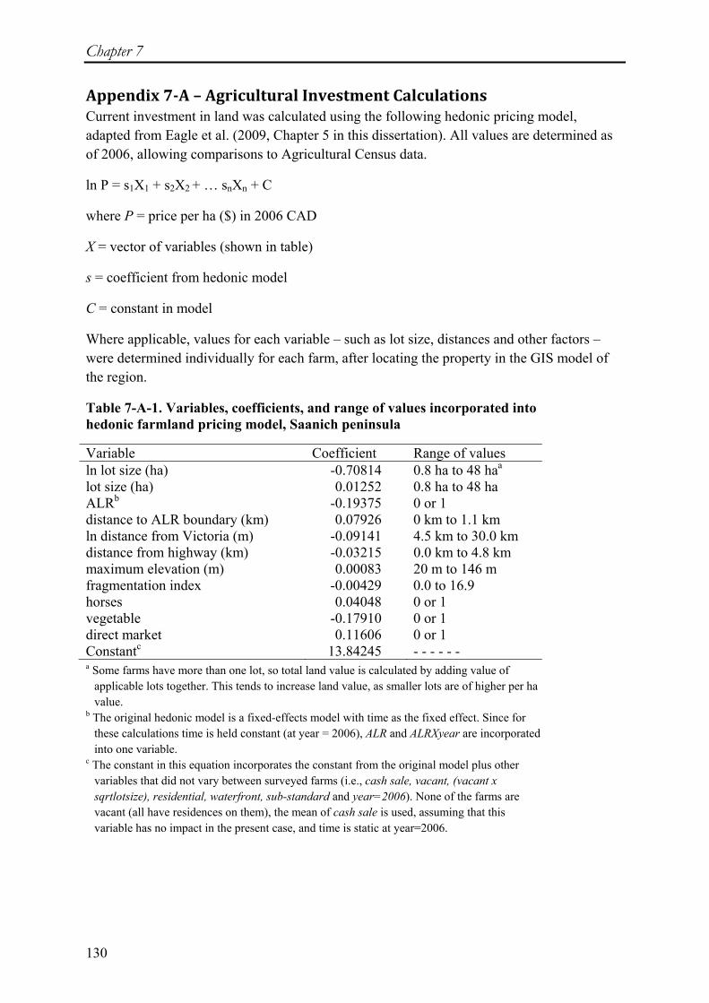
Chapter 7

130

Appendix 7-A – Agricultural Investment Calculations Current investment in land was calculated using the following hedonic pricing model, adapted from Eagle et al. (2009, Chapter 5 in this dissertation). All values are determined as of 2006, allowing comparisons to Agricultural Census data.

ln P = s1X1 + s2X2 + … snXn + C

where P = price per ha ($) in 2006 CAD

X = vector of variables (shown in table)

s = coefficient from hedonic model

C = constant in model

Where applicable, values for each variable – such as lot size, distances and other factors – were determined individually for each farm, after locating the property in the GIS model of the region.

Table 7-A-1. Variables, coefficients, and range of values incorporated into hedonic farmland pricing model, Saanich peninsula

Variable Coefficient Range of values ln lot size (ha) -0.70814 0.8 ha to 48 haa lot size (ha) 0.01252 0.8 ha to 48 ha ALRb -0.19375 0 or 1 distance to ALR boundary (km) 0.07926 0 km to 1.1 km ln distance from Victoria (m) -0.09141 4.5 km to 30.0 km distance from highway (km) -0.03215 0.0 km to 4.8 km maximum elevation (m) 0.00083 20 m to 146 m fragmentation index -0.00429 0.0 to 16.9 horses 0.04048 0 or 1 vegetable -0.17910 0 or 1 direct market 0.11606 0 or 1 Constantc 13.84245 - - - - - - a Some farms have more than one lot, so total land value is calculated by adding value of

applicable lots together. This tends to increase land value, as smaller lots are of higher per ha value.

b The original hedonic model is a fixed-effects model with time as the fixed effect. Since for these calculations time is held constant (at year = 2006), ALR and ALRXyear are incorporated into one variable.

c The constant in this equation incorporates the constant from the original model plus other variables that did not vary between surveyed farms (i.e., cash sale, vacant, (vacant x sqrtlotsize), residential, waterfront, sub-standard and year=2006). None of the farms are vacant (all have residences on them), the mean of cash sale is used, assuming that this variable has no impact in the present case, and time is static at year=2006.

Farming on the urban fringe – The economic impacts of niche and direct marketing strategies

131

Appendix 7-B – Building Replacement Values Building replacement costs (in 2006 CAD) were calculated from construction costs for the different building types as reported by industry and government sources. Average greenhouse replacement value was estimated at $16.50/sq ft (1, 4, 5, 7, 8), refrigeration units at $12.00/cu ft (2, 3) and storage and packing building costs at $20.00/sq ft (6, 9).

1. Etkin, L. 1990. Floriculture in the United States: A Research Agenda [Online]. University of Minnesota. www.maes.umn.edu/mnsci/floriculture.asp (accessed 7 October 2008)

2. Flores, R.A. and K.L.B. Gast. 1992. Postharvest Management of Commercial Horticultural Crops – Storage Construction, Fruits & Vegetables. MF-1039. Cooperative Extension Service, Kansas State University, Manhattan, KS.

3. Foster, K.A., J.C. Klotz, L.K. Clark, D.D. Jones, and A.L. Sutton. 1997. Estimated Costs of Alternative Dead Hog Disposal Methods [Online]. Purdue University. cobweb.ecn.purude.edu/~epados/swine/econ/swineday93.htm (accessed 7 October 2008)

4. Government of Indiana. 2008. Real Property Assessment Guideline, Chapter 7 – Commercial and Industrial Yard Structures [Online]. Department of Local Government Finance, Indiana. www.in.gov/dlgf/files/bk2ch7.pdf (accessed 7 October 2008)

5. Government of Manitoba. 2006. Greenhouse Bedding Plant Production in Manitoba [Online]. Manitoba Agriculture, Food and Rural Initiatives. http://www.gov.mb.ca/agriculture/crops/fruit/blm01s00.html (accessed 6 October 2008)

6. Holtz, B.A., R.A. Duncan, P.S. Verdegaal, K.M. Klonsky and R.L. De Moura. 2002. Sample costs to produce organic almonds - San Joaquin Valley north. University of California Cooperative Extension, Davis, CA.

7. Mirza, M. 2007. Starting a Commercial Greenhouse Business in Alberta [Online]. Alberta Agriculture and Rural Development. www1.agric.gov.ab.ca/$department/deptdocs.nsf/all/opp11207 (accessed 6 October 2008)

8. North Carolina State University. n.d. Selecting Greenhouse Structures [Online]. NC State University. http://legacy.ncsu.edu/classes/hs734001/ppt/pdf/structures.pdf (accessed 9 October 2008);

9. Schmidt, D. n.d. Dead Animal Compost Design [Online]. Biosystems and Agricultural Engineering, University of Minnesota. http://www.manure.umn.edu/applied/assets/FacilityDesign.pdf (accessed 9 October 2008).

133

8. Discussion and Conclusions 8.1 Introduction The general objective of this research was to determine the economic implications of specific environmental and social threats to agricultural production systems at the extensive and intensive margins of land-use in western North America. In these places, where agricultural land use connects with natural and urban land-use needs; societal values of environmental conservation, land-use externalities, and concerns about farmland preservation interact with economic sustainability of present agricultural production systems. In the case studies presented, the threats to agriculture are ones where regional or local decisions have direct impacts on the severity and expression of the problems. This is especially in contrast with other larger-scope or less controllable issues related to global markets or climate. Therefore, the relevant policy decisions tend to be at the municipal and state or provincial level.

The economic framework is suitable, and perhaps the only practical means available for the integration of environmental, social and economic sustainability objectives. At the intensive and extensive margins of land use – agriculture interfacing with urban and natural demands for land – agriculture faces competition for land and other resources, and private land-use decisions have significant impacts on society through externalities and other spillovers. Such multi-functional demands on agricultural land (e.g., agrarian, conservation, landscape) increase the need for institutional refinement and flexibility in order to achieve social objectives and ecosystem resilience (Holling and Meffe, 1996; Oskam and Feng, 2008).

Although the empirical evidence and economic analyses in this dissertation have potential to guide the design of policy, it is important to remember that vested interests also play a significant role in all land use decisions. Inertia maintains considerable barriers to the implementation of change from the status quo. For example, while population pressure plays a significant role in the increased competition for land use at the urban fringe, it is not the only player. Individuals in urban areas are often unwilling to approve densification (including high-rise buildings) in their neighbourhoods, thereby only serving to increase development pressure on nearby agricultural land. Similar vested interests also appear in range management decisions, where ranching communities and ranchers want to keep the status quo because anything else (primarily reduced access to public forage) has a negative impact on their lifestyles. At the same time, ranchers seek to capture rents, as demonstrated by ranchers in California who hope that the government will fund programs to eradicate weeds that negatively affect the productivity of their own range as well as public range.

In this chapter, we review the main outcomes of this research. We start by addressing the economic theory and methods that were key components in the research. Then, for each agricultural system considered here, the findings and implications of our analysis are discussed. This includes interactions with relevant literature, some discussion of deficiencies, and an assessment of where further research would be useful. The chapter concludes by summarizing the contributions made by this research.

Chapter 8

134

8.2 Economic Theory and Methods Social interactions with agricultural production begin in the market, where 98% of the population in Canada and the United States rely almost entirely on the other 2% to provide food and fibre.43 However, since agricultural land use is a significant aspect of human interaction with the earth’s resources, the non-farming population also has a significant interest in the non-market impacts of agriculture. Because public goods or externalities create market failure, judicious public policy is essential to ensure that fiscal and natural resources are allocated in the most effective and equitable manner possible. Compensation of rural landowners for the provision of positive public goods (such as attractive landscapes) has been recently implemented as a more effective and less market (and land-use) distorting means of agricultural policy than were the previously common commodity payments (Baylis et al., 2008). The determination of societal values, such as that done through hedonic or contingent valuation, is useful for estimating the economic contribution of public goods and externalities associated with agricultural land uses (Bergstrom and Ready, 2009). Working in the public interest, policy decision-makers can, for example, observe costs borne by farmers as a result of invasive weeds (Chapter 3) or urban encroachment (Chapter 6) and compare these with the public benefits that are gained by maintaining active agricultural production in the affected region.

Economic modelling and data analysis have been used in this research to provide answers to some of the questions asked by farmers, the public and policy makers when addressing complicated agricultural land use issues. In three of the five research papers, large datasets (most of which are publicly available but difficult to work with) were acquired, compiled, cleaned and assessed to determine inter-relationships between relevant factors that impact wildlife populations, farmland values, and applications to remove land from agricultural zoning status. The other two papers make use of producer surveys to ascertain the economic impacts of an invasive weed on rangeland and the adaptations made by farmers at the urban-rural fringe.

Where relationships between factors formed the research questions, the primary econometric tool is multiple regression analysis, with model adaptations for missing values (Heckman sample selectivity), heteroskedasticity (robust standard errors), autocorrelation (fixed effects model), binomial dependent variables (logit model) and non-linear relationships (logarithmic factor transformations). Full models were compared with restricted ones in all cases to assess and select appropriate regressors. We utilize various technical research tools to create and compare econometric models, analyze spatial relationships within data, and determine the nature of factor impacts on these important public issues.

43 Of course, this is simplified, as international trade also plays a significant role. The point is that only a very small proportion of the population is directly involved in farming. Only 2.2% of Canada’s population was included in farm families/households as of 2006. In 1990 (the latest farm population data available), 1.6% of the total U.S. population was involved in farming.

Discussion and Conclusions

135

8.3 Sage Grouse Population Dynamics in Nevada In Chapter 2, the main research interest was the relationship between sage grouse population dynamics and agriculturally influenced factors in eastern Nevada. In estimating a regression model, all available relevant natural factors were also included, including weather and wildfire. We find that the most important influences on population declines are weather and climate related, with only a small negative impact due to cattle grazing. Concerned citizens and some previous research had suggested that grazing contributes most to population decline (Beck and Mitchell, 2000; Deibert, 2004), but many of these conclusions are based on narrow time-frames or only limited data. This research contributes by incorporating 50 years of population measures into a complex regression analysis. Accordingly, we increase the potential for considering numerous interactions in the system, with the goal of contributing to ecosystem resilience as discussed in detail by Holling and Meffe (1996).

Since there is little available information about sage grouse predator dynamics, there is some possibility that the specified model excluded important biophysical relationships, resulting in mis-specification of the model as presented. However, while sage grouse are the prey of interest, there are many interactions between multiple predators of the sage grouse. For example, coyotes are sage grouse predators, and they also prey on other sage grouse predators (i.e., foxes, ravens) (Mezquida et al., 2006). Therefore, although only a small amount of predator data were available for inclusion in our model, further details may not have contributed much additional knowledge, even if they could have been obtained.

Social wellbeing is enhanced by conservation action and success – of the sage grouse and other threatened or endangered species. Our research shows that changes to policy that reduce public grazing permits will not likely meet this societal demand, since the relationship between sage grouse population numbers and grazing pressure is only statistically significant (and negative) in one of the three models. In fact, public funds earmarked for conservation may be more effectively utilized by sponsoring further study of the ways that sage grouse can increase resilience in the face of adverse climatic conditions. This is one area where further research could be helpful. It is important to note that these results are specific to one region in Nevada, and system interactions may vary among other ecosystems that support sage grouse populations.

Further decreases in public grazing allotments could also negatively affect the ranching economy and community. The conclusions from this research mark a shift from the assumptions that ranching activity is to blame for sage grouse decline, and consequently, ranchers could become less likely to be accused of rangeland damage. In order to keep this tenuous positive reputation, ranchers will need to show their willingness to be good stewards of the public land resource. In this case, as in many others, communication and social capital are very important, just as in land use issues at the urban fringe (Sharp and Smith, 2003).

8.4 Yellow Starthistle Infestation in California In Chapter 3, we find that statewide damages due to YST amount to $17 million dollars every year in the ranching sector alone. While broad studies such as those by Pimentel et al. (2005;

Chapter 8

136

2000) alert the general public and policy makers to the severity of the issues of invasive weeds, assessments of specific weed damages are essential to determine appropriate control efforts. To this end, the California Department of Food and Agriculture sponsored the research because they suspected high levels of economic damages, but needed proof to convince the state government to allocate funds for YST control (and possibly eradication in some areas). The results from this research have been used by policy analysts in the California government to argue that this invasive weed causes significant damage to the state’s agricultural economy and to natural ecosystems.

Since economic costs and damages are now better understood as a result of this research, the next public decision step is to determine optimal management strategies for YST. Previous studies have developed bio-economic models of invasive weed control that incorporate efficacy and costs of control methods, spillover impacts on native species, and various other interactions within the ecological system (Eiswerth and van Kooten, 2002) (Haghighi, 2009). These models both used stochastic dynamic approaches to show that even where there is significant uncertainty as to the impact of a pest or the impact of a control strategy, optimal control strategies can still be determined. Such research can be significantly strengthened by the calculations of economic damages and costs developed in this current work.

As in this case, it can be socially desirable to maintain economic and ecological stability in rural communities. These communities often serve as public resource managers (land, water, air quality, forest resources, recreation) and have significant impacts on public goods. Government-supported weed control efforts can prevent further ecological damages, and minimize costs to the society at large that are related to negative YST impacts on water resources and recreation uses. Therefore, when combined with the damages borne by the agricultural production system (as measured by our research), these societal values add further impetus to public YST control efforts and expenditures. Future impacts of control efforts versus no control also play a role in the decision. In fact, the ranchers themselves spend more on control than they experience in losses with respect to forage value, suggesting that they place a high value on the protection of future productivity.

8.5 Urban-Fringe Agriculture in British Columbia In Chapters 5, 6 and 7, the research focus moves from the extensive margin to the intensive margin of land-use. While agricultural production faces significant challenges at the urban fringe in British Columbia, we find that BC’s Agricultural Land Reserve has successfully decreased farmland values (and thus costs of production) by removing development rights from property within the ALR zone. This impact demonstrated an observable change over the 35-year time period, suggesting that the value of development rights increased over time, or that original land-owners did not seem to lose the entire development value immediately. Therefore, this “taking” of development rights that applied to all agricultural land in the province may not have been as negative for farmers as some have thought (Garrish, 2003; Hanna, 1997). The possibilities for some adjustments in boundaries, especially during the early years, could also have served as a moderating influence.

Discussion and Conclusions

137

8.5.1 The ALR as a Farmland Conservation Technique In the past, various farmland conservation techniques have been contrasted with one another in theory and practice, posing questions of effectiveness, cost to the public, and social wellbeing (Conklin and Lesher, 1977; Duke and Lynch, 2006; Kline and Wichelns, 1996; Lynch and Musser, 2001; Machado et al., 2006). Some researchers have investigated the impacts of zoning and other conservation techniques on land prices, although many of these have been voluntary (Nickerson and Lynch, 2001), applicable to small regions (Henneberry and Barrows, 1990) or only over a short period of time (Vaillancourt and Monty, 1985). Therefore, this research provides a unique contribution to the literature with a long-term (35 year) examination of the farmland price impacts of wide-ranging, non-voluntary farmland conservation zoning at the urban fringe. For the hedonic price model, we also incorporate spatial variables that are made possible with recent developments in GIS technology (i.e. fragmentation index, multiple distance variables, elevation and slope).

As Duke and Lynch articulate in their summary of farmland conservation methods, “Effective techniques better coordinate landowners’ expectations” (Duke and Lynch, 2006, p. 191). Our research indicates that the ALR is indeed effective, with many expectations of development removed, as is evidenced by lower land prices for protected land (Chapter 5), even though the removal of development rights was not associated with direct compensation to landowners. It is likely that these changes in expectation have taken some time to fully materialize, as we see significant shifts over time in the land price differential. Would participatory methods be more effective, where development rights are instead purchased? They indeed carry a greater initial public cost burden, require significant coordination to prioritize conservation areas, and can only protect limited area (Machado et al., 2006). However, such conservation measures may be strengthened by the removal of all development expectations, and little incentive for variance requests.

By restricting development and reducing land prices (the major capital investment for agriculture), the ALR policy prevents urban sprawl and provides more open space and related ecological services, than would be provided without the intervention. This achieves publicly expressed goals related to farmland conservation (Kline and Wichelns, 1996; Machado et al., 2006), although it remains an empirical question whether active local agriculture (with existence value) and attractive agricultural landscapes are positively impacted or whether the lower land prices provide greater support to non-agricultural uses (e.g., parks and rural residential). From a societal point of view, such land-use changes to parks or natural habitat may be more desirable, providing more environmental or amenity benefits than active agriculture (Hardie et al., 2004).

8.5.2 Urban and Residential Influences As discussed by Hardie et al. (2004, p. 105) with respect to land at the intensive margin in general, there is still an observable dominance of urban land use, which is evident in the degree of farmland fragmentation, especially nearer to the central business district of Victoria. Therefore, although farmers do have reduced land investment costs, they may also have more competition for that land from urban residents who desire to purchase acreages for residential purposes. These demanders of urban land services are willing to pay a high price

Chapter 8

138

for land, and so claim significant areas otherwise intended for agricultural purposes. As a result, rural residential landowners benefit from public policies that are intended for agricultural preservation.

In this research, there is much evidence that residential functions impact the farmland market (Chapter 5). Property tax assessments that favour agricultural land over residential property inadvertently also encourage hobby farm use as the thresholds on farm production to acquire farm status (and much reduced taxes) are set low in order to encourage farming and prevent landowners from arguing that their sales are too low to justify retaining land in agricultural production. However, hobby farms are associated with residential use of land; that is, lower tax rates for farm-status and low thresholds to qualify for farm status encourage the use of farmland for residences, leading to low-density “rurban” sprawl. Although the professed goal of the ALR is to preserve land for agriculture (Agricultural Land Commission, 2006), at the current time the reserve is supporting much open space through parks and large lot development. In future research, an appropriate valuation of different public goods would serve as a useful guide for policy that determines whether the current state of land use is socially optimal.

The research in Chapters 5 and 7 also demonstrates that there exist significant negative externalities imposed on farmers near non-farming neighbours. Using the hedonic model, we show that farmland value is significantly increased when farmland is situated farther within a farmland block and with more outside perimeter joined to other farms. Survey data summarized in Chapter 7 indicate an average annual time and monetary cost of 220 hrs and $5900 for conflict prevention and resolution. These negative externalities further reduce the provision of agricultural products and cause land use to deviate even more from the social optimum. Beginning with the data already collected on farmer expenditures with respect to dispute prevention and resolution, further research could investigate the costs that are associated with farm/non-farm disputes, for example those that are brought to the Farm Practices Review Board in BC. There are also opportunities to explore how edge/buffer planning reduces costs borne by farmers and increases the value of a development. If land values are positively affected by edge/buffer planning, the municipality wins by gaining tax revenue and happier citizens (social capital).

8.5.3 Durability of the Agricultural Land Reserve When wide-ranging, restrictive farmland preservation schemes such as the ALR are instituted, option values for development are taken from the landowners rather than purchased (unless there is provision for compensation through a transferable development rights scheme or some other means). Farmland conservation programs that remove development rights from land ownership will only achieve full impact and success if the zoning or easement policy is viewed as solid and irrevocable. Because there were very significant differences in price between land within and outside the ALR (Chapter 5), the results from this research indicate that the ALR demonstrates significant strength in keeping land within the agricultural zone. Thus, the measured development option value is likely to be more reliable than in situations where zoning changes are more readily attained. The main complicating factor is the increasing prevalence of hobby farms and rural estates, which

Discussion and Conclusions

139

distorts the development option value by utilizing land for a non-agricultural purpose while still remaining within the agricultural zone.

Location, size and the political environment impact re-zoning application success. In addition, the examination of re-zoning proposals indicated that applications for ALR exclusion are more likely to be approved over time (Chapter 6). This latter fact may be a result of more stringent selection processes at the municipal level, before even going to the final decision maker – the Agricultural Land Commission – so that proposed exclusions are, on average, less agriculturally important than those in earlier years. Even so, the fact that time impacted the success of exclusion applications evokes questions about the viability and longevity of the ALR. Is public support now and in the future sufficient to prevent whole-scale dismantling of the system through legislative action?

8.5.4 Farm Adaptations at the Urban Fringe In Chapter 7, we find evidence that direct-marketing farmers near Victoria could have more long-term resilience than typical farmers in the region. There is also a high proportion of certified organic growers, and most others reported significant use of other environmentally conserving farming practices. As well, those with higher production intensity rates (gross income per unit of land) are able to rely less on off-farm income, demonstrating a measure of greater success in the farming enterprise. Higher productivity is associated with recent farm investment, greater crop diversity, intensification through greenhouse or nursery production, and rented farmland. This difference between rented versus owned land suggests that landowners and renters differ in their incentives to put effort into increasing production from a set unit of land.

8.6 Final Remarks and Future Research The research presented in this dissertation provides insights into the implications of government intervention in agricultural land-use decisions at the extensive and intensive margins of land use. Where socially optimum levels of wildlife habitat, weed control, and productive agricultural land cannot (or will not) be met in the free market, appropriate policy corrects the market failure. Policy makers need clear and informative models in order to understand relationships between relevant factors and make knowledgeable decisions. While assumptions or circumstantial evidence may be useful, they are often not specific enough to guide decisions about allocation, zoning or levels of taxation. With models that use current economic and statistical data, results from this research can be used to inform policy makers, urban planners and other stakeholders about issues related to endangered species, public support for weed control, and farmland conservation.

Future research could answer some of the questions raised in the discussions of results. Clarification of answers to the questions posed at the extensive margin will rely on modelling of biological interactions as well as economic costs and benefits to human interference in the systems. For example, extensions of the previously developed bio-economic models (Eiswerth and Johnson, 2002; Eiswerth and van Kooten, 2002; Haghighi, 2009) with updated

Chapter 8

140

biological information and the economic results from this paper would be useful for policy analysis.

With a significant amount of public attention currently directed to local agricultural systems, urban agriculture, and agriculture at the urban fringe; further research into increased social wellbeing that results from agricultural production and open space is well warranted. The effectiveness and functionality of the ALR are common topics of discussion in BC public policy. Extension of the current research to additional regions in BC would benefit through the addition of more observations, as well as the potential to contrast and compare relevant factors in different regions. Such an effort could provide useful information to decision-makers, who would then have indications of the relative economic impacts of strengthening the ALR zoning, encouraging active agriculture or creating buffer zones between urban and rural land uses.

The GIS analysis provided important spatial information for both the hedonic price model (Chapter 5) and the logistical regression of ALR exclusion applications (Chapter 6). With much of the base model and data management techniques in place, the value in these resources would be well utilized by extending the GIS model to additional regions. The Ministry of Agriculture and Lands has already completed Land Use Inventories for at least six other municipalities with significant urban-rural interactions. A logical first extension would be to Abbotsford, since the GIS map is already established, including links to the LUI for that region. Land sales and characteristics would need to be obtained and fragmentation indices calculated, along with significant data cleaning, both for the sales dataset and the GIS parcel-level layers.

Because the survey was conducted in-person and effort was made to respect and value their contributions, farmers responded favourably to requests for participation and shared detailed data regarding their finances, economic survival and success. Further research that focuses on direct-marketing farmers could expand the current knowledge base related to ecological interactions and farm level decisions as impacted by agri-environmental policy. If these farm actions enhance economic and environmental resilience, they would benefit the farming community and increase social wellbeing in general.

Public policy related to agricultural land use intersections with demands for natural or urban land uses is necessary to correct market failure, as a result of externalities and public goods. While the decisions may be politically charged and complex, an improved understanding of the economic implications is essential to determine impacts on private landowners and the public. It is in this context that the current research provides an important contribution.

141

References Abbott, C., S. Adler and D. Howe. 2003. A quiet counterrevolution in land use regulation:

The origins and impact of Oregon's Measure 7. Housing Policy Debate 14:383–425. Acs, S., P.B.M. Berentsen, M. de Wolf and R.B.M. Huirne. 2007. Comparison of

conventional and organic arable farming systems in the Netherlands by means of bio-economic modelling. Biological Agriculture & Horticulture 24:341–61.

Agricultural Land Commission. 2005. 2004/05 Annual Service Plan Report. Government of British Columbia, Victoria, BC.

Agricultural Land Commission. 2006. Preserving our Foodlands. [Online]. Agricultural Land Commission. http://www.alc.gov.bc.ca/publications/preserve/preserve-print.htm (verified 24 January 2006).

Agricultural Land Commission. 2009. ALR Statistics. [Online]. Agricultural Land Commission. http://www.alc.gov.bc.ca/alr/stats/Statistics_TOC.htm (verified March 16 2009).

Aldridge, C.L. and R.M. Brigham. 2003. Distribution, abundance, and status of the Greater Sage-Grouse, Centrocercus urophasianus, in Canada. Canadian Field-Naturalist 117:25–34.

Anderson, J.E. 1993. Use-value property tax assessment: Effects on land development. Land Economics 69:263–9.

Anselin, L. 2001. Spatial econometrics, p. 310–330. In B. H. Baltagi, ed. A Companion to Theoretical Econometrics. Blackwell Publishers Ltd., Malden, MA and Oxford, UK.

Barichello, R.R., R.M. Porter and G.C. van Kooten. 1995. Institutions, economic incentives and sustainable rural land use in British Columbia., p. 7–53. In A. Scott, J. Robinson and D. Cohen, eds. Managing Natural Resources in British Columbia. Markets, Regulations, and Sustainable Development. UBC Press, Vancouver.

Barry, S. 1995. Cattle fecal fax. October Report, 7 November 1995. University of California Cooperative Extension Newsletter. Glenn County University of California Cooperative Extension Office, Orland, CA.

Batte, M.T., D.L. Forster and F.J. Hitzhusen. 1993. Organic agriculture in Ohio – an economic perspective. Journal of Production Agriculture 6:536–42.

Baum, C.F. 2006. An Introduction to Modern Econometrics Using Stata. Stata Press, College Station, TX.

Baumol, W.J. 1968. Social rate of discount. American Economic Review 58:788–802. Baylis, K., S. Peplow, G.C. Rausser and L.K. Simon. 2008. Agri-environmental policies in

the EU and United States: A comparison. Ecological Economics 65:753–764. BC Ministry of Agriculture, Food and Fisheries. 2004. AgFocus – A Guide to Agricultural

Land Use Inventory. BC Ministry of Agriculture Food and Fisheries, Resource Management Branch, Abbotsford, BC.

BC Ministry of Small Business and Revenue. 2007. Small Business Profile 2007. BC Ministry of Small Business and Revenue, Victoria, BC.

Beauchesne, A. and C. Bryant. 1999. Agriculture and innovation in the urban fringe: The case of organic farming in Quebec, Canada. Tijdschrift Voor Economische en Sociale Geografie 90:320–8.

Beaulieu, S. and L. DiPiétro. 2003. Canadian farm families more dependent on off-farm income. Vista on the Agri-Food Industry and the Farm Community. Statistics Canada, Ottawa.

Beck, J.L. and D.L. Mitchell. 2000. Influences of livestock grazing on sage grouse habitat. Wildlife Society Bulletin 28:993–1002.

References

142

Beck, J.L., D.L. Mitchell and B.D. Maxfield. 2003. Changes in the distribution and status of sage-grouse in Utah. Western North American Naturalist 63:203–14.

Bengtsson, J., J. Ahnstrom and A.C. Weibull. 2005. The effects of organic agriculture on biodiversity and abundance: a meta-analysis. Journal of Applied Ecology 42:261–9.

Bergstrom, J.C. and R.C. Ready. 2009. What Have We Learned from Over 20 Years of Farmland Amenity Valuation Research in North America? Review of Agricultural Economics 31:21–49.

Berry, D. 1978. Effects of Urbanization on Agricultural Activities. Growth and Change 9:2–8.

Blewett, R.A. and J.I. Lane. 1988. Development rights and the differential assessment of agricultural land: Fractional valuation of farmland is ineffective for preserving open space and subsidizes speculation. American Journal of Economics and Sociology 47:195–205.

Born, B. and M. Purcell. 2006. Avoiding the local trap – Scale and food systems in planning research. Journal of Planning Education and Research 26:195–207.

Brabec, E. and C. Smith. 2002. Agricultural land fragmentation: the spatial effects of three land protection strategies in the eastern United States. Landscape and Urban Planning 58:255–8.

Braun, C.E. and T.D.I. Beck. 1996. Effects of research on sage grouse management. Paper presented at Transactions of the North American Wildlife and Natural Resources Conference, Tulsa, OK. 22–27 March.

Brueckner, J.K. 2000. Urban sprawl: Diagnosis and remedies. International Regional Science Review 23:160–71.

Brundtland, G.H., M. Khalid, S. Agnelli, S.A. Al-Athel, B. Chidzero, L.M. Fadika and V. Hauff. 1987. Our Common Future: World Commission on Environment and Development. Oxford University Press, Oxford and New York.

Bureau of Land Management (BLM). 2000. Management guidelines for sage grouse and sagebrush ecosystems in Nevada. Bureau of Land Management, Department of the Interior, Carson City, NV.

California Agricultural Statistics Service (CASS). 2001. County agricultural commissioners’ data, 2001. California Department of Food and Agriculture, Agricultural Statistics Branch, Sacramento, CA.

Callihan, R.H., T.S. Prather and F.E. Northam. 1993. Longevity of yellow starthistle (Centaurea solstitialis) achenes in soil. Weed Technology 7:33–5.

Campbell, C. 2006. Forever Farmland: Reshaping the Agricultural Land Reserve for the 21st Century. David Suzuki Foundation, Vancouver, BC.

Canadian Cooperative Association. 2007. Local Food Initiatives in Canada – An Overview and Policy Recommendations. Canadian Cooperative Association, Ottawa, ON.

Cho, S.-H., J.M. Bowker and W.M. Park. 2006. Measuring the contribution of water and green space amenities to housing values: An application and comparison of spatially weighted hedonic models. Journal of Agricultural and Resource Economics 31:485–507.

Clifford, H. 2002. Last dance for the sage grouse? High Country News 34(2). Conklin, H.E. and W.G. Lesher. 1977. Farm-value assessments as a means for reducing

premature and excessive agricultural disinvestment in urban fringes. American Journal of Agricultural Economics 59:755–9.

Connelly, J.W., W.L. Wakkinen, A.D. Apa and K.P. Reese. 1991. Sage grouse use of nest sites in Southeastern Idaho. Journal of Wildlife Management 55:521–4.

Connelly, J.W., M.A. Schroeder, A.R. Sands and C.E. Braun. 2000. Guidelines to manage sage grouse populations and their habitats. Wildlife Society Bulletin 28:967–85.

References

143

Connelly, J.W., K.P. Reese, E.O. Garton and M.L. Commons-Kemner. 2003. Response of greater sage-grouse Centrocercus urophasianus populations to different levels of exploitation in Idaho, USA. Wildlife Biology 9:335–40.

Connelly, J.W., S.T. Knick, M.A. Schroeder and S.J. Stiver. 2004. Conservation assessment of greater sage-grouse and sagebrush habitats. (Unpublished report). Western Association of Fish and Wildlife Agencies, Cheyenne, WY.

Cordy, D.R. 1978. Centaurea species and equine nigropallidal encephalomalacia, p. 327–36. In R. F. Keeler, K. R. Van Kampen and L. F. James, eds. Effects of poisonous plants on livestock. Academic Press, New York, NY.

Cotteleer, G. 2008. Valuation of land use in the Netherlands and British Columbia; A spatial hedonic GIS-based approach. PhD dissertation, Wageningen University, Wageningen, the Netherlands.

Cotteleer, G., C. Gardebroek and J. Luijt. 2008. Market power in a GIS-based hedonic price model of local farmland markets. Land Economics 84:573–92.

Cotteleer, G., T.E. Stobbe and G.C. van Kooten. 2009. Farmland conservation in the Netherlands and British Columbia, Canada: A comparative analysis using GIS-based hedonic pricing models, In F. Brouwer and C. M. van der Heide, eds. Multifunctional Rural Land Management – Economics and Policies. Earthscan, London.

Crawford, J.A., R.A. Olson, N.E. West, J.C. Mosley, M.A. Schroeder, T.D. Whitson, R.F. Miller, M.A. Gregg and C.S. Boyd. 2004. Synthesis Paper – Ecology and management of sage-grouse and sage-grouse habitat. Journal of Range Management 57:2–19.

Curran, D. 2005. Protecting the working landscape of agriculture: A smart growth direction for municipalities in British Columbia. West Coast Environmental Law, Vancouver, BC.

Curtis, F. 2003. Eco-localism and sustainability. Ecological Economics 46:83–102. D'Antonio, C.M. and P.M. Vitousek. 1992. Biological invasions by exotic grasses, the

grass/fire cycle, and global change. Annual Review of Ecology and Systematics 23:69–87.

Darby, K., M.T. Batte, S. Ernst and B. Roe. 2008. Decomposing local: a conjoint analysis of locally produced foods. American Journal of Agricultural Economics 90:476–86.

Darmon, N. and A. Drewnowski. 2008. Does social class predict diet quality? American Journal of Clinical Nutrition 87:1107–17.

Deibert, P. 2004. Endangered and threatened wildlife and plants; 90-day finding for petitions to list the greater sage-grouse as threatened or endangered. Federal Register Proposed Rules, Vol. 69, No. 77, 21 April 2004. Fish and Wildlife Service, Department of the Interior, Cheyenne, WY.

Dideriksen, R. 1976. Potential cropland: A regional view. Soil Conservation 42:5–9. DiTomaso, J.M. 2007. Yellow starthistle information. [Online]. University of California,

Davis. http://wric.ucdavis.edu/yst/yst.html (verified 26 March 2007). DiTomaso, J.M. and J.D. Gerlach. 2000. Centaurea solstitialis L, p. 101–06. In C. C. Bossard,

J. M. Randall and M. C. Hoshovsky, eds. Invasive plants of California’s wildlands. University of California Press, Berkeley, CA.

DiTomaso, J.M., G.B. Kyser, S.B. Orloff and S.F. Enloe. 2000. Integrated strategies offer site-specific control of yellow starthistle. California Agriculture 54:30–6.

Drozd, D.J. and B.B. Johnson. 2004. Dynamics of a rural land market experiencing farmland conversion to acreages: the case of Saunders County, Nebraska. Land Economics 80:294–311.

Duke, J.M. and L. Lynch. 2006. Farmland retention techniques: Property rights implications and comparative evaluation. Land Economics 82:189–213.

References

144

Duncan, C.A., J.J. Jachetta, M.L. Brown, V.F. Carrithers, J.K. Clark, J.M. Ditomaso, R.G. Lym, K.C. McDaniel, M.J. Renz and P.M. Rice. 2004. Assessing the economic, environmental, and societal losses from invasive plants on rangeland and wildlands. Weed Technology 18:1411–16.

DuPuis, E.M. and D. Goodman. 2005. Should we go "home" to eat?: toward a reflexive politics of localism. Journal of Rural Studies 21:359–71.

Eaton, E. 2008. From feeding the locals to selling the locale: Adapting local sustainable food projects in Niagara to neocommunitarianism and neoliberalism. Geoforum 39:994–1006.

Edwards-Jones, G., L.M.i. Canals, N. Hounsome, M. Truninger, G. Koerber, B. Hounsome, P. Cross, E.H. York, A. Hospido, K. Plassmann, I.M. Harris, R.T. Edwards, G.A.S. Day, A.D. Tomos, S.J. Cowell and D.L. Jones. 2008. Testing the assertion that 'local food is best': the challenges of an evidence-based approach. Trends in Food Science & Technology 19:265–74.

Eiswerth, M.E. and W.S. Johnson. 2002. Managing Nonindigenous Invasive Species: Insights from Dynamic Analysis. Environmental and Resource Economics 23:319–42.

Eiswerth, M.E. and G.C. van Kooten. 2002. Uncertainty, economics, and the spread of an invasive plant species. American Journal of Agricultural Economics 84:1317–22.

Eiswerth, M.E., G.C. van Kooten and J.M. Lines. 2006. Dynamic programming and learning models for management of a nonnative species. University of Victoria, Working Paper, Victoria, BC.

Elad, R.L., I.D. Clifton and J.E. Epperson. 1994. Hedonic estimation applied to the farmland market in Georgia. Journal of Agricultural and Applied Economics 26:351–66.

Frederiksen, P. and V. Langer. 2004. Localisation and concentration of organic farming in the 1990s – The Danish case. Tijdschrift Voor Economische en Sociale Geografie 95:539–49.

Gardebroek, C. 2006. Comparing risk attitudes of organic and non-organic farmers with a Bayesian random coefficient model. European Review of Agricultural Economics 33:485–510.

Garrish, C.J. 2003. Unscrambling the omelette: Understanding British Columbia's Agricultural Land Reserve. BC Studies Issue 136:25–55.

Geoghegan, J. 2002. The value of open spaces in residential land use. Land Use Policy 19:91–8.

Gerlach, J.D., Jr. 2004. The impacts of serial land-use changes and biological invasions on soil water resources in California, USA. Journal of Arid Environments 57:365–79.

Glover, J.D., J.P. Reganold and P.K. Andrews. 2000. Systematic method for rating soil quality of conventional, organic, and integrated apple orchards in Washington State. Agriculture Ecosystems & Environment 80:29–45.

Gosling, P. and M. Shepherd. 2005. Long-term changes in soil fertility in organic arable farming systems in England, with particular reference to phosphorus and potassium. Agriculture, Ecosystems and Environment 105:425–32.

Government of Canada. 2008. News Release: Government Announces the New Product of Canada Food Labelling Guidelines Take Effect December 31.

Green, R. 2006. Case Studies of Agricultural Land Commission Decisions: The Need for Inquiry and Reform. Environmental Law Clinic, University of Victoria, Victoria, BC.

Greene, W.H. 2000. Econometric analysis. 4th ed. Prentice Hall, Upper Saddle River, NJ. Gregg, M.A., J.A. Crawford, M.S. Drut and A.K. DeLong. 1994. Vegetational cover and

predation of sage grouse nests in Oregon. Journal of Wildlife Management 58:162–6. Groom, B., C. Hepburn, P. Koundouri and D. Pearce. 2005. Declining discount rates: The

long and the short of it. Environmental & Resource Economics 32:445–93.

References

145

Gujarati, D.N. 1995. Basic Econometrics. 3rd ed. McGraw-Hill, Inc., Toronto. Haghighi, M.C. 2009. Economics of controlling invasive species: The case of Californian

thistle in New Zealand. PhD dissertation, Wageningen University, Wageningen, The Netherlands.

Hanna, K.S. 1997. Regulation and land-use conservation: A case study of the British Columbia Agricultural Land Reserve. Journal of Soil and Water Conservation 52:166–70.

Hardie, I.W., P.J. Parks and G.C. van Kooten. 2004. Land use decisions and policy at the intensive and extensive margins, p. 101–38. In T. Tietenberg and H. Folmer, eds. The International Yearbook of Environmental and Resource Economics 2004/2005: A Survey of Current Issues. Edward Elgar, Cheltenham, UK and Northampton, MA, USA.

Hartmans, M.A., H. Zhang and E.L. Michalson. 1997. The costs of yellow starthistle management. Cooperative Extension Bulletin 793. University of Idaho, Agricultural Experiment Station, Moscow, ID.

Henneberry, D.M. and R.L. Barrows. 1990. Capitalization of exclusive agricultural zoning into farmland prices. Land Economics 66:249–58.

Herman, D.R., G.G. Harrison, A.A. Afifi and E. Jenks. 2008. Effect of a targeted subsidy on intake of fruits and vegetables among low-income women in the special supplemental nutrition program for women, infants, and children. American Journal of Public Health 98:98–105.

Hirsch, S.A. and J.A. Leitch. 1996. The impact of knapweed on Montana’s economy. Agricultural Economics Report No. 355. North Dakota State University, Agricultural Experiment Station, Fargo, ND.

Hoeppner, J.W., M.H. Entz, B.G. McConkey, R.P. Zentner and C.N. Nagy. 2005. Energy use and efficiency in two Canadian organic and conventional crop production systems. Renewable Agriculture & Food Systems 21:60–7.

Holling, C.S. and G.K. Meffe. 1996. Command and control and the pathology of natural resource management. Conservation Biology 10:328–37.

Huang, H., G.Y. Miller, B.J. Sherrick and M.I. Gomez. 2006. Factors influencing Illinois farmland values. American Journal of Agricultural Economics 88:458–70.

Ipsos-Reid. 2007. Canadians' Attitudes Towards Food and Farming. Ipsos-Reid: Agribusiness, Food and Animal Health.

Isgin, T. and D.L. Forster. 2006. A hedonic price analysis of farmland option premiums under urban influences. Canadian Journal of Agricultural Economics 54:327–40.

Jarosz, L. 2008. The city in the country: Growing alternative food networks in Metropolitan areas. Journal of Rural Studies 24:231–44.

Jetter, K.M., J.M. DiTomaso, D.J. Drake, K.M. Klonsky, M.J. Pitcairn and D.A. Sumner. 2003. Biological control of Yellow Starthistle, In D. A. Sumner, ed. Exotic Pests and Diseases: Biology and Economics for Biosecurity. Wiley-Blackwell, Ames, IA.

Johnson, K.H. and C.E. Braun. 1999. Viability and conservation of an exploited sage grouse population. Conservation Biology 13:77–84.

Kennedy, G.A., S.A. Henning, L.R. Vandeveer and M. Dai. 1997. An empirical analysis of the Louisiana rural land market. Louisiana State University, Department of Agricultural Economics and Agribusiness.

Kjelland, M.E., U.P. Kreuter, G.A. Clendenin, R.N. Wilkins, X. Ben Wu, E.G. Afanador and W.E. Grant. 2007. Factors related to spatial patterns of rural land fragmentation in Texas. Environmental Management 40:231–44.

Kline, J.D. 2005. Forest and farmland conservation effects of Oregon's (USA) land-use planning program. Environmental Management 35:368–80.

References

146

Kline, J.D. and D. Wichelns. 1996. Public Preferences Regarding the Goals of Farmland Preservation Programs. Land Economics 72:538–49.

Kyser, G.B. and J.M. DiTomaso. 2002. Instability in a grassland community after the control of yellow starthistle (Centaurea solstitialis) with prescribed burning. Weed Science 50:648–57.

Lass, L.W., J.P. McCaffrey, D.C. Thill and R.H. Callihan. 1999. Yellow starthistle: biology and management in pasture and rangeland. Cooperative Extension Bulletin 805. University of Idaho, Moscow, ID.

Lazaruk, S. 2008. World-class housing prices in B.C. The Province. 30 January:A3. Leistritz, F.L., F. Thompson and J.A. Leitch. 1992. Economic-Impact of Leafy Spurge

(Euphorbia-Esula) in North-Dakota. Weed Science 40:275–80. Leitch, J.A., F.L. Leistritz and D.A. Bangsund. 1996. Economic effect of leafy spurge in the

upper great plains: methods, models and results. Impact Assessment 14:419–33. Libby, L.W. and J.S. Sharp. 2003. Land-use compatibility, change, and policy at the rural-

urban fringe: Insights from social capital. American Journal of Agricultural Economics 85:1194–200.

Lisansky, J. and G. Clark. 1987. Farmer-nonfarmer conflicts in the urban fringe: will right-to-farm help?, In W. Lockeretz, ed. Sustaining Agriculture Near Cities. Soil and Water Conservation Society, Ankeny, IA.

Lohr, L. and L. Salomonsson. 2000. Conversion subsidies for organic production: results from Sweden and lessons for the United States. Agricultural Economics 22:133-146.

Lynch, L. and W.N. Musser. 2001. A Relative Efficiency Analysis of Farmland Preservation Programs. Land Economics 77:577–94.

Machado, E.A., D.M. Stoms, F.W. Davis and J. Kreitler. 2006. Prioritizing farmland preservation cost-effectively for multiple objectives. Journal of Soil and Water Conservation 61:250–8.

Maddox, D.M. and A. Mayfield. 1985. Yellow starthistle infestations are on the increase. California Agriculture 39:10–2.

Marin, M.C. 2007. Impacts of urban growth boundary versus exclusive farm use zoning on agricultural land uses. Urban Affairs Review 43:199–220.

Meert, H., G. Van Huylenbroeck, T. Vernimmen, M. Bourgeois and E. van Hecke. 2005. Farm household survival strategies and diversification on marginal farms. Journal of Rural Studies 21:81–97.

Mezquida, E.T., S.J. Slater and C.W. Benkman. 2006. Sage-Grouse and indirect interactions: Potential implications of coyote control on Sage-Grouse populations. Condor 108:747-759.

Neel, L.A. 2001. Nevada Sage Grouse Conservation Strategy. Final report of the Governor's Sage Grouse Conservation Team. Office of the Governor, State of Nevada, Carson City, NV.

Nelson, A.C. 1992. Preserving prime farmland in the face of urbanization – Lessons from Oregon. Journal of the American Planning Association 58:467–88.

Nelson, A.C. 1999. Comparing states with and without growth management – Analysis based on indicators with policy implications. Land Use Policy 16:121-127.

Nevada Natural Heritage Program. 2004. Sensitive animal list. [Online]. http://heritage.nv.gov/sensanim.htm (verified 30 April 2004).

Nickerson, C.J. and L. Lynch. 2001. The effect of farmland preservation programs on farmland prices. American Journal of Agricultural Economics 83:341–51.

Oskam, A.J. and S. Feng. 2008. Sustainable land use under different institutional settings. NJAS Wageningen Journal of Life Sciences 55:295–306.

References

147

Pedersen, E.K., J.W. Connelly, J.R. Hendrickson and W.E. Grant. 2003. Effect of sheep grazing and fire on sage grouse populations in southeastern Idaho. Ecological Modelling 165:23–47.

Penner, D. 2008. Land prices outstrip economics of farming. Vancouver Sun. 24 May 2008. Pimentel, D., R. Zuniga and D. Morrison. 2005. Update on the environmental and economic

costs associated with alien-invasive species in the United States. Ecological Economics 52:273–88.

Pimentel, D., L. Lach, R. Zuniga and D. Morrison. 2000. Environmental and economic costs of nonindigenous species in the United States. BioScience 50:53–65.

Pitcairn, M.J., S. Schoenig, J. Gendron, R. Yacoub and R. O'Connell. 2004. Yellow starthistle infestations are still increasing, in preparation for California Agriculture, Sacramento, CA.

Plantinga, A.J. and D.J. Miller. 2001. Agricultural land values and the value of rights to future land development. Land Economics 77:56–67.

Poudel, D.D., W.R. Horwath, W.T. Lanini, S.R. Temple and A.H.C. van Bruggen. 2002. Comparison of soil N availability and leaching potential, crop yields and weeds in organic, low-input and conventional farming systems in northern California. Agriculture, Ecosystems and Environment 90:125–37.

Pretty, J.N., A.S. Ball, T. Lang and J.I.L. Morison. 2005. Farm costs and food miles: An assessment of the full cost of the UK weekly food basket. Food Policy 30:1–19.

Purdy, J. 2005. High-tech vegetables: Canada's booming greenhouse vegetable industry. Vista on the Agri-Food Industry and the Farm Community. 21-004-XIE. Statistics Canada, Ottawa.

Pyke, D.A., T.O. McArthur, K.S. Harrison and M. Pellant. 2003. Coordinated intermountain restoration project-fire, decomposition and restoration. Paper presented at Fifth International Rangelands Congress, Durban, South Africa. 26 July-1 August.

Pyne, S.J. 1997. World fire: The culture of fire on earth. University of Washington Press, Seattle.

Quayle, M. 1998. Stakes in the Ground. Provincial Interest in the Agricultural Land Commission Act. Report to the Minister of Agriculture and Food, Government of British Columbia. [Online]. http://www.agf.gov.bc.ca/polleg/quayle/stakes.htm (verified 17 January 2008).

Ramsey, F.L. and D.W. Schafer. 2002. The statistical sleuth. Duxbury, Pacific Grove, CA. Reganold, J.P., L.F. Elliott and Y.L. Unger. 1987. Long-Term Effects of Organic and

Conventional Farming on Soil-Erosion. Nature 330:370–2. Rigby, D., T. Young and M. Burton. 2001. The development of and prospects for organic

farming in the UK. Food Policy 26:599–613. Rosen, S. 1974. Hedonic Prices and Implicit Markets: Product Differentiation in Pure

Competition. The Journal of Political Economy 82:34–55. Ross, N.J. 2006. How civic is it? Success stories in locally focused agriculture in Maine.

Renewable Agriculture and Food Systems 21:114–23. Runka, G.G. 2006. BC’s Agricultural Land Reserve – Its Historical Roots. Paper presented at

Post World Planners Congress Seminar – Planning for Food, Vancouver, BC. 21 June 2006.

Schroeder, M.A. and R.K. Baydack. 2001. Predation and the management of prairie grouse. Wildlife Society Bulletin 29:24–32.

Sharp, J.S. and M.B. Smith. 2003. Social capital and farming at the rural-urban interface: the importance of nonfarmer and farmer relations. Agricultural Systems 76:913–27.

Shi, Y.J., T.T. Phipps and D. Colyer. 1997. Agricultural land values under urbanization influence. Land Economics 73:90–100.

References

148

SmartGrowthBC. 2005. Smart Growth BC's Position on the Provincial Agricultural Land Reserve (ALR), pp. 1-7, Vancouver, BC.

Stata Corporation. 2003. Stata Reference Manual, Volume 3, N-R, Release 8. Stata Corporation, College Station, TX.

Statistics Canada. 2002. 2001 Census of Agriculture: Profile of farm operators The Daily. Statistics Canada, Ottawa.

Statistics Canada. 2006. Agricultural Census of Canada. 95-629-XIE. Government of Canada, Ottawa, ON.

Statistics Canada. 2007. Statistics on Income of Farm Families 2004. Statistics Canada, Agriculture Division, Whole Farm Dada Projects Section, Ottawa.

Statistics Canada. 2008. Total and average off-farm income by source and total and average net operating income of farm operators by revenue class, incorporated and unincorporated sectors CANSIM II. Statistics Canada.

Stobbe, T.E. 2008. The economics and externalities of agricultural land in the urban fringe. PhD dissertation, University of Victoria, Victoria, BC.

Stobbe, T.E., A.J. Eagle, G. Cotteleer and G.C. van Kooten. 2008. Hobby farms and protection of farmland in British Columbia, REPA Working Paper 2008-01A. University of Victoria, Victoria, BC.

Stockdale, E.A., N.H. Lampkin, M. Hovi, R. Keatinge, E.K.M. Lennartsson, D.W. Macdonald, S. Padel, F.H. Tattersall, M.S. Wolfe and C.A. Watson. 2001. Agronomic and environmental implications of organic farming systems. Advances in Agronomy 70:261–327.

Stonehouse, D.P., E.A. Clark and Y.A. Ogini. 2001. Organic and conventional dairy farm comparisons in Ontario, Canada. Biological Agriculture & Horticulture 19:115–25.

Sullivan, W.C., O.M. Anderson and S.T. Lovell. 2004. Agricultural buffers at the rural-urban fringe: an examination of approval by farmers, residents, and academics in the Midwestern United States. Landscape and Urban Planning 69:299–313.

Sveum, C.M., W.D. Edge and J.A. Crawford. 1998. Nesting habitat selection by sage grouse in south-central Washington. Journal of Range Management 51:265–9.

Terres, J.F. 1991. The Audubon Society encyclopedia of North American birds. Reprint of 1980 edition. Wings Books, New York.

Thomsen, C.D., W.A. Williams, M.P. Vayssie'res, F.L. Bell and M.R. George. 1993. Controlled grazing on annual grassland decreases yellow starthistle. California Agriculture 47:36–40.

Torell, L.A., N.R. Rimbey, L.W. Van Tassell, T. Darden, J.A. Tanaka and A. Harp. 2002. Ranch-Level Impacts of Changing Grazing Policies on BLM Land to Protect the Greater Sage-Grouse: Evidence from Idaho, Nevada and Oregon. PACWPL Policy Paper SG-01-02. Policy Analysis Center for Western Public Lands, Caldwell, ID.

Tweeten, L. 1998. Competing for scarce land: Food security and farmland preservation. Occasional Paper ESO #2385. Department of Agricultural, Environmental and Development Economics, Columbus, OH.

U.S. Department of Agriculture (USDA). 2006. Plants profile: Centaurea solstitialis L. . [Online]. http://plants.usda.gov (verified 1 February 2006).

U.S. Geological Survey (USGS). 2005. Centaurea solstitialis L. [Online]. http://el.erdc.usace.army.mil (verified 9 February 2005).

Vaillancourt, F. and L. Monty. 1985. The effect of agricultural zoning on land prices, Quebec, 1975–1981. Land Economics 61:36–42.

van Kooten, G.C., R.W. Thomsen and T.G. Hobby. 2006a. Resolving Range Conflict in Nevada? Buyouts and Other Compensation Alternatives. Review of Agricultural Economics 28:515–30.

References

149

van Kooten, G.C., R.W. Thomsen, T.G. Hobby and A.J. Eagle. 2006b. Social dilemmas and public range management in Nevada. Ecological Economics 57:709–23.

Walker, K. 2005. Central Saanich Perspectives on Agriculture and Victoria Estate Winery. Kim Walker Community and Environment, prepared for Victoria Estate Winery, Victoria, BC.

Washington Department of Fish and Wildlife. 2000. History of the species of concern list. [Online]. http://wdfw.wa.gov/wlm/diversty/soc/sochist.htm (verified 30 April 2004).

151

Summary Reliable and consistent agricultural production is regularly threatened by environmental degradation, the loss of productive land to development, and socio-economic forces. Further, private land use decisions can have considerable positive or negative impacts on other people and on society as a whole, without requiring compensation from or to the affected party. Such impacts include provision of wildlife habitat, maintenance of a beautiful view, traffic congestion from increased development, the promotion of urban sprawl, or damage to the environment. Without appropriate government policy, negative social impacts will lead to land use decisions that are privately desirable but not socially optimum, with over-production of some goods (e.g., intensive livestock) and under-production of public goods such as open space, wildlife habitat and so on.

How can economic models of contemporary threats to agriculture assist in reducing negative impacts and in achieving land use decisions that are in the best interests of society? With a focus on land-use interactions between agriculture and nature (extensive margin) and between agriculture and urban demands (intensive margin), this research investigates (1) the economic impacts of selected threats to agricultural production, (2) how these issues interact with societal values, and (3) the effectiveness of policy and individual farmers’ responses.

With the aid of economic models and Geographic Information Systems (GIS), the current research seeks to inform and determine impacts of land use decisions and policy in two dissimilar agricultural systems: extensive rangeland grazing in the American west, and intensive crop production at the urban-rural fringe in British Columbia (BC), Canada. Where agricultural land uses intersect with those of natural ecosystems, agricultural decision-makers tend to emphasize private agricultural values, while conservation and environmental groups focus on values that might be of more interest to the broader society (including water, soil and air quality; wildlife populations; and the existence of natural systems). Interactions among multiple species, demands for wildlife habitat, and damages from wildfires and invasive weeds seriously impact both nature and agriculture. At the urban-rural fringe, population growth increases the demand for urban land uses; agricultural uses are challenged by competition for land resources and negatively affected by amplified traffic congestion and complaints from neighbours. These interactions are complicated by the desire of many urban residents to maintain a certain level of open space which may be under-provided by agriculture because of lack of financial incentive or ability.

The first two research studies address issues facing cattle grazing systems in the western United States. In the hills and mountains of Nevada (NV) and California (CA), rangeland for grazing livestock is interconnected with the natural environment, and careful management is needed to ensure a balance between native species conservation, control of invasive species and productive grazing. In Chapter 2, we examine population dynamics of the potentially endangered sage grouse in Elko County, NV to determine relative impacts of cattle grazing and other natural or human-imposed factors on sage grouse populations. While initial inspection of population counts suggests declining numbers, when these are adjusted by the

Summary

152

effort made to count grouse, there is no discernable decline. More consistent counting efforts and methods are needed to facilitate effective year-to-year comparisons. We used regression analysis to test relationships of sage grouse population levels with natural and human factors. These include wildfire (and suppression), cattle grazing, weather, predator control and hunting. While there is some evidence showing negative impacts of grazing, climate and weather are more important determinants of sage grouse populations.

Major invasive weeds, such as the yellow starthistle from Europe that has infested rangeland in western foothills in the US, cause significant damage and economic losses for agricultural systems. In Chapter 3, a survey of CA ranchers was used to gather data on infestation rates, losses in forage quality and quantity, and private control efforts. The economic impact was then extended to county and state levels. Annual state-wide losses were estimated at $7.65 million in forage value plus $9.45 million in out-of-pocket weed control expenses, with total losses amounting to 6–7% of the annual harvested pasture value for the state.

In many regions of North America, agriculture at the urban-rural fringe faces challenges associated with the loss of land to development, high land costs, urban spillovers and nuisance complaints about farming activities. None the less, the general public highly regards the open space, environmental amenities and views provided by agricultural land. A Geographic Information System (GIS) model of a peri-urban agricultural region in BC was developed and used to analyze various aspects of farmland protection via the province’s Agricultural Land Reserve (ALR), a land zoning instrument implemented in 1974. Chapter 4 details the data and methods involved in the GIS model, including linking of data sets.

Relying heavily on data from the GIS model, hedonic price models were estimated in Chapter 5 to determine the relative land price impacts of urban proximity, farm size, farm type and farmland protection offered by the ALR. Using data available from the Saanich peninsula, north of Victoria, a total of 1201 sales of active farmland and 955 sales of potential (not actively farmed) farmland from 1974 through 2008 were studied. A recent land use inventory detailed farm type, the sale information indicated the presence of buildings, and current land assessment data indicated neighbourhood type and property condition. Average land prices increased by 162% from 1974–78 to 2004–08. For active farmland, higher prices were associated with smaller parcels, waterfront or prime views, and direct market farm activity. Increased distance from Victoria and the main commuting corridor, vegetable farm type, and the absence of buildings were associated with lower land prices. Vegetable farms may be less desirable for rural residential uses, because the intense agricultural activity requires significant management. The land price impact of protection within the ALR changed over time, with protected land worth significantly more at ALR inception, but decreasing over time to a value that was 24% less than that of similar non-ALR property in 2008. Potential farmland exhibited many similar price indicators, except that in this case alone, commercial and forested land uses had significant positive impacts. Commercial uses include some value of an established business on the property, and forested land use may have timber value.

Since average land prices were above what could be generated from agricultural land rental or agricultural production, residential values seem to play a large role. However, the ALR

Summary

153

appears to have some permanency, with lower farmland prices occurring within the protected zone. Farmland inside, but near the edge, of the protected zone is of lower value than that further within, most likely due to additional costs that result from having non-farming neighbours (e.g., conflict and traffic issues). Potential farmland was priced higher that active farmland, especially outside of the ALR, indicating that the demand for residential properties is much stronger than that for agricultural land. Active agriculture itself seems to exert downward price pressure, thereby improving the long-term economic outlook for agriculture.

For two representative jurisdictions of south-western BC, 90 applications for exclusion from the ALR were submitted from 1974 through 2006. In Chapter 6, details about each application were compiled, including location, parcel size, soil quality, whether the application had support from the local government, and the political party in power at the provincial level. The impacts of these factors on application acceptance were estimated with a logistic regression model. Unlike what was anticipated due to vocal public opinion, applications are not more likely to be approved under the current Liberal provincial government. However, applications were more likely to be approved under the earlier Social Credit government, or if nearer to the major highway, smaller in size, having poorer soil quality and/or comprising only a portion of the total land parcel. There was also an increasing trend over time for application approvals, although it was difficult to determine whether this was a function of greater applicant discernment and preparation. Local government opposition was only recorded in applications prior to 1984, suggesting that after that point, ALR exclusion applications with local opposition either did not proceed past the local council or were adapted sufficiently to eliminate opposition.

Direct- and niche-marketing of agricultural products is a farm survival strategy employed by farmers at the urban fringe. In Chapter 7, a survey of direct-marketing farmers in BC is analyzed. It found indications of long-term stability, with 54% of the total farm product sold directly to consumers at the farm gate, avoiding distribution costs. More than 80% of farm area was devoted to vegetable and berry production, few farmers had farm-related debt, and for large farms less than 11% of total household income came from off-farm. Production intensity (gross earnings per unit of land) is higher on smaller farms with greater crop diversity and/or greenhouse production, but negatively related to education levels, female principal operators, total area farmed and agri-tourism. Retired farmers still living on their farms demonstrated low production intensity. Farms that used mostly rented land were significantly more productive per unit area than owner-operated farms. This suggests that compared to landowners, farmers who rent land have greater incentive to maximize productivity after paying a set rental price. Results also indicate that decisions at the farm-level take into account family, environmental and social values. For example, female farm operators (some of whom mentioned that farming was a suitable career to combine with child-rearing) may be willing to forego current direct economic gains in favour of greater family and personal fulfillment. These factors may enhance long-term farm survival beyond that expected by comparable returns on investment, provided that profits are sufficient to cover necessary expenses.

Summary

154

Chapter 8 provides a summary of the research results obtained in Chapters 2-7 and discusses the policy issues and implications raised. This research uses methods that have been developed and applied in other land use research (e.g., hedonic land price models and farmer surveys). The contribution to the literature is primarily the solid application of these methods to previously under- and un-studied policy dilemmas. New data were obtained from government sources (Chapter 2) and through surveys (Chapters 3 and 7), and publicly available spatial data were combined in GIS models with sales and zoning decision details to create new models of farmland markets and policy-impacted decisions (Chapters 5 and 6).

In conclusion, government intervention that targets agricultural land use at the extensive and intensive margins is justified mainly because of the associated externalities and public goods that impact greater society. Active farming provides a number of benefits to society in addition to food and fibre production, not the least of which are land stewardship for future generations and the provision of open space. Public support for agriculture, including expenditures on weed control, farmland protection programs and lower agricultural property tax rates, is only ultimately useful when local farmers can maintain long-term economic and ecological sustainability. Policy decisions that try to help farmers address the threats of competing land uses need to determine the social benefits gained from retaining local agricultural landscapes, preserving native species, preventing further spread of invasive weeds, and maintaining a local agricultural economy and food source. While these are difficult decisions, an improved understanding of the economic implications is a constructive place to start. It is in this context that the current research provides an important contribution.

155

Samenvatting (Summary in Dutch) De betrouwbaarheid en continuïteit van de agrarische productie wordt regelmatig bedreigd door milieudegradatie, het verlies van productieve grond voor urbane ontwikkeling en socio-economische factoren. Voorts kunnen beslissingen over privaat grondgebruik - zonder compensatie voor de gedupeerde partij - aanzienlijke positieve en negatieve gevolgen hebben voor andere mensen en de op samenleving als geheel. Deze gevolgen kunnen betrekking hebben op het aanbod van natuurlijke habitat, het in stand houden van mooie uitzichten, verkeerscongestie door toegenomen bedrijvigheid, het bevorderen van urbane spreiding of milieuschaden. Zonder een passend overheidsbeleid zullen negatieve maatschappelijke invloeden leiden tot beslissingen over grond die vanuit privaat-economisch standpunt aantrekkelijk maar maatschappelijk gezien niet optimaal zijn, met overproductie van bepaalde goederen (bijvoorbeeld intensieve veehouderij) en onderproductie van collectieve goederen zoals open ruimte, natuur, biodiversiteit, e.d.

Een centrale vraag in dit proefschrift is hoe kunnen economische modellen van de hedendaagse bedreigingen voor de landbouw behulpzaam zijn in het reduceren van de negatieve invloeden en in het bereiken van beslissingen over grondgebruik die het beste de belangen van de samenleving dienen. Met een focus op interacties van het grondgebruik tussen landbouw en nature (extensief gebruik) en tussen landbouw en urbaan grondgebruik (intensief gebruik) richt dit onderzoek zich op: (1) de economische effecten van een aantal geselecteerde bedreigingen voor de agrarische productie; (2) hoe deze issues op elkaar in werken; (3) de effectiviteit van het beleid en de reacties van de individuele boeren.

Met de hulp van economische modellen en geografische informatiesystemen (GIS) probeert het onderhavige onderzoek de invloed van beslissingen over het grondgebruik en het beleid te doorgronden en de effecten van twee verschillende agrarische systemen te analyseren. Dit zijn de extensieve begrazing op uitgestrekte weidegronden in het westen van Amerika en de intensieve akkerbouw in het overgangsgebied tussen stad en platteland in British Columbia (BC) in Canada. Waar agrarische grondgebruik en die van natuurlijke ecosystemen elkaar kruisen proberen agrarische besluitvormers de privaat-economisch agrarische waarde te benadrukken terwijl natuurbeschermers en milieugroepen zich richten op waarden die een breder maatschappelijk belang dienen (waaronder water, bodem en luchtkwaliteit, natuur en landschap, biodiversiteit en natuurlijke systemen).

Interacties tussen verspreid voorkomende dier- en plantsoorten, de vraag naar natuurlijke habitat en de schade van spontane branden in de natuur en zich sterk verbreidende onkruiden beïnvloeden zowel natuur als landbouw. In het overgangsgebied tussen stad en platteland vergroot de bevolkingsgroei de vraag naar urbaan grondgebruik. Agrarisch grondgebruik heeft daar te maken met een sterke concurrentie om het grondgebruik en ondervindt hinder van verhoogde verkeerscongestie en klachten van de omwonenden. De complexiteit van deze interacties wordt vergroot door het verlangen van veel stedelijke bewoners om een zeker niveau van open ruimte te handhaven. Gebrek aan financiële incentives of bereidheid kan leiden tot een onderaanbod door de landbouw op dit terrein.

Samenvatting

156

De eerste twee onderzoekstudies richten zich op het begrazingssysteem in het westen van de Verenigde Staten. Het open grasland (rangeland) voor grazende kuddes in de heuvels en bergen van Nevada (NV) en Californie is nauw verbonden met de natuurlijke omgeving. Zorgvuldig beheer is nodig om een balans te waarborgen tussen bescherming van inheemse dieren- en plantensoorten, het beheersen van zich sterk verbreidende soorten en een goede begrazingsopbrengst.

In hoofdstuk 2 onderzoeken we de populatiedynamiek van de bedreigde waaierhoen in Elko County in NV. Het onderzoek richt zich op het bepalen van de relatieve impact van de grazende kuddes in het open grasland, en andere natuurlijke of op menselijk gedrag gebaseerde factoren, op de waaierhoen (Centrocercus urophasianus). De initiële overzichten van de populatie suggereren een daling in het aantal, terwijl een telling gebaseerd op feitelijke waargenomen aantallen geen waarneembare daling laat zien. Consistentere tellingsinspanningen en methoden zijn nodig om effectievere jaarlijkse vergelijkingen te kunnen uit voeren.

Om de relatie te testen tussen waaierhoenpopulaties en de niveaus van de natuurlijke en menselijke factoren hebben we regressie-analyses uitgevoerd. Daarin werden opgenomen spontane branden (en onderdrukking) in de natuur, begrazing, klimaat en weer, predatorbeheersing en jagen. Hoewel er enige evidentie is over de negatieve effecten van begrazing, zijn klimaat en weer belangrijkere determinanten zijn voor de waaierhoenpopulaties.

Belangrijke en sterk overheersende onkruidsoorten, zoals de gele sterdistel (centaurea solstitialis) uit Europa zijn een plaag voor de open graslanden in de westelijke heuvels in de VS en veroorzaken aanzienlijke schade en economische verliezen. In hoofdstuk 3 is een survey onder CA-ranchers gebruikt om gegevens te verzamelen over de graad van veronkruiding, de verliezen in voerkwaliteit en kwantiteit, en private beheersmaatregelen. De economische impact is geaggregeerd op county en state niveau. De jaarlijkse verliezen op staatsniveau worden geschat op $7,65 miljoen in voerkwaliteit plus $ 9,45 miljoen uitgaven voor onkruidbestrijding. In totaal bedroegen totale verliezen 6–7 % van de jaarlijkse opbrengstwaarde van grasland.

De landbouw in de overgangsgebieden tussen stad en platteland ziet zich in veel regio’s van Noord Amerika geconfronteerd met het verlies van grond voor urbane ontwikkeling, hoge grondprijzen, urbane spillovers en klachten over geluidsoverlast door agrarische activiteiten. In het algemeen waarderen de burgers niettemin hooglijk de open ruimte, de natuur en landschap geproduceerd door agrarisch grondgebruik. Voor een peri-urbane agrarische regio in BC is een GIS model ontwikkeld. Dit model is gebruikt om verschillende aspecten van het beschermen van agrarische grond door de provinciale Agrarische Hoofdstructuur (AHS) te analyseren. De AHS is een zoneringinstrument, geïmplementeerd in 1974. Hoofdstuk 4 geeft een overzicht van de data en methoden gebruikt in het GIS-model, inclusief de onderlinge samenhang van de dataset.

Samenvatting

157

Gebaseerd op de data van het GIS-model zijn in hoofdstuk 5 hedonic price modellen geschat voor het bepalen van de relatieve invloed van stedelijke nabijheid, bedrijfsgrootte, bedrijfstype en bescherming van de AHS voor landbouwgronden op de agrarische grondprijs. De gebruikte data waren afkomstig van het schiereiland Saanich, ten noorden van Victoria. In totaal werden 1201 verkopen van in gebruik zijnde agrarische gronden en 955 verkopen van potentiële agrarische gronden in de periode 1974 tot 2008 geanalyseerd. Een recentelijk uitgevoerde inventarisatie over het grondgebruik gaf informatie over het bedrijfstype. De informatie over de verkoop gaf inzicht in de aanwezigheid van gebouwen. Voorts verstrekte actuele data over de grondwaardering informatie over het type van de buurtschappen en de kwaliteit van de bezittingen. De gemiddelde grondprijs steeg in de periode 1974–78 tot 2004–08 met 162%.

Voor gronden met bestemming landbouw hingen de hogere prijzen samen met kleinere percelen, gelegen aan het water of een mooi uitzicht, en verkoop aan huis. Toenemende afstand van Victoria en de belangrijkste toegangsweg, bedrijfstype groenteteelt en de afwezigheid van gebouwen hingen samen met lagere grondprijzen. Omdat groenteteelt een intensieve bedrijfsactiviteit is zijn groenteteeltbedrijven misschien minder aantrekkelijk als woongelegenheid op het platteland. Het prijseffect van de bescherming in de AHS veranderde in de loop van de tijd. Bij het instellen van de AHS waren de grondprijzen daarbinnen significant hoger, maar inde loop van de tijd daalden deze prijzen tot 24% beneden de prijzen van vergelijkbare objecten van niet-AHS objecten. Potentiële agrarische gronden - gronden die in potentie geschikt zijn voor landbouw maar niet als zodanig worden gebruikt worden vertonen vergelijkbare prijsindicatoren. Alleen voor dit type hebben gronden voor commercieel gebruik en voor bosbouw significant positieve effecten op de grondprijs. Bij gronden voor commercieel gebruik kan de waarde van de bedrijfsactiviteit ook neer slaan in de waarde van de grond. Voor bosgrond kan ook de waarde van het hout neer slaan in de grondprijs.

Grondprijzen worden niet alleen beïnvloed door hun status – verpacht of onverpacht – en de voortgebrachte agrarische productie, maar ook door de waarde om er te kunnen wonen. Vooral deze laatste waarde speelt in bepaalde gebieden een belangrijke rol. De AHS vertoont echter een zekere bestendigheid. Binnen de beschermde zone van de AHS zijn grondprijzen lager.

Agrarische gronden binnen de AHS, maar dicht bij de hoeken gelegen van de beschermde zone, hebben een lagere waarde dan de meer naar binnen gelegen gronden. Dit is waarschijnlijk te wijten aan de additionele kosten die een gevolg zijn van het hebben niet-agrarische buren (bijvoorbeeld door conflicten en verkeersproblemen). Vooral buiten de AHS hebben de potentiële agrarische gronden een hogere prijs dan de in gebruik zijnde agrarische gronden. Dit geeft aan dat de vraag door burgers naar objecten om buiten te kunnen wonen groter is dan de vraag naar agrarische gronden. Het uitoefenen van landbouw lijkt te leiden tot lagere prijzen. Dit kan positief zijn voor lange termijn economische vooruitzichten voor de landbouw.

Samenvatting

158

Voor twee districten in het zuidwesten van BC waren in de periode 1974 tot en met 2006 gediend 90 aanvragen voor uitzonderingen van de AHS ingediend. In hoofdstuk 6 worden de details van iedere aanvraag samengevat. Zij bevatten onder andere gegevens over de locatie, perceelsgrootte, kwaliteit van de bodem, of de aanvraag ondersteuning had van de lokale overheid en de politieke partij die aan de macht was. De invloeden van de factoren op de honorering van het verzoek tot uitzondering werden geschat met een logistic regressiemodel. In tegenstelling tot wat verwacht zou mogen worden gezien de veelgehoorde publieke opinie, worden verzoeken niet gemakkelijk ingewilligd door de huidige (Liberal) progressieve provinciale overheid.

Verzoeken werden voorheen echter gemakkelijk ingewilligd door de vroegere Social Credit overheid, of indien de percelen dichterbij bij de grote autoweg gelegen waren, kleiner waren, een slechtere bodemkwaliteit hadden en/of een klein deel uitmaakte van een groot perceel. Er is ook een toenemende trend in het inwilligen van verzoeken in de loop van de tijd, ofschoon het moeilijk is om vast te stellen of dit een functie is een betere voorbereiding van de verzoeken. Bezwaren van lokale overheden tegen de uitzonderingen werden alleen gevonden in de aanvragen voor 1984. Dit suggereert dat verzoeken tot uitzonderingen op de AHS ingediend met de ondersteuning van de oppositie of niet de lokale gemeenteraad passeerden of niet voldoende werden aangepast om de bezwaren weg te halen.

Aan huisverkoop en niche-marketing van agrarische producten is een overlevingsstrategie toegepast door boeren in stadsrandgebieden. In hoofdstuk 7 wordt een survey van boeren die aan huisverkoop doen geanalyseerd. De volgende indicaties van lange termijnstabiliteit werden gevonden. Van de totale productie wordt 54 % direct aan huis verkocht. Daarmee vermijden zij distributiekosten. Meer dan 80% van de bedrijfsoppervlakte werd gebruikt voor groente- en bessenteelt, weinig boeren hadden bedrijfsgerelateerde schulden en voor grote bedrijven kwam minder dan 11% van het totale huishoudinkomen van buiten het bedrijf. Saldo’s per eenheid grondoppervlakte zijn hoger op kleine bedrijven met grotere gewasdiversiteit en/of glastuinbouwproductie, maar negatief gerelateerd aan opleidingsniveau, vrouwelijke ondernemers, de totale agrarische oppervlakte en agri-tourisme. Gepensioneerde boeren die op hun bedrijf leven hebben een lager saldo. Landbouwbedrijven die overwegend gepacht land gebruiken saldo per eenheid grond.

Dit suggereert dat vergeleken met eigenaren-boeren, boeren die grond pachten een sterkere incentive hebben om hun saldo na het betalen van een vaste pachtprijs te maximaliseren. De resultaten geven ook aan dat beslissingen op bedrijfsniveau rekening houden met gezins-, milieu- en sociale waarden. Vrouwelijke agrarische ondernemers waren bijvoorbeeld (sommigen van hen gaven aan dat boeren een geschikt beroep was om te combineren met het opvoeden van kinderen) bereid om directe economische voordelen op te geven ten gunste van meer gezins- en persoonlijke voldoening. Deze factoren kunnen de lange termijn overlevingskansen, buiten dat wat verwacht wordt op basis van de verwachte opbrengst van de investeringen, vergroten, onder de veronderstelling dat opbrengsten toereikend zijn om de noodzakelijke uitgaven te dekken.

Samenvatting

159

Hoofdstuk 8 geeft een samenvatting van de verkregen onderzoekresultaten in de hoofdstukken 2-7. Voorts worden politieke kwesties en implicaties bediscussieerd. Dit onderzoek maakt gebruik van methoden die ontwikkeld en toegepast zijn in ander onderzoekingen over grondgebruik (hedonic grondprijsmodellen en surveys onder boeren). De bijdrage aan de literatuur bestaat vooral uit een solide toepassing van deze methoden op tot nu toe onder-bestudeerde en niet-bestudeerde politieke dilemma’s. Nieuwe data werden verkregen door gebruik te maken van overheidsbronnen (hoofdstuk 2) en door surveys (hoofdstuk 3 en 7). Vrijelijk beschikbare ruimtelijke data werden in GIS modellen gecombineerd met gedetailleerde verkoop- en zoneringbeslissingen voor het maken nieuwe modellen van landbouwgrond markten en beslissingen met beleidsimpact (hoofdstuk 5 en 6).

Afsluitend kunnen we stellen dat overheidsgrijpen dat zich richt op extensief en intensief gebruik van landbouwgrond hoofdzakelijk wordt gerechtvaardigd vanwege de verbonden externaliteiten en publieke goederen voor de samenleving. Landbouw levert naast voedsel- en vezelproductie een aantal andere baten aan de samenleving. Niet de minste van deze baten is het rentmeesterschap over grond voor toekomstige generaties en het voorzien in open ruimte. Steun van de overheid voor de landbouw, waaronder overheidsuitgaven voor onkruidbeheersing, bescherming voor agrarische gronden en lagere belastingtarieven voor agrarisch onroerend goed is uiteindelijk alleen maar zinvol als lokale agrariërs op lange term economische en ecologische duurzaamheid kunnen handhaven. Politieke beslissingen die proberen agrariërs te helpen om te gaan met de bedreigingen van concurrerend grondgebruik moeten ook de maatschappelijke baten ervan voor de samenleving vaststellen. Deze kunnen bestaan uit het handhaven van lokale agrarische landschappen, het in stand houden van inheemse dieren- en plantensoorten, het voorkomen van een verdere verspreiding van agressieve onkruiden en het handhaven van de lokale agrarische economie en voedselproductie. Omdat dit moeilijke beslissingen zijn vormt een goed begrip van de economische implicaties een constructief startpunt. In dit licht bezien levert de onderhavige studie hier aan een belangrijke bijdrage.

161

Related Publications Scientific papers in peer reviewed journals Eagle, A.J., M.E. Eiswerth, W.S. Johnson, S.E. Schoenig, and G.C. van Kooten. 2007. Costs

and Losses Imposed on California Ranchers by Yellow Starthistle. Rangeland Ecology and Management. 60: 369–77.

van Kooten, G.C., A.J. Eagle and M.E. Eiswerth, 2007. Determinants of Threatened Sage Grouse in Northeastern Nevada. Human Dimensions of Wildlife. 12(1): 53–70.

van Kooten, G.C., R. Thomsen, T.G. Hobby and A.J. Eagle, 2006. Social Dilemmas and Range Management in Nevada. Ecological Economics. 57(4): 709–23.

van Kooten, G.C. and A.J. Eagle, 2005. Forest Carbon Sinks: A Temporary and Costly Alternative to Reducing Emissions for Climate Change Mitigation. Chapter 11 in Institutions, Sustainability, and Natural Resources: Institutions for Sustainable Forest Management, Vol. 2. (pp.233–55). Edited by S. Kant and R.A. Berry. Amsterdam: Kluwer.

van Kooten, G.C., A.J. Eagle, J. Manley, and T.M. Smolak. 2004. How Costly Are Carbon Offsets? A Meta-Analysis of Carbon Forest Sinks. Environmental Science & Policy. 7(4): 239–51.

Schwankl, L.J., A.J. Eagle, C.A. Frate, and B. Nydam. 2003. Flow meters tested on dairy lagoon water. California Agriculture. July–September: 93–96.

Bird, J.A., A.J. Eagle, W.R. Horwath, M.W. Hair, E.E. Zilbert, and C. van Kessel. 2002. Long-term studies find benefits, challenges in alternative rice straw management. California Agriculture. March/April: 69–75.

Eagle, A.J., J.A. Bird, J.E. Hill, W.R. Horwath, and C. van Kessel. 2001. Nitrogen dynamics and fertilizer N use efficiency in rice following straw incorporation and winter flooding. Agronomy Journal. 93(6): 1346–54.

Bird, J.A., W.R. Horwath, A.J. Eagle, and C. van Kessel. 2001. Immobilization of fertilizer nitrogen in rice: effects of straw management practices. Soil Science Society of America Journal. 65(4): 1143–52.

Eagle, A.J., J.A. Bird, W.R. Horwath, B.A. Linquist, S.M. Brouder, J.E. Hill, and C. van Kessel. 2000. Rice yield and nitrogen utilization efficiency under alternative straw management practices. Agronomy Journal. 92(6): 1096–103.

Conference Presentations Eagle, A.J.*, R. Tunnicliffe, and G.C. van Kooten. 2008. Farming on the Urban Fringe: The

Economic Impacts of Niche and Local Marketing Strategies. At: Farm Level Policy Network Workshop, 23 October 2008. Ottawa, ON.

Eagle, A.J.*, G.C. van Kooten, and T.E. Stobbe. 2008. Hobby Farms and Protection of Farmland in British Columbia. At: 42nd Annual Meetings of the Canadian Economics Association, 6–8 June 2008, Vancouver, BC.

Stobbe, T.E., A.J. Eagle*, and G.C. van Kooten. 2007. Protecting Agricultural Land in the Rural-Urban Fringe: A Case Study of British Columbia’s Agricultural Land Reserve. At: Joint 2007 Annual Meetings of the Agriculture, Food, and Human Values Society (AFHVS) and the Association for the Study of Food and Society (ASFS), 30 May – 3 June 2007. Victoria, BC.

Krcmar, E.M.*, A.J. Eagle, and G.C. van Kooten, 2006. Forest strategies for the Little Red River Cree Nation’s sustainable development – Tradeoffs and uncertainties. At:

Related Publications

162

Sustaining Canada’s Forests: Building Momentum, Sustainable Forest Management Network Conference, 20–22 June 2006. Edmonton, AB.

Eagle, A.J., M.E. Eiswerth*, and G.C. van Kooten. 2004. Alien Invaders: The Economic Costs of Yellow Starthistle on California Rangelands. Paper presented at the Mid-Continent Regional Science Association Annual Conference, 3–5 June 2004. Madison, WI.

van Kooten, G.C.*, M.E. Eiswerth, and A.J. Eagle. 2004. Population Dynamics for a Threatened Species: Sage Grouse in Nevada. Selected paper presented at the Annual Meeting of the American Agricultural Economics Assoc., 1–4 August 2004. Denver, CO.

Eagle, A.J.*, M.J. Arana, C.A. Frate, M.C. Mathews, D.M. Meyer, S.C. Mueller, G.S. Pettygrove, and D.H. Putnam. 2002. Improved Dairy Manure Nutrient Management Systems for Irrigated Forage Crops. At 2002 Annual Meetings of the American Society of Agronomy, Crop Science Society of America, and Soil Science Society of America. 10–14 November 2002. Indianapolis, IN.

Schwankl, L.J., A.J. Eagle*, C.A. Frate, B. Nydam. 2001. Measuring the Flow Rate of Dairy Manure Pond Water. In: Proceedings, 2001 California Plant and Soil Conference. 7–8 February, 2001. Fresno, CA. California Chapter of American Society of Agronomy and California Plant Health Association. p. 149.

van Kessel, C.*, A.J. Eagle, J.A. Bird, M. Hair, and W.R. Horwath. 2000. Yield Response of Rice Following Straw Incorporation and Winter Flooding. At: 2000 Annual Meetings of the American Society of Agronomy, Crop Science Society of America, and Soil Science Society of America. 5–9 November 2000. Minneapolis, MN.

Eagle, A.J.*, C. van Kessel, W.R. Horwath, J.A. Bird, and J.E. Hill. 1999. Nitrogen Cycling Dynamics Under Alternative Rice Straw Management Practices. At: 1999 Annual Meetings of the American Society of Agronomy, Crop Science Society of America, and Soil Science Society of America. 31 October – 4 November 1999. Salt Lake City, UT.

Eagle, A.J.*, C. van Kessel, W.R. Horwath, J.A. Bird, and J.E. Hill. 1999. Nitrogen Fertilizer Use Efficiency and Other Nitrogen Dynamics in Rice As Affected By Rice Straw Management and Winter Flooding. At: 2nd Temperate Rice Conference. 13–17 June 1999. Sacramento, CA.

Conference Posters Stobbe, T.E.* A.J. Eagle, and G.C. van Kooten. 2008. The Value of Agricultural Land in the

Urban Fringe. At: Canadian Agricultural Economics Association workshop “What Makes Agricultural Economics Research Relevant for Policy Advice?” 24–25 October 2008. Ottawa, ON.

Eagle, A.J.*, R. Tunnicliffe, and G.C. van Kooten. 2008. Niche and Local Marketing in Urban Fringe Agriculture. At: Canadian Agricultural Economics Association workshop “What Makes Agricultural Economics Research Relevant for Policy Advice?” 24–25 October 2008. Ottawa, ON.

Eagle, A.J.*, S.C. Mueller, D.H. Putnam, G.S. Pettygrove. 2002. Successful use of dairy manure applied by border check irrigation to alfalfa. At 2002 Annual Meetings of the American Society of Agronomy, Crop Science Society of America, and Soil Science Society of America. 10–14 November 2002. Indianapolis, IN.

Eagle, A.J.*, R.J. Zasoski, E.S. Littlefield, G.S. Pettygrove, M.C. Mathews. 2000. Determination of Ammonium and Organic N in Dairy Waste Pond Water. At: 2000 Annual Meetings of the American Society of Agronomy, Crop Science Society of America, and Soil Science Society of America. 5–9 November 2000. Minneapolis, MN.

Related Publications

163

Eagle, A.J.*, J.A. Bird, W.R. Horwath, C. van Kessel. 1998. Nitrogen Availability to Rice Crop of 15N Labelled Fertilizer and Rice Straw: Influence of Alternative Rice Straw Management Practices. At: 1998 Annual Meetings of the American Society of Agronomy, Crop Science Society of America, and Soil Science Society of America. 18–22 October 1998. Baltimore, MD.

Eagle, A.J.*; Horwath, W.R.; van Kessel, C.; Bird, J.A.; Hill, J.E.; Scardaci, S.C. 1998 Fertilizer 15N recovery in rice as affected by residue management and winter flooding. At: 27th Rice Technical Working Group. 1–4 March 1998. Reno, NV.

Workshops and Non-academic Presentations Tunnicliffe, R.*, A.J. Eagle, M. McMahon, and G.C. van Kooten. 2008. Local and Organic

Food Production – How Do (or Can) Farmers Make it Work? At: Food Secure Canada National Assembly. 8 November 2008. Ottawa, ON.

Eagle, A.J. 2005. Seeds and the Soil: Cultivating a Sustainable Food System. At: A Rocha Canada/ Victoria Conference, 19 November 2005. Victoria, BC.

Eagle, A.J. 2002. Effectively Managing Dairy Manure Nutrients in California’s Central Valley. At: California Association of Registered Professional Animal Scientists Annual Meeting. 8 May 2002. Fresno, CA.

Eagle, A.J. 2001. The Dairy Biologically Integrated Farming Systems Project. At: California Alfalfa and Forage Symposium. 11 December 2001. Modesto, CA. University of California Cooperative Extension.

Non-refereed Publications Tunnicliffe, R., M. McMahon, and A.J. Eagle. Say So-Long to Value Added: Hello Value

Retention. Small Farm Canada. September/October 2008. Schwankl, L.J., A.J. Eagle, C.A. Frate, and B. Nydam. Measuring the Flow Rate of Dairy

Manure Pond Water. California Dairy. January 2002. Pettygrove, G.S. and A.J. Eagle. Happy Cows, Happy Environment: It’s the Manure.

Integrating Dairy Manure Water Nutrient Use with Forage Production. Hoard’s West. March 25, 2002.

165

Curriculum Vitae Alison Joy Eagle née Strydhorst was born on 17 May 1974 and raised on a farm north-west of Edmonton, Alberta, Canada. She graduated from the University of Alberta with a BSc in Agriculture in 1997, earning the Alberta Institute of Agrologist Medal for top grades in the faculty. From there she entered the International Agricultural Development program at the University of California-Davis, to achieve a MS degree with a specialization in Soil Science in 2000. From 1999 through 2002, employed by the University of California Cooperative Extension service (UCCE), she collaborated with dairy/forage producers, farm advisors and specialists in California’s Central Valley, developing and demonstrating improved dairy manure nutrient management practices. The region regularly experiences excess nutrient loading and subsequent environmental quality challenges. This work involved research and extension, data collection and analysis, and the translation of scientific concepts from university researchers to farm decision-makers.

In 2003, Alison joined the REPA (Resource and Environmental Economics and Policy Analysis) Research Group at the University of Victoria, contributing research and analytical expertise and practical experience in agriculture and forestry to a diverse set of projects pertaining to forest and agricultural interactions with the environment and long-term sustainability. Beginning with economic aspects of climate change and carbon sequestration, her research expanded to include invasive weeds and endangered species. In 2004, the Farm Level Policy Network (FLPN, funded by Agriculture and Agri-Food Canada) provided support for the shifting of her research to the study of agricultural land use issues at the urban-rural fringe of British Columbia, beginning a process that utilized Geographic Information Systems and more intense econometric modeling. In concert with that work, Alison prepared and collaborated on two successful grants from the FLPN in 2007 and 2008 that supported more detailed study (via survey) of the economic and policy issues facing representative local farms. While continuing research work with the University of Victoria, she also renewed collaboration with UCCE in 2008–09 as a consulting writer by assisting in the development of extension curriculum pertaining to dairy manure nutrient management.