International Diffusion of New Technologies: Intensive and Extensive Margins

INTERNATIONAL DIFFUSION OF NEW TECHNOLOGIES: INTENSIVE AND EXTENSIVE MARGINS

By

Anni-Maria Pulkki and Paul Stoneman* Warwick Business School

University of Warwick Coventry CV4 7AL

This version March 3rd 2006

Abstract: It is argued that international diffusion involves two margins, the extensive

and intensive respectively, reflecting usage extending to previously non using

countries and to increasing usage in countries post first use. We show that the

extensive margin only plays a major role in overall international diffusion in the early

years of the diffusion process. In the later years it is the intensive margin that is

important. The issue that is raised from this for future research is how the internal and

external margins are linked. In particular: (i) is intra-country diffusion affected by

inter-country diffusion or the extensive margin? – a question never asked, as far as we

are aware, in the extensive body of domestic diffusion studies; and (ii) is inter–

country diffusion affected by intra-country diffusion or the intensive margin?

JEL Classification: O3 Key words: Inter-country diffusion, intra-country diffusion

* Corresponding author: Tel +44 (0)2476 418408; e-mail [email protected]. We wish to thank the Economic and Social Research Council for their support of the research of Anni-Maria Pulkki.

1(23)

mailto:[email protected]

1 INTRODUCTION

There is no clear definition in the literature as to precisely what is meant by the

international diffusion of new technology, it is however natural to consider that it

relates to changes over time in the extent to which world output is produced using, or

world consumption is made up of products incorporating, a specific new technology.

Examples would include the proportion of cars in the world produced using robots or

the proportion of world televisions that incorporate HDTV. We label such measures

as indicators of the overall diffusion of new technology. Overall diffusion is the result

of two, possibly related, processes. The first concerns the extensive margin and relates

to the spread of first use of a new technology across different countries (inter-country

diffusion). Thus international diffusion may occur as a new technology is first used by

firms or consumers in the United States, then Japan, then France, Germany and so on.

It appears to us that the majority of the literature on the international diffusion of new

technology is concerned with this extensive margin. The second process concerns the

intensive margin and reflects the increasing extent to which the technology is used in

different countries post first use (intra-country diffusion)1. It seems to us that the

literature on international diffusion2 rarely considers this dimension (e.g. see the

review by Keller 2004).3 However, in terms of welfare it will be the latter process that

is most important, for it is only as technology is widely disseminated that substantial

benefits arise.

This distinction between extensive and intensive margins has been picked up by

Comin et al. (2006) where, inter alia, they also argue that the intensive margin has

been largely ignored. In that paper4 they analyse a number of related issues such as

whether international diffusion is getting faster, whether overall diffusion is logistic

and whether there are differences in inter-country adoption patterns for different

technologies. Comin et al. (2006) are mostly concerned with the path of overall

diffusion whereas our prime concern is with the relative importance of inter-country

1 Much of the literature considers the study of international diffusion to involve just a comparison of national diffusion paths. That is not, a priori, appropriate. 2 For a general survey of the diffusion literature see Stoneman (2002). 3 It is however fair to say also that many national studies of diffusion consider the intensive margin but ignore the extensive. 4 We may also note that Comin et al. (2006) have a larger data set available than that in Comin and Hobijn (2004a, b) which we use here.

2(23)

and intra-country diffusion in the overall diffusion process and how this changes as

overall diffusion proceeds. The approach taken here is similar to that of Battisti and

Stoneman (2003) who explored the relative importance of inter-firm and intra-firm

diffusion in overall industry diffusion. That previous exercise illustrated that although

inter-firm diffusion was most commonly studied, intra-firm diffusion was in fact the

main factor in overall diffusion for most of the study period.5

The data we use is from the Historical Cross-Country Technology Adoption Dataset

(HCCTAD) collected by Diego A. Comin and Bart Hobijn.6 The HCCTAD features

panel data for 21 technologies in 23 countries with observations between 1788 and

2001. Various sources have been used to provide information on additional country-

level variables such as population size, Gross Domestic Product, educational

achievement, and other variables that capture aspects of the political and social

environment. The data has been used for various analyses in Comin and Hobijn

(2004a, b), but not in such an exercise as is performed here.

The paper proceeds by detailing the objectives and methods of analysis in the next

section followed by a convenient example with very good data, the international

diffusion of postal services, in section 3. We then extend to other technologies in

section 4, discuss implications in section 5, and present our conclusions in section 6.

2 ANALYTICAL METHODS

The prime objective of this analysis is to explore the relative importance of inter-

country and intra-country diffusion in the overall diffusion process of a new

technology at different stages in that overall process.

Usage of new technology can be measured in a number of ways, three of which are

most common: (i) total usage or ownership in time t, which we label D1(t); (ii) usage

or ownership relative to some total output measure, e.g. Gross Domestic Product,

which we label D2(t); and (iii) total usage relative to some estimated post-diffusion

5 For the current study we fortunately also have better data available.

3(23)

(asymptotic or saturation) level of usage. In this paper we do not want to become

involved in actually estimating diffusion curves and thus concentrate upon the first

two measures.

The extent of diffusion in any particular country, intra-country diffusion, is measured

by the same indicator as overall diffusion but for the individual country. Defining this

as Dk(i,t), k =1,2 for country i, intra-country diffusion may be measured, for example,

by usage or ownership relative to GDP in country i.

The appropriate measure of inter-country diffusion is the number (or proportion) of

countries that are using the new technology at a level Dk(i,t) in excess of some

externally chosen base level Dk*. The most obvious choice for Dk* would be zero.

However, data sources rarely pick up very first usage and there are considerable

differences across countries in the level of usage that is first recorded. In order to

make our analysis less sensitive to such differences in data availability, it is necessary

to choose a positive Dk* for each given measure of diffusion (see further discussion

below).

Let there be N(t) countries in total, of which M(t) in time t are users in the sense that

intra-country diffusion exceeds Dk*. Define x(i,t) as total usage or ownership in

country i at time t. If overall diffusion is to be measured by total usage or ownership

then diffusion is simply the sum of x(i,t) across all M(t) using countries. Defining this

sum as X(t), overall diffusion is given by

(1) = X(t) ),()()(

1

1 tixtDtM

i∑=

=

which can be written as

(2) )()(*)()(1

tMtXtMtD =

6 The HCCTAD has been made publicly available at http://www.nber.org/hccta.

4(23)

with M(t) being an absolute measure of inter-country diffusion and X(t)/M(t) a

measure of average intra-country diffusion equal to the average level of use across the

using countries.

Alternatively, if overall diffusion is measured by usage or ownership relative to some

measure such as GDP or total output, overall diffusion D2(t) will be given by total

usage across all (using) countries X(t) relative to total output produced in all N(t)

countries

(3) ∑

∑

=

== )(

1

)(

12

),(

),()( tN

i

tM

i

tiy

tixtD

where y(i,t) is output of country i at time t. Denoting total output of countries in the

sample by Y(t) overall diffusion is given by

(4) )()()(2

tYtXtD =

which may be written as

(5) )(/)()(/)(*

)()()(2

tNtYtMtX

tNtMtD =

Here, M(t)/N(t) is a measure of the proportion of countries using the technology, an

obvious inter-country measure and [X(t)/M(t)] / [Y(t)/N(t)] is average usage in using

countries relative to the average output of all countries, a not quite so obvious intra-

country diffusion measure . Thus for both D1(t) and D2(t) overall diffusion reflects

two multiplicative indicators reflecting (i) the number or proportion of using countries

and (ii) the average intensity of use in each country.

5(23)

Denoting measures of inter-country diffusion by z(t) and measures of intra-country

diffusion by w(t) we may express (2) and (5) as relationships between growth rates

rather than levels by taking natural logarithms and differentiating with respect to time:

(6) dttwddttzddttDd k /)(ln/)(ln/)(ln +=

The discrete time analogue is

(7) )(ln)(ln)(ln twtztDk Δ+Δ=Δ

Looking at growth in overall diffusion over a time period in this manner allows the

analysis of the relative contributions of inter- and intra-country diffusion (∆ ln z(t) and

∆ ln w(t) respectively) to overall diffusion.

3 A FIRST EXAMPLE

We take postal services as our first technology of interest primarily because the data is

good and extensive. The HCCTAD provides annual data on the units of mail handled

in up to 21 countries over the period 1830-1993. There are a considerable number of

early observations (the earliest are for France and Austria in 1830) and from 1860

onwards annual figures are available for 15 countries or more without many

consecutive missing observations. We consider two measures of diffusion, first the

units of mail handled and second mail relative to GDP. Annual figures for GDP are

available since 1870, but we also have information on GDP for the year 1850 for

several countries. Until 1870 the amount of mail handled overall was generally low,

and most of the growth in both the level of mail and the level relative to GDP has

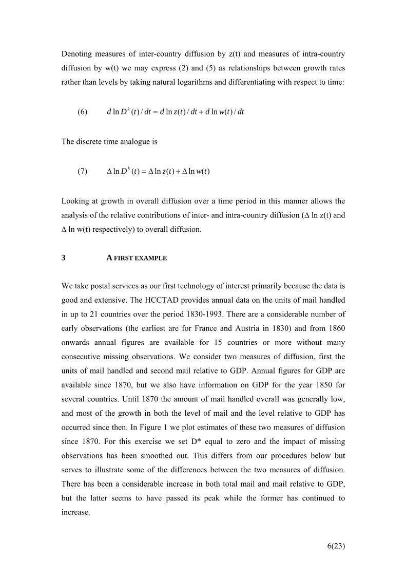
occurred since then. In Figure 1 we plot estimates of these two measures of diffusion

since 1870. For this exercise we set D* equal to zero and the impact of missing

observations has been smoothed out. This differs from our procedures below but

serves to illustrate some of the differences between the two measures of diffusion.

There has been a considerable increase in both total mail and mail relative to GDP,

but the latter seems to have passed its peak while the former has continued to

increase.

6(23)

Figure 1: Total sample usage of postal services 1870-1993

Diffusion of postal services

0

50,000

100,000

150,000

200,000

250,000

300,000

350,000

1870 1880 1890 1900 1910 1920 1930 1940 1950 1960 1970 1980 1990

mill

ion

units

of m

ail

0

5

10

15

20

25

30

35

mai

l uni

ts p

er $

1000

real

GD

P

Total units of mail(all observations)

Mail units relative to real GDP

(all observations)

To undertake a formal separation between the importance of inter- and intra-country

effects in the illustrated overall diffusion process, as per the last section, we need first

to consider some issues of data availability. The first issue is that for many of the

countries in HCCTAD the first observation does not correspond with the very

beginning of the diffusion process. This is a frequent occurrence in diffusion studies

but is not necessarily a problem if it can be assumed that the level of usage in the

unobserved period is below the arbitrary threshold level D*; that is, such countries in

this period were effectively non-users. To this end we experiment with different

values of D* for each measure of diffusion. An appropriate choice has to be low

enough to justify the interpretation of D* as distinguishing users of a technology from

non-users, but not so low that we are left with data on users alone (implying that no

changes in inter-country diffusion can be captured). Also, an appropriate value should

be high enough that the given measure of inter-country diffusion (equal to or a

function of the number of users M(t)), Dk(i,t), would be initially relatively low, and

low enough that even countries in which usage never reaches a very high level can be

considered users of the technology.

7(23)

The second issue is that there are some countries (namely the United States, Japan,

and Ireland) for which the level of usage at the first observation is so high that the

countries cannot plausibly be regarded as non-users prior to that date but must be

excluded from the analysis until that first observation.7 Therefore we face the task of

deciding which of the 21 countries in the HCCTAD can be included in the sample

(determining N(t)). Clearly, with missing observations the sample size cannot be 21

for the whole period of analysis. The alternative of fixing N(t) at the number of

countries for which data is available in say 1850 is also not attractive because the

sample would be insufficient to represent “international” usage and more importantly

because we would not capture the inter-country spread of technology over time.

Finally, to let N(t) vary with the availability of data would imply that changes in

(especially inter-country) diffusion would reflect increases in the availability of data

over time. Fortunately, because our concern is with changes in overall, inter- and

intra-country diffusion over a given time period, we can allow the sample size to vary

between periods as long as it is kept fixed within each period. Such a measure of N(t)

is also valid because we are interested in the relative (rather than absolute)

contributions of inter- and intra-country diffusion to changes in overall diffusion.

Measuring the diffusion of postal services by total usage or ownership, i.e. D1(t) as

defined above, we have decomposed the growth in overall diffusion for the period

1850-1990 using two alternative values for D1* of 10 million and 50 million units of

mail handled. With D1* equal to 10 million we have sufficient data for 15 countries at

the start of the period (i.e. N(t)=15). In 8 of these countries the amount of mail

handled exceeded 10 million in 1850.8 Initial overall diffusion (i.e. the total amount of

mail handled in these 8 countries) was 812 million units and initial intra-country

diffusion (i.e. average usage) was 102 million units. In 1990 all 15 countries were

users with the overall level of diffusion equal to 82,954 million units.

7 In particular, the earliest data for the United States is from 1886 (at 3747 million units) and Japan does not appear in the data set until 1902 (911 million), while e.g. for Greece we have a first figure of 800 000 units in 1840. 8 The countries in the sample are: Austria, Belgium, France, Germany, Netherlands, Spain, Switzerland, United Kingdom (the users in 1850) and Australia, Denmark, Finland, Greece, New Zealand, Norway, Sweden (who become users during the period).

8(23)

Applying equation (7) we obtain that 13.6% of the growth in overall diffusion was

due to an increase in inter-country diffusion (that is an increase in the number of users

M(t) from 8 to 15) and 86.4% was due to higher intra-country diffusion (that is an

increase in average usage from 102 million to 5,530 million units). Taking D1* equal

to 50 million units the growth in overall diffusion between 1850 and 1990

decomposes such that 35.9% can be attributed to inter-country diffusion and 64.1% to

intra-country diffusion.9 This example suggests, not surprisingly, that in the long run,

overall diffusion is primarily driven by an increasing intensity of usage within using

countries.

Omitting the war years 1938-1950 because the amount of mail appears very volatile

and several countries do not report any figures at all during these years10 we have

conducted the decomposition exercise as described above for each of the decades

1830-1990. The data is presented in Table 1, the two panels corresponding to D1*

equal to 10 and 50 million units respectively. As described above, we allow N(t) to

vary across time but keep it fixed within each decade. N(t) is higher for the higher D1*

because we include some countries with no data as ‘non-users’ – these can be

assumed to have a level of usage below 50 million (but not below 10 million).

Missing data is approximated by values for a year in close proximity to the start of

each decade where available, or by assuming linear growth if there are several

consecutive missing observations.

9 With D1*=50 million the sample consists of 17 countries 3 of which were users in 1850. 10 The extreme case is Canada for which no data is available for 1915-1947.

9(23)

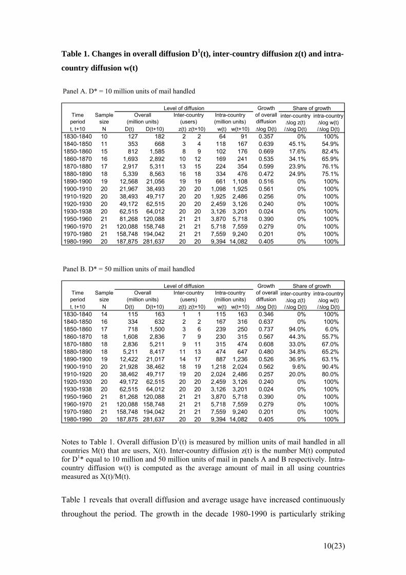
Table 1. Changes in overall diffusion D1(t), inter-country diffusion z(t) and intra-

country diffusion w(t)

Panel A. D* = 10 million units of mail handled

Growthof overall diffusion

t, t+10 N D(t) D(t+10) z(t) z(t+10) w(t) w(t+10) ∆log D(t)1830-1840 10 127 182 2 2 64 91 0.357 0% 100%1840-1850 11 353 668 3 4 118 167 0.639 45.1% 54.9%1850-1860 15 812 1,585 8 9 102 176 0.669 17.6% 82.4%1860-1870 16 1,693 2,892 10 12 169 241 0.535 34.1% 65.9%1870-1880 17 2,917 5,311 13 15 224 354 0.599 23.9% 76.1%1880-1890 18 5,339 8,563 16 18 334 476 0.472 24.9% 75.1%1890-1900 19 12,568 21,056 19 19 661 1,108 0.516 0% 100%1900-1910 20 21,967 38,493 20 20 1,098 1,925 0.561 0% 100%1910-1920 20 38,493 49,717 20 20 1,925 2,486 0.256 0% 100%1920-1930 20 49,172 62,515 20 20 2,459 3,126 0.240 0% 100%1930-1938 20 62,515 64,012 20 20 3,126 3,201 0.024 0% 100%1950-1960 21 81,268 120,088 21 21 3,870 5,718 0.390 0% 100%1960-1970 21 120,088 158,748 21 21 5,718 7,559 0.279 0% 100%1970-1980 21 158,748 194,042 21 21 7,559 9,240 0.201 0% 100%1980-1990 20 187,875 281,637 20 20 9,394 14,082 0.405 0% 100%

Overall (million units)

Inter-country (users)

Intra-country (million units)

inter-country ∆log z(t) /∆log D(t)

Time period

Sample size

Level of diffusion Share of growthintra-country ∆log w(t) /∆log D(t)

Panel B. D* = 50 million units of mail handled


t, t+10 N D(t) D(t+10) z(t) z(t+10) w(t) w(t+10) ∆log D(t)1830-1840 14 115 163 1 1 115 163 0.346 0% 100%1840-1850 16 334 632 2 2 167 316 0.637 0% 100%1850-1860 17 718 1,500 3 6 239 250 0.737 94.0% 6.0%1860-1870 18 1,608 2,836 7 9 230 315 0.567 44.3% 55.7%1870-1880 18 2,836 5,211 9 11 315 474 0.608 33.0% 67.0%1880-1890 18 5,211 8,417 11 13 474 647 0.480 34.8% 65.2%1890-1900 19 12,422 21,017 14 17 887 1,236 0.526 36.9% 63.1%1900-1910 20 21,928 38,462 18 19 1,218 2,024 0.562 9.6% 90.4%1910-1920 20 38,462 49,717 19 20 2,024 2,486 0.257 20.0% 80.0%1920-1930 20 49,172 62,515 20 20 2,459 3,126 0.240 0% 100%1930-1938 20 62,515 64,012 20 20 3,126 3,201 0.024 0% 100%1950-1960 21 81,268 120,088 21 21 3,870 5,718 0.390 0% 100%1960-1970 21 120,088 158,748 21 21 5,718 7,559 0.279 0% 100%1970-1980 21 158,748 194,042 21 21 7,559 9,240 0.201 0% 100%1980-1990 20 187,875 281,637 20 20 9,394 14,082 0.405 0% 100%

Level of diffusionOverall

(million units)Inter-country

(users)Time period

Sample size

Share of growthinter-country ∆log z(t) /∆log D(t)

intra-country ∆log w(t) /∆log D(t)

Intra-country (million units)

Notes to Table 1. Overall diffusion D1(t) is measured by million units of mail handled in all countries M(t) that are users, X(t). Inter-country diffusion z(t) is the number M(t) computed for D1* equal to 10 million and 50 million units of mail in panels A and B respectively. Intra-country diffusion w(t) is computed as the average amount of mail in all using countries measured as X(t)/M(t).

Table 1 reveals that overall diffusion and average usage have increased continuously

throughout the period. The growth in the decade 1980-1990 is particularly striking

10(23)

because our data does not include telefaxes or electronic mail, which, as substitute

technologies, we anticipate would reduce demand for traditional mail. There were no

increases in inter-country diffusion after 1890 (1920) for D1* equal to 10 million (50

million).

Using these estimates and applying equation (7) we plot changes in the log of the

overall, inter- and intra-country usage measures in Figure 2. We observe first that

growth in overall diffusion has tended to be smaller in the second half of the

observation period. Secondly, we note that inter-country diffusion slowed as the

diffusion process proceeded, especially when D1* is set at 50 million units.

11(23)

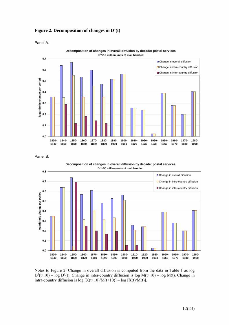
Figure 2. Decomposition of changes in D1(t)

Panel A.

Decomposition of changes in overall diffusion by decade: postal servicesD1*=10 million units of mail handled

0.0

0.1

0.2

0.3

0.4

0.5

0.6

0.7

1830-1840

1840-1850

1850-1860

1860-1870

1870-1880

1880-1890

1890-1900

1900-1910

1910-1920

1920-1930

1930-1938

1950-1960

1960-1970

1970-1980

1980-1990

loga

rithm

ic c

hang

e pe

r per

iod

Change in overall diffusion

Change in intra-country diffusion

Change in inter-country diffusion

Panel B.

Decomposition of changes in overall diffusion by decade: postal servicesD1*=50 million units of mail handled

0.0

0.1

0.2

0.3

0.4

0.5

0.6

0.7

0.8

1830-1840

1840-1850

1850-1860

1860-1870

1870-1880

1880-1890

1890-1900

1900-1910

1910-1920

1920-1930

1930-1938

1950-1960

1960-1970

1970-1980

1980-1990

loga

rithm

ic c

hang

e pe

r per

iod




Notes to Figure 2. Change in overall diffusion is computed from the data in Table 1 as log D1(t+10) – log D1(t). Change in inter-country diffusion is log M(t+10) – log M(t). Change in intra-country diffusion is log [X(t+10)/M(t+10)] – log [X(t)/M(t)].

12(23)

In Figure 3 we plot the percentage contribution of changes in inter- and intra-country

diffusion to the growth of overall diffusion. We observe that after the initial decades

in which the number of users was constant changes in inter-country diffusion

accounted for nearly 50 per cent of overall diffusion. As diffusion (and time)

proceeded changes in intra-country diffusion began to dominate the overall growth

process. The declining importance of inter-country diffusion is especially evident for

D1* equal to 50 million after the decade 1850 – 1860 during which 94 per cent of

overall growth was due to an increase in the number of users.

13(23)

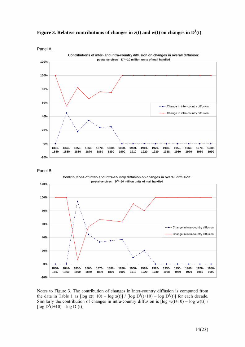
Figure 3. Relative contributions of changes in z(t) and w(t) on changes in D1(t)

Panel A.

Contributions of inter- and intra-country diffusion on changes in overall diffusion: postal services D1*=10 million units of mail handled

-20%

0%

20%

40%

60%

80%

100%

120%

1830-1840

1840-1850

1850-1860

1860-1870

1870-1880

1880-1890

1890-1900

1900-1910

1910-1920

1920-1930

1930-1938

1950-1960

1960-1970

1970-1980

1980-1990



Panel B.

Contributions of inter- and intra-country diffusion on changes in overall diffusion: postal services D1*=50 million units of mail handled

-20%

0%

20%

40%

60%

80%

100%

120%

1830-1840

1840-1850

1850-1860

1860-1870

1870-1880

1880-1890

1890-1900

1900-1910

1910-1920

1920-1930

1930-1938

1950-1960

1960-1970

1970-1980

1980-1990



Notes to Figure 3. The contribution of changes in inter-country diffusion is computed from the data in Table 1 as [log z(t+10) – log z(t)] / [log D1(t+10) – log D1(t)] for each decade. Similarly the contribution of changes in intra-country diffusion is [log w(t+10) – log w(t)] / [log D1(t+10) – log D1(t)].

14(23)

We now repeat the decomposition exercise using D2(t) as in equation (5) measuring

the diffusion of postal services in country i by units of mail handled x(i,t) relative to

real GDP y(i,t). From HCCTAD we measure GDP in 1990 international Stone-Geary

dollars. A country is defined as a user if x(i,t)/y(i,t) exceeds the base level D2* which

we set at 5 units of mail per $1000 real GDP.

In Table 2 below we present the data for each of the decades 1850 – 1990 omitting the

war years 1938 – 1950 as above. All three measures of diffusion, overall, inter and

intra, grew until 1920 (with the exception of intra-country diffusion which declined

1850 – 1860). In the following decades up to but excluding 1980 – 1990, overall

diffusion fell because sample average usage was falling, i.e. GDP was growing more

than proportionally to the amount of mail. However, in the last decade, 1980 – 1990,

the increase in mail was so considerable that our measure of overall diffusion D2(t)

also increased (compare Table 1). This occurred despite a reduction in inter-country

diffusion (which was due to x(i,t)/y(i,t) dropping below D2* in one country).11

Changes in logs of overall, inter-, and intra-country diffusion by decade are plotted in

Figure 4, from which it is immediately clear that overall diffusion grew fastest in the

early decades of the study period. Changes in inter-country diffusion follow a similar

(and perhaps even more pronounced) pattern to that found above for D1(t). That is,

increases in inter-country diffusion were large in the first three sample decades, but

since then the ratio M(t)/N(t) has changed very little if at all.

11 All changes in intra-country diffusion in 1960-1990 were due to Greece. Greece proved a difficulty for our analysis since usage x(i,t)/y(i,t) was very low throughout the period. We experimented with lower values of D2* but data availability for other countries suggested that 5 units per $1000 was the most appropriate choice.

15(23)

Table 2. Changes in overall diffusion D2(t), inter-country diffusion z(t) and intra-

country diffusion w(t)

D*=5 units of mail handled per $1000 real GDP


t, t+10 N X(t) X(t+10) D(t) D(t+10) z(t) z(t+10) w(t) w(t+10) ∆log D(t)1850-1860 13 350 1,288 1.7 5.2 0.08 0.38 22.2 13.4 1.106 145.5% -45.5%1860-1870 13 1,288 2,538 5.2 8.6 0.38 0.54 13.4 16.0 0.513 65.6% 34.4%1870-1880 17 2,602 5,182 7.6 12.5 0.53 0.76 14.3 16.4 0.507 72.6% 27.4%1880-1890 17 5,210 8,377 12.6 16.5 0.82 0.88 15.3 18.7 0.270 25.5% 74.5%1890-1900 18 12,382 21,040 17.2 22.3 0.89 1 19.3 22.3 0.262 44.9% 55.1%1900-1910 19 21,951 38,462 22.1 29.9 1 1 22.1 29.9 0.302 0% 100%1910-1920 20 38,462 49,717 29.7 33.4 0.95 1 31.2 33.4 0.118 43.6% 56.4%1920-1930 20 49,172 62,515 33.6 32.6 1 1 33.6 32.6 -0.031 0% 100%1930-1938 20 62,515 64,012 32.6 29.7 1 1 32.6 29.7 -0.090 0% 100%1950-1960 21 81,268 120,088 26.1 25.1 1 1 26.1 25.1 -0.040 0% 100%1960-1970 21 120,088 158,478 25.1 20.0 1 1 25.1 21.0 -0.225 21.7% 78.3%1970-1980 21 158,478 194,042 20.0 17.7 1 1 21.0 17.7 -0.124 -39.4% 139.4%1980-1990 20 187,875 281,199 17.8 20.2 1 1 17.8 21.2 0.128 -40.2% 140.2%


(mail/$1000 GDP)Inter-country

(user proportion)Intra-country

(mail/$1000 GDP)inter-country ∆log z(t) /∆log D(t)


Share of growthTime period

Sample size

Mail (million units)

Notes to Table 2. Overall diffusion D2(t) is measured by units of mail handled per $1000 real GDP in 1990 international Stone-Geary dollars. Inter-country diffusion z(t) is the proportion M(t)/N(t). Intra-country diffusion w(t) is the average amount of mail in all using countries divided by the average real GDP across all countries N(t), that is w(t) = [X(t)/M(t)] / [Y(t)/N(t)] where X(t) = ∑M(t)x(i,t) and Y(t) = ∑N(t)y(i,t).

16(23)

Figure 4. Decomposition of changes in D2(t)

Decomposition of changes in overall diffusion by decade: postal services D2 *=5 units of mail handled per $1000 GDP

-0.6

-0.4

-0.2

0.0

0.2

0.4

0.6

0.8

1.0

1.2

1.4

1.6

1.8

1850-1860

1860-1870

1870-1880

1880-1890

1890-1900

1900-1910

1910-1920

1920-1930

1930-1938

1950-1960

1960-1970

1970-1980

1980-1990

loga

rithm

ic c

hang

e pe

r per

iod




Notes to Figure 4. Change in overall diffusion is computed from the data in Table 2 as log D2(t+10) – log D2(t). Change in inter-country diffusion is log (M(t+10)/N) – log (M(t)/N) where N is held constant for each decade. Change in intra-country diffusion is log{[X(t+10)/M(t+10)]/[Y(t+10)/N]} – log{[X(t)/M(t)]/[Y(t)/N]}. Finally we plot the percentage contribution of changes in inter- and intra-country

diffusion to growth in overall diffusion (Figure 5). A very similar pattern emerges as

above for D1(t). Namely, while growth in the number of users was driving changes in

overall diffusion in the first three decades (1850 – 1880) since then it has been the

increasing intensity of usage by existing users that has dominated.

17(23)

Figure 5. Relative contributions of changes in z(t) and w(t) on changes in D2(t)

Contributions of inter- and intra-country diffusion on changes in overall diffusion:postal services D2*=5 units of mail handled per $1000 real GDP

-50%

-25%

0%

25%

50%

75%

100%

125%

150%

1850-1860

1860-1870

1870-1880

1880-1890

1890-1900

1900-1910

1910-1920

1920-1930

1930-1938

1950-1960

1960-1970

1970-1980

1980-1990



Notes to Figure 5. The contribution of changes in inter-country diffusion is calculated from the data in Table 2 as [log z(t+10) – log z(t)] / [log D2(t+10) – log D2(t)] for each decade. Similarly the contribution of changes in intra-country diffusion is [log w(t+10) – log w(t)] / [log D2(t+10) – log D2(t)].

18(23)

4 OTHER TECHNOLOGIES.

In order to confirm that our findings are not technology specific we have undertaken

similar exercises for three other technologies in the HCCTAD data set (although had

others been chosen the essence of the results would have been no different). The three

are electricity, telephones and the basic oxygen steel making processes. Diffusion in

these we measure respectively by megawatt hours of electricity output, the number of

telephone lines, and tonnes of steel produced. In each case we have undertaken the

analysis using both D1(t) and D2(t) diffusion indicators. For brevity however we

present only results for D2(t) measures which look at usage relative to an indicator of

total output.

4.1 Electricity

In Table 3 we present the results relating to the diffusion of electricity measured as

megawatt hours of electricity output relative to GDP. D2* is chosen as 0.50 mwhrs per

million dollars real GDP). Clearly since 1900 through to the end of the period world

electricity output relative to GDP has increased continuously. Inter-country diffusion

however was complete in this sample of countries by around 1950 after which all

further extensions of use reflected greater intra-country diffusion. This is illustrated

also by the fact that, by the 1930s, extensions of intra-country diffusion were already

contributing more to overall diffusion than further inter-country diffusion.

Table 3: The diffusion of electricity (1900 – 1998)

D2*= 0.50 mwhrs per $1 million real GDP


t, t+10 N X(t) X(t+10) D(t) D(t+10) z(t) z(t+10) w(t) w(t+10) ∆log D(t)1900-1910 14 0 691 0 0.06 0 0.07 0.80 - - -1910-1920 15 691 7,744 0.06 0.55 0.07 0.20 0.85 2.76 2.271 48.4% 51.6%1920-1930 20 9,648 25,803 0.65 1.32 0.40 0.75 1.62 1.75 0.709 88.6% 11.4%1930-1938 21 25,881 37,216 1.32 1.69 0.76 0.86 1.73 1.97 0.251 46.9% 53.1%1938-1950 21 37,216 74,083 1.69 2.38 0.86 0.95 1.97 2.50 0.341 30.9% 69.1%1950-1960 21 74,083 162,223 2.38 3.39 0.95 1 2.50 3.39 0.354 13.8% 86.2%1960-1970 21 162,223 344,751 3.39 4.35 1 1 3.39 4.35 0.252 0% 100%1970-1980 21 344,751 529,466 4.35 4.83 1 1 4.35 4.83 0.103 0% 100%1980-1990 21 529,466 701,783 4.83 4.85 1 1 4.83 4.85 0.006 0% 100%1990-1998 21 701,783 827,901 4.85 5.29 1 1 4.85 5.29 0.085 0% 100%

Inter-country (user proportion)

Overall (mwhrs/$m GDP)

Intra-country (mwhrs/$m GDP)

Level of diffusionTime period

Sample size

Electricity output (100 mwhrs)



19(23)

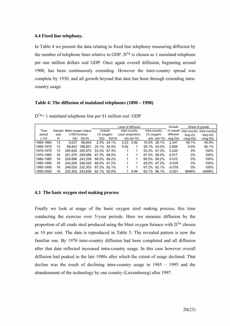
4.4 Fixed line telephony. In Table 4 we present the data relating to fixed line telephony measuring diffusion by

the number of telephone lines relative to GDP. D2* is chosen as 1 mainland telephone

per one million dollars real GDP. Once again overall diffusion, beginning around

1900, has been continuously extending. However the inter-country spread was

complete by 1930, and all growth beyond that date has been through extending intra-

country usage.

Table 4: The diffusion of mainland telephones (1890 – 1998)

D2*= 1 mainland telephone line per $1 million real GDP


t, t+5 N X(t) X(t+5) D(t) D(t+5) z(t) z(t+10) w(t) w(t+10) ∆log D(t)1960-1965 13 5,037 68,843 2.3% 24.1% 0.23 0.92 10.0% 26.1% 2.347 59.1% 40.9%1965-1970 13 68,843 198,851 24.1% 54.0% 0.92 1 26.1% 54.0% 0.806 9.9% 90.1%1970-1975 15 205,628 250,975 53.3% 67.3% 1 1 53.3% 67.3% 0.235 0% 100%1975-1980 16 251,276 259,688 67.3% 68.5% 1 1 67.3% 68.5% 0.017 0% 100%1980-1985 16 259,688 243,208 68.5% 69.2% 1 1 68.5% 69.2% 0.010 0% 100%1985-1990 16 243,208 246,020 69.2% 67.2% 1 1 69.2% 67.2% -0.030 0% 100%1990-1995 16 246,020 232,303 67.2% 62.1% 1 1 67.2% 62.1% -0.079 0% 100%1995-2000 16 232,303 243,836 62.1% 62.0% 1 0.94 62.1% 66.1% -0.001 6699% -6599%


(% oxygen)Inter-country

(user proportion)Intra-country (% oxygen)

inter-country ∆log z(t) /∆log D(t)


Time period

Sample size

Share of growthBlast oxygen output

(1000 tonnes)

4.3 The basic oxygen steel making process

Finally we look at usage of the basic oxygen steel making process, this time

conducting the exercise over 5-year periods. Here we measure diffusion by the

proportion of all crude steel produced using the blast oxygen furnace with D2* chosen

as 10 per cent. The data is reproduced in Table 5. The revealed pattern is now the

familiar one. By 1970 inter-country diffusion had been completed and all diffusion

after that date reflected increased intra-country usage. In this case however overall

diffusion had peaked in the late 1980s after which the extent of usage declined. That

decline was the result of declining intra-country usage in 1985 – 1995 and the

abandonment of the technology by one country (Luxembourg) after 1997.

20(23)

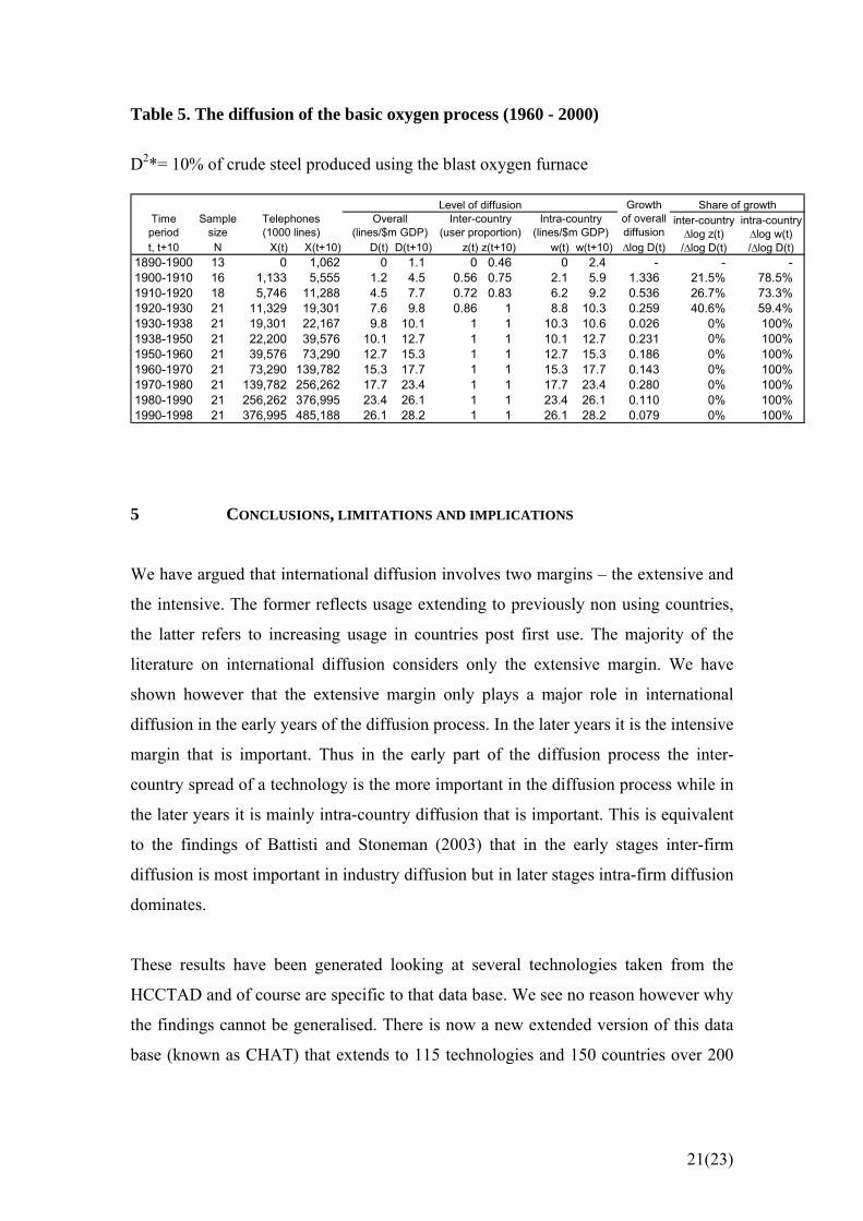
Table 5. The diffusion of the basic oxygen process (1960 - 2000)

D2*= 10% of crude steel produced using the blast oxygen furnace


t, t+10 N X(t) X(t+10) D(t) D(t+10) z(t) z(t+10) w(t) w(t+10) ∆log D(t)1890-1900 13 0 1,062 0 1.1 0 0.46 0 2.4 - - -1900-1910 16 1,133 5,555 1.2 4.5 0.56 0.75 2.1 5.9 1.336 21.5% 78.5%1910-1920 18 5,746 11,288 4.5 7.7 0.72 0.83 6.2 9.2 0.536 26.7% 73.3%1920-1930 21 11,329 19,301 7.6 9.8 0.86 1 8.8 10.3 0.259 40.6% 59.4%1930-1938 21 19,301 22,167 9.8 10.1 1 1 10.3 10.6 0.026 0% 100%1938-1950 21 22,200 39,576 10.1 12.7 1 1 10.1 12.7 0.231 0% 100%1950-1960 21 39,576 73,290 12.7 15.3 1 1 12.7 15.3 0.186 0% 100%1960-1970 21 73,290 139,782 15.3 17.7 1 1 15.3 17.7 0.143 0% 100%1970-1980 21 139,782 256,262 17.7 23.4 1 1 17.7 23.4 0.280 0% 100%1980-1990 21 256,262 376,995 23.4 26.1 1 1 23.4 26.1 0.110 0% 100%1990-1998 21 376,995 485,188 26.1 28.2 1 1 26.1 28.2 0.079 0% 100%




(lines/$m GDP)Inter-country

(user proportion)Intra-country

(lines/$m GDP)Time period

Sample size

Telephones (1000 lines)

5 CONCLUSIONS, LIMITATIONS AND IMPLICATIONS

We have argued that international diffusion involves two margins – the extensive and

the intensive. The former reflects usage extending to previously non using countries,

the latter refers to increasing usage in countries post first use. The majority of the

literature on international diffusion considers only the extensive margin. We have

shown however that the extensive margin only plays a major role in international

diffusion in the early years of the diffusion process. In the later years it is the intensive

margin that is important. Thus in the early part of the diffusion process the inter-

country spread of a technology is the more important in the diffusion process while in

the later years it is mainly intra-country diffusion that is important. This is equivalent

to the findings of Battisti and Stoneman (2003) that in the early stages inter-firm

diffusion is most important in industry diffusion but in later stages intra-firm diffusion

dominates.

These results have been generated looking at several technologies taken from the

HCCTAD and of course are specific to that data base. We see no reason however why

the findings cannot be generalised. There is now a new extended version of this data

base (known as CHAT) that extends to 115 technologies and 150 countries over 200

21(23)

years (see Comin et al. 2006), but that data is not available to us at this time. It would

be useful at some future date to see if our results still hold for this larger sample.

The relative importance of the internal and external margins provides a more solid

foundation upon which to evaluate the international competitiveness of different

countries and also suggests how one may better compare relative diffusion

performance across different countries (for an earlier approach to this see Canepa and

Stoneman, 2004). Perhaps more important however are the implications of our

findings for future research in this area. The implication that seems most important to

us is that the above is only an accounting exercise. It provides no information upon

the forces that drive diffusion. We consider of prime importance to be how the

internal and external margins are linked. In particular: (i) is intra-country diffusion

affected by inter-country diffusion or the extensive margin? – a question never asked

in the extensive body of domestic diffusion studies as far as we are aware; and (ii) is

inter-country diffusion affected by intra-country diffusion or the intensive margin? –

again a question we do not recall seeing before. These seem to us to be crucial

questions in understanding the overall diffusion process.

22(23)

23(23)

REFERENCES

Battisti G and Stoneman P (2003), ‘Inter- and intra-firm effects in the diffusion of

new process technology’ Research Policy, 32(9), pp. 1641-1655.

Canepa A and Stoneman P (2004), ‘Comparative International Diffusion: Patterns,

Determinants and Policies’, Economics of Innovation and New Technology, 13(3), pp.

279-298.

Comin D and Hobijn B (2004a), ‘Cross-country technological adoption: making the

theories face the facts’ Journal of Monetary Economics, 51(1), pp. 39-83.

Comin D and Hobijn B (2004b), ‘Neoclassical Growth and the Adoption of

Technologies’, NBER Working Paper, 10733, August, Cambridge, Mass.

Comin D, B Hobijn and E Rovito (2006), ‘Five Facts you need to know about

technology diffusion’, NBER Working Paper, 11928, January, Cambridge, Mass.

Keller, W (2004), ‘International Technology Diffusion’ Journal of Economic

Literature, 42(3), pp. 752-782.

Stoneman P (2002), The Economics of Technological Diffusion, Blackwell, Oxford.

International Diffusion of New Technologies: Intensive and Extensive Margins

Documents

Transcript of International Diffusion of New Technologies: Intensive and Extensive Margins