Thesis Front Matter - University of Calgary
187
UCGE Reports Number 20391 Department of Geomatics Engineering Map Aided Indoor and Outdoor Navigation Applications (URL: http://www.geomatics.ucalgary.ca/graduatetheses) by Mohamed Ali Attia September 2013
-
Upload
khangminh22 -
Category
Documents
-
view
0 -
download
0
Transcript of Thesis Front Matter - University of Calgary

UCGE Reports Number 20391
Department of Geomatics Engineering
Map Aided Indoor and Outdoor Navigation Applications
(URL: http://www.geomatics.ucalgary.ca/graduatetheses)
by
Mohamed Ali Attia
September 2013
UNIVERSITY OF CALGARY
Map Aided Indoor and Outdoor Navigation Applications
by
Mohamed Ali Attia
A THESIS
SUBMITTED TO THE FACULTY OF GRADUATE STUDIES
IN PARTIAL FULFILMENT OF THE REQUIREMENTS FOR THE
DEGREE OF DOCTOR OF PHILOSOPHY
DEPARTMENT OF GEOMATICS ENGINEERING
CALGARY, ALBERTA
SEPTEMBER, 2013
© Mohamed Attia 2013

ii
Abstract
Navigation systems play an important role in many vital disciplines. Determining the location of
a user relative to the physical environment (e.g. roadway, intersections, and services) is an
important part of transportation services such as in-vehicle navigation, fleet management and
infrastructure maintenance. In addition, other navigation services are required for locating the
position of a user in an indoor physical environment (e.g. airports, shopping malls, public
buildings, university campus). This indoor-based navigation can assist in several applications
such as user navigation, enhanced 911 (E911), law enforcement, location-based and marketing
services. Both indoor and outdoor navigation applications require a reliable, trustful and
continuous navigation solution that overcomes the challenge of Global Navigation Satellite
System (GNSS) signal unavailability. To compensate for this issue, GNSS is now commonly
used in tandem with other navigation systems such as Inertial Navigation System (INS). This
dual-system integration method provides a solution to GNSS signal outages. However, over time
there is a significant amount of drift, characteristic of INS but especially common with low-cost
commercial sensors. The effects of drift on INS accuracy highlight the need for additional
absolute aiding sensors that can survive for longer periods of time.
In this thesis, a map aided navigation solution is developed for GNSS-denied environments.
Maps have been the primary medium to visualize the navigation trajectories of a user’s everyday
travels. This research investigates and develops an aiding system that utilizes geospatial data
models in more than just a visual way. It assists the navigation solution by providing virtual
boundaries for the navigation trajectories and limits its possibilities only when it is logical to
locate the user on a map. The algorithms subsequently developed integrate several navigation

iii
sensors for different navigation solutions. Several geospatial models for both indoor and outdoor
environments (e.g. urban canyons) in addition to various map matching algorithms were used to
match and project navigation position estimates on the geospatial map and used as an additional
feedback for the navigation filter. The developed algorithms were field tested in several indoor
and outdoor environments and yielded accurate matching results as well as a significant
enhancement to positional accuracy. The achieved results demonstrate that the contribution of
the developed map aided system enhances the reliability, usability, and accuracy of navigation
trajectories in GNSS-denied environments.

iv
Acknowledgements
I would like to thank my supervisor Dr. Naser El-Sheimy for all his support and guidance. I am
very grateful for having him as my teacher, supervisor and mentor. He knew how and when to
encourage, push and support me. His valuable contribution, ideas and vision have enlightened
my research. I would like to extend my gratitude to Dr. Steve Liang for his constant support,
kind assistance and valuable feedback on my research. I am also indebted to Dr. Aboelmagd
Noureldin for his valuable advice, continuous encouragement and constructive suggestions. I am
forever grateful to have all of you as my supervisory committee.
I would like to thank all my colleagues and roommates in the Mobile Multi Sensors Systems
(MMSS) research group for their friendship, support, help in field testing and valuable
discussions; Dr. Mohamed El-Habiby, Dr. Zainab Syed, Dr. Chris Goodall, Dr. Hassan
Elhifnawy, Dr. Yigiter Yuksel, Dr. Ahmed Shawky, Dr. Bassem Sheta, Adel Moussa, Ahmed
Elghazouly, Abdelrahman Ali, Sara Saeedi and Xing Zhao—special thanks to my dear friend and
colleague Adel Moussa for our useful and productive discussions.
This work was supported in part by research funds from TECTERRA Commercialization and
Research Centre, Canada Research Chairs program and the Natural Science and Engineering
Research Council of Canada (NSERC) to Dr. Naser El-Sheimy. In addition, Members of
Trusted Positioning Inc. (TPI) are acknowledged for their efforts in providing field tests datasets.
I would like to extend my thanks to my beloved family. No words can express my gratitude to
my dear mother; her love and prayers are the most precious things in my life. Many thanks to my

v
father; his advice, care, love and support were always there when I needed them. My lovely wife
Riham, without you I would be unable to do anything; your love, care, sacrifice, understanding
and support were always there for me. You have stood by my side and believed in me all the
way—for that I am eternally grateful. Finally, my beloved sons Abdelrahman and Omar, you fill
my life with joy and happiness; your laughs when I come back home everyday show me the
main meaning and purpose of my life. No words can express how grateful I am for you two.

vi
Dedication
To My Parents
To My Wife
To My Sons
Forever grateful for you all being a part of my life

vii
Table of Contents
Abstract ............................................................................................................................... ii Acknowledgements ............................................................................................................ iv
Dedication .......................................................................................................................... vi Table of Contents .............................................................................................................. vii List of Tables .......................................................................................................................x List of Figures and Illustrations ......................................................................................... xi List of Symbols, Abbreviations and Nomenclature ...........................................................xv
Symbols........................................................................................................................... xvii
CHAPTER ONE: INTRODUCTION ..................................................................................1 1.1 Background ................................................................................................................1
1.2 Motivation and Problem Statement ...........................................................................2 1.3 Research Objectives ...................................................................................................3
1.3.1 Developing better models for geospatial databases that fit navigation
applications ........................................................................................................3 1.3.2 Investigating and designing map matching algorithms .....................................4
1.3.3 Investigating and designing a multi-sensor integrated navigation system ........4 1.3.4 Assessment of the proposed integrated system .................................................4
1.4 Research Contributions ..............................................................................................5
1.5 Thesis Outline ............................................................................................................6
CHAPTER TWO: GEOSPATIAL DATA MODELS FOR NAVIGATION
APPLICATIONS ........................................................................................................9 2.1 The Geospatial Data Model .......................................................................................9
2.2 Requirements for Maps in Navigation Applications ...............................................10 2.2.1 Map Display ....................................................................................................11
2.2.2 Address matching ............................................................................................13 2.2.3 Map matching ..................................................................................................13 2.2.4 Path Finding .....................................................................................................14
2.2.5 Road guidance .................................................................................................15 2.3 Map sources for navigation applications .................................................................15
2.3.1 Major Mapping Sources ..................................................................................16 2.3.2 Maps for specific projects ...............................................................................17
2.3.3 Crowdsourcing ................................................................................................21 2.4 Designing the Geospatial Data Models ...................................................................25
2.4.1 Street network for vehicle navigation application ...........................................25
2.4.1.1 Geospatial model for Downtown Calgary .............................................26 2.4.2 Building information model for indoor application ........................................30
2.4.2.1 Geospatial Model for the Engineering Building at University of
Calgary ....................................................................................................31
2.4.2.2 Geospatial Model for MacEwan Hall and Kinesiology Buildings at
University of Calgary ..............................................................................35
CHAPTER THREE: MAP MATCHING ALGORITHMS ...............................................39
3.1 Background of Map Matching Algorithms ..............................................................39
viii
3.1.1 Geometric and Topological Algorithms ..........................................................39
3.1.2 Probabilistic Algorithms ..................................................................................42 3.1.3 Advanced Algorithms ......................................................................................45 3.1.4 Evaluating the Map matching Results .............................................................47
3.2 Designing the Map Matching Algorithms ...............................................................49 3.2.1 Geometrical based algorithm ...........................................................................49 3.2.2 Automatic turn detection algorithm .................................................................52 3.2.3 Geometrical and topological algorithm ...........................................................55
CHAPTER FOUR: MOBILE-MULTI SENSOR INTEGRATED NAVIGATION
SYSTEMS.................................................................................................................58 4.1 Introduction to Navigation systems .........................................................................58 4.2 Inertial Sensors ........................................................................................................60
4.2.1 MEMS Inertial Sensors ...................................................................................62 4.2.2 Inertial Sensors Errors .....................................................................................64
4.3 INS Mechanization ..................................................................................................68
4.3.1 Attitude Estimation ..........................................................................................73 4.3.2 Velocity Estimation .........................................................................................74
4.3.3 Position Estimation ..........................................................................................75 4.4 GPS/INS Integrated Navigation System ..................................................................75 4.5 Pedestrian Dead Reckoning .....................................................................................82
4.5.1 Step Detection .................................................................................................84 4.5.2 Step length Estimation .....................................................................................85
4.5.3 Heading Estimation .........................................................................................86 4.6 Wi-Fi Positioning System ........................................................................................87
CHAPTER FIVE: MAP AIDED NAVIGATION SYSTEMS ..........................................91 5.1 Integrated Map Aided Navigation Systems .............................................................91
5.1.1 Integrated Map aided Navigation for Vehicle Application .............................94 5.1.1.1 Direct Map Matching Navigation System .............................................95 5.1.1.2 Sequential Updated Kalman filter for Map aided Navigation System ..96
5.1.2 Integrated Map Aided Navigation for Indoor Applications ............................99 5.1.2.1 Map Aided Navigation using Building Information ..............................99
5.1.2.2 Map Aided PDR for Smartphone Sensors using Building
Information............................................................................................100
5.2 Constrained Kalman Filter for GPS/INS Integration .............................................102 5.2.1 Estimate Projection Constrained Kalman Filter for GPS/INS Integration
(relative height change constraint) .................................................................103
5.2.2 Zero Velocity Updates (ZUPT) based on Automatic Stop detection technique
using decision trees ........................................................................................104 5.3 Integrity Measures for Map Aided Navigation Systems .......................................107
5.3.1 Integrity Measures for Navigation Solutions ................................................108
5.3.2 Effect of Geospatial data on positioning accuracy ........................................109 5.3.3 Integrity measures for the Map Matching Algorithms ..................................112 5.3.4 Overall fused Integrity Measures for Map Aided Navigation Systems ........117
CHAPTER SIX: FIELD TESTING, RESULTS, DISCUSSION AND ANALYSIS .....118
ix
6.1 Vehicle Outdoor Field Tests ..................................................................................118
6.1.1 Field Test Description ...................................................................................118 6.1.1.1 First Field Test (Constrained Kalman Filtering Field Test) ................118 6.1.1.2 Second Field Test (Map Aided Vehicle Navigation Systems Field
Test) ......................................................................................................121 6.1.2 Results, Discussion and Analysis for Vehicle Outdoor Applications ...........123
6.1.2.1 Estimate Projection Constrained Kalman Filtering .............................123 6.1.2.2 Direct Map matching Navigation System ............................................127 6.1.2.3 Sequential Updated Kalman filter for Map aided Navigation System 130
6.2 Indoor Tests Descriptions ......................................................................................132 6.2.1 Field Test Description ...................................................................................132
6.2.1.1 First Field Test (Portable Navigation System) ....................................132 6.2.1.2 Second Field Test (Smartphone Sensors)........................................136
6.2.2 Results, Discussion and Analysis for Pedestrian Indoor Applications ..........141 6.2.2.1 Map Aided Navigation using Building Information ............................141
6.2.2.2 Map Aided PDR for Smartphones Sensors Using Building
Information............................................................................................145
CHAPTER SEVEN: SUMMARY, CONCLUSIONS AND RECOMMENDATIONS .152 7.1 Summary ................................................................................................................152 7.2 Conclusions ............................................................................................................153
7.3 Recommendations for Future Work ......................................................................157
REFERENCES ................................................................................................................159
APPENDIX A ..................................................................................................................162
APPENDIX B ..................................................................................................................166
x
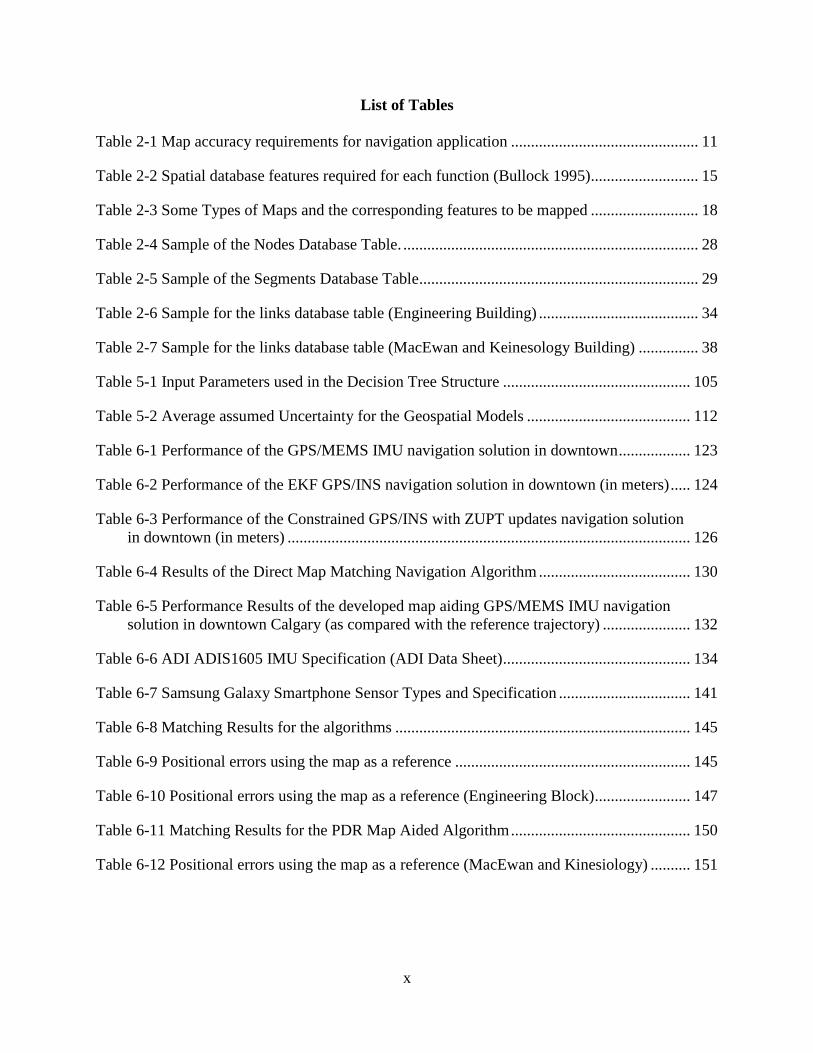
List of Tables
Table 2-1 Map accuracy requirements for navigation application ............................................... 11
Table 2-2 Spatial database features required for each function (Bullock 1995) ........................... 15
Table 2-3 Some Types of Maps and the corresponding features to be mapped ........................... 18
Table 2-4 Sample of the Nodes Database Table. .......................................................................... 28
Table 2-5 Sample of the Segments Database Table ...................................................................... 29
Table 2-6 Sample for the links database table (Engineering Building) ........................................ 34
Table 2-7 Sample for the links database table (MacEwan and Keinesology Building) ............... 38
Table 5-1 Input Parameters used in the Decision Tree Structure ............................................... 105
Table 5-2 Average assumed Uncertainty for the Geospatial Models ......................................... 112
Table 6-1 Performance of the GPS/MEMS IMU navigation solution in downtown .................. 123
Table 6-2 Performance of the EKF GPS/INS navigation solution in downtown (in meters) ..... 124
Table 6-3 Performance of the Constrained GPS/INS with ZUPT updates navigation solution
in downtown (in meters) ..................................................................................................... 126
Table 6-4 Results of the Direct Map Matching Navigation Algorithm ...................................... 130
Table 6-5 Performance Results of the developed map aiding GPS/MEMS IMU navigation
solution in downtown Calgary (as compared with the reference trajectory) ...................... 132
Table 6-6 ADI ADIS1605 IMU Specification (ADI Data Sheet)............................................... 134
Table 6-7 Samsung Galaxy Smartphone Sensor Types and Specification ................................. 141
Table 6-8 Matching Results for the algorithms .......................................................................... 145
Table 6-9 Positional errors using the map as a reference ........................................................... 145
Table 6-10 Positional errors using the map as a reference (Engineering Block) ........................ 147
Table 6-11 Matching Results for the PDR Map Aided Algorithm ............................................. 150
Table 6-12 Positional errors using the map as a reference (MacEwan and Kinesiology) .......... 151
xi
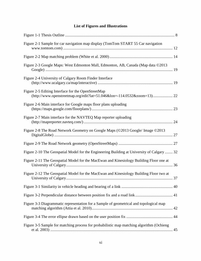
List of Figures and Illustrations
Figure 1-1 Thesis Outline ............................................................................................................... 8
Figure 2-1 Sample for car navigation map display (TomTom START 55 Car navigation
www.tomtom.com) ............................................................................................................... 12
Figure 2-2 Map matching problem (White et al. 2000) ................................................................ 14
Figure 2-3 Google Maps: West Edmonton Mall, Edmonton, AB, Canada (Map data ©2013
Google) ................................................................................................................................. 19
Figure 2-4 University of Calgary Room Finder Interface
(http://www.ucalgary.ca/map/interactive) ............................................................................ 19
Figure 2-5 Editing Interface for the OpenStreetMap
(http://www.openstreetmap.org/edit?lat=51.046&lon=-114.0532&zoom=13) .................... 22
Figure 2-6 Main interface for Google maps floor plans uploading
(https://maps.google.com/floorplans/) .................................................................................. 23
Figure 2-7 Main interface for the NAVTEQ Map reporter uploading
(http://mapreporter.navteq.com/) .......................................................................................... 24
Figure 2-8 The Road Network Geometry on Google Maps (©2013 Google/ Image ©2013
DigitalGlobe) ........................................................................................................................ 27
Figure 2-9 The Road Network geometry (OpenStreetMaps) ....................................................... 27
Figure 2-10 The Geospatial Model for the Engineering Building at University of Calgary ........ 32
Figure 2-11 The Geospatial Model for the MacEwan and Kinesiology Building Floor one at
University of Calgary ............................................................................................................ 36
Figure 2-12 The Geospatial Model for the MacEwan and Kinesiology Building Floor two at
University of Calgary ............................................................................................................ 37
Figure 3-1 Similarity in vehicle heading and bearing of a link .................................................... 40
Figure 3-2 Perpendicular distance between position fix and a road link ...................................... 41
Figure 3-3 Diagrammatic representation for a Sample of geometrical and topological map
matching algorithm (Attia et al. 2010) .................................................................................. 42
Figure 3-4 The error ellipse drawn based on the user position fix ............................................... 44
Figure 3-5 Sample for matching process for probabilistic map matching algorithm (Ochieng
et al. 2003) ............................................................................................................................ 45
xii
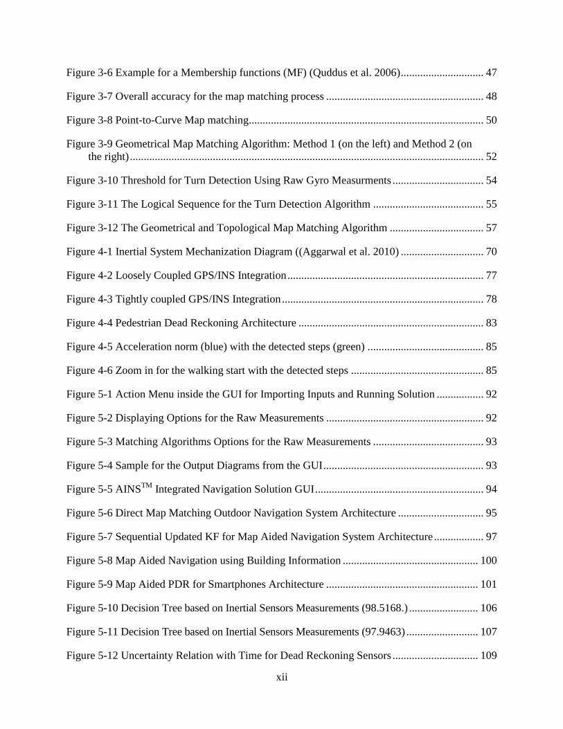
Figure 3-6 Example for a Membership functions (MF) (Quddus et al. 2006) .............................. 47
Figure 3-7 Overall accuracy for the map matching process ......................................................... 48
Figure 3-8 Point-to-Curve Map matching..................................................................................... 50
Figure 3-9 Geometrical Map Matching Algorithm: Method 1 (on the left) and Method 2 (on
the right) ................................................................................................................................ 52
Figure 3-10 Threshold for Turn Detection Using Raw Gyro Measurments ................................. 54
Figure 3-11 The Logical Sequence for the Turn Detection Algorithm ........................................ 55
Figure 3-12 The Geometrical and Topological Map Matching Algorithm .................................. 57
Figure 4-1 Inertial System Mechanization Diagram ((Aggarwal et al. 2010) .............................. 70
Figure 4-2 Loosely Coupled GPS/INS Integration ....................................................................... 77
Figure 4-3 Tightly coupled GPS/INS Integration ......................................................................... 78
Figure 4-4 Pedestrian Dead Reckoning Architecture ................................................................... 83
Figure 4-5 Acceleration norm (blue) with the detected steps (green) .......................................... 85
Figure 4-6 Zoom in for the walking start with the detected steps ................................................ 85
Figure 5-1 Action Menu inside the GUI for Importing Inputs and Running Solution ................. 92
Figure 5-2 Displaying Options for the Raw Measurements ......................................................... 92
Figure 5-3 Matching Algorithms Options for the Raw Measurements ........................................ 93
Figure 5-4 Sample for the Output Diagrams from the GUI .......................................................... 93
Figure 5-5 AINSTM
Integrated Navigation Solution GUI ............................................................. 94
Figure 5-6 Direct Map Matching Outdoor Navigation System Architecture ............................... 95
Figure 5-7 Sequential Updated KF for Map Aided Navigation System Architecture .................. 97
Figure 5-8 Map Aided Navigation using Building Information ................................................. 100
Figure 5-9 Map Aided PDR for Smartphones Architecture ....................................................... 101
Figure 5-10 Decision Tree based on Inertial Sensors Measurements (98.5168.) ......................... 106
Figure 5-11 Decision Tree based on Inertial Sensors Measurements (97.9463) .......................... 107
Figure 5-12 Uncertainty Relation with Time for Dead Reckoning Sensors ............................... 109

xiii
Figure 5-13 Accuracy limits when Creating Links Centrelines .................................................. 111
Figure 5-14 Projected Distance Relation with Time for Map Matching Algorithms ................. 113
Figure 5-15 Uncertainty Estimation with Time for Turn Detection Algorithm ......................... 114
Figure 5-16 Travelled Distance Relation with Time for Map Matching Algorithms ................. 115
Figure 5-17 Historical Combined Uncertainty Measures for Map Matching Algorithm ........... 116
Figure 5-18 Overall Uncertainty Measures for Map Aided Navigation Solution ...................... 117
Figure 6-1 The Trajectory of the First Outdoor Field Test (©2013 Google/ Image ©2013
DigitalGlobe) ...................................................................................................................... 119
Figure 6-2 Downtown Trajectory of the First Outdoor Field Test (©2013 Google/ Image
©2013 DigitalGlobe) .......................................................................................................... 120
Figure 6-3 The Whole Trajectory of the Second Outdoor Field Test (©2013 Google/ Image
©2013 DigitalGlobe) .......................................................................................................... 121
Figure 6-4 Results for EKF GPS/INS solution (red) versus the reference trajectory (green)
(©2013 Google/ Image ©2013 DigitalGlobe) .................................................................... 124
Figure 6-5 Height for the EKF solution versus the Reference Height ........................................ 125
Figure 6-6 Results for Constrained Kalman filter GPS/INS with ZUPT solution (yellow)
versus the reference trajectory (green) (©2013 Google/ Image ©2013 DigitalGlobe) ...... 126
Figure 6-7 Height for the Constrained Kalman Filter with ZUPT updates solution versus the
Reference Height................................................................................................................. 127
Figure 6-8 Results of the map matching and turn detection algorithm for the real field data
(©2013 Google/ Image ©2013 DigitalGlobe) .................................................................... 128
Figure 6-9 Results of the map matching and turn detection algorithm for the 30 second
outage simulated data (©2013 Google/ Image ©2013 DigitalGlobe) ................................ 128
Figure 6-10 Results of the map matching and turn detection algorithm for the 60 second
outage simulated data (©2013 Google/ Image ©2013 DigitalGlobe) ................................ 129
Figure 6-11 Results for after Map Matching Updates for the downtown dataset (©2013
Google/ Image ©2013 DigitalGlobe) ................................................................................. 131
Figure 6-12 Results for before and after Map Matching updates compared to the reference
trajectory for the downtown dataset (©2013 Google/ Image ©2013 DigitalGlobe) .......... 131
Figure 6-13 First Field Test Trajectory (Engineering Block) (©2013 Google/ Image ©2013
DigitalGlobe) ...................................................................................................................... 133
xiv
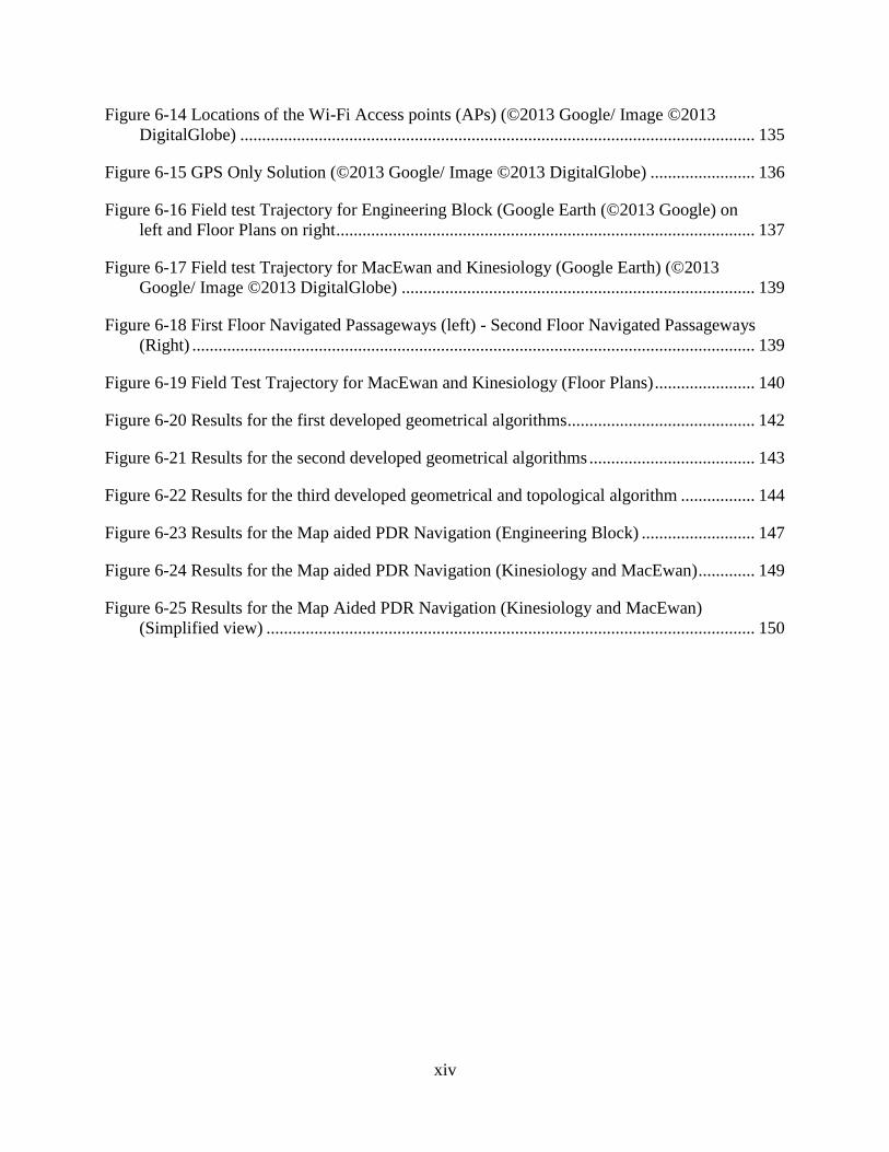
Figure 6-14 Locations of the Wi-Fi Access points (APs) (©2013 Google/ Image ©2013
DigitalGlobe) ...................................................................................................................... 135
Figure 6-15 GPS Only Solution (©2013 Google/ Image ©2013 DigitalGlobe) ........................ 136
Figure 6-16 Field test Trajectory for Engineering Block (Google Earth (©2013 Google) on
left and Floor Plans on right ................................................................................................ 137
Figure 6-17 Field test Trajectory for MacEwan and Kinesiology (Google Earth) (©2013
Google/ Image ©2013 DigitalGlobe) ................................................................................. 139
Figure 6-18 First Floor Navigated Passageways (left) - Second Floor Navigated Passageways
(Right) ................................................................................................................................. 139
Figure 6-19 Field Test Trajectory for MacEwan and Kinesiology (Floor Plans) ....................... 140
Figure 6-20 Results for the first developed geometrical algorithms ........................................... 142
Figure 6-21 Results for the second developed geometrical algorithms ...................................... 143
Figure 6-22 Results for the third developed geometrical and topological algorithm ................. 144
Figure 6-23 Results for the Map aided PDR Navigation (Engineering Block) .......................... 147
Figure 6-24 Results for the Map aided PDR Navigation (Kinesiology and MacEwan) ............. 149
Figure 6-25 Results for the Map Aided PDR Navigation (Kinesiology and MacEwan)
(Simplified view) ................................................................................................................ 150

xv
List of Symbols, Abbreviations and Nomenclature
Abbreviations
2D
Two dimensional
3D Three dimensional
AINS Aided Inertial Navigation System
AP Access Point
ARW Angular Random Walk
b-frame Body frame
CAD Computer Aided Design
CUPT Coordinates Update
DGPS Differential Global Positioning System
DR Dead Reckoning
E911 Enhanced 9-1-1
e-frame Earth fixed frame
EKF Extended Kalman Filter
ENU East, North and Up
FIS Fuzzy Inference System
GIS Geographical Information System
GNSS Global Navigation Satellite System
GPS Global Positioning System
i-frame Inertial frame
IMU Inertial Measurement Unit
INS Inertial Navigation System

xvi
KF Kalman Filter
LN200 Litton 200
LSB Least Significant Bit
MEMS Micro Electro Mechanical Sensors
MH Membership Function
NAD North American Datum
NED North, East and Down
n-frame Navigation frame
PDR Pedestrian Dead Reckoning
PND Portable Navigation Devices
PNS Portable Navigation System
PPS Pulse Per Second
PVA Position, velocity and attitude
RMS Root Mean Square
STD Standard Deviation
UTM
UWB
Universal Transverse Mercator
Ultra Wideband
VRW Velocity Random Walk
WGS84 World Geodetic System
ZUPT Zero Velocity Update

xvii
Symbols
a Confidence ellipse semi-major axis
b Confidence ellipse semi-minor axis
Confidence ellipse rotation angle
Variance for the estimated position x
y ariance for the estimated positions y
Covariance for the position (x,y)
D Minimum distance from position fix to the network link
XS, YS Position fix from the navigation sensor
(X1, Y1), (X2, Y2) Start and end nodes for the network link
XP, YP Projected coordinates on the network link
Specific force
Gravitation force
User acceleration
User position
User velocity
Initial velocity
Initial position
ΔV Velocity increment
Δt Sampling interval
Accelerometer bias
Gyro bias
Roll angle

xviii
Pitch angle
Azimuth angle
Gyroscope measurement
R(τ) Autocorrelation sequence
Ω Angular rates
M Meridian radius of curvature
N Prime vertical radius of curvature
Rotation matrix between the body frame and local level frame
q Quaternion matrix
E, N Easting and northing coordinates
Distance travelled by the user since time ( t-1)
User heading at time (t-1)
The walking frequency
The dynamic matrix
Navigation States
The shaping matrix
The sensor noise
Transition matrix from epoch k-1 to epoch k
The measurements vector
The design matrix
White noise for the measurements
System noise matrix
Kalman gain matrix

xix
Euclidian distance between the database vector and the online vector
The signal strength vector at the surveyed positions
The signal strength vector at the user positions
The states at epoch k
The variance of the states at epoch k
1
Chapter One: Introduction
1.1 Background
Maps have been used for centuries to transit users from a one place to another. In the last decade
navigation devices have used digital maps to locate the position of the user and assist in
providing navigational directions. Recently, maps have become more than just a visualization
tool in navigation systems; they are now an aiding tool for enhancing the reliability of the
obtained navigation solutions.
Many navigation tools now, rely on digital maps as the primary media for displaying navigation
information to the user. These applications usually use a navigation system consisting of a GPS
receiver, a map and a geospatial database. Although these systems usually provide accurate
positioning information, they can only do so in GPS-friendly environments. Navigation in GPS-
denied environments, such as indoor facilities and urban centers, usually has difficulty
maintaining accurate positioning information due to GPS signal blockage and multipath. The
performance of these systems can be improved by integrating other navigation sensors such as
INS. Although useful in some cases, the drift in position errors over time due to errors in inertial
sensors significantly reduces the reliability of this solution in some applications.
In this thesis, map aiding navigation techniques are designed to assist navigation applications in
outdoor and indoor environments. The developed techniques are based on the integration of
GPS/INS navigation systems, geospatial data models and other additional aiding sensors (e.g.
magnetometer, barometer, and Wi-Fi) which all depend on the working environment of the user

2
(indoor/outdoor). Improving the performance of navigation systems through the implementation
of additional sensors or the application of certain constraints has proven helpful in enhancing the
navigation solution and reliable navigation solution. In this thesis, the geospatial data models
for the navigated environments will be used to provide the navigation system with additional
updates and boundaries. The model uses geometrical and topological information such as
connectivity, adjacency, proximity, probability of height change, and traffic direction to help the
navigation system locate the user by map matching techniques. Map matching in this case has
the advantage of assisting the navigation solution by providing a logical threshold of where the
user could be, forcing the navigation solution to be in certain regions. This map matching
algorithm will fuse several measurements and constraints such as user position, heading, height
constraint, and INS raw data to produce a better estimation for the correctly navigated street link
(outdoor) or passageway link (indoor).
One of the main concepts in map aiding systems is that the objective of the navigation system
shifts from obtaining high position accuracy information to the obtaining positions with enough
accuracy to allow the system to select the correct link.
1.2 Motivation and Problem Statement
Navigation systems play an important role in many vital disciplines. Determining the accurate
location of a user relative to its physical environment (e.g. roadway, intersections, services) is an
important part of transportation services such as in-vehicle navigation, fleet management and
infrastructure maintenance. Other services in which enhanced navigation applications are
required are: E911, law enforcement, assistance for persons with disabilities and marketing
3
services, to name a few. These services generally require a user be located within a variety of
physical indoor environments (e.g. airports, shopping mall, public buildings) and can
subsequently benefit greatly from indoor position data. Given the serious nature of these
practical applications, this positioning must be highly trusted and reliable—even if the user is
located in a GPS-denied environment. However, there is a major challenge in maintaining this
reliability. Several researchers have addressed possible methodologies to aid current navigation
systems with either additional sensors or certain filtering but reaching the absolute accurate and
most trusted position in these environments remains a challenge. This research will address a
method for aiding navigation systems with mapping information and benefitting from the
geospatial information for the navigated regions (either street networks or floor plans).
1.3 Research Objectives
The main purpose of this research is to improve the performance of current navigation systems in
environments where GPS accuracy is either deteriorated or its signal is totally blocked. For this
purpose, the research will address several topics to achieve the main objectives. The goals of
each topic are summarized in the following minor objectives:
1.3.1 Developing better models for geospatial databases that fit navigation applications
This minor objective of the research will investigate a suitable and efficient geospatial database
structure relevant to the navigation applications. It is important to reach the conceptual,
geometrical and physical modeling of the reality to best describe the navigated areas. Extracting
the useful geometrical and topological characteristics of the navigated areas will assist in finding

4
the threshold for any processed navigation solution. The final model, when implemented in the
navigation system, should assist in achieving all required navigation functions.
1.3.2 Investigating and designing map matching algorithms
Several map matching algorithms are available, however the concept and constraints used is
dependent on the exact application. This minor objective will focus on developing smart fusion
algorithms for integrating multi-measurements (position, height, and direction) with the
geospatial information of the studied region. This will assist in developing an intelligent map
matching algorithm.
1.3.3 Investigating and designing a multi-sensor integrated navigation system
This minor objective will focus on developing an integrated navigation system that has the
necessary capability to provide a low-cost, real-time and accurate solution. The investigation of
the appropriate sensors and the mathematical combination of their measurements will lead to the
appropriate set of sensors required for navigating in poor or denied GPS environments.
1.3.4 Assessment of the proposed integrated system
The main goal of this minor objective is to test the developed integrated map aiding navigation
system in several environments. The performance for the system, either in an urban canyon or
indoor environments, is evaluated according to its improvement from the currently-used
navigation system.

5
1.4 Research Contributions
The main contribution of this research is an enhanced level of reliability in the navigation
solutions of GPS-denied environments. The research on aiding navigation applications is a very
important topic nowadays due to the enormous need for reliable navigation solution that account
for different applications. The developed map aided, low-cost, user-friendly navigation system
can be used in many systems such as in-vehicle navigation or smartphone location-based tools.
Additionally, this new system can be used for emergency or law-enforcement purposes, regular
indoor navigation, providing assistance to people with disabilities and can also assist other
navigation applications. The improvements made to the navigation solution accuracy provide a
more reliable and robust navigation alternative for users. In this thesis, the following algorithms
and techniques were developed:
A direct geometrical and topological map matching navigation algorithm that achieved a
very high matching percentage for the roads network inside challenging urban centers
using an automatic turn detection technique with a geospatial data model for the urban
center road network.
A sequential updated navigation filtering by using the map matched outputs as a
continuous feedback update for the Kalman filter that produced significant improvements
in positional errors when tested in urban centres.
A map aided navigation using building information and map matching algorithm with a
Wi-Fi/GPS/INS integrated navigation solution using a pedestrian navigation unit that
achieved high performance in indoor environments.
A map aided navigation using building information and map matching algorithm with a
PDR navigation solution using smartphone sensors, achieving steady and accurate

6
performance in several indoor environments both for correct matched passageways and
improvement in positional errors.
An enhanced constrained Kalman filter using estimate projection height constraints with
zero velocity updates detected automatically by decision trees, achieving improvement in
positional errors and height estimations when tested in urban canyon areas.
Several integrity measures to express the uncertainty of the different map aided
navigation components; geospatial data model, map matching and navigation sensors.
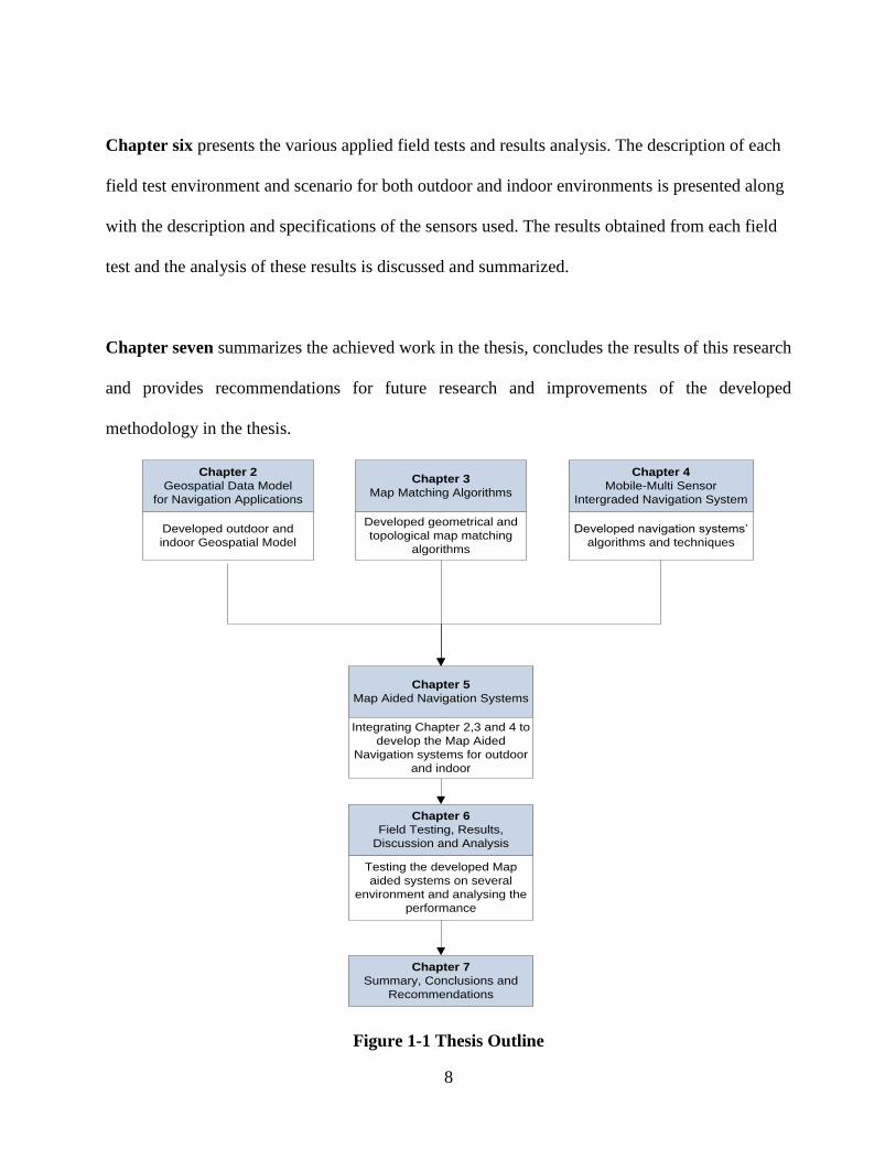
1.5 Thesis Outline
This thesis is organized into seven chapters, as shown in Figure 1-1. In this chapter a brief
background on the research topic, the problem statement and the motivation behind this research
are presented. The research objectives and main contributions are listed, and the thesis outline is
stated
Chapter two discusses the geospatial data models for navigation applications. The discussion
covers the different sources for these models and the modeling procedures based on the required
navigation application. The developed outdoor and indoor geospatial model used for this
research will be presented and investigated.
Chapter three reviews the different map matching algorithms and analyzes the advantages and
disadvantages of each algorithm. In this chapter, the developed map matching algorithms for the
map aided navigation system are introduced, discussed and a detailed description of each

7
technique is presented. The automatic turn detection technique used in the aiding system is
investigated and discussed.
Chapter four investigates and discusses the multi-mobile sensors integration. This chapter
includes thenavigationsystem’salgorithmsandtechniquesusedinthisresearchtodevelopthe
map aided navigation systems. A brief but informative description of inertial sensors, their errors
and mechanization equations is given. Additionally, the pedestrian dead reckoning and wireless
location techniques are explained in this chapter. The GPS/INS integration techniques and the
Kalman filter modeling are reviewed.
Chapter five introduces the developed map aided multi-sensor integrated systems. The chapter
introduces the newly developed estimate projection constrained Kalman filter to enhance the
GPS/INS navigation solution. This constrained system uses the height information to constrain
the Kalman filter. For outdoor applications two map aided systems are presented: a direct map
aiding system uses the navigation outputs to project the solution, and a continuous feedback
system that after map matching the position uses the matched positions as a feedback update to
the navigation filter. For indoor applications several map aiding navigation techniques are
presented; geometrical only map matching technique and a geometrical and topological map
matching techniques, both based on Personal Navigation System sensors and integrated through
GPS/INS/Wi-Fi solution. Another indoor map aided technique based on Personal Dead
Reckoning algorithm and smartphone sensors is introduced. Finally, the chapter presents several
integrity measures to evaluate the map aided navigation systems components.
8
Chapter six presents the various applied field tests and results analysis. The description of each
field test environment and scenario for both outdoor and indoor environments is presented along
with the description and specifications of the sensors used. The results obtained from each field
test and the analysis of these results is discussed and summarized.
Chapter seven summarizes the achieved work in the thesis, concludes the results of this research
and provides recommendations for future research and improvements of the developed
methodology in the thesis.
Chapter 2
Geospatial Data Model
for Navigation Applications
Chapter 4
Mobile-Multi Sensor
Intergraded Navigation System
Chapter 3
Map Matching Algorithms
Chapter 5
Map Aided Navigation Systems
Chapter 6
Field Testing, Results,
Discussion and Analysis
Chapter 7
Summary, Conclusions and
Recommendations
Developed outdoor and
indoor Geospatial Model
Developed navigation systems’
algorithms and techniques
Developed geometrical and
topological map matching
algorithms
Integrating Chapter 2,3 and 4 to
develop the Map Aided
Navigation systems for outdoor
and indoor
Testing the developed Map
aided systems on several
environment and analysing the
performance
Figure 1-1 Thesis Outline

9
Chapter Two: Geospatial Data Models for Navigation Applications
This chapter will discuss the geospatial data models for navigation applications. The discussion
will cover the sources for these models and the modeling procedures based on the required
navigation application. Both outdoor and indoor geospatial models developed for this research
will be presented.
2.1 The Geospatial Data Model
The geospatial data models are simply GIS maps with specific attributes required for a particular
application. In navigation applications, maps and their attributes have several roles in the
different stages of a navigation process (Bullock 1995). The main role, and the most commonly
used, is the visualization role. The map is used to present the user location and direction, as well
as any other required navigation states such as velocity and orientation. In addition, and since the
map can include many relevant attributes for roads and passageways, it can be used for aiding
the navigation solution by implementing a logical threshold based on the geospatial model. Other
attributes for other features, such as buildings, rooms, stores, and utilities are essential for many
other location-based service applications. The map used for navigation should include several
layers based on the region and the exact application (Arto et al. 2009). Selection of the specific
required layer and its associated attributes are a critical issue in designing the geospatial model
(Attia et al. 2011-b).

10
2.2 Requirements for Maps in Navigation Applications
There are many specifications and requirements involved in using a map for navigation
applications. Many factors will affect the choice of the conceptual or geometric model and
database contents. Furthermore, when dealing with navigation applications, the accuracy of the
digital map plays an important role (Quddus et al. 2009). If the positional accuracy of the spatial
data is higher than that of the navigation solution, specifically in GPS-denied environments, then
the spatial data itself can help in improving the accuracy of the navigation system (Quddus et al.
2009).
Several factors are taken into consideration when expressing map accuracy. Comparative studies
have been developed to evaluate the accuracy of the main map provider for location-based
services (Cipeluch et al. 2010; Haklay 2010). However, it was concluded that both the accuracy
and quality of a provider are significantly dependent on the coverage area. For example, major
city centres, which make up a large coverage area are more accurate than smaller, country-side
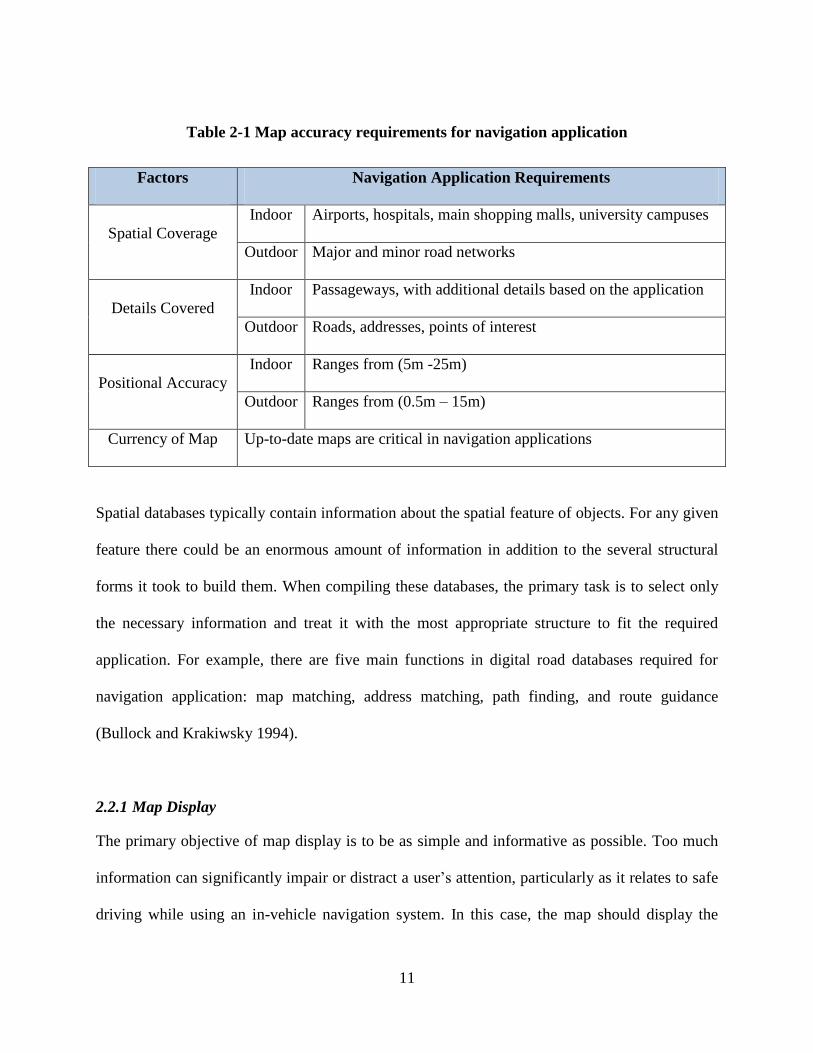
cities. Table 2-1 shows a sample of the main requirements for map accuracy in a navigation
application.
11
Table 2-1 Map accuracy requirements for navigation application
Factors Navigation Application Requirements
Spatial Coverage
Indoor Airports, hospitals, main shopping malls, university campuses
Outdoor Major and minor road networks
Details Covered
Indoor Passageways, with additional details based on the application
Outdoor Roads, addresses, points of interest
Positional Accuracy
Indoor Ranges from (5m -25m)
Outdoor Ranges from (0.5m – 15m)
Currency of Map Up-to-date maps are critical in navigation applications
Spatial databases typically contain information about the spatial feature of objects. For any given
feature there could be an enormous amount of information in addition to the several structural
forms it took to build them. When compiling these databases, the primary task is to select only
the necessary information and treat it with the most appropriate structure to fit the required
application. For example, there are five main functions in digital road databases required for
navigation application: map matching, address matching, path finding, and route guidance
(Bullock and Krakiwsky 1994).
2.2.1 Map Display
The primary objective of map display is to be as simple and informative as possible. Too much
information can significantly impair or distract a user’s attention, particularly as it relates to safe
driving while using an in-vehicle navigation system. In this case, the map should display the
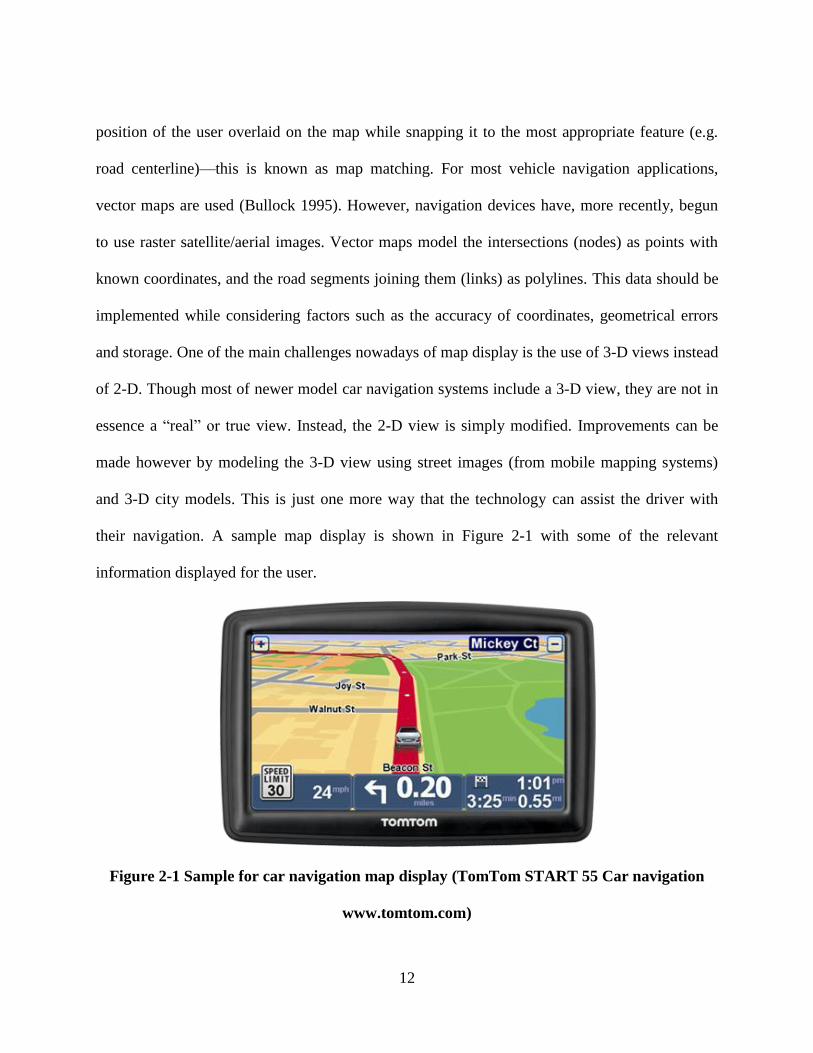
12
position of the user overlaid on the map while snapping it to the most appropriate feature (e.g.
road centerline)—this is known as map matching. For most vehicle navigation applications,
vector maps are used (Bullock 1995). However, navigation devices have, more recently, begun
to use raster satellite/aerial images. Vector maps model the intersections (nodes) as points with
known coordinates, and the road segments joining them (links) as polylines. This data should be
implemented while considering factors such as the accuracy of coordinates, geometrical errors
and storage. One of the main challenges nowadays of map display is the use of 3-D views instead
of 2-D. Though most of newer model car navigation systems include a 3-D view, they are not in
essence a “real”or true view. Instead, the 2-D view is simply modified. Improvements can be
made however by modeling the 3-D view using street images (from mobile mapping systems)
and 3-D city models. This is just one more way that the technology can assist the driver with
their navigation. A sample map display is shown in Figure 2-1 with some of the relevant
information displayed for the user.
Figure 2-1 Sample for car navigation map display (TomTom START 55 Car navigation
www.tomtom.com)

13
2.2.2 Address matching
Address matching is a process by which an address provided by the user is matched to its
location on a map. To achieve this function in a map database addresses must be included.
Historically, the main problem with address storage was the sheer amount of space required for a
database to be effective. As a result, early car navigation devices typically required addresses to
be added by range between node and node such that the link would include a range of addresses.
However, withtheadvancementoftoday’sstoragedevices,itisnotlonger an issue to add every
address to the exact point where it is located on the map since the link will include a number of
points of known addresses. The addresses added to the databases are not only residential, but
also include main landmarks such as schools, hospitals, roads names, and shopping centers.
These are included to assist the user in navigating to the desired destination.
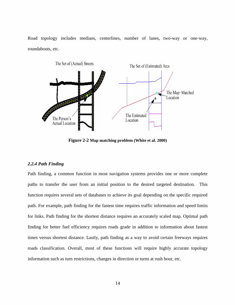
2.2.3 Map matching
Map matching is the process of locating a user’spositionon a specific feature of a map. Refer to
Figure 2-2. It has two objectives in navigation systems: to visualize the user’s position on the
map and improve the positioning accuracy. In cases of land vehicle navigation, map matching
occurs by forcing the position to be related to the road path. Since the map matching process
seeks to improve the positioning accuracy of the user, maps must be of better positioning quality
than the positioning system. By comparing the available maps for navigation (e.g. Navteq maps,
Google maps, etc.) with their average accuracy (around 1m overall) to the accuracy of the
navigation sensors, which could reach more than 50m in urban areas, it is easy to conclude that
map matching can enhance positioning accuracy. The database features required for map
matching are similar to the above functions; however complete road topology must be included.
14
Road topology includes medians, centerlines, number of lanes, two-way or one-way,
roundabouts, etc.
Figure 2-2 Map matching problem (White et al. 2000)
2.2.4 Path Finding
Path finding, a common function in most navigation systems provides one or more complete
paths to transfer the user from an initial position to the desired targeted destination. This
function requires several sets of databases to achieve its goal depending on the specific required
path. For example, path finding for the fastest time requires traffic information and speed limits
for links. Path finding for the shortest distance requires an accurately scaled map. Optimal path
finding for better fuel efficiency requires roads grade in addition to information about fastest
times versus shortest distance. Lastly, path finding as a way to avoid certain freeways requires
roads classification. Overall, most of these functions will require highly accurate topology
information such as turn restrictions, changes in direction or turns at rush hour, etc.

15
2.2.5 Road guidance
Road guidance requires no additional information other than address matching and path finding.
In other words, it is very common to have this function when both of these functions are present.
The goal of road guidance is to provide the user with turn-by-turn instructions to guide the user
from one location to another.
The requirements for each function are summarized in Table 2-2.
Table 2-2 Spatial database features required for each function (Bullock 1995)
Function Database features required
Map display Links (roads or passageways), nodes (intersections), coordinates of nodes
Address matching Links, names of links, nodes, coordinates of nodes, addresses along the
links, rooms or stores listing (indoor applications)
Map matching Links, nodes, coordinates of nodes, complete topology
Path finding Link classification, connectivity between nodes, driving and turn
restrictions, auxiliary attributes
Route guidance All address matching and path-finding features
2.3 Map sources for navigation applications
Maps for navigation applications can be provided by several sources. These sources can be from
one of three categories: Major map providers such as Google or NAVTEQ, public-contributed
mapping solutions such as OpenStreetMap, or specially designed and developed maps by
mapping and surveying companies based on a required specific application.
16
2.3.1 Major Mapping Sources
There are several sources of digital maps today. Some of the major sources according to both
coverage and accuracy are Tele Atlas, NAVTEQ (provider of Bing Maps), Google Maps and
OpenStreetMap. Tele Atlas is a Dutch company that provides digital maps for applications like
navigation, location-based services, mobile and web mapping applications. NAVTEQ is an
American provider of Geographic Information Systems (GIS) data and base electronic navigable
maps. Nokia Ovi map applications use NAVTEQ data. Furthermore, NAVTEQ provides map
data used in the navigation applications of companies like Chrysler, Mercedes-Benz, Garmin,
Magellan, Yahoo Maps, Bing Maps, and MapQuest. Bing Maps is a web mapping service
developed by Microsoft that spans the whole globe. It provides services such as road views,
aerial views,streetsideimagery,bird’seyeviews (presents aerial imagers acquired from using
low-flying aircraft), venue maps (several venues that Bing has mapped in North America,
Europe and Asia according to Bing Maps’ website), and 3-D maps. Google Maps is a web
mapping application provided by Google. It supports many map-based services including the
Google Maps website, Google Transit, and the Google Maps API, which allows developers to
implement Google Maps into their websites or devices. It has been used by many navigation
applications including smart cell phones and navigators. The powers of Google’s free maps are
their global coverage and reliable accuracy for navigation applications. OpenStreetMap is a free
digital mapping service based on the concepts of Crowdsourcing and Volunteered Geographical
Information (VGI), which will be discussed in detail in section 2.3.3.
17
2.3.2 Maps for specific projects
There are several categories of maps that are required for navigation and location based
applications. For outdoor navigation applications, the main content of the map is a basic roads
map, which includes the road networks with street names, building numbers and main
landmarks. For indoor applications, the map depends mainly on the application. There are
several indoor applications that can require maps.
The main applications are:
Location-based services: for finding the nearest store, or locating what gate your flight is
departing from and where it is on the map.
Navigation applications: for providing the shortest path from the user’s location to a
required destination.
Emergency: for assisting fire, police and EMS departments. The user can locate
themselves on a map to navigate more quickly through a building (especially if there is a
smoke).
People with disabilities: People who are visually impaired or blind can benefit
significantly with help navigating through different buildings, shopping centers or
markets.
In addition to these applications, a user can be in a shopping mall and when they approach a
store, he/she can receive a message to his/her smartphone with current offers and promotions.
Furthermore, indoor maps can bring an added dimension to sports such as laser tag or combat

18
games, where each team has the map for a certain recreation area. Based on these
applications, there should be different types of maps as shown in Table 2-3.
Table 2-3 Some Types of Maps and the corresponding features to be mapped
Types of Maps Main covered features
Buildings Floor Plans Rooms, corridors, stairs, elevators and all relevant landmarks.
Airport Plans Flight gates location, boarding location, airlines kiosks, washrooms, etc.
Shopping Malls Plans
Store locations, washrooms, parking, exits, security, customer services,
etc.
Campus Plans
Lecture venues, staff rooms, food court, washroom, transit, security,
convention centers, etc.
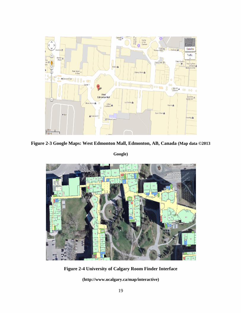
The maps used for indoor navigation application can be in several formats; such as BIM
(Building Information Modeling), GML (Geography Markup Language), ArcGIS Geo-databases,
shape-files and CAD files. The selection of the required format is based on availability, the
targeted application and the required output. The following figures represent samples for the
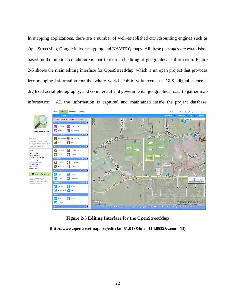
indoor maps. For the shopping mall plans, Figure 2-3 represents the West Edmonton Shopping
Mall, provided by Google Maps. As a sample for the campus maps, Figure 2-4 represents the
Room Finder interface on the University of Calgary Maps website.
19
Figure 2-3 Google Maps: West Edmonton Mall, Edmonton, AB, Canada (Map data ©2013
Google)
Figure 2-4 University of Calgary Room Finder Interface
(http://www.ucalgary.ca/map/interactive)

20
It is important to consider many factors when selecting a map most appropriate for providing the
necessary information. The following guidelines can be used to define the most appropriate maps
for an indoor application:
Start with any already available map. Many airports and shopping malls have their own
map that can easily be found on their website or at the location itself. Usually these maps
are updated and suitably scaled.
Check the accuracy of the required map based on the required application. Maps required
for emergency navigation purposes could need maps with an accuracy range of
approximately 1m; however, maps required for shopping promotions could have an
accuracy of 10m.
Find ways to get regular updates for the map. Some locations can have room information
changed regularly. These updates can be done by checking the online map, requesting
regular feedbacks from the user (crowdsourcing), or performing a site visit along with
doing an as-built update regularly.
Find ways to verify the information on the map, especially if you are depending on public
input.
If the initial map is not available, there should be other ways to obtain maps for indoor
navigation applications. The most common is traditional surveying methods such as using total
stations measurements, CAD drafting, to name a few. There have been several researches
conducted on automatic indoor mapping using robotic and different sensors, such as UWB radar,
terrestrial laser scanners, and range finder. These applications provide a 3-D model for the indoor
environment offering up such features as walls, corridors, and windows. Other possible solutions

21
for obtaining maps include outsourcing the mapping task to a private company or using the
power of crowdsourcing.
Several considerations should be made when designing geospatial models for indoor navigation
applications. For indoor navigation, absolute positioning and direction are not as important as
relative positioning and direction. It might be more useful for a user to describe his location in
terms of how far they are from a certain store in a mall than to get an absolute position.
Referencing user location data to the nearest landmark is more helpful for most applications of
indoor navigation (Arto et al. 2009). The use of barometers as sensors for obtaining height
information helps to identify on which floor the user is located. The application requires this
information in order to display the correct floor map. Although an international standard and
well-defined cartographic labeling is not yet in use, especially for indoor landmarks, it will
become the norm in the near future as the market for indoor navigation continues to grow.
2.3.3 Crowdsourcing
Crowdsourcing is an operation of outsourcing several tasks for a specific project to a group of
people; however, the main concept is that it is not outsourced to any specific group of people.
There are many examples of crowdsourcing projects such as Wikipedia and OpenStreetMap.
Crowdsourcing processes are highly beneficial to projects requiring brainstorming, product
testing and reviews, advertising ideas, and marketing. Traffic updating interfaces are especially
useful for crowdsourcing operations.
22
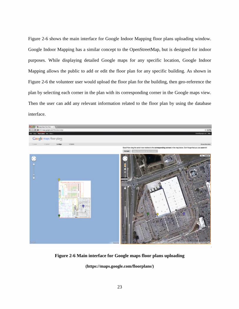
In mapping applications, there are a number of well-established crowdsourcing engines such as
OpenStreetMap, Google indoor mapping and NAVTEQ maps. All these packages are established
based on the public’scollaborative contribution and editing of geographical information. Figure
2-5 shows the main editing interface for OpenStreetMap, which is an open project that provides
free mapping information for the whole world. Public volunteers use GPS, digital cameras,
digitized aerial photography, and commercial and governmental geographical data to gather map
information. All the information is captured and maintained inside the project database.
Figure 2-5 Editing Interface for the OpenStreetMap
(http://www.openstreetmap.org/edit?lat=51.046&lon=-114.0532&zoom=13)
23
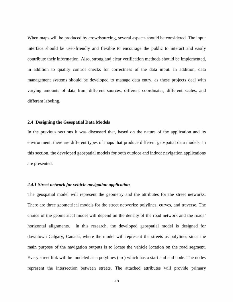
Figure 2-6 shows the main interface for Google Indoor Mapping floor plans uploading window.
Google Indoor Mapping has a similar concept to the OpenStreetMap, but is designed for indoor
purposes. While displaying detailed Google maps for any specific location, Google Indoor
Mapping allows the public to add or edit the floor plan for any specific building. As shown in
Figure 2-6 the volunteer user would upload the floor plan for the building, then geo-reference the
plan by selecting each corner in the plan with its corresponding corner in the Google maps view.
Then the user can add any relevant information related to the floor plan by using the database
interface.
Figure 2-6 Main interface for Google maps floor plans uploading
(https://maps.google.com/floorplans/)

24
Figure 2-7 shows the main interface for the NAVTEQ Mapping Reporter uploading window.
NAVTEQ Map Reporter allows the public user to add or edit Navteq online maps. As shown in
the figure (based on the NAVTEQ website) these modifications and editing include:
Point of Interest editing: adding, removing, or making changes to an existing shop
business,
Address Marker or Location: making changes to the location of a house or building
Roads and Roads Features: adding, editing or removing roads and road features such as
signs, one-ways, or restrictions.
Other modifications and editing can include reporting on cartography, signs, postal and
administrative areas, bridges, tunnels and electric vehicle charging stations.
Figure 2-7 Main interface for the NAVTEQ Map reporter uploading
(http://mapreporter.navteq.com/)
25
When maps will be produced by crowdsourcing, several aspects should be considered. The input
interface should be user-friendly and flexible to encourage the public to interact and easily
contribute their information. Also, strong and clear verification methods should be implemented,
in addition to quality control checks for correctness of the data input. In addition, data
management systems should be developed to manage data entry, as these projects deal with
varying amounts of data from different sources, different coordinates, different scales, and
different labeling.
2.4 Designing the Geospatial Data Models
In the previous sections it was discussed that, based on the nature of the application and its
environment, there are different types of maps that produce different geospatial data models. In
this section, the developed geospatial models for both outdoor and indoor navigation applications
are presented.
2.4.1 Street network for vehicle navigation application
The geospatial model will represent the geometry and the attributes for the street networks.
There are three geometrical models for the street networks: polylines, curves, and traverse. The
choice of the geometrical model will depend on the density of the road network and the roads’
horizontal alignments. In this research, the developed geospatial model is designed for
downtown Calgary, Canada, where the model will represent the streets as polylines since the
main purpose of the navigation outputs is to locate the vehicle location on the road segment.
Every street link will be modeled as a polylines (arc) which has a start and end node. The nodes
represent the intersection between streets. The attached attributes will provide primary

26
information about navigation purposes such as the nodes coordinates, links start and end sites,
ands all possible diverged links form every link and traffic direction. The geospatial model itself
is designed to allow the incorporation of any additional information, such as the elevation
(height) of the nodes. The system will use OpenStreetMaps to extract the roads network in order
to build the geospatial model. For most vehicle navigation applications, the accuracy of
OpenStreetMaps (around 10 m) is acceptable. In the downtown regions, specifically downtown
Calgary, the accuracy of the Maps should range between 0.5 and 1 meters.
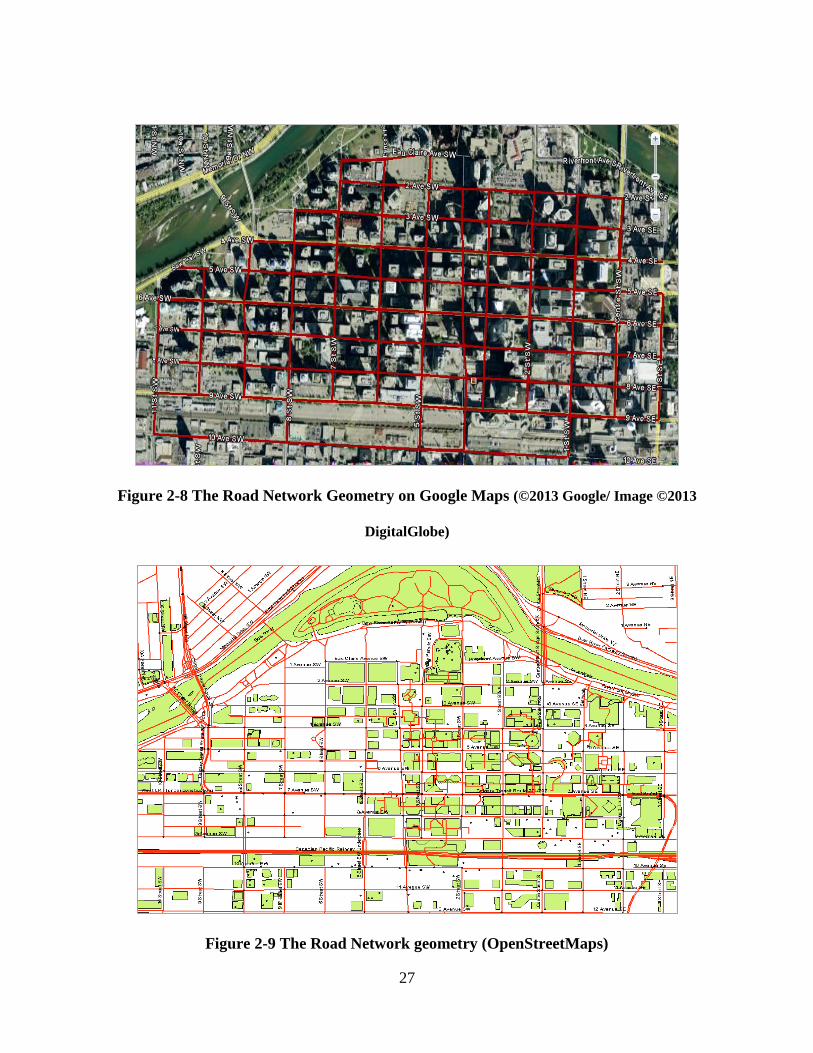
2.4.1.1 Geospatial model for Downtown Calgary
A geospatial database was built to incorporate the developed map matching algorithms (to be
discussed in Chapter 3) and was used for selecting the appropriate road link where the user is
located. The geospatial database covers the study areas where the field tests would occur (refer to
Chapter 6)—downtown Calgary. Downtown Calgary is the ideal place to test the developed
algorithms in GPS-denied environment because of its high buildings, which cause GPS signal
blockage. The geospatial model uses OpenStreetMaps to construct the geometry of the road
networks, where its accuracy ranges between 0.5m and 1m. Google Maps was used for the
downtown Calgary area as an additional source of geometry and associated attributes. Figure 2-8
and Figure 2-9 show the geometry for the road network of the study area. The downtown
Calgary region is made up of a network of roads that are mostly perpendicular to each other. The
roads that run East-West are classified as Avenues and those that run North-South are Streets.
Every intersection in the roads network is represented as a point (node) whose coordinates are
known as well as its street and avenue numbers (Attia et al. 2010; Attia et al. 2011-a).
27
Figure 2-8 The Road Network Geometry on Google Maps (©2013 Google/ Image ©2013
DigitalGlobe)
Figure 2-9 The Road Network geometry (OpenStreetMaps)
28
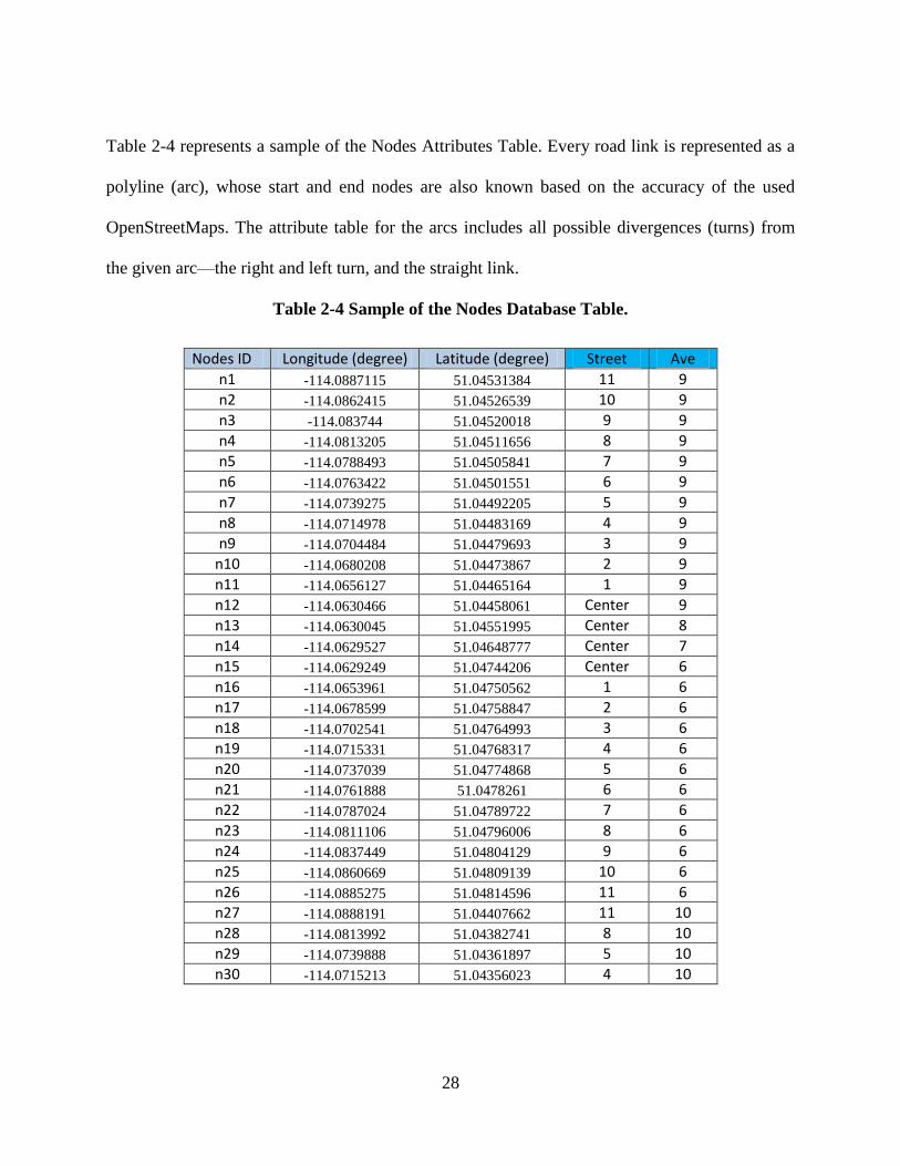
Table 2-4 represents a sample of the Nodes Attributes Table. Every road link is represented as a
polyline (arc), whose start and end nodes are also known based on the accuracy of the used
OpenStreetMaps. The attribute table for the arcs includes all possible divergences (turns) from
the given arc—the right and left turn, and the straight link.
Table 2-4 Sample of the Nodes Database Table.
Nodes ID Longitude (degree) Latitude (degree) Street Ave
n1 -114.0887115 51.04531384 11 9
n2 -114.0862415 51.04526539 10 9
n3 -114.083744 51.04520018 9 9
n4 -114.0813205 51.04511656 8 9
n5 -114.0788493 51.04505841 7 9
n6 -114.0763422 51.04501551 6 9
n7 -114.0739275 51.04492205 5 9
n8 -114.0714978 51.04483169 4 9
n9 -114.0704484 51.04479693 3 9
n10 -114.0680208 51.04473867 2 9
n11 -114.0656127 51.04465164 1 9
n12 -114.0630466 51.04458061 Center 9
n13 -114.0630045 51.04551995 Center 8
n14 -114.0629527 51.04648777 Center 7
n15 -114.0629249 51.04744206 Center 6
n16 -114.0653961 51.04750562 1 6
n17 -114.0678599 51.04758847 2 6
n18 -114.0702541 51.04764993 3 6
n19 -114.0715331 51.04768317 4 6
n20 -114.0737039 51.04774868 5 6
n21 -114.0761888 51.0478261 6 6
n22 -114.0787024 51.04789722 7 6
n23 -114.0811106 51.04796006 8 6
n24 -114.0837449 51.04804129 9 6
n25 -114.0860669 51.04809139 10 6
n26 -114.0885275 51.04814596 11 6
n27 -114.0888191 51.04407662 11 10
n28 -114.0813992 51.04382741 8 10
n29 -114.0739888 51.04361897 5 10
n30 -114.0715213 51.04356023 4 10
29
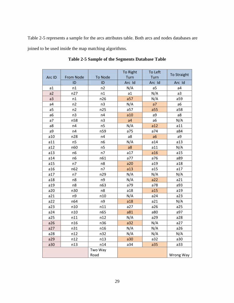
Table 2-5 represents a sample for the arcs attributes table. Both arcs and nodes databases are
joined to be used inside the map matching algorithms.
Table 2-5 Sample of the Segments Database Table
Arc ID From Node To Node To Right
Turn To Left
Turn To Straight
ID ID Arc Id Arc Id Arc Id
a1 n1 n2 N/A a5 a4
a2 n27 n1 a1 N/A a3
a3 n1 n26 a57 N/A a59
a4 n2 n3 N/A a7 a6
a5 n2 n25 a57 a55 a58
a6 n3 n4 a10 a9 a8
a7 n58 n3 a4 a6 N/A
a8 n4 n5 N/A a12 a11
a9 n4 n59 a75 a74 a84
a10 n28 n4 a8 a6 a9
a11 n5 n6 N/A a14 a13
a12 n60 n5 a8 a11 N/A
a13 n6 n7 a17 a16 a15
a14 n6 n61 a77 a76 a89
a15 n7 n8 a20 a19 a18
a16 n62 n7 a13 a15 a17
a17 n7 n29 N/A N/A N/A
a18 n8 n9 N/A a22 a21
a19 n8 n63 a79 a78 a93
a20 n30 n8 a18 a15 a19
a21 n9 n10 N/A a24 a23
a22 n64 n9 a18 a21 N/A
a23 n10 n11 a27 a26 a25
a24 n10 n65 a81 a80 a97
a25 n11 n12 N/A a29 a28
a26 n16 n36 a32 N/A a27
a27 n31 n16 N/A N/A a26
a28 n12 n32 N/A N/A N/A
a29 n12 n13 a30 a32 a30
a30 n13 n14 a34 a35 a33
Two Way Road
Wrong Way

30
2.4.2 Building information model for indoor application
The developed map aided navigation system will use the University of Calgary GIS maps
provided by the University’s GIS library to build the geospatial model. The use of these maps is
significantly more time-efficient since new maps do not have to be built and because they are
already to georeferenced and projected according to the world global system WGS84, the system
used by the GPS device. Similar to the outdoor model, the geospatial model for indoor
applications will represent the links as polylines connecting nodes. The links will represent the
possible passageways (corridors) where the user could be located in. In this thesis, the navigation
application is based on the assumption that the user would be located on the passageways.
According to the indoor navigation applications, the ability to link the location of the user to the
nearest passageway can achieve a level of accuracy required for applications such as E911,
personal navigation, law-enforcement, and disability assistance. The attached indoor attributes
are different than the outdoor ones as the height change factor plays an important role in indoor
applications. Height change by stairs and elevation will produce a change in the navigated floor
map. Therefore, the system must provide all information about both height values and places
where height change can occur. Other relevant attributes such as link nodes, nodes coordinates,
and all possible links diverged from each link in the straight, right and left directions, stairs, and
elevators are created.
The next two sections present the geospatial model for two different locations. Both locations are
at the University of Calgary Campus. The input for both datasets is GIS shape files of the ESRI
ArcGIS GIS software. The geographical coordinate datum used is the GCS (Geographic
Coordinate system) North American 1983. The projected coordinate system used is NAD (North

31
American datum) 1983 UTM (Universal Transverse Mercator) Zone 11N with Transverse
Mercator Projection. The projection used false easting of 500000.00, false northing of 0.00,
central meridian of -117.00, scale factor of 0.999600 and latitude of origin of 0.00.
2.4.2.1 Geospatial Model for the Engineering Building at University of Calgary
In order to assist the map aided navigation systems for indoor applications, a modeling for the
building floor information was developed. The first study area, where field tests were performed,
is the Engineering building at the University of Calgary campus. Both geometrical and
topological characteristics for the building were implemented in the geospatial model (Attia et al.
2011-b). The model considered primary characteristics such as the length of passageways,
location, alignment, and connectivity. The geospatial model itself is implemented in the three
main modeling phases: conceptual, logical and physical modeling. Conceptually, the model
assumes that users would be located at any time through a passageway (the corridors located in
building floors), which would be geometrically modeled as polylines locates at the centerline of
each corridor. The passageways cover all possible corridors and stairways. If the user enters any
room, the system will locate the user on the corresponding nearest corridor. The passageways
polylines (would be called links) connect two points of known coordinates (would be called
nodes). Figure 2-10 represents the geometrical layout for the geospatial model of the building.
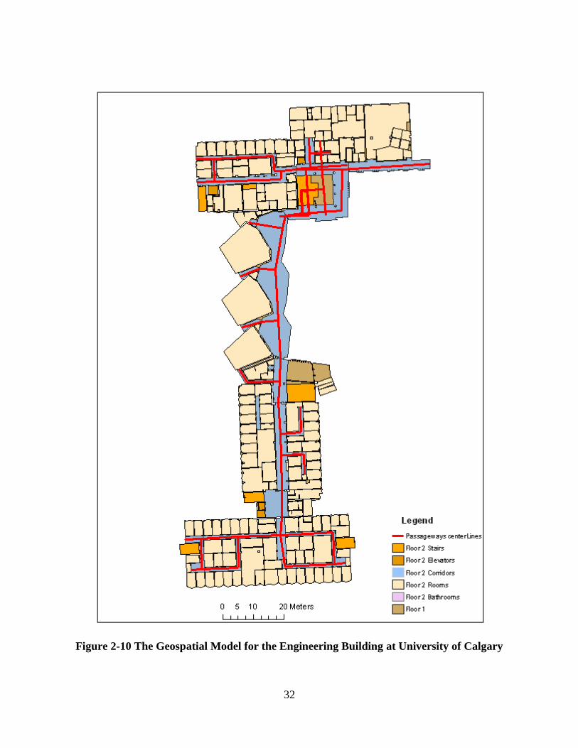
32
Figure 2-10 The Geospatial Model for the Engineering Building at University of Calgary

33
The logical model deals with the relational database, where each passageway is defined by
several attributes. Table 2-6 shows a sample of the links database table for the engineering
building. As shown in the table, each passageway should be defined by a unique identification
number (ID), its start and end (destination) nodes UTM coordinates, passageway length, floor
number, and if there are stairs on any of its sides. In addition, and to enable the turn detection
algorithm inside the map aiding system, each passageway is provided with the identification
number for all possible diverged passageways from both its start and end nodes. Diverged
passageways are divided to the three directions: right and left turns and straight directions. The
physical model, which deals with the internal structure of data objects by transferring the logical
model into implementation, was performed using the GeoDatabase of ArcGIS software. The
geospatial model was created using ArcGIS feature classes for each layer such as corridors,
rooms, and stairs. Each class was categorized under a georeferenced GeoDatabase with UTM
projected northing and easting.
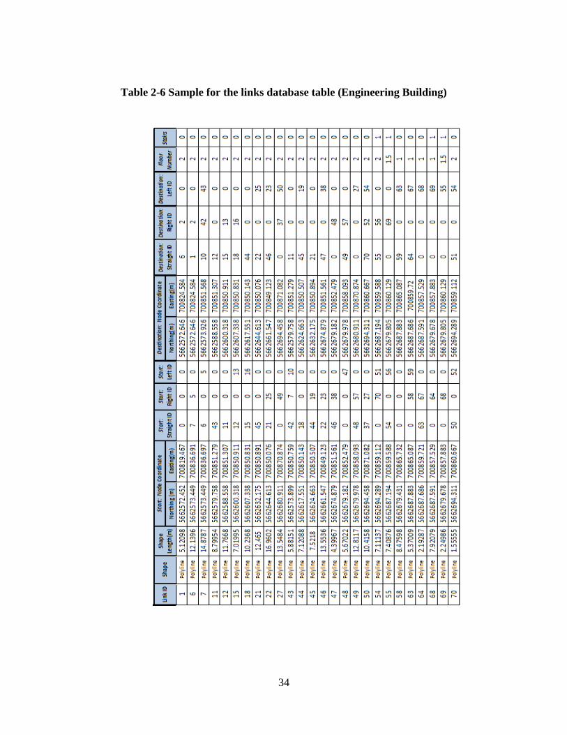
34
Table 2-6 Sample for the links database table (Engineering Building)
35
2.4.2.2 Geospatial Model for MacEwan Hall and Kinesiology Buildings at University of
Calgary
The second study area, where field tests were performed, is the MacEwan Hall and Kinesiology
building at the University of Calgary campus. Similar to the Engineering building, both
geometrical and topological characteristics for these two study areas were implemented in the
geospatial model. The model considered primary characteristics such as the length of
passageways, location, alignment, and the connectivity. The geospatial model itself is
implemented in three main modeling phases: conceptual, logical and physical modeling. The
three modeling phases are similar to the phases described previously in Section 2.4.2.1. Figure
2-11 and Figure 2-12 present the geometrical layout for the geospatial model of MacEwan Hall
and the Kinesiology Building’s floors 1 and 2 respectively. Table 2-7 shows a sample of the
links database table for MacEwan Hall and the Kinesiology Building

36
Figure 2-11 The Geospatial Model for the MacEwan and Kinesiology Building Floor one at
University of Calgary
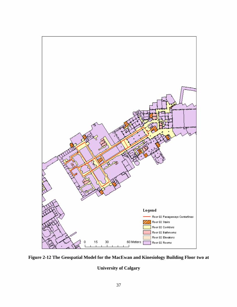
37
Figure 2-12 The Geospatial Model for the MacEwan and Kinesiology Building Floor two at
University of Calgary
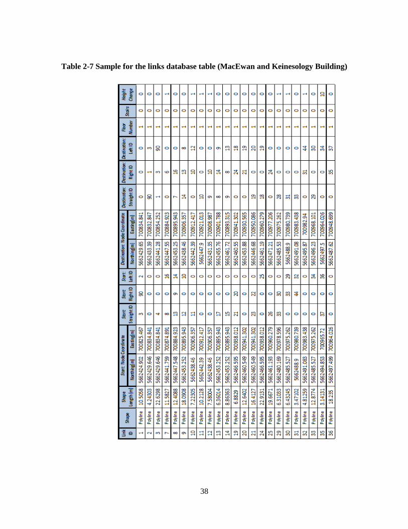
38
Table 2-7 Sample for the links database table (MacEwan and Keinesology Building)

39
Chapter Three: Map Matching Algorithms
3.1 Background of Map Matching Algorithms
In order to use map matching to aid navigation systems, it must meet the accuracy requirements
for the specific application, as discussed in Chapter 2. Map matching accuracy depends on three
major factors: the navigation system(s) in use, the model of spatial data, and the implemented
map matching algorithm (Quddus et al. 2009). Based on many researches in the last three
decades (after GPS had been introduced to the civil markets), one can conclude that the
integration of GPS and dead reckoning systems (especially inertial sensors) can achieve greater
accuracy, especially in urban areas. Since GPS suffers from signal outages and blockage in
certain areas, such as urban canyons and tunnels, inertial systems can bridge to some extent these
outages. Map matching is used as well to bridge these outages by being integrated into the
navigation system. To achieve highly accurate results, one must choose the most appropriate
map matching algorithm. Choosing a map matching algorithm depends on the required
application and the input constraints (position, velocity and heading). The following sections will
provide a brief discussion of the most used map matching algorithms, in addition to those
currently in development to be used in this research.
3.1.1 Geometric and Topological Algorithms
Geometrical and topological modelings are considered the simplest conventional algorithms that
can achieve high map matching accuracy. Many researchers have used this algorithm and have
achieved acceptable results (Basnayake et al. 2005), (Quddus et al. 2007), (White et al. 2000),
(Scott 1994), (Greenfeld 2002). It is not recommended to use geometric algorithms as a

40
standalone algorithm, instead it is suggested they be used with topological modeling. The main
purpose of this algorithm is to choose a suitable link where the vehicle is located. This selection
is based on the shortest distance between the position fix (the position provided by the navigation
sensor) and the links. The link that yields the shortest distance will be selected. In addition, many
other constraints can be used with the previous proximity constraint such as the bearing or
heading. This constraint is implemented by calculating the angle between the bearing of the link
(using coordinate information from the spatial database) and the heading of the vehicle (from
navigation sensor output). The link with the smallest angle will be selected. The selection of a
suitable link is then based on a weighting between the proximity and bearing factors, as shown in
Figure 3-1 and Figure 3-2.
Heading of vehicle
Direction of Road Segment
Start Node A(x1,y1) End Node B(x2,y2)
Heading Difference
Figure 3-1 Similarity in vehicle heading and bearing of a link
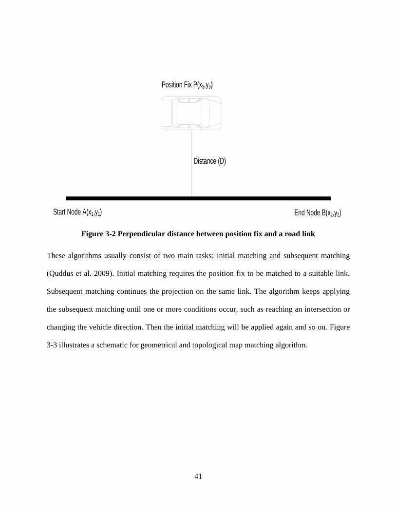
41
Position Fix P(x3,y3)
Distance (D)
Start Node A(x1,y1) End Node B(x2,y2)
Figure 3-2 Perpendicular distance between position fix and a road link
These algorithms usually consist of two main tasks: initial matching and subsequent matching
(Quddus et al. 2009). Initial matching requires the position fix to be matched to a suitable link.
Subsequent matching continues the projection on the same link. The algorithm keeps applying
the subsequent matching until one or more conditions occur, such as reaching an intersection or
changing the vehicle direction. Then the initial matching will be applied again and so on. Figure
3-3 illustrates a schematic for geometrical and topological map matching algorithm.
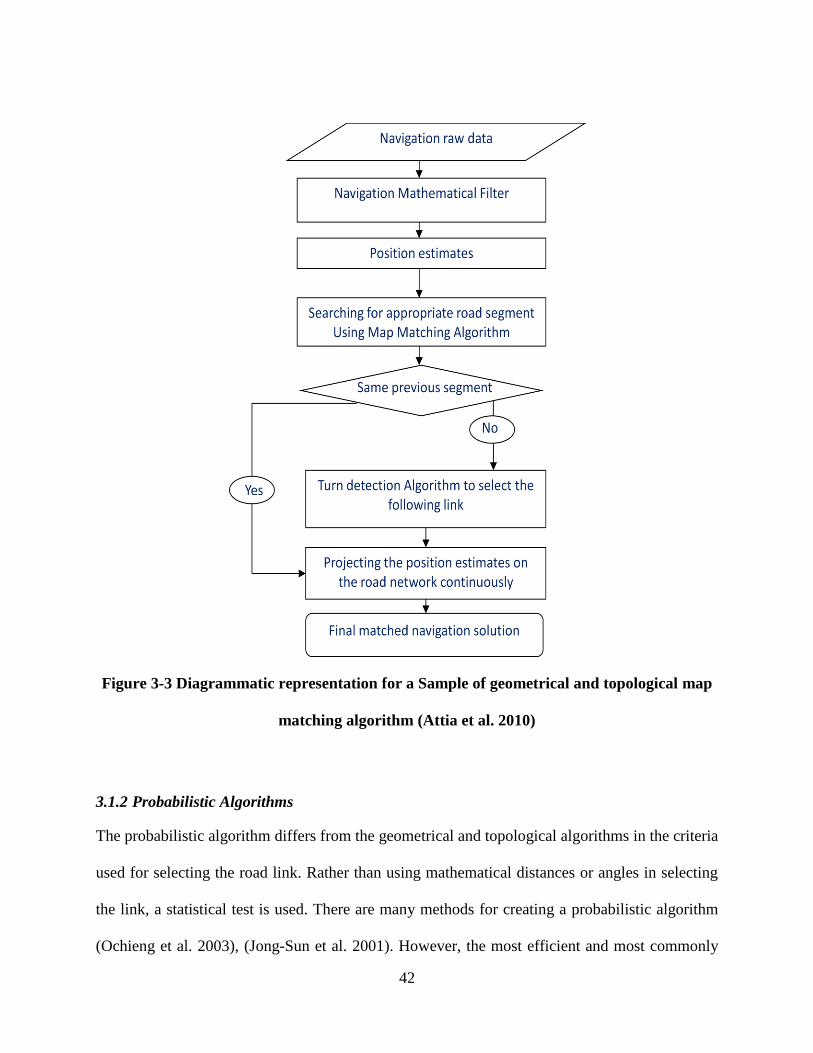
42
Figure 3-3 Diagrammatic representation for a Sample of geometrical and topological map
matching algorithm (Attia et al. 2010)
3.1.2 Probabilistic Algorithms
The probabilistic algorithm differs from the geometrical and topological algorithms in the criteria
used for selecting the road link. Rather than using mathematical distances or angles in selecting
the link, a statistical test is used. There are many methods for creating a probabilistic algorithm
(Ochieng et al. 2003), (Jong-Sun et al. 2001). However, the most efficient and most commonly

43
used is the confidence ellipse. The confidence ellipse is drawn from the statistical data of the
position fix (standard deviation and covariance). It is centered at the position fix, with semi
major axis (a), semi minor axis (b) and rotation angle ( ) (Mikhail and Ackermann 1976).
Equations 3-1, 3-2 and 3-3 show how to calculate these parameters.
3-1
3-2
3-3
Where ( and
are the variances for the x and y estimated positions from the navigation
sensors respectively and ( ) is the covariance for the position. Figure 3-4 presents a diagram
for the error ellipse drawn based on the user position fix at a certain epoch.

44
ab θ
Figure 3-4 The error ellipse drawn based on the user position fix
When obtaining the position fix, the confidence ellipsoid is drawn, which will intersect one or
more links. If one link is selected then it is obvious there is only this link to choose from, but if
several links are intersected with the ellipsoid, the selection is based on further criteria. The most
commonly used criteria to choose between the links are their connectivity and/or historical
information of the vehicle location, in that the vehicle will not jump from one link to another if
they are not connected. Figure 3-5 illustrates a schematic diagram for the implementation of a
probabilistic algorithm.
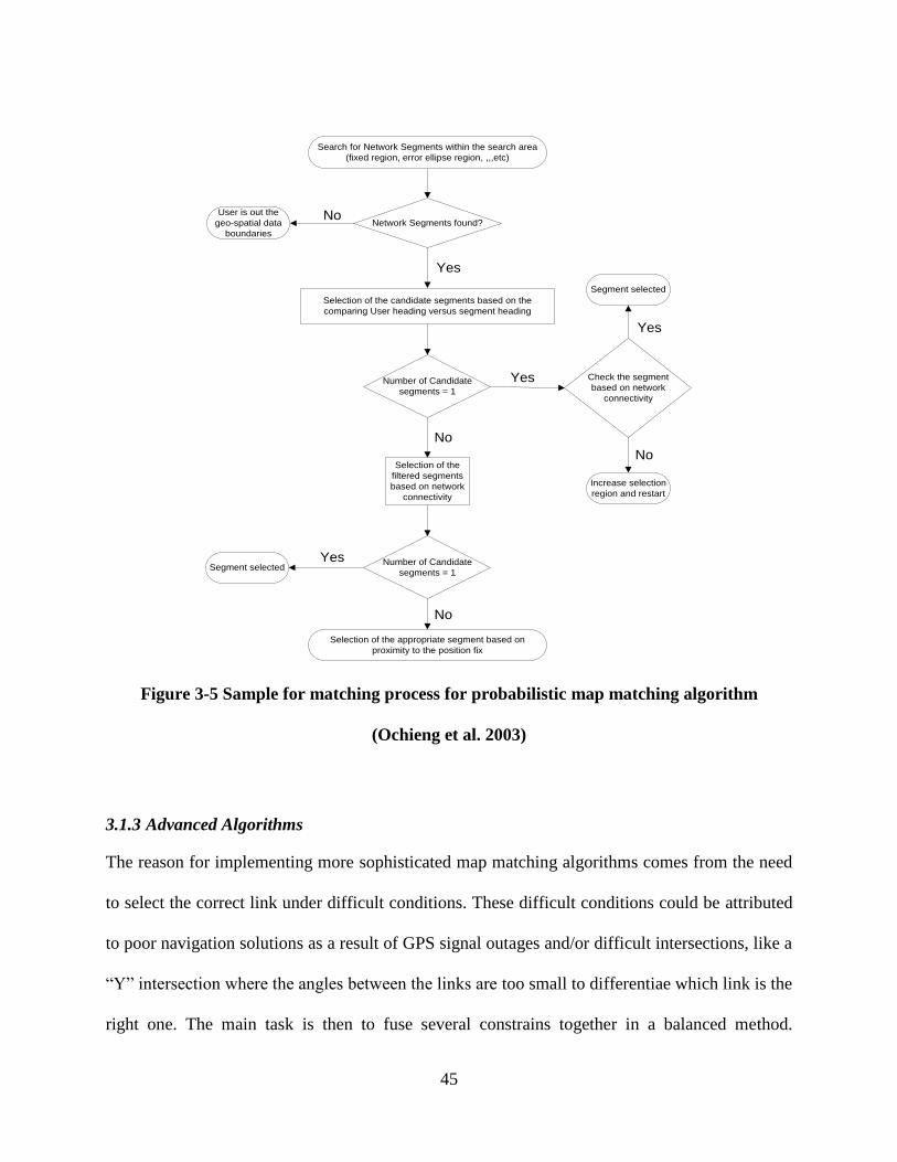
45
Network Segments found?
Selection of the candidate segments based on the
comparing User heading versus segment heading
Number of Candidate
segments = 1
Selection of the
filtered segments
based on network
connectivity
Number of Candidate
segments = 1
Check the segment
based on network
connectivity
No
Yes
Yes
Yes
Yes
No
No
No
Search for Network Segments within the search area
(fixed region, error ellipse region, ,,,etc)
Selection of the appropriate segment based on
proximity to the position fix
Segment selected
Segment selected
Increase selection
region and restart
User is out the
geo-spatial data
boundaries
Figure 3-5 Sample for matching process for probabilistic map matching algorithm
(Ochieng et al. 2003)
3.1.3 Advanced Algorithms
The reason for implementing more sophisticated map matching algorithms comes from the need
to select the correct link under difficult conditions. These difficult conditions could be attributed
to poor navigation solutions as a result of GPS signal outages and/or difficult intersections, like a
“Y”intersectionwheretheanglesbetweenthelinksaretoo small to differentiae which link is the
right one. The main task is then to fuse several constrains together in a balanced method.

46
Examples for these advanced algorithms include the use of Fuzzy Logic (Quddus et al. 2006),
(Syed and Cannon 2004), Belief Theory (El Najjar and Bonnifait 2005), particle filters, and
extended Kalman filter updates (El Najjar and Bonnifait 2005), (Yu et al. 2006).
Fuzzy logic has been considered one of the most promising techniques in the field of
probabilistic algorithms (Syed and Cannon 2004). The main structure of fuzzy logic is the
formation of what is known as the fuzzy inference system (FIS), which takes its input from the
navigation sensor and gives its output as the likelihood link. Within the FIS certain rules will be
applied on the inputs based on their membership function. A membership function (MH)
represents the degrees of truth by numerical values as shown in Figure 3-6. These rules are based
on the common logic to reach to the most likely output. Like previous algorithms, this algorithm
is divided into two tasks, initial and subsequent matching.
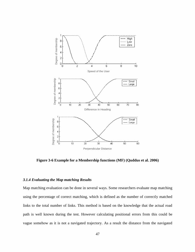
47
Speed of the User
Perpendicular Distance
Difference in Heading
De
gre
e o
f m
em
be
rsh
ipD
eg
ree
of m
em
be
rsh
ipD
eg
ree
of m
em
be
rsh
ip
Figure 3-6 Example for a Membership functions (MF) (Quddus et al. 2006)
3.1.4 Evaluating the Map matching Results
Map matching evaluation can be done in several ways. Some researchers evaluate map matching
using the percentage of correct matching, which is defined as the number of correctly matched
links to the total number of links. This method is based on the knowledge that the actual road
path is well known during the test. However calculating positional errors from this could be
vague somehow as it is not a navigated trajectory. As a result the distance from the navigated
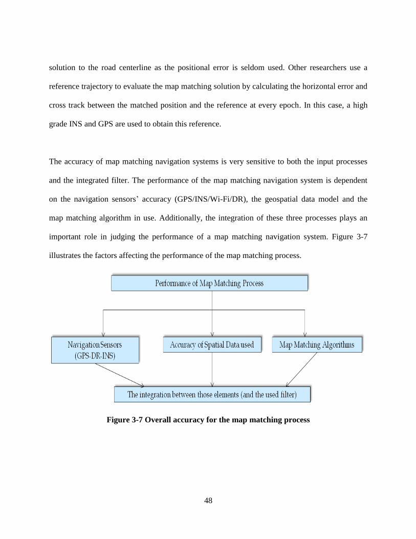
48
solution to the road centerline as the positional error is seldom used. Other researchers use a
reference trajectory to evaluate the map matching solution by calculating the horizontal error and
cross track between the matched position and the reference at every epoch. In this case, a high
grade INS and GPS are used to obtain this reference.
The accuracy of map matching navigation systems is very sensitive to both the input processes
and the integrated filter. The performance of the map matching navigation system is dependent
on the navigation sensors’ accuracy (GPS/INS/Wi-Fi/DR), the geospatial data model and the
map matching algorithm in use. Additionally, the integration of these three processes plays an
important role in judging the performance of a map matching navigation system. Figure 3-7
illustrates the factors affecting the performance of the map matching process.
Figure 3-7 Overall accuracy for the map matching process
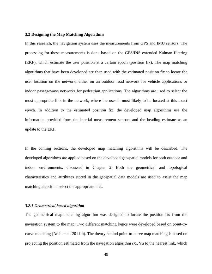
49
3.2 Designing the Map Matching Algorithms
In this research, the navigation system uses the measurements from GPS and IMU sensors. The
processing for these measurements is done based on the GPS/INS extended Kalman filtering
(EKF), which estimate the user position at a certain epoch (position fix). The map matching
algorithms that have been developed are then used with the estimated position fix to locate the
user location on the network, either on an outdoor road network for vehicle applications or
indoor passageways networks for pedestrian applications. The algorithms are used to select the
most appropriate link in the network, where the user is most likely to be located at this exact
epoch. In addition to the estimated position fix, the developed map algorithms use the
information provided from the inertial measurement sensors and the heading estimate as an
update to the EKF.
In the coming sections, the developed map matching algorithms will be described. The
developed algorithms are applied based on the developed geospatial models for both outdoor and
indoor environments, discussed in Chapter 2. Both the geometrical and topological
characteristics and attributes stored in the geospatial data models are used to assist the map
matching algorithm select the appropriate link.
3.2.1 Geometrical based algorithm
The geometrical map matching algorithm was designed to locate the position fix from the
navigation system to the map. Two different matching logics were developed based on point-to-
curve matching (Attia et al. 2011-b). The theory behind point-to-curve map matching is based on
projecting the position estimated from the navigation algorithm (XS, YS) to the nearest link, which
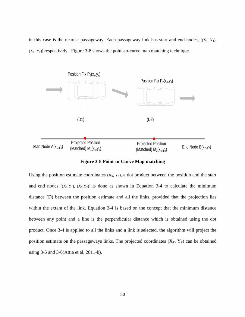
50
in this case is the nearest passageway. Each passageway link has start and end nodes, [(X1, Y1),
(X2, Y2)] respectively. Figure 3-8 shows the point-to-curve map matching technique.
Position Fix P1(xs,ys)
(D1)
Start Node A(x1,y1) End Node B(x2,y2)Projected Position
(Matched) M1(xp,yp)
Position Fix P2(xs,ys)
(D2)
Projected Position
(Matched) M2(xp,yp)
Figure 3-8 Point-to-Curve Map matching
Using the position estimate coordinates (XS, YS), a dot product between the position and the start
and end nodes [(X1,Y1), (X2,Y2)] is done as shown in Equation 3-4 to calculate the minimum
distance (D) between the position estimate and all the links, provided that the projection lies
within the extent of the link. Equation 3-4 is based on the concept that the minimum distance
between any point and a line is the perpendicular distance which is obtained using the dot
product. Once 3-4 is applied to all the links and a link is selected, the algorithm will project the
position estimate on the passageways links. The projected coordinates (XP, YP) can be obtained
using 3-5 and 3-6(Attia et al. 2011-b).

51
2
21
2
21
12212121
)()(
)()()(
YYXX
YXYXXXYYYXD ss
3-4
2
21
2
21
122112121212
)()(
))(()]()()[(
YYXX
YXYXYYYYYXXXXXXp ss
3-5
2
21
2
21
122112121212
)()(
))(()]()()[(
YYXX
YXYXXXYYYXXXYYYp ss
3-6
Two algorithms have been implemented based on how the navigation solution is projected. As
for the first algorithm, it will read the first epoch position and project it onto the nearest link
using the minimum distance technique. It will then keeps reading epoch by epoch and project
them on the nearest links. Figure 3-9 (on the left) shows the logical sequence for the first
geometrical map matching algorithm. The second algorithm will begin similarly to the first;
however, it will compute the shift between the first position estimate and the projected position.
The algorithm will shift the whole navigation solution with this value before projecting the
second epoch. Therefore for every epoch, the algorithm will first shift the solution with the
previous epoch shift value, and then project its position on the nearest link. Figure 3-9 (on the
right) shows the logical sequence for the second geometrical map matching algorithm.

52
Position Estimate (Xs, Ys)
Query for the nearest Link
Project the position estimate on the
Link (Xp, Yp)
Go to the next Xs, Ys
Position Estimate (Xs, Ys)
Query for the nearest Link
Project the position estimate on the Link (Xp, Yp)
Calculate the Shift between (Xs, Ys) and (Xp, Yp)
Apply the Shift to the next Xs, Ys
Figure 3-9 Geometrical Map Matching Algorithm: Method 1 (on the left) and Method 2 (on
the right)
3.2.2 Automatic turn detection algorithm
The implementation of the map matching algorithm begins with a reading of the first epoch
position and projecting it onto the nearest link using the techniques described in the previous
section. In order to activate the turn detection algorithm, the algorithm must first check if the
selected link is the same as the previous epoch or if it has been changed. Upon reaching a new
link, the turn detection algorithm is then activated to select the successive link. Selection of the
correct link at intersections is more challenging since there could be more links achieving the
small distance and it is not guaranteed that the minimum distance could lead to the correct link.
In a typical four-corridor intersectionorevena“T” intersection, theusercouldhave a similar

53
distance to all the links. However, waiting until the distance coincides on a certain link would
fail the real-time processing concept.
The newly proposed map matching algorithm includes a turn detection algorithm based on the
raw gyro data for the heading direction sensor. Observing the gyro raw data for heading, and
depending on the angular rate magnitude and direction, the algorithm detects whether a change
in direction occurred. Real-tests datasets were used to develop the threshold in turning detection
using the gyro measurements, subsequently creating a library for all the sudden changes in the
angular rate magnitude and their correlation to the direction (heading) of the user. Data from the
Micro-electro-mechanical systems (MEMS) based ADI ADXRS150, ADIS16405 MEMS Gyros
and Samsung Galaxy SII phone sensors were used to build a library for all the sudden changes in
the angular rate magnitude and relate them to the direction (heading) of the user. For example in
vehicle applications, it was noticed that turns will begin from 0.3 rad/sec to more than 3 rad/sec,
depending on whether it is just changing lanes or a 90 degree turn. Based on several trials, the
threshold was chosen to be ± 0.7 rad/sec (around 40 degree/ sec), which will reflect a complete
turn of the vehicle from one road segment to another. Figure 3-10 shows a sample of the signal
from a gyro aligned on the Z direction to sense the rotation of the vehicle heading. The figure
shows the trajectory with time stamps for a vehicle having a left turn on the left-hand side, and
on the right-hand side the signal values for the gyro sensor. It is clear from the figure that for the
exact region of the turning action, there is a huge jump in the signal magnitude. The threshold
was chosen to reflect the regular common user walking patterns, which will differentiate between
a complete turn of the user from one passageway segment to another. The sign of the angular rate
will detect whether it is a right or left turn, depending on the orientation of the Gyro axes for
54
example a right handed system with the vertical upward will make a left turn positive and a right
turn negative. This algorithm is used in all intersections for selecting the successive passageways
links.
Figure 3-10 Threshold for Turn Detection Using Raw Gyro Measurments
Figure 3-11 presents a flowchart diagram describing the logical steps for the turn detection
algorithm. The algorithm is activated upon detecting whether the link is different than the
previous epoch and/or the vehicle is approaching an intersection. Once a turn is detected, and
based on the threshold sign, the algorithm then detects whether the turn is a right or left turn. The
final decision for the appropriate link is then based on the occurrence of a turn link in the
associated geospatial model. For example if there a right turn is detected using the gyro
measurements, there must also be a right diverged link from the current link in the geospatial
database to indicate that this is the correct link, otherwise the algorithm will choose the
successive straight link.
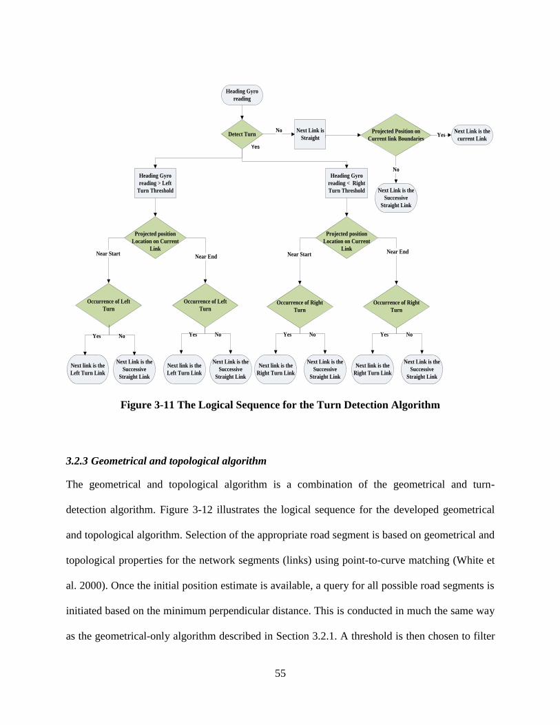
55
Detect Turn
Heading Gyro
reading > Left
Turn Threshold
Heading Gyro
reading < Right
Turn Threshold
Next Link is
Straight
No
Projected position
Location on Current
LinkNear Start
Near End
Occurrence of Left
Turn
Yes No
Near End
Yes No Yes No
Projected Position on
Current link BoundariesYes
No
Occurrence of Left
TurnOccurrence of Right
Turn
Occurrence of Right
Turn
Projected position
Location on Current
Link
Heading Gyro
reading
Next link is the
Left Turn Link
Next Link is the
Successive
Straight Link
Next link is the
Left Turn Link
Next Link is the
Successive
Straight Link
Next link is the
Right Turn Link
Next Link is the
Successive
Straight Link
Next link is the
Right Turn Link
Next Link is the
Successive
Straight Link
Yes
Next Link is the
current Link
Next Link is the
Successive
Straight Link
Near Start
Yes No
Figure 3-11 The Logical Sequence for the Turn Detection Algorithm
3.2.3 Geometrical and topological algorithm
The geometrical and topological algorithm is a combination of the geometrical and turn-
detection algorithm. Figure 3-12 illustrates the logical sequence for the developed geometrical
and topological algorithm. Selection of the appropriate road segment is based on geometrical and
topological properties for the network segments (links) using point-to-curve matching (White et
al. 2000). Once the initial position estimate is available, a query for all possible road segments is
initiated based on the minimum perpendicular distance. This is conducted in much the same way
as the geometrical-only algorithm described in Section 3.2.1. A threshold is then chosen to filter

56
any illogical returns and is fused according to the GPS/INS position fix accuracy and the features
of the navigating environment. In outdoor applications, the threshold is assumed using the value
of half the minimum distance between two parallel roads (building block). In indoor
applications, the value is assumed similarly to the road networks by using the distance between
near corridors. Therefore, to select a certain network segment, the initial position estimate should
have a minimum distance (less than the threshold) to this arc. Its projection should also be
located between its nodes. The algorithm will then continue to match the following position
estimates until the user approaches an intersection. For the appropriate segment to be selected at
an intersection, further information is required in addition to the minimum distance since several
links can give a minimum distance for several epochs but not necessarily the right one. The turn
detection algorithm is activated in this situation, as discussed in Section 3.2.2.
After applying the turn-detection algorithm, the successive link is selected and the position is
projected on its boundaries depending on whether the user’sdirection is straight, right or left.
The shift between the position fix and the projected position is computed and fed back as a
transitional shift towards the next epoch’s position fix. The algorithm will shift the whole
navigation solution with this value before projecting the position of the second epoch. In other
words, for every epoch, the algorithm will first shift the solution using the previous epoch shift
value and then project its position on the nearest link (Attia et al. 2011-b).

57
Figure 3-12 The Geometrical and Topological Map Matching Algorithm
For each epoch, the map matching algorithm uses a verification tool based on the heading value.
The algorithm calculates the heading for the current selected link based on its start and end
coordinates, and this value is then compared to the estimated heading state from the navigation
filter. The tolerance for the difference between both headings to be accepted or rejected as a
candidate link is based on the quality of the navigation sensor and the uncertainty of the heading
state.
58
Chapter Four: Mobile-Multi Sensor Integrated Navigation Systems
The accuracy of map aiding navigation systems depends on the navigation systems used. The
errors from any navigation system can produce an incorrect link selection, which could lead to a
complete failure in locating the user on the appropriate link. As a result, it is not just the purpose
of good algorithm, but the requirement of a reliable and accurate position solution, to assist the
algorithm in selecting the appropriate link. Therefore, this chapter discusses integrated mobile-
multi sensor navigation systems to overcome the challenges that exist with stand-alone navigation
systems.
4.1 Introduction to Navigation systems
Different navigation systems are available for vehicle and pedestrian navigation applications. GPS
is still the most commonly used sensor in navigation systems. It provides accurate and reliable
position and velocity estimates depending on the availability of a GPS signal. Unfortunately, GPS
performance in low signal environments such as urban canyons, tunnels and indoor facilities is not
reliable enough for many navigation applications. More recently, with an understanding and
acceptance that these techniques must inevitably cost more than a GPS-based system alone, the
practice of combining INS with GPS has become more widely accepted for commercial
applications (Syed 2009). The integration of inertial sensors with GPS provides a system that has
superior performance in comparison to either a GPS receiver or INS alone. For instance, GPS
derived positions have approximate white noise characteristics over the whole frequency range.
Therefore, GPS-derived positions and velocities are excellent external measurements that can be
used for updating the INS with position parameters thereby improving long-term accuracy.

59
Similarly, the INS can provide precise position and velocity data for GPS signal acquisition and
reacquisition after outages. In general, the fact that redundant measurements are available for the
determination of the vehicle trajectory parameters greatly enhances the reliability of the system
(Shin 2005).
It has certainly always been a maxim of safety-related applications, that to depend on one single
navigation technique would be imprudent. For maximum safety, complimentary navigation
systems should have error mechanisms that are disjoint. The resulting system design is then driven
by a trade-off between cost and performance. Advances in Micro-Electro Mechanical System
(MEMS) technology, combined with the miniaturization of electronics, have made it possible to
produce chip-based inertial sensors for use in measuring angular velocity and acceleration. These
chips are small, lightweight and consume very little power. As a result, they have been used in a
wide range of applications in the automotive, indoor navigation and other industrial industries.
MEMS technology, therefore, can be used to develop navigation systems (for outdoor or indoor
environments) that are inexpensive, small, and consume very little power (Abdel-Hamid 2004).
However, MEMS-bases INS systems typically exhibit very high positional drift when working in
the stand-alone mode (e.g. during GPS signal outages). These sensor measurements must be
professionally tuned in order to achieve the required accuracy. The tuning must occur in a lab
setting where estimation techniques can be properly applied, though not to the same extent as high
grade IMUs, which can have uncertainty values even just from the manufacturer. Many factors
must be carefully studied when tuning MEMS sensors such as the type of integrating estimation
filter, the inputs, measurements model, dynamic model, updating system, and observations
uncertainty.
60
Depending on the operational environment or whether the application is for vehicle or indoor
pedestrian use, some other sensors or constraints can be added to the navigation system. Sensors
or constraints such as odometers, magnetometers, barometers, Wi-Fi, RFID, UWB, map matching,
height constraints, non-holonomic constraints can assist in a very positive way the enhancing and
converging of navigation solutions obtained from these integrated navigation systems (El-Sheimy
and Niu 2007).
In order to deal with the input and output position information for the navigation systems, many
reference frames will be used in the navigation algorithms. In Appendix A, a brief definition of
the frames used in this thesis is discussed.
4.2 Inertial Sensors
Inertial sensors have been used for navigation and more specifically for situations in which GPS
suffers frequent signal outages and unavailability, which typically happens in urban centres and
indoor environments. Compared to GPS, inertial navigation has the advantage of providing the
orientation in addition to the position and velocities information. Inertial navigation is based on
Newton’s second law, where velocity and displacement can be derived from acceleration
measurements by integration. Inertial Measurement Unit (IMU) is used to measure the user
acceleration and angular velocity. It includes a 3-axial accelerometer and a 3-axial gyroscope.
Position, attitude and velocity are estimated by measuring the user acceleration and angular
velocity in the inertial frame of reference, transferring these measurements into the navigation
frame, and integrating them with respect to time. What follows is a description of the
fundamental measurements of inertial sensors:
61
Accelerometers: Accelerometers measure a specific force (f) by compensating for the gravitation
force (g), and result in estimating the user acceleration (a) based on Equation 4-1
4-1
By integrating the acceleration with respect to time (t), the velocity (v) and position (p) can be
estimated as shown in equations 4-2, 4-3 and 4-4:
4-2
4-3
4-4
where and are the initial position and velocity, respectively. The actual output of most
accelerometersisthevelocityincrementΔV, which is then converted to the specific force using
thesamplingintervalΔt, which is based on the relation . The accuracy of the obtained
navigation states depends on the grade of the navigation sensor. The most common grades are
the navigational grade with an average cost of $150K and a bias of 50-100μg,thetacticalgrade
with an average cost of $50-75K and a bias of 200-1000μg,andfinally the consumer (low-cost)
grade with a cost ranging from $1 to $100 and a bias of 0.1-0.5g (El-Sheimy 2010).
Gyroscopes: Gyroscopes measure the angular rates of the moving vehicle or pedestrian.
Integrating the observed angular rates with respect to time provides the angular change from
epoch to epoch. Each gyroscope observes the rotational motion in a direction perpendicular to
62
the plane of motion. There are two categories of gyroscopes: mechanical and optical. Mechanical
gyroscopes are not commonly used nowadays in navigation since optical gyroscopes (Ring laser
Gyroscopes (RLGs) or Fiber Optic Gyroscopes (FOGs)) are specified with high accuracy and no
moving parts. As for the performance of the sensor grade, the navigation grade has a gyro drift
rate of 0.015 deg/hr, the tactical grade has a gyro drift rate of 0.1-10 deg/hr, and the consumer
(low-cost) grade has a gyro drift rate of 100-360 deg/hr.
Magnetometer: Magnetometers provide the absolute magnetic heading value for the moving
object. The total Earth magnetic field value depends on the user location. The use of the
magnetometer is beneficial for the purpose of estimating a heading since a gyroscope’s derived
heading usually drifts with time. The main disadvantage of magnetometers is its sensitivity to the
elements in the environment, such as metals, which create challenges for navigating indoor
environments (Afzal 2011).
Barometer: Barometers (pressure sensor) estimate the altitude using atmospheric pressure and
temperature. The use of pressure sensors is beneficial for estimating the height of the user, when
the required height accuracy is not high since it is characterized by steady results over time even
with a low accuracy. Barometers usually assist the other sensors in providing a threshold for the
height or for floor selection in indoor navigation applications.
4.2.1 MEMS Inertial Sensors
Inertial sensors have a wide range of applications for determining body attitudes. Given their
affordability, MEMS sensors are used in several devices such as gaming consoles (transferring
63
the user’s body movement to the game), sports goggles (displaying motion parameters to the user
while racing), digital cameras and camcorders (image stabilization), handheld tablets and
smartphones (compass and screen orientation change detection).
MEMS inertial sensors were introduced as a substitute for tactical and navigation grade sensors
in low-cost navigation applications. The idea that MEMS sensors are low-cost, small, and
consume very little power makes them highly suitable for portable navigation systems and smart
phones (Goodall 2009). All recent smartphones now include MEMS sensors, even if not directly
used for navigation.
The integration of MEMS inertial sensors with GPS is essentially akin to the integration of other
higher grade IMUs with GPS. However, there are challenges with these low-cost sensors due to
the large errors they produce, which require additional considerations in the integration filter.
Furthermore, calibration of MEMS sensors are not usually done by the manufacturer due to the
nature of mass production and the higher chance of producing an inefficient calibration on each
individual sensor, which leads to a degradation in the overall integrated navigation solution
(Goodall 2009). The sensor errors are estimated by using a developed error stochastic model.
The integration Kalman filter should include most of the relevant errors (accelerometers and
gyroscopes biases and scale factors) into its state estimation. The selection of the error stochastic
model is a very sensitive operation due to the high noise-to-signal ratio characteristic of these
low-cost sensors. (Shin and El-Sheimy 2001; Aggarwal et al. 2010; Yuksel 2011) described
several error models for improving the accuracy and performance of low-cost MEMS sensors.

64
Allan Variance analysis can efficiently determine the noise, angle random walk, velocity random
walk and bias instability for the sensors.
4.2.2 Inertial Sensors Errors
In order to predict the performance of inertial sensors upon their integration with navigation
systems, their characteristics must first be well understood. Since inertial sensor errors
dramatically affect the reliability of a navigation solution they must be estimated and modeled
correctly. The performance characteristics of inertial sensors can be represented in four main
error categories: sensor bias, sensor scale factor, random noise, and axes misalignment.
Sensor bias: The accelerometer bias is measured in (g) while the gyroscope bias in (deg/hr). It
consists of two parts
Bias offset: a deterministic part that is the offset in measurement provided by the inertial
sensor. It can be eliminated using certain methods of sensor calibration
Bias drift: a stochastic part that is the rate of bias offset changes with time. It can be
estimated with an appropriate stochastic modeling process.
Sensor scale factor: Otherwise known as sensitivity, is the ratio between the changes in output
to the input.
Scale factor stability is the capability to accurately sense the acceleration/angular
velocities at different accelerations/ angular rates, expressed in part per million (ppm).
The sensor output differs from the input because of sensor fabrication imperfections.

65
The nature of the scale factor error is mainly deterministic, which can be minimized
using calibration.
The scale factor errors can be linear or non-linear. However, they are usually modeled
linearly as higher order errors are overshadowed by sensor noise (Afzal 2011).
Axes misalignment is the non-orthogonality of the body frame axes due to either fabrication
imperfection or mounting errors.
It is deterministic and can be estimated using calibration.
The effect of misaligned axes is critical since the two other axes can affect each
measurement.
When sensor calibration is performed, it involves a comparison between the sensor outputs and
well-defined reference information. This helps determine the corresponding coefficients that
cause sensor outputs to match the reference. There are several common calibration techniques
that can be used such as: the six-position static test to determine the accelerometer and gyroscope
bias and scale factors; the Local Level Frame (LLF) calibration, which can determine the six
misalignments, biases and scale factors; and the angle rate test to determine the gyroscope biases
and scale factors. (Shin and El-Sheimy 2001) developed a calibration technique that used up to
26 different positions to determine the bias, scale factor and non-orthogonality of the IMU
sensors.
The importance of sensor calibration can be illustrated by processing an uncompensated inertial
sensor error and project its effect on the navigation parameters (El-Sheimy and Niu 2007). An
66
uncompensated accelerometer bias (bf) would introduce a linear error in velocity (v) and a
quadratic error in the position (p) as shown in Equations 4-5 and 4-6.
4-5
4-6
An uncompensated gyro bias (bw) would introduce a quadratic error in velocity (v) and a cubic
error in the position (p) as shown in equations 4-7and 4-8.
4-7
4-8
Sensor Alignment refers to the process of aligning the IMU body frame with the navigation
frame (local level frame). Coarse alignment should be carried out just after calibration to ensure
that the errors have been minimized. However, further fine alignment must be implemented in
the Kalman filter as well. The two main alignment processes are sensor (accelerometer) levelling
and sensor (gyroscope) compassing. Accelerometer levelling aligns the accelerometer body
frame on the upward (Z) axis to the local level frame (navigation) Z-axis. This is achieved by
forcing the horizontal (X and Y) axes for the body frame to zero (i.e. level surface). Once the
accelerometer levelling is complete, the Gyroscope compassing occurs when the heading
gyroscope, with its sensitive axis, is on the horizontal plane, such that the sensitive axis will
sense the maximum value when it points to north, and zero when it points to east. In the NED
frame, the roll (r), pitch (p) and azimuth (A) angles can be calculated as shown in Equations 4-9,
4-10, and 4-11 respectively:
67
4-9
4-10
4-11
Where fx, fy. fz are the accelerometer measurements in x, y and z axis, respectively, and and
are the gyroscope measurements in x and y axis, respectively.
Stochastic modeling is used to model the un-deterministic parts of the sensor errors after
calibrating the deterministic parts. There are several stochastic models that can model the sensor
errors (Brown and Hwang 1992). Choosing the one that is most suitable requires a calculation of
the autocorrelation sequence R(τ) after a long run of the sensor output x(t), as shown in Equation
4-12:
4-12
White noise process and first order Markov process are two of the most commonly used
stochastic models for inertial sensors (Petovello 2003).
An accelerometer measurement model uses the observation Equation 4-13 (El-Sheimy 2010)
4-13
Where:
is the accelerometer measurement (m/sec2)

68
is the true specific force (m/sec2)
is the accelerometer bias (m/sec2)
is the linear scale factor
is the non-orthogonality of accelerometer triad
is the anomalous gravity vector
is the accelerometer sensor noise (m/sec2)
Gyroscope measurement model uses the observation Equation 4-14 (El-Sheimy 2010)
4-14
Where:
is the gyroscope measurement (deg/hr)
is the true angular velocity (deg/hr)
is the gyroscope bias (deg/hr)
is the gyroscope scale factor
is the non-orthogonality of gyroscope triad
is the gyroscope sensor noise (deg/hr)
4.3 INS Mechanization
Mechanization is the process by which the position, velocity, and attitude (P,V, A) are derived
from the inertial sensors measurements using the body frame accelerometer specific force (f b)
and the gyroscope angular rates (Ωb
ib) measurements. The observed measurements would then be
integrated based on the main equation
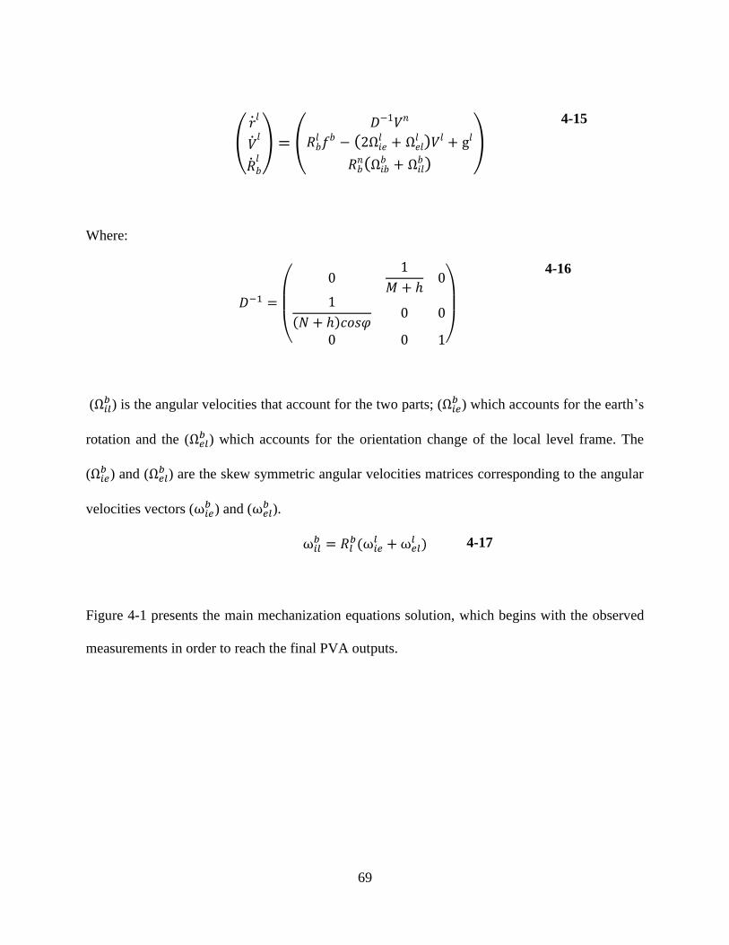
69
4-15
Where:
4-16
( ) is the angular velocities that account for the two parts; (
) which accounts for the earth’s
rotation and the ( ) which accounts for the orientation change of the local level frame. The
( ) and (
) are the skew symmetric angular velocities matrices corresponding to the angular
velocities vectors ( ) and (
).
4-17
Figure 4-1 presents the main mechanization equations solution, which begins with the observed
measurements in order to reach the final PVA outputs.
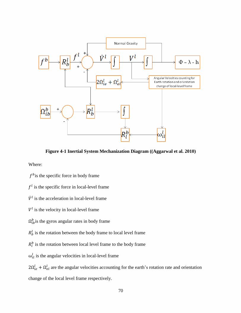
70
Figure 4-1 Inertial System Mechanization Diagram ((Aggarwal et al. 2010)
Where:
is the specific force in body frame
is the specific force in local-level frame
is the acceleration in local-level frame
is the velocity in local-level frame
is the gyros angular rates in body frame
is the rotation between the body frame to local level frame
is the rotation between local level frame to the body frame
is the angular velocities in local-level frame
are the angular velocities accounting for the earth’s rotation rate and orientation
change of the local level frame respectively.
71
The mechanization begins with assuming initial values for the positions and velocities.
4-18
4-19
Earth’s rotation rate (ωe) is 0.00007292115147 rad/sec, and the WGS84 ellipsoidal parameters
are a (semi-major axis) 6378137 m and e2 (
first eccentricity) 0.00669438. The meridian radius of
curvature (M) and the prime vertical radius of curvature (N) are then calculated as
2
322
2
sin1
1
e
eaM
4-20
21
22 sin1 e
aN
4-21
The gravity is then obtained from the well-known normal gravity model as follows
4-22
Where:
a1 = 9.7803267715 a2 = 0.0052790414 a3 = 0.0000232718
a4 = -0.000003087691089 a5 = 0.000000004397731 a6 = 0.000000000000721
The accelerometers and gyroscopes biases and scale factors deterministic parts should be
compensated for by removing them from the raw signal ( and ). These values are
extracted by the manufacturer sensor data sheet or lab calibration.
72
Coarse alignment is performed to estimate the initial value for the roll (r), pitch (p) and azimuth
(A) angles based on Equations 4-9, 4-10, and 4-11. These angles are then used to construct the
rotation matrix ( ) as follows
4-23
4-24
4-25
4-26
In order to solve these equations the first step is the parameterization of the rotation matrix ( );
the most commonly used method is the quaternion parameterization. The quaternion is based on
Euler’s theoremwhich states that the rotationof thebody frame (b-frame) with respect to the
navigation frame (l-frame)isexpressedintermsofsinglerotationangle(θ)aroundafixedaxis
and the direction cosines of the rotation axis with respect to the navigation frame (Aggarwal et
al. 2010). The initial value for the quaternion is calculated according to the following equation:
4-27

73
Where ( ) is the element at the row (i) and column (j) in the rotation matrix ( ). The obtained
quaternion matrix should them be normalized to preserve its condition
4-28
Hence;
4-29
4.3.1 Attitude Estimation
The following equation shows the calculation of the rotation rate vector of the e-frame with
respect to the i-frame and projected to the l-frame:
4-30
Calculating the transport rate of the l-frame with respect to the e-frame is expressed in terms of
the rate of change of latitude
4-31
These angular velocities matrices are then used to calculate the new rotation angles, which are
used to update the quaternion matrix at the new epoch
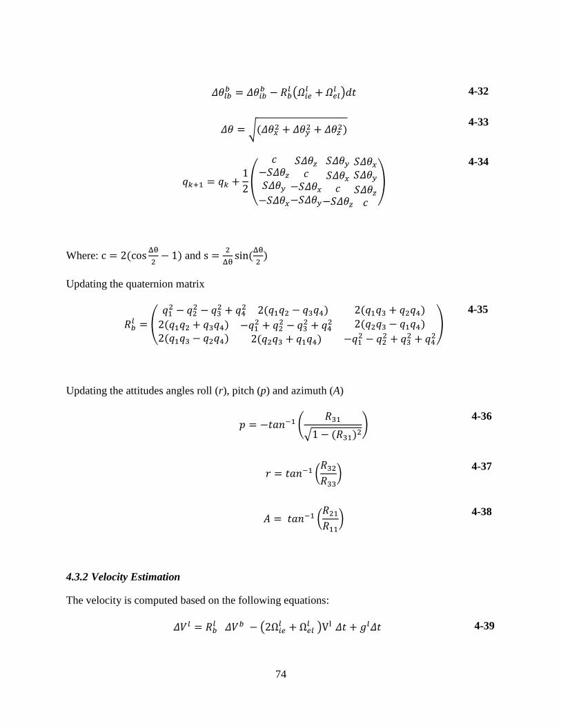
74
4-32
4-33
4-34
Where:
and
Updating the quaternion matrix
4-35
Updating the attitudes angles roll (r), pitch (p) and azimuth (A)
4-36
4-37
4-38
4.3.2 Velocity Estimation
The velocity is computed based on the following equations:
4-39

75
Where the first part ( ) accounts for the measured velocity increments after
transformation to the local-level frame and the second part (
) for the the
Coriolis correction that compensates for the earth’s rotation and local-level frame change of
orientation. The third part ( ) accounts for the gravity correction. Finally, to determine the
velocity at a certain time, the following equation is applied:
4-40
4.3.3 Position Estimation
Similarly to the velocity estimation, the position components would be estimated based on the
following equations:
4-41
4-42
4-43
4.4 GPS/INS Integrated Navigation System
Integrating mobile multi-sensor is a sensitive process that involves the fusion of several
measurements and constraints with different accuracy and behaviours. Navigation applications,
especially in GPS-denied environment, generally require the integration of multi-sensors to
estimate the navigation states in a trusted and reliable form. Kalman filter is considered the most
common integration technique used in navigation application due to its efficient capability of
combining several measurements (Brown and Hwang 1992). Other available techniques involve

76
using unscented Kalman filter, the extended Kalman filter, the particle filter or artificial
intelligence algorithms to estimate the navigation states. The estimates for navigation states
include: three-dimensional positions, velocity, attitude, and sensors errors.
The first step in building the integration technique is to choose the required sensors. The sensor
selection depends on the application, working environment, and accuracy limit, since it is a
precarious balancing act between accuracy, cost and reliability. The most common sensor used in
navigation is an integrated GPS and INS sensor. However, additional sensors such as odometers,
magnetometers, barometers and Wi-Fi signal strength sensors could be used. Calibrating and
modeling the sensor errors is an important step when using the sensors to ensure the
manufacturer’s specifications. The second step involves choosing the characteristics of the
selected filter.
Kalman filtering for GPS/INS integration could be loosely or tightly coupled (El-Sheimy 2010).
Loosely coupled Kalman filter uses two Kalman filters, one is used for processing the GPS
position estimates while the second is for updating the INS errors with the GPS positions, as
shown in Figure 4-2. The GPS derived estimates are the position and velocity, while the INS
derived estimates are the position, velocity and attitude.
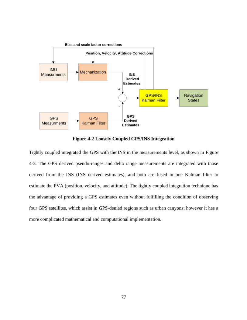
77
IMU
MeasurmentsMechanization
GPS
Measurments
GPS
Kalman Filter
GPS/INS
Kalman Filter
Navigation
States
GPS
Derived
Estimates
INS
Derived
Estimates
Position, Velocity, Attitude Corrections
Bias and scale factor corrections
+
-
Figure 4-2 Loosely Coupled GPS/INS Integration
Tightly coupled integrated the GPS with the INS in the measurements level, as shown in Figure
4-3. The GPS derived pseudo-ranges and delta range measurements are integrated with those
derived from the INS (INS derived estimates), and both are fused in one Kalman filter to
estimate the PVA (position, velocity, and attitude). The tightly coupled integration technique has
the advantage of providing a GPS estimates even without fulfilling the condition of observing
four GPS satellites, which assist in GPS-denied regions such as urban canyons; however it has a
more complicated mathematical and computational implementation.

78
IMU
MeasurmentsMechaniziation
GPS
Measurments
GPS/INS
Kalman Filter
Navigation
States
GPS Derived Pseudo range
and Delta range estimates
INS
Derived
Estimates
(Pseudo
and Delta
ranges)
Position, Velocity, Attitude Corrections
Bias and scale factor corrections
+
-
Figure 4-3 Tightly coupled GPS/INS Integration
Both the loosely and tightly coupled GPS/INS integration is realized by an extended Kalman
filter (EKF). The KF estimates the state of a process controlled by a linear stochastic difference
equation (Syed 2009). The linearity condition is not guaranteed all the time and for all
applications, such as the integration of GPS/INS using a KF where the system is non-linear. The
non-linearity comes from estimating the navigation position, velocity and attitude from the
mechanization equations. There are two cases for these non-linear navigation estimates, the first
where the system can be linearized about a nominal or approximate trajectory during the design
of the KF. The second case, where the nominal trajectory is not available, the process can be
linearized about the actual trajectory, which is done by linearization of the process around the
current state. The second case where the process is linearized around the current state is
commonly known as the EKF (Aggarwal et al. 2010).
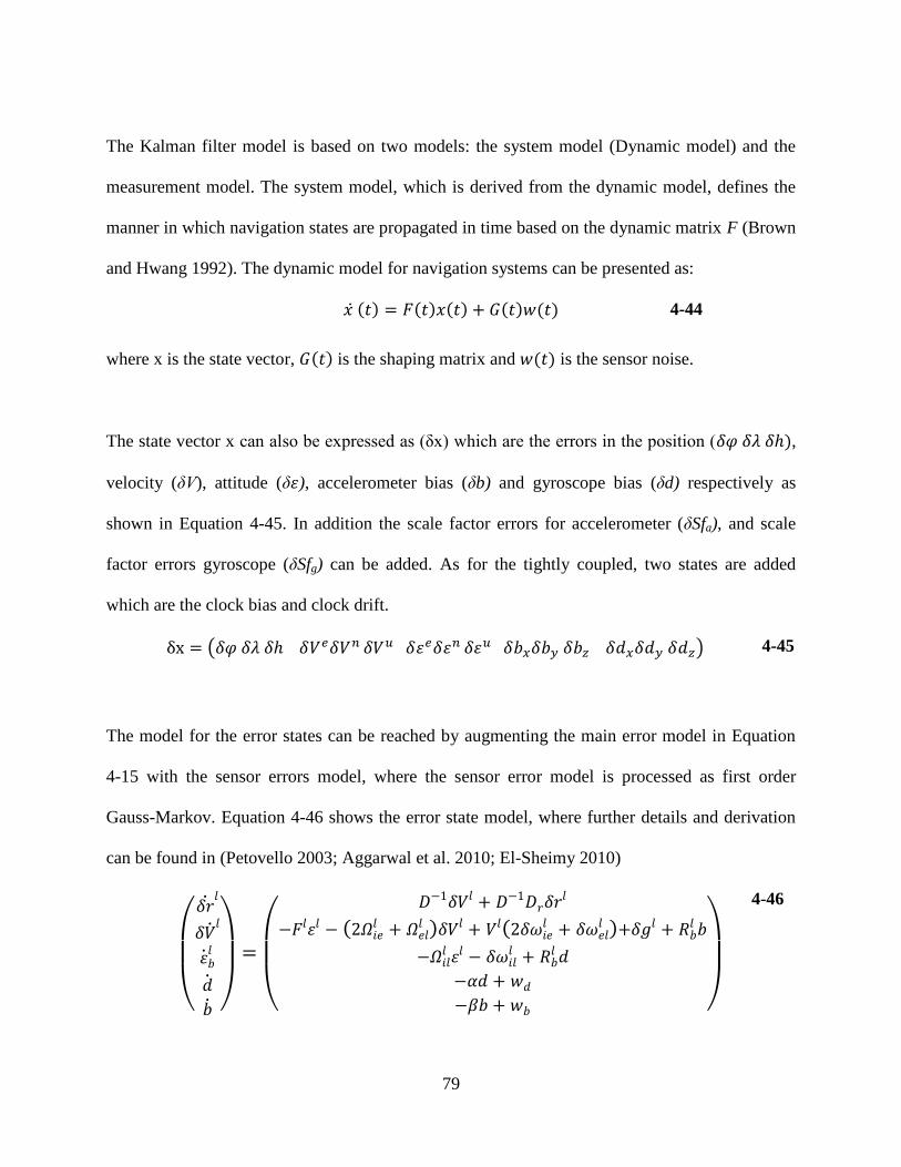
79
The Kalman filter model is based on two models: the system model (Dynamic model) and the
measurement model. The system model, which is derived from the dynamic model, defines the
manner in which navigation states are propagated in time based on the dynamic matrix F (Brown
and Hwang 1992). The dynamic model for navigation systems can be presented as:
4-44
where x is the state vector, is the shaping matrix and is the sensor noise.
The state vector x canalsobeexpressedas(δx)whicharetheerrorsintheposition( ,
velocity (δV), attitude (δ ), accelerometer bias (δb) and gyroscope bias (δd) respectively as
shown in Equation 4-45. In addition the scale factor errors for accelerometer (δSfa), and scale
factor errors gyroscope (δSfg) can be added. As for the tightly coupled, two states are added
which are the clock bias and clock drift.
4-45
The model for the error states can be reached by augmenting the main error model in Equation
4-15 with the sensor errors model, where the sensor error model is processed as first order
Gauss-Markov. Equation 4-46 shows the error state model, where further details and derivation
can be found in (Petovello 2003; Aggarwal et al. 2010; El-Sheimy 2010)
4-46
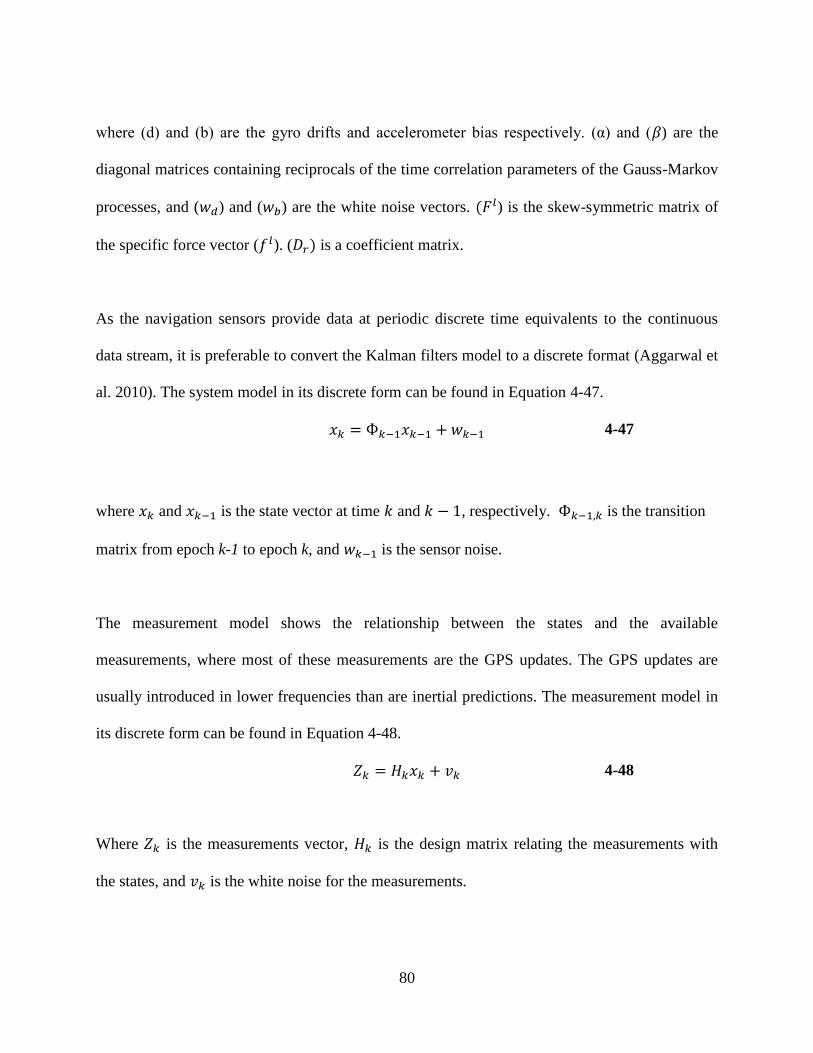
80
where (d) and (b) are the gyro drifts and accelerometer bias respectively. (α) and ( ) are the
diagonal matrices containing reciprocals of the time correlation parameters of the Gauss-Markov
processes, and ( ) and ( ) are the white noise vectors. ) is the skew-symmetric matrix of
the specific force vector ( ). ( is a coefficient matrix.
As the navigation sensors provide data at periodic discrete time equivalents to the continuous
data stream, it is preferable to convert the Kalman filters model to a discrete format (Aggarwal et
al. 2010). The system model in its discrete form can be found in Equation 4-47.
4-47
where and is the state vector at time and , respectively. is the transition
matrix from epoch k-1 to epoch k, and is the sensor noise.
The measurement model shows the relationship between the states and the available
measurements, where most of these measurements are the GPS updates. The GPS updates are
usually introduced in lower frequencies than are inertial predictions. The measurement model in
its discrete form can be found in Equation 4-48.
4-48
Where is the measurements vector, is the design matrix relating the measurements with
the states, and is the white noise for the measurements.
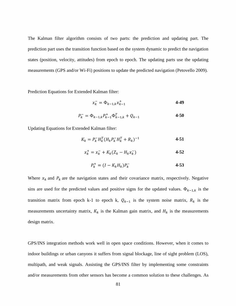
81
The Kalman filter algorithm consists of two parts: the prediction and updating part. The
prediction part uses the transition function based on the system dynamic to predict the navigation
states (position, velocity, attitudes) from epoch to epoch. The updating parts use the updating
measurements (GPS and/or Wi-Fi) positions to update the predicted navigation (Petovello 2009).
Prediction Equations for Extended Kalman filter:
4-49
4-50
Updating Equations for Extended Kalman filter:
4-51
4-52
4-53
Where and are the navigation states and their covariance matrix, respectively. Negative
sins are used for the predicted values and positive signs for the updated values. is the
transition matrix from epoch k-1 to epoch k, is the system noise matrix, is the
measurements uncertainty matrix, is the Kalman gain matrix, and is the measurements
design matrix.
GPS/INS integration methods work well in open space conditions. However, when it comes to
indoor buildings or urban canyons it suffers from signal blockage, line of sight problem (LOS),
multipath, and weak signals. Assisting the GPS/INS filter by implementing some constraints
and/or measurements from other sensors has become a common solution to these challenges. As

82
previously mentioned, assistance can given by using measurements from the odometer to update
the velocity errors, magnetometer to update the heading, barometer to update the height, or by
using some constraints as non-holonomic constraints that assume zero values for the velocity in
upward or side-cross directions.
Some other assisted constraints could be achieved by providing a pre-information for the
expected estimated states. Map information is a very rich and trusted source for such assistance.
Having geospatial information for the street networks in addition building floor plans provides a
logical threshold of where to expect a user’s position. These thresholds, if implemented through
the mobile multi-sensor integration technique, would assist in converging the navigation solution
of the correct path.
4.5 Pedestrian Dead Reckoning
Pedestrian dead reckoning (PDR) is a relative positioning technique used to estimate the position
of on-foot users either in outdoor or indoor environments. These estimates are based on the
user’spreviousposition and the travelled distance and orientation calculated by inertial sensors
measurements. The typical inertial sensors used for PDR are tri-axial accelerometers and
gyroscopes. The use of magnetometer is an added assistance that is used to enhance the heading
estimation. The PDR process typically includes three phases: Step Detection, Stride (Step)
Length, and Heading Estimation (user direction). Figure 4-4 illustrates the main architecture for
the PDR algorithm. In this thesis the used PDR is based on the assumption that the user is
walking or running with the smart-phone on the compass mode, i.e. the phone is leveled while
the screen is facing up.

83
Figure 4-4 Pedestrian Dead Reckoning Architecture
Equations 4-54 and 4-55 show the common PDR equations for computing the coordinates of
successive navigated points
4-54
4-55
Equations 4-54 and 4-55 compute the coordinates ( , ) of the new position at time (t) with
respect to a previously known position (Et-1, Nt-1) at time (t-1), where is the distance
travelled by the user since time ( t-1), and is the user heading at time (t-1). The is
estimated based on the Step Detection and Step Length algorithms, and the is estimated
based on the Heading Estimation algorithm.
Accelerometer
Step Detection
Gyroscope Magnetometer
Gyro-Heading Mag- Heading
HeadingStride Length
Estimation
PDR
Position
Estimate
84
4.5.1 Step Detection
Step detection is the first part to any PDR algorithm. Several algorithms were developed to
detect the steps in on-foot trajectories. The two main methods are peak detection of the
accelerometer data ((Zhao et al. 2009), and the zero crossing method (Shin et al. 2007). Peak
detection is usually performed on the forward accelerometer sensor; however it can occasionally
be performed on the norm of the three axial accelerometers. When the latter occurs, the step is
detected when a local maximum of the acceleration is found within an acceptable time period.
Equation 4-56 calculates the norm for the three axial accelerometers.
4-56
Steps can also be detected based on gait cycle (Zhao et al. 2009). The gait cycle is the time
between when the foot leaves the ground to when it hits the ground again. In this situation, the
accelerometer signal would detect a change in amplitude corresponding to the movement, which
subsequently allows for easy detection of the user’s steps. In some cases, the accelerometer
variance over a certain number of samples using a sliding window is a more suitable solution
than using accelerometer signals since the former removes the bias shift (Ali et al. 2012). The
steps detection method is simply a tool that detects the steps based on the waveform of the
overall acceleration vector—a step is detected for each complete cycle around the mean value.
Figure 4-5 shows the steps detected based on the waveform of the overall acceleration vector for
a dataset of accelerometer from the Samsung Galaxy smart-phone. Figure 4-6 is a zoomed view
of the walking start region. The step length could be estimated based on the cycle width and
peak-to-peak values of the detected step.
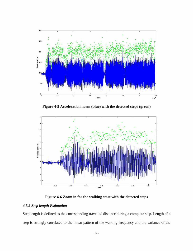
85
Figure 4-5 Acceleration norm (blue) with the detected steps (green)
Figure 4-6 Zoom in for the walking start with the detected steps
4.5.2 Step length Estimation
Step length is defined as the corresponding travelled distance during a complete step. Length of a
step is strongly correlated to the linear pattern of the walking frequency and the variance of the
86
acceleration (Shin et al. 2007). As a result, this step length can be estimated based on a linear
combination of both the walking frequency and the variance of the acceleration.
The walking frequency can be calculated using the following Equation:
4-57
where is the walking frequency from time to time for a given step .
The variance of the acceleration signal can be calculated using the following Equation:
4-58
where , the accelerometer signal at time t is , the average of accelerometer signals during
one step and N is the number of sensor outputs during one step.
The inputs from the walking frequency and the variance of the acceleration, in addition to the
learned parameters that are estimated based on calibration for different conditions and different
grounds, is then used to estimate the stride length.
4.5.3 Heading Estimation
The user heading is estimated using the gyroscope signals, the magnetometer signals or a fusion
algorithm of both. The gyroscope measurement is not affected by the magnetic anomalies that
occur in indoor environments; however there is drift with time because of its bias drift. The
magnetometer measurement faces the affect of the magnetic disturbances but provides an
absolute heading that can be used to update the gyroscope. In addition, the gyroscope can detect
87
the magnetic disturbance, which results in a complimentary solution that uses the advantages of
each sensor. Equation 4-59 shows the heading calculation using the gyroscope signal after
levelling and sensor calibration have been conducted.
4-59
where istheheadingcomputedusingthegyroscopemeasurementsandω(t)istheangularrate
of the gyroscope. Equation 4-60 shows the heading calculation using the magnetometer signal
(before considering the magnetic declination angle e.g. ~ 15° for Calgary, Alberta, Canada)
4-60
where is the heading computed using the magnetometer measurements, and are the
magnetometer measurements in the X and Y-axes, respectively. Several fusion algorithms have
been developed to best optimize the fusion of gyroscope and magnetometer heading estimation
(Ali et al. 2012).
4.6 Wi-Fi Positioning System
Wi-Fi positioning techniques are considered a useful aiding tool for GPS/INS navigation
systems, particularly when GPS signals are unavailable. Wi-Fi positioning occurs mainly in
indoor environments where usually there is a good Wi-Fi network but no GPS coverage. Wi-Fi
positioning provides an absolute consistent positioning solution which, although could face some
accuracy problems, is suitable enough to assist inertial sensors with their problem of drift over
time.
88
Wi-Fi positioning uses the availability and good coverage of Wi-Fi networks in indoor
environments. Wi-Fi networks connect computers and mobile devices with one another and to
the Internet. Wi-Fi networks include several access points (AP), which transmit what is referred
to as beacon message. Each message sent by APs includes identification information that is
unique to each AP such as the MAC address. The user’s Wi-Fi receiver (Wi-Fi network card)
receives this message, and immediately stores the received signal strength (RSS) and the
corresponding time stamp (Atia et al. 2012).
There are three main categories of Wi-Fi localization that use observed received signal strength
(RSS). The first category is based on the radio propagation model (path loss modeling), which is
used to relate the RSS to the distance (d) between the user and the AP. This relationship is used
in a ranging estimation in order to apply the position triangulation (Zhao et al. 2010). Using the
path loss modeling, the signal strength is approximately linear to the log of the distance while
taking into account the range of distance, radio wave length and the distance between the access
and reference points. The main drawback to this propagation modeling is that it is very
dependent on the surrounding environment, such that each area should have its own path-loss
model.
The second category is referred to as the time-based ranging technique. This technique uses the
“sent time” stamp of the beacon messages and the “receiving time”stampon the user’sWi-Fi
receiver. Ranging estimation is performed based on the time of travel information. This method
89
can face the issue of discontinuous availability of line of sight (LOS) and multipath inside the
indoor environments, which causes a fade in accuracy (Atia et al. 2011).
The third, and most commonly used technique in today’s applications is the fingerprint
positioning. This technique is based on the matching of observed signal strength with a reference
previously surveyed and recorded locations. An offline database is constructed as a result of
navigating all possible passageways in an indoor environment and recording the RSS from all
APs to build what is known as a radio map. Although this technique requires pre-surveyed data,
which could pose some cost issues, it is expected that in the near future certain indoor facilities
can provide this radio map upon constructing its Wi-Fi network. Matching the real-time signal
strength can be done by several pattern matching and classification methods. One simple
method is to find the minimum Euclidian distance (Zhao et al. 2010). Equation 4-61 illustrates
this Euclidian distance between the database vector and the online vector.
4-61
where Dn is the Euclidean distance, Vn is the signal strength vector at the surveyed positions, Vu
is the signal strength vector at the user positions, K is the number of effective access points, and
n is the number of surveyed positions in the database with the known coordinates.
Another matching technique involves the use of the k-nearest neighbour (K-NN) method. The K-
NN algorithm selects the k-point in the surveyed database that is nearest to the observed signal

90
strength. The current position (Pc) is calculated using the weighted average (Wi) as shown in
Equations 4-62 and 4-63.
4-62
4-63
where ( ) is the recorder signal strength at position ( ) in the surveyed database.

91
Chapter Five: Map Aided Navigation Systems
In this Chapter the development of the map aided navigation systems is presented. The map
aided navigation systems build on the integration of three previously developed components: the
geospatial data models for navigation applications (Chapter 2), the map matching algorithms
(Chapter 3) and the navigation solution estimated from several sensors measurements (Chapter
4). In addition, this chapter will present a constrained Kalman filter for GPS/INS integration as
an attempt to enhance the common EKF using several constraints. Finally, an investigation of
integrity measures for the map aided navigation systems is illustrated with some results based on
the map aided PDR navigation solution applied to a specific real trajectory.
5.1 Integrated Map Aided Navigation Systems
This section will discuss the different integrated map aided navigation systems for both outdoor
vehicle and indoor pedestrian navigation applications. For each system, the main components,
their integration technique and its operational architecture will be discussed. For building the
different map aided systems, it is required to interact with the different geospatial data models,
navigation solution, and map matching algorithms. Therefore, a simple Graphical User Interface
(GUI) was developed to allow the user to input the required geospatial model, the navigation
solution, the inertial measurements and select the required matching technique.
The main window includes an action menu, as shown in Figure 5-1. This action menu is used to
input the following files and information: a nodes file for the road networks, road network files,
indoor passageways file, the navigation file, and the inertial measurements file. For the first
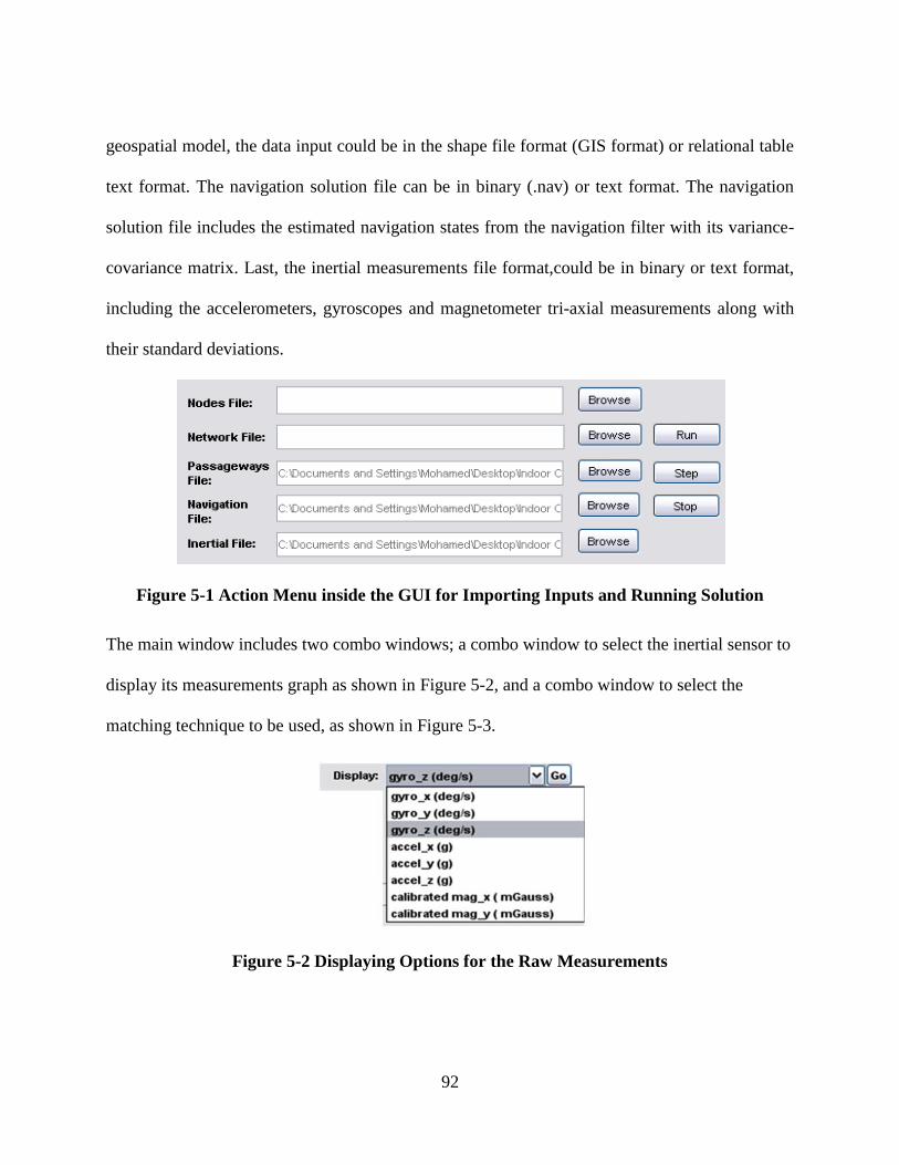
92
geospatial model, the data input could be in the shape file format (GIS format) or relational table
text format. The navigation solution file can be in binary (.nav) or text format. The navigation
solution file includes the estimated navigation states from the navigation filter with its variance-
covariance matrix. Last, the inertial measurements file format,could be in binary or text format,
including the accelerometers, gyroscopes and magnetometer tri-axial measurements along with
their standard deviations.
Figure 5-1 Action Menu inside the GUI for Importing Inputs and Running Solution
The main window includes two combo windows; a combo window to select the inertial sensor to
display its measurements graph as shown in Figure 5-2, and a combo window to select the
matching technique to be used, as shown in Figure 5-3.
Figure 5-2 Displaying Options for the Raw Measurements

93
Figure 5-3 Matching Algorithms Options for the Raw Measurements
Figure 5-4 presents a sample of GUI use with a map aided system with an input of the
Kinesology and MacEwan passageways centrelines shapefile, the PDR navigation solution, and a
selection of the geometrical and topological map matching algorithm (named: Stream with initial
link).
Figure 5-4 Sample for the Output Diagrams from the GUI
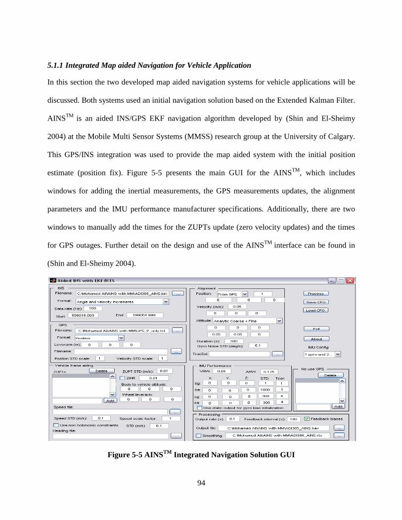
94
5.1.1 Integrated Map aided Navigation for Vehicle Application
In this section the two developed map aided navigation systems for vehicle applications will be
discussed. Both systems used an initial navigation solution based on the Extended Kalman Filter.
AINSTM
is an aided INS/GPS EKF navigation algorithm developed by (Shin and El-Sheimy
2004) at the Mobile Multi Sensor Systems (MMSS) research group at the University of Calgary.
This GPS/INS integration was used to provide the map aided system with the initial position
estimate (position fix). Figure 5-5 presents the main GUI for the AINSTM
, which includes
windows for adding the inertial measurements, the GPS measurements updates, the alignment
parameters and the IMU performance manufacturer specifications. Additionally, there are two
windows to manually add the times for the ZUPTs update (zero velocity updates) and the times
for GPS outages. Further detail on the design and use of the AINSTM
interface can be found in
(Shin and El-Sheimy 2004).
Figure 5-5 AINSTM
Integrated Navigation Solution GUI
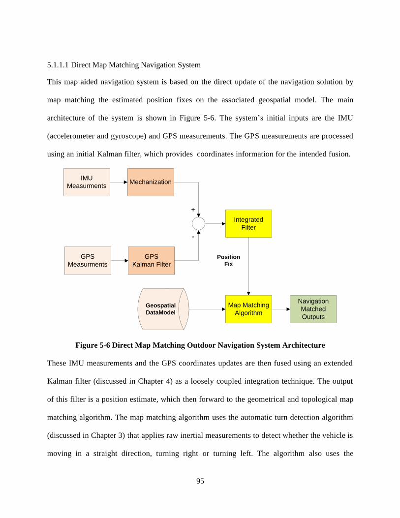
95
5.1.1.1 Direct Map Matching Navigation System
This map aided navigation system is based on the direct update of the navigation solution by
map matching the estimated position fixes on the associated geospatial model. The main
architecture of the system is shown in Figure 5-6. The system’s initial inputs are the IMU
(accelerometer and gyroscope) and GPS measurements. The GPS measurements are processed
using an initial Kalman filter, which provides coordinates information for the intended fusion.
IMU
MeasurmentsMechanization
GPS
Measurments
GPS
Kalman Filter
Integrated
Filter
Navigation
Matched
Outputs
Position
Fix
`
+
-
Map Matching
AlgorithmGeospatial
DataModel
Figure 5-6 Direct Map Matching Outdoor Navigation System Architecture
These IMU measurements and the GPS coordinates updates are then fused using an extended
Kalman filter (discussed in Chapter 4) as a loosely coupled integration technique. The output
of this filter is a position estimate, which then forward to the geometrical and topological map
matching algorithm. The map matching algorithm uses the automatic turn detection algorithm
(discussed in Chapter 3) that applies raw inertial measurements to detect whether the vehicle is
moving in a straight direction, turning right or turning left. The algorithm also uses the

96
geospatial data model for the road networks (developed in Chapter 2) to match the position
fixes on the road links. The algorithm then reads the position estimate at each epoch and
immediately matches them on the most appropriate link. The output is a matched navigation
trajectory projected on the network links (Attia et al. 2010).
5.1.1.2 Sequential Updated Kalman filter for Map aided Navigation System
This map aided navigation system is based on an update of the navigation solution by the map
matched positions. The system uses the same architecture as the direct map matching system in
addition to the map matched projected positions as an additional correction update to the Kalman
filter. The system’s main architecture is shown in Figure 5-7.
The feedback algorithm integrates the second Kalman filter by updating the previously updated
GPS states such as the initial position estimates of the map matched positions. The updating is
conducted using a sequential updating technique (Bullock 1995; Petovello 2003). Two sequential
measurements are also used to to update the error states from GPS positions and map matched
positions. The main advantage to these sequential updates is that they will allow for the accuracy
and effectiveness of every update to be evaluated independently. The uncertainty of the map
matched measurements is derived from the roads geometry (Attia et al. 2011-a).
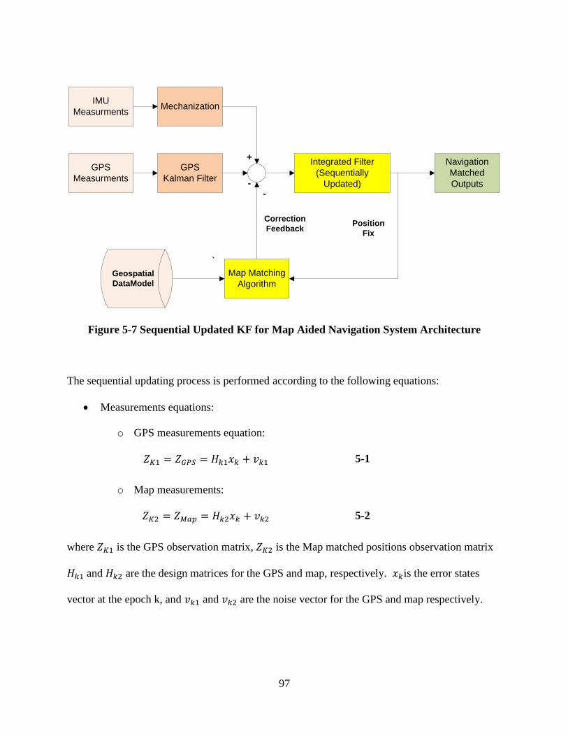
97
IMU
MeasurmentsMechanization
GPS
Measurments
GPS
Kalman Filter
Integrated Filter
(Sequentially
Updated)
Navigation
Matched
Outputs
Position
Fix
`
+
-
Map Matching
AlgorithmGeospatial
DataModel
Correction
Feedback
-
Figure 5-7 Sequential Updated KF for Map Aided Navigation System Architecture
The sequential updating process is performed according to the following equations:
Measurements equations:
o GPS measurements equation:
5-1
o Map measurements:
5-2
where is the GPS observation matrix, is the Map matched positions observation matrix
and are the design matrices for the GPS and map, respectively. is the error states
vector at the epoch k, and and are the noise vector for the GPS and map respectively.
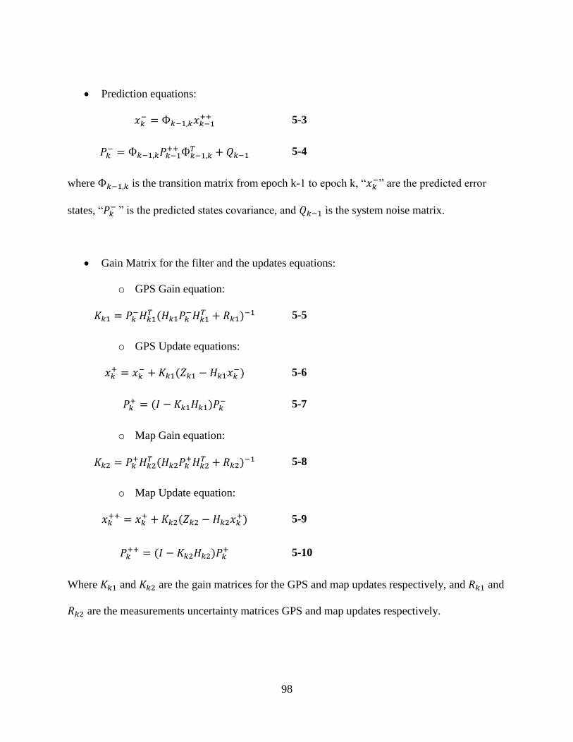
98
Prediction equations:
5-3
5-4
where is the transition matrix from epoch k-1toepochk,“ ”arethepredictederror
states, “ ”isthepredictedstatescovariance,and is the system noise matrix.
Gain Matrix for the filter and the updates equations:
o GPS Gain equation:
5-5
o GPS Update equations:
5-6
5-7
o Map Gain equation:
5-8
o Map Update equation:
5-9
5-10
Where and are the gain matrices for the GPS and map updates respectively, and and
are the measurements uncertainty matrices GPS and map updates respectively.

99
The final output from the sequential updated map aided system is a complete navigation solution
with its corresponding variance covariance matrix.
5.1.2 Integrated Map Aided Navigation for Indoor Applications
5.1.2.1 Map Aided Navigation using Building Information
The architecture for the first map aided navigation for indoor applications is presented in Figure
5-8. The system used the direct map matching technique to update the navigation solution by
matching the estimated position fix on the developed geospatial data model (discussed in
Chapter 2). This algorithm uses the geospatial model for the Engineering building at the
University of Calgary. The system uses a navigation solution based on the GPS/INS/Wi-Fi
integration. A loosely coupled Extended Kalman Filter is applied to integrate tri-axial
accelerometers and gyroscopes with Wi-Fi and GPS updates (discussed in Chapter 4). The
algorithm begins by using both accelerometer and gyroscope data, which is integrated with GPS
measurements as they become available. During good GPS/Wi-Fi updates, misalignment attitude
angles between body frame and person frame are estimated (Attia et al. 2011-b). A PDR is
adopted to minimize sensors integration errors and drifts by exploiting the kinematics of human
gait with the traveled distance and heading information (discussed in Chapter 4). The algorithm
contains step detection, stride length estimation and heading determination (Zhao et al. 2010).
Once a mechanization derived heading is converged, the heading is used in PDR to compute
Easting and Northing for the Kalman Filter. However, if the heading drifts too much, or if steps
are not detected with enough certainty, only mechanization is used.
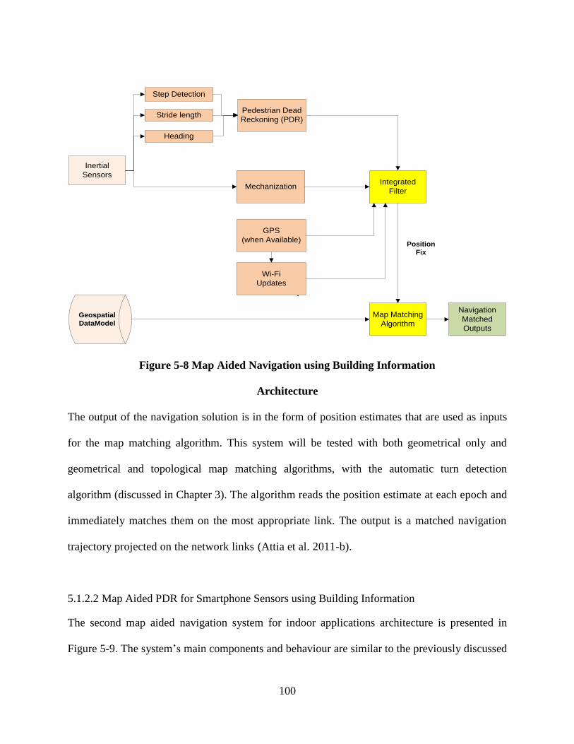
100
Inertial
Sensors
Mechanization
GPS
(when Available)
Wi-Fi
Updates
Integrated
Filter
Navigation
Matched
Outputs
Position
Fix
`
Map Matching
AlgorithmGeospatial
DataModel
Pedestrian Dead
Reckoning (PDR)
Step Detection
Stride length
Heading
Figure 5-8 Map Aided Navigation using Building Information
Architecture
The output of the navigation solution is in the form of position estimates that are used as inputs
for the map matching algorithm. This system will be tested with both geometrical only and
geometrical and topological map matching algorithms, with the automatic turn detection
algorithm (discussed in Chapter 3). The algorithm reads the position estimate at each epoch and
immediately matches them on the most appropriate link. The output is a matched navigation
trajectory projected on the network links (Attia et al. 2011-b).
5.1.2.2 Map Aided PDR for Smartphone Sensors using Building Information
The second map aided navigation system for indoor applications architecture is presented in
Figure 5-9. The system’s main components and behaviour are similar to the previously discussed
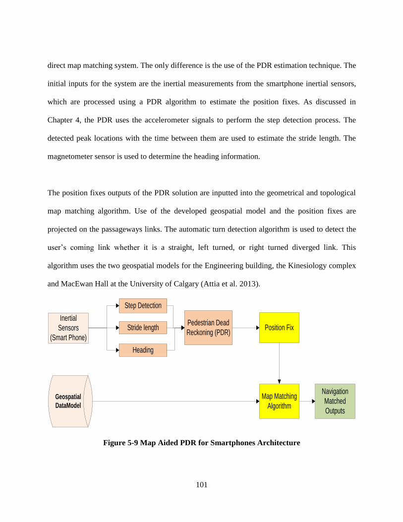
101
direct map matching system. The only difference is the use of the PDR estimation technique. The
initial inputs for the system are the inertial measurements from the smartphone inertial sensors,
which are processed using a PDR algorithm to estimate the position fixes. As discussed in
Chapter 4, the PDR uses the accelerometer signals to perform the step detection process. The
detected peak locations with the time between them are used to estimate the stride length. The
magnetometer sensor is used to determine the heading information.
The position fixes outputs of the PDR solution are inputted into the geometrical and topological
map matching algorithm. Use of the developed geospatial model and the position fixes are
projected on the passageways links. The automatic turn detection algorithm is used to detect the
user’s coming link whether it is a straight, left turned, or right turned diverged link. This
algorithm uses the two geospatial models for the Engineering building, the Kinesiology complex
and MacEwan Hall at the University of Calgary (Attia et al. 2013).
Inertial
Sensors
(Smart Phone)
Position Fix
Navigation
Matched
Outputs
Map Matching
AlgorithmGeospatial
DataModel
Pedestrian Dead
Reckoning (PDR)
Step Detection
Stride length
Heading
Figure 5-9 Map Aided PDR for Smartphones Architecture

102
5.2 Constrained Kalman Filter for GPS/INS Integration
In addition to the map aided navigation algorithms developed in this thesis and in an attempt to
enhance the initial common navigation solution for the vehicle applications, a newly constrained
Kalman filter was investigated, developed and field-tested. The constrained Kalman filter is
considered a significantly helpful integrated navigation-filtering tool that uses several constraints
and conditions to limit and restrict the navigation solution to a specific behaviour.
EKF is also considered one of the most common optimal estimators for inertial integrated
navigation systems. Its optimality stems from its ability to handle non-linear dynamics, where
the common Kalman filter can only handle linear models. Although the Kalman filter is a
powerful and trustful minimum-variance state estimator, it can still miss relevant information
that is not incorporated (Simon 2010).
Adding state constraints through the implementation of the EKF, either in the form of equality or
inequality constraints, should improve the filtering performance. This improvement is guided by
the quality and importance of the implemented constraints and by how the amount of description
it provides about the expected states behaviour (Sircoulomb et al. 2008). The two most common
methods for constraining the Kalman filter are either a restriction of the optimal Kalman gain as
a means of forcing the updated states to follow the constraint, or a projection of the estimated
states on the constrained region (Gupta and Hauser 2007). The latter is applied in this thesis.
The developed algorithm is based on constraining the GPS/INS integrated navigation EKF for
urban centers applications with two constraints. The first constraint is the relative height change
103
from epoch to epoch, where the assumption is that the vehicle height will not change
dramatically from one epoch to another under a specific value. Whenever this value is violated,
the estimator should project the solution back to that limit. The second constraint uses the static
condition information for the vehicle to perform what is known as zero velocity updates (ZUPT).
However, this information is gathered based on an automatic classifier (decision trees) to
increase its reliability. In this thesis, an EKF is used as the core for the developed
implementation.
5.2.1 Estimate Projection Constrained Kalman Filter for GPS/INS Integration (relative height
change constraint)
Vehicle navigation in urban canyons faces a huge challenge to maintain reliable accuracy during
GPS signal outages. However, there are relevant characteristics that can enhance its
performance. The height change is not expected to change dramatically from epoch to epoch, and
this fact could be modeled efficiently as a state constraint to improve the performance of the
navigation filter. In this algorithm, the relative height change is constrained using inequality
constrained Kalman filtering and projecting the state estimate in the space of 20 cm each second.
This value is assumed based on the approximate street slope and vehicle speed in urban
environments.
For an n state vector x, subject to the following inequality constraint:
5-11
where ( is the state estimate, M is a known n by n matrix, b is n by 1 vector and k is the time
step.
104
Solving this equation as a minimization problem
5-12
where ( ) is the constrained state estimate and ( ) is a weighting matrix, will give the
constrained estimate and its corresponding covariance as the following two equations:
5-13
5-14
where ( ) is the constrained state covariance matrix and ( ) is the state covariance matrix.
5.2.2 Zero Velocity Updates (ZUPT) based on Automatic Stop detection technique using
decision trees
One of the most common updates for the navigation filtering is the zero velocity update (ZUPT).
The concept of applying this constraint is based on the fact that once a vehicle stops, the
corresponding navigation states (i.e. velocities and changes in positions) should be forced to
zero. The key issue facing this constraint is how to detect when a vehicle stops. Various
researchers have implemented several methods, mostly based on setting a threshold for the
inertial measurements and/or GPS positions (in cases where it is available) to detect the stop
condition. However, these methods are limited by the uncertainty of the threshold selection.
Usually the threshold is selected based on the developer interpretation and, occasionally, on
some estimation methods based on inputs. In this thesis, the stops are detected based on
classification techniques rather than estimation methods. Decision tree classifiers can detect the
stop conditions in a fully automatic manner, which is considered a simple and fast technique over
other mathematical models (Breiman et al. 1984).

105
Decision tree is a sequence of decisions modeled in a binary tree graph to conclude a final
decision. The tree itself includes several nodes, where at each node an input parameter is
compared against a threshold value to reach a new node until the final leaf is reached (Quinlan
1993). These parameters, structures and thresholds are developed based on training and learning
sessions, where several input parameters, along with the corresponding outputs, are used to train
the tree The decision tree training is based on repeatedly scanning the input values to identify the
parameter and the value to be used as a split node in order to minimize what is called the tree
impurity function. The tree impurity function is a measure of how the different classes are mixed
among the nodes. The impurity i(t) of node t can be defined as:
5-15
Where n is the number of cases belonging to node t, p(j|t) is the proportion of the node cases
that belong to class j (Breiman et al. 1984; Moussa et al. 2011).
The tree in this algorithm was trained using 12 different inputs as listed in Table 5-1. Upon
applying the decision tree to the measured inertial observations during the vehicle trajectory, it
provided the stopping intervals.
Table 5-1 Input Parameters used in the Decision Tree Structure
X1 X Gyroscope Mean X5 Y Accelerometer Mean X9 Z Gyroscope Std.
X2 Y Gyroscope Mean X6 Z Accelerometer Mean X10 X Accelerometer Std
X3 Z Gyroscope Mean X7 X Gyroscope Std. X11 Y Accelerometer Std
X4 X Accelerometer Mean X8 Y Gyroscope Std. X12 Z Accelerometer Std

106
In order to show the effectiveness of the proposed decision tree, the land vehicle data of
downtown Calgary was used to test the developed method. In this test, 50% of the data was used
as a training session. In the training session, the input to the system was the ZUPT data detected
from GPS reference data. It should be mentioned here that the ZUPTs periods for the test data
also known. It is important to mention here that the decision tree results will be dependent on the
user sensors.
In Figure 5-10, the decision tree structure and input parameters are presented. The parameters
used by the tree are x11, x3, x4 and x5. The developed decision trees achieved a detection accuracy
of 98.5168%, which means that applying the values for the input parameters would detect the
stopping conditions of the vehicle by 98%.
Figure 5-10 Decision Tree based on Inertial Sensors Measurements (98.5168.)
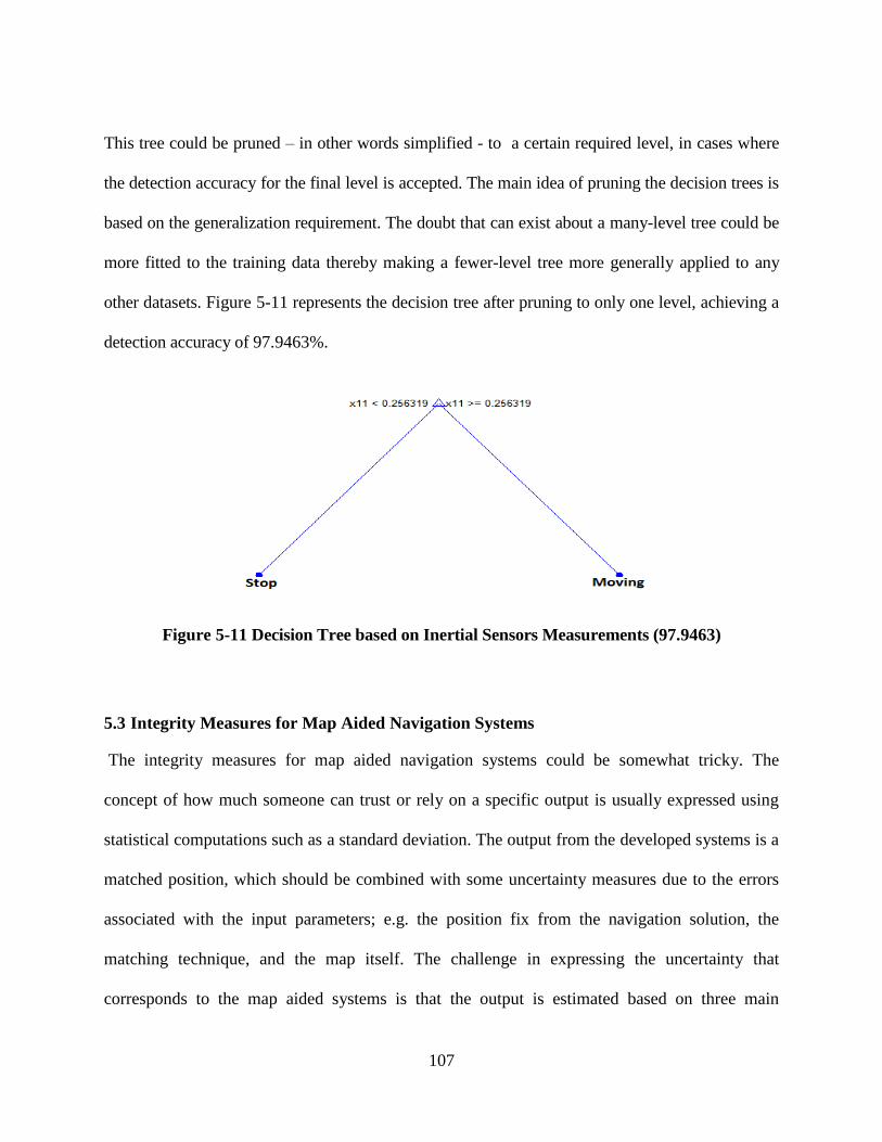
107
This tree could be pruned – in other words simplified - to a certain required level, in cases where
the detection accuracy for the final level is accepted. The main idea of pruning the decision trees is
based on the generalization requirement. The doubt that can exist about a many-level tree could be
more fitted to the training data thereby making a fewer-level tree more generally applied to any
other datasets. Figure 5-11 represents the decision tree after pruning to only one level, achieving a
detection accuracy of 97.9463%.
Figure 5-11 Decision Tree based on Inertial Sensors Measurements (97.9463)
5.3 Integrity Measures for Map Aided Navigation Systems
The integrity measures for map aided navigation systems could be somewhat tricky. The
concept of how much someone can trust or rely on a specific output is usually expressed using
statistical computations such as a standard deviation. The output from the developed systems is a
matched position, which should be combined with some uncertainty measures due to the errors
associated with the input parameters; e.g. the position fix from the navigation solution, the
matching technique, and the map itself. The challenge in expressing the uncertainty that
corresponds to the map aided systems is that the output is estimated based on three main

108
components: the navigation solution from the sensors, the map matching algorithm and the
geospatial data model.
5.3.1 Integrity Measures for Navigation Solutions
In this thesis, several integrated navigation solutions were developed and used in the map aided
navigation system. The primary contributed output from a navigation sensor is the position fix
with its variance-covariance matrix expressing the estimated errors. In order to express the
uncertainty associated with the position estimate (or any other navigation state estimate such as
heading, velocity, etc.), the most common and efficient method is an analysis of the associated
variance-covariance matrix. Other methods use the ellipsoidal confidence region. The location of
the matched positions within the confidence regions estimated from the variance of the
navigation solution can be used as integrity measures for the effect of the navigation solution
accuracy on the overall output (Quddus et al. 2006).
When employing the developed map aided navigation system in a GPS-denied environment, the
navigation sensor is usually only be a dead reckoning sensor. The dead reckoning positioning
estimation technique is based on accumulated differential easting and northing values that are
added epoch by epoch. The uncertainty associated with(ΔE)and(ΔN)canbeestimatedbasedon
the simple error propagation equation as follow:
5-16
5-17
5-18
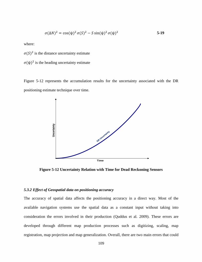
109
5-19
where:
is the distance uncertainty estimate
is the heading uncertainty estimate
Figure 5-12 represents the accumulation results for the uncertainty associated with the DR
positioning estimate technique over time.
Un
cert
ain
ty
Time
DR Uncerta
inty
Figure 5-12 Uncertainty Relation with Time for Dead Reckoning Sensors
5.3.2 Effect of Geospatial data on positioning accuracy
The accuracy of spatial data affects the positioning accuracy in a direct way. Most of the
available navigation systems use the spatial data as a constant input without taking into
consideration the errors involved in their production (Quddus et al. 2009). These errors are
developed through different map production processes such as digitizing, scaling, map
registration, map projection and map generalization. Overall, there are two main errors that could

110
develop in digital map production: geometrical and topological errors. Geometrical errors are the
difference between the links’ position and the modeled position on the map. Topological errors
are the result of simplifying or deleting important features such as road medians when modeling
the real world to the map.
Several methods can be used to estimate the map accuracy. The main method depends on
calculating the geometric error between the measurements on the map and the true values, which
are computed using higher accuracy surveying techniques such as ground surveying or
photogrammetry. Other methods are usually empirical methods based on assuming the sources of
errors in building the geospatial model and trying to model these errors to compensate for their
effects. In this thesis, and when building the geospatial model, the outdoor roads and indoor
passageways links were modeled as centrelines. In order to estimate the uncertainty associated
with the geospatial model or to express the effect of the map errors on the overall performance of
the map aided system, the accuracy of creating the centrelines was investigated.
An assumption was made that upon creating the centrelines there is a tolerance for creating the
start and end nodes equal to 1/8 from the link width (w). This (w/8) linear value would affect the
projected travelled distance upon estimating the matched trajectory. In addition, this (w/8) would
cause an angular error in the heading of the links, which would affect the turning angle on each
link.

111
The angular error can be calculated easily based on the length of each link as
Figure 5-13 shows the accuracy tolerance when creating the centrelines for the links.
Figure 5-13 Accuracy limits when Creating Links Centrelines
The estimated linear and angular uncertainty for the developed geospatial database could be
considered constant over time. Upon applying these linear and angular error values for the
developed geospatial models, and in assuming an average width and length for the whole dataset,
the map uncertainty values can be estimated as shown in Table 5-2
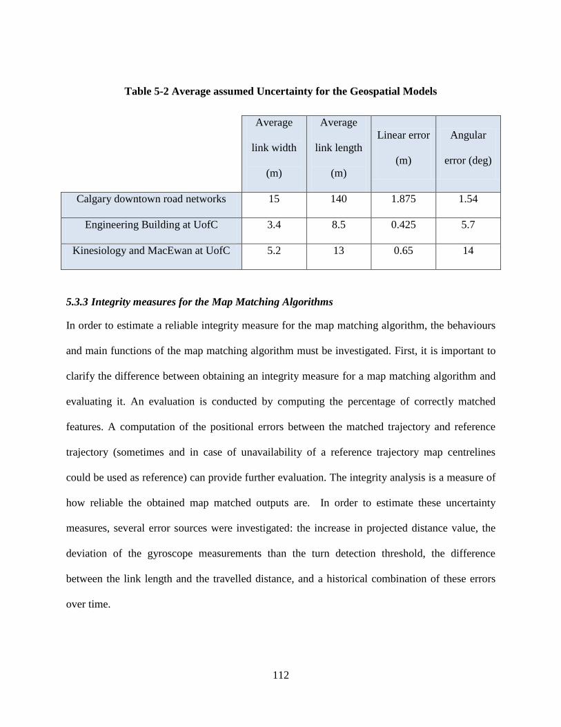
112
Table 5-2 Average assumed Uncertainty for the Geospatial Models
Average
link width
(m)
Average
link length
(m)
Linear error
(m)
Angular
error (deg)
Calgary downtown road networks 15 140 1.875 1.54
Engineering Building at UofC 3.4 8.5 0.425 5.7
Kinesiology and MacEwan at UofC 5.2 13 0.65 14
5.3.3 Integrity measures for the Map Matching Algorithms
In order to estimate a reliable integrity measure for the map matching algorithm, the behaviours
and main functions of the map matching algorithm must be investigated. First, it is important to
clarify the difference between obtaining an integrity measure for a map matching algorithm and
evaluating it. An evaluation is conducted by computing the percentage of correctly matched
features. A computation of the positional errors between the matched trajectory and reference
trajectory (sometimes and in case of unavailability of a reference trajectory map centrelines
could be used as reference) can provide further evaluation. The integrity analysis is a measure of
how reliable the obtained map matched outputs are. In order to estimate these uncertainty
measures, several error sources were investigated: the increase in projected distance value, the
deviation of the gyroscope measurements than the turn detection threshold, the difference
between the link length and the travelled distance, and a historical combination of these errors
over time.
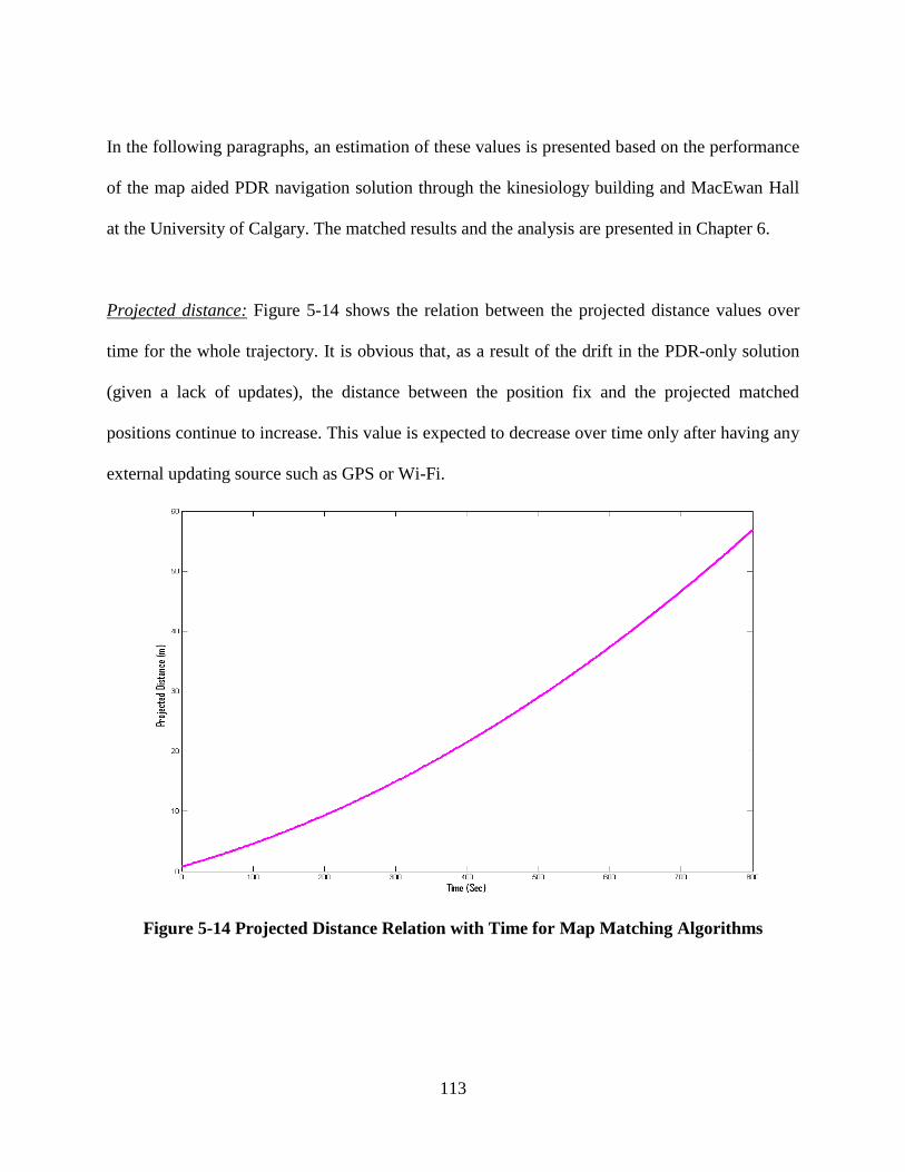
113
In the following paragraphs, an estimation of these values is presented based on the performance
of the map aided PDR navigation solution through the kinesiology building and MacEwan Hall
at the University of Calgary. The matched results and the analysis are presented in Chapter 6.
Projected distance: Figure 5-14 shows the relation between the projected distance values over
time for the whole trajectory. It is obvious that, as a result of the drift in the PDR-only solution
(given a lack of updates), the distance between the position fix and the projected matched
positions continue to increase. This value is expected to decrease over time only after having any
external updating source such as GPS or Wi-Fi.
Figure 5-14 Projected Distance Relation with Time for Map Matching Algorithms
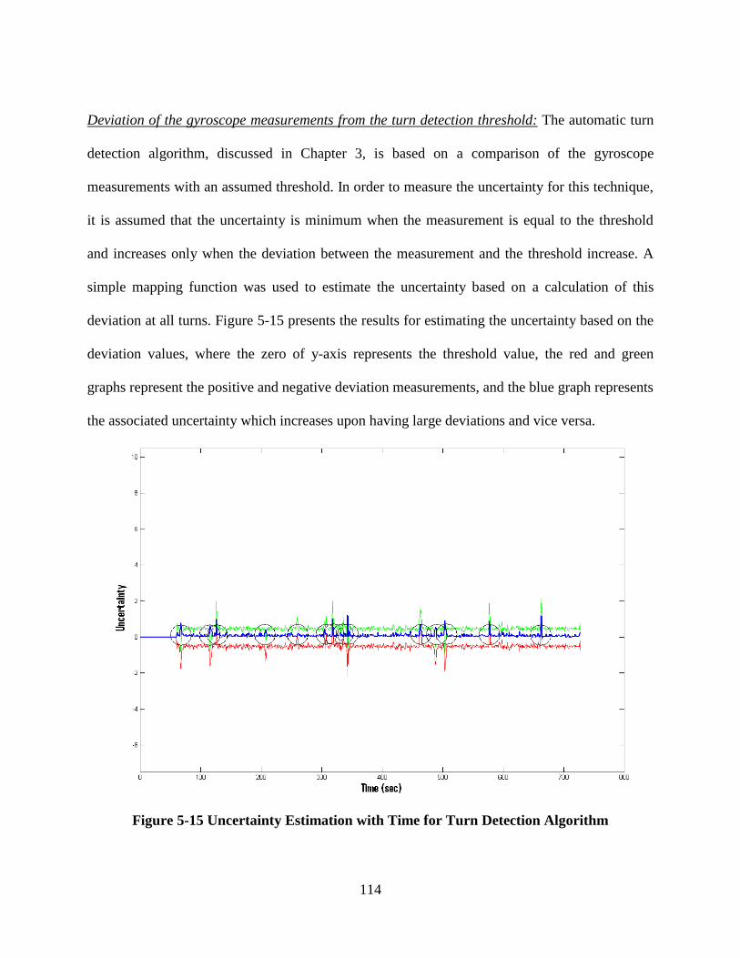
114
Deviation of the gyroscope measurements from the turn detection threshold: The automatic turn
detection algorithm, discussed in Chapter 3, is based on a comparison of the gyroscope
measurements with an assumed threshold. In order to measure the uncertainty for this technique,
it is assumed that the uncertainty is minimum when the measurement is equal to the threshold
and increases only when the deviation between the measurement and the threshold increase. A
simple mapping function was used to estimate the uncertainty based on a calculation of this
deviation at all turns. Figure 5-15 presents the results for estimating the uncertainty based on the
deviation values, where the zero of y-axis represents the threshold value, the red and green
graphs represent the positive and negative deviation measurements, and the blue graph represents
the associated uncertainty which increases upon having large deviations and vice versa.
Figure 5-15 Uncertainty Estimation with Time for Turn Detection Algorithm
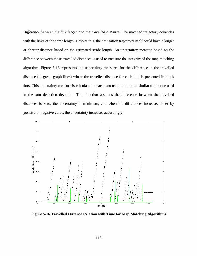
115
Difference between the link length and the travelled distance: The matched trajectory coincides
with the links of the same length. Despite this, the navigation trajectory itself could have a longer
or shorter distance based on the estimated stride length. An uncertainty measure based on the
difference between these travelled distances is used to measure the integrity of the map matching
algorithm. Figure 5-16 represents the uncertainty measures for the difference in the travelled
distance (in green graph lines) where the travelled distance for each link is presented in black
dots. This uncertainty measure is calculated at each turn using a function similar to the one used
in the turn detection deviation. This function assumes the difference between the travelled
distances is zero, the uncertainty is minimum, and when the differences increase, either by
positive or negative value, the uncertainty increases accordingly.
Figure 5-16 Travelled Distance Relation with Time for Map Matching Algorithms
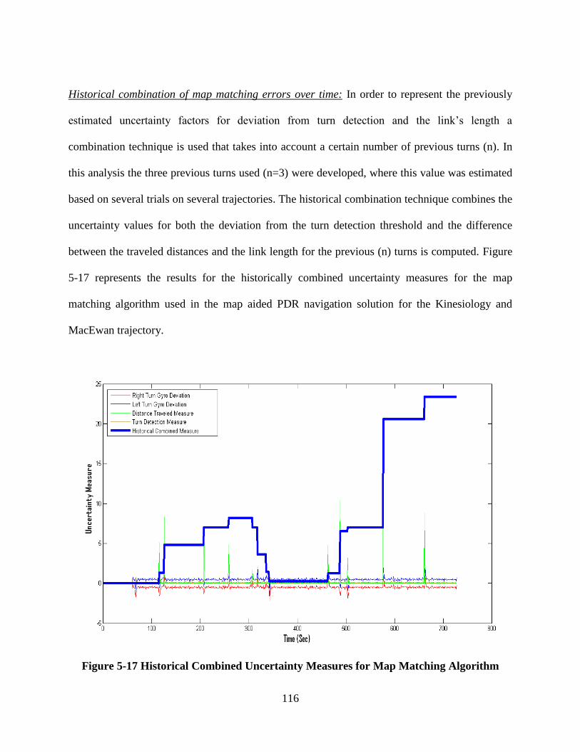
116
Historical combination of map matching errors over time: In order to represent the previously
estimated uncertainty factors for deviation from turn detection and the link’s length a
combination technique is used that takes into account a certain number of previous turns (n). In
this analysis the three previous turns used (n=3) were developed, where this value was estimated
based on several trials on several trajectories. The historical combination technique combines the
uncertainty values for both the deviation from the turn detection threshold and the difference
between the traveled distances and the link length for the previous (n) turns is computed. Figure
5-17 represents the results for the historically combined uncertainty measures for the map
matching algorithm used in the map aided PDR navigation solution for the Kinesiology and
MacEwan trajectory.
Figure 5-17 Historical Combined Uncertainty Measures for Map Matching Algorithm
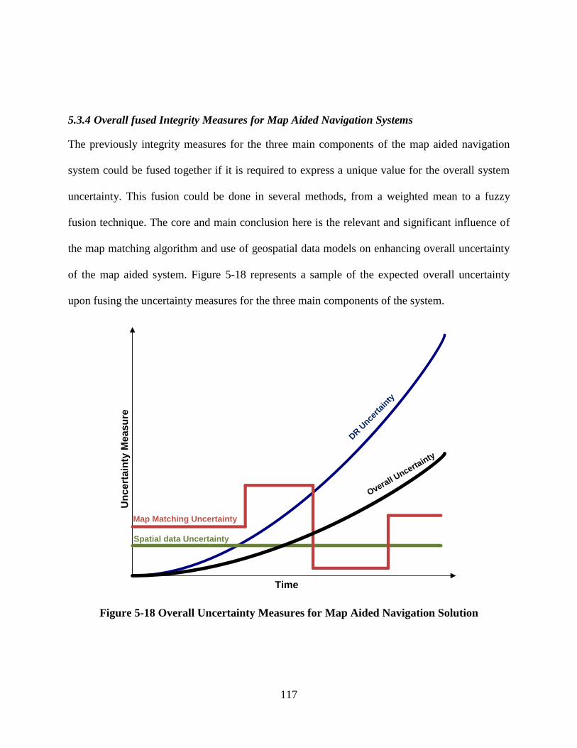
117
5.3.4 Overall fused Integrity Measures for Map Aided Navigation Systems
The previously integrity measures for the three main components of the map aided navigation
system could be fused together if it is required to express a unique value for the overall system
uncertainty. This fusion could be done in several methods, from a weighted mean to a fuzzy
fusion technique. The core and main conclusion here is the relevant and significant influence of
the map matching algorithm and use of geospatial data models on enhancing overall uncertainty
of the map aided system. Figure 5-18 represents a sample of the expected overall uncertainty
upon fusing the uncertainty measures for the three main components of the system.
Un
ce
rta
inty
Me
as
ure
Time
Map Matching Uncertainty
Spatial data Uncertainty
DR U
ncertai
nty
Overall U
ncertainty
Figure 5-18 Overall Uncertainty Measures for Map Aided Navigation Solution

118
Chapter Six: Field Testing, Results, Discussion and Analysis
In this chapter the verification, evaluation and analysis of applying the developed map aided
navigation systems on real data is performed. Several field tests were conducted to evaluate the
performance of the developed system under GPS-challenged environments. The field tests
included two main categories: outdoor field tests for vehicle navigation applications and indoor
field tests for pedestrian navigation in indoor environments. This chapter presents the description
of each field test describing the test scenario and the navigation sensors that were used. It will
then present a discussion of the obtained results and analysis of the system’sperformance.
6.1 Vehicle Outdoor Field Tests
The first field test is for vehicle navigation applications. Two field tests were performed, both of
which took place in the downtown Calgary region, which is characterized by high buildings and
low GPS availability. The tests have been used to assess the three developed navigation
algorithms: constrained Kalman filtering with automatic ZUPT detection, direct map matching
navigation system, and the sequential updated Kalman filter for a map aided navigation system.
In the subsequent subsections, a description for each test is introduced and the results, discussion
and analysis of applying the developed navigation algorithms are presented.
6.1.1 Field Test Description
6.1.1.1 First Field Test (Constrained Kalman Filtering Field Test)
Field Test Scenario
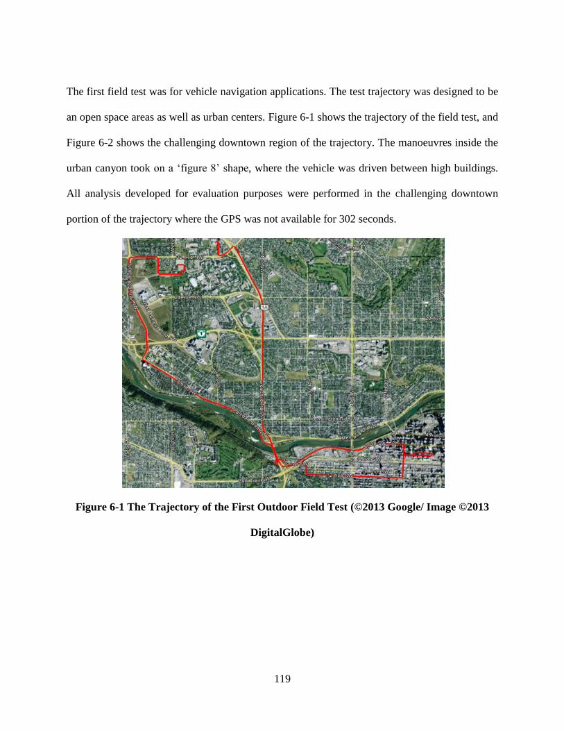
119
The first field test was for vehicle navigation applications. The test trajectory was designed to be
an open space areas as well as urban centers. Figure 6-1 shows the trajectory of the field test, and
Figure 6-2 shows the challenging downtown region of the trajectory. The manoeuvres inside the
urban canyon took ona‘figure8’shape, where the vehicle was driven between high buildings.
All analysis developed for evaluation purposes were performed in the challenging downtown
portion of the trajectory where the GPS was not available for 302 seconds.
Figure 6-1 The Trajectory of the First Outdoor Field Test (©2013 Google/ Image ©2013
DigitalGlobe)
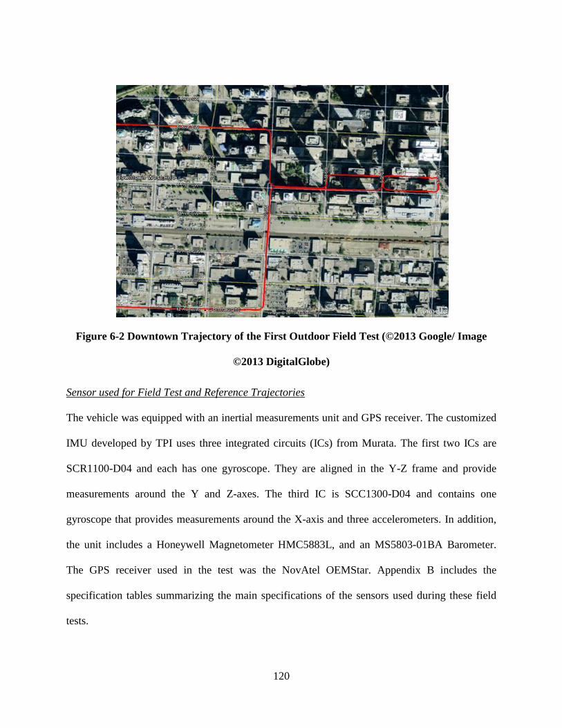
120
Figure 6-2 Downtown Trajectory of the First Outdoor Field Test (©2013 Google/ Image
©2013 DigitalGlobe)
Sensor used for Field Test and Reference Trajectories
The vehicle was equipped with an inertial measurements unit and GPS receiver. The customized
IMU developed by TPI uses three integrated circuits (ICs) from Murata. The first two ICs are
SCR1100-D04 and each has one gyroscope. They are aligned in the Y-Z frame and provide
measurements around the Y and Z-axes. The third IC is SCC1300-D04 and contains one
gyroscope that provides measurements around the X-axis and three accelerometers. In addition,
the unit includes a Honeywell Magnetometer HMC5883L, and an MS5803-01BA Barometer.
The GPS receiver used in the test was the NovAtel OEMStar. Appendix B includes the
specification tables summarizing the main specifications of the sensors used during these field
tests.
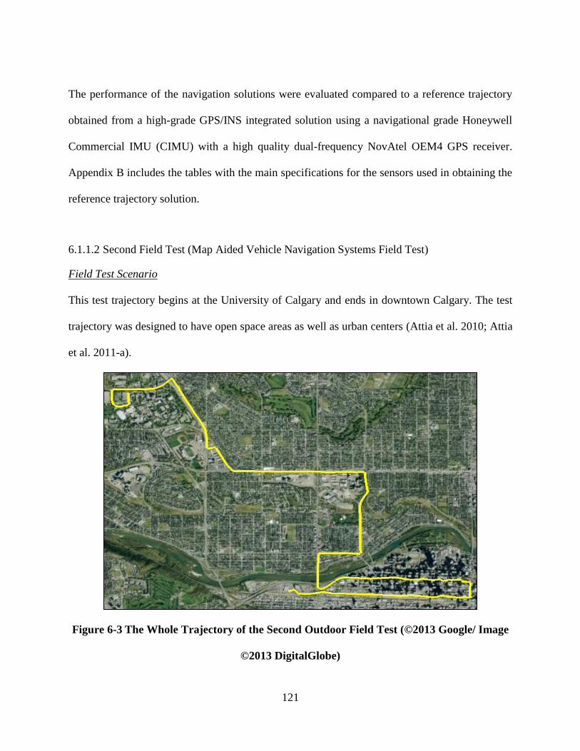
121
The performance of the navigation solutions were evaluated compared to a reference trajectory
obtained from a high-grade GPS/INS integrated solution using a navigational grade Honeywell
Commercial IMU (CIMU) with a high quality dual-frequency NovAtel OEM4 GPS receiver.
Appendix B includes the tables with the main specifications for the sensors used in obtaining the
reference trajectory solution.
6.1.1.2 Second Field Test (Map Aided Vehicle Navigation Systems Field Test)
Field Test Scenario
This test trajectory begins at the University of Calgary and ends in downtown Calgary. The test
trajectory was designed to have open space areas as well as urban centers (Attia et al. 2010; Attia
et al. 2011-a).
Figure 6-3 The Whole Trajectory of the Second Outdoor Field Test (©2013 Google/ Image
©2013 DigitalGlobe)
122
For the entire test, the number of satellites ranged from four to 11. Figure 6-3 shows the
trajectory of the field test. The downtown region is the study area on which the developed
algorithm was applied. It is covered by the developed road network and database (discussed in
Chapter 2).
Sensor used for Field Test and Reference Trajectories:
A number of sensors were used to collect data in this test and include the SIRF STAR III single
point high sensitivity GPS receiver, the ADI ADXRS150 MEMS Gyroscope, and the ADI
ADXL105 MEMS Accelerometer. Two additional sets of data were simulated from the field test
by inserting GPS signal outages at four different periods through the entire test. One set was
simulated with a 30-second GPS signal outage and the second by introducing a 60-second GPS
signal outage. The datasets were evaluated using a high-order navigation system consisting of the
LN 200 tactical grade IMU with DGPS solution for the NovAtel OEM4. The performance for the
three datasets (GPS/MEMS IMUs) in the downtown area was compared to the reference
trajectory as illustrated in Table 6-1. The table clearly indicates that the position errors increased
as the GPS signal blockage time increased—a typical behaviour of INS systems. The RMS of the
position error during the GPS outages is about 21 m for a 30-second GPS signal outage and 88 m
for a 60-second GPS signal outage. This hardly meets the accuracy requirement of land vehicle
navigation applications (Attia et al. 2010).
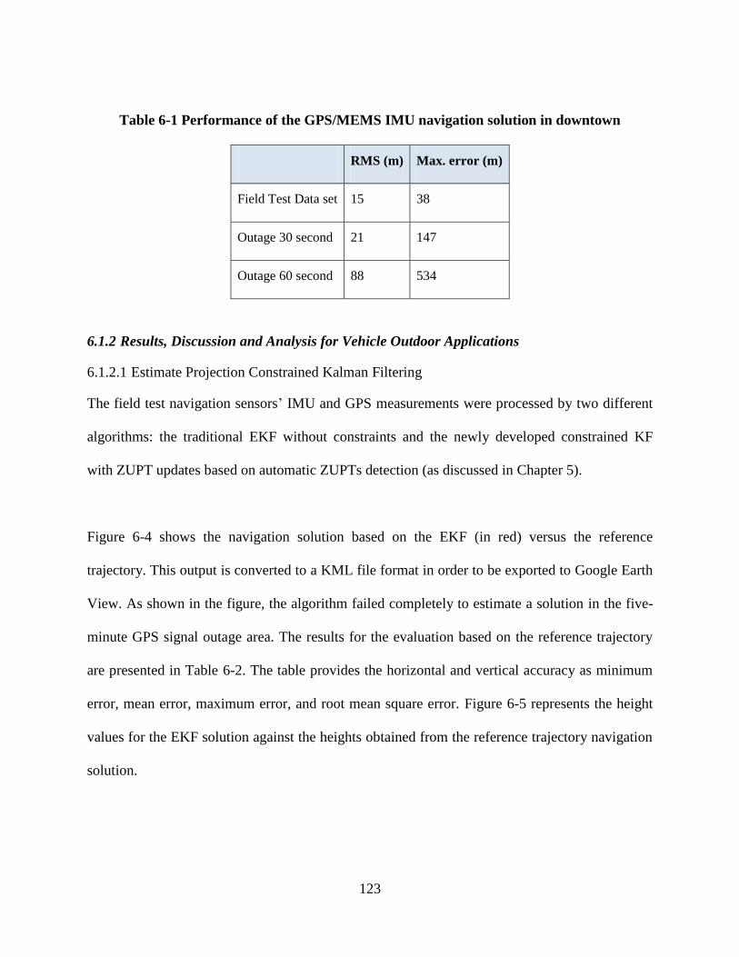
123
Table 6-1 Performance of the GPS/MEMS IMU navigation solution in downtown
RMS (m) Max. error (m)
Field Test Data set 15 38
Outage 30 second 21 147
Outage 60 second 88 534
6.1.2 Results, Discussion and Analysis for Vehicle Outdoor Applications
6.1.2.1 Estimate Projection Constrained Kalman Filtering
The field test navigation sensors’ IMU and GPS measurements were processed by two different
algorithms: the traditional EKF without constraints and the newly developed constrained KF
with ZUPT updates based on automatic ZUPTs detection (as discussed in Chapter 5).
Figure 6-4 shows the navigation solution based on the EKF (in red) versus the reference
trajectory. This output is converted to a KML file format in order to be exported to Google Earth
View. As shown in the figure, the algorithm failed completely to estimate a solution in the five-
minute GPS signal outage area. The results for the evaluation based on the reference trajectory
are presented in Table 6-2. The table provides the horizontal and vertical accuracy as minimum
error, mean error, maximum error, and root mean square error. Figure 6-5 represents the height
values for the EKF solution against the heights obtained from the reference trajectory navigation
solution.
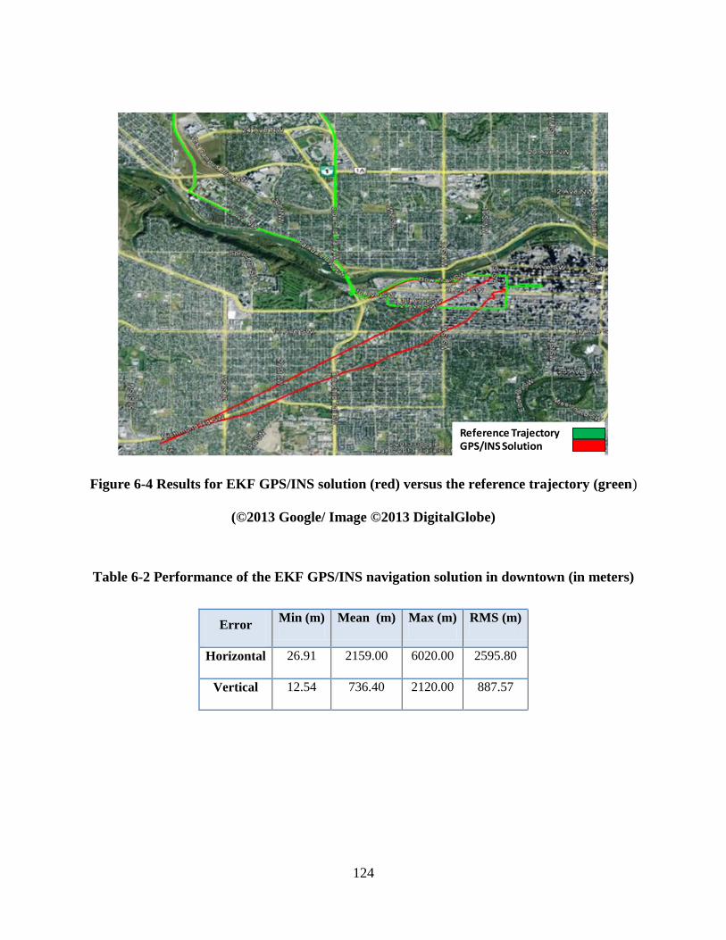
124
Figure 6-4 Results for EKF GPS/INS solution (red) versus the reference trajectory (green)
(©2013 Google/ Image ©2013 DigitalGlobe)
Table 6-2 Performance of the EKF GPS/INS navigation solution in downtown (in meters)
Error Min (m) Mean (m) Max (m) RMS (m)
Horizontal 26.91 2159.00 6020.00 2595.80
Vertical 12.54 736.40 2120.00 887.57
Reference TrajectoryGPS/INS Solution
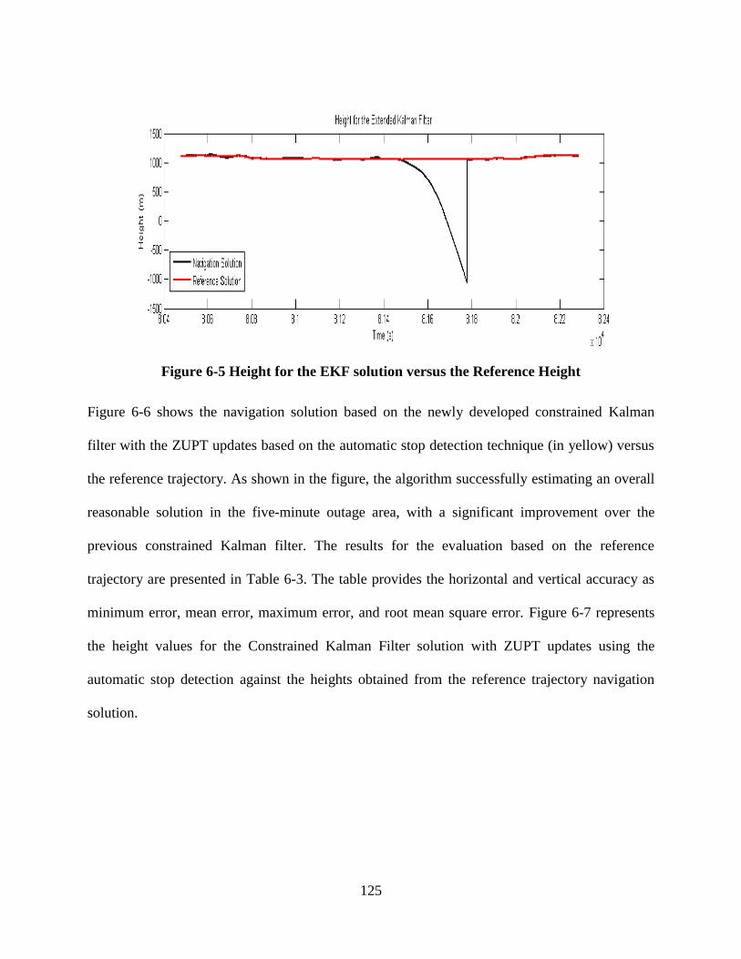
125
Figure 6-5 Height for the EKF solution versus the Reference Height
Figure 6-6 shows the navigation solution based on the newly developed constrained Kalman
filter with the ZUPT updates based on the automatic stop detection technique (in yellow) versus
the reference trajectory. As shown in the figure, the algorithm successfully estimating an overall
reasonable solution in the five-minute outage area, with a significant improvement over the
previous constrained Kalman filter. The results for the evaluation based on the reference
trajectory are presented in Table 6-3. The table provides the horizontal and vertical accuracy as
minimum error, mean error, maximum error, and root mean square error. Figure 6-7 represents
the height values for the Constrained Kalman Filter solution with ZUPT updates using the
automatic stop detection against the heights obtained from the reference trajectory navigation
solution.
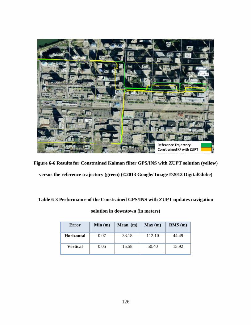
126
Figure 6-6 Results for Constrained Kalman filter GPS/INS with ZUPT solution (yellow)
versus the reference trajectory (green) (©2013 Google/ Image ©2013 DigitalGlobe)
Table 6-3 Performance of the Constrained GPS/INS with ZUPT updates navigation
solution in downtown (in meters)
Error Min (m) Mean (m) Max (m) RMS (m)
Horizontal 0.07 38.18 112.10 44.49
Vertical 0.05 15.58 50.40 15.92
Reference TrajectoryConstrained KF with ZUPT
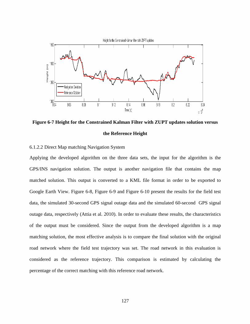
127
Figure 6-7 Height for the Constrained Kalman Filter with ZUPT updates solution versus
the Reference Height
6.1.2.2 Direct Map matching Navigation System
Applying the developed algorithm on the three data sets, the input for the algorithm is the
GPS/INS navigation solution. The output is another navigation file that contains the map
matched solution. This output is converted to a KML file format in order to be exported to
Google Earth View. Figure 6-8, Figure 6-9 and Figure 6-10 present the results for the field test
data, the simulated 30-second GPS signal outage data and the simulated 60-second GPS signal
outage data, respectively (Attia et al. 2010). In order to evaluate these results, the characteristics
of the output must be considered. Since the output from the developed algorithm is a map
matching solution, the most effective analysis is to compare the final solution with the original
road network where the field test trajectory was set. The road network in this evaluation is
considered as the reference trajectory. This comparison is estimated by calculating the
percentage of the correct matching with this reference road network.
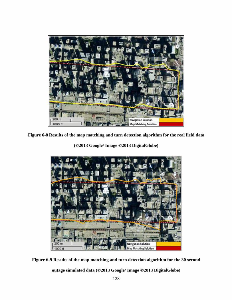
128
Figure 6-8 Results of the map matching and turn detection algorithm for the real field data
(©2013 Google/ Image ©2013 DigitalGlobe)
Figure 6-9 Results of the map matching and turn detection algorithm for the 30 second
outage simulated data (©2013 Google/ Image ©2013 DigitalGlobe)
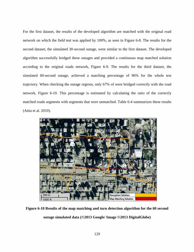
129
For the first dataset, the results of the developed algorithm are matched with the original road
network on which the field test was applied by 100%, as seen in Figure 6-8. The results for the
second dataset, the simulated 30-second outage, were similar to the first dataset. The developed
algorithm successfully bridged these outages and provided a continuous map matched solution
according to the original roads network, Figure 6-9. The results for the third dataset, the
simulated 60-second outage, achieved a matching percentage of 96% for the whole test
trajectory. When checking the outage regions, only 67% of were bridged correctly with the road
network, Figure 6-10. This percentage is estimated by calculating the ratio of the correctly
matched roads segments with segments that were unmatched. Table 6-4 summarizes these results
(Attia et al. 2010).
Figure 6-10 Results of the map matching and turn detection algorithm for the 60 second
outage simulated data (©2013 Google/ Image ©2013 DigitalGlobe)
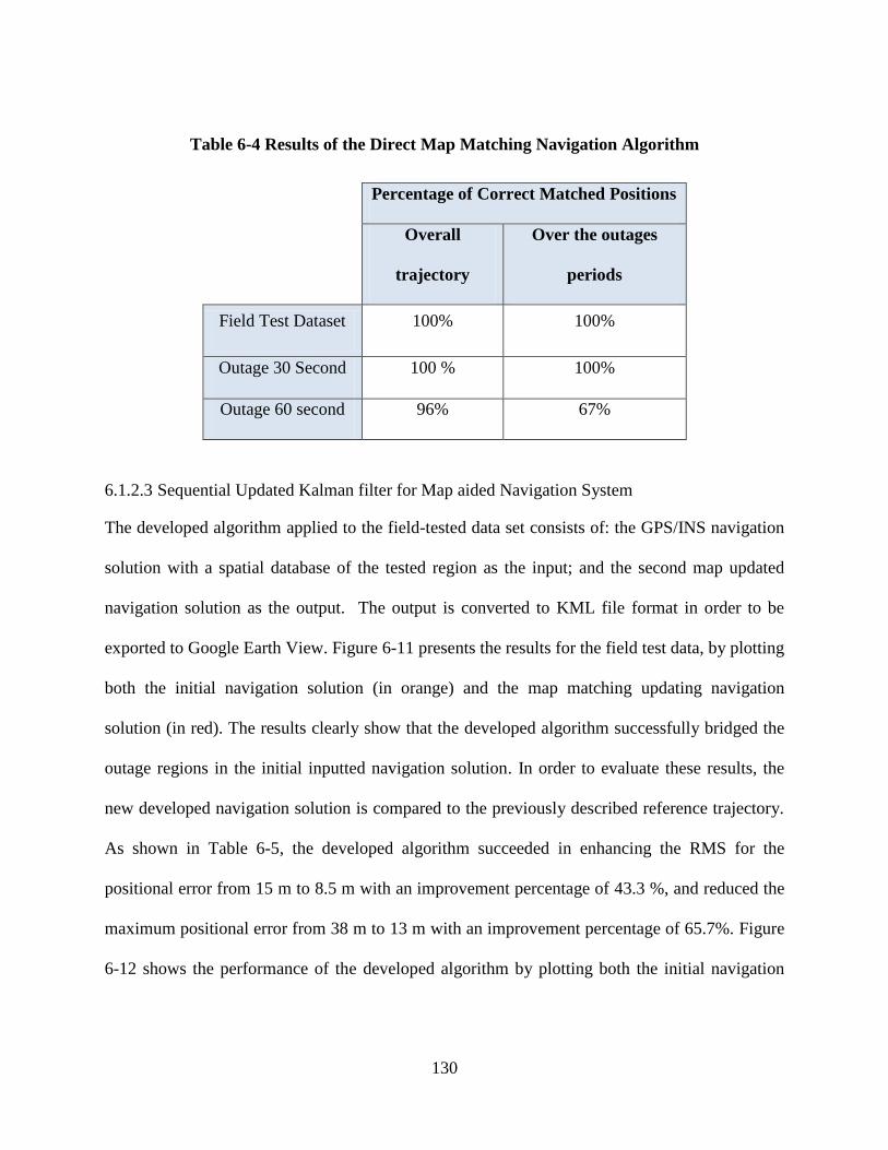
130
Table 6-4 Results of the Direct Map Matching Navigation Algorithm
Percentage of Correct Matched Positions
Overall
trajectory
Over the outages
periods
Field Test Dataset 100% 100%
Outage 30 Second 100 % 100%
Outage 60 second 96% 67%
6.1.2.3 Sequential Updated Kalman filter for Map aided Navigation System
The developed algorithm applied to the field-tested data set consists of: the GPS/INS navigation
solution with a spatial database of the tested region as the input; and the second map updated
navigation solution as the output. The output is converted to KML file format in order to be
exported to Google Earth View. Figure 6-11 presents the results for the field test data, by plotting
both the initial navigation solution (in orange) and the map matching updating navigation
solution (in red). The results clearly show that the developed algorithm successfully bridged the
outage regions in the initial inputted navigation solution. In order to evaluate these results, the
new developed navigation solution is compared to the previously described reference trajectory.
As shown in Table 6-5, the developed algorithm succeeded in enhancing the RMS for the
positional error from 15 m to 8.5 m with an improvement percentage of 43.3 %, and reduced the
maximum positional error from 38 m to 13 m with an improvement percentage of 65.7%. Figure
6-12 shows the performance of the developed algorithm by plotting both the initial navigation
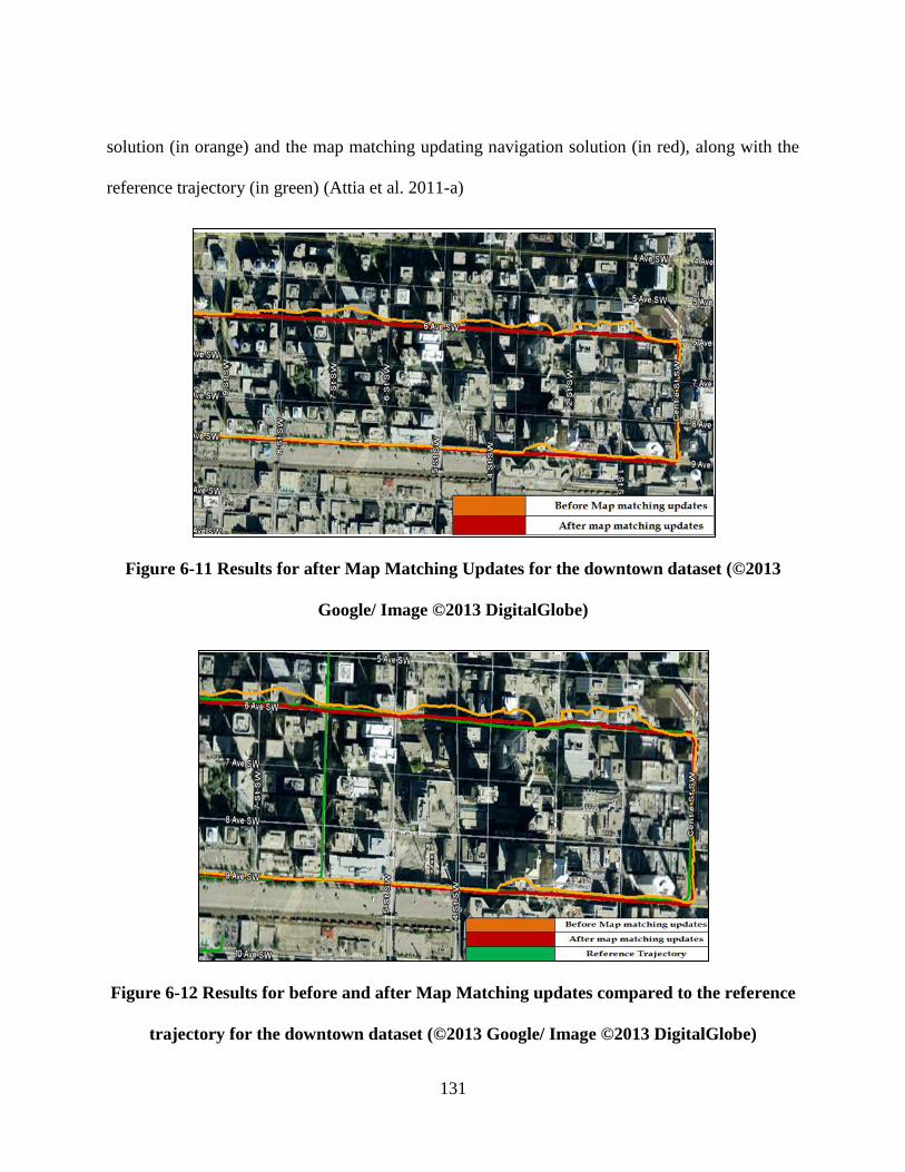
131
solution (in orange) and the map matching updating navigation solution (in red), along with the
reference trajectory (in green) (Attia et al. 2011-a)
Figure 6-11 Results for after Map Matching Updates for the downtown dataset (©2013
Google/ Image ©2013 DigitalGlobe)
Figure 6-12 Results for before and after Map Matching updates compared to the reference
trajectory for the downtown dataset (©2013 Google/ Image ©2013 DigitalGlobe)

132
Table 6-5 Performance Results of the developed map aiding GPS/MEMS IMU navigation
solution in downtown Calgary (as compared with the reference trajectory)
RMS (m) Max. error (m)
Field Test Data set 15 38
Results after MM updates 8.5 13
Percentage of improvement 43.3% 65.7%
6.2 Indoor Tests Descriptions
6.2.1 Field Test Description
6.2.1.1 First Field Test (Portable Navigation System)
Field Test Scenario:
In order to verify the performance of the developed map matching algorithms, a set of indoor
field tests were performed. The field tests took place on the main campus of the University of
Calgary. The field test was a ten-minute walk beginning outdoors, to maintain a GPS initial
solution, and then moved indoors to the Schulich School of Engineering building on the
University of Calgary campus. The tester walked double loops outdoors, and then entered the
building on the first floor at the north gate. They then climbed the stairs to the second floor,
walked around the stairs and inside the building to the south direction in the main corridor before
reaching the end of the Engineering block. Figure 6-13 shows the navigation solution in blue, the
building passageways in red, and the navigated passageways in yellow (Attia et al. 2011-b).
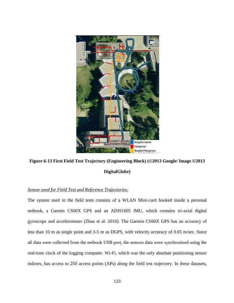
133
Figure 6-13 First Field Test Trajectory (Engineering Block) (©2013 Google/ Image ©2013
DigitalGlobe)
Sensor used for Field Test and Reference Trajectories:
The system used in the field tests consists of a WLAN Mini-card hooked inside a personal
netbook, a Garmin CS60X GPS and an ADIS1605 IMU, which contains tri-axial digital
gyroscope and accelerometer (Zhao et al. 2010). The Garmin CS60X GPS has an accuracy of
less than 10 m as single point and 3-5 m as DGPS, with velocity accuracy of 0.05 m/sec. Since
all data were collected from the netbook USB port, the sensors data were synchronized using the
real-time clock of the logging computer. Wi-Fi, which was the only absolute positioning sensor
indoors, has access to 250 access points (APs) along the field test trajectory. In these datasets,

134
due to the signal strength factor, only 12 access points from the 250 were used, as shown in
Figure 6-14 (Attia et al. 2011-b).
The integration between the GPS and the INS was not sufficient at all to have a reliable
navigation solution. As shown in Figure 6-15, the GPS only solution is presented to illustrate the
effect of the non-availability of the GPS through the tested trajectory. The aiding of the Wi-Fi
positioning and the map matching algorithm is essential for indoor navigation when counting on
just the INS stand-alone solutions. The inertial sensors errors have a large drift in the navigation
solution due to the uncompensated inertial sensors errors. The used ADIS1605 IMU gyroscope
has manufacturer specifications of initial bias error of ± 3 deg/ hour and in-run bias stability of
0.007 deg/ hour, and the accelerometer has specification of initial bias error ± 50 mg and in-run
bias stability of 0.2 mg. Table 6-6 summarizes the used ADI IMU sensors specifications.
Table 6-6 ADI ADIS1605 IMU Specification (ADI Data Sheet)
ADI ADIS1605 Parameters Value
Gyroscope Initial Bias error ± 3 deg/ hour
Gyro in-run bias stability 0.007 deg/ hour
Dynamic Range ± 350 deg/sec
Accelerometer Initial bias error ± 50 mg
In-run bias stability of 0.2 mg
Dynamic Range ± 18 g
In order to illustrate the effect of these errors, when considering only the uncompensated in-run
bias stability, the gyroscope will introduce a positional error greater than 5000 m for the five-
minute trajectory (positional error = 1/6*bias*g*time3), and the accelerometer could add another
100 m (positional error = 1/2*bias*time2).
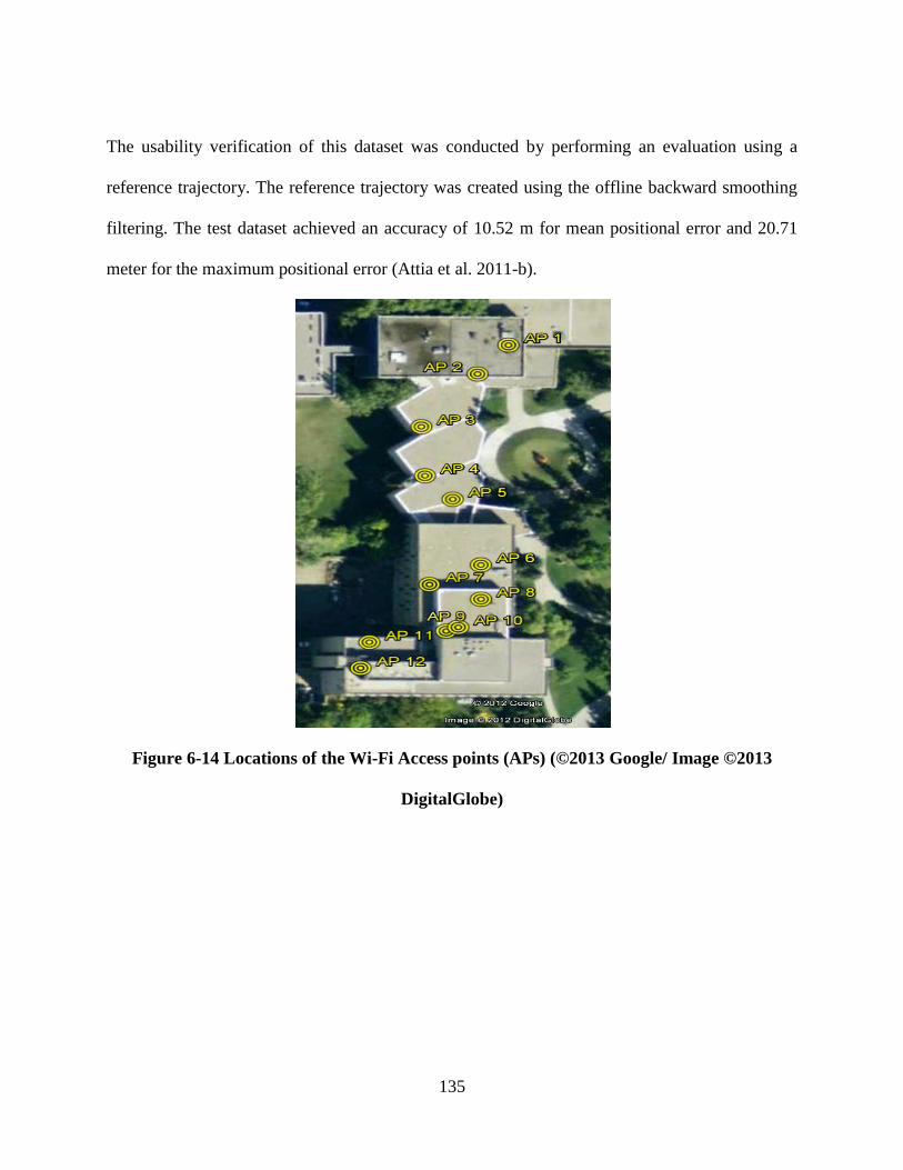
135
The usability verification of this dataset was conducted by performing an evaluation using a
reference trajectory. The reference trajectory was created using the offline backward smoothing
filtering. The test dataset achieved an accuracy of 10.52 m for mean positional error and 20.71
meter for the maximum positional error (Attia et al. 2011-b).
Figure 6-14 Locations of the Wi-Fi Access points (APs) (©2013 Google/ Image ©2013
DigitalGlobe)
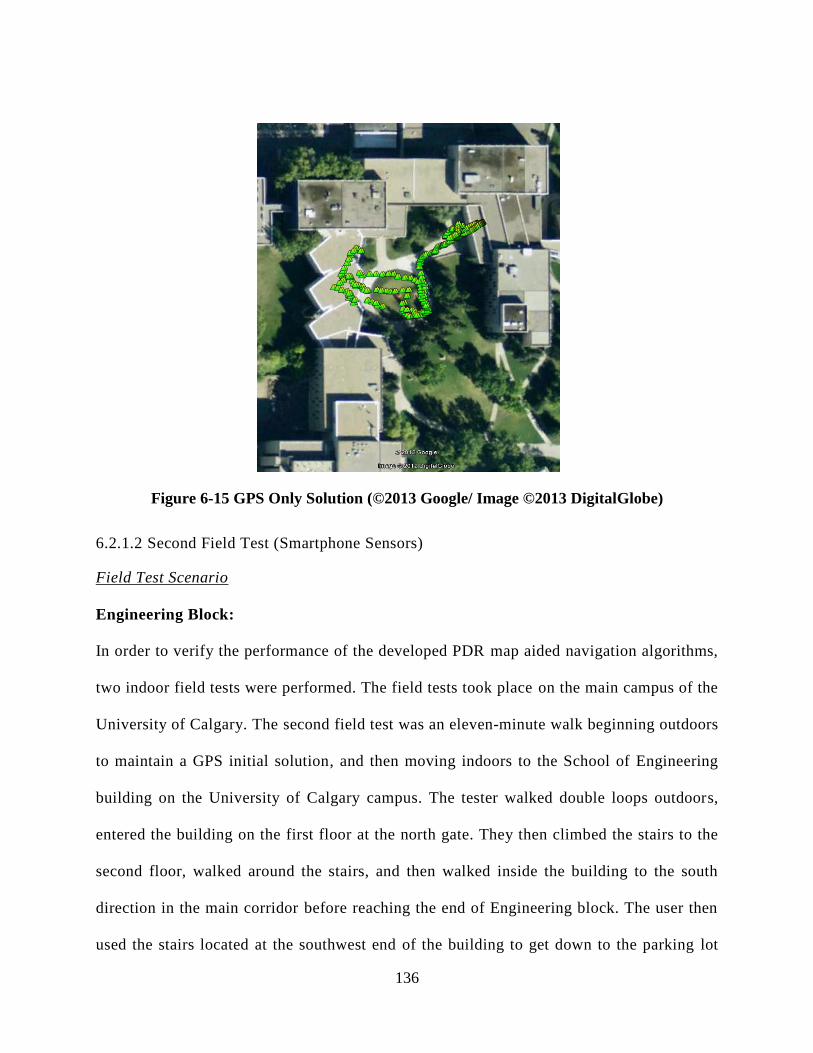
136
Figure 6-15 GPS Only Solution (©2013 Google/ Image ©2013 DigitalGlobe)
6.2.1.2 Second Field Test (Smartphone Sensors)
Field Test Scenario
Engineering Block:
In order to verify the performance of the developed PDR map aided navigation algorithms,
two indoor field tests were performed. The field tests took place on the main campus of the
University of Calgary. The second field test was an eleven-minute walk beginning outdoors
to maintain a GPS initial solution, and then moving indoors to the School of Engineering
building on the University of Calgary campus. The tester walked double loops outdoors,
entered the building on the first floor at the north gate. They then climbed the stairs to the
second floor, walked around the stairs, and then walked inside the building to the south
direction in the main corridor before reaching the end of Engineering block. The user then
used the stairs located at the southwest end of the building to get down to the parking lot
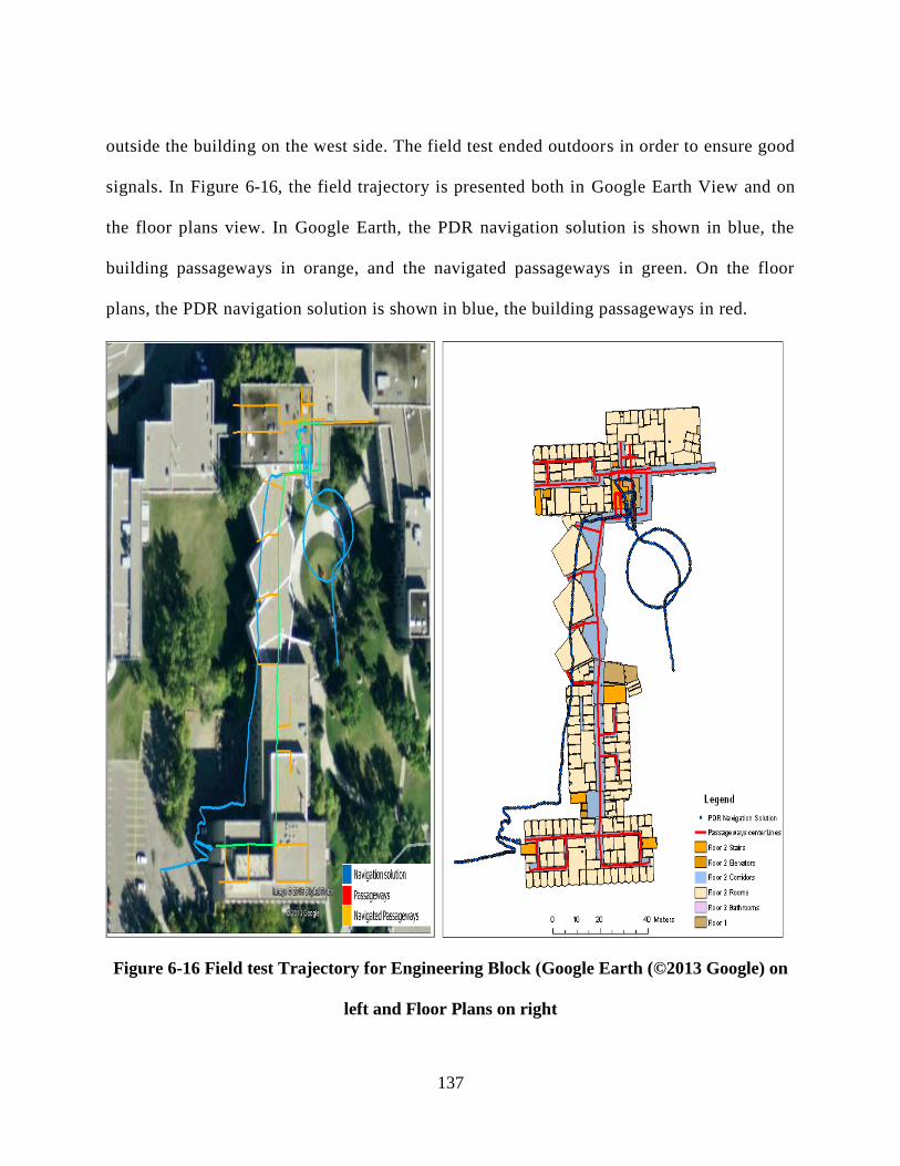
137
outside the building on the west side. The field test ended outdoors in order to ensure good
signals. In Figure 6-16, the field trajectory is presented both in Google Earth View and on
the floor plans view. In Google Earth, the PDR navigation solution is shown in blue, the
building passageways in orange, and the navigated passageways in green. On the floor
plans, the PDR navigation solution is shown in blue, the building passageways in red.
Figure 6-16 Field test Trajectory for Engineering Block (Google Earth (©2013 Google) on
left and Floor Plans on right
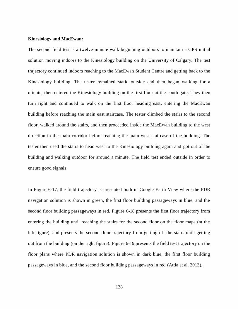
138
Kinesiology and MacEwan:
The second field test is a twelve-minute walk beginning outdoors to maintain a GPS initial
solution moving indoors to the Kinesiology building on the University of Calgary. The test
trajectory continued indoors reaching to the MacEwan Student Centre and getting back to the
Kinesiology building. The tester remained static outside and then began walking for a
minute, then entered the Kinesiology building on the first floor at the south gate. They then
turn right and continued to walk on the first floor heading east, entering the MacEwan
building before reaching the main east staircase. The tester climbed the stairs to the second
floor, walked around the stairs, and then proceeded inside the MacEwan building to the west
direction in the main corridor before reaching the main west staircase of the building. The
tester then used the stairs to head west to the Kinesiology building again and got out of the
building and walking outdoor for around a minute. The field test ended outside in order to
ensure good signals.
In Figure 6-17, the field trajectory is presented both in Google Earth View where the PDR
navigation solution is shown in green, the first floor building passageways in blue, and the
second floor building passageways in red. Figure 6-18 presents the first floor trajectory from
entering the building until reaching the stairs for the second floor on the floor maps (at the
left figure), and presents the second floor trajectory from getting off the stairs until getting
out from the building (on the right figure). Figure 6-19 presents the field test trajectory on the
floor plans where PDR navigation solution is shown in dark blue, the first floor building
passageways in blue, and the second floor building passageways in red (Attia et al. 2013).
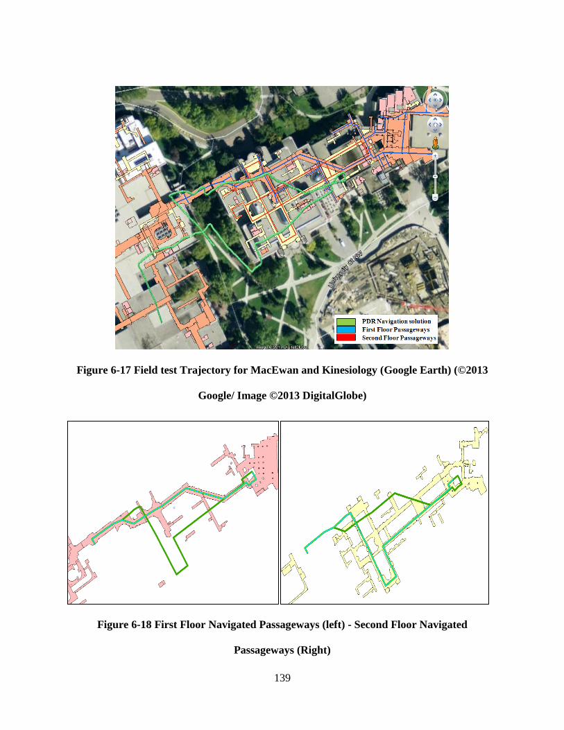
139
Figure 6-17 Field test Trajectory for MacEwan and Kinesiology (Google Earth) (©2013
Google/ Image ©2013 DigitalGlobe)
Figure 6-18 First Floor Navigated Passageways (left) - Second Floor Navigated
Passageways (Right)

140
Figure 6-19 Field Test Trajectory for MacEwan and Kinesiology (Floor Plans)
Sensor used for Field Test and Reference Trajectories
The field tests were carried out using the Samsung Galaxy Smartphone sensors, logging the data
using a commercial application called “Data logger” and transferring the logged data offline.
Table 6-7 summarizes the Samsung Galaxy Smartphone sensor types and specification. The
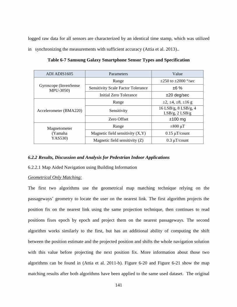
141
logged raw data for all sensors are characterized by an identical time stamp, which was utilized
in synchronizing the measurements with sufficient accuracy (Attia et al. 2013)..
Table 6-7 Samsung Galaxy Smartphone Sensor Types and Specification
ADI ADIS1605 Parameters Value
Gyroscope (InvenSense
MPU-3050)
Range ±250 to ±2000 °/sec
Sensitivity Scale Factor Tolerance ±6 %
Initial Zero Tolerance ±20 deg/sec
Accelerometer (BMA220)
Range ±2, ±4, ±8, ±16 g
Sensitivity 16 LSB/g, 8 LSB/g, 4
LSB/g, 2 LSB/g
Zero Offset ±100 mg
Magnetometer
(Yamaha
YAS530)
Range ±800μT
Magnetic field sensitivity (X,Y) 0.15 μT/count
Magnetic field sensitivity (Z) 0.3 μT/count
6.2.2 Results, Discussion and Analysis for Pedestrian Indoor Applications
6.2.2.1 Map Aided Navigation using Building Information
Geometrical Only Matching:
The first two algorithms use the geometrical map matching technique relying on the
passageways’ geometry to locate the user on the nearest link. The first algorithm projects the
position fix on the nearest link using the same projection technique, then continues to read
positions fixes epoch by epoch and project them on the nearest passageways. The second
algorithm works similarly to the first, but has an additional ability of computing the shift
between the position estimate and the projected position and shifts the whole navigation solution
with this value before projecting the next position fix. More information about those two
algorithms can be found in (Attia et al. 2011-b). Figure 6-20 and Figure 6-21 show the map
matching results after both algorithms have been applied to the same used dataset. The original
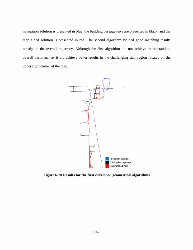
142
navigation solution is presented in blue, the building passageways are presented in black, and the
map aided solution is presented in red. The second algorithm yielded good matching results
mostly on the overall trajectory. Although the first algorithm did not achieve an outstanding
overall performance, it did achieve better results in the challenging stair region located on the
upper right corner of the map.
Figure 6-20 Results for the first developed geometrical algorithms
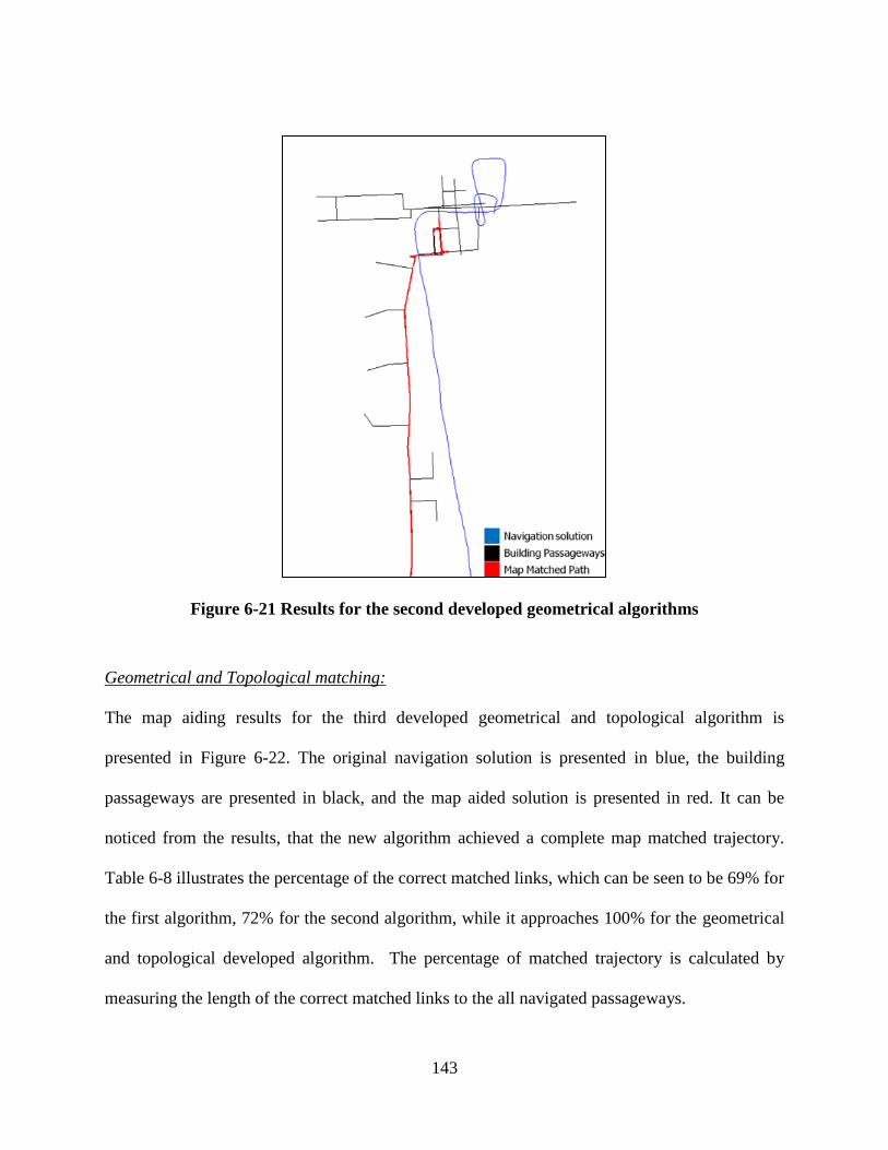
143
Figure 6-21 Results for the second developed geometrical algorithms
Geometrical and Topological matching:
The map aiding results for the third developed geometrical and topological algorithm is
presented in Figure 6-22. The original navigation solution is presented in blue, the building
passageways are presented in black, and the map aided solution is presented in red. It can be
noticed from the results, that the new algorithm achieved a complete map matched trajectory.
Table 6-8 illustrates the percentage of the correct matched links, which can be seen to be 69% for
the first algorithm, 72% for the second algorithm, while it approaches 100% for the geometrical
and topological developed algorithm. The percentage of matched trajectory is calculated by
measuring the length of the correct matched links to the all navigated passageways.
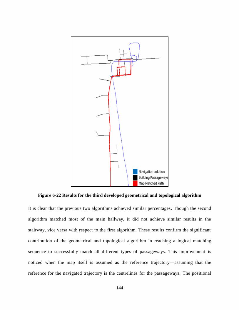
144
Figure 6-22 Results for the third developed geometrical and topological algorithm
It is clear that the previous two algorithms achieved similar percentages. Though the second
algorithm matched most of the main hallway, it did not achieve similar results in the
stairway, vice versa with respect to the first algorithm. These results confirm the significant
contribution of the geometrical and topological algorithm in reaching a logical matching
sequence to successfully match all different types of passageways. This improvement is
noticed when the map itself is assumed as the reference trajectory—assuming that the
reference for the navigated trajectory is the centrelines for the passageways. The positional
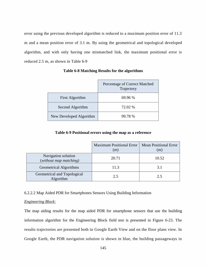
145
error using the previous developed algorithm is reduced to a maximum position error of 11.3
m and a mean position error of 3.1 m. By using the geometrical and topological developed
algorithm, and with only having one mismatched link, the maximum positional error is
reduced 2.5 m, as shown in Table 6-9
Table 6-8 Matching Results for the algorithms
Percentage of Correct Matched
Trajectory
First Algorithm 69.96 %
Second Algorithm 72.02 %
New Developed Algorithm 99.78 %
Table 6-9 Positional errors using the map as a reference
Maximum Positional Error
(m)
Mean Positional Error
(m)
Navigation solution
(without map matching) 20.71 10.52
Geometrical Algorithms 11.3 3.1
Geometrical and Topological
Algorithm 2.5 2.5
6.2.2.2 Map Aided PDR for Smartphones Sensors Using Building Information
Engineering Block:
The map aiding results for the map aided PDR for smartphone sensors that use the building
information algorithm for the Engineering Block field test is presented in Figure 6-23. The
results trajectories are presented both in Google Earth View and on the floor plans view. In
Google Earth, the PDR navigation solution is shown in blue, the building passageways in
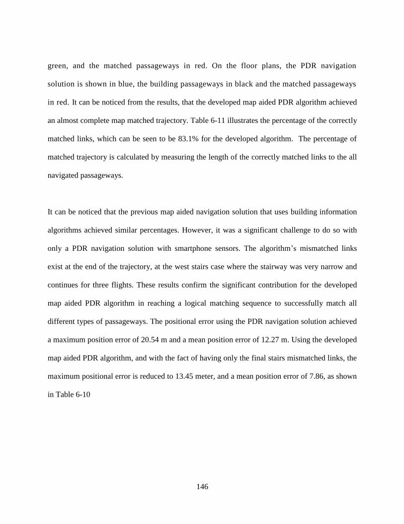
146
green, and the matched passageways in red. On the floor plans, the PDR navigation
solution is shown in blue, the building passageways in black and the matched passageways
in red. It can be noticed from the results, that the developed map aided PDR algorithm achieved
an almost complete map matched trajectory. Table 6-11 illustrates the percentage of the correctly
matched links, which can be seen to be 83.1% for the developed algorithm. The percentage of
matched trajectory is calculated by measuring the length of the correctly matched links to the all
navigated passageways.
It can be noticed that the previous map aided navigation solution that uses building information
algorithms achieved similar percentages. However, it was a significant challenge to do so with
only a PDR navigation solution with smartphone sensors. The algorithm’s mismatched links
exist at the end of the trajectory, at the west stairs case where the stairway was very narrow and
continues for three flights. These results confirm the significant contribution for the developed
map aided PDR algorithm in reaching a logical matching sequence to successfully match all
different types of passageways. The positional error using the PDR navigation solution achieved
a maximum position error of 20.54 m and a mean position error of 12.27 m. Using the developed
map aided PDR algorithm, and with the fact of having only the final stairs mismatched links, the
maximum positional error is reduced to 13.45 meter, and a mean position error of 7.86, as shown
in Table 6-10
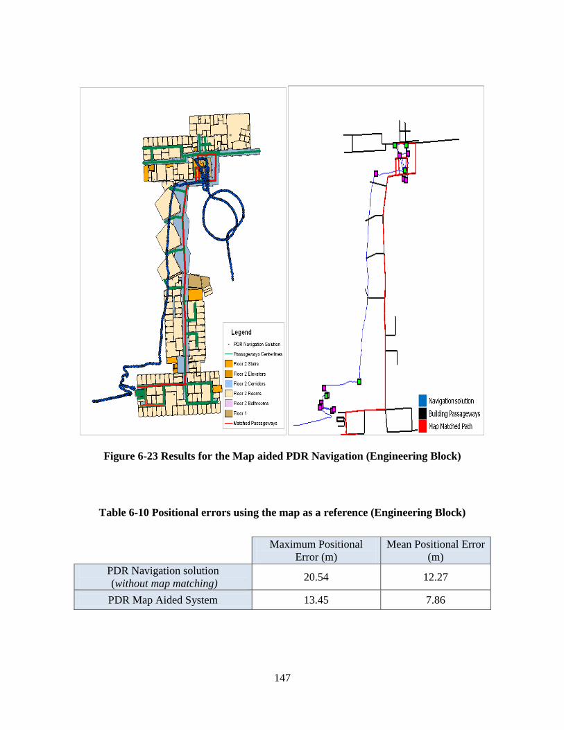
147
Figure 6-23 Results for the Map aided PDR Navigation (Engineering Block)
Table 6-10 Positional errors using the map as a reference (Engineering Block)
Maximum Positional
Error (m)
Mean Positional Error
(m)
PDR Navigation solution
(without map matching) 20.54 12.27
PDR Map Aided System 13.45 7.86

148
Kinesiology and MacEwan:
The map aiding results for the map aided PDR for smartphones sensors used the building
information algorithm for the Kinesiology and MacEwan field test as presented in Figure 6-24
and Figure 6-25. Figure 6-24 presents the results trajectories on the floor maps, where the
PDR navigation solution is shown in blue, the first floor building passageways in blue, the
second floor building passageways in green, and the matched passageways in red. Figure
6-25 shows a simplified floor plan with only the centrelines for the passageways and
trajectories. The PDR navigation solution is shown in blue, the building passageways in
black and the matched passageways in red. It can be seen from the results, that the developed
map aided PDR algorithm achieved a complete map matched trajectory, with just one missing
horizontal link at the end of the matched trajectory due to the length difference between the PDR
navigation solution and the links database reference length. This was because the estimation for
the user stride length was not completely achieved for the actual trajectory length. However, and
upon detecting the final left turn, the final link was correctly detected. Table 6-11 lists the
percentages of the correctly matched links, which were 97.3% for the developed algorithm. The
percentage of matched trajectory is calculated by measuring the length of the correctly matched
links to the all navigated passageways.
These results continue to confirm the significant contribution of the developed map aided
PDR algorithm in reaching a logical matching sequence that successfully matches all
different types of passageways. The positional error that uses the PDR navigation solution
achieved a maximum position error of 64.01 m and a mean position error of 38.49 m. By
using the developed map aided PDR algorithm, despite only having the final stairs as
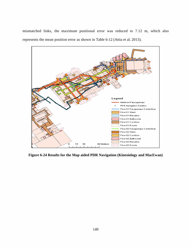
149
mismatched links, the maximum positional error was reduced to 7.12 m, which also
represents the mean position error as shown in Table 6-12 (Attia et al. 2013).
Figure 6-24 Results for the Map aided PDR Navigation (Kinesiology and MacEwan)
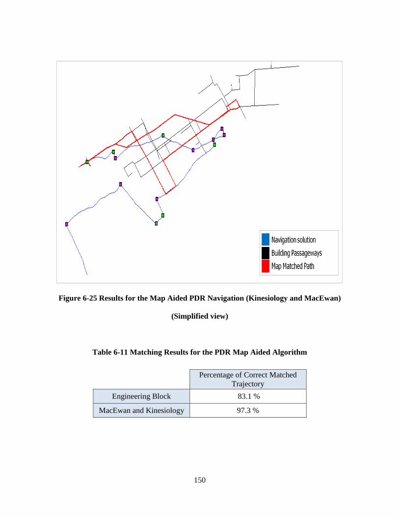
150
Figure 6-25 Results for the Map Aided PDR Navigation (Kinesiology and MacEwan)
(Simplified view)
Table 6-11 Matching Results for the PDR Map Aided Algorithm
Percentage of Correct Matched
Trajectory
Engineering Block 83.1 %
MacEwan and Kinesiology 97.3 %
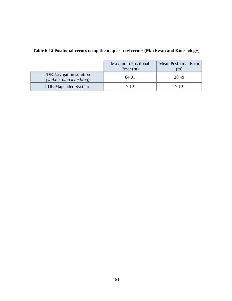
151
Table 6-12 Positional errors using the map as a reference (MacEwan and Kinesiology)
Maximum Positional
Error (m)
Mean Positional Error
(m)
PDR Navigation solution
(without map matching) 64.01 38.49
PDR Map aided System 7.12 7.12
152
Chapter Seven: Summary, Conclusions and Recommendations
7.1 Summary
The main objective of this thesis was to develop a map aided navigation technique that assisted
and enhanced navigation applications in GPS-denied environments for both outdoor and indoor
applications, and for both vehicle and pedestrians users. The developed techniques have several
different architectures based on the navigation application and environment. The three main
components of the developed techniques are: a geospatial data model with navigation related
attributes to be used as a virtual boundary that forces the estimated navigation trajectory on a
certain logical track, a map matching algorithm based on the geometrical and topological
characteristics for the navigated regions networks in order to match the estimated position fixes
on the geospatial model, and an integrated navigation model based on multi-sensors integration
to estimate the position fixes with sufficient accuracy as to be implemented in the map aided
system.
In this thesis, each component was introduced with a short description and followed up with
presentation of the state of the art technology and work this research would develop. The
integration of these components was also introduced in addition to a discussion on the way in
which they were implemented according to each application and environment. The evaluation of
these techniques in real life navigation applications (with the use of several sensors and at
differing accuracies) was investigated and the results were presented. Based on the achieved
results, it is fair to state that the developed map aided navigation systems have succeeded in
enhancing the navigation solutions for GPS-denied environments such as indoor buildings and

153
urban centers. Furthermore, these map aided navigation systems have improved the data
reliability.
7.2 Conclusions
The navigation applications are considered essential and vital for many areas of use: daily
activities, industrial, commercial, law enforcement, and emergency. Navigating in open space
has been well researched, and despite some of the challenges it might face it can be considered in
many cases a stable and consistent application. Navigation challenges in GPS-denied
environments is currently one of the most relevant areas of research and as such, can produce
significantly beneficial navigational aid solutions for either urban canyons or isolated indoor
buildings.
In this thesis, indoor and outdoor aided navigation solutions were developed using several
constraints and mapping information. Map aiding systems were developed based on geospatial
models and map matching algorithms. The geospatial data models were built according to
navigation applications requirements and characteristics. Several models were created for both
indoor and outdoor environments to be used in implementing the map aided algorithms, and for
evaluating the performance and testing of the systems in real-life trajectories. Both geometrical
and topological map matching algorithms based on automatic turn detection techniques were
developed to project the obtained navigation solution position fix into the created geospatial data
model.

154
Vehicle navigation applications, especially in urban centers where there is poor or no GPS
signal, struggle to maintain a reliable and continuous navigation solution. GPS/INS integrated
navigation systems have an advantage in bridging this unavailability. However, they still require
some help to avoid drifts in the solution due to long outage periods.
In this thesis, an enhanced constrained Kalman filter was developed. It used the relative
height change from epoch to epoch as constrains in the filter, forcing the solution to be
projected through these thresholds. ZUPT updates were developed and implemented in
the Kalman filter as well, making use of an automatic detection technique based on
decision trees to detect the stop intervals and apply the ZUPT within them. The results
show a significant improvement when the enhanced Kalman filter is used. Moreover, the
trajectory path and manoeuvres were detected efficiently compared to the traditional
extended Kalman filtering method. The ZUPT updates also improved the solution as
well.
Map matching nowadays is considered not only as a visualization technique for the
navigation solution, but also as an enhancing technique that has the ability to bridge
navigation systems. A map matching technique based on the integration of a GPS/INS
navigation solution and geospatial database was proposed and tested on several datasets.
The results show identical matching with the road network for the real data and the
simulated 30-second outage. As for the 60-second outage dataset, 67% matching results
were achieved over the outage regions using the specific sensors tested in this thesis.

155
In this thesis, a map matching updating navigation algorithm was developed. The
algorithm uses a GPS/INS/ map database input to provide an initial navigation solution
and its map matching output. These map matched positions were then fed back to the
navigation solution to obtain the final updated navigation solution. The results indicate an
improvement of 43% in the positional RMS and 66% in the maximum positional error.
Personal navigation for indoor applications is facing huge challenges providing a reliable
positioning accuracy to the user. The main challenge is the unavailability of a robust absolute
positioning sensor in indoor environments (i.e. GPS). Even when the Wi-Fi signal strength is
used the navigation solution accuracy is good but not reliable over long periods or for all
applications.
In this thesis, in order to enhance the reliability of positioning solutions for indoor
environments, two geometrical map matching techniques were developed to assist a
current pedestrian navigation system. The input for the algorithm is the navigation
solution obtained from the GPS/INS/Wi-Fi integrated system. The algorithm uses the
map matching to locate the solution on the most probable location (passageways),
thereby increasing the reliability of the overall navigation output. Two matching logics
were field tested at the engineering building on the University of Calgary campus and the
matching percentage was approximately 70% for both. The enhancement in the mean
positional errors was 70% as compared without map matching. The achieved results for
locating the navigated passageways can be highly significant to many mobile mapping
applications.
156
A geometrical and topological map aiding navigation algorithm was developed, which
uses the map matching technique to assist the navigation solution. The input for the
developed algorithm is a navigation solution from a GPS/INS/Wi-Fi integrated
navigation system. The map aiding navigation algorithm uses the navigation position, the
raw inertial measurements and the building information to produce a more reliable
navigation position matched to the navigated area map. The developed algorithm was run
through a field test using a PNS inside the engineering building of the University of
Calgary campus, and a matching percentage of 99% was achieved. The enhancement in
the mean positional errors was 76% as compared without map matching. This developed
low-cost, user-friendly algorithm would assist in enhancing personal navigation
applications in indoor environments, thereby providing a reliable positioning accuracy,
which is essential to many applications such as law enforcement, E911 services,
consumer indoor navigation, assistance for people with disabilities and mobile mapping.
A map aided PDR navigation solution was developed using the Samsung Galaxy
smartphone sensors. The PDR solution used the accelerometer and magnetometer
measurements from the smartphone to estimate a navigation solution with sufficient
accuracy to be entered in the map aided algorithm. The map aided algorithm utilized the
obtained PDR solution, the developed geometrical and topological map matching with
turn detection technique and the geospatial data modeled for navigation applications. The
algorithm provides a reliable, accurate and continuous matched navigation solution. The
developed system was field-tested twice on different trajectories in different buildings

157
(Engineering building and the Kinesiology and MacEwan buildings) and achieved a
significantly reliable matched navigation solution with matching percentage of 83% and
97% respectively. The enhancement in the mean positional errors was 36% and 81%
respectively as compared without map matching.
7.3 Recommendations for Future Work
Based on the achieved positive results and conclusions about the use of map aided indoor and
outdoor navigation systems, it is recommended to extend this research for future developments.
The recommendations for future work are based on developing the established map aided
systems imbedded in real-time smartphone applications. The primary recommended future
research points are:
Utilizing crowdsourcing geospatial data for indoor environments such as shopping malls,
airport terminals, office buildings, or medical centers for creating the map aided
navigation geospatial models. This should save significant time and money in developing
these applications for a wide range of uses. Further investigation of the evaluation
techniques for the integrity of the obtained spatial data is recommended.
Implementing the map aided navigation algorithms on smartphone engines to enable real-
time map aided navigation in indoor environments. Adding manual map-location updates
could be beneficial in aiding the mobile PDR navigation solution, such as the user
inputting the nearest store in front of his/her location at the exact time.
Investigating the enhancement of map matching algorithms using the trajectories
sequences certainty matching, should improve the matching performance in indoor

158
environments. This technique should make use of the current trajectory sequence and
match it to a database of trajectories sequences for the same location.
Using the map-matched updates as both coordinates and heading constraints inside the
estimated projection constrained Kalman filtering technique. The map matched solution
can provide both matched positions and the matched link heading, which can be used
similar to the developed height constraints as equality constraints for the Kalman filter.

159
References
Abdel-Hamid, W. (2004). Accuracy enhancement of integrated MEMS-IMU/GPS systems for
land vehicular navigation applications, University of Calgary, Department of Geomatics
Engineering.
Afzal, M. H. (2011). Use of Earth's Magnetic Field for Pedestrian Navigation, Ph. D. Thesis,
University of Calgary, Calgary, AB, Canada.
Aggarwal, P., Z. Syed, A. Noureldin and N. El-Sheimy (2010). MEMS-based integrated
navigation, Artech House Publishers.
Ali, A., S. Siddarth, N. El-Sheimy and Z. Syed (2012). "An Improved Personal Dead-Reckoning
Algorithm for Dynamically Changing Smartphone User Modes." Proceedings of the 25th
International Technical Meeting of The Satellite Division of the Institute of Navigation
(ION GNSS 2012), Nashville, TN, September 2012: 2432-2439.
Arto, P., S. Ari-Heikki, H. Merja, H. Jussi, H. Jonna and kkil (2009). Towards designing better
maps for indoor navigation: experiences from a case study. Proceedings of the 8th
International Conference on Mobile and Ubiquitous Multimedia. Cambridge, United
Kingdom, ACM.
Atia, M., M. Korenberg and A. Noureldin (2012). "Particle-Filter-Based WiFi-Aided Reduced
Inertial Sensors Navigation System for Indoor and GPS-Denied Environments."
International Journal of Navigation and Observation 2012.
Atia, M., A. Noureldin, J. Georgy and M. Korenberg (2011). "Bayesian filtering based WiFi/INS
integrated navigation solution for GPS-denied environments." Navigation 58(2): 111-125.
Attia, M., A. Moussa and N. El-Sheimy (2010). "Bridging Integrated GPS/INS Systems with
Geospatial Models for Car Navigation Applications." Proceedings of the 23rd
International Technical Meeting of The Satellite Division of the Institute of Navigation
(ION GNSS 2010): 1697 - 1703.
Attia, M., A. Moussa and N. El-Sheimy (2011-a). "Updating Integrated GPS/INS Systems with
Map Matching for Car Navigation Applications." Proceedings of the 24th International
Technical Meeting of The Satellite Division of the Institute of Navigation (ION GNSS
2011): 3539 - 3545.
Attia, M., A. Moussa, X. Zhao and N. El-Sheimy (2011-b). "Assisting Personal Positioning in
Indoor Environments Using Map Matching." Archives of Photogrammetry, Cartography
and Remote Sensing, 22: 39-49.
Attia, M., A. Moussa and N. El-Sheimy (2013). "Map Aided Pedestrian Dead Reckoning Using
Buildings Information for Indoor Navigation Applications." Positioning 4(3): 227-239.
Basnayake, C., O. Mezentsev, G. Lachapelle and M. E. Cannon (2005). "An HSGPS, inertial and
map-matching integrated portable vehicular navigation system for uninterrupted real-time
vehicular navigation." International Journal of Vehicle Information and Communication
Systems 1(1): 131-151.
Breiman, L., J. Friedman, C. J. Stone and R. A. Olshen (1984). Classification and regression
trees, Chapman & Hall/CRC.
Brown, R. and P. Hwang (1992). "Introduction to random signals and applied Kalman
filtering(Book)." New York, John Wiley & Sons, Inc., 1992. 512.

160
Bullock, B. (1995). A prototype portable vehicle navigation system utilizing map aided GPS.
Proceedings of the 8th International Technical Meeting of the Satellite Division of The
Institute of Navigation (ION GPS 1995).
Bullock, J. B. (1995). A Prototype Portable Vehicle Navigation System Utilizing Map Aided
GPS, University of Calgary.
Bullock, J. B. and E. J. Krakiwsky (1994). Analysis of the use of digital road maps in vehicle
navigation. Position Location and Navigation Symposium, 1994., IEEE.
Cipeluch, B., R. Jacob, P. Mooney and A. Winstanley (2010). Comparison of the accuracy of
OpenStreetMap for Ireland with Google Maps and Bing Maps. Proceedings of the Ninth
International Symposium on Spatial Accuracy Assessment in Natural Resuorces and
Enviromental Sciences 20-23rd July 2010, University of Leicester.
El-Sheimy, N. (2010). "Inertial Techniques and INS/DGPS Integration " Lecture Notes,
Geomatics Department, University of Calgary.
El-Sheimy, N. and X. Niu (2007). "The promise of MEMS to the navigation community." Inside
GNSS 2(2): 46-56.
El Najjar, M. E. and P. Bonnifait (2005). "A Road-Matching Method for Precise Vehicle Localization
Using Belief Theory and Kalman Filtering." Autonomous Robots 19(2): 173-191.
Goodall, C. (2009). Improving usability of low-cost INS/GPS navigation systems using
intelligent techniques, PhD thesis, University of Calgary, Calgary, Canada.
Greenfeld, J. S. (2002). Matching GPS observations to locations on a digital map. National
Research Council (US). Transportation Research Board. Meeting (81st: 2002:
Washington, DC). Preprint CD-ROM.
Gupta, N. and R. Hauser (2007). "Kalman filtering with equality and inequality state
constraints." arXiv preprint arXiv:0709.2791.
Haklay, M. (2010). "How good is volunteered geographical information? A comparative study of
OpenStreetMap and Ordnance Survey datasets." Environment and planning. B, Planning
& design 37(4): 682.
Jong-Sun, P., S. Dong-Ho and S. Tae-Kyung (2001). Development of a map matching method
using the multiple hypothesis technique. Intelligent Transportation Systems, 2001.
Proceedings. 2001 IEEE.
Mikhail, E. M. and F. E. Ackermann (1976). Observations and least squares, IEP New York.
Moussa, A., W. W. Abdel-Hamid and N. El-Sheimy (2011). "Decision Trees based GPS Cycle
Slip Detection and Correction " ENC2011, London, December 2011.
Ochieng, W. Y., M. Quddus and R. B. Noland (2003). "MAP-MATCHING IN COMPLEX
URBAN ROAD NETWORKS." Brazilian Journal of Cartography 55(2) 1-18.
Petovello, M. (2009). "Estimation For Navigation." Lecture Notes, Geomatics Department,
University of Calgary.
Petovello, M. G. (2003). Real-time integration of a tactical-grade IMU and GPS for high-
accuracy positioning and navigation.
Quddus, M., R. Noland and W. Ochieng (2009). "The Effects of Navigation Sensors and Spatial
Road Network Data Quality on the Performance of Map Matching Algorithms."
GeoInformatica 13(1): 85-108.
Quddus, M. A., R. B. Noland and W. Y. Ochieng (2006). "A High Accuracy Fuzzy Logic Based
Map Matching Algorithm for Road Transport." Journal of Intelligent Transportation
Systems 10(3): 103-115.

161
Quddus, M. A., W. Y. Ochieng and R. B. Noland (2006). "Integrity of map-matching
algorithms." Transportation Research Part C: Emerging Technologies 14(4): 283-302.
Quddus, M. A., W. Y. Ochieng and R. B. Noland (2007). "Current map-matching algorithms for
transport applications: State-of-the art and future research directions." Transportation
Research Part C: Emerging Technologies 15(5): 312-328.
Quinlan, J. R. (1993). C4. 5: programs for machine learning, Morgan kaufmann.
Scott, C. (1994). Improved GPS positioning for motor vehicles through map matching.
Proceedings of the 7th International Technical Meeting of the Satellite Division of The
Institute of Navigation (ION GPS 1994).
Shin, E.-H. (2005). "Estimation techniques for low-cost inertial navigation." UCGE
report(20219).
Shin, E.-H. and N. El-Sheimy (2001). Accuracy improvement of low cost INS/GPS for land
applications, University of Calgary, Department of Geomatics Engineering.
Shin, E. and N. El-Sheimy (2004). "Aided InertialNavigationSystem(AINS™)Toolboxfor
MatLab® Software." INS/GPS integration software, Mobile Multi-Sensors System
(MMSS) research group, the University of Calgary http://mms. geomatics. ucalgary.
ca/Research/Tech% 20transfer/INS_toolbox. htm.
Shin, S., C. Park, J. Kim, H. Hong and J. Lee (2007). Adaptive step length estimation algorithm
using low-cost MEMS inertial sensors. Sensors Applications Symposium, 2007. SAS'07.
IEEE, IEEE.
Simon, D. (2010). "Kalman filtering with state constraints: a survey of linear and nonlinear
algorithms." Control Theory & Applications, IET 4(8): 1303-1318.
Sircoulomb, V., G. Hoblos, H. Chafouk and J. Ragot (2008). State estimation under nonlinear
state inequality constraints. A tracking application. Control and Automation, 2008 16th
Mediterranean Conference on, IEEE.
Syed, S. and M. Cannon (2004). Fuzzy logic-based map matching algorithm for vehicle
navigation system in urban canyons. ION National Technical Meeting, San Diego, CA.
Syed, Z. F. (2009). "Design and Implementation Issues of a Portable Navigation System." PhD
thesis, University of Calgary, Calgary, Canada.
White, C. E., D. Bernstein and A. L. Kornhauser (2000). "Some map matching algorithms for
personal navigation assistants." Transportation Research Part C: Emerging Technologies
8(1-6): 91-108.
Yu, M., Z. Li, Y. Chen and W. Chen (2006). "Improving integrity and reliability of map
matching techniques." Journal of Global Positioning Systems 5(1-2): 40-46.
Yuksel, Y. (2011). "Design and analysis of inertial navigation systems with skew redundant
inertial sensors." UCGE report 20328.
Zhao, X., C. Goodall, Z. Syed, B. Wright and N. El-Sheimy (2010). Wi-Fi assisted multi-sensor
personal navigation system for indoor environments. Proceedings of the International
TechnicalMeetingofTheInstituteofNavigation(ION’10).
Zhao, X., Z. Syed, D. Wright and N. El-Sheimy (2009). An Economical and Effective Multi-
sensor Integration for Portable Navigation System. Proceedings of the 22nd International
Technical Meeting of The Satellite Division of the Institute of Navigation (ION GNSS
2009).
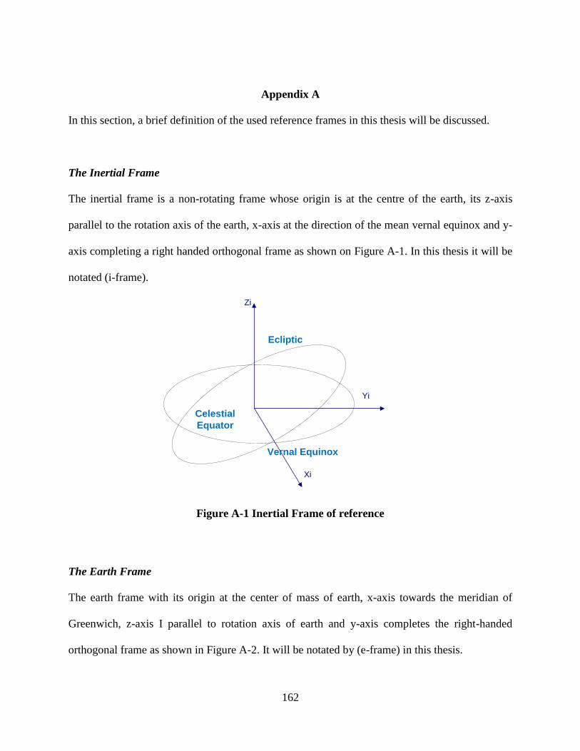
162
Appendix A
In this section, a brief definition of the used reference frames in this thesis will be discussed.
The Inertial Frame
The inertial frame is a non-rotating frame whose origin is at the centre of the earth, its z-axis
parallel to the rotation axis of the earth, x-axis at the direction of the mean vernal equinox and y-
axis completing a right handed orthogonal frame as shown on Figure A-1. In this thesis it will be
notated (i-frame).
Yi
Zi
Xi
Ecliptic
Vernal Equinox
Celestial
Equator
Figure A-1 Inertial Frame of reference
The Earth Frame
The earth frame with its origin at the center of mass of earth, x-axis towards the meridian of
Greenwich, z-axis I parallel to rotation axis of earth and y-axis completes the right-handed
orthogonal frame as shown in Figure A-2. It will be notated by (e-frame) in this thesis.
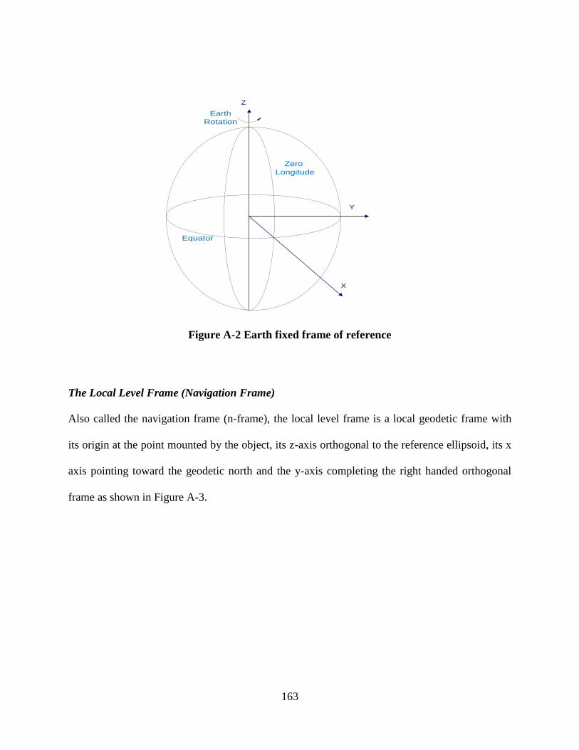
163
Y
Z
X
Zero
Longitude
Equator
Earth
Rotation
Figure A-2 Earth fixed frame of reference
The Local Level Frame (Navigation Frame)
Also called the navigation frame (n-frame), the local level frame is a local geodetic frame with
its origin at the point mounted by the object, its z-axis orthogonal to the reference ellipsoid, its x
axis pointing toward the geodetic north and the y-axis completing the right handed orthogonal
frame as shown in Figure A-3.
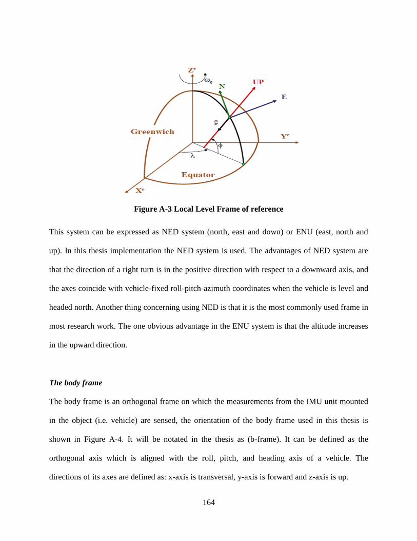
164
Figure A-3 Local Level Frame of reference
This system can be expressed as NED system (north, east and down) or ENU (east, north and
up). In this thesis implementation the NED system is used. The advantages of NED system are
that the direction of a right turn is in the positive direction with respect to a downward axis, and
the axes coincide with vehicle-fixed roll-pitch-azimuth coordinates when the vehicle is level and
headed north. Another thing concerning using NED is that it is the most commonly used frame in
most research work. The one obvious advantage in the ENU system is that the altitude increases
in the upward direction.
The body frame
The body frame is an orthogonal frame on which the measurements from the IMU unit mounted
in the object (i.e. vehicle) are sensed, the orientation of the body frame used in this thesis is
shown in Figure A-4. It will be notated in the thesis as (b-frame). It can be defined as the
orthogonal axis which is aligned with the roll, pitch, and heading axis of a vehicle. The
directions of its axes are defined as: x-axis is transversal, y-axis is forward and z-axis is up.
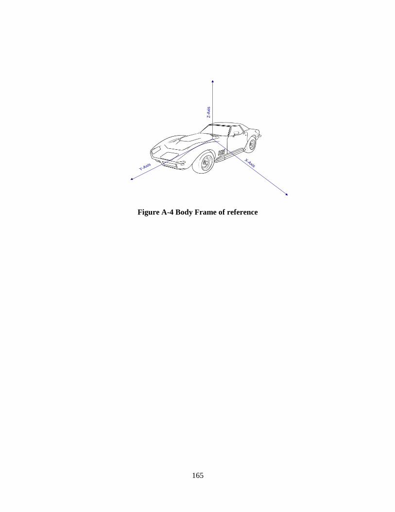
165
X-Axis
Z-A
xis
Y-Axis
Figure A-4 Body Frame of reference
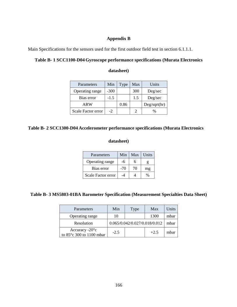
166
Appendix B
Main Specifications for the sensors used for the first outdoor field test in section 6.1.1.1.
Table B- 1 SCC1100-D04 Gyroscope performance specifications (Murata Electronics
datasheet)
Parameters Min Type Max Units
Operating range -300 300 Deg/sec
Bias error -1.5 1.5 Deg/sec
ARW 0.86 Deg/sqrt(hr)
Scale Factor error -2 2 %
Table B- 2 SCC1300-D04 Accelerometer performance specifications (Murata Electronics
datasheet)
Parameters Min Max Units
Operating range -6 6 g
Bias error -70 70 mg
Scale Factor error -4 4 %
Table B- 3 MS5803-01BA Barometer Specification (Measurement Specialties Data Sheet)
Parameters Min Type Max Units
Operating range 10 1300 mbar
Resolution 0.065/0.042/0.027/0.018/0.012 mbar
Accuracy -20°c
to 85°c 300 to 1100 mbar -2.5 +2.5 mbar
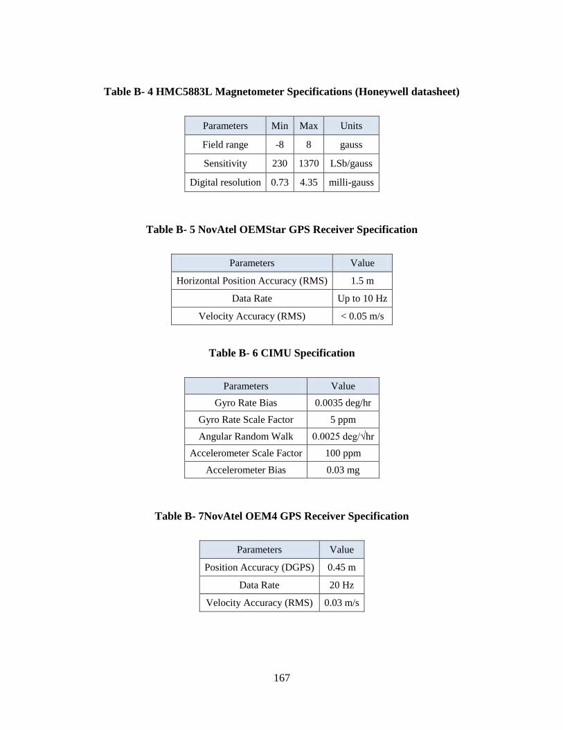
167
Table B- 4 HMC5883L Magnetometer Specifications (Honeywell datasheet)
Parameters Min Max Units
Field range -8 8 gauss
Sensitivity 230 1370 LSb/gauss
Digital resolution 0.73 4.35 milli-gauss
Table B- 5 NovAtel OEMStar GPS Receiver Specification
Parameters Value
Horizontal Position Accuracy (RMS) 1.5 m
Data Rate Up to 10 Hz
Velocity Accuracy (RMS) < 0.05 m/s
Table B- 6 CIMU Specification
Parameters Value
Gyro Rate Bias 0.0035 deg/hr
Gyro Rate Scale Factor 5 ppm
Angular Random Walk 0.0025deg/√hr
Accelerometer Scale Factor 100 ppm
Accelerometer Bias 0.03 mg
Table B- 7NovAtel OEM4 GPS Receiver Specification
Parameters Value
Position Accuracy (DGPS) 0.45 m
Data Rate 20 Hz
Velocity Accuracy (RMS) 0.03 m/s