Aucker, W. Brian. "Hodge and Warfield on Evolution." Presbyterion 20.2 (1994) 131-42.
Upload
khangminh22Category
view
0download
0
574
NN
T:2
021I
PPA
X07
3
Theorie de Hodge tropicale etapplications
These de doctorat de l’Institut Polytechnique de Parispreparee a l’Ecole polytechnique
Ecole doctorale n574 Ecole Doctorale de Mathematiques Hadamard (EDMH)Specialite de doctorat : Mathematiques fondamentales
These presentee et soutenue a Palaiseau, le 16 novembre 2021, par
MATTHIEU PIQUEREZ
Composition du Jury :
Sebastien BoucksomDirecteur de recherche, Ecole polytechnique (CMLS) President
June HuhProfesseur, Princeton University (Department of Mathematics) Rapporteur
Ilia ItenbergProfesseur, Sorbonne Universite (IMJ-PRG) Rapporteur
Johannes NicaiseProfesseur, Imperial College London (Department of Mathematics) Examinateur
Vincent PilaudCharge de recherche, Ecole polytechnique (LIX) Examinateur
Kris ShawProfesseur associee, University of Oslo (Department ofMathematics) Examinatrice
Tony Yue YuProfesseur, California Institute of Technology (PMA) Examinateur
Omid AminiCharge de recherche, Ecole polytechnique (CMLS) Directeur de these


Remerciements
En tout premier lieu, je tiens à remercier mon directeur de thèse, Omid Amini. Cette thèsen’aurait pu voir le jour sans sa disponibilité, sa patience et sa gentillesse apparemment sanslimite. Si j’ai bien appris une chose grâce à lui, c’est que même les tâches qui semblent les plusdifficiles peuvent être entreprises, et le résultat dépasse souvent nos espérances. J’espère quecette thèse marque le début d’une longue et fructueuse collaboration.
Je souhaite ensuite remercier June Huh et Ilia Itenberg pour m’avoir fait l’honneur derapporter ma thèse, ainsi que Sébastien Boucksom, Johannes Nicaise, Vincent Pilaud, KrisShaw et Tony Yue Yu pour avoir accepté de faire partie de mon jury.
Je remercie également le personnel et les membres du CMLS et du DMA, et plus généra-lement de Polytechnique et de l’ÉNS, pour leur accueil chaleureux et leur efficacité à réglertoute sorte de problèmes.
Merci également à tous les membres de la communauté mathématique avec qui j’ai pudiscuter ou qui ont organisé ou participé aux différentes conférences auxquelles j’ai pu assister.
Enfin, je remercie tous ceux qui m’ont soutenu de près ou de loin pendant ma thèse, enparticulier ma famille qui m’a littéralement soutenu de très près pendant ces quelques moisde confinement.
5

Préface
Version française
L’objet principal de cette thèse est d’établir une théorie de Hodge pour les variétés tro-picales. Cette théorie tire toute sa richesse de ses nombreuses interactions avec différentsdomaines des mathématiques allant de la géométrie complexe ou tropicale à la théorie deHodge asymptotique en passant par la théorie quantique des champs et la combinatoire despolytopes, des complexes simpliciaux et des matroïdes. Tous ces domaines apportent des intui-tions sur les objets et les phénomènes apparaissant dans la théorie développée, et, en retour,cette dernière offre de nombreuses perspectives d’applications.
Depuis une vingtaine d’année, la géométrie tropicale s’est révélée être une théorie trèsféconde en apportant une nouvelle façon d’aborder des problèmes difficiles en mathématiques.En première approximation, elle permet de faire de la géométrie algébrique sur des espaceslinéaires par morceaux, sur lesquels on peut plus facilement faire des calculs et utiliser desméthodes combinatoires. L’objectif est en général d’en déduire des résultats en géométrieclassique, souvent en géométrie réelle ou complexe. Par exemple, plusieurs résultats montrentque les courbes tropicales sont très similaires aux surfaces de Riemann, et la géométrie tropicalepermet de mieux comprendre la dégénérescence de ces surfaces [BN07,GK08,MZ08,Cop16,CV10,AB15,CDPR12b,BJ16,ABBF16,AN20].
Dans cette thèse, nous nous intéressons plutôt aux variétés tropicales de dimensions quel-conques. Ces dernières apparaissent notamment en tant que limites de familles de variétéscomplexes qui dégénèrent. Plusieurs indices laissent penser que, comme pour le cas de ladimension un, les variétés tropicales devraient encoder beaucoup d’information sur ces dégé-nérescences. Les résultats que nous obtenons vont dans ce sens, l’analogie entre une variététropicale et une famille de variétés complexes étant sous-jacente à une grande partie de nostravaux.
Récemment, dans l’objectif de mieux comprendre cette interaction entre une dégénéres-cence d’une famille de variétés complexes et sa limite tropicale, Itenberg, Katzarkov, Mikhalkinet Zharkov ont introduit une homologie tropicale dans [IKMZ19]. Cette homologie et la co-homologie associée se sont révélées très riches et avoir de nombreuses applications [JSS19,MZ14, JRS18,GS19b,GS19a,AB14,ARS19,Aks19,AP20b,Mik20a,AP20c,AP21].À bien des égards, la cohomologie d’une variété tropicale ressemble à celle d’une variété com-plexe. Une théorie très importante en géométrie complexe est la théorie de Hodge qui montretoute la richesse de la structure cohomologique des variétés complexes et dont les applicationssont innombrables. Dans cette thèse, nous parvenons à établir une théorie de Hodge tropi-cale. Nous obtenons ainsi une bien meilleure compréhension de la cohomologie d’une variététropicale. Cela ouvre de nombreuses perspectives pour l’étude des dégénérescences de variétéscomplexes, ce qui forme la majeure partie des applications que nous envisageons pour notrethéorie.
Comme nous l’avons dit, un des intérêts de la géométrie tropicale est que l’on peut uti-liser des outils combinatoires. Ainsi, pour établir notre théorie, nous nous inspirons des mé-thodes développées en théorie de Hodge combinatoire. Cette théorie et celles qui lui sontassociées ont permis de résoudre des conjectures importantes en combinatoire des complexes
7
8 PRÉFACE
simpliciaux, des matroïdes, etc., avec les travaux précurseurs de Stanley [Sta80], ou des tra-vaux plus récents [McM93,Kar04,AHK18,Adi18,BHM`20a,BHM`20b,BH19]. Cettethèse montre que certains objets combinatoires importants apparaissant dans les articles citéspeuvent être compris grâce à la cohomologie tropicale. Cela, nous donne un nouveau point devue pour mieux comprendre et dépasser certains de ces résultats.
Ainsi l’on voit se dessiner deux domaines principaux. D’une part, l’étude des dégénéres-cences de variétés complexes, et d’autre part, certains champs de la combinatoire. En ajoutantles outils de la géométrie tropicale, la théorie de Hodge tropicale crée un pont entre ces deuxdomaines et ouvre de nouvelles perspectives d’applications dans chacun d’eux, mais aussi dansd’autres sujets que nous n’avons pas encore évoqués. En plus de présenter le fondement de lathéorie de Hodge tropicale, cette thèse propose un aperçu de développements et d’applications,réelles ou potentielles, de cette théorie, dont plusieurs feront l’objets de nos futurs travaux.
Organisation de la thèse. La thèse contient cinq chapitres. Les quatre derniers sontles quatre articles écrits durant la thèse, simplement concaténés, avec quelques retouches mi-neures. Il nous a paru bon d’écrire une présentation détaillée, constituant le premier chapitre,et qui reprend l’ensemble des résultats de la thèse et les met en perspective.
Les chapitres 2, 3, 4 correspondent aux articles [AP21,AP20b,AP20c] 1. Ils ont été écritsen collaboration avec Omid Amini. Ils constituent le début d’un programme de recherche quenous menons ensembles dont le but est d’établir une théorie de Hodge tropicale et d’en déduiredifférentes applications.
Le dernier chapitre reprend et complémente un travail effectué par l’auteur de cette thèseau début de celle-ci, [Piq19b], au sujet de la géométrie de certains polynômes associés à descomplexes simpliciaux. Il s’agit en fait d’un sujet proche de la théorie de Hodge tropicale,créée a posteriori.
Décrivons brièvement ces quatre articles. Nous parlerons ensuite plus en détail du contenude la présentation détaillée qui est spécifique à cette thèse.
Homologie des éventails tropicaux. Le second chapitre étudie le cas local de la géomé-trie tropicale, c’est-à-dire le cas des éventails tropicaux. Nous y étendons la notion de lissitétropicale en allant au-delà de celle utilisée jusqu’à présent qui s’appuie sur les éventails deBergman des matroïdes. En effet, nous pensons que cette nouvelle notion sera utile dans nosfuturs travaux sur les dégénérescences de variétés complexes. Pour nous, une variété tropi-cale sera lisse si elle vérifie localement la dualité de Poincaré. La lissité tropicale a pour butde refléter le fait que la limite tropicale se souvient de nombreuses informations concernantla dégénérescence. Elle est liée à la notion de dégénérescence maximale en géométrie com-plexe, et nos travaux tendent à montrer qu’une définition purement homologique devrait êtreparticulièrement adaptée.
Nous construisons ensuite une famille d’éventails tropicaux, dits tropicalement épluchables,qui sont lisses. Celle-ci contient notamment les éventails de Bergman, montrant que notrenotion de lissité est plus générale que la précédente.
Par ailleurs, nous étudions les anneaux de Chow des éventails unimodulaires. Il s’agit d’ob-jets importants en combinatoire. Dans le chapitre 2, nous montrons que l’anneau de Chow d’unéventail est inclus dans la cohomologie tropicale de la compactification canonique de l’éven-tail. Dans le cas où l’éventail est lisse, nous obtenons un isomorphisme. Ainsi, cela fournit unenouvelle interprétation, et une généralisation, de l’article d’Adiprasito, Huh et Katz [AHK18]
1. Notons que la version de l’article [AP20b] ici présente s’appuie sur [AP21] bien qu’elle ait été rédigéeauparavant. Aussi mériterait-elle une révision pour harmoniser les notations et améliorer certaines preuves quenous comprenons désormais mieux. Cela sera fait très prochainement et l’article révisé sera disponible peuaprès la publication de cette thèse.
VERSION FRANÇAISE 9
sur l’anneau de Chow des éventails de Bergman. Les propriétés qui y sont montrées sont enfait des propriétés de la cohomologie tropicale de la compactification canonique de l’éventail.
Cette compactification canonique des éventails et des complexes polyédraux joue un rôlecentral dans tout notre travail. On peut la voir comme une généralisation d’un analoguetropical de la théorie des compactifications magnifiques de complémentaires d’arrangementsd’hyperplans introduites par De Concini et Procesi [DP95]. Par la suite, Feichtner et Yuzvinskiont montré dans [FY04] que la cohomologie de ces compactifications est calculée par l’anneaude Chow de l’éventail correspondant. Nos travaux permettent de généraliser leur résultat,notamment grâce à l’introduction d’un analogue tropical de la suite spectrale de Deligne dansle cas spécifique des éventails tropicaux lisses. Nous l’appelons la suite exacte de Delignetropicale.
Théorie de Hodge pour les variétés tropicales. Dans le troisième chapitre, nousétablissons à proprement parler la théorie de Hodge tropicale. Nous démontrons que la co-homologie tropicale d’une variété tropicale projective lisse localement kählérienne vérifie plu-sieurs propriétés de symétrie appelées propriétés kählériennes. Ces propriétés sont la dualitéde Poincaré, le théorème de Lefschetz difficile, les relations de Hodge-Riemann et la conjecturemonodromie-poids.
Ce résultat est d’abord démontré pour les éventails grâce aux outils développés dans lechapitre 2. Nous généralisons en particulier l’article [AHK18] où les auteurs établissent lespropriétés kählériennes pour les éventails de Bergman.
Nous obtenons alors le résultat global. Pour ce faire, nous nous inspirons de [IKMZ19]et introduisons un analogue tropical de la suite spectrale de Steenbrink. Nous généralisons lerésultat de [IKMZ19] au cas non approximable, résultat qui montre que cette suite spectraledégénère vers la cohomologie tropicale. Pour cela nous utilisons de nouveau la suite exacte deDeligne tropicale.
Nous nous inspirons ensuite du travail de Guillén et Navarro Aznar sur le théorème descycles invariants [GN90]. Cela nous permet de montrer que la cohomologie tropicale ainsicalculée est une structure de Hodge-Lefschetz polarisée au sens de Saito [Sai88], c’est-à-direqu’elle vérifie les propriétés kählériennes.
Notons qu’en l’absence du contexte géométrique, nous ne pouvons nous appuyer simple-ment sur les résultats préexistant. Nous devons construire des analogues tropicaux des diffé-rents objets et redémontrer les résultats directement dans le cadre tropical grâce à de nouvellestechniques de preuve. Certains des outils développés, comme l’analogue tropical des formes deKähler, jouent un rôle central dans les applications en géométrie complexe sur lesquels noustravaillons actuellement.
Une dernière étape de la preuve consiste à étendre nos résultats à toutes les variétés tro-picales concernées. Pour cela nous utilisons un théorème d’existence de bonnes triangulationsdémontré pour l’occasion, ainsi qu’un théorème de fibré projectif tropical permettant de mon-trer que, sous certaines conditions, les propriétés souhaitées sont stables lorsque l’on éclate oucontracte un diviseur tropical à l’infini.
L’opérateur eigenwave introduit dans [MZ14] par Mikhalkin et Zharkov, aussi appeléopérateur de monodromie tropical, joue un rôle central dans ce travail. Notamment nousrésolvons la conjecture monodromie-poids apparaissant dans [MZ14,Liu19] et qui énonceque l’opérateur induit un isomorphisme entre les parties de bidegrés pp, qq et pq, pq pour deuxentiers p et q.
Suite de Clemens et Schmid tropicale et existence de cycles tropicaux. Vientensuite une application de la théorie de Hodge tropicale. Dans le chapitre 4, nous résolvonsla conjecture de Hodge tropicale pour les variétés tropicales projectives lisses localement käh-lériennes admettant une triangulation rationnelle : les classes de Hodge sont exactement les

10 PRÉFACE
classes de bidegrés pp, pq dans le noyau de la monodromie. Dans [Zha20], Zharkov présenteune idée de Kontsevich selon laquelle un contre-exemple à la conjecture de Hodge tropicalepour une variété tropicale abélienne fournirait un contre-exemple à la conjecture de Hodgeclassique. Sans pour autant infirmer cette idée, notre résultat va nettement dans le sens inverse.
Pour démontrer notre théorème, nous introduisons un analogue tropical de la suite exactede Clemens et Schmid [Cle77, Sch73]. Nous obtenons ainsi un analogue du théorème descycles invariants, et la preuve consiste ensuite à construire des cycles tropicaux associés à cescycles invariants, ce que nous faisons grâce aux résultats de [AP20b].
Une généralisation des polynômes de Symanzik en dimensions supérieures.Finalement, dans le dernier chapitre, motivé par la description de l’asymptotique de l’ac-couplement de hauteur de cycles sur une famille de variétés complexes qui dégénère, nousgénéralisons les polynômes de Symanzik au cas des complexes simpliciaux et au-delà.
En dimension un, les deux polynômes de Symanzik d’un graphe métrique sont utilisés enthéorie quantique des champs pour calculer les intégrales de Feynman. Ils sont connus pouravoir de nombreuses propriétés. Il s’agit notamment de spécialisations du polynôme de Tuttemultivarié, aussi connu sous le nom de modèle de Potts en physique. Notre généralisationconserve la plupart de ses propriétés.
D’autre part, les polynômes que nous définissons sont entre autres liés à un théorème detype Kirchhoff pour les complexes simpliciaux découvert récemment [DKM09], et à d’autrestravaux sur les probabilités déterminantales et les complexes simpliciaux aléatoires [Lyo03,Lyo09].
Récemment, Amini, Bloch, Burgos Gil et Fresán ont montré dans [ABBF16] que le rap-port des deux polynômes de Symanzik sur la limite tropicale peut décrire l’asymptotique del’accouplement de hauteur de deux cycles de degré zéro sur une famille de surfaces de Riemann.Ces polynômes sont aussi reliés à la limite tropicale des mesures canoniques sur les fibres dela famille. Notre généralisation peut être vue comme une première étape pour étendre cesrésultats en dimensions supérieures.
En particulier, nous généralisons un théorème de stabilité sur le rapport des deux poly-nômes de Symanzik vis-à-vis d’une variation bornée de la géométrie du complexe simplicial.Un cas particulier de ce théorème en dimension un est étudié dans [Ami19] pour apporter unenouvelle preuve des résultats de [ABBF16]. Ce phénomène de stabilité doit par ailleurs êtrelié aux théorèmes de l’orbite SL2 et de l’orbite nilpotente en théorie de Hodge asymptotique.
Pour démontrer le théorème de stabilité, nous fournissons une description complète dugraphe d’échange des paires d’indépendants d’un matroïde. Ce résultat est par exemple lié àune conjecture de White [Whi80] et pourrait avoir un intérêt en soi.
Présentation détaillée. Le premier chapitre, écrit en français, est spécifique à cettethèse et vise plusieurs objectifs.
Tout d’abord, il s’agit d’une présentation détaillée de l’ensemble des quatres articles. Il estconçu pour pouvoir être lu indépendamment, bien que nous renvoyons régulièrement aux autreschapitres pour les détails. Nous y esquissons tout de même une sélection de démonstrationsqui nous ont paru particulièrement dignes d’intérêt.
Au fur et à mesure de l’élaboration des quatre articles, des liens avec d’autres théorieset des application potentielles sont apparus. Notre travail est par exemple lié à la conjecturede Hodge tropicale ou à la théorie de Hodge asymptotique. De manière plus intéressante,nous mettons en lumière des liens étroits, jusqu’alors apparemment passés inaperçus, entrele programme que nous développons en théorie de Hodge tropicale et les travaux menés parexemple par Adiprasito et Huh en théorie de Hodge combinatoire. Cette connexion pourraitpermettre de mieux comprendre voir de dépasser certains travaux dans ce domaine.
VERSION FRANÇAISE 11
Un second objectif de la présentation détaillée est d’expliciter tous ces liens entretenusavec la combinatoire mais aussi avec les autres théories mentionnées. Nous ne présenterons pastoujours ces dernières de manière précise, soit parce qu’une telle présentation nous emmèneraittrop loin de notre sujet, soit parfois parce que l’auteur de cette thèse ne maîtrise pas forcémentsuffisamment bien ces différentes théories. Dans ces cas-là, notre but est plutôt de donner uneintuition quitte à perdre en rigueur. Nous espérons que cette simplification de certains conceptspourra être utile à des lecteurs peu familier des thèmes présentés pour mieux comprendre oudécouvrir de nouvelles notions.
Pour expliciter certains de ces liens, des généralisations attendues de notre travail sontnécessaires. C’est pourquoi nous proposons un cadre suffisamment général pour donner unsens précis à ces relations et à certaines questions associées. En plus de généraliser plusieursthéorèmes et d’obtenir une meilleure compréhension des précédents travaux, nous obtenonsaussi quelques résultats originaux intéressants. Un aperçu de ces nouvelles contributions estdonné ci-dessous. Pour ne pas trop alourdir la présentation, les preuves de ces résultats sontsimplement esquissées. Si notre cadre généralisé permet en effet d’obtenir les applicationsenvisagées, ces démonstrations seront de toute façon complètement rédigées dans de futursarticles.
Par ailleurs il se trouve que le cadre dans lequel nous travaillons permet de simplifiersignificativement certaines preuves, notamment parmi celles utilisées dans la présente versionde [AP20b]. Ces nouvelles idées apparaîtront dans une future version de l’article.
Décrivons les principales nouveautés de la présentation détaillée par rapport aux articles.
Liens avec la combinatoire des complexes simpliciaux. Dans le chapitre 1, noustravaillons avec des structures simpliciales affines, objets créés pour l’occasion, qui sont descomplexes simpliciaux abstraits munis localement d’une structure affine semblable à celleprésente sur les variétés tropicales triangulées. Ces structures ne sont pas forcément localementplongeables dans Rn car deux faces peuvent se superposer, par exemple si la restriction desfonctions affines à ces deux faces coïncident.
Un des avantages de cette description est de pouvoir généraliser un théorème de l’ar-ticle [AP21] aux complexes simpliciaux abstraits. Dans cet article, nous montrons que l’an-neau de Chow d’un éventail Σ est isomorphe à la cohomologie tropicale de la compactificationcanonique de Σ restreinte aux parties de bidegrés pp, pq pour 0 ď p ď dimpΣq.
Plus généralement, si ∆ est un complexe simplicial de dimension d, on peut regarder l’an-neau de Stanley-Reisner SR‚p∆q et choisir d éléments suffisamment génériques dans SR1p∆q.Le quotient de SR1p∆q par l’idéal Θ engendré par ces d éléments est l’analogue de l’anneaude Chow pour l’éventail conep∆q induit par ∆. On le note A‚p∆q. Par exemple cet anneauvérifie la dualité de Poincaré si ∆ est une sphère simpliciale.
Les d éléments engendrant Θ induisent une structure simpliciale linéaire naturelle surconep∆q. Notons la Σ. Nous montrons que
App∆q » Hp,ppΣq,
où le membre de droite est la cohomologie tropicale de la compactification canonique de Σ.Ce résultat pourrait permettre d’introduire des outils cohomologiques ou faisceautiques pourétudier A‚p∆q. Par exemple, l’isomorphisme ci-dessus permet de redémontrer la dualité dePoincaré pour App∆q lorsque ∆ est une sphère simpliciale.
Nous montrons aussi que le complexe de partition utilisé par Adiprasito dans [Adi18] pourdémontrer la g-conjecture pour les sphères simpliciales correspond à ce que nous appelons lasuite exacte de Deligne tropicale, que nous utilisons de manière cruciale à plusieurs reprisesdans nos travaux. Peut-être que ce lien permettra dans le futur d’apporter un nouveau pointde vue voire de dépasser le travail d’Adiprasito.
12 PRÉFACE
Structures simpliciale rationnelles. Dans [AP20b] nous travaillons avec des com-plexes simpliciaux unimodulaires. Or l’unimodularité est une condition qui n’est pas toujoursfacile à conserver. Nous avons ainsi besoin de théorèmes combinatoires relativement difficilesà démontrer. Cette condition d’unimodularité est très importante lorsque l’on travaille à co-efficients entiers, comme on peut le constater dans [AP21]. Mais pour le cas rationnel, onpeut en fait se passer de cette condition d’unimodularité et travailler directement avec descomplexes simpliciaux rationnels quelconques, ou bien des structures simpliciales rationnelles.Cela permet de simplifier considérablement certaines preuves comme nous le verrons dans lechapitre 1.
Par ailleurs, nos preuves s’appuient systématiquement sur des triangulations. Comme lacohomologie est indépendante de la triangulation choisie sur la variété tropicale, il devraitêtre possible de travailler directement avec la variété sans choisir de triangulation. Néanmoinsnous ignorons comment faire pour le moment. Cela entraîne une certaine limite à nos résul-tats car certaines variétés tropicales rationnelles n’admettent pas de triangulation rationnelle.Notamment notre travail sur la conjecture de Hodge tropicale [AP20c] ne s’applique pas àces variétés. Pour tenter de pallier à cette limite, nous définissons les structures simplicialesfaiblement rationnelles qui semblent bien adaptées à ce problème. Nous autorisons des facesrationnelles et d’autres non rationnelles à coexister. On peut par exemple définir les classesde Hodge rationnelles dans ce contexte et ainsi poser précisément la conjecture de Hodgetropicale. Notamment, nous présentons l’intérêt de cette définition pour étudier les variétésabéliennes tropicales, ce qui nous permet d’inclure le problème posé par Kontsevich et Zharkovdans [Zha20] dans notre théorie.
English version
The main objective of this thesis is to establish a Hodge theory for tropical varieties.The power of this theory comes from its numerous interactions with various other fields ofmathematics: with algebraic, tropical, and complex geometry, with algebraic topology, withasymptotic Hodge theory, but also with quantum field theory or the combinatorics of simplicialcomplexes, polytopes and matroids. These classical subjects provide a guiding intuition andprinciples on the objects and the phenomena that appear in the theory we wish to develop.As a counterpart, our theory leads to many perspectives of applications.
For two decades, tropical geometry has established itself as a very productive theory whichprovides a new approach towards difficult until now resisting problems in mathematics, in dif-ferent branches. At a first glance, it is a way to do algebraic geometry on piecewise linearspaces, on which one can more easily do some computations or use powerful combinatorialmethods. Usually, the primary goal is to deduce some results in classical geometry, for in-stance in real or complex geometry. For example, many results show that tropical curvesare very similar to Riemann surfaces, and tropical geometry leads to a better understandingof degenerations of these surfaces [BN07,GK08,MZ08,Cop16,CV10,AB15,CDPR12b,BJ16,ABBF16,AN20].
In this thesis, we are interested in tropical varieties of any dimension. They appear, forinstance, as tropical limits of degenerating families of complex varieties. Several evidenceslet us think that, as in dimension one, tropical varieties should encode much data about thedegenerations. The results we obtain provide new evidences: the analogy between tropicalvarieties and family of complex varieties underlies a large part of our work.
Recently, in order to better understand the interactions between a family of complex va-rieties and its tropical limit, Itenberg, Katzarkov, Mikhalkin et Zharkov introduced a tropicalhomology [IKMZ19]. This homology and the corresponding cohomology have been alreadystudied a lot and have led to many applications [JSS19,MZ14, JRS18,GS19b,GS19a,
ENGLISH VERSION 13
AB14,ARS19,Aks19,AP20b,Mik20a,AP20c,AP21]. The cohomology of a tropical va-riety mimics that of a complex variety. A theory of great importance in complex geometry isHodge theory. It shows numerous interesting properties of cohomologies of complex varieties,and over the decades it has plenty of applications. In this thesis, we achieve to establish atropical Hodge theory, that is a Hodge theory for tropical varieties. This leads to a betterunderstanding of the cohomology of tropical varieties, and opens up diverse perspectives inthe study of degenerations of complex varieties, which are the main applications we have inmind for the development of our theory.
One of the interesting features of tropical geometry is that one can use combinatorial tools.In particular, in our work, we use ideas coming from combinatorial Hodge theory. This theoryhas been used to overcome important conjectures concerning the combinatorics of simplicialcomplexes, matroids, etc. We can cite in particular the pioneering work of Stanley [Sta80],or more recent works as [McM93,Kar04,AHK18,Adi18,BHM`20a,BHM`20b,BH19].This thesis shows that some combinatorial objects at the heart of these recent papers couldbe computed thanks to tropical cohomology. We thus get a new point of view and a bridge toclassical Hodge theory that should lead to a better understanding or generalizations of someof these results.
We can therefore see two main underlying topics. On the one hand, the study of degenera-tions of complex varieties. And on the other hand some parts of combinatorics. With the helpof tools coming from tropical geometry, tropical Hodge theory brings a bridge between thesetwo fields, opening new perspectives of applications to both, and also to other domains wedid not mention yet. Apart from presenting foundations of tropical Hodge theory, this thesisgives an overview of some developments and some applications, either potential or concrete,of our theory. Several of them will be part of our future work.
Organization of the thesis. This thesis consists of five chapters. The last four chaptersare actually four concatenated papers, which were written during the thesis, with a few minormodifications. Moreover, we wrote a detailed presentation in French as a first chapter. Itpresents the different results of the thesis and highlights the links they maintain with othersubjects in mathematics.
Chapters 2, 3 and 4 correspond to the papers [AP21,AP20b,AP20c] 2. These are jointworks with Omid Amini and they are part of our program aiming to establish a tropical Hodgetheory and to deduce diverse applications.
The last chapter takes up, and complements by adding some new materials, a work done atthe beginning of the thesis [Piq19b] on geometry of polynomials associated to combinatorialstructures. It is in fact about a subject having many relations with tropical Hodge theory,which was developed later.
In the rest of this introduction, we give brief overview of the four articles. Then we willdescribe in more details the content of the first chapter.
Homology of tropical fans. The second chapter studies the local case of tropical geom-etry, namely that of tropical fans. We extend the notion of tropical smoothness beyond the onethat is currently in use in tropical geometry, which is based on matroids and their Bergmanfans. We believe that this new notion will be useful in our future work about degenerationsof complex varieties. In our work, a tropical variety is smooth if it verifies Poincaré dualitylocally. Tropical smoothness aims to reflect the intuitive idea that the tropical limit recalls as
2. The current version of [AP20b] is based on [AP21] though it was written before. That is why it woulddeserve further revision in order to harmonize the notations and to improve some of the proofs that we nowunderstand better. This will be done soon, and the revised article should appear just after the publication ofthis thesis.
14 PRÉFACE
much as possible data about the degeneration. This is linked to the notion of maximal degen-eracy in complex geometry, and our work tends to show that a purely homological definitionsuits for our purpose.
We then build a family of tropical fans, called tropically shellable, which are smooth.Among them one can find Bergman fans. Hence our notion of smoothness generalizes theprevious one.
Furthermore, we study the Chow rings of unimodular fans. These rings are important forinstance because of their applications in combinatorics. In Chapter 2, we show that the Chowring of a fan is included in the tropical cohomology of the canonical compactification of thefan. If the fan is smooth, we even get an isomorphism. This leads to a new interpretation anda generalization of the work of Adiprasito, Huh and Katz in [AHK18] about Chow rings ofBergman fans. The results of that article are in fact properties of the tropical cohomology ofthe canonical compactifications of fans.
Canonical compactifications of fans and polyhedral complexes play a fundamental role inour whole work. One can consider them as a generalization of a tropical analog of the theoryof wonderful compactifications, for example that of hyperplane arrangements complements inthe torus introduced by De Concini and Procesi in [DP95]. Later, Feichtner and Yuzvinskiproved in [FY04] that the cohomology of these compactifications in the case of hyperplanearrangements can be computed thanks to the Chow ring of the corresponding fans. Our workgeneralizes their results. To do so, we introduce the tropical Deligne exact sequence for smoothtropical fans, which is the tropical analog of the Deligne spectral sequence in this specific case.
Hodge theory for tropical varieties. In the third chapter, we establish tropical Hodgetheory. More precisely, we prove that a smooth projective tropical variety that is locallyKähler verifies the Kähler package. Namely, it verifies the Poincaré duality, the hard Lefschetztheorem, the Hodge-Riemann bilinear relations and the monodromy-weight conjecture.
We first prove the result for fans thanks to the tools developed in Chapter 2. In particular,we generalize, by providing a new proof, of the work of Adiprasito-Huh-Katz [AHK18] inwhich the authors prove the Kähler package for Bergman fans.
To obtain the global result, we build on [IKMZ19] and introduce an tropical analogof the Steenbrink spectral sequence. Then we generalize a result of [IKMZ19] to tropicalvarieties that are not approximable: we show that the spectral sequence computes the tropicalcohomology. Once again, we use the tropical Deligne exact sequence.
Then, we look at the work of Guillén and Navarro Aznar about invariant cycles theo-rem [GN90]. We are able to prove that the tropical cohomology computed by the Steenbrinkspectral sequence is a polarized Hodge-Lefschetz structure in the sense of Saito [Sai88], i.e.,it verifies the Kähler package.
We note that without the geometric context in background, we cannot simply rely onpreexisting results. We have to construct tropical analogs of the different objects and to doagain the whole proof directly in the tropical world thanks to new technics of proof. Someof the tools developed, like the tropical analog of Kähler forms, play a central role in theapplications of the results in complex geometry we are currently investigating.
The last step is to extend the theorem to all the suitable tropical varieties. This is donethanks to theorems that state the existence of good triangulations on these varieties, and toa tropical projective bundle formula which prove that, under some good assumptions, theKähler package is preserved when we perform blow-ups or blow-downs on a tropical divisorat infinity.
The eigenwave operator introduced in [MZ14] by Mikhalkin and Zharkov, also calledthe tropical monodromy operator, plays a major role in our work. In particular we solvethe monodromy-weight conjecture which appears in [MZ14,Liu19] and which states that
ENGLISH VERSION 15
the operator induces an isomorphism between the parts of bidegree pp, qq and pq, pq for anyintegers p and q.
Tropical Clemens-Schmid sequence and existence of tropical cycles. Chapter 4is about an application of tropical Hodge theory. We solve the tropical Hodge conjecturefor smooth projective tropical varieties that are locally Kähler and that admit a rationaltriangulation. More precisely, we prove that the Hodge classes are exactly the classes ofbidegree pp, pq that are in the kernel of the monodromy. In [Zha20], Zharkov presents an ideaof Kontsevich, according to which any counter-example of the tropical Hodge conjecture for anabelian tropical variety would give a counter-example for the classical Hodge conjecture. Ourtheorem goes into the opposite direction, even if it does not invalidate the idea of Kontsevich.
In order to prove the theorem, we introduce a tropical analog of the Clemens-Schmid exactsequence [Cle77,Sch73]. Hence we obtain an analog of the invariant cycle theorem. Thenthe proof consists in constructing a tropical cycle associated to these invariant cycles. Weachieve to do this thanks to the results of [AP20b].
A multidimensional generalization of Symanzik polynomials. Finally, in the lastchapter, motivated by describing the asymptotic of height pairing between cycles on degen-erating families of complex varieties, we provide a generalization of Symanzik polynomials tosimplicial complexes and beyond.
In dimension one, the two Symanzik polynomials of a metric graph are used in quantumfield theory to compute Feynman integrals. Both polynomials have many known properties.In particular, they are some specializations of the multivariate Tutte polynomial, also knownas Potts model in physics. Most of these properties remain true for our generalization.
Besides, the polynomials we defined are linked to a Kirchhoff matrix-tree theorem onsimplicial complexes that has been discovered recently [DKM09], and to other works ondeterminantal probabilities and random simplicial complexes [Lyo03,Lyo09].
Recently, Amini, Bloch, Burgos Gil and Fresán proved that the ratio of the two Symanzikpolynomials on the tropical limit of a family of Riemann surfaces can describe the asymptoticof the height pairing between two degree zero divisors. The polynomials are also linked to thetropical limit of canonical measures on the fibers of the family. Our generalization could beregarded a first step to higher dimensional extensions of these results.
In particular, we prove a somehow surprising stability theorem for the ratio of the twopolynomials under some bounded variations of the geometry of the simplical complex. A one-dimensional specific case of this theorem is studied in [Ami19] in order to give a new proof ofthe results in [ABBF16]. This stability phenomenon should also have links to the nilpotentand SL2 orbit theorems in asymptotic Hodge theory.
In the course of the proof of the stability theorem, we provide a complete description ofthe exchange graph of pair of independent sets of a general matroid. This result is linked toa conjecture of White [Whi80] and might be of independent interest.
Detailed presentation. The first chapter, written in French, is specific to this thesisand has several objectives.
First, it is a detailed presentation of the four papers. It can be read on its own, thoughwe often refer to the papers for the details. Nevertheless, we occasionally sketch some notableproofs.
While we were working on the four papers, some connections to other theories and po-tential applications appeared. For example it is linked to the tropical Hodge conjecture orto asymptotic Hodge theory. More interestingly, we highlight some strong links, which hasapparently not been noticed yet, between our program about tropical Hodge theory and theworks undertaken, for instance, by Adiprasito and Huh in combinatorial Hodge theory. These
16 PRÉFACE
connections might give a better understanding or even a generalization of some works in thisdomain.
The second objective of this detailed presentation is to make explicit the connections withcombinatorics and with the other theories mentioned above. We do not always present thesetheories in detail, either because it would take us too far away from our present subject, orbecause the author of this thesis does not have enough understanding of those theories yet.In these cases, our goal is more to give a general idea of the theories even if the presentationis not entirely rigorous. We hope that these simplifications of some concepts will be useful tothe readers who are not familiar with these topics, and will help them to better understandor to discover new concepts.
In order to present some of those links, some generalizations of our work are necessary.That is why establishing a sufficiently general framework was necessary to give a precisemeaning to some of the connections and to associated questions. We do not only generalizeseveral theorems but we also obtain some new and interesting results. An overview of theseresults could be found below. To not make the presentation too technical, we only sketch theproof of the results. Anyway, if our generalized framework would actually allow us to get someof the applications, those proofs would be fully given in future papers.
Moreover, the framework we are working with makes some of the previous proofs muchsimpler, especially among those of [AP20b]. The new ideas might be given in a future versionof this paper.
Let us describe the main additions of the detailed presentation compared to the otherchapters.
Links to the combinatorics of simplicial complexes. In chapter 1, we work withaffine simplicial structures. These are abstract simplicial complexes endowed with an affinestructure similar to those that we find on the triangulable tropical varieties. These structurescannot necessarily be embedded in Rn because two faces might overlap. For example thatmight happen if the restrictions of affine forms to two different faces coincide.
One of the benefits of this description is that we can generalize one of the theoremsof [AP21] to abstract simplicial complexes. In this paper, we show that the Chow ring of afan Σ is isomorphic to the tropical cohomology of the canonical compactification of Σ restrictedto the parts of bidegree pp, pq for 0 ď p ď dimpΣq.
More generally, if ∆ is a simplicial complex of dimension d, we can consider the Stanley-Reisner ring SR‚p∆q and choose d sufficiently generic elements in SR1p∆q. Let Θ be the idealgenerated by these elements. The quotient of SR1p∆q by Θ is the analogous of the Chow ringfor the fan conep∆q induced by ∆. We denote it by A‚p∆q. For example this ring verifies thePoincaré duality if ∆ is a simplicial sphere.
The d elements generating Θ induce a natural linear simplicial structure on conep∆q. Wedenote it by Σ. We prove that
App∆q » Hp,ppΣq,
where the right hand-side member is the cohomology of the canonical compactification of Σ.This result might let one use cohomological tools or sheaf theory to study A‚p∆q. For instance,thanks to the above isomorphism, we can give a new proof of the Poincaré duality for App∆qwhen ∆ is a simplicial sphere.
We also prove that the partition complex used by Adiprasito in [Adi18] to prove theg-conjecture for simplicial spheres corresponds to what we call the tropical Deligne exactsequence that we use in a critical way throughout our series of work discussed above. Thisconnection might lead to a new point of view and a better understanding of the work ofAdiprasito.
ENGLISH VERSION 17
Rational simplicial structures. In [AP20b] we work with unimodular simplicial com-plexes. But the unimodularity condition is not always easy to preserve. Hence we need somecombinatorial theorems rather hard to prove. This unimodularity condition is very importantwhen we work with integral coefficients, as we can see in [AP21]. But in the rational case, wedo not need this unimodularity condition anymore and we can directly work with any rationalsimplicial complex, or with rational simplicial structures. This allows to simplify considerablysome of the proofs, as we will see this in Chapter 1.
Moreover, our proofs in [AP20b,AP20c] are systematically based on triangulations. Asthe cohomology is independent of the chosen triangulation on the tropical variety, it should bepossible to work directly without choosing any triangulation. Nevertheless, we do not knowyet how to do this. This puts some limitations on our results because some rational tropicalvarieties do not admit any rational triangulation. In particular, our work on the tropicalHodge conjecture does not apply to these varieties. In order to overcome this limitation, wedefine weakly rational simplicial structures that seem well fitted to this problem. We allowsome rational and non-rational faces to coexist. In this context we can for instance define therational Hodge classes and therefore state precisely the tropical Hodge conjecture. We willpresent the utility of such a definition for abelian tropical varieties. This allows us to includethe problem stated by Kontsevich and Zharkov in [Zha20] in our theory.


Contents
Remerciements 5
Préface 7Version française 7English version 12
Chapitre 1. Présentation détaillée du travail de thèse 211. Rappels de géométrie tropicale 212. Structures simpliciales 363. Cohomologie tropicale, dualité de Poincaré et lissité 444. Comparaison de H‚,‚pΣq, H‚,‚c pΣq et H‚,‚pΣq 535. Théorie de Hodge combinatoire et anneau de Chow d’un éventail 616. Théorie de Hodge pour les structures simpliciales linéaires 717. Théorie de Hodge pour les structures simpliciales affines 888. Conjecture de Hodge pour les structures simpliciales kählériennes fortement
rationnelles 1059. Comparaison des compactifications des sous-variétés du tore complexe et du tore
tropical 11010. Une généralisation des polynômes de Symanzik 112
Chapter 2. Homology of tropical fans 1191. Introduction 1192. Preliminaries 1283. Smoothness in tropical geometry 1344. Tropical divisors 1405. Tropical shellability 1446. Chow rings of tropical fans 1577. Hodge isomorphism for unimodular fans 1698. Tropical Deligne resolution 1789. Compactifications of complements of hyperplane arrangements 18110. Homology of tropical modifications and shellability of smoothness 18411. Examples and further questions 189
Chapter 3. Hodge theory for tropical varieties 1931. Introduction 1932. Tropical varieties 2073. Local Hodge-Riemann and Hard Lefschetz 2184. Quasi-projective unimodular triangulations of polyhedral complexes 2345. Tropical Steenbrink spectral sequence 2446. Kähler tropical varieties 2697. Hodge-Lefschetz structures 2808. Projective bundle theorem 2909. Proof of Theorem 1.7 296Appendix 299
19

20 CONTENTS
10. Spectral resolution of the tropical complex 29911. Tropical monodromy 311
Chapter 4. Tropical Clemens-Schmid sequence and existence of tropical cycles with agiven cohomology class 313
1. Introduction and statement of the main theorem 3132. Preliminaries on tropical varieties 3153. Minkowski weights and tropical cycles 3244. Integral tropical Hodge conjecture in the local case 3255. Tropical Steenbrink double complex and the comparison theorem 3276. Tropical surviving and relative cohomology groups 3337. Tropical Clemens-Schmid sequence 3358. Existence of cycles with a given Hodge class: proof of Theorem 1.1 3399. Proof of Theorem 1.3 340
Chapter 5. A multidimensional generalization of Symanzik polynomials 3431. Introduction 3432. Kirchhoff and Symanzik polynomials and duality 3523. Symanzik polynomials on simplicial complexes 3614. Generalization to matroids over hyperfields 3745. Exchange graph for matroids 3826. Variation of Symanzik rational fractions 387
Bibliography 397
Chapitre 1
Présentation détaillée du travail de thèse
1. Rappels de géométrie tropicale
L’objet principal de cette thèse est de développer une théorie de Hodge tropicale. À uneexception près, voir section 9, les résultats de cette thèse, bien qu’analogue à des résultatsde la géométrie classique, sont inhérents au monde tropical dans le sens où ils peuvent êtreétablis indépendamment de la géométrie classique. Toutefois nous discuterons abondammentde l’interprétation géométrique de nos résultats et des applications potentielles de ceux-ci,par exemple en liant avec la théorie de Hodge classique ou asymptotique, avec la géométrietorique mais aussi avec d’autres domaines notamment en combinatoire. La présente sectionexpose entre autre certains objets qui ne sont pas formellement utiles pour nos résultats maisqui sont liés à ces applications. Plusieurs d’entres elles feront d’ailleurs l’objet de nos futurstravaux, et nous présentons dors et déjà certains résultats partiels et certaines idées dans cettethèse.
À dire vrai, dans ce chapitre nous ne travaillerons pas avec des variétés tropicales maisavec des objets que nous appelons structures simpliciales et qui sont façonnés spécifiquementpour pouvoir appliquer notre théorie à certains domaines. Ces objets se comportent globale-ment comme les variétés tropicales mais sont plus abstraits. Afin d’avoir une bonne intuitiondu comportement de ces structures simpliciales, il est bien de connaître les objets que nousgénéralisons. Cette section est là pour cela. Nous y définissons des objets dont nous reparle-rons régulièrement dans la suite, le plus souvent comme des exemples d’application de notrethéorie généralisée.
Ainsi, pour les lecteurs non familiers du sujet, nous faisons ici quelques rappels sur lagéométrie tropicale, sur les variétés tropicales, mais aussi sur les éventails de Bergman d’unmatroïde et sur les dégénérescences de familles de variétés complexes, sur leurs limites tropi-cales et sur les liens entre les deux. Ceci dit, en particulier concernant la géométrie tropicale,ce court chapitre ne peut valoir la lecture de l’une ou l’autre des nombreuses introductions dusujet disponibles dans la littérature [BIMS15,Mik06,RGST05,MS15,MR09, IMS09].
Conventions et notations. Dans toute cette thèse, nous désignerons par N l’ensembledes entiers strictement positifs, et par R`, resp. R´, les nombre réels positifs ou nuls, resp.négatifs ou nuls. Si n P N, la notation rns désigne l’ensemble t1, 2, . . . , nu.
Si E est un ensemble et si e P E, nous noterons parfois E ´ e l’ensemble E r teu. Si e estun élément qui n’est pas dans E, nous noterons parfois E ` e l’ensemble E Y teu.
Nous aurons souvent affaire à un ensemble ordonné de faces, pX,ăq. Pour les objets indexéspar les faces δ, nous utilisons δ en indice pour les objets liés à l’espace tangent de δ, par exempleCδ, et δ en exposant pour les objets liés au quotient par l’espace tangent de δ, par exempleCδ. Si γ ă δ est une autre face, nous aurons en général des applications de Cγ dans Cδ, oude Cγ dans Cδ, que nous noterons avec l’indice γ ă δ, par exemple iγăδ, ou des applicationsdans l’autre sens, et nous utiliserons alors l’indice δ ą γ, par exemple i˚δąγ . Si l’on préfère,on peut voir la description ci-dessus comme des notations pour des foncteurs covariants oucontravariants de domaine la catégorie induite par pX,ăq.
Si E est un ensemble et k un corps, on note kE :“À
ePE ke l’espace vectoriel sur k dedimension cardpEq engendré par les éléments de e.
21
22 1. PRÉSENTATION DÉTAILLÉE DU TRAVAIL DE THÈSE
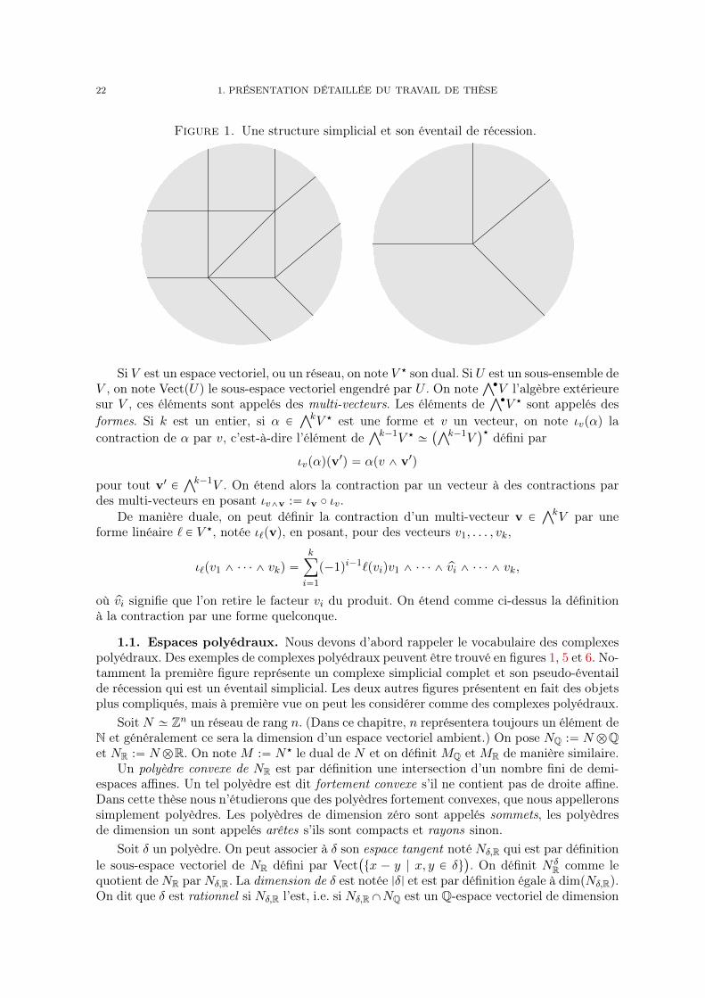
Figure 1. Une structure simplicial et son éventail de récession.
Si V est un espace vectoriel, ou un réseau, on note V ‹ son dual. Si U est un sous-ensemble deV , on note VectpUq le sous-espace vectoriel engendré par U . On note
Ź‚V l’algèbre extérieuresur V , ces éléments sont appelés des multi-vecteurs. Les éléments de
Ź‚V ‹ sont appelés desformes. Si k est un entier, si α P
ŹkV ‹ est une forme et v un vecteur, on note ιvpαq lacontraction de α par v, c’est-à-dire l’élément de
Źk´1V ‹ »`Źk´1V
˘‹ défini par
ιvpαqpv1q “ αpv ^ v1q
pour tout v1 PŹk´1V . On étend alors la contraction par un vecteur à des contractions par
des multi-vecteurs en posant ιv^v :“ ιv ˝ ιv.De manière duale, on peut définir la contraction d’un multi-vecteur v P
ŹkV par uneforme linéaire ` P V ‹, notée ι`pvq, en posant, pour des vecteurs v1, . . . , vk,
ι`pv1 ^ ¨ ¨ ¨ ^ vkq “kÿ
i“1
p´1qi´1`pviqv1 ^ ¨ ¨ ¨ ^ pvi ^ ¨ ¨ ¨ ^ vk,
où pvi signifie que l’on retire le facteur vi du produit. On étend comme ci-dessus la définitionà la contraction par une forme quelconque.
1.1. Espaces polyédraux. Nous devons d’abord rappeler le vocabulaire des complexespolyédraux. Des exemples de complexes polyédraux peuvent être trouvé en figures 1, 5 et 6. No-tamment la première figure représente un complexe simplicial complet et son pseudo-éventailde récession qui est un éventail simplicial. Les deux autres figures présentent en fait des objetsplus compliqués, mais à première vue on peut les considérer comme des complexes polyédraux.
Soit N » Zn un réseau de rang n. (Dans ce chapitre, n représentera toujours un élément deN et généralement ce sera la dimension d’un espace vectoriel ambient.) On pose NQ :“ N bQet NR :“ N bR. On note M :“ N‹ le dual de N et on définit MQ et MR de manière similaire.
Un polyèdre convexe de NR est par définition une intersection d’un nombre fini de demi-espaces affines. Un tel polyèdre est dit fortement convexe s’il ne contient pas de droite affine.Dans cette thèse nous n’étudierons que des polyèdres fortement convexes, que nous appelleronssimplement polyèdres. Les polyèdres de dimension zéro sont appelés sommets, les polyèdresde dimension un sont appelés arêtes s’ils sont compacts et rayons sinon.
Soit δ un polyèdre. On peut associer à δ son espace tangent noté Nδ,R qui est par définitionle sous-espace vectoriel de NR défini par Vect
`
tx ´ y | x, y P δu˘
. On définit N δR comme le
quotient deNR par Nδ,R. La dimension de δ est notée |δ| et est par définition égale à dimpNδ,Rq.On dit que δ est rationnel si Nδ,R l’est, i.e. si Nδ,RXNQ est un Q-espace vectoriel de dimension

1. RAPPELS DE GÉOMÉTRIE TROPICALE 23
|δ|. On pose alors Nδ,Q “ Nδ,R XNQ et Nδ “ Nδ,R XN . On définit de même N δQ et N δ ainsi
que les espaces duaux Mδ :“ N‹δ , etc.Si H est un hyperplan affine, on peut définir H´ et H` comme les deux demi-espaces
fermés délimités par H. Si δ est inclus dans H´ et si δ XH ‰ ∅, alors δ XH est un polyèdreγ. On dit que γ est une face de δ et l’on note γ ă δ. On considère aussi que δ est une face delui-même. Si de plus |γ| “ |δ|´ 1, on note γ ă δ.
Un polytope (convexe) de NR est un polyèdre compact, ou, de manière équivalente, l’enve-loppe convexe d’un nombre fini de points. Un cône (fortement convexe) de NR est un polyèdreayant pour seul sommet l’origine de NR. Un cône σ est dit simplicial si ses rayons sont linéai-rement indépendants : si l’on note ρ1, . . . , ρk les rayons de σ et si l’on prend des vecteurs nonnuls vi dans Nρi,R pour chaque i P t1, . . . , ku, alors σ est simplicial si les vi sont linéairementindépendants. Si de plus σ est rationnel, on dit que σ est unimodulaire si l’on peut choisir lesvi dans N de sorte qu’ils forment une base de Nσ.
Considérons l’espace NR ˆ R`. Dans cet espace, on a les hyperplans H0 :“ NR ˆ t0u etH1 :“ NRˆt1u. Soit δ un polyèdre de NR. Notons δ1 l’image de δ dans H1. On appelle le cônesur δ et l’on note conepδq l’adhérence de R`δ1. Il s’agit bien entendu d’un cône. On définit lecône de récession de δ par δrec :“ conepδq XH0 ãÑ NR, qui est aussi la limite limλÑ0 λδ pourλ ą 0.
On dit que δ est simplicial, resp. unimodulaire, si conepδq l’est. Un polytope est simplicialsi et seulement si c’est un simplexe. Pour les polyèdre généraux, si δ est simplicial, alors onpeut montrer que δ possède une unique face compacte maximale, qui est un simplexe, et quel’on note δf : c’est la partie finie de δ. De plus, on peut montrer que δrec est simplicial, queNδf ,R et Nδrec,R sont transverses et que
δ “ δf ` δrec :“ tx` y | x P δf , y P δrecu.
Un complexe polyédral dans NR est un ensemble X de polyèdres tel que si δ est dans X,toutes les faces de δ sont dans X et si δ1 est une autre face de X, alors δX δ1 est soit vide, soitune face commune à δ et à δ1. Les faces maximales de X sont appelées facettes. On dit queX est pur de dimension d si toutes les facettes de X sont de dimension d. En général nous neconsidérerons que des complexes polyédraux purs.
Le support de X est noté |X| et est par définition Ť
δPX δ Ď NR. On dit que X est completsi |X| “ NR. Un espace polyédral dans NR est par définition un sous-ensemble de NR qui estle support d’un complexe polyédral de NR. Un complexe polyédral est dit simplicial, resp.rationnel, resp. unimodulaire, si ses faces le sont. Un éventail est un complexe polyédral donttoutes les faces sont des cônes. On note 0 l’unique sommet d’un éventail. Par exemple, le cônede X, noté conepXq et défini par conepXq “ tconepδq | δ P Xu Ď NR ˆ R`, est un éventail.
Si X est un complexe polyédral et si γ est une face de X, on note Xγ et l’on appelleéventail transverse autour de γ l’éventail de Nγ
R induit par les faces δ ą γ. Plus précisément,à δ ą γ on associe le cône
δγ :“ R`tπ0ăγpx´ yq | x P δ, y P γu
où π0ăγ : NR Ñ NγR est la projection naturelle. Xγ est alors l’ensemble tδγ | δ ą γu.
Si X est un complexe polyédral, on définit son pseudo-éventail de récession Xrec commel’ensemble des cônes δrec pour δ P X. Comme son nom l’indique, il ne s’agit pas toujours d’unéventail car deux polyèdres δ et δ1 peuvent être disjoints mais vérifier que δrec X δ1rec ne soitpas une face commune des deux cônes.
Nous utiliserons parfois le terme assez vague de pseudo-éventail dans la suite. En premièreapproche, on peut voir un pseudo-éventail Σ comme un multi-ensemble de cônes tel que siσ P Σ alors toutes les faces de σ sont dans Σ. Si l’on souhaite une définition rigoureuse, ladéfinition suivante devrait être raisonnable. Un pseudo-éventail de NR est un éventail Σ dans
24 1. PRÉSENTATION DÉTAILLÉE DU TRAVAIL DE THÈSE
Rm pour un certain entier m et une projection linéaire π : Rm Ñ NR tels que la restriction deπ à tout cône σ de Σ induit un isomorphisme sur son image (autrement dit, |σ| “ |πpσq|). Deplus, on identifie deux pseudo-éventails pΣ, πq et pΣ1, π1q de NR s’il existe une bijection entreles cônes de Σ et les cônes de Σ1 qui préserve l’ordre des faces et telle que toute paire de cônes σet σ1 en bijection vérifie πpσq “ π1pσ1q. Nous pourrions de même définir les pseudo-complexespolyédraux.
1.2. Première approche de la géométrie tropicale : les amibes. Il y a plusieursfaçons d’aborder la géométrie tropicale. Commençons par la tropicalisation des variétés com-plexes. Soit X une sous-variété complexe de Cn. Pour 0 ă t ă 1 on définit l’amibe en base tde X par l’image LogtpXq où
Logt : Cn ÝÑ Rn,pz1, . . . , znq ÞÝÑ
`
logtp|z1|q, . . . , logtp|zn|q˘
.
Comme t ă 1, il faut plutôt penser à la fonction logt comme à la fonction ´ log. On définitalors la tropicalisation de X par
TroppXq “ limtÑ0
LogtpXq.
On peut montrer que cette tropicalisation est toujours le support d’un éventail. Le termed’amibe a été introduit dans [GKZ94], mais ces objets étaient déjà étudiés auparavant. Voirpar exemple [Ber71,EKL06,Mik04b,Mik04a,PR04] et les introductions à la géométrietropicale sus-citées.
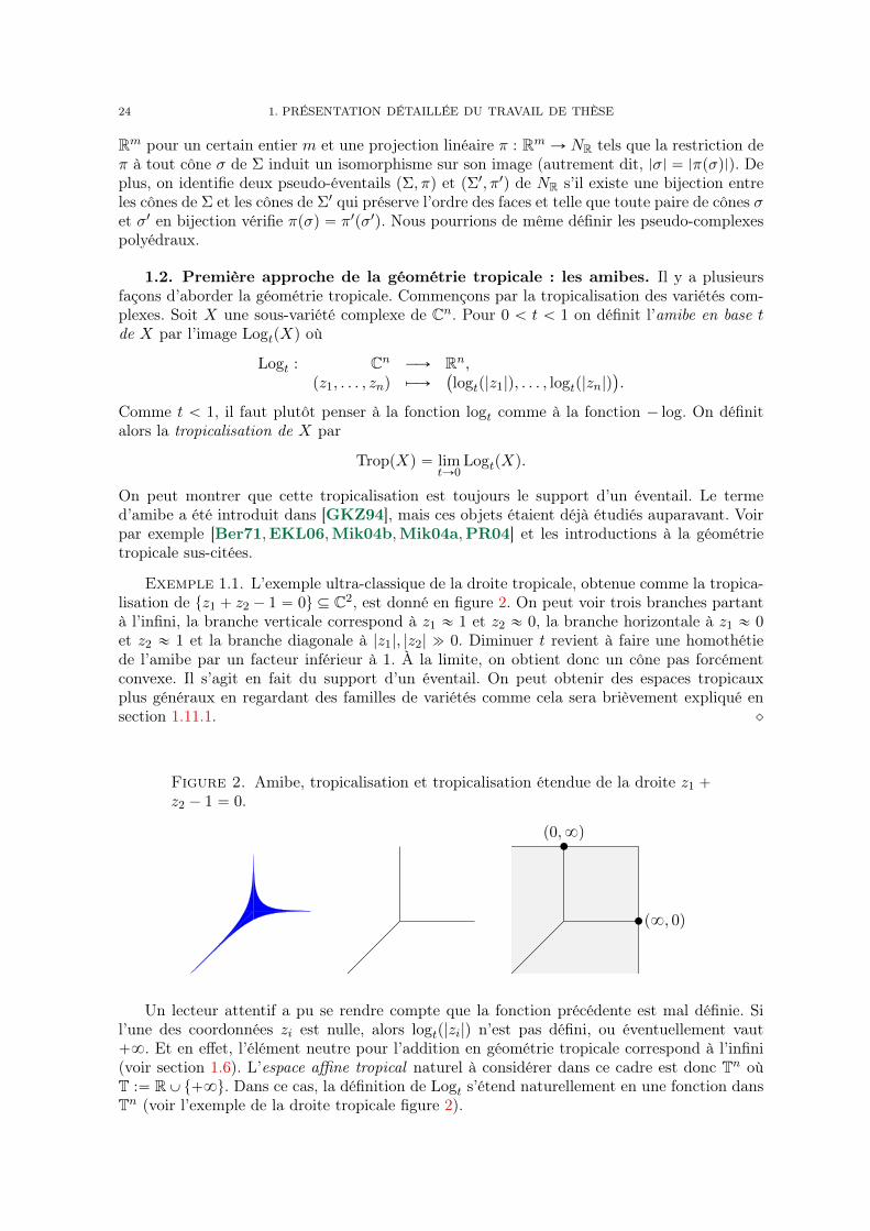
Exemple 1.1. L’exemple ultra-classique de la droite tropicale, obtenue comme la tropica-lisation de tz1 ` z2 ´ 1 “ 0u Ď C2, est donné en figure 2. On peut voir trois branches partantà l’infini, la branche verticale correspond à z1 « 1 et z2 « 0, la branche horizontale à z1 « 0et z2 « 1 et la branche diagonale à |z1|, |z2| " 0. Diminuer t revient à faire une homothétiede l’amibe par un facteur inférieur à 1. À la limite, on obtient donc un cône pas forcémentconvexe. Il s’agit en fait du support d’un éventail. On peut obtenir des espaces tropicauxplus généraux en regardant des familles de variétés comme cela sera brièvement expliqué ensection 1.11.1. ˛
Figure 2. Amibe, tropicalisation et tropicalisation étendue de la droite z1 `
z2 ´ 1 “ 0.
p8, 0q
p0,8q
Un lecteur attentif a pu se rendre compte que la fonction précédente est mal définie. Sil’une des coordonnées zi est nulle, alors logtp|zi|q n’est pas défini, ou éventuellement vaut`8. Et en effet, l’élément neutre pour l’addition en géométrie tropicale correspond à l’infini(voir section 1.6). L’espace affine tropical naturel à considérer dans ce cadre est donc Tn oùT :“ RYt`8u. Dans ce cas, la définition de Logt s’étend naturellement en une fonction dansTn (voir l’exemple de la droite tropicale figure 2).
1. RAPPELS DE GÉOMÉTRIE TROPICALE 25
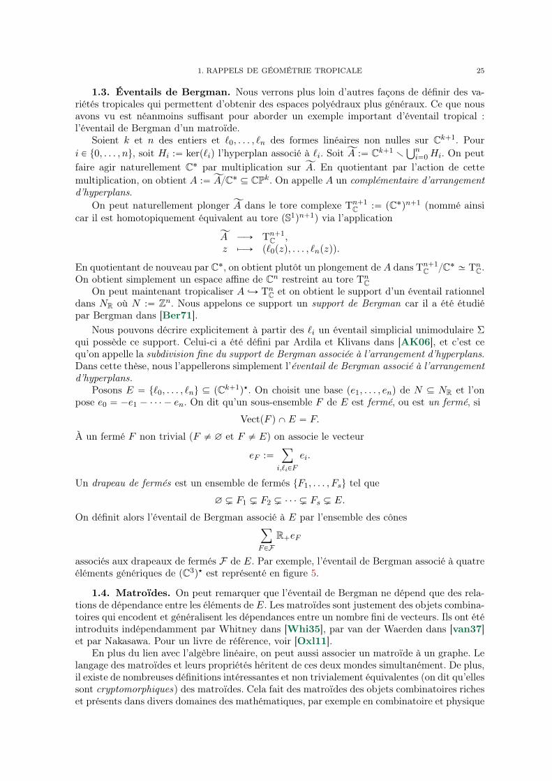
1.3. Éventails de Bergman. Nous verrons plus loin d’autres façons de définir des va-riétés tropicales qui permettent d’obtenir des espaces polyédraux plus généraux. Ce que nousavons vu est néanmoins suffisant pour aborder un exemple important d’éventail tropical :l’éventail de Bergman d’un matroïde.
Soient k et n des entiers et `0, . . . , `n des formes linéaires non nulles sur Ck`1. Pouri P t0, . . . , nu, soit Hi :“ kerp`iq l’hyperplan associé à `i. Soit ĂA :“ Ck`1 r
Ťni“0Hi. On peut
faire agir naturellement C˚ par multiplication sur ĂA. En quotientant par l’action de cettemultiplication, on obtient A :“ĂAC˚ Ď CPk. On appelle A un complémentaire d’arrangementd’hyperplans.
On peut naturellement plonger ĂA dans le tore complexe Tn`1C :“ pC˚qn`1 (nommé ainsi
car il est homotopiquement équivalent au tore pS1qn`1) via l’application
ĂA ÝÑ Tn`1C ,
z ÞÝÑ p`0pzq, . . . , `npzqq.
En quotientant de nouveau par C˚, on obtient plutôt un plongement de A dans Tn`1C C˚ » Tn
C.On obtient simplement un espace affine de Cn restreint au tore Tn
COn peut maintenant tropicaliser A ãÑ Tn
C et on obtient le support d’un éventail rationneldans NR où N :“ Zn. Nous appelons ce support un support de Bergman car il a été étudiépar Bergman dans [Ber71].
Nous pouvons décrire explicitement à partir des `i un éventail simplicial unimodulaire Σqui possède ce support. Celui-ci a été défini par Ardila et Klivans dans [AK06], et c’est cequ’on appelle la subdivision fine du support de Bergman associée à l’arrangement d’hyperplans.Dans cette thèse, nous l’appellerons simplement l’éventail de Bergman associé à l’arrangementd’hyperplans.
Posons E “ t`0, . . . , `nu Ď pCk`1q‹. On choisit une base pe1, . . . , enq de N Ď NR et l’onpose e0 “ ´e1 ´ ¨ ¨ ¨ ´ en. On dit qu’un sous-ensemble F de E est fermé, ou est un fermé, si
VectpF q X E “ F.
À un fermé F non trivial (F ‰ ∅ et F ‰ E) on associe le vecteur
eF :“ÿ
i,`iPF
ei.
Un drapeau de fermés est un ensemble de fermés tF1, . . . , Fsu tel que
∅ Ĺ F1 Ĺ F2 Ĺ ¨ ¨ ¨ Ĺ Fs Ĺ E.
On définit alors l’éventail de Bergman associé à E par l’ensemble des cônesÿ
FPFR`eF
associés aux drapeaux de fermés F de E. Par exemple, l’éventail de Bergman associé à quatreéléments génériques de pC3q‹ est représenté en figure 5.
1.4. Matroïdes. On peut remarquer que l’éventail de Bergman ne dépend que des rela-tions de dépendance entre les éléments de E. Les matroïdes sont justement des objets combina-toires qui encodent et généralisent les dépendances entre un nombre fini de vecteurs. Ils ont étéintroduits indépendamment par Whitney dans [Whi35], par van der Waerden dans [van37]et par Nakasawa. Pour un livre de référence, voir [Oxl11].
En plus du lien avec l’algèbre linéaire, on peut aussi associer un matroïde à un graphe. Lelangage des matroïdes et leurs propriétés héritent de ces deux mondes simultanément. De plus,il existe de nombreuses définitions intéressantes et non trivialement équivalentes (on dit qu’ellessont cryptomorphiques) des matroïdes. Cela fait des matroïdes des objets combinatoires richeset présents dans divers domaines des mathématiques, par exemple en combinatoire et physique

26 1. PRÉSENTATION DÉTAILLÉE DU TRAVAIL DE THÈSE
statistique [Tut65,MP67,GGW06,SS14,Piq19b], en topologie [Mac91,GM92], ou engéométrie algébrique [Mnë88,Laf03,BB03,BL18,Stu02].
La définition que nous proposons est celle mimant les relations de dépendance dans unefamille de vecteurs.
Définition 1.2. Un matroïde M “ pE,Iq est la donnée d’un ensemble de base fini E etd’un ensemble d’indépendants I Ď 2E tel que
— ∅ P I,— si I P I et J Ď I alors J P I,— si I, J P I et cardpJq ą cardpIq alors il existe un élément j P J tel que pI` jq P I. ˛
Par exemple, si E est un ensemble de formes linéaires comme ci-dessus, si l’on définitI comme l’ensemble des sous-familles de E linéairement indépendantes, alors pE,Iq est unmatroïde.
On peut définir le rang rkpGq d’un sous-ensemble G de E comme étant le cardinal duplus grand indépendant I inclus dans G. Une base de E est un élément maximal de I pourl’inclusion. On peut montrer que toutes les bases ont le même rang r, que l’on appelle le rangde M et qui est noté rkpMq. Si G Ď E, la clotûre de G, notée clpGq, est le plus grand ensemblecontenant G et de même rang que G. Enfin, un fermé de M est un ensemble F Ď E, tel queclpF q “ F .
Comme auparavant, on peut associer un éventail de Bergman ΣM de dimension rkpMq´1
dans NR, où N » ZcardpEq´1, à tout matroïde M. Dans la suite, nous appellerons éventail deBergman l’éventail de Bergman d’un matroïde quelconque. Un support de Bergman désignerale support de n’importe quel éventail de Bergman. De plus nous définissons un éventail deBergman généralisé comme étant n’importe quel éventail isomorphe, via un isomorphismepréservant le réseau N , à un éventail dont le support est un support de Bergman.
Ajoutons que la plupart des matroïdes ne sont pas issus d’une famille de vecteurs, ont ditqu’ils ne sont pas réalisables. De même, les support de Bergman ne sont pas tous réalisables,voir par exemple [Yu17], dans le sens où ils ne sont pas la tropicalisation d’une variété. Nousreparlerons de réalisabilité des variétés tropicales en remarque 1.10.
Remarque 1.3 (Espaces linéaires tropicaux). Les support de Bergman jouent le rôle desespaces linéaires en géométrie tropicale. En effet, on a déjà vu qu’un espace linéaire de Cnque l’on restreint au tore a pour tropicalisation un support de Bergman. De plus, on peutdéfinir une notion de degré tropical, et, par un résultat de Fink, on sait que les supports deBergman sont exactement les supports des éventails tropicaux de degré un. Entre autre, deuxsupports de Bergman de dimensions complémentaires translatés génériquement ont un uniquepoint d’intersection. Voir [Fin13,Spe08] pour plus de détails. ˛
1.5. Tropicalisation par valuation. Nous allons maintenant parler d’une autre mé-thode qui permet de définir la tropicalisation de variétés sur des corps non archimédiensvalués.
Plutôt que de définir ce que sont ces corps, nous allons simplement définir un exemple detel corps : le corps des séries de Puiseux sur C, noté Ctttuu. Une série de Puiseux sur C estune somme formelle de la forme
QpT q :“`8ÿ
i“i0
aimTim
pour des entiers m P N et i0 P Z et des coefficients aim P C. On peut montrer que CttT uuest algébriquement clos. On définit le degré de Q, noté degpQq, comme le plus petit nombrerationnel q tel que aq ‰ 0, et l’on pose degp0q “ `8.
On obtient une valuation : si Q et Q1 sont deux séries de Puiseux, alors

1. RAPPELS DE GÉOMÉTRIE TROPICALE 27
— degpQq “ `8 ðñ Q “ 0,— degpQQ1q “ degpQq ` degpQ1q,— degpQ`Q1q ě minpdegpQq, degpQ1qq avec égalité si degpQq ‰ degpQ1q.
Maintenant, si V est une variété algébrique dans CttT uun, par exemple si V est le lieud’annulation d’un polynôme P pz1, . . . , znq, alors on peut définir la tropicalisation de V , notéeTroppV q Ď Tn comme l’adhérence de l’image de V par l’application
trop : CttT uun ÝÑ Tn,pQ1, . . . , Qnq ÞÝÑ
`
degpQ1q, . . . ,degpQnq˘
.
On peut montrer que TroppV q restreint à Rn est un espace polyédral rationnel.
Exemple 1.4. Si l’on prend la droite V d’équation z1` z2´ 1 “ 0 dans CttT uu2, TroppV qest la droite tropicale de la figure 2. Si l’on regarde plutôt l’équation T´az1 ` T
´bz2 ´ 1 “ 0avec a, b P Q, on obtient la droite tropicale de centre de coordonnées pa, bq. ˛
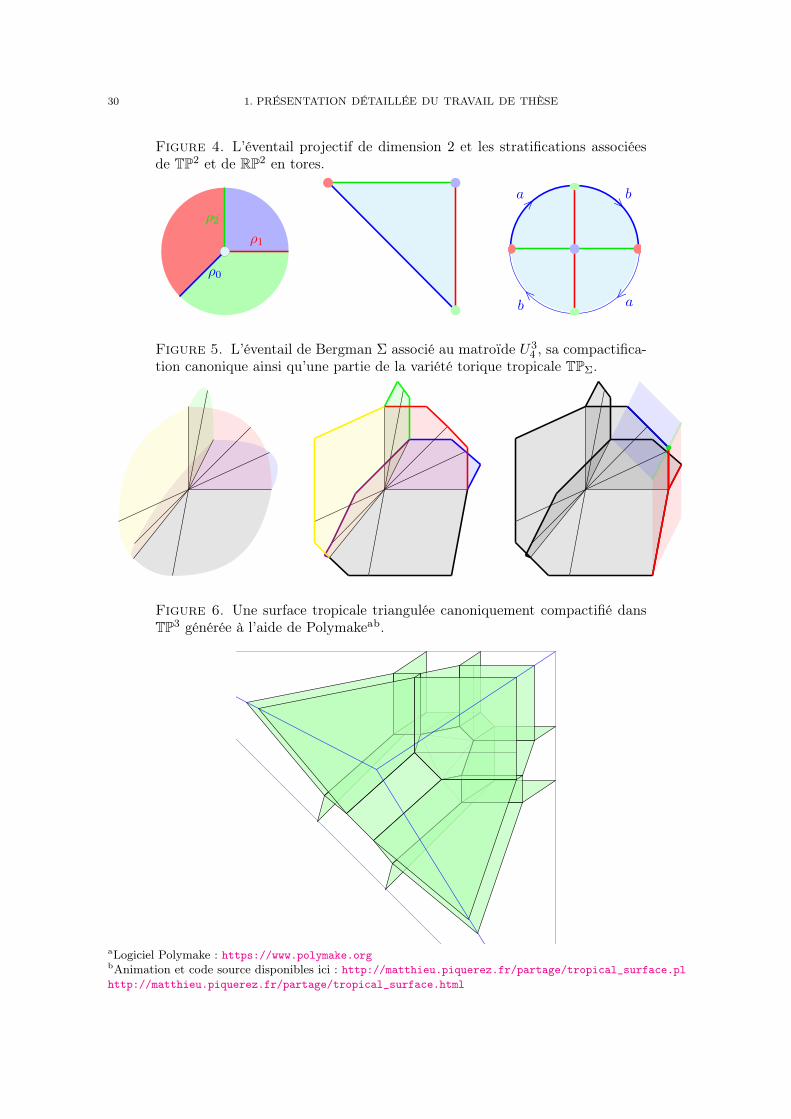
Exemple 1.5. La figure 6 est la surface tropicale obtenue comme la tropicalisation de lasurface d’équation
1` Tz1 ` Tz2 ` Tz3 ` z2z3 ` T3z1z3 ` T
3z1z2 ` T5z2
1 ` T5z2
2 ` T5z2
3 “ 0.
Il existe en fait une méthode combinatoire élémentaire pour construire des hypersurfaces tro-picales ayant la forme voulue en utilisant le polytope de Newton du polynôme et un théorèmede dualité : voir les références sus-cités. ˛
1.6. Hypercorps tropical. On peut en fait définir directement des polynômes tropicauxdans Trx1, . . . , xns et considérer leurs lieux d’annulation. Définissons donc les opérations sur T.Généralement on définit T comme un semi-corps (l’addition n’a pas d’inverse) en le munissantdes opérations a‘ b “ minpa, bq et ab b “ a` b. En fait, il est souvent plus utile de considérerT comme un hypercorps, que l’on notera rT, en posant
a‘ b “
#
tminpa, bqu si a ‰ b,rminpa, bq,`8s si a “ b.
Ainsi par exemple,
p1 ‘ 1q‘ 0 “ r1;`8s‘ 0 “ď
aPr1;`8s
ta‘ 0u “ t0u.
On se rend compte que ces opérations miment les propriétés de la valuation.Nous n’utiliserons pas vraiment la notion d’hypercorps par la suite, et nous n’allons donc
pas entrer dans les détails de la définition (celle-ci est disponible dans [BB19]), mais c’est unedéfinition que l’auteur apprécie et qui permet de comprendre de nombreuses définitions de lagéométrie tropicale, comme la définition du lieu d’annulation des polynômes tropicaux dontnous parlons ci-dessous. Pour une jolie application simple de ce point de vue, nous renvoyonsà [BL21]. Pour plus de littérature sur les hypercorps, sur la géométrie associée et sur les liensavec la géométrie tropicale, voir [BB19,BL18,Lor15,Lor19].
Dans T, l’élément neutre pour l’addition est `8 et l’élément neutre pour la multiplicationest 0. Si P pz1, . . . , zkq est un polynôme sur CttT uu. On peut définir le polynôme tropical associétroppP qpx1, . . . , xkq en remplaçant les coefficients par leurs valuations, les produits par b etles sommes par ‘. Le lieu des zéros du polynôme troppP q est par définition l’ensemble despoints px1, . . . , xkq tels que `8 P troppP qpx1, . . . , xkq. C’est aussi l’ensemble des points telsqu’au moins deux monômes de P voient leurs valeurs coïncider et être minimales comparéesaux autres monômes. Le théorème fondamental de la géométrie tropicale énonce que le lieudes zéros de troppP q coïncide avec la tropicalisation du lieu des zéros de P . Ce théorème segénéralise à l’intersection des variétés associée à un idéal sous certaines conditions (voir parexemple [MS15]).
28 1. PRÉSENTATION DÉTAILLÉE DU TRAVAIL DE THÈSE
1.7. Condition d’équilibre. Un phénomène important en géométrie tropicale est lacondition d’équilibre [SS03,Spe05,Mik04b] ou les introductions suscités. Si l’on prend unevariété tropicale X dans NR provenant d’une variété algébrique comme ci-dessus, on peutchoisir un complexe polyédral rationnel X de support X. Il y a une manière naturelle demettre des poids wpσq P N sur les facettes σ de X qui vérifie la condition suivante.
Soit τ une face de X de codimension un. Xτ est un éventail de dimension un dont lesrayons sont στ pour σ ą τ . Pour chaque rayon στ , on note ντσ le vecteur générateur de N Xστ .
Théorème 1.6 (Condition d’équilibre). Avec les notations ci-dessus, on aÿ
σ ąτ
wpσqντσ “ 0.
Nous verrons en section 3.4 que cette condition d’équilibre est l’analogue de la notiond’orientabilité en topologie.
1.8. Compactification canonique. Dans cette thèse, nous sommes surtout intéresséspar les variétés tropicales compactes qui, comme pour les variétés complexes compactes, ontgénéralement de meilleures propriétés que les variétés quelconques. Pour l’instant, les sous-variétés tropicales que nous avons définies sont rarement compactes. Il va donc falloir com-pactifier. Pour un éventail, la compactification canonique est la bonne façon de compactifier,du moins allons-nous essayer de le justifier. Comme c’est un objet central dans ce travail, quifournit de nombreux moyens pour étudier non seulement les variétés tropicales mais aussi desobjets apparaissant en théorie de Hodge combinatoire, comme les éventails de Bergman oul’anneau de Stanley-Reisner de complexes simpliciaux, il nous semble important de commentercette construction et de donner une intuition par des illustrations.
1.8.1. Espace projectif tropical. Nous avons vu dans l’exemple 1.1 à propos de la droitetropicale que l’on peut partiellement compactifier les sous-variétés de Rn dans l’espace affinetropical Tn. Mais comme l’espace affine n’est pas compact, ses sous-variétés ne le sont pas nonplus en général. Cela nous amène à définir l’espace projectif tropical TPn.
Dans le cas complexe, on a par définition CPn “ pCn`1rtp0, . . . , 0quqL
C˚. La transpositionexacte dans le cadre tropical est donc
TPn “ pTn`1 r tp8, . . . ,8quqL
Rp1, . . . , 1q,
où le quotient signifie que l’on identifie deux points de Tn`1 de la forme pa0, . . . , anq et pa0 `
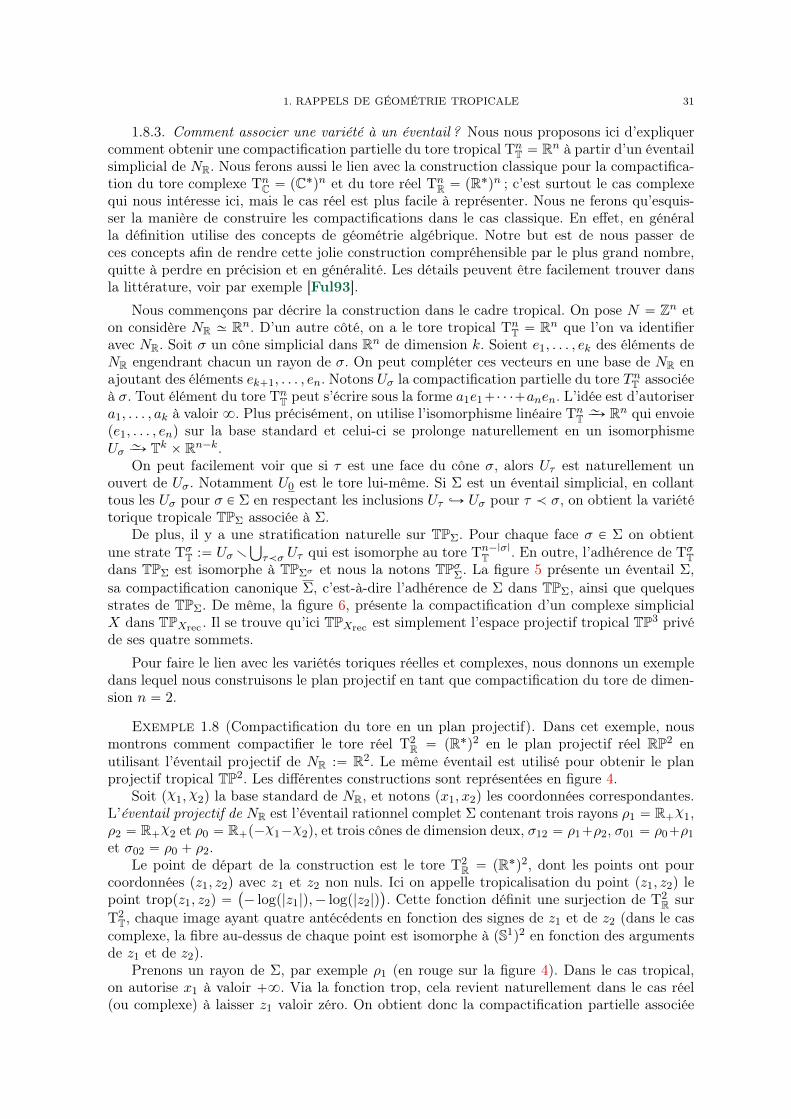
λ, . . . , an`λq pour tout λ P R, ce qui correspond bien à multiplier au sens tropical un point parle scalaire λ. L’espace obtenu est naturellement homéomorphe à un simplexe 4 à n sommetsdont le bord se situe à l’infini. Les faces de codimension k du simplexe correspondent auxpoints ayant au moins k coordonnées infinies (voir figures 4 et 6).
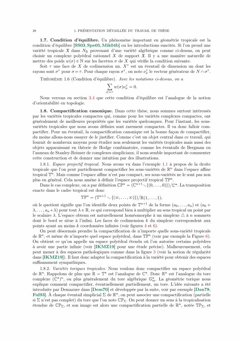
On peut désormais prendre la compactification de n’importe quelle sous-variété tropicalede Rn, et même de n’importe quel espace polyédral, dans TPn (voir par exemple la Figure 6).On obtient ce qu’on appelle un espace polyédral étendu où l’on autorise certains polyèdresà avoir une partie infinie (voir [IKMZ19] pour une étude précise). Malheureusement, celapeut mener à des espaces pathologiques comme dans la figure 3 (voir la notion de régularitédans [IKMZ19]). Il faut donc adapter la compactification à la variété pour obtenir des espacessuffisamment sympathiques.
1.8.2. Variétés toriques tropicales. Nous voulons donc compactifier un espace polyédralde Rn. Rappelons de plus que R “ T˚ est l’analogue de C˚. Donc Rn est l’analogue du torecomplexe pC˚qn, ou plus généralement du tore algébrique Gn
m. La géométrie torique nousexplique comment compactifier, éventuellement partiellement, un tore. L’idée suivante a étéintroduite par Demazure dans [Dem70] et développée par la suite, voir par exemple [Dan78,Ful93]. À chaque éventail simplicial Σ de Rn, on peut associer une compactification (partiellesi Σ n’est pas complet) du tore que l’on note CPΣ. On peut donner un sens à la tropicalisationétendue de CPΣ, et son image est alors une compactification partielle de Rn, notée TPΣ, et
1. RAPPELS DE GÉOMÉTRIE TROPICALE 29
Figure 3. Compactification pathologique dans TP2.
ÝÑ
que l’on nomme variété torique tropicale associée à Σ. Il se trouve que la compactification deΣ dans TPΣ est un espace sympathique, facile à décrire. Notamment, si Σ est simplicial, onretrouve la compactification canonique que nous allons définir dans la section 1.8.4.
Les définitions et les descriptions détaillées de TPΣ et de la compactification canoniquede Σ peuvent être trouvées en chapitre 2 section 2.2, ou encore dans [Pay09,Kaj08,Thu07,OR11,MR18]. Nous nous contenterons en section 1.8.3 d’un bref aperçu, en insistant sur lesliens entre TPΣ et CPΣ dans le cas simplicial.
Le cas des compactifications canoniques des éventails non simpliciaux serait intéressant àétudier et à comparer par exemple avec le travail de Karu [Kar04]. Nous en reparlerons plusen détail avec la question 5.1 et la discussion associée (voir aussi la question 1.9).
Il nous faut maintenant parler des travaux importants qui expliquent en partie pourquoiles compactifications canoniques sont des espaces si sympathiques (pour ne pas dire magni-fiques). Dans [DP95], De Concini et Procesi expliquent comment compactifier de manièresympathique un complémentaire d’arrangement d’hyperplans. Ici sympathique signifie quel’on obtient une compactification lisse en ajoutant un diviseur à croisements normaux. Cescompactifications sont appelées compactifications magnifiques. La construction s’appuie surdes objets combinatoires nommés « building sets » et « nested sets ». Ces objets permettentde trouver des éventails Σ tels que la compactification X de X dans CPΣ soit magnifique.Ce qui est particulièrement intéressant est que l’on peut notamment prendre Σ l’éventail deBergman associé à l’arrangement d’hyperplans.
Par la suite, Feichtner et Yuzvinsky ont montré dans [FY04] que la cohomologie de Xest calculée par l’anneau de Chow de Σ, résultat que nous généralisons en section 9. Danscette thèse, nous montrons que cet anneau de Chow correspond en fait à la cohomologiede la compactification canonique de Σ, voir théorème 5.7. Il se trouve que Σ Ď TPΣ est latropicalisation étendue de X Ď CPΣ. Ainsi, dans ce cas précis, la cohomologie de Σ est égaleà la cohomologie d’une variété complexe projective lisse et vérifie donc toutes les propriétésassociées (notamment le théorème de Lefschetz difficile et les relations de Hodge-Riemann).
Dans [Tev07], Tevelev montre que, plus généralement, la tropicalisation d’une sous-variétéX du tore fournit un support d’éventail intéressant pour compactifier cette variété. Parexemple, un éventail Σ ayant ce support va vérifier que l’adhérence de X dans CPΣ est com-pacte. Pour certaines variétés, qualifiées de schön, les compactifications obtenues ont de bonnespropriétés similaires à celles des compactifications des complémentaires d’arrangement d’hy-perplans. Une description plus précise est donnée en chapitre 2 section 9. Le travail de Tevelevpourrait être un premier pas pour tenter de répondre à la question suivante : peut-on trouverdes propriétés intéressantes vérifiées par une variété en ne connaissant que sa tropicalisation ?Voici un exemple de question concrète que l’on peut se poser.
Question 1.7. Quelles sont les sous-variétés du tore dont la tropicalisation est lisse ausens de la section 3.7 ? ˛
On sait par exemple qu’une sous-variété du tore dont la tropicalisation est un support deBergman est forcément un complémentaire d’arrangement d’hyperplans (cf. [IKMZ19]).
30 1. PRÉSENTATION DÉTAILLÉE DU TRAVAIL DE THÈSE
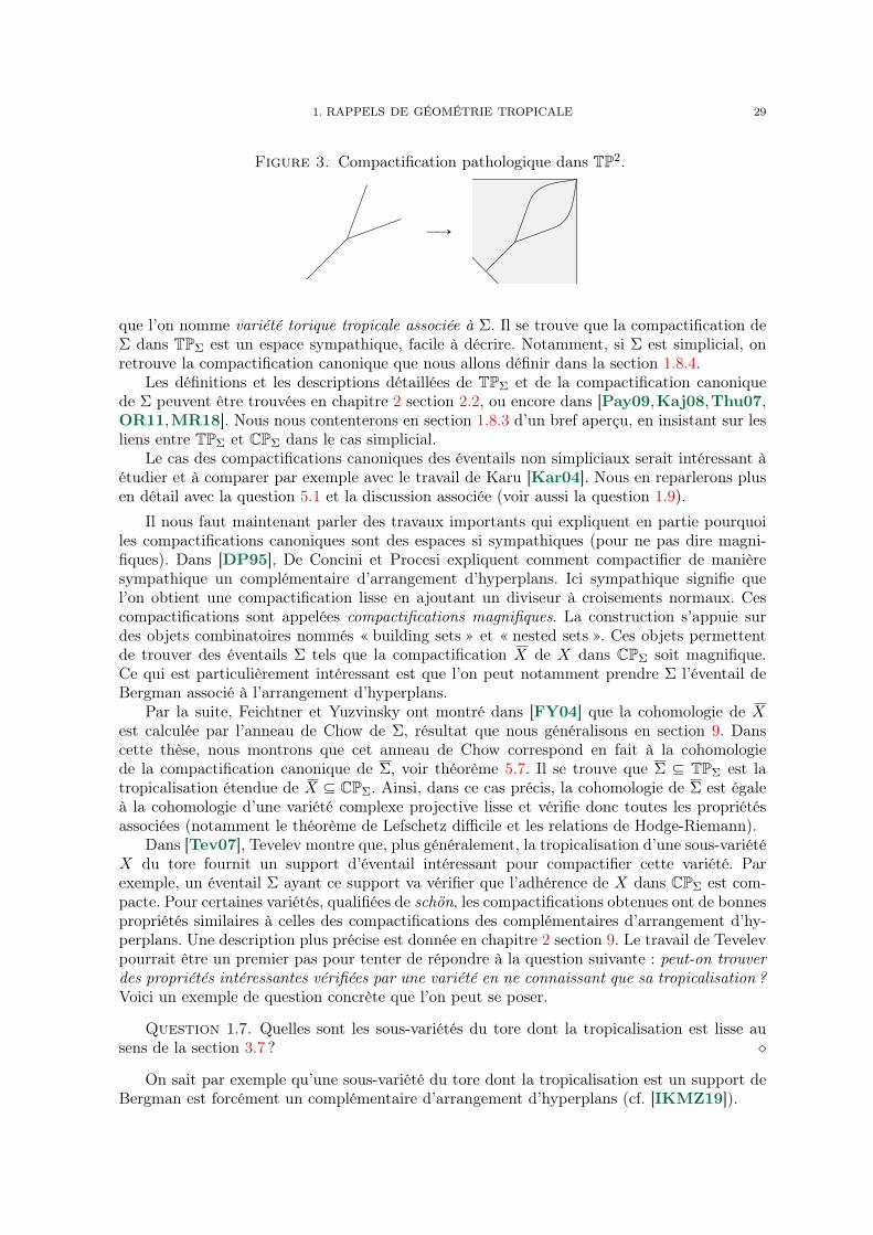
Figure 4. L’éventail projectif de dimension 2 et les stratifications associéesde TP2 et de RP2 en tores.
ρ1
ρ2
ρ0
aą
a
ą
bą
b
ą
Figure 5. L’éventail de Bergman Σ associé au matroïde U34 , sa compactifica-
tion canonique ainsi qu’une partie de la variété torique tropicale TPΣ.
Figure 6. Une surface tropicale triangulée canoniquement compactifié dansTP3 générée à l’aide de Polymakeab.
aLogiciel Polymake : https://www.polymake.orgbAnimation et code source disponibles ici : http://matthieu.piquerez.fr/partage/tropical_surface.plhttp://matthieu.piquerez.fr/partage/tropical_surface.html
1. RAPPELS DE GÉOMÉTRIE TROPICALE 31
1.8.3. Comment associer une variété à un éventail ? Nous nous proposons ici d’expliquercomment obtenir une compactification partielle du tore tropical Tn
T “ Rn à partir d’un éventailsimplicial de NR. Nous ferons aussi le lien avec la construction classique pour la compactifica-tion du tore complexe Tn
C “ pC˚qn et du tore réel TnR “ pR˚qn ; c’est surtout le cas complexe
qui nous intéresse ici, mais le cas réel est plus facile à représenter. Nous ne ferons qu’esquis-ser la manière de construire les compactifications dans le cas classique. En effet, en généralla définition utilise des concepts de géométrie algébrique. Notre but est de nous passer deces concepts afin de rendre cette jolie construction compréhensible par le plus grand nombre,quitte à perdre en précision et en généralité. Les détails peuvent être facilement trouver dansla littérature, voir par exemple [Ful93].
Nous commençons par décrire la construction dans le cadre tropical. On pose N “ Zn eton considère NR » Rn. D’un autre côté, on a le tore tropical Tn
T “ Rn que l’on va identifieravec NR. Soit σ un cône simplicial dans Rn de dimension k. Soient e1, . . . , ek des éléments deNR engendrant chacun un rayon de σ. On peut compléter ces vecteurs en une base de NR enajoutant des éléments ek`1, . . . , en. Notons Uσ la compactification partielle du tore TnT associéeà σ. Tout élément du tore Tn
T peut s’écrire sous la forme a1e1`¨ ¨ ¨`anen. L’idée est d’autorisera1, . . . , ak à valoir 8. Plus précisément, on utilise l’isomorphisme linéaire Tn
T„ÝÑ Rn qui envoie
pe1, . . . , enq sur la base standard et celui-ci se prolonge naturellement en un isomorphismeUσ „ÝÑ Tk ˆ Rn´k.
On peut facilement voir que si τ est une face du cône σ, alors Uτ est naturellement unouvert de Uσ. Notamment U0 est le tore lui-même. Si Σ est un éventail simplicial, en collanttous les Uσ pour σ P Σ en respectant les inclusions Uτ ãÑ Uσ pour τ ă σ, on obtient la variététorique tropicale TPΣ associée à Σ.
De plus, il y a une stratification naturelle sur TPΣ. Pour chaque face σ P Σ on obtientune strate Tσ
T :“ UσrŤ
τăσ Uτ qui est isomorphe au tore Tn´|σ|T . En outre, l’adhérence de Tσ
Tdans TPΣ est isomorphe à TPΣσ et nous la notons TPσΣ. La figure 5 présente un éventail Σ,sa compactification canonique Σ, c’est-à-dire l’adhérence de Σ dans TPΣ, ainsi que quelquesstrates de TPΣ. De même, la figure 6, présente la compactification d’un complexe simplicialX dans TPXrec . Il se trouve qu’ici TPXrec est simplement l’espace projectif tropical TP3 privéde ses quatre sommets.
Pour faire le lien avec les variétés toriques réelles et complexes, nous donnons un exempledans lequel nous construisons le plan projectif en tant que compactification du tore de dimen-sion n “ 2.
Exemple 1.8 (Compactification du tore en un plan projectif). Dans cet exemple, nousmontrons comment compactifier le tore réel T2
R “ pR˚q2 en le plan projectif réel RP2 enutilisant l’éventail projectif de NR :“ R2. Le même éventail est utilisé pour obtenir le planprojectif tropical TP2. Les différentes constructions sont représentées en figure 4.
Soit pχ1, χ2q la base standard de NR, et notons px1, x2q les coordonnées correspondantes.L’éventail projectif de NR est l’éventail rationnel complet Σ contenant trois rayons ρ1 “ R`χ1,ρ2 “ R`χ2 et ρ0 “ R`p´χ1´χ2q, et trois cônes de dimension deux, σ12 “ ρ1`ρ2, σ01 “ ρ0`ρ1
et σ02 “ ρ0 ` ρ2.Le point de départ de la construction est le tore T2
R “ pR˚q2, dont les points ont pourcoordonnées pz1, z2q avec z1 et z2 non nuls. Ici on appelle tropicalisation du point pz1, z2q lepoint troppz1, z2q “
`
´ logp|z1|q,´ logp|z2|q˘
. Cette fonction définit une surjection de T2R sur
T2T, chaque image ayant quatre antécédents en fonction des signes de z1 et de z2 (dans le cas
complexe, la fibre au-dessus de chaque point est isomorphe à pS1q2 en fonction des argumentsde z1 et de z2).
Prenons un rayon de Σ, par exemple ρ1 (en rouge sur la figure 4). Dans le cas tropical,on autorise x1 à valoir `8. Via la fonction trop, cela revient naturellement dans le cas réel(ou complexe) à laisser z1 valoir zéro. On obtient donc la compactification partielle associée
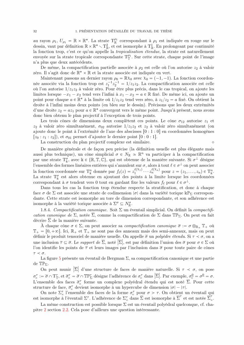
32 1. PRÉSENTATION DÉTAILLÉE DU TRAVAIL DE THÈSE
au rayon ρ1, Uρ1 “ R ˆ R˚. La strate Tρ1
R correspondant à ρ1 est indiquée en rouge sur ledessin, vaut par définition RˆR˚rT2
R, et est isomorphe à T1R. En prolongeant par continuité
la fonction trop, c’est ce qu’on appelle la tropicalisation étendue, la strate est naturellementenvoyée sur la strate tropicale correspondante Tρ1
T . Sur cette strate, chaque point de l’imagen’a plus que deux antécédents.
De même, la compactification partielle associée à ρ2 est celle où l’on autorise z2 à valoirzéro. Il s’agit donc de R˚ ˆ R et la strate associée est indiquée en vert.
Maintenant passons au dernier rayon ρ0 “ Rχ0 avec χ0 “ p´1,´1q. La fonction coordon-née associée via la fonction trop est z´1
1 z´12 “ 1z1z2. La compactification associée est celle
où l’on autorise 1z1z2 à valoir zéro. Pour être plus précis, dans le cas tropical, on ajoute leslimites lorsque ´x1 ´ x2 tend vers l’infini à x1 ´ x2 “ a P R fixé. De même ici, on ajoute unpoint pour chaque a P R˚ à la limite où 1z1z2 tend vers zéro, à z1z2 “ a fixé. On obtient ladroite à l’infini moins deux points (en bleu sur le dessin). Précisons que les deux extrémitésd’une droite z2 “ az1 pour a P R˚ convergent vers le même point. Jusqu’à présent, nous avonsdonc bien obtenu le plan projectif à l’exception de trois points.
Les trois cônes de dimensions deux complètent ces points. Le cône σ12 autorise z1 etz2 à valoir zéro simultanément, σ02 autorise 1z1z2 et z2 à valoir zéro simultanément (onajoute donc le point à l’extrémité de l’axe des abscisses r0 : 1 : 0s en coordonnées homogènesrz0 : z1 : z2s), et σ01 permet d’ajouter le dernier point r0 : 0 : 1s.
La construction du plan projectif complexe est similaire. ˛
De manière générale et de façon peu précise (la définition usuelle est plus élégante maisaussi plus technique), un cône simplicial σ P NR » Rn va participer à la compactificationpar une strate Tσ
k , avec k P tR,T,Cu, qui est obtenue de la manière suivante. Si σK désignel’ensemble des formes linéaires entières qui s’annulent sur σ, alors à tout ` P σK on peut associerla fonction coordonnée sur Tn
k donnée par f`pzq “ z`pχ1q
1 ¨ ¨ ¨ z`pχnqn pour z “ pz1, . . . , znq P Tn
k .La strate Tσ
k est alors obtenue en ajoutant des points à la limite lorsque les coordonnéescorrespondant à σ tendent vers 0 tout en gardant fixe les valeurs f` pour ` P σK.
Dans tous les cas la fonction trop étendue respecte la stratification, et donc à chaqueface σ de Σ est associée une strate de codimension |σ| dans la variété torique kPΣ correspon-dante. Cette strate est isomorphe au tore de dimension correspondante, et son adhérence estisomorphe à la variété torique associée à Σσ Ď Nσ
R .1.8.4. Compactification canonique. Soit Σ un éventail simplicial. On définit la compactifi-
cation canonique de Σ, notée Σ, comme la compactification de Σ dans TPΣ. On peut en faitdécrire Σ de la manière suivante.
À chaque cône σ P Σ, on peut associer sa compactification canonique σ :“ σ bR` T` oùT` “ r0,`8s. Ici, R` et T` ne sont pas des anneaux mais des semi-anneaux, mais on peutdéfinir le produit tensoriel de manière usuelle. On appelle σ un polyèdre étendu. Si τ ă σ, on aune inclusion τ Ď σ. Le support de Σ, noté |Σ|, est par définition l’union des σ pour σ P Σ oùl’on identifie les points de τ et leurs images par l’inclusion dans σ pour toute paire de cônesτ ă σ.
La figure 5 présente un éventail de Bergman Σ, sa compactification canonique et une partiede TPΣ.
On peut munir |Σ| d’une structure de faces de manière naturelle. Si τ ă σ, on poseστ8
:“ σXTτT, et σ
τ8“ σXTPτΣ désigne l’adhérence de στ
8dans |Σ|. Par exemple, σ0
8“ σ0 “ σ.
L’ensemble des faces στ8
forme un complexe polyédral étendu qui est noté Σ. Pour cettestructure de face, στ
8devient isomorphe à un hypercube de dimension |σ|´ |τ |.
On note Στ8l’ensemble des faces de la forme στ
8pour σ ą τ . On obtient un éventail qui
est isomorphe à l’éventail Στ . L’adhérence de Στ8dans Σ est isomorphe à Σ
τ et est notée Στ8.
La même construction est possible lorsque Σ est un éventail polyédral quelconque, cf. cha-pitre 2 section 2.2. Cela pose d’ailleurs une question intéressante.

1. RAPPELS DE GÉOMÉTRIE TROPICALE 33
Question 1.9. Soit σ un cône polyédral quelconque. La structure de faces naturelle surσ est-elle la structure de face d’un polytope ? ˛
On peut facilement montrer qu’il s’agit du moins d’un polytope abstrait, c’est-à-dire quel’ensemble ordonné des faces obtenues vérifie la propriété diamant, i.e. pour toute paire defaces γ ă η avec |η| “ |γ|` 2, il existe exactement deux faces δ et δ1 telles que γ ă δ,δ1 ă η.
On peut de même compactifier canoniquement des complexes simpliciaux (voire des com-plexes polyédraux). Nous avons vu que chaque face δ de X est de la forme δf ` δrec. On définitalors δ :“ δf ` δrec. Ainsi δ devient le produit d’un simplexe et d’un hypercube. En recollanttous les δ, on obtient la compactification canonique de X, notée X. Elle est naturellementmunie d’une structure de faces comme pour le cas des éventails : les faces sont de la formesδσ
:“ δf ` δσrec,8 Ď δ pour δ P X et σ ă δrec. Ce n’est plus un complexe cubique comme dans le
cas des éventails mais plutôt une structure hybride simplicial-cubique. Par exemple la figure 6présente la compactification canonique d’une surface tropicale.
Dans le cas où le pseudo-éventailXrec est un éventail,X est simplement la compactificationde X dans TPXrec . On a alors une stratification de X par les strates Xσ
8:“ X XTPσXrec
pourσ P Xrec.
1.9. Variétés tropicales. La définition d’une variété tropicale générale est assez tech-nique et ne nous sera pas utile dans ce chapitre. Nous donnons des définitions approximativesafin que le lecteur ait une idée des objets dont nous parlons. Des définitions formelles peuventêtre trouvées en chapitre 3 section 2 ou dans [JSS19].
Un espace polyédral étendu est un espace topologique connexe muni d’un atlas de cartesφi : Ui Ñ Xi où Xi est un ouvert de la compactification dans Tn d’un espace polyédral deRn, et les applications de transitions entre deux cartes sont des applications affines étendues.Un complexe polyédral étendu est un espace polyédral étendu muni d’une structure de faces,chaque face vivant entièrement dans au moins une carte.
Une variété tropicale pondérée est un complexe polyédral étendu dont chaque facette estmunie d’un poids et qui vérifie la condition d’équilibre. Une telle variété est dite localementmatroïdale si elle est localement isomorphe à |Σ|ˆ Tk où Σ est un éventail de Bergman. Êtrelocalement matroïdale et de poids constant égal à un est la définition classique de lissité pourles variétés tropicales. En section 3.7, nous proposerons une nouvelle définition de lissité plusgénérale.
Remarque 1.10 (Réalisabilité d’une variété tropicale). En général, toutes les sous-variétéstropicales de Rn ne sont pas la tropicalisation d’une variété. On dit qu’elles ne sont pasréalisables. Si l’on souhaite obtenir une variété tropicale comme limite tropicale de variétéscomplexes au sens de la section 1.11.1 on parle plutôt d’approximabilité.
On peut montrer que les hypersurfaces tropicales sont approximables, voir [Vir01,Rul01,Mik04b]. Notamment la méthode du « patchwork » de Viro permet de construire des variétésapproximant une hypersurface tropicale et est très utilisées pour construire des hypersurfacesréelles intéressantes : voir [Vir80,Vir06] ou la plupart des introductions suscitées.
Pour les variétés tropicales de codimensions supérieures, même pour le cas des courbes,la réalisabilité d’une variété tropicale est un problème difficile : voir [BS15] et les nombreuxtravaux qui y sont mentionnés. ˛
1.10. Espaces de Berkovich. Dans ce chapitre, nous ne ferons que mentionner lesespaces de Berkovich [Ber90,Ber93]. Nous en parlons très brièvement ici, pour plus de détail,voir par exemple [DFN15]. L’analytifié de Berkovich d’une variété peut être vu comme lalimite projective de toutes les tropicalisations possibles d’une variété [Pay09,FGP14]. C’estun espace très gros qui contient la variété de départ. Ainsi si l’on a un résultat sur suffisammentde tropicalisations possibles d’une variété, on peut espérer passer à la limite et obtenir desrésultats sur la variété.

34 1. PRÉSENTATION DÉTAILLÉE DU TRAVAIL DE THÈSE
1.11. Familles de variétés complexes. Dans cette dernière partie sur les rappels, nousprésentons les familles de variétés complexes, leurs limites tropicales et les liens entre les deux.Une fois de plus nous serons assez imprécis étant donné que nous n’utiliserons ces concepts quedans des discussions et des exemples. Pour nous il s’agira du passage privilégié pour espérerobtenir des résultats en théorie de Hodge asymptotique à partir de la géométrie tropicale.
1.11.1. Limite tropicale d’une famille de variétés complexes. Commençons par décrire lalimite tropicale d’une famille de variétés complexes dans un cas simple. Soit ∆ Ď C le disqueunité complexe, et ∆˚ “ ∆r t0u. On peut considérer par exemple une famille d’hypersurfacesWt pour t P ∆˚, chacune dans le tore Tn
C “ pC˚qn, où la fibre générale Wt est le lieu des zérosdu polynôme Ptpz1, . . . , znq dont les coefficients sont, par exemple, analytiques en t. Si l’onprend n “ 2 et Ptpz1, z2q “ z1` tz2`z1z2` t
2z22`z
21z2` tz1z
22 , une fibre générale de la variété
est une courbe complexe qui pourrait ressembler à la première image de la figure 7 (sansles points bleus). Au lieu de prendre une seule famille de polynômes, on peut en considérerplusieurs pour obtenir des familles de variétés de codimensions supérieures.
L’amibe associée à t P ∆˚ est par définition égale à LogtpWtq où, on le rappelle,
Logt`
pz1, . . . , znq˘
“`
logtp|z1|q, . . . , logtp|zn|q˘
.
On peut alors définir la limite tropicale comme précédemment par limtÑ0 LogtpWtq. Cette fois-ci, comme la variété considérée dépend elle aussi de t, augmenter t ne revient pas simplementà faire une homothétie. À la limite, on obtient un espace polyédral, qui est en fait une variététropicale, ressemblant à celui de la figure 8. Notons cet espace X. Le cône asymptotique Xrec deX, c’est-à-dire limλÑ0 λX, est simplement la tropicalisation deWt pour n’importe quel t P ∆˚.
Ainsi, si l’on subdivise Xrec en un éventail noté Xrec, on peut considérer la compactificationde chacune des variétés Wt dans CPXrec . Nous noterons cette compactification W t. On peutde même regarder la compactification X de X dans TPXrec . Sur la figure, la partie ajoutéeen-dehors du tore est indiquée en bleu.
1.11.2. Réduction semi-stable. Un autre point de vue pour la famille de variétés pWtqtP∆˚
est de considérer la variété W˚ Ď TnC ˆ ∆˚ qui est le lieu des zéros de P pz1, . . . , zn, tq “
Ptpz1, . . . , znq, ainsi que la projection π : W˚ Ñ ∆˚. Les éléments de la famille sont alorssimplement les fibres de la projection :Wt “ π´1ptq. On peut aussi voir P comme un polynômesur Ctttuu. La variété tropicale associée à ce polynôme est simplement la limite tropicale de lafamille. Supposons maintenant que W˚ et toutes les fibres sont lisses.
Nous aimerions compléter W˚ au-dessus de zéro, c’est-à-dire obtenir une compactificationpartielle W de W˚ avec une projection π : W Ñ ∆ tel que W˚ “ π´1p∆˚q. De plus, nousaimerions que la fibre centrale W0 “ π´1p0q soit sympathique. Si les coefficients de Pt seprolonge en 0, on peut bien prolonger W˚ en W. Supposons que W est lisse. Une constructionde Mumford et coauteurs [KKMS06] nous explique que, quitte à prendre un revêtementétal fini de ∆˚, on peut faire en sorte que W0 soit un diviseur à croisements normaux dansW, c’est-à-dire une union de composantes irréductibles lisses dont les intersections sont elles-mêmes lisses et de la dimension attendue. La fibre W0 obtenue est appelée la fibre spéciale oula fibre centrale. Notons que toutes les fibres générales sont homéomorphes. Nous considéronsaussi W 0 la compactification de W0 dans CPXrec . Notons que W se rétracte par déformationsur W0.
Géométriquement, ce que l’on voit c’est que lorsque t tend vers 0, certains cycles de Wt secontractent. Dans la figure 7, nous avons ainsi représenté en seconde image une fibre proche,c’est-à-dire une variété Wt pour t proche de 0. À la limite t “ 0, ces cycles ont entièrementdisparus : ce sont les cycles évanescents.
1.11.3. Complexe dual à la fibre spéciale. La construction de Mumford utilise un complexesimplicial compact inclus dans X. Soit X un complexe simplicial de support X. Supposons queson éventail de récession soit Xrec et que sa partie finie nous donne la réduction semi-stable.On obtient alors une stratification intéressante de la fibre spéciale indexée par les faces de X.
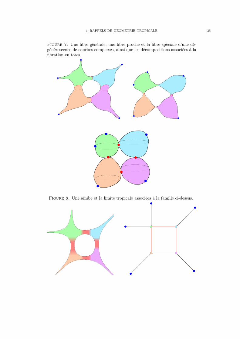
1. RAPPELS DE GÉOMÉTRIE TROPICALE 35
Figure 7. Une fibre générale, une fibre proche et la fibre spéciale d’une dé-générescence de courbes complexes, ainsi que les décompositions associées à lafibration en tores.
Figure 8. Une amibe et la limite tropicale associées à la famille ci-dessus.
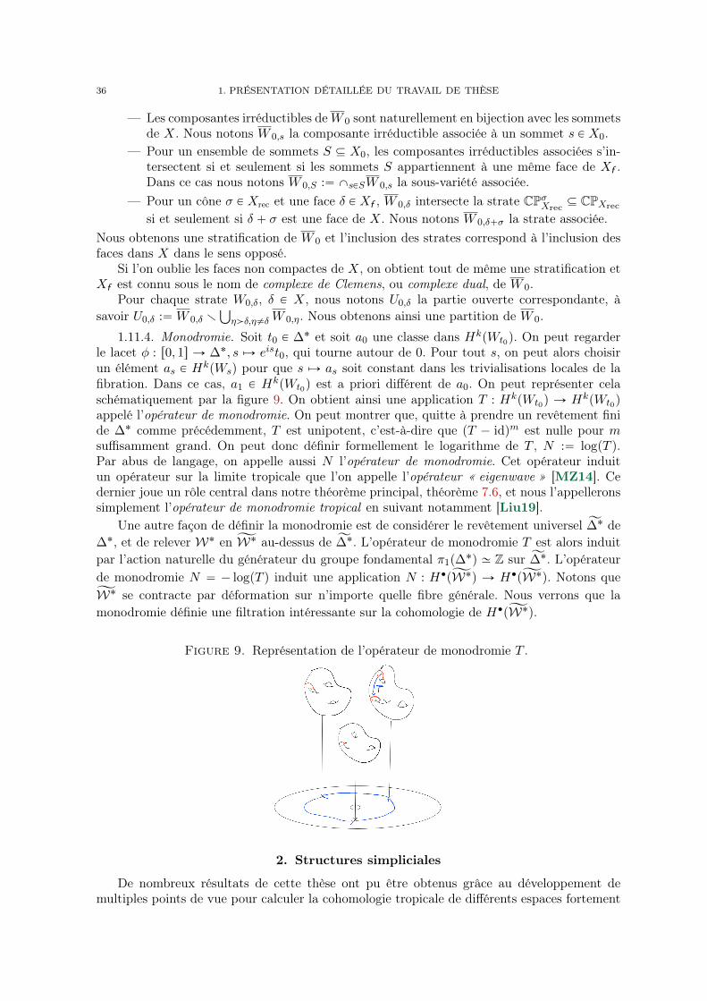
36 1. PRÉSENTATION DÉTAILLÉE DU TRAVAIL DE THÈSE
— Les composantes irréductibles deW 0 sont naturellement en bijection avec les sommetsde X. Nous notons W 0,s la composante irréductible associée à un sommet s P X0.
— Pour un ensemble de sommets S Ď X0, les composantes irréductibles associées s’in-tersectent si et seulement si les sommets S appartiennent à une même face de Xf .Dans ce cas nous notons W 0,S :“ XsPSW 0,s la sous-variété associée.
— Pour un cône σ P Xrec et une face δ P Xf , W 0,δ intersecte la strate CPσXrecĎ CPXrec
si et seulement si δ ` σ est une face de X. Nous notons W 0,δ`σ la strate associée.Nous obtenons une stratification de W 0 et l’inclusion des strates correspond à l’inclusion desfaces dans X dans le sens opposé.
Si l’on oublie les faces non compactes de X, on obtient tout de même une stratification etXf est connu sous le nom de complexe de Clemens, ou complexe dual, de W 0.
Pour chaque strate W0,δ, δ P X, nous notons U0,δ la partie ouverte correspondante, àsavoir U0,δ :“W 0,δ r
Ť
ηąδ,η‰δW 0,η. Nous obtenons ainsi une partition de W 0.
1.11.4. Monodromie. Soit t0 P ∆˚ et soit a0 une classe dans HkpWt0q. On peut regarderle lacet φ : r0, 1s Ñ ∆˚, s ÞÑ eist0, qui tourne autour de 0. Pour tout s, on peut alors choisirun élément as P HkpWsq pour que s ÞÑ as soit constant dans les trivialisations locales de lafibration. Dans ce cas, a1 P H
kpWt0q est a priori différent de a0. On peut représenter celaschématiquement par la figure 9. On obtient ainsi une application T : HkpWt0q Ñ HkpWt0q
appelé l’opérateur de monodromie. On peut montrer que, quitte à prendre un revêtement finide ∆˚ comme précédemment, T est unipotent, c’est-à-dire que pT ´ idqm est nulle pour msuffisamment grand. On peut donc définir formellement le logarithme de T , N :“ logpT q.Par abus de langage, on appelle aussi N l’opérateur de monodromie. Cet opérateur induitun opérateur sur la limite tropicale que l’on appelle l’opérateur « eigenwave » [MZ14]. Cedernier joue un rôle central dans notre théorème principal, théorème 7.6, et nous l’appelleronssimplement l’opérateur de monodromie tropical en suivant notamment [Liu19].
Une autre façon de définir la monodromie est de considérer le revêtement universel Ă∆˚ de∆˚, et de relever W˚ en ĄW˚ au-dessus de Ă∆˚. L’opérateur de monodromie T est alors induitpar l’action naturelle du générateur du groupe fondamental π1p∆
˚q » Z sur Ă∆˚. L’opérateurde monodromie N “ ´ logpT q induit une application N : H‚pĄW˚q Ñ H‚pĄW˚q. Notons queĄW˚ se contracte par déformation sur n’importe quelle fibre générale. Nous verrons que lamonodromie définie une filtration intéressante sur la cohomologie de H‚pĄW˚q.
Figure 9. Représentation de l’opérateur de monodromie T .
2. Structures simpliciales
De nombreux résultats de cette thèse ont pu être obtenus grâce au développement demultiples points de vue pour calculer la cohomologie tropicale de différents espaces fortement
2. STRUCTURES SIMPLICIALES 37
liés entre eux. Le but de cette section est de définir un cadre général plutôt vaste dans lequel cesoutils peuvent être appliqués. L’objectif est double. D’abord, dans ce cadre nous ne considéronspas le réseau entier N inhérent à la géométrie tropicale qui rajoute un peu de technicité auxpreuves, sans que cela soit utile pour les applications que nous proposons. Ensuite, l’oubli dece réseau rapproche nos travaux de la théorie de Hodge combinatoire. Nous montrons ainsicomment la théorie des faisceaux pourrait être utilisée dans ce domaine en section 5.
2.1. Structures simpliciales linéaires. Soit E un ensemble fini. Un éventail simplicialabstrait Σ sur E est un ensemble de parties de E contenant notamment les parties de cardinalau plus un et stable par inclusion : si σ P Σ et τ Ď σ, alors τ P Σ. Les éléments de Σ sontappelés des cônes ou des faces de Σ. La dimension d’un cône σ de Σ est notée |σ| et est égaleau cardinal de σ. L’ensemble des faces de dimension k est noté Σk. Le sous-éventail constituédes faces de dimensions au plus k est appelé le k-squelette de Σ et noté Σďk. L’unique cônede dimension zéro est noté 0, et les cônes de dimension un sont appelés des rayons. Nousidentifions naturellement Σ1 et E. Les cônes maximaux pour l’inclusion sont appelés facettes.La dimension de Σ est par définition le maximum de |σ| pour σ P Σ et Σ est dit pur dedimension d si toutes les facettes ont dimension d. Sauf mention contraire, tous les éventailsconsidérés seront purs.
Remarque 2.1. La définition ci-dessus est très proche de la définition d’un complexesimplicial abstrait. Les principales différences sont la définition des dimensions, et le fait quel’on considère toujours l’ensemble vide comme une face. On peut voir un éventail simplicialabstrait comme le cône sur un complexe simplicial abstrait. ˛
Si τ et σ sont deux faces de Σ, on notera τ ă σ si τ est une face de σ, c’est-à-dire siτ Ď σ. Cela définit un ordre partiel sur Σ. On peut prolonger cet ordre à LΣ :“ Σ \ t1u enposant σ ă 1 pour tout σ P LΣ. En notant 0 “ 0, on obtient un treillis d’élément minimal 0et d’élément maximal 1. Pour τ, σ P Σ, les opérations associées sont données par
— la rencontre : τ ^ 1 :“ τ et τ ^ σ :“ τ X σ,— et la jointure : τ _ 1 :“ 1 et τ _ σ vaut τ Y σ si cette union est dans Σ et 1 sinon.
Si σ couvre τ , c’est-à-dire si σ ą τ est |σ| “ |τ |` 1, nous utiliserons la notation σ ą τ . Siσ _ τ ‰ 1, nous dirons que σ et τ sont comparables. Finalement, nous noterons σ „ τ si σ etτ sont comparables et si σ ^ τ “ 0.
L’éventail étoile de Σ autour de σ, noté StσpΣq, est le sous-éventail constitué de tous lescônes comparables avec σ. L’éventail transverse de Σ autour de σ est par définition l’éventailabstrait tη r σ | η ą σu sur E r σ. On le note Σσ. La face η r σ sera alors noté ησ.
Si l’on a deux éventails simpliciaux abstraits Σ sur E et Σ1 sur E1, on peut définir leurproduit Σˆ Σ1 sur E \ E1 dont les faces sont de la forme σ \ σ1 pour σ P Σ et σ1 P Σ1.
Définition 2.2. Une structure simpliciale linéaire est une paire pΣ, Linq où Σ est unéventail simplicial abstrait et Lin est l’espace des formes linéaires sur Σ, c’est-à-dire un sous-espace linéaire de pREq‹ tel que pour tout σ P Σ, la projection de Lin sur pRσq‹ soit surjective.
˛
La projection de Lin sur pRσq‹ est notée Linσ et on l’appelle l’espace des formes linéairesrestreintes à σ. Elle est par définition isomorphe à pRσq‹. Lorsqu’il n’y a pas d’ambiguïté,nous noterons simplement Σ la structure simpliciale linéaire, et Lin désignera naturellementles formes linéaires sur Σ.
Exemple 2.3. L’image à avoir en tête est celle d’un éventail simplicial dans NR » Rn.Rappelons d’abord qu’un cône simplicial est de la forme R`e1 ` ¨ ¨ ¨ `R`es où e1, . . . , es sontdes vecteurs indépendents de NR. Les faces de σ sont simplement les cônes engendrés parune sous-famille de pe1, . . . , esq. Un éventail simplicial est naturellement muni d’une structure
38 1. PRÉSENTATION DÉTAILLÉE DU TRAVAIL DE THÈSE
d’éventail abstrait aussi noté Σ. Pour chaque rayon ρ de Σ, on peut choisir un vecteur eρ P ρque l’on appellera vecteur unitaire de ρ. Pour chaque forme linéaire ` dans MR, ` induitune fonction Σ1 Ñ R, ρ ÞÑ `peρq, fonction qui se prolonge naturellement en un élémentde pRΣ1q‹. En considérant toutes les formes linéaires de MR, on obtient donc un sous-espacelinéaire Lin de pRΣ1q‹. La paire pΣ, Linq est alors une structure simpliciale linéaire. Néanmoins,une structure simpliciale linéaire n’a en général pas de représentation en tant qu’éventail deRn. ˛
Exemple 2.4. Soit pΣ, Linq une structure simpliciale linéaire. Soit n la dimension de Lin.On peut choisir une base `1, . . . , `n de Lin. Pour chaque rayon % P Σ1, on définit le vecteurunitaire du rayon par e% “ p`1p%q, . . . , `np%qq P NR » Rn. On obtient une représentation de Σen prenant l’ensemble des cônes convexes
ÿ
%ăσ%PΣ1
R`e%
pour σ P Σ. Ce n’est a priori pas un éventail au sens habituel car deux cônes convexes peuventavoir une intersection qui n’est pas une face commune. Il s’agit plutôt d’un pseudo-éventail.L’espace vectoriel Lin est alors induit par MR. ˛
Soit pΣ, Linq une structure simpliciale linéaire. Si ∆ est un sous-éventail de Σ, i.e. si ∆ estun éventail abstrait inclus dans Σ, on note Lin|∆ la restriction de Lin aux rayons de ∆. Onobtient alors une structure simpliciale linéaire p∆, Lin|∆q.
Soit σ un cône de Σ. On définit Linpσq :“ Lin|StσpΣql’espace des formes linéaires stellaires
autour de σ. L’espace des formes transverses autour de σ, noté Linσ, sera le noyau de la pro-jection Linpσq Ñ Linσ. Notamment, on obtient une structure linéaire pΣσ, Linσq sur l’éventailtransverse. On définit de manière naturelle Linτσ par
Linτσ :“ pLinτ qστ “ pLinσqτ .
Si pΣ, Linq et pΣ1, Lin1q sont deux structures simpliciales linéaires sur E et E1 respective-ment, on peut définir le produit ΣˆΣ1 en munissant l’éventail abstrait sous-jacent de l’espacedes formes linéaires produits Lin‘ Lin1 Ď pRE\E1q‹.
Définition 2.5. Une structure simpliciale linéaire faiblement rationnelle est un tripletpΣ, Lin,MQq où MQ » QdimpLinq est un Q-espace vectoriel inclus dans Lin tel que MQ b Rsoit naturellement isomorphe à Lin. On exige de plus que pour toute face σ de Σ, le Q-espacevectoriel MQpσq induit par la restriction LinÑ Linpσq vérifie dim
`
MQpσq˘
“ dim`
Linpσq˘
.Dans ce cas, pour σ P Σ, σ est une face rationnelle de Σ si l’espace Mσ,Q induit par MQ
sur Linσ est de dimension |σ|.Enfin, Σ est dite fortement rationnelle, ou simplement rationnelle, si toutes ses faces sont
rationnelles. ˛
Notons que la condition dim`
MQpσq˘
“ dim`
Linpσq˘
pour tout σ P Σ est équivalente àdemander la même égalité uniquement pour les facettes de Σ.
Remarque 2.6. En pratique nous travaillerons surtout avec les structures fortement ra-tionnelles. Nous définissons les structures faiblement rationnelles principalement pour énoncerdes conjectures et proposer un cadre pour les résoudre, voir en particulier la conjecture 8.2. ˛
Exemple 2.7. Soit rΣ un éventail dans NR et soit Σ la structure simpliciale induite. Ladéfinition ci-dessus est cohérente avec les définitions analogues pour Σ. Notamment, les facesrationnelles pour rΣ sont les faces rationnelles pour Σ. Le fait d’être faiblement rationnellesignifie pour Σ que toutes les facettes sont incluses dans des espaces linéaires rationnels.
Supposons que Σ soit rationnel. Soit Σ1 une subdivision simpliciale de Σ. À toute faceσ1 de Σ1 on peut associer la face minimale de Σ qui contient σ1. Remarquons que MQpσ
1q “
2. STRUCTURES SIMPLICIALES 39
MQpσq. Donc, même si la subdivision n’est pas rationnelle, Σ1 est tout de même une structuresimpliciale linéaire faiblement rationnelle. Cette définition plus souple nous permettra par lasuite de considérer des objets comme le tore affine RZ ˆ RθZ, avec θ un réel générique,qui est naturellement muni d’une structure faiblement rationnelle mais qui n’admet pas detriangulation rationnelle (voir section 8.4). ˛
Par analogie avec la section 1, pour une structure simpliciale Σ quelconque, on poseraMR :“ Lin et NR :“ M‹
R. Si σ P Σ, Mσ,R désigne Linσ et Nσ,R est son dual, et l’on définit demême MRpσq,M
σR , NRpσq et Nσ
R . Si Σ est faiblement rationnelle et si σ P Σ, on pose NQpσqle dual de MQpσq à Mpσq. Si σ est rationnel dans Σ, on pose Nσ,Q le dual de Mσ,Q. Nousdéfinissons alors Mσ
Q comme le noyau de la projection MQpσq ÑMσ,Q et NσQ comme son dual.
Convention. Dans les prochaines sections, par souci de compatibilité avec les autres chapitreset pour simplifier, nous utiliserons la notation MR au lieu de Lin.
2.2. Représentation géométrique. Avec les définitions très générales précédentes, iln’est pas tout à fait clair comment donner un sens aux subdivisions d’une structure simplicialelinéaire Σ. Pour définir cette notion, nous allons définir le support de Σ.
Soit pΣ, LinΣq une structure simpliciale linéaire sur E. On définit la représentation géo-métrique de Σ comme étant l’éventail de RE dont les cônes sont t
ř
ePσ R`e | σ P Σu. Nousnotons pΣ cet éventail. Le support de Σ désigne le support de pΣ et est noté |Σ|. On peut aussiassocier à chaque face σ P Σ son support |σ| Ď Σ. N.B., si la structure simpliciale Σ provientd’un éventail, par abus de notation, le support de Σ désignera parfois le support de l’éventailplutôt que le support de pΣ.
On peut vérifier que pΣ est bien un éventail, et l’éventail abstrait induit est Σ. Notonstoutefois que la structure linéaire induite par RE sur pΣ est a priori très différente de celle deΣ. Néanmoins, l’ensemble LinΣ forme naturellement un sous-espace de pREq‹.
Soit r∆ une subdivision simpliciale de pΣ et soit ∆ l’éventail abstrait associé. On peutchoisir un élément dit unitaire eρ pour chaque rayon ρ de r∆. Dans ce cas, par évaluation surces éléments, LinΣ induit naturellement une structure simpliciale linéaire p∆, Lin∆q sur ∆. Ondit que p∆, Lin∆q est une subdivision simpliciale, ou une triangulation, de Σ.
2.3. Structures simpliciales affines. Nous voulons maintenant généraliser les com-plexes simpliciaux. Notons que dans [Car19], Cartwright définit des complexes tropicauxqu’il serait intéressant de comparer à nos définitions.
Soit X un complexe simplicial. Rappelons que si δ est une face de X, alors δ “ δf ` δrec
où δf P Xf et δrec P Xrec.Si E est un ensemble fini, une structure simpliciale abstraite X sur E est la donnée d’un
éventail simplicial abstrait sur E ainsi que d’une partition de E en deux ensembles, E “
Erec \ Ef , avec Ef ‰ ∅, où Erec désigne l’ensemble des rayons asymptotiques de E et Efl’ensemble des sommets de E.
La structure X restreinte à Erec est un éventail simplicial abstrait noté Xrec et appelééventail de récession de X. Les faces de X sont les éléments de l’éventail simplicial abstraitcorrespondant qui ne sont pas dans Xrec. Par abus de notations, on écrit δ P X si δ est une facede X. Pour désigner n’importe quel élément de X, face ou cône, nous parlerons simplementd’élément de X. Toute face δ de X peut être séparée en une face δf “ δ XXf et un cône deXrec, δrec :“ δXXrec. La partie finie de X, notée Xf est la restriction de X à Ef . Les faces deXf correspondent aux faces compactes. Xf peut naturellement être vue comme un complexesimplicial abstrait au sens usuel, et nous dirons que X est connexe si Xf l’est. La dimensiond’une face δ de X est de nouveau notée |δ| mais désigne désormais cardpδq ´ 1. On note denouveau Xk l’ensemble des faces de dimension k, et l’on appelle sommets les faces de X0.Les faces de X1 incluses dans Ef sont appelées des arêtes de X, les autres faces de X1 sont
40 1. PRÉSENTATION DÉTAILLÉE DU TRAVAIL DE THÈSE
appelées rayons. On définit comme précédemment la dimension de X, les facettes de X etl’on dit que X est pure de dimension d si toutes les facettes ont dimensions d, et si tous leséléments maximaux de X sont des faces, autrement dit, si tous les cônes de Xrec sont inclusdans au moins une face de X.
Dans la suite, sauf mention contraire, nous considérerons uniquement des structures sim-pliciales abstraites pures et connexes.
À partir d’une structure simpliciale abstraiteX sur E, on obtient naturellement un éventailabstrait E en oubliant la partition sur E. On note cet éventail conepXq. Pour toute face δ deX, on définit l’éventail transverse autour de δ par Xδ :“ conepXqδ.
Remarque 2.8 (Éventail en tant que structure affine). Inversement, si Σ est un éventailsimplicial abstrait sur E, on peut considérer la structure simpliciale abstraite X sur E \ tOudont l’unique sommet est O et dont les faces sont de la forme σ`O pour tout σ P Σ. Le plussouvent, une définition concernant les structures simpliciales affines peut ainsi être étendueau cas des structures simpliciales linéaires. Nous nous contenterons donc généralement d’unedéfinition dans le premier cas. ˛
Exemple 2.9. Considérons un complexe simplicial X dans Rn. Alors conepXq, commedéfini en section 1.1 induit un éventail simplicial abstrait sur l’ensemble des rayons E deconepXq. Notons H0 l’hyperplan Rn ˆ t0u. Posons Erec l’ensemble des rayons inclus dans H0
et notons Ef le complémentaire. On obtient alors une structure simpliciale abstraite ĂX sur E.Les notions de faces et de dimensions pour ĂX coincident avec les notions habituelles sur X.De plus, ĂXf correspond aux faces compactes, ĂXrec est l’éventail abstrait associé à la restrictionde conepXq à H0, et conepĂXq est la version abstraite de conepXq. ˛
Nous cherchons maintenant à définir les formes affines aux voisinage de δ. Pour cela,remarquons que ces formes affines peuvent être prolongées comme des formes linéaires surStδpconepXqq. Nous munissons l’éventail étoile StδpconepXqq d’un espace de formes linéaires,noté Affpδq, pour obtenir une structure simpliciale linéaire
`
StδpconepXqq,Affpδq˘
. Si l’on ap-pelle fonctions constantes les fonctions valant une constante a, pour a P R, sur Ef et 0 surErec, on demandera de plus que les restrictions de ces fonctions constantes à Stδ appartiennentà Affpδq.
Définition 2.10. Une structure simpliciale affine est la donnée d’une structure simplicialeabstraite X et, pour chaque face δ P X, d’un espace de fonctions affines au voisinage de δ notéAffpδq et défini comme ci-dessus. De plus, on demande que pour toute paire de faces δ, δ1 etpour tout élément ζ de X tel que ζ ă δ et ζ ă δ1,
Affpδq|StζpconepXqq“ Affpδ1q|StζpconepXqq
. ˛
Si X est une structure simpliciale affine, on obtient localement des structures simplicialeslinéaires pXδ, Linδq où Linδ “ Affpδqδ (remarquons que Xδ “ StδpconepXqqδ). On obtient alorsune suite exacte courte
0 ÝÑ Linδ ÝÑ Affpδq ÝÑ Affδ ÝÑ 0,
où Affδ “ pRδq‹. On définit Linpδq en quotientant Affpδq par les fonctions constantes, et l’onobtient une seconde suite exacte courte
0 ÝÑ Linδ ÝÑ Linpδq ÝÑ Linδ ÝÑ 0,
où Linδ peut être identifié à pLinsqδs pour n’importe quel sommet s P δ.
Définition 2.11. Une structure simpliciale affine faiblement rationnelle est la donnéed’une structure simpliciale affine X et, pour chaque face δ P X, d’un Q-espace vectorielMQpδq Ă Linpδq tel que MQpδq b R “ Linpδq. De plus pour chaque paire de faces δ, δ1 et pourtout élément ζ tel que ζ ă δ et ζ ă δ1, les Q-espaces vectoriels induits par MQpδq et MQpδ
1q
dans Linpζq doivent coïncider. ˛
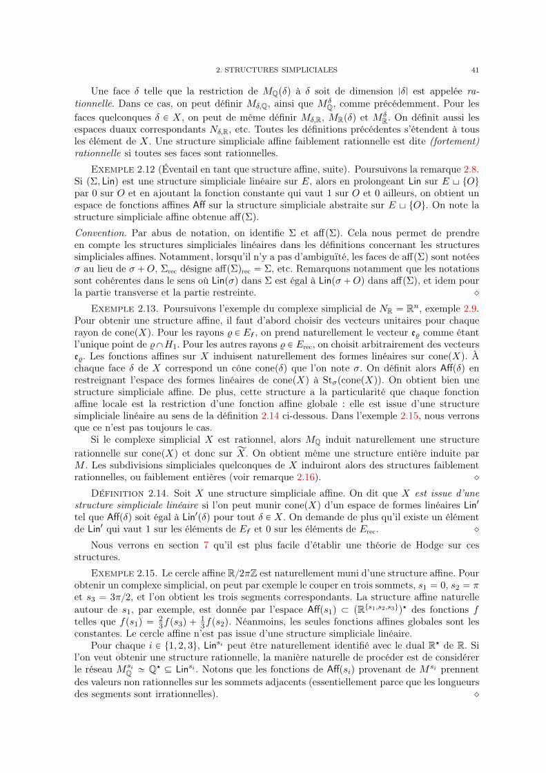
2. STRUCTURES SIMPLICIALES 41
Une face δ telle que la restriction de MQpδq à δ soit de dimension |δ| est appelée ra-tionnelle. Dans ce cas, on peut définir Mδ,Q, ainsi que M δ
Q, comme précédemment. Pour lesfaces quelconques δ P X, on peut de même définir Mδ,R, MRpδq et M δ
R. On définit aussi lesespaces duaux correspondants Nδ,R, etc. Toutes les définitions précédentes s’étendent à tousles élément de X. Une structure simpliciale affine faiblement rationnelle est dite (fortement)rationnelle si toutes ses faces sont rationnelles.
Exemple 2.12 (Éventail en tant que structure affine, suite). Poursuivons la remarque 2.8.Si pΣ, Linq est une structure simpliciale linéaire sur E, alors en prolongeant Lin sur E \ tOupar 0 sur O et en ajoutant la fonction constante qui vaut 1 sur O et 0 ailleurs, on obtient unespace de fonctions affines Aff sur la structure simpliciale abstraite sur E \ tOu. On note lastructure simpliciale affine obtenue affpΣq.
Convention. Par abus de notation, on identifie Σ et affpΣq. Cela nous permet de prendreen compte les structures simpliciales linéaires dans les définitions concernant les structuressimpliciales affines. Notamment, lorsqu’il n’y a pas d’ambiguïté, les faces de affpΣq sont notéesσ au lieu de σ`O, Σrec désigne affpΣqrec “ Σ, etc. Remarquons notamment que les notationssont cohérentes dans le sens où Linpσq dans Σ est égal à Linpσ`Oq dans affpΣq, et idem pourla partie transverse et la partie restreinte. ˛
Exemple 2.13. Poursuivons l’exemple du complexe simplicial de NR “ Rn, exemple 2.9.Pour obtenir une structure affine, il faut d’abord choisir des vecteurs unitaires pour chaquerayon de conepXq. Pour les rayons % P Ef , on prend naturellement le vecteur e% comme étantl’unique point de %XH1. Pour les autres rayons % P Erec, on choisit arbitrairement des vecteurse%. Les fonctions affines sur X induisent naturellement des formes linéaires sur conepXq. Àchaque face δ de X correspond un cône conepδq que l’on note σ. On définit alors Affpδq enrestreignant l’espace des formes linéaires de conepXq à StσpconepXqq. On obtient bien unestructure simpliciale affine. De plus, cette structure a la particularité que chaque fonctionaffine locale est la restriction d’une fonction affine globale : elle est issue d’une structuresimpliciale linéaire au sens de la définition 2.14 ci-dessous. Dans l’exemple 2.15, nous verronsque ce n’est pas toujours le cas.
Si le complexe simplicial X est rationnel, alors MQ induit naturellement une structurerationnelle sur conepXq et donc sur ĂX. On obtient même une structure entière induite parM . Les subdivisions simpliciales quelconques de X induiront alors des structures faiblementrationnelles, ou faiblement entières (voir remarque 2.16). ˛
Définition 2.14. Soit X une structure simpliciale affine. On dit que X est issue d’unestructure simpliciale linéaire si l’on peut munir conepXq d’un espace de formes linéaires Lin1
tel que Affpδq soit égal à Lin1pδq pour tout δ P X. On demande de plus qu’il existe un élémentde Lin1 qui vaut 1 sur les éléments de Ef et 0 sur les éléments de Erec. ˛
Nous verrons en section 7 qu’il est plus facile d’établir une théorie de Hodge sur cesstructures.
Exemple 2.15. Le cercle affine R2πZ est naturellement muni d’une structure affine. Pourobtenir un complexe simplicial, on peut par exemple le couper en trois sommets, s1 “ 0, s2 “ πet s3 “ 3π2, et l’on obtient les trois segments correspondants. La structure affine naturelleautour de s1, par exemple, est donnée par l’espace Affps1q Ă pRts1,s2,s3uq‹ des fonctions ftelles que fps1q “
23fps3q `
13fps2q. Néanmoins, les seules fonctions affines globales sont les
constantes. Le cercle affine n’est pas issue d’une structure simpliciale linéaire.Pour chaque i P t1, 2, 3u, Linsi peut être naturellement identifié avec le dual R‹ de R. Si
l’on veut obtenir une structure rationnelle, la manière naturelle de procéder est de considérerle réseau M si
Q » Q‹ Ď Linsi . Notons que les fonctions de Affpsiq provenant de M si prennentdes valeurs non rationnelles sur les sommets adjacents (essentiellement parce que les longueursdes segments sont irrationnelles). ˛
42 1. PRÉSENTATION DÉTAILLÉE DU TRAVAIL DE THÈSE
Remarque 2.16 (Structures entières). En général, les variétés tropicales triangulées sontnon seulement munies d’une structure faiblement rationnelle, mais aussi d’une structure fai-blement entière. Toutefois, il n’est pas clair quelle est la bonne définition pour une structuresimpliciale affine entière. Pour définir la cohomologie tropicale, il suffit de se donner des ré-seaux de rang maximaux Mpηq Ď Linpηq pour chaque facette η de X. La question est alors desavoir quelles sont les conditions de compatibilité à demander. Il faudrait par exemple que lesMQpηq :“Mpηq bQ soient induits par une structure faiblement rationnelle.
Une première définition naturelle qui se rapproche du travail de Gross et Shokrieh [GS19b]serait de choisir des réseaux Mpδq Ď Linpδq pour chaque face δ de manière compatible. Cettefaçon de faire, combinée avec une définition légèrement différente de la cohomologie tropicaleà coefficients entiers que celle que nous proposons au chapitre 2, permet d’obtenir des résul-tats plus élégants (voir le commentaire sous le théorème 1.3 du chapitre 2). Toutefois, cettedéfinition ne dépend pas uniquement du support de la variété, dans le sens où connaître leréseau Nη “M‹
η sur les facettes η ne suffit pas en général pour connaître la variété.Si l’on souhaite au contraire une définition qui ne dépend que du support, une possibilité
est de choisir des réseaux de rangs maximaux Mpσq pour chaque face σ tels que Mpσq “ř
ηąσMpηq et que, pour chaque η ą σ, Mpηq soit la restriction de Mpσq à MRpηq.Dans tous les cas, ces définitions induisent la même structure faiblement rationnelle, et
généralement l’étude du cadre rationnel, voire réel, suffit pour la plupart des applications.Dans ce chapitre, pour éviter une gestion délicate de la torsion, nous nous contenterons doncd’étudier les cas réelles et rationnelles. Toutefois le chapitre 2 propose une étude du cas entierpour les éventails simpliciaux. ˛
On étend la notion de représentation géométrique aux structures simpliciales affines de lafaçon suivante. On considère la représentation géométrique de conepXq dans RE . Soit pxeqePEle système de coordonnées correspondant. Soit H1 l’hyperplan affine défini par
ř
ePEfxe “ 1.
Alors la représentation géométrique de X est par définition le complexe simplicial obtenu enintersectant H1 avec conepXq. Notons-la xX. Le support de X, noté |X|, est le support de cecomplexe simplicial. Chaque face δ P X a son support |δ| Ď |X|.
Si Σ est une subdivision simpliciale de conepXq, alors Σ induit un sous-complexe simplicialrY de xX. On note Y la structure simpliciale abstraite associée. Il faut ensuite choisir des vecteursunitaires pour chaque rayon de rY . Maintenant, à chaque face δ P Y on peut associer une faceminimale η de X telle que le support de δ dans rY soit inclus dans |η|. Les fonctions affinesAffXpηq induisent alors naturellement un espace de fonctions affines AffY pδq au voisinage deδ. On obtient ainsi une structure simpliciale affine sur Y , et on dit que Y est une subdivisionsimpliciale de X.
2.4. Fonctions linéaires par morceaux.2.4.1. Définition. Commençons par le cas d’un complexe simplicial.
Exemple 2.17. Soit X un complexe simplicial dans Rn. On peut étudier les fonctionscontinues f : |X| Ñ R qui sont affines sur chaque face. Cela revient à se donner une valeursur chaque sommet et une pente de manière cohérente sur chaque rayon infini. En fait, pourforcer la cohérence et obtenir une fonction intéressante, on va supposer que le pseudo-éventailde récessionXrec est un éventail de récession et que f induit naturellement une fonction linéairepar cône frec sur chaque cône de Xrec. Voir chapitre 3 section 4 pour plus de détail.
Si de plus frec “ 0 alors f s’étend naturellement sur la compactification canonique X. ˛
Soit X une structure simpliciale affine sur E. Une fonction affine par morceaux sur Xdésigne n’importe quelle fonction f : E Ñ R. Dans le cas où X est de la forme affpΣq avecΣ une structure simpliciale linéaire, nous parlerons de fonction linéaire par morceaux sur Xsi de plus f est nulle sur l’unique sommet de X. Dans les deux cas, ces fonctions forment un
2. STRUCTURES SIMPLICIALES 43
R-espace vectoriel. La restriction de f à Erec définie une fonction linéaire par morceaux surXrec notée frec. De même, la restriction de f à Ef induit une fonction affine par morceaux surXf notée ff .
Si frec est nulle, alors f s’étend naturellement sur la compactification canonique X de Xen une fonction f : X1 Ñ R en envoyant pσ` sqσ sur fpsq pour tout sommet s P Xf ,1 et toutcône σ P Xrec comparable à s. Les fonctions de la forme f comme ci-dessus sont appelées lesfonctions affines par morceaux sur X.
2.4.2. Convexité. De nouveau, guidons notre intuition par un exemple.
Exemple 2.18. En général, une fonction g : Rn Ñ R est convexe si pour tout x P Rn ilexiste une forme affine ` : Rn Ñ R telle que f ´ ` est nulle sur x et positive autour de x.L’ensemble des fonctions convexes forme un cône, et les éléments dans l’intérieur relatif de cecône sont appelés strictement convexes. On peut restreindre cette définition à un support pluspetit, par exemple à un espace polyédral. On obtient alors la définition suivante.
Si X est un complexe simplicial, on dit qu’une fonction affine par morceaux f est convexe,resp. strictement convexe, si pour toute face δ P X, il existe une forme affine ` telle que f ´ `soit nulle sur |δ| et positive, resp. strictement positive, sur un voisinage de l’intérieur relatifde δ dans |X|. ˛
Soit f est une fonction affine par morceaux sur X. Soit δ une face de X. La fonctionf induit naturellement une fonction affine par morceaux sur l’éventail étoile StδpXq. Notonscette fonction fδ. On peut lui soustraire n’importe quelle fonction affine ` P Affpδq. On dit quef est convexe autour de δ, resp. strictement convexe autour de δ, s’il existe ` P Affpδq telle quefδ ´ ` est nulle sur δ et positive, resp. strictement positive, sur pStδpXqq1 r δ. On dit que fest convexe, resp. strictement convexe, si elle l’est autour de chaque face.
On dit que X est quasi-projective si X admet une fonction strictement convexe. La com-pactification canonique X est alors dite projective.
Remarque 2.19. Dans le cas où Σ est un éventail simplicial rationnel de Rn, alors lastructure simpliciale linéaire associée à Σ est quasi-projective si et seulement si CPΣ estquasi-projectif. L’article [GM12] explicite le lien entre la convexité des fonctions sur Σ etles propriétés des diviseurs associés sur CPΣ. ˛
Question 2.20. Soit X un complexe simplicial dans Rn dont la structure simplicialeaffine associée est quasi-projective. Peut-on plonger X dans un espace projectif TPn telle quel’adhérence de l’image soit isomorphe à X ? ˛
2.5. Compactification canonique revisitée. SoitX une structure simpliciale. On noteX et on appelle compactification canonique de X le complexe polyédral abstrait dont les facessont les couples pσ, δq où σ est un cône de Xrec et δ est une face de X contenant σ. On note untel élément δσ, ou parfois δσ
8pour éviter de confondre avec les éléments de Xσ
rec. Un tel coupleest appelé une face de X, et σ est appelé la sédentarité de cette face et est noté sedpδσq. Parabus de langage, on appelle aussi sédentarité la dimension de sedpδσq. La dimension de δσest |δσ| “ cardpδq ´ cardpσq ´ 1. Toujours par notre convention, nous utiliserons la notationη P X pour signifier que η est une face de X. En ajoutant un élément minimal 0 et un élémentmaximal 1, les faces de X forment un treillis où γσ ă δτ si γ ă δ et σ ą τ . Notons que Xn’est pas simplicial en général (voir section 1.8).
Pour chaque cône σ P Xrec, l’ensemble des faces de X de la forme δσ forme naturellementles faces d’une structure simpliciale que l’on note Xσ
8(notamment X0
8“ X). L’éventail de
récession associé Xσ8,rec est isomorphe à pXrecq
σ. Sa compactification Xσ8peut être vue comme
incluse dans X : les faces correspondantes sont celles de la forme δη pour η ą σ. Les structuresXσ8pour σ P Xrec sont appelées les strates divisorielles ouvertes de X et forment une partition
de X. Les éléments Xσ8seront appelés les strates divisorielles fermées. Pour justifier cette
44 1. PRÉSENTATION DÉTAILLÉE DU TRAVAIL DE THÈSE
dénomination, si ρ P Xrec est un rayon et si X est associée à une variété tropicale, la strateXρ8est un diviseur tropical de X (lié au diviseur de CPXrec associé au rayon ρ).
Définition 2.21. Si X est une structure simpliciale affine, la compactification canoniqueX de X est la compactification de la structure simpliciale sous-jacente munie des espacesaffines Affpδσq “ Affpδqσ.
La compactification canonique X de X est dite faiblement rationnelle, resp. rationnelle, siX est faiblement rationnelle, resp. rationnelle, et si Xrec est rationnelle. ˛
On aura donc Linδσ“ Linδ, Linpδσq “ Linpδqσ, où l’on voit σ comme un cône de StδpXq,
et Linδσ “ Linσδ .En particulier, si γσ ă δτ sont deux faces deX, on a une flèche naturelle Linpγσq Ñ Linpδτ q.
Celle-ci est obtenue en composant l’inclusion Linpγσq ãÑ Linpγτ q et la restriction Linpγτ q Linpδτ q.
À propos de la rationalité, on doit exiger que Xrec soit fortement rationnelle pour que lesstrates à l’infini soient elles-mêmes rationnelles. Ainsi, si X est faiblement rationnelle, resp.rationnelle, alors Xσ est faiblement rationnelle, resp. rationnelle, pour tout cône σ P Xrec.
Exemple 2.22 (Éventail en tant que structure affine, suite et fin). Par notre conventionde l’exemple 2.13, on peut considérer qu’une structure linéaire Σ est une structure affine. No-tamment sa compactification canonique Σ a un sens. Ses faces sont στ
8pour τ ă σ (ici l’indice
8 est particulièrement important) et la structure linéaire associée est Linpστ8q “ Linpσqτ . N.B.,
|στ8| “ |σ|´ |τ |, de plus on note parfois 8σ au lieu de σσ
8pour les sommets. ˛
La représentation géométrique de X est simplement l’adhérence de la représentation géo-métrique de X dans REf ˆTErec (ou de manière équivalente dans TE). La topologie sur T estcelle induite par R et par les voisinages ouverts de l’infini sa;8s, pour a P R. On munit |X|de la topologie induite par la topologie produit sur TE .
Si X 1 est une subdivision de X telle que X 1rec “ Xrec, alors on appelle X 1 une subdivisionde X.
Exemple 2.23. Si X est issue d’un complexe polyédral ĂX de Rn, alors il existe un homéo-morphisme entre le support |X| de X et le support de ĂX qui est compatible avec le support desfaces. Dans 1.8, nous avons vu comment construire directement la compactification canoniquede ĂX, et l’homéomorphisme se prolonge alors sur les compactifications respectives. Dans cecadre-là, nous identifierons naturellement le support de X avec celui de ĂX. ˛
Remarque 2.24. Nous considérerons souvent des sous-structures d’une compactifica-tion canoniques qui ne sont pas à proprement parler des structures simpliciales affines, voirl’exemple 2.25 ci-dessous. On pourra facilement étendre certaines définitions à ce cadre, parexemple la cohomologie tropicale fait sens pour ces sous-structures. ˛
Exemple 2.25. On peut considérer la structure simpliciale affine induite par le complexepolyédral sur R constitué de trois faces : t0u, R´ et R`. La compactification canonique peutêtre vue comme un complexe polyédral étendu sur r´8,`8s. On peut alors considérer le sous-complexe induit sur s´8,`8s, que l’on peut qualifier de structure simpliciale affine naturellesur T. ˛
3. Cohomologie tropicale, dualité de Poincaré et lissité
Rappelons que, par convention, nous remplaçons désormais Lin par MR, et de même pourtoutes les formes dérivées.
L’homologie tropicale a été introduite par Itenberg, Katzarkov, Mikhalkin et Zharkovdans [IKMZ19] pour retrouver les nombres de Hodge d’une fibre générale d’une famille devariétés complexes à partir de sa limite tropicale. Nous reviendrons en section 3.8 sur les

3. COHOMOLOGIE TROPICALE, DUALITÉ DE POINCARÉ ET LISSITÉ 45
résultats de cet article en proposant une justification pour la définition ci-dessous qui est peunaturelle a priori.
3.1. Éléments canoniques et orientation. Soit X une structure simpliciale affine (oulinéaire). Si γ ă δ, on note nδγ et on appelle vecteur canonique de δ normal à γ tout vecteurde Nδ,R tel que pour tout ` PMγ
R, la valeur de ` sur la projection de nδγ vaut `pδγq. Dans lecas où δ est représentée par un simplexe, nδγ peut par exemple être n’importe quel vecteurd’origine un point de γ et d’extrémité le sommet de δ qui n’est pas dans γ.
Si e est une arête de X et si v1, v2 sont les extrémités de e, alors nev1“ ´nev2
. On choisitarbitrairement l’un de ces deux vecteurs que l’on note νe. Si ρ P X1 est un rayon, on poseνρ :“ nρv où v est l’extrémité du rayon. Plus généralement, si δ est une face de X et si s estun sommet de δ, on pose νδ P
Ź|δ|pNδ,Rq égal à ˘
Ź
eνe où e parcourt les arêtes de δ contenants. Ce multi-vecteur est bien défini modulo un signe, on choisit ce signe arbitrairement. Deplus, si δ “ s est un sommet, on prend νs “ 1 P
Ź0Ns,R » R. On appelle νδ le multi-vecteurcanonique de δ. On note ωδ P
Ź|δ|Mδ,R » R le dual de νδ, que l’on appelle la forme canoniquede δ.
Remarque 3.1. Dans les chapitres 2, 3 et 4, νδ et nδγ désignent en fait des multiples desdéfinitions données ci-dessus pour qu’ils deviennent unitaires pour le réseau sous-jacent. Dansle cas d’une triangulation unimodulaire, les deux définitions coïncident. ˛
En notant sign : R Ñ t´1, 0,`1u la fonction associant à chaque nombre son signe, onpeut définir signδ :“ sign˝ωδ. La donnée psignδqδPX définie une orientation sur X. Pour toutepaire γ ă δ, on définit alors le signe
signpγ, δq :“ signδpnδγ ^ νγq.
Ces signes ne dépendent pas du choix précis des νδ mais seulement de l’orientation. Dansla suite, on supposera toujours que les structures simpliciales affines sont munies de multi-vecteurs canoniques, des formes canoniques correspondantes et de l’orientation correspon-dante.
On étend ces définitions de manière naturelle à X, c’est-à-dire que pour tout δ P X etpour toute paire τ ă σ dans Xrec avec σ ă δ, on prend νδσ8 égal à la projection de νδrσ dansNσδ,R “ Nδσ ,R, et l’on pose nδτδσ égal à la projection de ´nδrτ δrσ dans Nδ,R.Toutes ces notions induisent des éléments naturels sur les structures transverses. À la face
δγ P Σγ on associe νγδ PŹ|δ|´|γ|Nγ
δ,R comme la projection de n’importe quel multi-vecteur v
de δ tel que νγ ^ v “ νδ. La définition ne dépend pas du choix de ce multi-vecteur.
Remarque 3.2 (Cas rationnel). Soit X est une structure simpliciale rationnelle de di-mension au moins deux. Supposons que pour toute paire de faces τ, τ 1 dans X1, il existe unesuite de faces τ0, . . . , τs dans X1 telle que τ0 “ τ , τs “ τ 1 et τi _ τi`1 P X2. C’est le cas dansla plupart des exemples intéressants, par exemple si X est irréductible et orientable commedéfinie en section 3.4. Soit σ P X2 et τ ă σ. On peut trouver un facteur λ non nul tel que λντsoit rationnel. On peut alors montrer que pour tout τ 1 ă σ, λντ 1 est rationnel. De proche enproche, on en déduit que tous les λντ2 pour τ2 P X1 sont rationnels. Quitte à effectuer unehomothétie de rapport λ, on peut donc supposer que tous les multi-vecteurs canoniques sontrationnels. ˛
3.2. Homologie et cohomologie tropicales. Soit Z une structure simpliciale affine dedimension d ou sa compactification canonique. Soit δ une face de Z. Soit k P tR,Qu (pourk “ Q, on suppose Z faiblement rationnelle). Pour tout p P t0, . . . , du, on pose
Fppδ, kq :“ÿ
ηąδ
ŹpNη,k ĎŹpNkpδq, et Fppδq “ Fppδq
‹.

46 1. PRÉSENTATION DÉTAILLÉE DU TRAVAIL DE THÈSE
Pour plus d’information sur l’origine de cette définition, nous renvoyons le lecteur à lasection 3.8. Pour toute paire γ ă δ, l’inclusion Nkpγq Ñ Nkpδq induit naturellement uneapplication Bδąγ : Fppδ, kq Ñ Fppγ,kq et l’application duale dγăδ : Fppγ,kq Ñ Fppδ, kq.
On définit, pour toute paire d’entiers p et q,
Cp,qpZ,kq :“à
δPZqδ compact
Fppδ, kq.
Si δ P Zq et si v P Fppδ, kq, nous noterons pδ,vq l’élément de Cp,qpZ,kq qui vaut v sur la faceδ et zéro ailleurs.
On obtient un complexe de chaînes
Cp,‚pZ, kq : ¨ ¨ ¨ ÝÑ Cp,q`1pZ,kqBq`1ÝÝÝÑ Cp,qpZ,kq
BqÝÝÑ Cp,q´1pZ,kq ÝÑ ¨ ¨ ¨
où les différentielles sont définies de manière habituelle en envoyant pδ,vq, avec δ P Zq etv P Fppδ, kq, sur
ÿ
γăδ
signpγ, δqpγ, Bδ ąγvq P Cp,q´1pZ,kq.
On obtient alors l’homologie tropicale à coefficients dans k en posant
Hp,qpZ, kq :“ker
`
Bq : Cp,qpZ,kq ÝÑ Cp,q´1pZ,kq˘
Im`
pBq`1 : Cp,q`1pZ,kq ÝÑ Cp,qpZ,kq˘ .
On peut définir de la même manière l’homologie de Borel-Moore tropicale de Z à coefficientdans k, HBM
p,q pZ, kq, à partir des groupes de chaînes suivants :
CBMp,q pZ,kq :“
à
δPZq
Fppδ, kq,
où cette fois-ci l’on n’exige plus la compacité des faces concernées.On définit ensuite les notions duales. On pose
Cp,qpZ, kq :“ Cp,qpZ,kq‹ »à
δPZqδ compact
Fppδ, kq,
et l’on obtient le complexe de cochaînes dual au complexe de chaînes Cp,‚,
Cp,‚pZ, kq : ¨ ¨ ¨ ÝÑ Cp,q´1pZ,kq dq´1
ÝÝÝÑ Cp,qpZ,kq dqÝÝÑ Cp,q`1pZ,kq ÝÑ ¨ ¨ ¨
On définit alors la cohomologie tropicale de Z à coefficients dans k, notée Hp,qpZ,kq, commeétant la cohomologie de ce complexe de cochaînes. Notamment on obtient Hp,qpZ,kq »Hp,qpZ, kq‹ car ici k est un corps, donc il n’y a pas de torsion.
De même, le dual de CBMp,q pZ, kq est noté C
p,qc pZ,kq. La cohomologie associée est appelée
la cohomologie tropicale à support compact de Z à coefficients dans k, et est notée Hp,qc pZ,kq.
On obtient un isomorphisme Hp,qc pZ,kq » HBM
p,q pZ,kq‹.On définit de plus le kème groupe d’homologie tropicale par
HkpZ,kq :“à
p`q“k
Hp,qpZ,kq,
et l’on définit HBMk pZ, kq, HkpZ, kq et Hk
c pZ,kq de manière similaire. Ces dernières définitionsamène une question naturelle.
Question 3.3. Existe-t-il une définition intrinsèque du kème groupe d’homologie tropicalsans passer par l’homologie bigraduée ? ˛
Notons que si Z est une compactification canonique, alors trivialement HBM‚,‚ pZ,kq »
H‚,‚pZ, kq et H‚,‚c pZ,kq » H‚,‚pZ, kq.
3. COHOMOLOGIE TROPICALE, DUALITÉ DE POINCARÉ ET LISSITÉ 47
Remarque 3.4. Si Z est faiblement rationnel, remarquons que, par le théorème des co-efficients universels, Hp,qpZ,Rq » Hp,qpZ,Qq bR, et de même pour la cohomologie à supportcompact et pour les deux versions d’homologie. ˛
Convention. Dans la suite, nous poserons k égal à R ou Q et nous omettrons de préciserle corps k utilisé pour calculer la cohomologie. Dans le cas k “ Q, nous supposerons que lesobjets concernés sont fortement rationnels. En effet, bien que certaines définitions s’étendentdirectement au cas faiblement rationnel, pour d’autres cela est moins évident. Nous feronsparfois quelques commentaires sur le cas faiblement rationnel.
3.3. Définitions alternatives. Bien que l’on étudie des cohomologies simpliciales dontles coefficients dépendent de la face, on peut, comme pour la cohomologie classique, calculerles mêmes groupes de cohomologie grâce à de nombreuses versions différentes.
Comme expliqué plus tôt, l’homologie tropicale, plus précisément la version cellulaire, aété introduite dans [IKMZ19]. Une étude plus générale de la cohomologie tropicale, notam-ment l’équivalence entre la version cellulaire et des versions singulières et faisceautiques, aété décrite par la suite dans [MZ14]. Pour étudier la dualité de Poincaré, les versions com-pactes et de Borel-Moore sont introduites dans [JSS19] et [JRS18]. Dans [JSS19] est aussiintroduite la cohomologie de Dolbeault tropicale, qui ressemble beaucoup à la cohomologiede Dolbeault classique, c’est-à-dire à une version complexe de la cohomologie de de Rham.C’est probablement la version qui peut paraître la plus naturelle pour une personne familièrede la théorie de Hodge classique. Elle s’appuie sur une définition similaire pour les espaces deBerkovich [CLD12,Jel16a,Jel16b,Liu20].
Nous n’utiliserons que la version cellulaire décrite ci-dessus dans la suite de ce chapitre.Toutefois, nous décrivons la version faisceautique ci-dessous. Celle-ci a été particulièrementfouillée dans [GS19b]. L’existence d’une version faisceautique nous est utile car elle montreque la cohomologie ne dépend que du support.
Un ouvert basique de |Z| est un ouvert connexe U tel qu’il existe une face γ P Z, appeléeface minimale de U , avec U X |γ| connexe et telle que U inclus dans l’union des intérieurs(relatifs) des |η| pour η ą γ. Ces ouverts forment une base pour la topologie sur Z.
On définit le faisceau FpZ,k en posant Fp
Z,kpUq “ Fppγq pour n’importe quel ouvert basiqueU de face minimale γ. Cela définit bien de manière unique un faisceau sur Z.
Théorème 3.5. Pour tout entier p, q, on a
Hq´
|Z|,FpZ,k
¯
» Hp,qpZ,kq et Hqc
´
|Z|,FpZ,k
¯
» Hp,qc pZ,kq.
Démonstration. Le faisceau FpZ,k est un faisceau constructible stratifié par les supports
|Zďk| pour k ě 0. On peut calculer sa cohomologie via le faisceau cellulaire correspondant(voir [She85]), qui est exactement la cohomologie tropicale définie plus haut. Nous renvoyonsà [She85,Cur14] pour la théorie générale des faisceaux cellulaires ou simpliciaux et à [MZ14,JSS19,JRS18] pour le cas particulier de la cohomologie tropicale.
Remarque 3.6. Du point de vue de la cohomologie de Dolbeault tropicale, le faisceauFpZ,k est l’analogue tropical du faisceau des p-formes holomorphes d’une variété complexes :
c’est le noyau pour les pp, 0q-formes lisses de la différentielle anti-holomorphe tropicale. Ainsi,Hq
´
|Z|,FpZ,k
¯
est bien l’analogue du groupe de cohomologie de Dolbeault classique de bidegrépp, qq. ˛
Corollaire 3.7. Soit X une structure simpliciale affine. Si X 1 est une subdivision sim-pliciale de X, alors H‚,‚pX,kq » H‚,‚pX 1,kq et H‚,‚c pX,kq » H‚,‚c pX 1, kq. De plus, si X 1rec “
Xrec, alors H‚,‚pX, kq » H‚,‚pX1, kq.

48 1. PRÉSENTATION DÉTAILLÉE DU TRAVAIL DE THÈSE
Le cadre des structures simpliciales affines est assez général. Toutefois, il n’est pas clairqu’il contient par exemple les variétés tropicales lisses au sens de [JSS19].
Question 3.8. Soit Z un espace polyédral compact au sens de [JSS19] qui est localementmatroïdal. Soit X sa partie de sédentarité nulle. Peut-on munir X d’une structure simplicialeX telle que Z soit le support de X ? ˛
Il existe aussi une notion de polyèdres étendus réguliers, par exemple dans [IKMZ19],qui sont des polyèdres respectant la stratification à l’infini. Dans la question précédente, sil’on suppose de plus que Z est munie d’une structure de faces régulières, alors il devrait êtrepossible de trouver une triangulation de la partie de sédentarité 0 de Z qui fournirait uneréponse positive à la question.
On devrait aussi pouvoir sans trop de difficulté définir des espaces topologiques enri-chis d’une structure affine généralisant simultanément les espaces polyédraux étendus et lesstructures simpliciales affines. Nous n’avons pas essayé de le faire ici car, de toute façon, lesdémonstrations des théorèmes principaux de cette thèse utilisent des triangulations. En sec-tion 7.1.3, nous verrons une tentative de preuve pour établir une théorie de Hodge tropicalesans passer par les triangulations, qui pour l’instant n’a pas aboutie.
3.4. Orientabilité, irréductibilité et classes fondamentales. Soit X une structuresimpliciale affine de dimension d. On dit que X est R-orientable, ou simplement orientable(à ne pas confondre avec les orientation au sens de la section 3.1), s’il existe un cycle dansCBMd,d pX,Rq de support Xd tout entier. On dit que X est R-orientée, ou simplement orientée,
si de plus on a fait le choix d’un tel cycle. Dans ce cas, on note ce cycle rXs et on l’appellel’élément canonique de X. La classe correspondante dans HBM
d,d pX,Rq est elle aussi notée rXset est appelée la classe fondamentale de X.
Cette notion est très liée à la notion de condition d’équilibre en géométrie tropicale.En effet, on a la proposition suivante qui se démontre immédiatement par le calcul (voirexemple 3.10).
Proposition 3.9. Un élémentř
ηPXdwpηqpη, νηq est un cycle si et seulement s’il est
équilibré dans le sens suivant : pour toute face τ P Xd´1,ÿ
η ąτ
wpηqnητ P Nτ,R.
Si X est orientée, alors pour tout δ P X la structure transverse Xδ de X est naturellementorientée. En effet, si rXs “
ř
ηPXd wpηqpη, νηq, alors on pose
rXδs “ÿ
ηPXd
ηąδ
wpηqpηδ, νδηq.
SiX est orientable et siHBMd,d pX,Rq est de dimension un, nous dirons queX est irréductible.
Dans ce cas, l’élément canonique de X est bien défini à un facteur près.Notons que CBM
d,d pX,Rq “ CBMd,d pX,Rq “ Cd,dpX,Rq. Ainsi, X sera dite orientable, resp.
orientée, resp. irréductible, si X l’est. L’élément canonique de X est l’élément induit par rXs.De même, si X est faiblement rationnelle, on peut définir la Q-orientabilité, etc., mais
par le théorème des coefficients universels, toutes ses propriétés sont équivalentes au cas réel.Toutefois, notons qu’une structure simpliciale Q-orientée a un élément canonique rationnel.
Convention. Dans le cas fortement rationnel, si une structure est Q-orientable, nous feronsautomatiquement l’hypothèse que les éléments canoniques νδ sont rationnels. Dans le cas oùla structure est de dimension au moins deux, cela peut se faire sans perte de généralité par laremarque 3.11. Une telle hypothèse n’est pas toujours possible pour la dimension un, mais cecas-là peut être traité à part et nous ne nous en préoccuperons pas ici.
3. COHOMOLOGIE TROPICALE, DUALITÉ DE POINCARÉ ET LISSITÉ 49
Exemple 3.10. Soit X une variété tropicale pondérée de dimension d dans Rn. Il s’agitdonc du support d’un complexe simplicial rationnel X de Rn. De plus, chaque facette σ deX est munie d’un poids wpσq. Pour simplifier en évitant d’introduire de nouvelles notations,supposons que X soit munie d’une triangulation unimodulaire par rapport à N “ Zn Ď Rn.Pour chaque face η P Σ, le multi-vecteur canonique νη P
Ź|η|Nη,Q est alors unitaire pour leréseau Nη.
Alors, comme on l’a vu en section 1.7, X vérifie la condition d’équilibre pondérée : pourtoute face τ P Xd´1,
ÿ
σ ąτ
wpσqnστ P Nτ .
Pour toute paire σ ą τ , on a νσ “ signpτ, σqnστ ^ ντ . Ainsi, par la condition d’équilibreci-dessus, pour toute face τ de codimension un,
ÿ
σ ąτ
signpτ, σqwpσqνσ “ 0.
Doncř
σPΣdpσ,wpσqνσq P C
BMd,d pXq est un cycle. C’est même un choix canonique pour l’élément
canonique rXs de X.Toute variété tropicale pondérée triangulée de Rn est donc naturellement une structure
simpliciale affine orientée faiblement rationnelle. On voit bien le lien ici entre le fait d’êtretropical, c’est-à-dire équilibré, et l’orientabilité. ˛
3.5. Cup-produit. Soit X une structure simpliciale affine de dimension d sur E. Alors ilexiste un cup-produit naturel ! : Hp,qpXqbHp1,q1
c pXq Ñ Hp`p1,q`q1c pXq. On peut l’obtenir en
adaptant le cup-produit simplicial classique sur conepXq, ou bien par exemple via les formesde Dolbeault comme dans [JSS19].
De même, nous avons un cup-produit ! : Hp,qpXq bHp1,q1pXq Ñ Hp`p1,q`q1pXq.
Exemple 3.11 (Cas d’un éventail). Traitons le cas d’une structure simpliciale linéaire Σ.Ce cas est particulièrement simple. En effet, Σ n’a qu’une seule face compacte : 0. Donc
Hp,qpΣq “ Cp,qpΣq “
#
Fpp0q si q “ 0,0 sinon.
On peut alors définir le cup-produit directement sur les cochaînes de la façon suivante. Sia “ p0, αq P Cp,0pΣq avec α P Fpp0q et si b “ pσ, βq est un élément de Cp1,q1pΣq, a ! b estsimplement égal à pσ, α^ βq.
Pour la compactification canonique, rappelons que Σ est naturellement un complexe cu-bique. Il existe une manière naturelle de définir le cup-produit sur les complexes cubiques. Onpeut ainsi donner une formule explicite, ce qui est fait en chapitre 2 section 7.4.
Dans le cas de la compactification canonique d’une structure simpliciale affine X, on peutcalculer le cup-produit en travaillant dans conepXq quitte à mettre 0 sur les éléments deconepXq ne correspondant pas à des faces de X. ˛
3.6. Dualité de Poincaré. Soit Z une structure simpliciale affine irréductible orientéeou sa compactification. Alors on note deg P Hd,d
c pZq‹ l’élément dual à rZs que l’on appellel’application degré, et que l’on peut aussi interpréter comme l’intégrale sur Z (cf. [JSS19]).Pour toute paire d’entiers p et q, en composant l’application degré et le cup-produit nousobtenons donc un accouplement
Hp,qpZq bHd´p,d´qc pZq Ñ k.
Définition 3.12. On dit que Z vérifie la dualité de Poincaré si l’accouplement ci-dessusest parfait, c’est-à-dire si Hp,qpZq Ñ Hd´p,d´q
c pZq‹ est un isomorphisme. ˛
50 1. PRÉSENTATION DÉTAILLÉE DU TRAVAIL DE THÈSE
Exemple 3.13. Poursuivons l’étude de la structure simpliciale linéaire Σ. Dans ce cas,la dualité de Poincaré revient à montrer que Hp,q
c pΣq est nul pour q ‰ d, et que Hp,dc pΣq »
Fd´pp0q. L’application Hp,dc pΣq Ñ Fd´pp0q peut être facilement décrite. Elle envoie pη, αq sur
ιαpνηq. On peut montrer que cette application est toujours surjective. Nous poursuivrons cetteétude en section 4. ˛
3.7. Lissité. Comment définir la lissité pour un espace polyédral ? La définition géomé-trique classique de lissité est difficile à adapter dans ce contexte. En effet, pour deux pointsquelconque, les voisinages des deux points peuvent être très différents.
Une première idée serait de définir la lissité en demandant d’être localement la tropicalisa-tion d’une variété lisse. C’est a priori une mauvaise définition car une telle tropicalisation peutprendre plusieurs formes dont certaines très singulières. De plus, les variétés tropicales ne sontpas toujours réalisables, même localement, comme nous l’avons vu dans la remarque 1.10.
Toutefois, les tropicalisations des complémentaires d’arrangement d’hyperplans dans letore ont de bonnes propriétés. Il s’agit de support de Bergman comme nous l’avons vu ensection 1.3. Jusqu’à présent, une variété tropicale était dite lisse si elle était localement ma-troïdale, c’est-à-dire, nous le rappelons, localement de la forme |Σ|ˆ Tk avec |Σ| un supportde Bergman. C’est la définition utilisée dans [IKMZ19] et par la suite dans [JSS19,MZ14,MR18,JRS18,GS19b,GS19a] par exemple. Les variétés tropicales lisses dans ce sens véri-fient la dualité de Poincaré [JSS19].
Nous souhaitons proposer une nouvelle définition de lissité, plus large. Nous allons proposerune définition purement homologique, allant dans le sens de l’étude des variétés homologiques,cf. [Čec33,Lef33,Beg42,Bor57,Wil65,BFMW96,BFMW07,Mio00,Wei02]. A priorila lissité doit être une notion locale, et une variété lisse doit vérifiée la dualité de Poincaré.Nous proposons donc la définition informelle suivante. Un espace polyédral muni des faisceauxtropicaux F‚ est lisse si tout ouvert connexe de cette variété vérifie la dualité de Poincaré. Demême, on souhaite dire qu’une structure simpliciale affine X est lisse si l’espace polyédral |X|est lisse au sens précédent.
Le paragraphe ci-dessus est une justification intuitive de la nouvelle définition de lissité.Toutefois, d’un point de vue pragmatique, si une variété tropicale est la limite d’une famillede variétés, nous souhaiterions que la lissité implique que la variété tropicale se souviennentde nombreuses informations des fibres proches de la fibre centrale. C’est un rôle que rempliparfaitement la notion d’être localement matroïdal. Avec Amini, nous avons pour projet demontrer que la nouvelle notion de lissité remplit bien ce rôle, notamment dans la perspec-tive d’étudier des variétés algébriques proches de la limites tropicales pour des familles plusgénérales que celles étudiées par [IKMZ19] (voir section 3.8).
À partir de la définition informelle de lissité ci-dessus, essayons de justifier la définition 3.14.Des résultats plus précis seront donnés plus tard. Dans les espaces polyédraux raisonnables(on souhaite entre autre éviter le cas de la figure 3, cf. [IKMZ19,JSS19,Sma17]), chaquepoint a un voisinage isomorphe à un espace de la forme |Σ| ˆ Rk ˆ Tl où |Σ| est le supportd’un éventail. Si le monde est bien fait, R et T devraient être lisses, et donc devraient vérifierla dualité de Poincaré. Le point essentiel est donc la dualité de Poincaré pour Σ.
Définition 3.14. Une structure simpliciale affine orientée X est lisse si Xδ vérifie ladualité de Poincaré pour toute face δ de X. De plus, X est dite lisse si X l’est. ˛
Théorème 3.15. Si X est une structure simpliciale affine orientée lisse, alors X et Xvérifient la dualité de Poincaré.
Nous n’avons pas encore les outils pour faire la preuve avec la cohomologie cellulaire, ce quenous ferons dans le cas des structures simpliciales linéaires en théorème 3.15. Nous donnonsci-dessous une preuve faisceautique qui, au passage, justifie la définition de la lissité.
3. COHOMOLOGIE TROPICALE, DUALITÉ DE POINCARÉ ET LISSITÉ 51
Démonstration. Montrons le résultat pour X. La preuve est similaire pour X. Soitδσ une face de X. Alors tout ouvert basique de |X| de face minimale δσ est homéomorphe à|Xδ|ˆR|δσ |ˆT|σ|. L’homéomorphisme induit des isomorphismes de faisceaux pour les faisceauxF‚ associés. On vérifie directement la dualité de Poincaré pour les espaces R et T. De plus, parhypothèse, |Xδ| vérifie aussi la dualité de Poincaré. Via la formule de Künneth (cf. [GS19b],voir aussi théorème 6.1), on en déduit que le produit, et donc l’ouvert de base, vérifie la dualitéde Poincaré. Rappelons que les ouverts de base forment une base d’ouverts pour la topologie.On obtient alors la dualité de Poincaré pour X en utilisant une résolution par des faisceauxfins comme dans [JSS19].
Dans [GS19b], Gross et Shokrieh ont montré que toute variété tropicale localement ma-troïdale vérifie la dualité de Verdier à coefficients entiers. Plus précisément, si Z est unevariété tropicale localement matroïdale de dimension d munie d’une structure entière, le fais-ceau Fp
Z est dual à Fd´pZ rds dans la catégorie dérivée des complexes de cochaînes bornées de
ZZ -modules. Voici une question qui nous a été posée par Shokrieh.
Question 3.16. Peut-on étendre ce résultat aux variétés tropicales lisses ? ˛
La proposition suivante est immédiate par la définition.
Proposition 3.17. Si X est lisse, alors pour toute face δ de X, Xδ et Xδ sont lisses. Deplus, pour toute face σ P Xrec, les strates à l’infini Xσ et Xσ sont lisses.
Exemple 3.18 (Cas de la dimension 1). Dans cette thèse, nous appellerons droite tropicaleune structure simpliciale linéaire Σ de dimension un orientable et irréductible, c’est-à-dire qu’iln’y a qu’une seule relation de dépendance entre les νρ pour ρ P Σ de la forme
ř
ρPΣ aρνρ “ 0et que les coefficients aρ sont tous non nuls. Il s’agit exactement des éventails de Bergman dedimension un.
On se convainc facilement qu’il s’agit des seules structures simpliciales linéaires lisses dedimension un. ˛
3.8. Lien avec les variétés complexes. Cette section ne vise qu’à développer uneintuition de certains phénomènes, souvent conjecturaux, et à suggérer des applications et desgénéralisations possibles des résultats de cette thèse. Nous ne prétendons pas énoncer desrésultats précis. Ainsi, toute affirmation de cette section doit être considérée avec précaution,et nous renvoyons le lecteur à différents articles pour plus de précision.
Pour mieux comprendre la définition de la géométrie tropicale et pourquoi elle possède desi bonnes propriétés, il nous semble utile d’expliquer son origine. Le but originel de l’homolo-gie tropicale, développé dans [IKMZ19], est de retrouver la cohomologie d’une fibre généraled’une famille de variétés projectives complexes à partir de sa limite tropicale dans des cas spé-cifiques (voir ci-dessous). Pour cela, les auteurs ont exploité la théorie de Hodge asymptotique.Nous en reparlerons plus loin.
D’un autre côté, dans le cas des hypersurfaces projectives complexes, il existe une joliedécomposition en pantalons de la fibre générale, décomposition dont les parties sont indexéespar les faces d’une certaine triangulation sur la limite tropicale [Mik04b]. En fait, la fibregénérale se projette sur la limite tropicale en des fibres que l’on peut décrire explicitement.Nous appelons cette fibration une fibration en tores pour une raison qui deviendra bientôtclaire. Dans le cas où la limite tropicale est lisse, le lien entre la cohomologie tropicale de lalimite et la cohomologie de la fibre générale peut être vu très naturellement (cf. [Arn20]).
L’existence d’une fibration en tores dans le cas général, notamment dans le cas des variétésde Calabi-Yau, est un problème intéressant lié notamment à la conjecture SYZ en symétriemiroir [SYZ96,Zha00,Li20].
Une fibration similaire apparaît dans [Cle69] pour essayer de comprendre l’action de lamonodromie sur une famille de variétés. Rappelons que la monodromie a un équivalent sur la
52 1. PRÉSENTATION DÉTAILLÉE DU TRAVAIL DE THÈSE
limite tropicale, l’opérateur eigenwave, qui est lié aux déformations de la variété tropicale età la famille l’approximant [MZ14].
Dans cette section, nous nous placerons dans un cas idéal où la fibration susmentionnéeexiste.
3.8.1. Fibration en tores. En s’inspirant des figures 7 et 8, nous pourrions espérer l’exis-tence d’une fibration en tores de la forme suivante pour les fibres proches Wt.
— L’application étendue Logt : W t Ñ TPXrec se rétracte en une application surjectivecontinue tropt : W t Ñ X qui respecte les stratifications des variétés toriques CPXrec
et TPXrec .
— À chaque face δσ de la compactification canonique X et à chaque point x de |δσ| Ď X
on peut associer Fx,δσ Ď trop´1t pxq qui est homéomorphe à UδˆpS1q
|δσ | » UδˆT|δσ |R ,
où l’on rappelle que Uδ est la partie ouverte de la composante associée à δ dans lafibre centrale (cf. section 1.11.3).
— On peut choisir ces homéomorphismes tels qu’il existe une application continueW t Ñ
W 0 qui induit les projections naturelles Uδ ˆ pS1q|δσ | Ñ Uδ.
— Pour chaque point x, si η est la face minimale de X contenant x dans son support,alors trop´1
t pxq “ F x,η “Ů
η1Qx Fx,η1 .
— Pour chaque ouvert basique de X de face minimale δσ, sa préimage par tropt esthoméomorphe à δσ ˆ Uδ ˆ pS1q
|δσ | ˆ C|σ|, c’est-à-dire à Uδ ˆ T|δσ |C ˆ C|σ|.
Notons qu’un analogue tropical de cette décomposition est valable sur X. Il faut alorsremplacer Uδ par un point qui se souvient que son éventail transverse est Xδ, remplacer S1
par un point et C par T.
Exemple 3.19. Dans les figures 7 et 8, nous obtenons bien cette décomposition. Chaquearête de la limite tropicale correspond à un cylindre (en rouge ou gris) homéomorphe à C˚. Lescycles représentés dans ces cylindres représente la préimage de l’un des points. Les sommetsde sédentarité zéro correspondent aux parties ouvertes des composantes irréductibles corres-pondantes. Enfin les points bleus représentent la partie de la compactification en-dehors dutore. ˛
Question 3.20. De manière générale, dans quel cas la fibration en tores décrite ci-dessusexiste-t-elle ?
Par ailleurs, en fixant une fibre spéciale et une variété tropicale associée, peut-on construireune famille de variétés qui dégénère vers cette fibre spéciale et dont les fibres générales ad-mettent une fibration en tores au-dessus de la limite tropicale ? ˛
Pour la seconde question, on pourrait par exemple tenter de généraliser la méthode dupatchwork en codimension supérieure.
3.8.2. Comparaison des cohomologies. Dans le cas où la limite tropicale est localementmatroïdale, on peut montrer que les strates ouvertes U0,δσ de la fibre spéciale sont des com-plémentaires d’arrangement d’hyperplans dont la tropicalisation est exactement le support deBergman |Xδσ
8| » |Xδ| (voir [IKMZ19]). Par un résultat de Zharkov [Zha13], le groupe de
cohomologie HppU0,δσq est isomorphe à Fpp0δσq, où 0δσ désigne le cône t0u de l’éventail Xδσ8,
et donc à Hp,0pXδσ8q » HppXδσq. Notons au passage que le fait que HppXδσq soit concentré
en bidegré pp, 0q est lié au fait que la structure de Hodge mixte associée à HppU0,δσq est purede poids 2p, [Sha93], nous y reviendrons en section 9.
Supposons que la décomposition en tores est possible. Remarquons de plus que la coho-mologie du tore HppTk
Cq est isomorphe àŹpRk, et donc à Hp,0pTk
Tq. Maintenant, si U estun ouvert basique de X de face minimale δσ, alors trop´1
t pUq » Uδ ˆ T|δσ |C ˆ C|σ| et, par la
4. COMPARAISON DE H‚,‚pΣq, H‚,‚C pΣq ET H‚,‚pΣq 53
formule de Künneth,
(3.1) H‚ptrop´1t pUqq » H‚pUδq bH
‚pT|δσ |C q bH‚pC|σ|q » F‚p0δσq b F‚pR|δσ |q » F‚pδσq.
Ainsi, le faisceau F‚X
a pour section locale la cohomologie de l’ouvert vivant au-dessus dansW t. Il est donc naturel de penser que la cohomologie tropicale de X calcule la cohomologiede W t. C’est ce qui est démontré dans [IKMZ19], sans toutefois utiliser la décompositionci-dessus, qui est conjecturale même dans ce cadre, mais en utilisant la théorie de Hodgeasymptotique comme nous le verrons en section 7.1.4.
Dans le cas où la limite tropicale n’est pas localement matroïdale, on peut remplacer lefaisceau F‚
Xpar le faisceau G‚ tel que, pour les ouverts basiques U , G‚pUq “ H‚ptrop´1
t pUqq.Le cofaisceau homologique cellulaire associé est appelé homologie ronde dans [Arn20]. Noustravaillons actuellement avec Amini pour généraliser les propriétés de la cohomologie tropicaleà d’autres faisceaux similaires à F‚.
Dans le cas où la décomposition en tores d’une fibre générale n’existe pas, nous pouvonstoujours construire un espace topologique W et une application trop : W Ñ X qui vérifie ladécomposition en tores. Dans ce cadre, on peut définir le faisceau G grâce à W. La cohomologieassociée calcule alors la deuxième page de la suite spectrale de Leray-Serre de la fibration, suitespectrale qui dégénère vers la cohomologie de W. De là, on peut tenter de calculer les pagessuivantes directement sur X.
Question 3.21. Le faisceau G permet-il de calculer la cohomologie d’une fibre généraleW t ? ˛
En cas de réponse affirmative, cela donnerait plus de légitimité à la question 3.20.
4. Comparaison de H‚,‚pΣq, H‚,‚c pΣq et H‚,‚pΣq
Comme nous l’avons déjà dit, la plupart des résultats de cette thèse ont été obtenusgrâce à des outils efficaces pour calculer et lier les deux versions des cohomologies tropicalesd’une variété tropicale, de ses éventails transverses et de leurs compactifications respectives.Ces outils sont en fait des suites spectrales issues de double complexes, et leurs natures trèsalgébriques nous permettent de facilement les généraliser à des structures simpliciales affinesquelconques. Dans cette section nous traitons le cadre des structures simpliciales linéaires.Nous définirons les différents double complexes dans ce cadre, et nous renverrons aux autreschapitres pour les preuves. Bien que ces preuves ne s’appliquent a priori qu’à des éventails deRn, le lecteur se convaincra facilement qu’elles se généralisent au cas général.
À propos des suites spectrales. « The words “spectral sequence” strike fear into the heartsof many hardened mathematicians. These notes will attempt to demonstrate that spectralsequences are not so scary, and also very powerful. » Ce sont les premières phrases d’une courte(et incomplète) introduction aux suites spectrales par Hutchings que l’auteur de cette thèserecommande à toute personne ne connaissant peu ou pas du tout ce domaine et souhaitant enapprendre plus [Hut]. Pour une référence plus complète, voir [McC00].
Pour rendre cette partie relativement lisible pour les lecteurs peu habitués aux suitesspectrales, et pour habituer les autres lecteurs aux notations utilisées, nous allons détailler lapremière utilisation de suites spectrales, et nous irons plus vite ensuite.
Nous n’étudierons que des suites spectrales bornées et issues de doubles complexes (à uneexception près), ce qui nous donne un cadre assez simple. Dans les diagrammes, la premierindice de la suite spectrale augmentera de gauche à droite, et le second indice de haut en bas.
Dans toute cette section, Σ est une structure simpliciale linéaire orientée de dimension d,et Σ est sa compactification canonique.
54 1. PRÉSENTATION DÉTAILLÉE DU TRAVAIL DE THÈSE
4.1. Principaux résultats. Nous énonçons ici les principaux résultats que nous mon-trons dans la suite de cette section.
Pour commencer, posons pour tout entier p, q,
Cp,q˝pΣq :“
à
σPΣq
Fp´qp8σq,
où nous rappelons que 8σ désigne le sommet σσ8. Notons que la somme porte bien sur des
faces de Σ et non de Σ. Nous obtenons le complexe de cochaînes suivant
Cp,‚˝pΣq : ¨ ¨ ¨ ÝÑ Cp,q´1
˝pΣq
dq´1˝
ÝÝÝÝÑ Cp,q˝pΣq
dq˝
ÝÝÝÑ Cp,q`1˝
pΣq ÝÑ ¨ ¨ ¨
dont la différentielle dq˝est donnée par la somme sur les paires de faces τ ă σ, τ P Σq, des
applicationsFqp8τ q ÝÑ Fq´1p8σq,
α ÞÝÑ πτăσ,˚pιντσ pαqq.
On note Hp,‚˝pΣq la cohomologie associée.
On peut définir un morphisme Cp,qpΣq Ñ Cp,q˝pΣq de la manière suivante. Soit σ P Σq.
Rappelons au passage que σ :“ σ08P Σ. On peut considérer les rayons ρ1, . . . , ρq qui engendrent
σ dans un ordre tel que νσ “ νρ1^¨ ¨ ¨^νρq . Le morphisme envoie alors pσ, αq, pour α P Fppσq,sur pσ, ινσpαqq P Cp,q
˝pΣq. Ce morphisme commute avec les différentielles, et on obtient le
théorème suivant.
Théorème 4.1. Le morphisme ci-dessus induit un isomorphisme en cohomologie :
H‚,‚˝pΣq „ÝÑ H‚,‚pΣq.
La preuve utilise une décomposition des faces de Σ en hypercubes, ce qui justifie l’utilisa-tion du symbole ˝ en indice.
De ce théorème, nous déduisons immédiatement le corollaire suivant.
Corollaire 4.2. La cohomologie Hp,qpΣq est triviale pour p ă q et pour p ą q “ 0. Side plus Σ vérifie la dualité de Poincaré, alors sa cohomologie est concentrée en bidegré pp, pqpour 0 ď p ď d.
Démonstration. Si p ă q, alors Cp,q˝pΣq est trivial. Donc Hp,qpΣq “ Hp,q
˝pΣq “ 0.
Pour q “ 0 et p ą 0, on a
Hp,0pΣq “ Hp,0˝pΣq “ ker
`
Fpp0q Ñà
%PΣ1
Fp´1p%q˘
.
Une forme α P Fpp0q qui est dans ce noyau doit être nulle lorsqu’on le contracte par ν% pourn’importe quel rayon % P Σ1. Cela implique que α est nulle (voir chapitre 2 section 7.3) etdonc que Hp,0pΣq “ 0.
La dernière partie de l’énoncé est triviale.
Ryota Mikami a démontré un théorème similaire dans [Mik20a] sur l’analytifié de Berko-vich d’une variété algébrique lisse pour un analogue de la cohomologie tropicale.
Le double complexe utilisé pour démontrer le théorème 4.1 nous permet aussi d’obtenir lerésultat suivant.
Théorème 4.3. Supposons que Σσ vérifie la dualité de Poincaré pour tout cône σ P Σdifférent de 0. Alors Σ vérifie la dualité de Poincaré si et seulement si Σ vérifie la dualité dePoincaré.
Voici deux corollaires immédiats, le second se montre par récurrence.
Corollaire 4.4. Si Σ est lisse, alors Σ vérifie la dualité de Poincaré.
En particulier, on retrouve le théorème 3.15 dans le cas linéaire.
4. COMPARAISON DE H‚,‚pΣq, H‚,‚C pΣq ET H‚,‚pΣq 55
Corollaire 4.5. Σ est lisse si et seulement Σσ vérifie la dualité de Poincaré pour tout
σ P Σ.
Nous avons vu dans l’exemple 3.13 que si Σ vérifie la dualité de Poincaré, alors Hp,qc pΣq est
trivial pour q ă d. Nous souhaitons citer ici une jolie réciproque trouvée par Edvard Aksnesdans [Aks21].
On dit que Σ est normal si pour toute face τ de codimension un dans Σ, Στ est lisse (i.e.Στ est une droite tropicale).
Théorème 4.6. Si un éventail simplicial tropical rationnel Σ de dimension d est normalet vérifie que pour toute face σ P Σ et toute paire d’entiers p, q avec q ă d´ |σ| Hp,q
c pΣσq “ 0,alors Σ est lisse.
Nos méthodes permettent de retrouver une version affaiblie de ce théorème pour toutestructure linéaire orientée qui nécessite une condition plus forte : on demande en plus de lanormalité que Σσ soit lisse pour toute face σ P Σ de codimension deux.
Enfin, une seconde suite spectrale nous permet d’obtenir le théorème suivant.
Théorème 4.7. Si Σ est lisse, alors pour tout entier p nous avons la suite exacte suivante.
0 Ñ Hp,ppΣq Ñà
σPΣ1
Hp,ppΣσq Ñ
à
σPΣ2
Hp,ppΣσq Ñ ¨ ¨ ¨ Ñ
à
σPΣd´p
Hp,ppΣσq Ñ Fd´pp0q Ñ 0.
Les différentielles sont obtenues en sommant les applications signpτ, σqi˚τăσ pour τ ă σ oùi˚τăσ : Cp,qpΣ
τ8q Ñ Cp,qpΣ
σ8q désigne la restriction.
Cette suite exacte est très importante et nous l’utiliserons à de nombreuses reprises carelle nous fournit une résolution du (dual du) faisceau F‚. De plus, cette résolution est donnéepar la cohomologie tropicale qui est elle-même calculée par le faisceau. C’est une sorte dethéorème d’inclusion-exclusion, ce qui sera d’autant plus clair lorsque nous verrons la preuve.Ce genre de phénomène a déjà été étudié dans [Pet17].
Nous reviendrons en section 4.6 sur le lien de cette suite exacte avec la théorie de Hodgeclassique et avec la suite spectrale de Deligne, et en section 5 sur son lien avec le complexe departition concernant la combinatoire des complexes simpliciaux.
Remarque 4.8. Les théorèmes 4.1 et 4.7 peuvent être généralisés aux structures simpli-ciales affines. Nous n’énonçons pas ces généralisations par souci de simplification. ˛
Dans la suite de cette section, nous allons démontrer en partie les résultats ci-dessus dansl’objectif d’introduire deux double complexes et de montrer leur importance. Nous éviteronsautant que possible trop de technicité, et renvoyons aux sections 7 et 8 du chapitre 2 pour despreuves complètes.
4.2. Décomposition cubique de la cohomologie. Nous commençons par introduireun double complexe qui calcule la cohomologie de Σ. Les suites spectrales associées donnentbeaucoup d’information sur Σ et permettent notamment de démontrer la plupart des résultatscités ci-dessus.
Rappelons que la cohomologie Hp,‚pΣq est par définition la cohomologie du complexe
Cp,‚pΣq : ¨ ¨ ¨ ÝÑà
ηPΣq´1
Fppηq ÝÑà
ηPΣq
Fppηq ÝÑà
ηPΣq`1
Fppηq ÝÑ ¨ ¨ ¨
À la place de simplement regarder la dimension des faces, on pourrait de plus regarder leurssédentarités, ce qui permet de décomposer Cp,‚ en un double complexe, c’est-à-dire en uncomplexe bigradué. Ainsi, on pose
pCuba,bpΣq :“
à
ηPΣaσPΣ´bσăη
Fppησq.
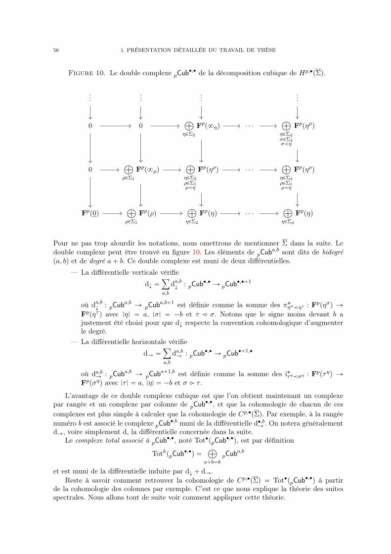
56 1. PRÉSENTATION DÉTAILLÉE DU TRAVAIL DE THÈSE
Figure 10. Le double complexe pCub‚,‚ de la décomposition cubique de Hp,‚pΣq.
......
......
0 0à
ηPΣ2
Fpp8ηq . . .à
ηPΣdσPΣ2σăη
Fppηρq
0à
ρPΣ1
Fpp8ρqà
ηPΣ2ρPΣ1ρăη
Fppηρq . . .à
ηPΣdρPΣ1ρăη
Fppηρq
Fpp0qà
ρPΣ1
Fppρqà
ηPΣ2
Fppηq . . .à
ηPΣd
Fppηq
Pour ne pas trop alourdir les notations, nous omettrons de mentionner Σ dans la suite. Ledouble complexe peut être trouvé en figure 10. Les éléments de pCub
a,b sont dits de bidegrépa, bq et de degré a` b. Ce double complexe est muni de deux différentielles.
— La différentielle verticale vérifie
dÓ “ÿ
a,b
da,bÓ
: pCub‚,‚Ñ pCub
‚,‚`1
où da,bÓ
: pCuba,bÑ pCub
a,b`1 est définie comme la somme des π˚ησăητ : Fppησq Ñ
Fppητ q avec |η| “ a, |σ| “ ´b et τ ă σ. Notons que le signe moins devant b ajustement été choisi pour que dÓ respecte la convention cohomologique d’augmenterle degré.
— La différentielle horizontale vérifie
dÑ “ÿ
a,b
da,bÑ : pCub‚,‚Ñ pCub
‚`1,‚
où da,bÑ : pCuba,bÑ pCub
a`1,b est définie comme la somme des i˚τηăση : Fppτηq ÑFppσηq avec |τ | “ a, |η| “ ´b et σ ą τ .
L’avantage de ce double complexe cubique est que l’on obtient maintenant un complexepar rangée et un complexe par colonne de pCub
‚,‚, et que la cohomologie de chacun de cescomplexes est plus simple à calculer que la cohomologie de Cp,‚pΣq. Par exemple, à la rangéenuméro b est associé le complexe pCub
‚,b muni de la différentielle d‚,bÑ . On notera généralementdÑ, voire simplement d, la différentielle concernée dans la suite.
Le complexe total associé à pCub‚,‚, noté Tot‚ppCub
‚,‚q, est par définition
TotkppCub‚,‚q “
à
a`b“kpCub
a,b
et est muni de la différentielle induite par dÓ ` dÑ.Reste à savoir comment retrouver la cohomologie de Cp,‚pΣq “ Tot‚ppCub
‚,‚q à partir
de la cohomologie des colonnes par exemple. C’est ce que nous explique la théorie des suitesspectrales. Nous allons tout de suite voir comment appliquer cette théorie.

4. COMPARAISON DE H‚,‚pΣq, H‚,‚C pΣq ET H‚,‚pΣq 57
4.3. Preuve du théorème 4.1. Étudions d’abord la suite spectrale ÓpCub‚,‚
‚induite par
la filtration selon la première coordonnée. Cela signifie simplement que l’on va commencer parcalculer la cohomologie des colonnes.
Par définition, la page 0 de la suite spectrale, notée ÓpCub‚,‚
0, est égale à pCub
‚,‚. Ensuitela première page ÓpCub
‚,‚
1est obtenue en calculant la cohomologie des colonnes :
ÓpCub
a,b
1:“
ker´
dÓ : ÓpCuba,b
0Ñ
ÓpCub
a,b`1
0
¯
Im´
dÓ : ÓpCuba,b´1
0Ñ
ÓpCub
a,b
0
¯ .
4.3.1. Calcul de la première page. La aème colonne est donnée parÓpCub
a,‚
0: ¨ ¨ ¨ ÝÑ
à
ηPΣaσPΣ´b`1σăη
Fppησq ÝÑà
ηPΣaσPΣ´bσăη
Fppησq ÝÑà
ηPΣaσPΣ´b´1σăη
Fppησq ÝÑ ¨ ¨ ¨
On peut voir qu’elle se décompose en une somme directe de complexesÓpCub
a,‚
0“
à
ηPΣa
ÓpCub
η,‚
0,
où chaque terme est défini parÓpCub
η,‚
0: ¨ ¨ ¨ ÝÑ
à
σPΣ´b`1σăη
Fppησq ÝÑà
σPΣ´bσăη
Fppησq ÝÑà
σPΣ´b´1σăη
Fppησq ÝÑ ¨ ¨ ¨
Fixons η P Σa. L’ensemble des faces de la forme ησ pour σ ă η forme un sous-treillis deΣ isomorphe au treillis de l’hypercube semi-ouvert T|η| (où l’on munit T des faces T et t8u).De plus, on a une décomposition non canonique
Fppησq »à
p1`p2“p
Fp1p8ηq b Fp2pR|η|´|σ|q.
Les détails de cette preuve sont dans la section 7.2.3 du chapitre 2, voir aussi section 7.4.3concernant la décomposition ci-dessus. Brièvement, on obtient
ÓpCub
η,‚0 »
à
p1`p2“p
Fp1p8ηq b Cp2,‚`|η|pT|η|q,
puis, comme la cohomologie de Tk est concentrée en bidegré pk, kq et Hk,kpTkq » k, on obtientfinalement que
ÓpCub
η,b1 :“ Hbp
ÓpCub
η,‚0 q “
#
Fp´|η|p8ηq si b “ 0,0 sinon.
Finalement la première page ÓpCub‚,‚
1est triviale partout sauf en rangée zéro où elle est
isomorphe à Cp,‚˝pΣq ; les isomorphismes de doubles complexes doivent conserver le degré donc
cela signifie que ÓpCuba,0
1“ Cp,a
˝pΣq.
4.3.2. Calcul de la deuxième page. On peut facilement montrer que la différentielle dÑ
induit une différentielle dÑ : ÓpCub‚,‚
1Ñ
ÓpCub
‚`1,‚
1sur la première page. La deuxième page
consiste à calculer la cohomologie selon cette différentielle :
ÓpCub
a,b
2:“ Ha
`
pÓpCub
‚,b
1, dÑq
˘
.
Ici, nous pouvons vérifier que la différentielle induite par dÑ est bien la différentielle associéeà Cp,‚
˝pΣq, c’est-à-dire
`
ÓpCub
‚,0
1,dÑ
˘
»`
Cp,‚˝pΣq,d˝
˘
.

58 1. PRÉSENTATION DÉTAILLÉE DU TRAVAIL DE THÈSE
Donc la deuxième page de la suite spectrale est concentrée en rang 0 et elle est isomorphe àla cohomologie de Cp,‚
˝pΣq :
ÓpCub
a,b
2“
#
Hp,a˝pΣq si b “ 0,
0 sinon.
4.3.3. Calcul des pages suivantes. Il existe une différentielle naturelle d2 sur la secondepage de toute suite spectrale E‚,‚‚ de bidegré p2,´1q c’est-à-dire que d2 : E‚,‚2 Ñ E‚`2,‚´1
2 . Latroisième page consiste à prendre la cohomologie pour cette différentielle.
De manière générale, nous obtenons à la kème page une différentielle dk : E‚`k,‚`1´kk et la
page E‚,‚k`1 est obtenue en prenant la cohomologie pour cette différentielle.Dans le cas qui nous intéresse ici, comme E‚,‚2 est concentrée en rang 0, la différentielle
d2 est triviale. Donc E‚,‚3 “ E‚,‚2 . De même, d3 est triviale et ainsi de suite. Donc E‚,‚r “ E‚,‚2pour tout r ě 2. On dit que la suite spectrale dégénère en page deux.
Comme nous n’étudions ici que des suites spectrales bornées (c’est-à-dire que Ea,b0 “ 0
pour |a| ou |b| grand), les suites spectrales vont forcément dégénérer en une page r fini, et l’onnote E‚,‚
8la page obtenue, c’est-à-dire E‚,‚
8“ E‚,‚k pour tout k ě r.
4.3.4. Fin de la preuve. Le théorème fondamental des suites spectrales nous dit que dansnotre cas
Tot‚pÓpCub‚,‚
8q » H‚
`
Tot‚pÓpCub‚,‚
0q˘
.
Cet isomorphisme est vrai ici car nous travaillons avec des espaces vectoriels, mais mêmedans ce cas, il n’est en général pas canonique. En toute généralité, les parties ÓpCub
a,b
8avec
a ` b “ q forment en fait les gradués d’une filtration de Hq`
Tot‚pÓpCub‚,‚
0q˘
. Comme il n’y apas forcément d’isomorphisme, on écrit généralement
ÓpCub
‚,‚
‚ùñ H‚
`
Tot‚pÓpCub‚,‚
0q˘
.
Dans notre cas, comme ÓpCub
‚,‚
8“
ÓpCub
‚,‚
2est concentrée en une seule rangée, le com-
plexe total associé est simplement Hp,‚˝pΣq. Chaque groupe du complexe total n’est constitué
que d’une seule partie non triviale, l’isomorphisme est donc canonique. En rappelant queTot‚
`
ÓpCub
‚,‚
0q˘
n’est autre que Cp,‚pΣq, nous obtenons finalement ce que nous souhaitions, àsavoir l’isomorphisme
H‚,‚˝pΣq » H‚,‚pΣq.
4.4. Preuve du théorème 4.3. Supposons que Σσ vérifie la dualité de Poincaré pourtoute face σ ‰ 0. Nous voulons montrer que Σ vérifie la dualité de Poincaré si et seulement sic’est le cas pour Σ. La preuve peut être trouvée en chapitre 2 section 7.2.4.
Montrons d’abord le sens direct. Pour cela, nous allons exploiter la seconde suite spectraleassociée à pCub
‚,‚, à savoir celle induite par la filtration selon les rangées. Nous la notonsnaturellement ÑpCub
‚,‚‚
.Calculons d’abord la première page, c’est-à-dire la cohomologie de chaque rangée. On peut
décomposer la rangée b en la somme directe suivanteÑpCub
‚,b0“
à
σPΣ´b
Cp,‚`bc pΣσ8q.
Si σ est de dimension ´b, par la dualité de Poincaré pour Σσ, comme nous l’avons déjà vudans l’exemple 3.13, alors
Hp,qc pΣσ
8q “
#
Fd`b´pp8σq si q “ d` b,
0 sinon.
4. COMPARAISON DE H‚,‚pΣq, H‚,‚C pΣq ET H‚,‚pΣq 59
Donc la première page est concentrée en colonne d et vérifieÑpCub
d,b1“
à
σPΣ´b
Fd`b´pp8σq.
On reconnaît le dual du complexe de cochaîne Cd´p,‚˝
pΣq. C’est en effet bien le cas car Σ estorientée (nous passons les détails ici). En utilisant le dual du théorème 4.1, on obtient doncque l’homologie de ce dual est isomorphe à Hd´p,‚pΣq.
En prenant en compte le décalage, on en déduit que la deuxième page ÑpCub‚,‚2
est concen-trée en colonne d et est isomorphe à Hd´p,d´‚pΣq. De plus, la suite spectrale dégénère en pagedeux. Comme précédemment,
ÑpCub
‚,‚‚ùñ Hp,‚pΣq.
On en déduit l’isomorphisme Hd´p,d´‚pΣq » Hp,‚pΣq. Il s’agit bien de la dualité de Poincaré.Le sens réciproque est plus délicat à montrer car a priori la rangée zéro de la première
page n’est pas triviale. Nous pouvons tout de même nous en sortir grâce à une étude pluspoussée de la suite spectrale. Nous ne la reproduisons pas ici.
La preuve du théorème 4.6 affaibli se fait de manière similaire. L’hypothèse queHp,qc pΣσq “
0 pour q ă d´ |σ| revient à dire que la première page ÑpCub‚,‚1
est concentrée en colonne d. Parrécurrence, on peut de plus supposer que tous les éventails Σσ vérifient la dualité de Poincarépour σ ‰ 0. La première page est donc isomorphe au dual de Cd´p,‚
˝pΣq (avec un décalage),
sauf le dernier terme : ÑpCubd,01“ Hp,d
c pΣq qui n’est pas forcément isomorphe Fd´pp0q. Commele début des deux complexes coïncident, on peut tout de même conclure comme précédemmentque Hp,qpΣq » Hd´p,d´qpΣq, sauf pour q égal à d ou d ´ 1. Mais dans ces cas-là, on utilisesimplement le fait que l’on a déjà la dualité pour q égal 0 ou 1. Cela ne fonctionne que sid ą 2, d’où la condition.
4.5. Preuve du théorème 4.7. Le double complexe précédent est une façon de décom-poser la cohomologie de Σ en les cohomologies à support compact des structures simplicialesΣσ8. Cela peut être interprété comme un analogue cohomologique du fait que Σ est l’union
disjointe des Σσ8.
Le théorème d’inclusion-exclusion nous dit alors que Σ peut être décomposée sous laforme
ř
σPΣp´1q|σ|Σσ8. Pour que cela ait un sens, on peut par exemple considérer les fonctions
caractéristiques sur les supports associés. En terme cohomologique, on peut interpréter celade la façon suivante. Considérons le double complexe Del‚,‚ définit par
Dela,‚ “à
ηPΣa
C‚cellpΣη8q,
où C‚cellpΣσ8q désigne le complexe de cochaînes cellulaire, ou polyédral, classique. Les dif-
férentielles horizontales sont donnés par les restrictions : on envoie rστ8s P CqcellpΣ
η8q sur
signpη, η1qrστ8s P CqcellpΣ
η1
8q où η ă η1 ă τ ă σ, et q “ |στ
8|. Chaque face στ apparaît une
fois pour chaque face η ă τ . En utilisant un argument similaire à la preuve de la formuled’inclusion-exclusion, on en déduit que seules les faces de sédentarité 0 survivent à la coho-mologie :
HapDel‚,bq »
#
Cbcell,cpΣq si a “ 0,0 sinon.
Ce n’est pas totalement immédiat mais le même argument fonctionne si l’on remplace lefaisceau constant par le faisceau Fp. On peut aussi faire le même argument avec le faisceauFp, c’est ce qui est fait en section 7 du chapitre 2 pour démontrer ce même théorème 4.7.Posons
pDela,‚“
à
ηPΣa
Cp,‚pΣη8q.
60 1. PRÉSENTATION DÉTAILLÉE DU TRAVAIL DE THÈSE
Étudions d’abord la suite spectrale induite par la filtration selon les rangées. Par l’argumentci-dessus, la première page ÑpDel
‚,‚1
est concentrée en colonne 0 et est isomorphe à Cp,‚c pΣq.Donc la suite spectrale dégénère en deuxième page et
ÑpDel
‚,‚‚ùñ Hp,‚
c pΣq.
Maintenant on peut étudier l’autre suite spectrale, qui elle aussi va calculer Hp,‚c pΣq. Par
la définition de pDel‚,‚, la première page est donnée par
ÓpDel
a,b
1“
à
ηPΣa
Hp,bpΣη8q.
Si Σ est lisse, par le corollaire 4.2, ÓpDel‚,‚
1est concentré en colonne p et est isomorphe au
complexe
0 Ñ Hp,ppΣq Ñà
σPΣ1
Hp,ppΣσq Ñ
à
σPΣ2
Hp,ppΣσq Ñ ¨ ¨ ¨ Ñ
à
σPΣd´p
Hp,ppΣσq Ñ 0.
Donc ÓpDel‚,‚
‚dégénère en page deux. On en déduit que la cohomologie du complexe ci-dessus
coïncide avec la cohomologie Hp,‚c pΣq. Comme Σ est lisse, cette dernière est triviale sauf en
degré d où elle est isomorphe à Fd´pp0q. Dans le complexe ci-dessus, le degré d correspond audernier terme. Ceci conclut la preuve de l’exactitude de la suite étudiée et donc le théorème 4.7.
4.6. Lien avec la suite spectrale de Deligne. Nous pouvons maintenant expliquerle lien entre le théorème 4.7 et ce qu’on appelle la suite spectrale de Deligne. Une variétéprojective lisse complexe W possède toujours une décomposition naturelle de sa cohomologieà coefficients complexes de la forme HkpW q “
À
k“p`qHp,qpW q. C’est ce qu’on appelle une
structure de Hodge. Nous souhaiterions avoir une telle décomposition pour toutes les variétésquasi-projectives lisses (et pour les variétés projectives non lisses), c’est-à-dire lorsque l’onne suppose plus que W est compacte. Une décomposition aussi simple n’est plus possibleen général, mais nous pouvons tout de même munir HkpW q d’une structure légèrement pluscompliquée appelée structure de Hodge mixte. C’est ce qu’a montré Deligne dans une séried’articles [Del71b,Del71a,Del74], pour une courte introduction parmi de nombreuses autres,voir [Dur81].
Pour assigner une telle structure à une variété non compacte V , l’idée est de trouver unebonne compactification V de V , puis d’utiliser la suite spectrale de Deligne qui calcule lastructure de Hodge mixte sur V à partir des structures de Hodge des strates qui, elles, sontcompactes.
Pour voir le lien avec notre travail, supposons que V soit le plongement d’un complé-mentaire d’arrangement d’hyperplans dans le tore. On peut utiliser la compactification deV donnée par l’éventail de Bergman associé. Comme les cohomologies des strates sont trèssimples, la suite spectrale de Deligne est elle-même très simple. On obtient finalement lethéorème suivant, ici donné sous sa forme tropicale.
Théorème 4.9 (Résolution de Deligne tropicale). Si Σ est lisse, nous avons la suite exactesuivante
0 Ñ Fkp0q Ñà
σPΣk
H0pΣσ8q Ñ
à
σPΣk´1
H2pΣσ8q Ñ ¨ ¨ ¨ Ñ
à
σPΣ1
H2k´2pΣσ8q Ñ H2kpΣq Ñ 0.
Cette suite exacte est simplement le dual de Poincaré du théorème 4.7en posant k “ d´p.Du point de vue de la discussion ci-dessus, si Σ est l’éventail de Bergman associé à V , on peutinterpréter Fkp0q comme la cohomologie de degré k de V , et H2kpΣ
σ8q comme la cohomologie
la strate fermée associée à σ dans la compactification V Ď CPΣ. En effet, par le travail deFeichtner et Yuzvinsky [FY04], comme nous le verrons en section 9, la cohomologie de cettestrate est nulle en degrés impairs et est égale à H2kpΣ
σ8q en degré 2k.
5. THÉORIE DE HODGE COMBINATOIRE ET ANNEAU DE CHOW D’UN ÉVENTAIL 61
Question 4.10. Peut-on établir une théorie des structures de Hodge tropicales mixtes ? ˛
Notamment, pour les structures simpliciales affines lisses, l’analogue du théorème 4.9 s’ap-plique à la compactification canonique. Pour le cas non lisse, il s’agirait de développer unethéorie de désingularisation pour les variétés tropicales, voir question 6.14.
5. Théorie de Hodge combinatoire et anneau de Chow d’un éventail
Commençons par donner un bref récapitulatif historique du développement de la théorie deHodge combinatoire. Le vocabulaire utilisé ci-dessous sera défini plus loin dans cette section.
Si P est un polytope simple de dimension d, c’est-à-dire si tous ses sommets sont adjacentsà d arêtes, on peut se demander quelle est la forme de son f -vecteur pf0, . . . , fnq où fi désignele nombre de faces de P de dimension i. En général, on regarde plutôt son h-vecteur qui estdéfini par
ÿ
i
hixi “
ÿ
i
fipx´ 1qi.
Par exemple, hd vaut toujours 1, et h0 est la caractéristique d’Euler-Poincaré du polytopedonc h0 “ 1. Plus généralement, Sommerville a montré en 1927 que hi “ hn´i. En 1970,McMullen va plus loin et énonce la g-conjecture dans [McM71] qui caractérise entièrementles h-vecteurs des polytopes simples. Dans [BL81], Billera et Lee montrent la suffisance desconditions de McMullen. Stanley a finalement résolu la conjecture dans [Sta80] en remarquantque la nécessité était impliquée par le théorème de Lefschetz difficile pour l’anneau de Chowassocié à P . Par la suite, la théorie de Hodge combinatoire s’est beaucoup développée. (Icion parle de théorie de Hodge dans un sens assez large ; on y inclut notamment le théorèmede Lefschetz difficile.) En particulier, cette théorie a connu d’importants résultats dans cesdernières années [Kar04,FK10,AHK18,Adi18,BHM`20a,BHM`20b].
Citons en premier lieu [Adi18] où Adiprasito généralise le théorème de Lefschetz difficile,et donc le g-théorème, aux sphères simpliciales. Dans cette section, nous souhaitons présenterun nouveau point de vue qu’apporte la théorie de Hodge tropicale sur certains outils employéspar Adiprasito, outils qui sont exposés dans [AY20].
Citons ensuite [AHK18] où Adiprasito, Huh et Katz montrent que l’anneau de Chow d’unéventail de Bergman vérifie le théorème de Lefschetz difficile et les relations de Hodge-Riemann.Cela a permis de résoudre plusieurs conjectures en combinatoire, comme la log-concavité descoefficients du polynôme caractéristique d’un matroïde. Dans cette thèse, nous montrons queces résultats sur les éventails de Bergman font en fait partie d’un cadre plus général à savoir lathéorie de Hodge tropicale. Entre autre, nous généralisons le résultat de [AHK18] à d’autreséventails, tout en apportant une nouvelle preuve plus naturelle sur certains points.
Nous souhaitons aussi parler du résultat de Karu dans [Kar04] où il montre que la coho-mologie d’intersection de l’éventail dual de n’importe quel polytope P , a priori ni rationnelni simple, vérifie le théorème de Lefschetz difficile et les relations de Hodge-Riemann. Cettecohomologie d’intersection combinatoire est étudiée dans [BBFK02]. Dans le cas rationnel,l’argument de Stanley donne déjà le résultat via la cohomologie d’intersection de la variété to-rique associée. Notons que les nombres de Betti de la cohomologie ne donnent pas le h-vecteurdu polytope P comme défini ci-dessus : le g-théorème est faux pour un polytope quelconque.Dans le cas d’un éventail non simplicial, on peut définir sa compactification canonique commedans 2.2 du chapitre 2.
Question 5.1. Y a-t-il un lien entre la cohomologie d’intersection d’un éventail completΣ et la cohomologie tropicale ou une cohomologie similaire sur la compactification canoniquede Σ ? ˛
Exemple 5.2. S’il existe, ce lien n’est pas trivial. En effet, soit σ un cône tridimensionnelà quatre rayon. Considérons σ sa compactification canonique, et U l’intérieur relatif de sa
62 1. PRÉSENTATION DÉTAILLÉE DU TRAVAIL DE THÈSE
compactification canonique. On vérifie facilement que Hp,qpUq est concentrée en bidegré p0, 0qalors que HBM
2,2 pUq est non trivial. On voit donc qu’en général la compactification canoniqued’un éventail non simplicial ne va pas vérifier pas la dualité de Poincaré localement et ne seradonc pas lisse. ˛
Bien que nous ne résolvons pas de nouveaux problèmes combinatoires à proprement parlerdans cette thèse, il nous semble important de souligner les nombreux points d’intersectionsentre la théorie de Hodge combinatoire et la théorie de Hodge tropicale. Dans cette section,nous énonçons les résultats allant dans cette direction, certaines preuves seront toutefois faitesdans les prochaines sections.
5.1. Anneau de Chow.5.1.1. Définition. Soit Σ une structure simpliciale linéaire de dimension d. Pour k “ Q,
on suppose de plus que Σ est rationnelle. Nous discutons du cas faiblement rationnel enremarque 5.29. Considérons l’algèbre de polynômes krx% | % P Σ1s. Si F est un sous-ensemblede Σ1, typiquement F “ σ P Σ, on pose xF “
ś
%PF x%. On définit un premier idéal
I1 “`
xF | F R Σ˘
.
Le quotient krx% | % P Σ1sI1 est appelé l’anneau de Stanley-Reisner de Σ. Le second idéal estdéfini par
I2 “`
ÿ
%PΣ1
`pν%qx% | ` PMk˘
.
Définition 5.3. L’anneau de Chow de Σ, noté A‚pΣq, est l’algèbre graduée sur k définiepar
krxρ | ρ P Σ1spI1 ` I2q.
La graduation est celle induite par le degré des polynômes. ˛
Le nom « anneau de Chow » est justifié par la propriété suivante. Si Σ est un éventailsimplicial rationnel unimodulaire dans Rn, alors l’anneau de Chow de Σ est isomorphe àl’anneau de Chow de la variété torique CPΣ, cf. [Dan78,BDP90,Bri96,FS97]. On peutse poser la question de l’analogue tropical. Les groupes de Chow tropicaux sont par exempledéfinis dans [AR10].
Question 5.4. Quel est le lien entre l’anneau de Chow tropical de TPΣ et A‚pΣq ? ˛
Venons-en au lien avec l’introduction de cette section.
Exemple 5.5. Soit P un polytope simple. Soit Σ son éventail dual, supposé rationnel.C’est un éventail simplicial. On a alors dimpAipΣqq “ hi où hi est le ième terme du h-vecteurde P . Ainsi, par exemple, la dualité de Poincaré pour A‚pΣq implique que le h-vecteur estsymétrique. ˛
En choisissant Θ une base de Mk, et en considérant Σ comme un complexe simplicialabstrait plutôt que comme un éventail abstrait, l’anneau de Chow de Σ correspond à l’algèbregraduée notée ApΣq dans [AY20].
5.1.2. Lemme de localisation. Nous présentons ici une description alternative importantede l’anneau de Chow, à comparer avec la proposition 3.1 de [Adi18], qui renvoie à [Lee96],et avec la preuve de la proposition 5.6 de [AHK18].
SoitZkpΣq “
à
σPΣk
kxσ ãÑ krx% | % P Σ1s.
Il s’agit donc de la partie sans facteur carré de l’anneau de Stanley-Reisner. On a une applica-tion naturelle ZkpΣq Ñ AkpΣq. Rappelons la notation σ „ τ qui signifie que σ et τ sont deux

5. THÉORIE DE HODGE COMBINATOIRE ET ANNEAU DE CHOW D’UN ÉVENTAIL 63
faces vérifiant σ ^ τ “ 0 et σ _ τ ‰ 1. De plus, pour toute face τ P Σk´1 et toute application` PMk qui est nulle sur τ , ce qu’on peut écrire ` PMK
τ,k, l’élémentÿ
%PΣ1%„τ
`pν%qx%xτ P ZkpΣq
est dans le noyau de ZkpΣq Ñ AkpΣq. En effet, modulo un élément de I1, cette somme estégale à xτ
ř
%PΣ1`pν%qx% P I2.
Lemme 5.6 (Lemme de localisation). L’application ZkpΣq Ñ AkpΣq est surjective et sonnoyau est engendré par les éléments de la forme
ÿ
%PΣ1%„τ
`pν%qx%xτ
pour τ P Σk et ` PMKτ,k.
Démonstration. Il n’est pas très difficile de se convaincre de la surjectivité. Considéronspar exemple un élément de la forme x2
ρxρ3 ¨ ¨ ¨ xρk , avec ρ, ρ3, . . . , ρk différents. Si l’élément n’estpas dans I1, alors les rayons forment un cône τ . Comme Mτ,k est de dimension dimpτq, onpeut trouver un élément ` P Mk qui est nul sur τ r tρu et qui vaut un sur νρ. Alors, moduloun élément de I2, notre élément de départ est équivalent à
ÿ
%PΣ1rtρu´`pν%qx%xρxρ3 ¨ ¨ ¨ xρk
qui n’a pas de facteur carré. En supprimant les termes qui sont dans I1, on obtient bien unélément de ZkpΣq. Cet argument peut facilement se généraliser pour prouver la surjectivité.Avec plus de travail, on peut aussi trouver une preuve élémentaire du lemme : voir la section 6.8du chapitre 2.
Il serait intéressant de définir un anneau de Chow pour les structures simpliciales affines.Par exemple, dans le cas où une telle structure est issue de la limite tropicale d’une famille devariétés, l’idée serait de comprendre la partie combinatoire de l’anneau de Chow de la fibrespéciale de la famille. Dans [Ami16], Amini étudie un anneau de Chow pour des produits degraphes et montre un théorème similaire au lemme de localisation ci-dessus.
5.1.3. Lien avec la cohomologie tropicale. Dans le cas où Σ est l’éventail dual d’un poly-tope qui est rationnel et unimodulaire, l’anneau de Chow de Σ est isomorphe à l’anneau deChow et aussi à la cohomologie de CPΣ qui est une variété complexe projective lisse. C’estd’ailleurs comme cela que Stanley en déduit le théorème de Lefschetz difficile pour A‚pΣq,puisque ce théorème est connu initialement pour les variétés complexes projectives lisses. Mc-Mullen a généralisé ce résultat au cas où Σ est l’éventail dual d’un polytope simple quelconquedans [McM93].
Dans le cas où Σ est un éventail de Bergman réalisable sur C, son support est donc latropicalisation d’un complémentaire d’arrangement d’hyperplansW dans le tore. Le travail deFeichtner et Yuzvinsky [FY04] nous explique qu’une fois de plus A‚pΣq est la cohomologie deW Ď CPΣ qui est projective lisse. On en déduit de nouveau le théorème de Lefschetz difficilepour Σ.
Toutefois, lorsque l’éventail de Bergman n’est plus réalisable, l’argument ci-dessus n’estplus possible, voir [AHK18, théorème 5.12]. (A‚pΣq est tout de même isomorphe l’anneau deChow de CPΣ mais cette variété n’est pas compacte.) Le théorème ci-dessous, combiné avecle théorème 6.31, montre qu’il s’agit bien de la cohomologie d’une variété projective lisse maisau sens tropical.
64 1. PRÉSENTATION DÉTAILLÉE DU TRAVAIL DE THÈSE
Théorème 5.7. Soit Σ une structure simpliciale linéaire. Alors
Hk,kpΣq ÝÑ AkpΣq,pσ, αq ÞÝÑ αpνσqxσ
est un isomorphisme. Cet isomorphisme induit un morphisme d’algèbres graduées H‚,‚pΣq ÑA‚pΣq en envoyant Hp,qpΣq sur zéro pour p ‰ q. De plus, si Σ vérifie la dualité de Poincaré,alors on obtient un isomorphisme H‚,‚pΣq „ÝÑ A‚pΣq.
Démonstration. Pour les détails, voir la preuve du chapitre 2 théorème 7.1. Par lethéorème 4.1,
Hk,kpΣq » Hk,k˝pΣq “ coker
´
à
τPΣk´1
F1p8τ q Ñà
σPΣk
F0p8σq
¯
.
Par comparaison avec le lemme de localisation 5.6, on obtient que ce conoyau est simplementAkpΣq.
Le fait que l’on obtient un morphisme d’algèbre est montré en chapitre 2 section 7.4, où l’ondonne un inverse explicite pour l’application Hk,kpΣq Ñ AkpΣq et où l’on décrit précisémentle cup-produit sur H‚,‚pΣq.
La dernière partie de la preuve est une simple conséquence du corollaire 4.2.
5.2. Morphisme de Gysin et restriction. Si σ P Σ, il y a un morphisme de restrictioni˚0ăσ : A‚pΣq Ñ A‚pΣσq. C’est un morphisme d’algèbres surjectif naturel correspondant à larestriction i˚0ăσ : H‚,‚pΣq H‚,‚pΣ
σq entièrement décrit par
i˚0ăσpxρq “
#
xpσ_ρqσ si ρ „ σ,0 si ρ n’est pas comparable à σ.
Si ρ P σ, l’image de xρ peut être calculé en ajoutant un élément de l’idéal I2.Si Σ est lisse, ou simplement si A‚pΣq et A‚pΣσq vérifie la dualité de Poincaré, alors
i˚ : AkpΣq Ñ AkpΣσq induit un morphisme Ad´kpΣq‹ Ñ Ad´|σ|´kpΣσq‹. Le morphisme dualest appelé morphisme de Gysin et noté gysσą0 : A‚pΣσq Ñ A‚`|σ|pΣq. C’est un morphismelinéaire injectif entièrement décrit par
gysσą0pxησq “ xη
pour tout η ą σ. On note de même l’application correspondante
gysσą0 : H‚,‚pΣσq Ñ H‚`|σ|,‚`|σ|pΣq.
Plus généralement, si Σ est lisse, pour toute paire de faces τ ă σ, on obtient des ap-plications i˚τăσ : A‚pΣτ q Ñ A‚pΣσq et gysσąτ : A‚pΣσq Ñ A‚`|σ|´|τ |pΣτ q, et de même encohomologie. On vérifie alors facilement la proposition suivante.
Proposition 5.8. La composition gysσąτ ˝ i˚τăσ : A‚pΣτ q Ñ A‚`|σ|´|τ |pΣτ q correspond àla multiplication par xσ.
5.3. Lefschetz difficile et Hodge-Riemann. Nous supposons désormais que Σ estorientée. Par le théorème 5.7, on obtient une application degré naturelle
deg : AdpΣq Ñ k,xη Ñ wpηq,
où wpηq désigne le poids de la face η dans l’élément canonique rΣs.
Définition 5.9 (Dualité de Poincaré). On dit que l’anneau de Chow de Σ vérifie la dualitéde Poincaré si pour tout entier k, la composition
AkpΣq bAd´kpΣq ÝÑ AdpΣqdegÝÝÑ k
est un accouplement parfait. ˛

5. THÉORIE DE HODGE COMBINATOIRE ET ANNEAU DE CHOW D’UN ÉVENTAIL 65
Voici une conséquence directe du théorème 5.7.
Proposition 5.10. Si la cohomologie tropicale de Σ vérifie la dualité de Poincaré alorsA‚pΣq vérifie la dualité de Poincaré.
La réciproque est fausse en générale car Hp,qpΣq pour p ą q n’est pas forcément nul (voirexemple 11.1 dans le chapitre 2).
Définition 5.11. Supposons que Σ vérifie la dualité de Poincaré. Soit ` un élément deA1pΣq. On dit que ` est un opérateur de Lefschetz si pour tout entier k ď d2, l’application
¨`d´2k : AkpΣq ÝÑ Ad´kpΣq,a ÞÝÑ `d´2ka,
est un isomorphisme. On note cette propriété HLpA‚pΣq, `q.On dit que A‚pΣq vérifie le théorème de Lefschetz difficile, noté HL en bref pour « Hard
Lefschetz », si A1pΣq contient au moins un opérateur de Lefschetz. ˛
Soit ` un opérateur de Lefschetz pour A‚pΣq. On peut alors définir les parties primitivesde Σ associées par
AkprimpΣq “ ker`
`d´2k`1 : AkpΣq Ñ Ad´k`1pΣq˘
Ď AkpΣq.
On démontre facilement la proposition suivante.
Proposition 5.12. L’application ¨` : AkpΣq Ñ Ak`1pΣq est injective pour k ă d2 etsurjective pour k ě d2. De plus, pour tout k ď d2,
AkpΣq “kà
i“0
`iAk´iprimpΣq.
Définition 5.13. Soit ` un opérateur de Lefschetz pour A‚pΣq. On dit que la pairepA‚pΣq, `q vérifie les relations de Hodge-Riemann, et l’on note HRpA‚pΣq, `q, si pour toutentier k ď d2, l’accouplement
AkpΣq b AkpΣq ÝÑ k,a b b ÞÝÑ degp`d´2kabq
est définie positive sur AkprimpΣq. ˛
De nombreuses propriétés liant ces trois différentes définitions peuvent être trouvées enchapitre 3, proposition 3.5. Les trois propriétés sont appelées dans cette thèse les propriétéskählériennes, ce qui est une tentative de traduction pour « Kähler package ».
Exemple 5.14. Soit V une variété complexe projective lisse, ou plus généralement unevariété kählérienne. Alors toute classe ample ` P H2pV q, ou plus généralement toute classe deKähler, vérifie le théorème de Lefschetz difficile HLpH2‚pV q, `q et les relations de Hodge-Riemann HRpH2‚pV q, `q où les définitions ci-dessus sont adaptées pour l’algèbre graduéeH2‚pV q. Tous les indices doivent être multipliés par deux ; par exemple, on a un isomorphisme¨`d´2k : H2kpV q Ñ H2d´2kpV q. ˛
Exemple 5.15. Soit P un polytope simple de dimension d et soit Σ son éventail dual.On a vu que A‚pΣq vérifie HL. On en déduit que AkpΣq » Ad´kpΣq et que dimpAkpΣqq ďdimpAk`1pΣqq, pour k ă d2. Ainsi, le h-vecteur de Σ est symétrique, hk “ hd´k, et unimodal,c’est-à-dire qu’il est croissant puis décroissant. C’est le genre d’application typique de la théoriede Hodge combinatoire. ˛
66 1. PRÉSENTATION DÉTAILLÉE DU TRAVAIL DE THÈSE
En section 6, nous construisons toute une famille de structures simpliciales linéaires quivérifient les propriétés kählériennes. Cette famille contient notamment les éventails duaux auxéventails des polytopes, ainsi que les éventails de Bergman généralisés, ce qui fournit unegénéralisation de [AHK18]. En section 7, nous montrons comment passer du local au global,c’est-à-dire des structures simpliciales linéaires aux structures simpliciales affines.
Rappelons que nous avons défini la notion de fonctions linéaires par morceaux sur Σ ensection 2.4. Si f est une telle fonction, on peut naturellement lui associer un élément de A1pΣqdéfini par
ř
%PΣ1fp%qx%. Si f est strictement convexe, alors l’élément obtenu est appelé une
classe ample. C’est l’exemple typique d’élément que l’on va prendre pour tenter d’avoir unopérateur de Lefschetz. Si de plus on a les propriétés kählériennes HLpΣ, `q et HRpΣ, `q, onappelle ` une classe kählérienne. Nous verrons en section 6.11 qu’une classe ample n’est pasforcément une classe kählérienne même si Σ lisse.
Définition 5.16. Soit Σ une structure simpliciale linéaire. On dit que Σ est kählériennesi elle est quasi-projective et si toute classe ample de A1pΣq est kählérienne. ˛
5.4. Dualité de Poincaré pour les sphères simpliciales. Dans cette section nousredémontrons grâce à la théorie développée précédemment certains résultats connus en théoriede Hodge combinatoire qui sont notamment présents dans l’article [AY20].
Soit Σ une structure simpliciale linéaire de dimension d. On dit que Σ est de dimensionmaximale si dimpΣq “ dimpMkq. Notons que, dans ce cas, toutes les structures transverses Σσ
sont elles aussi de dimensions maximales.
Proposition 5.17. Si Σ est de dimension maximale, alors Hp,qc pΣq “ Hq
sing,cpΣqbŹpMk.
Ici H‚singpΣq désigne l’homologie singulière classique de Σ à coefficients dans k
Démonstration. CommeMk est de dimension d, pour toute facette η P Σd,Mη,k “Mk.Donc pour toute face σ P Σ, Mkpσq “ Mk. La cohomologie tropicale Hp,‚
c pΣq est alors àcoefficients constants, à savoir à coefficients dans
ŹpMk. Le théorème des coefficients universelsconclut la démonstration.
On dit qu’une structure simpliciale linéaire Σ, ou plus généralement qu’un éventail abstraitΣ, est de Cohen-Macaulay si pour tout cône σ P Σ, la cohomologie classique H‚sing,cpΣ
σq del’éventail transverse est concentrée en degré d´ |σ|.
Proposition 5.18. Soit Σ une structure simpliciale linéaire de Cohen-Macaulay de di-mension maximale. Alors la projection H‚,‚pΣq Ñ A‚pΣq est un isomorphisme.
Démonstration. Par la proposition 5.17, comme Σ est de Cohen-Macaulay, la cohomo-logie Hp,‚
c pΣσq est concentrée en degré d ´ |σ| pour tout σ P Σ. Comme pour la preuve dethéorème 4.6, nous en déduisons que la première page ÑpCub
‚,‚1
de Σ est concentrée en colonned. De plus, ÑpCub
‚,‚‚
est concentrée entre les rangées ´pd´ pq et 0. Ainsi la première page estconcentrée entre les degrés p “ d` p´pd´ pqq et d “ d` 0. Comme ÑpCub
‚,‚‚ñ Hp,‚pΣq, on
en déduit que Hp,‚pΣq est concentrée en degré au moins p. Par le corollaire 4.2, on sait quele complexe est trivial en degrés plus que p. Donc Hp,qpΣq est trivial pour p ‰ q. On conclutavec le théorème 5.7.
On dit qu’une structure simpliciale linéaire Σ, ou plus généralement qu’un éventail abstraitΣ, est le cône d’une sphère simpliciale si Σ est de Cohen-Macaulay et si de plus, pour toutσ P Σ, dim
`
Hd´|σ|sing,c pΣ
σq˘
“ 1.
Exemple 5.19. Un éventail complet de Rd induit une structure simpliciale linéaire qui estle cône d’une sphère simpliciale et qui est de dimension maximale. ˛
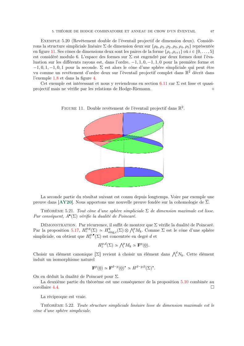
5. THÉORIE DE HODGE COMBINATOIRE ET ANNEAU DE CHOW D’UN ÉVENTAIL 67
Exemple 5.20 (Revêtement double de l’éventail projectif de dimension deux). Considé-rons la structure simpliciale linéaire Σ de dimension deux sur tρ0, ρ1, ρ2, ρ3, ρ4, ρ5u représentéeen figure 11. Ses cônes de dimensions deux sont les paires de la forme tρi, ρi`1u où i P t0, . . . , 5uest considéré modulo 6. L’espace des formes sur Σ est engendré par deux formes dont l’éva-luation sur les différents rayons est, dans l’ordre, ´1, 1, 0,´1, 1, 0 pour la première forme et´1, 0, 1,´1, 0, 1 pour la seconde. Σ est alors le cône d’une sphère simpliciale qui peut êtrevu comme un revêtement d’ordre deux sur l’éventail projectif complet dans R2 décrit dansl’exemple 1.8 et dans la figure 4.
Cet exemple est intéressant et nous y reviendrons en section 6.11 car Σ est lisse et quasi-projectif mais ne vérifie par les relations de Hodge-Riemann. ˛
Figure 11. Double revêtement de l’éventail projectif dans R2.
La seconde partie du résultat suivant est connu depuis longtemps. Voire par exemple unepreuve dans [AY20]. Nous apportons une nouvelle preuve fondée sur la cohomologie de Σ.
Théorème 5.21. Tout cône d’une sphère simpliciale Σ de dimension maximale est lisse.Par conséquent, A‚pΣq vérifie la dualité de Poincaré.
Démonstration. Par récurrence, il suffit de montrer que Σ vérifie la dualité de Poincaré.Par la proposition 5.17, Hp,q
c pΣq » Hqsing,cpΣq b
ŹpMk. Comme Σ est le cône d’une sphèresimpliciale, on obtient que Hp,‚
c pΣq est concentrée en degré d et
Hp,dc pΣq »
ŹpMk » Fpp0q.
Choisir un élément canonique rΣs revient à choisir un élément dansŹdNk. Cette élément
induit un isomorphisme naturel
Fpp0q » Fd´pp0q‹ » Hd´p,0pΣq‹.
On en déduit la dualité de Poincaré pour Σ.La deuxième partie du théorème est une conséquence de la proposition 5.10 combinée au
corollaire 4.4.
La réciproque est vraie.
Théorème 5.22. Toute structure simpliciale linéaire lisse de dimension maximale est lecône d’une sphère simpliciale.
68 1. PRÉSENTATION DÉTAILLÉE DU TRAVAIL DE THÈSE
Démonstration. Pour tout σ P Σ, Σσ vérifie la dualité de Poincaré. Notamment, pourq ă d´ |σ|,
Hqsing,cpΣ
σq » H0,qc pΣσq “ 0,
et pour q “ d´ |σ|,
Hd´|σ|sing,c pΣ
σq » H0,d´|σ|c pΣσq » Fd´|σ|p8σq »
Źd´|σ|Mkp8σq.
Comme Σσ est de dimension maximale, dim`
Mkp8σq˘
“ d ´ |σ| et le produit extérieur ci-dessus est isomorphe à k. Donc dim
`
Hd´|σ|sing,c pΣ
σq˘
“ 1. Ainsi, Σ est le cône d’une sphèresimpliciale.
On peut améliorer le théorème précédent de la façon suivante.
Proposition 5.23. Soit Σ une structure linéaire orientée de Cohen-Macaulay de dimen-sion maximale. Supposons que Σσ est lisse pour toute face σ de codimension deux. Alors Σ estle cône d’une sphère simpliciale lisse.
Dans la proposition précédente, on peut probablement affaiblir la condition et demandersimplement que Σ soit normale. Il suffirait pour le vérifier de généraliser la preuve d’Aksnesdu théorème 4.6 au cas des structures simpliciales linéaires.
Démonstration. Par la proposition 5.17, comme Σ est de Cohen-Macaulay, on sait queHp,qpΣσq “ 0 pour σ P Σ et q ă d ´ |σ|. Comme Σ est orientée, on peut appliquer lagénéralisation du théorème 4.6 pour obtenir que Σ est lisse.
Le fait que l’anneau de Chow du cône d’une sphère simpliciale vérifie la dualité de Poincaréest connu de longue date. Dans [Adi18], Adiprasito montre que si Σ est un éventail abstraitqui est le cône d’une sphère simpliciale, si l’on prend un espace de fonctions linéaire génériqueMk tel que pΣ,Mkq soit une structure linéaire affine de dimension maximale et si l’on prendun élément générique ` de A1pΣq, alors ` est un opérateur de Lefschetz pour l’anneau de Chowde Σ.
Question 5.24. Peut-on mieux comprendre le théorème de Lefschetz difficile pour lessphères simpliciales en exploitant le lien avec la cohomologie tropicale ? ˛
5.5. Complexe de partition. Dans [Adi18,AY20] apparaît un complexe intéressantappelé le complexe de partition :
Pk,‚ : AkpΣq Ñà
%PΣ1
AkpΣ%q Ñà
σPΣ2
AkpΣσq Ñ ¨ ¨ ¨ Ñà
σPΣd
AkpΣσq.
Le morphisme de bord est donné par les restrictions i˚ avec un signe. Rappelons que parle théorème 5.7, AkpΣq » Hk,kpΣq, et dans le cas lisse Hk,kpΣq » H2kpΣq. Ainsi, via cesisomorphismes, le complexe de partition est isomorphe à la suite du théorème 4.7 auquel on aenlevé le dernier terme, c’est-à-dire au dual de Poincaré de la résolution de Deligne tropicaledu théorème 4.9.
Ce nouveau point de vue permet par exemple d’obtenir une nouvelle preuve du théorèmede partition de l’unité de [AY20].
Théorème 5.25. Soit Σ une structure linéaire de dimension maximale telle que Σσ est deCohen-Macaulay pour tout σ ‰ 0. Alors,
HqpPp,‚q » Hp,p`qc pΣq.
Notamment,
dim`
HqpPp,‚q˘
“
ˆ
dimpΣq
p
˙
dim`
Hp`qsing,cpΣq
˘
.
5. THÉORIE DE HODGE COMBINATOIRE ET ANNEAU DE CHOW D’UN ÉVENTAIL 69
Démonstration. Reprenons la preuve du théorème 4.7 écrite en section 4.5. On a unesuite spectrale
ÓpDel
‚,‚
‚ùñ Hp,‚
c pΣq.
Rappelons de plus que la première page est donnée parÓpDel
a,b
1“
à
σPΣa
Hp,bpΣσq.
Décrivons la seconde page. Dans le cas qui nous concerne, pour σ ‰ 0, Σσ est de Cohen-Macaulay et de dimension maximale. Notamment, par la proposition 5.18, la cohomologieHp,‚pΣ
σq est concentrée en degré p. De plus, par le corollaire 4.2, Hp,qpΣq est nulle pour
q ą p. Donc ÓpDela,b
2est non nul seulement pour a “ 0 et b ď p et pour b “ p. Notamment, la
suite spectrale dégénère en page deux et
Hp,kc pΣq »
#
ÓpDel
0,k
2si k ď p
ÓpDel
k´p,p
2si k ě p.
Ajoutons que ÓpDela,p
2est égale à HapPp,‚q, ce qui conclut la première partie du théorème. Pour
la seconde partie, il suffit d’utiliser la proposition 5.17.
5.6. Poids de Minkowski. Soit Σ une structure simpliciale linéaire de dimension d. Onsuppose toujours Σ fortement rationnelle si k “ Q.
Définition 5.26. Un poids de Minkowski de dimension k de Σ est une fonction w : Σk Ñ ktelle que
ÿ
σPΣk
wpσqpσ, νσq
est un cycle dans CBMk,k pΣq. On note MWkpΣq l’espace vectoriel des poids de Minkowski de
dimension k de Σ. ˛
La définition fournit une inclusion naturelle MWkpΣq ãÑ CBMk,k pΣq, que l’on peut prolonger
en MWkpΣq ãÑ Ck,kpΣq. Dans les deux cas, l’image est un cycle. Dans le cadre de la géométrietropicale, on peut interpréter la condition d’être un cycle comme une condition d’équilibrepondérée par le poids w.
Si w P MWkpΣq, on obtient naturellement une sous-structure simpliciale linéaire orientéede dimension k de Σ dont les facettes sont les cônes σ P Σk tels que wpσq ‰ 0.
Il y a un accouplement naturel ZkpΣqbMWkpΣq Ñ k défini par xxσ, wy “ wpσq pour toutσ P Σk. Cela induit un accouplement AkpΣq bMWkpΣq qui est bien défini par le théorèmesuivant.
Théorème 5.27. Le groupe MWkpΣq est naturellement isomorphe à AkpΣq‹. De plus, cettedualité est compatible avec la dualité en homologie : l’application MWkpΣq Ñ Hk,kpΣq est dualeà l’isomorphisme Hk,kpΣq „ÝÑ AkpΣq décrit dans le théorème 5.7. Notamment, MWkpΣq ÑHk,kpΣq est un isomorphisme.
Démonstration. La première partie découle du lemme de localisation 5.6, cf. [AHK18,Proposition 5.6]. Le reste du théorème s’en déduit aisément.
Si Σ est orientée, l’élément canonique rΣs P HBMd,d pΣq fournit un élément canonique dans
MWdpΣq, noté aussi rΣs, qui correspond à l’application degré dans AdpΣq‹.Dans le cas où A‚pΣq vérifie la dualité de Poincaré, la structure d’anneau sur A‚pΣq
induit un produit d’intersection sur MW‚pΣq. Ce produit d’intersection et son lien avec lesvariétés toriques est étudié dans [FS97]. Plus généralement, le produit d’intersection sur leséventails ou sur les variétés tropicales est un objet très étudié [RGST05,Mik06,AR10,Sha11,Sha13b,OP13,OR11,Kat12,Ham14].
70 1. PRÉSENTATION DÉTAILLÉE DU TRAVAIL DE THÈSE
Remarque 5.28 (Conjecture de Hodge locale). Si Σ vérifie la dualité de Poincaré, lacomposition
MWkpΣq Ñ Hk,kpΣq „ÝÑ Hk,kpΣq‹ „ÝÑ Hd´k,d´kpΣq
correspond à l’application classe de cycle. Par le théorème précédent, cette application est unisomorphisme. Cela montre la conjecture de Hodge pour les structures simpliciales linéairesrationnelles. Nous résolvons en section 8 un analogue de la conjecture de Hodge dans le cadredes structures simpliciales affines rationnelles.
Notons que l’isomorphisme Ad´kpΣq „ÝÑ Hk,kpΣq est facile à décrire. Il suffit d’envoyer xσ,pour σ P Σd´k, sur iσą0,˚prΣ
σsq. ˛
Remarque 5.29 (Cas faiblement rationnel). Soit Σ une structure simpliciale linéaire fai-blement rationnelle et posons k “ Q. Il paraît naturel de définir MWkpΣ,Qq comme les poidsw : Σk Ñ Q dont l’image dans CBM
k,k pΣq est un cycle et tel que wpσq “ 0 si σ P Σk n’estpas rationnel. Vue la remarque précédente, on pourrait alors définir l’anneau de Chow de Σà coefficients rationnels comme l’image de MW‚pΣ,Qq Ñ Ad´‚pΣ,Rq. Une définition plusexplicite devrait exister. Une telle définition pourrait aider à résoudre la conjecture de Hodgetropicale 8.2 pour les structures simpliciales affines faiblement rationnelles. ˛
Exemple 5.30. Justifions la dénomination « poids de Minkowski ». Soit P un polytopede dimension maximale dans Rd et soit Σ son éventail dual dans l’espace vectoriel normé Rd.Pour rester dans notre cadre de travail, supposons P simple, mais ce qui suit est vrai dans lecas général. Pour tout entier k et à chaque face σ de Σk correspond une face σ_ de codimensionk dans P . On suppose que les vecteurs canoniques de chaque rayon sont choisis de norme undans Rd. On peut montrer assez facilement que le poids w qui à σ associe le volume de σ_ estun élément de MWkpΣq, c’est ce qu’on appelle la relation de Minkowski, cf. [McM96].
Minkowski a démontré une réciproque : à un élément strictement positif w P MW1pΣq, onpeut associer un unique polytope P à translation près qui est un inverse pour l’applicationdécrite ci-dessus (cf. [Kla04]). Un tel polytope P fournit en retour un élément a P A1pΣqdonné par
a “ÿ
%PΣ1
xν%, u%yx%
où u% est n’importe quel point de la facette de P correspondant à %. Si l’on translate P , onajoute un élément de l’idéal I1 à a donc a est bien défini. On peut montrer que l’élémenta obtenu est ample, et que tout élément ample de A1pΣq provient d’un polytope de cettefaçon. On obtient donc une bijection entre les éléments strictement positifs de MW1pΣq et leséléments amples de A1pΣq. Cette bijection est donnée par l’application
A1pΣq Ñ Ad´1pΣq Ñ A1pΣq‹ „ÝÑ MW1pΣq
qui envoie ` sur le dual de Poincaré de `d´1pd´ 1q! [McM96]. Le fait que l’élément obtenusoit strictement positif deviendra clair après la discussion ci-dessous. ˛
Cet exemple nous amène à énoncer la proposition suivante.
Proposition 5.31. Soit ` un élément ample de A1pΣq. Alors pour tout élément w P
MWkpΣq positif non nul, l’accouplement x`k, wy est strictement positif.
Démonstration. Cette proposition découle directement de la proposition suivante.
Proposition 5.32. Soit ` un élément ample de A1pΣq et soit a P AkpΣq, k ă d, quipossède un antécédent dans ZkpΣq dont tous les coefficients sont strictement positifs. Alors` ¨a P Ak`1pΣq possède un antécédent dans Zk`1pΣq dont tous les coefficients sont strictementpositifs.
6. THÉORIE DE HODGE POUR LES STRUCTURES SIMPLICIALES LINÉAIRES 71
Démonstration. Soit τ P Σk un cône de dimension k. Alors par convexité, on peut écrire` sous la forme
ÿ
%PΣ1
`%x%
avec `% “ 0 si % ă τ et `% ą 0 si % „ τ . Donc
` ¨ xτ “ÿ
%„τ
`%xτ_%
possède un antécédent dans ZkpΣq dont tous les coefficients sont positifs et dont les coefficientscorrespondant aux faces σ ą τ sont strictement positifs. De là la preuve se conclut facilement.
On peut se poser la question de la réciproque.
Question 5.33 (Critère de Nakai-Moishezon). Un élément de ` P A1pΣq est-il ample selonnotre définition si et seulement si pour tout élément positif w de MWkpΣq, x`k, wy ą 0 ? ˛
6. Théorie de Hodge pour les structures simpliciales linéaires
Dans cette section, nous construisons une famille de structures simpliciales linéaires, ditesépluchables, qui sont lisses. Ces structures sont construites à partir des cônes de sphères simpli-ciales en utilisant les opérations suivantes : le produit, la modification tropicale et l’éclatement,aussi appelé la subdivision étoilée, ainsi que son inverse la contraction, ou soudure étoilée. Sil’on se restreint aux structures épluchables quasi-projectives construites à partir de cônes desphères simpliciales vérifiant HR, on obtient une famille vérifiant HR. Ces familles contiennentnotamment tous les éventails de Bergman généralisés quasi-projectifs.
6.1. Formule de Künneth. La cohomologie du produit de deux structures simplicialeslinéaires est très simple à calculer car la formule de Künneth s’applique.
Théorème 6.1 (Formule de Künneth). Soient Σ et Σ1 deux structures simpliciales li-néaires. Alors on a des isomorphismes d’algèbres
H‚,‚pΣˆ Σ1q » H‚,‚pΣq bH‚,‚pΣ1q,
H‚,‚c pΣˆ Σ1q » H‚,‚c pΣq bH‚,‚c pΣ1q,
H‚,‚`
Σˆ Σ1˘
» H‚,‚`
Σ˘
bH‚,‚`
Σ1˘
,
A‚pΣˆ Σ1q » A‚pΣq bA‚pΣ1q.
De plus, on a un isomorphisme
MW‚pΣˆ Σ1q » MW‚pΣq bMW‚pΣ1q.
Démonstration. La preuve classique de la formule de Künneth peut facilement êtreadaptée à ce cadre pour la cohomologie. Voir aussi [GS19b]. Pour l’anneau de Chow et lespoids de Minkowski, voir chapitre 2 proposition 6.3.
6.2. Diviseurs. Soit Σ une structure simpliciale linéaire orientée de dimension d. Soitf une fonction linéaire par morceaux sur Σ. Soit τ une face de codimension un dans Σ. Soitw : Σd Ñ k le poids associé à l’élément canonique rΣs P MWdpΣq. On a alors la conditiond’équilibre
ÿ
σ ąτ
wpσqnστ P Nτ,k.
On définit l’ordre d’annulation de f sur τ , noté ordτ pfq, par
ordτ pfq “ ´ÿ
σ ąτ
wpσqfσpnστ q ` fτ`
ÿ
σ ąτ
wpσqnστ˘
,
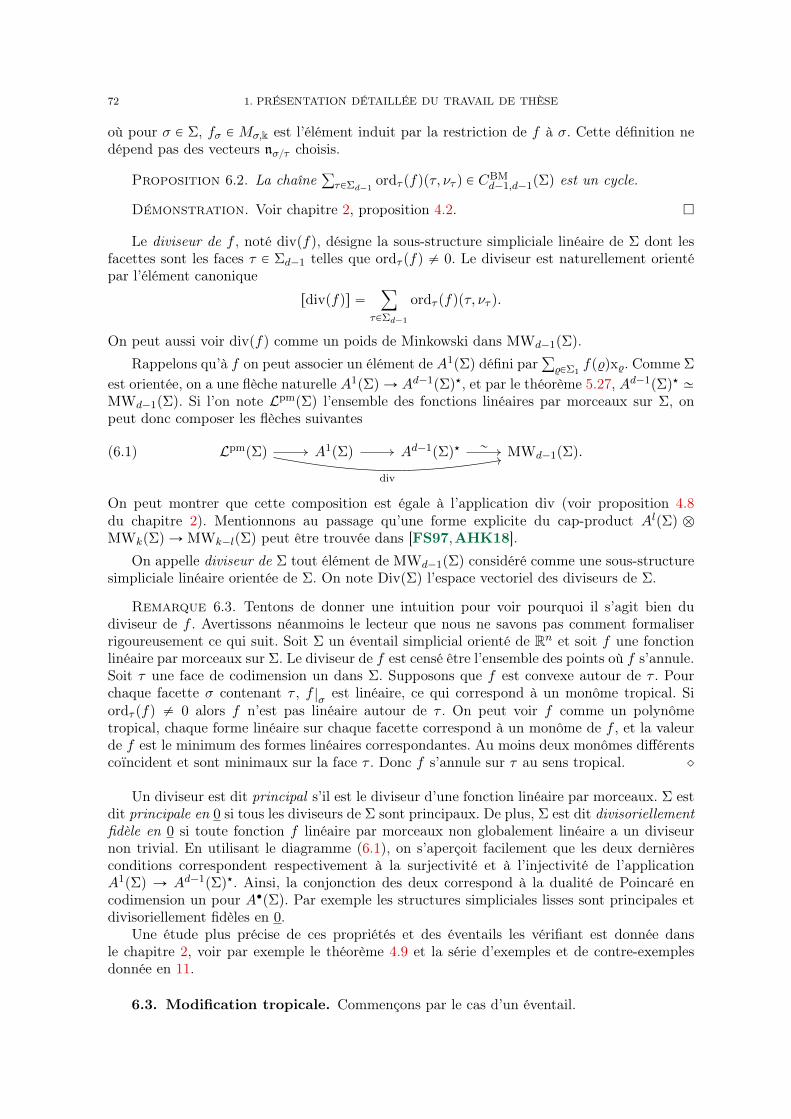
72 1. PRÉSENTATION DÉTAILLÉE DU TRAVAIL DE THÈSE
où pour σ P Σ, fσ P Mσ,k est l’élément induit par la restriction de f à σ. Cette définition nedépend pas des vecteurs nστ choisis.
Proposition 6.2. La chaîneř
τPΣd´1ordτ pfqpτ, ντ q P C
BMd´1,d´1pΣq est un cycle.
Démonstration. Voir chapitre 2, proposition 4.2.
Le diviseur de f , noté divpfq, désigne la sous-structure simpliciale linéaire de Σ dont lesfacettes sont les faces τ P Σd´1 telles que ordτ pfq ‰ 0. Le diviseur est naturellement orientépar l’élément canonique
rdivpfqs “ÿ
τPΣd´1
ordτ pfqpτ, ντ q.
On peut aussi voir divpfq comme un poids de Minkowski dans MWd´1pΣq.Rappelons qu’à f on peut associer un élément de A1pΣq défini par
ř
%PΣ1fp%qx%. Comme Σ
est orientée, on a une flèche naturelle A1pΣq Ñ Ad´1pΣq‹, et par le théorème 5.27, Ad´1pΣq‹ »MWd´1pΣq. Si l’on note LpmpΣq l’ensemble des fonctions linéaires par morceaux sur Σ, onpeut donc composer les flèches suivantes
(6.1) LpmpΣq A1pΣq Ad´1pΣq‹ MWd´1pΣq.
div
„
On peut montrer que cette composition est égale à l’application div (voir proposition 4.8du chapitre 2). Mentionnons au passage qu’une forme explicite du cap-product AlpΣq bMWkpΣq Ñ MWk´lpΣq peut être trouvée dans [FS97,AHK18].
On appelle diviseur de Σ tout élément de MWd´1pΣq considéré comme une sous-structuresimpliciale linéaire orientée de Σ. On note DivpΣq l’espace vectoriel des diviseurs de Σ.
Remarque 6.3. Tentons de donner une intuition pour voir pourquoi il s’agit bien dudiviseur de f . Avertissons néanmoins le lecteur que nous ne savons pas comment formaliserrigoureusement ce qui suit. Soit Σ un éventail simplicial orienté de Rn et soit f une fonctionlinéaire par morceaux sur Σ. Le diviseur de f est censé être l’ensemble des points où f s’annule.Soit τ une face de codimension un dans Σ. Supposons que f est convexe autour de τ . Pourchaque facette σ contenant τ , f |σ est linéaire, ce qui correspond à un monôme tropical. Siordτ pfq ‰ 0 alors f n’est pas linéaire autour de τ . On peut voir f comme un polynômetropical, chaque forme linéaire sur chaque facette correspond à un monôme de f , et la valeurde f est le minimum des formes linéaires correspondantes. Au moins deux monômes différentscoïncident et sont minimaux sur la face τ . Donc f s’annule sur τ au sens tropical. ˛
Un diviseur est dit principal s’il est le diviseur d’une fonction linéaire par morceaux. Σ estdit principale en 0 si tous les diviseurs de Σ sont principaux. De plus, Σ est dit divisoriellementfidèle en 0 si toute fonction f linéaire par morceaux non globalement linéaire a un diviseurnon trivial. En utilisant le diagramme (6.1), on s’aperçoit facilement que les deux dernièresconditions correspondent respectivement à la surjectivité et à l’injectivité de l’applicationA1pΣq Ñ Ad´1pΣq‹. Ainsi, la conjonction des deux correspond à la dualité de Poincaré encodimension un pour A‚pΣq. Par exemple les structures simpliciales lisses sont principales etdivisoriellement fidèles en 0.
Une étude plus précise de ces propriétés et des éventails les vérifiant est donnée dansle chapitre 2, voir par exemple le théorème 4.9 et la série d’exemples et de contre-exemplesdonnée en 11.
6.3. Modification tropicale. Commençons par le cas d’un éventail.
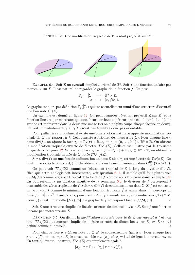
6. THÉORIE DE HODGE POUR LES STRUCTURES SIMPLICIALES LINÉAIRES 73
Figure 12. Une modification tropicale de l’éventail projectif sur R2.
Exemple 6.4. Soit Σ un éventail simplicial orienté de Rn. Soit f une fonction linéaire parmorceaux sur Σ. Il est naturel de regarder le graphe de la fonction f . On pose
Γf : |Σ| ÝÑ Rn ˆ R,x ÞÝÑ px, fpxqq.
Le graphe est alors par définition Γf p|Σ|q qui est naturellement muni d’une structure d’éventailque l’on note Γf pΣq.
Un exemple est donné en figure 12. On peut regarder l’éventail projectif Σ sur R2 et lafonction linéaire par morceaux qui vaut 0 sur l’orthant supérieur droit et ´1 sur p´1,´1q. Legraphe est représenté dans la deuxième image (ici on a de plus coupé chaque facette en deux).On voit immédiatement que Γf pΣq n’est pas équilibré donc pas orientable.
Pour pallier à ce problème, il existe une construction naturelle appellée modification tro-picale de Σ par rapport à f . Cela consiste à rajouter des faces à Γf pΣq. Pour chaque face τdans divpfq, on ajoute la face τ :“ Γf pτq ` R`e où e “ p0, . . . , 0, 1q P Rn ˆ R. On obtientla modification tropicale ouverte de Σ notée TMf pΣq. Celle-ci est illustrée par la troisièmeimage dans la figure 12. Si l’on remplace τ par τ :“ Γf pτq ` T`e Ď Rn ˆ T, on obtient lamodification tropicale fermée de Σ notée CTMf pΣq.
Si τ P divpfq est une face de codimension un dans Σ alors τ est une facette de TMf pΣq. Onpeut lui associer le poids ordf pτq. On obtient alors un élément canonique dans CBM
d,d
`
TMf pΣq˘
.On peut voir TMf pΣq comme un éclatement tropical de Σ le long du diviseur divpfq.
Bien que cette analogie soit intéressante, voir question 6.14, il semble qu’il faut plutôt voirCTMf pΣq comme le graphe tropical de la fonction f , comme nous le verrons dans l’exemple 6.9.En poursuivant la justification intuitive de la remarque 6.3, le diviseur de f correspond àl’ensemble des zéros tropicaux de f . Soit τ P divpfq de codimension un dans Σ. Si f est concave,on peut voir f comme le minimum d’une fonction tropicale rf à valeur dans l’hypercorps T,ainsi rf : |Σ| Ñ 2T. Dans ce cas, pour tout x P τ , rf s’annule sur τ , c’est-à-dire que rfpxq Q 8.Donc rfpxq est l’intervalle rfpxq,8s. Le graphe de rf correspond bien à CTMf pΣq. ˛
Soit Σ une structure simpliciale linéaire orientée de dimension d sur E. Soit f une fonctionlinéaire par morceaux sur Σ.
Définition 6.5. On définit la modification tropicale ouverte de Σ par rapport à f et l’onnote TMf pΣq la structure simpliciale linéaire orientée de dimension d sur E :“ E Y te udéfinie comme ci-dessous. ˛
Pour chaque face σ P Σ, on note σo Ď E le sous-ensemble égal à σ. Pour chaque faceτ P divpfq, on note τ Ď E le sous-ensemble τ Y tρ u où ρ “ te u désigne le nouveau rayon.En tant qu’éventail abstrait, TMf pΣq est simplement égale à
tσo | σ P Σu Y tτ | τ P divpfqu.
74 1. PRÉSENTATION DÉTAILLÉE DU TRAVAIL DE THÈSE
On a une projection naturelle p : kE Ñ kE qui envoie e sur zéro. Notons f P pkE q‹ lafonction linéaire telle que, pour e P E ,
f peq “
#
fpeq si e P E1 si e “ e .
On définit alors l’espace des fonctions linéaires sur TMf pΣq, noté M ,k comme le sous-espacede pkE q‹ engendré par p˚pMkq Y tf u. On suppose de plus que νρ est choisi de sorte quef pνρ q “ 1 et que l’orientation sur TMf pΣq vérifie signpτo, τ q “ `1 pour tout τ P divpfq.
Passons à la définition de l’élément canonique rTMf pΣqs. Notons w : Σd Ñ k le poids derΣs P MWdpΣq. On pose alors
w : TMf pΣqd ÝÑ kσo ÞÝÑ wpσq pour σ P Σd,τ ÞÝÑ ordf pτq pour τ P divpfq X Σd´1.
Proposition 6.6. L’élémentř
σPTMf pΣqdpw pσq, νσq P C
BMd,d
`
TMf pΣq˘
est un cycle.
Démonstration. Soit τ une face de codimension un dans TMf pΣq. Soit g P M ,k uneforme linéaire qui est nulle sur τ . En décomposant g sous la forme p˚h ` af , avec h P Mket a P k, on vérifie facilement que g s’annule sur
ř
%„τ wpτ _ %qν%, et donc que cette sommeest dans Nτ,k, ce qui permet de conclure. Voir aussi chapitre 2 proposition 5.1 dans le casparticulier où ordf pτq vaut zéro ou un pour toute face τ P Σd´1.
Le poids w est donc un poids de Minkowski qui fournit un élément canonique rTMf pΣqs PMWd
`
TMf pΣq˘
. Ceci conclut la définition de TMf pΣq. ˛
Rappelons que par notre remarque 2.24, nous nous permettons de considérer des sous-structures de compactifications canoniques qui ne sont pas à proprement parler des structuressimpliciales affines ou linéaires ni des compactifications canoniques de celles-ci.
Définition 6.7. On définit la modification tropicale fermée de Σ par rapport à f , notéeCTMf pΣq, comme la restriction de TMf pΣq aux faces de sédentarité 0 ou ρ .
La modification tropicale fermée étendue de Σ par rapport à f , notée CTMf pΣq, désigneTMf pΣq.
Enfin, la modification tropicale ouverte étendue de Σ par rapport à f , notée TMf pΣq,désigne la sous-structure de TMf pΣq contenant les faces δ telles que e R sedpδq. ˛
Exemple 6.8. Soit W une variété sur un corps non archimédien suffisamment gros (voirles articles cités ci-dessous pour plus de précision). Supposons que l’on peut plonger W dansune variété torique. On peut alors regarder la tropicalisation pour les coordonnées associées.Rappelons que l’analytifié de Berkovich W an de W peut être vu comme la limite projectivedes tropicalisations de W (voir section 1.10).
Si X est une tropicalisation de W et si X 1 est une modification tropicale de X, onpeut penser à X 1 comme à une nouvelle tropicalisation lorsque l’on ajoute une coordonnée(voir [Mik06,Mik07] et la section 9.2). Notamment la projection W an Ñ X se factorise enW an Ñ X 1 Ñ X. On peut donc considérer la modification tropicale comme un moyen devoir un nouveau bout de W an qui ne change pas fondamentalement la variété sous-jacente.D’ailleurs, dans [Jel19], Jell montre que, si W est normale et admet au moins un plongementfermé dans une variété torique, alors la cohomologie de Dolbeault à support compact de W an
est la limite de la cohomologie tropicale des tropicalisations de W . Ceci est à comparer avecle théorème 6.10 ci-dessous, montrant que dans certains cas la modification tropicale préservela cohomologie. ˛
6. THÉORIE DE HODGE POUR LES STRUCTURES SIMPLICIALES LINÉAIRES 75
6.4. Propriétés de la modification tropicale. Nous avons vu que la modification tro-picale d’une structure simpliciale linéaire doit être considérée comme le graphe d’une fonctionsur celle-ci. Poursuivons l’analogie.
Exemple 6.9. Soit V une variété topologique de Rn. Soit f une fonction de V dansR. Notons Γf pV q le graphe de f dans Rn ˆ R. Alors la cohomologie classique de Γf pV qest clairement égale à celle de V . Dans le cadre tropical, on peut donc conjecturer que lamodification tropicale d’un éventail a la même cohomologie tropicale que cet éventail. Danscette section, nous verrons que c’est bien le cas si l’éventail est lisse, mais que ce n’est pasforcément vrai dans le cas général. ˛
Si Σ est une structure simpliciale linéaire et si ∆ est une sous-structure de Σ, on définitnaturellement l’homologie de Borel-Moore de Σ relative à ∆ par
HBMp,q pΣ,∆q :“ Hq
´
coker`
CBMp,‚ p∆q ãÑ CBM
p,‚ pΣq˘
¯
.
Théorème 6.10. Soit Σ une structure simpliciale linéaire lisse. Soit f une fonction linéairepar morceaux sur Σ. Alors,
HBM‚,‚
`
TMf pΣq˘
» HBM‚,‚
`
Σ,divpfq˘
et H‚,‚`
CTMf pΣq˘
» H‚,‚`
Σ˘
.
Les relations analogues que l’on peut imaginer pour la cohomologie et pour les différentesmodifications tropicales sont aussi vraies : voir le théorème 10.1 du chapitre 2. Nous nousplaçons ici dans le cadre homologique car il nous semble que cela rend les isomorphismes plussimples à comprendre.
Pour une face τ P ∆, on peut considérer τ comme une face de ∆ ou comme une face deΣ, ce qui peut mener à une ambiguïté sur la notation F‚pτq. Pour lever cette ambiguïté, ondifférenciera F∆
‚ pτq et FΣ‚ pτq.
Remarque 6.11. Décrivons brièvement les différents isomorphismes du théorème. Le pre-mier isomorphisme est simplement induit par la projection p˚ : F‚pσoq Ñ FΣ
‚ pσq pour σ P Σ.Pour le second isomorphisme, on doit y ajouter les inclusions i˚ : F‚pτ
ρ8q » F∆
‚ pτq ãÑ FΣ‚ pτq
pour τ P ∆. ˛
La preuve s’appuie essentiellement sur le lemme suivant.
Lemme 6.12 (Formule locale pour la modification tropicale). Soit Σ une structure sim-pliciale linéaire lisse, et soit ∆ “ divpfq avec f une fonction linéaire par morceaux sur Σ.Posons rΣ :“ TMf pΣq.
Soient σ une face de Σ r ∆, τ une face de ∆, et p un entier positif. Alors on a les suitesexactes suivantes.
0 FrΣp pσoq FΣ
p pσq 0,
0 F∆p´1pτq F
rΣp pτ q F∆
p pτq 0,
0 F∆p´1pτq F
rΣp pτoq FΣ
p pτq 0
p˚
p˚
p˚
où la première flèche de chacune des deux dernières suites exactes est donnée par v ÞÑ e ^p˚pvqoù p˚pvq désigne n’importe quelle préimage de v par p˚.
Démonstration. Voir le lemme 10.3 du chapitre 2. La seconde suite exacte est triviale.Ce n’est pas le cas des deux autres. Pour la première, on peut montrer que cela découle du faitque Σσ est divisoriellement fidèle (voir l’exemple 6.13). Pour la dernière, l’idée est d’utiliserles résolutions des faisceaux F‚ données par le théorème 4.7, c’est-à-dire par le dual de larésolution de Deligne tropicale. L’une des difficultés est qu’il ne s’agit d’une résolution quepour FΣ
‚ car Σ est lisse, mais pas forcément pour F∆‚ et FrΣ
‚ .
76 1. PRÉSENTATION DÉTAILLÉE DU TRAVAIL DE THÈSE
Exemple 6.13. Soit Σ la croix tropicale, c’est-à-dire l’éventail de dimension un dans R2
de rayons ρ1, . . . , ρ4 engendrés par e1, e2,´e1 et ´e2 respectivement où pe1, e2q est la basestandard de R2. On peut considérer la fonction f linéaire par morceaux qui vaut 1 sur e1, ´1
sur e2 et 0 sur ´e1 et ´e2. Alors divpfq est trivial. La modification tropicale rΣ :“ TMf pΣq
est isomorphe à la droite tropicale dans R3. Notamment FrΣ1 p0oq n’est pas isomorphe à FΣ
1 p0q.Cela ne contredit pas le lemme 6.12 car Σ n’est pas lisse. Le problème ici est essentiellement
que Σ n’est pas divisoriellement fidèle en 0. Notons que la modification tropicale, elle, est lisse.Il est donc naturel de se poser la question suivante.
Question 6.14. Existe-t-il une théorie de désingularisation tropicale fondée sur les mo-difications tropicales ? ˛
Cette question va dans le sens à considérer la modification tropicale plutôt comme unéclatement que comme le graphe d’une fonction. ˛
Démonstration du théorème 6.10. À partir du lemme 6.12, la preuve est essentiel-lement déjà présente dans [Sha15,JSS19,JRS18]. Nous proposons une nouvelle preuve ensection 10 du chapitre 2 qui consiste à utiliser le lemme 6.12 pour décomposer les complexesde chaînes CBM
‚,‚ pΣq et C‚,‚pΣq et ainsi obtenir pour chacun une suite exacte courte de com-plexes de chaînes. Les suites exactes longues associées en cohomologie permettent de montrerle théorème.
Le théorème 6.10 possède un analogue pour le groupe de Chow qui nécessite moins deconditions.
Théorème 6.15. Soit Σ une structure simpliciale linéaire orientée. Soit f une fonctionlinéaire par morceaux sur Σ. Alors on a un morphisme d’anneau surjectif
A‚pΣq A‚`
TMf pΣq˘
.
Si de plus Σ est divisoriellement fidèle, alors cette application est un isomorphisme.
Démonstration. L’application consiste à envoyer x% sur x%o pour tout rayon % P Σ1. Onvérifie facilement que l’application est bien définie, et aussi qu’elle est surjective car la nouvellevariable xρ peut facilement être exprimée grâce aux autres variables. L’injectivité dans le casdivisoriellement fidèle est plus délicate, voir chapitre 2 section 10.3.
6.5. Subdivision étoilée. Soit Σ une structure simpliciale linéaire sur E. Soit η uneface de Σ. On dit qu’un vecteur v P Nη,k est à l’intérieur de η si
v “ÿ
%PΣ1%ăη
a%ν%
où les a% sont des coefficients strictement positifs.
Définition 6.16. La subdivision étoilée de Σ le long de v est notée Σpvq et est une structuresimpliciale linéaire sur E Y tevu définie de la manière suivante. L’ensemble des faces de Σpvqest
tσ P Σ | σ ą ηu Y tτ Y tevu | τ ą η, τ comparable à ηu.L’espace des formes linéaires sur Σpvq est engendré par les formes linéaires ` P Mk que l’onprolonge sur pkEYtevuq‹ par `pevq “
ř
a%`pν%q. ˛
Notons que Σpvq est bien une subdivision simpliciale de Σ au sens de la section 2.2. Si Σ estorientée, alors Σpvq est naturellement orientée : chaque facette de Σpvq hérite du multi-vecteurde rΣs associé à l’unique facette de Σ lui correspondant (la face correspondant à τ _ tevu estτ _ η).
6. THÉORIE DE HODGE POUR LES STRUCTURES SIMPLICIALES LINÉAIRES 77
Remarque 6.17. La définition ci-dessus est encore valide si v est à l’extérieur de η. Dansce cas nous n’obtenons pas une subdivision de Σpvq mais il est probable que certaines propriétésde l’éclatement décrites en section 6.6 restent vraies dans ce cadre, ce qui peut permettre deconstruire de nouvelles structures simpliciales intéressantes. ˛
Exemple 6.18. La subdivision étoilée est bien connue en géométrie torique pour la raisonsuivante. Soit Σ un éventail unimodulaire de Rn. Prenons ν% unitaire pour tout % P Σ1. SoitCPΣ la variété torique associée. Soit η une face de Σ et soit
v :“ÿ
%PΣ1%ăη
ν%,
son barycentre. Alors CPΣpvq correspond à l’éclatement de CPΣ le long de la strate ferméeassociée à η.
L’étude du lien entre l’éclatement combinatoire et l’éclatement des variétés toriques estau cœur du théorème de factorisation faible dans l’article [AKMW02] d’Abramovich, Karu,Matsuki et Włodarczyk. Ce théorème énonce que n’importe quelle application birationnelleentre deux variétés complexes projectives lisses peut être décomposée en un nombre fini d’écla-tements et de contractions (l’inverse d’un éclatement) de sous-variétés lisses. Nous utilisonscertains de leurs résultats dans cette thèse : voir le théorème 6.29 et le commentaire en-dessous. ˛
Par analogie avec l’exemple précédent, on appelle également Σpvq l’éclatement de Σ le longde v. À l’inverse, Σ est appelé la soudure étoilée, ou la contraction, de Σpvq le long de ρv oùρv “ tevu est le nouveau rayon associé à v.
6.6. Propriétés de l’éclatement. Comme pour les modifications tropicales, l’effet d’unéclatement sur la cohomologie d’une structure simpliciale est très bien compris. D’abord,comme l’éclatement ne modifie pas le support de l’éventail, la cohomologie ne change pas(cf. corollaire 3.7) :
H‚,‚pΣpvqq » H‚,‚pΣq et H‚,‚c pΣpvqq » H‚,‚c pΣq.
L’éclatement devient plus intéressant lorsque l’on s’intéresse à l’anneau de Chow de Σ où à lacohomologie de Σ.
Dans le cas de l’éclatement d’une variété le long d’une sous-variété, le lemme de Keel(théorème 1 de l’annexe dans [Kee92]) permet de calculer l’anneau de Chow de l’éclatementpar rapport à l’anneau de Chow de la variété de départ. Voici l’analogue dans notre cadre.
Soient Σ une structure simpliciale linéaire lisse, η une face de Σ et v P Nη,k à l’intérieurde η. Soit Σpvq l’éclatement de Σ le long de v et soit ρv le nouveau rayon. On peut écrire
νρv “ÿ
%PΣ1%ăη
a%ν%,
pour d’uniques coefficients a% ą 0. Pour différencier les variables de A‚pΣq des variables deA‚pΣpvqq, nous notons x1σ les variables du second anneau.
Théorème 6.19 (Lemme de Keel). Soit J le noyau de la surjection i˚0ăη : A‚pΣq Ñ
A‚pΣηq. PosonsP pT q :“
ź
%PΣ1%ăη
px% ` a%T q.
AlorsA‚pΣpvqq » A‚pΣqrT s
L
pJT ` P pT qq,

78 1. PRÉSENTATION DÉTAILLÉE DU TRAVAIL DE THÈSE
et l’isomorphisme est donné par l’application
χ : A‚pΣqrT sL
pJT ` P pT qq „ÝÑ A‚pΣpvqq
qui envoie T sur ´x1ρv et qui vérifie
@ % P Σ1, χpx%q “
#
x1% ` a%x1ρv si % ă η,
x1% sinon.
En particulier on obtient une décomposition de A‚pΣpvqq en tant qu’espace vectoriel
A‚pΣpvqq » A‚pΣq ‘A‚´1pΣηqT ‘ ¨ ¨ ¨ ‘A‚´|η|`1pΣηqT |η|´1.(6.2)
Le reste de la section 6.6 est consacré à la description des parties importantes de lapreuve de ce théorème. Nous allons voir que la décomposition 6.2 possède de bonnes propriétésnotamment vis-à-vis de la dualité de Poincaré. Notons que dans le cas où Σ est un éventailunimodulaire et que v est choisi comme dans l’exemple 6.18, la proposition découle simplementdu lemme de Keel classique. Dans le cas général, on peut établir une preuve élémentaire, quenous décrivons brièvement ici (à comparer avec [AHK18, Section 6] qui traite un problèmesimilaire).
Précisons d’abord ce que signifie la dernière décomposition dans l’énoncé du théorème.Considérons le complexe simplicial η qui est la restriction de Σ aux faces de η. On peut éclaterη en v pour obtenir η
pvq. Notons ∆ “ ηρv
pvq l’éventail transverse autour du nouveau rayon. AlorsΣρvpvq » ∆ˆ Ση. Notamment, par la formule de Künneth,
A‚pΣρvpvqq » A‚p∆q bA‚pΣηq.
On a donc une inclusion naturelle A‚pΣηq ãÑ A‚pΣρvpvqq qui envoie a sur 1ba. On peut montrer
que l’on a le diagramme commutatif
A‚pΣq A‚pΣηq A‚pΣqrT s
A‚pΣpvqq A‚pΣρvpvqq A‚`1pΣpvqq
¨T
i˚
χ ¨T χ
i˚
¨p´x1vρ q
´gys
Le terme A‚pΣηqT désigne donc l’image de A‚pΣηq par l’application ¨T définie par le dia-gramme ci-dessus.
Revenons à la preuve. On vérifie facilement que l’application A‚pΣq Ñ A‚pΣpvqq est biendéfinie et se prolonge en un morphisme surjectif A‚pΣqrT s A‚pΣpvqq. De plus P pT q estenvoyé sur
ś
%PΣ1,%ăηx1% qui est nul dans A‚pΣpvqq. Ensuite, vu le diagramme ci-dessus, tout
élément a P J vérifie χpaT q “ 0.Il reste à montrer l’injectivité. Pour cela on utilise la dualité de Poincaré. En posant
C “ś
%ăη a%, un calcul (cf. la preuve du théorème 6.13 du chapitre 2) montre que l’on a lediagramme commutatif suivant
(6.3)Ad´|η|pΣηq AdpΣpvqq AdpΣq
k
gysηą0
¨p´CT |η|q„
„
degdeg
„
χ„
deg„
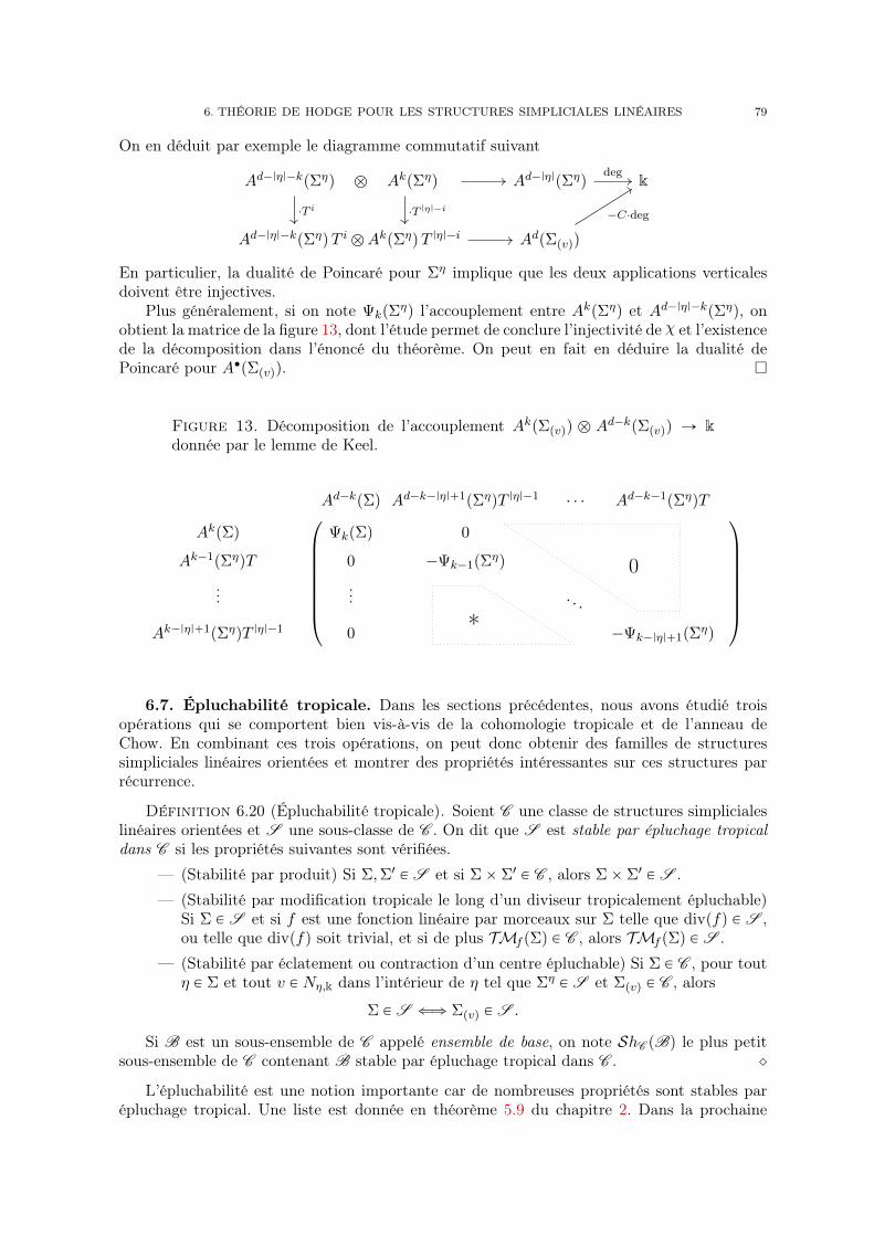
6. THÉORIE DE HODGE POUR LES STRUCTURES SIMPLICIALES LINÉAIRES 79
On en déduit par exemple le diagramme commutatif suivant
Ad´|η|´kpΣηq b AkpΣηq Ad´|η|pΣηq k
Ad´|η|´kpΣηqT i bAkpΣηqT |η|´i AdpΣpvqq
¨T i ¨T |η|´i
deg
´C¨deg
En particulier, la dualité de Poincaré pour Ση implique que les deux applications verticalesdoivent être injectives.
Plus généralement, si on note ΨkpΣηq l’accouplement entre AkpΣηq et Ad´|η|´kpΣηq, on
obtient la matrice de la figure 13, dont l’étude permet de conclure l’injectivité de χ et l’existencede la décomposition dans l’énoncé du théorème. On peut en fait en déduire la dualité dePoincaré pour A‚pΣpvqq.
Figure 13. Décomposition de l’accouplement AkpΣpvqq b Ad´kpΣpvqq Ñ kdonnée par le lemme de Keel.
Ad´kpΣq Ad´k´|η|`1pΣηqT |η|´1 ¨ ¨ ¨ Ad´k´1pΣηqT
AkpΣq ΨkpΣq 0
Ak´1pΣηqT 0 ´Ψk´1pΣηq
...... ¨ ¨ ¨
Ak´|η|`1pΣηqT |η|´1 0 ´Ψk´|η|`1pΣηq
0
*
¨
˚
˚
˚
˚
˚
˚
˚
˝
˛
‹
‹
‹
‹
‹
‹
‹
‚
6.7. Épluchabilité tropicale. Dans les sections précédentes, nous avons étudié troisopérations qui se comportent bien vis-à-vis de la cohomologie tropicale et de l’anneau deChow. En combinant ces trois opérations, on peut donc obtenir des familles de structuressimpliciales linéaires orientées et montrer des propriétés intéressantes sur ces structures parrécurrence.
Définition 6.20 (Épluchabilité tropicale). Soient C une classe de structures simplicialeslinéaires orientées et S une sous-classe de C . On dit que S est stable par épluchage tropicaldans C si les propriétés suivantes sont vérifiées.
— (Stabilité par produit) Si Σ,Σ1 P S et si Σˆ Σ1 P C , alors Σˆ Σ1 P S .
— (Stabilité par modification tropicale le long d’un diviseur tropicalement épluchable)Si Σ P S et si f est une fonction linéaire par morceaux sur Σ telle que divpfq P S ,ou telle que divpfq soit trivial, et si de plus TMf pΣq P C , alors TMf pΣq P S .
— (Stabilité par éclatement ou contraction d’un centre épluchable) Si Σ P C , pour toutη P Σ et tout v P Nη,k dans l’intérieur de η tel que Ση P S et Σpvq P C , alors
Σ P S ðñ Σpvq P S .
Si B est un sous-ensemble de C appelé ensemble de base, on note ShC pBq le plus petitsous-ensemble de C contenant B stable par épluchage tropical dans C . ˛
L’épluchabilité est une notion importante car de nombreuses propriétés sont stables parépluchage tropical. Une liste est donnée en théorème 5.9 du chapitre 2. Dans la prochaine
80 1. PRÉSENTATION DÉTAILLÉE DU TRAVAIL DE THÈSE
section, nous nous contenterons d’énoncer les deux propriétés les plus importantes parmicelles-ci, à savoir la lissité et HR.
En pratique, la restriction à C de l’épluchage évite de faire n’importe quel éclatementou contraction. Pour C nous prendrons typiquement Orient, à savoir l’ensemble de toutes lesstructures simpliciales linéaires orientées, ou Oqproj, à savoir l’ensemble de celles qui sontquasi-projectives. Ces deux ensembles sont stables par produits, modifications tropicales etéclatements (voir le théorème 5.6 du chapitre 2), mais Oqproj n’est pas stable par contraction.
Un ensemble de base typique est
t0u,Λ(
où Λ “ t0,R`,R´u est la droite tropicale dansR. En section 6.10, nous verrons que ShOqprojpB0q contient déjà de nombreuses structuresintéressantes, notamment les éventails de Bergman généralisés.
6.8. Théorèmes principaux. Citons maintenant les résultats montrant l’importance dela notion que nous venons d’introduire.
Théorème 6.21 (Stabilité de la lissité par épluchage). L’ensemble des structures linéairessimpliciales lisses est stable par épluchage tropical dans Orient. Notamment les éléments deShOrientpB0q et de ShOrientpSSq sont lisses, où SS désigne l’ensemble des cônes de sphèressimpliciales de dimensions maximales.
Démonstration. Voir le théorème 10.4 dans le chapitre 2. Nous nous contentons d’es-quisser la preuve ici.
Si Σ est lisse, alors Σσ est lisse pour tout σ P Σ. Par récurrence sur la dimension, on peutdonc se contenter de montrer la stabilité de la dualité de Poincaré par les différentes opérations(cet argument n’est pas tout à fait trivial, voir le lemme 5.10 du chapitre 2).
— La stabilité par produit est une conséquence directe de la formule de Künneth, théo-rème 6.1.
— Pour la stabilité par modification tropicale, on justifie de la manière suivante. SoitΣ une structure simpliciale linéaire lisse et soit f une fonction linéaire par morceauxsur Σ telle que divpfq soit lisse. Posons rΣ :“ TMf pΣq. Si Σ est lisse, alors Σ estlisse par définition, et, par le corollaire 4.4, Σ vérifie la dualité de Poincaré. Par lethéorème 6.10, on sait que H‚,‚pCTMf pΣqq » H‚,‚pΣq. Donc CTMf pΣq vérifie ladualité de Poincaré. Par récurrence sur la dimension, on sait que pour tout σ P rΣ
avec σ ‰ 0, rΣσ est lisse. Comme de plus rΣ “ CTMf pΣq vérifie la dualité de Poincaré,on peut appliquer le théorème 4.3 pour obtenir la dualité de Poincaré pour Σ, ce quiconclut.
— La stabilité par éclatement et contraction est triviale ici car la lissité est stable parsubdivision par le corollaire 3.7.
Pour la seconde partie du théorème, comme t0u et B0 sont lisses et comme les éventailslisses sont stables par épluchage tropical dans Orient, ShOrientpB0q est un sous-ensemble del’ensemble des éventails lisses. On utilise le même argument pour SS.
Théorème 6.22 (Stabilité de HR par épluchage). L’ensemble des structures linéairessimpliciales kählériennes est stable par épluchage dans Oqproj. Notamment les éléments deShOqprojpB0q vérifient cette propriété.
Notons que comme A‚pΣq est isomorphe à H‚,‚pΣq dans le cas lisse, le théorème précédentmontre les relations de Hodge-Riemann pour la cohomologie de Σ.
Avant d’esquisser la preuve, faisons quelques remarques importantes sur les classes ampleset les fonctions convexes.
Soit Σ une structure simpliciale linéaire quasi-projective. Soit f une fonction strictementconvexe sur Σ. Pour tout σ P Σ, f induit une fonction strictement convexe sur Σσ, notéefσ, qui est bien définie modulo une forme linéaire. À f on peut associer la classe ample ` :“
6. THÉORIE DE HODGE POUR LES STRUCTURES SIMPLICIALES LINÉAIRES 81
ř
%PΣ1fp%qx% P A
1pΣq. On obtient alors des classes amples `σ sur chaque éventail transverseΣσ.
Si rΣ est une modification tropicale de Σ alors la fonction f prolongée par zéro sur lenouveau rayon ρ est une fonction strictement convexe. Donc rΣ est quasi-projective et l’onobtient une classe ample dans A1prΣq.
Si η P Σ est une face de Σ et si v P Nη,k est à l’intérieur de η avec
v “ÿ
%PΣ1%ăη
a%ν%,
alors Σpvq est quasi-projective. En effet, la fonction f prolongée sur le nouveau rayon par
´ε`ÿ
%PΣ1%ăη
a%fp%q
est strictement convexe pour tout ε ą 0 suffisamment petit.Enfin, si Σ1 est une autre structure quasi-projective munie d’une classe ample `1, alors
l’élement`b 1` 1b `1 P A1pΣq bA0pΣ1q ‘ A0pΣq bA1pΣ1q » A1pΣˆ Σ1q
est ample dans Σˆ Σ1. Notamment le produit Σˆ Σ1 est quasi-projectif.
Démonstration. Tous les détails sont dans la section 3 du chapitre 3, voir notamment laremarque 3.21. La formule de Künneth, théorème 6.1, permet de montrer la stabilité par pro-duit de HL et HR. Le théorème 6.15 montre que l’anneau de Chow est préservé par modificationtropicale et donc HL et HR sont aussi préservées. Le point délicat est de démontrer la stabilitépar éclatement et contraction. Pour ce point, on peut s’inspirer de la preuve de [AHK18]. Lapreuve est essentiellement en deux étapes.
D’abord, un calcul assez simple montre que si l’on a HRpΣ%, `%q pour tout rayon % de Σ,alors on a HLpΣ, `q. Donc par récurrence sur la dimension, on obtient HLpΣ, `q pour touteclasse ample ` P A1pΣq. L’ensemble des classes amples forme un cône connexe dans A1pΣq notéK`. De plus, on montre facilement en utilisant la décomposition en parties primitives que lavéracité de HRpΣ, `q est entièrement déterminée par la signature des formes quadratiquesinduites par ` sur AkpΣq pour k ď d2 : voir la définition 3.3 et la propriété (3.3) dans lechapitre 3. Par le théorème de Lefschetz difficile, les éléments de K` induisent des formesquadratiques non dégénérées, donc la signature ne peut pas changer sur K` qui est connexe.On s’est donc ramené à démontrer HRpΣ, `q pour une unique classe ample.
La deuxième partie de la preuve consiste à démontrer la propriété suivante. Soit Σpvq unéclatement de Σ et ρ le nouveau rayon. Si ` est une classe kählérienne sur Σ, on a vu que`ε :“ χp``εT q est une classe ample pour tout ε ą 0 suffisamment petit, où χ est l’applicationA‚pΣqrT s Ñ A‚pΣpvqq définie dans le lemme de Keel, théorème 6.19. On veut alors montrerque
HRpΣ, `q ðñ @ 0 ă ε ! 1, HRpΣpvq, χp`εqq.
Le sens direct, correspondant à l’éclatement, est appelé l’ascension, et le sens réciproque,associé à la contraction, est appelé la descente. L’idée pour la preuve de l’ascension est assezconnue : par exemple, elle est utilisée pour déduire la conjecture standard de type Lefschetzpour un éclatement à partir du même résultat pour la variété de départ. La descente estlégèrement plus compliquée, notamment on utilise HLpΣ, `q, ce qui n’est pas nécessaire pourl’ascension. Remarquons que dans les deux cas on utilise HRpΣη, `ηq où η est la face qui a étééclatée.
En effet, cette deuxième partie de la preuve repose sur une étude précise de l’action del’opérateur de Lefschetz sur la décomposition de A‚pΣpvqq donnée par le lemme de Keel. Lesdétails sont présents en section 3.11 du chapitre 3. Ici nous nous contenterons de montrer HR
82 1. PRÉSENTATION DÉTAILLÉE DU TRAVAIL DE THÈSE
pour A1pΣpvqq en supposant HR pour A‚pΣq. Dans ce cas, HR signifie simplement que la formequadratique Qε induite par `ε sur A1pΣpvqq a pour signature p1,dim
`
A1pΣpvqq˘
´1q. Le lemmede Keel nous donne une décomposition
A1pΣpvqq » A1pΣq ‘ TA0pΣηq.
La forme quadratique induite par `ε sur la partie A1pΣq est égale à celle induite par ` plus ungrand O de ε, donc pour ε petit, sa signature est p1, dimpA1pΣqq ´ 1q. Il reste à montrer quela forme est définie négative sur TA0pΣq, c’est-à-dire que
deg`
p`η ` εT qd´2T 2˘
ă 0.
Lorsque l’on développe, comme p`ηqd´|η|`1 “ 0, on trouve que ce degré vaut
ε|η|´2
ˆ
d´ 2
|η|´ 2
˙
´
deg`
T |η|p`ηqd´|η|˘
`Opεq¯
.
Comme on a HRpΣη, `ηq, ou simplement parce que `η est ample, le degré de p`ηqd´|η| PAd´|η|pΣηq est positif, et donc le degré de T |η|p`ηqd´|η| est négatif par le diagramme 6.3.C’est ce que l’on souhaitait. La preuve en degrés supérieurs est essentiellement dans le mêmeesprit mais plus technique.
La dernière partie du théorème découle du fait que les éléments de B0 vérifient que toutesleurs classes amples sont kählériennes.
Dans la section 7 nous expliquons comment étendre ces résultats aux structures simplicialesaffines.
6.9. Théorème de factorisation faible. Nous énonçons maintenant un théorème defactorisation faible réelle. Ce théorème est très utile pour montrer que les familles stables parépluchage tropical dans Orient ou Oqproj contiennent beaucoup d’éléments, cf. théorème 5.7 duchapitre 2. Nous citerons ensuite le théorème de factorisation faible classique pour les éventailsqui a été mentionné dans l’exemple 6.18.
Théorème 6.23 (Théorème de factorisation faible réelle). Soient Σ et Σ1 deux structuressimpliciales linéaires qui possèdent une subdivision commune. Alors il existe une suite de struc-tures simpliciales linéaires Σ “ Σp0q,Σp1q, . . . ,Σpkq “ Σ1 telle que pour tout 0 ď i ă k, Σpi`1q
soit obtenue à partir de Σpiq par un éclatement ou une contraction.Si de plus Σ et Σ1 sont quasi-projectives alors on peut supposer que Σp0q, . . . ,Σpkq sont
quasi-projectives.
Rappelons que dans le cas de deux éventails de Rn, avoir une subdivision commune estéquivalent à avoir le même support.
Avant de passer à la preuve, énonçons la définition suivante.
Définition 6.24. Soit Σ une structure simpliciale linéaire et ∆ une subdivision de Σ. Ondit que ∆ est projective relativement à Σ s’il existe une fonction linéaire par morceaux f sur∆ telle que la restriction de f à la sous-structure ∆|σ de ∆ induite par n’importe quelle faceσ de Σ est strictement convexe. Une telle fonction f est dite strictement convexe relativementà Σ. ˛
Par exemple, Σ est toujours projective relativement à elle-même (on peut prendre la fonc-tion nulle), et si ∆ est quasi-projective, alors ∆ est projective relativement à Σ. Cette définitionest fort utile car nous avons les deux propositions et les deux exemples suivants.
Exemple 6.25 (Découpe par un hyperplan). Les détails de cette construction sont ensection 4.2.1 du chapitre 3. Soit Σ un éventail simplicial (ou un complexe simplicial) de Rn etsoit H un hyperplan dans Rn. On peut considérer la découpe hyperplane de Σ par H notéeΣ¨H qui est une subdivision (par forcément simpliciale) de Σ dont toutes les faces sont incluses
6. THÉORIE DE HODGE POUR LES STRUCTURES SIMPLICIALES LINÉAIRES 83
dans l’un des deux demi-espaces délimités par H. On peut considérer la fonction distance àH. La restriction de cette fonction à Σ ¨H est strictement convexe relativement à Σ. ˛
Exemple 6.26 (Éclatement). Soient Σ une structure simpliciale linéaire, η P Σ et v àl’intérieur de η. Alors Σpvq est projective relativement à Σ. En effet, on peut considérer lafonction f linéaire par morceaux sur Σ qui vaut zéro sur tous les rayons sauf sur v où elle vaut´ε pour ε ą 0 petit. ˛
Proposition 6.27. La bijection entre les subdivisions d’une structure simpliciale linéaireΣ et les subdivisions de sa représentation géométrique pΣ vue comme un éventail de RE induitune bijection entre les subdivisions projective relatives.
Proposition 6.28. Soient Σ une structure simpliciale linéaire, ∆ une subdivision simpli-ciale de Σ et ∆1 une subdivision simpliciale de ∆.
— Si ∆1 est projective relativement à Σ, alors ∆1 est projective relativement à ∆.
— Si ∆1 est projective relativement à ∆ et ∆ est projective relativement à Σ, alors ∆1
est projective relativement à Σ.
— Si ∆ est projective relativement à Σ et si Σ est quasi-projective, alors ∆ est quasi-projective.
Démonstration. La preuve est moins immédiate que pour la première proposition.L’idée est simple. Pour la troisième partie par exemple, si g est une fonction linéaire parmorceaux strictement convexe sur Σ et si f est une fonction linéaire par morceaux sur ∆strictement convexe relativement à Σ, alors g ` εf est strictement convexe sur Σ pour εsuffisamment petit. Voir 4.3 du chapitre 3 pour plus de détail.
Démonstration du théorème 6.23. Commençons par la première partie où l’on nesuppose pas la quasi-projectivité. Soit ∆2 une subdivision commune de Σ et Σ1.
Nous commençons en construisant une subdivision ∆1 de ∆2 qui est projective relativementà Σ et à ∆2. La première étape de cette construction consiste à considérer la subdivision del’éventail pΣ correspondant à ∆2 et de découper pΣ par des hyperplans bien choisis afin qu’aprèsla découpe on obtienne une subdivision (pas forcément simpliciale) de celle induite par ∆2.Ensuite on effectue des éclatements des faces non simpliciales pour obtenir une subdivisionsimpliciale (voir chapitre 3 proposition 4.4). En utilisant les exemples et les propositions ci-dessus, on a bien obtenu une subdivision ∆1 de ∆2 qui est projective relativement à Σ et à∆2.
Comme ∆1 est une subdivision de Σ1, on peut de même construire une subdivision ∆ de ∆1
qui est relativement projective par rapport à Σ1 et à ∆1. On obtient finalement une subdivisioncommune ∆ de Σ et Σ1 qui est relativement projective par rapport à chacun.
Maintenant, on s’est ramené au problème suivant. Soit ∆ une subdivision relativementprojective de Σ. Alors on peut trouver une série d’éclatements et de contractions pour allerde Σ à ∆. Pour faire cela, on peut s’inspirer d’une construction classique, par exemple utiliséepar McMullen dans [McM93] ; pour un livre de référence, voir [DRS10].
On va d’abord considérer un cas simple. Soit 4 un simplexe dans Rd et soit Υ une subdi-vision simpliciale relativement projective de 4. Nous voulons montrer que l’on peut obtenir Υà partir de 4 par une série d’éclatements et de contractions. Notons v0, . . . , vr les sommets deΥ. Soit f : Υ0 Ñ R une fonction linéaire par morceaux sur Υ strictement convexe relativementà 4 (donc strictement convexe tout court). Quitte à modifier légèrement les valeurs de f enchaque sommet, on peut supposer f suffisamment générique. On peut considérer le graphe dela fonction f ,
Γf : Υ0 Ñ Rd ˆ R,v ÞÑ pv, fpvqq.

84 1. PRÉSENTATION DÉTAILLÉE DU TRAVAIL DE THÈSE
L’enveloppe convexe de Γf pΥ0q est un polytope Pf . Les faces inférieures de Pf sont par défi-nitions les facettes de Pf dont le vecteur normal extérieur a sa dernière coordonnée négative,ainsi que toutes les faces de ces facettes. On peut projeter ces faces inférieures sur Rd, et l’onretrouve la subdivision Υ, comme dans la figure 14.
Figure 14. Une triangulation du carré donnée par une fonction convexe, et un flip.
CC BY 4.0 : issue d’une présentation par Jorathan Richard Shewchuk publié par Pranav Kant Gaurhttps://www.slideshare.net/PranavKantGaur/shewchuk
Pour mieux visualiser la suite, supposons que f est négative. Maintenant on va descendreles points un par un. Par exemple, si l’on numérote les sommets de Υ par v0, . . . , vr, on peutposer
h : RˆΥ0 ÝÑ R,
pt, viq ÞÝÑ
$
’
&
’
%
0 si t ď i,pt´ iqfpviq si i ď t ď i` 1,fpviq si i` 1 ď t.
Ainsi, hp0, ¨ q est la fonction nulle et hpr`1, ¨ q “ f . À chaque instant t, on regarde l’enveloppeconvexe Pt des points pvi, hpt, viqq, et l’enveloppe inférieure de Pt définit une subdivision Υt
de 4. Mis à part en un nombre fini d’instants, on est dans un intervalle de temps ouvertdans lequel la subdivision simpliciale ne change pas. Mais de temps en temps, un sommetpeut apparaître ou disparaître, ce qui correspond respectivement à un éclatement ou unecontraction (vu notre construction, la disparition n’est pas possible ici), ou encore, il peut yavoir à certains instants t une face de dimension s avec s` 2 sommets, qui n’est donc pas unsimplexe. Ce dernier cas est représenté à droite dans la figure 14. (Dans cette figure tous lespoints bougent en même temps, mais l’idée reste la même.) Soit t0 un tel instant. Dans ce cas,juste avant et juste après, nous avons bien des triangulations Υt0´ et Υt0` de 4. L’opérationpour passer de Υt0´ à Υt0` est connue sous le nom de flip ou d’opération bistellaire, et c’estla composée d’un éclatement et d’une contraction. Rien d’autre ne peut arriver durant ladescente des différents sommets. Comme Υ0 “ 4 et Υr`1 “ Υ, cela montre bien que l’on peutobtenir Υ à partir de 4 par une série d’éclatements et de contractions.
On peut facilement se convaincre que le cas du simplexe peut être généralisé à tout com-plexe simplicial, ou éventail simplicial ou même structure simpliciale linéaire, en traitant lessommets de la subdivision un par un et en considérant les faces indépendamment mais si-multanément : on choisit une fonction relativement projective globale, on descend un par unles sommets comme ci-dessus, mais l’on considère les enveloppes convexes et les subdivisionsinduites face par face, en regardant pour chaque face le graphe de la restriction de la fonctionà cette face. Cela conclut la première partie de la preuve.
6. THÉORIE DE HODGE POUR LES STRUCTURES SIMPLICIALES LINÉAIRES 85
Pour la deuxième partie, notons que pour le simplexe, par construction, Υt est projectiverelativement à 4 à tout moment. Donc la construction généralisée aux complexes simpliciauxdonnera à tout moment une triangulation relativement projective, et donc quasi-projective.Ceci conclut la preuve du théorème.
Comme nous l’avons expliqué plus tôt, le théorème de factorisation faible est utilisé engéométrie birationnelle pour décomposer un morphisme birationnel en série d’éclatements etde contractions. Nous souhaitons alors que toutes les variétés intermédiaires et que tous lescentres des éclatements soient lisses. Dans le cas des variétés toriques, la lissité est l’analoguede l’unimodularité pour les éventails. Ainsi, le théorème de factorisation faible utilisé dans cecadre est le suivant.
Théorème 6.29 (Théorème de factorisation faible pour les éventails). Soient Σ et Σ1
deux éventails unimodulaires ayant le même support. Alors il existe une suite d’éventails Σ “Σp0q,Σp1q, . . . ,Σpkq “ Σ1 tels que tous ces éventails soient unimodulaires et que Σpi`1q soitobtenu depuis Σpiq par un éclatement ou une contraction.
De plus, si Σ et Σ1 sont quasi-projectifs, on peut supposer que tous les éventails intermé-diaires le sont aussi.
Démonstration. Voir section 3.12 du chapitre 3.
Ce théorème est nettement plus compliqué à démontrer et les démonstrations utilisentsouvent des résultats non élémentaires, comme le théorème d’Hironaka dans le cas toriquepar exemple. C’est le théorème 6.29 que nous utilisons dans l’article original [AP20b], ici lechapitre 3, où nous étudions des variétés tropicales munies d’une triangulation unimodulaire.La nouvelle approche que nous proposons ici permet d’éviter cela. Notons toutefois que lacondition d’unimodularité est très utile dans le cas de la cohomologie à coefficients entiers(voir le chapitre 2).
Concluons ce commentaire en citant la conjecture de factorisation forte dans le cas deséventails, aussi connue sous le nom de conjecture d’Oda. Le lecteur intéressé pourra regar-der [dSK11] pour un aperçu sur l’état d’avancement de la résolution de cette conjecture.
Conjecture 6.30 (Conjecture de factorisation forte d’Oda). Soient Σ et Σ1 deux éventailsunimodulaires ayant le même support. Alors il existe une série d’éventails Σ“Σ0,Σ1, . . . ,Σk“
Σ1 et un entier l entre 0 et k tels que tous ces éventails soient unimodulaires et que Σi`1 soitobtenu depuis Σi par un éclatement si i ă k et par une contraction si i ě k.
Par exemple, si cette conjecture est vraie, si Σ et Σ1 sont quasi-projectifs, alors tousles éventails intermédiaires sont automatiquement quasi-projectifs puisque les éclatementspréservent la quasi-projectivité.
6.10. Épluchabilité des éventails de Bergman généralisés. Les résultats des sec-tions précédentes permettent d’obtenir une grande famille d’éventails lisses : c’est la famille deséventails de Bergman généralisés définies en section 1.3. Rappelons que, traditionnellement,une variété tropicale est dite lisse si elle est localement modelée par des supports de Bergman.Le théorème suivant montre que notre notion de lissité étend celle utilisée précédemment.
Théorème 6.31. Une structure simpliciale linéaire Σ issue d’un éventail de Bergmangénéralisé est lisse. De plus, si Σ est quasi-projective, alors les classes amples dans ` P A1pΣqsont kählériennes.
La deuxième partie du théorème généralise le travail de [AHK18]. Cette généralisationa été prouvée indépendamment dans [ADH20]. Adiprasito nous a également informé qu’ilétait au courant de cette généralisation étant donné qu’elle découle de [AHK18] en utilisantla méthode décrite dans [McM93,FK10]. Ceci dit, le théorème 6.22 va au-delà de cettegénéralisation, cf. exemple 6.34.

86 1. PRÉSENTATION DÉTAILLÉE DU TRAVAIL DE THÈSE
Remarquons que l’ensemble des éventails de Bergman généralisés est clairement stable paréclatement et par contraction, mais aussi par produit par la proposition 5.14 du chapitre 2.
Si l’on a une famille de vecteurs pv1, . . . , vnq, on peut considérer la famille privée de vnainsi que la famille obtenue en projetant le long de vn. Pour un matroïde M sans boucle (uneboucle correspond au vecteur nul) et un élément e de M, les opérations correspondantes sontla suppression M r teu et la contraction Mteu. Dans la suite, on supposera sans perte degénéralité que les matroïdes considérés n’ont pas de boucle. Notons ΣM l’éventail de Bergmanassocié au matroïde M. En effet, supprimer les boucles ne change pas l’éventail associé.
Si e n’est pas une co-boucle (il ne correspond pas à un vecteur indépendant des autres),alors l’éventail de Bergman ΣMteu est naturellement un diviseur de codimension un de ΣMrteu.Un principe important en théorie des matroïdes et que l’on peut souvent travailler par récur-rence en récupérant des propriétés sur M à partir des propriétés correspondantes sur Mr teuet Mteu. Dans le cadre qui nous concerne, cela se traduit par l’existence d’une fonction flinéaire par morceaux sur ΣMrteu telle que
|ΣM| “ |TMf pΣMrteuq|, et divpfq “ ΣMteu.
Remarque 6.32. Notons que ΣM n’est en général pas égal à TMf pΣMrteuq. Il faut effec-tuer un certain nombre d’éclatements pour obtenir ΣM à partir de la modification tropicale.Ces éclatements correspondent à des rayons ρFYteu associés aux fermés F de M qui sontmaximaux dans ce qu’on appelle la coupe modulaire de l’extension M au-dessus de Mteu.On note S l’ensemble de ces fermés.
Par le théorème 6.31, ΣMrteu est lisse. Donc par le théorème 6.15,
A‚`
TMf pΣMrteuq˘
» A‚pΣMrteuq.
De là, on peut comprendre l’anneau de Chow après les différents éclatements par des élé-ments ρFYteu avec F P S grâce au lemme de Keel 6.19, et finalement calculer A‚pΣMq. Nousn’avons pas vérifié les détails mais cela permet probablement de retrouver le résultat de l’ar-ticle [BHM`20a] qui montre que l’on peut décomposer A‚pΣMq sous la forme suivante
A‚pΣMq » θ`
A‚pΣMrteuq˘
‘à
FPSxρFYteuθ
`
A‚pΣMrteuq˘
,
où θ est une certaine application définie dans l’article. ˛
Proposition 6.33. Les éventails de Bergman généralisés sont dans ShOrientpB0q. Deplus, ceux qui sont quasi-projectifs sont dans ShOqprojpB0q.
Démonstration. On travaille par récurrence sur la taille des matroïdes. Soit M unmatroïde à k éléments.
Une première possibilité est que tous les éléments de M sont des co-boucles, auquel casΣM est un éventail complet de support Rn avec n “ rkpMq ´ 1. Dans ce cas, on sait que Λn,où Λ est l’éventail de support R, est dans ShOrientpB0q, et ΣM a le même support. Donc, parle théorème 6.23, ΣM est aussi dans ShB0pΣq.
Sinon, M a au moins un éléments e qui n’est pas une co-boucle. Par récurrence, ΣMrteu etΣMteu sont dans ShB0pΣq. Donc la modification tropicale TMf pΣMrteuq avec divpfq “ ΣMteu
est dans ShB0pΣq. Comme cette modification tropicale a le même support que ΣM, de nouveaupar le théorème 6.23, ΣM appartient à ShB0pΣq, et c’est aussi le cas de tous les éventailssimpliciaux qui ont le même support que ΣM. Ceci montre la première partie.
La deuxième partie se démontre de la même façon car ΣM est toujours quasi-projectif.
Démonstration du théorème 6.31. Le théorème découle directement de la proposi-tion 6.33 et des théorèmes 6.21 et 6.22.
Exemple 6.34. L’exemple 11.11 du chapitre 2 est un éventail de ShOrientpB0q qui n’estpas un éventail de Bergman généralisé. Cela montre que notre notion de lissité est strictement
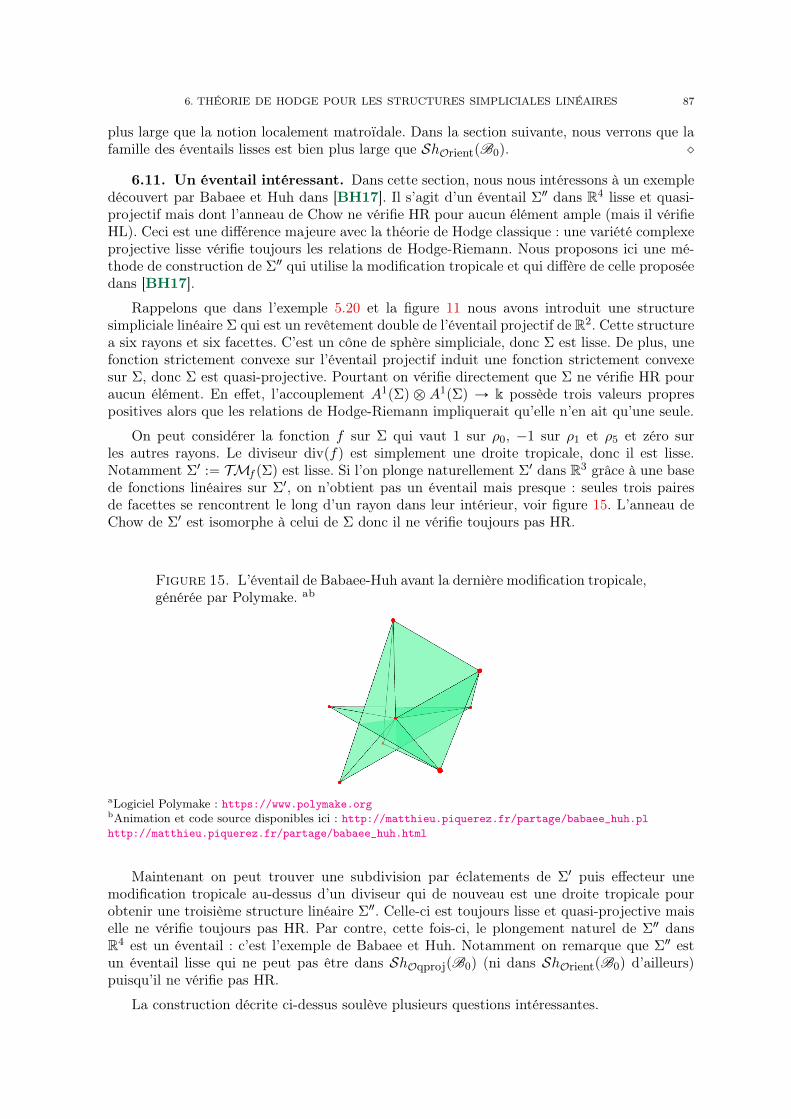
6. THÉORIE DE HODGE POUR LES STRUCTURES SIMPLICIALES LINÉAIRES 87
plus large que la notion localement matroïdale. Dans la section suivante, nous verrons que lafamille des éventails lisses est bien plus large que ShOrientpB0q. ˛
6.11. Un éventail intéressant. Dans cette section, nous nous intéressons à un exempledécouvert par Babaee et Huh dans [BH17]. Il s’agit d’un éventail Σ2 dans R4 lisse et quasi-projectif mais dont l’anneau de Chow ne vérifie HR pour aucun élément ample (mais il vérifieHL). Ceci est une différence majeure avec la théorie de Hodge classique : une variété complexeprojective lisse vérifie toujours les relations de Hodge-Riemann. Nous proposons ici une mé-thode de construction de Σ2 qui utilise la modification tropicale et qui diffère de celle proposéedans [BH17].
Rappelons que dans l’exemple 5.20 et la figure 11 nous avons introduit une structuresimpliciale linéaire Σ qui est un revêtement double de l’éventail projectif de R2. Cette structurea six rayons et six facettes. C’est un cône de sphère simpliciale, donc Σ est lisse. De plus, unefonction strictement convexe sur l’éventail projectif induit une fonction strictement convexesur Σ, donc Σ est quasi-projective. Pourtant on vérifie directement que Σ ne vérifie HR pouraucun élément. En effet, l’accouplement A1pΣq b A1pΣq Ñ k possède trois valeurs proprespositives alors que les relations de Hodge-Riemann impliquerait qu’elle n’en ait qu’une seule.
On peut considérer la fonction f sur Σ qui vaut 1 sur ρ0, ´1 sur ρ1 et ρ5 et zéro surles autres rayons. Le diviseur divpfq est simplement une droite tropicale, donc il est lisse.Notamment Σ1 :“ TMf pΣq est lisse. Si l’on plonge naturellement Σ1 dans R3 grâce à une basede fonctions linéaires sur Σ1, on n’obtient pas un éventail mais presque : seules trois pairesde facettes se rencontrent le long d’un rayon dans leur intérieur, voir figure 15. L’anneau deChow de Σ1 est isomorphe à celui de Σ donc il ne vérifie toujours pas HR.
Figure 15. L’éventail de Babaee-Huh avant la dernière modification tropicale,générée par Polymake. ab
aLogiciel Polymake : https://www.polymake.orgbAnimation et code source disponibles ici : http://matthieu.piquerez.fr/partage/babaee_huh.plhttp://matthieu.piquerez.fr/partage/babaee_huh.html
Maintenant on peut trouver une subdivision par éclatements de Σ1 puis effecteur unemodification tropicale au-dessus d’un diviseur qui de nouveau est une droite tropicale pourobtenir une troisième structure linéaire Σ2. Celle-ci est toujours lisse et quasi-projective maiselle ne vérifie toujours pas HR. Par contre, cette fois-ci, le plongement naturel de Σ2 dansR4 est un éventail : c’est l’exemple de Babaee et Huh. Notamment on remarque que Σ2 estun éventail lisse qui ne peut pas être dans ShOqprojpB0q (ni dans ShOrientpB0q d’ailleurs)puisqu’il ne vérifie pas HR.
La construction décrite ci-dessus soulève plusieurs questions intéressantes.
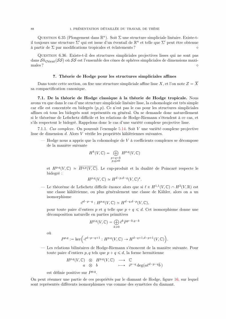
88 1. PRÉSENTATION DÉTAILLÉE DU TRAVAIL DE THÈSE
Question 6.35 (Plongement dans Rn). Soit Σ une structure simpliciale linéaire. Existe-t-il toujours une structure Σ1 qui est issue d’un éventail de Rn et telle que Σ1 peut être obtenueà partir de Σ par modifications tropicales et éclatements ? ˛
Question 6.36. Existe-t-il des structures simpliciales projectives lisses qui ne sont pasdans ShOrientpSSq où SS est l’ensemble des cônes de sphères simpliciales de dimensions maxi-males ? ˛
7. Théorie de Hodge pour les structures simpliciales affines
Dans toute cette section, on fixe une structure simpliciale affine lisse X, et l’on note Z “ Xsa compactification canonique.
7.1. De la théorie de Hodge classique à la théorie de Hodge tropicale. Nousavons vu que dans le cas d’une structure simpliciale linéaire lisse, la cohomologie est très simplecar elle est concentrée en bidegrés pp, pq. Ce n’est pas le cas pour les structures simplicialesaffines où tous les bidegrés sont représentés en général. On se demande donc naturellementsi le théorème de Lefschetz difficile et les relations de Hodge-Riemann s’étendent à ce cas, ets’ils respectent le bidegré. Rappelons donc le cas d’une variété complexe projective lisse.
7.1.1. Cas complexe. On poursuit l’exemple 5.14. Soit V une variété complexe projectivelisse de dimension d. Alors V vérifie les propriétés kählériennes suivantes.
— Hodge nous a appris que la cohomologie de V à coefficients complexes se décomposede la manière suivante
HkpV,Cq “à
p`q“kp,qě0
Hp,qpV,Cq
et Hp,qpV,Cq » Hq,ppV,Cq. Le cup-produit et la dualité de Poincaré respecte lebidegré :
Hp,qpV,Cq » Hd´p,d´qpV,Cq‹.
— Le théorème de Lefschetz difficile énonce alors que si ` P H1,1pV,Cq XH2pV,Rq estune classe kählérienne, ou plus généralement une classe de Kähler, alors on a unisomorphisme
¨`d´p´q : Hp,qpV,Cq » Hd´q,d´ppV,Cq,pour toute paire d’entiers p et q telle que p ` q ď d. Cet isomorphisme donne unedécomposition naturelle en parties primitives
Hp,qpV,Cq “à
kě0
`kP p´k,q´k
oùP p,q :“ ker
´
¨`d´p´q`1 : Hp,qpV,Cq Ñ Hd´q`1,d´p`1pV,Cq¯
.
— Les relations bilinéaires de Hodge-Riemann s’énoncent de la manière suivante. Pourtoute paire d’entiers p, q tels que p` q ď d, la forme hermitienne
Hp,qpV,Cq b Hp,qpV,Cq ÝÑ Ca b b ÞÝÑ ip´q degpa`d´p´qb q
est définie positive sur P p,q.
On peut résumer une partie de ces propriétés par le diamant de Hodge, figure 16, sur lequelsont représentés différents isomorphismes vus comme des symétries du diamant.
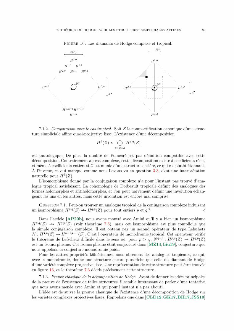
7. THÉORIE DE HODGE POUR LES STRUCTURES SIMPLICIALES AFFINES 89
Figure 16. Les diamants de Hodge complexe et tropical.
H0,0
H1,0 H0,1
H2,0 H1,1 H0,2
Hn,0 H0,n
Hn,n´1Hn´1,n
Hn,n
conj
¨`‚
pd
H0,0
H0,dHd,0
Hd,d
˝
˝˝
‚
N‚
¨`‚
pd
7.1.2. Comparaison avec le cas tropical. Soit Z la compactification canonique d’une struc-ture simpliciale affine quasi-projective lisse. L’existence d’une décomposition
HkpZq Ȉ
p`q“k
Hp,qpZq
est tautologique. De plus, la dualité de Poincaré est par définition compatible avec cettedécomposition. Contrairement au cas complexe, cette décomposition existe à coefficients réels,et même à coefficients entiers si Z est munie d’une structure entière, ce qui est plutôt étonnant.À l’inverse, ce qui manque comme nous l’avons vu en question 3.3, c’est une interprétationnaturelle pour HkpZq.
L’isomorphisme donné par la conjugaison complexe n’a pour l’instant pas trouvé d’ana-logue tropical satisfaisant. La cohomologie de Dolbeault tropicale définit des analogues desformes holomorphes et antiholomorphes, et l’on peut naïvement définir une involution échan-geant les uns en les autres, mais cette involution est encore mal comprise.
Question 7.1. Peut-on trouver un analogue tropical de la conjugaison complexe induisantun isomorphisme Hp,qpZq „ÝÑ Hq,ppZq pour tout entiers p et q ? ˛
Dans l’article [AP20b], nous avons montré avec Amini qu’il y a bien un isomorphismeHp,qpZq „ÝÑ Hq,ppZq (voir théorème 7.6), mais cet isomorphisme est plus compliqué quela simple conjugaison complexe. Il est obtenu par un second opérateur de type LefschetzN : H‚,‚pZq Ñ H‚´1,‚`1pZq. C’est l’opérateur de monodromie tropical. Cet opérateur vérifiele théorème de Lefschetz difficile dans le sens où, pour p ą q, N q´p : Hp,qpZq Ñ Hq,ppZqest un isomorphisme. Cet isomorphisme était conjecturé dans [MZ14,Liu19], conjecture quenous appelons la conjecture monodromie-poids.
Pour les autres propriétés kählériennes, nous obtenons des analogues tropicaux, ce qui,avec la monodromie, donne une structure encore plus riche que celle du diamant de Hodged’une variété complexe projective lisse. Une représentation de cette structure peut être trouvéeen figure 16, et le théorème 7.6 décrit précisément cette structure.
7.1.3. Preuve classique de la décomposition de Hodge. Avant de donner les idées principalesde la preuve de l’existence de telles structures, il semble intéressant de parler d’une tentativeque nous avons menée avec Amini et qui pour l’instant n’a pas abouti.
L’idée est de suivre la preuve classique de l’existence d’une décomposition de Hodge surles variétés complexes projectives lisses. Rappelons que dans [CLD12,GK17,BH17,JSS19]
90 1. PRÉSENTATION DÉTAILLÉE DU TRAVAIL DE THÈSE
est défini l’analogue tropicale des formes holomorphes et antiholomorphes ainsi que les diffé-rentielles correspondantes. On note Ap,qpZq l’espace des pp, qq-formes de Dolbeault tropicalessur Z. On a des différentielles d1 : A‚,‚pZq Ñ A‚`1,‚pZq et d2 : A‚,‚pZq Ñ A‚,‚`1pZq.
Pour adapter la preuve classique au cas tropical, il faudrait d’abord obtenir un élémentfermé de A1,1pZq qui donne une métrique non dégénérée en tout point. Cela n’est pas possibleavec la définition actuelle des formes de Dolbeault tropicales, mais en modifiant légèrementla définition on peut en trouver. Ensuite on souhaite définir les opérateurs duaux à d1 età d2, en utilisant par exemple l’étoile de Hodge. Le problème est que cette étoile est trèsirrégulière au niveau des faces de codimension au moins un. Si l’on arrive à passer cetteétape, on peut définir un laplacien A‚,‚pZq Ñ A‚,‚pZq de bidegré p0, 0q. Le noyau de celaplacien donne les formes harmoniques tropicales et chaque classe cohomologique a un uniquereprésentant harmonique. Le reste de la décomposition découle ensuite naturellement via unepreuve purement algébrique.
Question 7.2. Peut-on définir un laplacien tropical ? Peut-on définir les formes harmo-niques tropicales ? ˛
Nous utilisons nous-même un autre type de laplacien en section 7.7 pour obtenir les pro-priétés kählériennes sur la décomposition, mais ce laplacien n’est pas directement défini surles formes de Dolbeault ni sur l’espace des cochaînes tropicales.
7.1.4. Le cas approximable. Nous allons maintenant expliquer les idées de la preuve d’unpoint de vue géométrique. Dans le cas où la structure simpliciale est la limite tropicale d’unefamille de variétés complexes, on peut s’inspirer de [IKMZ19]. Reprenons notre discussionde la section 3.8. Nous avons une famille de variétés complexes projectives lisses W t, pourt P ∆˚, une fibre centrale W 0, et la limite tropicale Z. Les composantes irréductibles de W 0
sont indexées par les sommets de Zf ; on les note W 0,s pour s P Zf ,0. De plus, les intersectionsde k de ces composantes sont naturellement indexées par les faces de Zf ,k.
On a aussi vu que l’on peut relever la famille W˚ en ĄW˚ au-dessus du revêtement universelde ∆˚. Il se trouve que l’on peut mettre une structure de Hodge mixte sur la cohomologiedu relevé ĄW˚ en utilisant la filtration induite par la monodromie [Sch73]. On l’appelle lastructure de Hodge limite. Les gradués de cette structure de Hodge sont calculés par la suitespectrale de Steenbrink notée ST‚,‚‚ [Ste76,SP08]. Celle-ci dégénère en page deux. Dans le casétudié dans [IKMZ19], où la limite Z est localement matroïdale et vit dans TPn, les graduésde la structure de Hodge limite sont très simples. En degré k, les parties de poids impairs sonttriviales et la partie de poids 2p, p P Z, est concentrée en bidegré pp, pq et est calculée parSTk´2p,2p
8. De plus, la dimension de STk´2p,2p
8est égal au nombre de Hodge d’une fibre générale
hp,k´p :“ dim`
Hp,k´ppW tq˘
.La première page de la suite spectrale ST‚,‚1 est entièrement décrite à partir de la cohomo-
logie (à coefficients rationnels) des différentes composantes. Or, dans le cas où les composantesouvertes sont des complémentaires d’arrangement d’hyperplans, comme nous le verrons avecle théorème 9.1
H‚,‚pW 0,δq » H‚,‚pZδq.
Donc on peut calculer la suite spectrale de Steenbrink, et donc les nombres de Hodge d’unefibre générale, directement sur la limite tropicale. Il ne reste plus qu’à montrer que la limitede la suite spectrale de Steenbrink correspond bien à la cohomologie tropicale, voir section 7.4à ce propos.
Pour que la structure de Hodge limite soit simple comme ci-dessus, il n’est pas nécessaireque les composantes W 0,δ de la fibre centrale soient des compactifications lisses de complé-mentaires d’arrangement d’hyperplans. Il suffit par exemple que la cohomologie de chaquecomposante soit concentrée en bidegrés pp, pq pour 0 ď p ď dimpW0,δq, ou bien que la dégéné-rescence soit maximale au sens de Deligne.
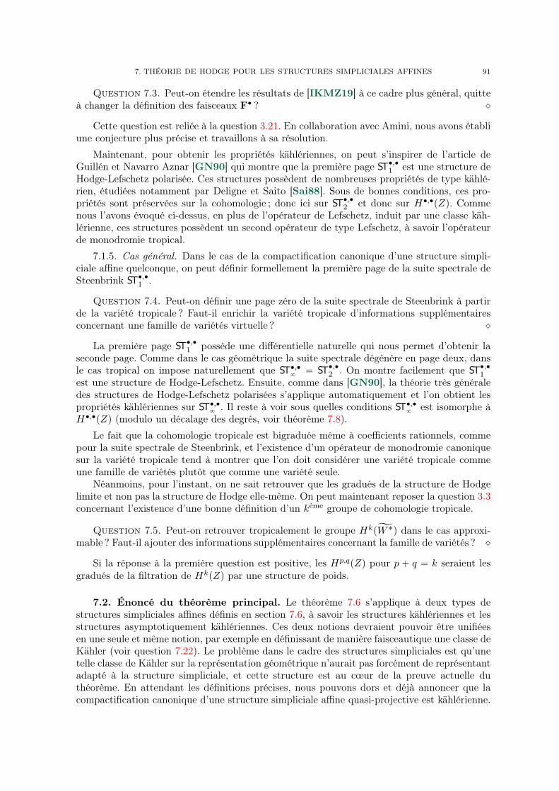
7. THÉORIE DE HODGE POUR LES STRUCTURES SIMPLICIALES AFFINES 91
Question 7.3. Peut-on étendre les résultats de [IKMZ19] à ce cadre plus général, quitteà changer la définition des faisceaux F‚ ? ˛
Cette question est reliée à la question 3.21. En collaboration avec Amini, nous avons établiune conjecture plus précise et travaillons à sa résolution.
Maintenant, pour obtenir les propriétés kählériennes, on peut s’inspirer de l’article deGuillén et Navarro Aznar [GN90] qui montre que la première page ST‚,‚1 est une structure deHodge-Lefschetz polarisée. Ces structures possèdent de nombreuses propriétés de type kählé-rien, étudiées notamment par Deligne et Saito [Sai88]. Sous de bonnes conditions, ces pro-priétés sont préservées sur la cohomologie ; donc ici sur ST‚,‚2 et donc sur H‚,‚pZq. Commenous l’avons évoqué ci-dessus, en plus de l’opérateur de Lefschetz, induit par une classe käh-lérienne, ces structures possèdent un second opérateur de type Lefschetz, à savoir l’opérateurde monodromie tropical.
7.1.5. Cas général. Dans le cas de la compactification canonique d’une structure simpli-ciale affine quelconque, on peut définir formellement la première page de la suite spectrale deSteenbrink ST‚,‚1 .
Question 7.4. Peut-on définir une page zéro de la suite spectrale de Steenbrink à partirde la variété tropicale ? Faut-il enrichir la variété tropicale d’informations supplémentairesconcernant une famille de variétés virtuelle ? ˛
La première page ST‚,‚1 possède une différentielle naturelle qui nous permet d’obtenir laseconde page. Comme dans le cas géométrique la suite spectrale dégénère en page deux, dansle cas tropical on impose naturellement que ST‚,‚
8“ ST‚,‚2 . On montre facilement que ST‚,‚1
est une structure de Hodge-Lefschetz. Ensuite, comme dans [GN90], la théorie très généraledes structures de Hodge-Lefschetz polarisées s’applique automatiquement et l’on obtient lespropriétés kählériennes sur ST‚,‚
8. Il reste à voir sous quelles conditions ST‚,‚
8est isomorphe à
H‚,‚pZq (modulo un décalage des degrés, voir théorème 7.8).
Le fait que la cohomologie tropicale est bigraduée même à coefficients rationnels, commepour la suite spectrale de Steenbrink, et l’existence d’un opérateur de monodromie canoniquesur la variété tropicale tend à montrer que l’on doit considérer une variété tropicale commeune famille de variétés plutôt que comme une variété seule.
Néanmoins, pour l’instant, on ne sait retrouver que les gradués de la structure de Hodgelimite et non pas la structure de Hodge elle-même. On peut maintenant reposer la question 3.3concernant l’existence d’une bonne définition d’un kème groupe de cohomologie tropicale.
Question 7.5. Peut-on retrouver tropicalement le groupe HkpĄW ˚q dans le cas approxi-mable ? Faut-il ajouter des informations supplémentaires concernant la famille de variétés ? ˛
Si la réponse à la première question est positive, les Hp,qpZq pour p ` q “ k seraient lesgradués de la filtration de HkpZq par une structure de poids.
7.2. Énoncé du théorème principal. Le théorème 7.6 s’applique à deux types destructures simpliciales affines définis en section 7.6, à savoir les structures kählériennes et lesstructures asymptotiquement kählériennes. Ces deux notions devraient pouvoir être unifiéesen une seule et même notion, par exemple en définissant de manière faisceautique une classe deKähler (voir question 7.22). Le problème dans le cadre des structures simpliciales est qu’unetelle classe de Kähler sur la représentation géométrique n’aurait pas forcément de représentantadapté à la structure simpliciale, et cette structure est au cœur de la preuve actuelle duthéorème. En attendant les définitions précises, nous pouvons dors et déjà annoncer que lacompactification canonique d’une structure simpliciale affine quasi-projective est kählérienne.
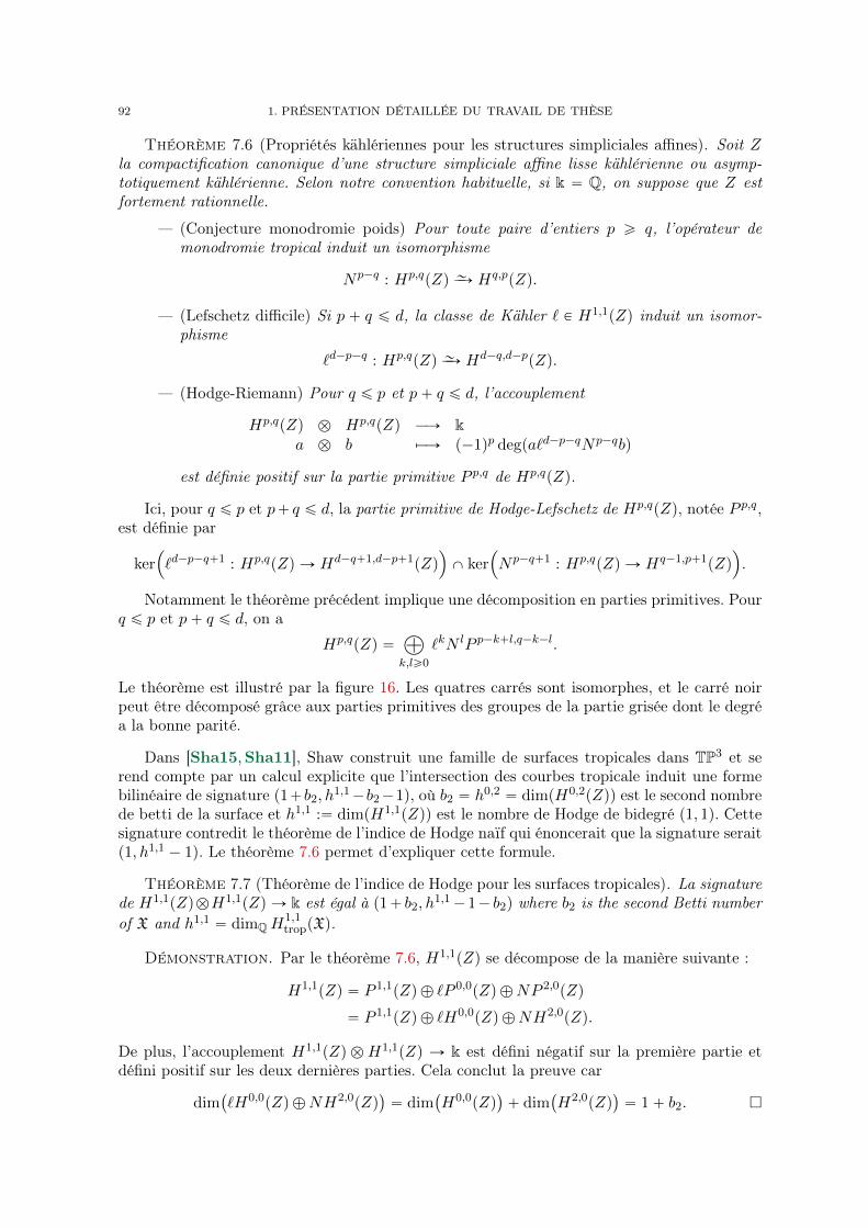
92 1. PRÉSENTATION DÉTAILLÉE DU TRAVAIL DE THÈSE
Théorème 7.6 (Propriétés kählériennes pour les structures simpliciales affines). Soit Zla compactification canonique d’une structure simpliciale affine lisse kählérienne ou asymp-totiquement kählérienne. Selon notre convention habituelle, si k “ Q, on suppose que Z estfortement rationnelle.
— (Conjecture monodromie poids) Pour toute paire d’entiers p ě q, l’opérateur demonodromie tropical induit un isomorphisme
Np´q : Hp,qpZq „ÝÑ Hq,ppZq.
— (Lefschetz difficile) Si p ` q ď d, la classe de Kähler ` P H1,1pZq induit un isomor-phisme
`d´p´q : Hp,qpZq „ÝÑ Hd´q,d´ppZq.
— (Hodge-Riemann) Pour q ď p et p` q ď d, l’accouplement
Hp,qpZq b Hp,qpZq ÝÑ ka b b ÞÝÑ p´1qp degpa`d´p´qNp´qbq
est définie positif sur la partie primitive P p,q de Hp,qpZq.
Ici, pour q ď p et p` q ď d, la partie primitive de Hodge-Lefschetz de Hp,qpZq, notée P p,q,est définie par
ker´
`d´p´q`1 : Hp,qpZq Ñ Hd´q`1,d´p`1pZq¯
X ker´
Np´q`1 : Hp,qpZq Ñ Hq´1,p`1pZq¯
.
Notamment le théorème précédent implique une décomposition en parties primitives. Pourq ď p et p` q ď d, on a
Hp,qpZq “à
k,lě0
`kN lP p´k`l,q´k´l.
Le théorème est illustré par la figure 16. Les quatres carrés sont isomorphes, et le carré noirpeut être décomposé grâce aux parties primitives des groupes de la partie grisée dont le degréa la bonne parité.
Dans [Sha15,Sha11], Shaw construit une famille de surfaces tropicales dans TP3 et serend compte par un calcul explicite que l’intersection des courbes tropicale induit une formebilinéaire de signature p1`b2, h1,1´b2´1q, où b2 “ h0,2 “ dimpH0,2pZqq est le second nombrede betti de la surface et h1,1 :“ dimpH1,1pZqq est le nombre de Hodge de bidegré p1, 1q. Cettesignature contredit le théorème de l’indice de Hodge naïf qui énoncerait que la signature seraitp1, h1,1 ´ 1q. Le théorème 7.6 permet d’expliquer cette formule.
Théorème 7.7 (Théorème de l’indice de Hodge pour les surfaces tropicales). La signaturede H1,1pZqbH1,1pZq Ñ k est égal à p1` b2, h1,1´1´ b2q where b2 is the second Betti numberof X and h1,1 “ dimQH
1,1troppXq.
Démonstration. Par le théorème 7.6, H1,1pZq se décompose de la manière suivante :
H1,1pZq “ P 1,1pZq ‘ `P 0,0pZq ‘NP 2,0pZq
“ P 1,1pZq ‘ `H0,0pZq ‘NH2,0pZq.
De plus, l’accouplement H1,1pZq b H1,1pZq Ñ k est défini négatif sur la première partie etdéfini positif sur les deux dernières parties. Cela conclut la preuve car
dim`
`H0,0pZq ‘NH2,0pZq˘
“ dim`
H0,0pZq˘
` dim`
H2,0pZq˘
“ 1` b2.
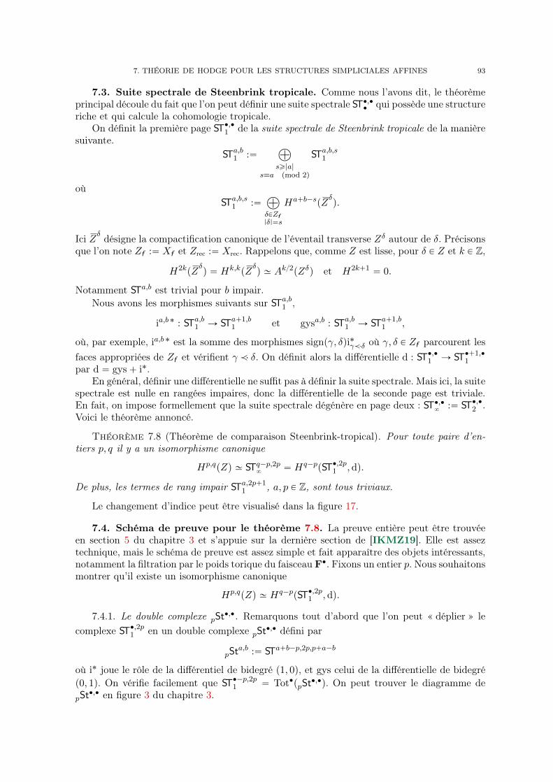
7. THÉORIE DE HODGE POUR LES STRUCTURES SIMPLICIALES AFFINES 93
7.3. Suite spectrale de Steenbrink tropicale. Comme nous l’avons dit, le théorèmeprincipal découle du fait que l’on peut définir une suite spectrale ST‚,‚‚ qui possède une structureriche et qui calcule la cohomologie tropicale.
On définit la première page ST‚,‚1 de la suite spectrale de Steenbrink tropicale de la manièresuivante.
STa,b1 :“à
sě|a|s”a pmod 2q
STa,b,s1
oùSTa,b,s1 :“
à
δPZf|δ|“s
Ha`b´spZδq.
Ici Zδ désigne la compactification canonique de l’éventail transverse Zδ autour de δ. Précisonsque l’on note Zf :“ Xf et Zrec :“ Xrec. Rappelons que, comme Z est lisse, pour δ P Z et k P Z,
H2kpZδq “ Hk,kpZ
δq » Ak2pZδq et H2k`1 “ 0.
Notamment STa,b est trivial pour b impair.Nous avons les morphismes suivants sur STa,b1 ,
ia,b˚ : STa,b1 Ñ STa`1,b1 et gysa,b : STa,b1 Ñ STa`1,b
1 ,
où, par exemple, ia,b˚ est la somme des morphismes signpγ, δqi˚γăδ où γ, δ P Zf parcourent lesfaces appropriées de Zf et vérifient γ ă δ. On définit alors la différentielle d : ST‚,‚1 Ñ ST‚`1,‚
1par d “ gys` i˚.
En général, définir une différentielle ne suffit pas à définir la suite spectrale. Mais ici, la suitespectrale est nulle en rangées impaires, donc la différentielle de la seconde page est triviale.En fait, on impose formellement que la suite spectrale dégénère en page deux : ST‚,‚
8:“ ST‚,‚2 .
Voici le théorème annoncé.
Théorème 7.8 (Théorème de comparaison Steenbrink-tropical). Pour toute paire d’en-tiers p, q il y a un isomorphisme canonique
Hp,qpZq » STq´p,2p8
“ Hq´ppST‚,2p1 ,dq.
De plus, les termes de rang impair STa,2p`11 , a, p P Z, sont tous triviaux.
Le changement d’indice peut être visualisé dans la figure 17.
7.4. Schéma de preuve pour le théorème 7.8. La preuve entière peut être trouvéeen section 5 du chapitre 3 et s’appuie sur la dernière section de [IKMZ19]. Elle est asseztechnique, mais le schéma de preuve est assez simple et fait apparaître des objets intéressants,notamment la filtration par le poids torique du faisceau F‚. Fixons un entier p. Nous souhaitonsmontrer qu’il existe un isomorphisme canonique
Hp,qpZq » Hq´ppST‚,2p1 , dq.
7.4.1. Le double complexe pSt‚,‚. Remarquons tout d’abord que l’on peut « déplier » le
complexe ST‚,2p1 en un double complexe pSt‚,‚ défini par
pSta,b :“ STa`b´p,2p,p`a´b
où i˚ joue le rôle de la différentiel de bidegré p1, 0q, et gys celui de la différentielle de bidegrép0, 1q. On vérifie facilement que ST‚´p,2p1 “ Tot‚ppSt
‚,‚q. On peut trouver le diagramme depSt
‚,‚ en figure 3 du chapitre 3.
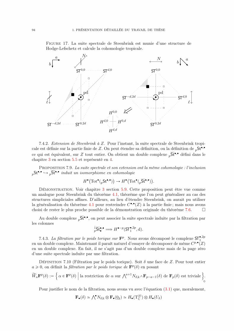
94 1. PRÉSENTATION DÉTAILLÉE DU TRAVAIL DE THÈSE
Figure 17. La suite spectrale de Steenbrink est munie d’une structure deHodge-Lefschetz et calcule la cohomologie tropicale.
ST0,0 STd,0
ST´d,2d ST0,2d
˝
˝
˝
‚
N
`
pd
a
b
ST0,0
STd,0ST´d,2d
ST0,2d
˝
˝˝
‚
N
`
pd
ab
H0,0
H0,dHd,0
Hd,d
7.4.2. Extension de Steenbrink à Z. Pour l’instant, la suite spectrale de Steenbrink tropi-cale est définie sur la partie finie de Z. On peut étendre sa définition, ou la définition de pSt‚,‚
ce qui est équivalent, sur Z tout entier. On obtient un double complexe pSt‚,‚ défini dans le
chapitre 3 en section 5.5 et représenté en 4.
Proposition 7.9. La suite spectrale et son extension ont la même cohomologie : l’inclusionpSt
‚,‚ ãÑ pSt‚,‚ induit un isomorphisme en cohomologie
H‚`
Tot‚ppSt‚,‚q
˘
Ñ H‚`
Tot‚ppSt‚,‚q
˘
.
Démonstration. Voir chapitre 3 section 5.9. Cette proposition peut être vue commeun analogue pour Steenbrink du théorème 4.1, théorème que l’on peut généraliser au cas desstructures simpliciales affines. D’ailleurs, au lieu d’étendre Steenbrink, on aurait pu utiliserla généralisation du théorème 4.1 pour restreindre C‚,‚pZq à la partie finie ; mais nous avonschoisi de rester le plus proche possible de la démonstration originale du théorème 7.6.
Au double complexe pSt‚,‚, on peut associer la suite spectrale induite par la filtration parles colonnes
Ó
pSt‚,‚‚ ùñ H‚´ppST‚,2p1 , dq.
7.4.3. La filtration par le poids torique sur Fp. Nous avons décomposé le complexe ST‚,2p1en un double complexe. Maintenant il paraît naturel d’essayer de décomposer de même Cp,‚pZqen un double complexe. En fait, il ne s’agit pas d’un double complexe mais de la page zérod’une suite spectrale induite par une filtration.
Définition 7.10 (Filtration par le poids torique). Soit δ une face de Z. Pour tout entiera ě 0, on définit la filtration par le poids torique de Fppδq en posant
ĂWaFppδq :“
!
α P Fppδqˇ
ˇ
ˇla restriction de α sur
Źa`1Nδ,k^Fp´a´1pδq de Fppδq est triviale)
.˛
Pour justifier le nom de la filtration, nous avons vu avec l’équation (3.1) que, moralement,
F‚pδq »Ź‚Nδ,k b F‚p0δq » H‚pT
|δ|C q bH‚pUδq
7. THÉORIE DE HODGE POUR LES STRUCTURES SIMPLICIALES AFFINES 95
où 0δ :“ δδ désigne le cône trivial dans Zδ et où Uδ est une certaine strate ouverte complexeassociée à δ. Ainsi, on peut définir de manière analogue ĂWaH
ppT|δ|C ˆ Uδq comme l’ensemble
des classes s’annulant sur Ha`1pT|δ|C q bHp´a´1pUδq, d’où le nom de la filtration.
En pratique, nous travaillerons plutôt avec la filtration décroissante
W aFppδq :“ ĂW´a`|δ|Fppδq.
Proposition 7.11. (1) Pour toute face δ, le aème gradué de la filtration vérifie
graWFppδq »
Ź|δ|´aMδ,k b Fp`a´|δ|p0δq.
(2) Pour toute paire de faces γ ă δ, la restriction Fppγq Ñ Fppδq respecte la filtrationW ‚.
La filtration induit une suite spectrale qui calcule la cohomologie tropicale
pC‚,‚‚ ùñ H‚pZ,Fpq “ Hp,‚
troppXq.
La page zéro est donnée par
pCa,b0 “ graWC
a`bpZ,Fpq “à
δPZ|δ|“a`b
ŹbMδ,k b Fp´bp0δq,
voir figure 2 du chapitre 3.7.4.4. Isomorphisme en page un. Pour démontrer le théorème 7.8, il nous reste donc à
montrer que pC‚,‚‚ et ÓpSt
‚,‚‚ calculent la même cohomologie. Commençons par montrer que
pCa,b1 »
Ó
pSta,b1 pour toute paire d’entiers a, b.
Pour cela, il suffit de montrer que pour tout entier a
pCa,‚0 : 0 Ñ
à
|δ|“a
Ź0Mδ,k b Fpp0δq Ñà
|δ|“a`1
Ź1Mδ,k b Fp´1p0δq Ñ ¨ ¨ ¨
¨ ¨ ¨ Ñà
|δ|“a`p
ŹpMδ,k b F0p0δq Ñ 0
est quasi-isomorphe àÓ
pSta,‚0 : 0 Ñ
à
|δ|“p`a|δrec|ďa
H0pδq Ñà
|δ|“p`a´1|δrec|ďa
H2pδq Ñ ¨ ¨ ¨ Ñà
|δ|“a|δrec|ďa
H2ppδq Ñ 0.
On introduit alors le double complexe aD‚,‚ défini par
aDb,b1 :“
à
|δ|“a`b
ŹbMδ,k b´
à
ηąδ|η|“p`a´b1
sedpηq“sedpδq
H2b1pηq¯
.
Les différentielles sont définies en section 5.6 du chapitre 3, la différentielle verticale est induitepar gys. Ce double complexe joue le rôle de pont entre les deux cohomologies car il a lespropriétés très particulières suivantes.
Proposition 7.12. Pour tout entier b, la colonne aDb,‚ est une résolution de pC
a,b0 , i.e.
la suite0 Ñ pC
a,b0 Ñ aD
b,0 Ñ aDb,1 Ñ ¨ ¨ ¨ Ñ aD
b,p´b Ñ 0
est exacte. De même, pour tout entier b1, la rangée aD‚,b1 est une résolution de ÓpSt
a,‚0 , i.e. la
suite0 Ñ
Ó
pSta,b1
0 Ñ aD0,b1 Ñ aD
1,b1 Ñ ¨ ¨ ¨ Ñ aDp´b1,b1 Ñ 0
est exacte.
96 1. PRÉSENTATION DÉTAILLÉE DU TRAVAIL DE THÈSE
Démonstration. Voir chapitre 3 section 5.6. Pour la première suite exacte, on peut laréécrire comme la somme directe
à
|δ|“a`1
ŹbMδ,k bK‚
où K‚ est exactement la suite exacte de Deligne 4.9 associée à Fpp0δq.Pour la seconde suite exacte, cette fois-ci on peut factoriser par le second facteur et l’on
obtient la décompositionà
|η|“p`a´b1L‚ bH2b1pηq
où L‚ est un complexe de cochaînes sur les faces de η de sédentarité sedpηq. Comme η est trèssimple, on peut faire un calcul explicite et vérifier que l’on obtient bien une suite exacte.
Les inclusions pCa,b0 ãÑ aD
b,0 de la proposition 7.12 induisent un morphisme de complexepC
a,‚0 ãÑ Tot‚paD
‚,‚q bien défini. On peut donc considérer le double complexe obtenu eninsérant pC
a,‚0 au-dessus de aD‚,‚ en rangée ´1. La proposition 7.12 montre que la cohomologie
de ce double complexe est triviale. Cela implique immédiatement que l’inclusion
pCa,‚0 ãÑ Tot‚paD
‚,‚q
induit un isomorphisme en cohomologie. (En effet, on a une suite exacte courte
0 Ñ Tot‚paD‚,‚q Ñ cone‚
´
pCa,‚0 ãÑ Tot‚paD
‚,‚q
¯
Ñ pCa,‚`10 Ñ 0,
voir par exemple [KS90] pour l’application cone, et la suite exacte longue associée nous donnel’isomorphisme.)
Le même raisonnement nous montre que l’inclusion
Ó
pSta,‚0 ãÑ Tot‚paD
‚,‚q
est un quasi-isomorphisme. On en déduit ce qu’on souhaitait, à savoir que pCa,‚0 et ÓpSt
a,‚0 ont
la même cohomologie et donc pCa,b1 »
Ó
pSta,b1 pour tout bidegré pa, bq.
7.4.5. Fin de la preuve. Le fait que les premières pages des deux suites spectrales coïn-cident ne signifie pas que leurs limites soient égales, et encore moins que les complexes ayantdonnés la page zéro aient la même cohomologie. Pour montrer cela, la preuve que nous fournis-sons dans le chapitre 3 ne fonctionne pas dans notre cadre, par exemple parce que l’on choisitun produit scalaire global sur l’espace ambient ce qui n’est pas possible dans le cas d’une struc-ture simpliciale affine quelconque. Il faut alors revenir à la preuve originelle de [IKMZ19].
Dans cet article, les auteurs définissent un double complexe K‚,‚ppq et une filtration W ‚ sur
ce double complexe (ce double complexe est défini en homologie dans l’article mais ici onconsidère son dual). Le aème gradué de K‚,‚
ppq est exactement
graWK‚,‚ppq “ aD
‚,‚.
De plus on a une inclusion Cp,‚ ãÑ Tot‚pK‚,‚ppqq qui respecte les filtrations respectives. La
discussion ci-dessus montrent que cette inclusion est un quasi-isomorphisme.De même, on a une inclusion de Tot‚ppSt
‚,‚q dans Tot‚pK‚,‚ppqq qui respecte les filtrations
(on considère toujours la filtration par colonnes sur pSt‚,‚). De nouveau, cette inclusion est unisomorphisme. Ceci conclut la démonstration du théorème 7.8.
7. THÉORIE DE HODGE POUR LES STRUCTURES SIMPLICIALES AFFINES 97
7.5. Monodromie. Reprenons la preuve du théorème principal. Nous avons un doublecomplexe
STa,b1 “à
sě|a|s”a pmod 2q
STa,b,s1 , STa,b,s1 “à
δPZf|δ|“s
Ha`b´spZδq.
On voit que STa,b,s1 ne dépend que de a`b et de s. On en déduit qu’il y a une inclusion trivialeSTa,b1 ãÑ STa`2,b´2
1 pour a ă 0 et une surjection triviale STa,b1 ãÑ STa`2,b´21 pour a ě ´1.
Définition 7.13. L’opérateur de monodromie sur ST‚,‚1 est défini par l’application
N : ST‚,‚1 Ñ ST‚`2,‚´21 ,
induite par les injections et les surjections décrites ci-dessus.Cet opérateur commute avec la différentielle et induit donc un opérateur noté et appelé
de la même manière sur ST‚,‚8“ ST‚,‚2 . ˛
Du côté tropical, l’opérateur de monodromie est plus délicat à définir. Il n’est pas définide manière canonique au niveau des cochaînes, voir [MZ14].
Pour une face δ P Zf , on choisit arbitrairement un point oδ dans |δ| Ď pZ. Si γ ă δ, oδ ´ oγcorrespond naturellement à un élément de Nδ,k. Pour les faces η P Z de sédentarité 0, on poseoη “ oηf et pour les faces η de sédentarité σ ‰ 0, on a η “ δσ pour un certain δ P Z desédentarité 0 et l’on pose oη égal à la projection de oδ.
Pour tout bidegré pp, qq, on obtient une application
N : Cp,qpZq Ñ Cp´1,q`1pZq,
pγ, αq ÞÑÿ
δ ąγsedpδq“sedpγq
signpγ, δq`
δ, ιoδ´oγ pαq˘
.
Définition - Proposition 7.14. L’application N définie ci-dessus induit une applica-tion N : Hp,qpZq Ñ Hp´1,q`1pZq qui ne dépend pas des points oδ choisis. On appelle cetteapplication l’opérateur de monodromie tropical.
Proposition 7.15. L’isomorphisme Steenbrink-tropical du théorème 7.8 commute avec lesopérateurs de monodromie respectifs.
Démonstration. Voir le théorème 6.20 du chapitre 3.
7.6. Variétés kählériennes. Passons à la définition d’une forme de Kähler. Ce doit êtreun cocycle dans C1,1pZq, ou dans ST0,2
1 , qui est localement positif. On a par définition
ST0,21 »
à
sPZf ,0
H2pZsq ‘
à
δPZf ,2
H0pZδq.
En rappelant queH2pZsq » A1pZsq, si Zs est kählérienne, on peut définir un élément kählérien
sur s.
Définition 7.16. Une forme de Kähler dans ST‚,‚1 est par définition un élément
p`sqsPZf ,0 Pà
sPZf ,0
H2pZsq Ď ST0,2
1
telle que `s soit kählérienne dans A1pZsq et avec la condition de compatibilité suivante. Pourchaque arête e P Zf ,1 d’extrémités s1 et s2,
i˚s1ăep`s1q “ i˚s2ăep`s2q. ˛
98 1. PRÉSENTATION DÉTAILLÉE DU TRAVAIL DE THÈSE
La condition de compatibilité revient exactement à demander que la forme de Kähler soitun cocycle. La définition correspondante dans C1,1pZq est moins satisfaisante. Une forme deKähler serait un cocycle ` dans C1,1pZq tel que, pour chaque sommet s P Xf , la sommesuivante soit kählérienne.
ÿ
eąs
`|epνeqxes P A1pZsq.
Définition 7.17. Soit Z la compactification d’une structure simpliciale affine lisse. AlorsZ est dite kählérienne si Z possède une subdivision possédant une forme de Kähler. ˛
Rappelons que, par définition, une subdivision de Z doit préserver l’éventail de récessionZrec.
Proposition 7.18. Si Z est projective et si Zδ est kählérienne pour tout δ P Zf , alors Zpossède une forme de Kähler.
Démonstration. Soit X la structure simpliciale affine telle que X “ Z. Soit f unefonction linéaire par morceaux strictement convexe sur X. Alors pour tout sommet s P Zf , finduit une fonction linéaire par morceaux fs strictement convexe sur Zs. Donc fs donne uneclasse ample `s P A1pZsq. Comme on a supposé que Zs est kählérienne, on en déduit que `sest kählérienne. La compatibilité des `s ainsi construits vient du fait que f induit aussi deséléments `e P A1pZeq pour chaque arête e “ ts1, s2u P Z1,f , et l’on a
i˚s1ăep`s1q “ `e “ i˚s2ăep`s2q.
Remarque 7.19. Si f est n’importe quelle fonction linéaire par morceaux sur X, onobtient de même un cocycle dans ST0,2
1 , et donc une classe de H1,1pZq. De plus, si l’on modifiela valeur de f sur un sommet, le nouveau cocycle diffère de l’ancien d’un cobord, donc cela nechange pas la classe obtenue dans H1,1pZq. Ainsi celle-ci ne dépend que de frec.
Par la dualité de Poincaré, on obtient un élément de Hd´1,d´1pZq. Cet élément correspondau cycle tropical
ÿ
%PXrec
fp%qrZ%8s P Cd´1,d´1pZq,
où, par l’inclusion Cd´1,d´1pZ%8q ãÑ Cd´1,d´1pZq, on peut voir rZ%
8s comme un élément de
Cd´1,d´1pZq (ici Zρ8 désigne Xρ8). ˛
Définition 7.20. La structure Z est dite asymptotiquement kählérienne si— Zδ est kählérienne pour tout δ P Zf ,— Z est issue d’une structure simpliciale linéaire Σ au sens de la définition 2.14,— et la structure simpliciale linéaire induite par Σ sur Zrec est quasi-projective kählé-
rienne. ˛
Définition 7.21. Si Z est kählérienne, on appelle classe de Kähler sur Z tout élément` P H1,1pZq tel qu’il existe une subdivision Z 1 de Z et une forme de Kähler `1 de Z 1 dont laclasse dans H1,1pZ 1q » H1,1pZq correspond à `.
Si Z est asymptotiquement kählérienne, on appelle classe de Kähler sur Z tout élémentde H1,1pZq qui est dual de Poincaré d’un élément de la forme
ÿ
%PZrec
frecp%qrZ%8s,
où frec est une fonction linéaire par morceaux strictement convexe sur Zrec. ˛
Notons que pour la deuxième partie, on peut par exemple prolonger frec par zéro sur Zfet on obtient la classe de Kähler directement dans H1,1pZq via la remarque 7.19.
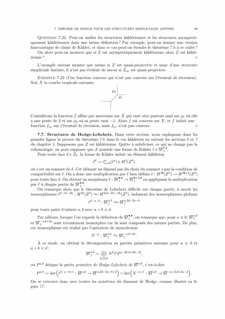
7. THÉORIE DE HODGE POUR LES STRUCTURES SIMPLICIALES AFFINES 99
Question 7.22. Peut-on unifier les structures kählériennes et les structures asymptoti-quement kählériennes dans une même définition ? Par exemple, peut-on donner une versionfaisceautique de classe de Kähler, et dans ce cas peut-on étendre le théorème 7.6 à ce cadre ?
Ou alors peut-on montrer que si Z est asymptotiquement kählérienne alors Z est kählé-rienne ? ˛
L’exemple suivant montre que même si Z est quasi-projective et issue d’une structuresimpliciale linéaire, il n’est pas évident de savoir si Zrec est quasi-projective.
Exemple 7.23 (Une fonction convexe qui n’est pas convexe sur l’éventail de récession).Soit X la courbe tropicale suivante.
ρ1
ρ2
Considérons la fonction f affine par morceaux sur X qui vaut zéro partout sauf sur ρ1 où ellea une pente de 2 et sur ρ2 où sa pente vaut ´1. Alors f est convexe sur X, et f induit unefonction frec sur l’éventail de récession, mais frec n’est pas convexe. ˛
7.7. Structures de Hodge-Lefschetz. Dans cette section, nous expliquons dans lesgrandes lignes la preuve du théorème 7.6 dans le cas kählérien en suivant les sections 6 et 7du chapitre 3. Supposons que Z est kählérienne. Quitte à subdiviser, ce qui ne change pas lacohomologie, on peut supposer que Z possède une forme de Kähler ` P ST0,2
1 .Pour toute face δ P Zf , la forme de Kähler induit un élément kählérien
`δ :“ i˚săδp`sq P H2pZδq
où s est un sommet de δ. Cet élément ne dépend pas du choix du sommet s par la condition decompatibilité sur `. On a donc une multiplication par ` bien définie ` : H2‚pZδq Ñ H2‚`2pZδq
pour toute face δ. On obtient un morphisme ` : ST‚,‚1 Ñ ST‚`2,‚1 en appliquant la multiplication
par ` à chaque partie de ST‚,‚1 .On remarque alors que le théorème de Lefschetz difficile sur chaque partie, à savoir les
isomorphismes `d´|δ|´2k : H2kpZδq „ÝÑ H2pd´|δ|q´2kpZδq, induisent des isomorphismes globaux
`d´a´b : STa,b1„ÝÑ STa,2d´2a´b
1
pour toute paire d’entiers a, b avec a` b ď d.
Par ailleurs, lorsque l’on regarde la définition de ST‚,‚1 , on remarque que, pour a ď 0, STa,b1
et ST´a,b`2a1 sont trivialement isomorphes car ils sont composés des mêmes parties. De plus,
cet isomorphisme est réalisé par l’opérateur de monodromie
N´a : STa,b1„ÝÑ ST´a,b`2a
1 .
À ce stade, on obtient la décomposition en parties primitives suivante pour a ď 0 eta` b ď d :
STa,b1 “à
k,lě0
Nk`lP a´2k,b`2k´2l,
où P a,b désigne la partie primitive de Hodge-Lefschetz de STa,b, c’est-à-dire
P a,b :“ ker´
`d´a´b`1 : STa,b Ñ STa,2d´2a´b`2¯
X ker´
N´a`1 : STa,b Ñ ST´a`2,b`2a´2¯
.
On se retrouve donc avec toutes les symétries du diamant de Hodge, comme illustré en fi-gure 17.
100 1. PRÉSENTATION DÉTAILLÉE DU TRAVAIL DE THÈSE
Ensuite, les dualités de Poincaré locales H2kpZδq » H2pd´|δ|q´2kpZδq‹ induisent des dua-lités de Poincaré globales. Pour toute paire d’entiers a et b, on a un isomorphisme
ST´a,b1 »`
STa,2d´b1
˘‹.
Cela nous fournit un accouplement global, appelé polarisation, ψ : ST‚,‚1 b ST‚,‚1 Ñ k, où l’onimpose à STa,b1 et à STa
1,b1
1 d’être orthogonaux si a` a1 ‰ 0 ou si b` b1 ‰ 2d, et sinon on utilisel’accouplement ci-dessus (avec un signe qui simplifie la suite de la discussion).
Une étude attentive montre alors que la forme bilinéaire ψp ¨ , `d´a´bNa ¨ q est définie po-sitive sur chaque partie primitive P a,b, avec a ď 0 et a ` b ď d. À ce stade-là, on a doncmontré le théorème 7.6 où l’on a remplacé la cohomologie tropicale par la première page de lasuite spectrale de Steenbrink STa,b1 . Il nous faut alors montrer les mêmes propriétés mais surla deuxième page.
En fait ST‚,‚1 a encore plus de structure puisqu’il possède une différentielle d. Tous cesopérateurs et la polarisation ont des relations de compatibilité : les opérateurs commutent(ou anticommutent) entre eux et ils sont autoadjoints (ou antiautoadjoints) par rapport à lapolarisation. On dit alors que ST‚,‚1 est une structure de Hodge-Lefschetz polarisée différentielle.
On utilise alors la théorie de structures de Hodge-Lefschetz, voir par exemple [GN90,SS20,Sai88], qui nous donne automatiquement que la cohomologie ST‚,‚2 est une structure deHodge-Lefschetz polarisée, i.e. elle vérifie le théorème 7.6 ce qui conclut la démonstration.
Commentons rapidement le fonctionnement de cette théorie dans notre cas, car la preuvepartage plusieurs similarités avec la preuve classique de l’existence de la décomposition deHodge dans le cas complexe.
On peut définir un opérateur w qui envoie isomorphiquement STa,b1 sur ST´a,2d´b1 pourtoute paire d’entiers pa, bq et qui effectue donc une symétrie centrale sur le diamant de Hodge.L’opérateur w est entièrement défini grâce à N et `. En posant φ “ ψp ¨ , w ¨ q on obtient uneforme symétrique définie positive partout sur ST‚,‚1 . On peut alors définir l’adjoint d‹ : ST‚,‚1 Ñ
ST‚´1,‚1 de la différentielle d par rapport à φ. Notamment, on obtient la formule
d‹ “ ´w´1dw,
donc w joue le rôle de l’étoile de Hodge. On définit alors le laplacien
4 :“ dd‹ ` d‹d.
Une étape délicate dans la preuve est de montrer que ` et N commutent avec le laplacien.Pour se faire, on peut utiliser le langage de la théorie des représentations. Nous proposonsaussi une preuve élémentaire, mais calculatoire, qui n’utilise pas cette théorie en section 7.6.
Ensuite on peut montrer que chaque classe dans ST‚,‚2 possède un unique représentantdans le noyau du laplacien, et l’on s’est donc ramené à montrer que le noyau du laplacien dansST‚,‚1 est une structure de Hodge-Lefschetz polarisée, ce qui se fait facilement grâce à toutesles relations de compatibilité entre les différents opérateurs.
7.8. Extension au cas des structures asymptotiquement kählériennes. Suppo-sons que Z est asymptotiquement kählérienne. Soit X la structure simpliciale affine telle queX “ Z et soit Σ une structure simpliciale linéaire sur conepXq qui induit la structure affinesur X. On veut étendre le théorème 7.6 à Z. Nous pouvons bien parler d’extension ici carnous allons partir d’une structure kählérienne Zp0q, qui vérifie donc déjà le théorème, et mon-trer de proche en proche le théorème pour des structures intermédiaires Zp1q, Zp2q, . . . , pourfinalement arriver à Z.
Proposition 7.24. La structure Σ admet une subdivision quasi-projective Σp0q.
Démonstration. Comme nous l’avons vu dans l’exemple 2.4, si l’on choisit une basede l’espace des formes linéaires Mk sur Σ, on obtient une projection π : RE Ñ Rn, où n “
7. THÉORIE DE HODGE POUR LES STRUCTURES SIMPLICIALES AFFINES 101
dimpMkq, qui envoie pΣ sur un pseudo-éventail rΣ et π induit un isomorphisme sur chaque cônede pΣ.
Soit ∆ un éventail quasi-projectif complet dans Rn. On peut découper ∆ par les hyperplanssupports des faces de rΣ, comme pour la preuve du théorème de factorisation faible 6.23,voir aussi chapitre 3 section 4.5. On effectue ensuite des éclatements pour obtenir finalementune subdivision quasi-projective simpliciale ∆p0q de ∆. Ces coupes par des hyperplans et ceséclatements peuvent être remontés dans pΣ et l’on obtient une subdivision pΣp0q de pΣ, et lasubdivision correspondante Σp0q de Σ. De plus, π induit un morphisme d’éventails : chaqueface de pΣp0q est envoyée de manière isomorphe sur une face de ∆p0q.
Maintenant, on peut choisir une fonction linéaire par morceaux strictement convexe f sur∆p0q et f induit une fonction strictement convexe sur Σp0q, ce qui conclut.
En appliquant la proposition, on obtient une subdivision Σp0q de Σ qui est quasi-projective,et donc une subdivision Xp0q de X qui est elle aussi quasi-projective. Rappelons de plus que,par hypothèse, les structures transverses Xδ, δ P Xf , sont kählériennes. Comme Xp0q est unesubdivision de X, on montre facilement que les Xδ
p0q, δ P Xp0q,f sont eux aussi kählériennes.Posons Zp0q “ Xp0q. Notons que Zp0q n’est pas nécessairement une subdivision de Z car
l’éventail de récession a pu changer. Cette remarque nous amène à formuler la question sui-vante. Une réponse affirmative à cette question fournirait automatiquement une réponse affir-mative à la dernière partie de la question 7.22.
Question 7.25. Existe-t-il toujours une subdivision projective de Z ? ˛
Soit f une fonction strictement convexe sur Σp0q. Alors frec est elle aussi strictementconvexe, et par la remarque 7.19 on peut associer une classe de Kähler ` P H1,1pZp0qq à f .Notons que ` est à la fois une classe de Kähler pour Zp0q vue comme structure kählérienne etpour Zp0q vue comme structure asymptotiquement kählérienne. Notamment, pZp0q, `q vérifieles propriétés kählériennes.
Maintenant la démonstration suit essentiellement celle du cas local, section 6.8, voir aussiles sections 8 et 9 du chapitre 3. Nous reprenons rapidement les différentes étapes.
Proposition 7.26. Si une structure asymptotiquement kählérienne vérifie les propriétéskählériennes pour une classe de Kähler, alors elle les vérifie pour toutes les classes de Kähler.
Démonstration. Une classe de Kähler quelconque ` induit des classes de Kähler `% PH1,1pZ%
8q sur chaque diviseur à l’infini. Par récurrence, on peut supposer que `% vérifie les
relations de Hodge-Riemann. Comme dans le cas local, cela implique que ` vérifie le théorèmede Lefschetz difficile dans Z. Les classes de Kähler de Z forment un cône connexe dansH1,1pZq.Comme le théorème de Lefschetz difficile est vrai sur l’ensemble de ce cône, on en déduit quesoit tous les éléments de ce cône vérifient les relations de Hodge-Riemann, soit aucun d’entreeux ne les vérifient.
On peut définir un éclatement sur une structure simpliciale affine X comme la subdivisioninduite par un éclatement sur conepXq. On définit la contraction comme étant l’opérationinverse.
Proposition 7.27. Il existe un entier k et une suite de structures affines Xp0q, . . . , Xpmq,où Xp0q est définie ci-dessus et Xpmq “ X, et telle que Xpi`1q est obtenue à partir de Xpiqpar un éclatement ou une contraction. De plus, on peut supposer que les Xpiq sont toutes dessubdivisions relativement projectives de X.
Démonstration. La preuve est exactement la même que dans le cas des structures sim-pliciales linéaires, voir la démonstration du théorème 6.23.
102 1. PRÉSENTATION DÉTAILLÉE DU TRAVAIL DE THÈSE
Comme toutes les structures intermédiaires Xpiq sont des subdivisions relativement pro-jectives de X, Xpiq,rec est relativement projective par rapport à Xrec. Comme Xrec est quasi-projective, on en déduit que Xpiq,rec est quasi-projective pour tout i, et donc Zpiq :“ Xpiq estasymptotiquement kählérienne.
Soit Y une structure simpliciale affine lisse, soit v un point à l’intérieur d’un élément de Yet soit Y 1 :“ Ypvq l’éclatement de Y le long de v. Il y a deux cas. Si le centre de l’éclatement vn’est pas dans un cône de Yrec, alors Y 1 est une subdivision de Y . Notamment les cohomologiesdes deux compactifications coïncident et donc les propriétés kählériennes sont préservées dansce cas.
Le cas intéressant est donc lorsque l’éclatement est le long d’un point v à l’intérieur d’uncône η de l’éventail de récession. Soit ρ le nouveau rayon. Soient W :“ Y , W 1 :“ Y 1 etT P H1,1pY 1q le dual de Poincaré de ´rW 1ρ
8s P Hd´1,d´1pY
1q. Dans ce cas, on a l’analogueglobal du lemme de Keel (théorème 6.19).
Théorème 7.28 (Lemme de Keel global). Avec les notations ci-dessus, on a une décom-position
HkpW 1q » HkpW q ‘ THk´2pW η8q ‘ T 2Hk´4pW η
8q ‘ ¨ ¨ ¨ ‘ T |η|´1Hk´2|η|`2pW η
8q.
Démonstration. Voir chapitre 3 section 8.4. On peut démontrer ce théorème grâce àST‚,‚1 . Dans ce cas, T peut être vu comme l’élément de
À
sPW 1f ,0A1pW 1sq Ď ST2,0
1 qui vautpT sqsPWf ,0 où T s P A1pW 1sq et
T s “
#
´xρs si s est comparable à ρ0 sinon.
La décomposition induite par le lemme de Keel sur chaque morceau de ST‚,‚1 induit unedécomposition globale qui passe à la cohomologie.
On peut aussi voir ce théorème comme une application de l’analogue tropical de la formuledu fibré projectif, ou de la formule de l’éclatement, ce qui donne une autre preuve intéressantede ce théorème, voir la section 8.5 du chapitre 3.
Si ` est une classe de Kähler sur W , alors ` ´ εT est une classe de Kähler sur W 1 pourtout ε ą 0 suffisamment petit. En utilisant la décomposition ci-dessus et en travaillant parrécurrence comme dans le cas local, on peut montrer que W vérifie les propriétés kählériennespour ` si et seulement W 1 vérifie les propriétés kählériennes pour ` ´ εT pour tout ε ą 0suffisamment petit.
Maintenant, on combine les propositions 7.27 et 7.26. Comme Zp0q vérifie les propriétéskählériennes pour une classe kählérienne, elle les vérifie pour toutes les classes kählériennes etdonc le théorème 7.6 est vrai sur Zp0q. Par la discussion ci-dessus, on en déduit de proche enproche que Zp1q, Zp2q, . . . , Zpmq “ Z vérifient aussi le théorème, ce qui conclut.
7.9. Existence d’une subdivision préservant l’éventail de récession. La versiondu théorème 7.6 présente dans le chapitre 3 est un peu différente. Elle ne traite que de cer-taines variétés tropicales X de Rn. Plus précisément, dans ce théorème, on suppose X estle support d’un complexe simplicial unimodulaire orienté X donc l’élément canonique dansrXs P MWdpXq n’a que des poids égaux à un. Rappelons que Xrec “ limλÑ0 λX. Dans ce cas,par contre, cette version est a priori plus générale que le théorème 7.6 car elle énonce que, siX est quasi-projectif et localement kählérienne, alors pour tout éventail unimodulaire quasi-projectif Σ de support Xrec, l’adhérence X Ď TPΣ a une cohomologie vérifiant les propriétéskählériennes.
Afin de confirmer que le théorème 7.6 est en effet plus général que la version correspondantedu chapitre 3 (théorème 1.7), on énonce le théorème suivant. Ce théorème affirme que X admet

7. THÉORIE DE HODGE POUR LES STRUCTURES SIMPLICIALES AFFINES 103
une triangulation X telle que Xrec “ Σ. Dans ce cas, X Ď TPΣ est isomorphe à |X|. CommeX est asymptotiquement kählérienne, on peut appliquer le théorème 7.6. Le théorème 7.29permet aussi de compléter la preuve du théorème 8.6 dans le chapitre 3.
Théorème 7.29. Soit X un complexe simplicial de Rn. On suppose de plus que rXs PMWdpXq n’a que des poids positifs. Soit Σ1 un structure simpliciale linéaire de support |X|rec.Alors il existe un complexe simplicial X 1 tel que X 1rec “ Σ1rec et telle que |X| “ |X 1|.
Une fois de plus, nous ne décrivons que les étapes principales de la preuve. Dans celle-ci,nous supposerons sans perte de généralité que tous les complexes simpliciaux X 1 considérésvérifient queX 1rec est un éventail. De plus, nous considéreronsX 1 comme un complexe simplicialde Rn et comme une structure simpliciale affine simultanément.
7.9.1. Réduction du problème. Posons Σ :“ Xrec. Le théorème de factorisation faible 6.23implique que l’on peut trouver une suite d’éventails Σ “ Σp0q,Σp1q, . . . ,Σpmq “ Σ1 telle queΣpi`1q est obtenue à partir de Σpiq par un éclatement ou une contraction. Supposons que l’ona construit une structure simpliciale affine Xpiq dont l’éventail de récession est Σpiq.
Si Σpi`1q est obtenu en éclatant Σpiq le long de v, on peut effectuer le même éclatementsur Xpiq pour obtenir une subdivision Xpi`1q dont l’éventail de récession est Σpi`1q.
Le cas délicat est lorsque Σpi`1q est une contraction de Σpiq. Dans ce cas, on peut supposersans perte de généralité que la contraction a pour centre un élément v dans une face dedimension deux de Σpi`1q. En effet, tout éclatement peut facilement être décomposé en unesérie d’éclatements et de contractions, chacun ayant pour centre un point dans une face dedimension deux.
On se ramène donc au problème suivant. Soient Σ un éventail et Σ1 l’éclatement de Σ lelong d’un point v à l’intérieur d’une face η P Σ2. Soit ρ le nouveau rayon. Soit X 1 un complexesimplicial orienté d’élément canonique positif et dont l’éventail de récession est Σ1. Existe-t-ilun complexe simplicial X de même support que X 1 dont l’éventail de récession est Σ ?
7.9.2. Description des faces contenant ρ. Soit n un vecteur non nul de Nη,R transverse àρ. Nous souhaitons montrer que toutes les facettes δ de X 1 avec δ ą ρ contiennent n dansleur espace tangent. De manière équivalente, on peut montrer que toutes les facettes de X 1ρcontiennent (la projection de) n.
On peut supposer sans perte de généralité que dimpX 1ρq ă dimpNρRq. Par l’absurde, soit δ
une facette de X 1ρ telle que n R Nδ,R. Soit H un espace affine générique de NρR de codimension
dimpX 1ρq ´ 1 qui contient n et qui intersecte δ. Posons G l’intersection de H avec X 1ρ. C’estun complexe simplicial orienté de dimension 1 tel que rGs P MW1pGq n’a que des poidsstrictement positifs.
On choisit une forme linéaire générique ` sur H qui est nulle sur n. On part d’un point xde l’arête e :“ GX δ et l’on va dans la direction ` croissant. À un moment, on va atteindre unsommet s. Par la condition d’équilibre, comme `pnesq ă 0, il doit exister une arête e1 incidenteà s telle que `pne1sq ą 0. On poursuit notre chemin en empruntant l’arête e1, et ainsi de suite.
Comme la valeur de ` ne cesse de croître le long de notre chemin, nous allons finalementarriver à un rayon non compact %1 de G qui n’est pas parallèle à n. Ce rayon correspond à unefacette non compacte δ1 de X 1ρ qui ne contient pas n dans son espace tangent. De plus, %1 estun rayon infini dans δ1, donc il induit un rayon dans δ1rec. Comme H a été choisi générique,δ1rec est nécessairement de dimension dimpX 1ρq. Donc δ1rec est une facette de X 1%rec dont l’espacetangent ne contient pas n.
Ceci est impossible. En effet, X 1rec vaut Σ1 qui est par hypothèse égal à l’éclatement Σpρq.Donc toutes les facettes σ1 de Σ1 contenant ρ proviennent d’une facette σ de Σ contenant η etNσ,R “ Nσ1,R Ě Nη,R Q n. On en déduit que toutes les facettes de X 1%rec doivent contenir n dansleur espace tangent. Notamment δ1rec et donc δ1 contiennent n dans leur espace tangent ce quiest une contradiction.
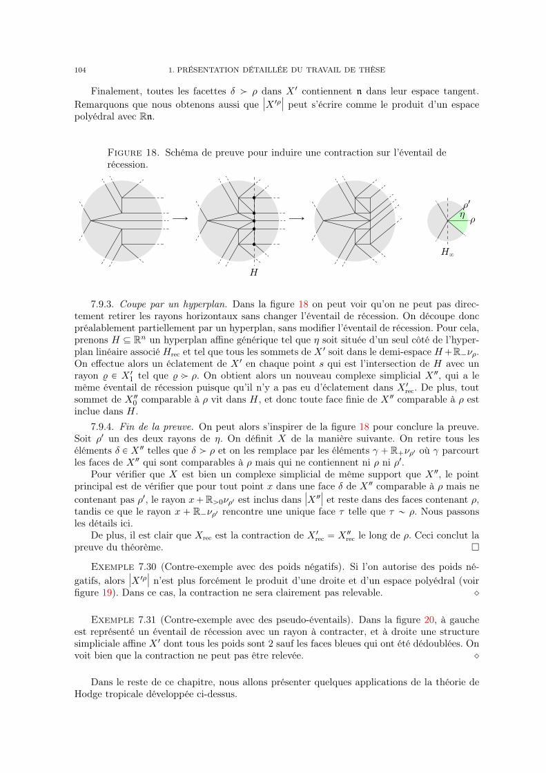
104 1. PRÉSENTATION DÉTAILLÉE DU TRAVAIL DE THÈSE
Finalement, toutes les facettes δ ą ρ dans X 1 contiennent n dans leur espace tangent.Remarquons que nous obtenons aussi que |X 1ρ| peut s’écrire comme le produit d’un espacepolyédral avec Rn.
Figure 18. Schéma de preuve pour induire une contraction sur l’éventail derécession.
ÝÑ
H
ÝÑ ηρ1
ρ
H8
7.9.3. Coupe par un hyperplan. Dans la figure 18 on peut voir qu’on ne peut pas direc-tement retirer les rayons horizontaux sans changer l’éventail de récession. On découpe doncpréalablement partiellement par un hyperplan, sans modifier l’éventail de récession. Pour cela,prenons H Ď Rn un hyperplan affine générique tel que η soit située d’un seul côté de l’hyper-plan linéaire associé Hrec et tel que tous les sommets de X 1 soit dans le demi-espace H`R´νρ.On effectue alors un éclatement de X 1 en chaque point s qui est l’intersection de H avec unrayon % P X 11 tel que % ą ρ. On obtient alors un nouveau complexe simplicial X2, qui a lemême éventail de récession puisque qu’il n’y a pas eu d’éclatement dans X 1rec. De plus, toutsommet de X20 comparable à ρ vit dans H, et donc toute face finie de X2 comparable à ρ estinclue dans H.
7.9.4. Fin de la preuve. On peut alors s’inspirer de la figure 18 pour conclure la preuve.Soit ρ1 un des deux rayons de η. On définit X de la manière suivante. On retire tous leséléments δ P X2 telles que δ ą ρ et on les remplace par les éléments γ `R`νρ1 où γ parcourtles faces de X2 qui sont comparables à ρ mais qui ne contiennent ni ρ ni ρ1.
Pour vérifier que X est bien un complexe simplicial de même support que X2, le pointprincipal est de vérifier que pour tout point x dans une face δ de X2 comparable à ρ mais necontenant pas ρ1, le rayon x`Rą0νρ1 est inclus dans |X2| et reste dans des faces contenant ρ,tandis ce que le rayon x ` R´νρ1 rencontre une unique face τ telle que τ „ ρ. Nous passonsles détails ici.
De plus, il est clair que Xrec est la contraction de X 1rec “ X2rec le long de ρ. Ceci conclut lapreuve du théorème.
Exemple 7.30 (Contre-exemple avec des poids négatifs). Si l’on autorise des poids né-gatifs, alors |X 1ρ| n’est plus forcément le produit d’une droite et d’un espace polyédral (voirfigure 19). Dans ce cas, la contraction ne sera clairement pas relevable. ˛
Exemple 7.31 (Contre-exemple avec des pseudo-éventails). Dans la figure 20, à gaucheest représenté un éventail de récession avec un rayon à contracter, et à droite une structuresimpliciale affine X 1 dont tous les poids sont 2 sauf les faces bleues qui ont été dédoublées. Onvoit bien que la contraction ne peut pas être relevée. ˛
Dans le reste de ce chapitre, nous allons présenter quelques applications de la théorie deHodge tropicale développée ci-dessus.

8. CONJECTURE DE HODGE POUR LES STRUCTURES KÄHLÉRIENNES RATIONNELLES 105
Figure 19. Un exemple de X 1ρ contredisant le théorème 7.29 pour des poidsnégatifs
´1
Figure 20. Contre-exemple au théorème 7.29 pour des pseudo-éventails
ρ
8. Conjecture de Hodge pour les structures simpliciales kählériennes fortementrationnelles
La limite tropicale d’une famille de variétés devrait donner des informations sur une fibregénérale de la variété. De plus, l’étude de la limite tropicale est potentiellement plus simpleque l’étude directe d’une fibre générale. Il est donc naturel de se demander si l’on pourraitavancer sur la conjecture de Hodge en regardant le cas tropical.
Ainsi, comme Zharkov l’explique dans [Zha20], Kontsevich a eu l’idée qu’il serait possiblede trouver un contre-exemple à la conjecture de Hodge en construisant un contre-exemple àla conjecture de Hodge tropicale. Plus précisément, certaines familles de variétés abéliennesont une limite tropicale de support le tore plat (voir section 8.4), et un contre-exemple à laconjecture de Hodge sur cette limite tropicale fournirait un contre-exemple à la conjecture deHodge sur les variétés abéliennes.
Au contraire, nous montrons dans ce chapitre que la conjecture de Hodge est valide pourles structures simpliciales kählériennes ou asymptotiquement kählériennes qui sont fortementrationnelles. Cela n’infirme pas la suggestion de Kontsevich car, en général, les limites tropi-cales étudiées ne sont que faiblement rationnelles.
8.1. Théorèmes principaux. Énonçons plus précisément le théorème que nous démon-trons. D’abord définissons les classes de Hodge. Soit X une structure simpliciale affine orientéede dimension d. On peut définir de manière naturelle les poids de Minkowski de dimension ksur X, que l’on note MWkpXq, comme étant les poids w : Xk Ñ k tels que l’élément
ÿ
δPXk
wpδqpδ, νδq P Ck,kpXq
soit un cycle. Comme dans le cas local, on peut aussi interpréter un tel poids comme une sous-structure simpliciale orientée de dimension k de X. Notons de plus que la somme ci-dessus
106 1. PRÉSENTATION DÉTAILLÉE DU TRAVAIL DE THÈSE
est un cycle dans X si et seulement si c’est un cycle dans Z :“ X car pour toute face δ desédentarité 0, la projection de νδ le long de n’importe quel rayon de δrec est nulle.
Soit w un poids de Minkowski de dimension k dans X. On peut associer à w sa classeclpwq dans Hd´k,d´kpZq via la composition
MWkpXq Ñ Hk,kpZq Ñ Hd´k,d´kpZq.
On appelle classe de Hodge de degré d ´ k tout élément de Hd´k,d´kpZq dans l’image de cl.On note Hodd´kpZq l’ensemble des classes de Hodge de degré d´ k.
Théorème 8.1 (Conjecture de Hodge pour les structures kählériennes fortement ration-nelles ou réelles). Soit X une structure simpliciale affine lisse kählérienne ou asymptotiquementkählérienne. Si k “ Q, on suppose que X est fortement rationnelle. Soit Z la compactificationcanonique de X. Alors pour tout entier k, HodkpZq coïncide avec le noyau de la monodromie
ker`
N : Hk,kpZq Ñ Hk´1,k`1pZq˘
.
Nous démontrons le théorème en section 8.3.On peut se demander si le même théorème est valide dans le cas faiblement rationnelle,
avec k “ Q. Dans ce cas on se restreint aux poids de Minkowski supportés sur les facesrationnelles.
Conjecture 8.2 (Conjecture de Hodge pour les structures kählériennes faiblement ra-tionnelles). Soit X une structure simpliciale affine lisse kählérienne ou asymptotiquementkählérienne faiblement rationnelle. Soit Z la compactification canonique de X. Existe-t-il unesubdivision de Z telle que, pour tout entier k, HodkpZq coïncide avec le noyau de la monodro-mie
ker`
N : Hk,kpZq Ñ Hk´1,k`1pZq˘
?
Dans le cas où k “ d´ 1, Jell, Rau et Shaw montrent dans [JRS18] le théorème p1, 1q deLefschetz tropical suivant. Soit X une variété tropicale localement matroïdale de dimensiond telle que rXs P MWdpXq ait un poids constant égal à 1. Alors l’image des cycles tropi-caux de dimension un dans X par l’application classe de cycle est exactement le noyau de lamonodromie dans Hd´1,d´1pXq.
Question 8.3. Peut-on étendre le résultat de [JRS18] aux structures simpliciales affineslisses ? ˛
Dans le cas complexe, la conjecture de Hodge implique que l’équivalence numérique etl’équivalence algébrique coïncident sur les cycles algébriques (conjecture standard D). Dans lecas tropical, nous obtenons un analogue, qui répond partiellement à une question de Gross etShokrieh dans [GS19c].
Théorème 8.4. Soit Z définie comme dans le théorème 8.1. Alors l’équivalence numériqueet l’équivalence homologique coïncident sur les cycles tropicaux.
Démonstration. Voir chapitre 4 théorème 1.3.
8.2. Suite exacte de Clemens et Schmid tropicale. La preuve du théorème 8.1s’appuie essentiellement sur un analogue de la suite exacte de Clemens et Schmid. En fait,la partie de la suite exacte qui nous intéresse est celle correspondant au théorème des cyclesinvariants. Pour une famille de variétés W sur le disque ∆, les cycles d’une fibre Wt invariantpar la monodromie T , et donc dans le noyau de N “ ´ logpT q, proviennent tous de W. Noussommes parvenu à traduire cela dans le monde tropical par l’existence de cycles tropicauxreprésentant les classes dans le noyau de la monodromie.
Dans le cas classique, cette suite exacte peut être décrite de la façon suivante. Soit Wune famille de variétés lisses sur le disque unité complexe ∆ comme dans la section 1.11. On

8. CONJECTURE DE HODGE POUR LES STRUCTURES KÄHLÉRIENNES RATIONNELLES 107
suppose de plus que la famille est projective. Comme précédemment, la fibre centrale W0 estun diviseur à croisements normaux qui a été construit par la méthode de [KKMS06] à partird’une triangulation X sur la limite tropicale.
On considère aussi le revêtement universel Ă∆˚ de ∆˚, et le relèvement ĄW˚ de W˚ au-dessus de Ă∆˚, ainsi que l’opérateur de monodromie N qui agit sur la cohomologie de ĄW˚, etla structure de Hodge mixte limite sur H‚pĄW˚q.
En considérant de plus la projection ĄW˚ Ñ W˚, on peut montrer que l’on obtient unesuite exacte longue
(8.1) ¨ ¨ ¨ Ñ H‚pW˚q Ñ H‚pĄW˚qNÝÑ H‚pĄW˚q Ñ H‚`1pW˚q Ñ ¨ ¨ ¨
À propos de cette suite exacte, remarquons simplement que T agit trivialement sur les cocyclesde H‚pW˚q, donc l’image de H‚pW˚q est bien dans le noyau de la monodromie N “ ´ logpT q.
D’un autre côté, l’inclusion W˚ ĎW permet de définir la cohomologie relative H‚pW,W˚q
et l’on obtient la suite exacte longue
(8.2) ¨ ¨ ¨ Ñ H‚pW,W˚q Ñ H‚pWq Ñ H‚pW˚q Ñ H‚`1pW,W˚q Ñ ¨ ¨ ¨
En combinant ces deux suites exactes, Clemens a construit dans [Cle77] la suite exactelongue (de période quatre !) de structures de Hodge mixtes suivante
(8.3) ¨ ¨ ¨ Ñ H‚pWq Ñ H‚pĄW˚qNÝÑ H‚pĄW˚q Ñ H‚`2pW,W˚q Ñ H‚`2pWq Ñ ¨ ¨ ¨
Les groupes H‚pWq forment ce qu’on va naturellement appeler la cohomologie survivante. Eneffet, W se rétracte par déformation sur W0, donc on a
H‚pW0q„ÝÑ H‚pWq Ñ H‚pW˚q,
et l’image de la composée de ces applications constitue les classes qui survivent sur la fibrecentrale.
Soit X une structure simpliciale affine lisse kählérienne, ou asymptotiquement kählérienneet soit Z :“ X.
On a vu queH‚pĄW˚q correspond à la structure de Hodge limite. Si l’on cherche un analoguetropical à la suite (8.3), on peut remplacer H‚pĄW˚q par H‚pZq.
Reste à savoir comment définir la cohomologie survivante tropicale H‚s pZq et la cohomolo-gie relative tropicale H‚relpZq. La première va être définie comme la cohomologie du noyau dela monodromie sur ST‚,‚1 , et la seconde comme la cohomologie du conoyau de la monodromiesur ST‚,‚1 .
Plus précisément, soit
Ka,b :“ ker`
N : STa,b1 Ñ STa`2,b´21
˘
“ STa,b,a1 .
On définit alorsHp,q
s pZq :“ Hq´ppK‚,2pq.
De plus, soitLa,b :“ coker
`
N : STa´2,b`21 Ñ STa,b1
˘
“ STa,b,´a.
On définit alorsHp,q
rel pZq :“ Hq´ppL‚,2pq.
Remarquons que, contrairement à Hp,qpZq, Hp,qs pZq et Hp,q
rel pZq ne sont pas stables parsubdivision en général.
Ces définitions sont justifiées par la proposition suivante qui montre qu’elles fournissentbien les analogues tropicaux des suites exactes (8.1) et (8.2).
108 1. PRÉSENTATION DÉTAILLÉE DU TRAVAIL DE THÈSE
Proposition 8.5. Pour tout entier p, nous avons deux suites exactes en cohomologie
¨ ¨ ¨ Ñ H‚`
cone‚´1pNq˘
Ñ Hp`1,‚pZqNÝÑ Hp,‚`1pZq Ñ H‚`1
`
cone‚´1pNq˘
Ñ ¨ ¨ ¨
¨ ¨ ¨ Ñ Hp,‚rel pZq
0ÝÑ Hp`1,‚
s pZq Ñ H‚`
cone‚´1pNq˘
Ñ Hp,‚`1rel pZq
0ÝÑ ¨ ¨ ¨
où cone‚pNq désigne le cône de l’opérateur monodromie décalé
cone‚pNq :“ cone‚´p´1´
N : ST‚,2p`21 Ñ ST‚`2,2p
1
¯
.
Démonstration. L’exactitude de la première suite est triviale par les propriétés du com-plexe de cône. Ensuite, comme la monodromie est très simple sur ST‚,‚1 , on peut tout y calculerexplicitement et montrer que la seconde suite est elle aussi exacte, voir proposition 6.2 dansle chapitre 4.
En combinant les deux suites exactes ci-dessus, on obtient le théorème suivant.
Théorème 8.6 (Suite exacte de Clemens et Schmid tropicale). Nous avons la suite exactesuivante
¨ ¨ ¨ Ñ Hks pZq Ñ HkpZq
NÝÑ HkpZq Ñ Hk`2
rel pZq Ñ Hk`2s pZq Ñ Hk`2pZq
NÝÑ Hk`2pZq Ñ ¨ ¨ ¨
On trouve en fait deux suites exactes en fonction de la parité de k.
Démonstration. Nous proposons un aperçu ici, voir chapitre 4 section 7 pour les détails.Pour tout entier p, on a une suite exacte à quatre termes
0 Ñ K‚,2p Ñ ST‚,2p1NÝÑ ST‚`2,2p´2
1 Ñ L‚`2,2p´2 Ñ 0.
De plus, comme N est un opérateur de type Lefschetz sur ST‚,‚1 , Ka,b est trivial pour a ă 0 etLa,b est trivial pour a ą 0. Donc la suite exacte ci-dessus est une suite exacte courte lorsquel’on restreint à chaque degré, mais ce n’est pas une suite exacte courte globale.
On peut tout de même appliquer le lemme du serpent sur les degrés suffisamment positifs(le cas négatif est similaire) pour obtenir une suite longue qui est exacte en degrés suffisammentpositifs
¨ ¨ ¨ Ñ H‚pK‚,2pq Ñ ST‚,2p2NÝÑ ST‚`2,2p´2
2 Ñ H‚`1pK‚,2pq Ñ ¨ ¨ ¨
Mais N est aussi un opérateur de type Lefschetz sur ST‚,‚2 . Donc la flèche N ci-dessus estsurjective en degrés positifs. La suite exacte longue se coupe donc en suites exactes courtes
0 Ñ H‚pK‚,2pq Ñ ST‚,2p2NÝÑ ST‚`2,2p´2
2 Ñ 0.
Pour les degrés suffisamment négatifs, on trouve de même des suites exactes courtes
0 Ñ ST‚,2p2NÝÑ ST‚`2,2p´2
2 Ñ H‚pL‚`2,2p´2q Ñ 0.
Autour du degré zéro toutefois, on ne peut plus appliquer le lemme du serpent. Une chasseau diagramme classique nous permet d’obtenir la suite exacte à six termes suivante.
0 Ñ ST´2,2p2 Ñ ST0,2p´2
2 Ñ H0pL‚,2p´2q Ñ H0pK‚,2pq Ñ ST0,2p2 Ñ ST2,2p´2
2 Ñ 0.
La suite exacte de Clemens et Schmid s’obtient comme la somme directe de toutes cescontributions.
8. CONJECTURE DE HODGE POUR LES STRUCTURES KÄHLÉRIENNES RATIONNELLES 109
8.3. Preuve du théorème 8.1. On peut réécrire la suite exacte à six termes avec lacohomologie tropicale.(8.4)0 Ñ Hp,p´2pZq
NÝÑ Hp´1,p´1pZq Ñ Hp´1,p´1
rel pZq Ñ Hp,ps pZq Ñ Hp,ppZq
NÝÑ Hp´1,p`1pZq Ñ 0.
On voit directement que c’est la partie qui va nous être utile. En effet, le noyau de la monodro-mie dans Hp,ppZq provient de la cohomologie survivante. Il reste à faire le lien entre Hp,p
s pZqet les classes de Hodge.
Soit α une classe de Hp,ps pZq. On veut construire un élément w P MWd´ppZq tel que
clpwq “ α. Comme K‚,2p est nul en degrés strictement négatifs, on a
Hp,ps pZq “ H0pK‚,2pq “ ker
`
ST0,2p,01
i˚ÝÑ ST1,2p,1
1
˘
.
Donc α est simplement un cocycle de
ST0,2p,01 “
à
sPZf ,0
H2ppZsq.
On peut décomposer α en pαsqsPZf ,0 . Par la conjecture de Hodge locale, théorème 5.27, pourchaque sommet s, il existe un poids de Minkowski ws P MWd´ppZ
sq tel que αs “ clpwsq.De plus, le fait que α soit un cocycle est équivalent au fait que les ws se recollent en unpoids de Minkowski global w P MWd´ppZq, voir la section 8 du chapitre 4 pour les détails(cela montre au passage que les classes des poids de Minkowski sont bien dans le noyau de lamonodromie). On vérifie ensuite que l’on a bien clpwq “ α, ce qui conclut la démonstrationdu théorème 8.1.
8.4. Variétés tropicales abéliennes. Dans [Zha20], Zharkov expose une idée de Kont-sevich. On peut faire dégénérer des variétés abéliennes complexes vers une variété abéliennetropicale Z que nous décrivons ci-dessous. Dans ce cas, un contre-exemple à la conjecturede Hodge tropicale sur Z pourrait être approximé par un contre-exemple de la conjecture deHodge classique.
Décrivons Z. On pose N :“ Zn. On choisit une forme bilinéaire symétrique définie positiveQ sur NR. Soit Γ Ď NR le réseau dual à N pour la forme Q. On définit Z comme le tore platNRΓ. Les fonctions affines rationnelles sur Z sont les éléments de MQ.
Nous travaillons à coefficients rationnels : k :“ Q. Montrons que Z admet une trian-gulation induisant une structure simpliciale affine faiblement rationnelle kählérienne. Notonsqu’un argument similaire à celui de la remarque 3.2 montre que Z n’admet pas de structuresimpliciale fortement rationnelle pour une forme Q générique.
Soit rΓ :“ Γm pour m P N suffisamment grand. Posons la fonction f définie par
f : NR ÝÑ R,x ÞÝÑ min
vPrΓ
a
Qpx´ v, x´ vq.
Clairement f induit une fonction de Z dans R.Mis à part les points de rΓ dans Z, les points de non dérivabilité de f forment le diagramme
de Voronoï du réseau Γ noté L. Montrons que l’on obtient un cycle tropical rationnel.D’abord il est connu que les cellules de Voronoï, c’est-à-dire les composantes connexes de
NR r L, sont des polyèdres. Si m est suffisamment grand, ces cellules forment un complexepolyédral sur Z. On obtient naturellement une structure de complexe polyédral sur L. De plusL est rationnel car ses facettes sont incluses dans des hyperplans de la forme pv1 ´ v2q
K pourv1, v2 des sommets de rΓ. Comme v1´v2 est rationnel par rapport à Γ, pv1´v2q
K est rationnelpar rapport à N par dualité.
Enfin justifions que L vérifie la condition d’équilibre. Soit x0 un point de L. Quitte àtranslater, on peut voir x0 comme l’origine de NR. Soit U0 une cellule de Voronoï qui contient
110 1. PRÉSENTATION DÉTAILLÉE DU TRAVAIL DE THÈSE
x0 dans son adhérence. Soit v0 le sommet de rΓ dans U0. Posons g “ f´a
Qpv0, v0q. Maintenantsoit U une autre cellule touchant x0 et soit v le sommet dans U . Alors sur U , au premier ordre,la fonction g ressemble à x ÞÑ Qpv, xq au voisinage de x0. Notons rg le linéariser de g autourde x0. Alors rg est une fonction linéaire par morceaux et, au voisinage de x0, L est simplementle diviseur de rg.
De plus, si x0 est un sommet de L, ´rg est convexe autour de x0. La fonction induit doncune classe kählérienne `x0 , qui de plus est rationnelle puisque son dual de Poincaré est L (voirremarque 5.29). En rassemblant toutes les classes `x0 pour les sommets x0 de L, on obtientune classe de Kähler rationnelle sur Z.
Quitte à effectuer des éclatements on peut obtenir une structure simpliciale affine faible-ment rationnelle sur Z munie d’une forme de Kähler. La forme de Kähler n’est plus forcémentrationnelle autour des points d’éclatements, mais sa classe est la même que précédemment. Laclasse associée est donc une classe de Kähler rationnelle.
Question 8.7. La variété abélienne tropicale Z vérifie-t-elle la conjecture de Hodge ? ˛
9. Comparaison des compactifications des sous-variétés du tore complexe et dutore tropical
Dans la section 1.8.2, nous avons discuté du phénomène suivant. SiW est une sous-variétédu tore complexe Tn
C, alors pour de bons éventails Σ dont le support est la tropicalisationTroppW q de W , la compactification W de W dans CPΣ vérifie de bonnes propriétés. Notam-ment, W est toujours compacte, et l’intersection de W avec la strate CPσΣ, σ P Σ, a toujourspour dimension dimpW q ´ |σ|. Voir la section 9 du chapitre 2 pour plus de détails. La tropi-calisation étendue de W est alors le support de la compactification canonique de Σ Ď TPΣ. Ilest naturel de se demander le lien entre la cohomologie de W et la cohomologie tropicale deΣ. C’est ce dont nous allons discuter dans cette section.
Nous rappelons une partie du résultat de Feichtner et Yuzvinsky [FY04]. Soit W un com-plémentaire d’arrangement d’hyperplans. La tropicalisation de W est le support de Bergmanassocié à cet arrangement d’hyperplans, et l’on peut regarder l’éventail de Bergman associé.C’est un éventail unimodulaire noté Σ. Alors le théorème de Feichtner et Yuzvinsky montreque l’application
A‚pΣq „ÝÑ A‚pTPΣq Ñ H‚,‚pW q
est un isomorphisme. Notamment, par le théorème 5.7, A‚pΣq » H‚,‚pΣq et l’on obtient bienun isomorphisme
H‚,‚pΣq » H‚,‚pW q.
En fait le résultat de Feichtner et Yuzvinsky s’applique aux compactifications magnifiquesdéfinies par De Concini et Procesi dans [DP95] qui repose sur des éventails construits à partirde « building sets » et de « nested sets ». Ces constructions ne permettent pas d’obtenir tousles éventails de Bergman unimodulaires généralisés.
Théorème 9.1. Soit W un complémentaire d’arrangement d’hyperplans plongé dans TnC.
Soit Σ un éventail de Bergman unimodulaire généralisé de support TroppW q. Soit W la com-pactification de W dans CPΣ. Alors l’application
H‚,‚pΣq „ÝÑ A‚pΣq „ÝÑ A‚pTPΣq Ñ H‚,‚pW q
est un isomorphisme.
Nous montrons ce résultat dans la section 9.1 en utilisant la suite exacte de Deligne,proposition 4.9, qui permet de travailler directement par récurrence sur la dimension. Dansla section 9.2, nous présentons une idée s’appuyant sur l’épluchabilité tropicale qui pourraitpeut-être aboutir à une généralisation plus vaste du théorème de Feichtner-Yuzvinsky.
9. COMPACTIFICATIONS DES TORES COMPLEXES ET TROPICAUX 111
9.1. Preuve du théorème 9.1. Nous présentons brièvement la preuve donnée en sec-tion 9 du chapitre 2.
Les résultats de Tevelev montrent que W rW forme un diviseur à croisements normaux.On peut alors appliquer la suite spectrale de Deligne qui calcule la structure de Hodge mixte deW à partir des strates de W . Comme W est un complémentaire d’arrangement d’hyperplans,la cohomologie de W est très simple [Sha93] : HppW q est pure de poids pp, pq. On a alorssimplement une suite exacte (voir [IKMZ19])
0 Ñ HppW q Ñà
σPΣp
H0pWσq Ñ
à
σPΣp´1
H2pWσq Ñ ¨ ¨ ¨ Ñ
à
σPΣ1
H2p´2pWσq Ñ H2ppW q Ñ 0.
D’un autre côté, nous avons montré l’existence d’une suite exacte de Deligne tropicale(théorème 4.9)
0 Ñ Fpp0q Ñà
σPΣp
H0pΣσ8q Ñ
à
σPΣp´1
H2pΣσ8q Ñ ¨ ¨ ¨ Ñ
à
σPΣ1
H2p´2pΣσ8q Ñ H2ppΣq Ñ 0.
Notons que, si σ P Σ, alorsW σ est un complémentaire d’arrangement d’hyperplans dont latropicalisation est |Σσ|. De plus,W σ est la compactification deW σ dans CPΣσ . Par récurrence,on peut donc supposer que pour toute face σ ‰ 0 de Σ, H‚pΣσ
8q » H‚pW
σq.
De plus, par un résultat de Zharkov [Zha13] que nous avons déjà cité, F‚p0q est isomorpheà la cohomologie de W .
Donc les deux suites exactes ci-dessus sont isomorphes sauf pour le dernier terme. On endéduit l’isomorphisme pour le dernier terme :
H2ppW q » H2ppΣq.
9.2. Schéma de preuve pour une généralisation. Nous souhaiterions généraliser lethéorème précédent. Avec Amini, nous avons une conjecture plus précise mais globalement laquestion est la suivante.
Question 9.2. Soit W une sous-variété du tore. Soit Σ un éventail sur sa tropicalisation.Supposons que la compactification W Ď CPΣ a de bonnes propriétés. Quitte à changer lefaisceau F‚ en un autre faisceau G‚, peut-on obtenir un isomorphisme
H‚pΣ,G‚q » H‚pW q ? ˛
Si les strates ouvertes W σ sont assez simples, par exemple si leur cohomologie de degré pest pure de poids pp, pq, et siWrW est un diviseur à croisements normaux, la preuve ci-dessusdevrait fonctionner à condition que le faisceau G‚ ait des propriétés similaires à celles de F‚,et que G‚p8σq soit isomorphe à H‚pW σq.
Pour des cas plus compliqués, il faudrait potentiellement développer une théorie des struc-tures de Hodge mixtes tropicales.
Une autre piste pour généraliser le théorème 9.1 serait d’utiliser la modification tropicale.Prenons une fonction régulière g : W Ñ C. Supposons que g corresponde à une fonction flinéaire par morceaux sur Σ telle que la tropicalisation de divpgq corresponde à divpfq. Dansce cas, le graphe ΓgpW q Ď Tn
CˆC de la fonction g devrait avoir pour tropicalisation le supportde CTMf pΣq Ď Tn
TˆT. Clairement, H‚pΓgpW qq » H‚pW q. De plus, si Σ est lisse, on sait parle théorème 6.10 que H‚
`
CTMf pΣq˘
est isomorphe à H‚pΣq.Posons Σ1 :“ TMf pΣq. En vérifiant que l’on a une correspondance entre les strates de
ΓgpW q Ď TPΣ1 et les strates de Σ1, on doit pouvoir montrer que si H‚pΣq » H‚pW q, alors
H‚pΓgpW qq » H‚pTMf pΣqq.
Ainsi on peut envisager le fait que l’isomorphisme entre H‚pW q et H‚pΣq soit stable parépluchabilité.
112 1. PRÉSENTATION DÉTAILLÉE DU TRAVAIL DE THÈSE
Un tel argument fonctionne dans le cas des éventails de Bergman généralisés et permet demontrer que
H‚pW,Zq » H‚pΣ,Zq,où l’on reprend les notations du théorème 9.1 pour Σ et W : voir chapitre 2 remarque 9.5.
Une fois que le cas local sera bien compris, on pourra s’attaquer au cas global et parexemple tenter de généraliser le théorème de [IKMZ19] à des dégénérescences de familles devariétés dont la fibre centrale n’a pas que des composantes ouvertes qui sont des complémen-taires d’arrangements d’hyperplans, voir question 7.3.
10. Une généralisation des polynômes de Symanzik
Une question naturelle sous-jacente à cette thèse est de savoir si l’étude de la limite tropi-cale d’une famille de variétés qui dégénèrent peut permettre de trouver des informations surla famille.
Par exemple, dans [AN20], dans le cas où les variétés sont de dimension un, Amini etNicolussi définissent des espaces hybrides mêlant la fibre centrale et la limite tropicale. Ilsdéfinissent des mesures canoniques sur les espaces hybrides ainsi construits. Ils obtiennentalors que les mesures canoniques sur les fibres générales d’une famille s’étendent de manièrecontinue à la fibre centrale hybride de cette famille. Pour définir ces mesures hybrides, lesauteurs s’inspirent d’un analogue de la mesure canonique, appelé mesure de Zhang [Zha93],qui peut être définie sur la partie finie de limite tropicale. Ici, cette partie finie est simplementun graphe métrique. L’une des définitions possibles pour la mesure de Zhang fait intervenir lepolynôme de Kirchhoff, c’est-à-dire le dual du polynôme de Symanzik qui nous intéresse ici.
Dans cette section, nous nous intéressons principalement à un autre exemple. Toujoursdans le cas d’une famille de surfaces de Riemann, Amini, Bloch, Burgos Gil et Fresán ont pumontrer dans [ABBF16] que l’asymptotique de l’accouplement de hauteur de deux diviseursde degrés zéro peut être décrite grâce aux rapports des deux polynômes de Symanzik sur lalimite tropicale, comme nous allons l’expliquer plus en détail en section 10.4.
Question 10.1. Peut-on étendre les résultats ci-dessus en dimensions supérieures ? ˛
Pour tenter de répondre à cette question, dans [Piq19b], qui correspond au chapitre 5,nous avons généralisé les polynômes de Symanzik en dimensions supérieures. Ces polynômesde Symanzik généralisés possèdent des propriétés étonnantes en lien avec différents sujets desmathématiques. Nous allons énoncer quelques-unes de ces propriétés dans cette section.
10.1. Origine des polynômes de Symanzik. Les polynômes de Symanzik sont utili-sés en théorie quantique des champs pour calculer des intégrales de Feynman, et leur étude aamené à développer différentes théories intéressantes [BB03,BEK06,Bro15,BS12,BY11].Une intégrale de Feynman est grossièrement une intégrale sur tous les parcours possiblesde particules qui interagissent. Cette intégrale est assez mal définie a priori, mais on peutla simplifier pour l’exprimer comme une somme sur des graphes G d’intégrales impliquantexpp´iSym2GSymGq où SymG et Sym2G sont respectivement le premier et le second poly-nôme de Symanzik du graphe G.
Soit G un graphe. Notons V l’ensemble des sommets du graphe G et E l’ensemble deses arêtes. Supposons G connexe. Rappelons qu’un arbre couvrant sur G est un sous-graphemaximal de G sans cycle. Alors SymG est un polynôme dans Rrye | e P Es défini par
SymGpyq “ÿ
TPTyErT ,
où T est l’ensemble des arbres couvrants de G et yErT désigne le produit des ye pour e unearête qui n’est pas dans T . Ici, y est un raccourci pour le E-uplet pyeqePE .
10. UNE GÉNÉRALISATION DES POLYNÔMES DE SYMANZIK 113
Nous ne définissons pas le second polynôme de Symanzik ici. Nous définirons directementsa généralisation plus loin.
Les polynômes de Symanzik ont de nombreuses propriétés, la plupart sont résuméesdans [BW10]. Notamment, le premier polynôme de Symanzik est une spécialisation du poly-nôme de Tutte multivarié, aussi connu aussi sous le nom de modèle de Potts en physique. Celaimplique déjà beaucoup de propriétés. Par exemple, il peut être calculé par récurrence parcontraction-suppression, voir la section 1.2 du chapitre 5. Citons aussi [Bro15] dans lequelapparaît un théorème de factorisation pour le polynôme qui fait intervenir les mineurs dugraphe et qui a son importance pour certaines applications en physique, voir la section susci-tées. Ces propriétés et celles dont nous allons parler dans la suite s’étendent le plus souventau cas des polynômes de Symanzik généralisés.
10.2. Polynômes de Kirchhoff et dualité. Le lecteur peut se référer aux sections 2et 3 pour les détails et les preuves sur cette section et la suivante.
On définit le polynôme de Kirchhoff du graphe G par
KirGpyq “ÿ
TPTyT .
Soit U P RVˆE la matrice d’incidence du graphe, qui est une matrice dont les rangées sontindexées par V , les colonnes par E, et telle que pour chaque arête e d’extrémités v1, v2, leterme Uv1,e vaut 1, et le terme Uv2,e vaut ´1 (ou l’inverse, on fait des choix arbitraires ici),et tous les autres termes Uv,e, pour v et e qui ne sont pas incidents, valent 0. Choisissons unsommet v0 quelconque et définissons rU P RpV´v0qˆE la matrice U à laquelle on a retiré larangée v0. Alors le théorème suivant est bien connu et peut-être montré grâce à la formule deCayley [Cay49].
Théorème 10.2 (Théorème de Kirchhoff pondéré). On a
KirGpyq “ detprUY rUᵀq
où Y est la matrice diagonale diag`
pyeqePE˘
.
Cela permet notamment de compter le nombre d’arbres couvrants du graphe puisque cenombre vaut KirGp1, . . . , 1q.
Le polynôme de Symanzik peut être vu comme le dual du polynôme de Kirchhoff car siG est un graphe planaire, le polynôme de Symanzik de G est le polynôme de Kirchhoff dugraphe dual à G.
De plus, on a le dual du théorème de Kirchhoff ci-dessus.
Théorème 10.3. Soit K une matrice de rang maximale, dont les colonnes sont indépen-dantes et telle que UK “ 0. Alors il existe un facteur C que l’on peut calculer explicitementtel que
SymGpyq “ C detpKᵀY Kq.
10.3. Généralisation du premier polynôme de Symanzik. La définition du poly-nôme de Kirchhoff ne dépend que de la matrice d’incidence. Ainsi, on peut remplacer cettematrice par n’importe quelle autre matrice (voire, ce qui est en fait assez naturel, par des ma-troïdes sur des hypercorps, voir la section 4 du chapitre 5). Soit E un ensemble quelconque.Soit U une matrice dont les colonnes sont indexées par E. Soit rU la même matrice où l’ona seulement gardé rkpUq rangées indépendantes. Soit enfin K une matrice de rang maximaledont les colonnes sont indépendantes et telle que UK “ 0.
Définition 10.4. On définit le polynôme de Kirchhoff de U par
KirpU ; yq “ detprUY rUᵀq
114 1. PRÉSENTATION DÉTAILLÉE DU TRAVAIL DE THÈSE
et le polynôme de Symanzik de U par
SympU ; yq “ detpKᵀY Kq.
Ces polynômes ne sont bien définis qu’à un facteur près. ˛
Le fait que les polynômes ne soient définis qu’à un facteur près ne sera plus un problèmelorsque l’on étudiera le rapport des deux polynômes de Symanzik. Dans le cas où la matrice Uest à coefficients entiers, nous donnons une manière canonique de définir les polynômes dansle chapitre 5, ce qui lève l’ambiguïté.
On peut trouver d’autres formulations pour ces polynômes en utilisant la formule deCayley. Toujours à un facteur près, on a
KirpU ; yq “ÿ
FĎE
detprU |F q2yF ,
SympU ; yq “ÿ
FĎE
detprU |F q2yErF ,
où la somme est sur les sous-ensembles de E de rang rkpUq. Notamment, la deuxième formulemontre qu’à un facteur près qui ne dépend pas de F ,
detprU |F q “ ˘detpKᵀ|ErF q.
Dans le cas des graphes, on a vu que le polynôme de Kirchhoff compte le nombre d’arbrescouvrants. Si l’on regarde une structure simpliciale affine X de dimension d, on peut définirun analogue de la matrice d’incidence pour X en prenant la matrice U P ZXd´1ˆXd associéeau morphisme de bord d : ZXd Ñ ZXd´1 de l’homologie simpliciale. On pose alors
KirpX; yq :“ KirpU ; yq et SympX; yq :“ SympU ; yq.
Dans ce cas, Duval, Klivans et Martin ont montré dans [DKM09] que KirpU ; 1, . . . , 1qcompte le nombre d’arbres couvrants avec multiplicités de X (voir aussi [BK16]). Expliquons-nous. Par analogie avec le cas des graphes, on peut appeler arbre couvrant de X tout sous-ensemble maximal acyclique de Xd. Par acyclique nous voulons dire que la restriction de X àce sous-ensemble a une cohomologie de degré d triviale. La multiplicité correspond aux facteursdetprU |F q
2 et est due à la torsion ; par exemple un arbre couvrant composé d’un plan projectifréel et de parties contractiles sera compté 22 fois.
Ce lien entre polynômes de Kirchhoff, déterminants et arbres couvrants est aussi étudiépar Lyons dans son article [Lyo09] à propos des complexes aléatoires. Le fait que le polynômede Kirchhoff soit défini à partir de déterminants le lie étroitement à la théorie des mesures deprobabilité déterminantales [Lyo03], qui sont des mesures ayant de bonnes propriétés dû aufait qu’elles sont définies à partir de certains déterminants.
Notons aussi que d’autres généralisations des polynômes de Symanzik ont été étudiéesmais dans des objectifs différents : voir [GR07,KRTW10].
10.4. Accouplements de hauteur et second polynôme de Symanzik. Prenonsune famille de courbes complexes projectives lisses pWtqtP∆˚ qui dégénèrent en t “ 0. Prenonsaussi deux familles de diviseurs de degré zéro pDtqt et pD1tqt. Supposons que sur chaque fibregénérale Wt, t P ∆˚, Dt et D1t sont de supports disjoints. On peut alors définir l’accouplementde hauteur
xDt, D1ty “ Re
´
ż
γDt
ωD1t
¯
,
où γDt est une 1-chaîne n’intersectant pas le support de D1t et dont le bord est Dt, et ωD1test une certaine forme différentielle logarithmique canonique de résidue D1t. On s’intéressemaintenant à l’asymptotique de l’accouplement ci-dessus lorsque t tend vers 0. Les auteursde [ABBF16] ont montré que, sous de bonnes conditions, l’asymptotique peut être décrite
10. UNE GÉNÉRALISATION DES POLYNÔMES DE SYMANZIK 115
grâce à un accouplement de hauteur défini sur la partie finie de la limite tropicale, qui ici estun graphe. Plus précisément,
(10.1) xDt, D1ty “ xDtrop, D
1tropyyptq `Op1q
où le second accouplement est l’accouplement tropical entre les limites tropicales de pDtqt etpD1tqt, et yptq est une famille de nombre réels tendant vers `8. Cet accouplement tropical estlui-même décrit comme le rapport des deux polynômes de Symanzik du graphe. C’est ce quenous allons expliquer maintenant, en toute dimension.
Soit X une structure simpliciale affine compacte (i.e. X “ Xf ) de dimension d. Soit D unbord simplicial, c’est-à-dire un élément dans l’image de la différentielle simpliciale d : RXd ÑRXd´1 . On peut voir D comme un diviseur tropical, mais aussi comme un vecteur dans RXd´1 .Soit y “ pyδqδPXd une famille de variables indexées par les facettes. On peut alors étudier lerapport des deux polynômes de Symanzik
ĆSympX,D; yq :“SympX,D; yq
SympX; yq
où le second polynôme de Symanzik est défini en appliquant la définition 10.5 à la matriced’incidence U de X et au vecteur associé au diviseur D.
Définition 10.5. Soient V et E deux ensembles, U P RVˆE une matrice et y “ pyeqePEune famille de variables. Soient u un vecteur dans l’image de U et yu une nouvelle va-riable. Alors on définit le second polynôme de Symanzik associé à la paire pU, uq, et l’on noteSympU, u; yq, le polynôme SympU 1; y, yuq évalué en yu “ 0 où U 1 est la matrice U à laquelleon a ajouté le vecteur u en dernière colonne. ˛
On vérifie facilement que ĆSympX,D; yq est quadratique en D. On peut donc définir saforme bilinéaire associée : si D et D1 sont deux bords simpliciaux dans ZXd´1 , alors on définitl’accouplement de hauteur tropical de D et D1 en y par
1
2
`
ĆSympX,D `D1; yq ´ĆSympX,D; yq ´ĆSympX,D1; yq˘
.
Question 10.6. L’accouplement de hauteur tropical ainsi défini permet-il de décrirel’asymptotique de l’accouplement de hauteur pour une famille de variétés de dimension quel-conque ? ˛
10.5. Invariance par subdivision. SoitX une structure simpliciale affine orientée com-pacte de dimension d. Dans le rapport des deux polynômes de Symanzik de X, on peut parexemple interpréter la variable pyδqδPXd comme le volume de la facette δ. Dans notre cadre,cela signifie que l’on obtient un invariant intéressant si l’on pose yδ “ 1wpδq où w P MWdpXqest l’élément canonique. Ici 1w représente bien un volume car si on subdivise une facette δen des facettes δ1, . . . , δs, pour i P t1, . . . , su on souhaite que
yδyδi
“Volpδq
Volpδiq;
or, comme wpδqνδ “ wpδiqνδi et
νδi “Volpδiq
Volpδqνδ,
on obtient bien la relation souhaitée en posant yδ “ 1wpδq.Par le corollaire 3.22 du chapitre 5, contrairement au polynôme de Kirchhoff, le rapport
des deux polynômes de Symanzik est invariant par subdivision si l’on évalue les yδ en 1wpδq.Cette invariance montre que l’on peut en fait définir les polynômes de Symanzik sur des espacespolyédraux mesurés même sans assigner de triangulation.
116 1. PRÉSENTATION DÉTAILLÉE DU TRAVAIL DE THÈSE
En fait, cette propriété est analogue aux propriétés des réseaux de résistances électriques,voir [CCK12]. Si X est un graphe, si wpeq représente la conductance d’une arête e, la dualitéentre les polynômes de Symanzik et les polynômes de Kirchhoff est l’analogue de la dualitéentre résistance et conductance. On peut par exemple calculer la résistance entre deux sommetsavec des sommes sur les arbres couvrants ressemblant beaucoup aux polynômes de Symanzik.Cela permet aussi de calculer certaines probabilités concernant la marche aléatoire sur legraphe, ce qui est très lié aux mesures de probabilités déterminantales et aux mesures deZhang dont nous avons déjà parlés.
10.6. Stabilité du rapport des deux polynômes. Reprenons notre discussion dela section 10.4. Pour montrer que l’asymptotique des accouplements de hauteur sur la fa-mille vérifie l’équation (10.1), une première étape est d’utiliser le théorème de l’orbite nilpo-tente. Il faut ensuite contrôler le rapport ĆSympX,D; yq. Pour cela on peut utiliser un résultatde [BGHdJ18], comme dans [ABBF16]. Dans [Ami19], Amini propose une autre démons-tration par des méthodes élémentaires. On obtient alors le théorème 10.7 ci-dessous restreintau cas des graphes. Nous avons nous-même généralisé ce théorème dans le cadre des polynômesde Symanzik généralisés (et même un peu au-delà), voir chapitre 5 section 6, ce qui est unepremière étape pour généraliser le calcul de l’asymptotique de l’accouplement de hauteur endimensions supérieures. Ainsi, notre généralisation devrait elle aussi être reliée aux théorèmesde l’orbite nilpotente et de l’orbite SL2.
Soient V et E deux ensembles, U P RVˆE une matrice et y “ pyeqePE des variables. Soitu un vecteur dans l’image de U .
Pour énoncer le théorème, nous devons d’abord expliciter la formule déterminantale per-mettant de calculer le second polynôme de Symanzik. Soit K une matrice de rang maximaldont les colonnes sont indépendantes et telle que UK “ 0. Soit ru un vecteur tel que Uru “ u.Soit enfin K 1 la matrice obtenue à partir de K en ajoutant le vecteur ru en dernière colonne.Alors, à un facteur près,
SympU, u; yq “ detpK 1ᵀY K 1q,
où Y est la matrice diagonale diagpyq.
Théorème 10.7 (Stabilité du rapport des deux polynômes de Symanzik). Soit Z “ Zpyqune matrice bornée fonction des variables y. Avec les notations ci-dessus, la différence
detpK 1ᵀY K 1q
detpKᵀY Kq´
detpK 1ᵀpY ` ZqK 1q
detpKᵀpY ` ZqKq
est bornée lorsque les variables de y tendent simultanément vers `8. Autrement dit, il existedes constantes positives C et M telles que la différence soit majorée en valeur absolue par Mlorsque ye ě C pour tout e P E.
Démonstration. Voir la section 6 du chapitre 5.
Commentons ce théorème. Remarquons d’abord que la première fraction est égale aurapport des deux polynômes de Symanzik. Si l’on interprète les valeurs y comme les volumesdes facettes d’une structure simpliciale que l’on fait diverger, et Z comme une perturbationbornée de ces volumes, le théorème ci-dessus peut être interprété comme le fait que le rapportdes deux polynômes de Symanzik répond de manière bornée à une déformation bornée de lagéométrie.
Ensuite, notons que ce théorème est plutôt surprenant a priori car les numérateurs sontdes polynômes de degré un de plus que les dénominateurs, et quand bien même ce ne seraitpas le cas, une variable ye qui n’apparaîtrait que dans le numérateur pourrait diverger bienplus vite que les autres, faisant diverger chaque fraction au passage.
Les polynômes de Symanzik vus comme des fonctions sont donc des polynômes aux proprié-tés remarquables, rentrant ainsi dans un domaine actif des mathématiques étudiant justement
10. UNE GÉNÉRALISATION DES POLYNÔMES DE SYMANZIK 117
les propriétés remarquables de certains polynômes associés à des structures combinatoires.D’autres propriétés de ces polynômes en tant que fonctions étaient déjà connues. Par exemple,on peut vérifier que les polynômes de Symanzik vérifie la propriété du demi-plan : il ne s’annulepas dans la partie où toutes les variables ye sont dans le demi-plan complexe supérieur. Lespolynômes vérifiant ce genre de propriétés ont été étudiés dans [COSW04,Brä07,BBL07].Citons aussi le récent article de Brändén et Huh, [BH19], sur les polynômes lorentzien, quiont aussi des propriétés remarquables, notamment des propriétés de type Hodge-Riemann quiles lient donc par ailleurs avec le reste de cette thèse.
10.7. Graphe d’échange d’un matroïde. Terminons cette section en citant un jolithéorème concernant les matroïdes que l’on peut trouver dans la section 5 du chapitre 5. Bienqu’à première vue ce théorème n’a pas de lien avec les polynômes de Symanzik, il est en faitutilisé pour montrer le théorème 10.7.
Sur un graphe connexeG, il est bien connu qu’à partir d’un arbre couvrant T , on peut obte-nir n’importe quel autre arbre couvrant T 1 par une suite d’arbres couvrants T “T0, T1, . . . , Ts“T 1 où, pour 1 ď i ď s, Ti est obtenu à partir de Ti´1 en effectuant un flip, c’est-à-dire en retirantune arête et en en rajoutant une autre. Le même théorème est en fait vrai pour tout matroïdeM. Pour toutes bases B et B1 de M, il existe une suite de bases B “ B0,B1, . . . ,Bs “ B1 tellesque, pour 1 ď i ď s, Bi est obtenue à partir de Bi´1 en retirant un élément et en en rajoutantun autre.
Nous généralisons ce principe à des paires d’indépendants du matroïde.Ce genre de propriétés peut être utile par exemple si l’on souhaite générer une base aléa-
toire. On part d’une base arbitraire, puis en faisant un certains nombre de flips aléatoire onobtient finalement une base aléatoire selon une mesure de probabilités intéressantes [FM92,ALOGV19], le second utilise d’ailleurs les résultats de [AHK18] à propos la log-concavitésur les matroïdes.
Soit M un matroïde sur l’ensemble E et soit I son ensemble d’indépendants. On définitle graphe d’échange G de M de la manière suivante. Les sommets de G sont les paires d’indé-pendants pI1, I2q P I
2. Deux sommets pI1, J2q et pJ 11, I 12q de G sont reliés s’il existe un élémenti P I1 r J2 tel que J 11 “ I1 ´ i et I 12 “ J2 ` i. Si a et b sont deux entiers avec 1 ď a ď rkpGq et0 ď b ď rkpGq ´ 1, on note Ga,b la restriction du graphe G aux paires d’indépendants pI1, I2q
avec cardpI1q “ a et cardpI2q “ b ou bien cardpI1q “ a´ 1 et cardpI2q “ b` 1.On s’intéresse aux composantes connexes de G. Remarquons d’abord l’existence d’un in-
variant trivial : deux sommets pI1, I2q et pI 11, I 12q d’une même composante vérifient que l’unionavec multiplicité I1 Z I2 est égale à I 11 Z I 12.
Un autre invariant moins évident est ce qu’on appelle la paire codépendante maximale.Soit pI1, I2q un sommet de G. Soient A Ď I1 et B Ď I2 telles que leurs clôtures clpAq et clpBqcoïncident. Alors pA,Bq est appelée une paire codépendante de pI1, I2q. On peut démontrerque l’ensemble de ces paires possède un maximum pour l’inclusion. On appelle cette paire lapaire codépendante maximale de pI1, I2q. Les éléments de cette paire ne peuvent pas passer del’autre côté sans casser l’indépendance : il s’agit bien d’un invariant.
Le théorème énonce que ces deux invariants forment un système complet d’invariants.
Théorème 10.8. Deux sommets pI1, I2q et pI 11, I12q de G sont dans la même composante
connexe si et seulement si I1ZI2 “ I 11ZI12 et les deux sommets ont la même paire codépendante
maximale.Le même résultat est vrai pour tous les sous-graphes Ga,b.Démonstration. Voir la section 5 du chapitre 5.
Citons finalement une conjecture en lien avec le théorème ci-dessus.Un ensemble I Ď E est un coindépendant dans M si ErI est indépendant dans le dual de
M, autrement dit s’il existe une base B de M incluse dans I. On peut alors étendre le graphe
118 1. PRÉSENTATION DÉTAILLÉE DU TRAVAIL DE THÈSE
G en prenant pour sommets les paires pI1, I2q où I1 est un indépendant ou un coindépendantet de même pour I2.
Conjecture 10.9. Le théorème 10.8 est vrai sur Gr,r où r :“ rkpMq.
Cette conjecture est équivalente à la conjecture 1.8 de [Bla08] qui fait partie de la conjec-ture de White concernant les idéaux toriques des matroïdes, voir aussi [Whi80,LM14].
CHAPTER 2
Homology of tropical fans
Abstract : The aim of this paper is to study homological properties of tropical fans andto propose a notion of smoothness in tropical geometry, which goes beyond matroids and theirBergman fans and which leads to an enrichment of the category of smooth tropical varieties.
Among the resulting applications, we prove the Hodge isomorphism theorem which assertsthat the Chow rings of smooth unimodular tropical fans are isomorphic to the tropical coho-mology rings of their corresponding canonical compactifications, and prove a slightly weakerstatement for any unimodular fan. We furthermore introduce a notion of shellability for tropi-cal fans and show that shellable tropical fans are smooth and thus enjoy all the nice homologicalproperties of smooth tropical fans. Several other interesting properties for tropical fans areshown to be shellable. Finally, we obtain a generalization, both in the tropical and in theclassical setting, of the pioneering work of Feichtner-Yuzvinsky and De Concini-Procesi on thecohomology ring of wonderful compactifications of complements of hyperplane arrangements.
The results in this paper form the basis for our subsequent works on Hodge theory fortropical and non-Archimedean varieties.
1. Introduction
The work undertaken in this paper is motivated by the following fundamental questionsin tropical geometry:
Question 1.1. — What it means for a tropical variety to be smooth?
— What are algebraic varieties which admit a smooth tropicalization? ˛
As in differential topology and algebraic geometry, tropical smoothness should be a localnotion. Since tropical fans and their supports form the building blocks of more general tropicalvarieties, the first part of the question will be reduced to the same one for tropical fans. Weprecise what we mean by a tropical fan.
Let N » Zn be a lattice of finite rank and denote by NR the vector space generated by N .Recall that a fan Σ in NR is a non-empty collection of strongly convex polyhedral cones whichverify the following two properties. First, for any cone σ P Σ, any face of σ belongs to Σ.Moreover, for two cones σ and η in Σ, the intersection σXη is a common face of both σ and η.In particular, Σ always contains the cone 0 :“ t0u. We denote by |σ| the dimension of a faceσ. A fan is called rational if any cone in Σ is rational in the sense that it is generated by rayswhich have non-zero intersection with the lattice N . In that case, each cone σ in Σ defines asublattice Nσ of N of the same rank as the dimension of σ, and given by the integral points ofthe vector subspace of NR generated by σ. A fan is pure dimensional if all its maximal coneshave the same dimension. The support of a fan Σ is denoted by |Σ|.
A tropical fan is a pure dimensional rational fan Σ in NR as above which in addition verifiesthe following foundational principle in tropical geometry called the balancing condition: forany cone τ of codimension one in Σ, we have the vanishing in the quotient lattice N
L
Nτ ofthe following sum
ÿ
σĄτ
eτσ “ 0
119
120 2. HOMOLOGY OF TROPICAL FANS
where the sum is over faces σ of maximal dimension containing τ and eτσ is the vector whichgenerates the quotient pσ X Nq
L
pτ X Nq » Zě0. This might be regarded as a polyhedralanalogue of orientability and leads to the definition of a fundamental class which plays an im-portant role in the treatment of the duality and other finer geometric properties in polyhedralgeometry.
A special class of tropical fans are the realizable ones which are those arising from (faith-ful) tropicalizations of subvarieties of algebraic tori over trivially valued fields. Tropical fansand their supports form the local charts for more general tropical varieties. This includesin particular the realizable ones which are those coming from (faithful) tropicalizations ofsubvarieties of algebraic tori and more general toric varieties over non-Archimedean fields.
As in classical geometry, the natural properties we can expect for a tropical notion ofsmoothness are the following:
(1) Tropical smoothness should be a property only of the support.(2) Smoothness for a tropical fan should be itself a local condition: local star fans which
appear around each point of a smooth tropical fan should be themselves smooth.(3) Smooth tropical fans should satisfy a polyhedral analogue of the Poincaré duality.
The main objective of this paper is to propose a notion of smoothness in tropical geometrywith the above desired list of properties. On the way to doing this, we establish several otherinteresting properties enjoyed by tropical fans in general, and by smooth tropical fans inparticular, which we hope could be of independent interest. We also derive some applicationsof our results to algebraic geometry; more in connection with Hodge theory and in the directionof answering the second part of Question 1.1 will be elaborated in our forthcoming work.
In the remaining of this introduction, we provide a brief discussion of our results.
1.1. Tropical smoothness. The definition of tropical smoothness that we propose inthis work is homological. In this regard, it is in the spirit of the notion of homology mani-fold [Čec33,Lef33,Beg42,Bor57,Wil65,BFMW96,BFMW07,Mio00,Wei02] and thehomological characterization of regular local rings [Ser55,AB56,AB57,Ser97].
Let Σ be a rational fan. We denote by Fp the sheaf of p-multivectors on Σ and by Fp itsdual. The sheaf Fp is simplicial and on each cone σ is defined by
Fppσq :“ÿ
ηPΣηĚσ
ŹpNη ĎŹpN, and Fppσq :“ Fppσq
‹.
The dual Fp (with real coefficients) can be regarded as the sheaf of tropical holomorphicp-forms on Σ, cf [JSS19].
The above coefficient sheaves lead to the definition of cohomology and homology groupsHp,qpΣq, Hp,q
c pΣq, Hp,qpΣq, and HBM
p,q pΣq, with the last one being the tropical analogue of theBorel-Moore homology. These were introduced in [IKMZ19] and further studied in [JSS19,MZ14,JRS18,GS19b,GS19a,AB14,ARS19,Aks19,AP20b,Mik20a,AP20c]. We re-call the relevant definitions in Section 2.
Let Σ be a tropical fan of dimension d. The Borel-Moore homology group HBM
d,dpΣq containsa canonical element νΣ, the analogue of the fundamental cycle in the tropical setting.
Using the cap product ", we get a natural map
¨" νΣ : Hp,qpΣq ÝÑ HBM
d´p,d´qpΣq.
We say that a simplicial tropical fan Σ verifies the Poincaré duality if the above map isan isomorphism for any bidegree pp, qq. As we will show later, it is easy to see that this is infact equivalent to the vanishing of HBM
a,b pΣq for b ‰ d, and the surjectivity of the natural maps
Fpp0q Ñ HBM
d´p,dpΣq, α ÞÑ ιαpνΣq,
1. INTRODUCTION 121
defined by contraction of multivectors. We will see in Section 3 that this map is alwaysinjective for any tropical fan. The question of classification of tropical fans which verify thePoincaré duality is an interesting problem, and some results in this direction has been obtainedby Edvard Aksnes in his master thesis [Aks19].
A tropical fan Σ is called smooth if for any cone σ P Σ, the star fan Σσ verifies the Poincaréduality. In this paper, the star fan Σσ refers to the fan in NR
L
Nσ,R induced by the cones η inΣ which contain σ as a face.
The following is a list of properties satisfied in the category of smooth tropical fans.
(1) Smoothness only depends on the support of the tropical fan.(2) Smoothness is a local condition, namely that, a tropical fan is smooth if it is smooth
around each of its points.(3) The category of smooth tropical fans is closed under products. In fact, we have the
following stronger property: Let Σ1,Σ2 be two tropical fans and set Σ “ Σ1 ˆ Σ2
(which is again a tropical fan). Then Σ is smooth if and only if Σ1 and Σ2 are bothsmooth.
(4) Any complete rational fan, i.e., a fan with support equal to NR, is tropically smooth.
The current-in-use notion of smoothness in tropical geometry has been so far based onthe notion of matroids and their associated Bergman fans. To any matroid M over a baseset E one associates a polyhedral fan ΣM called the Bergman fan of the matroid in the realvector space RE
L
Rp1, . . . , 1q. We give the precise definition in Section 5.10. In the case thematroid is given by an arrangement of hyperplanes, the Bergman fan can be identified with thetropicalization of the complement of the hyperplane arrangement, for the coordinates givenby the linear functions which define the hyperplane arrangement. From the calculation ofhomology groups of Bergman fans, proved in [Sha13b,JSS19,JRS18], and the observationthat star fans of Bergman fans are themselves Bergman, it follows that
(5) Bergman fans of matroids are tropically smooth in the above sense.
This last property shows that the results we will prove in this paper in particular apply tothose tropical varieties which are locally modeled by the support of Bergman fans of matroids.
The proof of the Poincaré duality for matroids is based on the use of tropical modifica-tions and the operations of deletion and contraction on matroids, which allow to proceed byinduction [Sha13b]. More generally, we will prove the following result.
(6) The category of smooth tropical fans is stable under tropical modifications alongsmooth divisors.
The notions of divisors and tropical modifications along a divisor will be studied in detailin Sections 4 and 5, and lead to a notion of tropical shellability for fans in tropical geometrydiscussed in Section 1.4 below. We prove that
(7) Any shellable tropical fan is smooth.
We will see that Bergman fans are shellable but there exist shellable tropical fans which arenot coming from matroids. This shows that the category of smooth tropical fans introducedin this paper is strictly larger than the category of generalized Bergman fans which are thosefans having the same support as the Bergman fan of a matroid.
From the above properties, we deduce the following global duality theorem.
Theorem 1.2 (Poincaré duality for smooth tropical varieties). Let X be a smooth con-nected tropical variety of dimension d. The cap product with the fundamental class νX P
HBM
d,dpXq leads to the Poincaré duality with integral coefficients
¨" νX : Hp,qpXq Ñ HBM
d´p,d´qpXq.
122 2. HOMOLOGY OF TROPICAL FANS
In particular, we have Hd,dc pX,Qq » Q and the natural pairing
Hp,qpX,Qq ˆHd´p,d´qc pX,Qq Ñ Hd,d
c pX,Qq » Q
is perfect.
1.2. Chow groups of unimodular fans and Hodge isomorphism theorem. Recallthat for a unimodular fan Σ in NR with the set of rays denoted by Σ1, the Chow ring A‚pΣqis defined as the quotient
A‚pΣq :“ ZrXρ | ρ P Σ1sL`
I1 ` I2
˘
where
— I1 is the ideal generated by the products Xρ1 ¨ ¨ ¨Xρk , k P N, such that ρ1, . . . , ρk donot form a cone in Σ, and
— I2 is the ideal generated by the elements of the formÿ
ρPΣ1
xm, eρyXρ
for m PM where eρ is the generator of N X ρ.
It is well-known that this can be identified with the Chow ring of the toric variety PΣ
associated to Σ, see [Dan78, Jur80] for complete unimodular fans and [BDP90,Bri96,FY04] for the general case.
We prove the following general theorem on the relation between Chow groups of unimod-ular fans and tropical cohomology groups of their canonical compactifications.
The canonical compactification Σ of a simplicial fan Σ in RN is defined as the resultof completing any cone of Σ to a hypercube, by adding some faces at infinity. So any ray% becomes a segment by adding a point 8% at infinity. Any two dimensional cone σ withtwo rays %1 and %2 becomes a parallelogram with vertex set the origin, 8%1 ,8%2 , and anew point 8σ associated to σ. The higher dimensional cones are completed similarly, seeSection 2 for more details. Alternatively, Σ is obtained by taking the closure of Σ in the partialcompactification of NR given by the tropical toric variety TPΣ associated to Σ, obtained bytaking the tropicalization of the toric variety PΣ.
Theorem 1.3 (Hodge isomorphism for unimodular fans). Let Σ be a unimodular fan ofdimension d. Assume that A1pΣσq is torsion-free for all σ P Σ. Then, for any non-negativeinteger p ď d, there is an isomorphism AppΣq „ÝÑ Hp,ppΣq. These isomorphisms togetherinduce an isomorphism of Z-algebras between the Chow ring of Σ and the tropical cohomologyring
À
pHp,ppΣq. Moreover, the cohomology groups Hp,qpΣq for p ă q or p ą q “ 0 are
all vanishing. Finally, the result holds with rational coefficients without the torsion-freenessassumption.
Torsion-freeness of A1pΣq in the statement of the theorem is equivalent to requiring thatthe primitive vectors of the rays of Σ generate the full lattice induced by N in the vector spacedefined by Σ. If this happens for all star fans Σσ, we say that the fan Σ is saturated. Withoutthis condition, the statement cannot be true. In this case, the map is always surjective but wemight have a torsion kernel. As stated in the theorem, the result holds for rational coefficientswithout the torsion-freeness assumption. The same holds with integral coefficients if one workswith the version of tropical cohomology given by Gross and Shokrieh [GS19b].
Note that in the above theorem, we do not assume that the fan is tropical. In the caseΣ is a smooth tropical fan, the canonical compactification Σ is a smooth tropical variety. ByPoincaré duality for Σ stated in Theorem 1.2, and by the vanishing result in Theorem 1.3, we
1. INTRODUCTION 123
get vanishing of the cohomology groups Hp,qpΣq for p ą q. This leads to the following refinedtheorem in the smooth setting. For each k P Zě0, define
HkpΣq :“à
p`q“k
Hp,qpΣq.
Theorem 1.4 (Hodge isomorphism for smooth unimodular tropical fans). Let Σ be asaturated unimodular tropical fan in NR. Suppose in addition that Σ is tropically smooth.Then we get an isomorphism of rings A‚pΣq „ÝÑ H2‚pΣq. Moreover, all the cohomology groupsH2‚`1pΣq are vanishing.
As we will see later, the Hodge isomorphism property actually leads to an equivalentformulation of the notion of smoothness in tropical geometry. The precise statement is asfollows.
Theorem 1.5 (Alternate characterization of tropical smoothness). A unimodular tropicalfan Σ is smooth if and only if for any face σ of Σ, the canonically compactified star fan Σ
σ
verifies the Poincaré duality. That is, if any only if, for any σ, Hp,qpΣσq “ 0 for p ą q and
the ring H‚pΣσq verifies the Poincaré duality.
More generally, a tropical fan Σ is smooth if any unimodular fan with the same support as Σverifies the content of Theorem 1.5. This theorem implies that the tropical smoothness studiedin this paper reflects a notion of maximal degeneracy in the polyhedral setting, consistent withthe work of Deligne [Del97]. We will elaborate on this in our forthcoming work.
The above results in particular provide on one side a tropical analogue of a generalizedversion of a theorem of Feichtner and Yuzvinsky [FY04], which proves a similar in spiritresult for some specific combinatorially defined wonderful compactifications of complementsof hyperplane arrangements, and on the other side shed light on the work of Adiprasito-Huh-Katz [AHK18] on Hodge theory for matroids:– Concerning the latter, as it was noted in [AHK18], in the case where the matroid M isnon-realizable over any field, the Chow ring A‚pΣMq does not correspond to the Chow ring ofany smooth projective variety over any field. So it came somehow as a surprise that in the non-realizable case, the Chow ring A‚pΣMq, which is the Chow ring of a non-complete smooth toricvariety, verifies all the nice properties enjoyed by the cohomology rings of projective complexmanifolds. Our Hodge isomorphism theorem above, combined with the observation that ΣM
is a smooth projective tropical variety, explains that although M is non-realizable, the ringA‚pΣMq is still the cohomology ring of a smooth projective variety... in the tropical world.The results in our series of work, starting with this and its companions [AP20b,AP20c],provide generalizations of the results of [AHK18] to more general classes of tropical varieties.
– Concerning the former, Feichtner and Yuzvinsky proved in [FY04] that the Chow ring of therealizable matroid M given by an arrangement of complex hyperplanes becomes isomorphicto the cohomology ring of a wonderful compactification of the complement of the hyperplanearrangement. Theorem 1.7 stated below provides a generalization of this result to any smoothtropical compactification (in the sense of Tevelev [Tev07], we will recall this later in Section 9)of the complement of the hyperplane arrangement, by doing away with the combinatorial dataof building and nested sets, assumed usually in the framework of wonderful compactificationsfor getting control on cohomology. Since Theorem 1.3 holds for any saturated unimodular fanand Theorem 1.4 for any smooth saturated tropical fan, which as we mentioned form a richerclass compared to generalized Bergman fans, one can expect that Theorem 1.7 stated belowshould also hold for more general classes of tropical compactifications.
A non-Archimedean version of the vanishing statement in Theorem 1.3, with rational co-efficients, is independently proved in a recent work of Ryota Mikami [Mik20a] where buildingon the work of Liu [Liu20], and using a non-Archimedean analogue of the Gersten resolu-tion [Mik20b], he proves that the tropical cohomology groups of the Berkovich analytification

124 2. HOMOLOGY OF TROPICAL FANS
Xan of a smooth variety X over a trivially valued field vanish in bidegrees pp, qq for p ă q.Mikami also establishes an isomorphism between the Chow groups of X and the tropical co-homology groups in Hodge bidegrees of the analytification Xan. By the work of Jell [Jel19],the cohomology groups of the Berkovich analytification Xan for projective X can be obtainedas the limit of its tropicalizations. In this regard, Mikami’s results and our theorem statedabove are complementing each other.
1.3. Tropical Deligne resolution and cohomology of wonderful compactifica-tions. Let Σ be a smooth unimodular tropical fan. By definition, for any σ P Σ, the star fanΣσ is a smooth unimodular tropical fan in Nσ
R . We denote by Σσ its canonical compactification
and as before setHkpΣ
σq :“
à
p`q“k
Hp,qpΣσq.
By our Theorem 1.4, HkpΣσq is non-vanishing only in even degrees in which case it becomes
equal to Hk2,k2pΣσq. In Section 8 we prove the following theorem.
Theorem 1.6 (Tropical Deligne resolution). Let Σ be a smooth unimodular tropical fan.Then for any non-negative integer p, we have the following long exact sequence
0 Ñ Fpp0q Ñà
σPΣ|σ|“p
H0pΣσq Ñ
à
σPΣ|σ|“p´1
H2pΣσq Ñ ¨ ¨ ¨ Ñ
à
σPΣ|σ|“1
H2p´2pΣσq Ñ H2ppΣq Ñ 0.
In the above sequence, the notation |σ| stands for the dimension of the face σ, and themaps between cohomology groups are given by the Gysin maps in tropical geometry, as wewill expand later in the paper.
The above theorem could be regarded as a cohomological version of the inclusion-exclusionprinciple in the sense that the cohomology groups are described with the help of coefficientsheaves and the coefficient sheaves themselves can be recovered from the cohomology groups.
The origin of the name given to the theorem comes from the Deligne spectral sequence inHodge theory [Del71a] which puts a mixed Hodge structure on the cohomology of smoothquasi-projective complex varieties. In the case of a complement of an arrangement of complexhyperplanes, by the results of Orlik-Solomon [OT13] and Zharkov [Zha13], the cohomologyin degree p coincides with Fpp0q of the Bergman fan ΣM, for the matroid M associated to thehyperplane arrangement, and a wonderful compactification of the hyperplanes complementproduces a long exact sequence as above with the cohomology groups of the strata in thecompactification, see [IKMZ19]. This is a consequence of a theorem of Shapiro [Sha93]which states that the complement of an arrangement of complex hyperplanes has a pure Hodgestructure of Hodge-Tate type, concentrated in bidegree pp, pq for the degree p cohomology. Theabove theorem generalizes this to any smooth tropical fan.
Note that the terms appearing in the statement of our theorem above are with integralcoefficients, so even in the case of a complex hyperplane arrangement, we get a refinementover the proof obtained by using Deligne spectral sequence.
The essence of the above stated theorem is thus the assertion that the coefficient groupFpp0q of any smooth tropical fan Σ should be regarded as the p-th cohomology group of avariety Y with a Hodge structure of Hodge-Tate type concentrated in bidegree pp, pq. Thisvariety is precisely the support of the tropical fan Y “ |Σ| which has cohomology HppY q “
Hp,0pΣq “ Fpp0q for any p. We will elaborate further on the connection to the Hodge theoryof tropical varieties in our upcoming work.
We note here that a similar in spirit sequence dealing with the Stanley-Reisner ringsof simplicial complexes and their quotients by (generic) linear forms play a central role inthe recent works [Adi18,AY20] on partition complexes, and have found several interestingapplications.

1. INTRODUCTION 125
We provide in Section 9 an application of the above result to the cohomology of compact-ifications of complements of hyperplane arrangements. (A second application is discussed inthe next section below.) Namely, consider a collection of hyperplanes H0, H1, . . . ,Hm in CPrgiven by linear forms `0, `1, . . . , `m. Assume furthermore that the vector space generated by`0, `1, . . . , `m has maximum rank, i.e., the intersection H0 X H1 X ¨ ¨ ¨ X Hm is empty. LetX be the complement CPr r
Ťmj“0Hj and consider the embedding X ãÑ T for the torus
T “ SpecpCrM sq with
M “ kerpdeg : Zm`1 Ñ Zq, degpx0, . . . , xmq “ x0 ` ¨ ¨ ¨ ` xm.
The embedding is given by coordinates r`0 : . . . : `ms. Denote by N the dual lattice to M .By the theorem of Ardila and Klivans [AK06], the tropicalization of X with respect to
the above embedding coincides with the support of the Bergman fan ΣM for the matroid Massociated to the arrangement. We prove the following theorem.
Theorem 1.7. Let Σ be a unimodular fan with support TroppXq “ |ΣM| and denote byX the corresponding compactification obtained by taking the closure of X in the toric complexvariety CPΣ. The cohomology ring of X is concentrated in even degrees and it is of Hodge-Tatetype, i.e., the Hodge-decomposition in degree 2p is concentrated in bidegree pp, pq. Moreover,the restriction map
A‚pΣq » A‚pCPΣq ÝÑ H2‚pXq
is an isomorphism of rings.
Combined with Theorem 1.4, this leads to an isomorphism
H2ppΣq » H2ppXq.
As we mentioned previously, the theorem provides a tropical generalization of the resultsof Feichtner-Yuzvinsky [FY04] and De Concini-Procesi [DP95], by doing away with thecombinatorial data of building and nested sets, assumed usually in the theory of wonderfulcompactifications. In this regard, it would be interesting to extend the above theorem to thesetting of arrangements of more general subvarieties, for examples those considered in [Li09,FM94,Kee93,DD15,CD17,CDD`20,DG18,DG19,DS18].
1.4. Tropical shellability. In order to show the category of smooth tropical fans is large,we introduce a tropical notion of shellability. This will be based on two types of operationson tropical fans: star subdivision and tropical modification. Star subdivision corresponds tothe fundamental notion of blow-up in algebraic geometry. And the importance of tropicalmodifications in tropical algebraic geometry was pointed out by Mikhalkin [Mik06,Mik07],and resides in the possibility of producing richer tropicalizations out of the existing ones byintroducing new coordinates. A tropical fan will be called shellable if, broadly speaking, it canbe obtained from a collection of basic tropical fans by only using these two operations.
We give the idea of the definition here and refer to Section 5 for more precisions. Let C bea class of tropical fans. Let B be a subset of C that we call the base set. The set of tropicallyC -shellable fans over B denoted by ShC pBq is defined as the smallest class of tropical fansall in C which verifies the following properties.
— (Any element in the base set is tropically C -shellable) B Ď ShC pBq.
— (Closeness under products) If Σ,Σ1 P ShC pBq and the product ΣˆΣ1 belongs to C ,then Σˆ Σ1 P ShC pBq.
— (Closeness under tropical modifications along a tropically shellable divisor) If Σ P
ShC pBq, then a tropical modification rΣ of Σ along a divisor ∆ which is in ShC pBqbelongs to ShC pBq provided that it remains in C .

126 2. HOMOLOGY OF TROPICAL FANS
— (Closeness under blow-ups and blow-downs with shellable center) If Σ P C , for anycone σ P Σ whose star fan Σσ belongs to ShC pBq and such that the star subdivisionof Σ at σ belongs to C , we have Σ P ShC pBq if and only if the star subdivisionbelongs to ShC pBq.
The main examples of classes C of tropical fans which are of interest to us are all, resp.simplicial, resp. unimodular, resp. quasi-projective, resp. principal, resp. div-faithful, and resp.locally irreducible tropical fans. If C is the class of all tropical fans, we just write ShpBq. Thelast three classes and their properties will be introduced and studied later in the paper.
An important example of the base set is the set B0 “ tt0u,Λu where Λ is the completefan in R with three cones 0,Rě0, and Rď0. In fact, already in this case, ShpB0q containsmany interesting fans. For example, complete and generalized Bergman fans are all withinthis class, but ShpB0q is strictly larger.
Definition 1.8. — If C is a class of tropical fans, a tropical fan Σ is called shellablein C if Σ P ShC pB0q. If C “ Trop, we simply say that Σ is shellable.
— If P is a predicate on tropical fans and C is a class of tropical fans, then P is calledshellable in C if the subclass S of fans of C verifying P verifies ShC pS q “ S . ˛
As we will show later in Sections 5, 6, and 10, several nice properties of tropical fans areshellable:
(1) Normality, local irreducibility, and div-faithfulness are all shellable.(2) Principality is shellable in the class of locally irreducible fans.(3) Poincaré duality for the Chow ring is shellable in the class of div-faithful unimodular
tropical fans.For the algebraic geometric terminology normal, irreducible, principal, div-faithful for tropicalfans, we refer to Sections 3 and 4.
Most notably, we prove the following result.
Theorem 1.9. Tropical smoothness is shellable.
The proof of this theorem is based on results we prove on cohomology groups of tropicalmodifications, which we hope could be of independent interest, and which we obtain as asecond application of the tropical Deligne resolution theorem.
We will prove in [AP20b] the following theorem which provides a generalization of themain result of Adiprasito, Huh, and Katz [AHK18] and its refinement for generalized Bergmanfans, proved independently in [ADH20] by Ardila, Denham, and Huh, and in an earlier versionof our work [AP20b]. (Further related results on geometry of matroids and their Bergman fanscan be found in [BHM`20a,BHM`20b,BES19,BEST21,Eur20,DR21,Ard18,Bak18,Cha18].)
Theorem 1.10. The fact to verify the Hard Lefschetz property and the Hodge-Riemannrelations for the Chow ring is shellable for quasi-projective unimodular fans.
This local result furthermore leads to the development of Hodge theory for smooth pro-jective tropical varieties, the account of which can be found in our work [AP20b].
1.5. Reformulation of the tropical smoothness. After finishing the writing of thispaper, we learned from Edvard Aksnes that in his forthcoming paper [Aks21] he proves thefollowing theorem.
Theorem 1.11. Let Σ be a tropical fan of dimension n ě 2. Suppose that for any face σ ofΣ, the Borel-Moore homology groups HBM
a,b pΣσ,Qq are vanishing for all pairs a, b with b ‰ |σ|.
Then Σ satisfies the Poincaré duality if each of the star-fans Σσ for σ ‰ 0 satisfies thePoincaré duality.
1. INTRODUCTION 127
From the above theorem, proceeding by induction, and working with rational coefficients(instead of integral), one can deduce the following reformulation of the smoothness.
Theorem 1.12. A tropical fan Σ is smooth if and only if it is smooth in codimension oneand the vanishing property HBM
a,b pΣσ,Qq “ 0 holds for any face σ of Σ and any pair of integers
a, b with b ‰ |σ|.
1.6. Organization of the paper. In Section 2 we provide necessary background in poly-hedral geometry, recall the definition of canonical compactifications and give the definitionsof tropical homology and cohomology groups.
Tropical fans are introduced in Section 3. That section introduces the notions of normality,(local) irreducibility, and smoothness for tropical fans and discuss basic properties enjoyed bysmooth tropical fans.
Divisors on tropical fans and their characteristics are studied in Section 4. In that sectionwe introduce the class of principal and div-faithful tropical fans and show that smooth tropicalfans are both principal and div-faithful.
In Section 5, we recall the definition of tropical modification along a divisor on tropical fansand introduce the above mentioned notion of shellability for tropical fans. Basic properties ofshellability are studied in this section.
In Section 6 we define the cycle class map from the Chow groups of a tropical fan tothe tropical homology groups of the canonical compactification, and show the compatibilityof tropical modifications with the cycle class map. Moreover, we show the invariance of theChow ring with respect to tropical modifications in the class of div-faithful tropical fans. Wefurthermore prove the shellability of principality and div-faithfulness, and use these resultsto show the property for the Chow ring of a tropical fan to satisfy the Poincaré duality isshellable in the class of unimodular div-faithful tropical fans.
In Section 7, we prove the Hodge isomorphism theorem for saturated unimodular fans,and derive the equivalent formulation of smoothness stated in Theorem 1.5.
Tropical Deligne resolution for smooth tropical fans is proved in Section 8.The generalization of the theorem of Feichtner and Yuzvinsky on cohomology rings of
tropical compactifications of complements of hyperplane arrangement is presented in Section 9.Finally, in Section 10 we prove Theorem 1.9 on shellability of tropical smoothness. The
technical part is to show that smoothness is preserved by tropical modifications along smoothdivisors, which we do by using the tropical Deligne resolution.
1.7. Basic notations. The set of natural numbers is denoted by N “ t1, 2, 3, . . .u. Forany natural number n, we denote by rns the set t1, . . . , nu. For a set E, a subset A Ď E andan element a P E, if a P A, we denote by A´ a the set Ar tau; if a R A, we denote by A` athe set AY tau.
The set of non-negative real numbers is denoted by R`.We use basic results and constructions in multilinear algebra. In particular, for a lattice
N , we view its dual M “ N‹ as (linear) forms on N and refer to elements of the exterioralgebras
Ź‚N andŹ‚M as multivectors and multiforms, respectively. If ` PM is a linear map
on N and if v PŹpN is a multivector, we denote by ι`pvq P
Źp´1N the classical contractionof v by `. For v1, . . . , vp P N and v “ v1 ^ ¨ ¨ ¨ ^ vp, this is given by
ι`pv1 ^ ¨ ¨ ¨ ^ vpq “
pÿ
i“1
p´1qi´1`pviqv1 ^ ¨ ¨ ¨ ^ pvi ^ ¨ ¨ ¨ ^ vp PŹp´1N,
where the notation pvi indicates, as usual, that the factor vi is removed from the wedge product.We extend this definition to k-forms, for any k P N, by setting, recursively, ι`^α :“ ια ˝ ι` forany α P
ŹkM and ` PM .
128 2. HOMOLOGY OF TROPICAL FANS
Given a poset pP,ăq and a functor φ from P to a category C, if φ is covariant (resp.contravariant), then for a pair of elements τ ă σ in P , we denote by φτăσ (resp. φσąτ ), thecorresponding map φpτq Ñ φpσq (resp. φpσq Ñ φpτq) in C, the idea being that in the subscriptof the map φ‚ representing the arrow in C, the first item refers to the source and the second tothe target. This convention will be in particular applied to the poset of faces in a polyhedralcomplex.
In this article, unless otherwise stated, we will work with homology and cohomology withintegral coefficients.
2. Preliminaries
The aim of this section is to introduce basic notations and definitions which will be usedall through the paper.
Throughout, N will be a free Z-module of finite rank and M “ N‹ “ HompN,Zq will bethe dual of N . We denote by NR and MR the corresponding real vector spaces, so we haveMR “ N‹R. For a rational polyhedral cone σ in NR, we use the notation Nσ,R to denote thereal vector subspace of NR generated by elements of σ and set Nσ
R :“ NRL
Nσ,R. Since σ isrational, we get natural lattices Nσ and Nσ in Nσ
R and Nσ,R, respectively, which are both offull rank.
For the ease of reading, we adopt the following convention. We use σ (or any other face ofΣ) as a superscript where referring to the quotient of some space by Nσ,R or to the elementsrelated to this quotient. In contrast, we use σ as a subscript for subspaces of Nσ,R or forelements associated to these subspaces.
We denote by T :“ R Y t8u the extended real line with the topology induced by that ofR and a basis of open neighborhoods of infinity given by intervals pa,8s for a P R. Extendingthe addition of R to T in a natural way, by setting 8 ` a “ 8 for all a P T, gives Tthe structure of a topological monoid called the monoid of tropical numbers. We denote byT` :“ R` Y t8u the submonoid of non-negative tropical numbers with the induced topology.Both monoids admit a natural scalar multiplication by non-negative real numbers (setting0 ¨ 8 “ 0). Moreover, the multiplication by any factor is continuous. As such, T and T`can be seen as modules over the semiring R`. Recall that modules over semirings are quitesimilar to classical modules over rings except that, instead of being abelian groups, they arecommutative monoids. Another important collection of examples of topological modules overR` are the cones. We can naturally define the tensor product of two modules over R`.
2.1. Fans. Let Σ be a fan of dimension d in NR. The dimension of a cone σ in Σ isdenoted by |σ|. The set of k-dimensional cones of Σ is denoted by Σk, and elements of Σ1
are called rays. We denote by 0 the cone t0u. Any k-dimensional cone σ in Σ is determinedby its set of rays in Σ1. The support of Σ denoted |Σ| is the closed subset of NR obtained bytaking the union of the cones in Σ. A facet of Σ is a cone which is maximal for the inclusion.Σ is pure dimensional if all its facets have the same dimension. The k-skeleton of Σ is bydefinition the subfan of Σ consisting of all the cones of dimension at most k, and we denote itby Σďk.
Let Σ be a fan in NR. The set of linear functions on Σ is defined as the restriction to |Σ|of linear functions on NR; such a linear function is defined by an element of MR. In the caseΣ is rational, a linear function on Σ is called integral if it is defined by an element of M .
Let f : |Σ|Ñ R be a continuous function. We say that f is conewise linear on Σ if on eachface σ of Σ, the restriction f |σ of f to σ is linear. In such a case, we simply write f : Σ Ñ R,and denote by fσ the linear form on Nσ,R which coincides with f |σ on σ. If the linear formsfσ are all integral, then we say f is conewise integral linear.
2. PRELIMINARIES 129
A conewise linear function f : Σ Ñ R is called convex, resp. strictly convex, if for each faceσ of Σ, there exists a linear function ` on Σ such that f ´ ` vanishes on σ and is non-negative,resp. strictly positive, on U r σ for an open neighborhood U of the relative interior of σ in|Σ|.
A fan Σ is called quasi-projective if it admits a strictly convex conewise linear function. Aprojective fan is a fan which is both projective and complete. In the case Σ is rational, it isquasi-projective, resp. projective, if and only if the toric variety PΣ is quasi-projective, resp.projective.
A rational fan Σ is called saturated at σ for σ P Σ if the set of integral linear functionson Σσ coincides with the set of linear functions which are conewise integral. This amounts inasking the lattice generated by Σσ XNσ to be saturated in Nσ. The fan Σ is called saturatedif it is saturated at all its faces.
We recall that in this paper the star fan Σσ refers to the fan in NRL
Nσ,R induced bythe cones η in Σ which contain σ as a face. This is consistent with the terminology usedin [AHK18] and differs from the one in [Kar04,BBFK02] where this is called transversalfan.
For any fan Σ of pure dimension d, we define the connectivity-through-codimension-onegraph of Σ as follows. This is the graph G “ pΣd, Eq whose vertex set is equal to the set offacets Σd and has an edge connecting any pair of facets σ and η which share a codimensionone face in Σ. We say Σ is connected through codimension one if the connectivity-through-codimension-one graph of Σ is connected.
Convention. In this paper we work with fans modulo isomorphisms. For a rational fanΣ, we denote by NΣ the restriction of the ambient lattice to the subspace spanned by Σ. Tworational fans Σ and Σ1 are called isomorphic if there exists an integral linear isomorphismφ : NΣbR „ÝÑ NΣ1 bR inducing an isomorphism between NΣ and NΣ1 such that for each faceσ P Σ, φpσq is a face of Σ1 and for each face σ1 P Σ1, φ´1pσ1q is a face of Σ.
Any rational fan is isomorphic to a fan in the space Rn endowed with the lattice Zn fora sufficiently big n. Hence we can talk about the set of isomorphism classes of rational fans.In practice, by an abuse of the language, we will make no difference between an isomorphismclass of rational fans and one of its representative.
2.2. Canonical compactification. In this section, we describe canonical compactifica-tions of fans, and describe their combinatorics. In the case the fan is rational, the compact-ification is the extended tropicalization of the corresponding toric variety. A more detailedpresentation of the constructions is given in [AP20b,OR11].
Let Σ be a fan in NR. We do not need to suppose for now that Σ is rational.For any cone σ, denote by σ_ the dual cone defined by
σ_ :“!
m PMRˇ
ˇ xm, ay ě 0 for all a P σ)
.
The canonical compactification σ of σ (called sometimes the extended cone of σ) is definedby
σ :“ σ bR` T`.Alternatively, σ is given by HomR`pσ
_,T`q, i.e., by the set of morphisms σ_ Ñ T`in the category of R`-modules. In both definitions, we can naturally identify σ with thecorresponding subset of σ.
The topology on σ is the natural one, i.e., the finest one such that the projections
pσ ˆ T`qk ÝÑ σpxi, aiq1ďiďk ÞÝÑ
ř
i xi b ai,

130 2. HOMOLOGY OF TROPICAL FANS
for k P N, are continuous. This makes σ a compact topological space whose induced topologyon σ coincides with the usual one.
There is a special point 8σ in σ defined by x b8 for any x in the relative interior of σ(equivalently by the map σ_ Ñ T which is zero on σK and 8 elsewhere). The definition doesnot depend on the chosen x. Note that for the cone 0, we have 80 “ 0.
For an inclusion of cones τ Ď σ, we get an inclusion map τ Ď σ. This identifies τ as thetopological closure of τ in σ.
The canonical compactification Σ is defined as the union of extended cones σ, σ P Σ, wherefor an inclusion of cones τ Ď σ in Σ, we identify τ with the corresponding subspace of σ. Thetopology of Σ is the induced quotient topology. Note that each extended cone σ naturallyembeds as a subspace of Σ.
2.3. Partial compactification TPΣ of NR. The canonical compactification Σ of a fanΣ naturally lives in a partial compactification TPΣ of NR defined by the fan Σ. Moreover, thispartial compactification allows to enrich the conical stratification of Σ that we will define inSection 2.4 into an extended polyhedral structure which will be described in Section 2.7.
We define TPΣ as follows. For any cone σ in Σ, we consider the space rσ defined as thepushout NR `σ σ in the category of R`-modules, for the inclusions NR Ðâ σ ãÑ σ, thatwe endow with the finest topology for which the sum NR ˆ σ Ñ rσ becomes continuous.Alternatively, one can define rσ as HomR`pσ
_,Tq. Notice that HomR`pσ_,Rq » NR. We set
Nσ8,R :“ NR `8σ Ď rσ. Note that with these notations we have N0
8,R “ NR.The space rσ is naturally stratified into a disjoint union of subspaces N τ
8,R each isomorphicto N τ
R for τ running over faces of σ. Moreover, the inclusions rτ Ď rσ for pairs of elementsτ Ď σ in Σ allow to glue these spaces and to define the space TPΣ.
The partial compactification TPΣ of NR is naturally stratified as the disjoint union ofNσ8,R » Nσ
R for σ P Σ.
We have a natural inclusion of σ into rσ. We thus get an embedding Σ Ď TPΣ whichidentifies Σ as the closure of Σ in TPΣ.
2.4. Conical stratification of Σ. The canonical compactification admits a naturalstratification into cones that we will enrich later into an extended polyhedral structure.
Consider a cone σ P Σ and a face τ of σ. Let Cτσ be the subset of σ defined by
Cτσ :“ t8τ ` x | x P σu.
Under the natural isomorphism N τ8,R » N τ
R, one can see that Cτσ becomes isomorphic to theprojection of the cone σ into the linear space N τ
R » N τ8,R; the isomorphism is given by adding
8τ . We denote by Cτσ the relative interior of Cτσ . The following proposition gives a precise
description of how these different sets are positioned together in the canonical compactification.
Proposition 2.1. Let Σ be a fan in NR.
— The canonical compactification Σ is a disjoint union of (open) cones Cτσ for pairs
pτ, σq of elements of Σ with τ Ď σ. The linear span of the cone Cτσ is the real vectorspace N τ
8,σ,R, i.e., the projection of Nσ,R into N τ8,R.
— For any pair pτ, σq, the closure Cτσ of Cτσ in Σ is the union of all the (open) conesCτ 1
σ1 with τ Ď τ 1 Ď σ1 Ď σ.
Note that in order to lighten the notations, we write Cτσ for the compactification of Cτσinstead of the more correct form Cτσ . We use this kind of simplifications all through the paper.
Proof. The proof is a consequence of the tropical orbit-stratum correspondence theoremin the tropical toric variety TPΣ and the observation we made previously that Σ is the closureof Σ in TPΣ. We omit the details.
2. PRELIMINARIES 131
The cones Cτσ form the open strata of what we call the conical stratification of Σ. We refer
to the topological closures Cτσ as the closed strata of Σ.In the case Σ is simplicial, closed stratum of dimension k are isomorphic to the hypercube
Tk`. In this case, we prefer to use the notation ˝τσ instead of Cτσ.
2.5. Stratification of Σ into fans. There is a second stratification of Σ into fans thatwe describe now.
Definition 2.2 (Fans at infinity). Let τ be a cone in Σ. The fan at infinity based at 8τ
denoted by Στ8is the fan in N τ
8,R which consists of all the cones Cτσ for σ in Σ with σ Ě τ .Note that we have Σ0
8“ Σ, and more generally, Στ
8is isomorphic to the star fan Στ of τ . ˛
From the above descriptions, we get the following proposition.
Proposition 2.3. The collection of fans at infinity Στ8, τ P Σ, provides a partition of Σ
into locally closed subspaces. The closure of Στ8in Σ is naturally isomorphic to the canonical
compactification Στ of the star fan Στ .
Proof. The proof follows directly from Proposition 2.1.
2.6. Combinatorics of the conical and fan stratifications of Σ. For a fan Σ, wedenote by LΣ the face poset of Σ in which the partial order ă is given by the inclusion of faces:we write τ ă σ if τ Ď σ. Set 0 :“ 0. The extended poset yLΣ is defined as yLΣ :“ LΣ \ t1u
obtained by adding an element 1 and extending the partial order to yLΣ by declaring σ ă 1for all σ P LΣ.
The join and meet operations _ and ^ on LΣ are defined as follows. For two cones σand τ of Σ, we set σ ^ τ :“ σ X τ . To define the operation _, note that the set of cones in Σwhich contain both σ and τ is either empty or has a minimal element η P Σ. In the formercase, we set σ _ τ :“ 1, and in the latter case, σ _ τ :“ η. The two operations are extendedto the augmented poset yLΣ by σ ^ 1 “ σ and σ _ 1 “ 1 for any cone σ of Σ.
Notations. The above discussion leads to the following notations. Let τ and σ be a pairof faces in Σ. We say σ covers τ and write τ ă σ if τ ă σ and |τ | “ |σ|´ 1. A family of facesσ1, . . . , σk are called comparable if σ1 _ ¨ ¨ ¨ _ σk ‰ 1. Moreover, we use the notation σ „ σ1
for two faces σ and σ1 if σ ^ σ1 “ 0 and σ _ σ1 ‰ 1.
The following proposition is straightforward.
Proposition 2.4. The poset pyLΣ,ăq with the operations ^ and _, and minimal andmaximal elements 0 and 1, respectively, is a lattice.
The term lattice in the proposition is understood in the sense of order theory [MMT18].For a poset pL ,ďq, and two elements a, b in L , the (closed) interval ra, bs is the set of
all elements c with a ď c ď b. By an abuse of the notation, we denote the empty interval by0. Note in particular that the interval r0,0s “ t0u is different from 0. We denote by I pL q
the poset of intervals of L ordered by inclusion.For a lattice yL , the poset of intervals I pyL q becomes a lattice for the join and meet
operations _ and ^ on the intervals defined by— ra1, b1s ^ ra2, b2s :“ ra1 _ a2, b1 ^ b2s, and
— ra1, b1s _ ra2, b2s :“ ra1 ^ a2, b1 _ b2s.
We have the following characterization of the combinatorics of open and closed strata inthe above two stratifications of the canonical compactification of a fan.
Theorem 2.5. Let Σ be a fan in NR and consider its canonical compactification Σ.
132 2. HOMOLOGY OF TROPICAL FANS
(1) There is a bijection between the open strata in the conical stratification of Σ andthe non-empty elements of the interval lattice I pLΣq. Under the above bijection,the poset of closed strata of Σ (for the partial order given by inclusion) becomesisomorphic to the poset I pLΣq ´ 0 of non-empty intervals in the lattice LΣ.
(2) Consider now the fan stratification of Σ. The induced poset by closed strata Στ in
this stratification is isomorphic to the opposite poset of LΣ.
Proof. Both the claims can be proved by straightforward verification.
Question 2.6. Characterize the interval lattices associate to the face lattices of polyhedra.In particular, is it true that the interval lattice of the face lattice of a polyhedron is itself theface lattice of a polyhedron? ˛
2.7. Extended polyhedral structure. The closed strata Cτσ, for τ ă σ a pair of facesof Σ, endow Σ with an extended polyhedral structure. We give a brief description of thesestructures here and refer to [JSS19,MZ14, IKMZ19,ACP15,AP20b] for more details.
Extended polyhedral structures in [JSS19,MZ14] are called polyhedral spaces with aface structure. In our context, the faces of Σ are the closed strata in the conical stratificationwe defined above. These faces verify the same axioms as those of polyhedral complexes withthe difference that each face is now an extended polyhedron. An extended polyhedron is theclosure of a polyhedron in the partial compactification of the ambient vector space inducedby this polyhedron. For instance, using the notations of Section 2.3, Cτσ is the closure of thepolyhedron Cτσ Ď N τ
8,R in the associated partial compactification rCτσ of N τ8,R, where the cone
Cτσ is seen as a face of Στ8» Στ .
In the rest of this article, all canonical compactifications Σ are considered as extendedpolyhedral structures. We extend to Σ the notations introduced for simplicial complexes. Inparticular, δ P Σ means that δ is a face of Σ, |Σ| denotes the support of Σ, and Σk denotesthe set of faces of dimension k in Σ.
In the setting considered in this paper, the sedentarity of a face δ “ Cτσ denoted by sedpδq
is by definition the element τ of Σ, and refers to the point 8τ at which the stratum Cτσ isbased. By an abuse of the terminology, remembering only the dimension of sedpδq, we mightsay sometimes that δ has sedentarity k where k is the dimension of τ .
2.8. Canonical elements, unit normal vectors and orientations. Let now Σ be arational fan of pure dimension d. Let σ be a cone of Σ and let τ be a face of codimensionone in σ. Then, Nτ,R cuts Nσ,R into two closed half-spaces only one of which contains σ.Denote this half-space by Hσ. By a unit normal vector to τ in σ we mean any vector v ofNσ XHσ such that Nτ `Zv “ Nσ. We usually denote such an element by nστ and note thatit induces a well-defined vector in N τ
σ “ Nσ
L
Nτ that we denote by eτσ. We naturally extendthe definition to similar pair of faces in Σ having the same sedentarity. In the case σ is a ray(and τ is a point of the same sedentarity as σ), we also use the notation eσ instead of nστ .
On each face σ of Σ, we choose a generator ofŹ|σ|Nσ denoted by νσ. We call this element
the canonical multivector of σ. The dual notion inŹ|σ|N‹σ is denoted ωσ and is called the
canonical form on σ. In the rest of the article, we assume that ν0 “ 1 and that νρ “ eρ forany ray ρ.
From the above discussion, we obtain in particular the canonical element of Σ that wedenote by νΣ as
νΣ :“ pνηqηPΣd Pà
ηPΣd
ŹdNη.
As we will see later, in the case of tropical fans, this defines an element of the Borel-Moorehomology HBM
d,dpΣq (defined in Section 2.9 below) that we call the fundamental class of Σ.
2. PRELIMINARIES 133
We extend the above definitions to Σ by choosing an element ντσ PŹ|σ|´|τ |N τ
σ for eachpolyhedron Cτσ (as we see below, for simplicial Σ, there is a natural choice).
These choices define an orientation on Σ. In particular, to any pair of closed faces γ ă δof Σ, we associate a sign defined as follows. If both faces have the same sedentarity, thensignpγ, δq is the sign of ωδ
`
nδγ^νγ˘
. Otherwise, there exists a pair of cones τ 1 ă τ and a cone
σ in Σ such that γ “ Cτσ and δ “ C
τ 1
σ . In this case, signpγ, δq is the sign of ´ωδpeτ1
τ ^π˚τ 1ăτ pνγqq
where πτ 1ăτ : N τ 18Ñ N τ
8is the natural projection and eτ
1
τ refers, as above, to the primitivevector of the ray Cτ 1τ in Cτ 1σ .
In the case Σ is simplicial, there is a natural choice for extending the orientation of Σ toΣ. If τ ă σ is a pair of cones, there exists a unique minimal τ 1 such that σ “ τ _ τ 1. Then weset ντσ to be the image of ντ 1 via the projection NR Ñ N τ
8,R » N τR.
2.9. Tropical homology and cohomology groups. Let Σ be a rational fan. Theextended polyhedral structure on Σ leads to the definition of tropical homology groups andcohomology groups introduced in [IKMZ19] and further studied in [JSS19,MZ14,JRS18,GS19b,GS19a,AB14,ARS19,Aks19,AP20b,Mik20a,AP20c].
We recall the definition of the multi-tangent and multi-cotangent (integral) spaces Fp andFp for Σ for the face structure given by the closed strata Cτσ in the conical stratification of Σ,for pairs of faces τ ă σ in Σ, and give a combinatorial complex which calculates the tropicalhomology and cohomology groups of Σ. The definitions are naturally adapted to faces in Σ.
For any face δ “ Cτσ, we set Nδ “ N τ
8,σ » Nσ,RL
Nτ,R. For any non-negative integer p, thep-th multi-tangent and the p-th multicotangent space of Σ at δ denoted by Fppδq and Fppδq,respectively, are given by
Fppδq :“ÿ
ηąδsedpηq“sedpδq
ŹpNη ĎŹpN τ , and Fppδq :“ Fppδq
‹.
For an inclusion of faces γ ă δ in Σ, we get maps iδąγ : Fppδq Ñ Fppγq and i˚γăδ : Fppγq Ñ
Fppδq defined as follows. If γ and δ have the same sedentarity, the map iδąγ is just an inclusion.If γ “ C
τ 1
σ and δ “ Cτσ with τ ă τ 1 ă σ, then the map iδąγ is induced by the projection
N τ8,R Ñ N τ 1
8,R. In the general case, iδąγ is given by the composition of the projection and theinclusion; the map i˚γăδ is the dual of iδąγ .
Let X be a fan or its compactification. For a pair of non-negative integers p, q, define
Cp,qpXq :“à
δPX|δ|“q
δ compact
Fppδq
and consider the corresponding complexes
Cp,‚ : . . . ÝÑ Cp,qpXqBqÝÝÑ Cp,q´1pXq
Bq´1ÝÝÝÝÑ Cp,q´2pXq ÝÑ ¨ ¨ ¨
where the differential is given by the sum of maps signpγ, δq ¨ iδąγ with the signs correspondingto a chosen orientation on X as explained in Section 2.8.
The tropical homology of X is defined by
Hp,qpXq :“ HqpCp,‚q.
Similarly, we have a cochain complex
Cp,‚ : . . . ÝÑ Cp,q´2pXqdq´2
ÝÝÝÝÑ Cp,q´1pXqdq´1
ÝÝÝÝÑ Cp,qpXq ÝÑ ¨ ¨ ¨

134 2. HOMOLOGY OF TROPICAL FANS
whereCp,qpXq :“ Cp,qpXq
‹ »à
δPX|δ|“q
δ compact
Fppδq
and the tropical cohomology of X is defined by
Hp,qpXq :“ HqpCp,‚q.
We can also define the compact-dual versions of tropical homology and cohomology byallowing non-compact faces. These are called Borel-Moore homology and cohomology withcompact support, and are defined as follows. We define
CBM
p,q pXq :“à
δPX|δ|“q
Fppδq and Cp,qc pXq :“à
δPX|δ|“q
Fppδq.
We get the corresponding (co)chain complexes CBM
p,‚ and Cp,‚c , and the Borel-Moore tropicalhomology and the tropical cohomology with compact support are respectively
HBM
p,q pXq :“ HqpCBM
p,‚pXqq and Hp,qc pXq :“ HqpCp,‚c pXqq.
If X is compact, then both notions of homology and both notions of cohomology coincide.Here, we defined the cellular versions of tropical homology and cohomology. As in the
classical setting, there exist other ways of computing the same groups: for instance usingeither of singular, cubical, or sheaf cohomologies. We note in particular that the homologyand cohomology only depends on the support. Moreover, when it is more convenient, wesometimes use one of these alternative versions.
Homology and cohomology in this paper refer to the tropical ones, so we usually omit themention of the word tropical.
3. Smoothness in tropical geometry
In this section we study a natural notion of smoothness in tropical geometry. As indifferential topology, the smoothness is a local notion, and we consider therefore local chartsfor tropical varieties which are supports of tropical fans.
3.1. Balancing condition and tropical fans. We start by giving the definition oftropical fans and present some of their basic properties. More results related to algebraic andcomplex geometry can be found in [Mik06,Mik07,AR10,GKM09,KM09,Kat12,Bab14,BH17,Gro18] and [MS15,MR09,BIMS15].
A tropical fan Σ is a rational fan of pure dimension d, for a natural number d P Zě0, whichin addition verifies the so-called balancing condition: namely, for any cone τ of dimension d´1in Σ, we require
ÿ
σ ąτ
nστ P Nτ .
Equivalently, this means, for any τ of dimension d´ 1, we haveÿ
σ ąτ
eτσ “ 0 in N τσ .(3.1)
If the above relation between the vectors nστ is the only one up to multiplication by ascalar, that is, if for any τ P Σd´1 and real numbers aσ for σ ą τ , the relation
ÿ
σ ąτ
aσnστ P Nτ
implies that all the coefficients aσ are equal, then we say that Σ is tropically normal, or simplynormal if it is understood that Σ is a tropical fan, or that Σ is smooth in codimension one.This is equivalent to requiring the one-dimensional star fan Στ to be a tropical line (i.e., its
3. SMOOTHNESS IN TROPICAL GEOMETRY 135
rays be generated by independent unit vectors e1, . . . , ek and a last vector e0 “ ´e1´¨ ¨ ¨´ek),for any codimension one face τ of Σ.
Under the normality condition for a tropical fan Σ, we also qualify the canonical compact-ification Σ as being normal.
Remark 3.1 (Balancing condition and tropicalization). The balancing condition is ex-tended naturally to weighted pure dimensional fans (or polyhedral complexes) where eachfacet is endowed with an (integral) number called weight of the facet. This is the point ofview taken in [GKM09,AR10], for example, for defining tropical fans and studying theirintersection theory. Weighted tropical fans arise naturally in connection with tropicaliza-tions of subvarieties of algebraic tori. In this regard, tropical fans we consider in this paper,with weights all equal to one, are the abstract generalization of those which arise from faith-ful tropicalizations: roughly speaking, if the tropicalization of X Ď T , for an algebraic toriT “ SpecpkrM sq, over a trivially valued field k, is a tropical fan Σ Ď NR with all weightsequal to one, then Σ naturally embeds in the Berkovich analytification Xan of X and forms askeleton in Xan, see [GRW17,GRW16] for more precise discussion.
Some of the results of this article extend naturally to the more general setting of tropicalfans in the presence of a nontrivial weight function. Since our primary purpose in this paper isto discuss the smoothness properties in tropical geometry, in which case all the weights shouldbe equal to one, in order to simplify the presentation, we restrict ourselves to the reduced casemeaning that we require all the weights to be equal to one on the ambient tropical fan. Thisbeing said, we note that even in this case, the weighted balancing condition appears naturallywhen we will talk later about divisors and Minkowski weights. ˛
As a follow-up to the above remark we make the following definition.Definition 3.2 (Realizable tropical fan). A tropical fan Σ which arises as the tropical-
ization of a subvariety X of an algebraic torus T “ SpecpkrM sq over a trivially valued fieldk is called realizable over k. A tropical fan is called realizable if it can be realized over somefield k. ˛
Remark 3.3 (Balancing condition and smoothness). In continuation of the previous re-mark, we note that the balancing condition is a crucial ingredient for extracting a tropicalnotion of smoothness. In fact, it can be seen as a tropical analogue of orientability whichallows to define a fundamental class for the fan. In the foundational works [CLD12,GK17,BH17,JSS19], this is used to establish a tropical analogue of the Stoke’s formula, ultimatelyleading to the Poincaré duality in [JSS19] under the extra condition for the tropical varietiesin question to be matroidal. It plays a central role as well in almost all the results we provein this paper. ˛
3.1.1. Localness of the balancing condition. A property P on rational fans is called localor stellar-stable if for any fan Σ verifying P , all the star fans Σσ for σ P Σ also verify P .
A property P is called a property of the support, or we say P only depends on the support,if a rational fan Σ inside NR verifies P if and only if any rational fan Σ1 considered with apossibly different lattice N 1 such that |Σ| “ |Σ1| and |Σ|XN “ |Σ1|XN 1 verifies P .
We have the following proposition which summarizes basic properties of tropical fans.Proposition 3.4. — (Support property) Both the balancing condition and the trop-
ical normality are properties of the support.— (Localness of the balancing condition) To be tropical, resp. tropically normal, is a
local property.Proof. The first part can be obtained by direct verification. The second part is obtained
by identifying star fans of cones in a star fan Ση, for η P Σ, as appropriate star fans in theoriginal fan Σ.
136 2. HOMOLOGY OF TROPICAL FANS
3.1.2. Stability under products. We have the following basic result.
Proposition 3.5. The category of tropical fans and their supports is closed under products.The same holds for the category of normal tropical fans.
Proof. A codimension one cone in the product Σ ˆ Σ1 of two fans Σ and Σ1 is of theform σ ˆ τ 1 or τ ˆ σ1 for facets σ and σ1 of Σ and Σ1, and codimension one faces τ and τ 1 ofΣ and Σ1, respectively. It follows that the star fan of a codimension one face in the productfan can be identified with the star fan of a codimension one face in either Σ or Σ1, from whichthe result follows.
3.1.3. The fundamental class of a tropical fan. Recall from Section 2 that to a rationalfan Σ of pure dimension d, we associate its canonical element νΣ
νΣ “ pνσqσPΣd Pà
σPΣd
ŹdNσ.
Here, for each facet σ of Σ, νσ is the canonical multivector of σ which is a generator ofŹ|σ|Nσ “
F|σ|pσq. We have the following well-known property, see for example [BH17,CLD12].
Proposition 3.6. The fan Σ is tropical if and only if νΣ is a cycle of CBM
d,dpΣq.
In this case, by an abuse of the notation, we denote by νΣ the corresponding element inH
BM
d,dpΣq and call it the fundamental class of Σ.3.1.4. Tropical irreducibility. We now present a tropical notion of irreducibility which as
we show below will be directly related to (but slightly stronger than) the normality of tropicalfans introduced in the previous section. This is a property which we will need to assume atsome occasions in the paper.
Definition 3.7 (Tropical irreducibility). A tropical fan Σ is called irreducible at η, for acone η P Σ, if the homology group HBM
d´|η|,d´|η|pΣηq is generated by the fundamental cycle νΣη .
A tropical fan irreducible at 0 is simply called irreducible.The fan Σ is called locally irreducible if it is irreducible at any cone η P Σ. ˛
Proposition 3.8 (Localness of local irreducibility). Being locally irreducible is a localproperty of tropical fans.
Proof. This is tautological from the definition.
The following theorem gives a link between normality and local irreducibility.
Theorem 3.9 (Characterization of locally irreducible tropical fans). A tropical fan Σ islocally irreducible if and only if it is normal and each star fan Ση, η P Σ, is connected throughcodimension one.
Proof. Suppose Σ is locally irreducible. Consider a cone τ of codimension one in Σ. Thestar fan Στ is an irreducible tropical fan of dimension one. Let ρ1, . . . , ρk be the rays of Στ .Then the balancing condition for Στ implies that the vectors eρ1 , . . . , eρk sum up to zero, andthe local irreducibility implies that the canonical cycle νΣτ is a generator of HBM
1,1pΣτ q. For
any relation in N τ of the formkÿ
j“1
ajeρj “ 0
for scalars aj , we get an element α P HBM
1,1pΣτ q. Since Στ is irreducible, α is a multiple of νΣτ
which implies that the scalars aj are all equal. This proves that Σ is normal.Consider now a cone η P Σ. It remains to prove that Ση is connected through codimension
one. Suppose this is not the case. Then we can find a partition of the facets of Σηd into a

3. SMOOTHNESS IN TROPICAL GEOMETRY 137
disjoint union S1 \ ¨ ¨ ¨ \ Sl, for some l ě 2, so that Sj form the connected components of theconnectivity-through-codimension-one graph of the facets of Ση. It follows that each elementαj :“ pνσqσPSj form a cycle in HBM
d,dpΣηq which contradicts the irreducibility of Ση.
We now prove the reverse implication. Suppose Σ is normal and that for each η P Σ, Ση
is connected through codimension one. Let η be a face of Σ and let α “ř
σPΣηd´|η|
aσνσ be
an element in HBM
d´|η|,d´|η|pΣηq. Applying the normality condition to a codimension one face
τ of Ση, we infer that the scalars ασ are all equal for σ ą τ . Using now the connectivity ofΣη through codimension one, we conclude that the scalars aσ are all equal. This shows α is amultiple of νΣη and the irreducibility at η follows. Since this holds for any η, we conclude thelocal irreducibility of Σ.
Theorem 3.9 justifies the following definition via Corollary 3.11.
Definition 3.10 (Irreducible components of a normal tropical fan). Let Σ be a normaltropical fan of dimension d. Consider the connectivity-through-codimension-one graph G “
pΣd, Eq of Σ. Any connected component of G with vertex set V Ď Σd defines a subfan of Σwhich is tropical, normal and connected through codimension one. We refer to these as theirreducible components of Σ. ˛
Corollary 3.11. Let Σ be a normal tropical fan of dimension d. The irreducible compo-nents of Σ are irreducible. Moreover, they induces a partition of the facets Σd.
Proof. This follows from the proof of Theorem 3.9 and from the definition.
Note that the statement in the corollary claims the irreducibility only at 0 (this is weakerthan local irreducibility by Example 11.3).
Remark 3.12. Another natural definition for irreducible components of a tropical fan Σis the following. A subfan ∆ of Σ is an irreducible component of Σ if it is the support of anonzero element in H
BM
d,dpΣq, and if it is minimal among the subfans with this property. Inthe case Σ is normal, this definition coincides with the one given above. However, for generaltropical fans, irreducible components might not induce a partition of Σd ( Example 11.13). ˛
Proposition 3.13. The category of locally irreducible tropical fans is closed under prod-ucts.
Proof. This follows from Theorem 3.9 and the same property for the category of tropicalnormal fans and fans which are connected through codimension one.
3.2. Poincaré duality and cap product. Recall that the coefficient ring of our homol-ogy and cohomology groups is Z unless otherwise stated.
Let Σ be a simplicial tropical fan. Then HBM
d,dpΣq contains a canonical element νΣ. Usingthe cap product "
" : Hp1,q1pΣq ˆHBM
p2,q2pΣq ÝÑ HBM
p2´p1,q2´q1pΣq,
that we describe below, we get a natural map
¨" νΣ : Hp,qpΣq ÝÑ HBM
d´p,d´qpΣq.
Definition 3.14 (Integral Poincaré duality). We say that a simplicial tropical fan Σverifies the integral Poincaré duality if the above map is an isomorphism for any bidegreepp, qq. ˛
Since the homology and cohomology groups of Σ only depend on the support |Σ|, we getthe following.
Proposition 3.15. The integral Poincaré duality is a property of the support.
138 2. HOMOLOGY OF TROPICAL FANS
The above notion of duality can be defined in the same way for the compactification ofΣ. In this case, Hd,dpΣq still contains a canonical element νΣ. Since Σ is simplicial, Σ is acubical complex, and so the cap product can be defined. For unimodular tropical fans, we getthe following theorem. (See Theorem 3.23 for a more general statement.)
Theorem 3.16. Let Σ be a unimodular tropical fan. Assume that for any face σ of Σ(including 0), Σσ verifies the integral Poincaré duality. Then Σ verifies the integral Poincaréduality.
Proof. There is a natural cover of Σ by open sets Uσ where Uσ is the union of all relativeinterior of faces containing 8σ. Then Uσ is isomorphic to a nice open set of ΣσˆT|σ| and thearguments of [JRS18, Section 5] can be applied to prove the Poincaré duality for the Uσ andto glue them together. An alternate proof can be obtained from the results we prove later inSection 7, see Theorem 7.9 and below.
3.2.1. Description of the cohomology of fans and of the cap product. Let Σ be a tropicalfan. The cohomology of Σ is very simple since the only compact face of Σ is 0. Thus,
Hp,qpΣq » Cp,qpΣq »
#
Fpp0q if q “ 0,0 otherwise.
Keeping this in mind, we now describe the cap product on Σ. Recall from Section 1.7 thatfor a k-form α P
ŹkM , we denote by ια the contraction of multivectors by α. Contractionnaturally extends to chains by linearity and gives a map
ια : CBM
p,q pΣq Ñ CBM
p´k,qpΣq.
Identifying now Ck,0pΣq with Fkp0q ĎŹkM , we can view this as the cap product.
3.2.2. Reformulation of the integral Poincaré duality. The discussion from the previoussection leads to a map
Fpp0q Ñ HBM
d´p,dpΣq, α ÞÑ ιαpνΣq.
For any p, this is an injective map. The surjectivity of this map in any degree as well as thevanishing of HBM
p,q pΣq for q ‰ d is the essence of the integral Poincaré duality for Σ.3.2.3. Stable invariance of the Poincaré duality. A property P of fans which only depends
on the support is called stably invariant if for a fan Σ and a positive integer k, fans supportedon |Σ| verify P if and only if those supported on |Rk ˆ Σ| verify P .
Proposition 3.17. Poincaré duality is stably invariant.
We actually prove the following stronger property.
Proposition 3.18. Let Σ and Σ1 be two tropical fans and consider the product Σ ˆ Σ1
which is a tropical fan. Then Σ ˆ Σ1 verifies the Poincaré duality if and only if Σ and Σ1
verify the Poincaré duality.
Proof of Proposition 3.17. Any fan Σ1 supported in Rk verifies the Poincaré duality.Applying the above proposition to Σ, Σ1 and the product Σˆ Σ1 leads to the result.
Proof of Proposition 3.18. Let d and d1 be the dimensions of Σ and Σ1, respectively.We first prove that if both Σ and Σ1 verify the Poincaré duality, then so does Σˆ Σ1.By Künneth decomposition [GS19b], since the cohomology groups H‚,‚pΣq and H‚,‚pΣ1q
are torsion-free, and since by Poincaré duality the same holds for the Borel-Moore homologygroups, we get decompositions
Hp,qpΣˆ Σ1q »à
0ďrďp0ďsďq
Hr,spΣq bHp´r,q´spΣ1q, and
3. SMOOTHNESS IN TROPICAL GEOMETRY 139
HBM
p,q pΣˆ Σ1q »à
0ďrďp0ďsďq
HBM
r,s pΣq bHBM
p´r,q´spΣ1q.
The Poincaré duality pairing (the cap product) is compatible with the Künneth decomposition.This leads to the assertion that Σˆ Σ1 verifies the Poincaré duality.
For the other direction, assume Σ ˆ Σ1 verifies the Poincaré duality. We show this holdsas well for Σ, and by symmetry, we get the result for Σ1. The cohomology H‚,‚pΣ ˆ Σ1q
is torsion-free, and the Poincaré duality implies that HBM
‚,‚pΣ ˆ Σ1q is torsion-free. ApplyingKünneth formula, we get that the cohomology groups and Borel-Moore homology groups ofΣ and of Σ1 are torsion-free and that the previous decompositions hold.
Once again, the cap product respects these decompositions. Hence, for any integers p, q,the isomorphism
Hp,qpΣˆ Σ1q „ÝÑ HBM
d`d1´p,d`d1´qpΣˆ Σ1q
induces an isomorphism on each part: for each pair r, s with 0 ď r ď p and 0 ď s ď q,
Hr,spΣq bHp´r,q´spΣ1q „ÝÑ HBM
d´r,d´spΣq bHBM
d1´p`r,d1´q`spΣ1q.
In particular, for r “ p and s “ q, we get the Poincaré duality for Σ in bidegree pp, qq.
3.3. Tropical smoothness.
Definition 3.19 (Tropical smoothness). A tropical fan Σ is called smooth if for any coneσ P Σ, the star fan Σσ verifies the Poincaré duality. ˛
Theorem 3.20. The property of being smooth depends only on the support of the tropicalfan.
Proof. Let Σ and Σ1 be two tropical fans with the same support X. Let x be a pointof X and denote by σ P Σ and τ P Σ1 the cones of Σ and Σ1 which contain x in theirrelative interiors. It follows that we have the isomorphism R|σ| ˆ Σσ » R|τ | ˆ Σ1τ . ApplyingProposition 3.17, we infer that Σσ verifies the Poincaré duality if and only if Σ1τ does. Sincethis happens for all points of X, the result follows.
Proposition 3.21. Let Σ and Σ1 be two tropical fans. Then ΣˆΣ1 is smooth if and onlyif Σ and Σ1 are smooth. In particular, the category of smooth tropical fans is stable underproducts.
Proof. These follow from Proposition 3.18, and the fact that for any face σˆσ1 of ΣˆΣ1,`
Σˆ Σ1˘σˆσ1
» Σσ ˆ Σ1σ1 .
Definition 3.22. — Let X be the support of a tropical fan. We say X is smoothif one, and so any, tropical fan Σ with support X is smooth.
— A tropical variety X is called smooth if each point of X has an open neighborhoodwhich is isomorphic to an open neighborhood of a point in the canonical compactifi-cation Σ of a smooth simplicial tropical fan Σ. ˛
A tropical variety in the above definition means a connected topological space with acompatible atlas of charts each identified with an open subset of a canonically compactifiedunimodular tropical fan such that the maps which give transition between the charts are affineintegral linear. We omit the formal definition here and refer to [AP20b] and [JSS19] for moredetails.
140 2. HOMOLOGY OF TROPICAL FANS
3.4. Integral Poincaré duality for smooth tropical varieties. As in the local set-ting, a tropical variety X of dimension d comes with its canonical class νX P H
sing,BM
d,d pXq.Here, H sing,BM
‚,‚ refers to singular Borel-Moore tropical homology as defined in [JRS18]. (Aspreviously mentioned, in the case X “ Σ or Σ, this coincides with the previously introducedBorel-Moore tropical homology.)
We say X verifies the Poincaré duality with integral coefficients if the cap product
¨" νX : Hp,qsingpXq Ñ H
sing,BM
d´p,d´qpXq
is an isomorphism.The following is the general form of Theorem 3.16.
Theorem 3.23 (Poincaré duality for smooth tropical varieties). A smooth tropical varietyverifies the Poincaré duality.
Proof. Combined with the results which preceded, concerning the calculation of thecohomology and the integral Poincaré duality for tropical fans, the proof is similar to the onegiven in [JRS18] for matroidal tropical varieties. We refer as well to [GS19b] for a sheaf-theoretic approach and to [JSS19] for a proof of the duality for cohomology with rationalcoefficients. Both these proofs are presented for tropical varieties which are locally matroidal,but combined with the results we proved in this section, they can be applied to the generalsetting considered in this paper.
Remark 3.24. We will later give Example 11.1 which is a normal unimodular tropicalfan Σ1 with rkpH2,1pΣ
1qq “ 2 but rkpH1,2pΣ
1qq “ 0. This shows the theorem does not hold in
general only assuming unimodularity, and the smoothness assumption is needed in general toensure the Poincaré duality for the canonical compactification Σ of a tropical fan Σ. ˛
4. Tropical divisors
In this section, we consider a tropical fan Σ of pure dimension d in NR » Rn for some nand study divisors associated to conewise linear functions.
4.1. Minkowski weights on rational fans. Let p, d be two non-negative integers withp ď d. Let Σ be a rational fan of dimension d in NR.
Assume for each cone σ of Σ of dimension d´ p we are given a weight which is an integerdenoted by wpσq. Let C :“ pΣďd´p, wq be the corresponding weighted fan with the weightfunction w on the facets of Σďd´p. The weight function w is called a Minkowski weight ofdimension d´ p on Σ if the following balancing condition is verified:
@ τ P Σd´p´1,ÿ
σ ąτ
wpσqnστ “ 0 P N τ .
We denote by MWd´ppΣq the set of all Minkowski weights of dimension d´ p on Σ. Additionof weights cell by cell turns MWd´ppΣq into a group.
Note that in the case where Σ is a tropical fan, we get a canonical element denoted by rΣsin MWdpΣq. This is given by the weight function 1 on facets of Σ.
4.2. Divisors on tropical fans. Let now Σ be a tropical fan. A divisor of Σ is thedata of a pair p∆, wq consisting of a (possibly empty) subfan ∆ Ă Σ of dimension d ´ 1 anda weight function w : ∆d´1 Ñ Z r t0u such that the weighted fan ∆ is balanced. This meansfor any cone η P ∆ of dimension d´ 2, the balancing condition
ÿ
τP∆d´1τ ąη
wpτqnτη P Nη
holds. Equivalently, a divisor in Σ is any element of MWd´1pΣq. In this case, the fan ∆ willbe the support of w, i.e., the subfan of Σ defined by all τ P Σd´1 with wpτq ‰ 0.
4. TROPICAL DIVISORS 141
In what follows, we denote by DivpΣq the group of divisors on Σ and note that we haveDivpΣq “ MWd´1pΣq.
4.3. Principal divisor associated to a conewise integral linear function. Letf : Σ Ñ R be a conewise integral linear function on Σ as defined in Section 2.1, i.e., f iscontinuous and it is integral linear on each cone σ of Σ. Recall that for each face η of Σ, wedenote by fη the linear form induced by f on Nη,R.
Let τ be a face of codimension one in Σ. The order of vanishing of f along τ denoted byordτ pfq is defined as
ordτ pfq :“ ´ÿ
σ ąτ
fσpnστ q ` fτ
´
ÿ
σ ąτ
nστ
¯
with the sums running over over all cones σ P Σd containing τ .
Proposition 4.1. Notations as above, the order of vanishing ordτ pfq is well-defined, thatis, it is independent of the choice of normal vectors nστ P Nσ.
Proof. For each pair σ ą τ , two different choices nστ and n1στ of normal vectors differby a vector in Nτ . It follows that
´ÿ
σ ąτ
fσpnστ q ` fτ
´
ÿ
σ ąτ
nστ
¯
`ÿ
σ ąτ
fσpn1στ q ´ fτ
´
ÿ
σ ąτ
n1στ
¯
“ ´ÿ
σ ąτ
fσpnστ ´ n1στ q ` fτ
´
ÿ
σ ąτ
nστ ´ÿ
σ ąτ
n1στ
¯
“ ´ÿ
σ ąτ
fτ pnστ ´ n1στ q ` fτ
´
ÿ
σ ąτ
nστ ´ÿ
σ ąτ
n1στ
¯
“ 0.
The order of vanishing function gives a weight function ordpfq : Σd´1 Ñ Z. We associateto f the data of the pair p∆, wq where ∆ is the fan defined by the support of ordpfq, i.e., bythose cones τ of dimension d´ 1 in Σ for which we have ordτ pfq ‰ 0, and the weight functionw : ∆d´1 Ñ Zr t0u is given by wpτq “ ordτ pfq. We have the following well-known result, seefor example [AR10].
Proposition 4.2. Notations as above, the pair p∆, wq is a divisor.
Proof. For the sake of completeness, we provide a proof. We need to prove the balancingcondition around each cone η in ∆ of dimension d ´ 2. It will be enough to work in Σ andextend the weight function w by 0 on all cones which are not included in ∆.
Replacing f with f ´ fη, and passing to the quotient by Nη,R, we can assume that Σ is atropical fan of dimension two and η “ 0. In this case, we have to show that
ÿ
τPΣ1
ordτ pfqeτ “ 0.
We choose primitive vectors nστ in N for any pair of non-zero cones σ ą τ in Σ such thatwe have the balancing condition
(4.1) @ τ P Σ1,ÿ
σ ąτ
nστ “ 0.
Consider a pair σ ą τ and denote by τ 1 the other ray of σ. We can write
bτ,τ 1 nστ “ eτ 1 ` aτ,τ 1 eτ
for a unique pair of integers aτ,τ 1 and bτ,τ 1 . Note that bτ,τ 1 ‰ 0. Equation (4.1) now readsÿ
τ 1„τ
1
bτ,τ 1eτ 1 “ ´
´
ÿ
τ 1„τ
aτ,τ 1
bτ,τ 1
¯
eτ ,
142 2. HOMOLOGY OF TROPICAL FANS
where, we recall, the notation τ 1 „ τ means τ 1 and τ are the two rays of a two dimensionalcone in Σ. To conclude note thatÿ
τPΣ1
ordτ pfqeτ “´ÿ
τPΣ1
ÿ
σ ąτ
fσpnστ qeτ `ÿ
τPΣ1
fτ
´
ÿ
σ ąτ
nστ
¯
eτ
“ ´ÿ
τPΣ1
ÿ
σ ąτ
fσpnστ qeτ
“ ´ÿ
τPΣ1
ÿ
τ 1„τ
fσ
´ eτ 1
bτ,τ 1`aτ,τ 1eτbτ,τ 1
¯
eτ (with σ “ τ _ τ 1)
“ ´ÿ
τPΣ1
ÿ
τ 1„τ
fτ 1peτ 1q
bτ,τ 1eτ ´
ÿ
τPΣ1
ÿ
τ 1„τ
fτ peτ qaτ,τ 1
bτ,τ 1eτ (since fσ|τ “ fτ for σ ą τ)
“ ´ÿ
τPΣ1
ÿ
τ 1„τ
fτ 1peτ 1q
bτ,τ 1eτ `
ÿ
τPΣ1
fτ peτ q´
´ÿ
τ 1„τ
aτ,τ 1
bτ,τ 1
¯
eτ
“ ´ÿ
τPΣ1
ÿ
τ 1„τ
fτ 1peτ 1q
bτ,τ 1eτ `
ÿ
τPΣ1
fτ peτ qÿ
τ 1„τ
1
bτ,τ 1eτ 1
“ ´ÿ
τPΣ1
ÿ
τ 1„τ
fτ 1peτ 1q
bτ,τ 1eτ `
ÿ
τPΣ1
ÿ
τ 1„τ
fτ peτ q
bτ,τ 1eτ 1 “ 0.
To see the last equality, note that bτ,τ 1 “ bτ 1,τ , both terms being equal to the covolume ofthe sublattice of N generated by eτ and eτ 1 . Using this and the symmetry, we infer that thedifference of the last sums is zero.
Definition 4.3 (Principal divisors). Let Σ be a tropical fan. For any conewise integrallinear function on Σ, we denote by divpfq the divisor associated to f . Such divisors are calledprincipal. Principal divisors form a subgroup of DivpΣq that we denote by PrinpΣq. ˛
Definition 4.4 (Effective and reduced divisors). A divisor p∆, wq on Σ is called effectiveif all the coefficients wpτq for τ a pd ´ 1q-dimensional cone in ∆ are positive. An effectivedivisor is called reduced if all the weights are equal to one, i.e., wpτq “ 1 for any facet τ of ∆.In such a case, we simply omit the mention of the weight function. ˛
4.4. Principal and div-faithful tropical fans. We now define a class of tropical fanson which divisors behave nicely.
Definition 4.5. Let Σ be a tropical fan and let η be a cone in Σ.
— We say that Σ is principal at η if any divisor on Ση is principal. We call the tropicalfan Σ principal if Σ is principal at any cone η P Σ.
— We say that Σ is divisorially faithful at η or simply div-faithful at η if for any conewiseintegral linear function f on Ση, if divpfq is trivial in DivpΣηq, then f is a linearfunction on Ση. We call the tropical fan Σ div-faithful if Σ is div-faithful at any coneη P Σ. ˛
The importance of div-faithfulness in our work relies on the fact that tropical modificationsbehave very nicely on div-faithful tropical fans, cf Section 5.1.6.
Proposition 4.6. The properties of being principal and div-faithful are both local.
Proof. The statement is tautological.
Remark 4.7. Examples 11.5 and 11.3 show that being principal, resp. div-faithful, at 0does not imply the fan is principal, resp. div-faithful. ˛
4. TROPICAL DIVISORS 143
4.5. Characterization of principal and div-faithful saturated unimodular trop-ical fans. We now provide a characterization of principality and divisorial faithfulness in thecase the tropical fan is saturated and unimodular. This will be given via the map
cl : A1pΣq Ñ DivpΣq » MWd´1pΣq
that we describe now. Here, as in the introduction, A‚pΣq refers to the Chow ring of Σ.We start by recalling the definition of the above map. First, for any k, we get a natural
isomorphismMWkpΣq » AkpΣq‹.
This is [AHK18, Proposition 5.6], and is a consequence of Localization Lemma 6.1, seeRemark 6.2.
For k “ d, this gives the degree map
deg : AdpΣq Ñ Z, αÑ
ż
Σα
where the notationş
Σ means evaluation at the canonical element rΣs of MWdpΣq given by theweight function 1 on Σd, see Remark 6.2.
The composition of the product map in the Chow ring with the degree
AkpΣq ˆAd´kpΣq AdpΣq Z,
pα, βq degpα ¨ βq,
gives the mapclk : AkpΣq Ñ Ad´kpΣq‹ » MWd´kpΣq.
For k “ 1, this gives the mapcl : A1pΣq Ñ DivpΣq.
Notice also that, since Σ is unimodular, Z1pΣq coincides with the set of conewise integrallinear forms on Σ. Moreover, since Σ is saturated, A1pΣq is isomorphic to conewise integrallinear forms modulo globally linear ones.
Proposition 4.8. The map cl is described as follows. Consider an element α P A1pΣqwith α “
ř
ρPΣ1aρXρ for some coefficients aρ P Z. Let f be the conewise linear function on Σ
which takes value aρ at eρ, for any ray ρ. Then we have clpαq “ ´divpfq.
Proof. Notations as above, we need to show that for each τ P Σd´1, we have the equality
degpα ¨ Xτ q “ ´ordτ pfq.
Let ` be an integral linear function on N which is equal to f on τ and let X` “ř
ρPΣ1`peρqXρ.
Since X` is zero in the Chow ring, replacing α by α ´ X`, we can assume that aρ “ 0 for anyray ρ in τ . The proposition now follows by observing that
degpα ¨ Xτ q “ÿ
ρPΣ1ρ„τ
aρ degpXρXτ q “ÿ
ρPΣ1ρ„τ
aρ “ ´ordτ pf ´ `q “ ´ordτ pfq.
Theorem 4.9 (Characterization of principal and div-faithful fans). Let Σ be a unimodulartropical fan of dimension d and let η be a cone in Σ. Assume Σ is saturated at η. Considerthe map clη : A1pΣηq Ñ DivpΣηq. We have
— Σ is principal at η if and only if clη is surjective.
— Σ is div-faithful at η if and only if clη is injective.
Proof. Both parts follow directly from Proposition 4.8 applied to Ση.
144 2. HOMOLOGY OF TROPICAL FANS
Remark 4.10. Notice that principality and div-faithfulness are independent of the latticeoutside the support of the fan. By this, we mean that a tropical fan Σ in NR is principal,resp. div-faithful, if and only if for any other lattice N 1 which verifies |Σ|XN “ |Σ|XN 1, Σis principal, resp. div-faithful, when considered equipped with this new lattice.
For such properties, replacing the lattice N by F1pΣq if necessary, there is no harm inassuming that the fan is saturated at 0 (though we cannot assume global saturation by Ex-ample 11.10). ˛
Theorem 4.11. A smooth tropical fan is both principal and div-faithful.
Proof. Let Σ be a smooth fan. We first assume that Σ is saturated and unimodular. Bythe Hodge Isomorphism Theorem 7.2 for smooth tropical fans, for any cone η P Σ, A‚pΣηq veri-fies the Poincaré duality. Hence, we get an isomorphism AkpΣηq » Ad´kpΣηq‹ » MWd´kpΣ
ηq.This implies that the map clη : A1pΣηq Ñ DivpΣηq is bijective. We infer from the previoustheorem that Σ is both principal and div-faithful at η. This being the case for any η P Σ, thetheorem follows.
We now argue that the saturation condition is not needed by Remark 4.10. What ismore, we do not need to require unimodularity, nor even simpliciality: Theorem 5.7 combinedwith Theorem 5.9 (3) and (4) imply that div-faithfulness and principality are properties of thesupport provided the support is locally irreducible. This finishes the proof of our theorem.
5. Tropical shellability
As in the previous section, Σ will be a tropical fan of pure dimension d in NR » Rn forsome natural number n. We moreover fix an orientation pνσqσPΣ, and consider the canonicalcompactification Σ of Σ with a compatible orientation.
5.1. Tropical modifications. We start by recalling the definition of tropical modifica-tions and introducing some variants of it in context related to canonical compactifications. Asurvey of results and references related to the concept can be found in [Kal15].
Let f : |Σ| Ñ R be a conewise integral linear function on Σ. Assume that the principaldivisor divpfq is reduced. Denote by ∆ the corresponding subfan of Σ. We allow the case thedivisor divpfq is trivial, in which case, ∆ will be empty. In this section, we will define threetypes of tropical modifications defined by ∆, or more precisely by f , that we call open, closed,and extended, as described below.
5.1.1. Open tropical modification. We start by defining the open tropical modification ofΣ with respect to f . This will be a fan in ĂNR » Rn`1 “ Rn ˆ R, for the lattice ĂN :“ N ˆ Z,that we will denote by TMf pΣq.
Consider the graph of f which is the map Γf defined as
Γ “ Γf : |Σ| ÝÑ ĂNR “ NR ˆ R,x ÞÝÑ px, fpxqq.
For each cone σ of Σ, we consider the cone σo in ĂNR which is the image of σ by Γf , i.e.,σo :“ Γf pσq Ă ĂNR. Moreover, to each face δ of ∆, we associate the face δ :“ δo`R`e , wheree “ p0, 1q P NR ˆ R. Here 0 in e “ p0, 1q refers to the origin in NR.
The open tropical modification of Σ along ∆ with respect to f , or simply the tropicalmodification of Σ along ∆ if the other terms are understood from the context, is the fanTMf pΣq in ĂNR » Rn`1 defined as
TMf pΣq :“
σo | σ P Σ(
Y
δ | δ P ∆(
.
Proposition 5.1. The tropical modification TMf pΣq is a tropical fan. Moreover, we havea natural projection map
p : |TMf pΣq|Ñ |Σ|
5. TROPICAL SHELLABILITY 145
which is conewise integral linear.
Before going through the proof, we make some remarks and introduce some notations.First, we observe that the fan TMf pΣq is rational with respect to the lattice ĂN , and that foreach face σ P Σ, the lattice ĂNσo can be identified with the image Γf pNσq. This shows that foran inclusion of cones τ ă σ, we can pick
nσoτo “ pnστ , fσpnστ qq PĂN “ N ˆ Z,
where, as before, fσ P N‹σ denotes the linear form which coincides with f on σ. Second, weobserve that for each δ P ∆, the lattice ĂNδ can be identified with ĂNδo ˆ Z » Nδ ˆ Z, andthat we can choose nδ δo “ e . Finally, for an inclusion of cones τ ą δ in ∆, we can setnτ δ “ pnτδ, 0q P ĂN .
Proof of Proposition 5.1. We need to prove the balancing condition around any codi-mension one face of TMf pΣq. These are of two kinds, namely faces of the form τo for τ P Σd´1
and those of the form δ for δ P ∆d´2.First let τ P Σd´1, and consider the codimension one face τo of TMf pΣq. Two cases
happen:
— Either τ P ∆, in which case the d-dimensional faces around τo are of the form σo for σ ą τin Σ as well as the face τ . The balancing condition in this case amounts to showing thatthe vector
nτ τ `ÿ
σ ąτσPΣ
nσoτo “ e `ÿ
σ ąτσPΣ
pnστ , fσpnστ qq “ p0, 1q `´
ÿ
σ ąτσPΣ
nστ ,ÿ
σ ąτσPΣ
fσpnστ q¯
belongs to ĂNτo . Since ordτ pfq “ 1, the term on the right hand side of the above equalitybecomes equal to
´
ÿ
σ ąτσPΣ
nστ , fτ`
ÿ
σ ąτσPΣ
nστ˘
¯
,
which by balancing condition at τ in Σ belongs to ĂNτo “ Γf pNτ q.
— Or we have τ R ∆, i.e., ordτ pfq “ 0. In this case, the facets around τo are of the form σofor σ ą τ in Σ, and we getÿ
σ ąτσPΣ
nσoτo “ÿ
σ ąτσPΣ
pnστ , fσpnστ qq “´
ÿ
σ ąτσPΣ
nστ ,ÿ
σ ąτσPΣ
fσpnστ q¯
“
´
ÿ
σ ąτσPΣ
nστ , fτ`
ÿ
σ ąτσPΣ
nστ˘
¯
,
which again belongs to ĂNτo “ Γf pNτ q.
It remains to check the balancing condition around a codimension one face of the formδ in TMf pΣq with δ P ∆d´2. Facets around δ are all the cones τ for τ P ∆d´1 and τ ą δ.Using the balancing condition in ∆ “ divpfq around δ, Proposition 4.2, we see that the sum
ÿ
τ ąδτP∆
nτ δ “´
ÿ
τ ąδτP∆
nτδ, 0¯
belongs to Nδ ˆ Z Ď ĂNδ , and the assertion follows.The second statement is straightforward.
We naturally endow TMf pΣq with the orientation induced by the one of Σ on faces of theform σo, for σ P Σ, and extend it so that signpδo, δ q “ `1 for any δ P ∆.
146 2. HOMOLOGY OF TROPICAL FANS
5.1.2. Closed tropical modification. The closed tropical modification lives in NR ˆ T, andis defined as the closure of the open tropical modification.
We still denote by σo the image in ĂNR “ NR ˆ R of a cone σ of Σ. For each δ P ∆, weconsider the cone δ “ δo`R`e defined in the previous section, and denote by δ the closureof δ in RnˆT. Moreover, for any δ P ∆, we denote by δ8 the extended polyhedron δo`8¨ e ,which is also equal to δ r pNR ˆ Rq.
The closed tropical modification of Σ with respect to f is the extended polyhedral complexin NR ˆ T which consists of faces tσo | σ P Σu Y tδ | δ P ∆u Y tδ8 | δ P ∆u. We denote it byCTMf pΣq. We extend the orientation induced by the one on TMf pΣq, adding the conditionsignpδ8, δ q “ ´1 for any δ P ∆.
5.1.3. Extended tropical modification. We now define the extended tropical modification.Let Σ be the canonical compactification of Σ, and let ∆ be the compactification of ∆ inside Σ.Then the closed extended tropical modification of Σ with respect to f denoted by CTMf pΣq isdefined as the canonical compactification of the fan TMf pΣq. The set of faces of CTMf pΣq isexactly
tσo | σ P Σu Y tδ | δ P ∆u Y tδ8 | δ P ∆u,
where σo, δ and δ8 are defined as above with the map Γf extended by continuity. Theprojection p extends to this context.
We also define the open extended tropical modification of Σ with respect to f denoted byTMf pΣq as follows. Let rΣ be the tropical modification TMf pΣq. Then, TMf pΣq is defined asthe restriction of CTMf pΣq to the space TP
rΣrTP
rΣe8. The set of faces of TMf pΣq is exactly
tσo | σ P Σu Y tδ | δ P ∆u.
5.1.4. Degenerate tropical modifications. In the case where ∆ is trivial, the tropical mod-ification of Σ with respect to f still has a meaning. In this case, the tropical modification iscalled degenerate. The closed and the open tropical modifications coincide: they become bothequal to the graph of f . The faces of the tropical modification are in one-to-one correspon-dance with faces of Σ. However, unless f is a linear form on Σ, the tropical modification is notisomorphic to Σ. We refer to Example 11.4 in Section 11 which explains this phenomenon. Onthe contrary, if f is integral linear, then we just obtain the image of Σ by a linear map, andin this case, the fans Σ and TMf pΣq are isomorphic. In particular, if Σ is div-faithful at 0,then the vanishing of divpfq implies that f is linear, and in this case, the tropical modificationbecomes isomorphic to Σ.
Unless otherwise stated, in this article we allow tropical modifications to be degenerate.5.1.5. The case of tropical fans which are both principal and div-faithful at 0. Assume Σ
is a tropical fan which is principal and div-faithful at the cone 0 P Σ. In this case any divisor∆ is the divisor of a conewise integral linear function f on Σ, and in addition, if g is anotherintegral conewise linear function on Σ such that divpgq “ ∆, then f ´ g is linear. Therefore,when ∆ is reduced, the two tropical modifications TMf pΣq and TMgpΣq are isomorphic viathe affine map which sends the point x P Rn`1 to the point x ` `pppxqqe where ` P M is alinear form restricting to f ´ g on |Σ|. Hence, working modulo isomorphisms, we can talkabout the open tropical modification of Σ along ∆. We denote it by TM∆pΣq. The sameapplies to the extended setting and leads for instance to what we call the closed extendedtropical modification of Σ along ∆ that we denote by CTM∆pΣq.
5.1.6. Star fans of a tropical modification. Let Σ be any fan and let σ P Σ. Let f bea conewise linear map on Σ. Then f induces a conewise linear map fσ on the star fan Σσ
defined as follows. Let ` P MR be a linear map that coincide with f on σ. Then f ´ ` iszero on σ and we set fσ “ π˚pf ´ `q where π : NR Ñ Nσ
R is the natural projection. Thenfσ is a conewise linear map on Σσ. Note that although fσ depends on the choice of `, it is
5. TROPICAL SHELLABILITY 147
well-defined up to an element of Mσ,R “ pNσRq‹. This is enough for our purpose. That is why,
abusing the terminology, we sometimes call fσ the conewise linear map induced by f on Σσ.We also note that in the case Σ is rational and f is integral, by choosing ` PM we can ensurethat fσ is conewise integral linear on Σσ.
Proposition 5.2. Let Σ be a tropical fan and let f be a conewise integral linear map onΣ. Assume the divisor divpfq is reduced and denote it by ∆. Set rΣ “ TMf pΣq. Then we havethe following description of the star fans of rΣ.
— If δ P ∆, then rΣδ » ∆δ.
— If σ P ∆, then rΣσo » TMfσpΣσq where fσ is the conewise integral linear map induced
by f on Σσ.
— If σ P Σ r ∆, then once again we have rΣσo » TMfσpΣσq. However, this time the
tropical modification is degenerate. In particular, if Σ is div-faithful (at σ), then rΣσo
is isomorphic to Σσ.
Proof. The proof is a direct verification.
5.2. Star subdivision. Let Σ be any rational fan. Let σ P Σ be any cone of Σ ofdimension at least one. Let ρ be a rational ray generated by a vector in the relative interiorof σ. The blow-up of Σ along ρ, also called the star subdivision of Σ along ρ, consists inreplacing any face σ_η1 for η1 „ σ by the faces of the form τ _ρ_η1 for any proper subface τof σ. We obtain a new fan with the same support which we denote by Σpρq. On the contrary,if Σ is the blow-up of some fan Σ1 along a ray ρ, then Σ1 is called the blow-down of Σ alongρ. By an abuse of the terminology we say a fan rΣ is obtained by a blow-up of Σ along σ ifthere exists a ray ρ in the relative interior of σ as above so that rΣ coincides with Σpρq.
If Σ is unimodular, a blow-up of Σ along σ is called unimodular if Σpρq is still unimodular.Such a blow-up is in fact unique. Indeed, for any face σ with rays %1, . . . , %k, there is exactlyone ray ρ such that the blow-up along ρ is unimodular. This ray is generated by e%1`¨ ¨ ¨`e%k .Via the link to toric geometry, the unimodular blow-up rΣ of Σ along σ corresponds to theblow-up of the toric variety PΣ along the closure Dσ of the torus orbit T σ associated to σ.For this reason, we denote this blow-up by B`σpΣq.
5.3. C -shellability. In the previous sections, we defined two types of operations ontropical fans: tropical modifications and star subdivisions. In this section, we define a notionof shellability using these operations. Roughly speaking, a tropical fan is shellable if it can beobtained from a collection of basic tropical fans by only using the above operations.
The idea behind the definition is that if a property P holds for our basic tropical fans andif, in addition, this property happens to be preserved by the above operations, we then obtaina wide collection of tropical fans all verifying the property P . This happens in practice formany examples of properties which will be discussed later in the paper.
Recall that by our convention from Section 2, we work with fans modulo isomorphisms,so that we can talk about the set of isomorphism classes of rational fans.
Definition 5.3 (Tropical shellability). Let C be a class of tropical fans (or more precisely,a set of isomorphism classes of tropical fans). Let B be a subset of C that we call the base set.The set of tropically C -shellable fans over B denoted by ShC pBq is defined as the smallestclass of tropical fans all in C which verifies the following properties.
— (Any element in the base set is tropically C -shellable) We have B Ď ShC pBq.
— (Closeness under products) If Σ,Σ1 P ShC pBq and the product ΣˆΣ1 belongs to C ,then Σˆ Σ1 P ShC pBq.
148 2. HOMOLOGY OF TROPICAL FANS
— (Closeness under tropical modifications along a tropically shellable divisor) If Σ P
ShC pBq and if f is a conewise integral linear function on Σ such that either thedivisor divpfq is reduced and divpfq P ShC pBq, or divpfq is trivial, and if in additionTMf pΣq P C , then TMf pΣq P ShC pBq.
— (Closeness under blow-ups and blow-downs with shellable center) If Σ P C , for anycone σ P Σ and any ray ρ in the relative interior of σ which verify Σσ P ShC pBq andΣpρq P C , we have
Σ P ShC pBq ðñ Σpρq P ShC pBq.
If C is the set of all tropical fans, we just write ShpBq. ˛
We note that the category of tropical fans is stable by the above list of operations. Themain purpose of restricting the operations to be performed inside C is to forbid arbitrary blow-ups and blow-downs. The main examples of classes C of tropical fans which are of interest tous are all, resp. simplicial, resp. unimodular, resp. unimodular quasi-projective, tropical fansthat we denote by Trop, Tropsimp
, Tropunim , and Tropuqproj , respectively. We call them the standardclasses of tropical fans. These classes only constrain blow-ups and blow-downs since they areall stable by products and by tropical modifications (see Theorem 5.6).
An important example of the base set is the set B0 “ tt0u,Λu where Λ is the completefan in R with three cones 0,Rě0, and Rď0. We will later see that ShpB0q contains manyinteresting fans.
Definition 5.4 (Shellable fans). A fan Σ is called shellable in C if Σ P ShC pB0q. IfC “ Trop, we simply say that Σ is shellable. ˛
Definition 5.5 (Shellable properties). Let C be a class of tropical fans.
— A subclass S of C is called stable by shellability in C if ShC pS q “ S .
— By extension, if P is a predicate on tropical fans of C , then P is called stable byshellability in C , or simply shellable, if the subclass of fans of C verifying P is stableby shellability. Equivalently, P is shellable if for any subclass B of C such that allelements of B verifies P , then all elements of ShC pBq verifies P . ˛
5.4. Stellar-stability. A class S of tropical fans is called stellar-stable if for any Σ P Sand any σ P Σ, the star fan Σσ also belongs to S . For instance, the four standard classesTrop, Tropsimp
, Tropunim , and Tropuqproj , as well as B0 are stellar-stable (cf Theorem 5.6). Recall thata predicate P on fans is called local or stellar-stable if P pΣq ñ P pΣσq for any σ P Σ.
There is a natural way to construct a stellar-stable predicate from an arbitrary one. If Pis any predicate on tropical fans, then we denote by P‹ the predicate
P‹pΣq : @ σ P Σ, P pΣσq.
For instance, local irreducibility, div-faithfulness, and principality are all defined in this wayrelative to the corresponding property at 0. The same holds for the smoothness propertywhere P is the Poincaré duality of the fan at cone 0. As we will see later in Lemma 5.10,viewing them this way allows to considerably simplify the proofs we give of their shellability.
5.5. Properties of standard classes. The following theorem summarizes several niceproperties enjoyed by the four standard classes of tropical fans that we introduced in theprevious section.
Theorem 5.6. Let C be one of the four standard classes of tropical fans. Then C verifiesthe following.
— (Closeness under products) If Σ and Σ1 belong to C , then we have Σˆ Σ1 P C .
5. TROPICAL SHELLABILITY 149
— (Closeness under tropical modifications) If Σ P C and if f is a conewise integrallinear function on Σ such that either divpfq is reduced, or it is trivial, then TMf pΣq PC .
— (Containment of the basic fans) Both fans of B0 are in C .
— (Stellar-stability) The class C is stellar-stable.
— (Existence of unimodular quasi-projective subdivisions) Any fan in C has a subdivi-sion in C which is unimodular and quasi-projective.
— (Weak factorization) Let Σ and Σ1 be two fans in C with the same support. Thenthere exists a sequence of fans Σ “ Σ0,Σ1,Σ2, . . . ,Σk “ Σ1 in C such that for anyi ď k ´ 1, Σi`1 is obtained from Σi by performing a blow-up or a blow-down.
Proof. We only sketch the proof here.
— (Closeness under products) For Trop this is stated by Proposition 3.5. Moreover, simplicialityand unimodularity are preserved by taking products. Let us justify that the product of twoquasi-projective fans Σ and Σ1 is quasi-projective. Let π : ΣˆΣ1 Ñ Σ and π1 : ΣˆΣ1 Ñ Σ1 bethe two natural projections. Let f and f 1 be two convex conewise linear functions on Σ andΣ1, respectively. Then a direct calculation proves that π˚pfq ` π1˚pf 1q is convex on Σ ˆ Σ1,and so the product remains quasi-projective.
— (Closeness under tropical modifications) For Trop, this is Proposition 5.1. The new cones ofthe form δ with δ in the divisor are simplicial, resp. unimodular, provided δ is simplicial, resp.unimodular. Hence, simpliciality and unimodularity are preserved by tropical modifications.For quasi-projectivity, if g is a convex conewise linear function on a fan Σ and if p is theprojection associated to a tropical modification rΣ of Σ, then we claim that p˚pgq is convex onrΣ. Take δ P ∆ and let us prove that p˚pgq is convex around δo. By the very definition, weknow that there exists a linear form ` such that g ´ ` is zero on δ and is strictly positive onrays ρ „ δ. Moreover, let l be a linear form which takes values one on e and 0 on δo. Then,for a small enough positive real number ε, p˚pgq ´ p˚p`q ` εl is zero on δo, takes value ε ą 0on e , and is strictly positive on rays ρo for ρ „ δ. This proves that p˚pgq is convex around δo.One can prove similarly that g is convex around other faces of rΣ. Hence rΣ is quasi-projective.
— (Containment of the basic fans) This is trivial.
— (Stellar-stability) For Trop, stellar-stability follows from Proposition 3.4. Simpliciality andunimodularity are local properties. For quasi-projectivity, a conewise linear convex functionon a fan induces convex functions on the star fans around its faces.
— (Existence of unimodular quasi-projective subdivisions) This is a well-known fact. We referto Section 4 of [AP20b] for more details.
— (Weak factorization) This last property is far from trivial. For Tropsimp and Tropunim , this is The-orem A of [Wło97], proved independently by Morelli [Mor96] and expanded by Abramovich-Matsuki-Rashid, see [AMR99].
For Tropuqproj , this can be obtained from relevant parts of [Wło97,Mor96,AKMW02] asdiscussed and generalized by Abramovich and Temkin in [AT19, Section 3].
5.6. Shellability, support and factorization. The following shows that in some casesof interest, shellability is only a property of the support and of the ambient lattice.
Theorem 5.7. Let C be a standard class. Let S be subclass of C which is both stellar-stable and stable by shellability. Then a tropical fan Σ of C is in S if and only if any tropicalfan of C with the same support |Σ| and considered with the same lattice is in S .
150 2. HOMOLOGY OF TROPICAL FANS
Notice that here we remember the ambient lattice. This is weaker than being a propertyof the support. For instance, if Σ is not saturated in NR and if Σ1 is the same fan consideredwith a different lattice N 1 “ F1pΣq, then the above theorem does not imply that Σ P S ifand only if Σ1 P S , even though ΣXN “ Σ1XN 1. For many applications, e.g., for propertiesdepending on Σ XN in the sense of Remark 4.10, this remark has no importance. However,for the study of the Chow ring, for instance for the shellability statement in Theorem 5.9 (5)in the next section, some counter-examples can be easily constructed (see Example 11.8).
Proof. Let Σ P S and let Σ1 be another fan of C with the same support and the samelattice. By the weak factorization property of Theorem 5.6, there exists a sequence of fansΣ “ Σ0,Σ1, . . . ,Σk´1,Σk “ Σ1 all belonging to C such that Σi`1 is obtained from Σi byperforming a blow-up or a blow-down.
Let us prove that Σ1 P S . If Σ1 is obtained from Σ by blowing up the face η P Σ, thenwe have Ση P S by stellar-stability. Hence S is closed by blow-up along η, and we haveΣ1 P S . Otherwise, this is Σ which is obtained from Σ1 by blowing up along a ray ρ which isin the relative interior of some face η1 P Σ1. In this case, notice that pΣ1qη
1
“ Στ_ρ where τ isany face of codimension one in η1. Once again, pΣ1qη
1 belongs to S and, by closeness underblow-downs, we get Σ1 P S .
Proceeding step by step and using the same argument for the next fans in the sequence,we obtain that Σ1 “ Σk P S .
Remark 5.8. Note that the proof is still valid if we just require S to be stellar-stableand closed by blow-ups and blow-downs along faces whose star fan belongs to S . ˛
5.7. Examples of shellable properties. The following theorem gives important exam-ples of properties which are shellable in relevant classes of tropical fans.
Theorem 5.9. We have the following.(1) Normality is shellable.(2) Local irreducibility is shellable.(3) Div-faithfulness is shellable.(4) Principality is shellable in the class of locally irreducible fans. More precisely, the
property of being both principal and locally irreducible is shellable.(5) Poincaré duality for the Chow ring is shellable in the class of div-faithful unimodular
fans. More precisely, the set of div-faithful fans whose Chow rings verify the Poincaréduality is stable by shellability in Tropunim .
(6) The fact to verify both Hodge-Riemann and Hard Lefschetz for the Chow ring isshellable in Tropuqproj .
(7) Smoothness is shellable.
Proof. In order to prove this theorem, we will introduce in Section 5.8 a useful toolcalled shellability meta lemma which allows to simplify the proofs of the different points inthe definition of shellability. Then, we will be able to prove points (1) and (2) in Section 5.9.
The other points are treated later: (3) and (4) are the contents of Theorems 6.9 and 6.7,both proved in Section 6. Property (5) is Theorem 6.10, which is also established in the samesection.
Point (6) is proved in [AP20b]. The last point is the content of Theorem 10.4 and willbe proved in Section 10, using tools we will introduce in Section 8.
All the properties of Theorem 5.9 are verified by elements of B0. Hence, all these propertiesare true in Sh
Tropuqproj pB0q. In Section 5.10, we prove that this class contains an interesting
class of fans, namely generalized Bergman fans.

5. TROPICAL SHELLABILITY 151
5.8. A tool to prove shellability. Checking all the axioms of shellability might besomehow tedious in general. The following meta lemma helps in practice to simplify theverification of these different points.
Lemma 5.10 (Shellability meta lemma). Let C be one of the four standard classes. Let Pbe a predicate on elements of C . Assume that the elements of B0 verify P .
Let Σ be an arbitrary fan in C such that for any face σ ‰ 0 in Σ, the star fan Σσ verifiesP‹, and such that at least one of the following points is verified.
— Σ is the product of two unimodular quasi-projective fans verifying P‹.
— Σ is the tropical modification of a unimodular quasi-projective fan verifying P‹ withrespect to some conewise integral linear function f such that either divpfq vanishes,or divpfq is reduced, unimodular, quasi-projective, and verifies P‹.
— Σ is the blow-up along some ray of a fan verifying P‹.
— Σ is the blow-down along some ray of a fan verifying P‹.If for any fan Σ as above, the property P is verified, then P‹ is shellable in C .
Moreover, if P is a predicate only depending on the support of the fan, we can restrictourselves to fans Σ verifying one of the two first points.
Using this lemma, one can now just focus on the following goal: proving that Σ verifies Pfor each of the four cases. For instance, we have to prove that if Σ is a product of two fansverifying P ‹, then Σ verifies P . To do so, we can assume without loss of generality that thetwo factors (and thus Σ itself) are unimodular and quasi-projective, and that every properstar fan of Σ verifies P ‹. Most of the time, it is not really needed to assume so many propertiesto be verified by Σ, and we can proceed in more generality. This being said, we will oftenassume Σ is unimodular for instance.
The rest of this section is devoted to the proof of the above lemma. First, notice that thevery last part of the proposition is clear since blow-ups and blow-downs do not change thesupport of the fan.
Let S Ď C be the class of fans verifying P‹. Since P‹ is stellar-shellable, so is S . Forany integer n, we use the notation Căn, resp. Cďn, to denote the subset of C of fans ofdimension less than n, resp. at most n. We define S ăn and S ďn similarly.
Let us prove that, under the assumption of the lemma, S is stable by shellability. Weprove it by induction on n. Assume that, for some integer n, S ăn is stable by shellability inCăn. This is clear for n “ 1. We prove that S ďn is stable by shellability inside Cďn.
5.8.1. Closeness under blow-ups and blow-downs. We verify that S ďn is closed underblow-ups and blow-downs. Let Σ be a fan in Cďn. Let η P Σ be a face and let ρ be the rayin the relative interior of η. Assume that Σpρq P Cďn. We need to show the equivalence
Σ P S ďn ðñ Σpρq P S ďn.
We first prove if Σpρq P S ďn, then Σ P S ďn. For this, we compare the star fans of Σ andΣpρq as follows. Consider a face σ of Σ different from 0. There are three cases.
— First, assume that σ is not comparable with η. In this case, the two star fans Σσpρq
and Σσ are identical. Since S is stellar-stable, the first one is in S by assumption.Hence Σσ P S .
— Second, we assume that σ ą η. In this case, we have Σσ » Στ_ρpρq where τ is any face
of codimension one in σ such that τ ^ η ă η. Once again Σσ P S .
— Finally, assume that σ and η are comparable but σ ą η. Denote by ησ, resp. ρσ, theface corresponding to η, resp. to ρ, in Σσ. Then ρσ is a ray in the relative interior ησ.The star fan Σσ
pρq is then naturally isomorphic to the blow-up star fan`
Σσ˘
pρσq. By
152 2. HOMOLOGY OF TROPICAL FANS
assumption, Σσpρq P S ăn. Moreover
`
Σσ˘ησ
“ Σσ_η which is in S ăn by the secondpoint above. Hence, applying the closeness by blow-down of S ăn, we deduce thatΣσ is also in S ăn Ď S .
In any case, Σσ P S for any face σ ‰ 0. One can apply the assumption of the lemma todeduce that Σ verifies P . Hence, Σ verifies P‹, thus Σ P S ďn. This proves the direction ð.
To prove the direction ñ, assume Σ P S ďn. Take a cone ζ in Σpρq different from 0.Apart from the faces which already appeared in the above case analysis for which the reversedargument applies, it remains to consider those faces ζ with ρ ă ζ. Denote by ζ ´ ρ the faceof ζ of codimension one which does not contain ρ. Set σ “ pζ ´ ρq _ η. Then we get
|Σζpρq| » |Σσ|ˆ Rk,
where k “ |σ| ´ |ζ| P t0, . . . , n ´ 1u. Since S ăn is stellar-stable and closed by blow-upsand blow-downs, we can apply Remark 5.8 and Theorem 5.7: Σζ
pρq is in S ăn if and onlyif there exists a fan with the same support in S ăn. This is the case. Indeed, Σσ P S ăn.Moreover, Λ and t0u belong to S by assumption. Since S ăn is stable by shellability, wededuce that ΣσˆΛk P S ăn. This last fan has the same support as Σζ
pρq. Hence, we infer that
Σζpρq P S ăn Ď S .
We have proved that Σζpρq P S for any nontrivial face ζ P Σpρq. As before, we apply the
assumption of the lemma to deduce that Σpρq P S ďn. Hence, S ďn is stable by blow-ups andblow-downs. In particular, we can apply Theorem 5.7 in S ďn for the rest of this proof.
5.8.2. Closeness under products. We whish to prove that S ďn is stable by products insideCďn. Let rΣ P Cďn be the product of two fans in S ďn. Let us prove that rΣ P S ďn.
Denote this two factors by rΣ1 and rΣ2. Let Σ1, resp. Σ2, be a unimodular quasi-projectivesubdivision in C of Σ1, resp. of Σ2, which exists by Theorem 5.6. Then, clearly Σ1 has thesame support as rΣ1, and by Theorem 5.7, we get Σ1 P S ďn. In the same way, we obtainΣ2 P S ďn. Set Σ “ Σ1 ˆ Σ2. Let σ1 ˆ σ2 be a nontrivial face of Σ. Then
Σσ1ˆσ2» pΣ1qσ
1ˆ pΣ2qσ
2.
By stellar-stability of S , both factors belong to S ăn. Hence, the stability by shellability ofS ăn implies that the product belongs to S ăn.
Therefore, for any nontrivial face σ of Σ, we get Σσ P S . Applying the assumption ofthe lemma, we deduce that Σ verifies P and thus Σ P S ďn. Since Σ and rΣ have the samesupport, we can apply Theorem 5.7 to deduce that rΣ P S ďn as well. Thus, S ďn is stable byproducts.
5.8.3. Closeness under tropical modifications. Let Σ1 be a fan in S ďn. Let f be a conewiseintegral linear function on Σ1 such that divpfq is reduced. Set rΣ1 “ TMf pΣ
1q. Set ∆1 “ divpfqand assume that ∆1 is in S ďn (by convention, we assume in this proof that ∅ P S ďn). Wewish to prove that rΣ1 is in S ďn.
Let Σ be a unimodular quasi-projective subdivision of Σ1. Then f is still conewise integrallinear on Σ. Moreover, ∆ :“ divpfq, taken in Σ, is a unimodular quasi-projective subdivisionof ∆1. As for the case of the product, Theorem 5.7 implies that both Σ and ∆ are in S ďn.Set rΣ “ TMf pΣq. A face rσ of dimension k ą 0 in rΣ is of two kinds, either it is equal to δ forδ P ∆k´1 or it coincides with σo for σ P Σk. By Proposition 5.2, in the first case, the star fanrΣδ is isomorphic to ∆δ and so belongs to S . So we can now assume that rσ “ σo for a coneσ P Σ. Then, rΣσo is the tropical modification of Σσ along ∆σ with respect to the function fσ.By convention here we set ∆σ “ ∅ if σ R ∆. Note that Σσ and ∆σ are in S ăn. Since S ăn
is stable by shellability, TMfσpΣσq P S ăn. We infer again that rΣσ P S , as desired.
5. TROPICAL SHELLABILITY 153
At this point we have verified that for any nontrivial cone rσ in rΣ, the star fan rΣrσ is inS . Using the assumption of the lemma, we deduce that rΣ verifies P and so rΣ P S ďn. ByTheorem 5.7, we deduce that rΣ1 P S ďn. Therefore, S ďn is closed by tropical modifications.
5.8.4. End of the proof. Finally, we have proved that S ďn is stable by shellability in Cďn.By induction, we deduce that S is stable by shellability, i.e., P‹ is shellable in C .
5.9. Normality and local irreducibility are shellable. In this section, we provePoints (1) and (2) of Theorem 5.9, namely that normality and local irreducibility are shellable.Let us start with normality.
First recall that a tropical fan Σ is shellable if and only if for any face η of codimension onein Σ, Ση is isomorphic to the tropical line in some Rk, i.e., if Ση has rays ρ0, . . . , ρk, then theonly linear relation of dependence between eρ0 , . . . , eρk is (up to a scalar) eρ0`¨ ¨ ¨`eρk “ 0. Inparticular, normality is stellar-stable and only depends on the support (see Proposition 3.4).
Denote by P the predicate for a tropical fan to be normal. Hence P “ P‹. Note thatelements of B0 are normal. Let Σ be a fan verifying the condition of Lemma 5.10. Inparticular, if the dimension of Σ is at least two, then for any face η of codimension one in Σ,the star fan Ση is normal. As a consequence Σ verifies P .
It remains to treat the case where Σ has dimension one. In this special situation, the onlynontrivial case is when Σ is the tropical modification of a normal fan, i.e., of the tropical linein Rk for some integer k. There are two cases.
— First, assume Σ is a non-degenerate tropical modification of the tropical line in Rk.Let e0, . . . , ek, e be the unit vectors of the rays of Σ with e the special one, i.e.,the one such that ppe q “ 0 for the projection map p associated to the tropicalmodification. Let a0, . . . , ak, a be some coefficients such that a0e0 ` ¨ ¨ ¨ ` a e “ 0.Applying p we deduce that a0ppe0q ` ¨ ¨ ¨ ` akppekq “ 0. The normality implies thata0 “ ¨ ¨ ¨ “ ak. Moreover, by the balancing condition on Σ, we get e0`¨ ¨ ¨` ek “ ´e .Thus, p´a0 ` a qe “ 0. Hence, we should have a0 “ ¨ ¨ ¨ “ ak “ a , which provesthat Σ is normal.
— Otherwise, Σ is a degenerate tropical modification of a tropical line. One can provein the same way that Σ is normal in this case.
We have proved that normality fulfills the conditions of Lemma 5.10. Hence, normality isshellable.
Denote by Q the property of being connected in codimension one. Recall that a fan Σ islocally irreducible if and only if it is normal and verifies Q‹ (this is Proposition 3.9). Thanksto Lemma 5.10, one can easily prove that Q‹ is shellable. Since normality is also shellable, itis clear that local irreducibility is shellable.
5.10. Shellability of the generalized Bergman fans. Recall that we say a tropicalfan Σ is a generalized Bergman fan if it is isomorphic to a tropical fan with the same supportas the Bergman fan of a matroid. In this section we prove the following theorem.
Theorem 5.11. The Bergman fan of a matroid is shellable in Tropuqproj . More generally,any unimodular quasi-projective generalized Bergman fan is shellable in Tropuqproj .
Note that the Bergman fan of a matroid is quasi-projective. Indeed, the Bergman fanof any matroid is a subfan of the Bergman fan of a free matroid, which is projective. Thislast observation also implies that any complete fan is a generalized Bergman fan. The abovetheorem thus implies that projective fans are shellable.
The rest of this section is devoted to recalling basic definitions and properties regardingmatroids and their Bergman fans, and then giving the proof of this theorem.
154 2. HOMOLOGY OF TROPICAL FANS
5.10.1. Matroids. We start by recalling basic definitions involving matroids and refer torelevant part of [Oxl06] for more details.
A matroid can be defined in different equivalent ways, for example by specifying what iscalled its collection of independent sets, or its collection of bases, or its collection of flats, or itscollection of circuits, or still by giving its rank function. The data of any of these collectionsdetermines all the others. The definition of a matroid with respect to independent sets is thefollowing.
Definition 5.12 (Matroid: definition with respect to the family of independent sets). Amatroid M is a pair pE,Iq consisting of a finite set E called the ground set and a collection I ofsubsets of E called the family of independent sets of M which verifies the following axiomaticproperties:
(1) The empty set is an independent set: ∅ P I.(2) (Hereditary property) I is stable under inclusion: if J Ă I and I P I, then J P I.
(3) (Augmentation property) for two elements I, J P I, if cardpJq ă cardpIq, then onecan find an element i in I r J such that J ` i P I. ˛
An example of a such a pair pE,Iq is given by a collection of vectors v1, . . . , vm in afinite dimensional vector space H over a field k. The corresponding matroid M has groundset E “ rms and has independent sets I consisting of all subsets I Ď rms verifying that thecorresponding vectors vi for i P I are linearly independent. A matroid M of this form is saidto be representable (over k). A recent result of Peter Nelson [Nel18] shows that almost anymatroid is non-representable over any field : denoting by εm the proportion of representablematroids on the ground set rms among all the matroids on this ground set, the numbers εmconverge to zero when m goes to infinity.
To a given matroid M “ pE,Iq we can associate the so-called rank function rk : 2E Ñ Zě0
which is defined as follows. Consider a subset A Ď E. The rank of A is then defined by takingthe maximum of cardpIq over all independent sets I which are included in A. The rank of Mis then the integer rkpEq. The rank function satisfies what is called the submodularity propertywhich is
@A,A1 Ď E, rkpAXA1q ` rkpAYA1q ď rkpAq ` rkpA1q.
The rank function rk determines I as the family of all subsets I Ď E which verify rkpIq “cardpIq.
A basis of M by definition is a maximal independent set. The collection of bases of M isdenoted by BpMq. On the contrary, a circuit of M is a minimal dependent set, where a setis dependent if it is not independent. The collection of circuits of M is denoted by CpMq.
The closure clpAq of a subset A in E is defined as
clpAq :“ ta P E such that rkpA` aq “ rkpAqu.
A flat of M is a subset F Ď E with clpF q “ F . Flats are also equally called closed sets andthe collection of flats of the matroid M is denoted by C pMq.
For a representable matroid, given by a collection of vectors v1, . . . , vm in a vector spaceH » kn, the above definitions coincide with the usual ones from linear algebra. For example,a flat F of M is a subset of rms such that tviuiPF is the set of all the vectors in the collectionwhich live in a vector subspace of H.
An element e in the ground set is a loop if teu is not in I, that is, if rkpteuq “ 0. Twoelements e and e1 of E are called parallel if rkpte, e1uq “ rkpteuq “ rkpte1uq “ 1. A simplematroid is a one which neither contains a loop nor parallel elements.
An element e P E is called a coloop if rkpE ´ eq “ rkpEq ´ 1. This is equivalent to E ´ ebeing a flat.
Finally, a proper element in a matroid is an element which is neither a loop nor a coloop.
5. TROPICAL SHELLABILITY 155
5.10.2. Bergman fans. For a simple matroid M on a ground set E, the Bergman fan of Mdenoted by ΣM is defined as follows.
Recall that for a subset A Ď E, we denote by eA the sumř
iPA ei. Here teiuiPE is thestandard basis of RE . Let N “ ZE
L
ZeE and denote by M the dual of N . By an abuse ofthe notation, we denote by the same notation eA the projection in NR of
ř
iPA ei. Note inparticular that eE “ 0.
The Bergman fan ΣM of M is a rational fan in NR of dimension rkpMq ´ 1 defined asfollows. First, a flag of proper flats F of M is a collection
F : ∅ ‰ F1 Ĺ F2 Ĺ ¨ ¨ ¨ Ĺ F` ‰ E
consisting of flats F1, . . . , F` of M. The number ` is called the length of F .To such a flag F , we associate the rational cone σF Ď NR generated by the vectors
eF1 , eF2 , . . . , eF` , that is
σF :“!
λ1eF1 ` ¨ ¨ ¨ ` λ`eF`
ˇ
ˇ
ˇλ1, . . . , λ` ě 0
)
.
Obviously, the dimension of σF is equal to the length of F .The Bergman fan of M is the fan consisting of all the cones σF , F a flag of proper flats
of M, i.e.,
ΣM :“!
σF
ˇ
ˇ
ˇF flag of proper flats of M
)
.
It is straightforward using the properties of matroids to check that ΣM is a tropical fan of puredimension rkpMq ´ 1. A generalized Bergman fan is any fan isomorphic to a fan of support|ΣM| (considered with the same lattice) for some matroid M.
We now mention some basic properties and examples of generalized Bergman fans. LetM be a matroid on the ground set E “ rms and denote by CpMq the circuits of M. Thesupport of ΣM can be described as follows, see [AK06] for more details. Let pΣM be the setof points x “ pxiqiPE P RE such that for every circuit C P CpMq, the minimum of xi for i P Cis achieved at least twice. Note that if x P pΣM, then x` λp1, . . . , 1q P pΣM for all λ P R.
Proposition 5.13 (Ardila-Klivans [AK06]). The support of ΣM coincides with the pro-jection of pΣM in RE
L
Rp1, . . . , 1q.
As we previously said, any complete rational fan Σ is a generalized Bergman fan. Tosee this, let Ur`1 be the uniform matroid on the ground set E “ rr ` 1s, with collection ofindependent sets I “ 2rr`1s. In this case, the support of ΣUr`1 is the full space Rr » Rr`1
L
ReE .Let now M be a realizable matroid on the ground set E “ rms defined by a collection
of non-zero vectors v1, . . . , vm in a vector space V over the field k. We can view v1, . . . , vmas elements of the dual vector space of V ‹ and in this case, we get a collection of hyper-planes H1, . . . ,Hm Ă V ‹ with Hj “ ker
´
vj : V ‹ Ñ k¯
, j P rms. This leads to a hyper-plane arrangement in the projective space PpV ‹q again denoted by an abuse of the notationH1, . . . ,Hm Ď PpV ‹q.
Let now X be the complement in PpV ‹q of the union H1Y¨ ¨ ¨YHm. The collection of linearforms vj gives an embedding of X ãÑ T “ SpecpkrM sq » Gm
m
L
Gm with Gm “ SpecpkrX˘1sq
the algebraic torus over k. The quotient Gmm
L
Gm here refers to the diagonal action of Gm
on Gmm. In this case, the tropicalization of X ãÑ T coincides with the Bergman fan ΣM,
see [AK06,MS15] for more details.As mentioned above, we have the following proposition.
Proposition 5.14. The product of two generalized Bergman fans is again a generalizedBergman fan.
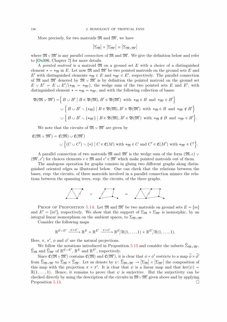
156 2. HOMOLOGY OF TROPICAL FANS
More precisely, for two matroids M and M1, we have
|ΣM|ˆ |ΣM1 | » |ΣM_M1 |where M_M1 is any parallel connection of M and M1. We give the definition below and referto [Oxl06, Chapter 7] for more details.
A pointed matroid is a matroid M on a ground set E with a choice of a distinguishedelement ˚ “ ˚M in E. Let now M and M1 be two pointed matroids on the ground sets E andE1 with distinguished elements ˚M P E and ˚M1 P E1, respectively. The parallel connectionof M and M1 denoted by M _M1 is by definition the pointed matroid on the ground setE _ E1 “ E \ E1
L
p˚M “ ˚M1q, the wedge sum of the two pointed sets E and E1, withdistinguished element ˚ “ ˚M “ ˚M1 , and with the following collection of bases:
BpM_M1q “
!
B YB1ˇ
ˇ B P BpMq, B1 P BpM1q with ˚M P B and ˚M1 P B1)
Y
!
B YB1 r t˚Muˇ
ˇ B P BpMq, B1 P BpM1q with ˚M P B and ˚M1 R B1)
Y
!
B YB1 r t˚M1uˇ
ˇ B P BpMq, B1 P BpM1q with ˚M R B and ˚M1 P B1)
.
We note that the circuits of M_M1 are given by
CpM_M1q “ CpMq Y CpM1q
Y
!
pC Y C 1qr t˚uˇ
ˇ C P CpMq with ˚M P C and C 1 P CpM 1q with ˚M1 P C 1)
.
A parallel connection of two matroids M and M1 is the wedge sum of the form pM, eq _pM1, e1q for choices elements e PM and e1 PM1 which make pointed matroids out of them.
The analogous operation for graphs consists in gluing two different graphs along distin-guished oriented edges as illustrated below. One can check that the relations between thebases, resp. the circuits, of three matroids involved in a parallel connection mimics the rela-tions between the spanning trees, resp. the circuits, of the three graphs.
> _ > “ >
Proof of Proposition 5.14. Let M and M1 be two matroids on ground sets E “ rmsand E1 “ rm1s, respectively. We show that the support of ΣM ˆ ΣM1 is isomorphic, by anintegral linear isomorphism on the ambient spaces, to ΣM_M1 .
Consider the following maps
RE_E1 φˆφ1ÝÝÝÝÑ RE ˆ RE
1 πˆπ1ÝÝÝÝÑ RE
L
Rp1, . . . , 1q ˆ RE1L
Rp1, . . . , 1q.
Here, π, π1, φ and φ1 are the natural projections.We follow the notations introduced in Proposition 5.13 and consider the subsets pΣM_M1 ,
pΣM and pΣM1 of RE_E1 , RE and RE1 , respectively.Since CpM_M1q contains CpMq and CpM1q, it is clear that φˆφ1 restricts to a map pφˆ pφ1
from pΣM_M1 to pΣM ˆ pΣM1 . Let us denote by ψ : pΣM_M1 Ñ |ΣM| ˆ |ΣM1 | the composition ofthis map with the projection π ˆ π1. It is clear that ψ is a linear map and that kerpψq “Rp1, . . . , 1q. Hence, it remains to prove that ψ is surjective. But the surjectivity can bechecked directly by using the description of the circuits in M_M1 given above and by applyingProposition 5.13.
6. CHOW RINGS OF TROPICAL FANS 157
5.10.3. Proof of the shellability of quasi-projective Bergman fans. We are now in positionto give the proof.
Proof of Theorem 5.11. Let M be a simple matroid with Bergman fan ΣM. We needto show that any quasi-projective fan Σ with |Σ| “ |ΣM| in Tropuqproj is shellable.
By Theorem 5.7, it will be enough to produce one such fan Σ and show it is shellable.First, we observe that since Λ P B0, the product Λn is shellable. This implies that complete
fans in Tropuqproj are all shellable.It follows that projective fans are shellable. We can therefore assume that M is not a free
matroid. We now proceed by induction on the size of M.There exists a proper element of M that is an element i in the ground set E of M
such that M r tiu has the same rank as M. It is well-known that in this case, the tropicalmodification of ΣMrtiu along the divisor ΣMtiu Ă ΣMrtiu is a quasi-projective fan of support|ΣM|, see [Sha13b]. By induction, both ΣMrtiu and ΣMtiu are shellable in Tropuqproj . Since ΣM
is quasi-projective, it is itself shellable in Tropuqproj and the result follows.
Example 11.11 shows that the property of being a generalized Bergman fan is not shellable,and at the same time provides an example of a shellable tropical fan which is not a generalizedBergman fan.
6. Chow rings of tropical fans
In this section, we study Chow rings of tropical fans. We define a natural cycle classmap from the Chow groups to the tropical homology groups of the compactification Σ, andmoreover, study the behavior of Chow groups under tropical modifications and blow-ups.From this description, we deduce the shellability of local irreducibility and div-faithfulnessstated in Theorem 5.9.
Unless otherwise explicitly stated, Σ will be a simplicial tropical fan; we will assumeunimodularity for the cycle class map and for the Poincaré duality.
6.1. The additive structure of the Chow ring of a simplicial fan. Consider arational simplicial fan Σ in NR. We do not assume in this subsection that Σ is tropical.
Recall that the Chow ring A‚pΣq is defined as the quotient
A‚pΣq “ ZrXρ | ρ P Σ1sL
pI1 ` I2q
where— I1 is the ideal generated by the products Xρ1 ¨ ¨ ¨Xρk , for k P N, such that ρ1, . . . , ρk
do not form a cone in Σ, and— I2 is the ideal generated by the elements of the form
ÿ
ρPΣ1
`peρqXρ
for ` PM where the primitive vector eρ is the generator of N X ρ.In order to distinguish to which fan we refer, sometimes we denote by NΣ and MΣ the latticesunderlying the definition of Σ, MΣ “ N‹Σ, and denote by IΣ,1 and IΣ,2 the ideals used abovein the definition of A‚pΣq.
In the following, if σ is a cone of Σ, we set
Xσ :“ź
ρPΣ1ρăσ
Xρ.
LetZkpΣq :“
à
σPΣk
ZXσ ãÑ ZrXρ | ρ P Σ1s

158 2. HOMOLOGY OF TROPICAL FANS
so that we get a well-defined map ZkpΣq Ñ AkpΣq.
Lemma 6.1 (Localization Lemma). The map ZkpΣq Ñ AkpΣq is surjective and its kernelis generated by elements of the form
ÿ
ρPΣ1τ„ρ
`peρqXρXτ ,
where τ P Σk´1 and ` is an element in M that is zero on τ .
Proof. This fact is a special case of a more general result stated in [FMSS95, Theorem1], which establishes an isomorphism between the Chow groups of a variety coming with anaction of a solvable linear algebraic group with the specific Chow groups defined by cycles andrelations which are all stable under the action of the group. A generalization of that theoremcan be found in [Tot14] and subsequent works [Fra06,Jos01,Pay06].
We will give an elementary combinatorial proof in Section 6.8.
Remark 6.2. In the case the fan Σ is unimodular, the above lemma provides an isomor-phism MWkpΣq » AkpΣq‹. Namely, we have a pairing
x¨ , ¨y : ZkpΣq ˆMWkpΣq Ñ Z, xXσ, pΣk, wqy Ñ wpσq
for any σ P Σk. By the balancing condition for the element pΣk, wq and Localization Lemma,the pairing vanishes on the kernel of the map ZkpΣq Ñ AkpΣq and we get the desired mapMWkpΣq Ñ AkpΣq‹. A direct application of Localization Lemma shows that this map isactually an isomorphism, see [AHK18, Proposition 5.6]. However, AkpΣq might have torsion(see Examples 11.8 and 11.10), in which case AkpΣq is not isomorphic to MWkpΣq
‹. We willdiscuss torsion-freeness of the Chow ring of tropical fans further in Section 7.
For k “ d and if Σ is tropical, this gives the degree map deg : AdpΣq Ñ Z which isobtained by evaluating at the canonical element rΣs P MWdpΣq. More precisely, the degreemap is obtained by sending the element Xσ of ZdpΣq to 1, for any σ P Σd. ˛
Proposition 6.3 (Künneth formula). Let Σ and Σ1 be two simplicial fans. Then
A‚pΣˆ Σ1q » A‚pΣq bA‚pΣ1q and MW‚pΣˆ Σ1q » MW‚pΣq bMW‚pΣ1q.
Moreover, the first isomorphism is a ring isomorphism.
In this section, every tensor product is over Z.
Proof. Notice that for two simplicial fans Σ and Σ1, we have MΣˆΣ1 »MΣˆMΣ1 . Thenone can check that
IΣ,1 b ZrX% | % P Σ11s ` ZrX% | % P Σ1s b IΣ1,1 “ IΣˆΣ1,1, and
IΣ,2 b ZrX% | % P Σ11s ` ZrX% | % P Σ1s b IΣ1,2 “ IΣˆΣ1,2.
The first part of the statement then follows because the tensor product is right-exact.For Minkowski weights, there is a perfect pairing ZkpΣqˆWkpΣq Ñ Z where WkpΣq » ZΣk
denotes the group of weights of dimension k on Σ. The orthogonal sum of the different degreesleads to a perfect pairing between Z‚pΣq and W‚pΣq. Denote by Zk0 pΣq the subgroup of ZkpΣqgenerated by elements of the form
ÿ
σ ąτ
`pnστ qXσ,
where τ P Σk´1 and ` is an element inMΣ that is zero on τ . From the definition of Minkowskiweights we infer that MWkpΣq is equal to Zk0 pΣqK. One can check that
Z‚0 pΣq b Z‚pΣ1q ` Z‚pΣq b Z‚0 pΣ
1q “ Z‚0 pΣˆ Σ1q.
Taking the orthogonal of each member in W‚pΣq bW‚pΣ1q » W‚pΣˆΣ1q, we get the desired
isomorphism MW‚pΣq bMW‚pΣ1q » MW‚pΣˆ Σ1q.
6. CHOW RINGS OF TROPICAL FANS 159
6.2. The cycle class map from the Chow ring to the tropical homology. Letnow Σ be a unimodular tropical fan. In this section, we prove the following proposition.
Proposition 6.4. For any integer k, there exists a well-defined map
ψ : AkpΣq Ñ Hd´k,d´kpΣq
defined by sending Xσ to the canonical element νΣσ8 associated to Σσ8.
For any σ, the support of νΣσ8 is the compactification of a tropical fan. Thus, it is a tropicalcycle of Σ. One can thus think of the image of A‚pΣq as a part of the homology generated bytropical Chow groups of Σ, endowed with the intersection product.
Recall from Section 2 that for simplicial Σ, and τ ă η, the face Cτη of Σ is denoted by ˝τη .
Proof. The fact that νΣσ8 is a cycle comes from the balancing condition. By LocalizationLemma 6.1, it remains to check that, for any τ P Σk´1 and any ` P M orthogonal to τ ,ř
ρ„τ `peρqνΣτ_ρ8is a boundary. This then shows the natural map Zk Ñ Hd´k,d´kpΣq passes
to the quotient and defines the map stated in the proposition.Since ` is orthogonal to τ , it induces a linear map on N τ which we also denote by `.
To each facet η ą τ , we associate the contraction of ντη by ` denoted ι`pντη q P Fd´kp˝
τηq: if
ρ1, . . . , ρd´k`1 are the rays generating ˝τη in N τ8,R such that ντη “ eρ1 ^ ¨ ¨ ¨ ^ eρd´k`1
, then
ι`pντη q “
d´k`1ÿ
i“1
p´1qi´1`peρiqeρ1 ^ ¨ ¨ ¨ ^xeρi ^ ¨ ¨ ¨ ^ eρd´k`1.
Set ι`pνΣτ8q :“ř
ηPΣdηąτ
ι`pντη q. A direct computation shows that
B`
´ι`pνΣτ8q˘
“ÿ
ρPΣ1ρ„τ
`peρqνΣτ_ρ8,
which proves the claim, and concludes the proof.
There is another natural cycle class map. It is given by the following composition.
φ : AkpΣq Ñ Ad´kpΣq‹ „ÝÑ MWd´kpΣq „ÝÑ Hd´k,d´kpΣq.
The first map sends α to`
β ÞÑ degpα ¨ βq˘
and the last map sends a Minkowski weightpΣďd´k, wq to
`
wpσqνσ˘
σPΣd´kP Cd´k,d´kpΣq. This last map is studied in detail in Section 7
where we prove that it is an isomorphism.We claim the above two cycle class maps coincide. Let us briefly justify this fact.Let σ be a face of dimension k in Σ. There is a natural ring morphism i˚ : A‚pΣq Ñ A‚pΣσ
8q
described for instance in [AHK18,AP20b]. This map is entirely determined by the propertythat, for a ray ρ ă σ, it maps Xρ to 0 if ρ is not comparable with σ, and to Xρσ if ρ „ σ whereρσ is the corresponding ray of Σσ
8. Using the arguments in Section 7.4, one can check that the
map AppΣq Ñ AppΣσ8q commutes with the restriction map i˚ : Hp,ppΣq Ñ Hp,ppΣ
σ8q. (This is
the reason the map between the Chow rings is denoted i˚.) With this in mind, we get thefollowing commutative diagram.
A0pΣσ8q Ad´kpΣσ
8q‹ MWd´kpΣ
σ8q Hd´k,d´kpΣ
σ8q
AkpΣq Ad´kpΣq‹ MWd´kpΣq Hd´k,d´kpΣq
„ „
i˚
„ „
The second and last vertical maps are the dual of the maps i˚ described above. The firstvertical map sends 1 to Xσ. In the first row, 1 is mapped to the Minkowski weight rΣσ
8s P
MWd´kpΣσ8q and then to νΣσ8 . Hence, the last vertical map sends νΣσ8 “ ψpXσq to φpXσq.
160 2. HOMOLOGY OF TROPICAL FANS
6.3. Chow ring and tropical modifications. In this section, we prove that the Chowring and the cycle class map behave well with respect to tropical modifications.
Let Σ be a simplicial tropical fan of dimension d and let ∆ “ divpfq be the principaldivisor associated to a conewise integral linear function on Σ. Assume that ∆ is effectivereduced, and let rΣ be the fan obtained by the open tropical modification of Σ with respect toΣ.
Proposition 6.5. Notations as above, we have a natural surjective ring morphism
A‚pΣq A‚prΣq.
Proof. Following the notations of Section 5.1, for any ray % P Σ1, we denotes by %o thecorresponding ray in rΣ1. We assume for now that ∆ is nontrivial and denote by ρ the onlyray of rΣ that does not come from Σ, that is, ρ “ 0 where 0 refers to the zero cone 0Σ of Σ.
Consider the map ψ : ZrX% | % P Σ1s Ñ ZrX% | % P rΣ1s defined by sending X% to X%0 . LetIΣ,1, IΣ,2, I
rΣ,1and I
rΣ,2be the ideals appearing in the definition of the Chow rings of Σ and
rΣ. We clearly have ψpIΣ,1q Ď IrΣ,1
. Moreover, if ` is a linear form on the ambient space of Σ
and if p denotes the projection associated to the tropical modification, since p˚` is zero on thespecial ray ρ, we get that
ψ´
ÿ
%PΣ1
`pe%qX%
¯
“ÿ
%PΣ1
p˚`pe%oqX%o “ÿ
%PrΣ1
p˚`pe%qX%.
This implies that ψpIΣ,2q Ď IrΣ,2
. All together, we thus get a well-defined map ψ from A‚pΣq
to A‚prΣq.To prove the surjectivity, by the definition of ψ, we just need to find a preimage for
Xρ P A‚prΣq. For this, take any integral linear form ` on ĂN that takes value one on theprimitive vector eρ of the special ray ρ. In the Chow ring A‚prΣq, using `, we can express Xρ
as a linear combination of the X% for % P rΣ1´ ρ. This linear combination is in the image of ψ,and the surjectivity of ψ follows. In the case ∆ “ divpfq is trivial, the proof is similar.
For the sake of completeness, we state the following proposition and refer to Sections 7and 10 for the definition of the relevant maps used in the statement.
Proposition 6.6. Let Σ be a unimodular tropical fan. The morphism A‚pΣq Ñ A‚prΣq
commutes via the Hodge isomorphism theorem with the map H‚,‚pΣq Ñ H‚,‚prΣq studied inSection 10. Hence, it also commutes with cycle class maps and we get the following diagram.
AkprΣq Hd´k,d´kprΣq
AkpΣq Hd´k,d´kpΣq
Proof. The proof is straightforward once the different maps have been defined.
6.4. Shellability of the principality. In this section we prove the following theorem.
Theorem 6.7 (Shellability of the principality for locally irreducible tropical fans). Theproperty for a tropical fan to be both principal and locally irreducible is shellable.
Local irreducibility assumption is needed here as shown by Example 11.7. To prove thetheorem, we need to check the different cases of Lemma 5.10. The fact that elements of B0
are locally irreducible and principal is trivial.
6. CHOW RINGS OF TROPICAL FANS 161
6.4.1. Closeness under products. Consider two locally irreducible principal tropical fansΣ,Σ1 of dimension d and d1, respectively. By Theorem 5.9 (2), local irreducibility is shellable.Hence Σ ˆ Σ1 is locally irreducible. Let us prove that Σ ˆ Σ1 is principal at 0. By Künnethformula for Minkowski weights, we get
MWd`d1´1pΣˆ Σ1q “ MWdpΣq bMWd1´1pΣ1q ‘ MWd´1pΣq bMWd1pΣ
1q.
Using the above decomposition, and arguing by symmetry, we only need to verify that divisorsof the form D ˆ C 1 for D P MWd´1pΣq and C 1 P MWd1pΣ
1q are principal.Since Σ1 is locally irreducible, we can suppose that C 1 is equal to the element rΣ1s in
MWd1pΣ1q given by Σ1. Since Σ is principal, we have D “ divpfq for a conewise integral linear
function f on Σ. Denote by π : Σ ˆ Σ1 Ñ Σ the natural projection. We have divpπ˚fq “divpfq ˆ rΣ1s “ D ˆ C 1, from which the result follows.
6.4.2. Closeness under tropical modifications. Let Σ be a locally irreducible principal trop-ical fan, and let rΣ be a tropical modification of Σ. Once again rΣ is locally irreducible. ByLemma 5.10, we can assume without loss of generality that Σ is unimodular.
By Proposition 6.5, the applications A1pΣq Ñ A1prΣq and Ad´1pΣq Ñ Ad´1prΣq are bothsurjective. It follows that the dual map Ad´1prΣq˚ Ñ Ad´1pΣq˚ is injective, and from theexplicit description of the map cl1 given in Proposition 4.8, we get the following commutativediagram
A1prΣq Ad´1prΣq˚ MWd´1prΣq
A1pΣq Ad´1pΣq˚ MWd´1pΣq
„
„
We now show that rΣ is principal at 0. By Theorem 4.9 this is equivalent to the surjectivityof the map A1prΣq Ñ MWd´1prΣq (saturation is not needed for this part of the theorem).Moreover, since Σ is principal, A1pΣq Ñ MWd´1pΣq is surjective. Using the above diagram,we obtain the surjectivity of A1prΣq Ñ MWd´1prΣq. This in turn implies that rΣ is principal at0, as desired.
6.4.3. Closeness under blow-ups and blow-downs. Once again, closeness of local irreducibil-ity has already been checked. Consider a tropical fan Σ of dimension d and let σ be a cone ofΣ and ρ a ray inside σ. Set Σ1 “ Σpρq. Assume that Σ and Σ1 are principal at any nontrivialface. We need to prove Σ is principal at 0Σ if and only if Σ1 is principal at 0Σ1 .
Assume first that Σ is principal. Let D be a divisor in Σ1. Let Dρ be the induced divisoron Σ1ρ. We infer the existence of a conewise integral linear function fρ on Σ1ρ such thatdivpfρq “ Dρ. Via the projection map NR Ñ Nρ
R, we view fρ as a conewise integral linearfunction on the fan Σ2 Ă Σ1 consisting of the cones τ comparable with ρ, and extend it toa conewise integral linear function on full Σ1. By an abuse of the notation, we denote thisfunction by fρ. The divisor D ´ divpfρq on Σ1 does not have any of the faces τ ą ρ withτ P Σ1d´1 in its support. This means it can be viewed as a divisor in Σ. Since Σ is principal,we can find a conewise integral linear function f on Σ with divpfq “ D ´ divpfρq. We inferthat D is the divisor of the conewise integral linear function f ` fρ on Σ1, which shows thatD is principal, as desired.
Assume now that Σ1 is principal. Let D be divisor in Σ. Viewing D as a divisor in Σ1, wefind a conewise integral linear function f on Σ1 such that divpfq “ D. Take a facet η ą σ inΣ. Denote by Σ1|η the fan of support η induced by Σ1. If f is not linear on η, then one canfind a face τ of dimension d´ 1 in Σ1|η rΣ such that ordf pτq ‰ 0. This is impossible since Dis supported on faces of Σ. Hence f is linear on all the facets of Σ containing σ. Therefore fis conewise integral linear on Σ which proves that D is principal in Σ.

162 2. HOMOLOGY OF TROPICAL FANS
6.4.4. Proof of Theorem 6.7. At this point, we have verified all the cases of Lemma 5.10and this concludes the proof of Theorem 6.7.
6.5. Div-faithfulness and stability of the Chow ring under tropical modifica-tions. The following theorem implies the invariance of the Chow ring under tropical modifi-cations under the assumption that the underlying tropical fan Σ is div-faithful.
We follow the preceding notations and denote by rΣ the tropical modification of Σ along∆ “ divpfq.
Theorem 6.8 (Stability of the Chow ring under tropical modifications). Notations asabove, let rΣ be the tropical modification of the tropical fan Σ along ∆. Assume furthermorethat Σ is div-faithful. Then we get an isomorphism
A‚prΣq » A‚pΣq
between the Chow rings. Moreover, this isomorphism is compatible with the Poincaré dualityfor Chow rings.
Proof. If ∆ is empty, since Σ is div-faithful, f is linear and rΣ » Σ from which the resultfollows. Hence, in what follows, we assume ∆ ‰ ∅, and we denote by ρ the special ray of rΣ.We already know there exists a surjective map ψ : A‚pΣq A‚prΣq given in Proposition 6.5.We now construct a surjective map φ : A‚prΣq A‚pΣq and show that φ ˝ ψ “ id, from whichwe get the result.
Consider first the surjective map φ : ZrX% | % P rΣ1s Ñ ZrX% | % P Σ1s, which appearedimplicitly in the proof of Proposition 6.5. This is defined on the level of generators as follows.Take the linear form ` on ĂN that takes value one on the primitive vector eρ of the special rayρ and that is zero on N ˆ t0u. For each ray of rΣ of the form %o for % P Σ1, set φpX%oq :“ X%,and define
φpXρq “ ´ÿ
%PΣ
`pe%oqX%.
Notice that from the equality e%o “ pe%, fpe%qq, we get `pe%oq “ fpe%q.We claim that φ passes to the quotient. In this case, it is clear that φ induces an inverse
to ψ, and the isomorphism between A‚pΣq and A‚prΣq stated in the theorem follows.Denote by IΣ,1, IΣ,2, I
rΣ,1and I
rΣ,2the ideals appearing in the definition of the Chow rings
of Σ and rΣ, as previously.We show that we have φpI
rΣ,2q Ď IΣ,2 and φpI
rΣ,1q Ď IΣ,1` IΣ,2, which allow to pass to the
quotient and get the above map on the level of Chow rings.
To show that φpIrΣ,2q Ď IΣ,2, consider an integral linear form l on ĂN . Let l1 :“ l ´ lpeρq`.
We have l1peρq “ 0 and so l1 gives an integral linear form on N » ĂNL
Zeρ. We have
φ´
ÿ
%PrΣ1
lpe%qX%
¯
“ lpeρqφpXρq `ÿ
%PΣ1
lpe%oqφpX%oq “ÿ
%PΣ1
l1pe%qX%.
This shows that φpIrΣ,2q Ď IΣ,2.
We now consider the image of IrΣ,1
. Consider a collection of distinct rays ρ1, . . . , ρk of rΣ,k P N, and suppose they are not comparable so that we have Xρ1 . . .Xρk P IrΣ,1. Two cases canhappen.
(1) Either ρ1, . . . , ρk are different from ρ.
(2) Or one of the rays, say ρ1, is equal to ρ.
6. CHOW RINGS OF TROPICAL FANS 163
Consider first the case (1). Then we have ρj “ p%jqo for j “ 1, . . . , k and rays %j in Σ.Moreover, the rays %1, . . . , %k do not form a cone in Σ and we get φpXρ1 . . .Xρkq “ X%1 . . .X%k P
IΣ,1, as desired.We now study the case (2). Let as in the previous case, ρj “ p%jqo for j “ 2, . . . , k and
rays %j in Σ. At this point, two cases can happen. Either, these rays do not form a cone in Σin which case we get
φpXρ1Xρ2 . . .Xρkq “ φpXρqX%2 . . .X%k P IΣ,1.
Or, %2, . . . , %k form a cone τ in Σ. Note that τ R ∆: otherwise τo and ρ would becomparable which would contradict our assumption. This implies that the divisor inducedby divpfq on Στ is trivial. In particular, taking an integral linear function l on NR whichhas restriction to τ equal to f , the difference f τ :“ f ´ l induces a conewise integral linearfunction π˚pf τ q on Στ , where π : N Ñ N τ is the projection, and divpπ˚pf
τ qq “ 0. Since Σ isdiv-faithful at τ , this implies that π˚pf τ q coincides with an integral linear function lτ on N τ
R.All together, this means f coincides with the restriction of the linear function lτ :“ l` π˚plτ q
on all faces σ of Σ with σ ą τ . Set rf “ f´ lτ . In particular, rf is zero on every ray comparablewith τ .
We now observe that
φpXρq “ ´ÿ
%PΣ1
fpe%qX% “ ´ÿ
%PΣ1
rfpe%qX% ´ÿ
%PΣ1
lτ pe%qX%,
and so, using the notation Xτ “ X%2 ¨ ¨ ¨X%k ,
φpXρ1Xρ2 . . .Xρkq “ φpXρqXτ “ ´ÿ
%PΣ1
rfpe%qX%Xτ ´
´
ÿ
%PΣ1
lτ pe%qX%
¯
Xτ .
Since rfpe%q is trivial if % is comparable with τ , the first sum is in IΣ,1. Since lτ P M , thesecond term is in IΣ,2.
In any case, we conclude that φpXρ1Xρ2 ¨ ¨ ¨Xρkq P IΣ,1 ` IΣ,2, as desired. This finishes theproof of the theorem.
6.6. Shellability of div-faithfulness. In this section we prove the following.
Theorem 6.9. The property for a tropical fan to be div-faithful is shellable.
Once again, we study the different cases of Lemma 5.10.6.6.1. Closeness under products. Consider two tropical fans Σ and Σ1 that are div-faithful.
It will be enough to show that ΣˆΣ1 is div-faithful at 0. We can assume without loss of gen-erality that Σ and Σ1 are unimodular (by Lemma 5.10) and saturated at 0 (see Remark 4.10).
We use the decomposition
MWd`d1´1pΣˆ Σ1q “ MWd´1pΣq bMWd1pΣ1q ‘ MWdpΣq bMWd1´1pΣ
1q.
We have injections Z “ A0pΣq ãÑ MWdpΣq and A0pΣ1q ãÑ MWd1pΣ1q. We have moreover a
decompositionA1pΣˆ Σ1q » A1pΣq bA0pΣ1q ‘ A0pΣq bA1pΣ1q.
The injectivity of the map A1pΣˆΣ1q Ñ MWd`d1´1pΣˆΣ1q now follows from the injectivityof the corresponding maps for Σ and Σ1, given by Theorem 4.9, which shows that Σ ˆ Σ1 isdiv-faithful at 0, as desired.
6.6.2. Closeness under tropical modifications. Let Σ be a tropical fan that is div-faithful.Let rΣ be a tropical modification of Σ and let us prove that rΣ is div-faithful at 0. Once againwe assume without loss of generality that Σ is unimodular and saturated at 0.
By Theorem 6.8, we get isomorphisms A1pΣq » A1prΣq and Ad´1pΣq » Ad´1prΣq. Theinjectivity of the map A1prΣq Ñ MWd´1prΣq then follows from the injectivity of A1pΣq Ñ
MWd´1pΣq. This implies that rΣ is div-faithful at 0.
164 2. HOMOLOGY OF TROPICAL FANS
6.6.3. Closeness under blow-ups and blow-downs. Consider a fan Σ, and let σ be a cone ofΣ and ρ a ray inside σ. Set Σ1 “ Σpρq. Assume that Σ and Σ1 are div-faithful at any nontrivialfaces. Let us prove that Σ is div-faithful at 0 if and only if Σ1 is div-faithful at 0.
First assume that Σ1 is div-faithful. Let f be a conewise integral linear function on Σsuch that divpfq “ 0. Then f is also a conewise linear function on Σ1, and since its divisor istrivial, it is linear. This proves the direction ð.
In the other direction, assume f is a conewise integral linear function on Σ1 whose divisor istrivial. Then the induced conewise integral linear function fρ on Σρ also verifies divpfρq “ 0.By assumption, Σρ is div-faithful. Thus, fρ is integral linear, and we deduce that f is integrallinear on each face η ą σ of Σ. Thus, f is conewise integral linear on Σ. We infer that f isglobally linear which concludes this part of the proof.
6.6.4. Proof of Theorem 6.9. We have studied all the cases of Lemma 5.10. This concludesthe proof of Theorem 6.9.
6.7. Shellability of the Poincaré duality for the Chow ring of div-faithful uni-modular fans. Let Σ be a unimodular tropical fan of dimension d. In this section, we denoteby PDChowpΣq the Poincaré duality for the Chow ring of Σ. This is the statement that the map
A‚pΣq ˆAd´‚pΣq Ñ Z, pα, βq Ñ degpα ¨ βq,
is a perfect pairing. Recall that the degree map deg : AdpΣq Ñ Z is given by rΣs P MWdpΣq »AdpΣq‹. In particular, it maps any element Xσ, σ a facet of Σ, to 1.
In case of Poincaré duality for the Chow ring, AdpΣq » Z has a natural generator ofdegree 1 that we denote ωΣ. We have ωΣ “ Xσ for any facet σ P Σd, this last element beingindependent of the choice of the facet.
Theorem 6.10. The set of div-faithful fans whose Chow rings verify the Poincaré dualityis stable by shellability in Tropunim .
As a corollary, we get the following theorem.
Theorem 6.11. The property PD‹Chow is shellable in Tropunim .
Proof. If Σ verifies PDChow, then it is div-faithful at 0. Indeed, in this case, we haveA1pΣσq » MWd´1pΣ
σq. Hence PD‹Chow implies div-faithfulness. The theorem now follows from
Theorem 6.10 via Lemma 5.10.
Remark 6.12. By Remark 7.6 in the next section, the Poincaré duality for Chow ring isimplied by the cohomological Poincaré duality for Σ. However, the two notions could be apriori different since the Poincaré duality for Chow groups does not imply the vanishing ofthe cohomology groups Hp,q of canonical compactifications for bidegrees p ą q. This is forinstance the case for Example 11.1 with rational coefficients. The authors are not aware ofany such example for integral coefficients.
Example 11.3 describes a fan Σ which verifies PDChow and such that Σ verifies the Poincaréduality, but Σ is not smooth and does not verify PD‹
Chow. This shows that PDChow is not a localproperty. ˛
The rest of this section is devoted to the proof of this theorem. This time, we cannotuse Lemma 5.10 since PDChow is not local as we discussed in the previous remark. We havealready proved that div-faithfulness is shellable. Hence in what follows we only focus on theshellability of PDChow.
6.7.1. Closeness under products. Let Σ and Σ1 be two unimodular tropical fans of dimen-sion d and d1, respectively. We know that we have a ring isomorphism
A‚pΣˆ Σ1q » A‚pΣq bA‚pΣ1q.
6. CHOW RINGS OF TROPICAL FANS 165
Moreover, the dual isomorphism sends degΣˆΣ1 to degΣbdegΣ1 . We infer that PDChowpΣˆΣ1qholds provided that PDChowpΣq and PDChowpΣ
1q both hold.6.7.2. Closeness under tropical modifications. Let Σ be a div-faithful tropical fan and let rΣ
be a tropical modification of Σ. Applying Theorem 6.8, we obtain the Chow stability of tropicalmodification, namely that the natural ring morphism A‚pΣq Ñ A‚prΣq is an isomorphism. Bycompatibility of the degree maps, we conclude that PDChowpΣq implies PDChowprΣq.
6.7.3. Closeness under blow-ups and blow-downs. Consider a unimodular fan Σ of dimen-sion d and let σ be a cone in Σ. Let Σ1 “ B`σpΣq be the unimodular star subdivisionof Σ obtained by star subdividing the cone σ and denote by ρ the new ray in Σ1, that is,ρ “ R`pe1`¨ ¨ ¨` ekq with e1, . . . , ek the primitive vectors of the rays of σ. Recall that for anyσ P Σ, we have a surjective map i˚0ăσ : A‚pΣq Ñ A‚pΣσq described in Section 6.2. We statethe following useful result.
Theorem 6.13 (Keel’s lemma). Let J be the kernel of the surjective map i˚0ăσ : A‚pΣq Ñ
A‚pΣσq and letP pT q :“
ź
%ăσ|%|“1
pX% ` T q.
We haveA‚pΣ1q » A‚pΣqrT s
L
pJT ` P pT qq.
The isomorphism is given by the map
χ : A‚pΣqrT sL
pJT ` P pT qq „ÝÑ A‚pΣ1q
which sends T to ´Xρ and which verifies
@ % P Σ1, χpX%q “
#
X% ` Xρ if % ă σ,X% otherwise.
In particular this gives a vector space decomposition of A‚pΣ1q as
(6.1) A‚pΣ1q » A‚pΣq ‘A‚´1pΣσqT ‘ ¨ ¨ ¨ ‘A‚´|σ|`1pΣσqT |σ|´1.
Proof. This follows from [Kee92, Theorem 1 in the appendix] for the map of toricvarieties PΣ1 Ñ PΣ. Here P pT q is the polynomial in A‚pPΣq whose restriction in A‚pPΣσq isthe Chern polynomial of the normal bundle for the inclusion of toric varieties PΣσ ãÑ PΣ.
For an elementary proof, one can follow the proof of an analogous statement in [AHK18].
Assume now PDChowpΣσq. We have to show the equivalence of PDChowpΣq and PDChowpΣ
1q.We follow the proof of an analogue result in [AHK18].
By Keel’s lemma, we get AdpΣq » AdpΣ1q, and under this isomorphism, the canonicalelement ωΣ gets identified with the canonical element ωΣ1 .
Let α be a lifting of the canonical element ωΣσ in Ad´|σ|pΣq, for the restriction mapi˚σ : A‚pΣq Ñ A‚pΣσq, so that we have ωΣσ “ i˚σpαq. We can obtain such a lifting by fixing atop dimensional cone in Σσ, i.e., a cone of the form ησ for η P Σd and η ą σ. Denoting by τthe face of η generated by all the rays of η not included in σ, we get
ωΣσ “ Xησ “ź
ζăησ
|ζ|“1
Xζ
and a lifting of ωΣσ in Ad´|σ|pΣq is given by
α “ Xτ “ź
%ăτ|%|“1
X%.

166 2. HOMOLOGY OF TROPICAL FANS
We now claim that the canonical element ωΣ1 can be identified with the element ´T |σ|αin A‚pΣ1q » A‚pΣqrT s
L
pJT ` P pT qq. Indeed, using the identity P pT q “ 0, we get
´T |σ| “
|σ|ÿ
j“1
SjT|σ|´j
with Sj referring to the j-th symmetric function in the variables X% P A1pΣ1q for % a ray in σ.
Therefore,
´T |σ|α “
|σ|ÿ
j“1
SjαT|σ|´j “
ź
%ăσ|%|“1
X% ¨ α`
|σ|´1ÿ
j“1
SjαT|σ|´j .
Since ωΣσ “ i˚σpαq lives in the top-degree part of A‚pΣσq, the products Sjα all belong to J.We infer that the terms of the sum are all vanishing for j “ 1, . . . , |σ|´ 1, and
´T |σ|α “ź
%ăσ|%|“1
X% ¨ α “ Xσ ¨ Xτ “ ωΣ “ ωΣ1 .
We thus obtain the following commutative diagram.
Ad´|σ|pΣσq AdpΣ1q AdpΣq
Z
¨p´T |σ|q„
„
deg
„
deg
„
deg„
Let us denote by ΨkpΣ1q the pairing AkpΣ1q ˆ Ad´kpΣ1q Ñ Z. We use similar notations for
Σ and Σσ. The above diagram allows us to describe the pairing induced by ΨkpΣ1q on the
different parts of the decomposition given by the Keel’s lemma.— Between AkpΣq and Ad´kpΣq we get the pairing ΨkpΣq.
— For any integer number i, between Ak´ipΣσqT i and Ad´|σ|´k`ipΣσqT |σ|´i we get thepairing ´Ψk´ipΣ
σq.
— For integers i ă j, between Ak´ipΣσqT i and Ad´|σ|´k`jpΣσqT |σ|´j the pairing istrivial since Ad´|σ|`j´ipΣσq is trivial.
— For any integer i ă |σ|, the pairing between AkpΣq and Ad´k´ipΣσqT i is trivial.Indeed, the product lives in Ad´ipΣσqT i which is trivial since d´ i ą d´ |σ|.
We do not need to compute the pairing between the other parts. The bilinear form ΨkpΣ1q
can be written in the form of a block matrix consisting of bilinear maps, as follows.
Ad´kpΣq Ad´k´|σ|`1pΣσqT |σ|´1 ¨ ¨ ¨ Ad´k´1pΣσqT
AkpΣq ΨkpΣq 0
Ak´1pΣσqT 0 ´Ψk´1pΣσq
...... ¨ ¨ ¨
Ak´|σ|`1pΣσqT |σ|´1 0 ´Ψk´|σ|`1pΣσq
0
*
¨
˚
˚
˚
˚
˚
˚
˚
˝
˛
‹
‹
‹
‹
‹
‹
‹
‚
The matrix is lower triangular. On the diagonal, all the bilinear maps apart from the first oneare non-degenerate, since we have PDChowpΣ
σq. Thus, ΨkpΣ1q is non-degenerate if and only if
ΨkpΣq is non-degenerate. This shows the properties PDChowpΣq and PDChowpΣ1q are equivalent
provided that PDChowpΣσq holds.
6. CHOW RINGS OF TROPICAL FANS 167
6.7.4. Proof of Theorem 6.10. At this point, we have verified all the needed properties forthe shellability of the property PDChow in Tropunim , and this concludes the proof of Theorem 6.10.
6.8. Elementary proof of Localization Lemma 6.1. In this section, we give a com-binatorial self-contained proof of Lemma 6.1. Although the proof is somehow technical, wehope it could be of independent interest for several reasons. First, the result is used byAdiprasito-Huh-Katz [AHK18] in order to prove the duality between the Chow groups andthe Minkowski weights of unimodular simplicial fans. While almost all the proofs in that pa-per are written to be accessible to a combinatorial audience, this one refers to a more generalresult taken from [FMSS95] on Chow rings of algebraic varieties admitting a solvable groupaction. The proof we give is elementary and arguably more transparent. Second, combinedwith a similar in spirit theorem proved in [Ami16] for the combinatorial Chow rings of prod-ucts of graphs, in connection with semi-stable reduction theorem, it suggests a more generalphenomenon concerning the combinatorial part of the Chow rings of algebraic varieties thatcertainly merits a further study.
6.8.1. Admissible expansions. Let Σ be any simplicial rational fan. It will be convenientin the course of the proof to introduce the following notation. For an element ` P M “ N‹,let
X` :“ÿ
ρPΣ1
`peρqXρ.
Let Bk be the group of homogeneous polynomials of degree k in ZrXρ | ρ P Σ1s. Recallthat I1 is the ideal generated by the products Xρ1 ¨ ¨ ¨Xρs , for s P N, such that ρ1, . . . , ρs do notbelong to a same cone in Σ, and that I2 is the ideal generated by the elements X` for ` PM .
Recall that Zk “À
σPΣkZXσ, which is thus a subgroup of Bk. We need to show that
Zk Ñ BkL
BkXpI1`I2q is surjective and to determine its kernel. We will prove the latter, theformer becomes clear in the course of the proof; one can also find a proof of the surjectivityin [AHK18].
Let Kk be the subgroup of Bk generated by elements of the formÿ
ρPΣ1ρ„τ
`peρqXρXτ ,
for τ P Σk´1 and ` an element in M which is orthogonal to τ . Consider an element a ofBk X
`
I1 ` I2
˘
which belongs to Zk. We want to prove that a P Kk.First, notice that we can write a as an element of I1 plus a sum of monomials of the form
X`X%2 ¨ ¨ ¨X%k for some ` PM “ N‹ and rays %2, . . . , %k. The first step is to prove the followingresult.
Claim 6.14. Each element a P Bk X pI1 ` I2q can be written as a sum consisting of anelement in I1 and a sum consisting of elements of the form X`1X`2 ¨ ¨ ¨X`sXτ for s P N, τ P Σk´s,and `1, . . . , `s PM .
An expansion of the form described in the claim for an element a P Bk X pI1 ` I2q will becalled admissible in the sequel.
Proof. To prove the above claim, it will be enough to prove the statement for an elementa of the form X`1 ¨ ¨ ¨X`sX
κs`1%s`1 ¨ ¨ ¨X
κr%r with κs`1 ě ¨ ¨ ¨ ě κr and %s`1, . . . , %r distinct and
comparable, i.e., they form the rays of some cone τ of dimension r ´ s. Actually, the cases “ 1 will already give the result, but considering arbitrary values for s allows to proceed byinduction on the lexicographical order of the k-tuples of non-negative integer numbers.
To a term of the form X`1 ¨ ¨ ¨X`sXκs`1%s`1 ¨ ¨ ¨X
κr%r with κs`1 ě ¨ ¨ ¨ ě κr we associate the k-tuple
of integers pκs`1, . . . , κr, 0, . . . , 0q. We now show that an element as above with κs`1 ą 1 can
168 2. HOMOLOGY OF TROPICAL FANS
be rewritten as the sum of an element of I1 and a sum of terms of the above form having ak-tuple with strictly smaller lexicographical order.
So suppose κs`1 ą 1. We take a linear form l which takes the value one on e%s`1 and 0 onthe other rays %s`2, . . . , %r. This is doable since τ is simplicial. Using
Xl “ X%s`1 `ÿ
ρPΣ1ρăτ
lpeρqXρ,
we get
X`1 ¨ ¨ ¨X`sXκs`1%s`1
¨ ¨ ¨Xκr%r “ X`1 ¨ ¨ ¨X`sXlXκs`1´1%s`1
Xκs`2%s`2
¨ ¨ ¨Xκr%r
´ÿ
ρPΣ1ρ ăτ
lpeρqX`1 ¨ ¨ ¨X`sXρXκs`1´1%s`1
Xκs`2%s`2
¨ ¨ ¨Xκr%r .
Each term in the right hand side is either in I1 or is of the form described above with a lowerlexicographic order. Proceeding by induction, we get the claim.
So each element a P Bk X pI1 ` I2q is the sum of an element of I1 plus a sum of terms ofthe form X`1 ¨ ¨ ¨X`sXτ with 1 ď s ă k and for a cone τ P Σk´s.
6.8.2. An auxilary filtration. Using admissible expansions, we now introduce an increasingfiltration F‚ on Zk X pI1 ` I2q as follows.
First, for each s ą 0, denote by Gs the group generated by the elements of Bk of the formX`1 ¨ ¨ ¨X`sXτ for some linear forms `1, . . . , `s PM and for some τ P Σk´s. Moreover, for s “ 0,define the subgroup G0 Ď G1 as the one generated by the elements of the form X`Xτ for someτ P Σk´1 and some linear form ` orthogonal to τ .
For any t ě 0, let Ht :“ G0 ` ¨ ¨ ¨ ` Gt and define Ft :“ Zk X pHt ` I1q. Note that Ht
is the subgroup generated by the elements which admit an admissible expansion having onlyterms X`1X`2 ¨ ¨ ¨X`sXτ with s ď t. In this way, we get a filtration
F0 Ď F1 Ď ¨ ¨ ¨ Ď Fk´1 Ď Fk Ď Zk X pI1 ` I2q.
We now prove that all these inclusions are equalities.
Claim 6.15. We have F0 “ F1 “ ¨ ¨ ¨ “ Fk´1 “ Fk “ Zk X pI1 ` I2q.
Proof. By Claim 6.14, we have Fk “ Zk X pI1 ` I2q, which proves the last equality. Weprove all the other equalities.
So fix s ą 0 and let a be an element of Fs “ Zk X pHs ` I1q admitting an admissibleexpansion consisting of an element of I1 plus a sum of terms each in G1, . . . ,Gs´1 or Gs. Weneed to show that a P Fs´1.
We can assume there is a term of a in this admissible expansion which lies in Gs, i.e.,of the form X`1 ¨ ¨ ¨X`sXτ , with τ P Σk´s. Otherwise, the statement a P Fs´1 holds trivially.Consider all the terms in the admissible expansion of a which are of the form X`11
¨ ¨ ¨X`1sXτ withthe same cone τ , but with possibly different linear forms `11, . . . , `1s. We will prove that thesum of those terms that we denote by aτ belongs to Gs´1` I1. Applying this to any τ P Σk´s,we obtain a P Fs´1 and the claim follows.
For each ray ρ of τ , choose a linear form `ρ,τ which takes value one on eρ and zero onother rays of τ . This is again possible since Σ is simplicial. Then `1, for instance, can bedecomposed as the sum
`1 “ l1 `ÿ
ρăτρPΣ1
`1peρq`ρ,τ
with l1 vanishing on τ .
7. HODGE ISOMORPHISM FOR UNIMODULAR FANS 169
The observation now is that the term Xl1X`2 ¨ ¨ ¨X`sXτ belongs to Gs´1 ` I1: this is bydefinition if s “ 1, and for s ą 1 is obtained by expanding the product
Xl1X`2 ¨ ¨ ¨X`sXτ “ÿ
ρPΣ1ρăτ
l1peρqXρX`2 ¨ ¨ ¨X`sXτ
and by observing that each term in the right hand side is either in I1 or is in Gs´1. (Notethat the sum is on rays ρ ă τ because l1 vanishes on τ .) Hence, in proving that aτ belongs toGs´1 ` I1, we can ignore this term.
Decomposing in the same way each X`i which appear in a term in the initial admissibleexpansion of aτ , we can rewrite aτ as a sum of terms which already belong to Hs´1 ` I1 plusa sum of terms of the form
(6.2)ź
ρăτρPΣ1
Xκρ`ρ,τ
Xτ , κρ P Zě0.
These all together give a new admissible expansion of a in which aτ (defined as before in thenew admissible expansion) is a sum of the terms of the form in (6.2). We will work from nowon with this admissible expansion of a.
Fix non-negative integers κρ for rays ρ of τ whose sum is s. Denote by“ś
ρPτ Xκρ`1ρ
‰
a thecoefficient of this monomial in a written as sum of monomials in Bk. Since a belongs to Zk,all the monomials of a are square-free. But the product
ś
ρPτ Xκρ`1ρ is not square-free since
s ą 0. Hence, the corresponding coefficient is zero.Consider now the monomial
ś
ρPτ Xκρ`1ρ and let us see in which terms in the admissible
expansion of a it can occur. Such a monomial cannot appear in a term of the admissibleexpansion of a which belongs to I1. It cannot neither be in a term of a of the form Xλ1 ¨ ¨ ¨Xλs1Xσ
with σ P Σk´s1 with s1 ă s nor with σ P Σk´s and σ ‰ τ .It follows that the monomial
ś
ρPτ Xκρ`1ρ can only appear in the terms of aτ . More precisely,
by the definition of `ρ,τ , it can only appear in each term of the formś
ρăτ Xκρ`ρ,τ
Xτ for the chosenκρ, and with coefficient one in each term. Hence, the sum of these terms have to cancel out.This proves that aτ is zero in the new admissible expansion, which shows that a P Fs´1 andthe claim follows.
6.8.3. End of the proof. We can now finish the proof of the lemma.
Proof of Lemma 6.1. Recall that Kk is the set generated by elements of the formÿ
ρPΣ1ρ„τ
`peρqXρXτ ,
where τ P Σk´1 and ` is orthogonal to τ . The following facts are then clear:
F0 Ď Kk ` I1, Kk Ď Zk, and I1 X Zk “ t0u.
Since F0 Ď Zk, we deduce that F0 Ď Kk. Applying Claim 6.15, we get Zk X pI1 ` I2q “ F0
which implies Zk X pI1 ` I2q Ď Kk. The inclusion Kk Ď Zk X pI1 ` I2q is obvious. So we getZk X pI1 ` I2q “ Kk which concludes the proof.
7. Hodge isomorphism for unimodular fans
In this section we prove the Hodge isomorphism theorem which relates the Chow group ofunimodular fans to their cohomology groups. As a byproduct of the methods we develop inthis section, we obtain an alternate characterization of tropical smoothness.
Unless otherwise stated, the fans which appear in this section are not assumed to betropical.
170 2. HOMOLOGY OF TROPICAL FANS
7.1. Statement of the main theorems. The main theorem we prove in this section isthe following.
Theorem 7.1 (Hodge isomorphism for unimodular fans). Let Σ be a saturated unimodularfan in NR. For any integer p, there is a well-defined isomorphism
Ψ: Hp,ppΣq„ÝÑ AppΣq
α ÞÝÑÿ
σPΣp
ασpνσqXσ
which induces a ring morphism H‚,‚pΣq Ñ A‚pΣq by mapping Hp,qpΣq to zero in bidegreesp ‰ q. Moreover, Hp,qpΣq is trivial in bidegrees p ă q and bidegrees pp, 0q for p ą 0.
As an immediate corollary, we get the following theorem.
Theorem 7.2 (Hodge isomorphism for smooth unimodular tropical fans). Let Σ be asaturated unimodular tropical fan in NR. Suppose in addition that Σ is tropically smooth. Thenwe get an isomorphism of rings A‚pΣq „ÝÑ H‚,‚pΣq. Moreover, A‚pΣq verifies the Poincaréduality. In particular, all these groups are torsion-free.
Proof. This follows from the discussion in Remark 7.6.
This saturation hypothesis is not always possible to obtain (see Example 11.10). Thefollowing dual version of the above theorem, which does not use the saturation hypothesis, issometimes more useful for applications.
Theorem 7.3. Let Σ be any unimodular fan in NR. Then the natural map MWppΣq Ñ
Hp,ppΣq is an isomorphism. Moreover, Hp,qpΣq is trivial in bidegrees p ă q and bidegrees pp, 0qfor p ą 0.
Proof. Once again, this follows from the discussion in Remark 7.6 (and from a directcomputation for the vanishing of Hp,0pΣq for p ą 0).
In the smooth case, we get the following corollary.
Theorem 7.4 (Hodge conjecture for tropical fans). If Σ is a smooth unimodular tropicalfan, Hp,qpΣq and Hp,qpΣq are trivial for p ‰ q. Moreover, to each element α in Hp,ppΣq onecan associate a tropical cycle whose class in Hd´p,d´ppΣq is the Poincaré dual of α.
Proof. The tropical cycle is obtained via the isomorphism
Hp,ppΣq » Hd´p,d´ppΣq » MWd´ppΣq.
The details can be found in Remark 7.6.
Before going through the proof of Theorem 7.1, we state some clarifying remarks.
Remark 7.5 (Non saturated case). The proof of Theorem 7.1 gives as well results in thecase Σ is not saturated. In this situation, we still have a surjective ring morphism A‚pΣq ÑH‚,‚pΣq, but this is never injective. Indeed, the kernel is a nontrivial torsion group. Inparticular, we get an isomorphism for rational coefficients, as well as a dual isomorphism forintegral coefficients: A‚pΣq‹ » H‚,‚pΣq‹. In any case, the last part of the theorem concerningthe vanishing are still valid. ˛
Remark 7.6 (Torsion-freeness and duality for Chow rings). Let Σ be a unimodular fan.By the universal coefficient theorem applied to the tropical chain and cochain complexes ofΣ, for each pair of non-negative integers p, q, we get the following exact sequences
0 Ñ Ext`
Hp,q`1pΣq,Z˘
Ñ Hp,qpΣq Ñ Hp,qpΣq‹ Ñ 0, and(7.1)
0 Ñ Ext`
Hp,q´1pΣq,Z˘
Ñ Hp,qpΣq Ñ Hp,qpΣq‹ Ñ 0.(7.2)

7. HODGE ISOMORPHISM FOR UNIMODULAR FANS 171
From the first exact sequence, using the vanishing result stated in Theorem 7.1, we obtain anisomorphism Hp,qpΣq » Hp,qpΣq‹ for p ď q. This shows the vanishing of Hp,qpΣq for p ă q
and an isomorphism Hp,ppΣq » Hp,ppΣq‹. This in turn implies in particular that Hp,ppΣq istorsion-free.
In the case Σ is saturated, the dual of the map fromHp,ppΣq to AppΣq depicted in the state-ment of Theorem 7.1 is the natural morphism from the group of Minkowski weights MWppΣq
to the tropical homology group Hp,ppΣq. This map is obtained by sending a Minkowski weightto its closure in Σ, which is a tropical cycle of dimension p, and then taking the correspondinghomology class in Hp,ppΣq, as described in Section 6.2; for the cycle class map, see for exam-ple [MZ14,Sha11,JRS18,GS19a]. Theorem 7.1 implies that this map is an isomorphism.By Remark 7.5, this isomorphism still exists in the non saturated case.
In the case Σ is a smooth saturated unimodular tropical fan, we get an isomorphismHp,qpΣq » H
BM
d´p,d´qpΣq “ Hd´p,d´qpΣq, p, q P Zě0, which implies as well the vanishing ofHp,qpΣq for p ą q. Applying the exact sequence (7.2), we infer the isomorphism Hp,qpΣq »
Hp,qpΣq‹. This in particular implies that the cohomology groups Hp,ppΣq and so AppΣq are all
torsion-free, we have AppΣq » MWppΣq‹, and the Chow ring verifies the Poincaré duality. ˛
Remark 7.7. The smoothness assumption in the statement of Theorem 7.2 is needed, andthe result is not true, in general, for any saturated unimodular tropical fan. Example 11.1 isa saturated unimodular tropical fan Σ with H2,1pΣq of rank two. ˛
In order to prove Theorem 7.1, we establish an alternative way of computing the coho-mology of Σ by using its decomposition into hypercubes. The proof of the first half thenfollows quite directly from this description by using the Localization Lemma 6.1 proved in theprevious section. To show the second half, concerning the products, we provide an explicitdescription of the inverse of the map Ψ from AppΣq to Hp,ppΣq, a result which might be ofindependent interest.
For non-negative integers p, q, we define
Cp,q˝pΣq :“
à
|σ|“q
Fp´qp8σq.
We get a cochain complex for each integer p
Cp,‚˝
: . . . ÝÑ Cp,q´2˝
pΣqdq´2˝
ÝÝÝÝÑ Cp,q´1˝
pΣqdq´1˝
ÝÝÝÝÑ Cp,q˝pΣq ÝÑ ¨ ¨ ¨
where the differential is given by the sum of the following maps for τ ă σ
Fkp8τ q ÝÑ Fk´1p8σq,α ÞÝÑ π˚pιeτσpαqq.
Here π : N τ Ñ Nσ is the natural projection.
Theorem 7.8. The cohomology of`
Cp,‚˝, d˝
˘
is Hp,‚pΣq.
The theorem is obtained by exploiting the decomposition of Σ into hypercubes. Thisexplains the notation for this new complex. Note that one can also use the dual complexwhich compute the homology of Σ.
The proof of Theorem 7.8 uses an interesting double complex. A deeper exploitation of thisdouble complex leads to the proof of the following alternate characterization of smoothness.
Theorem 7.9 (Alternate characterization of tropical smoothness). A unimodular tropicalfan Σ is smooth if and only if, for any face σ P Σ, Σ
σ verifies the Poincaré duality.
Note that, in particular, this theorem gives a new proof of Theorem 3.16 which states thatif Σ is smooth, then Σ verifies the Poincaré duality.
The rest of this section is devoted to the proof of the above results.
172 2. HOMOLOGY OF TROPICAL FANS
7.2. Proof of Theorem 7.8. We start with the proof of Theorem 7.8. We fix a non-negative integer p.
7.2.1. The fine double complex. The idea behind the proof is quite natural. The originaltropical cochain complex Cp,‚pΣq has a finer decomposition. Namely, for a face ˝τσ “ C
τσ of
Σ, instead of using a grading just following its dimension |σ| ´ |τ |, which is what is done inCp,‚pΣq, one can remember both |σ| and |τ |. In this way, the tropical cochain complex Cp,‚pΣqcan be unfolded and identified with the total complex of the following double complex:
pEa,b :“
à
τăσ|σ|“a|τ |“´b
Fpp˝τσq
where the differentials are given by the ones between the coefficient groups Fp of faces of Σwhich define the differentials of Cp,‚pΣq. So we have Cp,‚pΣq “ Tot‚ppE
‚,‚q.The cohomology of Cp,‚pΣq can be calculated by using the spectral sequence associated to
the filtration given by the columns of pE‚,‚. (We will use below the other filtration, the onegiven by the rows, in the proof the other stated results.)
We denote by ÓpE‚,‚0 the 0-th page of this spectral sequence which has abutment
ÓpE‚,‚0 ùñ Hp,‚pΣq.
7.2.2. Computation of the first page. The proof of Theorem 7.8 is given by the followingclaim.
Claim 7.10. On the first page of the spectral sequence, we have
ÓpE
a,b1 “
#
Cp,a˝pΣq for b “ 0,
0 otherwise.
Moreover, the differential on the first page for b “ 0 coincides with the differential d‚˝of
Cp,‚˝pΣq.
We prove the claim. Fix an integer a. Then the a-th column in page zero of the spectralsequence is
ÓpE
a,‚0 : . . . ÝÑ
à
τăσ|σ|“a
|τ |“´b`1
Fpp˝τσq ÝÑà
τăσ|σ|“a|τ |“´b
Fpp˝τσq ÝÑà
τăσ|σ|“a
|τ |“´b´1
Fpp˝τσq ÝÑ ¨ ¨ ¨
This complex can be decomposed as a direct sum running on the faces σ P Σa of the complexes
. . . ÝÑà
τăσ|τ |“´b`1
Fpp˝τσq ÝÑà
τăσ|τ |“´b
Fpp˝τσq ÝÑà
τăσ|τ |“´b´1
Fpp˝τσq ÝÑ ¨ ¨ ¨
Denote this last complex by ÓpEσ,‚0 , σ P Σ, and let ÓpE
σ,‚1 be its cohomology. We thus have
(7.3) ÓpE
a,‚0 “
à
σPΣa
ÓpE
σ,‚0 , Ó
pEa,‚1 “
à
σPΣa
ÓpE
σ,‚1 .
These latter cohomology groups are given by the following lemma.
Lemma 7.11 (Hypercube vanishing lemma). For any face σ of Σ, the cohomology ÓpEσ,‚1
of the complex ÓpEσ,‚0 is given by
ÓpE
σ,b1 »
#
Fp´|σ|p8σq if b “ 0,0 otherwise.
This isomorphism is moreover induced by the natural mapÓpE
σ,00 » Fppσq ÝÑ Fp´|σ|p8σq,
α ÞÝÑ π˚pινσpαqq
7. HODGE ISOMORPHISM FOR UNIMODULAR FANS 173
with π referring to the projection N Ñ Nσ, extended to the exterior algebra and restricted tothe corresponding subspaces Fp.
Let us assume the lemma for the moment and finish the proof of the claim.
Proof of Claim 7.10. By the above lemma, and in view of the decomposition givenin 7.3, the first page of the spectral sequence is concentrated in the 0-th row and is given by
ÓpE
a,01 “
à
|σ|“a
Fp´ap8σq,
which is exactly Cp,a˝pΣq. It thus remains to check that the differentials coincide. Let τ ă σ
and denote by dτăσ : Fp´|τ |p8τ q Ñ Fp´|σ|p8σq the corresponding part of the differential inÓpE‚,0. By Lemma 7.11, we have the following commutative diagram.
Fppτq Fppσq
Fp´|τ |p8τ q Fp´|σ|p8σq
signpτ,σqi˚
πτ˚˝ ιντπσ˚˝ ινσ
dτăσ
We infer that the bottom map should be given by π˚ ˝ ιeτσ with π : N τ Ñ Nσ, i.e., by thedifferential of Cp,‚
˝pΣq. This concludes the proof of the claim.
7.2.3. Proof of the hypercube vanishing lemma. It remains to prove Lemma 7.11. For facesτ ă σ, we have isomorphisms
Fpp˝τσq »à
p1`p2“p
Źp1N τ ‹σ b Fp2p8σq.
These isomorphisms are not canonical, nevertheless, we can choose them in a compatible way.In fact, the terms appearing in the above decomposition of FpΣp˝
τσq correspond to the graded
pieces associated to a natural filtration on FpΣp˝τσq, that we name the toric weight filtration,
which plays an important role in the results we prove in [AP20b]. In order to simplify thepresentation here, we do not detail this filtration here and refer to the relevant part of [AP20b]for more information.
We can decompose ÓpEσ,‚0 as a direct sum of complexes
ÓpE
σ,‚0 »
à
p1`p2“p
´
¨ ¨ ¨ ÝÑà
τąσ|τ |“´b`1
Źp1N τ ‹σ ÝÑ
à
τąσ|τ |“´b
Źp1N τ ‹σ ÝÑ ¨ ¨ ¨
¯
b Fp2p8σq.
Since σ is unimodular, the cochain complex appearing in the above summand is isomorphicto Cp1,‚`|σ|
c pT|σ|q for the natural subdivision tT,8u|σ|:ÓpE
σ,‚0 »
à
p1`p2“p
Cp1,‚`|σ|c pT|σ|q b Fp2p8σq.
Hence, the cohomology is given byÓpE
σ,‚1 »
à
p1`p2“p
Hp1,‚`|σ|c pT|σ|q b Fp2p8σq.
The cohomology of H‚,‚c pTkq is easy to compute: this is only nontrivial in bidegree pk, kqwhere it is isomorphic to Z. It follows that ÓpE
σ,b1 is trivial unless b “ 0 in which case it becomes
equal to Fp´|σ|p8σq. The last part of the lemma follows from a cautious study of the differentisomorphisms, that we omit here. This concludes the proof of Lemma 7.11.
7.2.4. Proof of Theorem 7.8. This is a direct consequence of Claim 7.10, which shows thatthe spectral sequence degenerates at page two, and, moreover, we have
Hp,qpΣq » pEq,02 “ Hq
`
Cp,‚˝pΣq
˘
.
174 2. HOMOLOGY OF TROPICAL FANS
Proof of Theorem 7.9. We have so far used only one of the two spectral sequencescoming from the double complex. The spectral sequence ÑpE‚,‚ given by the filtration by rowswill allow to prove Theorem 7.9. We explain this now before going through the proof of thehodge isomorphism theorem.
We first prove the forward direction. Assume that Σ is a smooth unimodular tropical fan.Recall that the b-th row of the double complex is
ÑpE‚,b0 : . . . ÝÑ
à
τăσ|σ|“a´1|τ |“´b
Fpp˝τσq ÝÑà
τăσ|σ|“a|τ |“´b
Fpp˝τσq ÝÑà
τăσ|σ|“a`1|τ |“´b
Fpp˝τσq ÝÑ ¨ ¨ ¨
We recognize the cochain complex for the cohomology with compact support of the star fansof codimension ´b:
ÑpE‚,b0 “
à
|τ |“´b
Cp,‚`bc pΣτ q.
All the star fans are smooth by assumption, and so Hp,qc pΣτ q is trivial unless q “ d ´ p´bq,
and for this q, we have Hp,d`bc pΣτ q » Fd´p`bp8τ q. Hence, the first page is given by
ÑpE
a,b1 “
#
À
|τ |“´bFd´p`bp8τ q if a “ d,0 otherwise.
Stated differently, ÑpEa,b is trivial unless a “ d andÑpE
d,‚ “ C˝
d´p,´‚pΣq,
where C˝
d´p,‚pΣq denotes the dual complex of Cd´p,‚˝
pΣq. Theorem 7.8 combined with the uni-versal coefficient theorem imply that the homology of C˝
d´p,‚pΣq computes Hd´p,‚pΣq. Hence,ÑpE‚,‚ degenerates at page two, and we have
ÑpE‚,‚ ùñ Hd´p,d´‚pΣq.
On the other hand, by the definition of the double complex, we know thatÑpE‚,‚ ùñ Hp,‚pΣq.
Therefore, we get the isomorphism of the Poincaré duality Hp,qpΣq » Hd´p,d´qpΣq; moreprecisely, we infer that
Hp,ppΣq » ÓpE
p,08» Ñ
pEd,p´d8
» Hd´p,d´ppΣq,
and every other terms of ÓpE‚,‚8 and ÑpE‚,‚8
are trivial. This concludes the forward direction.
Remark 7.12. In the same way that ÓpEp,08is naturally isomorphic to AppΣq (in the satu-
rated case), for any unimodular fan Σ we have the following isomorphisms
Hd´p,d´ppΣq » C˝
p,d´ppΣq “ ker´
à
|σ|“d´p
F0p8σq Ñà
|τ |“d´p´1
F1p8τ q
¯
» MWd´ppΣq.
Moreover, if Σ is smooth as above, the study of the spectral sequences gives us a newnatural cycle class map Hp,ppΣq „ÝÑ MWd´ppΣq. To a cocycle a in Cp,ppΣq, one can associatethe Minkowski weight pΣďd´p, wq where wpσq “ xa, νΣσ8y for any σ P Σd´p. ˛
We now prove the other direction. Assume that Σσ verifies the Poincaré duality for any
face σ of Σ. By induction, we can assume that Σσ is smooth for any proper face σ of Σ.We have a natural inclusion of complexes Cp,‚c pΣq » pE
‚,0 ãÑ pE‚,‚. Denote by pE
‚,‚ă0 thecokernel. We get a short exact sequence of complexes:
(7.4) 0 ÝÑ Cp,‚c pΣq ÝÑ Tot‚ppE‚,‚q ÝÑ Tot‚ppE
‚,‚ă0q ÝÑ 0.

7. HODGE ISOMORPHISM FOR UNIMODULAR FANS 175
We already know the cohomology of the first two terms. For the last one, we can compute thefirst page as before (since the proper star fans are smooth) and we get pE
d,‚ă01 “ C
˝
d´p,´‚ą0pΣqwhere
C˝
d´p,‚ą0pΣq :“ coker´
Fd´pp0q ãÑ C˝
d´p,‚pΣq¯
,
and every other terms are trivial. Assume for now that p ă d ´ 1. The case p “ d is trivialand the case p “ d´ 1 is studied later below. Then we get
HkpC˝
d´p,‚ą0pΣqq “
$
’
&
’
%
Hd´p,d´ppΣq if k “ d´ p,Fd´pp0q if k “ 1,0 otherwise.
We are now ready to study the long exact sequence associated to (7.4):
¨ ¨ ¨ ÝÑ Hp,qc pΣq ÝÑ Hp,qpΣq ÝÑ HqpC
˝
d´p,pd´‚qą0pΣqq ÝÑ Hp,q`1c pΣq ÝÑ ¨ ¨ ¨
The two middle terms are trivial unless q “ p or q “ d´ 1. In the case q “ p, we get a mapHp,ppΣq Ñ Hd´p,d´ppΣq. By assumption, this is an isomorphism, and we can just replaceboth terms by 0 in the long exact sequence. For q “ d´ 1, Hp,d´1pΣq “ Hp,dpΣq “ 0 and weget
0 ÝÑ Fd´pp0q ÝÑ Hp,dc pΣq ÝÑ 0.
All the other terms of Hp,‚c pΣq vanish. Using the universal coefficient theorem, we get
HBM
p,dpΣq » Hp,dc pΣq‹ » F d´ppΣq, and H
BM
p,q pΣq “ 0 for q ‰ d. This is exactly the Poincaréduality for (the homology with coefficients in) Fp.
It remains to treat the case p “ d´ 1. In this case, C˝
1,‚ą0pΣq contains only one nontrivialterm: C
˝
1,1ą0pΣq “À
%PΣ1F0p8%q. Its cohomology is identical. In the above long exact
sequence, the only interesting part is the first row of the following diagram.
0 Hd´1,d´1c pΣq Hd´1,d´1pΣq
À
%PΣ1F0p8%q Hd´1,d
c pΣq 0
0 MW1pΣq W1pΣq F1pΣq 0
„ „
Let us describe the second row and the vertical maps. We know thatHd´1,d´1pΣq » H1,1pΣq »MW1pΣq. Here, W1pΣq :“ ZΣ1 »
À
%PΣ1F0p8%q denotes the group of one dimensional weights
of Σ. Note also that we have a natural map Hd´1,dc pΣq Ñ F1pΣq: it is induced by the dual
of the map F1pΣq Ñ HBM
d´1,dpΣq. By the definition of the Minkowski weights, the second rowis a short exact sequence. The five lemma implies that the first and the last vertical mapsare isomorphisms. Therefore, Hd´1,q
c pΣq is trivial for q ‰ d, and Hd´1,qc pΣq » F1pΣq. Using
the universal coefficient theorem as above, and dualizing, we get the Poincaré duality forH
BM
d´1,‚pΣq. All together we obtain the Poincaré duality for HBM
‚,‚pΣq.
7.3. Proof of Theorem 7.1. We conclude with the proof of Theorem 7.1, given in thissection and the next one.
First, we note that by Theorem 7.8, we have Hp,qpΣq » HqpCp,‚˝pΣqq. Notice as well that
for p ă q, Cp,q˝pΣq is trivial. Hence Hp,qpΣq is trivial for p ă q.
For q “ 0 and p ą 0, we get
Hp,0pΣq » ker`
Fpp0q Ñà
%PΣ1
Fp´1p8%q˘
.
Let α P Fpp0q be an element of the kernel. Then ιe%pαq “ 0 for any % P Σ1. Let V Ď NRbe the subspace spanned by Σ. Then α P
ŹpV ‹. Since the vectors e%, % P Σ1, span V , any
176 2. HOMOLOGY OF TROPICAL FANS
element ofŹpV ‹ whose contraction by each e% is trivial must be trivial. Hence, we obtain
α “ 0 and Hp,0pΣq “ 0.For p “ q, we get
Hp,ppΣq » coker`
Cp,p´1˝
pΣq Ñ Cp,p˝pΣq
˘
» coker´
à
|τ |“p´1
F1p8τ q Ñà
|σ|“p
F0p8σq
¯
.
We have a natural isomorphismÀ
|σ|“pF0p8σq » ZppΣq. Moreover, since Σ is saturated at
any face τ P Σp´1,À
|τ |“p´1 F1p8τ q is naturally isomorphic to the kernel of ZppΣq Ñ AppΣq as
described in the Localization Lemma 6.1. Hence Hp,ppΣq » AppΣq. Moreover, by Lemma 7.11,the isomorphism is induced by the map
Cp,ppΣq Cp,p˝pΣq ZppΣq
αř
σPΣp αpνσqXσ.
It remains to prove that the above isomorphism respects the products. This can be doneby an explicit calculation of the inverse of the map Ψ in the statement of 7.1, given in thenext section, which shows that the cup-product in cohomology corresponds to product inChow ring. The theorem thus follows.
7.4. Explicit description of the inverse Ψ´1 : AppΣq Ñ Hp,ppΣq. In this section, weprovide an explicit description of the inverse of Ψ.
Before going through the description, let us introduce some new notations which will helpin working with the cohomology of Σ. In the following, if a is a cochain in Cp,qpΣq withq “ |σ|´ |τ |, we denote by aτσ P Fpp˝τσq the part of a which lives on the face ˝τσ. If τ “ 0, wejust write aσ. Moreover, if δ is any face of dimension q in Σ and α P Fppδq, then we denote bypδ, αq the cochain in Cp,qpΣq whose restriction to δ is α and which vanishes everywhere else.
7.4.1. The inverse in cohomology degree one. We consider first the part A1pΣq. Let ρ P Σ1.We give an element of H1,1pΣq whose image by Ψ coincides with Xρ. For this, we first define anelement a P C1,1pΣq as follows. For any cone σ „ ρ in Σ, we choose an element ασ P F1p˝σσ_ρq
which takes value one on the vector eσσ_ρ. We then set
a :“ÿ
σ„ρ
p˝σσ_ρ, ασq.
Note that the only part of a which has sedentarity 0 is p˝ρ, αρq, and we have Ψpaq “α0peρqXρ “ Xρ. So the statement would have followed if a were a cocycle. The idea now is tofind an element b in C1,1pΣq supported only on faces of non-zero sedentarity such that a ´ bis a cocycle: in that case, since Ψpbq “ 0, we still get Ψpa´ bq “ Xρ and the inverse image ofXρ will be represented by the class of a´ b.
Recall that eσσ_ρ is the projection of eρ at infinity into Nσ8. We now describe ra :“ da.
Consider a pair of faces τ ă η in Σ with |η|´ |τ | “ 2. Then, we have raτη “ 0 if either ρ ă η orρ ă τ . In the remaining cases, there must exist a ray ρ1 such that η “ τ _ ρ_ ρ1, and in thiscase, we get
raτη “ ˘paττ_ρ ´ π
˚paτ_ρ1
τ_ρ1_ρqq “ ˘pατ ´ π˚pατ_ρ1qq,
where π is the projection N τ Ñ N τ_ρ1 . In particular, we notice that raτη is zero on theprojection of eρ.
From the above discussion, we obtain a well-defined pushforward πρ˚praτηq P F1p˝τ_ρη q where
πρ : N τ8Ñ N τ_ρ
8is the natural projection.
Setb :“
ÿ
τ,η
signp˝τ_ρη , ˝τηq´
˝τ_ρη , πρ˚praτηq
¯

7. HODGE ISOMORPHISM FOR UNIMODULAR FANS 177
where the sum is restricted to pairs τ ă η for which the term is well-defined, that is thosewith ρ ă τ , ρ ă η and |η|´ |τ | “ 2. The element b has been defined in order to get db “ daon every face which is not in Σ
ρ8. In particular, the coboundary c :“ dpa ´ bq of a ´ b has
support in Σρ8. Since dc “ 0, the positive-sedentarity-vanishing lemma 7.13 below implies that
c “ 0. This shows that a ´ b is a cocycle. Since b has support only on the faces of non-zerosedentarity, we get in addition Ψpa´ bq “ Xρ, as required.
Lemma 7.13 (Positive-sedentarity-vanishing lemma). Let Σ be a unimodular fan. Let ζ bea non-zero face of Σ and let c P Cp,qpΣq be a cochain supported in Σζ
8. Assume that dc “ 0.
Then we have c “ 0.
Proof. Actually this is a consequence of the vanishing of ÓpEa,b8 for b ă 0. Let us give amore elementary proof here. Since c is supported in Σζ
8, we need to show the vanishing of cτσ
for τ, σ in Σ with |σ|´ |τ | “ q and ζ ă τ .Let ρ be a ray of ζ and set η ă τ so that we get τ “ ρ _ η. Consider the face δ “ ˝
ησ
of Σ and note that δ is (a hypercube) of dimension q ` 1. The only face of dimension q in δwhich lies in Σ
ζ8is ˝τσ. Since c has support in Σ
ζ8, it follows that the components of c on faces
of δ different from ˝τσ are all zero. Denoting by π the projection Nη8Ñ N τ
8, which induces a
surjection π˚ : Fpp˝ησq Ñ Fpp˝
τσq and in injection π˚ : Fpp˝τσq Ñ Fpp˝ησq, we thus get
π˚pcτσq “ ˘pdcqησ “ 0.
This implies that cτσ “ 0, and the lemma follows.
7.4.2. Cup-product in cubical complexes. To extend the description of the inverse of Ψ tohigher degrees, we need to recall the formula for the cup product in cubical complexes. Leta P Cp,qpΣq and b P Cp1,q1pΣq. Then for any pair of faces τ ă η with |η|´ |τ | “ q ` q1,
pa! bqτη “ÿ
τăσăη|σ|´|τ |“q
ωτη pντσ ^ π
˚pνση qq ¨ aτσ ^ π
˚pbση q
where, for each τ ă σ, π : N τ Ñ Nσ is the projection. As usual, this cup product induces acup product on cohomology ! : Hp,qpΣq ˆHp1,q1pΣq Ñ Hp`p1,q`q1pΣq.
7.4.3. The inverse in higher cohomological degrees. Let σ be a cone of dimension p in Σ.By Localization Lemma 6.1, it suffices to find a preimage of Xσ. Let ρ1, . . . , ρp be the raysof σ. For i P t1, . . . , pu, we denote by ia the preimage of Xρi as defined in Section 7.4.1. Inparticular, we note that ia is supported by faces of the form ˝τσ with ρi ă σ. We claim thatthe element
a :“ 1a! 2a! ¨ ¨ ¨! pa
is a preimage of Xσ. We compute a as follows. Consider a face σ1 P Σp and denote byρ11, . . . , ρ
1p P Σ1 the rays of σ1. In the following, for a permutation s P Sp of rps and k P rps,
we setσ1ps, kq :“ ρ1sp1q _ ¨ ¨ ¨ _ ρ
1spkq,
the face of σ1 with rays ρ1sp1q, . . . , ρ1spkq.
Expanding the cup product using the formula stated in the previous section, we find
aσ1 “ÿ
sPSp
ωσ1pνρ1sp1q^ ¨ ¨ ¨ ^ νρ1
sppqq ¨ 1a
σ1ps,0qσ1ps,1q ^ 2a
σ1ps,1qσ1ps,2q ^ ¨ ¨ ¨ ^ pa
σ1ps,p´1qσ1ps,pq ,
where for the ease of reading, we omit to precise the pullback by different projections. Eachterm in the above sum is nontrivial only if ρ1 ă σ1ps, 1q, ρ2 ă σ1ps, 2q, . . . , and ρp ă σ1ps, pq,i.e., if and only if σ1 “ σ and the permutation s is identity.
Since πσ1pid,jqpeρiq “ 0 for j ě i, we get that
aσpνσq “ ωσpeρ1 ^ ¨ ¨ ¨ ^ eρpq ¨ aσpeρ1 ^ ¨ ¨ ¨ ^ eρpq

178 2. HOMOLOGY OF TROPICAL FANS
“`
ωσpeρ1 ^ ¨ ¨ ¨ ^ eρpq˘2`
1aσpid,0qσpid,1q ^ 2a
σpid,1qσpid,2q ^ ¨ ¨ ¨ ^ pa
σpid,p´1qσpid,pq
˘`
eρ1 ^ ¨ ¨ ¨ ^ eρp˘
“ 1aσpid,0qσpid,0q_ρ1
peρ1q ¨ ¨ ¨ paσpid,p´1qσpid,p´1q_ρp
peρpq
“ 1.
We thus infer that a is a preimage of Xσ. This achieves the description of the inverse of themap Ψ.
8. Tropical Deligne resolution
Let Σ be a smooth unimodular tropical fan. We follow the notations of previous sections.In particular, for each cone σ, we denote by Σσ the star fan of σ in Σ, which is a smoothunimodular tropical fan in Nσ
R , and by Σσ, we denote its canonical compactification. For the
canonical compactification of a tropical fan Σ, recall as well that we set
HkpΣq :“à
p`q“k
Hp,qpΣq.
In the case of a smooth unimodular tropical fan Σ, by Theorem 7.4, HkpΣq is non-vanishingonly in even degrees and in that case it is equal to Hk2,k2pΣq.
The aim of this section is to prove the following theorem.
Theorem 8.1 (Tropical Deligne resolution). Notations as above, we have the followinglong exact sequence
0 Ñ Fpp0q Ñà
σPΣp
H0pΣσ8q Ñ
à
σPΣp´1
H2pΣσ8q Ñ ¨ ¨ ¨ Ñ
à
σPΣ1
H2p´2pΣσ8q Ñ H2ppΣq Ñ 0.
The maps between cohomology groups in the above sequence are given by the sum ofGysin maps. Namely, for a cone σ P Σ, using the notations of Section 2, the fan Σσ
8is
based at the point 8σ of Σ, is naturally isomorphic to Σσ, and has closure Σσ8in Σ which
can be identified with the canonical compactification Σσ of Σσ. This means the canonical
compactification Σσ8naturally lives in Σ. Moreover, for an inclusion of cones τ ă σ, we get
an inclusion iσ ąτ : Σσ8ãÑ Σ
τ8. This induces a map on cohomology i˚τăσ : H‚pΣ
σ8q Ñ H‚pΣ
τ8q,
which, by applying the Poincaré duality for the smooth tropical varieties Σσ8and Σ
τ8, leads to
the Gysin map Gysσ ąτ : H‚pΣσ8q Ñ H‚`2pΣ
τ8q.
In what follows, in order to simplify the notations, sometimes we drop 8 from indices andidentify Σ
σ with Σσ8living naturally in Σ as the closure of those points which have sedentarity
equal to σ.Apart from the last subsection, where we study what happens is the non-smooth case, the
rest of this section is devoted to the proof of this theorem. As it becomes clear from the abovediscussion, using the Poincaré duality for canonical compactifications Σ
σ, it will be enough toprove the exactness of the following complex for each k (here k “ d´ p):
(8.1)0 Ñ H2kpΣq Ñ
à
σPΣ1
H2kpΣσq Ñ
à
σPΣ2
H2kpΣσq Ñ ¨ ¨ ¨ Ñ
à
σPΣd´k
H2kpΣσq Ñ Fd´kp0q Ñ 0.
8.1. The sheaf of tropical holomorphic forms. Let Z be a tropical variety with anextended polyhedral structure. We will be only interested here in Z “ Σ or Σ, for a tropicalfan Σ, so there is no harm in assuming this in what follows in this section.
For the tropical variety Z, we denote by ΩkZ the sheaf of tropical holomorphic k-forms on
Z. With real coefficients, this can be defined as the kernel of the second differential operatorfrom Dolbeault pk, 0q-forms to Dolbeault pk, 1q-forms on Z, as in [JSS19,CLD12,GK17].We will give an alternative characterization of this sheaf which shows that it is actually defined

8. TROPICAL DELIGNE RESOLUTION 179
over Z as the sheafification of the combinatorial sheaf Fk. As we are going to use some resultsfrom [JSS19], it might be helpful to note that this sheaf is denoted LkZ in loc. cit.
Let Z be a tropical variety with an extended polyhedral structure. If U is an open subsetof Z, we say that U is nice if either U is empty, or there exists a face γ of Z intersecting Usuch that, for each face δ of Z, every connected components of UXδ contains UXγ. (Comparewith the basic open sets from [JSS19].) This implies that U is connected, and that for eachface δ P Z which intersects U , γ is a face of δ and the intersection δXU is connected. We callγ the minimum face of U . We have the following elementary result.
Proposition 8.2. Nice open sets form a basis of open sets on Z.
The sheaf ΩkZ is the unique sheaf on Z such that for each nice open set U of Z with
minimum face γ, we haveΩkZpUq “ Fkpγq.
Suppose now Z is a compactification of Z and denote by i : Z ãÑ Z the inclusion. Wedenote by Ωk
Z,c the sheaf of holomorphic k-forms on Z with compact support in Z defined onconnected open sets by
ΩkZ,cpUq :“
#
ΩkZpUq if U Ď Z,
0 otherwise.
In other words, we haveΩkZ,c “ i!Ω
kZ
that is the direct image with compact support of the sheaf ΩkZ . In particular, in the case
we study here, the cohomology with compact support of ΩkZ is computed by the usual sheaf
cohomology of ΩkZ,c, i.e., we have
H‚c pZ,ΩkZq “ H‚pZ,Ωk
Z,cq.
8.2. Cohomology with coefficients in the sheaf of tropical holomorphic forms.We now specify the above set-up for Z “ Σ and Σ the canonical compactification of Σ.
For each cone σ P Σ, we get the sheaf ΩkΣσ8
of holomorphic k-forms on Σσ8ãÑ Σ which by
extension by zero leads to a sheaf on Σ. We denote this sheaf by Ωkσ. The following proposition
describes the cohomology of these sheaves.
Proposition 8.3. Notations as above, for each pair of non-negative integers m, k, wehave
HmpΣ,Ωkσq “
#
H2kpΣσq “ Hk,kpΣ
σq if m “ k,
0 otherwise.
Proof. We have
HmpΣ,Ωkσq » HmpΣ
σ8,Ωk
Σσ8
q » HmpΣσ,Ωk
Σσq » Hk,mpΣ
σq.
The result now follows from our Theorem 7.4.
8.3. The resolution Ωk‚ of the sheaf Ωk
Σ,c. For a pair of faces τ ă σ in Σ, from theinclusion maps Σ
σ8ãÑ Σ
τ8ãÑ Σ, we get natural restriction maps of sheaves i˚τăσ : Ωk
τ Ñ Ωkσ on
Σ. Here as before, the map iτăσ “ iσąτ denotes the inclusion Σσ8ãÑ Σ
τ8.
We consider now the following complex of sheaves on Σ
(8.2) Ωk‚ : Ωk
0 Ñà
%PΣ1
Ωk% Ñ
à
σPΣ2
Ωkσ Ñ ¨ ¨ ¨ Ñ
à
σPΣd´k
Ωkσ
180 2. HOMOLOGY OF TROPICAL FANS
concentrated in degrees 0, 1, . . . , d ´ k, given by the dimension of the cones σ in Σ, whoseboundary maps are given by
α P Ωkσ ÞÑ dα :“
ÿ
ζ ąσ
signpσ, ζqi˚σăζpαq.
We will derive Theorem 8.1 by looking at the hypercohomology groups H‚pΣ,Ωk‚q of this
complex and by using the following proposition.
Proposition 8.4. The following sequence of sheaves is exact
0 Ñ ΩkΣ,c Ñ Ωk
0 Ñà
%PΣ1
Ωk% Ñ
à
σPΣ2
Ωkσ Ñ ¨ ¨ ¨ Ñ
à
σPΣd´k
Ωkσ Ñ 0.
Proof. It will be enough to prove that taking sections over nice open sets U give exactsequences of abelian groups.
If U is included in Σ, clearly by definition we have ΩkΣ,cpUq » Ωk
0pUq, and the other sheavesof the sequence have no nontrivial section over U . Thus, the sequence is exact over U .
It remains to prove that, for every nice open set U having non-empty intersection withΣ r Σ, the sequence
0 Ñ Ωk0pUq Ñ
à
%PΣ1
Ωk%pUq Ñ
à
σPΣ2
ΩkσpUq Ñ ¨ ¨ ¨ Ñ
à
σPΣd´k
ΩkσpUq Ñ 0
is exact. Let γ P Σ be the minimum face of U . Let σ P Σ be the sedentarity of γ. The closedstrata (for the fan stratification) of Σ which intersect U are exactly those of the form Σ
τ8» Σ
τ
with τ ă σ. Moreover, if τ is a face of σ, we have
Ωkτ pUq “ Fkpγq.
Thus, the previous sequence can be rewritten in the form
0 Ñ Fkpγq Ñà
τăσ|τ |“1
Fkpγq Ñà
τăσ|τ |“2
Fkpγq Ñ ¨ ¨ ¨ Ñà
τăσ|τ |“|σ|
Fkpγq Ñ 0.
This is just the cochain complex of the simplicial cohomology (for the natural simplicialstructure induced by the faces) of the cone σ with coefficients in the group Fkpγq. Thisitself corresponds to the reduced simplicial cohomology of a simplex shifted by 1. This lastcohomology is trivial, thus the sequence is exact. That concludes the proof of the proposition.
Proof of Theorem 8.1. We have
HmpΣ,ΩkΣ,cq “ Hm
c pΣ,ΩkΣq “ Hk,m
c pΣq “
#
Fd´kp0q‹ “ Fd´kp0q if m “ d,0 otherwise.
By proposition 8.4, the cohomology of ΩkΣ,c becomes isomorphic to the hypercohomology
HpΣ,Ωk‚q. Thus, we get
HpΣ,Ωk‚q » Fd´kp0qr´ds,
meaning
HmpΣ,Ωk‚q “
#
Fd´kp0q for m “ d,0 otherwise.
On the other hand, using the hypercohomology spectral sequence, combined with Proposi-tion 8.3, we infer that the hypercohomology of Ωk
‚ is given by the cohomology of the followingcomplex:
0 Ñ H2kpΣqr´ks Ñà
σPΣ1
H2kpΣσqr´k ´ 1s Ñ ¨ ¨ ¨ Ñ
à
σPΣd´k
H2kpΣσqr´ds Ñ 0.
9. COMPACTIFICATIONS OF COMPLEMENTS OF HYPERPLANE ARRANGEMENTS 181
We thus conclude the exactness of the sequence(8.3)
0 Ñ H2kpΣq Ñà
σPΣ1
H2kpΣσq Ñ
à
σPΣ2
H2kpΣσq Ñ ¨ ¨ ¨ Ñ
à
σPΣd´k
H2kpΣσq Ñ Fd´kp0q Ñ 0,
and the theorem follows.
8.4. The non-smooth case. In the case where Σ is not necessarily smooth, we still havethe following proposition that we will use in Section 10.
Proposition 8.5. Let Σ be any unimodular tropical fan and let k be an integer. Then thefollowing sequence is exact
à
σPΣd´k´1
Hk,kpΣσq ÝÑ
à
σPΣd´k
Hk,kpΣσq ÝÑ Hk,d
c pΣq ÝÑ 0.
In the smooth case, one can recognize the end of the long exact sequence (8.1): indeed,when Σ is smooth, we have Hk,d
c pΣq » Fd´kp0q.
Proof. Proposition 8.4 still holds. However, we only get that
H‚pΣ,Ωk‚q » Hk,‚
c pΣq,
with no further simplification.If we denote by E‚,‚‚ the hypercohomology spectral sequence, we get
Ea,b1 “à
σPΣa
Hk,bpΣσq.
By Theorem 7.1 and Remark 7.5, we know that for any σ P Σ, Hk,bpΣσq is trivial if b ą k.
Moreover,Hk,bpΣσq is clearly trivial if |σ| ą d´k. Hence Ea,b1 is nontrivial only for 0 ď a ď d´k
and 0 ď b ď k. Computing the further pages, we get that
Ed´k,k8
“ Ed´k,k2 “ coker`
Ed´k´1,k1 Ñ Ed´k,k1
˘
.
Since Ed´k,k8
is the only nontrivial term of degree d, we get
Hk,dc pΣq » Ed´k,k
8“ coker
´
à
σPΣd´k´1
Hk,kpΣσq ÝÑ
à
σPΣd´k
Hk,kpΣσq
¯
,
which concludes the proof.
9. Compactifications of complements of hyperplane arrangements
The aim of this section is to discuss an application of the results we proved previously inthe study of cohomology rings of wonderful compactifications.
9.1. Tropical compactifications of subvarieties of tori. Let N be a lattice of finiterank n and denote by M the dual lattice. Let T “ SpecpCrM sq be the corresponding complextorus of dimension n.
Let X ãÑ T be a connected closed subvariety of T and let TroppXq Ď NR be the trop-icalization of X, which comes with a natural weight function. Any fan with support inthe tropicalization TroppXq equipped with this weight function verifies the balancing condi-tion [BIMS15,MR09,MS15]. In particular, if the weight function is equal to one, thenTroppXq is a tropical fan. That is the assumption we make in this section.
We are interested in compactifications ofX obtained by taking the closure in a toric varietywhich contains T as open torus. The following theorem summarizes several known propertiesof these compactifications.
Theorem 9.1. Notations as above, let X ãÑ T . Consider a unimodular fan Σ in NR anddenote by CPΣ the corresponding toric variety. Let X be the closure of X in CPΣ.
182 2. HOMOLOGY OF TROPICAL FANS
— ([Tev07,KKMS06]) X is proper if and only if |Σ| Ě TroppXq.
— ([ST08,Hac08]) The following conditions are equivalent
(1) |Σ| “ TroppXq.
(2) for any torus orbit T σ, σ P Σ, the intersection XXT σ has pure dimension equalto m´ |σ|.
— ([Tev07,Hac08]) Assume |Σ| “ TroppXq. The following conditions are then equiv-alent(1) for each σ P Σ, the intersection X X T σ is smooth.
(2) the multiplication map m : T ˆX Ñ CPΣ is smooth.
— ([Tev07]) Assume that m : T ˆX Ñ CPΣ is smooth. Then for any unimodular fanΣ1 with support TroppXq, denoting by X 1 the closure of X in CPΣ1 , the multiplicationmap m1 : T ˆX
1Ñ CPΣ1 is smooth.
We have the following definitions introduced by Tevelev [Tev07].
Definition 9.2 (Tropical compactification). Let X be a subvariety of the algebraic torusT .
— Let Σ be a unimodular fan with support TroppXq. The compactification X obtainedby taking the closure of X in CPΣ is called tropical if the multiplication map m : T ˆX Ñ CPΣ is faithfully flat.
— The subvariety X of the torus T is called schön if a compactification X Ď CPΣ withΣ unimodular with support |Σ| “ TroppXq (and so any such compactification) hasthe property that the multiplication map m : T ˆX Ñ CPΣ is smooth. ˛
Tevelev proved in [Tev07] that any subvariety X of a torus T has a tropical compactifi-cation X. Moreover, a tropical compactification X has the following properties:
(1) The boundary X rX is divisorial.Denote this divisor by D and let D1, . . . , Dr be its irreducible components.
(2) The boundary divisor has combinatorial normal crossings: for any collection of rirreducible divisors Di1 , . . . , Dir in D, the intersection Di1X¨ ¨ ¨XDir is either emptyor it has codimension r in X.
It follows from the properties listed above that in the case X is schön, the tropical com-pactification X is smooth and the boundary divisor D is strict normal crossing (we assumethe underlying fan Σ is always unimodular, so the toric varieties we consider are all smooth).
9.2. Compactifications of the complement of a hyperplane arrangement. Con-sider now a collection of hyperplanesH0, H1, . . . ,Hm in CPr given by linear forms `0, `1, . . . , `m.We assume that the vector space generated by `0, `1, . . . , `m has maximum rank, i.e., the inter-section H0XH1X ¨ ¨ ¨ XHm is empty. Let X be the complement CPr r
Ťmj“0Hj and consider
the embedding X ãÑ T for the torus T “ SpecpCrM sq with
M “ kerpdeg : Zm`1 Ñ Zq, degpx0, . . . , xmq “ x0 ` ¨ ¨ ¨ ` xm.
The embedding is given by coordinates r`0 : . . . : `ms. Denote by N the dual lattice to M .
Theorem 9.3. Notations as above, we have the following.— (Tevelev [Tev07, Theorem 1.5]) The subvariety X ãÑ T is schön.
— (Ardila-Klivans [AK06]) The tropicalization of X coincides with the support of theBergman fan ΣM of the matroid M associated to the hyperplane arrangement.
9. COMPACTIFICATIONS OF COMPLEMENTS OF HYPERPLANE ARRANGEMENTS 183
Here is the main theorem of this section.
Theorem 9.4. Let Σ be a unimodular fan with support TroppXq “ |ΣM| and denote by Xthe corresponding compactification. The cohomology ring of X is concentrated in even degreesand it is of Hodge-Tate type, i.e., the Hodge-decomposition in degree 2p is concentrated inbidegree pp, pq. Moreover, the restriction map
A‚pΣq » A‚pCPΣq ÝÑ H2‚pXq
is an isomorphism of rings.
Combined with Theorem 7.2, this leads to an isomorphism
H2ppΣq » H2ppXq.
The theorem provides a tropical generalization of the results of Feichtner-Yuzvinsky andDe Concini-Procesi [FY04,DP95], by going beyond the combinatorial data of building andnested sets, assumed usually in the theory of wonderful compactifications.
Proof of Theorem 9.4. We give the proof with rational coefficients, and sketch analternate proof in Remark 9.5 which works with integral coefficients.
Consider a cone σ P Σ and let Xσ be the intersection of X with the torus orbit T σ in CPΣ
associated to σ. We have the following properties:
— Xσ is itself isomorphic to the complement of a hyperplane arrangement. The embed-ding Xσ ãÑ T σ has tropicalization given by TroppXσq “ |Σσ
8| ãÑ Nσ
8.
— The closure of Xσ in X coincides with the compactification Xσ of Xσ in the toricvariety CPΣσ8 .
Proceeding by induction on the dimension of X, we can thus assume that the theorem holdsfor all the strata Xσ for any cone σ ‰ 0 in Σ.
Consider now the smooth compactification X ãÑ X with strict normal crossing divisor,as stated by Tevelev’s theorem. The Deligne spectral sequence, which describes the mixedHodge structure on the cohomology of X in terms of the cohomology of the closed strata inthe stratification of X given by the intersection of components of the boundary divisor, givesthe following exact sequence:
0 Ñ HppXq Ñà
σPΣ|σ|“p
H0pXσq Ñ
à
σPΣ|σ|“p´1
H2pXσq Ñ ¨ ¨ ¨ Ñ
à
σPΣ|σ|“1
H2p´2pXσq Ñ H2ppXq Ñ 0,
where the maps between cohomology groups are again given by the Gysin maps for the embed-dings Xσ
ãÑ Xτ for pair of faces τ ă σ. This was proved by [IKMZ19] and is a consequence
of a theorem of Shapiro [Sha93] which states that the p-th cohomology of the complement ofa hyperplane arrangement is pure of weight 2p concentrated in bidegree pp, pq.
In Section 8 we proved a tropical analogue of the above exact sequence for any smoothtropical fan, the tropical Deligne resolution:
0 Ñ Fpp0q Ñà
σPΣ|σ|“p
H0pΣσ8q Ñ
à
σPΣ|σ|“p´1
H2pΣσ8q Ñ ¨ ¨ ¨ Ñ
à
σPΣ|σ|“1
H2p´2pΣσ8q Ñ H2ppΣq Ñ 0,
where the maps between cohomology groups are given by the Gysin maps for the embeddingsΣσ8ãÑ Σ
τ8for pair of faces τ ă σ.
It was also proved by Zharkov [Zha13] that the coefficient group Fpp0q is naturally iso-morphic to the cohomology group HppXq. Under this isomorphism and the isomorphismbetween H2ppΣ
σq and H2ppX
σq, obtained by combining the isomorphism of Theorem 7.2 and
the restriction maps A‚pΣσq » H2‚pCPΣσq Ñ H2‚pXσq, for all σ ‰ 0, we get that the above
184 2. HOMOLOGY OF TROPICAL FANS
two Deligne exact sequences are actually isomorphic up to the last piece on the right. Thisshows that the natural map
H2ppΣq Ñ H2ppXq,
given by the composition of maps H2ppΣq » AppΣq » AppCPΣq Ñ AppXq Ñ H2ppXq, mustbe an isomorphism as well, which proves the theorem in even cohomological degrees.
Again, proceeding by induction, the Deligne spectral sequence implies that the cohomol-ogy groups H2p`1pXq are all vanishing. The same statement was proved for H2p`1pΣq inTheorem 7.2, so the isomorphism H‚pΣq » H‚pXq holds as well in odd cohomological de-grees.
Remark 9.5. We sketch an alternative argument which allows to get the result withintegral coefficients.
First, the case where the hyperplanes form the uniform matroid, and the fan Σ has thesame support as the Bergman fan ΣM, is direct. In this case, the toric variety and the com-pactification coincide, and the result follows from the isomorphism between the cohomologyring of the toric variety and the Chow ring of the fan, combined with the Hodge isomorphismtheorem.
Proceeding now by induction, we prove the result for the case of an arbitrary hyperplanearrangement with Σ having the same support as ΣM, for M the matroid of the hyperplanearrangement. Combining Keel’s lemma, the weak factorization theorem, and Theorem 9.3,it will be enough to produce one specific fan with the same support as ΣM for which theresult holds. We take the linear form ` which defines one of the hyperplanes. We take thetropicalization TroppX 1q of the complement X 1 of all the other hyperplanes with respect tothe embedding given by their linear forms, and take the tropicalization of `, viewed as arational function defined on X 1, to obtain a piecewise integral linear function f on TroppX 1q.The tropical modification of TroppX 1q along the divisor divpfq produces a fan Σ with thesame support as the Bergman fan ΣM. Let Σ1 be the fan structure on TroppX 1q and X 1 thecorresponding compactification. Let X be the compactification of X with respect to Σ. Thenwe get an isomorphism X » X
1, given by the graph of `, and an isomorphism between theChow rings of Σ and Σ1, given by Theorem 6.8. Combining these isomorphisms and applyingthe hypothesis of the induction, we get the theorem for Σ, and thus for any unimodular fanwith the same support as Σ. ˛
10. Homology of tropical modifications and shellability of smoothness
The aim of this section is to study the behavior of homology and cohomology groups undertropical modifications, and to prove shellability of smoothness for tropical fans.
10.1. Computation of the homology and cohomology of a tropical modification.This section is devoted to the proof of the following theorem.
Theorem 10.1 (Tropical modification formula). Let Σ be a smooth tropical fan. Let f bea conewise integral linear function on Σ such that divpfq is reduced. Set ∆ “ divpfq. Thenthe following equalities between different homology and cohomology groups hold.
— (Open tropical modifications) We have
H‚,‚c pTMf pΣqq » H‚,‚c pΣ,∆q and HBM
‚,‚pTMf pΣqq » HBM
‚,‚pΣ,∆q,
where H‚,‚c pΣ,∆q and HBM
‚,‚pΣ,∆q denote the relative cohomology with compact sup-port and the relative Borel-Moore homology respectively.
— (Closed tropical modifications) We have
H‚,‚c pCTMf pΣqq » H‚,‚c pΣq and HBM
‚,‚pCTMf pΣqq » HBM
‚,‚pΣq,
and these isomorphisms are compatible with the Poincaré duality.

10. HOMOLOGY OF TROPICAL MODIFICATIONS AND SHELLABILITY OF SMOOTHNESS 185
— (Open extended tropical modifications) We have
H‚,‚c pTMf pΣqq » H‚,‚c pΣ,∆q and HBM
‚,‚pTMf pΣqq » HBM
‚,‚pΣ,∆q.
— (Closed extended tropical modifications) We have
H‚,‚c pCTMf pΣqq » H‚,‚c pΣq and HBM
‚,‚pCTMf pΣqq » HBM
‚,‚pΣq,
and these isomorphisms are compatible with the Poincaré duality.
Remark 10.2. Let us describe briefly the different isomorphisms. For non-extended trop-ical modifications, it is simply induced by the maps p˚ : F‚pσoq Ñ FΣ
‚ pσq for σ P Σ. For theextended tropical modification however, one has to add the maps induced by the inclusionsi : F‚pδ8q » F∆
‚ pδq ãÑ FΣ‚ pδq for δ P ∆. ˛
Notice that the notation F‚pδq is ambiguous for δ P ∆. That is why, here and in the restof this section, we precise as a superscript in which fan we consider F‚pδq: either F∆
‚ pδq orFΣ‚ pδq.First note that the theorem is trivial in the case of a degenerate tropical modification, i.e.,
if ∆ “ 0. Indeed, since Σ is smooth, it is div-faithful by Theorem 4.11, and then TMf pΣq isisomorphic to Σ (see Proposition 5.2) and the theorem follows easily.
In what follows, we assume the tropical modification is non-degenerate. As usual, we usethe notations of Section 5.1. In particular, recall that p is the projection associated to thetropical modification, and that e is the unit vector of the special new ray above 0 in thetropical modification.
The key point in the proof of the theorem above is the following lemma which provides adescription of the coefficient sheaves in the tropical modification.
Lemma 10.3 (Local tropical modification formula). Let Σ be a smooth tropical fan, andlet ∆ “ divpfq be a reduced divisor associated to a conewise integral linear function on Σ. LetrΣ “ TM∆pΣq.
Let σ be a face in Σ r ∆, δ be a face in ∆, and let p be a non-negative integer. We havethe following short exact sequences.
0 FrΣp pσoq FΣ
p pσq 0,
0 F∆p´1pδq F
rΣp pδ q F∆
p pδq 0,
0 F∆p´1pδq F
rΣp pδoq FΣ
p pδq 0
p˚
p˚
p˚
where the first map in the two last sequences is given by v ÞÑ e ^ p˚pvq with p˚pvq denotingany preimage of v by p˚.
Note that the map v ÞÑ e ^ p˚pvq does not depend on the chosen preimage of v. Theproof of this lemma is based on the tropical Deligne sequence and will be given in Section 10.3.We now proceed with the proof of the tropical modification formula.
Proof of Theorem 10.1. It is possible to derive the theorem by using the above locallemma and by following the proof of Proposition 5.5 in [JRS18]. We present another proofhere using cellular homology.
We first prove the isomorphism stated in the theorem concerning open tropical modifica-tions. Let rΣ “ TM∆pΣq. Summing the short exact sequences of Lemma 10.3 over all faces ofrΣ, we get the following short exact sequence for any pair of integers p, q:
0 CBM
p´1,q´1p∆q ‘ CBM
p´1,qp∆q CBM
p,q prΣq C
BM
p,q´1p∆q ‘ CBM
p,q pΣq 0.
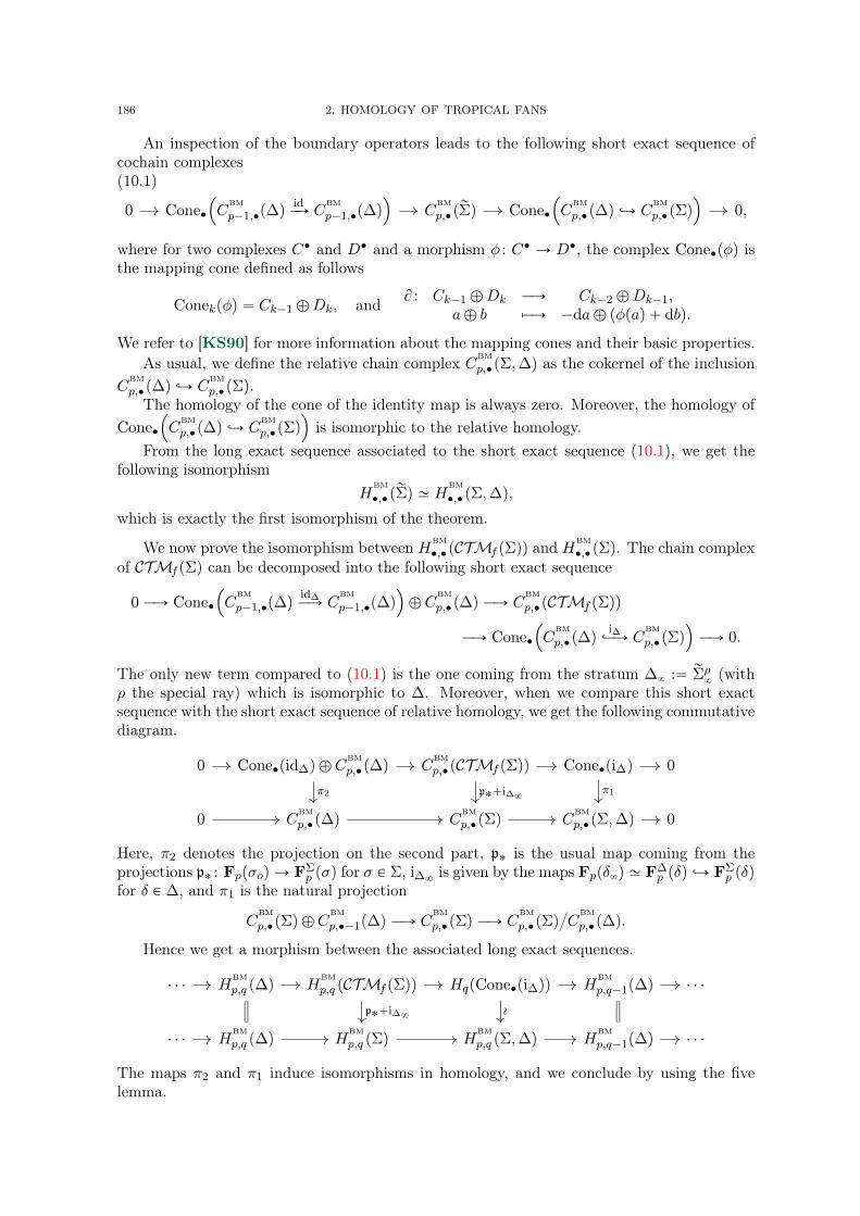
186 2. HOMOLOGY OF TROPICAL FANS
An inspection of the boundary operators leads to the following short exact sequence ofcochain complexes(10.1)
0 Cone‚
´
CBM
p´1,‚p∆qidÝÑ C
BM
p´1,‚p∆q¯
CBM
p,‚prΣq Cone‚
´
CBM
p,‚p∆q ãÑ CBM
p,‚pΣq¯
0,
where for two complexes C‚ and D‚ and a morphism φ : C‚ Ñ D‚, the complex Cone‚pφq isthe mapping cone defined as follows
Conekpφq “ Ck´1 ‘Dk, and B : Ck´1 ‘Dk ÝÑ Ck´2 ‘Dk´1,a‘ b ÞÝÑ ´da‘ pφpaq ` dbq.
We refer to [KS90] for more information about the mapping cones and their basic properties.As usual, we define the relative chain complex CBM
p,‚pΣ,∆q as the cokernel of the inclusionC
BM
p,‚p∆q ãÑ CBM
p,‚pΣq.The homology of the cone of the identity map is always zero. Moreover, the homology of
Cone‚
´
CBM
p,‚p∆q ãÑ CBM
p,‚pΣq¯
is isomorphic to the relative homology.From the long exact sequence associated to the short exact sequence (10.1), we get the
following isomorphismH
BM
‚,‚prΣq » H
BM
‚,‚pΣ,∆q,
which is exactly the first isomorphism of the theorem.
We now prove the isomorphism between HBM
‚,‚pCTMf pΣqq and HBM
‚,‚pΣq. The chain complexof CTMf pΣq can be decomposed into the following short exact sequence
0 ÝÑ Cone‚
´
CBM
p´1,‚p∆qid∆ÝÑ C
BM
p´1,‚p∆q¯
‘ CBM
p,‚p∆q ÝÑ CBM
p,‚pCTMf pΣqq
ÝÑ Cone‚
´
CBM
p,‚p∆qi∆ãÝÑ C
BM
p,‚pΣq¯
ÝÑ 0.
The only new term compared to (10.1) is the one coming from the stratum ∆8 :“ rΣρ8(with
ρ the special ray) which is isomorphic to ∆. Moreover, when we compare this short exactsequence with the short exact sequence of relative homology, we get the following commutativediagram.
0 Cone‚pid∆q ‘ CBM
p,‚p∆q CBM
p,‚pCTMf pΣqq Cone‚pi∆q 0
0 CBM
p,‚p∆q CBM
p,‚pΣq CBM
p,‚pΣ,∆q 0
π2 p˚`i∆8 π1
Here, π2 denotes the projection on the second part, p˚ is the usual map coming from theprojections p˚ : Fppσoq Ñ FΣ
p pσq for σ P Σ, i∆8is given by the maps Fppδ8q » F∆
p pδq ãÑ FΣp pδq
for δ P ∆, and π1 is the natural projection
CBM
p,‚pΣq ‘ CBM
p,‚´1p∆q ÝÑ CBM
p,‚pΣq ÝÑ CBM
p,‚pΣqL
CBM
p,‚p∆q.
Hence we get a morphism between the associated long exact sequences.
¨ ¨ ¨ HBM
p,q p∆q HBM
p,q pCTMf pΣqq HqpCone‚pi∆qq HBM
p,q´1p∆q ¨ ¨ ¨
¨ ¨ ¨ HBM
p,q p∆q HBM
p,q pΣq HBM
p,q pΣ,∆q HBM
p,q´1p∆q ¨ ¨ ¨
p˚`i∆8 „
The maps π2 and π1 induce isomorphisms in homology, and we conclude by using the fivelemma.

10. HOMOLOGY OF TROPICAL MODIFICATIONS AND SHELLABILITY OF SMOOTHNESS 187
The other isomorphisms in the statement of the theorem can be obtained in similar ways(using if necessary, for the cohomology, the dual of the local tropical modification formula,Lemma 10.3). The theorem follows.
10.2. Shellability of smoothness. As a consequence of Theorem 10.1, we get the fol-lowing.
Theorem 10.4. Smoothness is shellable in Trop.Proof. We use Lemma 5.10. It is a trivial fact that elements of B0 are smooth. Moreover,
since smoothness only depends on the support (Theorem 3.20), we only have to prove thecloseness by products and the closeness by tropical modifications. Closeness by products isgiven by Proposition 3.21. It remains to prove the closeness by tropical modifications.
Let Σ be a tropical fan. Let f be a conewise integral linear function on Σ such that divpfq
is reduced. Set ∆ “ divpfq and let rΣ “ TMf pΣq. Assume moreover that ∆ is smooth (andnon-empty). By Lemma 5.10, we just have to prove the Poincaré duality for rΣ.
By Theorem 10.1, we know that HBM
‚,‚prΣq » H
BM
‚,‚pΣ,∆q. Using the long exact sequence ofrelative homology, we get the following exact sequence
. . . ÝÑ HBM
p,q p∆q ÝÑ HBM
p,q pΣq ÝÑ HBM
p,q prΣq ÝÑ H
BM
p,q´1p∆q ÝÑ ¨ ¨ ¨
Since Σ (resp. ∆) verifies the Poincaré duality, its Borel-Moore homology is trivial except forq “ d (resp. q “ d ´ 1). We deduce that HBM
p,‚prΣq is trivial except in degree d and that we
have a short exact sequence
0 ÝÑ HBM
p,dpΣq ÝÑ HBM
p,dprΣq ÝÑ H
BM
p,d´1p∆q ÝÑ 0.
The cap products ¨ " νΥ for Υ any of the tropical fans Σ, ∆ or rΣ induces the followingcommutative diagram.
0 Fd´ppΣq Fd´pprΣq Fd´p´1p∆q 0
0 HBM
p,dpΣq HBM
p,dprΣq H
BM
p,d´1p∆q 0
„ „
We have already seen that the second row is exact. The first row is also a short exact sequenceby the dual of Lemma 10.3. The first and last vertical maps are isomorphisms because Σ and∆ verify the Poincaré duality. Hence, by the five lemma, the second vertical map is anisomorphism, and therefore, rΣ verifies the Poincaré duality.
10.3. Proof of Lemma 10.3. In this final section, we prove Lemma 10.3. So let Σ bea smooth tropical fan. Let f be a conewise integral linear function on Σ such that divpfq
is reduced. Let ∆ “ divpfq and rΣ “ TMf pΣq. We have to prove the following three exactsequences for any face σ P Σ r ∆ and any δ P ∆.
0 FrΣp pσoq FΣ
p pσq 0,
0 F∆p´1pδq F
rΣp pδ q F∆
p pδq 0,
0 F∆p´1pδq F
rΣp pδoq FΣ
p pδq 0.
p˚
p˚
p˚
For the first exact sequence, let σ P Σ r ∆. Let ` P M be any integral linear map whichcoincides with f on σ. Denote by πσ : N Ñ Nσ the natural projection. Then, f ´ ` inducesa conewise integral linear map fσ “ πσ˚pf ´ `q on Σσ. Since no codimension one face of Σcontaining σ is in divpfq, we deduce that divpfσq is trivial. Since Σ is smooth, it is div-faithful
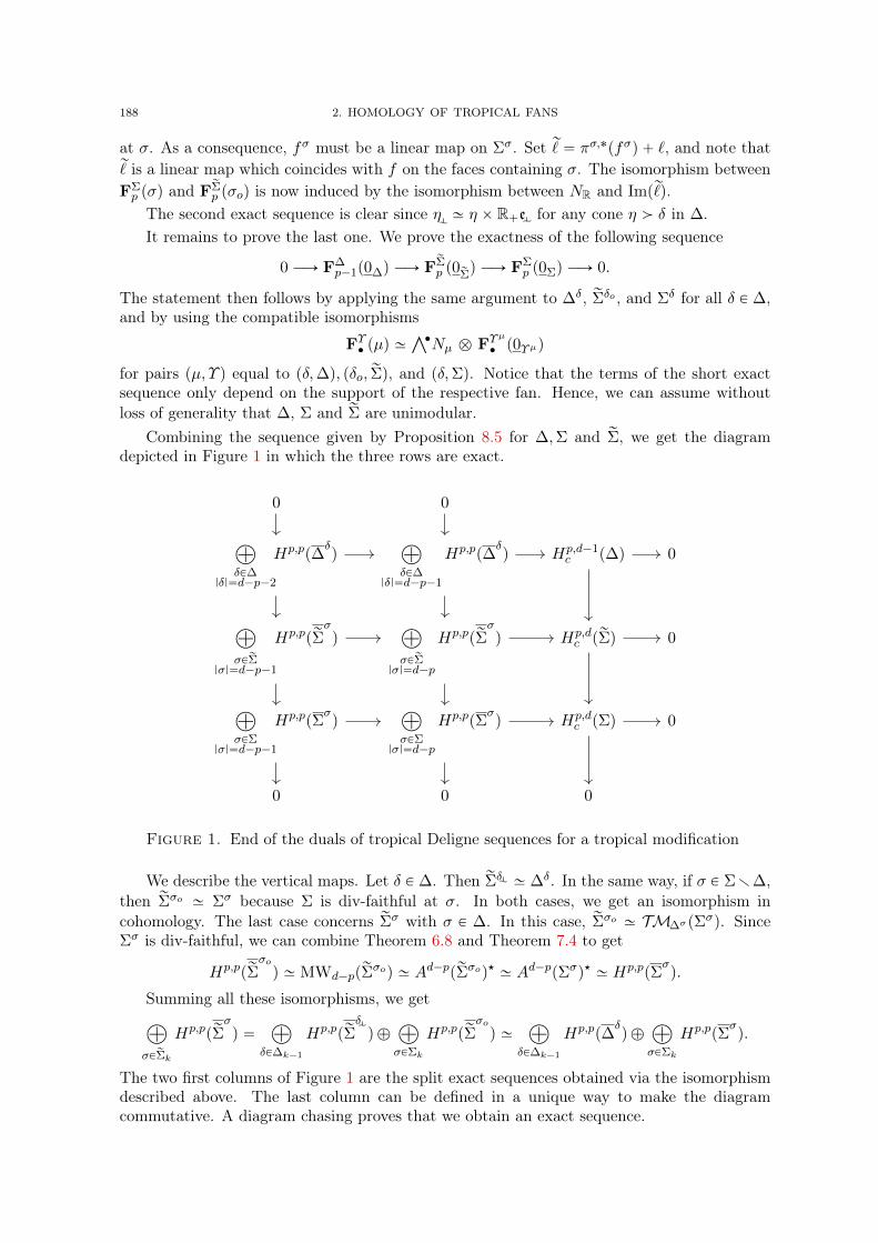
188 2. HOMOLOGY OF TROPICAL FANS
at σ. As a consequence, fσ must be a linear map on Σσ. Set r` “ πσ,˚pfσq ` `, and note thatr` is a linear map which coincides with f on the faces containing σ. The isomorphism betweenFΣp pσq and F
rΣp pσoq is now induced by the isomorphism between NR and Impr`q.
The second exact sequence is clear since η » η ˆ R`e for any cone η ą δ in ∆.It remains to prove the last one. We prove the exactness of the following sequence
0 ÝÑ F∆p´1p0∆q ÝÑ F
rΣp p0rΣ
q ÝÑ FΣp p0Σq ÝÑ 0.
The statement then follows by applying the same argument to ∆δ, rΣδo , and Σδ for all δ P ∆,and by using the compatible isomorphisms
FΥ‚ pµq »Ź‚Nµ b FΥ
µ
‚ p0Υµq
for pairs pµ, Υ q equal to pδ,∆q, pδo, rΣq, and pδ,Σq. Notice that the terms of the short exactsequence only depend on the support of the respective fan. Hence, we can assume withoutloss of generality that ∆, Σ and rΣ are unimodular.
Combining the sequence given by Proposition 8.5 for ∆,Σ and rΣ, we get the diagramdepicted in Figure 1 in which the three rows are exact.
0 0
à
δP∆|δ|“d´p´2
Hp,pp∆δq
à
δP∆|δ|“d´p´1
Hp,pp∆δq Hp,d´1
c p∆q 0
à
σPrΣ|σ|“d´p´1
Hp,pprΣσq
à
σPrΣ|σ|“d´p
Hp,pprΣσq Hp,d
c prΣq 0
à
σPΣ|σ|“d´p´1
Hp,ppΣσq
à
σPΣ|σ|“d´p
Hp,ppΣσq Hp,d
c pΣq 0
0 0 0
Figure 1. End of the duals of tropical Deligne sequences for a tropical modification
We describe the vertical maps. Let δ P ∆. Then rΣδ » ∆δ. In the same way, if σ P Σr∆,then rΣσo » Σσ because Σ is div-faithful at σ. In both cases, we get an isomorphism incohomology. The last case concerns rΣσ with σ P ∆. In this case, rΣσo » TM∆σpΣσq. SinceΣσ is div-faithful, we can combine Theorem 6.8 and Theorem 7.4 to get
Hp,pprΣσoq » MWd´pprΣ
σoq » Ad´pprΣσoq‹ » Ad´ppΣσq‹ » Hp,ppΣσq.
Summing all these isomorphisms, we getà
σPrΣk
Hp,pprΣσq “
à
δP∆k´1
Hp,pprΣδq ‘
à
σPΣk
Hp,pprΣσoq »
à
δP∆k´1
Hp,pp∆δq ‘
à
σPΣk
Hp,ppΣσq.
The two first columns of Figure 1 are the split exact sequences obtained via the isomorphismdescribed above. The last column can be defined in a unique way to make the diagramcommutative. A diagram chasing proves that we obtain an exact sequence.
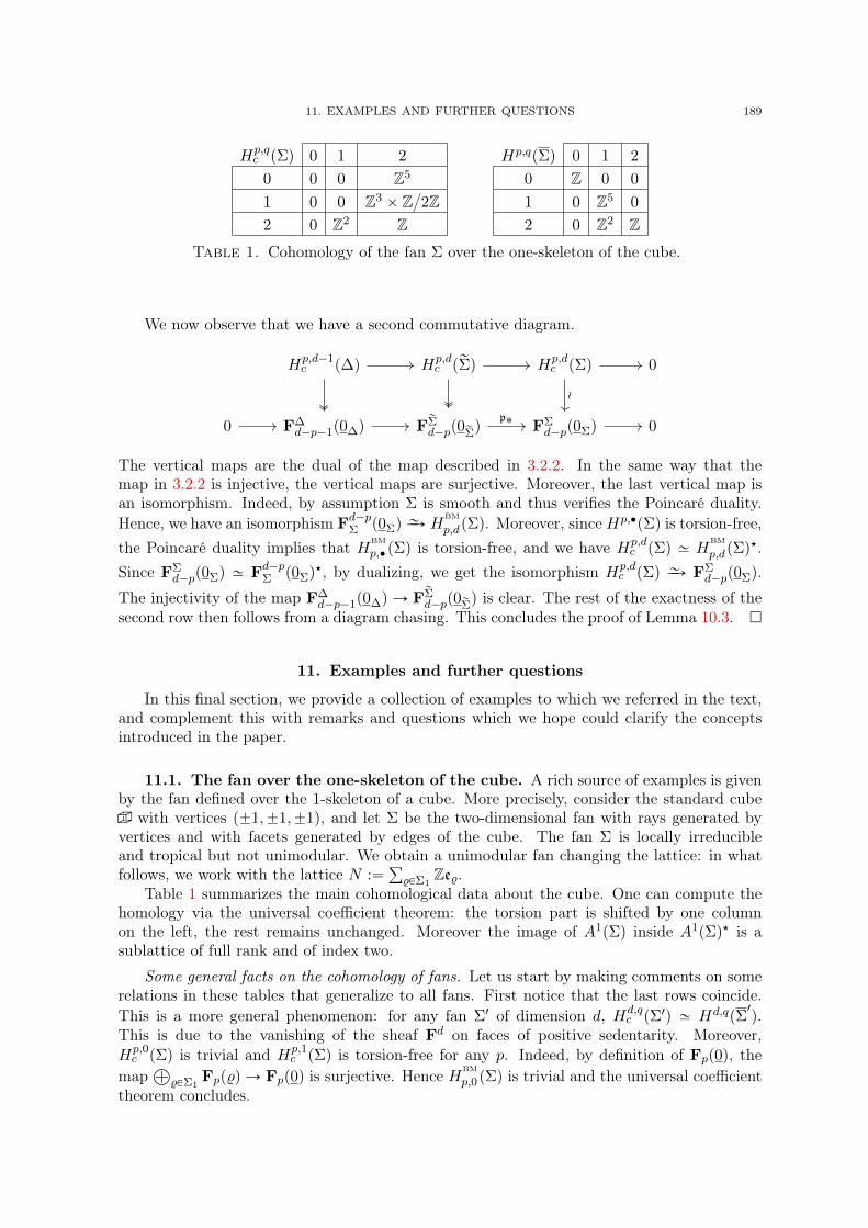
11. EXAMPLES AND FURTHER QUESTIONS 189
Hp,qc pΣq 0 1 2 Hp,qpΣq 0 1 2
0 0 0 Z5 0 Z 0 0
1 0 0 Z3 ˆ ZL
2Z 1 0 Z5 0
2 0 Z2 Z 2 0 Z2 Z
Table 1. Cohomology of the fan Σ over the one-skeleton of the cube.
We now observe that we have a second commutative diagram.
Hp,d´1c p∆q Hp,d
c prΣq Hp,dc pΣq 0
0 F∆d´p´1p0∆q F
rΣd´pp0rΣ
q FΣd´pp0Σq 0
„
p˚
The vertical maps are the dual of the map described in 3.2.2. In the same way that themap in 3.2.2 is injective, the vertical maps are surjective. Moreover, the last vertical map isan isomorphism. Indeed, by assumption Σ is smooth and thus verifies the Poincaré duality.Hence, we have an isomorphism Fd´pΣ p0Σq
„ÝÑ HBM
p,dpΣq. Moreover, sinceHp,‚pΣq is torsion-free,the Poincaré duality implies that HBM
p,‚pΣq is torsion-free, and we have Hp,dc pΣq » H
BM
p,dpΣq‹.
Since FΣd´pp0Σq » Fd´pΣ p0Σq
‹, by dualizing, we get the isomorphism Hp,dc pΣq „ÝÑ FΣ
d´pp0Σq.
The injectivity of the map F∆d´p´1p0∆q Ñ F
rΣd´pp0rΣ
q is clear. The rest of the exactness of thesecond row then follows from a diagram chasing. This concludes the proof of Lemma 10.3.
11. Examples and further questions
In this final section, we provide a collection of examples to which we referred in the text,and complement this with remarks and questions which we hope could clarify the conceptsintroduced in the paper.
11.1. The fan over the one-skeleton of the cube. A rich source of examples is givenby the fan defined over the 1-skeleton of a cube. More precisely, consider the standard cube with vertices p˘1,˘1,˘1q, and let Σ be the two-dimensional fan with rays generated byvertices and with facets generated by edges of the cube. The fan Σ is locally irreducibleand tropical but not unimodular. We obtain a unimodular fan changing the lattice: in whatfollows, we work with the lattice N :“
ř
%PΣ1Ze%.
Table 1 summarizes the main cohomological data about the cube. One can compute thehomology via the universal coefficient theorem: the torsion part is shifted by one columnon the left, the rest remains unchanged. Moreover the image of A1pΣq inside A1pΣq‹ is asublattice of full rank and of index two.
Some general facts on the cohomology of fans. Let us start by making comments on somerelations in these tables that generalize to all fans. First notice that the last rows coincide.This is a more general phenomenon: for any fan Σ1 of dimension d, Hd,q
c pΣ1q » Hd,qpΣ1q.
This is due to the vanishing of the sheaf Fd on faces of positive sedentarity. Moreover,Hp,0c pΣq is trivial and Hp,1
c pΣq is torsion-free for any p. Indeed, by definition of Fpp0q, themap
À
%PΣ1Fpp%q Ñ Fpp0q is surjective. Hence H
BM
p,0pΣq is trivial and the universal coefficienttheorem concludes.
190 2. HOMOLOGY OF TROPICAL FANS
Poincaré duality for fans and classical cohomology. Pursuing our study of the cohomologyof Σ, one can notice that the first row is just the reduced classical homology of the one-skeletonof the cube shifted by one. This is clear because for p “ 0 we retrieve the classical homology.This gives us a precious information: a fan Σ1 of dimension d which verifies the Poincaréduality must verify that Σ1 r t0u has its classical cohomology concentrated in degree d ´ 1,and moreover, Hd´1
sing pΣ1q » ZrkpFdp0qq. Combined with the fact that rkpFdp0qq ď
`
nd
˘
, withn the dimension of the space spanned by Σ, we deduce that locally irreducible tropical fansverifying the Poincaré duality are very specific.
On cohomology groups of Σ for p ą q ą 0. Notice that by Theorem 7.1, the cohomologygroups Hp,qpΣq are trivial when either p ă q, or q “ 0 and p ą 0, and that Hp,ppΣq » AppΣq.The theorem however provides no information about H2,1pΣq for a general fan. For the fanΣ consider here, this cohomology group is nontrivial, hence Σ does not verify the Poincaréduality.
Other properties of Σ. The fan Σ can be served in the following examples.
Example 11.1 (A Chow-duality tropical fan which does not verify the Poincaré duality).The cohomology of Σ does not verify the Poincaré duality. Its Chow ring with integral coef-ficients neither. On the other hand, its Chow ring with rational coefficients does verify thePoincaré duality. It also verifies the hard-Lefschetz property and the Hodge-Riemann bilinearrelations. ˛
Example 11.2 (A non-principal locally irreducible unimodular fan). The map A1pΣq ÑA1pΣq‹ is not surjective, hence Σ is not principal at 0 for integral coefficients (though it isprincipal for rational coefficients). Indeed, the divisor D “ R ¨ p1, 1, 1q is not principal, but2D is. In fact, this divisor is not a boundary for integral coefficients, and H
BM
1,1pΣq » ZL
2Zhas torsion. ˛
11.2. The cross. Consider the cross txy “ 0u in R2 with four rays. We denote it by ∆.It is the simplest singular tropical fan. It can be used in several constructions to find variouscounter-examples. We propose some of them below.
Example 11.3 (Poincaré duality for a non normal compactified fan). Recall that Λk is thecomplete fan on Rk whose facets are the 2k orthants. Consider Σ :“ TM∆pΛ
2q. Since Λ2 is div-faithful, by Theorem 6.8, A‚pΣq » A‚pΛ2q. Moreover, since Λ2 is smooth, H‚,‚pΣq » H‚,‚pΛ2q.Hence, despite Σ being not normal, both the Chow ring of Σ and the cohomology of Σ verifythe Poincaré duality. In particular, Σ is irreducible, principal and div-faithful at 0. On theother hand, it is neither locally irreducible nor div-faithful globally. However, Σ does notverify the homological Poincaré duality: HBM
0,2pΣq » Z4 but F2p0q is of rank 3. ˛
Example 11.4 (A nontrivial degenerate tropical modification). Let f be the conewiseintegral linear function on ∆ given by f “ x´y on tx`y ě 0u and 0 on the complement. Thendivpfq is trivial. The tropical modification TMf p∆q is a smooth tropical line. In particularit verifies the Poincaré duality, which is not the case of ∆. This example is quite interesting:it seems that tropical modifications tend to desingularize tropical varieties as blow-ups do inalgebraic geometry. ˛
Example 11.5 (Two non-principal unimodular tropical fans). Consider the fan Σ “ ∆ˆΛof dimension two in R3, i.e., it has the six rays of the axes and support tx “ 0uYty “ 0u Ă R3.The divisor ty “ z “ 0u in Σ is not principal. This means Σ is not principal at 0.
Following the idea of Example 11.3, one can go further and create a fan which is principalat 0 but not globally principal: it suffices to take TMΣpΛ
3q. ˛
Example 11.6 (Non-irreducible unimodular fans). We can find higher dimensional ana-logues of the cross in R2. Consider any unimodular fan ∆1 of support tx1 “ x2 “ 0u Y tx3 “
x4 “ 0u in R4. The fan Σ is normal, div-faithful and principal, but it is not irreducible. ˛
11. EXAMPLES AND FURTHER QUESTIONS 191
Example 11.7 (A normal div-faithful unimodular fan which is neither irreducible norprincipal). Let ∆1 be the fan defined in the previous example. Set Σ “ ∆1 ˆ Λ. We geta tropical fan Σ of dimension three which is still normal and div-faithful but it is neitherirreducible, nor principal: the divisor tx1 “ x2 “ 0u ˆ t0u is not a principal divisor in Σ1. ˛
11.3. Non saturated and non unimodular fans. Let pe1, e2q be the standard basisof Z2 and let e0 “ ´e1 ´ e2. Denote by ρi “ R`ei, i P t0, 1, 2u the corresponding rays. Let Nbe the lattice Zp1, 0q ` Zp´13,´13q. Then the lattice Z2 generated by e0, e1, e2 is of indexthree in N .
Example 11.8. Let Σ in R2 be the one-dimensional fan with rays ρi, for i “ 0, 1, 2. ThenΣ is tropical, and tropically smooth, but it is not saturated. Any element of pZ2q‹ Ă Minduces an integral linear form on Σ. As a consequence, A1pΣq has torsion. For instance,Xρ1 ´ Xρ2 is non-zero, but 3 ¨ pXρ1 ´ Xρ2q is zero in A1pΣq. ˛
Example 11.9. Let Σ be the complete fan in the plane R2, with N “ Z2, whose rays arethe ρi. This time, Σ is not unimodular. As in example 11.8, A1pΣq has torsion. Moreover, thecohomology group H1,2pΣq » Z
L
3Z is nontrivial even though we are in bidegree pp, qq “ p1, 2qwith p ă q. ˛
Example 11.10. Consider again the complete fan Σ of the previous Example. Let f bethe conewise integral linear function on Σ which maps e0 on ´3 and e1 and e2 on 0. Thendivpfq is the reduced divisor ∆ with rays ρi for i “ 0, 1, 2.
Let Σ1 be a unimodular subdivision of Σ; for instance one can add the rays along thevectors 1
3ei`23ej for distinct i, j P t0, 1, 2u. This fan is smooth. Set rΣ “ TMf pΣ
1q and denoteby ρ the new ray. Then rΣ is a smooth unimodular fan which is saturated at 0 but not at ρ.Even worse, there is no way to change the lattice N to make it saturated without changingrΣXN .
Since rΣ is saturated at 0, A1prΣq has no torsion. However, the element XρpXρ1 ´ Xρ2q P
A2prΣq is an element of order three. ˛
The three previous examples show that the saturation and unimodularity assumptions inTheorem 7.1 are needed in general.
11.4. Further examples.
Example 11.11 (A shellable tropical fan which is not generalized Bergman). Let Σ bethe two-dimensional skeleton of the fan of the projective space of dimension three: it has fourrays generated by vectors e1, e2, e3 and e0 “ ´e1´ e2´ e3, where pe1, e2, e3q is a basis of N , andthe six facets R`ei ` R`ej for 0 ď i ă j ď 3. We have |Σ| “ |ΣM| for the uniform matroidM “ U3
4 of rank three on four elements. Let ∆ be the tropical curve in |Σ| with four raysρ1, ρ2, ρ3 and ρ4 with
ρ1 “ R`pe1 ` e2q, ρ2 “ R`e2, ρ3 “ R`pe0 ` 2e3q, ρ4 “ R`pe0 ` e1q.
Then we have ∆ » ΣM1 with M1 “ U24 the uniform matroid of rank two on four elements.
The tropical modification TM∆pΣq is shellable but does not have the same support as theBergman fan of any matroid. It means it is not generalized Bergman. ˛
Example 11.12 (A non-shellable smooth fan). We study here an interesting examplediscovered by Babaee and Huh [BH17]. We would like to thank Edvard Aksnes and KrisShaw for pointing out the relevance of this example to us.
A full description of the fan is given in [BH17,Aks19]. We just mention its main proper-ties. It is a normal unimodular tropical fan Σ of dimension two living in R4. Aksnes computesits rational homology in [Aks19] and concludes that it is smooth (this remains true withintegral coefficients). However, Σ does not verify the Hodge-Riemann bilinear relations: it is

192 2. HOMOLOGY OF TROPICAL FANS
quasi-projective, but the pairing A1pΣq ˆ A1pΣq Ñ Z has more than one positive eigenvalue.In particular it is not shellable. Indeed, by Theorem 5.9 (6), any quasi-projective shellablefan verifies the Hodge-Riemann bilinear relations. ˛
Example 11.13 (Irreducible components of non normal fans). Let Σ “ be the 1-skeleton of U3,3 in R2. There are five irreducible components in the sense of minimal supportof an element of HBM
1,1pΣq, but they do not induce a partition of Σ1. ˛
11.5. Questions. We end this section with a list of questions naturally arising in ourstudy.– Is the smoothness of a tropical fan Σ implied by the surjectivity of the map Fpp0Σσq Ñ
HBM
d´p,dpΣσq, σ P Σ. In other words, does the vanishing of HBM
p,q pΣq follow from the surjectivity?
– Provide examples of unimodular fans Σ with torsion in Hp,qpΣq, for p ą q.– Provide a classification of smooth tropical fans.
CHAPTER 3
Hodge theory for tropical varieties
Abstract : In this paper we prove that the cohomology of smooth projective tropicalvarieties verify the tropical analogs of three fundamental theorems which govern the cohomol-ogy of complex projective varieties: Hard Lefschetz theorem, Hodge-Riemann relations andmonodromy-weight conjecture.
On the way to establish these results, we introduce and prove other results of indepen-dent interest. This includes a combinatorial study of the tropical version of the Steenbrinkspectral sequence, a treatment of Kähler forms in tropical geometry and their associatedHodge-Lefschetz structures, a tropical version of the projective bundle formula, and a re-sult in polyhedral geometry on the existence of quasi-projective unimodular triangulations ofpolyhedral spaces.
Moreover, we provide a generalization with a new proof of the results of Adiprasito, Huh,and Katz, Hodge theory for combinatorial geometries, Annals of Mathematics 188 (2018), no.2, 381–452, by showing that being Kähler for tropical fans is shellable, in the sense of ourwork homology of tropical fans. This shows that any quasi-projective shellable tropical fan isKähler.
1. Introduction
The aim of this work and its forthcoming companions is to study Hodge theoretic aspectsof tropical and non-archimedean geometry.
Tropical geometry studies degenerations of algebraic varieties by enriching the theory ofsemistable models and their dual complexes by polyhedral geometry. This enrichment moti-vates the development of algebraic geometry for combinatorial and polyhedral spaces [Mik06,MS15,GS11,MZ14,IKMZ19,Car19,JSS19] and their hybrid counter-parts, which containa mixture of algebraic and polyhedral components [Ber09,AB15,BJ17,AN20,Mik06].
In dimension one, it is now well-understood that graphs and metric graphs are in manyways similar to Riemann surfaces and algebraic curves. For example, the analog of manyclassical theorems governing the geometry of Riemann surfaces, Riemann-Roch, Abel-Jacobi,Clifford and Torelli, are now established for graphs and metric graphs [BN07,GK08,MZ08,Cop16,CV10,AB15].
This viewpoint and its subsequent extensions and refinements have been quite powerfulin applications in the past decade, and have resulted in several advances ranging from thestudy of curves and their moduli spaces (e.g. Brill-Noether theory [CDPR12a], maximumrank conjecture [JP16], the Kodaira dimension of the moduli spaces of curves [FJP20]) toarithmetic geometry of curves (e.g. uniform bounds on the number of rational points oncurves [KRZ16] and equidistribution results [Ami14]). An overview of some of these resultscan be found in the survey paper [BJ16].
It is expected that higher dimensional combinatorial and polyhedral analogs of graphsand metric graphs should fit into the same picture and fundamental theorems of algebraicgeometry should have their combinatorial and polyhedral analogs.
193

194 3. HODGE THEORY FOR TROPICAL VARIETIES
Representative examples of this fresco in higher dimension have emerged in the pioneeringwork of McMullen and Karu [McM93,Kar04] on hard Lefschetz theorem for polytopes, andmore recently, in connection with Hodge theory, in the work of Adiprasito-Huh-Katz [AHK18]in the development of Hodge theory for matroids, in the work of Babaee-Huh [BH17] onDemailly’s strong reformulation of the Hodge conjecture for currents, in the work of Elias andWilliamson [EW14] on Hodge theory of Soergel bimodules and positivity of Kazhdan-Lustigpolynomials, and in the work of Adiprasito-Bjöner [AB14] and Adiprasito [Adi18] on weakand combinatorial Lefschetz theorems, respectively.
Our aim here is to show that cohomology of Kähler tropical varieties verify the tropicalanalogs of three fundamental theorems which govern the cohomology of complex projectivevarieties: Hard Lefschetz theorem, Hodge-Riemann relations and monodromy-weight conjec-ture. As we will explain below, this provides a uniform treatment and a generalization ofmany of the above mentioned results within the framework of tropical geometry.
In the rest of this introduction, we provide a brief discussion of the results presented inthis article.
1.1. Tropical fans. Tropical fans and their supports form the local charts for moregeneral tropical varieties. Let N » Zn be a lattice of finite rank and denote by NR the vectorspace generated by N . Recall that a fan Σ in NR is a non-empty collection of strongly convexpolyhedral cones which verify the following two properties. First, for any cone σ P Σ, anyface of σ belongs to Σ. Moreover, for two cones σ and η in Σ, the intersection σ X η is acommon face of both σ and η. In particular, Σ always contains the cone 0 :“ t0u. We denoteby |σ| the dimension of a face σ. A fan is called rational if any cone in Σ is rational in thesense that it is generated by rays which have non-zero intersection with the lattice N . In thatcase, each cone σ in Σ defines a sublattice Nσ of N of the same rank as the dimension of σ,and given by the integral points of the vector subspace of NR generated by σ. A cone σ issimplicial if it is of the form
ř
iR`ei for some family of independent vectors peiqi in NR. If σis rational, we say it is unimodular if we can choose a basis of Nσ for the family peiqi. A fanΣ is called simplicial, resp. unimodular, if all its cone are simplicial, resp. unimodular. A fanis pure dimensional if all its maximal cones have the same dimension. The support of a fan Σ
is denoted by |Σ|.A tropical fan is a pure dimensional simplicial rational fan Σ in NR as above which in
addition verifies the following foundational principle in tropical geometry called the balancingcondition: for any cone τ of codimension one in Σ, we have the vanishing in the quotientlattice N
L
Nτ of the following sumÿ
σĄτ
eστ “ 0
where the sum is over faces σ of maximal dimension containing τ and eστ is the vector whichgenerates the quotient pσ X Nq
L
pτ X Nq » Zě0. This might be regarded as a polyhedralanalogue of orientability and leads to the definition of a fundamental class which plays an im-portant role in the treatment of the duality and other finer geometric properties in polyhedralgeometry.
1.2. Smoothness in tropical geometry. The smoothness is understood in the senseof our work [AP21]. The definition of tropical smoothness that we propose in that work ishomological.
Let Σ be a rational fan. We denote by Fp the sheaf of p-multivectors on Σ and by Fp itsdual. The sheaf Fp is simplicial and on each cone σ is defined by
Fppσq :“ÿ
ηPΣηĚσ
ŹpNη ĎŹpN, and Fppσq :“ Fppσq‹.
1. INTRODUCTION 195
The dual Fp (with real coefficients) can be regarded as the sheaf of tropical holomorphicp-forms on Σ, cf. [JSS19].
The above coefficient sheaves lead to the definition of cohomology and homology groupsHp,qpΣq, Hp,q
c pΣq, Hp,qpΣq, and HBM
p,q pΣq, with the last one being the tropical analogue of theBorel-Moore homology. These were introduced in [IKMZ19] and further studied in [JSS19,MZ14,JRS18,GS19b,GS19a,AB14,ARS19,Aks19,AP21,Mik20a,AP20c]. We recallthe relevant definitions in Section 2.
Let Σ be a tropical fan of dimension d, and let νΣ be the canonical element in the Borel-Moore homology group HBM
d,dpΣq.Using the cap product ", we get a natural map
¨" νΣ : Hp,qpΣq ÝÑ HBM
d´p,d´qpΣq.
We say that a simplicial tropical fan Σ verifies the Poincaré duality if the above map is anisomorphism for any bidegree pp, qq. A tropical fan Σ is called smooth if for any cone σ P Σ,the star fan Σσ verifies the Poincaré duality. In this paper, the star fan Σσ refers to the fanin NR
L
Nσ,R induced by the cones η in Σ which contain σ as a face.In [AP21] we introduced the notion of shellability and class of shellable tropical fans. One
of the main theorems of [AP21] is the following theorem.
Theorem 1.1. Smoothness is shellable. In particular, any shellable tropical fan is smooth.
1.3. Matroids and their Bergman fans. Central objects underlying our results inthis paper and [AP21] are combinatorial structures called matroids. Discovered by Whit-ney [Whi35] in his study on classification of graphs with the same cycle structure, and inde-pendently by van der Waerden [van37] and Nakasawa, matroids provide combinatorial axiom-atization of central notions of linear algebra. In this way, they lead to a common generalizationof other combinatorial structures such as graphs, simplicial complexes and hyperplane arrange-ments. They appear naturally in diverse fields of mathematics, e.g., in combinatorics andstatistical physics [Tut65,MP67,GGW06, SS14,Piq19b], optimization theory [Sch03],topology [Mac91,GM92], and algebraic geometry [Mnë88,Laf03,BB03,BL18,Stu02]. Intropical geometry, they are combinatorial structures underlying the idea of maximal degener-ations of algebraic varieties [Del97,KS06], and in this way give rise to a tropical notion ofsmoothness. We refer to [Wil73,Kun86,Oxl11] for an introduction and a historical accountof the theory of matroids.
To any matroid M over a ground set E one associates a fan ΣM called the Bergman fan ofM which lives in the real vector space RE
L
Rp1, . . . , 1q and which is rational with respect to thelattice ZE
L
Zp1, . . . , 1q. In the case the matroid is given by an arrangement of hyperplanes, theBergman fan can be identified with the tropicalization of the complement of the hyperplanearrangement, for the coordinates given by the linear functions which define the hyperplanearrangement [AK06].
The fan ΣM has the following description. First, recall that a flat of M is a set F ofelements of E which is closed with respect to the linear dependency, i.e., an element e P Ewhich is linearly dependent to F already belongs to F . A non-empty flat F Ĺ E is calledproper. The Bergman fan ΣM consists of cones σF in correspondence with flags of proper flatsof M
F : F1 Ĺ F2 Ĺ ¨ ¨ ¨ Ĺ Fk, k P NY t0u.For such a flag F , the corresponding cone σF is the one generated by the characteristic vectorseF1 , . . . , eFk of F1, . . . , Fk in RERp1, . . . , 1q. In particular, the rays of ΣM are in bijection withthe proper flats F of M.
We call a Bergman support or a tropical linear space any subspace of a real vector spacewhich is isomorphic via a linear map of real vector spaces to the support of the Bergman fanof a simple matroid. The terminology comes from [Ber71,Spe08].
196 3. HODGE THEORY FOR TROPICAL VARIETIES
By a generalized Bergman fan we mean any fan which is supported on a Bergman support.In particular, Bergman fan ΣM of a matroid M is an example of a generalized Bergman fan.Moreover, with this terminology, any complete fan in a real vector space is a generalizedBergman fan. Indeed, for each integer d, the real vector space Rd is the support of theBergman fan of the uniform matroid Ud`1 of rank d` 1 on ground set rds :“ t0, 1, . . . , du. (InUd every subset of rds is an independent set.) Thus, generalized Bergman fans generalize bothcomplete fans and Bergman fans of matroids. In addition, products of Bergman fans remainBergman.
A unimodular generalized Bergman fan in a real vector space V is a generalized Bergmanfans Σ which is moreover rational with respect to a full rank sublattice N of V and unimodular(smooth in the language of toric geometry). This means any cone σ in Σ is simplicial, thatis generated by |σ|, the dimension of σ, rays. Moreover, denoting %1, . . . , %|σ| the rays of σ,each ray %i is rational, and in addition, if e%i denotes the primitive vector of the ray %i, theset of vectors e%1 , . . . , e%|σ| is part of a basis of the lattice N . The product of two unimodulargeneralized Bergman fans remains a unimodular generalized Bergman fan.
We proved in [AP21] the following theorem.
Theorem 1.2. Unimodular Bergman fans are shellable. As a consequence they are smooth.
This shows that our notion of smoothness and the corresponding smooth tropical varietiesinclude the previous ones modeled by the supports of Bergman fans.
1.4. Chow rings of tropical fans. Let Σ be a unimodular tropical fan in a vector spaceV and let N be the corresponding full rank lattice of V , so V “ NR :“ N b R.
The Chow ring of Σ denoted by A‚pΣq is defined as the quotient of the polynomial ringZrx% | % P Σ1s, with generators x% associated to the rays % of Σ, by the ideal I1 ` I2 definedas follows:
— I1 is the ideal generated by all monomials of the formś
%PS x% for any subset S Ď Σ1
which do not form a cone in Σ; and
— I2 is the ideal generated by the elements of the formÿ
%PΣ1
xm, e%yx%
for any m in the dual lattice M “ N‹,
where e% denotes the primitive vector of %, and x ¨ , ¨ y is the duality pairing between M andN .
This ring is known to be the Chow ring of the toric variety PΣ defined by Σ, cf. [Dan78,BDP90,Bri96,FS97].
In the case Σ “ ΣM is the Bergman fan of a simple matroid M, by the description of thefan ΣM, it is easy to see that the ring A‚pΣMq coincides with the Chow ring A‚pMq of thematroid defined as follows.
To any flat F of M one associates a variable xF . The Chow ring A‚pMq is then a quotientof the polynomial ring ZrxF : F flat of Ms by the ideal IM generated by the polynomials
— xFxH for any two incomparable flats F and H, i.e., with F Ć H and H Ć F ;
—ř
FQe xF ´ř
FQf xF for any pair of elements e, f P E.
In the case the matroid M is given by an arrangement of hyperplanes, the Chow ringgets identified with the Chow ring of the wonderful compactification of the complement of thehyperplane arrangement [DP95,FY04]. We generalized this result to any tropical compact-ifications of the complement of the hyperplane arrangement in [AP21].
1. INTRODUCTION 197
1.5. Canonical compactifications. The canonical compactification of a simplicial fanΣ in a real vector space V » Rn is defined as the result of completing any cone of Σ to ahypercube, by adding some faces at infinity. This is defined more precisely as follows. The fanΣ can be used to define a partial compactification of V which we denote by TPΣ. The spaceTPΣ is the tropical analog of the toric variety associated to Σ. In fact, in the case the fan Σ isrational with respect to a full rank lattice N in V , the tropical toric variety TPΣ coincides withthe tropicalization of the toric variety PΣ associated to Σ, see e.g. [Pay09,Thu07]. Thesepartial compactifications of V coincide as well with the ones called manifolds with cornersconsidered in [AMS`10,Oda88].The canonical compactification of Σ denoted by Σ is then defined as the closure of Σ in thetropical toric variety TPΣ. The space Σ has the following description as the cubical completionof Σ, see Section 2 for a more precise description. Any ray % of Σ becomes a segment by addinga point 8% at infinity to %. Any two dimensional cone σ with two rays %1 and %2 becomes aparallelogram with vertex set the origin, 8%1 ,8%2 , and a new point 8σ associated to σ. Thehigher dimensional cones are completed similarly to parallelepipeds.
Canonical compactifications of fans serve as building blocks for the description and thestudy of more general tropical varieties, as we will explain below.
1.6. Hodge isomorphism theorem and Poincaré duality. Let Σ be a unimodularsmooth tropical fan and let Σ be the canonical compactification of Σ. The compactificationΣ is a smooth tropical variety in the sense that it is locally modelled by unimodular smoothtropical fans, see Section 1.8 below and Section 2 for a precise definition of smoothness builtin [AP21].
Denote by Hp,qtroppΣq the tropical cohomology group of Σ of bidegree pp, qq introduced by
Itenberg-Katzarkov-Mikhalkin-Zharkov in [IKMZ19]. We recall the definition of these groupsin Section 2. We proved in [AP21] the following general theorem which allows in particular,when applied to the Bergman fan ΣM of a matroid M, to reinterpret the results of Adiprasito-Huh-Katz [AHK18] as statements about the cohomology groups of a specific projective trop-ical variety, the canonical compactification of the Bergman fan of the matroid.
Theorem 1.3 (Hodge isomorphism for unimodular smooth tropical fans [AP21]). Forany unimodular smooth tropical fan Σ of dimension d, and for any non-negative integer p ď d,there is an isomorphism
AppΣq „ÝÝÑ Hp,ptroppΣ,Zq.
These isomorphisms induce an isomorphism of Z-algebras between the Chow ring of Σ and thetropical cohomology ring
Àdp“0H
p,ptroppΣ,Zq. Furthermore, the cohomology groups Hp,q
troppΣ,Zqfor p ‰ q are all trivial.
Saying it differently, the theorem states that the cycle class map from Chow groups totropical cohomology is an isomorphism, and in particular, the tropical cohomology groups ofΣ are generated by Hodge classes.
As a corollary of the above theorem, we obtain the following result [AP21].
Theorem 1.4 (Poincaré duality). Let Σ be a unimodular tropical fan of dimension d.There is a canonical isomorphism deg : AdpΣq Ñ Z called the degree map. With respect to thisisomorphism, the Chow ring of Σ satisfies the Poincaré duality, in the sense that the pairing
AkpΣq ˆAd´kpΣq AdpΣq Z
pa, bq degpabq
deg
„
is non-degenerate.
198 3. HODGE THEORY FOR TROPICAL VARIETIES
For generalized Bergman fans, this can be obtained via the Hodge isomorphism theorem bythe Poincaré duality for matroidal tropical varieties, established by Jell-Shaw-Smacka [JSS19]for rational coefficients and by Jell-Rau-Shaw [JRS18] for integral coefficients. In that case,this was also independently proved by Gross-Shokrieh [GS19a], as well as by Ardila-Denham-Huh [ADH20].
1.7. Kähler tropical fans and shellability. For a unimodular smooth tropical fan Σof dimension d and an element ` P A1pΣq, we say that the pair pΣ, `q verifies the Hard Lefschetzproperty HLpΣ, `q if the following holds:
(Hard Lefschetz) for any non-negative integer k ď d2 , the multiplication map by `d´2k induces
an isomorphism
AkpΣq Ad´kpΣq , a `d´2k ¨ a.„
We say the pair pΣ, `q verifies Hodge-Riemann relations HRpΣ, `q if for any non-negativeinteger k ď d
2 , the following holds:
(Hodge-Riemann relations) for any non-negative integer k ď d2 , the symmetric bilinear form
AkpΣq ˆAkpΣq Z , pa, bq p´1qk degp`d´2k ¨ a ¨ bq
is positive definite on the primitive part P kpΣq Ď AkpΣq, which by definition, is the kernel ofthe multiplication by `d´2k`1 from AkpΣq to Ad´k`1pΣq.
A smooth unimodular tropical fan Σ is called Kähler if it is quasi-projective and moreoverfor an ample element ` P A1pΣq, pΣ, `q verifies Hard Lefschetz and Hodge-Riemann relations.Here ` is called ample if ` can be represented in the form
ř
%PΣ1fpe%qx% for a strictly convex
cone-wise linear function f on the fan Σ, see Section 2 for the definition of strict convexity. Afan which admits such a function is called quasi-projective. (Note that the Bergman fan ΣM
of any matroid M is quasi-projective.)In Section 3 we will show the following theorem.
Theorem 1.5 (Shellability of Kähler property). To be Kähler for quasi-projective unimod-ular tropical fans is shellable.
Theorem 1.4 generalizes Poincaré duality for matroids proved in [AHK18] to any smoothtropical fan. As a consequence of the above theorem, we infer that Chow rings of shellablequasi-projective unimodular tropical fans verify Hard Lefschetz theorem and Hodge-Riemannrelations, thus generalizing results of Adiprasito-Huh-Katz [AHK18] to any shellable quasi-projective unimodular tropical fan.
Theorem 1.6 (Kähler package for shellable fans). Let Σ be a shellable quasi-projectiveunimodular tropical fan of dimension d. For any ample element ` P A1pΣq, the pair pΣ, `qverifies HLpΣ, `q and HRpΣ, `q. That is Σ is Kähler.
To prove the above theorem we proceed by induction by using the shellability meta lemma.We use tropical modifications to produce a fan structure on the support of a shellable trop-ical fan for which the theorem holds by the hypothesis of our induction. The main idea inour approach which allows to proceed by induction, basically by starting from trivial casesand deducing the theorem in full generality, are the ascent and descent properties proved inSection 3. We then use the weak factorization theorem for quasi-projective fans and theseproperties to get the theorem in its full generality.
We note that an alternate proof of the main result of [AHK18] for the Chow ring of amatroid based on semi-simple decomposition of the Chow ring has been obtained recentlyby Braden-Huh-Matherne-Proudfoot-Wang [BHM`20a]. Moreover, in an independent workparallel to ours, Ardila-Denham-Huh [ADH20] have used weak factorization theorem to get
1. INTRODUCTION 199
the above theorem for any unimodular quasi-projective generalized Bergman fan. We notethat in the case of generalized Bergman fan, Adiprasito informed us that the above theoremalso follows from their theorem [AHK18] and McMullen’s observation refined by Fleming-Karu [McM93,FK10], stating that a support preserving quasi-projective flip preserves bothHodge-Riemann and Hard Lefschetz properties.
As a special case of our theorem, we thus get an alternate proof of all these results. Tomake a comparison with the above mentioned results, our methods lead to arguably moretransparent proofs of these results, trivializing the proof of the existence of a tropical fan ona given support which satisfies the Kähler package. The properties established in the proofof Theorem 1.6 are also throughly used in the rest of the paper. In particular, the ascentand descent properties are the final piece of arguments we will need in the global setting toconclude the proof of the main theorems of this paper for any Kähler tropical variety. Thepossibility of having these nice properties is guaranteed by Keel’s lemma for fans in the localsetting, and by our projective bundle formula for tropical cohomology groups in the globalsetting, cf. the discussion below and the corresponding sections for more details.
1.8. Smoothness in tropical geometry revisited. A tropical variety X is an extendedpolyhedral space with a choice of an integral affine structure. A polyhedral complex structureon a tropical variety is a polyhedral complex structure which induces the integral affine struc-ture. We refer to Section 2 which provides the precise definitions of these terminologies.
A tropical variety is called smooth if it can be locally modeled by supports of smoothtropical fans [AP21].
The smoothness is meant to reflect in polyhedral geometry the idea of maximal degeneracyfor varieties defined over non-Archimedean fields. We elaborate on this remark and connectionto the work of Deligne [Del97] in our future work.
Examples of smooth tropical varieties include smooth affine manifolds, canonical compact-ifications of Bergman fans, and tropicalizations of Mumford curves [Jel18].
1.9. Hodge-Riemann and Hard Lefschetz for Kähler tropical varieties. In viewof Hodge isomorphism Theorem 1.3 and Kähler package for shellable unimodular quasi-projective tropical fans, Theorem 1.6, the results in Section 1.7 can be regarded as statementsconcerning the tropical cohomology ring of the canonical compactifications Σ of shellableunimodular quasi-projective tropical fans. Moreover, one can show that when Σ is quasi-projective, the canonical compactification is projective [AP20a]. One of our aim in this paperis to show that all the results stated above hold more generally for the tropical cohomologygroups of any (compact) Kähler tropical variety.
Let V “ NR be a vector space of dimension n and N a full rank sublattice in V. For afan ∆ in V , we denote by TP∆ the corresponding tropical toric variety, which is a partialcompactification of V .
Let now Y be a polyhedral subspace of V , and let Y be a unimodular polyhedral complexstructure on Y with a quasi-projective unimodular recession fan Yrec, cf. Section 2 for thedefinitions of these terminologies. Let X be the closure of Y in TPYrec , equipped with theinduced polyhedral structure that we denote by X. Let ` be a strictly convex cone-wise linearfunction on Yrec. We will show that ` defines an element ω of H1,1
troppTPYrec ,Rq, which livesin H1,1
troppTPYrec ,Qq if ` has integral slopes. By restriction, this element gives an element inH1,1
troppX,Qq which, by an abuse of the notation, we still denote by ω. Multiplication by ωdefines a Lefschetz operator on H‚,‚troppX,Qq still denoted by ω.
We say Y is Kähler if it is smooth and the star fan Σσ around each face σ of Y is Kähler.In this case, X is also Kähler, that is the star fans of X are all Kähler.
Here is the main theorem of this paper.
200 3. HODGE THEORY FOR TROPICAL VARIETIES
Theorem 1.7 (Kähler package for compact Kähler tropical varieties). Notations as aboveand working with Q coefficients, let X be Kähler. Then we have
— (weight-monodromy conjecture) For any pair of non-negative integers p ě q, we havean isomorphism
φ : Hp,qtroppXq
„ÝÑ Hq,p
troppXq.
— (Hard Lefschetz) For p` q ď d, the Lefschetz operator ` induces an isomorphism
`d´p´q : Hp,qtroppXq
„ÝÑ Hd´q,d´p
trop pXq.
— (Hodge-Riemann) The pairing⟨¨ , `d´p´qφ ¨
⟩induces a positive-definite symmetric
bilinear form on the primitive part P p,q of Hp,qtrop, where
⟨¨ , ¨
⟩denotes the pairing
Hp,qtroppXq bH
d´p,d´qtrop pXq ÝÑ Hd,d
troppXqdeg
ÝÝÝÝÝÝÑ„
Q,⟨a, b
⟩ÞÝÑ p´1qp degpaY bq,
and φ is the isomorphism given in the first point.
As a consequence of the above theorem we get the following theorem.
Theorem 1.8 (Kähler package for projective locally shellable tropical varieties). Anyprojective tropical variety which is locally shellable verifies the properties (weight-monodromyconjecture), (Hard Lefschetz), and (Hodge-Riemann) listed above.
In particular, this holds for projective matroidal tropical varieties. The first part of thetheorem answers in positive a conjecture of Mikhalkin and Zharkov from [MZ14] where theyprove the isomorphism ofHp,q
troppXq andHq,ptroppXq in the approximable case when X is matroidal.
Recall that a projective tropical variety X is called approximable if it is the tropical limit of afamily of complex projective manifolds.
Various versions of weak Lefschetz and vanishing theorems for projective matroidal tropicalvarieties were previously obtained by Adiprasito and Bjöner in [AB14]. Our work answersseveral questions raised in their work for more general classes of tropical varieties, cf. [AB14,Section 11], as well as [AB14, Section 9], and the results presented in the next sections
We mention that an integral version of the weak Lefschetz theorem for hypersurfaces wasobtained recently by Arnal-Renaudineau-Shaw in [ARS19].
1.10. Hodge index theorem for tropical surfaces. Our main theorem in the case ofsmooth tropical surfaces implies the following tropical version of the Hodge index theorem.Let X be a compact Kähler tropical surface. In particular, we can take X a matroidal pro-jective tropical surface. By Poincaré duality, we have H2,2
troppXq » Q, and the cup-product oncohomology leads to the pairing⟨
¨ , ¨⟩
: H1,1troppXq ˆH
1,1troppXq Ñ Q,
which coincides with the intersection pairing on tropical homology group H1,1pXq.
Theorem 1.9 (Hodge index theorem for tropical surfaces). The signature of the intersec-tion pairing on H1,1
troppXq is equal to p1` b2, h1,1´ 1´ b2q where b2 is the second Betti numberof X and h1,1 “ dimQH
1,1troppXq.
This theorem was previously known by explicit computations for an infinite family ofsurfaces in TP3, that of floor decomposed surfaces of varying degree d in TP3, see [Sha13a].In that case, the second Betti number counts the number of interior points in the standardsimplex of width d, i.e., with vertices p0, 0, 0q, pd, 0, 0q, p0, d, 0q, p0, 0, dq.
1.11. What follows next gives an overview of the materials we need to establish in orderto conclude the proof of Theorem 1.7. A sketch of our strategy appears in Section 1.19 andcould be consulted at this point ahead of going through the details of the next coming sections.
1. INTRODUCTION 201
1.12. Kähler tropical forms and classes. In this paper we introduce a notion ofKähler forms and their corresponding Kähler classes in tropical geometry. Our definition ismotivated by the study of the tropical Steenbrink sequence and its Hodge-Lefschetz structure,see below for a succinct presentation. A closely related notion of Kähler classes in non-Archimedean geometry has been introduced and studied in an unpublished work of Kontsevich-Tschinkel [KT02] and in the work of Yu on non-Archimedean Gromov compactness [Yu18](see also [Bou19,BFJ15,BGS95b,CLD12,GK17,Zha95] for related work).
Consider a smooth compact tropical variety X equipped with a unimodular polyhedralcomplex structure X. The polyhedral structure is naturally stratified according to sedentarityof its faces, which is a measure of how far and in which direction at infinity a point of X lies.We denote by Xf the finite part of X consisting of all the faces which do not touch the partat infinity, cf. Section 2 for the precise definition. A Kähler form for X is the data of ampleclasses `v in the Chow ring of the local fan around the vertex v, for each vertex v P Xf , suchthat for each edge e “ tu, vu of Xf , the restriction of the two classes `v and `u in the Chowring of the local fan around the edge e are equal.
We show in Theorem 6.6 that any Kähler form defines a class inH1,1troppXq. We call any class
ω induced by a Kähler form coming from a unimodular triangulation a Kähler class. A smoothcompact tropical variety is then called Kähler if it admits a Kähler class. In particular, ourdefinition of Kähler requires the variety to admit a unimodular triangulation. This definitioncoincides with the definition of Kähler tropical varieties given previously. That is as in theclassical setting, we prove the following theorem.
Theorem 1.10. A smooth projective tropical variety which admits a quasi-projective tri-angulation, and has all star fans Kähler, is Kähler in the above sense.
We believe that all smooth projective tropical varieties admit quasi-projective triangula-tions, and plan to come back to this question in a separate publication. In the next section,we explain a weaker triangulation theorem we will prove in this paper which will be enoughfor our purpose.
1.13. Quasi-projective and unimodular triangulations of polyhedral spaces.Our treatment of projective tropical varieties is based on the existence of what we call rel-atively projective unimodular triangulations, or regular unimodular triangulations, of rationalpolyhedral spaces in Rn. Regular triangulations are fundamental in the study of polytopes andtheir applications across different fields in mathematics and computer science, cf. the book byDe Lorea-Rambau-Santos [DRS10] and the book by Gelfand-Kapranov-Zelvinsky [GKZ94],one of the pioneers to the field of tropical geometry, for the definition and its relevance inalgebraic geometry.
Regularity for triangulations of a polytope is a notion of convexity, and as such, can be de-fined for any polyhedral subspace of Rn. Generalizing the pioneering result of Kemp-Knudson-Mumford and Saint-Donat [KKMS06] in the proof of the semistable reduction theorem, aswell as previous variants proved by Itenberg-Kazarkov-Mikhalkin-Zharkov in [IKMZ19] andWłodarczyk [Wło97], we obtain the following theorem on the existence of unimodular quasi-projective triangulations.
Theorem 1.11 (Triangulation theorem). Let X be a rational polyhedral complex in Rn.There exists a relatively projective triangulation of X which is quasi-projective and unimodularwith respect to the lattice 1
kZn, for some integer k P N.
We expect stronger versions of the theorem, as well as a theory of secondary structures onrelatively projective triangulations, and plan to come back to these questions in a future work.

202 3. HODGE THEORY FOR TROPICAL VARIETIES
1.14. Canonical compactifications of polyhedral spaces. Let Y be a polyhedralspace in V “ NR. The asymptotic cone of Y which we denote by Yrec is defined as the point-wise limit of the rescaled subsets Xt when t goes to `8. The term asymptotic cone is bor-rowed from geometric group theory, originating from the pioneering work of Gromov [Gro81,Gro83], and exceptionally refers here to non-necessarily convex cones.
Let Y be a smooth polyhedral space in V “ NR. Let ∆ be a unimodular fan structureon the asymptotic cone of Yrec. Let X be the closure of Y in TP∆. The compactification X isthen smooth. We call it the canonical compactification of Y with respect to ∆.
As in the theory of toric varieties, the tropical toric variety TP∆ has a natural stratificationinto tropical toric orbits. For each cone η P ∆, we have in particular the corresponding tropicaltoric subvariety denoted by TPη∆ and defined as the closure of the torus orbit associated to η.
For the canonical compactification X of Y as above, we define for any η P ∆ the closedstratum Dη of X as the intersection X X TPη∆. With these definitions, we see that the com-pactification boundary D :“ XzY is a simple normal crossing divisor in X, meaning that
— D0 “ X, where 0 is the zero cone in V consisting of the origin.
— Dη are all smooth of dimension d´ |η|.
— We haveDη “
č
%ăη|%|“1
D%.
1.15. Projective bundle formula. Notations as in the previous section, let δ be a conein ∆, and denote by ∆1 the fan obtained by the barycentric star subdivision of ∆. Denote byX1 the closure of Y in TP∆1 and π : X1 Ñ X the projection map. The tropical variety X1 issmooth again.
Let ρ be the new ray in ∆1 obtained after the star subdivision of δ P ∆. Consider thecorresponding tropical divisor D1ρ Ď X1, i.e., the closed stratum in X1 associated to ρ.
The divisor D1ρ defines by the tropical cycle class map an element clpD1ρq of H1,1troppX
1q.For any smooth compact tropical variety W , and for each integer k, we define the k-th
cohomology of W byHkpW q :“
ÿ
p`q“k
Hp,qtroppW q.
Theorem 1.12 (Projective bundle formula). We have an isomorphism
HkpX1q » HkpXq ‘ THk´2pDδq ‘ T 2Hk´4pDδq ‘ ¨ ¨ ¨ ‘ T |δ|´1Hk´2|δ|`2pDδq.
Here the map from the right hand side to the left hand side restricts to π˚ on HkpXq andsends T to ´clpD1ρq. It is given on each factor T sHk´2spDδq by
T sHk´2spDδq ÝÑ HkpX1q
T sα ÞÝÑ p´1qsclpD1ρqs´1 Y π˚ ˝Gyspαq,
where π˚ and Gys are the pull-back and Gysin maps for the tropical cohomology groups, withrespect to the projection π : X1 Ñ X and the inclusion Dδ ãÑ X, respectively.
The decomposition stated in the theorem provides for each pair of non-negative integerspp, qq, a decomposition of the form
Hp,qpX1q » Hp,qpXq ‘ THp´1,q´1pDδq ‘ T 2Hp´2,q´2pDδq ‘ ¨ ¨ ¨ ‘ T |δ|´1Hp´|δ|`1,q´|δ|`1pDδq.
1. INTRODUCTION 203
Remark 1.13 (Tropical Chern classes). The theorem describes the cohomology of theblow-up X1 of X along the subvariety Dδ Ă X. Our proof actually provides more generallya projective bundle theorem for the projective bundle associated to a vector bundle E on asmooth tropical variety X. As in the classical setting, it allows to define Chern classes ofvector bundles in tropical geometry over smooth projective tropical varieties.In the situation above, we get
T |δ| ` c1pNDδqT|δ|´1 ` c2pNDδqT
|δ|´2 ` ¨ ¨ ¨ ` c|δ|pNDδq “ 0
where ci are the Chern classes of the normal bundle NDδ in X.Chern classes of matroids were previously defined and studied by López de Medrano, Rincón,and Shaw in [LRS20]. ˛
1.16. Tropical Steenbrink sequence. Let X be a smooth compact tropical variety andlet X be a unimodular polyhedral structure on X. Denote by Xf the set of faces of X whoseclosures do not intersect the boundary at infinity of X, i.e., the set of compact faces of X0.
Inspired by the shape of the first page of the Steenbrink spectral sequence [Ste76], wedefine bigraded groups STa,b1 with a collection of maps between them as follows.
For all pair of integers a, b P Z, we define
STa,b1 :“à
sě|a|s”a pmod 2q
STa,b,s1
whereSTa,b,s1 “
à
δPXf|δ|“s
Ha`b´spΣδq.
Here Σδ is the star fan of X around δ (also called the transversal fan of δ in the literature),and Σ
δ“ Σδ is the canonical compactification of Σδ.
The bigraded groups STa,b1 come with a collection of maps
ia,b˚ : STa,b1 Ñ STa`1,b1 and Gysa,b : STa,b1 Ñ STa`1,b
1 .
Both these maps are defined by our sign convention introduced in Section 5 as an alternatingsum of the corresponding maps on the level of cohomology groups appearing in the definitionof STa,b,s1 above. In practice, we drop the indices and denote simply by i˚ and Gys thecorresponding maps.
Using these two maps, we define the differential d: STa,b1 Ñ STa`1,b1 as the sum d “
i˚`Gys. For a unimodular triangulation X of X and for any integer b, we will show that thedifferential d makes ST‚,b1 into a cochain complex.
For a cochain complex pC‚,dq, denote by HapC‚,dq its a-th cohomology group, i.e.,
HapC‚, dq “ker
´
d: Ca Ñ Ca`1¯
Im´
d: Ca´1 Ñ Ca¯ .
We prove the following comparison theorem.
Theorem 1.14 (Steenbrink-Tropical comparison theorem). The cohomology of pST‚,b1 , dq
is described as follows. For b odd, all the terms STa,b1 are zero, and the cohomology is vanishing.For b even, let b “ 2p for p P Z. Then for q P Z, we have a canonical isomorphism
Hq´ppST‚,2p1 ,dq » Hp,qtroppXq.
204 3. HODGE THEORY FOR TROPICAL VARIETIES
In the approximable case, i.e., when X arises as the tropicalization of a family of com-plex projective varieties, this theorem was proved by Itenberg-Katzarkov-Mikhalkin-Zharkovin [IKMZ19]; see also the work of Gross-Siebert [GS10,GS06] for a similar statement forthe special case where X is an integral affine manifold with singularities.
Our proof is inspired by the one given in the approximable case [IKMZ19], as well asby the use of the sheaf of logarithmic differentials on both Deligne’s construction of a mixedHodge structure on the cohomology of a smooth algebraic variety [Del71a] and Steenbrink’sconstruction of the limit mixed Hodge structure on the special fiber of a semistable degener-ation [Ste76].
In order to prove the theorem in this generality, we will introduce and develop a certainnumber of tools which we hope could be of independent interest and which will be used in ourforthcoming work.
As a first ingredient, we will use an analogous result in the tropical setting of the Deligneresolution which gives a resolution of the coefficient groups Fp with cohomology groups ofthe canonically compactified fans Σ
δ. (The coefficient group Fp is the discrete tropical analogof the sheaf of holomorphic forms of degree p, and is used to define the tropical cohomologygroups Hp,qpXq for all non-negative integer q.) This was established in our work [AP21].
In the approximable case for matroidal tropical varieties, this resolution is a consequenceof the Deligne spectral sequence in mixed Hodge theory as was observed in [IKMZ19]. Theproof we present in [AP21] for the general setting is entirely within tropical geometry, and isbased on the hypercohomology of a complex of sheaves which provides a resolution of the sheafof tropical holomorphic forms of a given order. It uses Poincaré duality as well as our Hodgeisomorphism Theorem 1.3, which provides a description of the tropical cohomology groups ofthe canonically compactified fans.
Inspired by the weight filtration on the sheaf of logarithmic differentials, we define a naturalfiltration on the coefficient groups Fpp ¨ q that we call toric weight filtration, also somehowexplicitly present in [IKMZ19], and study the corresponding spectral sequence on the levelof tropical cohomology groups. The resolution of the coefficient groups given by the Deligneexact sequence gives a double complex which allows to calculate the cohomology of the gradedcochain complex associated to the weight filtration.
We then show that the spectral sequence associated to the double complex correspondingto the weight filtration which abuts to the tropical cohomology groups, abuts as well to thecohomology groups of the Steenbrink cochain complex. The proof of this latter fact is basedon an unfolding of the Steenbrink sequence into a double complex, which allows to define newSteenbrink type spectral sequences on each degree, and on a spectral resolution lemma whichallows to make a bridge between spectral sequences.
While the treatment we give of these constructions might appear quite technical, we wouldlike to note that this should be merely regarded as a manifestation of the rich combinatorialstructure of the Steenbrink spectral sequence, and the geometric informations it contains. Wehope the effort made to make a surgery of this spectral sequence in this paper should paid offin further applications and developments, some of them will appear in our forthcoming work.
1.17. Main theorem for triangulated tropical Kähler varieties. In order to proveTheorem 1.7, we first establish it for a unimodular triangulation of a smooth tropical varietywhich admits a Kähler form. The advantage of these triangulations is that we can use thetropical Steenbrink spectral sequence in order to study the tropical cohomology groups. Weshow that this spectral sequence can be endowed with a Hodge-Lefschetz structure, wherethe monodromy operator is the analog of the one arising in the classical Steenbrink spectralsequence and the Lefschetz operator corresponds to multiplication with the Kähler form. Thisleads to the following theorem.
1. INTRODUCTION 205
Theorem 1.15. Let X be a unimodular triangulation of a smooth tropical variety whichadmits a Kähler form given by classes `v P H1,1pvq for v vertices of the triangulation. Denoteby ` the corresponding Lefschetz operator and by N the corresponding monodromy operator.We have
— (Weight-monodromy conjecture) For q ą p two non-negative integers, we get anisomorphism
N q´p : Hq,ptroppXq Ñ Hp,q
troppXq.
— (Hard Lefschetz) For p` q ď d, the Lefschetz operator ` induces an isomorphism
`d´p´q : Hp,qtroppXq Ñ Hd´q,d´p
trop pXq.
— (Hodge-Riemann) For p ` q ď d and p ď q, lhe pairing p´1qp⟨¨ , `d´p´qN q´p ¨
⟩is
positive-definite on the primitive part P q,p, where⟨¨ , ¨
⟩is the natural pairing⟨
¨ , ¨⟩
: Hq,ppXq bHd´q,d´ppXq Ñ Hd,dpXq » Q.
1.18. Hodge-Lefschetz structures. In order to prove the theorem of the previous sec-tion, we show that ST‚,‚1 and the tropical cohomologyH‚,‚trop admit a Hodge-Lefschetz structure.To define this, we need to introduce the monodromy and Lefschetz operators on ST‚,‚1 .
The monodromy operator is of bidegree p2,´2q and it is defined in such a way to mimic theone obtained from the Steenbrink spectral sequence if we had a semistable family of complexvarieties. So it is the data of maps Na,b : STa,b1 Ñ STa`2,b´2
1 defined as
Na,b “à
sě|a|s”a mod 2
Na,b,s
with
(1.1) Na,b,s “
#
id : STa,b,s1 Ñ STa`2,b´2,s1 if s ě |a` 2|,
0 otherwise.
Moreover, it coincides with the monodromy operator on the level of Dolbeault cohomologygroups defined in [Liu19], via our Steenbrink-Tropical comparison Theorem 1.14 and thecomparison theorem between Dolbeault and tropical cohomology groups proved in [JSS19].
The definition of the Lefschetz operator depends on the choice of the Kähler form `. Recallthat a Kähler form is the data of ample classes `v at vertices v which are moreover compatiblealong edges. This guaranties the compatibility of restrictions to higher dimensional facesgiving an ample element `δ P H2pδq “ A1pδq for all faces δ P Xf .
The Lefschetz operator `a,b : STa,b1 Ñ STa,b`21 is then defined as the sum
`a,b “à
`a,b,s :à
sě|a|s”a pmod 2q
STa,b,s1 Ñà
sě|a|s”a pmod 2q
STa,b`2,s1
where `a,b,s is the sum of the contributions of local ample elements
`a,b,s “à
`δ :à
δPXf|δ|“s
Ha`b´spδq ÝÑà
δPXf|δ|“s
Ha`b`2´spδq.
In practice, the indices are dropped and this is denoted simply by `.The Monodromy and Lefschetz operators N and ` verify the following properties
— r`,N s “ 0, r`, i˚s “ r`,Gyss “ 0, and rN, i˚s “ rN,Gyss “ 0.
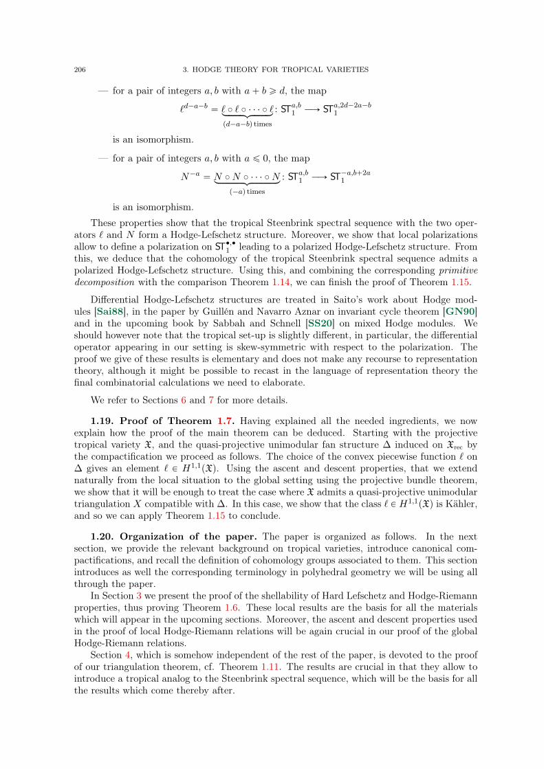
206 3. HODGE THEORY FOR TROPICAL VARIETIES
— for a pair of integers a, b with a` b ě d, the map
`d´a´b “ ` ˝ ` ˝ ¨ ¨ ¨ ˝ `loooooomoooooon
pd´a´bq times
: STa,b1 ÝÑ STa,2d´2a´b1
is an isomorphism.
— for a pair of integers a, b with a ď 0, the map
N´a “ N ˝N ˝ ¨ ¨ ¨ ˝Nloooooooomoooooooon
p´aq times
: STa,b1 ÝÑ ST´a,b`2a1
is an isomorphism.
These properties show that the tropical Steenbrink spectral sequence with the two oper-ators ` and N form a Hodge-Lefschetz structure. Moreover, we show that local polarizationsallow to define a polarization on ST‚,‚1 leading to a polarized Hodge-Lefschetz structure. Fromthis, we deduce that the cohomology of the tropical Steenbrink spectral sequence admits apolarized Hodge-Lefschetz structure. Using this, and combining the corresponding primitivedecomposition with the comparison Theorem 1.14, we can finish the proof of Theorem 1.15.
Differential Hodge-Lefschetz structures are treated in Saito’s work about Hodge mod-ules [Sai88], in the paper by Guillén and Navarro Aznar on invariant cycle theorem [GN90]and in the upcoming book by Sabbah and Schnell [SS20] on mixed Hodge modules. Weshould however note that the tropical set-up is slightly different, in particular, the differentialoperator appearing in our setting is skew-symmetric with respect to the polarization. Theproof we give of these results is elementary and does not make any recourse to representationtheory, although it might be possible to recast in the language of representation theory thefinal combinatorial calculations we need to elaborate.
We refer to Sections 6 and 7 for more details.
1.19. Proof of Theorem 1.7. Having explained all the needed ingredients, we nowexplain how the proof of the main theorem can be deduced. Starting with the projectivetropical variety X, and the quasi-projective unimodular fan structure ∆ induced on Xrec bythe compactification we proceed as follows. The choice of the convex piecewise function ` on∆ gives an element ` P H1,1pXq. Using the ascent and descent properties, that we extendnaturally from the local situation to the global setting using the projective bundle theorem,we show that it will be enough to treat the case where X admits a quasi-projective unimodulartriangulation X compatible with ∆. In this case, we show that the class ` P H1,1pXq is Kähler,and so we can apply Theorem 1.15 to conclude.
1.20. Organization of the paper. The paper is organized as follows. In the nextsection, we provide the relevant background on tropical varieties, introduce canonical com-pactifications, and recall the definition of cohomology groups associated to them. This sectionintroduces as well the corresponding terminology in polyhedral geometry we will be using allthrough the paper.
In Section 3 we present the proof of the shellability of Hard Lefschetz and Hodge-Riemannproperties, thus proving Theorem 1.6. These local results are the basis for all the materialswhich will appear in the upcoming sections. Moreover, the ascent and descent properties usedin the proof of local Hodge-Riemann relations will be again crucial in our proof of the globalHodge-Riemann relations.
Section 4, which is somehow independent of the rest of the paper, is devoted to the proofof our triangulation theorem, cf. Theorem 1.11. The results are crucial in that they allow tointroduce a tropical analog to the Steenbrink spectral sequence, which will be the basis for allthe results which come thereby after.
2. TROPICAL VARIETIES 207
In Section 5 we study the tropical Steenbrink spectral sequence, introduce the weightfiltration on tropical coefficient groups Fp, and prove the tropical Deligne resolution theoremas well as the comparison theorem between Steenbrink sequence and tropical cohomologygroups, cf. Theorem 1.14. For the ease of reading, few computational points of this sectionare treated separately in Appendix.
Kähler tropical varieties are introduced in Section 6. For a unimodular triangulation of asmooth tropical varieties which admits a Kähler form, the corresponding tropical Steenbrinkspectral sequence can be endowed with a Hodge-Lefschetz structure, where the monodromyoperator is the analog of the one arising in the classical Steenbrink spectral sequence and theLefschetz operator corresponds to multiplication with the Kähler class. Using an adaptationof the theory of Hodge-Lefschetz structure to the tropical setting, Sections 6 and 7 are devotedto the proof of the Kähler package for triangulated tropical varieties, cf. Theorem 1.15. Thefact that the Hodge-Lefchetz structure will be inherited in the cohomology in the tropicalsetting is treated in Section 7.
The last two sections are then devoted to the proof of Theorem 1.7. In Section 8, wepresent the proof of the projective bundle theorem, cf. Theorem 1.12. Section 9 then finishesthe proof of the main theorem using the materials developed in the previous sections, ascent-descent property, projective bundle theorem and Theorem 1.15.
The results presented in Appendix show that a certain triple complex constructed inSection 5 provides a spectral resolution of the tropical spectral sequence, associated to theweight filtration on the tropical complex. Due to the calculatory nature of the content ofthis section, and necessity of introducing extra notations, we have decided to include it onlyas an appendix. It is also written somehow independently of the rest of the paper. Thismeans we reproduce some of the materials from the paper there, and in few places, we adapta terminology slightly different from the one used in the main body. We have found thismore adapted both in terms of rigour and compactness to the purpose of this appendix whichrequires through case by case computations. Every time this change of terminology happens,we make a comment of comparison to the one used in the previous sections.
2. Tropical varieties
The aim of this section is to provide the necessary background on polyhedral spaces andtropical varieties. It contains a brief review of polyhedral geometry, tropical and Dolbeaultcohomology, as well as a study of canonical compactifications of polyhedral spaces, which willbe all used in the consequent sections. This will be also the occasion to fix the terminologyand notations which will be used all through the text.
2.1. Recollection in polyhedral geometry. A (closed convex) polyhedron of a realvector space V » Rn is a non-empty intersection of a finite number of affine half-spaces. Allthrough this paper, a polyhedron means a strongly convex one in the sense that we require itdoes not contain any affine line.
Let P be a polyhedron. The affine tangent space of P denoted by TaffP is by definition thesmallest affine subspace of Rn which contains P ; it is precisely the set of all linear combinationsof elements of P whose coefficients sum up to one. The linear tangent space, or simply tangentspace, of P denoted by TP is the linear subspace of Rn spanned by the differences x ´ y forany pair of elements x, y of P .
The dimension of P is denoted by |P |, which is by definition that of its tangent space. Aface of P is either P or any nom-empty intersection P XH for any affine hyperplane H suchthat P Ă H` where H` is one of the two half-spaces delimited by H. Note that a face of apolyhedron P is itself a polyhedron. We use the notation γ ă δ for two polyhedra if γ is aface of δ. If moreover γ is of codimension one in δ, i.e., |γ| “ |δ|´ 1, then we write γ ă δ. Aface of dimension zero is called a vertex of P . A face of dimension one is called an edge. The
208 3. HODGE THEORY FOR TROPICAL VARIETIES
interior of a polyhedron P refers to the relative interior of P in its affine tangent space, whichis by definition the complement in P of all the proper faces of P .
A cone is a polyhedron with a unique vertex which is the origin of Rn. (By our assumption,we only consider strongly convex cones, which means that the cone does not include any line.)A compact polyhedron is called a polytope; equivalently, a polytope is a polyhedron which isthe convex-hull of a finite number of points.
Suppose now that the vector space V » Rn comes with a full rank lattice N » Zn. Apolyhedron P in V is called rational if the half-spaces used to define P can be defined inNQ » Qn. We denote by NP the full-rank lattice N X TpP q in TpP q.
A polyhedron is called integral with respect to N if it is rational and all its vertices are inN . In the sequel, we simply omit to mention the underlying lattice N if this is clear from thecontext.
The Minkowski sum of two polyhedra P and Q in V is defined by
P `Q : “
x` yˇ
ˇ x P P, y P Q)
.
By Minkowski-Weyl theorem, every polyhedron P can be written as the Minkowski sumQ ` σ of a polytope Q and a cone σ. Moreover, one can choose Q to be the convex-hull ofthe vertices of P and the cone σ is uniquely characterized by the property that for any pointx P P , σ is the maximal cone verifying x` σ Ď P . We denote this cone by Prec.
It follows that for any polyhedron P , one can choose points v0, . . . , vk and vectors u1, . . . , ulin V such that
P “ convpv0, . . . , vkq `lÿ
i“1
R`ui.
Here and in the whole article, R` denotes the space of non-negative real numbers.A polyhedron P is called simplicial if we can choose the points vi and the vectors uj in
the above decomposition so that the collection of vectors pv1 ´ v0, . . . , vk ´ v0, u1, . . . , ulq beindependent. In this case, there is a unique choice for points v0, . . . , vk, which will be thevertices of P . (And the vectors u1, . . . , ul are in bijection with the rays of Prec.) We define
Pf :“ convpv0, . . . , vkq,
and we have P “ Pf ` Prec. Furthermore, any point x P P can be decomposed in a uniqueway as the sum x “ xf ` xrec of a point xf P Pf and a point xrec P Prec.
A simplicial polyhedron P is called unimodular with respect to the lattice N in V if it isintegral with respect to N and moreover, the points vi and the vectors uj can be chosen in Nso that pv1 ´ v0, . . . , vk ´ v0, u1, . . . , ulq is part of a basis of N (or equivalently, if they form abasis of the lattice NP “ N X TpP q).
A polyhedral complex in a real vector space V » Rn is a finite non-empty setX of polyhedrain Rn called faces of X such that for any pair of faces δ, δ1 P X
(i) any face of δ belongs to X, and
(ii) the intersection δ X δ1 is either empty or is a common face of δ and δ1.
A finite collection of polyhedraX which only verifies the first condition (i) is called a polyhedralpseudo-complex.
If P is a polyhedron, the set of faces of P form a polyhedral complex which we denoteby facepP q. A polyhedral complex which has a unique vertex is called a « fan » if the uniquevertex is the origin of V . In this case, all the faces of the complex are cones. The finite partof X denoted by Xf is the set of all compact faces of X, which is itself again a polyhedralcomplex. The support of X denoted by |X| is the union of the faces of X in V . A polyhedralcomplex whose support is the entire vector space V is said to be complete.

2. TROPICAL VARIETIES 209
A polyhedral complex is called simplicial, rational, integral, or unimodular (with respectto the lattice N), if all faces of X are simplicial, rational, integral, or unimodular (with respectto N), respectively.
Let X and Y be two polyhedral complexes in a real vector space V . We say that Y is asubdivision of X if X and Y have the same support, and each face of Y is included in a faceof X. We say that Y is a triangulation of X if in addition Y is simplicial. We say that Y is asubcomplex of X or that X contains Y if Y Ď X. In particular, the support of X contains thatof Y . We say that X contains a subdivision of Y if there exists a subdivision Z of Y whichis a subcomplex of X. The same terminology will be used for polyhedral pseudo-complexes.
Let S be a subset of a real vector space V » Rn. The set of affine linear functions on Sis defined as the restrictions to S of affine linear functions on V and is denoted by LpSq. Fora polyhedral complex, we simplify the notation and write LpXq instead of Lp|X|q.
Let f : |X| Ñ R be a continuous function. We say that f is piecewise linear on X if oneach face δ of X, the restriction f |δ of f to δ is affine linear. The set of piecewise linearfunctions on X is denoted by LpmpXq. (Lpm reads linéaire par morceaux.)
A function f P LpmpXq is called convex, resp. strictly convex, if for each face δ of X, thereexists an affine linear function ` P LpV q such that f ´ ` vanishes on δ and is non-negative,resp. strictly positive, on Uzδ for an open neighborhood U of the relative interior of δ in |X|.
We denote by KpXq, resp. , K`pXq, the set of convex, resp. strictly convex, functions inLpmpXq. A polyhedral complex X is called quasi-projective if the set K`pXq is non-empty.We will treat this notion of convexity in more detail in Section 4.3.
2.2. Canonical compactifications of fans. Let T “ RYt8u be the extended real linewith the topology induced by that of R and a basis of open neighborhoods of infinity givenby intervals pa,8s for a P R. Extending the addition of R to T in a natural way, by setting8 ` a “ 8 for all a P T, gives T the structure of a topological monoid. We call pT,`q themonoid of tropical numbers and denote by T` “ R` Y t8u the submonoid of non-negativetropical numbers with the induced topology.
Both monoids admit a natural scalar multiplication by non-negative real numbers (setting0 ¨ 8 “ 0). Moreover, the multiplication by any factor is continuous. As such, T and T` canbe seen as module over the semiring R`. Recall that modules of semirings are quite similarto classical modules over rings, except that such modules are commutative monoids instead ofbeing abelian groups. Another important collection of examples of topological modules overR` are the cones.
We can consider the tensor product of two modules over R`. In this section, every tensorproduct will be over R`, thus we will sometimes omit to mention it.
All through, N will be a free Z-module of finite rank and M “ N‹ denotes the dual ofN . We denote by NR and MR the corresponding real vectors spaces, so we have MR “ N‹R.For a polyhedron δ in NR, we use both the notations Nδ,R or Tδ, depending on the context,to denote the linear tangent space to δ which is the real vector subspace of NR generated bydifferences x ´ y for pairs of elements x, y in δ. Furthermore, we define the normal vectorspace of δ denoted N δ
R by N δR :“ NR
L
Nδ,R. If the polyhedron δ is rational, then we naturallyget lattices of full rank N δ and Nδ in N δ
R and Nδ,R, respectively.
By convention, all through this article, we most of the time use δ (or any other face) as asuperscript to denote the quotient of some space by Tδ, or to denote elements related to thisquotient. On the contrary, we use δ as a subscript for subspaces of Tδ or elements associatedto these subspaces.
For a fan Σ in NR, we denote by Σk the set of k-dimensional cones of Σ; elements of Σ1 arecalled rays. In the case the fan is rational, for any ray % P Σ1, we denote by e% the generatorof %XN .

210 3. HODGE THEORY FOR TROPICAL VARIETIES
For any cone σ, denote by σ_ ĎMR the dual cone defined by
σ_ :“!
m PMRˇ
ˇ xm, ay ě 0 for all a P σ)
.
The canonical compactification σ of a cone σ, called as well the extended cone of σ, isdefined by
σ :“ σ bR` T`.The topology on σ is the natural one, i.e., the finest one such that the projections
pσ ˆ T`qk ÝÑ σpxi, aiq1ďiďk ÞÝÑ
ř
i xi b ai,
for k P N, are continuous. The space σ is a compact topological space, whose restriction to σcoincides with the usual topology.
Remark 2.1. One can also define σ in the following way. If we work in the category ofR`-modules whose morphisms are morphisms of R`-modules. Then, by duality, we have
σ “ HomR`pσ_,T`q.
The advantage of this definition is that the link with the compactifications of toric varietiesis more direct (cf. below). However, the description of the topology and of the general shapeof σ is easier with the first definition. ˛
There is a distinguished point 8σ in σ defined by xb8 for any x in the relative interiorof σ. The definition does not depend on the chosen x. Note that for the cone 0, we have80 “ 0.
For an inclusion of cones τ ă σ, we get a map τ Ď σ. This inclusion identifies τ as thetopological closure of τ in σ.
Let Σ be a rational fan in NR. The canonical compactification Σ is defined as the union ofextended cones σ for any cone σ P Σ where we identify τ with the corresponding subspace ofσ for any inclusion of cones τ ă σ in Σ. The topology of Σ is the induced quotient topology.Each extended cone σ naturally embeds as a subspace of Σ.
The canonical compactification Σ of Σ naturally lives in a partial compactification of NRdefined by Σ that we denote by TPΣ. We define TPΣ as follows. For any cone σ in Σ,we consider the space rσ “ homR`pσ
_,Tq. The topology is defined in a way similar thanfor σ. We have a natural inclusion of σ into rσ. Notice that homR`pσ
_,Rq » NR. We setNσ8,R :“ 8σ `NR Ă rσ. Clearly N0
8,R “ NR. Moreover, from the fact that for any x P σ andany λ P R, 8σ ` λx “ 8σ, we can see the map
NR Ñ Nσ8,R, z ÞÑ z `8σ
as a projection along σ b R » Nσ,R. Indeed, one can prove that Nσ8,R » Nσ
R .Then, rσ is naturally stratified into a disjoint union of subspaces N τ
8,R, each isomorphic toN τ
R, for τ running over faces of σ. Because of this isomorphism, we might sometimes omit the8, when it is clear from the context that we are considering the stratum at infinity. Moreover,the inclusions rτ Ď rσ for pairs of elements τ ă σ in Σ allow to glue these spaces and define thespace TPΣ.
The partial compactification TPΣ of NR is naturally stratified as the disjoint union ofNσ8,R » Nσ
R for σ P Σ.For a rational fan Σ, we have TPΣ “ TroppPΣq the extended tropicalization of the toric
variety PΣ. In other words, TPΣ can be viewed as the tropical toric variety associated to thefan Σ. In particular, the tropical projective space TPn coincides with TPΣ for Σ the standardfan of the projective space Pn. We refer to [AP21,BGJK20,Kaj08,Pay09,Thu07] formore details.

2. TROPICAL VARIETIES 211
The canonical compactification Σ of Σ admits a natural stratification into cones and fansthat we describe now. Moreover, this stratification can be enriched into an extended polyhedralstructure [AP20a], see Section 2.3 for more details.
Consider a cone σ P Σ and a face τ of σ. Let Cτσ :“ 8τ ` σ Ď σ. From this description,one sees that Cτσ is isomorphic to the projection of the cone σ in the linear space Nσ,R
L
Nτ,R ãÑ
N τ8,R. We denote by C˝τσ the relative interior of Cτσ .One can show that the canonical compactification Σ is a disjoint union of (open) cones
C˝τσ for pairs τ ă σ of elements of Σ.For a fixed cone τ P Σ, the collection of cones Cτσ for elements σ P Σ with τ ă σ form a
fan with origin 8τ that we denote by Στ8Ă N τ
8,R. Note that with this terminology, for thecone 0 of Σ we have Σ0
8“ Σ.
The fan Στ8is canonically isomorphic to the star fan of τ in Σ denoted by Στ and defined
by
Στ :“!
πτ pσqˇ
ˇ
ˇσ ą τ is a cone in Σ
)
,
where πτ : NR Ñ N τR. Note that our use of the star fan is consistent with the one used
in [AHK18] and differs from the usual terminology, e.g., in [Kar04,BBFK02] where this iscalled transversal fan.
If there is no risk of confusion, we sometimes drop 8 and write Στ when referring to thefan Στ
8based at 8τ .
For any pair pτ, σq with τ ă σ, the closure Cτσ of Cτσ in Σ is the union of all the cones C˝τ1
σ1
with τ ă τ 1 ă σ1 ă σ. The closure of Στ8is indeed canonically isomorphic to the canonical
compactification of Στ Ď N τR.
The stratification of Σ by cones Cτσ and their closures is called the conical stratification ofΣ. Note that there is a second stratification of Σ into fans Στ
8for τ P Σ.
By definition, from the inclusion of spaces σ Ď rσ, we get an embedding Σ Ď TPΣ. Sincethe strata Στ
8of Σ lives in N τ
8,R, this embedding is compatible with the stratification of bothspaces. In particular, Σ is the compactification of the fan Σ in the tropical toric variety TPΣ.
2.3. Extended polyhedral structures. We now describe an enrichment of the cate-gory of polyhedral complexes and polyhedral spaces into extended polyhedral complexes andextended polyhedral spaces by replacing the ambient spaces V » Rn with Tn, or more gener-ally, with a partial compactification TPσ for the fan facepσq associated to a cone σ in V , asdescribed in the previous section. For more details we refer to [JSS19,MZ14, IKMZ19].
Let n be a natural number and let x “ px1, . . . , xnq be a point of Tn. The sedentarity ofx denoted by sedpxq is the set J of all integers j P rns with xj “ 8. The space Tn is stratifiedinto subspaces RnJ for J Ď rns where RnJ consists of all points of x of sedentarity J . Note thatRnJ » Rn´|J |.
More generally, let σ be a cone in V . By an abuse of the notation, we denote by σ the fanin V which consists of σ and all its faces. By the construction described in the previous section,σ provides a partial compactification TPσ of V , where we get a bijection between strata V τ
8
of TPσ and faces τ of the cone σ. In the context of the previous section, the stratum V τ8
wasdenoted N τ
8,R.Generalizing the definition of the sedentarity, for any point x P TPσ which lies in the
stratum V τ8, with τ ă σ, the sedentarity of x is by definition sedpxq :“ τ . For σ the positive
quadrant in Rn, these definitions coincide with the ones in the preceding paragraph, as we getTPσ “ Tn and the subfaces of σ can be identified with the subsets rns.
An extended polyhedron δ in TPσ is by definition the topological closure in TPσ of anypolyhedron included in a strata V τ
8for some τ ă σ. A face of δ is the topological closure of a
212 3. HODGE THEORY FOR TROPICAL VARIETIES
face of δX V ζ8for some ζ ă σ. An extended polyhedral complex in TPσ is a finite collection X
of extended polyhedra in TPσ such that the two following properties are verified.— For any δ P X, any face γ of δ is also an element of X.— For pair of elements δ and δ1, the intersection δ X δ1 is either empty or a common
face of δ and δ1.The support of the extended polyhedral complex |X| is by definition the union of δ P X.The space X “ |X| is then called an extended polyhedral subspace of TPσ, and X is called anextended polyhedral structure on X.
We now use extended polyhedral subspaces of partial compactifications of vector spacesof the form TPσ as local charts to define more general extended polyhedral spaces.
Let n and m be two natural numbers, and let V1 » Rn and V2 » Rm be two vector spaceswith two cones σ1 and σ2 in V1 and V2, respectively. Let φ : V1 Ñ V2 be an affine map betweenthe two spaces and denote by A be the linear part of φ. Let I be the set of rays % ă σ1 suchthat A% lives inside σ2. Let τI be the cone of σ1 which is generated by the rays in I. Theaffine map φ can be then extended to a map
Ť
ζăσ1ζĎτI
V ζ1,8 Ñ TPσ2 denoted by φ by an abuse
of the notation. We call the extension an extended affine map. More generally, for an opensubset U Ď TPσ1 , a map φ : U Ñ TPσ2 is called an extended affine map if it is the restrictionto U of an extended affine map φ : TPσ1 Ñ TPσ2 as above. (The definition thus requires thatU is a subset of
Ť
ζăσ1ζĎτI
V ζ1,8.) In the case V1 and V2 come with sublattices of full ranks, the
extended affine map is called integral if the underlying map φ is integral, i.e., if the linear partA is integral with respect to the two lattices.
An extended polyhedral space is a Hausdorff topological space X with a finite atlas of charts´
φi : Wi Ñ Ui Ď Xi
¯
iPIfor I a finite set such that
—
Wi
ˇ
ˇ i P I(
form an open covering of X;— Xi is an extended polyhedral subspace of TPσi for a finite dimensional real vector
space Vi » Rni and a cone σi in Vi, and Ui is an open subset of Xi; and— φi are homeomorphisms between Wi and Ui such that for any pair of indices i, j P I,
the transition map
φj ˝ φ´1i : φipWi XWjq Ñ TPσj
is an extended affine map.
The extended polyhedral space is called integral if the transition maps are all integral withrespect to the lattices Zni in Rni .
Let X be an extended polyhedral space with an atlas of charts´
φ : Wi Ñ Ui Ď Xi
¯
iPIas above. A face structure on X is the choice of an extended polyhedral complex Xi with|Xi| “ Xi for each i and a finite number of closed sets θ1, . . . , θN , for N P N, called facetswhich cover X such that the following two properties are verified.
— Each facet θj is contained in some chartWi for i P I such that φipθjq is the intersectionof the open set Ui with a face ηj,i of the polyhedral complex Xi.
— For any subset J Ď rN s, any j P J , and any chart Wi which contains θj , the imageby φi of the intersection
Ş
jPJ θj in Ui is the intersection of Ui with a face of ηj,i.
A face of the face structure is the preimage by φi of a face of ηj,i for any j P rN s and for anyi P I such that θj Ď Wi. Each face is contained in a chart Wi and the sedentarity of a face δin the chart Wi is defined as the sedentarity of any point in the relative interior of φipδq seenin Xi.
2. TROPICAL VARIETIES 213
Proposition 2.2. Let Σ be a fan in NR. The canonical compactification Σ naturallyadmits the structure of an extended polyhedral space, and a face structure given by the closureCτσ in Σ of the cone Cτσ in the conical stratification of Σ, for pairs of cones τ ă σ in Σ. The
extended polyhedral structure is integral if Σ is a rational fan.
Proof. This is proved in [AP20a].
Note that the sedentarity of the face Cτσ of the conical stratification of Σ is the set of raysof τ .
2.4. Recession fan and canonical compactification of polyhedral complexes. LetX be a polyhedral complex in a real vector space NR » Rn. The recession pseudo-fan of Xdenoted by Xrec is the set of cones tδrec
ˇ
ˇ δ P Xu. In fact the collection of cones δrec donot necessary form a fan, as depicted in the following example; we will however see later inSection 4 how to find a subdivision of X whose recession pseudo-fan becomes a fan. In sucha case, we will call Xrec the recession fan of X. Recession fans are studied in [BS11].
Example 2.3. Let V “ R3 and denote by pe1, e2, e3q the standard basis of R3. Define
σ1 “ R`e1 ` R`e2 Ă R3,
σ2 “ R`e1 ` R`pe1 ` e2q Ă R3,
X “ facepσ1q Y face pe3 ` σ2q .
Note that Xrec contains the cones σ1 and σ2 whose intersection is not a face of σ1. ˛
Let X be a polyhedral complex in NR » Rn whose recession pseudo-fan Xrec is a fan.Let TPX8 be the corresponding tropical toric variety. The canonical compactification of Xdenoted by X is by definition the closure of X in TPX8 .
We now describe a natural stratification ofX. Let σ P Xrec, and consider the correspondingstratum Nσ
8,R of TPσ. Define Xσ8to be the intersection of X with Nσ
8,R, that without risk ofconfusion, we simply denote Xσ by dropping 8. Note that X0 “ X, which is the open partof the compactification X.
Let D “ XzX be the boundary at infinity of the canonical compactification of X. Foreach non-zero cone σ in Xrec, we denote by Dσ the closure of Xσ in X.
Theorem 2.4 (Tropical orbit-stratum correspondence). Notations as above, let X be apolyhedral complex in NR » Rn. We have the following.
(1) For each cone σ P Xrec, the corresponding strata Xσ is a polyhedral complex in Nσ8,R.
(2) The pseudo-recession fan pXσqrec of Xσ is a fan which coincides with the fan pXrecqσ8
in Nσ8,R in the stratification of the canonical compactification Xrec of the fan Xrec.
(3) The closure Dσ of Xσ coincides with the canonical compactification of Xσ in Nσ8,R,
i.e., Dσ “ Xσ.
(4) If X has pure dimension d, then each stratum Xσ as well as their closures Dσ havepure dimension d´ |σ|.
In particular, the canonical compactification X is an extended polyhedral structure with a facestructure induced from that of X.
Proof. The theorem is proved in [AP20a].
214 3. HODGE THEORY FOR TROPICAL VARIETIES
2.5. Tropical homology and cohomology groups. We recall the definition of tropicalcohomology groups and refer to [IKMZ19,JSS19,MZ14,GS19b] for more details.
Let X be an extended polyhedral space with a face structure. We start by recalling thedefinition of the multi-tangent and multi-cotangent spaces Fppδq and Fppδq, respectively, forthe face δ of X. This leads to the definition of a chain, resp. cochain, complex which calculatesthe tropical homology, resp. cohomology, groups of X.
For a face δ of X and for any non-negative integer p, the p-th multi-tangent and the p-thmulticotangent space of X at δ denoted by Fppδq and Fppδq are defined by
Fppδq “ÿ
ηąδsedpηq“sedpδq
ŹpTη, and Fppδq “ Fppδq‹.
For an inclusion of faces γ ă δ in X, we get maps iδąγ : Fppδq Ñ Fppγq and i˚γăδ : Fppγq ÑFppδq.
For a pair of non-negative integers p, q, define
Cp,qpXq :“à
δPX|δ|“q
Fppδq
and consider the cellular chain complex, defined by using maps iδąγ as above,
Cp,‚ : . . . ÝÑ Cp,q`1pXqB
tropq`1ÝÝÝÑ Cp,qpXq
Btropq
ÝÝÝÝÑ Cp,q´1pXq ÝÑ ¨ ¨ ¨
The tropical homology of X is defined by
Htropp,q pXq :“ HqpCp,‚q.
Similarly, we have a cochain complex
Cp,‚ : . . . ÝÑ Cp,q´1pXqBq´1tropÝÝÝÑ Cp,qpXq
Bqtrop
ÝÝÝÝÑ Cp,q`1pXq ÝÑ ¨ ¨ ¨
whereCp,qpXq :“
à
δPX|δ|“q
Fppδq.
The tropical cohomology of X is defined by
Hp,qtroppXq :“ HqpCp,‚q.
In the case X comes with a rational structure, one can define tropical homology andcohomology groups with integer coefficients. In this case, for each face δ, the tangent spaceTδ has a lattice Nδ. One defines then
Fppδ,Zq “ÿ
ηąδsedpηq“sedpδq
ŹpNη, and Fppδ,Zq “ Fppδ,Zq‹.
Similarly, we get complexes with Z-coefficients CZp,‚ and C
p,‚Z , and define
Htropp,q pX,Zq :“ HqpC
Zp,‚q Hp,q
troppX,Zq :“ HqpCp,‚Z q.
Similarly, working with the cochain Cp,‚c with compact support, one can define tropicalcohomology groups with compact support. We denote them by Hp,q
trop,cpX,Aq with coefficientsA “ Z,Q, or R. If the coefficient field is not specified, it means we are working with realcoefficients. We define as well the homology groups HBM
p,q pX,Aq the tropical analogue of theBorel-Moore homology.
2. TROPICAL VARIETIES 215
2.6. Dolbeault cohomology and comparison theorem. In this section we brieflyrecall the formalism of superforms and their corresponding Dolbeault cohomology on ex-tended polyhedral complexes. The main references here are [JSS19,JRS18], see also [Lag12,CLD12,GK17].
Let V » Rn be a real vector space and denote by V ‹ its dual. We denote by Ap the sheafof differential forms of degree p on V . Note that the sheaf Ap is a module over the sheaf ofrings of smooth functions C8. The sheaf of (super)forms of bidegree pp, qq denoted by Ap,q isdefined as the tensor product Ap bC8 Aq. Choosing a basis Bx1 , . . . , Bxn of V , we choose twocopies of the dual vector space V ‹ with the dual basis d1x1, . . . ,d
1xn for the first copy andd2x1, . . . ,d
2xn for the second. In the tensor product ApbAq the first basis is used to describethe forms in Ap and the second basis for the forms in Aq. So for an open set U Ď V , a sectionα P Ap,q is uniquely described in the form
α “ÿ
I,JĎrns|I|“p,|J |“q
αI,J d1xI ^ d2xJ
for smooth functions αI,J P C8pUq. Here for a subset I “ ti1, . . . , i`u Ď rns with i1 ă i2 ă
¨ ¨ ¨ ă i`, we denote by d1xI and d2xI the elements of the two copies ofŹ`V ‹ defined by
d1xI “ d1xi1 ^ ¨ ¨ ¨ ^ d1xi` and d2xI “ d2xi1 ^ ¨ ¨ ¨ ^ d2xi` ,
respectively. Moreover, for subsets I, J Ď rns, d1xI ^ d2xJ is the element ofŹpV ‹ b
ŹqV ‹
given by d1xI b d2xJ . The usual rules of the wedge product apply. In particular, for anyi, j P rns,
d2xj ^ d1xi “ ´d1xi ^ d2xj .
Observing that Ap,q » Ap bRŹqV ‹ and Ap,q »
ŹpV ‹ b Aq, the collection of bigradedsheaves Ap,q come with differential operators d1 : Ap,q Ñ Ap`1,q and d2 : Ap,q Ñ Ap,q`1 definedby d1 “ dp b id and d2 “ id b dq where for non-negative integer `, d` : A` Ñ A``1 is thedifferentiation of smooth `-forms. More explicitly, the differential map d2 is defined by itsrestriction to open sets U Ď V
Ap,qpUq Ñ Ap,q`1pUq
and sends a pp, qq-form α “ř
I,J αI,J d1xI ^ d2xJ to
d2α “ÿ
I,J
nÿ
`“1
Bx`αI,J d2x` ^ d1xI ^ d2xJ “ p´1qpÿ
I,J
nÿ
`“1
Bx`αI,J d1xI ^ pd2x` ^ d2xJq.
The operator d1 has a similar expression.
Consider now a fan Σ in V , and let TPΣ be the corresponding partial compactification ofV . We define the sheaf of bigraded pp, qq-forms Ap,q on TPΣ as follows. For each pair of conesτ ă σ of Σ, we have a natural projection πτăσ : V τ
8Ñ V σ
8. This projection induces a map
π˚σąτ : Ap,qpV σ8q Ñ Ap,qpV τ
8q. Let U Ď TPΣ be an open set. A section α P Ap,qpUq is the data
of the collection of pp, qq-forms ασ P Ap,qpU XV σ8q, where U XV σ
8is viewed as an open subset
of the real vector space V σ8» V
L
Tσ, so that the following compatibility at infinity is verifiedamong these sections. For each pair of cones τ ă σ in Σ, there exists a neighborhood U 1 ofU X V σ
8in U such that the restriction of ατ to U 1 is given by the pullback π˚σąτ
`
ασ˘
|U 1 .The differential operators d1 and d2 naturally extend to TPΣ and define operators
d1 : Ap,q Ñ Ap`1,q and d2 : Ap,q Ñ Ap,q`1
for any pair of non-negative integers pp, qq.
Let now X be a closed polyhedral complex in TPΣ, and denote ι : X ãÑ TPΣ the inclusion.The sheaf of pp, qq-forms Ap,q
X is defined as a quotient of the restriction ι˚Ap,qTPΣ
of the sheafof pp, qq-forms on TPΣ to X modulo those sections which vanish on the tangent space of X.
216 3. HODGE THEORY FOR TROPICAL VARIETIES
Thus for an open set U in X, a section α P Ap,qX pUq is locally around each point x given by
a section αx P Ap,qpUxq for an open subset Ux Ď TPΣ with Ux X X Ď U , and two sectionsα and β in Ap,q
X pXq are equivalent if for any point x living in a face σ of X, the differenceαpxq ´ βpxq vanishes on any pp, qq-multivector in
ŹpTσ bŹqTσ.
The definition above can be extended to any extended polyhedral complex.The two differential operators d1 and d2 naturally extend to TPX8 and we get d1 : Ap,q
X Ñ
Ap`1,qX and d2 : Ap,q
X Ñ Ap,q`1X for any pair of non-negative integers pp, qq.
The above definition only depends on the support of X and not on the chosen polyhedralstructure on this support. As a consequence, if X is any polyhedral space, the sheaf Ap,q
X iswell-defined.
The Dolbeault cohomology group Hp,qDolpXq of bidegree pp, qq is by definition the q-th coho-
mology group of the cochain complex`
Ap,‚X pXq,d
2˘
: Ap,0X pXq Ñ Ap,1
X pXq Ñ ¨ ¨ ¨ Ñ Ap,q´1X pXq Ñ Ap,q
X pXq Ñ Ap,q`1X pXq Ñ ¨ ¨ ¨
Similarly, we define Dolbeault cohomology groups with compact support Hp,qDol,cpXq as the
q-th cohomology group of the cochain complex`
Ap,‚X,cpXq,d
2˘
: Ap,0X,cpXq Ñ Ap,1
X,cpXq Ñ ¨ ¨ ¨
where Ap,qX,cpXq is the space of pp, qq-forms whose support forms a compact subset of X.
Denote by ΩpX the kernel of the map d2 : Ap,0
X Ñ Ap,1X . We call this the sheaf of holomorphic
p-forms on X. By Poincaré lemma for superforms, proved in [Jel16a,JSS19], the complexpAp,‚, d2q provides an acyclic resolution of the sheaf Ωp
X . We thus get the isomorphism
Hp,qDolpXq » HqpX,Ωp
Xq,
and similarly,Hp,q
Dol,cpXq » Hqc pX,Ω
pXq.
Moreover, we have the following comparison theorem from [JSS19].
Theorem 2.5 (Comparison theorem). For any extended polyhedral complex X, we have
Hp,qtroppXq » Hp,q
DolpXq, and Hp,qtrop,cpXq » Hp,q
Dol,cpXq.
2.7. Tropical fans, smoothness and shellability. We recall the definition of tropicalfans and refer to [AP21] for their basic properties. More results related to algebraic andcomplex geometry can be found in [Mik06,Mik07,AR10,GKM09,KM09,Kat12,Bab14,BH17,Gro18] and [MS15,MR09,BIMS15].
A tropical fan Σ is a rational fan of pure dimension d, for a natural number d P Zě0, whichverifies the balancing condition: namely, for any cone τ of dimension d´ 1 in Σ, we require
ÿ
σ ąτ
eστ “ 0 P N τ .
Here eστ is the primitive vector of the ray ρστ corresponding to σ in N τR.
Let Σ be a tropical fan of dimension d. The Borel-Moore homology group HBM
d,dpΣq containsa canonical element νΣ, the analogue of the fundamental cycle in the tropical setting. Usingthe cap product ", we get a natural map
¨" νΣ : Hp,qpΣq ÝÑ HBM
d´p,d´qpΣq.
We say that a simplicial tropical fan Σ verifies the Poincaré duality if the above map is anisomorphism for any bidegree pp, qq. A tropical fan Σ is called smooth if for any cone σ P Σ,the star fan Σσ verifies the Poincaré duality. In this paper, the star fan Σσ refers to the fanin NR
L
Nσ,R induced by the cones η in Σ which contain σ as a face.We have the following list of properties of the category of smooth tropical fans.
2. TROPICAL VARIETIES 217
(1) Smoothness only depends on the support of the tropical fan.
(2) Smoothness is a local condition, namely that, a tropical fan is smooth if it is smootharound each of its points.
(3) The category of smooth tropical fans is closed under products. In fact, we have thefollowing stronger property: Let Σ1,Σ2 be two tropical fans and set Σ “ Σ1 ˆ Σ2
(which is again a tropical fan). Then Σ is smooth if and only if Σ1 and Σ2 are bothsmooth.
(4) Any complete rational fan, i.e., a fan with support equal to NR, is tropically smooth.
(5) Bergman fans of matroids are tropically smooth in the above sense.
(6) The category of smooth tropical fans is stable under tropical modifications alongsmooth divisors.
We refer to [AP21] for more details.In order to show the category of smooth tropical fans is large, we introduce in [AP21] a
tropical notion of shellability. This is based on two types of operations on tropical fans, thatof star subdivision and tropical modification. A tropical fan is called shellable if it can beobtained from a collection of basic tropical fans by only using these two operations. We referto [AP21] for the formal definition and basic properties.
We prove the following result in [AP21].
Theorem 2.6. Any shellable tropical fan is smooth.
2.8. Tropical cycles and divisors. Let V “ NR » Rn be a real vector space of dimen-sion n with a full rank lattice N . Let Y be a rational polyhedral complex of pure dimensiond in V . For each facet σ of Y , suppose we are given a weight which is an integer wpσq. LetC :“ pY,wq be the weighted polyhedral complex Y with the weight function on its facetsw. The weighted polyhedral complex C is called a tropical cycle if the following balancingcondition is verified:
@τ P Y of dimension d´ 1,ÿ
σ ąτ
wpσqeστ “ 0 P N τ .
The following is a direct consequence of the definition of a tropical fan given in the previoussection.
Proposition 2.7. The tropical fan Σ with weights equal to one on facets is a tropicalcycle.
A tropical regular function f on a tropical cycle C is a piecewise affine function withintegral slopes which is the restriction to C of a concave function on Rn. In other words, it isa function of the form
f “ miniPI
xαi, ¨ y ` βi(
for a finite index set I and αi P Zn, βi P Q.Any tropical regular function induces a subdivision of the tropical cycle C. On each face
δ of C, the new polyhedral structure consists of set of the form tx P δˇ
ˇ fpxq “ gpxqu whereg is an affine linear function such that gpxq ě fpxq for every x. Keeping the same weight onfacets, this leads to a new tropical cycle that we denote by C1 and note that C and C1 havethe same support and same weight function.
Given a tropical regular function f on C, we can consider the graph Γf of f in V ˆ R »Rn`1, with the polyhedral structure obtained by that of the subdivided C1. The graph Γf isnot necessary a tropical cycle in V ˆR anymore, as it might have unbalanced codimension onefaces. In this case, we can add new faces to Γf to obtain a tropical cycle. For this, consider
218 3. HODGE THEORY FOR TROPICAL VARIETIES
a codimension one face δ of C1 which turns to be unbalanced in the graph Γf . Consider thepolyhedron Eδ defined by
Eδ :“!
px, tqˇ
ˇ x P δ and t ě fpxq)
Ă V ˆ R.
Define rC as the union of Γf with the polyhedra Eδ and there faces, one polyhedron for eachunbalanced codimension one face δ of Γf . Note that for each such face δ, the primitive vectoreEδδ is the one given by the last vector en`1 in the standard basis of V ˆ R » Rn`1.
One verifies there is a unique integer weight wpEδq which we can associate to new faces Eδin order to make rC a tropical cycle in V ˆR. The new tropical cycle in V ˆR is called tropicalmodification of C along divCpfq, where divCpfq is the union of the δ in C1 of codimensionone which happens to be unbalanced when seen in Γf .
2.9. Tropical smoothness of the support. An extended polyhedral complex X is saidto have a tropically smooth, or simply smooth, support if its support |X| is locally isomorphicto a product Ta ˆ |Σ| for a non-negative integer a and a smooth tropical fan Σ.
We prove in [AP21] that the canonical compactification of any unimodular smooth tropicalfan is smooth. In fact, we have the following more general result.
Theorem 2.8. Let X be a rational polyhedral complex in NR with smooth support. Supposethat the recession fan Xrec is unimodular. Then the canonical compactification X of X hassmooth support. Moreover, if the polyhedral structure on X is unimodular, then the inducedextended polyhedral structure on X, given in Theorem 2.4, is unimodular as well.
3. Local Hodge-Riemann and Hard Lefschetz
The aim of this section is to study the local situation and to prove Theorem 1.6.The results in this section are valid for integral, rational, or real Chow rings of smooth
tropical fans when they are definable. Since our primary objective in this paper is to establishglobal versions of these results, and we do not have tried to control the torsion part of thetropical cohomology for more general tropical varieties, to simplify the presentation, we willonly consider the case of rational fans and we suppose the coefficient ring K be either Q or R.
3.1. Basic definitions and results. In this section, we review some basic results con-cerning Hodge theory of finite dimensional algebras.
Let A‚ “À
iPZAi be a graded vector space of finite dimension over K such that the graded
pieces of negative degree are all trivial.
Definition 3.1 (Poincaré duality). We say that A‚ verifies
- weak Poincaré duality for an integer d denoted by WPDdpA‚q if for any integer k, wehave the equality dimKA
k “ dimKAd´k.
Let Φ: A‚ˆA‚ Ñ K be a symmetric bilinear form on A‚. We say that the pair pA‚,Φq verifies
- Poincaré duality for an integer d that we denote by PDdpA‚,Φq if Φ is non-degenerateand for any integer k, Ak is orthogonal to Al for all l ‰ d´ k. ˛
Let A‚ be a graded K-vector space of finite dimension as above, let d be a positive integer,and let Q be a symmetric bilinear form on the truncation
À
kď d2Ak such that Ai and Aj are
orthogonal for distinct pair of non-negative integers i, j ď d2 .
Definition 3.2 (Hard Lefschetz). Notations as above, we say that the pair pA‚, Qq verifies
- Hard Lefschetz property denoted HLdpA‚, Qq if A‚ verifies WPDdpA‚q and Q is non-degenerate. ˛
3. LOCAL HODGE-RIEMANN AND HARD LEFSCHETZ 219
In the sequel, for any k ď d2, we denote by Qk the restriction of Q to Ak.
Definition 3.3 (Hodge-Riemann). We say the pair pA‚, Qq verifies
- Hodge-Riemann relations HRdpA‚, Qq if A‚ verifies WPDdpA‚q and moreover, foreach non-negative integer k ď d
2 , the signature of Qk is given by the sumkÿ
i“0
p´1qi`
dimpAiq ´ dimpAi´1q˘
. ˛
Remark 3.4. As we will show in Proposition 3.5 below, the above definitions are in factequivalent to the ones given in the introduction. ˛
3.1.1. Bilinear form associated to a degree map. Assume that A‚ is a unitary graded K-algebra with unit 1A‚ and suppose A0 “ K ¨ 1A‚ . Moreover, suppose that we are given alinear form deg : Ad Ñ K called the degree map which we extend to the entire algebra A‚ bydeclaring it to be zero on each graded piece Ak for k ‰ d. In this way, we get a bilinear formon A‚ denoted by Φdeg and defined by
Φdeg : A‚ ˆA‚ Ñ K,pa, bq ÞÑ degpabq.
3.1.2. Lefschetz operator and its associated bilinear form. Notations as in the precedingparagraph, let now L : A‚ Ñ A‚`1 be a morphism of degree one which sends any element a ofA‚ to the element La P A‚`1. Let Φ be a symmetric bilinear form on A‚. For example, if wehave a degree map on A‚, we can take Φ “ Φdeg.
We define a bilinear form QL,Φ on A‚ by setting
@ a P Ak, b P Aj , QL,Φpa, bq :“ Φpa, Ld´2kbq
for all pairs of integers k, j ď d2. We furthermore require Aj and Ak to be orthogonalfor j ‰ k. In the case Φ “ Φdeg, we will have QL,Φpa, bq “ degpa ¨ Ld´2kbq and this latterrequirement will be automatic.
Assuming that L is auto-adjoint with respect to QL,Φ, i.e., Φpa, Lbq “ ΦpLa, bq for alla, b P A‚, we get a symmetric bilinear form Q “ QL,Φ on A‚.
If L is given by multiplication by an element ` P A1 and Φ “ Φdeg, we write ` instead ofL for the corresponding map, and write Q` for the corresponding bilinear form, which is thenautomatically symmetric: in fact, we have
Q`pa, bq “ degp`d´2kabq
for any pair of elements a, b P Ak. In this case, we write HLdpA‚, `q and HRdpA‚, `q insteadof HLdpA‚, Q`,Φdeg
q and HRdpA‚, Q`,Φdegq, respectively. If there is no risk of confusion, we
furthermore omit the mention of the top dimension d in the above notations. Moreover, wesometimes use deg instead of Φdeg in order to simplify the notation.
3.1.3. Primitive parts induced by a Lefschetz operator. For a Lefschetz operator L : A‚ ÑA‚`1, as in the preceding section, and for a non-negative integer k ď d
2 , the primitive part ofAk with respect to L denoted by Akprim,L is by definition the kernel of the map
Lr´2k`1 : Ak ÝÑ Ak´r`1.
If L is given by an element ` P A1, we denoted by Akprim,` the primitive part of Ak withrespect to `.
If there is no risk of confusion, and L or ` are understood from the context, we simplydrop them and write Akprim for the primitive part of Ak.
220 3. HODGE THEORY FOR TROPICAL VARIETIES
3.1.4. Basic implications and consequences. For future use, we state here basic resultsaround these notions and some of their consequences.
We start by the following proposition which gathers several useful implications and rela-tions between the properties introduced above.
We use the notations of the preceding paragraph. We suppose the Lefschetz operator L isauto-adjoint with respect to Φ so that the corresponding bilinear form becomes symmetric.
Proposition 3.5. Notations as above, the following properties are verified.
(3.1) HRdpA‚, L,Φq ùñ HLdpA‚, L,Φq ùñ PDdpA‚,Φq ùñ WPDdpA‚q.
(3.2)HLdpA‚, L,Φq ðñ
#
PDdpA‚,Φq and@ k ď d2, Ld´2k : Ak Ñ Ad´k is an isomorphism.
(3.3)
HRdpA‚, L,Φq ðñ
#
WPDdpA‚q
@k ď d2, the restriction p´1qkQL,Φ|Akprimis positive definite.
(3.4) For S : A‚ Ñ A‚ an automorphism of degree 0,
PDpA‚,Φq ðñ PDpA‚,Φ ˝ Sq,
HLpA‚, Qq ðñ HLpA‚, Q ˝ Sq,
HRpA‚, Qq ðñ HRpA‚, Q ˝ Sq.
(3.5) For two graded K-algebras A‚ and B‚, we have
WPDpA‚q and WPDpB‚q ðñ WPDpA‚q and WPDpA‚ ‘B‚q,
PDpA‚,ΦAq and PDpB‚,ΦBq ðñ PDpA‚,ΦAq and PDpA‚ ‘B‚,ΦA ‘ ΦBq,
HLpA‚, QAq and HLpB‚, QBq ðñ HLpA‚, QAq and HLpA‚ ‘B‚, QA ‘QBq,
HRpA‚, QAq and HRpB‚, QBq ðñ HRpA‚, QAq and HRpA‚ ‘B‚, QA ‘QBq.
(3.6) For two graded K-algebras A‚ and B‚, we have
WPDpA‚q and WPDpB‚q ùñ WPDpA‚ bB‚q,
PDpA‚,ΦAq and PDpB‚,ΦBq ùñ PDpA‚ bB‚,ΦA b ΦBq,
HLpA‚, QAq and HLpB‚, QBq ùñ HLpA‚ bB‚, QA bQBq,
HRpA‚, QAq and HRpB‚, QBq ùñ HRpA‚ bB‚, QA bQBq.
(3.7) For two graded K-algebras A‚ and B‚
ΦdegA b ΦdegB “ ΦdegAb degB , andQLA,ΦA ‘QLB ,ΦB “ QLA‘LB ,ΦA‘ΦB .
(3.8) For two graded K-algebras A‚ and B‚, we have
HRpA‚, LA,ΦAq and HRpB‚, LB,ΦBq ùñ HRpA‚ bB‚, LA b id` idb LB,ΦA b ΦBq.
Most of these statements are routine. We only give the proof of the first three and thevery last statements.
Proof of (3.1). The last implication is trivial. If HLdpA‚, L,Φq holds, then the bilinearform Q “ QL,Φ is non-degenerate. This implies that for each non-negative integer k ď d2, themap Ld´2k is injective on Ak. By WPDdpA‚q, this implies that Ld´2k induces an isomorphismbetween Ak and Ad´k, and so, as Aj and Ak are orthogonal for distinct pair of integers j andk, by our requirement, this implies that Φ is non-degenerate and so we have PDdpA‚,Φq.
3. LOCAL HODGE-RIEMANN AND HARD LEFSCHETZ 221
It remains to prove the first implication. We prove by induction on k that Qk is non-degenerate. The case k “ 0 is immediate by the assumption on the signature and the factthat A0 “ K ¨ 1A‚ . Assume this holds for k´ 1 and k ď d2. Since L is auto-adjoint, we havefor any a, b P Ak´1,
Qk´1pa, bq “ QkpLa,Lbq
which implies that L : Ak´1 Ñ Ak is injective, and Qk restricted to LpAk´1q is non-degenerateand has signature that of Qk´1. Since the difference between the signature of Qk and that ofQk´1 is p´1qk
`
dimpAkq´dimpAk´1q˘
“ p´1qk`
dimpAkq´dimpLAk´1q˘
, it follows that Qk isnon-degenerate.
Proof of (3.2). The implication ñ follows from the proof of (3.1). The reverse impli-cation is a consequence of our requirement that Aj and Ak are orthogonal for Φ if j and k aredistinct, which combined with the non-degeneracy of Φ and the isomorphism between Ak andAd´k induced by Ld´2k, implies that Qk is non-degenerate.
Proof of (3.3). Let Q “ QL,Φ. By (3.1), HRdpA‚, L,Φq implies HLdpA‚, L,Φq. ByProposition 3.6 below this leads to an orthogonal decomposition
Ak “kà
i“0
Lk´iAiprim “ Akprim ‘ LAk´1
where the restriction of Qk to LAk´1 coincides with that of Qk´1 on Ak´1. Proceeding byinduction and using HRdpA‚, L,Φq which gives the signature of Qk, we get the implicationñ.
It remains to prove the reverse implication ð. We proceed by induction and show thatthe bilinear form Qk is non-degenerate, that Ld´2k : Ak Ñ Ad´k is an isomorphism, andthat we have an orthogonal decomposition Ak “ Akprim
À
LAk´1. This shows that L isan isometry with respect to Qk´1 and Qk on the source and target, respectively, and theresult on signature follows by the positivity of p´1qkQk on the primitive part combined withdimAkprim “ dimpAkq ´ dimpAk´1q.
The case k “ 0 comes from the assumption on the positivity of Q0, since A0 “ A0prim,
which implies Ld : A0 Ñ Ad is injective, and the property WPDdpA‚q. Suppose the propertyholds for k ´ 1 and that k ď d2. By the assumption of our induction, L : Ak´1 Ñ Ak isinjective, and in addition, it preserves the bilinear forms Qk´1 and Qk. Moreover, Akprim isorthogonal to LAk´1. We now explain why an element a P Ak which is orthogonal to LAk´1
is in the primitive part Akprim: for such an element, and for an element b P Ak´1, we have
Qkpa, Lbq “ Φpa, Ld´2k`1bq “ ΦpLd´2k`1a, bq “ 0.
Since Qk´1 is non-degenerate, using WPDd, we infer the bilinear form Φ restricted to Ad´k`1ˆ
Ak´1 is non-degenerate. This implies that Ld´2k`1a is zero and so a P Akprim.
We thus get the orthogonal decomposition Ak “ Akprim ‘ LAk´1. We infer that Qk isnon-degenerate, and using WPDdpA‚q, we get the isomorphism Ld´2k : Ak Ñ Ad´k.
Proof of (3.8). By (3.1) and Proposition 3.6, we can decompose each graded piece Akand Bl for k ď dA2 and l ď dB2 into the orthogonal sum
Ak “kà
i“0
Lk´iA Aiprim Bl “
là
i“0
Ll´iB Biprim
such that QA,k and QB,j are definite on Akprim and Bjprim, respectively. Taking an orthonormal
basis of the primitive parts Akprim and Bjprim, and making a shift in the degree of graded
pieces, by Proposition 3.5, we can reduce to verifying the statement in the case where A‚ “Krxs
L
xr`1 and B‚ “ KrysL
ys`1, for two non-negative integers r and s, and LA and LB
222 3. HODGE THEORY FOR TROPICAL VARIETIES
are multiplications by x and y, respectively. The proof in this case can be obtained eitherby using Hodge-Riemann property for the projective complex variety CPr ˆ CPs, or by thedirect argument given in [BBFK02, Proposition 5.7], or still by the combinatorial argumentgiven in [McD11, Lemma 2.2] and [AHK18, Lemma 7.8] based on the use of Gessel-Viennot-Lindström lemma [GV85,Lin73].
Proposition 3.6 (Lefschetz decomposition). Assume that HLdpA‚, L,Φq holds. Then fork ď d
2 , we have the orthogonal decomposition
Ak “kà
i“0
Lk´iAiprim,
where, for each i P t0, . . . , ku, the map Lk´i : Aiprim„ÝÑ Lk´iAiprim is an isomorphism which
preserves respective bilinear forms (Qi on Ai and Qk on Ak).
Proof. First, we observe that for i ď k, the map Lk´i induces an isomorphism betweenAi and its image Lk´iAi in Ak. This follows from the fact previously stated that for a, b P Aj ,
Qjpa, bq “ Qj`1pLa,Lbq
which implies that L : Aj Ñ Aj`1 is injective provided that j ` 1 ď d2. Note that Aprim isorthogonal to LAk´1. Indeed for a P Aprim and b P Ak´1, we have
Φpa, Ld´2kLbq “ ΦpLd´2k`1a, bq “ 0.
Moreover, an element a P Ak orthogonal to LAk´1 is necessarily in the primitive part, cf. theproof of (3.3). We thus get the orthogonal decomposition
Ak “ Akprim ‘ LAk´1.
Proceeding by induction on k, this leads to the orthogonal decomposition
Ak “ Akprim ‘ LAk´1 “
kà
i“0
Lk´iAiprim.
The following proposition is straightforward.
Proposition 3.7. The properties HR and HL are open conditions in Q (and so in Φ andL). The property PD is open in Φ. Moreover, HR is a closed condition in Q when restrictedto the space
!
Qˇ
ˇ HLdpA‚, Qq)
consisting of those Q which verify HL.
3.2. Chow rings of fans. For a simplicial fan Σ of dimension d in a real vector spaceV , we denote by A‚pΣq its Chow ring with K coefficients. It is defined as follows.
For each ray % P Σ1, pick a vector e% which generates %. If Σ is a rational fan with respectto a lattice, a natural choice for the generating vector is the primitive vector in the latticewhich generates the ray.
Consider the polynomial ring Krx%s%PΣ1 with indeterminate variables x% associated to rays% in Σ1. The Chow ring A‚pΣq is by definition the quotient ring
A‚pΣq :“ Krx%s%PΣ1
L`
I1 ` I2
˘
where
— I1 is the ideal generated by the products x%1x%2 . . .x%k for any positive integer k andrays %1, . . . , %k which do not form a cone in Σ;
— I2 is the ideal generated by the homogeneous polynomials of degree one of the formř
%PΣ1fpe%qx% where f P V ‹ is a linear form on the vector space V , and fp%q is the
evaluation of f at the generator e% of %.
3. LOCAL HODGE-RIEMANN AND HARD LEFSCHETZ 223
Note that since the ideal I1 ` I2 is homogeneous, the Chow ring inherits a graded ringstructure. Moreover, the definition is well-posed even in the case of non-rational fans, inwhich case K “ R, as any two different choices of generating vectors for the rays lead to anisomorphism of the quotient rings. (This isomorphism sends the generator x% in the Chow ringdefined with respect to the first generator set to c%x% in the second, for a constant c% P Rą0.)
For each ray % of Σ, we denote by x% the image of x% in A1pΣq.Any cone-wise linear function f on Σ gives an element of A1pΣq defined as
ÿ
%PΣ1
fpe%qx%.
In fact, all elements of A1pΣq are of this form, and A1pΣq can be identified with the space ofcone-wise linear functions on Σ modulo linear functions.
In the case the fan Σ is rational and unimodular with respect to a lattice N in V , one candefine Chow rings with integral coefficients by choosing e% to be the primitive vector of %, foreach ray %, and by requiring f in the definition of I2 to be integral. In this case, we have thefollowing characterization of the Chow ring, cf. [Dan78,BDP90,Bri96,FS97].
Theorem 3.8. Let Σ be a unimodular fan, and denote by PΣ the corresponding toricvariety. The Chow ring A‚pΣq is isomorphic to the Chow ring of PΣ.
In the sequel, unless otherwise stated, we will be only considering tropical fans, which arethus fans verifying the balancing condition.
3.3. Shellable supports are smooth. We recall the following result from [AP21].
Theorem 3.9. A shellable tropical fan Σ is smooth. Moreover, Σ is connected in codi-mension one.
3.4. The canonical element and the degree map. The following proposition allowsto define a degree map for the Chow ring of a smooth tropical fan. It is proved in [AP21].
Proposition 3.10. Let Σ be a smooth unimodular tropical fan of dimension d. For eachcone σ P Σd, the element
ź
%ăσ|%|“1
x% P AdpΣq
does not depend on the choice of σ.
We call this element the canonical element of AdpΣq and denote it by ωΣ.We recall the following consequence of the localization lemma from [AP21].
Proposition 3.11. Let Σ be a simplicial fan. Then, for each k P t0, . . . , du, AkpΣq isgenerated by square-free monomials.
Corollary 3.12. Let Σ be a smooth unimodular tropical fan. Then we have ωΣ ‰ 0 andAdpΣq is generated by ωΣ.
Proof. This follows from the fact that AdpΣq is generated by square-free monomialsassociated to top-dimensional cones, which by Poincaré duality A0pΣq » AdpΣq‹ and Propo-sition 3.10 ensures the non-vanishing of ωΣ.
Let deg : AdpΣq Ñ K be the linear map which takes value 1 on the canonical element.This degree map and the corresponding bilinear map Φdeg is systematically used below, so weuse our convention and omit the mention of Φ and deg in HL and HR.
224 3. HODGE THEORY FOR TROPICAL VARIETIES
3.5. Chow rings of products. Let Σ and Σ1 be two fans.We have the following proposition for the Chow ring of the product fan whose proof is
given in [AP21].
Proposition 3.13. Let Σ and Σ1 be two fans. There exists a natural isomorphism of rings
A‚pΣˆ Σ1q » A‚pΣq bA‚pΣ1q.
Moreover, under this isomorphism, one has
ωΣˆΣ1 “ ωΣ b ωΣ1 ,
degΣˆΣ1 “ degΣbdegΣ1 .
3.6. Restriction and Gysin maps. For a pair of cones τ ă σ in Σ, we define therestriction and Gysin maps i˚τăσ and Gysσąτ between the Chow rings of Στ and Σσ.
The restriction mapi˚τăσ : A‚pΣτ q Ñ A‚pΣσq
is a graded K-algebra homomorphism given on generating sets
i˚τăσ : A1pΣτ q Ñ A1pΣσq
by
@ ρ ray in Στ , i˚τăσpxρq “
$
’
&
’
%
xρ if σ ` ρ is a cone ζ ą σ,
´ř
%PΣσ1fpe%qx% if ρ P σ
0 otherwise,
where in the second equality, f is any linear function on N τ , viewed naturally in N‹, whichtakes value 1 on eρ and value zero on all the other rays of σ, and the sum is over all the rays% of Σσ. Note that any two such choices of f and f 1 differ by a linear function on Nσ, and sothe element
ř
%PΣσ fpe%qx% in A1pΣσq does not depend on the choice of f .
Remark 3.14. For a pair of cones τ ă σ as above, we get an inclusion of canonical com-pactifications i : Σ
σãÑ Σ
τ . The map i˚τăσ : AkpΣτ q Ñ AkpΣσq coincides with the restrictionmap
i˚ : Hk,ktroppΣ
τq ÝÑ Hk,k
troppΣσq
via the isomorphism between the Chow and tropical cohomology groups given in Theorem 1.3.˛
The Gysin map is the K-linear morphism
Gysσąτ : A‚pΣσq ÝÑ A‚`|σ|´|τ |pΣτ q
defined as follows. Let r “ |σ|´ |τ |, and denote by ρ1, . . . , ρr the rays of σ which are not in τ .Consider the K-linear map
Krx%s%PΣσ1 ÝÑ Krx%s%PΣτ1defined by multiplication by xρ1xρ2 . . .xρr . Obviously, it sends an element of the ideal I2 inthe source to an element of the ideal I2 in the target. Moreover, any linear function on Nσ
defines a linear function on N τ via the projection
N τ “ NL
Nτ ÝÑ Nσ “ NL
Nσ.
This shows that the elements of I1 in the source are sent to elements of I1 in the target aswell. Passing to the quotient, we get a K-linear map
Gysσąτ : AkpΣσq ÝÑ Ak`|σ|´|τ |pΣτ q.

3. LOCAL HODGE-RIEMANN AND HARD LEFSCHETZ 225
Remark 3.15. For a pair of cones τ ă σ as above, from the inclusion of canonical com-pactifications i : Σ
σãÑ Σ
τ , we get a restriction map
i˚ : Hd´|σ|´k,d´|σ|´ktrop pΣ
τq ÝÑ Hd´|σ|´k,d´|σ|´k
trop pΣσq
which by Poincaré duality on both sides, gives the Gysin map
Gysσąτ : Hk,ktroppΣ
σq ÝÑ Hk`|σ|´|τ |,k`|σ|´|τ |
trop pΣτq.
This map coincides with the Gysin map between Chow groups defined in the preceding para-graph, via the isomorphism of Chow and tropical cohomology given in Theorem 1.3. ˛
The following proposition gathers some basic properties of the restriction and Gysin maps.
Proposition 3.16. Let τ ă σ be a pair of faces, and let x P A‚pΣτ q and y P A‚pΣσq.Denote by ρστ the unique ray associated to σ in Στ , and by xστ the associated element ofA1pΣτ q. The following properties hold.
i˚τăσ is a surjective ring homomorphism.(3.9)Gysσ ąτ ˝ i˚τăσpxq “ xστ ¨ x.(3.10)
Gysσ ąτ p i˚τăσpxq ¨ yq “ x ¨Gysσ ąτ pyq.(3.11)
Moreover, if degτ : Ad´|τ |pΣτ q Ñ K and degσ : Ad´|σ|pΣσq Ñ K are the corresponding degreesmaps, then
(3.12) degσ “ degτ ˝Gysσ ąτ .
Finally, Gysσ ąτ and i˚τăσ are dual in the sense that
(3.13) degτ px ¨Gysσ ąτ pyqq “ degσp i˚τăσpxq ¨ yq.
Proof. In order to simplify the presentation, we drop the indices of Gys and i˚. Proper-ties (3.9) and (3.10) follow directly from the definitions. From Equation (3.10), we can deduceEquation (3.11) by the following calculation. Let ry be a preimage of y by i˚. Then,
Gysp i˚pxq ¨ yq “ Gysp i˚px ¨ ryqq “ xδγ ¨ x ¨ ry “ x ¨Gys ˝ i˚pryq “ x ¨Gyspyq.
For Equation (3.12), let η be a maximal cone of Σσ. Let rη be the corresponding cone containingρστ in Στ . The cone rη is maximal in Στ . We have the respective corresponding generatorsxrη P A
d´|τ |pΣτ q and xη P Ad´|σ|pΣσq. By definition of the degree maps, degτ pxrηq “ degσpxηq.Using the definition of Gys, we get that x
rη “ Gyspxηq. Thus, we can conclude that
degσ “ degτ ˝Gys.
Finally, we get Equation (3.13):
degτ px ¨Gyspyqq “ degτ pGysp i˚pxq ¨ yqq “ degσp i˚pxq ¨ yq.
3.7. Primitive parts of the Chow ring. Let Σ be a smooth tropical fan of dimensiond. For an element ` P A1pΣq and any non-negative integer number k ď d
2 , the primitivepart Akprim,`pΣq of A
kpΣq is the kernel of the Lefschetz operator given by multiplication with`d´2k`1
`d´2k`1 ¨ ´ : AkpΣq ÝÑ Ad´k`1pΣq.
Let Q be the bilinear form defined on Ak, for k ď d2 , by
@ a, b P AkpΣq, Qpa, bq “ degp`d´2kabq.
Note that by Propositions 3.5 and 3.6, we have the following properties.— HLpΣ, `q is equivalent to the following: For each k ď d
2 , the map
`d´2k ¨ ´ : AkpΣq Ñ Ad´kpΣq
is an isomorphism.

226 3. HODGE THEORY FOR TROPICAL VARIETIES
— HRpΣ, `q is equivalent to the following: The bilinear form p´1qkQp ¨ , ¨ q restricted tothe primitive part AkprimpΣq is positive definite.
— Assume that HLpΣ, `q holds. Then for k ď d2 , we have the Lefschetz decomposition
AkpΣq “kà
i“0
`k´iAiprimpΣq.
3.8. Hodge-Riemann for star fans of rays implies Hard Lefschetz. Let ` P A1pΣq.We assume that ` has a representative in A1pΣq with strictly positive coefficients, i.e.,
` “ÿ
%PΣ1
c%x%
for scalars c% ą 0 in K. For each % P Σ1, define `% “ i˚0ă%p`q P A1pΣ%q.
The following is well-known, see e.g. [dCM05] or [AHK18, Proposition 7.15].
Proposition 3.17. If HRpΣ%, `%q holds for all rays % P Σ1, then we have HLpΣ, `q.
Proof. Let k ď d2 be a non-negative integer where d denotes the dimension of Σ. We
need to prove that the bilinear form Q` defined by
@ a, b P AkpΣq, Q`pa, bq “ degp`d´2kabq
is non-degenerate. By Poincaré duality for A‚pΣq, Theorem 1.4, this is equivalent to showingthe multiplication map
`d´2k ¨ ´ : AkpΣq ÝÑ Ad´kpΣq
is injective. Let a P AkpΣq such that `d´2k ¨ a “ 0. We have to show that a “ 0.
There is nothing to prove if k “ d2, so assume 2k ă d. For each % P Σ1, define a% :“i˚0ă%paq. It follows that
p`%qd´2k ¨ a% “ i˚0ă%p`d´2kaq “ 0,
and so a% P Akprim,`%pΣ%q for each ray % P Σ1.
Using now Proposition 3.16, for each % P Σ1, we get
deg%`
p`%qd´2k´1 ¨ a% ¨ a%˘
“ deg%`
i˚0ă%p`d´2k´1 ¨ aq ¨ a%
˘
“ deg`
`d´2k´1 ¨ a ¨ x% ¨ a˘
.
We infer thatÿ
%PΣ1
c% deg%`
p`%qd´2k´1 ¨ a% ¨ a%˘
“ deg`
`d´2k´1 ¨ a ¨`
ÿ
%
c%x%˘
¨ a˘
“ degp`d´2k ¨ a ¨ aq “ 0.
By HRpΣ%, `%q, since a% P Akprim,`%pΣ%q, we have p´1qk deg%
`
p`%qd´2k´1 ¨ a% ¨ a%˘
ě 0 withequality if and only if a% “ 0. Since c% ą 0 for all %, we conclude that a% “ 0 for all % P Σ1.
Applying Proposition 3.16 once more, we infer that
x%a “ Gys%ą0 ˝ i˚0ă%paq “ Gys%ą0pa%q “ 0.
By Poincaré duality for A‚pΣq, and since the elements x% generate the Chow ring, thisimplies that a “ 0, and the proposition follows.
3. LOCAL HODGE-RIEMANN AND HARD LEFSCHETZ 227
3.9. Isomorphism of Chow groups under tropical modification. We recall the fol-lowing theorem proved in [AP21] which states that tropical modifications as defined in [AP21]preserve the Chow groups. This will be served as the basis to prove that HR and HL propertiesare shellable for tropical fans.
We use the notations of [AP21] and denote by rΣ the tropical modification of Σ along∆ “ divpfq for a conewise linear function f on Σ.
Theorem 3.18 (Stability of the Chow ring under tropical modifications). Let rΣ be thetropical modification of the tropical fan Σ along ∆. Assume furthermore that Σ is div-faithful.Then we get an isomorphism
A‚prΣq » A‚pΣq
between the Chow rings. Moreover, this isomorphism is compatible with the Poincaré dualityfor Chow rings.
3.10. Keel’s lemma. Let Σ be a unimodular fan and let σ be a cone in Σ. Let Σ1 bethe star subdivision of Σ obtained by star subdividing σ. Denote by ρ the new ray in Σ1. Inthis paper we only consider barycentric star subdivisions of rational fans. This means thatρ “ R`pe1 ` ¨ ¨ ¨ ` ekq where e1, . . . , ek are the primitive vectors of the rays of σ.
Theorem 3.19 (Keel’s lemma). Let J be the kernel of the surjective map i˚0ăσ : A‚pΣq Ñ
A‚pΣσq and letP pT q :“
ź
%ăσ|%|“1
px% ` T q.
We haveA‚pΣ1q » A‚pΣqrT s
L
pJT ` P pT qq.
The isomorphism is given by the mapχ : A‚pΣqrT s
L
pJT ` P pT qq „ÝÑ A‚pΣ1q
which sends T to ´xρ and which verifies
@% P Σ1, χpx%q “
#
x% ` xρ if % ă σ
x% otherwise.
In particular this gives a vector space decomposition of A‚pΣ1q as
A‚pΣ1q » A‚pΣq ‘A‚´1pΣσqT ‘ ¨ ¨ ¨ ‘A‚´|σ|`1pΣσqT |σ|´1.(3.14)
We refer to [AP21] for the proof.
3.11. Ascent and Descent. Situation as in Section 3.10, let Σ be a unimodular fan andσ a cone in Σ. Let Σ1 be the star subdivision of Σ obtained by star subdividing σ. Denote byρ the new ray in Σ1. Let ` be an element of A1pΣq, and denote by `σ the restriction of ` toΣσ, i.e., the image of ` under the restriction map A‚pΣq Ñ A‚pΣσq.
Theorem 3.20. We have the following properties.— (Ascent) Assume the property HRpΣσ, `σq holds. Then HRpΣ, `q implies HRpΣ1, `1 ´
εxρq for any small enough ε ą 0, where
`1 “ÿ
%PΣ
`pe%qx% ``
ÿ
%ăσ|%|“1
`pe%q˘
xρ.
— (Descent) We have the following partial inverse: if both the properties HRpΣσ, `σqand HLpΣ, `q hold, and if we have the property HRpΣ1, `1` εT q for any small enoughε ą 0, then we have HRpΣ, `q.

228 3. HODGE THEORY FOR TROPICAL VARIETIES
Notice that the definition of `1 does not depend on the chosen representative of the classof ` as a cone-wise linear function on Σ.
Remark 3.21. One can check in the proof of Theorem 3.20 below that we only use Keel’slemma, Poincaré duality and Proposition 3.5. For instance, we do not use that we are dealingwith fans. Therefore, Theorem 3.20 might be useful in other contexts where an analog ofKeel’s lemma holds. In particular, this remark will be useful in Section 9 where we need asimilar ascent-descent theorem in the global case. ˛
In preparation for the proof, we introduce some preliminaries. Let d be the dimension ofΣ. By Keel’s lemma, we have AdpΣq » AdpΣ1q, and under this isomorphism, the canonicalelement ωΣ corresponds to the canonical element ωΣ1 .
Let α be a lifting of ωΣσ in Ad´|σ|pΣq for the restriction map A‚pΣq Ñ A‚pΣσq. Such alifting can be obtained for example by fixing a maximum dimensional cone τ in Σσ; in thiscase we have
ωΣσ “ź
%ăτ|%|“1
x%
and a lifting α of ωΣσ is given by taking the productś
%ărτ x% in Ad´|σ|pΣq, where rτ is theface of Σ corresponding to τ .
Using this lifting, the canonical element ωΣ1 can be identified with ´T |σ|α in A‚pΣ1q »A‚pΣqrT s
L
pJT ` P pT qq. Indeed, since P pT q “ 0, we get
´T |σ| “
|σ|´1ÿ
j“0
SjT|σ|´j ,
with Sj the j-th symmetric function in the variables x% for % a ray in σ, seen as an elementof A‚pΣ1q. Therefore we get
´T |σ|α “
|σ|ÿ
j“1
SjαT|σ|´j
“ź
%ăσ|%|“1
x% ¨ α`
|σ|´1ÿ
j“1
SjαT|σ|´j .
Since ωΣσ “ i˚σpαq lives in the top-degree part of A‚pΣσq, the products SjωΣσ belongs to J.Thus the terms of the sum are all vanishing for j “ 1, . . . , |σ|´ 1. Therefore, we get
´T |σ|α “ź
%ăσ|%|“1
x% ¨ α “ź
%ăσ|%|“1
x% ¨ź
%ărτ|%|“1
x% “ ωΣ “ ωΣ1 .
We infer that the following commutative diagram holds.
Ad´|σ|pΣσq AdpΣ1q AdpΣq
K
¨p´T |σ|q„
„
deg
„
deg
„
deg„
We are now ready to give the proof of the main theorem of this section.
Proof of Theorem 3.20. (Ascent) The idea for the proof of the ascent property is well-known, e.g., it is used as a way to derive Grothendieck’s standard conjecture of Lefschetz typefor a blow-up from the result on the base. It is also used in [AHK18]. We give the proofhere. Let ε ą 0 and define the linear automorphism
Sε : A‚pΣ1q Ñ A‚pΣ1q
3. LOCAL HODGE-RIEMANN AND HARD LEFSCHETZ 229
of degree 0 which is the identity map id on A‚pΣq and multiplication by ε´|σ|2`kid on eachA‚pΣσqT k, in the direct sum decomposition in Theorem 3.19.
We admit for the moment that Q`1`εT ˝Sε admits a limit Q such that the pair pA‚pΣ1q, Qq,consisting of a graded vector space and a bilinear form on this vector space, is naturallyisomorphic to the pair
Ξ :“´
A‚pΣq ‘`
T ¨ pRrT sL
T |σ|´1q bA‚pΣσq˘
, `‘ pT b id` idb `σq¯
.
It follows from the statement (3.8) in Proposition 3.5, the hypothesis of the theorem, andHRpRrT s
L
T |σ|´1, T q, that the pair Ξ verifies HRpΞq. Using Keel’s lemma, it follows that wehave HRpA‚pΣ1q, Qq. By Proposition 3.7, the property HRpA‚pΣ1q, Q`1`εT ˝ Sεq holds for anysmall enough value of ε ą 0. Finally, applying Proposition 3.5, we get HRpA‚pΣ1q, Q`1`εT q,which finishes the proof of the ascent part of our theorem.
Before turning to the proof of the existence of the limit, let us explain the proof of thedescent part.
(Descent) We again use Proposition 3.5. By our assumption, we have HLpA‚pΣq, `q andHRpA‚pΣσ, `σq, from which we get the property
HR´
pT ¨ pRrT sL
T |σ|´1q bA‚pΣσq˘
, pT b id` idb `σq¯
.
Defining Ξ as in the first part of the proof, we deduce HLpΞq by applying Proposition 3.5.By the statement (3.5) in that proposition, it will be enough to prove HRpΞq in order to getHRpA‚pΣq, `q.
Note that by the hypothesis in the theorem, we have HRpA‚pΣ1q, Q`1`εT q for small enoughvalues of ε ą 0. Using Proposition 3.5, we deduce that HRpA‚pΣ1q, Q`1`εT ˝Sεq holds for ε ą 0small enough. It follows that we have as well HLpA‚pΣ1q, Q`1`εT ˝ Sεq.
Applying now Proposition 3.7, since HR is a closed condition restricted to the spaceof bilinear forms which verify HL, we deduce that HRpΞq holds: indeed, Q is the limit ofQ`1`εT ˝ Sε and HRpA‚pΣ1q, Q`1`εT ˝ Sεq and HLpA‚pΣ1q, Q`1`εT ˝ Sεq hold for ε ą 0 smallenough.
We are thus left to prove the last point, namely the existence of the limit limεÑ0 Q`1`εT ˝Sε.Consider the decomposition (3.14) given in Keel’s lemma. The decomposition for degree
k part AkpΣ1q of the Chow ring has pieces AkpΣq and Ak´ipΣσqT i for 1 ď i ď mintk, |σ|´ 1u.Consider the bilinear form ΦA‚pΣ1q given by the degree map of A‚pΣ1q.
For this degree bilinear form, each piece Ak´ipΣσqT i is orthogonal to the piece Ad´kpΣqas well as to the piece Ad´k´jpΣσqT j for j ă |σ|´ i, in the decomposition of Ad´kpΣ1q givenin Keel’s lemma.
We now work out the form of the matrix of the bilinear forms Q`1`εT ˝Sε in degree k withrespect to the decomposition given in (3.14).
First, note that for a, b P AkpΣq, we have
Q`1`εT pa, bq “ degpa`1d´2kbq `Opε|σ|q.
Second, for an element a P AkpΣq and an element b P Ak´ipΣσqT i, we get the existence ofan element c P Ad´2k´|σ|`ipΣ1q such that
Q`1`εT pa, bq “ degpacpεT q|σ|´iε´|σ|2`ibq “ Opε|σ|2q.

230 3. HODGE THEORY FOR TROPICAL VARIETIES
Third, for an element a P Ak´ipΣσqT i and an element b P Ak´jpΣσqT j , with i ` j ď |σ|,we get
Q`1`εT pa, bq “ deg´
ε´|σ|2`ia`
CpεT q|σ|´i´j`1d´2k´|σ|`i`j `Opε|σ|´i´j`1q˘
ε´|σ|2`jb¯
“ C degA‚pΣσqpap`σqd´
|σ|´2k`i`jbq `Opεq,
with C “`
d´2k|σ|´i´j
˘
.Finally, if a P Ak´ipΣσqT i and b P Ak´jpΣσqT j , with i` j ą |σ|, we get
Q`1`εT pa, bq “ degpε´|σ|2`iaOp1qε´|σ|2`jbq “ Opεi`j´|σ|q.
Doing the same calculation for the bilinear form QrLassociated to the linear map of degree
one rL : A‚pΣ1q Ñ A‚`1pΣ1q given by the matrix¨
˚
˚
˚
˚
˚
˚
˝
`0 `σ 0
T `σ
0. . . . . .
T `σ
˛
‹
‹
‹
‹
‹
‹
‚
relative to the decomposition (3.14) given in Keel’s lemma, we see that
limεÑ0
Q`1`εT “ QrL.
To conclude, we observe that the pair pA‚pΣ1q, QrLq is isomorphic to the previously introduced
pair,Ξ “
´
A‚pΣq ‘`
T ¨ pRrT sL
T |σ|´1q bA‚pΣσq˘
, `‘ pT b id` idb `σq¯
,
as claimed.
3.12. Weak factorization theorem. Two unimodular fans with the same support arecalled elementary equivalent if one can be obtained from the other by a barycentric starsubdivision. The weak equivalence between unimodular fans with the same support is thendefined as the transitive closure of the elementary equivalence relation.
Theorem 3.22 (Weak factorization theorem). Two unimodular fans with the same supportare always weakly equivalent.
Proof. This is Theorem A of [Wło97] proved independently by Morelli [Mor96] andexpanded by Abramovich-Matsuki-Rashid, see [AMR99].
We will be interested in the class of quasi-projective unimodular fans on the same support.In this class, we define the weak equivalence between quasi-projective unimodular fans as thetransitive closure of the elementary equivalence relation between quasi-projective unimodularfans with the same support. This means all the intermediate fans in the star subdivision andstar assembly are required to remain quasi-projective.
Theorem 3.23 (Weak factorization theorem for quasi-projective unimodular fans). Twoquasi-projective unimodular fans with the same support are weakly equivalent within the classof quasi-projective fans.
Proof. This can be obtained from relevant parts of [Wło97,Mor96,AKMW02] asdiscussed and generalized by Abramovich and Temkin in [AT19, Section 3].
We thank Kenji Matsuki and Kalle Karu for helpful correspondence and clarification onthis subject.
3. LOCAL HODGE-RIEMANN AND HARD LEFSCHETZ 231
3.13. Ample classes. Let Σ Ď NR be a unimodular tropical fan. Let f be a strictlyconvex cone-wise linear function on Σ. Recall that if % is a ray in Σ1, we denote by e% theprimitive element of % and by x% the corresponding element of A1pΣq. We denote by `pfq theelement of A1pΣq defined by
`pfq :“ÿ
%PΣ1
fpe%qx%.
Proposition 3.24. Notations as above, let σ be a cone of Σ and let φ be a linear form onNR which coincides with f on σ. The function f ´ φ induces a cone-wise linear function onΣσ which we denote by fσ. Then
`pfσq “ i˚0ăσp`pfqq.
In particular, `pfσq does not depend on the chosen φ.Moreover, if f is strictly convex on Σ, then fσ is strictly convex on Σσ.
Proof. We write % „ σ if % is a ray in the link of σ, i.e., % R σ and σ ` % is a face of Σ.Such rays are in one-to-one correspondence with rays of Σσ. Recall the following facts:
`pφq “ 0, i˚0ăσpx%q “ 0 if % σ and % R σ, fpe%q “ φpe%q if % ă σ.
Then we have
i˚0ăσp`pfqq “ i˚0ăσp`pf ´ φqq
“ÿ
%PΣ1
pf ´ φqpe%q i˚0ăσpx%q “ÿ
%PΣ1%„σ
pf ´ φqpe%q i˚0ăσpx%q
“ÿ
%PΣσ
|%|“1
fσpe%qx% “ `pfσq.
For the last point, let f be a strictly convex cone-wise linear function on Σ. We have toprove that fσ is strictly convex. Let ζ be a cone of Σσ. The cone ζ corresponds to a uniquecone rζ in Σ that contains σ. Since f is strictly convex, there exists a linear form ψ on NRsuch that f ´ ψ is strictly positive around rζ (in the sense of Section 4.3). Then ψ ´ φ is zeroon σ, thus induces a linear form ψσ on Nσ
R . We get that fσ ´ ψσ is strictly positive aroundζ, thus fσ is strictly convex around ζ. We infer that fσ is strictly convex on Σσ.
Definition 3.25. Let Σ be a tropical fan. An element ` P A1pΣq is called an ample classif there exists a strictly convex cone-wise linear function f on Σ such that ` “ `pfq. ˛
3.14. Main Theorem. Here is the main theorem of this section.
Theorem 3.26. Any shellable quasi-projective unimodular tropical fan Σ verifies HRpΣ, `qfor any ample class ` P A1pΣq.
The following proposition is the base of our proof. It allows to start with a fan on a supportwhich verifies the Hodge-Riemann relations, and then use the ascent and descent propertiesto propagate the property to any other fan on the same support.
Proposition 3.27. For any shellable tropical fan support, there exists a quasi-projectiveunimodular fan Σ on this support and a strictly convex element ` P A1pΣq which verifiesHRpΣ, `q.
We prove both statements, in the theorem and proposition, by induction on the dimensionof the ambient space. So suppose by induction that the theorem and the proposition hold forall shellable support of Rk with k ă n, and for any quasi-projective unimodular fan with ashellable support lying in Rk for k ă n.
232 3. HODGE THEORY FOR TROPICAL VARIETIES
Proof of Proposition 3.27. If the support is Rn, that is if the tropical fan is complete,in this case, we can take any projective unimodular fan. For example, the fan of the projectivespace Pn, equivalently of TPn, ΣTPn has Chow ring isomorphic to Rrxs
L
xn`1. In this case, wecan take ` “ x, and we have HRpRrxs
L
xn`1,xq.
Otherwise, the support is obtained by one of the operations in the definition of shellabilityout of other fans. Consider the case where we have a tropical fan rΣ obtained by the tropicalmodification of Σ along the divisor ∆ “ divpfq for a conewise linear function f on Σ. By theinduction hypothesis, there exists a quasi-projective unimodular fan Σ1 of support Σ. Doingsome blow-ups if necessary, we can assume that Σ1 contains a subdivision ∆1 of ∆ (cf. Section 4for more details on this argument). Let `1 be a strictly convex function on Σ1. Modifying `1by adding a linear function if necessary, we can suppose without loss of generality that `1 isstrictly positive on |Σ1|zt0u. Let rΣ1 be the unimodular fan with support |rΣ| obtained as thetropical modification of ∆1 in Σ1. Using Theorem 3.18, we deduce HRprΣ1, `q from HRpΣ1, `1qwhere ` is the cone-wise linear function on Σ which takes value 0 on the new ray ρ of Σ andwhich coincides on other rays with Γ˚p`
1q where Γ: Σ1 ãÑ rΣ1 is the natural injective map. Oneeasily verifies that ` is strictly convex. So the proposition follows.
For the other operations in the definition of the shellability, we argue similarly. In partic-ular, for the product, we use property (3.8).
Proposition 3.28. For any unimodular fan Σ of dimension d, we have the equivalence ofthe following statements.
— HRpΣ, `q is true for any strictly convex element ` P A1pΣq.
— HRpΣ, `q is true for a strictly convex element ` P A1pΣq.
Proof. Let ` be a strictly convex piecewise linear function on Σ. For all σ P Σ, weget a strictly convex function `σ on Σσ. By the hypothesis of our induction, we know thatHRpΣσ, `σq holds. By Proposition 3.17 we thus get HLpΣ, `q.
By Proposition 3.7 we know that HRpΣ, `q is an open and closed condition on the set ofall ` which satisfy HLpΣ, `q. In particular, if there exists `0 in the cone of strictly convexelements which verifies HRpΣ, `0q, any ` in this cone should verify HRpΣ, `q.
Let Σ be a unimodular fan of dimension d, ` a strictly convex element on Σ, and let Σ1
be the fan obtained from Σ by star subdividing a cone σ P Σ. Denote by ρ the new ray in Σ1,and let
`1 :“ ```
ÿ
%ăσ|%|“1
`pe%q˘
xρ.
The following is straightforward.
Proposition 3.29. For any small enough ε ą 0, the element `1´ εxρ of A1pΣ1q is strictlyconvex.
Proposition 3.30. Notations as above, the following statements are equivalent.
(i) We have HRpΣ, `q.
(ii) The property HRpΣ1, `1 ´ εxρq holds for any small enough ε ą 0.
Proof. It will be enough to apply Theorem 3.20. A direct application of the theorem, andthe fact that T is identified with ´xρ via Keel’s lemma, leads to the implication (i)ñ (ii).
We now explain the implication (ii)ñ (i). By the hypothesis of our induction, we haveHRpΣσ, `σq. Moreover, Proposition 3.17 and our induction hypothesis imply that we haveHLpΣ, `q. Applying now the descent part of Theorem 3.20 gives the result.
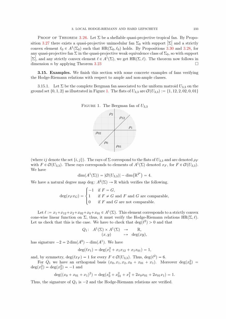
3. LOCAL HODGE-RIEMANN AND HARD LEFSCHETZ 233
Proof of Theorem 3.26. Let Σ be a shellable quasi-projective tropical fan. By Propo-sition 3.27 there exists a quasi-projective unimodular fan Σ0 with support |Σ| and a strictlyconvex element `0 P A1pΣ0q such that HRpΣ0, `0q holds. By Propositions 3.30 and 3.28, forany quasi-projective fan Σ in the quasi-projective weak equivalence class of Σ0, so with support|Σ|, and any strictly convex element ` P A1pΣq, we get HRpΣ, `q. The theorem now follows indimension n by applying Theorem 3.23
3.15. Examples. We finish this section with some concrete examples of fans verifyingthe Hodge-Riemann relations with respect to ample and non-ample classes.
3.15.1. Let Σ be the complete Bergman fan associated to the uniform matroid U3,3 on theground set t0, 1, 2u as illustrated in Figure 1. The flats of U3,3 are C pU3,3q :“ t1, 12, 2, 02, 0, 01u
Figure 1. The Bergman fan of U3,3
ρ1
ρ12
ρ2
ρ02
ρ0ρ01
(where ij denote the set ti, ju). The rays of Σ correspond to the flats of U3,3 and are denoted ρFwith F P C pU3,3q. These rays corresponds to elements of A1pΣq denoted xF , for F P C pU3,3q.We have
dimpA1pΣqq “ |C pU3,3q|´ dim`
R2‹˘
“ 4.
We have a natural degree map deg : A2pΣq Ñ R which verifies the following.
degpxFxGq “
$
’
&
’
%
´1 if F “ G,1 if F ‰ G and F and G are comparable,0 if F and G are not comparable.
Let ` :“ x1`x12`x2`x02`x0`x01 P A1pΣq. This element corresponds to a strictly convex
cone-wise linear function on Σ, thus, it must verify the Hodge-Riemann relations HRpΣ, `q.Let us check that this is the case. We have to check that degp`2q ą 0 and that
Q1 : A1pΣq ˆA1pΣq Ñ R,px, yq ÞÑ degpxyq,
has signature ´2 “ 2 dimpA0q ´ dimpA1q. We have
degp`x1q “ degpx21 ` x1x12 ` x1x01q “ 1,
and, by symmetry, degp`xF q “ 1 for every F P C pU3,3q. Thus, degp`2q “ 6.For Q1 we have an orthogonal basis px0, x1, x2, x0 ` x01 ` x1q. Moreover degpx2
0q “
degpx21q “ degpx2
2q “ ´1 and
degppx0 ` x01 ` x1q2q “ degpx2
0 ` x201 ` x
21 ` 2x0x01 ` 2x01x1q “ 1.
Thus, the signature of Q1 is ´2 and the Hodge-Riemann relations are verified.
234 3. HODGE THEORY FOR TROPICAL VARIETIES
3.15.2. Let us give another example in the same Chow ring treated in the previous para-graph. Let `1 “ x1` x12` x2. The cone-wise linear function associated to `1 is not convex. Itis even zero around ρ0, which implies that i˚0ăρ0
p`1q “ 0. Nevertheless, `1 verifies the Hodge-Riemann relations HRpΣ, `1q. We only have to check that degp`12q ą 0, since Q1 does notdepend on `1 and we have already checked that Q1 has signature ´2. We have
degppx1 ` x12 ` x2q2q “ degpx2
1 ` x212 ` x
22 ` 2x1x12 ` 2x12x2q “ 1 ą 0.
This gives us an example of a non-ample element verifying the Hodge-Riemann relations.
3.15.3. As a last example, let Σ be the Bergman fan of the uniform matroid U3,4 on theground set t0, 1, 2, 3u, and let ` “ p2`2εqx0`x2`x3` εx01`p3` εqpx02`x03q´x23 P A
1pΣqwhere ε is a small positive number. Then ` is not ample, but we have HRpΣ, `q. Indeed, wehave something stronger: `σ is ample for any σ P Σzt0u where `σ “ i˚0ăσp`q.
4. Quasi-projective unimodular triangulations of polyhedral complexes
In this section we show that any rational polyhedral complex in Rn admits a simplicialsubdivision which is both quasi-projective and unimodular with respect to the lattice 1
kZn, for
some natural number k, in a sense which we will precise in a moment. Moreover, we will showthis property holds for any tropical compactification of X. The novelty here is in ensuring theconvexity property underlying the definition of quasi-projective triangulations which will bethe crucial property used in what will follow later, as well as in ensuring the unimodularity ofunbounded polyhedra which form the polyhedral subdivision of X. The theorem thus extendsthe pioneering result proved in [KKMS06], in Mumford’s proof of the semistable reductiontheorem, as well as previous variants proved in [IKMZ19] and [Wło97].
4.1. Statement of the triangulation theorem. This theorem corresponds to Theo-rem 1.11 stated in the introduction. However, we add a technical result about the existenceof strictly convex functions to the statement which will be needed later.
Theorem 4.1 (Triangulation theorem). Let X be a rational polyhedral complex in Rn.There exists an integer k and a triangulation X 1 of X which is quasi-projective and unimodularwith respect to the lattice 1
kZn.
Moreover we ensure that X 1rec is a fan, and that there exists a strictly convex function fon X 1 such that frec is well-defined and strictly convex.
The terminology will be introduced in the next section.
Furthermore, we will prove the following theorem which will be later used in Section 8.
Theorem 4.2 (Unimodular triangulation preserving the recession fan). Let X be a poly-hedral complex in Rn such that its pseudo-recession fan Xrec is a unimodular fan. Then thereexists a positive integer k and a subdivision Y of X which is unimodular with respect to 1
kZn
and which verifies Yrec “ Xrec.
4.2. Preliminary definitions and constructions. This section presents certain con-structions which will be needed later. While definitions are given here for the case of polyhedralcomplexes and fans, we note that the majority of the constructions naturally extend to thecase of polyhedral pseudo-complexes and pseudo-fans.
4.2.1. Restriction, intersection, and hyperplane cut. Let X be a polyhedral complex of Rnand let S be a subset of Rn. The restriction of X to S denoted by X|S is by definition thepolyhedral complex consisting of all the faces of X which are included in S. If S is an affinehyperplane, an affine half-space, or more generally a polyhedron of Rn, the intersection of Xwith S denoted by X X S is the polyhedral complex whose faces are δ X S for any face δ ofX, i.e.,
X X S :“
δ X Sˇ
ˇ δ P X(
.
4. QUASI-PROJECTIVE UNIMODULAR TRIANGULATIONS OF POLYHEDRAL COMPLEXES 235
For an affine hyperplane H in Rn, the hyperplane cut of X by H denoted by X ¨ H is thesubdivision of X defined by
X ¨H :“ pX XHq Y pX XH`q Y pX XH´q,
where H` et H´ are the two half-spaces of Rn defined by H.4.2.2. Slicing with respect to a pencil of hyperplanes. Let Σ be a fan of Rn. For any
cone σ P Σ, choose a collection of half-spaces H`σ,1, . . . ,H`σ,kσ
for kσ P Zą0 each defined byhyperplanes Hσ,1, . . . ,Hσ,kσ , respectively, such that σ is the intersection of these half-spaces.We call the collection of hyperplanes
PΣ :“!
Hσ,j
ˇ
ˇ σ P Σ and j “ 1, . . . , kσ
)
a pencil of hyperplanes defined by Σ.
Let now ∆ be a complete fan in Rn and let Σ be a second (arbitrary) fan in Rn. Theslicing of ∆ with a pencil of hyperplanes PΣ defined by Σ is the fan denoted by ∆ ¨PΣ anddefined by
∆ ¨PΣ :“ ∆ ¨Hσ1,1 ¨Hσ1,2 ¨ ¨ ¨Hσ1,kσ1¨ ¨ ¨Hσm,kσm ,
i.e., defined by starting from ∆ and successively taking hyperplane cuts by elements Hσ,j ofthe pencil PΣ.
Proposition 4.3. The slicing of a complete fan with a pencil of hyperplanes PΣ definedby a fan Σ necessarily contains a subdivision of Σ.
Proof. First note that if ∆ is a fan in Rn and H is a hyperplane, all the cones δ P ∆ ¨Hlive in one of the two half-spaces H` and H´ defined by H. This property holds as well forany subdivision of ∆ ¨H.
Let now ∆ be complete. Let PΣ be a pencil of hyperplanes defined by the fan Σ consistingof hyperplanes Hσ,j for σ P Σ and j “ 1, . . . , kσ as above. Let ∆1 “ ∆ ¨PΣ. In order to provethe proposition, we will need to show the following two properties:
(1) the support of the restriction ∆1||Σ| is the entire support |Σ|; and
(2) any face of ∆1||Σ| is included in a face of Σ.
In order to prove (1), let x be a point in |Σ|. It will be enough to show the existence of aface of ∆1 which contains x and which is entirely in |Σ|.
Let δ be the smallest face of ∆1 which contains x; δ is the face which contains x in itsinterior. Let σ P Σ be a face which contains x. We will show that δ Ď σ.
By what preceded, for each i P t1, . . . , kσu, there exists εi P t`,´u such that δ is includedin Hεi
σ,i. Recall that by definition, we have σ “ Xkσi“1H
`σ,i. We will show that we can take
εi “ ` for each i, which gives the result. Suppose εi “ ´ for an i P t1, . . . , kσu. In particular,x belongs to both half-spaces H´σ,i and H
`σ,i, and so x P Hσ,i. Since δ XHσ,i is a non-empty
face of δ which contains x, by minimality of δ, we infer that δ Ă Hσ,i which shows that wecan choose εi “ `. This proves (1).
In order to prove the second assertion, let δ be a face of the restriction ∆1||Σ|. Let x be a
point in the interior of δ, so δ is the smallest face of ∆1 which contains x. Let σ be a face ofΣ which contains x. As we showed in the proof of (1), we have the inclusion δ Ď σ, which isthe desired property in (2).
It follows that ∆1||Σ| is a subdivision of Σ and the proposition follows.

236 3. HODGE THEORY FOR TROPICAL VARIETIES
4.2.3. Blow-ups and existence of triangulations. Let σ be a cone in Rn and let x be avector of Rnzt0u. The blow-up of σ at x is the fan denoted by σpxq and defined by
σpxq :“
$
’
’
&
’
’
%
ď
τăσxRτ
τ, τ ` R`x(
if x P σ,
facepσq otherwise.
Note that σpxq is a polyhedral subdivision of facepσq. Moreover, the definition depends onlyon the half line R`x.
More generally, if Σ is a fan, we define the blow-up of Σ at x to be the fan denoted byΣpxq and defined as the union of blow-ups σpxq for σ P Σ, i.e.,
Σpxq “ď
σPΣ
σpxq.
Then Σpxq is a subdivision of Σ.
For a pair of points x1, x2, we denote by Σpx1qpx2q the fan obtained by first blowing-up Σat x1, and then blowing-up the resulting fan at x2. The definition extends to any orderedsequence of points x1, . . . , xk in Rn.
Proposition 4.4. Let Σ be a fan. Let σ1, . . . , σk be the minimal faces of Σ which are notsimplicial. For each such face σi, i P t1, . . . , ku, pick a vector xi in its interior. Then
Σpx1qpx2q¨¨¨pxkq
is a triangulation of Σ.
Proof. Faces of Σpx1q which were not in Σ are of the form τ ` R`x1 where τ P Σ andx1 R Tτ . Let τ 1 “ τ ` R`x1 be such a new face. Clearly τ 1 is simplicial if and only if τ issimplicial. By contrapositive, if τ 1 is not simplicial, then τ ă τ 1 is not simplicial. In any case,τ 1 is not a non-simplicial minimal cone of Σpx1q. Therefore, the non-simplicial minimal conesof Σpx1q are included in (in fact, equal to) tσ2, . . . , σku. We concludes the proof by repeatingthis argument k-th time.
4.2.4. External cone over a polyhedral complex. We now define external cones over poly-hedral complexes.
First, let φ : Rn Ñ Rm be an affine linear application and let X be a polyhedral complexin Rn. The image of X by φ denoted by φpXq is the polyhedral pseudo-complex tφpδq
ˇ
ˇ δ P Xuof Rm. If the restriction φ||X| is injective, φpXq is a polyhedral complex.
For a subset S of Rn, we denote by adhpSq the topological closure of S in Rn.
Proposition 4.5 (Coning over a polyhedron). Let δ be an arbitrary polyhedron whichdoes not contain the origin in Rn. Let H be any affine hyperplane containing Taffδ but not 0,and denote by H0 the linear hyperplane parallel to H. Let H`0 be the half-space defined by H0
which contains δ in its interior. Then(1) σ :“ adhpR`δq is a cone which verifies δ “ σ XH and δrec “ σ XH0.
(2) Moreover, σ is the unique cone included in H`0 which verifies δ “ σ XH.(3) In addition, if δ is rational, resp. simplicial, then so is σ.
Note that by the terminology adapted in this paper, part (1) means σ is strongly convex,i.e., it does not contain any line.
Proof. For part (1), we will show more precisely that if
δ “ convpv0, . . . , vlq ` R`u1 ` ¨ ¨ ¨ ` R`um,
4. QUASI-PROJECTIVE UNIMODULAR TRIANGULATIONS OF POLYHEDRAL COMPLEXES 237
for points v0, . . . , vl in Rn and vectors u1, . . . , um in H0, then σ “ σ1 where
σ1 :“ R`v0 ` ¨ ¨ ¨ ` R`vl ` R`u1 ` ¨ ¨ ¨ ` R`um.
Note that obviously we have δ Ă σ1, which implies the inclusion σ Ď σ1. To prove theinclusion σ1 Ď σ, since v0, . . . , vl P σ, we need to show u1, . . . , um P σ. Let x be an element ofδ. For all λ ě 0, all the points x` λuj are in δ. Dividing by λ, we get xλ` uj P σ. Makingλ tend to infinity, we get uj P σ for all j “ 1, . . . ,m. This proves σ “ σ1.
We now show that σ is a cone, i.e., it does not contain any line. To show this, letλ0, . . . , λl, µ1, . . . , µm P R` such that λ0v0 ` ¨ ¨ ¨ ` λlvl ` µ1u1 ` ¨ ¨ ¨ ` µmum “ 0. It will beenough to show all the coefficients λj and µi are zero.
First, if one of the coefficients λj was non-zero, dividing by the linear combination abovewith the sum
řlj“1 λj , we would get 0 P δ, which would be a contradiction. This shows all the
coefficients λj are zero. Moreover, δrec is a cone, i.e., it is strongly convex, which proves thatall the coefficients µi are zero as well. (Note that in our definition of polyhedra, we assumethat a polyhedron is strongly convex, that is it does not contain any affine line.)
To finish the proof of part (1), it remains to show δ “ σ XH and that δrec “ σ XH0.Obviously, we have the inclusion δ Ď σ X Taffδ Ď σ XH. Proceeding by absurd, suppose
there exists y P pσ X Hqzδ. We can write y “ λ0v0 ` ¨ ¨ ¨ ` λlvl ` µ1u1 ` ¨ ¨ ¨ ` µmum withnon-negative coefficients λj , µi.
We first show that all the coefficients λj are zero. Otherwise, let Λ “ř
i λi, which isnon-zero. Since we are assuming y R δ, we get Λ ‰ 1. The point x “ yΛ belongs to δ, andso both points x, y P δ Ă H. It follows that any linear combination p1 ´ λqx ` λy for λ P Rbelongs to H. In particular,
0 “Λ
1´ Λx´
1
1´ Λy P H,
which is a contradiction. This shows λ0 “ ¨ ¨ ¨ “ λl “ 0.We thus infer that y “ µ1u1 ` ¨ ¨ ¨ ` µmum belongs to H0. But this is a contradiction
because H XH0 “ ∅. We conclude with the equality δ “ σ XH.We are left to show δrec “ σ XH0. Take a point y P σ XH0, and write y “ λ0v0 ` ¨ ¨ ¨ `
λnvn`µ1u1`¨ ¨ ¨`µmum with non-negative coefficients λj , µi. Then by a similar reasoning asabove, all the coefficients λi should be zero, which implies y P δrec. This implies the inclusionσ X H0 Ď δrec. The inclusion δrec Ă H0 comes from the inclusion δrec Ă Tδ Ď H0 and theinclusion δrec Ă σ.
We now prove part (2). Let σ1 be a cone included in H`0 such that σ1XH “ δ. Obviously,σ “ adhpR`δq Ď σ1. To prove the inverse inclusion, let y be a point σ1. If y R H0, then thereexists a scalar λ ą 0 such that λy P H. It follows that λy P δ and so y P σ. If now y P H0,then for all points x P δ and any real λ ą 0, the point x`λy belongs to σXH, which is equalto δ by the first part of the proposition. We infer that y P δrec Ă σ. This implies that σ1 “ σand the unicity follows.
Part (3) follows from the description of the cone σ given in the beginning of the proof.
Let now X be a polyhedral complex in Rn. We define the cone over X denoted by R`Xby
R`X :“!
adhpR`δqˇ
ˇ δ P X)
Y
!
0)
.
In particular, we note that this is not always a pseudo-fan. However, if one assumes that|X| does not contain 0, then R`X is indeed a pseudo-fan which contains Xrec.
We define the external cone over X denoted by conepXq as the pseudo-fan of Rn`1 definedas follows. This is also called sometimes the homogenization of X,
238 3. HODGE THEORY FOR TROPICAL VARIETIES
Let pe0, . . . , enq be the standard basis of Rn`1, and let x0, . . . , xn be the correspondingcoordinates. Consider the projection π : Rn`1 Ñ Rn defined by
πpx0, . . . , xnq “ px1, . . . , xnq.
Consider the affine hyperplane H1 of Rn`1 given by the equation x0 “ 1. The restrictionof π to H1 gives an isomorphism π1 : H1
„ÝÑ Rn, and we define
conepXq :“ R`π´11 pXq.
In particular, for any polyhedron δ, we get the external cone
conepδq :“ R`π´11 pδq.
By Proposition 4.5, intersecting with H1 gives
πpconepXq XH1q “ X.
The pseudo-fan conepXq is included in tx0 ě 0u. Moreover, denoting by H0 the linearhyperplane tx0 “ 0u, we get
conepXq|H0“ conepXq XH0.
Applying again Proposition 4.5, we deduce that πpconepXq XH0q is the recession pseudo-fanXrec of X.
4.2.5. From Xrec to X and vice-versa. Let X be any polyhedral complex such that Xrec isa fan. Let f be a piecewise linear function on X. The function f naturally induces a functionon R`pXq X H1. This function can be extended by linearity to R`XzH0. We denote thisextension by rf . We say that frec is well-defined if rf can be extended by continuity to H0. Inthis case, we define frec to be the restriction of rf to Xrec “ conepXq XH0.
Remark 4.6. Notice that if f is strictly convex and if frec is well-defined, then frec isstrictly convex. ˛
Assume X is simplicial. In this case, recall that for any polyhedron δ P X and any pointx in δ, there is a unique decomposition x “ xf ` xrec with xf P δf and xrec P δrec. We definethe projection onto the finite part πf : |X| Ñ |Xf | as the map x ÞÑ xf . Similarly, we definethe projection onto the asymptotic part πrec : |X|Ñ |Xrec| by x ÞÑ xrec. If Yf is subdivision ofXf , we define
π´1f pYf q :“
ď
δPX
!
γ ` σˇ
ˇ σ ă δrec, γ P Yf , γ Ă δf
)
.
Remark 4.7. Setting Z :“ π´1f pYf q, one can show that Z is a polyhedral complex, which
is moreover simplicial if Yf is simplicial. In addition, we have Zf “ Yf et Zrec “ Xrec. ˛
4.3. Regular subdivisions and convexity. Let now X be a polyhedral complex inRn, and let δ be a face of X. Recall that a function f is called strictly positive around δ ifthere exists a a neighborhood V of the relative interior of δ such that f vanishes on δ and itis strictly positive on V zδ. Recall as well from Section 2 that a function f P LpmpXq is calledstrictly convex around δ if there exists a function ` P LpRnq such that f ´ ` is strictly positivearound the relative interior of δ in |X|. We also note that K`pXq denotes the set of strictlyconvex functions on X, i.e., the set of those functions in LpmpXq which are strictly convexaround any face δ of X.
Remark 4.8. For a polyhedral complex X, the set K`pXq is an open convex cone in thereal vector space LpmpXq, i.e., it is an open set in the natural topology induced on LpmpXq,and moreover, if f, g P K`pXq, then we have f ` g P K`pXq and λf P K`pXq for any positivereal number λ ą 0. In addition, for ` P LpXq, we have f ` ` P K`pXq. ˛
4. QUASI-PROJECTIVE UNIMODULAR TRIANGULATIONS OF POLYHEDRAL COMPLEXES 239
Example 4.9. If P is a polyhedron in Rn, then we have 0 P K`pfacepP qq. Indeed, foreach face τ of P , by definition of faces δ in a polyhedron, there exists a linear form ` on Rnwhich is zero on δ and which is strictly negative on P zδ, so 0 ´ ` “ ´` is strictly positivearound δ. ˛
We call a polyhedral complex X quasi-projective if the set K`pXq is non-empty. Quasi-projective polyhedral complexes are sometimes called convex in the literature.
Remark 4.10. In the case of fans, the notion coincides with the notion of quasi-projectivity(convexity) used in the previous section. ˛
We are now going to make a list of operations on a polyhedral complex which preservesthe quasi-projectivity property. To start, we have the following which is straightforward.
Proposition 4.11. Any subcomplex of a quasi-projective polyhedral complex is itself quasi-projective.
Let now Y be a subdivision of X. For each face δ of X, recall that the restriction Y |δconsists of all the faces of Y which are included in δ.
Let X be a polyhedral complex. A relatively projective subdivision of X is a subdivisionY such that there exists a function f P LpmpY q whose restriction to Y |δ for any face δ P Xis strictly convex. In this case, we say Y is projective relative to X, and that the function fis strictly convex relative to X. For example, a strictly convex function f on Y is necessarystrictly convex relative to X (but the inverse is not necessarily true).
Remark 4.12. In the theory of triangulations of polytopes and secondary polytopes(see [GKZ94,DRS10]), a polyhedral subdivision of a polytope is relatively projective inour sense if and only it is regular in the sense of [GKZ94]. ˛
Remark 4.13. To justify the terminology, we should emphasize that our notion is indeeda relative notion : the underlying polyhedral complex of a relatively projective subdivisiondoes not need to be quasi-projective. ˛
Remark 4.14. A function f P LpmpY q which is strictly convex relative to X allows torecover the subdivision Y as the polyhedral complex whose collection of faces is
ď
δPX
ď
`PpRnq‹`|δďf|
δ
!
x P δˇ
ˇ `pxq “ fpxq)
z
!
∅)
. ˛
Proposition 4.15. A relatively projective subdivision of a quasi-projective polyhedral com-plex is itself quasi-projective.
Proof. Let X be a quasi-projective polyhedral complex in Rn and let f P K`pXq. LetY be a relatively projective subdivision of X and let g P LpmpY q be strictly convex relative toX. We show that for any small enough ε ą 0, the function f ` εg P LpmpY q is strictly convexon Y , which proves the proposition.
Let γ be a face of Y . It will be enough to show that f ` εg is strictly convex around γ forany sufficiently small value of ε ą 0.
Let δ be the smallest face of X which contains γ. Let ` P LpXq and `1 P LpY |δq be twoaffine linear functions such that f´` is strictly positive around δ and g|δ´`
1 is strictly positivearound γ. Without loss of generality, we can assume that `1 P LpXq.
Let V be a small enough neighborhood of the interior of γ in |X|. Equipping Rn with itsEuclidean norm, we can in addition choose V in such a way that for each point x P V , theclosest point of x in δ belongs to V .
240 3. HODGE THEORY FOR TROPICAL VARIETIES
Since f and g are piecewise linear, we can find c, c1 ą 0 such that for any x P V ,
fpxq ´ `pxq ě c distpx, δq and
gpxq ´ `1pxq ě minyPVXδ
gpyq ´ `1pyq(
´ c1 distpx, δq “ ´c1 distpx, δq,
where distpx, δq denotes the Euclidean distance between the point x and the face δ.We infer that the function f ` εg ´ p`` ε`1q is strictly positive around γ for any value of
ε ă cc1. It follows that f ` εg is strictly convex around γ for small enough values of ε ą 0, asrequired. This shows that Y is quasi-projective.
As an immediate consequence we get the following.
Corollary 4.16. The relation of « being a relatively projective subdivision » is transitive.
Proof. Let Y be a relatively projective subdivision of a polyhedral complex X withf P LpmpY q strictly convex relative to X, and let Z be a relatively projective subdivision of Ywith g P LpmpZq strictly convex relative to Y . It follows that for a face δ P X, the restrictionf |δ is strictly convex on Y |δ, and the restriction g|δ, seen as a function in LpmpZ|δq, is strictlyconvex relative to Y |δ.
By the previous proposition, more precisely by its proof, for sufficiently small values ofε ą 0, the function f |δ` εg|δ is strictly convex on Z|δ. Taking ε ą 0 small enough so that thisholds for all faces δ of X, we get the result.
Proposition 4.17. Let Σ be a fan in Rn and take a point x P Rnzt0u. The blow-up Σpxqof Σ at x is projective relative to Σ.
Proof. There exists a unique function f P LpmpΣpxqq which vanishes on any face of Σthat does not contain x and which takes value ´1 at x. We show that this function is strictlyconvex relative to Σ, which proves the proposition.
Let σ P Σ. If σ does not contain x, then σ belongs to Σpxq, and f is zero, therefore convex,on Σpxq|σ “ facepσq. Consider now the case where x P σ. Let τ be a face of σ not containingx. By the definition of the blow-up, we have to show that f |σ is convex around τ and aroundτ `R`x. Let ` P LpRnq be an affine linear function which vanishes on τ and which is strictlynegative on σzτ . Moreover, we can assume without losing generality that `pxq “ ´1. Thefunction f ´ ` is therefore zero on τ ` R`x. In addition, if ν is a face of σ not containing x,f vanishes on ν, so f ´ ` is strictly positive on νzτ . If now y is a point lying in σzpτ `R`xq,there is a face ν of σ such that y belongs to pνzτq`R`x, so we can write y “ λx` z for somereal number λ ě 0 and an element z P νzτ . Given the definition of f and the choice of `, wesee that
pf ´ `qpyq “ λ ¨ 0` pf ´ `qpzq ą 0.
Thus, f ´ ` is strictly positive around τ ` R`x in σ. In the same way, we see that f ´ 2`is strictly positive around τ in σ. So f |σ is strictly convex around τ ` R`x and around τ inΣpxq|σ, and the proposition follows.
Proposition 4.18. Let P be a polytope in Rn which contains 0. The fan
Σ :“ R`facepP q|Rnzt0u
consisting of cones of the form R`σ for σ a face of P is quasi-projective.
Proof. We omit the proof that Σ is a fan. In order to prove the quasi-projectivity, let τbe a face of P which does not contain 0. There exists an affine linear `τ function on Rn whichtakes value 0 on τ and which takes negative values on P zτ . Moreover, we can assume that`τ p0q “ ´1. The restrictions `τ |R`τ glue together to define a piecewise affine linear functionf on Σ. One can show that f is strictly convex on Σ.
4. QUASI-PROJECTIVE UNIMODULAR TRIANGULATIONS OF POLYHEDRAL COMPLEXES 241
Proposition 4.19. Let X be a polyhedral complex and let H be an affine hyperplane inRn. The hyperplane cut X ¨H is projective relative to X.
Proof. Let distp ¨ , ¨ q be the Euclidean distance in Rn. It is easy to see that the distancefunction x ÞÑ distpx,Hq is strictly convex on X ¨H relative to X.
Corollary 4.20. Suppose that X is quasi-projective. Then the intersection X X H isquasi-projective as well.
Proof. If X is quasi-projective, then combining the preceding proposition with Proposi-tion 4.15, we infer that the hyperplane cut X ¨H is quasi-projective as well. Since X XH “
pX ¨Hq|H is a polyhedral subcomplex of X ¨H, it will be itself quasi-projective by Proposi-tion 4.11.
Proposition 4.21. Let X be a polyhedral complex in Rn. If X is simplicial and Yf is arelatively projective subdivision of Xf , the subdivision Y :“ π´1
f pYf q of X is projective relativeto X. Moreover, there exists a function f P LpmpY q which is strictly convex relative to X andsuch that frec “ 0.
Proof. By Remark 4.7, the polyhedral complex Y is a subdivision of X whose finite partcoincides with Yf .
Let ff be a piecewise affine linear function on Yf which is strictly convex relative to Xf .Let f :“ π˚f pff q “ ff ˝ πf be the extension of f to |Y | “ |X|. It is clear that frec “ 0. For aface γ P Y , since both the projection πf |γ : γ Ñ γf and the restriction ff |γf
are affine linear,f |γ is also affine linear. This shows that f P LpmpY q. We now show that f is strictly convexrelative to X, which proves the proposition.
Let δ be a face of X and let γ be a face in Y which is included in δ. We need to show thatf |δ, as a piecewise linear function on Y |δ, is strictly convex around γ. By the choice of ff , weknow that ff is strictly convex around γf in Yf |δf
. Let `f be an element of Lpδf q such thatff |δf
´ `f is strictly positive around intpγf q in δf , where intpγf q denotes the relative interiorof γf .
The function ` :“ π˚f p`f q is an element of Lpδq. Moreover, the difference f ´ ` is strictlypositive around intpγf q`δrec in δ. Notice that the relative interior of γ is included in intpγf q`
δrec. Let `1 P Lpδq be an affine linear function which is zero on γ and which takes negativevalues on
`
γf ` δrec
˘
zγ. Then, for ε ą 0 small enough, f ´ ` ´ ε`1 is strictly positive aroundintpγq. Thus, f is strictly convex around γ, and the proposition follows.
4.4. Unimodularity. In this section, we discuss the existence of unimodular subdivisionsof a rational polyhedral complex in Rn.
Proposition 4.22. Let Σ be a rational simplicial fan in Rn. There exists a subdivision rΣprojective relative to Σ which is in addition unimodular with respect to Zn. Moreover, we canassume that unimodular cones of Σ are still in rΣ.
Proof. This follows from the results of [Wło97, Section 9], where it is shown how to geta unimodular subdivision rΣ of Σ by a sequence of blow-ups on some non-unimodular cones.By Proposition 4.17 and Corollary 4.16, the resulting fan rΣ is a projective subdivision of Σ,from which the result follows.
For a rational vector subspace W of Rn, we denote by pW : Rn Ñ RnL
W the resultingprojection map. We endow the quotient Rn
L
W by the quotient lattice ZnL
Zn XW .
Let now P be a simplicial polyhedron in Rn and W :“ TpPf q. We say that Prec isunimodular relative to Pf if the projection pW pPrecq is unimodular in Rn
L
W .
242 3. HODGE THEORY FOR TROPICAL VARIETIES
Remark 4.23. If Prec is unimodular relative to Pf , then for any polytope Q included inTpPf q, for the Minkowski sum R :“ Q` Prec we see that Rrec is unimodular relative Rf ˛
Proposition 4.24. Let P be an integral simplicial polyhedron in Rn. Then P is unimod-ular if and only if both the following conditions are verified:
(1) Pf is unimodular; and(2) Prec is unimodular relative to Pf .
For a collection of vectors v1, . . . , vm in a real vector space, we set Vectpv1, . . . , vmq :“Rv1 ` ¨ ¨ ¨ ` Rvm the vector subspace generated by the vectors vi.
Proof. We can write P “ convpv0, . . . , vlq ` R`vl`1 ` ¨ ¨ ¨ ` R`vm, as in Section 2.1.Moreover, we can suppose without loss of generality that v0 “ 0, that vi is primitive in R`vifor i P tl` 1,m, . . . ,, and that TpP q “ Rn. The claimed equivalence can be rewritten in theform: pv1, . . . , vmq is a basis of Zn if and only if pv1, . . . , vlq is a basis of ZnXVectpv1, . . . , vmqand pvl`1, . . . , vmq is a basis of Zn
L
Zn XVectpv1, . . . , vmq. This is clear.
Corollary 4.25. If a polyhedron P is rational and its coning conepP q is unimodular inRn`1, with respect to the lattice Zn`1, then Prec is unimodular relative to Pf .
Proof. We use the notations used in the definition of conepP q. So let π : Rn`1 Ñ Rnbe the projection, and let H0 be the hyperplane tx0 “ 0u and π0 :“ π|H0
. Let u1, . . . , ul,ul`1, . . . , um in Rn`1 be so that conepP q “ R`u1 ` ¨ ¨ ¨ ` R`um and u1, . . . , ul R H0 whileul`1, . . . , um P H0, and u1, . . . , um is part of a basis of Zn.
We apply the preceding proposition to P 1 :“ convp0, u1, . . . , ulq ` R`ul`1 ` ¨ ¨ ¨ ` R`umwhich is clearly unimodular. Setting W 1 “ TpP 1f q, we infer that pW 1pP 1recq is a unimodularcone in Rn`1
L
W 1. Note that Rn`1L
W 1 “ H0
L
W 1XH0. Moreover, the linear applicationπ0 : H0 Ñ Rn is an isomorphism which preserves the corresponding lattices, and which sendsP 1rec “ conepP q X H0 onto Prec, and W 1 X H0 onto W :“ TpPf q. Therefore, π0 induces anisomorphism from H0
L
W 1XH0 to RnL
W which sends pW 1pP 1recq onto pW pPrecq. This finallyshows that pW pPrecq is unimodular.
Theorem 4.26. Let X be a compact rational polyhedral complex in Rn (so Xrec “ t0u).There exists a positive integer k and a subdivision Y projective relative to X such that Y isunimodular with respect to the lattice 1
kZn.
Proof. This is a consequence of Theorem 4.1 of [KKMS06, Chapter III].
Remark 4.27. Note that if a fan Σ in Rn is unimodular with respect to Zn, then it is aswell unimodular with respect to any lattice of the form 1
kZn. ˛
4.5. Proof of Theorem 4.1. We are now in position to prove the main theorem of thissection. Let ΣX :“ conepXq, which is a pseudo-fan, and define H0, H1 and π : Rn`1 Ñ Rn asin the definition of the external cone. We thus have X “ πpΣXXH1q and Xrec “ πpΣXXH0q.
We first prove the existence of a relatively projective subdivision of ΣX .
Let P be a polytope containing 0 in its interior. Define the fan Σ1 :“ R`facepP q|Rn`1zt0u.
This is a complete fan which moreover, by Proposition 4.18, is projective. Define Σ2 as thefan obtained by slicing Σ1 with respect to a pencil of hyperplanes associated to ΣX . (Wedefined the slicing with respect to a fan but as mentioned previously, the definition extendsto pseudo-fans.)
By Proposition 4.3, Σ2 contains a subdivision of ΣX . Moreover, since Σ1 is quasi-projective, and since by Proposition 4.19, Σ2 is projective relative to Σ1 (being obtainedby a sequence of hyperplane cuts), it follows that Σ2 is quasi-projective.
Let Σ3 :“ Σ2 ¨ H0, and note that this is a relatively projective subdivision of Σ2 by thesame proposition. In particular, Σ3 itself is quasi-projective. The fan Σ3 is special in that if
4. QUASI-PROJECTIVE UNIMODULAR TRIANGULATIONS OF POLYHEDRAL COMPLEXES 243
Σ1 if a subdivision of Σ3, then any cone in Σ1 is included in one of the two half-spaces H`0 orH´0 defined by H0.
Let Σ4 be a rational triangulation of Σ3 obtained from Σ3 by applying Proposition 4.4.Note that Σ4 is obtained from Σ3 by blow-ups, thus, by Proposition 4.17, it is projectiverelative to Σ3. In particular, it is quasi-projective.
Let Σ5 be a unimodular subdivision of Σ4, which exists by Proposition 4.22. The fan Σ5
is therefore unimodular and quasi-projective, and it contains moreover a subdivision of ΣX .
We now use Σ5 to get a subdivision of X. Let X1 :“ πpΣ5 XH1q.
Since Σ5 is quasi-projective, the intersection Σ5XH1 is quasi-projective as well. Since Σ5
contains a subdivision of ΣX , it follows that Σ5XH1 contains a subdivision of ΣX XH1 “ X.Passing now to the projection, we infer that X1 is quasi-projective and contains a subdi-
vision of X. More precisely, there exists a strictly convex function f on X1 such that frec iswell-defined.
Pick δ in X1, and let σ be a cone in Σ5 such that πpσXH1q “ δ. Applying Proposition 4.5to δ1 :“ σ XH1 and to the hyperplane H1, given that σ is included in the half-space definedby H0 which contains δ1, we infer that σ “ adhpR`δq “ conepδq. Since σ is unimodular, byCorollary 4.25 we infer that δrec is unimodular relative δf .
Let X2 :“ X1||X|. It follows that X2 is a subdivision of X which is rational, simplicial,and quasi-projective, and moreover, for any δ P X2, the cone δrec is unimodular relative to δf .
At this moment, we are left to show the existence of a unimodular subdivision Y that isprojective relative to X2. By Theorem 4.26, there exists an integer k ě 1 and a relativelyprojective subdivision Yf of X2,f such that Yf is unimodular with respect to the lattice 1
kZn.
Define Y :“ π´1f pYf q. By Proposition 4.21, Y is projective relative to X2, and so by quasi-
projectivity of X2, it is quasi-projective itself. More precisely, there exists a function f strictlyconvex on Y such that Yrec is well-defined.
Using Remark 4.23, we infer that for each face δ P Y , the cone δrec is unimodular relativeto δf , with respect to the lattice Zn of Rn. By Remark 4.27, this remains true for the lattice1kZ
n as well.
Applying Proposition 4.24, we finally conclude that Y is unimodular with respect to thelattice 1
kZn. At present, we have obtained a relatively projective subdivision Y of X which
is moreover quasi-projective and unimodular with respect to the lattice 1kZ
n. Moreover, it isclear that Yrec is a fan. This finishes the proof of Theorem 4.1.
4.6. Unimodular triangulations preserving the recession fan. We finish this sec-tion by presenting the proof of Theorem 4.2. We use the same notations as in the previoussection for external cones.
Proof of Theorem 4.2. Let Σ1 “ conepXq. We know that Σ1|H0“ Xrec is a unimod-
ular fan. Thus Σ1 is a fan.
By Proposition 4.4, we can construct a simplicial subdivision Σ2 of Σ1. Moreover, sincefaces of Σ1|H0
are already simplicial, the construction described in Proposition 4.4 does notchange this part of the fan, i.e., Σ2|H0
“ Σ1|H0.
In the same way, by Proposition 4.22, there exists a unimodular subdivision Σ3 of Σ2.Moreover, since Σ2|H0
is unimodular, the same proposition ensures we can assume Σ3|H0“
Σ2|H0.
Set X1 “ πpΣ3 XH1q. Then X1 is a triangulation of X with X1,rec “ Xrec.
244 3. HODGE THEORY FOR TROPICAL VARIETIES
By Theorem 4.26, there exists an integer k ě 1 and a subdivision Yf of X1,f such that Yf isunimodular with respect to the lattice 1
kZn. Define Y :“ π´1
f pYf q. Clearly, Yrec “ X1,rec “ Xrec.
Using the same argument as in the final part of the proof of Theorem 4.1 in the previoussection, we infer that Y is unimodular, which concludes the proof.
5. Tropical Steenbrink spectral sequence
Let V :“ Rn be a vector space. Denote by N the lattice Zn Ă V , thus V “ NR. LetY be a unimodular polyhedral complex of dimension d in NR whose support |Y | is a smoothtropical variety. Assume that the recession pseudo-fan of Y is a fan Yrec. This fan induces apartial compactification TPY8 of Rn. Denote by X the extended polyhedral complex inducedby Y on the closure of Y in TPY8 . Then, |X| is a smooth compact tropical variety. To simplifythe notations, we will denote by Xrec the recession fan Yrec of Y , and by TPX8 the partialcompactification TPY8 of Rn.
Recall from Section 2 that the space TPX8 is naturally stratified by open strata NσR for
σ P Xrec. If σ P Xrec, we denote by Xσ the intersection of X with NσR . Notice that Xσ is a
unimodular simplicial complex of dimension d ´ |σ|. In particular, X0 “ Y . If δ P X is aface, we denote by sedpδq P Xrec its sedentarity: this is the unique cone σ P Xrec such that therelative interior of δ is in Nσ
R .
Recall that for a simplicial polyhedron δ in Rn, we defined δrec and δf in Section 2. Weextend the definition to faces δ of X of higher sedentarity as follows. By δrec (resp. δf ) we meanpδ XN
sedpδqR qrec (resp. pδ XN sedpδq
R qf ) which belongs to the fun pXsedpδqqrec (resp. pXsedpδqqf ).
The max-sedentarity of a face δ P X that we denote by maxsedpδq is defined as
maxsedpδq :“ max!
sedpγqˇ
ˇ γ ă δ)
.
One verifies directly that we have maxsedpδq “ sedpδq ` δrec and that this is the maximumcone σ P Xrec such that δ intersects Nσ
R .
For each δ P X, let Σδ be the fan in N sedpδqR
L
Tδ induced by the star of δ in X. Unimod-ularity of X implies that the fan Σδ is unimodular. We denote as before by Σ
δ the canonicalcompactification of Σδ.
We define the k-th cohomology Hkpδq of Σδ by
Hkpδq :“à
r`s“k
Hr,stroppΣ
δq “
#
Hk2,k2trop pΣ
δq » Ak2pΣδq if k is even
0 otherwise
where the last equalities follows from Theorem 1.3, proved in [AP21].
5.1. Basic maps. We define some basic maps between the cohomology groups associatedto faces of X.
5.1.1. The sign function. We will need to make the choice of a sign function for X. Thisis a function
sign:!
pγ, δq P X ˆXˇ
ˇ γ ă δ)
ÝÑ t´1,`1u
which takes a value signpγ, δq P t´1,`1u for a pair of faces γ, δ P X with γ ă δ, and whichverifies the following property that we call the diamond property.
Definition 5.1 (Diamond property for a sign function). Let δ be a face of dimensionat least 2 in X and ν be a face of codimension 2 in δ. The diamond property of polyhedra
5. TROPICAL STEENBRINK SPECTRAL SEQUENCE 245
ensures that there exist exactly two different faces γ, γ1 P X such that ν ă γ,γ1 ă δ. Then, werequire the sign function to verify the following compatibility
signpν, γqsignpγ, δq “ ´signpν, γ1qsignpγ1, δq.
Moreover, if e is an edge in X and if u and v are its extremities, then we require the signfunction to verify
signpu, eq “ ´signpv, eq.
˛
For the existence, note that such a sign function can be easily defined by choosing anorientation on each face.
From now on, we assume that a sign function for X has been fixed once for all.5.1.2. The restriction and Gysin maps. If γ and δ are two faces with γ ă δ, we have the
Gysin mapGysδ ąγ : Hkpδq Ñ Hk`2pγq,
and the restriction mapi˚γăδ : Hkpγq Ñ Hkpδq,
where we define both maps to be zero if γ and δ do not have the same sedentarity. If γ andδ have the same sedentarity, these maps correspond to the corresponding maps in the level ofChow groups defined in Section 3.
Remark 5.2. We recall that if γ and δ have the same sedentarity, using the isomorphismof the Chow groups with the tropical cohomology groups, the two maps have the followingequivalent formulation. First, we get an inclusion Σ
δãÑ Σ
γ . To see this, note that δ gives aray ρδγ in Σγ . The above embedding identifies Σ
δ with the closure of the part of sedentarity
ρδγ in Σγ . The restriction map i˚γăδ is then the restriction map HkpΣ
γq Ñ HkpΣ
δq induced
by this inclusion. The Gysin map is the dual of the restriction map i˚γăδ : H2d´2|δ|´kpΣγq Ñ
H2d´2|δ|´kpΣδq, which by Poincaré duality for Σ
δ and Σγ , is a map from HkpΣ
δq to Hk`2pΣ
γq.˛
In addition to the above two maps, if two faces γ and δ do not have the same sedentarity,the projection map πδ ąγ : N
sedpδqR Ñ N
sedpγqR induces an isomorphism Σδ » Σγ , which leads
to an isomorphism of the canonical compactifications, and therefore of the correspondingcohomology groups that we denote by
π˚γăδ : Hkpγq „ÝÑ Hkpδq.
Remark 5.3. All the three above maps can be defined actually even if γ is not ofcodimension 1 in δ. Note that in this case, the Gysin map is a map Gysδąγ : Hkpδq „ÝÑ
Hk`2|δ|´2|γ|pγq. ˛
Let now S and T be two collections of faces of X. We can naturally define the map
i˚S,T :À
γPS Hkpγq ÝÑ
À
δPTHkpδq,
by sending, for any γ P S, any element x of Hkpγq to the element
i˚S,T pxq :“ÿ
δPTδ ąγ
signpγ, δq i˚γăδpxq,
and extend it by linearity to the direct sumÀ
γPS Hkpγq.
In the same way, we define
GysS,T :À
δPSHkpδq ÝÑ
À
γPT Hk`2pγq,
246 3. HODGE THEORY FOR TROPICAL VARIETIES
by setting for x P Hkpδq, for δ P S,
GysS,T pxq :“ÿ
γPTδ ąγ
signpγ, δqGysδ ąγpxq.
Similarly, we getπ˚S,T :
À
γPS Hkpγq ÝÑ
À
δPTHkpδq.
In what follows, we will often extend maps in this way. Moreover, we will drop the indicesif they are clear from the context.
5.2. Combinatorial Steenbrink and the main theorem. Denote by Xf the set offaces of X whose closures do not intersect the boundary of TPX , i.e., the set of compact facesof X0. Note that this was previously denoted by X0,f that we now simplify to Xf for the easeof presentation.
In what follows, inspired by the shape of the first page of the Steenbrink spectral se-quence [Ste76], we define bigraded groups STa,b1 with a collection of maps between them. Inabsence of a geometric framework reminiscent to the framework of degenerating families ofsmooth complex projective varieties, the heart of this section is devoted to the study of thiscombinatorial shadow in order to obtain interesting information about the geometry of X.
For all pair of integers a, b P Z, we define
STa,b1 :“à
sě|a|s”a pmod 2q
STa,b,s1
whereSTa,b,s1 “
à
δPXf|δ|“s
Ha`b´spδq.
The bigraded groups STa,b1 come with a collection of maps
ia,b˚ : STa,b1 Ñ STa`1,b1 and Gysa,b : STa,b1 Ñ STa`1,b
1 ,
where both these maps are defined by our sign convention introduced in the previous section.In practice, we drop the indices and denote simply by i˚ and Gys the corresponding maps.
Remark 5.4. More precisely, we could view the collection of maps i˚ and Gys bi-indexedby a, b as maps of bidegree p1, 0q
i˚ “à
a,b
ia,b˚ :à
a,b
STa,b1 ÝÑà
a,b
STa,b1 ,
andGys “
à
a,b
Gysa,b :à
a,b
STa,b1 ÝÑà
a,b
STa,b1 . ˛
Proposition 5.5. The two collections of maps i˚ and Gys have the following properties.
i˚ ˝ i˚ “ 0, Gys ˝Gys “ 0, i˚ ˝Gys`Gys ˝ i˚ “ 0.
Proof. Section 5.10 is devoted to the proof of this proposition.
We now define the differential d: STa,b1 Ñ STa`1,b1 as the sum d “ i˚ ` Gys. It follows
from the properties given in the above proposition that we have the following.
Proposition 5.6. For a unimodular triangulation of X and for any integer b, the differ-ential d makes ST‚,b1 into a cochain complex.
5. TROPICAL STEENBRINK SPECTRAL SEQUENCE 247
Remark 5.7. This proposition suggests ST‚,‚1 might be the first page of a spectral sequenceconverging to the cohomology of X. We could think that such a spectral sequence could bedefined if we could deform infinitesimally the tropical variety. In the sequel we will only usethe property stated in the proposition, that the lines of ST‚,‚1 with the differential d form acochain complex, as well as certain combinatorial properties of these cochain complexes. ˛
For a cochain complex pC‚,dq, denote by HapC‚,dq its a-th cohomology group, i.e.,
HapC‚, dq “ker
´
d: Ca Ñ Ca`1¯
Im´
d: Ca´1 Ñ Ca¯ .
In this section we prove the following theorem, generalizing the main theorem of [IKMZ19]from approximable setting (when X arises as the tropicalization of a family of complex pro-jective varieties) to any general smooth tropical variety.
Theorem 5.8 (Steenbrink-Tropical comparison theorem). The cohomology of pST‚,b1 ,dq isdescribed as follows. For b odd, all the terms STa,b1 are zero, and the cohomology is vanishing.For b even, let b “ 2p for p P Z, then for q P Z, we have
Hq´ppST‚,2p1 ,dq “ Hp,qtroppXq.
The rest of this section is devoted to the proof of Theorem 5.8.In absence of a geometric framework reminiscent to the framework of degenerating families
of smooth complex projective varieties, the heart of our proof is devoted to introducing anddeveloping certain tools, constructions, and results about the combinatorial structure of theSteenbrink spectral sequence.
Broadly speaking, the proof which follows is inspired by the one given in the approx-imable case [IKMZ19], as well as by the ingredients in Deligne’s construction of the mixedHodge structure on the cohomology of a smooth algebraic variety [Del71a] and by Steen-brink’s construction of the limit mixed Hodge structure on the special fiber of a semistabledegeneration [Ste76], both based on the use of the sheaf of logarithmic differentials and theircorresponding spectral sequences.
In particular, we are going to prove first an analogous result in the tropical setting of theDeligne exact sequence which gives a resolution of the coefficient groups Fp with cohomologygroups of the canonically compactified fans Σ
δ. The proof here is based on the use of Poincaréduality and our Theorem 1.3, the tropical analog of Feichtner-Yuzvinsky theorem [FY04],which provides a description of the tropical cohomology groups of the canonically compactifiedfans. We then define a natural filtration that we call the tropical weight filtration or toricweight filtration on the coefficient groups Fpp¨q, inspired by the weight filtration on the sheafof logarithmic differentials, and study the corresponding spectral sequence. The resolutionof the coefficient groups given by the Deligne spectral resolution gives a double complexwhich allows to calculate the cohomology of the graded cochain complex associated to theweight filtration. We then show that the spectral sequence associated to the double complexcorresponding to the weight filtration which abuts to the tropical cohomology groups, abuts aswell to the cohomology groups of the Steenbrink cochain complex, which concludes the proof.The proof of this last result is based on the use of our Spectral Resolution Lemma 5.25 whichallows to make a bridge between different spectral sequences.
5.3. Tropical Deligne resolution. Let Σ be a smooth unimodular tropical fan. Wefollow the notations of the previous section. In particular, for each cone σ, we denote by Σσ
the induced fan on the star of σ in Σ, and by Σσ its canonical compactification. We proved
in [AP21] the following theorem.
248 3. HODGE THEORY FOR TROPICAL VARIETIES
Theorem 5.9 (Tropical Deligne resolution). We have the following exact sequence of Q-vector spaces:
0 Ñ Fpp0q Ñà
σPΣ|σ|“p
H0pσq Ñà
σPΣ|σ|“p´1
H2pσq Ñ ¨ ¨ ¨ Ñà
σPΣ|σ|“1
H2p´2pσq Ñ H2pp0q Ñ 0,
where the maps between cohomology groups are given by Gys.
5.4. Toric weight filtration on Fp. In this section, we introduce a natural filtration onthe structure sheaf Fp. This filtration could be regarded as the analog in polyhedral geometryof the weight filtration on the sheaf ΩpplogX0q of logarithmic differentials around the specialfiber X0 of a semistable degeneration X over the unit disk.
Let δ be a face of the triangulation X of the tropical variety X. First we define a filtrationdenoted by ĂW‚ on Fppδq, and then define the weight filtration W‚ by shifting the filtrationinduced by ĂW‚.
The tangent space Tδ of δ is naturally included in F1pδq. More generally, for any integers, we have an inclusion
ŹsTδ Ď Fspδq, which in turn gives an inclusionŹsTδ ^ Fp´spδq Ď Fppδq
for any non-negative integer s.
Definition 5.10. For any integer s ě 0, define ĂWsFppδq as follows
ĂWsFppδq :“!
α P Fppδqˇ
ˇ restriction of α on subspaceŹs`1Tδ^Fp´s´1pδq of Fppδq is trivial
)
.
˛
Recall that for a pair of faces γ ă δ, we denote by i˚γăδ the restriction map Fppγq Ñ Fppδq.
Proposition 5.11. Let γ be a face of codimension one of δ. We have the following twocases.
— If γ and δ have the same sedentarity, then the natural map i˚γăδ : Fppγq Ñ Fppδqsends ĂWs´1Fppγq into ĂWsFppδq.
— If γ and δ do not have the same sedentarity, then the natural map π˚γăδ : Fppγq ÑFppδq sends ĂWsFppγq into ĂWsFppδq.
Proof. For the first point, let nδγ be a primitive normal vector to Tγ in Tδ. The mapFppδq Ñ Fppγq restricted to the subspace
Źs`1Tδ ^ Fp´s´1pδq can be decomposed as thecomposition of the following maps
Źs`1Tδ ^ Fp´s´1pδq “ŹsTγ ^ nδγ ^ Fp´s´1pδq `
Źs`1Tγ ^ Fp´s´1pδq
ÝÑŹsTγ ^ nδγ ^ Fp´s´1pγq `
Źs`1Tγ ^ Fp´s´1pγq ãÝÑŹsTγ ^ Fp´spγq.
An element of ĂWs´1Fppγq is thus sent to an element of Fppδq which restricts to zero onthe subspace
Źs`1Tδ ^ Fp´s´1pδq, in other words, to an element of ĂWsFppδq.
For the second point, the projection πδ ąγ maps Tδ onto Tγ. Thus, it also mapsŹs`1Tδ
ontoŹs`1Tγ. The image of an element of ĂWsFppγq thus restricts to zero on
ŹsTδ, i.e., it isan element of ĂWsFppδq.
We now consider the graded pieces grrWs Fppδq :“ ĂWsFppδq
L
ĂWs´1Fppδq.
For δ P X, we denote as before by 0δ the zero cone of the fan Σδ induced by the triangu-lation X around δ. The following proposition gives the description of the graded pieces of thefiltration.

5. TROPICAL STEENBRINK SPECTRAL SEQUENCE 249
Proposition 5.12. For each face δ, we have
grrWs Fppδq »
ŹsT‹δ b Fp´sp0δq.
Here T‹δ is the cotangent space of the face δ.
In order to prove this proposition, we introduce some useful maps. Denote by πδ thenatural projection N sedpδq
R Ñ N δR. We choose a projection pδ : N
sedpδqR Ñ Tδ. Both projections
naturally extend to exterior algebras, and for any integer p, we get maps
pδ :ŹpN
sedpδqR Ñ
ŹpTδ,
πδ :ŹpN
sedpδqR Ñ
ŹpN δR.
Furthermore, we get a mapπδ : Fppδq Ñ Fpp0δq.
We have the corresponding pullback p˚δ and π˚δ between the corresponding dual spacesFppδq and Fp0δq. Moreover, if α P Fppδq is zero on Tδ ^ Fp´1pδq, since Tδ “ kerpπδq, wecan define a natural pushforward πδ ˚pαq of α in Fpp0δq. This leads to a map (in fact anisomorphism)
πδ ˚ : ĂW0pFppδqq Ñ Fpp0δq.
Proof of Proposition 5.12. Let α be an element of ĂWsFppδq. Let u PŹsTδ. Recall
that the contraction of α by u is the multiform β :“ αpu^ ¨ q P Fp´spδq.Since α is in ĂWsFppδq, and u ^ Tδ ^ Fp´s´1pδq Ď
Źs`1Tδ ^ Fp´s´1pδq, by definition ofthe filtration ĂW‚, the contracted multiform β is zero on Tδ ^ Fp´s´1pδq. Thus, β P ĂW0pδq.Hence, we get a morphism
Ψ: ĂWsFppδq ÝÑ Hom´
ŹsTδ , Fp´sp0δq¯
»ŹsT‹δ b Fp´sp0δq,
α ÞÝÑ`
u ÞÝÑ πδ ˚pαpu^ ¨ qq˘
.
Notice that the kernel of Ψ is ĂWs´1pFppδqq, i.e., its cokernel is grĂWs pF
ppδqq.Set
Φ:ŹsT‹δ b Fp´sp0δq, ÝÑ Fppδq
xb y ÞÝÑ p˚δ pxq ^ π˚δ pyq,
and extended by linearity.
One verifies directly that ImpΨq Ď ĂWsFppδq, and Ψ˝Φ is identity onŹsT‹δbFp´sp0δq. In
particular, Ψ is surjective. We thus infer that Ψ induces an isomorphism between its cokerneland
ŹsT‹δ b Fp´sp0δq. This concludes the proof as we have seen that its cokernel of Ψ isgr
ĂWs pF
ppδqq.
Definition 5.13 (Toric weight filtration). For each δ P X, we define the tropical weightfiltration or toric weight filtration W‚ on Fppδq and its opposite filtration W ‚ by
WsFppδq “ ĂWs`|δ|Fppδq, and
W sFppδq “ ĂW´s`|δ|Fppδq,for each integer s. ˛
Proposition 5.12 directly translates into the following facts about the filtration W ‚.
Corollary 5.14. The following holds.(1) For each face δ, we have
grsWFppδq »
Ź|δ|´sT‹δ b Fp`s´|δ|p0δq.
250 3. HODGE THEORY FOR TROPICAL VARIETIES
(2) For inclusion of faces γ ă δ, the map Fppγq Ñ Fppδq respects the filtration W ‚. Inparticular, we get an application at each graded piece grsWF
ppγq Ñ grsWFppδq.
5.4.1. Description of the restriction maps on graded pieces of the weight filtration. Wewould now like to explicitly describe the map induced by i˚ on the level of graded pieces.In what follows, we identify grsWF
ppδq with the decompositionŹ|δ|´sT‹δ b Fp`s´|δ|p0δq and
also, by duality, with Hom´
Ź|δ|´sTδ , Fp`s´|δ|p0δq¯
. We callŹ|δ|´sT‹δ and Fp`s´|δ|p0δq the
parallel part and the transversal part of the graded piece of the filtration, respectively. We usethe notation α, β, etc. when referring to the elements of the parallel part, and use αK, βK,etc. when referring to the elements of the transversal part. In particular, each element of thegraded piece is a sum of elements of the form α b αK.
We denote by Ψs,δ : WsFppδq Ñ grsWFppδq the projection. As we have seen in the proof of
Proposition 5.12, this map is explicitly described byΨs,δ : W sFppδq ÝÑ grsWF
ppδq
α ÞÝÑ`
u ÞÝÑ πδ ˚pαpu^ ¨ qq˘
.
We also have a section Φs,δ, which this time depends on the chosen projection pδ, and whichis given by
Φs,δ : grsWFppδq ÝÑ W sFppδq
α b αK ÞÝÑ p˚δ pαq ^ π˚δ pαKq.
Consider now two faces γ ă δ in X. We define two maps i˚and i˚K between parallel and
transversal parts of the graded pieces as follows. For each non-negative integer t, the map
i˚
:ŹtT‹γ ÝÑ
Źt`1T‹δ
sends an element α PŹtT‹γ to the element β “ i˚
pαq of
Źt`1T‹δ defined as follows. Themultiform β is the unique element of
Źt`1T‹δ which restricts to zero onŹt`1Tγ under the
inclusion mapŹt`1Tγ ãÑ
Źt`1Tδ, and which verifies
βpu^ nδγq “ αpuq for any u PŹtTγ Ă
ŹtTδ.
Here nδγ is any primitive normal vector to Tγ in Tδ. In other words,
β “ p˚γpαq|Tδ ^ n‹δγ ,
where n‹δγ is the form on Tδ which vanishes on Tγ and which takes value 1 on nδγ .For any positive integer t, the other map
i˚K : Ftp0γq ÝÑ Ft´1p0δq
between transversal parts is similarly defined as follows. This is the unique linear map whichsends an element αK of Ftp0γq to the element βK “ i˚KpαKq which verifies
αKpeδγ ^ vq “ βKpπγăδpvqq for any v P Ft´1p0γq.
Here, as in the previous sections, eδγ is the primitive vector of the ray ρδγ corresponding to
δ in Σγ , and πγăδ is the projection from Σγ to Σ
δ (along Reδγ), which naturally induces asurjective map from Ft´1p0
γq Ñ Ft´1p0δq. In other words, βK is the pushforward by πγăδ of
the contraction of αK by eδγ (which is well-defined because kerπγăδ “ Reδγ).
Proposition 5.15. Let γ ă δ be two faces in X. Notations as above, the induced mapon graded pieces grsWF
ppγq Ñ grsWFppδq is zero provided that sedpγq ‰ sedpδq. Otherwise, it
coincides with the map
i˚b i˚K :
Ź|γ|´sT‹γ b Fp`s´|γ|p0γq ÝÑŹ|δ|´sT‹δ b Fp`s´|δ|p0δq,
α b αK ÞÝÑ signpγ, δqβ b βK,
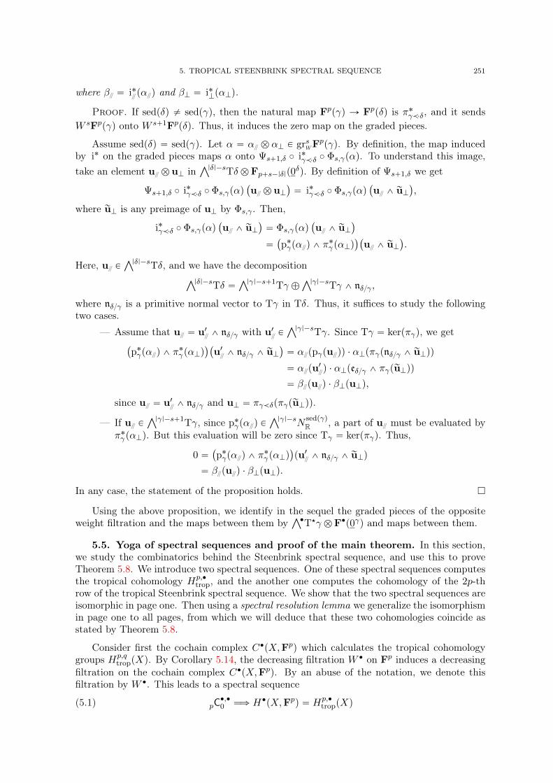
5. TROPICAL STEENBRINK SPECTRAL SEQUENCE 251
where β “ i˚pαq and βK “ i˚KpαKq.
Proof. If sedpδq ‰ sedpγq, then the natural map Fppγq Ñ Fppδq is π˚γăδ, and it sendsW sFppγq onto W s`1Fppδq. Thus, it induces the zero map on the graded pieces.
Assume sedpδq “ sedpγq. Let α “ α b αK P grsWFppγq. By definition, the map induced
by i˚ on the graded pieces maps α onto Ψs`1,δ ˝ i˚γăδ ˝ Φs,γpαq. To understand this image,take an element u b uK in
Ź|δ|´sTδ b Fp`s´|δ|p0δq. By definition of Ψs`1,δ we get
Ψs`1,δ ˝ i˚γăδ ˝ Φs,γpαq`
u b uK˘
“ i˚γăδ ˝ Φs,γpαq`
u ^ ruK˘
,
where ruK is any preimage of uK by Φs,γ . Then,
i˚γăδ ˝ Φs,γpαq`
u ^ ruK˘
“ Φs,γpαq`
u ^ ruK˘
“`
p˚γpαq ^ π˚γ pαKq
˘`
u ^ ruK˘
.
Here, u PŹ|δ|´sTδ, and we have the decomposition
Ź|δ|´sTδ “Ź|γ|´s`1Tγ ‘
Ź|γ|´sTγ ^ nδγ ,
where nδγ is a primitive normal vector to Tγ in Tδ. Thus, it suffices to study the followingtwo cases.
— Assume that u “ u1^ nδγ with u1
PŹ|γ|´sTγ. Since Tγ “ kerpπγq, we get
`
p˚γpαq ^ π˚γ pαKq
˘`
u1^ nδγ ^ ruK
˘
“ αppγpuqq ¨ αKpπγpnδγ ^ ruKqq
“ αpu1q ¨ αKpeδγ ^ πγpruKqq
“ βpuq ¨ βKpuKq,
since u “ u1^ nδγ and uK “ πγăδpπγpruKqq.
— If u PŹ|γ|´s`1Tγ, since p˚γpαq P
Ź|γ|´sNsedpγqR , a part of u must be evaluated by
π˚γ pαKq. But this evaluation will be zero since Tγ “ kerpπγq. Thus,
0 “`
p˚γpαq ^ π˚γ pαKq
˘
pu1^ nδγ ^ ruKq
“ βpuq ¨ βKpuKq.
In any case, the statement of the proposition holds.
Using the above proposition, we identify in the sequel the graded pieces of the oppositeweight filtration and the maps between them by
Ź‚T‹γ b F‚p0γq and maps between them.
5.5. Yoga of spectral sequences and proof of the main theorem. In this section,we study the combinatorics behind the Steenbrink spectral sequence, and use this to proveTheorem 5.8. We introduce two spectral sequences. One of these spectral sequences computesthe tropical cohomology Hp,‚
trop, and the another one computes the cohomology of the 2p-throw of the tropical Steenbrink spectral sequence. We show that the two spectral sequences areisomorphic in page one. Then using a spectral resolution lemma we generalize the isomorphismin page one to all pages, from which we will deduce that these two cohomologies coincide asstated by Theorem 5.8.
Consider first the cochain complex C‚pX,Fpq which calculates the tropical cohomologygroups Hp,q
troppXq. By Corollary 5.14, the decreasing filtration W ‚ on Fp induces a decreasingfiltration on the cochain complex C‚pX,Fpq. By an abuse of the notation, we denote thisfiltration by W ‚. This leads to a spectral sequence
(5.1) pC‚,‚0 ùñ H‚pX,Fpq “ Hp,‚
troppXq
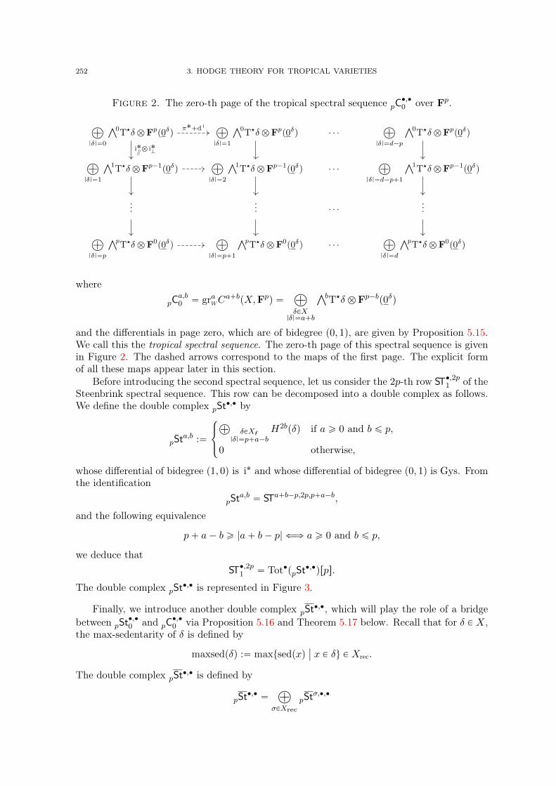
252 3. HODGE THEORY FOR TROPICAL VARIETIES
Figure 2. The zero-th page of the tropical spectral sequence pC‚,‚0 over Fp.
à
|δ|“0
Ź0T‹δ b Fpp0δq
à
|δ|“1
Ź0T‹δ b Fpp0δq . . .
à
|δ|“d´p
Ź0T‹δ b Fpp0δq
à
|δ|“1
Ź1T‹δ b Fp´1
p0δqà
|δ|“2
Ź1T‹δ b Fp´1
p0δq . . .à
|δ|“d´p`1
Ź1T‹δ b Fp´1
p0δq
...... . . .
...
à
|δ|“p
ŹpT‹δ b F0
p0δqà
|δ|“p`1
ŹpT‹δ b F0
p0δq . . .à
|δ|“d
ŹpT‹δ b F0
p0δq
i˚b i˚K
π˚`d i
where
pCa,b0 “ graWC
a`bpX,Fpq “à
δPX|δ|“a`b
ŹbT‹δ b Fp´bp0δq
and the differentials in page zero, which are of bidegree p0, 1q, are given by Proposition 5.15.We call this the tropical spectral sequence. The zero-th page of this spectral sequence is givenin Figure 2. The dashed arrows correspond to the maps of the first page. The explicit formof all these maps appear later in this section.
Before introducing the second spectral sequence, let us consider the 2p-th row ST‚,2p1 of theSteenbrink spectral sequence. This row can be decomposed into a double complex as follows.We define the double complex pSt
‚,‚ by
pSta,b :“
$
&
%
À
δPXf|δ|“p`a´b
H2bpδq if a ě 0 and b ď p,
0 otherwise,
whose differential of bidegree p1, 0q is i˚ and whose differential of bidegree p0, 1q is Gys. Fromthe identification
pSta,b “ STa`b´p,2p,p`a´b,
and the following equivalence
p` a´ b ě |a` b´ p|ðñ a ě 0 and b ď p,
we deduce thatST‚,2p1 “ Tot‚ppSt
‚,‚qrps.
The double complex pSt‚,‚ is represented in Figure 3.
Finally, we introduce another double complex pSt‚,‚, which will play the role of a bridge
between pSt‚,‚0 and pC
‚,‚0 via Proposition 5.16 and Theorem 5.17 below. Recall that for δ P X,
the max-sedentarity of δ is defined by
maxsedpδq :“ maxtsedpxqˇ
ˇ x P δu P Xrec.
The double complex pSt‚,‚ is defined by
pSt‚,‚ “
à
σPXrec
pStσ,‚,‚
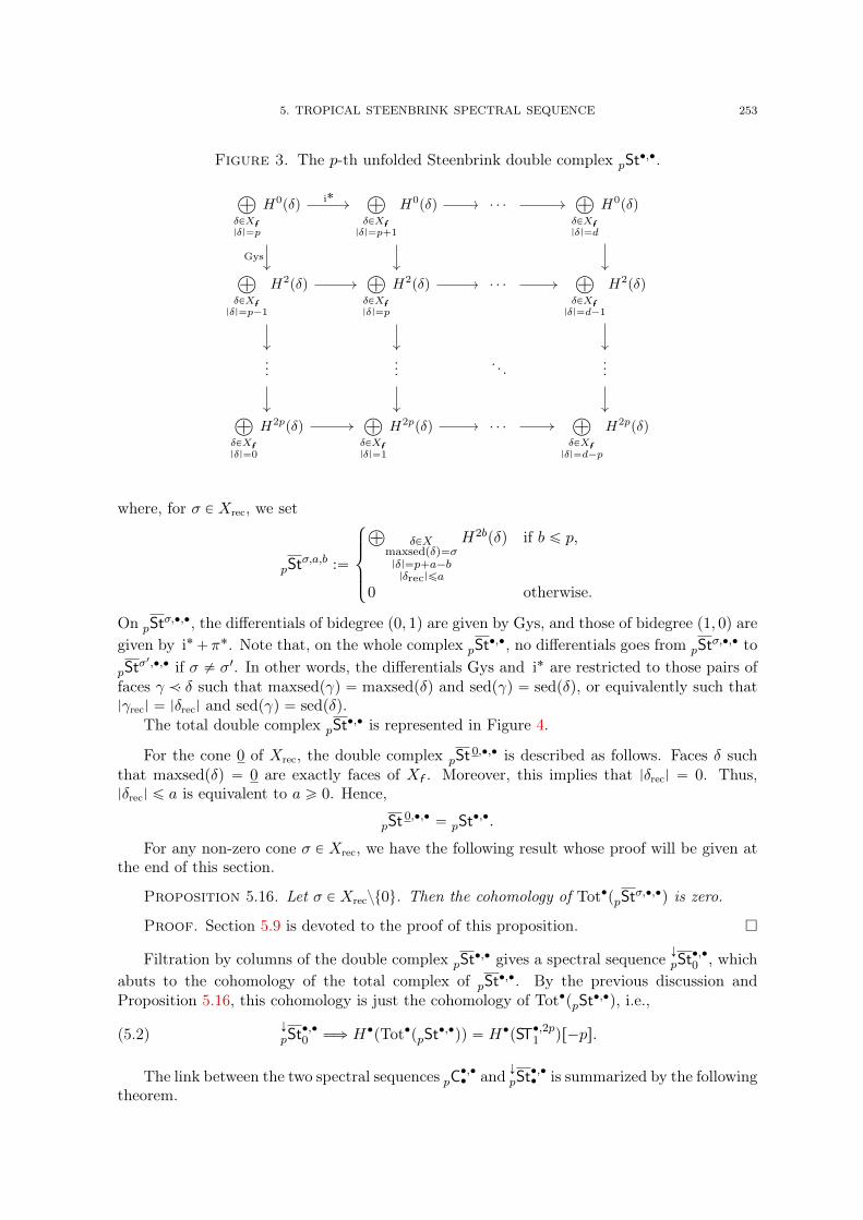
5. TROPICAL STEENBRINK SPECTRAL SEQUENCE 253
Figure 3. The p-th unfolded Steenbrink double complex pSt‚,‚.
à
δPXf|δ|“p
H0pδqà
δPXf|δ|“p`1
H0pδq . . .à
δPXf|δ|“d
H0pδq
à
δPXf|δ|“p´1
H2pδqà
δPXf|δ|“p
H2pδq . . .à
δPXf|δ|“d´1
H2pδq
......
. . ....
à
δPXf|δ|“0
H2ppδqà
δPXf|δ|“1
H2ppδq . . .à
δPXf|δ|“d´p
H2ppδq
Gys
i˚
where, for σ P Xrec, we set
pStσ,a,b :“
$
’
’
&
’
’
%
À
δPXmaxsedpδq“σ|δ|“p`a´b|δrec|ďa
H2bpδq if b ď p,
0 otherwise.
On pStσ,‚,‚, the differentials of bidegree p0, 1q are given by Gys, and those of bidegree p1, 0q are
given by i˚`π˚. Note that, on the whole complex pSt‚,‚, no differentials goes from pSt
σ,‚,‚ to
pStσ1,‚,‚ if σ ‰ σ1. In other words, the differentials Gys and i˚ are restricted to those pairs of
faces γ ă δ such that maxsedpγq “ maxsedpδq and sedpγq “ sedpδq, or equivalently such that|γrec| “ |δrec| and sedpγq “ sedpδq.
The total double complex pSt‚,‚ is represented in Figure 4.
For the cone 0 of Xrec, the double complex pSt0,‚,‚ is described as follows. Faces δ such
that maxsedpδq “ 0 are exactly faces of Xf . Moreover, this implies that |δrec| “ 0. Thus,|δrec| ď a is equivalent to a ě 0. Hence,
pSt0,‚,‚ “ pSt
‚,‚.
For any non-zero cone σ P Xrec, we have the following result whose proof will be given atthe end of this section.
Proposition 5.16. Let σ P Xreczt0u. Then the cohomology of Tot‚ppStσ,‚,‚q is zero.
Proof. Section 5.9 is devoted to the proof of this proposition.
Filtration by columns of the double complex pSt‚,‚ gives a spectral sequence ÓpSt
‚,‚0 , which
abuts to the cohomology of the total complex of pSt‚,‚. By the previous discussion and
Proposition 5.16, this cohomology is just the cohomology of Tot‚ppSt‚,‚q, i.e.,
(5.2) Ó
pSt‚,‚0 ùñ H‚pTot‚ppSt
‚,‚qq “ H‚pST‚,2p1 qr´ps.
The link between the two spectral sequences pC‚,‚‚ and ÓpSt
‚,‚‚ is summarized by the following
theorem.
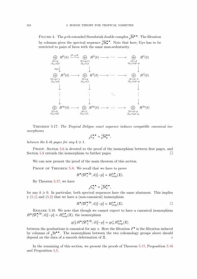
254 3. HODGE THEORY FOR TROPICAL VARIETIES
Figure 4. The p-th extended Steenbrink double complex pSt‚,‚. The filtration
by columns gives the spectral sequence ÓpSt‚,‚‚ . Note that here, Gys has to be
restricted to pairs of faces with the same max-sedentarity.
à
|δ|“p|δ8|ď0
H0pδqà
|δ|“p`1|δ8|ď1
H0pδq . . .à
|δ|“d|δ8|ďd´p
H0pδq
à
|δ|“p´1|δ8|ď0
H2pδqà
|δ|“p|δ8|ď1
H2pδq . . .à
|δ|“d´1|δ8|ďd´p
H2pδq
......
. . ....
à
|δ|“0|δ8|ď0
H2ppδqà
|δ|“1|δ8|ď1
H2ppδq . . .à
|δ|“d´p|δ8|ďd´p
H2ppδq
Gys
i˚`π˚
Theorem 5.17. The Tropical Deligne exact sequence induces compatible canonical iso-morphisms
pC‚,‚k »
Ó
pSt‚,‚k ,
between the k-th pages for any k ě 1.
Proof. Section 5.6 is devoted to the proof of the isomorphism between first pages, andSection 5.8 extends the isomorphism to further pages.
We can now present the proof of the main theorem of this section.
Proof of Theorem 5.8. We recall that we have to prove
H‚pST‚,2p1 ,dqr´ps “ Hp,‚troppXq.
By Theorem 5.17, we have
pC‚,‚k »
Ó
pSt‚,‚k ,
for any k ě 0. In particular, both spectral sequences have the same abutment. This impliesy (5.1) and (5.2) that we have a (non-canonical) isomorphism
H‚pST‚,2p1 ,dqr´ps » Hp,‚troppXq.
Remark 5.18. We note that though we cannot expect to have a canonical isomorphismH‚pST‚,2p1 ,dqr´ps » Hp,‚
troppXq, the isomorphism
grsFH‚pST‚,2p1 , dqr´ps » grsWH
p,‚troppXq
between the graduations is canonical for any s. Here the filtration F ‚ is the filtration inducedby columns of pSt‚,‚. The isomorphism between the two cohomology groups above shoulddepend on the data of a smooth deformation of X. ˛
In the remaining of this section, we present the proofs of Theorem 5.17, Proposition 5.16and Proposition 5.5.
5. TROPICAL STEENBRINK SPECTRAL SEQUENCE 255
5.6. From pC‚,‚1 to Ó
pSt‚,‚1 . In this section and the two following ones, we prove Theo-
rem 5.17, which states that pC‚,‚k is canonically isomorphic to pSt
‚,‚k for k ě 1. As a warm-up,
in this section, we study the case of the first page k “ 1. Some of the results and construc-tions in this section will be used in the next section to achieve the isomorphism of otherpages. In order to keep the reading flow, a few technical points of this section will be treatedin Appendix 10.
We have to prove that, for every integer a, the cochain complex
pCa,‚0 : 0 Ñ
à
|δ|“a
Ź0T‹δ b Fpp0δq Ñà
|δ|“a`1
Ź1T‹δ b Fp´1p0δq Ñ ¨ ¨ ¨
¨ ¨ ¨ Ñà
|δ|“a`p
ŹpT‹δ b F0p0δq Ñ 0
is quasi-isomorphic to
pSta,‚0 : 0 Ñ
à
|δ|“p`a|δrec|ďa
H0pδq Ñà
|δ|“p`a´1|δrec|ďa
H2pδq Ñ ¨ ¨ ¨ Ñà
|δ|“a|δrec|ďa
H2ppδq Ñ 0.
Moreover, the induced isomorphisms in cohomology must commute with the differentials ofdegree p1, 0q on the respective first pages:
pCa,‚1 pC
a`1,‚1
Ó
pSta,‚1
Ó
pSta`1,‚1
„ „
i˚`π˚
In order to calculate the cohomology of the first cochain complex, we use the tropicalDeligne resolution. Applying that exact sequence to the unimodular fan Σδ and to any integers, we get the exact sequence
0 Ñ Fsp0δq Ñà
ζPΣδ
|ζ|“s
H0pζq Ñà
ζPΣδ
|ζ|“s´1
H2pζq Ñ ¨ ¨ ¨ Ñà
ζPΣδ
|ζ|“1
H2s´2pζq Ñ H2sp0δq Ñ 0.
Given the correspondence between cones ζ P Σδ, and faces η P X which contain δ, withthe same sedentarity, we rewrite the exact sequence above in the form
0 Ñ Fsp0δq Ñà
ηąδ|η|“s`|δ|
sedpηq “ sedpδq
H0pηq Ñà
ηąδ|η|“s´1`|δ|
sedpηq “ sedpδq
H2pηq Ñ ¨ ¨ ¨ Ñà
ηąδ|η|“1`|δ|
sedpηq “ sedpδq
H2s´2pηq Ñ H2spδq Ñ 0.
Replacing now each Fsp0δq in pCa,‚0 by the resolution given by the tropical Deligne complex,
we get the double complex aDb,b1 whose total complex has the same cohomology as pCa,‚. More
precisely, define the double complex aD‚,‚ as follows.
aDb,b1 :“
à
|δ|“a`b
ŹbT‹δ b´
à
ηąδ|η|“p`a´b1
sedpηq“sedpδq
H2b1pηq¯
.
The differential d1 of bidegree p0, 1q comes from the Deligne sequence and is id b Gys. Thedifferential of bidegree p1, 0q is defined as follows, thanks to the map i˚
:ŹsT‹γ Ñ
Źs`1T‹δwhich has been defined right before Proposition 5.15. The differential d of bidegree p1, 0q ischosen to be i˚
b id (extended using our sign function as in Section 5.1) on rows with even
indices and to be ´ i˚b id on rows with odd indices. More concisely, we set
d :“ p´1qb1
i˚b id.

256 3. HODGE THEORY FOR TROPICAL VARIETIES
Proposition 5.19. We have dd1 ` d1d “ 0. Moreover, the inclusion ppCa,‚0 , i˚
b i˚Kq ãÑ
paD‚,0,d1q is a morphism of cochain complexes.
Proof. This follows by a simple computation. The details are given in Appendix 10.
By the exactness of the tropical Deligne sequence that we proved in Proposition 5.9, weknow that the b-th column of aD
b,‚0 of aD
‚,‚0 is a right resolution of pC
a,b0 .
We claim the following result.
Proposition 5.20. The b1-th row aD‚,b1
0 of aD‚,‚0 is a right resolution of pSt
a,b1
0 .
The proof of this proposition is given in Section 5.7. Admitting this result for the moment,we explain how to finish the proof of the isomorphism between first pages. We will need thefollowing Lemma, which seems to be folklore, for which we provide a proof.
Lemma 5.21 (Zigzag isomorphism). Let A‚,‚ be a double complex of differentials d and d1
of respective degree p1, 0q and p0, 1q. Assume that
— dd1 ` d1d “ 0,
— Ab,b1
“ 0 if b ă 0 or b1 ă 0,
— Ab,‚ is exact if b ą 0,
— A‚,b1
is exact if b1 ą 0.
Then, there is a canonical isomorphism
H‚pA0,‚q » H‚pA‚,0q.
Moreover, if B‚,‚ is another double complex with the same property, and if Φ: A‚,‚ Ñ B‚,‚
is a morphism of double complexes, then the following diagram commutes.
H‚pA0,‚q H‚pB0,‚q
H‚pA‚,0q H‚pB‚,0q
„
Φ
„
Φ
where Φ denotes the induced maps on the cohomologies. This also holds if Φ anticommuteswith the differentials.
The isomorphism H‚pA0,‚q » H‚pA‚,0q comes from the inclusions
pA0,‚,d1q ãÑ pTotpA‚,‚,d` d1qq Ðâ pA‚,0,dq
which are both quasi-isomorphisms. In the following, we give a canonical description of thisisomorphism.
Let b be a non-negative integer and b1 be any integer. Define
Lb,b1
:“kerpdd1q X Ab,b
1
`
Impdq ` Impd1q˘
X Ab,b1 and Rb,b
1
:“kerpdq X kerpd1q X Ab,b
1`1
Impdd1q X Ab,b1`1
.
We claim the following.
Claim 5.22. Notations as in Lemma 5.21, the map d1 induces an isomorphism
Lb1b1 „ÝÝÑ
d1Rb,b
1
.
Proof. Let y be an element of kerpdq X kerpd1q X Ab,b1`1. By the exactness of the b-
th column, there exists a preimage x of y by d1. Moreover, x P kerpdd1q X Ab,b1
. Hence,
5. TROPICAL STEENBRINK SPECTRAL SEQUENCE 257
d1 is surjective from kerpdd1q X Ab,b1
to kerpdq X kerpd1q X Ab,b1`1. From the trivial identity
Impdd1q “ d1Impdq, we get
d1´1`
Impdd1q X Ab,b1`1
˘
“`
Impdq ` kerpd1q˘
X Ab,b1
“`
Impdq ` Impd1q˘
X Ab,b1
.
This gives the isomorphism d1 : Lb,b1„ÝÑ Rb,b
1`1.
Proof of Lemma 5.21. Let b be a non-negative and b1 be any integer. By the previousclaim, we have an isomorphism d1 : Lb,b
1„ÝÑ Rb,b
1`1.By symmetry, if b1 is non-negative and b is any integer, we get a second isomorphism
d: Lb,b1„ÝÑ Rb`1,b1 . Thus, for any non-negative integer k, we obtain a zigzag of isomorphisms:
‚
‚
‚
‚
‚
‚
‚
‚
‚
‚
‚
‚
‚
‚
‚
‚
L0,k
Lk,0
Lk,0 Rk,1 Lk´1,1 Rk´1,2 ¨ ¨ ¨ R1,k L0,k.„
d1„
´d
„
d1„
´d
„
d1„
´d
Notice that we take ´d and not d. We refer to Remark 5.23 for an explanation of this choice.
Since d1 is injective on A‚,0, and since Impd1q X Ak,0 “ t0u, we obtain
Lk,0 “kerpdd1q X Ak,0
`
Impdq ` Impd1q˘
X Ak,0“
kerpdq X Ak,0
Impdq X Ak,0“ HkpA‚,0q.
By a symmetric argument, L0,k “ HkpA0,‚q. This gives an isomorphism
HkpA‚,0q „ÝÑ HkpA0,‚q.
The second part of the lemma is clear from the above claim and the preceding arguments.(In the case Φ anticommutes, the commutative diagram holds for p´1qb`b
1
Φ which commutes.)
Remark 5.23. We now explain why we choose the isomorphisms d1 and ´d in the aboveproof. Let a P Rk´i,i`1. The zigzag map sends a to b P Lk´i,i such that d1b “ a, and also toa1 “ ´db P Rk´i`1,i. Thus, a ´ a1 “ pd ` d1qb P Impd ` d1q. Moreover, by the definition ofR‚,‚, it is clear that a and a1 belong to kerpd` d1q. Hence, a and a1 are two representatives ofthe same element of
Hk`1`
TotpA‚,‚,d` d1q˘
,
i.e., the zigzag isomorphism is just identity on the cohomology of A‚,‚. ˛
Proof of Theorem 5.17 in page one. Define the double complex aAb,b1 by shifting
the double complex aDb,b1 by the vector p1, 1q and by inserting the the complexes pC
a,‚0 r´1s
and pSta,‚0 r´1s as the zero-th row and the zero-th column, respectively. More precisely, we set
aAb,b1 “
$
’
’
’
&
’
’
’
%
0 if b ă 0 or b1 ă 0,
pCa,b´10 if b1 “ 0
pSta,b1´10 if b “ 0
aDb´1,b1´1 if b ą 0 and b1 ą 0,
with the corresponding differentials d and d1 of respective bidegree p1, 0q and p0, 1q such that
aA‚,0 “ pC
a,‚´10 ,
aA‚,b1 “
´
pSta,b1´10 ãÑ aD
‚´1,b1´1¯
@b1 ě 1,
aA0,‚ “ pSt
a,‚´10 , and
aAb,‚ “
´
pCa,b´10 ãÑ aD
b´1,‚´1¯
@b ě 1.
258 3. HODGE THEORY FOR TROPICAL VARIETIES
One can easily extend Proposition 5.19 to get that d and d1 commute (the details are givenin Appendix 10). Moreover, by the exactness of Deligne sequence and by Proposition 5.20,all rows but the 0-th one and all columns but the 0-th one are exact. Thus we can applyLemma 5.21 to get an isomorphism
H‚paA‚,0q „ÝÑ H‚paA
0,‚q.
Looking at the definition of aA‚,‚, up to a shift by 1, this isomorphism is just what we want,i.e., the following isomorphism in page one.
pCa,‚1
„ÝÑ pSta,‚1 .
It remains to prove the commutativity of the following diagram.
pCa,‚1 pC
a`1,‚1
Ó
pSta,‚1
Ó
pSta`1,‚1
„
i˚`π˚„
i˚`π˚
To prove this, we construct two anticommutative morphisms of double complexes.The first morphism corresponds to π˚ and is naturally defined as follows. On pC
a,b itis given by π˚ b id, on pSt
a,b1 it equals π˚, and on aDb,b1 it is defined by π˚ b id. The
anticommutativity properties are easy to check.The second morphism, which we denote d i, corresponds to i˚ and is defined as follows. To
keep the reading flow, we postpone the proof that d i is indeed a morphism and more detailsabout the construction to Appendix 10.
For each face δ P X, let pδ : NsedpδqR Ñ Tδ be a projection as defined just after Proposi-
tion 5.12. Assume moreover that the projections are compatible in the following sense:
— if γ ă δ have not the same sedentarity, then πsedpδqăsedpγqpδ “ pγπsedpδqăsedpγq, whereπsedpδqăsedpγq : N
sedpδqR Ñ N
sedpγqR is the natural projection;
— if γ ă δ, then pγpδ “ pγ .
For instance, we can choose an inner product on NR and extend it naturally on all thestrata Nσ
R for σ P Xrec. Then, if the projections pδ are chosen to be the orthogonal projectionswith respect to this inner product, then they are compatible in the above sense.
With these conventions, we define d i on pSta,b1 by d i :“ i˚. On pC
a,b, let α b β PŹbT‹γ b Fp´bp0γq, where δ ą γ is a pair of faces of same sedentarity and |γ| “ a ` b. Thenthe part of its image by d i in
ŹbT‹δ b Fp´bp0δq is defined by
(5.3) signpγ, δqpγ |˚
Tδpαq b pu ÞÑ π˚δ βpu
1qq,
where, for u P Fp´bp0δq, the multivector u1 denotes the only element ofŹp´b kerppγq such
that πδpu1q “ u (one can check that u P Fp´bpγq).
On aDb,b1 , let αb x P
ŹbT‹γ bH2b1pηq where η ą γ is a face of dimension |γ|` p´ b´ b1.Then the part of its image by d i in
ŹbT‹δ bH2b1pµq, with µ ą δ, is given by
signpη, µqn‹δγppδpuqqpγ |˚
δpαq b i˚ηăµpxq,
where u is a vector going from any point of Tγ to the vertex of µ which is not in η.We will prove in Appendix 10 that this map is indeed a morphism, and that the induced
map on the first page pCa,‚1 is equal to the differential corresponding to i˚ given by the spectral
sequence. This concludes the proof of the proposition.
5. TROPICAL STEENBRINK SPECTRAL SEQUENCE 259
5.7. Proof of Proposition 5.20. In order to conclude the proof of isomorphism betweenthe first pages,we are thus left to prove Proposition 5.20. This proposition claims the exactnessof the following sequence for any integer b1:
0 Ñà
|η|“p`a´b1|η8|ďa
H2b1pηq Ñà
|δ|“a
Ź0T‹δ b´
à
ηąδ|η|“p`a´b1
sedpηq“sedpδq
H2b1pηq¯
Ñà
|δ|“a`1
Ź1T‹δ b´
à
ηąδ|η|“p`a´b1
sedpηq“sedpδq
H2b1pηq¯
Ñ
¨ ¨ ¨ Ñà
|δ|“a`p´b1
Źp´b1T‹δ b´
à
ηąδ|η|“p`a´b1
sedpηq“sedpδq
H2b1pηq¯
Ñ 0,
where we recall that the maps are i˚b id and that the relations η ą δ only concern those
faces which have the same sedentarity sedpηq “ sedpδq.
As the form of each term suggests, we can decompose this sequence as a direct sum ofsequences over fixed η of dimension s :“ p` a´ b1 as follows:
à
|η|“s
´
0 Ñ Rεη Ñà
δăη|δ|“a
Ź0T‹δ Ñà
δăη|δ|“a`1
Ź1T‹δ Ñ ¨ ¨ ¨ Ñà
δăη|δ|“s
Źp´b1T‹δ Ñ 0¯
bH2b1pηq,
where
εη “
#
1 if |ηrec| ď a,0 otherwise.
Therefore, the following result clearly implies Proposition 5.20.
Proposition 5.24. For each pair of non-negative integers r ď n, and for each (simplicial)unimodular polyhedron η of dimension n, the cochain complex
C‚r pηq : 0 ÝÑà
δăη|δ|“r
Ź0T‹δr´rs ÝÑà
δăη|δ|“r`1
Ź1T‹δr´r´1s ÝÑ . . . ÝÑà
δăη|δ|“n
Źn´rT‹δr´ns ÝÑ 0,
whose maps are given by i˚, has cohomology
#
Rr´rs if |ηrec| ď r,
0 if |ηrec| ą r.
Proof. We will reduce the statement to the computation of some appropriate cohomologygroups of the tropical projective spaces.
We begin with the case |ηrec| “ 0, i.e., η is a unimodular simplex. Let us study the dualcomplex instead, which using the duality between
ŹrT‹δ andŹ|δ|´rT‹δ for each simplex δ,
has the following form
0 ÝÑà
δăη|δ|“n
ŹrT‹δr´ns ÝÑà
δăη|δ|“n´1
ŹrT‹δr´n` 1s ÝÑ . . . ÝÑà
δăη|δ|“r
ŹrT‹δr´rs ÝÑ 0.
The maps in this complex are induced by restriction mapŹrT‹δ Ñ
ŹrT‹ζ for inclusion offaces ζ ă δ, extended with sign according to our convention in Section 5.1.
For the ease of arguments, it will be convenient to choose an inner product x ¨ , ¨ y on Tη.This inner product restricts to Tδ for each face δ and extends naturally to multivectors. Moreprecisely, for any collection of vectors u1, . . . , uk, v1, . . . , vk, we set
xu1 ^ ¨ ¨ ¨ ^ uk, v1 ^ ¨ ¨ ¨ ^ vky :“ det´
`
xui, vjy˘
1ďi,jďk
¯
.
Let γ ă δ be a pair of faces. We define pδ ąγ : Tδ Ñ Tγ to be the orthogonal projectionand naturally extend it to multivectors in the exterior algebra.

260 3. HODGE THEORY FOR TROPICAL VARIETIES
Let α PŹrT‹δ. We denote by α‹ the dual multivector of α, defined by the property
αpuq “ xα‹,uy
for any u PŹrTδ.
Moreover, we denote by α|γ the restriction of α onŹrTγ. By adjunction property, we get
the following equality:pδ ąγpα
‹q “ pα|γq‹.
Indeed, for any u PŹrTγ Ă
ŹrTδ, we have
α|γpuq “ αpuq “ xα‹,uy “ xpδ ąγpα‹q,uy.
This implies that the linear map which sends α ÞÑ α‹ provides an isomorphism betweenthe two following complexes: our original complex on one side,
0à
δăη|δ|“n
ŹrT‹δà
δăη|δ|“n´1
ŹrT‹δ . . .à
δăη|δ|“r
ŹrT‹δ 0,
and its dual
0à
δăη|δ|“n
ŹrTδà
δăη|δ|“n´1
ŹrTδ . . .à
δăη|δ|“r
ŹrTδ 0.
Note that the maps of the second complex are given by the orthogonal projections p.
We claim that the second complex above computes Hr,‚troppTPnq, which leads the result.
Indeed, the only non-trivial cohomology groups of TPn are Hp,ptroppTPnq » R for 0 ď p ď n.
Denote by δ0, . . . , δn all the faces of codimension one of η. For each δi, let `i be the affinemap on η which is identically equal to 1 on δi and takes value 0 on the opposite vertex toδi. Let `0i P T‹η be the linear map corresponding to `i. It is easy to see that
ř
i `0i “ 0. Set
ui :“ p`0i q‹ P Tη. Let pe0, . . . , enq be the standard basis of Rn. We get a linear isomorphism
Tη „ÝÑ NR “ Rn`1L
p1, . . . , 1q by mapping the ui to ei seen in NR. The family peiqi induce anatural compactification of NR into TPn, and each face δ of η corresponds to a stratum Nδ,Rof dimension |δ|. Moreover, the linear isomorphism Tη „ÝÑ NR induces a linear isomorphismTδ „ÝÑ Nδ,R. The projections π on TPn and p on η commute with these isomorphisms. Thuswe get an isomorphism between complexes:
0à
δăη|δ|“n
ŹrTδà
δăη|δ|“n´1
ŹrTδ . . .à
δăη|δ|“r
ŹrTδ 0,
0 FrpNRqà
δăη|δ|“n´1
FrpNδ,Rq . . .à
δăη|δ|“r
FrpNδ,Rq 0.
The second complex is just the tropical simplicial complex of TPn for the coarsest simplicialsubdivision. Hence, its cohomology is Hr,‚
troppTPnq “ Rr´rs. These concludes the case |ηrec| “0.
It remains to generalize to any simplicial polyhedron η. If η “ ρ is a ray, by a directcomputation, the proposition holds: H‚pC‚0 pρqq is trivial and H‚pC‚1 pρqq “ Rr´1s. In general,

5. TROPICAL STEENBRINK SPECTRAL SEQUENCE 261
η is isomorphic to ηf ˆ ρˆ ¨ ¨ ¨ ˆ ρlooooomooooon
m times
, where ρ is a ray and m :“ |ηrec|. Moreover,
C‚r pηq »à
r0,...,rmě0r0`¨¨¨`rm“r
C‚r0pηf q b C‚r1pρq b ¨ ¨ ¨ b C
‚rmpρq.
By the Künneth formula for cochain complexes of vector spaces, this decomposition also holdsfor cohomology. I.e., we have
H‚pC‚r pηqq »à
r0,...,rmě0r0`¨¨¨`rm“r
H‚pC‚r0pηf qq bH‚pC‚r1pρqq b ¨ ¨ ¨ bH
‚pC‚rmpρqq.
Looking at the cohomology of the rays, all terms are trivial except the term of indices r1 “
¨ ¨ ¨ “ rm “ 1 and r0 “ r ´m if m ď r. In this case, we get
H‚pC‚r pηqq » H‚pC‚r´mpηf qq bH‚pC‚1 pρqq
bm
» Rr´r `ms b Rr´1sbm
H‚pC‚r pηqq “ Rr´rs.
This concludes the proof of the proposition.
We have so far proved that the first pages of pC‚,‚ and of pSt‚,‚ coincide. Unfortunately,this is not sufficient in general to conclude that the two spectral sequences have the sameabutment. Thus, we have to extend the isomorphism to further pages. A direct use of thezigzag lemma on further pages is tedious. Therefore, in the next section, we present a proofusing a kind of generalization of the zigzag lemma.
5.8. Isomorphisms on further pages. In this section, we achieve the proof of The-orem 5.17. To do so, we start by stating a general lemma about spectral sequences whichwe call the spectral resolution lemma. Roughly speaking, this lemma states that, under somenatural assumptions, a resolution of a spectral sequence results in another spectral sequencewhich coincides with the first one on any further pages.
To prove Theorem 5.17, we will apply this lemma to the triply indexed differential complexp‚D
‚,‚, B “ d i ` π˚ ` d ` d1q introduced above (actually a slight modification obtained byinserting the Steenbrink and tropical sequences). This triply indexed complex plays the roleof a bridge between the two spectral sequences pC‚,‚ and
Ó
pSt‚,‚. In fact, as we will show below,
it provides a spectral resolution, in a sense which will be made precise in a moment, of boththe spectral sequences at the same time. Thus, applying the spectral resolution lemma allowsto directly conclude the proof of Theorem 5.17.
Though the method presented below gives an alternate proof of the isomorphism in pageone, independent of the one given in the previous section, the intermediate results of theprevious section will be crucial in showing the stated resolution property, and so to verifythe assumption of the spectral resolution lemma. In a sense, this lemma stands upon thebasic case treated in the previous section. Moreover, as the proof of the spectral resolutionlemma shows, this lemma can be regarded as a generalization of the zig-zag lemma used inthe previous section.
5.8.1. Triply indexed differential complexes. Before we state the lemma, we introduce someconventions. By a triply indexed differential complex pE‚,‚,‚, Bq, we mean
— Ea,b,c “ 0 unless a, b, c ě 0;

262 3. HODGE THEORY FOR TROPICAL VARIETIES
— the map B : E‚,‚,‚ Ñ E‚,‚,‚ is of degree one, i.e., it can be decomposed as follows:
B “à
i,j,kPZi`j`k“1
Bi,j,k, with
@i, j, k P Z, Bi,j,k “à
a,b,cPZBi,j,k|Ea,b,c ,
where Bi,j,k|Ea,b,c is a map from Ea,b,c to Ea`i,b`j,c`k;
— we have BB “ 0.
With these assumptions, the total complex Tot‚pE‚,‚,‚q becomes a differential complex.
The filtration induced by the first index on E‚,‚,‚ is by definition the decreasing filtration
E‚,‚,‚ “ Eě0,‚,‚ Ě Eě1,‚,‚ Ě Eě2,‚,‚ Ě . . . ,
whereEěa,‚,‚ “
à
a1ěa
Ea1,‚,‚.
Notice that the differential B preserves the filtration induced by the first index if and onlyif Bi,j,k “ 0 for any i ă 0. In such a case, we denote by IE‚,‚0 the 0-th page of the inducedspectral sequence abutting to the cohomology of the total complex Tot‚pE‚,‚,‚q. It has thefollowing shape:
IEa,b0 “ Tota`bpEa,‚,‚q “à
m,nm`n“b
Ea,m,n
endowed with the differentialIB :“
ÿ
j,lPZB0,j,l.
The k-th page of this spectral is denoted by IE‚,‚k .
We use analogous conventions as above to define bi-indexed differential complexes.5.8.2. Statement of the spectral resolution lemma. Let pC‚,‚,dq be a bi-indexed differential
complex. We assume that d preserves the filtration induced by the first index, i.e., we assumedi,j “ 0 if i ă 0.
A spectral resolution of pC‚,‚, dq is a triply indexed differential complex pE‚,‚,‚, Bq whichverifies the following properties enumerated R1-R4:
(R1) There is an inclusion i : C‚,‚ Ñ E‚,‚,0 Ď E‚,‚,‚ which respects the bi-indices, i.e., suchthat i d “ B i (here B is not restricted to E‚,‚,0).
(R2) The differential B of E‚,‚,‚ preserves the filtration induced by the first index, i.e., wehave Bi,j,k “ 0 if i ă 0.
(R3) We have Bi,j,k “ 0 if k ě 2.
Denote by B3 :“ B0,0,1. From the fact that B is a differential and the assumptions above,we deduce that B3B3 “ 0. Finally, we assume the following resolution property.
(R4) For any a, b in Z, the differential complex pEa,b,‚, B3|Ea,b,‚q is a right resolution of Ca,b.
Lemma 5.25 (Spectral resolution lemma). Let pC‚,‚, dq be a bi-indexed complex such thatthe differential d preserves the filtration induced by the first index. Let pE‚,‚,‚, Bq be a spectralresolution of C‚,‚.
5. TROPICAL STEENBRINK SPECTRAL SEQUENCE 263
Denote by IE‚,‚ and IC‚,‚ the spectral sequences induced by the filtration by the first indiceson E‚,‚,‚ and C‚,‚, respectively. Then, the inclusion i : C‚,‚ ãÑ E‚,‚,‚ induces canonicalcompatible isomorphisms
IC‚,‚k » IE‚,‚kbetween k-th pages of the two spectral sequences for any values of k ě 1.
We assume for the moment this lemma and finish the proof of Theorem 5.17.5.8.3. Proof of Theorem 5.17. We use the notations of Section 5.6. We will apply the
spectral resolution lemma twice in order to achieve the isomorphism of pages staged in thetheorem.
We start by gathering the double complexes aD‚,‚ together for all a in order to constructa triply indexed differential complex pD‚,‚,‚, Bq as follows. First, set
Da,b,b1
:“ aDb,b1
and let the two differentials of multidegrees p0, 1, 0q and p0, 0, 1q be equal to the differentialsd and d1 of the double complexes aD‚,‚.
In the course of proving the isomorphism between the first pages of the spectral sequencesin Theorem 5.17, we introduced in Section 5.6 two anticommutative morphisms π˚ and d i ofmultidegree p1, 0, 0q from aD
‚,‚ Ñ a`1D‚,‚.
We set B “ d i ` π˚ ` d` d1.
Proposition 5.26. We have BB “ 0.
Proof. The proof consists of calculating directly all the terms which appear in this de-composition. This will be explained in Appendix 10.
Denote by pC‚,‚ the bi-indexed complex pC
‚,‚0 which is endowed with the differential d i `
π˚` d, where di, π˚ and d are the maps defined on A‚,0 “ Tot‚ppC‚,‚q in the previous section
that we restrict to its zero-th row.The inclusion A‚,0 Ñ A‚,1 gives an inclusion of complexes of pC‚,‚ into pD
‚,‚,‚. Moreover,for any integers a and b, the complex pDa,b,‚,d1q is the Deligne resolution of pC
a,b0 . Thus we
can apply the spectral resolution lemma. This gives canonical isomorphisms
(5.4) @ k ě 1, IpC‚,‚k » ID‚,‚k .
A priori, IpC‚,‚k could be different from pC
‚,‚k . So it might appear somehow surprising to
see that they are actually equal thanks to the following proposition.
Proposition 5.27. The natural isomorphism Cp,‚trop„ÝÑ Tot‚ppC
‚,‚q is an isomorphism offiltered differential complexes. Here Cp,‚trop comes with differential Btrop and weight filtrationW ‚, the differential on Tot‚ppC
‚,‚q is d i ` π˚ ` d and the filtration is induced by the firstindex.
Proof. The proof of this proposition is given in Appendix 10.
In the same way, from Section 5.6, we deduce an inclusion of complexes of aSt‚,‚, withthe usual differentials Gys and i˚ ` π˚, into D‚,0,‚. Moreover, by Proposition 5.20, proved inSection 5.7, for any pair of integers a and b1, the complex pDa,N,b
1
, dq is a resolution of pSta,b1
0 .
Thus, by applying again the spectral resolution lemma, we get canonical isomorphisms
(5.5) @ k ě 1,Ó
pSt‚,‚k » ID‚,‚k .
From (5.4) and (5.5), we infer canonical isomorphisms
264 3. HODGE THEORY FOR TROPICAL VARIETIES
pC‚,‚k »
Ó
pSt‚,‚k
between k-th pages for any k ě 1 of the two spectral sequences, which concludes the proof ofTheorem 5.17.
5.8.4. Proof of the spectral resolution lemma. In this section we prove the resolutionlemma. Assume that i : C‚,‚ ãÑ A‚,‚,0 Ď A‚,‚,‚ is a spectral resolution of the bi-indexeddifferential complex C‚,‚.
Proof of Lemma 5.25. Let k ě 1. By construction of the pages of the spectral se-quences, we have
IEa,bk “
!
x P Tota`bpE‚,‚,‚q X Eěa,‚,‚ˇ
ˇ Bx P Eěa`k,‚,‚)
Eěa`1,‚,‚ ` BEěa´k`1,‚,‚.
(To be more rigorous, we should replace here the denominator by the intersection of thenumerator with the denominator.)
The idea is to prove that one can take a representative of the above quotient in the imageof i. To do so, we use the following induction which can be seen as a generalization of thezigzag lemma.
Claim 5.28. Let a be an integer. The following quotient!
x P Tota`bpE‚,‚,‚q X Eěa,‚,‚ˇ
ˇ Bx P Eěa`k,‚,‚)
Eěa`k,‚,‚ ` BEěa´k`1,‚,‚ ` ipCěa,‚q
is zero.
Notice that, in the denominator, we did not use Eěa`1,‚,‚ but Eěa`k,‚,‚. Doing so we geta stronger result which will be needed later.
Let x be an element of the numerator of the following quotient. We first explain how toassociate a vector in Z2 to any x in the numerator. Endowing Z2 with the lexicographic order,and proceeding by induction on the lexicographical order of vectors associated to the elementsx, we show that x is zero in the quotient.
We decompose x as follows
x “ÿ
α,β,cPZαěa
α`β`c“a`b
xα,β,c, xα,β,c P Eα,β,c.
Let α be smallest integer such that there exists β, c P Z with xα,β,c ‰ 0. Note that if no suchα exists, then x “ 0 and we are done. Having chosen α, let now c be the largest integer suchthat xα,β,c ‰ 0 for β “ a` b´ α´ c. We associate to x the vector p´α, cq.
In order to prove the claim for a fixed value of a, we proceed by induction on the lexico-graphic order of the associated vectors p´α, cq. Given a vector p´α, cq, in what follows, weset β :“ a` b´ α´ c.
Base of the induction: α ě a` k. Writing x “ř
xm,n,p for xm,n,p P Em,n,p we see by thechoice of α that m ě α ě a ` k for all non-zero terms xm,n,p it follows that all these termsbelong to Eěa`k,‚,‚, and so x obviously belongs to the denominator.
first case: α ă a ` k and c ą 0. Denote by y “ř
yα1,β1,c1 the boundary Bx of x. Then,since Bx belongs to Eěa`k,‚,‚, the element yα,β,c`1 must be zero. Moreover, since Ba1,b1,c1 “ 0if c1 ě 2 or a1 ă 0, the part yα,β,c`1 of y must be equal to B3pxα,β,cq. Thus xα,β,c is in the
5. TROPICAL STEENBRINK SPECTRAL SEQUENCE 265
kernel of B3. Since pEα,β,‚, B3q is a resolution, we can take a preimage z of xα,β,c in Eα,β,c´1
for B3. ThenBz P BEěa,‚,‚ Ď BEěa´k`1,‚,‚.
Thus, x is equivalent to x1 “ x´Bz, the vector associated to x1 is strictly smaller than p´α, cq,and we conclude again by the the hypothesis of our induction for x1.
second case: α ă a ` k and c “ 0. We can follow the arguments used in the second caseabove up to the moment xα,β,0 P kerpB3q. Then, xα,β,0 belongs to ipCα,‚q. Since ipCěa,‚q isin the denominator, we can subtract xα,β,0 from x and conclude by induction.
In any case, we have proved x is equal to zero and the claim follows. As a consequence,we infer that
(5.6) IEa,bk “
!
x P Tota`bpE‚,‚,‚q X Eěa,‚,‚ˇ
ˇ Bx P Eěa`k,‚,‚)
X Imp iq`
Eěa`1,‚,‚ ` BEěa´k`1,‚,‚˘
X Imp iq.
This has to be compared with
ICa,bk “
!
z P Tota`bpC‚,‚q X Cěa,‚ˇ
ˇ dz P Cěa`k,‚)
Cěa`1,‚ ` dCěa´k`1,‚.
From id “ B i, we get that the induced map i : IEa,bk Ñ ICa,bk is well-defined. Moreover, it isnow clear that this map is surjective. For the injectivity, we have to work a bit more on thedenominator of IEa,bk .
Let x be an element of the intersection of the denominator with the numerator of (5.6).In particular, we have x P Eěa,‚,‚. Let z P Eěa´k`1,‚,‚ be such that x´ Bz P Eěa`1,‚,‚.
Now we show that we can reduce to the case z P Imp iq`Eěa`1,‚,‚. Notice that Bz P Eěa,‚,‚.Thus, z belongs to the numerator of IEa´k`1,b`k´2
k´1 . If k ě 2, we can apply the induction aboveto get that z “ z1 ` Bz2 ` iz3 with z1 P Eěa,‚,‚, z2 P Eěa´2k`3,‚,‚ and z3 P C
ěa´k`1,‚. Thisdecomposition also holds for k “ 1 setting z1 “ z and z2 “ z3 “ 0. Since we are onlyconcerned by Bz, we can assume without loss of generality that z2 “ 0.
If z1 R Eěa`1,‚,‚, let c be the maximum integer such that za,β,c ‰ 0 for β “ b´1´c. Denote
by y “ř
yα1,β1,c1 the boundary Bz of z. Since B iz3 P E‚,‚,0, we get that ya,β,c`1 “ B3 za,β,c.Moreover x ´ y “ x ´ Bz P Eěa`1,‚,‚. Hence, xa,β,c`1 must be equal to ya,β,c`1. Sincex P Imp iq Ď E‚,‚,0, xa,β,c`1 “ 0. From this we get ya,β,c`1 “ B3za,β,c “ 0. Therefore, za,β,c isin the kernel of B3. Two cases can occur.
— If c ą 0, then we can find w P Ea,β,c´1 such that za,β,c “ B1w. In this case, z1 :“ z´Bwhas the same boundary as z, and the maximal c1 such that z1a,b´1´c1,c1 ‰ 0 verifiesc1 ă c. Thus, we can apply again the previous argument until we get an element ofEěa,‚,‚, or until we are in the following case.
— If c “ 0, then za,β,0 P ipCa,βq.
We deduce that, up to a cycle, we can assume that z1 “ z11 ` z21 with z11 P ipCa,‚q andz21 P E
ěa`1,‚,‚, i.e., z P ipCěa´k`1,‚q ` Eěa`1,‚,‚.
Therefore,
x P`
Eěa`1,‚,‚ ` B`
iCěa´k`1,‚ ` Eěa`1,‚,‚˘˘
X Imp iq
“`
Eěa`1,‚,‚ ` idCěa´k`1,‚˘
X Imp iq
“ Eěa`1,‚,‚ X Imp iq ` idCěa´k`1,‚
“ i`
Cěa`1,‚ ` dCěa´k`1,‚˘
.
266 3. HODGE THEORY FOR TROPICAL VARIETIES
We can replace Equation (5.6) by
IEa,bk “
!
x P Tota`bpE‚,‚,‚q X Eěa,‚,‚ˇ
ˇ Bx P Eěa`k,‚,‚)
X Imp iq
i`
Cěa`1,‚ ` dCěa´k`1,‚˘ .
The injectivity of i : IEa,bk Ñ ICa,bk now follows from the injectivity of i : C‚,‚ Ñ E‚,‚,0, whichconcludes the proof of the spectral resolution lemma.
The two remaining section contain the proofs of the two Propositions 5.16 and 5.5.
5.9. Vanishing of the cohomology of Tot‚pStσ,‚,‚ for σ ‰ 0. In this section, we prove
Proposition 5.16, which, we recall, claims that the total cohomology of pStσ,‚,‚0 is trivial for
σ ‰ 0, where
pStσ,a,b :“
$
’
’
&
’
’
%
À
δPXmaxsedpδq“σ|δ|“p`a´b|δrec|ďa
H2bpδq if b ď p,
0 otherwise.The differential of bidegree p1, 0q is i˚ ` π˚, and the differential of bidegree p0, 1q is Gys.
This double complex can be unfolded into a triple complex: Tot‚ppStσ,‚,‚q “ Tot‚pE‚,‚,‚q
where
Ea,b,a1
:“
$
’
’
&
’
’
%
À
δPXmaxsedpδq“σ|δ|“p`a`a1´b
|δrec|“a1
H2bpδq if b ď p and a ě 0,
0 otherwise.where the differentials of multidegree p1, 0, 0q, p0, 1, 0q and p0, 0, 1q are respectively i˚, Gysand π˚.
To prove that the total cohomology of E‚,‚,‚ is trivial, it suffices to show that pEa,b,‚, π˚qis exact for any integers a and b.
Let η be a face of sedentarity 0 such that maxsedpηq “ σ. Notice that sedpηq “ 0 impliesmaxsedpηq “ ηrec. For any cone τ ă σ, we denote by ητ
8the face of η of sedentarity τ , which
is given byητ8“ η XN τ
R.
Note that each face of X of max-sedentarity σ can be written in a unique way in this form.Notice also that
— πσ induces an isomorphism from ηf to pητ8qf .
— Ση » Σητ8 . In particular H‚pητ8q » H‚pηq.
— π˚δ ąγ is nontrivial if and only if γ “ ητ8and δ “ ηζ
8for some η of sedentarity 0, and
some pair of cones ζ ă τ which are faces of maxsedpηq.
From all these observations, we deduce that the sequence pEa,b,‚, π˚q can be decomposedas a direct sum:
à
ηPX0
maxsedpηq“σ|η|“p`a`|σ|´b
´
0 Ñ H2bpησ8q Ñ
à
τăσ|τ |“|σ|´1
H2bpητ8q Ñ ¨ ¨ ¨ Ñ
à
τăσ|τ |“1
H2bpητ8q Ñ H2bpηq Ñ 0
¯
.
This sequence can be rewritten asà
ηPX0
maxsedpηq“σ|η|“p`a`|σ|´b
´
0 Ñ RÑà
τăσ|τ |“|σ|´1
RÑ ¨ ¨ ¨ Ñà
τăσ|τ |“1
RÑ RÑ 0¯
bH2bpηq.
5. TROPICAL STEENBRINK SPECTRAL SEQUENCE 267
Thus, it just remains to prove that these sequences are exact for every η. The complexis clearly isomorphic to the simplicial homology of σ with real coefficients. This homology istrivial since it corresponds to the reduced homology of a simplex.
This concludes the proof of Proposition 5.16 and thus that of Theorem 5.8.
5.10. Proof of Proposition 5.5. In this final part of this section, we prove Proposi-tion 5.5 which concerns the three basic relations concerning the composition of maps Gys andi˚.
Let us start by proving that the composition Gys ˝Gys is vanishing.Let a, b be a pair of integers, and let s ě |a| be an integer with s ” a mod 2. Let
x P STa,b,s1 . We have to prove that Gys ˝Gyspxq “ 0. By linearity of the Gysin maps, we canassume that x P Ha`b´spδq for some δ P Xf of dimension s. If s´1 ă |a`1|, or s´2 ă |a`2|,then Gys ˝Gyspxq “ 0. Otherwise,
Gys ˝Gyspxq “ÿ
γăδ
ÿ
νăγ
signpν, γqsignpγ, δqGysγ ąν ˝Gysδ ąγpxq.
This sum can be rewritten in the form
Gys ˝Gyspxq “ÿ
νăδ|ν|“s´2
ÿ
γăδγ ąν
signpν, γqsignpγ, δqGysγ ąν ˝Gysδ ąγpxq.
If ν is a subface of δ of codimension 2, then, by the diamond property, there exist exactly twofaces γ and γ1 such that ν ă γ,γ1 ă δ. Moreover, the composition is just the natural Gysinmap from δ to ν. Thus, we have
Gysγ1 ąν ˝Gysδ ąγ1pxq “ Gysγ ąν ˝Gysδ ąγpxq,
andsignpν, γqsignpγ, δq “ ´signpν, γ1qsignpγ1, δq.
This shows that the previous sum vanishes, which proves Gys ˝Gys “ 0.
One can prove in the same way that i˚ ˝ i˚ “ 0, so we omit the details.
We now study the map i˚ ˝ Gys ` Gys ˝ i˚. Let a, b, s, δ and x P Ha`b´spδq Ď STa,b1be defined as above. If s ´ 1 ă |a ` 1|, then a ě 0 and s ă |a ` 2| and the codomain ofi˚ ˝ Gys ` Gys ˝ i˚ is trivial. Otherwise, as in the previous paragraph, we can decomposei˚ ˝Gyspxq `Gys ˝ i˚pxq as a sum
ÿ
δ1PXf|δ1|“s
´
Să,δ1 ` Są,δ1¯
where
Să,δ1 “ÿ
γăδγăδ1
signpγ, δ1qsignpγ, δq i˚γăδ1 ˝Gysδ ąγpxq and
Są,δ1 “ÿ
η ąδη ąδ1
signpδ1, ηqsignpδ, ηqGysη ąδ1 ˝ i˚δăηpxq,
and the sums are over faces in Xf . We claim that for each δ1, the sum Să,δ1 ` Są,δ1 is zero.This will finish the proof of our proposition.
Four cases can happen.
(i) Suppose δ1 ‰ δ and |δ X δ1| ă s´ 1.
268 3. HODGE THEORY FOR TROPICAL VARIETIES
In this case, both sums Să,δ1 and Są,δ1 have no terms, and they are both zero.
(ii) Suppose δ1 ‰ δ, the face γ :“ δ X δ1 is of dimension s ´ 1, and no face η of dimension s ` 1contains both δ and δ1.
In this case, Są,δ1 is a sum with no term. The other sum, Să,δ1 , contains only one termwhich is i˚γăδ1 ˝Gysδ ąγpxq. This term is zero because the ray corresponding to δ and the raycorresponding to δ1 in the fan Σγ are not comparable.
(iii) Suppose δ1 ‰ δ, the face γ :“ δ X δ1 is of dimension s ´ 1, and there exists a face η P X ofdimension s` 1 containing both δ and δ1.
In this case, notice that η “ convpδ Y δ1q, thus η P Xf . Moreover the four faces form adiamond, i.e., we have γ ă δ, δ1 ă η. We infer that both sums Să ,δ1 and Są,δ1 contain a uniqueterm, and the sum is given by
signpγ, δ1qsignpγ, δq i˚γăδ1 ˝Gysδ ąγpxq ` signpδ1, ηqsignpδ, ηqGysη ąδ1 ˝ i˚δăηpxq.
This is zero because
i˚γăδ1 ˝Gysδ ąγpxq “ Gysη ąδ1 ˝ i˚δăηpxq, and
signpγ, δ1qsignpγ, δq “ ´signpδ1, ηqsignpδ, ηq.
It remains only the case δ “ δ1.(iv) Suppose δ “ δ1.
This case is more technical. We need some notations. Let v0, . . . , vs be the vertices of δ.For j P t0, . . . , su let γj ă δ be the face opposite to vj . Let η1, . . . , ηr be the compact facesof dimension s ` 1 containing δ and ηr`1, . . . , ηr`t be the non-compact ones. For each i Pt1, . . . , ru we denote by wi the only vertex of ηi which is not in δ. For each i P tr`1, . . . , r`tu,we define ui to be the primitive vector of the ray ηi,rec. We will work with the Chow rings.For each i P t1, . . . , r ` tu, the face ηi corresponds to a ray ρi in Σδ and to an element xiin A1pδq. Note that every ray of Σδ is of this form. Moreover, for any j P t0, . . . , su, eachray ρi corresponds to a ray in Σγj which we will also denote by ρi. We also denote by xi thecorresponding element in A1pγjq. We denote by ρδ,j the ray of Σγj corresponding to δ, andby xδ,j the associated element in A1pγjq. If ` is a linear form on Nη
R for some face η, and if %is a ray in Ση, we will write `p%q for the value of ` on the primitive vector of %.
Since Gys and i˚ are ring homomorphisms, we can assume without loss of generality thatthe chosen element in STa,b,s1 pXq is the unity 1 of A0pΣq. Then, for any i P t1, . . . , ru,
Gysηi ąδ ˝ i˚δăηip1q “ xi.
In this case, Są,δ is given by the sum over compact faces η of dimension s` 1 containingδ of
signpδ, ηq2Gysη ąδ ˝ i˚δăηp1q.
It follows that
Są,δ “rÿ
i“1
xi.
Let j P t0, . . . , su. We have Gysδ ąγj p1q “ xδ,j P A1pγjq. Choose an affine form `j on NR
that is zero on γj and ´1 on vj . Let `0j be the corresponding linear form. It induces a linearform λj on N
γjR . Moreover, we have the following properties for λj :
λjpρδ,jq “ `pvjq “ ´1,
@i P t1, . . . , ru, λjpρiq “ `jpwiq, and
@i P tr ` 1, . . . , r ` tu, λjpρiq “ `0j puiq.

6. KÄHLER TROPICAL VARIETIES 269
Thus, xδ,j P A1pγjq is equal to
rÿ
i“1
`jpwiqxi `r`tÿ
i“r`1
`0j puiqxi ` x1,
where x1 P A1pγjq is incomparable with xδ,j in the sense that x1xδ,j “ 0. Hence, the image ofxδ,j by i˚γjăδ is
i˚γjăδ ˝Gysδ ąγj p1q “rÿ
i“1
`jpwiqxi `r`tÿ
i“r`1
`0j puiqxi P A1pδq.
Set ` “ `0` ¨ ¨ ¨ ` `s and denote by `0 the corresponding linear form. Summing over all γj , weget
Să,δ “rÿ
i“1
`pwiqxi `r`tÿ
i“r`1
`0puiqxi.
Let 1 be the constant function on NR which takes value 1 everywhere. We can rewrite
Są,δ “rÿ
i“1
xi “rÿ
i“1
1pwiqxi.
Set `1 “ `` 1 and let `10 “ `0 be the corresponding linear form. We have
Să,δ ` Są,δ “rÿ
i“1
`1pwiqxi `r`tÿ
i“r`1
`10puiqxi.
Since ` equals ´1 on each vertex of δ, `1 is zero on δ. Thus, it induces a linear form λ1 on N δR
which verifies
@i P t1, . . . , ru, λ1pρiq “ `1pwiq and
@i P tr ` 1, . . . , r ` tu, λ1pρiq “ `10puiq.
Therefore, Să,δ ` Są,δ “ 0 in A1pδq, which is what we wanted to prove.
In each of the four cases above we showed that Să,δ1 ` Są,δ1 “ 0, thus Gys ˝ i˚pxq ` i˚ ˝Gyspxq “ 0.
The proof of Proposition 5.5 is complete.
6. Kähler tropical varieties
The aim of this section is to show that ST‚,‚1 and the tropical cohomology H‚,‚trop admit aHodge-Lefschetz structure. The precise meaning will only appear in Section 7 where we givea precise definition of Hodge-Lefschetz structures and treat the consequences of the materialsintroduced in this section in detail.
We introduce the monodromy and Lefschetz operators on ST‚,‚1 in this section. The defi-nition of the latter is based on the definition of Kähler forms in tropical geometry which areintroduced in this section as well.
270 3. HODGE THEORY FOR TROPICAL VARIETIES
6.1. Monodromy operator N on ST‚,‚1 . The monodromy operator is the data of mapsNa,b : STa,b1 Ñ STa`2,b´2
1 defined as follows. Writing STa,b1 “À
STa,b,s1 for s ě |a| with s ” ap
mod 2q, then Na,b is defined by setting its restrictions Na,b,s on STa,b,s1 to be
(6.1) Na,b,s “
#
id : STa,b,s1 Ñ STa`2,b´2,s1 if s ě |a` 2|,
0 otherwise.
If there is no risk of confusion, we drop all the superscripts and denote simply by N theoperator Na,b and all its restrictions Na,b,s.
Remark 6.1. More precisely, we could view the collection of maps Na,b as a map N ofbidegree p2,´2q
N “à
a,b
Na,b :à
a,b
STa,b1 ÝÑà
a,b
STa,b1 .
˛
We have the following proposition which summaries the main properties of the monodromyoperator.
Proposition 6.2. We have
— rN, i˚s “ rN,Gyss “ 0
— for a ď 0, we have an isomorphism N´a : STa,b1 Ñ ST´a,b`2a1
— for a ď 0, kerN´a`1 X STa,b1 “ STa,b,´a1 .
Proof. For the first point, let a, b, s be three integers with a ” s pmod 2q. We have thefollowing commutative diagrams.
STa,b,s1 STa`2,b´2,s1
STa`1,b,s`11 STa`3,b´2,s`1
1
id
i˚ i˚
id
STa,b,s1 STa`2,b´2,s1
STa,b`2,s1 STa`2,b,s
1
id
Gys Gys
id
To get the commutativity in ST‚,‚1 , it remains to check that, in each diagram, if the top-leftand bottom-right pieces appear in ST‚,‚1 , then the two other pieces appear as well. This comesfrom the following facts, which are easy to check.
s ” a ” a` 2 pmod 2q and s` 1 ” a` 1 ” a` 3 pmod 2q, ands ě |a| and s` 1 ě |a` 3| ùñ s ě |a` 2| and s` 1 ě |a` 1|.
For the second point, for a ď 0, s ě |a| implies s ě |a` 2k| for any k P t0, . . . ,´au. ThusN´a induces the isomorphism STa,b,s1 » ST´a,b`2a,s
1 , which implies the result.
For the last point, for a ď 0, we have
kerN´a`1 X STa,b1 “ pN´aq´1 ker`
N : ST´a,b`2a1 Ñ ST´a`2,b`2a´2
1
˘
“ pN´aq´1ST´a,b`2a,´a1
“ STa,b,´a1 .
Definition 6.3 (Primitive parts of the monodromy). For a ď 0, the kernel of N´a`1 onSTa,b1 is called the primitive part of bidegree pa, bq for the monodromy operator N . ˛
6.2. Kähler forms.
6. KÄHLER TROPICAL VARIETIES 271
6.2.1. Local ample classes. Let Σ Ď NR be a smooth unimodular tropical fan. Recall thatan element ` P A1pΣq is called an ample class if it corresponds to a strictly convex cone-wiselinear function on Σ.
Proposition 6.4. Let Σ be a Kähler tropical fan. Let ` P A1pΣq be an ample class of Σ.Then
— ` verifies the Hodge-Riemann relations HRpΣ, `q,
— for any cone σ P Σ, i˚σp`q P A1pΣσq is an ample class of Σσ.
Proof. The first point is Theorem 3.26. The second point follows from Proposition 3.24combined with 3.26.
The proposition in particular applies to unimodular shellable quasi-projective tropical fans.6.2.2. Kähler class. Let X be a unimodular polyhedral complex structure on a smooth
compact tropical variety. Assume that all the star fans of X are Kähler.
Definition 6.5. A Kähler class for X is the data of ample classes `v P H2pvq for eachvertex v P Xf such that, for each edge e of Xf of extremities u and v, we have the compatibility
i˚uăep`uq “ i˚văep`
vq
in H2peq. ˛
Theorem 6.6. Each Kähler class defines an element ω P H1,1pXq.
Proof. Let ` be a Kähler class. We have
` Pà
vPXf|v|“0
H2pvq “ ST0,2,01 Ď ST0,2
1 .
Thus, ` can be seen as an element of ST0,21 . Moreover,
d` “ÿ
vPXf|v|“0
ÿ
ePXfeąv
signpv, eq i˚văep`vq
“ÿ
ePXf|e|“1u,văe
signpu, eq i˚uăep`uq ` signpv, eq i˚văep`
vq,
“ 0.
Hence, ` is in the kernel of ST0,21 and thus induces an element ω P ST0,2
2 » H1,1pXq.
Definition 6.7. - An element ω in H1,1pXq is called a Kähler class if there existample elements `v P H2pvq as above which define ω P H1,1pXq.
- A smooth compact tropical variety is called Kähler if it admits a unimodular trian-gulation X, all the star fans of X are Kähler and moreover there is a Kähler classω P H1,1pXq. ˛
6.2.3. Projective tropical varieties with Kähler star fans are Kähler. In this section, weconsider the case of a unimodular polyhedral complex Y Ď Rn and the compactification X ofY in the tropical toric variety TPYrec . In this situation Y Ď Rn is the part of X of sedentarity0.
We assume that the triangulation Y is quasi-projective. Under this assumption, we willshow that X is Kähler, i.e., that there exists a Kähler class in H1,1pXq, provided that all thestar fans of X are Kähler. In particular, if all the star fans are shellable, then X is Kähler.This applies to tropical varieties which are locally matroidal.
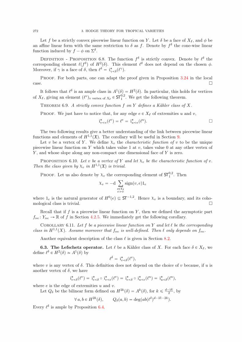
272 3. HODGE THEORY FOR TROPICAL VARIETIES
Let f be a strictly convex piecewise linear function on Y . Let δ be a face of Xf , and φ bean affine linear form with the same restriction to δ as f . Denote by f δ the cone-wise linearfunction induced by f ´ φ on Σδ.
Definition - Proposition 6.8. The function f δ is strictly convex. Denote by `δ thecorresponding element `pf δq of H2pδq. This element `δ does not depend on the chosen φ.Moreover, if γ is a face of δ, then `δ “ i˚γăδp`
γq.
Proof. For both parts, one can adapt the proof given in Proposition 3.24 in the localcase.
It follows that `δ is an ample class in A1pδq “ H2pδq. In particular, this holds for verticesof Xf , giving an element p`vqv vertex of Xf P ST
0,21 . We get the following theorem.
Theorem 6.9. A strictly convex function f on Y defines a Kähler class of X.
Proof. We just have to notice that, for any edge e P Xf of extremities u and v,
i˚văep`vq “ `e “ i˚uăep`
uq.
The two following results give a better understanding of the link between piecewise linearfunctions and elements of H1,1pXq. The corollary will be useful in Section 9.
Let v be a vertex of Y . We define χv the characteristic function of v to be the uniquepiecewise linear function on Y which takes value 1 at v, takes value 0 at any other vertex ofY , and whose slope along any non-compact one dimensional face of Y is zero.
Proposition 6.10. Let v be a vertex of Y and let χv be the characteristic function of v.Then the class given by χv in H1,1pXq is trivial.
Proof. Let us also denote by χv the corresponding element of ST0,21 . Then
χv “ ´dÿ
ePYfeąv
signpv, eq1e
where 1e is the natural generator of H0peq Ď ST´1,2. Hence χv is a boundary, and its coho-mological class is trivial.
Recall that if f is a piecewise linear function on Y , then we defined the asymptotic partfrec : Yrec Ñ R of f in Section 4.2.5. We immediately get the following corollary.
Corollary 6.11. Let f be a piecewise linear function on Y and let ` be the correspondingclass in H1,1pXq. Assume moreover that frec is well-defined. Then ` only depends on frec.
Another equivalent description of the class ` is given in Section 8.2.
6.3. The Lefschetz operator. Let ` be a Kähler class of X. For each face δ P Xf , wedefine `δ P H2pδq » A1pδq by
`δ “ i˚văδp`vq,
where v is any vertex of δ. This definition does not depend on the choice of v because, if u isanother vertex of δ, we have
i˚văδp`vq “ i˚eăδ ˝ i˚văep`
vq “ i˚eăδ ˝ i˚uăep`uq “ i˚uăδp`
uq,
where e is the edge of extremities u and v.Let Qδ be the bilinear form defined on H2kpδq “ Akpδq, for k ď d´|δ|
2 , by
@ a, b P H2kpδq, Qδpa, bq “ degpabp`δqd´|δ|´2kq.
Every `δ is ample by Proposition 6.4.

6. KÄHLER TROPICAL VARIETIES 273
For each δ, let
P 2kpδq :“ ker´
p`δqd´|δ|´2k`1 : H2kpδq Ñ H2d´2|δ|´2k`2pδq¯
be the primitive part of H2kpδq. Note that with the notations of Section 3, we have P 2kpδq “Ak
prim,`δpΣδq.
The following properties hold.
— (Hard Lefschetz) For each k ď d´|δ|2 , the map
p`δqd´|δ|´2k : H2kpδq Ñ H2d´2|δ|´2kpδq
is an isomorphism.— (Hodge-Riemann) The bilinear form p´1qkQδp ¨ , ¨ q restricted to the primitive part
P 2kpδq “ ker´
p`δqd´|δ|´2k`1 : H2kpδq Ñ H2d´2|δ|´2k`2pδq¯
is positive definite.
— (Lefschetz decomposition) For k ď d´|δ|2 , we have the orthogonal decomposition
H2kpδq “kà
i“0
`k´iP 2ipδq,
where, for each i P t0, . . . , ku, the map `k´i : P 2ipδq „ÝÑ `k´iP 2ipδq is an isomorphismpreserving Qδ.
We now define the Lefschetz operator `a,b : STa,b1 Ñ STa,b`21 by
`a,b “à
`a,b,s :à
sě|a|s”a pmod 2q
STa,b,s1 Ñà
sě|a|s”a pmod 2q
STa,b`2,s1
and the operator `a,b,s is defined by
`a,b,s “à
`δ :à
δPXf|δ|“s
Ha`b´spδq ÝÑà
δPXf|δ|“s
Ha`b`2´spδq.
We usually drop the indices a, b and simply denote by ` the operator of bidegree p0, 2q.
Remark 6.12. More precisely, we could view the collection of maps `a,b as a map `
` “à
a,b
`a,b :à
a,b
STa,b1 ÝÑà
a,b
STa,b`21 .
˛
We now recast Lemma 3.16 in the following.
Proposition 6.13. Let γ ă δ be a pair of faces, and let x P A‚pγq and y P A‚pδq. Denoteby ρδγ the ray associated to δ in Σγ, and by xδγ the associated element of A1pγq.
i˚γăδ is a surjective ring homeomorphism,(6.2)Gysδ ąγ ˝ i˚γăδpxq “ xδγ ¨ x,(6.3)
Gysδ ąγp i˚γăδpxq ¨ yq “ x ¨Gysδ ąγpyq.(6.4)
Moreover, if degγ : Ad´|γ| Ñ R and degδ : Ad´|δ| Ñ R are the natural degrees map, then
(6.5) degδ “ degγ ˝Gysδ ąγ .
Finally, Gysδ ąγ and i˚γăδ are dual in the sense that
(6.6) degγpx ¨Gysδ ąγpyqq “ degδp i˚γăδpxq ¨ yq.
Proof. The proof is similar to the one given in the local case.

274 3. HODGE THEORY FOR TROPICAL VARIETIES
The following proposition summarizes basic properties of the Lefschetz operator `.
Proposition 6.14. We have
— r`,N s “ 0, r`, i˚s “ r`,Gyss “ 0.
— for a pair of integers a, b with a` b ě d, the map `d´a´b : STa,b1 ÝÑ STa,2d´2a´b1 is an
isomorphism.
Proof. For the first point, let γăδ be a pair of faces of Xf . We recall that i˚γăδ : A‚pγq Ñ
A‚pδq is a surjective ring homeomorphism. Thus, for any a P A‚pγq,
i˚γăδp`γaq “ i˚γăδp`
γq i˚γăδpaq “ `δ i˚γăδpaq.
By Equation (6.4), for any x P A‚pδq,
Gysδ ąγp`δxq “ Gysδ ąγp i˚γăδp`
γqxq “ `γGysδ ąγpxq.
Let a, b, s be three integers with a ” s pmod 2q. Multiplying the previous equationsby signpγ, δq and summing over couples γ ă δ, we get that the three following diagrams arecommutative.
STa,b,s1 STa,b`2,s1
STa`2,b´2,s1 STa`2,b,s
1
`
id id
`
STa,b,s1 STa,b`2,s1
STa`1,b,s`11 STa`1,b`2,s`1
1
`
i˚ i˚
`
STa,b,s1 STa,b`2,s1
STa`1,b,s´11 STa`1,b`2,s´1
1
`
Gys Gys
`
To get the commutativity in ST‚,‚1 , it remains to check that, in each diagram, if the top-leftand bottom-right pieces appear in ST‚,‚1 , then the two other pieces appear as well, which isimmediate.
For the second point, we have
STa,b1 “à
sě|a|s”a pmod 2q
à
δPXf|δ|“s
Ha`b´spδq
STa,2d´2a´b1 “
à
sě|a|s”a pmod 2q
à
δPXf|δ|“s
H2d´a´b´spδq
and `d´a´b : STa,b1 Ñ STa,2d´2a´b1 can be rewritten asà
sě|a|s”a pmod 2q
à
δPXf|δ|“s
p`δqd´a´b : Ha`b´spδq ÝÑ H2d´a´b´spδq.
For each δ of dimension s, since `δ is ample, we get an isomorphism
p`δqd´a´b : Ha`b´spδq ÝÑ H2d´a´b´spδq “ H2pd´|δ|q´pa`b´sq.
Thus, we conclude that `d´a´b : STa,b1 Ñ STa,2d´2a´b1 is an isomorphism.
6.4. The Hodge-Lefschetz-primitive part P a,b. For a ď 0 and b ď d´ a, define theHodge-Lefschetz (or simply HL) primitive part P a,b of bidegree pa, bq as
P a,b :“ STa,b1 X kerpN´a`1q X kerp`d´a´b`1q.
Proposition 6.15. We have
P a,b “à
δPXf|δ|“´a
P 2a`bpδq.
6. KÄHLER TROPICAL VARIETIES 275
Figure 5. The tropical Hodge diamond
ST0,0 STd,0
ST´d,2d ST0,2d
˝
˝
˝
‚
N
`
pd
a
b
ST0,0
STd,0ST´d,2d
ST0,2d
˝
˝˝
‚
N
`
pd
ab
H0,0
H0,dHd,0
Hd,d
Proof. For b odd, both parts are zero. So suppose b is even. In this case, we have
STa,b1 X kerpN´a`1q “à
δPXf|δ|“´a
H2a`bpδq,
and thus
P a,b “ ker´
à
δPXf|δ|“´a
p`δqd´a´b`1 :à
δPXf|δ|“´a
H2a`bpδq ÝÑà
δPXf|δ|“´a
H2d´b`2pδq¯
.
To conclude, note that since |δ| “ ´a, we have d´ a´ b` 1 “ d´ |δ|´ p2a` bq ` 1, andthus
ker´
p`δqd´a´b`1 : H2a`bpδq Ñ H2d´b`2pδq¯
“ P 2a`bpδq,
and the proposition follows.
6.5. Hodge diamond. By what we proved in the previous sections, ST‚,‚1 forms a Hodgediamond as illustrated in Figure 5. Let us explain what this means.
We do a change of coordinates pa, bq Ñ pa, d´ a´ bq to form
HDa,d´a´b :“ STa,b1 .
The result of this transformation is that the nonzero terms of HD‚,‚ now form a rhombus.The horizontal symmetry maps a piece of HD‚,‚ onto an isomorphic piece by applying the
monodromy operator N enough number of times. More precisely, for an integer a ě 0, we get
Na : HD´a,b „ÝÑ HDa,b.
Similarly, the vertical symmetry maps a piece of HD‚,‚ onto another isomorphic piece byapplying the Lefschetz operator ` enough number of times: for b ě 0,
`b : HDa,´b „ÝÑ HDa,b.
In the figure, the four squares in both diagrams, in ST‚,‚1 and HD‚,‚, represent four isomorphicpieces. Moreover, the central symmetry corresponds to the Poincaré duality HD´a,´b » Ha,b.
276 3. HODGE THEORY FOR TROPICAL VARIETIES
To justify the name of tropical Hodge diamond, on the bottom of the figure is shownthe tropical Hodge groups to which the Steenbrink diamond degenerates. We show in Theo-rem 6.23 that the symmetries described above also hold for the tropical Hodge decomposition,as in the usual Hodge diamond.
Finally, notice that HD‚,‚ defined by HDa,b “ HD´a,´b is a HL-structure as defined inSection 7, cf. Definition 7.1.
6.6. Polarization on ST‚,‚1 . We now describe a natural polarization on ST‚,‚1 . We provein the next section that it induces a positive definite symmetric bilinear form on the HL-primitive parts P a,b defined above.
We first define a bilinear form ψ on ST‚,‚1 as follows. Let x P STa,b,s1 and y P STa1,b1,s1
1 . Write
x “ÿ
δPXf|δ|“s
xδ
with xδ P Ha`b´spδq, and similarly for y. We define the degree map
degpx ¨ yq :“
$
&
%
ř
δPXf|δ|“s
degpxδ ¨ yδq if s “ s1,
0 otherwise.
The bilinear form ψ is then defined by
(6.7) ψpx, yq :“
#
εpa, bq degpx ¨ yq if a` a1 “ 0, b` b1 “ 2d, and s1 “ s,0 otherwise,
where for a pair of integers a, b, with b even,
εpa, bq :“ p´1qa`b2 ,
and otherwise, if b is odd, εpa, bq “ 1 (but in this case, we necessarily have x “ 0).
The following proposition gathers basic properties of the the bilinear pairing ψ.
Proposition 6.16. We have for all pairs of elements x, y PÀ
a,b STa,b1 ,
(i) ψpx, yq “ p´1qdψpy, xq.(ii) ψpNx, yq ` ψpx,Nyq “ 0.(iii) ψp`x, yq ` ψpx, `yq “ 0.(iv) ψp i˚x, yq ` ψpx,Gysyq “ 0.(v) ψpGysx, yq ` ψpx, i˚yq “ 0.(vi) ψpdx, yq ` ψpx,dyq “ 0.
Proof. Let x P STa,b,s1 and y P STa1,b1,s1
1 be two nonzero elements for integers a, b, s, a1, b1, s1with s ě |a| and s1 ě |a1|. We proceed by verifying the statements point by point.
(i) if a` a1 ‰ 0 or b` b1 ‰ 2d, then both ψpx, yq and ψpy, xq are zero. Otherwise,
εpa1, b1q “ εp´a, 2d´ bq “ p´1q´a`2d´b
2 “ p´1qdεpa, bq.
Thus, ψpx, yq “ p´1qdψpy, xq.
(ii) Recall that N is a map of bidegree p2,´2q. If a` a1 ` 2 ‰ 0 or b` b1 ´ 2 ‰ 2d or s ‰ s1, thenboth ψpNx, yq and ψpx,Nyq are zero. Otherwise, s “ s1 ě |a1| “ |a ` 2|. Thus Nx ‰ 0. Bysymmetry, Ny ‰ 0. Since N acts as identity on both x and y, we get degpNx¨yq “ degpx¨Nyq.Moreover, εpa` 2, b´ 2q “ ´εpa, bq. Hence, we obtain ψpNx, yq ` ψpx,Nyq “ 0.
6. KÄHLER TROPICAL VARIETIES 277
(iii) Recall that ` is a map of bidegree p0, 2q. If a` a1 ‰ 0 or b` b1 ` 2 ‰ 2d or s ‰ s1, then bothψp`x, yq and ψpx, `yq are zero. Otherwise,
degp`x ¨ yq “ÿ
δPXf|δ|“s
degp`δ ¨ xδ ¨ yδq “ degpx ¨ `yq.
Moreover, εpa, b` 2q “ ´εpa, bq. Thus, we get ψp`x, yq ` ψpx, `yq “ 0.
(iv) If a ` a1 ` 1 ‰ 0 or b ` b1 ‰ 2d or s ` 1 ‰ s1, then ψp i˚x, yq and ψpx,Gysyq are both zero.Otherwise, s1´ 1 “ s ě |a| “ |a1` 1|. Thus, the Gysin map Gys: STa
1,b1,s1
1 Ñ STa1`1,b1,s1´1
1 hasa codomain belonging to ST‚,‚1 . This also holds for i˚. Moreover, using Equation (6.6), we get
degp i˚pxq ¨ yq “ÿ
δPXf|δ|“s`1
ÿ
γPXfγăδ
degpsignpγ, δq i˚γăδpxγq ¨ yδq
“ÿ
γPXf|γ|“s
ÿ
δPXfδ ąγ
degpxγ ¨ signpγ, δqGysδ ąγpyδqq
“ degpx ¨Gyspyqq.
Since εpa` 1, bq “ ´εpa, bq, we get ψp i˚x, yq ` ψpx,Gysyq “ 0.
(v) The equality ψpGysx, yq ` ψpx, i˚yq “ 0 follows from the points (i) and (iv).
(vi) Summing up the equalities in (iv) and (v) gives ψpdx, yq ` ψpx,dyq “ 0 by the definition ofthe differential d.
6.7. Induced polarization on the Hodge-Lefschetz primitive parts. The bilinearform ψ induces a positive definite symmetric bilinear form on the Hodge-Lefschetz primitiveparts P a,b that we now describe.
Proposition 6.17. For integer a ď 0 and b ď d´ a, the bilinear form ψp ¨ , `d´a´bN´a ¨ qis symmetric positive definite on P a,b. More precisely, it is the orthogonal sum of polarizationsp´1qa`b2Qδp ¨ , ¨ q for δ P Xf on the primitive part P 2a`bpδq, under the identification
P a,b “à
δPXf|δ|“´a
P 2a`bpδq.
Proof. By the properties of the monodromy operator, the isomorphism
N´a : STa,2d´2a´b1 Ñ ST´a,2d´b1
is the identity map on each isomorphic piece H2a`bpδq of STa,2d´2a´b1 and ST´a,2d´b1 , for any
δ P Xf with |δ| “ ´a.By definition of ψ, for a pair of elements x, y P P 2a`bpδq, we get
ψpx, `d´a´bN´ayq “ ψpx,N´a`d´a´byq
“ εpa, bqdegpx ¨ `d´a´byq
“ p´1qa`b2 degpx ¨ `d´a´byq
“ p´1qa`b2Qδpx, yq.
This concludes the proof since p´1qa`b2Qδ is symmetric positive definite by local Hodge-Riemann relations.
278 3. HODGE THEORY FOR TROPICAL VARIETIES
6.8. Hodge-Lefschetz decomposition. From the preceding discussion, we get the fol-lowing theorem. It can be illustrated as in Figure 5: the black square can be decomposed asthe direct sum of primitive parts lying in the grey area.
Theorem 6.18. For each pair of integers a ď 0 and b ď d´ a, we have the decomposition
STa,b1 “à
s,rě0
`rN sP a´2s,b`2s´2r.
Proof. We give here a direct proof based on the definition of ST‚,‚1 and using localLefschetz decompositions. We however note that this theorem can be proved thanks to thegeneral theory of HL-structures, cf. Proposition 7.2. We have
STa,b1 “à
sě0
STa,b,2s´a1
“à
sě0
N sSTa´2s,b`2s,2s´a1
“à
sě0
N sà
δPXf|δ|“2s´a
H2a`b´2spδqloooooomoooooon
ĎSTa´2s,b`2s1
“à
sě0
N sà
δPXf|δ|“2s´a
à
rě0
`r P 2a`b´2s´2rpδqloooooooomoooooooon
ĎSTa´2s,b`2s´2r1
“à
r,sě0
`rN sà
δPXf|δ|“2s´a
P 2a`b´2s´2rpδq,
STa,b1 “à
r,sě0
`rN sP a´2s,b`2s´2r.
6.9. Polarized Hodge-Lefschetz structure on the cohomology of pST‚,b1 ,dq. In thissection we show that when passing to the cohomology, the operators N , ` and the polarizationψ induce a polarized Hodge-Lefschetz structure on the cohomology groups La,b :“ HapST‚,b1 ,dq.By this we mean the following.
First, since rd, `s “ 0 and rd, N s “ 0, we get induced maps
` : La,b Ñ La,b`2
andN : La,b Ñ La`2,b´2
such that rN, `s “ 0.Second, since ψpd ¨ , ¨ q “ ´ψp ¨ ,d ¨ q, we get an induced pairing
ψ : L‚,‚ ˆ L‚,‚ Ñ K.
Moreover, we will show that
Theorem 6.19. We have the following properties.
— For a ď 0, the map N´a : La,b Ñ L´a,b`2a is an isomorphism.
— For a, b with d´ a´ b ě 0, the map `d´a´b : La,b Ñ La,2d´2a´b is an isomorphism.
— Let a ď 0 and b ď d´ a and denote by La,b0 the HL-primitive part of La,b defined by
La,b0 “ La,b X kerpN´a`1q X kerp`d´a´b`1q.
The polarization ψ induces a symmetric bilinear form ψp ¨ , `d´a´bN´a ¨ q which ispositive definite on La,b0 .
6. KÄHLER TROPICAL VARIETIES 279
— For integers a ď 0 and b ď d´ a, we have the decomposition
La,b “à
s,rě0
`rN sLa´2s,b`2s´2r0 .
Moreover, this decomposition is orthogonal for the pairing ψp ¨ , `d´a´bN´a ¨ q.
Proof. We can use the change of coordinates HD´a,´pd´a´bq :“ STa,b1 for any integers a, b.By the previous discussion, we get that pHD´a,´pd´a´bq, N, `, φ, dq is a differential polarizedHL-structure in the sense of Section 7. We can therefore apply Theorem 7.9 to conclude.
6.10. Singular monodromy operator. We define the singular tropical monodromy op-erator as follows. For each face δ P Xf , let oδ be a point in the affine tangent space Taffδ Ď NR.For instance, we can take oδ to be the centroid of δ. Let γ be a face in Xf of dimension q.For other faces of δ of sedentarity 0, set oδ :“ oδf . For any face δ of any sedentarity σ, setoδ “ πσpoηq, where η is the only face of sedentarity 0 such that δ “ ησ
8. Then we set
N : Cp,qpXq Ñ Cp´1,q`1pXq,
α P F ppγq ÞÑà
δ ąγsedpδq“sedpγq
α`
¨ ^poδ ´ oγq˘
.
Theorem 6.20. The singular tropical monodromy operator corresponds to the monodromyoperator on ST‚,‚1 via the isomorphism of Theorem 5.8.
Proof. This is a direct consequence of Proposition 11.1.
Corollary 6.21. The operator N : Hp,q Ñ Hp´1,q`1 coincides with the eigenwave oper-ator φ constructed in [MZ14].
Proof. One can show that the singular tropical monodromy operator coincides with theeigenwave operator. So the statement follows from Theorem 6.20.
Remark 6.22. It follows that the monodromy operator N coincides as well with themonodromy operator defined on the level of Dolbeault cohomology groups [Liu19]. This is aconsequence of [Jel19] which relates the eigenwave operator to the monodromy on Dolbeaultcohomology. ˛
6.11. HL, HR and Monodromy for tropical cohomology. From the result in theprevious section, we get the following theorem.
Theorem 6.23. We have
— (Weight-monodromy conjecture) For q ą p two non-negative integers, we get anisomorphism
N q´p : Hq,ptroppXq Ñ Hp,q
troppXq.
— (Hard Lefschetz) For p` q ď d, the Lefschetz operator ` induces an isomorphism
`d´p´q : Hp,qtroppXq Ñ Hd´q,d´p
trop pXq.
— (Hodge-Riemann) For q ą p, the pairing p´1qp⟨¨ , `d´p´qN q´p ¨
⟩induces a positive-
definite pairing on the primitive part P q,p, where⟨¨ , ¨
⟩is the natural pairing
⟨¨ , ¨
⟩: Hq,ppXq bHd´q,d´ppXq Ñ Hd,dpXq » Q.
280 3. HODGE THEORY FOR TROPICAL VARIETIES
6.12. Hodge index theorem for tropical surfaces. In this final part of this section,we explain how to deduce the Hodge index theorem for tropical surfaces from Theorem 6.23.
Proof of Theorem 1.9. The primitive part decomposition theorem implies that we candecompose the cohomology group H1,1
troppX,Qq into the direct sum
H1,1troppX,Qq “ `H0,0
troppX,Qq ‘N H2,0troppX,Qq ‘H
1,1primpX,Qq,
where H1,1primpX,Qq “ kerp`q X kerpNq. Moreover, by Hodge-Riemann, the pairing is positive
definite on `H0,0troppX,Qq and N H2,0
troppX,Qq, and it is negative definite on H1,1primpX,Qq.
By Poincaŕe duality, we have H2,0troppX,Qq » H0,2
troppX,Qq. By definition of tropical coho-mology, since F 0 is the constant sheaf Q, we have H0,2
troppX,Qq » H2pX,Qq. Moreover, wehave H0,0
troppX,Qq „ Q. We conclude that the signature of the intersection pairing is given byp1` b2, h
1,1 ´ 1´ b2q, as stated by the Hodge index theorem.
7. Hodge-Lefschetz structures
In this section, we prove that the homology of a differential Hodge-Lefschetz structure isa polarized Hodge-Lefschetz structure, thus finishing the proof of Theorem 6.19 and the maintheorem of the previous section.
The main references for differential Hodge-Lefschetz structures are Saito’s work on Hodgemodules [Sai88], the paper by Guillén and Navarro Aznar on invariant cycle theorem [GN90]and the upcoming book by Sabbah and Schnell [SS20] on mixed Hodge modules, to whichwe refer for more information. We note however that our set-up is slightly different, in partic-ular, our differential operator is skew-symmetric with respect to the polarization. The proofin [SS20] is presented also for the case of mono-graded complexes and is based on the useof representation theory of SL2pRq as in [GN90]. So we give a complete self-contained proofof the main theorem. Our proof is direct and does not make any recourse to representationtheory, although it might be possible to recast in the language of representation theory thefinal combinatorial calculations we need to elaborate.
In order to simplify the computations, it turns out that it will be more convenient to workwith coordinates different from the ones in the previous section, and that is what we will bedoing here. The new coordinates are compatible with the ones in [SS20].
7.1. Hodge-Lefschetz structure.
Definition 7.1. A (bigraded) Hodge-Lefschetz structure, or more simply an HL-structure,pH‚,‚, N1, N2q is a bigraded finite dimensional vector space H‚,‚ endowed with two endomor-phisms N1 and N2 of respective bidegree p´2, 0q and p0,´2q such that,
— rN1, N2s “ 0,— for any pair of integers a, b with a ě 0, we have Na
1 : Ha,b Ñ H´a,b is an isomorphism,— for any pair of integers a, b with b ě 0, we have N b
2 : Ha,b Ñ Ha,´b is an isomorphism.˛
For the rest of this section, we fix a HL-structure pH‚,‚, N1, N2q.
We define the primitive parts of H‚,‚ by
@ a, b ě 0, Pa,b :“ Ha,b X kerpNa`11 q X kerpN b`1
2 q.
We have the following decomposition into primitive parts.
Proposition 7.2. For each pair of integers a, b ě 0, we have the decomposition
Ha,b “à
s,rě0
N r1N
s2Pa`2r,b`2s.

7. HODGE-LEFSCHETZ STRUCTURES 281
Denote by H`‚,‚ the bigraded subspace
H`‚,‚ “à
a,bě0
Ha,b.
Define N‹1 : H`‚,‚ Ñ H`‚,‚ of bidegree p2, 0q, by
N‹1 |Ha,b“
´
`
N1|Ha`2,b
˘a`2¯´1´
N1|Ha,b
¯a`1@a, b ě 0.
It verifies the following properties. Let a, b ě 0. Then,
N‹1N1|Ha`2,b“ id|Ha`2,b
and kerpN‹1 q XHa,b “ kerpNa`11 q XHa,b.
In particular, N1 : Ha`2,b Ñ Ha,b is injective, and N‹1 : Ha,b Ñ Ha`2,b is surjective.From this, we can deduce that the map N1N
‹1 |Ha,b
is the projection along kerpNa`11 qXHa,b
onto N1Ha`2,b, i.e., for the decomposition
Ha,b “ N1Ha`2,b ‘
´
kerpNa`11 q XHa,b
¯
.
We define N‹2 in a similar way, and note that it verifies similar properties. In particular,N2N
‹2 |Ha,b
is the projection along kerpN b`12 q XHa,b onto N2Ha,b`2 for the decomposition
Ha,b “ N2Ha,b`2 ‘
´
kerpN b`12 q XHa,b
¯
.
Moreover, from the commutativity of N1 and N2, more precisely, from
rNa`21 , N2s|Ha`2,b`2
“ rN1, Nb`22 s|Ha`2,b`2
“ rNa`21 , N b`2
2 s|Ha`2,b`2“ 0,
we infer thatrN‹1 , N2s|Ha,b`2
“ rN1, N‹2 s|Ha`2,b
“ rN‹1 , N‹2 s|Ha,b
“ 0.
In particular,N1N
‹1N2N
‹2 “ N2N
‹2N1N
‹1 “ N1N2N
‹1N
‹2 .
Notice that N1N2N‹1N
‹2 |Ha,b
is a projection onto N1N2Ha`2,b`2.
We come back to the proof of the proposition.
Proof of Proposition 7.2. Clearly, N1 : Ha`2,b Ñ Ha,b is injective for a ě 0. Similarlyfor N2. Therefore, proceeding by induction, it suffices to prove that for any pair of integersa, b ě 0, we have
Ha,b “`
N1Ha`2,b `N2Ha,b`2
˘
‘ Pa,b and N1Ha`2,b XN2Ha,b`2 “ N1N2Ha`2,b`2.
This can be deduced from the following lemma applied to N1N‹1 |Ha,b
and N2N‹2 |Ha,b
and thecorresponding decompositions of Ha,b.
Lemma 7.3. Let V be a finite dimensional vector space. For i P t1, 2u, suppose we havedecompositions V “ I1‘K1 “ I2‘K2 for subspaces I1,K1, I2,K2 Ď V . Denote by πi : V Ñ Vthe projection of V onto Ii along Ki. Then, if π1 and π2 commute, we get
V “ I1 X I2 ‘ I1 XK2 ‘ K1 X I2 ‘ K1 XK2 and I1 X I2 “ Impπ1 ˝ π2q.
Proof. Since π1 and π2 commute, π2pI1q Ď I1. Thus, π2 can be restricted to I1. Thisrestriction is a projection onto I2 X I1 along K2 X I1. Thus,
I1 “ I2 X I1 ‘ K2 X I1 and I1 X I2 “ Impπ2 ˝ π1q.
Applying the same argument to the commuting projections id´ π1 and id´ π2, we get that
K1 “ K2 XK1 ‘ I2 XK1.
282 3. HODGE THEORY FOR TROPICAL VARIETIES
Hence,V “ I1 ‘K1 “ I1 X I2 ‘ I1 XK2 ‘ K1 X I2 ‘ K1 XK2.
7.2. Polarization ψ and its corresponding scalar product φ. A polarization on theHL-structure H‚,‚ is a bilinear form ψp ¨ , ¨ q such that:
— for any integers a, b, a1, b1 and any elements x P Ha,b and y P Ha1,b1 , the pairing ψpx, yqis zero unless a` a1 “ b` b1 “ 0,
— for any a, b ě 0, the pairing ψp ¨ , Na1N
b2 ¨ q is symmetric definite positive on Pa,b,
— N1 and N2 are skew-symmetric for ψ.For the rest of this section, we assume that H‚,‚ is endowed with a polarization ψ.
Denote as in the previous section H`‚,‚ the bigraded subspace
H`‚,‚ “à
a,bě0
Ha,b.
We define the operator w on H‚,‚ as follows.Let a, b ě 0 and r, s ě 0 be four integers. Let x P Pa,b. Then, we set
wN r1N
s2x :“
#
p´1qr`s r!pa´rq!
s!pb´sq!N
a´r1 N b´s
2 x if r ď a and s ď b
0 otherwise.
Using the decomposition into sum of primitive parts from the previous section, one canverify that w is well-defined.
We will provide some explanations about the choice of the operator w, in particular aboutthe choice of the renormalization factors, at the beginning of Section 7.6.
Set φp ¨ , ¨ q :“ ψp ¨ ,w ¨ q.
Proposition 7.4. We have the following properties.— The operator w is invertible with its inverse verifying
w´1N r1N
s2x “ p´1qa`bwN r
1Ns2x.
— The pairing φ is symmetric positive definite.— The decomposition into primitive parts of H‚,‚ is orthogonal for φ. More precisely,
let a, b, r, s ě 0 and a1, b1, r1, s1 ě 0 be eight integers and let x P Pa,b and y P Pa1,b1 .Then,
φpN r1N
s2x,N
r1
1 Ns1
2 yq “ 0 unless r “ r1, s “ s1, a “ a1 and b “ b1.
Proof. The first point is an easy computation. For the two other points, take x P Pa,band y P Pa1,b1 . We can assume that r ď a, s ď b, r1 ď a1 and s1 ď b1. Set
C “r1! s1!
pa1 ´ r1q! pb1 ´ s1q!.
We have
φpN r1N
s2x,N
r1
1 Ns1
2 yq “ ψpN r1N
s2x,wN
r1
1 Ns1
2 yq
“ p´1qr1`s1CψpN r
1Ns2x,N
a1´r1
1 N b1´s1
2 yq
“ p´1qa1`b1CψpNa1´r1`r
1 N b1´s1`s2 x, yq
“ p´1qr1`s1`r`sCψpx,Na1´r1`r
1 N b1´s1`s2 yq.
Suppose the value of the above pairing is nonzero. Then, since x P Ha,b and
Na1`r´r1
1 N b1`s´s1
2 y P H´a1`2r1´2r,´b1`2s1´2s,

7. HODGE-LEFSCHETZ STRUCTURES 283
we should have a´ a1 ` 2r1 ´ 2r “ 0. Moreover, since x P kerpNa`11 q and y P kerpNa1`1
1 q, weget
a1 ´ r1 ` r ď a and a1 ´ r1 ` r ď a1.
Hence, we getr ´ r1 ď a´ a1 “ 2pr ´ r1q and r ´ r1 ď 0,
which in turn implies that r ´ r1 “ a ´ a1 “ 0, i.e., r “ r1 and a “ a1. By symmetry, we gets “ s1 and b “ b1. We infer that
φpN r1N
s2x,N
r1N
s2yq “ Cψpx,Na
1Nb2yq,
which concludes the proof since ψp ¨ , Na1N
b2 ¨ q is symmetric positive definite on Pa,b.
7.3. Differential polarized HL-structure. On a polarized HL-structure H‚,‚, a dif-ferential is an endomorphism d of bidegree p´1,´1q such that
— d2 “ 0,
— rd, N1s “ rd, N2s “ 0,
— d is skew-symmetric for ψ.
In the rest of this section, we fix a differential d on H‚,‚.
Proposition 7.5. The following holds for any pair of integers a, b ě 0:
dPa,b Ď Pa´1,b´1 ‘N1Pa`1,b´1 ‘N2Pa´1,b`1 ‘N1N2Pa`1,b`1,
where, by convention, Pa1,b1 “ 0 if a1 ă 0 or b1 ă 0.
Proof. Since d and N1 commute,
dPa,b Ď kerpNa`11 q XHa´1,b´1 “
à
rě0
N r2Pa´1,b´1`2r ‘N1N
r2Pa`1,b´1`2r.
Notice that this is true even if a “ 0 or b “ 0. We conclude the proof by combining this resultwith the symmetric result for N2.
Using this proposition, if x P Pa,b, then for i, j P t0, 1u, we define xi,j P Pa´1`2i,b´1`2j
such thatdx “
ÿ
i,jPt0,1u
N i1N
j2xi,j .
Since d commutes with N1 and N2, more generally, for any pair of integers r, s ě 0, we get
dN r1N
s2x “
ÿ
i,jPt0,1u
N r`i1 N s`j
2 xi,j .
With this notation, the fact that d2 “ 0 can be reformulated as follows.
Proposition 7.6. With the above notations, for any pair k, l P t0, 1, 2u,
N ε11 N
ε22
ÿ
i,j,i1,j1Pt0,1ui`i1“kj`j1“l
pxi,jqi1,j1 “ 0.
where,
ε1 “
#
1 if a “ 0 and k “ 1
0 otherwise,and ε2 “
#
1 if b “ 0 and l “ 1
0 otherwise.
284 3. HODGE THEORY FOR TROPICAL VARIETIES
Proof. From the previous discussion, we get that
d2x Pà
k,lPt0,1,2u
Nk1N
l2Pa´2`2k,b´2`2l.
Moreover, the piece corresponding to a fixed k and l isÿ
i,j,i1,j1Pt0,1ui`i1“kj`j“l
Nk1N
l2pxi,jqi1,j1 .
Since, d2 “ 0, this last sum is zero:
Nk1N
l2
ÿ
i,j,i1,j1Pt0,1ui`i1“kj`j“l
pxi,jqi1,j1 “ 0.
We know that, for any b1, Nk1 |Pa´2`2k,b1
is injective if k ď a ´ 2 ` 2k. This is also true if
a´ 2` 2k ă 0 because, in this case, the domain is trivial. In both cases, we can remove Nk1
in the above equation. The last case is
0 ď a´ 2` 2k ă k.
This implies k “ 1 and a “ 0, in which case we cannot a priori remove the Nk1 “ N1 in the
previous equation. This concludes the proof of the proposition.
7.4. The Laplace operator 4. The Laplace operator 4 : H‚,‚ Ñ H‚,‚ is defined by
4 :“ dd‹ ` d‹d
where d‹ : H‚,‚ Ñ H‚,‚ denotes the codifferential of bidegree p1, 1q defined by
d‹ :“ ´w´1dw.
Note that 4 is of bi-degree p0, 0q. The following summarizes basic properties one expectfrom the Laplace operator and its corresponding Hodge decomposition.
Proposition 7.7. We have the following properties.— d‹ is the adjoint of d with respect to φ.— 4 is symmetric for φ.— On each graded piece Ha,b, we have the following orthogonal decomposition for φ
kerpdq XHa,b “ kerp4q XHa,b
K
‘ Impdq XHa,b.
Proof. To get the first point, note that for any x, y P H‚,‚, we have
φpx,d‹yq “ ´ψpx,ww´1dwyq “ ψpdx,wyq “ φpdx, yq.
It follows that the adjoint of 4 “ dd‹ ` d‹d is 4 itself.
Last point follows directly from the first two statements, as usual. Denote by V :“ pHa,b, φqthe vector space Ha,b endowed with the inner product φ. In order to simplify the notations,we will write Impdq instead of V X Impdq, and similarly for other intersections with V . Wehave to show that
kerpdq “ kerp4qK
‘ Impdq.
From the decomposition V “ ImpdqK ‘ Impdq, and the inclusion Impdq Ď kerpdq, we get
kerpdq “ ImpdqK X kerpdqK
‘ Impdq.
By adjunction, we get ImpdqK “ kerpd‹q. To conclude, note that kerp4q “ kerpdqXkerpd‹q.Indeed, if x P kerp4q, then
0 “ φpx,4xq “ φpx, dd‹xq ` φpx,d‹dxq “ φpd‹x,d‹xq ` φpdx,dxq,
7. HODGE-LEFSCHETZ STRUCTURES 285
which, by positivity of φ, implies that d‹x “ dx “ 0, i.e., x P kerpdq X kerpd‹q. The otherinclusion kerpdq X kerpd‹q Ď kerp4q trivially holds.
Proposition 7.8. The Laplace operator commutes with N1 and N2, i.e., r4, N1s “
r4, N2s “ 0.
The proof of this theorem is given in Section 7.6.
7.5. Polarized Hodge-Lefschetz structure on the cohomology of H‚,‚. In this sec-tion, we show that, when passing to the cohomology, the operators N1, N2 and the polarizationψ induce a polarized Hodge-Lefschetz structure on the cohomology groups
La,b :“kerpd: Ha,b Ñ Ha´1,b´1q
Impd: Ha`1,b`1 Ñ Ha,bq.
By this we mean the following.First, since rd, N1s “ 0 and rd, N2s “ 0, we get induced maps
N1 : La,b Ñ La´1,b and N2 : La,b Ñ La,b´2.
Second, since ψpd ¨ , ¨ q “ ´ψp ¨ ,d ¨ q, we get a pairing
ψ : L‚,‚ ˆ L‚,‚ Ñ R.Then, we will show that
Theorem 7.9. For the corresponding induced map, pL‚,‚, N1, N2, φq is a polarized HL-structure. Moreover, the decomposition by primitive parts is induced by the correspondingdecomposition on H‚,‚.
Proof. By Proposition 7.7, the kernel of the Laplace operator gives a section of thecohomology L‚,‚. Moreover, since the Laplacian commutes with N1 and N2, both N1 andN2 preserve the kernel of the Laplacian. Consequently, it suffices to prove that kerp4q isa polarized HL-substructure of H‚,‚. By abuse of notation, we denote by La,b the kernelkerp4 : Ha,b Ñ Ha,bq.
Clearly, N1 and N2 commutes. Let a ě 0 and b P Z. Let us prove that Na1 induces an
isomorphism La,b „ÝÑ L´a,b. Since 4 is symmetric for φ,
Ha,b “ kerp4q XHa,b
K
‘ Imp4q XHa,b.
Since N1 preserves kerp4q and Imp4q, the isomorphism Na1 : Ha,b
„ÝÑ H´a,b induces isomor-phisms for both parts kerp4q and Imp4q. In particular, we get an isomorphism Na
1 : La,b „ÝÑL´a,b. We use the symmetric argument for N2.
The primitive part of La,b is, by definition,
La,b X kerpNa`11 q X kerpN b`1
2 q “ La,b X Pa,b.
Thus, the decomposition by primitive parts is the one induced by the decomposition of Ha,b.Finally, the properties about ψ on La,b comes from the analogous properties on Ha,b.
7.6. Commutative property of the Laplacian. In this section, we prove Proposi-tion 7.8, that r4, N1s “ r4, N2s “ 0.
Let us start by justifying our definition of the operator w.
Remark 7.10. We feel necessary to provide an explanation of why we are not using thesimpler more natural operator rw which is defined by taking values for a, b, r, s ě 0 and x P Pa,bgiven by
rwN r1N
s2x “ p´1qr`sNa´r
1 N b´s2 x,
where negative powers of N1 and N2 are considered to be zero.With this operator, the bilinear form rφ :“ ψp ¨ , rw¨ q will be still positive definite, and we
can define the corresponding Laplace operator r4. However, this Laplacian will not commute

286 3. HODGE THEORY FOR TROPICAL VARIETIES
with N1 and N2 in general. In order to explain where the problem comes from, let us try toproceed with a natural, but wrong, proof that this Laplacian commutes N1. More precisely,setting rd‹ “ ´rw´1drw the adjoint of d, let us try to prove that r rd‹, N1s “ 0. Assume 0 ď r ď aand 0 ď s ď b. Then we can write
rd‹N r1N
s2x “ ´rw´1drwN r
1Ns2x
“ p´1qr`s`1rw´1dNa´r
1 N b´s2 x
“ÿ
i,jPt0,1u
p´1qr`s`1rw´1Na´r`i
1 N b´s`j2 xi,j .
We recall that xi,j P Pa´1`2i,b´1`2j . Notice that a´ 1` 2i´ pa´ r ` iq “ r ´ 1` i. Thus,
rd‹N r1N
s2x “
ÿ
i,jPt0,1u
p´1qr`s`1p´1qr´1`i`s´1`jN r´1`i1 N s´1`j
2 xi,j
“ÿ
i,jPt0,1u
p´1qi`j`1N r´1`i1 N s´1`j
2 xi,j .
Then, rd‹N1pNr1N
s2xq can be obtained replacing r by r ` 1 and similarly for N1
rd‹pN r1N
s2xq.
Thus, we would conclude that N1 and rd‹ commute!Where is the mistake? First, notice that the formula for the derivation can only be applied
if a ´ r and b ´ s are both non-negative. Thus, if r “ a, we cannot just replace r by r ` 1
to compute rd‹N1pNr1N
s2xq. Second, notice that 0 “ N1N
´11 ‰ N0
1 . If r “ 0 and i “ 0, weget r ´ 1 ` i “ ´1. Multiplying the corresponding term by N1 is not equivalent to simplyreplacing r by r`1. Notice moreover that we did not use the condition d2 “ 0 at any moment.Thus, roughly speaking, everything goes well except on the boundaries r “ a, s “ b, r “ 0 ands “ 0. These problems still exist for the operator r4, which justify why r4 does not commutein general with Ni.
The solution to remedy these boundary issues is to modify rw in such a way that somezero factors on the boundary solve the above evoked problem: if the term N r´1`i
1 N s´1`j2 xi,j is
multiplied by some zero factor due to the new operator when r “ 0 and i “ 0, then multiplyingby N1 corresponds to replacing r by r ` 1. To find the right form of the Laplacian, one canuse tools of representation theory, where Lie brackets can be used to study commutationproperties. This is what is done in [GN90, SS20]. These proofs however take place in aslightly different context. For example, our differential is skew symmetric, and not symmetric,and we work in the real instead of the complex world. Nevertheless, one should be ableto adapt their proofs to our setting. However, instead of doing this, we decided to providea completely elementary proof. The arguments which follow are somehow technical but noknowledge in representation theory is needed. ˛
We now begin the proof of the commutativity of the Laplacian 4 with the operators N1
and N2.
Convention. In order to simplify the calculations, we avoid to write symmetric factorsby using the following notations. If A,B,C are some sets, then we follow the followingrules to extend the operations between these sets coordinatewise to operations involving theirCartesian products A2, B2 and C2: if ζ : AÑ C and θ : AˆB Ñ C are some operations, thenwe extend them as follows.
ζ : A2 Ñ C2, pa1, a2q ÞÑ pζpa1q, ζpa2qq,θ : AˆB2 Ñ C2,
`
a, pb1, b2q˘
ÞÑ pθpa, b1q, θpa, b2qq, andθ : A2 ˆB2 Ñ C2,
`
pa1, a2q, pb1, b2q˘
ÞÑ pθpa1, b1q, θpa2, b2qq.
Moreover, if A is endowed with a product structure, we define m : A2 Ñ A by mpa1, a2q “ a1a2.

7. HODGE-LEFSCHETZ STRUCTURES 287
Example 7.11. Let us give some examples. Let a “ pa1, a2q and r “ pr1, r2q for integersa1, a2, r1, r2 ě 0 with r1 ď a1 and r2 ď a2, and let x P Pa,b. With our convention, weget 1 ` a “ 1 ` pa1, a2q “ p1 ` a1, 1 ` a2q, p´1qa “ p´1qpa1,a2q “
`
p´1qa1 , p´1qa2˘
, andm`
p´1q1`a˘
“ m`
p´1qa˘
.Let now N “ pN1, N2q. The formula
wN r11 N r2
2 x “ p´1qr1`r2r1!
pa1 ´ r1q!
r2!
pa2 ´ r2q!Na1´r1
1 Na2´r22 x,
can be rewritten with our notation as follows
wmpN rqx “ m´
p´1qrr!
pa´ rq!Na´r
¯
x.
In the same way, we recall that
dN r11 N r2
2 x “ÿ
i“pi1,i2qPt0,1u2
N r1`i11 N r2`i2
2 xi1,i2 ,
if r1 and r2 are non-negative, where xi1,i2 P Pa1´1`2i1,a2´1`2i2 . With our notations, thisformula reads
dmpN rqx “ÿ
iPt0,1u2
mpN r`iqxi.
˛
We further use the following conventions. By pa1, a2q ě pb1, b2q we mean a1 ě b1 anda2 ě b2. Moreover, 00 “ 1 and N r
1 “ N r2 “ 0 if r is negative. Notice that N1N
´11 ‰ N0
1 ,thus we have to be cautious with negative exponents. This is the main difficulty in the proof,besides the exception k “ 1 and a “ 0 in Proposition 7.6.
Let a “ pa1, a2q ě 0. Let r “ pr1, r2q P Z2 with 0 ď r ď a. Let x P Pa “ Pa1,a2 andy “ N r1
1 N r22 x. Set N “ pN1, N2q. We recall that
4 “ ´pdw´1dw ` w´1dwdq
We now explicit dw´1dy. We omit ranges of indices in the sums which follow if they areclear from the context.
dy “ÿ
iPt0,1u2
m`
N r`i˘
xi.
w´1dy “ÿ
ir`iďa´1`2i
m´
p´1qa´1`2ip´1qr`ipr ` iq!
ppa´ 1` 2iq ´ pr ` iqq!N pa´1`2iq´pr`iq
¯
xi,
“ÿ
ia´r´1`iě0
m´
p´1qa`r`i`1 pr ` iq!
pa´ r ´ 1` iq!Na´r´1`i
¯
xi.
dw´1dy “ÿ
i,i1Pt0,1u2
a´r´1`iě0
m´
p´1qa`r`ipr ` iq!
pa´ r ´ 1` iq!Na´r´1`i`i1
¯
pxiqi1 .
where we used the fact that m`
p´1qa`r`i`1˘
“ m`
p´1qa`r`i˘
(since m`
p´1qp1,1q˘
“ 1).
We can compute in the same way dwdy, in which case, using
m`
p´1qa´1`2i˘
“ m`
p´1qa˘
,
we getdwdy “ m
`
p´1qa˘
dw´1dy.
288 3. HODGE THEORY FOR TROPICAL VARIETIES
To get dw´1dwy, it suffices to multiply by the good factor and to replace r by a´ r:
dw´1dwy “ m´
p´1qrr!
pa´ rq!
¯
ÿ
i,i1Pt0,1u2
r`i´1ě0
m`
p´1qr`ipa´ r ` iq!
pr ´ 1` iq!N r´1`i`i1
˘
pxiqi1
“ÿ
i,i1
r`i´1ě0
m`
p´1qir!
pr ´ 1` iq!
pa´ r ` iq!
pa´ rq!N r´1`i`i1
˘
pxiqi1
“ÿ
i,i1
r`i´1ě0
m´
p´1qir1´ipa´ r ` 1qiN r´1`i`i1¯
pxiqi1 .
Note that in the last sum we can remove the condition r ` i´ 1 ě 0. Indeed, if, for instance,r1` i1´ 1 ă 0, then, since r1, i1 are non-negative, we should have r1 “ i1 “ 0, and the factorr1´i1
1 is automatically zero.
Now, since
pa´ 2` 2i` 2i1q ´ pa´ r ´ 1` i` i1q “ r ´ 1` i` i1,
we get
w´1dwdy
“ÿ
i,i1
a´r`i´1ě0
m´
p´1qr`ipr ` iq!
pa´ r ´ 1` iq!p´1qr´1`i`i1 pa´ r ´ 1` i` i1q!
pr ´ 1` i` i1q!N r´1`i`i1
¯
pxiqi1
“ÿ
i,i1
a´r`i´1ě0
m´
p´1qi1
pr ` iq1´i1
pa´ r ` iqi1
N r´1`i`i1¯
pxiqi1 .
In the last sum, we can again remove the condition a´ r` i´ 1 ě 0. Indeed, if, for instance,a1 ´ r1 ` i1 ´ 1 ă 0, then since r1 ď a1 and i1 P t0, 1u, we get a1 “ r1 and i1 “ 0. Then,either i11 “ 1 and pa1 ´ r1 ` i1q
i11 “ 0, or i11 “ 0 and
Nr1´1`i1`i111 pxiqi1 “ Na1´1
1 pxiqi1 “ 0,
becausepxiqi1 “ px0,i2q0,i12
P Pa1´2,a2´2`i2`i12Ď kerpNa1´1
1 q.
In any cases, we get
´4y “ÿ
i,i1
´
m`
p´1qir1´ipa´ r ` 1qi˘
`m`
p´1qi1
pr ` iq1´i1
pa´ r ` iqi1˘¯
mpN r´1`i`i1qpxiqi1
“ÿ
i,i1
´
m`
r1´ipr ´ a´ 1qi˘
`m`
pr ` iq1´i1
pr ´ a´ iqi1˘¯
mpN r´1`i`i1qpxiqi1
“ÿ
i,i1
´
m`
r ` 01´ip´a´ 1qi˘
`m`
r ` i1´i1
p´a´ iqi1˘¯
mpN r´1`i`i1qpxiqi1 .
For a fixed a, let κ : t0, 1, 2u2 Ñ Z2 be the function defined by taking for every i, i1 P t0, 1u2,the value
κpi` i1q :“ 01´ip´a´ 1qi ` i1´i1
p´a´ iqi1
.
One can verify that the function is well-defined, i.e., if i` i1 “ j` j for i, i1, j, j1 P t0, 1u2 then
01´ip´a´ 1qi ` i1´i1
p´a´ iqi1
“ 01´jp´a´ 1qj ` j1´j1p´a´ jqj1
.
The only nontrivial case is when i1` i11 “ 1 or when i2` i12 “ 1. For instance, if i1 “ 0, i11 “ 1and j1 “ 1, j11 “ 0, then we get κpi` i1q1 “ 0´ a1 “ ´a1 which is equal to κpj ` j1q1.

7. HODGE-LEFSCHETZ STRUCTURES 289
We also define C : t0, 1u2 Ñ Z by
Cpi, i1q :“ m`
01´ip´a´ 1qi˘
`m`
i1´i1
p´a´ iqi1˘
.
We will use the following specific values later:
κ`
p1, k2q˘
1“ ´a1,
C`
p0, i2q, p0, i12q˘
“ 0, and
C`
p1, i2q, p1, i12q˘
“ p´a1 ´ 1qκ`
p2, i2 ` i12q˘
2.
Using these terminology, we can now write
4y “ ´ÿ
i,i1
p2r1r2 ` κpi` i1q2r1 ` κpi` i
1q1r2 ` Cpi, i1qqmpN r´1`i`i1qpxiqi1 .
Set
(7.1) 41y :“ ´ÿ
i,i1
Cpi, i1qmpN r´1`i`i1qpxiqi1 .
We claim that 4y “ 41y. Indeed, we can write
p41 ´4qy “ÿ
kPt0,1,2u2
´
2r1r2 ` κpkq2r1 ` κpkq1r2
¯
mpN r´1`kqÿ
i,i1Pt0,1u2
i`i1“k
pxiqi1 .
Since d2 “ 0, using Proposition 7.6, we get
mpN r´1`kqÿ
i,i1Pt0,1u2
i`i1“k
pxiqi1 “ 0
in the above sum unless either, for k1 “ 1 and a1 “ 0, or for k2 “ 1 and a2 “ 0.In the first case k1 “ 1 and a1 “ 0, we should have r1 “ 0 and the remaining factor is
κpp1, k2qq1r2. We have seen that κpp1, k2qq1 “ ´a1. Thus, here, the factor is zero and there isno contribution in the sum. The same reasoning applies by symmetry to the case k2 “ 1 anda2 “ 0. Therefore, in any case, we get 4y “ 41y for any y, and the claim follows.
Finally, we prove that 41 commutes with N1. Recall that y “ N r11 N r2
2 x and x P Pa1,a2 .We divide the proof into three cases, depending on whether r1 “ 0, a1 or 0 ă r1 ă a1
— If 0 “ r1 ă a1, we can compute 41N1y by replacing r1 by r1 ` 1 in Equation (7.1). ForN141y, this remains true except for the terms with i1 “ i11 “ 0. Indeed,
N1Nr1´1`0`01 “ 0 ‰ N r1`1´1`0`0
1 “ id.
Luckily, for those terms, the factor is Cpp0, i2q, p0, i12qq, which is zero. Thus, in fact, we canalso do the replacement for those terms. Hence, 41N1y “ N141y.
— If 0 ă r1 ă a1, then we can compute 41N1y by replacing r1 by r1 ` 1, and N141y in thesame way. Thus, they are equal.
— Finally, if r1 “ a1, since we used the hypothesis r1 ď a1 in all the computations leadingto the expression of 41, we cannot apply those computations to N1y. However, in this case,we have N1y “ 0. Thus, we just need to prove that N141y “ 0. This can be done thanks tothe defining Equation (7.1).
If i1`i11 ď 1, then 1`r1´1`i1`i11 ě a1´2`2pi1`i
11q`1. Since pxiqi1 P Pa1´2`2pi1`i11q,b
1
for some b1, we getCpi, i1qN1mpN
r´1`i`i1qpxiqi1 “ 0.
290 3. HODGE THEORY FOR TROPICAL VARIETIES
The only remaining terms are those where i1 “ i11 “ 1. For these terms, we have Cpi, i1q “p´a1 ´ 1qκpi` i1q2. Thus,
N141y “ pa1 ` 1qN1
ÿ
k2Pt0,1,2u
κpp2, k2qq2mpNr´1`i`i1q
ÿ
i2,i12Pt0,1u2
i2`i12“k2
px1,i2q1,i12.
As in the first case, we apply Proposition 7.6 to infer that all the terms in this sum are zerounless for k2 “ 1 and a2 “ 0. For these values of k2 and a2, we use κpp2, 1qq2 “ ´a2 “ 0 toconclude.
In all the cases, we see that N1 commutes with 41. Since we proved 4 “ 41, we concludewith r4, N1s “ 0, and by symmetry, r4, N2s “ 0, as required.
8. Projective bundle theorem
Let X be a polyhedral space in V “ NR. We define the asymptotic cone of X which wedenote by Xrec to be the limit set of the rescaled spaces Xt when t goes to `8. Exceptionally,the terminology cone here might refer to a non-necessarily convex cone. Note that, if X isany polyhedral complex structure on X, then Xrec “ |Xrec|.
Let Y be a smooth polyhedral space in V “ NR. Let ∆ be a unimodular fan subdividingYrec. Let X be the closure of Y in TP∆. For each cone η P ∆, we define Dη as the closure ofthe intersection XX TPη∆.
Using these notations, we see in particular that we have
— D0 “ X.
— Dη are all smooth of dimension d´ |η|.
— We have
Dη “č
%ăη|%|“1
D%.
In other words, the boundary D “ XzY is a simple normal crossing divisor in X.
8.1. Cycle classes associated to cones in ∆. In this section, we recall how to asso-ciate elements of the tropical cohomology groups to the strata Dη defined in the precedingparagraph. So we fix the notations as above. Let ∆ be a unimodular fan structure on theasymptotic cone Yrec, and take η P ∆. The stratum Dη Ă X defines then an element clpDηq
of H |η|,|η|trop pXq obtained as follows.
Let d be the dimension of Y . From the inclusion Dη Ď X, we get a map
Hd´|η|,d´|η|pDηq Hd´|η|,d´|η|pXq
´
Hd´|η|,d´|η|pXq¯‹
H |η|,|η|pXq
rDηs clpDηq,
„ „
i.e., clpDηq is the image of rDηs P Hd´|η|,d´|η|pDηq in H |η|,|η|pXq by the composition of above
maps. Note that the last isomorphism in the above chain of maps follows from the Poincaréduality for X.
8. PROJECTIVE BUNDLE THEOREM 291
8.2. Explicit description of the divisor classes associated to the rays. Considernow the situation where X comes with a unimodular polyhedral complex structure X withXrec “ ∆. Moreover, we consider a ray ρ of ∆ and its associated stratum Dρ and its cycleclass clpDρq P H1,1
troppXq. In this case, there is a nice representative c “ pcζq ζPX|ζ|“1
in C1,1troppXq
of clpDρq, with cζ P F1pζq, as we explain now. For details of this construction, we referto [AP21].
First we define the elements ζ P X of dimension one which are parallel to ρ.So let ζ be a one dimensional face of X and denote by τ P ∆ the sedentarity of ζ. We say
ζ is parallel to ρ if the following two properties hold:(1) σ :“ ρ` τ is a cone of ∆ which properly contains τ ; and(2) ζ XN τ
8,R “ στ8.
Here στ8is στ seen in the stratum N τ
8,R of TP∆.
With this preliminary discussion, the element c “ pcζq ζPX|ζ|“1
in C1,1troppXq is defined as follows.
First, consider a face ζ P X which is not parallel to ρ and which has sedentarity τ suchthat τ does not contain ρ as a ray. For such ζ, we set cζ “ 0.
Second, consider a one dimensional cone ζ of X which is parallel to ρ. Let τ be thesedentarity of ζ and choose a linear form φζ on N τ
8,R which takes value one on the primitivevector eζrec of ζrec. The elements φζ can be naturally seen as an element of F1pζq. We denotethis element by cζ .
All the remaining ζ in X are those whose sedentarity contains ρ as a ray. In particular,they are not parallel to ρ. Any such ζ form a side of a unique quadrilateral in X with two sidesζ1, ζ2 parallel to ρ, and the last side ζ3 which is neither parallel to ρ nor with a sedentaritysedpζ3q containing ρ. By the construction of the previous two cases, we have cζ3 “ 0. Moreover,the difference cζ1 ´ cζ2 naturally defines a linear form on N τ
8,R. We define cζ “ ˘pcζ1 ´ cζ2q,for a convenient choice of sign that we omit to precise here.
The element c “ pcζq ζPX|ζ|“1
in C1,1troppXq thereby defined is closed and its class in the coho-
mology H1,1troppXq coincides with clpDρq.
Moreover, to each face ζ with sedentarity 0 which is parallel to ρ, we can associate thecorresponding element xζ of A1pζf q “ H2pζf q. Note that ζf is a vertex of Xf . Since ζf isa vertex in Xf , we get an element of ST0,2,0
1 Ď ST0,21 . By summing all the xζ , we get an
element of ST0,21 which is closed in the Steenbrink sequence, and which corresponds to c via
the isomorphism of Theorem 5.8.
Remark 8.1. We have seen in Section 6.2.3 how to associate an element of ST0,2,01 to a
piecewise linear function f on Y :“ X0. Let us describe such a function giving the element cconsidered in the preceding paragraph.
Assume X is simplicial. Denote by χρ the characteristic function of ρ on ∆ which takesvalue one on eρ, value zero on each e% for all ray % ‰ ρ of ∆, and which is linear on each coneof ∆. Pick any linear form e‹ρ on NR which takes value 1 on eρ. Then χρ can be naturallyextended to ∆ as follows. For any cone σ P ∆ not containing ρ, we extend χρ by continuity on∆σ. For any cone σ P ∆ containing ρ, we define the extension χρ on ∆σ to be the continuousextension of χρ ´ e‹ρ to this space.
Then χρ naturally induces a piecewise linear function rχρ on X defined by x ÞÑ χρpxrecq.Moreover, the element of ST0,2,0
1 associated to this function does not depend on the choice ofe‹ρ and is equal to the element c constructed above. ˛
292 3. HODGE THEORY FOR TROPICAL VARIETIES
8.3. Statement of the theorem. Let now σ be a cone in ∆, and denote by ∆1 the fanobtained by the barycentric star subdivision of σ in ∆. Denote by X1 the closure of Y inTP∆1 . By Theorem 2.8 we have the following.
Proposition 8.2. The variety X1 is smooth.
For each cone ζ in ∆1, we define similarly as in the preceding section, the correspondingclosed stratum D1ζ of X1. Let ρ be the new ray in Σ1 obtained after the star subdivision ofσ P ∆.
Note that ρ is the ray generated by the sum of the primitive vectors of the rays of σ, i.e.,
ρ “ R``
ÿ
%ăσ|%|“1
e%˘
.
Consider the divisor D1ρ Ď X1 and its corresponding cycle class clpD1ρq of H1,1troppX
1q.
Recall that for any smooth compact tropical variety W , and for each integer k, we definethe k-th cohomology of W by
HkpW q “ÿ
p`q“k
Hp,qtroppW q.
For the inclusion i : Z ãÑ W of smooth compact tropical varieties, as in the local case, weget the corresponding restriction maps
i˚ : HkpW q Ñ HkpZq,and the Gysin map
Gys: HkpZq Ñ Hk`2 dimpW q´2 dimpZqpW q,
which is the Poincaré dual to the restriction map H2 dimpZq´kpW q Ñ H2 dimpZq´kpZq. Therestriction maps respect the bi-degree pp, qq, while the Gysin map sends elements of bidegreepp, qq to elements of bidegree pp` dimpW q ´ dimpZq, q ` dimpW q ´ dimpZqq.
Proposition 8.3. Let Z be a divisor in W , and denote by clpZq the class of Z in H1,1pW q.For any β P HkpW q, we have
Gysp i˚pβqq “ clpZq Y β.
Proof. This follows for example by duality from the projection formula for tropical ho-mology groups established in [GS19b, Proposition 4.18].
From the map of fans π : ∆1 Ñ ∆, we get a projection map π : TP∆1 Ñ TP∆ which byrestriction leads to a projection map π : X1 Ñ X. This map is birational in the sense that itinduces an isomorphism on the open set Y of X and X1: in fact, the map π restricts to anisomorphism from X1zD1ρ to XzDσ. Moreover, it sends D1ρ to Dσ.
The compositions of Gys and π˚ gives now a map
Gys ˝ π˚ : HspDσq Ñ Hs`2pX1q.
With these preliminaries, we can state the main theorem of this section.
Theorem 8.4 (Projective bundle formula). We have an isomorphism
HkpX1q » HkpXq ‘ THk´2pDσq ‘ T 2Hk´4pDσq ‘ ¨ ¨ ¨ ‘ T |σ|´1Hk´2|σ|`2pDσq.
Here the map from the right hand side to the left hand side restricts to π˚ on HkpXq andsends T to ´clpD1ρq, so in view of Proposition 8.3, it is given on each factor T sHk´2spDσq by
T sHk´2spDσq ÝÑ HkpX1q
T sα ÞÝÑ p´1qsclpD1ρqs´1 YGys ˝ π˚pαq.

8. PROJECTIVE BUNDLE THEOREM 293
The decomposition stated in the theorem gives a decomposition for each pair of non-negativeintegers pp, qq
Hp,qpX1q » Hp,qpXq ‘ THp´1,q´1pDσq ‘ T 2Hp´2,q´2pDσq ‘ ¨ ¨ ¨ ‘ T |σ|´1Hp´|σ|`1,q´|σ|`1pDσq.
Remark 8.5. In this case, we have
T |σ| ` c1pNDσqT|σ|´1 ` c2pNDσqT
|σ|´2 ` ¨ ¨ ¨ ` c|σ|pNDσq “ 0
where cipNDσq are the Chern classes of the normal bundle NDσ in X. ˛
The proof of this theorem is given in the next section. We actually give two proofs, onebased on the use of the materials developed in the previous sections, using triangulations andthe Steenbrink spectral sequence, and the other one based on Mayer-Vietoris exact sequencefor tropical cohomology groups.
It is worth noting that the second proof is more classical in spirit, while the first one beingmore interesting, requires more refined results about the geometry of tropical varieties whichare not developed here and will only appear in our future work.
8.4. Proof of Theorem 8.4 using triangulations. In this section, we give a proof ofTheorem 8.4 using the tropical Steenbrink spectral sequence and the isomorphism theorem(Theorem 5.8). We need the following theorem.
Theorem 8.6. Suppose Y is a polyhedral space in Rn, and let ∆ be a unimodular fanstructure on Yrec. There is a unimodular triangulation Y of Y with Yrec “ ∆.
Proof. In the case when Y comes with a polyhedral structure Y0 with recession fan ∆,this is proved in Section 4, cf. Theorem 4.2. The point is to show that any polyhedral space Yadmits a polyhedral structure compatible with the choice of such a unimodular fan structure∆, i.e., with recession fan ∆. This is more subtle and will be treated in our forthcomingwork [AP20a].
Let Y be such a triangulation of Y . Let X be its extensions to X.
Proposition 8.7. The star subdivision ∆1 of ∆ induces a polyhedral structure Y 1 onY . Moreover, this polyhedral structure is unimodular and induces a unimodular polyhedralstructure X 1 on X1 with the same finite part as X, i.e., Xf “ X 1f .
Proof. The polyhedral structure Y 1 is the one obtained as follows. Consider a face η inY , and decompose η “ ηf ` ηrec, with ηf in Xf and ηrec in the recession fan Yrec. We definethe subdivision η1 of η obtained as the result of the barycentric star subdivision of σ in ηrec:this means if σ is not a face of ηrec, then η1 “ η remains unchanged. On the other hand, ifσ ă ηrec, then we subdivide ηf ` ηrec by first taking the star subdivision η1rec of σ in ηrec, anddefine the subdivision η1 as the one consisting of the faces of the form γ ` τ with γ ă ηf andτ ă η1rec.
The following proposition describes the star fans of Y 1 in terms of those of Y . By an abuseof the notation, we also denote by Dσ the subdivision induced by X on Dσ.
Proposition 8.8. Let η P Xf “ Yf be a compact polyhedron. The star fan Σ1η of η in X 1is obtained from the star fan Ση of η as the result of star subdividing σ. In particular, if thestar fan of η does not contain σ, the two fans Σ1η and Ση are isomorphic.
In the above proposition, by star subdividing σ in Ση we mean the fan obtained by thestar subdivision of the image of σ in the space Nη
R “ NRL
Nη,R, where we recall Nη,R “ Tη.
Proof. This follows directly from the description of the polyhedra in Y 1.
294 3. HODGE THEORY FOR TROPICAL VARIETIES
In the following, in order to distinguish the star fans and their cohomology in an ambientpolyhedral complex, we use the following terminology. For a polyhedral complex W , and aface η of W , we write ΣηpW q in order to emphasize that the star fan Ση is taken in W . Wefurthermore use H‚W pηq for the cohomology groups H‚
`
ΣηpW q˘
. In particular, H‚Xpηq andH‚X 1pηq denote the cohomology groups H‚
`
Ση˘
and H‚`
Σ1 η˘
, respectively.
By Keel’s lemma (Theorem 3.19) and the above proposition, for each face η P Xf whosestar fan Ση contains the cone σ, we obtain a decomposition of the cohomology groups Hk
X 1pηq.
Proposition 8.9. For each cone η P Xf with σ P Ση, we have
HkX 1pηq “ Hk
Xpηq ‘ T ¨Hk´2Ση pσq ‘ T
2 ¨Hk´4Ση pσq ‘ ¨ ¨ ¨ ‘ T
|σ|´1 ¨Hk´2|σ|`2Ση pσq,
where T is the class of ´xρ P A1pΣ1ηq “ H2X 1pηq.
For W “ X 1, X, or Dσ, and for any integer l, we denote by lSt‚,‚W the double complex we
constructed in Section 5.5 whose total complex is the shifted cochain complex ST‚,2l1 r´ls, the2l-th line of the Steenbrink spectral sequence calculated in W .
Let p be a non-negative integer. The previous proposition allows to get a decompositionof the double complex pSt
‚,‚X 1 in terms of the Steenbrink double complexes associated to X and
Dσ.
Proposition 8.10. Notations as above, we have
pSt‚,‚X 1 “ pSt
‚,‚X ‘ T ¨p´1St
‚,‚´1Dσ ‘ T 2 ¨p´2St
‚,‚´2Dσ ‘ ¨ ¨ ¨ ‘ T |σ|´1 ¨p´|σ|`1St
‚,‚´|σ|`1Dσ .
The map from the decomposition to pSt‚,‚X 1 is made clear in the proof.
Proof. By definition of the Steenbrink double complexes, we have
pSta,bX 1 :“
$
’
’
&
’
’
%
à
ηPX 1f|η|“p`a´b
H2bX 1pηq if a ě 0 and b ď p,
0 otherwise,
whose differential of bidegree p1, 0q is i˚ and whose differential of bidegree p0, 1q is Gys. Notethat we have Xf “ X 1f . From the previous proposition, for any η P Xf whose star fan Ση inX contains σ, we can decompose
H2bX 1pηq “ H2b
X pηq ‘ T ¨ H2b´2Ση pσq ‘ T 2 ¨H2b´4
Ση pσq ‘ ¨ ¨ ¨ ‘ T |σ|´1 ¨H2b´2|σ|`2Ση pσq.
Here T is the class of ´xρ in H2Σηpσq.
Moreover, for any other polytope η P Xf , we have H2bX 1pηq “ H2b
X pηq.
Let η P Xf whose star fan Ση contains σ. Then the cone σ P Ση corresponds to the facerη :“ η ` σ P X. We obtain a polytope rη X Dσ P X in pDσqf for the polyhedral structureinduced by X on Dσ. We denote this polytope by ησ. The projection πσ : Y Ñ Dσ along Tσinduces an isomorphism η „ÝÑ ησ. Moreover, the star fan of σ in Ση is naturally isomorphic tothe star fan of rη in X and of ησ in Dσ.
Using this observation, we rewrite the above decomposition as
H2bX 1pηq “ H2b
X pηq ‘ T ¨ H2b´2Dσ pησq ‘ T 2 ¨H2b´4
Dσ pησq ‘ ¨ ¨ ¨ ‘ T |σ|´1 ¨H2b´2|σ|`2Dσ pησq.
Moreover, the morphisms i˚ and Gys are compatible with this decomposition. It followsthat
pSt‚,‚X 1 “ pSt
‚,‚X ‘ T ¨p´1St
‚,‚´1Dσ ‘ T 2 ¨p´2St
‚,‚´2Dσ ‘ ¨ ¨ ¨ ‘ T |σ|´1 ¨p´|σ|`1St
‚,‚´|σ|`1Dσ .

8. PROJECTIVE BUNDLE THEOREM 295
Here T can be seen as the element of 1St0,1X 1 Ď ST0,2
1 pX 1q defined by
T “ÿ
vPXf|v|“1ΣvQσ
´xρloomoon
PH2X1pvq
Pà
vPXf|v|“1
H2X 1pvq Ď pSt
0,1X 1 .
The multiplication by T is similar to the multiplication by a Kähler class. It multiplies anelement of H‚pηq by ´xρ P H2pηq if σ P Ση, and by zero otherwise.
We are now ready to prove the projective bundle theorem.
Proof of Theorem 8.4. Applying the previous proposition, and taking the total com-plexes on both sides, after shifting, gives a decomposition of cochain complexes
ST‚,2p1 pX 1q “ ST‚,2p1 pXq ‘ T ¨ ST‚,2p´21 pDσq ‘ ¨ ¨ ¨ ‘ T |σ|´1 ¨ ST‚,2p´2|σ|`2
1 pDσq.
Taking the cohomology of degree q´p on both sides, and using our Isomorphism Theorem 5.8,we get the decomposition
Hp,qpX1q » Hp,qpXq ‘ THp´1,q´1pDσq ‘ T 2Hp´2,q´2pDσq ‘ ¨ ¨ ¨ ‘ T |σ|´1Hp´|σ|`1,q´|σ|`1pDσq,
as stated in the theorem. Taking the sum over all p, q with p` q “ k, gives the decompositionfor the k-th cohomology group of X 1.
It remains to prove that T corresponds to minus the cycle class associated to D1ρ inH1,1pX 1q. To see that, it suffices to compare the definition of T in the proof of the previousproposition with the description of clpD1ρq in Section 8.2.
8.5. Proof of Theorem 8.4 using Mayer-Vietoris. Notations as in the beginning ofthe section, let X and X1 be the closure of Y in TP∆ and TP∆1 . We consider the open coveringof X obtained by V :“ XzDσ “ X1zD1ρ and a tubular neighborhood U of Dσ. Let W be theintersection of V and U . Let π : X1 Ñ X be the projection map, and let U 1 : π´1pU q, whichis a tubular neighborhood of D1ρ. Note that W “ V XU 1.
The Mayer-Vietoris exact sequences associated to these coverings of X1 and X for tropicalcohomology groups with coefficients in Fp lead to the following pair of long exact sequenceswhere the vertical arrows are induced by the pullbacks.
¨ ¨ ¨ Hp,qpXq Hp,qpV q ‘Hp,qpU q Hp,qpW q Hp,q`1pXq ¨ ¨ ¨
¨ ¨ ¨ Hp,qpX1q Hp,qpV q ‘Hp,qpU 1q Hp,qpW q Hp,q`1pX1q ¨ ¨ ¨
The following is straightforward.
Proposition 8.11. The projection map from the tubular neighborhood to Dσ induces anisomorphism
Hp,qpU q » Hp,qpDσq
for any q. In a similar way, we get
Hp,qpU 1q » Hp,qpD1ρq.
Proposition 8.12. The projection map D1ρ Ñ Dσ is a fibration with tropical projectivespaces of dimension |σ|´ 1.
Proof. Define the normal vector bundle NDσ associated to the embedding Dσ ãÑ X.
Dρ » TPpNDσq,
the projectivization of NDσ , from which the result follows.

296 3. HODGE THEORY FOR TROPICAL VARIETIES
Theorem 8.13. Let E be a vector bundle of rank r over a compact tropical variety Z, andlet Z 1 “ TPpEq be the projectivization of E. Then we get an isomorphism
Hp,qpZ 1q » Hp,qpZq ‘ THp´1,q´1pZq ‘ T 2Hp´2,q´2pZq ‘ ¨ ¨ ¨ ‘ T r´1Hp´r`1,q´r`1pZq.
Proof. Applying the Mayer-Vietoris exact sequence, we reduce to the case where the vec-tor bundle is trivial, i.e., E “ RrˆZ. In this case, we have TPpEq “ TPr´1ˆZ. The theoremnow follows by Künneth decomposition theorem for tropical cohomology groups [GS19b].
Proof of Theorem 8.4. The theorem now follows by combining the two Mayer-Vietorislong exact sequences associated to covers tV ,U u and tV ,U 1u of X and X1, and Theorem 8.13applied to the fibration D1ρ Ñ Dσ, by using Proposition 8.12, which allows to decompose thecohomology of D1ρ in terms of the cohomology of Dσ. Indeed, the image of T in Hp,qpW q istrivial, and the decomposition follows from a diagram chasing.
9. Proof of Theorem 1.7
In this section, we prove Theorem 1.7. We start by recalling the statement of the theorem.Let Y be a smooth rational polyhedral space in V “ NR » Rn. Assume that all the star fansof Y are Kähler, that is they are support of Kähler fans. Let ∆ be a unimodular recession fanon Yrec. Let X be the closure of Y in TP∆. Let ` be a strictly convex function on ∆. Then, `defines an element of H1,1pXq given by
ÿ
%P∆|%|“1
`p%qclpD%q.
By an abuse of the notation, we denote this element and the corresponding Lefschetz operatoron H‚,‚pXq by ` as well.
Working with Q coefficients, we have to prove the following statements.— (Weight-monodromy conjecture) For q ą p two non-negative integers, we get an
isomorphismN q´p : Hq,p
troppXq Ñ Hp,qtroppXq.
— (Hard Lefschetz) For p` q ď d, the Lefschetz operator ` induces an isomorphism
`d´p´q : Hp,qtroppXq Ñ Hd´q,d´p
trop pXq.
— (Hodge-Riemann) The pairing p´1qp⟨¨ , `d´p´qN q´p ¨
⟩induces a positive-definite
pairing on the primitive part P p,q of Hp,qtrop, where
⟨¨ , ¨
⟩is the natural pairing⟨
¨ , ¨⟩
: Hq,ptroppXq bH
d´q,d´ptrop pXq Ñ Hd,d
troppXq » Q.
9.1. Global ascent-descent. Situation as in the previous section, let ∆ “ Yrec be uni-modular and let σ be a cone in ∆. Let ∆1 be the star subdivision of ∆ obtained by starsubdividing σ. Denote by ρ the new ray in ∆1. For an element ω in H1,1pXq, we denote by ωσthe restriction of ω to Dσ, i.e., the image of ω under the restriction map H1,1pXq Ñ H1,1pDσq,for the inclusion of tropical varieties Dσ ãÑ X.
Let ` be a strictly convex cone-wise linear function on ∆. Denote by `1 the convex functioninduced by ` on ∆1. As in the previous section, we denote by ` and `1 the correspondingelements of H1,1pXq and H1,1pX1q, respectively.
The strictly convex function ` induces a strictly convex function `σ on the star fan Σσ ofσ in ∆. By identification of Σσ with the recession fan of Dσ, we get a strictly convex function`σ on the recession fan Dσ
rec. This defines an element in H1,1pDσq that we denote with ourconvention above by `σ.
Proposition 9.1. The element `σ P H1,1pDσq coincides with the restriction of ` PH1,1pXq to Dσ ãÑ X.
9. PROOF OF THE MAIN THEOREM 297
Proof. We can assume without loss of generality that ` is zero on σ and that `σ is thepushforward of ` by the projection Σ Ñ Σσ. Denote by D` the Poincaré dual of ` in H
trop1,1 pXq,
and by D`σ the Poincaré dual of `σ in Htrop1,1 pDσq. By Poincaré duality, it suffices to prove
that the cap product D` XDσ P Htrop
1,1 pDσq equals D`σ . For a ray % of Σ, we write % „ σ if %
is in the link of σ, i.e., if σ ` % is a face of Σ and % R σ. From our assumption that ` is zeroon σ, we get
D` XDσ “
ÿ
%PΣ|%|“1
`p%qpD% XDσq “ÿ
%„σ|%|“1
`p%qpD% XDσq “ D`σ .
We now state and prove the following global version of Theorem 3.20.
Theorem 9.2. Notations as above, we have the following properties.— (Ascent) Assume the property HRpDσ, `σq holds. Then HRpX, `q implies HR
`
X1, `1´
εclpDρq˘
for any small enough ε ą 0.— (Descent) We have the following partial inverse: if both the properties HRpDσ, `σq
and HLpX, `q hold, and if we have the property HR`
X1, `1 ´ εclpDρq˘
for any smallenough ε ą 0, then we have HRpX, `q.
Proof. The projective bundle formula (Theorem 8.13) is the global analog of local Keel’slemma (Theorem 3.19). Moreover Poincaré duality holds for X and X1. Thus, by Remark 3.21,the proof is identical to that of the corresponding local theorem, Theorem 3.20.
9.2. Proof of Theorem 1.7. We proceed as in the proof of the properties HR and HLin the local case.
So let Y be a smooth tropical variety of dimension d in V » Rn which is locally the supportof Kähler fans. Any unimodular recession fan ∆ on Yrec provides a compactification of Y bytaking its closure in TP∆. We denote by X∆ this compactification in order to emphasize thedependence in ∆. Since Y is smooth, the variety X∆ for any unimodular fan ∆ is a smoothtropical variety. Moreover, all the stars of X∆ are also Kähler support.
From now on we restrict to fans ∆ on the support of Yrec which are in addition quasi-projective. We have to show that for any such fan ∆ and any strictly convex function ` on ∆,the pair pH‚pXq, `q verifies HR, HL, and the weight-monodromy conjecture.
Proceeding by induction, we suppose that the theorem holds for all smooth projectivetropical varieties of dimension strictly smaller than d.
As in the local case, the following proposition is the base of our proof. It allows to start witha fan structure on the asymptotic cone of Y such that the corresponding compactification ofY verifies the Hodge-Riemann relations, and then use the global ascent and descent propertiesto propagate the property to any other smooth compactification of Y , given by any other fanstructure on Yrec.
Proposition 9.3. Notations as above, there exists a quasi-projective unimodular fan ∆0
on Yrec such that, for any strictly convex element `0 on ∆0, we have the properties HRpX∆0 , `0qand HLpX∆0 , `0q for the compactification X∆0 of Y in TP∆0.
Proof. By Theorem 4.1, replacing the lattice N with 1kN for some integer k, we can
find a projective unimodular triangulation Y0 of Y such that the recession fan ∆0 of Y0 isquasi-projective and unimodular.
Let X∆0 be the compactification of Y0 in TP∆0 . Let r`0 be a strictly convex function onY0. By the second part of Theorem 4.1, we can assume that `0 :“ pr`0qrec is a well-defined andstrictly convex function on ∆0. By theorem 6.9, r`0 defines a Kähler class of X∆0 . Moreover,by Corollary 6.11 and Remark 8.1, this class equals clp`0q P H
1,1pX∆0q. It thus follows fromour Theorem 6.23 that the pair pX∆0 , `0q verifies HL and HR.
298 3. HODGE THEORY FOR TROPICAL VARIETIES
Proposition 9.4. For any unimodular fan ∆ on the support of Yrec, we have the equiva-lence of the following statements.
— HRpX∆, `q is true for any strictly convex function ` on ∆.— HRpX∆, `q is true for one strictly convex element ` on ∆.
The proof uses the following proposition.
Proposition 9.5. If HRpD%, `%q holds for all rays % P ∆, then we have HLpX, `q.
Proof. By Proposition 9.1, we know that `% “ i˚p`q where i is the inclusion D% ãÑ X.One can now adapt the proof of 3.17 to the global case to prove the proposition.
Proof of Proposition 9.4. Let ` be a strictly convex piecewise linear function on ∆.For all % P ∆, we get a strictly convex function `% on the star fan Σ% of % in ∆. By thehypothesis of our induction, we know that HRpD%, `%q holds. By Proposition 9.5 we thus getHLpX∆, `q.
By Proposition 3.7, we get that HRpX∆, `q is an open and closed condition on the set ofall ` which satisfy HLpX∆, `q. In particular, if there exists `0 in the cone of strictly convexelements which verifies HRpX∆, `0q, any ` in this cone should verify HRpX∆, `q.
Let ∆ be a unimodular fan of dimension d on Yrec, let ` be a convex piecewise linearfunction on ∆, and let ∆1 be the fan obtained from ∆ by star subdividing a cone σ P ∆.Denote by ρ the new ray in ∆1, and let `1 be the piecewise linear function induced by ` on ∆1.
Denote by χρ the characteristic function of ρ on ∆1 which takes value one on eρ, valuezero on each e% for all ray % ‰ ρ of ∆1, and which is linear on each cone of ∆1. The followingis straightforward.
Proposition 9.6. For any small enough ε ą 0, the function `1 ´ εχρ is strictly convex.
Proposition 9.7. Notations as above, the following statements are equivalent.(i) We have HRpX∆, `q.(ii) The property HRpX∆1 , `
1 ´ εχρq holds for any small enough ε ą 0.
Proof. This follows from Theorem 9.2. We first observe that the p1, 1q-class associatedto the convex function `1 ´ εχρ is precisely `1 ´ εclpDρq, where in this second expression `1
represents the class of the convex function `1 in H1,1pX∆1q. Moreover, by the hypothesis of ourinduction, we have HRpDσ, lσq. Now, a direct application of the ascent part of Theorem 9.2leads to the implication (i)ñ (ii).
We now prove (ii) ñ (i). Proposition 9.5 and our induction hypothesis imply that wehave HLpX∆, `q. Applying now the descent part of Theorem 9.2 gives the result.
Proof of Theorem 1.7. By Proposition 9.3, there exists a fan ∆0 with support Yrec
and a strictly convex element `0 on ∆0 such that the result holds for the pair pX∆0 , `0q. ByPropositions 9.7 and 9.4, for any quasi-projective unimodular fan ∆ with support Yrec whichcan be obtained from ∆0 by a sequence of star subdivisions and star assemblies, and for anystrictly convex function ` on ∆, we get HRpX∆, `q. The properties HR and HL both follow byapplying Theorem 3.23.
The weight-monodromy conjecture is preserved by the projective bundle formula, The-orem 8.4. Thus the property propagates from ∆0 to all quasi-projective fans by Theo-rem 3.23.
10. SPECTRAL RESOLUTION OF THE TROPICAL COMPLEX 299
Appendix
10. Spectral resolution of the tropical complex
In this section, we prove that the objects used to apply the spectral resolution lemma inSection 5 verify the hypothesis of this lemma. We also prove Proposition 5.27, which statesthat the isomorphism between the tropical complex Cp,‚ and Tot‚ppC
‚,‚q is an isomorphism offiltered complexes for the corresponding differentials and filtrations. We recall all the objectsbelow.
We suppose X is a compact smooth tropical variety with a unimodular triangulation thatwe denote X. We suppose in addition that the underlying polyhedral space X is obtained bycompactifying a polyhedral space Y in Rn. This will allow later to fix a scalar product in Rnand define compatible projections on subspaces of Rn, in a sense which will be made clear.
10.1. The triple complex A‚,‚,‚. We start by recalling the definition of the triple com-plex A‚,‚,‚, which is the main object of study in this section (and which is roughly obtainedfrom ‚D
‚,‚ by inserting the Steenbrink and tropical chain complexes into it).
Let p be a non-negative integer. The triple complex A‚,‚,‚ is defined as follows. We set
A‚,‚,´1 :“ pC‚,‚, A‚,´1,˛ :“ pSt
‚,˛, and A‚,‚,˛ :“ ‚D‚,˛.
More explicitly, let a, b, b1 ě 0 be three non-negative integers. We set
- Aa,b,´1 :“à
|δ|“a`b
Aa,b,´1rδs with Aa,b,´1rδs “ŹbT‹δ b Fp´bp0δq.
- Aa,´1,b1 “
$
&
%
À
|η|“p`a´b1|ηrec|ďa
Aa,´1,b1rηs if b1 ď p,
0 otherwise,with Aa,´1,b1rηs :“ H2b1pηq.
- Aa,b,b1
“ Da,b,b1
“À
δăηsedpδq“sedpηq
|δ|“a`b|η|“p`a´b1
Aa,b,b1
rδ, ηs with Aa,b,b1
rδ, ηs :“ŹbT‹δ bH2b1pηq.
- All the other pieces Aa,b,b1
are trivial.
We now set A‚,‚trop :“ A‚,‚,´1, A‚,˛ST :“ A‚,´1,˛, and define A‚,‚,‚D as the truncation of A‚,‚,‚
at non-negative indices, i.e., such that
Aa,b,b1
D “
#
Aa,b,b1
if a, b, b1 ě 0,
0 otherwise.
Note that Aa,b,b1
D “ aDb,b1 for the double complex aD
b,b1 of Section 5.
For σ P Xrec, we set
σA‚,‚,‚ :“
à
δ with sedpδq“σ
A‚,‚,‚rδs,
and define σA‚,‚trop, σA
‚,‚ST , and σA
‚,‚,‚D , similarly.
The differentials on Aa,b,b1
of respective degree p1, 0, 0q, p0, 1, 0q and p0, 0, 1q are denoted d,d and d1. We will recall all these maps in Section 10.5. Their restrictions to A‚,‚trop are denotedby dtrop,dtrop and d1trop respectively. We only restrict the domain here, and not the codomain.Thus d1trop is a morphism from A‚,‚trop to A‚,‚,‚. We use the same terminology for the two othercomplexes A‚,‚ST , and A‚,‚,‚D .
300 3. HODGE THEORY FOR TROPICAL VARIETIES
The notation d“
Aa,b,b1
rηs Ñ Aa,b`1,b1rµs‰
denotes restriction of the differential d to Aa,b,b1
rηs
projected to the piece Aa,b`1,b1rµs, i.e., this is the composition πd i where i : Aa,b,b1
rηs ãÑ A‚,‚,‚
is the natural inclusion and π : A‚,‚,‚ Aa,b`1,b1rµs is the natural projection.Moreover, the star ˚ in the expressions dr˚ Ñ Aa,b`1,b1s and drAa,b,b
1
Ñ ˚s, denotes thenatural domain and codomain of d, i.e., A‚,‚,‚, respectively. Similarly, in the expressionsdr σ˚ Ñ Aa,b`1,b1s, drAa,b,b
1
Ñ σ˚ s, and dr σ˚ Ñ σ˚ s, the σ˚ denotes σA‚,‚,‚.We use similar notations for other differentials and other pieces of A‚,‚,‚.
We decompose the differential d as the sum d i ` dπ where
d i :“à
σPXrec
dr σ˚ Ñ σ˚ s, and
dπ :“à
τ,σPXrecσ ąτ
dr σ˚ Ñ τ˚ s.
The two other differential d and d1 preserve σA‚,‚,‚ for any σ P Xrec.
The first main result of this section is the following.
Proposition 10.1. The complex Tot‚pA‚,‚trop, dtrop ` dtropq is isomorphic as a complex topCp,‚trop, Btropq where Btrop is the usual tropical differential.
The second result is Proposition 5.26, which, we recall, states the following.
Proposition 10.2. The map B “ d` d` d1 is a differential, i.e.,
BB “ 0.
This section is supposed to be self-contained, in particular we will recall the maps below.We start by (re)introducing some notations and making some conventions. We note that afew of the notations below differ from the ones used in the previous sections.
10.2. Notations and conventions. Here is a set of conventions and notations we willuse.
Naming convention on faces. In what follows, we take faces γă δ,δ1 ăχ forming a diamondand ζ ă η,η1 ă µ forming another diamond such that γ ă ζ, δ ă η, δ1 ă η1, and χ ă µ.
Moreover, we make the convention that if a relation involves both γ and δ, then it isassumed that γ ă δ. However, for this relation, we do not a priori assume that there exists aface χ such that χ ą δ: δ might be a face of maximum dimension. Unless stated otherwise,we assume that all these faces have the same sedentarity.
Moreover, τ ă σ ă ξ will be all the time three cones of Xrec.
Convention on maps π, ι, i and p. If φ and ψ are two faces of X or cones of Xrec, we define,when this has a meaning, the map πφψ : Nψ
R NφR to be the natural projection. Recall that
for φ a face of X of sedentarity 0 or a cone of Xrec, we define Nφ,R “ Tφ and NφR “ NR
L
Nφ,R,and extend this to faces and cones of higher sedentarity by Nφ
R “ NsedpφqR
L
Tφ.
For the map πφψ, it might happen that we use the notation πψzφ in order to insist on thefact that the domain of the map concerns the face ψ and the codomain φ.
To simplify the notations, if ψ “ sedpφq, we set πφ :“ πψzφ. Sometimes, we will put thesuperscript as a subscript instead, for example π˚φψ is another notation for πφψ˚. Moreover,depending on the context and when this is clear, we use πψzφ to denote as well the naturalprojection
ŹkNφR
ŹkNψR , and also the restriction of this projection to some subspace.
To give an example of these conventions, for instance, the map Fkpδq Fkp0δq is repre-sented by the notation πδ.
10. SPECTRAL RESOLUTION OF THE TROPICAL COMPLEX 301
We denote by ηδ the face corresponding to η in Σδ, i.e., ηδ “ R`πδpηq. In the same way,if σ ă δrec, we set
δσ8
:“ πσpδq “`
δ `Nσ,R˘L
Nσ,R.
If sedpδq “ 0, it is the intersection of the closure of δ in TPX8 with the stratum of sedentarityσ.
If γ ă δ are two faces of different sedentarities, then πsedpδqzsedpγq induces a projectionfrom Tδ to Tγ. We denote this projection by πsed
δγ . Note that this is quite different fromπγzδ; for such a pair, the projection πγzδ is in fact an isomorphism N δ
R„ÝÑ Nγ
R and induces anisomorphism Σδ „ÝÑ Σγ . We denote these maps and the corresponding pushforwards by idδγ ,and the inverse maps and the corresponding pushforwards by idγzδ.
In the same way, we set ιηzδ : F‚η ãÑ F‚δ and ιδ : F‚δ ãÑŹ‚N
sedpδqR to be the natural
inclusions. (By our convention on faces, we have δ ă η.) The inclusion concerning thecanonical compactifications of fans is denoted by iηδ : Ση ãÑ Σδ. The same simplificationshold.
We also introduce projections pδ : NsedpδqR Tδ as follows. Let p ¨ , ¨ q be an inner product
on NR. If sedpδq “ 0, then we define pδ to be the orthogonal projection with respect to p ¨ , ¨ q.(This new definition differs from the previous notation for p used in the rest of this article.)We extend this definition to other strata as follows.
For any face φ of sedentarity σ, we observe that we can find a unique face δ of sedentarity0 such that φ “ δσ
8, and we define pφ as the quotient map
pφ :“ πσ˚ppδq,
making the following diagram commutative:
NR Tδ
NσR “ NR
L
Nσ,R Tφ “ TδL
Nσ,R
πσ
pδ
πσ
pφ
In addition, if sedpηq “ sedpδq, then we define the relative projection map pηδ by setting
pηδ :“ pδ|Tη.
If φ is a subface of δ with the same sedentarity, we set pφδ :“ πφ˚ppδq and pφηδ :“ πφ˚ppηδq. Wealso set pδ :“ id ´ pδ the orthogonal projection onto kerppδq. We use the same notation forpφδ , etc.
Notice that πδ|kerppδq: kerppδq Ñ N δ
R is an isomorphism. To simplify the notation, we setπ´1δ :“ pπδ|kerppδq
q´1. In the same way, π´1ηδ :“ pπηδ|kerppδηq
q´1.
Operations on local cohomology groups. Recall that the map iηδ induces a surjective mapi˚δzη : H‚pδq H‚pηq of weight 0, where H‚pδq :“ H‚pΣδq. The Poincaré dual map of i˚δzη isdenoted Gysηδ. It is an injective map of weight 2p|η|´ |δ|q from H‚pηq to H‚pδq. We denoteby 1δ P H0pδq the corresponding unit. We denote by xδγ P A
1pδq » H2pδq the elementcorresponding to the ray δγ .
Operations on faces. If φ and ψ are subfaces of a same face δ, we denote by φ ` ψ thesmallest face containing φ and ψ. When this has a meaning, we denote by η ´ δ the smallestface φ such that φ ` δ “ η. By η ´ δ ` γ, for instance, we mean pη ´ δq ` γ. Abusing ofthe notation, by pη´δ`γγ we mean ppη´δ`γqγ . We might sometimes write pη´δγ instead ofpη´δ`γγ .

302 3. HODGE THEORY FOR TROPICAL VARIETIES
Multivectors and multiforms e and ν. We have a sign function ε¨ ¨ “ signp ¨ , ¨ q whichverifies the diamond property
εδγεηδ “ εδ1γεηδ1 ,
here the faces are allowed to have different sedentarities, and εev “ ´εev1 if v and v1 are thetwo extremities of an edge e.
Let eδγ P Tδγ be the primitive element of the ray δγ . Let eδγ :“ εδγeδγ . Let s :“ |η|´|δ|and let δ0, δ1, . . . , δs be a flag of faces such that
δ “ δ0 ă δ1 ă ¨ ¨ ¨ ă δs “ η.
We define the multivector eηδ PŹsTηδ by
eηδ :“ εδ1δ0 . . . εδsδs´1eδ1δ ^ epδ2´δ1qδ ^ ¨ ¨ ¨ ^ epδs´δs´1qδ.
This definition is independent of the choice of the flag δ0, . . . , δs.
We set nδγ :“ π´1γ peδγq and νηδ :“ π´1
δ peηδq. (Recall that by our convention, π´1δ
denotes the inverse of the restriction of πδ to the kernel of the projection map pδ, which is anisomorphism.)
If φ is a subface of δ with the same sedentarity, we set νφηδ :“ πφpνηδq. In particular,
νδηδ “ eηδ. Similarly, for a subface φ of γ with the same sedentarity, we set nφδγ :“ πφpnδγq.
Let e‹δzη PŹsT‹ηδ be the dual of eηδ. Set ν‹δzη :“ π˚δ pe
‹δzηq P
ŹsT‹η and νφ˚ηzδ :“
π˚δφpe‹ηzδq P
ŹsT‹ηφ.
We also denote by 1‹δ PŹ0T‹δ the corresponding unit.
Operations on multivectors and on multiforms. Let V is a vector space. Let α PŹrV ‹ be
a multiform on V and u PŹsV be a multivector in V . Then we denote by α _ u P
Źr´sV ‹
the right contraction of α by u, i.e.,
α_ u :“
#
αp ¨ ^ uq if s ě r,
0 otherwise.
We also define the left contraction of α by u by
u_ α :“
#
αpu^ ¨ q if s ě r,
0 otherwise.
We denote by kerpαq the subspace of V defined by
kerpαq :“ tu P Vˇ
ˇ α_ u “ 0u.
If α is nonzero, the kernel is of dimension dimpV q ´ r. If β PŹt kerpαq‹ then we denote by
β ^α PŹt`rV ‹ the multiform rβ ^α where rβ is any extension of β to
ŹtV . The definition ofβ ^ α does not depend on the chosen extension.
10.3. Useful facts. In this section, we list some useful facts which will be used in theproofs of Propositions 10.1 and 10.2.
Proposition 10.3. Using the conventions introduced in the previous section, the followingholds.(10.1) If sedpγq ą sedpδq then
maxsedpγq “ maxsedpδq.
(10.2) maxsedpδqL
sedpδq “ δrec.
(10.3) If sedpηq “ sedpδq ă sedpγq, then
ζ “ ηsedpγq8
.
10. SPECTRAL RESOLUTION OF THE TROPICAL COMPLEX 303
Let ` and `1 be two linear forms, α be a multiform and u and v be two multivectors on a vectorspace V . the following holds.
(10.4) α_ pu^ vq “ α_ v _ u.
(10.5) If u P kerp`q, thenα^ `_ u “ ´α_ u^ `.
(10.6) If u1 P kerp`q, then
p`^ `1qpu^ u1q “ `puq ¨ `1pu1q.
(10.7)i˚ζηGysηζpxq “ i˚ζηGysηζp1ηqx.
(10.8)Gysηζ i˚ζηpxq “ Gysηζ i˚ζηp1
ηqx.
(10.9)Gysηζp1ηq “ i˚γzζpxη´ζγq.
(10.10) νηφ “ νδφ ^ νηδ.
(10.11) ν‹φzη “ ν‹φzδ ^ ν‹δzη.
(10.12) If sedpγq “ sedpδq ą sedpδ1q “ sedpηq, then,
πsed˚χδ pν
‹γzδq “ ν‹δ1zχ.
(10.13) If β is a multiform on N δR,
πδzη˚ pβ _ νδηδq is well-defined.
(10.14) If φ is a subface of δ of same sedentarity, then
pδpνηφq “ νηδ.
(10.15) pδpνδ1γq “ ν‹γzδppδpνδ1γqqνδγ .
(10.16) If η “ δ ` ζ, even if sedpδq ‰ sedpγq (in which case πγzδ “ idγzδ),
πγzδpeηδq “ p´1q|η|´|δ|εδγεηζeζγ .
(10.17) p˚γzδ “ p ¨ ^ ν‹γzδq _ νδγ .
(10.18) pδpη “ pδpη “ pδ and pδpη “ pηpδ.
(10.19) If sedpγq “ sedpδq ą sedpδ1q “ sedpηq, then
πsedδ1γpχδ1 “ pδγπ
sedχδ.
Proof. We omit the proof which can be obtained by straightforward computations.
304 3. HODGE THEORY FOR TROPICAL VARIETIES
10.4. Proof of Proposition 10.1. In this section, we define a (non canonical) isomor-phism Φ: Tot‚pA‚,‚tropq
„ÝÑ Cp,‚trop. We then prove that we can choose two differentials dtrop
and dtrop of bidegree p1, 0q and p0, 1q on A‚,‚trop such that we have the equality dtrop ` dtrop “
Φ´1BtropΦ where Btrop is the usual tropical differential on Cp,‚trop. The two differentials weobtain are those we have already seen in Section 5. This will prove Proposition 10.1.
Recall that, if |δ| “ a` b,
Aa,btroprδs “ŹbT‹δ b Fp´bp0δq and Cp,
|δ|troprδs “ Fppδq,
and other pieces are zero. The differential Btrop is equal to the sum ι˚trop ` π˚trop where
ι˚trop
“
Cp,|γ|
trop rγs Ñ Cp,|δ|
troprδs‰
“ εδγι˚γzδ
and, if sedpγq ą sedpδq, then
π˚trop
“
Cp,|γ|
trop rγs Ñ Cp,|δ|
troprδs‰
“ εδγπ˚γzδ.
Recall as well from Section 5 that we have a filtration W ‚ on Cp,‚trop. With our notationsintroduced above, this is defined by
W sCp,|δ|
troprδs :“!
α P Fppδqˇ
ˇ @u PŹ|δ|´s`1Tδ, α_ u “ 0
)
.
We proved in Section 5 that this filtration is preserved by Btrop.
By an abuse of the notation, we also denote by W ‚ the filtration on A‚,‚trop induced by thefirst index.
We now define Φ: A‚,‚trop Ñ Cp,‚trop by
Φ“
Aa,btroprδs Ñ Cp,a`btrop rδs‰
“ p˚δ ^ π˚δ
if a` b “ |δ|, and all other pieces are zero. Set
Φa :“ ΦrAa,‚trop Ñ ˚s.
We define Ψ: Cp,‚trop Ñ A‚,‚trop by
Ψ“
Cp,a`btrop rδs Ñ Aa,btroprδs‰
pαqpub vq “ αpu^ π´1δ pvqq
if a` b “ |δ|, and other pieces are zero. Set
Ψa :“ Ψr˚ Ñ Aa,‚trops.
Proposition 10.4. The map Φ and Ψ are inverse isomorphisms of weight zero, andboth preserve the filtration W ‚. Moreover, for any a and k, Ψa`kBtropΦa is zero except fork P t0, 1u.
Set dtrop :“À
a ΨaBtropΦa and dtrop :“ d itrop ` dπtrop where
d itrop :“ Ψa`1ι
˚tropΦa and dπtrop :“ Ψa`1π
˚tropΦa.
By the previous proposition it is now clear that Φ: pTot‚pA‚,‚tropq, dtrop`dtropq„ÝÑ pCp,‚trop, Btropq
is an isomorphism of complexes which respects the filtrations. It remains to give an explicitformula of dtrop and dtrop. This can be shown by direct computations.
Proposition 10.5. If |δ| “ a` b, then
dtrop
“
Aa,b´1trop rγs Ñ Aa,btroprδs
‰
pαb βq “ εδγpα^ ν‹γzδq b pπ
γzδ˚ peδγ _ βqq,
as stated in Proposition 5.15, and
d itrop
“
Aa´1,btrop rγs Ñ Aa,btroprδs
‰
“
#
εδγp˚γzδ b pπ´1δγq
˚, if sedpγq “ sedpδq,0 otherwise,
10. SPECTRAL RESOLUTION OF THE TROPICAL COMPLEX 305
as stated by Equation (5.3). Moreover,
dπtrop
“
Aa´1,btrop rγs Ñ Aa,btroprδs
‰
“
#
εδγπsed˚γzδ b id if sedpγq ą sedpδq,
0 otherwise.
It thus follows that dtrop and dtrop defined above coincide with differential d and d i ` π˚
on pC‚,‚ of Section 5.
10.5. Differentials of A‚,‚,‚. We now recall the definition of the differentials on A‚,‚,‚.Recall that, for |δ| “ a` b and |η| “ p` a´ b1,
Aa,btroprδs “ŹbT‹δ b Fp´bp0δq,
Aa,b1
ST rηs “ H2b1pηq if |ηrec| ě a and b1 ě p, and
Aa,b,b1
D rδ, ηs “ŹbT‹δ bH2b1pηq.
When the domain or the codomain of a map is clear, we only indicate the concerned faces.For dπ, we assume that sedpγq “ sedpζq ą sedpδq “ sedpηq. We have
dtroprγ Ñ δs “ εδγp ¨ ^ ν‹γzδq b π
γzδ˚ peδγ _ ¨ q,
d1trop
“
Aa,btroprδs Ñ δ, η‰
“ p´1qpa`1qpb`pq`|sedpδq|idb p ¨ _ eηδq1η,
d itroprγ Ñ δs “ εδγp˚γzδ b pπ
´1γzδq
˚,
dπtroprγ Ñ δs “ εδγπsed˚γzδ b idγzδ,
dST“
Aa,b1
ST rηs Ñ δ, η‰
“ p´1qa`b1
1‹δ b id if maxsedpδq “ maxsedpηq,
d1STrµÑ ηs “ εµηGysµη if maxsedpηq “ maxsedpµq,
d iSTrη Ñ µs “ εµη i˚ηzµ if maxsedpηq “ maxsedpµq,
dπSTrη Ñ µs “ εµηidηzµ (by (10.1), maxsedpηq “ maxsedpµq),
dD“
Aa,b,b1
rγ, ηs Ñ δ, η‰
“ p´1qa`b1
εδγp ¨ ^ ν‹γzδq b id,
d1Drδ, µÑ δ, ηs “ εµηidbGysµη,
d iDrγ, ζ Ñ δ, ηs “ εηζn
‹γzδppδpnη´ζγqqp
˚γzδ b i˚ζzη,
dπDrγ, ζ Ñ δ, ηs “ εηζπsed˚γzδ b idζzη.
10.6. Proof that B “ d` d` d1 is a differential. Let B “ d` d` d1 with d “ d i ` dπ.In this section, we prove that B ˝ B “ 0. To do so, we separate thirty cases summarized in thefollowing table. For example, the first case (denoted a in the top-left corner) concerns the proofthat pd2qrA‚,‚trop Ñ ˚s “ 0. The case just after is the proof that pdd1`d1dqrA‚,‚trop Ñ ˚s “ 0, etc.Some cases has been gathered (in particular the easy cases and those that have been alreadydone). In each case, we fix a context by precising the faces involved. We let the reader checkthat the studied case is general: no other configuration of faces can be involved.
trop ST Dd d1 d i dπ d d1 d i dπ d d1 d i dπ
d a b a a h f i f j j l jd1 c d e g g f k m, n, o jd i a a g f p qdπ a f j
306 3. HODGE THEORY FOR TROPICAL VARIETIES
(a) pdtrop ` dtropq2 “ 0. This was already done in Section 10.4.
(b) dd1 ` d1d “ 0 in A‚,‚trop. We need to show that for integers a, b, a face γ with |γ| “ a` b, andα b β P
ŹbT‹γ b Fp´bp0γq, we have pdd1 ` d1dq“
Aa,btroprγs Ñ Aa,b,0rδ, ηs‰
pα b βq “ 0. This isobtained by the following chain of implications.
νγηγ “ νγδγ ^ νγηδ
ùñ p´1qaβ _ eηγ “ ´p´1qa`1peδγ _ βq _ π´1δγpeηδq
ùñ p´1qa`0εδγp´1qpa`1qpb`pq`|sedpγq|α_ ν‹γzδ b pβ _ eηγq1η
` p´1qpa`1qpb`1`pq`|sedpδq|εδγα_ ν‹γzδ b pπ
γzδ˚ peδγ _ βq _ eηδq1η “ 0,
which is the desired equality given the differentials.
(c) We have d1˝d1 “ 0 in A‚,‚trop. Let a, b be two integers, let δ be a face of dimension |δ| “ a`b, andchoose αbβ P
ŹbT‹δbFp´bp0δq. Then we have to prove that pd12q“
Aa,btroprδs Ñ Aa,b,1rδ, ηs‰
pαbβq “ 0. We have, using the linear relations in the cohomology ring H‚pηq via the isomorphismwith the Chow ring of Ση,
ř
µ1`
πδzη˚ pβ _ νδηδq
˘
peµ1ηqxµ1η “ 0
ùñ p´1q|η|´|δ|ř
µ1pβ _ νδηδ _ nδµ1ηqxµ1η “ 0
ùñř
µ1εµ1ηpβ _ νδµ1η _ ν
δηδqxµ1η “ 0
ùñÿ
µ1 ąηsedpµ1q“sedpηq
εµ1ηp´1qpb`pqpa`1q`|sedpδq|αb pβ _ eµ1δqGysµ1ηp11µq “ 0.
(d) We have to show that d1d i ` d id1 “ 0 in A‚,‚trop. Let a, b be two integers, let γ be a face ofdimension |γ| “ a` b, and choose αb β P
ŹbT‹γ b Fp´bp0γq. We need to prove
pd1d i ` d id1qrAa,btroprγs Ñ Aa`1,b,0rδ, ηsspαb βq “ 0.
This is equivalent to
ðñ εδγp´1qpa`2qpb`pq`|sedpδq|p˚γzδpαq b ppπ´1γzδq
˚pβq _ eηδq1η
`ÿ
ζ1ăηζ1ąγ
εηζ1p´1qpa`1qpb`pq`|sedpγq|n‹γzδppδpnη´ζ1γqqp˚γzδpαq b pβ _ eζ1γq i˚ζ1zηp1ζ1q “ 0
ðñ εδγp´1qp´pb`1qπ´1δγpeηδq “
ř
ζ1εηζ1n‹γzδppδpnη´ζ1γqqeζ1γ
ðñ νηδ “ εδγp´1q|η|´|δ|ř
ζ1εηζ1n‹γzδppδpnη´ζ1γqqνζ1γ .
Thus, we reduce to proving the last equation. Let s “ |η|´ |δ|. Let δ0, . . . , δs such that
δ “ δ0 ă δ1 ă ¨ ¨ ¨ ă δs “ η.
Set ε “ δ ´ γ, γi “ δi ´ ε and ζi “ η ´ pδi`1 ´ δiq “ η ´ pγi`1 ´ γiq. Then
νηδ “s´1ľ
i“0
εδi`1δinδi`1´δiδ
“Ź
i ´ εδiγiεγi`1γiεδi`1γi`1pδpnγi`1´γiγq
“ p´1qsεδ0γ0εδsγs
Ź
iεγi`1γi
`
nγi`1´γiγ ´ pδpnγi`1´γiγq˘
.
By (10.15),pδpnγi`1´γiγq “ n‹γzδppδpnη´ζiqqnδγ .

10. SPECTRAL RESOLUTION OF THE TROPICAL COMPLEX 307
Hence,
νηδ “ p´1qsεδγεηη´ε
´
Ź
iεγi`1γinγi`1´γiγ
´ÿ
i
p´1qs´i´1εγi`1γin‹γzδppδpnη´ζiγqq
s´1ľ
j“0j‰i
εγj`1γjnγj`1´γjγ ^ nδγ
¯
.
In the big brackets, the first wedge product is simply νγsγ0“ νη´εγ . For the sum, set
κi :“ γi`1 ´ γi. We get
εγj`1γjnγj`1´γjγ “
´ εγjγj´κiεγj`1´κiγj´κiεγj`1γj`1´κinpγj`1´κiq´pγj´κiqγ .
Hence,s´1ľ
j“i`1
εγj`1γjnγj`1´γjγ
“ p´1qs´i´1εγi`1γi`1´κiεγsγs´κiνγs´κiγi`1´κi
“ p´1qs´i´1εγi`1γiεη´εζi´ενζi´εγi .
Thus, the i-th term of the sum equals
εη´εζi´εn‹γzδppδpnη´ζiqqνγiγ ^ νζi´εγi ^ nδγ
“ εη´εζi´εn‹γzδppδpnη´ζiγqqνζi´εγ ^ εζiζi´ενζiζi´ε
“ ´εηζiεηη´εn‹γzδppδpnη´ζiγqqνζiγ .
Therefore,
νηδ “ p´1qsεδγ
´
εηη´ενη´εγ `ÿ
i
εηζin‹γzδppδpnη´ζiqqνζiγ
¯
.
Notice that the ζi are exactly the faces ζ 1 such that δ ă ζ 1 ă η, and η ´ ε is the only face ζ 1such that γ ă ζ 1 ă η and such that δ ă ζ 1. Moreover,
ν‹γzδppδpnη´pη´εqγqqq “ ν‹γzδppδpnδγqqq “ 1.
Finally,νηδ “ p´1qsεδγ
ÿ
ζ1ăηζ1ąγ
εηζ1n‹γzδppδpnη´ζ1γqqνζ1γ ,
which is what we wanted to prove.
(e) We have to show that d1dπ ` dπd1 “ 0 in A‚,‚trop. Let a, b be two integers, let γ be a faceof dimension |γ| “ a ` b, and choose α b β P
ŹbT‹γ b Fp´bp0γq. Suppose moreover thatsedpηq “ sedpδq ă sedpγq. Let ζ “ ηsedpγq
8. Then, we have
pd1dπ ` dπd1q“
Aa,btroprγs Ñ Aa,b,0rδ, ηs‰
pαb βq “ 0
ðñ p´1qpa`2qpb`pq`|sedpδq|εδγπsed˚γzδ pαq b pid
γzδpβq _ eηδq1η
` εηζp´1qpa`1qpb`pq`|sedpγq|πsed˚γδ pαq b pβ _ eζγqid
ζzηp1ζq “ 0,
ðñ p´1qb`p`1εδγ idδγpeηδq “ ´εηζeζγ ,
ðñ idδγpeηδq “ p´1q|η|´|δ|εδγεηζeζγ ,
which follows from the definition.

308 3. HODGE THEORY FOR TROPICAL VARIETIES
(f) We need to show that pdπSTq2 “ d idπST`dπd i
ST “ d1dπST`dπd1ST “ ddπST`dπdST “ d id1ST`d1d iST “
0 in A‚,‚ST . This is clear by looking at the definitions and using (10.3) and the defining propertyof the sign function.
(g) We have to show that pd1 ` d iq2“
Aa,b1
ST rηs Ñ ˚‰
“ 0.Assume σ “ sedη and ξ “ maxsedη. If σ “ ξ the statement holds by applying Proposi-
tion 5.5 to pXσqf . Otherwise, we can reduce to the previous case as follows. By (f), the twodifferentials d1ST and d i
ST anticommute with dπST. Recall that dπST is, up to a sign, identity oneach piece. Thus, setting
B :“ pdπq|ξ|´|σ|r sed“ξmaxsed“ξ
A‚,‚ST Ñ sed“σmaxsed“ξ
A‚,‚ST s,
we getB´1pd1 ` d iq2B “ p´1q|ξ|´|σ|pd1 ` d iq2r sed“ξ
maxsed“ξ
A‚,‚ST Ñ ˚s.
(h) This says that pd2qrAa,b1
ST rηs Ñ Aa,1,b1
rδ, ηsspxq “ 0. This is equivalent to
ðñÿ
γ1ăδmaxsedpγ1q“maxsedpηq
sedpγ1q“sedpηq
p´1qa`b1
p´1qa`11εδγp1‹δ ^ ν
‹γ1zδq b x “ 0
ðñř
γ1n‹γ1zδ “ 0.
Notice that the sum has no term if maxsedpδq ‰ maxsedpηq. Otherwise, the sum is over facetsof δ of same sedentarity and such that γrec “ δrec. Thus, every linear forms of the sum is zeroon δrec. Let u and u1 be two vertices of δf . For any γ1,
n‹γ1zδpu1 ´ uq “
$
’
&
’
%
1 if u1 P γ1 and u R γ1,´1 if u P γ1 and u1 R γ1
0 otherwise.
The first condition can be rewritten as « if γ1 “ δ ´ u » and the second condition as « ifγ1 “ δ ´ u1 ». Thus, the first condition and the second condition each occurs exactly once.Hence, the sum of form applied to u ´ u1 is zero. To conclude, notice that Tδ is spanned bythe union of the edges of δf and of δrec.
(i) If maxsedpδq “ maxsedpζq “ maxsedpηq, we have to show that pdd i ` d idq“
Aa,b1
ST rζs Ñ
Aa`1,0,b1rδ, ηs‰
pxq “ 0. This is equivalent to
ðñ p´1qa`1`b1εηζ1‹δ b i˚ζzηpxq
`ÿ
γ1ăδmaxsedpγ1q“maxsedpδq
εηζp´1qa`b1
n‹γ1zδppδpnη´ζγ1qqp˚γ1zδp1
‹γ1q b i˚ζzηpxq “ 0
ðñ 1 “ř
γ1n‹γ1zδppδpnη´ζγ1qq.
Let v be any vertex of δf . We have already seen in (h) thatř
γ1n‹γ1zδ “ 0.
Thus,ř
γ1n‹γ1zδppδpnη´ζγ1qq “
ř
γ1n‹γ1zδppδpnη´ζγ1 ´ nη´ζvqq.
For each γ1, set uγ1 :“ nη´ζγ1 ´ nη´ζv. Then uγ1 . is a vector going from some point of Tγ1
to v. Thus, if v P γ1, then uγ1 P Tγ1 and
n‹γ1zδppδpuγ1qq “ 0.
10. SPECTRAL RESOLUTION OF THE TROPICAL COMPLEX 309
Otherwise, i.e., for γ1 “ δ ´ v, up to an element of Tγ1, uδ´v will be equal to νδγ , and
n‹γ1zδppδpuδ´vqq “ 1.
Thus, the sum equals 1.
(j) We have to show that d2D “ dDd1D` d1DdD “ dDdπD` dπDdD “ d1DdπD` dπDd1D “ pd
πDq
2 “ 0. Thisfollows directly from the definitions, the property of 娨, (10.11), (10.3) and (10.12).
(k) We need to show that d12D “ 0; see the proof that Gys2 “ 0 in Section 5.10.
(l) This is the property dd i ` d id“
Aa,b,b1
D rγ, ηs Ñ Aa,b,b1
D rχ, µs‰
pαb xq “ 0, which is equivalent to
ðñÿ
δPtδ,δ1u
p´1qa`1`b1εχδεµηn‹γzδppδpnµ´ηγqqp
˚γzδpαq ^ ν
‹δzχ b i˚ηzµpxq
` p´1qa`b1
εµηn‹δzχppχpnµ´ηδqqεδγp˚δzχpα^ ν
‹γzδq b i˚ηzµpxq “ 0
ðñř
δ ´ εχδn‹γzδppδpnµ´ηγqqpα^ ν
‹γzδ _ νδγq ^ ν
‹δzχ (10.17)
` εδγn‹δzχppχpnµ´ηδqqα^ ν
‹γzδ ^ ν
‹δzχ _ νχδ “ 0
ðñ α^ ν‹γzχ´
ř
δεχδn‹γzδppδpnµ´ηγqqνδγ ` εδγn
‹δzχppχpnµ´ηδqqνχδ
¯
“ 0 (10.5), (10.11)
ðùř
δεχδεδγpδpnµ´ηγq ` εδγεχδpχpnµ´ηδq “ 0 (10.15)
ðñ pδpnµ´ηγq ` pχpnµ´ηδq “ pδ1pnµ´ηγq ` pχpnµ´ηδ1q
ðñ pχpδpnµ´ηγq ` pχpδpnµ´ηγq “ pχpδ1pnµ´ηγq ` pχpδ1pnµ´ηγq
ðñ pχpnµ´ηγq “ pχpnµ´ηγq,
which is obvious.
For cases (m), (n) and (o), recall our naming convention of faces: we have γ ă η, η1. Wehave to prove that
pd1d i ` d id1q“
Aa,b,b1
D rγ, η1s Ñ Aa`1,b,b1`1D rδ, ηs
‰
, and
pd1d i ` d id1q“
Aa,b,b1
D rγ, ηs Ñ Aa`1,b,b1`1D rδ, ηs
‰
pαb xq equals 0.
For the first equation, we consider two cases depending on whether there exists µ such thatη, η1 ă µ or not.
(m) If µ exists, then we have
pd1d i ` d id1q“
Aa,b,b1
D rγ, η1s Ñ Aa`1,b,b1`1D rδ, ηs
‰
pαb xq “ 0
ðñ εµηεµη1n‹γzδppδpnµ´η1γqqp
˚γzδpαq bGysµη i˚η1zµpxq
` εηζεη1ζn‹γzδppδpnη´ζγqqp
˚γzδpαq b i˚ζzηGysη
1ζpxq
ðñ n‹γzδppδpnµ´η1γqq
“ n‹γzδppδpnη´ζγqq
ðñ µ´ η1 “ η ´ ζ,
which is obviously the case.
(n) If µ does not exist, then pd1d i ` d id1q“
Aa,b,b1
D rγ, η1s Ñ Aa`1,b,b1`1D rδ, ηs
‰
pα b xq “ 0. We onlyhave the second term from the case (m). However, here, i˚ζzηGysη
1ζpxq “ 0 since ηζ and η1ζ
are not comparable.
310 3. HODGE THEORY FOR TROPICAL VARIETIES
(o) It remains to prove pd1d i`d id1q“
Aa,b,b1
D rγ, ηs Ñ Aa`1,b,b1`1D rδ, ηs
‰
pαbxq “ 0. This is equivalentto
ðñÿ
µ1 ąηsedpµ1q“sedpηq
εµ1ηεµ1ηn‹γzδppδpnµ1´ηγqqp
˚γzδpαq bGysµ
1η i˚ηzµ1pxq
`ÿ
ζ1ăηζ1ąγ
sedpζ1q“sedpηq
εηζ1εηζ1n‹γzδppδpnη´ζ1γqqp
˚γzδpαq b i˚ζ1zηGysηζ
1
pxq “ 0
ðñř
µ1p˚δ pn
‹γzδqpnµ1´ηγqGysµ
1η i˚ηzµ1p1ηq `
ř
ζ1p˚δ pn
‹γzδqpnη´ζ1γq i˚ζ1zηGysηζ
1
p1ηq “ 0
ðñř
µ1ppγδ q˚pe‹γzδqpeµ1´ηγq i˚γzηpxµ1´ηγq `
ř
ζ1ppγδ q˚pe‹γzδqpeη´ζ1γq i˚γzηpxη´ζ1γq “ 0.
Notice now that rays of the form µ1γ ´ ηγ are exactly the rays of Σγ in the link of ηγ , andthe rays of the form ηγ ´ ζ 1γ are exactly the rays of ηγ . Moreover, if % is a ray which is notin the link of ηγ nor in ηγ , then i˚γzηpx%q “ 0. Thus, the above sum equals
i˚γzη
´
ÿ
%PΣγ
|%|“1
ppγδ q˚pe‹γzδqpe%qx%
¯
,
which is clearly zero.
(p) We have to show that pd iq2“
Aa,b,b1
D rγ, ζs Ñ Aa`2,b,b1
D rχ, µs‰
pαb xq “ 0. This is equivalent to
ðñÿ
ηPtη,η1u
ÿ
δPtδ,δ1uδăη
εµηn‹δzχppχpnµ´ηδqqεηζn
‹γzδppδpnη´ζγqqp
˚δzχp˚γzδpαq b i˚ηzµ i˚ζzηpxq “ 0
ðñř
η,δεµηεηζεχδεδγν‹δzχppχpδpnµ´ηγqqν
‹γzδppχpδpnη´ζγqq “ 0
ðñř
η,δεµηεηζεχδεδγν‹γzχppδpχpnµ´ηγq ^ pδpχpnη´ζγqq “ 0.
Notice that, if δ1 ă η, then µ´η “ δ1´γ and pδ1pχpnµ´ηγq “ 0. Using the same argumentfor δ and η1, this shows that we can now remove the condition δ ă η in the above sum.
Set u “ pχpnµ´η1γq “ pχpnη´ζγq and u1 “ pχpnµ´ηγq “ pχpnη1´ζγq. The above sumequals
εµηεηζεχδεδγν‹γzχ
´
pδpu1q ^ pδpuq ´ pδpuq ^ pδpu
1q ´ pδ1pu1q ^ pδ1puq ` pδ1puq ^ pδ1pu
1q
¯
.
Then we have
pδpu1q ^ pδpuq ´ pδpuq ^ pδpu
1q
“`
pδpu1q ` pδpu
1q˘
^`
pδpuq ` pδpuq˘
´ pδpu1q ^ pδpuq ´ pδpu
1q ^ pδpuq
“ u1 ^ u´ 0´ πδpu1q ^ πδpuq.
Notice that ν‹γzχpvq “ 0 if v PŹ2Tδ. Thus, up to a sign, the above sum equals
ν‹γzχpu1 ^ u` u^ u1q “ 0.
(q) Finally, we have to show that pd idπ ` dπd iq“
Aa,b,b1
D rγ, ζs Ñ Aa`2,b,b1
D rχ, µs‰
pα b xq “ 0 withsedpµq “ sedpχq “ sedpη1q “ sedpδ1q ă sedpηq “ sedpδq “ sedpζq “ sedpγq. This is equivalentto
εµη1n‹δ1zχppχpnµ´η1δ1qqεη1ζp
˚δ1zχπ
sed˚γδ1 pαq b i˚η1zµidζzη
1
pxq
` εµηεηζn‹γzδppδpnη´ζγqqπ
sed˚δzχ p˚γzδpαq b idηzµ i˚ζzηpxq “ 0,
11. TROPICAL MONODROMY 311
which is implied by
e‹δ1zχppδ1χ peµ´η1δ1qq “ e‹γzδpp
γδ peη´ζγqq and π
sedγzδ1pδ1zχ “ pγzδπ
sedδzχ.
11. Tropical monodromy
In this section, we prove Theorem 6.20 that describes the simplicial tropical monodromyoperator and claims that it corresponds to the monodromy operator on Steenbrink. We usethe notations and conventions of Section 10. Recall that there is one triple complex A‚,‚,‚
for each even row ST‚,2p1 of the steenbrink spectral sequence. To distinguish these spectralsequences, we precise the corresponding p as follows: pA‚,‚,‚.
For each face δ P Xf , let oδ be a point of Taffδ Ď NR, for instance the centroid of δ.For other faces of δ of sedentarity 0, set oδ :“ oδf . For any faces δ of any sedentarity σ, setoδ “ πσpoηq, where η is the only face of sedentarity 0 such that δ “ ησ
8. If γ ă δ are two faces
with the same sedentarity, we define vδzγ :“ oδ ´ oγ .
Let V and W be any vector spaces such that Tδ Ď V and k be an integer. We define themorphism ĂNγzδ :
ŹkV ‹ bW ÑŹk´1V ‹ bW by
ĂNγzδ “ p ¨ _ vγzδq b id.
We define a map between triple complexes N : pA‚,‚,‚ Ñ p´1A‚,‚,‚ as follows. Assume γ isa face of dimension a` b and η of dimension a` p´ b1, with b1 ď p, and such that |ηrec| ď a.Then,
N”
pAa,btroprγs Ñp´1A‚,‚troprδs
ı
“ ĂNγzδpdtrop ` dtropq,
N”
pAa,b,b1
D rγ, ηs Ñ p´1A‚,‚,‚D rδ, ηsı
“ ĂNγzδpdD ` dDq,
N”
pAa,b1
ST rηs Ñp´1Aa`1,b1
ST rηsı
“
#
id if b1 ď p´ 1,0 otherwise.
Proposition 11.1. The map N commutes with the differentials of pA‚,‚,‚ and p´1A‚,‚,‚.
Proof. The fact that Ndπ ` dπN “ 0 is easy to check.
Let us prove that pNd´ dNq“
pAa,btroprγs Ñp´1Aa`1,b`1
trop rχs‰
“ 0. The key point is that
pdĂNγzδ `ĂNγzδdq
“
pAtroprηs Ñ ˚‰
“ 0,
which can easily been checked. We simplify the notations by writing rγ Ñ χs instead of“
pAa,btroprγs Ñp´1Aa`1,b`1
trop rχs‰
, or when the corresponding domain and codomain are clear.
Then we get
pNd´ dNqrγ Ñ χs “ÿ
δPtδ,δ1u
N rδ Ñ χsdrγ Ñ δs ´ drδ Ñ χsN rγ Ñ δs
“ÿ
δPtδ,δ1u
pĂNδzχ `ĂNγzδqdrδ Ñ χsdrγ Ñ δs.
From d2 “ 0, we deduce that drδ1 Ñ χsdrγ Ñ δ1s “ ´drδ Ñ χsdrγ Ñ δs. Thus,
pNd´ dNqrγ Ñ χs “ pĂNδzχ `ĂNγzδ ´
ĂNδ1zχ ´ĂNγzδ1qdrδ Ñ χsdrγ Ñ δs.
312 3. HODGE THEORY FOR TROPICAL VARIETIES
By definition of ĂN , to prove this is zero, it suffices to check that
vδzχ ` vγzδ ´ vδ1zχ ´ vγzδ1 “ 0.
But this vector is by definition
poχ ´ oδq ` poδ ´ oγq ´ poχ ´ oδ1q ´ poδ1 ´ oγq,
which is clearly zero.
One can prove with a similar argument that N and d ` d1 ` d commute on the tropicalpart and also on the D part.
For the Steenbrink part, Proposition 6.2 proves that N commutes with d1ST and d iST on
Xf . The proposition can easily been extended to all the faces, and the commutativity withdπST is also easy to check. Thus, it only remains to see the commutativity with dST, i.e., withthe inclusion A‚,‚ST ãÑ A‚,0,‚D .
We have
pdN ´Ndq“
pAa,b1
ST rηs Ñp´1Aa,0,b
1
D rδ, ηs‰
pxq
“ p´1qa`1`b11‹δ b x´ÿ
γ1ăδmaxsedpγ1q“maxsedpδq
p´1qa`b1
εδγ1vγ1zδ _ p1‹γ1 ^ ν
‹γ1zδq b x
“`
´1`ř
γ1n‹γ1zδpvγ1zδq
˘
1‹δ b x.
The terms of the sum are the normalized barycentric coordinates of oδ in δf . Hence, the termssum up to one. This concludes the proof of the commutativity of N with the differentials.
CHAPTER 4
Tropical Clemens-Schmid sequence and existence of tropicalcycles with a given cohomology class
Abstract : This is a sequel to our work in tropical Hodge theory. Our aim here is toprove a tropical analogue of the Clemens-Schmid exact sequence in asymptotic Hodge theory.As an application of this result, we prove the tropical Hodge conjecture for smooth projectivetropical varieties which are Kähler and rationally triangulable. This in particular appliesfor those projective tropical varieties which are locally matroidal or more generally, locallyshellable.
This provides a partial answer to a question of Kontsevich who suggested the validity ofthe tropical Hodge conjecture could be used as a test for the validity of the Hodge conjecture.
1. Introduction and statement of the main theorem
1.1. Tropical Hodge conjecture. In this paper we prove the following theorem.
Theorem 1.1 (Hodge conjecture for rationally triangulable smooth projective Kählertropical varieties). Let X be a projective tropical variety. Assume that X is rationally tri-angulable and Kähler. The locus of Hodge classes in Hp,p
troppX,Qq associated to codimension ptropical cycles in X coincides with the kernel of the tropical monodromy map N : Hp,p
troppX,Qq ÑHp´1,p`1
trop pX,Qq.
The Kähler notion for tropical varieties was introduced in our paper [AP20b], and meansthat all the star fans of X are supports of Kähler tropical fan. We will recall this, the notionof rational triangulability, and the definition of the tropical cohomology groups in Section 2.
In [Zha20], Zharkov explains a suggestion of Kontsevich on how to test the validity ofthe Hodge conjecture via integral affine manifolds by specialization: if the tropical Hodgeconjecture turned out to be false for some tropical limit of abelian varieties, for example, thenthis would imply that the classical conjecture would be false as well. On the other hand, thevalidity of the tropical Hodge conjecture for general tropical varieties might be regarded as anevidence for the validity of the Hodge conjecture. Our Theorem 1.1 above goes in the directionof this suggestion. While it does not answer the question of Kontsevich in its original form,which concerns tropical abelian varieties which are in general not rationally triangulable, itgoes beyond the case of affine manifolds.
A stronger form of the above theorem in codimension one, the tropical analogue of Lef-schetz p1, 1q-theorem, with integral coefficients and without the triangulability assumption,was proved by Jell-Rau-Shaw [JRS18]. The general form of the tropical Hodge conjecture,without the triangulability assumption, is as follows.
Conjecture 1.2 (Tropical Hodge conjecture). Let X be a Kähler projective tropical va-riety. The locus of Hodge classes in Hp,p
troppX,Qq generated by classes of codimension p tropicalcycles in X coincides with the kernel of the tropical monodromy operator N : Hp,p
troppX,Qq ÑHp´1,p`1
trop pX,Rq.
In the case where X is rationally triangulable, the monodromy operator is rational, andthe statement above is the content of Theorem 1.1. In general, N is only defined with realcoefficients.
313
314 4. TROPICAL CLEMENS-SCHMID AND EXISTENCE OF TROPICAL CYCLES
It is well-known that the Hodge conjecture implies the Grothendieck’s standard conjectureof type D, that the numerical and homological equivalence on algebraic cycles coincide, forvarieties over a field of characteristic zero. We prove the tropical analogue of this standardconjecture.
Theorem 1.3. Let X be a Kähler projective tropical variety which is rationally triangulable.The numerical and homological equivalences on tropical cycles coincide.
This answers a question of Gross and Shokrieh [GS19c] for rationally triangulable smoothprojective tropical varieties.
1.2. Tropical Clemens-Schmid. In order to prove the above results, we prove a tropicalanalogue of the Clemens-Schmid exact sequence in asymptotic Hodge theory [Cle77,Sch73]and its extension to algebraic cycles by Bloch-Gilet-Soulé [BGS95a]. This will be based onresults we proved in our paper [AP20b], which we will recall in Sections 2 and 5.
We start by recalling the classical Clemens-Schmid sequence. Let X ˚ be a projectivefamily of smooth complex varieties over the punctured disk 4˚. Passing to a finite étale coverof the punctured disk if necessary, we can complete X ˚ to a regular semistable family X overthe disk 4. This gives a special fiber X0 over 0, whose addition as relative boundary resultsin a relative compactification X of X ˚ over the disk 4.
Let Ă4˚ Ñ 4˚ be the universal cover of the punctured disk 4˚ and denote by ĄX ˚ thefamily of complex varieties over Ă4˚ obtained by pulling back X ˚ over Ă4˚.
There is a monodromy operator T : ĄX ˚ Ñ ĄX ˚ associated to the generator of the funda-mental group of the punctured disk 4˚, which induces an automorphism on each fiber of theoriginal family. The induced operator T on the cohomology of ĄX ˚ is unipotent and leads tothe (logarithmic) monodromy operator N :“ ´ logpT q : H‚pĄX ˚q Ñ H‚pĄX ˚q. The operatorN is nilpotent and the corresponding Jacobson-Morosov filtration together with an appropri-ate Hodge filtration endows the cohomology H‚pĄX ˚q of ĄX ˚ with a mixed Hodge structurecalled the limit mixed Hodge structure of the family [Sch73]. This limit mixed Hodge structurecan be computed algebraically thanks to the Steenbrink spectral sequence [Ste76].
Since the family X retracts by deformation to X0, we get an isomorphism of the coho-mology H‚pX q with that of X0. For this reason, these cohomology groups might be namedthe surviving cohomology of the family. Each surviving cohomology group comes with a mixedHodge structure which can be defined using the Deligne spectral sequence [Del71a].
The inclusion X ˚ ãÑ X leads to the definition of the cohomology groups H‚pX ,X ˚q,which can be named the relative cohomology of the family. Again, Deligne’s theory endowsthese cohomology groups with mixed Hodge structures.
The Clemens-Schmid exact sequence [Cle77] is an exact sequence which establishes a linkbetween the above mixed Hodge structures, on various degrees. This is the following longexact sequence of mixed Hodge structures
¨ ¨ ¨ Ñ HkpX q Ñ HkpĄX ˚qNÝÑ HkpĄX ˚q Ñ Hk`2pX ,X ˚q Ñ Hk`2pX q Ñ ¨ ¨ ¨ ,
where the morphisms in the sequence are of specific degrees that we do not precise here.
We also have two distinguished triangles in the derived category:
H‚pĄX ˚q H‚pĄX ˚q
H‚pX ˚q
N
`1
H‚pX q H‚pX ˚q
H‚pX ,X ˚q
`1

2. PRELIMINARIES ON TROPICAL VARIETIES 315
In this paper, we define the tropical analogue of the surviving and relative cohomologygroups for a smooth projective tropical variety X. Assume that X is Kähler.
The definition of these cohomology groups is dependent on the choice of a unimodulartriangulationX on X (which exists after changing the underlying lattice by a rational multiple,by the rational triangulability assumption). For each pair of non-negative integers p, q, wewill define the bigraded surviving and relative cohomology groups Hp,q
s pX,Qq and Hp,qrel pX,Qq,
respectively, and set for any non-negative integer k,
Hks pXq :“
à
p`q“k
Hp,qs pX,Qq and Hk
relpXq :“à
p`q“k
Hp,qrel pX,Qq.
These cohomology groups come with canonical maps Hks pXq Ñ HkpXq and Hk
relpXq Ñ
Hks pXq. Here, we set
HkpXq :“à
p`q“k
Hp,qtroppX,Qq
and note that it does not depend on the choice of the triangulation.The above cohomology groups fit together and give the following long exact sequence.
Theorem 1.4 (Tropical Clemens-Schmid exact sequence). We have the following exactsequence
¨ ¨ ¨ Ñ Hks pXq Ñ HkpXq
NÝÑ HkpXq Ñ Hk`2
rel pXq Ñ Hk`2s pXq Ñ Hk`2pXq
NÝÑ Hk`2pXq Ñ ¨ ¨ ¨
where the morphism N : HkpXq Ñ HkpXq is given by the sum of the tropical monodromy mapsN : Hp,q
troppX,Qq Ñ Hp´1,q`1trop pX,Qq.
1.3. Explicit description of the tropical cycle associated to a Hodge class. LetX be a Kähler projective tropical variety. Suppose that X is rationally triangulable. Let αbe a tropical Hodge class, that is α P Hp,ppX,Qq X kerpNq, for some non-negative integer p.We fix a unimodular triangulation X of X (which again exists after changing the underlyinglattice by a rational multiple). Using the Clemens-Schmid exact sequence, we construct anexplicit tropical cycle C with cohomology class equal to α. The tropical cycle C is defined bya Minkowski weight on the p-dimensional cells of the triangulation X, which is itself obtainedby gluing local Minkowski weights around vertices of the triangulation. The existence of localMinkowski weights is a consequence of the tropical Clemens-Schmid exact sequence. The factthat the image of C by the tropical cycle class map coincides with α is a consequence of ourproof of the Steenbrink-Tropical comparison theorem [AP20b].
1.4. Organization of the paper. In Section 2, we recall basis results and definitionsconcerning tropical varieties. In Section 3, we define Minkowski weights in the local and globalsetting. In Section 4, we discuss the tropical Hodge conjecture in the local setting. Section 5recalls some results concerning the tropical Steenbrink sequence and the comparison theoremfrom [AP20b] by making them more explicit for some specific primitive parts which will beof later use in the study of the tropical cycle class map. In Section 6 we introduce the tropicalsurviving and relative cohomology groups, relative to a triangulation of the tropical variety. InSection 7, we define the tropical Clemens-Schmid sequence and prove Theorem 1.4. Section 8contains the proof of Theorem 1.1. Finally, Theorem 1.3 is proved in Section 9.
2. Preliminaries on tropical varieties
The aim of this section is to provide a brief account of tropical geometry and the neces-sary background on the terminology used in the statement of our main theorems. We referto [AP20b] for more details.

316 4. TROPICAL CLEMENS-SCHMID AND EXISTENCE OF TROPICAL CYCLES
2.1. Polyhedral complexes and star fans. We start by fixing the polyhedral geometryterminology and introducing (extended) polyhedral complexes.
A polyhedron P in a real vector space V » Rn is by definition a non-empty intersection ofa finite number of affine half-spaces. We consider only polyhedra which are strongly convexin the sense that they do not contain any affine line. The tangent space of P that we denoteby TpP q or by TP is the linear subspace of V spanned by the differences x ´ y for pairs ofelements x, y of P . We denote by |P | the dimension of P . A face of a polyhedron P is eitherP itself or a nom-empty intersection of P with an affine hyperplane H provided that P liesin one of the two half-spaces delimited by H. For two polyhedra γ and δ, we write γ ă δ toindicate that γ is a face of δ. We use the notation γ ă δ if moreover γ is of codimension onein δ. The partial order ă puts a lattice structure on the set of faces of a polyhedron. A faceof dimension zero in P is called a vertex and a face of dimension one is called an edge.
By a cone we mean a strongly convex polyhedron with a unique vertex which is the originof Rn. A polytope is a compact polyhedron.
Assume now that the real vector space V » Rn comes with a lattice N » Zn of full rank,so that NR :“ N bZ R “ V . In such a case, we say a polyhedron P in V is rational if all thehalf-spaces which are used to define P can be defined in NQ :“ N bZ Q » Qn. For a rationalpolyhedron P , we denote by NP :“ N XTpP q the full-rank lattice of the tangent space TpP q.
We say P is integral with respect to N if it is rational and its vertices are all in N . If thelattice N is understood from the context, we omit to mention it.
A polyhedral complex Y in a real vector space V is a finite non-empty collection of poly-hedra in V called faces of Y such that for any pair of faces δ, δ1 in Y , the following twoproperties hold.
(i) Any face of δ is contained in Y .(ii) The intersection δ X δ1 is either empty or is a face of both δ and δ1.A fan is a polyhedral complex Σ which has a unique vertex the origin of V . In this case,
all the faces of Σ are cones. A cone of dimension one is called a ray.For a polyhedral complex Y and for a non-negative integer k, we denote by Yďk the k-
skeleton of Y which consists of all the faces of Y of dimension at most k and by Yk the set ofk-dimensional faces of Y . The dimension d of Y is the maximum of the dimension of its faces.The elements of Yd are called facets. We say that Y is of pure dimension d if every face of Yis included in some facet of Y .
The support of a polyhedral complex Y denoted by |Y | is the union of all the faces of Yin V .
A polyhedral complex Y is called rational, integral, unimodular with respect to the latticeN if all faces of Y are rational, integral, or unimodular with respect to N , respectively. Wealready defined the terminology rational and integral, we recall what unimodular means here.
First, recall that for two polyhedra A and B in V , the Minkowski sum A`B is by definitionthe polyhedron
A`B :“
x` yˇ
ˇ x P A, y P B(
.
Every polyhedron P can be written as the Minkowski sum Q` σ of a polytope Q and a coneσ by Minkowski-Weyl theorem. The cone σ in the above decomposition is in addition uniqueand we will denote it by Prec; for Q we can choose the convex-hull of the vertices of P . Inparticular, this implies that we can write
P “ convpv0, . . . , vkq `lÿ
i“1
R`ui
for points v0, . . . , vk and vectors u1, . . . , ul in V , where R` denotes the space of non-negativereal numbers. A polyhedron P is called unimodular if it is integral with respect toN and more-over, the points vi and the vectors uj can be chosen in N in such a way that the collection of
2. PRELIMINARIES ON TROPICAL VARIETIES 317
vectors pv1´v0, . . . , vk´v0, u1, . . . , ulq form a basis of the lattice NP “ NXTpP q. In this case,the points v0, . . . , vk coincide with the vertices of P so that defining Pf :“ convpv0, . . . , vkq,we get the decomposition P “ Pf `Prec. In this decomposition, any point x can be written ina unique way as the sum of two points xf P Pf and xrec P Prec. If we relax the above conditionand only ask the collection of vectors pv1 ´ v0, . . . , vk ´ v0, u1, . . . , ulq to be independent wesay the polyhedron P is simplicial.
For a free Z-module N of finite rank, we denote by M “ N_ its dual. The real vectorsspaces corresponding to N and M are denoted by NR and MR, respectively, and we haveMR “ N‹R. Note that we use the following convention in this paper: every time we work witha vector space, we use ‹ for the dual vector space, and if we deal with a free Z-module or acone, we use instead _ for the dual Z-module and cone, respectively. Recall that for a rationalpolyhedron δ in NR, we use the notation Nδ to denote the lattice N X Tδ. We thus get theequality Nδ,R “ Tδ. Furthermore, we define the normal vector space of δ which we denote N δ
Rby taking the quotient N δ
R :“ NRL
Nδ,R. It comes with a full rank lattice N δ “ NL
Nδ.
Let X be a rational polyhedral complex in NR. For any face δ of X, one can choose abasis of Nδ. The exterior product of the elements of this basis gives a generator of
Ź|δ|Nδ.This element is well-defined (that is independent of the choice of the basis) up to a sign.The choice of such an element for each face defines an orientation on X. In this article, weassume that every polyhedral complex is endowed with a fixed orientation. We denote by nδthe generator of
Ź|δ|Nδ corresponding to this orientation and we call it the canonical unitmultivector associated to δ. Moreover, we denote by n‹δ its dual that we call the canonical|δ|-form associated to δ. Note that n‹δ lives in the dual space
Ź|δ|N_δ .Let γ ă δ be a pair of faces with γ of codimension one in δ. There is a unique generator
uδγ of Nδ
L
Nγ » Z that lives in the part corresponding to δ. We denote by ν‹δγ the linearform on Tδ induced by the one on Tδ
L
Tγ » R which takes value one at uδγ . The chosenorientation on X induces a sign function on pair of faces γ ă δ defined by the equation
n‹δ “ signpγ, δqn‹γ ^ ν‹δγ ,
where signpγ, δq P t´1,`1u.
We will follow the terminology introduced in our paper [AP20b]: we will use a face δas a subscript for subspaces of the ambient space or lattice or elements associated to thesesubspaces. And we use a face δ as a superscript to denote the quotient by Nδ or Nδ,R of theambient lattice or space, or to denote elements related to this quotient.
For a fan Σ and a cone τ P Σ, the star fan of τ denoted by Στ is defined by
Στ :“!
πτ pσqˇ
ˇ
ˇσ ą τ is a cone in Σ
)
.
Here πτ : NR Ñ N τR is the projection map to the quotient. Our star fans are sometimes
called transversal fans in other places, e.g., in [Kar04,BBFK02]. Our use is consistentwith [AP20b,AHK18].
The above definition naturally extends to any polyhedral complex Y and, for a face δ ofY , we denote by Σδ the corresponding star fan.
We now recall what we mean by subdivisions and triangulations. We say that a polyhedralcomplex Y is a subdivision of another polyhedral complex Z if Z and Y share the same support,and in addition, each face of Y is included in a face of Z. A subdivision Y of Z which is inaddition simplicial is called a triangulation of Z.
2.2. Canonical compactifications: local case. We denote by T “ R Y t8u the ex-tended real line with the topology extending that of R by a basis of open neighborhoods of8 given by intervals pa,8s for any real number a. The addition of R naturally extends toT and gives a monoid pT,`q that we call the monoid of tropical numbers. We denote by
318 4. TROPICAL CLEMENS-SCHMID AND EXISTENCE OF TROPICAL CYCLES
T` “ R` Y t8u the submonoid of non-negative tropical numbers with the induced topology.Both monoids are modules over the semiring R`.
For any cone σ in NR, we denote by σ_ Ď MR and σK Ď MR the dual cone and theorthogonal plane to σ, respectively, defined by
σ_ :“!
m PMRˇ
ˇ xm, ay ě 0 for all a P σ)
, and
σK :“!
m PMRˇ
ˇ xm, ay “ 0 for all a P σ)
.
The canonical compactification σ of the cone σ, also called the extended cone associatedto σ, is defined by the tensor product
σ :“ σ bR` T`,
endowed with the topology which is the finest one making all the endomorphisms
z ÞÑ z ` z1, a ÞÑ xb a, and x ÞÑ xb a
continuous for any z, z1 P σ, a P T` and x P σ. This topology turns the extended cone σ intoa compact topological space. Moreover, its restriction to σ coincides with the usual topologyof σ.
We note that σ can be equivalently defined as follows. Denote by M the category ofR`-modules. Then, we have, as a set,
σ “ HomMpσ_,T`q.
The extended cone σ has a distinguished point that we denote by 8σ. It is defined as8σ :“ x b8 for any x in the relative interior of σ. This definition does not depend on thechoice of x. Alternatively, 8σ is the point of HomMpσ
_,T`q which takes value zero at anyelement of σK and sends all the elements of σ_zσK to 8. Note in particular that we have80 “ 0 where 0 denotes the cone t0u.
The definition of the canonical compactification is compatible with the inclusion of faces.For a face τ ă σ, we naturally get a map τ Ď σ, which identifies τ with the topological closureof τ in σ.
Let now Σ be a rational fan in NR. We define the canonical compactification of Σ denotedby Σ as the union of σ for any cone σ in Σ, where the compactification τ of τ is identifiedwith the corresponding subspace of the extended cone σ for any τ ă σ in Σ. We endow Σwith the induced quotient topology. In this way, each extended cone σ naturally embeds as asubspace of Σ.
A rational fan Σ gives naturally rise to a partial compactification of NR that we denoteby TPΣ. This partial compactification coincides with the tropicalization of the toric varietyPΣ associated to Σ. For this reason it is sometimes called the tropical toric variety definedby Σ. The canonical compactification Σ naturally lives in TPΣ: in fact, it coincides with theclosure of Σ in TPΣ.
The tropical toric variety TPΣ is defined as follows. We refer to [AP21,BGJK20,Kaj08,OR11,Pay09,Thu07] for more details.
For any cone σ in Σ, we setrσ :“ HomMpσ
_,Tqendowed with a natural topology that we do not precise here. Clearly, we have a naturalinclusion of σ into rσ. We set Nσ
8,R :“ 8σ ` NR Ď rσ. This is the set of all elements ofHomMpσ
_,Tq which take value 8 at any point of σ_zσK (and finite values on σK). ClearlyN
08,R “ NR. Moreover, the natural map
NR Ñ Nσ8,R, z ÞÑ z `8σ
2. PRELIMINARIES ON TROPICAL VARIETIES 319
identifies Nσ8,R » Nσ
R . The space rσ admits a natural stratification into a disjoint union ofsubspaces N τ
8,R » N τR, for τ a face of σ.
For a pair of cones τ ă σ in Σ, we get an open inclusion rτ Ď rσ. This allows to define TPΣ
as the gluing of rσ, for σ P Σ, along these inclusions. From the description above, we get astratification of TPΣ into the disjoint union of Nσ
8,R » NσR for σ P Σ.
For a point x P TPσ which lies in the stratum N τ8,R for τ ă σ, the sedentarity of x is by
definition sedpxq :“ τ . In particular, if σ is the positive quadrant in Rn, the compactificationTPσ can be identified with Tn and the faces of σ with the subsets rns such that under theseidentifications, the sedentarity of a point becomes the subset of rns corresponding to thosecoordinates which are equal to 8. This is consistent with the notation in [JSS19].
The canonical compactification of a fan Σ admits a similar natural stratification into conesand fans that we describe now.
For a cone σ P Σ and a face τ ă σ of σ, define Cτσ :“ 8τ `σ Ď σ. This coincides with theset of all elements of HomMpσ
_,Tq which take value 8 on τ_zτK, and finite values elsewhere.The cone Cτσ is isomorphic to the projection of σ in Nσ,R
L
Nτ,R ãÑ N τ8,R. We denote by Cτσ
the relative interior of Cτσ .For τ P Σ, the collection of cones Cτσ for σ P Σ with σ ą τ form a fan in N τ
8,R, with origin8τ , that we denote by Στ
8Ď N τ
8,R. We note that the fan Στ8is canonically isomorphic to the
star fan Στ . For the cone 0 of Σ, we have Σ08“ Σ.
For any pair τ ă σ in Σ, the closure Cτσ of the cone Cτσ in Σ is the union of Cτ 1σ1 withτ ă τ 1 ă σ1 ă σ. Moreover, the closure of Στ
8becomes canonically isomorphic to the canonical
compactification of the fan Στ Ď N τR.
2.3. Extended polyhedral structures. Tropical compactifications of fans form ex-amples of extended polyhedral complexes, which provide an enrichment of the category ofpolyhedral complexes and polyhedral spaces. We give a brief description and refer to [JSS19,MZ14, IKMZ19,AP20a] for more details. We restrict to the rational case since these arethe only spaces we consider in this paper.
Let σ be a rational cone in NR. An extended polyhedron δ in TPσ is the topological closurein TPσ of any polyhedron included in a strata N τ
8,R for some τ ă σ. The topological closureof a face of δ X N ζ
8,R for some face ζ of σ is called a face of δ. By an extended polyhedralcomplex in TPσ we mean a finite collection X of extended polyhedra in TPσ verifying the twofollowing properties:
— Any face γ of an element δ P X belongs to X.
— The intersection of a pair of elements δ and δ1 of X is either empty or a common faceof δ and δ1.
The support of X denoted by |X| is the union of δ P X. The space X “ |X| is called anextended polyhedral subspace of TPσ, and X an extended polyhedral structure on X.
More general extended polyhedral spaces are then defined by using extended polyhedralsubspaces of partial compactifications of vector spaces of the form TPσ as local charts.
An integral extended polyhedral space X is by definition a Hausdorff topological spaceendowed with a finite atlas of charts
´
φi : Wi Ñ Ui Ď Xi
¯
iPI, I a finite set, with the following
properties:
— The collection
Wi
ˇ
ˇ i P I(
gives an open covering of X.
— Each Xi, i P I, is an extended polyhedral subspace of TPσi for a finite dimensionalreal vector space Ni,R with Ni a free Z-module of finite rank and σi a rational conein Ni,R. Moreover, Ui is an open subset of Xi.
320 4. TROPICAL CLEMENS-SCHMID AND EXISTENCE OF TROPICAL CYCLES
— The map φi is a homeomorphism between Wi and Ui. Moreover, for any pair ofindices i, j P I, the transition map
φj ˝ φ´1i : φipWi XWjq Ñ TPσj
is an extended integral affine map (with respect to lattices Ni and Nj).Recall that for two finite rank lattices N1 and N2, and rational cones σ1 and σ2 in N1,R andN2,R, respectively, an extended integral affine map from an open subset U Ď TPσ1 to TPσ2 isa map which can be obtained as an extension of an integral affine map ψ : N1,R Ñ N2,R. Bythis we mean the following. Denote by A the linear part of ψ which is thus a Z-linear mapfrom N1 to N2. Consider the set J consisting of all the rays % of σ1 with the property thatA% lives inside σ2. Denote by τJ the face of σ1 generated by these rays. The affine map ψ
naturally extends to a map ψ :Ť
ζăτJpN1q
ζ8,R Ñ TPσ2 . We call this the extended affine map.
The requirement in the above definition is that there exists an extended integral affinemap ψ from an open subset of TPσi to TPσj such that φipWi X Wjq Ď
Ť
ζăτJpN1q
ζ8,R for
the corresponding face τJ of σi, and the transition map φj ˝ φ´1i is the restriction of ψ to
φipWi XWjq.
A face structure on an extended polyhedral space X endowed with the corresponding atlasof charts, as above, is the choice, for each i, of an extended polyhedral complex structure Xi
with |Xi| “ Xi, and a finite collection θ1, . . . , θN of closed set called facets for some integerN P N such that the following properties hold:
— The facets cover X.— Each θk is entirely contained in some chart Wi for i P I so that the image φipθkq is
the intersection of a face ηk,i of Xi with the open set Ui.— For a subset J Ď rN s containing k, and for any chart Wi containing θk, the image
of the intersectionŞ
jPJ θj by φi in Ui coincides with the intersection of a face of ηk,iwith Ui.
A face in this face structure is the preimage by φi of a face of ηj,i for a j P rN s and for ani P I with θj ĎWi. Note that each face is contained in a chart Wi. We define the sedentarityof a face δ in a given chart Wi as the sedentarity of any point in the relative interior of φipδq,viewed in Xi.
2.4. Canonical compactifications: global case. Consider a polyhedral complex Y ina real vector space NR » Rn. The recession pseudo-fan of Y that we denote by Yrec is the setof cones tδrec
ˇ
ˇ δ P Y u. In the case where this collection forms a fan, we call Yrec the recessionfan of Y . Any polyhedral complex Y admits a subdivision whose recession pseudo-fan is afan [AP20b,OR11].
Let now Y be a polyhedral complex in NR » Rn with recession fan Yrec. The canonicalcompactification of Y denoted by Y is defined as the closure of Y in the tropical toric varietyTPYrec . It has a natural stratification given by cones σ P Yrec. Consider a stratum Nσ
8,R of TPσand define Y σ
8as the intersection of Y with Nσ
8,R. We drop 8 if there is no risk of confusionand simply write Y σ. We call Y 0 “ Y the open part of the compactification Y . The boundaryat infinity D is defined as D “ Y zY . For each non-zero cone σ in Yrec, let Dσ be the closureof Y σ
8in Y .
Theorem 2.1 (Tropical orbit-stratum correspondence). Notations as above, for each coneσ P Yrec, we have the following.
(1) The stratum Y σ8
is a polyhedral complex in Nσ8,R.
(2) The recession pseudo-fan pY σ8qrec of Y σ
8is a fan. Moreover, it coincides with the fan
pYrecqσ8in Nσ
8,R.
2. PRELIMINARIES ON TROPICAL VARIETIES 321
(3) Dσ coincides with the canonical compactification of Y σ8
in Nσ8,R, i.e., D
σ “ Y σ8.
(4) If Y has pure dimension d, then Y σ8
and Dσ are of pure dimension d´ |σ|.
It follows from the above properties that Y is an extended polyhedral structure with aface structure induced from that of Y .
2.5. Tropical homology and cohomology. Tropical homology and cohomology groupswere introduced by Itenberg-Katzarkov-Mikhalkin-Zharkov [IKMZ19] and further studiedin [JSS19,MZ14,JRS18,GS19b,AP20b]. We briefly recall the definition of these groups.
Consider an extended polyhedral space X with a face structure. We define the multi-tangent and multi-cotangent coefficient groups Fppδq and Fppδq associated to each face δ ofX. All together, they lead to the definition of chain and cochain complexes which define thetropical homology and cohomology groups of X.
Let δ be a face of X and p be a non-negative integer. The p-th multi-tangent and the p-thmulti-cotangent spaces Fppδq and Fppδq of X at δ are defined by
Fppδq “ÿ
ηąδsedpηq“sedpδq
ŹpTη, and Fppδq “ Fppδq‹,
where as before Fppδq‹ means the dual of Fppδq. An inclusion of faces γ ă δ of X gives naturalmaps iδąγ : Fppδq Ñ Fppγq and i˚γăδ : Fppγq Ñ Fppδq.
For a non-negative integer p, the cellular chain complex
Cp,‚ : . . . ÝÑ Cp,q`1pXqB
tropq`1ÝÝÝÑ Cp,qpXq
Btropq
ÝÝÝÝÑ Cp,q´1pXq ÝÑ ¨ ¨ ¨
is defined by settingCp,qpXq :“
à
δPX|δ|“q
Fppδq,
for any non-negative integer q, and by using maps iδąγ with signs as in cellular homologytheory. The tropical homology of X is defined by taking the homology of the tropical chaincomplex, that is,
H tropp,q pXq :“ HqpCp,‚q.
Similarly, we can define the cochain complex
Cp,‚ : . . . ÝÑ Cp,q´1pXqBq´1tropÝÝÝÑ Cp,qpXq
Bqtrop
ÝÝÝÝÑ Cp,q`1pXq ÝÑ ¨ ¨ ¨
withCp,qpXq :“ Cp,qpXq
‹ »à
δPX|δ|“q
Fppδq,
and define the tropical cohomology of X by
Hp,qtroppXq :“ HqpCp,‚q.
If the polyhedral structure X is rational, tropical homology and cohomology groups canbe defined with integer or rational coefficients. In fact, for each face δ, we have Tδ “ Nδ,R forthe lattice Nδ associated to δ, and one can define
Fppδ,Zq “ÿ
ηąδsedpηq“sedpδq
ŹpNη, and Fppδ,Zq “ Fppδ,Zq_
and define the corresponding complexes CZp,‚ and C
p,‚Z with Z-coefficients. This gives
H tropp,q pX,Zq :“ HqpC
Zp,‚q Hp,q
troppX,Zq :“ HqpCp,‚Z q.
Similarly, we get H tropp,q pX,Qq and H
p,qtroppX,Qq.
322 4. TROPICAL CLEMENS-SCHMID AND EXISTENCE OF TROPICAL CYCLES
The above coefficient sheaves lead as well to the definition of cohomology and homologygroups Hp,q
c pΣq and HBM
p,q pΣq, with the last one being the tropical analogue of the Borel-Moorehomology. We refer to [AP21] and [JSS19] for the definition.
In this paper, unless otherwise stated, the cohomology and homology groups are all withrational coefficients.
2.6. Smooth tropical varieties. Tropical fans and their supports form the local chartsfor more general tropical varieties. A tropical fan is a pure dimensional simplicial rational fanΣ in NR which in addition verifies the following foundational principle in tropical geometrycalled the balancing condition: for any cone τ of codimension one in Σ, we have the vanishingin the quotient lattice N
L
Nτ of the following sumÿ
σĄτ
eτσ “ 0
where the sum is over faces σ of maximal dimension containing τ and eτσ is the vector whichgenerates the quotient pσ X Nq
L
pτ X Nq » Zě0. This might be regarded as a polyhedralanalogue of orientability and leads to the definition of a fundamental class which plays an im-portant role in the treatment of the duality and other finer geometric properties in polyhedralgeometry.
Smoothness in tropical geometry reflects in polyhedral geometry the idea of maximal de-generacy for varieties defined over non-Archimedean fields. We will elaborate on this in ourforthcoming work. Since this is a local notion, it amounts to fixing a good class of fans andtheir supports as local charts. Building on the Hodge theoretic interpretation of maximal de-generacy [Del97], our work [AP20b] suggests these are fans which should satisfy the Poincaréduality for tropical cohomology, and which should have canonical compactifications of Tatetype, meaning that the tropical cohomology of the canonical compactification is concentratedin Hodge bidegrees pp, pq.
In [AP21] we introduced a a homological notion of smoothness. We recall the definitionof tropical varieties and tropical smoothness here.
Let Σ be a tropical fan of dimension d, and let νΣ be the canonical element in the Borel-Moore homology group HBM
d,dpΣq.Using the cap product ", we get a natural map
¨" νΣ : Hp,qpΣq ÝÑ HBM
d´p,d´qpΣq.
We say that a simplicial tropical fan Σ verifies the Poincaré duality if the above map is anisomorphism for any bidegree pp, qq. A tropical fan Σ is called smooth if for any cone σ P Σ,the star fan Σσ verifies the Poincaré duality. In this paper, the star fan Σσ refers to the fanin NR
L
Nσ,R induced by the cones η in Σ which contain σ as a face.In [AP21] we introduced the notion of shellability and class of shellable tropical fans. One
of the main theorems of [AP21] is the following theorem.
Theorem 2.2. Smoothness is shellable. In particular, any shellable tropical fan is smooth.
Generalized Bergman fans are shellable. It follows that the class of tropically smooth fanscontains all Bergman fans including therefore complete fans. Since prior to our work [AP21],generalized Bergman fans and their support were used to define smoothness of tropical vari-eties, we recall what a generalized Bergman fan means.
A generalized Bergman fan is a fan which has the same support as the Bergman fan of amatroid (the condition concerns only the support and not the fan structure itself). We explainwhat this means.
Let M be a simple matroid on a ground set E of rank r` 1. We refer to [Oxl11,Wel10]for the definition and basic properties of matroids. A discussion can be also found in ourpaper [AP21]. Denote by teiuiPE the standard basis of ZE . For a subset A Ď E, let eA be
2. PRELIMINARIES ON TROPICAL VARIETIES 323
the sumř
iPA ei in ZE . Consider the lattice N “ ZEL
ZeE . The Bergman fan of M denotedby ΣM is a rational fan in NR of dimension r defined as follows. A flag of proper flats F inM is a collection
F : ∅ ‰ F1 Ĺ F2 Ĺ ¨ ¨ ¨ Ĺ F` ‰ E
consisting of proper flats F1, . . . , F` of M. To such a flag, we associate the rational coneσF Ď NR of dimension ` generated by the vectors eF1 , eF2 , . . . , eF` , i.e.,
σF :“!
λ1eF1 ` ¨ ¨ ¨ ` λ`eF`
ˇ
ˇ
ˇλ1, . . . , λ` ě 0
)
.
The Bergman fan ΣM of M consists of all the cones σF for F a flag of proper flats of M:
ΣM :“!
σF
ˇ
ˇ
ˇF flag of proper flats of M
)
.
It has pure dimension r.A Bergman support in a real vector space W is a subset S Ď W which is isomorphic to
|ΣM| via a linear map φ : W Ñ REL
ReE . A fan Σ in W is called generalized Bergman if itssupport |Σ| is Bergman. If W is equipped with a full rank lattice NW and the map φ inducesan isomorphism between the two lattices NW XTS and N , we say Σ is a rational generalizedBergman fan.
Note that the above terminologies are consistent in the sense that the Bergman fan ΣM
of a matroid M is an example of a generalized Bergman fan. In addition, any complete fanin a real vector space is generalized Bergman. The tropicalization of the complement of ahyperplane arrangement is Bergman as well [AK06]. The category of generalized Bergmanfans is closed under product, this is in fact a more general properties for smooth tropicalfans [AP21].
A smooth tropical variety is an extended polyhedral space with an integral affine structurethat is locally modeled by supports of smooth tropical fans [AP21]. In other words, any pointhas a neighborhood which is isomorphic to an open set in Σ ˆ Tk for some smooth tropicalfan Σ.
We have the following theorem.
Theorem 2.3. Consider a rational polyhedral complex Y in NR with smooth support.Assume the recession fan Yrec of Y is unimodular. In this case, the canonical compactificationY of Y has smooth support. If the polyhedral structure on Y is unimodular, then the extendedpolyhedral structure induced on Y is unimodular as well.
In particular, canonical compactifications of unimodular smooth tropical fans are smooth.
A rationally triangulable smooth projective tropical variety X is by definition a smoothtropical variety which is isomorphic to the canonical compactification Y of a rational poly-hedral complex Y with smooth support such that the recession fan Yrec is unimodular andquasi-projective. Recall that a rational fan Σ in NR is called quasi-projective if the corre-sponding toric variety PΣ is quasi-projective [Ful93]. By the triangulation theorem provedin [AP20b], any rationally triangulable smooth projective tropical variety admits a triangu-lation which is unimodular with respect to the lattice 1
mN for some positive integer m.Compact smooth tropical varieties satisfy Poincaré duality [AP21].
2.7. Kähler tropical varieties. We recall the definition of Kähler tropical fans andKähler tropical varieties introduced in our papers [AP20b].
Let Σ be a unimodular tropical fan in a vector space V and let N be the correspondingfull rank lattice of V , so V “ NR :“ N b R.
The Chow ring of Σ denoted by A‚pΣq is defined as the quotient of the polynomial ringZrx% | % P Σ1s, with generators x% associated to the rays % of Σ, by the ideal I1 ` I2 definedas follows:
324 4. TROPICAL CLEMENS-SCHMID AND EXISTENCE OF TROPICAL CYCLES
— I1 is the ideal generated by all monomials of the formś
%PS x% for any subset S Ď Σ1
which do not form a cone in Σ; and
— I2 is the ideal generated by the elements of the formÿ
%PΣ1
xm, e%yx%
for any m in the dual lattice M “ N‹,
where e% denotes the primitive vector of %, and x ¨ , ¨ y is the duality pairing between M andN .
For a unimodular smooth tropical fan Σ of dimension d and an element ` P A1pΣq, we saythat the pair pΣ, `q verifies the Hard Lefschetz property HLpΣ, `q if the following holds:
(Hard Lefschetz) for any non-negative integer k ď d2 , the multiplication map by `d´2k induces
an isomorphism
AkpΣq Ad´kpΣq , a `d´2k ¨ a.„
We say the pair pΣ, `q verifies Hodge-Riemann relations HRpΣ, `q if for any non-negativeinteger k ď d
2 , the following holds:
(Hodge-Riemann relations) for any non-negative integer k ď d2 , the symmetric bilinear form
AkpΣq ˆAkpΣq Z , pa, bq p´1qk degp`d´2k ¨ a ¨ bq
is positive definite on the primitive part P kpΣq Ď AkpΣq, which by definition, is the kernel ofthe multiplication by `d´2k`1 from AkpΣq to Ad´k`1pΣq.
A smooth unimodular tropical fan Σ is called Kähler if it is quasi-projective and moreoverfor an ample element ` P A1pΣq, pΣ, `q verifies Hard Lefschetz and Hodge-Riemann relations.Here ` is called ample if ` can be represented in the form
ř
%PΣ1fpe%qx% for a strictly convex
cone-wise linear function f on the fan Σ. A fan which admits such a function is called quasi-projective. (Note that the Bergman fan ΣM of any matroid M is quasi-projective.)
In [AP20b] we proved the following theorem.
Theorem 2.4 (Shellability of Kähler property). To be Kähler for quasi-projective unimod-ular tropical fans is shellable.
In particular we get the following result.
Theorem 2.5 (Kähler package for shellable fans). Let Σ be a shellable quasi-projectiveunimodular tropical fan of dimension d. For any ample element ` P A1pΣq, the pair pΣ, `qverifies HLpΣ, `q and HRpΣ, `q. That is Σ is Kähler.
A smooth rationally triangulated projective tropical variety Y with support in NR iscalled Kähler if all the star fans Σσ around each face σ of Y is Kähler. Assume that Yrec is aunimodular fan and let X be the corresponding canonical compactification with the inducedpolyhedral structure. It follows that X is also Kähler, that is the star fans of X are all Kähler.
We proved in [AP20b] that a Kähler projective tropical variety X verifies the Kählerpackage.
3. Minkowski weights and tropical cycles
The aim of this section is to introduce the Minkowski weights and to explain how theygive rise to tropical cycles. We refer to [AR10,MS15,MR09,GS19a] for the definition oftropical cycles and their basic properties.
4. INTEGRAL TROPICAL HODGE CONJECTURE IN THE LOCAL CASE 325
MWd´ppY q H trop
d´p,d´ppXq Hd´p,d´ptrop pXq‹ Hp,p
troppXq
Cd´ppXq Hd´p,d´pDolb pX,Rq‹ Hd´p,d´p
trop pX,Rq‹
»
PD
»
Figure 1. Main relations between Minkowski weights, tropical cycles andtropical homology and cohomology.
3.1. Minkowski weights. Let p, d be two non-negative integers with p ď d, and let Ybe a unimodular polyhedral complex with support a smooth tropical variety of pure dimensiond in NR with a unimodular recession fan Yrec. By Theorem 2.3, the closure X “ Y of Y inTPYrec is smooth. We denote by X and Y the supports of X and Y , respectively.
Assume for each face δ of Y of dimension d´ p we are given a weight which is an integer(or a rational number, depending on the context) denoted by wpδq. Let C :“ pYďd´p, wq bethe corresponding weighted polyhedral complex Y with the weight function w on the facetsof Yďd´p. The weight function w is called a Minkowski weight of dimension d´ p on Y if thefollowing balancing condition is verified:
@ γ P Yd´p´1,ÿ
δ ąγ
wpδqeδγ “ 0 P Nγ .
Here eδγ is the primitive vector of the ray ρδγ corresponding to δ in NγR and the sum is over
the face δ such that γ is a subface of codimension one in δ. We denote by MWd´ppY q theset of all Minkowski weights of dimension d ´ p on Y . Addition of weights cell by cell turnsMWd´ppY q into a group.
From an element of w P MWd´ppY q, we naturally obtain an element of the homology groupH trop
d´p,d´ppXq by setting on each pd´ pq-dimensional face δ the canonical unit multivector nδof δ in Fd´ppδq with the corresponding coefficient wpδq.
3.2. Tropical cycle associated to a Minkowski weight. Each Minkowski weight onY gives a tropical cycle in X. This is obtained by taking the closure C “ pY ďd´p, wq ofYd´p in X with the same weight function w on its facets. We call C the tropical cycle in Xcorresponding to the Minkowski weight w on Y . Tropical cycles in X which are of this form,for a given choice of a rational polyhedral structure Y on the open part Y of X, are calledadmissible.
3.3. Relation with tropical homology. Each tropical cycle of codimension p gives byintegration an element of Hd´p,d´p
Dolb pX,Rq‹, and thus of Hd´p,d´ptrop pX,Rq‹ via the isomorphism
between tropical Dolbeault cohomology and tropical singular cohomology [JSS19]. This isdepicted in the diagram of Figure 1. In this diagram, we represent the set of tropical cyclesof codimension p on X by Cd´ppXq.
4. Integral tropical Hodge conjecture in the local case
In this section, unless otherwise explicitly stated, we work with integral coefficients.
4.1. Hodge isomorphism for smooth unimodular tropical fans. Let Σ be a smoothunimodular tropical fan of dimension d and consider its canonical compactification Σ. In thissection we explain why Theorem 4.1 below, proved in [AP21], induces an integral version ofthe Hodge conjecture.
Theorem 4.1 (Hodge isomorphism for smooth unimodular tropical fans). For a unimod-ular smooth tropical fan Σ of dimension d, the cycle class map
cl : AppΣq „ÝÝÑ Hp,ptroppΣq
326 4. TROPICAL CLEMENS-SCHMID AND EXISTENCE OF TROPICAL CYCLES
AppΣ,Zq MWd´ppΣ,Zq H trop
d´p,d´ppΣ,Zq Hd´p,d´ptrop pΣ,Zq_ Hp,p
troppΣ,Zq
Cd´ppΣ,Zq Hd´p,d´pDolb pΣ,Rq‹ Hd´p,d´p
trop pΣ,Rq‹
» »
PD
»
Figure 2. The local analogue of the diagram of Figure 1.
induces an isomorphism between the Chow groups of Σ and the tropical cohomology groups ofΣ. Moreover, this isomorphism is compatible with the diagram of Figure 2.
This theorem can be regarded as the tropical analogue of a theorem of Feichtner andYuzvinsky [FY04], which establishes a similar result for wonderful compactifications of hy-perplane arrangement complements.
We note that the theorem above actually holds for more general classes of fans. However,for smooth unimodular tropical fans, we furthermore show in [AP21] that the cohomologygroups Hp,q
troppΣq for p ‰ q are all trivial.
4.2. Poincaré duality for the Chow ring of a smooth unimodular tropical fan.The definition of the Chow groups of a fan is given in the previous section; connection totropical cycles is explained in the next subsection.
Let Σ be a smooth unimodular tropical fan and let A‚pΣq be its Chow ring. If σ is anycone of Σ of dimension p, we set
xσ :“ź
%PΣ1%ăσ
x% P Appσq.
One can show that for any two maximal cones η, η1 P Σd, we have xη “ xη1 . Moreover, thetop degree part AdpΣq is of rank one and is generated by xη.
From this, we deduce the degree map deg : AdpΣq „ÝÑ Z by mapping α onto 1. By Poincaréduality [AP21], this map induces a perfect pairing
AkpΣq ˆ Ad´kpΣq Ñ Z,y , z ÞÑ degpy ¨ zq.
4.3. Integral tropical Hodge conjecture in the local case. We can adapt the dia-gram of Figure 1 to our local case. The diagram can be furthermore completed thanks to thefollowing theorem from [AHK18].
Theorem 4.2. Let Σ be a unimodular fan in NR of dimension d. Then, there is anisomorphism AppΣq » MWd´ppΣq.
Thereby, we obtain the diagram in Figure 2. By Theorem 4.1, every map in the first rowis an isomorphism. (The one in the middle concerning H trop
d´p,d´ppΣ,Zq » Hd´p,d´ptrop pΣ,Zq_ is
explained in [AP21].) As a consequence, to any element α of Hp,ptroppΣ,Zq we can associate an
admissible tropical cycle in Cd´ppΣq with integral coefficients whose image by the cycle classmap is α. This is the integral Hodge conjecture in the local case.
We will prove Theorem 1.1 by generalizing this picture to the global setting, by showingthat each element in the kernel of the monodromy is the image by the cycle class map of anadmissible tropical cycle with rational coefficients.
5. TROPICAL STEENBRINK DOUBLE COMPLEX AND THE COMPARISON THEOREM 327
5. Tropical Steenbrink double complex and the comparison theorem
Let X be a rationally triangulable compact smooth tropical variety of dimension d. Let Xbe a unimodular triangulation of X. Denote by Xf the set of faces of X that do not intersectthe boundary at infinity of X. In [AP20b] we defined the first page of the tropical Steenbrinksequence associated to X by
STa,b1 :“à
sě|a|s”a pmod 2q
STa,b,s1
whereSTa,b,s1 :“
à
δPXf|δ|“s
Ha`b´spδq.
Here, we set Hkpδq :“ HkpΣδq “
À
p`q“kHp,qtroppΣ
δq. The definition is motivated by classical
Hodge theory where the Steenbrink spectral sequence is a spectral sequence which calculatesthe weight-graded pieces of the limit mixed Hodge structure for a degenerating family X ˚
over the punctured disk 4˚. It has a first page with a shape similar to the tropical one above,and described by the the special fiber of a semistable extension X of the family X ˚ over4 (which exists after a finite ramified base change of the base). In the tropical setting, thegroup Hkpδq is zero unless k is even in which case, we get Hkpδq “ H
k2,k2trop pΣ
δq » Ak2pΣδq.
In particular, the bigraded piece STa,b1 in the tropical setting is trivial if b is odd.In the tropical Steenbrink sequence, the differentials of bidegree p1, 0q are given by d :“
Gys` i˚, where
ia,b˚ : STa,b1 Ñ STa`1,b1 , and Gysa,b : STa,b1 Ñ STa`1,b
1 .
The map i˚ corresponds to the restriction in cohomology, and Gys is the Poincaré dual ofthe restriction map. The precise definition can be found in [AP20b]. We proved in [AP20b]that for a unimodular triangulation X of X and for any integer b, the differential d makesST‚,b1 into a cochain complex. We denote by HapST‚,b1 , dq the a-th cohomology of this cochaincomplex.
The cohomology of the Steenbrink cochain complex can be computed by the followingtheorem.
Theorem 5.1 (Steenbrink-Tropical comparison theorem). Notations as above, let X be acompact smooth tropical variety of dimension d. Let X be a unimodular triangulation of X.The cohomology of pST‚,b1 , dq is described in the following way. If b is odd, then all the termsSTa,b1 are zero, and the cohomology is vanishing. For b even, writing b “ 2p for p P Z, we havefor any q P Z a canonical isomorphism
Hq´ppST‚,2p1 ,dq » Hp,qtroppXq.
In the complex approximable case, i.e., when X arises as the tropicalization of a familyof complex projective varieties, this theorem is proved in [IKMZ19]. The statement in thisgenerality is proved in [AP20b]. Related work on integral affine manifold with singularitiescan be found in [GS10,GS06,Rud10,Rud20].
This isomorphism restricted to the kernel of the monodromy in Hp,ptroppXq will be explicitly
described in Section 5.3.
5.1. Monodromy. Suppose now that X is Kähler and projective. The monodromy op-erator N on ST‚,‚1 is of bidegree p2,´2q and is given by the identity map id on the relevant
328 4. TROPICAL CLEMENS-SCHMID AND EXISTENCE OF TROPICAL CYCLES
parts. More precisely, N : STa,b1 Ñ STa`2,b´21 is given on each nontrivial part by
N |STa,b,s1“
#
id : STa,b,s1 Ñ STa`2,b´2,s1 if s ě |a` 2|,
0 otherwise.
It is not hard to see that it is a Lefschetz operator which verifies the Hard Lefschetzproperty around 0, that is, the map
Nk : ST´k,b`k1 Ñ STk,b´k1
is an isomorphism for any k. The Hard Lefschetz property around 0 will be denoted by HLin the sequel.
The operator N commutes moreover with the differential and induces a monodromy op-erator on the cohomology ST‚,‚2 that we still denote by N . This induced operator verifies aswell HL as we proved in [AP20b].
We have the following characterization of the monodromy operator in terms of the eigen-wave map φ defined in [MZ14] and the monodromy on tropical Dolbeault cohomology [Liu19].
Theorem 5.2. The monodromy operator N : Hp,qtroppXq Ñ Hp´1,q`1
trop pXq coincides with theeigenwave operator φ. With real coefficients, it coincides as well with the monodromy operatoron Dolbeault cohomology.
Proof. The proof of the first statement is given in [MZ14] for matroidal tropical varietieswhich are complex approximable case, i.e., in the case the tropical variety arises as a tropicallimit of a family of complex projective varieties, and it is proved in [AP20b] for the generalcase. The proof of the second statement is a consequence of [Jel19] which relates the eigenwaveoperator to the monodromy operator on tropical Dolbeault cohomology.
5.2. Polarization. We now describe a natural polarization on ST‚,‚1 , which after pass-ing to the cohomology, induces a polarization on cohomology groups HapST‚,b1 ,dq. We referto [AP20b] for more details. The material in this section will allow us later to describe thecohomology classes associated to Minkowski weights.
We can define a natural bilinear form ψ on ST‚,‚1 as follows. Take two elements x P STa,b,s1
and y P STa1,b1,s1
1 , for integers a, b, s, a1, b1, s1. We can write
x “ÿ
δPXf|δ|“s
xδ
with xδ P Ha`b´spδq, and similarly for y. The degree map is defined by setting
degpx ¨ yq :“
$
&
%
ř
δPXf|δ|“s
degpxδ ¨ yδq if s “ s1,
0 otherwise.
where degpxδ ¨yδq is defined in Section 4.2. Note that the notation x ¨y in the above expressionsimply means
ř
δxδyδ whenever this makes sense, with the sum running over the corresponding
δ, and it is set to zero otherwise. The bilinear form ψ is now defined by
ψpx, yq :“
#
εpa, bqdegpx ¨ yq if a` a1 “ 0, b` b1 “ 2d, and s1 “ s,0 otherwise,
where for a pair of integers a, b, with b even, we set
εpa, bq :“ p´1qa`b2 ,
and for b odd, we define εpa, bq :“ 1. In this latter case, we necessarily have x “ 0.
We proved in [AP20b] that the bilinear pairing ψ satisfies the following nice properties.
5. TROPICAL STEENBRINK DOUBLE COMPLEX AND THE COMPARISON THEOREM 329
Proposition 5.3. For any pair of elements x, y PÀ
a,b STa,b1 , we have
(i) ψpx, yq “ p´1qdψpy, xq.(ii) ψpNx, yq ` ψpx,Nyq “ 0.(iii) ψpdx, yq ` ψpx,dyq “ 0.
It follows from this proposition that the polarization ψ induces a polarization on thecohomology groups HapST‚,b1 ,dq. By this we mean the following. First, since rd, N s “ 0, weget an induced map
N : HapST‚,b1 ,dq Ñ Ha`2pST‚,b´21 , dq.
Now, since ψpd ¨ , ¨ q “ ´ψp ¨ ,d ¨ q, we get an induced pairing
ψ : H‚pST‚,‚1 , dq ˆH‚pST‚,‚1 ,dq Ñ Q.We have the following theorem.
Theorem 5.4. The following properties hold. For any integer a ě 0, we have
— The map Na : H´apST‚,b1 , dq Ñ HapST‚,b´2a1 ,dq is an isomorphism. In other words,
the induced monodromy operator N on cohomology groups satisfies the Hard Lefschetzproperty HL.
— The polarization ψ induces a non-degenerate bilinear form
ψp ¨ , Na ¨ q : H´apST‚,b1 , dq ˆH´apST‚,2d´b`2a1 , dq Ñ Q.
— Let a ě 0 and b be two integers. Denote by P´a,b the primitive part of H´apST‚,b1 ,dqwith respect to the monodromy defined by
P´a,b :“ ker´
Na`1 : H´apST‚,b1 ,dq ÝÑ Ha`2pST‚,b´2a´21 , dq
¯
.
Then, we have the decomposition into primitive parts
H´apST‚,b1 ,dq “à
sě0
N sP´a´2s,b`2s.
Moreover, this decomposition is orthogonal for the pairing ψp ¨ , Na ¨ q meaning that theterm N sP´a´2s,b`2s of the above decomposition and the term N s1P´a´2s1,2d´b`2a`2s1
in the primitive decomposition of H´apST‚,2d´b`2a1 , dq are orthogonal for s ‰ s1.
Proof. This follows from the assumption that X is Kähler and projective, which showsthe existence of a tropical Kähler form on X, and from Theorem 6.19 in [AP20b] which provesa more refined statement in terms of the corresponding Hodge-Lefschetz structure.
By Steenbrink-Tropical comparison theorem, the above statement can be translated totropical cohomology. In particular, we get the decomposition
Hp,qtroppX,Qq “
à
sě0
N sPHp`s,q´strop pX,Qq
where for any pair of integers p, q with p ě q, we set
PHp,qtroppX,Qq :“ ker
´
Np´q`1 : Hp,qtroppX,Qq ÝÑ Hq´1,p`1
trop pX,Qq¯
,
for the primitive parts with respect to the monodromy operator. Moreover, the decompositionis orthogonal with respect to the pairing ψp ¨ , Np´q ¨ q.
5.3. Explicit isomorphism between primitive parts P 0,2p and PHp,ptrop. In this sec-
tion we describe more explicitly the isomorphism given by the comparison Theorem 5.1 re-stricted to primitive parts of respective bidegree p0, 2pq and pp, pq in the Steenbrink sequenceand tropical cohomology groups, respectively. These are the relevant parts for our purpose.
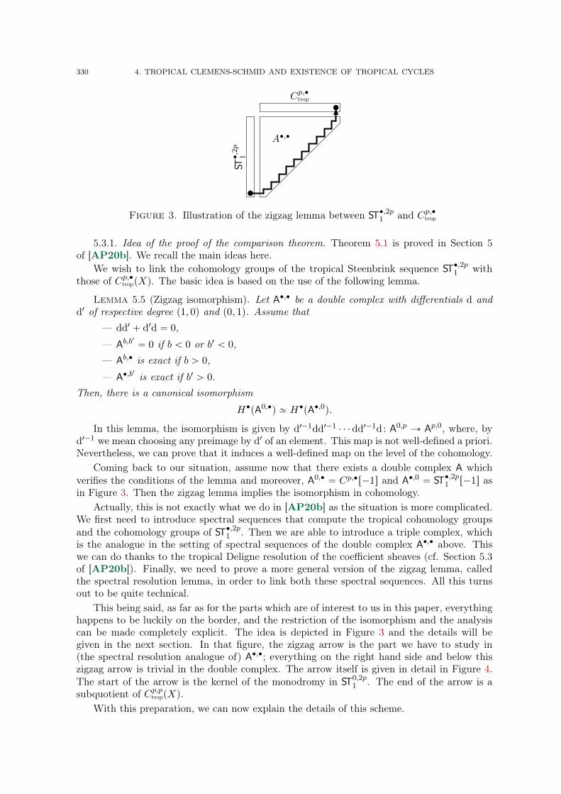
330 4. TROPICAL CLEMENS-SCHMID AND EXISTENCE OF TROPICAL CYCLES
Cp,‚trop
ST‚,2p
1
A‚,‚
Figure 3. Illustration of the zigzag lemma between ST‚,2p1 and Cp,‚trop
5.3.1. Idea of the proof of the comparison theorem. Theorem 5.1 is proved in Section 5of [AP20b]. We recall the main ideas here.
We wish to link the cohomology groups of the tropical Steenbrink sequence ST‚,2p1 withthose of Cp,‚troppXq. The basic idea is based on the use of the following lemma.
Lemma 5.5 (Zigzag isomorphism). Let A‚,‚ be a double complex with differentials d andd1 of respective degree p1, 0q and p0, 1q. Assume that
— dd1 ` d1d “ 0,
— Ab,b1
“ 0 if b ă 0 or b1 ă 0,— Ab,‚ is exact if b ą 0,
— A‚,b1
is exact if b1 ą 0.Then, there is a canonical isomorphism
H‚pA0,‚q » H‚pA‚,0q.
In this lemma, the isomorphism is given by d1´1dd1´1 ¨ ¨ ¨ dd1´1d: A0,p Ñ Ap,0, where, byd1´1 we mean choosing any preimage by d1 of an element. This map is not well-defined a priori.Nevertheless, we can prove that it induces a well-defined map on the level of the cohomology.
Coming back to our situation, assume now that there exists a double complex A whichverifies the conditions of the lemma and moreover, A0,‚ “ Cp,‚r´1s and A‚,0 “ ST‚,2p1 r´1s asin Figure 3. Then the zigzag lemma implies the isomorphism in cohomology.
Actually, this is not exactly what we do in [AP20b] as the situation is more complicated.We first need to introduce spectral sequences that compute the tropical cohomology groupsand the cohomology groups of ST‚,2p1 . Then we are able to introduce a triple complex, whichis the analogue in the setting of spectral sequences of the double complex A‚,‚ above. Thiswe can do thanks to the tropical Deligne resolution of the coefficient sheaves (cf. Section 5.3of [AP20b]). Finally, we need to prove a more general version of the zigzag lemma, calledthe spectral resolution lemma, in order to link both these spectral sequences. All this turnsout to be quite technical.
This being said, as far as for the parts which are of interest to us in this paper, everythinghappens to be luckily on the border, and the restriction of the isomorphism and the analysiscan be made completely explicit. The idea is depicted in Figure 3 and the details will begiven in the next section. In that figure, the zigzag arrow is the part we have to study in(the spectral resolution analogue of) A‚,‚; everything on the right hand side and below thiszigzag arrow is trivial in the double complex. The arrow itself is given in detail in Figure 4.The start of the arrow is the kernel of the monodromy in ST0,2p
1 . The end of the arrow is asubquotient of Cp,ptroppXq.
With this preparation, we can now explain the details of this scheme.
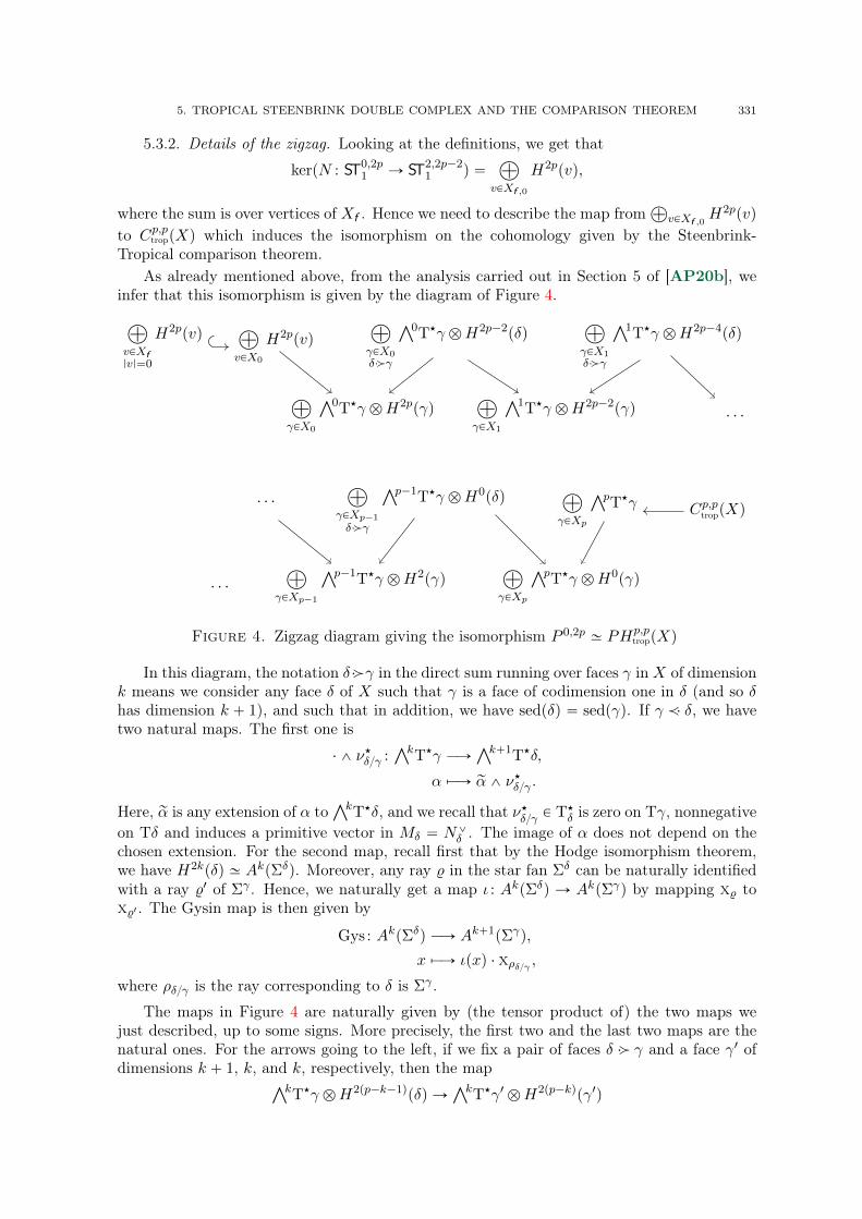
5. TROPICAL STEENBRINK DOUBLE COMPLEX AND THE COMPARISON THEOREM 331
5.3.2. Details of the zigzag. Looking at the definitions, we get that
kerpN : ST0,2p1 Ñ ST2,2p´2
1 q “à
vPXf ,0
H2ppvq,
where the sum is over vertices of Xf . Hence we need to describe the map fromÀ
vPXf ,0H2ppvq
to Cp,ptroppXq which induces the isomorphism on the cohomology given by the Steenbrink-Tropical comparison theorem.
As already mentioned above, from the analysis carried out in Section 5 of [AP20b], weinfer that this isomorphism is given by the diagram of Figure 4.
à
vPX0
H2ppvqà
vPXf|v|“0
H2ppvqà
γPX0δ ąγ
Ź0T‹γ bH2p´2pδqà
γPX1δ ąγ
Ź1T‹γ bH2p´4pδq
à
γPX0
Ź0T‹γ bH2ppγqà
γPX1
Ź1T‹γ bH2p´2pγq ¨ ¨ ¨
¨ ¨ ¨
à
γPXp´1
δ ąγ
Źp´1T‹γ bH0pδq à
γPXp
ŹpT‹γ Cp,ptroppXq
¨ ¨ ¨
à
γPXp´1
Źp´1T‹γ bH2pγqà
γPXp
ŹpT‹γ bH0pγq
Figure 4. Zigzag diagram giving the isomorphism P 0,2p » PHp,ptroppXq
In this diagram, the notation δ ąγ in the direct sum running over faces γ inX of dimensionk means we consider any face δ of X such that γ is a face of codimension one in δ (and so δhas dimension k ` 1), and such that in addition, we have sedpδq “ sedpγq. If γ ă δ, we havetwo natural maps. The first one is
¨ ^ ν‹δγ :ŹkT‹γ ÝÑ
Źk`1T‹δ,
α ÞÝÑ rα^ ν‹δγ .
Here, rα is any extension of α toŹkT‹δ, and we recall that ν‹δγ P T‹δ is zero on Tγ, nonnegative
on Tδ and induces a primitive vector in Mδ “ N_δ . The image of α does not depend on thechosen extension. For the second map, recall first that by the Hodge isomorphism theorem,we have H2kpδq » AkpΣδq. Moreover, any ray % in the star fan Σδ can be naturally identifiedwith a ray %1 of Σγ . Hence, we naturally get a map ι : AkpΣδq Ñ AkpΣγq by mapping x% tox%1 . The Gysin map is then given by
Gys: AkpΣδq ÝÑ Ak`1pΣγq,
x ÞÝÑ ιpxq ¨ xρδγ ,
where ρδγ is the ray corresponding to δ is Σγ .
The maps in Figure 4 are naturally given by (the tensor product of) the two maps wejust described, up to some signs. More precisely, the first two and the last two maps are thenatural ones. For the arrows going to the left, if we fix a pair of faces δ ą γ and a face γ1 ofdimensions k ` 1, k, and k, respectively, then the map
ŹkT‹γ bH2pp´k´1qpδq ÑŹkT‹γ1 bH2pp´kqpγ1q
332 4. TROPICAL CLEMENS-SCHMID AND EXISTENCE OF TROPICAL CYCLES
is given by 0 if γ ‰ γ1, and bysignpγ, δqidbGysδąγ ,
if γ “ γ1. For the arrows going to the right, and for a pair of faces δ ą γ and a face δ1 ofdimensions k ` 1, k, and k ` 1, respectively, the map
ŹkT‹γ bH2pp´k´1qpδq ÑŹkT‹γ1 bH2pp´kqpγ1q
is given by 0 if δ ‰ δ1, and byp ¨ ^ ν‹δγq b id
if δ “ δ1.Note that all the maps except the first one are surjective. Therefore, to an element of
À
vPXf ,0H2ppvq we can associate an element of Cp,ptroppXq by following the diagram, and making
some choices. However, as explained above, the induced map on the level of the cohomologygroups does not depend on these choices and is thus well-defined. The resulting map weobtain in this way is the restriction of the Steenbrink-Tropical comparison isomorphism ofTheorem 5.1 which goes from P 0,2p to PHp,p
trop.
5.4. Pairing with Minkowski weights. Let Y be the open part of X and let Y be theunimodular triangulation induced by X on Y . Let p ě 0 and let w be a Minkowski weight inMWppY q. The weight w naturally induces a map w : Xp Ñ Q which we also denote by w.
Let v be a vertex on Xf . Let αv P H2ppvq. We can represent αv as follows
αv “ÿ
ηąv|η|“p
av,ηxη P AppΣvq.
The Minkowski weight w naturally induces an element wv in MWppΣvq. Via the pairing
AppΣvq ˆMWppΣvq Ñ Q, we thus get the rational number
xαv, wvy “ÿ
ηăv|η|“p
av,ηwvpηq.
The fact that this sum does not depend on the chosen representative of αv is a consequenceof the balancing condition (cf. [AHK18]). By summing over all the vertices of Xf , we get apairing between kerpN : ST0,2p
1 Ñ ST2,2p´21 q »
À
vH2ppvq and MWppY q. One can prove that
this induces a pairingP 0,2p ˆMWppY q Ñ Q.
On the other hand, let c P Cp,ppXq. We write c “ř
ηPXp cη with cη P Fppηq. Then we geta pairing between Cp,ppXq and MWppY q by setting
xc, wy “ÿ
ηPXp
wpηqcηpnηq,
where we recall that nη is the canonical unit multivector inŹpTη. Once again, this induces
a pairingPHp,p
troppXq ˆMWppY q Ñ Q.Let α P PHp,p
troppXq. Let C “ pXďd´p, wq be the tropical cycle associated to w. Then theabove pairing is compatible with the integration on tropical Dolbeault cohomology in thesense of [JSS19]:
ż
Cα “ xα,wy,
for any α P PHp,ppXq ãÑ Hp,pDolbpX,Rq.
The following theorem states that the two pairing defined above are compatible with theSteenbrink-Tropical comparison theorem.
6. TROPICAL SURVIVING AND RELATIVE COHOMOLOGY GROUPS 333
Theorem 5.6. The restriction of the isomorphism of Theorem 5.1 to P 0,2p „ÝÑ PHp,ptroppXq
commutes with the pairing with MWppY q in the sense that the following diagram commutes.
P 0,2p PHp,ptroppXq
MWppY q‹
„
Proof. It suffices to extend the pairing in a consistent way to all the pieces appearing inthe zigzag of Figure 4. We do it as follows. Let w be a Minkowski weight in MWppY q, andlet w : Xp Ñ Q be the corresponding map on Xp, as above. Let δ ą γ be a pair of faces ofdimensions k ` 1 and k. Let βγ P
ŹkT‹γ and let αδ P H2pp´k´1qpδq. We set
xβγ b αδ, wy :“ signpγ, δqβγpnγqxαδ, wδy
where wδ is the natural element of MWd´k´1pΣδq induced by w. In the same way, if αγ P
H2pp´kqpγq, then we setxβγ b αγ , wy :“ βγpnγqxαγ , wγy.
A direct computation shows that these pairings commute with the maps of the zigzag. Thisconcludes the proof of the theorem.
6. Tropical surviving and relative cohomology groups
In this section we define the tropical surviving and relative cohomology groups.
First, we denote by K‚,‚ the kernel of the monodromy operator N : ST‚,‚1 Ñ ST‚,‚1 . It isexplicitly given by
Ka,b :“ STa,b,a1 “à
δPXf|δ|“a
Hbpδq.
In particular, since the monodromy operator is injective on STa,b1 for a ă 0, the groups Ka,b
are all trivial for any value of a ă 0. We can naturally endow Ka,b with the restriction of thedifferential d, i.e., with i˚. We set
Hp,qs pXq :“ Hq´ppK‚,2pq
and we call it the surviving cohomology of the tropical variety X with respect to the triangulationX.
Remark 6.1. To justify the terminology, we note that in the approximable case, when thetropical variety appears as the tropical limit of a projective family of complex varieties, usingthe correspondence between faces of the tropical limit and the intersection of components ofthe special fiber, the surviving cohomology gives a way to compute the weight-graded piecesof the cohomology of X . More precisely, using the Deligne spectral sequence, the cohomologygroup Hp,q
s pXq coincides with the weight 2p graded piece of the cohomology group Hp`q ofthe special fiber. In the general case, a triangulation equipped with the double complex K‚,‚
given above plays the role of a virtual special fiber. ˛
Similarly, we denote by R‚,‚ the cokernel of the monodromy operator N : ST‚,‚1 Ñ ST‚,‚1 .It is explicitly given by
Ra,b :“ STa,b,´a1 “à
δPXf|δ|“´a
H2a`bpδq.
Since the monodromy operator is surjective on STa,b1 for any a ą 0, the group Ra,b is trivialfor a ą 0. We can endow Ra,b with the restriction of the differential d, i.e., with Gys. We set
Hp,qrel pXq :“ Hq´ppR‚,2pq
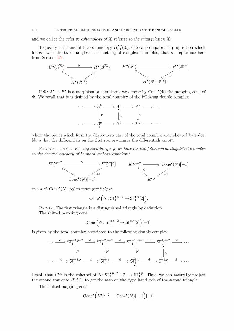
334 4. TROPICAL CLEMENS-SCHMID AND EXISTENCE OF TROPICAL CYCLES
and we call it the relative cohomology of X relative to the triangulation X.
To justify the name of the cohomology H‚,‚rel pXq, one can compare the proposition whichfollows with the two triangles in the setting of complex manifolds, that we reproduce herefrom Section 1.2.
H‚pĄX ˚q H‚pĄX ˚q
H‚pX ˚q
N
`1
H‚pX q H‚pX ˚q
H‚pX ,X ˚q
`1
If Φ: A‚ Ñ B‚ is a morphism of complexes, we denote by Cone‚pΦq the mapping cone ofΦ. We recall that it is defined by the total complex of the following double complex
¨ ¨ ¨ A0 A1
‚A2 ¨ ¨ ¨
¨ ¨ ¨ B0
‚B1 B2 ¨ ¨ ¨
Φ Φ Φ
where the pieces which form the degree zero part of the total complex are indicated by a dot.Note that the differentials on the first row are minus the differentials on A‚.
Proposition 6.2. For any even integer p, we have the two following distinguished trianglesin the derived category of bounded cochain complexes
ST‚,p`21 ST‚,p1 r2s
Cone‚pNqr´1s
N
`1
K‚,p`2 Cone‚pNqr´1s
R‚,p`1
0
in which Cone‚pNq refers more precisely to
Cone‚´
N : ST‚,p`21 Ñ ST‚,p1 r2s
¯
.
Proof. The first triangle is a distinguished triangle by definition.The shifted mapping cone
Cone´
N : ST‚,p`21 Ñ ST‚,p1 r2s
¯
r´1s
is given by the total complex associated to the following double complex
¨ ¨ ¨ ST´3,p`21 ST´2,p`2
1 ST´1,p`21 ST0,p`2
1‚
¨ ¨ ¨
¨ ¨ ¨ ST´1,p1 ST0,p
1 ST1,p1‚
ST2,p1 ¨ ¨ ¨
d d
N
d
N
d
N
d
N
d d d d d
Recall that R‚,p is the cokernel of N : ST‚,p`21 r´2s Ñ ST‚,p1 . Thus, we can naturally project
the second row onto R‚,pr1s to get the map on the right hand side of the second triangle.The shifted mapping cone
Cone‚´
K‚,p`2 Ñ Cone‚pNqr´1s¯
r´1s
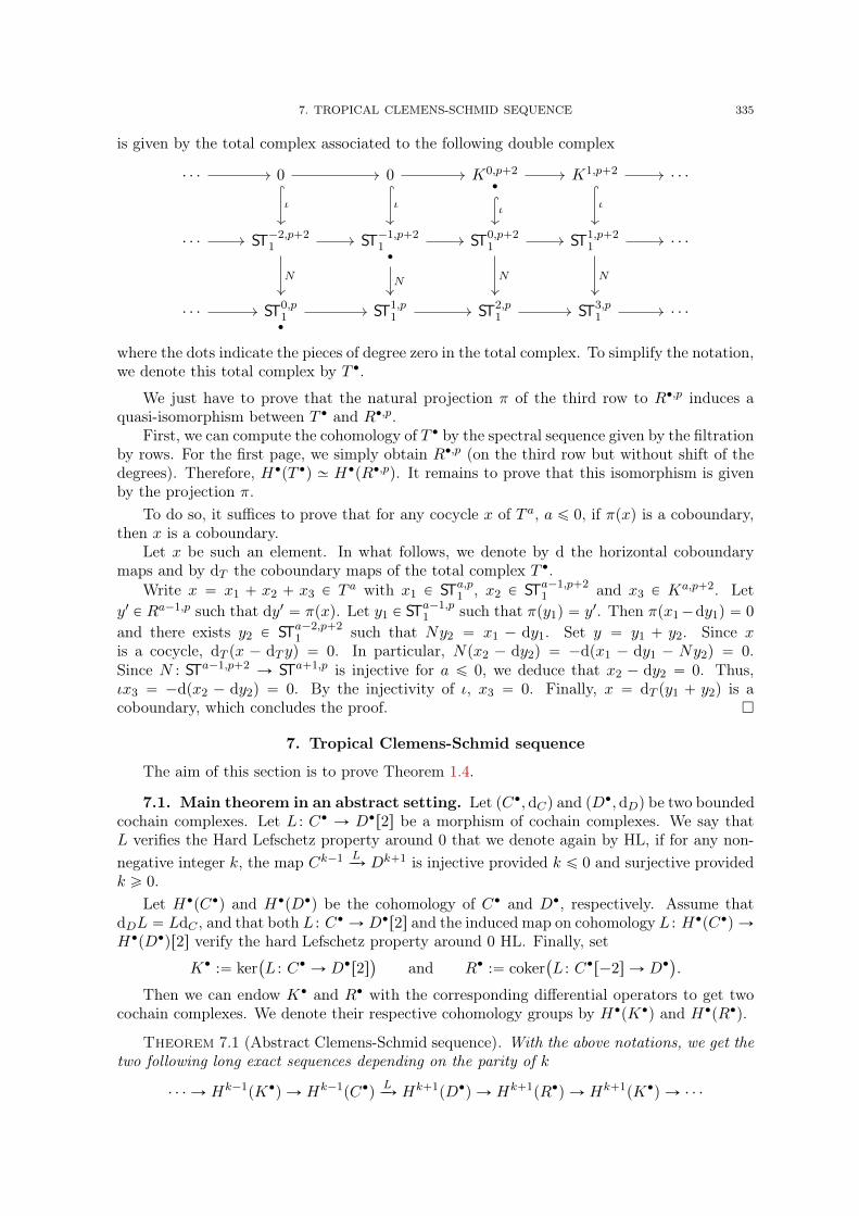
7. TROPICAL CLEMENS-SCHMID SEQUENCE 335
is given by the total complex associated to the following double complex
¨ ¨ ¨ 0 0 K0,p`2
‚K1,p`2 ¨ ¨ ¨
¨ ¨ ¨ ST´2,p`21 ST´1,p`2
1‚
ST0,p`21 ST1,p`2
1 ¨ ¨ ¨
¨ ¨ ¨ ST0,p1‚
ST1,p1 ST2,p
1 ST3,p1 ¨ ¨ ¨
ι ι ι ι
N N N N
where the dots indicate the pieces of degree zero in the total complex. To simplify the notation,we denote this total complex by T ‚.
We just have to prove that the natural projection π of the third row to R‚,p induces aquasi-isomorphism between T ‚ and R‚,p.
First, we can compute the cohomology of T ‚ by the spectral sequence given by the filtrationby rows. For the first page, we simply obtain R‚,p (on the third row but without shift of thedegrees). Therefore, H‚pT ‚q » H‚pR‚,pq. It remains to prove that this isomorphism is givenby the projection π.
To do so, it suffices to prove that for any cocycle x of T a, a ď 0, if πpxq is a coboundary,then x is a coboundary.
Let x be such an element. In what follows, we denote by d the horizontal coboundarymaps and by dT the coboundary maps of the total complex T ‚.
Write x “ x1 ` x2 ` x3 P Ta with x1 P STa,p1 , x2 P STa´1,p`2
1 and x3 P Ka,p`2. Let
y1 P Ra´1,p such that dy1 “ πpxq. Let y1 P STa´1,p1 such that πpy1q “ y1. Then πpx1´dy1q “ 0
and there exists y2 P STa´2,p`21 such that Ny2 “ x1 ´ dy1. Set y “ y1 ` y2. Since x
is a cocycle, dT px ´ dT yq “ 0. In particular, Npx2 ´ dy2q “ ´dpx1 ´ dy1 ´ Ny2q “ 0.Since N : STa´1,p`2 Ñ STa`1,p is injective for a ď 0, we deduce that x2 ´ dy2 “ 0. Thus,ιx3 “ ´dpx2 ´ dy2q “ 0. By the injectivity of ι, x3 “ 0. Finally, x “ dT py1 ` y2q is acoboundary, which concludes the proof.
7. Tropical Clemens-Schmid sequence
The aim of this section is to prove Theorem 1.4.
7.1. Main theorem in an abstract setting. Let pC‚,dCq and pD‚,dDq be two boundedcochain complexes. Let L : C‚ Ñ D‚r2s be a morphism of cochain complexes. We say thatL verifies the Hard Lefschetz property around 0 that we denote again by HL, if for any non-negative integer k, the map Ck´1 L
ÝÑ Dk`1 is injective provided k ď 0 and surjective providedk ě 0.
Let H‚pC‚q and H‚pD‚q be the cohomology of C‚ and D‚, respectively. Assume thatdDL “ LdC , and that both L : C‚ Ñ D‚r2s and the induced map on cohomology L : H‚pC‚q ÑH‚pD‚qr2s verify the hard Lefschetz property around 0 HL. Finally, set
K‚ :“ ker`
L : C‚ Ñ D‚r2s˘
and R‚ :“ coker`
L : C‚r´2s Ñ D‚˘
.
Then we can endow K‚ and R‚ with the corresponding differential operators to get twocochain complexes. We denote their respective cohomology groups by H‚pK‚q and H‚pR‚q.
Theorem 7.1 (Abstract Clemens-Schmid sequence). With the above notations, we get thetwo following long exact sequences depending on the parity of k
¨ ¨ ¨ Ñ Hk´1pK‚q Ñ Hk´1pC‚qLÝÑ Hk`1pD‚q Ñ Hk`1pR‚q Ñ Hk`1pK‚q Ñ ¨ ¨ ¨
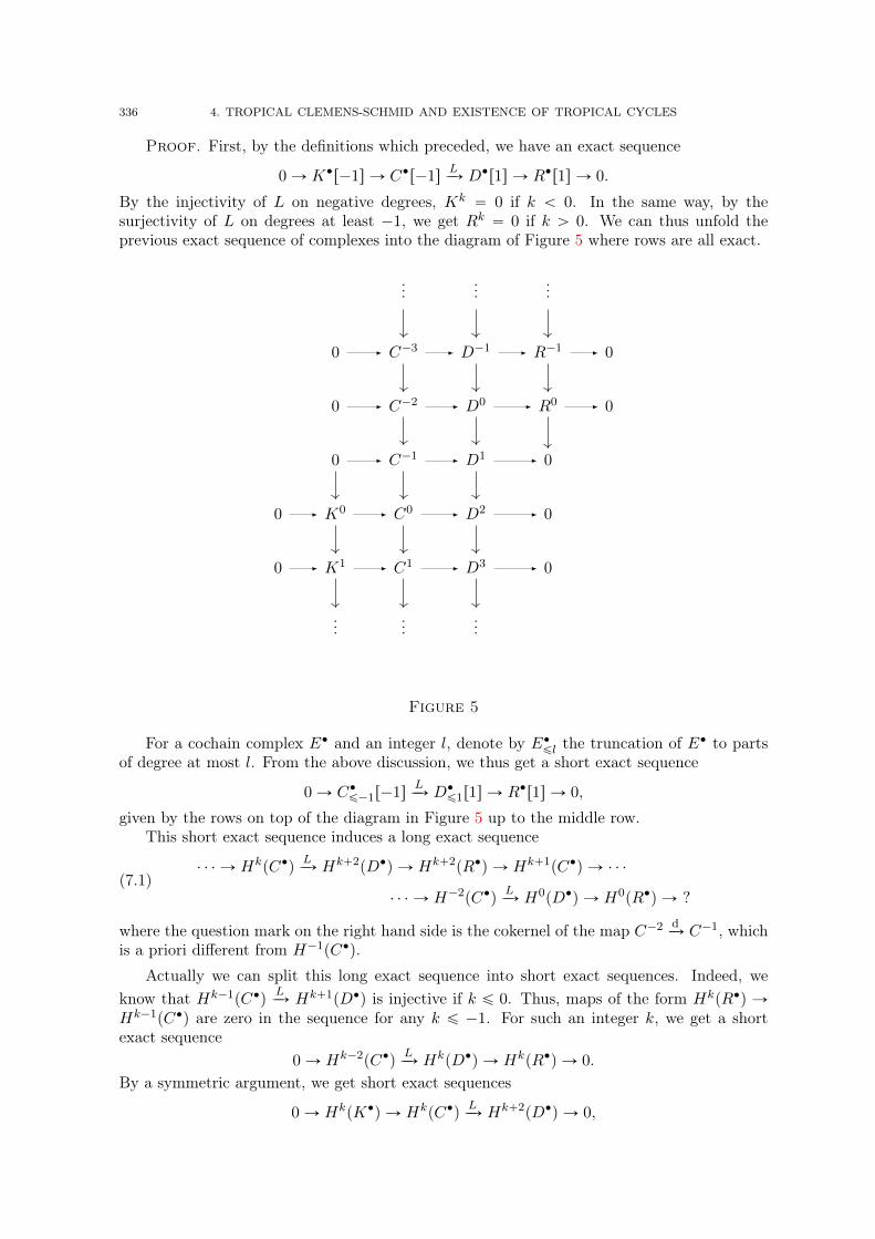
336 4. TROPICAL CLEMENS-SCHMID AND EXISTENCE OF TROPICAL CYCLES
Proof. First, by the definitions which preceded, we have an exact sequence
0 Ñ K‚r´1s Ñ C‚r´1sLÝÑ D‚r1s Ñ R‚r1s Ñ 0.
By the injectivity of L on negative degrees, Kk “ 0 if k ă 0. In the same way, by thesurjectivity of L on degrees at least ´1, we get Rk “ 0 if k ą 0. We can thus unfold theprevious exact sequence of complexes into the diagram of Figure 5 where rows are all exact.
......
...
0 C´3 D´1 R´1 0
0 C´2 D0 R0 0
0 C´1 D1 0
0 K0 C0 D2 0
0 K1 C1 D3 0
......
...
Figure 5
For a cochain complex E‚ and an integer l, denote by E‚ďl the truncation of E‚ to partsof degree at most l. From the above discussion, we thus get a short exact sequence
0 Ñ C‚ď´1r´1sLÝÑ D‚ď1r1s Ñ R‚r1s Ñ 0,
given by the rows on top of the diagram in Figure 5 up to the middle row.This short exact sequence induces a long exact sequence
(7.1)¨ ¨ ¨ Ñ HkpC‚q
LÝÑ Hk`2pD‚q Ñ Hk`2pR‚q Ñ Hk`1pC‚q Ñ ¨ ¨ ¨
¨ ¨ ¨ Ñ H´2pC‚qLÝÑ H0pD‚q Ñ H0pR‚q Ñ ?
where the question mark on the right hand side is the cokernel of the map C´2 dÝÑ C´1, which
is a priori different from H´1pC‚q.
Actually we can split this long exact sequence into short exact sequences. Indeed, weknow that Hk´1pC‚q
LÝÑ Hk`1pD‚q is injective if k ď 0. Thus, maps of the form HkpR‚q Ñ
Hk´1pC‚q are zero in the sequence for any k ď ´1. For such an integer k, we get a shortexact sequence
0 Ñ Hk´2pC‚qLÝÑ HkpD‚q Ñ HkpR‚q Ñ 0.
By a symmetric argument, we get short exact sequences
0 Ñ HkpK‚q Ñ HkpC‚qLÝÑ Hk`2pD‚q Ñ 0,
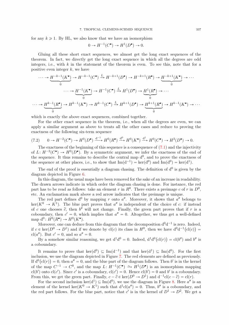
7. TROPICAL CLEMENS-SCHMID SEQUENCE 337
for any k ě 1. By HL, we also know that we have an isomorphism
0 Ñ H´1pC‚q Ñ H1pD‚q Ñ 0.
Gluing all these short exact sequences, we almost get the long exact sequences of thetheorem. In fact, we directly get the long exact sequence in which all the degrees are oddintegers, i.e., with k in the statement of the theorem is even. To see this, note that for apositive even integer k, we have
¨ ¨ ¨ Ñ H´k´1pK‚qloooooomoooooon
0
Ñ H´k´1pC‚qLÝÑ H´k`1pD‚q Ñ H´k`1pR‚q Ñ H´k`1pK‚q
loooooomoooooon
0
Ñ ¨ ¨ ¨
¨ ¨ ¨ Ñ H´1pK‚qloooomoooon
0
Ñ H´1pC‚qLÝÑ H1pD‚q Ñ H1pR‚q
looomooon
0
Ñ ¨ ¨ ¨
¨ ¨ ¨ Ñ Hk´1pR‚qloooomoooon
0
Ñ Hk´1pK‚q Ñ Hk´1pC‚qLÝÑ Hk`1pD‚q Ñ Hk`1pR‚q
loooomoooon
0
Ñ Hk´1pK‚q Ñ ¨ ¨ ¨
which is exactly the above exact sequences, combined together.For the other exact sequence in the theorem, i.e., when all the degrees are even, we can
apply a similar argument as above to treats all the other cases and reduce to proving theexactness of the following six-term sequence
(7.2) 0 Ñ H´2pC‚q Ñ H0pD‚qd´1
ÝÝÑ H0pR‚qd0
ÝÑ H0pK‚qd1
ÝÑ H0pC‚q Ñ H2pD‚q Ñ 0.
The exactness of the beginning of this sequence is a consequence of (7.1) and the injectivityof L : H´2pC‚q Ñ H0pD‚q. By a symmetric argument, we infer the exactness of the end ofthe sequence. It thus remains to describe the central map d0, and to prove the exactness ofthe sequence at other places, i.e., to show that Impd´1q “ kerpd0q and Impd0q “ kerpd1q.
The end of the proof is essentially a diagram chasing. The definition of d0 is given by thediagram depicted in Figure 6.
In this diagram, the usual maps have been removed for the sake of an increase in readability.The drawn arrows indicate in which order the diagram chasing is done. For instance, the redpart has to be read as follows: take an element r in R0. There exists a preimage c of r in D0,etc. An exclamation mark above a red arrow indicates that the preimage is unique.
The red part defines d0 by mapping r onto a2. Moreover, it shows that a2 belongs tokerpK0 Ñ K1q. The blue part proves that a2 is independent of the choice of c: if insteadof c one chooses rc, then b2 will not change. Finally, the green part proves that if r is acoboundary, then c1 “ 0, which implies that a2 “ 0. Altogether, we thus get a well-definedmap d0 : H0pR‚q Ñ H0pK‚q.
Moreover, one can deduce from this diagram that the decomposition d0d´1 is zero. Indeed,if c P kerpD0 Ñ D1q and if we denote by clpcq its class in H0, then we have d0d´1
`
clpcq˘
“
clpa2q. But c1 “ 0, and so a2 “ 0.By a somehow similar reasoning, we get d1d0 “ 0. Indeed, d1d0
`
clprq˘
“ clpb2q and b2 isa coboundary.
It remains to prove that kerpd0q Ď Impd´1q and that kerpd1q Ď Impd0q. For the firstinclusion, we use the diagram depicted in Figure 7. The red elements are defined as previously.If d0
`
clprq˘
“ 0, then a2 “ 0, and the blue part of the diagram follows. Then b1 is in the kernelof the map C´1 Ñ C0, and the map L : H´1pC‚q „ÝÑ H1pD‚q is an isomorphism mappingclpb1q onto clpc1q. Since c1 is a coboundary, clpc1q “ 0. Hence clpb1q “ 0 and b1 is a coboundary.From this, we get the green part. Finally, c´ rc P kerpD0 Ñ D1q and d´1clpc´ rcq “ clprq.
For the second inclusion kerpd1q Ď Impd0q, we use the diagram in Figure 8. Here a2 is anelement of the kernel kerpK0 Ñ K1q such that d1clpa2q “ 0. Thus, b2 is a coboundary, andthe red part follows. For the blue part, notice that c1 is in the kernel of D1 Ñ D2. We get a
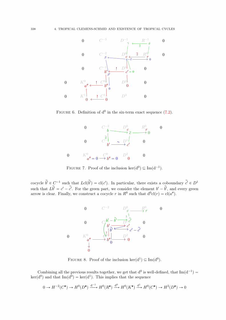
338 4. TROPICAL CLEMENS-SCHMID AND EXISTENCE OF TROPICAL CYCLES
0 C´3 D´1 R´1 0
0 C´2 D0 R0 0
0 C´1 D1 0
0 K0 C0 D2 0
0 K1 C1 D3 0
0 0
0 0
0 0
0 0
0 0
´c´c
´r´r
bb
cc
rr
b1b1
c1c1
a2a2
b2b2
c2c2
b3b3
a3a3
rD
c
c1
0
!b1
b2!
a2
0!
0
%D
γ
“ 0
c´rc 0β
β1
0
Figure 6. Definition of d0 in the six-term exact sequence (7.2).
0 C´2 D0 R0 0
0 C´1 D1 0
0 K0 C0 D2 0
0 0
0 0
0 0
b c r
b1 c1
a2 b2 c2a2 b2 0
b1 c1
c r
“ 0 “ 0
„
rc 0D
b
Figure 7. Proof of the inclusion kerpd0q Ď Impd´1q.
cocycle rb1 P C´1 such that Lclprb1q “ clpc1q. In particular, there exists a coboundary rc1 P D1
such that Lrb1 “ c1 ´ rc1. For the green part, we consider the element b1 ´ rb1, and every greenarrow is clear. Finally, we construct a cocycle r in R0 such that d0clprq “ clpa2q.
0 C´2 D0 R0 0
0 C´1 D1 0
0 K0 C0 D2 0
0 0
0 0
0 0
b c r
b1 c1
a2 b2 c2
0
a2 b2
D
b1 c1
0
rb1
0
c1 ´ rc1
b1 ´ rb1 rc1D
c r
Figure 8. Proof of the inclusion kerpd1q Ď Impd0q.
Combining all the previous results together, we get that d0 is well-defined, that Impd´1q “
kerpd0q and that Impd0q “ kerpd1q. This implies that the sequence
0 Ñ H´2pC‚q Ñ H0pD‚qd´1
ÝÝÑ H0pR‚qd0
ÝÑ H0pK‚qd1
ÝÑ H0pC‚q Ñ H2pD‚q Ñ 0
8. EXISTENCE OF CYCLES WITH A GIVEN HODGE CLASS 339
is exact. Gluing all these exact sequences together, we get the long exact sequence of thetheorem consisting only of even degrees. This means for an odd integer k ě 3, we have theexact sequence
¨ ¨ ¨ Ñ H´k´1pK‚qloooooomoooooon
0
Ñ H´k´1pC‚qLÝÑ H´k`1pD‚q Ñ H´k`1pR‚q Ñ H´k`1pK‚q
loooooomoooooon
0
Ñ ¨ ¨ ¨
¨ ¨ ¨ Ñ H´2pK‚qloooomoooon
0
Ñ H´2pC‚q Ñ H0pD‚q Ñ H0pR‚q Ñ H0pK‚q Ñ H0pC‚q
Ñ H2pD‚q Ñ H2pR‚qlooomooon
0
Ñ ¨ ¨ ¨
¨ ¨ ¨ Ñ Hk´1pR‚qloooomoooon
0
Ñ Hk´1pK‚q Ñ Hk´1pC‚qLÝÑ Hk`1pD‚q Ñ Hk`1pR‚q
loooomoooon
0
Ñ Hk`1pK‚q Ñ ¨ ¨ ¨
This concludes the proof of the theorem.
7.2. Tropical Clemens-Schmid sequence. We can now derive the tropical Clemens-Schmid sequence from the theorem established in the previous section. So let X be a rationallytriangulable Kähler projective tropical variety and fix a unimodular triangulation X of X.Consider the monodromy operator N , of bidegree p2,´2q, acting on the tropical Steenbrinkdouble sequence ST‚,‚1 associated to N . We know that N verifies the Hard Lefschetz propertyHL. In particular, N : STa´1,b
1 Ñ STa`1,b´21 is injective if a ď 0 and surjective if a ě 0. Thus,
the restriction N : ST‚,b1 Ñ ST‚,b´21 r2s is a monodromy operator verifying HL around 0 in the
sense of Section 7.1. Moreover, we know that N induces an operator on ST‚,‚2 “ ST‚,‚8
whichverifies HL. Thus, N : H‚
`
ST‚,b1
˘
Ñ H‚`
ST‚,b´21
˘
r2s also verifies HL around 0.
We can apply Theorem 7.1, setting p “ b2 and q “ a`b2, to get the long exact sequence
¨ ¨ ¨ Ñ Hp,qs pX,Qq Ñ Hp,q
troppX,QqNÝÑ Hp´1,q`1
trop pX,Qq Ñ Hp´1,q`1rel pX,Qq Ñ Hp,q`2
s pX,Qq Ñ ¨ ¨ ¨
SettingHkpX,Qq :“
à
p`q“k
Hp,qtroppX,Qq, and
Hks pX,Qq :“
à
p`q“k
Hp,qs pX,Qq, Hk
relpX,Qq :“à
p`q“k
Hp,qrel pX,Qq,
we can sum up the above exact sequences to get the tropical Clemens-Schmid exact sequence
¨ ¨ ¨ Ñ Hks pX,Qq Ñ HkpX,Qq N
ÝÑ HkpX,Qq Ñ HkrelpX,Qq Ñ Hk`2
s pX,Qq Ñ ¨ ¨ ¨
as required. This finishes the proof of Theorem 1.4.
8. Existence of cycles with a given Hodge class: proof of Theorem 1.1
In this section, we prove Theorem 1.1. Let X be a Kähler projective tropical variety ofdimension d. Assume that X is rationally triangulable. We need to prove that any Hodge classα, i.e., any element α in ker
`
N : Hp,ptroppX,Qq Ñ Hp´1,p`1
trop pX,Qq˘
, is represented by a tropicalcycle. The statement that the image of the tropical cycle class map is in the kernel of thetropical monodromy follows from Theorem 5.2 and the same result proved by Mikhalkin andZharkov [MZ14] for the eigenwave operator.
Replacing the underlying lattice by a rational multiple, we fix a unimodular triangulationX of X with open part Y , and we will show the existence of a Minkowski weight in MWd´ppY qwhose associated cycle in X represents the Hodge class α.
By the tropical Clemens-Schmid exact sequence, we know that
ker´
N : Hp,ptroppX,Qq Ñ Hp´1,p`1
trop pX,Qq¯
“ Im´
Hp,ps pX,Qq Ñ Hp,p
troppX,Qq¯
.
340 4. TROPICAL CLEMENS-SCHMID AND EXISTENCE OF TROPICAL CYCLES
Moreover, by definition, we have
Hp,ps pX,Qq “ ker
´
à
vPXf ,0
H2ppvq ÝÑà
ePXf ,1
H2ppeq¯
.
Thus, every Hodge class is represented by a cocycle of
K0,2p “à
vPXf ,0
H2ppvq.
The Hodge class α corresponds therefore to a collection of elements αv P H2ppvq, for v avertex in the finite part Xf , with the compatibility condition
@ e “ uv P Xf ,1, i˚văepαvq “ i˚uăepαuq.
For each simplex δ in Y and integer k, let MWkpδq :“ MWkpΣδq. By Theorems 4.1
and 4.2 we have H2ppv,Qq » AppΣv,Qq » MWd´ppv,Qq. The fact that α is a cocycle and theisomorphism H2ppe,Qq » MWd´ppe,Qq now imply that the Minkowski weights around eachvertex coincides on the star fans of the incident edges. This shows that αv glue together andproduce a Minkowski weight C “ pYďd´p, wq of dimension d ´ p on Y . As we explained inSection 3, this provides a tropical cycle C on X.
It remains to prove that the cohomology class clpCq inHp,ptroppX,Qq associated to C coincides
with α. Let β “ pβvqv P K0,2d´2p. For each vertex v in Xf ,0 and for each face η of dimensiond´ p containing v, we choose a rational coefficient bv,η P Q such that
βv “ÿ
ηąv
bv,ηxη P Ad´ppΣv,Qq,
where the sum is over faces η of dimension d ´ p. The local isomorphism between the Chowring and the Minkowski weights given in Theorem 4.2 verifies the following equality for anyv P Xf ,0
degpαv ¨ βvq “ÿ
ηąv
wpηqbv,η.
Hence,degpα ¨ βq “
ÿ
vPXf ,0
ÿ
ηąv
wpηqbv,η.
Moreover, by Section 5.4, the pairing between w and β is
xβ,wy “ÿ
vPXf ,0
ÿ
ηąv
wpηqbv,η.
Using Theorem 5.6, we getż
Cβ “ xβ,wy “ degpα ¨ βq
which shows that the class of C coincides with α.We proved that any Hodge class comes from a tropical cycle, which is the statement of
Theorem 1.1.
9. Proof of Theorem 1.3
In this final section, we prove the equivalence of numerical and homological equivalencefor tropical cycles on Kähler projective tropical varieties which admit a rational triangulation.
Let X be such a tropical variety of dimension d and consider a unimodular triangulation Xof X, which exists after replacing the lattice by a rational multiple. The monodromy operatorN is a Lefschetz operator on ST‚,‚1 and induces a Lefschetz operator on the cohomology of thetropical Steenbrink double sequence. From this, and using the Steenbrink-Tropical comparison
9. EQUIVALENCE OF NUMERICAL AND HOMOLOGICAL EQUIVALENCE 341
theorem, we infer that Hp,ptroppX,Qq » H0pST‚,2ppXqq can be decomposed as a direct sum of the
form
Hp,ppX,Qq “ ker´
N : Hp,ppXq Ñ Hp´1,p`1pXq¯
à
Im´
N : Hp`1,p´1pXq Ñ Hp,ppXq¯
,
where all the cohomology groups are with rational coefficients. Similarly, we get for q “ d´p,
Hq,qpX,Qq “ ker´
N : Hq,qpXq Ñ Hq´1,q`1pXq¯
à
Im´
N : Hq`1,q´1pXq Ñ Hq,qpXq¯
.
Consider as in Section 5 the polarization ψ on ST‚,‚1 which induces a polarization on thecohomology. The bilinear pairing ψ restricted to Hp,ppXq ˆHq,qpXq coincides moreover withthe Poincaré duality pairing. The operator N verifies N‹ “ ´N , for N‹ the adjoint of Nwith respect to ψ. It follows that the above decompositions of Hp,ppXq and Hq,qpX,Qq areorthogonal to each other, namely that
ker´
N : Hp,ppXq Ñ Hp´1,p`1pXq¯
K Im´
N : Hq`1,q´1pXq Ñ Hq,qpXq¯
,
and similarly,
ker´
N : Hq,qpXq Ñ Hq´1,q`1pXq¯
K Im´
N : Hp`1,p´1pXq Ñ Hp,ppXq¯
.
From the non-degeneracy of ψ on tropical cohomology, we infer that the induced pairing by thepolarization between ker
´
N : Hp,ppXq Ñ Hp´1,p`1pXq¯
and ker´
N : Hq,qpXq Ñ Hq´1,q`1pXq¯
is a duality pairing.By Theorem 1.1 the two kernels above are generated by the classes of tropical cycles of
codimension p and q, respectively. Moreover, the intersection between cycles is compatiblewith the polarization evaluated at the pair consisting of the cohomological classes associatedto the two cycles. With this preparation, we can now finish the proof.
Proof of Theorem 1.3. Let p be a fixed integer between 0 and d. A tropical cycle ofcodimension p which is homologically trivial has a trivial intersection with any tropical cycle ofcodimension q “ d´ p. This proves the implication (Homological equivalence) ñ (Numericalequivalence).
We now prove the other direction. Consider a tropical cycle C of codimension p in X andsuppose that C has trivial intersection with any tropical cycle of codimension q “ d´p. It fol-lows from Theorem 1.1 that clpCq has a trivial pairing with any element of ker
`
N : Hq,qpXq Ñ
Hq´1,q`1pXq˘
. Moreover, it belongs to ker`
N : Hp,ppXq Ñ Hp´1,p`1pXq˘
. Since the polar-ization induces a non-degenerate pairing between the two kernels, we finally infer that clpCqvanishes. This proves the implication (Numerical equivalence) ñ (Homological equivalence),and the theorem follows.

CHAPTER 5
A multidimensional generalization of Symanzik polynomials
Abstract : Symanzik polynomials are defined on Feynman graphs and they are used inquantum field theory to compute Feynman amplitudes. They also appear in mathematics fromdifferent perspectives. For example, recent results show that they allow to describe asymptoticlimits of geometric quantities associated to families of Riemann surfaces.
In this paper, we propose a generalization of Symanzik polynomials to the setting of higherdimensional simplicial complexes and study their basic properties and applications. We statea duality relation between these generalized Symanzik polynomials and what we call Kirchhoffpolynomials, which have been introduced in recent generalizations of Kirchhoff’s matrix-treetheorem to simplicial complexes. Moreover, we obtain geometric invariants which computeinteresting data on triangulable manifolds. As the name indicates, these invariants do notdepend on the chosen triangulation.
We furthermore prove a stability theorem concerning the ratio of Symanzik polynomialswhich extends a stability theorem of Amini to higher dimensional simplicial complexes. Inorder to show that theorem, we will make great use of matroids, and provide a completeclassification of the connected components of the exchange graph of a matroid, a graph whichencodes the exchange properties between independent sets of the matroid. We hope that thisresult could be of independent interest.
Finally, we explain how to generalize Symanzik polynomials to the setting of matroidsover hyperfields defined recently by Baker and Bowler.
1. Introduction
The aim of this paper is to introduce a family of polynomials that we call generalizedSymanzik polynomials, and to study their geometric and combinatorial properties.
Classical Symanzik polynomials arising in quantum field theory are associated to Feynmangraphs and used for computing Feynman amplitudes. They are defined as follows.
Let G “ pV,Eq be a connected graph with vertex set V and edge set E. Let p “ ppvqvPV bea collection of vectors called the external momenta such that each pv, the external momentumof v P V , is an element of the real vector space RD, for some positive integer D, whichis endowed with a Minkowski bilinear form. Moreover, we suppose that the collection ofexternal momenta verify the conservation of momenta hypothesis, namely that
ř
vPV pv “ 0.Such a pair pG, pq is called a Feynman graph. In what follows we will only consider the caseD “ 1, but the results can be extended to the more general setting as in [ABBF16].
The first Symanzik polynomial denoted by ψG is defined by
(1.1) ψGpxq :“ÿ
TPT
ź
eRT
xe,
where T denotes the set of spanning trees of G, where x “ pxeqePE is a collection of variablesindexed by the edges of the graph, and the product for a spanning tree T P T is on all edges ofG which are not in T . (A spanning tree of G “ pV,Eq is a connected subgraph of G which hasvertex set V and which does not have any cycle.) Note in particular that the first Symanzikpolynomial does not depend on the external momenta.
343
344 5. A MULTIDIMENSIONAL GENERALIZATION OF SYMANZIK POLYNOMIALS
The second Symanzik polynomial denoted φG is defined by
(1.2) φGpp, xq :“ÿ
FPSF2
qpF qź
eRF
xe.
In this formula, SF2 denotes the set of spanning forests of G which have two connectedcomponents. (A spanning forest of G is a subgraph with vertex set V and without any cycle.)For a spanning forest F P SF2, the term qpF q is defined by qpF q :“ ´xpF1 , pF2y where F1 andF2 are the two connected components of F , and where, for i P t1, 2u, pFi is the sum of themomenta of vertices in Fi. Using these polynomials, the Feynman amplitude can be computedthen as a path integral of expp´iφGψGq.
The above polynomials have many known interesting properties, most of them are sum-marized in [BW10]. In this paper, we present natural generalizations of the above definitions.In particular, we are going to extend the setting to higher dimensional simplicial complexes.Other generalizations already exist, see e.g., [GR07] and [KRTW10], though the purposeis different from ours. In addition to introducing a larger family of polynomials with interest-ing properties, we hope that this generalization will provide a better understanding of thesepolynomials and will widens their applications.
Symanzik polynomials are known to have tight connection to other concepts in mathemat-ics. Before going to the heart of our construction and presenting an overview of our results,we would like to start by highlighting some of these links and making a series of comments tomotivate the study undertaken in this paper.
First, Symanzik polynomials of graphs are known to be in a sense dual to Kirchhoffpolynomials. These latter polynomials are those obtained applying the well-known (weighted)Kirchhoff matrix-tree theorem, which counts the number of spanning trees of a graph as thedeterminant of a matrix linked to the Laplacian of the graph. Recently, the notion of aspanning tree has been extended to the case of higher dimensional simplicial complexes, andKirchhoff’s theorem has been generalized to this setting, c.f. [DKM09,Lyo09] and [BK16].In order to generalize the definition of Symanzik polynomials to this setting, it is thus naturalto exploit and formulate an appropriate version of the duality theorem in this setting. This iswhat we have done to find our definition of generalized Symanzik polynomials. In the classicalcase, this duality infers a determinantal formula for Symanzik polynomials. This is still trueafter the generalization.
This leads us to our second point which concerns determinantal probability measures (seefor instance [Lyo03]). This tight relation between Kirchhoff polynomials, spanning trees anddeterminants is studied thoroughly in the paper [Lyo09] of Lyons on random complexes. Infact, what appears here are determinantal probabilities. For instance, the probability for auniform (or suitably weighted) spanning tree of a graph to contain a specific edge can be easilycomputed because it is given by the determinant of some matrix. The Laplacian of the graphis used to define this matrix. In the same way, Kirchhoff polynomials are also obtained usingthis Laplacian. By analogy, the matrix whose determinant gives the first Symanzik polynomialallows us to compute the probability for a spanning tree not to contain a specific edge. Inthis paper, we will also generalize Kirchhoff and Symanzik polynomials in two different ways:first to spanning forests and second to higher order determinants (the classical definition is oforder two). This naturally leads to hyperdeterminants which are also linked to determinantalprobability measures as it was shown in [EG09].
This brings us naturally to the third point, which is the link to the theory of matroids.Matroids are mathematical objects obtained by abstracting and generalizing some of the mainnotions of linear algebra and, in particular, of graph theory, as spanning trees for example(we refer to [Oxl11] for further information). In [BW10], the link between matroid theoryand Symanzik polynomials is noticed. We go further than [BW10] by defining Kirchhoff
1. INTRODUCTION 345
and Symanzik polynomials for matroids and for their recent generalization matroids overhyperfields obtained by Baker and Bowler in [BB16] (see also [BB19]). This generalizationis needed to understand the generalized operations of deletion and contraction, which are lessnatural than in the case of graphs. These two operations are at the heart of many properties ofclassical Kirchhoff and Symanzik polynomials, in particular deletion-contraction formula anda partial factorization of the polynomials used, for instance, in [Bro15] (see below). Behindall this, there is the multivariate Tutte polynomial, which is also known as the Potts modelpartition function by physicists (cf. [Sok05, (4.11) and (2.18)]). Unfortunately, a canonicalTutte polynomial for matroids over hyperfields does not seem to exist. Though, using therecent work of Dupont, Fink and Moci in [DFM18] (itself based on [KMT18]), we will seethat Kirchhoff and Symanzik polynomials over hyperfields still preserve all the properties onecould expect of Tutte polynomial and its specializations.
Apart from this generalization, we show that matroids play a major role in understandingsome other interesting features of the Symanzik polynomials. These purely combinatorial re-sults about matroids, which we hope should be of independent interest, concern the exchangeproperties between independent sets of a general matroid, which generalize well-known ex-change properties between bases. For a connected graph, it is well-known that any spanningtree can be obtained from any other by a sequence consisting of exchanging one edge at atime. The exchange properties between spanning trees and spanning 2-forests in a graphwere studied by Amini in [Ami19] for the purpose of understanding the asymptotic of somegeometrically defined quantities in a family of Riemann surfaces. Generalizing the definitionof the exchange graph of a graph from [Ami19] to any general matroid, we provide a com-plete characterization of the connected components of this graph and use it to generalize thestability theorem of [Ami19] to higher dimensional simplicial complexes.
Let us make two further remarks at this point. It is well-known that the connectivityproperties of different kind of exchange graphs is the first step for creating simple and effi-cient random generation of bases based on Markov chains, c.f. [FM92] and the recent workof [ALOGV19] based on combinatorial Hodge theory for matroids [AHK18]. What we provein this paper is another geometric manifestation of the exchange properties in matroids. Fur-thermore, the results we obtain on the exchange graph of a matroid has very close ties toan old conjecture of White on toric ideals of matroids [Whi80,Bla08,LM14]. In fact, bythe work of [Bla08], a part of White’s conjecture can be rephrased as whether a particulargeneralization of our exchange graph is always connected, c.f. Remark 5.16. So our resultsand methods might lead to a new approach in that direction.
As we mentioned previously, Symanzik polynomials for graphs originated from Physics,and recent advances has shown that their properties govern the mathematics of Feynman am-plitudes, see e.g., BB03, BEK06, Bro15, BS12, BY11. In particular, Brown shows in [Bro15]how certain arithmetic factorization properties satisfied by the Symanzik polynomials of graphsand their minors play a crucial role in defining the cosmic Galois group, a Galois group forFeynman amplitudes. We extend these properties to generalized Symanzik polynomials in thisarticle.
From a point of view inclined towards Physics, we will show that our generalized poly-nomials present a certain stability (rather different from the stability theorem evoked above).This means that if we start with a sufficiently nice topological space S, then the Symanzikpolynomials of any triangulation of S come from (more precisely can be factorized into) thesame Symanzik polynomial, which can be directly defined then as the Symanzik polynomial ofS. In other words, this stability indicates that these polynomials might be useful for comput-ing interesting features of continuous objects by approximating them with discrete ones. Forinstance, path integrals are fundamental in the formulation of quantum field theory. But theyare generally ill-defined. A way to go through this difficulty is to discretize the paths, andRegge calculus gives a way to do this (originally in the framework of quantum gravity), see,
346 5. A MULTIDIMENSIONAL GENERALIZATION OF SYMANZIK POLYNOMIALS
e.g., the original article of Regge [Reg61], the introductory paper [Wil92], and a more recentapproach [Ori07] in the framework of group field theory. We have found striking similaritiesbetween the geometry of generalized Symanzik polynomials and Regge calculus, although atthis point we are not still able to formalize this.
About the geometrical data computed by generalized Symanzik polynomials, in simplecases as compact orientable manifolds endowed with a volume form, the Symanzik polynomialsimply computes the volume of the manifold (setting the good values to variables). There isnot always a simple interpretation for the value computed in more complex cases. However,for general metric graphs, the first Symanzik polynomial evaluated at positive reals computesthe volume of the Jacobian torus of the graph, which is defined in [KS00].
The Symanzik polynomials of graphs has been generalized in the context of non-commuta-tive quantum field theory [KRTW10]. The article [KRV11] shows how these new polynomialinvariants derive from the Bollobás-Riordan polynomial [BR02], which is a generalization ofthe Tutte polynomial for ribbon graphs. The Bollobás-Riordan polynomial itself has been gen-eralized to higher rank graphs (which are, under some conditions, dual to some pseudo simpli-cial complexes of higher dimension) in [AGH13] and [Avo16]. Two recent papers [KMT18]and [DFM18] provides a generalization of these polynomials in the context of Hopf algebras.Another recent paper [BC17] studies this kind of generalization for a different purpose. Itconcerns the geometric Brownian motion, also linked to quantum theory. As far as we know,multidimensional generalizations of Symanzik polynomials have not been studied prior to thiswork, and it would be certainly valuable to compare our approach to the above cited works.
Symanzik polynomials of graphs form a family of graph polynomials with very interestingproperties. As already seen, they are specializations of the multivariate Tutte polynomial.Recent papers study graph polynomials which usually reveal surprising geometric properties.It is not hard to prove that the first Symanzik polynomials of the connected graphs verifythe half-plane property, i.e., they are nonvanishing whenever all the variables lie in theopen right complex half-plane. The papers [COSW04,Brä07] and [BBL07] study invariantpolynomials verifying this property and other linked properties. They might be extended insome cases to our generalization.
Moreover, in [Ami19], it has been proved that a bounded geometrical deformation of thegraph only induces a variation of the ratio of the two Symanzik polynomials that is boundedindependently of the initial geometry. At the end of this article, we will generalize this stabilitytheorem. The initial goal of Amini in [Ami19] was to give a combinatorial proof of a result heobtained with Bloch, Burgos Gil and Fresán in [ABBF16]. In that work, they expressed theasymptotic of the Archimedean height pairing between two 0-divisors on degenerating fami-lies of Riemann surfaces as to the ratio of the two Symanzik polynomials. The generalizationpresented in this paper should have links to the generalization of that work to higher dimen-sional varieties. In another direction, Scott and Sokal study in [SS14] strict monotonicityproperties of the inverse powers of the Kirchhoff polynomials of graphs and matroids. Theygive a complete characterization of the exponents in the strict monotonicity range for series-parallel graphs, and raise several questions and conjectures. One might naturally wonder ifsuch results could be generalized to the setting of generalized Symanzik polynomials studiedin this paper.
In the rest of this introduction, we give a quick overview of the main results of this paper.
1.1. The generalization. The idea of the generalization comes from Kirchhoff’s matrix-tree theorem (observed by Kirchhoff [Kir47]) in its weighted form. We briefly sketch this ideahere. Example 2.9 contains all the details. Let G “ pV,Eq be a connected graph of vertex setV and edge set E “ te1, . . . , enu. Set a weight ye P R on each edge e P E. Set Q the incident
1. INTRODUCTION 347
matrix of G, and Y the diagonal matrix diagpye1 , . . . , yenq. Then, the theorem states that
(1.3)ÿ
TPT
ź
ePT
ye “ detp rQY rQᵀ
q,
where we removed a row from Q to get rQ. Let E1 Ď E be a subset of |V | ´ 1 edges. Werestrict the matrix rQ to the columns indexed by the elements of E1. We denote this squarematrix by rQE1 . A step of the proof is to notice that detp rQE1q
2 equals 1 if E1 corresponds toa spanning tree of G, 0 otherwise. Thus, the first Symanzik polynomial verifies
ψGpxq “ÿ
E1ĎE|E1|“|V |´1
detp rQE1q2ź
eRE1
xe.
In the right-hand member, the graph G is almost absent. The main data we use is its incidentmatrix. Thus, one can define the Symanzik polynomial of any matrix.
However, we needed to delete a row from the matrix. When the matrix does not comefrom graphs, we could have to remove several rows, and the result could depend on the chosenrows. To avoid any problem, we introduce a very useful tool: the standard inner product onthe exterior algebra. This is used by Lyons in [Lyo03] to deal with a subject not far fromours, as explained above.
Before going through details of our constructions, we need to introduce some terminologywhich will be used all through the paper.
Notations and conventions. If p, q are integers with p ď q, then the set tp, p`1, . . . , quwill be written rp . . qs, or more simply rqs if p “ 1. Let I be a finite set. Then |I| is itscardinality and PpIq is its power set. If J P PpIq is a subset of I and if there is no ambiguity,then Jc :“ IzJ denotes the complement of J . If i P Ic, then I ` i :“ I Ytiu, and if i P I, thenI ´ i :“ Iztiu (using these notations means, respectively, that i P Ic and that i P I). If thereis an ordering on the elements I, we will also use I to denote the ascending family of elementsin I (see below).
Let n be a positive integer. In the whole article, x “ px1, . . . , xnq will be a family ofvariables. Zrxs is the ring of polynomials over Z with variables x1, . . . , xn. Following a usualnotation, if I Ď rns,
xI :“ź
iPI
xi.
If ∆ is a set, Zx∆y is the free Z-module on ∆. By convention, if a P Z, then
a0 “
"
0 if a “ 0,1 otherwise.
Let n, p be positive integers. Then Mp,npZq will denote the set of matrices with p rowsand n columns over Z and MnpZq is a simpler notation for Mn,npZq. If P P Mn,ppZq, thenP
ᵀPMp,npZq denotes the transpose of P .Let n, p, q be positive integers. Let u “ pu1, . . . , unq be a family of n vectors in Rp. Then,
when there is no ambiguity, the same letter in uppercase, U , will denote the matrix inMp,npRqwhose columns are the coordinates of the vectors of u. Reciprocally, if U is a matrix, thenone can associate to U a family of vectors u. If I “ pi1, . . . , iqq is a family of elements of rns,then uI will be the family pui1 , . . . , uiqq, and UI PMp,qpRq will be the associated matrix. Wewill sometimes use this notation for variables: xI :“ pxi1 , . . . , xiqq. Moreover, uᵀ will be thefamily of p vectors in Rn associated to U ᵀ . If I is an (unordered) subset of rns of size q, thenuI , resp. UI , will denote the family upi1,...,iqq, resp. the matrix Upi1,...,iqq, where I “ ti1, . . . , iquand i1 ă i2 ă ¨ ¨ ¨ ă iq.
348 5. A MULTIDIMENSIONAL GENERALIZATION OF SYMANZIK POLYNOMIALS
If u and v are two families of elements of a same set of respective size n and m, then u ‹ vwill denote the concatenation of the two families, i.e.,
u ‹ v “ pu1, . . . , un, v1, . . . , vmq.
By extension, if U PMp,npRq and V PMp,mpRq are two matrices, then U ‹ V is the matrixof Mp,n`mpRq associated to u ‹ v.
LetŹ
Rp “À
lě0
ŹlRp be the exterior algebra over Rp. With the notations of the previousparagraphs, we will denote by u P
ŹnRp, resp. uI PŹqRp, the exterior product u1^ ¨ ¨ ¨^ul,
resp. ui1 ^ ¨ ¨ ¨ ^ uiq . We endowŹ
Rp with the standard inner product: if n and m are twononnegative integers, if u, v are two families of respective sizes n and m in Rp, then
pu,vq “
#
detpUᵀV q if n “ m,
0 otherwise.
We have the associated norm ‖u‖ :“ pu,uq12.Note that, if e is the standard basis of Rp, then the family peIqIĎrps,|I|“l forms an or-
thonormal basis ofŹlRp.
We have the standard inclusion Zp Ă Rp. If F is a vector subspace of Rp, then we denoteby FZ the sublattice F X Zp. If u is a family of vectors in Zp Ă Rp, then we denote by Zuthe sub-Z-module generated by u, and by xuy the subspace of Rp spanned by u. If A is asub-Z-module of Zp, we will denote by ‖A‖ the covolume of A, i.e., the value ‖f‖ where f isany basis of A.
If U PMp,npZq, then ImpUq, resp. kerpUq, will always denote vector subspaces, i.e., theimage, resp. kernel, of U in Rp, resp. Rn.
Let n and p be two positive integers. Let u be a family of n vectors of Zp Ă Rp. Let r bethe rank of u. We define the Symanzik polynomial of u by
Sym2pu;xq :“1
‖xuyZ‖2
ÿ
IĎrns|I|“r
‖uI‖2xIc.
Actually, one can replace the exponents 2 by any nonnegative even integer k. We willcall k the order of the polynomial (see Definition 2.10). The order 0 has some theoreticalinterests, as we will see for matroids. Moreover, Theorem 6.1 about stability holds for everyorders. That is why, we will study the case of all the orders in this article. This widens theset of interesting polynomials. However, in this introduction, we set k “ 2.
The main result of Section 2 is the close link between Symanzik polynomials and theKirchhoff theorem. To enlight this link, we introduce the Kirchhoff polynomial of u:
Kir2pu;xq :“1
‖xuyZ‖2
ÿ
IĎrns|I|“r
‖uI‖2xI .
Then, the link is given by the duality theorem (Theorem 2.13). If v is a family of maximalrank of kerpUqZ, then the theorem states that there exists an explicit factor c P Q such that
Kir2pvᵀ;xq “ cSym2pu;xq.
Here is the generalization of the second Symanzik polynomial in a specific case (see Defi-nition 2.17 for the general case). If a is an element of Zu, then the Symanzik polynomial of uwith parameter a is
Sym2pu; paq;xq :“ Sym2pu ‹ paq;x ‹ p0qq.
The justification of the definitions of Symanzik polynomials without parameters and ofKirchhoff polynomials are given respectively in Examples 2.12 and 2.9. However, the linkbetween Symanzik polynomials with parameters and second Symanzik polynomials is harder
1. INTRODUCTION 349
to establish. We need Proposition 2.20. In this proposition, some orientations hidden inSymanzik polynomials with parameters appear. These orientations are already well-known.They are called chirotopes in the theory of oriented matroid (see [FL78,GR13]). One canthink about them in the following way. We take a spanning 2-forests pF1, F2q of a graph.Then we can orient all edges that link F1 and F2, from F1 to F2. Much detail is given inExample 2.21.
Propositions 2.6, 2.16 and 2.19 state determinantal formulæ similar to that of Equa-tion (1.3). For instance, let v be a basis of kerpUq belonging to Zn, a P Zu and b P Znsuch that Ub “ a. Set rv :“ v ‹ pbq. Then,
Sym2pu; paq;xq “ cdetprVᵀX rV q,
for some factor c we explicit in Proposition 2.16, where X “ diagpx1, . . . , xnq.
1.2. Deletion-contraction formula and partial factorization. Among the many in-teresting properties of classical Symanzik polynomials, we will generalize two of them of par-ticular interest.
The first one is the deletion-contraction formula (see, e.g., [BW10,Bro15]). In theclassical case, if G “ pV,Eq is a graph and if e is edge of G, then
(1.4) ψGpxq “ xeψG´epxE´eq ` ψGteupxE´eq,
where G ´ e is the graph without e and Gteu is the graph obtained from G by contractinge (i.e., we removed the edge e and identify the two extremities of e). We will provide ageneralized version of this property for polynomials defined in this paper. In the context offamilies of vectors, the result will be the same except that deletion and contraction are moreinvolved to define. For this reason, we do not give more details in this introduction and referto Section 4.
The second formula we generalize is a partial factorization, used for example in [Bro15].Let G “ pV,Eq be a graph and let γ “ pV, F q be a spanning subgraph of G. If Gγ is thegraph obtained from G by contracting every edge in γ, then
(1.5) ψGpxq “ ψγpxF qψGγpxEzF q `Rψγ,Gpxq,
where the degree of Rψγ,Gpxq in xF is greater than the degree of ψγpxF q. See Proposition 4.13to see precisely what we mean here. This time, the generalized formula is the same up to afactor. Once more, we refer to Section 4 for more details.
1.3. Geometrical aspects of Symanzik polynomials. Following an idea of Kalaiin [Kal83], Duval, Klivans and Martin stated in [DKM09] a generalization of Kirchhoff’stheorem for simplicial complexes. This theorem counts the number of generalized spanningtrees with some weights. In Section 3.1, we will call these spanning trees 0-forests (or, moreexactly, we use the more convenient definition of spanning trees of Bernardi and Klivansin [BK16]). Readers who are not familiar with simplicial homology theory could consult thedetails in Section 3.1.
The definition of a 0-forest is really simple: it is a maximal simplicial subcomplex withoutnontrivial cycles of maximal dimension. To be more precise, let ∆ be a finite simplicial complexof dimension d, and let B∆ be the d-th boundary operator of ∆. Let Γ be a subcomplex of∆ with the same pd ´ 1q-skeleton, and let BΓ be the d-th boundary operator of Γ. Then,for an integer κ, Γ is a κ-forest of ∆ if kerpBΓq “ t0u and rkpB∆q ´ rkpBΓq “ κ. Forests inhigher dimensions mostly behave like forests in graphs. Moreover, the two notions coincideon connected graphs. In this case, κ-forests are the spanning forests with κ ` 1 connectedcomponents.
The boundary operator B∆ is a linear map. Let U be the associated matrix for some naturalbases of simplicial d-chains and of simplicial pd´1q-chains. It is natural to define the Symanzik
350 5. A MULTIDIMENSIONAL GENERALIZATION OF SYMANZIK POLYNOMIALS
polynomial, resp. Kirchhoff polynomial, of ∆ as the one of u. Then Kir2p∆;xq is what we getapplying the higher dimensional Kirchhoff weighted theorem to ∆ (see Theorem 3.7):
Kir2p∆;xq “ |TorpHd´1p∆qq|2
ÿ
Γ 0-forest of ∆
|Bd´1p∆qL
Bd´1pΓq|2
ź
δ d-face of Γ
xδ,
where Bd´1p∆q, resp. Bd´1pΓq, is the group of pd ´ 1q-boundaries of ∆, resp. of Γ, andTorpHd´1p∆qq denotes the torsion part of the pd´ 1q-th homology group of ∆.
Unlike the case of graphs, setting x “ p1, . . . , 1q does not give the number of 0-forests.Finding this number is difficult in general: there exist examples where all the coefficients ofthe polynomial are not equal (look at Example 3.27). Knowing the value of the Kirchhoffpolynomial for all order k might help us.
However, the weighted number of 0-forests for the order k “ 2 seems to be the mostnatural object to consider. The first reason is in [BK16]. The authors explain that thisnumber counts 0-forests of ∆ taking into account a fitted orientation. The second reason is thatKalai computed in [Kal83] the weighted number of 0-forests of the complete d-dimensionalsimplicial complex over N vertices. He obtains a pretty nice formula: Np
N´2d q.
Now, for each facet δ of ∆, assign to the variable xδ a positive number yδ P R` thatrepresents the volume of δ. This is natural. For example, let S be a compact orientedmanifold of dimension d, and let ω be a volume form on it. Let ∆ be a triangulation of S (seeSection 3.4 for a rigorous definition of triangulation). Then ω induces a volume yδ P R` foreach facet δ of ∆. It is not hard to verify that
Sym2p∆; yq “ VolpSq.This is more general. Set S the topological space of any d-dimensional finite CW-complex.We endow S with a diffuse measure µ (i.e., a measure which is 0 on any subset homeomorphicto r0; 1sd´1). Let ∆ be a triangulation of S, and y “ pyδq be the induced volume for each facetδ. Then
Sym2p∆; yq does not depend on the chosen triangulation ∆.The proof essentially consists on defining directly Sym2pS;µq, which will be the value we getfor any triangulation.
The case of a metric graph G is of particular interest. Sym2pG;µq (with µ induced by themetric) is the volume of the Jacobian torus of G introduced by Kotani and Sunada in [KS00](see Example 3.12).
1.4. Stability theorem. Let v be any free family of n elements of Rp. Let a be anelement of Rp independent from v and let w “ v ‹ paq. Let yptq “ py1ptq, . . . , ynptqq bea family of n elements of R` depending on some parameter t. Let Y ptq be the diagonalmatrix diagpy1ptq, . . . , ynptqq. Let Zptq be an element of MnpRq depending on t whose entriesare bounded. Theorem 6.1 states, with different notations, that there exists two constantc, C P R` such that, for any t verifying y1ptq, . . . , ynptq ě C,
(1.6)ˇ
ˇ
ˇ
ˇ
detpWᵀY ptqW q
detpV ᵀY ptqV q´
detpWᵀpY ptq ` ZptqqW q
detpV ᵀpY ptq ` ZptqqV q
ˇ
ˇ
ˇ
ˇ
ď c.
This result generalizes Theorem 1.1 of [Ami19]. Notice that both ratios are of degree 1 iny. Moreover, even if the ratios were of degree zero, terms like y1y2 are unbounded at infinity.Thus this property is quite rare among ratios of polynomials and it is somehow surprising thatSymanzik rational functions verifies it.
Let us roughly explain what this theorem implies for Symanzik polynomials. For the sakeof simplicity, we assume that Z is the diagonal matrix diagpz1ptq, . . . , znptqq for all t. One canthink about the left-hand member of (1.6) as the absolute value of
Sym2p∆; pbq; yq
Sym2p∆; yq´
Sym2p∆; pbq; y ` zq
Sym2p∆; y ` zq,

1. INTRODUCTION 351
for some simplicial complex ∆ and some parameter b (which is a pd´1q-boundary of ∆). Thus,the first ratio simply corresponds to the ratio of the two Symanzik polynomials. The secondone corresponds to the same ratio after a bounded deformation of the geometry of ∆. Hence,such a deformation only induces a variation of the ratio of the two Symanzik polynomials thatis bounded independently of how great are the volumes of the facets.
Surprisingly, in order to prove this stability theorem, we crucially use a theorem describingthe connected components of the exchange graph of some matroid. This theorem is quiteinteresting by itself, and for this reason, it seems important to us to give some details aboutit in this introduction. More can be found in the corresponding section.
1.5. Exchange graph of a matroid. Let T and T 1 be two spanning trees on someconnected graph G. There is a well-known property: for any edge e of T , there exists an edgee1 of T 1 such that T ´ e ` e1 and T 1 ´ e1 ` e are still spanning trees of G. We will consideranother kind of exchanges. Let F and F 1 be two spanning forests of G. We authorize thefollowing operation: if there exists e P F such that F 1 ` e is still a forest, one can remove efrom F and add it to F 1. Following the same rule, one can also take an edge from F 1 andadd it to F . Then, one can wonder which pairs of forests can be obtained from F and F 1.Moreover, what happens if we add the constraint that the exchanges have to alternate (firstfrom F to F 1, then from F 1 to F , etc.)? We answer these questions in this article, generalizingthe partial answer of [Ami19, Theorem 2.13].
The natural objects to consider for this kind of questions are matroids. In fact, forestsof a graph, but also of a simplicial complex, are encoded by the independents of the matroidassociated to this graph. In this setting, the previous questions can be reformulated thanks tothe exchange graph of the matroid. Let M be a matroid and let I be its set of independents.The exchange graph G “ pV, Eq associated to M is the graph with vertex set V :“ Iˆ I andedge set E such that two vertices pI1, I2q and pI 11, I 12q are adjacent if there exists i P E suchthat either, I 11 “ I1 ` i and I 12 “ I2 ´ i, or, I 11 “ I1 ´ i and I 12 “ I2 ` i. The first questionnow corresponds to: « under which conditions two vertices pI1, I2q and pI 11, I 12q of V are in thesame connected component of G ? » For the second question, one has to restrict G to someappropriate induced subgraph (see Section 5).
A trivial condition in both cases is that I1 Z I2 (the union with multiplicities) must equalI 11ZI
12. But this is not sufficient. For example, there cannot be any exchange between two bases
(i.e., every pair of bases is isolated in G) because bases have maximum number of elementsamong independent sets. More generally, one can find other isolated pairs of independents.If such a pair pA,Bq is included in some larger pair pI, Jq (in the sense A Ď I and B Ď J),no exchange will happen between A and B. This new kind of constraints is encoded by themaximal codependent pair (or MCP) of pI, Jq. One can define MCPpI, Jq as the largest vertexpA,Bq isolated in G and included in pI, Jq (we will prove that such a vertex always exists). Infact, what we have introduced here is sufficient to classify the connected components of G.
Theorem (Corollary 5.15). Let pI, Jq, pI 1, J 1q be two arbitrary vertices of G. Then pI, Jqand pI 1, J 1q are in the same connected component of G if and only if
I Z J “ I 1 Z J 1 and MCPpI, Jq “ MCPpI 1, J 1q.
For the second question, where we force the exchanges to alternate, the same result holds(up to some isolated vertices, cf. Theorem 5.13).
1.6. Structure of the paper. Section 2 is devoted to the generalization in an abstractsetting, and to the important duality theorem (Theorem 2.13) linking Symanzik polynomialsto the well-known Kirchhoff theorem. In the third section we develop applications of Symanzikpolynomials to geometry. In Section 4 we generalize some other properties of these polynomialsthanks to matroids over hyperfields. The two last sections follow Sections 2 and 3 of [Ami19]and generalize the results of this paper to our setting. Section 5 describes a combinatorial
352 5. A MULTIDIMENSIONAL GENERALIZATION OF SYMANZIK POLYNOMIALS
result about what we call the exchange graph of a matroid, which is needed for the last section.In this last section, we state and prove the stability theorem.
Acknowledgements. We whish to express our thanks to our Ph.D. supervisor OmidAmini for suggesting the problem, for his many advices and for careful and patient readingand correcting of the paper. We gratefully acknowledge the many references given by AdrienKassel, Vincent Rivasseau and Alan Sokal, and the helpful suggestions of Spencer Bloch andRazvan Gurau.
2. Kirchhoff and Symanzik polynomials and duality
2.1. Preliminaries. We begin this section setting up some more tools in order to dealwith Symanzik polynomials of higher orders. Note that some important notations and con-ventions, which we will use all through the paper, have already been introduced in Section 1.1.
In the whole article, k will always be any nonnegative even integer.Let p be a positive integer. If k is nonzero, let a1 “ pa1,1, . . . , a1,pq, . . . , ak be k vectors of
Rp. We define the standard k-multilinear symmetric product to be
pa1, . . . , akqk :“
pÿ
i“1
kź
j“1
aj,i.
If y is a family of p variables, then we define the k-multilinear symmetric product associatedto y by
pa1, . . . , akqk,y :“
pÿ
i“1
ˆ kź
j“1
aj,i
˙
yi.
We will omit the index k when the number of variables is clear.Let us define what we call matrix of higher order, and some basic operations on it. Hy-
perdeterminants were first discovered by Arthur Cayley in 1843 (see [Cay49]).Let A be any commutative ring. A matrix of order k and size pn1, . . . , nkq on A, where k
is a positive integer, and where the size is a k-tuple of positive integers, is a family of elementsof A indexed by rn1s ˆ ¨ ¨ ¨ ˆ rnks. We can naturally sum two matrices of the same size bysumming corresponding entries.
Let C “ pci1,...,ikqpi1,...,ikqPrn1sˆ¨¨¨ˆrnks be such a matrix. Let l P rks and P “ ppi,jq PMnl,mpAq be a usual matrix. Then the (right) multiplication of C by P along the l-th direction,denoted by C ¨l P , is the k-dimensional matrix B of size
sizepBq “ pn1, . . . , nl´1,m, nl`1, . . . , nkq,
verifying,
bi1,...,ik “nlÿ
a“1
ci1,...,a,...,ik ¨ pa,il ,
where a is the l-th index of c.Let CknpAq denote the set of hypercubic matrices of order k and of size n, i.e., of matrices
having size pn, . . . , nlooomooon
k times
q. Let C P CknpAq. We define the hyperdeterminant of C by
detpCq :“1
n!
ÿ
τ1,...,τkPSn
kź
j“1
σpτjqnź
a“1
cτ1paq,...,τkpaq,
where Sn is the set of permutations on rns, and σpτq denotes the signature of the permutationτ . Notice that this definition coincides with the usual one for k “ 2. Moreover, the determinant
2. KIRCHHOFF AND SYMANZIK POLYNOMIALS AND DUALITY 353
would be 0 if k was odd. Let D be the diagonal hypermatrix D :“ diagkpa1, . . . , anq definedby
Di1,...,ik “
#
ai1 if i1 “ ¨ ¨ ¨ “ ik,
0 otherwise.Then detpDq “ a1 ¨ ¨ ¨ an. The determinant is multiplicative: if l P rks and if P PMnpAq, then
detpC ¨l P q “ detpCqdetpP q.
Let u1, . . . , uk be k families of vectors in Rp of respective size l1, . . . , lk. If p ¨ , . . . , ¨ q˚ isany k-multilinear symmetric product from pRpqk to a commutative ring, we can extend it toŹ
Rp by
pu1, . . . ,ukq˚ “
#
detppu1i1, . . . , ukikq˚q1ďi1,...,ikďl1 if l1 “ ¨ ¨ ¨ “ lk,
0 otherwise.One can replace Rp by any real vector space. We allow ourselves to use standard terminologiesand notations of inner products in this case. For instance, ‖u‖k˚ denoted pu, . . . ,uq˚.
For instance, if l1 “ ¨ ¨ ¨ “ lk “ n, then
pu1,u2qx “ detppU1qᵀXpU2qq,
where X “ diagpx1, . . . , xnq, and,
pu1, . . . ,ukqx “ detpX ¨1 U1 ¨ ¨ ¨ ¨k U
kq,
where X is the diagonal hypercubic matrix diagkpx1, . . . , xnq (and U i is the matrix associatedto ui).
We state a simple but very useful lemma.
Lemma 2.1. Let r, p, n be three positive integers and U PMp,npZq be a matrix of rank r.Let F PMp,rpZq. Assume that Zu Ď Zf . Then, there exists a unique V PMr,npZq such thatU “ FV . Moreover, we have the following points.
(1) The following properties are equivalent.— f is a basis of Zu.— v
ᵀ is a basis of xuᵀyZ.
Furthermore, if they hold, v generates Zr and ‖uI‖ “ ‖Zu‖ ¨ ‖vI‖ for any subset I ofrns of size r.
(2) The following properties are equivalent.— f is a basis of xuyZ.— v
ᵀ is a basis of Zuᵀ.Furthermore, if they hold, ‖uI‖ “ ‖xuyZ‖ ¨ ‖vI‖ for any subset I of rns of size r.
Proof. The first part of the lemma is clear. Notice that columns of F , resp. rows of V ,have to be free. Let us prove Point (1).
If f is a basis of Zu, then there exists V 1 PMn,rpZq such that F “ UV 1 “ FV V 1. Sincecolumns of F are free, V V 1 “ Idr. Thus, v generates Zr. Let w be such that wᵀ is a basisof xuᵀ
yZ (which equals xvᵀyZ). This last space contains vᵀ . Therefore, there exists a square
matrix G such that V “ GW . Then,
1 “ detpV V 1q “ detpGWV 1q “ detpGqdetpWV 1q,
which implies that G is invertible, and then that vᵀ is in fact a basis of xvᵀyZ.
Let us prove the converse. If vᵀ is a basis of xuᵀyZ, then v
ᵀ can be completed into a basisrvᵀof Zn. Set V 1 “
`
rV´1˘
rrs. As UV 1 “ FV V 1 “ F , Zf Ď Zu. The other inclusion follows
from the existence of V . Thus, f is in fact a basis of Zu.
354 5. A MULTIDIMENSIONAL GENERALIZATION OF SYMANZIK POLYNOMIALS
Moreover,‖uI‖2 “ detpU
ᵀ
I UIq “ detpVᵀ
I FᵀFVIq.
But VI and F ᵀF are square matrices. Thus, since f is a basis of Zu,
detpVᵀ
I FᵀFVIq “ detpVIq
2detpFᵀF q “ ‖vI‖2‖Zu‖2.
The second point can be proven in a similar way.
Some specific notations will be introduced later but we can already deal with the heart ofthe subject.
2.2. Kirchhoff polynomials. In this article, Kirchhoff polynomials are a generalizationof polynomials appearing in the weighted Kirchhoff’s matrix tree theorem, whereas Symanzikpolynomials generalize first and second Symanzik polynomials better known in Physics (seeExamples 2.9, 2.12 and 2.21, Theorem 3.7 and the introduction for more details). They aredual in a very precise way as we will show at the end of this subsection, cf. Theorem 2.13.
We will fix some objects for the rest of the section. Let p, n be two positive integers, u bea family of n elements in Zp, and r :“ rkpuq be the rank of this family. Recall that k is aneven nonnegative integer.
Definition 2.2. The Kirchhoff polynomial of order k of u is defined by
Kirkpu;xq :“1
‖xuyZ‖kÿ
IĎrns|I|“r
‖uI‖kxI . ˛
Remark 2.3. Another definition would be obtained replacing ‖xuyZ‖ by ‖Zu‖. A priori,no definition is better than the other. We choose our definition in order to get determinantalformula without any factor (see Propositions 2.6 and 2.7). As a counterpart, factors appearin the duality theorem 2.13. This choice is also justified by Remark 2.5. ˛
Let I be a subset of rns of size r, let v be such that vᵀ is a basis of Zuᵀ , and let F PMp,rpZqbe the unique matrix such that U “ FV . By Lemma 2.1, f is a basis of xuyZ. If uI is nonzero,then ZuI is a submodule of xuyZ of maximal rank, and we therefore have all the followingequalities:
(2.1)‖uI‖‖xuyZ‖
“ ‖vI‖ “ |detpVIq| “ |xuyZL
ZuI | “ |pvᵀ, eIq|,
where e is the standard basis of Zn. In particular, the coefficients of Kirk are in Z.Moreover, vᵀ could be any basis of Zuᵀ . But Equation (2.1) gives a formula of the coeffi-
cients depending on v alone. Thus,
(2.2) Kirkpu;xq only depends on Zuᵀ.
Remark 2.4. Using detpVIq instead of ‖uI‖‖xuyZ‖ in Definition 2.2, it is possible todefine Kirchhoff polynomials for k odd, or even for u a family of vectors over An where A isany PID. However, one has to be careful because the k-th power of an element of A˚ couldbe different from 1. The polynomial depends on the chosen v (up to a k-th power of aninvertible of A˚). Moreover, one has to add some artificial signs to the Symanzik polynomial(see Definition 2.10) in order to make Theorem 2.13 about the duality true. For more details,we refer to [Piq19a]. ˛
Remark 2.5. One can also use |xuyZL
ZuI | instead of ‖uI‖‖xuyZ‖ in Definition 2.2. Thenthe definition makes sense for any order k. As a counterpart, determinantal formulæ as inProposition 2.6 are not true anymore. However, for k “ 1, we recover the main example ofarithmetic matroid for the group G “ Zn: see [DM11, Subsection 2.4]. ˛
2. KIRCHHOFF AND SYMANZIK POLYNOMIALS AND DUALITY 355
Kirchhoff polynomials of order 2 have a more computable definition under the conditionr “ p.
Proposition 2.6. If r “ p (or equivalently if uᵀ is free), then
Kir2pu;xq “ ‖uᵀ‖2x “ detpUXU
ᵀq,
where X PMnpZrxsq is the diagonal matrix diagpx1, . . . , xnq.
Proof. The second equality comes directly from the definitions. Let e be the standardbasis of Rn. As the standard orthonormal basis of
ŹrRn (for the standard inner product) isan orthogonal basis for p ¨ , ¨ qx, we obtain,
‖uᵀ‖2x “
ÿ
IĎrns|I|“r
puᵀ, eIq
2‖eI‖2x
“ÿ
IĎrns|I|“r
‖uI‖2xI .
It remains to check that ‖xuyZ‖ “ 1, but this is true because xuyZ “ Zp.
For orders larger than 2, one can obtain a similar formula.
Proposition 2.7. If r “ p (or equivalently if uᵀ is free), then
Kirkpu;xq “ ‖uᵀ‖kk,x “ det`
X ¨1 Uᵀ¨2 ¨ ¨ ¨ ¨k U
ᵀ˘
,
where X is the diagonal hypercubic matrix diagkpx1, . . . , xnq.
Proof. The same proof works if one replaces the computation by
‖uᵀ‖kk,x “ÿ
IĎrns|I|“r
puᵀ, eIq
k‖eI‖kk,x
“ÿ
IĎrns|I|“r
‖uI‖kxI .
Example 2.8. How to compute the Kirchhoff polynomial of any family u with the deter-minantal formula? Take v a family such that vᵀ is a basis of Zuᵀ . Let F be the unique matrixsuch that U “ FV (it is not necessary to compute f). By Lemma 2.1, for any subset I Ď rnsof size r,
‖uI‖ “ ‖vI‖‖xuyZ‖.As xvyZ “ Zr, one can rewrite last equation as
‖uI‖‖xuyZ‖
“‖vI‖‖xvyZ‖
.
Thus,Kirkpu;xq “ Kirkpv;xq “ ‖vᵀ‖kk,x.
Note that, if instead of taking a basis of Zuᵀ , one takes a basis of xuᵀyZ, you will divide all
coefficients by a common divisor equal toˆ
‖Zu‖‖xuyZ‖
˙k
.
We will see a meaning of this factor in Remark 3.8. ˛
356 5. A MULTIDIMENSIONAL GENERALIZATION OF SYMANZIK POLYNOMIALS
Example 2.9. Let us now explain more precisely the link between Kirchhoff as mathe-matician and Kirchhoff polynomials. Let G “ pV,Eq be a connected graph with vertex set Vof size p and edge set E of size n. Suppose that vertices are labelled from 1 to p and edgesfrom 1 to n. By abuse of notation, the same letter will denote a vertex, resp. an edge, and itslabel. Similarly, a set of edges could denote a set of numbers. Let Q “ pqv,eq P Mp,npZq bean incidence matrix of G, i.e., put an orientation on edges of G and set, for each v P V andeach e P E,
qv,e :“
$
’
’
&
’
’
%
0 if e is a loop,1 if v is the head of e,´1 if v is the tail of e,0 if v and e are not incident.
Let i P rps be any number, and U be the matrix Q where we deleted the i-th row. Thewell-known Kirchhoff’s matrix-tree theorem, in its weighted form, states that
detpUXUᵀq “
ÿ
IPTxI ,
where X “ diagpx1, . . . , xnq, and T Ď PpEq is the family of all subsets I Ď E that verify thatthe spanning subgraph of G with edge set I is a spanning tree of G. Then Proposition 2.6implies that
Kir2pu;xq “ÿ
IPTxI .
In fact, in this very special case, Kirkpu;xq does not depend on k. Moreover one can seethat Zqᵀ “ Zuᵀ . Thus, by (2.2), we even have
(2.3) Kirkpq;xq “ÿ
IPTxI .
We will see later, in Theorem 3.7, a generalization of Kirchhoff’s theorem to the case of finitesimplicial complexes. ˛
2.3. Symanzik polynomials. Symanzik polynomials have a similar definition, but notethe complement in the last exponent.
Definition 2.10. The Symanzik polynomial of order k of u is defined by
Symkpu;xq :“1
‖xuyZ‖kÿ
IĎrns|I|“r
‖uI‖kxIc. ˛
Remark 2.11. Kirchhoff and Symanzik polynomials are so similar that one can easilydefine ones from the others thanks to following formulæ.
Symkpu;xq “ x1 ¨ ¨ ¨xnKirkpu; px´11 , . . . , x´1
n qq,
Kirkpu;xq “ x1 ¨ ¨ ¨xnSymkpu; px´11 , . . . , x´1
n qq. ˛
Example 2.12. What is the link between Symanzik polynomials of Definition 2.10 and thefirst Symanzik polynomial of the introduction (Equation (1.1))? Let G be a graph as definedin Example 2.9. Set k “ 2. We have seen in Example 2.9 that, using the same notations,
Kirkpq;xq “ÿ
IPTxI .
Using Remark 2.11, we obtain
Symkpq;xq “ x1 ¨ ¨ ¨xnKirkpq; px´11 , . . . , x´1
n qq
“ÿ
IPTxI
c,
which is exactly the first Symanzik polynomial. ˛
2. KIRCHHOFF AND SYMANZIK POLYNOMIALS AND DUALITY 357
Symanzik polynomials also have a determinantal formula, cf. Proposition 2.16. As we willshow, this formula will be a direct consequence of the duality theorem 2.13. Therefore, wepostpone the statement and the proof of the formula to the end of next subsection.
2.4. Duality Theorem. We can now state the duality theorem.
Theorem 2.13 (Duality). Let q be a positive integer and v be a family of n vectors in Zqsuch vᵀ spans kerpUq. Then
(2.4)1
akSymkpu;xq “
1
bkKirkpv;xq,
where
a :“‖Zu‖‖xuyZ‖
“ |xuyZL
Zu| and
b :“‖Zv‖‖xvyZ‖
“ |xvyZL
Zv|.
Note that kerpUq denotes a vector subspace of Rn, and that kerpUq “ xuᵀyK.
Proof. Set ru a family of vectors such that ruᵀis a basis of xuᵀ
yZ. By Lemma 2.1, one canfind a matrix U 1 PMr,npZq such that rUU 1
ᵀ“ Idr. Similarly, set rv such that rv
ᵀis a basis of
xvᵀyZ, and V 1 PMn´r,npZq such that rV V 1
ᵀ“ Idn´r.
Let I be a subset of rns of size r. The coefficient of xIc in the left-hand side of (2.4) is´‖xuyZ‖
‖Zu‖‖uI‖‖xuyZ‖
¯k.
Therefore, by Lemma 2.1, this coefficient is equal to ‖ruI‖k. Applying the same argument onthe right-hand side, it remains to prove that
‖ruI‖ “ ‖rvIc‖.We will deduce this last equality from
(2.5)
¨
˝
rUI rUIc
V 1I V 1Ic
˛
‚
¨
˝
Idr rVᵀ
I
0 rVᵀ
Ic
˛
‚“
¨
˝
rUI 0
˚ Ids
˛
‚,
where s :“ n´ r, and from¨
˝
U 1I U 1Ic
rVI rVIc
˛
‚
¨
˝
rUᵀ
I 0
rUᵀ
Ic Ids
˛
‚“
¨
˝
Idr ˚
0 rVIc
˛
‚.
Indeed, this implies
‖ruᵀ^ v1
ᵀ
‖ ¨ ‖rvIc‖ “ ‖ruI‖,
‖u1ᵀ
^ rvᵀ‖ ¨ ‖ruI‖ “ ‖rvIc‖.
Since all these factors are nonnegative integers. We must have
‖ruI‖ “ ‖rvIc‖,which concludes the proof.
Remark 2.14. In the proof above, the equality of coefficients implies that‖uI‖‖Zu‖
“‖vIc‖‖Zv‖
.
In fact, one can prove something stronger, namely,
ZuL
ZuI » ZvL
ZvIc . ˛

358 5. A MULTIDIMENSIONAL GENERALIZATION OF SYMANZIK POLYNOMIALS
We need a lemma for the proof of Theorem 6.1. We state this lemma here because its proofis very similar to that of Theorem 2.13. If I is a subset of rns and if I is an ordering of theelements of I, then we write εpIq :“ peI , eIq, i.e., p´1qι where ι is the number of inversionsin I.
Lemma 2.15. Let p,m be two positive integers. Let ru and rv be such that ruᵀ and rvᵀ are
two free families of vectors in Rm of respective size p and m´ p. Assume that rU rVᵀ
“ 0. LetI be a subset of rms of size p. Then
detprUIq “ λ εpI ‹ IcqdetprVIcq,
where λ P R˚ does not depend on I.
Proof. We define V 1 P Mm´p,mpRq as in the proof of Theorem 2.13, i.e., such thatrV V 1
ᵀ“ Idm´p. We still get Equation (2.5). By reordering columns and by transposing, this
equation leads toεpI ‹ IcqdetprU
ᵀ‹ V 1
ᵀqdetprVIcq “ detprUIq.
Then set λ “ detprUᵀ‹ V 1
ᵀq to conclude the proof (λ cannot be 0 since there exists an I such
that detprUIq ‰ 0).
Let us now extend determinantal formulæ to Symanzik polynomials. From the deter-minantal formula for Kirchhoff polynomials (Propositions 2.6 and 2.7) and from the dualitytheorem (Theorem 2.13), we immediately obtain the following formula.
Proposition 2.16. If v is a family of vectors in Zn´r such that vᵀ is a basis of the vectorsubspace kerpUq, then
Symkpu;xq “´a
b
¯k‖vᵀ‖kk,x
where a “ ‖Zu‖‖xuyZ‖ and b “ ‖Zv‖‖xvyZ‖ are defined as in Theorem 2.13.
2.5. Symanzik polynomials with parameters. We now wish to generalize the sec-ond Symanzik polynomials defined in the introduction (Equation (1.2)). Actually, one cannaturally add more than one parameter.
Definition 2.17. Let l be a nonnegative integer and let w “ pw1, . . . , wlq be a familyof elements in xuy. The Symanzik polynomial of order k of u with parameters w1, . . . , wl isdefined by
Symkpu;w;xq :“1
‖xuyZ‖kÿ
IĎrns|I|“r´l
‖uI ^w‖kxIc . ˛
Remark 2.18. In the case w1, . . . , wl P Zu, one simply has
Symkpu;w;xq “ Symkpu ‹ w;x ‹ p0, . . . , 0loomoon
l times
qq. ˛
Once more, there is a determinantal formula.
Proposition 2.19. Let l be a nonnegative integer and w be a family of l elements in xuy.For i P rls, let rwi P Rn be such that wi “ U rwi. Let v be a family of vectors in Zn´r such thatvᵀ is a basis of the vector subspace kerpUq. Then,
Symkpu;w;xq “´a
b
¯k‖vᵀ
^ rw‖kk,x
where a “ ‖Zu‖‖xuyZ‖ and b “ ‖Zv‖‖xvyZ‖ are defined as in Theorem 2.13.
2. KIRCHHOFF AND SYMANZIK POLYNOMIALS AND DUALITY 359
Proof. By the multilinearity of the determinant and by a density argument, we canrestrict our study to the case w1, . . . , wl P Zu. Applying Proposition 2.16 to Symkpu ‹ w;x ‹p0, . . . , 0qq, one obtains that
Symkpu;w;xq “´a1
b1
¯k‖v1ᵀ‖kk,x1 ,
where
V 1 :“
¨
˚
˚
˝
Vᵀ
ĂW
0 Idl
˛
‹
‹
‚
ᵀ
,
x1 “ px1, . . . , xn, 0, . . . , 0q,
a1 “‖Zpu ‹ wq‖‖xu ‹ wyZ‖
and
b1 “‖Zv1‖‖xv1yZ‖
.
It is not difficult to see that a1 “ a, b1 “ b and ‖v1ᵀ‖kk,x1 “ ‖vᵀ^ rw‖kk,x.
We now give another form of Symanzik polynomials which will allow us to explain thelink between Definition 2.17 and the second Symanzik polynomial of the introduction (Equa-tion (1.2)). We need to define the following orientation. Choose a volume form ω on xuy and,for two subsets I and J of respective sizes r´ l and l, set εIpJq :“ signpωpuI‹Jqq P t´1, 0, 1u.Depending on ω, we will get an orientation or its opposite.
Proposition 2.20. Let l be a nonnegative integer and w be a family of l elements in xuy.Then,
Symkpu;w;xq “1
‖xuyZ‖kÿ
IĎrns|I|“r´l
´
ÿ
JĎIc
|J |“l
εIpJq‖uIYJ‖prw, eJq¯kxI
c,
where e is the standard basis of Rn and rw is defined as in Proposition 2.19.
Note that, since k is even, the right-hand side does not depend on ω.
Proof. Without loss of generality, assume that members of w are in Zu. Let f be abasis of Zu “ Zpu ‹ wq such that ωpfq ą 0. Let V P Mr,npZq be such that U “ FV . Then,εIpJq “ signpdetpVI‹Jqq. Let T “ VĂW . Lemma 2.1 shows that, for I Ď rns of size r ´ l, wehave
(2.6) ‖uI ^w‖k “ ‖Zu‖k‖vI ^ t‖k “ ‖Zu‖kpvᵀ, eI ^ rwqk.
Then,
pvᵀ, eI ^ rwq “
ˆ
vᵀ, eI ^
´
ÿ
JĎrns|J |“l
prw, eJqeJ
¯
˙
“ÿ
JĎIc
|J |“l
pvᵀ, eI ^ eJqprw, eJq
“ÿ
JĎIc
|J |“l
εIpJq‖vIYJ‖prw, eJq.
360 5. A MULTIDIMENSIONAL GENERALIZATION OF SYMANZIK POLYNOMIALS
Hence, by (2.6),
‖uI ^w‖k “ ‖Zu‖kˆ
ÿ
JĎIc
|J |“l
εIpJq‖vIYJ‖prw, eJq˙k
.
By Lemma 2.1, ‖Zu‖‖vIYJ‖ “ ‖uIYJ‖. We conclude the proof using Definition 2.17.
Example 2.21. In this example, we will explain the link between the second Symanzikpolynomial from the introduction and Symanzik polynomials with one parameter introducedabove. More precisely, we wish to show that
(2.7) φGpp, xq “ Sym2pq; ppq;xq,
where we recall notations below.Let G “ pV,Eq be a connected graph as in Example 2.9, and Q PMp,npZq be an incidence
matrix of G. Take p a vector in Rp such thatř
vPV pv “ 0 (this is a slightly less general casecompared to the definition in the introduction since we take D “ 1). The second Symanzikpolynomial, denoted by φG, is defined by
φGpp, xq :“ÿ
FPSF2
´pF1pF2
ź
eRF
xe,
with the following notations. The set SF2 denotes the set of spanning forests of G that havetwo connected components. For F P SF2, F1 and F2 denotes the two connected componentsof F . Then, pFi :“
ř
vPFipv for i P t1, 2u. Since the sum of pv is zero, one can replace ´pF1pF2
by p2F1.
Since G is a connected graph,ř
vPV pv “ 0 is equivalent to p P xqy. Now, we compareφGpp, xq with the Symanzik polynomial Sym2pq; ppq;xq. By Proposition 2.20, with similarnotations,
Sym2pq; ppq;xq “1
‖xqyZ‖2
ÿ
IĎrns|I|“r´1
´
ÿ
jPIcεIpjq‖qI`j‖rpj
¯2xI
c,
where we write εIpjq instead of εIppjqq. By (2.3), the ratio ‖qI`j‖2‖xqyZ‖2 equals 1 if I ` jforms a spanning tree of G, and 0 otherwise. Thus, we can restrict the sum to the sets I thatcorrespond to 2-forests of G. It remains to show that, if I Ď rns corresponds to F P SF2,then ∣∣∣ ÿ
jPIcεIpjqrpj
∣∣∣ “ |pF1 |.
Let us try to better understand what happens here. On each edge e, we put a weight rpe suchthat, for each vertex v, pv equals the algebraic sum of the weight of the edges incident to v:
pv “ÿ
ePE
qv,erpe.
Thus, when we sum pv over all vertices v of F1, each edge in F1 appears two times withopposite signs and each edge in F2 does not appear in the sum. Thus, it only remains edgesjoining F1 and F2:
pF1 “ÿ
ePEpF1,F2q
εF2,F1peqrpe,
where EpF1, F2q is the set of edges joining F1 and F2, and εF2,F1peq equals `1 if e is orientedfrom F2 to F1, and equals ´1 otherwise. Let us now see how εI computes this orientation.
More precisely, it remains to show that, if e and e1 are two edges of EpF1, F2q, then eand e1 have the same orientation (between F1 and F2) if and only if εIpeq “ εIpe
1q. Supposethat they do not have the same orientation. In this case, there exists an oriented cycle in
3. SYMANZIK POLYNOMIALS ON SIMPLICIAL COMPLEXES 361
F ` e` e1 respecting their orientation. This means that, for some nonnegative integer l, thereexist i1, . . . , il P I and η1, . . . , ηl P t´1,`1u such that
η1qi1 ` ¨ ¨ ¨ ` ηlqil ` qe ` qe1 “ 0.
Thus,
εIpeq “ signpωpqI ‹ qeqq
“ signpωpqI ‹ p´η1qi1 ´ ¨ ¨ ¨ ´ ηlqil ´ qe1qqq
“ signpωpqI ‹ p´qe1qqq
“ ´εIpe1q.
The other case, with e and e1 having the same orientation, leads to the opposite equality. Thus,εF2,F1peqεIpeq P t´1,`1u does not depend on the chosen e. Finally, we have proved (2.7). ˛
2.6. Symanzik rational fractions. In this subsection, we introduce Symanzik rationalfractions. The following definition is more canonical than Definition 2.10 on Symanzik poly-nomials. Indeed, the problems highlighted in Remarks 2.3 and 2.4 disappear for Symanzikrational fractions. For instance, one can easily define Symanzik rational fractions for familiesof vectors in Rp. This is useful in order to compute the nonarchimedean height pairing, aswe will see in Section 3.3. Moreover, these rational fractions have a nice property of stabilitydiscussed in Section 6.
Definition 2.22. Let u be a family of vectors in Rp, let l be a nonnegative integer andw be a family of l vectors in xuy. The (normalized) Symanzik rational fraction of order k ofu with parameters w1, . . . , wl is defined by
ĆSymkpu;w;xq :“
ÿ
IĎrns|I|“r´l
‖uI ^w‖kxIc
ÿ
IĎrns|I|“r
‖uI‖kxIc . ˛
If elements of u are in Zp, then we simply have
ĆSymkpu;w;xq “Symkpu;w;xq
Symkpu;xq.
Later in Remark 3.18, we will give a determinantal formula for Symanzik rational fractionsin the case k “ 2.
We have seen in Example 2.9 that Kirchhoff and Symanzik polynomials are linked tographs. In the next section, we will use our generalization to define Symanzik polynomialsover simplicial complexes.
3. Symanzik polynomials on simplicial complexes
Every result in this section can be extended to CW-complexes.
Before extending Symanzik polynomials to simplicial complexes, we will generalize thenotion of forests in graph theory to the case of simplicial complexes. Generalized forests willreveal interesting properties of these polynomials.
3.1. Simplicial complexes and forests. Let V be a finite set of vertices. An abstractsimplicial complex on V is a nonempty set ∆ of subsets of V called faces such that ∆ is stableby inclusion: if δ is a face and if γ Ď δ, then γ is also a face. A simplicial complex Γ is asubcomplex of ∆ if Γ Ď ∆. If δ is a face, its dimension is dimpδq :“ |δ| ´ 1. Notice that ∆has always a unique face of dimension ´1: the empty set. The dimension of ∆ is the maximaldimension of its faces. We call it d. The d-dimensional faces are called facets. If l is an

362 5. A MULTIDIMENSIONAL GENERALIZATION OF SYMANZIK POLYNOMIALS
1
2
4
5
3
t1,2,3uÑ
t1,2,4uÑ
t1,3,4uÑ
t2,3,4uÑ
t2,3,5uÑ
t2,4,5uÑ
t3,4,5uÑ
t1, 2u Ñt1, 3u Ñt1, 4u Ñt2, 3u Ñt2, 4u Ñt2, 5u Ñt3, 4u Ñt3, 5u Ñt4, 5u Ñ
¨
˚
˚
˚
˚
˚
˚
˚
˚
˚
˚
˚
˚
˝
1 1 0 0 0 0 0´1 0 1 0 0 0 00 ´1 ´1 0 0 0 01 0 0 1 1 0 00 1 0 ´1 0 1 00 0 0 0 ´1 ´1 00 0 1 1 0 0 10 0 0 0 1 0 ´10 0 0 0 0 1 1
˛
‹
‹
‹
‹
‹
‹
‹
‹
‹
‹
‹
‹
‚
Figure 1. A bipyramid and its d-th incidence matrix.
integer, l ě ´1, then ∆l is the set of faces of ∆ of dimension l. The l-skeleton ∆ďl of ∆ isthe subcomplex of all faces of dimension at most l of ∆:
∆ďl :“lď
i“´1
∆i.
In this article, we will suppose that a complex ∆ is always endowed with an enumerationon each set of faces ∆l, l P r´1 . . ds, by numbers from 1 to |∆l|.
Let Clp∆q :“ Zx∆ly be the set of l-chains of ∆, where each simplex has the standardorientation given by the enumeration of ∆0. Let B∆ be the d-th boundary operator of theaugmented simplicial chain complex:
B∆ : Cdp∆q ÝÑ Cd´1p∆q,
ti0, . . . , idu with i0 ă ¨ ¨ ¨ ă id ÞÝÑřdj“0p´1qjti0, . . . , ij´1, ij`1, . . . , idu.
If δi denotes the i-th facet for the chosen enumeration, then pδ1, . . . , δ|∆d|q is a basis of Cdp∆q.
We identify Cdp∆q with Z|∆d| mapping this basis to the standard basis. We obtain in the sameway a basis of Cd´1p∆q and an identification Cd´1p∆q » Z|∆d´1|. We can now represent B∆
by a matrix in M|∆d´1|,|∆d|pZq which we will call the d-th incidence matrix of ∆. The kernel
of B∆ in Cdp∆q is denoted by Zdp∆q and its elements are called d-cycles. The image of B∆ inCd´1p∆q is denoted by Bd´1p∆q and its elements are called pd´ 1q-boundaries.
We can also define Zlp∆q and Bl´1p∆q for l ă d as the kernel and the image of B∆,l :“ B∆ďl .Abusing notation, in this section we will denote in the same way an l-chain (or a family
of l-chains) and its image by the identification Clp∆q » Z|∆l|.
Example 3.1. Figure 1 is an example of a 2-dimensional simplicial complex ∆ called thebipyramid. Its 2nd incidence matrix is shown on the right. We represented a 2-cycle in blueand a 1-boundary, B∆
`
t2, 3, 5u ` t3, 4, 5uq, in red. ˛
For the rest of this section, we fix V a finite set, ∆ an abstract simplicial complex on V ,d :“ dimp∆q, n :“ |∆d| and p :“ |∆d´1|. We set U P Mp,npZq the d-th incidence matrix of∆. As in the previous section, we set r :“ rkpUq.
Now we define (simplicial) κ-forests of ∆ following [BK16] which is based on [DKM09]and [Kal83]. This definition is one possibility to generalize the notion of forests in graphs tohigher dimensions (see [DKM09] for a slightly different definition). Indeed, in dimension one,

3. SYMANZIK POLYNOMIALS ON SIMPLICIAL COMPLEXES 363
our definition will coincide with the usual one if one sees graphs as 1-dimensional simplicialcomplexes.
Definition 3.2. Let Γ Ď ∆ be a simplicial subcomplex of ∆ such that Γďd´1 “ ∆ďd´1.Let κ be a nonnegative integer. Then Γ is a κ-forest of the simplicial complex ∆ if it verifiesthe following three properties.
(1) acyclicity : Γ has no nonzero d-cycle,(2) rkpB∆q ´ rkpBΓq “ κ,(3) |Γd| “ |∆d| ´ rk
`
Zdp∆q˘
´ κ.The set of κ-forests of ∆ is denoted by Fκp∆q. Moreover, we will call Γ a subforest of ∆ if itis acyclic. By Proposition 3.5 below, this is equivalent to being a κ-forest for some κ ě 0. ˛
Example 3.3. Let Γ be the bipyramid where we removed facets t1, 3, 4u and t3, 4, 5u. Tocheck that it is a 0-forest, we look at the d-th incidence matrix UΓ of BΓ (which is a submatrixof U). Clearly Γď1 “ ∆ď1. Moreover, the three conditions are verified:
(1) the kernel of UΓ is trivial. Thus, Γ is acyclic.(2) ImpUΓq “ ImpUq. Thus, rkpB∆q ´ rkpBΓq “ 0.(3) |Γ2| “ 5, |∆2| “ 7 and rkpZ2p∆qq “ rkpkerpB∆qq “ 2. Thus,
|Γ2| “ |∆2| ´ rkZ2p∆q ´ 0. ˛
We will see easier ways to check whether a subcomplex is a κ-forest in this section. Butbefore, let us motivate the name of forest.
Example 3.4. If G “ pV,Eq is a simple graph, then it can be seen as a 1-dimensionalcomplex. The three conditions of Definition 3.2 for a subgraph F “ pVF , EF q to be a κ-forestcan be rewritten as
(1) F is acyclic,(2) F has κ more connected components than G,(3) |EF | “ |E|´gG´κ (which equals |V |´ cG´κ) where cG is the number of connected
components of G and gG is the genus of G which equals |E| ´ |V | ` cG.Thus, for instance, if G is connected, a 0-forest is exactly a spanning tree, and a κ-forest inour definition is what is usually called a pκ ` 1q-forest (because in graphs it is more naturalto count the number of connected components). ˛
It is well-known that, in graphs, only two out of the three conditions enumerated in theprevious example are needed to be a κ-forest. This is still true in simplicial complexes.
Proposition 3.5. A subcomplex Γ of ∆ such that Γďd´1 “ ∆ďd´1 is a κ-forest for a non-negative integer κ if and only if it verifies two out of the three conditions of the Definition 3.2.
Proof. By the rank-nullity theorem, acyclicity (i.e., triviality of kerpBΓq) is equivalentto rkpBΓq “ |Γd|. The same theorem implies that rkpZdp∆qq “ |∆d| ´ rkpB∆q. Thus, the threeconditions can be rewritten as:
(1) rkpBΓq “ |Γd|,(2) rkpB∆q ´ rkpBΓq “ κ,(3) |Γd| “ |∆d| ´ p|∆d| ´ rkpB∆qq ´ κ.
Now, the proposition is clear.
Two more remarks before we end this subsection. First, there is a natural bijection betweenthe set of κ-forests ∆ and the set of independent subfamilies of u of size r ´ κ. Thus, the
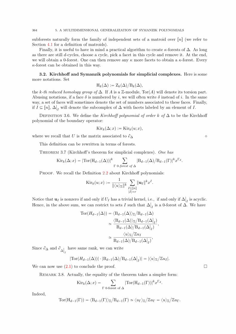
364 5. A MULTIDIMENSIONAL GENERALIZATION OF SYMANZIK POLYNOMIALS
subforests naturally form the family of independent sets of a matroid over rns (we refer toSection 4.1 for a definition of matroids).
Finally, it is useful to have in mind a practical algorithm to create κ-forests of ∆. As longas there are still d-cycles, choose a cycle, pick a facet in this cycle and remove it. At the end,we will obtain a 0-forest. One can then remove any κ more facets to obtain a κ-forest. Everyκ-forest can be obtained in this way.
3.2. Kirchhoff and Symanzik polynomials for simplicial complexes. Here is somemore notations. Set
Hkp∆q :“ Zkp∆qL
Bkp∆q,
the k-th reduced homology group of ∆. If A is a Z-module, TorpAq will denote its torsion part.Abusing notations, if a face δ is numbered by i, we will often write δ instead of i. In the sameway, a set of faces will sometimes denote the set of numbers associated to these faces. Finally,if I Ď rns, ∆
ˇ
ˇ
Iwill denote the subcomplex of ∆ with facets labeled by an element of I.
Definition 3.6. We define the Kirchhoff polynomial of order k of ∆ to be the Kirchhoffpolynomial of the boundary operator:
Kirkp∆;xq :“ Kirkpu;xq,
where we recall that U is the matrix associated to B∆ ˛
This definition can be rewritten in terms of forests.
Theorem 3.7 (Kirchhoff’s theorem for simplicial complexes). One has
Kirkp∆;xq “ |TorpHd´1p∆qq|k
ÿ
Γ 0-forest of ∆
|Bd´1p∆qL
Bd´1pΓq|kxΓd .
Proof. We recall the Definition 2.2 about Kirchhoff polynomials:
Kirkpu;xq :“1
‖xuyZ‖kÿ
IĎrns|I|“r
‖uI‖kxI .
Notice that uI is nonzero if and only if UI has a trivial kernel, i.e., if and only if ∆ˇ
ˇ
Iis acyclic.
Hence, in the above sum, we can restrict to sets I such that ∆ˇ
ˇ
Iis a 0-forest of ∆. We have
TorpHd´1p∆qq “ xBd´1p∆qyZL
Bd´1p∆q
»xBd´1p∆qyZ
L
Bd´1p∆ˇ
ˇ
Iq
Bd´1p∆qL
Bd´1p∆ˇ
ˇ
Iq,
»xuyZ
L
ZuIBd´1p∆q
L
Bd´1p∆ˇ
ˇ
Iq,
Since B∆ and B∆ˇ
ˇ
I
have same rank, we can write
|TorpHd´1p∆qq| ¨ |Bd´1p∆qL
Bd´1p∆ˇ
ˇ
Iq| “ |xuyZ
L
ZuI |.
We can now use (2.1) to conclude the proof.
Remark 3.8. Actually, the equality of the theorem takes a simpler form:
Kirkp∆;xq “ÿ
Γ 0-forest of ∆
|TorpHd´1pΓqq|kxΓd .
Indeed,TorpHd´1pΓqq “ xBd´1pΓqyZ
L
Bd´1pΓq » xuΓyZL
ZuΓ “ xuyZL
ZuΓ.
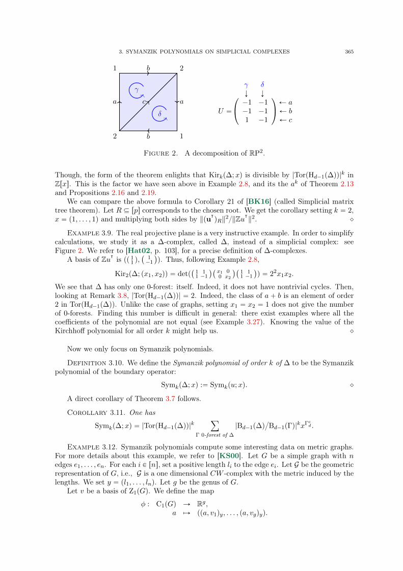
3. SYMANZIK POLYNOMIALS ON SIMPLICIAL COMPLEXES 365
a
1 b 2
a
1b2
c
δ
γγ δÓ Ó
U “
¨
˝
´1 ´1´1 ´11 ´1
˛
‚
Ð aÐ bÐ c
Figure 2. A decomposition of RP2.
Though, the form of the theorem enlights that Kirkp∆;xq is divisible by |TorpHd´1p∆qq|k in
Zrxs. This is the factor we have seen above in Example 2.8, and its the ak of Theorem 2.13and Propositions 2.16 and 2.19.
We can compare the above formula to Corollary 21 of [BK16] (called Simplicial matrixtree theorem). Let R Ď rps corresponds to the chosen root. We get the corollary setting k “ 2,x “ p1, . . . , 1q and multiplying both sides by ‖puᵀ
qR‖2‖Zuᵀ‖2. ˛
Example 3.9. The real projective plane is a very instructive example. In order to simplifycalculations, we study it as a ∆-complex, called ∆, instead of a simplicial complex: seeFigure 2. We refer to [Hat02, p. 103], for a precise definition of ∆-complexes.
A basis of Zuᵀ is pp 11 q,
`
1´1
˘
q. Thus, following Example 2.8,
Kir2p∆; px1, x2qq “ detp`
1 11 ´1
˘`
x1 00 x2
˘`
1 11 ´1
˘
q “ 22x1x2.
We see that ∆ has only one 0-forest: itself. Indeed, it does not have nontrivial cycles. Then,looking at Remark 3.8, |TorpHd´1p∆qq| “ 2. Indeed, the class of a` b is an element of order2 in TorpHd´1p∆qq. Unlike the case of graphs, setting x1 “ x2 “ 1 does not give the numberof 0-forests. Finding this number is difficult in general: there exist examples where all thecoefficients of the polynomial are not equal (see Example 3.27). Knowing the value of theKirchhoff polynomial for all order k might help us. ˛
Now we only focus on Symanzik polynomials.
Definition 3.10. We define the Symanzik polynomial of order k of ∆ to be the Symanzikpolynomial of the boundary operator:
Symkp∆;xq :“ Symkpu;xq. ˛
A direct corollary of Theorem 3.7 follows.
Corollary 3.11. One has
Symkp∆;xq “ |TorpHd´1p∆qq|k
ÿ
Γ 0-forest of ∆
|Bd´1p∆qL
Bd´1pΓq|kxΓcd .
Example 3.12. Symanzik polynomials compute some interesting data on metric graphs.For more details about this example, we refer to [KS00]. Let G be a simple graph with nedges e1, . . . , en. For each i P rns, set a positive length li to the edge ei. Let G be the geometricrepresentation of G, i.e., G is a one dimensional CW -complex with the metric induced by thelengths. We set y “ pl1, . . . , lnq. Let g be the genus of G.
Let v be a basis of Z1pGq. We define the map
φ : C1pGq Ñ Rg,a ÞÑ ppa, v1qy, . . . , pa, vgqyq.
366 5. A MULTIDIMENSIONAL GENERALIZATION OF SYMANZIK POLYNOMIALS
Actually, φ could be naturally extended to the singular 1-chains on G. We now define theJacobian torus of G to be
JacpGq :“ RgφpZ1pGqq.
The standard inner product in Rg induces an inner product on C1pGq. The latter is associatedto the symmetric matrix rY :“ Y V V
ᵀY . Thus,
(3.1) VolpJacpGqq “b
detpV ᵀrY V q “
a
detpV ᵀY V q2 “ Sym2pG, yq.
In fact, this equality holds for a deeper combinatorial reason, (cf. [KS00]). Choosing anarbitrary point p of G leads to a bijection between the set of so-called break divisors of Gand its Jacobian torus. This bijection induced a quasi-partition of the Jacobian torus intoparallelotopes labelled by spanning trees of G (see Figure 1 of [ABKS14]). The parallelotopeassociated to a spanning tree T has volume
ź
i,eiREpT q
li.
This gives another proof of the equality (3.1). ˛
In the previous example, the value of the Symanzik polynomial obtained at the end willnot change if one adds or deletes some vertices inside an edge of the metric graph. We willsee in the next subsection that this result is more general. Before that, let us define Symanzikpolynomials with parameters for simplicial complexes.
Definition 3.13. Let w be a family of size l of pd ´ 1q-boundaries of ∆. We define theSymanzik polynomial of order k of ∆ with parameters w to be the Symanzik polynomial of uwith parameters w:
Symkp∆;w;xq :“ Symkpu;w;xq. ˛
The following result is a direct corollary of both Theorem 3.7 and Proposition 2.20.
Corollary 3.14. Let w be a family of size l of pd´ 1q-boundaries. Then
Symkp∆;w;xq “ |TorpHd´1p∆qq|k
ÿ
ΓPFlp∆q
ÿ
FĎΓcdΓYFPF0p∆q
´
εΓdpF q
ˇ
ˇ
ˇ
ˇ
Bd´1p∆q
Bd´1pΓY F q
ˇ
ˇ
ˇ
ˇ
prw, eF q¯kxΓcd ,
where ε is defined before Proposition 2.20, and rw is a family of d-chains of ∆ such thatB rwj “ wj for every j P rls.
Remark 3.15. As in Example 2.21, εΓd has a geometrical meaning. For instance, if l “ 1and if Γ is a 1-forest of ∆, εΓd is one of the two opposite canonical orientations on facets δ ofΓcd such that Γ` δ is a 0-forest of ∆. These orientations are characterized by the fact that, forany two different such facets δ, δ1, any cycle of Γ` δ` δ1 will follow the orientation of exactlyone of them.
In matroid theory, such orientations are encoded by oriented matroids, or by generaliza-tions of them like R-matroids. For more details, one can consult [Piq19a] and [BB16]. ˛
3.3. Nonarchimedean height pairing. Let us introduce an interesting inner productwhich is linked to the Archimedean height pairing. Before going through this construction,let us roughly sketch this link and motivate the results of this section. For more details, thereader can compare Proposition 3.17 with Theorem 1.2 of [ABBF16]. On a smooth projectivecomplex curve X of dimension n, if b and b1 are two divisors of degree 0 with disjoint support,one can define the Archimedean height pairing
xb, b1yX :“ Re´
ż
γb
ωb1¯
,
3. SYMANZIK POLYNOMIALS ON SIMPLICIAL COMPLEXES 367
where γb is a 1-chain disjoint from the support of b1 with boundary b, and ωb1 is a canonicallogarithmic differential form with residue b1. If one considers, instead of a single curve X,a degenerating family of curves X “ pXsqs, parametrized by s and degenerating at s “ 0,and two families of divisors pbsqs‰0 and pb1sqs‰0 on it, one can wonder what is the asymptoticof xbs, b1syXs as s approaches 0. Authors of [ABBF16] proved that, under some good condi-tions, the asymptotic can be described thanks to a Symanzik rational fraction as defined inSection 2.6. More precisely, one can associate to the singular fiber X0 a dual graph G. Con-sidering G as a 1-dimensional simplicial complex, the divisors will induce some boundariesb0, b
10 P B0pGq on G. Then one can write
xbs, b1syXs “ xb0, b
10yypsq ` hpsq,
where h is a bounded function and xb0, b10yypsq is defined as below (Definition 3.16) whereypsq is a vector depending on s and whose coordinates diverge to `8, as s approaches 0.This asymptotic is strongly linked to Theorem 6.1 of Section 6. The dual graph appears inthe nonarchimedean analytification of Xs, for any s ‰ 0. Thus, one can interpret x ¨ , ¨ yyas a nonarchimedean height pairing. Moreover, as we mentioned above, this nonarchimedeanheight pairing, or more precisely the associated quadratic form, can be expressed as a Symanzikrational fraction. This is stated by Proposition 3.17.
If one replaces curves by higher dimensional projective complex manifolds, one can stilldefine an analogous of the dual graph, which will be a higher dimensional complex. One canalso define an analogous of the Archimedean height pairing. Thus, one can wonder if theasymptotic of the height pairing can be described thanks to a nonarchimedean height pairingon the dual complex as the one we define in Definition 3.16 below.
Let y be a family of n positive real numbers. We denote by Cdp∆;Rq the vector subspacexCdp∆qy. We endow Cdp∆;Rq with the inner product p¨, ¨qy and Cd´1p∆;Rq with the standardinner product p ¨ , ¨ q. This allows us to define the adjoint B˚ : Cd´1p∆;Rq Ñ Cdp∆;Rq of Baccording to these products.
Notice that ImpB˚q Ď kerpBqK and kerpB˚q “ ImpBqK. Thus, rkpB˚q ` dimpkerpBqq ďdimpCdp∆;Rqq and dimpkerpB˚qq ` rkpBq “ dimpCd´1p∆;Rqq. Using the rank-nullity theoremtwice, we deduce that the inequality must be an equality. Hence,
ImpB˚q “ Zdp∆;RqK.Let b and b1 be two pd´ 1q-boundaries. One can find a unique preimage a P Cdp∆;Rq of
b which is orthogonal to Zdp∆;Rq. The orthogonal of Zdp∆;Rq is the image of B˚. Let f beany preimage of a by B˚. Then, we have the following definition.
Definition 3.16. With the above notation, we set
xb, b1yy :“ pf, b1q. ˛
Choosing f 1 such that b1 “ BB˚f 1, one has
xb, b1yy :“ pf, BB˚f 1q “ pB˚f, B˚f 1qy.
Thus, the product is indeed well-defined, symmetric and positive-definite.
Proposition 3.17. If y is a family of n positive real numbers and if b is a pd´1q-boundaryof ∆, then
xb, byy “ĆSym2p∆; pbq; yq :“Sym2p∆; pbq; yq
Sym2p∆; yq.
Proof. Let a be the preimage of b orthogonal to Zdp∆;Rq, and let v be a basis of Zdp∆;Rq.By Propositions 2.16 and 2.19, after simplification of the factors,
Sym2p∆; pbq; yq
Sym2p∆; yq“
‖v ^ a‖2y
‖v‖2y
“ ‖a‖2y “ xb, byy.
368 5. A MULTIDIMENSIONAL GENERALIZATION OF SYMANZIK POLYNOMIALS
Remark 3.18. If rows of U are free, then the matrix corresponding to B˚ is Y ´1Uᵀ .
Therefore,
ĆSym2p∆; pbq; yq “ xb, byy “ pb, pBB˚q´1bq “ b
ᵀpUY ´1U
ᵀq´1b.
Following the proof of Proposition 3.17, one can generalize the previous formula. Let w be afamily of vectors in xuy. Then
ĆSym2p∆;w; yq “ detpWᵀpUY ´1U
ᵀq´1W q. ˛
3.4. Symanzik polynomials on triangulable topological spaces. So far, we onlydiscussed the case of discrete objects. Actually, we can define the Symanzik polynomial ofany sufficiently nice topological space endowed with a diffuse measure (see details below).This definition is consistent with above definitions when we discretize the space by taking atriangulation.
Let S be the topological space underlying a finite CW-complex of dimension d. Assumethere is some finite diffuse measure µ on S, i.e., a measure which is zero on every subsethomeomorphic to a pd´ 1q-dimensional ball. The main idea of this subsection is to introducea characteristic function of some sufficiently nice d-dimensional singular chains. For instance,if a is a function from a d-simplex to S which is a homeomorphism onto its image, one canintroduce a function ωa : S Ñ R which equals 1 on the image of a (or ´1 depending on theorientation), and 0 elsewhere. One can then introduce the canonical k-multilinear symmetricproduct for this kind of functions with respect to µ. This product will be the continuousanalogous of p ¨ , . . . , ¨ qk,y and will be sufficient to define a natural Symanzik polynomialSymkpS;µq. In the previous description a is a particular d-chain. In order to take intoaccount enough singular d-chains, we need to use the language of sheaves and of relativesingular homology.
Let Ssm be the subset of points z of S such that z has a neighborhood homeomorphicto a d-dimensional ball (thus, Ssm is a topological d-manifold). Let pC˚,singpSq, Bsingq be thecomplex of singular homology of S with coefficient in Z, as defined for example in [Hat02].Let R be the presheaf of relative homology defined by RpUq :“ Hd,singpS,SzUq for any opensubset U (we refer to [Hat02] for a definition of relative homology). We believe that R maybe a sheaf, but we have not found any proof of this in the literature. Anyway, this is notcrucial for our purpose, so we leave it as an open question for the moment. One can restrictR to Ssm to get the orientation sheaf of Ssm denoted by Rsm. Note that any stalk of Rsm
is isomorphic to Z. Though Rsm is not always isomorphic to the constant sheaf ZSsm , (forinstance Ssm could be the projective plane), we have a canonical isomorphism of sheaves (see,e.g., [KS90, Proposition 3.3.4])
Rsm bRsm – ZSsm .
Let a P Cd,singpSq be a singular d-chain of S with coefficients in Z. To a we associatethe section ωa P RpSzsupppBsingaqq where supppBsingaq is the support of the boundary of a(i.e., the union of the images of terms in Bsinga). If z P S, providing it is well-defined, wedenote by ωapzq the germ of ωa at z. By an abuse of notations, we also denote by ωa therestriction of ωa to Rsm. We denote Creg
d,singpSq the vector subspace of all a P Cd,singpSq suchthat ωa is defined µ-almost everywhere. In particular, if a P ZdpSq, then ωa is defined on S,thus a P Creg
d,singpSq.One can do the same remarks replacing Z by R. In particular, if a P Cd,singpS;Rq is a
singular d-chain with coefficients in R, one can associate to a the section
ωa P pR b RSqpSzsupppBsingaqq.
3. SYMANZIK POLYNOMIALS ON SIMPLICIAL COMPLEXES 369
We put a (positive semidefinite) multilinear inner product on Cregd,singpS;Rq: for k chains
a1, . . . , ak P Cregd,singpS;Rq,
pa1, . . . , akqk,µ :“ pωa1 , . . . , ωakqLkpµq :“
ż
Sωa1 b ¨ ¨ ¨ b ωakdµ,
where the tensor product is considered as a section of RU on some open set U of Ssm of fullmeasure. This inner product is also well-defined on Hd,singpS;Rq – pR b RSqpSq. Thus, wehave the following definition.
Definition 3.19. With the above notations, the Symanzik polynomial of S of order kwith respect to the measure µ is defined by
SymkpS;µq :“ |TorpHd´1,singpSqq|k‖v‖kk,µ,
where v is any basis of Hd,singpSq.Moreover, if w is a family of l elements of Bd´1,singpS;Rq whose supports have measure
zero, then the Symanzik polynomial of S of order k with respect to the measure µ and withparameters w is defined by
SymkpS;w;µq :“ |TorpHd´1,singpSqq|k‖v ^ rw‖kk,µ,
where rw is a family of elements of Cd,singpS;Rq such that Bsing rwj “ wj for any j P rls. ˛
Example 3.20. For example, the Symanzik polynomial of any order of a compact ori-entable manifold endowed with a volume form equals its entire volume (the torsion is trivialby the universal coefficient theorem and Poincaré duality). ˛
Let us now study triangulations. We recall that ∆ is a simplicial complex on some vertexset V . Let m :“ |∆0| be the number of vertices of ∆ and assume that V “ rms. Set
ν∆ : ∆ Ñ PpRmq,ti0, . . . , ilu ÞÑ convpei0 , . . . , eilq,
where pe1, . . . , emq is the standard basis of Rm. We denote by |∆| the standard geometricalrealization of ∆ defined by
|∆| :“ď
δP∆
ν∆pδq.
A triangulation of S consists of a simplicial complex ∆ and an application Ψ of the formΨ “ Φ ˝ ν∆ where Φ : |∆| Ñ S is a homeomorphism.
If S comes from a regular finite CW-complex, such a triangulation exists. Fix one of them:p∆,Ψq. The dimension of ∆ is also d.
Theorem 3.21. With above notations, one has
SymkpS;µq “ Symkp∆; yq,
where yδ :“ µpΨpδqq for every δ P ∆d.
Proof. The homeomorphism Ψ induces a map Ψ1 : Cdp∆q Ñ Cd,singpSq. If δ is a facetof ∆, for each z P intpΨpδqq, ωΨ1pδqpzq is a generator of the stalk of Rsm over z, and for eachz P SsmzΨpδq, ωΨ1pδqpzq “ 0. Thus, for k facets δ1 . . . , δk of ∆,
pΨ1pδ1q, . . . ,Ψ1pδkqqµ “
#
µpΨpδ1qq if δ1 “ ¨ ¨ ¨ “ δk,0 otherwise
“ pδ1, . . . , δkqy.
Moreover, it is well-known that Ψ1 induces an isomorphism Ψ˚ : Hdp∆q„ÝÑ Hd,singp∆q [Hat02,
Theorem 2.27]. Thus, Ψ˚ maps bases of Zdp∆q to bases of Hd,singpSq. If v is a basis of Zdp∆q,
370 5. A MULTIDIMENSIONAL GENERALIZATION OF SYMANZIK POLYNOMIALS
and if w is its image by Ψ1, the last equality implies that ‖w‖kk,µ “ ‖v‖kk,y. Moreover, Theorem2.27 of [Hat02] also implies
|TorpHd´1,singpSqq|k “ |TorpHd´1p∆qq|k.
We conclude by Definition 3.19, Proposition 2.16 and Remark 3.8.
Thus, the specialization of the polynomial does not depend on the triangulation. Let usstudy the abstract meaning of this fact.
3.5. Geometrical factorization of Symanzik polynomials. In this subsection, weuse Theorem 3.21 to prove that Symanzik polynomials of simplicial complexes are stable bysubtriangulation in the sense of Corollary 3.22. Moreover, we deduce a canonical factorizationof the Symanzik polynomial of a simplicial complex.
Here is a corollary of Theorem 3.21. Let ∆ be any d-dimensional simplicial complex withn facets. Let pΓ,Ψq be a triangulation of |∆|. Assume that there exists a map ϕ : Γd Ñ ∆d
such that, for any facet γ of Γ, Ψpγq Ď ν∆pϕpγqq. In this case, we call pΓ,Ψq a subtriangulationof ∆. Set n1 :“ |Γd|.
Corollary 3.22. Let x1 be a family of n1 variables. For δ P ∆d, let
xδ :“ÿ
γPϕ´1pδq
x1γ .
ThenSymkpΓ;x1q “ Symkp∆;xq.
Proof. Let y1 be a family of n1 positive real numbers. It is not hard to create a finitediffuse measure µ on |∆| such that µpΨpγqq “ y1γ for every γ P Γd. Thus, considering p∆, ν∆q
as a second triangulation of |∆|, Theorem 3.21 implies
SymkpΓ; y1q “ Symkp∆; yq,
where, for δ P ∆d,yδ “
ÿ
γPϕ´1pδq
y1γ .
As this is true for any family y1 of positive numbers, the equality holds in Zrx1s.
One can go further in the factorization. Let us use notations of the last subsection. Wesay that two points z, z1 P Ssm are equivalent if, for every c P Hd,singpSq, ωcpzq is zero if andonly if ωcpz1q is zero. In particular, all points of a connected component of Ssm are equivalent.Equivalent classes form a partition Ssm
1 , . . . ,Ssml of Ssm (notice that some Ssm
j could containseveral connected components: see Example 3.26). In what follows, we do not consider thepossible class of points z belonging to no cycle, i.e., such that ωcpzq “ 0 for every cycle c.Let j P rls, zj P Ssm
j and cj P Hd,singpSq be such that |ωcj pzq| P Z` is nonzero and minimal.Finally, let τj P RsmpSsmq be zero on pSsm
j qc and equal to ωcj
ˇ
ˇ
Ssmj
on Ssmj .
Proposition 3.23. With above notations, τj does not depend on zj nor cj. Moreover,there exists a polynomial PS P ZrT1, . . . , Tls such that, for every finite diffuse measure µ on S,
SymkpS;µq “ PSp‖τ1‖kLkpµq, . . . , ‖τl‖kLkpµqq.
Proof. Let v be a basis of Hd,singpSq. Let n be the size of v. The Symanzik polyno-mial equals P1ppvi1 , . . . , vikqk,µqi1,...,ikPrns, where P1 is the integer polynomial on nk variablescorresponding to TorpHd´1,singpSqqk ¨ det.
3. SYMANZIK POLYNOMIALS ON SIMPLICIAL COMPLEXES 371
Let c P Hd,singpSq. Then
(3.2) ωc “lÿ
j“1
ωcpzjq
τjpzjqτj .
Indeed, for the sake of a contradiction, assume there exists z P Ssm such that ωcpzq ‰ ω1cpzq,where ω1c denote the right-hand side. Let j P rls be such that z P Ssm
j . Then the cycle
c1 :“ωcpzjq
τjpzjqcj ´ c
verifies ωc1pzjq “ 0, but ωc1pzq “ ω1cpzq ´ ωcpzq ‰ 0. This is absurd since z and zj areequivalent.
In particular, if z P Ssmj , then
ωcpzq
τjpzq“ωcpzjq
τjpzjq.
This implies that τj does not depend on zj and cj .Notice that the ratios in (3.2) are integers by the minimality condition on cj . Rewriting
the elements of v in terms of the τj , we get that the Symanzik polynomial equals
P2ppτj1 , . . . , τjkqk,µqj1,...,jkPrls
for some integer polynomial P2. But clearly, if j1, . . . , jk P rls, then
pτj1 , . . . , τjkqk,µ “
#
‖τj1‖kLkpµq if j1 “ ¨ ¨ ¨ “ jk,
0 otherwise.
Finally, there exists PS P ZrT1, . . . , Tls such that
SymkpS;µq “ PSp‖τ1‖kLkpµq, . . . , ‖τl‖kLkpµqq.
Now suppose that S “ |∆| for some simplicial complex ∆. For every δ P ∆d, intpν∆pδqq isincluded in a connected component of Ssm, thus, in a Ssm
j for some j P rls. We pick a pointzδ in the interior of ν∆pδq for every facet δ P ∆d. Then we set, for j P rls,
Qjpxq “ÿ
δP∆d
pτjpzδqqbkxδ.
Using the argument we used to deduce Corollary 3.22 from Theorem 3.21, we infer the followingcorollary from Proposition 3.23.
Corollary 3.24. With above notations,
Sym2p∆;xq “ P|∆|pQ1pxq, . . . , Qlpxqq.
Example 3.25. For example, if ∆ is the bipyramid (Figure 1), |∆| has three equivalenceclasses: the equatorial plane and both pyramids. The corresponding factorized polynomial is
Symkp∆;xq “ px1 ` x2 ` x3qx4 ` px1 ` x2 ` x3qpx5 ` x6 ` x7q ` x4px5 ` x6 ` x7q. ˛
Example 3.26. Let S be the following ∆-complex. We take two copies of Figure 2 andwe identify the four edges labeled by a, and the four edges labeled by b. Then Ssm has twoconnected components: the interiors of each copy. But it has only one equivalent class becauserkpZ2pSqq “ 1. ˛
Example 3.27. For any U P Mp,lpZq, it is not hard to create a regular CW-complex S(of dimension 2) such that U is the matrix associated to the cellular boundary operator ofS. Thus, triangulating S, there is a simplicial complex ∆ and a factorization of Sym2p∆;xqof the form detpUX 1U
ᵀq. Hence, one can somehow obtain any possible Symanzik polynomial
from simplicial complexes. ˛
372 5. A MULTIDIMENSIONAL GENERALIZATION OF SYMANZIK POLYNOMIALS
3.6. Symanzik polynomials with parameters and geometry. We have seen a ge-ometrical interpretation of Symanzik polynomials. In this subsection, we tackle the case ofSymanzik polynomials with parameters. We will see in Section 4 that adding a parameter cor-responds to doing a matroidal contraction. However, this matroidal contraction has, a priori,no concrete geometrical interpretation in general. Nevertheless, in this subsection, we showthat, in some simple cases, adding a parameter is equivalent to doing a topological contraction,and we give insight on how to deal with the parameters geometrically for more complex cases.
Recall that ∆ is a simplicial complex of dimension d. Let a be a pd ´ 1q-chain of ∆.If δ P ∆d´1, then rδsa P Z will denote the coefficient of δ in a. The support of a, denotedby supppaq, is the set of pd ´ 1q-faces associated to a nonzero coefficient in a. One can see∆ as a CW-complex. Then, ∆
L
supppaq denotes the CW-complex obtained as the result ofcontracting elements in supppaq (see the following example).
Example 3.28. The cellular homology of ∆L
supppaq is naturally isomorphic to the rel-ative simplicial homology H˚p∆,∆
ˇ
ˇ
supppaqq (see [Hat02]). For instance, Cd´1p∆
L
supppaqq “
Cd´1p∆qL
Zxsupppaqy. If U is the d-th incidence matrix of ∆, then the d-th incidence matrixof ∆
L
supppaq is obtained by removing rows of U corresponding to elements of supppaq. Hencewe can still define the Symanzik polynomial of ∆
L
supppaq.In fact, if p∆,Ψq is the triangulation of some CW-complex S, and if µ is some diffuse finite
measure on S, then
Sym2p∆L
supppaq; yq “ Sym2pSL
ď
αPsupppaq
Ψpαq; rµq,
where, for δ P ∆d, yδ “ µpΨpδqq, the quotient on the right-hand side is the topologicalcontraction, and rµ is the induced measure on the contracted space. ˛
Definition 3.29. Let b P Bd´1p∆q be a nonzero boundary. Then b is a simple boundaryof ∆ if it is a generator of Zxsupppbqy X Bd´1p∆q.
Let b, b1 P Bd´1p∆q be two boundaries. Then they are called cosimple boundaries if theyare simple and if they form an independent family of maximal rank of ZxsupppbqY supppb1qyXBd´1p∆q. In this case, we define:
θb,b1 :“‖Zpb, b1q‖
‖Zxsupppbq Y supppb1qy X Bd´1p∆q‖.
˛
Proposition 3.30. For any pd´ 1q-boundary b P Bd´1p∆;Rq with real coefficients, thereexist simple boundaries b1, . . . , bl, pairwise cosimple, and real numbers λ1, . . . , λl such that
b “ λ1b1 ` ¨ ¨ ¨ ` λlbl.
Proof. Let D be a maximal subset of supppbq such that rkpZdp∆L
Dqq “ rkpZdp∆qq. Letδ P supppbqzD. Then Zdp∆pD`δqq
L
Zdp∆q has rank 1. Let raδ be a generator of this quotient.Let aδ P Cdp∆q be a representative of raδ. Let bδ be its boundary. One can easily check thatpbδqδPsupppbqzD forms a family of simple and pairwise cosimple boundaries, and that
b “ÿ
δPsupppbqzD
rδsb
rδsbδbδ.
Remark 3.31. Let b, b1 be cosimple boundaries of ∆ and let a, a1 be d-chains such thatBa “ b and Ba1 “ b1. Let v be a basis of Zdp∆q. Then, v ‹ paq is a basis of Zdp∆
L
supppbqq,and that v ‹ pa, a1q is a basis of the vector subspace xZdp∆
L
psupppbq Y supppb1qqqy. Thus, byPropositions 2.16, 2.19 and Remark 3.8,
Symkp∆;xq “ TorpHd´1p∆qqk‖v‖kk,x,
3. SYMANZIK POLYNOMIALS ON SIMPLICIAL COMPLEXES 373
Symkp∆; pbq;xq “ TorpHd´1p∆qqk‖v ^ a‖kk,x,
Symkp∆L
supppbq;xq “ TorpHd´1p∆L
supppbqqqk‖v ^ a‖kk,x,
Symkp∆; pb, b1q;xq “ TorpHd´1p∆qqk‖v ^ a^ a1‖kk,x,
Symkp∆L
psupppbq Y supppb1qq;xq “Tor
`
Hd´1p∆L
psupppbq Y supppb1qqq˘k
θkb,b1‖v ^ a^ a1‖kk,x.
The last denominator comes from the following diagram:
0 xvyZ xv ‹ pa, a1qyZ Zxsupppbq Y supppb1qy X Bd´1p∆q 0
0 Zv Zpv ‹ pa, a1qq Zpb, b1q 0
„
B
ĎB
Ď
Thus, adding a parameter which is a simple boundary is equivalent to contracting topo-logically the support of this boundary, up to a factor. This is still true for two parameterswhich are cosimple. ˛
Let y be a family of n variables and b, b1 P Bd´1p∆;Rq. We recall from Section 3.3 that
xb, b1yy “ ph, h1qy,
where h, resp. h1, is the unique preimage of b, resp. b1, by B that is orthogonal to Zdp∆;Rq forthe scalar product p ¨ , ¨ qy.
Thanks to Proposition 3.30 and to Remark 3.31, the following proposition allows us todeal with more complex cases for order 2.
Proposition 3.32. Let y be a family of n positive real numbers. If v is a basis of Zdp∆qand if a1, . . . , al are some d-chains of ∆ with real coefficients, then
‖v ^ pa1 ` ¨ ¨ ¨ ` alq‖2y “
lÿ
i“1
‖v ^ ai‖2y ` 2‖v‖2
y
ÿ
1ďiăjďl
xBai, Bajyy and
‖v‖2yxBai, Bajyy “ signpxBai, Bajyyq
b
‖v ^ ai‖2y‖v ^ aj‖2
y ´ ‖v‖2y‖v ^ ai ^ aj‖2
y.
Proof. Let π be the orthogonal projection onto xvy “ Zdp∆,Rq for the scalar productp ¨ , ¨ qy. For each i P rns, let hi :“ ai ´ πpaiq. Then,
‖v ^ pa1 ` ¨ ¨ ¨ ` alq‖2y “ ‖v‖2
y‖h1 ` ¨ ¨ ¨ ` hl‖2y “ ‖v‖2
y
lÿ
i“1
‖hi‖2y ` 2‖v‖2
y
ÿ
1ďiăjďl
phi, hjqy.
We have phi, hjqy “ xBai, Bajyy. Moreover one can factorize ‖v‖y‖hi‖y into ‖v ^ ai‖y. Thefollowing calculation gives us the second part of the proposition:
‖v ^ ai ^ aj‖2y “ ‖v‖2
y‖hi ^ hj‖2y “ ‖v‖2
y
`
‖hi‖2y‖hj‖2
y ´ phi, hjq2y
˘
.
Remark 3.33. Notice that
P pyq :“ ‖v‖2yxBai, Bajyy “ pv ^ ai,v ^ ajqy
is a polynomial in y. More precisely, it is one of the two square roots of the polynomial‖v ^ ai‖2
y‖v ^ aj‖2y ´ ‖v‖2
y‖v ^ ai ^ aj‖2y. Let J Ď rns and αJ P R˚ be such that αJyJ
c is anonzero monomial of P pyq. It is enough to find the sign of αJ to infer which square root isP pyq. The set J corresponds to a 1-forest of ∆. Let δ P Jc be a facet such that Γ :“ ∆
ˇ
ˇ
J`δis
a 0-forest of ∆. Then let a1i, a1j P CdpΓ;Rq be such that Ba1i “ Bai and Ba
1j “ Baj . Then,
P pyq “ pv ^ a1i,v ^ a1jqy, and
αJ “ pv ^ a1i, eJcqpv ^ a
1j , eJcq “ p˘detpVIcqrδsa
1iqp˘detpVIcqrδsa
1jq,
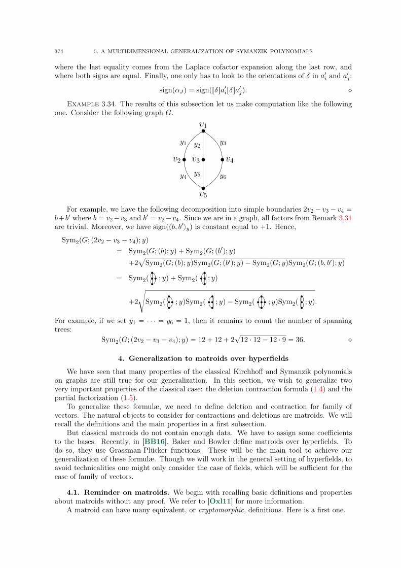
374 5. A MULTIDIMENSIONAL GENERALIZATION OF SYMANZIK POLYNOMIALS
where the last equality comes from the Laplace cofactor expansion along the last row, andwhere both signs are equal. Finally, one only has to look to the orientations of δ in a1i and a
1j :
signpαJq “ signprδsa1irδsa1jq. ˛
Example 3.34. The results of this subsection let us make computation like the followingone. Consider the following graph G.
‚v1
‚v2 ‚v3 ‚v4
‚v5
y1
y4
y2
y5
y3
y6
For example, we have the following decomposition into simple boundaries 2v2´ v3´ v4 “
b`b1 where b “ v2´v3 and b1 “ v2´v4. Since we are in a graph, all factors from Remark 3.31are trivial. Moreover, we have signpxb, b1yyq is constant equal to `1. Hence,
Sym2pG; p2v2 ´ v3 ´ v4q; yq
“ Sym2pG; pbq; yq ` Sym2pG; pb1q; yq
`2a
Sym2pG; pbq; yqSym2pG; pb1q; yq ´ Sym2pG; yqSym2pG; pb, b1q; yq
“ Sym2p‚
‚
‚‚ ; yq ` Sym2p‚
‚
‚‚ ; yq
`2
d
Sym2p‚
‚
‚‚ ; yqSym2p‚
‚
‚‚ ; yq ´ Sym2p‚
‚
‚‚‚ ; yqSym2p‚
‚
‚ ; yq.
For example, if we set y1 “ ¨ ¨ ¨ “ y6 “ 1, then it remains to count the number of spanningtrees:
Sym2pG; p2v2 ´ v3 ´ v4q; yq “ 12` 12` 2?
12 ¨ 12´ 12 ¨ 9 “ 36. ˛
4. Generalization to matroids over hyperfields
We have seen that many properties of the classical Kirchhoff and Symanzik polynomialson graphs are still true for our generalization. In this section, we wish to generalize twovery important properties of the classical case: the deletion contraction formula (1.4) and thepartial factorization (1.5).
To generalize these formulæ, we need to define deletion and contraction for family ofvectors. The natural objects to consider for contractions and deletions are matroids. We willrecall the definitions and the main properties in a first subsection.
But classical matroids do not contain enough data. We have to assign some coefficientsto the bases. Recently, in [BB16], Baker and Bowler define matroids over hyperfields. Todo so, they use Grassman-Plücker functions. These will be the main tool to achieve ourgeneralization of these formulæ. Though we will work in the general setting of hyperfields, toavoid technicalities one might only consider the case of fields, which will be sufficient for thecase of family of vectors.
4.1. Reminder on matroids. We begin with recalling basic definitions and propertiesabout matroids without any proof. We refer to [Oxl11] for more information.
A matroid can have many equivalent, or cryptomorphic, definitions. Here is a first one.
4. GENERALIZATION TO MATROIDS OVER HYPERFIELDS 375
Definition 4.1. A matroid M is a pair which consists of a ground set E, which canbe any finite set, and a family of independent sets I, which is a subset of PpEq. We writeM “ pE,Iq. A matroid has to verify three axioms:
(1) H P I,(2) (hereditary property) I is stable by inclusion (J Ď I P Iñ J P I),(3) (augmentation property) if I, J P I and if |J | ă |I|, then there exists i P IzJ such
that J ` i P I. ˛
One could think of E as a set of vectors generating some vector space, and I as the set offree subfamilies of E (though, there are matroids which have not such a representation).
Let M “ pE,Iq be a matroid. If I Ď E, we define the rank of I by
rkpIq :“ maxJPPpIqXI
|J |.
The rank of M is the rank of E. We call the closure of I the set
clpIq :“ ti P Eˇ
ˇ rkpI Y tiuq “ rkpIqu Ď E.
This is a closure operator: it is extensive, increasing and idempotent.A basis is an independent set maximal for the inclusion. The set of all bases is denoted by
BpMq. If l is a nonnegative integer, the set of all independents of rank l is denoted by Il. Notethat we have, BpMq “ IrkpMq and that, for a given ground set E, a matroid is characterized byits bases. The bases verify the following exchange property : if B1, B2 are two different bases,then for any i P B1zB2, there exists j P B2zB1 such that B1 ´ i ` j (i.e., B1ztiu Y tju) is abasis.
An element e P E is said to be:— a loop if teu R I,— free if it is in every basis, and— proper otherwise.
Let I be a subset of E. One can delete I from M to get a new matroid denoted by MzIand defined by
MzI :“ pEzI, IX PpEzIqq.We also define the restriction of M to I by M|I :“MzIc.
One can also contract I in M to get a new matroid denoted by MI and defined by
MI :“ pEzI, I1q,
where
I1 “ tJ Ď EzIˇ
ˇ DB P BpM|Iq, J YB P Iu“ tJ Ď EzI
ˇ
ˇ@B P BpM|Iq, J YB P Iu.Concerning the bases, we have the following characterizations:
BpM|Iq “ tB X Iˇ
ˇB P BpMq and |B X I| is maximalu, and
BpMIq “ tB X Icˇ
ˇB P BpMq and |B X Ic| is minimalu.(4.1)
Moreover, if I Ď E and B Ď E, any two of the following statements imply the third one.$
’
&
’
%
‚ B X I P BpM|Iq,‚ B X Ic P BpMIq,‚ B P BpMq.
(4.2)
From (4.1) and (4.2), we deduce the following equivalence.
(4.3) B P BpMq and |B X I| “ rkpIq ðñ B X I P BpM|Iq and B X Ic P BpMIq.
376 5. A MULTIDIMENSIONAL GENERALIZATION OF SYMANZIK POLYNOMIALS
The dual of the matroid M will be denoted by xM and is defined by
BpxMq “ tBcˇ
ˇB P BpMqu.
This is a duality in the sense that we have x
xM “M. Moreover, zMzI “ xMI.
4.2. Kirchhoff and Symanzik polynomials of a matroid. Let n be a positive integer,E :“ rns be a finite set and M “ pE,Iq be a matroid of rank r.
If u “ pu1, . . . , unq is a family of elements of a Z-module, we denote by Mu “ pEu, Iuq,with Eu “ rns and
Iu “ tI Ď Eˇ
ˇuI is freeu,
the matroid representing the family u.Here is the definition of Kirchhoff and Symanzik polynomials of a matroid.
Definition 4.2. The Kirchhoff polynomial (of order 0) of the matroid M with variablesx1, . . . , xn is defined by
Kir0pM;xq “ÿ
IPBpMqxI .
The Symanzik polynomial (of order 0) of the matroid M with variables x1, . . . , xn is definedby
Sym0pM;xq “ÿ
IPBpxMq
xI . ˛
This definition is natural because of the following claim, whose proof is straightforward.
Claim 4.3. Let u be a family of n elements in Zp. Then
Kir0pu;xq “ Kir0pMu;xq,
Sym0pu;xq “ Sym0pMu;xq.
The analogous for matroids of the duality Theorem 2.13 is given by the following claim,which is a direct corollary of Claim 4.3 and of Theorem 2.13 for k “ 0.
Claim 4.4. Let q be a positive integer and v be a family of n vectors in Zq such that vᵀ
spans kerpUq, then Mu “ xMv.
Next proposition shows that parameters of Symanzik polynomials correspond to a so-calledquotient of the matroid.
If w is a family of elements of xuy, then Mu‹w is an extension of Mu, i.e., we have Mu
equals Mu‹w|rns.
Proposition 4.5. Let w consist of independent elements of xuy. Then
Sym0pu;w;xq “ Sym0pMu‹wrn` 1 . .n` ls;xq.
Proof. Looking at Definition 2.17, the left-hand side is the sum of xIc over all I Ď rnsof size r ´ l such that uI ‹w is an independent family. But such sets I exactly correspond tothe bases of the matroid Mu‹wrn` 1 . .n` ls. Thus, Definition 4.2 ends the proof.
Remark 4.6. In particular, if I Ď rns is of size r ´ l, then xIc appears with a nonzero
coefficient in Symkpu;w;xq only if I is in Iu. Therefore, if Symkpu;w;xq “ ‖rvᵀ‖kk,x for somefamily rv, then detprVIcq ‰ 0 implies that I P pIuqr´l. This implication is an equivalence in thecase l “ 0. ˛
In the next subsection, we generalize the definitions to higher orders.
4. GENERALIZATION TO MATROIDS OVER HYPERFIELDS 377
4.3. Grassman-Plücker functions. In this subsection we introduce the main tool towork with orders higher than 0. We will work with hyperfields, which are similar to fieldsexcept that the operation of addition is multivalued. We will quickly reproduce the ax-ioms from [BB16] below and refer for more information and examples to the literature (see,e.g., [BB16,BL21]). However, if the reader prefers, it is possible to think of F as a field (inthis case, « Q 0 » have to be replaced by « “ 0 »).
In a hyperfield F, the addition is a hyperoperation, i.e., a map ‘ : Fˆ FÑ PpFqztHu. IfA,B Ď F, we define
A‘B :“ď
aPAbPB
a‘ b.
We require ‘ to be associative: pa‘ bq‘ c “ a‘ pb‘ cq for every a, b, c P F.A commutative hypergroup is a tuple pG,‘, 0q, where ‘ is a commutative and associative
hyperoperation on G such that:— 0 ‘ x “ txu for every x P G,— for every x P G, there is a unique element ´x P G such that 0 P x‘´x,— x P y ‘ z if and only if z P x‘´y.
A hyperfield is a tuple pF, ¨ ,‘, 1, 0q with 0 ‰ 1 such that:— pFzt0u, ¨ , 1q is a commutative group,— pF,‘, 0q is a commutative hypergroup,— 0 ¨ x “ x ¨ 0 “ 0 for every x P F,— a ¨ px‘ yq “ pa ¨ xq‘ pa ¨ yq for all a, x, y P F.
Let n be a positive integer and E :“ rns be a finite set. A Grassman-Plücker function overF of rank r is a function ϕ : Er Ñ F such that
— ϕ is not identically zero,— (alternating) for any I “ pi1, . . . , irq P Er and for any two different indices `,m,
ϕpi1, . . . , i`, . . . , im, . . . , irq “ ´ϕpi1, . . . , im, . . . , i`, . . . , irq,
and ϕpi1, . . . , i`, . . . , im, . . . , irq “ 0 if i` “ im,— (Grassman-Plücker relations) for any I “ pi1, . . . , irq, J “ pj1, . . . , jrq P Er and any
` P rrs,r
‘m“1
ϕpi1, . . . , im´1, j`, im`1, . . . , irqϕpj1, . . . , j`´1, im, j``1, . . . , jrq‘´ϕpIqϕpJq Q 0.
Recall that, if I “ ti1, . . . , ilu Ď E with i1 ă ¨ ¨ ¨ ă il, then we also denote by I thel-tuple pi1, . . . , ilq P El. We this convention, a Grassman-Plücker function ϕ of rank r inducesa function on the subsets of E of size r. Moreover, since ϕ is alternating, ϕ is characterizedby its value on the subsets of E of size r.
Let ϕ be a Grassman-Plücker function over F of rank r . Then one can verify that the set
tI Ď Eˇ
ˇ |I| “ r and ϕpIq ‰ 0u
is the set of bases of some matroid over the ground set E. We call this matroid the underlyingmatroid of ϕ and denote it by Mϕ.
For example, if u “ pu1, . . . , unq is a family of elements of Zp of rank r, we define
ϕu : Er Ñ R,I ÞÑ detpVIq,
where V is defined as in Equation (2.1). Then ϕu is a Grassman-Plücker function and itsunderlying matroid is Mu, as defined in the previous subsection.
Here is the main definition of this section.

378 5. A MULTIDIMENSIONAL GENERALIZATION OF SYMANZIK POLYNOMIALS
Definition 4.7. Let F be a hyperfield and let ϕ be a Grassman-Plücker function over F.Let M be its underlying matroid. Then we define
Kirkpϕ;xq :“ÿ
IPBpMqϕpIqkxI ,
Symkpϕ;xq :“ÿ
IPBpMqϕpIqkxI
c. ˛
Note that this definition is compatible with Section 2, i.e.,
Kirkpϕu;xq “ Kirkpu;xq and Symkpϕu;xq “ Symkpu;xq.
Remark 4.8. In order to take into account complex matroids (i.e., matroids over thephase hyperfield, cf. [AD12,BB16]), one may want to consider an involution ϕ ÞÑ ϕ. In thiscase, ϕ must be replaced by ϕ in the definition of the Symanzik polynomials. ˛
Remark 4.9. One has to be careful with polynomials with coefficients in a hyperfield.Several definitions are possible (cf. [BL18, Appendix A]). However, in this article, everypolynomials over hyperfields will be of the form
P pxq “ÿ
IĎE
pIxI
with coefficients pI in F (and not a subset of F nor a sum of elements in F). In particular,if P pxq “
ř
I pIxI and Qpxq “
ř
I qIxI , we will only add P and Q if, for any I, pI “ 0 or
qI “ 0. In the same way, we will only multiply P and Q if for any I and J such that pI ‰ 0and qJ ‰ 0, their intersection I X J is empty. ˛
We now explain how to extend deletion, contraction and duality. Let ϕ be a Grassman-Plücker function of rank r over F and let M be its underlying matroid. For any subset I Ď E,we choose a basis BϕI P BpM|Iq, and a basis BϕzI P BpMIcq.
Following [BB16], we define ϕzI : pEzIqrkpMzIq Ñ F by
pϕzIqpJq “ ϕpJ ‹BϕzIq.
We also define the restriction: ϕ|I :“ ϕzIc. Similarly, we define ϕI : pEzIqrkpMIq Ñ F by
pϕIqpJq “ ϕpJ ‹BϕIq.
If I 1 Ď E is disjoint from I, we set
pϕI 1zIqpJq “ ϕpJ ‹BϕI 1 ‹BϕzIq.
We define pϕ : En´rkpMq Ñ F to be the unique Grassman-Plücker function such that, for anysubset J of E of size n´ rkpMq,
pϕpJq “ σpJ ‹ JcqϕpJcq,
where σpJ ‹ Jcq denotes the signature of the permutation J ‹ Jc. Moreover, we choose
BpϕzI :“ IzBϕI and B
pϕI :“ IzBϕzI .
As stated in [BB16], the four new functions are Grassman-Plücker functions, and theunderlying matroids are respectively MzI, MI, MI 1zI and xM. Moreover, the functionsare independent of the chosen bases up to a nonzero factor (up to a sign for pϕ). We alsokeep the usual rules p
pϕ “ p´1qrpn´rqϕ and yϕI “ ˘pϕzI. Article [BB16] refers to anotherarticle, [AD12], for the proofs. The latter proves the results in the special case of complexmatroids. For the sake of completeness, we provide a proof in full generality.
4. GENERALIZATION TO MATROIDS OVER HYPERFIELDS 379
Proof. Many points are easy to check. We will only check the Grassman-Plücker rela-tions, the independency up to a factor, and the formula yϕI “ ˘pϕzI.
First, we prove the Grassman-Plücker relations for the contraction or the deletion of oneelement. For some cases, for example the case of the contraction of a loop, there is nothingto prove. Otherwise, for any e P E, I “ pi1, . . . , ir´1q P E
r´1, J “ pj1, . . . , jr´1q P Er´1 and
` P rr ´ 1s,
r´1
‘m“1
ϕpi1, . . . , im´1, j`, im`1, . . . , ir´1, eqϕpj1, . . . , j`´1, im, j``1, . . . , jr´1, eq
‘ ϕpi1, . . . , ir´1, j`qϕpj1, . . . , j`´1, e, j``1, . . . , jr´1, eq‘´ϕpI ‹ peqqϕpJ ‹ peqq Q 0.
Sinceϕpj1, . . . , j`´1, e, j``1, . . . , jr´1, eq “ 0,
we get the Grassman-Plücker relation for ϕzteu and for ϕteu. The Grassman-Plücker relationsfor a general ϕzI follow easily by induction using that
ϕzI “ ϕzBϕzI
“ p. . . ppϕztbsuqztbs´1uq . . . qztb1u,
where BϕzI “ pb1, . . . , bsq. A similar argument works for ϕI and ϕI 1zI.
For the independency, let us first do a simple case. Let e, e1 P E be two parallel elementsand let J, J 1 Ď E of size r´1. Applying the Grassman-Plücker function to J ‹ peq and J 1 ‹ pe1qfor ` “ r, most of the terms will be zero because
ϕp. . . , e1, . . . , eq “ 0.
Then, we will get
(4.4) ϕpJ ‹ pe1qqϕpJ 1 ‹ peqq “ ϕpJ ‹ peqqϕpJ 1 ‹ pe1qq.
Let I Ď E. Let J, J 1 Ď I of size rkpIq and K,K 1 Ď Ic of size r ´ rkpIq. Let us prove that
(4.5) ϕpJ ‹KqϕpJ 1 ‹K 1q “ ϕpJ 1 ‹KqϕpJ ‹K 1q.
First, by (4.3), ϕpJ ‹Kq is nonzero if and only if J P BpM|Iq and K P BpMIq. Thus, eitherJ, J 1 P BpM|Iq and K,K 1 P BpMIq, and then both members of (4.5) are nonzero, or bothmembers are zero, and then (4.5) is verified. In the first case, assume that J ‰ J 1. By thebasis exchange property, one can find e P J and e1 P J 1 such that e ‰ e1 and J1 :“ J ´ e` e1
is a basis of M|I. In M|IpJ ´ eq “ MpJ ´ eq|I, elements e and e1 are parallel. Thus, theyare parallel in MpJ ´ eq. Hence, using Formula (4.4) for ϕpJ ´ eq, we get
pϕpJ´eqqpK ‹ peqq pϕpJ´eqqpK 1 ‹ pe1qq “ pϕpJ´eqqpK 1 ‹ peqq pϕpJ´eqqpK ‹ pe1qq.
Being careful with signs, we deduce
ϕpK ‹ JqϕpK 1 ‹ J1q “ ϕpK 1 ‹ JqϕpK ‹ J1q, thusϕpK ‹ Jq
ϕpK 1 ‹ Jq“ϕpK ‹ J1q
ϕpK 1 ‹ J1q.
Using |J 1zJ | times the basis exchange property, we getϕpK ‹ Jq
ϕpK 1 ‹ Jq“ϕpK ‹ J 1q
ϕpK 1 ‹ J 1q,
which completes the proof of (4.5). As a direct consequence, we get the independency up toa factor of ϕI and ϕ|I.
It remains to prove that, if J Ď Ic is of size rkppϕzIq, then
pyϕIqpJq “ ˘ppϕzIqpJq.
380 5. A MULTIDIMENSIONAL GENERALIZATION OF SYMANZIK POLYNOMIALS
Then, recalling that we chose BpϕzI “ IzBϕI , we get
ppϕzIqpJq “ pϕpJ ‹BpϕzIq
“ ˘ϕppIczJq ‹BϕIq
“ ˘pϕIqpIczJq
“ ˘pyϕIqpJq.
We now explain how to generalize Symanzik polynomials with parameters. Let ϕ1 be aGrassman-Plücker function on some set E YW with W a finite set disjoint from E. Assumethat W is independent in Mϕ1 . Suppose that ϕ “ ϕ1zW and notice that there is only one wayto define ϕ1zW . We call ϕ1W the quotient of ϕ by W. It is uniquely defined. Then we define
Symkpϕ;W ;xq :“ Symkpϕ1W ;xq.
Once more, this extends Definition 2.17.
4.4. Deletion-contraction formula. Thanks to the definitions of last subsections, wecan state the generalization of the deletion-contraction formula (cf. Equation (1.4) in theintroduction). From those definitions, the following result is immediate.
Proposition 4.10 (Deletion-contraction formula). Let e P E. We set
N1peq :“
#
0 if e is a loop in M,xe otherwise,
and N2peq :“
#
0 if e is free in M,1 otherwise.
Then,Kirkpϕ;xq “ N1peqKirkpϕteu;xE´eq `N2peqKirkpϕzteu;xE´eq.
Moreover, setting
xN1peq :“
#
0 if e is a loop in M,1 otherwise,
and xN2peq :“
#
0 if e is free in M,xe otherwise,
we haveSymkpϕ;xq “ xN1peqSymkpϕteu;xE´eq `xN2peqSymkpϕzteu;xE´eq.
The notations of the previous proposition follows those of [DFM18]. This article describesUniversal Tutte characters which unify objects behaving like Tutte polynomials. By thefollowing proposition, we show that the polynomials Kirk and Symk belong to this big family.In particular, we have the following formulæ.
Proposition 4.11. Let I Ď E. We extend N1 and N2 by
N1pϕ|Iq “
#
0 if M|I is not the free matroid,ś
iPI xi otherwise,N2pϕIq “
#
0 if rkpIq ą 0,1 otherwise.
Then,Kirkpϕ;xq “
ÿ
IĎE
N1pϕ|Iqτpϕ|IIqN2pϕIq,
where, denoting by ∅ the 0-tuple,
τpϕ|IIq :“ pϕ|IIqp∅qk.
Moreover,
xN1pϕ|Iq “
#
0 if M|I is not the free matroid,1 otherwise,
xN2pϕIq “
#
0 if rkpIq ą 0,ś
iPIc xi otherwise,

4. GENERALIZATION TO MATROIDS OVER HYPERFIELDS 381
we haveSymkpϕ;xq “
ÿ
IĎE
xN1pϕ|Iqτpϕ|IIqxN2pϕIq.
One might have noticed that xN2 in Proposition 4.11 is not an extension of xN2 in Propo-sition 4.10. Actually, xN2peq must be understood as xN2pϕteu
cq (cf. [DFM18]).To understand why this last proposition holds, notice that a term of the right-hand side
sum is zero if I is not a basis of M. If I is a basis, then, for the Kirchhoff polynomial forinstance, we have
N1pϕ|Iqτpϕ|IIqN2pϕIq “ź
iPI
xi ¨ pϕ|IIqp∅qk.
Since I is a basis, Bϕ|I “ ∅ and BϕI “ I. Thus,
ϕ|IIp∅q “ ϕpIq.
Remark 4.12. Following this idea, one might define the Tutte polynomial of ϕ byÿ
IĎE
px´ 1qrkpEq´rkpIqpy ´ 1q|I|´rkpIqϕ|IIp∅qk.
Unfortunately, this formula strongly depends on the bases of Bϕ|I and BϕI (unless for termswhere I is a basis). ˛
4.5. Partial factorization. Let us conclude this section by a generalization of the usefulformula of partial factorization (cf. Equation (1.5) in the introduction).
LetP pxq “
ÿ
J
pJxJ
be a multivariate polynomial. Let I be a subset of rns. We define the set of the degrees of themonomials of P with respect to the variables xI as
degsxI pP pxqq :“ t|J X I|ˇ
ˇ pJ ‰ 0u.
Here is the generalization of the formula.
Proposition 4.13. Let I Ď E. Then
Kirkpϕ;xq “1
ϕ|IIp∅qkKirkpϕ|I;xIqKirkpϕI;xIcq `Rϕ,Ipxq
for some polynomial Rϕ,Ipxq verifying
max degsxI pRϕ,Ipxqq ă degpKirkpϕ|I;xIqq “ rkpIq,
min degsxIc pRϕ,Ipxqq ą degpKirkpϕI;xIcqq “ rkpMIq.
Similarly,
Symkpϕ;xq “1
ϕ|IIp∅qkSymkpϕ|I;xIqSymkpϕI;xIcq ` pRϕ,Ipxq,
for some polynomial pRϕ,Ipxq verifying
min degsxI ppRϕ,Ipxqq ą degpSymkpϕ|I;xIqq,
max degsxIc ppRϕ,Ipxqq ă degpSymkpϕI;xIcqq.
Proof. We haveKirkpϕ;xq “
ÿ
BPBpMqϕpBqkxBXII xBXI
c
Ic .

382 5. A MULTIDIMENSIONAL GENERALIZATION OF SYMANZIK POLYNOMIALS
If B P BpMq, then, by (4.1), |B X Ic| is minimal if and only if |B X I| is maximal if and onlyif B X I is a basis of M|I. By (4.2), we can cut the sum in two parts in the following way:
Kirkpϕ;xq “ÿ
B1PBpM|Iq
ÿ
B2PBpMIqϕpB1 ‹B2qkxB
1
I xB2
Ic `Rϕ,Ipxq,
whereRϕ,Ipxq :“
ÿ
BPBpMq|BXI|ărkpIq
ϕpBqkxB.
The sum is of degree rkpIq in xI and rkpMIq in xIc . Moreover, the degree of each term ofRϕ,Ipxq is less than rkpIq in xI and greater than rkpMIq in xIc .
We also have
Kirkpϕ|I;xIqKirkpϕI;xIcq “ÿ
B1PBpM|Iqpϕ|IqpB1qkxB
1
I
ÿ
B2PBpMIqpϕIqpB2qkxB
2
Ic .
Hence, it remains to prove that if B1 P BpM|Iq and if B2 P BpMIq, thenpϕ|IqpB1q pϕIqpB2q “ ˘pϕ|IIqp∅qϕpB1 ‹B2q.
This is equivalent to
ϕpB1 ‹Bϕ|IqϕpB2 ‹BϕIq “ ˘ϕpBϕI ‹Bϕ|IqϕpB
1 ‹B2q.
But this is just a consequence of (4.5). The proof for Symanzik polynomials is similar.
5. Exchange graph for matroids
This section could seem out of context: we will not talk about Symanzik polynomials.However, we need Corollary 5.14 below in the next section. Theorem 5.13 and its corollariesare interesting combinatorial results about connected components of what we call the exchangegraph of a matroid. These results generalize Theorem 2.13 of [Ami19] to the matroids, andthey go further in the study of the exchange graph.
Notations and reminders about matroids can be found in Section 4.1. In this section, wefix a matroid M “ pE,Iq. We set r :“ rkpMq. If I Ď E, frpIq will denote the set of elementsindependent from I, i.e., the complement of clpIq in E.
We are interested in finding the different connected components of some interesting sub-graphs of the exchange graph of a matroid we define right below.
Definition 5.1. The exchange graph G “ pV, Eq associated to M is the graph with vertexset V :“ Iˆ I and edge set E such that two vertices pI1, I2q and pI 11, I 12q are adjacent if thereexists i P E such that either, I 11 “ I1 ` i and I 12 “ I2 ´ i, or, I 11 “ I1 ´ i and I 12 “ I2 ` i. ˛
We fix G “ pV, Eq the exchange graph of M. If U is a subset of V, then GrUs denotes theinduced subgraph of G with vertex set U , i.e., the subgraph of G of vertex set U and edge setall the edges connecting pairs of vertices in U . If p, q P r0 . . rs, then we set Vp,q :“ Ip ˆ Iq.Moreover, if p “ 0 and q “ r, we define the bipartite graph Gp,q :“ GrVp,q \ Vp´1,q`1s.
Remark 5.2. If p P r1 . . rs and q P r0 . . r´1s, then we have a natural graph isomorphism:
Φp,q : Gp,q„ÝÝÑ Gq`1,p´1,
pI1, I2q P Vp,q \ Vp´1,q`1 ÞÝÝÑ pI2, I1q P Vq,p \ Vq`1,p´1.˛
There are two important invariants in connected components of G. They correspond toDefinitions 5.3 and 5.6 below.
Definition 5.3. If I, J are two non necessarily disjoint sets, we write IZJ for the multisetcontaining elements of I and, disjointly, elements of J (such that elements in I X J appear inI Z J with multiplicity 2). ˛
5. EXCHANGE GRAPH FOR MATROIDS 383
Abusing notation, if pU, V q and pI, Jq are two ordered pairs of sets, then we write pU, V q ĎpI, Jq if U Ď I and V Ď J . That defines a partial order on ordered pairs of sets.
Definition 5.4. If pI, Jq P I ˆ I is an ordered pair of independent sets and if pU, V qis another one, we say that pU, V q is a codependent pair of pI, Jq if pU, V q Ď pI, Jq andclpUq “ clpV q. ˛
Claim 5.5. Let pI, Jq P IˆI be an ordered pair of independent sets. Let pU, V q, pU 1, V 1q PIˆI be two codependent pairs of pI, Jq. Then pUYU 1, V YV 1q is a codependent pair of pI, Jq.
Proof. Clearly pU Y U 1, V Y V 1q Ď pI, Jq. And,
clpU Y U 1q “ clpclpUq Y clpU 1qq “ clpclpV q Y clpV 1qq “ clpV Y V 1q.
Thanks to the previous claim, and noticing that pH,Hq is always a codependent pair, onecan state the following definition.
Definition 5.6. If pI, Jq P I ˆ I is an ordered pair of independent sets, we call max-imal codependent pair (or MCP) of I and J , denoted by MCPpI, Jq, the unique maximalcodependent pair of pI, Jq for the inclusion. ˛
Proposition 5.7. If pI, Jq P V, then IZJ and MCPpI, Jq are invariant in the connectedcomponent of pI, Jq in G, i.e., if pI 1, J 1q is any element of the connected component of pI, Jq,then
I Z J “ I 1 Z J 1 and MCPpI, Jq “ MCPpI 1, J 1q.
Proof. Let pI, Jq and pJ 1, I 1q be two neighbors in V such that there exists i P E suchthat I 1 “ J ` i, and I “ J 1 ` i. One has
I Z J “ pJ 1 ` iq Z J “ J 1 Z pJ ` iq “ J 1 Z I 1.
Moreover, if pU, V q :“ MCPpI, Jq, since i P frpJq, i R clpV q, and so i R U . Thus, MCPpI, Jq “MCPpI ´ i, Jq “ MCPpJ 1, Jq. Using the same argument on pJ 1, I 1q, one obtains the equalityMCPpI, Jq “ MCPpJ 1, I 1q. The end of the proof is now straightforward.
Let us fix p P r1 . . rs and q P r0 . . r ´ 1s. The nice result is that the two invariants ofProposition 5.7 form a complete set of invariants (see Corollary 5.15). This is also true forGp,q if we ignore isolated vertices. That is why we first study which vertices are isolated.
Proposition 5.8. Let pI, Jq be a vertex of G. Then:(1) pI, Jq is an isolated vertex of G if and only if clpIq “ clpJq, i.e., MCPpI, Jq “ pI, Jq;
(2) if pI, Jq P Gp,q, then pI, Jq is an isolated vertex of Gp,q if and only if one of the twofollowing cases happens.
— either pI, Jq P Vp,q and I Ď clpJq,
— or pI, Jq P Vp´1,q`1 and J Ď clpIq;
(3) if p “ q ` 1, Gp,q has no isolated vertex.
Proof. Let pI, Jq P Vp,q. The neighborhood of pI, Jq in Gp,q consists of all vertices of theform pI ´ i, J ` iq for i P I X frpJq. Thus, Point (2) is clear. Then, pI, Jq is isolated in G ifand only if it is isolated in Gp,q and in Gp`1,q´1 (if p ‰ r and q ‰ 0). By Point (2), this isequivalent to I Ď clpJq and J Ď clpIq, i.e., to clpIq “ clpJq (notice that the second inclusionis trivial if p “ r or q “ 0). Finally, if p ą q, rkpIq ą rkpJq, thus I cannot be a subset ofclpJq. Thus, if p “ q ` 1, we can get Point (3) from Point (2).
Let us introduce another definition below. Actually, it is equivalent to Definition 5.6.

384 5. A MULTIDIMENSIONAL GENERALIZATION OF SYMANZIK POLYNOMIALS
Definition 5.9. Let pI, Jq P Vp,q and let W be the connected component of pI, Jq in Gp,q.Then we define the ordered pair of fixed elements of pI, Jq by
PFEpI, Jq :“
ˆ
č
pU,V qPWU,
č
pU,V qPWV
˙
. ˛
Proposition 5.10. If pI, Jq is a non-isolated vertex of Gp,q, thenMCPpI, Jq “ PFEpI, Jq.
We need the following lemma which is a direct consequence of Proposition 1.1.6 of [Oxl11].
Lemma 5.11. If U P I and i P clpUq, then tC Ď Uˇ
ˇ i P clpCqu admits a least element forthe inclusion.
Proof of the proposition. Let pP1, P2q :“ PFEpI, Jq. Denote by W the set of ver-tices in the connected component of pI, Jq in Gp,q and by Wp,q, resp. by Wp´1,q`1, the intersec-tion WXVp,q, resp. WXVp´1,q`1. By Proposition 5.7, it is clear that MCPpI, Jq Ď PFEpI, Jq.
In order to prove the other inclusion, we introduce the two following sets
Q1 :“č
pJ1,I1qPWp´1,q`1
clpJ1q, Q2 :“č
pI2,J2qPWp,q
clpJ2q.
Clearly,
(5.1) P1 Ď Q1 and P2 Ď Q2.
The interesting property of these sets is that
(5.2) Q1 “ Q2.
In order to prove this, it is enough to show that any element of E which is not in Q2, is notin Q1 either. Let i be an element of E which is not in Q2. There exists pI2, J2q P Wp,q suchthat i R clpJ2q. If i R clpI2q, then i R clpJ1q for any neighbor pJ1, I1q of pI2, J2q, and so i R Q1.Otherwise, assume i P clpI2q. By Lemma 5.11, there exists a least element for the inclusionC Ď I2 such that i P clpCq. Since i R clpJ2q, we have C Ć clpJ2q. Let j P C X frpJ2q. Oneobtains that pI2´ j, J2` jq PWp´1,q`1, and that i R clpI2´ jq since C Ć I2´ j. Thus, i R Q1.
The third result is
(5.3) Q2 Ď clpP2q.
To see this, let i P Q2. Let pJ1, I1q be a neighbor of pI, Jq. One has i P clpJq, and so i P clpI1q
(since J Ď I1). Thus, by Lemma 5.11, one can choose C, resp. C1, minimal for the inclusionin J , resp. I1, such that i is in the closure of C, resp. C1. By minimality, C “ C1. Hence, byconnectivity, for all pU, V q PW, C Ď V . Thus, we have C Ď P2, and so i P clpP2q.
We now have all the needed intermediate results. Equations (5.1), (5.2) and (5.3) implythat P1 Ď Q1 “ Q2 Ď clpP2q, and so clpP1q Ď clpP2q. Using a symmetric argument, we obtainthat clpP2q Ď clpP1q and so clpP1q “ clpP2q. Thus, pP1, P2q is a dependent ordered pair ofpI, Jq. In particular, pP1, P2q “ PFEpI, Jq Ď MCPpI, Jq.
In what follow, we will use the following lemma, which is easy to prove.
Lemma 5.12. Let U,U 1 P I be such that |U | “ |U 1| and frpUq “ frpU 1q. Then, U X frpU 1qand U 1 X frpUq are nonempty.
We can now state the main theorem of this section.
Theorem 5.13. Let pI, Jq and pI 1, J 1q be two non-isolated vertices of Gp,q. Then pI, Jqand pI 1, J 1q are in the same connected component of Gp,q if and only if
I Z J “ I 1 Z J 1 and MCPpI, Jq “ MCPpI 1, J 1q.
5. EXCHANGE GRAPH FOR MATROIDS 385
Proof. The forward direction is given by Proposition 5.7.Let pI0, J0q and pI 10, J 10q be two non-isolated vertices of Gp,q such that I0 Z J0 “ I 10 Z
J 10 and MCPpI0, J0q “ MCPpI 10, J10q. Denote by W, resp. W 1, the set of vertices in the
connected component of pI0, J0q, resp. of pI 10, J 10q, in Gp,q. Define Wp,q :“WXVp,q, and definesimilarly Wp´1,q`1,W 1
p,q,W 1p´1,q`1. Since both vertices are assumed to be non-isolated, the
four previous sets are nonempty. If pI, Jq and pI 1, J 1q are two elements of Vp,q, we set
dppI, Jq, pI 1, J 1qq :“ |IzI 1| “ p´ |I X I 1|.
Now, set pI, Jq P Wp,q and pI 1, J 1q P W 1p,q such that dppI, Jq, pI 1, J 1qq is minimal. Set d :“
dppI, Jq, pI 1, J 1qq. We must show that d “ 0.For the sake of a contradiction, assume that d “ 0. Set pP1, P2q :“ PFEpI, Jq and
pP 11, P12q :“ PFEpI 1, J 1q. Assume for now the following equation.
(5.4) @prI, rJq PWp,q, JzJ1 Ď rJ.
First, if p rJ, rIq P Wp´1,q`1, one can find a neighbor prI1, rJ1q P Wp,q of p rJ, rIq. We have JzJ 1 ĎrJ1 Ď rI. Thus, one can replace Wp,q by W in (5.4), i.e.,
JzJ 1 Ď P2.
Secondly, since d ‰ 0, J ‰ J 1. Hence
JzJ 1 ‰ H.
Thirdly, P 12 Ď J 1. ThuspJzJ 1q X P 12 “ H.
Finally, the three last equations implies that P2 ‰ P 12. Therefore PFEpI, Jq ‰ PFEpI 1, J 1q.By Proposition 5.10, MCPpI, Jq ‰ MCPpI 1, J 1q. Applying Proposition 5.7, MCPpI0, J0q ‰
MCPpI 10, J10q. This contradicts our assumption.
It remains to prove Equation (5.4). We note first that
(5.5) I X J “ I 1 X J 1.
This can be easily deduced from I Z J “ I 1 Z J 1.Next, we have
(5.6) frpJq “ frpJ 1q.
To see this, suppose for the sake of a contradiction that this equation is false. By Lemma 5.12,there exists an i P J X frpJ 1q. One can see that i P I 1, because i P pI Y JqzJ 1. Moreover, letj P frpI 1 ´ iq X I, which exists because rkpI 1 ´ iq ă rkpIq. Similarly, j P J 1 ` i. One obtainsthat pI 1 ´ i` j, J 1 ` i´ jq PW 1
p,q and pI 1 ´ i` jq X I “ pI 1 X Iq ` j, because j P I and i R I(otherwise one would have i P I X J , and so i P I 1 X J 1 by (5.5); but i P frpJ 1q). The lastequality contradicts minimality of d.
Now set i P frpJq X I, which exists by Proposition 5.8, (2). One has directly by (5.6) thati P frpJ 1q, and so i P I X I 1. Then we prove that
frpI ´ iq “ frpI 1 ´ iq.(5.7)
Otherwise, by Lemma 5.12, one could set j P pI 1´iq X frpI´iq and j1 P pI´iq X frpI 1´iq. ButpI´i`j, J`i´jq PWp,q and pI 1´i`j1, J 1`i´j1q PW 1
p,q. Moreover pI´i`jq X pI 1´i`j1q “pI X I 1q ´ i` j ` j1. Once more, that contradicts minimality of d.
If pJ1, I1q is a neighbor of pI, Jq, and if pI2, J2q is a neighbor of pJ1, I1q, then there exists ani P frpJq such that I1 “ J ` i, and there exists a j P frpJ1q “ frpI ´ iq such that I2 “ I ´ i` j.By (5.6), i P frpJ 1q, and, by (5.7), j P frpI 1 ´ iq. Setting pI 12, J 12q :“ pI 1 ´ i` j, J 1 ` i´ jq, oneobtains that pI 12, J 12q PW 1
p,q. First observe that
J2zJ12 “ pJ ` i´ jqzpJ
1 ` i´ jq “ JzJ 1,(5.8)
386 5. A MULTIDIMENSIONAL GENERALIZATION OF SYMANZIK POLYNOMIALS
I2zI12 “ pI ´ i` jqzpI
1 ´ i` jq “ IzI 1.(5.9)
Hence, dppI2, J2q, pI12, J
12qq “ d is minimal. We infer that this two vertices also verifies Equa-
tions (5.5), (5.6) and (5.7).Now let prI, rJq P Wp,q. Since pI2, J2q has been arbitrarily chosen among neighbors of
neighbors of pI, Jq, one can in the same way choose a path in W:
ppI, Jq, pJ1, I1q, pI2, J2q, pJ3, I3q, . . . , pIn, Jnq “ prI, rJqq.
To this path corresponds a path in W 1:
ppI 1, J 1q, pJ 11, I11q, pI
12, J
12q, pJ
13, I
13q, . . . , pI
1n, J
1nqq.
Set prI 1, rJ 1q :“ pI 1n, J1nq. Equations (5.5), (5.6), (5.7), (5.8) and (5.9) propagate along the paths.
In particular, rJz rJ 1 “ JzJ 1. Hence,JzJ 1 Ď rJ.
We conclude that (5.4) is true, which prove the theorem.
This first corollary will be useful in Section 6.
Corollary 5.14. Let pI, Jq, pI 1, J 1q be two arbitrary vertices of Gr,r´1. Then pI, Jq andpI 1, J 1q are in the same connected component of Gr,r´1 if and only if
I Z J “ I 1 Z J 1 and MCPpI, Jq “ MCPpI 1, J 1q.
Proof. It suffices to combine Theorem 5.13 with Point (3) of Proposition 5.8.
The second corollary extends Theorem 5.13 to the case of the whole exchange graph.
Corollary 5.15. Let pI, Jq, pI 1, J 1q be two arbitrary vertices of G. Then pI, Jq and pI 1, J 1qare in the same connected component of G if and only if
I Z J “ I 1 Z J 1 and MCPpI, Jq “ MCPpI 1, J 1q.
Proof. The forward direction is given by Proposition 5.7. For the other direction, letpI, Jq and pI 1, J 1q be two vertices of G such that IZJ “ I 1ZJ 1 and MCPpI, Jq “ MCPpI 1, J 1q.Let
p :“
R
|I| ` |J |
2
V
“
R
|I 1| ` |J 1|
2
V
,
q :“
Z
|I| ` |J |
2
^
“
Z
|I 1| ` |J 1|
2
^
.
Note that p ´ q is either zero or one. If |J | ą |I|, then J X frpIq is nonempty. Let j be anelement of this set. Then pI ` j, J ´ jq is adjacent to pI, Jq. Iterating this process, it is clearthat, if |J | ą |I|, the connected component of pI, Jq contains a vertex of Gp,q. Actually, thisis still true if |J | ď |I| putting elements of I in J and stopping at the right time. Let prI, rJq,resp. prI 1, rJ 1q, be an element of Gp,q in the connected component of pI, Jq, resp. of pI 1, J 1q. Wehave rI Z rJ “ rI 1 Z rJ 1 and MCPprI, rJq “ MCPprI 1, rJ 1q. Thus, prI, rJq and prI 1, rJ 1q are connectedin Gp,q, thus in G, provided they are not isolated in Gp,q. There are two possibilities.
If p “ q ` 1, then they cannot be isolated by Proposition 5.8 (3). Otherwise, p “ q. Inthis case, suppose, for example, that prI, rJq is isolated in Gp,q. Then, by Proposition 5.8 (2),rI Ď clp rJq. But, since | rJ | “ |rI|, clp rJq “ clprIq, thus MCPprI, rJq “ prI, rJq, and so MCPprI 1, rJ 1q “
prI, rJq. Looking at cardinalities, this last equality implies that prI, rJq “ prI 1, rJ 1q.In every case, prI, rJq and prI 1, rJ 1q are in the same connected component, so are pI, Jq and
pI 1, J 1q.

6. VARIATION OF SYMANZIK RATIONAL FRACTIONS 387
Remark 5.16. Let I Ď E be a subset of size l ě r. We call I a coindependent of rank l ifIc is an independent of the dual of M. Let J be the set containing all the independents andall the coindependents. One can extend G setting V :“ J ˆ J and defining the edges in asimilar way to Definition 5.1. Then Conjecture 1.8. of [Bla08] is equivalent to the conjecturalextension of Corollary 5.14 to Gr,r. This conjecture is a part of the White’s conjecture abouttoric ideals of matroids. ˛
Now we arrive to the last section of this paper which generalizes Theorem 1.1 of [Ami19].
6. Variation of Symanzik rational fractions
In this section, if Y,Z P CknpRq are any two hypercubic matrices of order k and of size n,we set, for k ` 1 families u, up1q, . . . , upkq of size p in Rn,
pup1q, . . . ,upkqqk,y :“ detpY ¨1 Up1q ¨ ¨ ¨ ¨k Upkqq, ‖u‖k,y :“ k
b
pu, . . . ,uqk,y,
where, in this section, pu, . . . , uqk,y will always be nonnegative. Moreover, we use the samedefinition replacing Y by Y `Z and y by y` z. In the rest of the section, we will omit k fromthis notation. In particular, ‖ ¨ ‖y :“ ‖ ¨ ‖k,y.
Let n, p be two positive integers, let u be a family of size n of elements of Rp, and letr be its rank. We set M :“ Mu the matroid associated to u. Let v be such that vᵀ is abasis of kerpUq. Let β P xuy be any nonzero vector, α P Rn be such that Uα “ β andw :“ pv
ᵀ‹ pαqq
ᵀ . Moreover, we set ∆ a simplicial complex of dimension d ą 0 with n facetsand p pd´ 1q-dimensional faces.
In this last section, we state a nice property of Symanzik rational fractions defined inDefinition 2.22. One can roughly states it as « a bounding deformation of the metric ofa simplicial complex only implies a uniformly bounded variation of the Symanzik rationalfraction with one parameter », where uniformly means that the bound does not depend on thechosen metric.
We can extend Propositions 2.16 and 2.19 to get
ĆSymkpu; pβq; yq “‖wᵀ‖ky‖vᵀ‖ky
.
If U is the d-th incidence matrix of the simplicial complex ∆ of dimension d, we have seenthat it is natural to assign the volume of the i-th facet of ∆ to yi, for each i P rns. That iswhy we will deform the metric of ∆ by slightly perturbing y.
Let k be any even positive integer. Let U be some space and Z : U Ñ CknpRq be a boundedmap (i.e., each entry is bounded). Let y1, . . . , yn : U Ñ R` be n functions and let
Y : U ÝÑ CknpRq,t ÞÝÑ diagkpy1ptq, . . . , ynptqq.
Suppose that pv, . . . ,vqyptq`zptq is positive for all t P U . This is always true for sufficientlylarge y1, . . . , yn.
If φ and ψ are two functions from U to R, then the notation φ “ Oypψq means that thereexist two positive constants c and C such that, for all t P U , y1ptq, . . . , ynptq ě C impliesthat |φptq| ď c|ψptq|. Similarly, the notation φ “ oypψq means that, for all positive real ε,there exists a positive real Cε such that, for all t P U , y1ptq, . . . , ynptq ě Cε implies that|φptq| ď ε|ψptq|.
Theorem 6.1. With the above notations, we have
‖wᵀ‖ky‖vᵀ‖ky
´‖wᵀ‖ky`z‖vᵀ‖ky`z
“ Oyp1q.

388 5. A MULTIDIMENSIONAL GENERALIZATION OF SYMANZIK POLYNOMIALS
Much of the rest of this section is devoted to the proof of this theorem. The proof essentiallyfollows that of Theorem 1.1 in [Ami19]. Here are the main steps of the proof. First we findan equivalent statement where the left-hand member is the difference of two polynomials(Claim 6.2, and beyond). Then we partially develop the polynomials in order to treat eachterm separately. Next, we introduce a graph G similar to the exchange graph G of Section 5.Each term corresponds to a vertex of G. Claim 6.4 states some properties of the terms whichcan be seen on the graph. For instance, if (the vertices corresponding to) two terms are linked,then the difference between them are negligible (more exactly, one has to multiply one of theterm by an explicit constant for this to be true). Thus, if a term is negligible, all terms in itsconnected components are negligible. For other terms, the idea is to use Section 5 to associatebijectively each such term with another term in its connected component that compensatesthe first one (Claim 6.6). Before that, Claim 6.5 explicits the link between G and G.
Let us set the following functions
f1 :“ ‖vᵀ‖ky , f2 :“ ‖wᵀ‖ky , g1 :“ ‖vᵀ‖ky`z, g2 :“ ‖wᵀ‖ky`z.
Let e be the canonical basis of Rn. Decomposing along the standard orthonormal basis,we obtain
g1 “ ‖vᵀ‖ky`z“
ÿ
K1,...,KkĎrns|K1|“¨¨¨“|Kk|“n´r
pvᵀ, eK1q ¨ ¨ ¨ pv
ᵀ, eKkqpeK1 , . . . , eKkqy`z.
Remind Remark 4.6 about a condition for detpVKq and detpWLq to be nonzero. The previousformula can be rewritten in the form
(6.1) g1 “ÿ
I1,...,IkPIr
detpVIc1 q ¨ ¨ ¨ detpVIckqpeIc1, . . . , eIckqy`z.
In the same way,
g2 “ÿ
J1,...,JkPIr´1
detpWJc1q ¨ ¨ ¨detpWJck
qpeJc1 , . . . , eJckqy`z,
f1 “ÿ
IPIr
detpVIcqkyI
c,
f2 “ÿ
JPIr´1
detpWJcqkyJ
c.
Notice that f1 is a homogeneous polynomial of Rrys of degree n ´ r and that all itscoefficients are positive. Moreover all coefficients of g1 and g2 as polynomials of Rrys arebounded.
If I is a subset of rns and if h P Rrys, let us denote by ryIsh the coefficient of the monomialyI in h. For example, if I P Ir, the monomial yIc of g1 is only present in the term where allIis are equal to I. Thus
ryIcsg1 “ ry
Ics
´
detpVIcqk‖eIc‖ky`z
¯
“ detpVIcqk.
We deduce that these coefficients are constant, and that for all I P I,
(6.2) ryIcsg1 “ ry
Icsf1.
The statements of the theorem is that f2f1´g2g1 “ Oyp1q. Let us simplify this statementthanks to the following claim.
Claim 6.2. We have g1 ´ f1 “ oypf1q.
6. VARIATION OF SYMANZIK RATIONAL FRACTIONS 389
Proof of the claim. By (6.2), g1 ´ f1 is a polynomial of degree at most n ´ r ´ 1.Moreover, its coefficients are bounded functions. Let K Ď rns be an arbitrary subset suchthat ryKspg1 ´ f1q is nonzero. Then, |K| ă n ´ r. Since f1 is homogeneous of degree n ´ r,ryKspg1´f1q “ ry
Ksg1. From (6.1) we infer that K Ď Ic1X¨ ¨ ¨XIck for some sets I1, . . . , Ik P Ir.
Thus, K Ĺ Ic1. It happens that ryIc1 sf1 “ detpVIc1 qk is a positive integer. Since ryKspg1 ´ f1q
is bounded,´
ryKspg1 ´ f1q
¯
yK “ oypyIc1 q.
Since all coefficients of f1 are positive, we can sum all terms of pg1 ´ f1q, and then concludethe proof.
Multiplying f2f1 ´ g2g1 by f1g1, and using the claim, it remains to show that
g1f2 ´ f1g2 “ Oypf21 q.
Notice that the monomials with nonzero coefficients in f21 are exactly the monomials of the
form yIcyI1c where pI, I 1q P Ir ˆ Ir.
Let us rewrite
g1ptqf2ptq “ÿ
I1,...,IkPIr
ÿ
JPIr´1
spI1, . . . , Ik, JqhpI1, . . . , Ik, J ; tq,
wherehpI1, . . . , Ik, J ; tq :“ peIc1 , . . . , eIckqy`zy
Jc
is a polynomial whose coefficients are functions, and
spI1, . . . , Ik, Jq “ detpVIc1 q ¨ ¨ ¨ detpVIckqdetpWJcqk
is a real number. Similarly,
f1ptqg2ptq “ÿ
J1,...,JkPIr´1
ÿ
IPIr
spJ1, . . . , Jk, IqhpJ1, . . . , Jk, I; tq,
where
hpJ1, . . . , Jk, I; tq :“ peJc1 , . . . , eJckqy`zyIc ,
spJ1, . . . , Jk, Iq :“ detpWJc1q ¨ ¨ ¨detpWJck
qdetpVIcqk.
We will not develop the polynomials further.It is clear that
hpK1, . . . ,Kk, L; tq “ OypyKc
1X¨¨¨XKcnyL
cq
“ OypypK1Y¨¨¨YKnqcyL
cq.(6.3)
Let us define a new graph which is slightly similar to the exchange graph Gr,r´1 of M. LetG “ pV,Eq be a bipartite graph with vertex set V “ Vr´1,r \Vr,r´1 and edge set E where
Vr´1,r :“ pIr´1qk ˆ Ir,
Vr,r´1 :“ pIrqk ˆ Ir´1,
and where two vertices pJ1, . . . , Jk, Iq P Vr´1,r and pI1, . . . , Ik, Jq P Vr,r´1 are connected byan edge if and only if there exists i P frpJ1qX¨ ¨ ¨X frpJkqXI such that I “ J`i and Il “ Jl`i,for all l P rks.
One can now see h and s as some functions on G. Moreover
g1ptqf2ptq “ÿ
aPVr,r´1
spaqhpa; tq,
g2ptqf1ptq “ÿ
aPVr´1,r
spaqhpa; tq.
390 5. A MULTIDIMENSIONAL GENERALIZATION OF SYMANZIK POLYNOMIALS
Thus, each vertex of G corresponds to a part of the difference between both polynomials.Let ε be define as in Lemma 2.15. Let a “ pI1, . . . , Ik, Jq P Vr,r´1 and b “ pJ1, . . . , Jk, Iq
be two adjacent vertices of G. Let i P rns be such that I “ J ` i. We define
ηa,b :“ ηb,a :“ εpIc1 ‹ iq ¨ ¨ ¨ εpIck ‹ iq,
where we omitted the brackets around i.
Definition 6.3. A vertex pJ1, . . . , Jk, Iq in Vr´1,r is said ordinary if frpJ1q “ ¨ ¨ ¨ “ frpJkq.A vertex pI1, . . . , Ik, Jq in Vr,r´1 is said ordinary if I1 X frpJq “ ¨ ¨ ¨ “ Ik X frpJq. A vertex ofV which is not ordinary is called special. ˛
Claim 6.4. Here are some properties of h and s.
(1) If a and b are two adjacent vertices of G, then hpa; tq ´ ηa,bhpb; tq “ Oypf21 q.
(2) If a is a special vertex of V, then hpa; tq “ Oypf21 q.
(3) Let b :“ pJ1, . . . , Jk, Iq P Vr´1,r be an ordinary vertex and let a :“ pI1, . . . , Ik, Jq PVr,r´1 be one of its neighbors. If detpWJc1
q ‰ 0 then, for all ` P rks,
detpVIc` q
detpVIc1 q“εpIc` ‹ iqdetpWJc`
q
εpIc1 ‹ iqdetpWJc1q,
where i verifies I “ J ` i.
(4) With the notations of the third point, if spaq and spbq are nonzero, then
spaq
detpVIc1 qkdetpWJcq
k“ ηa,b
spbq
detpWJc1qkdetpVIcqk
.
Proof. (1) Let a “ pJ1, . . . , Jk, Iq P Vk´1,k and b “ pI1, . . . , Ik, Jq be two adjacentvertices. Let i P rns be such that I “ J ` i. Let us extract yi from hpa; tq and fromhpb; tq. One has
hpI1, . . . , Ik, J ; tq “ peIc1 , . . . , eIckqy`zyJc
“
´
peIc1 , . . . , eIckqy`zyIc¯
yi,
and, using the Laplace cofactor expansion along the column of the determinant whichcontains yi,
hpJ1, . . . , Jk, I; tq “ peJc1 , . . . , eJckqy`zyIc
“ εpIc1 ‹ iq ¨ ¨ ¨ εpIck ‹ iqpeIc1 ^ ei, . . . , eIck ^ eiqy`zy
Ic
“
´
ηa,bpeIc1 , . . . , eIckqy`zyi `OypyIc1X¨¨¨XI
ckq
¯
yIc.
Thus,
hpa; tq ´ ηa,bhpb; tq “ OypyIc1X¨¨¨XI
ckyI
cq
“ OypyIc1yI
cq.
The monomial yIc1yIc is present in f21 with a positive coefficient. Thus,
hpa; tq ´ ηa,bhpb; tq “ Oypf21 q.
(2) Since there are two kinds of special vertices, we will make two cases.Let a “ pJ1, . . . , Jk, Iq be a special vertex of Vr´1,r. Assume, without loss of
generality, that frpJ1q ‰ frpJ2q. We have seen in Equation (6.3) that
hpa; tq “ OypypJ1Y¨¨¨YJkq
cyI
cq.
6. VARIATION OF SYMANZIK RATIONAL FRACTIONS 391
By Lemma 5.12, frpJ1q ‰ frpJ2q implies that there exists j P J1 X frpJ2q. SincerkpJ2q “ r ´ 1, the set I 1 :“ J2 ` j is in Ir. But I 1 Ď J1 Y ¨ ¨ ¨ Y Jk, and so
ypJ1Y¨¨¨YJkqc“ Oypy
I 1cq.
Then,hpa; tq “ Oypy
I 1cyIcq “ Oypf
21 q.
In the same way, if a “ pI1, . . . , Ik, Jq is a special vertex of Vr,r´1, we have
hpa; tq “ OypypI1Y¨¨¨YIkq
cyJ
cq.
Assume, without loss of generality, that there exists an element i in pI1X frpJqqzpI2X
frpJqq. One has
i R pI1 Y ¨ ¨ ¨ Y Ikqc, pI1 Y ¨ ¨ ¨ Y Ikq
c Ď Ic2, i P Ic2.
This implies pI1 Y ¨ ¨ ¨ Y Ikqc ` i Ď Ic2. Moreover, the set I :“ J ` i is in Ir. One
obtains
ypI1Y¨¨¨YIkqcyJ
c“ ypI1Y¨¨¨YIkq
c`iyJc´i
“ OypyIc2yI
cq.
Finally,hpa; tq “ Oypf
21 q.
(3) Let rw :“ w ‹ pp0, . . . , 0,´1qq and ru such that ruᵀ is a basis of xpu ‹ pβqqᵀy. Notice thatrUĂW
ᵀ
“ 0. The statement is equivalent to
detpĂWIc``pn`1qq
detpĂWIc1`pn`1qq“εpIc` ‹ iqdetpĂWJc`
q
εpIc1 ‹ iqdetpĂWJc1q.
The families ru and rw verify the conditions of Lemma 2.15. Applying the lemma, lastequation is equivalent to
(6.4)εppIc` ` pn` 1qq ‹ I`qdetprUI`q
εppIc1 ` pn` 1qq ‹ I1qdetprUI1q“εpIc` ‹ iqεpJ
c` ‹ pJ` ` pn` 1qqqdetprUJ``pn`1qq
εpIc1 ‹ iqεpJc1 ‹ pJ1 ` pn` 1qqqdetprUJ1`pn`1qq
.
We can make some simplifications. For example,
εppIc` ` pn` 1qq ‹ I`q “ p´1q|I`|εpIc` ‹ I` ‹ pn` 1qq “ p´1q|I`|εpIc` ‹ I`q.
After simplification, we get
εpIc` ‹ I`qεpJ` ‹ iqdetprUJ` ‹rUiq
εpIc1 ‹ I1qεpJ1 ‹ iqdetprUJ1 ‹rUiq
“εpIc` ‹ i ‹ J`qdetprUJ``pn`1qq
εpJc1 ‹ i ‹ J1qdetprUJ1`pn`1qq.
As b is ordinary, clpJ`q “ clpJ1q. Thus there exists P P Mr´1pRq such that UJ` “UJ1P . Hence, setting
rP “
¨
˚
˝
P0
¨¨¨
0
0 ¨¨¨ 0 1
˛
‹
‚
,
one obtains rUJ` ‹rUi “ prUJ1 ‹
rUiq rP and rUJ``pn`1q “rUJ1`pn`1q
rP . So, both ratiosequal detpP q up to a sign.
We now compute the sign of the numerators:
εpIc` ‹ I`qεpJ` ‹ iqεpIc` ‹ i ‹ J`q “ εpIc` ‹ i ‹ J`qεpi ‹ J`qεpJ` ‹ iqεpI
c` ‹ i ‹ J`q
“ p´1qr´1.
392 5. A MULTIDIMENSIONAL GENERALIZATION OF SYMANZIK POLYNOMIALS
The signs of the numerators and the denominators simplify, which concludes theproof.
(4) Since spaq and spbq are nonzero, detpWJcq and detpWJc1q are nonzero too. Thus we
can apply Point (3) for all ` P rks. Multiplying left-hand members and right-handmembers, we get the equality of Point (4).
Let CCpGq be the set of connected components of G. If H “ pV1,E1q P CCpGq, we set
V1r´1,r :“ V1 XVr´1,r and
V1r,r´1 :“ V1 XVr,r´1.
Moreover, we denote by OCCpGq the set of ordinary connected components of G that onlycontain ordinary vertices. Let SCCpGq :“ CCpGqzOCCpGq be the set of special connectedcomponents of G.
The equation we wanted to show, namely,
g1f2 ´ g2f1 “ Oypf21 q,
is equivalent toÿ
pV1,E1qPCCpGq
ˆ
ÿ
aPV1r,r´1
spaqhpa; tq ´ÿ
aPV1r´1,r
spaqhpa; tq
˙
“ Oypf21 q.
In the above sum, we can remove the special connected components because of Points (2)and (1) of Claim 6.4. Thus, it remains to show
ÿ
pV1,E1qPOCCpGq
ˆ
ÿ
aPV1r,r´1
spaqhpa; tq ´ÿ
aPV1r´1,r
spaqhpa; tq
˙
“ Oypf21 q.
Actually, we will prove that, for all H “ pV1,E1q P OCCpGq,
(6.5)ÿ
aPV1r,r´1
spaqhpa; tq ´ÿ
aPV1r´1,r
spaqhpa; tq “ Oypf21 q.
We now see that any ordinary connected component of G is naturally isomorphic to aconnected component of (a subgraph of) the exchange graph of M. This will allow us toapplied the results of Section 5. More precisely, for each a P V1r,r´1, we will find b P V1r´1,r inthe same connected component such that
spaqhpa; tq ´ spbqhpb; tq “ Oypf21 q.
Fix a connected component H “ pV1,E1q in OCCpGq. Let G “ pV, Eq be the exchangegraph of M, as defined in Section 5. We define the following projection:
π : V Ñ Vr,r´1 \ Vr´1,r,pK1, . . . ,Kk, Lq ÞÑ pK1, Lq.
Let H :“ GrπpV1qs be the induced subgraph of G with vertex set the image of V1 by π. LetV 1 be its vertex set and E 1 be its edge set. We have the following claim.
Claim 6.5. H is a connected component of Gr,r´1, and the map π induces an isomorphismof graphs between H and H.
Proof. First we prove that π is injective on H. Notice that, as for G, for every l P rks,Kl Z L is invariant in the connected components of G, i.e., if a “ pK1, . . . ,Kk, Lq andb “ pK 1
1, . . . ,K1k, L
1q are two vertices in H, then Kl Z L “ K 1l Z L
1 for all l P rks. Thus, if weknow a, we can retrieves b only knowing L1. But L1 is encoded in πpbq. That concludes theinjectivity. Thus π induces a bijection between V1 and V 1.
6. VARIATION OF SYMANZIK RATIONAL FRACTIONS 393
Next, we prove that π induces a natural bijection between E1 and edges of Gr,r´1 whichare incident to a vertex of H. Let e P E1 and let a and b be its two endpoints. Using thedefinitions, it is clear that πpaq and πpbq are linked.
Reciprocally, let e be an edge of Gr,r´1 which is incident to a vertex a of V 1. Let a P V1
such that πpaq “ a. Let b be the other endpoint of e. We want to show that there exists b inV such that πpbq “ b and that a and b are connected by an edge. There are two cases.
— If a “ pJ1, . . . , Jk, Iq P Vr´1,r, then a “ pJ1, Iq. There exists i P frpJ1q such thatb “ pJ1 ` i, I ´ iq. Since a is an ordinary vertex, i P frpJ1q implies that i P frpJlq forall l P rks. Thus, b :“ pJ1 ` i, . . . , Jr ` i, I ´ iq is a neighbor of a such that πpbq “ b.
— If a “ pI1, . . . , Ik, Jq P Vr,r´1, then a “ pI1, Jq. There exists i P frpJq X I1 such thatb “ pI1 ´ i, J ` iq. Since a is a special vertex, i P frpJq X Il for all l P rks. Finally,b :“ pI1 ´ i, . . . , Ik ´ i, J ` iq is a neighbor of a in H, and πpbq “ b.
We have proved that π induces a natural bijection between vertices of H and vertices ofH, and between edges of H and edges of Gr,r´1 which are incident to a vertex of H. Thus, theclaim is true.
Let us denote by π1 : HÑ H the isomorphism induced by π.
We now study a second bijection. The well-definiteness will be justified in Claim 6.6 below.Set
Φ : V 1r,r´1 Ñ V 1r´1,r,
pI, Jq ÞÑ
´
AY pJzBq, B Y pIzAq¯
,
where pA,Bq is the MCP of any vertex of H. This map induces a map on H:rΦ : V1r,r´1 Ñ V1r´1,r,
a ÞÑ π1´1 ˝ Φ ˝ π1paq.
Claim 6.6. Φ and rΦ have the following properties.
(1) Φ and rΦ are well-defined, and both are bijections.
(2) If a P V1r,r´1, then spaqhpa; tq ´ sprΦpaqqhprΦpaq; tq “ Oypf21 q.
Proof. We prove the two points independently.(1) It is enough to show the first point for Φ. Let pI, Jq P V 1r,r´1. Let pA,Bq :“
MCPpI, Jq. Let pJ 1, I 1q :“´
AYpJzBq, BYpIzAq¯
. We want to apply Corollary 5.14in order to show that pJ 1, I 1q P V 1. In the definition of pJ 1, I 1q, the unions are disjoint.Indeed, if i P A X J , resp. i P B X I, then ptiu, tiuq is a codependent pair of pI, Jq,and so i P B, resp. i P A. Thus
pA\ pJzBqq Z pB \ pIzAqq “ I Z J.
Set pA1, B1q :“ MCPpJ 1, I 1q. Clearly pA,Bq Ď pA1, B1q. Moreover
clpA1q “ clpA\ pA1zAqq
“ clpclpAq \ pA1zAqq
“ clpclpBq \ pA1zAqq
“ clpB \ pA1zAqq.
Similarly,clpB1q “ clpA\ pB1zBqq.
But B \ pA1zAq Ď B \ pJ 1zAq “ J and A\ pB1zBq Ď I. Since
clpA\ pB1zBqq “ clpB1q “ clpA1q “ clpB \ pA1zAqq,
394 5. A MULTIDIMENSIONAL GENERALIZATION OF SYMANZIK POLYNOMIALS
´
A \ pB1zBq, B \ pA1zAq¯
is a codependent pair of pI, Jq. Thus, it is included inpA,Bq, and so A1zA and B1zB are empty. Finally,
I Z J “ J 1 Z I 1 and MCPpI, Jq “ MCPpJ 1, I 1q.
We can apply Corollary 5.14, and we obtain pJ 1, I 1q P V 1r´1,r. Thus, Φ is well-defined.One can easily retrieve pI, Jq from pJ 1, I 1q by pI, Jq :“ pAY pI 1zBq, B Y pJ 1zAqq.
Thus, Φ is a bijection. So is rΦ.
(2) Let a “ pI, I2, . . . , Ik, Jq P Vr,r´1 be a vertex and let b “ pJ 1, J2, . . . , Jk, I1q P Vr´1,r
be the image of a by rΦ. Let pa “ a0, a1, . . . , am “ bq be a path from a to b. Point (1)of Claim 6.4 used m times show that
hpa; tq ´ ηa0,a1 ¨ ¨ ¨ ηam´1,amhpb; tq “ Oypf21 q.
It remains to prove that
(6.6) spaq “ ηa0,a1 ¨ ¨ ¨ ηam´1,amspbq.
We can assume without loss of generality that spa0q, . . . , spamq are nonzero. Indeed,this is true for all β belonging to a dense subset of xuy. Moreover, both members ofEquation (6.6) are continuous in β.
Point (4) of Claim 6.4 used m times show that
spaq
detpVIcqkdetpWJcqk“ ηa0,a1 ¨ ¨ ¨ ηam´1,am
spbq
detpWJ 1cqkdetpVI 1cqk
.
It remains to show that detpVIcqkdetpWJcq
k “ detpVI 1cqkdetpWJ 1cq
k, i.e., thatˇ
ˇ
ˇ
ˇ
detpVI 1cq
detpVIcq
ˇ
ˇ
ˇ
ˇ
“
ˇ
ˇ
ˇ
ˇ
detpWJcq
detpWJ 1cq
ˇ
ˇ
ˇ
ˇ
.
The proof will be very similar to the proof of (3) in Claim 6.4. We use the samenotations. It is enough to show that the analogous of Equation (6.4) holds. Since wedo not care about signs, this analogous is
(6.7)
ˇ
ˇ
ˇ
ˇ
ˇ
detprUI 1q
detprUIq
ˇ
ˇ
ˇ
ˇ
ˇ
“
ˇ
ˇ
ˇ
ˇ
ˇ
detprUJ`pn`1qq
detprUJ 1`pn`1qq
ˇ
ˇ
ˇ
ˇ
ˇ
.
Set pA,Bq :“ MCPpI, Jq. From clpAq “ clpBq we deduce that there exists a (unique)matrix rP PMrpRq, of the form
¨
˝
P 0
0 Id
˛
‚,
such that rUB ‹ rUJzB ‹ rUtn`1u “ prUA ‹ rUJzB ‹ rUtn`1uq
rP . Therefore, the second ratioof (6.7) equals |detpP q|. Moreover, rUB ‹ rUIzA “ prUA ‹ rUIzAq rP . Thus, the first ratioalso equals |detpP q|. Finally, Equation (6.6) is true, which concludes the proof.
We recall that we wanted to show Equation (6.5), which is:ÿ
aPV1r,r´1
spaqhpa; tq ´ÿ
aPV1r´1,r
spaqhpa; tq “ Oypf21 q.
By Claim 6.6, this equation is equivalent toÿ
aPV1r,r´1
spaqhpa; tq ´ sprΦpaqqhprΦpaq; tq “ Oypf21 q,
6. VARIATION OF SYMANZIK RATIONAL FRACTIONS 395
which is true by the second point of the claim. Finally,
g1f2 ´ f1g2 “ Oypf21 q,
which concludes the proof of the theorem. ˝
One can easily obtain from Theorem 6.1 the following corollary.
Corollary 6.7. Let l be a positive integer, u1 be a family of l vectors in xuy and v1 besuch that Uv1i “ u1i, for every i P rls. Let Z and Y be two functions as in Theorem 6.1. Then
‖vᵀ^ v1‖ky
‖vᵀ‖ky´
‖vᵀ^ v1‖ky`z
‖vᵀ‖ky`z“ Oypmax
iPrnspyl´1i qq.
Proof. If u1 is not free, then both ratios equal zero. Otherwise, one can apply Theo-rem 6.1 to well-chosen families, and obtain
‖vᵀ^ v1‖ky`z
‖vᵀ‖ky`z“
‖vᵀ^ v1‖ky`z
‖vᵀ^ v1rl´1s‖ky`z
‖vᵀ^ v1rl´1s‖ky`z
‖vᵀ^ v1rl´2s‖ky`z
¨ ¨ ¨‖vᵀ
^ v1r1s‖ky`z‖vᵀ‖ky`z
“
˜
‖vᵀ^ v1‖ky
‖vᵀ^ v1rl´1s‖ky
`Oyp1q
¸
¨ ¨ ¨
˜
‖vᵀ^ v1r1s‖ky‖vᵀ‖ky
`Oyp1q
¸
.
In last member, every ratio is a Symanzik rational fraction. Let us prove that all Symanzikrational fraction always are a OypmaxiPrnspyiqq. Indeed, all coefficients are positive, and ifλKy
K is a monomial of the numerator, then Kc P Ir´1. Therefore, there exists I P IrpMqcontaining Kc. Then, yIc appears in the denominator with a positive coefficient. And,yKyI
c“ OypmaxiPrnspyiqq. Finally, the product equals
‖vᵀ^ v1‖ky
‖vᵀ‖ky`Oypmax
iPrnspyl´1i qq.
As the following example shows, one cannot expect a better asymptotic for Corollary 6.7.
Example 6.8. We set
U “
¨
˝
0 1 0 00 0 1 00 0 0 1
˛
‚, Vᵀ“
¨
˚
˚
˝
1000
˛
‹
‹
‚
, V 1 “
¨
˚
˚
˝
0 0 01 0 00 1 00 0 1
˛
‹
‹
‚
.
And Z will be constant equal to¨
˚
˚
˝
0 0 0 00 0 0 00 0 0 00 0 0 ´1
˛
‹
‹
‚
.
Thus,
‖vᵀ^ v1‖ky “ y1y2y3y4, ‖vᵀ‖ky “ y1, ‖vᵀ
^ v1‖ky`z “ y1y2y3py4 ´ 1q, ‖vᵀ‖ky`z “ y1.
Finally,‖vᵀ
^ v1‖ky‖vᵀ‖ky
´‖vᵀ
^ v1‖ky`z‖vᵀ‖ky`z
“y1y2y3y4
y1´y1y2y3py4 ´ 1q
y1“ y2y3. ˛

Bibliography
[AB14] Karim Alexander Adiprasito and Anders Björner, Filtered geometric lattices and Lefschetz sectiontheorems over the tropical semiring, arXiv preprint arXiv:1401.7301 (2014).
[AB15] Omid Amini and Matthew Baker, Linear series on metrized complexes of algebraic curves, Math-ematische Annalen 362 (2015), no. 1-2, 55–106.
[AB56] Maurice Auslander and David Buchsbaum, Homological dimension in Noetherian rings, Proceed-ings of the National Academy of Sciences of the United States of America 42 (1956), no. 1,36–38.
[AB57] Maurice Auslander and David Buchsbaum, Homological dimension in local rings, Transactions ofthe American Mathematical Society 85 (1957), no. 2, 390–405.
[ABBF16] Omid Amini, Spencer Bloch, José Burgos Gil, and Javier Fresán, Feynman amplitudes and limitsof heights, Izvestiya: Mathematics 80 (2016), no. 5, 813–848.
[ABKS14] Yang An, Matthew Baker, Greg Kuperberg, and Farbod Shokrieh, Canonical representatives fordivisor classes on tropical curves and the matrix-tree theorem, Forum of Mathematics, Sigma 2(2014).
[ACP15] Dan Abramovich, Lucia Caporaso, and Sam Payne, The tropicalization of the moduli space ofcurves, Ann. Sci. Éc. Norm. Supér. (4) 48 (2015), no. 4, 765–809.
[AD12] Laura Anderson and Emanuele Delucchi, Foundations for a theory of complex matroids, Discrete& Computational Geometry 48 (2012), no. 4, 807–846.
[ADH20] Federico Ardila, Graham Denham, and June Huh, Lagrangian geometry of matroids, arXivpreprint arXiv:2004.13116 (2020).
[Adi18] Karim Adiprasito, Combinatorial Lefschetz theorems beyond positivity, arXiv preprintarXiv:1812.10454 (2018).
[AGH13] Remi Avohou, Joseph Ben Geloun, and Mahouton Hounkonnou, Extending Tutte and Bollobás-Riordan polynomials to rank 3 weakly-colored stranded graphs, arXiv preprint arXiv:1301.1987(2013).
[AHK18] Karim Adiprasito, June Huh, and Eric Katz, Hodge theory for combinatorial geometries, Annalsof Mathematics 188 (2018), no. 2, 381–452.
[AK06] Federico Ardila and Caroline Klivans, The Bergman complex of a matroid and phylogenetic trees,Journal of Combinatorial Theory, Series B 96 (2006), no. 1, 38–49.
[AKMW02] Dan Abramovich, Kalle Karu, Kenji Matsuki, and Jarosław Włodarczyk, Torification and fac-torization of birational maps, Journal of the American Mathematical Society 15 (2002), no. 3,531–572.
[Aks19] Edvard Aksnes, Tropical Poincaré duality spaces, Master’s Thesis, 2019. University of Oslo.[Aks21] Edvard Aksnes, Tropical Poincaré duality spaces, in preparation (2021).
[ALOGV19] Nima Anari, Kuikui Liu, Shayan Oveis Gharan, and Cynthia Vinzant, Log-concave polynomialsII: High-dimensional walks and an FPRAS for counting bases of a matroid, Proceedings of the51st Annual ACM SIGACT symposium on theory of computing, 2019.
[Ami14] Omid Amini, Equidistribution of Weierstrass points on curves over non-Archimedean fields,preprint (2014), revised version 2021.
[Ami16] Omid Amini, The combinatorial Chow ring of products of graphs, preprint (2016), revised version2021.
[Ami19] Omid Amini, The exchange graph and variations of the ratio of the two Symanzik polynomials,Annales de l’Institut Henri Poincaré D 6 (2019), no. 2, 155–197.
[AMR99] Dan Abramovich, Kenji Matsuki, and Suliman Rashid, A note on the factorization theorem oftoric birational maps after Morelli and its toroidal extension, Tohoku Mathematical Journal,Second Series 51 (1999), no. 4, 489–537.
397
398 BIBLIOGRAPHY
[AMS`10] Avner Ash, David Mumford, Peter Scholze, Michael Rapoport, and Yung-sheng Tai, Smoothcompactifications of locally symmetric varieties, Cambridge University Press, 2010.
[AN20] Omid Amini and Noema Nicolussi, Moduli of hybrid curves and variations of canonical measures,arXiv preprint arXiv:2007.07130 (2020).
[AP20a] Omid Amini and Matthieu Piquerez, Geometry of tropical varieties and extended polyhedral com-plexes, in preparation (2020).
[AP20b] Omid Amini and Matthieu Piquerez, Hodge theory for tropical varieties, arXivpreprint arXiv:2007.07826 (2020), current version of the preprint available athttp://omid.amini.perso.math.cnrs.fr/Publications/AP–THT.pdf.
[AP20c] Omid Amini and Matthieu Piquerez, Tropical Clemens-Schmid sequence and existence of tropicalcycles with a given cohomology class, arXiv preprint arXiv:2012.13142 (2020).
[AP21] Omid Amini and Matthieu Piquerez, Homology of tropical fans, arXiv preprint arXiv:2105.01504(2021).
[AR10] Lars Allermann and Johannes Rau, First steps in tropical intersection theory, Mathematischezeitschrift 264 (2010), no. 3, 633–670.
[Ard18] Federico Ardila, The geometry of matroids, Notices of the AMS 65 (2018), no. 8.
[Arn20] Charles Arnal, Patchworking, tropical homology, and Betti numbers of real algebraic hypersurfaces,Ph.D. Thesis, 2020.
[ARS19] Charles Arnal, Arthur Renaudineau, and Kristin Shaw, Lefschetz section theorems for tropicalhypersurfaces, arXiv preprint arXiv:1907.06420 (2019).
[AT19] Dan Abramovich and Michael Temkin, Functorial factorization of birational maps for qe schemesin characteristic 0, Algebra & Number Theory 13 (2019), no. 2, 379–424.
[Avo16] Remi Cocou Avohou, Polynomial invariants for arbitrary rank D weakly-colored stranded graphs,Symmetry, Integrability and Geometry: Methods and Applications 12 (2016), no. 30.
[AY20] Karim Adiprasito and Geva Yashfe, The partition complex: an invitation to combinatorial com-mutative algebra, arXiv preprint arXiv:2008.01044 (2020).
[Bab14] Farhad Babaee, Complex tropical currents, extremality, and approximations, arXiv preprintarXiv:1403.7456 (2014).
[Bak18] Matthew Baker, Hodge theory in combinatorics, Bulletin of the American Mathematical Society55 (2018), no. 1, 57–80.
[BB03] Prakash Belkale and Patrick Brosnan, Matroids, motives, and a conjecture of Kontsevich, DukeMathematical Journal 116 (2003), no. 1, 147–188.
[BB16] Matthew Baker and Nathan Bowler, Matroids over hyperfields, arXiv preprint arXiv:1601.01204(2016), available at arXiv:1601.01204.
[BB19] Matthew Baker and Nathan Bowler, Matroids over partial hyperstructures, Advances in Mathe-matics 343 (2019).
[BBFK02] Gottfried Barthel, Jean-Paul Brasselet, Karl-Heinz Fieseler, and Ludger Kaup, Combinatorialintersection cohomology for fans, Tohoku Mathematical Journal, Second Series 54 (2002), no. 1,1–41.
[BBL07] Julius Borcea, Petter Brändén, and Thomas Liggett, Negative dependence and the geometry ofpolynomials, Journal of the American Mathematical Society 22 (2007), 521–567.
[BC17] Joseph Ben Geloun and Francesco Caravelli, On an ordering-dependent generalization of the Tuttepolynomial, Journal of Statistical Physics 168 (2017), no. 5, 1105–1124.
[BDP90] Emili Bifet, Corrado De Concini, and Claudio Procesi, Cohomology of regular embeddings, Ad-vances in mathematics 82 (1990), no. 1, 1–34.
[Beg42] Edward Begle, Locally connected spaces and generalized manifolds, American Journal of Mathe-matics 64 (1942), no. 1, 553–574.
[BEK06] Spencer Bloch, Hélène Esnault, and Dirk Kreimer, On motives associated to graph polynomials,Communications in Mathematical Physics 267 (2006), no. 1, 181–225.
[Ber09] Vladimir Berkovich, A non-Archimedean interpretation of the weight zero subspaces of limit mixedHodge structures, Algebra, arithmetic, and geometry, 2009, pp. 49–67.
[Ber71] George M Bergman, The logarithmic limit-set of an algebraic variety, Transactions of the Amer-ican Mathematical Society 157 (1971), 459–469.
BIBLIOGRAPHY 399
[Ber90] Vladimir Berkovich, Spectral theory and analytic geometry over non-Archimedean fields, Mathe-matical Surveys and Monographs, vol. 33, American Mathematical Society, Providence, RhodeIsland, 1990.
[Ber93] Vladimir Berkovich, Étale cohomology for non-Archimedean analytic spaces, Publications Math-ématiques de l’Institut des Hautes Études Scientifiques 78 (1993), no. 1, 5–161.
[BES19] Spencer Backman, Christopher Eur, and Connor Simpson, Simplicial generation of Chow ringsof matroids, arXiv preprint arXiv:1905.07114 (2019).
[BEST21] Andrew Berget, Christopher Eur, Hunter Spink, and Dennis Tseng, Tautological classes of ma-troids, arXiv preprint arXiv:2103.08021 (2021).
[BFJ15] Sébastien Boucksom, Charles Favre, and Mattias Jonsson, Solution to a non-Archimedean Monge-Ampère equation, Journal of the American Mathematical Society 28 (2015), no. 3, 617–667.
[BFMW07] John Bryant, Steven Ferry, Washington Mio, and Shmuel Weinberger, Desingularizing homologymanifolds, Geometry & Topology 11 (2007), no. 3, 1289–1314.
[BFMW96] John Bryant, Steven Ferry, Washington Mio, and Shmuel Weinberger, Topology of homologymanifolds, Annals of Mathematics 143 (1996), no. 3, 435–467.
[BGHdJ18] José Ignacio Burgos Gil, David Holmes, and Robin de Jong, Singularities of the biextension metricfor families of Abelian varieties, Forum of Mathematics, Sigma 6 (2018). Publisher: CambridgeUniversity Press.
[BGJK20] José Burgos Gil, Walter Gubler, Philipp Jell, and Klaus Künnemann, A comparison of positivityin complex and tropical toric geometry, arXiv preprint arXiv:2003.08644 (2020).
[BGS95a] Spencer Bloch, Henri Gillet, and Christophe Soulé, Algebraic cycles on degenerate fibers, Arith-metic geometry (Cortona, 1994), 45–69, Sympos. Math., XXXVII, Cambridge Univ. Press, Cam-bridge (1995).
[BGS95b] Spencer Bloch, Henri Gillet, and Christophe Soulé, Non-archimedean Arakelov theory, Journal ofAlgebraic Geometry 4 (1995), no. 4, 427–486.
[BH17] Farhad Babaee and June Huh, A tropical approach to a generalized Hodge conjecture for positivecurrents, Duke Mathematical Journal 166 (2017), no. 14, 2749–2813.
[BH19] Petter Brädén and June Huh, Lorentzian polynomials, arXiv preprint arXiv:1902.03719 (2019).[BHM`20a] Tom Braden, June Huh, Jacob Matherne, Nicholas Proudfoot, and Botong Wang, A semi-small
decomposition of the Chow ring of a matroid, arXiv preprint arXiv:2002.03341 (2020).[BHM`20b] Tom Braden, June Huh, Jacob Matherne, Nicholas Proudfoot, and Botong Wang, Singular Hodge
theory for combinatorial geometries, arXiv preprint arXiv:2010.06088 (2020).[BIMS15] Erwan Brugallé, Ilia Itenberg, Grigory Mikhalkin, and Kristin Shaw, Brief introduction to tropical
geometry, Proceedings of the Gökova Geometry-Topology Conference, 2015, pp. 1–75.[BJ16] Matthew Baker and David Jensen, Degeneration of linear series from the tropical point of view
and applications, Nonarchimedean and tropical geometry, 2016, pp. 365–433.[BJ17] Sébastien Boucksom and Mattias Jonsson, Tropical and non-archimedean limits of degenerating
families of volume forms, Journal de l’École Polytechnique-Mathématiques 4 (2017), 87–139.[BK16] Olivier Bernardi and Caroline Klivans, Directed rooted forests in higher dimension, The Electronic
Journal of Combinatorics 23(4) (2016), no. #P4.35.[BL18] Matthew Baker and Oliver Lorscheid, The moduli space of matroids, arXiv preprint
arXiv:1809.03542 (2018).[BL21] Matthew Baker and Oliver Lorscheid, Descartes’ rule of signs, Newton polygons, and polynomials
over hyperfields, Journal of Algebra 569 (2021), 416–441.[BL81] Louis Billera and Carl Lee, A proof of the sufficiency of McMullen’s conditions for f-vectors of
simplicial convex polytopes, Journal of Combinatorial Theory, Series A 31 (1981), no. 3, 237–255.[Bla08] Jonah Blasiak, The toric ideal of a graphic matroid is generated by quadrics, Combinatorica 28
(2008), no. 3, 283–297.[BN07] Matthew Baker and Serguei Norine, Riemann–Roch and Abel–Jacobi theory on a finite graph,
Advances in Mathematics 215 (2007), no. 2, 766–788.[Bor57] Armand Borel, The Poincaré duality in generalized manifolds, Michigan Mathematical Journal 4
(1957), no. 3, 227–239.[Bou19] Sébastien Boucksom, Variational and non-archimedean aspects of the Yau–Tian–Donaldson
conjecture, Proceedings of the International Congress of Mathematicians (ICM 2018), 2019,pp. 591–617.
400 BIBLIOGRAPHY
[BR02] Béla Bollobás and Oliver Riordan, A polynomial of graphs on surfaces, Mathematische Annalen323 (2002), 81–96.
[Brä07] Petter Brändén, Polynomials with the half-plane property and matroid theory, Advances in Math-ematics 216 (2007), 302–320.
[Bri96] Michel Brion, Piecewise polynomial functions, convex polytopes and enumerative geometry, BanachCenter Publications 36 (1996), no. 1, 25–44.
[Bro15] Francis Brown, Feynman amplitudes and cosmic Galois group, arXiv preprint arXiv:1512.06409(2015).
[BS11] José Ignacio Burgos Gil and Martín Sombra, When do the recession cones of a polyhedral complexform a fan?, Discrete & Computational Geometry 46 (2011), no. 4, 789–798.
[BS12] Francis Brown and Oliver Schnetz, A K3 in φ4, Duke Mathematical Journal 161 (2012), no. 10,1817–1862.
[BS15] Erwan Brugallé and Kristin Shaw, Obstructions to approximating tropical curves in surfaces viaintersection theory, Canadian Journal of Mathematics 67 (June 2015), no. 3, 527–572. Publisher:Cambridge University Press.
[BW10] Christian Bogner and Stefan Weinzierl, Feynman graph polynomials, International Journal ofModern Physics A 25 (2010), no. 13, 2585–2618.
[BY11] Francis Brown and Karen Yeats, Spanning forest polynomials and the transcendental weight ofFeynman graphs, Communications in Mathematical Physics 301 (2011), 357–382.
[Čec33] Eduard Čech, Théorie générale des variétés et de leurs théorèmes de dualité, Annals of Mathe-matics (1933), 621–730.
[Car19] Dustin Cartwright, Tropical complexes, Manuscripta mathematica (2019), 1–35.
[Cay49] Arthur Cayley, On the theory of determinants, Transactions of the Cambridge PhilosophicalSociety VIII (1849), 75–88.
[CCK12] Michael Catanzaro, Vladimir Chernyak, and John Klein, Kirchhoff’s theorems in higher dimen-sions and Reidemeister torsion, Homology, Homotopy and Applications 17 (2012).
[CD17] Filippo Callegaro and Emanuele Delucchi, The integer cohomology algebra of toric arrangements,Advances in Mathematics 313 (2017), 746–802.
[CDD`20] Filippo Callegaro, Michele D’Adderio, Emanuele Delucchi, Luca Migliorini, and Roberto Pagaria,Orlik-Solomon type presentations for the cohomology algebra of toric arrangements, Transactionsof the American Mathematical Society 373 (2020), no. 3, 1909–1940.
[CDPR12a] Filip Cools, Jan Draisma, Sam Payne, and Elina Robeva, A tropical proof of the Brill–Noethertheorem, Advances in Mathematics 230 (2012), no. 2, 759–776.
[CDPR12b] Filip Cools, Jan Draisma, Sam Payne, and Elina Robeva, A tropical proof of the Brill–Noethertheorem, Advances in Mathematics 230 (2012), no. 2, 759–776.
[Cha18] Antoine Chambert-Loir, Relations de Hodge-Riemann et combinatoire des matroïdes (d’après K.Adiprasito, J. Huh et E. Katz), Séminaire Bourbaki (2018), 70e.
[CLD12] Antoine Chambert-Loir and Antoine Ducros, Formes différentielles réelles et courants sur lesespaces de Berkovich, arXiv preprint arXiv:1204.6277 (2012).
[Cle69] Hebert Clemens, Picard-Lefschetz theorem for families of nonsingular algebraic varieties acquiringordinary singularities, Transactions of the American Mathematical Society 136 (1969), 93–108.
[Cle77] Hebert Clemens, Degeneration of Kähler manifolds, Duke Mathematical Journal 44 (1977), no. 2,215–290.
[Cop16] Marc Coppens, Clifford’s theorem for graphs, Advances in Geometry 16 (2016), no. 3, 389–400.
[COSW04] Young-Bin Choe, James Oxley, Alan Sokal, and David Wagner, Homogeneous multivariate polyno-mials with the half-plane property, Advances in Applied Mathematics 32 (2004), no. 1-2, 88–187.
[Cur14] Justin Curry, Sheaves, cosheaves and applications, Ph.D. Thesis, 2014.
[CV10] Lucia Caporaso and Filippo Viviani, Torelli theorem for graphs and tropical curves, Duke Math-ematical Journal 153 (2010), no. 1, 129–171.
[Dan78] Vladimir Ivanovich Danilov, The geometry of toric varieties, Uspekhi Matematicheskikh Nauk 33(1978), no. 2, 85–134.
[dCM05] Mark Andrea de Cataldo and Luca Migliorini, The Hodge theory of algebraic maps, Annalesscientifiques de l’école normale supérieure, 2005, pp. 693–750.
BIBLIOGRAPHY 401
[DD15] Giacomo D’Antonio and Emanuele Delucchi, Minimality of toric arrangements, Journal of theEuropean Mathematical Society 17 (2015), no. 3, 483–521.
[Del71a] Pierre Deligne, Théorie de Hodge : II, Publications Mathématiques de l’IHÉS 40 (1971), 5–57.[Del71b] Pierre Deligne, Théorie de Hodge I, Actes du congrès international des mathématiciens, Nice 1970
(Gauthier-Villars 1971), 1971, pp. 425–430.[Del74] Pierre Deligne, Théorie de Hodge : III, Publications Mathématiques de l’IHÉS 44 (1974), 5–77.[Del97] Pierre Deligne, Local behavior of Hodge structures at infinity, AMS/IP Studies in advanced math-
ematics 1 (1997), 683–699.[Dem70] Michel Demazure, Sous-groupes algébriques de rang maximum du groupe de Cremona, Annales
scientifiques de l’École Normale Supérieure 3 (1970), no. 4, 507–588.[DFM18] Clément Dupont, Alex Fink, and Luca Moci, Universal Tutte characters via combinatorial coal-
gebras, Algebraic Combinatorics 1 (2018), no. 5, 603–651.[DFN15] Antoine Ducros, Charles Favre, and Johannes Nicaise (eds.), Berkovich spaces and applications,
Lecture Notes in Mathematics, Springer International Publishing, 2015.[DG18] Corrado De Concini and Giovanni Gaiffi, Projective wonderful models for toric arrangements,
Advances in Mathematics 327 (2018), 390–409.[DG19] Corrado De Concini and Giovanni Gaiffi, Cohomology rings of compactifications of toric arrange-
ments, Algebraic & Geometric Topology 19 (2019), no. 1, 503–532.[DKM09] Art Duval, Caroline Klivans, and Jeremy Martin, Simplicial matrix-tree theorems, Transactions
of the American Mathematical Society 361 (2009), no. 11, 6073–6114.[DM11] Michele D’Adderio and Luca Moci, Arithmetic matroids, Tutte polynomial, and toric arrange-
ments, Advances in Mathematics 232 (2011).[DP95] Corrado De Concini and Claudio Procesi, Wonderful models of subspace arrangements, Selecta
Mathematica 1 (1995), no. 3, 459–494.[DR21] Jeshu Dastidar and Dustin Ross, Matroid psi classes, arXiv preprint arXiv:2102.08425 (2021).
[DRS10] Jesús De Loera, Jörg Rambau, and Francisco Santos, Triangulations: Structures for algorithmsand applications, Springer, 2010.
[DS18] Graham Denham and Alexander Suciu, Local systems on complements of arrangements of smooth,complex algebraic hypersurfaces, Forum of Mathematics, Sigma 6 (2018).
[dSK11] Sergio da Silva and Kalle Karu, On Oda’s strong factorization conjecture, Tohoku MathematicalJournal 63 (2011), no. 2.
[Dur81] Alan Durfee, A naive guide to mixed Hodge theory (complex analysis of singularities), RIMSKôkyûroku 415 (1981), 48–63.
[EG09] Steven Evans and Alex Gottlieb, Hyperdeterminantal point processes, Metrika 69 (2009), 85–99.[EKL06] Manfred Einsiedler, Mikhail Kapranov, and Douglas Lind, Non-archimedean amoebas and tropical
varieties, Journal für die reine und angewandte Mathematik (Crelles Journal) 601 (2006).[Eur20] Christopher Eur, Divisors on matroids and their volumes, Journal of Combinatorial Theory, Se-
ries A 169 (2020), 105–135.[EW14] Ben Elias and Geordie Williamson, The Hodge theory of Soergel bimodules, Annals of Mathematics
180 (2014), no. 3, 1089–1136.[FGP14] Tyler Foster, Philipp Gross, and Sam Payne, Limits of tropicalizations, Israel Journal of Mathe-
matics 201 (2014), 835–846.[Fin13] Alex Fink, Tropical cycles and Chow polytopes, Beiträge zur Algebra und Geometrie / Contribu-
tions to Algebra and Geometry 54 (2013), no. 1, 13–40.[FJP20] Gavril Farkas, David Jensen, and Sam Payne, The Kodaira dimensions of M22 and M23, arXiv
preprint arXiv:2005.00622 (2020).[FK10] Balin Fleming and Kalle Karu, Hard Lefschetz theorem for simple polytopes, Journal of Algebraic
Combinatorics 32 (2010), no. 2, 227–239.[FL78] Jon Folkman and Jim Lawrence, Oriented matroids, Journal of Combinatorial Theory, Series B
25 (1978), 199–236.[FM92] Tomás Feder and Milena Mihail, Balanced matroids, Proceedings of the twenty-fourth annual acm
symposium on theory of computing, 1992, pp. 26–38.[FM94] William Fulton and Robert MacPherson, A compactification of configuration spaces, Annals of
Mathematics 139 (1994), no. 1, 183–225.
402 BIBLIOGRAPHY
[FMSS95] William Fulton, Robert MacPherson, Frank Sottile, and Bernd Sturmfels, Intersection theory onspherical varieties, Journal of algebraic geometry 4 (1995), no. 1, 181–194.
[Fra06] Matthias Franz, The integral cohomology of toric manifolds, Proceedings of the Steklov Instituteof Mathematics 252 (2006), no. 1, 53–62.
[FS97] William Fulton and Bernd Sturmfels, Intersection theory on toric varieties, Topology 36 (1997),no. 2, 335–353.
[Ful93] William Fulton, Introduction to toric varieties, Princeton University Press, 1993.
[FY04] Eva Maria Feichtner and Sergey Yuzvinsky, Chow rings of toric varieties defined by atomic lattices,Inventiones mathematicae 155 (2004), no. 3, 515–536.
[GGW06] Jim Geelen, Bert Gerards, and Geoff Whittle, Towards a structure theory for matrices and ma-troids, International Congress of Mathematicians, 2006, pp. 827–842.
[GK08] Andreas Gathmann and Michael Kerber, A Riemann–Roch theorem in tropical geometry, Math-ematische Zeitschrift 259 (2008), no. 1, 217–230.
[GK17] Walter Gubler and Klaus Künnemann, A tropical approach to nonarchimedean Arakelov geometry,Algebra & Number Theory 11 (2017), no. 1, 77–180.
[GKM09] Andreas Gathmann, Michael Kerber, and Hannah Markwig, Tropical fans and the moduli spacesof tropical curves, Compositio Mathematica 145 (2009), no. 1, 173–195.
[GKZ94] Israel Gelfand, Mikhail Kapranov, and Andrei Zelvinsky, Discriminants, resultants, and multidi-mensional determinants, Birkhäuser Boston Inc., Boston, MA, 1994.
[GM12] Angela Gibney and Diane Maclagan, Lower and upper bounds for nef cones, International Math-ematics Research Notices 2012 (2012), no. 14, 3224–3255.
[GM92] Israel Gelfand and Robert MacPherson, A combinatorial formula for the Pontrjagin classes, Bul-letin of the American Mathematical Society 26 (1992), no. 2, 304–309.
[GN90] Francisco Guillén and Vicente Navarro Aznar, Sur le théoreme local des cycles invariants, DukeMath. J 61 (1990), no. 1, 133–155.
[GR07] Razvan Gurau and Vincent Rivasseau, Parametric representation of noncommutative field theory,Communications in Mathematical Physics 272 (2007), 811–835.
[GR13] Emeric Gioan and Jorge Ramirez Alfonsin, Éléments de théorie des matroïdes et matroïdes ori-entés, Informatique mathématique - une photographie en 2013, 2013, pp. 47–95.
[Gro18] Andreas Gross, Intersection theory on tropicalizations of toroidal embeddings, Proceedings of theLondon Mathematical Society 116 (2018), no. 6, 1365–1405.
[Gro81] Michael Gromov, Groups of polynomial growth and expanding maps (with an appendix by JacquesTits), Publications Mathématiques de l’IHÉS 53 (1981), 53–78.
[Gro83] Mikhael Gromov, Filling Riemannian manifolds, Journal of Differential Geometry 18 (1983),no. 1, 1–147.
[GRW16] Walter Gubler, Joseph Rabinoff, and Annette Werner, Skeletons and tropicalizations, Advancesin Mathematics 294 (2016), 150–215.
[GRW17] Walter Gubler, Joseph Rabinoff, and Annette Werner, Tropical skeletons, Annales de l’InstitutFourier 67 (2017), no. 5, 1905–1961.
[GS06] Mark Gross and Bernd Siebert, Mirror symmetry via logarithmic degeneration data I, Journal ofDifferential Geometry 72 (2006), no. 2, 169–338.
[GS10] Mark Gross and Bernd Siebert, Mirror symmetry via logarithmic degeneration data, II, Journalof Algebraic Geometry 19 (2010), no. 4, 679–780.
[GS11] Mark Gross and Bernd Siebert, From real affine geometry to complex geometry, Annals of math-ematics (2011), 1301–1428.
[GS19a] Andreas Gross and Farbod Shokrieh, Cycles, cocycles, and duality on tropical manifolds, arXivpreprint arXiv:1910.04805 (2019).
[GS19b] Andreas Gross and Farbod Shokrieh, A sheaf-theoretic approach to tropical homology, arXivpreprint arXiv:1906.09245 (2019).
[GS19c] Andreas Gross and Farbod Shokrieh, Tautological cycles on tropical Jacobians, arXiv preprintarXiv:1910.07165 (2019).
[GV85] Ira Gessel and Gérard Viennot, Binomial determinants, paths, and hook length formulae, Advancesin mathematics 58 (1985), no. 3, 300–321.
BIBLIOGRAPHY 403
[Hac08] Paul Hacking, The homology of tropical varieties, Collectanea mathematica 59 (2008), no. 3,263–273.
[Ham14] Simon Hampe, Algorithmic aspects of tropical intersection theory, Ph.D. Thesis, 2014.
[Hat02] Allen Hatcher, Algebraic topology, Cambridge University Press, 2002.
[Hut] Michael Hutchings, Introduction to spectral sequences, 13.
[IKMZ19] Ilia Itenberg, Ludmil Katzarkov, Grigory Mikhalkin, and Ilia Zharkov, Tropical homology, Math-ematische Annalen 374 (2019), no. 1-2, 963–1006.
[IMS09] Ilia Itenberg, Grigory Mikhalkin, and Eugenii Shustin, Tropical algebraic geometry, 2nd ed., Ober-wolfach Seminars, Birkhäuser Basel, 2009.
[Jel16a] Philipp Jell, A Poincaré lemma for real-valued differential forms on Berkovich spaces, Mathema-tische Zeitschrift 282 (2016), no. 3-4, 1149–1167.
[Jel16b] Philipp Jell, Real-valued differential forms on Berkovich analytic spaces and their cohomology,Ph.D. Thesis, 2016.
[Jel18] Philipp Jell, Constructing smooth and fully faithful tropicalizations for Mumford curves, arXivpreprint arXiv:1805.11594 (2018).
[Jel19] Philipp Jell, Tropical cohomology with integral coefficients for analytic spaces, arXiv preprintarXiv:1909.12633 (2019).
[Jos01] Roy Joshua, Algebraic K-theory and higher Chow groups of linear varieties 130 (2001), no. 1,37–60.
[JP16] David Jensen and Sam Payne, Tropical independence II: The maximal rank conjecture forquadrics, Algebra & Number Theory 10 (2016), no. 8, 1601–1640.
[JRS18] Philipp Jell, Johannes Rau, and Kristin Shaw, Lefschetz p1, 1q-theorem in tropical geometry, Épi-journal de Géométrie Algébrique 2 (2018).
[JSS19] Philipp Jell, Kristin Shaw, and Jascha Smacka, Superforms, tropical cohomology, and Poincaréduality, Advances in Geometry 19 (2019), no. 1, 101–130.
[Jur80] Jerzy Jurkiewicz, Chow ring of projective nonsingular torus embedding, Colloquium Mathe-maticum 2 (1980), no. 43, 261–270.
[Kaj08] Takeshi Kajiwara, Tropical toric geometry, Contemporary Mathematics 460 (2008), 197–208.
[Kal15] Nikita Kalinin, A guide to tropical modifications, arXiv preprint arXiv:1509.03443 (2015).
[Kal83] Gil Kalai, Enumeration of Q-acyclic simplicial complexes, Israel Journal of mathematics 45(1983), no. 4, 337–351.
[Kar04] Kalle Karu, Hard Lefschetz theorem for nonrational polytopes, Inventiones mathematicae 157(2004), no. 2, 419–447.
[Kat12] Eric Katz, Tropical intersection theory from toric varieties, Collectanea mathematica 63 (2012),no. 1, 29–44.
[Kee92] Sean Keel, Intersection theory of moduli space of stable n-pointed curves of genus zero, Transac-tions of the American Mathematical Society (1992), 545–574.
[Kee93] Sean Keel, Intersection theory of linear embeddings, Transactions of the American MathematicalSociety (1993), 195–212.
[Kir47] Gustav Kirchhoff, Über die auflosung der gleichungen auf welche man sie der untersuchung derlinearen verteilung galvanischer strome gefuhrt wird, Annalen der Physik 148 (1847), no. 12,497–508.
[KKMS06] George Kempf, Finn Knudsen, David Mumford, and Bernard Saint-Donat, Toroidal embeddings 1,Vol. 339, Springer, 2006.
[Kla04] Daniel Klain, The Minkowski problem for polytopes, Advances in Mathematics 185 (2004), no. 2,270–288.
[KM09] Michael Kerber and Hannah Markwig, Intersecting psi-classes on tropical M0,n, InternationalMathematics Research Notices 2009 (2009), no. 2, 221–240.
[KMT18] Thomas Krajewski, Iain Moffatt, and Adrian Tanasa, Hopf algebras and Tutte polynomials, Ad-vances in Applied Mathematics 95 (2018), 271 –330.
[KRTW10] Thomas Krajewski, Vincent Rivasseau, Adrian Tanasa, and Zhituo Wang, Topological graph poly-nomials and quantum field theory, part I: Heat kernel theories, Journal of Noncommutative Ge-ometry 4 (2010), 29–82.
404 BIBLIOGRAPHY
[KRV11] Thomas Krajewski, Vincent Rivasseau, and Fabien Vignes-Tourneret, Topological graph polyno-mial and quantum field theory part II: Mehler kernel theories, Annales Henri Poincaré 12 (2011),no. 3, 483.
[KRZ16] Eric Katz, Joseph Rabinoff, and David Zureick-Brown, Uniform bounds for the number of rationalpoints on curves of small Mordell–Weil rank, Duke Mathematical Journal 165 (2016), no. 16,3189–3240.
[KS00] Motoko Kotani and Toshikazu Sunada, Jacobian tori associated with a finite graph and its abeliancovering graphs, Advances in Applied Mathematics 24 (2000), no. 2, 89–110.
[KS06] Maxim Kontsevich and Yan Soibelman, Affine structures and non-archimedean analytic spaces,The unity of mathematics, 2006, pp. 321–385.
[KS90] Masaki Kashiwara and Pierre Schapira, Sheaves on manifolds, Grundlehren der mathematischenWissenschaften, vol. 292, Springer-Verlag, 1990.
[KT02] Maxim Kontsevich and Yuri Tschinkel, Non-archimedean Kähler geometry (2002).
[Kun86] Joseph Kung, A source book in matroid theory, Springer, 1986.
[Laf03] Laurent Lafforgue, Chirurgie des grassmanniennes, American Mathematical Soc., 2003.
[Lag12] Aron Lagerberg, Super currents and tropical geometry, Mathematische Zeitschrift 270 (2012),no. 3-4, 1011–1050.
[Lee96] Carl Lee, P.L.-spheres, convex polytopes, and stress, Discrete & Computational Geometry 15(1996), 389–421.
[Lef33] Solomon Lefschetz, On generalized manifolds, American Journal of Mathematics 55 (1933), no. 1,469–504.
[Li09] Li Li, Wonderful compactification of an arrangement of subvarieties, The Michigan MathematicalJournal 58 (2009), no. 2, 535–563.
[Li20] Yang Li, Metric SYZ conjecture and non-archimedean geometry, arXiv preprint arXiv:2007.01384(2020).
[Lin73] Bernt Lindström, On the vector representations of induced matroids, Bulletin of the LondonMathematical Society 5 (1973), no. 1, 85–90.
[Liu19] Yifeng Liu, Monodromy map for tropical Dolbeault cohomology, Algebraic Geometry 6 (2019),no. 4, 384–409.
[Liu20] Yifeng Liu, Tropical cycle classes for non-archimedean spaces and weight decomposition of deRham cohomology sheaves, Annales Scientifiques de l’École Normale Supérieure (4) 53 (2020),no. 2, 291–352.
[LM14] Michał Lasoń and Mateusz Michałek, On the toric ideal of a matroid, Advances in Mathematics259 (2014), 1–12.
[Lor15] Oliver Lorscheid, Scheme theoretic tropicalization, arXiv preprint arXiv:1508.07949 (2015).
[Lor19] Oliver Lorscheid, Tropical geometry over the tropical hyperfield, arXiv preprint arXiv:1907.01037(2019).
[LRS20] Lucía López de Medrano, Felipe Rincón, and Kristin Shaw, Chern–Schwartz–MacPherson cyclesof matroids, Proceedings of the London Mathematical Society 120 (2020), no. 1, 1–27.
[Lyo03] Russell Lyons, Determinantal probability measures, Publications mathématiques de l’Institut desHautes Études Scientifiques 98 (2003), 167–212.
[Lyo09] Russell Lyons, Random complexes and `2-betti numbers, Journal of Topology and Analysis 01(2009), no. 2, 153–175.
[Mac91] Robert D MacPherson, Combinatorial differential manifolds, Topological methods in modernmathematics, Proc. of a symposium in honor of John Milnor’s sixtieth birthday, SUNY StonyBrook, 1991, pp. 203–221.
[McC00] John McCleary, A user’s guide to spectral sequences, 2nd ed., Cambridge Studies in AdvancedMathematics, Cambridge University Press, 2000.
[McD11] Chris McDaniel, The strong Lefschetz property for coinvariant rings of finite reflection groups,Journal of Algebra 331 (2011), no. 1, 68–95.
[McM71] Peter McMullen, The numbers of faces of simplicial polytopes, Israel Journal of Mathematics 9(1971), no. 4, 559––570.
[McM93] Peter McMullen, On simple polytopes, Inventiones mathematicae 113 (1993), no. 1, 419–444.
BIBLIOGRAPHY 405
[McM96] Peter McMullen, Weights on polytopes, Discrete & Computational Geometry 15 (1996), no. 4,363–388.
[Mik04a] Grigory Mikhalkin, Amoebas of algebraic varieties and tropical geometry, Different faces of geom-etry, 2004, pp. 257–300.
[Mik04b] Grigory Mikhalkin, Decomposition into pairs-of-pants for complex algebraic hypersurfaces, Topol-ogy 43 (2004), 1035–1065.
[Mik06] Grigory Mikhalkin, Tropical geometry and its applications, Proceedings of the International Con-gress of Mathematicians (ICM 2006), 2006, pp. 827–852.
[Mik07] Grigory Mikhalkin, Moduli spaces of rational tropical curves, Proceedings of Gökova Geometry-Topology Conference 2006, 2007, pp. 39–51.
[Mik20a] Ryota Mikami, A tropical analog of the Hodge conjecture for smooth algebraic varieties overtrivially valued fields, arXiv preprint arXiv:2009.04690 (2020).
[Mik20b] Ryota Mikami, Tropical analogs of Milnor K-groups and tropicalizations of Zariski-Riemannspaces, arXiv preprint arXiv:2009.04677 (2020).
[Mio00] Washington Mio, Homology manifolds, Surveys on surgery theory 1 (2000), 323–343.
[MMT18] Ralph McKenzie, George McNulty, and Walter Taylor, Algebras, lattices, varieties I, Vol. 383,American Mathematical Soc., 2018.
[Mnë88] Nicolai Mnëv, The universality theorems on the classification problem of configuration varietiesand convex polytopes varieties, Topology and geometry–rohlin seminar, 1988, pp. 527–543.
[Mor96] Robert Morelli, The birational geometry of toric varieties, Journal of Algebraic Geometry 5(1996), no. 4, 751–782.
[MP67] Leon Mirsky and Hazel Perfect, Applications of the notion of independence to problems of com-binatorial analysis, Journal of Combinatorial Theory 2 (1967), no. 3, 327–357.
[MR09] Grigory Mikhalkin and Johannes Rau, Tropical geometry, MPI for Mathematics, 2009.
[MR18] Grigory Mikhalkin and Johannes Rau, Tropical geometry, To appear, 2018.
[MS15] Diane Maclagan and Bernd Sturmfels, Introduction to tropical geometry, Vol. 161, AmericanMathematical Soc., 2015.
[MZ08] Grigory Mikhalkin and Ilia Zharkov, Tropical curves, their Jacobians and theta functions, Curvesand abelian varieties 465 (2008), 203–230.
[MZ14] Grigory Mikhalkin and Ilia Zharkov, Tropical eigenwave and intermediate Jacobians, Homologicalmirror symmetry and tropical geometry, 2014, pp. 309–349.
[Nel18] Peter Nelson, Almost all matroids are non-representable, Bull. London Math. Soc. 50 (2018),245–248.
[Oda88] Tadao Oda, Convex bodies and algebraic geometry, Vol. 15, Ergebnisse der Mathematik und ihrerGrenzgebiete, Springer-Verlag, Berlin, 1988.
[OP13] Brian Osserman and Sam Payne, Lifting tropical intersections, Documenta Mathematica (2013),121–175.
[OR11] Brian Osserman and Joseph Rabinoff, Lifting non-proper tropical intersections, Tropical and non-Archimedean geometry 605 (2011), 15–44.
[Ori07] Daniele Oriti,Quantum gravity as a quantum field theory of simplicial geometry, Quantum gravity:Mathematical models and experimental bounds, 2007.
[OT13] Peter Orlik and Hiroaki Terao, Arrangements of hyperplanes, Vol. 300, Springer Science & Busi-ness Media, 2013.
[Oxl06] James Oxley, Matroid theory, Vol. 3, Oxford University Press, USA, 2006.
[Oxl11] James Oxley, Matroid theory, Oxford University Press, New York, 2011.
[Pay06] Sam Payne, Equivariant Chow cohomology of toric varieties, Mathematical research letters 13(2006), no. 1, 29–42.
[Pay09] Sam Payne, Analytification is the limit of all tropicalizations, Mathematical Research Letters 16(2009), no. 3, 543–556.
[Pet17] Dan Petersen, A spectral sequence for stratified spaces and configuration spaces of points, Geom-etry & Topology 21 (2017), no. 4, 2527–2555.
[Piq19a] Matthieu Piquerez, A generalization of symanzik polynomials, 2019.

406 BIBLIOGRAPHY
[Piq19b] Matthieu Piquerez, A multidimensional generalization of Symanzik polynomials, arXiv preprintarXiv:1901.09797 (2019).
[PR04] Mikael Passare and Hans Rullgård, Amoebas, Monge-Ampère measures, and triangulations of theNewton polytope, Duke Mathematical Journal 121 (2004).
[Reg61] Tullio Regge, General relativity without coordinates, Il Nuovo Cimento 19 (1961), 558–571.[RGST05] Jürgen Richter-Gebert, Bernd Sturmfels, and Thorsten Theobald, First steps in tropical geometry,
Contemporary Mathematics, 2005, pp. 289–317.[Rud10] Helge Ruddat, Log Hodge groups on a toric Calabi-Yau degeneration, Mirror Symmetry and
Tropical Geometry, Contemporary Mathematics 527 (2010), 113–164.[Rud20] Helge Ruddat, A homology theory for tropical cycles on integral affine manifolds and a perfect
pairing, arXiv preprint arXiv:2002.12290 (2020).[Rul01] Hans Rullgård, Polynomial amoebas and convexity, 2001, pp. 49.[Sai88] Morihiko Saito, Modules de Hodge polarisables, Publications of the Research Institute for Math-
ematical Sciences 24 (1988), no. 6, 849–995.[Sch03] Alexander Schrijver, Combinatorial optimization: polyhedra and efficiency, Vol. 24, Springer, 2003.[Sch73] Wilfried Schmid, Variation of Hodge structure: the singularities of the period mapping, Inventiones
mathematicae 22 (1973), no. 3-4, 211–319.[Ser55] Jean-Pierre Serre, Sur la dimension homologique des anneaux et des modules noethériens, Pro-
ceedings of the International Symposium on Algebraic Number Theory, 1955, pp. 175–189.[Ser97] Jean-Pierre Serre, Algèbre locale, multiplicités : cours au Collège de France, 1957-1958, Vol. 11,
Springer Science & Business Media, 1997.[Sha11] Kristin Shaw, Tropical intersection theory and surfaces, Ph.D. Thesis, 2011.[Sha13a] Kristin Shaw, Tropical (1,1)-homology for floor decomposed surfaces, Algebraic and combinatorial
aspects of tropical geometry, 2013, pp. 529–550.[Sha13b] Kristin Shaw, A tropical intersection product in matroidal fans, SIAM Journal on Discrete Math-
ematics 27 (2013), no. 1, 459–491.[Sha15] Kristin Shaw, Tropical surfaces, arXiv preprint arXiv:1506.07407 (2015).[Sha93] Boris Zalmanovich Shapiro, The mixed Hodge structure of the complement to an arbitrary arrange-
ment of affine complex hyperplanes is pure, Proceedings of the American Mathematical Society117 (1993), no. 4, 931–933.
[She85] Allan Shepard, A cellular description of the derived category of a stratified space, Ph.D. Thesis,1985.
[Sma17] Jascha Smacka, Differential forms on tropical spaces, Ph.D. Thesis, 2017.[Sok05] Alan Sokal, The multivariate Tutte polynomial (alias Potts model) for graphs and matroids, Sur-
veys in combinatorics 2005, 2005, pp. 173–226.[SP08] Joseph Steenbrink and Chris Peters, Mixed hodge structures, Ergebnisse der Mathematik und
ihrer Grenzgebiete, vol. 52, Springer Berlin Heidelberg, Berlin, Heidelberg, 2008.[Spe05] David Speyer, Tropical geometry, Ph.D. Thesis, 2005.[Spe08] David E Speyer, Tropical linear spaces, SIAM Journal on Discrete Mathematics 22 (2008), no. 4,
1527–1558.[SS03] David Speyer and Bernd Sturmfels, The tropical Grassmannian, Advances in Geometry 4 (2003),
no. 3.[SS14] Alexander Scott and Alan Sokal, Complete monotonicity for inverse powers of some combinato-
rially defined polynomials, Acta Mathematica 213 (2014), no. 2, 323–392.[SS20] Claude Sabbah and Christian Schnell, The MHM Project, http://www.cmls.polytechnique.fr/
perso/sabbah/MHMProject/mhm.html, 2020.[ST08] Bernd Sturmfels and Jenia Tevelev, Elimination theory for tropical varieties, Mathematical re-
search letters 15 (2008), no. 2, 543–562.[Sta80] Richard Stanley, The number of faces of a simplicial convex polytope, Advances in Mathematics
35 (1980), no. 3, 236–238.[Ste76] Joseph Steenbrink, Limits of Hodge structures, Inventiones mathematicae 31 (1976), no. 3,
229–257.[Stu02] Bernd Sturmfels, Solving systems of polynomial equations, American Mathematical Soc., 2002.

BIBLIOGRAPHY 407
[SYZ96] Andrew Strominger, Shing-Tung Yau, and Eric Zaslow, Mirror symmetry is T-duality, NuclearPhysics B 479 (1996), no. 1, 243–259.
[Tev07] Jenia Tevelev, Compactifications of subvarieties of tori, American Journal of Mathematics 129(2007), no. 4, 1087–1104.
[Thu07] Amaury Thuillier, Géométrie toroïdale et géométrie analytique non Archimédienne. Applicationau type d’homotopie de certains schémas formels, Manuscripta Math. 123 (2007), no. 4, 381–451.
[Tot14] Burt Totaro, Chow groups, Chow cohomology, and linear varieties, Forum of Mathematics, Sigma2 (2014).
[Tut65] William Thomas Tutte, Lectures on matroids, J. Research of the National Bureau of Standards(B) 69 (1965), 1–47.
[van37] Bartel Leendert van der Waerden, Moderne algebra, 2nd. ed., Springer, Berlin, 1937.[Vir01] Oleg Viro, Dequantization of real algebraic geometry on logarithmic paper, European congress of
mathematics, 2001, pp. 135–146.[Vir06] Oleg Viro, Patchworking real algebraic varieties, arXiv preprint arXiv:0611382 (2006).[Vir80] Oleg Viro, Curves of degree 7, curves of degree 8 and the Ragsdale conjecture., Doklady Akademii
Nauk SSSR 254 (1980), no. 6, 1306–1310.[Wei02] Shmuel Weinberger, Homology manifolds, Handbook of geometric topology (2002), 1085–1102.[Wel10] Dominic Welsh, Matroid theory, Courier Corporation, 2010.[Whi35] Hassler Whitney, On the abstract properties of linear dependence, American Journal of Mathe-
matics 57 (1935), no. 3, 509–533.[Whi80] Neil White, A unique exchange property for bases, Linear Algebra and its Applications 31 (1980),
81–91.[Wil65] Raymond Louis Wilder, Topology of manifolds, Vol. 32, American Mathematical Soc., 1965.[Wil73] Robin Wilson, An introduction to matroid theory, The American Mathematical Monthly 80
(1973), no. 5, 500–525.[Wil92] Ruth Williams, Discrete quantum gravity: the Regge calculus approach, International Journal of
Modern Physics B 06 (1992), 2097–2108.[Wło97] Jaroslaw Włodarczyk, Decomposition of birational toric maps in blow-ups and blow-downs, Trans-
actions of the American Mathematical Society (1997), 373–411.[Yu17] Josephine Yu, Algebraic matroids and set-theoretic realizability of tropical varieties, Journal of
Combinatorial Theory, Series A 147 (2017), 41–45.[Yu18] Tony Yue Yu, Gromov compactness in non-archimedean analytic geometry, Journal für die reine
und angewandte Mathematik (Crelle’s Journal) 2018 (2018), no. 741, 179–210.[Zha00] Ilia Zharkov, Torus fibrations of Calabi-Yau hypersurfaces in toric varieties, Duke Mathematical
Journal - DUKE MATH J 101 (2000).[Zha13] Ilia Zharkov, The Orlik-Solomon algebra and the Bergman fan of a matroid, Journal of Gökova
Geometry Topology 7 (2013), 25–31.[Zha20] Ilia Zharkov, Tropical Abelian varieties, Weil classes and the Hodge conjecture, arXiv preprint
arXiv:2002.02347 (2020).[Zha93] Shou-Wu Zhang, Admissible pairing on a curve, Inventiones mathematicae 112 (1993), no. 1,
171–193.[Zha95] Shou-Wu Zhang, Positive line bundles on arithmetic varieties, Journal of the American Mathe-
matical Society 8 (1995), no. 1, 187–221.


Titre : Theorie de Hodge tropicale et applications
Mots cles : Geometrie tropicale, Theorie de Hodge combinatoire, Theorie de Hodge asymptotique,Degenerescences de varietes algebriques, Conjecture de Hodge, Polynomes de Symanzik
Resume : Dans cette these, nous demontrons que lacohomologie tropicale d’une variete tropicale projec-tive lisse verifie plusieurs proprietes de symetries ap-pelees proprietes kahleriennes. Ces proprietes sontla dualite de Poincare, le theoreme de Lefschetz dif-ficile, les relations de Hodge-Riemann et la conjec-ture monodromie-poids. Nous proposons de plusquelques applications.Dans le cas local, nous construisons une vaste familled’eventails, dits tropicalement epluchables, dont lescompactifications canoniques verifient les proprieteskahleriennes. Nous montrons aussi que la cohomolo-gie tropicale calcule leurs anneaux de Chow et cer-tains quotients des anneaux de Stanley-Reisner par-ticulierement importants en combinatoire.Pour le cas global, la preuve du theoreme principalmentionne ci-dessus fait entre autre apparaıtre destheoremes d’existence de bonnes triangulations etdes versions particulieres d’analogues tropicaux dela suite spectrale de Deligne, de la suite spectrale deSteenbrink et de l’operateur de monodromie aussi ap-pele operateur eigenwave.
Comme application, nous generalisons le travail deDe Concini-Procesi et Feichtner-Yuzvinsky concer-nant les compactifications magnifiques aux cas deseventails de Bergman generalises.Par ailleurs, nous montrons une conjecture de Hodgetropicale pour les varietes tropicales projectives lissesadmettant une triangulation rationnelle : les classesde Hodge sont exactement les classes de degre (p,p)dans le noyau de la monodromie.Finalement, nous generalisons les polynomes de Sy-manzik en dimensions superieures. En dimension un,ces polynomes apparaissent en physique, en com-binatoire et plus recemment en theorie de Hodgeasymptotique. Ils possedent de nombreuses pro-prietes qui restent valides pour notre generalisation.Ce travail est une premiere etape pour comprendrel’asymptotique de certaines donnees associees aune degenerescence de varietes complexes en di-mension quelconque. Par ailleurs, nous fournissonsune description complete du graphe d’echange desindependants d’un matroıde quelconque.
Title : Tropical Hodge theory and applications
Keywords : Tropical geometry, Combinatorial Hodge theory, Asymptotic Hodge theory, Degenerations of al-gebraic varieties, Hodge conjecture, Symanzik polynomials
Abstract : In this thesis, we prove that the tropi-cal cohomology of a smooth projective tropical va-riety verifies several symmetry properties: namely,tropical analogs of the Kahler package composedof the Poincare duality, the hard Lefschetz theo-rem, the Hodge-Riemann bilinear relations and themonodromy-weight conjecture. We also give someapplications.In the local case, we construct a wide family of fans,called tropically shellable fans, whose canonical com-pactifications verify the Kahler package. We show thatthe tropical cohomology computes their Chow ringsand some quotients of the Stanley-Reisner rings ofsimplicial complexes which are of particular interest incombinatorics.In the global case, the proof of the main theorem men-tioned above uses interesting objects as the existenceof some good triangulations and specific versions oftropical analogs of the Deligne spectral sequence, theSteenbrink spectral sequence and the monodromyoperator also known as the tropical eigenwave ope-
rator.As an application of our results, we get a generaliza-tion of the work of De Concini-Procesi and Feichtner-Yuzvinski about wonderful compactifications to thecase of toric compactifications induced by unimodu-lar subfans of Bergman fans.In another direction, we prove a tropical Hodgeconjecture for smooth projective varieties admitting arational triangulation: the tropical Hodge classes coin-cide with the kernel of the monodromy restricted toparts of bidegree (p,p).Finally, we provide a generalization of Symanzik po-lynomials in higher dimensions. In dimension one,these polynomials appear in combinatorics, in phy-sics and recently in asymptotic Hodge theory. Theyhave many known properties that are still valid in ourgeneralization. This is a first step to understand theasymptotic of some data on degenerating families ofcomplex varieties in any dimension. We also providea complete description of the exchange graph of inde-pendent sets of any matroid.
Institut Polytechnique de Paris91120 Palaiseau, France
Copyright © 2022 FDOKUMEN