The WR and O-type star population predicted by massive star evolutionary synthesis

New Astronomy ELSEVIER New Astronomy 3 (1998) 443-492

The WR and O-type star population predicted by massive star evolutionary synthesis

D. Vanbeverena*b31, E. De Dander”‘*, J. Van Bevera*3, W. Van RensbergenaT4, C. De Loorea’5

“Astrophysical Institute, Vrije Universiteit Brussel, Pleinlaan 2, 1050 Brussels, Belgium hInstitute of Technology, Groep T, Campus Vesalius, Vesaliusstraat 13, 3ooO Leuven, Belgium

Received 15 December 1997; accepted I1 May 1998 Communicated by Edward P.J. van den Heuvel

Abstract

Evolutionary calculations of massive single stars and of massive close binaries that we use in the population number synthesis (PNS) code are presented. Special attention is given to the assumptions/uncertainties influencing these stellar evolutionary computations (and thus the PNS results). A description is given of the PNS model together with the initial statistical distributions of stellar parameters needed to perform number synthesis.

We focus on the population of O-type stars and WR stars in regions where star formation was continuous in time and in starburst regions. We discuss the observations that have to be explained by the model. These observations are then compared

the PNS predictions. We conclude that:

probably the majority of the massive stars are formed as binary components with orbital period between 1 day and 10 yr; most of them interact.

at most 8% of the O-type stars are runaways due to a previous supernova explosion in a binary; recent studies of pulsar space velocities and linking the latter to the effect of asymmetrical supernova explosions, reveal that only a small

percentage of these runaways will have a neutron star companion. with present day stellar evolutionary computations, it is difficult to explain the observed WR/O number ratio in the solar neighbourhood and in the inner Milky Way by assuming a constant star formation rate, with or without binaries. The observed ratio for the Magellanic Clouds is better reproduced. the majority of the single WR stars may have had a binary past. probably merely 2-3% (and certainly less than 8%) of all WR stars have a neutron star companion. a comparison between theoretical prediction and observations of young starbursts is meaningful only if binaries and the effect of binary evolution are correctly included. The most stringent feature is the rejuvenation caused by mass transfer.

1998 Elsevier Science B.V. All rights reserved.

‘E-mail: [email protected]

2E-mail: [email protected]


4E-mail: [email protected]


1384-1076/98/$ - see front matter 0 1998 Elsevier Science B.V. All rights reserved.

PII: S1384-1076(98)00020-7

444 D. Vanbeverm et al. I New Astronomy 3 (1998) 443-492

PACS: 98.62.L~; 98.58.Hf; 97. IO.Cv; 97.10.Me

Keywords: Binaries: close; Blue stragglers; Stars: mass-loss; Stars: evolution; Stars: statistics; Stars: Wolf-Rayet

-

1. Introduction

To study the theoretically expected number of

O-type stars and WR stars in large groups of stars, a population number synthesis model needs

an evolutionary model for massive single stars

an evolutionary model for massive close binaries

(MCB) an unambiguous definition of when a massive star will be observed as an O-type star and as a WR

star and the lifetime of single stars and of binary components during these different evolutionary

phases, input parameter distributions for stellar objects at birth, i.e. l the IMF of single stars and of primaries of

binaries

l the binary frequency (f) l the period (P) and mass ratio (q) distribution of

binaries l a parameter distribution describing the

asymmetry of the supernova (SN) explosion.

The theoretically predicted distribution of WR and O-type stars in regions of continuous star formation

with a realistic frequency of binaries, has been studied by Dalton & Sarazin (1995) and by Van-

beveren (1995). In the former paper, binary evolution was simulated using the single star evolutionary computations of Schaller et al. (1992). The formation and evolution of post-supernova binaries and the effect on the WR and O-type star population was not considered in detail in either of the two papers but

was discussed by Vanbeveren et al. (1997) and by De Donder et al. ( 1997).

The early discovery of galaxies with emission line spectra like those of HII regions (Sargent & Searle, 1970; Searle et al., 1973) started a new era in PNS studies: the evolution of young and massive starbursts and the formation of ‘WR galaxies’ (Conti, 1991, 1994). Theoretical PNS models of starbursts have been calculated by Leitherer & Heckman

(1995), Mass-Hesse & Kunth (1991), Cervino & Mass-Hesse (1994), Leitherer et al. (1995), Meynet

(1995), however binaries were not included in either of these studies.

Binaries were included in starburst computations

by Vanbeveren et al. (1997). Van Bever & Van-

beveren (1998) introduced the concept ‘the rejuvenation of starbursts due to massive close binary (MCB) evolution’, making the determination of the age of a

starburst not unambiguous. Evolutionary computations of massive single stars

and MCBs and evolutionary time scales needed to calculate the number of WR and O-type stars, depend critically on the stellar wind (SW) mass loss

rate formalisms during the core hydrogen burning (CHB) phase and during the core helium burning (CHeB) phase that are used in stellar evolutionary

codes. The SW during the red supergiant (RSG) phase decides whether or not a single star becomes a WR star and the length of the WR phase of single

stars and of binary components is a strong function of the SW formalism during the WR phase. As an illustration, a hydrogen deficient core helium burning

(CHeB) primary with post-Roche lobe overflow mass of lOM, has a CHeB lifetime of 350000 yr when stellar wind mass loss is small. However, when

the star loses mass at a rate appropriate for WR stars, its CHeB lifetime increases to 540000 yr (Van-

beveren & Packet, 1979). It is therefore obvious that, when SW mass-loss

rate formalisms are updated (improvements of the theory of hydrodynamic atmospheres and of the observations), the stellar evolutionary calculations have to be updated in order to obtain realistic PNS results for WR and O-type stars. In Section 2 we first summarize the present state of SW research of massive stars during the OB, WR and RSG phases and we describe the formalisms that we adopted in our evolutionary computations.

Evolutionary computations of massive single stars are discussed in Section 3 using the SW mass-loss formalisms of Section 2. We present new results with special emphasis on the time scales that a star will be

D. Vanbeveren et al. I New Astronomy 3 (1998) 443-492 445

observed as an O-type star (= the O-type lifetime), as a WR star (= the WR lifetime) and as a RSG star (the RSG lifetime).

Massive binary evolutionary calculations are con-

sidered in Section 4. It is obvious to realize that also the evolution of the primary depends on the adopted

stellar wind mass-loss formalism (we will show that

this is especially true during CHeB when the star becomes a WR star) and also here we adopt the formalisms of Section 2.

Instead of simulating the evolution of the mass-

accreting secondary in interacting close binaries, we performed a detailed set of evolutionary calculations in which the effect of mass accretion is explicitly

included. After the accretion phase, the further evolution of the star is followed (again explicitly) till

the final collapse. Section 5 lists the parameters of the PNS model

whereas Section 6 deals with the observations of

regions of constant star formation and of starbursts that need to be reproduced by the PNS model and which may help to constrain the PNS parameters.

The PNS computations are compared to observations in Section 7.

A PNS code to study the O-type star and WR star content in stellar populations, where binaries are included, is much more complicated compared to the case where only single stars are considered. Further-

more, the number of evolutionary computations that are needed increases significantly. We will therefore

also present a short computational recipe which

allows a drastic reduction of the latter number. Finally, in Section 8, we will discuss qualitatively

the effect of rotation on stellar evolution and the

possible effect on PNS results.

2. The stellar wind mass-loss rate formalisms used in the stellar evolutionary code

Stellar wind (SW) mass loss determines critically the evolution of a massive star. We distinguish four phases: the normal OB phase prior to the possible

luminous blue variable (LBV) phase, the LBV phase of stars with initial mass larger than -40 M,, the yellow and red supergiant (YSG and RSG) and finally the WR phase. In the proposed formulae, M is expressed in M,/yr and the luminosity L in L,.

2.1. The normal OB phase

Puls et al. (1996) obtained k values for 24 Galactic stars with spectral type ranging between 03

and 09.5 with high-quality data. The following relation can be deduced:

logti = 1.671ogL - 1551ogT,,, - 8.29 (1)

with a standard error of 0.33 dex and a correlation coefficient of 0.88 1.

In the evolutionary computations for massive single stars and for massive close binaries that we

use in the PNS, Eq. (1) is used during the whole CHB phase of a massive star (prior to the LBV phase). Note that the ti values result from a comparison of the data (emission lines and the infrared

excess) with theoretical models of outflowing atmospheres. The assumptions made in these models may

affect the derived rates. To illustrate, Puls et al. did

not account for rotation or clumping. However, Petrenz & Puls (1996) concluded that neglecting

rotation may result into a significant overestimation of the semi-empirical k, even if u, is as small as - 100 km/s.

Fortunately, when Eq. (1) is applied in an evolutionary code, we can conclude that the evolution of a massive star does not depend critically on the SW mass-loss rate during CHB prior to the LBV

phase.

2.2. The LBVphase

LBVs are very hot, unstable and very luminous

OB-type supergiants. Most of them have enhanced nitrogen, depleted carbon/oxygen atmospheres and

they are losing mass by a more or less steady stellar wind (M= 10-7-10-4 Mo/yr) and by eruptions where the star may lose mass at a rate of 10m3- 10e2 M,lyr. Typically, outflow velocities are higher than a few 100 km/s.

There are two types of LBVs (Humphreys &

Davidson, 1994): those brighter than the observed upper luminosity limit for RSGs (Mb,,, = - 9.5, Humphreys & McElroy, 1984) (a.o. 77 Car, P Cyg) and the fainter ones (a.o. R71, RlOl). The latter have smaller amplitudes in variability, show lower mass

446 D. Vanbeveren et al. I New Astronomy 3 (1998) 443-492

loss rates and are presumably in a post-RSG phase of

stellar evolution. When the star becomes an LBV with M,,, 5

-9.5, the SW mass-loss rate becomes very large

although the exact rate is poorly known. Due to the fact that no RSGs are observed brighter than MbO, =

- 9.5, we use as a working hypothesis for evolution

‘the k during the LBVphase of a star with M,,“, 5 - 9.5 must be sujficiently large to suppress a large expansion, hence to prohibit the redward evolution in the HRD’ or relaxing somewhat the foregoing criterion ‘the M during the LBVand RSG phase of a star with M bol I - 9.5 must be sujjiciently large to assure an RSG phase which is short enough to explain the lack of observed RSGs with Mho, < - 9.5’.

The limit MbO, = - 9.5 corresponds to stars with

initial mass - 40 M,, i.e. the working hypothesis is applied for all stars with initial mass larger than

4OM,.

2.3. The YSG, RSG phase

Yellow supergiants (YSG) and RSGs are massive

stars with logT,,, I 4 and luminosities extending to 1ogL = 5.4. Not much information is available con-

cerning their surface abundance but they suffer mass

loss by stellar wind with relatively small outflow velocity (of the order of 10 km/s). The observed

rates are quite uncertain. Probably the best relation between k and stellar parameters can be derived as follows:

Jura (1987) proposed a mass-loss rate formula for

RSGs using infrared data. Using IRAS data, Reid et al. (1990) determined the stellar wind mass-loss rate using Jura’s formalism for 16 RSGs in the LMC with MbO, % - 7. Using an average distance modulus to the LMC of 18.55, the following equation gives a surprisingly well defined relation between the mass- loss rate and the luminosity of these RSGs, i.e.,

log(-ti) = 0.8logL - 8.7 (2)

Eq. (2) is valid for the LMC. If the metallicity

dependence of the stellar wind mass loss expressed by Eq. (4) also applies for RSGs, using Z = 0.008 for the LMC and Z = 0.02 for the Galaxy, the mass-

loss rates for Galactic YSGs/RSGs may be 1.6 times

larger than predicted by Eq. (2). As will be discussed in Appendix A, Eq. (2) [in

combination with Eq. (4)] predicts significant mass

loss during the YSG/RSG phase. Even in the mass range 12M,-20M,, stars may lose a significant fraction of their hydrogen rich layers.

2.4. The WR phase

In the evolutionary code, we use a formalism that satisfies the following observational facts and/or

criteria:

l SW mass-loss rates for a number of galactic WR

stars have been determined semi-empirically,

using similar techniques as for OB-type stars (for a review, see Hamann, 1994). The M values were

determined by interpreting WR spectra with atmosphere models that assume homogeneity of the stellar wind. However, there is increasing evi-

dence that WR winds are inhomogeneous (Mof- fat, 1996; Hillier, 1996), i.e. WR winds consist of clumps. First order estimates of the effect of a

clumpy wind on the k determination have been

reviewed by Hillier (1996). In general, it can be concluded that homogeneous models overestimate

the $ at least by a factor 2-3 (see also Hamann

& Koesterke, 1998), l the mass-loss rate of the WNE component of the

binary V444 Cyg resulting from the observed orbital period variation is - (1.1 kO.5) + 10e5 M,l yr (Khaliullin et al., 1984; Underhill et al., 1990).

The orbital mass of the WR star is very well known and equals - 9 M, implying a luminosity

logLIL, = 5, l a detailed wind model of the WN5 star HD 50896

including clumping has been performed by Schmutz (1997). The model yields a luminosity

of logLIL, = 5.6-5.7 and a SW mass-loss rate = (44 1). 10e5 M,lyr,

l the discovery of very massive BHs in X-ray binaries (e.g. Cyg X-l) indicates that stars with initial mass > 40 M, should end their life with a mass larger than 10 M, (= the mass of the star at the end of core helium burning = CHeB),

l the observed star number ratio of WN/WC in the solar neighbourhood = 1; the theoretically pre-


dieted one is largely dependent on the adopted M;

an ti that is too large (respectively too small) predicts a too small (respectively too large) WN/ WC ratio.

Anticipating, a WR k relation that meets these

constraints (within the errors) is given by

log(@) = 1ogL - 10 (3)

predicting a WR M that is indeed 2-3 times smaller (for logLIL, 2 4.5) than the value obtained when

homogeneous SW models are used.

2.5. The dependence of ki on the metallic@ Z

Most of the semi-empirically determined ti rates are uncertain by at least a factor 2 and it is therefore difficult to deduce any kind of metallicity dependen-

cy. The theory of outflowing atmospheres predicts a

relation between the i of OB-type stars (prior to the

LBV phase) and Z, i.e.

MMZ’ with 0.5 s 5 5 1 (4)

Whether this dependency also applies for LBVs, YSGs, RSGs and WR stars is unclear at present.

The PNS results correspond to the case where the SW mass-loss rate during the OB, YSG and RSG phase is proportional to fi. The WR mass loss is assumed to be metallicity independent. Since in the

Magellanic Clouds (abbreviated as MCs) there seems to be a lack of YSGs and RSGs with MbO, 5 - 9.5 as

well, we applied the same LBV criterion for MC stars with an initial mass larger than 40M, as for galactic stars.

3. Evolutionary computations of massive single StWS

The evolutionary computations of massive single stars, used in our PNS model, depend on the following assumptions:

a. semi-convection is treated as a very inefficient diffusion process (the Ledoux criterion, Ledoux, 1947); as discussed by Langer & Maeder (1995),

this seems to be a necessary condition in order to

explain the large number of RSGs observed in small metallicity environments,

b. the effects of rotation are not included. In Section 8 we will present a qualitative discussion on how rotation could affect the PNS results,

c. the effect on stellar evolution of stellar wind mass

loss during CHB and during CHeB is included according to the formalisms discussed in Section

2.

d. convective core overshooting during CHB is small and is treated in a similar way as in Schaller et al. (1992).

Our single star evolutionary calculations are sum-

marized in Appendix A (see also Vanbeveren et al., 1998). Notice that our results differ significantly

from those of Schaller et al. (1992) since the SW mass-loss formalisms that we prefer are different

(and, in our opinion more realistic), especially during the RSG and the WR phase.

The PNS model needs respectively: the O-type

lifetime, the WR lifetime, the YSG and RSG lifetime, defined as the lifetime that a star will be

observed as an O-type star (respectively as WR star and as a YSG/RSG).

3.1. The O-type lifetime

A stellar model in evolutionary computations will

be defined as an O-type star when its luminosity and effective temperature correspond to the O-type star calibration as summarized by Humphreys & McEl-

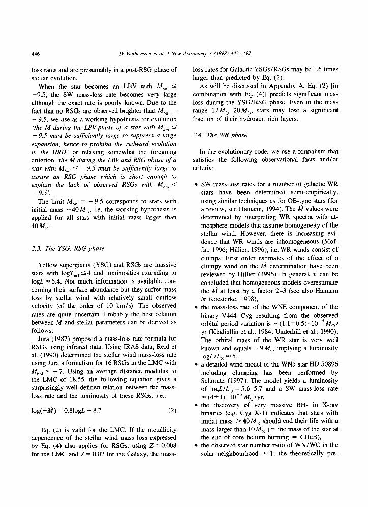
roy (1984). Fig. 1 gives the resulting O-type lifetime as a function of the ZAMS mass for the Galaxy and

the Small Magellanic Cloud, using (X,Z) = (0.7,0.02) for the Galaxy and (0.76, 0.002) for the SMC. The LMC results are intermediate with (X,Z) = (0.74,0.008).

3.2. The YSG and RSG lifetime

A CHeB star that has not yet lost most of its hydrogen-rich layers, will be observed either as an A-type supergiant (YSG), or as a RSG. The time spent as YSG or as RSG depends on the treatment of convection and semi-convection in the envelope of


8

0 10 20 30 40 30 60 m 80 90 100

I&ill mass

Fig. 1. The O-type lifetime as a function of the ZAMS mass for the Galaxy (full line), the LMC (dashed line) and for the SMC

(dashed-dotted line). Explanation is given in the text.

the star but their sum (rYRsG) is largely independent

of the convection criteria.

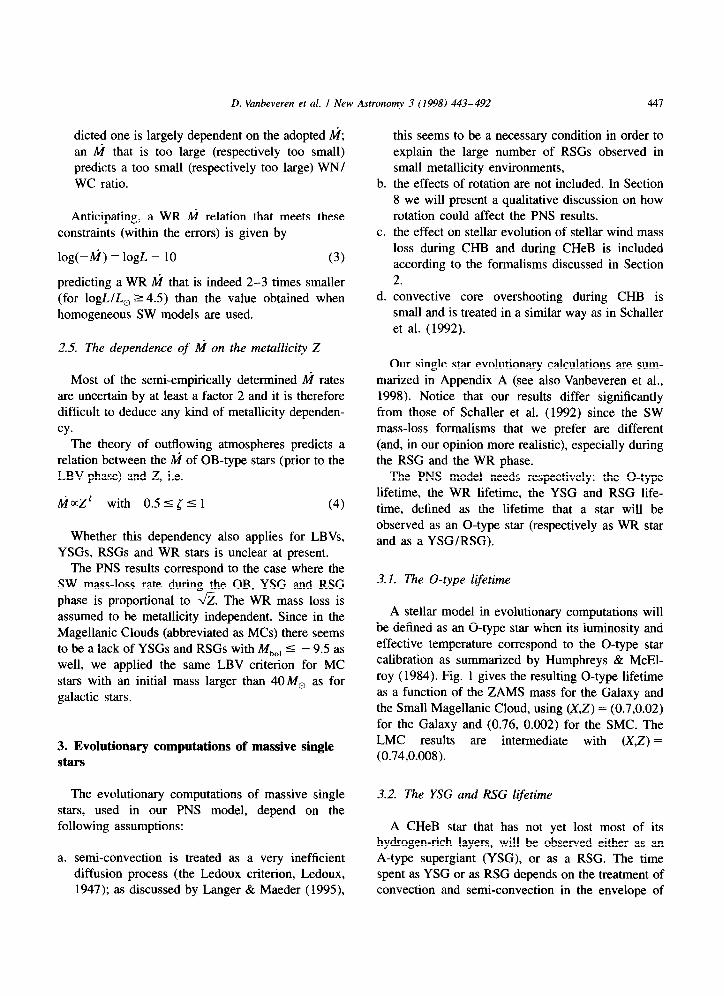
Fig. 2 shows t,,,, as a function of initial mass. To illustrate the importance of M during the RSG phase, we also show the relation, derived from

computations with a mass-loss rate M = half the value predicted by Eq. (2).

For stars with initial mass larger than 40M,,

t YRSG is always very small (of the order of a few times lo4 yr). However, remark that for initial mass-

es smaller than 40M,, these time scales depend critically on the adopted ti values during the YSG/

RSG phase.

3.3. The WR lifetime

Before WR lifetimes can be calculated, we need an evolutionary definition of a WR star (i.e. when does a stellar evolutionary model matches the fea-

tures of a WR star). We account for the following:

WR stars have atmospheric hydrogen abundance X,,, I 0.3-0.4; this can be considered as evidence that most of the WR stars are CHeB stars that have lost most of their hydrogen rich layers, either by LBV or RSG stellar wind, the majority of the observed WR stars seems to have luminosities Log L/L, 2 4.5 and logT,,, 2

4.5 (Hamann, 1994, 1998); from the theoretically predicted mass-luminosity relation of massive

hydrogen poor CHeB stars (Vanbeveren & Pac- ket, 1979; Vanbeveren et al., 1998), this means

that the majority of the observed WR stars must have masses exceeding 5 M,.

c. For most of the observed WR stars in galactic

binaries the Msin3i value is larger than - 5 M,; when we also account for the spectral type of the OB companion and we use a normal mass-spec-

tral type relationship, it follows that most of the

WR stars in galactic binaries have a mass larger than 8-9 M, (Section 6.2). There is a small group of WR like stars, such as the WR like component

in the binary V Sagittae (Herbig et al., 1965) that have rather low masses. These stars are related to nuclei of planetary nebulae. This indicates that the mass limit given above cannot be considered as a

condition sine qua non for a hydrogen deficient CHeB star to be a WR star. We concentrate here, however, only on WR stars that are related to massive stars.

In Figs. 3,4 we give the total WR lifetime and the WC lifetime (i.e. WN = WR - WC) for single stars

as a function of initial mass when it is assumed that

l a hydrogen deficient CHeB star will be observed

D. Vinbeveren et al. I New Astronomy 3 (1998) 443-492 449

10

0

8

7

0

: 5 ir:

4

3

2

1

0 -?

Fig. 2. The yellow and red supergiant time scale tYRsG (in lo5 yr) as a function of the ZAMS mass for stars in the Galaxy (full line), for the

SMC (dashed-dotted line). and for the Galaxy in case the RSG mass-loss rate has been lowered by a factor 2 (dashed line).

as a WR star when its mass is larger than 5 M,, i.e.

tWR = t C.eB(Xatm 5 0.3,M 2 5M,) (5a)

or l a hydrogen deficient CHeB star will be observed

as a WR star when its mass is larger than 8 M,, i.e.

tWR = kHeB (X,,, 5 0.3,M 2 8M,) (5b)

Corresponding to observations, a hydrogen de-

ficient CHeB star is defined as a WN star (respectively WC star) when the atmosphere is composed of hydrogen burning products and thus shows CNO equilibrium abundances (respectively 3a-products, i.e. N is lacking and the CO-abundance is comparable to the He abundance).

We further use the notation MWR,min to designate the minimum WR mass.

Remark that for stars with initial mass 5 40 M,, the WR time scales depend critically on the adopted M during the YSG/RSG phase.


6

0

10 20 30 40 50 60 70 60

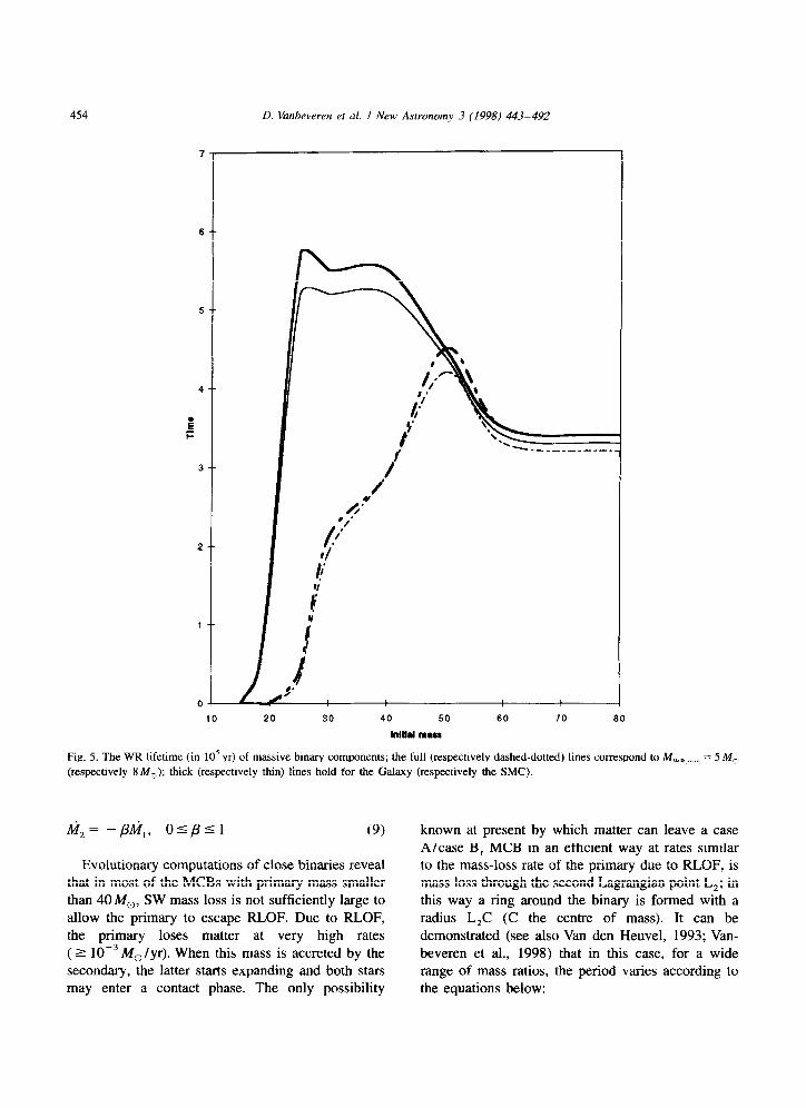
InM~mr"

Fig. 3. The WR lifetime (in 10’ yr) of massive single stars as a function of initial ZAMS mass; the full thick line (respectively dashed-dotted

line) holds for the Galaxy when the minimum WR mass = 5 M, (respectively 8 M,); the dashed line is similar to the full-thick line for the

case that the RSG mass-loss rate has been lowered by a factor 2; the thin-full line holds for the SMC.

4. Massive binaries

We distinguish unevolved binaries (Roche lobe overflow has not started yet) and evolved ones. We will always define the primary as the component which was originally the most massive component; the originally less massive star is called the secondary. This evolutionary definition differs sometimes from the observational one (there primary means the visually most luminous component), so in

WR + OB binaries e.g., the observational primary is the OB star however the evolutionary primary is the WR star since it is this star which was originally the most massive component. Throughout this work, the mass ratio q means the mass of the secondary divided by the mass of the primary.

The primary that is losing mass by Roche lobe overflow (RLOF) is sometimes called the mass loser or the mass donor. The secondary may be designated as the mass gainer or the accretor.


40 50

Inltld rnw*

Fig. 4. Same as Fig. 3 but for WC stars.

4.1. Different types of unevolved massive binaries .

A massive binary is called a massive close binary (MCB) if its period is small enough that during the

evolution one or both components will fill the Roche lobe. Using the single star evolutionary results discussed in Appendix A, calculating the Roche .

radius with the formalism of Eggleton (1983), and adopting the classical definition of case A, case B, case C binaries (Kippenhahn & Weigert, 1967; l

Lauterbom, 1969), we conclude that

the LBV phase of a primary with a mass larger than 4OMo may significantly reduce the importance of the RLOF as mass-loss process. MCBs with a primary more massive than 4OMo will be called ‘Very Massive Close Binaries ‘, abbreviated as VMCBs. in binaries with a primary mass smaller than 4OM,, RLOF occurs in MCBs with periods up to 3ooO days. most MCBs (with a primary mass smaller than 4OM,) with period smaller than 2-4 days


(respectively between 4 and - 1000 days, be- by the primary (Darwin, 1908; Kopal, 1972; Coun- tween - loo0 and 3000 days) will evolve selman, 1973; Sparks & Stecher, 1974): the two according to case A (respectively case B, case C). components merge.

Due to YSG/RSG mass loss, a star with initial mass between Mmin and 40M, does avoid the He

shell burning expansion and therefore case C will not occur. The value of M,,, obviously depends on the YSG/RSG stellar wind mass-loss rates. With our formalism [Eq. (2)]. Mmin ^I 15-20 Mo in the Galaxy

and the LMC. When RSG mass loss depends on the metallicity as predicted by the radiatively driven

wind theory [Eq. (4)]. M,i, 2 40 M, in the SMC.

One expects a different evolutionary behavior of the primary in binaries where RLOF starts when the latter has a mostly radiative envelope (case B,)

compared to binaries where RLOF starts when the mass loser has a deep convective envelope (case B,).

The reason is the adiabatic reaction of a star with a convective envelope to mass loss, i.e. the larger the mass loss rate the faster the star’s expansion. The

evolutionary computations of Appendix A reveal that among all case B types, case B, binaries are the most frequent ones.

Evolutionary computations of binaries indicate that although a massive star may shrink in response to loss of matter, it may not shrink fast enough to

compete with the rapid shrinking of the Roche lobe

when initially the binary has a mass ratio q 5 0.2. It is therefore conceivable that in most of the binaries with initial mass ratio q % 0.2, the secondary is

engulfed by the primary during the RLOF and the two components merge.

Since. at the moment of the merging process in a massive binary, the lower mass component has amply left the ZAMS and thus is very nearly homogeneous, it is reasonable to simulate the evolu-

tion of such a binary by means of the evolution of a star that accretes an amount of mass equal to the

mass of the smaller mass component.

The separation (in terms of period and mass ratio)

between case A and case B,, between case B, and case B,, for binaries with primary mass smaller than

40M,, is very similar for the Magellanic Clouds. The separation between case B, and case C which is affected by the RSG stellar wind mass loss and the

effect of LBV mass loss when the primary mass is

larger than 40Mo obviously depends on the relation between the metallicity and the SW rates.

In our PNS code, we assume that the further evolution of the star (now with mass equal to the sum of the masses of the two components) is similar to the evolution of a single star with the same mass. This can be criticized. It is obvious to realize that in

most cases, the merging process will start when the primary is a post-CHB star where the He-core mass

is fixed. When mass is added to such a star, the ratio He-core mass/stellar mass decreases. It is a general

evolutionary property that in this case the star will have the tendency to remain a blue star rather than to become red, i.e. these objects may populate the so

called Blue Hertzsprung Gap.

4.2. The evolution of binaries with q 10.2 4.3. The evolution of binaries with q > 0.2 till the final collapse of the primary

As a primary in a close binary evolves, it expands, first on the nuclear time scale during CHB, then on the Kelvin-Helmholtz time scale during hydrogen shell burning. As a consequence of this expansion the star will spin down and rotation becomes asynchronized with the orbital motion. Due to tidal interaction, it will try to absorb orbital angular momentum of the component in order to spin up. It can readily be checked that, for small mass ratios (q 5 0. 1 ), the available orbital angular momentum is not sufficient to meet the need of the primary, as a consequence the low mass companion is swallowed

4.3. I. The primary mass is larger than 4OM, In our PNS computations, we assume that a

primary with an initial mass larger than 40 M, loses all its hydrogen rich layers due to a spherically symmetric SW [OB wind + LBV wind] and the RLOF does not occur: the LBV scenario for MCBs

(Vanbeveren, 1991). It is easy to demonstrate that in this case the orbital period varies like

(6)


where the subscript ‘0’ stands for values at the

beginning of the stellar wind mass-loss phase. At the end of the mass-loss phase, the star is at the

beginning of CHeB and has lost most of its hydrogen rich layers (the atmospheric hydrogen abundance by

weight X,,, = 0.25). The evolution of the primary is thus entirely similar to the evolution of a single star

with the same mass (Table 6 in Appendix A).

4.3.2. The primary mass is smaller than or equal

to 40M,

Prior to the onset of the RLOF, one or both components are losing mass by a spherical symmet-

ric SW [Eq. (l)] and thus the orbital period varies like in Eq. (6). To describe the evolution during and after the RLOF process, we distinguish the following

cases.

a. Case AICase B,: the primary. Case B, is the most frequent class and for PNS calculations it is very reasonable to treat case A binaries in the same

way as case B, binaries. An important property of case B, evolution is that

the relation between the pre-RLOF mass Mb and post-RLOF mass IV, of the primary is largely independent of the initial orbital period, of the mass

of the secondary, and of the details of the RLOF process itself, i.e. during CHB, SW mass loss according to Eq. (l), convective core overshooting

during CHB similar as for single stars (Section 3) results into:

for the Galaxy: M‘, = 0.093M;.44

for the LMC: M, = 0.085M;.52 (7)

for the SMC: Mu = O.O48M;.’

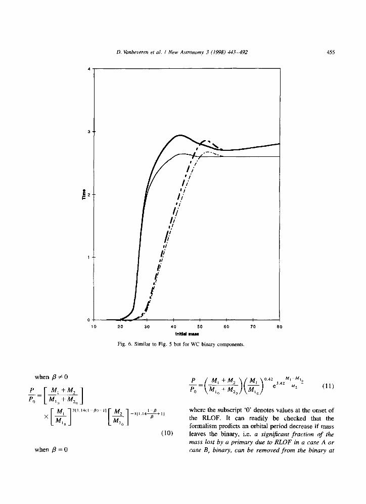
When merging does not occur (mergers are discussed in Section 4.4), the post-RLOF evolution (time scales, the mass-luminosity variation as a function of time, etc.) of the primary depends critically on the adopted SW mass-loss formalism: we use Eq. (3) in the evolutionary code. Using the same WR definition as for single stars (Section 3) Figs. 5,6 give the WR and WC lifetimes as a function of the initial primary mass.

b. Case AICase B,: the secondary. The evolution of the secondary (= the evolution of a star that gains matter lost by the primary during its RLOF) is very important for the study of the time variation of the

stellar content in regions where star formation is

continuous in time and in starburst regions. We summarize the present state in Appendix B.

We have available an extended set of evolutionary tracks of mass gaining stars for the two limiting

accretion models: the standard accretion model

where the effect of convection and semi-convection on top of the convective core of the gainer is treated as a very fast diffusion process (the Schwarzschild

criterion), and the accretion induced full-mixing

model. It is important to realize that the evolution of the

massive mass gainers in our PNS code is NOT

simulated and the time scales are NOT deduced from qualitative arguments. All our evolutionary calcula-

tions and time scales result from detailed evolution-

ary computations. The O-type lifetimes which are necessary to determine the number of O-type mass gainers in a population are given in Table 8 in Appendix B .

c. Case Alcase B,: the period variation. Since the mass-loss rate due to RLOF is much larger than

possible SW mass-loss rate, the effect of SW mass loss on the variation of the binary period during

RLOF can be neglected. We distinguish the conservative and the non-conservative case.

Conservative RLOF. All mass leaving the primary

(mass loser) due to RLOF is accreted by the secondary (mass gainer). Since the rotational angular

momentum of a binary component is always much smaller than the orbital angular momentum, conservation of mass implies conservation of total orbital angular momentum and this means that

P W”M2 3 -_=

( ) u

PiI M,M, (8)

where the subscript ‘0’ denotes values at the beginning of the RLOF phase.

Non-conservative RLOF. At least part of the mass lost by the primary during its RLOF leaves the binary system.

It is customary to define a parameter p describing the fraction of the mass lost by the mass loser that is accreted by the mass gainer, i.e. if ni, (respectively k2) denotes the mass loss (respectively mass gain) rate of the mass loser (respectively mass gainer), it follows that


7

0

10 20 30 40 50 60 70 60

InlIla fnam

Fig. 5. The WR lifetime (in lo5 yr) of massive binary components; the full (respectively dashed-dotted) lines correspond to M,,,,, = 5 M,

(respectively 8M,); thick (respectively thin) lines hold for the Galaxy (respectively the SMC).

@= -p&j,, 05p51 (9)

Evolutionary computations of close binaries reveal that in most of the MCBs with primary mass smaller than 4OM,, SW mass loss is not sufficiently large to allow the primary to escape RLOF. Due to RLOF, the primary loses matter at very high rates ( 2 lop3 M, /yr). When this mass is accreted by the secondary, the latter starts expanding and both stars may enter a contact phase. The only possibility

known at present by which matter can leave a case A/case B, MCB in an efficient way at rates similar to the mass-loss rate of the primary due to RLOF, is mass loss through the second Lagrangian point L,; in this way a ring around the binary is formed with a radius L,C (C the centre of mass). It can be demonstrated (see also Van den Heuvel, 1993; Van- beveren et al., 1998) that in this case, for a wide range of mass ratios, the period varies according to the equations below:

when p #O


20 30 40 50 60 70 60

Mid mur

Fig. 6. Similar to Fig. 5 but for WC binary components.

when p = 0

where the subscript ‘0’ denotes values at the onset of the RLOF. It can readily be checked that the formalism predicts an orbital period decrease if mass leaves the binary, i.e. a sign$cant fraction of the mass lost by a primary due to RLOF in a case A or case B, binary, can be removed from the binary at

456 D. Vanbeveren et al. J New Astronomy 3 (1998) 443-492

the expense of a reduction of the available orbital common envelope. It can reasonably be expected energy, leading to a decrease of the orbital period. that the rate is similar to that of supergiants, a few

We investigated the effect of /3 on PNS results as times 10e6 -10-5M0/yr. follows: An efficient use of orbital energy may result into

l when the binary mass ratio q is larger than some

minimum value (q,i,), /3 is assumed to be

constant ( = &,,), l between q = 0.2 (where /3 = 0) and q,,,, /3 is

assumed to vary linearly. Note that the PNS

results do not critically depend on the value of

9 mln or on how p varies when q 4 q,,,.

After RLOF (when merging is avoided, see Sec- tion 4.4), SW of the primary [Eq. (3)] implies an increase of the binary period, as predicted by Eq. (6).

larger mass loss rates. The idea: owing to viscosity, orbital energy of the secondary is transformed into

thermal energy of the common envelope and the secondary spirals into the envelope (a common

envelope phase is thus always accompanied by a spiral-in process). Part of the thermal energy is

radiated away, part is used to drive the matter of the common envelope out of the binary. Obviously, large

mass-loss rates can be expected if the energy trans- formation by viscosity is a fast process.

d. Case B,lCase Cc the primary. By definition. the orbital period is large enough for the primary to

become a RSG prior to the onset of the RLOF. We

thus have to account for the effect of SW during the YSG/RSG phase of a massive star. It is clear that

the amount of matter lost by SW and, consequently,

the amount of matter lost by the ensuing RLOF, depends on the exact value of the period, i.e. on the

moment the primary fills its RLOF.

Since viscosity is involved, we can only try to answer the following general question: if viscosity between the secondary and the envelope of the primary is able to transform orbital energy into thermal energy of the envelope in an efjcient way, how much orbital energy is required to remove this envelope ?

When A&, is the binding energy of the envelope,

the total orbital energy (potential + kinetic) A&tot needed to remove this envelope, can be determined from the relation

It is important to realize that, similarly to a Case

B, binary, the mass-loss process in a Case B,/Case C binary (i.e. SW and/or RLOF) will stop when

most of the hydrogen rich layers of the primary are removed, i.e. relation Eq. (7) should also hold here.

When merging is avoided (Section 4.4), the further evolution of the primary is similar as the

evolution of the primary in a case B, system. e. Case B(.lCase C: the secondav. A star with a

convective envelope expands faster the larger the mass-loss rate (due to RLOF). This means that soon after the onset of RLOF of the primary a common envelope will be formed. We assume that during this common envelope phase no significant matter accretion occurs, i.e. the mass of the secondary remains constant.

where (Y is the fraction of the orbital energy (first

transformed into thermal energy) not radiated away, hence is effectively used to drive mass from the star

(O<a<l). If the primary is a RSG with a convective

envelope, accounting for the adiabatic reaction of the star when it loses mass at a high rate, it is reasonable to assume that the radius R, of the common envelope is constant during the whole mass-loss process (of the order of the orbital separation at the onset of the process). A rough estimate of the total binding

energy of the common envelope that leaves the binary is then given by

f- Case B,fCase C: the period variation. The period variation caused by the YSG/RSG stellar

wind mass loss is computed with Eq. (6). In order to study the effect of common envelope

evolution, we essentially follow the formalism of Webbink (1984).

Radiation pressure is able to drive a SW from the =G

M,“fM, +2lV,

2Ri (Ml0 -M,J (13)

D. Vanbeveren et al. I New Astronotq 3 (1998) 443-492 451

with M, = the final mass of the star after the

removal gf the hydrogen rich layers. Since the total orbital energy of the binary is given

by

& tot =& pot + ‘kin = - G 2A (14)

it can readily be checked that the removal by orbital energy of only a few solar masses implies a large

period decrease. g. Case B,lcase C: the effect on the O-type star

and WR star population. The total mass lost by primaries in case B,/case C binaries equals the mass

lost by the same primary but in a case B, binary. This matter may be removed first by SW during the YSG/RSG phase before common envelope evolution

starts. The relative importance of both mass-loss phases is uncertain due to the uncertainty in the RSG

stellar wind mass-loss rates. However, anticipating, our calculations allow to conclude that the overall PNS results (O-type star and WR population, the evolution of starbursts) depend only marginally on the number and the evolution of case B,lcase C binaries, i.e. on the common envelope process and on the way the SW during the RSG phase affects the latter.

4.4. The formation and evolution of mergers

The effect of matter leaving the system during the

RLOF in a Case A/Case B/Case C binary is a significant reduction of the orbital period [Eqs. (10)

and (11) or Eq. (12)] and, just as for binaries with q 5 0.2, in some of the cases the two components

can merge. How these systems will further evolve is uncer-

tain. A possibility may be similar to the one pro-

posed above for binaries with small mass ratio, i.e. the evolution of the merger resembles the evolution of a star that has accreted an amount of mass equal to the mass of the secondary. However, in this case,

the chemical composition of the secondary may be significantly different from that of a homogeneous star, and therefore the effect of merging is not easy to predict and requires further investigation.

For the PNS computations we always treat mergers as single stars with a mass equal to the sum of the masses of the two components.

In order to decide upon the remnant system after

the RLOF for binaries with initially q > 0.2, one

may proceed as follows:

knowing the mass that will be lost by the primary

before it becomes a hydrogen stripped CHeB star, the period (orbital separation) of the binary after

the RLOF, and thus the final Roche radii of the

binary, can be estimated: for case A/case B, binaries evolving non-con-

servatively: possible mass loss from the system

through L,, and we use Eq. (10) or Eq. (1 I), for case B, /case C binaries with q > 0.2: the

common envelope prescription, and we use Eq.

(12). when the final Roche radii are larger than the

equilibrium radii of both stars, we are left with a binary consisting of a hydrogen deficient CHeB

star and an OB component. A hydrogen stripped

post-RLOF star with mass M at the onset of CHeB is in thermal equilibrium. Our evolutionary calcu-

lations of hydrogen deficient post-RLOF CHeB primaries reveal that their equilibrium radius R, can very well be described by the following relation

R, = 0.62. 10-4M3 - 0.49. 10-2M2 + 0.18M

+ 0.17 (15)

R, in R,, M in M,. Relation (Eq. (15)) hardly depends on the metallicity,

when one of the Roche radii is smaller than the equilibrium radius of the corresponding component, it is plausible that both stars merged before

the end of the RLOF.

4.5. The evolution of a MCB after the collapse of the core of the primary

The evolution of the primary comes to an end

when its core is composed mainly of iron and nickel, and nuclear reactions stop.

When the mass of the FeNi core is larger than some critical value, it is very probable that the whole star will collapse to form a massive black hole (BH). This critical value depends on the details of the equation of state of matter where electrons and nuclei are degenerate, and this is still uncertain.


Furthermore, also the post-CHeB evolution of a

massive star contains uncertainties so that translating the critical core mass value into a critical value for

the initial mass of a star is uncertain. The current

‘theoretical’ idea promotes a minimum initial mass

of - 40-5OM, above which binary components

may form BHs. The observations of massive X-ray

binaries reveal that NSs are remnants of binary components with initial mass up to at least 40M,,

(e.g., Kaper et al., 1995), which seems to agree with the theoretical value. The PNS results presented here were calculated adopting 40M, as limiting mass for

BH formation in binary components. Assuming that the supernova (SN) explosion does

not happen when a BH is formed, we expect that the

majority of binaries with primary mass larger than - 40 M, will first evolve through an LBV mass-loss

phase (possibly followed by a RLOF but, due to the LBV SW, with a largely reduced mass loss/mass

transfer) and then form an OB + BH binary. When the initial mass of the primary is smaller

than - 40 M,, its final FeNi core collapses into a NS

accompanied by a SN explosion and the ejection of the layers outside the core.

4.5.1. The SN disrupts the binary If the SN event disrupts the binary, it is clear that

the further evolution of the OB component is that of

a single star but, owing to previous accretion, with a chemical composition that may differ from the chemical composition of a normal single star. We distinguish the following possibilities:

l the OB-type mass gainer has a mass > 40 M,. We may expect that in this case the further evolution of the gainer will be similar to the evolution of a single star with the same mass and

thus will be governed by the LBV/RSG mass-loss

processes, l the OB-type mass gainer has a mass 5 40 M,.

When the initial mass ratio of the binary is not too close to one, the further evolution of the gainer after the mass transfer phase is comparable to the evolution of a single star with the same mass. However, when the initial mass ratio is close to one (the exact value depends on the treatment of semi-convection, Appendix B) and when accretion is treated in the standard way, the

star can remain a blue star during its entire life and thus populate the BHG. These stars will then

explode as blue supergiants, producing events like SN 1987A (Podsiadlowski et al., 1990; De Loore

& Vanbeveren, 1992). In our binary evolutionary code, when the

standard accretion model is applied, independent

from the fact that during accretion a p-barrier is formed on top of the core (Appendix B), the core boundary is always determined by the condition Vrad = V,, and we account for a small amount of overshooting similarly as in single stars. In this

case the number of single mass gainers evolving

as outlined above is expected to be very small. Therefore, the PNS results presented here do not

account explicitly for this type of objects.

Independent of the accretion model, we used the single star WR time scales given in Figs. 3,4 to

estimate the number of WR single stars with a binary

history.

4.5.2. The SN does not disrupt the binary When the binary is not disrupted as a consequence

of the SN explosion, an OB + NS binary remains.

The evolution of an OB + BH or an OB + NS binary (both are designated as OB + cc binaries) depends on the orbital period, on the mass of the OB component but also on the initial mass ratio of the

system, since this determines the evolutionary phase of the mass gainer at the onset of the mass transfer

(Appendix B). We distinguish the following subclas-

ses:

l when the mass of the OB-type component is larger than the minimum mass of LBVs ( - 40 M,

for the Galaxy), the OB star will lose most of its

hydrogen rich layers first by a LBV type SW possibly followed by a spiral-in phase. The total

mass lost by the OB star as a consequence of the latter process is largely reduced due to the preceding SW mass loss. It may be expected that the binary will evolve into a CHeB + cc (WR + cc) binary. It is obvious that such systems are rare. In our PNS calculations, we assume that all hydrogen rich layers are removed by SW and no spiral-in phase occurs.

As an illustration, let us consider a 6OM, +


5OMo binary. After two LBV phases the system evolves into a 28 M, (WNL) + 10 M, (BH) binary with a period of the order of some days to some decades, when the mass of the OB-type component is smaller than -40 M,, accretion onto the mass gainer in the progenitor binary is treated in the standard way and if it started late enough (how late depends on the treatment of semi-convection, Appendix B), after accretion the gainer will stay in the blue part of the HR diagram during its remaining lifetime. In this case we expect that the OB + cc binary will remain an OB + cc binary till the SN explosion of the OB-type star. This explosion will be a type II SN event but from a blue progenitor, much like SN 1987A. Note that, since the OB + cc binaries are high-mass-X-ray candidates (thus also the class of OB + cc binaries discussed here), the X-ray lifetime of this class could be very long, possibly the whole CHeB lifetime of the OB-type star.

As outlined in the previous subsection, the number of single star mass gainers remaining in

the blue is expected to be very small. For the same reasons the number of binaries evolving as

outlined above is expected to be very small. Therefore, the PNS results presented here do not account explicitly for this type of systems,

when the mass of the OB-type component is smaller than - 40 M,, and the accretion started earlier in its evolution, this star after accretion

evolves as a normal star. If in this case, the period

of the OB + cc binary is small enough, the OB star will fill its critical Roche volume before becoming a RSG: we will call them case A/case B, OB + cc binaries. Similarly as for binaries with mass ratio q 5 0.2, this will result in a

common envelope where, due to viscosity, the cc will start to spiral-in into the envelope of the primary.

The remnant binary after the spiral-in process can be estimated as follows.

Webbink (1984) introduces a parameter A to express AE, as

Aq = G Mlpfl” - MI,)

hR

0 (16)

with M, = the final mass of the star at the end of

.

the spiral-in process, M,O (respectively R,) = the

mass (respectively the radius) of the star at the beginning of the spiral-in phase.

Since the primary is a blue star with a radiative

envelope and since spiral-in is a consequence of the fact that the secondary is a compact compan-

ion, Aq in Eq. (12) can also be approximated by

the binding energy of the hydrogen rich layers prior to the spiral-in phase. We therefore need the mass concentration M(r) in the stellar

the onset of the mass-loss process

(neglecting the effect of the cc)

MI”

interior at

and thus

(17)

Using the evolutionary computations of massive

stars (Appendix A), it follows that the value of the

parameter A ranges between 0.3 and 0.5. when the mass of the OB-type component is

smaller than -40 M, and the period is sufficiently large to allow the OB star to evolve into a RSG before it starts filling the critical Roche

volume; we propose to call these systems case

B,/case C OB + cc binaries. We first have to account for the effect of RSG stellar wind. When spiral-in starts, the period variation is calculated

using Eqs. (12) and (16). The star is a RSG and

Eq. (17) gives A values between 0.7 and 1.5. Similarly as in non-evolved case B,/case C

binaries, the uncertainty in the SW rates during the RSG phase introduces an uncertainty in the evolution of case B,/case C OB + cc binaries.

However, anticipating, our PNS results allow to conclude that the overall PNS results (O-type star

and WR population, the evolution of starbursts)

depend only marginally on the number and the

evolution of case B,lcase C OB + cc binaries.

The characteristics of the final system after the spiral-in phase can be estimated as follows:

l use the general property that a massive star loses its tendency to expand when most of its hydrogen rich layers have been removed; M, equals M,

and can therefore be calculated us&z Ea. (7).


This means that we did not account for the fact

that mass gainers are accretion stars and that accretion could have changed the chemical profile

in the stellar interior (Appendix B). Furthermore the equilibrium radius R, of such a hydrogen stripped star is given by Eq. (15),

l starting from an initial OB + cc binary, we

determine the Roche lobe radius of the remnant after the removal of the hydrogen rich layers of

the OB-type star using Eqs. (12) and (161, either

with A-0.4 or A= 1, l when the Roche lobe radius is larger than the

equilibrium radius R,, we conclude that initially

there was sufficient orbital energy available to justify the formation of a binary with a hydrogen

poor CHeB star and a compact companion (when the mass of the CHeB star is large enough, a WR

+ cc), l when the Roche lobe radius is smaller than R,,

both stars merged before the removal of the whole hydrogen rich envelope, i.e. the systems

consists of a massive (hydrogen shell burning) star with a compact star in its He core: a Thome-

Zytkow object (TZO) (Thome & Zytkow, 1977). From the detailed structure models of Biehle (1991) and Cannon et al. (1992) it follows that

TZOs have the structure of a RSG. Due to SW mass loss, first the hydrogen rich layers will be stripped off; if its mass and SW are large enough, the star may be observed as a ‘weird’ WR star (WR,,). Most probably this mass-loss dominated

evolution continues until the whole stellar mass has been blown away and the cc becomes visible

again. To estimate the number of WR,, we assumed

that the evolution of a merged OB + cc binary is similar to the evolution of an OB single star with

the same mass.

When merging due to the spiral-in of the compact star does not occur and a CHeB + (NS or BH) is formed, the further evolution of the CHeB components is assumed to be similar to the post-RLOF CHeB evolution of a primary with the same mass. The PNS computation of the frequency of WR + (NS or BH) systems is performed using the same WR time scales as given in Figs. 5,6.

5. The PNS model for the O-type and WR star population

5.1. Method of computation

Given the mass of a single star, from the IMF and

the evolutionary time scales, we compute in a straightforward way its contribution to the number of

O-type stars, of WR stars and of RSGs. Given a close binary with initial primary mass M, ,

the initial mass ratio 4 and period P, depending on the IMF for primaries of close binaries, the mass ratio and period distribution, we determine its contri-

bution to the number of O-type binaries. Due to the SW mass loss during CHB the period variation is

given by Eq. (6). The evolution of the binary period is followed in detail during the RLOF. We determine the contribution to the number of mergers, to the number of WR + OB binaries, and to the number of CHeB + OB binaries. After RLOF, the variation of

the binary period depends on the SW mass loss during CHeB. The PNS code contains a detailed

model for the effect of the SN explosion on the orbital parameters of the binary (Vanbeveren et al.,

1997). When the primary explodes, given an adopted

value of ukicL and an adopted direction of the kick, we determine what the binary looks like after the SN

explosion. When the SN explosion disrupts the binary, the further evolution of the OB-type single star is determined by the adopted single star

scenario. If the binary is not disrupted, we use the spiral-in prescription in order to estimate the further evolution. Since we can calculate the runaway

velocity of the post-SN binary component, it is possible to estimate the frequency of runaway stars formed by the SN explosion in binaries. A star will

be defined as a runaway when its peculiar space velocity is larger than 30 km/s (Blaauw, 1961).

We assume that the direction of the kick during the SN is isotropic whereas the ukick distribution is given by the distribution of pulsar velocities [Section 5.2.41. In this way we determine the contribution to the number of OB-type runaways (with and without a cc), to the number of single WR star but with a binary history, to the number of CHeB + cc binaries and thus when the conditions are fulfilled, to the number of WR + cc, to the number of TZOs.


Finally, when the CHeB component in a CHeB + cc

binary explodes, using the same assumptions as during the first SN explosion, we determine the

contribution to the number of binaries with two compact stars, i.e. the number of NS + NS (binary pulsars), BH + NS or the number of BH + BH.

Let us remind that all the time scales that are needed are taken from our stellar evolutionary library which contains ONLY real evolutionary results, i.e.

we do NOT use results which are simulated or formalism which are based on qualitative arguments.

5.2. The stellar parameters in the PNS model

5.2.1. The initial muss function We assume that the initial mass function of single

stars and of primaries of binaries follow the same

power law, i.e.

IMFaKa (18)

The computations were performed for the usual IMF

(a = 2.7, Scala, 1986) and for an IMF that is

significantly flatter, i.e. ty = 2.

5.2.2. The observed MCB frequency

Garmany et al. (1980) studied the binary frequency among all known O-type stars brighter than

m, = 7 and north of - 50” (a total of 67 O-type single stars or primaries of binaries). Deleting the O-type high mass X-ray binaries from the sample,

one concludes that 33% of 0 stars are primaries of massive close binaries (+ 13% accounting for small number statistics) with mass ratio q > 0.2 and period

P 5 100 days. This conclusion about the O-type MCB frequency

is supported by the MCB frequency among the massive BO-B3 stars. Vanbeveren et al. (1998) concluded that also in this massive star range - 32% are primaries of interacting close binaries and most of them have periods smaller than - 100 days.

-5.2.3. The adopted MCB frequency, mass ratio

and period distribution Short period binaries and/or binaries with large

mass ratio are easier to detect than binaries with longer periods and/or binaries with small mass ratio. This obviously biases the q and P distributions

derived from observations and it underestimates the

binary frequency. A detailed study of the implications of these

selection effects on the q distribution of all spectro-

scopic binaries in the DA08 catalogue has been presented by Hogeveen ( 199 1, 1992) (see also

Halbwachs, 1987). He concludes that the true overall q distribution for all spectroscopic binaries can be

described by the relation:

-2 @Cd 1 Ocq if 0.3 5 q 5 1

= const if q < 0.3 (19)

According to Popova et al. (1982) (see also Vereshchagin et al., 1987, 1988) the semi-major axis A of the relative orbit of (all) binary systems, is

distributed according to:

II(A)

and thus the period (P) distribution according to:

(21)

extending up to a period of 10 yr. It is not meaningful to make such a separate

detailed statistical study for the O-type and the early B-type binaries, since their numbers are too small to

allow this. We assume that the period distribution of massive close binaries satisfies Eq. (21) as well. For the mass ratio distribution, we either adopt a flat

distribution, either the distribution given by Eq. (19).

A population of O-type stars consists of different subsamples defined in Section 7.1.1 and thus the MCB frequency of a population of stars can deviate considerably from the binary frequency at birth of a

population of stars. When we define f as the total

O-type binary frequency at birth, the theoretically predicted MCB frequency becomes an implicit function of fi The theoretically predicted frequency of MCBs with period P 5 100 days and mass ratio q h 0.2 is not only an implicit function off but also of the adopted mass ratio and period distribution. In our population model we retain only those values off predicting the observed frequency of MCBs with P 5 100 days and q 2 0.2. Anticipating, with the period and mass ratio distributions discussed above, only the PNS models with f > 0.7 reproduce the observations.

462 D. Vunbeveren et al. I New A,stronomy 3 (1998) 443-492

5.2.4. The distribution of kick velocities A 1% asymmetry in the neutrino momentum flux

during the SN explosion of a massive star, is sufficient to give a NS a kick velocity of - 400 km/s (Shklovskii, 1969; Sutantyo, 1978; Bailes, 1989). Unfortunately, the physics of SN explosions does not yet allow reasonable guesses of the possible asymmetry. We thus have to rely on observations. It is possible to derive the space velocity of a large number of pulsars (u,). This space velocity is then linked to the kick velocity ukick a compact remnant gets due to an asymmetric SN explosion.

Probably the most thourough discussion has been presented by Lyne & Lorimer ( 1994) and Lorimer et al. (1997). They conclude that the pulsar velocity distribution has a very large average value (- 5OOkm/s). This distribution (used in our PNS calculations) can very well be described by

(22)

There is indirect evidence for large average kicks. It was shown by De Donder et al. (1997) that the binary pulsar formation rate in our Galaxy can be reproduced if a kick velocity distribution is used with average value = 400-500 km/s (see also De Donder & Vanbeveren, 1998). Fryer et al. (1998) performed population synthesis for neutron star systems with intrinsic kicks. They considered the populations of LMXBs, HMXBs, double neutron star systems and globular cluster neutron stars and concluded that the kick velocity distribution that explains all observations best has an average -4OOkm/s and is double peaked; about 30% of the pulsars receive almost no kick at all whereas the remaining 70% have an

average exceeding 600 km/s. Remark: Small proper motions are hard to mea-

sure and errors may be substantial. These errors may not at all be Gaussian (as assumed above). The effect of such errors has been discussed by Hartmann

(1997) and it was concluded that a distribution with an average around 300 km/s (rather than 450 km/s) cannot be excluded. However, a detailed discussion on the effect of measurement and statistical errors and selection effects has been presented by Lorimer et al. (1997). They confirm the large (450-500 km/s) average runaway velocity of pulsars. In order to investigate the effect of a smaller average uklch, we also present our results for a distribution

f(u,) = 2.70. 10~5u~‘2e~~“p’60

predicting an average ukick = 15Okm/s.

(23)

6. Observations that need to be reproduced by the PNS model

6.1. The BIR, WRIO and WCIWN number ratios

The definition of the WR/O and WCIWN number ratio is obvious. The B/R ratio is the number ratio of the OBA supergiants and the RSGs brighter than

M,,, = - 7”.5 (e.g., Langer & Maeder, 1995). We make a distinction between regions where star

formation was constant in time and starburst regions.

6.1.1. Continuous star formation regions Constant star formation means constant within the

lifetime scale of the lowest mass considered. For massive stars we considered as lowest mass - 8 M, leading to a time scale of = 30 million years.

Using the catalogues of Humphreys & McElroy (1984), Van der Hucht et al. (1981, 1988),

Breysacher ( 198 1) complemented by Lortet (199 l), Azzopardi & Breysacher (1979), we summarize in Table 1 the metallicity dependence of the number

ratios WR/O, WC/WN and B/R. Note that for the galactic WR + OB binaries with period P 5 112 days, the ratio WN/WC = 2 which differs considera-

bly from the overall value. At present, a comparison between a theoretically

predicted B/R number ratio and the observed one is meaningless. The reason is that the B number may be very much affected by binary mergers and by mass gainers in MCBs with initial mass ratio close to

Table 1 The observed WR/O, WC/WN and B/R number ratios in

different stellar environments

Z WRIO WCIWN B/R

0.002 (SMC) 0.017 0.13 4

0.008 (LMC) 0.04 0.26 10

0.013 (outer MW) 0.03 0.5 14

0.02 (sn) 0.1 1 28

0.03 (inner MW) 0.2 1.2 48

This is for different values of the metallicity Z; sn = solar

neighbourhood within 3 kpc from the Sun.


one (Appendix B). The evolution of the latter

depends critically on the treatment of semi-convection and is therefore still very uncertain.

6.1.2. Starburst regions A starburst region is a region where in a recent

past, for a short period, a sudden and important

increase of the star formation rate has occurred. In the case of starburst of massive stars, it can easily be

understood that the number ratios discussed in the previous subsection may be very different from those in regions with a constant star formation rate.

Moreover, the precise values depend on the time elapsed since the beginning of the burst. A galaxy

where such an event has occurred is called a ‘starburst galaxy’.

In distant galaxies the O-type stars and the WR stars cannot be resolved as individual stars. However certain features in the integrated spectra can be

attributed to the presence of WR stars. A method to derive a WR/O number ratio from these spectra has

been derived by Kunth & Sargent (1981) and applied to the dwarf galaxy To1 3. They did not account for evolutionary effects and simply adopted an average

IMF of stars during their CHB. They conclude that WR/O = 0.3- 1 for To1 3, far above typical values for regions of constant star formation.

Since this pioneering work, 40-50 galaxies were detected showing a broad He II emission feature at 4686 A. From long-slit optical spectra, Vacca & Conti (1992) estimated the WR/O number ratio in 14 starburst galaxies using the same method as the

one used by Kunth and Sargent for To1 3. Evolutionary effects were introduced by a number

of research groups (see, e.g., Robert et al. (1993), Leitherer & Heckman (1995), Leitherer et al. (1995) and references therein) and the term ‘population synthesis models’ was introduced. However, in all studies only the evolution of single stars is consid-

ered. In Section 7 we will illustrate to what extent binaries are important for PNS.

Since most known starburst galaxies are very far away (NGC 1569 is probably the closest one known and has a distance estimate of 2.2?0.6Mpc, Israel, 1988) spectra may contain information of several starburst regions with different ages as well as the stellar information of the whole galaxy. Features which are attributed to the presence of very young

stars may be visible together with WR and/or RSG

features but it is hard to tell whether or not they were produced by a single starburst (as an illustration, see

the discussion in Gonzales-Delgado et al. (1997) and in De Marchi et al. (1997)).

The interpretation of the observations of starburst

galaxies also depends critically on the time scale of

star formation in starbursts, i.e. whether or not stars in a starburst form coevally. Since the individual

stars in starburst regions cannot be resolved at present, direct evidence is lacking.

Although the number of stars in starburst regions of starburst galaxies is significantly larger than the

number of stars in clusters and associations in the Milky Way or in the MCs, the study of the latter may

provide important hints. The stellar content of massive star clusters and

associations in our Galaxy has been studied by

Humphreys & McElroy (1984). Two OB associations in the LMC (i.e. LH117 and LH118) and one in

the SMC (NGC 346) have been discussed in detail

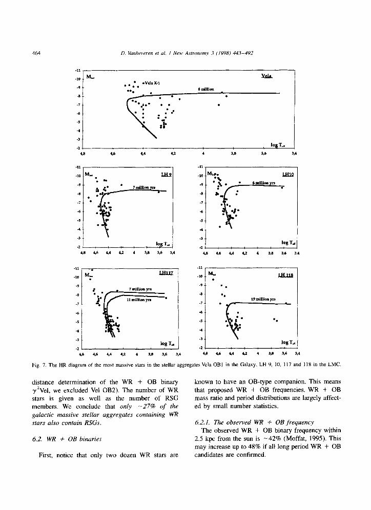
respectively by Massey et al. (1989a,b). Parker et al. (1992) presented results for the LMC associations LH 9 and 10. In Fig. 7 we show the HR diagram of the most massive stars of Vela OBl in the Galaxy

and of the four LMC aggregates. Van Rensbergen et al. ( 1996) argued that the high mass X-ray binary

Vela X-l originates from Vela OBl. We therefore show the HRD position of the optical star of the binary as well. When the HRD position of the massive stars in these aggregates is compared with evolutionary tracks and time-isochrones, one has to

conclude that massive stars in an aggregate in the Galaxy and in the MCs form over a time scale of several million years, i.e. star formation is not coeval.

Particularly interesting is that in all of them a class

of stars younger than the aggregate turn off seems to exist (defined as there, where the observed star sequence tends to bend towards the red). The authors suggest that this may be an indication that star formation was bimodal, the highest mass stars being formed later. We will show however that this phe- nomenon is a natural consequence of the effect of binaries on the evolution of starburst regions.

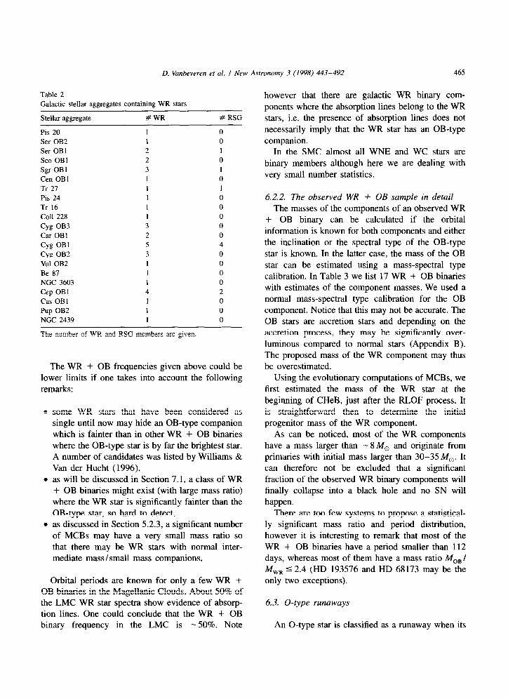
In Table 2 we present a list of galactic stellar aggregates containing WR stars (from Lundstrom & Stenholm (1984); however based on the Hipparcos

464 D. Vanbeveren ef al. I New Astronomy 3 (1998) 443-492

-24 : : IqgL

4s 46 4A 4.2 4 3.5 36 3,4

-11 r

-10

-9

-6

-7

d

-5

-4

-3

-2

. Mw .

log Tr

4s 4.4 4.4 4.2 4 36 3# 3/(

-11

LHlQ

lol$Ts -27 :

4.4 4.4 4,4 4a 4 3,4 3.6 34

-11 T

-10 MU -- .

-9 -. '.

-4 -. l * 19million yrs

1ogT.w

Fig. 7. The HR diagram of the most massive stars in the stellar aggregates Vela OBI in the Galaxy, LH 9, 10, 117 and 118 in the LMC.

distance determination of the WR + OB binary

y’Ve1, we excluded Vel OBZ). The number of WR stars is given as well as the number of RSG members. We conclude that only -27% of the galactic massive stellar aggregates containing WR stars also contain RSGs.

6.2. WR + OB binaries

First, notice that only two dozen WR stars are

known to have an OB-type companion. This means that proposed WR + OB frequencies, WR + OB mass ratio and period distributions are largely affected by small number statistics.

6.2.1. The observed WR + OB frequency The observed WR + OB binary frequency within

2.5 kpc from the sun is -42% (Moffat, 1995). This may increase up to 48% if all long period WR + OB candidates are confirmed.


Table 2

Galactic stellar aggregates containing WR stars

Stellar aggregate #WR # RSG

Pis 20

Ser 0B2

Ser OBI

Sco OBI

Sgr OB1

Cen OBl

Tr 27

Pis 24

Tr 16

co11 228

Cyg OB3

Car OBl

Cyg OBl

Cyg OB2

Vu1 OB2

Be 87

NGC 3603

Cep OBl

Cas OB1

Pup OB2

NGC 2439

2

2

2

5

3

1

4

1

0

0

0

0

0

0

0

0 0

4

0

0

0

0

2

0

0

0

The number of WR and RSG members are given.

The WR + OB frequencies given above could be lower limits if one takes into account the following

remarks:

some WR stars that have been considered as single until now may hide an OB-type companion which is fainter than in other WR + OB binaries

where the OB-type star is by far the brightest star. A number of candidates was listed by Williams & Van der Hucht (1996),

as will be discussed in Section 7.1, a class of WR + OB binaries might exist (with large mass ratio)

where the WR star is significantly fainter than the

OB-type star, so hard to detect, as discussed in Section 5.2.3, a significant number

of MCBs may have a very small mass ratio so that there may be WR stars with normal intermediate mass/small mass companions,

Orbital periods are known for only a few WR + OB binaries in the Magellanic Clouds. About 50% of the LMC WR star spectra show evidence of absorption lines. One could conclude that the WR + OB binary frequency in the LMC is - 50%. Note

however that there are galactic WR binary com-

ponents where the absorption lines belong to the WR stars, i.e. the presence of absorption lines does not

necessarily imply that the WR star has an OB-type

companion. In the SMC almost all WNE and WC stars are

binary members although here we are dealing with

very small number statistics.

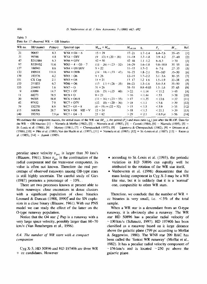
62.2. The observed WR + OB sample in detail The masses of the components of an observed WR

+ OB binary can be calculated if the orbital

information is known for both components and either the inclination or the spectral type of the OB-type

star is known. In the latter case, the mass of the OB

star can be estimated using a mass-spectral type calibration. In Table 3 we list 17 WR + OB binaries with estimates of the component masses. We used a

normal mass-spectral type calibration for the OB component. Notice that this may not be accurate. The OB stars are accretion stars and depending on the

accretion process, they may be significantly overluminous compared to normal stars (Appendix B). The proposed mass of the WR component may thus be overestimated.

Using the evolutionary computations of MCBs, we first estimated the mass of the WR star at the

beginning of CHeB, just after the RLOF process. It

is straightforward then to determine the initial progenitor mass of the WR component.

As can be noticed, most of the WR components have a mass larger than - 8 M, and originate from primaries with initial mass larger than 30-35M,. It

can therefore not be excluded that a significant fraction of the observed WR binary components will finally collapse into a black hole and no SN will

happen. There are too few systems to propose a statistical-

ly significant mass ratio and period distribution,

however it is interesting to remark that most of the WR + OB binaries have a period smaller than 112 days, whereas most of them have a mass ratio Mo,l M,, 5 2.4 (HD 193576 and HD 68173 may be the only two exceptions).

6.3. O-type runaways

An O-type star is classified as a runaway when its

466

Table 3

D. Vanbeveren et al. I New Astronomy 3 (1998) 443-492

Data for 17 observed WR + OB binaries

WR no. HD (name) P(days) Spectral type %I, + Mo, M aRLOF 4‘2 P” M ,!I,, Ref.

21 90657 8.3 WN4+04-6

31 94546 4.8 WN4 + 08V

47 E311884 6.3 WN6 + 05v

97 E320102 11.6 WN3-4+05-7

127 186943 8.6 WN4 + 09/BOV

133 190918 111.8 WN4 + 091b

139 193576 4.2 WN5 + 06

151 CX Cep 2.1 WN5 + 08

153 211853 6.7 WN6 + 06

155 214419 1.6 WN7iO

9 63099 14.7 WC5 + 07

11 68273 78.5 WC8+0

30 94305 18.8 WC6 + 06/8

42 97152 7.9 WC7 + 07v

79 152270 8.9 WC7+05-8

113 168206 28.7 WC8+08-9111-V

15+29

(9- 13)+(20-30)

42 + 50

(11 - 26) + (23 - 52)

9 + 22

(14~ 18)+(33-42)

9 + 26

II +21

(1317)+(26-35)

31 +26

(16-25)+(25-40)

9 + 23

(11 - 16) + (23 - 35)

(12~18)+(20-30)

(8~ 19)+(22-52)

12+24

17-21

1 l-18

42-44

14-29

11-15

16-23

12-15

13-17

16-23

31-33

>22

> 16

> 17

> 18

> 15

> 18

1.7-1.4 6.4-7.6 35-45

1.7-1.8 3.9-4.2 27-40

1.1-1.2 6-6.3 > 70 1.6-1.8 9.8-10.8 35-55 1.5-2 6-7.6 27-35

1.8-2.1 95-103 35-50

1.7-2.2 3.1-3.6 30-35

1.2-1.6 1.5-1.9 33-38

1.5-1.6 5.4-5.8 35-50

0.8-0.85 1.5-1.6 57-65

< 1.14 < 11.2 >45 < 1.44 <53 > 38

< 1.35 < 13.6 >37 < 1.1 < 5.6 > 39

< 1.5 <5.9 > 35 < 1.3 c21.1 > 39

III

PI ]31

141

[51

[61

[71

WI

[51

[91

[41

[lOI

(111

[I21

[I21

[I31 140 193793 7.9 yr WC7 + 04 - 5 23 + 62 >29 i2.1 < 6.9 yr >56 Cl41

We estimate the component masses, the initial mass of the WR star (M,,,,), the period (P,) and mass ratio (4,) just after the RLOF. Data for

the WR + OB binaries: [I] = Niemela & Moffat (1982), [2] = Niemela et al. (1985), [3] = Certuti (1984), [4] = Niemela (1995). [5] =

St.-Louis et al. (1988), [6] = Massey (1981), [7] = Cherepaschuk (1975), [8] = Lipunova & Cherepaschuk (1982). [9] = Drissen et al.

(1986). [IO] = Pike et al. (1983),Van der Hucht et al. (1997). [I I] = Niemela et al. (1983), [12] = St.-Louis et al. (1987). [13] = Eaton et

al. (1985), [14] = Annuk (1995).

peculiar space velocity up_ is larger than 30 km/s (Blaauw, 1961). Since upec is the combination of the radial component and the transverse component, its value is often not known. Therefore the real per-

centage of observed runaways among OB-type stars is still highly uncertain. The careful study of Gies (1987) promotes a percentage of - 10%. ,.

There are two processes known at present able to

form runaways: close encounters in dense clusters with a significant population of close binaries Leonard & Duncan (1988, 1990y’and the SN explosion in a close binary (Blaauw, 1961). With our PNS

model we can study the effect of the latter on the O-type runaway population.

Notice that the 04 star 5 Pup is a runaway with a very large space velocity, possibly larger than 60-70 km/s (Van Rensbergen et al., 1996).

6.4. The number of WR stars with a compact companion

Cyg X-3, HD 50896 and HD 197406 are three WR + cc candidates. However

l according to St.-Louis et al. (1993), the periodic variation in HD 50896 can equally well be attributed to the rotation of the WR star itself,

l Vanbeveren et al. (1998) demonstrate that the mass losing component in Cyg X-3 may be a WR like star, but it is unlikely that it is a ‘normal’ one, comparable to other WR stars.

Therefore, we conclude that the number of WR + cc binaries is very small, i.e. < 5% of the total

sample. When a WR star is a descendant from an O-type

runaway, it is obviously also a runaway. The WR star HD 50896 has a peculiar radial velocity of - lOOkm/s (Schmutz, 1997). HD 197406 has been classified as a runaway based on it large distance above the galactic plane (799 pc according to Moffat & Seggewiss, 1980). The WN8 star 209 BAC has been called the ‘fastest WR runaway’ (Moffat et al., 1982). It has a peculiar radial velocity component of - 156 km/s and is located - 250 pc above the galactic plane.


7. PNS model computations and comparison to observations

7. I. Continuous star formation regions

Detailed PNS computations have been performed for different values of all parameters that enter the

code.

7.1.1. The population of O-type stars The population of O-type stars consists of:

0, = number of O-type single stars, formed as single stars

0, = number of O-type primaries in a binary with an OB or a low mass component; we separately consider the number of O-type

primaries in a binary with q 20.2 and orbital period P 5 100 days. Since it is this number that

may be comparable to the observed number, we denote it as O,,,.

0 +CHeB = number of O-type mass gainers with a CHeB (WR) companion

O,, = the number of single post-SN O-type mass gainers where the SN disrupted the binary; we separately consider those with a space velocity 2 30 km/s (the runaways)

OX = the number of post-SN O-type mass gainers with a compact companion (NS or BH); also here we separately consider those with a NS

companion and with a space velocity L 30 km/s (the runaways).

Results are given in Table 4 for the Galaxy. The results for the MCs are very similar. The number of O-type mass gainers is calculated assuming that 50%

were formed through the standard accretion model

(and thus the other 50% through the accretion induced full-mixing model). The frequencies of the

different types of mass gainers quoted below are

typically 25% smaller (respectively 25% larger) when ALL mass gainers went through the standard

accretion process (respectively the accretion induced

full-mixing process). We conclude:

a comparison between the predicted O,,, numbers

and the observed O-type frequency (33%+- 13%, Section 5.2.2) forces us to conclude that the majority of the O-type stars are formed as binary

components with orbital period between 1 day and 10 yr (f>0.7),

between 15% and 25% of all O-type stars are post-SN mass gainers of MCBs; if the kick- velocity distribution has an average value of 150

km/s (respectively 500 km/s), - 40% (respective-

ly < 12%) of these post-SN O-type mass gainers have a NS companion. It is clear then that if the kick-velocity distribution has an average value of 500 km/s, a very significant fraction of the population of ‘single’ O-type stars are single post-

SN O-type mass gainers of MCBs, at most l-2% of all O-type stars may have a BH companion,

at most 8% of the O-type stars are runaways due to a previous SN explosion in a binary; if

(ukick) = 5OOkm/s (respectively 150 km/s),

Table 4

The O-type population predicted by the PNS model for different parameters

f &ax %E IMF @(4) (u,,,,) 0, 0, Ok0 o+Cx&! O,, + NS O,, + BH O,, OS,.,

0.8 1 1 2.7 F 500 0.1 0.51 0.25 0.14 0.03 0.007 0.22 0.05 0.8 I 1 2.7 H 500 0.15 0.59 0.24 0.09 0.03 0.008 0.16 0.05 0.5 1 1 2.7 H 500 0.31 0.31 0.16 0.11 0.02 0.005 0.18 0.03 0.5 1 1 2.7 H 500 0.41 0.41 0.09 0.07 0.02 0.007 0.13 0.05 0.8 1 0.5 2.7 F 500 0.1 0.4 0.18 0.14 0.03 0.007 0.22 0.05 0.8 1 1 2 F 500 0.11 0.59 0.29 0.09 0.02 0.013 0.17 0.04 0.8 1 1 2 H 500 0.15 0.64 0.25 0.06 0.02 0.017 0.13 0.03 0.8 0.5 1 2.7 F 500 0.12 0.64 0.32 0.06 0.03 0.008 0.15 0.08 0.8 0.5 1 2.7 H 500 0.16 0.69 0.28 0.03 0.02 0.010 0.09 0.05 0.8 1 1 2.7 F 150 0.1 0.49 0.18 0.14 0.11 0.007 0.16 0.05 0.8 1 1 2.7 H 150 0.15 0.53 0.13 0.1 0.10 0.009 0.12 0.04


< 20% (respectively > 50%) of these runaways have a NS companion. Gies (1987) and Gies & Bolton (1986) investigated the presence of com-

pact companions among O-type runaways and

concluded that only a small percentage may hide one. This is predicted by our PNS model provided

that the kick velocity during the SN explosion is

very large, l in Fig. 8a we have plotted the theoretically

predicted distribution of runaway velocities of the

O-type runaways, with (Obinary.r) and without

(Oaingb2.r ) a neutron star companion. We separately

consider the distribution at birth and the distribution where we account for the remaining CHB lifetime of the runaway. It can be concluded

that the sample of O-type runaways (with or

without a NS companion), which became runaway as a consequence of a previous SN explosion

in a binary, has an average space velocity of - 5Okm/s whereas a runaway with a velocity

larger than - lOOkm/s is very rare.

l For comparison purposes, we also predicted the

population of early B-type stars. At most 5-8% of them are runaways (the majority is single if (ukick) = 500 km/s) which is very similar to the

O-type runaway frequency. Also the space velocity distribution is very similar to the one for

the O-type runaways (Fig. 8b).

7.1.2, The WR population

A realistic WR population consists of

l WR, = number of single WR stars descendent from the 0, class,

l WR, = number of WR binary components with

an OB or low mass component, descendants from the 0, sample; this class can be subdivided into

l WR,, = number of WR stars with an OB-type

or ldw mass companion, where RLOF and binary interaction played a dominant role,

l WR,,,,, = number of WR stars with an OB-

type or low mass companion where, due to very large SW during an LBV phase, RLOF and thus binary interaction may have played only a minor role,

. WR b.merged = number of (single) WR stars, descendent from those interacting binaries that merge,

’ WRb.SG = number of WR binaries with an

OB-tipe or low mass companion orbiting with very large period, where interaction did not

happen and where the WR star was formed by SW during the RSG stage,

’ WR,b = the number of single post-SN WR stars

descendent from the O,, class, l WR,, = the number of WR + cc binaries that

survived the spiral-in phase of the 0 + cc binary,

l WR,, = the number of WR stars with a cc in their center, descendent from 0 + cc binaries

where during the spiral-in phase a Thome-Zytkov

object is formed.

The solar neighbourhood. Table 5 illustrates the

WR population for the solar neighbourhood (Z =

0.02). Unlike for the O-type population, the results for the WR stars depend only marginally on the way accretion is treated in mass gainers but remark that

they depend critically on the value of MWR,min. We

conclude:

l the observed WR/O number ratio in the solar neighbourhood cannot be reproduced if it is

assumed that MWRsmin = 8 MO; the comparison is

better assuming MWR,,,,” = 5 M, although the theoretical value is still somewhat smaller than

the observed one.

A few remarks are appropriate

l some of the lower luminosity (logLIL, 5 5) WR stars may be post-AGB stars, descendants from intermediate mass stars, on their way to become

WDs, l the theoretical O-star lifetime is calculated assum-

ing that a star will be visible as an O-type star from the beginning of CHB (the ZAMS). How- ever, when the theoretical HR diagram of O-type stars is compared to the observed one, there appears to be a lack of stars close to the ZAMS (Garmany et al., 1980),

l when the HR diagram of aggregate stars within the solar neighbourhood is compared to the theoretical evolutionary tracks and one counts the number of stars within time-isochrones of 1 million years apart, it looks as if the incomplete- ness of massive stars is very large (and not only


(a) rohr. f&s1 and cvk>=500

rel.nr. h,=l and <vk>=150

l Oe,r.birth

0 Ob,r,birth L-I n Os,r,obs

ROb,r,obs

rdnr.

Oh OP

03 03

OS 02

0,15 OJ

ops

p,,,,,=O.5 and -cvk>=500

Fig. 8. (a) The theoretically expected distribution of space velocities of O-type runaways. We separately consider the distributions at birth

and the real distribution accounting for the remaining CHB lifetime of the runaway. We furthermore distinct O-type single runaways where

the SN explosion disrupted the binary, and the O-type binary runaways where the SN explosion did not disrupt the binary (i.e. the O-type

runaway still has a NS companion), (b) Similar to (a) but for the early B-type runaways.

.

close to the ZAMS) or that the massive star formation rate was significantly larger a few million years ago (Vanbeveren, 1990), the decision whether or not an O-type star or a WR star has a distance smaller than - 3 kpc (the

solar neighbourhood) relies on calibration in many cases. This may introduce non-negligible errors. As an illustration, a few O-type stars that have been listed by Humphreys & McElroy (1984) as member of Vela OB 1 at a distance of


(b) rdnr. bl and <vk>=500

rdnr.

0,4

op

02

$1

b=l and <v,>=150

Fig. 8. (continued)

1.8 kpc, seem to have Hipparcos distances .

- 400-500 pc,

when MwR min = 5 M, (respectively 8Mo) it fol-

lows that in - 70% (respectively 30%) of the WR + OB binaries (where also the OB star is a massive star) RLOF and mass transfer occurred;

the other - 30% (respectively 70%) evolved

either according to the LBV scenario either according to the RSG scenario, .

3-5% of the WR stars may have a normal intermediate mass or low mass companion,

depending on the adopted efficiency for converting orbital energy into kinetic energy of the envelope of the OB-type star during the spiral-in of the cc, at most 3% (respectively 8%) of the WR stars may have a compact star in their center

(WR,,) if the kick-velocity distribution has an average value of 500 km/s (respectively 150

km/s), the PNS model predicts a small percentage of WR stars with a compact companion. Depending on the adopted efficiency for converting orbital

Tab

le 5

Th

e W

R

popu

lati

on o

f th

e so

lar

nei

ghbo

urh

ood

pred

icte

d by

th

e P

NS

mod

el,

for

diff

eren

t va

lues

of

the

para

met

ers

M W

R.r

ni”

f

Pm

acE

IM

F

@C

d

h,,

,,)

WR

, W

R,,

, W

R,,

,,,

Wk

.,,,

W

&,,

,,,,

, W

R

+ N

S

WR

+

BH

W

R,,

W

R,,

W

RlO

h

5 M

, 0.

8 1

1 2.

1 F

50

0 0.

101

0.31

9 0.

128

0.03

6 0.

8 1

1 2.

7 H

50

0 0.

128

0.26

5 0.

162

0.05

0.

5 1

1 2.

7 F

50

0 0.

309

0.24

5 0.

098

0.02

8 0.

5 1

1 2.

1 H

50

0 0.

371

0.19

1 0.

117

0.03

6 0.

8 1

0.5

2.1

F

500

0.10

1 0.

313

0.12

8 0.

036

0.8

1 1

2 F

50

0 0.

111

0.28

7 0.

198

0.03

2 0.

8 1

1 2

H

500

0.13

8 0.

233

0.24

6 0.

044

0.8

0.5

1 2.

1 F

50

0 0.

111

0.27

1 0.

148

0.04

2 0.

8 0.

5 1

2.1

H

500

0.14

2 0.

2 0.

119

0.05

5 0.

8 1

1 2.

1 F

15

0 0.

099

0.31

5 0.

126

0.03

5 0.

8 1

1 2.

1 H

15

0 0.

127

0.26

2 0.

161

0.04

9

8 M

o 0.

8 1

1 2.

7 F

50

0 0.

135

0.11

8 0.

307

0.03

5 0.

8 1

1 2.

7 H

50

0 0.

161

0.08

9 0.

363

0.04

4 0.

5 1

1 2.

1 F

50

0 0.

368

0.11

0.

209

0.02

4 0.

5 1

1 2.

1 H

50

0 0.

428

0.08

5 0.

242

0.03

0.

8 1

0.5

2.1

F

500

0.12

7 0.

148

0.28

8 0.

033

0.8

1 1

2 F

50

0 0.

135

0.12

1 0.

362

0.02

6 0.

8 1

1 2

H

500

0.16

4 0.

098

0.43

9 0.

035

0.8

0.5

1 2.

1 F

50

0 0.

135

0.11

8 0.

307

0.03

5

0.8

0.5

I 2.

7 H

50

0 0.

161

0.08

9 0.

363

0.04

4 0.

8 1

1 2.

7 F

15

0 0.

121

0.15

1 0.

287

0.03

3 0.

8 1

1 2.

7 H

15

0 0.

151

0.12

5 0.

355

0.04

3

0.16

9 0.

241

0.33

9 0.

083

0.20

6 0.

233

0.27

5 0.

051

0.11

2 0.

074

0.05

4 0.

125

0.23

3 0.

275

0.01

0.

164

0.01

5 0.

049

0.03

0.

008

0.02

6 0.

021

0.01

1 0.

038

0.02

3 0.

006

0.01

9 0.

015

0.00

8 0.

05

0.03

4 0.

012

0.08

1

0.02

4 0.

006

0.04

3 0.

011

0.00

6 0.

057

0.02

1 0.

002

0.02

9 0.

01

0.06

6 0.

049

0.08

4 0.

036

0.02

6 0.

055

0.00

3 0.

103

0.01

1 0.

001

0.04

2 0.

004

0.01

0.

07

0.01

8 0.

004

0.02

8 0.

01

0.01

1 0.

097

0.02

7 0.

011

0.01

3 0.

018

0.00

5 0.

056

0.01

1 0.

003

0.10

3 0.

011

0.00

1 0.

042

0.00

4 0.

056

0.09

7 0.

066

0.02

4 0.

041

0.03

1

0.23

8 0.

132

0.18

2 0.

095

0.23

9 0.

184

0.10

4 0.

091

0.04

3 0.

144

0.07

1 0.

055

0.02

0.

141

0.06

3 0.

194

0.14

2 0.

068

0.05

5 0.

02

0.11

4

0.05

6 0.

064

0.05

6 0.

062

0.05

3 0.

063

0.06

9 0.

061

0.07

1

0.05

7 0.

065

0.02

9 0.

035

0.02

6 0.

03

0.02

4 0.

035

0.03

8 0.

029

0.03

5 0.

025

0.02

9


Fig. 9. (a) The theoretically predicted mass ratio distribution of WR + OB binaries at the beginning of the WR phase for two initial mass

ratio distributions. for the two values of MWR,,,,,, and for two values of /3,,, in interacting binaries: A: &,, = 1, IV,,,,,, = 8M,, d(q) flat;

B: Pm,, = 1, M,,,,,,, = 5 Mj, 4(q) flat; C: p,,,,, = 0.5, M,,,R,m,n = 8M,, +(q) flat; D: /3,,, = 0.5, MWR,m,n = 5 M,, 4(q) flat; E: &,, = 1,

M WR,m,n = 8M,,, 4(q) Hogeveen; F: /I,,, = 1, MWR ,,“,” =5M,,, 6(q) Hogeveen; G: P,,,,, =0.X MWR,*,” = 8M,, 4(q) Hogeveen; A:

P ma, = 0.5. wwm” = SM,,, 4(q) Hogeveen. (b) The theoretically predicted period (in days) distribution of WR + OB binaries at the

beginning of the WR phase for parameter sets A and B (defined in (a)). The other sets give very similar distributions.

D. Vanbeveren et al. I New Astronoy 3 (1998) 443-492

n n ;, i

Lao(P)

473

Fig. 9. (continued)

energy into kinetic energy of the envelope of the OB-type star during the spiral-in of the cc, at

most 2% (respectively 8%) of the WR stars may .

have an NS companion if the kick-velocity distribution has an average value = 500 km/s

(respectively 150 km/s). Between 3%-5% (re-

spectively - 10%) of the WR stars may have a BH companion when MWrrmin = 5 M, (respectively 8M,). The WR + BH numbers depend on the value of the minimum mass of BH formation in binaries. They were calculated assuming

M binary BH,m,n = 40 M,. Using 50 M, instead lowers

the WR + BH numbers by a factor of 2, between 40% and 50% of all WR stars are single WR stars. However, it cannot be excluded that - 70-80% (or more) of these single WR have had

a binary history, i.e. are WR stars, descendants from OB-type mass gainers in binaries where the SN explosion disrupted the binary, or are WR stars descendants from binaries where during the RLOF both components merged. The latter class is largest when the Hogeveen mass ratio dis-

414 D. Vanbeveren et al. I New Astronoq 3 (1998) 443-492

tribution applies and/or when the RLOF in case A/case B, MCBs is highly non-conservative

cp 5 0.5), l at most 5% of all WR stars have a space velocity

larger than 30 km/s (WR runaway) caused by the recoil of the SN explosion in a binary.

The WR space velocity distribution should obviously be very similar to the O-type runaway

distribution. Although a binary scenario could be involved to explain the space velocity of HD 50896 and of 209 BAC (Section 6.4), it can be

concluded from Fig. 8 that the probability is very

small, l in Fig. 9a, we show the theoretically predicted

mass ratio distribution of WR + OB binaries at

the beginning of the WR phase for the two values

of M,, m,nr for two values of &,, in interacting

binaries’ with initial mass smaller than 40 M, and for two initial mass ratio distributions. Fig. 9b illustrates the WR + OB period distribution. We

only consider two parameter sets since all others give very similar distributions. When compared to the observed periods and mass ratios of the 17 WR + OB binaries in Table 3, we have to

conclude that theory predicts many more WR + OB binaries with periods between 100 days and 1000 days and/or WR + OB binaries with mass

ratio larger than 2.2-2.4 or with a small mass

ratio (q < 0.8). This discrepancy can obviously be attributed to

still unrecognized physical processes not yet included in the evolutionary code. However, also observations may still be highly incomplete. Long

period binaries are hard to detect whereas when the mass ratio of the WR + OB binary is smaller (respectively larger) than 0.8 (respectively 2.2-

2.4), the OB component (respectively the WR component) may be barely visible,

The inner Milky Way. The metallicity Z in the inner MW = 0.03. The evolution of MCBs hardly depends on Z whereas when compared to Z = 0.02, significant differences in single star evolution are expected only if the RSG stellar wind mass loss scales linearly with Z (i.e. the RSG M is a factor 1.5 larger compared to Z = 0.02).

Our computations reveal that, unless MWR,min is very small, it is hard to explain the observed WR/O

number ratio ( = 0.2) by means of a continuous star formation model.

However, a WR/O number ratio as large as 0.2 is not unusual if, instead of a continuous star formation

history, there has been an increased star formation rate a few million years ago.

The Magellanic Clouds. We focus on the LMC since the SMC numbers are very small. The formation of a WR single star depends primarily on the

SW mass-loss rate during the LBV phase and/or during the RSG phase, while the duration of the WR phase depends on the WR SW mass-loss rate as well.

Furthermore the evolution of a MCB hardly depends on the metallicity. Adopting a continuous star formation history in the LMC, the theoretically predicted

WR/O number ratio - 0.02-0.03 (respectively 0.04-

0.05) if MWR,min = 8 M, (respectively 5 M,) which

is very close to the observed value.

7.2 Starburst regions

7.21. The population of O-type stars and WR stars

We assume that the overall formation frequency of single stars and of binaries in starbursts is similar to

that in regions where star formation was continuous. In Fig. 10, we show the time evolution of the

number of O-type stars and of WR stars (normalized so that initially the number equals one) of an instantaneous starburst with PNS parameters: f = 0.8, IMFmMp2.‘, flat mass ratio distribution, /3,,, = 1 in

case A/case B, binaries, MWR,min = 5 M,. Fig. 11 illustrates the evolution in the HR diagram of a

starburst with 1000 massive stars for a starburst which lasted for 1 million years, with the same PNS parameters. We define the O-phase (respectively the

WR phase) and the corresponding O-lifetime (respectively WR lifetime) of a starburst as the phase or the time where the starburst shows O-type (respectively

WR-type) features. We conclude

l the evolution of a starburst older than - 4 . lo6 yr depends critically on the binary frequency. If binaries are included, the total elapse of time the starburst shows O-type and WR star features, is much longer than in starbursts where binaries are omitted. This is due to the effect of accretion in

D. Vanbeveren et al. I New Astron0m.v 3 (1998) 443492

7

0 5 10 15 20 2s 30

Ago In Myr

Fig. 10. The time evolution of the number of O-type. stars (thick line) and of WR stars (thin line) for an instantaneous starburst with PNS

parameters: f= 0.8, IMFG-‘.‘, flat mass ratio distribution, p,,,,, = 1 in case A/case B, binaries, M,,,,,, = 5 M,,. Both figures are

normalized so that at the moment the O-type star frequency (respectively the WR frequency) is maximum, this maximum equals one. The

WR/O number ratio is obtained by deviding the numbers of both curves at the corresponding time steps and then multiplying the result by

0.033.

MCBs and the appearance of a class of young O-type mass gainers when the starburst is older than -4. lo6 yr: we propose to call this the ‘starburst rejuvenation’. Fig. 11 shows the situation of a burst of 7 * lo6 yr old and where, owing

to O-type mass gainers, it looks younger than 4. lo6 yr.

The following simple example illustrates what happens. Assume a starburst with 50 O-type

single stars with an average mass of 30 MO, and 50 MCBs with average mass 30 M, + 20 M, (this is the most likely progenitor of the WR

binary V444 Cyg, a WNE + 06V, Vanbeveren et al., 1998). After -7. lo6 yr, all single O-type stars have disappeared and only a class of single WR stars is left. The binaries on the contrary, evolved (on average) into a WR + 05/06 class (just as V444 Cyg), i.e. we will observe a starburst with a significant number of O-type mass gainers, no O-type singles, and a large WR sample. If binary effects were not taken into

account, one should be led to the conclusion that the starburst is at most 3-4 * lo6 yr old and has a

number ratio WR/O = 1-2, a comparison between theoretical prediction and observations of young starbursts is meaningful

only if binaries and the effect of binary evolution are correctly included. Most important is the

rejuvenation caused by mass transfer, when the observed HR diagram of stellar aggre-

gates in the Galaxy and MCs (Fig. 7) is compared with the predicted HR diagram of starbursts (Fig. 1 l), although the number of stars is smaller in the former, it looks as if the effects of interaction in binaries offer a natural explanation for the presence of a younger class of stars, bluer and more luminous than the cluster turn-off (blue stragglers).

Schaerer & Vacca (1996) concluded that binaries

play no role in the interpretation of data of young starburst regions. This may be true for starbursts

a

a.. .

.

1

3 ..a

..

f ‘..

Se‘

,, 3

1..

.,

. v.

s,

0.

!i ‘, v 8.

v

3 ’ I

i v 1 1

v

Fig.

11

. T

he

evol

utio

n in

the

HR

di

agra

m

of a

sta

rbur

st

with

10

00

mas

sive

st

ars

for

a st

arbu

rst

whi

ch

last

ed

for

1 m

illio

n ye

ars,

w

ith

the

sam

e PN

S pa

ram

eter

s as

in

Fig.

10

The

fi

gure

s la

belle

d A

(re

spec

tivel

y B

, C

and

D

) co

rres

pond

to

the

bur

st

afte

r 4

mill

ion

year

s (r

espe

ctiv

ely

6, 8

and

10

mill

ion

year

s)

(fro

m

Van

Bev

er

& V

anbe

vere

n,

1998

)

The

op

en

circ

les

are

reju

vena

ted

mas

s ga

iner

s of

ca

se

A/B

, bi

nari

es.


younger than - 4 * lo6 yr. However, the age determi-

nation of a starburst is based on theoretical models where results of stellar evolution are used as input

(a.o. Leitherer & Heckman, 1995). Until now, only

single star evolution has been included in these models. This is precisely where the shoe pinches, and makes the conclusion of Schaerer and Vacca

doubtful.

7.2.2. The population of RSGs and WR-type stars in starbursts

up to - 4 * lo6 yr, starbursts shows no signature

of RSGs. After - 4 * lo6 yr RSGs and WR stars are

simultaneously present. However, although the lifetime of a starburst where WR stars and RSGs are

simultaneously present may be comparable to the one where only WR stars (and no RSGs) will be observed, during most of that lifetime, the number of

WR stars is larger than the number of RSGs. One may wonder whether or not this is compatible

with the statement made in Section 6.1.2 that only - 27% of the galactic massive stellar aggregates

containing WR stars, also contain RSGs. Compared to starbursts, the number of massive

stars in galactic associations or clusters is very small (much smaller than in a typical extra-galactic star-

burst region). As a matter of fact, Table 2 reveals that a large number of them contain merely 1 WR

star and no RSG. This is compatible with the statement that when in a starburst (where a large number of massive stars is formed) WR and RSGs are simultaneously present, the number of WR stars is larger than the number of RSGs.

There may be another important difference be-

tween extra-galactic starburst regions and galactic massive star aggregates. Due to the fact that many rejuvenated OB-type accretion stars in a starburst are

post-SN, they may have a large space velocity ( > 3Okm/s). It takes a few million years before these OB runaways possibly become WR, i.e. at the

moment these OB runaways become WR runaways, they have traveled a few 100 pc from their birth

place. The WR runaways will still be visible in the spectrum of an extra-galactic starburst, but as far as galactic aggregates are concerned, they may not any longer be considered as association/cluster member. It is interesting to remark here that this runaway process may be responsible for the fact that the

number ratio [aggregate O-type star/field O-type

star] is larger than the number ratio [aggregate WR star/field WR star], which is (marginally) observed in the Galaxy within 2.5 kpc from the Sun (Gar-

many, 1997).

7.2.3. Short computational recipe Accounting for all parameters governing binary

evolution and for all binary parameter distributions

(IMF, r#$q), U(P), f(ukick)), the direction of the kick velocity), the evolution of a starburst where binaries are taken into account, takes significantly more

computer time than the evolution of a starburst restricted to single stars. For population number synthesis, this does not appear to be an obstacle.

However, at present, to study population spectral synthesis of starbursts with a realistic binary fre-

quency at birth, accounting for all spectral features, a shorter computational recipe seems useful. Based on our PNS computations, the following simplifications are justified.

l Since case B, binaries are the most frequent class

of binaries, do not account for case A, case B,, case C.

l If the u,i,,-distribution, predicting the large ukick values discussed in Section 5.2.4, is confirmed,

compute the evolution of the starburst with the

assumption that all binaries where the primary explodes, are disrupted. The further evolution of the rejuvenated mass gainer can be simulated by the evolution of a single star with the same mass and chemical composition.

l If the foregoing applies, the detailed evolution of the binary period is not strictly necessary since only a small fraction of the case B, binaries (with initial mass ratio larger than 0.2) that affect the

evolution of a starburst will merge. Since the evolution of case B, binaries should be largely independent on the initial period, one only needs

a case B, frequency and the integration over the period accounting for the distribution n(P) can be omitted.

l Assume that all binaries with initial mass ratio q 5 0.2 merge, and simulate the further evolution of these mergers by means of single star evolution with mass equalling the sum of the masses of both components. Whether this is correct or not


has to be verified by more evolutionary calcula-

tions. We advise to follow this class separately in order to estimate their effect.

8. The effect of rotation

8.1. Observations of stellar rotation

Observed features due to stellar rotation can give

us only a hint on the rotation of the outer layers of a star. How the rotational angular momentum is dis-

tributed inside the star rests on assumptions or on indirect arguments.

Using the list of Howarth & Prinja (1989) and the current Bright Star Catalogue, we collected 162 O-

type stars, 209 early B-type stars (B3 and earlier) and 65 early Be/Bnn_n stars for which u,sini values are known. Fig. 12 displays the histogram. A prob-

0,45

0,4

0,35

OS3

E 0,25

i

f 0,2

0,15

o,t

0.05

0

able u, distribution is shown in Fig. 13 (the method to derive the distribution is outlined in Appendix C). Penny (1996) reinvestigated the rotational properties

of a sample of O-type stars. We also give the u, distribution using her data. As can be noticed - 20% of the O-type stars and - 30-40% of the early

B-type stars (including the Be/Bnn_n types) can be considered as fast rotators for which the evolution can deviate from the models that we used in the

PNS. Only indirect arguments can be given concerning

the rotation of MCB components.

For given component masses and fixed angular

momentum, a binary has minimum mechanical

energy when both stars have circular orbits and

synchronized spins (Lynden-Bell & Pringle, 1974). Since all physical systems tend to such a stable equilibrium, as a consequence of the action of torque’s and/or the exchange of energy, binaries will

n 162 O-type stars

0209 early B-type stars

10 65 early Be+Bn_nn stars 1

ve*atnl

Fig. 12. The distribution of u_sini of O-type stars. normal early B-type stars and early Be + Bn_nn stars.


25

Fig. 13. A probable u, distribution of O-type stars [using the Howarth & Prinja (1989) data and using the data of Penny (1996)], of normal

-O-type stars: H 5 P

- - -normal early B-8

early B-type stars and of early Be and Bn_nn-type stars.

tend to achieve circularization and synchronization.

Typical time scales are given by Zahn (1977) for small eccentricities. They depend strongly on the binary period (the smaller the period, the smaller the

time scale) and on the stellar radius (the larger the radius, the smaller the time scale).

Since v, = 2rrRlP,,,, it can readily be checked

that for most MCBs with a short period and with a synchronized primary (i.e. P,,, = Porb) the latter has

a rotational velocity smaller than - lOOkm/s. The effect of rotation on the evolution of the mass

gainer in a MCB deserves special attention. When, during the RLOF, a flow of matter leaves the

primary across the first Lagrangian point and is trapped into the potential well of the secondary, two situations can be distinguished:

a. the gas-stream hits the secondary directly

b. the gas-stream first forms a disc around the secondary.

When the gas-stream forms a Keplerian disc

around the mass gainer, the mass gainer will start spinning-up and it cannot be excluded that after the

accretion process the gainer is a very rapid rotator.

If the gas-stream hits the mass gainer directly, the computation of the transfer of angular momentum is not as straightforward as in the disc-formation case.

However, the tangential component of the stream velocity is obviously smaller than in the disc-formation case. Even more, the detailed computations of

Lubow & Shu (1975) reveal that the larger the radius of the gainer, the smaller the tangential component. The spin-up rate depends on this tangential com-

ponent, hence one may expect a spinning-up process that acts more slowly as in the disc-formation case.

On the other hand, the case where the gas-stream hits the gainer directly applies in general to binaries with smaller periods. Smaller periods imply a more efficient process of synchronization by tidal effects, which may remove the superfluous rotational angular momentum of the gamer.

480 D. Vanbevrren ct al. I New Asrronomy 3 (1998) 443-492

The process discussed above has most probably been effective for the spinning-up of the early B-type

components in Be/X-ray binaries and the rapidly

rotating OB supergiant components of the high mass

X-ray binaries (see Van den Heuvel (1993) and references therein).

A number of OB-type runaways are rapid rotators ( IJ Pup, 5 Oph etc.). If the stars became runaway as a consequence of the SN explosion in a binary, it is

most plausible that they became rapid rotators as a consequence of the process discussed above.

8.2. The effect of rotation on the evolution of a massive star

The effect of rotation on stellar evolution has been studied by the Geneva group (Maeder, 1998;

Meynet, 1998; Talon et al., 1997) and by the Potsdam group (Langer & Heger, 1998; Heger et al., 1998). The assumptions behind the calculations of both groups are rather different: the Geneva group

uses a parametrized model in order to describe the transport of angular momentum in the stellar interior. The meridional circulation first transports matter

from core to the surface along the polar axis. This material then moves across the surface to the equator, increasing its angular momentum. Finally, it

transports this momentum inwards along the equatorial plane. The Potsdam group assumes that rigid rotation is a good approximation to describe the

redistribution of angular momentum in the stellar interior during the CHB phase (their assumption is based on the study of Zahn, 1994). In this way momentum is transported from the stellar core towards the stellar surface. Despite these differences, a number of overall conclusions can be deduced.

Apart from the outward diffusion of chemical

elements produced in the hydrogen burning core, one of the main effects of rotation is an enlargement of

the convective core during core hydrogen burning (CHB). It is fair to state that the effect of rotation on stellar evolution and thus on PNS computations is similar to the effect of convective core overshooting during CHB in non-rotating models; models that rotate faster correspond to non-rotating models with larger convective core overshooting.

The test computations made by the Geneva group reveal that the evolution of a massive star with an

equatorial rotational velocity u, = 100 km/s resembles the evolution of a non-rotating star with a convective core overshooting region during CHB

-0.2 times the pressure scale height (H,). The single star computations used here, assume a

convective core overshooting distance of -0.2Hv during CHB. We consider them to be representative for the class of rotators with u, around 100 km/s.

Since rotation may induce mixing, the discussion

above illustrates that the evolution during RLOF of the secondary in a case B, may be affected by rotational mixing.

8.3. Critical remark

During the evolution, the stellar convective core is assumed to rotate rigidly with rotational period P,=. Let us assume for the moment that there is no transport of angular momentum from core to external layers and vice versa. The rotational angular momentum J of a convective core with radius R,, and mass M,, can be written as cM,,R%,(2~rlP,,). We assume

that c’ is constant in time. This is certainly not true

but for the present purposes it is more than sufficient. A mass shell leaving the retreating core has a

rotational angular momentum dJ = +dMRa,(24P,,).

If MK.f = the mass of the final FeNi core

(= 1.5Mo) and MccO = the mass of the convective

core on the ZAMS, ‘it follows that

(24)

J, = the rotational angular momentum of the FeNi

core, J, = the rotational angular momentum of the

convective core on the ZAMS, a = 213~. Typical values of c range between 0.2 (convective cores of ZAMS stars) and 0.4 (incompressible compact spheres, appropriate for convective cores at the end of a star’s life) and therefore a generous upper limit is a = 4.

If it can be assumed that the momentum of the FeNi core does not change as a consequence of the instantaneous SN explosion, J, can be replaced by the rotational angular momentum of a neutron star = +M,,Rf,s(24P,,) (MNs = 1.5 M,, R,, = 10 km) and therefore


(25)

Most of the periods of - 900 known pulsars range

between 0.1 s and 1 s. Even accounting for the fact that shortly after the formation of the pulsar, the rotation period may increase quite fast due to

magnetic dipole radiation (Pacini, 1967), it seems very plausable that most pulsars have a spin period at birth larger than 0.01 s. A massive ZAMS star has a core mass of a few solar masses and a core radius of

a few solar radii. Eq. (24) then implies that most of the ZAMS stars should have a very slowly rotating convective core. We therefore conclude that the

rotational periods of pulsars indicate that either convective cores of the majority of the massive core hydrogen burning stars rotate extremely slow (and thus the evolution of the majority of the massive stars is only marginally affected by rotation), or that there must be a very efhcient mechanism to transport rotational angular momentum from the core towards the outer layers of a star.

The evolutionary models with rotation of Geneva and Potsdam do not indicate that an efficient mecha-

nism to transport momentum from core towards the outer layers is present. We are therefore inclined to accept the possibility that the evolution of only a very small fraction of the massive stars is sig-

nificantly affected by rotational processes.

8.4. The effect of rotation on PNS results

If the conclusion of the previous subsection is

correct, it is clear that the consequences of rotation

and rotational mixing on a population of O-type stars and WR stars will be marginal. However, we list a few minor remarks which deserve some thought:

a rapidly rotating primary will have a larger post-RLOF mass than a slowly rotating one. The

initial masses deduced in Table 3 of the WR components in the 17 observed WR + OB binaries may therefore be smaller due to rotation, rotation will not alter the overall conclusions about the number of WR stars with a compact companion or about the number of WR stars that are apparently single but had a binary past,

if most of the mass gainers are rapid rotators

(populating the high rotational velocity tail of the curves in Fig. 13) and if rapid rotation induces

efficient mixing, the effect of rejuvenation of starbursts discussed in Section 7.2 may be en-

hanced.

Overall conclusion

ln the present paper we discuss the theoretically predicted number synthesis of a realistic population of massive stars consisting of single stars and of

close binaries and we focus on the O-type stars and on the WR stars. We summarized the available

observations and studied in how far they are re-

produced by the PNS model. The latter then predicts that:

probably the majority of the massive stars are formed as interacting close binary components, about 8% of the O-type stars are runaways due to

a previous supernova explosion in a binary; observations reveal that few O-type runaways hide a compact companion. This is predicted by the PNS model if the asymmetry of the SN

explosion is large, e.g. if the disruption probability of a binary during the SN explosion of the primary is very large,

the WR/O number ratio predicted by the PNS model explains in a satisfactory way the observed

WR/O number ratio of the LMC, approaches the value observed in the solar neighbourhood but

does deviate considerably from the observed value in the inner Milky Way,

the majority of the WR stars that are observed as single stars may have had a binary past, very few WR stars are expected to have a compact companion; this explains why so few ‘single’ WR stars show any signature of hard X-radiation with energies 2 2 keV.

the age determination of young starbursts (WR galaxies) may be not unique due to the effect of interacting close binaries.

The effect of binaries on population synthesis depends obviously on the binary frequency, but also (and critically) on the value of p during the RLOF of

482 D. Vanbeveren et 01. I New Astronomy 3 (1998) 443-492

a massive O-type binary, describing the amount of mass lost by the primary due to RLOF that is

accreted by the secondary. If /3 = 0 (a popular statement among massive star

astrophysicists, although not sustained by any quan- titative physics), a population will contain only few

mass gainers. However, if the removal of matter out of a binary is accompanied by an orbital period

decrease predicted by Eq. (1 l), it can readily be checked that most of the case A and case B, binaries

will merge in this case. Since - 33% of the massive stars are primary in a case A/case B, binary,

mergers may dominate a massive star population and

although they will be observed as a single star, their evolution may not resemble at all the evolution of a normal single star.

The consequences of a conservative binary scenario (j3 = 1) have been discussed in Section 7.

We demonstrate that in this case a population may

contain a significant fraction of mass gainers and thus that binaries affect significantly the content of a

population.

6

5#5

We therefore conclude that predicting the O-type star and WR star content of a massive star population by neglecting the effect of massive close binaries has at most an academic value but may be far from reality.

Acknowledgements

We thank the referee, Prof. Dr. E.P.J. Van den

Heuvel, for very valuable remarks and critical read-

ing of the paper.

Appendix A. The evolution of massive single stars

Fig. 14 shows examples of evolutionary tracks of massive single stars which we calculated. Quantita- tive results are given in Table 6 which also includes

the results for the SMC.

4

5.2 5 4.4 /4 4/l 42 4 33 3.4 3.4

Log Teff

Fig. 14. Evolutionary tracks of galactic massive single stars with initial mass larger than 12 M,. The evolution of the 60M, star is first

computed by assuming that the LBV stellar wind is large enough in order to prohibit redward evolution (full track); the dashed evolutionary

track corresponds to the case where the LBV mass loss is smaller, the star becomes a RSG and loses its remaining hydrogen rich layers

there.

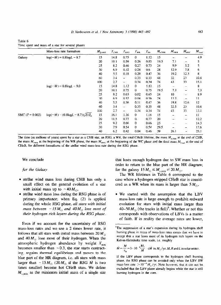
Table 6


Time spent and mass of a star for several phases

Mass-loss rate formalism M T T T ZAMS CHB RSC WR T “c M M M M eCHB bWR hWC li”ll

Galaxy log(-M) = O.llogL - 8.7 15 14.8 0.75 0 1.12 15 -

20 10.1 0.59 0.26 0.85 19.5 7.1

25 8.2 0.46 0.27 0.73 24 9.9

30 6.9 0.32 0.28 0.6 28 12.9

40 5.5 0.18 0.29 0.47 36 19.2

60 3.4 - 0.35 0.35 48 32

100 2.7 - 0.34 0.34 74 43 log(-M) = O.BlogL - 9.0 15 14.8 1.12 0 1.12 15 _

20 10.1 0.75 0 0.75 19.5 7.3

25 8.2 0.63 0.02 0.65 24 10

30 6.9 0.52 0.04 0.56 28 13.2

40 5.5 0.36 0.11 0.47 36 19.8

60 3.4 - 0.35 0.35 48 32.5

100 2.7 - 0.34 0.34 74 43 SMC (Z = 0.002) log(-M) = (0.8logL - 8.7)6 15 16.1 1.16 0 1.16 15 _

20 11.5 0.77 0. 0.77 20 _

25 9.2 0.66 0 0.66 25 _

30 7.9 0.54 0 0.54 29.5 _

40 6.2 0.42 0.04 0.46 39 26.1

4.9

_ 5

5.2 5

7.8 6

12.3 8

23 10.6

33 15.1

_ 8

_ 7.3

8.9

11

12.6 12

23 10.6

33 15.1

_ 11

_ 12.2

_ 14.3

_ 17.6

23.1

The time (in millions of years) spent by a star as a CHB star, an RSG, a WR, the total CHeB lifetime, the mass M,,,, at the end of CHB,

the mass M,,, at the beginning of the WR phase, the mass M,,, at the beginning of the WC phase and the final mass M,,na, at the end of

CHeB, for different formalisms of the stellar wind mass-loss rate during the RSG phase.

We conclude

for the Galaxy

stellar wind mass loss during CHB has only a small effect on the general evolution of a star with initial mass up to - 40 M,, stellar wind mass loss during the RSG phase is of primary importance; when Eq. (2) is applied during the whole RSG phase, all stars with initial mass between - 15M, and 40M, lose most of their hydrogen rich layers during the RSG phase.

Even if we account for the uncertainty of RSG mass-loss rates and we use a 2 times lower rate, it follows that all stars with initial mass between 20 M, and 4OM, lose most of their hydrogen, When the

atmospheric hydrogen abundance by weight X,,, becomes smaller than -0.3, the star starts contract- ing, regains thermal equilibrium and moves to the blue part of the HR diagram, i.e. all stars with mass larger than - 15 M, (2OM, if the RSG A!$ is two times smaller) become hot CHeB stars. We define M,,,i, as the minimum initial mass of a single star

that loses enough hydrogen due to SW mass loss in order to return to the blue part of the HR diagram; for the galaxy 15 M, 5 MS.,i, 5 20 M,,.

The WR lifetimes in Table 6 correspond to the

case where a hydrogen stripped CHeB star is considered as a WR when its mass is larger than 5 M,,

. We started with the assumption that the LBV mass-loss rate is large enough to prohibit redward evolution for stars with initial mass larger than

40-50 M, (the tracks in fu11)6. Whether or not this corresponds with observations of LBVs is a matter

of faith. If in reality the average rates are lower,

%te suppression of a star’s expansion during its hydrogen shell

burning phase in terms of mass-loss rates means that we have to

accept that a star loses most of its hydrogen rich layers on the

Kelvin-Helmholtz time scale, i.e. roughly

M-~=3.10~‘~ (M in M,/yr,M,RandLinsolarunits).

If the LBV phase corresponds to the hydrogen shell burning

phase, the RSG phase can be avoided only when the LBV SW

mass-loss rate > 10m4M,/yr. Note however, that it can not be

excluded that the LBV phase already begins while the star is still

burning hydrogen in the core.


.

also stars with initial mass larger than 40M, will

evolve to the red part of the HR diagram. This is illustrated in Fig. 14. As an example, let us consider the evolution of a 6OM, star. The star

loses - 12 M, during CHB as a consequence of a normal O-type SW. At the end of CHB, it still has

a - 16 MO hydrogen rich envelope. In order to avoid the redward evolution (i.e. to avoid an RSG

phase), this whole envelope has to be removed during the LBV phase. However, if we suppose

that the real (observed) SW is two times lower than is needed, only 8 M,, will be lost during the

LBV phase and the star becomes an RSG with luminosity logLIL, = 6.1. Applying Eq. (2), the RSG will lose mass by SW at a rate - 2. low4 M,lyr. It thus takes - 40000 yr in order to

remove the 8 M, envelope that was left after the LBV phase. This time scale is sufficiently short to

explain the lack of observed RSGs with MbO, < -

9.5. Table 7 shows the relation between the initial ZAMS mass, the final mass of the star just before

the SN explosion and the final mass of the CO core for galactic stars. For the 20 M, and 15 M,

star, also the results are given when the RSG SW mass-loss rate is a factor 2 smaller than predicted by Eq. (2). Since the evolution of the final CO core should be largely independent from the mass

layers outside this core (if they were not yet removed by SW), the final mass of the FeNi core is estimated from the detailed computations of

Woosley (1986), Woosley & Weaver (1995) and

Woosley et al. (1993), (1995). We conclude: l from the masses of the final FeNi core it cannot

be excluded that all single stars with mass larger

Table I Core masses for stars as function of ZAMS mass

15 518 2.513 1.511.65 20 517 3.514.3 1.712.0

40 8 6.5 2.9

60 IO 8 3.1

The pre-SN mass, the CO-core mass and the final FeNi-core mass

for stars with ZAh4S mass between 20M, and 60M,. For the

15 M, and the 20 M, model, we also give the results when the

RSG SW mass loss is a factor 2 smaller.

than 20-30 M, collapse to form a BH and no SN explosion happens,

l with the SW mass-loss rate of WR stars used

here, our evolutionary computations predict the existence of BHs with masses larger than 10 M,. If we believe the observed mass of BH components of X-ray binaries, like Cyg X- 1, we

consider this as a necessary condition evolutionary computations of massive stars have to fulfill, and this restricts the SW formalism during

CHeB, the above discussion and the evolutionary results hardly depend on the treatment of semi-convec-

tion.

for the Magellanic Clouds:

for Z < 0.004, when semi-convection is a very

inefficient mixing process, all massive stars with

initial mass I4OM, become RSGs and thus at least some of them could become single WR stars provided that the YSG/RSG stellar wind mass loss is large enough. The computations shown in

Fig. 15 correspond to the case where the RSG mass loss depends on the metallicity as predicted by the radiation driven wind theory [Eq. (4)] and the SMC value is a factor 3 smaller than in the Galaxy. In this case the stars remain in the red part of the HRD and no WR types are formed, if the ti during the RSG phase depends on the

metallicity, the minimum mass for BH formation

could be smaller in low metallicity environments (LMC or SMC) compared to the Galaxy.

Appendix B. The evolution of the mass gainer during the RLOF of the mass loser in case A/ case B, binaries. Two (limiting) accretion models

1. The standard accretion model (Neo et al., 1977) When dealing with MCBs, it can be assumed

that the envelope of the mass gainer is in radiative equilibrium and has a positive entropy gradient. In the ‘standard accretion model’ it is assumed that the radiative equilibrium of the outer layers is not affected by accretion. This applies when the entropy of the in-falling matter is equal or larger


5 es 4,s e4 4R 4 3,B 3‘4 3#4

Log Teff

Fig. 15. Evolutionary tracks of massive single stars with initial mass > 12M,, with initial abundance’s holding for the SMC (X = 0.76,

Z = 0.002). semi-convection is treated as a very inefficient mixing mechanism (Ledoux criterion), the stellar wind mass-loss rates during the

RSG phase are assumed to depend on the metalhcity as predicted by the radiatively driven wind theory (Eq. (4) with 5 = 0.5); in order to

explain the lack of RSGs with M,,, 5 - 9.5, we applied the same LBV SW as in the Galaxy.

than the entropy of the envelope of the mass gainer and when the effect of rotation (thus of rotational mixing) is neglected.

Two important effects: The over-luminosity. The entropy gradient in the

outer layers of the mass gainer remains positive during accretion and this causes an increase of the luminosity: the star becomes overluminous with

respect to its mass. This overluminosity becomes significant when the star does not have sufficient time to radiate away this excess energy, i.e.

roughly when the accretion time scale (-M/k) becomes shorter than the thermal time scale, i.e. when

03.1)

(ki in M,lyr, R, L and M in solar units). As a consequence of a significant overlumin-

osity, the outer layers of the star may start expanding and a situation may occur in which also the mass gainer fills its critical equipotential:

when this happens the binary is classified as a contact binary.

The effect of accretion on the evolution of the convective core. Of particular importance is the reaction of the convective core of a mass accreting star when the standard accretion model applies. A secondary in an interacting close binary may have already performed a significant part of

its own CHB at the onset of the RLOF of the primary and thus at the onset of the mass transfer phase. This means that it has built up a molecular weight gradient in its interior. increasing the mass of the star results into an increase of the stellar convective core. However, this immediately leads to the formation of a molecular weight ( p) barrier at its border which may prohibit a fast increase of the convective core when the stellar mass in-

creases. The way convection and semi-convection are

treated is of fundamental importance here. We can distinguish two limiting cases:

case I : the diffusion process in the layer on top

486 D. Vanbeveren et al. I New Astronom_v 3 (1998) 443-492

of the convective core of the mass gainer is fast enough to overcome the p-barrier. This assumption recovers the case in which, independently of the existence of a molecular weight gradient, the

convective core boundary is determined by the Schwarzschild criterion Vrad = V,,.

case 2: the diffusion process in semi-convec-

tive regions is always very slow. Compared to case 1, we obviously expect a much slower

increase of the convective core when the star accretes mass and a situation can arise where the convective core does not increase at all.

2. Accretion case 1

Evolutionary computations have been presented by Hellings (1983), De Loore & Vanbeveren

(1994). We summarize the main conclusions: l when the accretion time scale is smaller than

the thermal time scale of the CHB star, the mass gainer always occupies a place in the HR

diagram which is very close to the HRD position of a normal CHB single star with the same mass and chemical composition; after the

accretion phase, the further evolution of the star is almost entirely the same as the evolution of a normal single star with the same

mass, l when the accretion time scale is larger than the

thermal time scale, the mass gainer becomes overluminous for its mass and its radius increases significantly. When this happens in a binary, also the mass gainer may reach its

critical Roche radius and a contact system is formed.

At the end of the rapid accretion phase, the star regains its thermal equilibrium very fast and moves in the HRD to the position of a normal single star with the same mass and chemical composition. Again its further evolution is normal,

l after accretion, the stars are rejuvenated. This means that in the HRD, they are on a time- isochrone with a time scale smaller than their real lifetime.

l When the mass ratio of a binary is close to one, the RLOF starts when the secondary is also a hydrogen shell burning star. Evolution- ary computations were published in De Loore & Vanbeveren (1992). Since in this case the

He core mass is fixed and somehow protected

by the hydrogen burning shell, accretion does not enlarge the core but instead produces an extended fully convective region on top of the hydrogen burning shell. After the accretion

phase the star is (slightly) underluminous for its mass.

The most important difference when com-

pared to a CHB mass gainer is the further

evolution of the gainer after the accretion process. The star has a He core which is small for its mass whereas due to the large convection region on top of the burning shell, the shell has a lot of fuel at its disposal and a rapid

expansion of the star does not occur during the hydrogen shell burning and CHeB phase. As a consequence the star stays in the blue part of the HRD and does not make an excursion towards the RSG region. Although we have

not continued the evolutionary computations after CHeB up to the SN explosion, we can reasonably accept that the star will remain a

blue star till the end. 3. Accretion case 2

Detailed computations were performed by Braun & Langer (1995). We conclude: l after accretion, the stars are underluminous

and are less rejuvenated compared to case 1.

Even when the gainer was a CHB star at the onset of mass transfer, it can remain a blue

star during its entire further evolution after accretion. Furthermore, although the stellar mass increased considerably, its core mass

remained almost the same as before the accretion process. Its further lifetime (and certainly its CHeB lifetime) may therefore

be considerably larger than that of a normal single star with the same mass. This scenario may explain (at least partly) the large number of AB-type supergiants observed in the Blue Hertzsprung Gap in the HR diagram.

4. The accretion induced full-mixing model If unlike the assumption made in the stan-

dard accretion model, the entropy of the accreted matter is significantly lower than the entropy of the envelope of the gainer, convection will start smearing out the entropy profile.


This convection zone will develop inwards as

long as its specific entropy exceeds that of the matter which is accreted on top of it. The limiting situation is of course a complete mixing of the whole star. We will call this the ‘accretion induced full-mixing model’.

It is quite obvious that in the fully mixed

case, the way how semi-convection is treated is much less important than in the standard accretion model. Evolutionary computations

were presented by Vanbeveren & De Loore

(1994). We conclude:

l as expected, the rejuvenation of a mass

gainer is very pronounced with the accretion induced full-mixing model.

l when accretion started during the second half of the CHB phase of the gainer, the

post-accretion star is significantly overluminous and remains overluminous during

its further evolution. Vanbeveren et al.

(1994) used this model in order to explain the overluminosity of the optical component in the high mass X-ray binary Vela X-l

5. The mass gainer evolutionary library We performed a detailed set of galactic

Table 8

Lifetime of O-type star mass gainer as function of initial mass of primary and secondary. Full mixing, p = 0.5

M, M2

4 5 8 10 12 15 20 25 30

11 0 0 0 5633000 0 0 0 0 0

12 0 0 0 5477000 0 0 0 0 0

13 0 0 0 5157000 5856000 0 0 0 0

14 0 0 0 4838000 5895000 0 0 0 0

1s 0 0 0 439OOMl 5934000 0 0 0 0

16 0 0 0 5800000 5974000 4968000 0 0 0

17 0 0 0 5447000 5990000 5084000 0 0 0

18 0 0 0 5315000 6OO6000 5206000 0 0 0

19 0 0 1568000 5595OcG 6001000 5217000 0 0 0

20 0 0 3135000 5930000 5997000 5201000 0 0 0 21 0 0 3496000 5814000 6040000 5367000 4245000 0 0

22 0 0 3857C@O 5697000 6083000 5375ooo 4194000 0 0

23 0 0 4217000 5885000 6023000 5434000 4954000 0 0

24 0 0 4578000 6073000 5963000 5273000 4781000 0 0

25 0 0 4031000 6045000 6013ooo 5436000 4608000 0 0 26 0 0 3483000 6018000 6062000 5486000 4436000 3385000 0 27 0 0 3870000 6072000 6056000 5475000 4494000 3060000 0

28 0 0 4257000 6125000 6050000 5464QOO 4335000 3207000 0

29 0 0 4643000 618OOOo 6032000 5444000 4516000 3292000 0

30 0 0 5030000 6234000 6015000 5424000 4459000 3542000 0

31 0 0 5239000 6144000 6015000 5443000 4275000 3133000 1283000

32 0 0 5447000 6054000 6015000 5461000 4092000 2724000 2567000

33 0 0 5517000 6079000 5966000 5364000 4087000 2809000 2769000

34 0 0 5586000 6105000 5917000 5267000 4081000 2894000 2971000

35 0 0 5725000 6167000 5966MMI 5357000 4556000 2960000 2989OOil

36 0 0 5950000 6229000 6015000 5447000 4237000 3026000 3006000

37 0 0 6175000 6161000 5991000 5442000 4237000 3033000 3024000

38 0 0 6400000 6093000 5968000 5437000 4238000 304OOOa 3042000

39 0 0 6251000 6055000 5877000 5375000 4421000 3111OOa 3105000

40 0 0 6102000 6018000 5785000 5313ooo 4605000 3181000 3168000

The lifetime that a post-mass transfer mass gainer will be visible as an O-type star, when the accretion induced full mixing model applies,

when the RLOF is quasi-conservative (p = 0.5). M, and M, are respectively the initial mass of the primary (respectively the secondary).

488 D. Vanbeveren et al. / New Astronomy 3 (1998) 443-492

MCB evolutionary computations in which the

evolution of the gainer after the mass transfer process was followed till the end of its own

CHB phase (880 evolutionary sequences). The computations were performed with the stan-

dard accretion model where the boundary of the convective core is determined by the

condition Vrad = V,, allowing for a small amount of convective core overshooting simi-

larly as in single stars, and with the accretion induced full-mixing model. The remaining lifetime that a mass gainer will be visible as an

O-type star is given in Tables 8- 11. The HRD evolutionary tracks are available upon request.

The results for Z = 0.002 holding for the

SMC differ by less than 10%.

Appendix C. The distribution of equatorial rotational velocities of massive stars

Starting from the observed $(u,sini) distribution,

the u, distribution 4p(u,) can be determined as follows:

Table 9

Lifetime of O-type star mass gainer as function of initial mass of primary and secondary. Full mixing, p = 1

M, M2

4 5 8 10 12 15 20 25 30

9 0 0 2542000 0 0 0

10 0 0 5084000 0 0 0

II 0 0 5451000 6021000 0 0

12 0 0 5817000 5777000 0 0

13 0 0 5861000 6005000 27 12000 0

14 0 0 5904cOO 5960000 5424000 0

15 0 796500 5965000 5963000 5417000 0

16 0 1593000 6027000 5914000 541OOoO 4596000

17 474700 3023000 6049000 5863000 5405000 4587000

18 949500 4453000 6072000 5813000 54OGQOO 4638000

19 2501000 4915000 6048000 5771000 539OQOo 4601000

20 4053000 5377000 6024000 5728000 5380000 4598000

21 0 5491000 5987000 5675000 5355Ocil 4639000

22 0 5605000 5950000 5622000 5330000 4680000

23 0 5718000 5908000 5579000 5283000 4685000

24 0 5832000 5866000 5536000 5237000 4690000

25 0 5946000 5857000 5498000 5170000 4677000

26 0 0 5848000 5460000 5103000 4663000

27 0 0 5786000 5415000 5095000 4627000

28 0 0 5724000 537OoOo 5086000 4592000

29 0 0 5595000 5269000 4983000 4569000

30 0 0 5466000 5168000 4881000 4545000

31 0 0 5428000 5221000 4940000 4467000

32 0 0 539OOOo 5274000 4999000 4390000

33 0 0 5351000 5243000 4944000 4429000

34 0 0 5313000 5212000 4889000 4467000

35 0 0 5275000 5171000 4875000 4446000

36 0 0 527oooO 5 129000 4862000 4425000

37 0 0 5265000 5025000 4761000 4355000

38 0 0 5260000 4920000 4660000 4286000

39 0 0 5255000 4947000 4694000 4329000

40 0 0 5250000 4974000 4728000 4373000

0 0 0

0 0 0

0 0 0

0 0 0

0 0 0 0 0 0

0 0 0

0 0 0

0 0 0

0 0 0

0 0 0

0 0 0

76CQOO 0 0

I52OOOII 0 0

228OOOCI 0 0

304OOOo 0 0

38OGQOO 0 0

3791000 3017000 0

3782000 3054000 0

3773000 3089000 0 3764000 3054000 0

3755000 3202000 0

3751000 3165000 1260000

3747000 3 127000 2520000

3742000 3 197000 2777000 3738000 3266000 3033000

3734000 3263000 2957000

3708OQo 3260000 2882000

3683000 3311000 2935000

3657000 3361000 2988000

3631000 3389000 3088000

3605000 3417000 3188ooO

The lifetime that a post-mass transfer mass gainer will be visible as an O-type star. when the accretion induced full mixing model applies.

when the RLOF is conservative (/3 = 1). M, and Ml are respectively the initial mass of the primary (respectively the secondary).


Table 10

Lifetime of O-type star mass gainer as function of initial mass of primary and secondary. Standard accretion model, p = 0.5

M, M,

4 5 8 10 12 15 20 25 30

17 0 0 0 0 281900 0 0 0 0

18 0 0 0 0 563700 332200 0 0 0

19 0 0 0 202300 1550000 1016000 0 0 0

20 0 0 0 1747000 2537000 1373000 0 0 0

21 0 0 0 1962000 2687000 1657000 0 0 0

22 0 0 0 1948000 2838000 1941000 294600 0 0

23 0 0 281900 2491000 3143000 2224000 589100 0 0

24 0 0 563700 3035000 3448000 2508000 811600 0 0

25 0 0 563700 3578000 3507000 2792000 1034000 0 0

26 0 0 563700 3740000 3566000 2904000 1220000 338400 0

27 0 0 1458000 3902000 3815000 3016000 1406000 402700 0

28 0 0 2353000 4064000 4065000 3127000 1592000 585400 0

29 0 0 2845000 4226000 4107000 3239000 1778000 442700 0

30 0 0 3337000 4388000 4 148000 335 1000 1848000 775300 0

31 0 0 3581000 4511000 4294000 3424000 1918000 897100 245100

32 0 0 3824000 4635000 4440000 3497000 1975OcG 1019000 367700

33 0 0 4068000 4758000 4538000 3569000 2032000 I1 loo00 478900

34 0 0 4311000 4882000 4636000 3642000 2139000 1201000 590000

35 0 0 4555000 5005000 4559000 3715000 2245000 1279000 603000

36 0 0 4668000 5039000 4483000 3766000 2311000 1356000 616000

37 0 0 4780000 5074000 4568000 3817000 2378000 1429000 695000

38 0 0 4893000 5108OCKI 4653ooO 3868000 2428000 1501000 775000

39 0 0 5005000 5143000 4657000 3919000 2474000 1507000 815000

40 0 0 5118OOcl 5177000 4661000 3970000 2584000 1514000 856000

The lifetime that a post-mass transfer mass gainer will be visible as an O-type star, when the standard accretion model applies, when the

RLOF is quasi-conservative (p = 0.5). M, and M, are respectively the initial mass of the primary (respectively the secondary).

a. correct the observed distribution &(v,sini) for the effect of observational errors and obtain the

distribution +(v,(u,sini). If the errors on the measured v,:ini follow a Gaussian distribution with variance (T- (our results were computed adopting an error u = 25 km/s), it follows that (see also Eddington,

1913)

&v,sini) = $( [)P(v,sinil&)de I

with

lo,sini-0’

P(v,sinil[) = &e-T

(C.1)

b. from the corrected distribution Jl(v,sini) we determine the distribution cp(v,) by solving the integral equation (see also Chandrasekhar & Munch, 1950)

$(v, sini ) = I

cp( &P(v, sini 1 &)A$

with

(C.2)

. .

P(v,sinile) = u,sIII1 5 &-&J(S - v+i)

(the function H is the classical Heavyside function). In order to solve the integral Eqs. (C.l) and (C.2)

an iterative technique has been developed by Lucy (1974). Compared to other techniques (a.o. Deutsch, 1970; Balona, 1975) it has the big advantage that no assumptions about P or p have to be made other than the obvious constraints

I d5)&!= 1 and dOLO (C.3)


Table 11 Lifetime of O-type star mass gainer as function of initial mass of primary and secondary. Standard accretion model, p = 1

4 5 8 IO 12 15 20 25 30

11 0 0 929800 18750 0 0 0 0 0

12 0 0 1860000 1575000 0 0 0 0 0

13 0 0 2622000 2439000 1582000 0 0 0 0

14 0 0 3385000 3037000 1989000 0 0 0 0

15 0 0 3895000 3665000 2395000 0 0 0 0 16 0 3176000 4405000 3999000 2802000 1441000 0 0 0

17 286300 3170000 4680000 4036000 3020000 1758000 0 0 0

18 563700 3161000 4956000 4313000 3239OiJO 2280000 0 0 0

19 2207ooO 4785000 1991000 4427000 3519000 2359000 0 0 0

20 3851000 5419000 5026000 4553006 3800000 2509000 0 0 0

21 0 5416000 5165000 4609000 3967000 2755000 1079000 0 0

22 0 5419000 5303000 4657000 4134000 3023000 1259000 0 0

23 0 5772000 5318000 4732000 4054000 3104000 1439OOtl 0 0

24 0 5796000 5333000 4681000 3974000 3184000 1632000 0 0

25 0 58oooOO 5323000 4629000 3981000 327 1000 1825000 0 0

26 0 0 5313000 4776000 3988000 3358000 1910000 973700 0

27 0 0 5289000 4755000 4056000 3383000 1996000 985900 0

28 0 0 5265000 4687000 4125000 3408000 2087OOtl 1062000 0

29 0 0 5212000 4688000 4115000 3420000 2177000 1154000 0

30 0 0 5158000 4660000 4 104000 3432000 2216000 1251000 0

31 0 0 5129OOil 4705000 4191000 3449000 2255000 1328000 799000

32 0 0 5099000 4666000 4278000 3466000 2297000 1404c@O 831500

33 0 0 5069006 4648000 4241000 3479000 2338000 1490000 863900

34 0 0 5040000 4675000 4204000 3493000 2370000 1575000 896400

35 0 0 5010000 4587000 4 197000 3488000 2402OCO 1603000 936800

36 0 0 4989000 4624000 4190000 3484000 2446000 1630000 977200

37 0 0 4967000 4546000 4166000 3486000 2491000 1680000 1003000

38 0 0 4946000 4562000 4143000 3488000 2534000 1730000 1028000

39 0 0 4925000 4569000 4115000 3537000 2577000 1761000 1077000

40 0 0 4903000 45 16000 4087000 3587000 2705000 1793000 1126000

The lifetime that a post-mass transfer mass gainer will be visible as an O-type star, when the standard accretion model applies, when the

RLOF is conservative (p = 1). M, and Mz are respectively the initial mass of the primary (respectively the secondary).

References

Annuk, K.. 1995, in: WR Stars: Binaries, Colliding Winds,

Evolution, eds. K.A. Van der Hucht & PM. Williams, IAUS.

Vol. 163 (KIuwer, Dordrecht), p. 231.

Azzopardi, M. & Breysacher, J.. 1979, A&A, 75, 120.

Bailes, M., 1989, ApJ, 342, 917.

Balona, L., 1975, MNRAS. 173, 449.

Biehle, G.T., 1991, ApJ, 380, 167.

Blaauw. A., 1961, BAN, 15, 265.

Braun, H. & Langer, N., 1995, A&A, 297, 483.

Breysacher, J., 1981, A&AS. 43, 203.

Cannon, R., Eggleton, P.P. Zytkow, A.N., & Podsiadlowski, Ph.,

1992, ApJ, 386, 206.

Cerruti, M.A., 1984, IBVS, 2637, 1.

Cervino, M. & Mass-Hesse, J.M., 1994, A&A. 284, 749.

Chandrasekhar, S. & Munch. G., 1950, ApJ, 111, 142.

Cherepaschuk. A.M., 1975, SvA. 19, 47.

Conti, P.S., 1991, ApJ. 377, 115.

Conti, P.S., 1994, in: Evolution of Massive Stars: a Confrontation

between Theory and Observation, eds. D. Vanbeveren, D., W.

Van Rensbergen, & C. De Loore (Kluwer, Dordrecht), p. 37. Counselman, C.C., 1973, ApJ, 180, 307.

Dalton, W.W. & Sarazin, C.L., 1995, ApJ, 448, 369.

Darwin, G.H., 1908. Scientific Papers, Vol. 2 (Cambridge Uni- versity Press, Cambridge).

De Donder. E.. Vanbeveren, D., & Van Bever, J., 1997, A&A, 3 18, 812.

De Donder. E. & Vanbeveren, D.. 1998, A&A. in press.

De Loore, C. & Vanbeveren, D., 1992, A&A, 260, 273.

De Loore. C. & Vanbeveren, D., 1994, A&A, 292, 463.

De Marchi. G.. Clampin, M., Greggio, L., Leitherer, C., Nota, A..

& Tosi, M., 1997, ApJ. 479, L27.

Deutsch, A.J., 1970, Stellar Rotation, ed. A. Slettebak (Reidel, Dordrecht), p. 207.


D&en. L., Lamonmgne, R.. Moffat, A.F.J., Bastein, P., &

Seguin, M., 1986, ApJ, 343, 426.

Eaton, J.A., Cherepaschuk, A.M., & Khaliullin, Kh.F., 1985, ApJ,

296, 222.

Eddington, A.S., 1913, MNRAS, 73, 359.

Eggleton, P.P., 1983, ApJ, 268, 368.

Fryer, C.. Burrows, A., & Benz. W., 1998, ApJ, 496, 333.

Garmany, C.D., 1997, in: Luminous Blue Variables: Massive Stars

in Transition, eds. A. Nota & H.J.G.L.M. Lamers, AS Conf.

Series.

Garmany, CD., Conti, P.S., & Massey, P., 1980, ApJ, 242, 1063.

Gies, D.R. & Bolton. C.T., 1986, ApJ, 304, 371.

Gies, D.R.. 1987, ApJS, 64, 545.

Gonzales-Delgado, R., Leitherer, C., Heckman, T., & Cervino, M.,

1997, ApJ, 483, 705.

Halbwachs, J.L., 1987, A&A, 183, 234.

Hamann, W.R., 1994, SSRv. 66, 237.

Hamann, W.R., 1998, A&A, in press.

Hamann, W.R. & Koesterke, L., 1998, A&A, in press.

Hartmann, J.W., 1997, A&A, 322, 127.

Heger. A., Jeannin, L., Langer, N.. & Baraffe, I., 1998, A&A, in

press.

Hellings, P., 1983, Ap&SS, 96, 37.

Herbig, G.H.. Preston, G.W.. Smak, J., & Paczynski, B., 1965, ApJ, 141, 617.

Hillier, D.J., 1996, in: Wolf-Rayet Stars in the Framework of

Stellar Evolution, eds. J.M. Vreux, A. Detal, D. Fraipont-Care,

E. Gosset, & G. Rauw, Universiti de Liege, p. 509.

Hogeveen, S., 1991, Ph.D. Thesis, University of Amsterdam.

Hogeveen, S.. 1992, Ap&SS, 196, 299.

Howarth, I.D. & Prinja, R.K.. 1989, ApJS, 69, 527.

Humphreys, R.M. & McElroy, D.B., 1984, ApJ, 284, 565.

Humphreys, R.M. & Davidson, K.. 1994, PASP, 106, 1025. Israel, F.P., 1988, A&A. 194, 24.

Jura, M., 1987. ApJ, 313, 743.

Khaliullin, Kh.F., Khaliullina, A.I., & Cherepashchuk, A.M.,

1984, SvAL, 10, 250.

Kaper. L., Lamer%, H.J.G.L.M., Ruymaekers, E., Van den Heuvel,

E.P.J., & Zuiderwijk, E.J., 1995, A&A, 300, 446.

Kippenhahn, R. & Weigert, A., 1967, ZA, 66, 58.

Kopal. Z., 1972, Ap&SS, 16, 3.

Kunth, D. & Sargent, W.L.W., 1981, A&A, 101, L5.

Langer. N. & Maeder. A., 1995, A&A, 295. 685.

Langer. N. & Heger. A., 1998, in: Properties of Hot, Luminous

Stars, ed. I. Howarth, ASP Conf. Proc., Vol. 131, in press.

Lauterbom. D.. 1969, in: Mass Loss from Stars, ed. M. Hack

(Reidel, Dordrecht), p. 262.

Ledoux, P.. 1947, ApJ, 105, 305.

Leitherer. C. & Heckman, T.M., 1995, ApJS, 96, 9.

Leitherer, C., Robert, C.. & Heckman, T.M., 1995, ApJS, 99, 173.

Leonard, P.J.T. & Duncan, M.J., 1988. AJ, 96, 222.

Leonard, P.J.T. & Duncan, M.J., 1990, AJ, 99, 608.

Lipunova, N.A. & Cherepaschuk, A.M., 1982, SvA, 26, 45.

Lotimer. D.R., Bailes, M., & Harrison, P.A., 1997, MNRAS, 289, 592.

Lortet. M.-C., 1991, A&A, 242, 410.

Lubow, S.H. & Shu, F.H., 1975, ApJ, 198, 383.

Lucy, L.B., 1974, AJ, 79, 745.

Lundstrom, I. & Stenholm, B., 1984, A&AS, 58, 163.

Lynden-Bell, D. & Pringle, J.E., 1974, MNRAS, 168, 603. Lyne, A.G. & Lorimer, D.R., 1994, Natur, 369, 127.

Maeder, A., 1998, in: Properties of Hot, Luminous Stars, ed. I. Howarth, ASP Conf. Proc., Vol. 131, in press.

Massey, P., 1981, ApJ, 246, 153.

Massey. P., Garmany, C.D., Silkey, M., & Degioia-Eastwood, K.,

1989a. AJ, 97, 107.

Massey, P., Parker, J.W., & Garmany, C.D., 1989b, AJ. 98, 1305.

Mass-Hesse, J.M. & Kunth, D., 1991, A&AS. 88, 399. Meynet, G., 1995, A&A, 298, 767.

Meynet, G., 1998, in: Properties of Hot, Luminous Stars, ed. I. Howarth, ASP Conf. Proc., Vol. 131, in press.

Moffat, A.F.J., 1995. in: WR stars: Binaries, Colliding Winds, Evolution. eds. K.A. Van der Hucht & P.M. Williams (Kluwer,

Dordrecht), p. 212.

Moffat, A.F.J., 1996, in: Wolf-Rayet Stars in the Framework of

Stellar Evolution, eds. J.M. Vreux, A. Detal, D. Fraipont-Caro,

E. Gosset, & G. Rauw, Universite de Liege, p. 199.

Moffat. A.F.J. & Seggewiss, W., 1980, A&A, 86, 87.

Moffat, A.F.J., Lamontagne, R., & Seggewiss, W.. 1982. A&A,

114, 135.

Neo. S.. Miyaji, S., Nomoto, K., & Sugimoto, D., 1977, PASJ, 29. 249.

Niemela, VS., 1995, in: WR stars: Binaries, Colliding Winds,

Evolution, eds. K.A. Van der Hucht & P.M. Williams (Kluwer,

Dordrecht), p. 223.

Niemela, VS., Mandrini, C.H., & Mendez, R.H., 1985. RMxAA,

11, 143.

Niemela, VS., Mendeze, R.H., & Moffat, A.F.J., 1983, ApJ, 272, 190.

Niemela, VS. & Moffat, A.F.J., 1982. ApJ, 259. 213. Pacini, F., 1967, Natur, 216. 567.

Parker, J.W., Garmany, CD., Massey, P., & Walbom, N.R., 1992, AJ, 103. 1205.

Penny, L.R., 1996, Tomographic Separation of Spectra of O-Type

Binary Systems, Ph.D. thesis, Georgia State University.

Petrenz, P. & Puls, J., 1996, A&A, 312. 195.

Pike, C.D., Stickland, D.J., & Willis, A.J., 1983, Obs, 103, 154.

Podsiadlowski, Ph., Joss, P.C.. & Rappaport. S.. 1990, A&A, 227, L9.

Popova, EL, Tutukov, A.V., & Yungelson, L.R., 1982, Ap&SS, 88, 55.

Puls, J., Kudritzki, R.P., Herrer, A., et al., 1996, A&A, 305, 171.

Reid, N., Tinney, C., & Mould, J., 1990, ApJ, 348, 98.

Robert, C., Leitherer, C., & Heckman, T.M., 1993, ApJ, 418, 749.

Sargent. W.L.W. & Searle, L., 1970, ApJL, 162. 155. Scala, J.M., 1986, FCPh, 11, 1.

Schaerer, D. & Vacca, W.D., 1996, in: Wolf-Rayet Stars in the

Framework of Stellar Evolution, eds. J.M. Vreux, A. Detal, D.

Fraipont-Care, E. Gosset, & G. Rauw, Universite de Liege, p. 641.

Schaller, G., Schaerer, D., Meynet, G., & Maeder, A., 1992, A&AS, 96. 269.

Schmutz, W., 1997, A&A, 321, 268.

Searle, L.. Sargent. W.L.W., & Bagnuolo, W.G., 1973, ApJ. 179, 427.


Shklovskii, IS., 1969, SvA, 13, 562.

Sparks, N.M. & Stecher, T.P., 1974, ApJ, 188, 148.

St.-Louis, N., Moffat, A.F.J., & Lapointe, 1993, ApJ. 410, 342.

St.-Louis, N., Drissen, L., Moffat, A.F.J., Bastien, P., & Tapia, S.,

1987. ApJ, 322, 870.

St.-Louis, N., Moffat, A.F.J., Drissen, L., Bastien, P., & Roberts,

C., 1988, ApJ, 330, 286.

Sutantyo, W., 1978, Ap&SS, 54, 479.

Talon, S., Zahn, J.P., Maeder, A., & Meynet. Cl., 1997, A&A, 322.

209.

Thome, K.S. & Zytkow, A.N., 1977, ApJ, 212. 832.

Underhill, A.B.. &eve, G.R., & Louth, H., 1990, PASP, 102, 749.

Vacca, W.D. & Conti, P.S., 1992, ApJ, 401, 543.

Van Bever, J. & Vanbeveren. D.. 1998, A&A, in press.

Vanbeveren, D., Herrero, A., Kunze. D., & Van Kerkwijk, M..

1994, SSRv, 66, 395.

Vanbcveren, D. & Packet, W., 1979, A&A, 80, 242.

Vanbeveren, D. & De Loore, C., 1994, A&A, 290. 129.

Vanbeveren, D., Van Bever, J., & De Donder, E., 1997. A&A, 3 17,

487 (Paper I).

Vanbeveren, D., Van Rensbergen, W., & De Loore, C., 1998. in:

The Brightest Binaries (Kluwer, Dordrecht), in press.

Vanbeveren, D., 1990. A&A, 234, 243.

Vanbeveren. D., 1991, A&A, 252, 159.

Vanbeveren, D., 1995, A&A, 294, 107.

Van den Heuvel, EPJ., 1993, in: Interacting Binaries, Saas-Fee

Advanced Course 22, eds. H. Nussbaumer & A. Orr (Springer-

Verlag, Heidelberg), p. 263.

Van der Hucht, K.A., Conti, P.S., Lundsrom, I., & Stenholm, B.,

1981, SSRv, 28, 227.

Van der Hucht, K.A., Hidayat, B., Admiranto, A.G., Supelli, K.R.,

& Doom, C., 1988, A&A, 199, 217.

Van der Hucht, K.A., Schrijver, H., Stenholm, B., et al., 1997,

NewA. 2, 245.

Van Rensbergen, W., Vanbeveren, D., & De Loore, C.. 1996, A&A,

305. 825.

Vereshchagin, S., Kraicheva. Z., Popova, E., Tutukov, A., &

Yungelson, L., 1987, PAZh, 13, 63.

Vereshchagin, S., Tutukov, A., Yungelson, L.. Kraicheva, Z., &

Popova, E., 1988, Ap&SS, 142, 245.

Webbink, R.F., 1984, ApJ, 277, 355.

Williams, P.M. & Van der Hucht, K.A., 1996, in: Wolf-Rayet Stars

in the Framework of Stellar Evolution, eds. J.M. Vreux, A.

Detal, D. Fraipont-Care, E. Gosset, & G. Rauw, Universite de

Liege, p. 353.

Woosley, S.E.. 1986, in: Nucleosynthesis and Chemical Evolution,

16th Saas-Fee Course, eds. B. Hauck et al., Geneva Observat-

ory, p. 1.

Woosley, S.E. & Weaver, T.A., 1995. ApJS, 101. 181.

Woosley, S.E., Langer, N., & Weaver, T.A.. 1993, ApJ, 411, 823.

Woosley, S.E., Langer, N.. & Weaver, T.A.. 1995, ApJ, 448, 315.

Zahn, J.P., 1977, A&A, 57, 383.

Zahn, J.P., 1994, in: Evolution of Massive stars: A Confrontation

between Theory and Observations, eds. D. Vanbeveren, W. Van

Rensbergen. & C. De Loore (Kluwer, Dordrecht), p. 285.

The WR and O-type star population predicted by massive star evolutionary synthesis

Documents

Transcript of The WR and O-type star population predicted by massive star evolutionary synthesis